Embed Size (px)
Citation preview
Retrospective Theses and Dissertations Iowa State University Capstones, Theses and Dissertations
1-1-2004
Carbon monoxide and hydrogen mass transfer in a stirred tank Carbon monoxide and hydrogen mass transfer in a stirred tank
reactor reactor
Seth S. Riggs Iowa State University
Follow this and additional works at: https://lib.dr.iastate.edu/rtd
Recommended Citation Recommended Citation Riggs, Seth S., "Carbon monoxide and hydrogen mass transfer in a stirred tank reactor" (2004). Retrospective Theses and Dissertations. 20253. https://lib.dr.iastate.edu/rtd/20253
This Thesis is brought to you for free and open access by the Iowa State University Capstones, Theses and Dissertations at Iowa State University Digital Repository. It has been accepted for inclusion in Retrospective Theses and Dissertations by an authorized administrator of Iowa State University Digital Repository. For more information, please contact [email protected].
Carbon monoxide and hydrogen mass transfer in a stirred tank reactor
by
Seth S. Riggs
A thesis submitted to the graduate faculty
in partial fulfillment of the requirements for the degree of
MASTER OF SCIENCE
Co-majors: Mechanical Engineering; Biorenewable Resources and Technology
Program of Study Committee: Theodore John Heindel, Co-major Professor
Robert C. Brown, Co-major Professor Alan A. DiSpirito
Iowa State University
Ames, Iowa
2004
11
Graduate College
Iowa State University
This is to certify that the master's thesis of
Seth S. Riggs
has met the thesis requirements of Iowa State University
Signatures have been redacted for privacy
111
TABLE OF CONTENTS
LIST OF TABLES ............................................................................................................. vi
LIST OF FIGURES .......................................................................................................... vii
NOMENCLATURE .......................................................................................................... ix
ACKNOWLEDGEMENTS ............................................................................................... xi
ABSTRACT ................................................................................................................... xii
CHAPTER 1: INTRODUCTION ....................................................................................... 1
1.1 Motivation .................................................................................................................. 1
1.2 Goals .......................................................................................................................... 2
CHAPTER 2: LITERATURE REVIEW ........................................................................... .4
2.1 Gas-Liquid Mass Transfer Studies Using Various Gases ......................................... .4
2.1.1 Gas-Liquid Mass Transfer Studies Using Oxygen ............................................ .4
2.1.1.1 Oxygen-Liquid Mass Transfer in Stirred Tank Reactors ............................ .4
2.1.1.2 Oxygen-Liquid Mass Transfer in Other Reactors ........................................ 8
2.1.2 Gas-Liquid Mass Transfer Using Synthesis Gas or Pure Carbon Monoxide ..... 9
2.2 Measuring Dissolved Gases in Water ...................................................................... 10
2.2.1 Dynamic Techniques ........................................................................................ 10
2.2.2 Static Methods .................................................................................................. 12
2.3 Synthesis Gas Fermentation ..................................................................................... 14
2.3.1 Microorganisms Used in Synthesis Gas Fermentation ..................................... 14
2.3.2 Synthesis Gas Fermentation Reactor Design .................................................... 16
2.4 Literature Review Summary .................................................................................... 18
CHAPTER 3: MATERIALS AND METHODS .............................................................. 19
3.1 Experimental Set-Up ................................................................................................ 19
3.1.1 Stirred Tank Bioreactor ..................................................................................... 19
IV
3.1.2 Trial Preparation ............................................................................................... 20
3.1.3 Trial Operation .................................................................................................. 21
3.2 Measuring Dissolved Carbon Monoxide Concentrations ........................................ 22
3.2.1 Dissolved Carbon Monoxide Sampling Equipment ......................................... 22
3.2.2 Making the Carbon Monoxide Saturated Buffer Solution ................................ 23
3.2.3 Making the Deoxygenated Buffer Solution ...................................................... 23
3.2.4 Preparing a Dissolved CO Sample .................................................................... 23
3.2.5 Identifying the Protein Concentration ............................................................... 24
3.2.6 Converting the Spectra Data to Usable Data for Spectra Solve ........................ 24
3.2.7 Fitting Spectra ................................................................................................... 25
3.2.8 Sample CO Concentration Results .................................................................... 25
3.3 Measuring Dissolved Hydrogen Concentration ....................................................... 25
3.3.1 Dissolved Hydrogen Sampling Equipment.. .................................................... .26
3.3.2 Gas Chromatograph Start-Up ........................................................................... 27
3.3.3 Sample Evaluation Procedure ........................................................................... 28
3.3.4 Gas Chromatograph Shut Down ....................................................................... 28
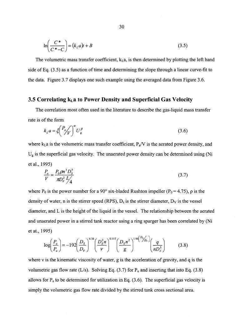
3.4 Determining the Volumetric Mass Transfer Coefficient from Concentration
Data ......................................................................................................................... 29
3.5 Correlating kLa to Power Density and Superficial Gas Velocity ............................. 30
CHAPTER 4: RESULTS .................................................................................................. 38
4.1 Carbon Monoxide Trial Results ............................................................................... 38
4.2 Hydrogen Trial Results ............................................................................................ 41
4.3 Comparing This Work to the Literature .................................................................. .45
CHAPTER 5: CONCLUSIONS ....................................................................................... 65
5.1 Conclusions .............................................................................................................. 65
5.2 Recommendations .................................................................................................... 66
v
BIBLIOGRAPHY .............................................................................................................. 67
APPENDIX A: CARBON MONOXIDE CONCENTRATION DATA .......................... 71
APPENDIX B: HYDROGEN CONCENTRATION DATA ........................................... 87
Vl
LIST OF TABLES
Table 4.1: Volumetric mass transfer coefficient and R2 value for all carbon
monoxide trial runs .................................................................................... 48
Table 4.2: Volumetric mass transfer coefficient and R2 value for all hydrogen
trial runs ..................................................................................................... 49
Table 4.3: Parameters used in Eq. (3.6) for gas-liquid mass transfer
correlations of various gases and liquids .................................................. 50
Table 4.4: Volumetric mass transfer rates for CO and H2 from various
literature experiments ................................................................................. 51
Vll
LIST OF FIGURES
Figure 3.1: Schematic of a stirred tank reactor. . ........................................................ .31
Figure 3.2: Concentration sampling experimental apparatus ...................................... .32
Figure 3.3: CO saturated and deoxygenated curves are the basis for
comparison to the trial sample curve in the software Spectra Solve ......... 33
Figure 3.4: Schematic representing the dissolved hydrogen testing equipment. ......... 34
Figure 3.5: Gas chromatograph output from a dissolved hydrogen trial.. ................... .35
Figure 3.6: Dissolved CO concentration as a function of time for five trials. . .......... 36
Figure 3.7: Determination ofkLa for CO in a stirred tank reactor. . ........................... 37
Figure 4.1: A typical CO data set. .............................................................................. 52
Figure 4.2: Typical carbon monoxide concentration data used to determine the
mass transfer rate (all data< 85% of the saturation limit) ....................... 53
Figure 4.3: The average of five CO concentration versus time trials shown
with+/- 1 standard deviation bars. .. ......................................................... 54
Figure 4.4: The slope of the line represents the volumetric mass transfer
coefficient. ................................................................................................ 55
Figure 4.5: Volumetric mass transfer coefficient versus stirrer speed for
different volumetric gas flow rates ............................................................ 56
Figure 4.6: Volumetric mass transfer coefficient versus volumetric gas flow
rate for different stirrer speeds ................................................................... 57
Figure 4.7: Experimental volumetric mass transfer coefficient as a function of
the correlated volumetric mass transfer coefficient shown with+/-
10% error lines ........................................................................................... 58
Figure 4.8: Typical hydrogen concentration data used to determine the mass
transfer rate. . ............................................................................................ 59
vm
Figure 4.9: The average of five H2 concentration versus time trials ............................ 60
Figure 4.10: The slope of the line represents the volumetric mass transfer
coefficient. ................................................................................................. 61
Figure 4.11: Volumetric mass transfer coefficient versus stirrer speed for
different volumetric gas flow rates ............................................................ 62
Figure 4.12: Volumetric mass transfer coefficient versus volumetric gas flow
rate for different stirrer speeds ................................................................... 63
Figure 4.13: Experimental volumetric mass transfer coefficient as a function of
the correlated volumetric mass transfer coefficient ................................... 64

IX
NOMENCLATURE
A Absorption value (-)
a Interfacial bubble area per unit volume (m-')
B Constant of integration (-)
c Concentration of dissolved gas in water (µM)
Ci Initial dissolved gas concentration present in water (µM)
c, Concentration of sodium sulfite (g L-')
C1,o Equilibrium concentration of sodium sulfite (g L-1)
Cp Protein concentration (µM)
C* Equilibrium concentration of dissolved gas in water (µM)
Ds Stirrer diameter (m)
Dv Vessel diameter (m)
G' Oxygen saturated liquid electrode response (-)
g Gravitational acceleration (m2 s-1)
K Adsorption coefficient (mol m-3)
kL Mass transfer coefficient (m s-1)
kLa Volumetric mass transfer coefficient (s-')
L Water height in vessel (m)
Pathlength of cuvette (cm)
N Stirrer speed (RPM)
n Stirrer speed (RPS)
Pa Aerated power (W)
Po Power number (-)
Pu Unaerated power (W)
Q Gas flow rate (L min-1)
x
q Gas flow rate (L s-1)
t Time (s)
Ug Superficial gas velocity (m s-1)
v Liquid volume in vessel (m3)
V1 Volumetric flow rate (L s-1)
Greek Symbols
a Model parameter (-)
p Model parameter (-)
e Absorption coefficient (µM- 1 cm-1)
es Solid volume fraction (-)
~ Model parameter (-)
p Liquid density (kg m-3)
v Liquid kinematic viscosity (m2 s-1)

xi
ACKNOWLEDGEMENTS
I would like to take this opportunity to thank those people who have helped me with this
achievement.
First, I would like to thank Dr. Ted Heindel for all of his instruction and guidance from
the very beginning. His help throughout my entire graduate program has undoubtedly kept
me on course and has helped me to produce one of my finest pieces of work. To him I am
very grateful. To the other members of my committee, Dr. Robert Brown for serving as my
co-major professor in the Biorenewable Resources and Technologies program and Dr. Alan
DiSpirito, for his help with designing the experimental apparatus and for serving on my
committee.
To my family, who put up with late arrivals and early departures for all family functions
and for the weeks of no communication while I was working on this project. To my parents,
for all of their love and support throughout my life, especially through these last few years,
thank you very much.
This project was partially supported through the Ames Laboratory Biorenewable
Resources Consortium, CRADA: AL-C-2002-06. Their support is greatly appreciated.
XU
ABSTRACT
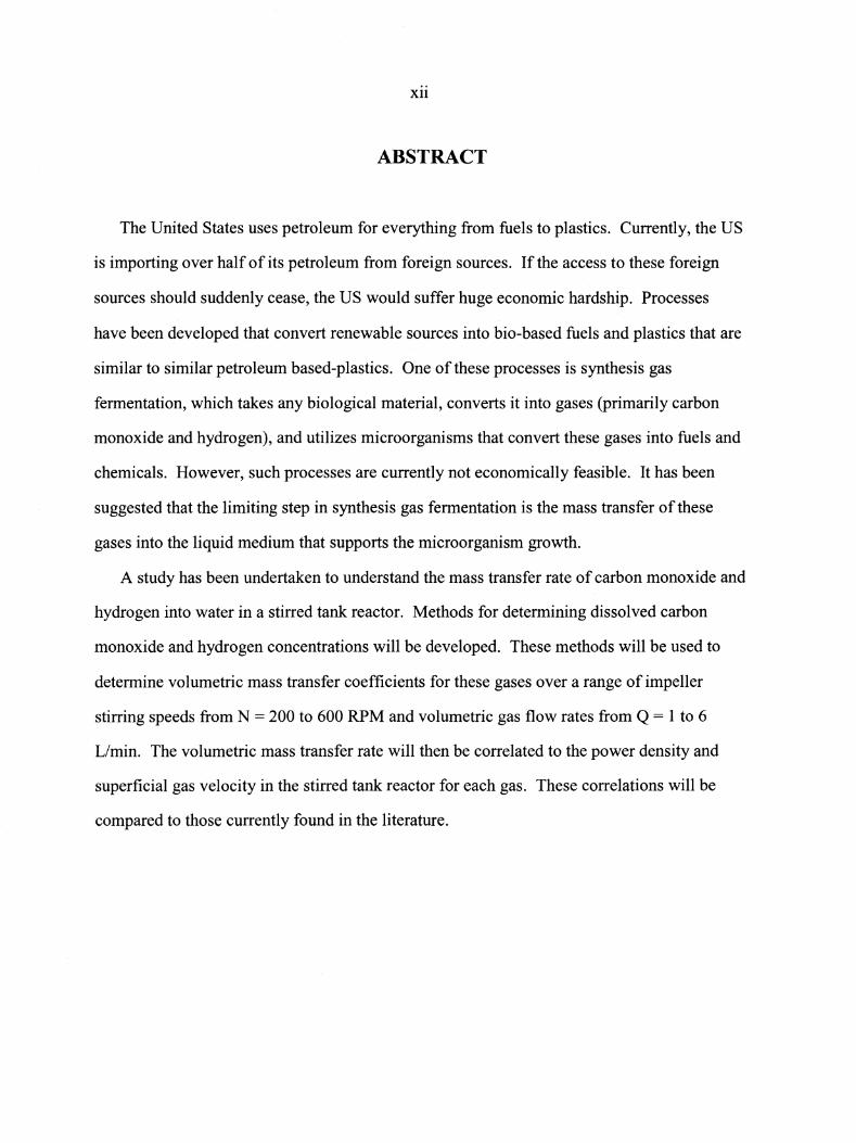
The United States uses petroleum for everything from fuels to plastics. Currently, the US
is importing over half of its petroleum from foreign sources. If the access to these foreign
sources should suddenly cease, the US would suffer huge economic hardship. Processes
have been developed that convert renewable sources into bio-based fuels and plastics that are
similar to similar petroleum based-plastics. One of these processes is synthesis gas
fermentation, which takes any biological material, converts it into gases (primarily carbon
monoxide and hydrogen), and utilizes microorganisms that convert these gases into fuels and
chemicals. However, such processes are currently not economically feasible. It has been
suggested that the limiting step in synthesis gas fermentation is the mass transfer of these
gases into the liquid medium that supports the microorganism growth.
A study has been undertaken to understand the mass transfer rate of carbon monoxide and
hydrogen into water in a stirred tank reactor. Methods for determining dissolved carbon
monoxide and hydrogen concentrations will be developed. These methods will be used to
determine volumetric mass transfer coefficients for these gases over a range of impeller
stirring speeds from N = 200 to 600 RPM and volumetric gas flow rates from Q = 1 to 6
L/min. The volumetric mass transfer rate will then be correlated to the power density and
superficial gas velocity in the stirred tank reactor for each gas. These correlations will be
compared to those currently found in the literature.
1
CHAPTER 1: INTRODUCTION
1.1 Motivation
For centuries humans have been using fermentation to produce things such as cheese,
wine, beer, and bread. It was Louis Pasteur in the late 1800's that discovered that tiny
organisms were responsible for the processes that made these products possible. His work
identifying the fermentation processes laid the path for modem fermentation technologies
that can produce such value added chemicals as antibiotics, enzymes, steroidal hormones,
vitamins, sugars, and organic acids (Williams, 2002).
In the United States there is a major emphasis on the fermentation of sugars into ethanol.
Currently, the US produces over 3.3 billion gallons per year of ethanol (Renewable Fuels
Association, 2004). Other commodity chemicals that are produced in the United States by
fermentation are monosodium glutamate, citric acid, lysine, and gluconic acid (Brown,
2003). These products, however, are the only commodity chemicals currently produced from
biorenewable sources. Advances in breaking down lignocellulosic material will hopefully
lead to the increased production of other chemicals such as lactic acid, 2,3-butanediol,
itaconic acid, and propanediol from organic sources.
For the most part, all other commodity chemicals are produced from petroleum. The
United States currently imports about 55% of all petroleum used here, an all time record high
(USDOE-Energy Efficiency and Renewable Energy, 2004). Approximately 70% of all the
world's petroleum reserves are located in the Middle East, a region that has always been
politically unstable. If the United States stopped petroleum imports from this region, our
country would suffer huge economic hardship. Utilizing biorenewable resources is a way to
help relieve the dependence this country has on foreign petroleum. Microbial fermentation is
a feasible mechanism for converting biomass into similar petroleum-based end products.
2
Most of these fermentation processes are achieved with a solid or liquid substrate, such as
glucose, for microorganism growth. This requires that the substrate be a constant
composition and quality to ensure optimal microorganism growth. However, there are some
microorganisms (e.g., Rhodospirillum rubrum) that can directly utilize carbon monoxide as a
carbon source and have no need for a solid substrate. Carbon monoxide could be utilized
from gasifying organic material to produce a mixture of carbon monoxide, hydrogen, and
carbon dioxide called synthesis gas. These microorganisms are therefore well suited for
converting synthesis gas to fuels and chemicals.
By using synthesis gas, the composition of the organic material becomes irrelevant.
Once the material is gasified, the only differences in composition are the ratios of the gas
components. Some bacteria will produce hydrogen by the water gas shift reaction, adding to
the already hydrogen rich stream from gasification.
The problem with using synthesis gas is that the gas components of interest (carbon
monoxide and hydrogen) are sparingly soluble in the water-based fermentation broth.
Therefore, the need exists to understand the gas-liquid mass transfer of these major synthesis
gas components to successfully utilize biomass gasification as a route to replacing petroleum
in the US economy.
1.2 Goals
This work has many goals to aid the understanding of synthesis gas fermentation. First is
the ability to measure dissolved carbon monoxide and hydrogen in water with enough
accuracy to determine the volumetric mass transfer coefficient for these gases. Processes
have been developed for measuring the concentration of dissolved carbon monoxide and
hydrogen but they have not been applied to volumetric mass transfer studies, so their
applicability in this area will be verified. The second goal is to determine how the
volumetric mass transfer coefficient varies with volumetric gas flow rate and mixing power
3
density in a stirred tank reactor. The experimental ranges for volumetric flow rate (Q = 1 to
6 L/min) and impeller speed (N = 200 to 600 RPM) are comparable with current literature
sources. The third goal is to compare these correlations to those that are found in the
literature. Many studies have been completed on systems that utilize microorganisms that
aerobically metabolize organic material so the vast majority of the correlations found in the
literature are for oxygen absorption into various water solutions. The final goal of this work
is to compare the carbon monoxide and hydrogen mass transfer correlations to each other.
This will help the understanding of synthesis gas systems and how one gas may be affected
by the presence of another, as is the case in all synthesis gas systems.
4
CHAPTER 2: LITERATURE REVIEW
This chapter is divided into four major sections. The first discusses gas-liquid mass
transfer studies that use gases such as oxygen, hydrogen, and carbon monoxide. The second
section reviews different measuring techniques that are available for measuring dissolved
gases in water. The third section discusses several different synthesis gas studies that have
been completed. The last section summarizes the literature review.
2.1 Gas-Liquid Mass Transfer Studies Using Various Gases
This section is separated into two main sub sections. The first sub section concerns the
largest body ofresearch that has been done in the field of gas-liquid mass transfer studies,
oxygen. In the second sub section, carbon monoxide and synthesis gas studies are
summarized.
2.1.1 Gas-Liquid Mass Transfer Studies Using Oxygen
Gas-liquid mass transfer studies using oxygen are very well studied because of the
popularity of microorganisms that utilize oxygen as a feedstock. Because of this large
popularity, oxygen-liquid mass transfer has been well studied in many different types of
reactors with various configurations. The three most common types of reactors are stirred
tank, bubble column, and airlift reactors.
2.1.1.1 Oxygen-Liquid Mass Transfer in Stirred Tank Reactors
Schmitz et al. (1987) studied a three phase system where the liquid was the continuous
phase and a solid catalyst and gas were the dispersed phases. They used the sulphite method
to determine dissolved oxygen concentration in their experiments because dissolved oxygen
probes gave inaccurate results in three phase systems. The vessel that was used in their
5
testing had a non-aerated liquid height equal to the diameter of the reactor and four equally
spaced baffles with a width equal to 10% of the reactor diameter. Their studies looked at the
differences in mass transfer in two- and three-phase systems as they varied the superficial gas
velocity, stirrer speed, and liquid viscosity.
Schmitz et al. (1987) found that when the stirrer speed was low (N < 200 RPM) the
bubble interfacial area was independent of stirrer speed because the stirrer was flooded. As
the stirrer speed increased the superficial gas velocity had very little effect on the interfacial
area. In experiments to determine the variation of the mass transfer coefficient, kL, with
interfacial area, they found that it varied only slightly with interfacial area. The dependence
ofkL on stirrer speed was influenced by two factors: (i) the increased stirrer power produced
smaller bubbles that acted as rigid spheres with a thicker surrounding liquid film that
increased the mass transfer resistance, and thus lowered the kL value, and (ii) the increased
stirrer power increased the turbulence in the tank and decreased the film thickness
surrounding the bubbles and mass transfer resistance, increasing the kL value. According to
Schmitz et al., these effects cancelled each other out and maintained a constant kL value in
their study.
The results of Schmitz et al. suggest that the mass transfer rate correlation should be
separated into two regimes for varying viscosity ranges. The higher viscosity range had a
reduced mass transfer rate, meaning that more power and gas flow were needed to get the
same mass transfer as that of a lower viscosity system (Schmitz et al., 1987).
Linek and Vacek ( 1998), however, ran the same set of experiments and found that the
reduction in mass transfer rate could be accounted for by the oxygen back pressure. Schmitz
et al. (1987) used the assumption that the chemical oxidation of sulphite would keep the
dissolved oxygen concentration in the liquid to near zero. However, the presence of
carboxymethyl cellulose (CMC) decelerates the oxidation reaction, thus leaving oxygen
dissolved in the liquid medium (Linek and Vacek, 1988). Linek and Vacek corrected the
6
oversight of Schmitz et al. and stated that there was no need for multiple correlations for
various operating conditions for oxygen-liquid mass transfer in stirred tanks with CMC, as
long as the oxygen back pressure was properly addressed.
Boon et al. (1992) determined the effect of oxygen adsorption to coal particles used in the
desulphurization process for coal and noticed that there were significant errors using the
dynamic method for measuring volumetric mass transfer rates where oxygen adsorption was
a factor. These researchers found that the results determined in glass bead slurries were not
in agreement with similarly sized coal particles. They proposed an alternative to the existing
correlations that took into account the adsorption coefficient, K,
c· ln •
kLa=(l-cs(l-K)) C -C t
(2.1)
where kLa is the volumetric mass transfer coefficient, Es is the solid volume fraction, C* is
the equilibrium concentration of dissolved gas in water, C is the concentration of dissolved
gas in water, and t is time.
Boon et al. ( 1992) assumed that the adsorption of oxygen on coal was linear and therefore
not a function of the oxygen concentration in the liquid. Their studies showed that the actual
mass transfer rate can be up to 50% lower than the apparent mass transfer rate when activated
carbon sources were present in the slurry, up to a volumetric fraction of 28%.
A four-phase (water, organic phase, cells, and gas phase) study on mass transfer was
conducted by van der Meer et al. (1992). Microorganisms (cells) were suspended in water
and fed on n-octane (organic phase) and air (gas phase). This study investigated how the
volumetric mass transfer coefficient was affected by the organic phase holdup, a
biosurfactant produced by the cells, and an emulsified n-octane phase. The results showed
that there was no difference in volumetric mass transfer coefficient with an organic phase
volumetric liquid fraction of up to 15%. The biosurfactant hindered the volumetric mass
transfer coefficient at low concentrations, but as the concentrations increased, the volumetric
7
mass transfer coefficient increased. This increase in mass transfer was attributed to the
biosurfactant acting as an emulsifier for the n-octane. Over 70% of the emulsified droplets
were small enough to penetrate the gas-liquid film for mass transfer (van der Meer et al.,
1992).
A different study was completed on the effects of viscous fluids (solutions of CMC,
xanthan gum, and polyacrylamide) in a stirred tank reactor with the use of a helical ribbon
screw (HRS) impeller for mixing (Tecante and Choplin, 1993). Using an HRS with non
Newtonian fluids eliminated stagnant zones due to the motion of the ribbon and the small
clearance from the vessel wall. The dynamic oxygen absorption method was used in this
study with a polargraphic probe. Results showed that the superficial gas flow rate had a
greater effect on the kLa performance than the power density, which was contrary to similar
tests in stirred tank reactors that used disc type impellers. This study effectively showed that
HRS impellers could be used for non-Newtonian fluids and produced efficient mass transfer
because HRS impellers provided a more homogeneous mixture than disc type impellers
(Tecante and Choplin, 1993).
Lines (2000) conducted a survey that compared different types of baffle geometries and
non-standard impeller configurations on their contribution to the volumetric mass transfer
coefficient. The only impeller configuration discussed in any detail consisted of a four-blade
45° down-turned angle blade impeller mounted above a standard six-bladed Rushton
impeller. The three baffle designs were a standard full height four wall baffle, a half height
wall baffle, and a beavertail baffle. Mass transfer was determined by the dynamic method
using a polargraphic probe. For a liquid height to vessel diameter ratio of 1, the half height
baffles were a clear improvement over the other two systems. For low speeds (N < 275
RPM), the beavertail baffles had a slight advantage in increased volumetric mass transfer
coefficient than the standard full baffles, but at higher speeds there was virtually no
advantage. When the height to diameter ratio was increased, the beavertail baffles had a
8
lower percentage decrease in mass transfer compared to the other designs so they were the
preferred configuration for systems where the liquid height ratio is greater than unity with
this system of impellers (Lines, 2000).
Yet another oxygen-water system was investigated using several different agitation
methods. This set of experiments consisted of reciprocating plates, Rushton impellers, and a
helical ribbon impeller. The Rushton impellers gave the best mass transfer when compared
on a power per unit volume basis. This became less clear as the superficial gas velocity was
increased from 0.784 cm/s to 0.860 emfs, but the Rushton impellers still gave better results
(Gagnon et al., 1998).
2.1.1.2 Oxygen-Liquid Mass Transfer in Other Reactors
Oxygen-liquid mass transfer rates were investigated in a yeast culture using a stirred tank
and batch pulsed baffled bioreactor by Ni et al. (1995). They measured the dissolved oxygen
using a P2-type probe in both systems. They also used a polargraphic oxygen meter in the
pulsed baffled bioreactor and an IL-type polargraphic probe in the stirred tank reactor. They
concluded that for a comparable power density, the pulsed baffled bioreactor had up to a 75%
improvement in volumetric mass transfer coefficient than the stirred tank reactor. Their work
also showed, by way of visualization experiments, that the pulsed baffled system was an
efficient way of mixing and suspending particles (Ni et al., 1995).
Another team investigated the effects of baffle types in a pulsed baffled reactor and their
relationship to the volumetric mass transfer coefficient. A central baffle, helical baffle, and a
wall or orifice baffle were used (Hewgill et al., 1992). Again, the dissolved concentrations
were obtained using a polargraphic probe. The results showed up to a six fold increase in
volumetric mass transfer coefficient when wall baffles and flow oscillation were present
compared to normal bubble column mass transfer. They also claimed that this system had
very good mixing, lending this type of reactor to fermentation type processes.
9
A bubble column and two types of airlift reactors were studied using an algae culture as
the oxygen absorbing medium (Miron et al., 2000). One of the airlift reactors was a split
cylinder with a riser to downcomer ratio of unity and the other was a draft tube reactor with a
ratio of 1.24. All three reactors had the same working volume and were similar in overall
geometry. This work showed that all three reactors had similar mass transfer rates for similar
operating conditions and that it was sufficient for growing algae cultures.
2.1.2 Gas-Liquid Mass Transfer Using Synthesis Gas or Pure Carbon Monoxide
Cowger et al. (1992) used a trickle bed reactor with ceramic Intalox saddles and a
continuous-stirred tank reactor to investigate steady state mass transfer rates using a
fermentation broth of water and nutrients and a gas mixture composed of hydrogen, argon,
carbon monoxide, and carbon dioxide (20/15/55/10%). This study did not produce any
correlations for volumetric mass transfer rates as a function of system parameters, but instead
found the values at two different cell recycle rates and compared those numbers between the
two types ofreactors. The k1a values that were determined were 22 and 38 h-1, and they
were consistent with presented literature data for trickle bed reactors (Cowger et al., 1992).
Their stirred tank studies were inconclusive because they believed that they were operating
the reactor at a kinetically limiting rate, so no data were presented.
Klasson et al. (1993b) conducted a similar study where they investigated the production
of hydrogen using Rhodospirillum rubrum growing on carbon monoxide. The experiments
were carried out in a stirred tank reactor where they measured the carbon monoxide
conversion and cell concentration. Measured mass transfer rates ranged from 13 to 35 h-1 for
an agitation range of 300 to 700 RPM, which were again comparable to those found in
presented literature sources.
Bredwell et al. (1999) completed detailed work on synthesis gas fermentation strategies,
and included various microorganisms and reactor configurations. Types of reactors that were
10
investigated include stirred tanks, bubble columns, packed bubble columns ( cocurrent and
trickle flow), trickle beds, and microbubble sparged columns. Mass transfer coefficients for
all of the reactor designs used, except the cocurrent packed column and the microbubble
column, were in the range of 10 to 860 h-1, depending on the operating conditions. For the
microbubble column, mass transfer rates ranged from 200 to 1800 h-1, and for the cocurrent
packed column rates of 1.5 to 3670 h-1 were determined.
Mass transfer correlations for hydrogen and carbon monoxide were developed by Yang et
al. (2001) for mass transfer in a slurry bubble column. Their results showed a strong mass
transfer dependence on several operating conditions including temperature, pressure, and
superficial gas velocity.
Cell growth was measured as a function of the carbon monoxide partial pressure using a
bubble column reactor (Chang et al., 2001). As would be expected, the cell growth rate
increased with carbon monoxide partial pressure, and the carbon monoxide mass transfer rate
was determined to be 72 h-1 for a partial pressure of 41.5 kPa.
2.2 Measuring Dissolved Gases in Water
This section addresses measurement techniques for determining dissolved gas
concentrations in water and is divided into two sections: the first deals with dynamic
response methods and the second handles the static response methods for determining the
volumetric mass transfer coefficient.
2.2.1 Dynamic Techniques
The dynamic oxygen electrode method employs the use of a dissolved oxygen electrode
to measure the dissolved oxygen concentration in water as a function of time. Usually the
reactor is deoxygenated with an inert gas such as nitrogen to remove all oxygen. Then as gas
flow is switched to pure oxygen (or alternately, air) the electrode response is measured as a
11
function of time. The volumetric mass transfer coefficient can be calculated from the
concentration versus time data. The start-up method is a variation of the dynamic oxygen
electrode method where the aeration is started as the electrode response is logged. The initial
gas holdup in the reactor is therefore nonexistent and eliminates the potential problem of the
inert gas being held up in a multiple stage impeller design. Difficulties lie in the necessity to
understand the entire system, including the dynamic response characteristics of the oxygen
electrodes over a range of concentrations.
One drawback to these types of dynamic methods is that air is sometimes used instead of
pure oxygen to measure the oxygen mass transfer rate and simultaneous nitrogen mass
transfer may affect the actual oxygen volumetric mass transfer rate (Gogate and Pandit,
1999). Another limitation of the dynamic electrode method is that the gas holdup is assumed
to be steady during the switch from inert gas to oxygen. This assumption is not correct
because the inert phase will be flushed out by the incoming oxygen phase (Gogate and
Pandit, 1999; Linek et al., 1993). The gas phase may not be as perfectly mixed as most
models assume so Stenberg and Andersson (1988) examined this and found that an average
volumetric mass transfer coefficient could be measured to solve this problem.
The dynamic pressure step method uses the same idea as the dynamic electrode method,
where the gas phase concentration is suddenly changed and the dissolved oxygen
concentration in water is observed. The difference in the dynamic pressure step method is
that the concentration change takes place when the pressure in the reactor is suddenly
increased by a small amount (15 to 20 kPa). This sudden increase changes the oxygen
concentration in all bubbles in the reactor regardless of the gas-phase mixing so the
hydrodynamics of the system do not necessarily need to be well understood to make
volumetric mass transfer coefficient measurements. Pressure change is easy to achieve by
simply adding gas to the free space above the liquid level.
12
The non-ideal pressure step method is a slightly different method from the dynamic
pressure step method. The difference in the two is that in the latter, the pressure step is
assumed to be instantaneous (ideal), such as one could achieve in a small scale reactor. The
pressure increase is achieved by closing the gas outlet and then subsequently throttling said
outlet to maintain a certain pressure.
A similar variation to the dynamic electrode method is the CO-bound hemoglobin
method. Liquid samples with dissolved gases are taken from the reactor at regular time
intervals. The CO concentration in the sample is evaluated by determining the concentration
of bound hemoglobin of a known CO concentration using a spectrophotometer. This method
is outlined by Kundu et al. (2003) and in Section 3.3. The major limitations of this technique
are the sampling rate and the time necessary for evaluating each sample.
2.2.2 Static Methods
The steady state method is a chemical method for determining the dissolved
concentration of oxygen in the sulfite medium. A reactor is allowed to come to steady state
with oxygen flowing and agitation. An inlet stream of sodium sulfite is added to the reactor
as an outlet stream of equal mass flow rate is withdrawn from the system. When the flow
rate of the sodium sulfite is sufficient enough to react completely with the oxygen in solution
there will be no response from a dissolved oxygen electrode. The oxygen and sodium sulfite
react in the presence of a cobalt catalyst to form sodium sulfate.
1 Co2+ Na 2S0 3 +-02 Na 2SO 4
2 (2.2)
This technique, however, is very unreliable at high aeration rates because the required
higher concentration of sodium sulfite enhances the oxygen to water mass transfer rate
(Gogate and Pandit, 1999).
13
A modification to the sulfite method exists to accommodate high aeration rates. This
method slowly feeds a sodium sulfite solution into the reactor until the concentration of
oxygen is between 90 and 95% of the equilibrium concentration (Gogate and Pandit, 1999).
The oxygen back pressure is then measured in the liquid volume with an oxygen probe. The
equation
kLa = 1 c[v/ I
2 ViC10 (l-G) (2.3)
shows how the volumetric mass transfer coefficient can be calculated, where V1 and C1 are
the volumetric flow rate and concentration of the sodium sulfite solution, C1,o is the
equilibrium oxygen concentration, and G' is the oxygen saturated liquid electrode response
(Gogate and Pandit, 1999). This version of the sulfite method eliminates the high
concentrations of sulfite needed to react with the larger amounts of oxygen present for the
higher aeration rates.
The peroxide method is a simple technique that uses hydrogen peroxide and a protein
catalyst ( catalase) to produce oxygen in the reactor liquid. This oxygen is then transferred
into the liquid and a carrier gas is used to take away the oxygen to be analyzed. At steady
state the oxygen production is equal to the oxygen transfer rate. Therefore this is a very
simple method where the only variables that need to be known are the inlet concentration of
hydrogen peroxide, the reactor liquid volume, the carrier gas flow rate, and the outlet oxygen
concentration. One problem with the peroxide method is that the catalyst used, catalase, is a
protein, which are known to enhance foam formation that can affect the mass transfer rates.
Also, the reactivity of hydrogen peroxide may deactivate catalase so this method should not
be used for fermentation broths (Gogate and Pandit, 1999).
14
2.3 Synthesis Gas Fermentation
Synthesis gas fermentation can be separated into two sections as described below. The
first is the microorganisms that are used in the fermentation process, and the second is the
design issues that need to be accounted for in designing fermentation reactors.
2.3.1 Microorganisms Used in Synthesis Gas Fermentation
Grethlein and Jain (1992) researched many different types of anaerobic bacteria that can
utilize synthesis gas for the production of synthetic fuels, chemical feedstocks, and other
chemicals. The bacteria in their study were Clostridium thermoaceticum, Clostridium
ljungdahlii, Peptostreptococcus productus, Eubacterium limosum, and Butyribacterium
methylotrophicum.
C. thermoaceticum utilized all three of the major synthesis gas components (CO, H2, and
C02) to produce acetic acid.
4CO + 2H 20--7 CH 3COOH + C02 (2.4)
(2.5)
C. ljungdahlii produced high concentrations of both ethanol and acetate from carbon
monoxide (Grethlein and Jain, 1992).
P. productus was one of the fastest growing bacteria that utilized CO with a doubling
time of 1.5 hours in a 50% CO atmosphere, or less than two hours in atmospheres
approaching 90% CO (high concentrations of CO are poisonous to these bacteria). These
bacteria produced acetate and carbon dioxide from CO or hydrogen and carbon dioxide with
a doubling time of five hours. These bacteria also showed a high tolerance to sulfur
compounds, which makes them especially useful in coal derived synthesis gas fermentation
(Grethlein and Jain, 1992).
B. methylotrophicum maintain the ability to produce acetate and butyrate under many
different conditions (Grethlein and Jain, 1992). These bacteria grew on hydrogen and carbon
15
dioxide and produced acetate with a nine hour doubling time. When growing on methanol in
the presence of acetate and carbon dioxide, it produced butyrate at a methanol:butyrate ratio
of 4: 1. A mutant strain exists that produced acetate and small amounts of butyrate on pure
carbon monoxide. The pH of the fermentation broth had a significant effect on the
production of acetate and butyrate from this microorganism (Grethlein and Jain, 1992). At a
pH of 6.8, the acetate to butyrate ratio was 32: 1, but at pH 6.0 the ratio was 1: 1. Additional
pH tests showed similar trends in the production of ethanol and butanol. Grethlein and Jain
(1992) were the first to demonstrate the production ofbutanol from carbon monoxide from
any organism.
The work of Grethlein and Jain ( 1992) showed that the production of acetate and butyrate
by E. limosum depended highly on the carbon substrate. When grown on hydrogen and
carbon dioxide, it produced acetate and minor amounts of butyrate with a 14 hour doubling
time. Using methanol as the substrate in the presence of acetate and carbon dioxide, E.
limosum produced equimolar amounts of acetate and butyrate in a 7 hour doubling time.
Acetate alone was produced in a 7 hour doubling time from a substrate of 50% carbon
monoxide and the doubling time increased to 18 hours when a concentration of 75% carbon
monoxide was used.
Chang et al. (2001) studied the effect of carbon monoxide partial pressure on E. limosum
using a bubble column reactor with both batch and continuous fermentation with cell recycle.
They showed that in batch operation, the cell concentration and acetate production increased
over their vial fermentation trials. They explained this by the increased pH and the much
better mass transfer in the batch bubble column. After 65 hours of batch operation they
turned on a recycle pump to operate the reactor in continuous mode. This portion of the
study determined the effect of dilution rate on cell concentration and acetate production. As
they increased the dilution rate, the cell concentration increased while the acetate production
decreased. When the dilution rate was decreased, the cell concentration decreased, the
16
acetate concentration increased and a small fraction of butyrate was produced. These results
showed that the cell concentration and the product concentration were very dependant on the
recycle rate.
Wolfrum and Scott (2002) studied Rubrivivax gelatinosus as a hydrogen producing
bacteria that used carbon monoxide as its substrate in a trickle bed reactor. This study
showed a strong similarity between geometrically similar reactors for producing hydrogen
from these bacteria. They believe that these data can be used to successfully predict the
performance of larger systems.
Cowger et al. (1992) and Klasson et al. (1993a, 1993b) studied Rhodospirillum rubrum as
a hydrogen producing bacteria. Cowger et al. (1992) showed that the limiting factor for
utilization of carbon monoxide by R. rubrum was the mass transfer rate. They also showed
that the cell concentration had no affect on the carbon monoxide conversion. An increase in
the liquid flow rate, however, gave an increase in the carbon monoxide conversion. Klasson
et al. (1993a) found overall mass transfer rates for a stirred tank system to be 15 to 35 h-1 for
a range of stirrer speeds from 300 to 700 RPM. The studies of Klassen et al. (1993a) show
that R. rubrum has a hydrogen production (.01 mol/g-h) similar to the highest reported
production as found in their literature search. Klasson et al. (1993b) extended the work of
Cowger et al. (1992), finding that the limiting factor for hydrogen production was not the
metabolism of R. rubrum, but the mass transfer of carbon monoxide into water.
2.3.2 Synthesis Gas Fermentation Reactor Design
Vega et al. ( 1990) studied Peptostreptococcus productus fermentation in a continuous
stirred tank reactor (CSTR) as it grew on carbon monoxide. They showed that the only way
to get complete carbon monoxide conversion was to have no gas flow rate due to the perfect
mixing of the stirred tank reactors. They also showed that with a bubble column, it was
possible to get complete carbon monoxide conversion at low gas flow rate to volume ratios.
17
Their results showed that for a constant retention time and mass transfer rate, the bubble
column converted 95% of the carbon monoxide, whereas a CSTR only achieved 80%
conversion. Vega et al. (1990) also investigated the effect of pressure on the cell growth in
their CSTR. It was shown that the carbon monoxide uptake increased with an increase in
pressure, but CO inhibited bacteria growth at elevated pressures. They tested a step increase
in carbon monoxide pressure and found that if sufficient time was given for the cells to grow,
they could handle the increased carbon monoxide concentration in the liquid.
Klas son et al. ( 1991) studied the fermentation of synthesis gas to produce ethanol and
methane in a CSTR. They found that to produce methane from synthesis gas, they needed to
go through an intermediate, acetate, using P. productus. The methane was then converted to
ethanol using Methanothrix sp. or Methanosarcina barkeri. A step-wise pressure increase
allowed sufficient P. productus growth before the carbon monoxide concentration in the
liquid became lethal to the bacteria. This increased the acetate production, and therefore
increased the M. barkeri production up to a concentration of 6 g/L. Similar results were
shown for the Methanothrix sp. Using an immobilized cell reactor they were able to utilize
an inlet acetate concentration of 10 g/L. They concluded that this type of fermentation
process was not economically feasible in the reactors investigated because of low growth
rates.
Klasson et al. (1991) also used Clostridium ljungdahlii to convert carbon monoxide,
hydrogen, and carbon dioxide into ethanol and acetate. Their research showed that the best
ethanol production was achieved using two CSTR's in series. The first was operated at a pH
of 4.5 and focused on growing the C. ljungdahlii bacteria. The second CSTR had a pH of
4.0, which changed the dilution rate and initiated ethanol production. This system showed a
30-fold improvement over a single CSTR operation.
Worden et al. ( 1997) studied Butyribacterium methylotrophicum with different
immobilized cell structures in a continuous cell-recycle fermentation system. They showed
18
that B. methylotrophicum could effectively be immobilized on celite, ion-exchange resin, and
molecular sieves. They showed that decreasing the pH in the cell-recycle experiments
increased the formation of butyrate and alcohols and decreased acetate production as long as
the pH was above 6.0. Below pH 6.0, the organisms oscillated between acetate and butyrate
production.
Bredwell et al. (1999) experimented with microbubbles for use in synthesis gas
fermentation. Microbubbles were formed through high shear at the gas-liquid interface. The
resulting microbubbles were assumed to have a multilayered shell, but this was not
experimentally verified during their study. The micro bubbles gave a range of volumetric
mass transfer coefficients from 200 to 1800 h-1 compared to bubble columns that had a range
of 18 to 864 h-1 (in their study). This work showed that high kLa values can be efficiently
achieved using microbubbles without the need for mechanical agitation.
2.4 Literature Review Summary
Numerous gas-liquid mass transfer studies have been completed using oxygen as the gas
phase. These studies, however, can only be used as guides for syngas-liquid mass transfer
because oxygen-liquid mass transfer rates are not identical to syngas-liquid mass transfer
rates (Incropera and DeWitt, 2002). Determining actual syngas-liquid mass transfer rates are
necessary to commercially produce fuels and chemicals through syngas fermentation. Before
these rates are determined, base-line gas-liquid mass transfer rates are required using pure
syngas components of interest (i.e., CO and H2). The work of this thesis will complete these
studies, and is part of a long term research effort to ultimately produce fuels and chemicals
through syngas fermentation.
19
CHAPTER3: MATERIALSANDMETHODS
3.1 Experimental Set-Up
This section is divided into three main sub-sections. The first describes the stirred tank
bioreactor. The second section summarizes the trial preparation. The third section outlines
the trial operation.
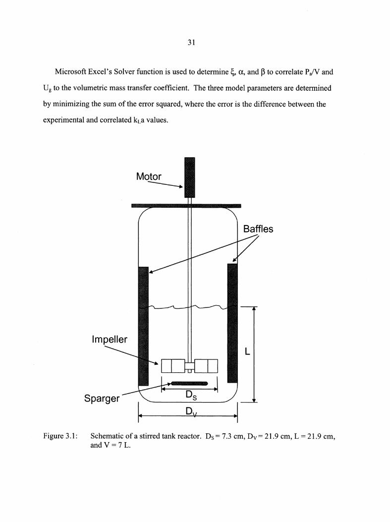
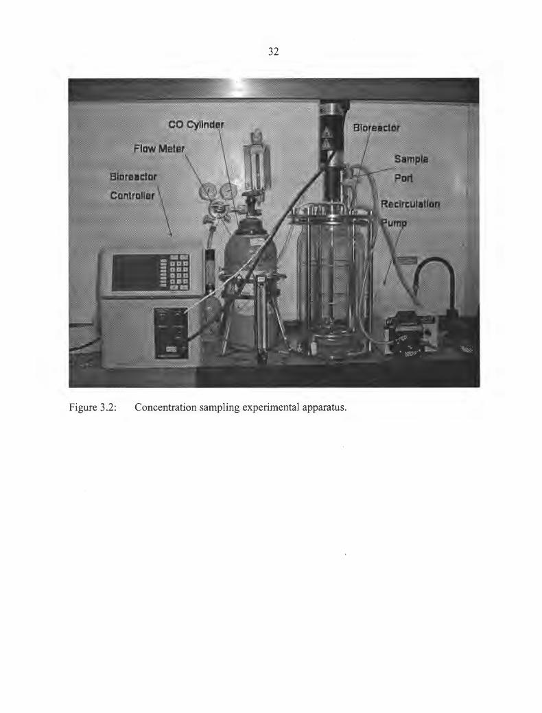
3.1.1 Stirred Tank Bioreactor
The fermentation vessel is a BioFlo 110 Autoclavable Fermentor & Bioreactor with a
14.0 liter total volume and a 10.5 liter maximum working volume supplied by New
Brunswick Scientific as shown in Fig. 3.1 and 3.2. (All figures in this thesis are located at
the end of the respective chapter.) The vessel diameter is Dv = 21.9 cm. A Rushton turbine
impeller, Ds = 7.3 cm in diameter and located 7.3 cm from the bottom of the vessel, provides
agitation. Four 2.2 cm wide baffles are symmetrically located around the periphery of the
bioreactor. Gas is fed into the vessel from a ring sparger located just below the impeller.
The impeller's rotational speed is regulated from a motor mounted to the top of the vessel,
and the motor is controlled by the fermentation system controller unit. Impeller speed can be
monitored and controlled from this unit up to 1200 RPM. Temperature can also be
monitored and regulated from this controller by means of a heating jacket and a temperature
probe.
Gas is supplied to the vessel from a 650 liter size G gas cylinder. This size cylinder is
used because it will fit in a stand located inside the fume hood ensuring that, if a gas leak
would occur, it would be contained. A two-stage regulator is mounted directly to the gas
cylinder to control outlet pressure. When using hydrogen, a flashback arrestor is also
connected directly to the regulator to prevent the possibility of any flames entering the gas
cylinder and causing an explosion. Note, however, that no flames were intentionally or
20
unintentionally present during any part of this study. The tubing from the cylinder to the
flow meter and then to the vessel is Tygon FEP-lined tubing to minimize gas diffusion
through the tube walls.
Gas flow is regulated using a 150 mm rotameter with a needle valve for precise flow rate
control. This rotameter can handle a gas flow rate of up to 10 liters per minute for carbon
monoxide and up to 3 7 liters per minute for hydrogen. A tripod base with a bubble level and
leveling screws is used to ensure the rotameter is completely vertical.
Dissolved gas samples are taken using a recirculation loop from the vessel sample line
(see Fig. 2). A short (approximately 5 cm) section ofTygon-FEP tubing connects the sample
port to a PTFE Swagelok union tee. Directly across from this connection is Tygon LFL
pumping tube that leads to a peristaltic pump and the vessel return line. The third outlet from
the union tee contains a septa and is used as a sampling port for a syringe needle to penetrate
and withdraw a liquid sample.
A Masterflex LIS peristaltic pump system is used for the recirculation tubing line. This
pump operates at 2.2 liters per minute. At this flow rate, it takes less than 0.5 seconds for the
fluid to travel through the sample line from the bioreactor to the sample port.
3.1.2 Trial Preparation
The tap water line in the fume hood is turned on and allowed to run directly to the drain
for 5 minutes to flush out rust or any other deposits that may have had time to collect in the
plumbing. The water is then directed to the bioreactor for filling.
With 7 L of water in the bioreactor, the stirrer speed is set to 400 RPM (this speed is the
median of all stirrer speeds used in these trials) and allowed to come up to speed. The gas
flow is turned on, and the rotameter needle valve is set to the gas flow rate that will be used
for the next trial. The gas cylinder flow control valve is then closed, leaving the rotameter
needle valve set at the desired value.
21
The bioreactor is completely filled to ensure that there is no remaining gas from a
previous trial. When the bioreactor is full, the water is shut off and the recirculation line is
taken from the return port and placed in the drain. The circulation pump is turned on and the
bioreactor is completely drained.
During the time it takes to drain the bioreactor, the syringes are prepared. This procedure
consists of flushing out each of the syringes with clean tap water. Each syringe is flushed at
least five times to guarantee that the previous sample no longer has a presence in the syringe.
After each syringe has been flushed, it is laid out on top of the controller unit of the
fermentation system in numerical order (each syringe is numbered, starting from 1 ).
After the bioreactor is drained and all of the syringes are flushed, the bioreactor is filled
to the 7 liter mark, corresponding to a water height-to-diameter ratio of 1. The recirculation
pump is turned on for several seconds to eliminate any bubbles in the return line. When
bubbles are no longer visible in the return line, the line is connected back to the top of the
vessel. The water level is checked and corrected to the seven liter mark.
The power unit and controller for the vessel are powered on at this time. The stirring
speed is set to the desired value and the stirrer is started. After a minute the stirrer will be up
to full speed and the value on the screen should match the set value.
3.1.3 Trial Operation
With the flow control valve closed on the dual stage regulator, the cylinder pressure valve
is opened. The pressure is checked to make sure that there is enough gas present to complete
the trail run. The first syringe is injected into the septa with the plunger depressed to save
time while taking the first sample.
A digital stopwatch is simultaneously started as the gas cylinder flow control valve is
completely opened. After the given time has passed, the plunger is pulled on the syringe.
When the syringe is full it is removed from the septa and the next in numerical order is
22
injected into the septa. When the given amount oftime has passed, the plunger is pulled, and
this process continues until the necessary time has expired or all of the syringes have been
used.
The gas cylinder is shut off first to conserve gas. The pump and stirrer are shut down
next. Water is again piped into the vessel to evacuate the remaining gas in the dead space
above the water. When the vessel is full the pump is turned on and the water is drained from
the vessel.
3.2 Measuring Dissolved Carbon Monoxide Concentrations
This section describes a globin protein technique used for measuring dissolved carbon
monoxide concentrations in the bioreactor; it involves several steps, each of which is
described below.
3.2.1 Dissolved Carbon Monoxide Sampling Equipment
Dissolved carbon monoxide concentration samples are measured using a Cary-50 Bio
spectrophotometer from Varian. The spectrophotometer measures light absorption in the 400
to 700 nm wavelength range.
Samples are prepared and scanned in 1.4 mL nominal volume semi-micro special optical
glass cuvettes. These cuvettes have a 1 cm path length and are usable for wavelengths from
320 to 2500 nm. The cuvettes have PTFE stoppers to reduce contamination and evaporation.
Syringes used for collection of liquid samples containing dissolved CO are Gastight high
performance 10 microliter syringes. The syringes have negligible losses up to 13.8 bar.
Needles are cemented into this type of syringe.
Myoglobin used in the dissolved CO concentration measurements is purchased through
Sigma-Aldrich and is derived from horse heart. The myoglobin comes as a lyophilized
powder at least 90% pure.
23
3.2.2 Making the Carbon Monoxide Saturated Buffer Solution
Approximately 30 cc of potassium phosphate pH 7 .0 solution is added to a 50 cc
needleless Gastight syringe, leaving a small air bubble in the syringe. The air bubble
functions as dead space for the liquid volume to expand as CO is bubbled through the
syringe. The syringe is placed under a fume hood in a three-pronged clamp to hold the
syringe body and the plunger from falling from the body. A small transfer pipette is
stretched to reduce the diameter so it will easily fit inside the syringe. Tubing runs from a
CO cylinder to the fume hood, where a needle on the end of the tubing is punctured into the
bulb of the transfer pipette. Carbon monoxide is bubbled through the syringe for 20 minutes
to completely saturate the solution. The gas is then shut off and the pipette is removed from
the syringe. The bubble is evacuated from the syringe. Sodium dithionite is added to the
carbon monoxide saturated solution to deactivate any remaining oxygen that is present in the
syringe. A rubber cap is placed on the syringe tip to keep the CO from coming out of
solution.
3.2.3 Making the Deoxygenated Buff er Solution
Approximately 50 mL of potassium phosphate pH 7 .0 solution is poured into a small
beaker. From this beaker 1 mL of solution is withdrawn using a 1 mL syringe and injected
into a 1 cm glass cuvette. Sodium dithionite is added to the solution to deactivate any
dissolved oxygen that is present. It is assumed that this solution contains no dissolved carbon
monoxide.
3.2.4 Preparing a Dissolved CO Sample
One mL of potassium phosphate solution is added to a 1 cm cuvette using a 1 mL
syringe. Sodium dithionite is then added to the solution. The solution is mixed by shaking
the cuvette several times with the cap in place to ensure the sodium dithionite is dissolved. A
24
specified amount (see Section 3.2.5) of globin protein is added to the cuvette. The cuvette is
again shaken to ensure proper mixing. Ten µL of either CO saturated, deoxygenated, or trial
sample is then added to the cuvette and, again, shaken.
3.2.5 Identifying the Protein Concentration
A sample of CO saturated solution is prepared. The amount of protein added to the
solution will depend on the prepared protein concentration. The goal is to obtain an
absorption value from the spectrophotometer near 1.5 at the highest peak. This peak occurs
at 416 nm for hemoglobin and at 423 nm for myoglobin.
The protein concentration is determined from
A Cp=-
1·£ (3.1)
where Cp is the protein concentration, A is the absorption value, 1 is the path length of the
cuvette, and i:: is the absorption coefficient (i:: = 180 µM- 1 cm-1 for hemoglobin and i:: = 157
µM- 1 cm-1 for myoglobin).
3.2.6 Converting the Spectra Data to Usable Data for Spectra Solve
Data from the spectrophotometer are provided in two columns in a spreadsheet format
and must be converted to text, tab delimited format for utilization by Spectra Solve. Spectra
Solve is software that will interpolate a third spectrum between two spectra that are of known
composition and report the percent match of each of the two known spectra. If column titles
are used, they must not contain any numerals or Spectra Solve will interpret that cell as a data
cell. The spectrophotometer file will also include some operating data at the bottom of the
two columns and these must be removed.
25
3.2. 7 Fitting Spectra
Spectra are fitted to the known values of the CO saturated and deoxygenated samples.
All of the spectrophotometer data from the CO saturated, deoxygenated, and trial sample
solutions are combined into one Spectra Solve file. The CO saturated and deoxygenated
spectra are placed in cells that will be used in fitting the trial sample spectra to these two
known values. The "Fit Shape" option in Spectra Solve interpolates a selected data cell
between the two assigned cells (i.e., the two known concentration cells) and provides a
percentage of similarity to each spectra. These data are used to determine the concentration
in the sample through the following equation:
SampleConcentraton =
( . X (TotalCuvetteVol.J Protem Cone. % of CO Sat. Spectra Sample Vol.
(3.2)
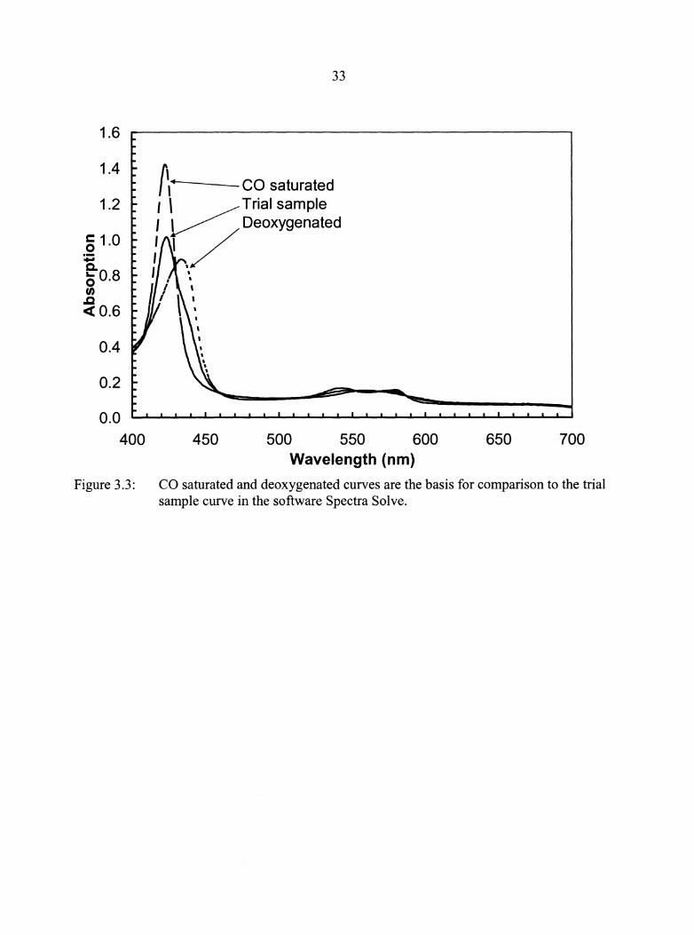
3.2.8 Sample CO Concentration Results
Figure 3.3 shows three separate dissolved CO concentration measurements on one plot.
The largest peak is the result of a CO saturated control sample. The smallest peak is from the
deoxygenated control sample. Spectra Solve will interpolate the third (middle) peak between
the two control samples and output a percent match to each of the control samples.
3.3 Measuring Dissolved Hydrogen Concentration
This section is divided into four sub-sections. The first is the sampling equipment used
for the hydrogen concentration measurements, second is the start-up procedure for the gas
chromatograph, the third is the sample taking procedure, and the final is the shut-down
procedure for the gas chromatograph.
26
3.3.1 Dissolved Hydrogen Sampling Equipment
Dissolved hydrogen gas concentrations are determined using a Gow-Mac series 580 gas
chromatograph. Column, detector, and injector temperatures are set to 100°C and the
detector current is set to 80 mA. Attenuation is set to 1 to achieve the highest accuracy.
Argon, at a flow rate of 30 mL per minute, is used as the carrier gas.
The gas flow rate through the gas chromatograph is measured using a bubble flow meter.
This flow meter is a 50 mL graduated cylinder with a 12 mL rubber bulb.
Argon carrier gas is supplied from a 9500 standard liter cylinder. A dual stage regulator
is mounted to the tank and regulates pressure from the cylinder.
Since moisture is detrimental to gas chromatograph operation, water must be separated
and removed from the dissolve hydrogen before the hydrogen enters the gas chromatograph
for analysis. This is accomplished by flashing the liquid sample to steam and then removing
the water vapor. Figure 3.4 schematically represents the complete set-up.
Samples are injected into the system via a septa mounted to a quartz tube that has three
inlet/outlet ports. The remaining two ports are the inlet and outlet for the carrier gas. The
quartz tube is approximately 1.91 cm outer diameter and 12.7 cm long.
The quartz tube is heated to 550°C in a Carbolite tube furnace (maximum operating
temperature of 1000°C).
Heating tape is wrapped around the inlet and exit tubing from the quartz and maintained
at 110°C. This tape minimizes condensation in the tubing directly before and after the tube
furnace.
All tubing in the system is made from Teflon. All connectors are made from Teflon,
brass, or stainless steel. These materials ensure that no gas mass transfer takes place
throughout the whole system.
A portion of the Teflon tubing is coiled and placed into an ice bath to condense the
vaporized water. A union tee located in the ice bath directs the flow to either gas
27
chromatograph (ideally H2 and carrier gas only) or a water reservoir (condensed water only).
The reservoir will hold up to 10 mL of condensed water. The gas travels through a silica gel
desiccant moisture filter, located between the ice bath and gas chromatograph, to remove any
remaining moisture.
The dissolved hydrogen samples are injected into the quartz tube from 1 mL Gastight
syringes. The syringes have a negligible loss at up to 13.8 bar.
3.3.2 Gas Chromatograph Start-Up
Hydrogen measurements are completed using the equipment as described in section 3.3.1.
The gas chromatograph (GC) requires about 3 hours to come to steady-state before any
measurements are made. Before the gas chromatograph is started, open the pressure
regulator on the argon cylinder to approximately 2.2 bar (the GC valves require at least 1 bar
to operate). The gas chromatograph power is then turned on. There is a large back pressure
in the piping of the system so the flow rate will not immediately show its steady state value at
the bubble flow meter. The system takes about 15 minutes to achieve a steady flow rate.
When the power is turned on and the gas flow is verified from the bubble flow meter, the
gas chromatograph parameters can be set. The detector current is set to 80 mA, and the
column, detector, and injector temperatures are set to 100°C. At this point, the fan switch
can be changed from "Fan Only" to "Col. Heater & Fan" to help the system get to steady
state.
The tube furnace is then powered on and the temperature is verified to be 550°C. The
heating tape is switched on as well and the temperatures should be approximately 110°C.
The ice bath is then prepared and the cooling coil and condensate reservoir are placed in a
one liter beaker. Ice is packed around all of the tubing and the reservoir. Cold tap water is
then poured over the ice to enhance the condenser contact area.
28
Peak Simple software is used to evaluate the gas chromatograph response. This program
integrates data from the gas chromatograph and provides the peak area for each gas P!esent.
Peak Simple is started and the response is monitored until steady state is achieved.
3.3.3 Sample Evaluation Procedure
When the system is at steady state, one syringe with dissolved hydrogen can be injected
into the septa mounted to the quartz tube. After approximately eight minutes the hydrogen
peak will begin to appear in the Peak Simple software. The peak area is found from the
results screen and this information is evaluated using a calibration curve that is produced
from peak areas of known hydrogen volumes.
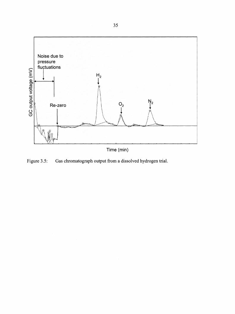
Figure 3.5 shows a typical gas chromatograph output. The vertical axis is the GC
response in m V and the horizontal axis is the time marked in units of one minute. The
injection was started at approximately time zero on the graph. The initial noise is the result
of the pressure fluctuations from the evaporation and condensation of the water in the tubing.
The vertical jog in the trace is a re-zeroing feature of the software to keep the trace centered
on the screen. The first peak is the hydrogen gas that was dissolved in the water.
Immediately following the hydrogen peak are two peaks that represent the dissolved oxygen
and nitrogen that are present in tap water.
3.3.4 Gas Chromatograph Shut Down
The tube furnace and heating tape are shut off as soon as sampling is complete. The gas
chromatograph can only be shut down after it has reached a certain temperature to ensure that
the filaments do not bum out prematurely. All of the settings on the gas chromatograph are
set to their minimal value and approximately 45 minutes must pass until the system is ready
to be shut off. The detector temperature should be below 80°C before the argon can be shut
29
off. When this temperature is reached, the gas chromatograph is shut off. Only after the GC
is shut off may the argon gas cylinder be shut off.
3.4 Determining the Volumetric Mass Transfer Coefficient from
Concentration Data
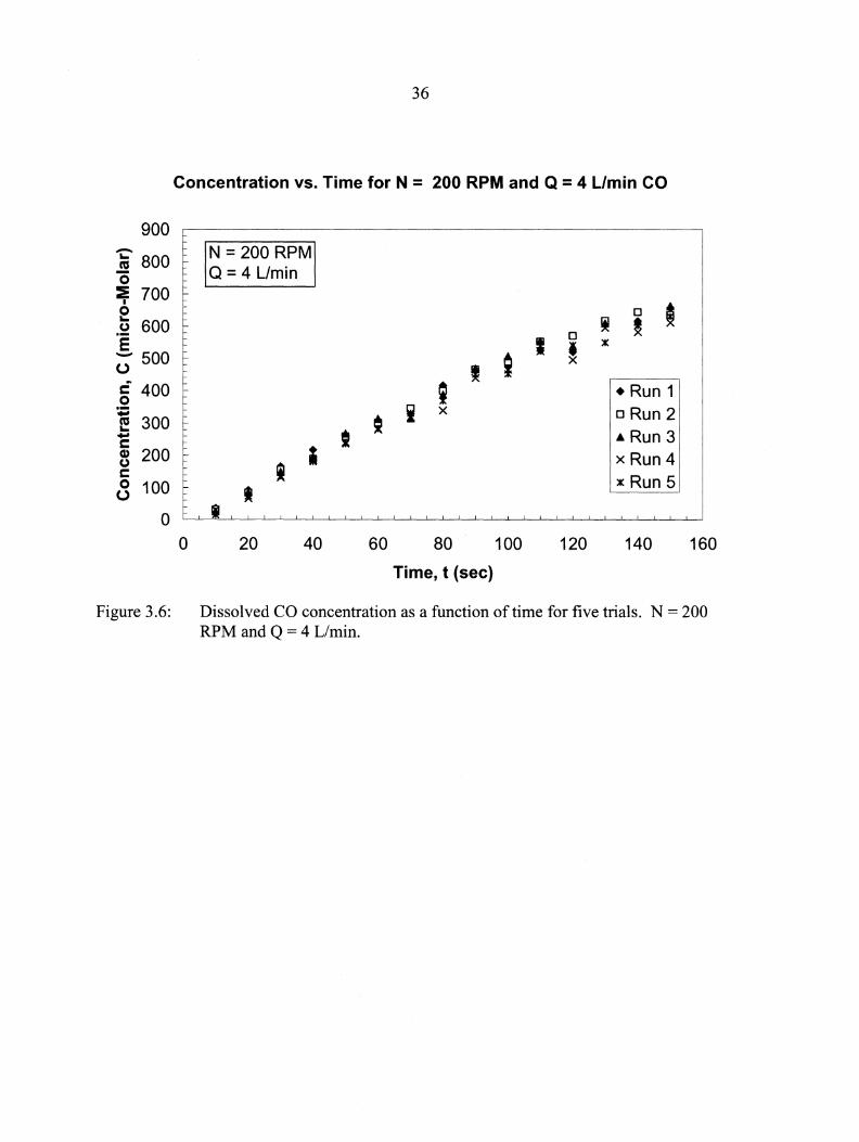
Figure 3.6 shows typical CO concentration data as a function of time in the stirred tank
reactor for a mixing speed of N = 200 RPM and a gas flow rate of Q = 4 L/min. Five sets of
data are shown because it was decided that five sets would achieve a good standard deviation
within a reasonable time frame. The volumetric mass transfer coefficient (kLa) is evaluated
from this concentration versus time data in the following way. First, the rate equation must
be simplified into a more usable form using three assumptions:
1. the liquid phase is well mixed;
2. gas absorption is liquid-phase controlled; and
3. the concentration of gas at the gas-liquid interface is in equilibrium with the gas-phase
in the bubble.
Then the rate equation reduces to
dC = k a(C * -C) dt L
(3.3)
where C is the concentration of dissolved gas in the liquid at any given time, t is the time of
when the concentration sample was withdrawn from the reactor, kLa is the volumetric mass
transfer coefficient, and C* is the maximum concentration of dissolved gas for standard
conditions. This simplified equation can be integrated to
ln ; =(kra)t+B ( C*-C) C*-C
(3.4)
where Ci is the initial dissolved concentration of gas present in the liquid volume and B is the
constant of integration. It is assumed that there is no dissolved carbon monoxide or hydrogen
present in the liquid at the start of any experiment. Hence, Eq. (3.4) reduces to
ln( C* ) = (kia)t+B C*-C
30
(3.5)
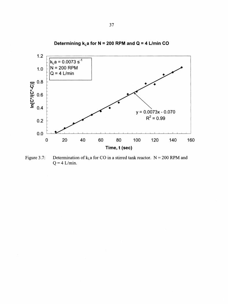
The volumetric mass transfer coefficient, kLa, is then determined by plotting the left hand
side of Eq. (3.5) as a function of time and determining the slope through a linear curve-fit to
the data. Figure 3.7 displays one such example using the averaged data from Figure 3.6.
3.5 Correlating kLa to Power Density and Superficial Gas Velocity
The correlation most often used in the literature to describe the gas-liquid mass transfer
rate is of the form
(3.6)
where kLa is the volumetric mass transfer coefficient, P aN is the aerated power density, and
Ug is the superficial gas velocity. The unaerated power density can be determined using (Ni
et al., 1995)
(3.7)
where Po is the power number for a 90° six-bladed Rushton impeller (Po= 4.75), pis the
density of water, n is the stirrer speed (RPS), Ds is the stirrer diameter, Dv is the vessel
diameter, and Lis the height of the liquid in the vessel. The relationship between the aerated
and unaerated power in a stirred tank reactor using a ring sparger has been correlated by (Ni
et at., 1995)
log pa = -192 Ds Dsn Dsn _q_ ( J ( J4.38( 2 J0.115( 2JI.96(D(ov)( J
Pu Dv V g nD~ (3.8)
where vis the kinematic viscosity of water, g is the acceleration of gravity, and q is the
volumetric gas flow rate (Lis). Solving Eq. (3.7) for Pu and inserting that into Eq. (3.8)
allows for Pa to be determined for utilization in Eq. (3.6). The superficial gas velocity is
simply the volumetric gas flow rate divided by the stirred tank cross sectional area.
31
Microsoft Excel's Solver function is used to determine~' a, and~ to correlate Pa/V and
Ug to the volumetric mass transfer coefficient. The three model parameters are determined
by minimizing the sum of the error squared, where the error is the difference between the
experimental and correlated kLa values.
Figure 3.1:
Sparger
Motor -------.
D" I
Baffles
L
·I Schematic of a stirred tank reactor. Ds = 7 .3 cm, Dv = 21.9 cm, L = 21.9 cm, and V = 7 L.
32
Figure 3.2: Concentration sampling experimental apparatus.
1.6
1.4
1.2
g 1.0 :;:; c. 0 0.8 ti)
.Q
<C 0.6
0.4
0.2
0.0
400 450
33
500 550 600 650 700 Wavelength (nm)
Figure 3.3: CO saturated and deoxygenated curves are the basis for comparison to the trial sample curve in the software Spectra Solve.
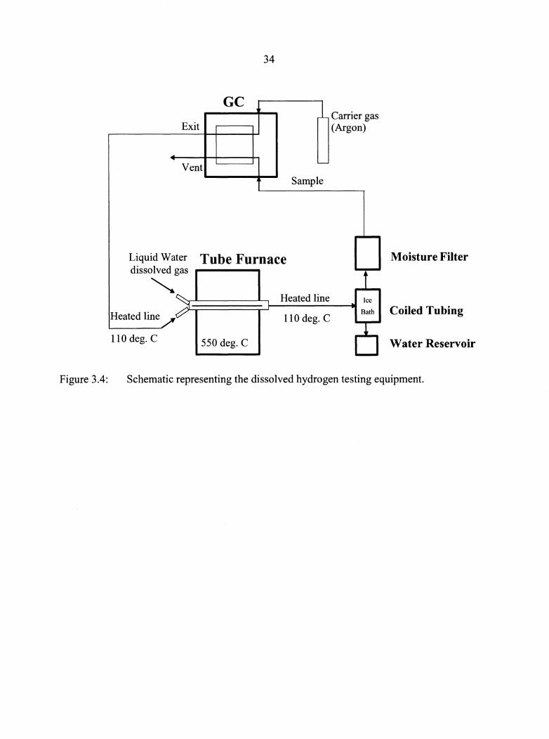
Figure 3.4:
34
GC
Exit
Vent
Liquid Water Tube Furnace dissolved gas
~
Sample
Heated line
Carrier gas (Argon)
Ice
Moisture Filter
Heated line h::;=========::;..-r-------, Bath Coiled Tubing
110 deg. C
110 deg. C 550 deg. C Water Reservoir
Schematic representing the dissolved hydrogen testing equipment.
Noise due to pressure fluctuations
~ l Q) ----+I C> ro ...... 0 > ...... :::J a. ...... :::J 0 () (!)
Re-zero
j
35
Time (min)
~2 l\ / \ / ~
Figure 3.5: Gas chromatograph output from a dissolved hydrogen trial.
36
Concentration vs. Time for N = 200 RPM and Q = 4 L/min CO
900 - N = 200 RPM ... 800 cu
Q = 4 Umin 0 :E 700
I
~ 0 D ... 600 ~ t (J
D E I t x - 500 Q (.) • c 400 ; •Run 1 0 ; i x o Run 2 cu 300 ~ ... - • 1. Run 3 c Cl) 200 ; x Run 4 (J
i c x Run 5 0 100 • (.)
0 0 20 40 60 80 100 120 140 160
Time, t (sec)
Figure 3.6: Dissolved CO concentration as a function oftime for five trials. N = 200 RPM and Q = 4 L/min.
37
Determining kLa for N = 200 RPM and Q = 4 Umin CO
1.2 kLa = 0.0073 s-1
1.0 N = 200 RPM Q = 4 Umin
~ 0.8 0
I -IC 0 :::::- 0.6 -IC 0 ...... c:
0.4
0.2
0.0 0 20 40 60 80
Time, t (sec)
y = 0.0073x - 0.070
R2 = 0.99
100 120 140 160
Figure 3.7: Determination ofkLa for CO in a stirred tank reactor. N = 200 RPM and Q =4 L/min.
38
CHAPTER4: RESULTS
This chapter is divided into three sections. The first and second sections discuss the
carbon monoxide and hydrogen trial results, respectively. The third section compares those
results to gas-liquid mass transfer correlations found in the literature.
4.1 Carbon Monoxide Trial Results
Figure 4.1 shows a typical test trial for determining the concentration of carbon monoxide
as a function of time. The various runs show a general logarithmic shape that has an
asymptote at the steady state (saturation limit) dissolved carbon monoxide concentration for
atmospheric conditions, 1000 µM. In order to measure dissolved concentrations that
approached the steady state limit with the globin protein technique, it was necessary to dilute
the 10 µL sample concentration by adding a smaller sample volume to the cuvette.
Unfortunately, this increased the error in the measurements that, on occasion, produced
carbon monoxide concentrations that were over the saturation limit of 1000 µM, which
should not be possible at atmospheric pressure. To reduce this error, data are eliminated at
concentrations over 85% of the steady state value, 850 µM. Figure 4.2 is a re-plot of the data
in Fig. 4.1 with the data above 85% of saturation eliminated; these data are used in all
subsequent analysis and this procedure was used for all test conditions.
Note there is data scatter among the five replicate runs in Fig. 4.2 and if individual run
data are connected, it does not appear to be a smooth logarithmic function as implied by Eq.
(3.5). The scatter is the result of errors associated with sampling and the globin protein
measurement technique. Possible errors in the CO concentration measurements include
sample dilution errors, sampling errors, bubbles in the syringes, inaccuracies built into the
syringes, and inaccuracy in taking samples at the correct time.
39
The sample dilution errors result in large variations as the CO concentration approaches
the saturation limit (discussed above). There is inherent sampling error in the fact that a 10
µL sample taken from a recirculation line is assumed to represent conditions within the
stirred tank reactor. Assuming plug flow in the recirculation line, the time lag from the
sample location to the sampling port is~ 0.5 secs. Mixing in the recirculation line and/or
additional gas dissolving into the liquid during this time could cause some of the scatter from
run to run.
At certain gas flow and stirrer speed conditions, the flow of bubbles would pass directly
over the inlet of the sample port. Bubbles would be pulled into the recirculation loop and
therefore pass the syringe needles. If a large amount of bubbles passed the sampling needle
at the time the sample was taken, it was likely that some gas entered the syringe along with
the water sample. This gas would continue to diffuse into the water and raise the
concentration of that sample.
Syringes have a built in error of+/- 5% from the manufacturer. This error is present in
all of the syringes regardless of the operator and cannot be eliminated. Over time syringes
"wear out" and possibly leak gas to the atmosphere. The syringes were changed frequently
in an attempt to eliminate this, but it is still possible that there was leakage. Syringe "aging"
at different rates is one possible explanation of why the standard deviation for a given sample
time may be larger than a sample directly before or after it.
The sample timing was measured by a stopwatch as the samples were taken by an
operator. Inaccuracies in operator control could account for variations in the time that the
sample was taken and therefore the concentration that the sample represented. An
approximate error in sample timing is+/- 1 second. Also, small pieces of the septa could get
lodged in the needle and cause the syringe to fill slower than usual, causing the sample to
represent a slightly later time.
40
All of the above errors contribute to the data scatter in Fig. 4.2; however, averaging the
five data runs produces the expected logarithmic increase in carbon monoxide concentration.
Figure 4.3 shows the averaged concentration versus time curve for the five test trials shown
in Fig. 4.2. Standard deviation bars are included to show the relative error at each time
stamp. It should be noted that at the higher concentration levels the standard deviation may
be small due to the elimination of data that were above the 85% criteria. Again, the standard
deviation varies from one sample time to another because of sampling errors, syringes
"wearing out", timing errors, and operator errors.
The left hand side of Eq. (3.5) is applied to the data that were used in Fig. 4.3 to give the
results shown in Fig. 4.4. This figure shows the determination of the volumetric mass
transfer coefficient from the concentration versus time data by the slope of the linear
regression line applied to the data. The R 2 value is shown to represent the accuracy of the
data fit to the (assumed) linear regression line. It should be noted that the intercept for the
linear regression is quite small, however, it is non-zero. This is because of the errors in
timing and the small time lag in the recirculation line from the tank outlet to the sample port.
Also note that the sample at time zero is not used in the determination of the volumetric mass
transfer coefficient for this reason.
Similar procedures were used for all other experimental conditions to determine the
respective volumetric mass transfer coefficients. The data used in these calculations is
summarized in Appendix A. Table 4.1 lists all of the resulting volumetric mass transfer
coefficients for carbon monoxide and their corresponding R2 value. The lower stirrer speeds
tend toward better R2 values because at those speeds, significant bubble entrainment into the
recirculation line was not observed. Thus, the syringes were free from bubbles and the
accuracy of the sample high.
Figure 4.5 shows the volumetric mass transfer coefficient as a function of stirrer speed
for all of the volumetric gas flow rates addressed in this study. From the plot it can be seen
41
that the volumetric mass transfer coefficient increases with stirrer speed and gas flow rate.
Figure 4.6 shows the volumetric mass transfer coefficient as a function of volumetric gas
flow rate for the various stirrer speeds. Again, this plot shows an increase in k1a with stirrer
speed and volumetric gas flow rate. Figure 4.6 also clearly demonstrates the errors from
bubbles in the syringes and sample timing that are produced at the higher stirrer speeds (N =
500 and 600 RPM) by the uneven increase in the volumetric mass transfer coefficients.
Equation (3.6) was used to determine the correlation for the carbon monoxide mass
transfer rate; this correlation is
(p )0.51
kLa=Q.051 ~ l/~ 65 (4.1)
Figure 4.7 compares this correlation to the experimental data. The data that fall outside
of the+/- 10% lines occur at high stirrer speeds, high volumetric gas flow rates, or both. The
primary reason for the inaccuracy at these conditions is due to small carbon monoxide
bubbles being entrained in the recirculation line at the higher stirring speeds, and the
subsequent increased likelihood of withdrawing a gas bubble with the liquid in the sampling
synnge.
4.2 Hydrogen Trial Results
Figure 4.8 shows a typical test trial for determining the concentration of hydrogen as a
function of time. The plot shows a logarithmic curve that has an asymptote at the steady
state dissolved hydrogen concentration under atmospheric conditions, 880 µM. It should be
noted here that the concentration of dissolved hydrogen was never allowed to reach the
steady state value. The reason for this is that the sample evaluation process was more time
intensive than that of the carbon monoxide sampling procedure. Therefore, in the interest of
time, only ten samples were taken per trial compared to the sixteen samples that were taken
42
for each carbon monoxide trial. Hence, there is no need for the 85% cutoff value for
hydrogen because the data never reached the saturation limit.
Like the dissolved CO measurements, there is scatter among the five replicate runs and if
individual run data are connected it does not appear to be a smooth logarithmic function as
implied by Eq. (3.5). The scatter is the result of errors associated with sampling and the flash
drying measurement technique. In addition to the sampling and syringe errors described in
Section 4.1 (sample dilution errors, sampling errors, bubbles in the syringes, inaccuracies
built into the syringes, inaccuracy in taking samples at the correct time), the dissolved H2
concentration measurement technique added some additional errors, including gas
chromatograph response float, Peak Simple software baseline errors, and the possibility of
hydrogen dissolving into the reservoir water.
The sample dilution errors result from the large volume of hydrogen gas that could
accumulate in the larger 1 mL syringes from bubbles passing the needles in the recirculation
loop. Unlike the smaller syringes used for the carbon monoxide trials, the larger 1 mL
syringes had enough volume for the bubbles to accumulate at the top of the syringe. This
allowed for the excess gas that accumulates there to be expelled from the syringe leaving a
smaller amount of water with dissolved hydrogen.
As mentioned in Section 3.3, the gas chromatograph would take up to 3 hours to achieve
steady state operation after start up. The GC would also take time to return to steady state
after large pressure fluctuations that came from several different areas. Injecting the sample
too quickly would cause a large pressure spike from the increase gas volume due to water
evaporation. At the end of each run, the water reservoir in the GC feed line had to be
emptied. The change in overall volume in the plumbing would cause a pressure change.
Also, after every three to four test runs the silica gel moisture filter required regeneration.
This involved switching the gas flow line from the main line to an alternate line that would
43
keep the gas flowing to the GC while the filter was being regenerated. This switching of gas
lines also caused a pressure spike.
Peak Simple software produced a baseline that followed along with the steady state GC
output. As a peak appears, the software automatically recognizes this and draws the baseline
to where it interprets the response returning to steady state. There are situations that exist
that cause the baseline to follow an incorrect path, forcing the operator to manually draw in
the baseline. These conditions include very small peaks that are produced from low gas flow
rates and stirrer speeds and small pressure fluctuations in the plumbing during the time the
peak is being produced. These small pressure fluctuations would come from small amounts
of water accumulating in plumbing joints and forming bubbles that would pop and re-form to
pop again. The small pressure fluctuations could also come from the plumbing being jostled
while the peak was being formed.
The water from sample injections evaporates, separating the hydrogen and gaseous water.
The water is then condensed and collected in a reservoir and the hydrogen is free to continue
to the GC. The possibility exists that a fraction of hydrogen re-dissolves into the water that is
condensed in the reservoir, lowering the amount of hydrogen that reaches the GC and
therefore lowering the apparent concentration for that sample.
Figure 4.9 shows the averaged H2 concentration versus time curve for the five test trials
shown in Fig. 4.8. Standard deviation bars are included to show the relative error at each
time stamp. Again, the standard deviation varies from one sample time to another because of
sampling errors, syringes "wearing out", timing errors, operator errors, and dissolved H2
measurement technique errors.
The left hand side of Eq. (3.5) is applied to the data that were used in Fig. 4.9 to give the
results shown in Fig. 4.10. This figure shows the determination of the volumetric mass
transfer coefficient from the concentration versus time data by the slope of the linear
regression line applied to the data. The R 2 value is shown to represent the accuracy of the
44
data fit to the (assumed) linear regression line. It should be noted that the intercept for the
linear regression is quite small, however, it is non-zero. This is because of the errors in
timing and the small time lag in the recirculation line from the tank outlet to the sample port.
Also note that the sample at time zero is not used in the determination of the volumetric mass
transfer coefficient for this reason.
Similar procedures were used for all other experimental conditions to determine the
respective volumetric mass transfer coefficient. The data used in these calculations is
summarized in Appendix B. Table 4.2 lists all of the resulting volumetric mass transfer
coefficients for hydrogen and their corresponding R2 value. R2 values are generally lower
than for CO, indicating more scatter in the linear fit. As in the CO trials, at the higher gas
flow rates and stirrer speeds the accuracy is lower because of bubble entrainment in the
recirculation loop. But the additional software baseline errors and GC accuracy add errors to
all trials, lowering the accuracy overall compared to the CO measurements.
Figure 4.11 shows the volumetric mass transfer coefficient as a function of stirrer speed
for all of the volumetric gas flow rates addressed in this study. From the plot it can be seen
that the volumetric mass transfer coefficient increases with stirrer speed and gas flow rate.
At 5 L/min the data drop below the data for 3 and 4 L/min. During the experimentation it
was noted that at this flow rate an unusually large amount of samples had bubbles and were
grossly inaccurate, and were eliminated. Figure 4.12 shows the volumetric mass transfer
coefficient as a function of volumetric gas flow rate for the various stirrer speeds. Again, this
plot shows an increase in kLa with stirrer speed and volumetric gas flow rate. The data at
stirrer speeds of 500 and 600 RPM have the lowest R 2 values compared to the other stirrer
speeds at the high volumetric gas flow rates. Hence, the accuracy for those trials is poor
which accounts for some of the scatter seen in Fig. 4.12. There appears to be a local
maximum at 3 L/min. There is no physical reason for this phenomenon. A possible
explanation is that all stirrer speed trials were completed at each volumetric gas flow rate
45
before the flow rate was changed for the next set of trials. It is possible that the GC float had
a high variance over that time period and caused the 3 L/min data to be skewed higher.
Equation (3.6) was used to determine the correlation for the hydrogen mass transfer rate;
this correlation is
(p )0.36
k La = 0.024 ~ U~.4? (4.2)
Figure 4.13 compares this correlation to the experimental data. In addition to the
previous errors at high stirrer speeds and volumetric flow rates, it is postulated that some of
the data that fall outside+/- 10% are due to the H2 measurement technique and the fickleness
of the GC. The data that fall outside+/- 25% are at the already mentioned speeds and flow
rates that have skewed data (N = 300 RPM, Q = 3 L/min; N = 500 RPM, Q = 5 L/min).
4.3 Comparing This Work to the Literature
Table 4.3 lists various gas-liquid mass transfer correlations found in the literature in the
form ofEq. (3.6). All of the correlations presented here were performed in a stirred tank
reactor with geometrically similar dimensions. Group A in this table are correlations that
have higher mass transfer rates at P a!V = 1000 W /m3 and Ug = 0.0022 mis in a stirred tank
reactor than the correlation for carbon monoxide from this work. Group B all have mass
transfer coefficients that lie between the carbon monoxide and hydrogen studies from this
work; Group Call fall below the hydrogen mass transfer rate at 1000 W/m3 and Ug = 0.0022
mis.
All of the correlations in Group A are for oxygen mass transfer into water or a dilute
solution in water. The work of Go gate and Pandit ( 1999) was to determine the quality of
measurement techniques in determining volumetric mass transfer rate correlations. Their
work determined that the dynamic pressure-step method (DPM) was the most accurate in
determining volumetric mass transfer coefficients. Their correlation for oxygen-water mass
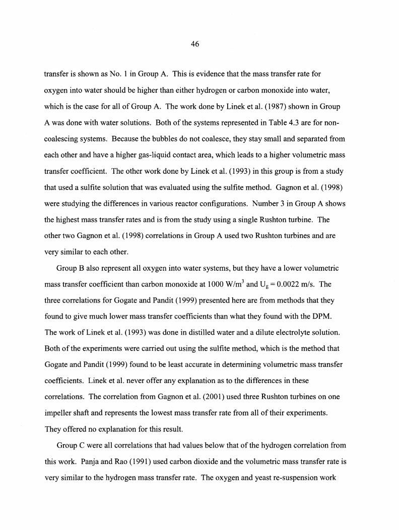
46
transfer is shown as No. 1 in Group A. This is evidence that the mass transfer rate for
oxygen into water should be higher than either hydrogen or carbon monoxide into water,
which is the case for all of Group A. The work done by Linek et al. (1987) shown in Group
A was done with water solutions. Both of the systems represented in Table 4.3 are for non
coalescing systems. Because the bubbles do not coalesce, they stay small and separated from
each other and have a higher gas-liquid contact area, which leads to a higher volumetric mass
transfer coefficient. The other work done by Linek et al. (1993) in this group is from a study
that used a sulfite solution that was evaluated using the sulfite method. Gagnon et al. ( 1998)
were studying the differences in various reactor configurations. Number 3 in Group A shows
the highest mass transfer rates and is from the study using a single Rushton turbine. The
other two Gagnon et al. ( 1998) correlations in Group A used two Rushton turbines and are
very similar to each other.
Group B also represent all oxygen into water systems, but they have a lower volumetric
mass transfer coefficient than carbon monoxide at 1000 W/m3 and Ug = 0.0022 mis. The
three correlations for Gogate and Pandit (1999) presented here are from methods that they
found to give much lower mass transfer coefficients than what they found with the DPM.
The work of Linek et al. (1993) was done in distilled water and a dilute electrolyte solution.
Both of the experiments were carried out using the sulfite method, which is the method that
Gogate and Pandit (1999) found to be least accurate in determining volumetric mass transfer
coefficients. Linek et al. never offer any explanation as to the differences in these
correlations. The correlation from Gagnon et al. (2001) used three Rushton turbines on one
impeller shaft and represents the lowest mass transfer rate from all of their experiments.
They offered no explanation for this result.
Group C were all correlations that had values below that of the hydrogen correlation from
this work. Panja and Rao (1991) used carbon dioxide and the volumetric mass transfer rate is
very similar to the hydrogen mass transfer rate. The oxygen and yeast re-suspension work
47
from Ni et al. (1995) had a very low volumetric mass transfer rate. It is possible that the
yeast somehow inhibits the transfer of oxygen into the liquid.
No carbon monoxide or hydrogen correlations could be found during an extensive
literature search; therefore, Table 4.4 is provided to show many different values for
volumetric mass transfer coefficients that have been calculated in the literature for carbon
monoxide and hydrogen systems. The researchers who presented these values either did so
as part of an overall mass balance including microbial systems or did not present the method
used to obtain the volumetric mass transfer coefficient values they presented. Two values
from this work are also presented in this table to show that the values from this work are
similar to those found in the literature.
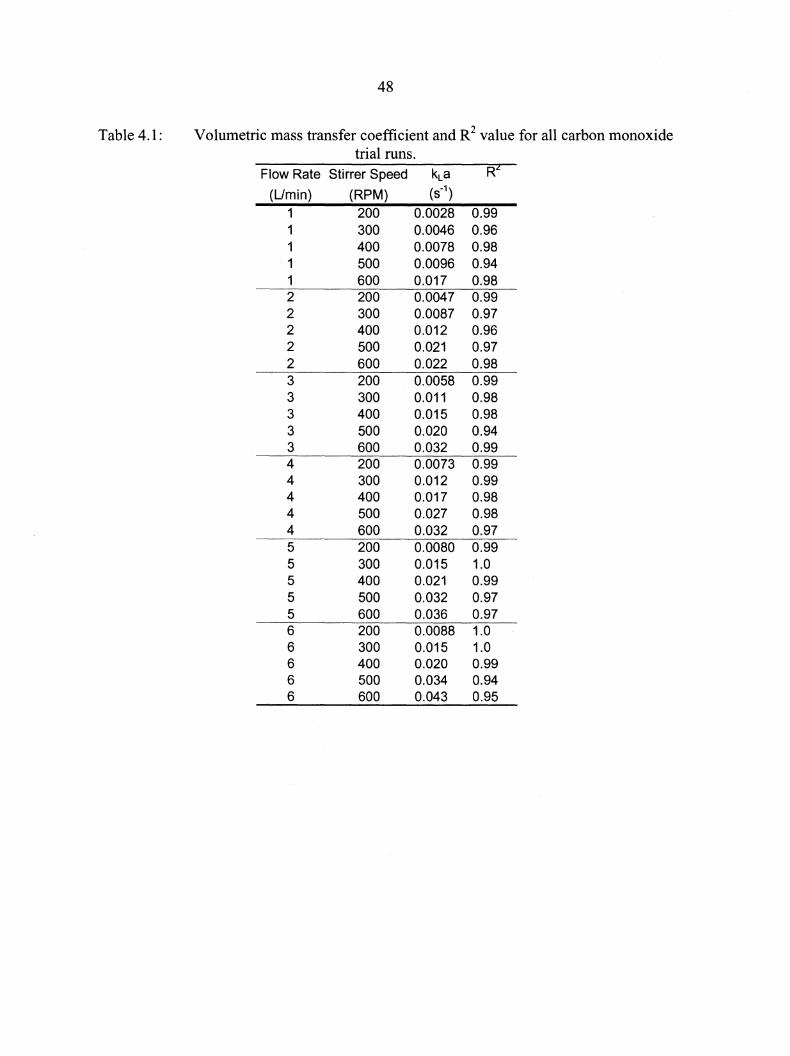
48
Table 4.1: Volumetric mass transfer coefficient and R2 value for all carbon monoxide trial runs.
Flow Rate Stirrer Speed kLa R
(Umin) (RPM) (s_,)
1 200 0.0028 0.99 1 300 0.0046 0.96 1 400 0.0078 0.98 1 500 0.0096 0.94 1 600 0.017 0.98 2 200 0.0047 0.99 2 300 0.0087 0.97 2 400 0.012 0.96 2 500 0.021 0.97 2 600 0.022 0.98 3 200 0.0058 0.99 3 300 0.011 0.98 3 400 0.015 0.98 3 500 0.020 0.94 3 600 0.032 0.99 4 200 0.0073 0.99 4 300 0.012 0.99 4 400 0.017 0.98 4 500 0.027 0.98 4 600 0.032 0.97 5 200 0.0080 0.99 5 300 0.015 1.0 5 400 0.021 0.99 5 500 0.032 0.97 5 600 0.036 0.97 6 200 0.0088 1.0 6 300 0.015 1.0 6 400 0.020 0.99 6 500 0.034 0.94 6 600 0.043 0.95
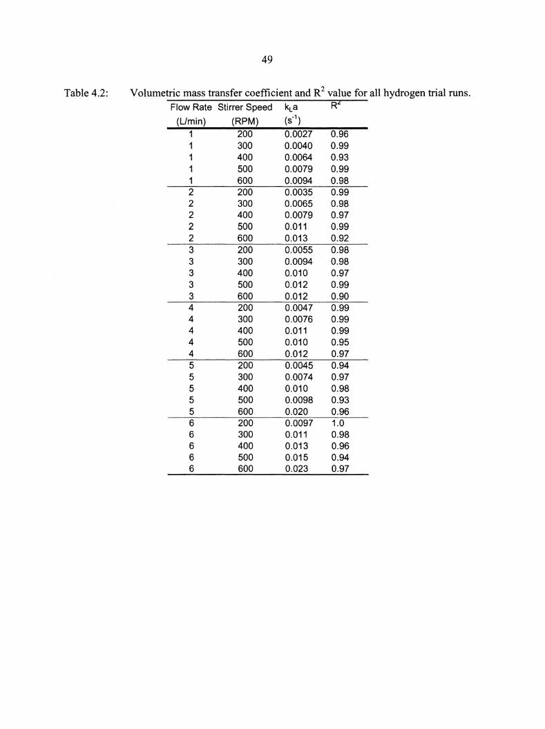
49
Table 4.2: Volumetric mass transfer coefficient and R2 value for all hydrogen trial runs. Flow Rate Stirrer Speed kLa R
(L/min) (RPM) (s_,)
1 200 0.0027 0.96 1 300 0.0040 0.99 1 400 0.0064 0.93 1 500 0.0079 0.99 1 600 0.0094 0.98 2 200 0.0035 0.99 2 300 0.0065 0.98 2 400 0.0079 0.97 2 500 0.011 0.99 2 600 0.013 0.92 3 200 0.0055 0.98 3 300 0.0094 0.98 3 400 0.010 0.97 3 500 0.012 0.99 3 600 0.012 0.90 4 200 0.0047 0.99 4 300 0.0076 0.99 4 400 0.011 0.99 4 500 0.010 0.95 4 600 0.012 0.97 5 200 0.0045 0.94 5 300 0.0074 0.97 5 400 0.010 0.98 5 500 0.0098 0.93 5 600 0.020 0.96 6 200 0.0097 1.0 6 300 0.011 0.98 6 400 0.013 0.96 6 500 0.015 0.94 6 600 0.023 0.97
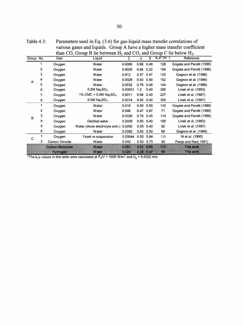
50
Table 4.3: Parameters used in Eq. (3.6) for gas-liquid mass transfer correlations of various gases and liquids. Group A have a higher mass transfer coefficient than CO, Group B lie between H2 and CO, and Group C lie below H2.
Group No. Gas Liquid ~ a ~ !<La• ilir ·~ Reference
Oxygen Water 0.0065 0.68 0.49 128 Gogate and Pandit (1999)
2 Oxygen Water 0.0020 0.64 0.22 156 Gogate and Pandit (1999) 3 Oxygen Water 0.012 0.57 0.47 125 Gagnon et al. (1998)
A 4 Oxygen Water 0.0029 0.83 0.50 152 Gagnon et al. (1998)
5 Oxygen Water 0.0032 0.79 0.48 144 Gagnon et al. (1998)
6 Oxygen 0.5M Na2S04 0.00031 1.2 0.40 385 Linek et al. (1993)
7 Oxygen 1% CMC + 0.5M Na2S04 0.0011 0.94 0.40 227 Linek et al. (1987)
8 Oxygen 0.5M Na2S04 0.0014 0.95 0.40 309 Linek et al. (1987)
Oxygen Water 0.015 0.59 0.55 110 Gogate and Pandit (1999) 2 Oxygen Water 0.046 0.47 0.67 71 Gogate and Pandit (1999)
B 3 Oxygen Water 0.0026 0.76 0.45 114 Gogate and Pandit (1999)
4 Oxygen Distilled water 0.0038 0.65 0.40 106 Linek et al. (1993) 5 Oxygen Water (dilute electrolyte soln.) 0.0050 0.59 0.40 92 Linek et al. (1987)
6 Oxl'.gen Water 0.0092 0.60 0.50 98 Gagnon et al. (1998)
c Oxygen 0.00044 0.50 0.64 1.0 Ni et al. (1995)
*The kLa values in this table were calculated at PJV = 1000 W/m and U9 = 0.0022 mis
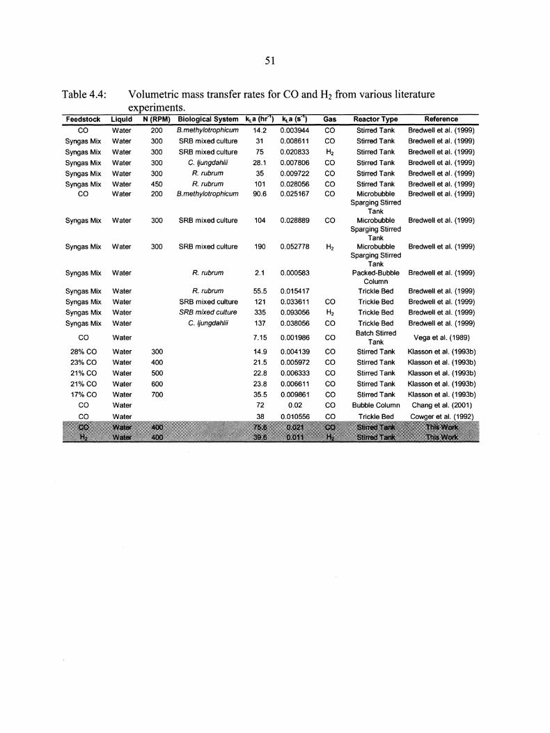
51
Table 4.4: Volumetric mass transfer rates for CO and H2 from various literature experiments.
Feedstock Liquid N (RPM) Biological System kLa (hr") kLa (s- ) Gas Reactor Type Reference
co Water 200 B. methylotrophicum 14.2 0.003944 co Stirred Tank Bredwell et al. (1999)
Syngas Mix Water 300 SRB mixed culture 31 0.008611 co Stirred Tank Bredwell et al. (1999)
Syngas Mix Water 300 SRB mixed culture 75 0.020833 H2 Stirred Tank Bredwell et al. (1999)
Syngas Mix Water 300 C. ljungdahlii 28.1 0.007806 co Stirred Tank Bredwell et al. (1999)
Syngas Mix Water 300 R. rubrum 35 0.009722 co Stirred Tank Bredwell et al. (1999)
Syngas Mix Water 450 R. rubrum 101 0.028056 co Stirred Tank Bredwell et al. (1999)
co Water 200 B.methylotrophicum 90.6 0.025167 co Microbubble Bredwell et al. (1999) Sparging Stirred
Tank Syngas Mix Water 300 SRB mixed culture 104 0.028889 co Microbubble Bredwell et al. (1999)
Sparging Stirred Tank
Syngas Mix Water 300 SRB mixed culture 190 0.052778 H2 Micro bubble Bredwell et al. (1999) Sparging Stirred
Tank Syngas Mix Water R. rubrum 2.1 0.000583 Packed-Bubble Bredwell et al. (1999)
Column Syngas Mix Water R. rubrum 55.5 0.015417 Trickle Bed Bredwell et al. (1999)
Syngas Mix Water SRB mixed culture 121 0.033611 co Trickle Bed Bredwell et al. (1999)
Syngas Mix Water SRB mixed culture 335 0.093056 H2 Trickle Bed Bredwell et al. (1999)
Syngas Mix Water C. ljungdahlii 137 0.038056 co Trickle Bed Bredwell et al. (1999)
co Water 7.15 0.001986 co Batch Stirred Vega et al. (1989)
Tank
28%CO Water 300 14.9 0.004139 co Stirred Tank Klasson et al. (1993b)
23%CO Water 400 21.5 0.005972 co Stirred Tank Klasson et al. (1993b)
21%CO Water 500 22.8 0.006333 co Stirred Tank Klasson et al. (1993b)
21%CO Water 600 23.8 0.006611 co Stirred Tank Klasson et al. ( 1993b)
17%CO Water 700 35.5 0.009861 co Stirred Tank Klasson et al. ( 1993b)
co Water 72 0.02 Bubble Column Chang et al. (2001)
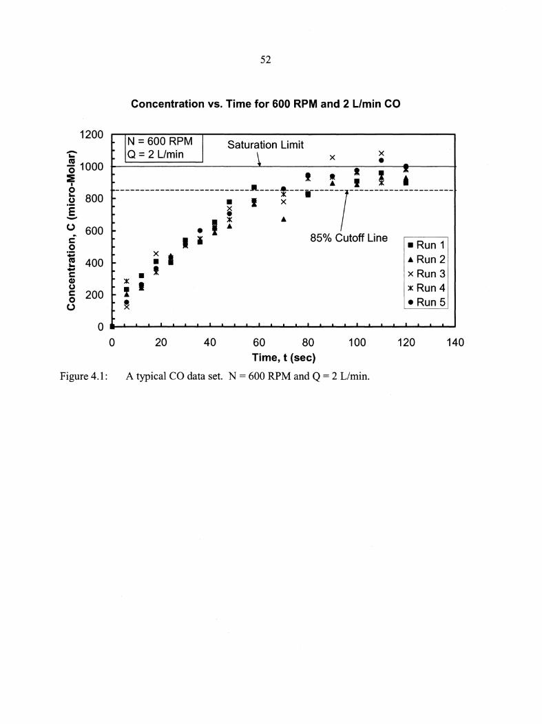
52
Concentration vs. Time for 600 RPM and 2 L/min CO
1200 ~ N = 600 RPM 'C'
Saturation Limit
~ ~ Q = 2 L/min x x . -~ 1000 :::!:
I
~ u 800 E -0 600
~---------------------~---~----~---!----~-~-;----~----~---------.. I i I 85% Cutoff Line c:
0 ; e -c: Cl) u c: 0 0
400
200
0
-• :t:: I
' ~ .
0
x • • !
' I I
20 40
•Run 1 ~Run 2 x Run 3 x Run 4 •Run 5
I I 1 1 1 I I
60 80 Time, t (sec)
100 120
Figure 4.1: A typical CO data set. N = 600 RPM and Q = 2 L/min.
140
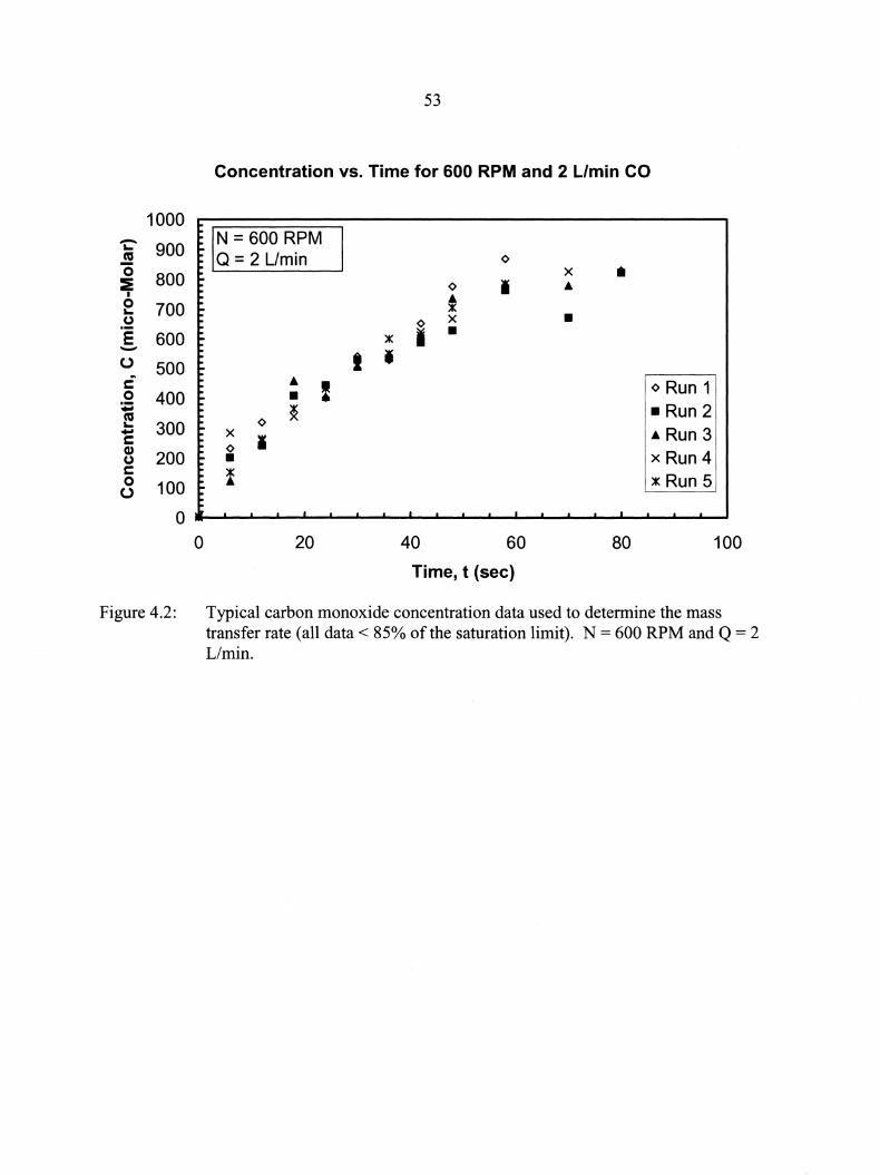
1000
..:::- 900 ns
~ 800 I e 100
(.)
E 600 -0 c: 0 ; e -c: G) (.) c: 0 0
500
400
300
200
100
53
Concentration vs. Time for 600 RPM and 2 L/min CO
N = 600 RPM Q = 2 L/min
x <> • I
<>
I
A
• ~
<> • <> t
I
x • • I
<>Run 1 •Run 2 •Run 3 x Run 4 )I( Run 5
0 ______ __.~...._ ______ ~..__.__.___..~.._ ....... _.__.___...__ ____ _.___,
0 20 40 60 80 100
Time, t (sec)
Figure 4.2: Typical carbon monoxide concentration data used to determine the mass transfer rate (all data< 85% of the saturation limit). N = 600 RPM and Q = 2 L/min.
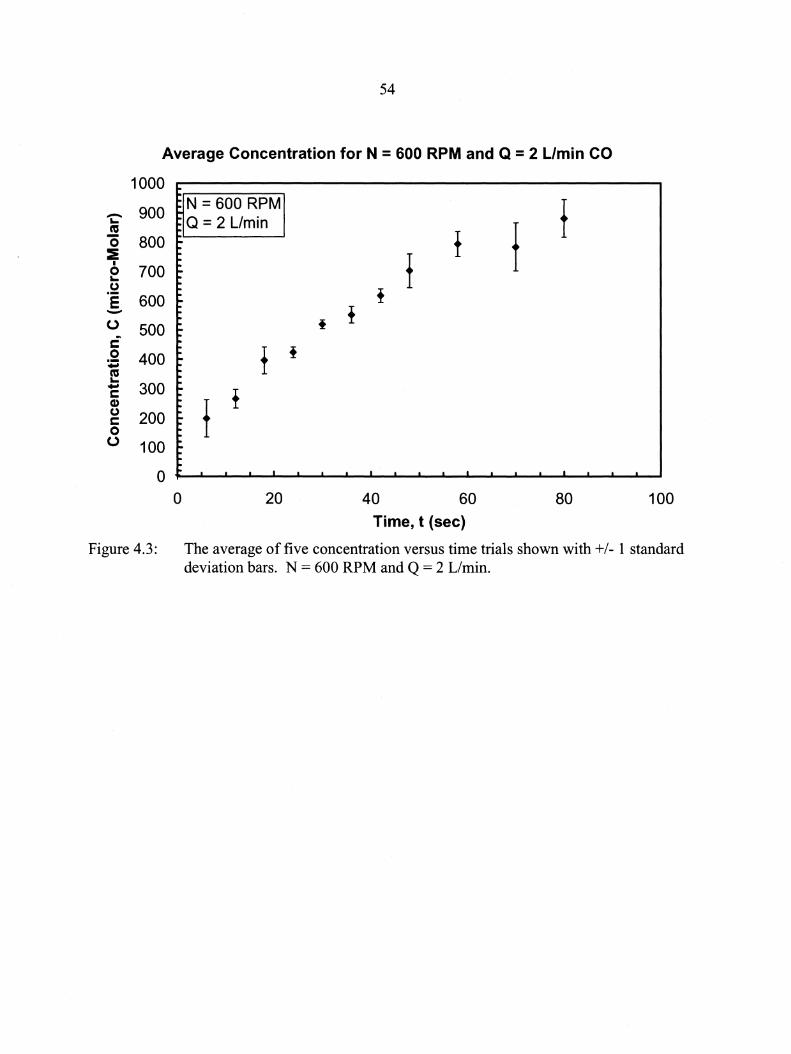
54
Average Concentration for N = 600 RPM and Q = 2 Umin CO
1000
'C 900 ns 0 800 :i
I e 100 .!::? E 600 -0 c 0
:,;::; e -c cu (,) c 0 0
500
400
300
200
100
0 0
N = 600 RPM Q = 2 L/min
f 20
f f
40 60 Time, t (sec)
f f
80 100
Figure 4.3: The average of five concentration versus time trials shown with+/- 1 standard deviation bars. N = 600 RPM and Q = 2 L/min.
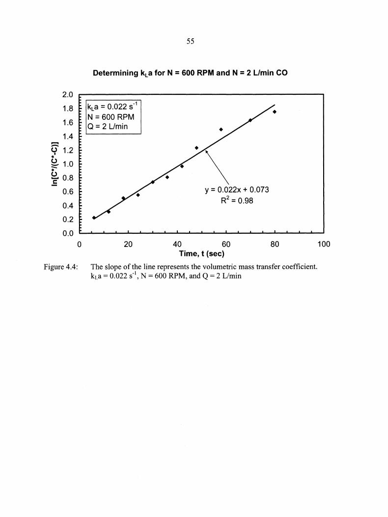
2.0
1.8
1.6
1.4 ...... -0 1.2 I
-IC 0 ::::::" 1.0 -IC 0 'E' 0.8
0.6
0.4
0.2
0.0
0
Figure 4.4:
55
Determining kLa for N = 600 RPM and N = 2 L/min CO
kLa = 0.022 s-1
N = 600 RPM Q = 2 Umin
20 40
y = 0.022x + 0.073
R2 = 0.98
60 Time, t (sec)
80
The slope of the line represents the volumetric mass transfer coefficient. kLa = 0.022 s-1, N = 600 RPM, and Q = 2 L/min
100
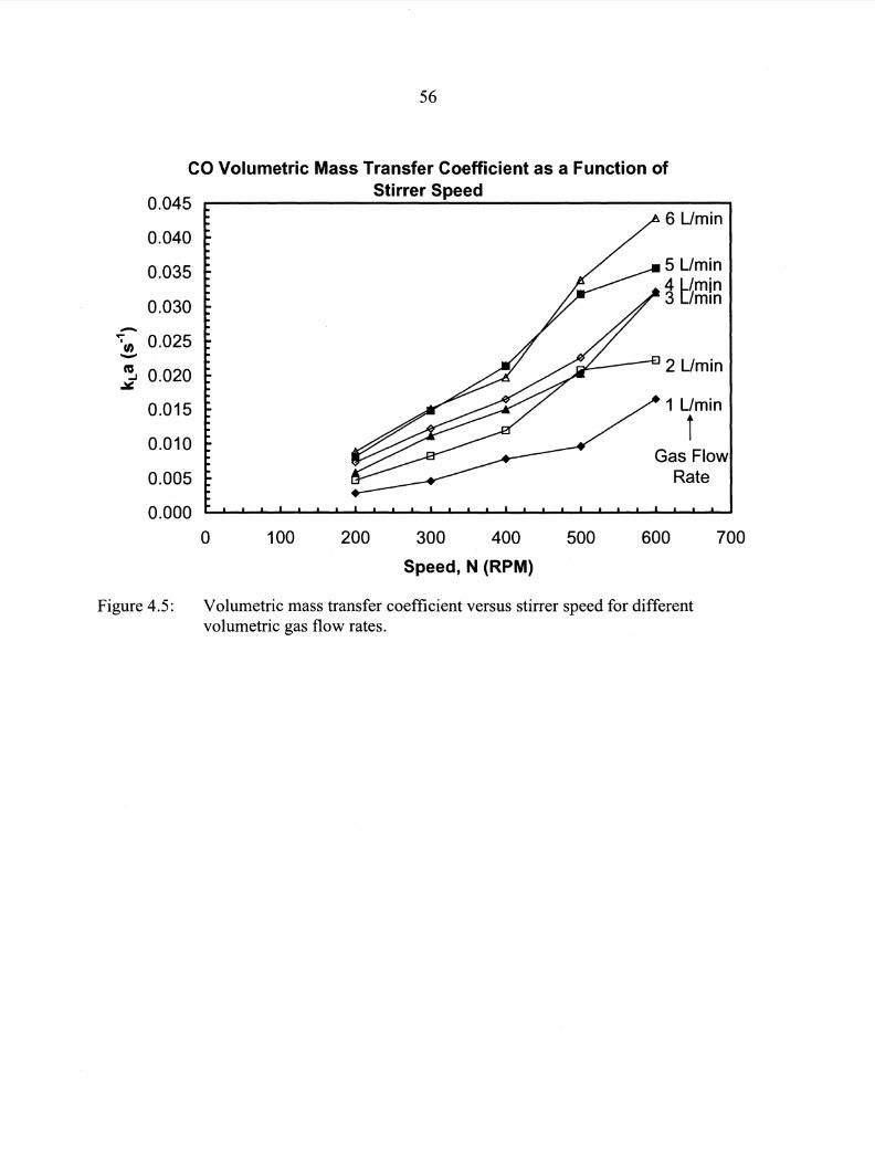
56
CO Volumetric Mass Transfer Coefficient as a Function of
-
0.045
0.040
0.035
0.030
";'en 0.025 -~ 0.020 ~
0.015
0.010
0.005
0.000
0
Stirrer Speed
100 200 300 400
Speed, N (RPM)
500
6 Umin
5 Umin
~H~i~
1 Umin
i Gas Flow
Rate
600 700
Figure 4.5: Volumetric mass transfer coefficient versus stirrer speed for different volumetric gas flow rates.
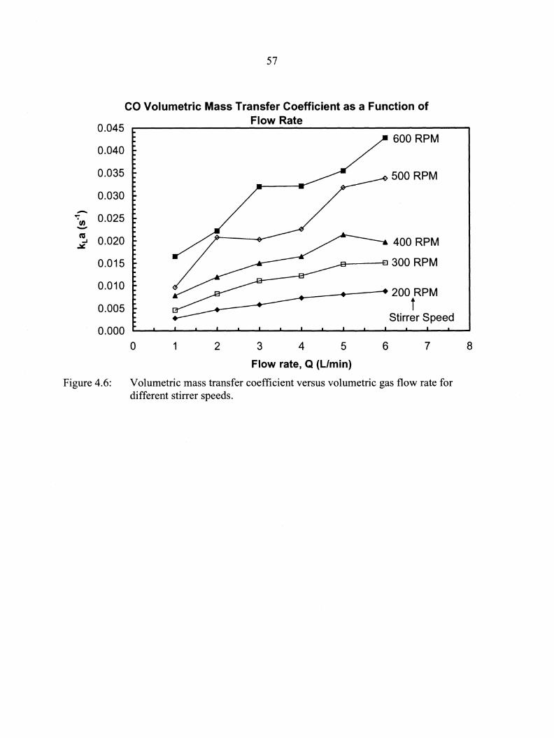
-"';" II> -ca
..J ~
0.045
0.040
0.035
0.030
0.025
0.020
0.015
0.010
0.005
0.000
57
CO Volumetric Mass Transfer Coefficient as a Function of Flow Rate
0 1 2 3
600 RPM
500 RPM
400 RPM
.i::i------10 300 RPM
----~~--~200RPM
t Stirrer Speed
4 5 6 7
Flow rate, Q (Umin)
Figure 4.6: Volumetric mass transfer coefficient versus volumetric gas flow rate for different stirrer speeds.
8
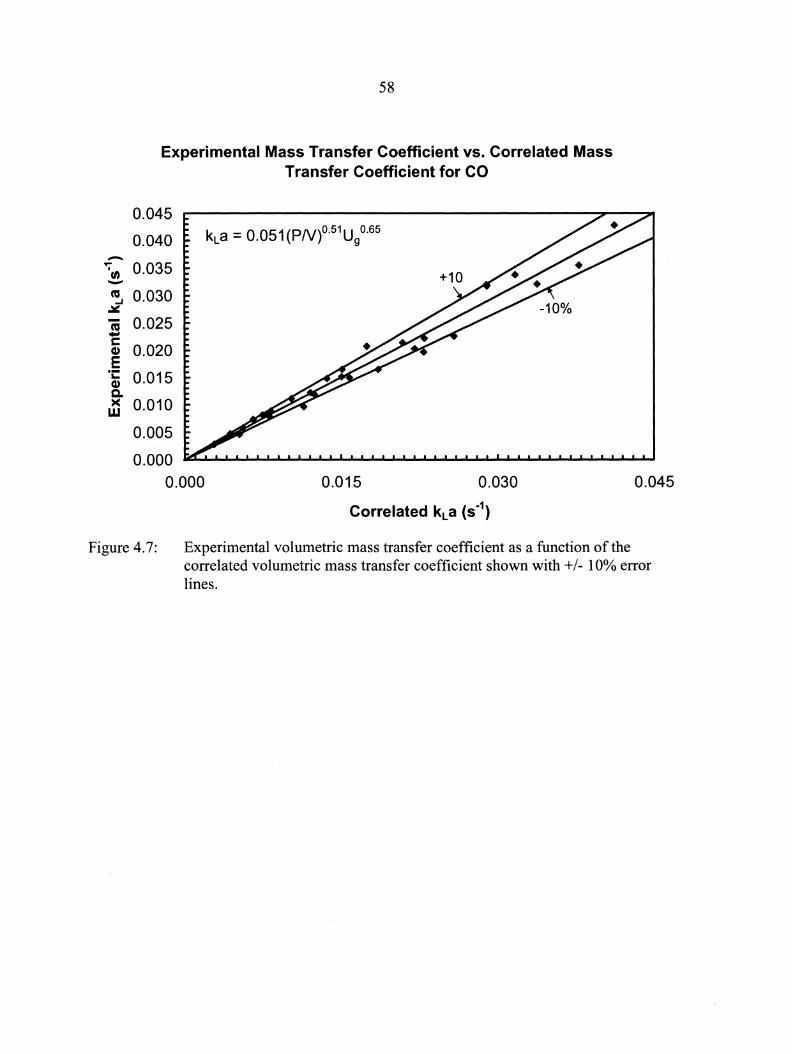
58
Experimental Mass Transfer Coefficient vs. Correlated Mass Transfer Coefficient for CO
-0.045
0.040
";"en 0.035 -~ 0.030 ~
ca 0.025 -~ 0.020
·c:: 0.015 G) Q. Jl 0.010
0.005
0.000 0.000 0.015 0.030 0.045
Figure 4.7: Experimental volumetric mass transfer coefficient as a function of the correlated volumetric mass transfer coefficient shown with+/- 10% error lines.
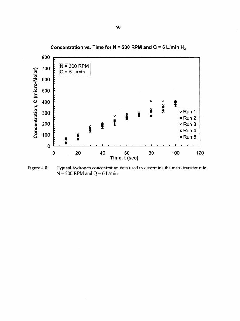
800
- 700 ... ..! 0 :E 600
I
0 ... 0 500 E -0 400 c: 0
300 :;::: ns ... -c: 200 Cl) 0 c: 0 100 0
0
Figure 4.8:
59
Concentration vs. Time for N = 200 RPM and Q = 6 L/min H2
0
N = 200 RPM Q = 6 Umin
I I I
20 40
0 i I
60 Time, t (sec)
x 0 I " i t o Run 1 • •Run 2
x Run 3 lK Run 4 •Run 5
80 100 120
Typical hydrogen concentration data used to determine the mass transfer rate. N = 200 RPM and Q = 6 Umin.
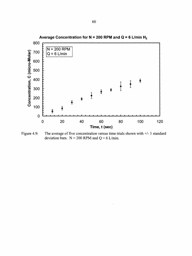
60
Average Concentration for N = 200 RPM and Q = 6 Umin H2
800
'i:" 700 ~ 0
:iiE 600 I
0 ... . ~ 500 E -0 ~ 400 c
0 ;
300 ca ... -c Q)
200 CJ c 0
0 100
0 0
N = 200 RPM Q = 6 Umin
20 40 60 Time, t (sec)
f f
80 100 120
Figure 4.9: The average of five concentration versus time trials shown with+/- 1 standard deviation bars. N = 200 RPM and Q = 6 L/min.
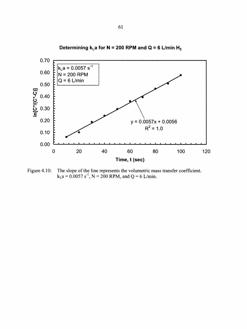
,......, -
0.70
0.60
0.50
0 .,.• 0.40 0 --.,. 0 0.30 ..... c
0.20
0.10
0.00
0
61
Determining kLa for N = 200 RPM and Q = 6 Umin H2
kLa = 0.0057 s-1
N = 200 RPM Q = 6 Umin
20 40
y = 0.0057x + 0.0056
R2 = 1.0
60
Time, t (sec)
80 100
Figure 4.10: The slope of the line represents the volumetric mass transfer coefficient. kLa = 0.0057 s-1, N = 200 RPM, and Q = 6 L/min.
120
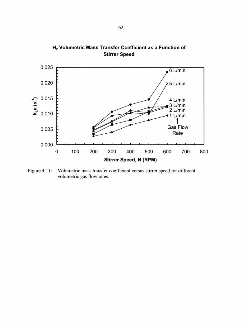
-";' tn -ca _. ~
62
H2 Volumetric Mass Transfer Coefficient as a Function of Stirrer Speed
0.025
0.020
0.015
0.010
0.005
0.000
0 100 200 300 400
6 Umin
5 Umin
4 Umin ~.f---==- 3 Umin
2 Umin 1 Umin
i Gas Flow
Rate
500 600 700
Stirrer Speed, N (RPM)
Figure 4.11: Volumetric mass transfer coefficient versus stirrer speed for different volumetric gas flow rates.
800
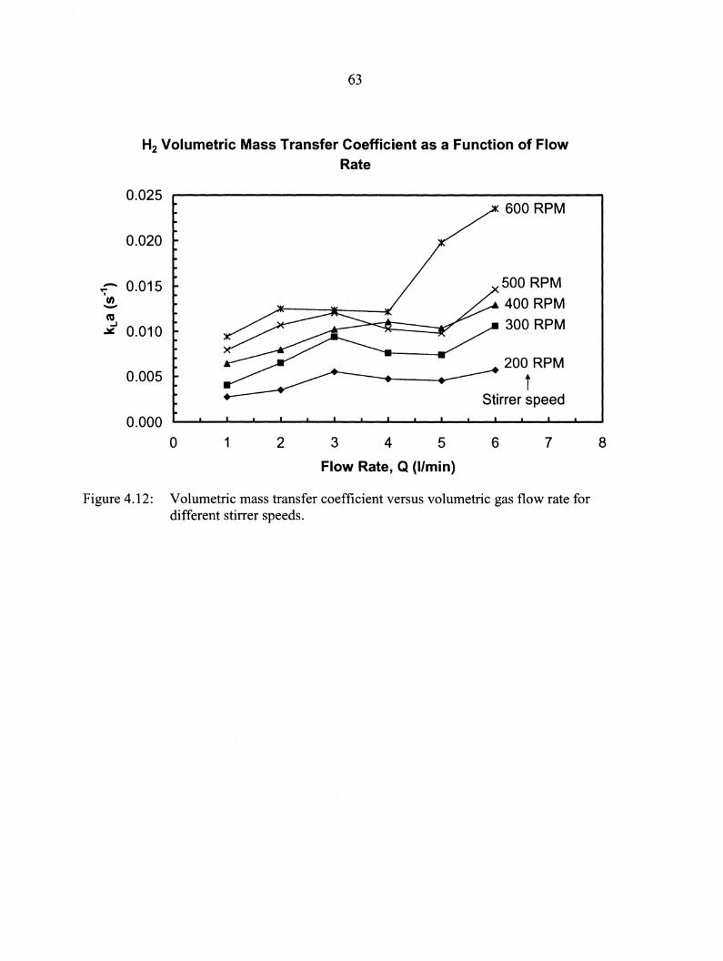
-";' "' -ca
..J ~
63
H2 Volumetric Mass Transfer Coefficient as a Function of Flow Rate
0.025
0.020
0.015
0.010
0.005
0.000
0 1 2 3 4 5
Flow Rate, Q (I/min)
600 RPM
500 RPM
400 RPM
300 RPM
200 RPM
i Stirrer speed
6 7
Figure 4.12: Volumetric mass transfer coefficient versus volumetric gas flow rate for different stirrer speeds.
8
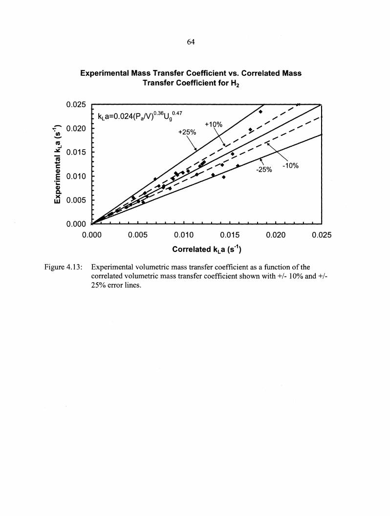
-';" en -cu ..J ~
n; -s::: Cl)
E "i: Cl) c.. >< w
64
Experimental Mass Transfer Coefficient vs. Correlated Mass Transfer Coefficient for H2
0.025 kLa=0.024(P 8N)0'36U9 0.4?
0.020 +25%
0.015
0.010
0.005
0.000 0.000 0.005 0.010 0.015 0.020
Correlated kLa (s-1)
0.025
Figure 4.13: Experimental volumetric mass transfer coefficient as a function of the correlated volumetric mass transfer coefficient shown with+/- 10% and +/-25% error lines.
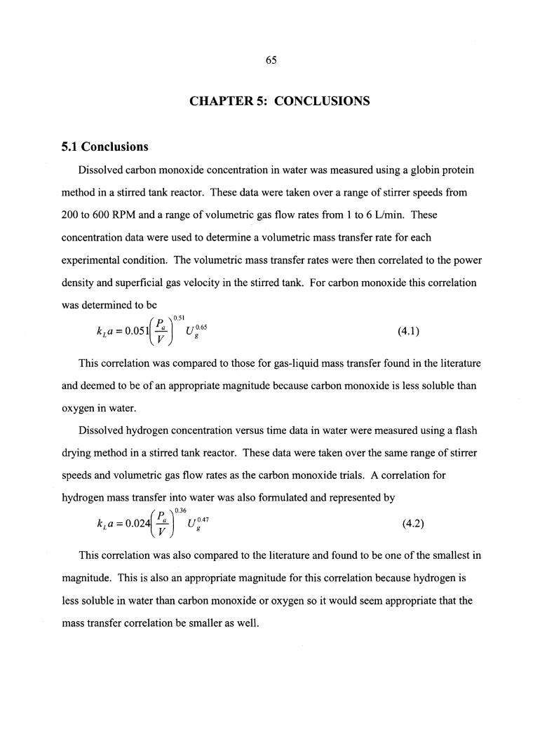
65
CHAPTER 5: CONCLUSIONS
5.1 Conclusions
Dissolved carbon monoxide concentration in water was measured using a globin protein
method in a stirred tank reactor. These data were taken over a range of stirrer speeds from
200 to 600 RPM and a range of volumetric gas flow rates from 1 to 6 L/min. These
concentration data were used to determine a volumetric mass transfer rate for each
experimental condition. The volumetric mass transfer rates were then correlated to the power
density and superficial gas velocity in the stirred tank. For carbon monoxide this correlation
was determined to be
(p )0.51
kLa=0.051 ~ U~·65 (4.1)
This correlation was compared to those for gas-liquid mass transfer found in the literature
and deemed to be of an appropriate magnitude because carbon monoxide is less soluble than
oxygen in water.
Dissolved hydrogen concentration versus time data in water were measured using a flash
drying method in a stirred tank reactor. These data were taken over the same range of stirrer
speeds and volumetric gas flow rates as the carbon monoxide trials. A correlation for
hydrogen mass transfer into water was also formulated and represented by
(p )0.36
k La = 0.024 ~ U~.4? (4.2)
This correlation was also compared to the literature and found to be one of the smallest in
magnitude. This is also an appropriate magnitude for this correlation because hydrogen is
less soluble in water than carbon monoxide or oxygen so it would seem appropriate that the
mass transfer correlation be smaller as well.
66
5.2 Recommendations
From comparing the R2 values for the carbon monoxide and hydrogen trials, it is obvious
that the flash drying technique used in measuring dissolved hydrogen in water is less accurate
than the globin protein method used for determining concentrations of carbon monoxide in
water. A more accurate method for measuring dissolved hydrogen should be investigated.
Synthesis gas is a mixture of multiple gases and a study should be conducted to assess the
effect that a mixture of gases would have on the mass transfer rates of the gases in this study.
Microbial fermentation systems not only have water, but nutrients, salts, microorganisms,
and biological byproducts dissolved in the system. Determining the effects of these solutes
on the mass transfer rate should be investigated.
Compared to the literature, the correlations for carbon monoxide and hydrogen are of a
smaller magnitude than those found for oxygen and water systems. Methods to increase the
mass transfer rate of CO and H2 should be investigated. This study used a geometrically
similar stirred tank reactor that was used in many of the gas-liquid mass transfer studies
found in the literature. Mass transfer rates have been shown to greatly increase when other
types of stirrers, geometries, and reactor types are used. An investigation into different .. reactors, stirrers, and geometries should be performed to determine the best possible
configuration for maximizing the mass transfer rate of these two sparingly soluble gases in
water.
67
BIBLIOGRAPHY
Boon, M., Meeder, T.A., Heijnen, J.J., Luyben, K.Ch.A.M., Influence of oxygen
adsorption on the dynamic kLa measurement in three-phase slurry reactors, Biotechnology
and Bioengineering, 40 (1992) pp. 1097-1106.
Bredwell, M.D., Srivastava, P., Worden, R.M., Reactor design issues for synthesis-gas
fermentations, Biotechnology Progress, 15 (1999) pp. 834-844.
Brown, R.C., Processing ofbiorenewable resources into chemicals and fuels,
Biorenewable Resources: Engineering New Products from Agriculture, Iowa State Press,
Ames, IA (2003) pp. 159-194.
Chang, I.S., Kim, B.H., Lovitt, R.W., Bang, J.S., Effect of CO partial pressure on cell
recycled continuous CO fermentation by Eubacterium limosum KIST612, Process
Biochemistry, 37(2001) pp. 411-421.
Cowger, J.P., Klasson, K.T., Ackerson, M.D., Clausen, E.C., Gaddy, J.L., Mass-transfer
and kinetic aspects in continuous bioreactors using Rhodospirillum rubrum, Applied
Biochemistry and Biotechnology, 34135 (1992) pp. 613-624.
Gagnon, H., Lounes, M., Thibault., Poser consumption and mass transfer in agitated gas
liquid columns: A comparative study, The Canadian Journal of Chemical Engineering, 76
(1998) pp. 379-389.
Grethlein, A.J., Jain, M.K., Bioprocessing of coal-derived synthesis gases by anaerobic
bacteria, Trends in Biotechnology, 10 (1992) pp. 418-423.
Gogate, P.R., Pandit, A.B., Survey of measurement techniques for gas-liquid mass
transfer coefficient in bioreactors, Biochemical Engineering Journal, 4 (1999) pp. 7-15.
Hewgill, M.R., Mackley, M.R., Pandit, A.B., Pannu, S.S., Enhancement of gas-liquid
mass transfer using oscillatory flow in a baffled tube, Chemical Engineering Science, 48
(1992) pp. 799-809.
68
Incropera, F.P., DeWitt, D.P., Diffusion mass transfer, Fundamentals of Heat and Mass
Transfer, John Wiley & Sons, Inc., New York, NY (2002) pp. 860-902.
Klassen, K.T., Ackerson, M.D., Clausen, E.C., Gaddy, J.L., Bioreactor design for
synthesis gas fermentations, Fuel, 70 (1991) pp. 605-614.
Klasson, K.T., Lundback, K.M.O., Clausen, E.C., Gaddy, J.L., Kinetics oflight limited
growth and biological hydrogen production from carbon monoxide and water by
Rhodospirillum rubrum, Journal of Biotechnology, 29 (1993a) pp. 177-188.
Klassen, K.T., Gupta, A., Clausen, E.C., Gaddy, J.L., Evaluation of mass-transfer and
kinetic parameters for Rhodospirillum rubrum in a continuous stirred tank reactor, Applied
Biochemistry and Biotechnology, 39140 (1993b) pp. 549-557.
Kundu, S., Premer, S.A., Hoy, J.A., Trent, J.T., III., Hargrove, M.S., Direct measurement
of equilibrium constants for high-affinity hemoglobins, Biophysical Journal, 84 (2003) pp.
3931-3940.
Linek, V., Benes, P., Sinkule, J., Moucha, T., Non-ideal pressure step method for kLa
measurement, Chemical Engineering Science, 48 (1993) pp. 1593-1599.
Linek, V., Vacek, V., Volumetric mass transfer coefficient in stirred reactors, Chemical
Engineering Technology, 11 (1988) pp. 249-251.
Lines, P.C., Gas-liquid mass transfer using surface-aeration in stirred vessels, with dual
impellers, Institution of Chemical Engineering, 78 (2000) pp. 342-347.
Miron, A.S., Camacho, F.G., Gomez, A.C., Grima, E.M., Chisit, Y., Bubble-column and
airlift photobioreactors for algal cultures, AIChE Journal,. 46 (2000) pp. 1872-1887.
Ni, X., Gao, S., Cumming, R.H., Pritchard, D.W., A comparative study of mass transfer
in yeast for a batch pulsed baffled bioreactor and a stirred tank fermenter, Chemical
Engineering Science, 50 (1995) pp. 2127-2136.
69
Panja, N.C., Phaneswara Rao, D., Experimental studies on kLa in a mechanically agitated
contactor from transient electrical conductivity response data, Trans /ChemE, 69 A ( 1991) pp.
302-307.
Renewable Fuels Association, US ethanol fuel production capacity, 2004, Renewable
Fuels Association, Accessed 15 June 2004, <http://www.ethanolrfa.org/eth_prod_fac.html>.
Schmitz, M., Steiff, A., Weinspach, P.M., Gas/liquid interfacial area per unit volume and
volumetric mass transfer coefficient in stirred slurry reactors, Chemical Engineering
Technology, 10 (1987) pp. 204-215.
Stenberg, 0., Andersson, B., Gas-liquid mass transfer in agitated vessels - I. Evaluation
of the gas-liquid mass transfer coefficient from transient-response measurements, Chemical
Engineering Science, 43 ( 1988) pp. 719-724.
Tecante, A., Choplin, L., Gas-liquid mass transfer in non-Newtonian fluids in a tank
stirred with a helical ribbon screw impeller, The Canadian Journal of Chemical Engineering,
71 (1993) pp. 859-865.
United States Department of Energy-Energy Efficiency and Renewable Energy, Oil
dependence and energy security, 2004, United States Department of Energy, Accessed 16
June 2004, <http://www.fueleconomy.gov/feg/oildep.shtml>.
van der Meer, A.B., Beenackers, A.A.C.M., Burghard, R., Mulder, N.H., Fok, J.J.,
Gas/liquid mass transfer in a four-phase stirred fermentor: Effects of organic phase hold-up
and surfactant concentration, Chemical Engineering Science, 47 (1992) pp. 2369-2374.
Vega, J.L., Clausen, E.C., Gaddy, J.L., Design of bioreactors for coal synthesis gas
fermentations, Resources, Conservation and Recycling, 3 ( 1990) pp. 149-160.
Williams, J.A., Keys to bioreactor selection, Chemical Engineering Progress, 98 (2002)
pp. 34-41.
Wolfrum, E.J., Watt, A.S., Bioreactor design studies for a hydrogen-producing
bacterium, Applied Biochemistry and Biotechnology, 98-100 (2002) pp. 611-625.
70
Worden, R.M., Bredwell, M.D., Grethlein, A.J., Engineering issues in synthesis gas
fermentation, Fuels and Chemicals from Biomass, American Chemical Society, Washington,
DC, (1997) pp. 320-335.
Yang, W., Wang, J., Jin, Y., Mass transfer characteristics of syngas components in slurry
system at industrial conditions, Chemical Engineering Technology, 24 (2001) pp. 651-657.
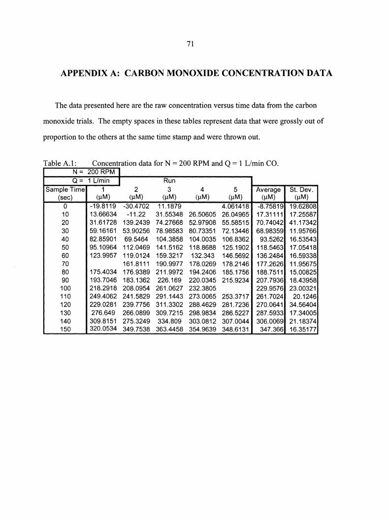
71
APPENDIX A: CARBON MONOXIDE CONCENTRATION DATA
The data presented here are the raw concentration versus time data from the carbon
monoxide trials. The empty spaces in these tables represent data that were grossly out of
proportion to the others at the same time stamp and were thrown out.
Table A.1: Concentration data for N = 200 RPM and Q = 1 L/min CO. N = 200 RPM I Q = 1 Umin I Run
Sample Time 1 2 3 4 5 Average St. Dev. (sec) (µM) (µM) (µM) (µM) (µM) (µM) (µM)
0 -19.8119 -30.4702 11.1879 4.061418 -8.75819 19.62808 10 13.66634 -11.22 31.55348 26.50605 26.04965 17.31111 17.25587 20 31.61728 139.2439 74.27668 52.97908 55.58515 70.74042 41.17342 30 59.16161 53.90256 78.98583 80.73351 72.13446 68.98359 11.95766 40 82.85901 69.5464 104.3858 104.0035 106.8362 93.5262 16.53543 50 95.10964 112.0469 141.5162 118.8688 125.1902 118.5463 17.05418 60 123.9957 119.0124 159.3217 132.343 146.5692 136.2484 16.59338 70 161.8111 190.9977 178.0269 178.2146 177.2626 11.95675 80 175.4034 176.9389 211.9972 194.2406 185.1756 188.7511 15.00825 90 193.7046 183.1362 226.169 220.0345 215.9234 207.7936 18.43958 100 218.2918 208.0954 261.0627 232.3805 229.9576 23.00321 110 249.4062 241.5829 291.1443 273.0065 253.3717 261.7024 20.1246 120 229.0281 239.7756 311.3302 288.4629 281.7236 270.0641 34.56404 130 276.649 266.0899 309.7215 298.9834 286.5227 287.5933 17.34005 140 309.8151 275.3249 334.809 303.0812 307.0044 306.0069 21.18374 150 320.0534 349.7538 363.4458 354.9639 348.6131 347.366 16.35177
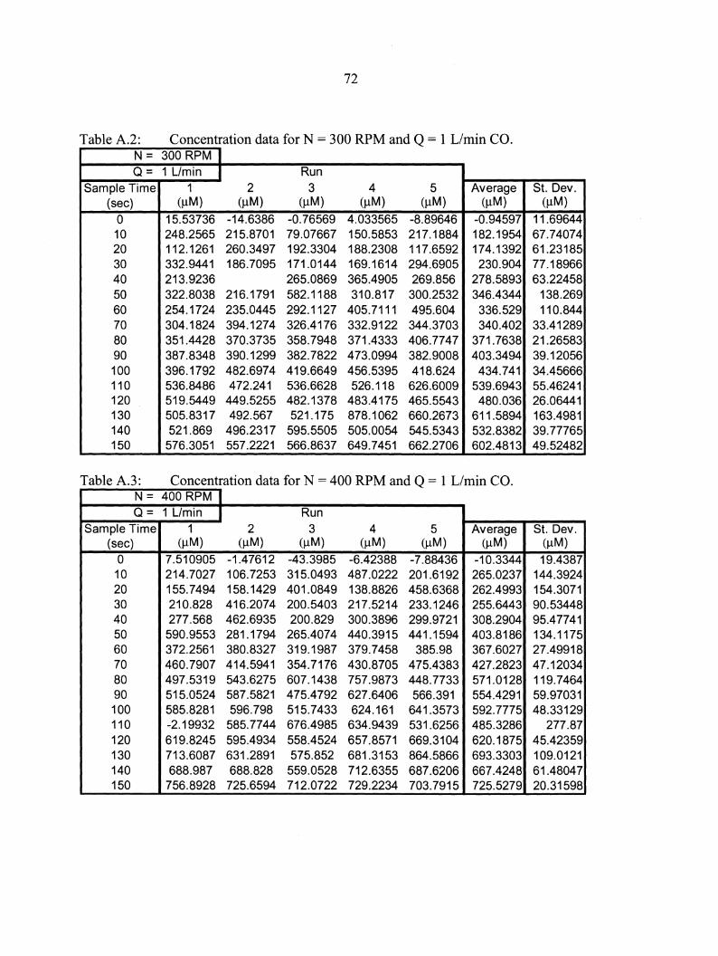
72
Table A.2: Concentration data for N = 300 RPM and Q = 1 L/min CO. N = 300 RPM I Q = 1 L/min I Run
Sample Time 1 2 3 4 5 Average St. Dev. (sec) (µM) (µM) (µM) (µM) (µM) (µM) (µM)
0 15.53736 -14.6386 -0.76569 4.033565 -8.89646 -0.94597 11.69644 10 248.2565 215.8701 79.07667 150.5853 217.1884 182.1954 67.74074 20 112.1261 260.3497 192.3304 188.2308 117.6592 174.1392 61.23185 30 332.9441 186.7095 171.0144 169.1614 294.6905 230.904 77.18966 40 213.9236 265.0869 365.4905 269.856 278.5893 63.22458 50 322.8038 216.1791 582.1188 310.817 300.2532 346.4344 138.269 60 254.1724 235.0445 292.1127 405.7111 495.604 336.529 110.844 70 304.1824 394.1274 326.4176 332.9122 344.3703 340.402 33.41289 80 351.4428 370.3735 358.7948 371.4333 406.7747 371.7638 21.26583 90 387.8348 390.1299 382.7822 473.0994 382.9008 403.3494 39.12056 100 396.1792 482.6974 419.6649 456.5395 418.624 434.741 34.45666 110 536.8486 472.241 536.6628 526.118 626.6009 539.6943 55.46241 120 519.5449 449.5255 482.1378 483.4175 465.5543 480.036 26.06441 130 505.8317 492.567 521.175 878.1062 660.2673 611.5894 163.4981 140 521.869 496.2317 595.5505 505.0054 545.5343 532.8382 39.77765 150 576.3051 557.2221 566.8637 649.7451 662.2706 602.4813 49.52482
Table A.3: Concentration data for N = 400 RPM and Q = 1 L/min CO. N = 400 RPM I Q = 1 L/min I Run
Sample Time 1 2 3 4 5 Average St. Dev. (sec) (µM) (µM) (µM) (µM) (µM) (µM) (µM)
0 7.510905 -1.47612 -43.3985 -6.42388 -7.88436 -10.3344 19.4387 10 214.7027 106.7253 315.0493 487.0222 201.6192 265.0237 144.3924 20 155.7494 158.1429 401.0849 138.8826 458.6368 262.4993 154.3071 30 210.828 416.2074 200.5403 217.5214 233.1246 255.6443 90.53448 40 277.568 462.6935 200.829 300.3896 299.9721 308.2904 95.47741 50 590.9553 281.1794 265.4074 440.3915 441.1594 403.8186 134.1175 60 372.2561 380.8327 319.1987 379.7458 385.98 367.6027 27.49918 70 460.7907 414.5941 354.7176 430.8705 475.4383 427.2823 47.12034 80 497.5319 543.6275 607.1438 757.9873 448.7733 571.0128 119.7464 90 515.0524 587.5821 475.4792 627.6406 566.391 554.4291 59.97031 100 585.8281 596.798 515.7433 624.161 641.3573 592.7775 48.33129 110 -2.19932 585.7744 676.4985 634.9439 531.6256 485.3286 277.87 120 619.8245 595.4934 558.4524 657.8571 669.3104 620.1875 45.42359 130 713.6087 631.2891 575.852 681.3153 864.5866 693.3303 109.0121 140 688.987 688.828 559.0528 712.6355 687.6206 667.4248 61.48047 150 756.8928 725.6594 712.0722 729.2234 703.7915 725.5279 20.31598
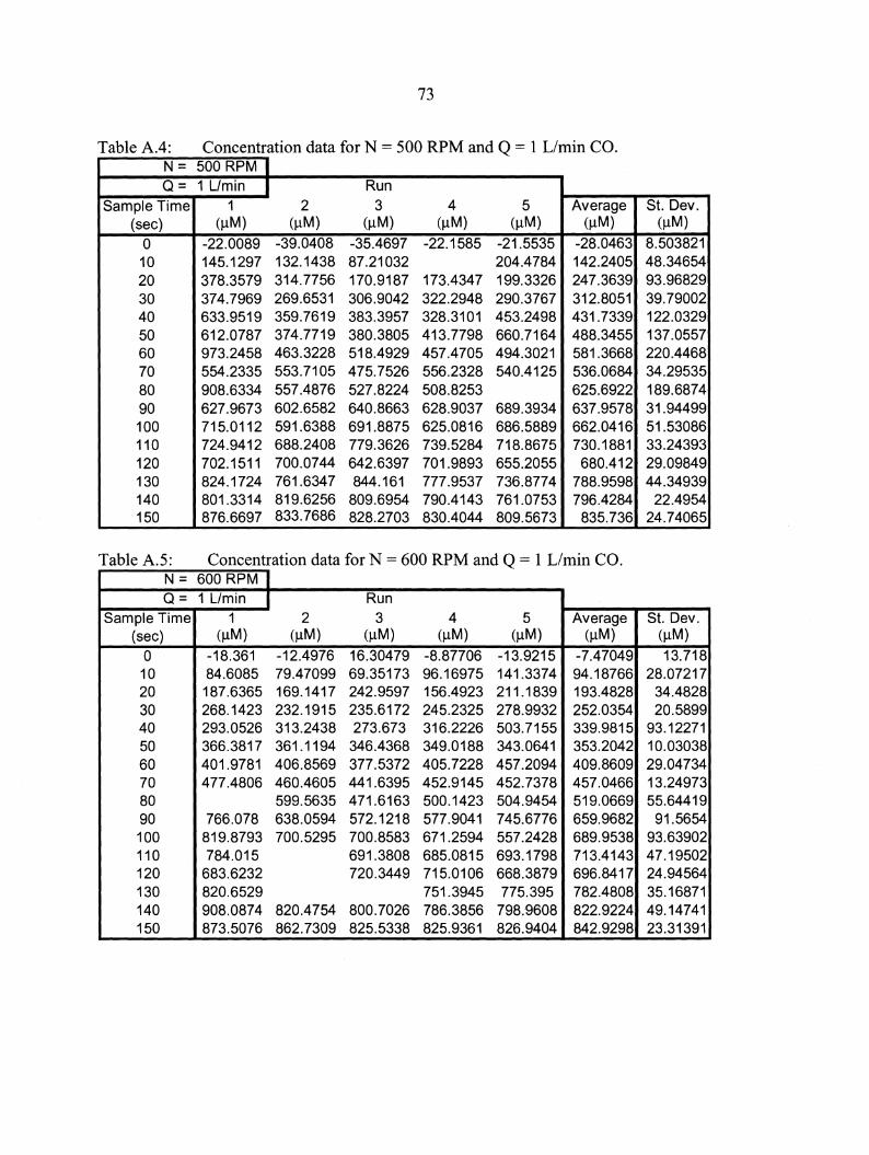
73
Table A.4: Concentration data for N = 500 RPM and Q = 1 Umin CO. N = 500 RPM I Q = 1 Umin I Run
Sample Time 1 2 3 4 5 Average St. Dev. (sec) (µM) (µM) (µM) (µM) (µM) (µM) (µM)
0 -22.0089 -39.0408 -35.4697 -22.1585 -21.5535 -28.0463 8.503821 10 145.1297 132.1438 87.21032 204.4784 142.2405 48.34654 20 378.3579 314.7756 170.9187 173.4347 199.3326 247.3639 93.96829 30 374.7969 269.6531 306.9042 322.2948 290.3767 312.8051 39.79002 40 633.9519 359.7619 383.3957 328.3101 453.2498 431.7339 122.0329 50 612.0787 374.7719 380.3805 413.7798 660.7164 488.3455 137.0557 60 973.2458 463.3228 518.4929 457.4705 494.3021 581.3668 220.4468 70 554.2335 553.7105 475.7526 556.2328 540.4125 536.0684 34.29535 80 908.6334 557.4876 527.8224 508.8253 625.6922 189.6874 90 627.9673 602.6582 640.8663 628.9037 689.3934 637.9578 31.94499 100 715.0112 591.6388 691.8875 625.0816 686.5889 662.0416 51.53086 110 724.9412 688.2408 779.3626 739.5284 718.8675 730.1881 33.24393 120 702.1511 700.0744 642.6397 701.9893 655.2055 680.412 29.09849 130 824.1724 761.6347 844.161 777.9537 736.8774 788.9598 44.34939 140 801.3314 819.6256 809.6954 790.4143 761.0753 796.4284 22.4954 150 876.6697 833.7686 828.2703 830.4044 809.5673 835.736 24.74065
Table A.5: Concentration data for N = 600 RPM and Q = 1 Umin CO. N = 600 RPM I Q = 1 Umin I Run
Sample Time 1 2 3 4 5 Average St. Dev. (sec) (µM) (µM) (µM) (µM) (µM) (µM) (µM)
0 -18.361 -12.4976 16.30479 -8.87706 -13.9215 -7.47049 13.718 10 84.6085 79.47099 69.35173 96.16975 141.3374 94.18766 28.07217 20 187.6365 169.1417 242.9597 156.4923 211.1839 193.4828 34.4828 30 268.1423 232.1915 235.6172 245.2325 278.9932 252.0354 20.5899 40 293.0526 313.2438 273.673 316.2226 503.7155 339.9815 93.12271 50 366.3817 361.1194 346.4368 349.0188 343.0641 353.2042 10.03038 60 401.9781 406.8569 377.5372 405.7228 457.2094 409.8609 29.04734 70 477.4806 460.4605 441.6395 452.9145 452.7378 457.0466 13.24973 80 599.5635 471.6163 500.1423 504.9454 519.0669 55.64419 90 766.078 638.0594 572.1218 577.9041 745.6776 659.9682 91.5654 100 819.8793 700.5295 700.8583 671.2594 557.2428 689.9538 93.63902 110 784.015 691.3808 685.0815 693.1798 713.4143 47.19502 120 683.6232 720.3449 715.0106 668.3879 696.8417 24.94564 130 820.6529 751.3945 775.395 782.4808 35.16871 140 908.0874 820.4754 800.7026 786.3856 798.9608 822.9224 49.14741 150 873.5076 862.7309 825.5338 825.9361 826.9404 842.9298 23.31391

74
Table A.6: Concentration data for N = 200 RPM and Q = 2 L/min CO. N = 200 RPM I Q = 2 Umin I Run
Sample Time 1 2 3 4 5 Average St. Dev. (sec) (µM) (µM) (µM) (µM) (µM) (µM) (µM)
0 13.50082 -10.0155 -9.95156 -23.0599 -22.8611 -10.4775 14.89229 10 31.82981 27.11291 24.66058 19.0558 17.34086 23.99999 5.920764 20 79.08777 66.91217 65.81236 77.24356 63.26807 70.46479 7.182733 30 116.1163 108.022 103.6644 96.34365 97.58198 104.3457 8.097938 40 169.4838 142.3157 143.7067 136.7579 136.0982 145.6725 13.7227 50 192.2972 179.8304 179.5737 183.7867 172.7856 181.6547 7.143688 60 211.5452 207.377 203.5785 215.3883 199.566 207.491 6.263596 70 256.2457 246.315 247.9678 246.1414 255.3881 250.4116 4.994783 80 304.0435 272.4537 278.875 283.8431 276.3822 283.1195 12.40467 90 306.7952 301.4409 313.0383 315.7388 311.0178 309.6062 5.611459 100 364.1294 331.3044 342.0286 347.9 343.5657 345.7856 11.93437 110 368.0057 367.5282 354.8213 370.4035 376.7527 367.5023 7.98513 120 413.0794 412.1223 416.8688 420.9474 412.5888 415.1213 3.760796 130 438.4716 429.5413 435.1863 434.5882 387.1955 424.9966 21.3716 140 449.0551 454.3693 472.8066 457.8772 477.7115 462.3639 12.30617 150 507.8219 506.0521 506.6718 513.1156 517.702 510.2727 5.001566
Table A.7: Concentration data for N = 300 RPM and Q = 2 L/min CO. N = 300 RPM I Q = 2 Umin I Run
Sample Time 1 2 3 4 5 Average St. Dev. (sec) (µM) (µM) (µM) (µM) (µM) (µM) (µM)
0 5.76698 -7.35698 -9.30715 -24.0717 -29.7361 -12.941 14.14516 10 109.9592 72.08432 125.5715 91.58928 54.18877 90.67863 28.58035 20 394.9305 141.8996 209.7286 170.5585 226.4456 228.7126 98.63103 30 521.4047 211.7139 208.9166 211.2686 186.1917 267.8991 142.1125 40 525.9239 266.1538 295.8464 379.9045 344.4852 362.4628 101.3165 50 377.505 400.0662 358.6945 401.7549 384.5052 20.4523 60 711.2605 370.6768 622.1054 377.2133 369.2387 490.099 164.2788 70 427.9047 580.4969 656.4414 426.638 426.4504 503.5863 108.2574 80 485.5451 477.5251 561.5482 728.8428 468.675 544.4273 109.5258 90 675.9715 520.5236 641.7466 623.1223 538.7525 600.0233 67.29939 100 718.0966 587.8854 660.1791 592.9343 639.7738 61.7446 110 746.2022 580.4047 709.712 606.2872 555.8637 639.694 83.52439 120 682.7829 676.0785 662.9585 635.1171 637.0249 658.7924 21.94342 130 853.5257 779.0004 696.4214 767.0296 653.6011 749.9156 77.47899 140 761.6848 700.9479 758.2202 753.504 710.587 736.9888 28.85054 150 760.9654 781.6732 720.0578 862.3615 772.7171 779.555 51.94625
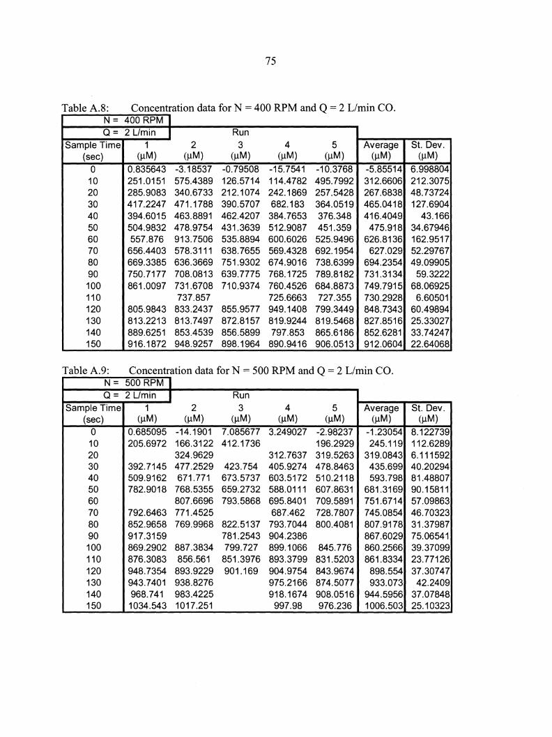
75
Table A.8: Concentration data for N = 400 RPM and Q = 2 L/min CO. N = 400 RPM I Q = 2 L/min I Run
Sample Time 1 2 3 4 5 Average St. Dev. (sec) (µM) (µM) (µM) (µM) (µM) (µM) (µM)
0 0.835643 -3.18537 -0.79508 -15.7541 -10.3768 -5.85514 6.998804 10 251.0151 575.4389 126.5714 114.4782 495.7992 312.6606 212.3075 20 285.9083 340.6733 212.1074 242.1869 257.5428 267.6838 48.73724 30 417.2247 471.1788 390.5707 682.183 364.0519 465.0418 127.6904 40 394.6015 463.8891 462.4207 384.7653 376.348 416.4049 43.166 50 504.9832 478.9754 431.3639 512.9087 451.359 475.918 34.67946 60 557.876 913.7506 535.8894 600.6026 525.9496 626.8136 162.9517 70 656.4403 578.3111 638.7655 569.4328 692.1954 627.029 52.29767 80 669.3385 636.3669 751.9302 674.9016 738.6399 694.2354 49.09905 90 750.7177 708.0813 639.7775 768.1725 789.8182 731.3134 59.3222 100 861.0097 731.6708 710.9374 760.4526 684.8873 749.7915 68.06925 110 737.857 725.6663 727.355 730.2928 6.60501 120 805.9843 833.2437 855.9577 949.1408 799.3449 848.7343 60.49894 130 813.2213 813.7497 872.8157 819.9244 819.5468 827.8516 25.33027 140 889.6251 853.4539 856.5899 797.853 865.6186 852.6281 33.74247 150 916.1872 948.9257 898.1964 890.9416 906.0513 912.0604 22.64068
Table A.9: Concentration data for N = 500 RPM and Q = 2 L/min CO. N = 500 RPM I Q = 2 L/min I Run
Sample Time 1 2 3 4 5 Average St. Dev. (sec) (µM) (µM) (µM) (µM) (µM) (µM) (µM)
0 0.685095 -14.1901 7.085677 3.249027 -2.98237 -1.23054 8.122739 10 205.6972 166.3122 412.1736 196.2929 245.119 112.6289 20 324.9629 312.7637 319.5263 319.0843 6.111592 30 392.7145 477.2529 423.754 405.9274 478.8463 435.699 40.20294 40 509.9162 671.771 673.5737 603.5172 510.2118 593.798 81.48807 50 782.9018 768.5355 659.2732 588.0111 607.8631 681.3169 90.15811 60 807.6696 793.5868 695.8401 709.5891 751.6714 57.09863 70 792.6463 771.4525 687.462 728.7807 745.0854 46.70323 80 852.9658 769.9968 822.5137 793.7044 800.4081 807.9178 31.37987 90 917.3159 781.2543 904.2386 867.6029 75.06541 100 869.2902 887.3834 799.727 899.1066 845.776 860.2566 39.37099 110 876.3083 856.561 851.3976 893.3799 831.5203 861.8334 23.77126 120 948.7354 893.9229 901.169 904.9754 843.9674 898.554 37.30747 130 943.7401 938.8276 975.2166 874.5077 933.073 42.2409 140 968.741 983.4225 918.1674 908.0516 944.5956 37.07848 150 1034.543 1017.251 997.98 976.236 1006.503 25.10323
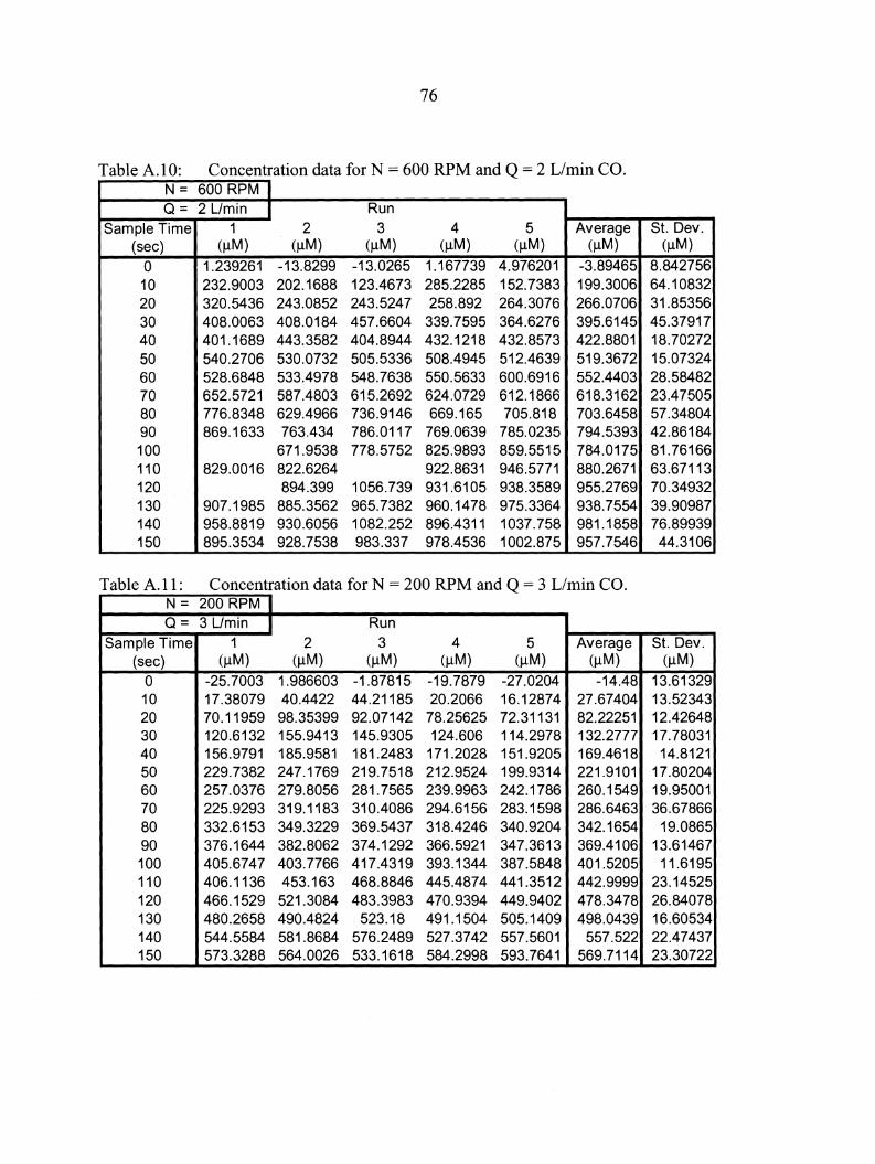
76
Table A.10: Concentration data for N = 600 RPM and Q = 2 Umin CO. N = 600 RPM I Q = 2 Umin I Run
Sample Time 1 2 3 4 5 Average St. Dev. (sec) (µM) (µM) (µM) (µM) (µM) (µM) (µM)
0 1.239261 -13.8299 -13.0265 1.167739 4.976201 -3.89465 8.842756 10 232.9003 202.1688 123.4673 285.2285 152.7383 199.3006 64.10832 20 320.5436 243.0852 243.5247 258.892 264.3076 266.0706 31.85356 30 408.0063 408.0184 457.6604 339.7595 364.6276 395.6145 45.37917 40 401.1689 443.3582 404.8944 432.1218 432.8573 422.8801 18.70272 50 540.2706 530.0732 505.5336 508.4945 512.4639 519.3672 15.07324 60 528.6848 533.4978 548.7638 550.5633 600.6916 552.4403 28.58482 70 652.5721 587.4803 615.2692 624.0729 612.1866 618.3162 23.47505 80 776.8348 629.4966 736.9146 669.165 705.818 703.6458 57.34804 90 869.1633 763.434 786.0117 769.0639 785.0235 794.5393 42.86184 100 671.9538 778.5752 825.9893 859.5515 784.0175 81.76166 110 829.0016 822.6264 922.8631 946.5771 880.2671 63.67113 120 894.399 1056.739 931.6105 938.3589 955.2769 70.34932 130 907.1985 885.3562 965.7382 960.1478 975.3364 938.7554 39.90987 140 958.8819 930.6056 1082.252 896.4311 1037.758 981.1858 76.89939 150 895.3534 928.7538 983.337 978.4536 1002.875 957.7546 44.3106
Table A.11: Concentration data for N = 200 RPM and Q = 3 L/min CO. N = 200 RPM I Q = 3 Umin I Run
Sample Time 1 2 3 4 5 Average St. Dev. (sec) (µM) (µM) (µM) (µM) (µM) (µM) (µM)
0 -25.7003 1.986603 -1.87815 -19.7879 -27.0204 -14.48 13.61329 10 17.38079 40.4422 44.21185 20.2066 16.12874 27.67404 13.52343 20 70.11959 98.35399 92.07142 78.25625 72.31131 82.22251 12.42648 30 120.6132 155.9413 145.9305 124.606 114.2978 132.2777 17.78031 40 156.9791 185.9581 181.2483 171.2028 151.9205 169.4618 14.8121 50 229.7382 247.1769 219.7518 212.9524 199.9314 221.9101 17.80204 60 257.0376 279.8056 281.7565 239.9963 242.1786 260.1549 19.95001 70 225.9293 319.1183 310.4086 294.6156 283.1598 286.6463 36.67866 80 332.6153 349.3229 369.5437 318.4246 340.9204 342.1654 19.0865 90 376.1644 382.8062 374.1292 366.5921 347.3613 369.4106 13.61467 100 405.6747 403.7766 417.4319 393.1344 387.5848 401.5205 11.6195 110 406.1136 453.163 468.8846 445.4874 441.3512 442.9999 23.14525 120 466.1529 521.3084 483.3983 470.9394 449.9402 478.3478 26.84078 130 480.2658 490.4824 523.18 491.1504 505.1409 498.0439 16.60534 140 544.5584 581.8684 576.2489 527.3742 557.5601 557.522 22.47437 150 573.3288 564.0026 533.1618 584.2998 593.7641 569.7114 23.30722
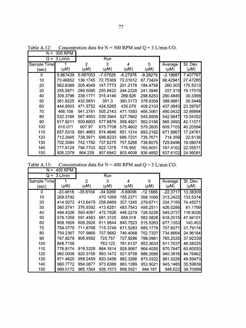
77
Table A.12: Concentration data for N = 300 RPM and Q = 3 L/min CO. N = 300 RPM I Q = 3 L/min I Run
Sample Time 1 2 3 4 5 Average St. Dev. (sec) (µM) (µM) (µM) (µM) (µM) (µM) (µM)
0 5.967439 5.687053 -7.07628 -6.27978 -9.28279 -2.19687 7.407787 10 73.46852 136.1745 72.75369 72.01612 87.73424 88.42941 27.47285 20 562.6389 205.4049 147.7773 201.2178 184.4759 260.303 170.5313 30 255.5871 289.5585 255.8422 244.2228 241.3846 257.319 19.17019 40 309.3796 239.1771 315.4146 289.626 298.8253 290.4845 30.3368 50 361.8225 432.5651 391.3 380.3173 378.9358 388.9881 26.5448 60 444.9303 471.5752 424.5265 435.079 409.2103 437.0643 23.39797 70 466.158 541.3781 505.2143 471.1593 466.3061 490.0432 32.99994 80 532.3166 567.4953 539.3944 527.7662 545.8509 542.5647 15.54352 90 617.9211 500.8803 577.6876 568.4921 562.0156 565.3993 42.11071 100 610.071 607.97 675.7708 575.4802 579.2605 609.7105 40.20584 110 657.5319 681.4663 674.4846 651.1314 693.2192 671.5667 17.24761 120 712.2845 738.3971 698.8233 686.7231 735.7671 714.399 22.6138 130 702.3084 742.1782 737.6275 707.5266 738.6075 725.6496 19.09074 140 777.8129 794.7703 822.1378 776.955 765.4051 787.4162 22.05571 150 826.2378 864.239 857.6842 803.4008 836.4892 837.6102 24.56081
Table A.13: Concentration data for N = 400 RPM and Q = 3 L/min CO. N = 400 RPM I Q = 3 L/min I Run
Sample Time 1 2 3 4 5 Average St. Dev. (sec) (µM) (µM) (µM) (µM) (µM) (µM) (µM)
0 -23.4618 -35.6104 -34.9268 -5.69096 -12.1688 -22.3717 13.38309 10 269.5192 470.1069 155.2371 358.1068 313.2425 133.5374 20 414.5072 413.6479 258.6469 307.1245 279.6711 334.7195 74.45571 30 360.5741 376.9392 413.6251 483.7543 495.2511 426.0288 61.1799 40 484.4326 593.4087 472.7826 446.2219 728.5228 545.0737 116.9026 50 578.1359 591.4583 681.3125 658.018 582.0828 618.2015 47.94101 60 808.1609 609.2826 611.9544 840.7523 515.5263 677.1353 140.453 70 754.0779 711.8768 715.3749 671.5283 685.1778 707.6071 31.79174 80 759.2367 707.9866 707.9682 746.4068 752.7337 734.8664 24.96184 90 767.8278 806.6582 725.757 727.9286 798.0961 765.2535 37.92339 100 848.7158 763.122 781.6137 853.3633 811.7037 46.08325 110 776.8174 918.5328 864.1614 929.9067 864.4055 870.7647 60.60053 120 980.0006 920.5156 993.1472 921.9758 886.2689 940.3816 44.76462 130 871.4625 958.2459 820.0458 882.3266 873.0322 881.0226 49.59473 140 960.7772 954.0877 973.8366 883.1389 953.9021 945.1485 35.59839 150 989.0172 985.1564 926.1573 898.5921 944.187 948.622 38.70999
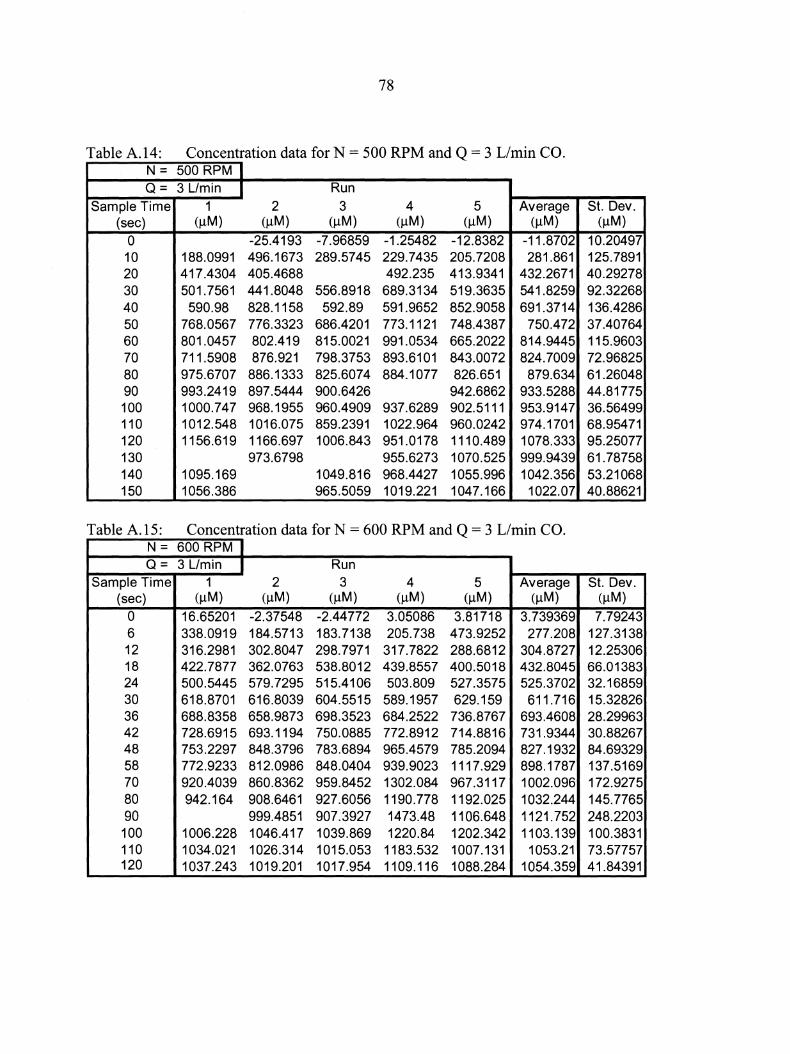
78
Table A.14: Concentration data for N = 500 RPM and Q = 3 L/min CO. N = 500 RPM I Q = 3 L/min I Run
Sample Time 1 2 3 4 5 Average St. Dev. (sec) (µM) (µM) (µM) (µM) (µM) (µM) (µM)
0 -25.4193 -7.96859 -1.25482 -12.8382 -11.8702 10.20497 10 188.0991 496.1673 289.5745 229.7435 205.7208 281.861 125.7891 20 417.4304 405.4688 492.235 413.9341 432.2671 40.29278 30 501.7561 441.8048 556.8918 689.3134 519.3635 541.8259 92.32268 40 590.98 828.1158 592.89 591.9652 852.9058 691.3714 136.4286 50 768.0567 776.3323 686.4201 773.1121 748.4387 750.472 37.40764 60 801.0457 802.419 815.0021 991.0534 665.2022 814.9445 115.9603 70 711.5908 876.921 798.3753 893.6101 843.0072 824.7009 72.96825 80 975.6707 886.1333 825.6074 884.1077 826.651 879.634 61.26048 90 993.2419 897.5444 900.6426 942.6862 933.5288 44.81775 100 1000.747 968.1955 960.4909 937.6289 902.5111 953.9147 36.56499 110 1012.548 1016.075 859.2391 1022.964 960.0242 974.1701 68.95471 120 1156.619 1166.697 1006.843 951.0178 1110.489 1078.333 95.25077 130 973.6798 955.6273 1070.525 999.9439 61.78758 140 1095.169 1049.816 968.4427 1055.996 1042.356 53.21068 150 1056.386 965.5059 1019.221 1047.166 1022.07 40.88621
Table A.15: Concentration data for N = 600 RPM and Q = 3 L/min CO. N = 600 RPM I Q = 3 L/min I Run
Sample Time 1 2 3 4 5 Average St. Dev. (sec) (µM) (µM) (µM) (µM) (µM) (µM) (µM)
0 16.65201 -2.37548 -2.44772 3.05086 3.81718 3.739369 7.79243 6 338.0919 184.5713 183.7138 205.738 473.9252 277.208 127.3138 12 316.2981 302.8047 298. 7971 317.7822 288.6812 304.8727 12.25306 18 422.7877 362.0763 538.8012 439.8557 400.5018 432.8045 66.01383 24 500.5445 579.7295 515.4106 503.809 527.3575 525.3702 32.16859 30 618.8701 616.8039 604.5515 589.1957 629.159 611.716 15.32826 36 688.8358 658.9873 698.3523 684.2522 736.8767 693.4608 28.29963 42 728.6915 693.1194 750.0885 772.8912 714.8816 731.9344 30.88267 48 753.2297 848.3796 783.6894 965.4579 785.2094 827.1932 84.69329 58 772.9233 812.0986 848.0404 939.9023 1117.929 898.1787 137.5169 70 920.4039 860.8362 959.8452 1302.084 967.3117 1002.096 172.9275 80 942.164 908.6461 927.6056 1190.778 1192.025 1032.244 145.7765 90 999.4851 907.3927 1473.48 1106.648 1121.752 248.2203 100 1006.228 1046.417 1039.869 1220.84 1202.342 1103.139 100.3831 110 1034.021 1026.314 1015.053 1183.532 1007.131 1053.21 73.57757 120 1037.243 1019.201 1017.954 1109.116 1088.284 1054.359 41.84391
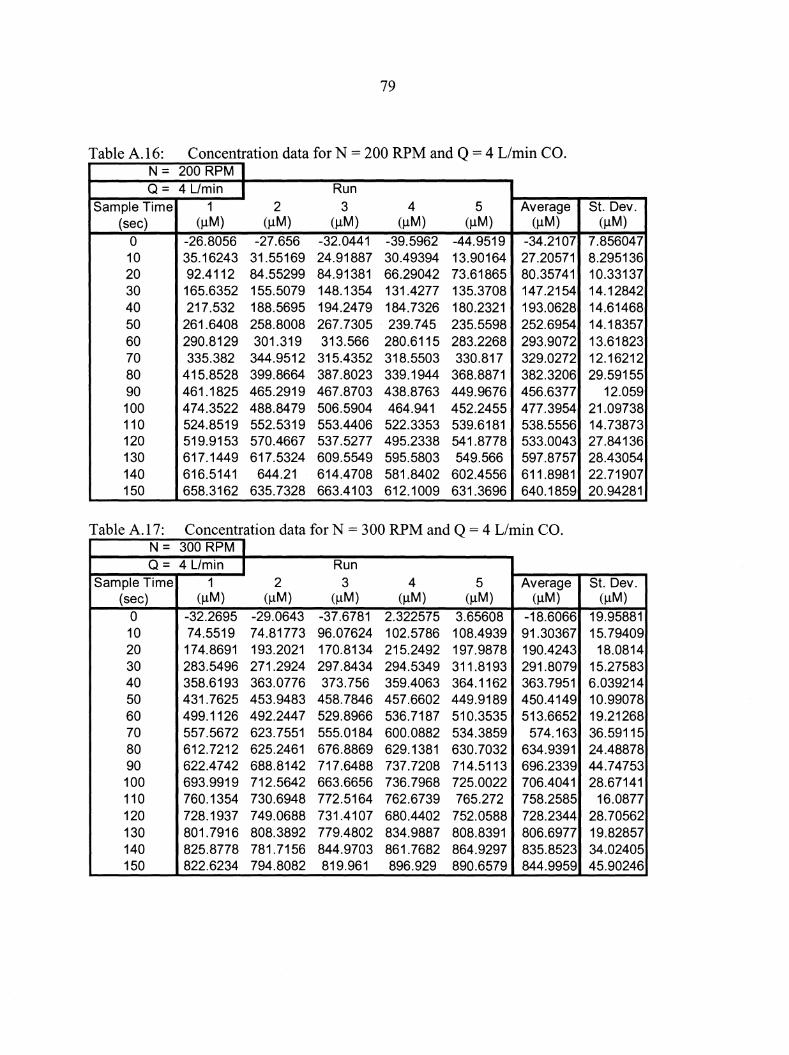
79
Table A.16: Concentration data for N = 200 RPM and Q = 4 Umin CO. N = 200 RPM I Q = 4 L/min I Run
Sample Time 1 2 3 4 5 Average St. Dev. (sec) (µM) (µM) (µM) (µM) (µM) (µM) (µM)
0 -26.8056 -27.656 -32.0441 -39.5962 -44.9519 -34.2107 7.856047 10 35.16243 31.55169 24.91887 30.49394 13.90164 27.20571 8.295136 20 92.4112 84.55299 84.91381 66.29042 73.61865 80.35741 10.33137 30 165.6352 155.5079 148.1354 131.4277 135.3708 147.2154 14.12842 40 217.532 188.5695 194.2479 184.7326 180.2321 193.0628 14.61468 50 261.6408 258.8008 267.7305 239.745 235.5598 252.6954 14.18357 60 290.8129 301.319 313.566 280.6115 283.2268 293.9072 13.61823 70 335.382 344.9512 315.4352 318.5503 330.817 329.0272 12.16212 80 415.8528 399.8664 387.8023 339.1944 368.8871 382.3206 29.59155 90 461.1825 465.2919 467.8703 438.8763 449.9676 456.6377 12.059 100 474.3522 488.8479 506.5904 464.941 452.2455 477.3954 21.09738 110 524.8519 552.5319 553.4406 522.3353 539.6181 538.5556 14.73873 120 519.9153 570.4667 537.5277 495.2338 541.8778 533.0043 27.84136 130 617.1449 617.5324 609.5549 595.5803 549.566 597.8757 28.43054 140 616.5141 644.21 614.4708 581.8402 602.4556 611.8981 22.71907 150 658.3162 635.7328 663.4103 612.1009 631.3696 640.1859 20.94281
Table A.17: Concentration data for N = 300 RPM and Q = 4 L/min CO. N = 300 RPM I Q = 4 L/min I Run
Sample Time 1 2 3 4 5 Average St. Dev. (sec) (µM) (µM) (µM) (µM) (µM) (µM) (µM)
0 -32.2695 -29.0643 -37.6781 2.322575 3.65608 -18.6066 19.95881 10 74.5519 74.81773 96.07624 102.5786 108.4939 91.30367 15.79409 20 174.8691 193.2021 170.8134 215.2492 197.9878 190.4243 18.0814 30 283.5496 271.2924 297.8434 294.5349 311.8193 291.8079 15.27583 40 358.6193 363.0776 373.756 359.4063 364.1162 363.7951 6.039214 50 431.7625 453.9483 458.7846 457.6602 449.9189 450.4149 10.99078 60 499.1126 492.2447 529.8966 536.7187 510.3535 513.6652 19.21268 70 557.5672 623.7551 555.0184 600.0882 534.3859 574.163 36.59115 80 612.7212 625.2461 676.8869 629.1381 630.7032 634.9391 24.48878 90 622.4742 688.8142 717.6488 737.7208 714.5113 696.2339 44.74753 100 693.9919 712.5642 663.6656 736.7968 725.0022 706.4041 28.67141 110 760.1354 730.6948 772.5164 762.6739 765.272 758.2585 16.0877 120 728.1937 749.0688 731.4107 680.4402 752.0588 728.2344 28.70562 130 801.7916 808.3892 779.4802 834.9887 808.8391 806.6977 19.82857 140 825.8778 781.7156 844.9703 861.7682 864.9297 835.8523 34.02405 150 822.6234 794.8082 819.961 896.929 890.6579 844.9959 45.90246
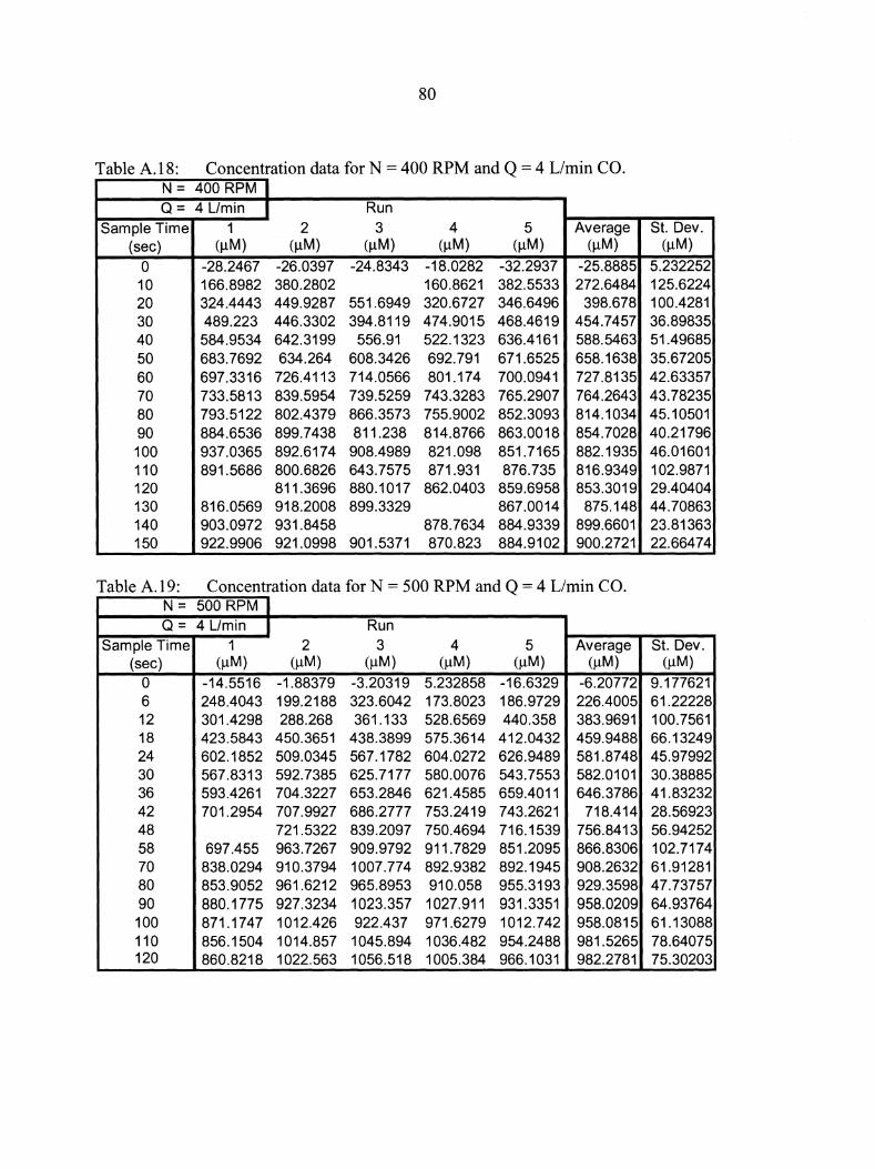
80
Table A.18: Concentration data for N = 400 RPM and Q = 4 L/rnin CO. N = 400 RPM I Q = 4 Umin I Run
Sample Time 1 2 3 4 5 Average St. Dev. (sec) (µM) (µM) (µM) (µM) (µM) (µM) (µM)
0 -28.2467 -26.0397 -24.8343 -18.0282 -32.2937 -25.8885 5.232252 10 166.8982 380.2802 160.8621 382.5533 272.6484 125.6224 20 324.4443 449.9287 551.6949 320.6727 346.6496 398.678 100.4281 30 489.223 446.3302 394.8119 474.9015 468.4619 454.7457 36.89835 40 584.9534 642.3199 556.91 522.1323 636.4161 588.5463 51.49685 50 683.7692 634.264 608.3426 692.791 671.6525 658.1638 35.67205 60 697.3316 726.4113 714.0566 801.174 700.0941 727.8135 42.63357 70 733.5813 839.5954 739.5259 743.3283 765.2907 764.2643 43.78235 80 793.5122 802.4379 866.3573 755.9002 852.3093 814.1034 45.10501 90 884.6536 899.7438 811.238 814.8766 863.0018 854.7028 40.21796 100 937.0365 892.6174 908.4989 821.098 851.7165 882.1935 46.01601 110 891.5686 800.6826 643.7575 871.931 876.735 816.9349 102.9871 120 811.3696 880.1017 862.0403 859.6958 853.3019 29.40404 130 816.0569 918.2008 899.3329 867.0014 875.148 44.70863 140 903.0972 931.8458 878.7634 884.9339 899.6601 23.81363 150 922.9906 921.0998 901.5371 870.823 884.9102 900.2721 22.66474
Table A.19: Concentration data for N = 500 RPM and Q = 4 L/rnin CO. N = 500 RPM I Q = 4 Umin I Run
Sample Time 1 2 3 4 5 Average St. Dev. (sec) (µM) (µM) (µM) (µM) (µM) (µM) (µM)
0 -14.5516 -1.88379 -3.20319 5.232858 -16.6329 -6.20772 9.177621 6 248.4043 199.2188 323.6042 173.8023 186.9729 226.4005 61.22228 12 301.4298 288.268 361.133 528.6569 440.358 383.9691 100.7561 18 423.5843 450.3651 438.3899 575.3614 412.0432 459.9488 66.13249 24 602.1852 509.0345 567.1782 604.0272 626.9489 581.8748 45.97992 30 567.8313 592.7385 625.7177 580.0076 543.7553 582.0101 30.38885 36 593.4261 704.3227 653.2846 621.4585 659.4011 646.3786 41.83232 42 701.2954 707.9927 686.2777 753.2419 743.2621 718.414 28.56923 48 721.5322 839.2097 750.4694 716.1539 756.8413 56.94252 58 697.455 963.7267 909.9792 911.7829 851.2095 866.8306 102.7174 70 838.0294 910.3794 1007.774 892.9382 892.1945 908.2632 61.91281 80 853.9052 961.6212 965.8953 910.058 955.3193 929.3598 47.73757 90 880.1775 927.3234 1023.357 1027.911 931.3351 958.0209 64.93764 100 871.1747 1012.426 922.437 971.6279 1012.742 958.0815 61.13088 110 856.1504 1014.857 1045.894 1036.482 954.2488 981.5265 78.64075 120 860.8218 1022.563 1056.518 1005.384 966.1031 982.2781 75.30203
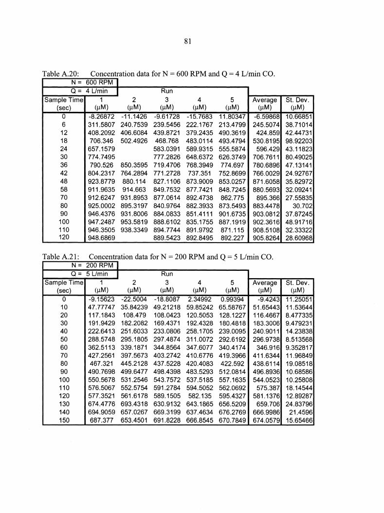
81
Table A.20: Concentration data for N = 600 RPM and Q = 4 L/min CO. N = 600 RPM I Q = 4 Umin I Run
Sample Time 1 2 3 4 5 Average St. Dev. (sec) (µM) (µM) (µM) (µM) (µM) (µM) (µM)
0 -8.26872 -11.1426 -9.61728 -15.7683 11.80347 -6.59868 10.66851 6 311.5807 240.7539 239.5456 222.1767 213.4799 245.5074 38.71014 12 408.2092 406.6084 439.8721 379.2435 490.3619 424.859 42.44731 18 706.346 502.4926 468.768 483.0114 493.4794 530.8195 98.92203 24 657.1579 583.0391 589.9315 555.5874 596.429 43.11823 30 774.7495 777.2826 648.6372 626.3749 706.7611 80.49025 36 790.526 850.3595 719.4706 768.3949 774.697 780.6896 47.13141 42 804.2317 764.2894 771.2728 737.351 752.8699 766.0029 24.92767 48 923.8779 880.114 827.1106 873.9009 853.0257 871.6058 35.82972 58 911.9635 914.663 849.7532 877.7421 848.7245 880.5693 32.09241 70 912.6247 931.8953 877.0614 892.4738 862.775 895.366 27.55835 80 925.0002 895.3197 840.9764 882.3933 873.5493 883.4478 30.702 90 946.4376 931.8006 884.0833 851.4111 901.6735 903.0812 37.87245 100 947.2487 953.5819 888.6102 835.1755 887.1919 902.3616 48.91716 110 946.3505 938.3349 894.7744 891.9792 871.115 908.5108 32.33322 120 948.6869 889.5423 892.8495 892.227 905.8264 28.60968
Table A.21: Concentration data for N = 200 RPM and Q = 5 L/min CO. N = 200 RPM I Q = 5 Umin I Run
Sample Time 1 2 3 4 5 Average St. Dev. (sec) (µM) (µM) (µM) (µM) (µM) (µM) (µM)
0 -9.15623 -22.5004 -18.8087 2.34992 0.99394 -9.4243 11.25051 10 47.77747 35.84239 49.21218 59.85242 65.58767 51.65443 11.53644 20 117.1843 108.479 108.0423 120.5053 128.1227 116.4667 8.477335 30 191.9429 182.2082 169.4371 192.4328 180.4818 183.3006 9.479231 40 222.6413 251.6033 233.0806 258.1705 239.0095 240.9011 14.23838 50 288.5748 295.1805 297.4874 311.0072 292.6192 296.9738 8.513568 60 362.5113 339.1871 344.8564 347.6077 340.4174 346.916 9.352817 70 427.2561 397.5673 403.2742 410.6776 419.3966 411.6344 11.96849 80 467.321 445.2128 437.5228 420.4083 422.592 438.6114 19.08518 90 490.7698 499.6477 498.4398 483.5293 512.0814 496.8936 10.68586 100 550.5678 531.2546 543.7572 537.5185 557.1635 544.0523 10.25808 110 576.5067 552.5754 591.2784 594.5052 562.0692 575.387 18.14544 120 577.3521 561.6178 589.1505 582.135 595.4327 581.1376 12.89287 130 674.4776 693.4318 630.9132 643.1865 656.5209 659.706 24.83796 140 694.9059 657.0267 669.3199 637.4634 676.2769 666.9986 21.4596 150 687.377 653.4501 691.8228 666.8545 670.7849 674.0579 15.65466
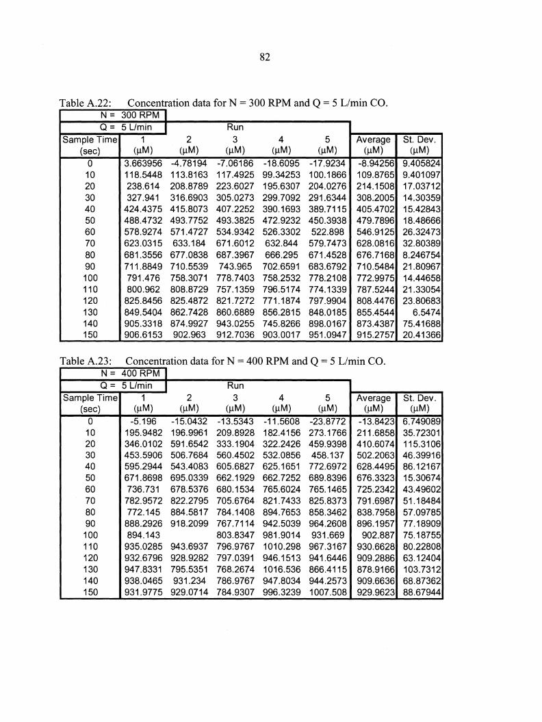
82
Table A.22: Concentration data for N = 300 RPM and Q = 5 L/min CO. N = 300 RPM I Q = 5 L/min I Run
Sample Time 1 2 3 4 5 Average St. Dev. (sec) (µM) (µM) (µM) (µM) (µM) (µM) (µM)
0 3.663956 -4.78194 -7.06186 -18.6095 -17.9234 -8.94256 9.405824 10 118.5448 113.8163 117.4925 99.34253 100.1866 109.8765 9.401097 20 238.614 208.8789 223.6027 195.6307 204.0276 214.1508 17.03712 30 327.941 316.6903 305.0273 299.7092 291.6344 308.2005 14.30359 40 424.4375 415.8073 407.2252 390.1693 389.7115 405.4702 15.42843 50 488.4732 493.7752 493.3825 472.9232 450.3938 479.7896 18.48666 60 578.9274 571.4727 534.9342 526.3302 522.898 546.9125 26.32473 70 623.0315 633.184 671.6012 632.844 579.7473 628.0816 32.80389 80 681.3556 677.0838 687.3967 666.295 671.4528 676.7168 8.246754 90 711.8849 710.5539 743.965 702.6591 683.6792 710.5484 21.80967 100 791.476 758.3071 778.7403 758.2532 778.2108 772.9975 14.44658 110 800.962 808.8729 757.1359 796.5174 774.1339 787.5244 21.33054 120 825.8456 825.4872 821.7272 771.1874 797.9904 808.4476 23.80683 130 849.5404 862.7428 860.6889 856.2815 848.0185 855.4544 6.5474 140 905.3318 874.9927 943.0255 745.8266 898.0167 873.4387 75.41688 150 906.6153 902.963 912.7036 903.0017 951.0947 915.2757 20.41366
Table A.23: Concentration data for N = 400 RPM and Q = 5 L/min CO. N = 400 RPM I Q = 5 L/min I Run
Sample Time 1 2 3 4 5 Average St. Dev. (sec) (µM) (µM) (µM) (µM) (µM) (µM) (µM)
0 -5.196 -15.0432 -13.5343 -11.5608 -23.8772 -13.8423 6.749089 10 195.9482 196.9961 209.8928 182.4156 273.1766 211.6858 35.72301 20 346.0102 591.6542 333.1904 322.2426 459.9398 410.6074 115.3106 30 453.5906 506.7684 560.4502 532.0856 458.137 502.2063 46.39916 40 595.2944 543.4083 605.6827 625.1651 772.6972 628.4495 86.12167 50 671.8698 695.0339 662.1929 662.7252 689.8396 676.3323 15.30674 60 736.731 678.5376 680.1534 765.6024 765.1465 725.2342 43.49602 70 782.9572 822.2795 705.6764 821.7433 825.8373 791.6987 51.18484 80 772.145 884.5817 784.1408 894.7653 858.3462 838.7958 57.09785 90 888.2926 918.2099 767.7114 942.5039 964.2608 896.1957 77.18909 100 894.143 803.8347 981.9014 931.669 902.887 75.18755 110 935.0285 943.6937 796.9767 1010.298 967.3167 930.6628 80.22808 120 932.6796 928.9282 797.0391 946.1513 941.6446 909.2886 63.12404 130 947.8331 795.5351 768.2674 1016.536 866.4115 878.9166 103.7312 140 938.0465 931.234 786.9767 947.8034 944.2573 909.6636 68.87362 150 931.9775 929.0714 784.9307 996.3239 1007.508 929.9623 88.67944
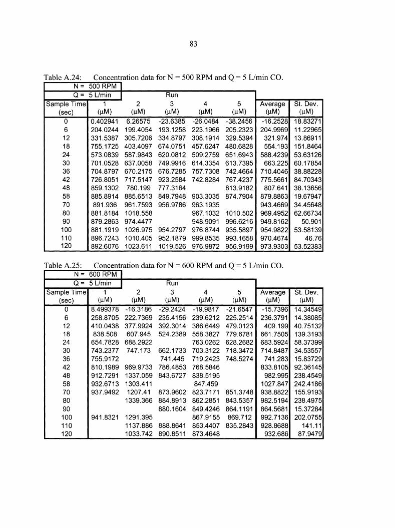
83
Table A.24: Concentration data for N = 500 RPM and Q = 5 L/min CO. N = 500 RPM I Q = 5 Umin I Run
Sample Time 1 2 3 4 5 Average St. Dev. (sec) (µM) (µM) (µM) (µM) (µM) (µM) (µM)
0 0.402941 6.26575 -23.6385 -26.0484 -38.2456 -16.2528 18.83271 6 204.0244 199.4054 193.1258 223.1966 205.2323 204.9969 11.22965 12 331.5387 305.7206 334.8797 308.1914 329.5394 321.974 13.86911 18 755.1725 403.4097 674.0751 457.6247 480.6828 554.193 151.8464 24 573.0839 587.9843 620.0812 509.2759 651.6943 588.4239 53.63126 30 701.0528 637.0058 749.9916 614.3354 613.7395 663.225 60.17854 36 704.8797 670.2175 676.7285 757.7308 742.4664 710.4046 38.88228 42 726.8051 717.5147 923.2584 742.8284 767.4237 775.5661 84.70343 48 859.1302 780.199 777.3164 813.9182 807.641 38.13656 58 885.8914 885.6513 849.7948 903.3035 874.7904 879.8863 19.67947 70 891.936 961.7593 956.9786 963.1935 943.4669 34.45648 80 881.8184 1018.558 967.1032 1010.502 969.4952 62.66734 90 879.2863 974.4477 948.9091 996.6216 949.8162 50.901 100 881.1919 1026.975 954.2797 976.8744 935.5897 954.9822 53.58139 110 896.7243 1010.405 952.1879 999.8535 993.1658 970.4674 46.76 120 892.6076 1023.611 1019.526 976.9872 956.9199 973.9303 53.52383
Table A.25: Concentration data for N = 600 RPM and Q = 5 L/min CO. N = 600 RPM I Q = 5 Umin I Run
Sample Time 1 2 3 4 5 Average St. Dev. (sec) (µM) (µM) (µM) (µM) (µM) (µM) (µM)
0 8.499378 -16.3186 -29.2424 -19.9817 -21.6547 -15.7396 14.34549 6 258.8705 222.7369 235.4156 239.6212 225.2514 236.3791 14.38085 12 410.0438 377.9924 392.3014 386.6449 479.0123 409.199 40.75132 18 838.508 607.945 524.2389 558.3827 779.6781 661.7505 139.3193 24 654.7828 688.2922 763.0262 628.2682 683.5924 58.37399 30 743.2377 747.173 662.1733 703.3122 718.3472 714.8487 34.53557 36 755.9172 741.445 719.2423 748.5274 741.283 15.83729 42 810.1989 969.9733 786.4853 768.5846 833.8105 92.36145 48 912.7291 1337.059 843.6727 838.5195 982.995 238.4549 58 932.6713 1303.411 847.459 1027.847 242.4186 70 937.9492 1207.41 873.9602 823.7171 851.3748 938.8822 155.9193 80 1339.366 884.8913 862.2851 843.5357 982.5194 238.4975 90 880.1604 849.4246 864.1191 864.5681 15.37284 100 941.8321 1291.395 867.9155 869.712 992.7136 202.0755 110 1137.886 888.8641 853.4407 835.2843 928.8688 141.11 120 1033.742 890.8511 873.4648 932.686 87.9479
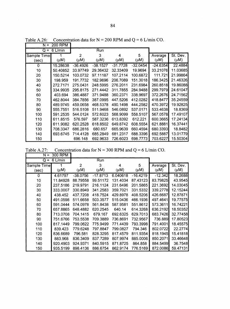
84
Table A.26: Concentration data for N = 200 RPM and Q = 6 L/min CO. N = 200 RPM I Q = 6 Umin I Run
Sample Time 1 2 3 4 5 Average St. Dev. (sec) (µM) (µM) (µM) (µM) (µM) (µM) (µM)
0 15.28638 -36.4926 -38.1527 -31.7728 -32.0454 -24.6354 22.4884 10 50.40852 33.97749 29.36432 32.33409 19.9694 33.21076 11.03685 20 150.5214 103.0732 97.11187 107.2114 100.6872 111.721 21.99864 30 198.959 191.7732 182.9696 206.7089 151.3018 186.3425 21.46326 40 272.7171 275.0431 248.5995 276.2011 231.6984 260.8518 19.86088 50 334.9935 295.8175 271.4442 311.7855 284.9488 299.7979 24.61047 60 403.694 386.4887 371.9488 360.2371 338.9697 372.2676 24.71562 70 462.8044 384.7856 387.0995 447.5206 412.0282 418.8477 35.24559 80 489.9745 459.0658 468.5378 490.1498 444.2582 470.3972 19.92825 90 555.7551 516.5108 511.9468 546.0892 537.0171 533.4638 18.8369 100 591.2535 544.0124 572.6023 568.9099 558.5107 567.0578 17.49107 110 611.8515 576.597 587.3236 613.8392 612.221 600.3665 17.24134 120 611.9082 620.2528 618.8502 649.8742 608.5554 621.8881 16.37441 130 708.3347 686.2816 680.657 665.9639 660.4594 680.3393 18.8482 140 693.6745 714.4128 685.2849 681.2317 688.3396 692.5887 13.01779 150 696.148 692.9633 726.6023 698.7773 703.6227 15.50304
Table A.27: Concentration data for N = 300 RPM and Q = 6 L/min CO. N = 300 RPM I Q = 6 Umin I Run
Sample Time 1 2 3 4 5 Average St. Dev. (sec) (µM) (µM) (µM) (µM) (µM) (µM) (µM)
0 4.61797 -38.0756 -17.8713 6.040618 -16.4219 -12.342 18.2688 10 11.84928 88.79558 99.51172 131.4034 87.43123 83.79825 43.9545 20 237.5186 219.9791 216.1124 231.6496 201.5865 221.3692 14.03045 30 333.0007 330.8949 341.2583 359.7021 331.5332 339.2778 12.15244 40 438.452 437.7208 418.7524 429.8978 408.5206 426.6687 12.87871 50 491.0598 511.6658 503.3577 515.0436 466.1936 497.4641 19.77575 60 591.0444 574.0978 561.8438 587.9581 551.8612 573.3611 16.74221 70 657.8865 648.4882 620.2545 640.14 614.3268 636.2192 18.50352 80 713.0708 704.1415 679.167 692.6325 629.7013 683.7426 32.77458 90 751.6766 753.5538 709.3889 736.8691 732.9567 736.889 17.80523 100 817.1449 799.0622 775.9499 771.4439 793.3998 791.4001 18.45575 110 839.423 779.6248 797.8847 799.0827 794.346 802.0722 22.2774 120 836.6689 796.581 828.3295 817.4579 811.9354 818.1945 15.41818 130 883.968 836.3409 837.7289 807.9974 885.0006 850.2071 33.46648 140 920.4903 924.9371 840.5915 871.8725 864.858 884.5499 36.7548 150 935.5199 898.4136 886.6754 862.9174 776.5169 872.0086 59.47131
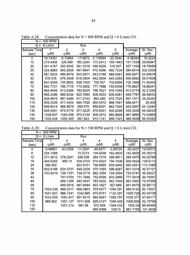
85
Table A.28: Concentration data for N = 400 RPM and Q = 6 Umin CO. N = 400 RPM I Q = 6 L/min I Run
Sample Time 1 2 3 4 5 Average St. Dev. (sec) (µM) (µM) (µM) (µM) (µM) (µM) (µM)
0 18.74351 -6.73964 -17.6972 0.178094 -22.3044 -5.56393 16.2224 10 219.4305 226.489 180.3244 173.2413 159.1843 191.7339 29.60847 20 341.4167 320.4242 361.2319 346.5029 316.007 337.1165 18.79089 30 524.8883 945.2838 487.6847 472.4266 492.7234 584.6014 202.5309 40 581.5533 589.9479 543.9571 543.0189 589.4581 569.5871 24.05918 50 678.376 676.5408 616.0904 642.2604 640.2285 650.6992 26.51608 60 641.6349 735.9652 838.1005 709.507 700.6954 725.1806 71.92405 70 800.7721 785.7716 770.0802 777.7588 749.9308 776.8627 18.86241 80 864.9406 813.6366 783.8025 788.7627 816.7446 813.5774 32.21226 90 895.2396 885.8334 823.7693 808.4033 835.6381 849.7767 38.58433 100 928.9816 881.5484 917.2142 883.289 874.7524 897.1571 24.25393 110 909.2039 917.4404 894.7595 854.0472 868.7847 888.8471 26.835 120 949.8014 968.5675 959.575 859.8301 862.7044 920.0957 54.12084 130 928.9391 979.5776 977.8225 879.8351 905.4288 934.3206 44.08225 140 1039.607 1040.038 970.0134 909.3212 880.9689 967.9895 73.03865 150 1025.434 1000.345 991.843 913.1141 899.7323 966.0938 56.05392
Table A.29: Concentration data for N = 500 RPM and Q = 6 Umin CO. N = 500 RPM I Q = 6 L/min I Run
Sample Time 1 2 3 4 5 Average St. Dev. (sec) (µM) (µM) (µM) (µM) (µM) (µM) (µM)
0 -5.99881 -30.2308 -11.2541 -49.8377 -3.89725 -20.2437 19.53512 6 204.1068 72.2273 134.6458 162.4633 143.3608 55.35013 12 271.5012 278.2241 249.039 264.7319 358.9911 284.4975 43.02769 18 444.6255 489.15 508.5103 610.8323 794.1938 569.4624 139.6112 24 586.592 823.9101 756.8895 605.6846 693.2691 115.7089 30 652.6166 634.3737 548.2328 575.1093 596.8267 601.4318 42.57131 36 763.9319 728.1761 724.0719 662.3354 724.3554 720.5741 36.59227 42 791.6765 731.7646 752.8399 833.2866 777.3919 44.76947 48 899.1295 940.0637 783.0433 943.7449 891.4953 75.07558 58 949.0916 987.8484 903.1827 927.669 941.9479 35.89113 70 1024.039 988.2217 868.0863 979.9577 1094.291 990.9192 82.15537 80 1041.637 966.1241 1042.665 875.8151 1122.397 1009.728 93.04739 90 1032.005 1081.817 991.6019 985.6647 1085.797 1035.377 47.69117 100 985.802 1051.127 1011.938 929.4127 1056.408 1006.938 52.15798 110 1051.214 981.56 872.954 1094.433 1000.04 96.64556 120 895.8388 1067.6 981.7195 121.4536

86
Table A.30: Concentration data for N = 600 RPM and Q = 6 L/min CO. N = 600 RPM I Q = 6 L/min I Run
Sample Time 1 2 3 4 5 Average St. Dev. (sec) (µM) (µM) (µM) (µM) (µM) (µM) (µM)
0 -33.3749 -29.352 -14.1959 -28.5624 -21.3646 -25.3699 7.599842 6 247.238 680.8303 292.2462 285.7207 346.8724 370.5815 177.0366 12 523.3474 418.6515 410.0736 495.1269 489.7127 467.3824 50.14849 18 639.8406 907.1323 620.5855 675.6995 625.3402 693.7196 121.2404 24 948.1363 666.4775 807.4857 913.8023 830.9479 833.3699 109.7379 30 728.7183 743.8151 735.2677 735.9337 7.570394 36 896.8623 809.8506 829.6743 819.4787 812.4977 833.6727 36.14643 42 857.7918 844.1236 833.3351 819.0345 834.2959 837.7162 14.35254 48 863.958 895.9781 995.7408 991.1921 936.7173 66.84528 58 950.8694 974.8159 1003.183 961.2108 972.5199 22.67275 70 1060.259 1060.259 80 1053.311 1053.311 90 1032.423 1032.423 100 1067.959 1067.959 110 1047.632 1047.632 120 1045.846 1045.846
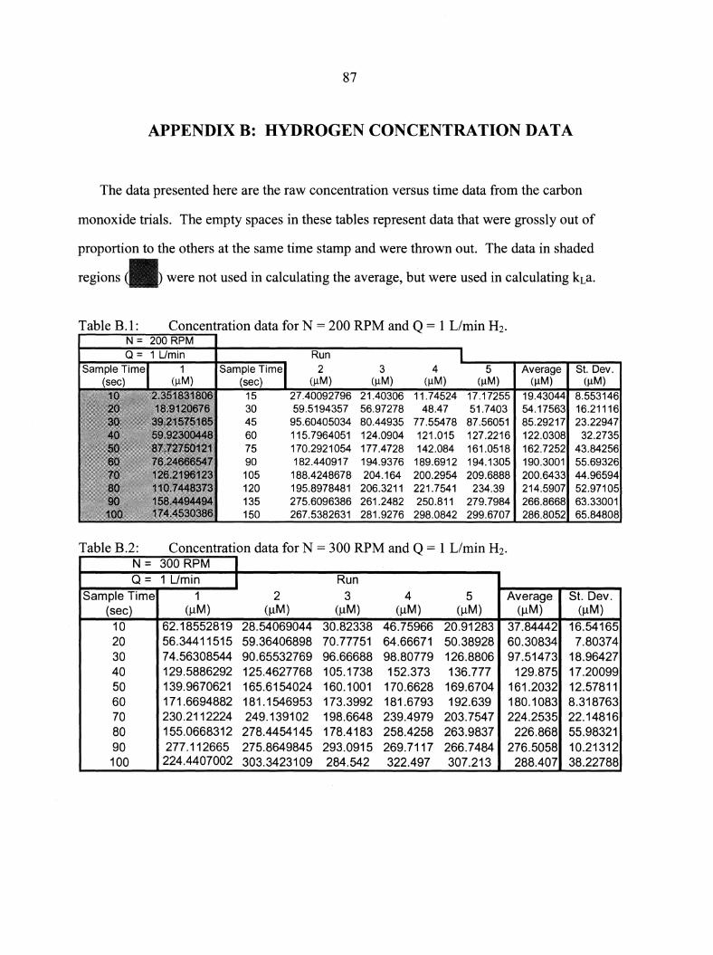
87
APPENDIX B: HYDROGEN CONCENTRATION DATA
The data presented here are the raw concentration versus time data from the carbon
monoxide trials. The empty spaces in these tables represent data that were grossly out of
proportion to the others at the same time stamp and were thrown out. The data in shaded
regions were not used in calculating the average, but were used in calculating kLa.
Table B.l: Concentration data for N = 200 RPM and Q = 1 L/min H2•
N = 200 RPM Run
Sample Time 2 3 4 5 Average St. Dev. (sec) (µM) (µM) (µM) (µM) (µM) (µM)
15 27.40092796 21.40306 11.74524 17.17255 19.43044 8.553146 30 59.5194357 56.97278 48.47 51.7403 54.17563 16.21116 45 95.60405034 80.44935 77.55478 87.56051 85.29217 23.22947 60 115. 7964051 124.0904 121.015 127.2216 122.0308 32.2735 75 170.2921054 177.4728 142.084 161.0518 162.7252 43.84256 90 182.440917 194.9376 189.6912 194.1305 190.3001 55.69326 105 188.4248678 204.164 200.2954 209.6888 200.6433 44.96594 120 195.8978481 206.3211 221.7541 234.39 214.5907 52.97105 135 275.6096386 261.2482 250.811 279.7984 266.8668 63.33001 150 267.5382631 281.9276 298.0842 299.6707 286.8052 65.84808
Table B.2: Concentration data for N = 300 RPM and Q = I L/min H2•
N = 300 RPM I Q = 1 L/min I Run
Sample Time 1 2 3 4 5 Average St. Dev. (sec) (µM) (µM) (µM) (µM) (µM) (µM) (µM)
10 62.18552819 28.54069044 30.82338 46.75966 20.91283 37.84442 16.54165 20 56.34411515 59.36406898 70.77751 64.66671 50.38928 60.30834 7.80374 30 74.56308544 90.65532769 96.66688 98.80779 126.8806 97.51473 18.96427 40 129.5886292 125.4627768 105.1738 152.373 136.777 129.875 17.20099 50 139.9670621 165.6154024 160.1001 170.6628 169.6704 161.2032 12.57811 60 171.6694882 181.1546953 173.3992 181.6793 192.639 180.1083 8.318763 70 230.2112224 249.139102 198.6648 239.4979 203.7547 224.2535 22.14816 80 155.0668312 278 .4454145 178.4183 258.4258 263.9837 226.868 55.98321 90 277.112665 275.8649845 293.0915 269.7117 266.7484 276.5058 10.21312 100 224.4407002 303.3423109 284.542 322.497 307.213 288.407 38.22788
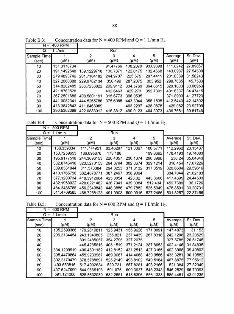
88
Table B.3: Concentration data for N = 400 RPM and Q = 1 L/min H2. N = 400 RPM I Q = 1 Umin I Run
Sample Time 1 2 3 4 5 Average St. Dev. (sec) (µM) (µM) (µM) (µM) (µM) (µM) (µM)
10 151.3170734 91.47766 108.2079 93.09398 111.0242 27.89867 20 191.1492548 139.1229718 130.7371 122.0175 132.4668 143.0987 27.54509 30 279.4893746 201.7184182 244.9707 225.575 207.4411 231.8389 31.56243 40 327.2060388 229.9782134 350.499 287.2075 303.952 299.7685 45.7503 50 314.8282485 286.7238822 299.9112 334.5769 364.8615 320.1803 30.66953 60 421.8763528 402.6463 429.273 352.7391 401.6337 34.47415 70 367.2501686 408.5801191 315.6773 396.0535 371.8903 41.27723 80 441.0082341 444.5265786 375.6085 443.3944 358.1835 412.5443 42.14302 90 413.3842843 411.6463069 463.2297 428.0678 429.082 23.92709 100 390.5362399 422.0883012 416.8812 490.0123 464.3073 436.7651 39.81746
Table B.4: Concentration data for N = 500 RPM and Q = 1 L/min H2.
N = 500 RPM I Q = 1 Umin I Run
Sample Time 1 2 3 4 5 Average St. Dev. (sec) (µM) (µM) (µM) (µM) (µM) (µM) (µM)
10 138.359034 111.774951 83.46297 121.3067 106.5771 112.2962 20.15437 20 153. 7259653 186.895876 173.186 199.8692 178.4193 19.74083 30 195.9177518 244.3696153 220.4057 230.1074 290.3996 236.24 35.04843 40 332.8746418 323.5270153 294.3794 302.3674 329.1214 316.454 17.07226 50 309.0381944 311.573384 294.0253 371.3132 317.3519 320.6604 29.59616 60 410.1766796 382.4878771 387.2467 358.9064 384.7044 21.02183 70 377.1200734 418.3912604 425.0054 423.32 443.3608 417.4395 24.44533 80 482.1958922 428.0221482 436.7041 439.3384 512.434 459.7389 36.1726 90 484.3486788 456.2349843 448.3886 479.7882 525.5349 478.8591 30.20731 100 511.4709585 468.7268123 491.0903 509.0916 527.2486 501.5257 22.37456
Table B.5: Concentration data for N = 600 RPM and Q = 1 L/min H2.
N = 600 RPM I Q = 1 Umin I Run
Sample Time 1 2 3 4 5 Average St. Dev. (sec) (µM) (µM) (µM) (µM) (µM) (µM) (µM)
10 105.2599386 179.2619811 125.9431 155.9626 171.0091 147.4873 31.153 20 206.3134454 243.1940805 255.821 237.4439 267.8318 242.1208 23.20529 30 301.2485057 354.2795 327.2075 327.5785 26.51745 40 445.4285616 405.1519 371.2124 387.8653 402.4146 31.84835 50 334.1209919 406.4801182 412.8152 431.2513 427.3165 402.3968 39.49802 60 395.44 70864 455.9233967 469.9067 414.4068 430.9566 433.3281 30.19582 70 392.3170479 378.5788697 525.2149 493.8102 549.5164 467.8875 77.95612 80 493.653816 517.4902634 539.731 557.8281 498.2166 521.384 27.32049 90 437.6247099 544. 9666198 591.075 609.3637 548.2343 546.2529 66.70393 100 591.124066 528.8632089 632.2651 618.8396 556.1333 585.4451 43.01235
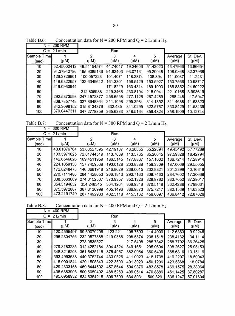
89
Table B.6: Concentration data for N = 200 RPM and Q = 2 L/min H2•
N = 200 RPM I Q = 2 Umin I Run
Sample Time 1 2 3 4 5 Average St. Dev. (sec) (µM) (µM) (µM) (µM) (µM) (µM) (µM)
10 52.45002412 49.54154574 44.74047 19.24606 51.42023 43.47966 13.86654 20 94.37942786 165.9085136 91.62403 93.07131 95.20048 108.0368 32.37968 30 126.3726901 100.057223 101.4071 118.2874 108.894 111.0037 11.2431 40 149.6822657 132.6349642 161.3301 156.5429 153.5927 150.7566 10.98717 50 219.0960944 171.8229 163.4314 189.1903 185.8852 24.60222 60 212.805988 219.3466 233.8194 218.0941 221.0165 8.993619 70 292.5873593 247.4572377 256.6558 277.1126 267.4269 268.248 17.5947 80 308. 78577 48 327.8648364 311.1098 295.3984 314.1852 311.4688 11.63823 90 342.3098152 315.8134379 332.485 341.0295 322.5767 330.8429 11.53439 100 370.0447311 347.2778859 365.6333 348.5164 359.4824 358.1909 10.12744
Table B.7: Concentration data for N = 300 RPM and Q = 2 L/min H2•
N = 300 RPM I Q = 2 Umin I Run
Sample Time 1 2 3 4 5 Average St. Dev. (sec) (µM) (µM) (µM) (µM) (µM) (µM) (µM)
10 48.01076764 53.63527395 42.19107 48.20855 55.22894 49.45492 5.177289 20 103.3971025 72.01744519 113.7689 113.5765 85.20645 97.59328 18.42794 30 142.6546026 169.4511959 186.5145 177.8867 157.1002 166.7214 17.28914 40 224.1059136 157. 7 459568 193.0128 203.8388 156.3309 187.0069 29.55055 50 172.82484 73 146.0681948 216.8629 238.0615 232.8821 201.3399 40.16346 60 270.7111486 284.4428053 266.1843 293.7163 308.7463 284.7602 17.30669 70 338.5663669 27 4.0152507 373.9357 352.1326 329.8762 333.7052 37.28017 80 354.3194652 354.248345 364.1264 368.9348 370.5148 362.4288 7.798631 90 375.5972807 367.3136999 405.1496 386.9873 375.7217 382.1539 14.63523 100 473.2191749 287 .1492983 402.5118 415.3162 456.0097 406.8412 72.87026
Table B.8: Concentration data for N = 400 RPM and Q = 2 L/min H2•
N = 400 RPM I Q = 2 Umin I Run
Sample Time 1 2 3 4 5 Average St. Dev. (sec) (µM) (µM) (µM) (µM) (µM) (µM) (µM)
10 120.4595497 99.59070206 123.221 105.7593 114.4009 112.6863 9.92246 20 296.2304756 232.0577388 219.0886 208.5374 236.1518 238.4132 34.1114 30 273.0535527 217.5498 285.7342 258.7792 36.26425 40 279.3183285 312.4282184 304.4324 349.1651 295.9694 308.2627 25.95153 50 348.8216203 361.5435116 375.4057 382.0964 360.5406 365.6816 13.15119 60 393.4993638 440.3752744 433.0526 411.0023 418.1738 419.2207 18.50043 70 415.0001844 429.1508843 422.3503 401.3029 450.1296 423.5868 18.0784 80 429.2333155 469.8444502 457.8644 504.9876 483.8578 469.1575 28.38064 90 436.6383905 500.6050492 488.5289 409.0514 470.8886 461.1425 37.80287 100 495.0958932 534.6354215 506.7599 634.8031 509.329 536.1247 57.01604
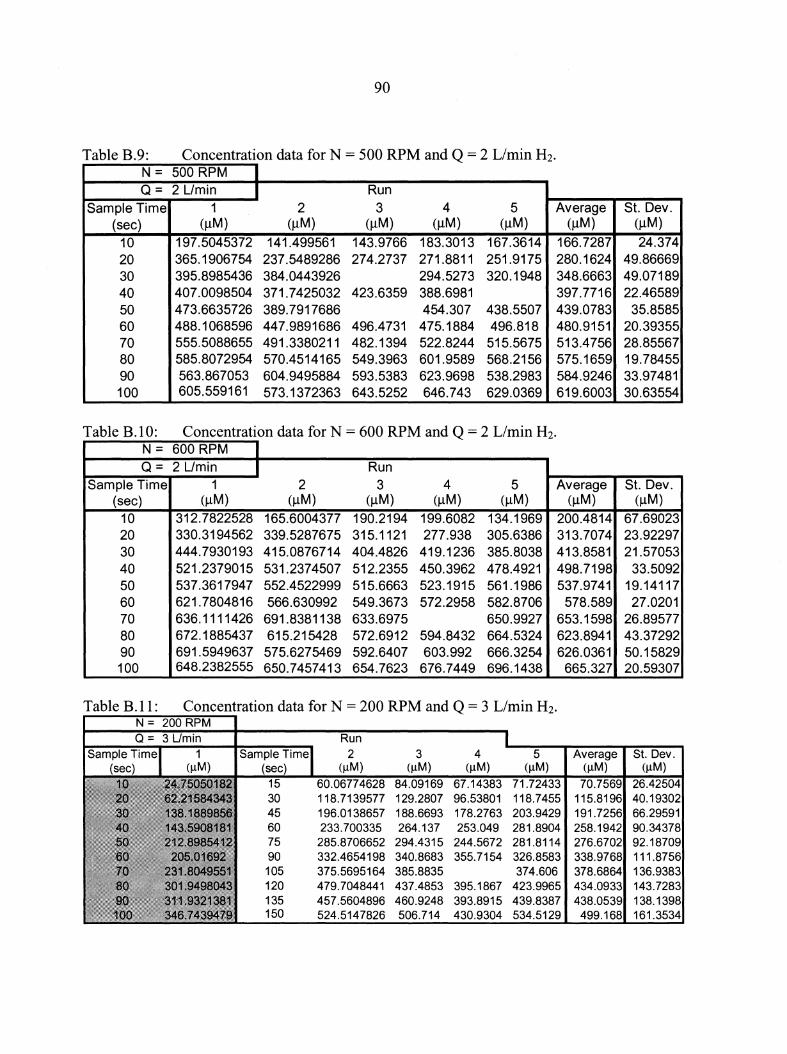
90
Table B.9: Concentration data for N = 500 RPM and Q = 2 Umin H2. N = 500 RPM I Q = 2 Umin I Run
Sample Time 1 2 3 4 5 Average St. Dev. (sec) (µM) (µM) (µM) (µM) (µM) (µM) (µM)
10 197.5045372 141.499561 143.9766 183.3013 167.3614 166.7287 24.374 20 365.1906754 237.5489286 274.2737 271.8811 251.9175 280.1624 49.86669 30 395.8985436 384.0443926 294.5273 320.1948 348.6663 49.07189 40 407.0098504 371.7425032 423.6359 388.6981 397.7716 22.46589 50 473.6635726 389. 7917686 454.307 438.5507 439.0783 35.8585 60 488.1068596 447.9891686 496.4731 475.1884 496.818 480.9151 20.39355 70 555.5088655 491.3380211 482.1394 522.8244 515.5675 513.4756 28.85567 80 585.8072954 570.4514165 549.3963 601.9589 568.2156 575.1659 19.78455 90 563.867053 604.9495884 593.5383 623.9698 538.2983 584.9246 33.97481 100 605.559161 573.1372363 643.5252 646.743 629.0369 619.6003 30.63554
Table B.10: Concentration data for N = 600 RPM and Q = 2 Umin H2•
N = 600 RPM I Q = 2 Umin I Run
Sample Time 1 2 3 4 5 Average St. Dev. (sec) (µM) (µM) (µM) (µM) (µM) (µM) (µM)
10 312. 7822528 165.6004377 190.2194 199.6082 134.1969 200.4814 67.69023 20 330.3194562 339.5287675 315.1121 277.938 305.6386 313.7074 23.92297 30 444. 7930193 415.0876714 404.4826 419.1236 385.8038 413.8581 21.57053 40 521.2379015 531.237 4507 512.2355 450.3962 478.4921 498.7198 33.5092 50 537.3617947 552.4522999 515.6663 523.1915 561.1986 537.9741 19.14117 60 621.7804816 566.630992 549.3673 572.2958 582.8706 578.589 27.0201 70 636.1111426 691.8381138 633.6975 650.9927 653.1598 26.89577 80 672.1885437 615.215428 572.6912 594.8432 664.5324 623.8941 43.37292 90 691.5949637 575.6275469 592.6407 603.992 666.3254 626.0361 50.15829 100 648.2382555 650.7457413 654.7623 676.7449 696.1438 665.327 20.59307
Table B.11: Concentration data for N = 200 RPM and Q = 3 Umin H2•
N = 200 RPM Run
Sample Time 2 3 4 5 Average St. Dev. (sec) (µM) (µM) (µM) (µM) (µM) (µM)
15 60.06774628 84.09169 67.14383 71.72433 70.7569 26.42504 30 118.7139577 129.2807 96.53801 118.7455 115.8196 40.19302 45 196.0138657 188.6693 178.2763 203.9429 191.7256 66.29591 60 233.700335 264.137 253.049 281.8904 258.1942 90.34378 75 285.8706652 294.4315 244.5672 281.8114 276.6702 92.18709 90 332.4654198 340.8683 355.7154 326.8583 338.9768 111.8756 105 375.5695164 385.8835 374.606 378.6864 136.9383 120 479.7048441 437.4853 395.1867 423.9965 434.0933 143.7283 135 457 .5604896 460.9248 393.8915 439.8387 438.0539 138.1398 150 524.5147826 506.714 430.9304 534.5129 499.168 161.3534
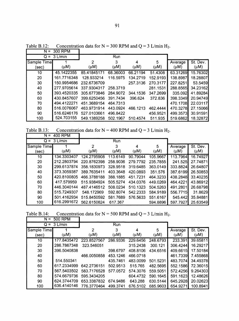
91
Table B.12: Concentration data for N = 300 RPM and Q = 3 L/min H2•
N = 300 RPM I Q = 3 Umin I Run
Sample Time 1 2 3 4 5 Average St. Dev. (sec) (µM) (µM) (µM) (µM) (µM) (µM) (µM)
10 45.1422355 85.41845171 68.36003 66.21194 51.4308 63.31269 15.76302 20 161. 7716348 128.933214 116.5975 134.2719 152.9193 138.8987 18.28807 30 150. 9954686 232.6736709 257.3136 270.3177 227.8251 53.5459 40 277.9705614 337.9304317 258.3719 281.1531 288.8565 34.23162 50 393.4520335 305.6773846 284.9072 344.1536 347.2699 335.092 41.89284 60 430.8457607 399.6250456 391.7434 396.624 372.836 398.3349 20.94749 70 494.4122271 451.3689154 464.7313 470.1708 22.03117 80 516.0076067 463.9731914 443.0924 466.1213 462.4444 470.3278 27.15066 90 516.6246176 527.0103661 496.8422 456.9521 499.3573 30.91591 100 524.703155 549.1389258 502.1967 510.4574 511.935 519.6862 18.32872
Table B.13: Concentration data for N = 400 RPM and Q = 3 L/min H2.
N = 400 RPM I Q = 3 Umin I Run
Sample Time 1 2 3 4 5 Average St. Dev. (sec) (µM) (µM) (µM) (µM) (µM) (µM) (µM)
10 134.3303407 124.2795908 113.6149 90.79044 105.9667 113.7964 16.74927 20 212.2803794 220.8762398 258.9036 279.7792 235.7855 241.525 27.74871 30 299.6137874 358.1830973 328.9518 319.6485 363.0149 333.8824 26.64807 40 373.3059387 389.7635411 403.3648 420.0893 351.576 387.6199 26.50853 50 420.8100805 466.3788188 388.1885 451.7231 464.3233 438.2848 33.40235 60 417.579959 515.9384924 505.5274 434.0376 449.0269 464.4221 43.86912 70 446.3040144 487.4146512 508.0234 510.1323 504.5263 491.2801 26.68798 80 515.7249307 548.172969 592.8074 542.2333 584.9189 556.7715 31.8629 90 501.4162934 515.8450592 581.7689 576.5633 551.6167 545.442 35.84881 100 616.2991672 562.6150824 617.367 594.8896 597.7927 25.63549
Table B.14: Concentration data for N = 500 RPM and Q = 3 L/min H2•
N = 500 RPM I Q = 3 Umin I Run
Sample Time 1 2 3 4 5 Average St. Dev. (sec) (µM) (µM) (µM) (µM) (µM) (µM) (µM)
10 177 .84354 72 223.8527567 286.9336 229.6456 248.6793 233.391 39.65811 20 286.7867348 323.546051 315.2438 300.121 306.4244 16.29217 30 396.5040838 398.6797 408.8106 434.6516 409.6615 17.50184 40 466.0050858 453.1246 466.0718 461.7339 7.455868 50 514.550341 435.7461 483.0099 501.5231 483.7074 34.49378 60 617.2334999 642.2736151 502.9513 515.765 482.5695 552.1586 72.36015 70 567.5403502 583.7176528 577.0572 574.3076 559.5051 572.4256 9.264303 80 574.6679736 595.3434205 604.4732 590.1645 591.1623 12.48626 90 624.3744709 653.3387832 674.9486 643.288 630.5144 645.2928 20.02623 100 636.4140146 776.3770464 499.3741 676.5102 685.9603 654.9271 100.8941
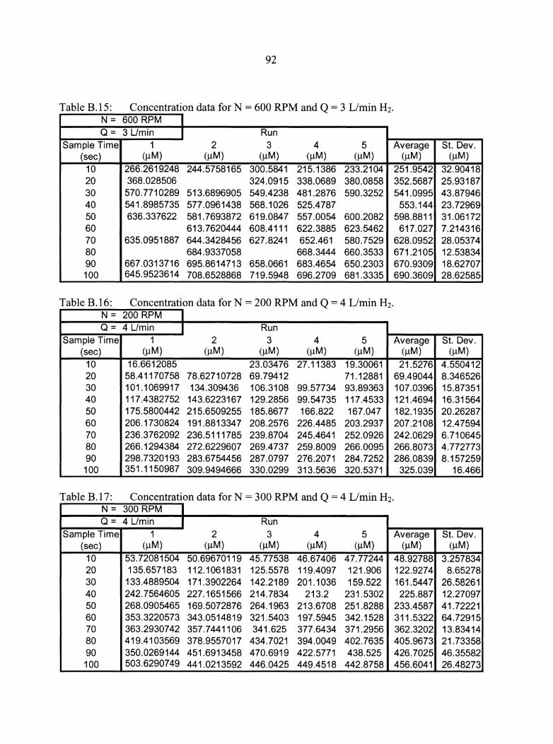
92
Table B.15: Concentration data for N = 600 RPM and Q = 3 Umin H2.
N = 600 RPM I Q = 3 Umin I Run
Sample Time 1 2 3 4 5 Average St. Dev. (sec) (µM) (µM) (µM) (µM) (µM) (µM) (µM)
10 266.2619248 244.5758165 300.5841 215.1386 233.2104 251.9542 32.90418 20 368.028506 324.0915 338.0689 380.0858 352.5687 25.93187 30 570. 7710289 513.6896905 549.4238 481.2876 590.3252 541.0995 43.87946 40 541.8985735 577.0961438 568.1026 525.4787 553.144 23.72969 50 636.337622 581 . 7693872 619.0847 557.0054 600.2082 598.8811 31.06172 60 613.7620444 608.4111 622.3885 623.5462 617.027 7.214316 70 635.0951887 644.3428456 627.8241 652.461 580.7529 628.0952 28.05374 80 684.9337058 668.3444 660.3533 671.2105 12.53834 90 667 .0313716 695.8614713 658.0661 683.4654 650.2303 670.9309 18.62707 100 645.9523614 708.6528868 719.5948 696.2709 681.3335 690.3609 28.62585
Table B.16: Concentration data for N = 200 RPM and Q = 4 Umin H2•
N = 200 RPM I Q = 4 Umin I Run
Sample Time 1 2 3 4 5 Average St. Dev. (sec) (µM) (µM) (µM) (µM) (µM) (µM) (µM)
10 16.6612085 23.03476 27.11383 19.30061 21.5276 4.550412 20 58.41170758 78.62710728 69.79412 71.12881 69.49044 8.346526 30 101.1069917 134.309436 106.3108 99.57734 93.89363 107.0396 15.87351 40 117.4382752 143.6223167 129.2856 99.54735 117.4533 121.4694 16.31564 50 175.5800442 215.6509255 185.8677 166.822 167.047 182.1935 20.26287 60 206.1730824 191.8813347 208.2576 226.4485 203.2937 207.2108 12.47594 70 236.3762092 236.5111785 239.8704 245.4641 252.0926 242.0629 6.710645 80 266.1294384 272.6229607 269.4737 259.8009 266.0095 266.8073 4.772773 90 298. 7320193 283.6754456 287.0797 276.2071 284.7252 286.0839 8.157259 100 351.1150987 309.9494666 330.0299 313.5636 320.5371 325.039 16.466
Table B.17: Concentration data for N = 300 RPM and Q = 4 Umin H2.
N = 300 RPM I Q = 4 Umin I Run
Sample Time 1 2 3 4 5 Average St. Dev. (sec) (µM) (µM) (µM) (µM) (µM) (µM) (µM)
10 53.72081504 50.69670119 45.77538 46.67406 47.77244 48.92788 3.257834 20 135.657183 112.1061831 125.5578 119.4097 121.906 122.9274 8.65278 30 133.4889504 171.3902264 142.2189 201.1036 159.522 161.5447 26.58261 40 242.7564605 227.1651566 214.7834 213.2 231.5302 225.887 12.27097 50 268.0905465 169.5072876 264.1963 213.6708 251.8288 233.4587 41.72221 60 353.3220573 343.0514819 321.5403 197.5945 342.1528 311.5322 64.72915 70 363.2930742 357.7441106 341.625 377.6434 371.2956 362.3202 13.83414 80 419.4103569 378.9557017 434.7021 394.0049 402.7635 405.9673 21.73358 90 350.0269144 451.6913458 470.6919 422.5771 438.525 426.7025 46.35582 100 503.6290749 441.0213592 446.0425 449.4518 442.8758 456.6041 26.48273
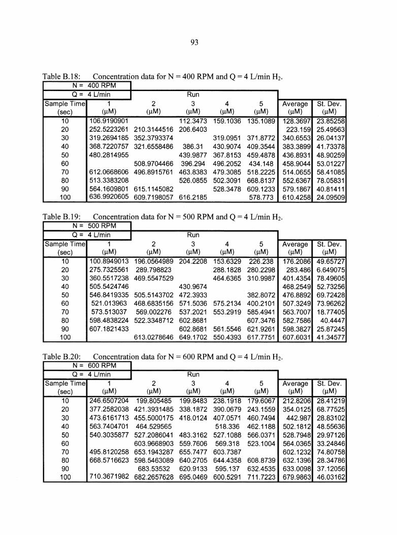
93
Table B.18: Concentration data for N = 400 RPM and Q = 4 L/min H2•
N = 400 RPM I Q = 4 Umin I Run
Sample Time 1 2 3 4 5 Average St. Dev. (sec) (µM) (µM) (µM) (µM) (µM) (µM) (µM)
10 106.9190901 112.3473 159.1036 135.1089 128.3697 23.85258 20 252.5223261 210.3144516 206.6403 223.159 25.49563 30 319.2694185 352.3793374 319.0951 371.8772 340.6553 26.04137 40 368. 7220757 321.6558486 386.31 430.9074 409.3544 383.3899 41.73378 50 480.2814955 439.9877 367.8153 459.4878 436.8931 48.90259 60 508.9704466 396.294 496.2052 434.148 458.9044 53.01227 70 612.0668606 496.8915761 463.8383 479.3085 518.2225 514.0655 58.41085 80 513.3383208 526.0855 502.3091 668.8137 552.6367 78.05831 90 564 .1609801 615.1145082 528.3478 609.1233 579.1867 40.81411 100 636.9920605 609. 7198057 616.2185 578.773 610.4258 24.09509
Table B.19: Concentration data for N = 500 RPM and Q = 4 L/min H2.
N = 500 RPM I Q = 4 Umin I Run
Sample Time 1 2 3 4 5 Average St. Dev. (sec) (µM) (µM) (µM) (µM) (µM) (µM) (µM)
10 100.8949013 196.0564989 204.2208 153.6329 226.238 176.2086 49.65727 20 275. 7325561 289.798823 288.1828 280.2298 283.486 6.649075 30 360.5517238 469.5547529 464.6365 310.9987 401.4354 78.49605 40 505.5424 7 46 430.9674 468.2549 52.73256 50 546.8419335 505.5143702 472.3933 382.8072 476.8892 69.72428 60 521.013963 468.6835156 571.5036 575.2134 400.2101 507.3249 73.96262 70 573.513037 569.002276 537.2021 553.2919 585.4941 563.7007 18.77405 80 598.4838224 522.3348712 602.8681 607.3476 582.7586 40.4447 90 607.1821433 602.8681 561.5546 621.9261 598.3827 25.87245 100 613.0278646 649.1702 550.4393 617.7751 607.6031 41.34577
Table B.20: Concentration data for N = 600 RPM and Q = 4 L/min H2•
N = 600 RPM I Q = 4 Umin I Run
Sample Time 1 2 3 4 5 Average St. Dev. (sec) (µM) (µM) (µM) (µM) (µM) (µM) (µM)
10 246.6507204 199.805485 199.8483 238.1918 179.6067 212.8206 28.41219 20 377.2582038 421.3931485 338.1872 390.0679 243.1559 354.0125 68.77525 30 473.6161713 455.5000175 418.0124 407.0571 460.7494 442.987 28.83102 40 563.7404701 464.529565 518.336 462.1188 502.1812 48.55636 50 540.3035877 527 .2086041 483.3162 527.1088 566.0371 528.7948 29.97126 60 603.9668903 559.7606 569.318 523.1004 564.0365 33.24846 70 495.8120258 653.1943287 655.7477 603.7387 602.1232 74.80758 80 668.5716623 598.5463089 640.2705 644.4358 608.8739 632.1396 28.34786 90 683.53532 620.9133 595.137 632.4535 633.0098 37.12056 100 710.3671982 682.2657628 695.0469 600.5291 711.7223 679.9863 46.03162
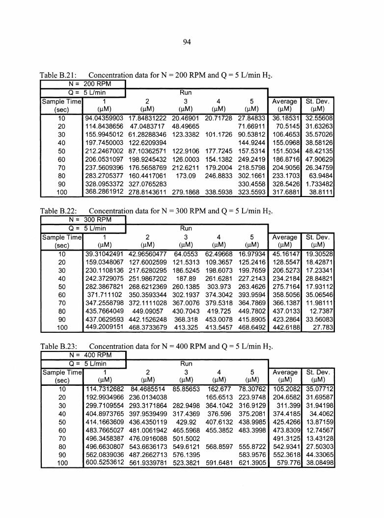
94
Table B.21: Concentration data for N = 200 RPM and Q = 5 L/min H2•
N = 200 RPM I Q = 5 Umin I Run
Sample Time 1 2 3 4 5 Average St. Dev. (sec) (µM) (µM) (µM) (µM) (µM) (µM) (µM)
10 94.04359903 17 .84831222 20.46901 20.71728 27.84833 36.18531 32.55608 20 114.8438656 47.0483717 48.49665 71.66911 70.5145 31.63263 30 155.9945012 61.28288346 123.3382 101.1726 90.53812 106.4653 35.57026 40 197. 7 450003 122.6209394 144.9244 155.0968 38.58126 50 212.2467002 87.10362571 122.9106 177.7245 157.5314 151.5034 48.42135 60 206.0531097 198.9245432 126.0003 154.1382 249.2419 186.8716 47.90629 70 237.5609396 176.5658769 212.6211 179.2004 218.5798 204.9056 26.34759 80 283.2705377 160.4417061 173.09 246.8833 302.1661 233.1703 63.9484 90 328.0953372 327.0765283 330.4558 328.5426 1.733482 100 368.2861912 278.8143611 279.1868 338.5938 323.5593 317.6881 38.8111
Table B.22: Concentration data for N = 300 RPM and Q = 5 L/min H2•
N = 300 RPM I Q = 5 Umin I Run
Sample Time 1 2 3 4 5 Average St. Dev. (sec) (µM) (µM) (µM) (µM) (µM) (µM) (µM)
10 39.31042491 42.96560477 64.0553 62.49668 16.97934 45.16147 19.30528 20 159.0348067 127.6002599 121.5313 109.3657 125.2416 128.5547 18.42871 30 230.1108136 217 .6280295 186.5245 198.6073 199.7659 206.5273 17.23341 40 242.3729075 251.9867202 187.89 261.6281 227.2143 234.2184 28.84821 50 282.3867821 268.6212369 260.1385 303.973 263.4626 275.7164 17.93112 60 371.711102 350.3593344 302.1937 374.3042 393.9594 358.5056 35.06546 70 347.2558798 372.1111028 367.0076 379.5318 364.7869 366.1387 11.98111 80 435.7664049 449.09057 430.7043 419.725 449.7802 437.0133 12.7387 90 437.0629593 442.1526248 368.318 453.0078 415.8905 423.2864 33.56083 100 449.2009151 468.3733679 413.325 413.5457 468.6492 442.6188 27.783
Table B.23: Concentration data for N = 400 RPM and Q = 5 L/min H2. N = 400 RPM I Q = 5 Umin I Run
Sample Time 1 2 3 4 5 Average St. Dev. (sec) (µM) (µM) (µM) (µM) (µM) (µM) (µM)
10 114.7312682 84.4685514 85.85653 162.677 78.30762 105.2082 35.07712 20 192.9934966 236.0134038 165.6513 223.9748 204.6582 31.69587 30 299. 7109554 293.3171864 282.9498 364.1042 316.9129 311.399 31.94198 40 404.8973765 397.9539499 317.4369 376.596 375.2081 374.4185 34.4062 50 414.1663609 436.4350119 429.92 407.6132 438.9985 425.4266 13.87159 60 483. 7665027 481.0061942 465.5968 455.3852 483.3998 473.8309 12.74567 70 496.3458387 476.0916088 501.5002 491.3125 13.43128 80 496.6630807 543.6636173 549.6121 568.8597 555.8722 542.9341 27.50303 90 562.0839036 487.2662713 576.1395 583.9576 552.3618 44.33065 100 600.5253612 561.9339781 523.3821 591.6481 621.3905 579.776 38.08498
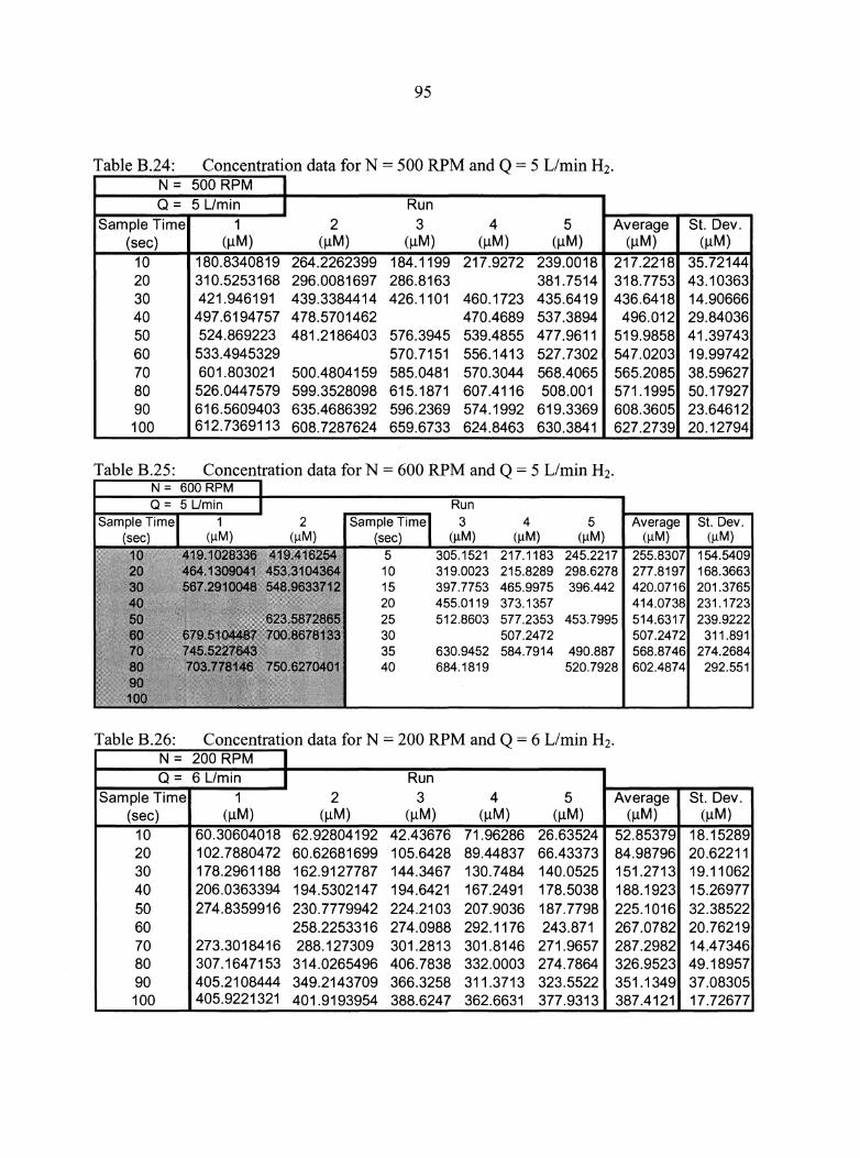
95
Table B.24: Concentration data for N = 500 RPM and Q = 5 Umin H2•
N = 500 RPM I Q = 5 Umin I Run
Sample Time 1 2 3 4 5 Average St. Dev. (sec) (µM) (µM) (µM) (µM) (µM) (µM) (µM)
10 180.8340819 264.2262399 184.1199 217.9272 239.0018 217.2218 35.72144 20 310.5253168 296.0081697 286.8163 381.7514 318.7753 43.10363 30 421.946191 439.3384414 426.1101 460.1723 435.6419 436.6418 14.90666 40 497 .6194 757 478.5701462 470.4689 537.3894 496.012 29.84036 50 524.869223 481 .2186403 576.3945 539.4855 477.9611 519.9858 41.39743 60 533.4945329 570.7151 556.1413 527.7302 547.0203 19.99742 70 601.803021 500 .4804159 585.0481 570.3044 568.4065 565.2085 38.59627 80 526.0447579 599.3528098 615.1871 607.4116 508.001 571.1995 50.17927 90 616.5609403 635.4686392 596.2369 574.1992 619.3369 608.3605 23.64612 100 612.7369113 608. 7287624 659.6733 624.8463 630.3841 627.2739 20.12794
Table B.25: Concentration data for N = 600 RPM and Q = 5 Umin H2•
N = 600 RPM Run
Sample Time 3 4 5 Average St. Dev. (sec) (µM) (µM) (µM) (µM) (µM)
5 305.1521 217.1183 245.2217 255.8307 154.5409 10 319.0023 215.8289 298.6278 277.8197 168.3663 15 397.7753 465.9975 396.442 420.0716 201.3765 20 455.0119 373.1357 414.0738 231.1723 25 512.8603 577.2353 453.7995 514.6317 239.9222 30 507.2472 507.2472 311.891 35 630.9452 584.7914 490.887 568.8746 274.2684 40 684.1819 520.7928 602.4874 292.551
Table B.26: Concentration data for N = 200 RPM and Q = 6 Umin H2 •
N = 200 RPM I Q = 6 Umin I Run
Sample Time 1 2 3 4 5 Average St. Dev. (sec) (µM) (µM) (µM) (µM) (µM) (µM) (µM)
10 60. 30604018 62.92804192 42.43676 71.96286 26.63524 52.85379 18.15289 20 102. 78804 72 60.62681699 105.6428 89.44837 66.43373 84.98796 20.62211 30 178.2961188 162.9127787 144.3467 130.7484 140.0525 151.2713 19.11062 40 206.0363394 194.530214 7 194.6421 167.2491 178.5038 188.1923 15.26977 50 274.8359916 230. 7779942 224.2103 207.9036 187.7798 225.1016 32.38522 60 258.2253316 274.0988 292.1176 243.871 267.0782 20.76219 70 273.3018416 288.127309 301.2813 301.8146 271.9657 287.2982 14.47346 80 307.1647153 314.0265496 406.7838 332.0003 274.7864 326.9523 49.18957 90 405.2108444 349.2143709 366.3258 311.3713 323.5522 351.1349 37.08305 100 405.9221321 401.9193954 388.6247 362.6631 377.9313 387.4121 17.72677
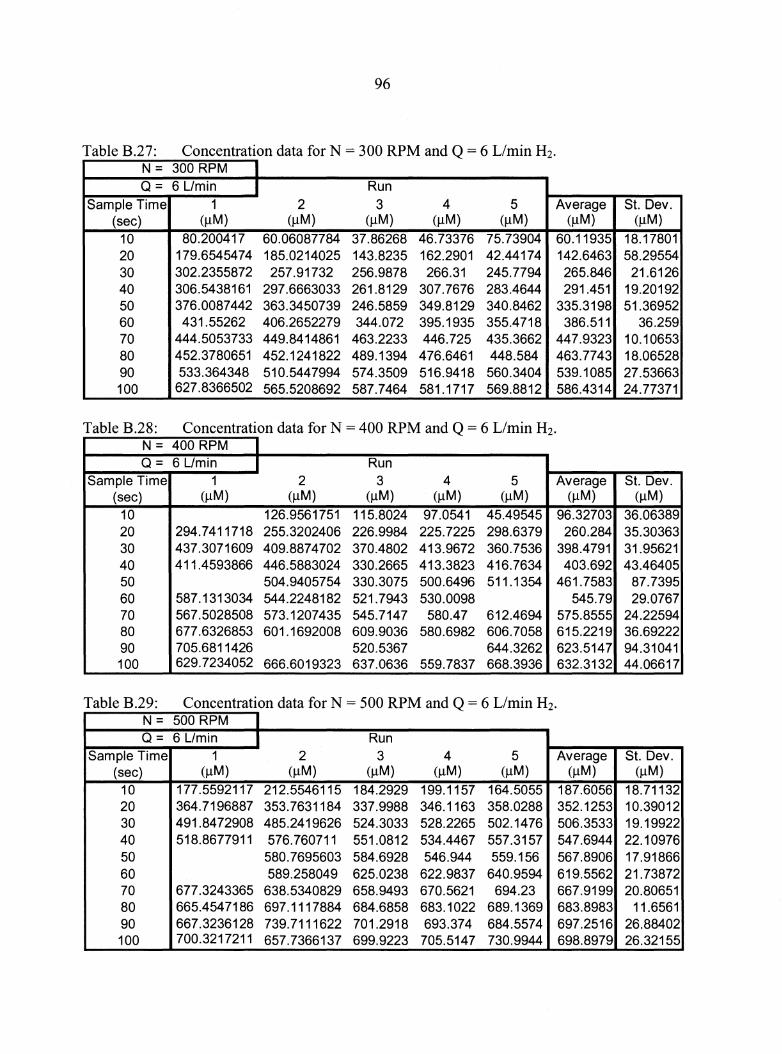
96
Table B.27: Concentration data for N = 300 RPM and Q = 6 L/min H2•
N = 300 RPM I Q = 6 L/min I Run
Sample Time 1 2 3 4 5 Average St. Dev. (sec) (µM) (µM) (µM) (µM) (µM) (µM) (µM)
10 80.200417 60.06087784 37.86268 46.73376 75.73904 60.11935 18.17801 20 179.6545474 185.0214025 143.8235 162.2901 42.44174 142.6463 58.29554 30 302.2355872 257.91732 256.9878 266.31 245.7794 265.846 21.6126 40 306.5438161 297.6663033 261.8129 307.7676 283.4644 291.451 19.20192 50 376.0087442 363.3450739 246.5859 349.8129 340.8462 335.3198 51.36952 60 431.55262 406.2652279 344.072 395.1935 355.4718 386.511 36.259 70 444.5053733 449.8414861 463.2233 446.725 435.3662 447.9323 10.10653 80 452.3780651 452.1241822 489.1394 476.6461 448.584 463.7743 18.06528 90 533.364348 510.544 7994 574.3509 516.9418 560.3404 539.1085 27.53663 100 627.8366502 565.5208692 587.7464 581.1717 569.8812 586.4314 24.77371
Table B.28: Concentration data for N = 400 RPM and Q = 6 L/min H2•
N = 400 RPM I Q = 6 L/min I Run
Sample Time 1 2 3 4 5 Average St. Dev. (sec) (µM) (µM) (µM) (µM) (µM) (µM) (µM)
10 126.9561751 115.8024 97.0541 45.49545 96.32703 36.06389 20 294.7411718 255.3202406 226.9984 225.7225 298.6379 260.284 35.30363 30 437.3071609 409.8874702 370.4802 413.9672 360.7536 398.4791 31.95621 40 411 .4593866 446.5883024 330.2665 413.3823 416.7634 403.692 43.46405 50 504.9405754 330.3075 500.6496 511.1354 461.7583 87.7395 60 587.1313034 544.2248182 521.7943 530.0098 545.79 29.0767 70 567.5028508 573.1207 435 545.7147 580.47 612.4694 575.8555 24.22594 80 677.6326853 601 .1692008 609.9036 580.6982 606.7058 615.2219 36.69222 90 705.6811426 520.5367 644.3262 623.5147 94.31041 100 629.7234052 666.6019323 637.0636 559.7837 668.3936 632.3132 44.06617
Table B.29: Concentration data for N = 500 RPM and Q = 6 L/min H2.
N = 500 RPM I Q = 6 L/min I Run
Sample Time 1 2 3 4 5 Average St. Dev. (sec) (µM) (µM) (µM) (µM) (µM) (µM) (µM)
10 177.5592117 212.5546115 184.2929 199.1157 164.5055 187.6056 18.71132 20 364. 7196887 353.7631184 337.9988 346.1163 358.0288 352.1253 10.39012 30 491.84 72908 485.2419626 524.3033 528.2265 502.1476 506.3533 19.19922 40 518.8677911 576.760711 551.0812 534.4467 557.3157 547.6944 22.10976 50 580. 7695603 584.6928 546.944 559.156 567.8906 17.91866 60 589.258049 625.0238 622.9837 640.9594 619.5562 21.73872 70 677.3243365 638.5340829 658.9493 670.5621 694.23 667.9199 20.80651 80 665.4547186 697 .1117884 684.6858 683.1022 689.1369 683.8983 11.6561 90 667.3236128 739.7111622 701.2918 693.374 684.5574 697.2516 26.88402 100 700.3217211 657.7366137 699.9223 705.5147 730.9944 698.8979 26.32155
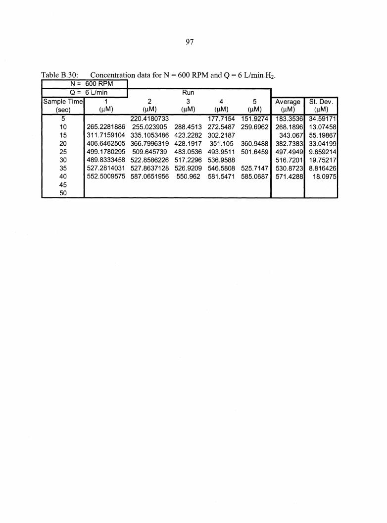
97
Table B.30: Concentration data for N = 600 RPM and Q = 6 L/min H2•
N = 600 RPM I Q = 6 L/min I Run
Sample Time 1 2 3 4 5 Average St. Dev. (sec) (µM) (µM) (µM) (µM) (µM) (µM) (µM)
5 220.4180733 177.7154 151.9274 183.3536 34.59171 10 265.2281886 255.023905 288.4513 272.5487 259.6962 268.1896 13.07458 15 311.7159104 335.1053486 423.2282 302.2187 343.067 55.19867 20 406.6462505 366. 7996319 428.1917 351.105 360.9488 382.7383 33.04199 25 499.1780295 509.645739 483.0536 493.9511 501.6459 497.4949 9.859214 30 489.8333458 522.8586226 517.2296 536.9588 516.7201 19.75217 35 527.2814031 527.8637128 526.9209 546.5808 525.7147 530.8723 8.816426 40 552.5009575 587.0651956 550.962 581.5471 585.0687 571.4288 18.0975 45 50


