Carbon monoxide, methane and carbon dioxide columns retrieved from SCIAMACHY by WFM-DOAS: year 2003 initial data set

Atmos. Chem. Phys., 5, 3313–3329, 2005www.atmos-chem-phys.org/acp/5/3313/SRef-ID: 1680-7324/acp/2005-5-3313European Geosciences Union

AtmosphericChemistry

and Physics

Carbon monoxide, methane and carbon dioxide columns retrievedfrom SCIAMACHY by WFM-DOAS: year 2003 initial data set

M. Buchwitz1, R. de Beek1, S. Noel1, J. P. Burrows1, H. Bovensmann1, H. Bremer1, P. Bergamaschi2, S. Korner3, andM. Heimann3

1Institute of Environmental Physics (IUP), University of Bremen FB1, Bremen, Germany2Institute for Environment and Sustainability, Joint Research Centre (EC-JRC-IES), Ispra, Italy3Max Planck Institute for Biogeochemistry (MPI-BGC), Jena, Germany

Received: 27 January 2005 – Published in Atmos. Chem. Phys. Discuss.: 1 April 2005Revised: 27 June 2005 – Accepted: 23 November 2005 – Published: 14 December 2005

Abstract. The near-infrared nadir spectra measured bySCIAMACHY on-board ENVISAT contain information onthe vertical columns of important atmospheric trace gasessuch as carbon monoxide (CO), methane (CH4), and car-bon dioxide (CO2). The scientific algorithm WFM-DOAShas been used to retrieve this information. For CH4 andCO2 also column averaged mixing ratios (XCH4 and XCO2)have been determined by simultaneous measurements of thedry air mass. All available spectra of the year 2003 havebeen processed. We describe the algorithm versions used togenerate the data (v0.4; for methane also v0.41) and showcomparisons of monthly averaged data over land with globalmeasurements (CO from MOPITT) and models (for CH4 andCO2). We show that elevated concentrations of CO result-ing from biomass burning have been detected in reasonableagreement with MOPITT. The measured XCH4 is enhancedover India, south-east Asia, and central Africa in Septem-ber/October 2003 in line with model simulations, where theyresult from surface sources of methane such as rice fields andwetlands. The CO2 measurements over the Northern Hemi-sphere show the lowest mixing ratios around July in quali-tative agreement with model simulations indicating that thelarge scale pattern of CO2 uptake by the growing vegetationcan be detected with SCIAMACHY. We also identified po-tential problems such as a too low inter-hemispheric gradientfor CO, a time dependent bias of the methane columns on theorder of a few percent, and a few percent too high CO2 overparts of the Sahara.

1 Introduction

Knowledge about the global distribution of carbon monox-ide (CO) and of the relatively well-mixed greenhouse gases

Correspondence to:M. Buchwitz([email protected])

methane (CH4) and carbon dioxide (CO2) is important formany reasons. CO, for example, plays a central role intropospheric chemistry (see, e.g.,Bergamaschi et al., 2000,and references given therein) as CO is the leading sink ofthe hydroxyl radical (OH) which itself largely determinesthe oxidizing capacity of the troposphere and, therefore, itsself-cleansing efficiency and the concentration of greenhousegases such as CH4. CO also has large air quality impact as aprecurser to tropospheric ozone, a secondary pollutant asso-ciated with respiratory problems and decreased crop yields.Satellite measurements of CH4, CO2, and CO in combinationwith inverse modeling have the potential to help better under-stand their surface sources and sinks than currently possiblewith the very accurate but rather sparse data from the net-work of surface stations (seeHouweling et al., 1999, 2004;Rayner and O’Brien, 2001, and references given therein). Abetter understanding of the sources and sinks of CH4 andCO2 is important for example to accurately predict the futureconcentrations of these gases and associated climate change.Monitoring of the emissions of these gases is also requiredby the Kyoto protocol.

The first CO measurements from SCIAMACHY havebeen presented inBuchwitz et al.(2004), and first resultson CH4 and CO2 have been presented inBuchwitz et al.(2005), both papers focusing on a detailed analysis of singleday data (except for CO2 for which also time averaged datahave been discussed). Here we present the first large data setof the above mentioned gases obtained by processing nearly ayear of nadir radiance spectra using initial versions (v0.4 andv0.41) of the WFM-DOAS retrieval algorithm. WFM-DOASis a scientific retrieval algorithm which is independent of theofficial operational algorithm of DLR/ESA.

The SCIAMACHY/WFM-DOAS data set has been com-pared with independent ground based Fourier TransformSpectroscopy (FTS) measurements. These comparisons,which are limited to the data close to a given ground station,

© 2005 Author(s). This work is licensed under a Creative Commons License.

3314 M. Buchwitz et al.: CO, CH4, and CO2 columns from SCIAMACHY

are described elsewhere in this issue (Dils et al., 2005; Suss-mann et al., 2005). Initial comparison for a sub-set of thedata can be found inde Maziere et al.(2004); Sussmannand Buchwitz(2005); Warneke et al.(2005). The findingsof these validation studies are consistent with the findingsthat will be reported in this study. Here, however, we focuson the comparison with global reference data.

High quality trace gas column retrieval from the SCIA-MACHY near-infrared spectra is a challenging task for manyreasons, e.g., because of calibration issues mainly related tohigh and variable dark signals (Gloudemans et al., 2005), be-cause the weak CO lines are difficult to be detected, and be-cause of the challenging accuracy and precision requirementsfor CO2 (Rayner and O’Brien, 2001; Houweling et al., 2004)and CH4. When developing a retrieval algorithm many deci-sions have to be made (selection of spectral fitting window,inversion procedure including definition of fit parameters anduse of a priori information, radiative transfer approximations,etc.) to process the data in an optimum way such that a goodcompromise is achieved between processing speed and accu-racy of the data products. In this context it is important topoint out that other groups are also working on this impor-tant topic using quite different approaches (seeGloudemanset al., 2004, 2005; Frankenberg et al., 2005a,b,c; Houwelinget al., 2005).

This paper is organized as follows: In Sect.2 the SCIA-MACHY instrument is introduced followed by a descriptionof the WFM-DOAS retrieval algorithm in Sect.3. Section4gives an overview about the processed data mainly in termsof time coverage. The main sections are the three Sects.5–7where the results for CO, CH4, and CO2 are separately pre-sented and discussed. The conclusions are given in Sect.8and a short summary of our latest developments (v0.5 COand XCH4) is given in Sect.9.

2 The SCIAMACHY instrument

The SCanning Imaging Absorption spectroMeter for At-mospheric CHartographY (SCIAMACHY) instrument (Bur-rows et al., 1995; Bovensmann et al., 1999, 2004) is part ofthe atmospheric chemistry payload of the European SpaceAgencies (ESA) environmental satellite ENVISAT, launchedin March 2002. ENVISAT flies in sun-synchronous polarlow Earth orbit crossing the equator at 10:00 AM local time.SCIAMACHY is a grating spectrometer that measures spec-tra of scattered, reflected, and transmitted solar radiation inthe spectral region 240–2400 nm in nadir, limb, and solar andlunar occultation viewing modes.

SCIAMACHY consists of eight main spectral channels(each equipped with a linear detector array with 1024 de-tector pixels) and seven spectrally broad band PolarizationMeasurement Devices (PMDs) (details are given inBovens-mann et al., 1999). For this study observations of channel 6(for CO2) and 8 (for CH4, CO, and N2O), and Polarization

Measurement Device (PMD) number 1 (∼320–380 nm) havebeen used. In addition, channel 4 has been used to determinethe mass of dry air from oxygen (O2) column measurementsusing the O2 A band. Channels 4, 6 and 8 measure simulta-neously the spectral regions 600–800 nm, 970–1772 nm and2360–2385 nm at spectral resolutions of 0.4, 1.4 and 0.2 nm,respectively. For SCIAMACHY the spatial resolution, i.e.,the footprint size of a single nadir measurement, depends onthe spectral interval and orbital position. For channel 8 datathe spatial resolution is 30×120 km2 corresponding to an in-tegration time of 0.5 s, except at high solar zenith angles (e.g.,polar regions in summer hemisphere), where the pixel size istwice as large (30×240 km2). For the channel 4 and 6 dataused for this study the integration time is mostly 0.25 s cor-responding to a horizontal resolution of 30×60 km2. SCIA-MACHY also performs direct (extraterrestrial) sun observa-tions, e.g., to obtain the solar reference spectra needed for theretrieval.

SCIAMACHY is one of the first instruments that performsnadir observations in the near-infrared (NIR) spectral region(i.e., around 2µm). In contrast to the ultra violet (UV) andvisible spectral regions where high performance Si detec-tors have been manufactured for a long time, no appropriatenear-infrared detectors were available when SCIAMACHYwas designed. The near-infrared InGaAs detectors of SCIA-MACHY were a special development for SCIAMACHY.Compared to the UV-visible detectors they are character-ized by a substantially higher pixel-to-pixel variability of thequantum efficiency and the dark (leakage) current. Each de-tector array has a large number of dead and bad pixels. Inaddition, the dark signal is significantly higher compared tothe UV-visible mainly because of thermal radiation gener-ated by the instrument itself. The in-flight optical perfor-mance of SCIAMACHY is overall as expected from the on-ground calibration and characterization activities (Bovens-mann et al., 2004). One exception is the time dependentoptical throughput variation in the SCIAMACHY NIR chan-nels 7 and 8 due the build-up of an ice layer on the detectors(”ice issue”) (Gloudemans et al., 2005). This effect is min-imized by regular heating of the instrument (Bovensmannet al., 2004) during decontamination phases. The ice lay-ers adversely influence the quality of the retrieval of all gasesdiscussed in this paper as they result in reduced throughput(transmission) and, therefore, reduced signal and signal-to-noise performance. In addition, changes of the instrumentslit function have been observed which introduce systematicerrors (Gloudemans et al., 2005). All these issues complicatethe retrieval.

3 WFM-DOAS retrieval algorithm

The Weighting Function Modified Differential Optical Ab-sorption Spectroscopy (WFM-DOAS) retrieval algorithmand its current implementation is described in detail

Atmos. Chem. Phys., 5, 3313–3329, 2005 www.atmos-chem-phys.org/acp/5/3313/

M. Buchwitz et al.: CO, CH4, and CO2 columns from SCIAMACHY 3315


Fig. 1. Number of orbits per day of the year 2003 processed by WFM-DOAS (blue lines). The maximum number of orbits per day is about14 (∼100%). The red shaded areas indicate the decontamination phases performed to get rid of the ice layer that grows on the near-infrareddetectors of channels 7 and 8. Data gaps are due to decontamination but also due to other (mostly ground processing related) reasons.


Fig. 1. Number of orbits per day of the year 2003 processed by WFM-DOAS (blue lines). The maximum number of orbits per day is about14 (∼100%). The red shaded areas indicate the decontamination phases performed to get rid of the ice layer that grows on the near-infrareddetectors of channels 7 and 8. Data gaps are due to decontamination but also due to other (mostly ground processing related) reasons.

elsewhere (Buchwitz et al., 2000a, 2004, 2005). Inshort, WFM-DOAS is an unconstrained linear-least squaresmethod based on scaling pre-selected trace gas vertical pro-files. The fit parameters are the desired vertical columns. Thelogarithm of a linearized radiative transfer model plus a low-order polynomial is fitted to the logarithm of the ratio of themeasured nadir radiance and solar irradiance spectrum, i.e.,observed sun-normalized radiance. The WFM-DOAS refer-ence spectra are the logarithm of the sun-normalized radi-ance and its derivatives. They are computed with a radiativetransfer model taking into account line-absorption and mul-tiple scattering (Buchwitz et al., 2000b). A fast look-up tablescheme has been developed in order to avoid time consumingon-line radiative transfer simulations. A detailed descriptionof the look-up table is given inBuchwitz and Burrows(2004)(please note that the current version of the look-up table is

based on HITRAN2000/2003 line parameters) (Rothmann etal., 2003). A short description is also provided inBuchwitzet al.(2005).

In order to identify cloud-contaminated ground pixels weuse a simple threshold algorithm based on sub-pixel infor-mation as provided by the SCIAMACHY Polarization Mea-surement Devices (PMDs) (details are given inBuchwitz etal., 2004, 2005). We use PMD1 which corresponds to thespectral region 320–380 nm located in the UV part of thespectrum. Strictly speaking, the algorithm detects enhancedbackscatter in the UV. Enhanced UV backscatter mainly re-sults from clouds but might also be due to high aerosol load-ing or high surface UV spectral reflectance. As a result, iceor snow covered surfaces may be wrongly classified as cloudcontaminated. This needs to be improved in future versionsof our retrieval method.

www.atmos-chem-phys.org/acp/5/3313/ Atmos. Chem. Phys., 5, 3313–3329, 2005


The quality of the WFM-DOAS fits in the near-infrared ispoor (i.e., the fit residuals are large) when applying WFM-DOAS to the operational Level 1 data products. In order toimprove the quality of the fits and thereby the quality of ourdata products we pre-process the operational Level 1 dataproducts mainly with respect to a better dark signal calibra-tion (seeBuchwitz et al., 2004, 2005). In addition, there areindications that the in-orbit slit function of SCIAMACHY isdifferent from the one measured on-ground (Gloudemans etal., 2005) due to the ice layer (see Sect.2). We use a slitfunction that has been determined by applying WFM-DOASto the in-orbit nadir measurements. We selected the one thatresulted in best fits, i.e., smallest fit residuum (seeBuchwitzet al., 2004, 2005).

4 WFM-DOAS data products: Time coverage

The WFM-DOAS trace gas column data products have beenderived by processing all consolidated SCIAMACHY Level1 operational product files (i.e., the calibrated and geolocatedspectra) of the year 2003 that have been made available byESA/DLR (up to mid-2004). Figure1 gives an overviewabout the number of orbits per day that have been processed.The maximum number of orbits per day is about fourteen.As can been seen (blue lines), all 14 orbits were available foronly a small number of days. For many days no data wereavailable. Many of the large data gaps are due to decontami-nation phases (see Sect.2) which are indicated by red shadedareas. For November and December 2003 no consolidated(i.e., full product) orbit files have been made available (forground processing related reasons).

5 Carbon monoxide (CO)

CO columns have been retrieved from a small spectral fittingwindow (2359–2370 nm) located in SCIAMACHY channel8. The fitting window covers four CO absorption lines.The retrieval is complicated by strong overlapping absorp-tion features of methane and water vapor. The first CO re-sults from SCIAMACHY have been presented inBuchwitzet al.(2004) focusing on a detailed analysis of three days ofdata of the year 2003. For details concerning pre-processingof the spectra (for improving the calibration), WFM-DOASv0.4 retrieval, vertical column averaging kernels, quality ofthe spectral fits, and a quantitative comparison with MO-PITT Version 3 CO columns (Deeter et al., 2003; Emmonset al., 2004) we refer toBuchwitz et al.(2004). An initialerror analysis using simulated measurements can be found inBuchwitz et al.(2004) and Buchwitz and Burrows(2004)where it is shown that the retrieval errors are expected tobe less than about 20%. InBuchwitz et al.(2004) it hasbeen shown that plumes of elevated CO can be detectedwith single overpass data in good qualitative agreement with

MOPITT. Globally, for measurements over land, the stan-dard deviation of the difference with respect to MOPITTwas shown to be in the range 0.4–0.6×1018 molecules/cm2

and the linear correlation coefficient between 0.4 and 0.7.The differences of the CO from the two sensors depend ontime and location but are typically within 30% for most lat-itudes. Perfect agreement with MOPITT is, however, not tobe expected for a number of reasons (differences in overpasstime, spatial resolution, etc.). In this context it is importantto point out that the sensitivity of SCIAMACHY measure-ments is nearly independent of altitude whereas the sensitiv-ity of MOPITT to boundary layer CO is low. On the otherhand, retrieval of CO from SCIAMACHY is not unproblem-atic. For example, the WFM-DOAS v0.4 CO columns arescaled with a constant factor of 0.5 to compensate for an ob-vious overestimation (seeBuchwitz et al., 2004, for details).This overestimation is most probably closely related to thedifficulty of accurately fitting the weak CO lines in the se-lected fitting window (note that the CO columns of our newversion 0.5 data product, which is retrieved from a differentfitting window, are not scaled any more; see Sect.9 for de-tails). The fit residuals, which are on the order of the COlines, are not signal-to-noise limited but dominated by (notyet understood) rather stable spectral artifacts.

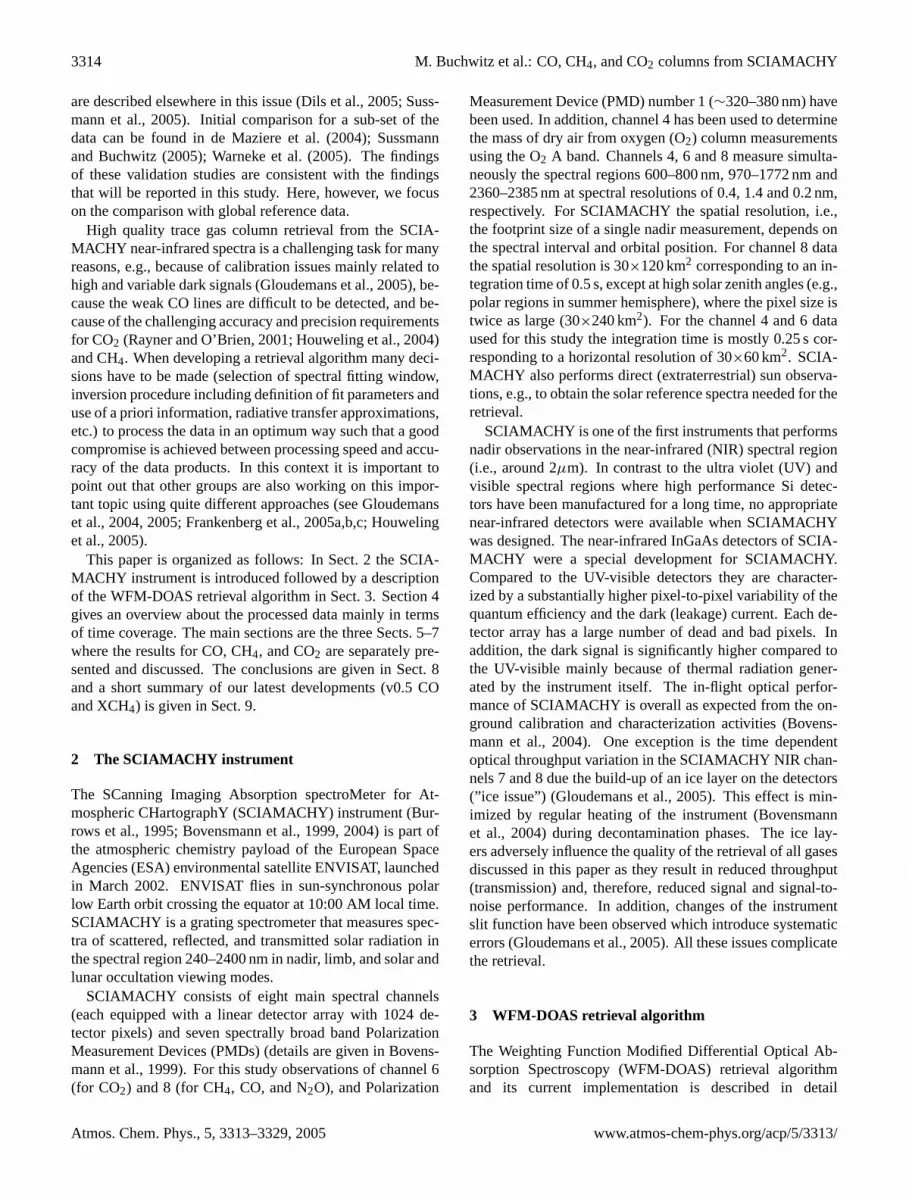
Figure 2 shows a comparison of tri-monthly averagedWFM-DOAS version 0.4 CO columns with CO from MO-PITT (version 3). Because of the low surface reflectivityof water in the NIR (outside sun-glint conditions) the nadirmeasurements are noisy over the ocean. Therefore, we focuson SCIAMACHY measurements over land. Only these mea-surements are shown in Fig.2. The same land mask as usedfor SCIAMACHY has also been used for MOPITT to easethe comparison. SCIAMACHY data have only been includedin Fig. 2 if the CO fit error was less than 60% and when thepixels were cloud free. As can be seen from Fig.1, thereare large SCIAMACHY data gaps. Therefore, the SCIA-MACHY data shown in Fig.2 are not tri-monthly averagesobtained from a bias free sampling. For example, the July-September average is strongly weighted towards July andSeptember due to a long decontamination period with no datain August. There are also gaps in the tropical region due topersistent cloud cover. Furthermore, there are no data overGreenland and Antarctica, and over large parts of the North-ern Hemisphere in the period January to March. This is par-tially also due to clouds but mainly due to ice/snow coveredsurfaces because of the limitations of the cloud detection al-gorithm.

When comparing the January–March data from SCIA-MACHY and MOPITT one can see that there are similari-ties but also differences. For example, the inter-hemisphericdifference is clearly visible for MOPITT but barely visiblefor SCIAMACHY. Both sensors see low columns over re-gions of elevated surface topography (Himalaya, Andes andRocky Mountains) and high columns over the western partof central Africa (where significant biomass burning is going




a bCO SCIA/WFMDv0.4 Jan−Mar 2003

< 1.20

1.40

1.60

1.80

2.00

2.20

2.40

2.60

2.80

3.00

3.20 >

< 1.20

1.40

1.60

1.80

2.00

2.20

2.40

2.60

2.80

3.00

3.20 >VC [1018/cm2]

SCIA/WFMDv0.4 ([email protected]−bremen.de)

CO MOPITT(land) Jan−Mar 2003

< 1.20

1.40

1.60

1.80

2.00

2.20

2.40

2.60

2.80

3.00

3.20 >

< 1.20

1.40

1.60

1.80

2.00

2.20

2.40

2.60

2.80

3.00

3.20 >VC [1018/cm2]

MOPITT data: NASA Langley via UniToronto/HBremer@uni−bremen.de (Figure: [email protected]−bremen.de)

c dCO SCIA/WFMDv0.4 Apr−Jun 2003

< 1.20

1.40

1.60

1.80

2.00

2.20

2.40

2.60

2.80

3.00

3.20 >

< 1.20

1.40

1.60

1.80

2.00

2.20

2.40

2.60

2.80

3.00

3.20 >VC [1018/cm2]


CO MOPITT(land) Apr−Jun 2003

< 1.20

1.40

1.60

1.80

2.00

2.20

2.40

2.60

2.80

3.00

3.20 >

< 1.20

1.40

1.60

1.80

2.00

2.20

2.40

2.60

2.80

3.00

3.20 >VC [1018/cm2]


e fCO SCIA/WFMDv0.4 Jul−Sep 2003

< 1.20

1.40

1.60

1.80

2.00

2.20

2.40

2.60

2.80

3.00

3.20 >

< 1.20

1.40

1.60

1.80

2.00

2.20

2.40

2.60

2.80

3.00

3.20 >VC [1018/cm2]


CO MOPITT(land) Jul−Sep 2003

< 1.20

1.40

1.60

1.80

2.00

2.20

2.40

2.60

2.80

3.00

3.20 >

< 1.20

1.40

1.60

1.80

2.00

2.20

2.40

2.60

2.80

3.00

3.20 >VC [1018/cm2]


Fig. 2. Tri-monthly averaged CO columns over land from SCIAMACHY/ENVISAT (left) and MOPITT/EOS-Terra (right). Only the columnsover land are shown because the quality of the SCIAMACHY CO columns over water is low due to the low reflectivity of water in the near-infrared. For SCIAMACHY only data have been averaged where the CO fit error is less than 60% and where the PMD1 cloud identificationalgorithm indicates a cloud free pixel. For MOPITT cloudy pixels are also not included.


Fig. 2. Tri-monthly averaged CO columns over land from SCIAMACHY/ENVISAT (left) and MOPITT/EOS-Terra (right). Only the columnsover land are shown because the quality of the SCIAMACHY CO columns over water is low due to the low reflectivity of water in the near-infrared. For SCIAMACHY only data have been averaged where the CO fit error is less than 60% and where the PMD1 cloud identificationalgorithm indicates a cloud free pixel. For MOPITT cloudy pixels are also not included.

on during the dry season), south-east Asia, parts of Europe,and the south-eastern part of the United States of Amer-ica. Over South America and the northern part of AustraliaSCIAMACHY sees elevated CO not observed by MOPITT.

During April to June both sensors see elevated CO overlarge parts of the Northern Hemisphere (eastern part of theUS, Canada, western Europe and large parts of Russia (theobserved pattern are, however, not exactly identical), south-east Asia and parts of China. Over India and parts ofsouth-east Asia SCIAMACHY sees elevated CO not seen byMOPITT. The largest difference over the Northern Hemi-sphere occurs over the western part of central Africa wherethe CO retrieved from SCIAMACHY is significantly higherthan the CO from MOPITT. The reason for the elevated

SCIAMACHY CO columns over the Sahel region is not yetexactly understood but it is very likely that this is an over-estimation due to systematic artifacts (caused by, for exam-ple, aerosol). This is supported by the fact that our new ver-sion 0.5 CO WFM-DOAS data product, which is shortly de-scribed in Sect.9, shows significantly lower values over thisregion compared to v0.4. The version 0.5 CO columns areless sensitive to errors related to average light path (or ob-served airmass) uncertainty resulting from the unknown dis-tribution of scattering material (aerosols, clouds) in the atmo-sphere and/or surface reflectivity variability. The reason forthis is that the CO v0.5 column is normalized by the methanecolumn obtained from the same spectral fitting window re-sulting in (at least partial) canceling of errors. Also over large




Fig. 3. The black diamonds show XCH4 (v0.4) as measured by SCIAMACHY over the Sahara normalized by a constant reference valueof 1750 ppbv as a function of day of the year 2003 (”methane bias curve”). The red diamonds (”Transmission (orig.)”) show independentmeasurements, namely the SCIAMACHY channel 8 transmission which changes due to the varying ice layer on the detector. This curvehas been determined by averaging the signal of the solar measurements and normalizing it. The magenta (m) ”Transmission (transformed)”curve has been obtained by a linear transformation of the red (r) curve, i.e., by computing m = A + B r. Applying the same coefficients Aand B as used for the data before day 230 also to the data after day 230 results in the yellow curve which still shows an offset with respect tothe black methane bias curve. To get a better match, two sets of coefficients have been used, one for the data before day 230 and another setfor the data after day 230. The reason why different coefficients are needed is most probably because the spatial distribution of the ice layeron the detector changes with time.


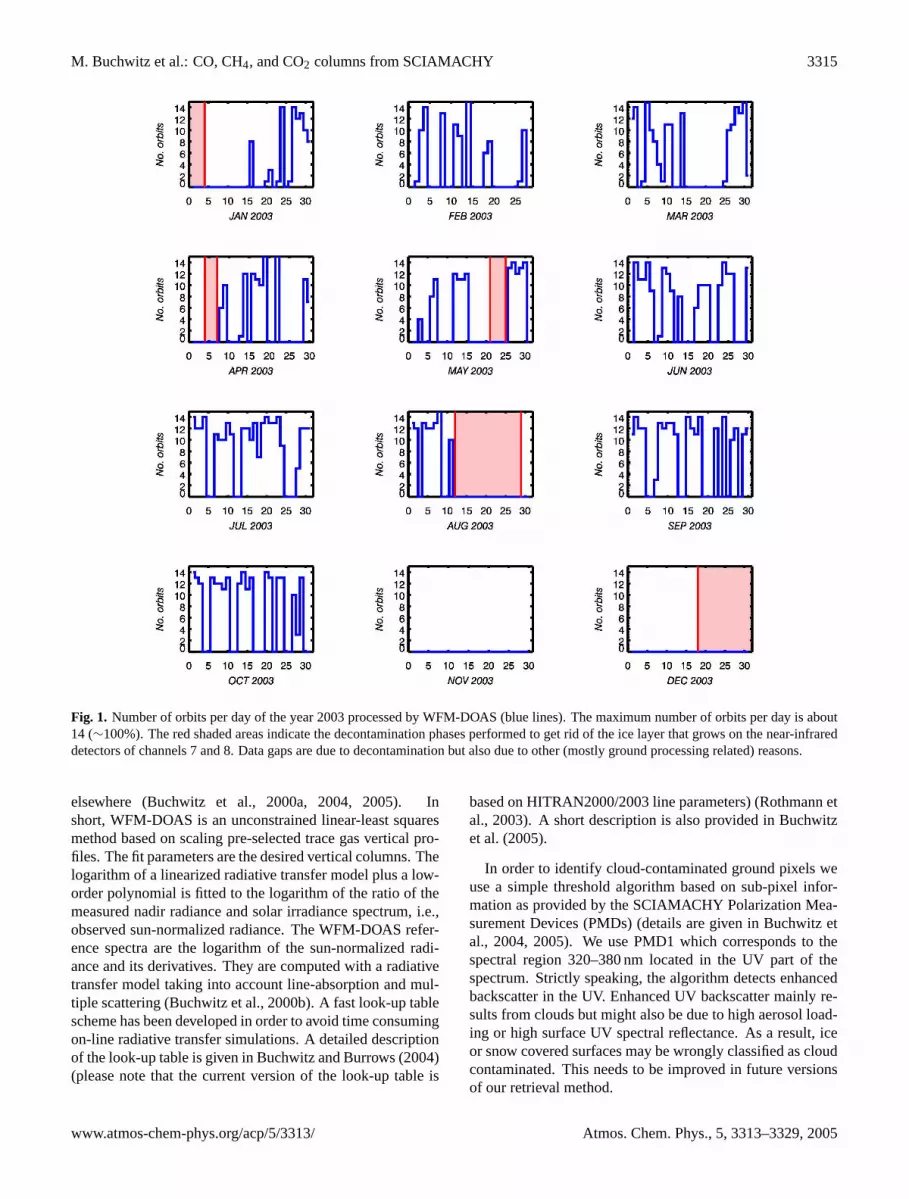
Fig. 3. The black diamonds show XCH4 (v0.4) as measured bySCIAMACHY over the Sahara normalized by a constant referencevalue of 1750 ppbv as a function of day of the year 2003 (“methanebias curve”). The red diamonds (“Transmission (orig.)”) show inde-pendent measurements, namely the SCIAMACHY channel 8 trans-mission which changes due to the varying ice layer on the detector.This curve has been determined by averaging the signal of the solarmeasurements and normalizing it. The magenta (m) “Transmission(transformed)” curve has been obtained by a linear transformationof the red (r) curve, i.e., by computingm=A+B r. Applying thesame coefficients A and B as used for the data before day 230 also tothe data after day 230 results in the yellow curve which still showsan offset with respect to the black methane bias curve. To get a bet-ter match, two sets of coefficients have been used, one for the databefore day 230 and another set for the data after day 230. The rea-son why different coefficients are needed is most probably becausethe spatial distribution of the ice layer on the detector changes withtime.

parts of South America the SCIAMACHY measurements aresignificantly higher than MOPITT (WFM-DOAS version 0.5also shows higher values than MOPITT confirming the v0.4results). For the time period July to September the patternof elevated CO as observed by SCIAMACHY is similar tothe SCIAMACHY observations during April to June. Themain differences are: (i) higher values over Southern Amer-ica (in quantitative agreement with MOPITT; note that thisis the time where most of the biomass burning takes placein this area) and (ii) higher values over the eastern part ofnorthern Russia (also observed by MOPITT). There are alsosignificant differences when comparing the SCIAMACHYdata with MOPITT especially over the northern part of cen-tral Africa, the eastern US, south-east Asia and over most ofthe mid to high latitude parts of the Northern Hemisphere.

In summary, the agreement with MOPITT is reasonablebut there are large differences at certain locations during cer-tain times of the year. More investigations are needed to ex-plain the observed differences taking into account the differ-ent altitude sensitivities of both sensors.

6 Methane (CH4)

The methane columns have been retrieved from asmall spectral fitting window (2265–2280 nm) located inSCIAMACHY channel 8 which covers several absorptionlines of CH4 and several (much weaker) absorption lines ofnitrous oxide (N2O) and water vapor (H2O). The main sci-entific application of the methane measurements of SCIA-MACHY is to obtain information on the surface sourcesof methane. The modulation of methane columns due tomethane sources is only on the order of a few percent. Thisis much weaker than the variation of the methane columndue to changes of surface pressure / surface elevation (be-cause methane is well-mixed the methane column is highlycorrelated with the total air mass over a given location and,therefore, with surface pressure). To filter out these muchlarger disturbing modulations, the methane columns need tobe normalized by the observed airmass to obtain a so calleddry air column averaged mixing ratio of methane (denotedXCH4). To accomplish this, oxygen (O2) columns have beenretrieved in addition to the methane columns. From the oxy-gen columns the airmass can be calculated using its constantmixing ratio of 0.2095. The O2 columns used to compute theWFM-DOAS v0.4 XCH4 data product have been retrievedfrom the SCIAMACHY measurements in the O2 A bandspectral region (around 760 nm; channel 4).

First CH4 results from SCIAMACHY have been presentedin Buchwitz et al.(2005) focusing on a detailed analysis offour days of data of the year 2003. For details concerningpre-processing of the spectra (to improve the calibration),WFM-DOAS (v0.4) processing, averaging kernels, qualityof the spectral fits, an initial error analysis (see alsoBuch-witz and Burrows, 2004), and a quantitative comparison withglobal models we refer to that study. According to the er-ror analysis errors of a few percent due to undetected cirrusclouds, aerosols, surface reflectivity, temperature and pres-sure profiles, etc., are to be expected. It has been shownin Buchwitz et al.(2005) that the WFM-DOAS Version 0.4methane columns have a time dependent (nearly globallyuniform) bias of up to –15% (low bias of SCIAMACHY)for one of the four days that have been analyzed. The biasis correlated with the time after the last decontamination per-formed to get rid of the ice layers on the detector. There-fore,Buchwitz et al.(2005) concluded that the bias might bedue to the “ice-issue” (see Sect.2). This is consistent withthe finding ofGloudemans et al.(2005) that the ice build-upon the detectors results in a broadening of the instrument slitfunction (the wider the slit function compared to the assumed




a b

c d

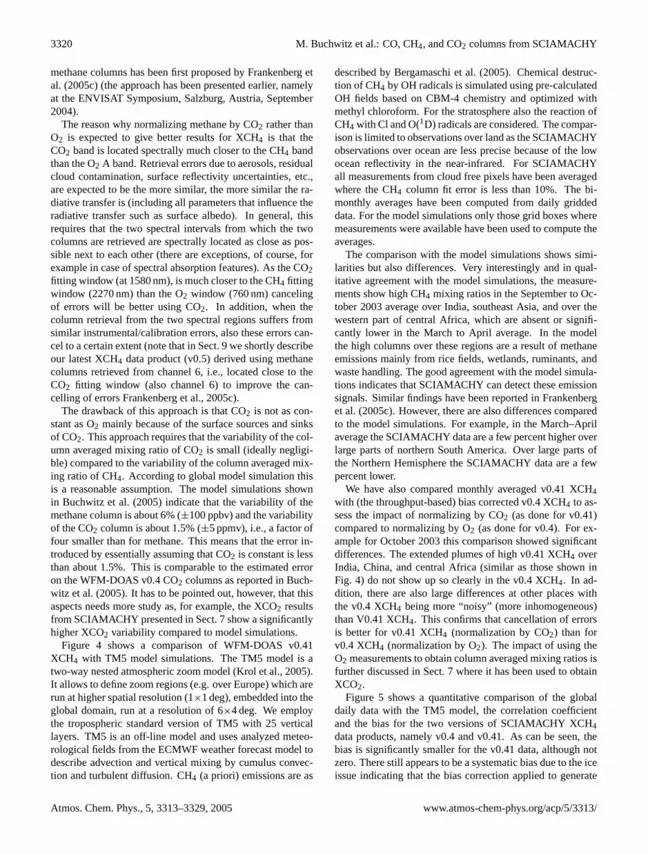
Fig. 4. Column averaged mixing ratios of methane (XCH4) as measured by SCIAMACHY over land using WFM-DOAS v0.41 (left)compared to TM5 model data (right). For SCIAMACHY only the measurements from cloud free pixels have been averaged where themethane error is less than 10%. The model data have been averaged taking into account the daily sampling of the SCIAMACHY data. Themodel data have been scaled by a constant factor of 1.03 to compensate for the bias between the two data sets (see Fig. 5).


Fig. 4. Column averaged mixing ratios of methane (XCH4) as measured by SCIAMACHY over land using WFM-DOAS v0.41 (left)compared to TM5 model data (right). For SCIAMACHY only the measurements from cloud free pixels have been averaged where themethane error is less than 10%. The model data have been averaged taking into account the daily sampling of the SCIAMACHY data. Themodel data have been scaled by a constant factor of 1.03 to compensate for the bias between the two data sets (see Fig.5).

slit function, the larger the underestimation of the retrievedmethane column).

Typically, the weak methane source signal is difficult tobe clearly detected with single overpass or single day SCIA-MACHY data. For accurate detection of methane sourcesaverages have to be computed. Because of the time depen-dent bias of the WFM-DOAS v0.4 methane columns this is,however, not directly possible.

In the following we describe how we have processedthe SCIAMACHY data to get an improved version of ourmethane data product (Version 0.41) by applying a bias cor-rection to the v0.4 methane columns. We assume that thedata can be sufficiently corrected by dividing the columnsby a globally constant scaling factor which only depends ontime (on the day of the measurement). The correction fac-tor has been determined as follows: For each day all cloudfree v0.4 XCH4 measurements over the Sahara have beenaveraged. The ratio of these daily average mixing ratios to aconstant reference value (chosen to be 1750 ppbv) is approx-imately the methane bias (because methane is not constantthis is not exactly the methane bias and a certain systematicerror is introduced by this assumption). This time depen-dent methane bias is shown in Fig.3 (black diamonds). Thisbias shows a similar time dependence as the independently

measured channel 8 transmission loss also shown in Fig.3(red diamonds). The transmission has been determined byaveraging the signal of the channel 8 solar measurementsnormalized to a reference measurement at the beginning ofthe mission. The varying transmission is a consequence ofthe varying ice layer on the detectors. Figure3 shows a thirdcurve, the (daily) correction factor (magenta diamonds). Thecorrection factor curve has been obtained by linearly trans-forming the transmission curve. The coefficients of the lin-ear transformation have been selected such that a good matchis obtained with the methane bias curve. In order to correctthe WFM-DOAS v0.4 methane columns for the systematicerrors introduced by the ice layer the correction factors areapplied as follows: All v0.4 methane columns of a given dayhave been divided by the correction factor for this day. Thecorrected WFM-DOAS v0.4 methane columns are the newWFM-DOAS v0.41 (absolute) methane columns.

In order to generate the new WFM-DOAS v0.41 XCH4product a second modification has been applied: Instead ofnormalizing the methane columns by the oxygen column re-trieved from the 760 nm O2 A band (as done for v0.4 XCH4),they have been normalized by the CO2 columns retrievedfrom the 1580 nm region (for details on CO2 retrieval seeSect. 7). Using CO2 rather than O2 for normalizing the



methane columns has been first proposed byFrankenberg etal. (2005c) (the approach has been presented earlier, namelyat the ENVISAT Symposium, Salzburg, Austria, September2004).

The reason why normalizing methane by CO2 rather thanO2 is expected to give better results for XCH4 is that theCO2 band is located spectrally much closer to the CH4 bandthan the O2 A band. Retrieval errors due to aerosols, residualcloud contamination, surface reflectivity uncertainties, etc.,are expected to be the more similar, the more similar the ra-diative transfer is (including all parameters that influence theradiative transfer such as surface albedo). In general, thisrequires that the two spectral intervals from which the twocolumns are retrieved are spectrally located as close as pos-sible next to each other (there are exceptions, of course, forexample in case of spectral absorption features). As the CO2fitting window (at 1580 nm), is much closer to the CH4 fittingwindow (2270 nm) than the O2 window (760 nm) cancelingof errors will be better using CO2. In addition, when thecolumn retrieval from the two spectral regions suffers fromsimilar instrumental/calibration errors, also these errors can-cel to a certain extent (note that in Sect.9 we shortly describeour latest XCH4 data product (v0.5) derived using methanecolumns retrieved from channel 6, i.e., located close to theCO2 fitting window (also channel 6) to improve the can-celling of errorsFrankenberg et al., 2005c).

The drawback of this approach is that CO2 is not as con-stant as O2 mainly because of the surface sources and sinksof CO2. This approach requires that the variability of the col-umn averaged mixing ratio of CO2 is small (ideally negligi-ble) compared to the variability of the column averaged mix-ing ratio of CH4. According to global model simulation thisis a reasonable assumption. The model simulations shownin Buchwitz et al.(2005) indicate that the variability of themethane column is about 6% (±100 ppbv) and the variabilityof the CO2 column is about 1.5% (±5 ppmv), i.e., a factor offour smaller than for methane. This means that the error in-troduced by essentially assuming that CO2 is constant is lessthan about 1.5%. This is comparable to the estimated erroron the WFM-DOAS v0.4 CO2 columns as reported inBuch-witz et al.(2005). It has to be pointed out, however, that thisaspects needs more study as, for example, the XCO2 resultsfrom SCIAMACHY presented in Sect.7 show a significantlyhigher XCO2 variability compared to model simulations.

Figure 4 shows a comparison of WFM-DOAS v0.41XCH4 with TM5 model simulations. The TM5 model is atwo-way nested atmospheric zoom model (Krol et al., 2005).It allows to define zoom regions (e.g. over Europe) which arerun at higher spatial resolution (1×1 deg), embedded into theglobal domain, run at a resolution of 6×4 deg. We employthe tropospheric standard version of TM5 with 25 verticallayers. TM5 is an off-line model and uses analyzed meteo-rological fields from the ECMWF weather forecast model todescribe advection and vertical mixing by cumulus convec-tion and turbulent diffusion. CH4 (a priori) emissions are as

described byBergamaschi et al.(2005). Chemical destruc-tion of CH4 by OH radicals is simulated using pre-calculatedOH fields based on CBM-4 chemistry and optimized withmethyl chloroform. For the stratosphere also the reaction ofCH4 with Cl and O(1D) radicals are considered. The compar-ison is limited to observations over land as the SCIAMACHYobservations over ocean are less precise because of the lowocean reflectivity in the near-infrared. For SCIAMACHYall measurements from cloud free pixels have been averagedwhere the CH4 column fit error is less than 10%. The bi-monthly averages have been computed from daily griddeddata. For the model simulations only those grid boxes wheremeasurements were available have been used to compute theaverages.

The comparison with the model simulations shows simi-larities but also differences. Very interestingly and in qual-itative agreement with the model simulations, the measure-ments show high CH4 mixing ratios in the September to Oc-tober 2003 average over India, southeast Asia, and over thewestern part of central Africa, which are absent or signifi-cantly lower in the March to April average. In the modelthe high columns over these regions are a result of methaneemissions mainly from rice fields, wetlands, ruminants, andwaste handling. The good agreement with the model simula-tions indicates that SCIAMACHY can detect these emissionsignals. Similar findings have been reported inFrankenberget al.(2005c). However, there are also differences comparedto the model simulations. For example, in the March–Aprilaverage the SCIAMACHY data are a few percent higher overlarge parts of northern South America. Over large parts ofthe Northern Hemisphere the SCIAMACHY data are a fewpercent lower.

We have also compared monthly averaged v0.41 XCH4with (the throughput-based) bias corrected v0.4 XCH4 to as-sess the impact of normalizing by CO2 (as done for v0.41)compared to normalizing by O2 (as done for v0.4). For ex-ample for October 2003 this comparison showed significantdifferences. The extended plumes of high v0.41 XCH4 overIndia, China, and central Africa (similar as those shown inFig. 4) do not show up so clearly in the v0.4 XCH4. In ad-dition, there are also large differences at other places withthe v0.4 XCH4 being more “noisy” (more inhomogeneous)than V0.41 XCH4. This confirms that cancellation of errorsis better for v0.41 XCH4 (normalization by CO2) than forv0.4 XCH4 (normalization by O2). The impact of using theO2 measurements to obtain column averaged mixing ratios isfurther discussed in Sect.7 where it has been used to obtainXCO2.

Figure 5 shows a quantitative comparison of the globaldaily data with the TM5 model, the correlation coefficientand the bias for the two versions of SCIAMACHY XCH4data products, namely v0.4 and v0.41. As can be seen, thebias is significantly smaller for the v0.41 data, although notzero. There still appears to be a systematic bias due to the iceissue indicating that the bias correction applied to generate




Fig. 5. Comparison of daily SCIAMACHY XCH4 measurements (versions 0.4 (blue triangles) and 0.41 (black diamonds)) with TM5 modelsimulations. The top panel shows the bias (SCIAMACHY-model), the middle panel the standard deviation of the difference, and the bottompanel Pearson’s linear correlation coefficient r.


Fig. 5. Comparison of daily SCIAMACHY XCH4 measurements (versions 0.4 (blue triangles) and 0.41 (black diamonds)) with TM5 modelsimulations. The top panel shows the bias (SCIAMACHY-model), the middle panel the standard deviation of the difference, and the bottompanel Pearson’s linear correlation coefficientr.

the v0.41 data is not perfect. Also the correlation with themodel results is typically significantly better for the version0.41 data.

7 Carbon dioxide (CO2)

The CO2 columns have been retrieved using a small spectralfitting window (1558–1594 nm) located in SCIAMACHYchannel 6 (which is not affected by an ice layer). This spec-tral region covers one absorption band of CO2 and weak ab-sorption features of water vapor. As for methane v0.4 (air or)

O2-normalized CO2 columns have been derived, the dry aircolumn averaged mixing ratios XCO2. First results of CO2from SCIAMACHY have been presented inBuchwitz et al.(2005). For details concerning pre-processing of the spectra(for improving the calibration), WFM-DOAS (v0.4) process-ing, vertical column averaging kernels, quality of the spectralfits, and a quantitative comparison with global model simu-lations we refer toBuchwitz et al.(2005). An initial erroranalysis using simulated measurements is given inBuchwitzet al. (2005) andBuchwitz and Burrows(2004). Accordingto this analysis, errors of a few percent due to undetected



cirrus clouds, aerosols, surface reflectivity, temperature andpressure profiles, etc., are to be expected. To compensatefor a not yet understood systematic underestimation of theinitially retrieved CO2 columns the WFM-DOAS v0.4 CO2columns have been scaled with a constant factor of 1.27 (seeBuchwitz et al., 2005, for details). The factor has been cho-sen to make sure that the CO2 column is near its expectedvalue of about 8×1021 molecules/cm2 for a cloud free scenewith a surface elevation close to sea level and moderate sur-face albedo. InBuchwitz et al.(2005) it has been shownthat the WFM-DOAS v0.4 CO2 (scaled) columns agree withmodel columns within a few percent (range –3.7% to +2.0%).Because of the scaling factor a meaningful comparison withreference data should focus on variability in time and spaceand not on the absolute level. Also the v0.4 O2 columns,used to compute XCO2, are scaled (by 0.85). The reasonfor the about 15% overestimation of the originally retrievedO2 columns is currently unclear. The factor has been chosento make sure that the O2 column is near its expected valueof about 4.5×1024molecules/cm2 for a cloud free scene witha surface elevation close to sea level and moderate surfacealbedo. In a recent paper ofvan Diedenhofen et al.(2005) anoverestimation of 2–5% over scenes with moderate to highsurface albedo is found when comparing their SCIAMACHYO2 columns with actual meteorological data. They found that2% can be explained by an offset on the measured reflectanceand argue that the remaining overestimation is likely due toaerosols. Taking this into account our retrievals are still over-estimated by 10%. At present we cannot offer an explana-tions for this discrepancy. The investigation of this will bea focus of our future work. For now we have to state thatthe v0.4 CO2 and O2 columns are scaled resulting in a quitelarge scaling factor for XCO2 of 1.49 (=1.27/0.85). Becauseof this we focus on variability rather than on absolute XCO2levels when comparing our XCO2 to reference data.

In Buchwitz et al.(2005) it has been shown that the spa-tial and temporal pattern of the retrieved column averagedmixing ratio is in reasonable agreement with the model dataexcept for the amplitude of the variability. The measuredvariability is about a factor of four higher than the variabil-ity of the model data (about 6% compared to about 1.5%for the model data). This is also confirmed in this studywhich provides more details on this finding. In this con-text it is important to note that an overestimation of the re-trieved variability of about a factor 2.2 (at maximum) maybe explained as follows: The SCIAMACHY/WFM-DOASCO2 column averaging kernels (shown inBuchwitz et al.,2005) peak in the lower troposphere and have a maximumvalue of about 1.5. This means that the retrieved variabil-ity is overestimated by 50% (e.g., 3 ppmv instead of 2 ppmv)if this column variability is entirely due to variability in thelower troposphere (note that the averaging kernels typicallydecrease with altitude and reach 1.0 (i.e., no over- or under-estimation) around 400 hPa (∼7 km); above 400 hPa they areless than 1.0). The scaling factor of 1.49 which is currently

applied to the retrieved XCO2 may also contribute to an en-hancement of the retrieved variability. This however requiresthat the initially retrieved columns are off by a constant off-set rather than a constant scaling factor (this aspect needsfurther investigation). The averaging kernels in combinationwith the scaling factor might explain at maximum a factorof 2.2 (=1.5×1.49) overestimated variability. The differentresolution of the SCIAMACHY measurements (60×30 km2)and the model simulations (1.8×1.8 deg) also contribute to adifference in the observed and the modeled variability. Fur-ther study is needed to identify the origin of the scaling fac-tors for CO2 and O2. Also the averaging kernels need to betaken into account when comparing with reference data. Thefactor of 2.2 however can only partially explain the observedvariability. At least a factor of 2 higher observed variabilitystill needs to be explained.

In the following we present a detailed comparison of theretrieved XCO2 with TM3 model simulations. TM3 3.8(Heimann and Korner, 2003) is a three-dimensional globalatmospheric transport model for an arbitrary number of ac-tive or passive tracers. It uses re-analyzed meteorologicalfields from the National Center for Environmental Predic-tion (NCEP) or from the ECMWF re-analysis. The modeledprocesses comprise tracer advection, vertical transport due toconvective clouds and turbulent vertical transport by diffu-sion. Available horizontal resolutions range from 8×10 degto 1.1×1.1 deg. In this case, TM3 was run with a resolu-tion of 1.8×1.8 deg and 28 layers, and the meteorology fieldswere derived from the NCEP/DOE AMIP-II reanalysis. CO2source/sink fields for the ocean originate fromTakahaschi etal. (2002), for anthropogenic sources from the EDGAR 3.2database and for the biosphere from the BIOME-BGC model(Thornton et al., 2002) with inclusion of a simple parameter-ization of the diurnal cycle in photosynthesis and respiration.For SCIAMACHY the averages have been computed usingonly the cloud free pixels with a XCO2 error of less than10%. Shown in Fig.6 are only the data over land becauseof the problems with measuring over the ocean in the near-infrared (see Sect.5).

For SCIAMACHY Fig. 6 shows absolute column aver-aged mixing ratios of CO2 in the range 335–385 ppmv. ForTM3 “uncalibrated” XCO2-offsets are shown which are inthe range 0–13.7 ppmv. These offsets do not include the(current) background concentration of CO2. Therefore, notthe absolute values but only the variability in space and timeshould be compared. The model simulations show low CO2columns (compared to the mean column) over the NorthernHemisphere in July 2003 compared to higher values in Mayand September. This is mainly due to uptake of CO2 by thebiosphere which results in minimum columns around July.Qualitatively the SCIAMACHY data show a similar time de-pendence with also lower columns in July compared to Mayand September. Thus the general time dependence of theSCIAMACHY retrievals is consistent with the model simu-lations.


M. Buchwitz et al.: CO, CH4, and CO2 columns from SCIAMACHY 3323M. Buchwitz et al.: CO, CH4, and CO2 columns from SCIAMACHY 17

Fig. 6. Comparison of SCIAMACHY XCO2 (left) with TM3 model simulations (right). For SCIAMACHY all cloud free measurementsover land have been averaged where the CO2 column fit error is less than 10%. For TM3 monthly averaged XCO2-offsets are shown. Theseoffsets do not include the background concentration of CO2. Therefore, only the spatial and temporal variability should be compared. Twodifferent scales have been used, one for SCIAMACHY (±25 ppmv) and one for the model simulations (±6.85 ppmv), to consider the 3-4times higher variability of the SCIAMACHY data compared to the model data.


Fig. 6. Comparison of SCIAMACHY XCO2 (left) with TM3 model simulations (right). For SCIAMACHY all cloud free measurementsover land have been averaged where the CO2 column fit error is less than 10%. For TM3 monthly averaged XCO2-offsets are shown. Theseoffsets do not include the background concentration of CO2. Therefore, only the spatial and temporal variability should be compared. Twodifferent scales have been used, one for SCIAMACHY (±25 ppmv) and one for the model simulations (±6.85 ppmv), to consider the 3–4times higher variability of the SCIAMACHY data compared to the model data.

Figure6 shows that over large parts of the (mostly west-ern) Sahara SCIAMACHY sees “plumes” of relatively highCO2 (red colored areas) not present in the model simulations.These few percent too high CO2 mixing ratios may resultfrom the high surface reflectivity over the Sahara in combina-tion with aerosol variability. This is qualitatively consistentwith the analysis ofHouweling et al.(2005) who performed adetailed study on the impact of aerosols and albedo on SCIA-MACHY CO2 column retrievals. We are optimistic that thisproblem can be substantially reduced in future versions of

our retrieval algorithm which currently only considers firstorder effects of albedo and aerosol variability (mainly by in-cluding a polynomial in our WFM-DOAS fit). Currently, forthe radiative transfer simulations, a constant surface albedoof 0.1 is assumed and only one aerosol scenario. Accord-ing to the error analysis presented inBuchwitz et al.(2005)the XCO2 error is estimated to be +4.5% (16 ppmv over-estimation) if the albedo is 0.3 instead of 0.1 (for a solarzenith angle of 50◦). Depending on the aerosol scenario andon a number of other parameters the actual error might be




Fig. 7. Comparison of daily gridded XCO2 from SCIAMACHY (considering only cloud free pixels over land) with TM3 model simulations(considering only those gridboxes for a given day where also observations have been made). First three panels: Black diamonds: SCIA-MACHY daily average. Blue triangles: as black diamonds but for TM3. Solid lines: 31 days running means of the daily data. Red lines:as black lines but using the TM3 surface pressure (instead of the retrieved O2 column) to convert the retrieved CO2 column to XCO2. Thetop panel shows a comparison of northern hemispheric averages, the middle panel a comparison of southern hemispheric averages, and thebottom panel a comparison of the inter-hemispheric differences (northern hemispheric mean minus southern hemispheric mean). Last threepanels: The top panel shows the mean difference (SCIA-TM3) for the global data, the middle panel the standard deviation of this difference,and the bottom panel Pearson’s linear correlation coefficient for the two data sets.


Fig. 7. Comparison of daily gridded XCO2 from SCIAMACHY (considering only cloud free pixels over land) with TM3 model simulations(considering only those gridboxes for a given day where also observations have been made). First three panels: Black diamonds: SCIA-MACHY daily average. Blue triangles: as black diamonds but for TM3. Solid lines: 31 days running means of the daily data. Red lines:as black lines but using the TM3 surface pressure (instead of the retrieved O2 column) to convert the retrieved CO2 column to XCO2. Thetop panel shows a comparison of northern hemispheric averages, the middle panel a comparison of southern hemispheric averages, and thebottom panel a comparison of the inter-hemispheric differences (northern hemispheric mean minus southern hemispheric mean). Last threepanels: The top panel shows the mean difference (SCIA-TM3) for the global data, the middle panel the standard deviation of this difference,and the bottom panel Pearson’s linear correlation coefficient for the two data sets.

somewhat higher or lower. This indicates that the high val-ues seen by SCIAMACHY over the Sahara may be explainedby retrieval algorithm limitations as the current version doesnot take albedo and aerosol variations fully into account.

To provide more confidence that the uptake (and re-lease) of CO2 by the biosphere can be observed with SCIA-MACHY, the year 2003 XCO2 data set has been investigatedin more detail. This is important, because the estimated re-trieval errors are on the same order as the few ppmv XCO2

variations shown by the model. It has to be made sure thatthe observed XCO2 modulations are not an artifact result-ing from, e.g., solar zenith angle dependent errors. Figure7shows a detailed comparison of the daily data as well as fortime averaged data (using a 31 days running mean) for theentire year 2003 data set.

Before we discuss the first three panels we will discuss thebottom part of Fig.7. The last three panels show the meandifference between SCIAMACHY (black) and TM3 (blue),



the standard deviation of the difference, and the correlationcoefficient. The mean difference is in the range -5 ppmv to–20 ppmv (–1.5% to –5.5%; low bias of SCIAMACHY), thestandard deviation is in the range 15–20 ppmv (∼4–5%), andthe correlation coefficient is typically around 0.3. The redlines correspond to the same comparison, except that the CO2columns have been normalized by the surface pressure of theTM3 model to obtain the observed XCO2. As one can see,using the models surface pressure instead of the retrieved O2column leaves the results either nearly unchanged (correla-tion coefficient) or results in larger differences (larger biasand standard deviation). From this one can conclude thatnormalizing the CO2 by O2 gives better results than normal-ization by model surface pressure although the normalizationby O2 is not unproblematic because the large spectral differ-ence between the O2 A band (760 nm) and the CO2 band(1580 nm) does not guarantee perfect cancellation of errors.

The first three panels of Fig.7 show a comparison of hemi-spheric averages of the two data sets. The data are plottedas anomalies, i.e., each data set has a mean value of zero.The SCIAMACHY data are shown in black, the TM3 data inblue. The symbols refer to daily mean values and the lines totime averaged data (31 days running means). The red lineshave the same meaning as described in the previous para-graph (XCO2 from SCIAMACHY obtained by normalizingwith TM3 surface pressure). The top panel shows a com-parison of northern hemispheric averages, the second panelthe comparison for the Southern Hemisphere, and the thirdpanel a comparison of the inter-hemispheric difference (NH-SH). Let us focus on the time averaged data (solid lines).In the top panel the blue lines show the time dependenceof the model XCO2. During the first half of the year (un-til around day 160) the model XCO2 is mostly larger thanthe average (which is zero), during the second half of theyear the model XCO2 is mostly lower than the average. Theminimum occurs end of July / beginning of August, after thepeak in the Northern Hemisphere land biosphere uptake. TheSCIAMACHY data (black solid line) show a similar time de-pendence (except at the beginning of the year where the ob-served XCO2 is rather constant but the model XCO2 slightlyincreases with time). Both curves cross the zero line at nearlythe same day. The main difference is the amplitude of the si-nusoidal time dependence, which is about a factor of fourlarger for SCIAMACHY (8 ppmv compared to 2–3 ppmv).The second panel shows the same comparison but for theSouthern Hemisphere. The main difference with respect tothe Northern Hemisphere is the expected six-month shift andthe much smaller amplitude of the time dependence of theobserved XCO2 (which is also “noisier”, i.e., shows moredeviation from the smooth sinusoidal behavior of the modelsimulations). This is most probably due to less availabledata points for the Southern Hemisphere which contains lessland surfaces than the Northern Hemisphere (remember thatonly data over land are compared). Over the Southern Hemi-sphere the amplitude of the observed variability is roughly


Fig. 8. Comparison of time series of regional XCO2 differences (shown as anomalies, i.e., with a mean value of zero). Top panel: TheSCIAMACHY data (shown in black) have been obtained as follows: Two regions have been defined (each 20 deg latitude× 20 deg longitude)which are denoted region 1 (the reference region) and region 2 (both regions are shown in Fig.9 where, for example, the reference region isshown as green rectangle). For each region its daily average XCO2 has been determined (considering only measurements over land). Thedaily time series for the reference region has been subtracted from the time series of region 2 (only if data were available for both regions; ifnot the day was ignored). The time series of the XCO2 difference has been smoothed (21 days running mean). Finally, the mean of the timeseries has been subtracted. The blue curve has been obtained by applying the same procedure to the TM3 model data. Annotation: r denotesPearson’s linear correlation coefficient and s is a scaling factor obtained from a linear least squares fit of the SCIAMACHY time series to theTM3 time series (s=4.7 means that the SCIAMACHY XCO2 anomaly time series has to be divided by 4.7 to match the TM3 time series).The middle and the bottom panels show the corresponding time series for two other regions denoted regions 3 and 4 (shown in Fig. 9).


Fig. 8. Comparison of time series of regional XCO2 differences(shown as anomalies, i.e., with a mean value of zero). Top panel:The SCIAMACHY data (shown in black) have been obtained asfollows: Two regions have been defined (each 20-deg latitude×

20-deg longitude) which are denoted region 1 (the reference region)and region 2 (both regions are shown in Fig.9 where, for example,the reference region is shown as green rectangle). For each regionits daily average XCO2 has been determined (considering only mea-surements over land). The daily time series for the reference regionhas been subtracted from the time series of region 2 (only if datawere available for both regions; if not the day was ignored). Thetime series of the XCO2 difference has been smoothed (21 daysrunning mean). Finally, the mean of the time series has been sub-tracted. The blue curve has been obtained by applying the sameprocedure to the TM3 model data. Annotation:r denotes Pear-son’s linear correlation coefficient ands is a scaling factor obtainedfrom a linear least squares fit of the SCIAMACHY time series tothe TM3 time series (s=4.7 means that the SCIAMACHY XCO2anomaly time series has to be divided by 4.7 to match the TM3 timeseries). The middle and the bottom panels show the correspondingtime series for two other regions denoted regions 3 and 4 (shown inFig. 9).

in agreement with the modeled variability. The third panelshows the observed and modeled inter-hemispheric XCO2difference.

The first three panels of Fig.7 show that the SCIA-MACHY observations are significantly correlated with themodel results. The time dependence of the observed XCO2cannot be explained by a solar zenith angle dependent er-ror. Over the Northern Hemisphere the minimum solar zenith




Fig. 9. Correlation coefficient r (top panel) and scaling factor s (bottom panel) for SCIAMACHY and TM3 time series of regional XCO2

differences (see Fig. 8 for a detailed explanation). The green area indicates the reference region (region 1). Details for regions 2-4 are shownin Fig. 8. The correlation coefficient is only shown for those regions where the final time series comprises at least 70 days. The scaling factor(bottom panel) is only shown for a subset of the regions shown in the top panel, namely only for regions where the correlation coefficient islarger than 0.7.


Fig. 9. Correlation coefficientr (top panel) and scaling factors (bottom panel) for SCIAMACHY and TM3 time series of regional XCO2differences (see Fig.8 for a detailed explanation). The green area indicates the reference region (region 1). Details for regions 2–4 are shownin Fig. 8. The correlation coefficient is only shown for those regions where the final time series comprises at least 70 days. The scaling factor(bottom panel) is only shown for a subset of the regions shown in the top panel, namely only for regions where the correlation coefficient islarger than 0.7.

angle occurs at summer solstice (21 June; around day 170),i.e., close to the day where the XCO2 values cross the zeroline and change sign. A solar zenith angle dependent errorwould be symmetric around summer solstice, but the curvesare anti-symmetric with respect to this day. This means thatthe observed XCO2 is not significantly influenced by a so-lar zenith angle dependent error. A significant error due tothe changing solar zenith angle was not to be expected asthe solar zenith angle dependence of the radiative transferis explicitely taken into account for WFM-DOAS retrievals.Similar arguments can be given for atmospheric temperaturerelated errors. Temperature variability is taken into accountbecause a temperature weighting function is included in theWFM-DOAS fit.

Now we will focus on the regional scale. A comparisonbetween observed and modeled XCO2 for regions of size 20deg latitude times 20 deg longitude yields similar sinusoidalcurves (not shown here) as displayed in the first two panelsof Fig. 7 for the hemispheric averages. In order to betterhighlight regional differences we have compared differencesbetween time series from two regions. Typical results areshown in Fig.8. We have selected a smaller interval for thetime averaging (21 days) compared to the interval used forFig. 7 (31 days) to better display the regional differences.

The top panel of Fig.8 shows the observed time series(in black) and the model time series (in blue). These curvesare the difference of the time series of two regions, region 2and region 1 (region 1 is denoted the reference region in the



following). The spatial positions of both regions (and of theregions 3 and 4 investigated in the remaining two panels) areshown in Fig.9. As in Fig.7 all curves are shown as anoma-lies. As can be seen, the measured and the modeled curveare significantly correlated (r=0.88). The main difference isthe amplitude. The SCIAMACHY curve has been dividedby a scaling factors, which is 4.7. This value has been deter-mined by a linear least-squares fit. The middle and the bot-tom panels show the same comparison for two other regions(shown in Fig.7) but using the same reference region (re-gion 1). Figure7 shows the extension of this analysis to theentire globe (but restricted to land surfaces) using the sameregion 1 as reference region as used for the detailed resultsshown in Fig.8. Shown in the top panel, which displays thecorrelation coefficientr (see Fig.8), are only those regionswhere at least 70 days with measurements were available inthis region and (for the same days) also in the reference re-gion. The bottom panel show the scaling factors (see Fig.8)for the sub-set of the regions shown in the top panel wherethe correlation coefficient is larger than 0.7 (otherwise thescaling does not make too much sense). The top panel showsthat significant correlations exist for most regions betweenobserved and modelled XCO2 . The bottom panel shown thatthe scaling factor is mostly in the range 3–7 and always lessthan 9. This analysis confirms earlier results obtained withthe same data set also indicating that the retrieved XCO2variability is typically significantly larger than the variabil-ity of the model simulations (typically larger than a factorof 2 which might be explained by the averaging kernels andthe applied scaling factor). This analysis also indicates thatSCIAMACHY seems is able to capture regional XCO2 dif-ferences which is important for the main application of thesemeasurements, namely the detection and quantification of re-gional sources and sinks of CO2.

8 Conclusions

Nearly one year (2003) of SCIAMACHY nadir measure-ments have been processed with the WFM-DOAS retrievalalgorithm (v0.4, for methane also v0.41) to generate a num-ber of data products: vertical columns of CO, CH4, andCO2. In addition, O2 columns have been retrieved to com-pute dry air column averaged mixing ratios for the relativelywell-mixed greenhouse gases CH4 and CO2, denoted XCH4and XCO2, respectively. The data products have been com-pared with independent measurements (CO from MOPITT)and model simulations (for CH4 and CO2).

For the CO columns the agreement with MOPITT ismostly within 30% (Buchwitz et al., 2004). SCIAMACHYdetects enhanced concentrations of CO due to biomass burn-ing similar as MOPITT. SCIAMACHY seems to system-atically overestimate the CO columns over large parts ofthe Southern Hemisphere at least for certain months whereMOPITT sees systematically lower columns in the Southern

Table 1. Current estimates of precision and accuracy of theSCIAMACHY/WFM-DOAS v0.4x vertical column data productsover land. The WFM-DOAS products are partially based on scaledinitially retrieved columns (the scaling factors are: 0.5 for CO, 1.27for CO2, 0.85 for O2, no scaling for methane).

Data Horizontal Estimated Estimatedproduct resolution precision accuracy

[km2] (scatter) (bias)[%] [%]

CO (v0.4) 30×120 10–20 10–30(mostly positive)

XCH4 (v0.4) 30×120 1–6 2–15(mostly negative)

XCH4 (v0.41) 30×120 1–4 2–5

XCO2 (v0.4) 30×60 1–4 2–5

Hemisphere compared to the Northern Hemisphere. This dis-crepancy is most probably related to the difficulty of accu-rately fitting the weak CO lines covered by SCIAMACHY(see Sect.9).

The WFM-DOAS Version 0.4 methane columns have atime dependent bias of up to about –15% related to ice build-up on the channel 8 detector. Using a simple bias correctionan improved methane data product (v0.41) has been gener-ated. The comparison with model simulations shows agree-ment within a few percent (mostly within 5%). The compari-son indicates that SCIAMACHY can detect elevated methanecolumns resulting from emissions from surface sources suchas rice fields and wetlands over India, southeast Asia and cen-tral Africa. Similar findings have been reported inFranken-berg et al.(2005c).

The (scaled) WFM-DOAS Version 0.4 CO2 columns showagreement with model simulations within a few percent(mostly within 5%). The comparison indicates that SCIA-MACHY is able to detect low columns of CO2 resulting fromuptake of CO2 over the Northern Hemisphere when the veg-etation is in its main growing season. Over highly reflectingsurfaces such as over the Sahara SCIAMACHY seems to sys-tematically overestimate the column averaged mixing ratio ofCO2 by a few percent most probably because of limitationsof the current version of the retrieval algorithm (simplifiedtreatment of albedo and aerosol variability).

A summary of our findings from the comparisons with in-dependent data shown here and elsewhere (Buchwitz et al.,2004, 2005; Gloudemans et al., 2004; de Maziere et al., 2004;Dils et al., 2005; Sussmann et al., 2005; Sussmann and Buch-witz, 2005; Warneke et al., 2005) is given in Table1 whichshows our current best estimates of precision and accuracyof our v0.4x data products.

Our future work will focus on identifying the reasons forthe observed biases and to improve the accuracy of the data



products. This work has already started an the latest status isshortly summarized in the next section.

9 Outlook

Recently (May 2005), we have reprocessed the year 2003data for CO and XCH4 with a new version (v0.5) of theWFM-DOAS retrieval algorithm. Our initial analysis indi-cates that at least some of the major problems identified forthe v0.4x data products discussed in this paper have beensolved. For example, the v0.5 CO is retrieved from an op-timized fitting window and is not scaled any more (the v0.4product was scaled with the factor 0.5). The v0.5 CO is nor-malized with the methane column retrieved from the samefitting window. This approach results (at least partially) incanceling of errors which are common to both gases (e.g.,errors due to slit function changes caused by the ice issue,partial clouds, aerosols). For v0.5 XCH4 the methane col-umn is obtained from channel 6 which is not affected by theice issue. More details concerning the v0.5 CO and methanedata products are given in a separate paper (de Beek et al.,2005).

Acknowledgements.We thank ESA and DLR for making availablethe SCIAMACHY Level 1 data. We thank the MOPITT teams atNCAR and University of Toronto for the MOPITT Level 2 Version3 data which have been obtained via the NASA Langley DAAC.Funding for this study came from the German Ministry for Re-search and Education (BMBF) via DLR-Bonn and GSF/PT-UKF,the European Commission (5th FP on Energy, Environment andSustainable Development, Contract no. EVG1-CT-2002-00079,project EVERGREEN), from ESA (via GMES project PROMOTE)and from the University and the State of Bremen. We acknowledgeexchange of information within the European Commission (EC)Network of Excellence ACCENT.

Edited by: U. Platt

References

Bergamaschi, P., Krol, M., Dentener, F., Vermeulen, A., Meinhardt,F., Graul, R., Peters, W., and Dlugokencky, E. J.: Inverse mod-elling of national and European CH4 emissions using the atmo-spheric zoom model TM5, Atmos. Chem. Phys., 5, 2431–2460,2005,SRef-ID: 1680-7324/acp/2005-5-2431.

Bergamaschi, P., Hein, R., Heimann, M., and Crutzen, P. J.: Inversemodeling of the global CO cycle, 1. Inversion of CO mixing ra-tios, J. Geophys. Res., 105, 1909–1927, 2000.

Bovensmann, H., Buchwitz, M., Frerick, J., Hoogeveen, R.,Kleipool, Q., Lichtenberg, G., Noel, S., Richter, A., Rozanov,A., Rozanov, V. V., Skupin, J., von Savigny, C., Wuttke, M.,and Burrows, J. P.: SCIAMACHY on ENVISAT: In-flight op-tical performance and first results, in: Remote Sensing of Cloudsand the Atmosphere VIII, edited by: Schafer, K. P., Comeron,A., Carleer, M. R., and Picard, R. H., vol. 5235 of Proceedings

of SPIE, 160–173 (PDF file available from WFM-DOAS website, see end of Sect. 9), 2004.

Bovensmann, H., Burrows, J. P., Buchwitz, M., Frerick, J., Noel, S.,Rozanov, V. V., Chance, K. V., and Goede, A.: SCIAMACHY –Mission Objectives and Measurement Modes, J. Atmos. Sci., 56,127–150, 1999.

Buchwitz, M., de Beek, R., Burrows, J. P., Bovensmann, H.,Warneke, T., Notholt, J., Meirink, Goede, A. P. H., Bergam-aschi, P., Korner, S., Heimann, M., and Schulz, A.: Atmosphericmethane and carbon dioxide from SCIAMACHY satellite data:Initial comparison with chemistry and transport models, Atmos.Chem. Phys., 5, 941–962, 2005,SRef-ID: 1680-7324/acp/2005-5-941.

Buchwitz, M., de Beek, R., Bramstedt, K., Noel, S., Bovensmann,H., and Burrows, J. P.: Global carbon monoxide as retrieved fromSCIAMACHY by WFM-DOAS, Atmos. Chem. Phys., 4, 1945–1960, 2004,SRef-ID: 1680-7324/acp/2004-4-1945.

Buchwitz, M. and Burrows, J. P.: Retrieval of CH4, CO, and CO2total column amounts from SCIAMACHY near-infrared nadirspectra: Retrieval algorithm and first results, in: Remote Sens-ing of Clouds and the Atmosphere VIII, edited by: Schafer, K.P., Comeron, A., Carleer, M. R., and Picard, R. H., vol. 5235 ofProceedings of SPIE, 375–388 (PDF file available from WFM-DOAS web site, see end of Sect. 9), 2004.

Buchwitz, M., Rozanov, V. V., and Burrows, J. P.: A near infraredoptimized DOAS method for the fast global retrieval of atmo-spheric CH4, CO, CO2, H2O, and N2O total column amountsfrom SCIAMACHY/ENVISAT-1 nadir radiances, J. Geophys.Res., 105, 15 231–15 246, 2000a.

Buchwitz, M., Rozanov, V. V., and Burrows, J. P.: A correlated-kdistribution scheme for overlapping gases suitable for retrievalof atmospheric constituents from moderate resolution radiancemeasurements in the visible/near-infrared spectral region, J. Geo-phys. Res., 105, 15 247–15 262, 2000b.

Burrows, J. P., Holzle, E., Goede, A. P. H., Visser H., and Fricke,W.: SCIAMACHY – Scanning Imaging Absorption Spectrom-eter for Atmospheric Chartography, Acta Astronautica, 35(7),445–451, 1995.

de Beek, R., Buchwitz, M., Noel, S., Burrows, J. P., Bovensmann,H., Bruns, M., Bremer, H., Bergamaschi, P., Korner, S., andHeimann, H.: Atmospheric carbon gases retrieved from SCIA-MACHY by WFM-DOAS: improved global CO and CH4 andinitial verification of CO2 over Park Falls (46◦ N, 90◦ W), At-mos. Chem. Phys. Discuss., accepted, 2005.

Deeter, M. N., Emmons, L. K., Francis, G. L., Edwards, D. P.,Gille, J. C., Warner, J. X., Khattatov, B., Ziskin, D., Lamarque,J.-F., Ho, S.-P., Yuding, V., Attie, J.-L., Packman, D., Chen, J.,Mao, D., and Drummond, J. R.: Operational carbon monoxideretrieval algorithm and selected results for the MOPITT instru-ment, J. Geophys. Res., 108, 4399–4409, 2003.

de Maziere, M., Barret, B., Blumenstock, T., Buchwitz, M., deBeek, R., Demoulin, P., Fast, H., Gloudemans, A., Griesfeller,A., Griffith, D., Ionov, D., Janssens, K., Jones, N., Mahieu,E., Melleqvist, J., Mittermeier, R. L., Notholt, J., Rinsland, C.,Schrijver, H., Schultz, A., Smale, D., Strandberg, A., Strong,K., Sussmann, R., Warneke, T., and Wood, S.: Comparison be-tween SCIAMACHY scientific products and ground-based FTIRdata for total columns of CO, CH4, and N2O, in: Proceedings of


http://direct.sref.org/1680-7324/acp/2005-5-2431




the Second Workshop on the Atmospheric Chemistry Validationof ENVISAT (ACVE-2), ESA/ESRIN, Frascati, Italy, 3–7 May2004, ESA SP-562 (on CD), 2004.

Dils, B., de Maziere, M., Blumenstock, T., et al.: Comparisonbetween SCIAMACHY and ground-based FTIR data for totalcolumns of CO, CH4, CO2 and N2O, Atmos. Chem. Phys. Dis-cuss., 5, 2677–2717, 2005,SRef-ID: 1680-7375/acpd/2005-5-2677.

Emmons, L. K., Deeter, M. N., Gille, J. C., Edwards, D. P., Attie,J.-L., Warner, J., Ziskin, D., Francis, G., Khattatov, B., Yudin,V., Lamarque, J.-F., Ho, S.-P., Mao, D., Chen, J. S., Drum-mond, J., Novelli, P., Sachse, G., Coffey, M. T., Hannigan,J. W., Gerbig, C., Kawakami, S., Kondo, Y., Takegawa, N.,Schlager, H., Baehr, J., and Ziereis, H.: Validation of Measure-ments of Pollution in the Troposphere (MOPITT) CO retrievalswith aircraft in situ profiles, J. Geophys. Res., 109, D03309,doi:10.1029/2003JD004101, 2004.

Frankenberg, C., Platt, U., and Wagner, T.: Iterative maximuma posteriori (IMAP-)DOAS for retrieval of strongly absorbingtrace gases: Model studies for CH4 and CO2 retrieval from near-infrared spectra of SCIAMACHY onboard ENVISAT, Atmos.Chem. Phys., 5, 9–22, 2005a,SRef-ID: 1680-7324/acp/2005-5-9.

Frankenberg, C., Platt, U., Wagner, T., Retrieval of CO from SCIA-MACHY onboard ENVISAT: Detection of strongly polluted ar-eas and seasonal patterns in global CO abundances, Atmos.Chem. Phys., 5, 1639–1644, 2005b,SRef-ID: 1680-7324/acp/2005-5-1639.

Frankenberg, C., Meirink, J. F., van Weele, M., Platt, U., and Wag-ner, T.: Assessing methane emissions from global spaceborneobservations, Science, 308, 1010–1014, 2005c.

Gloudemans, A. M. S., Schrijver, H., Straume, A. G., Aben, I.,Maurellis, A. N., Buchwitz, M., de Beek, R., Frankenberg, C.,Wagner, T., and Meirink, J. F.: CH4 and CO total columns fromSCIAMACHY: Comparisons with TM3 and MOPITT, in: Pro-ceedings of Second Workshop on the Atmospheric ChemistryValidation of ENVISAT (ACVE-2), ESA/ESRIN, Frascati, Italy,3–7 May 2004, ESA SP-562 (on CD), 2004.

Gloudemans, A. M. S., Schrijver, H., Kleipool, Q., van den Broek,M. M. P., Straume, A. G., Lichtenberg, G., van Hess, R. M.,Aben, I., and Meirink, J. F.: The impact of SCIAMACHY near-infrared instrument calibration on CH4 and CO total columns,Atmos. Chem. Phys., 5, 2369–2383, 2005,SRef-ID: 1680-7324/acp/2005-5-2369.

Heimann, M. and Korner, S.: The Global Atmospheric TracerModel TM3, Model Description and Users Manual Release 3.8a,No. 5, Max Planck Institute for Biogeochemistry (MPI-BGC),Jena, Germany, 2003.

Houweling, S., Kaminski, T., and Dentener, F., Lelieveld, J., andHeimann, M.: Inverse modeling of methane sources and sinksusing the adjoint of a global transport model, J. Geophys. Res.,105 (D21), 26 137–26 160, 1999.

Houweling, S., Breon, F.-M., Aben, I., Rodenbeck, C., Gloor, M.,Heimann, M., and Ciais, P.: Inverse modeling of CO2 sourcesand sinks using satellite data: A synthetic inter-comparison ofmeasurement techniques and their performance as a function ofspace and time, Atmos. Chem. Phys., 4, 523–538, 2004,SRef-ID: 1680-7324/acp/2004-4-523.

Houweling, S., Hartmann, W., Aben, I., Schrijver, H., Skidmore, J.,Roelofs, G.-J., and Breon, F.-M.: Evidence of systematic errorsin SCIAMACHY-observed CO2 due to aerosols, Atmos. Chem.Phys., 5, 3003–3013, 2005,SRef-ID: 1680-7324/acp/2005-5-3003.

Krol, M. C., Houweling, S., Bregman, B., van den Broek, M.,Segers, A., van Velthoven, P., Peters, W., Dentener, F., andBergamaschi, P.: The two-way nested global chemistry-transportzoom model TM5: Algorithm and applications, Atmos. Chem.Phys., 5, 417–432, 2005,SRef-ID: 1680-7324/acp/2005-5-417.

Rayner, P. J. and O’Brien, D. M.: The utility of remotely sensedCO2 concentration data in surface inversions, Geophys. Res.Lett., 28, 175–178, 2001.

Rothman, L. S., Barbe, A., Benner, D. C., Brown, L. R., Camy-Peyret, C., Carleer, M. R., Chance, K., Clerbaux, C., Dana, V.,Devi, V. M., Fayt, A., Flaud, J. M., Gamache, R. R., Goldman,A., Jacquemart, D., Jucks, K. W., Lafferty, W. J., Mandin, J. Y.,Massie, S. T., Nemtchinov, V., Newnham, D. A., Perrin, A., Rins-land, C. P., Schroeder, J., Smith, K. M., Smith, M. A. H., Tang,K., Toth, R. A., Vander Auwera, J., Varanasi, P., and Yoshino,K.: The HITRAN molecular spectroscopic database: edition of2000 including updates through 2001, J. Quant. Spectrosc. Ra-diat. Transfer, 82, 5–44, 2003.

Sussmann, R. and Buchwitz, M.: Initial validation of EN-VISAT/SCIAMACHY columnar CO by FTIR profile retrievalsat the ground truthing station Zugspitze, Atmos. Chem. Phys., 5,1497–1503, 2005,SRef-ID: 1680-7324/acp/2005-5-1497.

Sussmann, R., Stremme, W., Buchwitz, M., and de Beek, R.: Val-idation of ENVISAT/SCIAMACHY columnar methane by solarFTIR spectrometry at the ground-truthing station Zugspitze, At-mos. Chem. Phys., 5, 2419–2429, 2005,SRef-ID: 1680-7324/acp/2005-5-2419.

Takahashi, T., Sutherland, S. C., Sweeney, C., Poisson, A., Metzl,N., Tilbrook, B., Bates, N., Wanninkhof, Feely, R. A., Sabine,C., Olafsson, J., and Nojiri, Y.: Global sea-air CO2 flux based onclimatological surface ocean pCO2, and seasonal biological andtemperature effects, Deep-Sea Research, 49, 1601–1622, 2002.

Thornton, P. E., Law, B. E., Gholz, H. L., Clark, K. L., Falge, E.,Ellsworth, D. E. , Goldstein, A. H., Monson, R. H., Hollinger,D. Y., Falk, M., and Falk, J. P.: Modeling and measuring theeffects of disturbance history and climate on carbon and waterbudgets in evergreen needleleaf forests, Agricultural and ForestMeteorology, 113, 185–222, 2002.

van Diedenhofen, B., O. P. Hasekamp, and Aben, I.: Surface pres-sure retrieval from SCIAMACHY measurements in the O2 Aband: validation of the measurements and sensitivity on aerosols,Atmos. Chem. Phys., 5, 2109–2120, 2005,SRef-ID: 1680-7324/acp/2005-5-2109.

Warneke, T., de Beek, R., Buchwitz, M., Notholt, J., Schulz, A.,Velazco, V., and Schrems, O.: Shipborne solar absorption mea-surements of CO2, CH4, N2O, and CO and comparison withSCIAMACHY WFM-DOAS retrievals, Atmos. Chem. Phys., 5,2029–2034, 2005,SRef-ID: 1680-7324/acp/2005-5-2029.


http://direct.sref.org/1680-7375/acpd/2005-5-2677











Documents

Carbon monoxide, methane and carbon dioxide columns retrieved from SCIAMACHY by WFM-DOAS: year 2003 initial data set