Cereal trade in developing countries:

stochastic spatial equilibrium models

A. Ruijs, C. Schweigman, C. Lutz, G. SirpJ

SOM Research Report

Cereal trade in developing countries:

stochastic spatial equilibrium models

A.Ruijs, C. Schweigman, C. Lutz, G. SirpJ

SOM-Theme C: Coordination and growth in economies

January 2001

Abstract:Since the introduction of the Structural Adjustment Programmes in WestAfrica, the role of the national governments has changed considerably. Pricesare no longer controlled by the state and governments do no longer interveneas major marketing agents. It remains to be seen whether the free marketsystem leads indeed to an efficient food allocation, especially in remote andless endowed regions. In this report a quantitative analysis is made of arbitragein time and space. We pursue two objectives. First, a model is developed tosimulate the interaction between the various agents on the market: producers,traders and consumers. Particular attention is given to 1) differences betweenperfect and monopolistic markets; 2) farmers’ supply behaviour in variousseasons, and 3) optimal traders’ strategies. A stochastic, spatial equilibriummodel is set up to analyse price formation and optimal supply, demand,transport and storage strategies by the market actors.

Secondly, the model is used to analyse the direct impact of transport andstorage costs on the distribution of cereals in space and time in Burkina Faso,in West Africa. In particular, it is analysed how changes in these costsinfluence cereal prices, consumption, sales, transport and storage in all regionsof the country and during all periods of the year. An important question is towhat extent the most vulnerable regions are affected by these changes. In theliterature on the functioning of food markets in West Africa transport costs areoften perceived as a major constraint for food marketing and ruraldevelopment in general. The results, however, indicate that the direct impactof these costs on prices and cereal distribution is only marginal. This is mainlydue to the inability of farmers to increase production, and the inability ofconsumers to increase purchases. The paper concludes with a discussion onthe usefulness of these models as instruments for policy analysis.

Table of contents:

1. Introduction ........................................................................................................1

2. Food allocation by the market: an overview of persistent imperfections .........5

2.1 Seasonal and spatial arbitrage with imperfect information

2.2 Thin markets

2.3 Missing or incomplete markets

2.4 Markets and famines

2.5 Alternative institutions to improve the food situation

2.6 Final remarks

3. Non-linear programming revisited...................................................................14

3.1 Non-negativity constraints

3.2 Equality constraints

3.3 Inequality constraints

3.4 Equality and inequality constraints

3.5 Stochastic programming

4. Supply functions, demand functions and equilibrium.....................................33

4.1 Supply functions

4.2 Demand functions

4.3 Seperability of supply and demand decisions

4.4 Equilibrium

5. Spatial equilibrium on n markets; one period model.......................................51

5.1 Strategies of producers, consumers and traders

5.2 Maximization of welfare; perfect competition between traders

5.3 Monopolistic behaviour of traders

6. Spatial equilibrium on n markets; multi-period model....................................69

6.1 Strategies of producers, consumers and traders

6.2 Maximization of welfare; perfect competition between traders

6.3 Monopolistic behaviour of traders

7. Spatial equilibrium on n markets in T periods: stochastic future prices .........83

7.1 Strategies of producers, consumers and traders

7.2 Maximizing welfare; stochastic future prices

7.3 Monopolistic behaviour of traders

8. Cereal markets in Burkina Faso .....................................................................120

8.1 Empirical evidence of supply and demand

8.1.1 Rural and urban population

8.1.2 Cereal production

8.1.3 Cereal sales

8.1.4 Cereal purchases

8.1.5 Revenues and expenditures

8.1.6 Agricultural prices

8.2 Trading costs

8.2.1 Transport costs

8.2.2 Storage and other trading costs

9. Estimation of cereal demand and supply functions for the case of Burkina

Faso.................................................................................................................153

9.1 Cereal demand functions

9.1.1 Linear expenditure system

9.1.2 Estimating cereal demand function for Burkina Faso

9.1.3 Cereal demand functions per period

9.2 Cereal supply functions

9.2.1 Cereal supply model

9.2.2 Estimating cereal supply functions for Burkina Faso

9.3 Review of the stochastic, multi-period, spatial equilibrium model

10 Discussion of model results ...........................................................................202

11 Final discussion ..............................................................................................212

References ..................................................................................................................217

Appendix 1: Proofs of Properties and Theorems in the Chapters 5, 6 and 7.............225

Appendix 2: Deriving the results of the supply model...............................................256

Appendix 3: Parameter estimation ..............................................................................268

Appendix 4: Trading costs ..........................................................................................330

1

1 Introduction

This report deals with trade on cereal markets in semi-arid West Africa, and the

distribution of cereals in particular. A quantitative analysis will be made of arbitrage

in space and time. In many West African countries trade costs, i.e. transport, storage

and transaction costs, are said to be high, induced by an inefficient market system. In

the literature on the functioning of food markets in West Africa, these costs are often

perceived as a major constraint for food trade and rural development in general. Since

the introduction of Structural Adjustment Programmes in Africa the role of national

governments in the food market has been reduced considerably. Prices are no longer

controlled by the state but have been liberalized, and governments do no longer

intervene as major marketing agents, because markets have been privatized. A lively

debate is taking place on the effects of these programmes on poverty alleviation (see

e.g. Sahn et al., 1997, Thorbecke, 2000). Despite some improvements, it is still an

open question whether the free market system leads indeed to a greater food security

in West Africa due to a more efficient market system, especially in remote and less

endowed regions. In this report this question is addressed.1

We pursue two objectives. First, an instrument will be developed to analyse the

interaction between the various actors on the market: producers, traders and

consumers. Spatial equilibrium models (see e.g. Samuelson, 1952; Takayama and

Judge, 1971; Judge and Takayama, 1973; Martin, 1981; Florian and Los, 1982; Labys

et al., 1989; Guvenen et al., 1990; Roehner, 1995; Van den Berg et al., 1995) are used

as instruments of analysis. They describe arbitrage in space and time. In the first part

of this paper the theory of these models is discussed. In three respects the spatial

1 This research is a component of a joint research programme on food security in West Africa, in whichresearchers of the University of Ouagadougou in Burkina Faso, of the Institute of the Environment andAgricultural Research (INERA) in Burkina Faso and of the Centre for Development Studies of theUniversity of Groningen participate. Some of the research deals with modelling the behaviour of variousagents on cereal markets and of interregional cereal flows between markets (see e.g. Yonli, 1997, SirpJ,2000, Bassolet, 2000, Maatman, 1996, 2000, Lutz and Bassolet, 1999).

2

equilibrium models as developed in this paper differ from standard theory. First,

equilibrium models are set up for both perfectly competitive and monopolistic

models. Secondly, the farmers’ supply of cereals in various periods of the year

depends on supply decisions in previous periods and on uncertain prices in later

periods. Thirdly, the traders’ optimal strategies of buying from the producers and

selling to the consumers are explicitly taken into account.

The second objective is the application of these models to the cereal market in

Burkina Faso. It will in particular be analysed what the direct impact is of transport

and storage costs on the distribution of cereals in space and time in Burkina Faso. It is

analysed how changes in these costs influence cereal prices, consumption, sales,

transport and storage in all regions of the country and during all periods of the year.

An important question is to what extent the most vulnerable regions and trade are

affected by these changes during the lean season. Marketed cereal flows between

surplus and shortage regions in the various periods of the year are calculated as

functions of farmers’ supply, consumers’ demand and traders’ strategies of

purchasing, selling, storage and transport. Key parameters in the models will be

estimated on the basis of an extensive exploration of many resources. 2

First, in Chapter 2, some characteristics of food markets in developing countries are

reviewed. Some persistent imperfections of the food market in many developing

countries are discussed. These imperfections determine to a large extent the

functioning of the food market, and are used as a background to the model .

The Chapters 3 and 4 are also of an introductory nature. A review is given of some

basic elements of optimization theory, stochastic programming and of

micro-economics, which will be used in later chapters. In Chapter 3, some elements

2 See for example studies of the University of Michigan and the University of Wisconsin (McCorkle,1987; Szarleta, 1987; Sherman et al., 1987), of CILSS (Pieroni, 1990), of ICRISAT (Reardon et al.,1987, 1988a, 1988b, 1989, 1992), of Yonli (1997), of Broekhuyse (1988, 1998), of INSD (1995a, 1995b,1996a, 1996b, 1998), of the Ministry of Agriculture and Animal Resource (1984-1996), and dataprovided by SIM/SONAGESS.

3

of non-linear programming will be discussed, in particular necessary conditions

(Lagrange and Kuhn-Tucker conditions) for optimality. These conditions play a key

role in the interpretation of results of applying spatial equilibrium models. The review

of the non-linear programming is set up step by step; we start with simple non-linear

programming problems with only non-negativity constraints and finish with

complicated problems with general non-linear equality and inequality constraints.

Furthermore, the theory of stochastic programming is briefly discussed in Section 3.5,

in order to analyse in Chapter 7 decision making under uncertainty. Chapter 4 reviews

some basic concepts from micro-economics. Attention is focused on supply and

demand functions and their properties and some basic concepts of equilibrium. These

introductory chapters are included, because the present paper is intended to be used as

well as teaching material for university students in developing countries, who not

always have easily access to the proper literature. Readers who are already familiar

with the contents, may skip these chapters.

Chapters 5, 6 and 7 deal with the theory of spatial equilibrium models. All models

deal with only one commodity, cereals. In the Chapters 5 and 6 a distinction is made

between equilibrium models for a perfect market system where a large number of

competitive producers, traders and consumers operate who are all price takers and for

a monopolistic market system where the traders can set the prices to some extent. The

spatial equilibrium models of Chapter 5 deal with n markets and one period of time.

No storage is involved. In Chapter 6 multi-period spatial equilibrium models are

discussed. Here storage is a key factor. For the model of Chapter 6, future prices are

assumed to be known. In Chapter 7 multi-period spatial equilibrium models are

discussed for a situation with uncertain future prices. Supply, demand and storage

decisions are based on what is observed on the market, and on what is expected to

happen in the future. In the Chapters 5, 6 and 7 much attention is given to the

interpretation of results and properties of the solutions, and to the optimality of the

individual strategies of the agents: producers, traders and consumers.

4

In Chapter 8 empirical evidence of the market behaviour of the different actors is

discussed for the case of Burkina Faso. On the basis of a large number of surveys

performed in the past, supply and demand behaviour of cereal producers and

consumers is discussed, as well as the costs involved in cereal trade. In Chapter 9

supply and demand functions, key elements of the stochastic, multi-period, spatial

equilibrium models, are presented for Burkina Faso. On the basis of the evidence

presented in Chapter 8 cereal demand is estimated per period as a function of cereal

prices. Furthermore, the distribution of cereal supply over the year as a function of

cereal production and cereal prices is estimated. In Section 9.3, the stochastic, multi-

period, spatial equilibrium model discussed in Chapter 7 is shortly summarized.

In Chapter 10, results of the stochastic, multi-period, spatial equilibrium model

presented in Chapter 7 are discussed. It is a case study of regional transport of cereals

in Burkina Faso. The paper concludes with some reflections on the results and on the

use of these models.

5

2 Food allocation by the market: an overview of persistent

imperfections

The functioning of food markets is a major policy issue in many developing

countries. The reason of its importance is twofold. Firstly, availability of food is a

precondition for survival and socio-economic stability and, secondly, many regions

regularly face climatic hazards (supply shocks). Food markets play an important role

in food distribution. Their performance is the result of a complex set of institutions

(rules) which regulates exchange and initiatives undertaken by individuals (traders,

farmers) and governmental and non-governmental organizations (cereal banks, co-

operatives).

In the commonly used neo-classical perfect market theory strong assumptions are

made to simplify this complex set of institutions:

• Farmers and traders are price takers, because their large numbers preclude any

influence on prices.

• No uncertainty or risk exists, as information on market conditions is perfect.

• No entry or exit barriers constrain the behaviour of potential competitors.

• The commodity is homogeneous: quality and variety do not influence prices.

Rural food markets in Africa differ from this ideal market type. This section presents

some of these features, which do not correspond with the ‘perfect conditions’.

In the debates on the food policy in the semi-arid tropics policy-makers and

researchers have tended to view sedentary rural households as dependent almost

exclusively on their own cereal production to ensure household food security.3 Rural

3 Indeed, farmers have taken new and promising initiatives to master the food situation. These activitiesinclude among others:- activities on the farm-household level: improvement of strategies to reduce risks of low yields bycareful choice of different varieties and of intercropping and rotation patterns, and by timelyland-preparation and sowing; adoption of low external input methods to restore soil fertility and watermanagement methods to improve hydrological capacities of soils; use of animal draught power for land

6

markets were seen as primary markets that should simply drain surpluses to urban

deficit markets. Various recent research results have undermined this view and show

that many farm households are net buyers of substantial food quantities (see Reardon

et al., 1989 and 1992). Revenues from livestock and nonfarm activities provide an

important part of the necessary food entitlements for the rural population. This

implies that trade flows within a country are much more complex than the simple

‘model’ of rural areas that provision urban centres. The rural economies are

increasingly monetized and nowadays food markets play a crucial role in food

distribution. Petty trade and processing activities are an important income source for

many of the poor.

Properly functioning markets will serve both the producers at the one end of the

marketing chain and the consumers at the other end; market failures will affect

opportunities for producers, as well as food availability for consumers. Views on the

performance of food markets in developing countries have shifted in the course of

time. During the 1960s the debate stressed the existence of market failures. For

example:

• Due to a lack of competition traders were alleged to abuse their market power.

• A lack of capital and credit constituted an entry barrier for small traders.

• Due to a lack of information, market integration was deficient.

preparation and weeding; agroforestry and the integration of animal husbandry and crop production;investments in non-farming activities (trade, processing);- ’collective activities’ by farmers’ groups: village cooperatives working together on the construction ofsmall water-reservoirs, anti-erosive measures and horticulture; exchange of information between farmergroups; education and information activities; establishment of cereal banks with the aim of building upreserve stocks to strengthen food security in the village and to improve the local distribution andmarketing system.They have taken up the twofold challenge: survival in the lean season and the transformation towards amore sustainable agrarian system. Some of these initiatives are almost entirely based on strategies of‘self-reliance’ in food production. However, others do rely directly or indirectly on market-exchanges.These initiatives can be individual or collective; the latter, often structured by ‘new’ forms of agrarianinstitutions, aim to improve access to product- and factor-markets (in particular food, finance and inputs)for some group of relatively ‘isolated’ farmers.

7

In line with the desire of the newly independent African states to plan economic

development, interventionist policies were developed to correct for these failures.

However, the 1970s have shown that many of the so-called ‘market failures’ were

only replaced by ‘government failures’. Ellis (1992) summarises the government

failures as follows:

• Information failures. It appeared almost always wrong to assume that state

officials have any clearer idea, of the supply and demand conditions in the market

than private sector operators. This resulted in serious misallocation and the

coexistence of a network of formal and informal parallel markets.

• Complex side effects. Interventions have secondary effects in an economy, e.g.

policies striving for low consumer prices may lower farm-gate prices or increase

government budget-deficits.

• Implementation and motivation failures. Most of the developing countries are

‘soft states’ with ‘soft bureaucracies’, making the implementation of market

policies all over the country's territory a difficult task. Moreover, low salaries

affect the motivation of the civil servants in charge.

• Rent-seeking. Under the above-mentioned conditions state action may easily lead

to bribery and malpractice.

As a result of the experiences in the 1970s, structural adjustment policies in the 1980s

and 1990s advocated market liberalization. These have put to an end the

interventionist policies of many governments. The new market policies foster the

functioning of the market. Despite the liberalization, several market imperfections

(market failures) persist.

2.1 Seasonal and spatial arbitrage with imperfect information

Food production is not synchrone with food consumption. For example, in the

semi-arid areas of West Africa, producers have only one harvest a year, while

consumption is continuous. Moreover, harvests are regularly threatened by climatic

hazards: yields are volatile and the start of the harvest (end of the lean season) differs

8

between the years. This seasonal aspect may cause substantial price fluctuations, as

storage costs (due to storage losses and capital needs to finance the cereals) are

important and information on local supply and demand conditions is imperfect.

Indeed, prices in the cereal market can be volatile: during the harvest the value of old

stocks depreciates quickly (30 to 50% in a few weeks) and, on the contrary, prices

may be sky-high at the end of the lean season as traders are hesitant to run the price

risk and keep only minimum amounts of cereals in stock. Under these conditions

traders may realize high speculative profits or losses, dependent on the accurateness

of their market price expectations. Moreover, the lack of access to credit seriously

hampers the functioning of seasonal arbitrage. Most traders operate with very small

funds and most farmers have little withholding capacity (they need money to settle

debts and household expenses), while credit, insurance or futures markets are

imperfect or missing.

In the same vein, we observe that the place of food production usually does not

correspond to the place of food consumption. In particular, after a bad year arbitrage

over long distances may be necessary to provision consumers. The food chain is

complex as many food producers are constrained by variable seasonal agro-ecological

conditions and appear to be net food buyers: local supply and demand conditions vary

between years and within years. This implies that adequate information on local

market conditions (prices, quantities, local market rules) is a prerequisite for

successful traders. In most of the African countries this information is difficult to

obtain as the telecommunication infrastructure is imperfect and market rules are

non-transparent. In many cases information depends on personal networks of

individual traders.

On a perfect market, prices convey information from households to firms concerning

what consumers want, and from firms to households about the production costs (see

Stiglitz, 1994:8). However, one of the major constraints, which hamper the

functioning of the rural markets, is imperfect information on the potential market

opportunities. In order to safeguard their existing trade relations, traders are reluctant

9

to share their information with competitors. Some information simply does not exist

for instance information on uncertainty in the production process. Other sources of

information may exist but are not always accessible for all traders and farmers.

Moreover, in many countries official regulations are not transparent and their

implementation arbitrary. The existence of oligopolistic markets often seems to be

based on the possibility for certain wholesalers to detain specific information. In

practice we observe that traders stick to their individual marketing networks which

are nested in particular geographical regions. This restricts competition, as a lack of

information constitutes an entry barrier.

2.2 Thin markets

Most producers are peasants who are to a high degree self-sufficient with regard to

cereals and are incidentally buying/selling their deficit/surplus in the market. The

grain stock is perceived as a liquid source that may be used for urgently needed

household necessities. The problem for the market is that most of these transactions

concern small and highly variable quantities, scattered all over the country’s territory.

This fragmented structure inflates transaction costs: the assembly and distribution of

cereals becomes a labour-intensive and costly activity. An example may explain this

argument. In Benin, the average retailers’ turnover per market day is often less than

100 kg. If we assume an average price of 50 Fcfa per kg and a normal average income

per day of 500 Fcfa, then a net margin of at least 10% is necessary to remunerate the

retailer’s labour time, who is only one of the intermediaries in the market chain. If the

turnover doubles the margin for labour remuneration can be lowered significantly.

Despite the somewhat higher turnover of wholesalers, the same argument applies for

their activities.

The development of a personal network of trade agents and clients (farmers and

consumers) may provide traders the necessary information on supply and demand.

These networks may reduce the number of intermediairies in the market chain, as

well as the transaction costs. However, the elaboration of such a network presupposes

the availability of sufficient working capital (the agent has to be pre-financed) and

10

takes time. This constitutes an entry barrier for potential competitors. Moreover,

small marketable surpluses also restrict competition among traders (in particular

wholesalers), as only a limited number of traders are sufficient to drain the surplus.

Thin markets increase market imperfections (e.g. lack of competition) and high

transaction costs make markets even thinner or may result in missing markets. In

order to evade the high transaction costs, farmers may increase the number of

non-market transactions. Cereals can be exchanged within the family and some

services and goods can be paid in kind. Matthews (1986) formulated this issue as

follows: ‘Family production tends to make for high production costs because it

restricts exploitation of scale economies and may create mismatches between talents

and occupation. On the other hand it tends to reduce transaction costs, because if

instead you have a lot of dealing with strangers you have to devote more resources to

checking up on their personal characteristics and safeguarding yourself against

opportunism’. If transaction costs are high, it will decrease the competitiveness of

farmers and, consequently, they may decide to withdraw from the market (see de

Janvry et al., 1991). However, the disadvantage of this strategy is that food security of

farmers, who have no other food entitlements, will be at stake if production falls

short. Market exchange makes it possible to specialize, or to exploit comparative

advantages and to spread production risks (production of cash and food crops,

insurance against crop failures). If the transaction costs are high, these markets may

be missing (or imperfect) and, consequently, these opportunities will not be available

(or not interesting).

2.3 Missing or Incomplete markets

In most developing countries, the set of commodity and service markets is highly

incomplete. Imperfections in three related markets, providing essential services for

cereal trade, hamper the functioning of the food market and increase the transaction

costs:

• Transport services are only available to a limited extent. A small group of

large-scale wholesalers have their own transport facilities, but the majority of

11

small-scale traders depend on public transport facilities, which are mainly

oriented toward the urban centres. During rainy seasons large rural areas may

even become inaccessible. Consequently, the transport of commodities is less

flexible than required for optimal trade flows.

• Credit facilities constrain the commercial activities of traders and farmers, in

particular the storage function. The formal financial sector does not provide credit

for trade activities and even if credit facilities do exist, most traders and farmers

lack the necessary collateral (see Zeller et al., 1997).

• Finally, an insurance (harvest failures) and futures (hedging) market, accessible to

individual traders and farmers, does not exist. Hedging against price fluctuations

is impossible. Only recently some experiences are noted (see below). However,

the institutional structure necessary to guarantee the enforcement of these

contracts between individuals is weak, often resulting in the non-existence of this

market.

2.4 Markets and Famines

Agricultural production in developing countries is highly dependent on climatic

circumstances. Climatic hazards may provoke serious supply shocks, leading to food

deficits. Various authors have studied food insecurity and hunger situations and

particularly discussed the relationship between famines and markets (Ravallion, 1987;

DrPze and Sen, 1989). They have documented situations where market failures, thin

markets and missing food markets have made hunger and famines more severe.

Markets work badly during famines when panic buying and excess hoarding

exacerbates scarcities. The food insecurity is aggravated by the seasonality of food

production, which makes that food demand is highest during the lean season, whereas

the availability of food stocks is at its lowest level. Consequently, governments

should be alert and guarantee sufficient supply in drought prone areas. Adequate

policies are necessary to attenuate the problem of transitory food-insecurity.

12

2.5 Alternative institutions to improve the food situation

Cereal Banks

Cereal banks are a type of organisation that may challenge the existing market

structure (Saul, 1987; Yonli, 1997). They concern a communal village organisation

that co-ordinates the marketing and storage of cereals. In general, cereals are bought

in harvest time and sold during the lean season to members of the community. The

idea behind this structure is that farmers in the rural areas are obliged to sell a part of

their production just after the harvest in order to settle debts and other financial

obligations. The same farmers have to buy during the lean season to supplement the

cereal deficit. Put differently, they sell low and buy high. The difference between

these prices may be considerable in a situation of remote semi-arid regions. In such

regions cereals may have to be imported over large distances. Rural population

density is low, meaning that the market is thin. Large-scale traders are not interested

in provisioning these regions, and supply may even be lacking. Under these

circumstances a farmers’ organisation (cereal bank) may be useful; there are

opportunities to beat the market.

Cereal banks substitute to a certain extent for market-exchanges, but at the same time

they may play a key-role in improving access of farmers to rural markets. The cereal

bank may provide farmers’ access to rural group credit schemes to finance cereal

stocks. The organization can also be helpful to develop new market strategies: buying

directly in surplus markets (rural centres), or selling directly in deficit markets (urban

centres). However, it should be noted that many cereal banks, established during the

last decade, failed. Often, the objectives were too ambitious and organisational

problems were frequent.

Cereal auction market (futures market)

A more recent initiative in Burkina Faso is quite interesting: the development of a

cereal auction market. In 1991 the auction started as an experiment, with the aim to

facilitate the exchange between farmers’ organisations, in particular cereal banks.

Nowadays also private traders are participating in this market. Yonli (1997) indicates

13

that the auction facilitates the functioning of cereal banks as it may provide the

structure to link directly surplus and deficit cereal banks and, consequently, limit

transaction costs. Moreover, the auction may introduce a futures cereal market as

contracts can be concluded for delivery at a certain time, which may result in an

effective instrument to protect farmers against price changes.

2.6 Final remarks

The presentation of persistent market failures is not meant to be a plea for

government intervention. Market institutions are complex and experiences with

interventions in the past have shown that also governments can fail. Nevertheless, the

challenge for market policies is still to foster improvements in market institutions that

decrease transaction costs and improve food-security.

The objective of this introduction was to enumerate some important imperfections

that characterize the functioning of food markets in developing countries. The models

presented in the following chapters are based on severe restrictions and do not take

into account all these imperfections. Mainly the problems of non-synchrone food

production and consumption (Section 2.1), and of thin markets (low supply and

demand by rural households; Section 2.2), are dealt with in the next chapters. The

models discussed in the Chapters 4, 5 and 6 pre-suppose perfect markets: atomistic

supply and demand, perfect information, perfect mobility (no entry or exit barriers),

homogeneity of commodities and, last but not least, the existence of a set of related

markets, such as transport, credit and insurance/futures markets. In Chapter 7 also the

problem of imperfect price information is discussed. In practice many of the perfect

market conditions are not fulfilled. This should be kept in mind when the results of

simplified models are interpreted.

14

3 Non-linear programming revisited

In the models to be described in the next chapters the behaviour of various agents -

producers, consumers and traders - is formulated in such a way that their decisions on

quantities to be produced, consumed or traded are the ‘best ones’. Of course, it will

not be easy to give a proper definition of the ‘best decisions’, in particular in a

situation where interests of producers, consumers and traders can be different, even

conflicting. This definition will be a key issue in the next chapters. The structure of

models describing the behaviour of the various agents is as follows: the maximum

value of a certain ‘objective function’ is to be found, where the decision variables

(e.g. quantities to be produced, consumed or traded) are determined in such a way that

certain conditions are to be satisfied (e.g. equilibrium conditions). Such models

belong to the class of optimization models, known as non-linear programming

models. In this chapter some basic elements of such models are reviewed.

Furthermore, in Section 3.5 the theory of stochastic programming is briefly discussed.

Let x be a n-dimensional vector with elements xj, j = 1,2,...,n. Here the problem of

determining the global or a local maximum of a non-linear function F(x) is dealt with.

The variables x may have to satisfy non-linear equality and inequality constraints. The

review is presented as follows. Stepwise, four maximization problems, (i) - (iv), will

be discussed. First in problem (i) the maximum of F(x) has to be found, where some

of the variables x have to satisfy (only) non-negativity constraints. Then, in problem

(ii), x has to satisfy only one (non-)linear equality constraint, in (iii) one (non-)linear

inequality constraint. Finally, in problem (iv) more (non-)linear equality and

inequality constraints are included. In this chapter a persistent distinction is made

between non-linear equality and inequality constraints on one hand and

non-negativity constraints on the other hand. The number n1 with n1 ≤ n refers to the

number of non-negativity constraints to be taken into account. The number m1 refers

to the number of (non-)linear equality constraints and m to the total number of

(non-)linear constraints - both equality and inequality constraints with the exception

of non-negativity constraints. Let g(x) and gi(x), i = 1, 2, …, m be (non-)linear

15

functions of x. In the next four sections the following maximization problems will be

discussed:

(i) max {F(x) | xj ≥ 0, j = 1,2,…,n1}

(ii) max { F(x) | g(x) = 0 }

(iii) max { F(x) | g(x) ≥ 0 }

(iv) max {F(x) | gi (x) = 0, i=1,2,…,m1; gi (x) ≥ 0, i = m1+1, m1+2,…,m;

xj ≥ 0, j = 1,2,…,n1}

In this paper all functions F(x), g(x) and g i (x), i = 1, 2, ..., m are assumed to be

differentiable. A function F(x) is called concave, if for all x* and x and the scalar λwith 0 ≤ λ ≤ 1 holds F(λ x + (1-λ )x* ) ≥ λ F(x) + (1-λ )F(x* ) ; strictly concave if

in this expression ≥ may be replaced by >. The function F(x) is (strictly) convex, if

-F(x) is (strictly) concave. A linear function is both concave and convex. A

differentiable function is concave if and only if for all x* and x holds

(3.1) F x F x x xF

xxj j

jj

n* *3 8 1 6 3 8 1 6− ≤ −

=∑ ∂

∂1

If F(x) is twice differentiable, then F(x) is (strictly) concave if and only if the n × n

Hessian matrix consisting of the elements ∂∂ ∂

2Fx xi j

, i = 1, 2, .., n; j = 1, 2, ..., n is negative

(semi-)definite (see e.g. Bazaraa et al., 1993: p. 91).

3.1 Non-negativity constraints

It can easily be seen that the solution x of (i) has to satisfy:

(3.2) xF

xjj

∂∂

= 0, j = 1,2,...,n1

16

(3.3) 0≤∂∂

jx

F, j = 1,2,...,n1

(3.4) 0=∂∂

jx

F, j = n1 +1, n1 +2, ..., n.

For a function in one variable x the conditions (3.2) and (3.3) are illustrated in Figure

3.1.

If F(x) is concave, the conditions (3.2) - (3.4) imply that the function F(x) is in the

point x the global maximum. This can be shown as follows. Consider any point x* ≠ x

satisfying *jx ≥ 0, j=1,2,...,n1. Then it may be written - by making use of property

(3.1) and the conditions (3.2) - (3.4) - that F(x* ) ≤ F(x). So F(x) is the global

maximum indeed. If F(x) is strictly concave, the point x is the only point where the

maximum is attained.

(a) (b)

x x

Figure 3.1: Illustration of the conditions (2) and (3) for a function F(x) in one variable

x. In situation (a) a maximum exists for x=0, in situation (b) for x>0.

17

3.2 Equality constraint

The derivation of necessary optimality conditions for optimization problems where

equality constraints have to be satisfied is greatly due to Lagrange (1736 - 1813).

Assume that from g(x) = 0 one of the variables, say x1, can be expressed in terms of

the other variables x2,...,xn and we can write

(3.5) x1 = ϕ ( x2, x3,..., xn ).

The function ϕ is assumed to be differentiable with respect to x2, x3, .. . , xn. The

maximization problem (ii) is equivalent to:

Max { F(x1, x2, . . . ,xn ) | x1 = ϕ (x2, . . . ,xn) },

which is a maximization problem in the n-1 variables x2, x3, .. . , xn. Substituting x1

= ϕ (x2,…,xn) in F(x), necessary conditions for x2, . . . , xn to be optimal are:

(3.6) ∂∂

∂ϕ∂

∂∂

F

x x

F

xj j1

+ = 0, j = 2, ...,n.

If ϕ is known, then (3.6) is a set of n-1 equations, from which the values of the n-1

variables x2, . . . , xn have to be determined. If ϕ is not known, then we can proceed as

follows. Since

g(ϕ (x2, x3,..., xn ), x2,…,xn ) = 0

for all values of x2, ..., xn, it may be written

(3.7) ∂∂

∂ϕ∂

∂∂

g

x x

g

xj j1

+ = 0, j = 2, ...,n.

18

Assume that in the solution of the maximization problem (ii) ∂∂

gx1

≠ 0 (otherwise in the

solution would hold, see (3.7), that all ∂∂

gx j

= 0). So, it follows that

1x

g

x

g

x jj ∂∂

∂∂−=

∂∂ϕ

So (3.6) may be written as:

(3.8) − +∂∂

∂∂

∂∂

∂∂

F

x

g

x

g

x

F

xj j1 1

= 0, j = 2,…,n.

All terms in (3.8) are functions of the n variables x1, . . . , xn. The solution of (ii) can

be found by solving the (n-1) equations (3.8) and the constraint g(x)=0.

Define

(3.9) 11 x

g

x

F

∂∂

∂∂−=λ

then the necessary conditions for the solution of (ii) may be rewritten as - see (3.8)

and (3.9):

(3.10) ∂∂

λ ∂∂

F

x

g

xj j

+ = 0, j = 1,2,..., n and

(3.11) g(x) = 0

Solving (x1, x2, . . . , xn) from (3.8) and (3.11) is equivalent to solving (x1, x2, . . . ,

xn) and λ from (3.10) and (3.11). Lagrange has shown that the conditions (3.10) and

19

(3.11) can also be written in a different way. He introduced a function, which became

later know as the Lagrangean function defined by:

(3.12) L(x,λ) = F(x) + λ g(x).

Note that the function L(x,λ ) is a function of both the variables x = x1, x2, . . . , xn

and λ.

The conditions (3.10) and (3.11) may be written as

(3.13) 0=∂∂

jx

L, j = 1,2,…,n

and

(3.14) 0=∂∂λL

So the conditions for optimality of the solution of (ii) are the same, if in (ii) the

function F(x) is replaced by the ‘Lagrangean’ function given by (3.12) and the new

optimization problem is considered as a problem in the variables x1, x2, . . . , xn and

λ. The coefficient λ is called the multiplier of Lagrange.

For all feasible points x (i.e. satisfying g(x)=0) the value of the Lagrangean function

(3.12) equals the value of F(x).

If in the maximization problem (ii) the function F(x) is concave, then the conditions

(3.10) and (3.11) or (3.13) and (3.14) do not necessarily imply that a global maximum

is found. This can be illustrated by an example. Let 22

21)( xxxF −−= be maximized

given the equality constraint g(x) = -20x2 - (5x1 - 6)2 + 36 = 0 . The function F(x)

is concave. The point (2 ,1) satisfies the conditions (3.10) and (3.11) as easily can be

verified. However, the global maximum is found for the point (0 ,0). Note that

20

concavity or convexity of the constraint function g(x) does not matter. Let F(x) be

concave and g(x) a linear function, so g(x) = a0 + a xj jj

n *

=∑ 1. In a point x satisfying

(3.10) and (3.11) F(x) takes a global maximum. This follows from the following

reasoning. Let x* be any point satisfying g(x*) = a0 + a xj jj

n *

=

Ê 1. Due to property

(3.1) and conditions (3.10) and (3.11) it may be written F(x*) – F(x) ≤

- -

=

Êλ x x aj j jj

n *3 81

. So F(x) is a global maximum indeed. If F(x) is strictly concave

and g(x) is linear, then x satisfying (3.10) and (3.11) is the only point where F(x)

takes its global maximum.

3.3 Inequality constraints

We pass now to maximization problem (iii). By introducing a slack variable s, the

maximization problem (iii) is equivalent to:

(3.15) max: { F(x) | g(x) – s = 0, s ≥ 0 }

It will again be assumed that x1 can be expressed in terms of x2, . . . ,xn and s, so

(3.16) ),,...,(~21 sxxx nϕ=

and that ϕ~ is differentiable with regard to xj , j =2,3,. . . ,n. Analogous to (3.7) it may

be written:

(3.17) ∂∂

∂ϕ∂

∂∂

g

x x

g

xj j1

~+ = 0, j = 2,3, ...,n.

(3.18) ∂∂

∂ϕ∂

g

x s1

1~

− = 0

21

Defining ),...,),,,...,(~(),,...,,(~

2232 nnn xxsxxFsxxxF ϕ= we may replace (3.15) by

(3.19) max { ),,...,,(~

32 sxxxF n | s ≥ 0 }

Referring to (3.2) - (3.4), necessary conditions of optimality are:

(3.20) ∂∂

∂∂

∂ϕ∂

∂∂

~ ~F

x

F

x x

F

xj j j

= +1

= 0, j = 2,…,n

(3.21) ∂∂

∂∂

∂ϕ∂

~ ~F

ss

F

x ss=

1

= 0

(3.22) ∂∂

∂∂

∂ϕ∂

~ ~F

s

F

x s=

1

≤ 0

(3.23) s ≥ 0

Making use of (3.17) and (3.18) and assuming that ∂∂

gx1

≠ 0 these conditions may be

written as:

011

=∂∂

+∂∂⋅

∂∂

∂∂−

jj x

F

x

g

x

g

x

F, j = 2,…,n

011

=∂∂

∂∂⋅

x

g

x

Fs

011

≤∂∂

∂∂

x

g

x

F

s ≥ 0.

Defining λ by (3.9) and because s=g(x), these conditions may be written as:

22

(3.24) ∂∂

λ ∂∂

F

x

g

xj j

+ = 0, j = 1,2,…,n

(3.25) g(x)λ = 0

(3.26) λ ≥ 0

(3.27) g(x) ≥ 0

Making use of the Lagrangean (3.12) the conditions (3.24) - (3.27) may be rewritten

as:

(3.28) 0=∂∂

jx

L, j = 1,2,…,n

(3.29) λ ∂∂λL

= 0

(3.30) λ ≥ 0

(3.31) 0≥∂∂λL

These conditions are usually referred to as the Kuhn-Tucker conditions.

These conditions correspond to the necessary conditions of optimality of the

Lagrangean function as function of both x and λ. In the optimal solution of (iii) the

value of the Lagrangean function equals the maximal value of F(x), due to (3.25). It

follows from (3.9), (3.18) and (3.22) that

(3.32) s

F

∂∂

−=~

λ

is the decrease of the value of the objective function, if s increases with one unit. So λcorresponds to the opportunity costs and -λ to the shadow price. If s=g(x)>0 then λ= 0 due to (3.25).

23

If F(x) is concave and g(x) is concave, then the conditions (3.24) - (3.27) imply that

the function F(x) takes in x its global maximum value. Consider any x* satisfying

g(x* ) ≥ 0 then due to property 3.1 and the conditions (3.24) - (3.27) we may write

∑ ∑= =

≤−⋅≤∂∂

⋅−⋅−=∂∂

⋅−≤−n

j

n

j jjj

jjj xgxg

x

gxx

x

FxxxFxF

1 1

**** 0))()(()()()()( λλ

So in point x satisfying (3.24) - (3.27) F(x) takes its global maximum. If F(x) and

g(x) are strictly concave the solution x is unique.

3.4 Equality and inequality constraints

For the optimal solution of the general non-linear programming problem (iv):

(iv) max {F(x) | gi (x) = 0, i = 1,2,…,m1; gi (x) ≥ 0, i = m1+1,m1+2,…,m;

xj ≥ 0, j = 1,2,…,n1}

the necessary conditions can be formulated as follows. Introduce the vector λconsisting of m multipliers of Lagrange, λ 1, λ 2, . . . , λ m. The function of Lagrange

L(x,λ ) is defined as:

(3.33) L(x,λ) = F x g xi ii

m

1 6 1 6+=∑λ

1

Referring to the previous sections and to many handbooks of non-linear

programming, see e.g. Hazell and Norton, 1986, Bazaraa et al, 1993, the necessary

conditions can be formulated as:

24

(3.34) 0=∂∂

i

L

λ, i =1, 2, ...,m1

(3.35) λ ∂∂λi

i

L = 0, i = m1+1, m1+2, ...,m

(3.36) λ i ≥ 0 , i = m1+1, m1+2, ...,m

(3.37) 0≥∂∂

i

L

λ, i = m1+1, m1+2, ...,m

(3.38) xL

xjj

∂∂

= 0, j = 1,2,…,n1

(3.39) 0≤∂∂

jx

L, j = 1,2,…,n1

(3.40) xj ≥ 0 , j = 1,2,…,n1

(3.41) 0=∂∂

jx

L, j = n1+1, n1+2,…,n

In the optimal solution of (iv) the value of the Lagrangean function equals the value

of F due to (3.34) and (3.35). For the inequality constraints λ i refers to the

opportunity costs of constraint i.

Next to the non-negativity constraint xj ≥ 0, in the next chapters also the constraints xj

≤ a j will play an important role. These constraints can be taken into account as new

inequality constraints. In that case g j(xj) ≥ 0 in (iv) is written as g j(xj) = a j - xj ≥ 0. A

Lagrange multiplier λ j can be introduced for this constraint, and the optimal solution

has to satisfy the necessary conditions (3.35) - (3.37). It is, however, simpler not to

introduce a new inequality constraint and a Lagrange multiplier λ j , but to deal with

the lower and upper bounds: 0 ≤ xj ≤ a j, by replacing (3.38) - (3.40) by:

(3.42) if 0 < x j < a j then ∂∂

L

x j

= 0, j = 1,2,…,n1

25

(3.43) if xj = 0 then ∂∂

L

x j

≤ 0, j = 1,2,…,n1

(3.44) if xj = a j then ∂∂

L

x j

≥ 0, j = 1,2,…,n1

Without the upper bound xj ≤ a j, (3.42) and (3.43) follow from (3.38) - (3.40). With xj

≤ a j, (3.42) and (3.44) follow from (3.38) - (3.40), by writing ξ j = a j – xj and

replacing in (3.38) - (3.40) xj by ξ j.

We return to (iv). Let F(x) be concave, g i (x), i =1,2 , . .. ,m1, linear functions and

gi (x), i = m1+1,m1+2,. . . ,m concave functions. If a point x=x1,x2, . . . ,xn and λsatisfy the conditions (3.34) - (3.41) then the function F(x) takes in point x its global

maximum. This follows in a similar way as derived in the previous sections from the

following reasoning. Let x and λ satisfy (3.34) - (3.41). Consider any feasible point x*

≠ x with g i (x* )=0, i =1,2 , . . . ,m1; gi (x* )≥0, i =m1+1,m1+2, . . . ,m; *jx ≥0,

j =1,2, . . . ,n1. Making use of property (3.1) and of (3.33) it may be written:

F x F x x xF

xx x

L

x

g

xj jjj

n

j jj

ii

ji

m

j

n* * *3 8 1 6 3 8 3 8− ≤ − = − −

���

���= ==

∑ ∑∑∂∂

∂∂

λ ∂∂1 11

Due to (3.38) and (3.41), to the linearity of the g i (x), i =1,2 , . . . ,m1 and to the

concavity of the functions g i (x), i =m1+1,m1+2,. .. ,m, see also (3.1), it follows that

F x F x xL

xg x g xj

ji i i

i m

m

j

n* * *3 8 1 6 1 6 3 84 9− ≤ + −

= +=∑∑ ∂

∂λ

1 11

Due to *jx ≥ 0, j =1,2, . . . ,n1, (3.39) and (3.41), (3.35), (3.36) and g i (x* )≥0,

i =m1+1,m1+2,.. . ,m, it follows that F(x* ) - F(x) ≤ 0 .

26

So the function F(x) takes its global maximum in the point x satisfying (3.34) -

(3.41). If g i(xi), i = 1,2,…,m1, are linear functions, F(x) is strictly concave, and g i (x),

i =m1+1,m1+2,.. . ,m are concave, the point x, where F(x) takes its global maximum,

is unique.

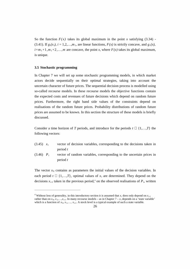
3.5 Stochastic programming

In Chapter 7 we will set up some stochastic programming models, in which market

actors decide sequentially on their optimal strategies, taking into account the

uncertain character of future prices. The sequential decision process is modelled using

so-called recourse models. In these recourse models the objective functions contain

the expected costs and revenues of future decisions which depend on random future

prices. Furthermore, the right hand side values of the constraints depend on

realisations of the random future prices. Probability distributions of random future

prices are assumed to be known. In this section the structure of these models is briefly

discussed.

Consider a time horizon of T periods, and introduce for the periods t ∈ {1,…,T} the

following vectors:

(3.45) xt vector of decision variables, corresponding to the decisions taken in

period t

(3.46) Pt vector of random variables, corresponding to the uncertain prices in

period t

The vector x0 contains as parameters the initial values of the decision variables. In

each period t ∈ {1,…,T}, optimal values of xt are determined. They depend on the

decisions xt-1 taken in the previous period,4 on the observed realisations of Pt, written

4 Without loss of generality, in this introductory section it is assumed that x t does only depend on x t-1

rather than on x0, x1,…,x t-1. In many recourse models – as in Chapter 7 – x t depends on a ‘state variable’which is a function of x0, x1,…, xt-1. A stock level is a typical example of such a state variable.

27

as pt, and on the expected future revenues which depend on the distribution of the

random future prices Pt+1,…, PT. Simultaneously, for each possible realisation of

Pt+1, Pt+2,…,PT, optimal values of xt+1, xt+2,…,xT are determined as well. Write this

as xt+1(Pt+1), xt+2(Pt+2),…,xT(PT). These decisions on future strategies, which are

expected to be optimal, are of a preliminary nature. They can be revised in period t+1,

when the realisations of Pt+1, i.e. pt+1, are observed, and new information comes

available on the probability distribution of Pt+2. The decision structure and the

deterministic and stochastic elements for the decision on x1 are illustrated in Figure

3.2.

xt−1 xt x Pt t+ +1 11 6pt P pt t+11 6 P p Pt t t+ +2 1,1 6

Figure 3.2: Recourse model: illustration of decisions taken in period 1: x1 depending

on x0 and observed price p1, preliminary decisions on x2,…,xT on random prices

P2,…,PT.

It is assumed that the random variables of Pt, for t ∈ {1,…,T}, have a finite discrete

probability distribution. Assume without loss of generality that P1, P2,..., PT, are

independent random variables. In Chapter 9, the stochastic programming models will

be reformulated for conditional probability distributions. Introduce for all t ∈{1,…,T} the set K t, containing the number of possible realisations of Pt. Define for t

∈ {1,…,T} the vector ptk , as the vector of possible outcomes of Pt for a k ∈ K t.

Define for each t ∈ {1,…,T}:

(3.47) Pr P p ft tk

tk

= =2 7 , k ∈ K t.

with probabilities ftk satisfying ft

k ≥ 0 and f tk

k Kt∈∑ = 1.

28

For each period t, the values of the decision variables xt and the preliminary decision

variables xt+1(Pt+1), xt+2(Pt+2),…,xT(PT) are based on the maximization of an

objective function, which consists of the net revenues in period t and the expected net

revenues in future periods. The value of the objective function depends on the

decisions taken in the previous period, xt-1, and the observed value of pt. In the theory

of recourse models, the value of the objective function as a function of pt and xt-1 is

called the value function. Define zt(xt-1,pt) the value function of the decision problem

of period t. The decision problems discussed in Chapter 7 can in short be written as,

for period t ∈ {1,…,T}:

(3.48) z x p Max c p x Ez x P W x T x h p xt t tx

t t t t t t t t t t t t tt

− + + −= + + = ≥1 1 1 1 0, , , ,1 6 1 6 1 6 1 6> C

where Ezt+1(⋅) refers to the expectation of zt+1(⋅) with respect to Pt+1, and zt+1(⋅) is the

value function of the decision problem for period t+1.5 We assume that zT+1(⋅) = 0. Wt

and Tt are matrices, ht(pt) is a vector depending on pt, and ct(pt,xt) is the net revenue

in period t. It is assumed that ct(pt,xt) is a function in xt, some parameters in the

function depend on pt. The vector xt contains the necessary slack variables, so that the

constraints can be written as equalities. Define xtk+1 the vector of preliminary decision

variables in period t+1 for a price realisation ptk+1 of Pt+1, for k ∈ K t+1. For period t, a

given value of decision variable xt, and realisations pt

k

+1, k ∈ K t+1, it may be written:

Ez x P f z x p

f Max c p x Ez x P

W x T x h p x

t t t tk

t t tk

k K

tk

k Kx

t tk

tk

t tk

t

t tk

t t t tk

tk

t

ttk

+ + + + +∈

+∈

+ + + + + +

+ + + + + +

=

= +�!

+ = ≥ "$#

+

++

∑

∑

1 1 1 1 1

1 1 1 1 2 1 2

1 1 1 1 1 1

1

11

0

, ,

, ,

,

1 6 3 8

3 8 3 8>

3 8 L

5 zt+1(⋅) refers to the corresponding expression zt+1(x t, Pt+1). (⋅) is introduced to simplify the notation,when no misunderstanding is possible.

29

(3.49) = +

%&K'K

+ = ≥

++

+∈

+ + + + + +

+ + + + + +

∑Max f c p x Ez x P

W x T x h p x

xtk

k Kt t

ktk

t tk

t

t tk

t t t tk

tk

tk

t1

1

1 1 1 1 2 1 2

1 1 1 1 1 1 0

, ,

,

3 8 3 8

3 8 L

In (3.49) Ezt+2(⋅) refers to the expectation of zt+2(⋅) with respect to Pt+2, and zt+2(⋅) isthe value function of the decision problem for period t+2. It follows that the recourse

problem (3.48) - (3.49) is equivalent to the following model:

(3.50) z x p Max c p x f c p x Ez x P

W x T x h p W x T x h p x x

t t tx x

t t t tk

t tk

tk

t tk

tk K

t t t t t t t tk

t t t tk

t tk

t tk

t

- + + + + + + +

³

- + + + + + +

= + +

%&K'K+ = + = �

+

+

Ê1 1 1 1 1 2 1 2

1 1 1 1 1 1 1

11

0

, , , ,

, , ,

,1 6 1 6 2 7 2 7

1 6 2 7 L

For realisations ptl+2 of Pt+2, for l ∈ K t+2, and period t+1 decision xt

k+1, Ezt+2(xt

k+1,

Pt+2) can be written analogous to model (3.49).

As an illustration of the structure of the decision problems if a short time horizon of

three periods is considered, i.e. T = 3, we write the three decision problems for the

periods 3, 2, and 1:

(3.51) z x p Max c p x W x T x h p xx

3 2 3 3 3 3 3 3 3 2 3 3 33

0, , ,1 6 1 6 1 6> C= + = ≥

(3.52) z x p Max c p x f c p x

W x T x h p W x T x h p x x k K

x x

k k k

k K

k k k

k2 1 2 2 2 2 3 3 3 3

2 2 2 1 2 2 3 3 3 2 3 3 2 3 3

2 33

0

, , ,

, , , ,

,1 6 1 6 2 7

1 6 2 7 L

= +

%&K'K+ = + = � ³

³

Ê

30

(3.53)

z x p Max c p x f c p x f c p x

W x T x h p W x T x h p

W x T x h p x x x k K l K

x x x

k k k l l lk

l Kk K

k k

lk k l k lk

k lk1 0 1 1 1 1 2 2 2 2 3 3 3 3

1 1 1 0 1 1 2 2 2 1 2 2

3 3 3 2 3 3 1 2 3 2 3

1 2 332

0

, , , ,

, ,

, , , , ,

, ,1 6 1 6 2 7 2 7

1 6 2 7

2 7 C

= + +

���

���

%&K'K+ = + =

+ = � ³ ³

³³

ÊÊ

In (3.53) xlk3 represents the preliminary decision variable x3 in period 3 for price

realizations pk2 and pl

3 in period 2 and 3.

If, for t = 1,2,3, xt is a n-dimensional vector, Wt and Tt m×n-dimensional matrices,

ht(pt) an m-dimensional vector depending on pt, and the set K t contains kt elements,

then model (3.53) is a model with n(1+k2(1+k3)) decision variables and

m(1+k2(1+k3)) constraints. These models are in fact large scale mathematical

programming models of the form:

(3.54) Max c y Wy h yy

1 6< A= ≥, 0

with y a vector of decision variables, c(y) a function in y, W a matrix, and h a vector.

Optimal solutions of the recourse models

To derive some properties of the optimal solution of these models, the same methods

can be used as discussed in the previous sections. As an illustration, we discuss the

Kuhn-Tucker conditions for model (3.52). For the other models, the approach is

similar. Introduce the vectors λ 1, λ 2k , for k ∈ K2, consisting of the Lagrange

multipliers of the constraints of model (3.52). Define L x x k Kk k1 2 1 2 2, , ,λ λ ∈3 8 the

Lagrange function of (3.52) as a function of x xk k1 2 1 2, , ,λ λ for all k ∈ K2:

31

(3.55)

L x x k K c p x f c p x

W x T x h p W x T x h p

k k k k k

k K

T k T k k

k K

1 2 1 2 2 1 1 1 2 2 2 2

1 1 1 1 0 1 1 2 2 2 2 1 2 2

2

2

, , , , ,λ λ

λ λ

∈ = + +

+ + − + + −

∈

∈

∑

∑

3 8 1 6 3 8

1 6 3 8

Recall that, for t ∈ {1,2} and k ∈ K2, x xk1 2, are n-dimensional vectors, the matrices

Wt and Tt are of dimension m×n, and ht are m-dimensional vectors. The multipliers λ 1

and λ 2k are m-dimensional. Define xj1 the jth element of the vector x1, for j ∈

{1,…,n}. x jk2 and λ λ

i ik

1 2, , for i ∈ {1,…,m}, j ∈ {1,…,n} are defined analogously.

Wij1 is defined as the element on the ith row and jth column of the matrix W1, for i ∈{1,…,m}, j ∈ {1,…,n}. Wij2, T ij1, and Tij2 are defined analogously. Furthermore,

define Wj1 as the jth column of the matrix W1, for j ∈ {1,…,n}. Wj1 is a m-

dimensional vector. Wj2, T j1, and Tj2 are defined analogously. Referring to (3.38) −(3.40), the necessary conditions of optimality can be written as:

(3.56) xL

x

L

xx j nj

j jj1

1 110 0 0 1

∂∂

∂∂

= � � ³, , ,...,: ?

(3.57) xL

x

L

xx j n k Kj

k

jk

jk j

k2

2 22 20 0 0 1

∂∂

∂∂

= � � ³ ³, , ,..., ,: ?

It follows that for j ∈ {1,…,n}, k ∈ K2:

(3.58)

if then

if then

xc

xp x W T

xc

xp x W T

jj

Tj

k T

jk K

jj

Tj

k T

jk K

11

11 1 1 1 2 2

11

11 1 1 1 2 2

0 0

0 0

2

2

= + + ≤

> + + =

%

&KK

'KK

∈

∈

∑

∑

∂∂

λ λ

∂∂

λ λ

,

,

1 6

1 6

32

(3.59)

if then

if then

x fc

xp x W

x fc

xp x W

jk k

jk

k k k T

j

jk k

jk

k k k Tj

2 22

22 2 2 2

2 22

22 2 2 2

0 0

0 0

= + �

> + =

%

&KK

'KK

∂∂

λ

∂∂

λ

,

,

2 7

2 7

In the models discussed in Section 7.1, the function ct(pt,xt) is a linear function

ct(pt,xt) = dt(pt)⋅xt, with dt(pt) a vector which is, without loss of generality, linear in

pt. In the models discussed in Section 7.2, the function ct(pt,xt) is a non-linear

function. The functions ct(pt,xt) and matrices Wt and Tt will be such that λ 2k ,

following from (3.59), can easily be substituted in (3.58). This results in a number of

elegant properties indicating the influence of the expected future prices on the current

optimal strategies (see Section 7.2).

33

4 Supply functions, demand functions and equilibrium

One of the objectives of building a spatial equilibrium model is to analyse the

functioning of the agricultural market system and the rationale for government

intervention on agricultural markets. The standard analysis of agricultural markets is

based on the microeconomic analysis of the behaviour of agricultural producers and

consumers. Producers are supposed to maximize profits and consumers to maximize

utility. From these assumptions demand and supply can be derived as a function of

prices. If markets are perfectly competitive, supply and demand will be in equilibrium

and equilibrium prices and quantities can be generated using supply and demand

functions. In standard economic theory it is usually assumed that producers sell all

production. In developing countries, however, many farmers consume on-farm a large

part of their own production. Therefore, production and consumption decisions are

interrelated, and can not always be analysed separately. Household models can be

applied to determine simultaneously production, consumption, sales and purchases of

agricultural households.

This chapter deals in particular with supply and demand functions. Their derivation

and properties will be shortly reviewed. Furthermore, the need to analyse

simultaneously supply and demand decisions will be shortly discussed. Finally, some

basic concepts of a market equilibrium will be discussed. For further reading on these

subjects see e.g. Varian (1992) and Nicholson (1995).

4.1 Supply functions

In standard economic theory it is supposed that goods are produced by firms which

maximize net profits, i.e. the difference between revenues received from selling the

produce and production costs incurred. Consider a firm producing one good. Let p be

the given price per unit, x the quantity to be produced and sold by the firm and c(x)

the costs of producing x. The question how much the firm should supply corresponds

to determining x by solving:

34

(4.1) W(p) = Max px c x xx

− ≥1 6< A0

W(p) gives the firm’s optimal profit as a function of prices, and is called the profit

function. Usually, it is assumed that c(x) is twice differentiable, and that it costs

more to produce more, so c′(x) > 0, and that the costs to produce one unit extra are

higher the more is produced, so

(4.2) c″(x) > 0

This last condition excludes economies of scale, so costs per unit can not be reduced

if more is produced. If the cost function is differentiable and satifies c′(x) > 0 and

c″(x) > 0, then the assumption of profit maximization induces that the profit function,

W(p), is non-decreasing, convex and continuous in output prices. Let x be the

optimal production level. Given prices p, the firm can easily derive the optimal

production x by solving (4.1). Call F(x)=px - c(x), then necessarily holds, see (3.2)

and (3.3):

xdF

dxx1 6 = 0,

dF

dxx1 6 ≤ 0

So,

(4.3) if x = 0, then F ′ (0) = p – c′ (0) ≤ 0

(4.4) if x > 0, then F ′(x) = p – c′(x) = 0

The solution x = 0, i.e. zero production, may be excluded by postulating, see (4.3):

(4.5) p > c′ (0)

So the (interior) solution x satisfies, see (4.4):

35

(4.6) p – c′(x) = 0

This shows that in the optimum, marginal revenues equal marginal costs. Stated

otherwise, profit is optimal if the revenues provided by the last unit sold, equal the

costs of the last unit produced. The marginal revenues equal the product price. The

optimization problem (4.1) gives for each price p a different optimal supply, x. x as a

function of p can now be interpreted as the supply function. This function gives the

firm’s most profitable production plan x as a function of price p. Writing the supply

function as x(p), it follows from (4.6) that

p - c′(x(p)) = 0

Since c(x) is differentiable, x(p) is differentiable in p. It then follows from

differentiating to p that:

1 0− ′′ =c xdx

dp1 6

implying that supply on food markets increases when prices increase, i.e.

(4.7) dx

dp c x=

′′>1

01 6 , due to (4.2)

In economic analysis one often uses a measure for the responsiveness of supply to

price changes. The price elasticity of supply measures the percentage change in

supplied quantity as a result of a percentage change in the goods’ price:

ε ps dx

dp

p

x=

36

Due to (4.7), spε > 0. Property (4.7) is not at all evident. Farmers in developing

countries who consume a large part of their production on-farm, are often obliged to

sell a part of their harvest in order to repay debts or to pay for daily important

expenses, even if they are in a food shortage situation. If a farmer needs a certain

amount of money m, he may sell a quantity x = m/p, so dxdp < 0, and s

pε < 0 . This

result differs from (4.7), since the objective function of such a farm household is

different from the profit maximizing objective of the firm discussed in this section.

Their objectives will be more concerned with satisfying household food security or

maximizing household utility. In section 4.3 some short notes will be made on

modeling household behaviour.

Example: Consider a quadratic cost function: c(x) = ax + ½bx2, with a>0, b>0. If

(4.5) is satisfied, p>a. For given price, p, profit can be written as: F(x) = px − ax

½bx2, and the supply function can be derived by (4.6): x = -a/b + p/b.

4.2 Demand functions

In a similar way the demand function of an individual consumer consuming a number

of goods is determined. In the analysis of consumer behaviour, it is studied how a

consumer chooses what to consume if (s)he can choose between various goods with

different prices and if (s)he is confronted with a limited income. Consumers have

preferences on the consumption of different goods. Consider a situation with k

different goods. Introduce the vector of consumed goods, y = (y1. . .yk) , with yi the

consumption of good i, i =1,. . . ,k. To the consumption of each bundle of goods, y, a

level of satisfaction is associated, called utility. A continuous utility function, u(y),

can be defined, which orders the consumers’ preferences. For each possible bundle of

goods, y, consumers get a certain level of utility u(y). In micro-economics it is

usually supposed that a consumer always chooses the most preferred bundle of goods

from the set of afordable alternatives. These alternatives depend on the available

budget. Expenses to the purchase of bundle y, may not exceed the available budget m.

37

Let π be the vector of prices the consumer has to pay when he purchases the goods on

the market. This is given for the consumer. Now the consumer problem of preference

maximization can be defined as:

(4.8) v(π,m) = Max u y y m yy

0 5< Aπ � �, 0

where v(π,m) is the indirect utility function. This function gives the maximum utility

as a function of price π and income m. Usually it is assumed that u′(y) > 0 and u″(y)

< 0. This means that utility increases if more is consumed, and that the increase of

utility by consuming one extra unit decreases if consumption increases. The

Lagrangian for the consumer problem can be written:

(4.9) L = u(y) + λ (m - πy),

with λ the Lagrange multiplier. Write the price of good i as πi , i = 1, ..., k. Let yi be

the optimal demand of good i, i = 1,…,k, and y = (y1,…,yk) be the vector of optimal

demanded goods. If the utility function is differentiable, then the optimal solution of

(4.8), y, has to satisfy the optimality conditions - see (3.34) - (3.41) :

yL

yyi

i

∂∂

1 6 = 0 ,∂∂

L

yy

i

1 6 ≤ 0 , yi ≥ 0, i = 1,…,k

λ ∂∂λL

y1 6 = 0 ,∂∂λL

y1 6 ≥ 0 , λ ≥ 0

Write ∂∂u

yy1 6 = ′u yi 1 6 . Then the above optimality conditions imply,

(4.10) πi ii

k

y m=∑ ≤

1

(4.11) if yi = 0, then necessarily ′ − ≤ui i0 01 6 λπ , i =1,2 ,…,k

38

(4.12) if yi > 0, then necessarily ′ − =u yi i1 6 λπ 0 , i =1,2 ,…,k

Assume that in the optimum of (4.8) y > 0 and π y = m, so that (4.10) and (4.12) have

to be satisfied. Multiply (4.12) with yi, sum over the number of goods, and fill in π⋅y= m to get the inverse demand function (i.e. the price as a function of demand and

income):

(4.13) πii

j jj

ky m

mu y

u y y

,1 6 1 6

1 6=

′

′=

∑1

Using the indirect utility function (4.8) it can also be shown that (see Varian,

1992:106, 149):

(4.14) y m

v m

v m

v m

v m

m

ii

jj

j

kiπ

∂ π∂π

∂ π∂π

π

∂ π∂π

∂ π∂

,

,

,

,

,1 6

1 6

1 6

1 6

1 6= = −

=∑

1

A type of utility function that is often used in applied economics is the quasilinear

utility function. With this utility function, simple demand functions can be derived. A

utility function, is quasilinear if it is linear in one of the goods, i.e. if it can be written

as:

),...,(),...,,(~2121 kk yyuyyyyu +=

Consider for simplicity a situation with 2 goods, y0 and y, where the variable y0 is the

amount of ‘money’, and the variable y is the amount of cereals consumed. Suppose πis the (given) price for cereals. Note that y and π are not vectors in this example.

39

Suppose that the ‘price’ for money is 1, π0 = 1. The consumer problem (4.8) can now

be written as:

(4.15) Max y u y y y m y yy y0

0 0 00 0,

, ,+ + ≤ ≥ ≥1 6< Aπ

In the optimum, all income will be spent on cereals and money, πy + y0 = m. If

income is large, the consumer will consume good y until marginal utility of

consuming y is smaller then marginal utility of consuming y0, i.e. until u′(y) < 1. The

remainder of income will be spent on consuming y0. In this case the constraint may be

substituted in the objective function. The problem may now be reduced to the

maximisation problem:

(4.16) Max u y y yy

1 6< A− ≥π 0

In that case, the solution will be independent of m. If the problem is written in this

way, it can be given a special interpretation which resembles the producer problem in

section 3.1. Utility u(y) may be interpreted as the ‘revenues of consuming y’ and π⋅yas the ‘costs of consumption’. So, (4.16) conveys a situation in which ‘revenues’

minus ‘costs’ are maximized. Analogous to section 2.1, we find two classes of

solutions, depending on whether the optimal demand y > 0 or y = 0. The solution of

(4.15) has a convenient form, if we find an interior solution, y > 0:

(4.17) u′(y) = π

which simply says that the marginal utility of consumption is equal to the price of the

good. This utility function, thus, results in a simple demand structure, and simplifies

the analysis of market equilibrium. Note, however, that this only holds for large

enough levels of income. If income is too low such that all income will be spent on

consuming y, and y0 is zero, (4.17) is not valid. Another feature of the quasilinear

40

utility function is that the indirect utility function (4.8) can be written as (Varian,

1992: 154):

(4.18) v(π,m) = v(π) + m

This is a special case of the so-called Gorman form. In section 4.4 this will be further

discussed. The demand function (4.14) for good y can now be written in the following

convenient form:

(4.19) πππ

∂∂

=)(

),(* vmy

Example: Linear expenditure system

As an example of how demand functions can be derived, consider the often used

utility function of the form:

u(y) = a yi i ii

k

ln −=∑ γ1 6

1

where yi > γi . In this utility function k goods are considered and γi is the minimum

consumption requirement of good i. The utility maximisation problem is:

v(π ,m) = Max u(y) s.t. π y = m.

Solving this problem, see Section 3.2, gives the following demand function:

yi = γπ γ

πi i

i ii

k

i

am

+−

=∑ 1

(see Varian 1992, p. 212). This demand system is often used in applied economics. A

drawback is, however, that it implies a linear relation between demand and income

41

(linear Engel functions) and that it can at best be true over a short range of variation

(Sadoulet and De Janvry, 1995). ~

Next to a measure for the price responsiveness of supply, economists also use a

measure for the responsiveness of demand to price or income changes. Analogous to

the price elasticity of supply, the price elasticity of demand for a good i measures the

percentage change of demand, *iy , after a percentage change of the goods price, πi :

(4.20) ε ∂∂π

πid i

i

i

i

y

y=

Demand of a good i depends not only on its own price, but also on the price of the

other goods j. So, the demand function has to be written as: yi = y i(π1,…,πi,…,πk), if

k goods are considered. The cross-price elasticity of demand, dijε , measures the

responsiveness of demand of good i after a price change of good j. Also the income

elasticity, η i , is often calculated. This measures the responsiveness of demand of

good i, if income changes.

(4.21) ε ∂∂π

πijd i

j

j

i

y

y=

(4.22) η ∂∂i

i

i

y

m

m

y=

Goods can be categorized according to the signs and magnitudes of the elasticities. A

good is a normal good if the goods’ price elasticity of demand is negative. Demand is

said to be elastic if diε < -1 . This means that demand decreases more then

proportionally if the price increases. If demand decreases less then proportionally

after a price increase, i.e. if -1 < diε < 0, then demand is said to be inelastic. Most

food crops have inelastic demand. If demand for a good decreases if its price

42

decreases, i.e. diε > 0, we call the good a Giffen good. An example are potatoes in the

Netherlands, or any other staple food crop which serves as base ingredient in daily

meals. If the price of the basic food decreases, people have to spend less money on

their basic expenditures, and consequently their purchasing power increases.

Accordingly, they shift their consumption pattern to the consumption of less basic and

more luxury foods, which are more appreciated (see Heijman et al., 1991). Two goods

i and j are gross complements if demand of good i decreases if the price of good j

increases, i.e. if dijε < 0 . An example are tobacco and cigarette paper. Goods are

gross substitutes of each other if demand of a good increases if the price of the other

good increases, i.e. if dijε > 0. An example of two substitutes are maize and rice in

West Africa. If the price of maize increases, maize consumption will be substituted by

rice consumption. Furthermore, goods are called normal goods if the income

elasticity, η i is positive. The good is a necessary normal good if 0 < η i < 1, and a

luxury normal good if η i > 1. A good is an inferior good if η i < 0. Examples of

inferior goods are basic food crops such as potatoes in the Netherlands and millet and

sorghum in some regions in West Africa. If income increases, people will shift their

consumption to more luxury goods (Varian, 1992).

4.3 Seperability of supply and demand decisions

In the previous discussion it was supposed that producers sell all their produce, and

consumers have to purchase all goods they consume. In developing countries, farmers

often save a part of their harvest, to be consumed on-farm, and only a small part of

production is sold. They integrate in the household decisions regarding production

and consumption. For that reason, we can not allways estimate supply and demand

functions the way we did above, but they have to be determined on an integrated way

in a household model.

Such an integrated analysis is not necessary if consumer prices and producer prices

are the same, and the markets function well. Then production and consumption

43

decisions can be analysed separately. In that case households are indifferent between

consuming their own produce or selling it to rebuy what they need for their own

consumption. The value of the consumed goods will in both cases be the same. In the

first case, if households consume their own produce, they still have to sell a part of

the harvest to pay for the production costs. Suppose the household produces a

quantity x* of a consumption good, which costs c(x* ) . Let the price be p. To cover

the production costs, the household has to sell a quantity c(x* )/p, and they can

consume a quantity x* − c(x* )/p. In the second case, if the household sells all

produce and rebuys the consumption, the income from agriculture will be m = px*

− c(x* ) . Suppose no income is earned from other sources, then a quantity m/p = x*

− c(x* ) /p can be purchased. This shows that consumption will be the same in both

cases. In this case, a supply function, x* (p) , can be derived analogous to section 4.1.

Using this supply function income can be calculated, m(p) = px* (p) − c(x* (p)),

which is an input in the consumer problem to determine demand.

However, if some markets fail, or if transaction costs exist, production, supply and

consumption decisions are no longer separable. Define p and π to be producer and

consumer prices of a good, respectively, with p < π. If producers consume, in this

case, a part of their produce on farm, they can consume a quantity x* − c(x* )/p. On

the other hand, if producers would sell all produce and rebuy their consumption, they

could only consume m/π = px* /π − c(x* )/π. So, in order to reflect reality,

production, supply, demand and consumption decisions have to be analysed

simultaneously, which can be done in a household model. In such models it is

supposed that a household optimizes utility. Consumed quantities may be partly

purchased and partly self produced. Decisions are constrained by a money income

constraint, labour time constraints and a production function that calculates

production as a function of inputs (see e.g. Ellis, 1993; Sadoulet and de Janvry, 1995).

The household allocates labour time of the members of the household between home

production, wage work, and leisure. The money income constraint is determined by

the time allocated to wage work, and revenues from own production. Many household

models have been built. Maatman et al. (1996) recently built one for a representative

44

household on the Central Plateau in Burkina Faso. Their linear programming model

evaluated production, consumption, trade and storage decisions of one houshold.

They analyzed, in a very detailed manner, the different production possibilities of a

household, and included the household’s consumption patterns. The model clearly

showed the interdependance between production and consumption decisions for

subsistence farmers in West Africa.

In spite of this, we suppose in the next chapters that supply and demand decisions can

be taken seperately. This is defensible since: 1) Subsistence households in many

developing countries safeguard a part of their harvest for own consumption; only a

small part may be sold on the market (see also Section 8.1.3); 2) In many developing

countries, supply and demand decisions in an extended family are taken by different

persons, with each their own, sometimes conflicting, objectives (see e.g. Maatman et

al., 1996).

4.4 Equilibrium

In section 4.1 and 4.2 supply and demand functions for a single good have been

derived, that represent the producer’s and consumer’s reaction on prices. Individual

consumers and producers have no influence on prices, but the total supply and

demand of all consumers and producers together certainly influence prices. Consider

a situation with k consumers and n producers. Suppose that markets are perfectly

competitive, and that supply and demand decisions can be analyzed separately. The

functions xi(p) and yj(π,mj) render the optimal supply and demand of for example

cereals, for a producer i and consumer j, for a certain producer price p, consumer

price π, and income level mj , for i = 1, ..., n, j = 1, ..., k. Total supply on the market is

the sum of all supplies. Define the market supply function x(p) = x pii

n 0 5=∑ 1

.6 Since

each producer chooses a production level such that marginal costs equal the price (see

6 Note the different denotation of the variables x, xi, y, and y j in this section and the Sections 4.1 and 4.2.

45

(4.6)), each producer must have the same marginal costs at price p, pxc ii =′ )( * . The

market demand function can be defined as y(π,m1,...,mk) = y mj jj

kπ,2 7

=∑ 1. In general

this demand function does not have properties like (4.14). It can be proven that the

aggregate demand function has the same properties as the individual demand

functions, if the indirect utlity function is of the Gorman form. This means that it can

be written as: vj (π,mj ) = a j (π) + b(π)mj , and aggregate indirect utility is: v(π,m) =

a jj

kπ0 5

=∑ 1 + b(π)mj, with m = mjj

k

=∑ 1. The quasilinear utility function is a special

case of the Gorman form, for which b(π)= 1 (see (4.18)).

Producers and consumers can sell and purchase all supply and demand only if the

market is in equilibrium. A market equilibrium in a closed economy can be defined as

follows: prices, p and π, and levels of supply and demand, x and y, exist for which

market demand equals market supply, so x(p) = y(π) , such that no producer or

consumer does have the tendency to change his decisions. This implies that the

producer will supply xi(p) and the consumer will demand yj(π,mj). One condition for

such an equilibrium to exist is that exit from or entrance to the market are free.

We consider two situations:

(i) Producers and consumers sell and buy on one market. There is one market

price, so p = π. This postulate together with the equilibrium condition

determines the market price p, which follows from x(p) = y(p). Note that no

trader is explicitly introduced, and that no trading costs are involved.

(ii) A trader buys from the producers at a producer price p, and sells to the

consumers at the consumer price π. What he buys is also sold. The consumer

price is assumed to be an amount γ higher than the producer price, so π = p +

γ. The equilibrium condition reads x(p) = y(π). Both conditions together

determine prices and produced and consumed quantities: x(p) = y(p+γ).Both conditions are illustrated in figure 4.1.

46

In stead of postulating p = π in situation (i), we can also rewrite the consumer and

producer problem. Suppose that producer i can produce a quantity of cereals xi with

costs ci (xi ) , i = 1, ..., n. Consumer j can choose between consuming a quantity y0j of

good 0 (money) and a quantity of cereals yj , j = 1, ..., k. Preferences for consumer j

are ordered by a quasilinear utility function (see (4.15)):

jjj yyu 0)( + , j = 1,…,k

In stead of postulating market equilibrium to determine output, we maximize a

welfare function which measures total consumer utility, subject to a money balance

and a production balance:

x,y

x=y

x(p)

y(B)

p=B p,B B=p+( p,Bp

Situation (i) Situation (ii)

x=y

x,y

x(p)

y(B)

Figure 4.1: Illustration of equilibrium prices and produced and consumed quantities

for situation (i) and (ii) as desribed in the text.

47

(4.23)

kjniyyx

yx

ymxcts

yyu

jji

k

jj

n

ii

k

jj

k

jj

n

iii

k

jj

k

jjj

,...,1;,...,1,0,0,0

)(..

)(max

0

11

10

11

10

1

==≥≥≥

=

−=

+

∑∑

∑∑∑

∑∑

==

===

==

If each mj is supposed to be large, this problem may be rewritten as:

(4.24)

kjniyx

yxts

xcmyu

ji

k

jj

n

ii

n

iii

k

jj

k

jjj

,...,1;,...,1,0,0

..

)()(max

11

111

==≥≥

=

−+

∑∑

∑∑∑

==

===

If λ is the lagrange multiplier on the constraint, the optimal solution xi, yj of (4.24)

has to satisfy, see also (3.12) and (3.13):

(4.25) ′ = = ′ ∀u y c x i jj j i i3 8 1 6λ , ,

In section 4.1 and 4.2 we have seen that producers supply a quantity such that

marginal costs equal the producer price, ′c xi i1 6 = p, and consumers demand a quantity

such that marginal utility equals the consumer price, ′u yj j3 8 = π. So, (4.25) shows

that welfare is optimal if p = π.

It is possible to rewrite the welfare function in (4.24) in a form which is common in

economics. First we rewrite the first term in (4.24), the summation of individual

48

utility. (4.17) showed that ′u yj j3 8 = π. Because the utility function is differentiable,

we can introduce the inverse demand function for consumer j, πj (yj ) . Suppose u j (0)

= 0, then:

(4.26) u j(yj) = π ξ ξj

y

dj

1 60I

By making use of π = π(yj) and of partial integration, the last term may be written as:

π ξ ξ π ξπ ξ ξ π ϑ ϑπ

j

y

j j

y

j jd y d y y dj j

1 6 1 6 1 60 0I I I= − ′ = +

∞

Total utility from consuming cereals can be written as:

(4.27)

u y d y y d

y y d y y d d

j jj

k

j

y

j

k

j jj

k

jj

k y

j

3 8 1 6 1 6

1 6 1 6 1 6

= =

∞

=

=

∞ ∞

∑ I∑ I∑

∑I I I

= = +�

!

"

$##

=

+�

!

"

$##

= +�

!

"

$##

=

1 01 1

1 0

π ξ ξ π ϑ ϑ

π ϑ ϑ π ϑ ϑ π ξ ξ

π

π π

Furthermore, rewrite the last term in the objective function of (4.24), the summation

of production costs. Suppose ci (0)=0, and introduce the inverse supply function for

producer i, p i (xi ). Given that ′c xi i1 6 = p - see (4.6) - for all i =1,2 ,…,n, we can

write:

(4.28) ci(xi) = p di

xi

ζ ζ1 60I

Since x(p) = x pii

n 0 5=∑ 1

we can write total production costs:

49

(4.29)

c x p d px p x d

px x d px x d p d

i ii

n

i

x

i

n

i i

p

i

n

ii

np p x

i

1 6 1 6 1 6 1 6

1 6 1 6 1 6

= = =

=

∑ I∑ I∑

∑I I I

= = +�

!

"

$##

+�

!

"

$##

= +�

!

"

$##

=

1 01 01

10 0 0

ζ ζ η η

η η η η ζ ζ

Because the summation of individual income, mjj

m

=∑ 1, has no influence on the

solution of (4.24) it may be skipped from the formulation. Using (4.27) and (4.29),

problem (4.24) can be rewritten as:

(4.30)

Max u y c x y x y x

Max d p d y x y x

y xj j

j

k

i ii

n

jj

k

ii

n

j i

y x

y x

j i,

,

, ,

, ,

3 8 1 6

1 6 1 6

= = = =

Ê Ê Ê Ê

I I

- = � �

%&K'K

()K*K=

- = � �

%&K'K

()K*K

1 1 1 1

0 0

0 0

0 0π ξ ξ ζ ζ

This gives the well known problem of maximising consumer plus producer surplus.

Consumer surplus is defined as:

π ξ ξ π1 6d yy

0I −

In fact, consumer surplus measures the difference between the optimal benefits from

consuming y and the expenditures to purchase it. Producer surplus is defined as:

px p dx

− I ζ ζ1 60

50

This surplus reflects, in fact, the optimal profits from producing x. Since in the

optimum y = x and p = π, the terms π⋅y and p⋅x are the same, and the sum of

consumer and producer surplus gives exactly (4.30). If producer plus consumer

surplus is optimized, the solution is the same as the solution of problem (4.23).

Samuelson (1952) was the first who showed that the surplus concept was relevant in

converting the market equilibrium problem into an optimization problem (Van den

Bergh et al., 1995b). The objective function of this problem is also called a

semi-welfare function.

Note that this derivation only holds for a quasilinear utility function and when all mj

are large. If welfare is defined as aggregate utility, consumer plus producer surplus

gives an exact measure of welfare only if the utility function is quasilinear. In other

cases, it will not be an exact measure. However, it often gives a reasonable

approximation to more precise but also more complicated measures. In the next

chapters the semi-welfare function will play an important role.

51

5 Spatial equilibrium on n markets; one period model

In Chapter 4, we discussed one of the basic concepts of equilibrium models. That is,

the market clears at a certain market price, which means that producer supply and

consumer demand are in equilibrium. This price, and the corresponding supply and

demand levels, are called equilibrium price and equilibrium quantities. In Section 4.4

we saw that a market equilibrium problem can be solved by writing it as an

optimization problem, in which consumer plus producer surplus are maximised. This

surplus is interpreted as ‘semi-welfare’. In the Chapters 5 and 6, this method is

extended, to be able to take into account several regions (Chapter 5) and several

periods (Chapter 6). The equilibrium models for competitive markets presented in the

Chapters 5 and 6, correspond with the methods first formulated by Samuelson (1952),

and discussed extensively and extended by Takayama and Judge (1971). Ever since,

these methods have been applied frequently, especially for agricultural, energy and

mineral resources problems (see e.g. Takayama and Judge, 1971; Judge and

Takayama, 1973; Labys et al., 1989; Guvenen et al., 1990; Roehner, 1995; Van den

Berg et al., 1995). In multi-region and multi-period-models, the concept of (price)

equilibrium requires special attention.

Dealing with equilibrium on spatially seperated, competitive markets, Takayama and

Judge use the term ‘Spatial Price Equilibrium’ (SPE) for a situation where prices and

quantities satisfy the following properties: 1) in each region, there is only one market

producer and one market consumer prices (p and π, see Chapter 4; i.e in any region

prices are homogeneous and unique); 2) there is no excess demand or supply in any of

the regions; and 3) commodities purchased in one region will only be transported to

another region, to be sold there, if the difference between the consumer price in the

importing region and the producer price in the exporting region is at least equal to

transport costs (Van den Bergh et al., 1985, p.50, see also Takayama and Judge, 1971,

p.34). An intertemporal SPE for multi-period equilibrium models, satisfies as well the

following property (see Takayama and Judge, 1971, p. 378): 4) commodities

purchased in a certain region, will only be stored, to be sold later in the same region,

52

if the difference between the consumer price in the selling period and the producer

price in the purchase period is at least equal to storage costs. For the multi-period

situation, excess supply is possible in every period. The surplus will be stored, and

sold in later periods. If a finite time horizon is considered, it is usually assumed that

excess demand and supply are zero in the last period. This means that no stock

remains after the last period. Takayama and Judge optimize in their equilibrium

models ‘semi-welfare’, subject to supply-demand equilibrium on the market. The

welfare optimal prices and quantities, satisfy the properties of a SPE. Takayama and

Judge conclude from this that the models are suitable for analysing price formation on

competitive markets. Why price formation on a competitive market can be decribed

accurately by a SPE, usually receives little attention. Takayama and Judge only

consider the behaviour of producers and consumers. Other market actors playing a

role in market price formation, like traders, are not taken into account explicitly. The

way prices are established on a market with traders, can, however, not be fully

understood if only producers and consumers are considered. The process of price

formation can be made more transparent, if traders are taken into account explicitly.

Traders purchase goods from producers and sell to consumers. A market will clear,

i.e. will be in equilibrium, because traders do only purchase from the producers the

quantities they can sell to the consumers or store for sales in later periods.

Furthermore, traders do only purchase from the producers, transport between the

regions, store, and sell to the consumers, if prices are such that they make no losses.

In the next chapters, we will show that the economic foundations of the SPE and the

equilibrium models of Takayama and Judge can be better comprehended, if also the

behaviour of traders is considered explicitly. We will show that the results of the

equilibrium models satisfy the profit maximizing behaviour of traders. The approach

to deal explicitly with traders’ behaviour will in particular be useful in Chapter 7, in

which the uncertain character of future prices is taken into account. In a situation of

uncertain prices, the definition of price equilibrium as presented by Takayama and

Judge is difficult to apply. By taking into account explicitly the behaviour of traders,

we are able to analyse such situations.

53

In this chapter we discuss an extension of the method of Takayama and Judge (1971),

to analyse cereal price formation and trade flows in a country where cereals are sold

by producers, distributed by traders over a number of regions, and purchased by

consumers. The quantities supplied, demanded and transported by individual

producers, consumers and traders are a function of producer and consumer prices. In

Section 5.1 we discuss the optimal strategies of the agents operating on the cereal

market, if producer and consumer prices are known. In Section 5.2 we set up a spatial

equilibrium model, which results in welfare optimal supply, demand and transport

plans. We will show that the welfare optimal quantites are equal to the aggregate

optimal sales, purchases and transport flows of the individual market agents, at

market equilibrium prices. In Section 5.3, a different market situation is considered,

in which a monopolistic trader determines market prices. A model is discussed to

analyse this situation.

5.1 Strategies of producers, consumers and traders

Consider a situation in which an area of land (e.g. a country) is divided into n regions,

which are numbered i = 1, 2, .., n. In each region is one market, numbered i = 1, 2, ...,

n as well. If a farmer produces cereals, part of it may be stored for home

consumption, the rest is sold on the market. Farmers of region i sell only to traders at

market i, not at other market places and not directly to consumers. At marketplace i,

farmers get a kg-price p i , called the producer price of region i. The total quantity of

cereals sold by the producers of region i is called the producer supply (of cereals) in

region i. Consumers in region i buy from traders at market i. They have to pay a

kg-price πi , called the consumer price. The quantity bought by the consumers of

region i is called the consumer demand in region i. Traders in region i purchase the

producer supply in this region, may transport cereals to regions j = 1,...,n, j ≠ i, where

they sell the consumer demand to the consumers.

54

Strategies of producers and consumers:

We define for i = 1,...,n:

xi producer supply in region i

(5.1) yi consumer demand in region i

p i producer price in region i

πi consumer price in region i

In analogy with Chapter 4 it is assumed that producer and consumer strategies are

reflected by (aggregate) market supply and demand functions, which are given by

xi(p i) and yi(πi). These functions give the producers’ profit maximizing cereal supply

at price p i, and the consumers’ utility optimizing demand at price πi. We prefer to use

here the inverse supply and demand functions p i(xi ) and πi(yi ) rather than xi(p i ) and

yi(pi ). For each region supply and demand functions are assumed to be known. It is

recalled that - see (4.26) and (4.28):

(5.2) u y di i i

yi

1 6 1 6= Iπ ξ ξ0

, i=1,2,…,n

(5.3) c x p di i i

xi

1 6 1 6= I ζ ζ0

, i=1,2,…,n

with

(5.4)

As in

chapter 4 it is assumed that πi(yi) > 0 and p i(xi) > 0, due to the assumptions that

′u yi i1 6 > 0 and ′c xi i1 6 > 0, that the derivatives of πi(yi) and p i(xi) exist and that:

(5.5) 0)( that assumption the todue 0)(

0)( that assumption the todue 0)(

>′′>′<′′<′

iii

iii

xcxp

yuyπ

ui (yi ) utility of consumption of yi by the consumers of region i

ci (xi ) costs of producing xi by the producers of region i

55

Some characteristics of traders’ strategies

In the sections 5.1 and 5.2 it is assumed that the traders operate on a competitive

market. They are all price followers who can not influence prices. The traders

together are called here the aggregated trader, who operates on all n markets.

Introduce the following variables for i,j= 1,...,n, i ≠ j:

qi total quantity of produce purchased by the aggregated trader from the

producers in region i

(5.6) r i total quantity of produce sold by the aggregated trader to the

consumers in region i

q ij total amount of produce transported by the aggregated trader from

region i to region j.

Assume that the (aggregated) trader does not want to have a stock left over, but that

he wants to sell the entire purchase. This means that the quantity he purchases on a

market i plus the quantity transported to this market, has to be equal to the quantity he

sells on market i plus the quantity transported to other markets to be sold there. We

call this the traders’ equilibrium condition for region i:

(5.7) q q r qi j ijj i

n

i i jjj i

n

+ = +=≠

=≠

∑ ∑1 1

Knowing producer and consumer price levels, p i and πi, also producer supply and

consumer demand levels are known, xi = x i(p i) and yi = y i(πi). The quantities the

trader can purchase and sell on the market are bound by these supply and demand

levels, q i ≤ xi and r i ≤ yi. We define the parameter:

(5.8) τ ij costs of transfer of one kg from market i to market j, i,j= 1,...,n, i ≠ j.

56

The costs of transfer, which obviously satisfy τ ij > 0, refer to transaction costs

including transport costs, costs of insurance, contracts, taxes, information collection

etc.. We define:

(5.9) jiij market tomarket from weight ofunit one ing transportof costs

costsation transportexcluding weight ofunit per costson transactiall *

*

ττ

and write:

(5.10) τ ij = τ * + *ijτ

In (5.9) τ* is assumed not to depend on i or j. Without loss of generality it is assumed

here that τ*=0. So τ ij refer to transportation costs only. The value of τ ij depends on the

mode of transport, for road transport on the size of trucks, on the distance between

market i and j, conditions of roads, etc.. Estimates of τ ij for a practical situation will

be discussed in Chapter 8.2. The definition of τ ij deserves further specification. τ ij is

often defined as the costs for the shortest route between market i and j. Here a

different definition is adopted. τ ij is defined as the minimum costs of transport

between market i and market j, i.e. if the cheapest way of transport is chosen. In

transport models, especially in industrialized countries, it is often assumed that

transport costs τ ij =c⋅d ij where d ij is the distance between towns i and j and c the costs

per km. Then the cheapest τ ij corresponds to the shortest distance between town i and

j. In developing countries the situation can be different. Taking the road with the

shortest distance between markets i and j is not necessarily the cheapest way of

transport, for instance if the direct road between market i and j is a dirt road in bad

condition and costs can be reduced by taking a longer tarmac road. In this chapter the

definition of τ ij as costs of transport for the cheapest way of transport will play an

important role. It follows from this definition that for any three different markets, i, j

and s - see Figure 5.1 - minimum costs of transport of one unit of weight between

market i and market j can never exceed the costs of transport if the route is taken from

market i via market s to market j. So it may be written: τ ij ≤ τ is + τ sj, i ≠ j, i ≠ s, j ≠ s.

57

If for the regions i,j and s, i ≠ j, i ≠ s, j ≠ s, τ ij = τ is + τ sj, a trader is indifferent

between transporting directly from region i to j, or to transport first from region i to s

and later from region s to j. The costs will for both possibilities be the same. In order

to avoid this situation and to simplify the mathematical reasoning and proofs later in

this chapter, it will be assumed that the ≤ in the triangle equation above may be

replaced by <, so:

(5.11) τ ij < τ is + τ sj, i ≠ j, i ≠ s, j ≠ s.

The trader’s objective is to maximize profits from cereal purchases, transport and

sales. We are interested in the optimal levels of r i, qi, and qij, if p i, πi, xi and yi, are

known. To show how a trader’s decisions depend on producer and consumer prices,

consider the following decision problem, in which he maximizes his profits subject to

equilibrium conditions and upper bounds:

(5.12)

Max r p q q q q r q

q x r y q i j n j i

r q qi i i i ij ij

jj i

n

i

n

i j ijj i

n

i i jjj i

n

i i i i i j

i i ij, ,;

; ; ; , ,..., ,

π τ- -

�

�

���

�

�

���

%&K

'K

+ = +

� � � � � = ā

()*

=

ā

= =

ā

=

ā

ÊÊ Ê Ê11 1 1

0 0 0 1

i

s

jτ ij

τsj

τ is

Figure 5.1: Schematic representation of three markets i, j and s with the

corresponding costs of transportation. Two situations are illustrated: direct

transportation from market i to market j and transport via market s.

58

Introduce λi the Lagrange multiplier of the equilibrium condition (5.7) in model

(5.12) – see also (3.33). The optimal quantities qi, r i, and q ij, have to satisfy

equilibrium condition (5.7) and the following conditions– see also (3.42) - (3.44):

if q i = 0 then λ i ≤ p i; if 0 < q i < xi then λ i = p i; if q i = xi then λ i ≥ p i;

(5.13) if r i = 0 then λ i ≥ πi; if 0 < r i < yi then λ i = πi; if r i = yi then λ i ≤ πi;

if q ij = 0 then λ j ≤ λ i + τ ij; if q ij > 0 then λ j = λ i + τ ij

From this, we can derive the following properties, which show the influence of the

difference between producer and consumer price levels, on purchased, sold and

transported quantities.

Trader property 5.1: For each region i ∈ {1,...,n}:

a) If πi < p i, then any optimal solution of (5.12) satisfies: q i = 0 or r i = 0.

b) If πi ≥ p i, then an optimal solution of (5.12) exists which satisfies the condition q i

= xi or r i = yi. Nota bene: for πi > p i, any optimal solution of (5.12) has to satisfy this

condition; for πi = p i, other optimal solutions may exist not satisfying this condition.

Proof: see Appendix 1.

Trader property 5.1 can be well understood. If πi < p i, the trader will certainly not

purchase and sell in the same region, since he would only make losses out of this

transaction. If πi > p i, it is obviously profitable for the trader to buy and sell in region

i. In that case he will buy the maximum possible quantity, xi, or sell the maximum

possible quantity, yi, in region i. We can not say that he will buy as much as possible

from the producers in region i to sell to the consumers in the same region. This

depends on producer and consumer prices in the other regions. It may be more

profitable to sell in another region j. We come back to this issue after Trader property

5.3 below. If πi = p i, the only thing we can say, is that the trader would not loose if he

would buy and sell in the same region.

59

Trader property 5.2: Let q i, r j, q ij, j ≠ i, i,j = 1,…,n, be an optimal solution of (5.12).

Let a trader transport from a region i to a region j, so q ij > 0, for i,j ∈ {1,…,n}, i ≠ j,

then:

a) no goods are transported from a region s = 1,…,n, s ≠ i, to region i, qsi = 0

b) no goods are transported from region j to a region s = 1,…,n, s ≠ j, q js = 0.

c) purchases in region i are positive, q i > 0

d) sales in region j are positive, r j > 0.

Proof: see Appendix 1.

q ij was defined – see (5.6) – as the amount transported from region i to region j.

Trader property 5.2 implies that the quantity q ij is purchased in region i and sold in

region j.

Trader property 5.3: For the regions i and j, i,j ∈ {1,...,n}, i ≠ j:

a) If πj < p i + τ ij, then any optimal solution of (5.12) satisfies q ij = 0.

b) If πj ≥ p i + τ ij and q ij > 0, then an optimal solution of (5.12) exists satisfying q i = xi

or r j = y j; for πj = p i + τ ij and q ij > 0 an optimal solution of (5.12) is not necessarily

unique.

Proof: see Appendix 1.

Also Trader property 5.3 can be well understood. If πj < p i + τ ij, the trader can only

make losses from transporting between region i and j. If πj = p i + τ ij, he would make

neither losses nor profits if he would transport between region i and j. If πj > p i + τ ij,

transport between i and j will be profitable. As a consequence, he will buy as much as

possible in region i, xi , or sell as much as possible in region j, yj. Note that it is

possible that qij = 0 if πj > p i + τ ij. If for example, πi - p i > πj - p i - τ ij > 0, selling in

region i will be more profitable than selling in region j.

60

These three Trader properties will play an important role in the next section:

solutions of the equilibrium models to be developed should not violate these

properties, otherwise the found solutions would not be acceptable for the traders.

5.2 Maximization of welfare; perfect competition between traders

In this section we extend equilibrium model (4.30), to take into account transport

between the different regions. We first discuss the set-up and results of the spatial

equilibrium model, in which semi-welfare is optimized for all agents together. In this

spatial equilibrium model optimal values of the following variables are determined

for all regions i = 1,…,n: producer and consumer prices (p i and πi), producer supply

(xi, total quantity sold by the producers), consumer demand (yi, total quantity

purchased by consumers) and total transported quantities to the various regions. We

define for j = 1,…,n and i ≠ j:

(5.14) xij total amount of produce transported from region i to region j.

This optimum is called the market equilibrium solution. Secondly, we show that this

solution is sustained by the individual market agents. This means that the market

equilibrium supplied, demanded and transported quantities, are equal to, respectively,

the aggregate optimal sales of the individual producers, the aggregate optimal

purchases of the individual consumers and the aggregate optimal transport flows of

the traders, at the market equilibrium prices. These individual strategies have been

discussed in the previous section.

In analogy with (4.30), in this section we maximize the sum of total utility minus all

costs made, which has been defined as semi-welfare. The following maximization

problem is solved:

61

(5.15) Max u y c x xy x x

i ii

n

i ii

n

ij ijjj i

n

i

n

i i ij, ,( ) ( )

= = =≠

=∑ ∑ ∑∑− −

1 1 11

Total utility Total producer costsTotal transportation costs

124 34 124 34

1 24 34

τ

where the variables xi , yi , xij, i,j = 1,2, ..., n; j ≠ i have to satisfy the market

equilibrium conditions -see also (5.7):

(5.16) x x y xi j ijj i

n

i i jjj i

n

+ = +=≠

=≠

∑ ∑1 1

, for i = 1,...,n

(5.17) xi ≥ 0, yi ≥ 0, xij ≥ 0, i, j = 1,2, ...,n; j ≠ i.

The utility and cost functions u i (yi ) and ci (xi ) are given in (5.2) and (5.3). In

principle, semi-welfare can also be defined as the sum of the ‘net revenues’ of the

consumers, producer, and traders, with ‘net consumer revenues’ defined as the utility

from consuming yi (i.e. u i(yi)) minus the costs from purchasing yi (i.e. πi⋅yi). This

definition of semi-welfare seems to be more appropriate than the definition in (5.15).

In other words, semi-welfare is:

(5.18) u y y p x c x y p x xi i i ii

n

i i i ii

n

i i i i ij ijjj i

n

i

n

1 62 7 1 62 7− + − + − −�

�

���

�

�

���= = =

≠=

∑ ∑ ∑∑π π τ1 1 11

Net consumer revenues Net producer revenuesNet trader revenues

1 2444 3444 1 244 344

1 244444 344444

(5.18) is equal to (5.15). Because of the properties of utility and production costs, the

objective function (5.15) can be replaced by the integral of the inverse demand

function minus the integral of the inverse supply function minus transport costs – see

(5.2) and (5.3). We arrive at the following maximization problem to be solved:

62

(5.19)

Max d p d x

x x y x x y x i j n j i

y x xi i

x

ij ijjj i

ny

i

n

i j ijj i

n

i i jjj i

n

i i ij

i i ij

ii

, ,( ) ( )

; , , , , ,..., ,

π ξ ξ ζ ζ τ− −�

!

"

$

###

%

&K

'K

+ = + ≥ = ≠

(

)K

*K

I ∑I∑

∑ ∑

=≠

=

=≠

=≠

0 101

1 1

0 1

Since the objective function in (5.15) is a linear combination with positive

coefficients of concave functions - see (5.5) - the objective function is concave.

Referring to the discussion at the end of section 3.4 it can easily be shown that a

global maximum is found and that the optimal values of xi , p i (xi ) , yi and πi (yi ) in

the solution are unique. The values of xij are not necessarily unique. Introduce λi, for i

∈ {1,2, ...,n}, the Lagrange multipliers for the constraints (5.16). The Lagrangean

function may be written as, see (3.33):

(5.20)

L x y x i j n j i

d p d x x x y x

i i ij i

i

y

i

x

ij ijjj i

n

i

n

i i jijj i

n

i i jjj i

n

i

ni i

, , , , ,..., ,

( ) ( )

λ

π ξ ξ ζ ζ τ λ

³ ā =

- -

�

!

"

$

###+ + - -

�

!

"

$

###

I I ÊÊ Ê ÊÊ=

ā

= =

ā

=

ā

=

1

0 0 11 1 11

: ?3 8

L(xi ,yi ,xi j ,λ i | i,j ∈ {1,…,n}, j ≠ i) signifies the Lagrangian function as a function of

xi, yi, xij, and λ i, for all i, j ∈ {1,2, ...,n}, j ≠ i. Let xi, yi, xij, i, j ∈ {1,2, ...,n}, j ≠ i, be

a solution of (5.19). From the Kuhn-Tucker optimality conditions, see (3.33) and

(3.38) - (3.40), follows that:

(5.21) if xi > 0 then ∂∂

L

xi

= −p i (xi ) + λ i = 0

(5.22) if xi = 0 then ∂∂

L

xi

= −p i (0) + λ i ≤ 0

63

(5.23) if yi > 0 then ∂∂

L

yi

= πi (yi ) − λ i = 0

(5.24) if yi = 0 then ∂∂

L

yi

= πi (0) − λ i ≤ 0

(5.25) if xij > 0 then ∂∂

L

xij

= −τ ij + λ j − λ i = 0

(5.26) if xij = 0 then ∂∂

L

xij

= −τ ij + λ j − λ i ≤ 0

Using these conditions we can derive some properties of a solution of (5.19).

Equilibrium property 5.1: For region i ∈ {1,…,n}:

a) In the optimal solution of (5.19), πi (yi ) ≤ p i (xi ) .

b) If in the optimal solution of (5.19), πi(yi) < p i(xi), then xi = 0 or yi = 0.

c) If in the optimal solution of (5.19), supply and demand in region i are both positive,

so xi > 0 and yi > 0, then necessarily p i(xi) = πi(yi).

Proof: see Appendix 1.

Equilibrium property 5.2: In the optimal solution of (5.19), let transport take place

from market i to market j, i.e. xij > 0, with i, j ∈ {1,2, ...,n}, j ≠ i,, then:

a) no cereals are transferred from other regions into market i, i.e. xsi = 0, for all s ≠ i

b) no cereals are transported from market j to other regions, i.e. xjs = 0, for all s ≠ j

c) the producer supply xi in region i satisfies xi > 0,

d) the consumer demand yj in region j satisfies yj > 0,

Proof: see Appendix 1.

Equilibrium property 5.3: For region i and j, i,j ∈ {1,…,n}, i ≠ j:

a) In the optimal solution of (5.19), πj(yj) ≤ p i(xi) + τ ij.

64

b) If in the optimal solution of (5.19), πj(yj) < p i(xi) + τ ij, then xij = 0.

c) If in the optimal solution of (5.19), transport between region i and j is positive, xij >

0, then the optimal prices satisfy necessarily πj(yj) = p i(xi) + τ ij.

Proof: see Appendix 1.

For a situation in which the optimal solution results in supply and demand in a certain

region i, so that xi > 0 and yi > 0, the producer price and consumer price are the same,

πi(yi) = p i(xi). If transport takes place between region i and j, so that xij > 0, i ≠ j, then

πj(y j) = p i(xi) + τ ij. If no commodities are supplied or demanded in region i, so xi = 0

or yi = 0, then πi(yi) ≤ p i(xi). Likewise, if no commodities are transported from region

i to region j, so xij = 0, i ≠ j, then πj(y j) ≤ p i(xi) + τ ij. One may wonder whether traders

are interested to buy xi from the producers, transport xij, and sell yj to the consumers.

This follows from the following theorem.

Theorem 5.1:

Let xi, yi, xij, i,j ∈ {1,…,n}, i ≠ j, be an optimal solution of the equilibrium model

(5.19). Let πi = πi(yi) , p i = p i(xi). The solution:

(5.27) q i = xi ; r i = y i ; q ij = xij for i,j ∈ {1,…,n}, i ≠ j

is an optimal solution of trader decision problem (5.12). The value of the objective

function is equal to 0, meaning that the trader makes no profits or losses.

Proof: see Appendix 1.

It follows from Theorem 5.1, that it is optimal for the traders to buy, sell, and

transport the equilibrium quantities. They will make no losses from these transactions.

The result that πi(yi) = p i(xi) on a competitive market on which yi > 0 and xi > 0, is a

well known result. The reasoning is as follows. Suppose that in region i, πi(yi) >

p i(xi). Then a trader could acquire all supply in region i, still make profits, and price

65

all his competitors out of the market, by offering a price just above the producer price

p i(xi). In that case xi would increase, due to (5.5). In order to sell this extra quantity

he would have to decrease the consumer price πi(yi), see (5.5). Other traders would

do the same, in this way increasing the producer price and lowering the consumer

price, until πi(yi) = p i(xi). Similarly, it is not possible on a competitive market that

πj(y j) > p i(xi) + τ ij.

Takayama and Judge (1971, p112) conclude that the optimal quantities of equilibrium

model (5.19) will indeed be transacted on a competitive market, because the “solution

satsifies the conditions for a spatial price equilibrium (SPE)” – see the introduction of

Chapter 5 for the definition of a SPE. We come to the same conclusion, but based on

other arguments. The optimal quantities of equilibrium model (5.19) will be

transacted on a competitive market, because they are equal to the aggregate quantities

which are optimal for each individual producer, consumer and trader. This implies

that each agent reaches optimal profits or utility if the equilibrium quantities are

transacted, and that the traders’ purchases and sales are in equilibrium. This argument

is more convincing than the argument that the solution satisfies a (debatable)

definition.

The result that price differences equal transport costs – see Equilibrium property 5.3 -

is usually argued by assuming perfect competition between traders. As was discussed

in Chapter 2, this mechanism of perfect competition is often not satisfied on food

markets in developing countries. In the next section the behaviour of a monopolistic

trader will be investigated.

5.3 Monopolistic behaviour of traders

In this section the trader is not a price taker, but a monopolist who can set prices. To

what extent do price formation on the market and the flows between the various

regions change, if not the semi-welfare function (5.15) or (5.19) would be maximized,

66

but the traders’ net profits? The model is based on the following assumptions, for i,j =

1,…,n, i ≠ j:

• The producers of region i sell an amount xi = xi(pi) to the monopolistic trader -

see (5.1) - at a producer price p i.

• If the monopolist buys from a producer from region i, he may sell (part of) the

purchases to the consumers of region i at price πi or transport it to an other

market j to be sold to the consumers there at a price πj.

• If an amount xij is transported between market i and market j, the transport costs

are τ ij⋅xij.

• Consumers of region i buy a quantity yi = yi(πi), at consumer price πi at market i

from the trader.

Using the inverse supply and demand functions, the monopolists profit maximization

problem may be written as – compare (5.12):

(5.28)

Max y y p x x x

x x y x x y x i j n

y x xi i i i i i ij ij

jj i

n

i

n

i j ijj i

n

i i jjj i

n

i i ij

i i ij, ,( ) ( )

; , , ; , ,...,

π τ- -

�

�

���

�

�

���

%&K

'K

+ = + � =

()K

*K

=

ā

=

=

ā

=

ā

ÊÊ

Ê Ê

11

1 1

0 1

The corresponding Lagrangean function is given by, see (3.33) and (5.20):

(5.29)

L y x x i j n j i

y y p x x x x x y x

i i ij i

i i i i i i ij ijjj i

n

i

n

i i jijj i

n

i i jjj i

n

i

n

, , , , ,..., ,

( ) ( )

λ

π τ λ

³ ā =

- -

�

!

"

$

###+ + - -

�

!

"

$

###=

ā

= =

ā

=

ā

=

ÊÊ Ê ÊÊ

1

11 1 11

: ?3 8

67

The corresponding conditions (5.21) - (5.26) result into:

(5.30) if xi > 0 then ∂∂

L

xi

= − − ′ +p x x p xi i i i i i( ) ( ) λ = 0

(5.31) if xi = 0 then ∂∂

L

xi

= − − ′ +p x x p xi i i i i i( ) ( ) λ ≤ 0

(5.32) if yi > 0 then ∂∂

L

yi

= π π λi i i i i iy y y1 6 1 6+ ′ − = 0

(5.33) if yi = 0 then ∂∂

L

yi

= π π λi i i i i iy y y1 6 1 6+ ′ − ≤ 0

(5.34) if xij > 0 then ∂∂

L

xij

= -τ ij + λ j - λ i = 0

(5.35) if xij = 0 then ∂∂

L

xij

= -τ ij + λ j - λ i ≤ 0

The following properties can easily be derived from (5.30) - (5.35)

Monopoly property 5.1: If xi > 0 and yi > 0, then: p x p x y yi i i i i i i i+ ′ = + ′( ) ( )π π .

This condition follows immediately from (5.30) and (5.32), and says that if a

monopolist purchases and sells in the same region, his marginal revenue equals his

marginal cost. It follows due to (5.5) that in that case: πi(yi) - pi(xi) ≥ 0.

Monopoly property 5.2: In the solution, let transport take place from market i to

market j, i.e. xij > 0, with i, j ∈ {1,2, ...,n} , j ≠ i, then (compare Equilibrium property

5.2):

a) no cereals are transferred from other regions into market i, i.e. xsi = 0, for all s ≠ i

b) no cereals are transported from market j to other regions, i.e. xjs = 0, for all s ≠ j

c) the producer supply xi in region i satisfies xi > 0

68

d) the consumer demand yj in region j satisfies yj > 0.

Monopoly property 5.3: If xij > 0, then necessarily - see (5.30) - (5.35):

τ ij = yj ′π j jy( ) + πj − x p xi i i′( ) − p i,.

It follows, due to (5.5), that: π τ π τj i ij j j j i i i ijp y y x p x− = − ′ + ′ ≥( ) ( )

Monopoly properties 5.1 and 5.3 differ from the Equilibrium properties 5.1 and 5.3,

in which it is not possible that in the solution πi(yi) - pi(xi) > 0 or πj(yj) - pi(xi) > τ ij.

This shows that on a monopolistic market, traders will make positive profits, whereas

traders play even on a competitive market. Note that we can not say on beforehand,

that producers and consumer are worse off on a monopolistic market. For example,

assume producer prices on a monopolistic market are lower than producer prices on a

competitive market. In that case, producer supply on the monopolistic market is lower

than on the competitive market. Consequently, due to (5.5), the costs a producer has

to make on a monopolistic market are lower than his costs on a competitive market.

In total, the producers’ net revenues may still be higher on the monopolistic market

than on the competitive market.

69

6 Spatial equilibrium on n markets; multi-period model

In this chapter the market situation of Chapter 5 is extended. A year, for instance from

one harvest to the next harvest, is divided in T periods of time, which we number t =

1,2, ...,T. 7 Now, cereals can not only be distributed over all n regions of a country, but

can also be stored for one or more periods. In Section 6.1 we discuss the strategies of

the agents operating on the market, if the producer and consumer prices are known. In

Section 6.2 and 6.3 we discuss methods to analyse cereal price formation and trade

flows for a competitive and a monopolistic market, respectively. The two models of

Chapter 5 - one for perfect competition between traders, one for monopolistic

behaviour of traders - are extended to multi-period models. Again, in Section 6.2 we

will show that the optimal quantities of the equilibrium model are equal to the

aggregate optimal sold, purchased, transported and stored quantities of the individual

market agents, at market equilibrium prices.

6.1 Strategies of producers, consumers and traders

Strategies of producers and consumers:

In analogy to (5.1) we define, for i = 1,...,n, t = 1,...,T:

xit producer supply in region i during period t

(6.1) yit consumer demand in region i during period t

p it producer price in region i during period t

πit consumer price in region i during period t

Suppose again that consumer demand and producer supply strategies are reflected by

demand and supply functions. Suppose, furthermore, that demand and supply in

period t depend only on current prices, and not on prices in the other periods, so yit =

yit(πit ) and xit = x it(p it) . In the next chapter we will consider a situation in which

7 In the semi-arid countries of West Africa, there is only one growing season.

70

�πit ity1 6 < 0, i = 1,...,n; t = 1,...,T

�p xit it1 6 > 0, i = 1,...,n; t = 1,...,T

supply depends also on prices in other periods. In analogy with (5.2) and (5.3) it is

assumed that:

(6.2) u y dit it it

yit

1 6 1 6= Iπ ξ ξ0

, i = 1,2,…,n, t = 1,...,T

(6.3) c x p dit it

xit

1 6 1 6= I ζ ζ0

, i = 1,2,…,n, t = 1,...,T

with:

(6.4) u it (yit ) utility of consumption of yit by consumer i during period t

cit (xit) costs of producing xit by producer i during period t.

Again, see (5.5) it is assumed that:

(6.5)

Some characteristics of traders’ strategies:

To describe the optimal strategies of the traders operating on a competitive market,

we introduce in analogy with (5.6) the following variables for the aggregated trader,

for i,j= 1,...,n, j≠ i, t=1,...,T:

r it quantity sold by the (aggregated) trader to the consumers in region i

in period t

q it quantity purchased by the trader from the producers in region i in

period t

(6.6) q ijt total quantity of produce transported by the trader from region i to

region j in period t

vit the quantity of produce in store by the trader in region i at the end of

period t.

71

We suppose that traders have perfect foresight, i.e. that they know in advance, or can

predict with certainty, the producer and consumer prices for all T periods, p it and πit.

Knowing prices, also producer supply, xit = xit(p it), and consumer demand, yit =

yit(πit), are known to the trader. Traders can not buy more than the producers supply

(q it ≤ xit), and they can not sell more than the consumers demand (r it ≤ yit). Introduce

the following parameters for i,j= 1,...,n, i ≠ j, t=1,...,T.

vi0 initial stock of the trader in region i

(6.7) τ ijt costs of transfer of one unit of weight from market i to market j

during period t

kit costs of storage of one unit of weight in region i during period t

Analogous to property (5.11), we assume that:

(6.8) τ ijt < τ ist + τ sjt, i ≠ j, i ≠ s, j ≠ s, t = 1,…,T.

Storage costs kit are the costs which will be paid in period t, to store one unit of

weight from the moment of storage in period t, until the moment when they will be

taken from the stock in period t+1. If no storage losses are taken into account, the

quantity in stock at the end of period t in region i, can be written as

(6.9) v q q v r qit it jitjj i

n

i t it ijtjj i

n

= + +�

�

���

�

�

���

− +�

�

���

�

�

���=

≠

−=≠

∑ ∑1

11

, , t = 1,…,T.

The traders’ objective is to maximize profits, i.e. the revenues from sales minus the

costs from purchases, transports and storage. To show how the (aggregated) trader’s

decisions depend on consumer and producer prices, we analyse the following decision

problem – compare (5.12):

72

(6.10)

Max r p q q k v

q q v r q v q x

r y q v i j n j i t T

q r q vit it it it ijt ijt

jj i

n

it iti

n

t

T

it jitjj i

n

i t it ijtjj i

n

it it it

it it ijt it

it it ijt it, , ,

, , ;

; , , , ,..., , , ,...,

π τ- - -

�

!

"

$

###

%&K

'K

+ + = + + � �

� � � = ā =

()*

=

ā

==

=

ā

-

=

ā

ÊÊÊ

Ê Ê

111

11

1

0

0 0 1 1

Introduce the Lagrangian multipliers of the equilibrium constraints, λit, for i ∈{1,…,n}, t ∈ {1,…,T}. The optimal solution of model (6.10), q it, yit, q ijt, vit for i,j =

1,…,n, j ≠ i, t = 1,…,T, has to satisfy the following Kuhn-Tucker conditions – see also

(3.42) - (3.44):

if q it = 0 then λ it ≤ p it if r it = 0 then λ it ≥ πit

if 0 < q it < xit then λ it = p it if 0 < r it < yit then λ it = πit

(6.11) if q it = xit then λ it ≥ p it if r it = yit then λ it ≤ πit

if q ijt = 0 then λ jt ≤ λ it + τ ijt if vit = 0 then λ i,t+1 ≤ λ it + k it, t = 1,…,T-1

if q ijt > 0 then λ jt = λ it + τ ijt if vit > 0 then λ i,t+1 = λ it + k it , t = 1,…,T-1

It follows immediately that viT = 0.8 From (6.11), we can derive some properties

which show the influence of the difference between producer and consumer price

levels, on the traders’ optimal purchases, sales, transports and storage:

8 For period T, the Kuhn-Tucker conditions (3.38) - (3.40) show that v iT⋅ (-k iT − λ iT) = 0, v iT ≥ 0, and -k iT

− λ iT ≤ 0. If v iT > 0, then λ iT = −k iT < 0, which is impossible due to (6.11), from which follows that λ iT ≥0. Consequently, v iT = 0.

73

Trader property 6.1: For region i ∈ {1,…,n}, and period t ∈ {1,…,T}:

a) If πit < p it, then any optimal solution of (6.11) satisfies q it = 0 or r it = 0

b) If πit ≥ p it, then an optimal solution of (6.11) exists satisfying the condition q it = xit

or r it = yit; for πit = p it, other optimal solutions of (6.11) may exist, not satisfying this

condition.

Proof: See Appendix 1.

Trader property 6.2: Let q it, r jt, q ijt, vit, j ≠ i, i,j = 1,…,n, t = 1,…,T, be an optimal

solution of (6.11). Let a trader transport in a period t from a region i to a region j, so

q ijt > 0, for i,j ∈ {1,…,n}, j ≠ i, t ∈ {1,…,T}, then:

a) in period t no goods are transported from region s = 1,…,n, s ≠ i, to region i, qsit = 0

b) in period t no goods are transported from region j to region s = 1,…,n, s≠ j, q jst = 0.

c) in period t, purchases in region i are positive, q it > 0, or the stock remaining from

the previous period is positive, vi,t-1 > 0.

d) in period t, sales in region j are positive, r jt > 0, or the stock at the end of period t in

region j is positive, vjt > 0.

Proof: See Appendix 1.

Trader property 6.3: For region i,j ∈ {1,…,n}, j ≠ i, and period t ∈ {1,…,T}:

a) If πjt < p it + τ ijt, then any optimal solution of (6.11) has to satisfy q it = 0 or q ijt = 0

or r jt = 0.

b) If πjt ≥ p it + τ ijt, and q it > 0, qijt > 0 and r jt > 0, then an optimal solution of (6.11)

exists satisfying q it = xit or r jt = yjt; for πjt = p it + τ ijt, an optimal solution of (6.11) is

not unique.

Proof: See Appendix 1.

74

Define the costs of storage of one unit of weight in region i, from the moment of

storage in period t to the moment when it will be taken from the stock in period τ , for

t = 1,…,T-1, τ = t+1,…,T – see (6.7):

(6.12) κ τ

τ

it ill t

k==

−

∑1

,

Trader property 6.4: For region i ∈ {1,…,n}, j ≠ i, period t ∈ {1,…,T-1}:

a) If πi,t+1 < p it + kit, then any optimal solution of (6.11) has to satisfy q it = 0 or vit = 0

or r i,t+1 = 0.

b) Analogously for τ ∈ {t+1,…,T}: if πiτ < p it + κ itτ, then any optimal solution of

(6.11) has to satisfy q it = 0 or vit = 0, or …, or vi,τ −1 = 0, or r iτ = 0.

c) If πi,t+1 ≥ p it + kit, and q it > 0, vit > 0 and r i,t+1 > 0, then an optimal solution of (6.11)

exists which satisfies the condition q it = xit or r i,t+1 = yi,t+1. Nota bene: for πi,t+1 > p it +

kit, any optimal solution of (6.11) has to satisfy this condition; for πi,t+1 = p it + kit, an

optimal solution is not unique.

d) Analogously for τ ∈ {t+1,…,T}: if πiτ ≥ p it + κ itτ, and q it > 0, vit > 0,…, vi,τ−1 > 0

and r iτ > 0, then an optimal solution of (6.11) exists satisfying the condition q it = xit or

r iτ = yiτ. For πiτ = p it + κ itτ, an optimal solution of (6.11) is not unique.

Proof: See Appendix 1.

The interpretation of the first and second property is the same as the interpretation of

Trader property 5.1 and 5.2 in Section 5.1. Trader property 6.3 describes for which

price levels a trader will purchase from producers in region i, and transport to region

j, where he sells to consumers. This property is almost similar to Trader property 5.3.

The difference is that it is possible that goods are transported from region i to j, even

if πjt < p it + τ ijt. In that case, it is not possible that a trader sells in region j the

commodities he purchased in region i in the same period. But the goods transported to

region j have to be taken from the stock from the previous period vi,t-1, or they have to

75

be put in stock in region j, v jt. Trader property 6.4 describes the possibility of the

trader to purchase in period t, store till period τ, and sell to the consumers in period τ,

for τ = t+1,…,T. A trader will not sell in period τ the goods purchased in period t, if

he would make a loss out of it, i.e. if πiτ < p it + κ itτ . For πiτ = p it + κ itτ , storage will

give losses nor profits. Finally, for πiτ > p it + κ itτ , selling in τ the commodities

purchased in t, will be profitable. The trader will purchase the maximum possible

quantity, xit, in period t, or sell the maximum possible quantity, yiτ, in period τ.

Note that it is possible that goods are transported from region i to j, even if πjt < p it +

τ ijt, or that goods are stored in period t, even if πi,t+1 < p it + kit, as show the following

examples:

• If πjt < p it + τ ijt but πjt > p i,t-1 + ki,t-1 + τ ijt, it will be profitable to purchase

commodities in region i in period t-1, store it until period t, and then transport it

to region j, where it is sold to the consumers. In that case it is possible that q i,t-1 >

0, vi,t-1 > 0, q it = 0, q ijt > 0 and r jt > 0.

• If πi,t+1 < p it + kit, but πi,t+2 > p it + kit + ki,t+1, then it will be profitable to purchase

in period t, store until period t+2, when it is sold the the consumers. So, possibly

q it > 0, vit > 0, r it = 0, vi,t+1 > 0, r i,t+1 = 0 and r i,t+2 > 0.

• If πi,t+1 < p it + kit, but πi,t+1 > p jt + τ jit + kit, it will be profitable to purchase in

period t in region j, transport it to region i, then store it until period t+1,

whereupon it is sold to the consumers. For those prices, it is possible that q jt > 0,

q it = 0, q jit > 0, vit > 0 and r i,t+1 > 0.

The above properties will be used in the next section to verify whether the optimal

solutions of the market equilibrium model to be developed, will satisfy the properties

of the traders’ optimal behaviour. The equilibrium solutions will only be acceptable

for the traders if they are also optimal for them individually.

76

6.2 Maximization of welfare; perfect competition between traders

In this section we extend equilibrium model (5.19), to take storage into account. We

set up a multi-period, spatial equilibrium model in which the optimal values of the

following variables are determined for all regions i = 1,…,n, and all periods t =

1,…,T: producer and consumer prices (p it and πit), producer supply (xit), consumer

demand (yit), total transported quantities to the various regions, and the quantity put in

store in period t. We define for i,j = 1,…,n, i ≠ j, t = 1,..,T:

(6.13)

Without loss of generality it may be assumed that no goods are in stock at the

beginning of period 1, si0 = 0. In analogy with Section 5.2, we first discuss the set-up

and results of the multi-period spatial, equilibrium model. Secondly, we show that the

welfare optimizing supplies, demand, transported and stored quantities, are equal to,

respectively, the aggregate optimal sales of the individual producers, the aggregate

optimal purchases of the individual consumers, the aggregate optimal transport flows

of the traders, and the aggregate optimal stock levels of the traders, at the market

equilibrium prices.

Semi-welfare in the multi-period, spatial equilibrium model may be written as total

consumer utility minus all costs made, which include producer, transport and storage

costs – see (4.30) and (5.15). As we may write consumer plus producer surplus as the

integral of the inverse demand function minus the integral of the inverse supply

funtion – see (6.2) and (6.3), semi-welfare can be written as:

(6.14) Max d p d x k sy x x s

it it

x

ijt ijtjj i

n

it it

y

i

n

t

T

it it ijt it

itit

, , ,( ) ( )π ξ ξ ζ ζ τ− − −

%&K

'K

()K

*K

I ∑I∑∑=≠

== 0 1011

xijt total produce transported from region i to region j in period t

sit the quantity of produce in stock in region i at the end of period t.

77

where πit(yit) and p it(xit) are given demand and supply functions satisfying (6.5), the

parameters τ ijt and kit have been defined in (6.7), and the variables xit, yit, sit and xijt

have to satisfy the equilibrium conditions and non-negativity conditions

(6.15) x x s y x sit jitjj i

n

i t it ijtjj i

n

it+ + = + +=≠

−=≠

∑ ∑1

11

,

(6.16) xit ≥ 0, yit ≥ 0, sit ≥ 0, xijt ≥ 0, i,j = 1, 2, ..., n; j ≠ i; t = 1,...,T.

Let xit, yit, sit and xijt, i,j = 1, 2, ..., n; j ≠ i; t = 1,...,T, be the optimal solution of

(6.14) - (6.16). The Kuhn-Tucker optimality conditions show that – see (3.33) and

(3.38) - (3.40), see also (5.21) - (5.26):

(6.17) if xit > 0 then -p it(xit) + λ it = 0

(6.18) if xit = 0 then -p it(0) + λ it ≤ 0

(6.19) if y it > 0 then πit(yit) - λ it = 0

(6.20) if yit = 0 then πit(0) - λ it ≤ 0

(6.21) if xijt > 0 then -τ ijt - λ it + λ jt = 0

(6.22) if xijt = 0 then -τ ijt - λ it + λ jt ≤ 0

(6.23) if sit > 0 then -kit - λ it + λ i,t+1 = 0 for t = 1,…,T-1

(6.24) if sit = 0 then -kit - λ it + λ i,t+1 ≤ 0 for t = 1,…,T-1

Analogous to the argumentation in footnote 8, and using (6.19) and (6.20), it follows

immediately that siT = 0. From these conditions we derive the following properties –

compare Equilibrium properties 5.1 to 5.3 in Section 5.2.

Equilibrium property 6.1: For region i ∈ {1,…,n}, and period t ∈ {1,…,T}:

a) In the optimal solution of (6.14) - (6.16) πit(yit) ≤ p it(xit) .

b) If in the optimal solution of (6.14) - (6.16) πit(yit) < p it(xit), then xit = 0 or yit = 0.

c) If in the optimal solution of (6.14) - (6.16), supply and demand are both positive,

xit > 0 and yit > 0, then the prices necessarily satisfy p it(xit) = πit(yit).

78

Proof: See Appendix 1.

Equilibrium property 6.2: Let in the optimal solution of (6.14) - (6.16) transport in

period t take place from a market i to a market j, so xijt > 0, with i,j ∈ {1,2, ...,n} , j ≠ i,

t ∈ {1,…,T}, then:

a) in period t, no cereals are transferred from other regions into market i, i.e. xsit = 0,

for all s ≠ i

b) in period t, no cereals are transported from market j to other regions, i.e. xjst = 0,

for all s ≠ j

c) in period t, the producer supply in region i in period t satisfies, xit > 0, or the stock

remaining from the previous period is positive, si,t-1 > 0.

d) in period t, the consumer demand in region j in period t satisfies yjt > 0, or the

quantity put in stock in region j is positive, sjt > 0.

Proof: See Appendix 1.

Equilibrium property 6.3: For region i and j, i,j ∈ {1,…,n}, i ≠ j, and period t ∈{1,…,T}:

a) In the solution of (6.14) - (6.16) πjt(yjt) ≤ p it(xit) + τ ijt.

b) If in the optimal solution of (6.14) - (6.16) πjt(yjt) < p it(xit) + τ ijt, then xit = 0 or xijt

= 0 or yjt = 0.

c) If in the optimal solution of (6.14) - (6.16) supplies in region i, transport between

region i and j, and demand in region j are positive, xit > 0 and xijt > 0 and yjt > 0, then

the optimal prices necessarily satisfy πjt(yjt) = p it(xit) + τ ijt.

Proof: See Appendix 1.

Equilibrium property 6.4: For region i ∈ {1,…,n}, and period t ∈ {1,…,T-1}:

a) In the optimal solution of (6.14) - (6.16) πi,t+1(yi,t+1) ≤ p it(xit) + kit. Analogously, for

τ ∈ {t+1,…,T}: πiτ(yiτ) ≤ p it(xit) + κ itτ.

79

b) If in the optimal solution of (6.14) - (6.16) πi,t+1(yi,t+1) < p it(xit) + kit, then xit = 0 or

sit = 0 or yi,t+1 = 0. Analogously, for τ ∈ { t+1,…,T} – see also (6.12): if πiτ < p it + κ itτ,

then any optimal solution of (6.14) - (6.16) has to satisfy xit = 0 or sit = 0 or si,t+1 = 0

… or si,τ-1 = 0 or yiτ = 0.

c) If in the optimal solution of (6.14) - (6.16) supplies in period t, stock levels at the

end of period t, and demand in period t+1 are positive, xit > 0 and sit > 0 and yi,t+1 > 0,

then the optimal prices necessarily satisfy πi,t+1(yi,t+1) = p it(xit) + kit.

d) If in the optimal solution of (6.14) - (6.16), supplies in period t, storage from

period t to the end of period τ-1, and demand in period τ are positive, xit > 0, sit > 0,

si,t+1 > 0,…, si,τ-1 > 0 and yiτ > 0, then the optimal prices satisfy πiτ(yiτ) = p it(xit) + κ itτ,

for τ ∈ {t+1,…,T}.

Proof: See Appendix 1.

The results of equilibrium model (6.14) - (6.16) are more or less similar to those of

model (5.16) - (5.19) in Section 5.2. Summarizing:

• For a situation in which the optimal solution results in supply and demand in

region i in period t, so xit > 0 and yit > 0 for i ∈ {1,…,n} and t ∈ {1,…,T}, the

producer price and consumer price are the same, πit(yit) = p it(xit).

• If in period t, commodities are supplied in region i, transported between region i

and j, and demanded in region j, so xit > 0, xijt > 0 and yjt > 0 for i,j ∈ {1,…,n}, i

≠ j and t ∈ {1,…,T}, then πjt(yjt) = p it(xit) + τ ijt.

• If in region i, commodities are supplied in period t, stored from period t to the end

of period τ-1 and demanded in period τ, so xit > 0, sit > 0,…,si,τ-1 > 0, and yiτ > 0

for i ∈ {1,…,n}, t ∈ {1,…,T-1} and τ ∈ {t+1,…,T}, then πiτ(y iτ) = p it(xit) + κ itτ.

One may wonder whether traders are interested to buy xit from the producers,

transport xijt, store sit, and sell yit to the consumers i,j ∈ {1,…,n}, i ≠ j and t ∈{1,…,T}. This follows from the following theorem.

80

Theorem 6.1:

Let xit, yit, xijt, sit, i,j ∈ {1,…,n}, i ≠ j, t ∈ {1,…,T}, be an optimal solution of the

equilibrium model (6.14) - (6.16). Let πit = πit(yit) , p it = p it(xit). The solution:

(6.25) q it = xit ; r it = y it ; q ijt = xijt ; vit = sit for i,j ∈ {1,…,n}, i ≠ j, t ∈{1,…,T}

is an optimal solution of trader decision problem (6.10). The value of the objective

function is equal to 0, meaning that the trader makes no profits or losses.

Proof: See Appendix 1.

From Theorem 6.1 it follows that it is optimal for the traders to buy, sell, transport,

and store the equilibrium quantities. They will make no losses from these

transactions. The equilibrium model can be used to analyse the optimal sales,

purchase, transport and storage behaviour of producers, consumers and traders on a

competitive market. For a monopolistic market situation, the results will be different.

This will be discussed in the next section.

6.3 Monopolistic behaviour of traders

If the market is not competitive, but the trader is a monopolist, the trader strategies

change. In Section 5.3 we described the market equilibrium solution for a

monopolistic trader. In this section we will extend this approach for a situation in

which the trader may store commodities. The multi-period model describing the

monopolist's objectives to maximize profits may be written as - compare (5.28):

81

(6.26)

Max y y p x x x k s

x x s y x s

x y x s i j n t T

y x x sit it it it it it ijt ijt

jj i

n

it iti

n

t

T

it jitjj i

n

i t it ijtjj i

n

it

it it ijt it

it it ijt it, , ,

,

( ) ( )

;

, , , , , ,..., , ,..,

π τ- - -

%&K

'K

+ + = + +

� = =

()*

=

ā

==

=

ā

-

=

ā

ÊÊÊ

Ê Ê

111

11

1

0 1 1

Formulating the Lagrangean function and taking the Kuhn-Tucker conditions,

analogous to the analysis in Section 5.3, we can derive some properties to which the

optimal solution of the monopolistic trader model will apply. Analogous to model

(6.14) - (6.16), it follows immediately that siT = 0. Instead of Equilibrium properties

6.1 - 6.4, we can write the following properties:

Monopoly property 6.1: If xit > 0 and yit > 0, then: p x p x y yit i t it it i t it it it+ ¼ � = + ¼ �( ) ( )π π .

This condition says that if a monopolist purchases and sells in the same region, his

marginal revenue equals his marginal cost. It follows due to (6.5) that in that case:

πit – p it = ′ − ′p x yit it it itπ ≥ 0

Monopoly property 6.2: In the solution, let transport in period t take place from a

market i to a market j, i.e. let xijt > 0, with i,j ∈ {1,2, ...,n}, j ≠ i, t ∈ {1,…,T}, then

(compare Equilibrium property 6.2):

a) in period t, no cereals are transferred from other regions into market i, i.e. xsit = 0,

for all s ≠ i

b) in period t, no cereals are transported from market j to other regions, i.e. xjst = 0,

for all s ≠ j

82

c) in period t, the producer supply in region i in period t satisfies, xit > 0, or the stock

remaining from the previous period is positive, si,t-1 > 0.

d) in period t, the consumer demand in region j in period t satisfies yjt > 0, or the

quantity put in stock in region j is positive, sjt > 0.

Monopoly property 6.3: If xit > 0, yjt > 0 and xijt > 0, then necessarily:

τ ijt = yjt �π jt jty( ) + πjt − xit �p xit i t( ) − p it

It follows, due to (6.5), that:

πjt − p it = τ ijt − y jt �π jt jty( ) + xit �p xit i t( ) ≥ τ ijt

Monopoly property 6.4: If xit > 0, yi,t+1 > 0 and sit > 0, then necessarily:

kit = yi,t+1 �+ +

πi t i ty, ,( )1 1 + πi,t+1 − xit �p xit i t( ) − p it

It follows, due to (6.5), that:

πi,t+1 − p it = kit − yi,t+1 �+ +

πi t i ty, ,( )1 1 + xit �p xit i t( ) ≥ kit

As can be seen from the Equilibrium properties 6.1 to 6.4, in the competitive case

discussed in Section 6.2, it was not possible that in the optimal solution πit - pit > 0 or

πjt - pit > τ ijt or πi,t+1 - pit > kit. Like in Section 5.3, traders will make positive profits on

a monopolistic market, whereas traders play even on a competitive market.

83

7 Spatial equilibrium on n markets in T periods: stochastic future

prices.

In the previous chapter we discussed the set-up of an equilibrium model for n regions

and T periods, for a situation in which the level of future prices was not an uncertain

factor for traders, producers and consumers. They were supposed to know future

prices, on which they based their storage, supply and demand decisions. In reality,

however, producers, consumers and traders do not have full knowledge on what will

happen in the future. In fact, their decisions are based on their observations of the

market, and on their expectations for the future. In this chapter we will analyse the

market situation in which future prices are stochastic.

In Section 7.1 we will first deal with the optimal strategies of the individual market

agents. In a period t ∈ {1,…,T}, the optimal strategies of the consumers are assumed

to depend only on the observed consumer price in period t. In this period, the optimal

strategy of the producers depends on the observed producer price in period t, and the

uncertain producer prices in the periods t+1 to T. Finally, the optimal trader strategies

in period t, depend on both observed producer and consumer prices in period t, and on

uncertain producer and consumer prices in the periods t+1 to T. In Section 7.2 we

discuss a stochastic, multi-region, multi-period, equilibrium model to analyse cereal

price formation in a situation in which future prices are stochastic. For each period t

∈ {1,…,T}, a model will be set up in which producer prices, consumer prices,

supplies by the producers, demands by the consumers, and quantities transported and

stored by the traders are computed for all regions i = 1,…,n. Furthermore, also future

supplies, demands and quantities transported and stored which are expected to be

optimal for future periods are derived. The objective function of this model is set up

in such a way, that the optimal equilibrium quantities for the period t correspond to

the optimal strategies of the individual agents in this period. This means that for p it

and πit the computed equilibrium producer and consumer price in the region i, the

optimal supplies of all individual producers together, optimal demand of all

84

individual consumers together, and optimal strategies of all individual traders

together, are equal to the computed equilibrium quantities.

7.1 Strategies of producers, consumers and traders

Consumer strategies

Again, we deal with a situation in which a country is divided in n regions, and a year

is divided in T periods, from one harvest to the other. Consumer demand strategies

are reflected by demand functions. Anticipating on the empirical implementation of

the model for cereal trade in Burkina Faso, we will assume that demand in period t

only depends on current prices, and not on prices in previous or expected prices in

future periods, so yit = y it(πit ) . In analogy with (6.1) and (6.2) it is assumed that:

(7.1) u y dit it it

yit

1 6 1 6= Iπ ξ ξ0

i = 1,2,…,n, t = 1,…,T.

Producer strategies

To describe producer supply strategies, we follow a different approach than in the

Chapters 5 and 6. We make use of the variables and parameters introduced in (6.1),

and of the parameters:

(7.2) w i0 available produce at the beginning of period 1 in region i

and of the variables

(7.3) wit the quantity in stock at the end of period t by the producers of region i

for i ∈ {1,…,n} and t ∈ {1,…,T}. We assume that the producers in region i can

supply during the T periods, from one harvest to the other, at most a quantity w i0,

which is known at the beginning of the first period. w i0 may contain the harvest and

the commodities still in store from the previous year. In the previous chapter, prices

85

p it for all periods t = 1,...,T, were assumed to be known at the beginning of period 1.

In this section, we assume that in a certain period t ∈ {1,...,T}, prices are known for

the periods 1,...,t, but future prices for the periods t+1,...,T are random variables, of

which the probability distributions are assumed to be known. Introduce, for i = 1,...,n,

t = 1,...,T:

(7.4) Pit random future producer price for period t in region i.

We will first assume that Pi1,..., PiT are independent random variables, and that Pit,

for t ∈ {1,…,T} has a discrete distribution, with possible price realizations pitk , for k

= 1,…,K. Define:

(7.5) Pr P p fit itk

itk= =3 8 , for t ∈ {1,…,T}, k ∈ {1,…,K}, i ∈ {1,...,n}

with probabilities f itk satisfying 0 1≤ ≤f it

k and f itk

k

K

=1∑ = 1. EPit = f pitk

itk

k

K

=1∑ is

the expected price in region i and period t, for t ∈ {1,…,T}, i ∈ {1,...,n}.

Different from the approach followed in the previous chapters, we assume that at the

beginning of the first period, producers do not make final decisions on the optimal

supplies for all periods. Based on w i0, the observed price pi1, and random future

prices, Pi2,...,PiT, at t = 1, producers decide on the optimal supplied quantity xi1 in the

first period. In each period t ∈ {2,...,T}, producers decide on the optimal supplies xit

for the period t. These decisions depend on the quantity remaining from the previous

period, w i,t-1, the observed price p it, and the distribution of the random future prices

Pi,t+1,...,PiT. Supplies in period t are constrained by the produce which is in stock at

the end of the previous period. If storage losses are not taken into account, w it can be

written as:

(7.6) w it = w i,t-1 – xit = w i0 − xi1 −…−xit, for t=1,…,T, i = 1,...,n

86

The condition w it ≥ 0, for t = 1,…,T, implies that:

(7.7) xit ≤ w i,t-1, for t = 1,…,T, i = 1,...,n.

To choose between selling now or later, the producer balances net revenues from

current sales and expected net revenues from selling later. He maximizes in each

period t his revenues for that period, p it⋅xit, minus the costs made to sell xit, called

cit(xit), plus the expected net revenues for future periods. We will assume here that the

cost function can be written as :

(7.8) cit(xit) = citxit, for i = 1,…,n, t = 1,…,T.

with cit > 0 a constant. The parameter cit may contain among other things, production

costs per unit, transport costs to the market place, and costs to store the goods until

period t. Consequently ′c xit it1 6> 0 and ′′c xit it1 6 = 0, for i = 1,…,n, t = 1,…,T, see also

Section 4.1. It will be discussed below why we assume that cit(xit) is a linear function.

In each period t ∈ {1,…,T}, a producer optimizes his revenues for the period t, plus

his expected revenues for the future periods t+1 to T, knowing the current price p it

and available stock w i,t-1. Define for i ∈ {1,…,n} and t ∈ {1,…,T}:

(7.9) z w pitpr

i t it, ,−12 7 the optimal current plus expected future net revenues

of the producer in region i for period t.

Optimal producer supply in period T

The sequential decision process can be modelled using a so called recourse model.

The model structure is the same as in model (3.48) in Section 3.5. Consider first the

producer’s supply in the last period t = T. In the last period the producer knows the

level of the stocks remaining from the previous period, w i,T-1, and also p iT is assumed

to be known. The producer in region i maximizes his net revenues for that period.

87

Produce remaining at the end of period T, xiT - w i,T-1, is assumed not to yield any

future revenues. The decision problem for period T may then be written as:

(7.10) z w p Max p x c x x w

Max p c x x w

iTpr

i T iTx

iT iT iT iT iT i T

xiT iT iT iT i T

iT

iT

, ,

,

,− −

−

= − ≤ ≤

= − ≤ ≤

1 1

1

0

0

2 7 1 6> C

1 6> C

It is easily seen that the optimal supply level xiT, for i = 1,...,n, is given by – see also

(3.42) - (3.44):

(7.11)

if then

if then

if then any solution between 0 and is optimal

p c x

p c x w

p c x w

iT iT iT

iT iT iT i T

iT iT iT i T

< =≥ ==

%&K

'K−

−

0

1

1

,

,

Optimal producer supply for the periods T-1 to 1

In the producers’ decision problems for the periods t = T-1, T-2,…,1, producers in

region i are assumed to know the level of the stock remaining from the previous

period, w i,t-1 – see (7.6), the producer price p it, and the probability distribution of

future prices – see (7.5). In a period t ∈ {1,…,T−1}, a producer optimizes his profits

for that period plus expected future profits. His decision problem for period t can be

written as:

(7.12) z w p

Max p c x Ez w P x w w w x

itpr

i t it

x wit it it i t

prit i t it i t it i t it

it it

,

,, , , ,

,

, ,

-

+ + - -

=

- + � � = -

1

1 1 1 10

2 71 6 2 7> C

Ez w Pi tpr

it i t, ,,+ +1 12 7 refers to the expectation of zi tpr, +1 with respect to the random price

Pi,t+1, i.e. the expectation of the optimal revenues for period t+1 plus expected future

revenues for the periods t+2 to T. Define xi tk, +1 and wi t

k, +1 for k = 1,…,K, the supply in

88

period t+1 and the stock at the end of period t+1, if the producer price in period t+1

takes the value pi tk, +1. Analogous to (3.49), Ez w Pi t

prit i t, ,,+ +1 12 7 in (7.12) is:

(7.13)

Ez w P Max f p c x Ez w P

x w w w x

i tpr

it i tx w

i tk

i tk

i t i tk

i tpr

i tk

i tk

K

i tk

it i tk

it i tk

i tk

i tk, ,

,, , , , , , ,

, , ,

, ,

,

, ,+ + + + + + + + +

=

+ + +

= - +

%&'

� � = -

()*

+ +

Ê1 1 1 1 1 1 2 1 21

1 1 1

1 1

0

2 7 2 7 2 7

Since we assumed above that remaining stocks at the end of period T will not yield

future revenues, Ezi Tpr, + ⋅11 6 = 0. The supply problem (7.12) for period t, t = T-1,…,1,

can be written as, with wi tk, +1 = w xit i t

k− +, 1 , see (3.50):

(7.14)

z w p Max p c x f p c x

Ez w x P x w x w w w x

itpr

i t itx x w

it it it i tk

i tk

i t i tk

k

K

i tpr

it i tk

i t i tk

it it i t it i t it

it i tk

it,

, ,, , , ,

, , , , , ,

,

, , ,

,- + + + +

=

+ + + + - -

= - + - +

%&'

- � � � � = -

()*

+

Ê1 1 1 1 11

2 1 2 1 1 1

1

0 0

2 7 1 6 2 7

2 7

Optimal producer supply for period T-1

Consider the optimal supply for period T-1, xi,T-1. For each region i = 1,…,n, the set of

possible realizations {1,…,K} in period T can be divided in two subsets – see (7.11):

(7.15) K k K p c

K k K p c

iT iTk

iT

iT iTk

iT

1

2

1

1

= ∈ <

= ∈ ≥

,...,

,...,

; @> C; @> C

Due to (7.11), it follows that the optimal solution xiTk in (7.14) may be written as xiT

k

= 0 for k ∈ KiT1 , and xiT

k = w i,T-1 = w i,T-2 – xi,T-1 for k ∈ KiT2 . For the k for which piT

k =

xiT the solution is not unique. Let (a)+ = max(a;0), the positive point of a. Define for

each region i = 1,…,n:

89

(7.16) ΨiT iTk

iTk

iTk K

iTk

iTk

iTk

K

f p c f p ci

= − = −∈

+

=∑ ∑3 8 3 8

2 1

= E P ciT iT− +

For t = T-1, (7.14) is:

(7.17)

z w p Max p c x

f p c f p c w x

x w w w x

Max p c

i Tpr

i T i Tx w

i T i T i T

iTk

iTk

iTk K

iTk

iTk

iT i T i Tk K

i T i T i T i T i T

x wi T i T

i T i T

iT iT

i T i T

, , ,,

, , ,

, ,

, , , , ,

,, ,

,

,

, .

, ,

- - - - - -

³

- -

³

- - - - -

-

= - +

%&'+ - + - -

� � = -

()*=

= -

- -

- -

Ê Ê

1 2 1 1 1 1

2 1

1 2 1 2 1

1

1 1

1 2

1 1

0

0

2 7 2 7

2 7 2 72 7

- - -

- - - - -

- +

� � = -

1 1 2

1 2 1 2 10

Ψ ΨiT i T iT i T

i T i T i T i T i T

x w

x w w w x

2 7>

C

, ,

, , , , ,,

ΨiT can be interpreted as the expected net revenues of selling one kg in period T or

not selling it at all. ΨiT is a constant. The solution of model (7.17) depends on the

difference between the current net revenues, p i,T-1 – ci,T-1, and the expected net

revenues for the next period Ψ iT:

(7.18)

if then

if then

if then any solution between 0 and is optimal

p c x

p c x w

p c x w

i T i T iT i T

i T i T iT i T i T

i T i T iT i T i T

, , ,

, , , ,

, , , ,

- - -

- - - -

- - - -

- < =

- � =

- =

%&K

'K

1 1 1

1 1 1 2

1 1 1 2

0ΨΨΨ

Optimal producer supply for period T-2

To determine an optimal solution of model (7.14) for the period T-2, analogous to the

derivation of optimal supplies for period T-1, the set {1,…,K} can be subdivided in

two subsets, see also (7.15):

90

Ki T, −11 = l K p ci T

li T iT∈ < +− −1 1 1,..., , ,; @> CΨ

Ki T, −12 = l K p ci T

li T iT∈ ≥ +− −1 1 1,..., , ,; @> CΨ

The optimal solution for period T-1 may be written as, xi Tl, −1 = wi,T-2 = wi,T-3 – xi,T-2,

for l ∈ Ki T, −12 . In that case nothing will be supplied in period T. For the l for which

pi Tl, −1 − ci,T-1 = Ψ iT, the solution is not unique. Finally, nothing will be supplied in

period T-1, xi Tl, −1 = 0, if l ∈ Ki T, −1

1 . In that case, supplies in period T will be equal to

xiTk = 0 for k ∈ KiT

1 , and xiTk = w i,T-2 = wi,T-3 – xi,T-2 for k ∈ KiT

2 – see (7.15). Filling in

model (7.14) for period T-2, the optimal supplies for the periods T-1 and T – see

(7.11) and (7.18) − it can be derived that the optimal supply in period T-2 satisfies:

(7.19)

if then

if then

if then any solution between 0 and is optimal

p c x

p c x w

p c x w

i T i T i T i T

i T i T i T i T i T

i T i T i T i T i T

, , , ,

, , , , ,

, , , , ,

- - - -

- - - - -

- - - - -

- < =

- � =

- =

%&K

'K

2 2 1 2

2 2 1 2 3

2 2 1 2 3

0ΨΨΨ

with – see (7.16):

Ψ

Ψ

i T i Tl

iTk

iTk

iT

k Kl K

i Tl

i Tl

i T

l K

i Tl

iTk

iTk

iT

k Kl

L

i Tl

i Tl

i T iTk

iTk

iT

k Kl K

iT i Tl

i Tl

f f p c f p c

f f p c f p c f p c

f p

iTi T i T

iT iTi T

, , , , ,

, , , ,

, ,

, ,

,

− −∈∈

− − −∈

−∈=

− − −∈∈

− −

= − + −

= − + − − −���

���

= + −

∑∑ ∑

∑∑ ∑∑

− −

−

1 1 1 1 1

11

1 1 1

1 1

21

11

2

2 21

2

3 8 3 8

3 8 3 8

ci T iTl

K

, −+

=

−∑ 11

Ψ3 8

Ψi,T-1 are the expected net revenues of selling one kg not in period T-2 but in one of

the later periods or not selling it at all.

91

Optimal producer supply for the periods 1 to T

The optimal supplies for the periods T-3 to 1 can be determined in a similar way. In

Appendix 2 the optimal supplied quantities are derived step by step for a slightly

different supply decision problem for cereal producers in Burkina Faso, in which a

year is divided in four periods, so T = 4. Define Ψit, t ∈ {1,…,T}, the expected net

revenues of selling one kg not in period t-1, but in one of the later periods or not

selling it at all. Analogous to (7.16), Ψit can be written for t ∈ {1,…,T}, as – see

Appendix 2:

(7.20) Ψ Ψ Ψit i t itk

itk

it i tk

K

f p c= + − −+ ++

=∑, ,1 1

1

3 8

with Ψ i,T+1 = 0. Since both terms on the right hand side are positive, it follows that Ψ it

≥ Ψ i,t+1, t ∈ {1,…,T}. In other words, expected net revenues from selling in one of the

periods t to T exceed expected net revenues from selling in one of the periods t+1 to

T. Analogous to (7.17), the producer supply model (7.14) for period t ∈ {1,…,T} is:

(7.21) z w p

Max p c x w x w w w x

itpr

i t it

x wit it i t it i t i t it i t it i t it

it it

,

,, , , , ,

,

;

-

+ + - - -

=

- - + � � = -

1

1 1 1 1 10

2 72 7> CΨ Ψ

The optimum supply levels xit, for the periods t = 1,…,T, satisfy – see Appendix 2:

(7.22)

if then

if then

if then any solution between 0 and is optimal

p c x

p c x w

p c x w

it it i t it

it it i t it i t

it it i t it i t

- < =

- � =

- =

%&K

'K

+

+ -

+ -

ΨΨΨ

,

, ,

, ,

1

1 1

1 1

0

These results indicate that the producer will sell his entire stock w i,t-1, if the net

revenues from sales in period t exceed the expected net revenues from sales in a later

period. Else he will sell nothing. This result will be used in the next section to

92

develop multi-period, spatial equilibrium models in which future prices are stochastic

variables.

If we did not suppose in (7.8) that ′′c xit it1 6 = 0, but that ′′c xit it1 6 ≥ 0, then ΨiT should be

written as:

ΨiT i T iTk

iTk

iT i Tk Kx f p c x

i, ,− −∈

= − ′∑1 12

2 7 2 74 8

with K i2(xi,T-1) = k K p c xiTk

iT i T∈ ≥ ′ −, 12 7J L . In that case K i2 would be a dynamic set

depending on xi,T-1, complicating the analysis considerably. Although it is possible to

derive the optimal producer supply in a similar way as above, this will not be done in

this paper.

Some characteristics of trader strategies:

To show how the behaviour of the traders depends on uncertain future prices, we

make use of the variables and parameters introduced in (6.6) and (6.7). The aggregate

trader operates on a competitive market, and can not influence producer and

consumer prices. We assume that in period t, he does know the prices p it and πit, but

that future prices are random variables of which the probability distributions are

known. As for the producers, the basic characteristic of the trader’s strategy to cope

with uncertain prices, and uncertain supply and demand, is the sequential nature of

the decision process. The trader’s decision problem has many similarities with the

producer’s supply problem discussed above. The structure of the models to analyse

their decision problem is similar to the structure of the producer model discussed

above and of model (3.48) in Section 3.5. In period t ∈ {1,...,T} he decides on the

optimal strategies for this period, taking into account the strategies which he expects

to be optimal in future periods. His decisions in period t are based on the observed

current market prices, p it and πit, and the probability distribution of possible prices for

the future periods τ = t+1,…,T. Introduce, for i ∈ {1,…,n}, t ∈ {1,…,T}:

93

(7.23) P t i

t iit

it

random future producer price for period in region

random future consumer price for period in region Π

We assume for the moment that random producer prices Pi1,…,PiT are mutually

independent, and that also random consumer prices Π i1,…,Π iT are mutually

independent. Random producer prices in a period t are not necessarily mutually

independent from the random consumer prices in period t. Assume that future prices

have a discrete empirical probability distribution, which are written as, for t ∈{1,…,T}, k ∈ {1,…,K}:

(7.24) Pr( ; ;....; ; ;....; ; )Π Π Π1 1 1 1t tk

t tk

it itk

it i tk

nt ntk

nt ntk

tkP p P p P p g= = = = = = =π π π

with possible price realizations pitk and πit

k , and corresponding probabilities gtk .9

Expected prices are:

(7.25) E git tk

itk

k

K

Π ==

∑ π1

and EP g pit tk

itk

k

K

==

∑1

, t ∈ {1 ,…,T}, i ∈ {1,…,n}.

Given current producer and consumer prices, p it and πit, the probability distributions

of random future prices, Piτ and Π iτ, τ = t+1,...,T, and the stock level at the end of

period t-1, the trader decides in period t on the quantity of goods q it he purchases

from the producers, the quantity q ijt he transfers to other regions, the quantity r it he

sells to the consumers, and the level of the stock vit at the end of period t to be sold

later – see (6.6).

9 (7.24) may also be written as: Pr( ; ;...; ; )Π Π1 1 1 1

1 1

t t

k

t t

k

nt nt

k

nt nt

kP p P pp

n

p

n

= = = =π ππ π = $

, ,..., ,g

it

k k k kp

n

p

n

π π1 1

, for

k i

π ∈ {1,..., K i

π } and kp

i ∈ {1,..., Kp

i}. We prefer to use (7.24), with k ∈ {1,...,K} = 1

1, . .. ,∏

=⋅%&'

()*i

n

K Ki

p

i

π.

94

In each period t ∈ {1,…,T} the trader optimizes his current revenues for period t, plus

the expected future revenues for the periods t+1 to T, knowing the current producer

and consumer prices, p it and πit, and the trader’s stock vi,t-1 in the region i = 1,…,n.

Define for t ∈ {1,…,T}:

(7.26) z p v i nttr

it it i tπ , , ,...,, − ∈1 1; @3 8 the optimal current plus expected future

revenues of the trader in period t. 10

Like the producer supply problem, the trader’s sequential decision process can be

modelled using a recourse model. For period t the problem can be written as – see

also (6.10) and (3.48):

(7.27)

z p v i n

Max r p q q k v Ez P v i n

q q v r q v q x

r y q

ttr

it it i t

r qq v

it it it it ijt ijtjj i

n

it iti

n

ttr

i t i t it

it jitjj i

n

i t it ijtjj i

n

it it it

it it

it it

ijt it

π

π τ

, , ,...,

, , ,...,

; ;

;

,

, ,,

, ,

,

-

=

ā

=

+ + +

=

ā

-

=

ā

³ =

- - -

�

!

"

$

###+ ³

%&K

'K

+ + = + + � �

� �

ÊÊ

Ê Ê

1

111 1 1

11

1

1

1

0

0

: ?2 7

: ?2 7Π

ijt itv i j n j i, , , ,..., ,� = ā0 1 B

The quantities vi,t-1 are the known stocks remaining from the previous period. In

analogy with (6.10), in (7.27) the producer supply xit and consumer demand yit, i =

1,...,n, are given upperbounds on the traders’ purchases from the producers and sales

to the consumers, with xit the optimal solution of model (7.10) for period T and of

10 z p v i nt

tr

it it i tπ , , , ... ,, − ∈ { }1 11 6 is a short notation for z p p v vt

tr

t nt t nt t n tπ π1 1 1 1 1,..., , ,..., , , ... ,, ,− −1 6 .

95

model (7.12) for period t = 1,…,T-1, and in which yit = yit(πit). Ezttr+ ⋅11 6 refers to the

expectation of zttr+

¼10 5 , with πi,t+1 and p i,t+1 replaced by the random prices Π i,t+1 and

Pi,t+1, see (3.49). We assume that EzTtr

+ ⋅11 6 = 0, i.e. stocks remaining at the end of

period T are assumed not to yield any future revenues. Define

q r q vi tk

i tk

ij tk

i tk

, , , ,, ,+ + + +1 1 1 1 and as the purchased, sold, transported and stored quantities,

and x yi tk

i tk

, ,+ +1 1 and the upperbounds on the traders’ purchases and sales, if producer

and consumer prices in period t+1 and region i would be pi tk, +1 and πi t

k, +1 . Analogous

to (3.49), Ezttr+ ⋅11 6 can be rewritten as – see also (7.13):

(7.28)

Ez P v i n

Max g r p q q k v

Ez P v

ttr

it it it

q r

q v

tk

i tk

i tk

i tk

i tk

ij t ij tk

jj i

n

i t i tk

i

n

k

K

ttr

i t i t

i tk

i tk

ij tk

i tk

+

+ + + + + + +

=

ā

+ +

==

+ + +

³ =

- - -

�

!

"

$

###+

�

!

%&K

'K+ +

+ +

ÊÊÊ

1

1 1 1 1 1 1 11

1 111

2 2 2

1

1 1

1 1

Π

Π

, , ,...,

, ,

, ,

, ,

, ,,

, , , , , , , ,

, ,

: ?2 7

π τ

i tk

i tk

ji tk

jj i

n

it i tk

ij tk

jj i

n

i tk

i tk

i tk

i tk

i tk

ij tk

i tk

i n

q q v r q v q x

r y q v i j n j i k K

,

, , , , , , ,

, , , ,

,...,

; ;

; , ; , ,..., , , ,...,

+

+ +

=

ā

+ +

=

ā

+ + +

+ + + +

³

"$#

+ + = + + � �

� � � = ā =

()*

Ê Ê

1

1 11

1 11

1 1 1

1 1 1 1

1

0

0 0 1 1

: ?2 7

with Ez P vttr

i t i t i tk i n+ + + + ∈2 2 2 1 1Π , , ., , ,...,; @3 7 = g z p vt

lttr

i tl

i tl

i tk

l

Ki n+ + + + +=∈∑ 2 2 2 2 11

1π , , ,, , ,...,; @3 7 ,

in which πi tl, +2 and pi t

l, +2 are the possible price realizations in period t+2, for l ∈

{1,….,K}. Purchased, sold, transported and stored quantities in period t+2, if producer

and consumer prices in period t+1 and t+2 are equal to, respectively, pi tk, +1, πi t

k, +1,

96

pi tl, +2 and πi t

l, +2 , can be defined as q r q vi t

k li tk l

ij tk l

i tk l

,,

,,

,,

,,, ,

+ + + +2 2 2 2 and , for k = 1,…,K, l =

1,…,K.

Introduce λ it the Lagrange multipliers of the equilibrium constraints of model (7.27),

λ i tk, +1 the Lagrange multipliers of the equilibrium constraints in Ezt

tr+ ⋅11 6 , and λ i t

k l,,+2

the Lagrange multipliers of the equilibrium constraints in Ezttr+ ⋅21 6 , for t= 1,…,T-1, k,l

= 1,…,K. A part of the Kuhn-Tucker conditions of model (7.27) read – see (3.38) -

(3.40) and (3.42) - (3.44):

(7.29)

If = 0 then

If < then

If = then

q p

q x p

q x p

it it it

it it it it

it it it it

λλ

λ

�

< =

�

%&K

'K0

If then

If 0 then

If then

q g p

q x g p

q x g p

i tk

i tk

tk

i tk

i tk

i tk

i tk

tk

i tk

i tk

i tk

i tk

tk

i tk

, , ,

, , , ,

, , , ,

+ + + +

+ + + + +

+ + + + +

= �

< < =

= �

%&KK

'KK

1 1 1 1

1 1 1 1 1

1 1 1 1 1

0 λ

λ

λ

(7.30)

If = 0 then

If < then

If = then

r

r y

r y

it it it

it it it it

it it it it

λ πλ π

λ π

�

< =

�

%&K

'K0

If then

If 0 then

If then

r g

r y g

r y g

i tk

i tk

tk

i tk

i tk

i tk

i tk

tk

i tk

i tk

i tk

i tk

tk

i tk

, , ,

, , , ,

, , , ,

+ + + +

+ + + + +

+ + + + +

= �

< < =

= �

%&KK

'KK

1 1 1 1

1 1 1 1 1

1 1 1 1 1

0 λ π

λ π

λ π

(7.31) If = 0 then

If > 0 then

q

q

ijt jt it ijt

ijt jt it ijt

λ λ τ

λ λ τ

� +

= +

%&K'K

(7.32) If = 0 then

If > 0 then

v k

v k

it i tk

k it it

it i tk

k it it

λ λ

λ λ

,

,

+

+

Ê

Ê

� +

= +

%&K

'K1

1

If = 0 then

If > 0 then

v g k

v g k

i tk

i tk l

l i tk

tk

i t

i tk

i tk l

l i tk

tk

i t

, ,,

, ,

, ,,

, ,

+ + + + +

+ + + + +

Ê

Ê

� +

= +

%&K

'K1 2 1 1 1

1 2 1 1 1

λ λ

λ λ

To derive condition (7.32) for vi tk, +1 , write out Ezt

tr+ ⋅21 6 , in which vi t

k, +1 occurs only in

the equilibrium constraint, with Lagrange multiplier λ i tk l,,+2 , for l ∈ {1,…,K}. The

Kuhn-Tucker conditions show that the results of model (7.27) satisfy a number of

properties. Like in Section 6.1, these properties show the influence of the producer

97

and consumer price levels, on the traders’ optimal purchased, sold, transported and

stored quantities. The interpretation of the properties is equal to the interpretation of

the Trader properties 6.1 to 6.4 in Section 6.1.

Trader property 7.1: For region i ∈ {1,…,n}, and period t ∈ {1,…,T}:

a) If πit < p it, then any optimal solution of (7.27) satisfies q it = 0 or r it = 0.

b) If πit ≥ p it, then an optimal solution of (7.27) exists, satisfying the condition q it = xit

or r it = yit. For πit = p it, other optimal solutions of (7.27) may exist, not satisfying this

condition.

Proof: See Appendix 1.

Trader property 7.2: Let q it, r jt, q ijt, vit, j ≠ i, i,j = 1,…,n, t = 1,…,T, be an optimal

solution of (7.27). Let a trader transport in a period t from region i to j, so q ijt > 0, i,j

∈ {1,…,n}, i ≠ j, t ∈ {1,…,T}, then:

a) no goods are transported from a region s = 1,…,n,s ≠ i, to region i, qsit = 0

b) no goods are transported from region j to a region s = 1,…,n, ,s ≠ j, q jst = 0.

c) purchases in region i are positive, q it > 0, or the stock remaining from the previous

period is positive, vi,t-1 > 0.

d) sales in region j are positive, r jt > 0, or the quantity put in stock in region j is

positive, vjt > 0.

Proof: See Appendix 1.

Trader property 7.3: For region i,j ∈ {1,…,n}, i ≠ j, and period t ∈ {1,…,T}:

a) If πjt < p it + τ ijt, then any optimal solution of (7.27) has to satisfy q it = 0 or q ijt = 0

or r jt = 0.

b) If πjt ≥ p it + τ ijt, and q it > 0, q ijt > 0 and r jt > 0, then an optimal solution of (7.27)

exists satisfying q it = xit or r jt = yit. For πjt = p it + τ ijt, an optimal solution of (7.27) is

not unique.

98

Proof: See Appendix 1.

We recall that storing from period t to the end of period τ-1 costs κitτ per unit – see

(6.12). Analogous to the results of (6.10), it follows that viT = 0.

Trader property 7.4: For region i ∈ {1,…,n}, and period t ∈ {1,…,T-1}:

a) If Eπi,t+1 < p it + kit, then any optimal solution of (7.27) has to satisfy q it = 0 or vit =

0 or ri tk, +1 = 0 for at least one k ∈ {1,...,K}.

b) Analogously, if Eπi,t+2 < p it + κ it,t+2, see also (6.12), then any optimal solution of

(7.27) has to satisfy q it = 0 or vit = 0 or vi tk, +1 = 0 or ri t

k l,,+2 = 0 for at least one k, l ∈

{1,...,K}. Analogous properties can be derived for storage until the periods τ =

t+3,...,T if Eπiτ < p it + κ itτ.

c) If Eπi,t+1 ≥ p it + kit and qit > 0 and sit > 0 and ri tk, +1 > 0 for all k = 1,…,K, then an

optimal solution of (7.27) exists satisfying q it = xit or ri tk, +1= yi t

k, +1 for at least one k ∈

{1,...,K}. For Eπi,t+1 = p it + kit, an optimal solution of (7.27) is not unique.

d) Analogously: if Eπi,t+2 ≥ p it + κ it,t+2 and q it > 0 and vit > 0, vi tk, +1 > 0 and ri t

k l,,+2 > 0,

for all k, l ∈ {1,…,K}, then a solution of (7.27) which satisfies q it = xit or ri tk l,,+2 =

yi tk l,,+2 , for at least one k, l ∈ {1,...,K}, is an optimal solution. For Eπi,t+2 = p it + κ it,t+2,

an optimal solution of (7.27) is not unique. Analogous properties can be derived for

storage until the periods τ = t+3,...,T if Eπiτ ≥ p it + κ itτ.

Proof: See Appendix 1.

In this problem, in which decisions are taken on the basis of expectations on future

prices, it is possible that a trader makes a loss out of a transaction. If the price in

period t is lower than the price for period t he expected in earlier periods (p it < EPit),

then it is possible that he makes a loss out of the sales from his stock vi,t-1. In the

previous chapter, this was not possible. In that situation he knew with certainty future

99

prices, giving him the possibility to know in advance the profits he could get from

storage.

These conditions will be used in the next section to verify whether the results of the

stochastic equilibrium model to be developed satisfy the optimal strategies of the

market agents.

7.2 Maximizing welfare; stochastic future prices

In this section we extend equilibrium model (6.14) - (6.16), to take into account

stochastic future prices. In the multi-period, spatial equilibrium model of Section 6.2,

optimal quantities and prices are determined for all T periods at once. In the model set

up in this section, the optimal strategies of producers and traders in a period t ∈{1,...,T} depend on known past strategies, on observed current prices in period t, and

on stochastic future prices. Therefore, in a period t ∈ {1,...,T}, we can only determine

strategies which are optimal for the current period t, and provisional strategies which

are expected to be optimal for future periods. We set up an equilibrium model for

each period t = 1,...,T, in which the optimal values of the following variables are

determined for i = 1,...,n: producer prices p it and consumer prices πit for period t,

producer supply xit for period t, consumer demand yit for period t, total transported

quantities xijt to the various regions, and stock levels sit at the end of period t – see

(6.13). These quantities depend on known stock levels at the end of period t-1, si,t-1,

on the available producer stock w i,t-1, see (7.6), and on uncertain future prices. In the

equilibrium model also future transacted quantities are determined, which are

expected to be optimal at the stochastic future prices. The structure of this model is

comparable to the structure of model (3.48) in Section 3.5

In analogy with the Sections 5.2 and 6.2, we will discuss the set-up and results of the

stochastic, multi-period, spatial equilibrium model, and show that the equilibrium

quantities are in line with the optimal strategies of the individual producers,

consumers and traders at the equilibrium producer and consumer prices.

100

Stochastic, multi-period, spatial equilibrium model

In the stochastic, multi-period, spatial equilibrium model for period t, we optimize

current semi-welfare for period t plus expected future semi-welfare for the periods t+1

to T. In principle, we are interested in current semi-welfare. After all, expected future

strategies can be adapted in later periods. However, since the strategies of the

producers and traders in a period t depend on what they expect to be optimal in the

future periods, expected future semi-welfare must be considered as well. In Section

5.2 semi-welfare was defined as the sum of consumer, plus producer, plus trader ‘net

revenues’, with consumer ‘revenues’ defined as utility from consuming yit minus the

costs to purchase yit: πit yit – see (5.18). Likewise, in this section, current semi-welfare

for period t can be defined as consumer, plus producer, plus trader revenues in period

t. Current net revenues in period t can be written as:

• Current consumer net revenues: utility from consuming yit minus costs to

purchase yit:

(7.33) u y yit it it iti

n

1 62 7−=∑ π

1

• Current producer net revenues: revenues minus costs from supplying xit – see

(7.8):

(7.34) p x c x p x c xit it it iti

n

it it it iti

n

− = −= =∑ ∑1 62 7 1 6

1 1

• Current trader net revenues: revenues from selling yit, minus costs to purchase xit,

minus costs to transport xijt, minus costs to store a quantity sit, see (6.7):

(7.35) π τit it it it ijt ijtjj i

n

it iti

n

y p x x k s− − −�

����

�

����=

≠=

∑∑11

101

Due to the properties of integrability of the utility and cost function and the properties

of producer and consumer theory discussed in Chapter 4, utility from consuming yit

was equal to the integral of the inverse demand function (see (7.1)), and the costs of

supplying xit to the integral of the inverse supply function (see (6.3)). The properties

of the supply problem discussed in Section 7.1 are, however, different from those in

the Chapters 4 to 6. For that reason, the cost function in the objective of the

stochastic equilibrium model can not be replaced by the integral of the inverse supply

function. Consequently, current semi-welfare (7.33) + (7.34) + (7.35) can be written

as:

(7.36) π ξ ξ τit

y

it it ijt ijtjj i

n

it iti

n

d c x x k sit

1 60 11I ∑∑ − − −

�

����

�

����=

≠=

where the variables, yit, xit, xijt, and sit have to satisfy the constraint and non-

negativity conditions:

(7.37) x x s y x sit jitjj i

n

i t it ijtjj i

n

it+ + = + +=≠

−=≠

∑ ∑1

11

,

(7.38) 0 ≤ xit ≤ w i,t-1, yit ≥ 0, sit ≥ 0, xijt ≥ 0, i,j = 1, 2, ..., n; j ≠ i.

for given stocks si,t-1 and w i,t-1.

Expected future semi-welfare for the periods t+1 to T are the sum of expected

consumer, expected producer, and expected trader revenues, with regard to random

future producer prices Piτ and consumer prices Π iτ, for τ = t+1 to T. The perception of

probability distributions of future prices may differ between producers, consumers

and traders, depending on the information they have. Assume that producers have a

price probability distribution function which is defined as in (7.5), and that the price

probability distribution of the traders is defined as in (7.24). For consumers in region

102

i, we assume that the random prices Π i1,...,Π iT are mutually independent stochastic

variables. The random price Π it for period t is assumed to have a discrete, empirical

distribution with possible realisations πitk , for k = 1,...,K, with:

(7.39) Pr Π it itk

itkh= =π3 8

with probabilities hitk . Expected future revenues for the consumers, producers, and

traders can be written as:

• Expected future consumer revenues: since consumer demand satisfies the demand

function yit = yit(πit) in all periods t ∈ {1,…,T}, see also (7.1), it follows that a

consumer will demand in a period τ, τ = t+1,...,T, a quantity yikτ = yi i

kτ τπ2 7 if the

consumer price is π τik , for k = 1,...,K. Demand in a period τ is assumed not to

depend on demanded quantities or prices in other periods. Optimal expected

future revenues for the periods t+1 to T, Ezi tc

i t, ,+ +1 1Π2 7 , can be defined as:

(7.40)

Ez h u y y Ez

h u y y

i tc

i t i tk

i t i tk

i tk

i tk

i tc

i tk

K

ik

i ik

ik

ik

k

K

t

T

, , , , , , ,. , ,+ + + + + + + + +=

== +

= − +

= −

∑

∑∑

1 1 1 1 1 1 1 2 21

11

Π Π2 7 3 8 2 74 9

3 84 9

π

πτ τ τ τ ττ

with Ezi Tc, + ⋅11 6 = 0.These revenues are a constant, since all elements are

constants.

• Expected future producer revenues have already been discussed in Section 7.1. If

a quantity xit is supplied in period t, a quantity w i,t-1 - xit can be supplied in the

remaining periods. In (7.13) we defined revenues expected to be earned in the

future by the producers as:

103

(7.41) Ez w x P Max f p c x

Ez w x x P x w x

i tpr

i t it i tx

i tk

i tk

i t i tk

k

K

i tpr

i t it i tk

i t i tk

i t it

i tk, , , , , , ,

, , , , , ,

,

,

,+ - + + + + +

=

+ - + + + -

- = - +

%&'- - � � -

+

Ê1 1 1 1 1 1 11

2 1 1 2 1 1

1

0

2 7 2 7

2 7 L

• Expected future trader revenues have already been discussed in Section 7.1 – see

(7.28). If the stock remaining from the period t is sit, then traders expect to earn in

the future revenues equal to (see also footnote 10):

(7.42)

Ez P s i n

Max g r p q q k v

Ez P v

ttr

i t i t it

q r

q v

tk

i tk

i tk

i tk

i tk

ij t ij tk

jj i

n

i t i tk

i

n

k

K

ttr

i t i t i

i tk

i tk

ij tk

i tk

+ + +

+ + + + + + +

=

ā

+ +

==

+ + +

³ =

= - - -

�

!

%&K

'K

+

+ +

+ +

ÊÊÊ

1 1 1

1 1 1 1 1 1 11

1 111

2 2 2

1

1 1

1 1

Π

Π

, ,

, ,,

, , , , , , , ,

, ,

, , ,...,

, ,

, ,

, ,

: ?2 7

π τ

,

, , , , ,

, , , , , ,

,...,

;

; ; , , , ,..., ,

tk

i tk

ji tk

jj i

n

it i tk

ij tk

jj i

n

i tk

i tk

i tk

i tk

i tk

ij tk

i tk

i n

q q s r q v

q x r y q v i j n j i

+

+ +

=

ā

+ +

=

ā

+

+ + + + + +

³

"$#

+ + = + +

� � � � � = ā

()*

Ê Ê

1

1 11

1 11

1

1 1 1 1 1 1

1

0 0 0 1

: ?2 7

Note that the upperbound on supply xi tk, +1 is a fixed bound, which is not

necessarily equal to optimal future producer supply xi tk, +1 at price pi t

k, +1. Below it

will be explained why for these upper bounds not the variables xi tk, +1 should be

taken, see Footnote 12 on page 108.

As will be proved later (see Theorem 7.2) welfare optimizing prices p it and πit in

period t are formed in such a way, that it is optimal for the traders to purchase exactly

the quantity the producers supply at producer price p it, q it = xit, and to sell exactly the

quantity consumers demand at consumer price πit, r it = yit(πit). In period t, producers

104

plan for each possible future producer price pikτ , k = 1,…,K, τ ∈ {t+1,...,T}, to supply

a quantity xikτ which is optimal for them individually. Similarly, in period t,

consumers plan for each possible consumer price π τik to demand in period τ ∈

{t+1,...,T} a quantity y yik

i ik

τ τ τπ= 2 7 which is optimal for them individually. It is,

however, not evident that it is also optimal for the traders to purchase the producer

supply and to sell the consumer demand. It may be optimal for them to purchase or

sell another quantity. Future strategies of the individual market agents are expected to

be optimal for them individually, but this does not mean that they are also optimal for

the other market agents. For that reason it is not possible to impose for each period

t+1 to T and for each possible price realization a market equilibrium as defined in

(7.37) for period t.

Define for each period t ∈ {1,…,T} the optimal current plus expected future semi-

welfare, knowing the producer and trader stocks available at the beginning of period t,

w i,t-1 and si,t-1:

(7.43) zt(si,t-1,wi,t-1 | i ∈ {1,…,n}) optimal current plus expected future semi-

welfare in period t.

Optimizing the sum of current semi-welfare for period t plus expected future semi-

welfare, subject to the market equilibrium condition (7.37) and non-negativity

conditions (7.38) for period t, and the supply upperbound xit ≤ w i,t-1, results in the

following stochastic, multi-period, spatial equilibrium model for period t ∈ {1,...,T-1}

as – see (7.36) - (7.38) and (7.40) - (7.42), see also (6.15), (6.16), and (3.48):

105

(7.44)

z s w i n

Max d c x x k s Ez

Ez w x P Ez P s i n

t i t i t

y xx s

it

y

it it ijt ijtjj i

n

it iti

n

i tc

i ti

n

i tpr

i t it i ti

n

ttr

i t i t it

it it

ijt it

it

, ,

, ,,

, ,

, , , , ,

, ,...,

, , , ,...,

- -

=

ā

=

+ +

=

+ - +

=

+ + +

³ =

- - -

�

!

"

$

###+ +

%&K

'K

+ - + ³

I ÊÊ Ê

Ê

1 1

0 111 1

1

1 1 11

1 1 1

1

1

: ?2 7

1 6 2 7

2 7

π ξ ξ τ Π

Π : ?2 7

x x s y x s

x w x y x s i j n j i

it jitjj i

n

i t it ijtjj i

n

it

it i t it it ijt it

+ + = + +

� � = ā

()*

=

ā

-

=

ā

-

Ê Ê1

11

1 0 1

,

, ; , , , , , ,..., ,

In period t, the initial stocks si,t-1 and w i,t-1 are known parameters. si,t-1 is the quantity

in stock at the end of period t-1, w i,t-1 is the stocks of the producers − see (7.6). The

model for period T is similar to (7.44), but without the terms for the expected future

revenues. Note that si0 = 0.

We will prove that the optimal supplied, demanded, transported and stored quantities

resulting from model (7.44), are equal to, respectively, the optimal producer supply,

consumer demand, trader transport flows, and trader stock levels, at the market

equilibrium prices, as discussed in Section 7.1.

Optimal equilibrium prices and quantities for period T

Consider first the model for period T. Let xiT, yiT, xijT, and siT, i,j = 1,…,n, i ≠ j, be

the optimal solution of model (7.44) for period T. Let λ iT be the value of the Lagrange

multiplier for the corresponding equilibrium condition. The Kuhn-Tucker conditions

result in the following expressions – see (3.34) and (3.38) - (3.40):

106

(7.45)

if then

if 0 < then

if then

x c

x w c

x w c

iT iT iT

iT i T iT iT

iT i T iT iT

= − + ≤< − + =

= − + ≥

%&K

'K−

−

0 0

0

01

1

λλλ

,

,

(7.46) if then

if then

y

y y

iT iT iT

iT iT it iT

= − ≤

> − =

%&K'K

0 0 0

0 0

π λπ λ

1 61 6

(7.47) if then

if then

x

x

ijT ijT iT jT

ijT ijT iT jT

= − − + ≤

> − − + =%&K'K

0 0

0 0

τ λ λτ λ λ

Analogous to the argumentation in footnote 6, it follows that siT = 0. The equilibrium

model for period T results in optimal values for supplies, demand, transport and

storage, from which optimal consumer price levels, πiT(yiT), follow. Due to the

peculiar form of producer supply, see (7.11), (7.18), and (7.19), the model can not not

determine a unique optimal value of the producer price, p iT(xiT). One may wonder for

which producer price, producers are interested in supplying the equilibrium supply

xiT. This follows from the following theorem.

Theorem 7.1a:

Let in the optimal solution of the equilibrium model (7.44) for period T, $xiT be the

optimal supply level and λ iT be the corresponding optimal value of the Lagrange

multiplier, for i = 1,…,n. If the producer price in period T in region i is equal to:

(7.48) p iT = λ iT

then xiT = $xiT is an optimal solution of model (7.10), the producer supply model for

period T. In other words, the optimal equilibrium supply level is a supply level which

107

gives the producers optimal profits in period T. Since the value of λ iT, depends on the

value of the equilibrium supply level, we write p iT(xiT) = λ iT.11

Proof: See Appendix 1.

Like in Theorem 6.1, we can also prove that in period T traders are interested in

buying xiT from the producers, transporting xijT, and selling yiT to the consumers. This

is proved in the following theorem.

Theorem 7.2a:

Let xiT, yiT, xijT, i,j ∈ {1,…,n}, i ≠ j, be an optimal solution of equilibrium model

(7.44) for period T. Let πiT = πiT(yiT) , p iT = p iT(xiT) = λ iT. The solution:

(7.49) q iT = xiT ; r iT = y iT ; q ijT = xijT for i,j ∈ {1,…,n}, i ≠ j

is an optimal solution of the trader decision problem (7.27) for period T.

Proof: See Appendix 1.

Theorem 7.1a and 7.2a prove that the welfare optimal quantities for period T are in

line with the optimal strategies of the individual agents.

Optimal equilibrium prices and quantities for period T-1

Consider now the equilibrium model for period T-1. Rewriting the expected future

semi-welfare in (7.44), results in the following equilibrium model, with the variables

y i,T-1, xi,T-1, xij,T-1, si,T-1, xiTk , riT

k , qiTk , qijT

k , and viTk :

11 λ iT > 0 due to the assumption that πiT(0) > 0.

108

(7.50)

z s w i n

d c x x k s

h d y f p c x

T i T i T

i T

y

i T i T ij T ij Tjj i

n

i T i Ti

n

iTk

iT

y

iTk

iTk

k

K

i

n

iTk

iTk

iT iTk

k

K

i

n

i T

iTk

− − −

− − − − −=≠

− −=

== ==

∈ =

− − −�

!

"

$

###

+ −�

���

�

��� + −

+

−

I ∑∑

I∑∑ ∑∑

1 2 2

1

0

1 1 1 11

1 11

011 11

1

1

, ,

, , , , , , ,

, ,...,

max,

; @3 8

1 6

1 6 3 8

π ξ ξ τ

π ξ ξ π

g r p q q k vTk

iTk

iTk

iTk

iTk

ijT ijTjj i

n

iT iTk

i

n

k

K

π τ− − −�

����

�

����=

≠==

∑∑∑111

subject to:

x x s y x s

q q s r q v x x w

r y q x

x y x s

i T ji Tjj i

n

i T i T ij Tjj i

n

i T i T

iTk

jiTk

jj i

n

i T iTk

ijTk

jj i

n

iTk

iTk

i T iTk

i T ik

iTk

iTk

iTk

iTk

iTk

iTk

i T i T ij T i

, , , , , , ,

, , ,

, , ,

;

; ;

; ;

, , ,

− −=≠

− − −=≠

− −

=≠

−=≠

− −

− − −

+ + = + +

+ + = + + + ≤

≤ ≤ ≤ ≤

∑ ∑

∑ ∑

1 11

2 1 11

1 1

11

11 2

1 1 1

0 0

λ

λ γ

µ ϑ

, , , , , ,..., ,T iTk

ijTkx q i j n j i− ≥ = ≠1 0 1

The terms between square brackets are the Lagrange multipliers. We will again prove

that the optimal supplied, demanded, transported and stored quantities resulting from

model (7.50), are equal to, respectively, the optimal producer supply, consumer

demand, trader transport flows, and trader stock levels, discussed in Section 7.1. Let

yi,T-1, xi,T-1, xij,T-1, si,T-1, xiTk , riT

k , qiTk ,qijT

k , and viTk , i,j = 1,…,n, i ≠ j, be the optimal

solution of model (7.50). Analogous to (3.56) - (3.60) in Section 3.5, the Kuhn-

Tucker conditions of model (7.50) can be derived. They are presented in Appendix 1.

With L(⋅) the Lagrange function and χ one of the variables of model (7.50), the Kuhn-

Tucker conditions signify that – see (3.33) and (3.59):

109

(7.51)

if then

if then

χ ∂∂χ

χ ∂∂χ

> ⋅ =

= ⋅ ≤

%

&KK

'KK

0 0

0 0

L

L

1 6

1 6

Using the Kuhn-Tucker conditions, it follows that viTk = 0 for all i ∈ {1,…,n} and k ∈

{1,…,K}. Furthermore, similar to Theorem 7.1a and 7.2a, the following two theorem

can be proved:

Theorem 7.1b:

Let in the optimal solution of the equilibrium model (7.50), $ ,xi T −1 and $xiTk be the

optimal supply levels for period T-1 and T, respectively, and let λ i,T-1, λ iTk and γ i

k be

the corresponding optimal values of the Lagrange multipliers, for i = 1,…,n and k =

1,…,K. If the producer price in period T-1 in region i is equal to:

(7.52) p i,T-1 = λ i,T-1

then xi,T-1 = $ ,xi T −1, and x xiTk

iTk= $ are optimal solutions of model (7.14), the producer

supply model for period T-1.12 In other words, the optimal equilibrium supply levels

give the producers optimal profits in period T-1. Since the value of λ i,T-1, depends on

the value of the equilibrium supply level, we write p i,T-1(xi,T-1) = λ i,T-1.

Proof: See Appendix 1.

12 Note that the upperbound on trader purchases in period T, xiT

k , has to be an exogenous upperbound,

and may not be the variable xiTk . If the upperbound would be the variable xiT

k , the Kuhn-Tucker

conditions would change, in that way not well reflecting producer strategies.

110

Like in Theorem 7.2a, we can also prove that in period T-1 traders are interested in

buying xi,T-1 from the producers, transporting xij,T-1, storing si,T-1, and selling yi,T-1 to

the consumers. This is proved in the following theorem.

Theorem 7.2b:

Let yi,T-1, xi,T-1, xij,T-1, si,T-1, $riTk , $qiT

k , and $qijTk , i,j ∈ {1,…,n}, i ≠ j, be an optimal

solution of model (7.50). Let πi,T-1 = πi,T-1(yi,T-1) , p i,T-1 = p i,T-1(xi,T-1) = λ i,T-1. The

solution:

(7.53) q i,T-1 = xi,T-1 ; r i,T-1 = y i,T-1 ; q ij,T-1 = xij,T-1 ; vi,T-1 = si,T-1 ;

riTk = $riT

k ; qiTk = $qiT

k ; qijTk = $qijT

k

for k ∈ {1,…,K}, i,j ∈ {1,…,n}, i ≠ j, is an optimal solution of the trader decision

problem (7.27) for period T-1.

Proof: See Appendix 1.

Theorem 7.1b and 7.2b prove that the welfare optimal quantities for period T-1 are in

line with the optimal strategies of the individual agents.

Optimal equilibrium prices and quantities for period t ∈ {1,…,T-2}

Consider now the equilibrium model for period t ∈ {1,…,T-2}. In this period optimal

values of x it, yit, xijt, and sit are determined, as well as optimal values of future

consumer demand, producer supply, and trader purchases, sales transports and

storage, for all possible future price realisations. We define:

• y x r q q vi tk

i tk

i tk

i tk

ij tk

i tk

, , , , , ,, , , , ,+ + + + + +1 1 1 1 1 11 1 1 1 1 1 : optimal consumer demand, producer supply,

and trader sales, purchases, transports and storage, for the period t+1, if consumer

and producer prices in this period are πi tk, +11 and pi t

k, +11 , for k1 = 1,…,K.

111

• y x r q q vi tk k

i tk k

i tk k

i tk k

ij tk k

i tk k

,,

,,

,,

,,

,,

,,, , , , ,+ + + + + +2 2 2 2 2 2

1 2 1 2 1 2 1 2 1 2 1 2: optimal consumer demand, producer

supply, and trader sales, purcases, transports and storage, respectively, for the

period t+2, if consumer and producer prices in period t+1 and period t+2 are

π πi tk

i tk

i tkp, , ,, ,+ + +1 1 2

1 1 2 and pi tk, +22 , for k1, k2 = 1,…,K.

• y x r q q vi tk k k

i tk k k

i tk k k

i tk k k

ij tk k k

i tk k k

,, ,...,

,, ,...,

,, ,...,

,, ,...,

,, ,...,

,, ,...,, , , , ,+ + + + + +τ τ τ τ τ τ

τ τ τ τ τ τ1 2 1 2 1 2 1 2 1 2 1 2 : optimal consumer

demand, producer supply, and trader sales, purcases, transports and storage,

respectively, for the period t+τ, if consumer and producer prices in the periods

t+1 to the period t+τ are π πi tk

i tk

i tk

i tkp p, , , ,, , , ,...+ + + +1 1 2 2

1 1 2 2 π ττ

i tk, + and pi t

k, +ττ for k1,

k2,…,kτ = 1,…,K, τ = 2,…,T-t.

Rewriting the expected future semi-welfare in (7.44) results in the following

equilibrium model, with the variables yit, xit, xijt, sit, x r q q vi tk

i tk

i tk

ij tk

i tk

, , , , ,, , , ,+ + + + +1 1 1 1 11 1 1 1 1 ,

x r q q vi tk k

i tk k

i tk k

ij tk k

i tk k

,,...,

,,...,

,,...,

,,...,

,,...,, , , ,+ + + + +τ τ τ τ τ

τ τ τ τ τ1 1 1 1 1 , τ = 2,…,T-t:

(7.54)

z s w i n d c x x k s

h d y f p c

t i t i t it

y

it it ijt ijt

jj i

n

it it

i

n

i tk

k

K

i t

y

i t i tk

i tk

i tk

i tk

i t

it

i t i tk

, ,

, , , , , , , ,

, ,..., max

, ,

- -

=

ā

=

+

=

+ + + + + + +

³ = - - -

+ - + -

{ }

�

!

"

$

###

�

���

�

���

I ÊÊ

Ê I+ +

1 1

0 11

1

1

1

0

1 1 1 1 1 1

1

1

1

1 11

1 1 1 1

1 6 0 5

0 5 2 73 8

π ξ ξ τ

π ξ ξ π ππ

2 7

1 6

x

g r p q q k v

h Ez f Ez w

i tk

k

K

i

n

tk

i tk

i tk

i tk

i tk

ij t ij tk

jj i

n

i t i tk

i

n

k

K

i tk

i tc

i t

k

K

i tk

i tpr

i t

,

, , , , , , , ,

, , , , , ,

+

==

+ + + + + + +

=

ā

+ +

==

+ + +

=

+ +

ÊÊ

ÊÊÊ

Ê

�

!

"

$##

�

���

�

���

"

$

###

+ - - -

+ +

1

11

1 1 1 1 1 1 1

1

1 1

11

1 2 2

1

1 2

1

1

1 1 1 1 1 1 1

1

1

1

1

π τ

Π- + +

==

+ + + + +

=

- -

+ ³

ÊÊ

Ê

�!

"$##

{ }

1 1 2

11

1 2 2 2 1

1

1

1

1 1

1

1

x x P

g Ez P v i n

it i tk

i t

k

K

i

n

tk

ttr

i t i t i tk

k

K

, ,

, , ,

,

, , ,...,

2 7

2 7Π

112

subject to

x x s y x s

q q s r q v

q q v r

it jit

jj i

n

i t it ijt

jj i

n

it it

i tk

ji tk

jj i

n

it i tk

ij tk

jj i

n

i tk

i tk

i tk k

ji tk k

jj i

n

i tk k

i tk

+ + = + +

+ + = + +

+ + =

=

ā

-

=

ā

+ +

=

ā

+ +

=

ā

+ +

+ +

=

ā

+ - +

Ê Ê

Ê Ê

Ê -

1

1

1

1 1

1

1 1

1

1 1

1

1

1 1 1 1 1 1

1 1 1 1 1

,

, , , , , ,

,,...,

,,...,

,,...,

,

;

;

λ

λ

τ τ τ ττ τ τ ,...,

,,...,

,,...,

,,..., ..., ;k

ij tk k

jj i

n

i tk k

i tk kq v T tτ τ τ τ

τ τ τλ τ+ + ³ -

+

=

ā

+ +Ê { }1 1 1

1

2,

0 0

0 0 2,

0

1 1 1 1 1 1

1 2

1 1 1 1 1 1

1 1 1 1 1 1

1 1

� � � �

� � � � ³ -

� + +

+ + + + + +

+ + + + + +

+ +

{ }

r y q x

r y q x T t

x x x

i tk

i tk

i tk

i tk

i tk

i tk

i tk k

i tk k

i tk

i tk k

i tk k

i tk k

it i tk

i tk

, , , , , ,

,,...,

,,...,

, ,,...,

,,...,

,,...,

, ,

; ;

; ..., ;

µ ϑ

µ ϑ ττ τ τ τ τ ττ τ τ τ τ

,,

, ,..., ,...,,

, ,....,

,,...,

,,...,

,,...,

,,...,

,,...,

... ... ; ,...,

, , , , , , , , ,

ki tk k k

iTk k

i t ik k k

it it ijt it i tk k

i tk k

i tk k

ij tk k

i tk k

x x w T t

x y x s x r q q v

T t T t2 1 2 1 1 2

1 1 1 1 1

1 3 1

0 1

+ + + + � ³ - -

� ³

+ -

+ + + + +

- - { }τ

τ τ τ τ τ

τ

τ τ τ τ τ

γ τ

τ ..., , , ,..., ,T t i j n j i- ³ ā{ } { }1

The terms between square brackets are the Lagrange multipliers. Analogous to the

models for the periods T and T-1, by writing out the Kuhn-Tucker conditions (see

Appendix 1), we can prove that optimal supplied, demanded, transported and stored

quantities resulting from model (7.54), are equal to, respectively, optimal producer

supply, consumer demand, trader transport flows, and trader stock levels, discussed in

Section 7.1. Similar to Theorem 7.1a and b, and Theorem 7.2a and b we can

formulate the following theorem.

Theorem 7.1c:

Let in the optimal solution of the equilibrium model (7.54) for period t, t = 1,…,T-2,

$ , $ , $ ,,x x xt tk

tk k

+ +1 21 1 2 ..., $ ,...,xT

k kT t1 − be the optimal supply levels and λ it be the corresponding

optimal value of the Lagrange multiplier of the equilibrium condition for period t, for

i = 1,…,n, k1,…,kT-t = 1,…,K. If the producer price in period t in region i is equal to:

(7.55) p it = λ it

113

then xit = $xit , x x x xtk

tk

Tk k

Tk kT t T t

+ += =

- -

1 11 1 1 1

$ ,..., $

,..., ,..., , for k1,…,kT-t = 1,…,K, is an optimal

solution of model (7.14). In other words, the optimal equilibrium supply levels give

the producers optimal profits. Since the value of λ it, depends on the value of the

equilibrium supply level, we write p it(xit) = λ it.

Proof: See Appendix 1.

Theorem 7.2c:

Let $ , $ , $ , $ , $ , $ , $ , $ , $ , $ , $ , $, , , , ,,...,

,,...,

,,...,

,,...,x y x s q r q v q r q vit it ijt it i t

ki tk

ij tk

i tk

i tk k

i tk k

ij tk k

i tk k

+ + + + + + + +1 1 1 11 1 1 1 1 1 1 1

τ τ τ ττ τ τ τ , τ = 2,…,T-t, i,j

∈ {1,…,n}, i ≠ j, be an optimal solution of equilibrium model (7.54). Let πit = πit( $yit )

, p it = p it( $xit ) = λ it. The solution:

(7.56)

q x r y q x v s

q q r r q q v v

q q r r q

it it it it ijt ijt it it

i tk

i tk

i tk

i tk

ij tk

ij tk

i tk

i tk

i tk k

i tk k

i tk k

i tk k

ij tk

= = = =

= = = =

= =

+ + + + + + + +

+ + + + +

$ ; $ ; $ ; $ ;

$ ; $ ; $ ; $ ;

$ ; $ ;

, , , , , , , ,

,,...,

,,...,

,,...,

,,...,

,,.

1 1 1 1 1 1 1 11 1 1 1 1 1 1 1

1 1 1 1 1τ τ τ τ τ

τ τ τ τ ..,,,...,

,,...,

,,...,

$ ; $ ;

,...,

kij tk k

i tk k

i tk kq v v

T t

τ τ τ ττ τ τ

τ

= =

³ -

+ + +

1 1 1

2for : ?

for i,j ∈ {1,…,n}, i ≠ j, is an optimal solution of the trader decision problem (7.27).

Proof: See Appendix 1.

We conclude that it is optimal for the individual agents to transact the equilibrium

quantities. The stochastic, multi-period, multi-region equilibrium model can be used

to analyse the optimal strategies of the market agents and price formation on a

competitive market under uncertainty of future prices.

114

Some Equilibrium properties

From the Kuhn-Tucker conditions of model (7.44) we can derive the following

properties – compare the Equilibrium properties 6.1 – 6.4 and the Trader properties

7.1 – 7.4:

Equilibrium property 7.1: For region i ∈ {1,…,n}, and period t ∈ {1,…,T}:

a) In the optimal solution of (7.44) πit(yit) ≤ p it(xit).

b) If in the optimal solution of (7.44) πit(yit) < p it(xit), then yit = 0.

c) If in the optimal solution of (7.44), supply and demand are both positive, xit > 0

and yit > 0, then the prices satisfy necessarily πit(yit) = p it(xit).

Proof: See Appendix 1.

Equilibrium property 7.2: In the optimal solution of (7.44), let transport take place

from market i to market j in period t, i.e. xijt > 0, with i,j ∈ {1,…,n}, j ≠ i, t ∈{1,…,n}, then:

a) no goods are transported from a region s = 1,…,n, to region i, xsit = 0, for s ≠ i.

b) no goods are transported from region j to a region s = 1,…,n, xjst = 0, for s ≠ j.

c) the producer supply in region i satisfies, xit > 0, or the stock remaining from the

previous period is positive, si,t-1 > 0.

d) the consumer demand in region j satisfies, yjt > 0, or the quantity in stock at the end

of period t in region j is positive, sjt > 0 (this is equal to the statement that the quantity

in stock at the end of period t, to be sold in period τ, is positive for at least one period

τ, &sjtτ > 0 , τ ∈ {t+1,…,T}).

Proof: See Appendix 1.

Equilibrium property 7.3: For region i and j, i,j ∈ {1,…,n}, j ≠ i, and period t ∈{1,…,n}:

a) In the solution of (7.44) πjt(y jt) ≤ p it(xit) + τ ijt.

115

b) If in the optimal solution of (7.44) πjt(yjt) < p it(xit) + τ ijt, then xijt = 0 or yjt = 0

c) If in the optimal solution of (7.44) supplies in region i, transport between region i

and j, and demand in region j are positive, xit > 0, xijt > 0 and yjt > 0, then the optimal

prices satisfy necessarily πit(yit) = p it(xit) + τ ijt.

Proof: See Appendix 1.

Equilibrium property 7.4: For region i ∈ {1,…,n}, and period t ∈ {1,…,n}, we can

derive that:

a) If in the optimal solution of (7.44) EΠ i,t+1 < p it(xit) + kit, then sit = 0 or ri tk, +1 = 0 for

at least one k ∈ {1,…,K}.

b) If in the optimal solution of (7.44) Eπi,t+1 ≥ p it + kit, storage in period t, and

planned sales in period t+1 are positive, sit > 0, and ri tk, +1

1 > 0 for all k1 ∈ {1,…,K},

then an optimal solution exists satisfying q it = xit or ri tk, +1= yi t

k, +1 for at least one k ∈

{1,...,K}. For Eπi,t+1 = p it + kit, an optimal solution is not unique.

Proof: See Appendix 1.

In Section 6.2, a trader would not make profits from storage, πi,t+1 ≤ p it + kit. In this

section it is possible that a trader expects to make profits from storage. From

Equilibrium property 7.4 follows that a trader will store if Eπi,t+1 ≥ p it + kit. On a

competitive market, it is expected that traders will continue purchasing commodities

in period t (so that p it will increase), until Eπi,t+1 = p it + kit. However, due to the

(exogenous) upperbound on the trader’s future sales (r i,t+1 ≤ yi tk, +1 − see (7.54)) it is

possible that a trader will not continue purchasing in period t until Eπi,t+1 = p it + kit.

The results of (7.44) are more or less similar to the results of the Equilibrium model

in Section 6.2. However, the difference between the consumer and producer price πit

and pit does, in this case, not influence the supply level, xit. Supply only depends on

116

the difference between the producer price p it and the term cit + Ψ i,t+1. Differences

between the situations discussed in the Sections 6.2 and 7.2 can be illustrated by

considering the case in which πit < p it:

• In Section 6.2, it was possible that yit > 0 for πit < p it. In that case xit = 0, and

demand in region i originated from transports to region i, or from stocks

remaining from previous periods.

• If in the present situation πit < p it, then yit = 0. It follows that, it is not possible to

take goods from the stock in region i or to transport goods to region i, not even if

πit = p jt + τ jit. In the present situation, necessarily πit = p it if yit > 0, see

Equilibrium Property 7.1.

So, in both sections, goods will not be purchased and sold in the same region for πit <

p it. In Section 6.2, goods demanded may originate from stocks or transports to region

i, whereas in Section 7.2 no goods will be demanded for these prices. If in Section 7.2

demand in region i is positive, then necessarily πit = p it.

In the next chapter we discuss the cereal market situation in Burkina Faso. Using this

information, we will discuss in the Chapters 9 and 10 a stochastic, temporal, spatial

equilibrium model for cereal trade in Burkina Faso. Using this model, we can analyse

the influence of for example storage and transport costs on cereal supply, demand,

transport and storage in Burkina Faso.

7.3 Monopolistic behaviour of traders

If the market is not competitive, but the trader is a monopolist, trader strategies

change. In that case the trader can set prices in each period t = 1,…,T. Consequently,

if he knows consumer and producer strategies as a function of market prices, future

prices are not stochastic for him. The trader decision problem is comparable to the

method discussed in Section 6.3. The difference is the price dependence of cereal

supply by the producers. It has been argued in Section 7.1, that producers supply

nothing in period t if p it < cit + Ψ i,t+1 – see (7.22). They supply the entire stock w i,t-1, if

p it > cit + Ψ i,t+1. If the price is equal to p it = cit + Ψ i,t+1, then any supply xit between 0

117

and w i,t-1 is optimal for the producer. Since the monopolistic trader will pay the least

possible for his purchases to the producer, he will offer a price p it = cit + Ψ i,t+1 to the

producer. Consequently, cereal purchases cost him: (cit + Ψ i,t+1)⋅xit. The model

describing the monopolist’s decision problem may be written as – compare (6.26),

(7.27) and (7.44):

(7.57)

Max y y c x x k s

x x s y x s x w w w x

x y x s w i j n t T

y x x sit it it it i t it ijt ijt

jj i

n

it iti

n

t

T

it jitjj i

n

i t it ijtjj i

n

it it i t it i t it

it it ijt it it

it it ijt it, , ,,

, , ,

( )

; ; ;

, , , , , , ,..., , ,...,

π τ− + − −�

!

"

$

###

%&K

'K

+ + = + + ≤ = −

≥ = =

+=≠

==

=≠

−=≠

− −

∑∑∑

∑ ∑

Ψ 1111

11

11 1

0 1 1

2 7

B

in which cit⋅xit = cit(xit) as in (7.8), and Ψ i,t+1 is defined in (7.20). For the period t = T,

the parameter Ψ i,T+1 = 0. Let xit, yit, xijt and sit, i,j = 1,…,n, i ≠ j, t = 1,...,T, be the

optimal solution of model (7.57). Formulating the Lagrangean function and taking the

Kuhn-Tucker conditions, we can write:

(7.58) If xit = 0 then –cit − Ψ i,t+1 + λ it ≤ 0

(7.59) If 0 < xit < w i,t-1 then –cit − Ψ i,t+1 + λ it = 0

(7.60) If xit = w i,t-1 then –cit − Ψ i,t+1 + λ it ≥ 0

(7.61) If yit > 0 then π π λit it it it it ity y x( ) ( )+ ′ − = 0

(7.62) If yit = 0 then π π λit it it it it ity y x( ) ( )+ ′ − ≤ 0

(7.63) If xijt > 0 then -τ ijt + λ jt - λ it = 0

(7.64) If xijt = 0 then -τ ijt + λ jt - λ it ≤ 0

(7.65) If sit > 0 then –kit − λ it + λ i,t+1 = 0

(7.66) If sit = 0 then –kit − λ it + λ i,t+1 ≤ 0

118

Analogous to model (6.26), siT = 0. Like in Theorem 7.1, the optimal supply level xit

of model (7.57) will also be an optimal level for the producers in region i, if:

(7.67) p it = λ it.

Instead of Equilibrium properties 6.1 - 6.4, we can write the following properties:

Monopoly property 7.1: If yit > 0, then − see (7.61) and (7.67):

p y yit it it it it= + ′π π ( ) .

According to this condition, marginal revenues from selling in region i equal marginal

costs of purchasing in region i. It follows due to (6.5) that in that case: πit – p it =

− ′πit it ity y1 6 ≥ 0

Monopoly property 7.2: Let in the solution transport in period t take place from a

market i to a market j, i.e. let xijt > 0, with i,j ∈ {1,2, ...,n}, j ≠ i, t ∈ {1,…,T}, then

(compare Equilibrium property 7.2):

a) in period t, no cereals are transferred from other regions into market i, i.e. xsit = 0,

for all s ≠ i

b) in period t, no cereals are transported from market j to other regions, i.e. xjst = 0,

for all s ≠ j

c) in period t, the producer supply in region i in period t satisfies, xit > 0, or the stock

remaining from the previous period is positive, si,t-1 > 0.

d) in period t, the consumer demand in region j in period t satisfies yjt > 0, or the

quantity put in stock in region j is positive, sjt > 0.

Monopoly property 7.3: If y jt > 0 and xijt > 0, then necessarily − see (7.61), (7.63) and

(7.67):

119

τ ijt = yjt �π jt jty( ) + πjt − p it.

It follows, due to (6.5), that: πjt – p it = τ ijt − yjt ′π jt jty3 8 ≥ τ ijt

Monopoly property 7.4: If yi,t+1 > 0 and sit > 0, then necessarily − see (7.61), (7.65)

and (7.67):

kit = πi,t+1 + y yi t i t i t, , ,( )+ + +′1 1 1π − p it.

It follows, due to (6.5), that: πi,t+1 − p it = kit − y yi t i t i t, , ,( )+ + +′1 1 1π ≥ kit.

As can be seen from the Equilibrium properties 7.1 to 7.4, in the competitive case

discussed in Section 7.2, it was not possible that in the solution πit - pit > 0, πjt - pit >

τ ijt, or πi,t+1 − p it ≥ kit. Like in Section 5.3 and 6.3, traders will make positive profits

on a monopolistic market, whereas traders play even on a competitive market.

120

8 Cereal markets in Burkina Faso

Before we can analyse the inter-regional cereal flows in Burkina Faso, first the

parameters of the models discussed in the previous section must be estimated. We

have to estimate cereal supply and demand functions, storage costs and losses per

stored unit per unit of time, transport costs per transported unit of cereals between the

various markets, and the trading costs per unit of cereals sold. Estimation of these

elements demands a careful review of the existing literature on these issues. In

Section 8.1 a survey is given of empirical evidence of cereal supply and demand, both

in terms of quantities and timing. It focuses on the major factors determining supply

and demand, as well as on regional differences. This survey is based on the review in

Appendix 3 of many studies focussing on cereal trade, production and consumption,

which have been performed in Burkina Faso in the past. In the next chapter the cereal

supply and demand functions are estimated using the data presented in this chapter. In

Section 8.2 and Appendix 4 we discuss some studies which analyse the costs involved

in cereal trade. We estimate the values of transport, storage and trading parameters of

the equilibrium model.

8.1 Empirical evidence of supply and demand

For our analysis a planning period of one year is considered. The planning year is

divided in four periods of three months each, starting at harvest time in October.

During the planning year producers sell, traders purchase and sell, and consumers

purchase the cereals harvested, as a function of the cereal prices in all four seasons.

Farmers are both producers and consumers. For each period producer supply

functions and consumer demand functions have to be estimated. In Figure 8.1 the

planning year is presented. Supply and demand functions, discussed in Chapter 7,

refer to aggregate regional supply and demand. The regions distinguished in this

study are the 12 BurkinabJ “agricultural extension” regions (the CRPA: Centre

Regional de Promotion Agricole). Figure 8.2 shows a map of Burkina Faso with the

provinces and CRPA’s of the country. As planning year the reference year October

121

2000 to September 2001 will be chosen. Quarterly supply and demand functions will

be estimated for this reference year.

A distinction is made between production and marketable supply functions. Production

functions refer to the level of cereal production as a function of among other things

rainfall, inputs and prices. Cereal supply functions, on the other hand, give the

quantity of cereals which is supplied on the market as a function of e.g. production

levels and market prices. For cash crops and industrial production, production and

supply functions are often similar: the quantity produced is also sold. In Sahelian

subsistence agriculture, however, both functions differ. In many households, certainly

in the shortage regions, the largest part of the production is consumed on farm, while

only a small part is sold. Production functions are not taken into account in this study.

Cereal harvest levels are supposed to be known before farm households make their

supply decisions. Supply decisions depend on cereal prices, harvest levels, and

various other factors. For instance, distress sales often force households to sell a part

of their production early in the season, even if prices are low (see e.g. Yonli, 1997).

Furthermore, in some regions, merchants purchase from farmers only during some

months of the year. During the rainy season villages may be inaccessible,

consequently farmers will not be able to sell their supply. These examples show that

supply functions must be set-up carefully, taking into account the particular

characteristics and timing of BurkinabJ agriculture and trade. The set-up of demand

functions is also not straightforward. Urban households purchase all or the largest part

of their consumption on the market. Rural households, on the other hand, only

Oct. 1 Sept. 30Jan. 1 Apr. 1 July. 1

Period 1 Period 2 Period 3 Period 4

Agricultural season: clearing, fertilisation, planting, weeding

Time

Agricultural season: harvesting

Figure 8.1 Schematic presentation of the planning year.

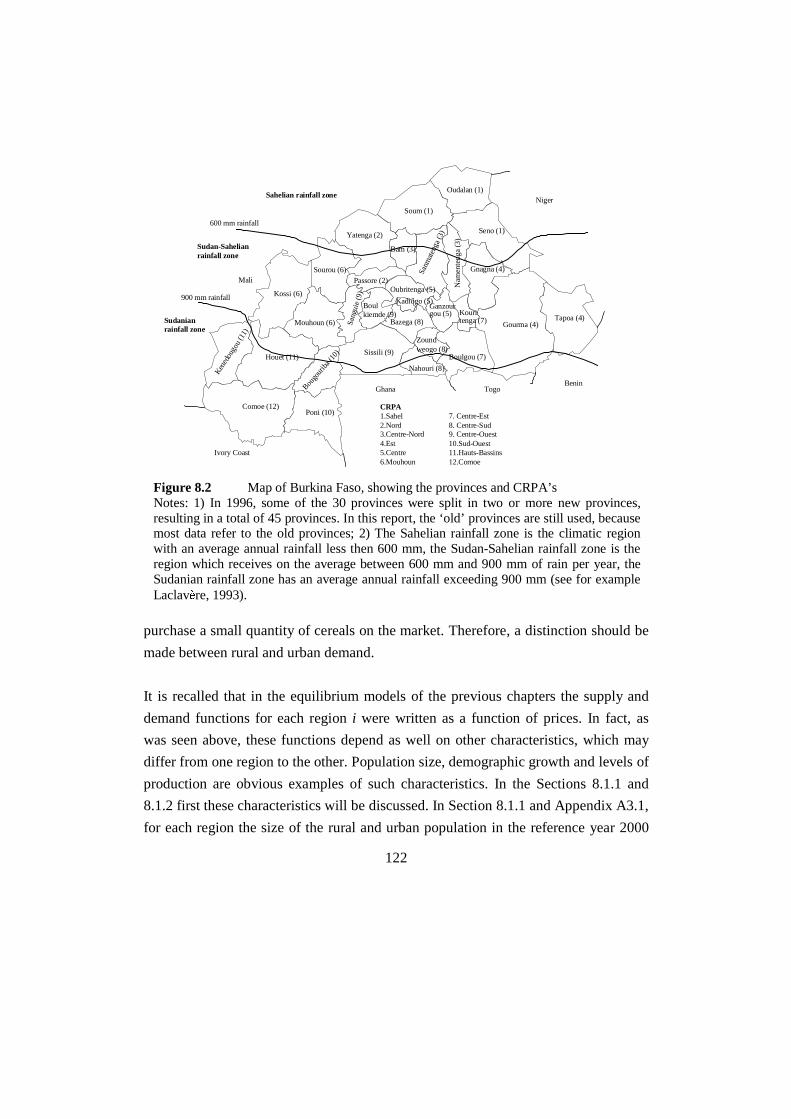
122

purchase a small quantity of cereals on the market. Therefore, a distinction should be

made between rural and urban demand.

It is recalled that in the equilibrium models of the previous chapters the supply and

demand functions for each region i were written as a function of prices. In fact, as

was seen above, these functions depend as well on other characteristics, which may

differ from one region to the other. Population size, demographic growth and levels of

production are obvious examples of such characteristics. In the Sections 8.1.1 and

8.1.2 first these characteristics will be discussed. In Section 8.1.1 and Appendix A3.1,

for each region the size of the rural and urban population in the reference year 2000

Oudalan (1)

Soum (1)

Seno (1)Yatenga (2)

Sourou (6)

Bam (3)

Passore (2)

Gnagna (4)

Gourma (4)Tapoa (4)

Oubritenga (5)

Kadiogo (5)

Kouritenga (7)

Ganzourgou (5)

Boulgou (7)

Bazega (8)

Zoundweogo (8)

Nahouri (8)

Sissili (9)

Boulkiemde (9)

Mouhoun (6)

Kossi (6)

Houet (11)

Comoe (12)Poni (10)

Sanm

aten

ga (3

)

Nam

ente

nga

(3)

Sang

uie

(9)

Ken

edou

gou

(11)

Bougo

uriba

(10)

Mali

Ivory Coast

Ghana TogoBenin

Niger

CRPA1.Sahel 7. Centre-Est2.Nord 8. Centre-Sud3.Centre-Nord 9. Centre-Ouest4.Est 10.Sud-Ouest5.Centre 11.Hauts-Bassins6.Mouhoun 12.Comoe

Sahelian rainfall zone

Sudan-Sahelianrainfall zone

Sudanianrainfall zone

600 mm rainfall

900 mm rainfall

Figure 8.2 Map of Burkina Faso, showing the provinces and CRPA’sNotes: 1) In 1996, some of the 30 provinces were split in two or more new provinces,resulting in a total of 45 provinces. In this report, the ‘old’ provinces are still used, becausemost data refer to the old provinces; 2) The Sahelian rainfall zone is the climatic regionwith an average annual rainfall less then 600 mm, the Sudan-Sahelian rainfall zone is theregion which receives on the average between 600 mm and 900 mm of rain per year, theSudanian rainfall zone has an average annual rainfall exceeding 900 mm (see for exampleLaclavPre, 1993).

123

will be estimated. These data will later be used in the process of estimating aggregate

regional supply functions and rural and urban demand functions. In Section 8.1.2 and

Appendix A3.2, for each region harvest levels are estimated. By making use of

demographic data and regional cereal production data during a series of years (1984-

1998), production per inhabitant and per rural inhabitant can be estimated. These data

are compared with data on required cereal consumption per person in order to

evaluate whether a region may be considered to be a shortage, a surplus or an

‘equilibrium’ region. Special attention will be put on the estimation of expected

harvest levels in the reference year 2000, taking into account possible trends in

production, yields and/or cultivated areas.

In Section 8.1.3 and Appendix A3.3 a review is given of empirical evidence at

household level of cereal sales and their timing. It is discussed to which extent in a

number of village level studies various characteristics have influenced cereal supply

on the market. A distinction will be made between the annual supply on the market

and the timing of the supply. Section 8.1.4 and Appendix A3.4 deal with cereal

purchases by rural and by urban consumers. Special points of interest are the relation

between cereal production levels and purchases. Both demand and supply of cereals

depend on the household’s ability to earn an income from other sources. In Section

8.1.5 and Appendix A3.5 a review is given of data on household’s incomes and

expenditures. For various regions average levels of household income are estimated.

Finally, Section 8.1.6 and appendix A3.6 deal with cereal prices on markets in

Burkina Faso. Especially seasonal price patterns are investigated. This information is

used to estimate price probability distribution functions, and serves as a reference for

validation of the calculation of (endogenous) prices in Chapter 10. A careful review

of all possible sources, thus allows for the estimation of regional, quarterly cereal

supply and demand functions in Chapter 9. Though not conform rigorous

econometrical rules, data limitations do not enable another estimation procedure. It is

recalled that in this paper cereals comprise millet, red sorghum, white sorghum and

maize. Rice and fonio have not been taken into account.

124

8.1.1 Rural and urban population

The size of the urban and rural population in Burkina Faso in the reference year 2000

can be estimated using census data for 1996 and 1985 (INSD, 1995a,b, 1998). INSD

data allow for the estimation of growth rates of the rural and urban population per

CRPA. The total, rural and urban population can be estimated for each region for the

year 2000, if it is supposed that

the yearly urban and rural

population growth between

1996 and 2000 is the same as

between 1985 and 1996 (see

Table 8.1 and Appendix A3.1).

The population estimates are

used in Section 8.1.2 to

estimate the cereal production

per person and the cereal

production per head of the rural

population, and in the Sections

9.1 and 9.2 to estimate the

aggregate regional cereal

demand and supply functions.

8.1.2 Cereal Production

Using the rural population estimates and production data which are published yearly

by the Ministry of Agriculture, the expected cereal production for the year 2000 and

the expected cereal production per head of the rural population can be estimated for

each region. The estimated level of cereal production per rural inhabitant is used in

Section 9.2 to estimate the annual cereal sales.

Table A3.2 in Appendix A3.2 shows production, cultivated area and yield data for the

years 1984-‘98. For each CRPA it can be indicated whether in most years cereal

Table 8.1: Estimated urban and rural population

in the reference year Oct 2000-Sept 2001.CRPA Total urban rural

Centre 1,787,175 843,454 943,721

Centre Nord 1,016,292 66,820 949,473

Centre Ouest 1,060,889 118,377 942,512

Centre Sud 518,920 18,343 50,0577

Sahel 792,889 31,499 761,390

Mouhoun 1,241,941 101,918 1,140,022

Est 1,049,317 55,799 993,518

Centre Est 836,249 103,372 732,877

Nord 1,039,819 104,111 935,708

Sud Ouest 543,289 19,221 524,068

Hauts Bassins 1,109,265 371,416 737,849

Comoe 359,652 76,996 282,655

Total 11,355,699 1,911,328 9,444,371

Estimates are based on 1985 and 1996 census data (INSD1995a,b, 1998) data, see Table A4.1 in Appendix 4.

125

production exceeds or is lower than the minimally required cereal consumption of

190 kg per person.13 In this paper we adopt the definition that a region is in shortage if

in most years average cereal production per person is lower than 170 kg (taken into

account 15% grain losses). A region is a surplus region if average production exceeds

210 kg per head for most years. The other regions (with production levels between

170 and 210 kg per person or having alternately a surplus or shortage production) are

called here equilibrium zones. In column (a) in Table 8.2 is indicated which CRPA

are shortage, surplus or equilibrium regions. The entire country is on average just in

equilibrium (between 1984 and 1998 the country had surplus in nine years, a shortage

in three years, and was in equilibrium in three years). The northern CRPA Sahel and

Nord, and the CRPA Centre (with the capital Ouagadougou) are in most years in a

shortage situation. The cotton areas Mouhoun, Hauts Bassins (with Bobo-Dioulasso),

ComoJ and Sud-Ouest and the CRPA Centre Ouest, Centre Sud, and Est have in

general a surplus. The other CRPA are in general in equilibrium.

Regression analyses executed on the data presented in Appendix A3.2 have

demonstrated that although the production data feature a significant linear trend, it is

risky to suppose that the cereal production for each CRPA in the reference year can

be estimated by extrapolating the data. Regression results showed that yield levels,

production and area cultivated are dependent upon rainfall (see Appendix A3.2 and

Figure A3.3). Yield levels show a jump after 1991. Part of this jump can be explained

by the good rainfall in 1991, 1994, 1995, 1997 and 1998. Yield levels were also high

during the average rainfall years 1992 and 1993, but the period is too short to be able

to draw conclusions upon the yield levels in the coming years. Furthermore,

13 The norms for required minimal consumption per adult equivalent differ per source and depend onsuppositions on the share of the different cereals in total consumption, and nutrient losses during foodpreparation. Estimated norms per person per year vary (see Bakker and KonatJ, 1988) between 180 kgused by FAO, 220 kg calculated by Bakker and KonatJ (taken into account the large losses due to mealpreparation) and even 270 kg estimated by CILSS. We use here the average norm of 190 kg per person,applied by the ministry of agriculture to calculate the yearly consumption balances. It is noted that thisnorm is not a strict norm, and that therefore the bounds between surplus and shortage households are notstrict.

126

regression analysis for the cultivated area showed a significant, positive, linear time

trend for the cultivated area at a national level. For most CRPA’s, however, this trend

was not significant. In order to forecast for each CRPA the expected production levels

in the reference year 2000-2001, average 1984-‘98 yield levels are multiplied with

forecasted cultivated area for each CRPA. This area is estimated as follows. The

national cultivated area for the reference year is estimated, and for each CRPA the

average 1984-‘98 share in total cultivated land is calculated. Cultivated area per

CRPA for the year 2000 is forecasted by multiplying these two (see Table 7.2).

Yearly production is corrected for grains lost or used as seeds for the next season,

which are supposed to be 15%.

The last two columns of Table 8.2 show the forecasted mean production per head of

the total and per head of the rural population. If the norm for minimally required

yearly consumption of 190 kg cereals is applied it is shown that in only 3 regions

(Center, Sahel and Nord) farmers are expected to produce much less than their own

consumption requirements. In the other regions, the farmers are expected to succeed

fairly well in producing enough cereals for their own consumption. In five regions

farmers are expected to produce a quantity of at least 50 kg of cereals above the norm.

Farmers in these regions, which are all in the south-western part of the country, have

the opportunity to sell a large quantity of their cereal production. It has to be noted

that these farmers, usually also produce cotton. So, despite their cotton production

activities, they also succeed in producing more cereals than needed. The data show

that the northern regions are not self-sufficient and need to be provisioned by the

surplus areas. The CRPA Centre, in which Ouagadougou is situated, is also in deficit.

The low production per head of the total population in Hauts Bassins is caused by the

large number of urban households in the city of Bobo-Dioulasso. Column (g) in Table

8.2 shows that for the reference year the CRPA Sahel, Nord, Centre, Centre Nord and

Centre Est are expected to have a shortage production. The CRPA Mouhoun, Centre

Table 8.2: Forecasts of mean cereal production per capita for the total and for the rural population for the

reference year 2000-2001.

Sur/

Def/

Eq

(a)

Average

yield

‘84-‘98

(kg/ha)

(b)

Share of

CRPA in

cultivated

land

(c)

Forecasted

cultivated

area 2000

(ha)

(d)

Forecasted

mean

production

2000 (tonnes)

(e)

Production (d)

–15% loss

(tonnes)

(f)

Production (e)

per person

(kg)

(g)

Production (e)

per rural

inhabitant

(kg)

(h)

Centre D 650 7% 222878 144926 123187 69 131

Centre Nord E 597 10% 306996 183210 155728 153 164

Centre Ouest S 668 11% 337521 225630 191786 181 203

Centre Sud S 759 7% 210916 160008 136006 262 272

Sahel D/E 483 9% 278245 134257 114118 144 150

Mouhoun S 812 15% 467667 379850 322873 260 283

Est S 808 10% 311393 251481 213759 204 215

Centre Est E/S 771 7% 203259 156614 133122 159 182

Nord D 584 9% 264955 154775 131559 127 141

Sud Ouest S 814 7% 206583 168071 142860 263 273

Hauts Bassins S 1211 7% 203726 246802 209782 189 284

Comoe S 1171 2% 74872 87671 74520 207 264

Burkina Faso S 740 100% 3089011 2293294 1949300 172 206

Notes: (a) According to the definition in the text, S = Surplus region, D = Deficit region, E = Equilibrium region; (b) Based on TableA3.2; (c) Average share of cultivated land of each CRPA in total cultivated area for the years 1984-98, see Table A3.2; (d) Totalforecasted cultivated area is estimated on the basis of extrapolation of the national cultivated area between 1984-1995; see Appendix 3;(d) = Forecasted area Burkina Faso * (c); (e) = (b)*(d); (f) = 0.85*(e); (g) = (f)/forecasted total population per CRPA in 2000, see Table8.1; (h) = (f)/forecasted rural population 2000, see Table 8.1.

128

Sud, and Sud Ouest are expected to be surplus zones. The other CRPA are expected

to be more or less self-sufficient and are equilibrium zones. This does not say

anything about the food security level of individual households, but shows whether in

principle much has to be transported to these areas or not. The cereal balances differ

from the official balances calculated by the government, since the last ones include

rice and fonio.

8.1.3 Cereal sales

Many farm households, certainly those with a shortage, prefer not to sell cereals, but

to earn an income by selling other crops, like groundnuts, cowpeas or cotton.

However, as discussed above they sometimes have to sell cereals because of urgent

cash needs. McCorkle (1987) speaks about a ‘code of honour’, which influences

cereal sales. Referring to her research in Dankuie, a village in the province of

Mouhoun, she reports that cereal sales to alleviate cash needs are usually

disapproved, except in special cases (extraordinary surplus, sales to village

cooperatives, sales in the lean period, just before the new harvest). Although the

people in Dankuie usually produce a large surplus, harvests in the survey year were

low. McCorkle uses a ‘commercial preference scale’ in order to classify the order in

which products would be sold if people had them, in case of cash needs. Millet and

sorghum occupy respectively the 17th and 18th place. Households prefer to sell cash

crops (cotton is the most prefered commercial good in case of cash needs) or

livestock (poultry is on the second place) or to borrow from parents (10th), farmer

cooperatives (11th) or traders (16th). Despite this code of honour, cereal sales can be

significant, especially when other ways to get an income are not conceivable.

In the past several marketing studies have been performed in Burkina Faso by for

example the University of Michigan and the University of Wisconsin (McCorkle,

1987; Szarleta, 1987; Sherman et al., 1987), by CILSS (Pieroni, 1990), by ICRISAT

(Reardon et al., 1987), by Yonli (1997) and by Broekhuyse (1988, 1998); see

Appendix A3.3. A comparison of sales patterns reported by these studies, reveals that

differences between years and regions as well as differences within regions are very

129

large. The quantity of cereals sold depends to a large extent on production levels. In a

good rainfall year, with a good harvest, more cereals can be sold. In bad rainfall

years, households will not be inclined to sell many cereals, but they sometimes have

to. For example, Szarleta reports a sale of 600 kg of cereals per household in the

province of Houet in the bad rainfall season 1983-84, while Pieroni (1990) reports a

household sale of 1806 kg in the same province in the abundant rainfall season 1986-

87. Furthermore, households in surplus zones usually sell more than households in

shortage areas (see for example Table A3.6). They sell both a larger quantity and a

larger part of their production. Not only total cereal supplies, but also the type of

crops offered differs per region. Szarleta (1987) shows that in the survey villages in

the CRPA’s Mouhoun and Hauts Bassins, large amounts of red sorghum but hardly

any maize are offered.

The influence of prices on annual sales is weak. Szarleta (1987) concludes from a

regression analysis among 5 villages scattered over Burkina Faso that, indeed,

production is the most important determinant of annual cereal sales. Cereal prices, on

the other hand, do not significantly influence cereal sales. In the long run production,

and consequently also sales, may be influenced by prices. In the short run (for a

period of only a few years), however, farmers will probably not immediately alter

their production plans if cereal prices turned out to be different than expected. So, in

the short run the dependence of supplies on prices can not be demonstrated.

McCorkle (1987) argues that for some households prices do not influence sales

decisions. For other households, however, prices are of influence, but not decisive.

Using data collected between April 1983 and March 1984, Lang (1985) finds for the 4

surplus villages surveyed by SAFGRAD (see also Appendix A3.3) a relationship

between prices and annual sales, which is negative for some and positive for other

cereals, though it is not significant. Regression analysis per village shows that

production is the most important determinant of annual sales. Prices do not

significantly influence annual sales. Pardy also points at the importance of the

household size. The larger the number of consumers, the lower the sales. Pieroni

(1990) agrees with the strong link between production and sales (see Table A3.8 in

130

Appendix A3.3), but argues, based on his village studies in the surplus zones of

Burkina Faso, that it is not a law. The production of a large surplus does, for some

households, not correspond to large sales. Cereal sales depend not only on the surplus

produced, but also on the need for capital, social relations, and market demand

(Pieroni, 1990; p. 44, 45). Cash needs may also be satified by earnings from other

activities (cash crop sales or non-cropping activities).14 Market development and

infrastructural conditions determine for a part the opportunity for such activities.

Households closer to main roads or to busy markets, have more possibilities to sell

handicrafts or processed food. Therefore, they also have the incentive to initiate

activities, which can replace their cereal sales. Such activities attract new traders, and

therefore enhance market competition and reduce marketing costs. Pieroni shows that

households selling large quantities are those with more land, more modern

techniques, less young children, and those closer to well functioning markets. This

argument is in favour of improving market functioning in Burkina Faso. Developing

other capital generating activities is, however, not only tied to the presence of roads

and markets. Reardon et al. (1988a) show that households in the shortage Sahelian

regions earn more income from non-cropping activities than households in the

Sudanian equilibrium regions in the centre of the country (see Figure 8.2). Sahelian

households provided most of their non-cropping income from livestock and

temporary migration. Activities related to crop production (product processing)

provided the largest part of the non-cropping income for most of the Sudanian

households. Due to the dependence of these activities on crop production, earnings

from these activities were low in years with bad harvest.

The ability to earn an income from other sources also influences the timing of sales. It

is often said that West African farmers sell usually in the post-harvest, low-price

season and buy in the pre-harvest, high-price season. Reasons for this are cash needs

14 Non-cropping activities refer to all activities other than crop cultivation activities, like livestockraising, processing agricultural crops (dolo preparation, making millet porridge bouillie), handicrafts,trade, off-farm employment, temporary migration, etc..

131

for celebrations, urgent daily expenses, wage payments, debt repayments, etc. Various

authors (see Appendix A3.3) observed that in general, most sales are effectuated

during the post-harvest season. It appears that the number of households selling

during the post-harvest season is higher than the number of households selling during

the rainy season, when prices are higher. However, the quantity of cereals sold per

selling household is smaller during the post-harvest season than during the rainy

season. The results seem to indicate that households which do not have to sell cheap,

prefer to wait until prices increase. Poorer households, who do not have other income

generating sources have to sell (small quantities) during more periods. Sales of

households posessing a large number of livestock seem to be dependent not only on

the cereal market, but also on the livestock market (Pardy, 1987). These households

may have the ability to postpone sales until prices increase. These patterns might

support the hypothesis that sales during the harvest and post-harvest season are a

function of cash needs (with a negative price elasticity of supply), whereas sales later

in the year are a function of prices (with a positive price elasticity of supply).

To summarize, the different surveys indicate that cereal production levels are the

most important determinant of annual cereal sales. Cereal prices do often not

influence annual cereal sales significantly. Some juxtaposed effects reduce the total

price effect which is overwhelmed by the effect of total production. Next to the

surplus produced, also the need for capital, social relations, and the possibility to

develop other income generating activities influences annual cereal sales. This also

influences the timing of sales. A general recognized pattern is that most farmers sell

during the post-harvest, low-price season. Some authors, however, observed that it are

especially the poorer households who sell small quantities during all periods of the

year. The wealthier households prefer to sell a larger quantity during the higher priced

seasons.

The levels of cereal sales observed in the different surveys, are used to estimate in

Section 9.2 the levels of annual cereal sales in each region. The information on sales

patterns is used to estimate average levels of revenues from cereal sales in each

132

period of the reference year which will be necessary to estimate the supply functions.

Furthermore, the results from the equilibrium models can be validated using the

information on cereal supply discussed here.

8.1.4 Cereal purchases

As only a part of the households sells cereals, most households purchase cereals on

the market. A comparison of the same studies as mentioned above, learns us

something about the purchase pattern of BurkinabJ households (see also Appendix

A3.4). Here a clear distinction must be made between urban and rural purchases.

About 18% of the population lives in urban areas, who have to purchase almost all

cereals consumed on the market. Urban households consume much more rice than

rural households, and more often they purchase prepared food (millet porridge

bouillie, bread, prepared meals).

Some studies only concentrated on urban consumption and demand. For example,

Sherman et al. (1987) executed in 1983-84 a survey among 125 households in

Ouagadougou and 108 households in Bobo-Dioulasso, and among 75 sellers of

prepared food in Ouagadougou and 75 in Bobo-Dioulasso. They report that cereals,

including rice, are the major staple of urban diets. White sorghum and millet are still

consumed in largest quantities, but rice is increasingly consumed by urban

households. Reardon et al. (1988b) report that rich households consume relatively

more rice (32% of total cereal consumption) than poor households (19% of total

cereal consumption). According to Sherman et al. (1987), red sorghum is not

regularly eaten, but only as a grain of last resort. Households purchase the largest part

from medium and small traders or from vendeuses (petty women traders) and to a

lesser extent from large traders. Large traders usually do not sell in quantities less

than 100 kg. The purchasing of 100 kg bags is typically reserved to civil servants and

private sector employees who receive salaries periodically. Since purchases per bag

are relatively cheaper than purchases in retail, the richer households can profit more

from lower prices than poorer households. Only few households purchase directly

from producers. Most prepared food sellers are women, who purchase and sell in

133

small quantities. Apart from some of the dolo brewers, they purchase in the morning

the cereals they need for preparing the food which is sold the same day. Purchases are

often on credit. Dolo brewers usually purchase red sorghum in larger quantities,

because it is not profitable to brew only small quantities.

The data presented in Table A3.18 in Appendix A3.4 show that almost all rural

households purchase cereals on the market. Many rural households have to purchase

large quantities in order to satisfy consumption requirements, certainly in the shortage

areas.15 As with sales patterns, purchases by rural households are dependent on

production levels. The data clearly show that purchases are less in the higher

production regions. So, on average, rural households in the surplus areas purchase

less than those in the shortage areas. However, as Reardon et al. (1987) show, even in

surplus zones there are many households who have to purchase large volumes of

cereals to satisfy consumption needs. It regularly happens that the same type of

cereals sold is rebought later in the season. This phenomenon is well known in Africa

and sometimes called overcommercialization (see also Yonli, 1997). This is also the

case for red sorghum, a part of which is consumed as dolo (see Table A3.19 in

Appendix A3.4). Seasonal data confirm that most purchases take place during the

lean, high price season. The data suggest, however, that richer farmers purchase

earlier, when prices are still lower (in the surplus village of BarJ most purchases were

made between January and March, Ellsworth and Shapiro (1989)).

The observation that high production levels in surplus regions lead to lower

purchases, may imply that purchases will be lower during the favourable rainfall

years. The only source which reports on differences in purchases between production

seasons is Reardon et al. (1987), who gives purchase data for 6 villages in three

provinces in Burkina Faso. We will try to use Reardon’s data to analyse the influence

15 Most households, both in urban and in rural areas, receive cereal gifts. These gifts are not taken intoaccount here, though they may be substantial (Szarleta, 1987; Broekhuyse, 1998; Appendix A3.5). It issupposed here that the quantity received is more or less equal to the quantity given to others. Therefore,they are not taken into consideration in this study.

134

of rainfall on purchases. The purchase data will be compared with rainfall data. For

we do not have data on cereal production for these villages, and local cereal

production levels may not be well represented by aggregate production data, we

compare purchases with rainfall data from the rainfall stations closest to the survey

villages. The data are obtained from the National Meteorological Institute of Burkina

Faso. For the province of Soum, rainfall data from the rainfall station in Djibo (1981

458 mm, 1982 304 mm, 1983 322 mm, 1984 227 mm) show that only 1981 rainfall

was above the 1970-93 average (of 333 mm). Table A3.23 in Appendix A3.4 shows

that for the province of Soum purchases are higher if rainfall is low, although

purchases in the 1983-84 season are rather low compared to the other low rainfall

years. Purchases of the province of PassorJ do not differ very much over the years,

although the slightly increasing purchases correspond to the slightly decreasing

rainfall in Kaya (1981 603 mm, 1982 583 mm, 1983 574 mm, 1984 533 mm; 1970-

’93 average 615 mm). Finally, rainfall in the rainfall station in DJdougou in the

province of Mouhoun are all below the 1970-‘96 average (1981 no observation, 1982

521 mm, 1983 621 mm, 1984 627 mm; 1970-’96 average 717 mm). The pattern of

decreasing purchases from 1982 to 1984 corresponds to the pattern of increasing

rainfall in this period. Although too few data are available to make conclusive

statements, the data are not in contradiction with the hypothesis that purchases are

inversely proportional to rainfall, and therefore also to production (in Appendix A3.2

it was shown that a positive, significant relation exists between rainfall and

production).

To analyse the influence of income or prices on cereal demand, income elasticities of

demand and price elasticities of demand are useful measures, see also Chapter 4. The

price elasticity of demand measures the percentage change in demand if the price

changes with 1%. Estimating elasticities is difficult since no time series data are

available for a large number of respondents, and since many other factors influence

demand behaviour as well. Because of the weakness of the available data in

developing countries, many studies apply elasticities reported by different authors for

similar situations in different countries. It is noted that elasticities also depend on the

135

degree of commodity aggregation. The demand for cereals is expected to be less price

elastic than the demand for white sorghum. If the price of white sorghum increases,

other cereals can serve as substitute. If, however, the prices of all cereals increase,

other types of food which can serve as a substitute, must be sought for. Some studies

estimating price elasticities of demand and income elasticities of demand are

discussed in Appendix A3.4.

The information on the timing of purchases is used in Section 9.1 to estimate the

share of total purchases in each period. Furthermore, the purchase data discussed

above are used to check the validity of the results from the equilibrium models. In

Section 9.1 estimates are also made of the income elasticity of cereal demand in the

different CRPA in Burkina Faso. These are necessary to estimate the share of the

revenues spent on cereal purchases.

8.1.5 Revenues and expenditures

Cereal supply and demand decisions depend on the total household revenues and

expenditures. If a household produces cash crops or has other sources of income,

probably not many cereals will have to be sold. If household expenditures are high in

a certain period, and if revenues (other than revenues from cereal sales) are not

sufficient, cereals must probably be sold. If total revenues are low, not many cereals

can be purchased for own consumption. In other words, household revenues and

expenditures are decisive factors in view of the quantities of cereals that can or have

to be sold or purchased.

Measurement of household revenues and expenses in developing countries is a

notorious difficult task. For interviewers it may be difficult to get reliable answers to

sensitive questions related to money. People are not always prepared to answer

questions on for example their expenditure pattern during the last 12 or 6 months,

people often forget many expenditures or (non-monetary) revenues, or give too low

figures because they do not want other people to know their wealth. Reliable results

can only be obtained if a relation of trust exists between the interviewer and the

people interviewed, and if they are interviewed on a regular basis. The unreliability of

136

the data clearly comes forward if revenue and expenditure data of different surveys

are compared. Various surveys have been carried out in Burkina Faso. The most

recent is a national poverty study by the national statistical and demographic institute

(INSD, 1996a, 1996b). Other studies were performed by Broekhuyse (1988) in the

province of Sanmatenga, Thiombano et al. (1988), Reardon et al. (1988a) and Lang et

al. (1983) who performed village studies in different villages spread over the country.

In Appendix A3.5 results of these studies are discussed. These studies will be used in

Section 9.1 to estimate average expenditures on cereals and average income levels per

capita per CRPA. The income per person turns out to be one of the major

determinants of cereal purchases.

8.1.6 Agricultural prices

It has already been mentioned that many households sell cheap during the post-

harvest season and purchase dear during the lean season. Cereal prices in Burkina

Faso, as in many West African countries show a clear seasonal fluctuation. Prices are

low immediately after the harvest, and increase considerably during the year, to start

decreasing again just before the new harvest. Seasonal price increases are caused by

demand and supply differences (supply is large during the post-harvest season,

whereas demand is highest during the lean season) and storage costs which are

charged in the prices. Prices in the lean season may be up to the double of post-

harvest prices. In Burkina Faso price data are gathered by SIM/SONAGESS (SystPme

d’Information sur les MarchJs/SociJtJ Nationale de Gestion des Stocks de SJcuritJ).

Since 1992 prices for all cereals are gathered on 37 markets scattered over the

country. A distinction is made between producer and consumer prices. Producer

prices ensue from transactions between producers and traders, consumer prices ensue

from transactions between consumers and traders or between consumers and

producers. For the analysis, we used prices for the crops white sorghum, millet and

white maize. Data for red sorghum and yellow maize have been omitted because only

very few data were available. In Appendix A3.6 the price data for the period 1992-

1999 are analysed and some other studies discussing these price data are briefly

discussed (Bassolet, 2000, Hoftijzer, 1998).

137

Four main conclusions can be drawn from the price analysis in Appendix A3.6:

1. Producer prices are lowest in the high production, surplus regions of the country,

the CRPA Mouhoun and Hauts Bassins. Consumer prices are highest in the

shortage regions Centre (with the capital Ouagadougou) and Sahel, See Table

A3.36 and A3.37. Producer prices in the CRPA Nord are lower than expected.

However, for this CRPA only data for Ouahigouya are available. This is a transit

market, through which large amounts of cereals pass from Bobo Dioulasso

towards the northern regions, and where supply from producers to traders is low.

Producer prices in the regions Centre Est, Centre Ouest and Est and consumer

prices in the regions Centre Sud and Centre Est are also high. This may be caused

by demand from traders from the neighbouring countries Ivory Coast, Ghana and

Togo. However, this can not be supported with data on cross-border trade.

Consumer prices in these regions may also be high due to low cereal demand

from the mainly rural population who usually can sell small surpluses – see

Section 8.1.2.

2. Producer and consumer prices increased a lot after the devaluation of the Franc

CFA in January 1994. This increase was not caused by lower cereal production in

these years – see Section 8.1.2. On average producer and consumer prices in the

period 1996 to 1999 were, respectively, 91% and 99% above the average prices

between 1992 and 1994, see Table A3.39. Prices in the cotton producing areas

have increased more than prices in the non-cotton areas, probably due to reforms

in the cotton sector. It looks as if prices stabilized after October 1996.

3. Retail trade margins (the difference between the consumer and producer price in a

region) increased significantly after the devaluation, see Table A3.39. Trade

margins from transport from the surplus zones to Ouagadougou did not change a

lot, whereas margins from transport to the other regions increased a lot. It looks

as if competition on the wholesale markets in Ouagadougou has become more

competitive, whereas traders make high profits from trade towards the retail

markets in the shortage regions. A more detailed inquiry of trade costs and

competition in Burkina Faso is needed to explain this.

138

4. In most years, consumer and producer prices reach their maximum in July and

August. Minimum prices are reached in November or December. It can be

concluded cautiously, that prices reach their minimum earlier if the harvest is bad,

see Table A3.36 and Figure A3.5. Prices in the period July-September exceed

prices between October and December on average with 17% and 18% for

producer and consumer prices, respectively, see Table A3.36. Differences

between CRPA are, however, large. It looks as if this did not change a lot after

the devaluation.

To estimate the parameters for the supply and demand functions in Section 8.2 and

8.3, average producer and consumer prices for each quarter are used. Due to the huge

price increase after the devaluation of the Franc CFA in 1994, we do not use ‘92-’99

averages, but average prices for the period October 1996 – September 1999. Although

these averages are based on only a short time period, this is more realistic than using

the prices for the entire period. Average cereal price levels for the period Oct ’96 –

Sept ‘99 are presented in Table 8.3.

8.2 Trading costs

Price differences between regions and between periods, are, as discussed in Chapter 5

to 7, caused by differences in supply and demand, and by the costs made by the

trading agents. In Chapter 5 to 7, a distinction has been made between transport and

storage costs. We distinguish also ‘other trading costs’, which include the costs which

are made when the cereals are sold or purchased on the market. These costs include

among other things costs to purchase bags, market taxes, and personnel costs. These

costs are not included in the theory discussed in the Chapters 4 to 7, but are discussed

here because they may amount to a significant part of the trading costs. In Appendix 4

the main conclusions and data of some studies on trading costs are discussed.

Table 8.3 Average seasonal cereal prices for the period Oct ’96 – Sept ‘99 in FCFA per kg.

Producer Cereal price Consumer Cereal priceOct ’96 –

Sept ‘99 Jan-Mar Apr-Jun Jul-Sept Oct-Dec

Year

Average Jan-Mar Apr-Jun Jul-Sept Oct-Dec

Year

average

Centre 128 136 140 133 134

Centre Nord 104 104 116 100 103 120 129 137 119 126

Centre Ouest 115 125 125 102 115 121 131 134 114 125

Centre Sud 122 131 133 116 123 126 139 126 122 128

Sahel 105 103 93 96 100 133 144 149 131 139

Mouhoun 89 101 103 83 94 103 114 120 96 108

Est 106 113 116 102 109 112 125 133 108 120

Centre Est 111 118 126 117 117 125 132 133 119 127

Nord1) 99 111 114 124 128 110 119

Sud Ouest1) 83 83 134 143 152 129 139

Hauts Bassins 86 89 95 86 89 108 117 118 108 113

Comoe 105 116 114 122 113 119 134 140 123 129

Burkina Faso 103 109 110 99 104 119 129 133 116 125

Note: 1) Not enough data were available for these CRPA to estimate the average prices for all periods.

Source: Data from SIM/SONAGESS

140

8.2.1 Transport costs

In Burkina Faso the costs for transporting cereals between the place of production and

the place of consumption, cause for a large part of the price differences between

regions. Transport costs taken into account in this study only include the transport

costs between markets, made by traders. Costs made by the producers to bring the

produce from the field to the compound and from the compound to the market, as

well as the costs made by the final consumers to transport their purchases from the

market to their houses are not taken into account.

Transport costs are much influenced by the road conditions, which may be poor. In

Burkina Faso, only a small portion of the road network is asphalted. Only the roads

leading from Ouagadougou to Bobo-Dioulasso, to Ouahigouya, to Kaya and to

Koudougou, and from Ouagadougou or Bobo-Dioulasso to the main border crossings

with Ivory Coast, Ghana, Togo, Benin, Niger and Mali are asphalted. The other roads

are unpaved roads. Some of the unpaved roads may be rather good, but others are

only small trails (in our analysis we call them ‘dirt roads’) which are almost

inaccesible for cars, not to mention trucks. Some roads, especially the dirt roads,

which are passable during the dry season turn into mud trails during the rainy season

inaccesible for cars. Some of the ‘good’ unpaved roads may also be closed for a few

hours or days during the rainy season if the lower parts of the roads (which are

sometimes constructed on purpose to prevent parts of the road to be washed away

during showers by the swirling water running to lower places) are flooded.

Because of these bad road conditions, travelling time may be long and maintenance

costs for trucks high. It regularly happens that trucks get stuck along the road because

of breakdowns, which may delay the journey considerably. These problems cause

transport costs to be high. If two villages are located along an asphalted road,

transport costs between these villages may be cheap. However, sending a truck to a

remote village in the Sahel during the rainy season may be a costly and risky

undertaking.

141

Most traders (certainly the small and medium) do not own their own transport means,

but have to rent a truck (if the traded quantities are large enough) or pay a certain

transport price for each bag transported by a truck owner (which is often a merchant).

DJjou (1987) reports that cereal transporters sometimes have monopolistic power.

Merchants owning a truck may force other traders who are dependent upon this

merchant for their transport, to respect mutual price agreements. However, according

to DJjou (1987), transport is in general not the limiting factor for most regions.

Competition is in most cases satisfactory. Transport costs between a number of

markets are given in Appendix A4.1. It can be expected that transport became

considerably more expensive after the devaluation of the Franc CFA in January 1994.

However, a comparison of Table A4.3 and Table A4.4 in Appendix A4.1 does not

give any evidence for such an increase. For some routes, the transport prices paid by

the cereal traders to the carriers even decreased. This corresponds with the

observation in Section 8.1.6 that the difference between the consumer price in

Ouagadougou and the producer price in the surplus zones hardly increased. It is,

however, in contradiction with observations that the difference between consumer

prices in the northern shortage regions and producer prices in the south-western

surplus zones increased considerably after the devaluation – see Section 8.1.6 and

Appendix A3.1. It also corresponds to observations in other recent reports (Egg et al.,

1997; Danida, 1999; UE, 1999), who also concluded on the basis of the

SIM/SONAGESS price data, that trade margins from trade between the surplus zones

and Ouagadougou, remained relatively stable after the devaluation, despite a

substantial increase of cereal prices and prices of fuel and spare parts. The stability of

margins for transport to Ouagadougou may be due to an increased competition on the

cereal market. However, it causes difficulties for transporters who can not face the

competition, and who may have difficulties of purchasing new vehicles in the near

future (Danida, 1999, p. 13).

Transport prices also depend on the means of transport used. SirpJ (2000) makes a

distinction between small pick-up trucks, 10-tonne trucks, and large 32-tonne trucks.

Pick-ups are most often used to transport goods over short distances; for example,

142

between villages, or from villages to the nearest city. The large, 32-tonne trucks are

mainly used for international transport. Transport between the main commercial

centres, and between the different provinces, mainly involves 10-tonne trucks. SirpJ

makes a persistent distinction between the transport costs carriers make (i.e. costs for

fuel, maintenance, personnel, depreciation), and transport prices to be paid to carriers

by traders who rent transport services from them. SirpJ evaluates average transport

costs per kilometer for each type of truck – see Appendix A4.1. The load rate (the

part of the loading capacity of the truck which is filled) plays an important role in the

costs. In this paper we only consider the distribution network between the main

centres of each CRPA. It is assumed that only 10-tonne trucks are involved.

Furthermore, the location of the carriers, an issue brought forward by Vogelzang

(1996), may play a role in transport prices. Transporting cereals between two remote

villages alongside tarmac roads in which no carriers are located will probably be

relatively more expensive than between Ouagadougou and Bobo-Dioulasso. For

example, if a carrier located in a city C has to transport goods from a village A to a

village B, not only the costs to travel between A and B, but also the costs to go from C

to A and to return from B to C have to be paid for. Furthermore, carriers transporting

towards remote cities have less possibilities to find a freight for the return journey

than carriers transporting between, for example, Ouagadougou and Bobo-Dioulasso.

For that reason, transport between the more frequented markets will probably be

cheaper than between more remote markets.

In this report we do not consider the transport costs made by the carriers. We only

look at the transport costs cereal traders have to make (which are the transport prices

charged by the carriers in the notation of SirpJ, see above). Using the studies

discussed in Appendix 4, transport costs have been estimated. A difference has been

made between 1) transport along the busy trade routes over asphalted roads (from

Ouagadougou to Bobo Dioulasso, to Pouytenga, and to Koudougou and from Bobo-

Dioulasso to Koudougou); 2) transport over less frequented trade routes over

asphalted roads; 3) transport over (all-weather) unpaved roads, and 4) transport over

(bad) dirt roads. Although most transport is done over asphalted and unpaved roads,

143

some of the cities are connected by dirt roads (for example, the route Bobo-Dioulasso

- Diebougou and a part of the route between Ouahigouya and Kaya). Transport along

busy trade routes is cheaper than transport along less frequented routes, since the

chance to have a return freight is larger for these routes. Transport over unpaved

roads is more expensive than over asphalted roads. Transport over dirt roads is even

more expensive. Furthermore, during the rainy season (July to September) transport

over unpaved roads and dirt roads is more expensive than during the dry season

(October to June). In this paper only transport between the main commercial centres

is considered. For each CRPA one or two centres have been chosen, for which

transport costs to other regions are estimated. The distance between each pair of cities

has been estimated using the road map of Burkina Faso (see Table A4.5 in Appendix

A4.1). For each road connection it has been estimated what part of the route is over

busy asphalted roads, less frequented asphalted roads, unpaved roads or dirt roads.

Next, transport costs per km per road type are estimated using the data in Appendix

A4.1. By multiplying the costs per km with the distance, the costs to transport goods

between two cities or two CRPA is estimated.

It is difficult to make balanced estimates of the transport costs. Most transport costs

presented in the transport surveys do not make a distinction in costs per road type,

although it is admitted that they differ a lot. Furthermore, the data of the different

studies do not always correspond. For example, transporting 100 kg of cereals

between Ouagadougou and Gorom-Gorom costs 2000 FCFA according to DJjou

(1987), and 950 FCFA according to Bassolet (2000). SirpJ (2000) argues that

transport costs depend on a lot of factors, of which the loading rate plays a major role.

By comparing the different studies, we can make the following observations:

• Transporting along the busy trade routes, between the most animated markets (i.e.

from Ouagadougou to Bobo-Dioulasso, to Pouytenga and to Koudougou and

from Bobo-Dioulasso to Koudougou), costs the traders, according to DJjou

(1987) and Bassolet (1997), less than 20 FCFA per kilometer per tonne

(observations range between 11 and 21 FCFA). These costs are considerably

lower than between the other markets. Reasons for these lower costs are that most

144

carriers are located on these markets, and that they have more possibilities to find

return freights.

• Transport costs between the other market depend on road type. Divide these trade

routes, presented in Table A4.3 and Table A4.4 in Appendix A4.1, in routes over

asphalted roads, routes which are both over asphalted and unpaved roads, and

routes which are only over unpaved roads and dirt roads.16 It can be observed that

transport costs between markets connected by asphalted roads are on average 40

FCFA per tonne per km (observations range between 20 and 52 FCFA; standard

deviation 15 FCFA). If it is also partly over unpaved roads, only a minor increase

is observed (on average 41 FCFA, observations range between 20 and 76 FCFA,

standard deviation 15 FCFA). If it is only over an unpaved road or if also dirt

roads must be passed, costs per tonne per km increase on average to 52 FCFA

(observations range between 24 and 82 FCFA, standard deviation 14 FCFA).

• It is striking that transport costs over unpaved roads and dirt roads paid by the

cereal traders, increase less than the rise of transport costs made by the carrier

reported in Table A4.2 in Appendix A4.1. Either the increases reported in the

table are too high, or the transport price charged by the carriers is too low to cover

their costs.

• The transport price charged by carriers of 112 FCFA, reported by SirpJ (2000)

seems to be very high. It is not clear why his estimates are more than twice the

averages observed by DJjou (1987) and Bassolet (1999).

• During the rainy season, the costs for transport over unpaved roads increases on

average with 17%.

These considerations bring us to make the following estimations for the transport

costs:

16 For these calculations the more lively transport routes (Bobo-Dioulasso, Koudougou, Ouagadougou,Pouytenga) with lower transport costs and the short routes (less than 80 km) with higher transport costsare not taken into consideration.

145

1. Transporting cereals over the less frequented asphalted roads is estimated to cost

during the dry and rainy season 40 FCFA per tonne per km.

2. For the busy routes between the CRPA Hauts-Bassins and Centre (Bobo-

Dioulasso to Ouagadougou), Centre–Est and Centre (from Pouytenga to

Ouagadougou) and between Koudougou and the CRPA Centre or Hauts Bassins

costs per tonne are estimated at 25 FCFA per kilometer. For these routes it is

supposed that transporters have return freights more often, so that transport costs

can be lower. Although the market of Ouahigouya is one of the most important

distribution centres of the country, transporting towards this market is not

reported to be cheaper.

3. Average transport costs from Hauts Bassins and Centre towards the CRPA Centre

Ouest, in which Koudougou is situated, exceeds 25 FCFA. To estimate the

average transport costs to the CRPA Centre Ouest, the average is taken of

transporting to Koudougou and to Leo. Since Leo is a less busy market than the

market of Koudougou, transport costs from Ouagadougou and Bobo-Dioulasso

towards Leo will exceed those for Koudougou.

4. Transport over unpaved roads is 20% more expensive than transport over the less

frequented asphalted roads during the dry season, and 40% more expensive

during the rainy season.

5. Transport over dirt roads is 40% more expensive than transport over the less

frequented asphalted roads during the dry season, and 140% more expensive

during the rainy season. Transporting over dirt roads during the rainy season is a

risky undertaking. If the truck gets stuck, it may take a few days before the

destination is reached.

Estimated transport costs between each CRPA are presented in Table 8.4.

Table 8.4 Estimation of the transport costs during the dry (October – June) and rainy season (July – September) in

FCFA per 100 kg bag.

Dry Season Centre Centre

Nord

Centre

Ouest

Centre

Sud

Sahel Mouhoun Est Centre

Est

Nord Sud

Ouest

Hauts

Bassins

Comoe

Centre 0 392 517 408 1084 840 695 343 724 1366 890 1230

Centre Nord 392 0 909 800 773 1294 1070 718 918 1758 1282 1622

Centre Ouest 517 909 0 875 1601 924 1212 860 1118 934 1120 1460

Centre Sud 408 800 875 0 1492 1248 940 588 1132 1769 1298 1638

Sahel 1084 773 1601 995 0 1652 1473 1473 1062 2450 1974 2314

Mouhoun 840 1294 924 1248 1652 0 1535 1183 686 1838 1094 1434

Est 695 1070 1212 940 1473 1535 0 352 1419 2061 1585 1925

Centre Est 343 718 860 588 1473 1183 352 0 1067 1709 1233 1573

Nord 724 918 1118 1132 1062 686 1419 1067 0 2090 1614 1954

Sud Ouest 1366 1758 934 1769 2450 1838 2061 1709 2090 0 744 1084

Hauts Bassins 890 1282 1120 1298 1974 1094 1585 1233 1614 744 0 340

Comoe 1230 1622 1460 1638 2314 1434 1925 1573 1954 1084 340 0

Table 8.4 (continuation)

Rainy season Centre Centre

Nord

Centre

Ouest

Centre

Sud

Sahel Mouhoun Est Centre

Est

Nord Sud

Ouest

Hauts

Bassins

Comoe

Centre 0 392 583 428 1232 940 695 343 724 1702 890 1230

Centre Nord 392 0 975 820 986 1652 1454 1102 1574 2094 1282 1622

Centre Ouest 583 975 0 1099 1815 1078 1278 926 1213 1100 1493 1833

Centre Sud 428 820 1099 0 1660 1368 1008 656 1152 2462 1318 1658

Sahel 1232 986 1815 1107 0 2152 1660 1660 1573 2934 2122 2462

Mouhoun 940 1652 1078 1368 2152 0 1634 1282 801 2501 1277 1617

Est 695 1454 1278 1008 1660 1634 0 352 1419 2397 1585 1925

Centre Est 343 1102 926 656 1660 1282 352 0 1067 2045 1233 1573

Nord 724 1574 1213 1152 1573 801 1419 1067 0 2426 1614 1954

Sud Ouest 1702 2094 1100 2462 2934 2501 2397 2045 2426 0 1224 1564

Hauts Bassins 890 1282 1493 1318 2122 1277 1585 1233 1614 1224 0 340

Comoe 1230 1622 1833 1658 2462 1617 1925 1573 1954 1564 340 0

148

8.2.2 Storage and other trading costs

Price differences between periods are, for an important part, caused by storage costs.

A trader will only store cereals if he expects to recover at least the storage costs.

Market equilibrium theory shows that the price difference between two periods on a

competitive market is expected to be equal to the storage costs if the traders store

cereals (see Chapter 6). An evaluation of some studies on strategies of cereal traders

(see Appendix A4.2, A4.3 and A4.4) showed that storage costs may include costs of

the storehouses (rent or maintenance), costs for pesticides and insecticides,

surveillance costs, and capital costs. Also storage losses must be considered. Many of

these costs are difficult to estimate. Many cereals are not stored by the traders for a

long time, but shipped quickly. Many of the storage costs are difficult to evaluate per

bag, but have to be paid independent of the number of bags stored. Moreover,

differences between traders are considerable.

The influence of capital costs on traders’ storage decisions demands some extra

explanation. In stead of capital costs, many authors take into account ‘opportunity

costs’. These are no ‘real’ costs to the traders. They reflect the foregone revenues if

the trader would have invested the money value of his cereal stock in other activities,

for instance put the money on the bank raising interest. In stead of calculating

‘opportunity costs’, which are rather difficult to determine, we prefer to estimate

‘capital costs’. 17 Capital costs correspond to the interest payments a cereal trader

should pay if he borrowed money from a bank to finance his cereal purchases. In each

period he should pay interest costs, which are a certain percentage of the money

17 In order to calculate opportunity costs, the traders’ capital balance and activity portfolio should beconsidered. In that case, a comparison could be made between the possible investment opportunities andcredit needs. For the moment we do not introduce this capital balance. Although we acknowledge thatthe development of credit facilities for cereal traders and farmers may be an important policy measure toimprove the functioning of the market, it goes too far for this paper to evaluate the importance of creditcosts in the strategies of cereal traders.

149

invested in the stock (i.e. of the quantity stored multiplied with producer price plus

transport costs plus storage costs).

Other costs involved in trading may constitute an important part of the trading costs.

These costs include personnel costs, costs to buy cereal bags, and taxes. Personnel

costs are the salaries paid to intermediaries of merchants, who may be resident buyers

and sellers or regional coordinators. They may receive a monthly salary or a

commission. Personnel costs also include truck loading and unloading costs. Taxes

include both trade and market taxes. The first category are the taxes which have to be

paid to be allowed to operate as a trader. The second category are the taxes which

have to be paid daily, weekly or monthly to be allowed to use the market

infrastructure of a certain market place. The level of these taxes depends on the

business size of the traders.

To calculate the equilibrium model discussed above, we also need estimates of

storage and other trading costs per bag. No precise estimates can be made because of

data limitations. For some of the services the costs per 100 kg bag are easy to estimate

(personnel who are paid on a commission basis, costs for bags, loading and unloading

costs), for others this turns out to be difficult. For example, personnel costs can be

estimated per month, but costs per bag will differ considerably between months and

traders. To estimate these costs per bag, not only the monthly costs, but also the

number of bags traded must be known. These data are missing in some of the surveys

available. Also costs for storehouses are difficult to estimate per kg. Monthly costs of

a storehouse can be estimated, but to estimate the costs per bag, it should be kept up

how long each bag is stored. Costs per bag are best described in Sherman et al. (1987)

– see Appendix A4.4. Based on their estimates, and using the studies of Bassolet

(2000) and DJjou (1987) as reference literature, we made estimates which are

presented in Table 8.5. Because of the weakness of the data we do not make seperate

estimates for the different CRPA. It is noted that the sensitivity of the model to the

estimates must be analysed carefully. The costs estimated are:

150

1. Storage costs, including renting costs, surveillance and insecticides: Sherman

does not present storage costs seperately, but places it under ‘sundry costs’, see

Table A4.9 column (c) in Appendix A4.4, which are renting costs for warehouses,

taxes, bribes and other costs. Sundry costs are on average 200 FCFA per bag. We

suppose that half of these costs, so 100 FCFA per bag, are renting costs for

warehouses and insecticides. Salaries paid to personnel engaged in storage is part

of the personnel costs mentioned in column (b) in Table A4.9 in Appendix A4.4.

The salary of a warehouseman per bag sold by the trader is estimated by Sherman

between 40 FCFA and 200 FCFA per bag, with an average of 100 FCFA per bag.

Suppose that also one of the apprentices of the trader (Sherman supposed that two

apprentices are working for the trader) is half of his time occupied with

controllling storage. Therefore, personnel costs for storage are 150 FCFA per bag.

Total storage costs are 250 FCFA per bag

2. Storage losses: Bassolet observes storage losses of 8% per year, and DJjou of 15

to 20% per year. We take an average of 12% per year, so 3% per quarter, see

Appendix A4.2.

3. Capital costs: the ongoing bank interest rate is 14% per year (3.5% per period) -

see Appendix A4.3. Capital costs per quarter are estimated at 3.5% of the

producer price of a bag of cereals. For the producer price we take the average

producer prices, which are given in Table 8.3.18 Producer prices for the CRPA

Centre and missing producer prices for the regions Nord and Sud Ouest are

supposed to be the average producer prices for Burkina Faso. The discount rate is

assumed to be equal to 1/(1+r), with r the interest rate of 3.5% per period.

Rounded off, the discount rate is 0.97.

4. Costs for bags: We adopt the estimate given by Sherman in Table A4.9 in

Appendix A4.4, who gives an average cost of 200 FCFA per bag. This is a little

18 We multiply the percentage capital costs with a predetermined, average value of the producer price,and not with the variable p it. This last option would complicate the model considerably because it wouldresult in an extra non-linear term (p it⋅sit) in the objective function.

151

lower than the observations of Bassolet and DJjou in Appendix A4.3.

Considering multiple uses of these bags 200 FCFA might still be high.

5. Annual and market taxes plus other trade costs: Bassolet and DJjou give trade

taxes as percentage of profits and market taxes per day. The average amount of

taxes paid per bag estimated by Bassolet in Table A4.10 and Table A4.11 in

Appendix A4.4 is very low. We suppose that taxes plus other trade costs are half

the ‘sundry costs’ given in column (c) in Table A4.9, so 100 FCFA per bag – see

also under 1).

6. Personnel costs: Again, the personnel costs estimated by Bassolet are very low.

Personnel costs and the payments to personnel paid on a commission basis are

estimated by Sherman in the columns (a) and (b) in Table A4.9. His estimates are

much higher than the estimates made by Bassolet, because Sherman includes the

‘salary’ of the trader. We also have to include this salary because the trade costs

considered in our model have to account for the total difference between cereal

consumer and producer prices. This difference includes the margin earned by the

trader (i.e. his salary). Total personnel costs reported by Sherman vary between

400 and 1250 FCFA per bag. Part of these personnel costs are storage costs – see

under 1). Other personnel costs ( which are part of the trade costs) are estimated

at 700 FCFA per bag.

7. Loading and unloading costs: Observations range between 50 FCFA per bag by

DJjou, 250 FCFA per bag by Bassolet and 100 FCFA per bag by Sherman. We

suppose it costs100 FCFA per bag to load or unload a truck. So, total loading and

unloading costs are 200 FCFA per bag. We do not consider them to be trade

costs, but treat them as transport costs.

Table 8.5 Trading costs in FCFA per 100 kg bag or in %.

1) Storage costs per quarter, including renting costs, surveillance and instecticides: 250 FCFA per bag

2) Storage losses: 3% per quarter

3) Capital costs: itp~*%5.3 , in FCFA per 100 kg bag, with itp~ the average producer price of a 100 kg bag in

region i in period t - see Table 8.3 for the producer prices per kg.

Discount rate: 0.97.

CRPA Oct-Dec Jan-Mar Apr-Jun Jul-Sep CRPA Oct-Dec Jan-Mar Apr-Jun Jul-Sep

Centre 3.47 3.59 3.81 3.86 Est 3.58 3.73 3.97 4.05

Centre Nord 3.50 3.64 3.64 4.05 Centre Est 4.10 3.88 4.14 4.39

Centre Ouest 3.59 4.03 4.37 4.39 Nord 3.47 3.59 3.81 3.86

Centre Sud 4.07 4.28 4.58 4.66 Sud Ouest 3.47 3.59 3.81 3.86

Sahel 3.36 3.69 3.60 3.25 Hauts Bassins 3.00 3.02 3.13 3.32

Mouhoun 2.89 3.10 3.52 3.60 Comoe 4.28 3.68 4.04 4.00

4) Costs for bags: 200 FCFA per bag

5) Taxes plus other costs: 100 FCFA per bag

6) Personnel costs: 700 FCFA per bag

7) Loading and unloading costs: 200 FCFA per bag

153

9 Estimation of cereal demand and supply functions for the case of

Burkina Faso

For the analysis of the inter-regional cereal flows in Burkina Faso, use is made of the

multi-period model (7.64) for a situation of a competitive market. The exogenous

elements of the models are the storage costs and losses per stored unit per unit of

time, the transport costs per transported unit of cereals between the various markets,

the trading costs per unit of cereals sold, and the cereal supply and demand

functions.19 Storage, transport and trade costs have already been estimated in Section

8.2. Supply and demand functions are not readily available. In Section 9.1 regional

demand functions will be estimated for each period, by choosing a functional form

and then estimating the parameters with the aid of data and information discussed in

Section 8.1. For the estimation of quarterly, regional producer supply in Section 9.2,

the method discussed in Section 7.1 is extended. Annual supply is estimated, based on

data on sales and production levels for each region discussed in Section 8.1. Annual

supply depend on production levels and other factors, rather than on prices. As

discussed in Section 8.1.3 the dependence of yearly supply on prices is weak. The

distribution of the annual cereal supply over the year does depend on prices. The

supply in each period is for a part influenced by cash needs, and for another part by

the expected price development within a year.

9.1 Cereal demand functions

In the preceding chapter we discussed the cereal purchase behaviour of househols. In

this section we will estimate cereal demand functions as a function of cereal prices for

an ‘average’ consumer for each CRPA. Regional demand functions per CRPA are

determined by aggregating the individual demand functions. First, in Section 9.1.1 a

functional form for the demand functions is chosen. In Section 9.1.2 differences

between the annual cereal demand functions for rural and for urban households are

19 The supply and demand functions are exogenous elements of the model, supply and demand itself areendogenous elements.

154

discussed and the parameters for the annual cereal demand functions are estimated.

Finally, in Section 9.1.3 the cereal demand functions per period are defined and the

aggregate, regional demand functions are estimated.

9.1.1 Linear Expenditure System

The demand function adopted in this paper is derived from the widely applied Linear

Expenditure System (LES) (see e.g. Roth (1986) for a discussion and application of

the LES, see also Theil (1980) and Section 4.2). The LES is derived from the Stone-

Geary utility function. It is widely applied because it is simple and has convenient

properties. Although more elaborate demand systems exist (see for example Deaton

and Muellbauer, 1980), data limitations prevent us from using them. To illustrate the

principles of the LES, consider the case where a consumer can consume different

commodities. The quantity consumed is purchased entirely on the market at consumer

prices (so that consumption equals market demand). Define K the set of goods the

consumers can purchase. Each consumer demands at least a minimally required, fixed

quantity of each commodity (it is supposed that they can afford to buy this minimum

quantity). This minimally required quantity may either be a minimum subsistence

level of consumption or a minimum preferred quantity. The income remaining after

purchasing all minimally required quantities, is divided in fixed shares over the

commodities from the set K. This remaining income is also called ‘supernumerary

income’, i.e. income after initial purchases. Introduce, for each commodity k 0 K the

elements:

U The utility level a consumer obtains from consuming the K

commodities,

Ck Consumption level of commodity k,

γk The minimally required purchase level of commodity k,20

20 This minimally required purchase level should not be compared with the minimally required quantityof nutrients which is necessary to remain healthy.

155

bk Weighing coefficients corresponding to the preferences of

consumption of commodity k.

then the Stone-Geary utility function can be written as:

(9.1) U = b Ck k kk K

ln −∈∑ γ1 6 , with

>−

=

<<

∑0

1

10

kk

kk

k

C

b

b

γ

Manipulation of the first order conditions from utility maximization subject to an

income constraint, gives the Linear Expenditure System. First introduce:

I Income level of a consumer which can be spent on buying the

commodities from K

πk Consumer price level of commodity k.

The Linear Expenditure System can now be written as:

(9.2) Ck = γπ

π γkk

ki i

i K

bI+ −���

���∈

∑with I ≥ π γi ii K∈∑ and 0 < bk < 1, and bkk K∈∑ = 1.

The expression I − π γi ii K∈∑ is the discretionary or supernumerary income which

remains after due allowance for the minimum requirements. This income is allocated

among the different goods in shares bk/πk. It follows that the parameter bk is the

share of supernumerary income spent on purchases of commodity k. It can also be

interpreted as the marginal buget share ∂ π

∂k kC

I1 6 , “which tells how expenditures on

each commodity change as income changes” (Sadoulet et al., 1995). Expression (9.2)

156

shows that expenditures on each good (Ckπk) are linear in prices and income. Tastes,

preferences, and subsistence requirements are implicitly included in the values of the

parameters bk and γk. The own-price, cross-price and income elasticity of demand of

this demand function can be written as, respectively:

(9.3)

ε ∂∂π

π γ ε ∂∂π

π π γπ

ε ∂∂ π

kkk

k

k

k

k

kk kj

k

j

j

k

j k j

k k

klk

k

k

k k

C

C Cb

C

C

b

C

C

I

I

C

b I

C

= = − + − = =−

= =

1 11 6, ,

.

From expression (9.3) it follows that -1 < εkk < 0 (since Ck > γk, see (9.1)). So,

demand decreases if consumer prices increase, but less than proportionally. A

consequence is that no inferior goods (for which εk k > 0) can be considered. This also

follows from the expression of the income elasticity, which is always positive.

Now suppose that cereals (comprising red sorghum, white sorghum, millet and

maize) is one of the commodities from the set K. The other commodities may contain

among other things rice. Since we do not intend to analyse the role of prices of the

other commodities on cereal distribution in Burkina Faso, it is not necessary to

specify all commodities of set K. Only the budget share bcer, the minimum cereal

purchase level γcer, and the minimum expenses on the other commodities,

π γk kk Kk cer

∈≠

∑ , need to be estimated.21 The cereal demand function as a function of

income I and cereal prices πcer, can now be written as - see equation (9.2):

(9.4) Cb

I bb

Icer cercer

cercer cer cer cer

cer

cer

= + − − = − + −γπ

π γ ξ γπ

ξ1 6 1 6 1 61

21 If the influence of the price of rice on cereal distribution is to be analysed, then also the minimum ricedemand, γri, and the minimum expenses on all commodities aside from cereals and rice,

π γk kk Kk cer ri

∈≠

∑,

, have to be estimated.

157

with ξ = π γk kk Kk cer

∈≠

∑ , and in which γcer, bcer and ξ are exogenously given parameters.

9.1.2 Estimating cereal demand functions for Burkina Faso

To analyse cereal demand in Burkina Faso demand functions have to be estimated

seperately for rural and urban consumers. Introduce the following set and variable:

H = {u, r} set of urban (u) and rural (r) consumers

yh the level of cereal demand by a consumer of type h, for h ∈ H

For the sake of readibility, we do not present here cereal demand in region i as, yih

like we did in Chapter 5 and 6. The region index i has been skipped, and the variable

yh refers now to cereal demand of an individual consumer. Redefine also the

parameters and variables introduced above, to indicate the type of consumer. For h ∈H:

Ch Cereal consumption level by a consumer of type h

γ h The minimally required cereal purchase level by a consumer of type h

bh Share of supernumerary income spent on cereal purchases by a

consumer of type h

I h Income level of a consumer of type h

ξ h Minimally required expenses on all commodities except cereals by a

consumer of type h

π Cereal consumer price level.

For urban consumers it is supposed that they demand their entire consumption on the

market. Their annual market demand is represented by (9.4), and can also be written

as:

158

(9.5) y C bb

Iu u u uu

u u= = − + −γπ

ξ13 8 3 8

For the urban consumers budget shares bu, minimum cereal purchase levels γ u , and

supernumerary income levels I u - ξ u have to be estimated. For rural households,

account has to be taken of the on-farm consumption of self produced cereals. For

them, consumption differs from demand on the market. Cereal consumption is the

sum of purchased cereals and on-farm consumption of self produced cereals. We

assume that their cereal production level is more than the minimally required cereal

purchase level. Then it is not necessary to purchase this required quantity on the

market, but it is taken from own stocks. So, the quantity purchased on the market

depends not on the minimally required level, γ r , but only on consumer price and

income levels. So, for rural households the parameter γ r is zero. Annual cereal

demand of rural households, yr , is- see (9.4):

(9.6) yb

Irr

r r= −π

ξ3 8

Annual cereal consumption of rural households is, if OCr is the on-farm consumption

of self-produced cereals:

(9.7) Cr = OCr + y r

A consequence of this definition is that for rural households the income elasticity of

cereal demand is equal to I r / ( I r -ξ r ) > 1 (see equation (9.3)).

We estimate average values of γ r and br . However, they depend for rural households

in principle on rainfall. After a good rainfall season with a higher cereal production,

on-farm consumption of self produced cereals will be higher and br lower, than after

a bad rainfall season. The influence of rainfall on demand, and consequently market

price levels, can be analysed with a sensitivity analysis.

159

To make the different estimates of the parameters, the data presented in Section 8.1

and in Appendix A3.5 are used. Differences between the various studies are

enormous. For example, Reardon et al. (1988a) estimated household income in the

Sudanian rainfall zone (see Figure 8.2) at 38,820 FCFA per year; Broekhuyse (1988)

observed an average household income of 65,831 FCFA per year in the province of

Sanmatenga; and INSD (1996a,b) came to an average monetary income in the Centre-

Nord region (including the province of Sanmatenga) of 128,598 FCFA. Often

samples are small, only one or two villages in a region are chosen, or income is

estimated for only one year, so it is not strange that observed differences are large.

Despite these problems, we will estimate the different parameters of the demand

functions.

a) Average income per consumer, Ih.

To estimate the average income per consumer, Ih, the results of the 1994 INSD

poverty surveys (INSD, 1996a,b, see Appendix A3.5) are used. The other studies

discussed in Appendix A3.5 give income levels which are probably too low. If it is

evaluated how many cereals can approximately be purchased with the income

reported by Broekhuyse (1988) and Reardon et al. (1988a), it is seen that these

possible purchases do not correspond with the purchases presented in Appendix A3.4.

In the INSD studies, revenues and expenditures include both monetary and non-

monetary revenues and expenses. The non-monetary terms include on-farm

consumption of own production and gifts and payments in kind. It has been supposed

here that the level of household revenues equals the level of expenditures. Average

monetary revenues per person, I h, are estimated as (see Table A3.31 for the values):

I h=

¼(total household expenses) (monetary revenues as a percentage of total revenues)

(average household size)

These estimates do not fully correspond with what could reasonably be expected. A

closer look to these estimates, shows that the income for the CRPA Sud Ouest (in the

INSD Area ‘Sud and Sud-Est’) is lower than what could be expected from the

160

production per capita given in Table 8.1 and the situation of this CRPA (see

Appendix A3). For that reason, the same estimate is chosen as for the CRPA

Mouhoun and Hauts Bassins, which are in a more or less similar situation. For the

CRPA Est a somewhat lower estimate is chosen, since there is no reason to believe

that their income is much higher than for the other CRPA in the same rainfall zone.

The resulting estimate, gives income per person for the year 1994. Income in the

reference year 2000 will be considerably higher, partly due to the devaluation of the

Franc CFA in 1994, which caused cereal prices to double (see Section 8.1.6).

Household income also increased, but no information is available on the percentage

increase. It is known that salaries of civil servants did increase, but they did not

double. Furthermore, also incomes of people working in private enterprises or in the

informal sector, or from farmers earning an income from off-farm labour, increased

but is is not known how much. For the moment we suppose that income in the year

2000, increased with 75% compared to income in 1994. The influence of income on

market prices and demand and supply must be evaluated using a sensitivity analysis.

The estimates of I h are presented in Table 9.1, with estimates for rural inhabitants in

column (a) and for urban inhabitants in column (b).

Table 9.1 Estimates of annual monetary income per person for each CRPA in

FCFA.

Rural Urban Rural UrbanCRPA

Annual

income I r

(a)

Annual

income I u

(b)

CRPA

Annual

income I r

(a)

Annual

income I u

(b)

Centre 24500 262500 Est 24500 152250

Centre Nord 25375 152250 Centre Est 24500 152250

Centre Ouest 24500 152250 Nord 25375 152250

Centre Sud 24500 152250 Sud Ouest 52500 152250

Sahel 38500 152250 Hauts Bassins 52500 262500

Mouhoun 52500 152250 Comoe 52500 152250

Source: Estimates are based on INSD (1996a,b) data and some additional assumptions, see above.

161

b) The share of supernumerary income spent on cereal purchases, bh.

The parameter bh can be estimated using the income elasticity of demand for a

consumer of type h, h ∈ H, hcerIε (see equation (9.3), (9.5) and (9.6)):22

(9.8) by

Ih

cerIh

h

h= ε π

To estimate this, introduce the share of total income spent on cereals by a consumer

of type h, sh. Note that the share parameter bh differs from the share of total income

spent on cereals, sh. Cereal demand yh can also be written as the income spent on

cereal purchases (I h⋅sh) divided by the cereal consumer price π:

(9.9) yI sh

h h

=π

Filling in (9.9) in expression (9.8) results in:

(9.10) bh = hcerIε sh

To estimate the income elasticities of cereal demand hcerIε we use the estimates made

by Roth (1986), which are presented in Table A3.28, see also Section 8.1.4. Roth

presents income elasticities for all cereal types seperately. For our purpose we need

estimates of income elasticities of demand for rural and urban households for the

commodity cereals (comprising red sorghum, white sorghum, millet and maize).

Elasticities for the rural households are supposed to be the same in all CRPA. Roth

gives elasticities for maize demand which are lower than for the other cereal types.

Since maize consumption is only a small part of cereal consumption, we suppose that

22 The share parameter bh

can not be estimated with equation (9.6), because we can not estimate averagevalues of yh and I h-ξ h

162

the income elasticity of cereal demand is equal to the income elasticities Roth gives

for sorghum and millet demand. For urban households not living in Ouagadougou or

Bobo-Dioulasso we suppose that the income elasticity is a little higher than the

elasticity for Ouagadougou. Estimates are given in Table 9.2.

Table 9.2 Estimates of income elasticities of cereal demand.

Urban households ucerIεCRPA Rural households

rcerIε Ouagadougou/

Bobo-Dioulasso

Other cities

Income elasticity of demand 0.95 0.7 0.75

Source: Estimates are based on Roth (1986) and some additional suppositions, see above.

The parameter Sh can be estimated using the INSD data of Table A3.31. We estimate

the parameter sh as:

sh = (monetary cereal expenses) / (monetary income),

with:

Monetary cereal expenses = (total cereal expenses) * (monetary cereal

expenses as a percentage of total cereal expenses); (see Table A3.31 for the

values).

Monetary income = (total expenses) * (monetary revenues as a percentage of

total revenues); (see Table A3.31 for the values).

Estimates of sh and bh are presented in Table 9.3.

The parameters bh are lower than the cereal budget shares mentioned in Roth (1986;

see Table A3.35, the cereal budget share is the sum of the shares for white sorghum,

red sorghum, millet and maize), who also deals with both monetary and non-

monetary expenses. If the budget shares from Roth are converted in monetary

expenses using the figures given by the INSD survey (using the percentage cereal

163

expenses and percentage monetary revenues given in Table A3.31), the difference

between the Roth and INSD study is not that large.

Table 9.3 Estimates of the share of annual supernumerary income on cereal

purchases for rural and for urban households per CRPA for an average

rainfall year.

Rural households Urban households

CRPA s r

(a)

rcerIε I

(b)

b r

(a)*(b)

s u

(c)

ucerIε(d)

b u

(c)*(d)

Centre 0.15 0.95 0.14 0.08 0.7 0.06

Centre Nord 0.14 0.95 0.13 0.09 0.75 0.07

Centre Ouest 0.15 0.95 0.14 0.09 0.75 0.07

Centre Sud 0.15 0.95 0.14 0.09 0.75 0.07

Sahel 0.16 0.95 0.16 0.09 0.75 0.07

Mouhoun 0.09 0.95 0.09 0.09 0.75 0.07

Est 0.14 0.95 0.13 0.09 0.75 0.07

Centre Est 0.15 0.95 0.14 0.09 0.75 0.07

Nord 0.14 0.95 0.13 0.09 0.75 0.07

Sud Ouest 0.14 0.95 0.13 0.09 0.75 0.07

Hauts Bassins 0.09 0.95 0.09 0.08 0.7 0.06

Comoe 0.09 0.95 0.09 0.09 0.75 0.07

Notes: (a) and (c) based on table Table A3.31, see above. (b) and (d) given in Table 9.2.

c) Minimally required cereal purchases, γ h .

Above it has been supposed that each urban consumer has to purchase at least a

minimum amount of cereals. Since there are no data on which to found this estimate,

it will be a rough estimate. If we consider a necessary cereal consumption to remain

healthy of approximately 190 kg of cereals per person per year, of which an

increasing part consists of rice, the minimum level of cereal purchases (of red

sorghum, white sorghum, millet and maize) will not be very high. Certainly for

consumers in Ouagadougou and Bobo-Dioulasso, who consume relatively more rice

than consumers in other cities, the minimum requirements will be moderate. In

Section 8.1.4 it has been discussed that rice consumption of urban households ranged

between 19% and 32% of total cereal consumption in Ouagadougou in the early ‘80s.

164

The data in Table A3.17 show that rice consumption per person (divide the sum of

rice production and imports by the urban population which is reported in Table 8.1)

maybe even exceeds this percentage. Suppose now that urban consumers in

Ouagadougou and Bobo Dioulasso consume each year about 90 kg of rice, and other

urban consumers 70 kg. The remainder of the required consumption of 190 kg will

consist of cereals. Suppose now that half of this remainder has to be purchased as the

minimally required purchases. The exact estimate of γ h is not very important, since

its influence on the total purchased quantity is small23. So, the parameter γ r is:

(9.11) For urban consumers in Ouagadougou or Bobo-Dioulasso: γ u = 50 kg.

For urban consumers in other cities: γ u = 60 kg.

For rural consumers it has been supposed that they produce the minimum requirement

themselves. They do not have to purchase a minimum amount of cereals on the

market. So,

(9.12) For rural consumers: γ r = 0.

d) Supernumerary income, Ih - ξ h.

To estimate the supernumerary income per person, I h - ξ h, we suppose that all other

goods of the commodity set K are aggregated in one commodity, k. It follows that, ifhkγ are the minimum requirements of commodity k for household h and πk the

23 For example, if the minimally required purchases increase from γh = 50 to 60, then the change ofconsumption is:

60 1 50 1

50 1

60 50

50

− +−

− − +−

− +−

== =

=

�

��

�

���

��

�

��

�

��

�

��

bb I

bb I

bb I

h

h h h

h

h h h

h

h h h

2 72 7

2 72 7

2 72 7

ξ

π

ξ

π

ξ

π

γ γ

γ

10 1

50 1

50 60

50 60

50

− + −−

− +−

= =

= =

=

�

��

�

��

�

��

�

��

b b I

bb I

h h h h

h

h h h

2 7 2 72 7

2 72 7

ξπ π

π π

ξ

π

γ γ

γ γ

γ

. The price difference

between π(γh = 50) and π(γh = 60) will probably be small, because of which the second term in thenumerator will be negligable. Consequently, the change of consumption will approximately be 1/5 kg.

165

consumer price of commodity k, then: ξ h= πk⋅ hkγ . We have no information available

on which to found estimates of ξ h. We therefore make a rough estimate, of which the

importance will later be analysed by doing a sensitivity analysis. For the commodity k

we suppose that for each consumer (rural and urban) the minimum requirement hkγ is

half the total purchases of commodity k ( hkγ = ½⋅ h

kC ). Considering consumption

function (9.2) for commodity k it follows that:

(9.13) Cb

Ib

bIk

hkh

kh k

h

k

hk k

h h hk k

h kh

kh

h h= = + - - Ã = =

+

-21

γ γπ

π γ πγ ξ π γ πγ2 7 2 7

Since it is supposed that the entire income I h is spent on cereals and commodity k

( 1=+ hhk bb ), the value of h

kb can be determined from Table 9.3. Income levels I h are

given in Table 9.1, average cereal consumer price levels π are given in Table 8.3, and

the value of γh is given in (9.11) and (9.12). Estimates of the supernumerary income

I h - ξ h are given in Table 9.4.

It is recognized that the estimates made under a) to f) in Table 9.4 are rather

unreliable. To analyse the impact of parameter changes, results will be analysed

carefully by making use of a sensitivity analysis.

9.1.3 Cereal demand functions per period

The estimates made in the previous section result in cereal demand functions for an

entire year. In order to come to quarterly demand functions some suppositions have to

be made concerning the timing of purchases for rural and urban consumers. This will

be discussed below.

Table 9.4 Estimation of annual supernumerary income I h - ξ h in FCFA.

Rural UrbanCRPA

I r

(a)

b r

(b)ξ r

(c)

I r - ξ r

(a) - (c)

I u

(d)

b u

(e)γu

(f)

π(g)

ξ u

(h)

I u - ξ u

(d) - (h)

Centre 24500 0.14 11322 13178 262500 0.06 50 134 124001 138499

Centre Nord 25375 0.13 11794 13581 152250 0.07 60 126 69810 82440

Centre Ouest 24500 0.14 11322 13178 152250 0.07 60 125 69847 82403

Centre Sud 24500 0.14 11322 13178 152250 0.07 60 128 69753 82497

Sahel 38500 0.16 17627 20873 152250 0.07 60 139 69437 82813

Mouhoun 52500 0.09 25033 27467 152250 0.07 60 108 70335 81915

Est 24500 0.13 11388 13112 152250 0.07 60 120 69979 82271

Centre Est 24500 0.14 11322 13178 152250 0.07 60 127 69776 82474

Nord 25375 0.13 11794 13581 152250 0.07 60 119 70010 82240

Sud Ouest 52500 0.13 24382 28118 152250 0.07 60 125 69858 82392

Hauts Bassins 52500 0.09 25033 27467 262500 0.06 50 113 124518 137982

Comoe 52500 0.09 25033 27467 152250 0.07 60 129 69720 82530

Note: Income (a) and (d) in Table 9.1; share parameters (b) and (e) in Table 9.3; minimum consumption level (f) in (9.11) and (9.12); consumercereal price (g) in Table 8.3; minimum expenditures on commodity k, (c) and (h), see (9.13).

167

Expressions (9.5) and (9.6) give the annual cereal demand functions for urban and

rural consumers, respectively. To define quarterly demand functions we slightly adapt

the variables and parameters introduced. Define the set of time periods (see also

figure 8.1):

T = {1, 2, 3, 4}

and introduce for t 0 T:

yth cereal demand level by a consumer of type h in period t

ht

htI ξ− supernumerary income level of a consumer of type h in

period t

(9.14) htγ minimally required cereal purchase level of a consumer of

type h in period thtb share of supernumerary income spent on cereals in period t

πt cereal consumer price in period t

The quarterly demand function for urban and rural consumers can now be written as

- see (9.5) and (9.6):

(9.15) yb

Ith

th t

h

tth

th

t th= + − −γ

πξ π γ3 8

in which rtγ = 0 for rural consumers. For the minimum cereal demand level u

tγ for

urban consumers, we suppose that they have to purchase in each period at least a

quarter of the annual level γu. So, - see (9.11):

(9.16) For urban consumers in Ouagadougou and Bobo-Dioulasso:utγ = 12.5

For urban consumers in other cities: utγ = 15.

168

Average quarterly cereal price levels πt , are presented in Table 8.3. No data are

available on income per period, but we suppose that each consumer, urban and rural,

is able to spread his income equally over the year. So, we define:

(9.17) ht

htI ξ− = ¼( I h - ξ h) ,

with the value of I h - ξ h given in Table 9.4 - see Table 9.5 and Table 9.6. Although

income levels are supposed to be the same in each period, expenses on cereal

purchases differ per period. Consequently, also the share of income spent on cereals,htb , differs per period.

For rural consumers the distribution of expenses on cereal purchases over the year

may be different for each CRPA. The data of Table A3.23, Table A3.24, and Table

A3.25 suggest that purchase patterns differ between the South-Western and the other

CRPA. They show that households in the CRPA Mouhoun, Hauts-Bassins, ComoJ

and Sud-Ouest purchase on average approximately 15% of their cereals in the first

period from October to December, 20% in the second period from January to March,

30% in the third period from April to June, and 35% in the fourth period from July to

September. The other CRPA purchase on the average approximately 17.5% of their

cereals during the first period, 17.5% during the second period, 25% during the third

period, and 40% during the fourth period. These approximations are used to

determine values of htb for rural consumers.

To estimate the level of rtb , we can not apply the same method as in Section 9.1.2

(see (9.10)), for we have no data on elasticities or share parameter sh per period. We

therefore use the average annual demand level of a rural consumer yr , which can be

calculated with equation (9.6) and the estimates of π and I r - ξ r given in Table 8.3

and Table 9.4, respectively - see Table 9.5. If the average quarterly cereal purchases

as a percentage of the total purchased quantity is δt , then the average cereal demand

169

in period t is ytr = yr⋅δt.Values of δt are given in the text above. It follows from

(9.15) and (9.12) that for rural consumers:

(9.18) by

I

y

Itr t t

r

tr

tr

t tr

tr

tr

=−

=−

πξ

π δξ1

4 3 8

Estimates of rtb for rural consumers are presented in Table 9.5.24

Estimating the budget share utb for urban consumers is done in a similar way as for

rural consumers. For urban consumers it has been supposed that they purchase their

entire consumption on the market, and that their cereal consumption is the same in

each period. So, they purchase in each period a quarter of the yearly consumption. For

we supposed in (9.17) that income for urban consumers is constant in each quarter,

the share of total budget spent on cereal purchases has to increase during the year

when cereal prices increase. To estimate the budget share utb , we first calculate an

average annual level of cereal demand for an urban consumer, yu. This can be

calculated using equation (9.5) and the estimates of γu, bu, π and I u - ξ u given in

(9.11), Table 9.3, Table 8.3 and Table 9.4, respectively - see Table 9.6. The average

level of cereal demand per quarter is: ytu = ¼ ⋅yu. It follows from (9.15) that:

(9.19) by

I

y

Itu t t

utu

tu

tu

t tu

tu u

u ut

u=

−

− −=

−

− −

π γξ π γ

π γ

ξ π γ3 8 3 8

3 8

14

14

Estimates of utb for urban consumers are presented in Table 9.6.

24 Note that to estimate rtb , we need estimates of the parameter br . br is used to estimate the value of ξ h

and of ξ th .

170

Table 9.5 Estimates of budget share for cereal purchases per period, rtb , for rural

consumers.

CRPA rt

rtI ξ−

(a)

ytr

(b)

rb1(c)

rb2(d)

rb3(e)

rb4(f)

Centre 3294 14 0.10 0.09 0.14 0.24Centre Nord 3395 14 0.09 0.09 0.13 0.23Centre Ouest 3294 15 0.09 0.10 0.15 0.24Centre Sud 3294 14 0.09 0.10 0.15 0.22Sahel 5218 23 0.10 0.10 0.16 0.27Mouhoun 6867 23 0.05 0.07 0.11 0.14Est 3278 14 0.08 0.09 0.14 0.23Centre Est 3294 15 0.09 0.10 0.15 0.24Nord 3395 15 0.09 0.09 0.14 0.23Sud Ouest 7030 30 0.07 0.10 0.17 0.20Hauts Bassins 6867 22 0.05 0.07 0.11 0.13Comoe 6867 19 0.05 0.07 0.11 0.13Note: (a) supernumerary income per period is defined in (9.17); (b) annual cereal demand is definedusing (9.6), Table 8.3, Table 9.3 and Table 9.4; (c) - (f) budget shares are defined in (9.18), quarterlycereal prices per CRPA, πt, are given in Table 8.3.

Table 9.6 Estimates of budget share for cereal purchases per period, utb , for urban

consumers.

CRPA ut

utI ξ−

(a)

ytu

(b)

ub1

(c)

ub2

(d)

ub3

(e)

ub4

(f)Centre 34625 108 0.06 0.06 0.06 0.06Centre Nord 20610 100 0.06 0.06 0.07 0.07Centre Ouest 20601 100 0.06 0.07 0.07 0.07Centre Sud 20624 99 0.06 0.07 0.07 0.07Sahel 20703 96 0.06 0.06 0.07 0.07Mouhoun 20479 107 0.06 0.06 0.07 0.08Est 20568 102 0.06 0.06 0.07 0.08Centre Est 20619 100 0.06 0.07 0.07 0.07Nord 20560 102 0.06 0.06 0.07 0.07Sud Ouest 20598 101 0.06 0.06 0.07 0.07Hauts Bassins 34496 119 0.06 0.06 0.06 0.06Comoe 20633 99 0.06 0.06 0.07 0.07Note: (a) supernumerary income per period is defined in (9.17); (b) annual cereal demand is definedusing (9.5), Table 8.3, Table 9.3 and Table 9.4; (c) - (f) budget shares are defined in (9.19), quarterlycereal prices per CRPA, πt, are given in Table 8.3.

171

Using the above discussion on cereal demand functions for rural and urban

consumers, we can now estimate the regional demand functions per CRPA. Introduce

a set with all the twelve CRPA, I, and call for i ∈ I:

yitu the cereal demand function for period t of an urban consumer in

CRPA i

yitr the cereal demand function for period t of a rural consumer in CRPA i

yit the regional cereal demand function for CRPA i for period t

The demand functions for rural and urban consumers is given in (9.15). Redefine the

parameters in (9.14) with an index i, to indicate the CRPA concerned: γ π ξith

it ith

ithI, , −

and bith . The parameter values γ π ξit

hit it

hithI, , − and bit

h are given in (9.12), (9.16),

Table 8.3, Table 9.5 and Table 9.6. Define also:

Popiu the size of the urban population in CRPA i

Popir the size of the rural population in CRPA i

Population size for each CRPA is given in Table 8.1. Now, total cereal demand in

period t in CRPA i, i ∈ I, is given by:

(9.20) y Pop y Pop yit iu

itu

ir

itr= + .

Note that the demand function is in fact a simple demand function of the form

(9.21) yit = α it + β it /πit ,

with

172

α γit iu

itu

ituPop b= −13 8 and

β ξ ξit iu

itu

itu

itu

ir

itr

itr

itrPop b I Pop b I= − + −3 8 3 8

see (9.20) and (9.15).

9.2 Cereal supply functions

Estimating supply functions is a more complicated task than estimating demand

functions. Supply differences between households are larger, and less is known about

the influence of prices on supply. What is needed for our analysis are functions

which, given cereal production levels, determine the distribution of cereal sales over

the periods as a function of cereal prices, taken into account on-farm consumption of

self produced cereals. In Chapter 7 it was argued that cereal supply in a period t

depends on the (given) stock level at the beginning of the period, on the cereal

producer price in period t, pt , and on the uncertain prices in the future periods. In

Section 9.2.1 and Appendix A2.1 the approach discussed in Section 7.1 is extended.

Now, producers have to supply in each period at least a certain quantity, to satisfy

cash needs. In Section 9.2.2 the parameters are estimated and the form of the resulting

supply functions are discussed.

9.2.1 Cereal supply model

Each producer knows after the harvest, at the beginning of period 1, the level of his

cereal production and how much he can sell during that year, w0. As in the previous

section we skip the region index i from the variables and parameters. So, for the

annual supply of a producer in region i we write w0 instead of w i0 - see (7.2). As in

Section 7.1, the producer takes a decision on his cereal sales xt in period t, when he

knows the available stock level wt-1 remaining from the previous period, and the

current price pt . Future prices for the periods t+1, t+2,..,4 are random variables, of

which the simultaneous probability distributions are assumed to be known by the

producers – see (7.4). Call the random future producer prices Pt+1, Pt+2,…, P4 – see

173

(7.3) and (7.4). In each period t the producer optimizes his revenues for that period,

pt ⋅xt , minus the costs made to sell xt, called ct (xt ) – see (7.8), plus the discounted,

expected net revenues for future periods – see (7.12) and (7.13). Define σ the discount

rate, which indicates the importance the producer attaches to future revenues. If σ is

low, the producer puts a low value to future revenues. If σ > 1, the producer puts a

higher value on future revenues than on current revenues. The discounted, expected,

future revenues can also be interpreted as the present value of future revenues. In that

case σ = 1/(1+r), with r the interest rate. The value of σ will be discussed in Section

9.2.2.

Important in this problem are the costs which have been made to sell xt : ct (xt ). In

Chapter 7 a linear cost function was adopted, see (7.8). This differs from standard

producer theory, in which it is usually supposed that: ′c xt t( ) > 0 and ′′c xt t( ) > 0, see

Chapter 4. However, not enough evidence is available to justify a cost function for

Burkinabè farmers, for which the first and second derivatives are positive. It is,

however, plausible to adopt a cost function which is linear in the quantity supplied. In

that case, ′c xt t( ) > 0 but ′′c xt t( ) = 0. If in period t a quantity xt is sold, then the

following costs are made:

1. Costs for supplying xt on the market, i.e. the transaction costs (transport costs,

negotiaton costs), assumed to be an amount α FCFA per kg of cereals sold during

period t.

2. Financial storage costs are ρ FCFA per kg per period. Physical storage losses of

keeping the quantity xt in stock until period t are supposed to be a fraction (1-δ)

per period, due to insects, rats and diseases. It is recalled that the periods t =

1,2,3,4 have all the same length of three months. To sell xt , a producer stores at

the beginning of the year a quantity xt /δt - 1. Despite the fact that the stock

decreases in each period due to storage losses, we suppose that the producer has

to pay in all the t-1 periods in which he stores approximately ρxt /δt - 1 FCFA per

kg stored. So, if a producer sells at the beginning of each period, the storage costs

which have been made to sell xt are approximately:

174

(9.22) ( )txtt

− −11

ρδ

3. Production costs per unit of cereals produced, amount β FCFA per kg. If one kg

is sold in period t, then a quantity 1/δt -1 must be reserved from the quantity

produced – see 2) above.

The values of the parameters α, β, δ and ρ are discussed in Section 9.2.2. Write the

cost function: c x c xt t t t( ) = ⋅ , with ct the costs per kg supplied, defined as:25

(9.23) ct

t t= + + −

−α β ρδ( )1

1

The sales in each period have to satisfy sales restrictions. First, as in Section 7.1, the

producer can not sell more then what remains from previous periods. In each period a

fraction 1-δ of the stock is lost. So, if we define wt as the level of the stock at the end

of period t, then wt = (w t -1 - xt) ⋅δ. The initial stock is w0. It follows, that – see

also (7.6):

(9.24) w w x w w x x x

w w x x w w x x x x

1 0 1 3 0 1 2 3

2 0 1 2 4 0 1 2 3 4

= − = − − −

= − − = − − − −

1 6 1 62 73 8

1 62 7 1 62 73 84 9

δ δ δ δ

δ δ δ δ δ δ

Secondly, different from Section 7.1, based on observed practice in Burkina Faso, it is

supposed that each producer sells in each period t, at least a minimum quantity, xt− .

25 Note that the cost function does not reflect the costs which have been made in period t. For example,you include the costs which have been made in the previous periods to store x t , but you do not includethe costs which have to be made in period t to store the remainder. This approach is correct, if it isassumed that sales in period t take place in the beginning of the period and approxiamelty correct if thesales take place somewhere in period t.

175

In principle, these minimum sales are based on urgent cash requirements. If a

producer needs an amount of capital, he sells a certain part of his stock. This would

mean that his minimum sales depend on prices; if the price is high, his sales will be

lower, than if prices are low – see Section 8.1.3. We do not take into account this

price dependence of minimum sales. It would complicate the analysis considerably,

and data are lacking to justify such a detailed approach. The requirement that sales

should exceed xt− implies:

(9.25) xt ≥ xt−

The values of xt− will be discussed in Section 9.2.2.

We come back now to the producer’s choice of xt . He chooses xt in such a way that

the expected net revenues will be maximal. We first deal with the last period, t = 4. In

period 4 the producer knows w3 and p4. The producer maximizes his net revenues for

that period subject to the minimum sales x4− , and the available stock level, w3. This

problem may be written as - see also (7.10):

(9.26) z w p Max p c x x x wx

4 3 4 4 4 4 4 4 34

;1 6 1 6> C= − ≤ ≤−

This model results in the optimal supply for a producer for period 4. In period 3, the

values of w2 and p3 are known. The value of the price in period 4 is uncertain, i.e. a

random variable P4, of which the probability distribution is assumed to be known.

Supplies in period 3 should not be less than the minimum sales x3− , and not exceed

the available stock minus the quantity which has to be reserved for future sales w2 −

x4− /δ. Maximization of the net revenues in period 3, plus the expected revenues for

the rest of the reference year, corresponds to the maximization problem – see (3.48)

in Section 3.5 and (7.12):

176

(9.27)

z w p Max p c x Ez w P

x x wx

w w x

x w3 2 3 3 3 3 4 3 4

3 3 24

3 2 3

3 3

0

; ,

,

,1 6 1 6 1 6

1 6

= - +

%&'

� � - = - �

()*K

-

-

σ

δδ

Ez4(w3;P4) refers to the expectation of z4 with regard to the random price P4. It will

be discussed below how it can be calculated. Model (9.27) results in the optimal

supply for the producer in period 3 and in the quantity which is expected to be

optimal for period 4. The optimal supply in period 4, calculated by (9.26) may differ

from this expected supply, if prices turn out to be different than expected. In analogy

with (9.27), for the periods 1 and 2 the following maximization problems have to be

solved:

(9.28)

z w p Max p c x Ez w P

x x wx x

w w x

x w2 1 2 2 2 2 3 2 3

2 2 13 4

2 2 1 2

2 2

; ;

,

,1 6 1 6 1 6

1 6

= - +

%&'

� � - - = -

()K*K

-

- -

σ

δ δδ

(9.29)

z w p Max p c x Ez w P

x x wx x x

w w x

x w1 0 1 1 1 1 2 1 2

1 1 02 3

243 1 0 1

1 1

; ;

,

,1 6 1 6 1 6

1 6

= - +

%&'

� � - - - = -

()K*K

-

- - -

σ

δ δ δδ

Model (9.28) results in optimal supply levels for period 2, x2, and in supplies for the

periods, 3 and 4, which are expected to be optimal. Analogously, model (9.29) gives

optimal supply levels for period 1, x1, and supplies for the periods 2, 3 and 4, which

are expected to be optimal. In models (9.27) - (9.29) Ezt+1( ⋅ ) refers to the expectation

of zt+1(⋅ ) with regard to all uncertain prices Pt+1,…,P4 – see (3.49) in Section 3.5.

The models (9.27) - (9.29) are typical examples of dynamic programming problems.

In order to estimate Ezt ( ⋅ ) , t = 4,3,2, in (9.27) - (9.29) we assume producers know the

177

probability distributions of random prices Pt, for the periods t = 2,3,4. For the model

for period t, we assume that stochastic prices for the future periods t+1,…,4, are

independent of pt. We have made this assumption to simplify the computations.26

However, stochastic prices for the period τ, for τ ∈ {t+2,…,4}, are assumed to

depend on the stochastic price for the period τ−1. In Section 8.1.6 and Appendix

A3.6, it has been discussed that producer prices show a clear seasonal pattern every

year: they are low after the harvest between October and December, then gradually

increase, to reach their maximum between July and September. Define pt , the

average ‘96-’99 producer price in quarter t, see Table 8.3. We suppose that cereal

producers (and traders) expect prices to follow more or less the same pattern every

year. They expect the price in quarter t to be pt − pt−1 above the price in period t-1.

Period 3:

In model (9.27) for period 3, expected prices for period 4 are independent of p3. We

assume they are equal to a parameter $p3 , plus the expected increase p p4 3− :27

(9.30) EP p p p4 3 4 3= + −$ 1 6

We suppose that the random producer price is equal to the expected producer price

plus a random disturbance. Define the discrete, random disturbance in period t, Θ t,

with EΘ t = 0, t = 2,3,4. Assume that the random disturbances for the periods t = 2,3,4

are mutually independent, and have a discrete empirical distribution with possible

realisations θ tk , for k = 1,…,K, and with

26 If the probability distribution of the stochastic prices would depend on p t, then the equilibrium modelspresented in Section 7.2 would be much more complicated and very difficult to handle. Moreover, in thatcase, the results of the equilibrium models would change, since p t is a variable in these models. In thatcase the results of the equilibrium models would not correspond to the optimal strategies of theindividual agents.27 How the parameter

$p3 is estimated, is discussed in the next section.

178

(9.31) Pr Θ t tk

tkf= =θ3 8

with f tk satisfying 0 ≤ f t

k ≤ 1 and f tk

k

K

=∑ 1 = 1. We can write in the model for

period 3, the stochastic price for period 4 as:

(9.32) P p p p4 3 4 3 4= + − +$ 1 6 Θ

Write the possible price realisations in period 4, pk4 , as:

(9.33) p p p pk k4 3 4 3 4= + − +$ 1 6 θ

and define – see (9.30) - (9.33):

(9.34) Pr P p fk k4 4 4= =3 8

Estimation of the probability distributions is discussed in Section 9.2.2. Define xk4 as

the supply in period 4, if the price in this period is pk4 , k = 1,…,K. Model (9.27) may

be written as – see (3.49):

z w p Max p c x f z w p

x x wx

w w x

x w

k k

k

K

3 2 3 3 3 3 4 4 3 41

3 3 24

3 2 3

3 3

; ,

,

,1 6 1 6 2 7

1 6

= - +

%&'

� � - = -

()*K

=

-

-

Êσ

δδ

(9.35)

= - + -

%&'

+ � � � =

()*K

=

- -

ÊMax p c x f p c x

xx

w x x x x k K

x x

k k k

k

K

kk

k3 4

3 3 3 4 4 4 41

34

2 3 3 4 4 1

,

, , , ,...,

1 6 2 7σ

δ

179

Period 2:

In model (9.28) for period 2, expected prices for period 3 and 4 are independent of p2.

We assume that expected prices for period 3 are equal to a parameter $p2 , plus the

expected increase p p3 2− . Furthermore, the expected price for period 4 depends on

the price realised in the previous period. We define:

(9.36) E

E

P p p p

P P p p p p

3 2 3 2

4 3 3 3 4 3

= + -

= = + -

$

|

1 61 6 1 6

Assume again that the random producer price is equal to the expected producer price

plus a random disturbance Θ t − see (9.31). Define for k,l = 1,…,k:

pk3 the possible price realisations for period 3,

pkl4 the possible price realisations in period 4 if the price in period 3 is pk

3 .

They are written as:

(9.37) p p p p

p p p p p p p

k k

kl k l k l

3 2 3 2 3

4 3 4 3 4 2 4 2 3 4

= + - +

= + - + = + - + +

$

$

1 61 6 1 6

θ

θ θ θ .

We define:

P p p p P P p p3 2 3 2 3 4 3 4 3 4= + − + = + − +$ 1 6 1 6Θ Θand

and write, see also (9.37):

180

(9.38) Pr Pr

Pr Pr Pr

P p f

P p P p f

k k k

kl k l k l l

3 3 3 3 3

4 4 3 3 4 4 3 3 4 4 4

= = = =

= = = = = = = =

3 8 3 8

4 9 4 9 3 8

Θ

Θ Θ Θ

θ

θ θ θ

We can rewrite the model for the period t = 2 – see (9.28). Define xk3 and xkl

4 as the

supply in the periods 3 and 4, if prices in these periods are pk3 and pkl

4 , respectively,

for k,l = 1,…,K – see (3.53).

(9.39)

z w p Max p c x f z w p

x x wx x

w w x

Max p c x f p c x f p c x

xx x

w x x

x w

k k

k

K

x x x

k k k l kl kl

l

K

k

K

k kl

k kl

2 1 2 2 2 2 3 3 2 31

2 2 13 4

2 2 1 2

2 2 2 3 3 3 3 4 4 4 411

23 4

2 1 2 2

2 2

2 3 4

; ;

,

,

,

, ,

1 6 1 6 2 7

1 6

1 6 2 7 2 7

= - +

%&'

� � - - = -

()K*K

= - + - + -

���

���

%&K'K

+ + � �

=

-

- -

==

Ê

ÊÊ

σ

δ δδ

σ σ

δ δ- - -

� � =

()K*K

, , , , ,...,x x x x k l Kk kl3 3 4 4 1

Period 1:

Similarly for model (9.29) for period 1, we define expected future prices as:

(9.40)

E

E

E

P p p p

P P p p p p

P P p p p p

2 1 2 1

3 2 2 2 3 2

4 3 3 3 4 3

= + −

= = + −

= = + −

$

|

|

1 61 6 1 61 6 1 6

Assume again that the random producer price is equal to the expected producer price

plus a random disturbance Θ t − see (9.31). Define for k,l,m = 1,…,k:

pk2 the possible price realisations for period 2

181

pkl3 the possible price realisation in period 3 if the price in period 2 is pk

2

pklm4 the possible price realisation in period 4 if the price in period 2 is pk

2

and the price in period 3 is pkl3

Write them as:

pk2 = $p p p k

1 2 1 2+ − +1 6 θ

(9.41) pkl3 = p p pk l

2 3 2 3+ − +1 6 θ = $p p p k l1 3 1 2 3+ − + +1 6 θ θ .

pklm4 = p p pkl m

3 4 3 4+ − +1 6 θ = $p p p k l m1 4 1 2 3 4+ − + + +1 6 θ θ θ .

We define:

P p p p

P P p p

P P p p

2 1 2 1 2

3 2 3 2 3

4 3 4 3 4

= + − +

= + − +

= + − +

$ 1 61 61 6

ΘΘΘ

and write:

(9.42)

Pr Pr

Pr Pr Pr

Pr , Pr ,

Pr

P p f

P p P p f

P p P p P p

f

k k k

kl k l k l l

klm k kl m k kl

m m

2 2 2 2 2

3 3 2 2 3 3 2 2 3 3 3

4 4 2 2 3 3 4 4 2 2 3 3

4 4 4

= = = =

= = = = = = = =

= = = = = = = =

= = =

2 7 2 7

4 9 4 9 2 7

4 9 4 9

2 7

Θ

Θ Θ Θ

Θ Θ Θ

Θ

θ

θ θ θ

θ θ θ

θ

Define xk2 , xkl

3 , and xklm4 as the supply in the periods 2, 3 and 4, if prices in these

periods are pk2 , pkl

3 , and pklm4 , respectively, for k,l,m = 1,…,K. Model (9.29) can be

written as:

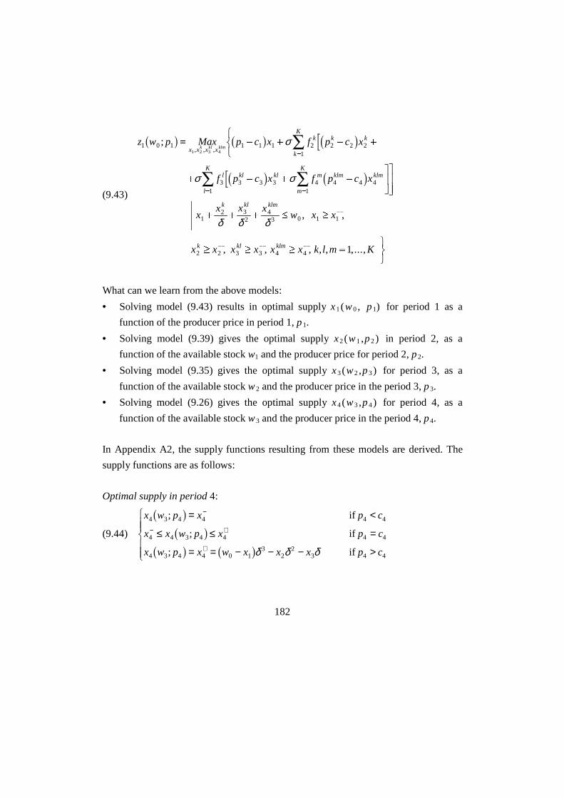
182

(9.43)

z w p Max p c x f p c x

f p c x f p c x

xx x x

w x x

x x x x x x k l m K

x x x x

k k k

k

K

l kl kl

l

Km klm klm

m

K

k kl klm

k kl klm

k kl klm1 0 1 1 1 1 2 2 2 21

3 3 3 31

4 4 4 41

12 3

24

3 0 1 1

2 2 3 3 4 4

1 2 3 4

1

;

, ,

, , , , , ,...,

, , ,1 6 1 6 2 7

2 7 2 7

= - + - +

%&'

+ - + -

"$#"

$##

+ + + � �

� � � =

()*

=

= =

-

- - -

Ê

Ê Ê

σ

σ σ

δ δ δ

What can we learn from the above models:

• Solving model (9.43) results in optimal supply x1(w0, p1) for period 1 as a

function of the producer price in period 1, p1.

• Solving model (9.39) gives the optimal supply x2(w1,p2) in period 2, as a

function of the available stock w1 and the producer price for period 2, p2.

• Solving model (9.35) gives the optimal supply x3(w2,p3) for period 3, as a

function of the available stock w2 and the producer price in the period 3, p3.

• Solving model (9.26) gives the optimal supply x4(w3,p4) for period 4, as a

function of the available stock w3 and the producer price in the period 4, p4.

In Appendix A2, the supply functions resulting from these models are derived. The

supply functions are as follows:

Optimal supply in period 4:

(9.44)

x w p x p c

x x w p x p c

x w p x w x x x p c

4 3 4 4 4 4

4 4 3 4 4 4 4

4 3 4 4 0 13

22

3 4 4

;

;

;

1 61 6

1 6 1 6

= <

≤ ≤ =

= = − − − >

%

&KK

'KK

−

− +

+

if

if

if δ δ δ

183

Optimal supply in period 3:

(9.45)

x w p x p c

x x w p x p c

x w p x wx

w x xx

p c

3 2 3 3 3 3 4

3 3 2 3 3 3 3 4

3 2 3 3 24

0 12

24

3 3 4

;

;

;

1 61 6

1 6 1 6

= < +

≤ ≤ = +

= = − = − − − > +

%

&

KKK

'

KKK

−

− +

+− −

if

if

if

Ψ

Ψ

Ψδ

δ δδ

with Ψ4 4 4 41

= −+

=∑σδ f p ck k

k

K

3 8 − see (A2.8) and (9.33), with a+ = max(a;0).

Optimal supply in period 2:

(9.46)

x w p x p c

x x w p x p c

x w p x w xx x

p c

2 1 2 2 2 2 3

2 2 1 2 2 2 2 3

2 1 2 2 0 13 4

2 2 2 3

;

;

;

1 61 6

1 6 1 6

= < +

≤ ≤ = +

= = − − − > +

%

&

KKK

'

KKK

−

− +

+− −

if

if

if

Ψ

Ψ

Ψδδ δ

with Ψ Ψ Ψ3 3 4 31

3 3 3 4 31

= + − −�!

"$#

=

+

=∑ ∑σδ f p f p c pk k

k

Kk k k

k

K

3 8 3 84 9 and

Ψ4 3pk2 7 = σδ f p cl kl

l

K

4 4 41

−+

=∑ 3 8 − see (A2.13) and (9.37).

Optimal supply in period 1:

(9.47)

x w p x p c

x x w p x p c

x w p x wx x x

p c

1 0 1 1 1 1 2

1 1 0 1 1 1 1 2

1 0 1 1 02 3

243 1 1 2

,

,

,

1 61 6

1 6

= < +

≤ ≤ = +

= = − − − > +

%

&

KKK

'

KKK

−

− +

+− − −

if

if

if

Ψ

Ψ

Ψδ δ δ

184

with: Ψ Ψ Ψ2 2 3 21

21

2 2 3 2= + − −�!

"$#

= =

+

∑ ∑σδ f p f p c pk k

k

Kk

k

Kk k3 8 3 84 9 ,

Ψ Ψ Ψ3 2 3 4 31

3 3 3 4 31

p f p f p c pk l kl

l

Kl kl kl

l

K

3 8 3 8 3 84 9= + − −�!

"$#

=

+

=∑ ∑σδ and

Ψ4 3pkl2 7 = σδ f p cm klm

m

K

4 4 41

−+

=∑ 3 8 − see (A2.18) and (9.41).

These functions show that optimal supply in each period has the following form:

• Supply in period t is the minimum quantity xt- , if the price is below the border

price, pt < ct + Ψ t+1.

• Supply in period t is the maximum possible quantity, taken into account

minimum sales in the other periods, if the price is above the border price, pt > c t

+ Ψ t+1.

• Supply in period t may take any value between the minimum and maximum

supply levels, if the price is exactly equal to the border price, pt = c t + Ψ t+1.

9.2.2 Estimating cereal supply functions for Burkina Faso

Before the supply functions (9.44) - (9.47) can be determined, first the values of the

parameters w0, xt− , α, δ, ρ and σ have to be estimated. The estimates will be

discussed below one by one.

a) Annual supply, w0For the determination of the level of annual cereal supply w0, use is made of cereal

production levels. Cereal production per producer is supposed to be the forecasted

mean production level for the year 2000 as presented in column (h) in Table 8.2. It is

recalled that on the basis of evidence discussed in section 8.1.3 we assumed that

annual supply w0 does not depend on prices. Therefore, w0 appears as a parameter in

the models (9.43), (9.39), (9.35), and (9.26). Given production, it can be explored on

the basis of the sales data presented in Appendix A3.3 which part of production can

185

reasonably be sold (which means that not too much is sold that hardly anything

remains to feed the own family, or that too little is sold so that stores are still full at

the end of the year). The observations on sales and sales as a percentage of production

give too little evidence to estimate per CRPA annual sales, w0. Therefore, three

different groups of CRPA are distinguished, with more or less the same sales and

production characteristics. For the first group, the CRPA Sahel, Nord and Centre

Nord, it is supposed that households sell on average 10% of their annual production.

Households in the second group, the CRPA Centre, Centre Ouest, Centre Sud, Est,

Centre Est, and Sud Ouest, sell on average 20%. Households in the third group, in the

CRPA Mouhoun, Hauts Bassins, and ComoJ, sell on average 35%. Using these

estimates and the forecasted cereal production for the planning period 2000-2001,

annual sales per person, w0, can be calculated (see Table 9.8).

b) Minimally required supplies, xt− .

Minimally required supplies in each period are also estimated for the three different

groups of CRPA. To estimate minimally required supplies, first, estimates are made

of the average percentage of production sold in each quarter. Comparing the different

surveys evaluated in Appendix A3.3 shows that the first group of CRPA sell on

average approximately 26% of their cereals in period 1 from October to December,

30% in period 2 from January to March, 25% in period 3 from April to June, and 19%

in period 4 from July to September – see Table 9.7. Producers from the second group

of CRPA sell on average approximately 27%, 39%, 12% and 23% in period 1, 2, 3

and 4, respectively. Finally, producers from the third group of CRPA sell on average

approximately 19%, 25%, 30% and 27% of their annual sales in period 1, 2, 3 and 4,

respectively.

186

Table 9.7 Evaluation of sales per season as % of annual sales for some different

studies.Author Province Year Oct-Dec Jan-Mar Apr-June July-Sept

Yonli sanmatenga 38% 48% 11% 4%

Reardon Soum 81-82 35% 29% 18% 18%

CRPA

group 1

83-84 10% 45% 35% 10%

Passoré 81-82 25% 25% 25% 25%

82-83 21% 13% 46% 21%

83-84 24% 24% 12% 40%

Average 26% 30% 25% 19%

Pardy Oubritenga 83-84 22% 40% 18% 21%

Zoundweogo 83-84 48% 24% 10% 19%

CRPA

group 2

Gourma 83-84 11% 53% 9% 28%

Average 27% 39% 12% 23%

Reardon Mouhoun 81-82 19% 19% 44% 19%

82-83 21% 21% 29% 29%

CRPA

group 3

Pardy Kossi 16% 34% 17% 33%

Average 19% 25% 30% 27%

Notes: See Appendix A3.3 for the details of the studies of Yonli (1997), Pardy (1987), and Reardon et al.(1987). Of these studies the years and provinces have been included of which most data were available.

Multiplying the average sales percentages given in Table 9.7 with the annual sales in

Table 9.8 gives estimates of average supplies from cereal sales per period. Minimally

required supplies from cereal sales to satisfy cash needs are now estimated as 60% of

these average quarterly supplies for the first period and second period, and 40% for

the third and fourth period – see Table 9.8. Minimally required supplies for the third

and fourth period are assumed to be lower than for the other two periods, for it is

supposed that non-cropping income is higher during these periods.

c) Discount rate: σ; Transaction costs: α; Production costs: β, Storage costs: ρ;

Storage losses, δ.

Reliable estimates of α, β, δ, ρ and σ are difficult to obtain, due to lack of

information on storage costs and transaction costs for the producers. The following

values have been adopted for all periods and all CRPA. The storage costs, which

include construction costs and time to build the stores, are ρ = 2.5 FCFA per kg per

187

period. Transaction costs, which include transport towards the market, costs to obtain

information on traders’ demand and time invested in the sales activities, are estimated

at α = 1 FCFA per kg per period. No data are available on production costs. We take

a value equal to 75% of the average ‘96-’99 producer price, presented in Table 8.3.

Storage losses are estimated to be 10% per year, so δ = 2.5% per period (see Section

8.4). For the discount rate, we suppose that it is equal to σ = 1/(1+r), with r the

interest rate. For r often the interest rate for lending money is chosen. These interest

rates may differ a lot. Private money lenders charge much higher interest rates than

official banks. Here an interest rate of 16% per year, so 4% per period is chosen (see

DJjou (1987) Bassolet 2000), see also Appendix A4.2). Therefore: σ = 0.96 per

period. The influence of these parameter values on the solution has to be analysed

using a sensitivity analysis.

Table 9.8 Sales per person, minimum supplies per quarter and maximum sales in

period 4.

Minimally required supplies (as % of annual sales)2Annual

sales1

(kg/person)

w 0

Period 1

Oct-Dec

x1−

Period 2

Jan-Mar

x2−

Period 3

Apr-June

x3−

Period 4

July-Sept

x4−

Centre 26 16% 23% 5% 9%

Centre Nord 16 15% 18% 10% 8%

Centre Ouest 41 16% 23% 5% 9%

Centre Sud 51 16% 23% 5% 9%

Sahel 15 15% 18% 10% 8%

Mouhoun 99 11% 15% 12% 11%

Est 43 16% 23% 5% 9%

Centre Est 36 16% 23% 5% 9%

Nord 14 15% 18% 10% 8%

Sud Ouest 55 16% 23% 5% 9%

Hauts Bassins 100 11% 15% 12% 11%

Comoe 92 11% 15% 12% 11%

Notes: 1) Annual sales are the average production per rural inhabitant (column (h) in Table 8.2)multiplied with the estimates of sales as percentage of production (see a) above); 2) Minimally requiredrevenues per period are calculated as the annual sales multiplied with the estimated sales per period as %

188

of annual sales (see Table 9.7), and the minimum requirements per period (60% of average revenues inthe first period and second period and 40% in the third and fourth period).

d) Random prices and probability distribution functions

In Chapter 7, it is argued that expected future revenues in the stochastic, multi-period

equilibrium model can be estimated using the probability distribution of future

producer prices. The discussion on cereal prices in Section 8.1.6 and Appendix A3.6,

however, shows that estimating the probability that the price in one of the quarters

reaches a certain level on the basis of the ‘92 – ‘99 price data, is not very accurate.

Before the devaluation a cereal consumer price of 50 FCFA per kg was not very

uncommon. After the devaluation in 1994 it is very rare. For that reason we do not

estimate the probability distribution of prices directly, but via a detour.

Define again the time periods t = 1,…,4, with t = 1 the post-harvest period from

October to December, t = 2 the period from January to March, t = 3 the period from

April to June, and t = 4 the hunger period from July to September, and define the

years Y = 1992,…,1999. Between 1992 and 1999 the average cereal prices per quarter

changed a lot, see Table A3.36, but the distribution of the differences between

observed and average prices remained more or less the same.28 It is possible to

estimate a discrete probability distribution function which gives the probability that

the observed price deviates from the average price with a certain value. For that

reason, we determine for each CRPA, each quarter and each year the average prices,

and the deviations of the price observations from the averages. 29 Using this, we

estimate the probability that the deviation from the average is within a certain

interval. Define pitY , the observed price in quarter t = 1,2,3,4, in CRPA i ∈ I, in year

28 To analyse the dispersion of prices, for each year the standard deviation has been calculated of the

relative difference between observed prices and the average price, P p pitY

itY

itY−3 8 , with Pit

Y a price

observation and pitY the average price for quarter t in CRPA i in year Y, t = 1,...,4, Y = ‘92-’99. These

standard deviations did not change significantly between 1992 and 1999. Furthermore, an analysis of thefirst, second, and third quartile distances and of the minimum and maximum relative difference betweenprices and average prices did not clearly show changes in time.29 Define the set of CRPA I = {Centre, Centre Nord, Centre Ouest, Centre Sud, Sahel, Mouhoun, Est,Centre Est, Nord, Sud Ouest, Hauts Bassins, Comoe}.

189

Y ∈ {’92,…,’99}, pitY the average price in CRPA i in quarter t in year Y, and

introduce the nine intervals:

(9.48) ∆1 = (-∞;-21] ∆2 = (-21;-15] ∆3 = (-15;-9] ∆4 = (-9;-3] ∆5 = (-3;3]

∆6 = (3;9] ∆7 = (9;15] ∆8 = (15;21] ∆9 = (21;∞].

For each of the quarters t = 2,3,4, we count the number of observations for which the

difference between the observed and the averge price PitY - pit

Y , was within the

interval ∆k, for k = 1,...,9. 30 The probability that the deviation from the average price

in a certain quarter is within the interval ∆k, is equal to the number of observations in

the interval divided by the total number of observations in the quarter. For some of

the CRPA, the number of observations was very small. For example, for the CRPA

Nord, only 2 observations were available for the period July – September.

Furthermore, the distributions did not differ a lot between the CRPA. For that reason

we estimate for each quarter one probability distribution on the basis of price data for

all CRPA, and suppose that it is the same for all regions. Define:

(9.49) Pr P p fitY

itY k

tk− ∈ =∆ ∆3 8

for t = 2,3,4, k = 1,…,9, i ∈ I, Y ∈ {’92,…,’99}, with 0 ≤ ftk∆ ≤ 1 and f t

k

k

∆∑ = 1.

The probability distributions are given in Table 9.9.

In Section 9.2.1, random producer prices Pit have been introduced for each CRPA for

the quarters t = 2, 3 and 4, to determine optimal revenues.31 Expectations for future

periods, change in each period. In period 1, a different price is expected for period 4,

than in period 2. In Section 9.2.1, we assumed that in the decision model for period t,

random prices for period t+1 do not depend on pt, whereas random prices for the

30 Note that we only need the probability distribution for the periods t = 2,3,4, see Section 9.2.1.31 In Section 9.2.1 the index i was skipped from the definition of the random price in quarter t.

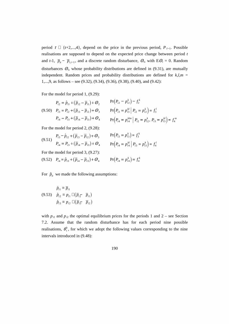
190

period τ ∈ { t+2,...,4}, depend on the price in the previous period, Pτ −1. Possible

realisations are supposed to depend on the expected price change between period t

and t-1, pit − pi t, −1, and a discrete random disturbance, Θ t, with EΘ t = 0. Random

disturbances Θ t, whose probability distributions are defined in (9.31), are mutually

independent. Random prices and probability distributions are defined for k,l,m =

1,...,9, as follows – see (9.32), (9.34), (9.36), (9.38), (9.40), and (9.42):

For the model for period 1, (9.29):

(9.50)

P p p p

P P p p

P P p p

i i i i

i i i i

i i i i

2 1 2 1 2

3 2 3 2 3

4 3 4 3 4

= + - +

= + - +

= + - +

$ 1 61 61 6

Θ

Θ

Θ

Pr

Pr

Pr ,

P p f

P p P p f

P p P p P p f

i ik k

i ikl

i ik l

i iklm

i ik

i ikl m

2 2 2

3 3 2 2 3

4 4 2 2 3 3 4

= =

= = =

= = = =

2 7

4 9

4 9For the model for period 2, (9.28):

(9.51) P p p p

P P p p

i i i i

i i i i

3 2 3 2 3

4 3 4 3 4

= + - +

= + - +

$ 1 61 6

Θ

Θ

Pr

Pr

P p f

P p P p f

i ik k

i ikl

i ik l

3 3 3

4 4 3 3 4

= =

= = =

2 7

4 9For the model for period 3, (9.27):

(9.52) P p p pi i i i4 3 4 3 4= + - +$ 1 6 Θ Pr P p fi ik k

4 4 4= =2 7

For $pit we made the following assumptions:

(9.53)

$

$

$

p p

p p p p

p p p p

i i

i i i i

i i i i

1 1

2 1 2 1

3 2 3 2

== + −

= + −

1 61 6

with p i1 and p i2 the optimal equilibrium prices for the periods 1 and 2 – see Section

7.2. Assume that the random disturbance has for each period nine possible

realisations, θ tk , for which we adopt the following values corresponding to the nine

intervals introduced in (9.48):

191

(9.54) θ1 = -24, θ2 = -18, θ3 = -12, θ4 = -6, θ5 = 0, θ6 = 6, θ7 = 12, θ8 = 18, θ9 = 24

Suppose that the probability distribution of Θ t is the same as the probability

distribution of ∆ t, ftk∆ , in (9.49). Define for k = 1,…,9, i ∈ I, t = 2,3,4, see Table 9.9:

(9.55) Pr Θ ∆t

ktk

tkf f= = =θ3 8

with 0 ≤ ftk ≤ 1 and f t

k

k∑ = 1.

Table 9.9 Probability distribution functions of deviations from average producer

prices – see (9.49) and of the disturbances – see (9.55), for the quarters t =

2, 3 and 4.1

ftk∆ ft

k t = 2

Jan – Mar

t = 3

Apr – Jun

t = 4

Jul – Sept

∆1 = (-∞ ; -21] θ1 = -24 0.018 0.027 0.026

∆2 = (-21 ; -15] θ2 = -18 0.028 0.034 0.047

∆3 = (-15 ; -9] θ3 = -12 0.079 0.071 0.096

∆4 = (-9 ; -3] θ4 = -6 0.228 0.230 0.192

∆5 = (-3 ; 3] θ5 = 0 0.300 0.307 0.259

∆6 = (3 ; 9] θ6 = 6 0.205 0.182 0.207

∆7 = (9 ; 15] θ7 = 12 0.099 0.086 0.113

∆8 = (15 ; 21] θ8 = 18 0.026 0.040 0.032

∆9 = (21 ; ∞) θ9 = 24 0.017 0.023 0.028

Note: 1 The numbers denote the probability the deviation from the average price is within one of the

intervals ∆k: Pr(pit - pit

∈ ∆k) or the probability that the price in period t has the value

p p pi t it i t

k

, ,− −+ − +1 11 6 θ . The probability density function for quarter t = 1 is not used in the analysis,

and therefore not shown in the table. Source: Price data from SIM/SONAGESS.

192

9.3 Review of the stochastic, multi-period, spatial equilibrium model

In Section 7.2 we argued, that we can analyse market functioning and market price

formation by solving the stochastic, multi-period, spatial equilibrium model (7.46). In

the previous sections we estimated consumer demand functions, discussed producer

supply behaviour, and estimated the other parameters necessary to solve model

(7.46). Before discussing the results of this model in the next chapter, in this section

we shortly reconsider this model.

Some extra parameters for the trader’s strategies

To simplify notation, in model (7.46) we only considered transport and storage costs.

However, in Section 8.2.2 and 9.2 it has been argued that also storage losses and

trading costs have to be taken into account, and that expected future profits have to be

discounted to their present value. Trading costs are the costs a trader has to make for

each unit of cereals transacted. They include costs for bags, personnel and taxes. We

calculate total trading costs as the unit costs multiplied with the quantity sold to the

consumers. In Section 9.2 storage losses and discount rates were already introduced

for the producers. For traders we introduce the following parameters:

1- $δ fraction of stock lost by the trader in each period due to insects, rats,

diseases, etc, see Table 8.5 - 2.

(9.56) $σ discount factor for the traders, to calculate the present value of future

profits, see Table 8.5 - 3.$α trading costs per unit of cereals transacted, see Table 8.5 - 4, 5, and 6.

These parameters may have different values than storage losses, δ, and discount rate,

σ , for the producers, introduced in Section 9.2.2.

Depending on the number of periods, regions, and possible price realisations taken

into account, the equilibrium model (7.64) can become very large. For example if 4

periods, 12 regions, and 9 possible combinations of price realisations in each period

193

(i.e. K = 9) are considered, the number of variables in the equilibrium model for

period 1 is almost 150,000, while we are only interested in the optimal values of 204

of them (the variables for the period 1). For that reason we are using a simplification

of model (7.64) to analyse cereal price formation in Burkina Faso. In the model for

period t, we assume the number of possible price realisations for period t+1 to be

equal to K = 9. For the other periods t+2,…,T we assume that producers and traders

consider only one possible price realisation, which is the expected price for that

period, given the price realisation in the previous period. So, for the possible producer

and consumer price realisations, taken into account by the traders and producers, we

assume, like we did in Section 9.2, that traders and producers expect prices in each

period t+1 to T, to increase with a fixed amount, and that the price in period t+1 may

also increase with a random disturbance. We assume that traders expect the prices in

the different regions to be linked, i.e. the disturbance on the expected price is the

same for each region. This is a rough simplification of the model, but is necessary to

avoid an unmanageable model. The possible prices taken into account by the traders

and producers are – see (9.50) - (9.52):

For the model for period 1:

(9.57)

p p

p p p p

p p p p

ik

ik

ik

ik

i i

ik

ik

i i

2 2 2

3 2 3 2

4 3 4 3

= +

= + −

= + −

θ

1 61 6

π π θπ π π π

π π π π

ik

ik

ik

ik

i i

ik

ik

i i

2 2 2

3 2 3 2

4 3 4 3

= +

= + −

= + −

1 61 6

For the model for period 2:

(9.58) p p p p

p p p p

ik

i i ik

ik

ik

i i

3 1 3 1 3

4 3 4 3

= + − +

= + −

1 61 6

θ π π π π θ

π π π πik

i i ik

ik

ik

i i

3 1 3 1 3

4 3 4 3

= + − +

= + −

1 61 6

For the model for period 3:

(9.59) p p p pik

i i ik

4 2 4 2 4= + − +1 6 θ π π π π θik

i i ik

4 2 4 2 4= + − +1 6

The average producer and consumer prices pit and πit are given in Table 8.3. For the

probability distributions of the random disturbances, we suppose that producers and

traders have the same probability distribution – see (9.55):

194

(9.60) Pr Θ tk

itk

tkf g= = =θ3 8

Consequently, in the model for period t = 1,2,3, for k = 1,…,9 – see (9.51) - (9.53):

(9.61) Pr

Pr ...

, , ,

, , , , , , , ,

P p f

P p P p g

i t i tk

i tk

t tk

t tk

n t n tk

n t n tk

tk

+ + +

+ + + + + + + + +

= =

= ∧ = ∧ ∧ = ∧ = =

1 1 1

1 1 1 1 1 1 1 1 1 1 1 1 1

3 8

3 8Π Ππ π

Parameters and variables:

Besides the parameters introduced in (9.56), the parameters used in the equilibrium

models are, for regions i = 1,…,12, periods t = 1,…,4, household types h = rural,

urban, price realisations k = 1,…,9:

Popih size of the population of type h in region i – see Table 8.1

I ith

ith− ξ supernumerary income level of a consumer of type h, in

region i, in period t, in FCFA – see (9.14), Table 9.5, and

Table 9.6.

bith share of supernumerary income spent on cereals, for a

consumer of type h, in region i, in period t – see (9.14),

Table 9.5, and Table 9.6.

γ ith minimally required cereal purchase level for a consumer of

type h, in region i, in period t, in kg – see (9.12), (9.14), and

(9.16).

δ 1 – storage losses for a producer – see page 187.

σ discount factor for a producer – see page 187.

cit producer costs of cereals supplied, in FCFA/kg – see (9.23)

and page 186.

w i0 annual cereal supply for a producer in region i, in kg – see

Table 9.8.

195

xit− minimally required cereal supplies in period t for a producer

in region i, in kg – see Table 9.8.

τ ijt costs to transport one kg in period t from region i to region j,

in FCFA/kg – see (6.7) and Table 8.4.

kit storage costs in region i in period t, in FCFA/kg – see (6.7)

and Table 8.5–1,3.

si0 initial trader stock; si0 = 0 – see (6.7).

y xitk

itk, upper bounds on trader sales and purchases, in kg – see

(9.62), (9.63) below.

f itk probability distribution of producer prices in region i in

period t – see (9.61) and Table 9.9.

gtk trader probability distribution of producer and consumer

prices in period t – see (9.61) and Table 9.9.

pitk ,πit

k possible producer and consumer price realisations in region i

in period t, in FCFA/kg – see (9.57) - (9.59), (9.53), (9.54),

and Table 8.3.

The variables in the equilibrium models are, for i = 1,…,12, t = 1,…,4, τ = t+1,…,4, k

= 1,…,9:

xit Producer supply in region i in period t, in kg.

yit Consumer demand in region i in period t, in kg.

xijt Trader’s transported quantity from region i to j in period t, in kg.

sit Trader’s stored quantity in region i in period t, for t = 1,2,3, in kg.

p it Producer price in region i in period t, in FCFA/kg.

πit Consumer price in region i in period t, in FCFA/kg.

xikτ Producer supply in region i in period τ, if future prices are pi

kτ , in kg.

qikτ Trader purchases in region i in period τ, if future prices are pi

kτ and

πitk , in kg.

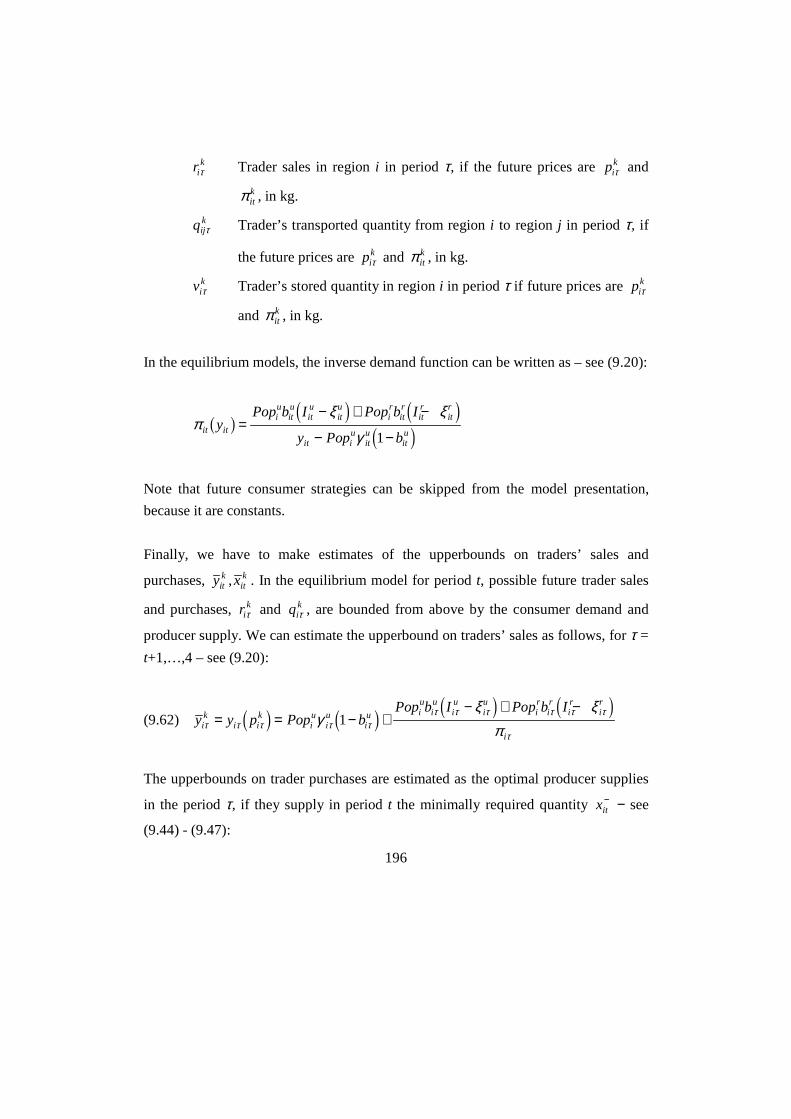
196

rikτ Trader sales in region i in period τ, if the future prices are pi

kτ and

πitk , in kg.

qijkτ Trader’s transported quantity from region i to region j in period τ, if

the future prices are pikτ and πit

k , in kg.

vikτ Trader’s stored quantity in region i in period τ if future prices are pi

kτ

and πitk , in kg.

In the equilibrium models, the inverse demand function can be written as – see (9.20):

πξ ξ

γit it

iu

itu

itu

itu

ir

itr

itr

itr

it iu

itu

itu

yPop b I Pop b I

y Pop b1 6

3 8 3 83 8

=− + −

− −1

Note that future consumer strategies can be skipped from the model presentation,

because it are constants.

Finally, we have to make estimates of the upperbounds on traders’ sales and

purchases, y xitk

itk, . In the equilibrium model for period t, possible future trader sales

and purchases, rikτ and qi

kτ , are bounded from above by the consumer demand and

producer supply. We can estimate the upperbound on traders’ sales as follows, for τ =

t+1,…,4 – see (9.20):

(9.62) y y p Pop bPop b I Pop b I

ik

i ik

iu

iu

iu i

uiu

iu

iu

ir

ir

ir

ir

iτ τ τ τ τ

τ τ τ τ τ τ

τγ

ξ ξπ

= = − +− + −

3 8 3 83 8 3 8

1

The upperbounds on trader purchases are estimated as the optimal producer supplies

in the period τ, if they supply in period t the minimally required quantity xit− − see

(9.44) - (9.47):

197

(9.63) x

Pop x p c

Pop w xx

p ci

ir

i ik

i i

ir

t it

T

ik

i i

τ

τ τ τ τ

νν τ

ν ττ τ τδ

δ=

< +

− −�!

"$# ≥ +

%&K

'KK

−+

−−

−

−= +

+∑

if

if

Ψ

Ψ

,

,

1

11

13 8

Equilibrium models:

The equilibrium models for the periods 1, 2, 3 and 4 can be written as:

For period 1: Determine the optimal values of the following variables: yi1, xi1, xij1,

si1, x r q qik

ik

ik

ijk

τ τ τ τ, , , , vikτ for τ = 2,3,4, k = 1,…,K, i = 1,…,n:

(9.64)

z s w d c x x k s y

f p c x p c x p c x

g r p q q

i i i

y

i i ij ij

jj i

n

i i i

i

n

ik

ik

i ik

ik

i ik

ik

i ik

k

K

i

n

kik

ik

ik

ik

ij ijk

jj i

n

i

1 0 0 1

0

1 1 1 1

1

1 1 1

1

2 2 2 2 3 3 3 4 4 4

11

2 2 2 2 2 2 2

1

1

, max $

$ $

0 5 0 5

2 7 2 7 2 7

2 7

= - - - -

+ - + - + -

+ - - -

I ÊÊ

ÊÊ

=

ā

=

==

=

ā

�

!

"

$

###

π ξ ξ τ α

σ σ σ

σ π α τÊÊÊ

Ê Ê

- + - -

- - - + - - - -

�

���

�

���

�

!

�

���

�

���

�

���

"

$

###

"

$

###

==

=

ā

=

ā

k v r

p q q k v r p q q k v

i ik

k

K

i

n

ik

ik

ik

ik

ij ijk

jj i

n

i ik

ik

ik

ik

ik

ij ijk

jj i

n

i ik

2 2

11

3 3

3 3 3 3

1

3 3 4 4 4 4 4 4

1

4 4

$ $

$ $

σ π α

τ σ π α τ

2 72

2 7

subject to

x x s y x s q q s r q v

q q v r q v q q v r q v

i j i

jj i

n

i i i j

jj i

n

i ik

jik

jj i

n

i ik

ijk

jj i

n

ik

ik

jik

jj i

n

ik

ik

ijk

jj i

n

ik

ik

jik

jj i

n

ik

ik

ijk

jj i

n

1 1

1

0 1 1

1

1 2 2

1

1 2 2

1

2

3 3

1

2 3 3

1

3 4 4

1

3 4 4

1

+ + = + + + + = + +

+ + = + + + + = + +

=

ā

=

ā

=

ā

=

ā

=

ā

=

ā

=

ā

=

ā

Ê Ê Ê Ê

Ê Ê Ê Ê

$ ; $ ;

$ ; $

δ δ

δ δ ik4 ;

198

r y q x r y q x r y q x

xx x x

w x x x x x x x x

x y x s x r q q v k

ik

ik

ik

ik

ik

ik

ik

ik

ik

ik

ik

ik

iik

ik

ik

i i i ik

i ik

i ik

i

i i ij i ik

ik

ik

ijk

ik

2 2 2 2 3 3 3 3 4 4 4 4

12 3

243 0 1 1 2 2 3 3 4 4

1 1 1 1 0 1

� � � � � �

+ + + � � � � �

� =

- - - -

; ; ; ; ; ;

; ; ; ; ;

, , , , , , , , ,..

δ δ δττ τ τ τ τ for = 2,3,4, .,K

For period 2: Determine the optimal values of the following variables: yi2, xi2, xij2,

si2, x r q qik

ik

ik

ijk

τ τ τ τ, , , , vik3 for τ = 3,4, k = 1,…,K, i = 1,…,n, with w i1 = (w i0 – xi1)⋅δ, and

with si1 and xi1 the optimal storage and producer supply for period 1:

(9.65)

z s w d c x x k s y

f p c x p c x

g r p q q k v

i i i

y

i i ij ij

jj i

n

i i i

i

n

ik

ik

i ik

ik

i ik

k

K

i

n

kik

ik

ik

ik

ij ijk

jj i

n

i ik

i

2 1 1 2

0

2 2 2 2

1

2 2 2

1

3 3 3 3 4 4 4

11

3 3 3 3 3 3 3

1

3 3

2

, max $

$ $

0 5 0 5

2 7 2 7

2 7

= - - - -

+ - + -

+ - - - -

I ÊÊ

ÊÊ

Ê

=

ā

=

==

=

ā

�

!

"

$

###

�

���

�

��

π ξ ξ τ α

σ σ

σ π α τ �

�

!

�

!

"

$

###

"

$

###

+

+ - - - -

==

=

ā

ÊÊ

Ê

k

K

i

n

ik

ik

ik

ik

ij ijk

jj i

n

i ikr p q q k v

11

4 4 4 4 4 4

1

4 4$ $σ π α τ2 7

subject to

x x s y x s q q s r q v

q q v r q v r y q x r y q x

i j i

jj i

n

i i i j

jj i

n

i ik

jik

jj i

n

i ik

ijk

jj i

n

ik

ik

jik

jj i

n

ik

ik

ijk

jj i

n

ik

ik

ik

ik

ik

ik

ik

ik

ik

2 2

1

1 2 2

1

2 3 3

1

2 3 3

1

3

4 4

1

3 4 4

1

4 3 3 3 3 4 4 4 4

+ + = + + + + = + +

+ + = + + � � � �

=

ā

=

ā

=

ā

=

ā

=

ā

=

ā

Ê Ê Ê Ê

Ê Ê

$ ; $ ;

$ ; ; ; ; ;

δ δ

δ

199

xx x

w x x x x x x

x y x s x r q q v k K

iik

ik

i i i ik

i ik

i

i i ij i ik

ik

ik

ijk

ik

23 4

2 1 2 2 3 3 4 4

2 2 2 2 0 1

+ + � � � �

� =

- - -

δ δττ τ τ τ τ

; ; ; ;

, , , , , , , , ,...,for = 3,4,

For period 3: Determine the optimal values of the following variables: yi3, xi3, xij3,

si3, x r q qik

ik

ik

ijk

4 4 4 4, , , and vik4 for k = 1,…,K, i = 1,…,n, with w i2 = (w i1 – xi2)⋅δ, and with

si2 and xi2 the optimal storage and producer supply for period 2:

(9.66)

z s w d c x x k s y

f p c x g r p q q k v

i i i

y

i i ij ij

jj i

n

i i i

i

n

ik

ik

i ik

k

K

i

nk

ik

ik

ik

ik

ij ijk

jj i

n

i ik

k

K

i

n

i

3 2 2 3

0

3 3 3 3

1

3 3 3

1

4 4 4 4

11

4 4 4 4 4 4 4

1

4 4

11

3

, max $

$ $

0 5 0 5

2 7 2 7

= - - - -

+ ¼ - + - - - -

I ÊÊ

ÊÊ ÊÊÊ

=

ā

=

== =

ā

==

�

!

"

$

###

�

���

�

���

π ξ ξ τ α

σ σ π α τ

subject to

x x s y x s q q s r q v

r y q x xx

w x x x x

x y x s x r q q v

i j i

jj i

n

i i i j

jj i

n

i ik

jik

jj i

n

i ik

ijk

jj i

n

ik

ik

ik

ik

ik

iik

i i i ik

i

i i ij i ik

ik

ik

ijk

i

3 3

1

2 3 3

1

3 4 4

1

3 4 4

1

4

4 4 4 4 34

2 3 3 4 4

3 3 3 3 4 4 4 4 4

+ + = + + + + = + +

� � + � � �

=

ā

=

ā

=

ā

=

ā

- -

Ê Ê Ê Ê$ ; $ ;

; ; ; ; ;

, , , , , , , ,

δ δ

δk k K� =0 1for ,...,

For period 4: Determine the optimal values of the following variables: yi4, xi4, xij4, for

i = 1,…,n, with w i3 = (w i2 – xi3)⋅δ, and with si3 and xi3 the optimal storage and

producer supply for period 3:

(9.67) z s w d c x x k s yi i i

y

i i ij ij

jj i

n

i i i

i

n i

4 3 3 4

0

4 4 4 4

1

4 4 4

1

4

, max $0 5 0 5= - - - -I ÊÊ=

ā

=

�

!

"

$

###

π ξ ξ τ α

subject to

200

x x s y x s x x w y s xi j i

jj i

n

i i i j

jj i

n

i i i i i i i j4 4

1

3 4 4

1

4 4 4 3 4 4 4 0+ + = + + � � �

=

ā

=

ā

-

Ê Ê$ ; ; , ,δ

The theorem 7.1 and 7.2 also hold for these models. The optimal producer price in

period t is defined as:

p it = λ it

with λ it the optimal value of the Lagrange multiplier of the equilibrium constraint for

period t in the model for period t. The results of these models will almost be the same

as the Equilibrium properties 7.1 to 7.4 in Section 7.2. Equilibrium property 7.2

remains the same. The other properties change in:

Equilibrium property 9.1: For region i and period t we can derive that:

a) In the optimal solution πit(yit) ≤ p it(xit) + $α .

b) If in the solution πit(yit) < p it(xit) + $α , then yit = 0.

c) If in the optimal solution, supply and demand are both positive, xit > 0 and yit > 0,

then the prices satisfy necessarily πit(yit) = p it(xit) + $α .

Equilibrium property 9.2: In the solution, let xijt > 0, with i,j = 1,…,n, j ≠ i, t = 1,…,n,

then:

a) xsit = 0, for s = 1,…,n, s ≠ i. c) xit > 0 or si,t-1 > 0.

b) xjst = 0, for s = 1,…,n, s ≠ j. d) yjt > 0 or sjt > 0

Equilibrium property 9.3:

a) In the optimal solution πjt(yjt) ≤ p it(xit) + $α + τ ijt.

b) If in the solution πjt(y jt) < p it(xit) + $α + τ ijt, then xijt = 0 or yjt = 0.

c) If in the optimal solution supplies in region i, transport between region i and j, and

demand in region j are positive, xit > 0, xijt > 0, and yjt > 0, then the optimal prices

satsify necessarily πjt(yjt) = p it(xit) + $α + τ ijt.

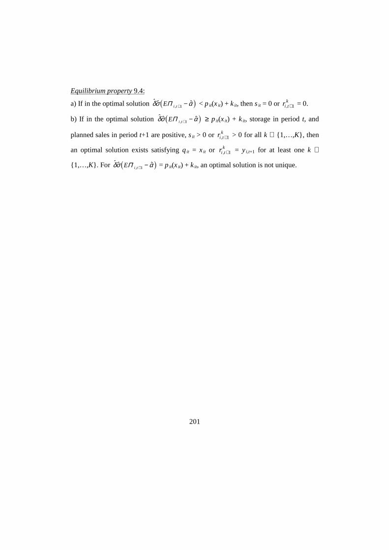
201

Equilibrium property 9.4:

a) If in the optimal solution $ $ $

,δσ αE i tΠ + −11 6 < p it(xit) + kit, then sit = 0 or ri tk, +1 = 0.

b) If in the optimal solution $ $ $

,δσ αE i tΠ + −11 6 ≥ p it(xit) + kit, storage in period t, and

planned sales in period t+1 are positive, sit > 0 or ri tk, +1 > 0 for all k ∈ {1,…,K}, then

an optimal solution exists satisfying q it = xit or ri tk, +1 = yi,t+1 for at least one k ∈

{1,…,K}. For $

$ $

,δσ αE i tΠ + −11 6 = p it(xit) + kit, an optimal solution is not unique.

202

10 Discussion of model results

Solving model (9.1), (9.2), (9.13), with demand functions given in (8.14) Section 8.1.3,

and supply functions determined by model (8.36) in Section 8.2.1, gives us results which

roughly reflect reality in Burkina Faso. We shortly discuss some of the main results.

Prices determined by the model are generally in line with the observed cereal prices given

in Table 8.3. The values of the consumer and producer prices do have more or less the

correct order and reflect seasonality - see Table 10.1. Price volatility is somewhat higher

than the average observed in Table 8.3. This was expected as we deal with a specific year

instead of the average for a number of years. The results show that prices are lowest in

the high production areas, from which many cereals are transported, and highest in the

low production and shortage areas.

Estimated transport flows are in line with the flows observed in reality. Most goods are

transported from the largest surplus zone Mouhoun towards the region Centre with the

capital Ouagadougou (see Figure 10.1). Also the shortage regions Sahel and Nord receive

a large part of the surplus from the regions Mouhoun and Est. Transport towards these

regions is highest during the lean period, from July to September, when farmers’ stocks

get depleted. In the period October – December the region Hauts Bassins has a relatively

low price and a large surplus that is transferred to Ouagadougou, where the prices are

relatively high. However, from april onwards, Hauts Bassins becomes a deficit region

that imports from the Mouhoun and the Centre-Ouest. It should be noted that many

cereals from the region Mouhoun, Sud Ouest and Comoe are transferred to the north and

center via traders based in Bobo Dioulasso, which is one of the most important

redistribution markets of the country. About 1/3 of the marketable surplus (see Table 8.1

and 9.8) is transported towards other regions.

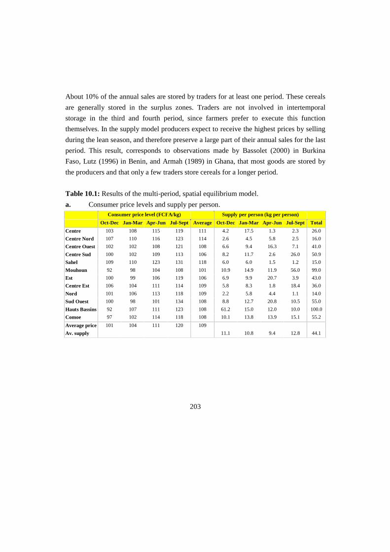
203

About 10% of the annual sales are stored by traders for at least one period. These cereals

are generally stored in the surplus zones. Traders are not involved in intertemporal

storage in the third and fourth period, since farmers prefer to execute this function

themselves. In the supply model producers expect to receive the highest prices by selling

during the lean season, and therefore preserve a large part of their annual sales for the last

period. This result, corresponds to observations made by Bassolet (2000) in Burkina

Faso, Lutz (1996) in Benin, and Armah (1989) in Ghana, that most goods are stored by

the producers and that only a few traders store cereals for a longer period.

Table 10.1: Results of the multi-period, spatial equilibrium model.

a. Consumer price levels and supply per person.Consumer price level (FCFA/kg) Supply per person (kg per person)

Oct-Dec Jan-Mar Apr-Jun Jul-Sept Average Oct-Dec Jan-Mar Apr-Jun Jul-Sept Total

Centre 103 108 115 119 111 4.2 17.5 1.3 2.3 26.0

Centre Nord 107 110 116 123 114 2.6 4.5 5.8 2.5 16.0

Centre Ouest 102 102 108 121 108 6.6 9.4 16.3 7.1 41.0

Centre Sud 100 102 109 113 106 8.2 11.7 2.6 26.0 50.9

Sahel 109 110 123 131 118 6.0 6.0 1.5 1.2 15.0

Mouhoun 92 98 104 108 101 10.9 14.9 11.9 56.0 99.0

Est 100 99 106 119 106 6.9 9.9 20.7 3.9 43.0

Centre Est 106 104 111 114 109 5.8 8.3 1.8 18.4 36.0

Nord 101 106 113 118 109 2.2 5.8 4.4 1.1 14.0

Sud Ouest 100 98 101 134 108 8.8 12.7 20.8 10.5 55.0

Hauts Bassins 92 107 111 123 108 61.2 15.0 12.0 10.0 100.0

Comoe 97 102 114 118 108 10.1 13.8 13.9 15.1 55.2

Average price 101 104 111 120 109

Av. supply 11.1 10.8 9.4 12.8 44.1

204

b. Cereal demand and consumption per rural and urban consumerCereal demand per rural consumer (kg/person) Cereal consumption per urban consumer

(kg/person)

Oct-Dec Jan-

Mar

Apr-

Jun

Jul-

Sept

annual

consump.1Oct-Dec Jan-

Mar

Apr-

Jun

Jul-

Sept

annual

consump

Centre 3.2 2.9 4.1 6.5 122 31.4 29.7 29.9 29.7 121

Centre Nord 2.8 2.7 3.9 6.3 163 26.2 26.0 26.2 26.3 105

Centre Ouest 2.9 3.1 4.5 6.6 179 26.4 27.1 27.5 26.4 107

Centre Sud 3.1 3.1 4.6 6.4 238 27.2 27.4 27.9 26.1 109

Sahel 4.9 4.9 6.9 10.6 162 26.0 26.1 25.8 25.4 103

Mouhoun 3.5 4.8 7.4 8.7 208 27.4 27.5 27.9 28.3 111

Est 2.7 2.8 4.2 6.4 188 26.4 27.1 27.7 26.8 108

Centre Est 2.9 3.1 4.3 6.8 163 26.4 27.2 26.9 26.8 107

Nord 2.9 2.8 4.1 6.5 143 26.7 26.5 26.8 26.6 107

Sud Ouest 5.2 7.3 11.5 10.5 253 27.0 27.5 28.2 25.2 108

Hauts Bassins 3.8 4.4 6.8 7.3 206 32.9 29.8 30.7 29.2 123

Comoe 3.6 4.4 6.6 7.8 231 27.6 26.6 26.6 26.9 108

Average 3.5 3.9 5.8 7.5 182 27.6 27.4 27.7 27.0 110

Note: 1) Annual consumption equals production per rural inhabitant (Table 8.1) + annual demand – annual supply perperson (Table 9.8).

c. Transported and stored quantities.Quantity transported (in 1000 tonnes) Quantity stored (in 1000 tonnes)

From To Oct-Dec Jan-Mar Apr-Jun Jul-Sept Total Oct-Dec Jan-Mar

Centre Ouest Centre 0 0 10.8 0 10.8 Centre 0 0

Centre Ouest Sud Ouest 0 0 0 0.46 0.46 Centre Nord 0 0

Centre Sud Centre 0 3.43 0.74 3.95 8.12 Centre Ouest 0.32 3.11

Centre Sud Centre Nord 0 0 0 5.33 5.33 Centre Sud 2.04 2.35

Mouhoun Centre 0 0.35 10.01 23.31 33.67 Sahel 0 0

Mouhoun Centre Ouest 0 0 0 3.08 3.08 Mouhoun 2.28 10.55

Mouhoun Sahel 0 0 0 7.93 7.93 Est 2.06 0

Mouhoun Nord 3.35 0 2.52 7.82 13.69 Centre Est 0 1

Mouhoun Hauts Bassins 0 0 0 8.83 8.83 Nord 0 0

Est Centre 0 7.48 6.28 0 13.76 Sud Ouest 1.36 3.35

Est Sahel 0 0 4.89 0 4.89 Hauts Bassins 2.41 0

Est Centre Est 0.61 0 3.66 0 4.26 Comoe 0 0

Centre Est Centre 0 0 0 1.73 1.73 Total 10.48 20.36

Centre Est Est 0 0 0 3.98 3.98 In Period 3 and 4 traders store nocereals

205

cont. Table 10.1.cSud Ouest Hauts Bassins 0 0.24 7.58 0 7.82

Hauts Bassins Centre 25.48 0 0 0 25.48

Hauts Bassins Centre Nord 1.96 0 0 0 1.96

Hauts Bassins Comoe 0.29 0 0 0 0.29

Comoe Hauts Bassins 0 0.62 0 0 0.62

Total 31.68 12.12 46.48 66.44 156.72

.

π ≤ 106

106 < π < 109

π ≥ 109

Total transport flowsandaverage annual price levels

A

C

C

B

BB A

A

A

B

C

C

CB

C

Figuur 10.1: Consumer prices and transport flows in Burkina Faso

Transport costs

The main objective of this paper was to analyse the direct impact of transport costs on

cereal trade. We recall that the total annual supply is given (see Chapter 9), however, the

distribution of supply over the year changes. The model shows that if transport costs

decrease, quarterly cereal prices in surplus regions increase, while cereal prices in deficit

regions decrease – see Table 10.2. The changes are, however, small. Halving the transport

costs causes average prices in the Sahel to decrease by 3.9% - see Table 10.2. This causes

an increased demand of 4.3% and an increased cereal consumption of only 0.7%.32

32 The impact on total consumption is smaller than the impact on market demand, as only a minor part of totalconsumption is purchased on the market (see Table 10.1.b).

206

Likewise, average prices in the region Centre, with the capital Ouagadougou, decrease

with 1.7%. As a consequence, urban consumption increases with 1.1%, and rural

consumption with only 0.2% (rural demand increases with 1.4%). A drawback from

decreased prices in a region, is that producers earn less from their supplies (since the

margin between producer and consumer prices is assumed to be fixed). Total transported

quantities increase with 7.8% if transport costs decrease with 50%. Stored quantities

decrease with 19%.

Looking at prices, it can be concluded that on average the price increase in the periods 2

and 3 is somewhat lower, whereas, the price increase in the last period is sharper than in

the situation with high transport costs. Consumers in the main deficit area Sahel and

producers in the main surplus area Mouhoun profit most from the reduction in transport

costs. For producers and consumers in other markets, the effects are less striking. These

results show that despite the large (50%) decrease in transport costs, the direct effects on

prices and consumption are small. This result contradicts popular claims that transport

costs are a major barrier for a more equal distribution of cereal production over the

country. The model indicates that the bad income position of the Sahelian population is

more likely to be responsible for the low demand. We note that the income position may

increase in the long run as a result of infrastructural improvements. It is, however, not our

intention to analyse the spin-off effects of infrastructural improvements on other sectors

in the economy. Our partial economic approach is not suitable to analyse these indirect

effects. We simply questioned the popular claim that high transport costs are a major

barrier for cereal marketing. The research results show that this claim needs to be

nuanced.

207

Table 10.2 Percentage change with base results if transport costs decrease with 50%.

a. Changes in consumer price levels and quantity stored.Changes in consumer price (%) Quantity stored (in 1000 tonnes)

Oct-Dec Jan-Mar Apr-Jun Jul-Sept average Oct-Dec Jan-Mar

Centre -1.8% -2.7% -3.2% 0.5% -1.7% Centre 0 0

Centre Nord -3.5% -2.9% -2.6% -1.1% -2.5% Centre Nord 0 0

Centre Ouest -1.9% -1.4% -1.0% -0.1% -1.1% Centre Ouest 0.24 2.97

Centre Sud -2.7% -0.8% 2.2% 2.4% 0.4% Centre Sud 1.94 0

Sahel -2.4% -2.6% -6.2% -4.2% -3.9% Sahel 0 0

Mouhoun 4.0% 4.0% 0.5% 4.9% 3.3% Mouhoun 0 8.95

Est 0.0% 0.6% -0.2% 0.5% 0.2% Est 2.66 0

Centre Est -2.9% -1.9% -1.8% 2.0% -1.1% Centre Est 0 0.6

Nord 0.2% 0.2% -2.6% 1.1% -0.3% Nord 0 0

Sud Ouest -0.8% -0.8% 0.8% -4.5% -1.6% Sud Ouest 1.34 1.7

Hauts Bassins 2.9% -4.2% -2.6% -0.9% -1.3% Hauts Bassins 1.28 0

Comoe 1.0% -2.8% -3.7% 0.0% -1.4% Comoe 0 0

average price -0.8% -1.3% -1.8% -0.1% -1.0% Total stored quantity 7.46 14.22

b. Change in cereal demand per rural and urban consumerChange in demand per rural consumer (%) Change in demand per urban consumer (%)

Oct-Dec Jan-Mar Apr-Jun Jul-Sept total Oct-Dec Jan-Mar Apr-Jun Jul-Sept total

Centre 1.6% 2.8% 3.4% -0.5% 1.4% 1.1% 1.6% 2.0% -0.3% 1.1%

Centre Nord 3.6% 3.0% 2.8% 1.1% 2.3% 1.7% 1.4% 1.3% 0.5% 1.2%

Centre Ouest 2.1% 1.3% 1.1% 0.2% 0.9% 0.9% 0.7% 0.5% 0.0% 0.5%

Centre Sud 2.6% 1.0% -2.2% -2.3% -0.8% 1.4% 0.4% -1.1% -1.1% -0.1%

Sahel 2.5% 2.6% 6.6% 4.4% 4.3% 1.1% 1.2% 3.0% 2.0% 1.8%

Mouhoun -4.0% -4.0% -0.5% -4.6% -3.1% -1.9% -1.9% -0.3% -2.4% -1.6%

Est 0.0% -0.4% 0.2% -0.5% -0.2% 0.0% -0.3% 0.1% -0.2% -0.1%

Centre Est 3.1% 1.9% 1.9% -1.9% 0.5% 1.4% 1.0% 0.9% -1.0% 0.6%

Nord 0.0% -0.4% 2.7% -1.1% 0.2% -0.1% -0.1% 1.3% -0.5% 0.1%

Sud Ouest 0.8% 0.8% -0.8% 4.7% 1.4% 0.4% 0.4% -0.4% 2.1% 0.6%

Hauts Bassins -2.9% 4.4% 2.8% 1.0% 1.5% -1.8% 2.7% 1.7% 0.5% 0.7%

Comoe -1.1% 3.0% 3.9% 0.0% 1.5% -0.5% 1.3% 1.8% 0.0% 0.7%

Average demand 0.6% 1.0% 1.7% 0.3% 0.9% 0.3% 0.7% 0.9% 0.0% 0.5%

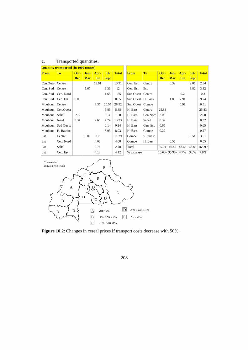
208

c. Transported quantities.Quantity transported (in 1000 tonnes)

From To Oct-

Dec

Jan-

Mar

Apr-

Jun

Jul-

Sept

Total From To Oct-

Dec

Jan-

Mar

Apr-

Jun

Jul-

Sept

Total

Cen.Ouest Centre 13.91 13.91 Cen. Est Centre 0.32 2.01 2.34

Cen. Sud Centre 5.67 6.33 12 Cen. Est Est 3.82 3.82

Cen. Sud Cen. Nord 1.65 1.65 Sud Ouest Centre 0.2 0.2

Cen. Sud Cen. Est 0.05 0.05 Sud Ouest H. Bass 1.83 7.91 9.74

Mouhoun Centre 8.37 20.55 28.92 Sud Ouest Comoe 0.91 0.91

Mouhoun Cen.Ouest 5.85 5.85 H. Bass Centre 25.83 25.83

Mouhoun Sahel 2.5 8.3 10.8 H. Bass Cen.Nord 2.08 2.08

Mouhoun Nord 3.34 2.65 7.74 13.73 H. Bass Sahel 0.32 0.32

Mouhoun Sud Ouest 0.14 0.14 H. Bass Cen. Est 0.65 0.65

Mouhoun H. Bassins 8.93 8.93 H. Bass Comoe 0.27 0.27

Est Centre 8.09 3.7 11.79 Comoe S. Ouest 3.51 3.51

Est Cen. Nord 4.08 4.08 Comoe H. Bass 0.55 0.55

Est Sahel 2.78 2.78 Total 35.04 16.47 48.65 68.83 168.99

Est Cen. Est 4.12 4.12 % increase 10.6% 35.9% 4.7% 3.6% 7.8%

∆π > 2%

Changes in annual price levels

1% < ∆π < 2%

-1% < ∆π <1%

-2% < ∆π < -1%

∆π < -2%

AC

D

E

D

D A

C

C

B

D

D

C

E

D

D

E

Figure 10.2: Changes in cereal prices if transport costs decrease with 50%.

209

Storage costs

The influence of storage costs on prices, supply, and demand is also weak. If storage

costs decrease with 50%, prices increase on average with 2.2% (see Table 10.3). Prices in

the first three periods increase on average, whereas prices in the fourth period remain the

same in most regions, but decrease sharply in the regions Centre Ouest and Sud Ouest.

This price increase is mainly due to changes in the producers’ supply schedule. The

general price increase is caused by the ‘fixed’ price expectations. Price expectations for

period t+1 do not depend on prices in period t. So, if storage costs decrease but price

expectations remain the same, traders expect to make higher profits from storage.

Consequently, their demand increases, causing producer prices (and consequently also

consumer prices) to increase. Stored quantities in the first and second period increase

sharply (respectively with 63% and 29%). Even when storage costs decrease with 50%,

traders do not store in the third and fourth period. Storage is expected not to be profitable

for traders, while farmers expect to earn high profits if they sell in the lean season.

Consumer demand and transported quantities decrease in this case due to the increased

prices.

If consumer price expectations for the next period do depend on the current producer

price, it is not clear whether consumer and producer prices will increase or decrease. But

it can be expected that average changes will be smaller than in the current situation.

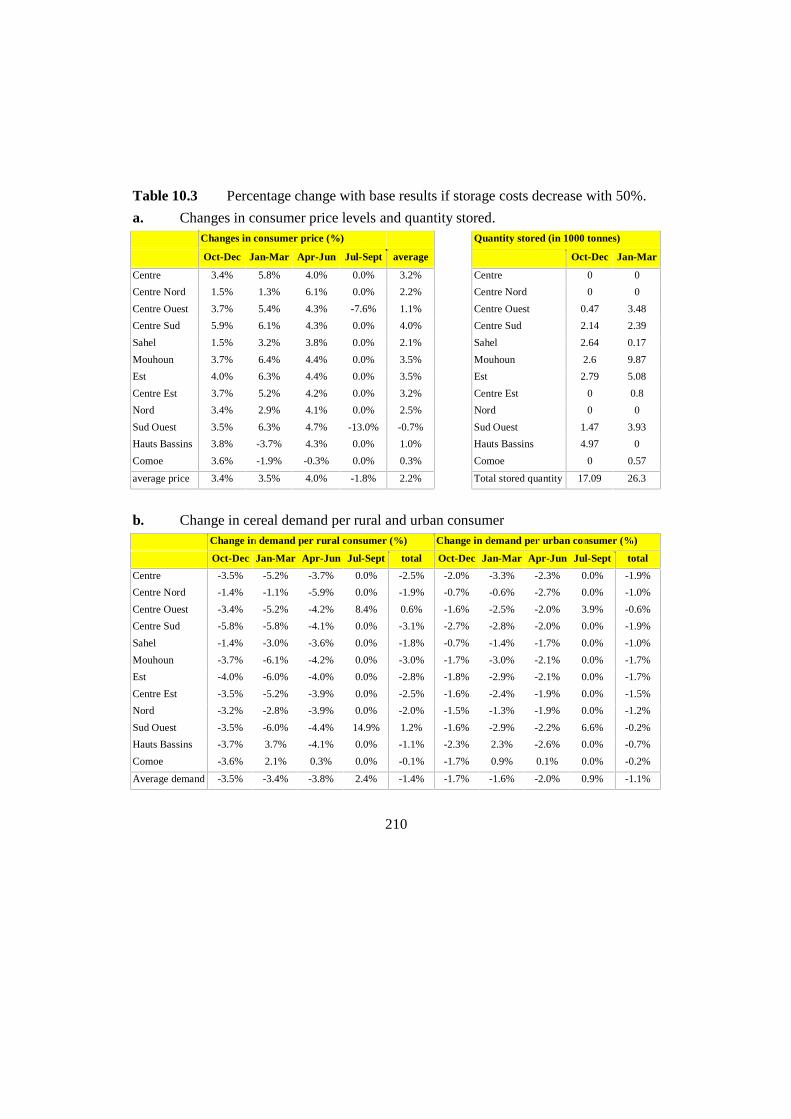
210

Table 10.3 Percentage change with base results if storage costs decrease with 50%.

a. Changes in consumer price levels and quantity stored.Changes in consumer price (%) Quantity stored (in 1000 tonnes)

Oct-Dec Jan-Mar Apr-Jun Jul-Sept average Oct-Dec Jan-Mar

Centre 3.4% 5.8% 4.0% 0.0% 3.2% Centre 0 0

Centre Nord 1.5% 1.3% 6.1% 0.0% 2.2% Centre Nord 0 0

Centre Ouest 3.7% 5.4% 4.3% -7.6% 1.1% Centre Ouest 0.47 3.48

Centre Sud 5.9% 6.1% 4.3% 0.0% 4.0% Centre Sud 2.14 2.39

Sahel 1.5% 3.2% 3.8% 0.0% 2.1% Sahel 2.64 0.17

Mouhoun 3.7% 6.4% 4.4% 0.0% 3.5% Mouhoun 2.6 9.87

Est 4.0% 6.3% 4.4% 0.0% 3.5% Est 2.79 5.08

Centre Est 3.7% 5.2% 4.2% 0.0% 3.2% Centre Est 0 0.8

Nord 3.4% 2.9% 4.1% 0.0% 2.5% Nord 0 0

Sud Ouest 3.5% 6.3% 4.7% -13.0% -0.7% Sud Ouest 1.47 3.93

Hauts Bassins 3.8% -3.7% 4.3% 0.0% 1.0% Hauts Bassins 4.97 0

Comoe 3.6% -1.9% -0.3% 0.0% 0.3% Comoe 0 0.57

average price 3.4% 3.5% 4.0% -1.8% 2.2% Total stored quantity 17.09 26.3

b. Change in cereal demand per rural and urban consumerChange in demand per rural consumer (%) Change in demand per urban consumer (%)

Oct-Dec Jan-Mar Apr-Jun Jul-Sept total Oct-Dec Jan-Mar Apr-Jun Jul-Sept total

Centre -3.5% -5.2% -3.7% 0.0% -2.5% -2.0% -3.3% -2.3% 0.0% -1.9%

Centre Nord -1.4% -1.1% -5.9% 0.0% -1.9% -0.7% -0.6% -2.7% 0.0% -1.0%

Centre Ouest -3.4% -5.2% -4.2% 8.4% 0.6% -1.6% -2.5% -2.0% 3.9% -0.6%

Centre Sud -5.8% -5.8% -4.1% 0.0% -3.1% -2.7% -2.8% -2.0% 0.0% -1.9%

Sahel -1.4% -3.0% -3.6% 0.0% -1.8% -0.7% -1.4% -1.7% 0.0% -1.0%

Mouhoun -3.7% -6.1% -4.2% 0.0% -3.0% -1.7% -3.0% -2.1% 0.0% -1.7%

Est -4.0% -6.0% -4.0% 0.0% -2.8% -1.8% -2.9% -2.1% 0.0% -1.7%

Centre Est -3.5% -5.2% -3.9% 0.0% -2.5% -1.6% -2.4% -1.9% 0.0% -1.5%

Nord -3.2% -2.8% -3.9% 0.0% -2.0% -1.5% -1.3% -1.9% 0.0% -1.2%

Sud Ouest -3.5% -6.0% -4.4% 14.9% 1.2% -1.6% -2.9% -2.2% 6.6% -0.2%

Hauts Bassins -3.7% 3.7% -4.1% 0.0% -1.1% -2.3% 2.3% -2.6% 0.0% -0.7%

Comoe -3.6% 2.1% 0.3% 0.0% -0.1% -1.7% 0.9% 0.1% 0.0% -0.2%

Average demand -3.5% -3.4% -3.8% 2.4% -1.4% -1.7% -1.6% -2.0% 0.9% -1.1%

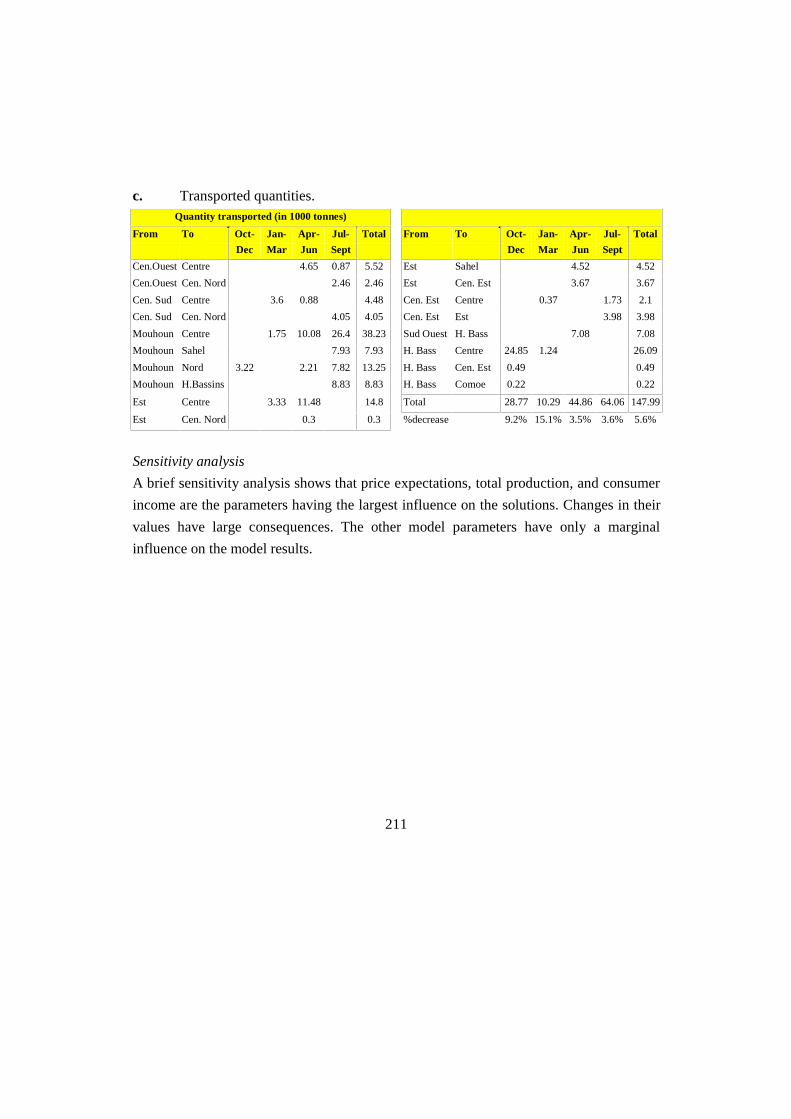
211

c. Transported quantities.Quantity transported (in 1000 tonnes)

From To Oct-

Dec

Jan-

Mar

Apr-

Jun

Jul-

Sept

Total From To Oct-

Dec

Jan-

Mar

Apr-

Jun

Jul-

Sept

Total

Cen.Ouest Centre 4.65 0.87 5.52 Est Sahel 4.52 4.52

Cen.Ouest Cen. Nord 2.46 2.46 Est Cen. Est 3.67 3.67

Cen. Sud Centre 3.6 0.88 4.48 Cen. Est Centre 0.37 1.73 2.1

Cen. Sud Cen. Nord 4.05 4.05 Cen. Est Est 3.98 3.98

Mouhoun Centre 1.75 10.08 26.4 38.23 Sud Ouest H. Bass 7.08 7.08

Mouhoun Sahel 7.93 7.93 H. Bass Centre 24.85 1.24 26.09

Mouhoun Nord 3.22 2.21 7.82 13.25 H. Bass Cen. Est 0.49 0.49

Mouhoun H.Bassins 8.83 8.83 H. Bass Comoe 0.22 0.22

Est Centre 3.33 11.48 14.8 Total 28.77 10.29 44.86 64.06 147.99

Est Cen. Nord 0.3 0.3 %decrease 9.2% 15.1% 3.5% 3.6% 5.6%

Sensitivity analysis

A brief sensitivity analysis shows that price expectations, total production, and consumer

income are the parameters having the largest influence on the solutions. Changes in their

values have large consequences. The other model parameters have only a marginal

influence on the model results.

212

11 Final discussion

In this report we pursued three objectives. The first was to develop a model to analyse

cereal arbitrage in space and time. The second was to to analyse the interaction between

the various actors on the cereal market in Burkina Faso. The third was to apply this model

to analyse the direct impact of transport and storage costs on the distribution of cereals

and on cereal prices in different regions of Burkina Faso. Much emphasis was put on

adapting standard micro-economic equilibrium theory to the specific situation of cereal

trade in West Africa. The two most challenging issues of the approach were 1) to model

behaviour of burkinabP farmers and traders, and 2) to take into account the uncertain

character of cereal prices.

What have we learned from this modelling approach? Firstly, by developing step by step

the equilibrium models we identified the limits and possibilities of spatial equilibrium

theory. By simply adopting the properties of a Spatial Price Equilibrium as discussed in

the introduction of Chapter 5, the existence of price uncertainty is neglected, as well as

other market situations deviating from a ‘perfect market’. By introducing explicitly trader

behaviour, the influence of stochastic future prices can be analysed. The model elaborated

in Chapter 5 to 7, is also useful to analyse other market imperfections. For example, a

lack of credit facilities, and the existence of oligopolistic market power.

Secondly, in the Chapters 5 to 7, we discussed the strategies of the market actors involved

in cereal trade, and developed a stochastic, multi-period, spatial equilibrium model. We

recall that we proved that the welfare optimizing results of the equilibrium model are in

line with the optimal strategies of the actors operating on the cereal market: producers,

traders and consumers. We have shown that prices on a market are formed by the joint

action of the market actors, who follow each their individual optimal strategy. This means

that actors do not trade if they lose money (or expect to lose, in the case of storage). As

213

long as each actor follows this principle (and market entry of new actors are free and

capital availability is not constraining), equilibrium prices will be realized satisfying the

equilibrium conditions discussed above. This explanation is more comprehensible and

satisfactory, then the often cited ‘invisible hand’, directing the market towards a price

level for which supply and demand are in equilibrium. The inclusion of trader behaviour

in the model makes the functioning of the ‘invisible hand’ explicit.

Thirdly, as for the practical results of the models, the results demonstrated that the

influence of transport and storage costs on cereal trade are limited. The direct effects of

lower transport costs on the food situation of the poorer, rural regions are small.

Furthermore, it was confirmed that long term storage is more often a task for producers

than for traders. It can not be said whether producers or consumers do profit the most

from decreasing transport or storage costs. The deficit regions do profit from decreased

transport costs, however, the influence on cereal consumption is only marginal.

Consumer income, total annual production, and price expectations are the factors which

determine the equilibrium prices and the timing of supplies and demand. The results of

the model provide useful elements for the discussions on improving the functioning of the

cereal market in Burkina Faso.

Although the use of the model can be criticised because of unrealistic assumptions,

unreliable estimates, and incomplete treatment of actors’ strategies, it is still a useful tool

to simulate the effects of market liberalization policies and agricultural development. The

subject of market functioning is very complex, as many factors are interrelated: price

formation results from the joint action of all market actors. With a descriptive or

statistical analysis these factors can not be analysed in their coherence. Furthermore, the

modelling approach forces the researcher to structure the descriptive analysis. For

example, the choice of a cereal demand function of a certain type, indicates which

parameters have to be estimated, and accordingly the elements which have to analysed. A

214

descriptive analysis on its turn identifies the factors which are important to include in the

model. A descriptive analysis of traders’ strategies in Burkina Faso, for example,

revealed that information on present and future prices are factors constraining traders’

strategies. Therefore, we introduced stochastic prices in our equilibrium models. Another

example concerns the timing of cereal sales and purchases within a year, which is

important for poor households’ survival strategies. A review of many surveys on farmers’

strategies revealed that a widespread belief, that most farmers sell their largest quantity in

the months following the harvest, had to be nuanced. This stressed once more the

importance of including the timing of sales and purchases in the equilibrium models.

Summarizing, a modelling approach ‘can structure the discussions and the understanding

of the issues considerably’ (Schweigman, 1994).

The model results nuanced a widespread belief that transport costs are a major barrier for

cereal trade. We do not want to claim that transport costs are not important for the

development of the agricultural sector, but the direct impact of lower transport costs, as

the direct impact of other price measures, are likely to be small. The reasons are clear.

Cereal demand elasticities are low, and annual cereal supply is unlikely to change a lot if

cereal prices change. Probably, a changed price will not rigourously alter the demand and

supply behaviour of consumers and producers. Whether demand is price inelastic because

other food commodities are hardly available on the market, or whether other food

commodities are not available because cereal demand is inelastic, is another question,

which is not addressed in this research. Similarly, whether annual cereal supply is price

inelastic because producers do not sell their produce on the market because producer

prices are considered to be too low, or because farmers are not able to produce more with

the limited resources available, is a question which is not addressed here. The results

subscribe to the more and more common view that improving single market constraining

elements (like e.g. transport prices) is fruitless if not more complementary measures, or

comprehensive packages of policy measures, are implemented to relax constraining

215

elements of food markets and food production (deJanvry et al., 1997; Thorbecke, 2000).

For example, the impact of an improved infrastructure will be larger, if this policy is

complemented by proper agricultural research and extension services. The models set up

in this paper can be used to learn about which measures are likely to yield the largest

benefits.

216

217

References:

• Bassolet, B., 1999. “Le marchJ de cJrJales au Burkina Faso”. Paper presented at

the SOM/CDS Seminar on food markets in Burkina Faso, April 16, 1999.

University of Groningen.

• Bassolet, B., 2000. “LibJralisation du marchJ cJrJalier au Burkina Faso: une

analyse NJo-institutionelle de son organisation et de son efficacitJ temporelle et

spatiale”. Ph.D. Thesis. Centre for Development Studies, University of

Groningen, the Netherlands.

• Bazaraa, M.S., Sherali, H.D., Shetty C.M., 1993. “Nonlinear Programming;

Theory and Algorithms”. sec.ed., Wiley.

• Broekhuyse, J.T., 1983. “Rural Mossi Economie, Deel I”. KIT, Amsterdam, the

Netherlands

• Broekhuyse, J.T., 1988. “De la survivance B la suffisance; Jtude des problPmes et

des perspectives du dJveloppement aboutissant B une idJologie paysanne au

Plateau Nord des Mossi”. Projet CEDRES/AGRISK, UniversitJ de

Ouagadougou, University of Groningen, the Netherlands.

• Broekhuyse, J.T., 1998. “Monografie van de Mossi: Noordelijk Plateau –

Sanmatenga, Burkina Faso”. KIT, Amsterdam, the Netherlands.

• Danida, 1999. “Burkina Faso: Plan d’actions sur les cJrJales (mil, sorgho, maVs)

2000-2010”. MinistPre des Affaires EtrangPres du Danemark, Danemark.

• Deaton, A., Muellbauer, J., 1980. “An Almost Ideal Demand System”. American

Economic Review, No.70:3: p. 312-326.

• Dreze, J., Sen, A., 1989. “Hunger and Public Action”. Oxford: Clarendon Press.

• Egg, J., Gabas, J.J., Ki-Zerbo, B., Ancey, V., 1997. “La hausse des prix des

cJrJales au Burkina Faso dans le contexte regional: ampleur et analyse” (version

provisoire). Club du Sahel/CILSS, RJunion du RJseau de PrJvention des Crises

Alimentaires au Sahel, 27-28 Nov. 1997. OCDE, Paris.

• Ellis, F., 1992. “Agricultureal Policies in Developing Countries”. Cambridge

University Press, Cambridge.

218

• Ellis, F., 1993. “Peasant economics: farm households and agrarian development”.

Wye Studies in Agricultural and rural development. Cambridge University Press,

Cambridge.

• Ellsworth, L, Shapiro, K., 1989. “Seasonality in Burkina Faso grain marketing:

Farmer strategies and government policy”. In: Sahn, E. (Ed.). “Seasonal

variability in Third World Agriculture: the consequences for food security”.

Johns Hopkins University Press, Baltimore, USA.

• Florian, M., Los, M., 1982. “A new look at spatial price equilibrium models”.

Regional Science and Urban Economics, No. 12, p. 579-597.

• Güvenen, O., Labys, W., Lesourd, J.B. (Eds.), 1990. “International commodity

market models : advances in methodology and applications”. International studies

in economic modelling, No. 7. Chapman and Hall, London, UK.

• Heijman, W.J.M., Hiel, R.T.R., Kroes, E.P., Van den Noort, P.C., Silvis, H.J.,

Slangen, L.H.G., 1991. “Leerboek algmene agrarische economie”. Stenfert

Kroese, Leiden, The Netherlands.

• Hoftijzer, M., 1998. “Seizoensbewegingen van de graanprijzen in Burkina Faso”.

M.Sc. Thesis University of Groningen, the Netherlands.

• INSD, 1995a. “Analyse des resultats de l’enquete dJmographique 1991”.

Direction de la DJmographie, Ouagadougou, Burkina Faso.

• INSD, 1995b. “Annuaire statistique du Burkina Faso: 1994”. Direction des

Statistiques Generales, Ouagadougou, Burkina Faso.

• INSD, 1996a. “Le profil de pauvretJ au Burkina Faso; premiPre Jdition; Etude

Statistique Nationale”. Programme “Dimensions Sociales de l’Ajustement”,

MinistPre de l’Economie des Finances et du Plan, Ouagadougou, Burkina Faso.

• INSD, 1996b. “Analyse des rJsultats de l’enquLte prioritaire sur les conditions de

vie des mJnages”. MinistPre de l’Economie des Finances et du Plan, Direction

des Statistiques Generales, Ouagadougou, Burkina Faso.

• INSD, 1998. “Population rJsidente des dJpartements, communes,

arrondissements et provinces. RJcensement gJneral de la population et de

l'habitation du Burkina Faso (du 10 au 20 DJcembre 1996). RJsultats Definitifs”.

Ouagadougou, Burkina Faso.

219

• Janvry, A. de, Fafchamps, M., Sadoulet, E., 1991. “Peasant Household Behaviour

with Missing Markets: some paradoxes explained”. The Economic Journal, Vol

101, pp 1400-1417.

• Judge, G.G. Takayama, T., 1973. “Studies in economic planning over space and

time”. Contributions to Economic Analysis, No. 82, North-Holland Publishing

Company, Amsterdam, The Netherlands.

• Labys, W.C., Takayama, T., Uri, N.D. (Eds.), 1989. “Quantitative methods for

market-oriented economic analysis over space and time”. Aldershot, Avebury,

UK.

• LaclavPre, G., 1993. “Atlas du Burkina Faso”. Les Jditions j.a., Paris, France.

• Lang, M.G., 1985. “Crop and livestock marketing patterns in Burkina Faso”.

• Lang, M.G., Cantrell, Cantrell, R.P., Sanders, J.H., 1983. “Identifying farm level

constraints and evaluating new technology in Uper Volta”. Paper presented at the

Farming Systems Research symposium, Kansas State University,

SAFGRAD/FSU, Kansas, USA.

• Lutz, C., Bassolet, B., 1999. franse artikel

• Maatman, A., Schweigman, C., Ruijs, A., 1996. “A study of farming systems on

the Central Plateau in Burkina Faso: application of linear programming; Volume

2”. RJseau SADAOC. University of Groningen, University of Ouagadougou,

INERA. Groningen, the Netherlands.

• Maatman, A., 2000. “Si le fleuve se tord, que le crocodille se torde; une analyse

des systPmes agraires de la rJgion Nord-Ouest du Burkina Faso B l’aide des

modPles de programmation linJaire”. Ph.D. Thesis, Centre for Development

Studies, University of Groningen, the Netherlands.

• Martin, L.J., 1981. “Quadratic single and multi-commodity models of spatial

equilibrium: a simplified exposition”. Canadian Journal of Agricultural

Economics, Vol. 29, No. 1, p. 21 – 48.

• McCorkle, C.M., 1987. “FiertJ, prJfJrence et pratique: dJcisions des cultivateurs

concernant l’Jcoulement des cJrJales dans une communautJ BurkinabJ”. La

Dynamique de la Commercialisation des CJrJales au Burkina Faso, Tome III,

220

Document de travail no. 1. CRED, University of Michigan, IAP, University of

Wisconsin.

• Ministry of Agriculture and Animal Resources, 1984-1996. “Resultats de

l’enquPte permanente agricole”, Annee 1984; Annee 1985; Annee 1986; Annee

1987; Annee 1988; Annee 1989; Campagne 1990-1991; Campagne 1991-1992;

Campagne 1992-1993; Campagne 1993-1994; Campagne 1994-1995; Campagne

1995-1996. Direction des Statistiques Agro-Pastorales, Burkina Faso.

• Nicholson, W., 1995. “Microeconomic theory: basic principles and extensions”.

Sixth edition. The Dryden Press, Fort Worth.

• Pardy, C.R., 1987. “Comportement relatif aux ventes de cJrJales dans les familles

d’exploitations de quatre villages du Burkina Faso”. La Dynamique de la

Commercialisation des cJrJales au Burkina Faso. Tome III, Doc. de travail 4.

CRED, University of Michigan, IAP, University of Wisconsin.

• Pieroni, O., 1990. “Le paysan, le sorgho et l’argent”. CILSS, Assistence

Technique, Ouagadougou, Burkina Faso.

• Ravallion, M., 1987. “Markets and Famines”. Oxford: Clarendon Press.

• Reardon, T., Delgado, C., Matlon P., 1987. “Farmer marketing behaviour and the

composition of cereals consumption in Burkina Faso”. Paper presented for the

IFPRI/ISRA conference: “Dynamics of cereals consumption and production

patterns in West Africa”. Dakar, Senegal.

• Reardon, T., Matlon, P., Delgado, C., 1988a. “Coping with household level food

insecurity in drought-affected areas of Burkina Faso”. World Development, vol.

16, no. 9, p. 1065-1074.

• Reardon, T., Thiombiano, T., Delgado, C., 1988b. “La substitution des cJrJales

locales par les cJrJales importJes: la consommation alimentaire des mJnages B

Ouagadougou Burkina Faso”. CEDRES-Etudes, No 2, Juin 1988. UniversitJ de

Ouagadougou, IFPRI, CEDRES, Burkina Faso.

• Reardon, T., Matlon, P., 1989. “Seasonal food insecurity and vulnerability in

drought- affected regions of Burkina Faso”. In: Sahn D.E. (ed.), “Seasonal

variability in Third World agriculture: the consequences for food security”. The

Johns Hopkins University Press.

221

• Reardon, T., Delgado, C., Matlon, P., 1992. “Determinants and Effects of Income

Diversification Amongst Farm Households in Burkina Faso”. Journal of

Development Studies, vol. 28, no. 2, pp 264-296.

• Roehner, B.M., 1995. “Theory of markets; Trade and space-time patterns of price

fluctuations. A study in analytical economics”. Springer-Verlag, Berlin,

Germany.

• Roth, M., 1986. “Economic evaluation of agricultural policy in Burkina Faso: a

sectoral modelling approach”. Ph.D. Thesis, Purdue University, USA.

• Sadoulet, E., De Janvry, A., 1995. “Quantitative development policy analysis”.

Johns Hopkins University Press, Baltimore.

• Sahn, D.E., Dorosh, P., Younger, S., 1997. ‘Structural Adjustment Reconsidered:

Economic policy and poverty in Africa”. Cambridge University Press, Cambridge

and New York.

• Samuelson, P.A., 1952. “Spatial price Equilibrium and Linear Programming”,

American Economic Review, 42; 283-303.

• Saul, M., 1987. “La dynamique de la commercialisation des cJrJales au Burkina

Faso”. University of Michigan and University of Wisconsin, USA.

• Schweigman, C., 1994. “Mathematical modelling and development related

research”. In; Harts-Broekhuis, A., Verkoren, O.. “No easy way out: essays on

third world development in honour of Jan Hinderink”. Nederlandse Geografische

Studies, No. 186, p. 114-119.

• Sedes Cedrat SA et Gopa (1990). “Plan cJrJalier du Burkina Faso, tome 1:

SynthPse”. MinistPre de l’Jlevage et de l’agriculture, CILLS, Ouagadougou,

Burkina Faso.

• Sherman, J.R., Shapiro, K.H., Gilbert, E., 1987. “An economic analysis of grain

marketing”. The Dynamics of Grain Marketing in Burkina Faso, Volume I.

CRED, University of Michigan, IAP, University of Wisconsin.

• SirpJ, G., 2000. “Transport routier et Jcoulement des produits agricoles: une

analyse Jconomique de l’influence des transports sur les mouvements

interrJgionaux de cJrJales au Burkina Faso”. FacultJ des Sciences Economiques,

UniversitJ de Ouagadougou, Burkina Faso.

222

• Stiglitz, J.E., 1994. “Whither socialism?”. MIT Press, Massachusetts, USA.

• Szarleta, E.J., 1987. “ExcJdents commerciaux au Burkina Faso: une Jtude des

schJmas d’Jcoulement des cJrJales”. La Dynamique de la Commercialisation des

CJrJales au Burkina Faso, Tome III, Document de travail no. 3. CRED,

University of Michigan, IAP, University of Wisconsin.

• Takayama, A., 1974. “Mathematical Economics”, Dryden.

• Takayama, T., Judge, G.G., 1971. “Spatial and Temporal Price and Allocation

Models”. Contributions to Economic Analysis, No. 73. North-Holland Publishing

Company, Amsterdam, the Netherlands.

• Theil, H., 1980. ‘The system-wide approach to microeconomics’. University of

Chicago Press.

• Thiombiano, T., Soulama, S., Wetta, C., 19??. “SystPmes alimentaires en zones

rurales B dJficits cJrJaliers: le cas des provinces du Bam, du Sanmatenga et du

Yatenga. Phase III”. CEDRES, UNRISD.

• Thiombiano, T., Soulama, S., Wetta, C., 1988. “SystPmes alimentaires du

Burkina Faso”. CEDRES-Etudes, No. 1, RJsultats de Recherche CEDRES,

Ouagadougou, Burkina Faso.

• Thorbecke, E., 2000. “Agricultural markets beyond liberalization: the role of the

state”. In Tilburg, A. van, H.A.J. Moll, A. Kuyvenhoven. “Agricultural markets

beyond liberalization”. Kluwer Academic Press.

• Union EuropJenne, 1999. “Les flux cJrJaliers, les stocks commerHants et la

stratJgie des commerHants de cJrJales au Burkina Faso”. DJlJgation de la

Commision EuropJenne au Burkina Faso, MinistPre de l’Economie et des

Finances, MinstPre de l’Agriculture. 7 ACP BK 054.

• Van den Bergh, J.C.J.M., Nijkamp, P., Rietveld, P. (Eds.), 1995. “Recent

advances in spatial equilibrium modelling: methodology and applications”.

Springer, Berlin, Germany.

• Van den Bergh, J.C.J.M., Nijkamp, P, Rietveld, P., 1995b. Spatial Equilibrium

models: A survey with special emphasis on transportation”. In: Van den Bergh,

J.C.J.M., Nijkamp, P., Rietveld, P. (Eds.), 1995. Chapter 2.

223

• Varian, H.R., 1992. “Microeconomic analysis”. Third edition.W.W. Norton &

Company, New York..

• Vogelzang, J., 1996. “Transports et Jchanges cJrJaliers entre rJgions dJficitaires

et rJgions excJdentaires du Burkina Faso: application de la programmation

linJaire”. M.Sc. thesis, University of Groningen, the Netherlands.

• Yonli, E.P., 1997. “StratJgies paysannes en matiPre de sJcuritJ alimentaire et de

commercialisation cJrJaliPre: le r^le des banques de cJrJales dans le Nord du

Plateau Central du Burkina Faso”. Ph.D. Thesis, Centre for Development Studies,

University of Groningen, the Netherlands.

• Zeller, M, Schrieder, G., Braun, J. von, Heidhuess, F., 1997. ”Rural Finance for

Food Security for the Poor. Implications for research and policy”. Food Policy

Review No. 4, IFPRI, Washington.

224

225

Appendix 1: Proofs of Properties and Theorems in the Chapters 5, 6 and 7

• Properties of Section 5.1:

Trader property 5.1: For each region i ∈ {1,...,n} :

a) If πi < p i, then any optimal solution of (5.12) satisfies: q i = 0 or r i = 0.

b) If πi ≥ p i, then an optimal solution of (5.12) exists which satisfies the condition q i

= xi or r i = yi. Nota bene: for πi > p i, any optimal solution of (5.12) has to satisfy this

condition; for πi = p i, other optimal solutions may exist not satisfying this condition.

Proof:

a) Let πi < p i. If in the optimal solution of (5.12) r i > 0 and q i > 0, then necessarily,

see (5.13), πi ≥ λ i and λ i ≥ p i, which contradicts πi < p i. So necessarily r i = 0 or q i =

0.

b) An optimal solution of the linear programming model (5.12) exists, since its

feasible region is bounded. We make a distinction between πi > p i and πi = p i.

* Let πi > p i. If in the optimal solution q i < xi and r i < yi, then necessarily, see (5.13),

p i ≥ λ i and λ i ≥ πi, which contradicts πi > p i. So necessarily, q i = xi or r i = yi.

* Let πi = p i. Consider an optimal solution qs, r s, qsj, s ≠ j, s,j = 1,…,n, in which

optimal purchases, sales and transports in region i, satisfy q i < xi and r i < yi. Call ∆ i =

min(xi-q i; yi-r i). The solution ′ ′ ′q r qs s sj, , , defined by ′qi = q i + ∆ i, ′ri = r i + ∆ i, ′qij = q ij,

′qs = qs, ′rs = r s, and ′qsj = qsj, for s≠j, is optimal as well, as can be seen easily by

inspecting (5.12). Moreover, ′qi = xi or ′ri = yi.

Trader property 5.2: Let q i, r j, q ij, j ≠ i, i,j = 1,…,n, be an optimal solution of (5.12).

Let a trader transport from a region i to a region j, so q ij > 0, for i,j ∈ (1,…,n}, i ≠ j,

then:

a) no goods are transported from a region s = 1,…,n, s ≠ i, to region i, qsi = 0

b) no goods are transported from region j to a region s = 1,…,n, s ≠ j, q js = 0.

c) purchases in region i are positive, q i > 0

226

d) sales in region j are positive, r j > 0.

Proof:

a) Let q ij > 0. Suppose that qsi > 0. In that case, see (5.13), λ j = λ i + τ ij and λ i = λ s +

τ si. This implies that λ j = λ s + τ si + τ ij. Due to (5.13) we know that λ j ≤ λ s + τ sj. It

would follow that τ sj ≥ λ j - λ s = τ si + τ ij. This is in contradiction with the analogue of

property (5.11), which says that τ sj < τ si + τ ij. So, necessarily qsi = 0.

b) The proof of the second property is similar to the proof under a).

c) If q ij > 0, then making use of a), the equilibrium condition (5.7) leads to a

contradiction if q i = 0. Consequently, q i > 0.

d) In a similar way it can be shown that necessarily r j > 0, if q ij > 0.

Trader property 5.3: For the regions i and j, i,j ∈ {1,...,n} , i ≠ j:

a) If πj < p i + τ ij, then any optimal solution of (5.12) satisfies q ij = 0.

b) If πj ≥ p i + τ ij and q ij > 0, then an optimal solution of (5.12) exists satisfying q i = xi

or r j = y j; for πj = p i + τ ij and q ij > 0 an optimal solution of (5.12) is not necessarily

unique.

Proof:

a) Let πj < p i + τ ij. If q ij > 0, then necessarily, see Trader property 5.2, q i > 0 and r j >

0. As a consequence, see (5.13), πj ≥ λ j, λ j = λ i + τ ij, and λ i ≥ p i, which contradicts πj

< p i + τ ij. So necessarily, q ij = 0.

b) An optimal solution of the linear programming model (5.12) exists, since its

feasible region is bounded. We make a distinction between πj > p i + τ ij and πj = p i +

τ ij:

* Let πj > p i + τ ij and q ij > 0. According to (5.13) λ j = λ i + τ ij. If q i < xi and r j < yj,

then necessarily, see (5.13), πj ≤ λ j and λ i ≤ p i, which contradicts πj > p i + τ ij. So

necessarily, q i = xi or r j = yj.

* Let πj = p i + τ ij and q ij > 0. Consider the optimal solution qs, r s, qsv, s,v = 1,…,n, s ≠v, and assume that for region i and j: q i < xi and r j < yj. Call ∆ ij = min(xi-q i; yj-r j).

227

The solution ′ ′ ′q r qs s sv, , defined by ′qi = q i + ∆ ij, �r j = r j + ∆ ij, ′qij = q ij + ∆ ij, ′qs = qs,

′rv = r v, ′qsv = qsv, for s≠i, v≠j, is optimal as well, as can be seen easily by inspecting

(5.12). Moreover, ′qi = xi or �r j = y j.

• Properties and Theorem of Section 5.2:

Equilibrium property 5.1: For region i ∈ {1,…,n}:

a) In the optimal solution of (5.19), πi (yi ) ≤ p i (xi ) .

b) If in the optimal solution of (5.19), πi(yi) < p i(xi), then xi = 0 or yi = 0.

c) If in the optimal solution of (5.19), supply and demand in region i are both positive,

so xi > 0 and yi > 0, then necessarily p i(xi) = πi(yi).

Proof:

a) Since the solution of (5.19) has to satisfy πi(yi) ≤ λ i and λ i ≤ p i(xi), see (5.21) –

(5.24), it is only possible that πi(yi) ≤ p i(xi).

b) Using (5.21) and (5.23), the proof is similar to the proof of Trader property 5.1 a).

c) This follows from a) and b).

Equilibrium property 5.2: In the optimal solution of (5.19), let transport take place

from market i to market j, i.e. xij > 0, with i, j ∈ {1,2, ...,n}, j ≠ i,, then:

a) no cereals are transferred from other regions into market i, i.e. xsi = 0, for all s ≠ i

b) no cereals are transported from market j to other regions, i.e. xjs = 0, for all s ≠ j

c) the producer supply xi in region i satisfies xi > 0,

d) the consumer demand yj in region j satisfies yj > 0,

Proof:

The proof is similar to the proof of Trader property 5.2.

Equilibrium property 5.3: For region i and j, i,j ∈ {1,…,n}, i ≠ j:

a) In the optimal solution of (5.19), πj(yj) ≤ p i(xi) + τ ij.

b) If in the optimal solution of (5.19), πj(yj) < p i(xi) + τ ij, then xij = 0.

228

c) If in the optimal solution of (5.19), transport between region i and j is positive, xij >

0, then the optimal prices satisfy necessarily πj(yj) = p i(xi) + τ ij.

Proof:

a) Since the solution of (5.19) always has to satisfy πj(yj) ≤ λ j, λ j ≤ λ i + τ ij and λ i ≤p i(xi), see (5.21) – (5.26), it is only possible that πj(yj) ≤ p i(xi) + τ ij.

b) Using (5.21), (5.23) and (5.25), the proof is similar to the proof of Trader property

5.3 a).

c) This follows from a) and b).

Theorem 5.1:

Let xi, yi, xij, i,j ∈ {1,…,n}, i ≠ j, be an optimal solution of the equilibrium model

(5.19). Let πi = πi(yi) , p i = p i(xi). The solution:

(5.27) q i = xi ; r i = y i ; q ij = xij for i,j ∈ {1,…,n}, i ≠ j

is an optimal solution of trader decision problem (5.12). The value of the objective

function is equal to 0, meaning that the trader makes no profits or losses.

Proof:

The proof will consist of three parts: a) (5.27) is a feasible solution of (5.12), b) the

solution (5.27) results in a value of the objective function of (5.12) which is equal to

0; c) the solution (5.27) is an optimal solution of (5.12).

a) See (5.27), (5.16), (5.7), and (5.12).

b) Due to (5.21) – (5.26), πi ⋅yi = λ i ⋅yi , pi ⋅xi = λ i ⋅xi , and τ ij⋅xij = (λ j - λ i )⋅xij,

with λ i the optimal value of the Lagrange multiplier of the equilibrium condition

in model (5.16) – (5.21). So, for the solution (5.27) the objective function of

model (5.12) can be written as follows:

229

λ λ λ λ λi i i i j i ijjj i

n

i

n

i i i jijj i

n

ijjj i

n

i

n

y x x y x x x− − −�

!

"

$

###

= − − +�

�

���

�

�

���

�

!

"

$

###

==≠

= =≠

=≠

=∑∑ ∑ ∑∑3 8

11 1 11

0

due to the equilibrium condition (5.7).

c) Consider any feasible solution q i, r i, qij of (5.12), and market prices πi = πi(yi)

and pi = p i(xi), with yi and xi the optimal demanded and supplied quantities of

equilibrium model (5.19), (5.16), and (5.17). Due to Equilibrium properties 5.1 –

5.3 πi ≤ λ i ≤ p i and πj ≤ λ j ≤ λ i + τ ij ≤ p i + τ ij, for all i,j = 1,…,n, i≠ j, with λ i the

Lagrange multiplier of the equilibrium condition in model (5.19), (5.16), and

(5.17). The objective function of model (5.12) can be written as:

π τ λ λ λ λ

λ

i i i i ij ijjj i

n

i

n

i i i i j i ijjj i

n

i

n

i i i jijj i

n

ijjj i

n

i

n

r p q q r q q

r q q q

− −�

!

"

$

###

≤ − − −�

!

"

$

###

= − − +�

�

���

�

�

���

�

!

"

$

###

=

=≠

= =≠

=

=≠

=≠

=

∑∑ ∑∑

∑ ∑∑

11 11

1 11

0

3 8

So, for market prices πi = πi(yi) and p i = p i(xi), the objective function always has a

value ≤ 0. The objective function of model (5.12) reaches a maximum for the solution

(5.27). Consequently, (5.27) is an optimal solution of (5.12).

• Properties of Section 6.1:

Trader property 6.1: For region i ∈ {1,…,n}, and period t ∈ {1,…,T}:

a) If πit < p it, then any optimal solution of (6.11) satisfies q it = 0 or r it = 0

230

b) If πit ≥ p it, then an optimal solution of (6.11) exists satisfying the condition q it = xit

or r it = yit; for πit = p it, other optimal solutions of (6.11) may exist, not satisfying this

condition.

Proof: Using (6.11), the proof is similar to the proof of Trader property 5.1 in Section

5.1.

Trader property 6.2: Let q it, r jt, q ijt, vit, j ≠ i, i,j = 1,…,n, t = 1,…,T, be an optimal

solution of (6.11). Let a trader transport in a period t from a region i to a region j, so

q ijt > 0, for i,j ∈ {1,…,n}, j ≠ i, t ∈ {1,…,T}, then:

a) in period t, no goods are transported from a region s = 1,…,n, s ≠ i, to region i, qsit

= 0

b) in period t, no goods are transported from region j to a region s = 1,…,n, s ≠ j, q jst

= 0.

c) in period t, purchases in region i are positive, q it > 0, or the stock remaining from

the previous period is positive, vi,t-1 > 0.

d) in period t, sales in region j are positive, r jt > 0, or the stock at the end of period t

in region j is positive, vjt > 0.

Proof: Using (6.9) and (6.11), the proof is similar to the proof of Trader property 5.2

in Section 5.1.

Trader property 6.3: For region i,j ∈ {1,…,n}, j ≠ i, and period t ∈ {1,…,T}:

a) If πjt < p it + τ ijt, then any optimal solution of (6.11) has to satisfy q it = 0 or q ijt = 0

or r jt = 0.

b) If πjt ≥ p it + τ ijt, and q it > 0, qijt > 0 and r jt > 0, then an optimal solution of (6.11)

exists satisfying q it = xit or r jt = yjt; for πjt = p it + τ ijt, an optimal solution of (6.11) is

not unique.

231

Proof:

a) Let πjt < p it + τ ijt. If q it > 0, q ijt > 0 and r jt > 0, then, see (6.11), λ it ≥ p it, λ jt = λ it +

τ ijt and λ jt ≤ πjt, which contradicts πjt < p it + τ ijt. So necessarily, q it = 0, q ijt = 0 or r jt =

0.

b) An optimal solution of problem (6.11) exists, since its feasible region is bounded.

We make a distinction between πjt > p it + τ ijt and πjt = p it + τ ijt:

* Let πjt > p it + τ ijt and q it > 0, qijt > 0 and r jt > 0. If the optimal solution satisfies q it <

xit and r jt < yjt, then, see (6.11), λ it = p it, λ jt = λ it + τ ijt and λ jt = πjt. It would follow

that πjt = p it + τ ijt, which is in contradiction with πjt > p it + τ ijt. So necessarily, q it = xit

or r jt = y jt.

* Let πjt = p it + τ ijt. Consider the optimal solution qsτ, qsvτ, r vτ, for s,v = 1,…,n, and τ= 1,…,T, in which purchases, transports and sales for the regions i and j, and for the

period t satisfy 0 < q it < xit, qijt > 0 and 0 < r jt < yjt. Call ∆ ijt = min(xit-q it; yjt-r jt). The

solution ′ ′ ′q r qs v svτ τ τ, , defined by ′qit = q it + ∆ ijt, ′r jt = r jt + ∆ ijt, ′qijt = q ijt + ∆ ijt, ′qsτ = qsτ,

′rvτ = r vτ, ′qsvτ = qsvτ, for s≠i, v≠j and τ≠t, is optimal as well, as can be seen easily by

inspecting (6.10). Moreover, ′qit = xit or ′r jt = yjt.

Trader property 6.4: For region i ∈ {1,…,n}, j ≠ i, period t ∈ {1,…,T-1}:

a) If πi,t+1 < p it + kit, then any optimal solution of (6.11) has to satisfy q it = 0 or vit = 0

or r i,t+1 = 0.

b) Analogously for τ ∈ {t+1,…,T}: if πiτ < p it + κ itτ, then any optimal solution of

(6.11) has to satisfy q it = 0 or vit = 0, or …, or vi,τ −1 = 0, or r iτ = 0.

c) If πi,t+1 ≥ p it + kit, and q it > 0, vit > 0 and r i,t+1 > 0, then an optimal solution of (6.11)

exists which satisfies the condition q it = xit or r i,t+1 = yi,t+1. Nota bene: for πi,t+1 > p it +

kit, any optimal solution of (6.11) has to satisfy this condition; for πi,t+1 = p it + kit, an

optimal solution is not unique.

d) Analogously for τ ∈ {t+1,…,T}: if πiτ ≥ p it + κ itτ, and q it > 0, vit > 0,…, vi,τ−1 > 0

and r iτ > 0, then an optimal solution of (6.11) exists satisfying the condition q it = xit

or r iτ = yiτ. For πiτ = p it + κ itτ, an optimal solution of (6.11) is not unique.

232

Proof:

a) Let πi,t+1 < p it + kit. If q it > 0, vit > 0 and r i,t+1 > 0, then, see (6.11), λ it ≥ p it, λ i,t+1 =

λ it + kit and λ i,t+1 ≤ πi,t+1, which contradicts πi,t+1 < p it + kit. So necessarily, q it = 0, vit

= 0 or r i,t+1 = 0.

b) Let πiτ < p it + κ itτ for τ ∈ { t+1,…,T}. If q it > 0, vit > 0,…, vi,τ−1 > 0 and r iτ > 0,

then, see (6.11), λ it ≥ p it, λ i,t+1 = λ it + kit, …, λ iτ = λ i,τ-1 + ki,τ−1 and λ iτ ≤ πiτ, which

contradicts πiτ < p it + κ itτ - see (6.12). So necessarily, q it = 0 or vit = 0,… or vi,τ-1 = 0

or r iτ = 0.

c) An optimal solution of problem (6.11) exists, since its feasible region is bounded.

For this proof we make a distinction between πi,t+1 > p it + kit and πi,t+1 = p it + kit:

* Let πi,t+1 > p it + kit and q it > 0, vit > 0 and r i,t+1 > 0. If the optimal solution satisfies

q it < xit and r i,t+1 < yi,t+1, then, see (6.11), λ it = p it, λ i,t+1 = λ it + kit and λ i,t+1 = πi,t+1. It

would follow that πi,t+1 = p it + kit, which is in contradiction with πi,t+1 > p it + kit. So

necessarily, q it = xit or r i,t+1 = yi,t+1.

* Let πi,t+1 = p it + kit. Consider the optimal solution qsτ, vsτ, r sτ for s = 1,…,n and τ =

1,…,T, for which in region i and period t and t+1: 0 < q it < xit, vit > 0 and 0 < r i,t+1 <

yi,t+1. Call ∆ it = min(xit-q it; yi,t+1-r i,t+1). The solution ′ ′ ′q r vs s sτ τ τ, , defined by ′qit = q it +

∆ it, ′ +ri t, 1= r i,t+1 + ∆ it, ′vit = vit + ∆ it, ′qsτ = qsτ, ′rsζ = r sζ, ′vsτ = vsτ, for s≠i, τ≠t, and

ζ≠t+1, is optimal as well, as can be seen easily by inspecting (6.10). Moreover, ′qit =

xit or ′ +ri t, 1= yi,t+1.

d) The proof of this property is similar to the proof under c). The main difference is

that, due to vit > 0,…, vi,τ -1 > 0, λ iτ = λ it + κ itτ , see (6.11) and (6.12).

• Properties and Theorem of Section 6.2:

Equilibrium property 6.1: For region i ∈ {1,…,n}, and period t ∈ {1,…,T}:

a) In the optimal solution of (6.14) – (6.16) πit(yit) ≤ p it(xit) .

b) If in the optimal solution of (6.14) – (6.16) πit(yit) < p it(xit), then xit = 0 or yit = 0.

233

c) If in the optimal solution of (6.14) – (6.16), supply and demand are both positive,

xit > 0 and yit > 0, then the prices necessarily satisfy p it(xit) = πit(yit).

Proof:

Using (6.17) – (6.24), the proof is similar to the proof of Equilibrium property 5.1 in

Section 5.2.

Equilibrium property 6.2: Let in the optimal solution of (6.14) – (6.16) transport in

period t take place from a market i to a market j, so xijt > 0, with i,j ∈ {1,2, ...,n}, j ≠ i,

t ∈ {1,…,T}, then:

a) in period t, no cereals are transferred from other regions into market i, i.e. xsit = 0,

for all s ≠ i

b) in period t, no cereals are transported from market j to other regions, i.e. xjst = 0,

for all s ≠ j

c) in period t, the producer supply in region i in period t satisfies, xit > 0, or the stock

remaining from the previous period is positive, si,t-1 > 0.

d) in period t, the consumer demand in region j in period t satisfies yjt > 0, or the

quantity put in stock in region j is positive, sjt > 0.

Proof:

The proof is similar to the proof of Equilibrium property 5.2 in Section 5.2.

Equilibrium property 6.3: For region i and j, i,j ∈ {1,…,n}, i ≠ j, and period t ∈{1,…,T}:

a) In the solution of (6.14) – (6.16) πjt(yjt) ≤ p it(xit) + τ ijt.

b) If in the optimal solution of (6.14) – (6.16) πjt(yjt) < p it(xit) + τ ijt, then xit = 0 or xijt

= 0 or yjt = 0.

c) If in the optimal solution of (6.14) – (6.16) supplies in region i, transport between

region i and j, and demand in region j are positive, xit > 0 and xijt > 0 and yjt > 0, then

the optimal prices necessarily satisfy πjt(yjt) = p it(xit) + τ ijt.

234

Proof:

Using (6.17) – (6.2), the proof is similar to the proof of Equilibrium property 5.3 in

Section 5.2.

Equilibrium property 6.4: For region i ∈ {1,…,n}, and period t ∈ {1,…,T-1}:

a) In the optimal solution of (6.14) – (6.16) πi,t+1(yi,t+1) ≤ p it(xit) + kit. Analogously, for

τ ∈ {t+1,…,T}: πiτ(yiτ) ≤ p it(xit) + κ itτ.

b) If in the optimal solution of (6.14) – (6.16) πi,t+1(yi,t+1) < p it(xit) + kit, then xit = 0 or

sit = 0 or yi,t+1 = 0. Analogously, for τ ∈ {t+1,…,T} – see also (6.12): if πiτ < p it + κ itτ,

then any optimal solution of (6.14) – (6.16) has to satisfy xit = 0 or sit = 0 or si,t+1 = 0

… or si,τ-1 = 0 or yiτ = 0.

c) If in the optimal solution of (6.14) – (6.16) supplies in period t, stock levels at the

end of period t, and demand in period t+1 are positive, xit > 0 and sit > 0 and yi,t+1 > 0,

then the optimal prices necessarily satisfy πi,t+1(yi,t+1) = p it(xit) + kit.

d) If in the optimal solution of (6.14) – (6.16), supplies in period t, storage from

period t to the end of period τ-1, and demand in period τ are positive, xit > 0, sit > 0,

si,t+1 > 0,…, si,τ-1 > 0 and yiτ > 0, then the optimal prices satisfy πiτ(yiτ) = p it(xit) + κ itτ,

for τ ∈ {t+1,…,T}.

Proof:

a) Since the solution always has to satisfy πi,t+1(yi,t+1) ≤ λ i,t+1, λ i,t+1 ≤ λ it + kit, and λ it ≤p it(xit) – see (6.17) – (6.24), πi,t+1(yi,t+1) ≤ p it(xit) + kit. Analogously, for τ ∈{t+1,…,T}, the solution has to satisfy πiτ(yiτ) ≤ λ iτ, λ iτ ≤ λ i,τ−1 + kiτ,…, λ i,t+1 ≤ λ it +

kit, and λ it ≤ p it(xit). Consequently, πiτ ≤ p it + κ itτ

b) Using (6.17), (6.19) and (6.23), the proof is similar to the proof of Trader property

6.4 a) and b) in Section 6.1.

c) This follows from a) and b).

d) This follows from a) and b) for τ ∈ {t+1,…,T}.

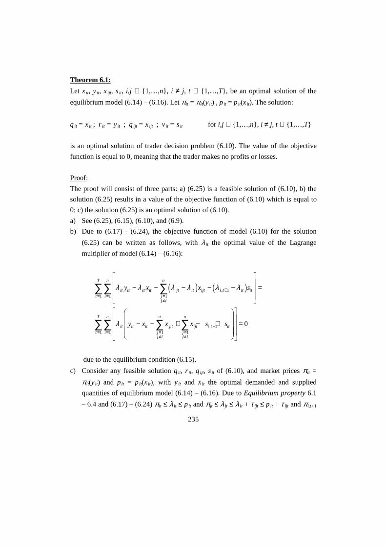
235

Theorem 6.1:

Let xit, yit, xijt, sit, i,j ∈ {1,…,n}, i ≠ j, t ∈ {1,…,T}, be an optimal solution of the

equilibrium model (6.14) – (6.16). Let πit = πit(yit) , p it = p it(xit). The solution:

q it = xit ; r it = y it ; q ijt = xijt ; vit = sit for i,j ∈ {1,…,n}, i ≠ j, t ∈ {1,…,T}

is an optimal solution of trader decision problem (6.10). The value of the objective

function is equal to 0, meaning that the trader makes no profits or losses.

Proof:

The proof will consist of three parts: a) (6.25) is a feasible solution of (6.10), b) the

solution (6.25) results in a value of the objective function of (6.10) which is equal to

0; c) the solution (6.25) is an optimal solution of (6.10).

a) See (6.25), (6.15), (6.10), and (6.9).

b) Due to (6.17) - (6.24), the objective function of model (6.10) for the solution

(6.25) can be written as follows, with λ it the optimal value of the Lagrange

multiplier of model (6.14) – (6.16):

λ λ λ λ λ λ

λ

it it it it jt it ijtjj i

n

i t it iti

n

t

T

it it it jitjj i

n

ijtjj i

n

i t iti

n

t

T

y x x s

y x x x s s

− − − − −�

!

"

$

###

=

− − + − +�

�

���

�

�

���

�

!

"

$

###

=

=≠

+==

=≠

=≠

−==

∑∑∑

∑ ∑∑∑

3 8 2 71

111

1 11

11

0

,

,

due to the equilibrium condition (6.15).

c) Consider any feasible solution q it, r it, qijt, sit of (6.10), and market prices πit =

πit(yit) and pit = p it(xit), with yit and xit the optimal demanded and supplied

quantities of equilibrium model (6.14) – (6.16). Due to Equilibrium property 6.1

– 6.4 and (6.17) – (6.24) πit ≤ λ it ≤ p it and πjt ≤ λ jt ≤ λ it + τ ijt ≤ p it + τ ijt and πi,t+1

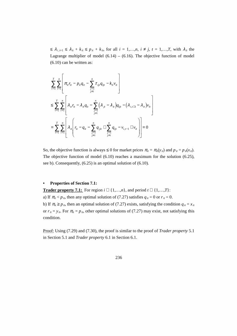
236

≤ λ i , t+1 ≤ λ it + kit ≤ p it + kit, for all i = 1,…,n, i ≠ j, t = 1,…,T, with λ it the

Lagrange multiplier of model (6.14) – (6.16). The objective function of model

(6.10) can be written as:

π τ

λ λ λ λ λ λ

λ

it it it it ijt ijtjj i

n

it iti

n

t

T

it it it it jt it ijtjj i

n

i t it iti

n

t

T

it it it jitjj i

n

ijtjj i

n

i t iti

n

t

T

r p q q k v

r q q v

r q q q v v

− − −�

!

"

$

###

≤ − − − − −�

!

"

$

###

= − − + − +�

�

���

�

�

���

�

!

"

$

###

=≠

==

=≠

+==

=≠

=≠

−==

∑∑∑

∑∑∑

∑ ∑∑∑

111

11

11

1 11

11

3 8 2 7,

, = 0

So, the objective function is always ≤ 0 for market prices πit = πit(yit) and p it = p it(xit).

The objective function of model (6.10) reaches a maximum for the solution (6.25),

see b). Consequently, (6.25) is an optimal solution of (6.10).

• Properties of Section 7.1:

Trader property 7.1: For region i ∈ {1,…,n}, and period t ∈ {1,…,T}:

a) If πit < p it, then any optimal solution of (7.27) satisfies q it = 0 or r it = 0.

b) If πit ≥ p it, then an optimal solution of (7.27) exists, satisfying the condition q it = xit

or r it = yit. For πit = p it, other optimal solutions of (7.27) may exist, not satisfying this

condition.

Proof: Using (7.29) and (7.30), the proof is similar to the proof of Trader property 5.1

in Section 5.1 and Trader property 6.1 in Section 6.1.

237

Trader property 7.2: Let q it, r jt, q ijt, vit, j ≠ i, i,j = 1,…,n, t = 1,…,T, be an optimal

solution of (7.27). Let a trader transport in a period t from region i to j, so q ijt > 0, i,j

∈ {1,…,n}, i ≠ j, t ∈ {1,…,T}, then:

a) no goods are transported from a region s = 1,…,n,s ≠ i, to region i, qsit = 0

b) no goods are transported from region j to a region s = 1,…,n, ,s ≠ j, q jst = 0.

c) purchases in region i are positive, q it > 0, or the stock remaining from the previous

period is positive, vi,t-1 > 0.

d) sales in region j are positive, r jt > 0, or the quantity put in stock in region j is

positive, vjt > 0.

Proof: Using (7.29) - (7.31), the proof is similar to the proof of Trader property 5.2 in

Section 5.1 and Trader property 6.2 in Section 6.1.

Trader property 7.3: For region i,j ∈ {1,…,n}, i ≠ j, and period t ∈ {1,…,T}:

a) If πjt < p it + τ ijt, then any optimal solution of (7.27) has to satisfy q it = 0 or q ijt = 0

or r jt = 0.

b) If πjt ≥ p it + τ ijt, and q it > 0, q ijt > 0 and r jt > 0, then an optimal solution of (7.27)

exists satisfying q it = xit or r jt = yit. For πjt = p it + τ ijt, an optimal solution of (7.27) is

not unique.

Proof: Using (7.29) - (7.31), the proof is similar to the proof of Trader property 6.3 in

Section 6.1.

Trader property 7.4: For region i ∈ {1,…,n}, and period t ∈ {1,…,T-1}:

a) If Eπi,t+1 < p it + kit, then any optimal solution of (7.27) has to satisfy q it = 0 or vit =

0 or ri tk, +1 = 0 for at least one k ∈ {1,...,K}.

b) Analogously, if Eπi,t+2 < p it + κ it,t+2, see also (6.12), then any optimal solution of

(7.27) has to satisfy q it = 0 or vit = 0 or vi tk, +1 = 0 or ri t

k l,,+2 = 0 for at least one k, l ∈

{1,...,K}. Analogous properties can be derived for storage until the periods τ =

t+3,...,T if Eπiτ < p it + κ itτ.

238

c) If Eπi,t+1 ≥ p it + kit and qit > 0 and sit > 0 and ri tk, +1 > 0 for all k = 1,…,K, then an

optimal solution of (7.27) exists satisfying q it = xit or ri tk, +1= yi t

k, +1 for at least one k ∈

{1,...,K}. For Eπi,t+1 = p it + kit, an optimal solution of (7.27) is not unique.

d) Analogously: if Eπi,t+2 ≥ p it + κ it,t+2 and q it > 0 and vit > 0, vi tk, +1 > 0 and ri t

k l,,+2 > 0,

for all k, l ∈ {1,…,K}, then a solution of (7.27) which satisfies q it = xit or ri tk l,,+2 =

yi tk l,,+2 , for at least one k, l ∈ {1,...,K}, is an optimal solution. For Eπi,t+2 = p it + κ it,t+2,

an optimal solution of (7.27) is not unique. Analogous properties can be derived for

storage until the periods τ = t+3,...,T if Eπiτ ≥ p it + κ itτ.

Proof:

a) Let Eπi,t+1 < p it + kit. If q it > 0, vit > 0 and ri tk, +1 > 0 for all k ∈ {1,...,K}, then, see

(7.29), (7.30) and (7.32), λ it ≥ p it, λ i tk

k

K

, +=∑ 11= λ it + kit and λ i t

k, +1 ≤ gt

ki tk

+ +1 1π , , which

contradicts, see (7.25), Eπi,t+1 < p it + kit. So necessarily, q it = 0, vit = 0 or ri tk, +1 = 0, for

at least one k ∈ {1,...,K}.

b) Let Eπi,t+2 < p it + κ it,t+2. If q it > 0, vit > 0, vi tk, +1 > 0 and ri t

k l,,+2 > 0 for all k, l ∈

{1,...,K}, then, see (7.29), (7.30) and (7.32), λ it ≥ p it, λ i tk

k

K

, +=

Ê 11= λ it + kit, λ i t

k l

l

K

,,+

=

Ê 21=

λ i tk

tk

i tg k, ,+ + ++1 1 1 and λ i tk l,,+2 ≤ g gt

ktl

i tl

+ + +1 2 2π , , which contradicts, see (7.25), Eπi,t+2 < p it

+ κ i,t,t+2. So necessarily, q it = 0, vit = 0, vi tk, +1 = 0 or ri t

k l,,+2 = 0 for at least one k, l ∈

{1,...,K}.

c) An optimal solution of problem (7.27) exists, since its feasible region is bounded.

For this proof we make a distinction between Eπi,t+1 > p it + kit and Eπi,t+1 = p it + kit:

* Let Eπi,t+1 > p it + kit and qit > 0, vit > 0 and ri tk, +1 > 0 for all k ∈ {1,…,K}. If the

optimal solution satisfies q it < xit and ri tk, +1 < yi t

k, +1 for all k ∈ {1,…,K}, then, see

(7.29), (7.30) and (7.32), λ it = p it, λ i tk

k

K

, +=∑ 11 = λ it + kit and λ i t

k, +1 = gt

ki tk

+ +1 1π , . It

239

would follow that Eπi,t+1 = p it + kit, which is in contradiction with Eπi,t+1 > p it + kit. So

necessarily, q it = xit or ri tk, +1 = yi t

k, +1 for at least one k ∈ {1,…,K}.

* Let Eπi,t+1 = p it + kit. Consider the optimal solution qst, vst, rs tk, +1 , s = 1,…,n, with

purchases, sales and storage for region i satisfying 0 < q it < xit, vit > 0 and 0 < ri tk, +1 <

yi tk, +1 , k = 1,…,K. Call ∆ it = min(xit-q it; yi t, +1

1 - ri t, +11 ;…; yi t

K, +1 - ri t

K, +1 ). The solution

′ ′ ′+q r vst s tk

st, ,, 1 defined by ′qit = q it + ∆ it, ′ +ri tk

, 1= ri tk, +1 + ∆ it, ′vit = vit + ∆ it, ′qst = qst, ′ +rs t

k, 1=

rs tk, +1 , ′vst = vst, for s≠i, is optimal as well, as can be seen easily by inspecting (7.27)

and (7.28). Moreover, ′qit = xit or ′ +ri tk

, 1= yi tk, +1 for at least one k ∈ {1,…,K}.

d) The proof of this property is analogous to the proof under c).

• Properties and Theorem of Section 7.2:

Optimal equilibrium prices and quantities for period T – see model (7.44)

Theorem 7.1a:

Let in the optimal solution of the equilibrium model (7.44) for period T, $xiT be the

optimal supply level and λ iT be the corresponding optimal value of the Lagrange

multiplier, for i = 1,…,n. If the producer price in period T in region i is equal to:

(7.48) p iT = λ iT

then xiT = $xiT is an optimal solution of model (7.10), the producer supply model for

period T. In other words, the optimal equilibrium supply level is a supply level which

gives the producers optimal profits in period T. Since the value of λ iT, depends on the

value of the equilibrium supply level, we write p iT(xiT) = λ iT.

240

Proof:

It is trivial that $xiT is a feasible solution of (7.10) for p iT( $xiT ) = λ iT. After all, it

follows from (7.44) that 0 ≤ $xiT ≤ w i,T-1. To prove that $xiT is an optimal solution of

(7.10), consider the following cases:

• if $xiT = 0, then p iT( $xiT ) ≤ ciT, see (7.45) and (7.46). For p iT ≤ ciT the producer

supply level xiT = 0 is an optimal solution of model (7.10) – see (7.11).

• if 0 < $xiT < w i,T-1, then p iT( $xiT ) = ciT, see (7.45) and (7.46). For p iT = ciT the

optimal producer supply level determined by model (7.10) is not unique. Also

supplying a level xiT = $xiT will be optimal for the producer – see (7.11).

if $xiT = w i,T-1, then piT( $xiT ) ≥ ciT, see (7.45) and (7.46). For p iT ≥ ciT the producer

supply level xiT = w i,T-1 is an optimal solution of model (7.10) – see (7.11).

Theorem 7.2a:

Let xiT, yiT, xijT, i,j ∈ {1,…,n}, i ≠ j, be an optimal solution of equilibrium model

(7.44) for period T. Let πiT = πiT(yiT) , p iT = p iT(xiT) = λ iT. The solution:

(7.49) q iT = x iT ; r iT = y iT ; qijT = x ijT for i,j ∈ {1,…,n} , i ≠ j

is an optimal solution of the trader decision problem (7.27) for period T.

Proof:

The proof will consist of three parts: a) (7.49) is a feasible solution of (7.27), b)

solution (7.49) results in a certain value of the objective function of (7.27); c) the

solution (7.49) is an optimal solution of (7.27), because any feasible solution of (7.27)

has an objective value less than the objective value for solution (7.49).

a) See (7.49), (7.44), and (7.27).

b) Due to (7.45) - (7.47) and (7.48), the objective function of model (7.27) for the

solution (7.49) can be written as, with λ iT the optimal value of the Lagrange

multiplier of model (7.44):

241

π τiT iT iT iT ijT ijTjj i

n

i

n

r p q q− −�

!

"

$

###=

≠=

∑∑11

= − − −�

!

"

$

###=

≠=

∑∑ λ λ λ λiT iT iT iT jT iT ijTjj i

n

i

n

y x x3 811

= − − +�

�

���

�

�

���=

≠=≠

=∑ ∑∑λ iT iT iT jiTjj i

n

ijTjj i

n

i

n

y x x x1 11

= −=∑λ iT i Ti

n

s , 11

due to the equilibrium condition of (7.44).

c) Consider any feasible solution q iT, r iT, qijT of (7.27), and market prices πiT =

πiT(yiT) and p iT = p iT(xiT), with yiT and xiT the optimal demanded and supplied

quantities of equilibrium model (7.44). Due to (7.45) - (7.47) and (7.48) πiT ≤ λ iT

= p iT and λ jT ≤ λ iT + τ ijT, for all i = 1,…,n, i ≠ j, with λ iT the optimal value of the

Lagrange multiplier of model (7.44). The objective function of model (7.27) can

be written as:

π τiT iT iT iT ijT ijTjj i

n

i

n

r p q q− −�

!

"

$

###=

≠=

∑∑11

≤ − − −�

!

"

$

###=

≠=

∑∑ λ λ λ λiT iT iT iT jT iT ijTjj i

n

i

n

r q q3 811

= −=∑λ iT i Ti

n

s , 11

due to the equilibrium condition of (7.27). So, (7.49) is an optimal solution of

model (7.27).

Optimal equilibrium prices and quantities for period T-1 – see model (7.50)

The Kuhn-Tucker conditions of model (7.50) result in the following expressions – see

(3.34) and (3.38) – (3.40):

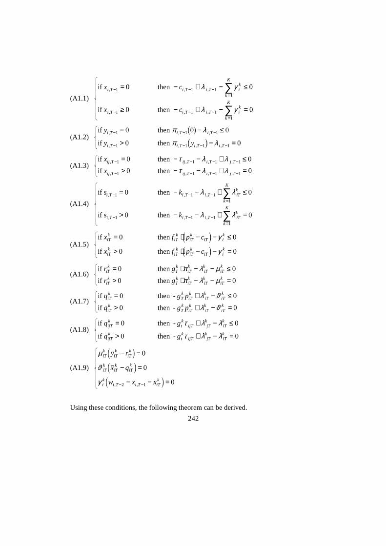
242

(A1.1)

if then

if then

x c

x c

i T i T i T ik

k

K

i T i T i T ik

k

K

, , ,

, , ,

− − −=

− − −=

= − + − ≤

≥ − + − =

%

&KK

'KK

∑

∑

1 1 11

1 1 11

0 0

0 0

λ γ

λ γ

(A1.2)if then

if then

y

y y

i T i T i T

i T i T i T i T

, , ,

, , , ,

− − −

− − − −

= − ≤

> − =

%&K

'K1 1 1

1 1 1 1

0 0 0

0 0

π λ

π λ

1 6

2 7

(A1.3)if then

if then

x

x

ij T ij T i T j T

ij T ij T i T j T

, , , ,

, , , ,

− − − −

− − − −

= − − + ≤

> − − + =%&K'K

1 1 1 1

1 1 1 1

0 0

0 0

τ λ λτ λ λ

(A1.4)

if then

if s then

s k

k

i T i T i T iTk

k

K

i T i T i T iTk

k

K

, , ,

, , ,

− − −=

− − −=

= − − + ≤

> − − + =

%

&KK

'KK

∑

∑

1 1 11

1 1 11

0 0

0 0

λ λ

λ λ

(A1.5)if then

if then

x f p c

x f p c

iTk

iTk

iTk

iT ik

iTk

iTk

iTk

iT ik

= ⋅ − − ≤

> ⋅ − − =

%&K

'K

0 0

0 0

3 8

3 8

γ

γ

(A1.6)if then

if then

r g

r g

iTk

Tk

iTk

iTk

iTk

iTk

Tk

iTk

iTk

iTk

= ⋅ − − ≤

> ⋅ − − =

%&K'K

0 0

0 0

π λ µπ λ µ

(A1.7)if then -

if then -

q g p

q g p

iTk

Tk

iTk

iTk

iTk

iTk

Tk

iTk

iTk

iTk

= + − ≤

> + − =

%&K'K

0 0

0 0

λ ϑλ ϑ

(A1.8)if then -

if then -

q g

q g

ijTk

tk

ijT jTk

iTk

ijTk

tk

ijT jTk

iTk

= + − ≤

> + − =

%&K

'K

0 0

0 0

τ λ λ

τ λ λ

(A1.9)

µ

ϑ

γ

iTk

iTk

iTk

iTk

iTk

iTk

ik

i T i T iTk

y r

x q

w x x

− =

− =

− − =

%

&KK

'KK − −

3 8

3 8

3 8

0

0

02 1, ,

Using these conditions, the following theorem can be derived.

243

Theorem 7.1b:

Let in the optimal solution of the equilibrium model (7.50), $ ,xi T −1 and $xiTk be the

optimal supply levels for period T-1 and T, respectively, and let λ i,T-1, λ iTk and γ i

k be

the corresponding optimal values of the Lagrange multipliers, for i = 1,…,n and k =

1,…,K. If the producer price in period T-1 in region i is equal to:

(7.52) p i,T-1 = λ i,T-1

then xi,T-1 = $ ,xi T −1, and x xiTk

iTk= $ are optimal solutions of model (7.14), the producer

supply model for period T-1. In other words, the optimal equilibrium supply levels

give the producers optimal profits in period T-1. Since the value of λ i,T-1, depends on

the value of the equilibrium supply level, we write p i,T-1(xi,T-1) = λ i,T-1.

Proof:

It is trivial that the solution $ ,xi T −1, $xiTk is a feasible solution of (7.14) for p i,T-1( $ ,xi T −1)

= λ i,T-1. After all, it follows from (7.50) that 0 ≤ $ ,xi T −1+ $xiTk ≤ w i,T-2. To prove that

$ ,xi T −1 and $xiTk are optimal solutions of (7.14), first determine the value of the

objective function of (7.14) for the solution $ ,xi T −1 and $xiTk , and then show that this

value is optimal:

• Due to (A1.1), (A1.5), (A1.9) and (7.52), the objective function of (7.14) can be

written as:

p c x f p c x x x wi T i T i T iTk

iTk

iT iTk

k

K

ik

i T iTk

k

K

ik

i Tk

K

, , , , ,$ $ $ $− − −=

−=

−=

− + − = + =∑ ∑ ∑1 1 11

11

21

2 7 3 8 3 8γ γ

• Consider any feasible solution of model (7.14), xi,T-1, xiTk for k = 1,…,K,

satisfying xi,T-1 + xiTk ≤ w i,T-2. Consider the optimal equilibrium market price p i,T-1

and Lagrange multiplier γ ik of equilibrium model (7.50), satisfying: p i,T-1 − ci,T-1

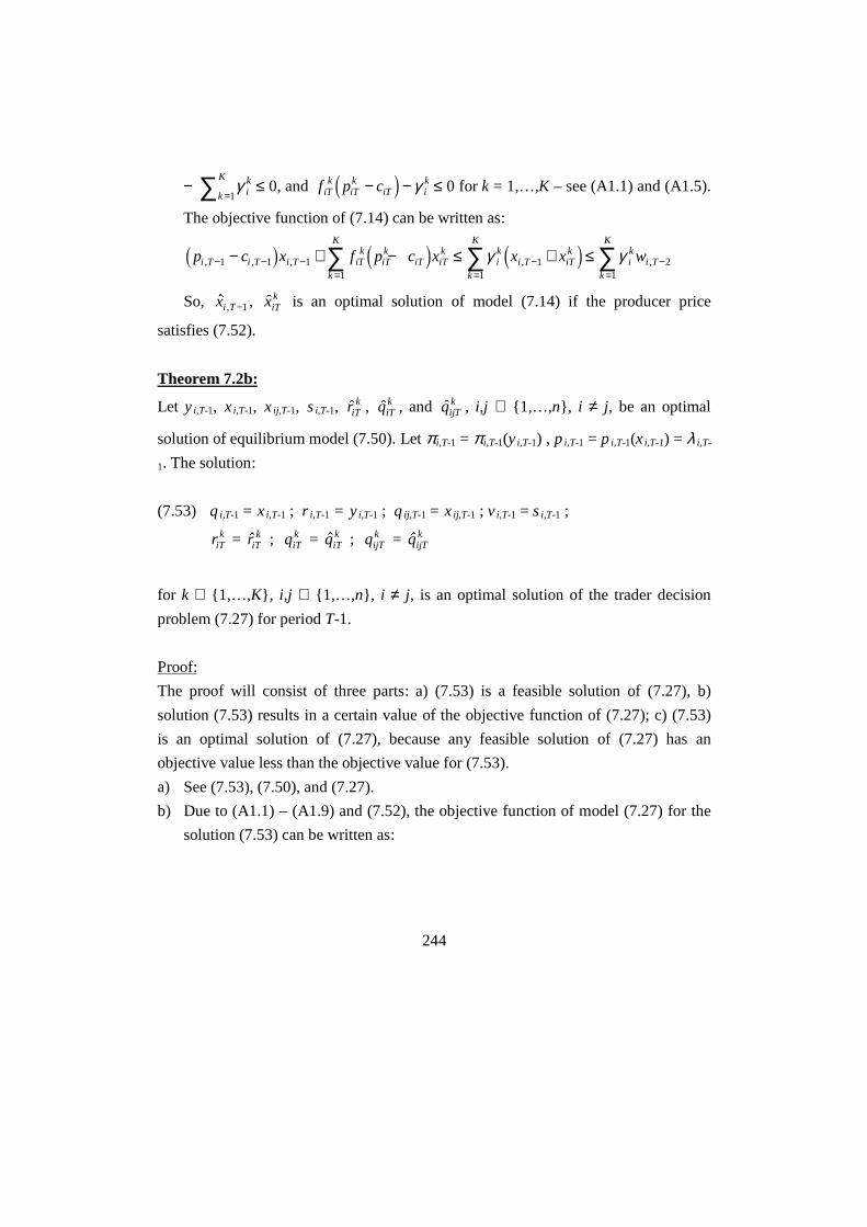
244

− γ ik

k

K

=∑ 1≤ 0, and f p ciT

kiTk

iT ik− −3 8 γ ≤ 0 for k = 1,…,K – see (A1.1) and (A1.5).

The objective function of (7.14) can be written as:

p c x f p c x x x wi T i T i T iTk

iTk

iT iTk

k

K

ik

i T iTk

k

K

ik

i Tk

K

, , , , ,− − −=

−=

−=

− + − ≤ + ≤∑ ∑ ∑1 1 11

11

21

2 7 3 8 3 8γ γ

So, $ ,xi T −1, $xiTk is an optimal solution of model (7.14) if the producer price

satisfies (7.52).

Theorem 7.2b:

Let yi,T-1, xi,T-1, xij,T-1, si,T-1, $riTk , $qiT

k , and $qijTk , i,j ∈ {1,…,n}, i ≠ j, be an optimal

solution of equilibrium model (7.50). Let πi,T-1 = πi,T-1(yi,T-1) , p i,T-1 = p i,T-1(xi,T-1) = λ i,T-

1. The solution:

(7.53) q i,T-1 = xi,T-1 ; r i,T-1 = y i,T-1 ; q ij,T-1 = xij,T-1 ; vi,T-1 = si,T-1 ;

riTk = $riT

k ; qiTk = $qiT

k ; qijTk = $qijT

k

for k ∈ {1,…,K}, i,j ∈ {1,…,n}, i ≠ j, is an optimal solution of the trader decision

problem (7.27) for period T-1.

Proof:

The proof will consist of three parts: a) (7.53) is a feasible solution of (7.27), b)

solution (7.53) results in a certain value of the objective function of (7.27); c) (7.53)

is an optimal solution of (7.27), because any feasible solution of (7.27) has an

objective value less than the objective value for (7.53).

a) See (7.53), (7.50), and (7.27).

b) Due to (A1.1) – (A1.9) and (7.52), the objective function of model (7.27) for the

solution (7.53) can be written as:

245

π τi T i T i T i T ij T ij Tjj i

n

i T i T Ttr

iT iT i Ti

n

r p q q k v EZ P v, , , , , , , , ,, ,− − − − − −=≠

− − −=

− − − +�

!

"

$

###

∑∑ 1 1 1 1 1 11

1 1 11

Π2 7

= − − − − −���

���

�

!

+ + − − − −�

!

"

$

###

"

$

###

− − − − − − −=≠

=− −

=

=≠

=

∑ ∑∑

∑∑

λ λ λ λ λ λ

λ µ λ ϑ λ λ

i T i T i T i T j T i T ij Tjj i

n

iTk

k

K

i T i Ti

n

iTk

iTk

iTk

iTk

iTk

iTk

jTk

iTk

ijTk

jj i

n

k

K

y x x s

r q q

, , , , , , , , ,1 1 1 1 1 1 11 1

1 11

11

3 8

3 8 3 8 3 8

= − + + +�

!

"

$#− −

=− −

==∑ ∑∑ λ λ λ µ ϑi T i T iT

k

k

K

i T iTk

i T iTk

iTk

iTk

iTk

k

K

i

n

s s s r q, , , ,1 21

1 111

= + +�

!

"

$#− −

==∑∑ λ µ ϑi T i T iT

kiTk

iTk

iTk

k

K

i

n

s y x, ,1 211

due to the equilibrium conditions of (7.50) and (A1.9).

c) Consider any feasible solution q i,T-1, r i,T-1, qij,T-1, vi,T-1, riTk , qiT

k , qijTk of (7.27), and

market prices πi,T-1 = πi,T-1(yi,T-1) and p i,T-1 = p i,T-1(xi,T-1), with yi,T-1 and xi,T-1 the

optimal demanded and supplied quantities of equilibrium model (7.50). Due to

(A1.1) – (A1.9) and (7.52):

πi,T-1 ≤ λ i,T-1 = p i,T-1 ; λ j,T-1 ≤ λ i,T-1 + τ ij,T-1; - ki,T-1 -λ i,T-1 + λ iTk

k

K

=∑ 1 ≤ 0

gTk

iTk

iTk

iTkπ λ µ− − ≤ 0 ; -g pT

kiTk

iTk

iTk+ − ≤λ ϑ 0 ; -gt

kijT jT

kiTkτ λ λ+ − ≤ 0

y riTk

iTk

- � 0; x qiTk

iTk

- � 0 ; µ ϑiTk

iTk, ≥ 0

for all i = 1,…,n, i ≠ j, with λ i,T-1, λ µ ϑiTk

iTk

iTk, , the optimal values of the Lagrange

multipliers of model (7.50). Analogous to b), for the objective function of model

(7.27) follows:

246

π τit it it it ijt ijtjj i

n

it it ttr

i t i t iti

n

r p q q k v EZ P v− − − +�

!

"

$

###=

≠

+ + +=

∑∑1

1 1 11

Π , ,, ,2 7 ≤

λ µ ϑi T i T ik

iTk

ik

iTk

k

K

i

n

s y x, ,− −==

+ +�

!

"

$#∑∑ 1 2

11

due to the equilibrium condition of (7.27). So, (7.53) is an optimal solution of

model (7.27).

Optimal equilibrium prices and quantities for period t ∈ {1,…,T-2} – see model

(7.54):

A part of the Kuhn Tucker conditions of model (7.54) are as follows:

(A1.10)

if then

if then

x c

x c

it it it ik k

k

K

k

K

it it it ik k

k

K

k

K

T t

T t

T t

T t

= − + − ≤

> − + − =

%

&KK

'KK

−

−

−

−

==

==

∑∑

∑∑

0 0

0 0

1

1

1

1

11

11

λ γ

λ γ

...

...

,...,

,...,

(A1.11)if then

if then

y

y y

it it it

it it it it

= − ≤

> − =

%&K'K

0 0 0

0 0

π λπ λ

1 61 6

(A1.12)if then

if then

x

x

ijt ijt it jt

ijt ijt it jt

= − − + ≤

> − − + =%&K'K

0 0

0 0

τ λ λτ λ λ

(A1.13)

if then

if s then

s k

k

it it it i tk

k

K

it it it i tk

k

K

= − − + ≤

> − − + =

%

&KK

'KK

+=

+=

∑

∑

0 0

0 0

11

11

1

1

1

1

λ λ

λ λ

,

,

247

(A1.14)

if then

if then

x f f p c

x f f p c

i tk k

i tk

i tk

i tk

i t ik k

k

K

k

K

i tk k

i tk

i tk

i tk

i t ik k

k

T t

T t

T t

T t

,,...,

, , , ,,...,

,,...,

, , , ,,...,

... ...

... ...

,...

,...

+ + + + +==

+ + + + +=

= ⋅ ⋅ − − ≤

> ⋅ ⋅ − −

−

−+

−

−

∑∑τ τ τ τ

τ τ τ τ

τ τ

τ

τ τ

γ

γ

1 1 1 1

1

1 1 1 1

0 0

0

111

11

3 8

3 8K

k

K

∑∑+ =

=

%

&KK

'KK

τ 1 1

0

for τ = 1,…,T-t

(A1.15)if then

if then

r g g

r g g

i tk k

tk

tk

i tk

i tk k

i tk k

i tk k

tk

tk

i tk

i tk k

i tk k

,,...,

, ,,...,

,,...,

,,...,

, ,,...,

,,...,

...

...

+ + + + + +

+ + + + + +

= ⋅ ⋅ − − ≤

> ⋅ ⋅ − − =

%&K

'Kτ τ τ τ τ

τ τ τ τ τ

τ τ τ τ τ

τ τ τ τ τ

π λ µ

π λ µ

1 1 1 1

1 1 1 1

0 0

0 0

1

1

for τ = 1,…,T-t

(A1.16)if then -

if then -

q g g p

q g g p

i tk k

tk

tk

i tk

i tk k

i tk k

i tk k

tk

tk

i tk

i tk k

i tk k

,,...,

, ,,...,

,,...,

,,...,

, ,,...,

,,...,

...

...

+ + + + + +

+ + + + + +

= ⋅ ⋅ + − ≤

> ⋅ ⋅ + − =

%&K

'Kτ τ τ τ τ

τ τ τ τ τ

τ τ τ τ τ

τ τ τ τ τ

λ ϑ

λ ϑ

1 1 1 1

1 1 1 1

0 0

0 0

1

1

for τ = 1,…,T-t

(A1.17)if then -

if then -

q g g

q g g

ij tk k

i tk

i tk

ij t j tk k

i tk k

ij tk k

i tk

i tk

ij t j tk k

i tk k

,,...,

, , , ,,...,

,,...,

,,...,

, , , ,,...,

,,...,

...

...

+ + + + + +

+ + + + + +

= ⋅ ⋅ + − ≤

> ⋅ ⋅ + − =

%&K

'Kτ τ τ τ

τ τ τ τ

τ τ τ τ

τ τ τ τ

τ λ λ

τ λ λ

1 1 1 1

1 1 1 1

0 0

0 0

1 1

1 1

for τ = 1,…,T-t

(A1.18)

if then

if then

v g g k

v g g k

i tk k

i tk

i tk

i t i tk k

i tk k

k

K

i tk k

i tk

i tk

i t i tk k

i tk k

k

,,...,

, , , ,,...,

,,...,

,,...,

, , , ,,...,

,,...,

...

...

+ + + + + + +=

+ + + + + + +

= − ⋅ ⋅ − + ≤

> − ⋅ ⋅ − +

+

+

+

+

∑τ τ τ τ τ

τ τ τ τ τ

τ τ τ τ

τ

τ τ τ τ

τ

λ λ

λ λ

1 1 1 1 1

1

1 1 1 1 1

1

0 0

0

1 11

1 1=

∑ =

%

&KK

'KK

1

0K

for τ = 1,…,T-t-1

(A1.19)

µ

ϑ

γ

τ τ τ

τ τ τ

τ τ τ

τ τ τ

i tk k

i tk k

i tk k

i tk k

i tk k

i tk k

ik k

i t it i tk

i tk k

iTk k

y r

x q

w x x x xT t T t

,,...,

,,...,

,,...,

,,...,

,,...,

,,...,

,...,, , ,

, ,...,...

+ + +

+ + +

− + +

− =

− =

− − − − − =

%

&KK

'KK − −

1 1 1

1 1 1

1 1 1 2 1

0

0

01 1 2

3 8

3 8

3 8

for τ = 1,…,T-t-1

248

Theorem 7.1c:

Let in the optimal solution of the equilibrium model (7.54) for period t, t = 1,…,T-2,

$ , $ , $ ,,x x xt tk

tk k

+ +1 21 1 2 ..., $ ,...,xT

k kT t1 − be the optimal supply level and λ it be the corresponding

optimal value of the Lagrange multiplier of the equilibrium condition for period t, for

i = 1,…,n, k1,…,kT-t = 1,…,K. If the producer price in period t in region i is equal to:

(7.55) p it = λ it

then xit = $xit , x x x xtk

tk

Tk k

Tk kT t T t

+ += =

- -

1 11 1 1 1

$ ,..., $

,..., ,..., , for k1,…,kT-t = 1,…,K, is an optimal

solution of supply model (7.14), the producer supply model for the periods 1 to T-2.

In other words, the optimal equilibrium supply levels give the producers optimal

profits. Since the value of λ it, depends on the value of the equilibrium supply level,

we write p it(xit) = λ it.

Proof:

Consider the optimal solution of model (7.54) for period t: $ , $ , $ ,..., $, ,...,x x x xt tk

tk k

Tk kT t

+ +−

1 21 1 2 1

for the periods t to T, at producer prices equal to p p p pt tk

tk

TkT t, , ,...,+ +

−1 2

1 2 , for k1,…,kT-t =

1,…,K. Is this solution an optimal solution of producer supply problem (7.14) for

period t? It is trivial that the solution is a feasible solution of model (7.14). To prove

that the solution is also optimal, first determine the value of the objective function of

(7.14), and then show that this value is optimal:

• Due to (A1.10), (A1.14), (A1.19), and (7.55), the objective function of (7.14) can

be written as:

249

p c x EZ w x P

p c x f p c x f p c x

f p c x

it it it i tpr

i t it i t

it it it i tk

i tk

i t i tk

i tk

i tk

i t i tk k

k

K

k

K

i Tk

i Tk

i T i TT t T t

- + -

= - + - + - +

�

!

+ -

+ - +

+ + + + + + + +

==

- - -

ÊÊ

- - -

1 6 2 7

1 6 3 8 3 8

3 8

$ $ ;

$ $ $ ...

... $

, , ,

, , , , , , , ,,

, , , ,

1 1 1

1 1 1 1 2 2 2 211

1 1 1

1 1 1 2 2 1 2

21

1-

==

- - - - -

-- -

+ -

�

!

"

$##

"

$##

"

$##ÊÊ 1

11

1 1 1

1

k kiTk

iTk

iT iTk k

k

K

k

KT t T t T t T t

T tT t

f p c x,..., ,...,$ ...3 8

= + +�

!

+�

!

+

−

−

−

−

−

−

− − −

−

==+

=+

===

−=

∑∑ ∑∑ ∑∑∑∑... $ ... $ ... $ ...

... $

,..., ,...,,

,...,,

,

,...,,

,...,

γ γ γ

γ

ik k

itk

K

k

K

ik k

i tk

k

K

k

K

ik k

i tk k

k

K

k

K

k

K

k

K

ik k

i Tk k

K

K

T t

T t

T t

T t

T t

T t

T t T t t

T t

x x x

x

1

1

1 1

2

1 1 2

321

1 1

111

12

111

11

∑ ∑∑ +�

!

"

$##

"

$##

"

$##

− −

−− − ==

γ ik k

iTk k

K

K

k

KT t T t

T tT t

x1 1

1 11

,..., ,...,$ ...

= −

− ==∑∑ ... ,...,γ i

k kit

k

K

k

KT t

T t

w1

1 11

• Consider any feasible solution of model (7.14): x x x xt tk

tk k

Tk kT t, , ,...,, ,...,

+ +−

1 21 1 2 1 for the

periods t to T, at producer prices equal to p p p pt tk

tk

TkT t, , ,...,+ +

−1 2

1 2 , for k1,…,kT-t =

1,…,K. Suppose that prices satisfy the following properties – see (A1.10),

(A1.14), (A1.19), and (7.55):

p cit it ik k

k

K

k

KT t

T t

− ≤ −

− ==∑∑... ,...,γ 1

1 11

f f p ci tk

i tk

i tk

i t ik k

k

K

k

KT t

T t

, , , ,,...,... ... ,...

+ + + +==

⋅ ⋅ − ≤ −

−+

∑∑111

1 1 1

1

τ τ ττ

τ

γ3 8

x x x x wit i tk

i tk k

iTk k

i tT t+ + + + ≤+ + −

−, ,

, ,...,,...1 2 1

1 1 2 1 γ ik kT t1 0,...,

- �

The value of the objective function of (7.14) for the feasible solution satisfies:

p c x EZ w x Pit it it i tpr

i t it i t− + −+ − +1 6 2 7, , ,;1 1 1

250

≤ + +�

!

+�

!

+ +

−

−

−

−

−

−

− − −

−

==+

=+

===

−=

∑∑ ∑∑ ∑∑∑∑

∑

... ... ... ...

...

,..., ,...,,

,...,,

,

,...,,

,...,

γ γ γ

γ γ

ik k

itk

K

k

K

ik k

i tk

k

K

k

K

ik k

i tk k

k

K

k

K

k

K

k

K

ik k

i Tk k

K

K

i

T t

T t

T t

T t

T t

T t

T t T t t

T t

x x x

x

1

1

1 1

2

1 1 2

321

1 1

111

12

111

11

k kiTk k

K

K

k

KT t T t

T tT t

x1 1

1 11

,..., ,..., ...− −

−− − ==∑∑

�

!

"

$##

"

$##

"

$##

≤ −

− ==∑∑... ,...,γ i

k kit

k

K

k

KT t

T t

w1

1 11

So, $ , $ , $ ,..., $, ,...,x x x xt tk

tk k

Tk kT t

+ +−

1 21 1 2 1 is an optimal solution of (7.14), if the producer price

satisfies (7.55).

Theorem 7.2c:

Let $ , $ , $ , $ , $ , $ , $ , $ , $ , $ , $ , $, , , , ,,...,

,,...,

,,...,

,,...,x y x s q r q v q r q vit it ijt it i t

ki tk

ij tk

i tk

i tk k

i tk k

ij tk k

i tk k

+ + + + + + + +1 1 1 11 1 1 1 1 1 1 1

τ τ τ ττ τ τ τ , τ = 2,…,T-t, i,j

∈ {1,…,n}, i ≠ j, be an optimal solution of equilibrium model (7.54). Let πit = πit( $yit )

, p it = p it( $xit ) = λ it. The solution:

(7.56)

q x r y q x v s

q q r r q q v v

q q r r q

it it it it ijt ijt it it

i tk

i tk

i tk

i tk

ij tk

ij tk

i tk

i tk

i tk k

i tk k

i tk k

i tk k

ij tk

= = = =

= = = =

= =

+ + + + + + + +

+ + + + +

$ ; $ ; $ ; $ ;

$ ; $ ; $ ; $ ;

$ ; $ ;

, , , , , , , ,

,,...,

,,...,

,,...,

,,...,

,,.

1 1 1 1 1 1 1 11 1 1 1 1 1 1 1

1 1 1 1 1τ τ τ τ τ

τ τ τ τ ..,,,...,

,,...,

,,...,

$ ; $ ;

,...,

kij tk k

i tk k

i tk kq v v

T t

τ τ τ ττ τ τ

τ

= =

³ -

+ + +

1 1 1

2for : ?

for i,j ∈ {1,…,n}, i ≠ j, is an optimal solution of the trader decision problem (7.27).

Proof:

The proof will consist of three parts: a) (7.56) is a feasible solution of (7.27), b)

solution (7.56) results in a certain value of the objective function of (7.27); c) (7.56)

is an optimal solution of (7.27), because any feasible solution of (7.27) has an

objective value less than the objective value for (7.56).

a) See (7.56), (7.54), and (7.27).

251

b) Due to (A1.10) – (A1.19) and (7.55), the objective function of model (7.27) for

the solution (7.56) can be written as:

π τit it it it ijt ijtjj i

n

it it ttr

i t i t iti

n

r p q q k v EZ P v− − − +�

!

"

$

###=

≠

+ + +=

∑∑1

1 1 11

Π , ,, ,2 7

= - - - - -

�

��

�

��

�

!

+ + - - - -

�

!

-

=

ā

+

==

+ + + + + + + + +

=

ā

=

+

Ê ÊÊ

ÊÊ

λ λ λ λ λ λ

λ µ λ ϑ λ λ

λ

it it it it jt it ijtjj i

n

i tk

k

K

it iti

n

i tk

i tk

i tk

i tk

i tk

i tk

j tk

i tk

ij tk

jj i

n

k

K

i t

y x x s

r q q

$ $ $ $

$ $ $

,

, , , , , , , , ,

,

3 8

3 8 3 8 3 8

11

11

1 1 1 1 1 1 1 1 111

1

1

1 1 1 1 1 1 1 1 1

1

21

1 11

1 2

2

1 1 1 1 1 1 1 1

1 1

k k

k

K

i tk

i tk

i tk k

i tk k

i tk k

i tk k

i tk k

i tk k

k

K

j tk k

i tk k

v r q,, , ,

,...,,,...,

,,...,

,,...,

,,...,

,,...,

,,...,

,,...,

$ ... $ $

$

=

+ + + + + + + +

=

+ +

Ê Ê-

�

��

�

�� + + + - -

- -

λ λ µ λ ϑ

λ λ

τ τ τ τ τ τ

τ τ

τ τ τ τ τ τ

τ

τ τ

3 8 3 8

3 8q v

r q

ij tk k

jj i

n

i tk k

k

K

i tk k

i tk k

iTk k

iTk k

iTk k

iTk k

iTk k

iTk

k

KT t T t T t T t T t

T t

,,...,

,,...,

,,...,

,,...,

,..., ,..., ,..., ,..., ,...,

$ ...

$ $

+

=

ā

+ +

=

+ +

=

Ê Ê

Ê

- -

�

��

�

�� + +

+ - -

-

+

+

- - - - -

-

τ τ τ ττ τ

τ

τ τλ λ

λ µ λ ϑ

1 1 1

1

1 1

1 1 1 1 1 1

11

1

1

3 8 3 8

λ λjTk k

iTk k

ijTk k

jj i

nT t T t T tq1 1 1

1

,..., ,..., ,...,$ ... ...- - -

-

"

$

###

"

$

###

"

$

###

"

$

####

=

ā

Ê3 8

252

= - + - +

�

!

�

!

+ - + +

- +

=

+ + +

===

+ + - + + +

=

Ê ÊÊÊ

Ê- +

+

λ λ λ λ

λ λ λτ τ τ ττ τ τ τ

τ

it i t i tk

itk

K

i tk

it i tk k

i tk

k

K

k

K

i

n

i tk k

i tk k

i tk k

i tk k

k

K

iTk

s s s v

v v

$ $ $ $ ...

$ $ ...

, , , ,,

,

,,...,

,,...,

,,...,

,,..., ,.

1 11

1 2 1111

1 11

1

1

1 1 2 1

21

1 1 1 1 1 1

1

1 ..,,

,...,

, , , , ,,

,,

,,

,,

,,..

$ ...

$ $ $ $ ...

ki Tk k

k

K

k

K

i tk

i tk

i tk

i tk

i tk k

i tk k

i tk k

i tk k

k

K

k

K

i

n

i tk

T t T t

T t

v

r q r q

- - -

-

-

==

+ + + + + + + +

===

+

ÊÊ

ÊÊÊ

�

!

"

$##

"

$##

"

$##

+ + + + +

�

!

+

111

1 1 1 1 1 1 1 1111

1 1

1 1 1 1 1 2 1 2 1 2 1 2

21

1

τ

µ ϑ µ ϑ

µ τ.,

,,...,

,,...,

,,...,

,..., ,..., ,..., ,...,

$ $ ...

$ $ ... ...

ki tk k

i tk k

i tk k

k

K

iTk k

iTk k

iTk k

iTk k

k

K

r q

r qT t T t T t T t

T t

τ τ τ τ

τ

τ τ τϑ

µ ϑ

+ + +

=

=

+ + +

+ +

"

$##

"

$##

"

$##

Ê

Ê - - - -

-

1 1 1

1 1 1 1

1

1

= + + + + +

�

!

+ +

-

=

+ + + + + + + +

===

+ + + +

Ê ÊÊÊλ µ ϑ µ ϑ

µ ϑτ τ τ ττ τ τ

it i ti

n

i tk

i tk

i tk

i tk

i tk k

i tk k

i tk k

i tk k

k

K

k

K

i

n

i tk k

i tk k

i tk k

i tk k

s y x y x

y x

$ ..., , , , , ,,

,,

,,

,,

,,...,

,,...,

,,...,

,,...,

11

1 1 1 1 1 1 1 1111

1 1 1 1 1 2 1 2 1 2 1 2

21

1 1 1 1 τ

τ

µ ϑ

+ +

+ +

"

$##

"

$##

"

$##

=

=

Ê

Ê - - - -

-

...

... ...,..., ,..., ,..., ,...,

k

K

iTk k

iTk k

iTk k

iTk k

k

KT t T t T t T t

T t

y x

1

1

1 1 1 1

due to the equilibrium conditions of (7.54) and (A1.19).

c) Consider any feasible solution q it, r it, qijt, vit, r q q vi tk

i tk

ij tk

i tk

, , , ,, , , ,+ + + +1 1 1 11 1 1 1

r q q vi tk k

i tk k

ij tk k

i tk k

,,...,

,,...,

,,...,

,,...,, , ,+ + + +τ τ τ τ

τ τ τ τ1 1 1 1 of model (7.27), and market prices πit = πit( $yit ) , p it

= p it( $xit ) = λ it. Due to (A1.10) – (A1.19) and (7.55):

πit ≤ λ it = p it λ jt ≤ λ it + τ ijt - ki,t -λ it + λ i tk

k

K

, +=∑ 111

1

≤ 0

gtk

i tk

i tk

i tk

+ + + +⋅ − − ≤1 1 1 11 1 1 1 0π λ µ, , , g gt

ktk

i tk k

i tk k

i tk k

+ + + + +⋅ ⋅ − − ≤11 1 1 1 0... ,

,...,,,...,

,,...,

τ τ τ ττ τ τ τπ λ µ

-g ptk

i tk

i tk

i tk

+ + + ++ − ≤1 1 1 11 1 1 1 0, , ,λ ϑ -g g pt

ktk

i tk k

i tk k

i tk k

+ + + + +⋅ ⋅ + − ≤τ τ τ τ ττ τ τ τλ ϑ1 1 1 1 0... ,

,...,,,...,

,,...,

253

-gtk

ij t j tk

i tk

+ + + ++ − ≤1 1 1 11 1 1 0τ λ λ, , , -g gt

ktk

ij t j tk k

i tk k

+ + + + +⋅ ⋅ + − ≤11 1 1 0... , ,

,...,,,...,

τ τ τ ττ τ ττ λ λ

-g ktk

i t i tk

i tk k

k

K

+ + + +=− + ≤∑1 1 1 21

1 1 1 2

2

0, , ,,λ λ

-g g ktk

tk

i t i tk k

i tk k

k

Kt

t+ + + + + +=

⋅ ⋅ − + ≤+ +

+∑1 11

1 1 1 1 0... , ,,...,

,,...,

τ τ τ ττ τ τ

τλ λ

y ri tk

i tk

, ,+ +- �1 1

1 1 0 y ri tk k

i tk k

,,...,

,,...,

+ +- �τ τ

τ τ1 1 0 µ ϑ µ ϑτ ττ τ

i tk

i tk

i tk k

i tk k

, , ,,...,

,,...,, , ,

+ + + +=1 1

1 1 1 1 0

x qi tk

i tk

, ,+ +- �1 1

1 1 0 x qi tk k

i tk k

,,...,

,,...,

+ +- �τ τ

τ τ1 1 0

for all τ = 2,…,T-t, i = 1,…,n, i ≠ j, with λ it, λ λ µττ

i tk

i tk k

i tk

, ,,...,

,, ,+ + +1 1

1 1 1 ,

µ ϑ ϑτ ττ τ

i tk k

i tk

i tk k

,,...,

, ,,...,, ,

+ + +

1 1 11 the optimal values of the Lagrange multipliers of model

(7.54). Analogous to b), for the objective function of model (7.27) follows:

π τit it it it ijt ijtjj i

n

it it ttr

i t i t iti

n

r p q q k v EZ P v− − − +�

!

"

$

###=

≠

+ + +=

∑∑1

1 1 11

Π , ,, ,2 7 ≤

= + + + + +

�

!

+ +

-

=

+ + + + + + + +

===

+ + + +

Ê ÊÊÊλ µ ϑ µ ϑ

µ ϑτ τ τ ττ τ τ

it i ti

n

i tk

i tk

i tk

i tk

i tk k

i tk k

i tk k

i tk k

k

K

k

K

i

n

i tk k

i tk k

i tk k

i tk k

s y x y x

y x

$ ..., , , , , ,,

,,

,,

,,

,,...,

,,...,

,,...,

,,...,

11

1 1 1 1 1 1 1 1111

1 1 1 1 1 2 1 2 1 2 1 2

21

1 1 1 1 τ

τ

µ ϑ

+ +

+ +

"

$##

"

$##

"

$##

=

=

Ê

Ê - - - -

-

...

... ...,..., ,..., ,..., ,...,

k

K

iTk k

iTk k

iTk k

iTk k

k

KT t T t T t T t

T t

y x

1

1

1 1 1 1

due to the equilibrium condition of (7.29). So, (7.76) is an optimal solution of model

(7.29).

Some equilibrium properties:

Equilibrium property 7.1: For region i ∈ {1,…,n}, and period t ∈ {1,…,T}:

a) In the optimal solution of (7.44) πit(yit) ≤ p it(xit).

254

b) If in the optimal solution of (7.44) πit(yit) < p it(xit), then yit = 0.

c) If in the optimal solution of (7.44), supply and demand are both positive, xit > 0

and yit > 0, then the prices satisfy necessarily πit(yit) = p it(xit).

Proof:

a) Since the solution always has to satisfy πit(yit) ≤ λ it = p it(xit), see for example

(A1.2) and (7.52), πit(yit) ≤ p it(xit).

b) Let πit(yit) < p it(xit). If in the optimal solution yit > 0, then necessarily, see for

example (A1.2) and (7.52), πit(yit) = λ it = p it(xit), which contradicts πit(yit) < p it(xit).

So, necessarily, yit = 0.

c) This follows from a) and b).

Equilibrium property 7.2: In the optimal solution of (7.44), let transport take place

from market i to market j in period t, i.e. xijt > 0, with i,j ∈ {1,…,n}, j ≠ i, t ∈{1,…,n}, then:

a) no goods are transported from a region s = 1,…,n, to region i, xsit = 0, for s ≠ i.

b) no goods are transported from region j to a region s = 1,…,n, xjst = 0, for s ≠ j.

c) the producer supply in region i satisfies, xit > 0, or the stock remaining from the

previous period is positive, si,t-1 > 0.

d) the consumer demand in region j satisfies, yjt > 0, or the quantity in stock at the end

of period t in region j is positive, sjt > 0 (this is equal to the statement that the quantity

in stock at the end of period t, to be sold in period τ, is positive for at least one period

τ, &sjtτ > 0 , τ ∈ {t+1,…,T}).

Proof: Using for example (A1.3), the proof is similar to the proof of Equilibrium

property 5.2.

Equilibrium property 7.3: For region i and j, i,j ∈ {1,…,n}, j ≠ i, and period t ∈{1,…,n}:

a) In the optimal solution of (7.44) πjt(y jt) ≤ p it(xit) + τ ijt.

255

b) If in the optimal solution of (7.44) πjt(yjt) < p it(xit) + τ ijt, then xijt = 0 or yjt = 0

c) If in the optimal solution of (7.44) supplies in region i, transport between region i

and j, and demand in region j are positive, xit > 0, xijt > 0 and yjt > 0, then the optimal

prices satisfy necessarily πit(yit) = p it(xit) + τ ijt.

Proof:

a) Since the solution always has to satisfy πjt(yjt) ≤ λ jt ≤ λ it + τ ijt = p it(xit) + τ ijt, see

for example (A1.2), (A1.3) and (7.52), πjt(yjt) ≤ p it(xit) + τ ijt.

b) Let πit(yit) < p it(xit) + τ ijt. If in the optimal solution xijt > 0 and yit > 0, then

necessarily, see for example (A1.2), (A1.3) and (7.52), πjt(yjt) = λ jt = λ it + τ ijt =

p it(xit) + τ ijt, which contradicts πit(yit) < p it(xit) + τ ijt. So, necessarily, xijt = 0 or yit = 0.

c) This follows from a) and b).

Equilibrium property 7.4: For region i ∈ {1,…,n}, and period t ∈ {1,…,n}, we can

derive that:

a) If in the optimal solution of (7.44) EΠ i,t+1 < p it(xit) + kit, then sit = 0 or ri tk, +1 = 0 for

at least one k ∈ {1,…,K}.

b) If in the optimal solution of (7.44) Eπi,t+1 ≥ p it + kit, storage in period t, and

planned sales in period t+1 are positive, sit > 0, and ri tk, +1

1 > 0 for all k1 ∈ {1,…,K},

then an optimal solution exists satisfying q it = xit or ri tk, +1= yi t

k, +1 for at least one k ∈

{1,...,K}. For Eπi,t+1 = p it + kit, an optimal solution is not unique.

Proof:

a) Let EΠ i,t+1 < p it(xit) + kit. Suppose that sit > 0 and ri tk, +1

1 = 0 for all k1 = 1,…,K.

Then, see for example (A1.2), (A1.4) and (7.52): EΠ i,t+1 ≥ λ it + kit = p it(xit) + kit,

which is in contradiction with EΠ i,t+1 < p it(xit) + kit.

b) The proof is similar to the proof of Trader property 7.4 in Section 7.1.

256

Appendix 2: The stochastic supply model

In Section 9.2, the cereal supply decision problems of cereal producers in Burkina

Faso have been discussed for all periods t = 1,…,4. In this appendix we derive the

optimal solutions of these models for each period. In Section 9.2, it has been

supposed that when producers decide on their optimal supplies for period t, they

know the stock level at the end of the previous period wt-1, and the producer price

level in period t, pt. For the stochastic future prices, Pt+1,…,P4, we assumed that the

stochastic price for period t+1 is independent of the price in period t, pt. The

stochastic prices for the other periods τ = t+2,…,4, Pτ, however, depend on the

stochastic price in the previous period, Pτ −1. In the model for period t, for t = 1,2,3,

future prices for the periods t+1 to 4 were written as – see (9.32), (9.37), and (9.41):

(A2.1) Pt+1 = $p p pt t t+ -

+11 6 + Θ t+1; Pτ = Pτ−1 + p pτ τ-

-11 6 + Θτ

for τ = t+2,…,4,

with $pt and pτ constants, and EΘυ = 0, for υ = t+1,…,4. Θ t+1 are random

disturbances from the expected price in period t+1: E(Pt+1); Θτ are random

disturbances from the expected price in period τ, given the price in period τ-1: E(Pτ

|Pτ−1=pτ−1) for τ = t+2,…,4. We assume that the random disturbances Θυ, for υ =

t+1,…,4, are independent, and have a discrete, empirical distribution with possible

realisations θk, for k = 1,…,K, and:

(A2.2) Pr(Θυ = θk) = f kυ for υ = t+1,…,4, and k = 1,…,K

with 0 ≤ f kυ ≤ 1 and f k

k

K

υ=∑ 1= 1. In the models for the periods 1, 2, and 3, possible

prices and probability distributions are defined, for k,l,m = 1,...,K, as follows – see

(9.33), (9.34), (9.38), (9.39), (9.42), and (9.43):

For the model for period 1, (9.29):

257

(A2.3)

p p p p

p p p p

p p p p

k k

kl k k

klm kl k

2 1 2 1 2

3 2 3 2 3

4 3 4 3 4

= + - +

= + - +

= + - +

$ 1 61 61 6

θ

θ

θ

Pr

Pr

Pr ,

P p f

P p P p f

P p P p P p f

k k

kl k l

klm k kl m

2 2 2

3 3 2 2 3

4 4 2 2 3 3 4

= =

= = =

= = = =

2 7

4 9

4 9For the model for period 2, (9.28):

(A2.4) p p p p

p p p p

k k

kl k l

3 2 3 2 3

4 3 4 3 4

= + - +

= + - +

$ 1 61 6

θ

θ

Pr

Pr

P p f

P p P p f

k k

kl k l

3 3 3

4 4 3 3 4

= =

= = =

2 7

4 9For the model for period 3, (9.27):

(A2.5) p p p pk l4 3 4 3 4= + - +$ 1 6 θ Pr P p fk k

4 4 4= =2 7

We start with the decision problem for period 4.

Optimal supply in period 4

When the producer decides on his supplies for period 4, he knows the quantities in

stock at the end of the previous period, w3, and the price in period 4, p4. He solves the

following problem – see (9.26):

(A2.6) z w p Max p c x x x wx

4 3 4 4 4 4 4 4 34

;1 6 1 6> C= − ≤ ≤−

From this it follows directly that the producer will earn negative profits if p4 < c4. In

that case, he will sell the smallest quantity possible, i.e. the minimum quantity x4− . If

p4 ≥ c4, the producer will earn positive profits if he supplies a positive quantity. In

that case it is optimal for him to sell the largest quantity possible, i.e his stock w3. If

p4 = c4, the solution is not unique. In that case the producer will make neither losses

nor profits if he sells. Supply for period 4 can be written as:

258

(A2.7)

if

if

if any solution between and is optimal

p c x x

p c x w

p c x x w

4 4 4 4

4 4 4 3

4 4 4 4 3

< =≥ =

=

%&K

'K

−

−

Optimal supply in period 3

Consider period 3. At the moment when the producer decides on his supplies, he

knows the stock at the end of period 2, w2, and the producer price for period 3, p3.

The distribution of the stochastic price for period 4 has been defined in (A2.1), (A2.2)

and (A2.5). Possible prices and the probability distribution have been defined in

(A2.5), see also (9.33) and (9.34). The decision problem for period 3 is – see (9.36):

(A2.8)

z w p Max p c x f p c x

xx

w x x x x k K

x x

k k k

k

K

kk

k3 2 3 3 3 3 4 4 4 41

34

2 3 3 4 4

3 4

1

;

, , , ,...,

,1 6 1 6 2 7= - + -

%&'

+ � � � =

()*K

=

- -

Êσ

δ

The supplies for period 4, xk4 , at producer price pk

4 , for k = 1,…,K, satsify (A2.7).

Introduce the sets:

K41 = k K p ck

= <1 4 4,...,> C ; K42 = k K p ck= ≥1 4 4,...,> C

For k ∈ K41, optimal supply in period 4 is xk

4 = x4− ; for k ∈ K4

2 , optimal supply may

be written as xk4 = w3 = (w2 – x3)⋅δ. For the k for which p ck

4 4= , optimal supply is

not unique. We can rewrite the objective of (A2.8) as – see (A2.7):

259

(A2.9)

p c x f p c x f p c w x

x p c f p c A B w

k k

k K

k k

k K

k k

k K

3 3 3 4 4 4 4 4 4 4 2 3

3 3 3 4 4 4 3 3 2

41

42

42

− + − + − −

= − − −���

��� + +

−

∈ ∈

∈

∑ ∑

∑

1 6 3 8 3 81 6

3 8

σ σ δ

σ δ

with A3 and B3 constants. The first term is the expected surplus value of selling the

quantity x3 now in stead of in period 4. It is the difference between revenues from

selling in period 3 and expected positive revenues from selling in period 4 or not

selling at all. Expected revenues for period 4 are multiplied with the time preference

indicator σ. This gives the discounted value of expected revenues in period 4. Define:

(A2.10) Ψ4 the expected revenues of selling one unit of cereals in period 4, or not

selling at all

(A2.11) Ψ4 4 4 41

4 3 4 3 4 41

= − = + − + −+

=

+

=∑ ∑σ δ σ θ δf p c f p p p ck k

k

Kk k

k

K

3 8 1 63 8$

with a+ = max(a;0). From (A2.9) and (A2.11), it follows that it is more profitable to

sell in period 3, if p3 − c3 – Ψ4 < 0. In that case the producer will supply the

minimally required quantity x3 = x3− , in period 3. If p3 − c3 – Ψ4 > 0, it is expected to

be more profitable to sell now in stead of in the next period. It will be optimal to sell

in this period a quantity as large as possible, and in the next period only the minimally

required quantity, x4- . The maximum possible quantity, taken into account the

minimum supplies in period 4 are: x3 = w2 - x4- /δ. If p3 - c3 – Ψ4 = 0, the optimal

solution is not unique. We can write the supply function for period 3 as:

260

(A2.12)

if

if

if any solution between and is optimal

p c x x

p c x wx

p c x x w

3 3 4 3 3

3 3 4 3 24

3 3 4 3 3 2

< + =

� + = -

= +

%

&KK

'KK

-

-

-

Ψ

Ψ

Ψδ

Optimal supply in period 2

Consider period 2. When the producer decides on his optimal supplies for period 2, he

knows the stock level at the end of the previous period, w1, and the price in period 2,

p2. Possible price realisations for period 3 and 4, and the probability distribution of

the stochastic prices have been defined in (A2.1), (A2.2), and (A2.4) – see also (9.38)

and (9.39). The decision problem for period 2 can be written as – see (9.40):

(A2.13)

z w p

Max p c x f p c x f p c x

xx x

w x x x x x x k l K

x x x

k k k l kl kl

l

K

k

K

k klk kl

k kl

2 1 2

2 2 2 3 3 3 3 4 4 4 411

23 4

2 1 2 2 3 3 4 4

2 3 4

1

;

, , , , , ,...,

, ,

1 6

1 6 2 7 2 7

=

- + - + -

���

���

%&K'K

+ + � � � � =

()K*K

==

- - -

ÊÊσ σ

δ δ

Supplies in period 3, xk3 , if the price in period 3 is pk

3 , satisfy (A2.12). Supplies in

period 4, xkl4 , if the prices in period 3 and period 4 are pk

3 and pkl4 , respectively,

satisfy (A2.7). Change definition (A2.11) in the following way:33

(A2.14) Ψ4 3 4 4 41

p f p ck l kl

l

K

3 8 3 8= −+

=∑σ δ

Introduce the following sets:

33 In Chapter 7, Ψ Ψ4 3 4pk2 7 = , because pl

4 is independent of pk3 in Chapter 7.

261

K31 = k K p c pk k= < +1 3 3 4 3,..., Ψ 3 8J L ; L k

41 = l K p ckl

= <1 4 4,...,> C

K32 = k K p c pk k= ≥ +1 3 3 4 3,..., Ψ 3 8J L ; L k

42 = l K p ckl= ≥1 4 4,...,> C

for k ∈ {1,...K}

For k ∈ K31, optimal supply in period 3 is xk

3 = x3- , and for k ∈ K3

2 , optimal supply

may be written as xk3 = (w1 − x2)δ − x4

− /δ. For the k for which p c pk k3 3 4 3= +Ψ 3 8 ,

optimal supply is not unique. For l ∈ L k41 , optimal supply in period 4 is x4

− , and for l

∈ L k42 , optimal supply may be written as xkl

4 = ((w1 − x2)δ − xk3 )δ. Note that for k ∈

K32 , supply in period 4 is equal to xkl

4 = x4− for all l = 1,...,K. In that case it is

expected in period 3, that it is more profitable to sell in period 3 a large quantity, and

in period 4 only the minimally required quantity. We can write the objective function

of (A2.13) as follows:

x p c f p c x f p c x

f p c w x x

f p c w x x f p c x

k k l kl

l Lk K

l kl

l L

k k l kl

k

K

k K

2 2 2 3 3 3 3 4 4 4 4

4 4 4 1 2 3

3 3 3 1 2 4 4 4 4 41

41

31

42

32

− + − + − +���

+ − − −���

+ − − − + −���

���

=

− −

∈∈

−

∈

− −

=∈

∑∑

∑

∑∑

1 6 3 8 3 8

3 8 1 63 8

3 8 1 63 8 3 8

σ σ

σ δ δ

σ δ δ σ/

= - - - - -

���

���+ +

³ ³³

Ê ÊÊx p c f p c f f p c A B wk k

k K

k l kl

l Lk K2 2 2 3 3 3

2 23 4 4 4 2 2 1

32

42

31

σδ σ δ2 7 2 7

(A2.15)

= − − − − −���

���

���

− −���

+ +

+

=∈

+

==

∑∑

∑∑

x p c f p c f p c

f f p c A B w

k k l kl

l

L

k K

k l kl

l

K

k

K

2 2 2 3 3 3 4 4 41

2 23 4 4 4

112 2 1

32

σδ σδ

σ δ

3 8

3 8

262

with A2 and B2 constants. The first term is the expected surplus value from selling in

period 2 the quantity x2, in stead of in period 3 or 4. It is the difference between

revenues from selling in period 2 and expected revenues from selling in period 3 or 4,

or not selling at all. Define:

(A2.16)

Ψ

Ψ Ψ

3 3 3 3 4 4 411

2 23 4 4 4

11

3 3 3 4 31

3 4 31

= - - -

���

���

+ -

= - - +

+

=

+

=

+

==

+

= =

ÊÊ

ÊÊ

Ê Ê

σδ σδ

σ δ

σδ σδ

f p c f p c

f f p c

f p c p f p

k k l kl

l

K

k

K

k l kl

l

K

k

K

k k k

k

Kk k

k

K

2 7

2 7

2 74 9 2 7

Now (A2.15) can be written as: x2 (p2−c2−Ψ3) + A2 + B2w1. From this it follows

again, that the producer will only sell the minimally required quantity, if p2−c2−Ψ3

< 0: x2 = x2- . If p2−c2−Ψ3 > 0, it turns out to be optimal to sell in period 2 in stead

of in one of the later periods. The producer will sell the maximum quantity possible,

i.e. the stock remaining from the first period, minus the quantities which have to be

saved for future periods: x2 = w1 – x3− /δ – x4

− /δ2. If p2−c2−Ψ3 = 0, the optimal

solution is not unique. Optimal supply for period 2 can be written as:

(A2.17)

if

if

if any solution between and is optimal

p c x x

p c x wx x

p c x x w

2 2 3 2 2

2 2 3 2 13 4

2

2 2 3 2 2 1

< + =

≥ + = − −

< +

%

&KK

'KK

−

− −

−

Ψ

Ψ

Ψδ δ

Optimal supply in period 1:

Analogously, we can derive the supply function for period 1. When the producer

decides on his optimal supplies for period 1, he knows the initial stock level, w0, and

263

the price in period 1, p1. The possible price realisations, and probability distributions

of the stochastic prices for the periods 2, 3 and 4 have been defined in (A2.1) - (A2.3)

– see also (9.42) and (9.43). Consider the supply problem for period 1 – see (9.44):

(A2.18)

z w p

Max p c x f p c x f p c x

f p c x xx x x

w x x

x x x x x x k l m K

x x x x

k k k

k

Kl kl kl

l

K

m klm klm

m

K k kl klm

k kl klm

k kl klm

1 0 1

1 1 1 2 2 2 21

3 3 3 31

4 4 4 41

12 3

24

3 0 1 1

2 2 3 3 4 4

1 2 3 4

1

;

, ,

, , ; , , ,...,

, , ,

1 6

1 6 2 7 2 7

2 7

=

- + - +

%&'

-

+ -

"$#"$##

+ + + � �

� � � =

()*

= =

=

-

- - -

Ê Ê

Ê

σ σ

σδ δ δ

For producer price pk2 , supply in period 2, xk

2 , satisfies (A2.17). For producer prices

pk2 and pkl

3 , supply in period 3, xkl3 , satisfies (A2.12). For producer prices pk

2 , pkl3 ,

and pklm4 , supply in period 4, xklm

4 , satisfies (A2.7). Change the definitions of (A2.14)

and (A2.16) into:

Ψ4 3 2 4 4 41

p p f p ckl k m klm

m

K

,3 8 3 8= −+

=∑σδ

Ψ Ψ Ψ3 2 3 3 3 4 3 21

3 4 3 21

p f p c p p f p pk l kl kl k

l

Kl kl k

l

K

3 8 3 84 9 3 8= − − ++

= =∑ ∑σδ σδ, ,

Introduce the following sets:

K21 = k K p c pk k= < +1 2 2 3 2,..., Ψ 3 8J L

K22 = k K p c pk k= ≥ +1 2 2 3 2,..., Ψ 3 8J L

(A2.19) L k31 = l K p c p pkl kl k

= < +1 3 3 4 3 2,..., ,Ψ 2 7J L

264

L k32 = l K p c p pkl kl k= ≥ +1 3 3 4 3 2,..., ,Ψ 3 8J L

M kl41 = m K p cklm

= <1 4 4,...,> CM kl

42 = m K p cklm= ≥1 4 4,...,> C for k,l ∈ {1,...,K}

Optimal supply in period 4 may be written as xklm4 = w3 =

w x x xk kl0 1 2 3− − −1 63 84 9δ δ δ , for m ∈ M kl

42 , see (A2.7). For l ∈ L k

32 , optimal supply in

period 3 may be written as xkl3 = w2 − x4

− /δ = w x xk0 1 2− −1 63 8δ δ − x4

− /δ, see

(A2.12). For k ∈ K22 , the optimal supply in period 2 may be written as xk

2 =

w x0 1−1 6δ − x3− /δ − x4

− /δ2. In that case supply in period 3 and 4 are the minimally

required quantities, x3− and x4

− even for l ∈ L k32 and m ∈ M kl

42 . Using (A2.7),

(A2.12), (A2.17) and (A2.19), we can rewrite the objective of model (A2.18) as

follows – see also (A2.15):

x p c f p c f f p c

f f f p c A B w

k k

k K

k l kl

l Lk K

k l m klm

m Ml Lk K

k

klk

1 1 1 2 2 22 2

2 3 3 3

3 32 3 4 4 4 1 1 0

22

32

21

42

31

21

− − − − −���

− −��� + + =

∈ ∈∈

∈∈∈

∑ ∑∑

∑∑∑

σδ σ δ

σ δ

3 8 3 8

3 8

265

= - - -

���

- - -

%&K'K

()K*K

- - - -

%&K'K

-

³

³³ ³³

³³³ ³³³

Ê

ÊÊ ÊÊ

ÊÊÊ ÊÊÊ

x p c f p c

f f p c f f p c

f f f p c f f f p c

f f

k k

k K

k l kl

l Lk K

k l kl

l Lk K

k l m klm

m Ml Kk K

k l m klm

m Ml Kk K

k l

k k

kl kl

1 1 1 2 2 2

2 22 3 3 3 2 3 3 3

3 32 3 4 4 4 2 3 4 4 4

2 3

22

32

32

22

42

42

22

σδ

σ δ

σ δ

2 7

2 7 2 7

2 7 2 7

f p c f f f p c

A B w

m klm

m Ml Lk K

k l m klm

m Ml Lk Kklk klk4 4 4 2 3 4 4 4

1 1 0

42

32

42

32

22

- - -

%&K'K

()K*K()K*K

�

���

+ + =

³³³ ³³³

ÊÊÊ ÊÊÊ2 7 2 7

= - - - - - -

���

���

- -

���- -

���

- - - -

���

���

- -

=³

+

=

+

+

==

+

=

+

==

ÊÊ

Ê ÊÊ

ÊÊÊ

x p c f p c f p c

f p c f f p c

f f p c f p c

f f f p c

k k l kl

l

K

k K

m klm

m

Kl m klm

m

K

l

K

k l kl m klm

m

K

l

K

k

K

k l m klm

1 1 1 2 2 2 3 3 31

4 4 41

2 23 4 4 4

11

2 22 3 3 3 4 4 4

111

3 32 3 4 4 4

22

σδ σδ

σδ σ δ

σ δ σδ

σ δ

2

2 7 2 7

2 7

2 7+===

ÊÊÊ���+ + =

m

K

l

K

k

K

A B w111

1 1 0

(A2.20) = − − − − −���

���

+ += =

∑ ∑x p c f p c p f p A B wk k k

k

Kk k

k

K

1 1 1 2 2 2 3 21

2 3 21

1 1 0σδ σδΨ Ψ3 84 9 3 8

with A1 and B1 constants. The term between brackets is the expected surplus value

from selling now in stead of in one of the periods 2, 3 or 4. It is the difference

between revenues from selling in period 1 and expected revenues from selling in

period 2, 3 or 4, or not selling at all. Define:

(A2.21) Ψ2 = σδ σδf p c p f pk k k

k

Kk k

k

K

2 2 2 3 21

2 3 21

− − ++

= =∑ ∑Ψ Ψ3 84 9 3 8

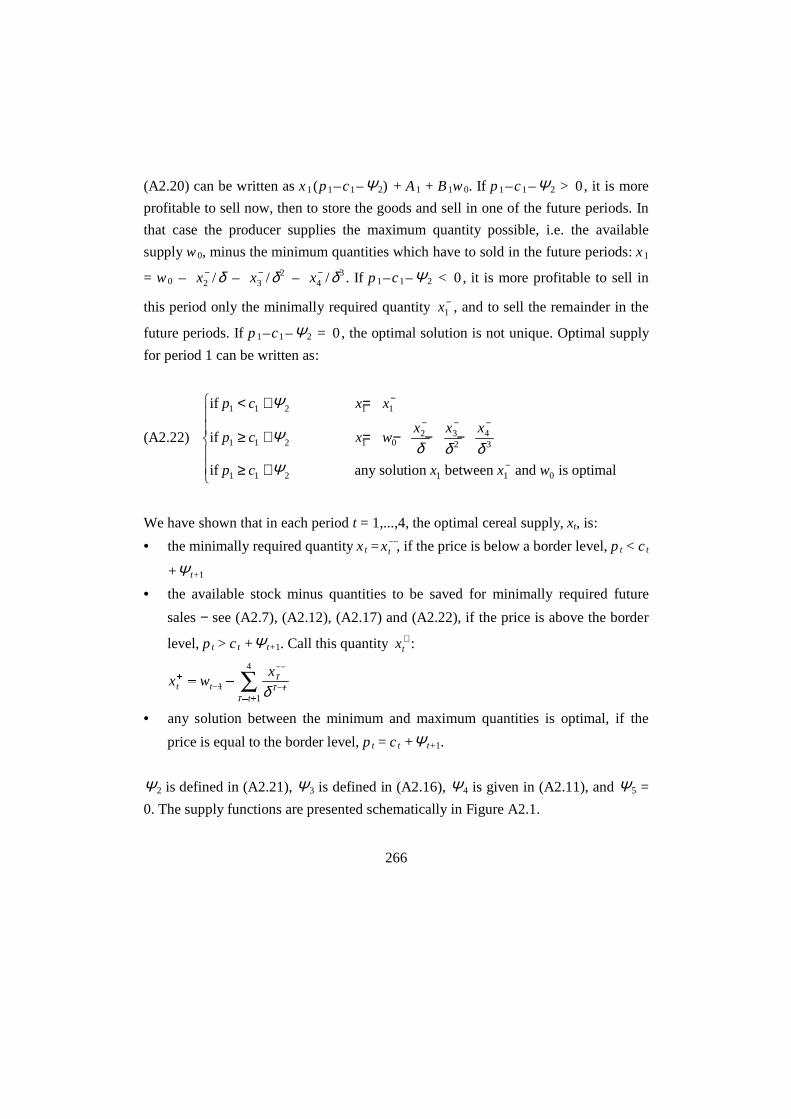
266

(A2.20) can be written as x1(p1–c1–Ψ2) + A1 + B1w0. If p1–c1–Ψ2 > 0, it is more

profitable to sell now, then to store the goods and sell in one of the future periods. In

that case the producer supplies the maximum quantity possible, i.e. the available

supply w0, minus the minimum quantities which have to sold in the future periods: x1

= w0 – x2− /δ – x3

− /δ2 – x4− /δ3. If p1–c1–Ψ2 < 0 , it is more profitable to sell in

this period only the minimally required quantity x1− , and to sell the remainder in the

future periods. If p1–c1–Ψ2 = 0 , the optimal solution is not unique. Optimal supply

for period 1 can be written as:

(A2.22)

if

if

if any solution between and is optimal

p c x x

p c x wx x x

p c x x w

1 1 2 1 1

1 1 2 1 02 3

243

1 1 2 1 1 0

< + =

≥ + = − − −

≥ +

%

&KK

'KK

−

− − −

−

Ψ

Ψ

Ψδ δ δ

We have shown that in each period t = 1,...,4, the optimal cereal supply, xt, is:

• the minimally required quantity xt =xt- , if the price is below a border level, pt < ct

+Ψ t+1

• the available stock minus quantities to be saved for minimally required future

sales − see (A2.7), (A2.12), (A2.17) and (A2.22), if the price is above the border

level, pt > ct +Ψ t+1. Call this quantity xt+ :

x wx

t t tt

+

-

-

-

= +

= - Ê11

4τ

ττ δ

• any solution between the minimum and maximum quantities is optimal, if the

price is equal to the border level, pt = ct +Ψ t+1.

Ψ2 is defined in (A2.21), Ψ3 is defined in (A2.16), Ψ4 is given in (A2.11), and Ψ5 =

0. The supply functions are presented schematically in Figure A2.1.

267

Figure A2.1: Schematic representation of the optimal supply for the periods 1, 2, 3

and 4.

pt < c t + Ψ t pt > c t + Ψt

Pricect +

xt+

xt−

Supply

268

Appendix 3: Parameter estimation

In Section 8.1 a survey is given of empirical evidence of cereal supply and demand,

both in terms of quantities and timing. This survey is based on a review of a number

of studies on cereal trade, supply and demand, which have been performed in Burkina

Faso in the past. The most important results of these studies will be discussed in this

Appendix. A comparison of the different studies is not given in this Appendix, but in

Section 8.1. Results of the studies are used in Section 9.1 and 9.2 to estimate the

parameters of cereal demand functions and of producer supply behaviour.

A3.1 Urban and rural population

In Section 8.1.1 the size of the urban and rural population is estimated for the year

2000. These estimates are used in Section 9.1 and 9.2 to estimate aggregate regional

demand and supply. Estimates of the urban and rural population are based on the

1985 and 1996 census (1995a,b, 1998). Based on these data, expected growth rates of

the urban and rural population can be calculated (see Table A3.1).

A remarkable observation is the annual growth of the urban population in Mouhoun

of 18.78%. The reason for this is that the demographic surveys define an area as

‘urban’ if it has a certain minimal socio-economic and administrative infrastructure

(administration services, schools, electricity, water), and if it houses more than 10,000

people (INSD, 1995a). In two of the three provinces in the CRPA Mouhoun

(Mouhoun and Kossi) no areas were characterised as ‘urban’ in 1985, which had

changed in 1996. Therefore, the urban population in these two provinces increased

from zero in 1985 to 68,394 in 1996, resulting in a yearly increase of 18.78% for the

entire CRPA. The same applies for the CRPA Centre Est, where the urban population

in the province of Kouritenga increases from zero in 1985 to 53,339 in 1996. Since it

is not realistic to assume that the yearly urbanisation rate continues to be that high,

these rates for the CRPA Mouhoun and Centre Est are supposed to be the same as the

Table A3.1 Urban and rural population in 1985 and 1996, and population growht rates.

Population1 Population 1996 Population 1985 annual growth 1985-19962

CRPA Total Urban Rural Total Urban Rural Total Urban Rural

Centre 1514048 709736 804312 959743 441514 518229 4.23% 4.41% 4.08%

Centre Nord 928321 51851 876470 729189 25814 703375 2.22% 6.55% 2.02%

Centre Ouest 989766 95024 894742 827419 51926 775493 1.64% 5.65% 1.31%

Centre Sud 530696 17146 513550 565227 14242 550985 -0.57% 1.70% -0.64%

Sahel 708332 23768 684564 521911 10956 510955 2.82% 7.29% 2.69%

Mouhoun 1146689 83612 1063077 889803 12588 877215 2.33% 18.78% 1.76%

Est 934275 42920 891355 682246 20857 661389 2.90% 6.78% 2.75%

Centre Est 772530 84805 687725 600722 23331 577391 2.31% 12.45% 1.60%

Nord 955420 86982 868438 760408 53057 707351 2.10% 4.60% 1.88%

Sud Ouest 518343 16424 501919 456375 10657 445718 1.16% 4.01% 1.09%

Hauts Bassins 988988 326352 662636 721695 228668 493027 2.91% 3.29% 2.72%

Comoe 325201 62548 262653 249967 35319 214648 2.42% 5.33% 1.85%

Total 10312609 1601168 8711441 7964705 928929 7035776 2.38% 5.07% 1.96%

1) INSD, 1995a,b, 1998, 2) Annual population growth (in %) = ((pop.1996/pop.1985)1/11-1)*100%

270

national average: 5.07%. For the other CRPA’s the growth rates are not exceptionally

high. For all CRPA’s it is supposed that the expected rural and urban growth rates

after 1996 remain the same as presented in Table A3.1. The expected urban, rural and

total population can now be estimated for the year 2000, see Table 8.1 in Section

8.1.1. These population figures are estimated as:

expected urban population 2000 = urban population 1996 * (1 + urban growth rate)4

expected rural population 2000 = rural population 1996 * (1 + rural growth rate)4

expected total population 2000 = urban population 2000 + rural population 2000.

A3.2 Cereal production

The annual cereal production per producer, is an important determinant of annual

cereal supplies. Annual cereal supply, estimated in Section 9.2, is based on forecasted

mean cereal production per producer. Production forecasts discussed in Section 8.1.2,

are based on production, cultivated area and yield data for all produced crops, which

are published each year by the ‘Direction des Statistiques Agro-Pastorales’ of the

Ministry of Agriculture and Animal Resources. Aggregating the production data of

millet, red sorghum, white sorghum and maize gives the total cereal production per

year, and the average cereal production for the period 1984-1998 (see Table A3.2).

The data presented in Table A3.2 to Table A3.5 and Figures A3.1 to A3.3 enable us

to make the following observations:

1. Production, cultivated area and yield levels show a clear trend. Regression

analysis shows that national production, cultivated area and yield levels increase

significantly with a linear trend (at the 99% significance level). Production

increases a bit faster than cultivated area, since this increase is caused by both

area expansion and yield improvement.

2. Production increases per CRPA between 1984 and 1998 were also significant at

the 95% level for most CRPA (except for Centre (significant at 80% level),

Centre Ouest (significant al 90% level), Centre Sud (significant at 80% level),

and ComoJ (significant at 70% level)).

271

3. Area increases were significant at the 95% significance level for the CRPA Sahel,

Centre Ouest, Mouhoun, Est, and Comoe, and at the 80% significance level for

the CRPA Nord and Hauts Bassins. Some of the area increases were rather

striking – see Table A3.3. Area increases in the CRPA Mouhoun may be logical

because of land reclamation programmes along the Volta Noire river. It is,

however, uncertain whether area increases as reported for the CRPA Sahel are

lasting. This region is not very suitable for agriculture, and it is therefore, risky to

suppose that the cultivated area continuous to increase as predicted by

extrapolation of the trend line. Also differences between years are large. In some

years acreage increases explosively, in other years, acreage decreases.

4. In 1991 average yields show a sharp increase (see Figure A3.1). Table A3.4

shows that compared to the period 1984-1990, the average cultivated area

between 1991-1998 was 15% higher, average yield was 28% higher and average

production even 48%. Although the pattern is the same for most CRPA, some

CRPA show on average a decreased cultivated area during the last seven years.

On the other hand, for example the CRPA Sahel shows an increased yield of 55%

and an increased production of even 100%. It is not realistic to assume that such

increases proceed for the years following this period. These high increases are

probably partly caused by favourable rainfall during those years – see Table A3.5.

Figure A3.1 also shows the trend lines if the period is cut in two: the period 1984-

1990 and the period 1991-1998. Yield levels and production in the second period

show a total different trend from the trend in the first period, they even slightly

decrease. However, because of the few observations, the trend lines are not

significant. Despite this, the figure shows that it is risky to assume that production

increases yearly as presented in the 1984-1998 trend line.

5. Comparing the yearly expansion (decrease) of cultivated area with the rural

population growth presented in Table A3.1 reveals that for some CRPA cultivated

area increases faster than rural population, whereas in most CRPA population

growth exceeds cultivated area growth (see Table A3.3). For the country as a

whole, acreage expansion is lower than rural population growth. This shows that

in total farmers cultivate less land per person every year.

272

6. Production, yield and acreage depend for a large part on rainfall. The tables and

figures show that production, yields and area cultivated were lower than average

in 1984, 1987, 1990 and 1997. These lower productions were mainly caused by

low rainfall. Rainfall data of the National Meteorological Institute of Burkina

Faso show that the 1984-’98 average yearly rainfall was 711 mm, while only 531

mm of rain fell in 1984, 601 mm in 1987, 577 mm in 1990, and 663 mm of rain

fell in 1997 (see table Table A3.5; see also figure A3.3). Linear regression

analysis shows that production, yield and acreage depend significantly (at 99%

significance level) on rainfall. This dependence is, however, not clear for all

years. For example for the years 1992 and 1993 rainfall decreases with 13%

compared to 1991, which is not reflected in lower cereal production. Production

even increases slightly in 1992 and 1993. Regression results show that production

forecasts depend for 58% on rainfall (R2 = .58), yield for 47% and the area

cultivated for 51%. Rainfall data per CRPA (aggregates for the rainfall stations in

each CRPA) did not demonstrate the same dependance of production, yield and

acreage on rainfall for all CRPA. Rainfall had a significant influence (90%

significance level) on production in the CRPA Centre Nord, Centre Sud, Sahel,

Mouhoun, Est and Nord, on cultivated area in the CRPA Sahel, Mouhoun, Centre

Est, Est and Nord, and on yield in the CRPA Centre Nord, Centre Ouest, Centre

Sud, Sahel, Est and Nord.

Table A3.2 Area cultivated with cereals (ha/year), cereal production (tonnes/year), and average cereal yields

(kg/ha/year) for each CRPA.Production 1984 1985 1986 1987 1988 1989 1990 1991 1992 1993 1994 1995 1996 1997 1998

CentreArea 197910 171575 186629 109727 196623 258140 197000 189000 196300 196346 203580 177638 181580 201529 216342

production 64227 113791 126353 46576 134871 170745 110700 163300 158900 156542 120157 146922 128927 83912 160239

average yield1 325 663 677 424 686 661 562 864 809 797 590 827 710 416 741

Centre NordArea 241556 247012 293209 250032 303680 317519 217000 201000 235600 293113 319035 250013 249264 268876 279946

production 88709 122436 158125 81666 216879 135118 107000 164900 205000 186034 201992 180514 168645 109013 231723

average yield 367 496 539 327 714 426 493 820 870 635 633 722 677 405 828

Centre OuestArea 184065 236443 274106 289740 298990 302641 320800 297600 293100 332888 365908 287705 286859 286501 303941

production 102276 165127 176629 161211 229037 211612 165000 218400 131400 289408 269952 208404 228080 171668 208200

average yield 556 698 644 556 766 699 514 734 448 869 738 724 795 599 685

Centre SudArea 168363 177319 199505 199758 193088 93791 179200 212500 207000 187150 201275 172568 162901 175038 195904

production 91075 136229 150079 112041 122314 71166 88000 203100 196100 169555 124066 145579 157873 137504 166518

average yield 541 768 752 561 633 759 491 956 947 906 616 844 969 786 850

SahelArea 132367 200741 201440 145095 221519 298341 252000 268100 279200 286515 335981 252926 236564 236357 248207

production 56084 62621 63830 46251 113210 109522 94100 182700 195200 155680 213183 119872 105453 93309 184133

average yield 424 312 317 319 511 367 373 681 699 543 635 474 446 395 742

Cont. Table A3.2

Production 1984 1985 1986 1987 1988 1989 1990 1991 1992 1993 1994 1995 1996 1997 1998

Mouhoun

Area 221322 270455 301380 327242 382496 388122 401000 478600 461500 480789 478129 419625 436827 502234 493242

production 172066 216453 253977 200907 297373 304094 244000 424600 456300 449722 379118 357454 464081 332820 393798

average yield 777 800 843 614 777 784 608 887 989 935 793 852 1062 663 798

Est

Area 112047 194010 287390 267065 258562 257720 234000 276300 290700 311383 297152 312205 301974 301368 321799

production 77122 156138 226559 190170 198380 205413 149000 185200 216700 291796 263146 309639 285466 227489 318286

average yield 688 805 788 712 767 797 637 670 745 937 886 992 945 755 989

Centre Est

area 143249 186338 190902 173044 218308 196549 62400 158800 168000 191673 197216 171353 188411 196424 183742

production 82965 126763 110108 114303 124823 153761 26300 119800 145300 188715 158743 202476 200341 141676 167278

Average yield 579 680 577 661 572 782 421 754 865 985 805 1182 1063 721 910

Nord

area 139253 216939 156830 246040 275414 249011 214000 261700 271500 248850 243104 194625 227721 209791 268843

Production 72333 109694 90073 101005 190761 118703 63300 195500 160200 146924 169412 108319 176608 99046 230854

Average yield 519 506 574 411 693 477 296 747 590 590 697 557 776 472 859

Sud Ouest

area 154069 150350 158814 195417 185626 188983 208000 192000 231000 173517 182467 175146 145803 160009 168165

Production 90083 109100 115504 114633 93696 112213 166000 173000 219000 160377 171893 156814 148596 162058 174906

Average yield 585 726 727 587 505 594 798 901 948 924 942 895 1019 1013 1040

Cont. Table A3.2Hauts Bassins

area 132437 141810 162370 178081 204413 227631 143000 156700 141800 202248 197391 187528 179121 190709 187208

Production 129248 143151 161915 172411 216960 235090 178000 254000 255800 203166 255428 218029 223040 275159 244848

Average yield 976 1009 997 968 1061 1033 1245 1621 1804 1005 1294 1163 1245 1443 1308

Comoe

area 69205 67812 66295 74266 75007 81863 58000 65000 82400 62271 57810 49500 49058 52851 56119

Production 67183 72821 64021 67661 74356 69960 66000 94000 77000 82536 87080 58331 72049 79630 72550

Average yield 971 1074 966 911 991 855 1138 1446 934 1325 1506 1178 1469 1507 1293

Total

Area 1895843 2260804 2478870 2455507 2813726 2860311 2486400 2757300 2858100 2966743 3079048 2650832 2646083 2781687 2923458

Production 1093371 1534324 1697173 1408835 2012660 1897397 1457400 2378500 2416900 2480455 2414170 2212353 2359159 1913284 2553333

Average yield 577 679 685 574 715 663 586 863 846 836 784 835 892 688 873

Notes: 1) Average yield levels are estimated by dividing total cereal production by total cultivated area. The ministry of agriculture estimatesregional production by multiplying estimated yield (the average of a sample of measured yield levels) by estimated acreage for each crop.However, we consider here aggregate cereal production and acreage. These are estimated by adding up the production levels and cultivatedareas of the different crops and provinces in a CRPA. Consequently, average ‘cereals’ yield levels can not be estimated on the basis of reportedyield levels for each crop, but have to be based on total cereal production and total cultivated acreage.Source: MinistPre de l’agriculture et de l’Jlevage, 1984-1999.

276

Table A3.3 Average yearly growth of cultivated area between 1984 and 1998 andaverage yearly growth of the rural population.Growth of

cultivated

area1

Growth of rural

population2

Growth of

cultivated

area1

Growth of rural

population2

Centre 0.79% 4.08% Centre Est 0.68% 1.60%

Centre Nord 0.25% 2.02% Nord 1.44% 1.88%

Centre Ouest 1.66% 1.31% Sud Ouest -0.01% 1.09%

Centre Sud 0.23% -0.64% Hauts Bassins 1.39% 2.72%

Sahel 2.83% 2.69% Comoe -2.23% 1.85%

Mouhoun 4.25% 1.76% Total 1.69% 1.96%

Est 3.41% 2.75%

Notes: 1) Based on a regression of yearly cultivated area as a function of time, see Table A3.2 for dataon cultivated area per CRPA. Growth of cultivated area = (predicted surface 1998/predicted surface1984)1/15 - 1; 2) Presented in Table A3.1.

Table A3.4 Average cultivated area (ha), production (tonnes) and yield (kg/ha) forthe periods 1984-1990 and 1991-1998, and the percentage increaseAverage

84-90Average

90-98%

increaseAverage

84-90Average

90-98%

increaseCentre Centre Est

Area 188229 195289 3.75% Area 167256 181952 8.79%production 109609 139862 27.60% production 105575 165541 56.80%

average yield 582 716 22.99% average yield 631 910 44.13%Centre Nord Nord

Area 267144 262106 -1.89% Area 213927 240767 12.55%production 129990 180978 39.22% production 106553 160858 50.97%

average yield 487 690 41.90% average yield 498 668 34.14%Centre Ouest Sud Ouest 0 0 0.00%

Area 272398 306813 12.63% Area 177323 178513 0.67%production 172985 215689 24.69% production 114461 170830 49.25%

average yield 635 703 10.70% average yield 645 957 48.25%Centre Sud Hauts Bassins

Area 173003 189292 9.42% Area 169963 180338 6.10%production 110129 162537 47.59% production 176682 241184 36.51%

average yield 637 859 34.89% average yield 1040 1337 28.65%Sahel Comoe

Area 207358 267981 29.24% Area 70350 59376 -15.60%Production 77945 156191 100.39% production 68857 77897 13.13%

average yield 376 583 55.05% average yield 979 1312 34.04%Mouhoun Total

Area 327431 468868 43.20% Area 2464494 2832906 14.95%production 241267 407237 68.79% production 1585880 2341019 47.62%

average yield 737 869 17.87% average yield 643 826 28.42%Est 0 0 0.00%

Area 230113 301610 31.07%production 171826 262215 52.61%

average yield 747 869 16.43%

277

Table A3.5 Average yearly rainfall (in mm) and national cereal production (in

1000 tonnes) from 1984 to 1998.Average annual rainfall per CRPA1

CRPA Centre Centre

Nord

Centre

Ouest

Centre

Sud

Sahel Mou-

houn

Est Centre

Est

Nord Hauts

Bassins

Average

rainfall

Burkina

Faso

Annual

cereal

prod.

Year (a) (b) (c) (d) (e) (f) (g) (h) (i) (j) (k) (l)

1984 511 473 602 622 301 676 522 532 443 789 531 1093

1985 617 437 764 764 345 782 534 628 501 1167 624 1534

1986 732 565 1021 1029 297 826 623 750 557 871 685 1697

1987 664 529 725 874 278 725 580 709 447 778 601 1409

1988 713 740 705 764 399 751 746 853 651 1060 713 2013

1989 658 579 772 1061 429 686 607 891 713 809 698 1897

1990 639 508 656 658 359 626 603 615 423 819 577 1457

1991 658 745 1037 1120 574 908 685 822 807 947 859 2379

1992 615 581 643 826 407 726 622 768 685 1028 697 2417

1993 715 587 776 962 266 823 658 592 548 793 668 2480

1994 718 588 760 826 543 1131 648 721 592 897 992 2414

1995 700 695 756 924 396 716 764 717 660 1278 779 2212

1996 677 558 826 1153 333 872 702 753 708 901 772 2359

1997 588 527 633 864 414 913 595 659 371 853 663 1913

1998 668 710 722 1068 594 990 830 803 782 1123 809 2553

Aver.2 658 588 760 901 396 810 648 721 592 941 711 1989

Notes: 1) Data are missing for the CRPA Sud Ouest and Comoe; 2) Average rainfall (column (a) – (k))and average production (column (l)) for the period 1984 - 1998. a) – j) Averages of annual rainfall datafor the following stations: a) Ouagadougou; b) Bam, Kaya; c) Koudougou, Leo; d) Po; e) Djibo, Dori,Arabinda; f) Boromo, Dedougou; g) Bogande, Diapaga, Fada N’Gourma, Kantchari; h)Tenkodogo,Zabre, Koupela; i) Ouahigouya, Yako; j) Hounde, Bobo Dioulasso. k) Average rainfall for Burkina Fasois the average over all stations. l) Annual cereal production is given in Table A3.2.Source: MJtJo: National Meteorological Institute of Burkina Faso.

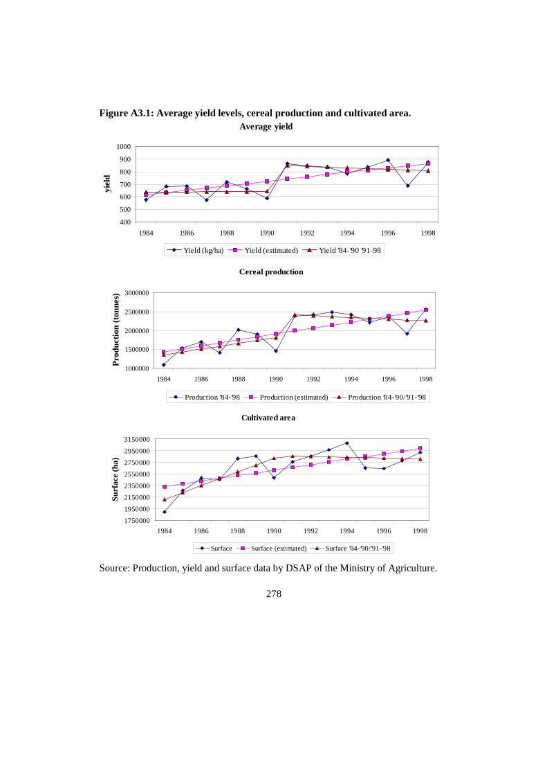
278

Figure A3.1: Average yield levels, cereal production and cultivated area.Average yield

400

500

600

700

800

900

1000

1984 1986 1988 1990 1992 1994 1996 1998

yiel

d

Yield (kg/ha) Yield (estimated) Yield ’84-’90 ’91-98

Cereal production

1000000

1500000

2000000

2500000

3000000

1984 1986 1988 1990 1992 1994 1996 1998

Pro

duct

ion

(ton

nes)

Production ’84-’98 Production (estimated) Production ’84-’90/’91-’98

Cultivated area

1750000

1950000

2150000

2350000

2550000

2750000

2950000

3150000

1984 1986 1988 1990 1992 1994 1996 1998

Sur

face

(ha

)

Surface Surface (estimated) Surface ’84-’90/’91-’98

Source: Production, yield and surface data by DSAP of the Ministry of Agriculture.

279

Figure A3.2a: Average yield levels for each CRPA.Yield per CRPA

300

500

700

900

1100

1984 1986 1988 1990 1992 1994 1996 1998

Yie

ld (

kg/h

a)

Centre Centre Nord Centre Ouest Centre Sud

300

500

700

900

1100

1984 1986 1988 1990 1992 1994 1996 1998

Yie

ld (

kg/h

a)

Sahel Mouhoun Est Centre Est

250

450

650

850

1050

1250

1450

1650

1850

1984 1986 1988 1990 1992 1994 1996 1998

Yie

ld (

kg/h

a)

Nord Sud Ouest Hauts Bassins "Comoe"

280

Figure A3.2b: Cereal production levels per CRPACereal production per CRPA

0

100000

200000

300000

1984 1986 1988 1990 1992 1994 1996 1998

Pro

duct

ion

(ton

nes)

Centre Centre Nord Centre Ouest Centre Sud

0

100000

200000

300000

400000

500000

1984 1986 1988 1990 1992 1994 1996 1998

Pro

duct

ion

(ton

nes)

Sahel Mouhoun Est Centre Est

0

100000

200000

300000

1984 1986 1988 1990 1992 1994 1996 1998

Pro

duct

ion

(ton

nes)

Nord Sud Ouest Hauts Bassins Comoe

281

Figure A3.2c: Cultivated area per CRPA

Cultivated area per CRPA

50000

150000

250000

350000

1984 1986 1988 1990 1992 1994 1996 1998

Sur

face

(ha

)

Centre Centre Nord Centre Ouest Centre Sud

50000

150000

250000

350000

450000

550000

1984 1986 1988 1990 1992 1994 1996 1998

Sur

face

(ha

)

Sahel Mouhoun Est Centre Est

0

50000

100000

150000

200000

250000

300000

1984 1986 1988 1990 1992 1994 1996 1998

Sur

face

(ha

)

Nord Sud Ouest Hauts Bassins Comoe

282

Figure A3.3: Production, yield and acreage as a function of rainfall

Rainfall Burkina Faso (mm)

450

650

850

1050

1984 1986 1988 1990 1992 1994 1996 1998

Rai

nfal

l (m

m)

Rainfall Burkina Faso (mm)

1000000

1500000

2000000

2500000

3000000

3500000

500 550 600 650 700 750 800 850 900

Rainfall (mm)

Pro

duct

ion

(ton

nes)

Production Surface Production (trendline) Surface (trendline)

500

600

700

800

900

500 550 600 650 700 750 800 850 900Rainfall (mm)

Yie

ld (

kg/h

a)

yield Yield (linear trend) Yield (Polynomal trend)

Source: Rainfall data by MJtJo, meteorological institute of Burkina Faso. Production,

surface and yield data by DSAP of the Minstry of Agriculture and Animal Resources.

283

A3.3 Sales

In Section 8.1.3 factors influencing annual cereal sales and distribution of cereal sales

over the year have been discussed. This discussion is based on a number of surveys

performed in the past in Burkina Faso on cereal sales behaviour of households, which

will be discussed below. The data presented are used in Section 9.2 to analyse

producer supply behaviour.

Surveys by the Universities of Michigan and Wisconsin

The Universities of Michigan and Wisconsin executed in the unfavourable rainfall

season 1983-‘84 a survey on the dynamics of grain marketing in Burkina Faso. Part of

this survey concentrated on producer behaviour. In five villages across three

ecological zones (the first five villages in Table A3.6) 224 households were sampled.

Results of a study by SAFGRAD and Purdue University in the same year among 102

households in four villages were also used. Szarleta (1987) and Sherman et al. (1987)

report on cereal sales in these nine villages (see Table A3.6). The difference between

deficit and surplus villages is clear. In general, households in surplus villages sell a

larger quantity of cereals and a larger part of their cereal harvest. Also the number of

households selling cereals is larger in surplus villages than in deficit villages. Figures

would be different in a normal rainfall year, but the pattern would probably remain

similar.

ICRISAT surveys

ICRISAT carried out extensive farming systems studies in six villages in Burkina

Faso from 1981 to 1985. They weekly surveyed 150 households from two villages in

the province of Soum (WourJ and Silgey; average household size 10.2 people) in the

north of Burkina Faso, two villages in the centre in the province of PassorJ (Ouonon

and Kolbila; average household size 12.2 persons) and two villages in the south-west

in the province of Mouhoun (Sayero and Koho; average household size 12 people).

Based on food production they classified households as surplus or shortage

household. Shortage households were those which had a food production with a calo-

284

Table A3.6 Average cereal sales per household in different regions in the season

1983-84, reported by Szarleta (1987) and Sherman et al. (1987).Province Village1 Households

selling

cereals2

(a)

Sales as

% of total

harvest

(b)

Average cereal

sales per selling

household (kg)

(c)

Average sales

per sample

household (kg)

(d)

Average sales per

sample household

per AE (kg)3

(e)

Yatenga

PassorJ

Sourou

Mouhoun

Houet

Kossi

Oubritenga

Zoundweogo

Gourma

MenP (D)

BougourJ (D)

Tissi(S/D)

Dankui (S/D)

BarJ (S)

Dissankuy (S)

NJdogo (S)

PoJdogo (S)

Diapangou (S)

7 (46)

6 (42)

24 (40)

3 (42)

47 (50)

13 (27)

28 (29)

18 (21)

22 (25)

3.1%

0.9%

9.6%

2.7%

22.1%

14.8%

20.7%

24.9%

21.3%

168

13

85

169

638

374

287

489

444

26

2

51

12

600

180

277

117

391

4.64

0.3

8.4

2.5

84.1

39.5

42.1

71.4

71.5

Notes: 1) S = village with a surplus during the survey period, D = village in deficit during the surveyperiod, S/D = village with a production which is more or less equal to the cereal consumptionrequirements of the village; 2) The total number of sample households between brackets; 3) Data for thefirst 5 villages are given in Consumer Equivalents (CE), and in Adult Equivalents (AE) for the last 4villages. CE and AE are used to convert the lower consumption requirements and labour productivity ofwomen and children in male consumption requirements and labour productivity units; (b) = total samplesales / total sample harvest; (c) = total sample sales / (a); (d) = total sample sales / total samplehouseholds; (e) = (d) / average household size in AE.Source: Szarleta (1987), Sherman et al. (1987), Pardy (1987).

ric value below 80% of the WHO average yearly caloric requirement (requirements

are 2,850 Kcal per adult equivalent; Reardon et al., 1988a). Reardon et al (1987)

report on cereal sales per adult equivalent. These data do not exhibit a clear pattern

between the regions. Sales by surplus households surpass sales of deficient

households, though this difference is small in the province of PassorJ. It has to be

noted that the survey period comprised a period of severe drought with lower than

usual production. This may cause the low production in the province of Mouhoun,

and the abnormal feature that production in Soum exceeds production in the other,

more fertile provinces. The sales pattern may not be representative for an average

rainfall year.

285

Table A3.7 Cereals sales and production per adult equivalent between 1981-1985,

by Reardon et al. (1987)Soum

(shortage region)

PassorJ

(shortage region)

Mouhoun

(equilibrium region)

Province

Deficient

household

Surplus

household

Deficient

household

Surplus

household

Deficient

household

Surplus

household

Sales (kg) 3.27 15.2 6.8 8.6 6.7 19.0

Production (kg) 109 303 85 216 112 272

Sales (as % of

production)

3% 5% 8% 4% 6% 7%

Source: Reardon et al. (1987)

Survey by J.T.Broekhuyse

Broekhuyse (1983, 1988, 1998) reports for 20 households in two villages in the

province of Sanmatenga (Koalma and BasberikP) the sales by households applying

manual labour (ML) or households using animal traction (AT) between 1979 and

1985. The average household size was 7.3 for ML housholds, and 10.2 people for AT

households. He observes that on average ML households sell only 25.2 kg of cereals

(3.8% of cereal production), and that AT households sell 58,5 kg of cereals (3.3% of

cereal production).

Survey by O. Pieroni

Pieroni (1990) executed, under the authority of CILSS, a study of the behaviour of

cereal producers. They interviewed between august 1986 and october 1987 114

households in 15 villages in the provinces of Houet (2 villages), ComoJ (3 villages),

KJnJdougou (1 village), Kossi (3 villages), Sissili (3 villages) and Boulgou (3

villages). Rainfall in the 1986-’87 production season had been normal (see Table

A3.5). He reports that in these villages 56.6% of the households sell more than 300

kg. He clearly observes a positive relation between production and the degree of

market participation (see Table A3.8 and Table A3.9). In the survey year, the villages

in ComoJ have a shortage, and the villages in Sissili are either just in equilibrium or

have a shortage. These villages lodge only a few households selling large quantities

of cereals. In Sissili, households selling more than 1000 kg are absent. On the other

286

hand, the villages in Houet, KJnJdougou and Boulgou have a surplus and most

households sell large quantities on the market. Hardly any household sells less than

100 kg. The province of Kossi holds an intermediate position, with two surplus

villages and one shortage village. In both the shortage and surplus villages in this

province, the number of households selling large quantities almost equals the

households selling little (see Table A3.9).

The provinces of Houet, KJnJdougou and Kossi are the cotton areas of the country,

where the use of modern agricultural techniques is widespread. Despite the fact that

much land and labour is allocated to cotton production, also cereal production is

generally higher than in the other regions of the country. In ComoJ sugar cane is

produced on plantations using the most fertile soil and employing many of the young

labourers. Cultivation of cereals is often not the main source of income, and is for a

large part done by women and older farmers, without the use of modern techniques.

In the provinces of Sissili and Boulgou modern agricultural techniques are not

widespread, but soil fertility and rainfall are suitable. Trade conditions are also pretty

favourable because of the presence of the Ghanian border. Pieroni clearly shows that

sales are highly correlated with production. Although it does not apply for all

households, it can be said that the more cereals a household produces, the more it

sells. Those households are most of the time the larger households cultivating more

land with more people. Other factors influencing household sales are capital needs,

social relations (household composition and ethnic lineage) and the regional

importance of the market (whether it is only a small local market or whether it is a

larger market on which more products are traded).

287

Table A3.8 Cereal sales for some villages in 1986-87, by Pieroni (1990).Villages/province1 N2 Average

household

size3

(a)

Cultivated

area per

household (ha)

(b)

Production

per household

(kg)

(c)

Sales per

household

(kg)

(d)

Sales per

person

(kg)

(e)

Sales as %

of

production

(f)

ZabrJ (S) 8 22.0 6.10 6340 2598 118.1 41.0%

Hono-bissa (S/D) 8 12.9 4.03 2488 1036 80.5 41.6%

Yoroko (S) 8 7.8 4.96 2660 1078 139.1 40.5%

Boulgou 24 14.2 5.03 3829 1571 110.6 41.0%

Fara Sissili (D) 8 15.8 3.42 2470 138 8.7 5.6%

Nabou (S/D) 8 15.3 4.87 2752 221 14.5 8.0%

Ton (S/D) 8 10.5 4.14 2060 232 22.1 11.3%

Sissili 24 13.8 4.14 2427 197 14.2 8.1%

Solenzo (S) 8 11.4 4.09 3139 1118 98.3 35.6%

KiJ (D) 7 12.4 2.82 1936 541 43.5 28.0%

LJkoro (S) 6 10.8 7.56 3846 626 57.8 16.3%

Kossi 21 11.6 4.66 2940 785 67.9 26.7%

DandJ (S) 8 20.0 11.17 5148 1606 80.3 31.2%

Fara KJnJdougou (S) 8 10.9 5.69 2994 1358 124.9 45.4%

KouJrJdJni (S) 7 10.7 6.53 4443 2548 237.8 57.3%

Houet/KJnJdougou 23 14.0 7.85 4184 1806 129.0 43.2%

SiniJna (D) 8 8.4 1.89 1127 155 18.5 13.7%

Diarabakoko (D) 7 13.6 3.88 1263 131 9.6 10.4%

Tangora (D) 7 13.0 2.71 1386 481 37.0 34.7%

ComoJ 22 11.5 2.78 1253 251 21.8 20.0%

Note: 1) S = village in surplus during the survey period, D = village in deficit during the survey period,S/D = village with a production which is more or less equal to the cereal consumption requirements ofthe village; 2) The number of sample households in the sample villages; 3) Average number ofhousehold members. (e) = (d)/(a), (f) = (d)/(c)*100%. Source: Pieroni (1990).

Survey by E.P. Yonli

Yonli (1997) executed a survey from October 1991 to June 1993 in 4 villages in

Yatenga (24 households; on average 14.6 people per household) and 4 villages in

Sanmatenga (21 households; on average 11.1 people per household), see Table A3.10.

In the 1991 agricultural season, rainfall was far above the 1970-’93 average in both

provinces.34 Production in the CRPA in which the villages are situated was above

34 Yatenga: average rainfall: 550 mm, 1991 rainfall: 680 mm; Sanmatenga: average rainfall: 617 mm,1991 rainfall: 821 mm. Data from National Meteorological Institute of Burkina Faso.

288

Table A3.9 Number of households (in %) selling less than 100 kg, between 100 kg

and 1000 kg, or more than 1000 kg of cereals, for some villages in

1986-87, by Pieroni (1990).

Villages/Provinces1) N2) < 100 kg 100-1000 kg > 1000 kg

Zabre (S) 8 12.5% 25.0% 62.5%

Hono-bissa (S/D) 8 0.0% 50.0% 50.0%

Yoroko (S) 8 0.0% 62.5% 37.5%

Boulgou 24 4.2% 45.8% 50.0%

Fara Sissili (D) 8 62.5% 37.5% 0.0%

Nabou (S/D) 7 42.9% 57.1% 0.0%

Ton (S/D) 8 37.5% 62.5% 0.0%

Sissili 23 47.8% 52.2% 0.0%

Solenzo (S) 8 50.0% 25.0% 25.0%

Kie (D) 7 28.6% 42.9% 28.6%

Lekoro (S) 6 33.3% 33.3% 33.3%

Kossi 21 38.1% 33.3% 28.6%

Dande (S) 8 0.0% 50.0% 50.0%

Fara Kenedougou (S) 8 0.0% 50.0% 50.0%

Koueredeni (S) 7 0.0% 0.0% 100.0%

Houet/Kenedougou 23 0.0% 34.8% 65.2%

Siniena (D) 8 50.0% 50.0% 0.0%

Diarabakoko (D) 7 71.4% 28.6% 0.0%

Tangora (D) 7 57.1% 14.3% 28.6%

Comoe 22 59.1% 31.8% 9.1%

Total 29.2% 39.8% 31.0%

Note: 1) See not 1 in Table A3.8; 2) Number of households in the sample. Source: Pieroni (1990).

average in both the ‘91-’92 and ‘92-’93 season, but nevertheless, both regions knew a

shortage production, or were almost in equilibrium (see Table A3.2). For the sample

villages, only the village of Noungou had a surplus production. It is remarkable to see

that this is also the village with the smallest average household size. Both provinces

produced mainly sorghum (Yatenga 61.7% and Sanmatenga 89.2% sorghum as

percentage of cereal production). In the village of Noungou even 94.8% of cereal

production consisted of sorghum. The data clearly show that, although a very small

part of production was sold, sales were higher in the higher production province. The

289

data per village show the same pattern. The differences between the villages are large,

but even within a village differences are considerable. The standard deviation of the

sold quantity was for most villages larger than the average sales.

Table A3.10 Cereal sales in some villages in Yatenga and Sanmatenga from

October 1991 to September 1992, by Yonli (1997).

Villages/

Provinces1Number of

households

Average

household size

(a)

Average sales per

household (kg)

(b)

Sales per

person (kg)

(c)

Production per

person (kg)

(d)

Ramsa 3 14.3 5.0 0.35 128.9

SJguJnJga 7 14.7 0.0 0.00 131

Kalsaka 7 15.6 0.0 0.00 111.0

Kossouka 7 13.4 3.2 0.24 132.4

Yatenga 24 14.6 1.6 0.11 125.3

Nessemtenga 1 12.0 0.0 0.00 n.a.2

Soubeira 5 14.2 26.8 1.89 172.6

Noungou 8 8.8 79.2 9.00 234.6

SinguJ 7 11.3 46.2 4.09 132.1

Sanmatenga 21 11.1 57.6 5.24 179.7

Notes: 1) The first four villages are in Yatenga, the last four villages are in Sanmatenga. (c) = (b)/(a). 2)n.a.: not available. Source: Yonli (1997)

Seasonal sales pattern

Some authors also report on the sales per season. Most authors observe, what has

become a general characteristic of African agriculture, that farmers sell in the post-

harvest, low-price season and buy in the pre-harvest, high-price season.

Surveys by Universities of Michigan and Wisconsin

The seasonal sales pattern is also observed by Sherman et al. (1987). Table A3.11

“reveals that the postharvest quarter is indeed the heaviest sales period for the largest

number of households” (Ellsworth and Shapiro, 1989). On the other hand, the sales

volume is more evenly distributed than is often thought. This indicates that many

households have to sell small quantities immediately following the harvest. A smaller

number of farmers can sell larger quantities later in the year. The sales pattern per

290

village shows that especially in BarJ, where by far the largest volume is sold (see

Table A3.6), most households sell in the two post-harvest quarters from October to

March. It has to be noted that cereal sales are only a part of the total amount of cereals

that leave the farm. The quantity of cereals given to others via non-market transfers

may be more than the amount sold. These gifts are often payments for agricultural

work, and therefore a veiled form of sales (Ellsworth and Shapiro, 1989).

Table A3.11 Total cereal sales per quarter for five Burkina Faso villages in 1984, by

Sherman et al. (1987).

Periods Jan-Mar Apr-June July-Oct 10 Oct 11-Dec Total number of

selling

households3

Sales (kg)1 9,520 (33%) 4,885 (17%) 6,347 (22%) 7,811 (27%)

Number of households2

MenJ (Yatenga) 2 0 3 0 5 (46)

BougourJ (PassorJ) 0 0 0 1 1 (42)

Tissi (Sourou) 1 1 1 9 12 (40)

Dankui (Mouhoun) 2 0 0 1 3 (42)

BarJ (Houet) 16 4 4 23 47 (50)

Total 21 5 8 34 68 (220)

Notes: 1) Percent of annual total between brackets; 2) The data give the number of households in fivevillages with their largest volume of sales in a certain quarter. Only those households are considered whosold more than 25 kg; 3) Number of sample households between brackets. Source: Sherman et al (1987)

Pardy (1987) confirms the phenomenon of post-harvest sales, based on an analysis of

the seasonal sales for the four surplus villages surveyed by SAFGRAD (see page

A.284). He divides the year in four seasons: the harvest season from October to

December, the dry season from January to March, the hot season from April to June

and the rainy season from July to September. His data show that for three of the four

villages sales were largest and most households were selling during the dry season

(see Table A3.12). However, for two villages the largest sales per household are made

during the rainy season when the prices are more favourable. Only in the village of

PoJdogo most cereals are sold during the harvest season. The large sales volume

during the dry season in Dissankuy, which is in a cotton producing area, is striking.

291

These sales may be due to late payments of cotton sales, which compels households

to earn money from other sources, for example cereal sales.

Table A3.12 Cereal sales per trimester for four villages from October 1983 to

September 1984.Oct. – Dec. Jan. – March April - June July - Sept. Yearly total

Dissankuy(Kossi)

41

7902

16.3%3

1984

91,64033.8%

182

6830

17.1%138

91,59932.9%

178

284,859100%174

NJdogo(Oubritenga)

201,74921.8%

88

273,21640.0%

119

181,42017.7%

79

101,64820.5%

165

758,033100%107

PoJdogo(Zound-weogo)

174,20447.8%247

152,09123.8%

139

11868

9.9%79

71,63618.6%

234

508,799100%176

Diapangou(Gourma)

71,02410.5%146

205,19653.2%

260

5845

8.7%169

72,70027.7%

386

399,765100%250

Notes: 1) Number of households selling during that period; 2) total sales in kg; 3) percentage of yearlytotal; 4) sales per selling household in kg. Source: Pardy (1987).

Pardy also looks at sales differences between households of different wealth (see

Table A3.13). He identifies very poor, poor, average and wealthy households on the

basis of the total value of their livestock in December 1983 and their agricultural

equipment in 1984. These posessions indicate the possibility to use other sources to

face cash needs. The majority of households sells during the dry season. The number

of households selling during the harvest season is also very large for all types of

households, except the weatlhy. From those households which profit from the higher

prices during the July – September period, most have an average wealth. They also

have the largest sales per household. Of all households selling between April and

June, the wealthy households sell the largest quantity. For all wealth groups, except

the very poor, at least 30% of the households which sell during the year, also sell

during the rainy season between July and September. Pardy notes that the richer

households sell in less periods. 56% of the poor households sells in three periods,

292

compared to 46% of the average and 38% of the wealthy households. This strategy

corresponds to the need to sell cereals to satisfy capital requirements for the poor

households.

Table A3.13 Cereal sales per trimester four different different types of households,

for four villages from October 1983 to September 1984.

Wealth Oct. – Dec. Jan. - March April - June July- Sept. Yearly total

Very poor 81

4482

20.9%3

564

131,20656.2%

93

485

4.0%21

4408

19.0%102

2,147100%

74Poor 18

3,89639.6%

216

212,96230.1%

141

161,22412.4%

77

91,76918.0%

197

9,854100%154

Average 172,15020.0%

126

213,58333.3%

171

121,0089.4%84

144,01437.3%

287

10,755100%168

Wealthy 51,27314.6%

255

164,39250.5%

275

81,64618.9%

206

61,39216.0%

232

8,703100%248.7

Notes: 1) Number of households selling during that period; 2) total sales in kg; 3) percentage of yearlytotal; 4) sales per selling household in kg. Source: Pardy (1987).

ICRISAT surveys

Reardon et al (1987) also report on seasonal sales patterns for the period harvest 1981

to rainy season 1985 (see Table A3.14). Their data do not exhibit evidence of ‘forced

sales’. It does not show up that deficient households sell in the post-harvest period,

and surplus households sell whenever prices are higher. It only follows, which was

already reported in Table A3.7, that surplus households sell more than deficient

households. The data in this table do not demonstrate a clear relation between

production and sales. It has to be noted, however, that sales patterns during the survey

years may have been different from normal because of the bad rainfall during these

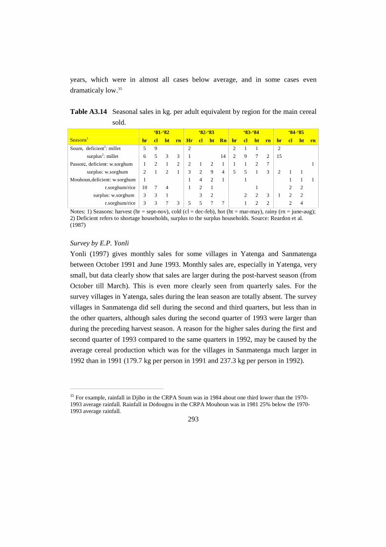
293

years, which were in almost all cases below average, and in some cases even

dramaticaly low.35

Table A3.14 Seasonal sales in kg. per adult equivalent by region for the main cereal

sold.‘81-‘82 ‘82-‘83 ‘83-‘84 ‘84-‘85

Seasons1 hr cl ht rn Hr cl ht Rn hr cl ht rn hr cl ht rn

Soum, deficient2: millet 5 9 2 2 1 1 2

surplus2: millet 6 5 3 3 1 14 2 9 7 2 15

PassorJ, deficient: w.sorghum 1 2 1 2 2 1 2 1 1 1 2 7 1

surplus: w.sorghum 2 1 2 1 3 2 9 4 5 5 1 3 2 1 1

Mouhoun,deficient: w.sorghum

r.sorghum/rice

1

10 7 4

1

1

4

2

2

1

1 1

1

1

2

1

2

1

surplus: w.sorghum

r.sorghum/rice

3

3

3

3

1

7 3 5

3

5

2

7 7

2

1

2

2

3

2

1 2

2

2

4

Notes: 1) Seasons: harvest (hr = sept-nov), cold (cl = dec-feb), hot (ht = mar-may), rainy (rn = june-aug);2) Deficient refers to shortage households, surplus to the surplus households. Source: Reardon et al.(1987)

Survey by E.P. Yonli

Yonli (1997) gives monthly sales for some villages in Yatenga and Sanmatenga

between October 1991 and June 1993. Monthly sales are, especially in Yatenga, very

small, but data clearly show that sales are larger during the post-harvest season (from

October till March). This is even more clearly seen from quarterly sales. For the

survey villages in Yatenga, sales during the lean season are totally absent. The survey

villages in Sanmatenga did sell during the second and third quarters, but less than in

the other quarters, although sales during the second quarter of 1993 were larger than

during the preceding harvest season. A reason for the higher sales during the first and

second quarter of 1993 compared to the same quarters in 1992, may be caused by the

average cereal production which was for the villages in Sanmatenga much larger in

1992 than in 1991 (179.7 kg per person in 1991 and 237.3 kg per person in 1992).

35 For example, rainfall in Djibo in the CRPA Soum was in 1984 about one third lower than the 1970-1993 average rainfall. Rainfall in DJdougou in the CRPA Mouhoun was in 1981 25% below the 1970-1993 average rainfall.

294

Table A3.15 Montly sales in kg per person between October 1991 and June 1993,

by Yonli (1997).Month/Year Yatenga Sanmatenga Month/Year Yatenga Sanmatenga

10-91 0 0 9-92 0 0

11-91 0.03 1.07 3d quarter 92 0 0.21

12-91 0.02 1.11 10-92 0 0.08

4th quarter 91 0.05 2.18 11-92 0.16 0.30

1-92 0 1.13 12-92 0.04 0.62

2-92 0.06 1.33 4th quarter 92 0.20 1.00

3-92 0 0.25 1-93 0.02 1.36

1st quarter 92 0.06 2.71 2-93 0 2.15

4-92 0 0.20 3-93 0 1.42

5-92 0 0.25 1st quarter 93 0.02 4.93

6-92 0 0.15 4-93 0 0.60

2nd quarter 92 0 0.60 5-93 0 1.46

7-92 0 0.11 6-93 0 0.91

8-92 0 0.10 2nd quarter 93 0 2.97

Note: In Yatenga 24 households and in Sanmatenga 21 households were surveyed. Source: Yonli (1997).

Survey by O. Pieroni

Finally, Pieroni (1990) observes that cereals are sold during the entire year.

Nevertheless, in general a negative relation exists between sales volume and cereal

price. Most cereals are sold during the post-harvest season. He points at a difference

between richer and poorer households. Richer household have the opportunity to

delay a part of their sales until prices are more favourable. For example in the

province of Kossi almost 60% of cereal sales is done between July and November,

wheras in Boulgou only 25% is sold in this period. In Boulgou, the largest part is sold

between December and May. Differences between villages and households within a

province are, however, considerable.

To summarize the above review, the different surveys indicate that only a small part

of cereal production is sold on the market. Cereal production levels are the most

important determinant of annual cereal sales, cereal prices are less important. Since

cereal production levels differ considerably between years (see Appendix A3.2), sales

295

levels will also fluctuate between the years. In good rainfall years, when cereal

production is good, sales will be higher than in bad rainfall years. In general, surplus

households sell larger quantities than shortage households. Differences between

provinces but also within provinces are large. Cereal sales depend, however, also on

many other factors. Seasonal studies show that most cereals are sold in the post

harvest season. Data suggest, however, that wealthier households prefer to sell later in

the year, when prices are higher. On the other hand poorer households are often

obliged to sell earlier in the year, at low prices, in order to repay debts. The data

presented in this section are used in Section 7.3 to estimate cereal supply functions.

A3.4 Purchases

Cereal purchase behaviour of BurkinabP consumers is discussed in Section 8.1.4. This

discussion is based on a number of surveys performed in the past in Burkina Faso

which are discussed below. To analyse cereal purchases, a distinction is made

between rural and urban consumers. Urban consumers purchase all cereals on the

market, wheras rural consumers purchase only a part of their cereals consumption on

the market. A large part of their consumption comes from own production. In this

appendix also the timing of cereal purchases and estimates of price and income

elasticities of cereal demand are discussed. The data presented in this appendix are

used in Section 9.1 to estimate cereal demand as a function of cereal prices. Before

analysing purchase patterns of rural households, first the studies concentrating on

urban cereal demand will be reviewed.

Urban studies

Reardon et al. (1988b) surveyed between October ’84 and September ’85 118

households in Ouagadougou. Their aim was to analyse the substition of traditional

cereals (millet, sorghum and maize) by non-traditional cereals (rice and flour). Based

on household revenues, they classified the households in three groups of equal size,

called poor households (average income 5036 FCFA per adult equivalent (AE) per

month), average households (average income 9082 FCFA/AE/month) and rich

households (average income 15449 FCFA/AE/month). For each household they

296

analysed the cereal consumption pattern. As expected, poor households spend a larger

share of their expenses on cereals. The poor spend 31% of their expenses on cereals,

the average households 23%, and the rich households only 16%. Daily purchases for

the different strata were given for four seasons in grams per person per day. In Table

A3.16 cereal purchases are given in percentages, since converting the daily purchases

into yearly purchases resulted in absurd quantities per person.36 They observed that all

households consumed large quantities of rice, though in total more traditional cereals

were used. As expected, the share of non-traditional cereals in daily meals is larger

for richer households than for poor households. Differences between the quarters are

not very large. Consumption of rice is almost the same in all periods. They also

looked at prices. It appeared that poor households paid, in general a higher price for

their cereals than richer households37. The main reason was that richer household had

the opportunity to purchase in larger quantities and to purchase from the

governmental cereal board OFNACER which mainly sold in 100 kg sacs.

The observations that rice consumption increases, is confirmed by the rice production

and import data (see Table A3.17). This table shows that rice production and imports

increase fast. These figures even seem to be very high if the rice consumption per

person is calculated. If the total rice availability (production + imports) in 1996/97 is

divided by the rural population (see Table 8.1), who consume much more rice than

urban households, it is seen that the average rice consumption per urban consumer

would be 100 kg. So, half their consumption would consist of rice. It is not realistic to

assume that all rice is consumed by urban households, but even if rural households

consume a part of the available rice, or if the data in the table are too high, the table

shows that rice consumption increases fast.

36 The rich should purchase 1682 kg of cereals per person per year. This is an absurd quantity, if youknow that required consumption is approximately 190 kg per person.37 This difference were significant for rice and maize, but not for sorghum and millet.

297

Table A3.16 Cereal purchases per stratum per quarter in Ouagadougou between

October 1984 and September 1985, Reardon et al. (1988b).Purchases differences between non-traditional and traditional cereals:

Household Cereal type1 Oct-dec jan-march apr-june july-sept Total

Poor Non-traditional 20% 18% 20% 20% 19%

Traditional 80% 82% 80% 80% 81%

Average Non-traditional 17% 20% 17% 19% 18%

Traditional 83% 80% 83% 81% 82%

Rich Non-traditional 38% 32% 28% 30% 32%

Traditional 62% 68% 72% 70% 68%

Notes: 1) Non-traditional cereals comprise rice and flour; traditional cereals are millet,sorghum and maize.Source: Reardon et al. (1988b).

Table A3.17 Local rice production and rice imports in tonnes.

1993/94 1994/95 1995/96 1996/97 1997/98

Local production 53809 61009 84026 111807 89516

Imports 87087 40093 63060 97377 n.a.

Notes: n.a. = not available. Source: MinistPre de l’Agriculture et CGP.

Rural Studies

Surveys by the Universities of Michigan and Wisconsin

Szarleta (1987) reports on the purchase behaviour of the five survey villages

mentioned on page 284. Almost all sample household purchased cereals on the

market. Differences between the villages were, however, large, as well as differences

between households within a village. Table A3.18 shows that purchases in BarJ, in

the surplus zone, are smallest, whereas purchases in MenJ, in the shortage zone, are

largest. Millet and white sorghum are purchased by most households. Also red

sorghum is purchased by many households in Tissi, Dankuie and BarJ, a large part of

which is used for dolo brewing. The data show that 92% of the households in BarJ

sold red sorghum, whereas 58% of them purchased it (on average less was purchased

than sold). So, most purchasing households rebought a part of the red sorghum they

sold. Furthermore, 39 of the 42 sample households in BougourJ and 30 of the 40

households in Tissi purchased white sorghum, whereas 5 households in BougourJ and

298

13 in Tissi sold it. So, at least some households rebought a part of their sold cereals.

Unfortunately, for the other cereals it can not be retrieved whether households bought

the same type of cereals as they had sold. It can, however, be expected that many

households which sold cereals early in the season had to rebuy during the lean season.

This phenomenon of rebuying the same type of cereals can partly be explained by the

different roles and responsiblities of a chief and his wife (wives) and the division of

tasks within a household. For example, if one wife of the household sells a part of the

harvest from her personal fields, it is possible that another wife of the household has

to purchase these cereals to feed her children. Except for BarJ, household purchases

are much larger than household sales (see Table A3.6). In 1983-84 BarJ was the only

surplus village in the sample. The other four villages were in shortage or just in

equilibrium. Many households also received and offered cereals to other households

as a gift. Szarleta (1987) observes large differences between the five villages. In Tissi,

almost a third of total consumption was received from gifts (on average 294 kg per

household). Households in this village also gave large quantities of cereals to others

(on average 416 kg per household). For the other villages these gifts were much lower

(on average 61 kg given and 70 kg received per household for the other four villages;

BarJ did not report any cereals given to others). Szarleta explains the importance of

gifts in Tissi by the large muslim population in this village.

Table A3.18 Average cereal purchases per household in different regions in 1983-

94, reported by Szarleta (1987).

Province Village2 Households

purchasing cereals1Average cereal

purchases per

household (kg)

Average cereal purchases

per consumption

equivalent (kg)

Yatenga

PassorJ

Sourou

Mouhoun

Houet

MenJ (D)

BougourJ (D)

Tissi (S/D)

Dankuie (S/D)

BarJ (S)

44 (46)

41 (42)

38 (40)

40 (42)

45 (50)

690

449

636

389

336

117

65

99

77

42

Note: 1) Number of sample households between brackets; 2) S = village in surplus during the surveyperiod, D = village in deficit during the survey period, S/D = village with a production which is more orless equal to the cereal consumption requirements of the village. Source: Szarleta (1987).

299

Although this paper only considers the aggregate ‘cereals’, and not the individual

crops, it is interesting to look for a moment at differences between the different crops.

Table A3.19 displays production, sales, purchases and consumption disaggregated per

crop for the five survey villages. Data are presented for all households of the sample

villages. Data per household are not representative because an individual household

does not produce or sell necessarily all types of crops. Another reason is that the

number of households producing, selling or purchasing presented in Szarleta (1987)

do not match. The number of selling households may be larger than the number of

producing households, which is rather odd. Aggregate data probably show a more

complete picture than individual data. The data also exhibit other odd patterns. First

of all, sold quantities sometimes exceed production. This might be true if these crops

were still in stock from the previous harvest. It is, however, unlikely that the shortage

village of MenJ has 700 kg of last years’ maize in stock. Secondly, consumption does

not match with produced, sold and purchased quantities. These differences are

influenced by the quantity of gifts received and offered, which Szarleta does not

present per crop. What is striking is the large volume of red sorghum purchases and

consumption in the last three villages. Probably a large part of this is consumed as

dolo. Furthermore, in the northern village of MenJ millet is consumed the most,

wheras the other villages prefer white sorghum. In BarJ, the richest and most fertile

of the five villages, also large quantities of maize are consumed. The data reveal that

in the south-western villages Tissi and BarJ red sorghum is sold in large quantities. It

can, however, not be concluded that it is sold to purchase other types of cereals with

it, as is sometimes suggested. For the villages of MenJ and BarJ, maize also serves as

an income generating crop, although the data for MenJ can be questioned.

ICRISAT surveys

Reardon et al. (1987) showed that purchases were much larger than sales. They

observed a clear difference between deficient and surplus households. The first group,

naturally, purchased more per adult equivalent. The difference between the three

provinces is less clear. They also looked at gifts received and offered, and concluded

that on average households offered more gifts than they received, though the

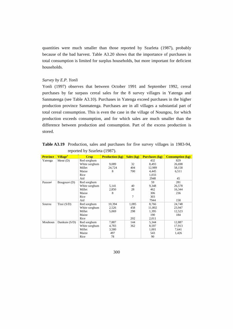
300

quantities were much smaller than those reported by Szarleta (1987), probably

because of the bad harvest. Table A3.20 shows that the importance of purchases in

total consumption is limited for surplus households, but more important for deficient

households.

Survey by E.P. Yonli

Yonli (1997) observes that between October 1991 and September 1992, cereal

purchases by far surpass cereal sales for the 8 survey villages in Yatenga and

Sanmatenga (see Table A3.10). Purchases in Yatenga exceed purchases in the higher

production province Sanmatenga. Purchases are in all villages a substantial part of

total cereal consumption. This is even the case in the village of Noungou, for which

production exceeds consumption, and for which sales are much smaller than the

difference between production and consumption. Part of the excess production is

stored.

Table A3.19 Production, sales and purchases for five survey villages in 1983-94,

reported by Szarleta (1987).Province Village1 Crop Production (kg) Sales (kg) Purchases (kg) Consumption (kg)Yatenga MenJ (D) Red sorghum

White sorghumMilletMaizeRiceAid

9,08924,724

8

32404700

4328,49312,9894,4451,0332948

82926,69858,1586,511

45PassorJ BougourJ (D) Red sorghum

White sorghumMilletMaizeRiceAid

5,1412,850

8

4028

7

599,3484623063037944

28126,57816,344

236

158Sourou Tissi (S/D) Red sorghum

White sorghumMilletMaizeRice

10,3942,5265,069

1,085458298

202

8,76611,8021,395190

2,011

24,74823,94712,523

184

Mouhoun Dankuie (S/D) Red sorghumWhite sorghumMilletMaizeRice

7,8874,7833,58049778

144362

5,3448,5971,00154390

12,88717,9137,6411,426

301

Cont. Table A3.19Houet BarJ (S) Red sorghum

White sorghumMilletMaizeRice

23,73217,9859,97716,092

21,5104,523446

3,46459

7,5492,0697394314320

8,89317,9979,75515,858

Notes: 1) S = village in surplus during the survey period, D = village in deficit during the survey period,S/D = village with a production which is more or less equal to the cereal consumption requirements ofthe village. Source: Szarleta (1987).

Table A3.20 Cereal purchases per adult equivalent, by Reardon et al. (1987)

Soum PassorJ MouhounProvince

Deficient Surplus Deficient Surplus Deficient Surplus

Purchases (kg) 35 16 28 5 21 11

Purchases (as % of consumption) 18% 4% 20% 2% 14% 3%

Source: Reardon et al. (1987).

Table A3.21 Cereal purchases in some villages in Yatenga and Sanmatenga

between October 1991 and September 1992, by Yonli (1997), see also

Table A3.10.

Village/

province1

Number of

households

Average

household size

(a)

Purchases per

household (kg)

(b)

Purchases per

person (kg)

(c)

Purchases as % of

consumption

(d)

Ramsa 3 14.3 798 55.8 28.1%

SJguJnJga 7 14.7 307 20.9 11.1%

Kalsaka 7 15.6 713 45.7 20.9%

Kossouka 7 13.4 525 39.2 20.1%

Yatenga 24 14.6 552 37.8 18.9%

Nessemtenga 1 12.0 358 29.8 34.6%

Soubeira 5 14.2 382 26.9 13.2%

Noungou 8 8.8 304 34.6 18.4%

SinguJ 7 11.3 384 34.0 16.0%

Sanmatenga 21 11.1 355 32.3 16.8%

Notes: 1) The first four villages are in Yatenga, the last four villages are in Sanmatenga. (c) = (b)/(a)Source: Yonli (1997).

Survey by Broekhuyse

Broekhuyse (1983, 1998) observes that in the province of Sanmatenga, the ‘modern’

households using animal traction (AT) purchase more cereals than households

302

applying manual labour (ML). AT households purchase on average 554 kg (average

household size 10.2 members), and ML households 322 kg (average household size

7.3 members). This is inconsistent with expectations. AT households produce more,

and accordingly need to purchase less. The data show that AT household purchase

large quantities of red sorghum for brewing dolo. If red sorghum purchases are

distracted from the figures, AT households still purchase more cereals (331 kg for AT

and 276 kg for ML households), but purchases per person are less (32 kg for AT and

38 kg for ML households).

If the different studies are compared it can be seen that preferences differ per

province. Households in the northern provinces (Yatenga and Soum) prefer to

purchase millet, whereas households in the other provinces (PassorJ, Sanmatenga,

Mouhoun, Houet, Kossi) purchase much more white sorghum. In the northern

provinces maize purchases per household were also reported much higher than in the

other provinces. Reardon et al. (1987) attribute this to the maize prices which were

low in these regions because they were sold by official, government sellers. In those

days the government sold cereals at fixed, predetermined prices.

Seasonal purchase pattern

CEDRES survey

Some studies also collected data on seasonal purchase patterns. Despite high prices,

many households purchase most cereals during the lean period, when stores are

almost empty. Researchers from CEDRES (Thiombiano et al. (1988) ) surveyed 104

households in the provinces of Yatenga (Thiou, Nomo, Gourcy and Rom), Bam

(Kongoussi and Loagha) and Sanmatenga (Barsalogho and Tamassogo). They looked,

among other things, to production, consumption, sales and purchases, but presented

results only in monetary terms. Consequently, sold and purchased quantities are

difficult to derive. Table A3.22 shows the distribution of cereal purchases for a period

of 7 months (as a % of total purchase expenditures over this period). The last period is

for households normally the most difficult period of the year. Stores are almost

empty, and people have to work hard on the fields. The province of Sanmatenga

303

shows the expected purchase pattern, that more cereals are purchased the closer one

approaches the new harvests (from sept-nov). In Bam, the last period is the period in

which most cereals are purchased, but the first period also shows a large percentage.

The only exception is the province of Yatenga, which shows the opposite pattern.

This is, for an important part, caused by the village of Thiou with exceptionally high

purchases in the first period. These purchases are so high (75% of total) that this

might be a data error. If the village of Thiou is skipped from the data, the pattern is

clearer (28% in feb-mar, 20% in apr-may and 52% in july-aug).

Table A3.22 Distribution of cereal purchases as % of total cereal sales in the period

february to august, by Thiombiano et al. (1988).Province Febr-Mar Apr-May July-Aug

Yatenga 49% 17% 33%

Sanmatenga 25% 29% 46%

Bam 38% 16% 46%

Source: Thiombiano et al. (1988)

ICRISAT surveys

Reardon et al. (1987) only report on seasonal purchases for deficient households (see

Table A3.23). High purchases in the season 1984-‘85 can be explained by bad

production in both ’83 and ’84. High purchases in ‘82-’83 can however not be

explained by low production, since production in ’81 and ’82 were reasonable. It

must, however, be noted that the table only reports on shortage households. Because

differences within villages and provinces are very large, it is well possible that many

households have a low production, even if total regional production is high. The table

clearly shows the pattern that purchases in the lean period (the hot and rainy season)

were highest. In most years, purchases were highest in the northern province.

Purchases in the province of Mouhoun were also rather high.

304

Table A3.23 Seasonal purchases of deficient households between 1981-84 per adult

equivalent by region, reported by Reardon et al. (1987).‘81-‘82 ‘82-‘83 ‘83-‘84 ‘84-‘85

Season1 hr cl ht rn hr cl ht rn hr cl ht rn hr cl ht rn

Soum: deficient 7 1 5 19 9 19 48 42 6 3 1 11 11 19 27 50

PassorJ: deficient 2 4 3 8 2 3 7 6 4 4 6 7 3 4 16 14

Mouhoun: deficient 5 5 8 2 16 14 21 5 7 13 16 3 4 7 4

Note: 1) Seasons: harvest (hr = sept-nov), cold (cl = dec-feb), hot (ht = mar-may), rainy (rn = june-aug).Source: Reardon et al. (1987)

Surveys from the Universities from Michigan and Wisconsin

Ellsworth and Shapiro (1989) also give data on seasonal cereal purchases, but only

aggregated for the five sample villages of the surveys from the University of

Michigan. These data clearly show that the largest volume is purchased during the

quarter July-October, the lean season. Also the number of households with their

largest volume of cereal purchases, is higher in this quarter than in the other quarters.

This corresponds with the expected purchase pattern for the country. Dissaggregation

by village reveals that nearly half of the households in BarJ, a relatively wealthy,

surplus village, made their largest purchases between January and March, when prices

were still low. In the other four villages, which had a chronically or occasional cereals

deficit, most households purchased their largest quantity of cereals during the other

two, higher priced, quarters.

Table A3.24 Cereal purchases in 1984, by Ellsworth and Shapiro (1989).Jan-Mar Apr-June July-Oct. 10 Oct. 11- Dec

Purchases1 25,366 35,846 57,158 12,085

Number of households2 45 61 64 7

Notes: 1) Sorghum, millet, maize, rice, food aid, miscellaneous foods. 2) Number of households withtheir largest volume of purchases in a certain quarter. Source: Ellsworth and Shapiro (1989).

Survey by E.P. Yonli

Yonli (1997) presents the monthly purchases aggregated for his survey villages in

Yatenga and Sanmatenga between October 1991 and June 1993. Table A3.25 clearly

shows that purchases are highest during the lean season (the second and third

305

quarter). For Yatenga monthly purchases always exceed montly sales (see also Table

A3.15). In Sanmatenga, sales exceed purchases in some months. The low purchases

in Sanmatenga during the second quarter of 1993 seem logical, considering the

relatively high sales during that period. The data indicate for Sanmatenga, though not

very clearly, that purchases decrease if production increases (production in ’92 was

much higher than production in ’91). For Yatenga, however, this can not be observed

(’91 production was higher than ’92 production).

Table A3.25 Monthly purchases (in kg per person) between October 1991 and June

1993, by Yonli (1997).

Month/

Year

Yatenga Sanmatenga Month/Year

Yatenga Sanmatenga

10-91 0.75 4.11 9-92 0.27 2.06

11-91 1.30 0.82 3d quarter 92 11.26 16.59

12-91 2.83 0.50 10-92 1.73 0.04

4th quarter 91 4.88 5.43 11-92 2.36 0.47

1-92 1.03 1.52 12-92 0.35 0.15

2-92 2.78 0.08 4th quarter 92 4.44 0.66

3-92 4.34 1.23 1-93 3.47 2.27

1st quarter 92 8.15 2.83 2-93 2.38 0.31

4-92 2.63 0.94 3-93 3.46 0.31

5-92 6.70 2.08 1st quarter 93 9.31 2.89

6-92 4.46 4.05 4-93 3.40 0.23

2nd quarter 92 13.79 7.07 5-93 3.77 0.47

7-92 4.68 10.67 6-93 4.31 1.88

8-92 6.31 3.86 2nd quarter 93 11.48 2.58

Note: In Yatenga 24 households and in Sanmatenga 21 households were surveyed. Source: Yonli (1997).

Price and income elasticities of cereal demand

Price elasticities of demand and income elasticities have been estimated in several

studies.

306

ICRISAT surveys

Reardon et al. (1988b) analysed the sensitivity of cereal consumption to cereal price

changes. Rice, maize and millet/white sorghum consumption were regressed at the

prices of these cereals, monthly household expenses, household size, and the number

of children. Elasticities are estimated, which indicate the percentage increase in

consumption, resulting from a percentage increase in the price of one of the cereals or

in the household expenses. The calculated R2 of the regressions were in most cases

low, which indicates that the purchases were only for a small part explained by the

independent variables. R2 only had reasonable values for rice purchases by poor

households (62%), and rice and millet/sorghum purchases by average households

(30% and 44%, respectively). For the other purchases, R2 was between 13% and 22%.

A remarkable result was that neither the rice price, nor the prices of the other cereals,

did have a significant influence on rice consumption. The income elasticity of rice

consumption (% increase of rice consumption relative to a 1% increase of household

revenues which are supposed to be equal to total household expenses) was for all

households between 0.72 and 1.01 (see Table A3.26). This indicates that rice is not a

luxury good (see Section 4.2). The same holds for maize and for millet/sorghum

consumption. The analysis also shows that households with less children consume

more rice (they consume more often rice purchased from prepared food sellers). On

the other hand maize cultivation turns out to be dependent on its own price (for the

average households) and the millet/sorghum price (for the poor and average

households). If the maize price increases, average households will consume much less

maize, and will substitute it partly with millet/sorghum. Finally, millet/sorghum

consumption did respond weakly and not significantly on cereal price changes.

307

Table A3.26 Price and income elasticities of cereal consumption, by Reardon et al.

(1988b).Poor Average Rich

Rice purchases

Total household expenses 0.79 0.72 1.01

Maize purchases

Maize price -7.00

Millet/sorghum price 3.11 3.80

Total household expenses 1.11 1.03 1.28

Millet/sorghum purchases

Total household expenses 0.87 0.91

Notes: Only elasticities with a significance level of at least 90% are shown. Source: Reardon et al.

(1988b).

Survey by Roth

Roth (1986) estimated income and demand elasticities for five rural and two urban

regions in Burkina Faso. For his estimates he used some empirical estimates from

other studies in different countries (see Table A3.27) and observations on rural-urban

consumption patterns (e.g. more rice consumption in cities, the position of maize in

daily consumption). His estimates of own-price, cross-price, and income-price

elasticities are presented in Table A3.28. In this table income compensated own-price

and cross-price elasticities are presented, which shows that changes in demand are not

only caused by a substitution effect, but also by an income effect. After all, if prices

increase also the purchasing power of households decreases. His estimates show

inelastic and negative own-price elasticities of demand, and very inelastic but positive

cross-price elasticities. Elasticities for the staple cereals millet and sorghum are on the

countryside more elastic than rice, maize and groundnuts. In the cities, sorghum

demand is not influenced by prices of the other goods. Urban households mainly

demand red sorghum for brewing dolo. Rice and white sorghum demand are more

elastic than millet. Millet is more a crop for the poor. Maize turns out to be very

inelastic for all households. The relatively elastic own-price elasticities for staple

crops is caused by the high proportion of income spent on them. If the price of these

goods increases, the purchasing power decreases, and cheaper substitutes will be

308

sought after. For commodities on which a smaller part of income is spent, price also

plays a minor role. Income elasticities for millet and sorghum are in rural areas

relatively elastic, compared to urban elasticities of these commodities. For rice, the

reverse is observed. Maize and groundnuts are less elastic in rural areas, but a little

more elastic in Ouagadougou and Bobo Dioulasso.

Table A3.27 Estimates of own-price and income elasticities, reported in Roth

(1986).Own-price elasticity Income elasticity

Crops1 So Mi Mz Rc Wt Oth So Mi Mz Rc Wt

USDA,1981

SahelWest Africa

-.06-.05

-.35-.53

-.30-.15

.15

.09.46.15

.92

.87.93.65

Sawadogo,1986, Ouaga-dougou

Low2

MiddleHighMean

1.13.99.63.94

.91

.971.211.02

Youngbloodet al., 1982,Khartoum

Low 25%Middle 50%Upper 25%Mean

.77

.50

.57

.59

1.21.90.88.97

Strauss, 1983,Sierra Leone

Low2

MiddleHighMean

-.15-.26-.31-.22

-1.26-.78-.45-.74

-1.17-.40-1.05-1.01

Notes: 1) So = sorghum, Mi = millet, Mz = maize, Rc = rice, Wt = wheat, Oth = others; 2) A distinctionhas been made between low, middle and high income groups. Source: Roth (1986).

Table A3.28 Own-price, cross-price and income elasticities for Burkina Faso, by

Roth (1986).Price elasticityRegions1 Income

elasticity Ws Rs Mi Mz Rc Gn Oth

CentralRegion

Ws2

RsMiMzRcGnOth

0.950.950.950.750.800.80

1.0462

-0.43860.03640.03640.02870.02300.03070.0402

0.0200-0.45500.02000.01580.01260.01680.0221

0.05010.0501-0.42490.03960.03160.04220.0553

0.00450.00450.0045-0.37150.00280.00380.0049

0.00710.00710.00710.0056-0.29550.00600.0078

0.00910.00910.00910.00720.0057-0.39230.0100

0.34520.34520.34520.27250.21800.2907-0.1433

309

Cont. Table A3.28

NorthernRegion

WsRsMiMzRcGnOth

0.950.950.950.750.600.80

1.0612

-0.43000.04500.04500.03550.02840.03790.0503

0.0012-0.47380.00120.00090.00070.00100.0013

0.08980.0898-0.38520.07090.05670.07570.1004

0.00740.00740.0074-0.36910.00470.00620.0083

0.00640.00640.00640.0051-0.29590.00540.0072

0.01070.01070.01070.00850.0068-0.39100.0120

0.31230.31230.31230.24650.19720.2630-0.1818

EasternRegion

WsRsMiMzRcGnOth

0.950.950.950.750.600.80

1.0330

-0.42680.04820.04820.03810.03050.04060.0524

0.0043-0.47070.00430.00340.00270.00370.0047

0.03460.0346-0.44040.02730.02180.02910.0376

0.00470.00470.0047-0.37130.00300.00400.0051

0.00370.00370.00370.0030-0.29760.00310.0041

0.00790.00790.00790.00630.0050-0.39330.0086

0.36970.36970.36970.29190.23350.3113-0.1145

WesternRegion

WsRsMiMzRcGnOth

0.950.950.950.750.600.80

1.0275

-0.47870.04380.04380.03460.02770.03690.0474

0.0157-0.50680.01570.01240.00990.01320.0170

0.03090.0309-0.49160.02440.01950.02600.0334

0.00460.00460.0046-0.40880.00290.00390.0050

0.00290.00290.00290.0023-0.32820.00240.0031

0.00830.00830.00830.00650.0052-0.43300.0090

0.41500.41500.41500.32770.26210.3495-0.1162

South-west

Region

WsRsMiMzRcGnOth

0.950.950.950.750.600.80

1.0305

-0.49040.03210.03210.02530.02030.02700.0348

0.0057-0.51680.00570.00450.00360.00480.0062

0.01270.0127-0.50980.01000.00800.107

0.00138

0.01470.01470.0147-0.40090.00930.01240.0160

0.00460.00460.00460.0036-0.32710.00380.0050

0.00580.00580.00580.00460.0037-0.43510.0063

0.44520.44520.44520.35150.28120.3749-0.0838

Ouaga-dougou

WsRsMiMzRcGnOth

0.700.700.700.800.950.85

1.0424

-0.40170.01830.01830.02090.02480.02220.0272

0-0.4200

00000

0.00490.0049-0.41510.00570.00670.00600.0074

0.00080.00080.0008-0.47900.00110.00100.0013

0.02290.02290.02290.0262-0.53890.02780.0341

0.01240.01240.01240.01420.0169-0.49490.0185

0.34900.34900.34900.39880.47360.4237-0.1058

BoboDiou-lasso

WsRsMiMzRcGnOth

0.700.700.700.800.950.85

1.0487

-0.40180.01820.01820.02060.02470.02210.0272

0-0.4200

00000

0.00330.0033-0.41670.00380.00450.00410.0050

0.01030.01030.0103-0.46830.01390.01250.0154

0.02100.02100.02100.0240-0.54150.02550.0314

0.01380.01380.01380.01570.0187-0.49330.0206

0.34250.34250.34250.39150.46490.4159-0.1161

Notes: 1) Central region = CRPA Centre, Centre Ouest, Centre Est, Centre Sud and the province ofPassorJ; North region = CRPA Centre Nord, Sahel and the province of Yatenga; East region = CRPAEst; Western region = CRPA Mouhoun; Southwest region = CRPA Hauts Bassins, Sud Ouest andComoJ; 2) Ws = white sorghum, Rs = Red sorghum, Mi = millet, Mz = maize, Rc = rice, Gn =Groundnuts, Oth = other.Source: Roth (1986).

310

Study by Colman and Young

Colman and Young (1989) also present some FAO estimates of income elasticities of

demand for some agricultural products (see Table A3.29). These estimates are much

lower than the estimates presented by Roth (1986). The most important reason for this

is that Colman and Young give aggregated estimates for all cereals. These are

normally lower than disaggregated elasticities for the different cereals. After all, if the

price of white sorghum increases, another cereal can substitute this demand, whereas

another type of commodity (not a cereal type) has to substitute for cereals, if the

‘cereal’ price increases.

Table A3.29 Income elasticities of demand for some agricultural products, by

Colman and Young (1989).

Egypt ‘74/75 India (‘73/74) Java (’78)

Rural Urban Rural Urban Rural Urban

Colombia

‘87

Mexico ‘77

Cereals 0.15 0.61 0.21 0.48 0.15 0.23 0.58 -0.16

Total food 0.75 1.28 0.79 0.82 0.74 0.72 0.64 0.09

Source: Colman and Young (1989).

We retain the following conclusions from the above review. Rice consumption of

urban households increases. Rice consumption is higher for wealthier households, and

poorer households spent a larger share of their income on cereal purchases. Almost all

rural households purchase cereals on the market. The quantity of cereals purchased is

for many households larger than the quantity sold. Cereal purchases are a

considerable part of total consumption, certainly for shortage households.

Furthermore, in general most purchases take place during the lean season, when

stocks are depleted, before the new harvest. Income and price elasticities of cereal

demand differ a lot between the different regions. Roth has estimated in his study

income elasticities of supply which we will also use in our study. We feel that his

estimates are more reliable than the other elasticities presented above, because he

estimated them on the basis of elasticities reported in other studies and on emprical

evidence from Burkina Faso.

311

A3.5 Revenues and expenditures

Non-cropping income is an important determinant of cereal purchases and sales. It is

one of the major elements of the cereal demand functions discussed in Section 9.1. In

Section 8.1.5 it has been showed that collecting data on these issues is a difficult task.

In this appendix some surveys performed in the past are reviewed.

INSD survey

In 1994 the national statistical institute of Burkina Faso, INSD, executed a large

survey on household living conditions among more than 8000 households scattered

over the country (INSD, 1996a,b). This was one of the first large surveys on living

conditions by the institute. Based on their surveys they divided the country in 5

representative rural regions and two urban regions. These regions are not the same as

the CRPA which are applied in this study. Table A3.30 shows which provinces lie in

which INSD survey region and CRPA. Assuming that revenues and expenditures are

the same in all provinces of the 5 regions, it is possible to estimate revenues and

expenditures per CRPA. In their reports, INSD admits that they encountered many

problems, and that therefore some of the results are not as reliable as required.

Table A3.31 shows for each region total and cereal expenses and revenues per

household. INSD measures total revenues and expenses as the sum of monetary and

non-monetary expenses and revenues. Monetary expenses are for example purchases

of cereals on the market. Non-monetary expenses comprises for example

consumption of self produced cereals. Consumption of self-produced crops has been

valued against the going market price to determine non-monetary expenses. An

average household in Burkina Faso consists on of 7.8 people (INSD, 1996a). Because

of difficulties measuring directly household revenues, only the distribution of

revenues over the different sources is presented. In INSD (1996b) it has been

supposed that total revenues equal total expenses.

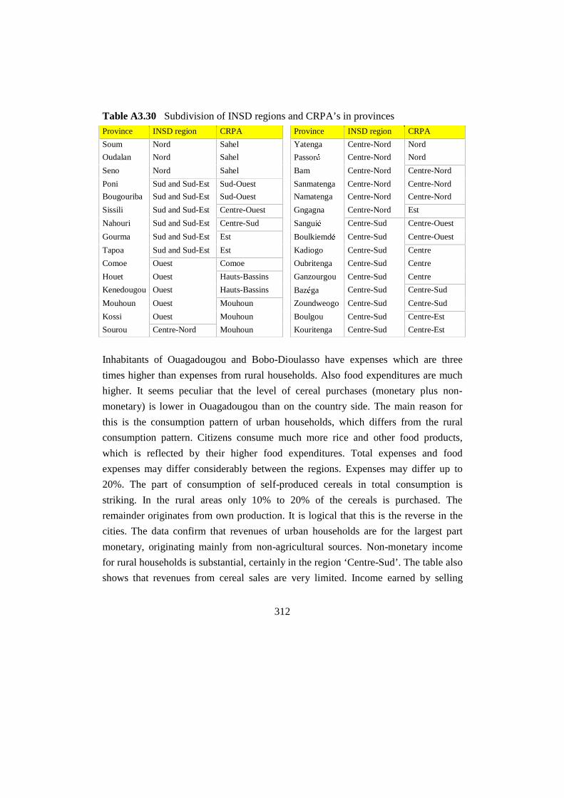
312

Table A3.30 Subdivision of INSD regions and CRPA’s in provincesProvince INSD region CRPA Province INSD region CRPA

Soum Nord Sahel Yatenga Centre-Nord Nord

Oudalan Nord Sahel PassorJ Centre-Nord Nord

Seno Nord Sahel Bam Centre-Nord Centre-Nord

Poni Sud and Sud-Est Sud-Ouest Sanmatenga Centre-Nord Centre-Nord

Bougouriba Sud and Sud-Est Sud-Ouest Namatenga Centre-Nord Centre-Nord

Sissili Sud and Sud-Est Centre-Ouest Gngagna Centre-Nord Est

Nahouri Sud and Sud-Est Centre-Sud SanguiJ Centre-Sud Centre-Ouest

Gourma Sud and Sud-Est Est BoulkiemdJ Centre-Sud Centre-Ouest

Tapoa Sud and Sud-Est Est Kadiogo Centre-Sud Centre

Comoe Ouest Comoe Oubritenga Centre-Sud Centre

Houet Ouest Hauts-Bassins Ganzourgou Centre-Sud Centre

Kenedougou Ouest Hauts-Bassins BazJga Centre-Sud Centre-Sud

Mouhoun Ouest Mouhoun Zoundweogo Centre-Sud Centre-Sud

Kossi Ouest Mouhoun Boulgou Centre-Sud Centre-Est

Sourou Centre-Nord Mouhoun Kouritenga Centre-Sud Centre-Est

Inhabitants of Ouagadougou and Bobo-Dioulasso have expenses which are three

times higher than expenses from rural households. Also food expenditures are much

higher. It seems peculiar that the level of cereal purchases (monetary plus non-

monetary) is lower in Ouagadougou than on the country side. The main reason for

this is the consumption pattern of urban households, which differs from the rural

consumption pattern. Citizens consume much more rice and other food products,

which is reflected by their higher food expenditures. Total expenses and food

expenses may differ considerably between the regions. Expenses may differ up to

20%. The part of consumption of self-produced cereals in total consumption is

striking. In the rural areas only 10% to 20% of the cereals is purchased. The

remainder originates from own production. It is logical that this is the reverse in the

cities. The data confirm that revenues of urban households are for the largest part

monetary, originating mainly from non-agricultural sources. Non-monetary income

for rural households is substantial, certainly in the region ‘Centre-Sud’. The table also

shows that revenues from cereal sales are very limited. Income earned by selling

313

cotton in the western regions, and by selling livestock in the other regions often

exceeds cereal income. This confirms that households prefer not to sell cereals.

Table A3.31 Annual revenues and expenses per household in FCFA in 1994.Ouest Sud et Centre- Centre- Nord Ouaga/ Other

Expenses Sud-Est Nord Sud Bobo cities

(a) Total expenses (FCFA)1 441,360 419,741 364,301 386,998 374,982 1,141,725 940,182

(b) Food expenses 232,841 230,438 191,844 198,547 239,610 372,388 363,323

(c) (as % of total expenses) 52,8% 54,9% 52,7% 51,3% 63,9% 32,6% 38,6%

(d) Cereal expenses 111,764 97,475 89,016 80,610 119,086 98,310 115,537

(e) (as % of food expenses) 48,0% 42,3% 46,4% 40,6% 49,7% 26,4% 31,8%

Suppositions:2

(f) Cereal expenses non-monetary (%) 80% 80% 80% 80% 80% 21% 49%

(g) Cereal expenses monetary (%) 20% 20% 20% 20% 20% 79% 51%

(h) Cereal expenses non-mon. (FCFA) 89,411 77,980 71,212 64,488 95,269 20,645 56,613

(i) Cereal expenses monetary (FCFA) 22,353 19,495 17,803 16,122 23,817 77,665 58,924

Revenues3

Monetary revenues (%) 54,3% 33,2% 35,3% 28,1% 38,8% 80,6% 69,6%

Non-monetary revenues (%) 45,7% 66,8% 64,7% 71,9% 61,2% 19,4% 30,4%

Structure of monetary revenues

*agriculture4: 71,2% 40,4% 46,3% 35,2% 43,5% 1,8% 5,8%

-cereals, groundnuts4 26,9% 15,9% 14,6% 13,3% 2,6% 0,5% 2,2%

-cotton4 33,4% 8,3% 0,9% 1,6% 0,1% 0,0% 0,1%

-livestock4 6,4% 10,7% 27,1% 13,1% 38,5% 0,5% 1,6%

Average household size 7.8 7.6 9.0 8.0 6.7 6.1 7.5

Notes: (c) = (b)/(a)*100%, (e) = (d)/(b)*100%, (h) = (f)*(d), (i) = (g)*(d) .1) Total expenses includemonetary and non-monetary expenses. Non-monetary expenses are calculated by multiplyingconsumption of self-produced crops with the observed market price; 2) On-farm consumption of self-produced base cereals millet and sorghum is estimated at 80% of total cereal expenses for the rural areas,against 49% for average cities and only 21% for Ouagadougou and Bobo-Dioulasso (INSD, 1996b: p.226); 3) It has been supposed that total revenues equal total expenses, which are given in (a). 4) As % oftotal monetary revenues.Source: data based on INSD (1996a,b)

Survey by Broekhuyse

Broekhuyse (1988) reports the revenues and expenditures for households using

animal traction (AT) and using manual labour (ML) in two villages in the province of

Sanmatenga, see Table A3.32. The average household size was 7.3 for ML housholds,

and 10.2 people for AT households. AT households had much larger revenues and

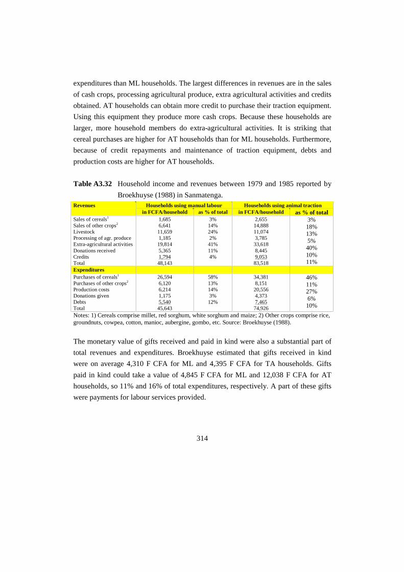
314

expenditures than ML households. The largest differences in revenues are in the sales

of cash crops, processing agricultural produce, extra agricultural activities and credits

obtained. AT households can obtain more credit to purchase their traction equipment.

Using this equipment they produce more cash crops. Because these households are

larger, more household members do extra-agricultural activities. It is striking that

cereal purchases are higher for AT households than for ML households. Furthermore,

because of credit repayments and maintenance of traction equipment, debts and

production costs are higher for AT households.

Table A3.32 Household income and revenues between 1979 and 1985 reported by

Broekhuyse (1988) in Sanmatenga.Households using manual labour Households using animal tractionRevenues

in FCFA/household as % of total in FCFA/household as % of totalSales of cereals1

Sales of other crops2

LivestockProcessing of agr. produceExtra-agricultural activitiesDonations receivedCreditsTotal

1,6856,64111,6591,18519,8145,3651,79448,143

3%14%24%2%41%11%4%

2,65514,88811,0743,78533,6188,4459,05383,518

3%18%13%5%40%10%11%

ExpendituresPurchases of cereals1

Purchases of other crops2

Production costsDonations givenDebtsTotal

26,5946,1206,2141,1755,54045,643

58%13%14%3%12%

34,3818,15120,5564,3737,46574,926

46%11%27%6%10%

Notes: 1) Cereals comprise millet, red sorghum, white sorghum and maize; 2) Other crops comprise rice,groundnuts, cowpea, cotton, manioc, aubergine, gombo, etc. Source: Broekhuyse (1988).

The monetary value of gifts received and paid in kind were also a substantial part of

total revenues and expenditures. Broekhuyse estimated that gifts received in kind

were on average 4,310 F CFA for ML and 4,395 F CFA for TA households. Gifts

paid in kind could take a value of 4,845 F CFA for ML and 12,038 F CFA for AT

households, so 11% and 16% of total expenditures, respectively. A part of these gifts

were payments for labour services provided.

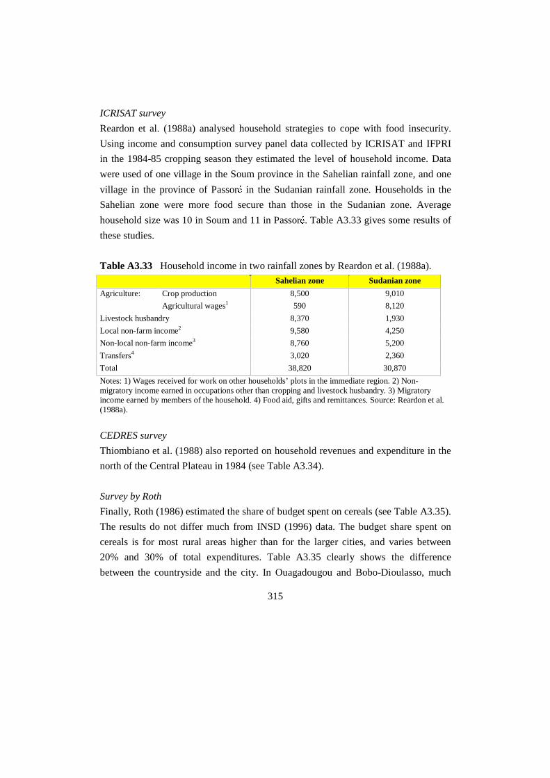
315

ICRISAT survey

Reardon et al. (1988a) analysed household strategies to cope with food insecurity.

Using income and consumption survey panel data collected by ICRISAT and IFPRI

in the 1984-85 cropping season they estimated the level of household income. Data

were used of one village in the Soum province in the Sahelian rainfall zone, and one

village in the province of PassorJ in the Sudanian rainfall zone. Households in the

Sahelian zone were more food secure than those in the Sudanian zone. Average

household size was 10 in Soum and 11 in PassorJ. Table A3.33 gives some results of

these studies.

Table A3.33 Household income in two rainfall zones by Reardon et al. (1988a).

Sahelian zone Sudanian zone

Agriculture: Crop production

Agricultural wages18,500

590

9,010

8,120

Livestock husbandry 8,370 1,930

Local non-farm income2 9,580 4,250

Non-local non-farm income3 8,760 5,200

Transfers4 3,020 2,360

Total 38,820 30,870

Notes: 1) Wages received for work on other households’ plots in the immediate region. 2) Non-migratory income earned in occupations other than cropping and livestock husbandry. 3) Migratoryincome earned by members of the household. 4) Food aid, gifts and remittances. Source: Reardon et al.(1988a).

CEDRES survey

Thiombiano et al. (1988) also reported on household revenues and expenditure in the

north of the Central Plateau in 1984 (see Table A3.34).

Survey by Roth

Finally, Roth (1986) estimated the share of budget spent on cereals (see Table A3.35).

The results do not differ much from INSD (1996) data. The budget share spent on

cereals is for most rural areas higher than for the larger cities, and varies between

20% and 30% of total expenditures. Table A3.35 clearly shows the difference

between the countryside and the city. In Ouagadougou and Bobo-Dioulasso, much

316

more rice is consumed than in rural areas. Furthermore, in the north, and to a lesser

extent also in the central region, millet is prefered, whereas white sorghum is prefered

in the other regions. It can be questioned whether the consumption of red sorghum in

the cities is indeed neglible. It is true that dolo consumption, for which much of the

red sorghum is used, is less important in larger cities, where bottled beer is consumed

more often. However, dolo consumption is certainly not zero in these areas.

Table A3.34 Household revenues and expenditure patterns for eight villages in the

north of the Central Plateau in 1984, in FCFA per household.Revenues Gourcy Rom Thiou Nomo Tamas-

sogo

Barsa-

logho

Kongous

-si

Loagha Average

Cowpea,

Voandzou,

vegetables

0 9692 346 0 12063 0 109742 8435 17535

Livestock 111934 11635 108444 33173 15469 7123 28815 32627 43653

Handicraft 91192 769 14923 9515 0 169 18300 20905 19472

Small trade 0 6346 19423 5278 2431 2980 2653 3731 5355

Retirements,

pensions

131692 0 26692 0 43077 0 0 0 25183

Other revenues 3846 34038 0 0 10576 846 13846 17308 10058

Total (FCFA) 338664 62480 169828 47966 83616 11118 173356 833006 215004

Source: Thiombiano et al. (1988)

Table A3.35 Average share of budget spent on different cereals; by Roth (1986).

Ws2 Rs Mi Mz Rc Gn Oth

Centre1 0.081 0.044 0.111 0.013 0.025 0.024 0.703

North 0.100 0.003 0.199 0.021 0.023 0.028 0.627

East 0.107 0.010 0.077 0.013 0.013 0.021 0.760

West 0.088 0.032 0.062 0.012 0.009 0.020 0.777

South-west 0.065 0.012 0.026 0.038 0.015 0.014 0.832

Ouagadougou 0.062 0 0.017 0.003 0.057 0.035 0.826

Bobo-Dioulasso 0.062 0 0.011 0.031 0.053 0.039 0.805

Notes: 1) Central region = CRPA Centre, Centre Ouest, Centre Est, Centre Sud and the province ofPassorJ; North region = CRPA Centre Nord, Sahel and the province of Yatenga; East region = CRPAEst; Western region = CRPA Mouhoun; Southwest region = CRPA Hauts Bassins, Sud Ouest andComoJ; 2) Ws = white sorghum, Rs = Red sorghum, Mi = millet, Mz = maize, Rc = rice, Gn =Groundnuts, Oth = other.Source: Roth (1986).

317

The above rewiew shows that income and expenditure levels reported by the different

surveys differ considerably. This is caused by the unreliability of the data, but on the

other hand differences between households, between regions, and also between years

are known to differ a lot. In Section 9.1 we estimate income levels per person mainly

on the basis of the INSD survey (1996a,b). Despite unexplained data errors in the

INSD reports, it is the most recent and largest survey available.

A3.6 Agricultural prices

To estimate the different parameters of the cereal demand functions in Section 9.1,

estimates are used of average cereal consumer prices per quarter. To determine cereal

supply functions in Section 9.2, the probability distribution of cereal producer prices

per quarter is used. In this appendix and Section 8.1.6 the price data used for these

purposes are discussed. Price data in Burkina Faso are gathered weekly by

SIM/SONAGESS on 37 markets in Burkina Faso for the cereals millet, red sorghum,

white sorghum, yellow maize and white maize. A distinction is made between

producer and consumer prices. Producer prices ensue from transactions between

producers and traders, consumer prices ensue from transactions between consumers

and traders or between consumers and producers. Before discussing these data for the

period 1992-199938, we first briefly discuss the analyses of Bassolet (2000) and

Hoftijzer (1998), who used the same data, but for the period 1992-1996.

In the study of Bassolet (2000) an analysis is made of: 1) changes in the cereal

market structure and the behavior of actors after market liberalization in Burkina

Faso, and of: 2) the economic efficiency of market transactions. He showed that the

grain policies of the government constrained the functioning of the market in the past.

Liberalization policies had some favorable effects on competition, mainly due to the

result of the increased number of traders and the market information system (SIM)

38 Data obtained from STATISTIKA, the statistical department from SIM/SONAGESS and frominternet: www.statistika.net.

318

which contributed to the transparency of the market. In the meanwhile, limited access

to credit, high taxes, bad infrastructure and the irregular dissemination of prices by

the market information system, still constrain competition.

Bassolet also showed that the new policies also changed farmer behaviour, in

particular in surplus regions. They changed their passive commercial strategies in

more active behavior. Nowadays, sales are planned in a way that the farmer profits

from seasonal price fluctuations, and surpluses are only sold to the highest bid. Also

traders profit from the increased transparency. They are better informed about supply

and demand conditions (prices) on local surplus markets and therefore they are able to

purchase the grain more efficiently. Remarkably, (semi-)wholesalers did not change

their storage strategies. Most of them sell their stocks within one month. Three

explanations are given for this behaviour: 1) traders are constrained by a limited

availability of working capital; 2) it is costly to conserve grain for a longer period; 3)

the grain board SONAGESS, responsible for the management of the national food

security grain stock, revolves the stock gradually and sells during the hungry season

(June - August). As a consequence, seasonal price increases in the grain market are

reduced, making investments in storage less attractive for traders.

Bassolet showed that producer prices increased after liberalization. He derived a

seasonal price index which is relatively stable for the consumer price series, but

instable for the producer price series. The collected price data show some evidence

for the conclusion that the seasonal price increase is lower than the costs of storage.

This result clearly explains why traders play only a minor role in the long term

storage activity. Finally, Bassolet showed that price differences between markets

decreased after liberalization. Net margins for traders are low, indicating that market

integration improved after liberalization. The results of tests for cointegration

(Johansen procedure) are in line with these observations and show that the number of

cointegrated markets increased. Bassolet concludes that this can be interpreted as a

positive effect of liberalization policies and, in particular, the upshot of the market

information system and the removal of regional trade barriers in the country.

319

An analysis of the weekly SIM prices for the period 1992-1996 for 16 villages by

Hoftijzer (1998) demonstrated that no evidence could be found for a seasonal pattern

with regular price increases and decreases. On most markets prices decreased after the

harvest and increased during the lean season. For some markets, however, this pattern

could not be observed. Furthermore, the timing of price increases and decreases as

well as the amplitude of seasonal changes differed per year. However, these

conclusions are based on data for only 4 harvest years. Differences between years and

between villages are large. A closer look to the white sorghum producer prices in

Banfora show that the price difference between the first and third quarter in 1993 is

only 8%, while it is 103% in 1996. Furthermore average ‘92-’96 millet consumer

prices in N’dorola are reported to have increased 130% between the first and the

second quarter, whereas prices in Niangoloko increased only 8%. Some of these

differences may be caused by data weakness (only few observations are available for

some markets), but volatility of prices is on the other hand a well known phenomenon

in African agriculture.

To estimate average prices and the distribution of cereal prices, we used cereal prices

for the period 1992 –1999. For the period 1992-1996 weekly price data were

available. For the period 1997-1999, however, we obtained only monthly data.

Therefore, we estimated for the period 1992-1996 for each crop type the average

monthly prices from the available weekly prices. Many of the data were missing39. A

reason for the large number of missing data is that some of the crops are not traded on

each market day on some of the markets. The thinness of the markets causes that

some of the weekly prices are based on only a few observations. Due to the large

number of missing data on red sorghum and yellow maize, not much value can be

adressed to these data. Red sorghum is most often used to brew dolo, and is not

39 From the 3552 possible observations (37 markets, 8 years, 12 months per year) for each crop, 44% ofthe millet producer prices were missing, 43% of the white sorghum data, 67% of the white maize data,90% of the red sorghum data and 97% of the yellow maize data. For the consumer prices, the share ofmissing data was 8% for millet, 6% for white sorghum, 31% for white maize, 76% for red sorghum and90% for yellow maize.

320

regularly traded on the market. Therefore, average monthly cereal prices are based on

the cereals millet, white sorghum and white maize, only.

Using these monthly cereal prices, average cereal prices per quarter can be estimated

for each CRPA40. In Table A3.36 these average quarterly prices are shown for each

year and for the entire period ‘92-‘99. We can make the following observations from

the price data:

1. The ‘92-‘99 cereal price averages (see Table A3.36 and Table A3.37) reveal that

the CRPA Mouhoun, Hauts Bassins, Sud Ouest and Nord have on average the

lowest producer prices, whereas the CRPA Centre Sud, Centre Est, Centre Ouest

and Est have the highest producer prices. The CRPA Hauts Bassins, Mouhoun

and Est have the lowest consumer prices, and the highest consumer prices can be

observed in the CRPA Centre, Sahel and Sud Ouest. It is logical that producer

prices in Mouhoun and Hauts Bassins are low, since these regions are the high

production regions of the country. Consumer prices in these regions are also low,

because costs to transport produce from the producers to the consumers are low.

The high consumer prices in the regions Centre, with the capital Ouagadougou,

and Sahel, correspond to the expectations. Prices in the Sahel are affected by high

transport costs, whereas prices in Ouagadougou are affected by high demand

levels from the urban consumers and from traders from the rest of the country. It

is striking that price differences between the region Sahel and the northern

regions Nord and Centre Nord are that large. This is partly caused by data

weakness. Price from the CRPA Nord are only based on prices for the city of

Ouahigouya. This market is a regional transit market, from which many cereals

are transported towards the sahelian regions. Prices in the other parts of the region

Nord may be substantially higher. The high producer prices in the regions Centre

40 The 37 markets on which SIM/SONAGESS collects price data are located in the following CRPA:Centre: Gounghin, Paglayiri, SankaryarJ; Centre Nord: Kaya, Kongoussi, Tougouri; Centre Ouest: Fara,HamJlJ, Koudougou, LJo; Centre Sud: Guelwongo, Manga; Sahel: Djibo, Dori, Gorom-Gorom;Mouhoun: DJdougou, Djibasso, Solenzo, Tougan; Est: Bitou, Bogande, Botou, Diapaga, Fada N’gourma,Namounou; Centre Est: Pouytenga, Tenkodogo, ZabrJ; Nord: Ouahigouya; Sud Ouest: DiJbougou,Gaoua; Hauts Bassins: Bobo Dioulasso, Dande, Faramana, N’dorola; ComoJ: Banfora, Niangoloko.

321

Sud, Centre Est, Centre Ouest and Est, and high consumer prices in the regions

Centre Sud and Centre Est, are probably caused by cross-border trade. Traders

from the neighbouring countries Ivory Coast, Ghana, Togo and Benin purchase

cereals on markets close to the border, selling it in their own country. No

conclusions can be drawn from the prices for the region Sud Ouest and Nord,

because averages are based on only a few observations.

2. The data in Table A3.36 clearly show that average cereal prices increased a lot

between 1994 and 1996 (see also Figure A3.4 and A3.5).

• The price increase between 1994 and 1996 can not only be caused by cereal

production. In almost all years prices increase if production decreases, and

vice versa. However, production decreases do not explain for the large price

increase between October 1994 and June 1996. In Table A3.38 cereal

production between 1992 and 1998 are compared with average cereal prices

for each agricultural year from October till September. The price increase is

more clearly seen by looking at the indexes in Table A3.38. Between the

years 94/95 and 95/96, the production index decreases from 100 to 92, and

the consumer price index increases from 126 to 178, an increase of 41%. On

the other hand, between the years 92/93 and 93/94, the production index

increased from 100 to 103, and the consumer price index decreased from 100

to 92, a decrease of only 8%.

• Prices seem to have stabilized after 1996. Between 1996 and 1998 price

changes due to production fluctuations seem not to be excessive, and are

similar to price changes in the period 1992–1994. However, the price series is

too short to draw final conclusions on this issue.

• Price increases between 1994 and 1996 are presumably caused by the

devalution of the Franc CFA in January 1994, which started to have effects

on cereal prices in 1995. As a result, the average Oct ’96 – Sept ’99 producer

and consumer prices increased with 91% and 99%, respectively, compared to

the average Jan ’92 – Sept ’94 cereal prices, see Table A3.39.

• According to Egg et al. (1997), the devaluation caused a price increase of

imported consumption goods and fertilizers, an increased export of cereals to

322

neighbouring countries, and changes in producer behaviour, due to an

increased purchasing power of the producers and an increased competition

between traders.

• Furthermore, due to the cotton sector reorganisation in 1994, cotton farmers

received payments for their production earlier (Egg et al., 1997). Therefore,

from 1994 onwards, distress sales to repay debts were less important,

resulting in lower cereal supplies in the period following the harvest. This is

confirmed by the cereal price data in Table A3.39, which show that cereal

prices in the cotton producing areas have increased more between the periods

‘92-’94 and ‘96-’99, than in the non-cotton producing regions.

3. Table A3.39 shows that the average ‘96-’99 average producer and consumer

prices are almost the double of the ‘92-’94 average producer prices. For the

region Centre, with the capital Ouagadougou, the increase is less, and for the

high production areas (Mouhoun, Hauts Bassins, and Comoe), the increase is

more than the double. For the region Sud Ouest the increase is small, but this is

probably caused by data weakness.

4. Looking at the commercial margins (the difference between consumer and

producer price) in Table A3.39, we have to conclude that the commercial margins

have increased after the devaluation. Both the margin in FCFA per kg and the

margin as a percentage of the producer price increased significantly. In most

regions, margins almost doubled or more than doubled. High margins for the

regions Sud Ouest, Centre Nord, and Sahel have to be treated with care, because

they may be caused by data weakness. This differs from the observations of Egg

et al. (1997), who concluded on the basis of the ‘92-’97 price data that margins

did not change significantly. It is not strange that commercial margins double, if

prices double. The increase is among other things caused by inflation and

increasing transport costs. The margin increased from an average of 8 FCFA per

kg between January 1992 and September 1994 to an average of 20 FCFA per kg

between October 1996 and September 1999. This indicates that traders make

larger profits. On the other hand, looking at the difference between the consumer

price in one region and the producer price in another region, we have to conclude

323

that margins for transport towards Ouagadougou did increase less than transport

towards the other regions. This indicates that competition on the wholesale

market of Ouagadougou has become more fierce, whereas this is less the case in

the other regions. A more detailed investigation of the market situation is needed

to confirm this.

5. In most cases prices increase during the lean season (from April to September).

Looking at the monthly cereal price average for Burkina Faso (see Figure A3.5),

it follows that in most years producer and consumer prices reach their maximum

in July and August. Looking at the production year from one harvest to the other

(from October to September), it follows that minimum price levels are in most

cases attained in November or December. However, for the production years

‘94/’95 and ‘97/’98 producer prices reach their minimum already in October. In

these years cereal production was lower than in other years, see also Table A3.38.

Furthermore, in the years ‘92/’93 and ‘93/’94 the average consumer price reaches

its minimum in December and January. In these years cereal production was

good. On average the minimum is attained in November, and the maximum in

August.

Table A3.36 Average seasonal cereal producer and consumer prices for each CRPA

for the period 1992-‘99 in FCFA per kg.Producer prices Average Quarterly Producer Price for the period 1992 - 1999

Period 1992 1993 1994 1995 1996 1997 1998 1999

Average

‘92-‘99

jan-mar 56 54 55 66 94 106 127 93 76

apr-jun 56 60 60 74 105 103 144 99 80

jul-sept 68 64 64 76 138 119 114 76

CentreNord

oct-dec 54 51 51 74 102 108 93 76 73

jan-mar 64 59 42 63 92 110 124 113 79

apr-jun 75 58 49 76 112 114 149 116 88

jul-sept 75 59 51 81 140 112 173 114 92

CentreOuest

oct-dec 61 40 51 78 91 104 115 88 77

jan-mar 68 64 56 80 86 127 129 108 88

apr-jun 71 71 60 92 138 159 109 91

jul-sept 67 67 64 99 128 118 203 109 92

CentreSud

oct-dec 63 54 65 68 122 113 113 82 88

324

Cont.Table A3.36

jan-mar 61 65 66 65 110 107 118 92 76

apr-jun 59 71 84 77 119 128 95 82

jul-sept 73 75 79 90 83 96 82

Sahel

oct-dec 63 56 60 79 101 102 86 94 73

jan-mar 51 38 36 51 82 80 101 99 67

apr-jun 54 43 46 60 96 86 127 88 76

jul-sept 61 48 45 68 128 81 137 87 83

Mouhoun

oct-dec 42 36 42 68 78 83 88 70 65

jan-mar 65 53 45 61 75 98 119 102 75

apr-jun 73 52 53 67 88 102 134 102 81

jul-sept 69 55 52 79 121 110 157 93 88

Est

oct-dec 51 42 51 64 94 101 112 69 72

jan-mar 69 57 49 78 90 114 118 106 79

apr-jun 69 61 57 89 107 104 139 102 84

jul-sept 74 63 60 94 133 118 161 103 93

CentreEst

oct-dec 59 52 63 81 114 113 123 79 81

jan-mar 62 54 46 68 123 63

apr-jun 65 59 61

jul-sept 63 63

Nord

oct-dec 61 55 49 83 99 65

jan-mar 68 69 57 72 89 78 88 70

apr-jun 70 59 65

jul-sept 72 68 89 83 73

SudOuest

oct-dec 64 58 64 75 63

jan-mar 46 39 33 51 79 83 93 82 62

apr-jun 52 37 41 63 90 86 107 75 66

jul-sept 53 48 40 70 114 86 121 85 73

HautsBassins

oct-dec 42 32 46 71 84 88 84 69 62

jan-mar 60 48 41 63 82 104 96 111 74

apr-jun 66 49 49 75 97 117 119 113 79

jul-sept 67 55 53 87 142 112 137 104 84

Comoe

oct-dec 49 43 53 81 113 95 168 85 75

jan-mar 61 53 47 63 85 99 112 97 74

apr-jun 64 55 52 72 98 103 131 97 79

jul-sept 66 58 54 79 128 101 146 94 84

BurkinaFaso

oct-dec 54 45 52 72 95 99 103 76 72

325

Consumer prices Average Quarterly Consumer Price for the year 1992 - 1999

Period 1992 1993 1994 1995 1996 1997 1998 1999

Average‘92-‘99

jan-mar 83 82 68 85 112 130 137 117 102

apr-jun 87 76 70 98 127 127 156 125 108

jul-sept 92 80 76 100 159 131 171 122 116

Centre

oct-dec 84 74 78 104 145 122 132 115 107

jan-mar 61 59 60 73 100 116 139 105 89

apr-jun 62 65 67 80 118 123 158 106 97

jul-sept 73 67 66 87 166 129 173 109 108

CentreNord

oct-dec 59 56 62 78 124 119 113 92 88

jan-mar 67 64 47 74 103 112 130 121 90

apr-jun 75 65 55 86 119 117 152 124 99

jul-sept 77 68 55 89 150 113 168 120 106

CentreOuest

oct-dec 64 51 56 88 103 108 129 100 89

jan-mar 71 66 57 87 96 125 138 114 94

apr-jun 79 74 65 105 104 139 158 119 105

jul-sept 72 68 69 109 128 122 151 104 102

CentreSud

oct-dec 66 56 71 83 123 123 122 85 92

jan-mar 73 67 68 78 115 131 146 121 99

apr-jun 78 69 78 85 131 131 174 126 109

jul-sept 87 73 77 92 174 133 189 125 119

Sahel

oct-dec 69 63 69 88 133 129 129 112 99

jan-mar 54 42 41 58 90 93 117 99 75

apr-jun 61 46 52 65 105 99 140 103 84

jul-sept 69 53 53 74 142 99 154 103 94

Mouhoun

oct-dec 48 41 49 76 91 98 101 84 75

jan-mar 69 57 47 66 78 106 129 103 79

apr-jun 74 59 54 73 93 115 155 111 89

jul-sept 77 63 58 86 124 116 175 106 99

Est

oct-dec 58 45 56 70 96 112 116 76 78

jan-mar 73 61 51 81 95 126 140 110 92

apr-jun 80 65 60 97 113 126 156 115 101

jul-sept 76 66 62 97 136 130 161 109 104

CentreEst

oct-dec 62 53 65 89 113 126 117 89 90

jan-mar 66 58 58 76 108 106 129 108 89

apr-jun 66 62 66 83 119 111 154 109 96

jul-sept 77 66 66 94 161 111 163 110 106

Nord

oct-dec 64 56 65 94 106 112 114 102 89

326

Cont. Table A3.36

jan-mar 70 70 56 74 98 127 141 133 97

apr-jun 74 70 61 85 115 137 152 138 103

jul-sept 80 74 64 94 147 134 186 135 115

SudOuest

oct-dec 69 62 60 90 124 117 148 113 101

jan-mar 51 46 41 57 86 102 110 108 75

apr-jun 57 42 48 68 98 106 136 105 82

jul-sept 61 50 47 74 129 95 151 108 90

HautsBassins

oct-dec 46 41 48 80 104 96 123 93 80

jan-mar 68 54 49 69 92 118 113 127 86

apr-jun 73 55 56 81 105 136 133 133 97

jul-sept 77 67 61 95 135 137 159 125 107

Comoe

oct-dec 64 55 61 95 109 116 139 109 93

jan-mar 66 59 52 72 96 115 130 112 88

apr-jun 72 61 60 82 111 120 152 116 96

jul-sept 76 65 61 89 144 119 167 114 104

BurkinaFaso

oct-dec 61 53 62 84 113 113 122 95 88

Notes: Cereal prices are the averages for the cereals millet, white sorghum and white maize. Averagesare based on 1992-1996 weekly prices and 1997-1999 monthly prices collected by SIM/SONAGESS on37 markets

Table A3.37 Ranking of average 1992 –1999 cereal prices, from lowest to highest

cereal price per quarter for each crpa.

Producer price1) Consumer priceJan-Mar

Apr-Jun

Jul-Sept

Oct-Dec

Annual Jan-Mar

Apr-Jun

Jul-Sept

Oct-Dec

Annual

1 HB N N HB N HB HB HB M HB2 N SO SO SO HB M M M E M3 M HB HB M SO E E E HB E4 SO M CN N M COM N CS CN N5 COM COM S E CN CN COM CE CO COM6 E CN M S S N CN CO N CN7 S E COM CN COM CO CO N CE CO8 CN S E COM E CE CE COM CS CE9 CE CE CO CO CO CS SO CN COM CS10 CO CO CS CE CE SO CS SO S SO11 CS CS CE CS CS S C C SO S12 C S S C CNotes: 1) No producer prices are available for the CRPA Centre. 2) Centre = C; Centre Nord = CN;Centre Ouest = CO; Centre Sud = CS; Sahel = S; Mouhoun = M; Est = E; Centre Est = CE; Nord = N;Sud Ouest = SO; Hauts Bassins = HB; Comoe = COM. Source: SIM/SONAGESS price data, see TableA3.36.

327

Table A3.38 Average annual producer and consumer prices (in FCFA/kg), cereal

production (in 1000 tonnes), and indexes for prices and production

(base year = Oct ‘92/Sept ‘93).

Jan ’92

–

Sept ‘92

Oct ’92

–

Sept ‘93

Oct ’93

–

Sept ‘94

Oct ’94

–

Sept ‘95

Oct ’95

–

Sept ‘96

Oct ’96

–

Sept ‘97

Oct ’97

–

Sept ‘98

Oct ’98

–

Sept ‘99

Producer price 63 55 49 67 94 99 117 98

Consumer price 71 62 57 77 109 117 140 116

Production1) 2378 2417 2480 2414 2212 2359 1913 2553

Index Producer price2) 115 100 90 122 171 181 213 179

Index Consumer price2) 116 100 92 126 178 190 228 189

Index Production2) 98 100 103 100 92 98 79 106

Notes: 1) Prices for the period Oct year t / Sept year t+1 are compared with production from the harvestfrom October – November from year t. Production is given in Table A3.2. 2) Index Producer price year t= Producer price year t / Producer price Oct ’92 / Sept ‘93, similar for Consumer price and Production.

Table A3.39 Average cereal prices for the periods January ’92 to September’94 and

October ’96 to September ’99 for each CRPA (in FCFA/kg).

Producer price Consumer price Margin 2)

Average

Jan ’92 –

Sept ‘94

Average

Oct ’96 –

Sept ‘99

%

Increase1)

Average

Oct ’92 –

Sept ‘94

Average

Oct ’96 –

Sept ‘99

%

Increase1)

Period

Jan ‘92-

Sept ‘94

Period

Oct ’96 –

Sept ‘99

Centre 79 134 69%

Centre Nord 58 103 78% 63 126 100% 5 23

Centre Ouest 57 115 103% 63 125 99% 6 10

Centre Sud 63 123 94% 68 128 90% 4 5

Sahel3) 66 100 50% 73 139 91% 7 39

Mouhoun 45 94 109% 51 108 113% 6 15

Est 54 109 100% 60 120 99% 6 11

Centre Est 61 117 92% 64 127 98% 3 10

Nord3) 58 111 92% 64 119 86% 6 8

Sud Ouest3) 65 83 28% 68 139 104% 4 56

Hauts Bassins 42 89 112% 48 113 133% 7 24

Comoe 52 113 117% 62 129 110% 10 17

Burkina Faso 55 104 91% 62 125 99% 8 20

Notes: 1) % Increase = ((average ‘92-’94 / average ‘96-’99) – 1)*100%. 2) Margin = Consumer price –Producer price. 3) The data for these regions have to be treated with care, since many data are missingfor the period ‘96-’99. Source: SIM/SONAGESS price data, see Table A3.36.

328

Figure A3.4: Average cereal prices for Burkina Faso for the period 1992 - 1999.

40

70

100

130

160

1992 1993 1994 1995 1996 1997 1998 1999

Pri

ce (

FC

FA

/kg

)

Producer price Consumer price

Figure A3.5: Average cereal producer and consumer price per month; 1992-1999.

A3.5a: Producer prices

40

60

80

100

120

140

160

Pro

du

cer

pri

ce (

Fcf

a/kg

)

1992 59 61 62 63 63 67 73 67 59 55 54 53

1993 53 54 54 53 55 57 62 58 55 48 45 42

1994 43 46 51 52 52 53 55 55 52 50 52 57

1995 59 63 67 71 72 72 76 81 81 76 71 69

1996 82 85 88 93 96 105 121 134 128 111 84 89

1997 97 101 100 103 104 101 107 104 92 93 97 105

1998 108 112 117 127 131 136 147 159 131 125 101 89

1999 93 100 101 99 97 95 101 96 86 77 75 76

Jan Feb Mar Apr May Jun Jul Aug Sep Oct Nov Dec

329

A3.5b: Consumer prices

40

60

80

100

120

140

160

180

Co

nsu

mer

pri

ce (

Fcf

a/kg

)

1992 64 66 69 70 71 74 80 77 70 64 60 59

1993 59 59 60 59 60 64 68 66 61 57 53 49

1994 48 52 57 59 60 61 61 62 61 59 60 69

1995 69 70 76 82 82 84 87 90 90 86 83 83

1996 92 96 99 104 109 119 137 150 143 129 104 105

1997 114 113 118 119 121 121 122 122 113 111 112 117

1998 124 129 136 145 153 156 163 175 163 142 118 106

1999 108 113 116 118 117 114 119 115 108 99 94 92

Jan Feb Mar Apr May Jun Jul Aug Sep Oct Nov Dec

330

Appendix 4: Trading costs

In Section 8.2 estimates are made of costs made by cereal traders in Burkina Faso.

Not many authors reported on the strategies of cereal traders and their trading costs.

In this appendix in particular recent surveys executed by Bassolet (2000) and SirpJ

(2000) and a large survey by the Universities of Michigan and Wisconsin (Sherman et

al.,1987; and DJjou, 1987) are evaluated in order to be able to estimate the trading

costs which are necessary for our modelling approach. Bassolet conducted a survey

among 357 cereal traders at 16 markets scattered over Burkina Faso. The main

objective of his inquiry was to get a picture of how cereal trade is organised and how

it has been changed since the market and price liberalisation in 1992. SirpJ analysed

the transport sector of Burkina Faso, with the accent on cereal transport. He

interviewed in 1995 354 carriers, in order to obtain a picture of their strategies, costs

and revenues. DJjou (1987) analysed the strategies of cereal traders, within the

framework of a large research project on the dynamics of cereal trade in Burkina

Faso, executed by the University of Michigan and the University of Wisconsin (see

also Sherman et al., 1987). Between February 1984 and February 1985 a large team

of BurkinabJ and American researchers conducted a survey among numerous cereal

traders, farmers and consumers scattered over the entire country.

A4.1 Transport costs

In Section 8.2 estimates are made of the cost of transporting a bag of cereals between

a number of markets. To determine the average costs to transport cereals between the

different markets, the organisation and functioning of the transport sector is of

importance. Transport costs depend much on the distance travelled. If cereals are

transported between two rural markets within one region, other types of trucks may

be used than for transport towards an urban or a redistribution centre, and

consequently prices will differ.

331

Survey by SirpJ

SirpJ (2000) distinguishes between three levels of transport. First, the local or

regional level, where goods are transported in small quantities between rural markets,

or between the rural markets and provincial towns. Roads are often not well

developed, and transport takes place using pick-ups or vans. Carriers are often traders

having their own means of transport. Secondly, the national level concerns

principally transport between provincial towns or between the two main centres

Ouagadougou and Bobo-Dioulasso. Distances usually do not exceed 400 km, and

most often small trucks with a carrying capacity of 10 tonnes are used. Carriers are

often traders. The third level concerns the international level, with transports between

Burkina Faso (most often Ouagadougou or Bobo-Dioulasso) and the harbours of the

neighbouring countries (Abidjan, LomJ, Cotonou), and to a lesser extent to the

capitals of Mali and Niger. These international connections are served by large trucks

with an average capacity of 32 tonnes which travel over 1000 km per journey. At this

international level many goods are transported. However, cereals are less important at

this level, and it is therefore not considered in our study. 41

A survey among 354 carriers showed that 60% of them owned only one truck. Only

2% owned more than 10 trucks. Those who are also trader, use their truck to transport

their own merchandise, and if possible, also from other traders. They usually do not

keep any records on the costs and benefits from transport. Carriers who are not also

trader, most of the times hold ties with only a few clients. They are more or less

specialized in transporting only a limited number of products, although also other

products may be transported occasionally. Among these carriers, the number of

enterprises which go bankrupt, is considerable. The number of new enterprises which

failed between 1986 and 1991 ranged between 26% and 51% (SirpJ, 2000). A reason

for this is that the prices charged for their services may cover the personnel and fuel

costs, but do often not cover for maintenance and depreciation. So, many

41 The cereals imported in Burkina Faso, often arrive in smaller quantities by traders who operate closeto the border. Rice, however, is imported in large quantities, and is transported with large trucks. Priceformation of rice is not analysed in this paper.

332

entrepreneurs enter the free transport market if they can gather the starting capital to

pay for the truck, the taxes and the insurance, but many of them do not earn enough to

keep their business running. Competition, especially on the local segment, may be too

fierce, which drives down prices below costs. This may not draw the attention of the

carrier if he does not keep books of his business, or it is not a big problem if the

carrier is also a trader owning his own means of transport.

A distinction is to be made between costs of transport (for the transport agent) and the

prices of transport which have to be paid by the trader paying for the transport

services. Evaluating all costs made by carriers, and the prices charged by them, SirpJ

concludes that for pick-ups and vans the transport costs made, on average, do just not

cover for the prices charged per ton per kilometer (Transport price = 178 FCFA per

tonne per kilometer; Transport costs = 179 FCFA per tonne per kilometer). For 10-

tonnes trucks, he concludes that the margin between the costs and the price charged is

large (Transport price = 112 FCFA per tonne per kilometer; Transport costs = 60

FCFA per tonne per kilometer; Margin = 47%), while large trucks (32 tonnes) just

cover the costs made (Transport price = 42 FCFA per tonne per kilometer; Transport

costs = 40 FCFA per tonne per kilometer). These conclusions must, however, be

treated with care, since price differences are caused by many factors, the differences

between the carriers are large and since the small and medium size carriers do often

not know all their costs. The transport costs are influenced considerably by the road

conditions. Not only maintenance costs increase, but also the costs for fuel, lubricants

and tires increases. SirpJ makes a distinction between three road types: asphalted

roads, unpaved roads, and dirt roads (bad unpaved roads). He discussed how much

transport costs should increase according to the ‘Direction des Transports’ of Burkina

Faso, if merchandise was transported over unpaved roads (see Table A4.1). This

shows that certainly maintenance costs should increase considerably for transports

between rural markets.

333

Table A4.1 Increase of transport costs if unpaved roads or dirt roads are crossed.

Increase of transport costs

Unpaved road Dirt road

Fuel and lubrifiants

Tires

Maintenance

+25%

+45%

+75 to 130%

+65%

+75%

+200 to 300%

Source: SirpJ (2000), obtained from the ‘Direction des Transports’ of Burkina Faso.

Surveys of the Universities of Michigan and Wisconsin

DJjou (1987) also reports on cereal transport in Burkina Faso. Unlike SirpJ who

analysed the transport sector from the viewpoint of the carrier, DJjou looks at the

price a trader has to pay if he hires the services from a carrier or a trader owning a

truck. In Table A4.2 it is shown which price a trader has to pay to transport a cereal

bag of 100 kg between two markets. The difference between the price presented by

DJjou (1987) and SirpJ (2000) is remarkable. If it is considered that 10-tonne trucks

are used for inter-regional transport, than the estimated transport price of 11 FCFA

per 100 kg bag per km observed by SirpJ, is extremely high compared to the transport

costs born by the traders, which are presented in Table A4.2. In this table a distinction

has been made between the dry and the rainy season. Transport during the rainy

season may be more difficult, causing for more time and fuel and maintenance costs.

Table A4.2 Transport costs per 100 kg bag of cereals, reported by DJjou (1987).Transport costs

Dry season Rainy season

From Province To Province Distance

(km)

(a)FCFA

(b)

FCFA/km

(c)

FCFA

(d)

FCFA/km

(e)

Increase

rainy

season

(f)

Bare Houet Ouagadougou Kadiogo 3701 600 1.6 600 1.6 0%

Bobo-Dioulasso Houet " " 3711 500 1.4 500 1.4 0%

Dano Bougouriba " " 2742 1,000 3.7 1,200 4.4 19%

Dedougou Mouhoun " " 2252 1,000 4.4 1,200 5.3 20%

Djibasso Kossi " " 3372 1,250 3.7 1,500 4.5 22%

Guelwongo Nahouri " " 2302 750 3.3 800 3.5 6%

Koudougou Boulkiemde " " 971 500 5.2 500 5.2 0%

Koupela Kouritenga " " 1371 350 2.6 350 2.6 0%

Leo Sissili " " 2053 750 3.7 1000 4.9 32%

334

Cont. Table A4.2

Nouna Kossi " " 2812 1,000 3.6 1,000 3.6 0%

Po Nahouri " " 1441 500 3.5 500 3.5 0%

Pouytenga Kouritenga " " 1401 350 2.5 350 2.5 0%

Solenzo Kossi " " 3122 1,250 4 1,250 4 0%

Tenkodogo Boulgou " " 1831 350 1.9 350 1.9 0%

Tougan Sourou " " 1282 1,250 9.8 1,500 11.7 19%

Zabre Boulgou " " 1812 800 4.4 900 5 14%

Ouagadougou Kadiogo Aribinda Soum 3803 1,250 3.3 2,000 5.3 61%

" " Boulsa Namentenga 1762 800 4.6 1,200 6.8 48%

" " Djibo Soum 2903 600 2.1 750 2.6 24%

" " Dori Seno 2652 1,000 3.8 1,500 5.7 50%

" " Gorom-Gorom Oudalan 3212 2,000 6.2 3,000 9.4 52%

" " Kaya Sanmatenga 981 350 3.6 600 6.1 69%

" " Kongoussi Bam 1153 400 3.5 400 3.5 0%

" " Markoye Oudalan 3582 2,000 5.6 3,000 8.4 50%

" " Ouahigouya Yatenga 1811 500 2.8 500 2.8 0%

" " Pissila Sanmatenga 1202 500 4.2 750 6.3 50%

" " Diebougou Bougouriba 3082 1,000 3.3 1,200 3.9 18%

" " Gaoua Poni 3812 1,000 2.6 1,200 3.2 23%

" " Kombissiri Bazega 401 350 8.8 400 10 14%

" " Fada N’Gourma Gourma 2251 500 2.2 500 2.2 0%

Bare Poni Bobo-Dioulasso Houet 303 500 16.7 500 16.7 0%

Dano Bougouriba " " 1753 750 4.3 800 4.6 7%

Dedougou Mouhoun " " 1793 1,000 5.6 1,000 5.6 0%

Djibasso Kossi " " 2903 700 2.4 700 2.4 0%

N’Dorola Kenedougou " " 952 500 5.3 700 7.4 40%

Nouna Kossi " " 2353 1,000 4.3 1,000 4.3 0%

Solenzo Kossi " " 1472 800 5.4 800 5.4 0%

Tougan Sourou " " 2773 1,250 4.5 1,250 4.5 0%

Bobo-Dioulasso Houet Kaya Sanmatenga 4541 1,000 2.2 1,000 2.2 0%

" " Koudougou Boulkiemde 2881 400 1.4 400 1.4 0%

" " Ouahigouya Yatenga 3713 1,250 3.4 1,275 3.4 0%

Bobo-Dioulasso Houet Diebougou Bougouriba 1383 1,000 7.3 1,000 7.3 0%

" " Gaoua Poni 2113 1,250 5.9 1,375 6.5 10%

Diebougou Bougouriba Gaoua Poni 733 600 8.2 700 9.6 17%

Dedougou Mouhoun Ouahigouya Yatenga 1923 1,000 5.2 1,000 5.2 0%

Djibasso Kossi " " 2543 1,000 3.9 1,000 3.9 0%

Solenzo Kossi " " 2793 1,250 4.5 1,250 4.5 0%

Tougan Sourou " " 943 700 7.5 800 8.5 13%

335

Cont. Table A4.2

Ouahigouya Yatenga Aribinda Soum 1993 1,000 5.0 1,000 5.0 0%

" " Djibo Soum 1093 500 4.6 500 4.6 0%

Nouna Kossi Koudougou Boulkiemde 1843 800 4.4 800 4.4 0%

Djibasso Kossi " " 2403 1,000 4.2 1,000 4.2 0%

Tougan Sourou " " 1313 1,000 7.6 1,000 7.6 0%

Leo Sissili " " 1373 1,500 11 1,750 12.8 16%

Dori Seno Gorom-Gorom Oudalan 563 1,500 26.8 2,000 35.7 33%

Pissila Sanmatenga Dori Seno 1373 700 5.1 1,000 7.3 43%

Djibasso Kossi Dedougou Mouhoun 1123 600 5.4 700 6.3 17%

Nouna Kossi " " 563 400 7.1 600 10.7 51%

Solenzo Kossi " " 873 700 8.1 800 9.2 14%

Tougan Sourou " " 983 700 7.1 700 7.1 0%

Dedougou Mouhoun Kaya Sanmatenga 3232 1,500 4.6 1,750 5.4 17%

Koudougou Boulkiemde " " 1951 1,000 5.1 1,000 5.1 0%

Solenzo Kossi " " 4102 1,500 3.7 1,750 4.3 16%

Notes: 1) transport over asphalted road, 2) transport over both asphalted and unpaved roads, 3) transportover unpaved and dirt roads. (c) = (b)/(a), (e) = (d)/(a), (f) = ((d)/(b)-1)*100%. Source: DJjou (1987)

A closer look at Table A4.2 shows that the transport costs of the dry and the rainy

season differ more if the villages are not connected by an asphalted road.

Furthermore, transport costs are much lower for asphalted roads than for unpaved

roads. For example, transporting from Ouagadougou to Fada N’Gourma is much

cheaper than transporting from DJdougou to Ouagadougou, while the distances are

more or less the same. The first route passes via an asphalted road, the second route is

partly via a mediocre unpaved road. Some of the differences reported in the table are

no longer valid today. Nowadays, the price between Ouagadougou and Kaya will no

longer be much higher during the rainy season, since this road has been asphalted.

The difference between dry season and rainy season transport to the Sahelian villages

is large. Road conditions in the Sahel are not very favourable. Even the road to Dori

and Gorom-Gorom is of a mediocre quality. Some strange observations made from

the table is that transporting directly from Bobo-Dioulasso to Kaya is during the dry

season more expensive than transporting from Bobo-Dioulasso to Ouagadougou and

later transporting from Ouagadougou to Kaya. This is not very realistic. It is

furthermore strange that transport costs from Bobo-Dioulasso to Ouagadougou are the

336

same as transport costs from Koudougou to Ouagadougou. Going from Bobo-

Dioulasso to Ouagadougou you pass by Koudougou, so you would expect transport

costs to differ.

Green (1987), like DJjou (1987) also working in the research project of the

Universities of Michigan and Wisconsin but concentrating on trade in the Volta Noire

region (CRPA Hauts Bassins and Mouhoun), also noted the differences in transport

costs between short and long distances. She concluded that for distances shorter than

15 km, transport costs per kilometer were approximately 17 FCFA for a 100 kg bag

(ranging between 14 and 25 FCFA). For distances between 25 and 80 kilometers

transport costs are on average 12 FCFA per bag per kilometer (between 8 and 17

FCFA). Transport costs for distances exceeding 80 kilometers amounted on average 5

FCFA per bag per kilometer (ranging between 4 and 6 FCFA).

Survey by Bassolet

Also Bassolet (2000) estimated transport prices, based on his survey among cereal

traders in 1997. Table A4.3 shows that on average transport costs per kilomer are

higher for transport over short distances than for transport over larger distances

(compare for example transport from Solenzo to Bobo-Dioulasso or to DJdougou, or

transport to Pouytenga from Fada N’Gourma, Bogande or Bobo-Dioulasso).

Furthermore, transport over asphalted roads is generally cheaper than transport over

unpaved roads. Differences between dry and rainy season do not show the same

pattern as in Table A4.2. In general transport is more expensive during the rainy

season, but the difference between asphalted and unpaved roads is less clear as in

Table A4.2. For example, transport from MannJ to Gorom-Gorom over an unpaved

road has the same price during both seasons. On the other hand transport from

Ouagadougou to Gorom-Gorom, which is partly over an asphalted road, is 1/3 more

expensive during the rainy season than during the dry season. Furthermore, for the

asphalted road between Bobo-Dioulasso and Ouagadougou and between Fada

N’Gourma and KoupJla transport costs are the same in both seasons, but for the

asphalted road LJo – Ouagadougou transport costs are twice as expensive during the

337

rainy season. Transport costs also depend upon the possibility for the carrier to have a

truck load on the return journey. If he is certain to have a return load, the price will be

lower. For that reason transport costs between the large urban centres are lower, than

between secondary markets. Compare for example transport costs between Pouytenga

and Bobo-Dioulasso (2.1 FCFA per km) and Pouytenga and BogandJ (8.2 FCFA per

km). The costs presented in this table reflect the costs paid by a trader if he hires the

services of a carrier. The traders interviewed who owned their own means of transport

were not asked properly to indicate the costs they made for transport and maintenance

of their vehicles.

Table A4.3 Transport costs per 100 kg bag, reported by Bassolet (2000).

Transport costs (FCFA)From Province To Province Distance(km)(a) Mai/June

(b)costs/km

(c)July/August

(d)costs/ km

(e)

Increaserainyseason

(f)Kouka Kossi Ouahigouya Yatenga 3153 1250 4,0 1575 5,0 26%

Solenzo Kossi " " 2793 1400 5,0 1675 6,0 20%

Ouahigouya Yatenga Djibo Soum 1093 550 5,0 650 6,0 18%

Manne Sanmatenga Gorom-Gorom Oudalan 2423 725 3,0 725 3,0 0%

Ouagadougou Kadiogo " " 3212 950 3,0 1300 4,0 37%

Bobo-Dioulasso Houet Pissila Sanmatenga 4672 925 2,0 1400 3,0 51%

Ouagadougou Kadiogo " " 1202 475 4,0 600 5,0 26%

Bobo-Dioulasso Houet Kaya Sanmatenga 4541 900 2,0 1350 3,0 50%

Ouagadougou Kadiogo " " 981 500 5,1 500 5,1 0%

Solenzo Kossi Ouagadougou Kadiogo 3122 625 2,0 625 2,0 0%

Leo Sissili " " 2053 500 2,4 1000 4,9 100%

Bobo-Dioulasso Houet " " 3711 700 1,9 700 1,9 0%

Pouytenga Kouritenga " " 1401 150 1,1 350 2,5 133%

Ouagadougou Kadiogo Dori Seno 2852 1000 3,5 1250 4,4 25%

Fada N’Gourma Gourma Koupela Kouritenga 881 600 6,8 600 6,8 0%

Fada N’Gourma Gourma Pouytenga Kouritenga 1201 750 6,3 1200 10,0 60%

Bogande Gnagna " " 923 750 8,2 750 8,2 0%

Bobo-Dioulasso Houet " " 5131 1075 2,1 1075 2,1 0%

Orodara Kenedougou N’Doroloa Kenedougou 973 500 5,2 850 8,8 70%

Koloko Kenedougou " " 1223 800 6,6

Koundougou Houet Dande Houet 172 250 14,7 350 20,6 40%

Kouka Kossi Bobo-Dioulasso Houet 1032 600 5,8 800 7,8 33%

Banwale Houet " " 752 600 8,0 800 10,7 33%

338

Cont. Table A4.3

Solenzo Kossi " " 1472 700 4,8 700 4,8 0%

Solenzo Kossi Dedougou Mouhoun 873 700 8,0 700 8,0 0%

Notes: 1) Connected by asphalted roads; 2) Transport over both asphalted and unpaved roads; 3)Connected by unpaved roads. (c) = (b)/(a), (e) = (d)/(a), (f) = ((d)/(b)-1)*100%. Source: Inquiry 1997 byBassolet (2000).

Distances

In Section 8.2 the transport costs between the main centres in the different CRPA are

estimated. The costs per kilometer are based on the above evaluation of transport

surveys. The distances between the centres, as well as the distance over asphalted

roads, unpaved roads and dirt roads are estimated on the basis of the road map of

Burkina Faso – see Table A4.4.

A4.2 Storage costs

Storage costs determine to a certain extent the price difference between two periods.

The storage costs estimated in Section 8.2 include physical and financial storage

costs. Physical costs include, according to Bassolet (2000) the costs for the

storehouses (rent, depreciation, maintenance), costs for conservation (insecticides,

shelves), and surveillance costs. Also storage losses must be taken into account.

Financial costs include, according to Bassolet, opportunity costs, which indicate the

benefits the trader could earn by investing in other activities. For many costs it is

difficult to estimate the costs per 100 kg bag. Rent or maintenance of a storehouse

must be paid, even if it is not totally full. A storehouse will not be totally filled during

the entire year. Surveillance costs must be paid, even if only one bag is stored.

Storehouses

DJjou (1987) reports that it is difficult to obtain detailed data concerning storage

houses and storage costs. For producers storage costs are low. They can easily and

cheaply build new cereal sheds. Storage costs for small traders are also low. They

store the few bags they trade at home. On the other hand, larger traders on the semi-

urban and urban markets have to rent storehouses. DJjou (1987) reports that the large

339

storehouses may cost up to 15,000 FCFA per month. She does, however, not mention

how many bags can be stored in such a storehouse. On the urban markets traders

often have to rent small hangars on the market place, to store the merchandise they

sell during the market day. These hangars, which are often rented with two or three

traders, cost 750 to 1000 FCFA monthly during the mid 80’s. Bassolet (2000) gives

monthly costs to rent storehouses on market places, subdivided by type of trader

(wholesaler or semi-wholesaler; see Table A4.5). Rents depend on the storage

capacity of the storehouses and the availability on the market. Bassolet, however,

does not mention the capacity of the storehouses.

Surveillance

For the larger store houses, also surveillance costs must be paid. According to DJjou

(1987), the former cereal board OFNACER charged a daily tariff of 200 FCFA for a

guard. Bassolet (2000) gives totally different surveillance costs. He mentions costs

which differ between 10,000 and 50,000 FCFA per month.

Table A4.4 Distances between the most important provincial centres (in km).Centre Centre

Nord

Centre

Ouest

Centre

Ouest

Centre

Sud

Sahel Sahel Mouhoun Mouhoun Est Centre

Est

Nord Sud

Ouest

Hauts

Bassins

ComoeDistances (km)

Ouaga-

dougou

Kaya Kou-

dougou

Leo Manga Dori Djibo Dedougou Tougan Fada

N’Gourma

Koupela Ouahi-

gouya

Die-

bougou

Bobo-

Dioulasso

Banfora

Centre Ouagadougou 0 98 97 165 97 265 203 225 218 225 137 181 308 356 441

Centre Nord Kaya 98 0 195 263 195 167 146 323 258 229 141 164 406 454 539

Centre Ouest Koudougou 97 195 0 137 197 362 300 128 131 322 234 165 240 288 373

Centre Ouest Leo 165 263 137 0 223 430 368 264 268 390 302 346 133 269 354

Centre Sud Manga 97 195 194 223 0 362 300 322 315 218 130 278 356 453 538

Sahel Dori 265 167 362 430 362 0 188 490 392 261 273 297 573 621 706

Sahel Djibo 203 146 300 368 300 188 0 301 203 428 340 109 511 559 644

Mouhoun Dedougou 225 323 128 264 322 490 301 0 98 450 362 192 317 179 264

Mouhoun Tougan 218 258 131 268 315 391 203 98 0 453 365 94 415 277 362

Est Fada N’Gourma 225 229 322 390 218 261 428 450 453 0 88 396 533 581 666

Centre Est Koupela 137 141 234 302 130 273 340 362 365 88 0 305 445 493 578

Nord Ouahigouya 181 164 165 346 278 297 109 192 94 396 305 0 489 371 456

Sud Ouest Diebougou 308 406 240 133 356 573 511 317 415 533 445 489 0 138 223

Hauts BassinsBobo-Dioulasso 356 454 288 269 453 621 559 179 277 581 493 371 138 0 85

Comoe Banfora 441 539 373 354 538 706 644 264 362 666 578 456 223 85 0

(Continuation Table A4.4) Distance over asphalted roadsCentre Centre

Nord

Centre

Ouest

Centre

Ouest

Centre

Sud

Sahel Sahel Mouhoun Mouhoun Est Centre

Est

Nord Sud

Ouest

Hauts

Bassins

ComoeDistances (km)

Ouaga-

dougou

Kaya Kou-

dougou

Leo Manga Dori Djibo Dedougou Tougan Fada

N’Gourma

Koupela Ouahi-

gouya

Dieb-

ougou

Bobo-

Dioulasso

Banfora

Centre Ouagadougou 0 98 97 0 97 98 0 97 97 225 137 181 224 356 441

Centre Nord Kaya 98 0 195 98 170 0 0 195 0 133 45 0 322 454 539

Centre Ouest Koudougou 97 195 0 0 172 195 97 0 0 322 234 74 132 267 352

Centre Ouest Leo 0 98 0 0 70 98 0 0 0 225 137 181 0 0 85

Centre Sud Manga 97 170 169 70 0 170 72 169 169 133 45 253 70 428 513

Sahel Dori 98 0 195 98 170 0 0 195 0 0 8 0 322 454 539

Sahel Djibo 0 0 97 0 72 0 0 0 0 225 137 0 224 356 441

Mouhoun Dedougou 97 195 0 0 169 195 0 0 0 322 234 0 0 0 85

Mouhoun Tougan 97 0 0 0 169 0 0 0 0 322 234 0 277 277 362

Est Fada

N’Gourma

225 133 322 225 133 0 225 322 322 0 88 396 449 581 666

Centre Est Koupela 137 45 234 137 45 8 137 234 234 88 0 305 361 493 578

Nord Ouahigouya 181 0 74 181 253 0 0 0 0 396 305 0 405 371 456

Sud Ouest Diebougou 224 322 132 0 70 322 224 0 277 449 361 405 0 0 85

Hauts

Bassins

Bobo-

Dioulasso

356 454 267 0 428 454 356 0 277 581 493 371 0 0 85

Comoe Banfora 441 539 352 85 513 539 441 85 362 666 578 456 85 85 0

(Continuation Table A4.4) Distance over unpaved roadsCentre Centre

Nord

Centre

Ouest

Centre

Ouest

Centre

Sud

Sahel Sahel Mouhoun Mouhoun Est Centre

Est

Nord Sud

Ouest

Hauts

Bassins

ComoeDistances (km)

Ouaga-

dougou

Kaya Kou-

dougou

Leo Manga Dori Djibo Dedougou Tougan Fada

N’Gourma

Koupela Ouahi-

gouya

Die-

bougou

Bobo-

Dioulasso

Banfora

Centre Ouagadougou 0 0 0 165 0 167 203 128 121 0 0 0 0 0 0

Centre Nord Kaya 0 0 0 165 25 167 91 128 145 0 0 0 0 0 0

Centre Ouest Koudougou 0 0 0 137 25 167 203 128 131 0 0 0 0 0 0

Centre Ouest Leo 165 165 137 0 58 332 368 264 268 165 165 165 81 81 81

Centre Sud Manga 0 25 25 58 0 192 228 153 146 85 85 25 139 25 25

Sahel Dori 167 167 167 332 192 0 188 295 283 261 195 188 167 167 167

Sahel Djibo 203 91 203 368 228 188 0 192 94 203 203 0 203 203 203

Mouhoun Dedougou 128 128 128 264 153 295 192 0 98 128 128 192 179 179 179

Mouhoun Tougan 121 145 131 268 146 282 94 98 0 131 131 94 0 0 0

Est Fada

N’Gourma

0 0 0 165 85 261 203 128 131 0 0 0 0 0 0

Centre Est Koupela 0 0 0 165 85 195 203 128 131 0 0 0 0 0 0

Nord Ouahigouya 0 0 0 165 25 188 0 192 94 0 0 0 0 0 0

Sud Ouest Diebougou 0 0 0 81 139 167 203 179 0 0 0 0 0 0 0

Hauts

Bassins

Bobo-

Dioulasso

0 0 0 81 25 167 203 179 0 0 0 0 0 0 0

Comoe Banfora 0 0 0 81 25 167 203 179 0 0 0 0 0 0 0

(Continuation Table A4.4) Distance over dirt roadsCentre Centre

Nord

Centre

Ouest

Centre

Ouest

Centre

Sud

Sahel Sahel Mouhoun Mouhoun Est Centre

Est

Nord Sud

Ouest

Hauts

Bassins

ComoeDistances (km)

Ouaga-

dougou

Kaya Kou-

dougou

Leo Manga Dori Djibo Dedougou Tougan Fada

N’Gourma

Koupela Ouahi-

gouya

Die-

bougou

Bobo-

Dioulasso

Banfora

Centre Ouagadougou 0 0 0 0 0 0 0 0 0 0 0 0 84 0 0

Centre Nord Kaya 0 0 0 0 0 0 55 0 113 96 96 164 84 0 0

Centre Ouest Koudougou 0 0 0 0 0 0 0 0 0 0 0 91 108 21 21

Centre Ouest Leo 0 0 0 0 95 0 0 0 0 0 0 0 52 188 188

Centre Sud Manga 0 0 0 95 0 0 0 0 0 0 0 0 147 0 0

Sahel Dori 0 0 0 0 0 0 0 0 109 0 70 109 84 0 0

Sahel Djibo 0 55 0 0 0 0 0 109 109 0 0 109 84 0 0

Mouhoun Dedougou 0 0 0 0 0 0 109 0 0 0 0 0 138 0 0

Mouhoun Tougan 0 113 0 0 0 109 109 0 0 0 0 0 138 0 0

Est Fada

N’Gourma

0 96 0 0 0 0 0 0 0 0 0 0 84 0 0

Centre Est Koupela 0 96 0 0 0 70 0 0 0 0 0 0 84 0 0

Nord Ouahigouya 0 164 91 0 0 109 109 0 0 0 0 0 84 0 0

Sud Ouest Diebougou 84 84 108 52 147 84 84 138 138 84 84 84 0 138 138

Hauts

Bassins

Bobo-

Dioulasso

0 0 21 188 0 0 0 0 0 0 0 0 138 0 0

Comoe Banfora 0 0 21 188 0 0 0 0 0 0 0 0 138 0 0

344

Table A4.5 Monthly rents for storehouses (FCFA), reported by Bassolet (2000).

Monthly rentMarket Province

Merchant1 Average trader1

Bobo-Dioulasso Houet 4,000 to 6,000 1,300 to 2,000

DandJ Houet 1,500

DJdougou Mouhoun 15,000 5,000 to 10,000

Djibo Soum 4,500 1,000 to 2,500

Dori Seno 15,000 7,000

Gorom-Gorom Oudalan 10,000 to 20,000 1,000 to 8,000

Guelwongo Nahouri 5,000 1,500 to 3,000

Kaya Sanmatenga 10,000 1,000 to 5,000

KoupJla Kouritenga 3,500 500 to 2,500

Manga Zoundweogo 4,000 500

N’Dorola Kenedougou 1,000

Ouagadougou Kadiogo 50,000 to 100,000 1,000 to 25,000

Ouahigouya Yatenga 10,000 1,000 to 5,000

Pissila Sanmatenga 7,500 1,000 to 5,000

Pouytenga Kouritenga 3,000 to 6,000 500 to 2,750

Solenzo Kossi 7,500 to 10,000 5,000

Note: 1) unfortunately Bassolet did not mention the business size in kg traded for merchantsand average traders. As a consequence we can not present the rents per bag.Source: Inquiry 1997 by Bassolet (2000)

Storage losses

Storage losses depend on the place and the way of storing. Sherman et al. (1987)

report storage losses to be approximately 10% per year if the cereals are stored on the

producers’ farms, and 15 to 20% per year if they are stored in storehouses. DJjou

(1987), however, believes that this is a little overestimated, and furthermore, this

figure is less important since most traders no not stock for such a long time. Sedes et

al. (1990) observed storage losses of 8% among traders in Bobo-Dioulasso, for a

storage time of 5 months. This resembles the annual losses reported by Sherman et al.

(1987).

345

Financial costs

DJjou (1987) also emphasizes the risk associated with borrowing money. Prices may

suddenly fall, or the price increase may be lower than the credit costs. These credit

costs may be considerable for many traders. Although official bank loans have

interest rates of approximately 11 to 15% (DJjou, 1987), only the large traders do

have the necessary collateral to obtain such loans (Bassolet (2000) reports that only

0.7% of the surveyed traders receive official bank loans). Other traders may obtain

short term loans (for 1 to 6 months) from family members, large traders, decentralised

financial institutions or other money lenders. Common interest rates for these money

lenders, observed by DJjou (1987), may be up to 2 to 4% per month. Other financial

institutions charge, according to Bassolet (2000) 20% per year (the cooperative

savings and credit organisation COPEC) or 13% per year (the national agency for

agricultural credit CNCA). Bassolet (2000) applies the interest rate of the CNCA

since most surveyed traders obtain loans from this organisation. Next to these interest

costs due to money borrowed, traders may have considerable costs due to loans that

are not reimbursed by their customers or by intermediaries working on the account of

the trader. DJjou (1987) reports that these costs appear to be significative. However,

no data are available on these losses.

A4.3 Other trading costs

Other costs which have to be made by traders include personnel costs, cereal bags,

and taxes. Finally, also opportunity costs must be considered. Estimates made in

Section 8.2 are based on the data discussed below.

Personnel costs

Personnel costs are difficult to estimate per 100 kg bag. Personnel costs differ a lot

between the different types of traders. Many traders operate alone, others have an

extensive network of buying and selling agents. Some pay salaries to their

middlemen, others pay them a commission per bag. Furthermore, as DJjou (1987) has

shown, the profit margin which remains after all costs have been subtracted from the

346

consumer price differs a lot between the different seasons and between the different

markets. The trader’s salary is not a fixed proportion of the price, and may even be

negative during some market days, if the trader made some speculation errors. DJjou

(1987) reports salaries of 15,000 to 20,000 FCFA per month for intermediaries with

lower responsabilities up to 60,000 FCFA per month for regional coordinators. She

does, however, not report how many bags are collected by these intermediaries.

Intermediaries may also obtain a commission per 100 kg bag collected, which may be

between 100 and 250 FCFA. Relatives sometimes only obtain an allowance for daily

expenses and some ‘gifts’ (DJjou, 1987). Furthermore, local personnel who load and

unload trucks receive 50 FCFA for each bag carried. Bassolet (2000) found other

personnel costs. He observed payments to assistents of 500 FCFA per market day,

and salaries of employees of 25,000 FCFA per month. Loading and unloading costs

were reported to be 250 FCFA per bag on average.

Cereal bags

Next to personnel costs, also the costs for purchasing bags must be considered. DJjou

(1987) reports bag prices which vary between 250 FCFA and 500 FCFA, depending

on the condition of the bags. During periods of scarcity of bags, the prices may

increase. Bassolet (2000) mentions prices between 275 and 300 FCFA.

Taxes

To sell on the market, traders must also pay taxes. Business taxes, which are

proportional to the quantity traded, must be paid on a yearly basis. Many traders do

not pay these taxes, but they pretend to work for a merchant whenever they are

inspected. Many other traders often pay less than required. For importing and

exporting merchants with sales exceeding 200 million FCFA annually, these taxes are

approximately 10%, for smaller im/exporters it is approximately 15-20% of annual

sales. Nationally operating traders pay a fixed fee and a part which is proportional to

their sales. The amount of the fixed fee for the mid ‘80s is shown in Table A4.6. The

fee proportional to their sales is between 8% and 12% (DJjou, 1987). Daily market

taxes are collected from all traders who want to sell on a market by the market

347

coordinators. These taxes may be 25 FCFA for small women retailers (vendeuses) but

vary according to the quantity sold (DJjou, 1987).

Table A4.6 Fixed annual trade taxes (in FCFA), reported by DJjou (1987).

Fixed annual trade tax Amount of annual transactions (FCFA)

Less than More thanOuagadougou and

Bobo-DioulassoOther markets

50 millions25 millions15 millions10 millions5 millions3 millions1,500,000500,000

50 millions25 millions15 millions10 millions5 millions3 millions1,500,000500,000

96,00072,00048,00024,00014,40012,8006,4003,2001,600

72,00054,00036,00018,00010,8009,6004,8002,4001,200

Source: MinistPre du Commerce, taken from DJjou (1987).

Bassolet (2000) distinguishes between three categories of taxes: trade taxes, market

taxes and rent for stores and shops on the market places. These last are no real taxes,

and have already been treated in the section on storage costs. According to him, the

trade tax is an annual tax which is proportional to the business size, which is

estimated by the treasury. Trade taxes mentioned by the traders on a number of

markets are presented in Table A4.7. The data in this table do not show the taxes

classified by the amount of transactions, like in Table A4.6. For that reason, the

maximum trade tax for wholesalers may differ. Bassolet notes that taxes on the ‘more

dynamic’ markets (like Pouytenga and Gorom-Gorom), and on the secondary markets

(like Ouahigouya and Dori) are higher than on the large urban centres (Ouagadougou

and Bobo-Dioulasso). This contradicts the trade taxes presented by DJjou (1987).

348

Table A4.7 Annual trade taxes, reported by Bassolet (2000).

Annual trade taxMarket Province

Wholesaler Retailer

Bobo-Dioulasso Houet 20,000 to 45,000 2,000 to 15,000

Dande Houet 25,000 7,500 to 15,000

Dedougou Mouhoun 45,000 15,000 to 19,000

Djibo Soum 45,000 7,000 to 40,000

Dori Seno 35,000 to 75,000 15,000 to 30,000

Gorom-Gorom Oudalan 50,000 to 75,000 20,000 to 25,000

Guelwongo Nahouri 25,000 to 50,000 10,000

Kaya Sanmatenga 50,000 8,000 to 40,000

Koupela Kouritenga 30,000 8,000 to 20,000

Manga Zoundweogo 25,000 15,000

N’Dorola Kenedougou 28,000 to 50,000 8,000 to 25,000

Ouagadougou Kadiogo 20,000 to 25,000 5,000 to 18,000

Ouahigouya Yatenga 37,500 to 200,000 18,000 to 35,000

Pissila Sanmatenga 30,000 4,000 to 20,000

Pouytenga Kouritenga 30,000 to 100,000 13,000 to 24,000

Solenzo Kossi 30,000 to 50,000 15,000 to 25,000

Source: Inquiry 1997 by Bassolet (2000).

Market taxes are paid daily by all traders, to pay for using the market infrastructure.

Wholesalers who rent a storehouse or shop on the market pay monthly, other traders

pay on a daily basis. The tax is proportional to the quality of the infrastructure. For

example, market taxes on non-furnished, rural market places are 25 FCFA per day,

while traders in Ouagadougou have to pay 50 FCFA per day and traders in

Ouahigouya and Djibo even have to pay 100 FCFA daily. In Table A4.8 these market

taxes are reported for a number of markets.

A4.4 Marketing margins

As becomes clear from the above discussion, it is difficult to indicate for all expenses

the costs per 100 kg bag. Many costs are fixed, and are independent on the level of

transactions. It is therefore complicated to estimate the marketing margins of cereal

traders. The estimates of trading costs discussed in Section 8.2, must however be

349

given in FCFA per bag of 100 kg. The surveys discussed below estimated the trading

costs discussed in the Appendices A2.1 to A2.4 per bag of 100 kg of cereals.

Studies by Universities of Michigan and Wisconsin

Sherman et al. (1987) made estimates of the market margins for some well described

trade routes. They argue that estimating margins is always a ‘best guess’ situation

even with excellent data, since the variability of costs and prices between traders and

between months is large. They estimated for four trade routes the costs made and the

margins earned by the traders, see Table A4.9. Each of the routes presented is

representative of comparable routes within the same region. For example, the costs

made by a trader to purchase white sorghum in Djibasso and sell it in Ouagadougou

are similar to the costs if the white sorghum would be purchased in other villages in

the CRPA Mouhoun.

Table A4.8 Market taxes (in FCFA) reported by Bassolet (2000).

Market taxMarket Province

Wholesaler(per month)

Semi-wholesaler(per month)

Retailer(per day)

Bobo-Dioulasso1 Houet 1000 750 25

Dande3 Houet 1000 1000 25

Dedougou3 Mouhoun 7500 625

Djibo3 Soum 1500 400 100

Dori3 Seno 400 200 100

Gorom-Gorom3 Oudalan 400 200 100

Guelwongo2 Nahouri 1000 1000 100

Kaya1 Sanmatenga 1000 500 25

Koupela2 Kouritenga 15

Manga2 Zoundweogo 1000 200 50

N’Dorola3 Kenedougou 100 25

Ouagadougou1 Kadiogo 1000 600 50

Ouahigouya1 Yatenga 1000 750 100

Pissila2 Sanmatenga 1000 500 25

Pouytenga2 Kouritenga 15

Notes: 1) Daily market; 2) Market every three days; 3) Weekly market. In some cities, smaller marketsare held every day, but some days are more important according to the regional schedule (once a week oronce every three days).Source: Inquiry 1997 by Bassolet (2000).

350

Table A4.9 Rough estimates of net margins per 100 kg bag of white sorghum for

large traders, by Sherman et al., 1987.

a) Nouna (Kossi) to Ouahigouya (Yatenga)Storage and other trading costsDate Pur-

chase

price

Tran-

sport Com-

mis-

sion

(a)

Person-

nel

costs

(b)

Sundry

costs

(c)

Bag

and

hand-

ling

(d)

Capital

costs

(e)

Total

storage

and other

costs

(f)

Sales

price

Estimated net

margin

Jan-Feb

Feb-Mar

Mar-Apr

Apr-Mai

Mai-Jun

Jun-Jul

Jul-Aug

Aug-Sep

Sep-Oct

Oct-Nov

Nov-Dec

5700

n.a.

7500

9300

9300

9300

9300

11000

11000

8500

6000

1250

1250

1250

1250

1250

1250

1250

1250

1250

1250

1250

0-250

0-250

0-250

0-250

0-250

0-250

0-250

0-250

0-250

0-250

0-250

580

580

580

580

1000

1000

1000

1000

1000

580

580

100-300

100-300

100-300

100-300

100-300

100-300

100-300

100-300

100-300

100-300

100-300

400

400

400

400

400

400

400

400

400

400

400

80-339

n.a.

98-411

116-483

121-500

121-500

121-500

138-568

138-568

108-451

83-351

1160-1869

n.a.

1178-1941

1196-2013

1621-2450

1621-2450

1621-2450

1638-2518

1638-2518

1188-1981

1163-1881

10500

n.a.

11750

11500

11500

11500

12000

12500

13000

n.a.

n.a.

1681 to 2390

n.a.

809 to 1572

-1063 to –246

-1500 to –671

-1000 to –171

-500 to 330

-2268 to –1388

-1768 to -888

n.a.

n.a.

b) Djibasso (Kossi) to Ouagadougou (Kadiogo)Storage and other trading costsDate Pur-

chase

price

Tran-

sport Com-

mis-

sion

(a)

Person-

nel

costs

(b)

Sundry

costs

(c)

Bag

and

hand-

ling

(d)

Capital

costs

(e)

Total

storage

and other

costs

(f)

Sales

price

Estimated net

margin

Jan-Feb

Feb-Mar

Mar-Apr

Apr-Mai

Mai-Jun

Jun-Jul

Jul-Aug

Aug-Sep

Sep-Oct

Oct-Nov

Nov-Dec

6000

n.a.

9200

10000

10000

10000

11000

11500

11500

8700

n.a.

1250

1250

1250

1250

1250

1500

1500

1500

1500

1250

1250

0-250

0-250

0-250

0-250

0-250

0-250

0-250

0-250

0-250

0-250

0-250

400

400

400

400

850

850

850

850

850

400

400

100-300

100-300

100-300

100-300

100-300

100-300

100-300

100-300

100-300

100-300

100-300

400

400

400

400

400

400

400

400

400

400

400

82-344

n.a.

114-472

122-504

126-522

129-532

139-572

144-592

144-592

109-542

n.a.

982-1694

n.a.

1014-1822

1022-1854

1476-2322

1479-2332

1489-2372

1494-2392

1494-2392

1009-1892

n.a.

10000

11666

12333

12200

11250

12400

13500

13812

13650

12000

n.a.

1056 to 1769

n.a.

61 to 870

-904 to –72

-2322 to –1476

-1432 to –579

-1372 to –489

-1580 to –682

-1742 to –844

248 to 1042

n.a.

351

c) Nouna (Kossi) to Bobo-Dioulasso (Houet)Storage and other trading costsDate Pur-

chase

price

Tran-

sport Com-

mis-

sion

(a)

Person-

nel

costs

(b)

Sundry

costs

(c)

Bag

and

hand-

ling

(d)

Capital

costs

(e)

Total

storage

and other

costs

(f)

Sales

price

Estimated net

margin

Jan-Feb

Feb-Mar

Mar-Apr

Apr-Mai

Mai-Jun

Jun-Jul

Jul-Aug

Aug-Sep

Sep-Oct

Oct-Nov

Nov-Dec

5700

n.a.

7500

9300

9300

9300

9300

11000

11000

8500

6000

1000

1000

1000

1000

1000

1000

1000

1000

1000

1000

1000

0-250

0-250

0-250

0-250

0-250

0-250

0-250

0-250

0-250

0-250

0-250

500

500

500

500

750

750

750

750

750

500

500

100-300

100-300

100-300

100-300

100-300

100-300

100-300

100-300

100-300

100-300

100-300

400

400

400

400

400

400

400

400

400

400

400

77-326

n.a.

95-398

113-470

116-480

116-480

116-480

133-548

133-548

105-438

80-338

1077-1776

n.a.

1095-1848

1113-1920

1366-2180

1366-2180

1366-2180

1383-2248

1383-2248

1105-1888

1080-1788

9966

10800

10800

10800

11000

11000

12680

13250

11700

8750

9000

1490 to 2189

n.a.

452 to 1205

-1420 to –613

-1480 to –666

-1480 to –666

200 to 1015

-998 to –133

-2548 to –1683

-2638 to –1855

212 to 920

d) Ouagadougou (Kadiogo) to Dori (Seno)Storage and other trading costsDate Pur-

chase

price

Tran-sport Com-

mis-sion

(a)

Person-

nelcosts

(b)

Sundry

costs

(c)

Bag

andhand-

ling

(d)

Capital

costs

(e)

Totalstorage

and other

costs

(f)

Salesprice

Estimated netmargin

Jan-Feb

Feb-Mar

Mar-Apr

Apr-Mai

Mai-Jun

Jun-Jul

Jul-Aug

Aug-Sep

Sep-Oct

Oct-Nov

Nov-Dec

n.a.

10000

11666

12333

12200

11250

12400

13500

13812

13650

12000

1000

1000

1000

1000

1000

1500

1500

1500

1000

1000

1000

none

none

none

none

none

none

none

none

none

none

none

900

900

900

900

530

530

530

530

530

530

900

200-400

200-400

200-400

200-400

200-400

200-400

200-400

200-400

200-400

200-400

200-400

400

400

400

400

400

400

400

400

400

400

400

n.a.

125-508

142-575

148-601

143-581

139-563

150-609

161-653

159-646

158-639

145-588

n.a.

1625-2208

1642-2275

1648-2301

1273-1911

1269-1893

1280-1939

1291-1983

1289-1976

1288-1969

1645-2288

11000

11000

11000

15000

n.a.

n.a.

16000

16000

n.a.

n.a.

n.a.

n.a.

-2208 to –1625

-3941 to –3308

-634 to 19

n.a.

n.a.

161 to 820

-983 to –291

n.a.

n.a.

n.a.

Notes: (a) Commision to village buyers and coordinators; (b) Personnel costs are discussed in the text below; (c)Sundry costs include taxes, licence fees, bribes, warehousing, etc; (d) the costs of a bag is 200 FCFA, loading andunloading a bag from a truck is 100 FCFA each; (e) Capital costs are estimated as the return the trader could havemade on his money if he had invested it in other activities, which are evaluated at 1% to 4% of the invested capital permonth; (f) total storage and other trading costs = (a) + (b) + (c) + (d) + (e); (g) The net margin is the sales price minusall the other costs. Source: Sherman et al., 1987.

352

To estimate the personnel costs in Table A4.9 it is supposed that wholesale traders

employ two apprentices and a warehouseman. The salaries of the employees are

supposed to be the same as for low-level civil servants, i.e. 20,000 FCFA/month. The

salary of the trader is evaluated at that of a high-level civil servant, which is supposed

to compensate for his expertise and managerial capabilities. To estimate the personnel

costs per bag, the salaries are divided by the number of bags traded. Since the number

of bags traded differs per season, personnel costs are not the same in all periods. The

warehousing costs are estimated for an estimated average storage time of one month.

Estimates of storage costs are not given seperately, but are included in the sundry

costs, which include taxes and license fees. Capital costs are interpreted as the returns

the trader could have made on his money if he would have invested it in other

activities. Sherman et al. (1987) evaluate them to be at least the commercial rate of

interest, which was 12% per year.

The last column in Table A4.9 shows the estimated net margins on cereal trade. These

turn out to be negative in most months. Reasons for this may be that the trader’s

salary is estimated too high, or that the purchase and sales prices for a 100 kg bag are

not correct. The prices given in the table are the observed market prices for a bag.

However, bags are normally heavier when purchased from producers then when sold

to consumers. A large part of the margins will be earned from this practice, which is

not taken into account in the data presented above. Another reason is that trade flows

are not occuring in all months. For example, not many cereals will be transported

from Ouagadougou to Dori in Februari. Traders will transport more to Dori later in

the year, when local stocks are depleted.

Study by B. Bassolet

Bassolet (2000) executed some case studies to be able to calculate for some traders

and for some well specified situations the total trading costs per bag. Using these

estimates it is possible to get an idea of the marketing margins of these traders.

Bassolet collected for a few traders detailed information on the costs they made, their

353

strategies, the quantity they trade, and the prices they paid and received per bag. On

the basis of this he calculated the costs per 100 kg bag. He measured the following

elements:

1. Transport costs: the costs per bag to transport a bag from the purchase to the sales

market.

2. Storage costs: renting costs, surveillance, insecticides if the traders store for at

least four months. The total costs are divided by the number of bags purchased by

the trader.

3. Bags: cost per bag to store cereals.

4. Annual taxes: Annual taxes are divided by the quantity traded to obtain taxes per

bag.

5. Daily market taxes: It is supposed that only one bag is traded per market day. So,

costs per bag are equal to the daily market tax.

6. Travel costs of the trader to travel to the markets, including costs for food, drinks,

etc.

7. Personnel costs: agents working on a commission basis receive a fixed amount

per bag. The personnel costs per bag for montly paid personnel is calculated as

their salary divided by the number of bags traded.

8. Loading costs: costs to load and unload the trucks.

9. Gifts, etc.

10. Opportunity costs: foregone profits during the storage period.

For three different types of transactions Bassolet (2000) estimated for five different

traders their trading costs. The first type of transaction considers intra-regional cereal

trade by a merchant in Solenzo in the province of Kossi, who purchases in

neighbouring villages, and who stores his merchandise for one month, before selling

it in Solenzo. He sells approximately 600 bags per month, and he sells in retail to

consumers and in bulk to merchants from the central and Sahelian regions of the

country. The second type of transaction considers interregional trade with a storage

period not exceeding one month. Two cases are distinguished here: a semi-merchant

354

and a merchant from Ouagadougou. The semi-merchant, who sells approximately 200

bags per month, purchases in the south-western regions of the country. His average

storage length is 15 days, and he sells to retailers and consumers. The merchant sells

approximately 1200 bags per month which are stored for an average length of one

month before selling it to the merchants of Dori and Ouahigouya. The third type of

transaction considers interregional cereal trade with a storage length of four months.

The costs of a merchant in Dori and one in Ouahigouya are evaluated. The merchant

in Dori purchases on average approximately 700 bags per month from traders in

Ouagadougou, MannJ and Bobo-Dioulasso. The merchant from Ouahigouya

purchases in Bobo-Dioulasso, Solenzo and Mali. He sells approximately 750 bags per

month to consumers and to other traders. He stocks for about 4 months before selling.

The trading costs of these traders are presented in Table A4.10 and Table A4.11.

Table A4.10 Trading costs in FCFA per 100 kg bag for a storage time not exceeding

one month.Merchant from Solenzo

(intra-regional trade)

Merchant from

Ouagadougou (inter-

regional trade)

Semi-merchant from

Ouagadougou (inter-

regional trade)

Transport costs

Storage costs

Bags

Annual taxes

Daily taxes

Travel costs

Personnel costs

Loading costs

Other costs

Opportunity costs

158

8

33

6

-

10.3

21

28

39

90

713

65

281

4

-

14

22

100

58

66

616

2

256

4

3

67

-

93

68

131

Total transport, storage

and marketing costs:

393.3 1323 1240

Purchase price 8250 11938 11993

Sales price 9300 12417 12528

Net margin1 657 -844 -705

Note: 1) Net margin = Sales price – Purchase price – Total costsSource: Bassolet (2000).

355

Table A4.11 Trading costs in FCFA per 100 kg bag for a storage time of

approximately four months.Merchant from Dori (intra-regional trade) Merchant from Ouahigouya (inter-

regional trade)

Transport costs

Storage costs

Bags

Annual taxes

Daily taxes

Travel costs

Personnel costs

Loading costs

Other costs

Opportunity costs

750

11

38

9

1

-

-

50

7

434

1000

100

31

1

1

7

-

79

-

391

Total transport, storage

and marketing costs:

1300 1610

Purchase price 9975 8950

Sales price 13333 11278

Net margin1 2058 718

Note: 1) Net margin = Sales price – Purchase price – Total costsSource: Bassolet (2000).

Some of the costs reported by Bassolet seem very low. For example, no personnel

costs are reported for three of the 5 traders interviewed. This is strange if you

consider the quantity traded, which can impossibly be handled by the merchant alone.

Salaries and commissions paid to personnel which are reported by DJjou (1987) and

Bassolet himself, amount at least 250 FCFA per bag (see Appendix A2.3).

Differences between storage costs are also large. It may be well possible that the

traders interviewed forgot some of the costs they have to make, either because it are

sunk costs or because activities are carried out by relatives who are paid in kind. The

opportunity costs are non-negligible. Bassolet estimates them on the basis of the

annual interest rate charged by the CNCA, which is 13% per year. The net margins

which can be calculated on the basis of the results of the two tables show large

differences. For two traders the net margins turn out to be negative, for the other three

they are positive and large. Unlike Sherman et al. (1987) above, Bassolet does not

include the salaries of the traders in the traders’ costs. This is one of the reason why

the estimated margins are high for some of the trade routes. Although it is normal to

356

exclude the traders’ salary if the traders’ margins are calculated, we have to include

them in our study. After all, the trade costs considered in our approach have to

account for the entire difference between consumer and producer prices. This

difference includes the margins earned by the traders (i.e. his salary).

The storage and trade costs estimated by Sherman et al. (1987) are considerably

higher than those estimated by Bassolet (2000). Reasons are that Bassolet neglected

some of the costs (e.g. salary of the trader himself), and that some of his estimates are

rather unreliable. We therefore apply in Section 8.2 above all the study of Sherman et

al. (1987) to estimate the storage and other trading costs.