Climate change impact on meteorological, agricultural, and hydrological drought in central Illinois

Climate change impact on meteorological, agricultural, andhydrological drought in central Illinois

Dingbao Wang,1,2 Mohamad Hejazi,1,3 Ximing Cai,1 and Albert J. Valocchi1

Received 2 August 2010; revised 22 July 2011; accepted 4 August 2011; published 27 September 2011.

[1] This paper investigates the impact of climate change on drought by addressing twoquestions: (1) How reliable is the assessment of climate change impact on drought based onstate-of-the-art climate change projections and downscaling techniques? and (2) Will theimpact be at the same level from meteorological, agricultural, and hydrologic perspectives?Regional climate change projections based on dynamical downscaling through regionalclimate models (RCMs) are used to assess drought frequency, intensity, and duration, andthe impact propagation from meteorological to agricultural to hydrological systems. Theimpact on a meteorological drought index (standardized precipitation index, SPI) is firstassessed on the basis of daily climate inputs from RCMs driven by three general circulationmodels (GCMs). Two periods and two emission scenarios, i.e., 1991–2000 and 2091–2100under B1 and A1Fi for Parallel Climate Model (PCM), 1990–1999 and 2090–2099 underA1B and A1Fi for Community Climate System Model, version 3.0 (CCSM3), 1980–1989and 2090–2099 under B2 and A2 for Hadley Centre CGCM (HadCM3), are undertaken anddynamically downscaled through the RCMs. The climate projections are fed to a calibratedhydro-agronomic model at the watershed scale in Central Illinois, and agricultural droughtindexed by the standardized soil water index (SSWI) and hydrological drought by thestandardized runoff index (SRI) and crop yield impacts are assessed. SSWI, in particularwith extreme droughts, is more sensitive to climate change than either SPI or SRI. Theclimate change impact on drought in terms of intensity, frequency, and duration grows frommeteorological to agricultural to hydrological drought, especially for CCSM3-RCM.Significant changes of SSWI and SRI are found because of the temperature increase andprecipitation decrease during the crop season, as well as the nonlinear hydrological responseto precipitation and temperature change.

Citation: Wang, D., M. Hejazi, X. Cai, and A. J. Valocchi (2011), Climate change impact on meteorological, agricultural, and

hydrological drought in central Illinois, Water Resour. Res., 47, W09527, doi:10.1029/2010WR009845.

1. Introduction[2] Droughts continue to be a major natural hazard, both

within the United States and internationally. On average,35%–40% of the area of the United States has been affectedby severe droughts in recent years [Wilhite and Pulwarty,2005]. Of the 46 U.S. weather-related disasters between1980 and 1999 causing damage in excess of $1 billion,eight were droughts. Among these, the most costly nationaldisaster was the 1988 drought, with an estimated loss of$40 billion [Ross and Lott, 2003].

[3] Mounting evidence of global warming confronts so-ciety with a pressing question: Will climate change aggra-vate the risk of drought at the regional or local scale?

According to the Fourth Assessment Report recentlyreleased by the Intergovernmental Panel on ClimateChange (IPCC), droughts have become longer and moreintense, and have affected larger areas since the 1970s; theland area affected by drought is expected to increase andwater resources availability in affected areas could declineas much as 30% by mid-century. In particular, U.S. cropsthat are already near the upper end of their temperature tol-erance range or depend on heavily used water resourcescould suffer with further warming [IPCC, 2006]. Unfortu-nately, there is still much uncertainty in the climate projec-tions which are needed to assess drought risk [NationalResearch Council (NRC ), 2006]. The difficulty lies in thefact that general circulation models (GCMs) which areused to project global climate change cannot adequatelyresolve factors that might influence regional climates[Hayes et al., 1999], and the reliability for extreme eventsis not as good as for climate averages at the continentalscale. Various methods have been developed to downscaleprecipitation from GCMs [Johnson and Sharma, 2011;Bardossy and Pegram, 2011]. Using multiple GCMs, Burkeand Brown [2008] assessed the impact of climate changeon worldwide drought on the basis of multiple drought

1Department of Civil and Environmental Engineering, University of Illi-nois at Urbana-Champaign, Urbana, Illinois, USA.

2Department of Civil, Environmental, and Construction Engineering,University of Central Florida, Orlando, Florida, USA.

3Now at Joint Global Change Research Institute, Pacific NorthwestNational Laboratory, College Park, Maryland, USA.

Copyright 2011 by the American Geophysical Union.0043-1397/11/2010WR009845

W09527 1 of 13

WATER RESOURCES RESEARCH, VOL. 47, W09527, doi:10.1029/2010WR009845, 2011

http://dx.doi.org/10.1029/2010WR009845

indicators, i.e., the standardized precipitation index (SPI),the precipitation and potential evaporation anomaly, andthe soil moisture anomaly, as well as the Palmer DroughtSeverity Index [Burke et al., 2006]. Few studies have ex-plicitly incorporated various uncertainties of regional cli-mate change into drought risk estimates at the local level.

[4] The first question to be addressed in this paper is theassessment of the impact of climate change on drought se-verity, duration, and frequency at the watershed scale. Weutilize a physically based dynamical downscaling tech-nique using a regional climate model with three differentGCMs and different emission scenarios to represent a spec-trum of possible climate projections. Dynamical downscal-ing involves nesting a regional climate model (RCM)[Leung et al., 2004] within a GCM. RCMs can provide thenecessary spatial and temporal downscaling steps requiredto make the use of GCM outputs feasible for the case studyand for quantifying the drought indices.

[5] The second objective of this paper is to understandthe propagation of climate change impacts across a cascadeof various levels of droughts from meteorological, to agri-cultural, hydrological, and economic systems. Are certaintypes of droughts more sensitive to projected climaticchange and variability than others and would the changeamplify or diminish as the impact of climate change propa-gates across different levels of drought indices? Understand-ing where climate change impact will be most significantcould potentially identify which sector is most sensitive tothe change of drought severity, duration, and frequency.Understanding the propagation through nonlinear hydrologicand agronomic processes among drought indices could alsoidentify threshold behaviors across drought indices; forexample, the change of agricultural drought severity will bedramatic once the meteorological drought change reaches acertain level. Recent empirical and theoretical studies sug-gest that the presence of extreme nonlinearity and thresholdsin water availability or other environmental variables mayform important constraints on economic decision-makingfor agriculture [Schlenker and Roberts, 2006], ecosystems[Brozovic and Schlenker, 2007], and industrial water users[Brozovic et al., 2007]. The impact triggered by meteorolog-ical drought may accumulate from meteorological to socioe-conomic responses.

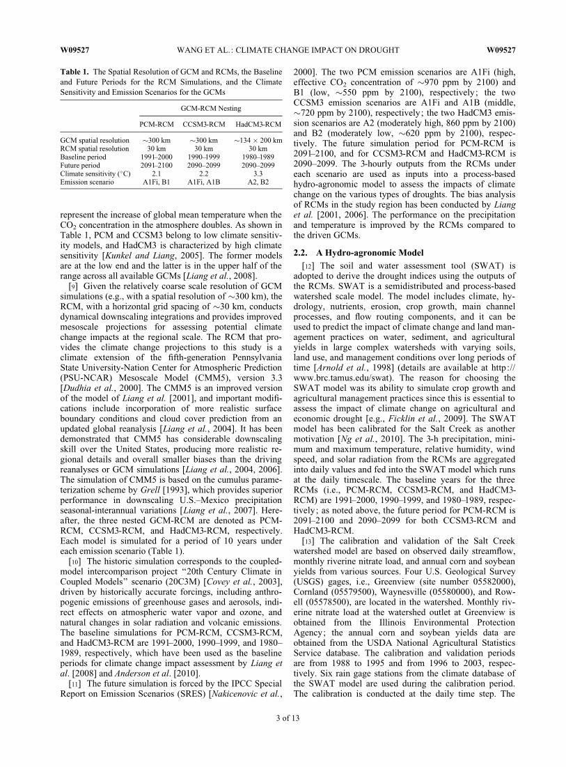
[6] The Salt Creek watershed in East-Central Illinois isused as a case study area. The watershed, �217 km south-west of Chicago, is a typical watershed in the Midwestwhere agriculture is the dominant activity (Figure 1). Theprimary crops are corn and soybeans planted in rotation.The Salt Creek is a tributary to the Sangamon River, whichin turn is a tributary to the Illinois River. The drainage areaof the Salt Creek watershed is 4786 km2. Approximately89% of the watershed is agricultural, with 80% cultivatedcrops and 9% rural grassland. One major urban area, thecity of Bloomington, is located in the watershed.

[7] Overall, our aim in this paper is to investigate the cli-mate change impact on drought by addressing two ques-tions: How reliable is the assessment of climate changeimpact on drought based on the state-of-the-art climatechange projections and downscaling techniques? Will theimpact be at the same level from meteorological, agricul-tural, and hydrologic perspectives? To deal with uncertaintyinvolved in climate change projection, the impact on a mete-

orological drought index is first assessed on the basis of dailyclimate inputs from RCMs driven by three GCMs in the cur-rent and a future period with two emission scenarios. Theclimate projections are fed to a calibrated hydro-agronomicmodel for the Salt Creek watershed in Central Illinois; theoutputs of the model are then used to evaluate the impact ofclimate change on agricultural drought and hydrologicaldrought. The intensity, duration, and frequency (IDF) of thevarious drought events are examined through IDF curves.Finally, an assessment of the drought impact on crop yieldin the study area is presented. In the remainder of the paper,we describe the methodology, followed by results, discus-sions, and conclusions.

2. Methodology2.1. Regional Climate Model (RCM)

[8] This study is based on high-resolution RCM simula-tions driven by output from historic and future simulationsof three GCMs, i.e., the U.S. Department of Energy andNational Center for Atmospheric Research Parallel ClimateModel (PCM) [Washington et al., 2000], the CommunityClimate System Model, version 3 (CCSM3) [Collins et al.,2006], and a global atmosphere-only model (HadAM3P)derived from the atmospheric GCM of the Hadley CentreCGCM (HadCM3) [Pope et al., 2000; Johns et al., 2003].These GCMs have different climate sensitivities, which

Figure 1. The regional climate grid, the Salt Creek Water-shed, and the boundaries of counties and State of Illinois.

W09527 WANG ET AL.: CLIMATE CHANGE IMPACT ON DROUGHT W09527

2 of 13

represent the increase of global mean temperature when theCO2 concentration in the atmosphere doubles. As shown inTable 1, PCM and CCSM3 belong to low climate sensitiv-ity models, and HadCM3 is characterized by high climatesensitivity [Kunkel and Liang, 2005]. The former modelsare at the low end and the latter is in the upper half of therange across all available GCMs [Liang et al., 2008].

[9] Given the relatively coarse scale resolution of GCMsimulations (e.g., with a spatial resolution of �300 km), theRCM, with a horizontal grid spacing of �30 km, conductsdynamical downscaling integrations and provides improvedmesoscale projections for assessing potential climatechange impacts at the regional scale. The RCM that pro-vides the climate change projections to this study is aclimate extension of the fifth-generation PennsylvaniaState University-Nation Center for Atmospheric Prediction(PSU-NCAR) Mesoscale Model (CMM5), version 3.3[Dudhia et al., 2000]. The CMM5 is an improved versionof the model of Liang et al. [2001], and important modifi-cations include incorporation of more realistic surfaceboundary conditions and cloud cover prediction from anupdated global reanalysis [Liang et al., 2004]. It has beendemonstrated that CMM5 has considerable downscalingskill over the United States, producing more realistic re-gional details and overall smaller biases than the drivingreanalyses or GCM simulations [Liang et al., 2004, 2006].The simulation of CMM5 is based on the cumulus parame-terization scheme by Grell [1993], which provides superiorperformance in downscaling U.S.–Mexico precipitationseasonal-interannual variations [Liang et al., 2007]. Here-after, the three nested GCM-RCM are denoted as PCM-RCM, CCSM3-RCM, and HadCM3-RCM, respectively.Each model is simulated for a period of 10 years undereach emission scenario (Table 1).

[10] The historic simulation corresponds to the coupled-model intercomparison project ‘‘20th Century Climate inCoupled Models’’ scenario (20C3M) [Covey et al., 2003],driven by historically accurate forcings, including anthro-pogenic emissions of greenhouse gases and aerosols, indi-rect effects on atmospheric water vapor and ozone, andnatural changes in solar radiation and volcanic emissions.The baseline simulations for PCM-RCM, CCSM3-RCM,and HadCM3-RCM are 1991–2000, 1990–1999, and 1980–1989, respectively, which have been used as the baselineperiods for climate change impact assessment by Liang etal. [2008] and Anderson et al. [2010].

[11] The future simulation is forced by the IPCC SpecialReport on Emission Scenarios (SRES) [Nakicenovic et al.,

2000]. The two PCM emission scenarios are A1Fi (high,effective CO2 concentration of �970 ppm by 2100) andB1 (low, �550 ppm by 2100), respectively; the twoCCSM3 emission scenarios are A1Fi and A1B (middle,�720 ppm by 2100), respectively; the two HadCM3 emis-sion scenarios are A2 (moderately high, 860 ppm by 2100)and B2 (moderately low, �620 ppm by 2100), respec-tively. The future simulation period for PCM-RCM is2091–2100, and for CCSM3-RCM and HadCM3-RCM is2090–2099. The 3-hourly outputs from the RCMs undereach scenario are used as inputs into a process-basedhydro-agronomic model to assess the impacts of climatechange on the various types of droughts. The bias analysisof RCMs in the study region has been conducted by Lianget al. [2001, 2006]. The performance on the precipitationand temperature is improved by the RCMs compared tothe driven GCMs.

2.2. A Hydro-agronomic Model[12] The soil and water assessment tool (SWAT) is

adopted to derive the drought indices using the outputs ofthe RCMs. SWAT is a semidistributed and process-basedwatershed scale model. The model includes climate, hy-drology, nutrients, erosion, crop growth, main channelprocesses, and flow routing components, and it can beused to predict the impact of climate change and land man-agement practices on water, sediment, and agriculturalyields in large complex watersheds with varying soils,land use, and management conditions over long periods oftime [Arnold et al., 1998] (details are available at http ://www.brc.tamus.edu/swat). The reason for choosing theSWAT model was its ability to simulate crop growth andagricultural management practices since this is essential toassess the impact of climate change on agricultural andeconomic drought [e.g., Ficklin et al., 2009]. The SWATmodel has been calibrated for the Salt Creek as anothermotivation [Ng et al., 2010]. The 3-h precipitation, mini-mum and maximum temperature, relative humidity, windspeed, and solar radiation from the RCMs are aggregatedinto daily values and fed into the SWAT model which runsat the daily timescale. The baseline years for the threeRCMs (i.e., PCM-RCM, CCSM3-RCM, and HadCM3-RCM) are 1991–2000, 1990–1999, and 1980–1989, respec-tively; as noted above, the future period for PCM-RCM is2091–2100 and 2090–2099 for both CCSM3-RCM andHadCM3-RCM.

[13] The calibration and validation of the Salt Creekwatershed model are based on observed daily streamflow,monthly riverine nitrate load, and annual corn and soybeanyields from various sources. Four U.S. Geological Survey(USGS) gages, i.e., Greenview (site number 05582000),Cornland (05579500), Waynesville (05580000), and Row-ell (05578500), are located in the watershed. Monthly riv-erine nitrate load at the watershed outlet at Greenview isobtained from the Illinois Environmental ProtectionAgency; the annual corn and soybean yields data areobtained from the USDA National Agricultural StatisticsService database. The calibration and validation periodsare from 1988 to 1995 and from 1996 to 2003, respec-tively. Six rain gage stations from the climate database ofthe SWAT model are used during the calibration period.The calibration is conducted at the daily time step. The

Table 1. The Spatial Resolution of GCM and RCMs, the Baselineand Future Periods for the RCM Simulations, and the ClimateSensitivity and Emission Scenarios for the GCMs

GCM-RCM Nesting

PCM-RCM CCSM3-RCM HadCM3-RCM

GCM spatial resolution �300 km �300 km �134 � 200 kmRCM spatial resolution 30 km 30 km 30 kmBaseline period 1991–2000 1990–1999 1980–1989Future period 2091–2100 2090–2099 2090–2099Climate sensitivity (�C) 2.1 2.2 3.3Emission scenario A1Fi, B1 A1Fi, A1B A2, B2


3 of 13

details of the SWAT model set up and calibration for SaltCreek watershed can be found from Ng et al. [2010].

2.3. Drought Indices[14] The literature is filled with numerous drought indi-

ces that have been developed and validated for variousregions of the globe. Keyantash and Dracup [2002] classi-fied droughts into three physical types: meteorologicaldrought resulting from precipitation deficits, agriculturaldrought identified by total soil moisture deficits, and hydro-logical drought related to a shortage of streamflow. In thisstudy, given that precipitation deficits can lead to thedecrease of soil moisture and streamflow deficits, and sub-sequently contribute to economic and agricultural losses,we incorporate an economic assessment component as afourth level of drought. Thus, to investigate the impactof projected climate change on drought at different levels,we select four indices to represent four different catego-ries, namely, meteorological, agricultural, hydrological,and economic.2.3.1. Meteorological Drought

[15] A well known meteorological drought index is thestandardized precipitation index (SPI) [Mckee et al., 1993],which has the advantages of flexibility, simplicity, adapta-bility to other hydroclimatic variables, and suitability forspatial comparison [Santos et al., 2010]. The SPI is used tomeasure precipitation shortage on the basis of the probabil-ity distribution of precipitation at different timescales. Forexample, to obtain the 1-month SPI, the distribution ofmonthly precipitation, which is typically similar to a gammadistribution [Wilks and Eggleston, 1992], is calculated foreach month separately. For the case of weekly SPI, whichalso follows a gamma distribution [Wu et al., 2005], SPI iscomputed at the weekly temporal scale using a 4 week aver-age precipitation to replace the value of the present week,and so on moving to the next week, i.e., a 4 week movingwindow is used for the statistics. In this setting it is possiblethat overlap exists between two drought events, and then thecounts of drought events may not be independent. For agiven value of precipitation, the cumulative probability forthe gamma distribution is transformed to a standard normaldistribution. Then, the SPI value is the z-value in the stand-ard normal distribution corresponding to the cumulativeprobability [McKee et al., 1993]. The transform ensures thatall distributions have a common basis. The detailed descrip-tion and the computer programs used to calculate SPI canbe found at the National Drought Mitigation Center web site(available online at http://www.drought.unl.edu/monitor).2.3.2. Agricultural and Hydrologic Droughts

[16] In this study, the agricultural drought index is repre-sented by a standardized soil water index (SSWI), which iscomputed using a similar procedure to the SPI calculation,but applied to the soil moisture time series obtained fromthe SWAT model simulation. The procedure for calculatingthe SSWI includes the following four steps: (1) the time se-ries of watershed averaged soil water content in the baselineperiod (10 years) is obtained from the SWAT model out-put; (2) the soil water content and runoff are fitted to proba-bility distributions; (3) the fitted distributions are used toestimate the cumulative probability of the soil moisturevalue of interest (either from the baseline year or from thefuture climate scenario); (4) the cumulative probability is

converted to the z-value of a normal distribution with zeromean and unit variance. The standardized runoff index(SRI) proposed by Shukla and Wood [2008] is used to rep-resent the hydrological drought. SRI is computed using aprocedure similar to the SPI and SSWI calculations.2.3.3. Economic Drought

[17] Crop yield is used as a monetary measure to quan-tify the economic impact associated with each of theprojected climate change scenarios. Crop yield is linked tothe three previously described drought indices (SPI, SSWI,and SRI). The crop yield is an annual value while the otherdrought indices are weekly. Given that each climate sce-nario is only 10 year long, the sample size of the crop yieldis 10 instead of 520 (52 weeks in 1 year � 10 years) for theother three drought indices. This limits our ability to derivean economic drought indicator in a similar fashion to thethree other indices. Thus, we limit our economic analysisto provide an economic assessment under both current(baseline) climatic conditions and future climatic projec-tions. Two crops are grown in the case study, i.e., corn andsoybeans which are rotated by year.

[18] In this study, the connections among the varioustypes of indices are implemented through the SWAT simu-lation model, allowing for a unified framework of compari-son among the indices under the impact of climate change.Note that the model is calibrated in terms of streamflowusing the USGS observations for the baseline period. Allthe drought indices in the future periods are computed withrespect to the baseline conditions, i.e., the fitted distribu-tions, through which the drought index values are com-puted for both baseline and future years, is constructed onthe basis of the baseline years. The weekly precipitation inthe baseline years is fitted by a gamma distribution; runoffis fitted by a lognormal distribution; for soil water content(�), a lognormal distribution is fitted to �0 ¼ �max � �,where �max is maximum soil water content.

[19] Next, we describe a consistent approach to quantifythe impacts of climate change projections on drought char-acteristics, such as intensity, duration, and frequency.

2.4. Intensity-Duration-Frequency Curve of Drought[20] Drought characteristics include onset, end, intensity,

duration, frequency and magnitude [Dracup et al., 1980],and areal extent [Andreadis et al., 2005]. These droughtcharacteristics can be quantified for any drought indicator.Following the concept of establishing intensity-duration-frequency (IDF) curves for rainfall, commonly used inhydrological design standards, we derive the IDF curvesfor droughts using a similar approach. Unlike rainfallevents, droughts tend to persist for much longer duration.Thus, drought intensity can be defined as the averagedrought severity or magnitude (measured as SPI, SSWI, orSRI) over a particular duration (here in weeks). These IDFcurves are specific to the case study, but in general candescribe how drought characteristics change under climatechange scenarios. The following procedures are employedin this study for deriving the drought IDF curves for thebaseline years and the future years:

[21] 1. Determine the temporal scale for computing thedrought indices. For both baseline and future years, the avail-able data are the 10 year daily time series of precipitation,soil moisture, and streamflow. In this study, the weekly


4 of 13

values of these variables are used to compute the corre-sponding drought indices.

[22] 2. Identify the drought events. SPI values between0 and �0.99, �1.00 and �1.49, �1.50 and �1.99, and lessthan �2.00 are defined as mild drought, moderate, severe,and extreme drought, respectively [McKee, 1993]. In thisstudy, drought events with intensity I less than �1.0 arepresented.

[23] 3. Perform drought frequency analysis. Given dura-tion and intensity, the number of drought event (N) iscounted during the 10 year period of baseline or future years.

[24] 4. Construct the intensity-duration-frequency curveof drought for the baseline period and the future period(2090–2100) under the two emission scenarios from eachnested GCM-RCM.

[25] It should be noted that given only the 10 year periodfor future projections available for this study, our analysisis limited to short-term instead of long-term droughts thatmay last for multiple years. To assess the uncertainty intro-duced by using 10 year simulations of the future, droughtanalysis is conducted on the basis of historical climate dataduring three 10 year periods (i.e., 1971–1980, 1981–1990,and 1991–2000).

2.5. Drought Characteristics of the Case StudyWatershed

[26] Coupling the climate change scenarios with thehydro-agronomic model to calculate the drought indices andtheir characteristics as discussed above, we proceed toaddress our research questions about the impact of climatechange on various drought indices and their characteristics.We start with the construction of each of the drought indextime series underlying each of the climate change scenarios.For both baseline and future periods, the daily average valuesof climate variables including precipitation from one gridpoint (Figure 1) are used as the input of the SWAT model.As we can see in Figure 1, four RCM grid points are withinthe Salt Creek watershed, and the values of the climate varia-bles from individual RCMs are almost identical over thesegrid points. Moreover, the historical observation of climatevariables is point-based, therefore the climate time seriesfrom one grid point is used for the impact assessment.

[27] The time series of SPI, SSWI, and SRI drought indi-ces are constructed using (1) daily precipitation outputfrom each of the nine scenarios of GCM-RCM and emis-sion scenarios, as well as the baseline scenario; and (2) thedaily outputs of soil water content and streamflow from theSWAT simulation model, which uses a number of sub-watersheds (100 for the case study area) in a semidistrib-uted form. The following procedures are undertaken: Theweekly SPI is computed from the daily meteorological dataduring the 10 year period from the RCMs and historicaldata. Recall that the weekly SPI is computed using a4 week moving average of the precipitation time series.The SSWI is based on the averaged soil water content overthe entire watershed, and the SRI is based on the runoffat the outlet of the watershed.

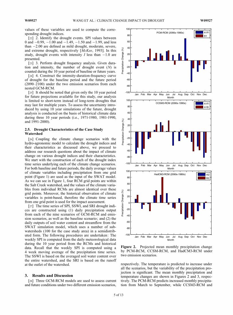
3. Results and Discussion[28] Three GCM-RCM models are used to assess current

and future conditions under two different emission scenarios,

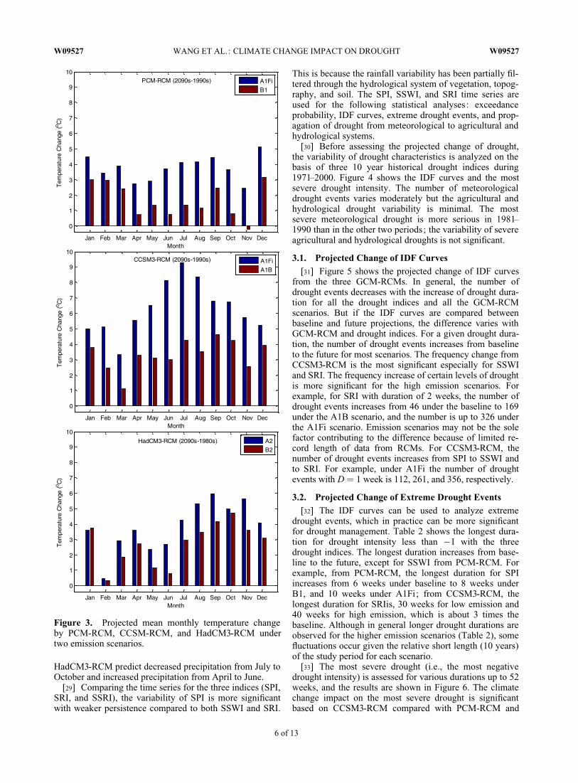
respectively. The temperature is predicted to increase underall the scenarios, but the variability of the precipitation pro-jection is significant. The mean monthly precipitation andtemperature changes are shown in Figures 2 and 3, respec-tively. The PCM-RCM predicts increased monthly precipita-tion from March to September, while CCSM3-RCM and

Figure 2. Projected mean monthly precipitation changeby PCM-RCM, CCSM-RCM, and HadCM3-RCM undertwo emission scenarios.


5 of 13

HadCM3-RCM predict decreased precipitation from July toOctober and increased precipitation from April to June.

[29] Comparing the time series for the three indices (SPI,SRI, and SSRI), the variability of SPI is more significantwith weaker persistence compared to both SSWI and SRI.

This is because the rainfall variability has been partially fil-tered through the hydrological system of vegetation, topog-raphy, and soil. The SPI, SSWI, and SRI time series areused for the following statistical analyses: exceedanceprobability, IDF curves, extreme drought events, and prop-agation of drought from meteorological to agricultural andhydrological systems.

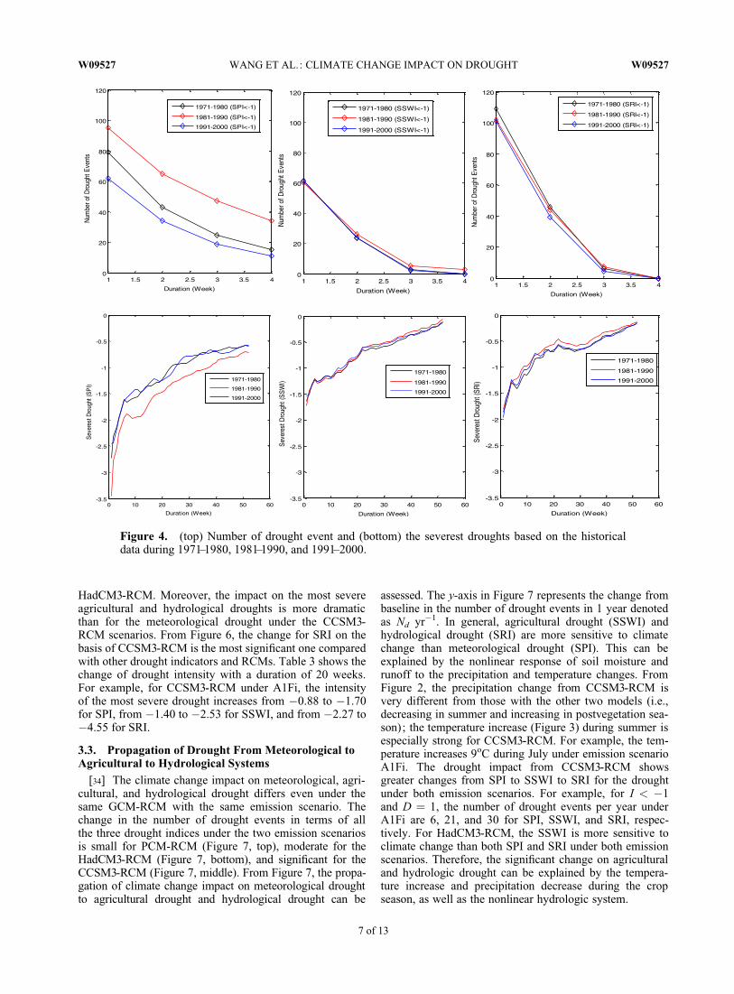
[30] Before assessing the projected change of drought,the variability of drought characteristics is analyzed on thebasis of three 10 year historical drought indices during1971–2000. Figure 4 shows the IDF curves and the mostsevere drought intensity. The number of meteorologicaldrought events varies moderately but the agricultural andhydrological drought variability is minimal. The mostsevere meteorological drought is more serious in 1981–1990 than in the other two periods; the variability of severeagricultural and hydrological droughts is not significant.

3.1. Projected Change of IDF Curves[31] Figure 5 shows the projected change of IDF curves

from the three GCM-RCMs. In general, the number ofdrought events decreases with the increase of drought dura-tion for all the drought indices and all the GCM-RCMscenarios. But if the IDF curves are compared betweenbaseline and future projections, the difference varies withGCM-RCM and drought indices. For a given drought dura-tion, the number of drought events increases from baselineto the future for most scenarios. The frequency change fromCCSM3-RCM is the most significant especially for SSWIand SRI. The frequency increase of certain levels of droughtis more significant for the high emission scenarios. Forexample, for SRI with duration of 2 weeks, the number ofdrought events increases from 46 under the baseline to 169under the A1B scenario, and the number is up to 326 underthe A1Fi scenario. Emission scenarios may not be the solefactor contributing to the difference because of limited re-cord length of data from RCMs. For CCSM3-RCM, thenumber of drought events increases from SPI to SSWI andto SRI. For example, under A1Fi the number of droughtevents with D ¼ 1 week is 112, 261, and 356, respectively.

3.2. Projected Change of Extreme Drought Events[32] The IDF curves can be used to analyze extreme

drought events, which in practice can be more significantfor drought management. Table 2 shows the longest dura-tion for drought intensity less than �1 with the threedrought indices. The longest duration increases from base-line to the future, except for SSWI from PCM-RCM. Forexample, from PCM-RCM, the longest duration for SPIincreases from 6 weeks under baseline to 8 weeks underB1, and 10 weeks under A1Fi; from CCSM3-RCM, thelongest duration for SRIis, 30 weeks for low emission and40 weeks for high emission, which is about 3 times thebaseline. Although in general longer drought durations areobserved for the higher emission scenarios (Table 2), somefluctuations occur given the relative short length (10 years)of the study period for each scenario.

[33] The most severe drought (i.e., the most negativedrought intensity) is assessed for various durations up to 52weeks, and the results are shown in Figure 6. The climatechange impact on the most severe drought is significantbased on CCSM3-RCM compared with PCM-RCM and

Figure 3. Projected mean monthly temperature changeby PCM-RCM, CCSM-RCM, and HadCM3-RCM undertwo emission scenarios.


6 of 13

HadCM3-RCM. Moreover, the impact on the most severeagricultural and hydrological droughts is more dramaticthan for the meteorological drought under the CCSM3-RCM scenarios. From Figure 6, the change for SRI on thebasis of CCSM3-RCM is the most significant one comparedwith other drought indicators and RCMs. Table 3 shows thechange of drought intensity with a duration of 20 weeks.For example, for CCSM3-RCM under A1Fi, the intensityof the most severe drought increases from �0.88 to �1.70for SPI, from �1.40 to �2.53 for SSWI, and from �2.27 to�4.55 for SRI.

3.3. Propagation of Drought From Meteorological toAgricultural to Hydrological Systems

[34] The climate change impact on meteorological, agri-cultural, and hydrological drought differs even under thesame GCM-RCM with the same emission scenario. Thechange in the number of drought events in terms of allthe three drought indices under the two emission scenariosis small for PCM-RCM (Figure 7, top), moderate for theHadCM3-RCM (Figure 7, bottom), and significant for theCCSM3-RCM (Figure 7, middle). From Figure 7, the propa-gation of climate change impact on meteorological droughtto agricultural drought and hydrological drought can be

assessed. The y-axis in Figure 7 represents the change frombaseline in the number of drought events in 1 year denotedas Nd yr�1. In general, agricultural drought (SSWI) andhydrological drought (SRI) are more sensitive to climatechange than meteorological drought (SPI). This can beexplained by the nonlinear response of soil moisture andrunoff to the precipitation and temperature changes. FromFigure 2, the precipitation change from CCSM3-RCM isvery different from those with the other two models (i.e.,decreasing in summer and increasing in postvegetation sea-son); the temperature increase (Figure 3) during summer isespecially strong for CCSM3-RCM. For example, the tem-perature increases 9oC during July under emission scenarioA1Fi. The drought impact from CCSM3-RCM showsgreater changes from SPI to SSWI to SRI for the droughtunder both emission scenarios. For example, for I < �1and D ¼ 1, the number of drought events per year underA1Fi are 6, 21, and 30 for SPI, SSWI, and SRI, respec-tively. For HadCM3-RCM, the SSWI is more sensitive toclimate change than both SPI and SRI under both emissionscenarios. Therefore, the significant change on agriculturaland hydrologic drought can be explained by the tempera-ture increase and precipitation decrease during the cropseason, as well as the nonlinear hydrologic system.

Figure 4. (top) Number of drought event and (bottom) the severest droughts based on the historicaldata during 1971–1980, 1981–1990, and 1991–2000.


7 of 13

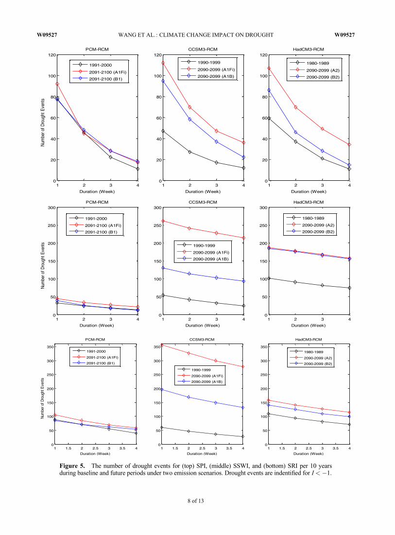
Figure 5. The number of drought events for (top) SPI, (middle) SSWI, and (bottom) SRI per 10 yearsduring baseline and future periods under two emission scenarios. Drought events are indentified for I < �1.


8 of 13

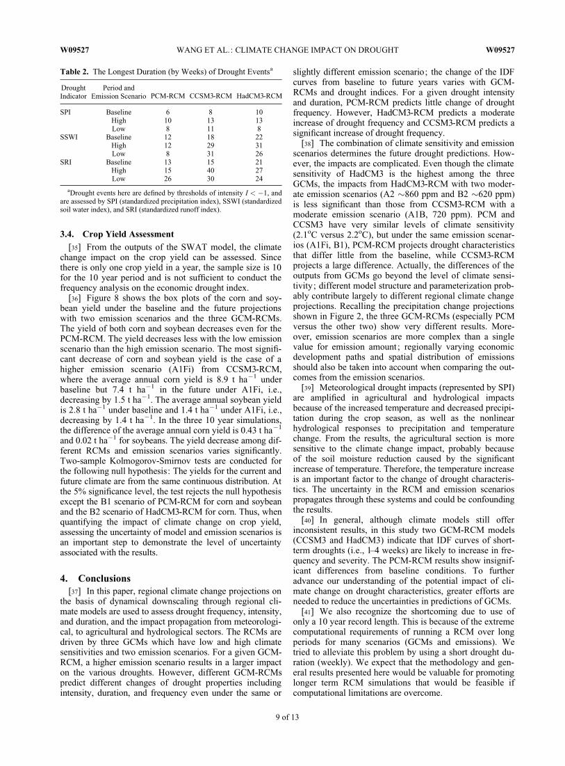
3.4. Crop Yield Assessment[35] From the outputs of the SWAT model, the climate

change impact on the crop yield can be assessed. Sincethere is only one crop yield in a year, the sample size is 10for the 10 year period and is not sufficient to conduct thefrequency analysis on the economic drought index.

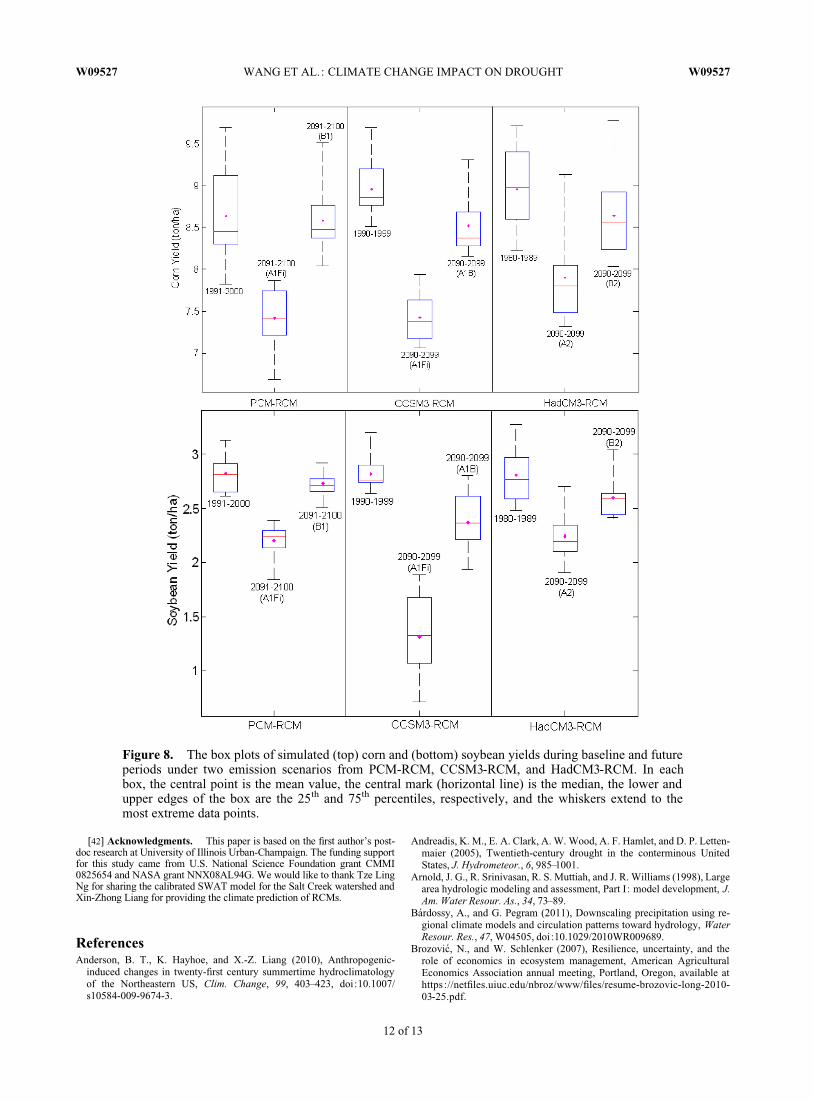
[36] Figure 8 shows the box plots of the corn and soy-bean yield under the baseline and the future projectionswith two emission scenarios and the three GCM-RCMs.The yield of both corn and soybean decreases even for thePCM-RCM. The yield decreases less with the low emissionscenario than the high emission scenario. The most signifi-cant decrease of corn and soybean yield is the case of ahigher emission scenario (A1Fi) from CCSM3-RCM,where the average annual corn yield is 8.9 t ha�1 underbaseline but 7.4 t ha�1 in the future under A1Fi, i.e.,decreasing by 1.5 t ha�1. The average annual soybean yieldis 2.8 t ha�1 under baseline and 1.4 t ha�1 under A1Fi, i.e.,decreasing by 1.4 t ha�1. In the three 10 year simulations,the difference of the average annual corn yield is 0.43 t ha�1

and 0.02 t ha�1 for soybeans. The yield decrease among dif-ferent RCMs and emission scenarios varies significantly.Two-sample Kolmogorov-Smirnov tests are conducted forthe following null hypothesis: The yields for the current andfuture climate are from the same continuous distribution. Atthe 5% significance level, the test rejects the null hypothesisexcept the B1 scenario of PCM-RCM for corn and soybeanand the B2 scenario of HadCM3-RCM for corn. Thus, whenquantifying the impact of climate change on crop yield,assessing the uncertainty of model and emission scenarios isan important step to demonstrate the level of uncertaintyassociated with the results.

4. Conclusions[37] In this paper, regional climate change projections on

the basis of dynamical downscaling through regional cli-mate models are used to assess drought frequency, intensity,and duration, and the impact propagation from meteorologi-cal, to agricultural and hydrological sectors. The RCMs aredriven by three GCMs which have low and high climatesensitivities and two emission scenarios. For a given GCM-RCM, a higher emission scenario results in a larger impacton the various droughts. However, different GCM-RCMspredict different changes of drought properties includingintensity, duration, and frequency even under the same or

slightly different emission scenario; the change of the IDFcurves from baseline to future years varies with GCM-RCMs and drought indices. For a given drought intensityand duration, PCM-RCM predicts little change of droughtfrequency. However, HadCM3-RCM predicts a moderateincrease of drought frequency and CCSM3-RCM predicts asignificant increase of drought frequency.

[38] The combination of climate sensitivity and emissionscenarios determines the future drought predictions. How-ever, the impacts are complicated. Even though the climatesensitivity of HadCM3 is the highest among the threeGCMs, the impacts from HadCM3-RCM with two moder-ate emission scenarios (A2 �860 ppm and B2 �620 ppm)is less significant than those from CCSM3-RCM with amoderate emission scenario (A1B, 720 ppm). PCM andCCSM3 have very similar levels of climate sensitivity(2.1oC versus 2.2oC), but under the same emission scenar-ios (A1Fi, B1), PCM-RCM projects drought characteristicsthat differ little from the baseline, while CCSM3-RCMprojects a large difference. Actually, the differences of theoutputs from GCMs go beyond the level of climate sensi-tivity; different model structure and parameterization prob-ably contribute largely to different regional climate changeprojections. Recalling the precipitation change projectionsshown in Figure 2, the three GCM-RCMs (especially PCMversus the other two) show very different results. More-over, emission scenarios are more complex than a singlevalue for emission amount; regionally varying economicdevelopment paths and spatial distribution of emissionsshould also be taken into account when comparing the out-comes from the emission scenarios.

[39] Meteorological drought impacts (represented by SPI)are amplified in agricultural and hydrological impactsbecause of the increased temperature and decreased precipi-tation during the crop season, as well as the nonlinearhydrological responses to precipitation and temperaturechange. From the results, the agricultural section is moresensitive to the climate change impact, probably becauseof the soil moisture reduction caused by the significantincrease of temperature. Therefore, the temperature increaseis an important factor to the change of drought characteris-tics. The uncertainty in the RCM and emission scenariospropagates through these systems and could be confoundingthe results.

[40] In general, although climate models still offerinconsistent results, in this study two GCM-RCM models(CCSM3 and HadCM3) indicate that IDF curves of short-term droughts (i.e., 1–4 weeks) are likely to increase in fre-quency and severity. The PCM-RCM results show insignif-icant differences from baseline conditions. To furtheradvance our understanding of the potential impact of cli-mate change on drought characteristics, greater efforts areneeded to reduce the uncertainties in predictions of GCMs.

[41] We also recognize the shortcoming due to use ofonly a 10 year record length. This is because of the extremecomputational requirements of running a RCM over longperiods for many scenarios (GCMs and emissions). Wetried to alleviate this problem by using a short drought du-ration (weekly). We expect that the methodology and gen-eral results presented here would be valuable for promotinglonger term RCM simulations that would be feasible ifcomputational limitations are overcome.

Table 2. The Longest Duration (by Weeks) of Drought Eventsa

DroughtIndicator

Period andEmission Scenario PCM-RCM CCSM3-RCM HadCM3-RCM

SPI Baseline 6 8 10High 10 13 13Low 8 11 8

SSWI Baseline 12 18 22High 12 29 31Low 8 31 26

SRI Baseline 13 15 21High 15 40 27Low 26 30 24

aDrought events here are defined by thresholds of intensity I < �1, andare assessed by SPI (standardized precipitation index), SSWI (standardizedsoil water index), and SRI (standardized runoff index).


9 of 13

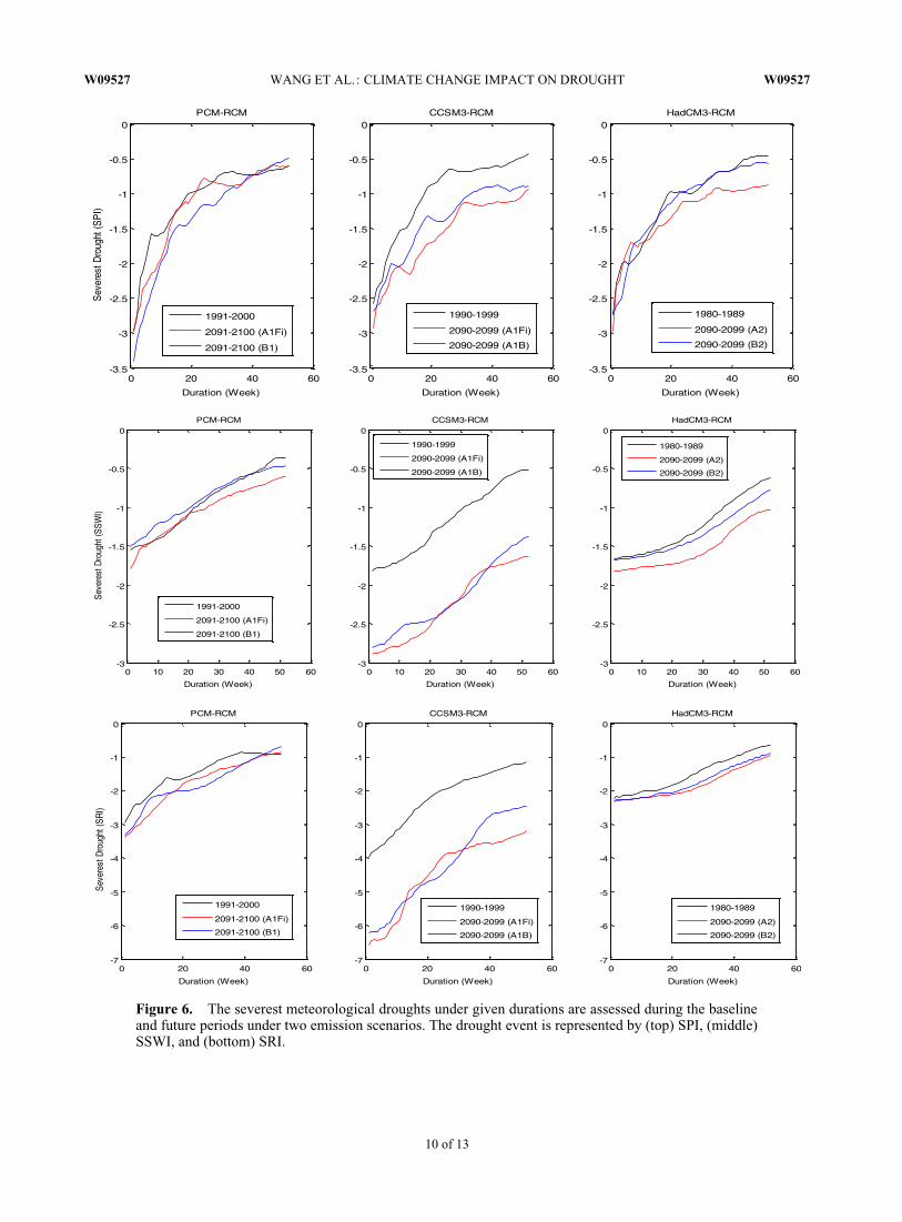
Figure 6. The severest meteorological droughts under given durations are assessed during the baselineand future periods under two emission scenarios. The drought event is represented by (top) SPI, (middle)SSWI, and (bottom) SRI.


10 of 13

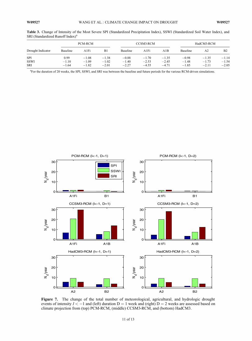
Table 3. Change of Intensity of the Most Severe SPI (Standardized Precipitation Index), SSWI (Standardized Soil Water Index), andSRI (Standardized Runoff Index)a

Drought Indicator

PCM-RCM CCSM3-RCM HadCM3-RCM

Baseline A1Fi B1 Baseline A1Fi A1B Baseline A2 B2

SPI 0.99 �1.08 �1.38 �0.88 �1.70 �1.35 �0.98 �1.35 �1.14SSWI �1.10 �1.09 �1.02 �1.40 �2.53 �2.45 �1.48 �1.73 �1.54SRI �1.64 �1.82 �2.01 �2.27 �4.55 �4.71 �1.85 �2.11 �2.05

aFor the duration of 20 weeks, the SPI, SSWI, and SRI was between the baseline and future periods for the various RCM-driven simulations.

Figure 7. The change of the total number of meteorological, agricultural, and hydrologic droughtevents of intensity I < �1 and (left) duration D ¼ 1 week and (right) D ¼ 2 weeks are assessed based onclimate projection from (top) PCM-RCM, (middle) CCSM3-RCM, and (bottom) HadCM3.


11 of 13

[42] Acknowledgments. This paper is based on the first author’s post-doc research at University of Illinois Urban-Champaign. The funding supportfor this study came from U.S. National Science Foundation grant CMMI0825654 and NASA grant NNX08AL94G. We would like to thank Tze LingNg for sharing the calibrated SWAT model for the Salt Creek watershed andXin-Zhong Liang for providing the climate prediction of RCMs.

ReferencesAnderson, B. T., K. Hayhoe, and X.-Z. Liang (2010), Anthropogenic-

induced changes in twenty-first century summertime hydroclimatologyof the Northeastern US, Clim. Change, 99, 403–423, doi:10.1007/s10584-009-9674-3.

Andreadis, K. M., E. A. Clark, A. W. Wood, A. F. Hamlet, and D. P. Letten-maier (2005), Twentieth-century drought in the conterminous UnitedStates, J. Hydrometeor., 6, 985–1001.

Arnold, J. G., R. Srinivasan, R. S. Muttiah, and J. R. Williams (1998), Largearea hydrologic modeling and assessment, Part I: model development, J.Am. Water Resour. As., 34, 73–89.

Bardossy, A., and G. Pegram (2011), Downscaling precipitation using re-gional climate models and circulation patterns toward hydrology, WaterResour. Res., 47, W04505, doi:10.1029/2010WR009689.

Brozovic, N., and W. Schlenker (2007), Resilience, uncertainty, and therole of economics in ecosystem management, American AgriculturalEconomics Association annual meeting, Portland, Oregon, available athttps ://netfiles.uiuc.edu/nbroz/www/files/resume-brozovic-long-2010-03-25.pdf.

Figure 8. The box plots of simulated (top) corn and (bottom) soybean yields during baseline and futureperiods under two emission scenarios from PCM-RCM, CCSM3-RCM, and HadCM3-RCM. In eachbox, the central point is the mean value, the central mark (horizontal line) is the median, the lower andupper edges of the box are the 25th and 75th percentiles, respectively, and the whiskers extend to themost extreme data points.


12 of 13

Brozovic, N., D. L. Sunding, and D. Zilberman (2007), Estimating businessand residential water supply interruption losses from catastrophic events,Water Resour. Res., 43(14), W08423, doi:10.1029/2005WR004782.

Burke, E. J., and S. J. Brown (2008), Evaluating uncertainties in the projec-tion of future drought, J. Hydrometeor., 9, 292–299.

Burke, E. J., S. J. Brown, and N. Christidis (2006), Modeling the recent evo-lution of global drought and projections for the 21st century with theHadley Centre climate model, J. Hydrometeor., 7, 1113–1125.

Collins, W. D., et al. (2006), The Community Climate System Model, ver-sion 3 (CCSM3), J. Clim., 19, 2122–2143.

Covey, C., K. M. AchutaRao, U. Cubasch, P. Jones, S. J. Lambert, M. E.Mann, T. J. Phillips, and K. E. Taylor (2003), An Overview of Resultsfrom the Coupled Model Intercomparison Project (CMIP), GlobalPlanet. Change, 37, 103–133.

Dracup, J. A., K. S. Lee, and E. G. Paulson Jr. (1980), On the definition ofdroughts, Water Resour. Res., 16(2), 297–302, doi:10.1029/WR016i002p00297.

Dudhia, J., D. Gill, Y. R. Guo, K. Manning, W. Wang, and J. Chiszar(2000), PSU/NCAR Mesoscale Modelling System Tutorial Class Notesand User’s Guide: MM5 Modelling System Version 3. Tech. Rep., 138pp., National Center for Atmospheric Research Boulder, CO,available athttp://www.mmm.ucar.edu/mm5/documents/.

Ficklin, D. L., Y. Luo, E. Luedeling, and M. Zhang (2009), Climate changesensitivity assessment of a highly agricultural watershed using SWAT, J.Hydrol., 374, 16–29.

Grell, G. A. (1993), Prognostic evaluation of assumptions used by cumulusparameterizations, Mon. Wea. Rev., 121, 764–787.

Hayes, M., D. A. Wilhite, M. Svodoba, and O. Vanyarkho (1999), Monitor-ing the 1996 drought using the standardized precipitation index, Bull.Am. Meteorol. Soc., 80, 429–438, doi:10.1175/1520-0477(1999),080<0429:MTDUTS>2.0.CO;2.

Intergovernmental Panel on Climate Change (IPCC) (2006), Fourth Assess-ment Report (FAR), Cambridge Univ. Press, Cambridge, U. K.

Johns, T. C. et al. (2003), Anthropogenic climate change for 1860 to 2100simulated with the HadCM3 model under updated emissions scenarios,Clim. Dyn., 583-612, doi:10.1007/s00382-002-0296-y.

Johnson, F., and A. Sharma (2011), Accounting for interannual variability: Acomparison of options for water resources climate change impact assess-ments, Water Resour. Res., 47, W04508, doi:10.1029/2010WR009272.

Keyantash, J., and J. A. Dracup (2002), The quantification of drought: Anevaluation of drought indices, Bull. Amer. Meteor. Soc., 83, 1167–1180.

Kunkel, K. E., and X.-Z. Liang (2005), GCM simulations of the climate inthe central United States, J. Clim., 18, 1016–1031.

Leung, L. R., Y. Qian, X. Bian, W. M. Washington, J. Han, and J. O. Roads(2004), Mid-century ensemble regional climate change scenarios for theWestern United States, Clim. Change, 62, 75–113.

Liang, X.-Z., K. E. Kunkel, and A. N. Samel (2001), Development of a re-gional climate model for U.S. Midwest applications. Part I : Sensitivity tobuffer zone treatment, J. Climate, 14, 4363–4378.

Liang, X.-Z., L. Li, K. E. Kunkel, M. Ting, and J. X. L. Wang (2004), Re-gional climate model simulation of U.S. precipitation during 1982–2002,Part 1: Annual cycle, J. Clim., 17, 3510–3528.

Liang, X.-Z., J. Pan, J. Zhu, K. E. Kunkel, J. X. L. Wang, and A. Dai (2006),Regional climate model downscaling of the U.S. summer climate and futurechange, J. Geophys. Res., 111, D10108, doi:10.1029/2005JD006685.

Liang, X.-Z., M. Xu, K. E. Kunkel, G. A. Grell, and J. Kain (2007), Re-gional climate model simulation of U.S.-Mexico summer precipitation

using the optimal ensemble of two cumulus parameterizations, J. Clim.,20, 5201–5207.

Liang, X.-Z., K. E. Kunkel, G. A. Meehl, R. G. Jones, and J. X. L. Wang(2008), Regional climate models downscaling analysis of generalcirculation models present climate biases propagation into future changeprojections, Geophys. Res. Lett., 35, L08709, doi:10.1029/2007GL032849.

McKee, T. B., N. J. Doesken, and J. Kliest (1993), The relationship ofdrought frequency and duration to time scales, paper presented at the 8thConference of Applied Climatology, Am. Meterol. Soc., Anaheim, Calif.

Nakicenovic, N. et al. (2000), Special Report on Emissions Scenarios: ASpecial Report of Working Group III of the Intergovernmental Panel onClimate Change, 599 pp., Cambridge University Press, Cambridge, U.K.[Available at: http://www.grida.no/climate/ipcc/emission/index.htm].

National Research Council (NRC) (2006), Completing the Forecast: Char-acterizing and Communicating Uncertainty for Better Decisions UsingWeather and Climate Forecasts, Washington DC.

Ng, T. L., J. W. Eheart, X. Cai, and F. Miguez (2010), Modeling miscanthusin the soil and water assessment tool (SWAT) to simulate its water qual-ity effects as a bioenergy crop, Environ. Sci. Technol., 44(18), 7138–7144, doi:10.1021/es9039677.

Pope, V. D., M. L. Gallani, P. R. Rowntree, and R. A. Stratton (2000), Theimpact of new physical parametrizations in the Hadley Centre climatemodel: HadAM3, Clim. Dyn., 16, 123–146.

Ross, T., and N. Lott (2003), A Climatology of 1980–2003 ExtremeWeather and Climate Events, Technical Report 2003-01, NOAA, Dept.of Commence, Asheville, NC.

Santos, J. F., I. Pulido-Calvo, and M. M. Portela (2010), Spatial and tempo-ral variability of droughts in Portugal, Water Resour. Res., 46, W03503,doi:10.1029/2009WR008071.

Schlenker, W., and M. Roberts (2006), Nonlinear effects of weather oncrop yields: implications for climate change, paper presented at the ThirdWorld Congress of Environmental and Resource Economists, Kyoto, Ja-pan, July 3–7.

Shukla, S., and A. W. Wood (2008), Use of a standardized runoff index forcharacterizing hydrologic drought, Geophys. Res. Lett., 35, L02405,doi:10.1029/2007GL032487.

Washington, W. M., et al. (2000), Parallel climate model (PCM) controland transient simulations, Clim. Dyn., 16, 755–774.

Wilhite, D. A., and R. S. Pulwarty (2005), Drought and water crises: Les-sons learned and the road ahead, in Drought and Water Crises: Science,Technology, and Management Issues, edited by D. A. Wilhite, pp. 389–398. CRC Press, Boca Raton, FL.

Wilks, D. S., and K. L. Eggleston (1992), Estimating monthly and seasonalprecipitation distributions using the 30- and 90-day outlooks, J. Climate,5, 252–259.

Wu, H., M. J. Hayes, D. Wilhite, and M. D. Svoboda (2005), The effect ofthe length of record on the Standardized Precipitation Index calculation,Int. J. Clim., 25, 505–520.

X. Cai, A. J. Valocchi, and D. Wang, Department of Civil and Environ-mental Engineering, University of Illinois at Urbana-Champaign, 301 N.Mathews Ave., Urbana, IL 61801, USA. ([email protected])

M. Hejazi, Joint Global Change Research Institute, Pacific NorthwestNational Laboratory, 5825 University Research Ct., Ste. 3500, CollegePark, MD 20740, USA.


13 of 13

Documents

Climate change impact on meteorological, agricultural, and hydrological drought in central Illinois