Cluster Mass Functions in the Large and Small Magellanic Clouds: Fading and Size-of-Sample Effects

arX

iv:a

stro

-ph/

0306

528v

1 2

5 Ju

n 20

03

Cluster Mass Functions in the Large and Small Magellanic

Clouds: Fading and Size of Sample Effects

Deidre A. Hunter

Lowell Observatory, 1400 West Mars Hill Road, Flagstaff, Arizona 86001 USA

[email protected]

Bruce G. Elmegreen

IBM T. J. Watson Research Center, PO Box 218, Yorktown Heights, New York 10598 USA

[email protected]

Trent J. Dupuy1,

and

Michael Mortonson2

Lowell Observatory, 1400 West Mars Hill Road, Flagstaff, Arizona 86001 USA

[email protected], [email protected]

ABSTRACT

The properties of ∼ 939 star clusters in the Large and Small Magellanic

Clouds were determined from ground-based CCD images in UBVR passbands.

The areal coverage was extensive, corresponding to 11.0 kpc2 in the LMC and 8.3

kpc2 in the SMC. After corrections for reddening, the colors and magnitudes of

the clusters were converted to ages and masses, and the resulting mass distribu-

tions were searched for the effects of fading, evaporation, and size-of-sample bias.

The data show a clear signature of cluster fading below the detection threshold.

The initial cluster mass function (ICMF) was determined by fitting the mass and

age distributions with cluster population models. These models suggest a new

method to determine the ICMF that is nearly independent of fading or disrup-

tion and is based on the slope of a correlation between age and the maximum

cluster mass in equally spaced intervals of log-age. For a nearly uniform star

formation rate, this correlation has a slope equal to 1/ (α − 1) for an ICMF of

dn(M)/dM ∝ M−α. We determine that α is between 2 and 2.4 for the LMC

and SMC using this method plus another method in which models are fit to the

http://arxiv.org/abs/astro-ph/0306528v1

– 2 –

mass distribution integrated over age and to the age distribution integrated over

mass. The maximum mass method also suggests that the cluster formation rate

in the LMC age gap between 3 and 13 Gy is about a factor of ten below that

in the period from 0.1 Gy to 1 Gy. The oldest clusters correspond in age and

mass to halo globular clusters in the Milky Way. They do not fit the trends

for lower-mass clusters but appear to be a separate population that either had

a very high star formation rate and became depleted by evaporation or formed

with only high masses.

Subject headings: galaxies: irregular—Magellanic Clouds—galaxies: star clusters

1. Introduction

Super-star clusters are extreme among clusters of stars. They are compact and very

luminous, and many are young versions of the massive globular clusters found in giant

galaxies like the Milky Way. The Milky Way, however, has not been able to form a cluster as

compact and massive as a globular cluster for about 10 Gy (although there is a controversial

claim that one is forming now—Knodlseder 2000). In spite of this, six super-star clusters are

known in five nearby dwarf irregular (dIm) galaxies and are inferred to be present, though

still embedded, in 4 others. This led Billett, Hunter, & Elmegreen (2002) to question what

conditions allowed these tiny Im galaxies to form such massive clusters.

Billett et al. (2002) undertook a survey of a sample of Im galaxies that had been observed

by the Hubble Space Telescope. They searched 22 galaxies for super-star clusters and the less

extreme populous clusters. They found that super-star clusters are actually relatively rare

in Im galaxies, but when they form, they seem to be anomalously luminous compared to

other clusters in the galaxy. That is, the super-star clusters in these galaxies are not part of

the normal cluster population as they are in spirals (Larsen & Richtler 2000). Furthermore,

most of the Im galaxies that contain them are interacting with another galaxy or undergoing

a starburst, suggesting that special events in the life of the galaxy are required to produce

the conditions necessary to form the most massive star clusters.

We were intrigued by the question of where the Magellanic Clouds would fall in this

scheme of cluster formation. We knew that the LMC contained at least one super-star cluster

1Current address: The University of Texas, Austin, Texas 78712 USA

2Current address: Massachusetts Institute of Technology, Cambridge, Massachusetts 02139 USA

– 3 –

and that both the LMC and SMC contained numerous populous clusters. Therefore, it was

not obvious to us that the massive star clusters in these galaxies would stand apart from

the rest of the cluster population. The work of Larsen & Richtler (2000), in fact, suggested

that the Magellanic Clouds follow the correlations set by giant spirals, implying that the

formation of massive star clusters is just part of the normal cluster formation process in

these galaxies.

Surveys of clusters in most Im galaxies are incomplete for all but the most massive star

clusters. The exceptions are the LMC and SMC which are close enough for a detailed survey

of even faint clusters. Hodge (1988) predicted that there are of order 4200 clusters in the

LMC, and current catalogues list 6659 clusters and associations (Bica et al. 1999). In the

SMC, Hodge (1986) predicted 2000 clusters and the Bica & Dutra (2000) catalog contains

1237 clusters and associations. By contrast, the survey of clusters in NGC 4449 by Gelatt,

Hunter, & Gallagher (2001) yielded 61 objects, yet NGC 4449 is comparable in luminosity to

the LMC and so one might expect NGC 4449 to contain thousands of clusters. Most of the

clusters in the NGC 4449 survey have MV < −7, and the survey was certainly not complete

to this magnitude. In addition, the LMC and SMC both contain clusters at the massive end

of the spectrum. Therefore, the LMC and SMC are the best Im galaxies in which to examine

the statistics of the cluster populations.

Therefore, we set out to answer the question: Are the super-star clusters and populous

clusters in the Magellanic Clouds merely the top end of the continuum of clusters, or do

they stand apart as anomalous relative to the rest of the cluster population? To answer

this question, we need the mass function of star clusters. However, masses are not known

for most of the clusters in the Clouds and there is no feasible way of measuring them all

directly. Instead, we used the luminosity of the cluster as an indicator of the mass. Under

the reasonable assumption that all star clusters have formed stars from the same stellar

initial mass function, the luminosity is proportional to the mass, and we can substitute the

luminosity function for the mass function. The complication is that clusters fade with time.

Therefore, we must compare the luminosities at a fiducial age. After Billett et al. (2002),

we adopt 10 My as the age at which to compare cluster luminosities. This, however, means

that we must determine the age of each cluster in order to correct the observed luminosity

to that at 10 My. Determining the age of each cluster is non-trivial, but doable, and that is

what we have done here.

In what follows we discuss the steps that led to the MV function and the resulting mass

function of star clusters in the LMC and SMC. We used existing catalogues of clusters;

measured UBVR photometry for each cluster; compared the colors to cluster evolutionary

models to determine an age; corrected the observed MV to MV (10 My), the MV the cluster

– 4 –

would have had at an age of 10 My; converted MV (10 My) to mass, and examined the

distribution functions of these quantities for the ensemble and functions of time.

2. Definitions

The term “populous cluster” was first used by Hodge (1961) to refer to the rich compact

clusters in the Magellanic Clouds. The use of the term “super-star cluster” arose later

to emphasize their extreme nature (van den Bergh 1971). However, these terms had no

quantitative definition. For their survey of clusters in Im galaxies, Billett et al. (2002)

adopted definitions based on the integrated MV of the cluster at the fiducial age of 10 My.

They defined a super-star cluster as a cluster with a magnitude at 10 My of −10.5 or brighter,

and, after Larsen & Richtler (2000), they used −9.5 as the faint limit for populous clusters.

We will adopt these definitions here.

3. Cluster Photometry

Extensive catalogues of star clusters in the Magellanic Clouds exist in the literature.

Most recently, Bica & Dutra (2000) have cataloged clusters in the SMC, and Bica et al.

(1999), in the LMC. The Optical Gravitational Lensing Experiment (OGLE) has also pro-

duced a catalog of clusters found using visual inspection and automatic algorithms from their

imaging materials taken for other purposes (Pietrzynski et al. 1998, 1999). These catalogues

include previous lists of clusters as well as new candidates found by the authors. These

are probably the most complete published catalogues, and so these are what we used. For

the SMC, we began with the Bica and Dutra catalog since it already included additional

clusters found by the OGLE group. For the LMC, we merged the Bica et al. and OGLE

catalogues. We selected objects in the Bica et al. catalogues that were classified by them as

“C” (star cluster), “CA” (cluster/association), “AC” (association/cluster), or “CN” (cluster

with nebulosity).

To determine ages and luminosities of the star clusters, we needed colors and magni-

tudes. For this, we had available to us images of the Magellanic Clouds taken by Massey

(2002) with the Michigan Curtis Schmidt telescope at Cerro Tololo Interamerican Observa-

tory (CTIO) and a Tektronix 2048×2048 CCD. Massey obtained UBVR images and copious

Landolt (1992) standard stars. He provided us with reduced CCD images and photometric

calibrations to the standard Johnson and Cousins system. The pixel scale of the CCD images

is 2.32′′.

– 5 –

Although BVI photometry was available for the OGLE catalog, we felt that the in-

clusion of U, the use of 4 filters, and the care with which Massey calibrated his data made

measuring photometry from the Schmidt images worthwhile. Similarly, the fine compilations

of integrated UBV photometry of clusters already in the literature (van den Bergh 1981, Bica

et al. 1996) are for small subsets of our list of clusters and are not complete enough for our

purposes.

For the LMC there are 11 fields each 1.2◦×1.2◦, and for the SMC there are 6 fields.

Massey’s (2002) fields together cover an area of 11.0 kpc2 of the LMC and 8.3 kpc2 of the

SMC. Thus, these fields cover most, although not all, of each galaxy. (See Massey’s Figures

1 and 2 for a sketch of the fields on large-field-of-view images of the SMC and LMC). We

take these portions of the galaxies as representative of the galaxies as a whole and deal only

with the cluster populations found on these images.

We used astrometric solutions of each V-band image to convert the RA and DECs of the

cluster catalogues to x,y pixel coordinates in each field. We began by placing a 23′′ radius

circle around each cluster position in each field and examining the region that was circled.

We found that in some cases there really was nothing in the circle that could be distinguished

from the rest of the star field of the galaxy. We discarded these clusters. Thus, to be included

in our final analysis a cluster had to be visually distinguishable from the background galaxy

and resolved with respect to an isolated star. In some cases, although there was a non-stellar

object or concentration of stars in the aperture, we were dubious whether the object was

really a star cluster. Usually these were tiny, faint objects that could be nothing more than

a few stars superposed along the line of sight. We flagged these objects as questionable, and

they are plotted with different symbols and given lower weight in the analysis that follows.

The number of clusters in the LMC was 854 with 181 flagged as questionable. In the SMC

there were 239 clusters with 106 flagged as questionable.

We also found that the cluster was not always in the center of the marked circle, and we

adjusted the position accordingly. From visual examination, we also determined the size of

the aperture needed for the photometry of the cluster. The aperture was chosen to include

the cluster, but exclude as much as possible extraneous field stars to the extent that this

was obvious. Sky was determined from an annulus around the cluster with an interior radius

that was 7′′ beyond the cluster aperture and 11.6′′ wide. Astrometry for each image was

used to transform the position of each aperture from the V-band image to the other filters.

Because the fields overlap, there were some clusters that appeared and were measured on

more than one field. In the LMC there were 247 duplicate measurements covering V from 9.5

to 16.5 and in the SMC, 70 covering V from 10.5 to 15.5. A comparison of the photometry

between pairs of measurements gives us an idea of the reliability of the photometry. For

– 6 –

both the LMC and SMC, the average difference in the measured V magnitude was 0.16

magnitudes. For the SMC the average differences in the colors was 0.04, 0.05, and 0.07 for

U−B, B−V, and V−R, respectively. For the LMC the average differences were 0.08, 0.07,

and 0.08. For the brighter clusters with V less than 12.5, the differences were 0.1 in V for

both the LMC and SMC, 0.03 and 0.04 for U−B for the two galaxies, 0.05 and 0.02 for B−V,

and 0.03 for V−R. Thus, the photometry of the clusters appears to be reasonable.

We corrected the colors and magnitudes for reddening using a single reddening for each

galaxy. For the LMC we used an E(B−V) of 0.13 mag. and for the SMC 0.09 mag. We used

these with the extinction curve of Cardelli, Clayton, & Mathis (1989). We used a distance

modulus of 18.48 for the LMC and 18.94 for the SMC.

4. Cluster ages

Motivated primarily by interest in the age distribution of clusters as a clue to the cluster

formation history, people have long been interested in the ages of clusters in the Magellanic

Clouds. Searle, Wilkinson, & Bagnuolo (1980) were perhaps the first to recognize that the

integrated colors of star clusters in the Magellanic Clouds produce an age sequence on a

color-color diagram (CCD). They used integrated uvgr colors to provide a relative ranking

of the ages of 61 clusters in the Large Magellanic Cloud. Frenk & Fall (1982) then moved to

the more common UBV-system in their study of 52 clusters in the LMC. Since then, various

studies have worked on determining a transformation from UBV colors to age, including

Frenk & Fall (1982), Elson & Fall (1985), Chiosi, Bertelli, & Bressan (1988), Girardi & Bica

(1993), and Girardi et al. (1995). Others have also applied various techniques for determining

ages of small samples, including examination of the upper asymptotic giant branch (Mould

& Aaronson 1982), integrated spectroscopy (Rabin 1982), and main-sequence photometry

(Hodge 1983). Others have examined the bigger clusters through the traditional method

of placing individual stars on a color-magnitude diagram (CMD) and comparing to stellar

evolutionary models.

The advantage of determining ages from integrated cluster colors is that the technique

can be applied to large samples; the disadvantage is that it is not as accurate. The best

method is CMD fitting of the individual stars within the cluster but this requires high resolu-

tion images in order to resolve the individual stars well enough for crowded-field photometric

techniques to work and careful attention to the photometry and to subtraction of the inter-

loper stellar population. Because of concerns for these issues and because of the need for a

complete sample of clusters, we have not used the ages determined by Pietrzynski & Udalski

(1999, 2000) from automatic photometry of the OGLE project.

– 7 –

Instead, we have used our UBVR integrated photometry and the new cluster evolu-

tionary models that are now available. In this way we have a uniform way of determining

ages for all clusters in our sample. We recognize that the ages of individual clusters are

uncertain, but expect that the sample taken as a whole will give an accurate picture of the

cluster population.

Specifically, we have used the Leitherer et al. (1999) cluster models for the evolution

to 1 Gy, with the Z=0.004 models for the SMC and the Z=0.008 models for the LMC. We

converted their V−R on the Johnson system to the Cousins system using the formula of

Bessell (1979). These are denoted (V−R)c. For ages beyond 1 Gy, we used the UBV colors

given by Searle, Sargent, & Bagnuolo (1973) for 3 and 10 Gy. The Searle et al. colors at 1 Gy

match those given by the Leitherer et al. models, so the Searle et al. models join smoothly

to the Leitherer et al. models. We then used the globular clusters for (V−R)c (Reed 1985)

and the work by Charlot & Bruzual (1991) for the evolution of V with age for 1–10 Gy.

We used two CCDs for comparison of clusters and models: UBV and BVR. The model

tracks are different in these diagrams for the SMC and LMC because of the difference in

metallicity between the two galaxies. One LMC field is shown in Figure 1 and one SMC field

is shown in Figure 2.

Determining the age of each cluster is fraught with problems. First, some clusters simply

fall in parts of the diagram not visited by the models. Therefore, no age could be assigned

and these clusters were eliminated. If a cluster was reasonable on one CCD and fell far from

the models on the other, we assigned an age based on the diagram that was reasonable.

Second, there are parts of the CCDs where the models loop back on themselves so that

clusters of different ages have similar colors. This is particularly the case in the age range

of about 6–30 My. For clusters falling in this region, we did our best to determine a most

likely age or took an average of possible ages. A third source of uncertainty is stochastic

effects due to small numbers of stars. This affects the smaller clusters more than the rich

clusters. This problem is discussed and simulated by Girardi & Bica (1993; see also Santos

& Frogel 1997, Brocato et al. 1999). Their simulations show a scatter of several tenths in

UBV colors for small clusters as individual stars evolving within the cluster jerk the cluster

colors around.

Some of the richer clusters have well-determined ages based on main-sequence turn-offs

or other features derived from stellar evolutionary models. In addition, the brightest clusters

were often saturated in some of our filters, making it impossible for us to determine some

colors. Therefore, we adopted the ages in the literature that we felt were on solid ground.

In the LMC these clusters included NGC 1711, NGC 1754, NGC 1786, NGC 1806, NGC

1835, NGC 1850, NGC 1856, NGC 1898, NGC 1953, NGC 2004, SL 503, and SL 569 (Hodge

– 8 –

& Lee 1984, Geisler et al. 1997, Olsen et al. 1998). In the SMC three clusters had CMD

ages: NGC 330, NGC 361, and NGC 416 (Carney et al. 1985; Mighell, Sarajedini, & French

1998a,b).

A comparison of our photometrically determined ages with the ages from CMDs is

given in Figure 3. We have plotted the clusters to show multiple ages determined from

colors measured from different fields and to show the range in ages given from CMDs. Ages

determined from colors agree well with each other, but not always with that determined

from the CMD. There is no systematic trend except for the oldest clusters for which colors

tend to underestimate the ages, giving ages of 1–3 Gy where CMDs give ages of 7–15 Gy.

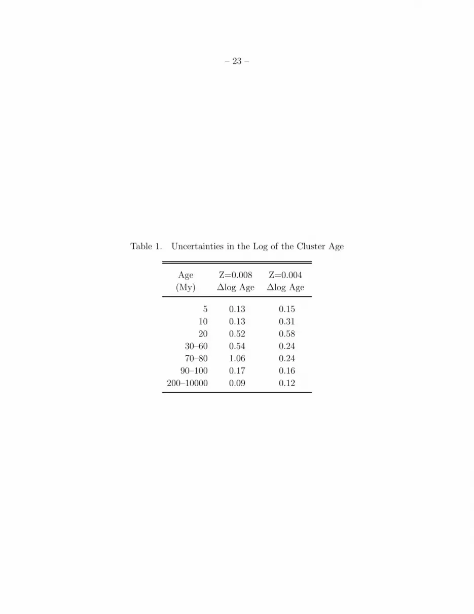
We have examined the uncertainties in the ages determined from integrated colors in

another way. We asked what age ranges would be consistent with colors extracted from

the cluster evolutionary models at particular ages and given a typical uncertainty of ±0.05

mag. The uncertainties in the log of the ages for the Z=0.008 and for the Z=0.004 models

are given in Table 1. The quantities that are tabulated are the absolute difference between

the log of the extreme in the allowed ages and the log of the input age. An uncertainty

in the log of the age of order 0.10–0.15 dex is typical except in regions of the color-color

diagrams where the cluster evolutionary tracks loop back on each other. For the Z=0.008

model, the uncertainty goes up to 0.53 dex between 20–60 My because of confusion with the

5-7 My part of the evolutionary track for 20–30 My old clusters and the 15–17 My part of

the track for 40–60 My old clusters. For clusters 70–80 My there is confusion, within the

allowed photometric uncertainties, with the 6–7 My and 13–16 My parts of the track, and

this causes the uncertainty to rise even higher to 1.06 dex. For the Z=0.004 model, confusion

with the 18–20 My part of the cluster evolutionary track causes an uncertainty of 0.31 dex

in the log of the age for a 10 My-old cluster. The 20 My-old cluster is confused with the

5–7 My and 9–12 My parts of the evolutionary tracks. For clusters with colors that have

uncertainties greater than 0.05 mag, the uncertainties in the ages will, of course, be higher

as well.

However, the preceding exercise assumed that clusters are evolving strictly along the

cluster evolutionary tracks and only uncertainties in the colors are causing confusion. The

comparisons with ages determined from CMDs given in Figure 3 may be more realistic and

they paint a less optimistic picture. There are not very many clusters with ages determined

this way, but the CMDs suggest that for clusters with ages <100 My the uncertainty in the

log of the age is 0.5 dex, for 100–1000 My it is 0.6 dex, and for >1000 My it is 0.8 dex.

Obviously, use of integrated colors is not the preferred way to determine the age of a cluster,

but it is hoped that the ensemble of clusters will still be statistically representative for our

purposes.

– 9 –

Cluster evaporation could cause the color ages to be lower than the CMD ages because

color ages are based on all the stars while CMD ages are based primarily on the most massive

stars. Since low mass stars are preferentially lost during evaporation, clusters should have an

excess of intermediate and high mass stars compared to the lowest mass stars, and therefore

be slightly too blue compared to a model cluster with the full stellar initial mass function

still present. Detailed modelling of the evaporation process will be needed to determine the

conversion from color ages to CMD ages. We note that the clusters with the most discrepant

ages in our study are those closest to the evaporation limit discussed below.

In the LMC we found that there are 5 star clusters with MV (10 My) of −13.1 to −14.9,

implying that these are very massive star clusters. All of these clusters are bright, with

current MV of −7.1 to −8.9. However, four of them have ages 14–15 Gy. These very old

ages come from CMDs and we can find no fault with the published work. The fifth cluster

has an age of 3 Gy that comes from colors, but the colors look very reasonable, so we have

no reason to discount the cluster. Therefore, we are forced to conclude that these really were

very luminous when they were young, and that the LMC has hosted some extreme clusters

in its distant past.

In the SMC we also find 4 clusters with MV (10 My) of −13 to −14. Again, the clusters

are bright and have ages of 2–8 Gy. The ages of two of these clusters come from CMDs. The

other two come from the CCDs but the colors fall on the models. Thus, it appears that even

the SMC has produced some extreme clusters in its distant past.

The final number of clusters in our sample for the LMC is 748 with 140 flagged as

questionable from their appearance. The total for the SMC is 191 with 76 flagged as ques-

tionable.

5. Mass and Age Distributions in the LMC

The distribution of present-day absolute V magnitude of the clusters in the LMC is

shown in Figure 4. The solid-line histogram in this figure and in the following figures are

for the certain 608 clusters, while the dotted histograms are the additional 140 clusters that

are questionable. The distribution has a cutoff at the faint end with a magnitude limit of

∼ −3.5 at the half-peak point, a long extension toward the bright end, and a number of very

bright clusters that exceeds a power-law extrapolation at this bright end. The questionable

clusters are mostly near the faint end, as expected. The various cluster ages are separated

in Figure 5. The lower limit of brightness is the same for each age bin less than 104 My,

and the upper limit is about the same for each age too. The oldest clusters are only massive

– 10 –

clusters.

The absolute magnitude of a present-day cluster was converted to the absolute magni-

tude the cluster had at an age of 10 My using the colors and evolution models discussed in

the previous section. This value of MV (10 My) was then converted to cluster mass using

−14.55 mag as the absolute magnitude of a 10 My old 106 M⊙ cluster with a metallicity of

Z = 0.008 for the LMC (Leitherer et al. 1999):

M = 106+0.4(−14.55−MV ) M⊙. (1)

Figure 6 shows the resulting distribution of cluster masses separated by age. The mass

distribution shifts toward higher cluster mass with increasing age because of two effects.

First, the low mass end of the distribution shifts toward higher cluster mass because clusters

fade with age, so higher mass clusters produce the same absolute magnitude at the limit of

the survey as the age increases. This shift in limiting detectable mass goes approximately as

Mfade = 982 (t/Gy)0.69 M⊙ (2)

for t/Gy > 0.01, based on a power law fit to the tabulated MV (t) in Leitherer (1999) for

metallicity Z = 0.008 (see Eqn. 6 and 7 below). Thus the limiting mass increases by a factor

of ∼ 5 for each decade in age.

Second, the upper limit of the cluster mass distribution increases with age because of

the size-of-sample effect, in which larger numbers of clusters sample further into the high

mass tail of the cluster mass distribution function. The logarithmic time intervals in Figure

6 mean that older age intervals encompass longer time intervals and more cluster formation.

For a cluster mass function, the number of clusters as a function of the mass of the cluster,

written in linear intervals of mass,

n(M)dM = n0M−αdM, (3)

the maximum likely cluster mass scales with the number N of clusters as

Mmax = MminN1/(α−1) (4)

which comes from the equations∫

∞

Mmaxn(M)dM = 1 and N =

∫

∞

Mminn(M)dM . This correla-

tion between N and Mmax was observed directly by Whitmore (2003) using a large number

of galaxy surveys, and it was used by Billett et al. (2002) and Larsen (2002) to help explain

the Larsen & Richtler (2000) correlation between the fraction of star formation in the form

of clusters and the star formation rate. For α in the likely range from 2 to 2.6, the maximum

mass scales with cluster number to a power between 1 and 0.62.

– 11 –

Figure 6 plots cluster mass histograms in logarithmic intervals of time. If the star

formation rate is about constant, dN/dt ∼constant, then the number of clusters that form

in each log-time interval increases directly with time (dN = (dN/dt) d ln(t)t). Thus the

maximum mass increases with time

Mmax ∝ t1/(α−1). (5)

In this context, a constant star formation rate means a constant average rate, averaged over

the time interval considered. If the star formation rate was larger at previous times, then the

number of clusters formed in each log time interval increases faster than t and the mass of the

largest cluster in log t intervals increases faster than t1/(α−1). For example, if (dN/dt) ∝ tβ,

then Mmax ∝ t(1+β)/(α−1).

The similarity between the time dependence of Mfade and the time dependence of Mmax

for α ∼ 2 to 2.5 explains why the mass distribution functions in Figure 6 shift to the right

with increasing t without changing their shape much. An exception occurs for the oldest

clusters, which are clearly lacking in low mass members although their highest masses fit

the extrapolation from younger clusters. For these very old clusters, evaporation is also

depleting the lower masses, as we shall see momentarily.

The dashed lines in each histogram are reference lines with slopes of −1 and −1.4 on

this log-log plot. These correspond to α = 2 and 2.4, which is in the range of solutions for

our LMC data (although this is not obvious from the mass functions in Figure 6).

An interesting feature of Figure 6 is that the high mass ends of the distributions in the

middle three age bins overlap in mass and are all more massive than the turnover masses,

where fading becomes important for each time. This means that the sum of the distributions,

which is the total mass distribution for all clusters regardless of age, will also be a power law

in this mass range, and the power will be about the same as it is in each age bin.

The distribution of cluster mass and age is shown in Figure 7, following Boutloukos &

Lamers (2003). The open circles are the questionable clusters. The lower limit to the cluster

mass, populated mostly by the questionable clusters, fits well to the fading limit (solid line

in Figure 7), given by the equation

Mfade(t) = 106+0.4(3.5+MV (t)) M⊙ (6)

where −3.5 is the observed cutoff magnitude of the survey, from Figure 4, and MV (t) is the

fading function from Figure 47c in Leitherer et al. (1999). For ages larger than the limit

in the Leitherer et al. table, which is 1 Gy, we use a linear extrapolation of the tabulated

values, which is

MV (t) = −14.47 + 1.725 log(

t/107 yr)

(7)

– 12 –

for a M = 106 M⊙ cluster. Equations 6 and 7 lead to Equation 2 above.

The dashed line in Figure 7 is the evaporation limit, given by the equation (Baumgardt

& Makino 2003)

tevap =R/kpc

V/220 km s−1

(

N

ln (0.02N)

)0.8

My (8)

for cluster number N = M/ (0.547 M⊙), galactocentric radius R, and galactic orbit speed V

in the LMC. The two lines represent radii of R = 0.5 kpc and 2 kpc, for which V = 25 km

s−1 and 50 km s−1, respectively, from Figure 6 in Kim et al. (1998). Masses smaller than

the limit given by the dashed line for their age should have evaporated by now.

The distribution of points in Figure 7 illustrates the simultaneous effects of fading and

size-of-sample that were discussed above in reference to Figure 6. The lower limit to the

mass increases with time approximately as a power law Mfade ∝ t0.69 from the fading limit,

and the upper limit increases right along with it from the size-of-sample effect, keeping the

total range in mass about constant for each time interval. The maximum cluster masses for

each logarithmic time interval are shown as plus-symbols. These plus symbols are placed at

the centers of the age intervals, so the corresponding dots for each symbol are shifted slightly

to the left or right.

Figure 8 shows the maximum cluster mass in each age interval, from the plus-signs in

Figure 7, versus the cluster age. In all cases except one at a low age, the maximum mass

cluster is a bonafide cluster, not a questionable cluster. The open circles are for age intervals

where the maximum mass cluster is close to or below the evaporation limit. The distribution

of points is fitted to a linear regression as log (M/M⊙) = 2.58+0.74 log(t/My). This fit does

not include the open circles because their masses could be severely depleted by evaporation.

A fit to ages less than 100 My gives a linear regression log (M/M⊙) = 2.35+1.05 log(t/My).

The maximum mass is expected to increase with the number of clusters, but the true number

of clusters that ever formed in the LMC is not observed because of fading effects. This figure

corrects for this cluster loss by considering that they form at a constant rate, in which case

the total number of clusters that formed in each log interval of time is proportional to the

age. By plotting maximum mass versus age we can reconstruct the expected size-of-sample

correlation without actually counting all the faded, destroyed, or evaporated clusters, which

tend to be lower mass. The slope of this correlation, 1.05 below 100 My and 0.74 overall,

suggests a cluster mass function with α in the range from 1.95 to 2.35, respectively, as given

by Equation 5. If the highest mass clusters are underestimated in age, as suggested by Figure

3, then the slope overall will be smaller than 2.35. Thus we consider the initial cluster mass

function in the LMC to have a slope in the range from 1.95 to 2.35.

Figure 8 can be used to find the cluster formation history in a galaxy if the initial

– 13 –

cluster mass function (ICMF), destruction rate, and fading rate are known independently.

The ICMF is the number of clusters as a function of the initial integrated mass of the cluster.

If we consider that α = 2 from the observation of young clusters, and we assume a cluster

formation rate (dN/dt) ∝ tβ as above, then the overall slope of 0.74 in the figure implies

(1 + β) / (α − 1) = 0.74 giving β = −0.26. In this case, the cluster formation rate in the age

period from 102 to 103 My was smaller than that in the age period from 101 to 102 My by

a factor of 0.54. This assumes that the destruction time is longer than the fading time, as

before, and that the color ages up to 103 My are reasonably accurate.

Figure 9 shows the total mass distribution function with all ages combined (see also

Boutloukos & Lamers 2003). This is the sum of the separate distributions in Figure 6; it

is also a count of clusters projected against the ordinate in Figure 7. For the LMC we

have the fortunate situation where clusters more massive than the fading limit have a wide

range of ages (cf. Fig. 7), so the total mass distribution shows a power law section that is

approximately the sum of the primeval power law sections from each separate age bin. The

flat part of the total distribution contains information about the cluster mass function as

well.

Both the flat and power-law parts of the total mass distribution were modelled using

an initial cluster mass function, n(M), that is a power law, and using the fading limit from

Equation 6 (which considers the tabulation in Leitherer et al. (1999) and our extrapolation

to larger ages). This model gives the expected number N of clusters above the fading limit

in each linear interval of mass as

N(M)dM = cdM

∫ tfade(M)

0

n(M)dt = cdMtfade (M) n(M) ∝ dMM−α+1/0.69 (9)

for adjustable constant c in the case where M < Mfade (tmax) for some maximum time of

cluster formation, tmax. For M > Mfade (tmax), the number of clusters varies with mass as

N(M)dM = cdMtmaxn(M), (10)

which is proportional to the initial cluster mass function, n(M). The plotted models are

M × N(M), which is appropriate for logarithmic intervals of mass. This is ∝ M2.45−α for

M < Mfade (tmax) and ∝ M−α for M > Mfade (tmax). This expression for M < Mfade (tmax)

shows right away that the total mass distribution can have the observed flat part at low

mass if α ∼ 2.45.

The model assumes a nearly constant star formation rate (as defined above) and that

fading alone provides the lower limit to the observed cluster mass. This latter assumption

is verified by the good fit between the fading line in Figure 7 and the lower limit to the ob-

served cluster masses. Other destruction mechanisms are possible, such as collisions between

– 14 –

clusters or between clusters and dense clouds. Our observation that fading contributed most

to the lower mass limit implies that for all masses the fading time is less than the destruction

time. If there were a mass range where the destruction time was less than the fading time

(as might be the case in other galaxies – see Boutloukos & Lamers 2003), then we would

have to take an upper limit to the integral in Equation 9 that is the minimum value of the

fading time and the destruction time.

Three maximum times are considered in Figure 9: 2 Gy, 5 Gy, and 7 Gy, as indicated.

For each time we adjust the constant c in front of Equation 9 to match the flat part of the

observed N(M) distribution. The excess low-mass clusters that come from the downward

dips in Mfade(t) at low t in Figure 7 are ignored. They do not affect the flat part of N(M)

and tend to influence only the integral under the N(M) curve, which is the total number

of clusters that forms. As a result, the theoretical fits for the next figure, which plots the

number of clusters versus age, are slightly too high for the same parameters.

Figure 9 has a kink at ∼ 2×103 M⊙ and this is the mass corresponding to the fading limit

at tmax. Masses beyond this have not faded (and apparently they have not been destroyed or

evaporated either except at much larger mass – cf. Fig. 7), and so they have not been lost

from our survey. As a result, the theoretical mass function integrated over all ages in Figure

9 has about the same slope as the initial cluster mass function, n(M), for M > 2× 103 M⊙.

This slope is taken to have three values in the figure, ranging from 2 to 2.4.

The model with initial cluster mass function slope α = 2 is too steeply rising compared

to the observations in the mass range from 102 to 2 × 103 M⊙, but it is acceptable for the

power law part above 2 × 103 M⊙, not counting the most massive clusters. The case with

α = 2.4 fits the flat part best, it fits the power law part reasonably well if the most massive

clusters are not included, and it has the best value for tmax (which was adjusted to match

the observed kink in N(M) at 2 × 103 M⊙) considering the observed distribution of ages in

Figure 7. The fading line in that figure was drawn with the extrapolation of the Leitherer

et al. model out to tmax = 7 Gy, which was the best fit in Figure 9.

Figure 9 shows an excess of massive clusters beyond ∼ 105 M⊙. Where this excess

begins determines the best fit to the power law part of the mass function; if it starts at 105

M⊙, then the best fit is α = 2.4, but if it starts at 3× 105 M⊙, then α = 2 may be preferred.

The massive clusters are also the oldest clusters (cf. Fig. 7). For these two reasons, they

appear to be a distinct population of clusters, like the halo globular clusters in the Milky

Way. Their distributions do not appear to be extrapolations of the distributions for the less

massive and younger clusters. This allows for the possibility that the oldest massive clusters

formed by a distinct mechanism, or that they formed by the same general mechanism but

at a much higher rate than the disk clusters, with substantial evaporation and destruction

– 15 –

of the lowest mass members, leaving only an excess of massive clusters now.

Figure 10 shows the distribution of cluster ages, summed over all masses (see also

Boutloukos & Lamers 2003). This is the count of clusters projected against the abscissa in

Figure 7. The distribution is flat over times less than ∼ 1 Gy because the fading rate of

clusters at the low mass end keeps pace with the broadening of the mass distribution at the

high mass end, which comes from the size-of-sample effect at increasing log(t). The three

models are the same as in Figure 9. The one with α = 2.4 is the best fit to the flat slope of the

distribution. All of the models lie above the distribution because of the over-representation

of low mass clusters at the wiggles in the Mfade (t) function.

The theoretical models for Figure 10 come from the equation

N(t)dt = cdt

∫

∞

Mfade(t)

n(M)dM ∝ M1−αfade ∝ t0.69(1−α) (11)

with the plotted quantity equal to tN(t) ∝ t1+0.69(1−α) in intervals of log t. The constants c

for the three cases are the same as in Figure 9. The flat part in this figure requires again

α = 1 + 1/0.69 = 2.45.

The age gap between ∼ 3 Gy and ∼ 13 Gy (Rich, Shara, & Zurek 2001) is evident from

Figure 10. This gap is consistent with the age cutoffs we have assumed for the models and

it reinforces our conclusion that the oldest massive clusters are a distinct population. Figure

7 suggests that this gap is partly the result of severe evaporation, but the most massive

clusters from this time period should still be visible if the star formation rate were the same

as it is today. As it is, the most massive clusters are close to the evaporation limit because

the cluster formation rate was low. There is no reason to think that the cluster formation

rate was zero in this period, only that it was so low that the most massive likely cluster

has suffered from evaporation. In that case, all the lower mass clusters would be gone or

imperceptible by now. Returning to Figure 8, we see that the open circles from this age

period have about the same maximum mass as those in the period from 102 to 103 My. This

means that the slope of a line drawn through these points is zero, and so (1 + β) / (α − 1) = 0

giving β = −1 independent of the ICMF slope, α. Thus the cluster formation rate was a

factor of at most ∼ 10 less in the period from ∼ 1 to ∼ 10 Gy than it was in the period from

102 - 103 My. The factor could have been smaller if the most massive clusters in this period

lost mass by evaporation. If our ages or masses turn out to be wrong for these few clusters,

then the drop in the cluster formation rate could have been greater. The clusters that are

important for this time period are listed in Table 2.

– 16 –

6. Mass and Age Distributions in the SMC

Analogous results for the Small Magellanic Cloud are shown in Figures 11 to 16. The

faintness limit to the absolute magnitude for the SMC is ∼ −4.5 mag, from Figure 11,

and that determines the fading line in Figure 13. The fading model for the SMC uses the

Z=0.004 case from Figure 47d in Leitherer et al. (1999). The SMC distance is assumed to

be 60 kpc. In this model, the absolute magnitude of a 106 M⊙ cluster is −14.778 for use in

Equation 1, and the extrapolated fit in Equation 7 is MV (t) = −14.51 + 1.708 log (t/107 yr).

The rotation curve is from Torres & Carranza (1987); it suggests V = 15 km s−1 at R = 0.5

kpc and V = 40 km s−1 at R = 2 kpc for the evaporation limit in Figure 13.

The results for the SMC are similar to those for the LMC: faintness limits the cluster

masses at the low end and size-of-sample limits them at the high end. The best fit to the

cumulative mass and age functions and to the maximum mass-versus-age plot is for a ICMF

with a negative slope near α = 2.4 for linear intervals of mass. This gives the slope of 0.69

in Figure 14, which is the clearest measure of the ICMF in this case.

The SMC is also like the LMC in having old massive clusters that are not simple

extrapolations of the total cluster mass function. Figures 12 and 15 show these clusters well.

7. Cluster Size Distributions

Figure 17 shows the cluster masses versus sizes (FWHM) for both galaxies. The symbol

types indicate age. The increase in mass with age shows up here as it did in earlier figures.

The young age symbols are at the bottom and the old age symbols are at the top. There

is no analogous shift of symbol-type to the right, which means that clusters do not get

significantly larger with time for a given mass. There is a slight trend for more massive

clusters to be physically larger. The maximum cluster size also increases with mass, as

shown schematically with a line on the right of each panel that marks the outer envelope.

Figure 18 shows the cluster size versus age. There is a trend for the largest clusters to

get larger with age, but this is probably the size-of-sample effect. Larger times correspond

to larger time intervals on this log-abscissa plot, and to a larger total number of clusters

forming in each log-time interval. Thus the maximum cluster mass increases to the right in

the figure, as discussed before, and the maximum size increases toward the right also, along

with the mass. The line in the figure shows the predicted size-of-sample effect based on the

relations between Mmax and time from Figures 8 and 14 and the schematic lines in Figure

– 17 –

17. These relations are

Rmax = 3.3 (t/My)0.077 pc (LMC) ; Rmax = 2.1 (t/My)0.081 pc (SMC). (12)

Our size measurements are not as accurate as those of Mackey & Gilmore (2003a,b),

who used HST data, but we have more clusters to see the size-of-sample effects better. Their

correlation between cluster size and age, which is slightly steeper than ours, could have the

same origin. In this case, there would be no specific physical explanation for the occurrence

of larger clusters at older ages, only a broader sampling of the massive end of the initial

cluster mass function at these ages.

8. Discussion

The agreement between the lower cluster mass limit as a function of age in Figures

7 and 13 and the fading limit suggests that clusters are lost from view mostly by fading

and not by destruction in these two galaxies. This is consistent with the conclusion by

Boutloukos & Lamers (2003) who found a long destruction time for the SMC (∼ 109 yrs).

They did not analyze data for the LMC. Our overall result for the SMC differs from theirs,

however, because we do not attempt to fit two distinct power law parts to the cluster mass

distribution integrated over age or to the cluster age distribution integrated over mass, but

instead we fit both distributions as a whole to the fading-statistical model. Boutloukos

& Lamers also assumed an ICMF slope of −2 for the SMC, but the flat part of the age

distribution integrated over mass requires a steeper initial function, α = 2.4, unless the star

formation rate was smaller by a factor of ∼ 2 from 102 to 103 My ago than it is today.

Figure 8 suggested a new way to determine the ICMF from the size of sample effect.

Size-of-sample effects appear as a hidden influence in many studies of star clusters. They

contribute to the impression that starburst regions form more massive clusters (Billett et

al. 2002; Larsen 2002). They may also account for the increase in cluster size with age that

was found by Mackey & Gilmore (2003a,b), as shown in the previous section. In Figure 8,

the size-of-sample effect appears as a correlation between the age and the mass of the most

massive cluster at that age (in logarithmic age bins). This may be a better way to determine

the ICMF than the slope on a log-log histogram of cluster mass for either a single age (which

can have poor statistics) or integrated over age (which can give the wrong slope because of

the age mixture).

The ICMF slopes found here are in the range from −2 to −2.4, depending on the cluster

formation history. The steeper end of this range exceeds the slope of −2 found in the Antenna

– 18 –

galaxy (Zhang & Fall 1999), but is consistent with values found by Larsen (2002) for several

galaxies after he corrected for size-of-sample effects.

The oldest clusters in the LMC and SMC are all massive. Lower mass counterparts

could have been observed above the fading limit, but they are not present. They may have

evaporated because the oldest clusters are close to the evaporation limit for all masses in

Figures 7 and 13. Alternatively, the oldest clusters in the LMC and SMC could have had

a different initial mass distribution, such as a Gaussian distribution in log-mass (Vesperini

2001). We cannot tell the difference between this initial function and a power law because

the number of massive clusters is too small and the evaporation mass limit is too high (all

lower mass clusters have evaporated). de Grijs, Bastian, & Lamers (2003) suggest that an

initially power-law cluster mass function in M82 has begun to turn over at low mass in its

gradual progression toward a Gaussian. M82 is a better place to observe this than the LMC

or SMC because the number of clusters and the tidal density in M82 are both large. The

large tidal density makes the cluster evaporation time smaller, and then fading is less severe

for clusters in the last stages of evaporation.

9. Conclusions

The integrated properties of clusters in the LMC and SMC were measured from ground-

based images and analyzed to determine the likely slope for the power-law form of the initial

cluster mass function. This slope cannot be determined by conventional means because

the blend of ages prevents the combined cluster mass function from revealing the initial

function, and because the sample is too small to get a statistically significant cluster mass

function in a narrow age range. We could still determine the initial cluster mass function

from the data, however, using a combination of theoretical fading limits and the size-of-

sample effect. The size-of-sample effect follows from the assumption that clusters randomly

sample a physically-determined mass function and so larger samples are likely to have larger

most-massive clusters.

The results suggest that the initial cluster mass function is a power law with a slope

between −2 and −2.4 for the LMC and SMC, nearly independent of time. The slope was

determined independently using three methods: a fit of the model to the total mass function

integrated over all cluster ages, a fit of the same model to the number of clusters versus age

integrated over all masses, and a least-squares fit to the maximum cluster mass versus age.

If there is a significant number of high mass clusters that are not part of the ICMF, then

α = 2.4 is preferred for each galaxy.

– 19 –

The maximum cluster mass and the maximum cluster size increase with age when plotted

in equal intervals of log-age because the total number of clusters increases linearly with age

in such a distribution. Then, as the number of clusters increases, the high ends of the

distribution functions get sampled further out. The lower limit to the observed cluster mass

increases with age too because of fading. Both vary with age in about the same way for the

LMC and SMC, so the histogram of cluster mass shifts in a nearly self-similar way toward

higher cluster masses for aging clusters.

The oldest clusters in the LMC and SMC stand apart from the most obvious extrapola-

tions found for younger clusters. They are all very massive and they lie far above the fading

limits. Either a large population of them has already evaporated or low mass clusters did

not form in early times.

We are grateful to Dr. Philip Massey for the use of his Schmidt images and calibrations.

TJD would like to thank the National Science Foundation for funding the Research Expe-

rience for Undergraduates program at Northern Arizona University under grant 9988007

to Northern Arizona University and Dr. Steven Tegler for running the program. MM ac-

knowledges the MIT Field Camp at Lowell Observatory run by Dr. Jim Elliot. Support to

DAH for this research came from the Lowell Research Fund and grant AST-0204922 from

the National Science Foundation. Support to BGE came from grant AST-0205097 from the

National Science Foundation.

REFERENCES

Baumgardt, H., & Makino, J. 2003, MNRAS, 340, 227

Bessel, M. S. 1979, PASP, 91, 589

Bica, E. L. D., Claria, J. J., Dottori, H., Santos, J. F. C., & Piatti, A. E. 1996, ApJS, 102,

57

Bica, E. L. D., & Dutra, C. M. 2000, AJ, 119, 1214

Bica, E., L. D., Schmitt, H. R., Dutra, C. M., & Oliveira, H. L. 1999, AJ, 117, 238

Billett, O. H., Hunter, D. A., & Elmegreen, B. G. 2002, AJ, 123 1454

Boutloukos, S. G., & Lamers, H. J. G. L. M. 2003, MNRAS, 338, 717

Brocato, E., Castellani, V., Raimondo, G., & Romaniello, M. 1999, A&AS, 136, 65

– 20 –

Cardelli, J. A., Clayton, G. C., & Mathis, J. S. 1989, ApJ, 345, 245

Carney, B. W., Janes, K. A., & Flower, P. J. 1985, AJ, 90, 1196

Charlot, S., & Bruzual, A. G. 1991, ApJ, 367, 126

Chiosi, C., Bertelli, G., & Bressan, A. 1988, A&A, 196, 84

de Grijs, R., Bastian, N., & Lamers, H. J. G. L. M. 2003, ApJ, 583 ,L17

Elson, R. A. W., & Fall, S. M. 1985, ApJ, 299, 211

Frenk, C. S., & Fall, S. M. 1982, MNRAS, 199, 565

Geisler, D., Bica, Eduardo, Dottori, H., Claria, J. J., Piatti, A. E., & Santos, J. F. C., Jr.

1997, AJ, 114, 1920

Gelatt, A. E., Hunter, D. A., & Gallagher, J. S. 2001, PASP, 113, 142

Girardi, L., & Bica, E. 1993, A&A, 274, 279

Girardi, L., Chiosi, C., Bertelli, G., & Bressan, A. 1995, A&A, 298, 87

Hodge, P. W. 1961, ApJ, 133, 413

Hodge, P. W. 1983, ApJ, 264, 470

Hodge, P. W. 1986, PASP, 98, 1113

Hodge, P. W. 1988, PASP, 100, 1051

Hodge, P. W., & Lee, S.-O. 1984, ApJ, 276, 509

Kim, S., Staveley-Smith, L., Dopita, M. A., Freeman, K. C., Sault, R. J., Kesteven, M. J.,

McConnell, D. 1998, ApJ, 503, 674

Knodlseder, J. 2000, A&A, 360, 539

Kontizas, E., Metaxa, M., & Kontizas, M. 1988, AJ, 96, 1625

Kontizas, M., Morgan, D. H., Hatzidimitriou, D., & Kontizas, E. 1990, A&AS, 84, 527

Landolt, A. U. 1992, AJ, 104, 340

Larsen, S. S. 2002, AJ, 124, 1393

Larsen, S. S., & Richtler, T. 2000, A&A, 354, 836

– 21 –

Leitherer, C., Schaerer, D., Goldader, J. D., Gonzalez Delgado, R. M., Robert, C., Kune, D.

F., de Mello, D. F., Devost, D., & Heckman, T. M. 1999, ApJS, 123, 3

Mackey, A.D., & Gilmore, G.F. 2003a, MNRAS, 338, 85

Mackey, A.D., & Gilmore, G.F. 2003b, MNRAS, 338, 120

Massey, P. 2002, ApJS, 141, 81

Mighell, K. J., Sarajedini, A., & French, R. S. 1998a, AJ, 116, 2395

Mighell, K. J., Sarajedini, A., & French, R. S. 1998b, ApJ, 494, L189

Mould, J., & Aaronson, M. 1982, ApJ, 263, 629

Olsen, K. A. G., Hodge, P. W., Mateo, M., Olszewski, E. W., Schommer, R. A., Suntzeff,

N. B., & Walker, A. R. 1998, 300, 665

Pietrzynski, G., & Udalski, A. 1999, AcA, 49, 157

Pietrzynski, G., & Udalski, A. 2000, AcA, 50 337

Pietrzynski, G., Udalski, A., Kubiak, M., Szymanski, M., Wozniak, P., & Zebrun, K. 1999,

AcA, 49, 521

Pietrzynski, G., Udalski, A., Kubiak, M., Szymanski, M., Wozniak, P., & Zebrun, K. 1998,

AcA, 48, 175

Rabin, D. 1982, ApJ, 261, 85

Reed, B. C. 1985, PASP, 97, 120

Rich, R.M., Shara, M.M., & Zurek, D. 2001, AJ, 122, 842

Santos, J. F. C., Jr., & Frogel, J. A. 1997, ApJ, 479, 764

Searle, L., Sargent, W. L. W., & Bagnuolo, W. G. 1973, ApJ, 179, 427

Searle, L., Wilkinson, A., & Bagnuolo, W. G. 1980, ApJ, 239, 803

Torres, G., & Carranza, G.J. 1987, MNRAS, 226, 513

van den Bergh, S. 1971, A&A, 12, 474

van den Bergh, S. 1981, A&AS, 46 79

– 22 –

Vesperini, E. 2001, MNRAS, 322, 247

Whitmore, B. C. 2003, in STScI Symp. 14, A Decade of HST Science, ed. M. Livio, K. Noll,

& M. Stiavelli (Baltimore: STScI)

Zhang, Q., & Fall, S.M. 1999, ApJ, 527, L81

This preprint was prepared with the AAS LATEX macros v5.0.

– 23 –

Table 1. Uncertainties in the Log of the Cluster Age

Age Z=0.008 Z=0.004

(My) ∆log Age ∆log Age

5 0.13 0.15

10 0.13 0.31

20 0.52 0.58

30–60 0.54 0.24

70–80 1.06 0.24

90–100 0.17 0.16

200–10000 0.09 0.12

– 24 –

Table 2. LMC Clusters in the Age Gap

Namea RA (2000) DEC (2000) Age (Gy) Mass (M⊙) C or Q

OGLE-LMC0531 5:30:02.05 -69:31:36.14 5 7.9 × 103 C

KMK88-38.H88-206 5:12:09.30 -68:54:40.58 6.5 1.1 × 104 C

OGLE-LMC0169 5:10:06.07 -69:05:19.66 10 9.5 × 104 C

BSDL917 5:13:04.00 -70:26:55.00 10 9.5 × 104 C

KMHK898 5:26:23.95 -68:02:48.09 10 4.9 × 104 Q

Note. — C and Q distinguish between certain and questionable clusters.

aOGLE-LMC refers to clusters from the catalog of Pietrzynski et al. 1999, KMK88 to

Kontizas, Metaxa, & Kontizas 1988, KMHK to Kontizas et al. 1990, BSDL to Bica et al.

1999, and H88 to Hodge 1988.

– 25 –

Fig. 1.— UBV and BVR color-color diagrams for Field 346 of Massey (2002) in the LMC.

The (V−R)c color is on the Cousins system, and the model color has been converted to

this system. The filled circles are the star clusters. The curved solid line in the left part of

the diagram is the cluster evolutionary track of Leitherer et al. (1999) for a metallicity of

Z=0.008. The X’s on this line mark ages of 1 to 9 My in steps of 1 My. The open circles

on this line mark 10, 20, and 30 My time steps. The short solid line in the upper right of

the diagrams denote the range in Milky Way globular clusters from Reed (1985). The open

squares in the upper right are 3 and 10 Gy models from Searle et al. (1973), where we have

estimated the (V−R)c colors from the globular clusters.

Fig. 2.— UBV and BVR color-color diagrams for Field 66 of Massey (2002) in the SMC.

The (V−R)c color is on the Cousins system, and the model color has been converted to

this system. The filled circles are the star clusters. The curved solid line in the left part of

the diagram is the cluster evolutionary track of Leitherer et al. (1999) for a metallicity of

Z=0.004. The X’s on this line mark ages of 1 to 9 My in steps of 1 My. The open circles

on this line mark 10, 20, and 30 My time steps. The short solid line in the upper right of

the diagrams denote the range in Milky Way globular clusters from Reed (1985). The open

squares in the upper right are 3 and 10 Gy models from Searle et al. (1973), where we have

estimated the (V−R)c colors from the globular clusters.

Fig. 3.— Comparison of cluster ages determined from our colors and cluster evolutionary

models with ages determined for the same clusters from color-magnitude diagrams. Points

with a connecting line are ages for the same cluster: from measurements of the cluster colors

that appear in different fields (x-axis) or from a range in ages given from the CMDs (y-axis).

The CMD ages are taken from Hodge & Lee (1984), Geisler et al. (1997), Olsen et al. (1998),

Carney et al. (1985), Mighell, Sarajedini, & French (1998a,b). The clusters are identified in

the text.

Fig. 4.— Histogram of present-day MV for all of the clusters in our LMC sample. In this

figure and in the following figures, the solid lines are for certain clusters and the dashed lines

are for the extra counts of questionable clusters.

Fig. 5.— Histogram of present-day MV for the LMC cluster sample, separated into logarith-

mic age intervals. The dashed lines are for questionable clusters.

Fig. 6.— Histogram of masses for the LMC cluster sample, separated into logarithmic age

intervals. The straight dashed lines in each histogram are reference lines with slopes of −1

and −1.4 which correspond to ICMF slopes α equal to 2 and 2.4.

– 26 –

Fig. 7.— Cluster mass versus age for all of the LMC clusters in our sample. The dots

are for certain clusters and the open circles are for questionable clusters. The solid line is

the fading limit given by Equation 6 which is based on the observed −3.5 sample cutoff in

MV and the fading function from the cluster evolutionary models of Leitherer et al. (1999)

with an extrapolation to ages >1 Gy. The two dashed lines are the evaporation limits given

by Baumgardt & Makino (2003); they correspond to galactocentric radii of 0.5 kpc and 2

kpc in the LMC. The plus symbols are the maximum cluster masses for each logarithmic

time interval. These symbols are placed at the centers of the age intervals, and so the

corresponding dot for each symbol is shifted slightly to the left or right.

Fig. 8.— The maximum cluster mass in each age interval (the plus signs in Figure 7) is

plotted as a function of cluster age. The dot-dashed line is a linear fit to the points; the

open circles are for age bins where the maximum mass is close to the evaporation limit and

are not included in the linear fit. The dotted line is a least squares fit for ages less than 100

My. The slope of this correlation is related to the slope of the initial cluster mass function

by the size of sample effect; the implied cluster mass functions are given.

Fig. 9.— Histogram of masses for the LMC clusters in our sample with all ages combined.

The solid lines are models given by Equation 9. The best fit is for α = 2.4, which has a flat

slope between 102 and 104 M⊙ and a power law drop off comparable to the observations for

all but the largest mass. The α = 2 model fits the power law better if more massive clusters

are included but it does not fit the flat part at lower mass. There are an excess of high mass

clusters over all the extrapolated power laws.

Fig. 10.— Histogram of cluster ages for all of the LMC clusters in our sample. The dashed

lines are models given by Equation 11. The best fit has α = 2.4.

Fig. 11.— Histogram of present-day MV for all of the clusters in our SMC sample. As in

the other figures, the dashed lines are for questionable clusters.

Fig. 12.— Histogram of masses for all of the clusters in our SMC sample, separated into

logarithmic age intervals.

– 27 –

Fig. 13.— Cluster mass versus age for all of our SMC clusters. The dots are for certain

clusters and the open circles are for questionable clusters. The solid line is the fading limit

given by Equation 6, which is based on the observed −4.5 sample cutoff in MV and the fading

function from the cluster evolutionary models of Leitherer et al. (1999) with an extrapolation

to ages >1 Gy. The dashed lines are the evaporation limits given by Baumgardt & Makino

(2003) for galactocentric radii of 0.5 kpc and 2 kpc in the SMC. The plus symbols are the

maximum cluster masses for each logarithmic time interval.

Fig. 14.— The maximum cluster mass in each age interval (the plus signs in Figure 13) is

plotted as a function of cluster age. The dot-dashed line is a linear fit to the points.

Fig. 15.— Histogram of masses for the SMC clusters with all ages combined. The dashed

lines are models given by Equation 9. The best fit has α = 2.4 because that is the flattest in

the mass interval from 102 to 104 M⊙ and it also fits the falling part reasonably well. There

are an excess of massive clusters for all models.

Fig. 16.— Histogram of cluster ages for all of the SMC clusters in our sample. The dashed

lines are models given by Equation 11. The best fit has α = 2.4 because this is the flattest.

The slow decrease in number versus age suggests that unless α > 2.4, the average star

formation rate was lower in the early galaxy by a factor of ∼ 2.

Fig. 17.— Cluster mass versus FWHM for the LMC and SMC clusters. The FWHM could

not be measured for all clusters in the samples. Symbol types indicate cluster age. The solid

lines mark the approximate outer envelopes of points and show the trend for more massive

clusters to be physically larger.

Fig. 18.— Cluster FWHM versus cluster age. The FWHM could not be measured for all

clusters in the two samples. The solid lines show the predicted size-of-sample effect, given

by Equation 12 combined with the solid lines in Fig. 16.

This figure "fig1.jpg" is available in "jpg" format from:

http://arxiv.org/ps/astro-ph/0306528v1





















































Documents

Cluster Mass Functions in the Large and Small Magellanic Clouds: Fading and Size-of-Sample Effects