Coevolution of width and sinuosity in meandering rivers

J. Fluid Mech. (2014), vol. 760, pp. 127–174. c© Cambridge University Press 2014doi:10.1017/jfm.2014.556

127

Coevolution of width and sinuosity inmeandering rivers

Esther C. Eke1,†, M. J. Czapiga1, E. Viparelli2, Y. Shimizu3, J. Imran2,T. Sun4 and G. Parker1,5

1Department of Civil and Environmental Engineering, University of Illinois at Urbana-Champaign,Urbana, IL 61801, USA

2Department of Civil and Environmental Engineering, University of South Carolina, Columbia,SC 29201, USA

3Laboratory of Hydraulic Research, Hokkaido University, Hokkaido, 060-0814, Japan4Chevron Energy Technology Company, Houston, TX 77382, USA

5Department of Geology, University of Illinois at Urbana-Champaign, Urbana, IL 61801, USA

(Received 3 December 2013; revised 22 July 2014; accepted 20 September 2014;first published online 4 November 2014)

This research implements a recently proposed framework for meander migration, inorder to explore the coevolution of planform and channel width in a freely meanderingriver. In the model described here, width evolution is coupled to channel migrationthrough two submodels, one describing bank erosion and the other describing bankdeposition. Bank erosion is modelled as erosion of purely non-cohesive bank materialdamped by natural armouring due to basal slump blocks, and bank deposition ismodelled in terms of a flow-dependent rate of vegetal encroachment. While these twosubmodels are specified independently, the two banks interact through the mediumof the intervening channel; the morphodynamics of which is described by a fullynonlinear depth-averaged morphodynamics model. Since both banks are allowed tomigrate independently, channel width is free to vary locally as a result of differentialbank migration. Through a series of numerical runs, we demonstrate coevolution oflocal curvature, width and streamwise slope as the channel migrates over time. Thecorrelation between the local curvature, width and bed elevation is characterized,and the nature of this relationship is explored by varying the governing parameters.The results show that, by varying a parameter representing the ratio between areference bank erosion rate and a reference bank deposition rate, the model is ableto reproduce the broad range of river width–curvature correlations observed in nature.This research represents a step towards providing general metrics for predicting widthvariation patterns in river systems.

Key words: river dynamics, sediment transport

1. IntroductionMeandering constitutes one very common channel form found in both sedimentary

and non-sedimentary environments. Meanders develop in alluvial rivers wandering

† Email address for correspondence: [email protected]

http://orcid.org/0000-0003-1962-0552

mailto:[email protected]

128 E. C. Eke and others

through floodplains, in incised bedrock rivers, in glacial meltwater systems and evenin submarine systems, where turbidity currents form gigantic meandering channelson submarine fans (e.g. Leopold & Wolman 1960; Hack 1965; Imran, Parker &Pirmez 1999; Seminara 2006; Karlstrom, Gajjar & Manga 2013; Konsoer, Zinger &Parker 2013). Understanding the morphology and evolution of meandering rivers innature has attracted the attention of the scientific community, in the fields of fluvialgeomorphology (e.g. Hooke 2007, 2008), fluid mechanics (e.g. Seminara 2006) andhydraulic engineering (e.g. Duan & Julien 2010).

The last three decades have seen the development of a mechanistic frameworkfor the quantitative understanding of meander dynamics. The mechanistic ‘bendtheory’ describing meandering rivers as products of bend instability has led to thequantitative determination of many key parameters in meander development, andhas also led to the development of models that establish the intrinsic ability ofmeander trains to evolve from incipient meander formation to and beyond neckcutoff. The basis for the bend formulation is the groundbreaking work on the roleof secondary flow in bends due to Rozovskii (1957), Engelund (1974) and Ikeda,Hino & Kikkawa (1976), who describe the morphodynamics of alluvial bends andmeandering rivers. Hasegawa (1977), Ikeda, Parker & Sawai (1981), Parker, Sawai& Ikeda (1982) and Howard & Knutson (1984) showed how the application of asimple relation between the transverse variation of streamwise velocity and channelcentreline migration rate (HIPS relation below) allows the description of channelmigration. Further contributions to the mechanics of meander migration, as well as thedescription of flow and morphodynamics of meandering rivers needed to understandthis mechanics, including (among many) Howard & Knutson (1984), Kitanidis &Kennedy (1984), Smith & McLean (1984), Blondeaux & Seminara (1985), Struiksmaet al. (1985), Parker & Andrews (1985, 1986), Colombini, Seminara & Tubino (1987),Johannesson & Parker (1989), Nelson & Smith (1989), Howard (1992, 1996), Sunet al. (1996), Zolezzi & Seminara (2001), Camporeale et al. (2007), Camporeale,Perucca & Ridolfi (2008), Blanckaert (2009), Frascati & Lanzoni (2009), Blanckaert& de Vriend (2010) and Luchi, Bolla Pittaluga & Seminara (2012), have brought usto the present, relatively advanced state of understanding of the morphodynamics ofmigrating meandering rivers.

A major gap nevertheless exists in our understanding of how rivers determinetheir own widths, and how sinuosity and width variation coevolve. This issue can bebest highlighted by considering the most commonly used relation describing channelmigration, i.e. the Hasegawa–Ikeda–Parker–Sawai (HIPS) formulation (Hasegawa1977; Ikeda et al. 1981).

The HIPS formulation for bank migration has been summarized by Parker et al.(2011), where the river is prescribed to have a constant width, here taken to be 2b,where b is channel half-width, and the tilde denotes a parameter with dimensions.The local normal rate of shift ζ of the channel centreline is taken to be linearlyproportional to the difference in the near-bank, depth-averaged streamwise velocity Ubetween the two banks, so that where n is normal distance from the channel centreline,

ζ = E∆U = E(U|n=b − U|n=−b). (1.1)

In the above relation, the streamwise velocities are interpreted not to be evaluatedat ±b (where they would be vanishing), but rather just outside the associated near-bank boundary layer. In the above relation, E is a prescribed dimensionless migrationcoefficient.

Coevolution of width and sinuosity in meandering rivers 129

The HIPS formulation for channel migration has been applied to the problemof meander migration using a wide variety of fluid dynamic and in-channelmorphodynamic formulations, the sophistication of which has gradually increasedin time. In addition, the cases studied have varied from the evolution of single bendsto the evolution of entire floodplains characterized by many bend cutoffs. Examplesof such applications include Beck, Harrington & Andres (1983), Parker, Diplas &Akiyama (1983), Howard & Knutson (1984), Blondeaux & Seminara (1985), Parker& Andrews (1986), Beck (1988), Crosato (1990), Howard (1992), Stolum (1996), Sunet al. (1996), Seminara et al. (2001), Lanzoni & Seminara (2006), Camporeale et al.(2007, 2008) and Frascati & Lanzoni (2009, 2010). In all of these examples, bothhalf-width b and migration coefficient E are prescribed constants.

In several recent examples, e.g. Güneralp & Rhoads (2011) and Motta et al.(2012b), the effect of either a prescribed variation in migration coefficient E ora prescribed rule for variation has been used to study, for example, the effect offloodplain heterogeneity on patterns of meander migration. These studies, however,retain the assumption of prescribed, constant width. Neither these nor the previouslyquoted contributions address the issue as to how a river establishes its own width.In addition, the migration coefficient E has remained an empirically useful parameterwith no clear physical basis.

The physics behind the problem of bank erosion has been studied by a number ofauthors including Darby & Thorne (1996), Darby, Rinaldi & Dapporto (2007) andLangendoen & Simon (2008). Nagata, Hosoda & Muramoto (2000), Rüther & Olsen(2007) and Duan & Julien (2010), for example, present models for meander migrationwith a physically based formulation for bank erosion, but channel width monotonicallyincreases over time due to the lack of a description of bank deposition. Motta et al.(2012a) also include a more physically based formulation for bank erosion, but thechannel migrates while maintaining constant width under the constraints of the HIPSformulation.

The assumption of a temporally constant width in a meandering river is partlyjustified by field observations over geomorphic time, which suggest that many riverstend to maintain a fairly constant mean channel width as they migrate (e.g. Lagasseet al. 2004). However, many other field observations have clearly shown that naturalrivers routinely undergo time periods of width adjustment as the river responds tochanges in flow regime and other environmental factors (e.g. Pizzuto 1994; ASCE1998). Spatially constant width is thus only a first crude approximation. Indeed,systematic spatial width variation patterns have been documented in many meanderingrivers by, e.g., Brice (1982) and Lagasse et al. (2004).

In recent years, the in-channel morphodynamics of channels with prescribedvariation in width has been the subject of considerable research. The case of a straightchannel with varying width has been studied by Bittner (1994), Repetto, Tubino &Paola (2002), Wu & Yeh (2005) and Wu, Shao & Chen (2011). Meandering riverswith prescribed variation of width have been studied by Luchi, Zolezzi & Tubino(2010, 2011), Zolezzi, Luchi & Tubino (2012) and Frascati & Lanzoni (2013). Noneof these analyses include, however, physically based descriptions of the processes ofbank erosion and deposition necessary to establish channel width itself, much lesswidth variation.

The work of Solari & Seminara (2005) and Luchi et al. (2012) offer a physicalbasis for patterns width variation. They hypothesized that, were the banks to be freeto adjust, a pattern of width variation would prevail, according to which the centrelinestreamwise free surface slope would become constant. The analysis does not, however,


describe the processes of bank erosion and deposition that might lead to such anadjustment of water surface slope.

An understanding of the coevolution of meander planform and width variation mustthen be predicated on a deeper understanding of the processes of both bank erosionand deposition. Mosselman (1998) pointed out that it is not possible to accuratelycapture channel migration in a model that allows bank erosion alone. Mosselman,Shishikura & Klaassen (2000) made the important step of incorporating both erosionaland depositional processes into a model of channel shift, albeit in the context ofanabranches of the braided Brahmaputra–Jamuna River, Bangladesh.

Here we study the coevolution of planform and width in the context of therecent framework of Parker et al. (2011), which allows channel banks to migrateindependently. In this formulation: bank erosion is modeled as erosion of purelynon-cohesive bank material damped by natural armouring due to basal slump blocks;and channel deposition is modelled as a function of vegetal encroachment dampedby flood flow. Since the banks are allowed to move independently, channel widthis allowed to vary locally as a result of differential bank migration. Eke, Parker &Shimizu (2014) describe closures for a full implementation of this model formulation,which links the processes of bank erosion and deposition to a reach-averagedchannel-formative Shields number τ ∗form. This parameter acts as a threshold belowwhich bank deposition occurs, and above which bank erosion occurs. A brief reviewof the model closures is presented in the following sections.

Eke et al. (2014) has applied this formulation to the case of the evolution of aspatially constant-curvature channel. They showed that for such migrating bend flows,the river converges to an asymptotic state where both erosion and deposition areroughly equal, and where channel width is slowly reducing in time as streamwiseslope reduces and curvature decreases in time. The paper delineates four regimesof bank interaction, i.e. both banks eroding, both banks depositing, bar push (fastermigration on the inside of bend) and bank pull (faster migration on the outside ofa bend). The analysis shows how a river bend can transition from one regime toanother as it evolves towards the asymptotic state.

This work goes beyond Eke et al. (2014) by extending the implementation ofthe model to the case of a freely meandering river rather than a bend of spatiallyconstant curvature. The outline for the rest of this paper is as follows. In § 2 wedocument observable trends of width variation from a few river reaches. Section 3is an overview of bankfull geometry as it relates to the formative Shields number.Section 4 details the model formulation for flow and bed morphodynamics withvarying width, along with the formulation for bank morphodynamics outlined in Ekeet al. (2014). To show how channel curvature, width and bed topography coevolve,§ 5 details numerical experiments on the growth and development of an idealizedsequence of periodic meander bends up to near cut-off conditions. Discussion andconclusions are presented in §§ 6 and 7 respectively.

2. Observed patterns of width variation in meandering rivers

Brice (1982) and Lagasse et al. (2004) observe that while nearly constant-widthchannels do exist, the majority of actively migrating channels exhibit spatial widthvariation. Channels that are systematically wider at bends apexes (where curvature ishighest) tend to exhibit the highest migration rates. They also identify another classof rivers for which width variation is uncorrelated with curvature, and migration ratesare low.


(a)

(c)

(b)

FIGURE 1. (Colour online) Meandering river reaches showing width variation: (a) ObRiver, Russia; (b) Trinity River, Texas, USA; (c) Vermillion River, Minnesota, USA.Arrows indicate direction of flow. For scale, typical river widths are 150, 190 and 15 mfor cases (a), (b) and (c), respectively. The images are from Google Earth.

Most of the observations of Brice (1982) and Lagasse et al. (2004) were based onchannel width defined from vegetation line to vegetation line. Figure 1 shows threereaches: the Ob River, Russia, the Trinity River, Texas, USA, and the VermillionRiver, Minnesota, USA. All three reaches display a pattern of width variation thatcorrelates with centreline curvature. In terms of vegetation line, the first two reachestend to be wider at bend apexes (maximum curvature) relative to crossings (vanishingcurvature). In the third reach, however, this pattern is reversed: the channel tendsto be narrower at apexes. Channel width can also be defined, however, in terms ofwater margin to water margin. In the case of the Trinity River, figure 1(b) showsthat the channel defined by vegetation lines is wider at apexes, but that the channeldefined by water margins is narrower at apexes. The former may reflect bankfull flowconditions, whereas the latter reflects below-bankfull stage. This stage dependence hasbeen pointed out by Luchi et al. (2011).

In order to analyse width-curvature relations, we used reaches of the VermillionRiver near Empire, MN and the Trinity River downstream of Livingston Dam inEastern Texas (figure 1). We also studied the reach of the Pembina River nearRossington in Alberta, Canada (figure 2). Table 1 gives the characteristics of each


Rossington

Eastburg

6.75 km

Freedom

Manola

Man

ola

subr

each

Lunnford

FIGURE 2. (Colour online) Study reach of the Pembina River Reach in Alberta, Canada.The arrow indicates direction of flow.

Bankfull Slope Bankfull Sinuosity Mean grain Migration ratedepth (m) (m m−1) width (m) size (mm) (m yr−1)

Vermillion 0.75 5.18× 10−4 15 2.62 2 0.75Trinity 3.85 1.24× 10−4 190.4 1.78 0.35 2.3Pembina 3.75 2.60× 10−4 91 1.9 0.4 2–5 (peak)

TABLE 1. Characteristics of study reaches.

reach. The data sources are as follows: Vermillion River, Lauer & Parker (2008);Trinity River, Smith (2012); Pembina River, Beck et al. (1983). All three reaches arehighly sinuous and actively migrating (Beck et al. 1983; Lauer & Parker 2008; Smith2012).

The channel banklines were digitized from aerial photographs using visiblevegetation lines, and the channel centreline was obtained from digitized banklines ina way similar to Lauer & Parker (2008). Local half-widths were obtained during theiterative procedure as the tangential distance from the centreline to the bank line ateach node.

Figure 3 shows the downstream variation in curvature and width for the Vermillionand the Trinity River reaches. Figure 4 shows linear regressions of half-width againstcurvature for each reach. Here dimensionless curvature c and half-width b are

c= bo

Rc; b= b

bo

(2.1a,b)

where b and Rc denote local half-width and centreline radius of curvature, respectively,and bo denotes the reach-averaged channel half-width. Again, tildes denote dimens-ioned parameters.


1.5(a)

1.0

0.5

–0.5

c, b

–1.00 01 2 1 2

Downchannel distance (m) Downchannel distance (m)

3

c

b

4

0

1.5(b)

1.0

0.5

–0.5

0

(× 102) (× 104)

FIGURE 3. Downchannel variation of dimensionless centreline curvature and dimensionlesschannel half-width: (a) Vermillion River; (b) Trinity River.

2.0

1.5

1.0

0.5

0 0.1 0.2 0.3 0.4 0.5

(a)

b

2.0

1.5

1.0

0.5

0 0.1 0.2 0.3 0.4 0.5

(b)

FIGURE 4. Linear regressions of dimensionless channel half-width and dimensionlesscentreline curvature correlation: (a) Vermillion River; (b) Trinity River. The stars indicatethe data.

The cases of the Vermillion and Trinity River reaches of figures 3 and 4 highlightthe range of tendencies in width variation in meandering rivers. In the VermillionRiver, points near the crossings (c∼ 0) tend to be wider than points near the apexes(c ∼ 0.3), but the variation is weak (fractional width variation of −0.04 as c variesfrom 0 to 0.35). In the Trinity River, points near apexes tend to be wider than thosenear crossings, and the variation is notably stronger (fractional variation of 0.19 as cvaries from 0 to 0.35).

The pattern observed for the Trinity River is in general agreement with the trendsreported in Brice (1982) and Lagasse et al. (2004). Field data on more than 1500meander bends reported by Lagasse et al. (2004) indicate that maximum values ofchannel width tend to be close to bend apexes and minimum width values tend tobe near inflections. Within a subset having significant width variations (type C ofthe Brice (1975) classification), width tended to be 14 % larger at apexes than atinflections.

The reach of the Pembina River in figure 2 is of particular interest, because therelevant parameters are used below in implementations of our model. Here we studythe entire reach shown in figure 2, along with the Manola subreach which has shownrapid migration in recent geomorphic time (Beck et al. 1983). Figure 5(a,b) show thecorrelations between b and c for the entire reach and the Manola subreach. Over the


2.0

1.5

1.0

0.5

0 0.1 0.2 0.3 0.4 0.5

(a)

b

2.0

1.5

1.0

0.5

0 0.1 0.2 0.3 0.4 0.5

(b)

FIGURE 5. Linear regression of dimensionless channel half-width and dimensionlesscentreline curvature correlation for the Pembina River. (a) The entire Pembina reach nearRossington. (b) Manola subreach. The ‘×’ indicate the data and the lines are linear fitsto the data.

entire reach, the fractional variation in width is 0.03 as c increases from 0 to 0.35;in the Manola subreach it is 0.09.

The observations presented here for the Vermillion, Trinity and Pembina Rivers,combined with the earlier analyses of Lagasse et al. (2004) suggest the following:meandering rivers may evolve so as to (a) have little systematic width variation,(b) show apexes that are slightly narrower than crossings or (c) show apexes that areslightly to significantly wider than crossings. Case (c) appears to be most commonin rivers that show significant rates of migration.

The above picture is supported by results on the Lower Trinity River, TX, reportedby Peyret (2011) and Smith (2012). The Trinity River reach shown in figure 1 is partof the Lower Trinity River, TX and is sandwiched between two low migration reaches:an upstream incising reach influenced by the presence of the Livingston Dam and adownstream backwater reach that feeds into the Trinity Bay. Peyret (2011) has shownthat width is weakly and negatively correlated with centreline curvature in zones oflow migration rate, whereas it is more strongly and positively correlated to curvaturein zones where the river shows higher migration rates.

Plots of the type of figures 4 and 5 are intended to illustrate trends, rather than toillustrate predictive relations. They do not give a complete picture of width variation,because they do not specify the locations of minimum and maximum width relativeto bend apexes. We address this with planform data from reaches of two rivers inFlorida, USA: the Apalachicola and Suwannee Rivers. These rivers have dense bankvegetation, which makes quantification of width variation straightforward. The segmentof the Suwannee River shown in figure 6 starts just north of Wannee in GilchristCounty, Florida, and ends at Fowler Bluff in Levee County, Florida. The segment ofthe Apalachicola River extends from New Hope, south of the Blountstown Gage, tothe intersection between the Gulf County border to the north and the Liberty Countyborder to the west.

An analysis 33 bends of the Suwannee River indicates that the point of maximumwidth is located upstream of the bend apex, i.e. between the apex and the nearestcrossing upstream, in 61 % of cases; in the other cases, maximum width was locatedbetween the apex and the next crossing downstream. A corresponding analysis of theApalachicola River showed that the point of maximum width is reached upstream of


FIGURE 6. View of the study reach of the Suwannee River. Flow is from left to right.The bend in the leftmost insert has a minimum width of 68 m and a maximum width of104 m.

100

% u

pstr

eam

of

bend

ape

x

80

60

Width maximum

Width minimum

40

20

0

Pembin

a

Trinity

Vermill

ion

Suwan

nee

Apalac

hicola

FIGURE 7. Percentage of bends in which the location of the width maximum and widthminimum are upstream of the bend apex for five river reaches: the Pembina River, theTrinity River, the Vermillion River, the Suwannee River and the Apalachicola River.

the apex in 75 % of 44 bends. Evidently, these rivers have a strong bias for maximumwidth to occur between the apex and the nearest crossing upstream.

That this behaviour is not universal is illustrated in figure 7. The Pembina River issimilar to the Apalachicola and Suwannee Rivers, with width maximums preferentiallylocated upstream of bend apexes. In the case of the Vermillion, the position of widthmaximum is equally split between upstream and downstream, and in the case of theTrinity River, width maximum is located preferentially downstream of bend apex.

Also shown in figure 7 is the percentage of bends for which the width minimum islocated upstream of the bend apex. It is seen that in all cases but the Vermillion River,the point of width minimum tends to be located downstream of the bend apex. In thecase of the Vermillion River, there is an equal likelihood for the width minimum tobe located upstream or downstream of the apex.


Whether or not a migrating, meandering river shows correlation between the spatialvariations of width and curvature, where maximum width is attained relative to bendapex, are determined by the internal dynamics of river itself. This dynamical picturecannot be understood without a model for width evolution itself. An attempt atdeveloping such a model has been presented in Parker et al. (2011) and Eke (2013).The analysis below applies this model in order to investigate the relation betweenwidth and curvature.

3. Width of an equivalent straight channel: bankfull geometryBefore exploring how meander planform and width variation coevolve, it is

necessary to specify a closure model for width that is applicable to an equivalentstraight channel. More generally, we pursue a model for bankfull channel geometry.We consider a channel with characteristic bed material size Ds, and for which thedominant model of bed material transport is bedload. Let Qo and Qso be the bankfullwater discharge and volume bedload transport rate at bankfull flow, respectively,and So denote the reach-averaged bed slope of a meandering reach. The bankfullhalf-width and bankfull depth of an equivalent straight reach at this slope are bo

and Ho. Bankfull flow velocity Uo is given according to the relation

Qo = 2boHoUo. (3.1)

In addition, Qso is related to the volume bedload transport rate per unit width qsoaccording to the relation

Qso = 2boqso. (3.2)

Bankfull streamwise bed shear stress τsbf is related to bankfull flow velocity Uo as

τsbf = ρCf U2o (3.3)

where Cf is a dimensionless bed friction coefficient and ρ is (dimensioned) waterdensity. The dimensionless parameter corresponding to channel-forming (i.e. bankfull)Shields number τ ∗form can be defined as

τ ∗form =τsbf

ρRgDs(3.4)

where R is the (dimensionless) submerged specific gravity of the sediment (1.65 forquartz) and g is (dimensioned) gravitational acceleration.

As outlined in Eke et al. (2014), the constraints of (a) normal flow momentumbalance, (b) a bedload transport relation, (c) a specified channel-formative (bankfull)Shields number τ ∗form and (d) specified grain size Ds result in four constraints on thefive parameters Qo, Qso, bo, Ho and So. Normal flow momentum balance takes theform

τsbf = ρgHoSo (3.5)

Here we use the Parker (1979) approximation of the Einstein (1950) relation forbedload transport applied to bankfull flow:

qso = 11.2√

RgDs Ds(τ ∗form

)1.5[

1− τ ∗cτ ∗form

]4.5

(3.6)


where τ ∗c takes the value 0.03. Reduction of the above relations yields the threeconstraints:

So = R

11.2C1/2f


4.5

(Qso

Q0

)(3.7)

2b0 = Qs0

11.2(τ ∗form

)1.5[


]4.5 √RgDsDs

(3.8)

Ho = 11.2τ ∗form

[1− τ ∗c

τ ∗form

]4.5

C1/2f Ds

(Qo

Qso

). (3.9)

For example, if bankfull discharge, bedload transport rate at bankfull flow, grain sizeDs and channel-forming Shields number are specified, the slope, width and depth ofthe channel can be computed from (3.7)–(3.9).

In the context of the present model, the specified parameters are bankfull dischargeQo, grain size Ds and reach-averaged bed slope So corresponding to a sinuous channelat a given time. In earlier implementations of the above formulation (as summarizedby Li et al. 2014), τ ∗form was taken to be a specified parameter, taking one valuefor sand-bed rivers and another value for gravel-bed rivers. As shown therein, thisassumption imposes an unrealistic constraint on meandering rivers.

MacDonald, Parker & Leuthe (1991) provide a compendium of data for 16 reachesof migrating, meandering rivers in Minnesota, USA. The sinuosity of these reachesvaries from 1.21 to 2.61. Now consider a river reach that is initially nearly straightwith bed slope Soi, but that evolves toward a tortuous state over time. According to(3.7) and (3.8) and the constraints of constant Cf and τ ∗form, as So drops from thestraight-channel value Soi to one corresponding to a sinuosity of 2.5, i.e. 0.4 Soi, widthshould correspondingly drop to 40 % of its value at the nearly straight state. No suchsharp drop in width with increasing sinuosity is observed in general, and in particularin the data set of MacDonald et al. (1991).

The resolution to this conundrum is contained in Li et al. (2014). They useempirical data to demonstrate the following relation for channel-forming (bankfull)Shields number, across the range from silt-bed to cobble-bed rivers:

τ ∗form = 1220 (D∗)−1 S0.53 (3.10)

where D∗ is a dimensionless grain size defined as

D∗ = (Rg)1/3

ν2/3Ds (3.11)

and ν denotes (dimensioned) kinematic viscosity of water. According to (3.10), asthe sinuosity of a reach increases, and thus as the reach-averaged bed slope So drops,τ ∗form drops accordingly. This effect, when embedded in (3.7) and (3.8), results inmodest, rather than extreme channel narrowing as sinuosity increases, as illustratedsubsequently in this paper.

The formulation for width-planform coevolution pursued herein is based ondeviation from the channel-forming Shields number. The flow under consideration is


Centralregion

Bankregion

So

0

0

(a)

(b)

(c)

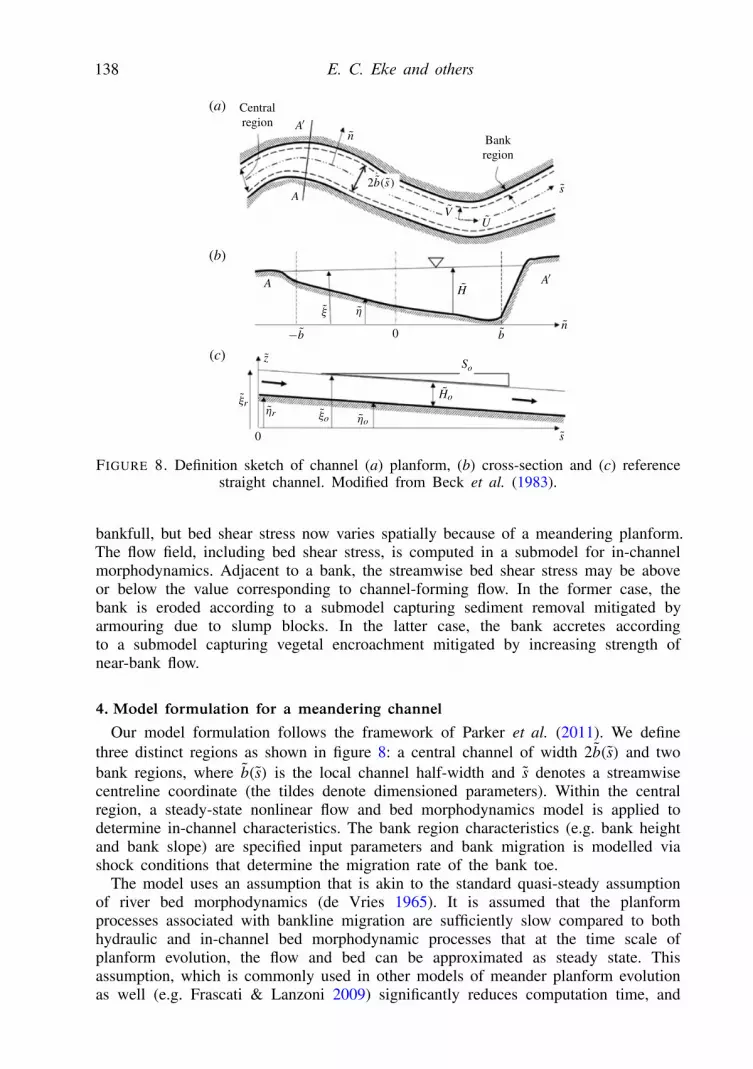
FIGURE 8. Definition sketch of channel (a) planform, (b) cross-section and (c) referencestraight channel. Modified from Beck et al. (1983).

bankfull, but bed shear stress now varies spatially because of a meandering planform.The flow field, including bed shear stress, is computed in a submodel for in-channelmorphodynamics. Adjacent to a bank, the streamwise bed shear stress may be aboveor below the value corresponding to channel-forming flow. In the former case, thebank is eroded according to a submodel capturing sediment removal mitigated byarmouring due to slump blocks. In the latter case, the bank accretes accordingto a submodel capturing vegetal encroachment mitigated by increasing strength ofnear-bank flow.

4. Model formulation for a meandering channel

Our model formulation follows the framework of Parker et al. (2011). We definethree distinct regions as shown in figure 8: a central channel of width 2b(s) and twobank regions, where b(s) is the local channel half-width and s denotes a streamwisecentreline coordinate (the tildes denote dimensioned parameters). Within the centralregion, a steady-state nonlinear flow and bed morphodynamics model is applied todetermine in-channel characteristics. The bank region characteristics (e.g. bank heightand bank slope) are specified input parameters and bank migration is modelled viashock conditions that determine the migration rate of the bank toe.

The model uses an assumption that is akin to the standard quasi-steady assumptionof river bed morphodynamics (de Vries 1965). It is assumed that the planformprocesses associated with bankline migration are sufficiently slow compared to bothhydraulic and in-channel bed morphodynamic processes that at the time scale ofplanform evolution, the flow and bed can be approximated as steady state. Thisassumption, which is commonly used in other models of meander planform evolutionas well (e.g. Frascati & Lanzoni 2009) significantly reduces computation time, and


allows for the model to be run at larger spatial and temporal scales. The drawbackof this assumption is that the model cannot incorporate the formation of free barsmigrating through a train of bends. Thus, we do not describe in detail the mechanismof bank collapse and the subsequent process of sediment removal followed bysediment redistribution downstream. Rather, we assume that this redistribution occursat bed morphodynamic time scale, but adjust the mean bed accordingly at the longerscale of bankline migration.

4.1. In-channel morphodynamic submodel for channel of varying widthAs shown in figure 8, the model uses an intrinsic curvilinear coordinate system todescribe the channel planform. In this coordinate system, the streamwise coordinate scorresponds to the channel centreline and the local transverse coordinate n is definedto be orthogonal to the channel centreline, and is always taken as increasing towardthe left bank of the river looking downstream. This transverse coordinate varies from−b(s, t) to b(s, t) as shown in figure 8(b).

The equations governing channel hydrodynamics/morphodynamics are presentedbelow. Unless otherwise specified, dimensioned parameters introduced below aredenoted so with a tilde superscript; the corresponding parameters without a tildeare dimensionless. Relevant scales for the non-dimensionalization are the previouslyintroduced dimensioned depth-averaged streamwise flow velocity Uo, flow depthHo and mean channel half-width bo, all in a reference straight channel as defined infigure 8(c). These reference quantities, as well as the reference sediment transport rateQso are time-dependent, so as to account for changes in reach-average characteristicsas meanders migrate, as indicated in (4.38) below. The Froude number Fo and ratioof half-width to depth γo of the base flow are given as

Fo = Uo√gHo

; γo = bo

Ho. (4.1a,b)

We introduce the following dimensionless parameters: s and n denote dimensionlessstreamwise and transverse coordinates, respectively, U and V denote dimensionless,depth-averaged streamwise and transverse flow velocities, respectively, H denotesdimensionless depth, c denotes dimensionless channel centreline curvature and ξdenotes dimensionless water surface elevation, defined as

s= s

bo

; n= n

b; b= b

bo

; (U, V)=(U, V

)Uo; (H, ξ)=

(H, ξ

)Ho; c= bo

Rc(4.2a−f )

where Rc is the local centreline radius of curvature. Note here that the transversecoordinate n defined above has been rescaled with the local channel width b(s)for geometric simplicity so that the dimensionless coordinate n always ranges from−1 to 1. The parameters (τs, τn) denote dimensionless streamwise and transversebed shear stresses, respectively, and (qs, qn) denote dimensionless streamwise andtransverse volume sediment transport rates per unit width, respectively: they aredefined in terms of their corresponding dimensioned variables as

(τs, τn)= (τs, τn)

ρU2o

; (qs, qn)= (qs, qn)√RgDsDs

. (4.3a,b)


The dimensionless steady-state depth-averaged equations of motion for a generalfluid flow with variable width can thus be written in intrinsic curvilinear coordinatesas follows:

∂HV∂n+NbcVH + bLsn (UH)= 0 (4.4)

V∂U∂n+UbLsn (U)+ bNcU (V + 2ϕ)+ 1

H∂HUϕ∂n=− 1

F2o

bLsn (ξ)− bγoτs

H(4.5)

V∂V∂n+UbLsn (V)+Nbc

(2Vϕ +ψ −U2

)+ 21H∂HVϕ∂n+ 1

H∂Hψ∂n+ 1

HbLsn (UHϕ)

=−F−2o∂ξ

∂n− b

γoτn

H(4.6)

where Lsn is a differential operator given as

Lsn =N(∂

∂s− n

bdbds

∂

∂n

). (4.7)

Here, N is the longitudinal metric coefficient of the coordinate system, i.e.

N = (1+ nbc)−1 (4.8)

and the parameters ϕ and ψ in (4.4) and (4.6) are secondary flow redistribution termsdefined in Eke et al. (2014).

The Exner equation of bed sediment conservation is given as

bLsn (qs)+ ∂qn

∂n+ qnNbc= 0. (4.9)

Closures for the components of bed shear stress and bedload transport are as givenin Eke et al. (2014), i.e.

(τs, τn)=Cf

√U2 + V2

(U, V + νs(0)

T(0)

)(4.10)

(qs, qn)=Φ (cos ϑ, sin ϑ)∼=Φ(

1,τ ∗nτ ∗s− rγo√τ ∗o

∂η

∂n

)(4.11)

where νs denotes dimensionless secondary flow (made dimensionless by thestreamwise velocity Uo, Cf is the bed friction coefficient (here assumed to be aconstant), T is a primary flow structure function (Johannesson & Parker 1989), ϑindicates the angle of direction of sediment transport relative to the channel centreline,r is a coefficient ranging from 0.3 to 1 (see also Johannesson & Parker 1989). Hereτ ∗s and τ ∗n are the dimensionless Shields stresses given as

(τ ∗s , τ

∗n

)= U2o

gRDs(τs, τn) (4.12)

and Φ is the bedload transport intensity, here estimated using the relation of Parker(1979):

Φ = 11.2(τ ∗s)1.5[

1− 0.03τ ∗s

]4.5

. (4.13)


The approximation for secondary flow adopted here is derived from the case of steady,uniform bend flow; and has been generalized to a channel of arbitrary curvature:

νs = UHχ1γoCf

cG (4.14)

where G is the normalized secondary flow structure function defined in Johannesson &Parker (1989) and χ1 = C−1/2

f /13 (see also Seminara & Solari 1998; Bolla Pittaluga,Nobile & Seminara 2009). More advanced nonlinear, approaches to secondary flow,e.g. Ottevanger, Blanckaert & Uijttewaal (2012) are available, but a linear approachis more suitable for a first model of meandering channels with self-formed width.

The lateral boundary conditions associated with (4.4)–(4.6) and (4.9) are no-penetration conditions for the flow and sediment transport, respectively. Thus,U · nb = q · nb = 0, where U and q are the velocity and bedload transport vectorsrespectively and nb is the unit vector normal to the banks. This translates to

− U(1± bC)

dbds± V = 0 at n=±1 (4.15)

− qs

(1± bC)dbds± qn = 0 at n=±1. (4.16)

In the streamwise direction, for simplification, periodic boundary conditions areapplied.

Finally, the imposed integral conditions for the conservation of water and sedimentdischarge within the channel are as follows:

b∫ 1

−1UH dn= 2 (4.17)

b∫ 1

−1qs dn= 2qso (4.18)

where qso is the streamwise bedload transport rate for the reference straight channel.The integral conditions (4.17) and (4.18) specify that the water discharge and sedimentdischarge in the channel respectively remain the same as for a reference straightchannel, regardless of sinuosity. As a result, the average channel slope S becomesa free variable represented by the deviation sdo from the reference channel slope So,such that

S= So(1+ sdo). (4.19)

Nonlinear effects assure that in the case of a bend with the same average width, thesame sediment transport rate is realized at a lower average bed slope than the case ofa straight channel (e.g. Luchi et al. 2012). In keeping with (4.19), constant deviatoricvelocity and depth parameters, udo and hdo respectively, arise which in the presence ofsinuosity allow total reach-averaged velocity and flow depth to differ from the valuescorresponding to the reference straight channel. Thus,

Hmean = Ho(1+ hdo); Umean = Uo(1+ udo). (4.20a,b)

At the linear level, however, the reach-averaged values of velocity, bed slope anddepth are found to be identical to the reference values (e.g. Imran et al. 1999).


The method to arrive at an iterative solution of the nonlinear system of equations isas outlined in Imran et al. (1999) and Camporeale et al. (2007). Herein we go a stepfurther to include the added complexity of width variation to the solution outlinedin Camporeale et al. (2007). Our method involves expressing each morphodynamicvariable as the sum of that for a reference straight channel and a deviation due to thecombined effect of channel curvature and width variation. Thus, local variables areexpressed as follows:

(U, V,H, η, ξ , c, b) = [1, 0, 1, ηr − Sos, ξr + 1− Sos, 0, 1]+ (udo + ud, vd, hdo + hd,

− Sosdos+ ηd, hdo − Sosdos+ ξd, c, bd) (4.21)

where hd = ξd − ηd, the subscript ‘d’ denotes the deviation and ξr, ηr are the referencewater and bed elevation as shown in figure 6(c). In the above equations, udo, sdoand hdo denote the constant deviatoric streamwise velocity, slope and water depth,respectively, which correspond to reach-averaged conditions and are independent ofs and n.

Meanwhile, qs is taken to be a nonlinear function of U such that qs=1 where U=1.As defined in (4.11) and (4.13), qs is evaluated from the relation of Parker (1979) andcan be expressed in the form of a Taylor expansion, i.e.

qs = 11.2(τ ∗s)1.5[

1− 0.03τ ∗s

]4.5

= qso(1+M (U − 1)+ Rq (U)

)(4.22)

where M = 2(τ ∗o /qso)(∂qs/∂τ∗)|τ=τo . The above equation illustrates the approach to

the nonlinear problem presented here; Rq represents the difference between the fullsediment transport relation and its linear form, or thus the nonlinear residual.

The deviations ud, ηd and ξd can be further decomposed as follows:

ud = udd(s, n)+ udc(s)ηd = ηdd(s, n)+ ηdc(s)ξd = ξdd(s, n)+ ξdc(s).

(4.23)

Here udc, ξdc and ηdc denote the cross-sectionally averaged deviations of streamwisevelocity ud, water surface elevation ξd, and bed elevation ηd, respectively. As such,they are functions of streamwise coordinate s only. In addition, the parameters udd,ξdd and ηdd represent functional forms for the corresponding differences ud − udc, ξd −ξdc and ηd − ηdc; they depend on s and n, and characterize the transverse variationsof streamwise velocity, water surface elevation and bed elevation. By definition, theparameters udd, ξdd and ηdd must satisfy the conditions∫ 1

−1udd dn= 0,

∫ 1

−1ξdd dn= 0,

∫ 1

−1ηdd dn= 0. (4.24a−c)

In addition, udc, ξdc and ηdc are assumed to be periodic with wavelength λ, and mustsatisfy the following conditions:∫ λ

0udc ds= 0,

∫ λ0ηdc ds= 0,

∫ λ0ξdc ds= 0. (4.25a−c)


At this point, it is seen that 10 unknowns, udo, Sdo, hdo, udc, ξdc, ηdc, udd, ξdd, ηddand vd appear in the above equations. According to these variables, three types ofproblems are defined: the ‘O’ problem with unknowns udo, Sdo and hdo independentof s and n; the ‘C’ problem with unknowns udc, ξdc and ηdc which are function of sonly; and the ‘D’ problem with unknowns udd, ξdd, ηdd and vd which are functions ofs and n. The methods of solution of each of these problems, which start from a linearformulation and use successive approximation so as to incorporate nonlinear residuals,are given in appendix A (‘D’ problem) and appendix B (‘O’ and ‘C’ problems).

4.2. Bank submodelsAs stated previously, in order to generate width oscillations by channel migration,the standard channel centreline migration model proposed by Hasegawa (1977) andIkeda et al. (1981) must be abandoned in favour of a model that allows each bankto migrate independently. The bank migration model formation proposed by Parkeret al. (2011) and modified by Eke et al. (2014) quantifies this migration rate througha shock condition, which can be applied to either an eroding or depositing bank. Forthe sake of brevity, only a summary is given here; details can be found in Eke et al.(2014).

For any bank j, which could be the left bank (LB) or right bank (RB), the lateralmigration rate ˙nj is computed as

˙nj = ζE + 1Ss,j

∂ηj

∂ t(4.26)

for an eroding bank and˙nj = ζD + 1

Ss,j

∂ηj

∂ t(4.27)

for a depositing bank.The terms ζE and ζD represent erosion and lateral accretion rates due to sediment

transport away from and toward the banks, respectively. The second term on theright-hand side of (4.26) and (4.27) represent lateral migration due to bed elevationchanges near the banks, where η is the channel bed elevation and ηj is the bedelevation at bank j corresponding to the elevation at n = b(t) and n = −b(t) for theleft and right bank, respectively, where n is the transverse coordinate, defined so asto increase toward the left bank looking downstream, and b is the half channel width.For simplicity, each bank j here has been assumed to have a constant side slope Ss,j.

Eke et al. (2014) details the process of deriving closures to quantify the erosionand deposition rates ζE and ζD in (4.26) and (4.27) above. These simple closures areexpressed in terms of parameters of a fairly intuitive nature namely, an armouringcoefficient Karmour associated with slump block armouring of an eroding bank, a floodintermittency factor If , a default rate of transverse migration ζveg in the absence ofa near-bank shear stress that acts to suppress vegetation, and the erosional bankmigration rate for a purely non-cohesive bank in the absence of slump blockarmouring ζnon,E. Specifically, the closure relation specifying the erosion rate ζEis given as

ζE =KarmourIf ζnon,E. (4.28)

That is to say, the erosion rate of a migrating channel corresponds to the erosionrate of the non-cohesive part of the bank for a channel with no bank armouring


(for which Karmour= 1) during the fraction of time If the river is in flood. This erosionrate reduces linearly with increased armouring (i.e. for Karmour < 1). Armouring in thismodel is considered to be through the presence of slump blocks of an upper cohesive,root-dense material, which form by e.g. undermining as a lower, non-cohesive part ofthe bank erodes. In the derivation of a functional form for this armouring coefficient,we have assumed that it is primarily a function of the erosion rate ζE (as more erosionproduces more slump blocks), and slump block and cohesive layer properties. Theseproperties include the height of the cohesive layer, the characteristic size of the slumpblocks and the residence time of the blocks, which is assumed to be a function of thenear-bank stresses. Thus,

Karmour =Karmour

(ζE, τ

∗E , ζEref , τ

∗form

)(4.29)

where τ ∗E is the flow Shields number near the eroding bank, ζEref is a reference erosionrate based purely on slump block characteristics and τ ∗form is a formative/thresholdShields number. The precise form of (4.29) is given by Eke et al. (2014). Substitutinginto (4.28), and rearranging, we get a simplified closure relation for ζE, namely

ζE = 1(1+

(τ ∗Eτ ∗form− 1)−1

If ,ref

∣∣ζnon,E

∣∣ζEref

) If ζnon,E. (4.30)

In (4.30), the parameter If ,ref is a reference intermittency corresponding to thereference erosion rate ζEref . The relation in (4.30) is appreciated better if we assumethe second term in the denominator is � 1, in which case the form for the erosionrate simplifies to

ζE = ζErefIf

If ,ref

(τ ∗Eτ ∗form− 1). (4.31)

The formative Shields number here is the threshold value above which bank erosionoccurs. As seen above, it also corresponds to the formative Shields number for astraight channel. The relation in (4.31) is very similar to the form of erosion rulesthat have been generally applied in previous work, with the difference being that termshave specifically defined closures based on measurable field parameters.

For a depositing/accreting bank, the model specifies a default rate of transversemigration ζveg of the inner accretional bank toward the channel centre associated withflows that are insufficient to suppress vegetation growth, i.e. during the fraction oftime 1− If . The model then assumes a linear suppression of this encroachment rateas the near-bank bed shear stress increases, so that

ζD = ζveg(1− If

) (1− τ ∗D

τ ∗form

)(4.32)

where ζD is a rate of transverse migration of the inner accretionary bank toward thechannel centre and τ ∗D is the Shields number based on the streamwise shear stressacting on the bed immediately adjacent to the depositing bank. Again here we haveassumed the formative Shields number to be a threshold above which lateral accretionis no longer possible.


The closures as presented in (4.30) and (4.32) allow a smooth transition from oneprocess to the other, i.e. erosion occurs when τ ∗j ≡ τ ∗E > τ ∗form and accretion occurswhere τ ∗j ≡ τ ∗D < τ ∗form where τ ∗j is the Shields number based on the streamwisebed shear stress immediately adjacent to a bank j. Model bank input parametersthus include a specification of a relation for the formative Shields number τ ∗form,an estimation of the lumped reference migration rate due to erosion ζEref and anestimation of the default vegetal encroachment rate ζveg.

4.3. Kinematic model for channel shiftThe channel axis is discretized through a sequence of equally spaced nodes (xc, yc),each representing a cross-section of the river identified by the streamwise coordinate s.The spatial distribution of the angle θ(s), formed by the local tangent to the channelaxis and the direction of a generic Cartesian axis of reference, is obtained by thefollowing relationship:

θ (i) = arctan(

yc(i+1) − yc(i−1)

xc(i+1) − xc(i−1)

)(4.33)

where the subscript i denotes the location along the streamwise coordinate. Thecentreline curvature distribution can thus be computed easily as

c(s)=−dθds. (4.34)

Central differences are used to calculate the derivative of θ and periodic boundaryconditions are applied at the reach boundaries.

Planimetric evolution of the channel centreline is calculated by displacing eachcentreline node orthogonally by an amount

∆(i)c = 1

2

[ ˙n(i)LB + ˙n(i)RB

]1t (4.35)

such that the new centreline coordinates are

xc(i)(t+1t)= xc(i)(t)−∆(i)c sin θ (i)

yc(i)(t+1t)= yc(i)(t)+∆(i)c cos θ (i).

}(4.36)

The corresponding channel half-width evolution is computed accordingly:

b(i) (t+1t)= b(i) (t)+ 12

( ˙n(i)LB − ˙n(i)RB

)1t. (4.37)

At each time step, once the centreline has been displaced according to (6.1), thenew centreline is regridded such that each node is equally spaced at an interval 1sset to be of the order of the mean channel half-width bo(t). Thus, as the channelmigrates, to maintain the specified grid spacing, the number of nodes in the channelgrid may increase or decrease. The channel half-width distribution corresponding tothe regridded centreline is obtained by cubic spline interpolation.

Insofar as the mean width, length and reach-averaged slope of the channel ischanging in time, the parameters Uo and Ho corresponding to the reference straight


channel solution also evolve in time, according to the following relations obtainedfrom (3.1), (3.3) and (3.5):

Ho =(

Cf Q2o

4b2ogSo

)1/3

; Uo =(

gQoSo

Cf 2bo

)1/3

; Qso = qso(RgD3

s

)1/22bo. (4.38a−c)

These parameters, which are embedded into the non-dimensionalization of (4.2), mustbe recomputed at every time step. The reference channel slope is varied under theconstraint of a constant elevation drop 1z as

So(t)= 1z

λ(4.39)

where λ is the channel centreline wavelength.The step size 1t is controlled as suggested by Frascati & Lanzoni (2009), by

requiring that

1t 6 0.011s( ˙nj

)max

. (4.40)

The form of (4.40) is similar to the relation used by Courant, Isaacson & Rees (1952)for the stability of explicit numerical schemes for computation of riverbed deformation.In this particular case, the celerity of propagation of an infinitesimal bed perturbationis replaced by the celerity of river migration.

5. Numerical simulations5.1. Set-up

Starting from a constant width, low-amplitude meander, we apply the aboveformulation to an initial sine-generated meander waveform, and run until incipientcut-off conditions. The sine-generated meander waveform is defined according to

θ = θ0 sin (κs) (5.1)

where θ specifies the angle orientation of the s coordinate, θo is the angular amplitudeand κ is the downstream channel wavenumber. Channel curvature distribution is thusevaluated as

c=−dθ(s)ds= υ cos (κs) . (5.2)

The test-case river channel for the calculations is based on a reach of the PembinaRiver (§ 2, figure 2) which represents a fairly typical actively meandering sand bedstream (Beck et al. 1983; Beck 1988; Imran et al. 1999). According to Beck et al.(1983), this reach has shown peak bank erosion rates ranging between 2 and 5 m yr−1,an estimated bankfull discharge that range 250–440 m3 s−1, a mean bankfull width of91 m, a mean bankfull depth of 3.75 m, a water surface slope of 0.00026, a sinuosityof 1.9 and an estimated friction coefficient Cf = 0.0068.

A representative bankfull discharge of 405 m3 s−1 is chosen which has a floodintermittency of approximately 0.2 (Beck et al. 1983). Characteristic grain size Ds isknown to be in the sand range for the reach in question; here it is set equal to 2.0 mm,i.e. the upper end of sand. This modification is made so that sediment transport can


Parameter Value Description

Qo (m3 s−1) 405 Bankfull discharge2boi (m) 99.7 Initial bankfull widthHoi (m) 2.85 Initial bankfull depthSoi 0.00049 Initial mean channel centreline slopeDs (mm) 2 Characteristic grain sizeτ ∗form,i 0.426 Initial channel-forming Shields numberIf , Ifref 0.2 Flood intermittenciesSs,LB; Ss,RB −1.5; 1.5 Bank side slope at left and right banks, respectivelyHb,LB;Hb,RB (m) 2.5 Thickness of non-cohesive layer at left and right banks,

respectivelyHc (m) 1.25 Cohesive layer thicknesspc 0.6 Cohesive layer porosityζEref (m yr−1) 5 Reference slump block-modulated bank erosion rateζveg (m yr−1) 10 Default vegetal encroachment rate

TABLE 2. Summary of input parameters for base run based on the Pembina River inAlberta, Canada. The subscript i indicates initial values of parameters that change overtime.

be computed solely from a bedload transport relation, here chosen to be Parker (1979).In the case of medium sand, the sediment transport rate would have to be decomposedinto bedload and suspended load parts, and the gravitational term in (4.12) would haveto be applied only to bedload transport.

In order to specify an appropriate initial state, the river bankfull parameters havebeen adjusted to correspond to a nearly straight channel with a water surface slopeequal to the channel downvalley slope Sv (= 0.00026× 1.9= 0.00049). The formativeShields number is estimated using the regression fit of Li et al. (2014) which isas expressed in (3.10), and the corresponding bankfull channel characteristics areobtained from (3.7) to (3.9). Table 2 shows the adopted model input parameterscorresponding to a nearly straight reach of the Pembina River. Comparing with thedataset of Parker et al. (2007) and Wilkerson & Parker (2011) for river reachescovering a broad range of grain size classes, we see, as shown in figure 9, that thechannel-forming Shields number τ ∗form corresponding to the model input parametersfits within the range for rivers of similar grain sizes. This value is used here as aninitial value τ ∗form,i corresponding to a nearly straight or low-sinuosity channel.

The estimated reference erosional migration rate ζEref = 5 m yr−1 is based on thefollowing assumptions: an average cut bank 3.75 m high with a third of the bankheight consisting of cohesive/rooted soil, a characteristic slump block size equal tothe cohesive layer thickness, a reference slump block decay time Tcref of 1.5 years,and a cohesive layer porosity pc = 0.6. A default vegetal encroachment rate ζveg

corresponding to approximately 10 % of initial bankfull width per year, or thus10 m yr−1 has been adopted. Here these numbers have been chosen in part by meansof numerical experiments, so as to produce results that correspond to observations. Inprinciple, all of these parameters are physically measurable, but measurement of Tcref

and ζveg in particular would require an extensive field campaign that is beyond thescope of this work.


103

102

101

10–1

10–2

10–3

10–5 10–4 10–3 10–2 10–1 100

100

S

Numericaltest case

FIGURE 9. (Colour online) Channel forming (bankfull) Shields number versus channelslope S. The datasets for bankfull geometry are from Parker et al. (2007) and Wilkerson& Parker (2011). A point for the numerical test reach considered here, for which Ds =2 mm, has been added to the figure. Also shown is the line corresponding to (3.10) forD= 2 mm.

Run γoi = boi/Hoi Ds = Ds/Ho τ ∗form,i κi = 2πboi/λi Υ = ζEref /ζveg

Base 17.5 0.0007 0.43 0.16 0.5G 8.6–17.5 0.0007 0.43 0.16 0.5D 17.5 0.0007–0.0035 0.85–0.17 0.16 0.5L 17.5 0.0007 0.43 0.1–0.21 0.5Y 17.5 0.0007 0.43 0.16 0.25–1.5

TABLE 3. Input conditions for different numerical runs to find the effect of non-dimensional parameters on width curvature correlation. The subscript i indicates initialvalues of parameters that change over time.

For the initial low-amplitude channel, we assume an along-channel centrelinewavelength λ of 2 km and an initial maximum curvature value capex = υ = 0.025.

The input parameters shown in table 2 are for the base run. In addition to thebase case, numerical experiments were carried out to determine model sensitivity toselected non-dimensional parameters. The input parameters for the various runs (RunsG,D, L and Y , as explained below) expressed in terms of dimensionless numbers areshown in table 3.

Going from left to right, the dimensionless parameters shown in each column arethe half-width to depth ratio or aspect ratio γo, the dimensionless grain size Ds, thechannel forming Shields number τ ∗form, the dimensionless channel wavenumber κ andthe ratio of reference erosion rate to reference deposition rate, Υ . The first fourparameters are considered to be key governing parameters in river morphodynamics.The last parameter, Υ , specifically defined as

Υ = ζEref

ζveg(5.3)


is here shown to be critical in determining the correlation between channel widthand curvature. By varying discharge within the range of estimated bankfull discharge,i.e. from 200 to 405 m3 s−1, we vary the initial value of the aspect ratio from 8.6to 17.5 in the G runs. We vary both the grain size and formative Shields number inthe D runs by increasing the grain size from coarse sand to medium gravel, i.e. from2 to 10 mm. Finally, we vary the reference migration parameter in runs Y by fixingthe reference erosion parameter ζEref = 5 m yr−1 and varying the deposition parameteraccordingly so that Υ varies from 0.25 to 1.5. As a check, the Y runs were repeatedfor different values of ζEref .

5.2. Constant versus slope-dependent channel-forming Shields numberWe indicated in § 3 that the adoption of a constant value of channel-forming Shieldsnumber τ ∗form equal to the initial value τ ∗form,i leads to a channel that becomesunacceptably narrow as sinuosity increases. This point is illustrated in more detail inEke (2013) and Eke et al. (2014). Here we illustrate this process, and also illustratehow the slope-dependent form (3.10) for channel-forming Shields number resolvesthis problem.

The calculation is first performed for the base case values under the assumption ofconstant τ ∗form = 0.426 (table 2). Figure 10(a) shows the planimetric evolution of thechannel centreline over time in terms of five snapshots from time t= 0, each at 1000-year intervals, and figure 10(b) plots the two banklines over the same time interval. Infigure 10(a) we see that the channel undergoes an initial rapid downstream and lateralchannel migration rate which reduces as the sinuosity increases. The figure also showsthe development of an upstream skewing bias as the channel elongates (e.g. Parkeret al., 1983). The simulation does not reach incipient cut-off, as the numerical modelfails not long after the last snapshot at t = 3400 yr. Figures 10(b) and 12 illustratesthe cause of failure.

The continuous variation of the downchannel slope triggered by planimetricevolution results in a variation of reach-averaged/reference channel characteristics.As shown in figures 10(b) and 11, with increasing sinuosity, channel width and depthadjust as expected. Mean bankfull width reduces and mean bankfull depth increaseswith the progressive decline in channel slope. The result is a channel that becomesprogressively deeper and narrower as it approaches cut-off. This narrowing yields awidth–depth ratio that is not only unrealistically small from a physical point of view,but also causes failure of the numerical model, as shown in figure 11.

Figures 12 and 13 show the corresponding calculations for the case of aslope-dependent channel-forming Shields number varying according to (3.10).Although channel narrowing is observed, the channel continues to develop sinuosityuntil incipient neck cutoff. This result highlights the significance of the work of Liet al. (2014), who demonstrate that bankfull Shields number increases to about thehalf power of channel slope. The model results show that the inclusion of this effectis important in the analysis of meandering channels with self-formed width.

In all cases below, the channel-forming Shields number is assumed to be slope-dependent according to (3.10).

5.3. Base caseThe planimetric evolution of the base simulation is as shown in figure 12. In additionto a migration rate and a mean channel width that declines, it can be discerned that the


4

3

2 Final

1

0

–1

–2

15

10

5

0

–5

–10

–1525 30 35 40 45 50

0 2 4

x (m)

y (m

)y

(m)

6 8

(a)

(b)

(× 103)

(× 103)

(× 102)55 60

(× 102)

FIGURE 10. An example model simulation of an idealized periodic channel from aninitial low amplitude to high amplitude, with constant channel-forming Shields number.(a) Centerline migration over time. (b) Planform showing evolution of channel width overtime. Time indicated is in years.

channel develops and maintains a spatial width variation pattern which becomes lessprominent over time as the channel elongates. The nature of this variation is illustratedmore clearly below.


60

50

40

30

20

10

0 2 4

Modelfailure

6

6

5

4

3 So

2

1

0

(× 10–4)

(× 103)Time (yr)

FIGURE 11. Reference channel adjustment over time in response to increasing channelsinuosity. As slope So reduces, the channel half-width bo reduces and flow depth Hoincreases. Model results assume a constant channel-forming Shields number.

Let capex denote the dimensionless curvature at the bend apex, ˙nmax denote the(dimensioned) magnitude of the maximum centreline lateral migration rate of thechannel bend, and δ denote the (dimensionless) strength of the width variationdeviation, here defined as

δ = Bmax − Bmin

4bo

(5.4)

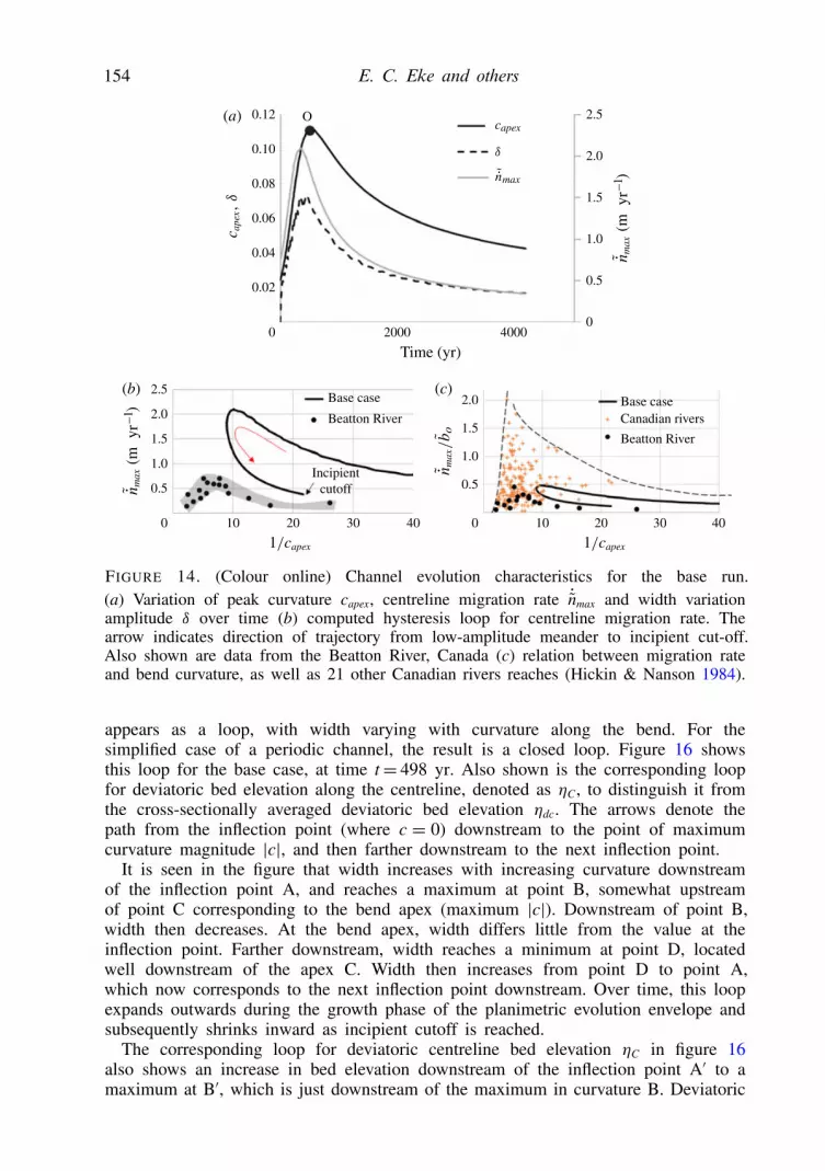
where Bmax and Bmin are the maximum and minimum widths for the reach at a giventime. Over the course of channel evolution, we observe, as shown in figure 14(a),that capex, δ and ˙nmax rapidly increase, reach a peak value at 498, 450 and 425 years,respectively, and then decline more slowly. The peak values obtained for the migrationrates and width variation are within the range of observed values for the reach of thePembina River in question.

In figure 14(b), the loop curve mapping the computed relationship betweenmaximum migration rate ˙nmax and dimensionless radius of curvature 1/capex up toincipient cutoff for the base case is shown. The peak migration rate shown on theloop falls toward the lower end of the observed range of peak values, i.e. 2–5 m yr−1

reported by Beck et al. (1983). Beck et al.’s values are for the relatively rapidlymigrating Manola subreach rather than the entire reach of figure 2.

Also shown in figure 14(b) are data of Hickin & Nanson (1984) for the BeattonRiver, Canada. These are included only to illustrate a similar trend for sufficientlylarge radius of curvature; evidently the Beatton River has a peak migration rate thatis substantially lower than the reach of the Pembina River studied here.

In figure 14(c), the computed loop curve in the form of ˙nmax/bo versus 1/capexis plotted against data for the Beatton River, as well as 21 other river reaches inCanada, including the Pembina River. Also shown in figure 14(c) is an envelopecurve bounding the data from above. Figure 14(b,c) suggest model performance


6

4

2

Final

0

–2

25

20

15

10

5

0

–5

–10

–15

–20

–25

0 2 4

x (m)

y (m

)y

(m)

6 8

(a)

(b)

(× 103)

(× 103)

2 3 4 5 6(× 103)

(× 102)

FIGURE 12. An example model simulation of an idealized periodic channel from an initiallow amplitude to high amplitude, with slope-dependent channel-forming Shields number.(a) Centerline migration over time. (b) Planform showing evolution of channel width overtime. Time indicated is in years.

that is in the expected range for meandering rivers. The model does not capture azone within which migration rate decreases with increasing curvature (decreasingradius of curvature 1/cmax). This may be due to (a) limitations of the model at highcurvature, or (b) behaviour observed in the field associated with the development ofbend complexity and cut-off (Hickin & Nanson 1984; Hooke 2003). The observedbehaviour at very high curvature is not captured in the simple implementation shown


60

50

40

30

20

10

0 2 4

Incipientcutoff

6

5

4

3 So

2

1

0

(× 10–4)

(× 103)Time (yr)

FIGURE 13. Reference channel adjustment over time in response to increasing channelsinuosity. As slope So reduces, the channel half-width bo reduces and flow depth Hoincreases. Model results assume a slope-dependent channel-forming Shields number.

in figure 12, corresponding to a periodic bend developing only as far as cutoff, butcan be partially captured in an implementation that includes non-periodicity and goesbeyond cutoff (Eke 2013).

Figure 15 shows the downstream variation in dimensionless curvature c, half-widthb and relative bed elevation ηd at channel right, left and centre (i.e. n=−1, 1 and 0,respectively) for the time t = 500 years. This time is when the bends reach peakcurvature, i.e. point O in figure 14(a). The downstream coordinate s has been scaledby the bend length λbend = λ/2.

The width is shown to spatially oscillate at twice the wavelength of curvature.The bed elevation at the left and right banks shows a primary oscillation at thewavelength of curvature, but hidden in the variation is a second harmonic. Thissecond harmonic, which appears only when nonlinear effects are included in thenumerical model (§ 4.1), is readily seen in terms of centreline bed elevation, which,like width, oscillates at twice the wavelength of curvature. This prominent secondharmonic at the channel centreline is present even for the case of a constant-widthchannel. It has been considered to be an indication of a tendency for central bars toemerge (Luchi et al. 2010) and has been used as a basis for the ‘curvature-forced’mechanism for mid-channel bar development proposed by Luchi et al. (2010).

Figure 15 shows that for the base run, the width maximum falls just upstream ofthe bend apex, and the minimum somewhat farther downstream of it. The bends ofthe Pembina do indeed show this behaviour, as can be seen in figure 7. The centrelinebed elevation responds in kind with its peak located just upstream of the bend apex.

At this point it is useful to recall the analysis of field data in § 2, in which localdimensionless width b is plotted against the absolute value of local dimensionlesscurvature |c| (figures 4 and 5). In the field data, the width–curvature correlationover multiple bends appears as a series of scatter points to which we have fitted aregression line. Along one wavelength of a single bend, however, the correlation


0.12

0.10

0.08

0.06

0.04

0.02

0 2000

Time (yr)4000

2.5

2.0

1.5

1.0

0.5

0

(a)

2.5(b) (c)

2.0

1.5

1.0

0.5

0 10 20 30 40

2.0

1.5

1.0

0.5

0 10 20 30 40

O

Base case

Beatton River

Incipientcutoff

Base case

Beatton River

Canadian rivers

r–1

r–1

FIGURE 14. (Colour online) Channel evolution characteristics for the base run.(a) Variation of peak curvature capex, centreline migration rate ˙nmax and width variationamplitude δ over time (b) computed hysteresis loop for centreline migration rate. Thearrow indicates direction of trajectory from low-amplitude meander to incipient cut-off.Also shown are data from the Beatton River, Canada (c) relation between migration rateand bend curvature, as well as 21 other Canadian rivers reaches (Hickin & Nanson 1984).

appears as a loop, with width varying with curvature along the bend. For thesimplified case of a periodic channel, the result is a closed loop. Figure 16 showsthis loop for the base case, at time t= 498 yr. Also shown is the corresponding loopfor deviatoric bed elevation along the centreline, denoted as ηC, to distinguish it fromthe cross-sectionally averaged deviatoric bed elevation ηdc. The arrows denote thepath from the inflection point (where c = 0) downstream to the point of maximumcurvature magnitude |c|, and then farther downstream to the next inflection point.

It is seen in the figure that width increases with increasing curvature downstreamof the inflection point A, and reaches a maximum at point B, somewhat upstreamof point C corresponding to the bend apex (maximum |c|). Downstream of point B,width then decreases. At the bend apex, width differs little from the value at theinflection point. Farther downstream, width reaches a minimum at point D, locatedwell downstream of the apex C. Width then increases from point D to point A,which now corresponds to the next inflection point downstream. Over time, this loopexpands outwards during the growth phase of the planimetric evolution envelope andsubsequently shrinks inward as incipient cutoff is reached.

The corresponding loop for deviatoric centreline bed elevation ηC in figure 16also shows an increase in bed elevation downstream of the inflection point A′ to amaximum at B′, which is just downstream of the maximum in curvature B. Deviatoric


0.1

–0.1

0

0 1 2 3 4 5 6

0 1 2 3 4 5 6

0 1 2 3 4 5 6

1.1

0.9

1.0

0.5

–0.5

0

(a)

(b)

(c)

b

c

FIGURE 15. (Colour online) Downstream variation in dimensionless curvature c,half-width b and relative bed elevation ηd at time t= 498 yr corresponding to peak bendamplitude (point O in figure 14a). Continuous vertical lines indicate bend apex location,thin (red online) dashed lines indicate maximum width, thin (red online) dash-dottedlines indicate location of minimum width, and thin (green online) dotted lines indicationlocation of maximum centreline bed elevation.

centreline bed elevation then declines farther downstream, but is still well above zeroat the bend apex C′. Minimum deviatoric centreline bed elevation continues to declineto point D′, located somewhat downstream of the point of minimum width D, andthen increases back to point A′ corresponding to the next inflection point downstream.The width at the apex is shown to be nearly the same as that at the crossing. Havingsaid this, the point of width maximum is upstream of the apex, and closer to theapex than the nearest crossing, which is in line with the general trends observed infigure 7.

To show how correlation trends change over time as the bend develops towardincipient cutoff, let φapex, φBmax, φBmin, φηcmax denote the respective dimensionless phasedistances, from an upstream inflection point to the location of the curvature maximum,width maximum, width minimum and centreline bed elevation maximum, respectively.The phase distance represents an arc length that has been rescaled by the channel bendlength λbend such that it ranges from 0 at the upstream inflection point to 1 at thedownstream inflection point. The time variation of φapex, φBmax, φBmin, φηcmax is shownin figure 17(a). The figure also shows the phase distance to the location of maximumcentreline migration rate φM.

In figure 17(a), the point φ = 0.5 corresponds to half the distance from inflectionpoint to the next inflection point downstream. Thus, 0 < φ < 0.5 corresponds to theupstream half of the bend, and 0.5<φ < 1 corresponds to the downstream half. It isseen from the curve of φapex in the figure that the bend apex quickly moves into the


1.2

b

b

1.1

1.0

0.9

0.10

0.05

0

–0.050 0.02 0.04 0.06 0.08 0.10

Widthmin.

Widthmax.

Bedmax.

D

A

B

C

Bedmin.

FIGURE 16. (Colour online) Loop curves along a meander bend at t= 498 yr for width band deviatoric centreline bed elevation ηC as functions of the absolute value of curvature.The locations A, B, C and D correspond respectively to the inflection point, point ofmaximum width, point of maximum curvature and point of minimum width along the loopfor b. The points A′, B′, C′ and D′ correspond respectively to the inflection point, pointof maximum deviatoric bed elevation, point of maximum curvature and point of minimumdeviatoric bed elevation along the loop for ηC. Arrows indicate direction of trajectory.

1.00(a)

0.75

0.50

0.25

0 1 2

Time (yr) Time (yr)3 4

1.0(b)

0.5

0

–0.5

–1.00

Upstream ofbend apex

Downstreamof bend apex

1 2 3 4

(× 103) (× 103)

FIGURE 17. (Colour online) Plots of time variation of normalized along-channel locationof width maximum (φBmax on the left, ωBmax on the right), maximum deviatoric centrelinebed elevation (φηcmax on the left, ωηcmax on the right), width minimum (φBmin on theleft, ωBmin on the right), maximum migration rate (φM on the left, ωM on the right) andmaximum curvature (bend apex: φapex on the left). (a) Variation of φBmax, φηcmax φBmin,φM and φapex, representing phase position downstream of the inflection point. The (redonline) dotted line indicates the bend geometric midpoint. (b) Variation of phase distancesωBmax, ωηcmax ωBmin and ωM, normalized relative to the bend apex.

upstream half of the bend, and stays there until incipient cutoff. This corresponds tobends that are skewed upstream (e.g. Parker et al. 1983).

The curves of φBmax and φBmin in figure 18(a) indicate that maximum width is alwaysattained upstream of the apex, and minimum width is always attained downstream of


0.08

(a) (b) (c)

0.06

0.04

0.02

0 0.05 0.10 0.1 0.2 0.1 0.2 0.30.15

0.15

0.10

0.0010.002

0.05

Ds

0

0.15

0.10

0.05

0

0.004

0.16

0.21

17.513.08.6

FIGURE 18. (Colour online) Sensitivity of time trajectories of width variation intensityδ versus downchannel wavenumber κ to variation in input parameters. (a) Sensitivity toaspect ratio γoi. (b) Sensitivity to dimensionless grain size Ds. (c) Sensitivity to initialwavenumber κi. The thick lines indicate the base run and the straight arrows indicate thedirection of increase. Temporal evolution along each curve is from right to left as indicatedby the curved arrow in (a).

the apex. The bend apex always falls downstream of the point of maximum widthand upstream of the point of minimum width, but is closer to the point of maximumwidth. The point of maximum width is always in the upstream half of the bend;this trajectory is also tracked by the phase location φηcmax corresponding to maximumdeviatoric centreline bed elevation. The location of minimum width φBmin shifts fromthe upstream half to the downstream half of the bend as the meander train evolves.The location of maximum migration rate φM tracks the location of minimum width.

Another way to measure width–curvature–bed elevation phasing is to define thephase distance relative to the bend apex, ω, as

ωq =

φq − φapex

φuφq − φapex < 0

φq − φapex

φdφq − φapex > 0

(5.5)

where q is a given variable (e.g. q=ηdc for deviatoric centreline bed elevation) and φuand φd denote the upstream and downstream phase distance relative to the bend apexas defined in figure 17(a), so that the two sum to unity. The parameter ωq is thusdefined such that it varies from −1 to 1 with 0 corresponding to the bend apex and −1and 1 corresponding to the upstream and downstream inflection points, respectively.The variations over time of location of the width maximum ωBmax, width minimumωBmin, maximum deviatoric centreline bed elevation ωηcmax and maximum migrationrate ωM are shown in figure 17(b). In the figure we see that over time, the normalizedlocations of the width maximum and deviatoric central bed elevation maximum remainfairly constant at approximately ω=−0.3. The locations of the width minimum andmaximum migration rate, on the other hand, shows significant change during benddevelopment, but eventually approach an asymptote of ω= 0.25 up to incipient cutoff.

5.4. Model sensitivity to channel parametersChanges to the aspect ratio, grain size and initial wavelength were found to alterthe lateral migration rates predicted by the model. For example, a reduction in theinitial aspect ratio γoi from the base value was found to result in lower curvature


peaks as well as reduced channel migration rates. Increased sediment size alsoresulted in a decrease in migration rates. Increasing the initial channel wavenumberκ (i.e. decreasing the wavelength) from the base value, however, was found toincrease the migration rate and yield a higher curvature peak. These tendencies werecomputed by performing the G runs (variation in γoi), D runs (variation in Ds) andL runs (variation in κ) of table 3. The results are summarized in figure 18.

Figure 18(a–c) all show time trajectories of width variation intensity δ versus down-channel meander wavenumber κ . In all cases temporal variation is from right to left,as indicated by the curved arrow in figure 18(a). The sensitivity of this trajectory tovariation in initial aspect ratio γoi is shown in figure 18(a); the sensitivity to varieddimensionless grain size Ds is shown in figure 18(b), and the sensitivity for variedinitial wavenumber κi is shown in figure 18(c). The base case is shown as the thickblack line for each figure. The straight arrow denotes the direction of increase of theparameter in question.

For each case, as the channel evolves over time, the channel wavenumber steadilydrops, corresponding to increasing sinuosity. As time passes and wavenumber drops,the intensity of width variation increases, reaches a peak, and then declines. Themagnitude of this peak evidently increases with increasing initial aspect ratio γoi andinitial wavenumber κi. Although the behaviour is less consistent in terms of grainsize, a grain size that is five times the base value results in a near-doubling of widthvariation intensity.

The phasing of width oscillation with respect to curvature is also impacted bychanges to the parameters γoi, Ds and κi. This sensitivity is illustrated in terms ofthe time trajectories of ωBmax and ωBmin versus κ given in figure 19(a–c). In all casestemporal evolution is from right to left, i.e. the direction of increasing wavenumber κ .The general trend is for the location of the width minimum to be shifted upstreamtoward the bend apex as sinuosity increases over time. This is seen in all cases shownin figure 19. The width minimum shifts upstream for increasing γoi and downstreamfor increasing grain size. The location of the width maximum is largely unaffectedby γoi, but shows a significant downstream shift toward the bend apex for larger grainsizes.

In all of the above simulations shown, while the width–curvature trajectory is seento change with changing input parameters, the general tendency is for the widthmaximum to be located just upstream of the bend apex and for the minimum to belocated slightly to significantly downstream. In the next section, however, we showthat this pattern is a strong function of the reference erosion and deposition rates. Westudy this by varying their ratio (Y runs of table 3).

5.5. Model sensitivity to bank parametersFigure 20 shows results for bed topography and bank lines obtained from modelsimulations from the Y runs of table 3, where the ratio of the reference erosion rateto reference deposition rate Υ = ζEref /ζveg is varied by holding the erosion rate ζEref

constant and varying the deposition rate ζveg accordingly. More specifically in additionto the base value Υ = 0.5, the values 0.25, 0.75, 1.0, 1.25 and 1.5 are also considered.Again each snapshot shown here represents the time at which curvature reaches thepeak of its envelope curve (e.g. figure 15a). The values of the peak curvature andmigration rates for each of the snapshots are indicated in the figure.

In the figures, the bank lines correspond to the bounds of the central region offigure 8. The contour lines shown indicate dimensionless relative bed elevation. The


1.0(a)0.8

0.6

0.4

0.2

–0.2

–0.4

–0.6

0

0 0.05 0.10 0.15 0 0.05 0.10 0.15 0.20

1.0(b)0.8

0.6

0.4

Ds

0.2

–0.2

–0.4

–0.6

0

0 0.1 0.2 0.3

1.0(c)0.8

0.6

0.4

0.2

–0.2

–0.4

–0.6

0

FIGURE 19. (Colour online) Sensitivity of time trajectories of normalized phase relativeto bend apex ωBmax ωBmin, corresponding to maximum and minimum width versusdownchannel wavenumber κ , to variation in input parameters. (a) Sensitivity to aspectratio γoi. (b) Sensitivity to dimensionless grain size Ds. (c) Sensitivity to initialwavenumber κi. The thick lines indicate the base run and the straight arrows indicate thedirection of increase. Temporal evolution along each curve is from right to left. The valuesof γoi,Ds and κI are the same as in figure 18.

near-zero contour of 0.05 has been highlighted to better visualize the point barconfiguration in each plot. Here we define the point bar in terms of the portion ofthe channel between the 0.05 contour and the lower bank in the plot.

Figure 20(a–f ) show a steady progression in pattern as Υ increases. This is mostreadily seen in terms of the two points, A and B, in figure 20(a). Point A, markedwith a solid arrow, shows the position of maximum width for Υ = 0.25, and point B,marked with an open arrow, shows the position of minimum width for the same valueof Υ . These same positions are marked with corresponding solid and open arrows forthe cases Υ = 0.50, 0.75, 1.0, 1.25 and 1.5 in figure 20(b–f ), respectively. The widthat the point of the solid arrow monotonically decreases with increasing Υ , so that thepoint becomes very nearly the narrowest point on the bend for Υ = 1.50. The widthat the point of the open arrow monotonically increases with increasing Υ , so that thispoint is not too far from the width maximum at Υ = 1.5. The systematic variation ofwidth at the points of the solid and open arrows is illustrated in figure 20.

It can also be seen that as Υ increases from 0.25 to 1.50, the intensity of widthvariation first decreases, and then increases. A corresponding pattern can be seensomewhat downstream of the bend apex at point ‘B’, with monotonically increasingwidth as Υ increases from 0.25 to 1.50. The value of the dimensionless width atpoint A and B for each of the cases shown in figure 20 are plotted as a function ofΥ in figure 21.


600

400

200

y (m

)y

(m)

y (m

)

x (m) x (m)

0

–200

(a)

3600 3800 4000 4200 4400 4600

600

400

200

0

–200

(b)

3400 3600 3800 4000 4200 4400

400

200

0

(c)

36003400 3800 4000 4200 4400

600

400

200

0

–200

(d)

3400 3600 3800 4000 4200 4400

400

200

0

(e)

36003400 3800 4000 4200 4400

600600

400

200

0

–200

( f )

3400 3600 3800 4000 4200 4400

A B

r–1 r–1

r–1r–1

r–1r–1

FIGURE 20. (Colour online) Plots of bed topography contours and bank lines illustratingsensitivity variation in the coefficient Υ = ζEref /ζveg. In the plots, ζEref is held constant at5 m yr−1 while ζveg is reduced from (a)–(f ), so yielding the increasing values of Υ . Thebank lines correspond to the bounds of the bank region of figure 8. Each plots correspondto the time at which peak bend amplitude was reached. Direction of flow is from left toright in all cases. The filled and white arrows correspond to the location of maximum andminimum width for Υ = 0.25, respectively. Width deviation has been magnified by 5 forvisualization.

The case Υ = 0.5 shown in figure 20(b) is of particular interest because itcorresponds to the base case. It is seen from the figure that the model predictsa point of maximum width that lies upstream of the bend apex just as seen in thefield.

The teardrop shape of the point bar delineated by the 0.05 bed elevation contour linealso undergoes a systematic transition as Υ increases, with the locus of maximum barwidth moving from upstream of the bend apex to downstream of it.


1.3

1.1

0.9

0.7

0.50 0.5 1.0

A

B

b

1.5 2.0

FIGURE 21. (Colour online) Dimensionless half-width at a fixed point A upstream of thebend apex and a fixed point B downstream of the bend apex as a function of Υ . Thepositions of these points are depicted in figure 21. The values for Υ = 0.25 correspondto maximum width (A) and minimum width (B).

This systematic change in the pattern of width variation with increasing Υ may beone reason why each of the four field cases shown in figures 4 and 5 shows a differentrelation for b versus |c|.

Bend migration patterns can be characterized in terms of ‘bank pull’ and ‘barpush’. Based on Stillwater Science (2007), Eke et al. (2014) defined these as follows:a cross-section is undergoing bank pull when the eroding bank is migrating fasterthan the depositing bank, and it undergoes bar push when the depositing bank ismigrating faster than the eroding bank. Stillwater Science (2007) relates these modesof migration to the effect of topographic steering of the flow by the point bar.

It might be thought that an increase in Υ = ζEref /ζveg would engender an across-the-board increase in erosion-dominated migration (bank pull) over deposition-dominatedmigration (bar push). The behaviour predicted by the model is at variance withthis. In the present model, the overall migration pattern tends to be predominantlydeposition-dominated, due to the net reduction in channel width over time documentedin figure 13. However, within the channel itself, it has been observed that there is aspatial distribution of patterns of bank pull and bar push. These have been documentedthrough field and experimental observation to correlate with the location of the pointbar (Stillwater Science 2007).

Figure 22 shows the centreline curvature distribution for cases corresponding toΥ = 0.25, 0.5, 1.25 and 1.5 in figure 20. The shaded regions indicates zones wherebank pull is the dominant channel migration mechanism. Regions without shading aredominated by bar push.

As shown in figure 22, bank-pull zones are found just downstream of the bendapex, for lower values of Υ . As Υ increases, these zones migrate upstream, even asthe location of the width maximum, as documented in figure 20, migrates downstream.Figures 20 and 22 present a consistent picture of the effect of topographic steeringin meander bends. The presence of significant width variation and the accompanyingenlarged point bar upstream of the bend apex steers flow toward the outer bankupstream, causing an elevated erosion rate at or downstream of the bend apex. Thus,as the width maximum shifts downstream towards the infection point, the zone ofelevated erosion rates shifts accordingly.

In figure 23, width b, centreline bed elevation, ηC and centreline water surfaceelevation ξC are plotted against curvature magnitude |c| for the cases Υ = 0.25, 0.75


0.2

0

–0.20 1 2 3 4 5 6

(a)

0.2

0

–0.20 1 2 3 4 5 6

(b)

0.2

0

–0.20 1 2 3 4 5 6

(c)

0.2

0

–0.20 1 2 3 4 5 6

(d)

c

c

c

c

FIGURE 22. Plots showing centreline curvature versus normalized streamwise distance forthe values Υ = 0.25, 0.5, 1.25 and 1.50 (a–d). The run conditions correspond to thoseof figure 20. Zones of bank pull are marked with shaded regions; the absence of whichimplies bar push.

and 1.5 of the Υ runs of table 3. This figure documents a transition from a generallypositive correlation between width and curvature for Υ = 0.25 to a generally negativeone for Υ = 1.25, similar to the transition observed in the field data comparisonbetween the Vermillion River and Trinity River Reaches in § 2. This suggests thatthe present model can encompass the full range of trends documented in figures 4and 5, including the positively correlated case of the Trinity River and the negativelycorrelated case of the Vermillion River.

The case of figure 23(b) is of particular interest, because it corresponds to the basecase Υ = 0.5 for the Pembina River. The predicted trend is for width to be positivelycorrelated with the magnitude of curvature, as is indeed the case for the Trinity Riverin figure 4.

Figure 23 also shows that the magnitude of the deviatoric centreline bed oscillationηC varies with the intensity of width variation. For the cases Υ = 0.25 and Υ = 1.5,corresponding to significant width variation, the values of ηC are significantly greaterthan for the Υ = 0.75, corresponding to very little width variation.

The above result (figures 16 and 23) is significant in the light of the recent workof Luchi et al. (2012) where an analytical model was developed to predict channelwidth variation for the equilibrium river. They hypothesized that the width variationobserved in an equilibrium channel should correspond to the one that yields theleast streamwise variation in centreline water surface elevation ξC, and thus themost nearly streamwise-constant water surface slope. They furthermore showed thatthis constraint results in a pattern of width variation such that width is maximum


1.2

1.1

1.0

0.9

0.80 0.05 0.10 0.15

(a)

b

1.2

1.1

1.0

0.9

0.8

0.3

0.2

0.1

0

–0.2

–0.1

0.3

0.2

0.1

0

–0.2

–0.1

0.3

0.2

0.1

0

–0.2

–0.1

0.3

0.2

0.1

0

–0.2

–0.1

0 0.05 0.10 0.15

b

(b)

1.2

1.1

1.0

0.9

0.80 0.05 0.10 0.15

(c)

b

1.2

1.1

1.0

0.9

0.80 0.05 0.10 0.15

(d )

FIGURE 23. (Colour online) Loop curves along a meander bend at the time of maximumapex curvature for width b, deviatoric centreline bed elevation ηC and deviatoric centrelinewater surface elevation ξC as functions of the absolute value of curvature. Results for thefour cases (a–d) Υ = 0.25, 0.5, 0.75 and 1.5 are shown; the base case corresponds toΥ = 0.5. Straight lines indicate the linear regression fit for width and absolute curvature.Arrows indicate direction of trajectory.

close to the crossings. Here, however, we find that the predicted pattern of widthoscillation is not necessarily associated with, nor does it require, any tendency towardconstant centreline water surface slope. Rather, the patterns of spatial variation ofwidth, centreline bed elevation and centreline water surface elevation are functions of(among other things) the dimensionless parameter Υ corresponding to the referenceerosion rate divided by the reference deposition rate.

6. Discussion

The model presented above has at least three limitations. First, it is applicable onlyto bedload-dominated rivers. In order to extend it to suspension-dominated rivers, thesediment transport needs to be reformulated so as to (a) divide bed material load intobedload and suspended load, (b) apply separate transport equations and (c) calculatetransverse load under the influence of gravity solely from bedload.

Second, the model cannot capture the formation and migration of free bars (e.g.Seminara 2006). This is because it uses a specific variant of quasi-steady assumption;the characteristic time for planform adjustment is assumed to be sufficiently longcompared with bed adjustment so as to allow a steady-state solution for bedmorphology. The model of Asahi et al. (2013) discussed below is not subject tothis constraint.

Third, the model captures only one type of natural armouring, i.e. slump blocks.In some cases, induration of otherwise non-cohesive floodplain sediment may act tothrottle bank erosion below its default non-cohesive value. In relatively large streams,


fallen trees and tree stumps may be more effective units of natural armouring thanslump blocks (Konsoer et al. 2012; Konsoer 2014).

Having said this, the parameters entering into the submodels for bank erosion anddeposition are all physically measurable quantities. More specifically, ζveg is the defaultrate of vegetal encroachment in the absence of near-bank shear stress long enough tolimit it, Hc is the characteristic thickness of the cut bank cohesive layer, Dc is thecharacteristic size of the slump blocks and Tc is the characteristic residence time ofslump blocks are all measurable in the field. The model assumes fairly simple relationsfor the way in which deposition rate ζD decreases, and erosion rate ζE increases, withincreasing near-bank Shields number. These relations can be refined as more field databecome available.

The model presented here merits comparison with that of Asahi et al. (2013). Anadvantage of the model of Asahi et al. (2013) compared with the present one is thatit encompasses free bars, and thus leads to a rather more complex pattern than thatobserved here. A disadvantage is that their model cannot yet be applied at field scale,whereas the present model has been applied using input values from the meanderingPembina River, Alberta, Canada. In addition, the model of Asahi et al. cannot beapplied to width evolution in straight reaches, and thus is not yet able to fully describehow average width is maintained in meandering rivers. All of these limitations couldbe overcome by means of a future amalgamation of the two models.

The treatment of Asahi et al. (2013) for bank erosion is similar to that used here.The treatment of bank deposition, however, is different. The present analysis assumesa default rate of deposition associated with unrestricted vegetal encroachment, whichis then reduced as near-bank bed shear stress during floods is increased. Asahiet al. (a) assume a two-step hydrograph, and (b) assign a characteristic time Tlandfor exposed point bar to become stabilized by vegetation. Once a zone of the bed hasbeen exposed for this time, it is stabilized, and is no longer a part of the riverbed.The only way the material can be removed is the river later erodes into it. For thesame flood return period, larger values of Tland result in wider channels, due thedecreasing effectiveness of vegetal stabilization.

In the present analysis, flow hydrograph is not explicitly modelled. Instead, it isimplicitly modelled via the forms (4.37) and (5.2) for the bank erosion rate anddeposition rate, respectively. The former is proportional to flood intermittency If ,so that longer flood flows yield higher erosion rates. The latter is proportionalto the fraction of time (1 − If ) corresponding to low flow, but decreases withincreasing near-bank bed shear stress during floods, when vegetation can be partiallyor completely uprooted.

One way to bring the models into closer accord is the addition of a time lag effectin (5.2), so that

ζD = ζveg[(

1− If)− Ilag

] (1− τ ∗D

τ ∗form

). (6.1)

Here Ilag corresponds to a fraction of the low-flow period necessary for thevegetation to take root. Larger values of Ilag might correspond to vegetation typesthat take longer to become established, or coarser point bar sediment which inhibitsestablishment.

One more limitation of both this model and that of Asahi et al. (2013) is that whilethey can erode floodplain, they cannot build floodplain above the top of the point bar.The formulation of morphodynamic models of meandering rivers will not be completeuntil the floodplain, as well as the channel is self-formed. A basis for the formulation


of a model that accounts for both the channel sediment material gained from channelerosion and that lost as the channel deposits and builds its floodplain can be found inLauer & Parker (2008).

The present model does not predict an ideal equilibrium for meandering channels.Instead, meanders develop to cutoff. In the present model, the cross-sectionallyaveraged sediment transport rate decreases in time as sinuosity increases, and thusmean slope decreases. In a long-term implementation of our model, the equilibriumstate would be statistical, with a local increase of the sediment transport rate dueto cutoffs. Frascati & Lanzoni (2009) offer a model that can capture this statisticalequilibrium, albeit not with a self-formed width.

7. Conclusions

A large body of research on the theoretical and numerical simulation of themigration of meandering rivers is based on the HIPS model (Hasegawa 1977; Ikedaet al. 1981). This formulation assumes that the river maintains a constant, prescribedwidth as it migrates. Since the time of that research, however, it has been shown thatmeandering rivers show systematic spatial patterns of width variation (Brice 1982;Lagasse et al. 2004).

We have used field data from five river reaches to demonstrate the existence of arange of patterns of spatial variation of width in meandering rivers. One end memberis the case of the Trinity River, Texas, USA, where width shows strong positivecorrelation with the absolute value of centreline curvature. In this case, points nearapexes tend to be wider than points near crossings. The other end member is thecase of the Vermillion River, Minnesota, USA, where width shows weak negativecorrelation with curvature. In the case of the Suwannee and Apalachicola Rivers,Florida, USA and the Pembina River, Alberta, Canada, maximum width tends tooccur upstream of the bend apex, whereas in Trinity River, maximum width tends tooccur downstream of the bend apex, and in the case of the Vermillion River, bothcases are equally likely.

We have invoked a physically based numerical model for self-formed, coevolvingchannel planform and width variation to study the underlying causes for these patterns.Our model uses the framework of Parker et al. (2011), applied to a stream for whichbedload is the dominant mode of sediment transport. More specifically, it uses thesubmodels given in Eke et al. (2014) for bank erosion and deposition. In the caseof an eroding bank, slump block armouring acts to hold the bank erosion rate wellbelow the value that would prevail in the case of purely non-cohesive material. In thecase of a depositing bank, vegetal encroachment stabilizes otherwise loose point barsediment, causing the bankline to advance. As opposed to the earlier HIPS model ofmeander migration (Hasegawa 1977; Ikeda et al. 1981), all of the input parameterspertain to physical quantities in the two submodels are at least potentially measurablein the field.

A model that predicts width variation must also be capable of predicting overallmean width as well. This is accomplished in terms of three relations: a relation formomentum balance, a relation for bedload transport and a relation for channel-forming(bankfull) Shields number. In previous implementations of this formulation (e.g. Parkeret al. 1998), channel-forming Shields number has been taken to be a prescribedconstant. The resulting relations predict a bankfull width that varies inversely with bedslope. Here we have shown that as sinuosity increases, and thus mean down-channelbed slope decreases, such a relation applied to meandering streams predicts a drastic


decrease in bankfull width. Li et al. (2014) have shown, however, that bankfullShields number is an increasing function of slope. We show here that this formulationovercomes the problem of over-narrowing; bankfull width decreases only mildly assinuosity increases.

The following two parameters play key roles; the default rate of migration of adepositing bank, ζveg due to vegetal encroachment in the absence of flood flow, and areference rate of migration of an eroding bank ζEref that corresponds to a near-bankbed shear stress that is twice the bankfull value. In applying our model to a reachof the Pembina River we find that the dimensionless parameter Υ = ζEref /ζveg controlsthe mode of spatial width variation. As Υ increases from 0.25 to 1.5, (a) the point ofmaximum width shifts from a position upstream of the apex to a position downstreamof it, (b) the correlation between width and the magnitude of curvature shifts frompositive to negative and (c) the locus of bank pull migrates from downstream of theapex to upstream of it. The case of least width variation is seen when Υ is near theintermediate value 0.75.

The predictions thus span the patterns of variation observed across the five fieldexamples. It is not possible to compare the results directly to each of the five fieldexamples, because the applicable input parameters are likely to be different fromreach to reach. The predictions for the base case Υ = 0.5 of the Pembina River are,however, in agreement with the trends in the observations: width correlates positivelywith the absolute value of curvature, and the position of the width maximum islocated upstream of the bend apex. A more detailed comparison awaits a morecomplete set of field data.

It should be borne in mind that the results presented here apply only to periodictrains of meanders. These trains begin as sine-generated curves, but evolve to periodicforms that deviate from the sine generated form. The case of bends evolving fromrandomly varying curvature is presented by Eke (2013).

The model for meander evolution presented here does not necessarily render theHIPS formulation obsolete. In the case Υ = 0.75, for example, width variation ispredicted to be modest. There may be a range of conditions for which the resultsof the present model for planform evolution do not differ too much from a parallelHIPS implementation with appropriately chosen input parameters. Such a parallelimplementation and comparison should be a goal of future research.

Acknowledgements

This research represents a contribution of the National Center for Earth-surfaceDynamics, a Science and Technology Center funded by the US National ScienceFoundation (agreement EAR-0120914). We thank R. Luchi for valuable advice onthe research and the text.

Appendix A. ‘D’ solutions

Integrating the continuity equation (4.4) from the left bank n=−1 to n subject tothe boundary conditions in (4.15), we get the following solution for the transversevelocity in integral form, i.e.

vd =−∂bd

∂s− (n+ 1)

(∂udc

∂s+ ∂ξdc

∂s− ∂ηdc

∂s

)− ∂

∂s

∫ n

−1(udd + hdd) dn′ + R1 (A 1)


where

R1 = − ∂∂s

∫ n

−1(hdo + ξd − ηd) (udo + ud) dn′ − vd [hdo + ξd − ηd + nbcH]

− ∂

∂sbd

∫ n

−1((udo + ud)H + hdo + ξd − ηd) dn′

+ n ((udo + ud)H + hdo + ξd − ηd)dbd

ds. (A 2)

The streamwise momentum equation (4.4) can be rewritten as follows:

∂ (udd + udc)

∂s+ 2ε (udo + udd + udc)− ε (hdo + ξdc + ξdd − ηdc − ηdd)

− εSdo + F−2o∂ (ξdd + ξdc)

∂s+ εnC= R2 (A 3)

where ε= γoCf and

R2 = ε (1+ bdSdo)− vd

N∂udd

∂n−U

(bd∂ (udc + udd)

∂s− n

dbd

ds∂udd

∂n

)− (udo + udc + udd)

∂ (udc + udd)

∂s− bcU (vd + 2ϕ)

− 1HN

∂HUϕ∂n− F−2

o

(bd∂ (ξdd + ξdc)

∂s− n

∂bd

∂s∂ξdd

∂n

)− bγo

τn

HN+ ε [2 (udo + udc + udd)− (hdo + ξdc + ξdd − ηdc + ηdd)+ nc+ bd] . (A 4)

Integrating (A 3) from the left bank to the right bank, we get

∂udc

∂s− εSdo + 2ε (udo + udc)− ε (hdo + ξdc − ηdc)+ F−2

o∂ξdc

∂s= R21 (A 5)

where

R21 = 12

∫ 1

−1R2dn. (A 6)

Further integrating (A 5) in the streamwise direction from 0 to L, we get

−Sdo + 2udo − hdo = R22 (A 7)

where

R22 = 1εL

∫ L

oR21ds. (A 8)

Thus, the solution to the ‘D’ components of the streamwise velocity is obtained inintegral form by subtracting (A 5) from (A 3), i.e.

udd = udd(0, n)e−2εs + e−2εs∫ s

oe2εs

[εξdd − ηdd − F−2

o∂ξdd

∂s− εnc+ R23

]ds′ (A 9)

where the periodic upstream boundary condition in (A 9) is given as

udd(0, n)= 1(e2εL − 1

) ∫ L

oe2εs

[ξdd − ηdd − nc− F−2

o∂ξdd

∂s+ R23

]ds′. (A 10)


In the above relation,

R23 = R2 − 12

∫ 1

−1R2dn. (A 11)

From (4.6) we get the solution for the ‘D’ component of the water surface elevation,i.e.

ξdd = F2ocn− F2

o

∫ n

−1R3dn′ + F2

o12

∫ 1

−1

∫ n

−1R3dn′dn′′ (A 12)

where

R3 = −vd∂vd

∂n−UbLsn (V)− 1

HbLsn (UHϕ)− cNb

(2vdϕ +ψ −U2

)+ c

− 21H∂HVϕ∂n− 1

H∂Hψ∂n− b

γoτn

H. (A 13)

Finally, the ‘D’ solution for the bed elevation perturbation is obtained from (4.9), i.e.

ηdd = γo√τ ∗so

r

[(∂bd

∂s+ G(0)

χεc)

n+∫ n

−1Λdn′ − 1

2

∫ 1

−1

∫ n

−1Λdn′dn′′

+∫ n

−1R4dn′ − 1

2

∫ 1

−1

∫ n

−1R4dn′dn′′

](A 14)

where

Λ=M∂

∫ n

−1(udd + udc) dn′

∂s+ vd (A 15)

and

R4 = ∂

∂s

(bd

∫ n

−1

(M (U − 1)+ Rq

)dn)+ ∂

∂s

∫ n

−1Rqdn′ − n

dbd

ds

(M (U − 1)+ Rq

)+ qn (1+ nbc)− vd − G(0)

χεc+ r

γo√τ ∗o

∂ηdd

∂n. (A 16)

Appendix B. ‘O’ and ‘C’ solutionsSubstituting the decompositions (4.21) and (4.22) into the constant discharge and

sediment transport conditions of (4.17) and (4.18), we get, respectively,

udo + udc + hdo + ξdc − ηdc + bd = R5

udo + udc + bd

M= R6

(B 1)

where

R5 = −(1+ bd)(udo + udc)(hdo + hdc)− bd [hdo + hdc + udo + udc]

− (1+ bd)12

∫ 1

−1uddhdddn′ (B 2)

R6 = −(udo + udc)bd − (1+ bd)1

2M

∫ 1

−1Rqdn. (B 3)


Integrating (B 1) in the streamwise direction from 0 to L, and considering (A 7) weget the ‘O’ solutions:

udo =− 1ML

∫ L

0bdds+ R61

hdo =(

1−MM

)1L

∫ L

0bdds+ R51 − R61

Sdo =−(

3−MM

)1L

∫ L

0bdds− R51 + 3R61 − R22.

(B 4)

The ‘C’ solutions are obtained from (B 1) and considering (A 5), we find that

udc =− 1M

(bd − 1

L

∫ L

0bdds

)+ R62

ξdc = ξdc(0)+ F2o

∫ s

0

[1M∂bd

∂s− ε

(1+M

M

)(bd − 1

L

∫ L

0bdds

)− ε (3R62 − R52)+ R24 − ∂R62

∂s

]ds′

ηdc = ξdc +(

M − 1M

)(bd − 1

L

∫ L

0bdds

)+ R62 − R52

(B 5)

where

R51 = 1L

∫ L

0R5ds′; R61 = 1

L

∫ L

oR6ds′

R24 = R21 − R22; R52 = R5 − R51; R62 = R6 − R61.

(B 6)

The upstream boundary condition in (4.22) is obtained using the condition defined in(4.7) so that

ξdc(0) = −F2o

1L

∫ L

o

∫ s

o

[1M∂bd

∂s− ε

(1+M

M

)(bd − 1

L

∫ L

0bdds

)+R24 − 3εR62 + εR52 − ∂R62

∂s

]ds′ds′′. (B 7)

It should be noted here that the character of the ‘C’ problem has changedcompletely compared to that described by Imran et al. (1999) for the case of flowover a fixed bed. The computation of ξdc in the case of a fixed bed is dependent onwhether the flow is Froude supercritical or Froude subcritical. The integration mustbe performed from upstream when the Froude number is greater than one, but fromdownstream when the Froude number less than one. Now by relaxing the fixed-bedcondition, with this new formulation there is no need to consider the direction ofintegration in accordance with the Froude number for the ‘C’ problem.

Substituting the above decomposition into the governing equations and applyingthe relevant closures, boundary and integral conditions, the solution of the governingequations are as expressed below and in order of iteration ν.


O-solutions

uν+1do =−

1M

1λ

∫ λ0

bdds+ Rv61 (B 8)

hν+1do =−

(M − 1)M

1λ

∫ λ0

bdds+ Rv51 − Rv61 (B 9)

sν+1do =−

(3−M

M

)1λ

∫ λ0

bdds− Rv51 + 3Rv61 − Rv22. (B 10)

C-solutions

ηv+1dc = ξ v+1

dc +(

M − 1M

)(bd − 1

λ

∫ λ0

bdds)+ Rv62 − Rv52 (B 11)

uν+1dc = −

1M

(bd − 1

λ

∫ λ0

bdds)+ Rv62 (B 12)

ξ ν+1dc = ξ ν+1

dc (0)+ F2o

∫ s

0

[1M∂bd

∂s− ε

(1+M

M

)(bd − 1

λ

∫ λ0

bdds)

− ε (3Rv62 + Rv52

)+ Rv24 −∂Rv62

∂s

]ds′. (B 13)

D-solutions

uν+1dd = uν+1

dd (0, n)e−2εs

+ e−2εs∫ s

oe2εs

[εξ νdd − εηvdd − F−2

o∂ξ νdd

∂s− εnc+ Rv23

]ds′ (B 14)

ξ v+1dd = F2

ocn+ F2o

∫ n

−1Rν3 dn′ − F2

o12

∫ 1

−1

∫ n

−1Rν3dn′dn′′ (B 15)

vν+1d = −∂bd

∂s− (n+ 1)

(∂uν+1

dc

∂s+ ∂ξ

ν+1dc

∂s− ∂η

ν+1dc

∂s

)− ∂

∂s

∫ n

−1

(uν+1

dd + ξ ν+1dd − ηv+1

dd

)dn+ Rν1 (B 16)

ην+1dd =

γo√τ ∗so

r

[(∂bd

∂s+ G(0)

χεc)

n+∫ n

−1Λν+1dn′

− 12

∫ 1

−1

∫ n

−1Λν+1dn′dn′′ +

∫ n

−1Rν4dn′ − 1

2

∫ 1

−1

∫ n

−1Rν4dn′dn′′

](B 17)

where the terms R1–R62 in the above equations are nonlinear residuals. These, alongwith the solution procedure, are presented in appendix A. The solution is obtainediteratively starting with a linear solution obtained by setting all nonlinear residuals tozero.

REFERENCES

ASAHI, K., SHIMIZU, Y., NELSON, J. & PARKER, G. 2013 Numerical simulation of river meanderingwith self-evolving banks. J. Geophys. Res. 118 (4), 2208–2229.


ASCE TASK COMMITTEE ON HYDRAULICS, BANK MECHANICS AND MODELING OF RIVER

WIDTH ADJUSTMENT 1998 River width adjustment. II: processes and mechanisms.J. Hydraul. Engng 124 (9), 881–902.

BECK, S. M. 1988 Computer-simulated deformation of meandering river patterns. PhD thesis,University of Minnesota.

BECK, S., HARRINGTON, R. A. & ANDRES, D. D. 1983 Lateral channel stability of the PembinaRiver near Rossington, Alberta. Alberta Research Council Report No. SWE 83-2.

BITTNER, L. 1994 River bed response to channel width variation. Master thesis, Univ. of Illinois.BLANCKAERT, K. 2009 Saturation of curvature induced secondary flow, energy losses and turbulence

in sharp open-channel bends. Laboratory experiments, analysis and modeling. J. Geophys.Res.-Earth Surf. 114, F03015.

BLANCKAERT, K. & DE VRIEND, H. J. 2010 Meander dynamics: a 1D flow model without curvaturerestrictions. J. Geophys. Res.-Earth Surf. 115, F04011.3.

BLONDEAUX, P. & SEMINARA, G. 1985 A unified bar-bend theory of river meanders. J. Fluid Mech.157, 449–470.

BOLLA PITTALUGA, M., NOBILE, G. & SEMINARA, G. 2009 A nonlinear model for river meandering.Water Resour. Res. 45, W04432.

BRICE, J. C. 1975 Airphoto interpretation of the form and behavior of alluvial rivers. Final reportto the US Army Research Office. Durham, NC, Washington University, St. Louis, MO, 10 p.

BRICE, J. 1982 Stream channel stability assessment. Report no. FHWA/RD, Federal HighwayAdministration, Offices of Research and Development.

CAMPOREALE, C., PERONA, P., PORPORATO, A. & RIDOLFI, L. 2007 Hierarchy of models formeandering rivers and related morphodynamic processes. Rev. Geophys. 45, RG1001.

CAMPOREALE, C., PERUCCA, E. & RIDOLFI, L. 2008 Significance of cutoff in meandering riversdynamics. J. Geophys. Res. 113, F01001.

COLOMBINI, M., SEMINARA, G. & TUBINO, M. 1987 Finite amplitude alternate bars. J. Fluid Mech.181, 213–232.

COURANT, R. E., ISAACSON, E. & REES, M. 1952 On the solution of nonlinear hyperbolic differentialequations by finite differences. J. Commun. Pure Appl. Maths 5, 243–255.

CROSATO, A. 1990 Simulation of meandering river processes. In Communication on Hydraulic andGeotechnical Engineering, Report 90-3, Delft University of Technology, Delft, NL.

DARBY, S. E., RINALDI, M. & DAPPORTO, S. 2007 Coupled simulations for fluvial erosion andmass wasting for cohesive river banks. J. Geophys. Res. 112, F03022.

DARBY, S. E. & THORNE, C. R. 1996 Development and testing of riverbank stability analysis.J. Hydraul. Engng 122 (8), 443–454.

DUAN, J. G. & JULIEN, P. Y. 2010 Numerical simulation of meandering evolution. J. Hydrol. 391,34–46.

EINSTEIN, H. A. 1950 The bed-load function for sediment transportation in open channel flows.Tech. Bull. 1026, US Dept. of the Army, Soil Conservation Service.

EKE, E. 2013 Numerical modeling of river migration incorporating erosional and depositional bankprocesses. PhD thesis, Dept. of Civil & Environmental Engineering, University of IllinoisUrbana-Champaign.

EKE, E., PARKER, G. & SHIMIZU, Y. 2014 Numerical modeling of erosional and depositional bankprocesses in migrating river bends with self-formed width: morphodynamics of bar push andbank pull. J. Geophys. Res. 119 (7), 1455–1483.

ENGELUND, F. 1974 Flow and bed topography in channel bends. J. Hydraul. Div. ASCE 100,1631–1648.

FRASCATI, A. & LANZONI, S. 2009 Morphodynamic regime and long-term evolution of meanderingrivers. J. Geophys. Res. 114, F02002.

FRASCATI, A. & LANZONI, S. 2010 Long-term river meandering as a part of chaotic dynamics? Acontribution from mathematical modelling. Earth Surf. Process. Landf. 35, 791–802.

FRASCATI, A. & LANZONI, S. 2013 A mathematical model for meandering rivers with varying width.J. Geophys. Res. Earth Surf. 118 (3), 1641–1657.


GÜNERALP, I. & RHOADS, B. L. 2011 Influence of floodplain erosional heterogeneity on planformcomplexity of meandering rivers. Geophys. Res. Lett. 38, L14401.

HACK, J. T. 1965 Post-glacial drainage evolution and stream geometry in the Ontonagon area,Michigan. US Geol. Surv. Prof. Paper No 504-13.

HASEGAWA, K. 1977 Computer simulation of the gradual migration of meandering channels. InProceedings of the Hokkaido Branch, Japan Society of Civil Engineering, pp. 197–202(in Japanese).

HICKIN, E. J. & NANSON, G. 1984 Lateral migration rates of river bends. J. Hydraul. Engng 110,1557–1567.

HOOKE, J. 2003 River meander behaviour and instability: a framework for analysis. Trans. Inst. Br.Geogr. NS 28, 238–253.

HOOKE, J. M. 2007 Spatial variability, mechanisms and propagation of change in an active meanderingriver. Geomorphology 84, 277–296.

HOOKE, J. M. 2008 Temporal variations in fluvial processes on an active meandering river over a20-year period. Geomorphology 100, 3–13.

HOWARD, A. 1992 Modelling channel evolution and foodplain morphology. In Floodplain Processes(ed. M. G. Anderson, D. E. Walling & P. D. Bates), pp. 15–62. John Wiley & Sons Inc.

HOWARD, A. D. 1996 Modeling channel migration and floodplain sedimentation in meanderingstreams. In Lowland Floodplain Rivers: Geomorphological Perspectives (ed. P. A. Carling &G. E. Petts), pp. 2–41. John Wiley & Sons Inc.

HOWARD, A. D. & KNUTSON, T. R. 1984 Sufficient conditions for river meandering: a simulationapproach. Water Resour. Res. 20, 1659–1667.

IKEDA, S., HINO, M. & KIKKAWA, H. 1976 Theoretical study on the free meandering of rivers.Proc. Japan. Soc. Civ. Engrs 255, 63–74 (in Japanese).

IKEDA, S., PARKER, G. & SAWAI, K. 1981 Bend theory of river meanders. Part 1. Linear development.J. Fluid Mech. 112, 363–377.

IMRAN, J., PARKER, G. & PIRMEZ, C. 1999 A nonlinear model of flow in meandering submarineand subaerial channels. J. Fluid Mech. 400, 295–331.

JOHANNESSON, H. & PARKER, G. 1989 Linear theory of river meanders. In River Meandering(ed. S. Ikeda & G. Parker), Water Resources Monograph, vol. 12, pp. 181–213. AmericanGeophysical Union.

KARLSTROM, L., GAJJAR, P. & MANGA, M. 2013 Meander formation in supraglacial streams.J. Geophys. Res. Earth Surf. 11 (3), 1897–1907.

KITANIDIS, P. K. & KENNEDY, J. F. 1984 Secondary current and river meander formation. J. FluidMech. 144, 217–229.

KONSOER, K. 2014 Influence of riparian vegetation on near-bank flow structure and erosion rateson a large meandering river. PhD thesis, University of Illinois Urbana-Champaign, 207p.

KONSOER, K. M., RHOADS, B. L., LANGENDOEN, E. J., JOHNSON, K. & URSIC, M. 2012 Influenceof riparian vegetation on near-bank flow structure and erosion rates on a large meanderingriver. In Abstract EP43C-06, 2012 Fall Meeting, AGU, San Francisco, CA, 3–7 December.

KONSOER, K., ZINGER, J. & PARKER, G. 2013 Bankfull hydraulic geometry of submarine channelscreated by turbidity currents: relations between bankfull channel characteristics and formativeflow discharge. J. Geophys. Res. Earth Surf. 118 (1), 216–228.

LAGASSE, P., SPITZ, W., ZEVENBERGEN, L. & ZACHMANN, D. 2004 Handbook for predicting streammeander migration. NHCRP Report 533, National Cooperative Highway Research Program.

LANGENDOEN, E. J. & SIMON, A. 2008 Modeling the evolution of incised streams. II: streambankerosion. J. Hydraul. Engng 134 (7), 905–915.

LANZONI, S. & SEMINARA, G. 2006 On the nature of meander instability. J. Geophys. Res. 111,F04006.

LAUER, J. W. & PARKER, G. 2008 Net local removal of floodplain sediment by river meandermigration. Geomorphology 96, 123–149.

LEOPOLD, L. B. & WOLMAN, M. G. 1960 River meanders. Geol. Soc. America 71 (6), 769–793.


LI, C., CZAPIGA, M. J., EKE, E. C., VIPARELLI, E. & PARKER, G. 2014 River bankfullgeometry: shear velocity is viscosity-dependent but grain size-independent. J. Hydraul Res.,doi:10.1080/00221686.2014.939113.

LUCHI, R., BOLLA PITTALUGA, M. & SEMINARA, G. 2012 Spatial width oscillations in meanderingrivers at equilibrium. Water Resour. Res. 48, W05551.

LUCHI, R., ZOLEZZI, G. & TUBINO, M. 2010 Modelling mid-channel bars in meandering channels.Earth Surf. Process. Landf. 35, 902–917.

LUCHI, R., ZOLEZZI, G. & TUBINO, M. 2011 Bend theory of river meanders with spatial widthvariations. J. Fluid Mech. 681, 311–339.

MACDONALD, T., PARKER, G. & LEUTHE, D. 1991 Inventory and analysis of stream meanderproblems in Minnesota. Project Report, St. Anthony Falls Hydraulic Laboratory, University ofMinnesota.

MOSSELMAN, E. 1998 Morphological modeling of rivers with erodible banks. Hydrol. Proc. 12,1357–1370.

MOSSELMAN, E., SHISHIKURA, T. & KLAASSEN, G. J. 2000 Effect of bank stabilization on bendscour in anabranches of braided rivers. Phys. Chem. Earth B 25 (7), 699–704.

MOTTA, D., ABAD, J. D., LANGENDOEN, E. J. & GARCIA, M. H. 2012a A simplified 2-D modelfor meander migration with physically based bank evolution. Geomorphology 163–164, 10–25.

MOTTA, D., ABAD, J. D., LANGENDOEN, E. J. & GARCIA, M. H. 2012b The effects of floodplainsoil heterogeneity on meander planform shape. Water Resour. Res. 48, W09518.

NAGATA, N., HOSODA, T. & MURAMOTO, Y. 2000 Numerical analysis of river channel processeswith bank erosion. J. Hydraul. Engng 126 (4), 243–251.

NELSON, J. M. & SMITH, J. D. 1989 Evolution and stability of erodible channel beds. In RiverMeandering (ed. S. Ikeda & G. Parker), Water Resources Monograph, vol. 12, pp. 321–377.American Geophysical Union.

OTTEVANGER, W., BLANCKAERT, K. & UIJTTEWAAL, W. S. J. 2012 Processes governing the flowredistribution in sharp river bends. Earth Surf. Process. Landf. 163–164, 45–55.

PARKER, G. 1979 Hydraulic geometry of active gravel rivers. J. Hydraul. Engng 105 (9), 1185–1201.PARKER, G. & ANDREWS, E. D. 1985 Sorting of bed load sediments by flow in meander bends.

Water Resour. Res. 21, 1361–1373.PARKER, G. & ANDREWS, E. D. 1986 On the time development of meander bends. J. Fluid Mech.

162, 139–156.PARKER, G., DIPLAS, P. & AKIYAMA, J. 1983 Meander bends of high amplitude. J. Hydraul. Engng

ASCE 109, 1323–1337.PARKER, G., PAOLA, C., WHIPPLE, K. X. & MOHRIG, D. 1998 Alluvial fans formed by channelized

fluvial and sheet flow: theory. J. Hydraul. Engng 123, 985–995.PARKER, G., SAWAI, K. & IKEDA, S. 1982 Bend theory of river meanders: part II, nonlinear

deformation of finite-amplitude bends. J. Fluid Mech. 115, 303–314.PARKER, G., SHIMIZU, Y., WILKERSON, G. V., EKE, E. C., ABAD, J. D., LAUER, J. W.,

PAOLA, C., DIETRICH, W. E. & VOLLER, V. R. 2011 A new framework for modelingthe migration of meandering rivers. Earth Surf. Process. Landf. 36, 70–86.

PARKER, G., WILCOCK, P. R., PAOLA, C., DIETRICH, W. E. & PITLICK, J. 2007 Physical basis forquasi-universal relations describing bankfull hydraulic geometry of single-thread gravel bedrivers. J. Geophys. Res. 112, F04005.

PEYRET, A. B. 2011 Morphodynamics and geometry of channels, turbidites and bedforms. Doctoraldissertation, University of Texas at Austin.

PIZZUTO, J. E. 1994 Channel adjustments to changing discharges, Powder River between Moorheadand Broadus, Montana. Geol. Soc. Amer. Bull. 106, 1494–1501.

REPETTO, R., TUBINO, M. & PAOLA, C. 2002 Planimetric instability of channels with variable width.J. Fluid Mech. 457, 79–109.

ROZOVSKII, I. L. 1957 Flow of Water in Bends of Open Channels. Academy of Sciences of theUkrainian SSR, Kiev 233 pp (translated from Russian by the Israel Program for ScientificTranslations, Jerusalem, 1961).

http://dx.doi.org.10.1080/00221686.2014.939113


RÜTHER, N. & OLSEN, N. R. B. 2007 Modelling free-forming meander evolution in a laboratorychannel using three-dimensional computational fluid dynamics. Geomorphology 89, 308–319.

SEMINARA, G. 2006 Meanders. J. Fluid Mech. 554, 271–297.SEMINARA, G. & SOLARI, L. 1998 Finite amplitude bed deformations in totally and partially

transporting wide channel bends. Water Resour. Res. 34 (6), 1585–1598.SEMINARA, G., ZOLEZZI, G., TUBINO, M. & ZARDI, D. 2001 Downstream and upstream influence

in river meandering, Part 2. Planimetric development. J. Fluid Mech. 438, 213–230.SMITH, V. B. 2012 Geomorphology of a coastal sand-bed river: lower Trinity River, Texas. Doctoral

dissertation, University of Texas at Austin.SMITH, D. & MCLEAN, S. R. 1984 A model of flow in meandering streams. Water Resour. Res.

20, 1301–1315.SOLARI, L. & SEMINARA, G. 2005 On width variations in river meanders. In Symp. on River, Coastal

and Estuarine Morphodynamics, Urbana, IL, 4–7 October.Stillwater Science 2007 Physical modeling experiments to guide river restoration projects: channel-

floodplain redesign experiments. Report Prepared for CALFED Ecosystem Restoration Program(Contract No. ERP-02D-P55).

STOLUM, H. H. 1996 River meandering as a self-organized process. Science 271, 1710–1713.STRUIKSMA, N., OLESEN, K. W., FLOKSTRA, C. & DE VRIEND, H. J. 1985 Bed deformations in

curved alluvial channels. J. Hydraul Res. 23, 57–79.SUN, T., MEAKING, P., JOSSANG, T. & SCHWARZ, K. 1996 A simulation model for meandering

rivers. Water Resour. Res. 32 (9), 2937–2954.DE VRIES, M. 1965 Considerations about non-steady bed-load transport in open channels. In

Proceedings of 11th Congress, International Association for Hydraulic Research, Leningrad,pp. 381–388.

WILKERSON, G. V. & PARKER, G. 2011 Physical basis for quasi-universal relations describingbankfull hydraulic geometry of sand-bed rivers. J. Hydraul. Engng 137 (7), 739–753.

WU, F.-C., SHAO, Y.-C. & CHEN, Y.-C. 2011 Quantifying the forcing effect of channel widthvariations on free bars: morphodynamic modeling based on characteristic dissipative Galerkinscheme. J. Geophys. Res. 116, F03023.

WU, F.-C. & YEH, T.-H. 2005 Forced bars induced by variations of channel width: implications forincipient bifurcation. J. Geophys. Res. 110, F02009.

ZOLEZZI, G., LUCHI, R. & TUBINO, M. 2012 Modeling morphodynamic processes in meanderingrivers with spatial width variations. Rev. Geophys. 50, 24 p.

ZOLEZZI, G. & SEMINARA, G. 2001 Downstream and upstream influence in river meandering. Part 1.General theory and application of overdeepening. J. Fluid Mech. 438, 183–211.

Documents

Coevolution of width and sinuosity in meandering rivers