Mixing in a Meandering Jet: A Markovian Approximation

2578 VOLUME 29J O U R N A L O F P H Y S I C A L O C E A N O G R A P H Y

q 1999 American Meteorological Society

Mixing in a Meandering Jet: A Markovian Approximation

MASSIMO CENCINI

Dipartimento di Fisica, Universita ‘‘la Sapienza,’’ and Istituto Nazionale Fisica della Materia, Unita di Roma,Rome, Italy

GUGLIELMO LACORATA

Dipartimento di Fisica, Universita dell’ Aquila, Coppito, and Istituto di Fisica dell’Atmosfera—CNR, Rome, Italy

ANGELO VULPIANI

Dipartimento di Fisica, Universita ‘‘la Sapienza,’’ and Istituto Nazionale Fisica della Materia, Unita di Roma,Rome, Italy

ENRICO ZAMBIANCHI

Istituto di Meteorologia e Oceanografia, Istituto Universitario Navale, Naples, Italy

(Manuscript received 8 January 1998, in final form 7 December 1998)

ABSTRACT

Mixing and transport in correspondence of a meandering jet are investigated. The large-scale flow field is akinematically assigned streamfunction. Two basic mixing mechanisms are considered separately and in com-bination: deterministic chaotic advection induced by a time dependence of the flow, and turbulent diffusiondescribed by means of a stochastic model for particle motion.

Rather than looking at the details of particle trajectories, fluid exchange is studied in terms of Markovianapproximations. The 2D physical space accessible to fluid particles is subdivided into regions characterized bydifferent Lagrangian behavior. From the observed transitions between regions it is possible to derive a numberof relevant quantities characterizing transport and mixing in the studied flow regime, such as residence times,meridional mixing, and correlation functions. These estimated quantities are compared to the corresponding onesresulting from the actual simulations. The outcome of the comparison suggests the possibility of describing ina satisfactory way at least some of the mixing properties of the system through the very simplified approachof a first-order Markovian approximation, whereas other properties exhibit memory patterns of higher order.

1. Introduction

Western boundary current extensions typically exhibita meandering jetlike flow pattern. The most renownedexample of this is given by the meanders of the GulfStream extension, which have been investigated in theirvariability by means of both in situ and remotely senseddata [see, e.g., Watts (1983) for a survey of earlier stud-ies, as well as Halliwell and Mooers (1983), Vazquezand Watts (1985), Cornillon et al. (1986), Tracey andWatts (1986), Kontoyiannis and Watts (1994), Lee(1994)].

These strong currents often separate regions of the

Corresponding author address: Dr. Enrico Zambianchi, Istituto diMeteorologia e Oceanografia, Istituto Universitario Navale, Via Ac-ton 38, 80133 Napoli, Italy.E-mail: [email protected]

oceans characterized by water masses, which are quitedifferent in terms of their physical and biogeochemicalcharacteristics. Consequently, they are associated withvery sharp and localized property gradients; this makesthe study of mixing processes across them particularlyrelevant also for interdisciplinary investigations. This isthe case of the Gulf Stream (Bower et al. 1985; Bowerand Lozier 1994), the Kuroshio, and the Brazil–Mal-vinas Current (Backus 1986).

A major mechanism for cross-frontal exchange inwestern boundary current extensions is represented bywarm or cold core ring shedding at either side of thejet and then migrating into the opposite region acrossthe jet itself. This has been clearly seen from satelliteinfrared imagery, and individual rings have been trackedby Lagrangian instruments [for a general review, seeOlson (1991)]. However, RAFOS float data collected inthe Gulf Stream (Bower and Rossby 1989) have drawnattention toward fluid exchange in the absence of rings,

OCTOBER 1999 2579C E N C I N I E T A L .

FIG. 1. Snapshot of the velocity field derived from the streamfunc-tion (2) with L 5 7.5, B0 5 1.2, c 5 0.12.

due to smaller-scale frontal mixing, which causes de-trainment or entrainment from or into the surroundingwaters [an excellent example is given by the RAFOStrajectories shown in Fig. 1 of Bower and Lozier (1994);see also the discussion therein].

The mixing properties of passive tracers across me-andering jets have been investigated in the recent pastby a number of authors, following essentially two dif-ferent approaches. The first one is that of dynamicalmodels, where the flow is produced by integrating theequations of motion, time dependence is typically pro-duced by (barotropic or baroclinic) instability processes,and dissipation is present (e.g., Yang 1996). These mod-els account for several mechanisms acting in mixing inthe real ocean, even if sorting out single processes ofinterest may be sometimes complicated.

A second and simpler approach, the one followed inthis paper, is that of kinematic models [Bower (1991,hereafter B91), Samelson (1992, hereafter S92), Dut-kiewicz et al. (1993, hereafter DGO93), Duan and Wig-gins (1996), for slightly different kinds of flows see alsoLacorata et al. (1996)]. In such models the large-scalevelocity field is represented by an assigned flow whosespatial and temporal characteristics mimic those ob-served in the ocean. However, the flow field may notbe dynamically consistent in the sense of being a so-lution of the equations of motion, or of conserving, forexample, potential vorticity. Despite their somehow ar-tificial character, these simplified models enable one tofocus on very basic mixing mechanisms and are partic-ularly appropriate for investigating individual processessuch as the relatively small-scale frontal mixing dis-cussed in the present study.

The paper B91 represents a first attempt at under-standing mixing in a two-dimensional eastward propa-

gating meandering jet, showing that the exchange is dueto the time-dependent propagation of the meanders,which causes fluid particles to cross streamlines.

The large-scale flow proposed in B91 has been uti-lized as a background field in further works where mix-ing is separately enhanced by two different transportmechanisms. S92 considers a modification of the B91flow field where fluid exchange is induced by chaoticadvection generated by a flow time dependence. Thebasic flow is made time dependent in three differentfashions: the superposition of a time-dependent merid-ional velocity, that of a propagating plane wave and atime oscillation of the meander amplitude, which is thecase we further investigate in this paper.

The Melnikov method (Lichtenberg and Lieberman1992, LL92 hereafter) is used in S92 to explore thechaotic behavior around the separatrices of the originalB91 flow when time dependence is added. One of theresults of this investigation is that while mixing occursbetween adjacent regions, over a broad range of themeander oscillation frequencies, it does not easily takeplace across the jet, that is, from recirculations south ofthe jet to recirculations north of it. This is inherentlydue to the oscillation pattern of the large-scale velocity,and we will discuss this in further detail in this paper.

Particle exchange in the same B91 flow is achievedby DGO93 by superimposing to the original time-in-dependent basic flow a stochastic term that describesmesoscale turbulent diffusion in the upper ocean. Thefocus of that paper is on the exchange among recircu-lations and the jet core and vice versa, and on the ho-mogenization processes in the recirculation. The nu-merical experiments presented in DGO93 are carriedout for quite short integration times, which do not allowfor exploring the mixing across the jet.

Since in the real ocean the two above mixing mech-anisms, that is, chaotic advection and turbulent diffu-sion, are simultaneously present, in this paper we in-vestigate how particle exchange varies through the pro-gression from periodic to stochastic disturbances, re-visiting and putting together the mixing processesstudied by S92 and DGO93.

This is done by looking at particle statistics obtainedby numerical computation of the trajectories of a largenumber of particles (or equivalently, since our systemis ergodic, following one particle for a very long time)in three different flows: one equivalent to S92, in whichmixing is induced by chaotic advection; one equivalentto DGO93, where it is due to turbulent diffusion; anda combination of them.

Dispersion processes in a flow field can be quanti-tatively characterized, in the Lagrangian description, interms of different quantities, such as the Lyapunov ex-ponent l (Benettin et al. 1980) and the diffusion co-efficients Dij (LL92).

However the above indicators, even if mathematicallywell defined, can be rather irrelevant for many purposes.The Lyapunov exponent is the inverse of a characteristic


time tL, related to the exponential growth of the distancebetween two trajectories initially very close together;however, other characteristic timescales may appear andresult just as relevantly in the description of a system,such as those involved in the correlation functions andin the mixing phenomena. It is worth stressing that thereis not a clear relationship, if any, among these timesand tL.

Also, the use of the diffusion coefficients can havesevere limitations; sometimes the Dij are not able to takeinto account the basic mechanisms of the spreading andmixing (Artale et al. 1997). Our western boundary cur-rent extension system has essentially a periodic structurein the zonal direction. It is thus possible to define and(numerically) compute the diffusion coefficients. Theyare related to the asymptotic behavior of a cloud oftracer particles. On the other hand, if one is interestedin the meridional mixing, which takes place over finitetimescales, the diffusion coefficients may not be veryuseful. In such situations it is then worthwhile to lookfor alternative methods of describing mixing processes,as was done by Artale et al. (1997) looking at dispersionin closed basins; by Buffoni et al. (1997), who employexit times for the characterization of transport in basinswith complicated geometry; or del Castillo-Negrete(1998), who studies the transport in terms of durationof flight probability distribution.

Our investigation is carried out with a nonconven-tional approach and in a geophysical contest as we tryto analyze the system from the standpoint of the ap-proximation in terms of Markovian processes (Fraedrichand Muller 1983; Fraedrich 1988; Kluiving et al. 1992;Cecconi and Vulpiani 1995; Nicolis et al. 1997).

We start from the consideration that the flow field, tobe characterized in terms of fluid transport, can be sub-divided into regions corresponding to different Lagrang-ian behavior: ballistic flight in the meandering jet core,trapping inside recirculations, and retrograde motion inthe far field. As an obvious consequence, we introducea partition of the two-dimensional physical space ac-cessible to fluid particles and divide it into these disjointregions selected in a natural way by the dynamics. Atthis point, the transition of fluid particles between dif-ferent regions can be studied as a discrete stochasticprocess generated by the dynamics itself.

In this paper we study the statistical properties of thisstochastic process and compare it with an approximationin terms of Markov chains. For some fluid exchangeproperties—such as the probability distribution of theparticle exit times from the jet or from the neighboringrecirculation regions—the effects of the two differentmixing mechanisms and the results of the Markovianapproximation are very similar. Other properties, suchas the meridional mixing across the jet, do not showsuch an obvious possibility to be described in terms ofMarkovian simple processes. However, for those prop-erties the Markovian description is seen to be relativelymore accurate in the case when chaotic advection and

turbulent diffusion are simultaneously present. Thecomparison between the results of the numerical sim-ulations and those computed in the Markovian approx-imation allows for a deeper understanding of the trans-port and mixing mechanisms.

In section 2 we introduce the kinematic model for thefield correspondent to the Gulf Stream flow and bothmodels for chaotic advection and turbulent diffusion.Section 3 is devoted to the description of the Markovianapproximation. In section 4 we discuss the numericalresults and the comparison of the dynamics shown bythe simulations with the Markovian approximation. Sec-tion 5 contains some discussion and conclusions. Theappendix summarizes some basic properties of Markovchains.

2. The flow field

The large-scale flow in its basic form, representingthe velocity field in correspondence of a meandering jet,is the same introduced in B91 and further discussed inS92; in a fixed reference frame the streamfunction isgiven by

y9 2 A cosk(x9 2 c t)xc(x9, y9, t) 5 c 1 2 tanh ,0 2 2 2 1/2[ ]l(1 1 k A sin k(x9 2 c t))x

(1)

where c0 represents half of the total transport and A, k,and cx are the amplitude, wavenumber, and phase speedof the pattern, respectively. A change of coordinates intoa reference frame moving eastward with a velocity co-inciding with the phase speed cx, and a successive non-dimensionalization, yield a streamfunction as follows:

y 2 B coskxf 5 2tanh 1 cy. (2)

2 2 2 1/2[ ](1 1 k B sin kx)

The relationship between variables in (1) and (2) isgiven by (see S92)

x9 2 c txx [ , y [ y9/l, B [ A /ll

c c Lxf [ 1 cy, c [ , k [ kl.c c0 0

The natural distance unit for our system is given bythe jet width l, here set to 40 km (B91, S92). The basicflow configuration is very similar to case (b) of B91: Bwas chosen as 1.2, c as 0.12. The only major differenceis the value assigned to L, that is, the meander wave-length, which was set as 7.5, as will be discussed below.

The evolution of the tracer particles is given by

dx ]f dy ]f5 2 , 5 . (3)

dt ]y dt ]x

In Fig. 1 we show the stationary velocity vector fieldin the moving frame: the field is evidently divided into


three very different flow regions (see also B91, S92,DGO93): the central, eastward moving, jet stream; re-circulation regions north and south of it; and a far field.The far field, given our choice of parameters, appearsto be moving westward at a phase speed of cx [ 20.12.This intrinsic self-subdivision of the flow field is crucialfor building a partition of the possible states availableto fluid particles, which will be investigated in Mar-kovian terms.

Chaotic advection may be induced in a two-dimen-sional flow field by introducing a time dependence (e.g.,Crisanti et al. 1991). This is simply achieved by addingto the basic steady flow some typically small pertur-bation that varies in time. Among three basic mecha-nisms discussed by S92, we chose here a time-dependentoscillation of the meander amplitude:

B(t) 5 B0 1 e cos(vt 1 u). (4)

In (4) we set B0 5 1.2, e 5 0.3, v 5 0.4, and u 5 p/2.These choices, as well as that for L, are motivated main-ly by the results of observations by Kontoyiannis andWatts (1994) and of numerical simulations by Dimasand Triantafylou (1995). Namely, the most unstablewaves produced in the latter work compare very wellwith the observations of the former, which show wave-lengths of 260 km, periods of ;8 days, and e-foldingtime and space scales of 3 days and 250 km. In ourcase, since the downstream speed was set to 1 m s21,our e-folding timescale would correspond, in dimen-sional units, to approximately 3 days. The flow fieldresulting from the time-dependent version of (2) isshown in Fig. 2 for three subsequent time snapshots t5 T/4 (Fig. 2a), t 5 T/2 (Fig. 2b), and t 5 3T/4 (Fig.2c), where T 5 2p/v is the period of the perturbation.Our system shows two different separatrices with a spa-tial periodic structure (see Fig. 2) north and south ofthe jet. At small e one has chaotic motion around thembut without meridional mixing. In order to have a‘‘large-scale chaos,’’ that is, the possibility that a par-ticle passes from north to south (and vice versa) crossingthe jet, one needs the overlapping of the resonances(Chirikov 1979) e . ec. In our case, indeed e . ec andec depends on v (in Fig. 3 we show ec vs v for oursystem).

The physical reason to have a ‘‘strong exchange’’regime is that, for small values of the perturbation am-plitude, the system would have stability isles inside thedomain, for example, the cores of the gyres, from whichparticles would never escape unless in the presence ofadditional diffusive mechanisms. Since the mechanismwe want to mimic, that is, the exchange in absence ofring detachment, has on the opposite a quite pervasiveeffect over the recirculation regions, in the frameworkof deterministic chaotic mixing this can be at least qual-itatively reproduced just in a strong exchange regime.

The Lagrangian motion of a fluid particle is formallya Hamiltonian system whose Hamiltonian is the stream-function f. If f 5 f 0(x, y) 1 df (x, y, t), where

df (x, y, t) 5 O(e) is a periodic function of t, there existsa well-known technique, due to Poincare and Melnikov,which allows one to prove whether the motion is chaotic(LL92). Basically if the steady part f 0(x, y) of thestreamfunction admits homoclinic (or heteroclinic) or-bits, that is, bounding streamlines on which one has aperiodic motion with infinite period (the separatrices),then the motion is usually chaotic in a small regionaround the separatrices for small values of e.

In S92 the Melnikov method has been explicitly usedfor the f 0 and df that we have used in this paper, andthus proved, in a rigorous way, the existence of La-grangian chaos. However, even if the Melnikov methodcan determine if the Lagrangian motion is chaotic, itmay not be suitable for the study of other interestingproperties, which will be the focus of section 4a.

Alternatively (or jointly), mixing in the flow field (2)can be created by adding a turbulent diffusion term.This was done using a stochastic model for particlemotion belonging to the category of the so-called ran-dom flight models (e.g., Thomson 1987), which can beseen as simple examples of a more general class ofstochastic models that can be nonlinear and have ar-bitrary dimensions, described by the generalized Lan-gevin equations (Risken 1989; for a review, see Pope1994):

dsi 5 hi(s, t) dt 1 gi,j(s, t) dmj, i 5 1, · · · , N, (5)

where s 5 (s1, . . . , sN) are N stochastic variables, which,in our context, are the turbulent velocity fluctuations,mi is a random process with independent increments,and hi and gi,j are continuous functions. A general, re-markable characteristic of these models is their Mar-kovian nature, which obviously has a particular interestfor this investigation. The theoretical motivation for thechoice of Markovian models to describe mesoscaleocean turbulence has been thoroughly discussed in Zam-bianchi and Griffa (1994a), Griffa (1996), and Lacorataet al. (1996); it is worth adding that this particular modelhas proved to accurately represent upper-ocean turbu-lence in regions characterized by homogeneity and sta-tionarity [see Colin de Verdiere (1983), Zambianchi andGriffa (1994b), Griffa et al. (1995), Bauer et al. (1998),but also the results of numerical simulations by Verronand Nguyen (1989), Yeung and Pope (1989), Davis(1991)], and is easily extended to more complex situ-ations (van Dop et al. 1985; Thomson 1986).

In our simulations, a turbulent velocity du (T )(x, t) isadded to the large-scale velocity field u (M )(x, t) resultingfrom the streamfunction (2). The resulting equation forthe particle trajectory is

dx5 u(x, t), (6)

dt

where u(x, t) is given by

u(x, t) 5 u (M )(x, t) 1 du (T )(x, t). (7)


FIG. 2. Streamlines of the time-dependent streamfunction (2), with B given by Eq. (4), B0 5 1.2, v 5 0.4, and e 5 0.3 (T 5 2p/v), atthree different times: (a) t 5 T/4, (b) t 5 T/2, and (c) t 5 3T/4. In (d) the partition is shown.

Our model assumes du (T )(x, t) 5 du (T )(t) as a Gauss-ian process with zero mean and correlation:

^ (t) (t9)& 5 2s 2dije2|t2t9|/t .(T) (T)du dui j (8)

With this choice, du (T )(t) is a Markovian process linearin time. The turbulent field is entirely described in termsof two parameters: the variance of the small-scale ve-locity s 2 and the e-folding timescale of the velocityautocorrelation function, that is, its typical correlationtimescale t . In absence of the large-scale velocity thediffusion coefficient is s 2t . The interdependence amongsmaller and larger timescales of the Lagrangian motionwill be investigated in the following chapters.

3. The Markovian approximation

a. Generalities

The idea of using stochastic processes to investigatechaotic behavior is fairly old (Chirikov 1979; Benettin1984). One of the most relevant and successful ap-proaches is symbolic dynamics, which allow one to givea detailed description of the statistical properties of achaotic system in terms of a suitable discrete stochasticprocess (Beck and Schlogl 1993).

Given a discrete dynamical system:

xt 5 Stx0, (9)


FIG. 3. Critical values of the periodic perturbation amplitude forthe overlap of the resonances, ec/B0 vs v/v0, for the streamfunction(2) with L 5 7.5, B0 5 1.2, c 5 0.12, and v0 5 0.25, which is thetypical frequency for the rotation of a tracer particle along the bound-ary of the recirculating gyres. The critical values have been estimatedfollowing a cloud of 100 particles initially located between the states1 and 2 for 500 periods.

a partition A can be introduced, dividing the phase spacein A1, A2, . . . , AN disjoint sets, or cells (with Ai ù Aj

5 0 if i ± j). Given a trajectory

x0, x1, . . . , xn, . . . . (10)

The point x0 ∈ is put in correspondence with theAi0

integer i0, the next one x1 ∈ the integer i1 and soAi1

on. Therefore any initial condition x0 determines a cer-tain symbol sequence:

x0 → (i0, i1, . . . , in, . . . ). (11)

Now the study of the coarse grained properties ofthe chaotic trajectories is reduced to the statistical fea-tures of the discrete stochastic process (i0, i1, . . . , in,. . . ). A useful and important characterization of theproperties of symbolic sequences is the Kolmogorov–Sinai entropy, which measures the time rate of loss ofinformation as a trajectory evolves (Eckmann and Ruel-le 1985; Badii and Politi 1997), defined by

h 5 lim (H 2 H ), (12)KS n11 nn→`

with

H 5 sup 2 P(C ) lnP(C ) (13)On n n[ ]{A} Cn

and

Cn 5 (i0, i1, . . . , in21), (14)

where P(Cn) is the probability of the sequence Cn and{A} is the set of all possible partitions. The quantityHn11 2 Hn represents the additional averaged infor-mation needed to specify the symbol in11 given the pre-vious in (Badii and Politi 1997).

Notice that, from a theoretical point of view, the supin (13) hides a very subtle point: there sometimes exists

a particular partition, called generating partition, fromwhich the sup is directly obtained. A partition is gen-erating if the infinite symbol sequence i0, i1, . . . , in,. . . uniquely determines the initial value x0.

However, assessing the possible existence of a gen-erating partition for a given system may be nontrivial;furthermore, from a practical point of view, even if asystem is known to admit a generating partition, deter-mining it may be a very hard task (see Beck and Schlogl1993, for more details).

The stochastic process given by the symbol dynamicswith a given partition can have rather nontrivial features.Of course the optimal case is when the symbolic sto-chastic process is a Markov chain; that is, the probabilityto be in the cell Ai at time t depends only on the cellat time t 2 1. In this case it is possible to derive all thestatistical properties (e.g., entropy and correlation func-tions) from the transition matrix Wij whose elements arethe probabilities to find the system in the cell Aj at timet if at time t 2 1 the system is in the cell Ai. See theappendix for a summary of the properties of Markovchains.

An accurate description of a chaotic system typicallyrequires a higher-order Markovian process, that is, onein which the probability for the system to be in the cellAj at time t depends on more previous steps (we havea k-order process, e.g., when the probability to be inthe cell Aj at time t depends only on the preceding ksteps t 2 1, t 2 2, . . . , t 2 k). In particular it is possibleto estimate the order of the Markov process necessaryto reproduce the statistics of the process (i0, i1, . . . , in,. . . ) generated by the dynamics by means of the quan-tities defined in Eqs. (12) and (13) and on the basis ofconsiderations drawn from information theory (seeKhinchin 1957). It can be shown (Khinchin 1957) that,defining

hn 5 Hn 2 Hn21 (15)

with Hn21 given by (13), if the process is a Markovprocess of order k then hn 5 hKS for n $ k 1 1. In thenext section we will apply this method to give an es-timate of the order k for our system.

Typically, using a Markovian approximation of orderk # 5, it is relatively easy to find a reasonable agreementwith the observed K–S entropy (12), or the Lyapunovexponent. On the other hand, correlation functions andother observables can be just roughly caught by evenquite higher order Markov processes (k . 10).

Mimicking a low-dimensional dynamical system interms of higher-order Markov processes represents aninteresting issue in the field of chaotic dynamics buthas, in our opinion, just a weak relevance for manypractical purposes in geophysics since very large sta-tistics are needed for the computation of the transitionprobabilities. Therefore we shall restrict our analysis tothe simplest case of the approximation in terms of aMarkov chain, that is, of a first-order process. This prac-tical approach has been successfully used in the study


of the dynamical properties of small astronomical bodiessuch as comets (see Rickmann and Froeschle 1979; Lev-inson 1991) and for the interpretation of atmosphericphenomena (Fraedrich 1988; Fraedrich and Muller1983).

b. The present application

In this section we explain how we expressed the be-havior of our Gulf Stream–like system in terms of sym-bolic dynamics. First we reduced the ordinary differ-ential equation (3) obtained by the streamfunction (2)to a dynamical system discrete in time. This was ac-complished building the Poincare map associated with(3). The aim of this method is to write a stroboscopicmap connecting the value of x at time t 5 nT with thoseat t 5 (n 1 1)T, that is, to write xn11 in terms of xn

[where xn 5 x(t 5 nT)]:

xn11 5 F[xn]; (16)

it is worth underlining the importance of the existenceof such a relationship, even if in general writing downan explicit expression for F[xn] may be nontrivial.

As discussed above, a crucial point is represented bythe suitable choice of a phase space partition. Consid-ering the streamline pattern of our flow field (Fig. 2),the structure of the physical space accessible to fluidparticles suggests an obvious, natural choice for the par-tition: a particle will find itself in state 1 when it isinside the jet core (open trajectories); states 2 and 3correspond to trapping in the northern and southern re-circulations, respectively (closed trajectories), and states4 and 5 to the far field (backward open trajectories).

This partition, see Fig. 2d, turns out to be particularlyappropriate to describe some important mixing prop-erties of our system, such as

(a) the residence time of particles in the trapping re-circulations or inside the jet, which in the languageof Markov chain (see appendix) correspond to thefirst exit time from state i (i 5 1, . . . , 5);

(b) the meridional mixing time (MMT), that is, the timeit takes a particle to enter the northern (southern)recirculation starting from the southern (northern)one, that is, the time of first passage from cell 2(3) to cell 3 (2);

(c) the correlation function for a variable xi(n), whichindicates if a determined state i is visited at time n[see below, Eqs. (23) and (24), and appendix].

Let us now describe how to compute statistics for thequantities (a, b, c). First of all, from a long trajectoryx0, x1, . . . , xn (n k 1) we can compute the transitionprobabilities:

N (i, j )nW 5 lim , (17)i j N (i)n→` n

where Nn(i) is the number of times that, along the tra-

jectory, xt (t , n) visits the cell Ai and Nn(i, j) is thenumber of times that xt ∈ Ai and xt11 ∈ Aj.

Notice that, for each i

W 5 1 (18)O i jj

and because of the system symmetries, states 2 and 3possess the same statistical properties and so do states4 and 5; in particular, the following equalities hold:

W 5 W , W 5 W ,12 13 23 32

W 5 W , W 5 W , and so on. (19)21 31 22 33

We can express the visit probabilities {Pi} (i.e., theprobability to be in the state i) in terms of the matrix{Wij} as follows:

P 5 P W . (20)Oi j j ij

Let us stress that Eqs. (18) and (20) hold even if theprocess is not a Markov chain.

Under the assumption (approximation) that the sym-bolic stochastic process generated by our deterministicchaotic model is a Markov chain, one can derive (seeappendix) the probability [Pi(n)] of the first exit timesfrom state i in n steps:

(1 2 W )i i nP (n) 5 (W ) , (21)i i i[ ]Wii

which is the statistics of residence times in state i. Aslightly more complicated computation gives the prob-abilities f ij(n) of first passage from state i to state j inn steps:

n21

n kf (n) 5 (W ) 2 f (n 2 k)(W ) , (22)Oi j i j i j j jk51

where Wk indicates the kth power of the matrix W. Forthe normalized correlation function Ci(n) of the variablexi(n), defined as

1, if x ∈ An ix (n) 5 (23)i 50, otherwise,

we have

Ci(n) 5 [(Wn)ii 2 Pi]/(1 2 Pi). (24)

The Kolmogorov–Sinai entropy for the Markov chainis nothing but the Shannon entropy for a Markov chain(Khinchin 1957):

h 5 h 5 2 P W lnW . (25)OKS S i ij i ji , j

Notice that for a Markov process hn 5 Hn 2 Hn21 5hKS for n 5 2 (see above). Since the discrete time systemis obtained observing it at times 0, T, 2T, . . . , the Lya-punov exponent l of the original system has to be com-pared with


hSl 5 . (26)M T

This last equation is easily understood by noticing thathKS gives the degree of information per step producedby the process, which, apart from a time rescaling, fora chaotic system in two dimensions corresponds to theLyapunov exponent.

Meiss and Ott (1986) and Mackay et al. (1987) pro-posed a Markov model for transport in two-dimensionalarea preserving maps (corresponding to Lagrangian mo-tion in a two-dimensional time-periodic incompressiblevelocity field). This approach, very interesting from adynamical systems point of view, involves a fairly com-plex subdivision of the phase space, which makes itsadoption quite hard for the study of realistic flows andanalysis of data. In particular, it implies the necessityof having a complete partition of the phase space intostochastic subregions where all orbits have an infiniteLyapunov exponent [these aspects are thoroughly dis-cussed in chapter 5 of Wiggins (1992)]. In practicalterms, this translates into building a partition made upby a very large number of cells, which goes in theopposite direction of the simplified but practical methodproposed in this paper, which uses a partition definedby relatively large-scale properties of the flow dynam-ics.

4. Numerical results

We now discuss the numerical results for the modelsintroduced in section 2 and their comparison with theMarkovian approximation illustrated in section 3.

a. Mixing induced by chaotic advection

We first consider the deterministic model with theparameter B of the streamfunction Eq. (2) varying pe-riodically in time according to Eq. (4) with the param-eters B0 5 1.2, e 5 0.3, v 5 0.4, f 5 p/2, and c 50.12 (see section 2). With this choice the system is cha-otic and exhibits mixing at large scale, that is, north–south mixing occurs.

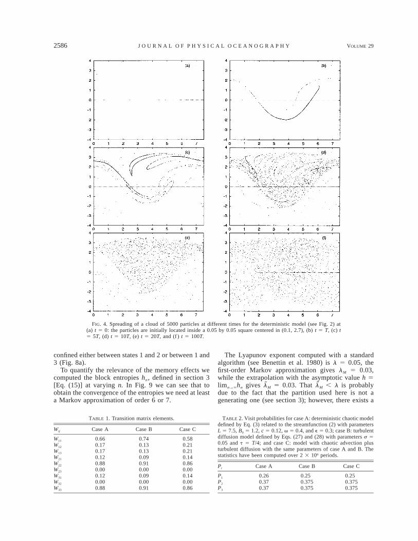
We show in Fig. 4 the spreading at different times ofa cloud of tracer particles. The domain is naturally de-fined from the basic cell that repeats itself creating azonal periodic structure of wavelength L; x thus variesin [0, L], while y in [24, 4]. We fixed a posteriori thesebounds for y since for our choice of parameters no par-ticles reach the far field, and no trajectory attains valuesin |y| larger than 4 (even though, in general, we expectlow but nonzero frequencies for these states, see alsoS92).

In general, whether a north–south mixing happens ornot depends sensibly on the values of e and v. Typicallythe system reveals a strong preference to have long res-idence times in the northern or the southern half of thedomain with respect to the jet core. This peculiar feature

will play an important role in the comparison with theMarkovian approximation.

The transition matrix elements Wij and the visit prob-abilities {Pi} were computed by means of Eq. (17),looking at x every period, that is, for t 5 T, 2T, . . . ,where T 5 2p/v, and the estimated values are reportedin Tables 1 and 2. At a first glance, we can see that therequested symmetry properties are respected [Eq. (19)].

In order to test whether the system is well approxi-mated by a first-order Markov process we computed exittimes, correlation functions, meridional mixing times,and Lyapunov exponent from the simulations and com-pared them with the Markovian predictions.

In Fig. 5 we show the first exit time probability dis-tributions for the states 1 and 2 (3) and the correspond-ing Markovian predictions. After underlining that thestraight lines of Fig. 5 are not to be confused with best-fit curves, we see that the agreement is good over acertain range both for states 1 and 2 (3). The agreementbetween the Markovian predictions and the simulationresults is rather poor for small and very large exit times.This behavior shows that the Markovian approximationcannot hold at small times since the details of the dy-namics are strongly relevant. In the same way nontriviallong time correlations cannot be accounted for in termsof a first-order Markovian process.

In Fig. 6 we can see how the correlation functions ofxi [see Eqs. (23)–(24)] for states 1 and 2 (3) are just invague agreement with the corresponding correlationsobtained for the Markovian process. The trajectories inthe recirculations (i.e., states 2 and 3) appear to be muchmore autocorrelated than those in the jet. Therefore wededuce that the system, although chaotic, has a strongmemory as to which half (northern or southern) of thespatial domain it is visiting. The typical evolution is a‘‘rebound game’’ between state 2 and the southern halfof the jet during a certain time interval; then it crossesthe jet core and performs again the same pattern betweenstate 3 and the northern half of the jet, until it jumpsback, and so on. This is strikingly evident if we lookat the distribution probabilities of the meridional mixingtimes, where the Markovian approximation completelyfails (Fig. 7).

This can be explained as follows: the simulationsshow that, when a tracer particle leaves a recirculationregion, say in the southern half, and enters the jet, mostof the time it returns back to some other close orbit inthe southern half of the basin rather than crossing thejet barrier, showing a long memory effect, which is notfeatured in the first-order Markov approximation. Thisis a clear indication that higher-order Markov processesare necessary to describe this portion of the statisticsproduced by the dynamics. This is shown in Fig. 8,where transitions between states 1 and 2, and 1 and 3,are compared: whereas in the first-order Markovian ap-proximation (Fig. 8b) a particle jumps very often fromnorth to south, the results of our numerical experimentsshow a stronger tendency for particles to keep being


FIG. 4. Spreading of a cloud of 5000 particles at different times for the deterministic model (see Fig. 2) at(a) t 5 0: the particles are initially located inside a 0.05 by 0.05 square centered in (0.1, 2.7), (b) t 5 T, (c) t5 5T, (d) t 5 10T, (e) t 5 20T, and (f ) t 5 100T.

TABLE 2. Visit probabilities for case A: deterministic chaotic modeldefined by Eq. (3) related to the streamfunction (2) with parametersL 5 7.5, B0 5 1.2, c 5 0.12, v 5 0.4, and e 5 0.3; case B: turbulentdiffusion model defined by Eqs. (27) and (28) with parameters s 50.05 and t 5 T/4; and case C: model with chaotic advection plusturbulent diffusion with the same parameters of case A and B. Thestatistics have been computed over 2 3 106 periods.

Pi Case A Case B Case C

P1

P2

P3

0.260.370.37

0.250.3750.375

0.250.3750.375

TABLE 1. Transition matrix elements.

Wij Case A Case B Case C

W11

W12

W13

W21

0.660.170.170.12

0.740.130.130.09

0.580.210.210.14

W22

W23

W31

W32

W33

0.880.000.120.000.88

0.910.000.090.000.91

0.860.000.140.000.86

confined either between states 1 and 2 or between 1 and3 (Fig. 8a).

To quantify the relevance of the memory effects wecomputed the block entropies hn, defined in section 3[Eq. (15)] at varying n. In Fig. 9 we can see that toobtain the convergence of the entropies we need at leasta Markov approximation of order 6 or 7.

The Lyapunov exponent computed with a standardalgorithm (see Benettin et al. 1980) is l 5 0.05, thefirst-order Markov approximation gives lM 5 0.03,while the extrapolation with the asymptotic value h 5limn→`hn gives 5 0.03. That , l is probablyl lM M

due to the fact that the partition used here is not agenerating one (see section 3); however, there exists a


FIG. 5. Probability distribution of the first exit times from states 1(diamonds), 2 (squares), and 3 (crosses) for the deterministic model(see Fig. 2). The straight lines are the Markovian predictions givenby Eq. (A5) with Wii of Table 1 (case A). The time unit is the periodT of the perturbation. The statistics is computed over 2 3 106 periods.

FIG. 6. Correlation functions of states 1 (diamonds) and 2 (crosses)compared with the Markovian predictions [continuous lines, Eq.(A11)] for the deterministic model (see Fig. 2).

FIG. 7. Probability distribution of the meridonal mixing times(MMT) compared with the Markovian predictions [continuous lines,Eq. (A5)] for the deterministic model (see Fig. 2).

fair agreement between and l. It is worth noticinglM

that the above features are fairly robust and do not varyin a relevant way after weak changes of parameters.

b. Mixing induced by turbulent diffusion

The same investigation discussed in the previous sub-section was carried out setting e 5 0 and turning onturbulent diffusion, which is described in terms of astochastic model for particle motion:

dx dy5 u 1 h , 5 y 1 h , (27)1 2dt dt

where u, y are given by the streamfunction (2) and hi

are zero-mean Gaussian stochastic processes with^hi(t)h j(t9)& 5 s 2dij exp(2|t 2 t9|/t). The Gaussian var-iable h i is generated by a Langevin equation (Chandra-sekhar 1943):

2dh h 2si i5 2 1 z , i 5 1, 2, (28)i!dt t t

where the variables zi are zero-mean Gaussian noiseswith ^z i(t)zj(t9)& 5 dijd(t 2 t9). The numerical integra-tion of the equations has been performed by means ofa stochastic fourth-order Runge–Kutta algorithm (Man-nella and Palleschi 1989).

Now the motion is unbounded for the presence of theisotropic diffusive terms; therefore, in order to get atransition matrix comparable with the matrix obtainedin the chaotic deterministic case and to be able to com-pare the two models, we need to limit the dispersionalong y inside a domain as similar as possible to theprevious one.

Since the chaotic model does not fill states 4 and 5,we impose that, if a tracer enters a backward motionregion, it is reflected back by changing the sign of the

meridional turbulent velocity. We emphasize that thisboundary condition practically does not affect the mix-ing process between the jet and the recirculation regions.

In the diffusive case we set the values s 5 0.05 andt 5 T/4 as representative of an observable situation (seeOkubo 1971) and compute again the transition matrixand stationary frequencies of the five states (see Tables1 and 2). The elements of the transition matrix are closeto those of the chaotic case. The transition probabilitieswere computed over a time period T as was done forthe chaotic case so that the two cases can be compared.

In Fig. 10 we show the spreading of a cloud of par-ticles. Figure 11 shows the probabilities of the first exittimes of the states 1, 2, and 3 and the relative Markovianpredictions. The distributions derived from the simu-lations are very well approximated by the first-orderMarkov process.

The correlation functions are shown in Fig. 12. Thedifference between the actual and the Markovian curvesis now smaller than in the chaotic case because of the


FIG. 8. Comparison between (a) the symbolic sequence of the states as function of time (for t 5T, 2T, . . . ) obtained by the integration of the deterministic model [Eqs. (1) and (2)] and (b) thesymbolic sequence generated from the Markov chain defined by the transition matrix computed asdescribed in Eq. (17) and reported in Table 1 (case A).

presence of diffusion that decreases sensibly the degreeof memory. This is much more evident looking at thedistributions of the meridional mixing times (see Fig.13).

Thus we can conclude that in the diffusive model theone-step Markovian approximation is much more ap-propriate than in the chaotic one. Looking at the blockentropies hn (15), we have a clear indication that the

process is of a lower order with respect to the chaoticcase (cf. Fig. 14 with Fig. 9).

Just like in the previous case we have investigatedthe behavior of the system, varying the parameters sand t . We have observed that, if we keep the quantitys 2t constant, the system displays a qualitatively con-stant behavior, even though the extent of the agreementbetween simulation results and Markovian approxima-


FIG. 9. Block entropies hn vs n (15) for the deterministic model(see Fig. 2), computed from a sequence of 106 symbols.

FIG. 10. Same as Fig. 4 but for the stochastic model given by Eqs. (27) and (28), with parameters s 5 0.05and t 5 T/4. The time unit T is set equal to the period of the deterministic perturbation (see Fig. 2). Theparticles are initially located inside a 0.05 by 0.05 square centered in (0.1, 2.7).

tion slightly differs for different values of the turbulenceparameters; this can be understood if we recognize thats 2t corresponds to the diffusion coefficient (see, e.g.,Zambianchi and Griffa 1994a). It has been shown thatvarying s and t even though keeping the diffusion co-efficient constant can indeed affect the quantitative es-timates of dispersion in cases characterized by inho-mogeneity and/or nonstationarity (see, again, Zambian-chi and Griffa 1994a). On the other hand, the qualitativefunctional behavior of the dispersion processes has beenseen to be affected very little by such changes in theparameters of turbulence (Lacorata et al. 1996).

c. Mixing jointly induced by chaotic advection andturbulent diffusion

A detailed analysis of Lagrangian data from the oceanaimed at determining contemporary presence and rel-ative importance of chaotic and turbulent mixing is at


FIG. 11. Probability distribution of the first exit times from states1, 2, and 3 for the stochastic model (see Fig. 10). The straight linesare the Markovian predictions given by Eq. (A5) with Wii of Table1 (case B).

FIG. 13. Probability distribution of the MMTs compared with theMarkovian predictions [Eq. (A7)] for the stochastic model (see Fig.10).

FIG. 14. Block entropies hn vs n for the stochastic model, comput-ed from a sequence of 106 symbols.

FIG. 12. Correlation functions compared with the Markovian pre-dictions [continuous lines, from Eq. (A11)] for the stochastic model(see Fig. 10).

present still lacking, as it would imply the evaluationof both one- and two-particle statistics parameters,which has been done only in the context of purely dif-fusive particle exchange investigations (see, e.g., Pou-lain and Niiler 1989). However, in the real ocean weexpect both the above mixing mechanisms, discussedin section 2, to be present at the same time.

One of the interesting results of the previous sectionsis not only that we can look at particle exchange interms of Markovian processes, but also that the samplingtime suitable for the description of chaotic and turbulentexchange are of the same order of magnitude for fairlyrealistic simulations. This suggests the feasibility of anumerical experiment in which a stochastic term is add-ed to a time-dependent large-scale velocity field.

In addition, in the introduction we mentioned the is-sue of a possible inconsistency of kinematic models asto the lack of Lagrangian conservation of quantities such

as potential vorticity. This difficulty, which has beenrecently discussed at length for two-dimensional chaoticflows (see, above all, Brown and Samelson 1994), isovercome in the combination of the two mixing pro-cesses, as turbulent diffusion can be seen as a sort ofdissipation, which therefore acts so as to ‘‘smear’’ po-tential vorticity gradients.

In this numerical experiment we use the model equa-tions (6) and (7) with u (M )(x, t) given by the stream-function (2) with the time-dependent perturbation (4),and for the turbulent velocity du (T )(x, t) we use thestochastic process defined in Eqs. (27)–(28); the param-eters are B0 5 1.2, e 5 0.3, v 5 0.4, u 5 p/2, s 50.05, and t 5 T/4 where T 5 2p/v. As can be seen,this choice for the parameters is simply a superpositionof the two previous cases.

Also in this case the matrix elements (i.e., the tran-sition probabilities) are comparable with the other ones(see Table 1). As shown in Figs. 15 and 16, the distri-butions of the residence times and of the meridional


FIG. 15. Probability distributions of the first exit times from states1, 2, and 3 in the model with chaotic advection combined with tur-bulent diffusion with parameters: B0 5 1.2, v 5 0.4, e 5 0.3, ands 5 0.05, t 5 T/4 where T 5 2p/v. The straight lines are theMarkovian predictions given by Eq. (A5) with Wii of Table 1 (caseC).

FIG. 16. Probability distributions of the MMT compared with theMarkovian predictions [Eq. (A7)] for the model and the parametersof Fig. 15.

FIG. 17. Correlation functions compared with the Markovian pre-dictions [Eq. (A11)] model and the parameters of Fig. 15.

mixing times display the same qualitative behavior asthe pure diffusive case (cf. Figs. 11 and 13), from whichwe can deduce that for these features the most relevanteffect is due to the diffusive term.

As to the correlation function (Fig. 17), there is aremarkable improvement in catching the correlationfunctions and the meridional mixing time distributionby means of the Markovian approximation with respectto either the purely chaotic or the purely diffusive case.In general, the presence of diffusion tends to decreasethe memory effects so that the Lagrangian dynamicsbecomes closer to a Markov chain than a purely deter-ministic case in which nontrivial long-term correlationsmay render a first-order Markovian approximation in-appropriate.

5. Discussion and conclusions

In this paper particle exchange in a meandering jethas been investigated by means of a kinematic modelin which mixing is obtained by two different mecha-nisms: chaotic advection and turbulent diffusion. Thelarge-scale structure of the jetlike flow is assigned interms of a stationary streamfunction. This has beenmodified in two ways in order to provide the requestedfluid exchange: chaotic advection is induced by addinga time-dependent, relatively small perturbation to thesteady portion of the streamfunction. Alternatively, tur-bulent diffusion has been introduced by superimposinga stochastic field to the latter. The turbulent field hasbeen selected so as to resemble as closely as possiblethe typical effect of upper ocean turbulence in the ab-sence of coherent structures. Numerical simulationshave been carried out for a case in which the two aboveeffects have been jointly present, trying to take intoaccount the richness and complexity of situations ob-

served in the ocean, where the two different mixingmechanisms are thought to be present simultaneously,even if possibly acting at different time and space scales.

The intrinsically different nature of the two investi-gated mixing mechanisms has resulted in the past indisjointed descriptions of their respective effects: cha-otic advection in correspondence of meandering jets hasbeen studied, for example, by means of methods derivedfrom the dynamical systems theory (Pierrehumbert1991; S92; Wiggins 1992; Duan and Wiggins 1996),whereas the action of turbulent diffusion was addressedby phenomenological Lagrangian motion analysis (B91;DGO93).

In this paper mixing is studied in terms of particletransitions among areas of the physical two-dimensionalspace characterized by qualitatively different flow re-gimes, observed as realizations of a Markovian process.Given the structure of the velocity field, the partition ofthe space accessible to particles is self-evident and phys-ically consistent. A delicate point is obviously the choice


of the appropriate timescale for sampling the process.However, in our cases an inherent timescale is presentin the velocity field, and this is set by, in turn, eitherthe space–time structure of the deterministic portion ofthe flow (chaotic case) or by the intrinsic memory time-scale present in the stochastic velocity field. The Mar-kovian approach is, in this sense, a quite natural one toundertake when looking at the overall mixing from aunified perspective, embedding elements of dynamicalsystems, and of stochastic process theory. Also, it is analternative way to look at diffusion avoiding the usualdiffusion coefficients, whose general relevance in geo-physics has been recently subject to debate (see Artaleet al. 1997).

For some fluid exchange properties, the effects of thetwo above mixing mechanisms are comparable with theresults of the Markovian approximation: this is the case,for instance, of the exit times of particles from the jetand the recirculating regions north and south of it. Onthe other hand, chaotic advection and turbulent diffusionact quite differently, under that perspective, when itcomes to meridional mixing and correlation functions.The failure of the Markovian approximation for thecharacterization of the meridional particle exchange inthe chaotic case is due to nontrivial long-term memoryeffects. Since turbulent diffusion is modeled by a non-white noise process in the stochastic velocity field, wewould expect for the turbulent case a closer behaviorto that predicted by the Markovian approximation. Forthe same reason, given the results for the purely chaoticsimulations, the combined effect of chaos and diffusionwas expected to be well described in Markovian terms.This is indeed the case, and the results for the joint fluidexchange situations agree quite closely with the Mar-kovian predictions.

This qualitative difference between chaotic and dif-fusive frontal mixing in our process model may con-tribute to the understanding of previous results: kine-matic models typically show relatively strong exchangebetween jet and recirculating regions and little cross-jetmixing (as mentioned in the introduction: see, e.g., S92and DGO93). The weakening of long-term memory ef-fects induced by the joint presence of chaotic and tur-bulent mixing, which is seen in our simulations, makesour results closer to reality with respect to the cases inwhich only one of the mechanisms is present. In otherwords, it makes the comparison with transport proper-ties derived from a first-order Markov process evenmore satisfactory. With increased availability of La-grangian data in the Gulf Stream, a natural further stepwill be to apply the technique proposed in this paper toexperimental drifter data; this will constitute the subjectof future investigation.

It is worth stressing that the possibility of looking interms of a Markovian approximation at mixing in re-gions characterized by a quite complex flow structure,even in the presence of different transport mechanisms,can have quite interesting applicative consequences.

When the small-scale details of mixing are beyond ourinterest, and if and when our flow system shows fairlywell-defined timescales, it is apparently possible to lookat particle exchange in a relatively simple manner, overtimescales that allow for a reduction of the samplingrate. This aspect often turns out to be a critical constraintfor the undertaking, for example, of Lagrangian inves-tigations of the real ocean, where reducing the requiredsampling rate can result in reducing the amount of datato be collected and transmitted.

Acknowledgments. We thank V. Artale, F. Bignami,M. Falcioni, A. Griffa, and S. Pierini for useful sug-gestions and discussions. We are particularly grateful toB. Marani for the continuous and warm encouragement.G. L. acknowledges the hospitality of the Istituto diFisica dell’Atmosfera of the Italian National ResearchCouncil (CNR). The ESF-TAO (Transport Processes inthe Atmosphere and the Oceans) Scientific Programmeprovided meeting opportunities. This paper has beenpartly supported by INFM (Progetto di Ricerca Avan-zato PRATURBO), CNR, and MURST (9702265437).

APPENDIX

Some Properties of Markov Chains

An excellent introduction to Markov chains can befound in Feller (1968). In this appendix we only sumup some formulas that are useful in describing somerelevant properties of our system.

A Markov chain is a stochastic process such that therandom variables describing state of the system (in ourcase the cell occupied by the tracer particle) and timeare discrete and the probability to be in a given state attime n depends only on the state at time n 2 1.

All the properties of a Markov chain can be derivedfrom the transition matrix, {Wij}, whose elements arethe probabilities to be in state j at some time n beingat time n 2 1 in state i. For example, the probabilityto go to state j starting from i in n steps is simply

Prob(i → j; n) 5 (Wn)ij. (A1)

First of all we have

W 5 1. (A2)O i jj

In addition to matrix {Wij} one can compute the station-ary probabilities Pi to visit the cells Ai as elements ofthe (left) eigenvector corresponding to the eigenvalue 1:

P 5 P W . (A3)Oj i i ji

Notice that Eqs. (A2) and (A3) are rather general resultsthat hold for a generic discrete stochastic process. Equa-tion (A2) describes the conservation of probability andEq. (A3) is nothing but the Bayes theorem. In order tohave ergodicity and mixing properties, the Markov


chain must have a nonzero probability to pass throughany state in a finite number of steps; that is, there existsa value of n such that (Wn) ij . 0 (Feller 1968). Definingri(t) as the probabilities to visit state i at time t, for aMarkov chain, we have

r (t 1 1) 5 r (t)W . (A4)Oj i i ji

In this way one obtains the evolution of the probabilityvector ri (see Rickman and Froeschle 1979). Equation(A3) corresponds to t → ` in Eq. (A4); that is, theequilibrium distribution ri(`) 5 Pi.

The probability of the first exit times from state i canbe simply defined as the probability to stay for n 2 1steps in state i times the probability to exit at step n;that is,

Pi(n) 5 (1 2 Wii)(Wii)n21, (A5)

which can be rewritten as

(1 2 W )i iP (n) 5 exp(2na), with a 5 |lnW |.i i i[ ]Wii

(A6)

In a similar way we can define the probability f ij(n)of the first arrival from state i to state j at step n. Thisis nothing but the probability to arrive at state j startingfrom i in n steps, that is, (Wn) ij, minus the probabilityof first arrival at step n 2 k times the probability ofreturn in k steps, that is, (Wk) jj, with k 5 1, . . . , n 2 1:

n21

n kf (n) 5 (W ) 2 f (n 2 k)(W ) . (A7)Oi j i j i j j jk51

For each state of a Markov process a correlation func-tion can be defined for the variable xi(n), which is equalto 1 if at time n state i is visited and to zero otherwise[see Eqs. (23)–(24)]. The normalized correlation func-tion

2^x (0)x (n)& 2 ^x (0)&i i iC (n) 5 (A8)i 2 2^x (0) & 2 ^x (0)&i i

is strictly related to the diagonal element (Wn) ii and tothe stationary frequency Pi. Notice that

^xi(0)& 5 Pi, ^xi(0)2& 5 Pi. (A9)

Furthermore, being Pi the probability that the initialstate at n 5 0 be i and (Wn)ii the probability to be in iagain after n iterations, one has

^xi(0)xi(n)& 5 Pi · (Wn)ii (A10)

and therefore

Ci(n) 5 [(Wn)ii 2 Pi]/(1 2 Pi). (A11)

REFERENCES

Artale, V., G. Boffetta, A. Celani, M. Cencini, and A. Vulpiani, 1997:Dispersion of passive tracers in closed basins: Beyond the dif-fusion coefficient. Phys. Fluids., 9, 3162–3171.

Backus, R. H., 1986: Biogeographic boundaries in the open ocean.Pelagic Biogeography, UNESCO Tech. Paper Mar. Sci. 49, 9–13. [Available from UNESCO-CSI, 1 rue Miollis, 75732 Paris,France.]

Badii, R., and A. Politi, 1997: Complexity: Hierarchical Structuresand Scaling in Physics. Cambridge University Press, 318 pp.

Bauer, S., M. S. Swenson, A. Griffa, A. J. Mariano, and K. Owens,1998: Eddy-mean flow decomposition and eddy-diffusivity es-timates in the tropical Pacific Ocean. Part 1: Methodology. J.Geophys. Res., 103, 30 855–30 871.

Beck, C., and F. Schlogl, 1993: Thermodynamics of Chaotic Systems.Cambridge University Press, 306 pp.

Benettin, G., 1984: Power-law behavior of Lyapunov exponents insome conservative dynamical systems. Physica D, 13, 211–220., L. Galgani, A. Giorgilli, and J. M. Strelcyn, 1980: Lyapunovcharacteristic exponents for smooth dynamical systems and forHamiltonian systems: A method for computing all of them. Mec-canica, 15, 9–24.

Bower, A. S., 1991: A simple kinematic mechanism for mixing fluidparcels across a meandering jet. J. Phys. Oceanogr., 21, 173–180., and H. T. Rossby, 1989: Evidence of cross-frontal exchangeprocesses in the Gulf Stream based on isopycnal RAFOS floatdata. J. Phys. Oceanogr., 19, 1177–1190., and M. S. Lozier, 1994: A closer look at particle exchange inthe Gulf Stream. J. Phys. Oceanogr., 24, 1399–1418., H. T. Rossby, and J. T. Lillibridge, 1985: The Gulf Stream—Barrier or blender? J. Phys. Oceanogr., 15, 24–32.

Brown, M. G., and R. M. Samelson, 1994: Particle motion in vorticity-conserving, two-dimensional incompressible flows. Phys. Flu-ids, 6, 2875–2876.

Buffoni, G., P. Falco, A. Griffa, and E. Zambianchi, 1997: Dispersionprocesses and residence times in a semi-enclosed basin withrecirculating gyres. An application to the Tyrrhenian Sea. J.Geophys. Res., 102 (C8), 18 699–18 713.

Cecconi, F., and A. Vulpiani, 1995: Approximation of chaotic systemsin terms of markovian processes. Phys. Lett. A, 201, 326–332.

Chandrasekhar, S., 1943: Stochastic problems in physics and astron-omy. Rev. Mod. Phys., 15, 1–89.

Chirikov, B. V., 1979: A universal instability of many-dimensionaloscillator systems. Phys. Rep., 52, 263–379.

Colin de Verdiere, A., 1983: Lagrangian eddy statistics from surfacedrifters in the Eastern North Atlantic. J. Mar. Res., 41, 375–398.

Cornillon, P., D. Evans, and D. Large, 1986: Warm outbreaks of theGulf Stream into the Sargasso Sea. J. Geophys. Res., 91, 6583–6596.

Crisanti, A., M. Falcioni, G. Paladin, and A. Vulpiani, 1991: La-grangian chaos: Transport, mixing and diffusion in fluids. LaRivista del Nuovo Cimento, 14, 1–80.

Davis, R. E., 1991: Observing the general circulation with floats.Deep-Sea Res., 38, S531–S571.

del Castillo-Negrete, D., 1998: Asymmetric transport and non-Gauss-ian statistics of passive scalars in vortices in shear. Phys. Fluids,10, 576–594.

Dimas, A. A., and G. S. Triantafylou, 1995: Baroclinic-barotropicinstabilities of the Gulf Stream extension. J. Phys. Oceanogr.,25, 825–834.

Duan, J., and S. Wiggins, 1996: Fluid exchange across a meanderingjet with quasiperiodic variability. J. Phys. Oceanogr., 26, 1176–1188.

Dutkiewicz, S., A. Griffa, and D. B. Olson, 1993: Particle diffusionin a meandering jet. J. Geophys. Res., 98, 16 487–16 500.

Eckmann, J. P., and D. Ruelle, 1985: Ergodic theory of chaos andstrange attractors. Rev. Mod. Phys., 57, 617–655.

Feller, W., 1968: An Introduction to Probability Theory and its Ap-plications. Vol. I. Wiley, 528 pp.

Fraedrich, K., 1988: El Nino–Southern Oscillation predictability.Mon. Wea. Rev., 116, 1001–1012.


, and K. Muller, 1983: On single station forecasting: Sunshineand rainfall Markov chains. Beitr. Phys. Atmos., 56, 108–134.

Griffa, A., 1996: Applications of stochastic particle models to ocean-ographic problems. Stochastic Modelling in Physical Ocean-ography, R. J. Adler, P. Muller, and B. L. Rozovskii, Eds., Birk-hauser, 113–140., K. Owens, L. Piterbarg, and B. Rozowskii, 1995: Estimates ofturbulence parameters from Lagrangian data using a stochasticparticle model. J. Mar. Res., 53, 371–401.

Halliwell, G. R., and C. N. K. Mooers, 1983: Meanders of the GulfStream downstream from Cape Hatteras. 1975–1978. J. Phys.Oceanogr., 13, 1275–1292.

Khinchin, A. I., 1957: Mathematical Foundations of Information The-ory. Dover, 120 pp.

Kluiving, R., H. W. Capel, and R. A. Pasmanter, 1992: Symbolicdynamics of fully developed chaos I. Physica A, 183, 67–95.

Kontoyiannis, H., and D. R. Watts, 1994: Observations on the var-iability of the Gulf Stream path between 748W and 708W. J.Phys. Oceanogr., 24, 1999–2013.

Lacorata, G., R. Purini, A. Vulpiani, and E. Zambianchi, 1996: Dis-persion of passive tracers in model flows: Effects of the param-etrization of small-scale processes. Ann. Geophys., 14, 476–484.

Lee, T., 1994: Variability of the Gulf Stream path observed fromsatellite infrared images. Ph.D. dissertation, University of RhodeIsland, 188 pp.

Levinson, H. F., 1991: The long-term dynamical behavior of smallbodies in the Kuipter belt. Astron. J., 102, 787–794.

Lichtenberg, A. J., and M. A. Lieberman, 1992: Regular and ChaoticDynamics. Springer, 692 pp.

MacKay, R. S., J. D. Meiss, and I. C. Percival, 1987: Resonances inarea-preserving maps. Physica D, 27, 1–20.

Mannella, R., and V. Palleschi, 1989: Fast and precise algorithm forcomputer simulation of stochastic differential equations. Phys.Rev., A40, 3381–3386.

Meiss, J. D., and E. Ott, 1986: Markov tree model of transport inarea-preserving maps. Physica D, 20, 387–402.

Nicolis, C., W. Ebeling, and C. Baraldi, 1997: Markov processes,dynamic entropies and statistical prediction of mesoscale weath-er regimes. Tellus, 49A, 108–118.

Okubo, A., 1971: Oceanic diffusion diagrams. Deep-Sea Res., 18,789–802.

Olson, D. B., 1991: Rings in the ocean. Ann. Rev. Earth Planet. Sci.,19, 283–311.

Pierrehumbert, R. T., 1991: Chaotic mixing of tracers and vorticity

by modulated travelling Rossby waves. Geophys. Astrophys. Flu-id Dyn., 58, 285–319.

Pope, S. B., 1994: Lagrangian PDF methods for turbulent flows. Ann.Rev. Fluid Mech., 26, 24–63.

Poulain, P. -M., and P. P. Niiler, 1989: Statistical analysis of the surfacecirculation in the California Current System using satellite-tracked drifters. J. Phys. Oceanogr., 19, 1588–1603.

Rickman, H., and C. Froeschle, 1979: Orbital evolution of short-period comets treated as a Markov process. Astron. J., 84, 1910–1917.

Risken, H., 1989: The Fokker–Planck Equation. Springer, 472 pp.Samelson, R. M., 1992: Fluid exchange across a meandering jet. J.

Phys. Oceanogr., 22, 431–440.Thomson, D. J., 1986: A random walk model of dispersion in tur-

bulent flows and its application to dispersion in a valley. Quart.J. Roy. Meteor. Soc., 112, 511–530., 1987: Criteria for the selection of stochastic models of particletrajectories in turbulent flows. J. Fluid Mech., 180, 529–556.

Tracey, K. L., and D. R. Watts, 1986: On Gulf Stream meandercharacteristics near Cape Hatteras. J. Geophys. Res., 91, 7587–7602.

van Dop, H., F. T. M. Niewstadt, and J. C. R. Hunt, 1985: Randomwalk models for particle displacements in inhomogeneous un-steady turbulent flows. Phys. Fluids, 28, 1639–1653.

Vazquez, J., and D. R. Watts, 1985: Observations on the propagation,growth and predictability of Gulf Stream meanders. J. Geophys.Res., 90, 7143–7151.

Verron, J., and K. D. Nguyen, 1989: Lagrangian diffusivity estimatesfrom a gyre-scale numerical experiment on float tracking. Ocean-ol. Acta, 12, 167–176.

Watts, D. R., 1983: Gulf Stream variability. Eddies in Marine Science,A. Robinson, Ed., Springer Verlag, 114–144.

Wiggins, S., 1992: Chaotic Transport in Dynamical Systems. Spring-er, 352 pp.

Yang, H., 1996: Chaotic transport and mixing by ocean gyre circu-lation. Stochastic Modelling in Physical Oceanography, R. J.Adler, P. Muller, and B. L. Rozovskii, Eds., Birkhauser, 439–466.

Yeung, P. K., and S. B. Pope, 1989: Lagrangian statistics from directnumerical simulations of isotropic turbulence. J. Fluid Mech.,207, 531–586.

Zambianchi, E., and A. Griffa, 1994a: Effects of finite scales ofturbulence on dispersion estimates. J. Mar. Res., 52, 129–148., and , 1994b: On the applicability of a stochastic modelfor particle motion to drifter data in the Brazil–Malvinas exten-sion. Annali Ist. Univ. Navale, 61, 75–90.

Documents

Mixing in a Meandering Jet: A Markovian Approximation