Secondary Current of Saline Underflow In A Highly Meandering Channel: Experiments and Theory

Journal of Sedimentary Research, 2011, v. 81, 787–813

Research Article

DOI: 10.2110/jsr.2011.61

SECONDARY CURRENT OF SALINE UNDERFLOW IN A HIGHLY MEANDERING CHANNEL:EXPERIMENTS AND THEORY

JORGE D. ABAD,1,2 OCTAVIO E. SEQUEIROS,3 BENOIT SPINEWINE,4 CARLOS PIRMEZ,5 MARCELO H. GARCIA,1 AND

GARY PARKER1,6

1Ven Te Chow Hydrosystems Laboratory, Department of Civil and Environmental Engineering, University of Illinois, Urbana, Illinois 61801, U.S.A.2Department of Civil and Environmental Engineering, University of Pittsburgh, Pittsburgh, Pennsylvania 15261, U.S.A.

3Shell International Exploration and Production, B.V., Postbus 60, 2280AB Rijswijk, The Netherlands4Fonds National de Recherche Scientifique, Rue d’Egmont 5, B-1000 Bruxelles, Belgium

5Shell International Exploration and Production, P.O. Box 481Houston, Texas 77001, U.S.A.6Department of Geology, University of Illinois, Urbana, Illinois 61801, U.S.A.

ABSTRACT: The flow of deep-sea turbidity currents in meandering channels has been of considerable recent interest. Here wefocus on the secondary flow associated with a subaqueous bottom current in a meandering channel. For simplicity, a salinebottom current can be used as a surrogate for a turbidity current driven by a dilute suspension of fine-grained sediment thatdoes not easily settle out. In the case of open-channel flow, i.e., rivers, the classical Rozovskiian paradigm is often invoked toexplain secondary flow in meandering channels. This paradigm indicates that the near-bottom secondary flow in a bend isdirected inward, i.e., toward the inner bank. It has recently been suggested based on experimental and theoreticalconsiderations, however, that this pattern is reversed in the case of subaqueous bottom flows in meandering channels, so that thenear-bottom secondary flow is directed outward (reversed secondary flow), towards the outer bank. Experimental resultspresented here, on the other hand, indicate near-bottom secondary flows that have the same direction as observed in a river(normal secondary flow). The implication is an apparent contradiction between experimental results. We use theory,experiments, and reconstructions of case studies from field-scale flows to resolve this apparent contradiction based on thedensimetric Froude number of the flow. We find three ranges of densimetric Froude number, such that a) in an upper regime,secondary flow is reversed, b) in a middle regime, it is normal, and c) in a lower regime, it is reversed. We apply our results atfield scale to previous studies on channel-forming turbidity currents in the Amazon submarine canyon fan system (AmazonChannel) and the Monterey Canyon and a saline underflow in the Black Sea flowing from the Bosphorus. Our analysisindicates that secondary flow should be normal throughout most of the Amazon submarine fan reach, lower-regime reversed inthe case of the Black Sea underflow, and upper-regime reversed in the case of the Monterey canyon. The theoretical analysispredicts both normal and reversed regimes in the Amazon submarine canyon reach.

INTRODUCTION

Turbidity currents in the deep sea often make their own meanderingchannels. Many submarine canyons show a meandering planform. Inaddition, leveed channels on submarine fans and fairways often display ameandering pattern (e.g., Abreu et al. 2003). Interest has recently beenfocused on the problem of the formation of meandering channels byturbidity currents traversing submarine fans or canyons (Imran et al.1999; Peakall et al. 2000; Parker et al. 2001; Kassem and Imran 2004;Corney et al. 2006; Keevil et al. 2006; Imran et al. 2007). Such a channel isshown in Figure 1 (Pirmez 1994). The overall fluid mechanics of flow inmeandering channels for the case of a sediment-laden bottom underflowhas the same structure as that for subaerial water flow in a meanderingriver (Imran et al. 1999; Parker et al. 2001). Yet there are enoughdifferences between the subaqueous case of slightly denser turbid waterunder clear water and the subaerial case of water under air (i.e., the caseof open-channel flow corresponding to a river) to result in somesurprising differences (e.g., Kolla et al. 2007).

One of these concerns the superelevation of flow around bends (e.g.,Komar 1969). For the same flow velocity and depth, the degree of

superelevation is one to two orders of magnitude larger in the subaqueouscase than in the subaerial case. This is because a sediment and watermixture in a subaqueous turbidity current is likely to be no more than afew percent denser than that of the ambient water above, whereas waterin a river is , 800 times denser than the air above.

Recently Corney et al. (2006) and Keevil et al. (2006) have suggestedanother potential difference, i.e., the direction of the near-bottomsecondary flow near the apex of a bend. Based on the classical work ofRozovskii (1961), the near-bottom secondary flow at the apex of a riverbend might be expected to be directed inward, i.e., from the outer bank tothe inner bank. We term near-bed secondary flow with such a direction as‘‘normal.’’ In the corresponding case of a dense subaqueous underflow,Corney et al. (2006) and Keevil et al. (2006) found the near-bottomsecondary flow at the bend apex to be instead directed from the innerbank to the outer bank, i.e., ‘‘reversed’’ as compared to a river.

This result is in disagreement with the results of Imran et al. (2007),who found the near-bed secondary flow of a subaqueous bottom flow tobe directed normally. Thus the results of Imran et al. (2007) are incorrespondence with the classical Rozovskiian paradigm, whereas the

Copyright E 2011, SEPM (Society for Sedimentary Geology) 1527-1404/11/081-787/$03.00

results of Corney et al. (2006) and Keevil et al. (2006) with reverseddirection appear to contradict it.

A third set of experimental data on secondary flow in bottomsubaqueous currents is presented here. The data indicate normallydirected near-bottom subaqueous.

We use this apparent contradiction as a starting point for revisitingthe analysis of Corney et al. (2006) and Corney et al. (2008) describingsecondary flow of bottom subaqueous currents in a confined channelof constant curvature. We then use experimental results, theory, andreconstructions of flows at field scale to illustrate the regimes for

FIG. 1.—Meandering reach of the AmazonChannel on the Amazon Submarine Fan. FromPirmez (1994).

788 J.D. ABAD ET AL. J S R

which normal versus reversed near-bed secondary flow can beexpected.

BACKGROUND

In order to place the result obtained by Corney et al. (2006), Keevil etal. (2006), and Imran et al. (2007) in proper context, it is of value toreview the literature on secondary flow in rivers. The classical theory ofRozovskii (1961) has provided the starting point for most subsequentanalyses. Rozovskii considered steady, developed bend flow in a channelof constant width and centerline curvature. He linearized the governingequations under the assumption of sufficiently large radius of curvatureas compared to flow depth. The channel was also assumed to have a ratioof width to depth that was sufficiently large to allow the neglect of walleffects. The analysis considered the balance between the outward-directedcentrifugal force of the flow and the inward-directed pressure forceassociated with superelevation at the outer bank. These forces mustbalance in a depth-integrated sense, so providing a predictive relation forsuperelevation. The two forces cannot balance locally, however, due tothe variation of the streamwise velocity in the vertical direction. The forcebalance is completed by the formation of a single cell of secondary flow,directed toward the outer bank in the upper part of the flow and towardthe inner bank in the lower part of the flow.

Although Rozovskii’s analysis was restricted to the case of a bed thatwas horizontal in the transverse direction, Engelund (1974) generalizedthe analysis to the case for which the bed has a transverse slopecorresponding to point-bar topography. For the case of developed bendflow in a bend of constant curvature, secondary flow over a bed with atransverse slope is found to have the same sense as that of Rozovskii.

Engelund (1974) also considered the case of a meandering channel inwhich centerline curvature changes continuously in the streamwisedirection, although he made no attempt to correct the calculation forsecondary flow to include the effect of a pattern of curvature that variesperiodically in the streamwise direction. He nevertheless demonstrated

that in the case of continuously changing curvature, the primary flowitself need not be directed solely in the downstream direction. Instead, thelocus of high streamwise velocity migrates from bank to bank, showing apattern that lags behind the variation of centerline curvature. Dependingupon the nature of this lag, the near-bed flow near the inside of a bendcan in some locations be directed toward the outer bank, rather than theinner bank. This does not mean that the fundamental mechanism ofsecondary flow described by Rozovskii is inoperative. It simply meansthan an additional term associated with changing channel curvature can,under some conditions and in certain locations, overcome it.

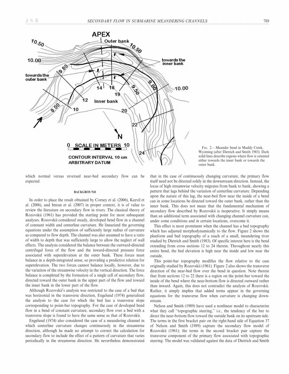
This effect is most prominent when the channel has a bed topographywhich has adjusted morphodynamically to the flow. Figure 2 shows theplanform and bed topography of a reach of a small, meandering riverstudied by Dietrich and Smith (1983). Of specific interest here is the bendextending from cross sections 12 to 24 therein. Throughout nearly thisentire bend, the bed elevation is high near the inside and low near theoutside.

This point-bar topography modifies the flow relative to the caseoriginally studied by Rozovskii (1961). Figure 2 also shows the transversedirection of the near-bed flow over the bend in question. Note thereinthat from sections 12 to 22 there is a region on the point-bar toward theinside of the bend where the near-bottom flow is directed outward ratherthan inward. Again, this does not contradict the analysis of Rozovskii.Rather, it simply implies that added terms appear in the governingequations for the transverse flow when curvature is changing down-stream.

Nelson and Smith (1989) have used a nonlinear model to characterizewhat they call ‘‘topographic steering,’’ i.e., the tendency of the bar todirect the near-bottom flow toward the outside bank on its upstream side.The terms in the first bracket pair on the right-hand side of Equation 37of Nelson and Smith (1989) capture the secondary flow model ofRozovskii (1961); the terms in the second bracket pair capture thetransverse component of the primary flow associated with topographicsteering. The model was validated against the data of Dietrich and Smith

FIG. 2.—Meander bend in Muddy Creek,Wyoming (after Dietrich and Smith 1983). Darksolid lines describe regions where flow is orientedeither towards the inner bank or towards theouter bank.

SECONDARY FLOW IN SUBMARINE MEANDERING CHANNELS 789J S R

(1983). Abad (2008) has similarly found a topographic steering effectassociated with migrating bedforms.

The models of neither Engelund (1974) nor Nelson and Smith (1989)consider the possibility that the secondary flow itself may lag downstreamin the case of continuously changing curvature. Johannesson and Parker(1989) developed a model for this lag. They found that the secondary flowlags only modestly behind curvature in natural meandering channels. Inthe case of several experimental channels, however, the lag was found tobe in the range 30u to 60u. The implication is that in certain experimentalchannels the secondary flow can lag so far behind curvature that its sensecan be reversed compared with the model of Rozovskii (1961).

The experiments of Corney et al. (2006), Keevil et al. (2006), and Imranet al. (2008), along with the experiments presented here, should be viewedin light of the above discussion. In all cases a) the flow was a salineundercurrent, b) the channel was meandering, and c) the channel bed washorizontal in the transverse direction, so that there was no analog of apoint-bar.

In the experiments reported herein, the near-bed secondary flow isfound to be normally directed, i.e., the same direction as predicted by theRozovskiian fluvial model, as well as the results of Imran et al. (2007) forsaline underflows. We use these experimental results as a springboard forthe development of a theoretical formulation that is able to characterizeboth a) the normal near-bed secondary flow of Imran et al. (2007) andour work reported here and b) the reversed flow reported in Corney et al.(2006) and Keevil et al. (2006). As shown below, the key discriminatingparameter turns out to be the densimetric Froude number.

THE FLUME

The flume used for our experiments, which is located at the Ven TeChow Hydrosystems Laboratory, University of Illinois, is shown inFigure 3. The channel consists of a highly meandering reach withcenterline arc length of 30 m, as well as one 1-m straight reach eachupstream and downstream of the meandering reach. Total flume length Lis thus 32 m. The flume has a width B of 60 cm and a depth of 40 cm. Thebottom of the flume is horizontal. The flume contains three identicalbends, each with a centerline arc wavelength of 10 m.

The flume is known as the ‘‘Kinoshita Flume,’’ in that the skewedshape of the bends was motivated by research conducted by Kinoshita(1961) on the shape of highly sinuous meander bends of rivers. Themeandering planform of the flume was designed according to theequation

h~h0sin2ps

l

� �zh0

3 Jscos 32ps

l

� �{Jf sin 3

2ps

l

� �� ð1Þ

where s denotes the channel centerline arc length coordinate, h denotesthe angle of inclination of the centerline relative to the mean streamwisedirection (valley orientation), ho denotes bend-angle amplitude (maxi-mum angular amplitude) and l denotes arc-length meander wavelength.In addition, Js and Jf denote dimensionless coefficients of bend skewnessand fatness (Parker et al. 1983). Note that in the limit Js 5 Jf R 0 theabove equation reduces to the equation for a sine-generated channel ofLangbein and Leopold (1966). The Kinoshita flume is designed such thatl 5 10 m, ho 5 1.92 radians (110u), Js 5 1/32, and Jf 5 1/192. Thechannel is skewed towards the upstream end. The sinuosity of themeandering reach of the flume is 3.69. The centerline radius of curvatureRc and the centerline curvature Cc are given from (1) as

Cc(s)~1

Rc(s)~{

dh

ds~

{2ph0

lcos

2ps

l

� �{3h0

2 Jssin 32ps

l

� �zJf cos 3

2ps

l

� �� ð2Þ

The minimum magnitude of the centerline radius of curvature Rc of theKinoshita Flume is achieved at the bend apices, where it takes a value of78.5 cm.

EXPERIMENTAL SETUP AND PROCEDURE

The Kinoshita Flume shown in Figure 3 was originally designed forexperiments on flow in meandering rivers (Abad and Garcia 2009a,2009b). The experiments reported here were operated in recirculatingmode. That is, saline water was first prepared in a holding tank to adesired specific gravity. This water was then introduced into the flume

FIG. 3.—The Kinoshita Flume. Acrylic plasticwindows are placed along the middle bend atboth inside and outside banks.


and recirculated. Three different initial specific gravities were used, 1.08,1.10, and 1.12. Here the layer-averaged fractional density excess of thesaline flow above the ambient fresh water is denoted as D. The initialfractional density excesses Di were thus 0.08, 0.10, and 0.12, or expressedin percent, 8%, 10%, and 12%. For any given run, the fractional densityexcess D declined over time for reasons explained below. The runs wereperformed in three sets. Each set consisted of three repeat runs at thesame initial density excess. The motivation for the repeat runs can beexplained with reference to Figure 4, which shows the locations of thecross sections where most of the data were measured.

An acoustic Doppler velocimeter (ADV) was used to measure velocitiesat cross sections 14 (just upstream of bend apex), 15 (bend apex), and 16(just downstream of bend apex). Because the density of the flow wasdeclining in time during any given run, performing velocity measurementsat all sections during a given run would lead to incompatible data sets. Asa result, the 8% run (10% run, 12% run) was performed three times, onceto obtain velocity measurements at Section 14 (Run 1-a), once to obtainvelocity measurements at Section 15 (Run 1-b), and once to obtainvelocity measurements at Section 16 (Run 1-c). In each case the velocitymeasurements were performed near the middle period of the run. ThusRuns 1-a, 1-b, and 1-c comprise Set 1. Set 2 at a 10% density differenceand Set 3 at a 12% density difference are similarly defined.

For each experiment, a volume of 3130 liters of saline water wasprepared in a holding tank adjacent to the flume. The saline water waslightly colored with a yellow dye in order to allow flow visualization. Thesaline water was pumped at a constant rate of 4.0 liters/s (6 0.05 liters/s)from the holding tank to the upstream end of the flume at a set rate, andthen pumped from the downstream end of the flume back to the holdingtank at the same rate.

As shown in Figure 3, the flume itself has a large, deep rectangulartank at each of its upstream and downstream ends. Bed traps are locatedjust downstream of the upstream tank (upstream trap) and just upstreamof the downstream tank (downstream trap). For the present experiments,the upstream tank was closed off by a weir. The flume and the

downstream tank were then filled with fresh water to a depth of 35 cm.This water-surface elevation was maintained throughout the experimentto within 6 0.2 cm. Saline water was injected into the channel throughthe upstream trap. The saline water then flowed out along the bottom ofthe channel through a headgate with a bottom flush with the channel bedand a height of 11.5 cm, so creating a saline underflow under essentiallystagnant fresh water. The saline flow exited the channel through thedownstream trap, from which it was pumped back to the holding tank.

Upon commencement of each experiment, the saline underflow formeda clearly defined front which gradually traveled the length of the flumeand debouched into the downstream trap. A quasi-steady flow wasallowed to set up before commencing measurements. Since the bed of theKinoshita Flume is horizontal, the saline underflow was driven by astreamwise gradient in the interface between the saline water and the freshwater above. The fresh water above the underflow was nearly stagnant, asdocumented below. As a result, the saline underflow was driven solely bygravity operating on the excess density imparted by salt, rather than bythe effect of gravity on the fresh water above. The flow was thus a truedensity underflow rather than some hybrid fluvial flow/underflow.

As the saline underflow plunged into the downstream trap, it invariablyentrained some fresh water with it. As a result, the specific gravity of thesaline water declined during the experiment. As noted below, mixing ofthe saline underflow with the freshwater above (mixing at the interface)between the upstream trap and the downstream trap was negligible. Theduration of each experiment was approximately 90 to 120 minutes.During the experiments, the excess density D of the salt water in theholding tank declined from initial values of 0.08, 0.10, and 0.12 torespective final values near 0.055, 0.07, and 0.08 respectively for theexperiments of Set 1, 2, and 3 respectively.

Visualization of the near-bed flow direction and structure was madepossible by using manifolds located at sections 13, 14, 15, 16, and 17 (S13,S14, S15, S16, and S17). Each manifold had five orifices, and was laidalong the bed perpendicular to the centerline down-channel direction. Themanifolds were constructed from 3.18 mm (1/8 inch) flexible tubing. The

FIG. 4.—Location of cross sections 13–17 inthe Kinoshita Flume.


tubing was taped to the bed as nearly flush as possible to minimizeinterference with the near-bed flow. Where n denotes the transversedistance from the channel centerline toward the outside of the bend(intrinsic coordinate system), the openings were located at valuesn 5 220 cm, 210 cm, 0 cm (centerline), 10 cm, and 20 cm. (Recallthat the banks are located at n 5 6 30 cm.) Saline fluid of the samedensity as that in the holding tank at the beginning of the run was injectedinto the manifold. This saline fluid was dyed red to allow for flowvisualization. The resulting streaks of dyed fluid emanating from themanifold served to visualize the direction of the bottom flow justdownstream of each section. Black lines parallel to the centerlinestreamwise direction were drawn onto the white bottom of the flumedownstream of each opening. A comparison between the direction of anystreak emanating from an opening of the manifold and the adjacent blackline allowed for a determination of the angle of flow, and thus direction ofthe near-bed secondary flow. Videotape was taken of the flow in thevicinity of the study sections where dye was injected, and photographswere taken opportunistically during the run. Several windows in the sideof the flume allowed for visualization of the superelevation of the salineunderflow as it traversed the bend.

Seven measuring sections were used to gather bulk parameters duringthe experiments. These sections are denoted by the numbers 0, 13, 14, 15,16, 17, and 30, indicating the arc distance in meters of the centerline pointdownstream from the junction between the 1 m upstream straight reachand the start of the meandering reach. S13 and S14 were located 1 m and2 m upstream of the bend apex, respectively, S15 was located at the bendapex, and S16 and S17 were located 1 m and 2 m downstream of the bendapex, respectively (Fig. 4). The local centerline radius of curvature (Rc) atS13, S14, S15, S16, and S17 were 1489, 79.4, 78.5, 158.2, and 146 cmrespectively. The following bulk parameters were obtained with a ruler ateach section; elevation of the interface between the underflow and thefresh water above at both the inside and the outside of the cross section,and the water-surface elevation itself at both the inside and the outside ofthe cross section. These measurements (taken throughout the experiment,

after reaching the quasi-steady equilibrium condition) were accurate toabout 1–2 mm in all cases except the interface elevations at sections 0 and30, where they were accurate to about 3–4 mm.

As noted above, detailed three-dimensional velocity measurementswere collected at S14, S15, and S16 by using an acoustic Dopplervelocimeter (ADV). These measurements were performed after the flowhad reached quasi-steady equilibrium conditions. ADV point measure-ments were collected at various stations in the transverse direction,(n 5 220, 210, 0, 10, and 20), with measurements at several points inthe vertical for each station. More specifically, measurements were takenat approximately seven points in the vertical, with different spacingbetween points so as to cover both the saline flow and the nearly stagnantambient water above it.

As noted above, due to the gradual decline in density excess over time,it was necessary to run experimental repeats in order to obtain velocitymeasurements at each section at a comparable specific density. Forexample, Runs 1-a, 1-b, and 1-c, all conducted at an initial excess densityof 8%, allowed velocity measurements at S14, S15, and S16, respectively.In total, then, nine experiments were necessary to cover the three differentinitial excess densities (8%, 10%, and 12%). These detailed velocitymeasurements allowed us to describe quantitatively the near-bottom floworientation.

During each experiment, the temperature of the saline underflow andof the fresh water above was measured at the beginning, at each ADVpoint measurement, and the end of the run. Calculations indicated thattemperature differences played a negligible role in flow stratification.

OVERALL CHARACTERISTICS OF THE FLOW

A view of the saline underflow and the fresh water above it is shown inFigure 5. The interface between the two was invariably extremely welldefined. While small-scale undulations were visible on the interface,turbulent eddies capable of effectively mixing saline and fresh water werenot observed. In addition, negligible smearing of the yellow dye in theunderflow was observed at the interface. As a first approximation, then,

FIG. 5.—Saline flow and fresh water aboveobserved just downstream of the bend apex (viewfrom window located at the outer bank).


mixing at the interface could be neglected. More support for thisassumption is given below.

As described above, a separate experiment was carried out for ADVvelocity measurements at each cross section (e.g., S14, S15, and S16) foreach initial excess density (Di 5 8%, 10%, and 12%). Listed in Table 1are the following parameters averaged over each set of experiments: [a]the mean layer-averaged excess density D measured during dataacquisition; [b] the mean water surface elevation j; [c] the ratio betweenthe mean thickness h of the saline underflow to the mean water surfaceelevation j, [d] the ratio between the channel width B and the meanthickness of the saline underflow h; [e] the mean flow velocity in the salinelayer U, estimated as

U~Qin

Bhð3Þ

where Qin denotes the inflow discharge ( 5 4000 cm3/s) and B 5 flumewidth ( 5 60 cm); [f] densimetric Froude number Frd of the saline flow,computed as

Frd~UffiffiffiffiffiffiffiffiDghp ð4Þ

where g denotes the acceleration of gravity; [g] the characteristic Reynoldsnumber Rec of the saline underflow, estimated as

Rec~Uh

vð5Þ

where the kinematic viscosity of the flow n was estimated based ontemperature measurements; [h] the characteristic bulk Richardson Ricnumber for the underflow, computed as

Ric~1

Fr2d

ð6Þ

and [i] the Keulegan number (Keulegan 1949), given as

Kec~Ric

Rec

� �1=3

ð7Þ

As noted earlier, the specific gravity of the saline mixture varied in timeduring the experiment. As a result, the value of D used to compute theFroude number Frd was measured at the inlet tank, around theintermediate time stage of each experiment.

The values for fractional excess density D in Table 1 are in each caseless than the corresponding initial value Di. This was because of mixingduring the experiment, as described below. The listed values of D arethose that correspond to the time window when the other flowmeasurements were performed.

The subcritical Froude numbers of the present study are likely to bereasonably characteristic of formative turbidity currents in manysubmarine meandering channels on fans and in wider fairways, in thatsupercritical flows are likely to induce so much entrainment of ambientwater that the flow can no longer be confined by its own levees (Pirmezand Imran 2003). The Reynolds number Rec of approximately 7.0 3 103

indicates a fully turbulent saline underflow below the interface, whichitself showed undulations but little turbulence.

This lack of turbulence at the interface between the underflow and theambient water is also reflected in the fact that very little mixing betweenthe lower and upper layers was observed there (Fig. 5). The mixingcriterion first proposed by Keulegan (1949) for turbulent stratified flowswas used to assess if mixing at the interface could be expected. Thedimensionless Keulegan number Kec is given by (7) (Vanoni 2006, p. 170).If the value computed with Equation 7 exceeds the critical value of 0.18determined experimentally by Keulegan (1949), no mixing should occur.However, the value computed for our experiment is in the range 0.14 to0.16 (see Table 1), indicating that some weak mixing and entrainment ofambient water took place.

Figure 6 shows characteristic plots of long profiles of the water surfaceand the saline–freshwater interface at the beginning and end of a run in Set1 (8% density excess). The lines shown therein represent averages over Runs1-a, 1-b, and 1-c. The overall water-surface slope is nearly zero, reflectingnearly stagnant water above the underflow. Indeed, flow visualizationusing buoyant particles placed at the water surface indicated essentially nomovement in time. The interface, however, slopes noticeably downstream,indicating that the flow is driven by the effect of gravity operating solely onthe excess density of the saline water of the underflow.

TABLE 1.— Experimental parameters (averaged over set of experiments).

EXPERIMENT [a] D [b] j (cm) [c] h/j [d] B/h [e] U (cm/s) [f] Frd [g] Rec [h] Ric [i] Kec

Set 1: 8% (Di 5 0.08) 0.0608 35.25 0.32 5.39 5.99 0.23 7098 18.9 0.14Set 2: 10% (Di 5 0.10) 0.0765 35.59 0.30 5.56 6.19 0.22 6831 20.7 0.14Set 3: 12% (Di 5 0.12) 0.0909 35.99 0.31 5.39 5.99 0.19 6190 27.7 0.16

FIG. 6.—Characteristic long profiles of thewater surface and the interface of the salineunderflow, based on averages for Set 1 (initial8% density excess). Two lines are shown for each,Ini 5 initial and End 5 final. Note that thewater surface is essentially horizontal, whereasthe interface slopes downstream The profiles‘‘End’’ are above the profiles ‘‘Ini’’ due to theeffect of mixing during the run, most of whichoccurred in the end tank.


More detailed measurements of the locations of the water-surface andinterface were taken between S13 and S17. The difference in water surfaceelevation between the inner and outer bank at S15 (bend apex) was only0.3 cm, whereas the difference Dhs in the elevation of the interfacebetween the saline and fresh flow at the same section was found to be, 1.0 cm. Thus superelevation at the bend apex was consequentlystrongly reflected by the interface, but only rather weakly reflected by thewater surface.

The Richardson number Ric can be used to estimate the role ofentrainment of ambient clear water into the saline underflow. Thedimensionless coefficient of entrainment ew of ambient water into theunderflow is given as

ew:1

U

dhU

dsð8Þ

where s denotes a streamwise distance down the channel centerline.Fukushima et al. (1985) have presented, and Parker et al. (1987) haveempirically justified the following relation between ew and Ric:

ew~0:00153

0:0204zRicð9Þ

The volume of fresh water Qent entrained per unit time over the length ofthe flume across the interface can be estimated as

Qent&ew Ricð ÞUBL ð10Þ

Using the characteristic value for Ric listed in Table 1 for each set tocharacterize that set, values of Qent were estimated to be 0.095, 0.087, and0.064 liters/s for the sets using 8%, 10%, and 12% initial densitydifferences, respectively. According to these estimates the discharge of thesaline underflow increased by only about 2 percent due to entrainment. Arepeat of the calculation using the entrainment relation in Garcia andParker (1986) yielded values of Qent that were similar to the valuespresented above.

Whereas the above results suggest little interfacial mixing, the plots ofFigure 7, which show the percent salt as a function of time for all nineexperiments, present a somewhat different story. In the runs of Set 3, forexample, the percent salinity, as measured in the holding tank, declinesfrom about 12% to 9% over the duration of the run. This decline can thusbe interpreted as resulting mostly from mixing as the underflow plunged

into the downstream trap. The values of D reported in Table 1 weredetermined from the regions of the curves of Figure 7 during which themeasurements of the flow were made.

Figure 8 shows the transverse slopes Sti and Stw of the interfacial andwater surface, respectively, along the middle bend, i.e., between S13 andS17. Positive values indicate superelevation toward the outside of thebend in Figure 4. The interfacial slopes clearly reflect the change in thesense of superelevation as centerline curvature changes downstream. Themaximum interfacial slopes are found near S14 and S15, points whichcorrespond to the zone of maximum local curvature (Abad and Garcia2009a).

The transverse water surface slopes in Figure 8 are greatly mutedcompared to those of the interface, again indicating that the fresh waterabove the current was essentially stagnant.

INTERFACE HEIGHT

Figure 9A shows the flow thicknesses h from bed to interface at theinner and outer walls of the bend apex (S15). Since the bed washorizontal, h also corresponds to the elevation of the interface above thebed. Values are shown for all nine runs. The elevation of the interface atthe outer bank is in every case greater than the one at the inner bank. Thecorresponding water surface elevations above the bed are shown inFigure 9B; they show a difference between the outer and inner wall that isgreatly muted compared to that for the interface.

In addition to the measurements for elevation of the interface of thesaline current at the banks, point gages were used to measure theinterfacial elevation along the transverse direction in a cross section.Figure 10 shows the transverse interface elevation profiles for Set 2 of theexperiments. As previously noted, the interface showed some undulations,which were nevertheless not observed to cause substantial mixing at theinterface.

FLOW VISUALIZATION OF NEAR-BOTTOM FLOW

As noted above, the direction of the near-bottom flow was recorded bydye streaks released from a bottom manifold placed at S13, S14, S15, S16,and S17 along the middle bend of the Kinoshita flume (Fig. 4). Eachmanifold contained five orifices from which dye emanated. Let n denote atransverse coordinate such that n 5 0 denotes the channel centerline andn 5 6 30 cm denotes the sidewalls. As shown in Figure 11A, the orificeswere placed at n 5 220, 210, 0, 10, and 20 cm.

FIG. 7.—Time decay of fractional densitydifference D due to salt. Curves for all nine runsare shown. On the horizontal axis, tn denotes atime that has been normalized with experimentalduration, so that tn 5 0 denotes the beginningof the experiment and tn 5 1 denotes the end ofthe experiment.


FIG. 9.—Elevations above the bed at the innerand outer walls of the bend apex (S15) of A) theinterface, h and B) the water surface, j. Resultsfor all nine runs are shown.

FIG. 8.—Transverse water surface slopes Stw

(dashed lines) and transverse interfacial slopes Sti

(solid lines) at various points in thedownstream direction.


FIG. 10.—Transverse profiles of interfacialelevation at S14, S15, and S16 of Set 2.

FIG. 11.—A) Plan view of middle bend, showing manifolds placed at S13, S14, S15, S16, and S17 (arrows). B) View of dye streaks, looking downstream from S13. C)Top view of dye streaks at S15. D) View from upstream of dye streaks at S16. The photographs correspond to an experiment with an initial 8% density excess.


Figure 11B, C, and D show the near-bottom flow directions asvisualized with dye for experiments in Set 1 (initial 8% density excess).The images are unambiguous: they show in every case that the near-bottom flow was directed exclusively toward the inner bank. The dyestreaks also revealed that the near-bottom flow was fully turbulent.Because of this turbulence, the dye streaks showed some tendency towander. This notwithstanding, the tendency for the near-bottomsecondary flow to be directed inward near the bend apex was readilyapparent and consistent throughout all measurements. While the dyevisualizations leave no room for doubt as to the direction of the near-bottom flow, they were supplemented and confirmed with ADVmeasurements, as described below.

VELOCITY MEASUREMENTS

Velocity measurements were performed using a 16 MHz Sontek micro-ADV (acoustic Doppler velocimeter) with a sampling frequency and atime interval of 50 Hz and 1 min respectively. The ADV consists of atransmit transducer which produces periodic short acoustic pulses thattravel along the beam. Due to the presence of microbubbles, suspendedsediment, or seeding material, a small fraction of the acoustic energy isscattered. This acoustic energy is detected in the form of echoes by threereceiving transducers. The sampling volume is located at 5 cm below theinstrument. The frequency of the echo is Doppler-shifted due to themotion of the packages of scatter, allowing the computation of a velocityvector. More details about this procedure are found in Kraus et al. (1994),SonTek (1997), and Abad and Garcia (2009a).

ADV measurements were taken at cross sections S14, S15, and S16according to the protocol described in the section on experimental setupand procedure. These measurements allowed the determination of thestreamwise and transverse velocities u and un averaged over turbulence.These values are here compared with the corresponding layer-averagedflow discharge U estimated in accordance with (3) at the cross section inquestion.

Figure 12 shows the normalized streamwise velocity u/U versus z/j,where j denotes the total depth (saline flow + stagnant water) at crosssections S14, S15, and S16 for Sets 1, 2, and 3 (Di 5 0.08, 0.10, and 0.12,respectively). It can be seen that velocity measurements were taken atdifferent elevations along the vertical. Smaller spatial intervals were usednear the bottom, and larger intervals were in the freshwater region above

the saline current, where velocities were low. The location of themaximum streamwise velocity is somewhat difficult to resolve in thefigures. This notwithstanding, the profiles are of the same general form asthose measured by Garcia (1993) for Froude-subcritical dense under-flows. The profiles also confirm that the fresh water above the interfacewas nearly stagnant, so that the saline flow was a true dense underflow.

By definition, the quantity u/U should average to unity over thethickness of the saline underflow. This condition is not precisely satisfiedin Figure 12, because of differing measuring techniques (yielding smalldeviations): u was determined from ADV measurements, whereas U wasdetermined from (3).

Figure 13 shows the vertical profiles of normalized transverse velocityun/U at cross sections S14, S15, and S16. At S14 (just upstream of bendapex) and S15 (bend apex), the near-bed secondary flow is unambigu-ously directed toward the inner bank in all of six runs. In the case of S16(just downstream of the bend apex), the transverse velocities are so lowthat it is difficult to make a decision concerning the direction of the flow.With this one caveat, the flow velocity measurements corroborate the dyevisualizations. More specifically, the flow measurements indicate that thenear-bed secondary flow at the bend apex is directed inward, in agreementwith the results of Imran et al. (2007) and in apparent contradiction withthe results of Corney et al. (2006) and Keevil et al. (2006).

Figure 14A shows the near-bottom velocity vectors for all experiments.At cross sections S14 and S15, all velocity vectors are definitely orientedinward. The results at cross section S16 are ambiguous, and are discussedin more detail below. Figure 14B shows the angular deviation of the near-bottom velocity vectors from the streamwise direction. Negative valuesimply an inward-directed flow. Again the measurements confirm aninward-directed near-bottom flow everywhere at cross sections S15 andS16. The cross-channel near-bottom flows at cross section S16 are seen tobe much weaker than those at the other two sections. This notwithstand-ing, 12 out of 15 measurements show an inward-directed flow.

COMPARISON WITH PREVIOUS EXPERIMENTS

As indicated previously, the experiments reported in Corney et al.(2006), Keevil et al. (2006), Imran et al. (2007), and those presented in thispaper were conducted under very similar conditions. That is, in all casesthe flow was a dense bottom flow driven by the excess weight of dissolvedsalt, and in all cases the flow traversed a meandering channel. In all cases,

FIG. 12.—Normalized streamwise velocity profiles at A) cross section 14, B) cross section 15, and C) cross section 16.


the relevant observations concerning the secondary flow were made at abend apex. These commonalities notwithstanding, the experimentalresults appear to be in contradiction.

In the case of the experiment reported in Corney et al. (2006) andfurther analyzed in Keevil et al. (2006), the near-bed secondary flow at thebend apex was found to be directed toward the outer bank, i.e., a sense

that is opposite from what is expected in rivers. In the case of theexperiments reported in Imran et al. (2007) and in this paper, however,the sense of the near-bed secondary flow at the bend apex was found to bethe same as in a river.

As a first step in identifying the reason for this apparent contradiction,it is of value to review the relevant experimental conditions. We provide

FIG. 13.—Normalized transverse velocity profiles at A) cross section 14, B) cross section 15, and C) cross section 16. Positive (negative) values are oriented toward theouter (inner) bank.

FIG. 14.—A) Plan view of near-bottom velocity vectors, and B) angular deviation of near-bottom velocity vectors from the streamwise direction.


such a review in Table 2. The table requires some clarification concerningthe two rows which quote Corney et al. (2006) and Keevil et al. (2006) astheir source. (Both studies refer to the same experiment.) Two rows in thetable for that experiment list different values for layer-averaged fractionaldensity D, flow thickness h, layer-averaged streamwise flow velocity U,densimetric Froude number Frd and Reynolds number Rec.

The lower row represents recalculations of the values of Corney et al.(2006) and Keevil et al. (2006) that we performed for this paper. Morespecifically, the values U, D, and h were calculated from the followingmoment definitions:

Uh~Ð?

0udz

U2h~Ð?

0u2dz

UDh~Ð?

0uddz

ð11a;b; cÞ

where z denotes elevation above the bed, and u and d denote the localstreamwise flow velocity fractional density excess, respectively, averagedover turbulence at elevation z (Ellison and Turner 1959). The profiles foru and d used to evaluate the integrals in (11) refer to data for section B2 ofKeevil et al. (2006), as given in Figure 2 therein. As a result of thesecalculations, we found the densimetric Froude number Frd of the flow inquestion to be 1.09, rather than the value 0.66 reported in Table 2 ofKeevil et al. (2006). The main reason for the difference is that Keevil et al.(2006) computed the densimetric Froude number using the initial value Diof fractional excess density of 0.025 of the saline water fed into theirchannel. Using their own data, however, we calculated a value D for theflow itself of 0.0142. The lower value is evidently the result of mixing withthe ambient fresh water. We thus argue that the experiment in questionshould thus be classified as supercritical rather than subcritical.

The parameters of most interest in Table 2 are the dimensionless ones.In all cases, it is seen that the Reynolds number Rec is at least an order ofmagnitude larger than the range 500 to 575 traditionally associated withthe onset of wall-generated (i.e., bed-generated) turbulence. So all theflows can be classified as fully turbulent. The values of fractional excessdensity D range from about 0.01 to 0.09. This variation is not, however,directly associated with a reversal in the direction of near-bed secondaryflow, because the (revised) value of this parameter for Keevil et al. (2006)falls above the value of Imran et al. (2007) and below the values reportedfor the present experiments. The values of l/B are of the same order ofmagnitude for all the experiments.

This leaves two possibilities for explaining the reversal in secondary flowdirection. One possibility is that the width-depth ratio B/h of the experimentof Keevil et al. (2006) took the very low value of 1.41, whereas in the otherexperiments B/h was 5 or larger. Values for this parameter in the range 15–20are common in meandering channels on submarine fans in the field (e.g.,Pirmez 1994). The low value of B/h suggests that sidewall effects may haveinterfered with the secondary flow in the experiment of Keevil et al. (2006),however, as outlined below and in Keevil et al. (2007), sidewall effects maynot be the major cause of the apparent contradiction. Here we pursue anotherpossibility. It is apparent from Table 2 that in all the cases for which inward-

directed near-bottom secondary flow was observed, the densimetric Froudenumber Frd was no more than 0.4. That is, the flow was well into thesubcritical range. In the single case for which outward-directed near-bottomsecondary flow was observed, the densimetric Froude number was (accordingto our recalculation) modestly supercritical. We show below that theborderline between the ranges of normal versus reversed near-bed secondaryflow are mediated to a large extent by the densimetric Froude number.

SECONDARY FLOW IN RIVER BENDS: THE ROZOVSKII PARADIGM

Corney et al. (2006) justify their observation of a reversal in thedirection of near-bed secondary flow with an ad hoc adaptation of afluvial model of secondary flow to a density underflow. The model inquestion is that of Kikkawa et al. (1976), which is a descendant of that ofRozovskii (1961). The basic conclusion of their analysis can be stated asfollows. When the maximum value of the primary (streamwise) flowvelocity is located at the top of a flow, as in a river, the near-bedsecondary flow is directed from outer to inner bank, i.e., normally. Whenthe maximum value of the primary flow is located near the bed, as was thecase in their experiment, however, the direction of the near-bed secondaryflow reverses.

The adaptation of the Rozovskiian model to dense underflows byCorney et al. (2006), while representing a valuable first step, contains anerror of significance. In order to identify this error and correct it, werevisit the entire framework, first in the context of rivers, and then in thecontext of density underflows.

The paradigm of Rozovskii (1961) for secondary flow in rivers wasobtained under the highly simplified condition of steady, uniform bendflow in a channel of constant width, as illustrated in Figure 15. Theuniformity refers to the streamwise direction. That is, the channel is notmeandering, but instead has a spiral configuration with constantcenterline radius of curvature Rc. This point must be kept in mind whenapplying the model to the secondary flow at the apex of a bend in ameandering channel. Johannesson and Parker (1989) point out that in thecase of continuously changing curvature represented by a meanderingchannel, the secondary flow may lag behind the curvature. An applicationof their analysis to the experiments of Table 2 suggests, however, that thislag effect was relatively unimportant in those cases.

Strictly speaking, even a density underflow in a spiral channel ofconstant curvature cannot be uniform in the streamwise direction,because such a flow can entrain ambient water from above. This isespecially important in the case of supercritical flow. With this in mind,the analysis must be restricted to a reach of sufficient shortness to allowthe neglect of the entrainment of ambient water. Here the ratios h/Rc andh/B are also assumed to be sufficiently small to allow for theapproximations inherent in a linearized version of the Rozovskiianformulation.

The case of flow in a river subject to the above constraints is firstconsidered. Let the centerline primary velocity distribution be expressedin the normalized form

TABLE 2.— Comparison of experimental settings.

Source D B (cm) h (cm) U (cm/s) Frd Rec l (cm) l/B B/h dnbsf

Set 1: 8% (This study) 0.0608 60 11.14 5.99 0.23 7098 1000 16.67 5.39 inSet 2: 10% (This study) 0.0765 60 10.79 6.19 0.22 6831 1000 16.67 5.56 inSet 3: 12% (This study) 0.0909 60 11.14 5.99 0.19 6190 1000 16.67 5.39 inImran et al. (2007) 0.01 60 12.00 4.36 0.40 5233 1000 16.67 5.00 inCorney et al. (2006), Keevil et al. (2006) 0.025 12 8.52 9.04 0.63 7831 104 8.67 1.41 outRecalculation of Corney et al. (2006),

Keevil et al. (2006) 0.0142 12 8.46 11.83 1.09 10,009 104 8.76 1.41 out

The abbreviation ‘‘dnbsf’’ stands for ‘‘direction of the near-bed secondary flow.’’


uU

~T(f) , f~z

hcð12a;bÞ

where here hc denotes centerline flow depth. Note that the verticalaverage of normalized primary flow velocity T must by definition beunity, i.e. ð1

0

Tdf~1 ð13Þ

In addition, let un denote the velocity of the secondary flow, tnz denote then-z component of the shear stress, Stw denote the transverse slope of thewater surface (defined to be positive for a surface that is higher on theoutside of the bend than on the inside), nt denote a turbulent eddyviscosity, g denote the acceleration of gravity, and r denote the density ofthe water. Transverse momentum balance then requires that

{U2

Rc

T2~{gStwz1

r

dtnz

dzð14aÞ

In the treatment below, tnz is evaluated using an eddy viscosity closure:

tnz~rvtdun

dzð14bÞ

Kikkawa et al. (1976) solved (14a) and (14b) for the secondary flow by a)assuming a logarithmic velocity profile to determine T and b) specifying nt

in terms of a vertical average of the distribution that is consistent with thelogarithmic law for the primary flow.

The analysis presented here uses the formulation of Engelund (1974)rather than that of Kikkawa et al. (1976) to solve for the secondary flow.The results of the two analyses are quite similar, and the replacement ofthe latter formulation with the former one does not change the essence ofthe results reported in Corney et al. (2006). The analysis of Engelund(1974), however, is preferred for two reasons. Firstly, that analysis issomewhat more consistent than that of Kikkawa et al. (1976) in terms ofthe treatment of the eddy viscosity. Kikkawa et al. (1976) use alogarithmic profile for the velocity of the primary flow, which in turnimplies an eddy viscosity that varies parabolically in the vertical. Whencomputing secondary flow, however, they use an eddy viscosity that istaken to be constant in the vertical. In the formulation of Engelund(1974), however, the same vertically constant eddy viscosity is used forboth the primary and secondary flow. In order to do this, the logarithmicprofile of the primary flow is replaced with a parabolic profile with a slipvelocity at the bed.

The second reason for using the analysis of Engelund (1974) concernsthe first term on the right-hand side of (14a), which encapsulates bendsuperelevation. The term is obtained from the assumption of ahydrostatic pressure distribution. In the case of a river, the term isconstant in the vertical direction z. Since the formulation of Kikkawa etal. (1976) is formulated in terms of the derivative of (14) with respect to z,however, the derivative of the superelevation term vanishes in the case ofa river. As shown below, however, it does not vanish in the case of adensity underflow. This is most easily shown using an analysis, such asthat of Engelund (1974), that uses (14a) directly.

As noted above, the Engelund (1974) formulation approximates thelogarithmic primary velocity profile with a parabolic profile that has aslip velocity at the bed. The structure function T(f) is given as

T~xzf{ 1

2f2

x1

, x1~xz1

3ð15a;bÞ

where x is related to the bed boundary condition. Now let u* denote thebed friction velocity of the primary flow and Cf denote a bed frictioncoefficient, such that

Cf ~u�U

2

ð16Þ

In the formulation of Engelund (1974),

Cf ~a

x1

� �2

, a~0:077 ð17a;bÞ

The same formulation allows the following evaluation of the eddyviscosity nt:

vt~au�hc ð18Þ

Johannesson and Parker (1989) provide a complete description of thecalculation of secondary flow for open-channel flows using the Engelund(1974) formulation. That formulation is summarized here. Equations 14aand 14b reduce with (18) to the dimensionless form

G~{T2zx20 ð19Þ

where G denotes a nondimensional secondary flow, given as

G~aRc

hc

u�U2

un ð20Þ

and x20 denotes an order-one nondimensional parameter describingsuperelevation:

x20~gRc

U2Stw ð21Þ

In (19), G denotes dG/df.

Equation 19 is constrained by two boundary conditions and an integralcondition. These are a) the condition of vanishing shear stress at the watersurface, b) a slip condition at the bed that describes bed resistance, and c)an integral condition constraining the transverse discharge of flow tovanish. These take the respective forms

G(1)~0 , G(0)~xG(0) ,Ð 1

0Gdf ~0 ð22a; b; cÞ

The solution to (19) subject to (22a, b, c) is found to be

G~

ðf

0

ð1

f0T2df00df0zx

ð1

0

T2df{x20 xzf{1

2f2

� �

x20~

Ð 1

0

Ð f

0

Ð 1

f0 T2df00df0dfzx

Ð 1

0T2df

x1

ð23a;bÞ

FIG. 15.—Bend of constant width (B) and radius of curvature (Rc).


This solution is easily enough evaluated analytically, as shown inEngelund (1974) and Johannesson and Parker (1989). As shown below,it indicates an inward, or normally directed, secondary flow near the bedunder all conditions. This is illustrated for the case x 5 0.25 in Figure 16,in which both G and T are shown. (Note that in that figure, a positivevalue of G denotes outward-directed secondary flow, and a negative valuedenotes inward-directed secondary flow.)

ADAPTATION OF THE FORMULATION FOR DENSE BOTTOM FLOWS

The adaptation of the above formulation to dense bottom flows is byno means straightforward, and is subject to a series of approximations. Inso far as space restrictions prevented Corney et al. (2006) from discussingthese approximations in detail, we describe them below.

Interface of the Flow with the Ambient Fluid.—In the case of a river, theambient fluid above the flowing water is air, and the interface is sharp. In thecase of a turbid or saline underflow, the ambient fluid is sediment- or salt-free water, and the interface is more diffuse. In the analysis below, however,we follow Corney et al. (2006), who a) treat the interface as well defined andlocated at z 5 h, and b) neglect the entrainment of ambient water across it.

Transverse Pressure Gradient.—The extension of (14a) to dense bottomflows requires a re-evaluation of the first term on the right-hand side of theequation. This terms result from the assumption of a hydrostatic pressuredistribution. In the case of a river, the hydrostatic law takes the form

Lp

Lz~{rg ð24Þ

where p denotes gage pressure. Integrating this equation subject to theboundary condition of vanishing gage pressure at the water surface resultsin the relation

p~rg(h{z) ð25Þ

Now let n denote a transverse coordinate that is positive outward from thecenterline. The first term on the right-hand side of (14a) originates from atransverse pressure gradient, or more specifically

1

r

Lp

Ln~gStw ð26Þ

Where

Stw~Lh

Lnð27Þ

denotes the transverse slope of the water surface.The corresponding form for (24) in the case of a turbidity current or

dense bottom flow is

Lpe

Lz~{ragd(z) ð28Þ

where pe denotes the excess of the hydrostatic pressure above the ambientvalue that would prevail in the absence of the dense bottom flow and ra

denotes the density of the ambient water. The relation between the localexcess fractional density d and its layer-averaged value D can be expressedas follows:

d

D~fd(f) ð29Þ

where the function fd(f) describes a normalized vertical variation of theexcess density.

It is seen from (11c) and (12) that fd(f) must satisfy the integralcondition ð?

0

Tfddf~1 ð30Þ

As a result, the integral of fd does not converge precisely to unity. Parkeret al. (1987) have introduced a shape factor a1 defined such thatð?

0

fddf~a1 ð31Þ

Parker et al. (1987) found a value of a1 of 0.99 for supercritical densityunderflows. The data of Sequeiros et al. (2010) for 74 density underflowsyield values in the range 0.97 to 1.10 for flows with Froude numbers Frd

ranging from 0.46 to 2.21. With this in mind, we approximate a1 as unityhere.

Assuming that pe R 0 far above the density underflow (where ambientwater prevails), (28) integrates with (29) to give the form

pe~raDgh

ð?f

fd(f0)df0 ð32Þ

where here h denotes the height to the interface. The term correspondingto (26) is then

1

ra

Lpe

Ln~DgSti

ð?f

fd(f0)df0zffd(f)

� �ð33aÞ

where Sti denotes the transverse slope of the interface;

Sti~Lh

Lnð33bÞ

The form of (14a) adapted to dense bottom flows is thus

{U2

Rc

T2~{DgStiWz1

r

dtnz

dzð34aÞ

Where

W (f)~

ð?f

fd(f0)df0zffd(f) ð34bÞ

FIG. 16.—Normalized primary flow (T) and secondary flow (G) in a river, forthe case x 5 0.25.


The Role of the Vertical Variation of Excess Density.—Corney et al.(2006) apply the analysis of Kikkawa et al. (1976) directly to a denseunderflow, without adjusting the pressure term accordingly. Theconsequences of this approximation are described in terms of their ownnotation in the Appendix. Expressed in terms of the present analysis, theyassume (without stating so) that the vertical variation of fractional excessdensity always obeys a unitary step function:

fd~1 , 0ƒfƒ1

0 , fw1

�ð35aÞ

In such a case W also must take the form of a unitary step function inaccordance with (34b)

W~1 , 0ƒfƒ1

0 , fw1

�ð35bÞ

and (34a) must reduce to

{U2

Rc

T2~{gDStiz1

r

dtnz

dzð36Þ

rather than the correct form, which is (34a) with vertically varying W.As an example, we evaluate the error introduced by using (35b) rather

than (34b) in terms of data for cross section B2 (bend apex) as reported inKeevil et al. (2006). Figure 17 shows plots of fd and W computed fromtheir data, along with the corresponding unitary step function. It can beseen therein that neither fd nor W is approximated well by such a stepfunction.

Equation 34a can be usefully written as

{1

ra

dtnz

dz~

U2

Rc

T2{gDStiW ð37Þ

In this form, the first term on the right-hand side of the equationrepresents the centrifugal force per unit mass, which is always directedoutward. The second term represents the pressure force per unit massassociated with superelevation, which is always directed inward. In allcases of interest, whether they are fluvial flows or dense bottom flows,the net of the centrifugal and pressure forces can be expected to be

directed inward near the bed. It is seen from Figure 17, however, that Wexceeds unity near the bed, so magnifying the role of the inwardpressure term there. In the same way, W drops below unity near theinterface, so suppressing the role of the inward pressure term there. Theapproximation of W with a unitary step function thus leads to error inthe computation of the secondary flow associated with a denseunderflow. As illustrated below, a proper accounting for this deviationresults in substantial modification to the results presented in Corney etal. (2006) and Keevil et al. (2006) concerning the sense of near-bedsecondary flow.

Solution for Secondary Flow.—Corney et al. (2006) make two moreimplicit assumptions in directly applying the solution of Kikkawa et al.(1976) to a dense bottom flow. First, they assume that the form for eddyviscosity nt that applies for river flow should also apply to dense bottomflows. In the present case, this means applying (18) to dense bottom flows.In addition, they carry over boundary condition (22a) for rivers to densebottom flows. This corresponds to the assumption of vanishing shearstress at the interface. Both of these assumptions can be expected tobecome increasingly inaccurate as the Froude number increases andinterfacial processes become more prominent.

Having said this, it is useful to explore the consequences of applying(22a, b, c), (18), and the nondimensionalization

x20~DgRc

U2Sti ð38Þ

corresponding to (21) to a solution of (34a), so yielding an approximate

solution for the secondary flow of dense bottom currents. The forms

corresponding to (23a, b) are

G~

ðf

0

ð1

f0T2df00df0zx

ð1

0

T2df{x20 x

ð1

0

Wdfz

ðf

0

ð1

f0Wdf00df0

� �

x20~

Ð 1

0

Ð f

0

Ð 1

f0 T2df00df0dfzx

Ð 1

0T2df

xÐ 1

0Wdfz

Ð 1

0

Ð f

0

Ð 1

f0 Wdf00df0df

ð39a;bÞ

Under the further assumption of (35b), the above equations reduce to(23a, b), so recovering the solution for a river.

FIG. 17.—Variation of fd and W for mea-surements by Keevil et al. (2006) at bendapex (B2).


Froude-Dependent Forms for T and W.—Forms for T and W must beassumed in order to implement (39). Corney et al. (2006) (implicitly) assumethat W satisfies the unitary step function (35b), and that T satisfies the relation

T(f)~20f(1{f)3 ð40Þ

Now let Tp denote the peak value of T, and fp denote the relative distanceabove the bed where the peak value is achieved. It is found from (40) that

Tp~20

9:5, fp~0:25 ð41a; bÞ

Thus the form for T assumed by Corney et al. (2006) is such that peakstreamwise flow velocity is achieved at a point corresponding to 0.25 of theflow thickness. The above assumptions for T and W inserted into (39a, b)do indeed lead to outward-directed near-bed secondary flow, incorrespondence to Corney et al. (2008).

Corney et al. (2008) illustrate in the context of the analysis of Corney etal. (2006) that the sense of the near-bed secondary flow is stronglydependent upon the relative elevation above the bed fp at which the peakvelocity Tp is reached. More specifically, their analysis indicates that thesense of the near-bed secondary flow should be normal for fp . 0.40–0.45 but reversed for lower values of fp.

Corney et al. (2006), and Corney et al. (2008), however, do not mentionthat the appropriate profiles for T and fd (and thus W) are stronglydependent upon the densimetric Froude number. These differences havebeen noted by a number of authors, including Lofquist (1960; fig. 4 therein)and Garcia (1993; figs. 5, 6 therein). Recently Sequeiros et al. (2010)conducted 74 experiments on saline and turbid underflows, including 58supercritical flows and 16 subcritical flows. Figure 18 (Left) shows verticalprofiles of u and dissolved salt concentration cs for a typical supercriticaldensity underflow (Frd 5 1.87), and Figure 18 (Right) shows correspond-ing profiles for a typical subcritical density underflow (Frd 5 0.61). In the

case of the supercritical flow, the velocity peak is close to the bed, and saltconcentration (which is proportional to excess density) declines monoton-ically away from the bed. In the case of the subcritical flow, however, thevelocity peak is close to the interface, and the profile of salt concentrationshows a zone of nearly constant concentration near the bed.

These trends are schematized in terms of T(f) and fd(f) in Figure 19Left and Right. In those figures, fp denotes the normalized distance abovethe bed where peak flow velocity Tp is reached. In addition, fc denotes thenormalized distance above the bed, below which fd can be approximated asconstant and equal to fdc. Figure 20 (Left and Right) show plots of fp and fc

as functions of Frd obtained from the data of Sequeiros et al. (2010). Thisdata set covers a wide range of flows and bed conditions, including rigidbeds and erodible beds with several kinds of bedforms. Within the scatter ofthe data, however, it can be seen that fp and fc increase with declining Frd.The following approximate relations can be fitted to the data of Sequeiroset al. (2010) over the range 0.19 # Frd # 2.21:

fp~0:80{0:27Frd

fc~1 , Frdv0:38

2:59e{2:5Frd , Frd§0:38

� ð42a; bÞ

Also included in Figure 20 are a) a characteristic point from the presentexperiments (Set 3 of Table 2), b) a single point corresponding to Corneyet al. (2006) and Keevil et al. (2006), c) a single point from Imran et al.(2007), and two points based on field measurements of the Black Seasaline underflow (Darby et al. 2009; Parsons et al. 2010). (The Black Seadata are explained in more detail below.) The figures indicate that all ofthis added data fits within the scatter of the points of Sequeiros et al.(2010) except that of Corney/Keevil, which is an outlier in both plots.Reasons for this discrepancy are discussed below.

Here we capture the trends embodied in (42a, b) using simplifiedstructure forms for T and fd. In evaluating T, we assume the Engelund(1974) parabolic slip velocity profile up to f 5 fp, at which maximum

FIG. 18.—Plot of vertical variation of flow velocity u and dissolved salt concentration cs for Left) a supercritical flow with Frd 5 1.87, and Right) a subcritical flowwith Frd 5 0.61. The data are from Sequeiros (2008).


normalized velocity Tp is reached. Above this point, velocity is allowed todecline linearly to 0 at the interface, where f 5 1. The resultant form is

T~Tp

xzf{ 12

f2

xzfp{12

fp2

, 0ƒfƒfp

1{f

1{fp

, fpƒfƒ1

8>>><>>>:

ð43aÞ

where satisfaction of the normalization condition (13) requires that

Tp~xfpz

f2p

2{

f3p

6

xzfp{1

2f2

p

z

1

2{fpz

1

2f2

p

1{fp

2664

3775

{1

ð43bÞ

In evaluating fd, we assume fd to be constant up to fc, and then linearlydeclining to 0 at the interface. The resultant form is then

FIG. 19.—Definition diagrams for Left) Tp and fp and Right) fdc and fc.

FIG. 20.—Plot of Left) relation between fp and Frd and Right) relation between fc and Frd. The gray diamonds are from Sequeiros et al. (2010) (gray diamonds); thesepoints were used to fit the solid lines, which correspond to (42a) for fp and (42b) for fc. Also included in each plot is a point from the present study (open circle), a pointfrom Imran et al. (2007) (open square), Corney et al. (2006) and Keevil et al. (2006) (open triangle), and field measurements from the Black Sea (black and gray circles)(Darby et al. 2009).


fd~fdc

1{f1{dc

, fcvfv1

1 , fvfc

(ð44aÞ

where satisfaction of the normalization condition (31) (with a1 5 1)requires that

fdc~2

(1zfc)ð44bÞ

It can be found from (34b), (44a), and (44b) that the correspondingform for W is

W~

1{f2

1{f2c

, fcvfv1

1 , fvfc

8<: ð45Þ

An example of the families of curves represented by (43), (44), and (45)in conjunction with (42) are shown in Figure 21A for T, Figure 21B forfd and Figure 21C for W. The calculations are based on a value of x of0.25 (Cf 5 0.0174); similar results are obtained for different values of x.In each figure, curves are shown for value of Frd 5 0.25, 0.50, 0.75, 1.0,1.5, and 2.0. Figure 21A is somewhat similar to the right-hand panel ofFigure 2 of Corney et al. (2008), but in the case of the present figuresthe dependence on the densimetric Froude number is explicitlyrepresented.

RESULTS OF CALCULATIONS: NORMAL AND REVERSED SECONDARY FLOW

Figure 22 shows not only profiles for normalized primary flow T, but alsofor the normalized secondary flow G for the case x 5 0.25 (Cf 5 0.0174), ascomputed from (39), (42), (43), and (45). As in the case of Figure 21,calculations were performed with values of Frd of 0.25, 0.50, 0.75, 1.0, 1.5, and2.0. The direction of the near-bed secondary flow can be inferred byexamining the value of G at f 5 0; a negative sign denotes normal (inward-directed) flow, and a positive sign denotes reversed (outward-directed) flow. Inthe case Frd 5 2.0, the secondary flow is reversed; in all other cases it has thenormal sense. A critical value of the densimetric Froude number Frdc belowwhich the sense is normal, and above which it is reversed, is found to be 1.76.

The specific choice of x 5 0.25 used in Figures 21 and 22 wasmotivated by a comparison against one of the experiments reported inthis paper. The experiment in question is the aggregate of Set 3(Di 5 0.12) reported in Table 2. This set consists of three repeat runs,which were performed sequentially in order to allow for completemeasurements. The relevant parameters are D 5 0.0909, hc 5 11.2 cm,Frd 5 0.19 and downstream interface slope Sdi 5 0.00052. The mea-sured primary and secondary flow velocities at the bend apex are given inFigures 12B and 13B, respectively. The peak primary velocity of 7.01 cm/s was realized at a distance z of 9.55 cm above the bed. The value of xback-calculated from the data is 0.27.

Density profiles were not measured in the experiments reported here.The saline water was, however, well mixed in the holding tank beforebeing introduced into the channel, and as described above, negligiblemixing was observed between the saline flow and the stagnant fresh water

FIG. 21.—Plot of A) T versus f, B) fd versus f and C) W versus f for values of Frd ranging from 0.25 to 2.0. The value of x used in the computation is 0.25.


above it. For this particular case, then, it is reasonable to assume that W

obeys the unitary step function of (35b). The value of fc estimated byextrapolation using the data of Sequeiros et al. (2010) alone is also unity.

Figure 23A shows the profile for T predicted from the aboveformulation and numbers. (In this calculation alone, however, the valueof fp, is taken to be the measured value of 0.86 rather than the value 0.75predicted from equation 42a). While the fit is not perfect, it is reasonable.Shown in Figure 23B are the corresponding measured and predicted valuesfor the ratio un/U. It can be seen that our formulation captures thesecondary flow reasonably well. More importantly, it captures the sense ofthe near-bed flow, i.e., toward the inner bank (negative value of un/U).

The above formulation yields a phase diagram for secondary flowregime as a function of densimetric Froude number Frd and Chezyresistance coefficient Cz, where

Cz~Cf{1=2 ð46Þ

This phase diagram is shown in Figure 24. It predicts three regimes. Forvalues of Frd that are sufficiently high near-bed secondary flow is reversed.For lower values of Frd, the near-bed secondary flow is normal. For evenlower values of Frd and sufficiently high values of Cz (sufficiently low bedresistance), a zone of reversed secondary flow again appears.

FIG. 22.—Plot of T and G versus f for valuesof Frd ranging from 0.25 to 2.0. The value of xused in the computation is 0.25.

FIG. 23.—Comparison between measurements (exp. 3-b 12% in the present paper and predictions using the present theory for A) the primary flow and B) thesecondary flow at a bend apex.


It is of value to explore the effect on this phase diagram of theerroneous assumption of Corney et al. (2006) that the vertical variation offractional excess density always obeys a unitary step function. Thus theresult of applying this assumption to the present analysis is also shown inFigure 24. The dashed line labeled CFED (constant fractional excessdensity) shows the border between reversed (above) and normal (below)secondary flow resulting from this assumption. The dashed line mergesinto the lowest bounding line of the present analysis for Cz . 12.8. Theimplication is that a key assumption in the analysis of Corney et al. (2006)results in a failure to capture most of the region on the phase diagramwhere normal secondary flow is indicated.

FROM LABORATORY TO FIELD SCALE

Perhaps the parameter most readily measured at field scale isdownchannel bed slope S. With this in mind, it is useful to convertFigure 24 to a form involving slope before proceeding. To do this, we

consider a ‘‘quasi-equilibrium’’ flow for which layer-averaged streamwiseflow velocity U remains (approximately) constant in the downstreamdirection. In the case of a saline underflow, the appropriate governingrelation is obtained from Parker et al. (1987) as

S~Cf zew 1z 1

2Fr{2

d

� �Fr{2

d

ð47Þ

The same relation can be applied as a first approximation to turbiditycurrents by neglecting the effect of sediment entrainment/deposition onflow dynamics. Equation 47 combined with (6) and (9) define a relationbetween bed slope S, densimetric Froude number Frd, and bed frictioncoefficient Cf. They allow calculation of Frd and Cz 5 Cf-1/2 from datafor which S, U, h and D can be estimated.

The experimental data for which Frd and Cz could be estimated areshown in Figure 25, which corresponds to the phase diagram of Figure 24

FIG. 24.—Phase diagram for near-bed sec-ondary flow direction, with Froude number Frd

versus Chezy resistance coefficient Cz 5 Cf-1/2.The solid lines with the diamonds denote thepresent analysis, with three regimes according toFrd; a lower one corresponding to reversed, amiddle one corresponding to normal, and anupper one corresponding to reversed near-bedsecondary flow. Also shown (and labeled asCFED) is a dashed line dividing normal flow(below) and reversed flow (above), correspond-ing to the assumption of constant fractionalexcess density used in Corney et al. (2006). Thedashed line merges smoothly with the lowest ofthe solid lines.

FIG. 25.—A) Plot of Frd versus Cz 5 Cf-1/2including the bounding lines and regimes pre-dicted by the present analysis, B) experimentaldata from meandering channels by Corney et al.(2006) and Keevil et al. (2006) (single opentriangle), Imran et al. (2007) (single open square)and the present study (open circles), C) data in astraight channel due to Sequeiros et al. (2010),(gray diamonds) used to determine the relationsfor fp and fc, D) ranges based on three flowreconstructions from the Amazon Channel onthe Amazon canyon and fan due to Pirmez andImran (2003) (with the canyon region boundedby bars and the fan region bounded by crosses),E) calculations based the field measurements ofXu et al. (2004) in the Monterey submarinecanyon (solid squares) and F) calculations basedon the Black Sea field measurements of Darby etal. (2009) (solid circles).


based on the present analysis. The data for experimental meanderingchannels in the three points of the present analysis, the single point ofImran et al. (2007), and the single point of Corney et al. (2006) and Keevilet al. (2006).

Figure 25 also includes data from a reconstruction of channel-formingflows of the Amazon Channel of the Amazon canyon-fan system due toPirmez and Imran (2003), measurements of the primary (but notsecondary) flow in the Monterey Submarine Canyon due to Xu et al.(2004), and measurements of the primary and secondary flow at a bend ofthe channel containing the Black Sea saline underflow, which emanatesfrom the Bosphorus, Turkey (Darby et al. 2009; Parsons et al. 2010). Inreconstructing flows in the Amazon Channel, Pirmez and Imran (2003)used three values of Cf (0.003, 0.005, and 0.007, corresponding to valuesof Cz of 18.3, 14.1, and 12.0) in order to bracket the likely range of values.The corresponding range of values of Frd are shown in Figure 24 asvertical lines bounded by bars (canyon) and vertical lines bounded bycrosses (fan). The two points given for the Black Sea underflowcorrespond to the same data set, but with somewhat different estimatesof the input data. The point corresponding to Cz 5 30.1 are based onvalues of U, h and D of Darby et al. (2009), whereas the pointcorresponding to Cz 5 42.3 are based on our recalculation of U, h and Dusing their measured profiles of u and d and the moment method of (11).In either case Cz represents a minimum estimate (corresponding to amaximum estimate of Cf) based on the neglect of ew in (47).

Finally, Figure 25 also shows the data of Sequeiros et al. (2010). Thesedata pertain to experiments in a straight channel, and were used todevelop the structure functions (42a, b) for fp and fc necessary to computethe regimes in that figure. In so far as the data of Sequeiros (2010) plotwithin or close to the range of the other points, the structure functions arelikely applicable to the corresponding flow conditions.

Five data points in Figure 25 correspond to experiments in meanderingchannels in which the secondary flow was measured. Normally-directnear-bed secondary flow was observed for the four cases of the presentstudy and Imran et al. (2007); these points plot within the predicted rangeof the phase diagram. The single point of Corney et al. (2006) and Keevilet al. (2006) corresponds to the measurement of reversed secondary flow,but plots in the region of normal secondary flow of the phase diagram.Reasons for this discrepancy are explored below.

The Black Sea points correspond to the single field case for whichsecondary flow was measured. The secondary flow was observed to bereversed near the bed. Both points plot with in the lower regime ofreversed secondary flow in Figure 25. (In the case Cz 5 42.3, thecomputed value of Frd is 0.611 and the upper bound for reversed flow is0.618.) Counting the Black Sea case as a single case, the phase diagramcorrectly predicts the direction of near-bed secondary flow for five out ofsix cases for which data are available.

In interpreting the results for the Amazon case, it is useful tocharacterize Figure 25 in terms an upper regime of reversed near-bedsecondary flow corresponding to high Frd, a lower regime of reversednear-bed secondary flow corresponding to low Frd, and a regime inbetween of normally directed near-bed secondary flow. The data for thecanyon plot in upper regime reversal for Cz 5 18.3, but in normal regimefor Cz 5 14.1 and 12.0. In the case of the fan, the lines for all threevalues of Cz plot completely or predominantly within the normal regime.

The canyon reach used in the Amazon Channel reconstruction has alength of 67 km, and the fan reach has a length of 730 km. In the caseCz 5 12.0, 100 percent of the canyon length and 100 percent of the fanlength are predicted to be normal. In the case Cz 5 14.1, 100 percent ofthe canyon length is normal. Over the fan, 97 percent is normal and 3percent is lower regime reversed. In the case Cz 5 18.1, 100 percent ofthe canyon length is normal. Over the fan, 25 percent is upper regimereversed, 66 percent is normal, and 9 percent is lower regime reversed.

The data of Xu et al. (2004) for the Monterey submarine canyon plot inthe upper regime of reversed secondary flow.

INTERPRETATION

Figure 25 allows inference of the following trends. The points of Xu etal. (2004) in the Monterey canyon, correspond to bed slopes take thevalues 0.046 and 0.037, and the points of Pirmez and Imran (2003) for theAmazon canyon correspond to bed slopes varying from 0.011 to 0.0084over a range of 68 km. Figure 25 suggests that turbidity currents insubmarine canyons can display reversed secondary flows at slopescorresponding to the Monterey canyon, and either reversed or normalflows at the lower slopes corresponding to the Amazon canyon.

The slopes in the Amazon channel on the fan decline downdip from0.0084 to 0.0015. Figure 25 suggests that overall or the greater part of thisrange, extending for 705 km, the near-bed secondary flow should benormally directed.

The difference between the positions in Figure 25 of the AmazonChannel and the Black Sea underflow are largely associated with slope.Whereas the lowest bed slope in the data for the Amazon Channel on thefan was 0.0015, the bed slope in the region of the bend in the Black Seawas , 0.0002, or one order of magnitude lower.

As noted above, the point labeled ‘‘Corney et al.’’ in Figure 25corresponds to reversed secondary flow, and yet plots in the zone whereFigure 25 predicts normal secondary flow. This does not imply incorrectmeasurement on the part of Corney et al. (2006) and Keevil et al. (2006).We used our recalculation of the parameters of their experiment reportedin Table 2, their reported bed slope of 0.052, and values of fp and fc

estimated from these profiles of 0.20 and 0.60, respectively. When thesevalues are input into the present formulation, it does indeed predictreversed secondary flow.

The reason that the observed sense of the near-bed secondary flow is indisagreement with that predicted by the phase diagram of Figure 25 isassociated with the observed values of fp and fc. As can be seen inFigure 20 (Left and Right), both of these points are outliers compared tothe others. Most importantly, the relative position fp of the peak primaryflow velocity is very low. All of the experiments in the data set ofSequeiros et al. (2010) in Figure 20 pertain to flows over granular beds(with and without bedforms) except one, which was conducted over asmooth, sediment-free bed. As shown in Figure 14 therein, this conditionresulted in an anomalously low value of fp of 0.17. This same condition,which prevailed in the case of the experiment of Corney et al. (2006) andKeevil et al. (2006), is the most likely cause of the anomalous position inFigure 25.

Having said this, it should be noted that the lines dividing regimes inFigure 25 are based on curves fitted to the data of Figure 20 (Left andRight) which show a fair amount of scatter. Sequeiros et al. (2010) explainmuch of this scatter in terms of the relative roughness of the bed, aparameter that is difficult to evaluate in the deep sea. As a result, thebounding lines in Figure 25 should be interpreted as somewhat fuzzy.

For the sake of reference, Figure 26 shows the phase diagram thatresults when the method for calculating secondary flow due to Engelund(1974) used here is replaced by the one used by Corney et al. (2006), i.e.,Kikkawa et al. (1976). We have, however, modified the analysis ofKikkawa et al. (1976) to account for variation in the fractional excessdensity in the upward normal direction. The resulting diagram is nearlythe same as that of Figure 25, except that the normal regime expandssomewhat at the expense of the reversed regime.

IMPLICATIONS FOR MORPHOLOGY OF MEANDERING SUBMARINE CHANNELS

The factors that affect the morphology of subaerial and subaqueousmeandering channels are myriad. Here we consider only the implications


of the highly simplified Rozovskiian model first applied to densityunderflows by Corney et al. (2006), and developed and corrected here.Such a model strictly applies only to the case of uniform bend flow(constant channel curvature Rc) in a wide (B/h , 1), gently curvingchannel (h/Rc , 1) with vertical sidewalls of sufficient height to preventoverspill, or flow stripping.

Such a simplified model has nevertheless yielded valuable informationwhen applied to the cross-sectional morphology of bends of meanderingrivers (e.g., Engelund 1974; Kikkawa et al. 1976). In the Rozovskiian modelof a river, uniform bend flow generates a secondary flow which is directed

inward near the bed. The result is a tendency to erode bed sediment fromnear the outer bank and to deposit it near the inner bank. This processcreates a transverse bed slope, with higher elevation near the inner bankand lower elevation near the outer bank. Steady-state submerged point-barmorphology is achieved when the downslope (outward) pull of gravityacting on sediment grains precisely balances the inward drag due tosecondary flow. This process is schematized in Figure 27A.

The steady, streamwise-uniform bed topography resulting from thisbalance can be quantified in terms of the coordinate system of Figure 15.That is, let (s, n) denote the (streamwise, transverse) directions, (tbs, tbn)denote the corresponding bed shear stresses and (qbs, qbn) denote thecorresponding volume bedload transport rates per unit width. For thechannel to reach equilibrium, the transverse bedload transport rate qbn

must drop to zero everywhere.

Garcia (2008) provides a review of vectorial relations for 2D vectorialbedload transport. Upon the linearization consistent with the Rozovski-ian formulation, all of these relations can be cast in the general form

qbn~qbstbn

tbs

zKStb

� �ð48Þ

where Stb denotes the transverse bed slope (defined as positive for a bedthat slopes downward toward the outer bank in Figure 27A) and K is aparameter that depends upon an appropriate measure of flow strength.The equilibrium transverse bed slope is obtained from (48) by setting qbn

equal to zero:

Stb~{1

K

tbn

tbs

ð49Þ

Since tbn , 0 for normally directed near-bed secondary flow, it followsthat in the case of a river, Stb . 0, so defining the point-bar morphologyof Figure 27A.

FIG. 26.—Extension of the phase diagram of Figure 24, in which the boundinglines that result from the use of the Kikkawa et al. (1976) model for secondary floware shown. The case for constant fractional density employed by Corney et al.(2006) is shown, along with the corrected case in which fractional excess densityvaries in the upward normal direction.

FIG. 27.—A) Definition diagram for secondary flow and transverse bed slope in a river. B) Diagram illustrating the effect of normally directed secondary flow ontransverse bed slope in a submarine channel. C) Diagram illustrating the effect of reversed secondary flow on transverse bed slope in a submarine channel.


The above analysis is strictly appropriate for a bedload-dominatedstream. In the case of a river or (more relevantly) a turbidity currentcarrying a significant amount of its bed material in suspension, therelevant balance for equilibrium morphology is

qbnzqsn~0 ð50Þ

In the above relation, qsn is the volume transport per unit width of thatpart of the suspended load that is sufficiently coarse to interact with thebed (bed-material suspended load, e.g., sand part of the suspended load).This transport rate is determined as follows: where c denotes the relevantvolume concentration of suspended sediment,

qsn~

ðuncdz ð51Þ

Between (49) and (50), then, the governing relation for equilibrium bedslope is

Stb~{1

K

tbn

tbs

zqsn

qbs

� �ð52Þ

Now consider Figure 27B and C. Both the streamwise bed shear stresstbs and the streamwise bedload transport rate qbs must be positive in thecase of steady, uniform bend flow. In the case of normally directedsecondary flow, both transverse bed shear stress tbn and transversesuspended load qsn are oriented inward, i.e., negative. According to (52),then, the point-bar morphology is as in a river, i.e., deep on the outsidebut shallow on the inside. In the case of reversed secondary flow,however, both tbn and qsn are directed outward. The result is anequilibrium morphology that is shallow on the outside and deep on theinside, i.e., anti point-bar morphology.

Whether a river or a channel sculpted by turbidity currents, then, aRozovskiian analysis predicts that normally directed secondary flowcreates normal point-bar topography, and reversed secondary flowcreates anti point-bar morphology. This distinction may be of use inthe interpretation of outcrops and seismic images.

An example of such an application is in order. Abreu et al. (2003) havestudied seismic images of meandering submarine channels in the lowerMiocene Green Channel Complex offshore Angola. The channels inquestion are characterized by packages associated with shingledreflections on the inside of bends that dip channelward. Abreu et al.(2003) interpret these lateral accretion packages in terms of standardpoint-bar morphology (Figure 27C, therein). The implication is that thesecondary flow that created these packages was normally directed.

DISCUSSION

The valuable work of Corney et al. (2006) has nevertheless allowedcertain misconceptions to enter the discussion of secondary flowassociated with dense bottom underflows in meandering channels. Thematerial presented above provides a basis for clarifying these miscon-ceptions.

Wynn et al. (2007) state as follows: ‘‘The position of the velocitymaximum in natural channelised turbidity flows…, continuous inputlaboratory currents…, and numerical simulations of natural-sizedflows… are in the range of 0.1–0.2 of the flow depth. Consequently, thedata suggest that submarine channel flows will predominantly show areversed secondary circulation relative to rivers…’’

The assumption that fp is in the range 0.1 to 0.2 for natural turbiditycurrents and continuous input laboratory currents does not appear to beof general validity, either for turbidity currents or for saline underflows.Substantially higher values of fp have been reported in the presentexperimental work, and in the experimental work of Lofquist (1960),

Garcia (1993), and Imran et al. (2007). The work of Garcia (1993), whichspecifically pertains to turbidity currents, shows values of fp that are near0.19 for highly supercritical flows (Frd < 2.04) but near 0.35 for mildlysubcritical flows (Frd < 0.88). In the case of our experiment reported inFigure 20, the measured value of fp is 0.86. Of the 74 points due toSequeiros et al. (2010) in Figure 20, only five have values lower than 0.2,and the highest value is 0.77. They indicate that the value of fp increaseswith decreasing densimetric Froude number Frd, with values in excess of0.7 for sufficiently low Froude number.

The present analysis suggests that the statement in Wynn et al. (2007)that ‘‘submarine channel flows will predominantly show a reversedsecondary circulation relative to rivers’’ is an oversimplification. In thecase of the Amazon Channel on the submarine fan studied by Pirmez(1994) and Pirmez and Imran (2003), where bed slope is in the range0.0084 $ S # 0.0015, the present analysis instead predicts normalsecondary flow over all or most of the channel length. It predictsreversed secondary flow in the Monterey submarine canyon, whereS < 0.04. The results in the Amazon submarine canyon, where0.011 $ S $ 0.0084 are ambiguous, but suggest that higher slope Sand lower resistance coefficient Cf (higher Cz) favor a reversal, and lowerS and higher Cf favor normal secondary flow. The analysis also predictsthe observed reversal of secondary flow in the case of the Black Seaunderflow (Darby et al. 2009), where S < 0.0002 is an order ofmagnitude smaller that the observed value of 0.0015 near the distal endof the Amazon channel analyzed by Pirmez and Imran (2003).

Corney et al. (2006) characterize as ‘‘unvalidated numerical modeling’’the result of normally directed secondary flow obtained by Kassem andImran (2004). It is important to note, however, that Imran et al. (2007)went on to validate their numerical model with experiments, and againobtained normally directed secondary flow. Wynn et al. (2007)characterize this result as ‘‘In contrast to all other physical modellingexperiments…’’ All of the other physical modeling to which Wynn et al.(2007) refer, however, appear to have been conducted in a single flume atLeeds University. The two papers of Corney et al. (2006) and Keevil et al.(2006) refer to a single experiment.

Wynn et al. (2007) interpret the result of normally directed secondaryflow obtained by Imran et al. (2007) as follows. ‘‘When [turbiditycurrents] have slowed and deposited most of their sediment this secondarycirculation may change to mimic fluvial systems (Imran et al. 2007),however, currents will be very weak and these late-stage secondary flowswould be expected to have very little influence on sedimentation.’’ Thisconclusion cannot be drawn from the experiments in question, whichwere conducted with a saline underflow, not sediment. Indeed, the resultsreported by Corney et al. (2006) and Keevil et al. (2006), as well as thosepresented here, pertain to saline underflows, not turbidity currents.

It is of value to note that the analysis presented herein does not negatethe assertion of Corney et al. (2006), Keevil et al. (2006), Wynn et al.(2007), and Corney et al. (2008) that the secondary flow associated withturbidity currents can be reversed as compared with a river. Instead, itdemonstrates that both normal and reversed secondary flow are possible,and delineates regimes for the occurrence of one or the other in terms ofthe densimetric Froude number Frd and Chezy bed friction coefficient Cz.

The bottom density flows reported here were completely containedwithin a meandering channel with vertical walls. The model of secondaryflow developed here specifically applies to these conditions. Theexperiments of Corney et al. (2006) and Imran et al. (2007), however,displayed some overflow across the channel walls. Knight and Shiono(1990) note that when fluvial flow in a meandering channel is allowed tospill onto the floodplain, the sense of the secondary flow can in somecases reverse. Islam et al. (2008) note that overspilling (flow stripping) canhave a strong effect on the secondary flow of turbidity currents. The effectof overflow on the direction of the secondary flow is not studied here.Also not taken into account are such factors as a) sidewalls that deviate


from vertical (Islam et al. 2008; Straub et al. 2008), b) the tendency for thesecondary flow to lag behind curvature in a continuously meanderingchannel (Johannesson and Parker 1989) and c) nonlinear effects leadingto the phenomenon of ‘‘topographic steering,’’ with the near-bedsecondary flow everywhere directed outward upstream of a bend apex(Nelson and Smith 1984). In addition, saline underflows are analogs ofturbidity currents only to the extent that the driving force for the turbiditycurrent is derived from suspended mud that is so fine that it does notreadily settle out. A similar analysis needs to be implemented for turbiditycurrents carrying multiple grain sizes. A full numerical model such as thatof Kassem and Imram (2004) is necessary to evaluate all of these effectssimultaneously.

It is interesting to note that a reversal in the sense of the secondary flowin a bend has also been reported in a tidal setting. Dyer (1973) speculatedthat a reversal might occur as a result of salinity stratification, andWinterwerp et al. (2006) observed the reversal in a bend of the tidalLower Scheldt Estuary. The secondary flow there had the same sense asthat of a river during ebb tide, but was reversed during flood tide, duringwhich time salinity stratification was observed. This phenomenon in tidalchannels is likely a relative of the reversal discussed here.

The experiments on secondary flow described here, as well as those ofCorney et al. (2006) and Imran et al. (2007), refer to saline underflowsrather than turbidity currents. In addition, nearly all of the data fromSequeiros et al. (2010) used to determine (42a, b) pertain to salineunderflows or hybrid saline-turbidity currents rather than pure turbiditycurrents. Further progress cannot be made in the absence of experimentalresults from pure turbidity currents (e.g., Straub et al. 2008).

The present analysis is limited to a regime within which the effect of theCoriolis acceleration on bend flow can be neglected. The work of Imran etal. (1999) and Cossu and Wells (2010) offer guidance as to how theanalysis could be generalized to encompass this case.

CONCLUSIONS

The essential conclusions of this paper are as follows.

1. We report on three sets of three experiments each on Froude-subcritical density underflows in a meandering channel. The experi-ments illustrate that near-bed secondary flow near a bend apex can benormally directed, i.e., from outer bank to inner bank, as in a river.The result of reversed near-bed secondary flow in laboratory-scaleunderflows, substantiated by the underflow experiment referred to inCorney et al. (2006) and Keevil et al. (2006), is not general.

2. We correct the Rozovskiian analysis of secondary flow associated withuniform bend flow reported in Corney et al. (2006) and Corney et al.(2008). The correction involves abandoning the (implicit) assumptionof excess density that is constant up to the interface with ambientwater. The consequence of this assumption is a significant underes-timation/overestimation of the regime for normal/reversed near-bedsecondary flow.

3. The vertical profiles of streamwise velocity and excess density ofdensity underflows vary systematically with densimetric Froudenumber Frd. More specifically, as Frd decreases, the point of peakvelocity is biased toward the interface with the ambient water, and theexcess density profile becomes more uniform everywhere except nearthe interface. As Frd increases, the point of peak velocity is biasedtoward the bed, and the excess density shows a more exponential-likevariation. Experimental data have been used to specifically incorpo-rate these variations into a Rozovskiian analysis of secondary flow.

4. The resulting Rozovskiian analysis results in the delineation of a phasediagram in which the direction of near-bed secondary flow can bediscriminated according to densimetric Froude number Frd anddimensionless Chezy resistance coefficient Cz. The analysis displaysthree regimes, a) an upper regime of high Frd (nearly all in the

supercritical range) with reversed secondary flow, b) a regime ofmiddling values of Frd, which can be either supercritical or subcritical,in which secondary flow is normally directed, and a lower regime oflow values of Frd (all subcritical) in which the secondary flow isreversed.

5. The analysis predicts normal secondary flow over 66 to 100 percent ofthe length of the channel on the Amazon submarine fan studied byPirmez and Imran (2003), reversed secondary flow in the region of theMonterey Submarine Canyon studied by Xu et al. (2004), reversedsecondary flow in the Black Sea saline underflow studied by Darby etal. (2090), and either normal or reversed secondary flow in theAmazon submarine canyon depending upon assumptions.

6. The experiment of Corney et al. (2008) and Keevil et al. (2008) appearsto plot anomalously on our phase diagram of Figure 24. This is likelybecause the rigid, smooth bed of that experiment promoted a very lowposition of the peak velocity,

7. River-like point-bar topography associated with lateral accretionpackages has been observed in seismics in the meandering deepwaterchannels of the Green Channel Complex off Angola. Normallydirected secondary flow is consistent with this topography. Reversedsecondary flow is consistent with anti-point-bar topography, such thatthe bed is deep near the inside of a bend and shallow near the outside.

ACKNOWLEDGMENTS

This research was motivated by vigorous discussions with Jasim Imran,David Mohrig, Jeff Peakall, and Daniel Parsons. Parsons and co-authorskindly provided the data for the Black Sea submarine channel, as well asinsightful discussion and comments during the review of the paper. KyleStraub and an anonymous reviewer are also acknowledged for theirthoughtful comments. The experiment would not have been possible withoutthe able technical assistance of Andrew Waratuke. This seed research wasconducted thanks to the support of the Chester and Helen Siess Professorshipin Civil Engineering (MG) and the W.H. Johnson Professorship in Geology(GP). The participation of Parker was made possible by the National Centerfor Earth-Surface Dynamics, a National Science Foundation Science andTechnology Center funded under agreement EAR-0120914.

REFERENCES

ABAD, J.D., 2008, Hydrodynamics and morphodynamics in Kinoshita MeanderingChannels [Ph.D. Thesis]: Department of Civil and Environmental Engineering,University of Illinois at Urbana-Champaign, Illinois, 152 p.

ABAD, J.D., AND GARCIA, M.H., 2009a, Experiments in a high-amplitude Kinoshitameandering channel. 1: Implications of bend orientation on mean and turbulent flowstructure: Water Resources Research, v. 45, W02401, doi: 10.1029/2008WR007016.

ABAD, J.D., AND GARCIA, M.H., 2009b, Experiments in a high-amplitude Kinoshitameandering channel. 2: Implications of bend orientation on bed morphodynamics:Water Resources Research, v. 45, W02402 p, doi: 10.1029/2008WR007017.

ABREU, V., SULLIVAN, M., PIRMEZ, C., AND MOHRIG, D., 2003, Lateral accretionpackages (LAPs): an important reservoir element in deep water sinuous channels,Marine and Petroleum Geology, v. 20, p. 631–648.

CORNEY, R.K.T., PEAKALL, J., PARSONS, D.R., ELLIOTT, L., AMOS, K.J., BEST, J.L.,KEEVIL, G.M., AND INGHAM, D.B., 2006, The orientation of helical flow in curvedchannels: Sedimentology, v. 53, p. 249–257.

CORNEY, R.K.T., PEAKALL, J., PARSONS, D.R., ELLIOTT, L., BEST, J.L., THOMAS, R.E.,KEEVIL, G.M., INGHAM, D.B., AND AMOS, K.J., 2008, Reply to discussion of Imran etal. on the orientation of helical flow in curved channels by Corney et al.(Sedimentology, v. 53, p. 249–257), Sedimentology, v. 55, p. 241–247.

COSSU, R., AND WELLS, M.E., 2010, Coriolis forces influence the secondary circulation ofgravity currents flowing in large-scale sinuous submarine channel systems: Geophys-ical Research Letters, v. 37, L17603, doi: 10.1029/2010GL044296, 6 p.

DARBY, S.E., PEAKALL, J., AND PARSONS, D.R., 2009, The dynamics of submarinemeandering channels: are terrestrial systems good analogues, (abstract): AmericanGeophysical Union, v. 90, Fall Meeting, H44C-01.

DYER, K.R., 1973. Estuaries: A Physical Introduction, London, John Wiley & Sons,140 p.

DIETRICH, W.E., AND SMITH, J.D., 1983, Influence of the point bar on flow throughcurved channels: Water Resources Research, v. 19, p. 1173–1192.

ELLISON, T.H., AND TURNER, J.S., 1959, Turbulent entrainment in stratified flows:Journal of Fluid Mechanics, v. 6, p. 423–448.


ENGELUND, F., 1974, Flow and bed topography in channel bends: Proceedings, Journalof the Hydraulics Division, American Society of Civil Engineers, v. 100HY11, .p.1637–1648.

FUKUSHIMA, Y., PARKER, G., AND PANTIN, H., 1985, Prediction of igniting turbiditycurrents in Scripps Submarine Canyon: Marine Geology, v. 67, p. 55–81.

GARCIA, M.H., 1993, Hydraulic jumps in sediment-driven bottom currents: Journal ofHydraulic Engineering, v. 119, p. 1094–1117.

GARCIA, M.H., 2008. Sedimentation Engineering: Processes, Measurements, Modeling,and Practice: Manual 110, American Society of Civil Engineers, 1150 p.

GARCIA, M.H., AND PARKER, G., 1986. On the numerical modeling of turbidity currents:Proceedings, 3rd International Symposium on River Sedimentation, University ofMississippi, p. 1556–1565.

IMRAN, J., PARKER, G., AND PIRMEZ, C., 1999, A nonlinear model of flow in meanderingsubmarine and subaerial channels: Journal of Fluid Mechanics, v. 400, p. 295–331.

IMRAN, J., ISLAM, M.A., HUANG, H., KASSEM, A., DICKERSON, J., PIRMEZ, C., AND

PARKER, G., 2007, Helical flow couplets in submarine gravity underflows: Geology,v. 35, p. 659–662.

IMRAN, J., ISLAM, M.A., AND KASSEM, A., 2008, The orientation of helical flow in curvedchannels by Corney et al. (Sedimentology, v. 53, 249–257)—Discussion, Sedimentol-ogy, v. 55, p. 235–239.

ISLAM, M.A., IMRAN, J., PIRMEZ, C., AND CANTELLI, A., 2008, Flow splitting modifies thehelical motion in submarine channels: Geophysical Research Letters, v. 35, 5 p.

JOHANNESSON, H., AND PARKER, G., 1989, Secondary flow in mildly sinuous channel:Journal of Hydraulic Engineering, v. 115, p. 289–308.

KASSEM, A., AND IMRAN, J., 2004, Three-dimensional modeling of density current. II.Flow in sinuous confined and unconfined channels: Journal of Hydraulic Research,v. 42, p. 591–602.

KEEVIL, G.M., PEAKALL, J., BEST, J.L., AND AMOS, K.J., 2006, Flow structure in sinuoussubmarine channels: velocity and turbulence structure of an experimental submarinechannel: Marine Geology, v. 229, p. 241–257.

KEEVIL, G.M., PEAKALL, J., AND BEST, J.L., 2007, The influence of scale, slope andchannel geometry on the flow dynamics of submarine channels: Marine andPetroleum Geology, v. 24, p. 487–503.

KEULEGAN, G.H., 1949, Interfacial instability and mixing in stratified flows: Journal ofResearch of the National Bureau of Standards, v. 43, p. 487–500.

KIKKAWA, H., IKEDA, S., AND KITAGAWA, A., 1976, Flow and bed topography in curvedopen channels: American Society of Civil Engineering, Proceeding, Journal of theHydraulics Division, v. 102, p. 1327–1342.

KINOSHITA, R., 1961. Investigation of channel deformation in Ishikari River: Ministry ofScience and Technology of Japan, Natural Resources Division, Publication 36, 139 p.(in Japanese).

KNIGHT, D.W., AND SHIONO, K., 1990, Turbulence measurements in a shear layer regionof a compound channel: Journal of Hydraulic Research, v. 28, p. 175–196.

KOLLA, V., POSAMENTIER, H.W., AND WOOD, L.J., 2007, Deep-water and fluvial sinuouschannels—Characteristics, similarities and dissimilarities, and modes of formation:Marine and Petroleum Geology, v. 24, p. 388–405.

KOMAR, P.D., 1969, The channelized flow of turbidity currents with application toMonterey Deep-Sea Channel: Geological Society of America, Bulletin, v. 78, p.4544–4558.

KRAUS, N.C., LOHRMANN, A., AND CABRERA, R., 1994, New acoustic meter formeasuring 3D laboratory flows: Journal of Hydraulic Engineering, v. 120, p. 406–412.

LANGBEIN, W.B., AND LEOPOLD, L.B., 1966. River Meanders—Theory of MinimumVariance: U.S. Geological Survey, Professional Paper 422-H, 15 p.

LOFQUIST, K., 1960, Flow and stress near an interface between stratified liquids: Physicsof Fluids, v. 3, p. 158–179.

NELSON, J.M., AND SMITH, D., 1989. Flow in meandering channels with naturaltopography, Ikeda, S., and Parker, G., eds., River Meandering: AmericanGeophysical Union, Water Resources Monograph, Washington, D.C., p. 69–102.

PARKER, G., DIPLAS, P., AND AKIYAMA, J., 1983, Meander bends of high amplitude:Journal of Hydraulic Engineering, v. 109, p. 1323–1337.

PARKER, G., GARCIA, M., FUKUSHIMA, Y., AND YU, W., 1987, Experiments on turbiditycurrents over an erodible bed: Journal of Hydraulic Research, v. 25, p. 123–147.

PARKER, G., IMRAN, J., AND PIRMEZ, C., 2001, Transverse slope of bed and turbid-clearwater interface of channelized turbidity currents flowing around bends, in Seminara,G., and Blondeaux, P., eds., River, Coastal and Estuarine Morphodynamics: Berlin,Springer-Verlag, p. 119–139.

PARSONS, D.R., PEAKALL, J., AKSU, A.E., FLOOD, R.D., HISCOTT, R.N., BESIKTEPE, S.,AND MOULAND, D., 2010, Gravity driven flows in a submarine channel bend: directfield evidence of helical flow reversal: Geology, v. 38, p. 1063–1066.

PEAKALL, J., MCCAFFREY, W.D., AND KNELLER, B.C., 2000, A process model for theevolution, morphology, and architecture of sinuous submarine channels: Journal ofSedimentary Research, v. 70, p. 434–448.

PIRMEZ, C., 1994, Growth of a Submarine Meandering Channel–levee System on theAmazon Fan [Ph.D. thesis]: Columbia University, New York, 587 p.

PIRMEZ, C., AND IMRAN, J., 2003, Reconstruction of turbidity currents in a meanderingsubmarine channel: Marine and Petroleum Geology, v. 20, p. 823–849.

ROZOVSKII, I.L., 1961. Flow of Water in Bends of Open Channels: Israel Program forScientific Translation, OTS 60-51133, Y. Prushansky, translator, Office of TechnicalService, U.S. Dept. of Commerce, Washington, D.C., originally published byAcademy of Sciences of the Ukrainian SSR, 1957, 233 p.

SEQUEIROS, O.E., 2008, Bedload Transport, Self-Acceleration, Downstream Sorting, andFlow Dynamics of Turbidity Currents [Ph.D. thesis]: University of Illinois, 189 p.

SEQUEIROS, O.E., SPINEWINE, B., BEAUBOUEF, R.T., TAO, S., CANTELLI, A., PIRMEZ, C.,GARCIA, M.H., AND PARKER, G., 2010, Characteristics of velocity and excess densityprofiles of saline underflows and turbidity currents flowing over a mobile bed: Journalof Hydraulic Engineering, v. 136, p. 412–433.

SONTEK, 1997. Pulse coherent doppler processing and the adv correlation, SonTektechnical notes.

STRAUB, K.M., MOHRIG, D., MCELROY, B., BUTTLES, J., AND PIRMEZ, C., 2008,Interactions between turbidity currents and topography in aggrading sinuoussubmarine channels: a laboratory study: Geological Society of America, Bulletin,v. 120, p. 368–385.

VANONI, V.A., 2006. Sedimentation Engineering: Classic Edition: American Society ofCivil Engineers, Manuals and Reports on Engineering Practice, 54.

WINTERWERP, J.C., WANG, Z.B., VAN dER KAAIJ, T., VERELST, K., BIJLSMA, A.,MEERSSCHAUT, Y., AND SAS, M., 2006, Flow velocity profiles in the Lower Scheldtestuary: Ocean Dynamics, v. 56, p. 284–294.

WYNN, R.B., CRONIN, B.T., AND PEAKALL, J., 2007, Sinuous deep-water channels:genesis, geometry and architecture: Marine and Petroleum Geology, v. 24, p. 341–387.

XU, J.P., NOBLE, M.A., AND ROSENFELD, L.K., 2004, In-situ measurements of velocitystructure within turbidity currents: Geophysical Research Letters, v. 31, L09311 p,DOI: 10.1029/2004GL019718.

XU, J.P., WONG, F.L., KVITEK, R., SMITH, D.P., AND PAULL, C.K., 2008, Sandwavemigration in Monterey Submarine Canyon, central California: Marine Geology,v. 248, p. 193–212.

Received 30 June 2010; accepted 26 April 2011.

APPENDIX

The simplification in in Corney et al. (2006) which results in the neglectof the vertical variation in excess density is contained in (2) therein, whichin their notation takes the form

d4Y

dz4~{

2

euh

duh

dzðA1Þ

They obtained this relation from Kikkawa et al. (1976). In the aboveequation, e is a kinematic eddy viscosity (denoted as nt in the presentwork), uh is the primary velocity at elevation z above the bed (denoted asthe product of U and T in the present work), and Y is a streamfunction,defined such that

un~1

R

LYLz

ðA2Þ

where in the notation of the present work

R~Rczn ðA3Þ

Kikkawa et al. (1976) do not state the more primitive equation fromwhich (A1) is derived. This equation is

{u2

h

R~{g

Lh

Lrze

L2un

Lz2ðA4Þ

The above equation becomes equivalent to (14a) upon approximating Rwith the centerline value Rc.

Now in the case of a river the term gh/r representing the transversepressure gradient does not vary in the z direction. This term thus vanisheswhen the derivative of (A4) is taken with respect to z. Further reducingwith (A2) results in (A1).

In the case of a density underflow, however, (A4) must be modified to aform corresponding to (33a), i.e.,

{u2

h

R~{Dg

Lh

LrWze

L2un

Lz2ðA5Þ

where W is given by (33b). Taking the derivative of the above equationwith respect to z and reducing with (A2), it is found that


d4Y

dz4~{

2

euh

duh

dzz

R

e

DgSti

hf

dfd

dfðA6Þ

The analysis of Corney et al. (2006) omits the second term on the right-hand side of (A6). The issue is paramount in regards to the differencebetween the results reported herein and those of Corney et al. (2006).

NOTATION

B channel widthCc(s) local curvatureCf friction coefficientc volume concentration of suspended sedimentcs concentration of dissolved saltdnbsf abbreviation for direction of the near-bed secondary flowew entrainment coefficientfd normalized vertical variation of excess densityfdc value of fd in a zone of constant excess density near the bed.Frd densimetric Froude number 5 U/(Dgh)1/2

G nondimensional secondary flow defined in (20)g acceleration of gravityh mean thickness of the saline underflowhc thickness of the saline underflow along centerlineJs, Jf skewness and fatness coefficientsK dimensionless parameter in (47)Kec Keulegan numberL channel length (m)n transverse coordinate (cm)p pressurepe excess pressure above hydrostatic pressureQent discharge of fresh water entrained at the interfaceqbn volume transverse bedload transport rate per unit widthqbs volume streamwise bedload transport rate per unit widthqsn volume streamwise suspended sediment transport rate per unit

width (restricted to bed material load)Rc(s) radius of curvatureRec Reynolds number 5 Uh/(n) where n 5 kinematic viscosity of

waterRic Richardson number 5 1/Frd

2

s streamwise coordinateS down-channel bed slope

Stb transverse slope of the bed, defined as positive when theinside bed elevation is higher than the outside bed elevation

Sti, Stw transverse slopes of the interface and water surface,respectively: defined as positive when the outside interface(water surface) elevation is higher than the inside one.

T normalized primary flow velocity (5 u/U)

Tp maximum normalized velocityu, un streamwise and transversal velocityu* shear velocity 5 bed friction velocityU layer-averaged mean flow velocityW dimensionless pressure correction term defined in (34b)z vertical coordinate (cm)

a coefficient 5 0.077x dimensionless parameter related to the slip boundary

condition for the primary flow; see (15b)x1 5 x +1/3

x20 order-one nondimensional parameter characterizing thesuperelevation of the water surface or interface

D mean layer-averaged density excess

Di initial fractional density excessd(z) local fractional density excess averaged over turbulence at

elevation z

l arc-length meander wavelength

n kinematic viscositynt turbulent eddy viscosityh angle between channel centerline and valley orientationh0 maximum angular amplituder density of water (g/cm3)ra density of ambient water

tbn bed shear stress in the transverse directiontbs bed shear stress in the streamwise directiontnz n-z component of shear stressj mean water surface elevationf normalized elevation ( 5 z/hc)fc value of f below which d is approximately constant

fp value of f at which u attains its maximum value


Documents

Secondary Current of Saline Underflow In A Highly Meandering Channel: Experiments and Theory