Comparison of stochastic and deterministic solution methods in Bayesian estimation of 2D motion

Comparison of stochastic and deterministic solution

methods in Bayesian estimation of 2D motion

Janusz Konrad and Eric Dubois

The estimation of 2D motion from spatio-temporally sampled image sequences is discussed, concentrating on the optimization aspect of the problem formulated through a Bayesian framework based on Markov random field (MRF) models. First, the Maximum A Posteriori Probability (MAP) formulation for motion estimation over discrete and continuous state spaces is reviewed along with the solution method using simulated annealing (SA). Then, instantaneous 'freezing' is applied to ,the stochastic algorithms resulting in well known deterministic methods. The stochastic algorithms are compared with their deterministic approximations over image sequences with natural data and synthetic as well as natural motion.

Keywords: 2D motion estimation, Markov random fields, stochastic and deterministic relaxation

The problem of estimating 2D motion fields from dynamical images has been a focus of research activity over the last decade. Many different approaches have addressed the ill-posedness and complexity (number of unknowns) of the problem. Each method accounts for motion unobservability by specifying a structural model relating motion vectors to the data (images). Thus, two classes of algorithms have emerged over the years: low- level algorithms using for example intensity, colour, etc.; and high-level methods relying on as complex image attributes as object boundaries or complete objects.

To deal with the issue of ill-posedness the low-level algorithms, with which we will be concerned here, have assumed a priori certain correlation among neighbour- ing motion vectors. In the early s patio-temporal gradient methods, spatial I or temporal~recursion has

INRS-T616communications, 3 Place du Commerce, Verdun, Qu6bec, Canada, H3E IH6

0262-8856/90/040304-14 ©

304

provided such a correlation, while in the block matching techniques 3 a single displacement vector fixed for the whole block has enforced piecewise constancy. An explicit motion model, describing inter-vector depend- ence, has been proposed by Horn and Schunck 4 through a motion smoothness constraint. Using an appropriatery formulated objective function they have simultaneously matched the data and imposed smoothness on the motion field. Similarly, Hildreth 5 has modelled sequences of motion vectors along contours.

Recently, stochastic structural and motion models have been proposed. Roug6e et al. 6 have used white noise to model the motion measurement error as well as the spatial variation of the motion field. They have solved the resulting iterative update equations using their own local relaxation method. Murray and Buxton 7 have formulated the problem of optical flow segmentation for moving planar surfaces using a MRF model and solved it using simulated annealing. Also, Barnard s has used MRFs to model stereo disparity, which can be thought of as motion in horizontal direction only. He solved the problem using the so called microannealing, a modified version of simulated annealing. In our recent work we have proposed a stochastic framework for the estimation of 2D motion from spatio-temporally sampled image sequences 9-11 We have used coupled vector-binary MRFs as motion and motion discontinuity models in the Bayesmn context, and have applied stochastic relaxation methods to compute estimates. Also Bouthemy and Lalande 12, and Heitz and Bouthemy 13 have used MRFs for 2D motion modelling, but they have applied deterministic relaxation methods during minimization.

Although both approaches to the optimization, the stochastic and the deterministic, have proved success- ful, no experimental comparison has been carried out so far. In this paper we propose two deterministic solution methods obtained from their stochastic counterparts through quenching or instantaneous

1990 Butterworth-Heinemann Ltd

image and vision computing

'freezing'. We compare experimentally both methods, which happen to be variants of two well known motion estimation algorithms, with related stochastic algorithms. In the next section we briefly summarize the MAP criterion and the models used to formulate the problem. Then, we recall the stochastic variant of the solution method, and we propose two deterministic approaches for the discrete and continuous state spaces of displacement vectors. Finally, we experimentally compare both approaches for natural images with synthetic and natural motion.

F O R M U L A T I O N

Terminology

Let u and g denote the true underlying and the observed time-varying images, respectively. Let g be a sample from a random field (RF) G, and be quantized in amplitude and sampled on a lattice Ag in R 3 14. Let (x, t) be a site in Ag, where x and t denote spatial and temporal positions, respectively. Le t d be the true displacement field (array of 2D vectors) associated with image u. Since it is not feasible to compute d on a continuum of spatial positions, it will be estimated on a lattice Aa in R 3, which may be different than Ag as in the case of temporal interpolation.

It is assumed that Ag and Ad are rectangular lattices with horizontal, vertical and temporal sampling periods (7~g, T~g, Tg) and (7~a, ~ , To), respectively. Each field of the image sequence contains Mg picture elements, and each motion field consists of Mo vectors.

Let d denote a sample vector field drawn from random vector field D. The true displacement field d is also assumed to be a sample from D. Let d be an estimate of d. Assuming a linear motion trajectory between two images we define a displacement field as follows:

The displacement field d defined over Ao is a set of 2D vectors such that for all (Xg, t) ~ Ao the preceding image point (Xg--At.d(xg, t), t_) has moved to the following image point (xi + (1 .0 - At). d(xg, 0, t+), where t = t - A t . Tg is the time instant of the preceding image h, t+ = t+ (1 .0 - At) . Tg is the time instant of the following image and At=( t /Tg ) - ([t/Tg]).

To model abrupt changes in displacement vector length and/orientation we use the concept of motion discontinuity. The true motion discontinuities 1 are defined over continuous coordinates (x, t), and are unobserv- able like the true motion. They can be understood as indicator functions for each (x, t). We assume that the field of true motion discontinuities 1 is a sample from RF L, and tha t / i s its estimate. The RF L will be called a line process, any sample l from L will be called a line field while individual discontinuities from l will be named line elements. We will estimate ! over a union of shifted lattices ~t = Oh ['j /~tv, where ~t h = Aa + [0, ~a/2, 0] r and 0v=Ao+[7*a/2, 0, Off are orthogonal cosets defining positions of horizontal and vertical line elements, respectively.

We assume that the random field D is defined over the state space 5~o = (5~) M", where oc~ is the single vector state space. Two cases of 5 ~ are considered: a

discrete state space (square 2D grid) and a continuous state space R 2. It is also assumed that the random field L is defined over the discrete state space 5(~ = (S}) M', where Y~ is the single line element state space and Mt is the number of line elements in one line field. Finally, let the subscript t denote the restriction of a random field (RF) or of its realization to time t.

MAP estimation criterion

To estimate the pair (dr, It) of true displacement and line fields corresponding to image u on the basis of the observations g, a pair (dr, it)e f d x o~t which maxi- mizes the a posteriori probability P(Dt = d , Lt = [t]gt-, gt+) must be found. Applying Bayes rule this probability can be factored as followsg:

P(Dt=dt, L,=I, lg,_, g,+)=

P (Gt+ = gt+ l dt, It, gt-)" P(Ot = dt II,, &_)" P(Lt = It I g,-) P(Gt+=g,+I&-)

(1)

Note that since the denominator is not a function of (d , lt), it can be ignored when maximizing equation (1). If displacement vectors are defined over a continuous state space 5W~=R 2, then Bayes rule for mixed random variables results in a similar probability distribution where a priori probability P(Dt = dtllt, gt-) is replaced by the probability density p (dt] It, gt-).

Displaced pel difference model Inference of motion from images requires a structural model relating motion vectors and image intensity values. Disregarding illumination and occlusion effects we assume that over the time interval [t_, t+] the intensity of image u along d is constant. Extrapolating this assumption to the observed image g9, which is a transformed and noise corrupted version of u, we model the displaced pel differences (DPD):

#(d(xi, t), xi, t )=~ , (x i+(1 .0 -At ) 'd (x i , t), t+)-

~,(x~-At.d(xg, /), t )

by independent Gaussian random variables. Note that ~?(x, t) expresses an intensity value at (xt) ~t Ag obtained by spatial interpolation. Consequently, the likelihood P(Gt+ = gt+ldt, It, gt-) from equation (1) can be expressed as the following Gaussian distribution*:

P(Gt+ = gt+ I dt, gt ) = (27r0"2) -M"/2" e~(g'+l'l'g20/2°-~

with energy function Ug defined as follows:

Md

Ug(gt+ld, gt-) = E [(e(d(xi, t), xi, t)] 2 i= I

(2)

(3)

Displacement field model Since motion fields are smooth functions of spatial posi- tion x (fixed t) except for occasional abrupt changes in vector length and/or orientation, we will model

4Note that dt constitutes a complete description of motion and a line field It is only an aid in estimation of dr. Hence, the conditioning on l, in P (G,+ = &+ I dt, l, &_ ) can be dropped.

vol 8 no 4 november 1990 305

displacement fields dt and displacement discontinuities It by vector and binary MRFs (D, Lt) 7'9"11~12.

Recall that the a priori displacement model in equation (1) is expressed by the probability P ( D t = d t l l , gt-) (density for the continuous state space case). Since the discontinuity model given by P(Lt=lt lgt_) depends on the data gt-, we assume that Dt can be described by the following Gibbs distribution9:

1 P (Dr -- d t [ It, g t ) = P (Dt = d t I It) = e-U°(d'lZ')/~"

Zd (4)

where Zu,/3a are constants and Ud(dtllt) is an energy function defined as:

Ua(d,]l,)= E Va(d,, cd)'[1--l((xi, xy), t)] ~.={~,,x~-. (5)

ca is a clique of vectors, while W a is a set of all such cliques defined over lattice Aa. ((xi, xj}, t) qrz denotes a site of line element located between vector sites xi and xj which belong to Aa. Va is a potential function crucial to characterization of the properties of displacement field dr.

• • • • • J •

0.0

• [ • • [ •

1.2 0.4

• • •

• J • •

a 0.8

0,0

m

0.0 b

0.0

° • [ °

I" " 1 " 1,2 2.0

• • J

0.0 0.0

I ' 1

• • •

• • O

• • •

0.0 0.0 3.2

We specify the a priori displacement model by using ]nd(xi, t ) - d ( x j , t)fl ~ as the potential function Vd for each clique ca= {xi,xj}, as well as the first-order neighbourhood system SCUd with two-element horizontal and vertical vector cliques 9.

Line field model Let the line field model be based on binary MRF Lt with the Gibbs probability distributionH:

1 P (Lt = It [gt-) = - - e -v'u'lg' )/~"

ZI

and energy function:

(6)

Ut(l, lg,_) = E Vz(l,, gt-, cl) (7) clE~t

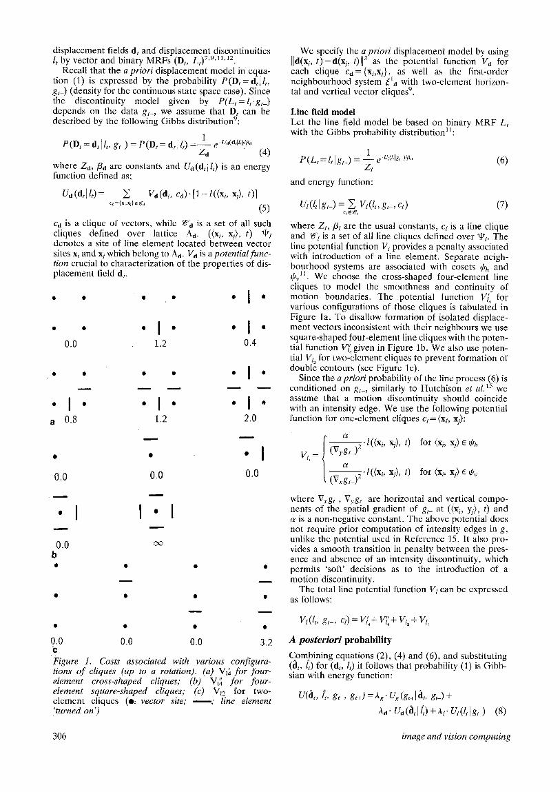
where Zz, fit are the usual constants, cl is a line clique and Wl is a set of all line cliques defined over 'ttl. The line potential function Vz provides a penalty associated with introduction of a line element. Separate neighbourhood systems are associated with cosets ~O h and g,v~. We choose the cross-shaped four-element line cliques to model the smoothness and continuity of motion boundaries. The potential function V/~ for various configurations of those cliques is tabulated in Figure la. To disallow formation of isolated displacement vectors inconsistent with their neighbours we use square-shaped four-element line cliques with the potential function V~' given in Figure lb. We also use potential Vt_, for two-element cliques to prevent formation of double contours (see Figure lc).

Since the a priori probability of the line process (6) is conditioned on gt , similarly to Hutchison et al. 15 we assume that a motion discontinuity should coincide with an intensity edge. We use the following potential function for one-element cliques ct= (x,, xj):

. O{ xj>, t)

(Vxg,_)2 .l((x,, xj), t)

for (xi, xj) ~ ~Oh

for (xi, xj) ~ ~v

where Vxgt_, Vygt_ are horizontal and vertical compo- nents of the spatial gradient of gt- at ((xi, yj), t) and a is a non-negative constant. The above potential does not require prior computation of intensity edges in g, unlike the potential used in Reference 15. It also provides a smooth transition in penalty between the pres- ence and absence of an intensity discontinuity, which permits 'soft' decisions as to the introduction of a motion discontinuity.

The total line potential function Vz can be expressed as follows:

Vt(lt, gt-, ct) = V[4 + V~] + vt2+ vz,

A pos ter ior i probabi l i ty

Combining equations (2), (4) and (6), and substituting Figure 1. Costs associated with various configura- (at, /t) for (dt, lt) it follows that probability (1) is Gibb- tions o f cliques (up to a rotation). (a) VI~ for four- sian with energy function: element cross-shaped cliques; (b) Vl] for four- element square-shaped cliques; (c) Vz2 for two- U(dt, it, gt-, gt+)--Ag'Ug(gt+l~lt, gt-)+ element cliques (O: vector site; • line element 'turned on') Ad" Ud(dtl~)+,it" U,(l,]g,_) (8)

306 image and vision computing

The conditional energies are defined in eguations (3), (5) and (7), respectively, and Ag = 1/(2o-~), ,~, = 1//3a, /3l--1/q)r. The MAP estimation can be achieved by minimization of energy (8) with respect to (at, [t). Note that the minimized energy consists of three terms and can be viewed as regularization: Ug describes the ill- posed matching problem of the data gt-, gt+ by the motion field at, while Ud and Ut are responsible for conforming to the properties of the a priori displacement and line models.

S O L U T I O N T O M A P E S T I M A T I O N

The energy U from (8) typically is a function of thous- ands of vectors and line elements. Since the energy Ug depends on a via gt- and gt+, in general it is non-convex (for a simple example of 1D matching see Reference 16)= Moreover, the energy Ul is in general non-convex in It, as is the case for the line potentials specified in Figure 1.

Recognizing that U is multi-dimensional and non- convex, we compute the MAP estimate of (dr, l~) (mini- mize U) using the method of simulated annealing which under certain conditions is capable of localizing the global optimum of an arbitrary objective function. Since simulated annealing is computationally costly, we will seek a reduction in this cost by instantaneously 'freezing' the algorithm.

Stochastic optimization via simulated annealing

Simulated annealing 17"1s is a general optimization method based on the analogy with the process of annealing of solids*. In simulated annealing the behav- iour of the solid is simulated by generating sample configurations from the Gibbs distribution with the energy function suitably crafted for the given optimization problem, while the temperature is replaced by the "temperature' parameter T. which is reduced according to some annealing schedule (e.g. logarithmic, exponential) is.

To implement the MAP estimation using simulated annealing, samples from MRFs Dt and Lt are needed. We generate such samples using the Gibbs sampler is which produces states according to probabilities of their occurrence, i.e. more likely states are generated more often while the less likely ones are produced less fre- quently. This property, incorporated into simulated annealing, allows the algorithm to escape local minima.

We use the Gibbs sampler based on the a posteriori probability (1) with energy (8). The displacement Gibbs sampler at location (xi, 0 is driven by a (Gibbs) marginal conditional probability characterized by the following energy function ~ 1:

t)fa;; gt-, gt+)=Ag'[r(a(xi, t), Xi, t ) ] 2 - [ -

E [la(xi, t ) -a(xj , t)ll2.[1-[(<x,, x/>, t)], j:x~ ~ na(x~)

(9)

*In this process the temperature of a solid is increased to a point at which all particles randomly arrange themselves in the liquid phase, followed by cooling through slowly lowering the temperature. If the initial temperature is sufficiently high and the cooling is sufficiently slow, the particles attain the configuration of the minimum energy.

where a7 = {a(xj, t): j4:i) and T]d(Xi) is a spatial neighbourhood of displacement vector at xi: Similarly, the line Gibbs sampler at location (yi, t )= ((xi, xj), t)

q~t is driven by another marginal conditional probability based on the energy function11:

Ut([(yi, t)l[7, at, gt-)=Aa • 2 ]]fi(Xm, t) Cd: {Xmt Xtt}: (xm, x,,)=yl

t)ll2.[1-/'(ys, t)]+As. E vtq,, g,_,, q) c/: Yi e'c! (10)

where [7 = {[(yj, t): j 4: i}.

Discrete state space Gibbs sampler For each candidate vector d(xi, t) e 5f~, the marginal probability distribution is computed from the local energy (9). Then, the new horizontal and vertical vector coordinates of d(xi, t) are obtained by sampling from this bivariate distribution. The necessity to obtain the complete probability distribution of a displacement vector at each xi is decisive in the computational complexity of the discrete state space Gibbs sampler. Sim- ilarly, for each line element l(yi, t) e 5~/ the marginal probability distribution is computed using (10) followed by appropriate sampling from this distribution. Since the line process Lt is binary regardless of state space used for the displacement process lDt, line elements are always inferred from the (discrete state space) line Gibbs sampler.

Continuous state space Gibbs sampler for Dt We avoid a very fine quantization of } (to obtain the continuous state space) by approximating the local energy (9) by a quadratic form in at so that the Gibbs sampler is driven by a Gaussian probability, distribution.

Assume that an approximate estimate d t of the true displacement field is known, and that the image intensity is locally approximately linear, Then, using the first-order terms of the Taylor expansion the DPD t" can be expressed as follows:

/~(a(X b t ) , Xi, t ) ~ / ~ ( d ( X b t), Xi, t)-~-

t), Xi, t),

where the spatial gradient of ~ is defined as:

rex( i(x/, 0, Xb t) Vd/~(d(Xi, t), Xi, t)~---[/~y(d(Xi, t),x,, t)]

t "x and ~Y are computed as an average of appropriate derivatives at the end points of vector d(x/, t) t6. Includ- ing the temperature T the local energy U~ can be written as follows:

A g u2 (a(x,, t) lfi, (,, g,_, g , + ) - T . [e(d(x,, t), x,, t) +

(a(x;, t)-d(xi, t)).v.e(d(x,, t), xi, 0] 2. A

+ - - Z Ita(x;, t)-d(x,., t)ll2-[t-{((x,, xj>, t)], T j:x, ~ n.(x,)

where ¢i is fixed. Note that now the local energy U~ is quadratic in at. it can be shown that the conditional probability density with the above energy is a 2D


Gaussian with the following mean vector m at location (Xi, t)16:

ei T " m = d(xi, t ) - - - V a P ( d ( x i , t),xi, t)

/~i

where the scalars ei and/x i are defined as follows:

8 i=~(d(x i , t ), xi, t)-I-(d(xi, t ) - d ( x i , t ))

• Vd/~(d(xi, t), xi, l)

/Zi=¢i /~d +llV, ei(x/' t), xi, t)[I 2 (11) /zg

and d(xi, t) is an average vector:

1 d(xi, t )= E a(xj, t)-[1-/(<x~, xj>, t)]

~i j:x/ ~ r/a(x)i

~i = E [ 1 - [((Xi, Xj>, t)] j:xj ~ ~a(x3

Note that averaging is disallowed across a motion boundary, which is a desirable property.

e The horizontal and vertical component variances o-x, 2 O-y, as well as the correlation coefficient p, which com-

prise the covariance matrix, have the following form:

Aa+[eY(~](xi, t), xi, t)121 4" r #l_ T as

" " [ ~ J 2~:faui sq" ~d-l-[/~x(d(Xb t), X b t)]eJ AS

--/~x(d(Xb t), X b t ) r y ( d ( x b t ) , xi, t) po-xCry = T

2(i hd/z i

The initial vector ti can be assumed zero throughout the estimation process, but then with increasing displacement vector estimates the error due to intensity non- linearity would significantly increase. Hence, it. is better to 'track' an intensity pattern by modifying d accord- ingly. An interesting result can be obtained when it is assumed that at every iteration of the Gibbs sampler d = a i.e., the initial (approximate) displacement field is equal to the average from the previous iteration. Then, the estimation process can be described by the following iterative equation:

a n+l (X b t ) = d n (xi, t ) - - E i v T e ( a n (Xi, t ) , Xi, t) +//i /zi (12)

where n is the iteration number, and s~i, /*i and the covariance matrix are defined as before except for d = d. At the beginning, when the temperature is high, the random vector ni has a large variance and the estimates assume quite random values. As the temperature T

2 2 and pO'xO'y get smaller, is reduced to zero, o-x, O-y thus reducing hi. In the limit the algorithm performs a

2 of the deterministic update. Note that the variance O'x horizontal vector component decreases with growing (x if At, aa, At and/~Y are constant. It means that when there is a significant horizontal gradient (detail) in the image structure the uncertainty of the estimate in hori-

2 zontal direction is small. The same applies to O-y. Hence, the algorithm takes image structure into account when determining the amount of randomness allowed at a given temperature.

Careful inspection of equation (12) reveals two interesting interpretations: a deterministic and a stochastic. For T = 0, when the random vector ni is zero, the equation is identical to the update equation of the Horn- Schunck algorithm 4, except for ei equal to DPD instead of the motion constraint equation and except for a different image model used. It is interesting that similar update equations result from two different approaches: Horn and Schunck using the calculus of variation have obtained a set of linear equations and have solved them by deterministic relaxation, while we have shown that the conditional probability driving the Gibbs sampler is a 2D Gaussian distribution. As to the stochastic interpretation, note that equation (12) is a variant of the diffusion equation discussed by Geman and Hwang 19, but applied locally at (xi, t). Convergence properties of such algorithms are difficult to establish, but for a general treatment of diffusions for global optimization see Reference 29.

As pointed out before, the discrete state space Gibbs sampler is used to sample from the line process Lt.

Determinist ic optimization using steepest descent method

Discrete state space

Note that for T=0 (deterministic update) the discrete state space Gibbs sampler generates only states with minimal local energy (9). This case can be interpreted as a 'steepest descent' algorithm which results only in an approximation to the MAP estimate.

Besag 2° proposed a similar approach called Iterated Conditional Modes (ICM). He argued that since it is difficult to maximize the joint a posteriori probability over the complete field, it should be divided into a minimal number of disjoint sets (or colours) such that any two random variables from a given set are condi- tionally independent given the states of the other sets. Besag recommended the use of a Maximum Likelihood (ML) estimate as an initial state for the ICM estimation. Using this approach displacement vectors or line elements can be computed individually (e.g. exhaustive search) for each location (xi, t) one colour at a time. Note that also this technique does not result in maxi- mization of probability (1), but provides separate MAP estimates for joint probabilities defined over corresponding colours. The difference between the ICM method and the Gibbs sampler for T = 0 is only the update order of variables161 Both techniques can be classified as a (pel) matching algorithm with smoothness constraint.

In the language of statistical mechanics the above processes are equivalent to quenching or instantaneous freezing in which the temperature is reduced to a minimum extremely rapidly, hence resulting in fast convergence. This procedure solidifies a material very quickly, however there remain various artifacts 'frozen' into the solid and its state may be far from the global minimum energy (in the sense of the MAP criterion).

Recently, Chou and Brown 21 proposed a method called Highest Confidence First (HCF) for Bayesian estimation based on MRF models. The method does not attempt to maximize a posteriori probability, but rather adaptively updates states according to their confidence. They have obtained better results using the HCF algorithm than applying the ICM or the SA algor-


ithm for boundary detection and depth estimation. Their results also indicate that ICM outperforms SA with the Gibbs sampler. This is inconsistent with our experience with 2D motion estimation (see the results below), and may be due to inappropriate choice of SA parameters. Nevertheless, HCF seems to be a very attractive method for discrete state space motion estimation as well. Also recently, methods based on mean field theory have been proposed for solving problems with Bayesian formulations a2. However, only solutions to problems with very simple line models, which need to be expressed in analytical .form, have been demonstrated. In our case where the line model is given through a table of potential values taking into account various clique configurations, derivation of the effec- tive potential proves very difficult.

Continuous state space

Let the displacement vector state space be continuous (5~ = R2). The energy function under minimization (8) is a general non-linear, non-quadratic function in dt as well as in It= We perform interleaved optimization with respect to dt and It. Assume that an estimate It of the line field is known. Then, the line energy Ut in (8) is constant and only minimization of AgUg+AaUa must be carried out. Using the linearization of the DPD ~, taking a derivative of A~Ug+Ad.Ud _with respect to d(xi, I) as well as assuming that d = d, it follows that the iterative update for this deterministic method is 46:

a n+l (x b t ) = a n (x b t ) - ei Vra P0] n (xi, t ) , xi, t) ,/-gi (13)

where ei and /x i are defined in (11) with t i=d. To resemble the Gibbs sampler as closely as possible, the Gauss-Seidet relaxation will be used in (13) rather than the Jacobi relaxation. Perhaps other relaxation algorithms could be used to improve convergence 6'23.

Once an estimate at is known, an improved estimate it should be obtained. For a fixed d t the energy AaUa + AtUt to be minimized is non-linear in it. Since l(xi, t) is binary for each i, simple exhaustive search with linear scan or the ICM method reported above can be used.

Note that if one disregards the line field [t, the iterative equation (13) is exactly the same as equation (12) for the first-order neighbourhood system jl/'~ (4:i=4) and for hi=0. In such a case there is no uncertainty involved in the estimation process, and similarly as in the case of the ICM estimation (discret e state space) the above algorithm is an example of quenching. Conse- quently, this rapid temperature reduction may not allow the system to attain the global minimum of the energy function.

The above approximation to the continuous state space MAP estimation is a spatio-temporal gradient technique which can be viewed as a modified version of the Horn and Schunck algorithm 4 where:

1 The modified algorithm (13) allows computation of displacement vectors for arbitrary Aa unlike the original Horn and Schunck algorithm in which Aa = Ag+0.5 G, rg] T.

2 The scalar e i is a displaced pel difference in the modified version rather than a motion constraint equation: no temporal derivative is needed.

3 The spatial intensity derivatives ~ and iY are computed from a separable polynomial model in both images and appropriately weighted, instead of the finite difference approximation over a cube, as proposed by Horn and Schunck 4.

The ability to estimate motion for abritary Aa is crucial for motion-compensated interpolation of sequences (the original Horn-Schunck algorithm would require 3D interpolation of motion fields).

The use of ~ instead of the motion constraint equation in ei is important because it allows intensity pattern tracking thus permitting more accurate intensity derivative computation, and also does not require the computation of the purely temporal derivative (actually

is an approximation to the directional derivative). The purely temporal derivative used in the Horn- Schunck algorithm is a reliable measure of temporal intensity change due to motion as long as small displacements are applied to linearly varying intensity pat- terns. Otherwise, significant errors may result, for example, an overestimation at moving edges of high contrast. Similar improvement by using an average of over the neighbouringvectors rather than evaluating for the average vector G, as is done here, has been proposed by Nagel a4.

The separable cubic interpolator 25, which we used to model the image at locations outside Ag, is characterized by Cl-continuity 16, as opposed to the linear, quadratic and some other cubic interpolators. We found this property to be critical for spatio-temporal gradient algorithms.

The deterministic algorithm (13) together with the ICM method for It is related to the algorithm proposed by Hutchinson et al. Ts. The major differences are those reported above for the Horn-Schunck algorithm as well as the line potentials: the potential Vl~ for single- element cliques is binary (0 or c~ in Reference 15), while here it varies continuously according to the local intensity gradient.

E X P E R I M E N T A L R E S U L T S

The algorithms described above have been tested on a number of image sequences with synthetic and natural motion. Results for two sequences are presented here. The images, which contain natural data captured by a video camera, have been stored in a displayable line- interlaced format with inter-field distance ~'6o=1/60 s.

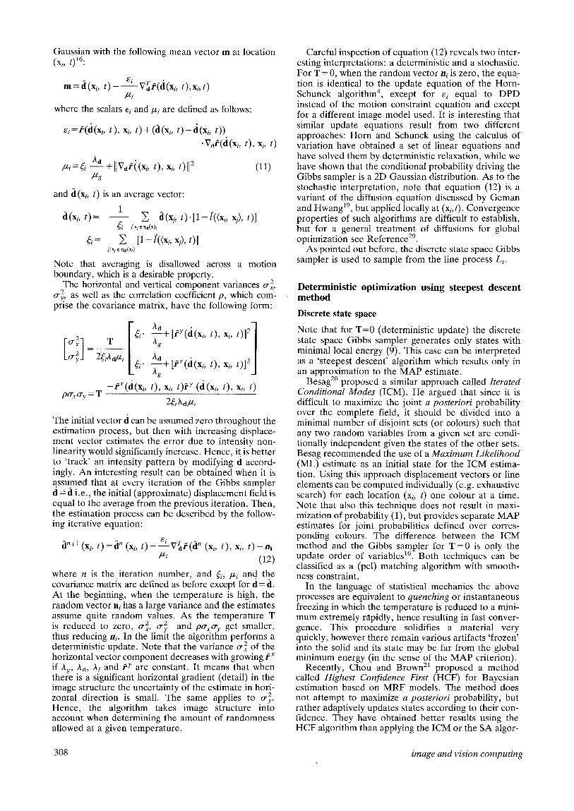
To provide a quantitative test we generated test image 1 (see Figure 2a) with stationary background provided by the test image from Figure 2b and a moving rectangle (45 by 20 pixels) obtained from another image through low-pass filtering, subsampling and pixel shifting. This test pattern permits non-integer displacements (ds-- [1.5, 0.5] for Figure 2a) so that there is no perfect data matching. Figure 2b shows test image 2 containing natural motion, acquired by a video camera. Areas to which motion estimation is applied cover cen- trally located rectangular regions of 77 by 49 pixels for test image 1 and 221 by 69 pixels fog test image 2.

The stochastic relaxation used was based either on the discrete state space Y~ with maximum displacement + 2.0 pixels and 17 quantization levels in each direction or on the continuous state space R ~. The first-

vo! 8 no 4 november 1990 309

b Figure 2. (a) Test image 1 with synthetic motion of rectangle (ds= [1.5,0.5]h, 45×20 pixels); (b) test image 2 with natural moiion

order displacement neighbourlaood system and, if applicable, the line neighbourhood with four-, two- and one-element line cliques have been used. The ratio ~/~g = 20.0 has been chosen experimentally, however, as pointed out by Konrad ~6, even a change of two orders magnitude did not have an excessively severe impact on the estimate quality. The motion estimates presented in the sequel have been obtained from pairs of images (fields) separated by Tg = 2~'6o. All estimates have been obtained with Keys bicubic interpolator ~6, except for the discrete state space

estimation applied to test image 2, when bilinear interpolation was used. We have chosen a slowly decaying exponential annealing schedule T~ = To" a ~-~ with To = 1.0 and a = 0.980 for the discrete state space and another one with To = 5.0 and a = 0.9944 for the continuous state space (more iterations).

Since the true motion field is known for the test image with synthetic motion (except for the occlusion and newly exposed areas), it is possible to assess the quality of motion field estimates. The Mean Squared Error (MSE) and the bias b measuring the departure of estimate d from the known motion field d~, are computed within the moving rectangle and given in figure captions.

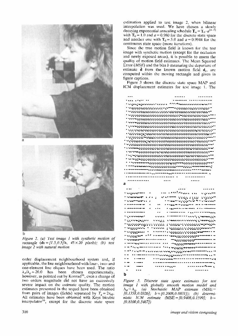
Figure 3 shows the discrete state space MAP and ICM displacement estimates for test image 1. The

a

b

Figure 3. Discrete state space estimates for test image 1 with globally smooth motion model and Aa= Ag. (a) Stochastic MAP estimate (MSE= [0.1358,0.0326]; b=[0.2008,0.0831]); (b) deterministic ICM estimate (MSE = [0.9408,0.1599]; b= [0.8100,0.3467])


stochastic MAP estimate is superior to the ICM estimate both subjectively and objectively (MSE, b). In both cases the zero displacement field has been used as an initial state. In other experiments, ML estimates (Aa/1~=0.0) have been computed and used as a starting point (as suggested by Besag for ICM estimation). The ML estimates were characterized by substantial randomness in vector lengths and orienta- tions, which can be explained by the lack of a prior model. As expected, the initial state had no impact on the stochastic MAP estimate, but the final !CM estimate was inferior to the ICM estimate presented above both subjectively and in terms of MSE.

b

c

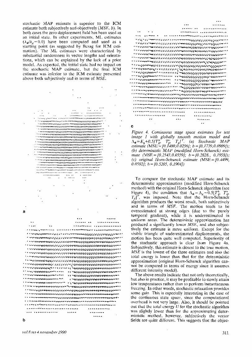
Figure 4. Continuous stage space estimates for test image 1 with globally smooth motion model and Aa=Eg+O.5tV h, T~g, Til T . (a) Stochastic MAP estimate (MSE = [0.1480, 0.0256]; b = [0.1739, 0.0909]); (b) deterministic MAP (modified Horn-Schunck) estimate (MSE = [0.2543,0.0559[; b=[0.2828., 0.1958]); (c) original Horn-Schunck estimate (MSE = [0.4499, 0.0592]; b=[0.5205, 0.19041)

To compare the stochastic MAP estimate and its deterministic approximation (modified Horn-Schunck method) with the original Horn-Schunck algorithm (see Figure 4), the condition that Aa=A.+0.5[Th., T~., Tg] r, was imposed. Note that the ~Horn-Sc~hunc~k algorithm produces the worst result, both subjectively and in terms of MSE. The motion tends to be overestimated at strong edges (due to the purely temporal gradient), while it is underestimated in uniform areas. The deterministic approximation has produced a significantly lower MSE, and also subjectively the estimate is more uniform. Except for the visible triangle of underestimated displacements, the motion has been quite well computed. Superiority of the stochastic approach is clear from Figure 4a. Subjectively, this estimate is closest to the true motion, MSE is the lowest of the three estimates and also the total energy is lower than that for the deterministic approximation (original Horn-Schunck algorithm can- not be compared in terms of energy since it assumes different intensity model).

The above results indicate that not only theoretically, but also in practice, it may be profitable to slowly attain low temperatures rather than to perform instantaneous freezing. In other words, stochastic relaxation provides some gain. This is especially interesting in the case of the continuous state space, since the computational overhead is not very large. Also, it should be pointed out that the total energy U for the stochastic algorithm was slightly lower than for the approximating deterministic method, however, subjectively the vector fields are quite different. This suggests that the objec-

vol 8 no 4 november 1990 311.

a

~ . . . ~ < ~ < . . ~ - . ~ + ' :

I ~ N \ " ~NNNNNN~ • NN~ .NNNX ~, . . . .

t ~ < < - < < . . . . . . . . . f I ~ N N X N N N N N N N N N N N N N X X ~

I ~~. , , .~ . -~>, . - . . - .> , ,~ . - , , .~- , , . - .a- , . - - .v . - . , . - . - - . - .~

- - _ J l " - - ' g " _ Laa._.'-a r~''L.~_~-_-;__~g+++~-_''-~-'~_+=+U.-a-" "

!~4,.-~'-~'-{&~.'.<'-~"" I--.-.-..--.-.--.--.-~--.--.-.--.--.--.--.--.--.-.-.~-"

b

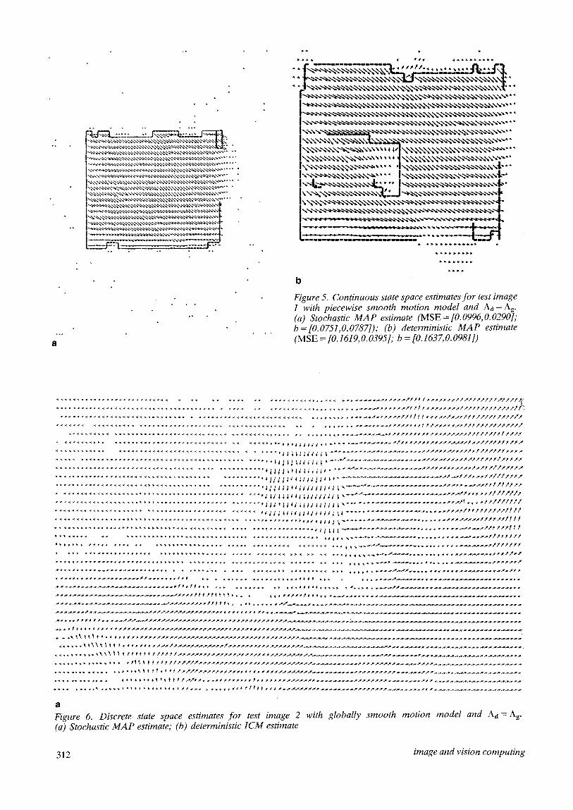
Figure 5. Continuous state space estimates for test image 1 with piecew~e smooth motion model and A~ = Ag. (a) Stochastic MAP estimate (MSE = [0. 0996, O. 0290]; b = [0.0751,0.0787]); (b) deterministic MAP estimate (MSE = [0.1619, O. 0395]; b = [0.163~ O. 09811)

. . . . . . . . . . . . . . . . . . . , , , . . . . . . . . . . . . . . . . . . . . . . . . ~¢7~11 i#~1717 i11~1~ i . . . . . . . . . . . . . . . . . . . , . . . . # # # # l l l l l l l l l l l ] l t

J ~ . . l ~ # f i # ~ . # . . ~ l l l - - ~ l l l # 1 1 1 1 l l l l # l l l l l l l # # l l # l # # # # # l l l j

. . . . t ~ i , ~ t % % ~ t l # # t l t # f l l l l l l l f t l l # l i l l l l l l l l l S x S l l l l t f t S l l . . . . . . . x . . . . . . . . i l l ~ . . . . . 1 ~

a

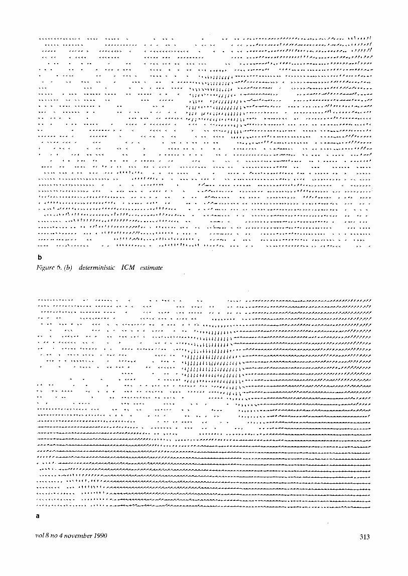
Figure 6. Discrete state space estimates for test image 2 (a) Stochastic MAP estimate," (b) deterministic ICM estimate

with globally smooth motion model and Aa = A g .


. . . . . . . . . . . . . . . . . . . . . . . . . . < < ~ , 1 ¢ . ~ . , * * ~ j 1 1 1 4 ~ ~ . . . . . . . . . , . . . . . . . f # , . ~ 1 # , , t . - - . t t . . . . .

b

Figure 6. (b) deterministic ICM estimate

I ~ I I - - - - ~ I [ I V ~ I - - v T


. . . . . . . . . . . . . . . . . . . . . . . . . . . . . ' ~ ; l l i ; l l l ~ . . . . . . . . . . . . . . # . . . . . . # # # # # # # # # # # # # # # # l ~ l l y l l l

. . . . . . . . . . . . . . . . . . , l ~ l i ; l i ; t l i i l l l l ; l i . - - . . . . . . . . . . . . . . . . . . . . . . . ~ . . ~ # . # # t t t f l l i ~ " ' > . . . . . . . . . . , i l l ~ l l i / l l T ; ~ / ~ j l l l ~ . . . . . . . . . . . . . . . . . . . . . . . . . x # t l # # # # # i l l l i # f l

b

e

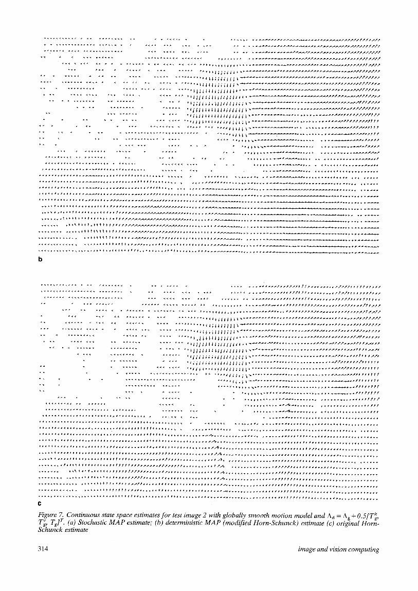
Figure 7. Continuous state space estimates for test image 2 with globally smooth motion model and A d = Ag + 0.5[T~, T~, T j T. (a) Stochastic MAP estimate; (b) deterministic MAP (modified Horn-Schunck) estimate (c) original Horn- Schunck estimate


. . . . . . . . . . . . . . . . . . . . . . . . . . . . . . . . . . . . . . . . . . . . . . iI li lililil¢l~t~-n 2 : : : . . . . . . . . . . . . . . . . . . . . . . . . . . . . .,i--~1.,I...,11.. . . . . . . . . . . . . . . . . . . . . . . . . . . . . . . . . . . . . . . . . . . . . . . '~J11 I l l 11 l i l l J l t l l ~ P l . . . . . . . . . . m ~ . , ' . ~ " I ,.~ .~I.-#IIIIII..A~IlIlIIII

H i i , , e , B l , ÷,, ,~,- r -

. . . . . . . . . . . . . . . . . . . . . . . . . . . . . . . . . . . . . . . . . . . . . . . . . / l 1~ # I I I i I i 7 I t 7 7 i 7, ,$ t . . . . . . . . . . . . . . . . . . "wX . . . . . . . ~ J ..-,,' t l l l l l t f

. . . . . . . . . . . . . . . . . . . . . . . . . . . . . . . . . . . . . . . . . . . . . . . . ~1 17"41"b i I I ~" I I I l I I I ~ | . . . . . . . . . . . . . . . . . . 1 7 . . . . . # f " ~ S l ' ~ # # ' ~ l l i i / t t

................................................... t,4 ..... ~ t . ~ i ~ll ir + .................. -" ............. ,,,-',,'-',,

........................................................ ::::.: ::::~i!i!l~-~ ........... . .......... : : : : : : : : : : : : : : : : : : : : : : : : : : : : : : : : : : : : : ":::. :: .::: "" :: : : : : : : : : :. : :: :: : ~g.__~ . . . " ===============================:::::::

.......... : ...... :'-':'.;'73373"':::.';7:::";..:: ................ ::" .......... :"': ....... ::'""

. . . . . . . . . . . . . . . . . . . . . . ~ . . . . . . . . . . . . . . . . . . . . . . . . . l l i l ~ l i ¢ I I l l l l l i l i ' ~ . . . . . . . . . . . . . . . . . . . . . . . . " ~ - - ~ a ' ' ~ l l ' t P t l t

........ .... i ii!i il i! i l i ..........................

................................. ~.,.,, .... ' .......... : .... ~.k.,~ ...................................

b

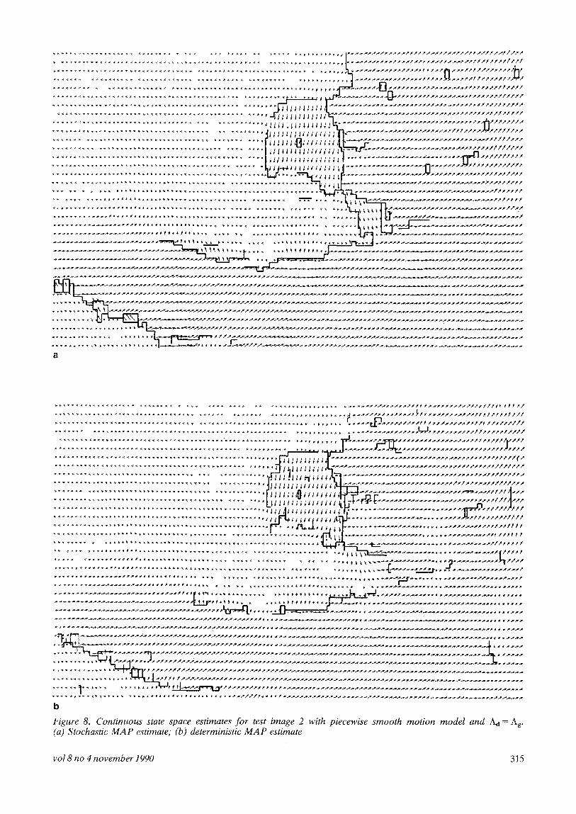
Figure 8 Con~nuous sta~ space es~m~te~ fo r test image 2 with piecewise smooth rnoUon mode! and A~ = A~ (a) ~ o ¢ ~ ¢ MAP estimate; (b) deterministic M A P estima~

vol 8 no 4 n o v e m b e r 1990 315

tive function (8) is multimodal, and for similar values of this function quite different solutions can be obtained.

Figure 5 shows the Stochastic and deterministic estimates for the piecewise smooth motion model. The parameters used are the same as before with addition of o~= 10.0. During experimentation we have observed that the ratio ~l/Ad had to be substantially lower for the deterministic algorithm (AI/Aa=O.15) to obtain results comparable with the stochastic MAP estimation (At/Ad=0.8). This may be explained by explicit averaging used in the deterministic algorithm. The continuous state space MAP estimation uses similar averaging, but it also involves a randomness factor, thus allowing switching line elements off and on, even if motion discontinuity does not quite allow it. Note that both subjectively and in terms of MSE the deterministic estimate is clearly inferior.

Figure 6 shows the discrete state space MAP and ICM displacement estimates for the test image 2. The ICM estimate is again subjectively poorer than the stochastic MAP estimate. The ICM algorithm failed to compute correctly the motion of the forearm and of the arm, except for the displacement vectors along the edge of the shirt sleeve. Also, the vectors on the neck and parts of the face suggest that there is no motion, which is incorrect.

Similarly, the three continuous state space methods have been applied to the test image 2 (see Figure 7). The original Horn-Schunck estimate shows some overestimated vectors (edge of shirt sleeve) and numerous underestimated ones (uniform area to the right). The deterministic approximation performs better: it is more uniform and has smaller edge effects. The stochastic estimate, however, is superior in terms of the total energy U as well as motion field smoothness and lack of edge effects.

Finally, in Figure 8 estimates Obtained by the stochastic and deterministic methods based on the piecewise smooth motion model are shown. Note that the displacement fields are quite similar, but the line contours estimated by the deterministic method are more fragmented. It has been our experience with other images as well, that deterministically updated line fields are usually more fragmented.

CONCLUSION

In this paper two types of solution methods to the problem of 2D motion estimation based on the MAP criterion have been presented and compared: stochastic and deterministic. It has been demonstrated that, as an example of instantaneous freezing, the deterministic methods may be incapable of localizing the global minimum not only theoretically but also in practice. Higher values of the energy function for the deterministic solutions were confirmed by inferior subjective and objective (synthetic motion) quality. Such an improvement in estimate quality comes at a cost of increased computational effort, however, The computational overhead (per iteration) of the continuous state space stochastic estimation compared to its deterministic approximation is small (less than 25%) because it includes only the computation of the random update term. The number of iterations required to provide a sufficiently slow annealing schedule, however, takes

the stochastic method more involved computationally by about an order of magnitude.

A C K N O W L E D G E M E N T S

The assistance of Christian Charbonneau in prepara- tion of the photographs is acknowledged. This work was supported by the Natural Sciences and Engineering Research Council of Canada under Strategic Grant STR0040524.

REFERENCES

1 Netravali, A and Robbins, JD 'Motion-compensated television coding: Part 1' Bell Syst. Tech. J. Vol 58 (March 1979) pp 631-670

2 Paquin, R and Dubois, E 'A spatio-temporal gradient method for estimating the displacement field in time-varying imagery' Comput. Vision, Graph. & Image Process. Vol 21 (1983) pp 205-221

3 Jain, CK 'Image data compression: a review' Proc. IEEE Vol 69 (March 1981) pp 349-389

4 Horn, BKP and Schunck, BG 'Determining optical flow' Artif. Intell. Vol 17 (1981) pp 185-203

5 Hildreth, EC 'Computations underlying the measurement of visual motion' Artif. Intell. Vol 23 (1984) pp 309-354

6 Roug(~e, A, Levy, BC and Willsky, AS 'Reconstruc- tion of two-dimensional velocity fields as a linear estimation problem' Proc. IEEE Int. Conf. Corn- put. Vision (1987) pp 646-650

7 Murray, DW and Buxton, BF 'Scene segmentation from visual motion using global optimization' IEEE Trans PAMI Vol 9 (March 1987) pp 220-228

8 Barnard, ST 'Stochastic stereo matching over scale' Int. J. Comput. Vision Vol 3 (1989) pp 17-32

9 Konrad, J and Dubois E 'Estimation of image motion fields: Bayesian formulation and stochastic solution' Proc. IEEE Int. Conf. Acoust., Speech & Signal Process. (1988) pp 1072-1074

10 Konrad, J and Duhois, E 'Multigrid Bayesian estimation of image motion fields using stochastic relaxation' Proc. IEEE Int. Conf. Comput. Vision (1988) pp 354-362

11 Konrad, J and Dubois, E 'Bayesian estimation of discontinuous motion in images using simulated annealing' Proc. Conf. Vision Interface (1989) pp 51-60

12 Bouthemy, P and Lalande, P 'Motion detection in an image sequence using Gibbs distributions' Proc. IEEE Int. Conf. Acoust., Speech & Signal Process. (1989) pp 1651-1654

13 Heitz, F and Bouthemy, P 'Motion estimation and segmentation using a global Bayesian approach' Proc. IEEE Int. Conf. Acoust., Speech & Signal Process. (1990) pp 2305-2308

14 Dubois, E 'The sampling and reconstruction of time-varying imagery with application in video systems' Proc. IEEE Vol 73 (April 1985) pp 502- 522

15 Hutchinson, J, Koch, Ch, Luo, J and Mead, C


'Computing motion using analog and binary resis- tive networks' Computer Vol 21 (March 1988) pp 52-63

16 Konrad, J 'Bayesian estimation of motion fields from image sequences' PhD Thesis, McGill Univer- sity, Canada (1989)

17 Kirkpatrick, S, Gelatt, CD (Jr) and Vecchi, MP 'Optimization by simulated annealing' Science Vol 220 (May 1983) pp 671-680

18 Geman, S and Geman, D 'Stochastic relaxation, Gibbs distributions, and the Bayesian restoration of images' IEEE Trans. PAMI Vol 6 (November 1984) pp 721-741

19 Geman, S and Hwang, C-R 'Diffusions for global optimization' SIAM J. Control & Optimization Vol 24 (September 1986) pp 1031-1043

20 Besag, J 'On the statistical analysis of dirty pictures' J. R. Statist. Soc. Vol 48 (1986) pp 259-279

21 Chou, PB and Brown, CM 'The theory and practice

of Bayesian image labelling' Int. J. Comput. Vision Vol 4 (1990) pp 185-210

22 Geiger, D and Girosi, F 'Parallel and deterministic algorithms for MRFs: surface reconstruction and integration' MIT Artificial Intelligence Laboratory A1, Memo 1114, USA (1989)

23 Lee, D, Papageorgiou, A and Wasilkowski, GW 'Computational aspects of determining optical flow' Proc. IEEE Int. Conf. Comput. Vision (1988) pp 612--618

24 Nagel, H-H and Enkelmann, W 'An investigation of smoothness constraints for the estimation of displacement vector fields from image sequences' IEEE Trans. PAMI Vol 8 (September 1986) pp 565-593

25 Keys, RG 'Cubic convolution interpolation for digital image processing' IEEE Trans. Acoust., Speech & Signal Process Vol 29 (December 1981) pp 1153-1160


Documents

Comparison of stochastic and deterministic solution methods in Bayesian estimation of 2D motion