A deterministic filter for non-Gaussian Bayesian estimation— Applications to dynamical system estimation with noisy measurements

OLIVER PAJONK, BOJANA V. ROSIC,ALEXANDER LITVINENKO, AND

HERMANN G. MATTHIES

A DETERMINISTIC FILTER FOR

NON-GAUSSIAN BAYESIAN

ESTIMATION

INFORMATIKBERICHT 2011-04

INSTITUTE OF SCIENTIFIC COMPUTINGCARL-FRIEDRICH-GAUSS-FAKULTATTECHNISCHE UNIVERSITAT BRAUNSCHWEIG

Braunschweig, Germany

http://www.digibib.tu-bs.de/?docid=00038994 01/04/2011

This document was created February 2011 using LATEX 2ε .

Institute of Scientific ComputingTechnische Universitat BraunschweigHans-Sommer-Straße 65D-38106 Braunschweig, Germany

url: www.wire.tu-bs.de

mail: [email protected]

CCScien

tifi omputing

Copyright c© by Oliver Pajonk, Bojana V. Rosic, Alexander Litvinenko, andHermann G. Matthies

This work is subject to copyright. All rights are reserved, whether the wholeor part of the material is concerned, specifically the rights of translation, reprint-ing, reuse of illustrations, recitation, broadcasting, reproduction on microfilm or inany other way, and storage in data banks. Duplication of this publication or partsthereof is permitted in connection with reviews or scholarly analysis. Permissionfor use must always be obtained from the copyright holder.

Alle Rechte vorbehalten, auch das des auszugsweisen Nachdrucks, der auszugs-weisen oder vollstandigen Wiedergabe (Photographie, Mikroskopie), der Speicher-ung in Datenverarbeitungsanlagen und das der Ubersetzung.


www.wire.tu-bs.de

mailto:[email protected]?subject=A Deterministic Filter for non-Gaussian Bayesian Estimation

A Deterministic Filter for non-GaussianBayesian Estimation

Oliver Pajonk, Bojana V. Rosic, Alexander Litvinenko, andHermann G. Matthies

Institute of Scientific Computing, TU [email protected]

Abstract

We present a fully deterministic method to compute sequential updates forstochastic state estimates of dynamic models from noisy measurements. It doesnot need any assumptions about the type of distribution for either data or meas-urement — in particular it does not have to assume any of them as Gaussian.It is based on a polynomial chaos expansion (PCE) of the stochastic variablesof the model. We use a minimum variance estimator that combines an a pri-ori state estimate and noisy measurements in a Bayesian way. For compu-tational purposes, the update equation is projected onto a finite-dimensionalPCE-subspace. The resulting Kalman-type update formula for the PCE coeffi-cients can be efficiently computed solely within the PCE. As it does not rely onsampling, the method is deterministic, robust, and fast.

In this paper we discuss the theory and practical implementation of themethod. The original Kalman filter is shown to be a low-order special case. Ina first experiment, we perform a bi-modal identification using noisy measure-ments. Additionally, we provide numerical experiments by applying it to thewell known Lorenz-84 model and compare it to a related method, the ensembleKalman filter.

Keywords: Bayesian estimation, polynomial chaos expansion, Kalman filter,inverse problem

AMS classification: 60H40, 65M32, 62L12

3


mailto:[email protected]?subject=A Deterministic Filter for non-Gaussian Bayesian Estimation

4


Contents

Contents 5

1 Introduction 1

2 Representation of Random Variables 3

3 Recursive Estimation for PCE Representations 5

4 The Kalman Filter as a Special Case 7

5 Ensemble Filter Methods 85.1 Implementation Details . . . . . . . . . . . . . . . . . . . . . . . . 9

6 The Lorenz-84 Model 116.1 Representation by an Ensemble . . . . . . . . . . . . . . . . . . . . 126.2 Representation by PCE . . . . . . . . . . . . . . . . . . . . . . . . 12

7 Numerical Experiments 137.1 Bimodal Identification . . . . . . . . . . . . . . . . . . . . . . . . 137.2 The Lorenz-84 Model . . . . . . . . . . . . . . . . . . . . . . . . . 17

7.2.1 Assimilation Example . . . . . . . . . . . . . . . . . . . . 177.2.2 Percentile Estimation . . . . . . . . . . . . . . . . . . . . . 197.2.3 Variance Estimation . . . . . . . . . . . . . . . . . . . . . 197.2.4 Probability Densities and Updates . . . . . . . . . . . . . . 30

8 Conclusions 31

A Multi-Indices 32

B Hermite Polynomials 32

C The Hermite Algebra 33

D The Hermite Transform 34

E Higher Order Moments 36

References 36

5


6


1 IntroductionThe problem of updating the knowledge of an uncertain quantity in a sequential wayfrom noisy and incomplete data is considered. This is a so-called inverse problem ofidentification. The goal is to regularise the ill-posed inverse problem by a Bayesianmethod, which uses a priori knowledge as additional information to the given set ofdata. For an introduction into the topic, e.g. see Tarantola (2004).

Well established methods for computing Bayesian estimates can be coarselygrouped into two classes: so-called “Linear Bayes” (Goldstein & Wooff, 2007)methods, which update functionals of the random variables (the simplest of whichare the Kalman-type methods), and updates based on Bayes’s formula itself. The lat-ter ones are usually implemented as sequential Monte Carlo (SMC) methods — alsocalled particle filters (e.g. Gordon et al. (1993)) — or Markov chain Monte Carlomethods (MCMC) (e.g. Hastings (1970)). However, due to the large number ofsamples required to obtain satisfying results they are computationally quite demand-ing and hence not very practical. Methods like the Gaussian sum filter (Alspach &Sorenson, 1972) are trying to approximate Bayes’s formula. But they, too, tend tohave a quite large computational overhead (Houtekamer & Mitchell, 2001).

On the other hand, methods like the extended Kalman filter run into closureproblems for non-linear models (Evensen, 1992). Additionally, they are not suitablefor high dimensions. Approaching these two problems, the class of Monte Carlobased Kalman-type filters has become quite popular over the last years. The factthat for constant variance the asymptotic rate of convergence of Monte Carlo meth-ods does not depend on the dimension of the sampled space makes these methodsapplicable to very high dimensional problems, which appear for example in weatherforecasting, oceanography, and geophysics. Additionally, these methods naturallyallow for non-linear forward models and thus avoid the possibly severe truncationerrors coming from linearisation, as they appear for example in the extended Kal-man filter.

Kalman-type SMC methods approximate the system covariance matrix, whichis central to the Kalman update, by a low-rank estimate from the involved ensemble.Several ensemble-based low-rank methods have been developed since the publica-tion of the original paper describing the ensemble Kalman filter (EnKF) (Evensen,1994). Most notable are the family of so-called “perturbed observation” imple-mentations (Burgers et al., 1998) and the family of ensemble square-root filters (En-SRF) (Anderson, 2001; Bishop et al., 2001; Whitaker & Hamill, 2002; Tippett et al.,2003). These methods avoid the perturbed observations and thus the sampling er-rors. For a thorough overview on EnKF and EnSRF see Evensen (2009b). Morerecent developments include an ODE-based implementation of Bergemann et al.(2009), where the analysis or assimilation solution is computed by numerically in-tegrating a specially crafted ODE. Related methods include the unscented Kalman

1


filter (Julier & Uhlmann, 2004), which employs a special, deterministic approachinstead of Monte Carlo sampling to obtain a second-order correct mean and errorcovariance estimate — but it also suffers from the curse of dimensionality.

The main idea of this work is to perform a Bayesian update without sampling,but in a direct, purely algebraic way by employing a polynomial chaos expansion(PCE) representation of the involved random variables. The method has been de-veloped as a sequel of ideas presented in (Marzouk et al., 2007; Kucerova & Mat-thies, 2010). A similar idea has independently appeared in a simpler form in Blan-chard (2010) in another context, where it is developed as a combination of polyno-mial chaos and extended Kalman filter theory. Related approaches include Penceet al. (2010) who combine polynomial chaos theory with maximum likelihood es-timation. There, the resulting optimisation problem is solved by gradient descent ora random search algorithm. In contrast, we use a minimum variance estimator basedon white noise analysis introduced by Wiener (1938). This kind of estimator is ob-tained by a simple orthogonal projection of an abstract estimation formula onto apolynomial chaos basis. In the special case when the problem is linear and employsGaussian random variables the method reduces to the Kalman filter, and in fact theKalman filter relations are the low-order part of the method.

The polynomial chaos expansion (Wiener, 1938; Ghanem & Spanos, 1991;Holden et al., 1996; Malliavin, 1997; Janson, 1997; Hida et al., 1999; Matthies,2005, 2008) has already been utilised for the solution of inverse problems, thoughjust for the approximation of the forward problem (Marzouk et al., 2007; Marzouk& Xiu, 2009; Arnst et al., 2010). There, the high computational efficiency of eval-uating the PCE solution is employed to estimate the likelihood function from theapproximated solution through sampling by an MCMC method. However, this kindof approach is still probabilistic and rather expensive. In order to improve the ac-ceptance probability of proposed MCMC moves, Christen & Fox (2005) have ap-plied a local linearisation of the forward model. However, MC sampling is not theonly possible way. For example, (Balakrishnan et al., 2003; Ma & Zabaras, 2009;Li & Xiu, 2009) use a collocation method which samples in a purely deterministicway. This is another way to evaluate the involved integrals. Unfortunately, alsocollocation needs a fairly high number of sample points when the dimension of theproblem becomes large enough.

In this paper we present an efficient numerical strategy for the Bayesian solutionof inverse problems. We represent the random variables in the state vector with thehelp of the PCE (section 2). This representation allows us to use a minimum vari-ance estimate and to directly update the PCE coefficients of the prior state (section3). In this updating procedure no sampling is involved at any stage. The originalKalman filter is shown to be a special case of the new method (section 4). Wethen shortly present the ensemble Kalman filter (EnKF) method (section 5) as an

2


elder relative of our method: they mainly differ in the representation of the involvedrandom variables. By a small numerical example we demonstrate the capability ofthe described method to update non-Gaussian quantities, after which we apply theEnKF and the described method to the well-known Lorenz-84 model (section 7) andcompare the results. Section 8 then concludes our work.

2 Representation of Random VariablesRandom variables (RVs) are usually formally defined as measurable functions r(ω)with values in some vector space V on a finite measure space with total mass equalto unity. The underlying probability space is given as a triplet (Ω ,A ,P), where Ω

is the set of elementary events ω ∈Ω , A a σ -algebra, and P the probability meas-ure. In many problems the space Ω is not concretely accessible (and usually is alsonot really needed, as one may work with the algebra of RVs as primitive objects,e.g. see Segal & Kunze (1978)), so that the usual idea of a function (e.g. given as aformula) looses much of its meaning. The representation of RVs is therefore oftenstrikingly different from what is used for “normal” functions. When propagating aRV through some model, say an evolutionary differential equation, we may recog-nise some distinctive methods tailored to its representations, which may take theform of:

Sampling: Formally an evaluation of the RV at some — randomly or determinist-ically — chosen points ωs ∈Ω . This concept is the simplest as it only needs— usually very many — evaluations of the deterministic model. However,this makes these methods computationally very costly, especially for real ap-plications (e.g. Snyder et al. (2008)).

Distribution: This is the measure Pr on V generated by an RV r. For a measurablesubset E ⊆ V one defines Pr(E) := P(r−1(E)). This description leads to theformulation of conservation equations for the probability, variously known asKolmogorov-equations, Fokker-Planck-equations, or master equations. Forlarger models these methods are usually not even contemplated for practicaluse due to their computational demand (Skorokhod, 1982).

Moments of r: These are the quantities MMM(k)r (see Appendix E). This approach

leads to — usually ever more complicated — evolutionary integro-differentialequations for the moments (Skorokhod, 1982).

Functional approximation: In recent years an alternative representation hasgained increasing momentum. The idea is to describe an RV r as a func-tion of other — known — RVs of some simple type. A typical example is

3


given by polynomials of normalised Gaussian RVs. This is Wiener’s poly-nomial chaos expansion (PCE) (Wiener, 1938; Janson, 1997), also known bya more recent name “white noise analysis” (Holden et al., 1996; Malliavin,1997; Hida et al., 1999). In some way this representation allows the idea ofusing the algebra of RVs as primitive objects, and hence it has a distinctlyfunctional analytic flavour (Segal & Kunze, 1978). This representation is thebasis of the estimation method described in this paper, so we present now itsbasic principles.

Let θ1(ω), ...,θk(ω), ... be normalised (zero mean, unit variance) GaussianRVs (for simplicity we assume real valued scalar RVs), viewed as elements in thespace L2(Ω) with the inner product

〈θ1|θ2〉L2(Ω) = E(θ1(ω)θ2(ω)). (1)

The Gaussian random variables span a subspace

H = spanθ1(ω), ...,θk(ω), ... ⊆ L2(Ω) (2)

which may be completed to a Hilbert subspace H of L2(Ω). Given this structure,we may assume that the RVs θ1(ω), ...,θk(ω), ... are orthonormal or — in otherwords — uncorrelated. This further means that they form a complete orthonor-mal system (CONS) for H . In addition, the products of Gaussian RVs from Hare again in L2(Ω) as Gaussian RVs possess moments of all orders. The Cameron-Martin theorem (Holden et al., 1996; Malliavin, 1997; Hida et al., 1999) then assuresus that the polynomial algebra of these RVs is dense in L2(Ω), i.e. we may writeany RV as a series of polynomials in variables from H . A convenient choice for anorthogonal generating set are the well-known Hermite polynomials in these Gaus-sian RVs, given in more detail in Appendix B. Following this, we consider RVs withvalues in some Hilbert vector space V with inner product 〈·|·〉V . A correspondinginner product in L2(Ω,V ) is given by

〈rrr1|rrr2〉L2(Ω,V ) := E(〈rrr1(·)|rrr2(·)〉V ). (3)

Any RV rrr ∈ L2(Ω ,V ) has an expansion in Hermite polynomials — this is the PCE:

rrr(ω) = ∑α∈J

rrrα Hα(θ1(ω), ...,θk(ω), ...), (4)

where J :=N(N)0 is a multi-index set (see Appendix A) discriminating the polyno-

mials Hα and coefficients rrrα ∈ V . The sequence of coefficients (rrrα)α∈J — alsocalled the Hermite transform H (rrr) of the RV rrr, see Matthies (2007) — representsthe RV and may be computed simply by projection:

∀α ∈J : rrrα = E(rrr(·)Hα(·))/〈Hα |Hα〉. (5)

4


Then, one may define the moments of RVs as it is shown in Eq. (E.1). The meanis denoted by rrr = MMM(1)

rrr , and for the covariance between rrr1 and rrr2 we write CCCrrr1rrr2 =

MMM(2)rrr1rrr2 (see Eq. (E.3)). Additionally, CCCrrr1 is used as a shorthand for CCCrrr1rrr1 .

For numerical computations the expansion naturally has to be truncatedto a finite total polynomial order and limited to a finite number of RVsθ1(ω), ...,θM(ω). This may be seen as a “stochastic discretisation”. The index α

now runs only in some finite set JZ ⊂J , where Z is defined by the number M ofGaussian RVs and the maximum total order P of the polynomials as

Z = (M+P)!/(M!P!). (6)

Such a truncated expansion can be used in any model involving the RVs. This isthe “ansatz” or trial function. Due to the truncation, the model equation will not besatisfied, but we can use the Galerkin-weighted residual idea to formulate equationsfor the coefficients rrrα . Formally this means a projection onto the finite dimensionalsubspace spanned by the Hα with α ∈JZ , by weighting the residual with some testfunctions — which are often again the Hermite polynomials.

As conclusion, we may now express anything dependent on the RVs throughtheir Hermite transform. At the same time, for the purpose of numerical computa-tion we may project the model onto some finite dimensional subspace, and thus givecompletely deterministic equations for the coefficients of the PCE.

3 Recursive Estimation for PCE RepresentationsLet us consider a dynamical system in Rn whose true state at time t is describedby the vector of state variables xxxt . In addition, let ∆t be a given time step, suchthat the state at time t +∆t (in notation t + 1) may be computed with the help of aknown model operator: xxxt+1 = G(xxxt). For notational simplicity let us consider thesystem at a certain, fixed time t = T , which allows us to omit the time index fromthe following notation.

The true state xxx can be considered as uncertain either because of uncertainty inthe initial state, or due to uncertainty in the model G, or both. The goal of the fol-lowing analysis is the approximate reconstruction of xxx with respect to the previousknowledge and some given data. We assume our prior knowledge to be destilled inan a priori distribution with corresponding random variable xxx f (ω), where the sub-script f denotes “forecast”. This information shall be combined with the data, ob-tained by measuring the quantities yyy(ω) ∈ Rd , which depend linearly on the “true”state but are disturbed by a measurement error εεε(ω), i.e. additive noise:

yyy(ω) = HHHxxx+ εεε(ω). (7)

5


Here, HHH : Rn→Rd denotes the known linear measurement operator. Note that oftend n, so we deal with an inverse problem that is usually ill-posed in the sense ofHadamard in the deterministic setting (Engl et al., 2000) — but see Stuart (2010) fora mathematical analysis and proof of well-posedness in the stochastic setting. Theuncertainty in the measurement error is modelled as an RV, and hence yyy(ω) is an RVas well. For simplicity we assume the measurement error to be a centred Gaussian— the method could also deal with other measurement error distributions — so thatits description is completely given by the covariance CCCεεε . In addition, we assumethat the measurement errors are not correlated with the state forecast, i.e. CCCxxx f εεε = 0.The forecast measurement on the other hand is zzz(ω) := HHHxxx f (ω)

We assume that all RVs involved are elements of L2(Ω), with inner productgiven by Eq. (1) or Eq. (3). To obtain an improved estimator xxxa(ω) reflecting theprior estimate xxx f (ω) as well as the measurements yyy(ω) (with subscript a denot-ing “analysis” or “assimilated”), a common linear Bayesian approach is to derive aminimum variance estimator using the projection theorem of Hilbert spaces (Luen-berger, 1969). In the case of a linear forward model G and purely Gaussian RVsthe resulting estimator is well known as the Kalman filter — but note that in thefollowing, linearity of G or the assumption of Gaussian RVs is not needed.

The following theorem presents the minimum variance update when additionaldata becomes available (Luenberger, 1969):

Theorem 3.1. Assume that xxx f (ω) is a vector valued random variable which rep-resents an estimator for the unknown xxx, and that a measurement yyy(ω) becomesavailable according to Eq. (7). The orthogonal projection xxxa(ω) — in the innerproduct from Eq. (1) or Eq. (3) and hence the best estimator in the L2(Ω) norm —of xxx on the subspace spanned by xxx f (ω) and yyy(ω) is given by

xxxa(ω) = xxx f (ω)+KKK(yyy(ω)− zzz(ω)), (8)

where KKK is the “Kalman gain” operator

KKK :=CCCxxx f zzz (CCCzzz +CCCεεε)−1 . (9)

If the involved RVs xxx f (ω), xxxa(ω),yyy(ω) and zzz(ω) are described via Monte Carloensembles the resulting method becomes the ensemble Kalman filter (EnKF, seesection 5 and Evensen (2009a)). Here we use the PCE instead as representation forthe RVs. Namely, we “project the projection formula” Eq. (8) onto the polynomialchaos in order to obtain directly the coefficients of the posterior PCE.

Due to the orthogonality of the polynomial chaos, one may simply projectEq. (8) by multiplying it with each Hα , taking the expectation of the obtained equa-tion and further dividing it by ‖Hα‖2

L2(Ω) = α! such that for all α :

xxxαa = E(xxxaHα)/α! (10)

6


and so on for xxxαf ,yyy

α ,zzzα and εεεα . For each α Eq. (8) leads to

xxxαa = xxxα

f +KKK(yyyα − zzzα), (11)

or in terms of the Hermite transform

H (xxxa) = H (xxx f )+KKK(H (yyy)−H (zzz)). (12)

The simplest representation of Eq. (11) is to collect all the column vectors xxxα into amatrix, e.g. XXX = [...,xxxα , ...], and with this interpretation the full update simply readsas

XXXa = XXX f +KKK(YYY −ZZZ). (13)

This is the final form of the PC updating approach developed in this paper.

4 The Kalman Filter as a Special Case

Let us remark that the term with α = 0 in Eq. (11) or Eq. (13) is the update of themean, thus recovering the well-known Kalman update for the mean (Luenberger,1969). The same conclusion is reached by taking the expectation of Eq. (8). But thepreviously mentioned equations also contain the Kalman update for the covariance.For any expansion like

xxxa(ω) = ∑α

xxxαa Hα(ω), (14)

the covariance is given by (see Appendix E)

CCCxxxa = E((xxxa(·)− xxxa)⊗ (xxxa(·)− xxxa))

= ∑α,β>0

xxxαa ⊗ xxxβ

a E(Hα Hβ

)(15)

= ∑α>0

xxxαa ⊗ xxxα

a α!,

where E(Hα Hβ

)= δαβ α! and xxxa = xxx0

a. Employing the matrix representation as inEq. (13) and introducing the diagonal Gram matrix (∆∆∆)

αβ=E

(Hα Hβ

)= diag(α!),

one may rewrite Eq. (15) to

CCCxxxa = XXXa∆∆∆ XXXTa , (16)

where XXXa is XXXa without the α = 0 term (the mean). Having CCCxxx f εεε = 0, we maytensorise Eq. (13), subtract the mean values and take the expectation of the obtained

7


equation in order to obtain the covariance:

CCCxxxa = XXXa∆∆∆ XXXTa

=(XXX f +KKK(YYY − ZZZ)

)∆∆∆(XXX f +KKK(YYY − ZZZ)

)T

=CCCxxx f +KKKCCCεεε KKKT +KKKCCCzzzKKKT (17)

−CCCxxx f zzzKKKT −KKKCCCTxxx f zzz

=CCCxxx f +KKK(CCCzzz +CCCεεε)KKKT −CCCxxx f zzzKKKT −KKKCCCTxxx f zzz.

Using Eq. (9) one has that

CCCxxxa =CCCxxx f +CCCxxx f zzz (CCCzzz +CCCεεε)−1 CCCT

xxx f zzz

−2CCCxxx f zzz (CCCzzz +CCCεεε)−1 CCCT

xxx f zzz (18)

=CCCxxx f −CCCxxx f zzz (CCCzzz +CCCεεε)−1 CCCT

xxx f zzz

=CCCxxx f −KKKCCCTxxx f zzz,

which is exactly the update for the covariance estimate from the original Kalmanfilter (Luenberger, 1969).

Let us point out that in Eq. (11) or Eq. (13) the complete random variable isupdated — up to the order kept in the PCE — and not just the first two moments, asit is usually done in the Gauss-Markov theorem — for example in the guise of theKalman filter (Luenberger, 1969; Jazwinski, 1970).

5 Ensemble Filter MethodsThe ensemble Kalman filter can be derived in the same way as the PC updatingapproach. Thus, in the following we use the same symbols and abbreviations asin section 3. The main difference is that instead of using the Hermite transformof the RVs xxx f (ω), xxxa(ω),yyy(ω), and zzz(ω) the variables are represented by a set ofMonte Carlo samples, here simply called “ensemble”: XXX f = [xxx f (ω1), ...,xxx f (ωN)],and similarly for xxxa(ω),yyy(ω), and zzz(ω). Each ensemble is conveniently written inmatrix form, with one sample in each column. This is in contrast to the matrices ofPCE coefficients in Eq. (13).

Consider the ensemble XXX f representing the RV xxx f (ω). Each ensemble mem-ber has independently been transformed through the (possibly non-linear) forwardmodel. The goal is, given a measurement yyy, to compute a new ensemble XXXa condi-tioned on this measurement. Theorem 3.1 shows that applying the Kalman updateEq. (8) to each ensemble member separately results in an ensemble which has therequired statistics.

8


Conveniently, all necessary covariances to compute the Kalman update can beapproximated from the forecast ensemble. For this first centralize XXX f and ZZZ:

XXX f := XXX f − xxx f 111TN

ZZZ := ZZZ− zzz111TN .

Here xxx := 1N ∑

Ni=1 xxx(ωi) denotes the sample mean, and 111T

N represents a row vector of1s of length N. Then one may estimate the covariances:

CCCxxx f zzz ≈ XXX f ZZZT (19)

CCCzzz ≈ ZZZ ZZZT. (20)

Note that all normalisation terms (N− 1)−1 from the covariance matrix estimatesmay be omitted, as they will cancel out in the update.

As it is very important to treat the measurement yyy as a random variable (shown inBurgers et al. (1998), but also clear from Eq. (8)), we form a measurement ensembleYYY by sampling the measurement RV yyy(ω). This RV is typically assumed to beGaussian with covariance matrix CCCεεε and mean yyy

∀i = 1, ...,N : yyyi ∼N (yyy,CCCεεε). (21)

We can now write the EnKF update equation as a special case of Eq. (8) as

XXXa = XXX f +KKK(YYY −ZZZ), (22)

where KKK is again the Kalman gain defined in Eq. (9).

5.1 Implementation Details

Eq. (22) can be implemented almost directly: inserting Eq. (9) into Eq. (22) gives

XXXa = XXX f +CCCxxx f zzz

=:AAA︷︸︸︷(CCCzzz +CCCεεε)

−1(YYY −ZZZ) . (23)

There are mainly three important points to consider: for numerical stability oneshould not solve the set of normal equations AAA = (CCCzzz +CCCεεε)

−1(YYY −ZZZ) straightfor-wardly. Due to possible ill conditioning, it is best solved by pseudo inversion, de-noted by (·)†, using a singular value decomposition (SVD) (e.g. Evensen (2009a)).For this, we replace CCCεεε with the ensemble estimate CCCyyy. This is an acceptable ap-proximation (see Evensen (2003), his section 3.4.3), which comes in handy now:

9


(CCCzzz +CCCyyy)† =

(ZZZ ZZZT

+ YYY YYY T)†

(24)

which is, taking into account that ZZZYYY T ≡ 0 and YYY ZZZT ≡ 0,

=((

ZZZ + YYY)(

ZZZ + YYY)T)†

, (25)

with the SVD of one factor being

UUUΣΣΣVVV T = ZZZ + YYY . (26)

Assume the singular values in the diagonal matrix ΣΣΣ arranged descending by size.Inserting Eq. (26) into Eq. (25) one obtains((

ZZZ + YYY)(

ZZZ + YYY)T)†

=(UUUΣΣΣΣΣΣ

TUUUT )†(27)

=(

UUUΣΣΣ†ΣΣΣ

†TUUUT), (28)

where ΣΣΣ† is the pseudo-inverse of ΣΣΣ , a diagonal matrix with the inverse of the

largest singular values from ΣΣΣ . Below a certain threshold in ΣΣΣ the correspondingelements in ΣΣΣ

† are set to zero (Golub & van Loan, 1996). Note that the samesolution procedure is used in the PCE-based update Eq. (13).

The second important point is that for the pseudo-inversion to work correctly, allcomponents of the RVs yyy(ω) and zzz(ω) have to be on the same scale. Otherwise, inthe pseudo-inversion, the singular vectors of small scale measurements are system-atically associated with small singular values — which obviously are more easilytruncated. Thus it could introduce a bias in the update towards large scale measure-ments. This can be easily fixed by scaling the RVs with the assumed measurementstandard deviation, thus making them non-dimensional.

The third important point is that we use second order exact sampling in anycase where a random number ensemble ΞΞΞ of size N is drawn from an n-dimensionalstandard normal distribution N (0, IIIn). This may be achieved by subtracting aneventual mean

ΞΞΞ := ΞΞΞ− ξξξ 111TN

and correcting the standard deviation of every row j = 1..n

∀ j : (ΞΞΞ) j := (ΞΞΞ) j ·(√

var((ΞΞΞ) j)

)−1

of the sample (Evensen, 2004).

10


6 The Lorenz-84 ModelFor the numerical evaluation of the estimation method described in section 3, weconsider the well-known “Lorenz-84” model (Lorenz, 1984, 2005). It is describedby a set of three state variables xxx = (x,y,z)T . There x represents a symmetric, glob-ally averaged westerly wind current, whereas y and z represent the cosine and sinephases of a chain of superposed large-scale eddies transporting heat polewards. Thestate evolution of this model, xxx= dxxx

dt = f (xxx); xxx(0)= xxx0, is described by the followingset of ordinary differential equations (ODEs):

dxdt

= −ax− y2− z2 +aF1

dydt

= −y+ xy−bxz+F2 (29)

dzdt

= −z− xz+bxy,

where F1 and F2 represent known thermal forcings, and a and b are fixed constants.Given some values for the initial conditions xxx0 = (x0,y0,z0)

T , this system can beintegrated forward in time using, for example, a Runge-Kutta (RK) scheme, as itwas done in (Lorenz, 2005; Shen et al., 2010).

The Lorenz-84 model shows chaotic behaviour and is very sensitive to the initialconditions. For this reason we model these as independent Gaussian RVs:

x0(ω) ∼ N (x0,σ1)

y0(ω) ∼ N (y0,σ2) (30)z0(ω) ∼ N (z0,σ3).

Due to the appearance of RVs, the deterministic model Eq. (29) turns into asystem of stochastic differential equations (SDEs, Øksendal (1998)), xxx(ω) =f (xxx(ω)); xxx(0,ω) = xxx0(ω), with

dx(ω)

dt= −ax(ω)− y(ω)2− z(ω)2 +aF1

dy(ω)

dt= −y(ω)+ x(ω)y(ω) (31)

−bx(ω)z(ω)+F2

dz(ω)

dt= −z(ω)− x(ω)z(ω)+bx(ω)y(ω),

which needs to be integrated in time to obtain the evolution of the stochastic statevector xxx(ω) = (x(ω),y(ω),z(ω))T . To be able to do so one has to choose a repres-entation for the involved RVs.

11


6.1 Representation by an EnsembleAs mentioned in section 2, one can represent the RVs by Monte Carlo sampling.To approximately solve the SDEs Eq. (31), each of the samples of the initial condi-tions can be independently integrated forward in time using the deterministic set ofODEs in Eq. (29). At any time t, the set of samples may be used to approximatelycalculate any statistics for the RVs xxx(ω). As this is precisely what ensemble filtermethods like the EnKF need, we use the representation by Monte Carlo sampleswhen applying those.

6.2 Representation by PCEOn the other hand, following (Shen et al., 2010) and the mathematical formulationgiven in section 2, we may readily use the PCE (see Eq. (4) and Eq. (14)) in orderto represent the RVs:

xxx(ω) = ∑α∈J

xxxα Hα(θ(ω)). (32)

For xxx(ω) = (x(ω),y(ω),z(ω))T denote the Hermite transform of x(ω) by ξ :=(xα)α∈J = H (x(ω)) (see Appendix D), and similarly by η := (yα)α∈J andζ := (zα)α∈J the transforms of the y(ω) and z(ω) components. The stochasticevolution equation Eq. (31) can then be written in terms of these Hermite trans-forms.

For computational purposes we have to truncate the Hermite transform, as ex-plained in section 2. Thus, we replace the variables by the approximations ξ ,η , and ζ , where denotes the projection on the finite subspace generated byHα |α ∈JZ. For simplicity we use the same finite subspace for x(ω), y(ω)and z(ω). Of course, now Eq. (31) cannot be satisfied anymore, e.g. the result ofa product of two truncated PCEs Q2(ξ , ζ ) does not necessarily lie in the subspaceanymore. To solve this problem we simply do a Galerkin projection onto above sub-space. The final result is then the stochastic evolution equation Eq. (31) projectedonto the subspace:

dξ

dt= −aξ − Q2(η , η)− Q2(ζ , ζ )+aF1e0

dη

dt= −η + Q2(ξ , η)−b Q2(ξ , ζ )+F2e0 (33)

dζ

dt= −ζ − Q2(ξ , ζ )+b Q2(ξ , η),

where e0 := (δ0α)α∈JZ = (1,0,0, ...). The terms Q2(·, ·) denote the trun-cated/projected PCE of the Hermite transform of the product of two RVs, which

12


may be computed analytically from the PCEs of the RVs (see Appendix D for de-tails). Now one may integrate Eq. (33) in the same way as in the deterministic caseby a RK scheme, for example.

7 Numerical Experiments

We would like to point out that it is our goal to find efficient methods which areable to reliably represent a practitioners “state of information”, given all availabledata (Tarantola, 2004). Following this, in the subsequent numerical experimentswe aim to assess and compare the combined uncertainty quantification and stateestimation capabilities of the methods. Thus we cannot simply evaluate how closelysome specific functional of the RV representation of a method — e.g. the meanor median — resembles the “truth”. We have to evaluate and compare the variancethat is captured by the different methods — especially in the presence of a non-linearmodel like Lorenz-84.

7.1 Bimodal Identification

First we would like to show that with the PC updating method it is quite easy totreat non-Gaussian RVs in the update. For this, one has to include non-zero higherorder terms into the PCE representing the measurement, YYY , and include this into thecomputation of the Kalman gain Eq. (9) and the update Eq. (13).

There are two possibilities to obtain these higher order terms: either one assumesa likelihood and sets the PCE coefficients accordingly (as done with the Gaussianlikelihood for the subsequent Lorenz-84 example), or one makes repeated meas-urements of the “truth” and computes a PCE directly from them — “sampling thetruth”, so to say.

We demonstrate the second variant using a simple example. We create a PCE ofa bi-modal, stationary, scalar “truth” (for simplicity there is no dynamic model in-volved in this experiment). We assume that we can make repeated measurements ofthis “truth” which are disturbed by Gaussian noise. For the prior we take, assumingto lack better knowledge, a Gaussian distribution with a large variance and meanzero.

In Fig. 1 – 3 some results of this experiment are shown. The continuous prob-ability density function (pdf) estimates have been obtained by applying a kerneldensity technique (Botev et al., 2010) to a random sample of the RV. Rememberfrom Eq. (4) that the arguments of the PCE are uncorrelated, standard normal RVsθ1, ...,θM — which are easy to sample. By inserting one such sample into thePCE, we obtain a sample of the RV represented by the PCE. Sampling the PCE is

13


p(x)

p(x)

−4 −2 0 2 4x

p(x)

truth prior data posterior

(a) N = 10

(b) N = 100

(c) N = 1000

Figure 1: Bi-modal identification experiment after 1 update. Here are shown the res-ults for different amounts of measurements used to determine the PCE coefficientsYYY . First, we use 10 measurements (a), then 100 (b) and finally 1000 (c). The plotcontains the truth, the prior and the posterior, as well as the last used measurementas an example.

14


p(x)

p(x)

−4 −2 0 2 4x

p(x)


(a) N = 10

(b) N = 100

(c) N = 1000

Figure 2: Bi-modal identification experiment after 10 updates (for details see Fig. 1).

computationally rather cheap as it only involves the repeated evaluation of polyno-mials. However, the sampling is not part of the updating method and only needed toshow the results. The same method is used throughout the paper to obtain continu-ous pdf estimates.

Going back to Fig. 1 one may see that after a single update the prior significantlydominates the posterior in all cases — as it is expected. But after just 10 updates, onemay see in Fig. 2 that the posterior already has some resemblance of the “truth” in allcases. The quality, of course, improves with an increased amount of measurementsused to determine YYY . After 100 updates, we can see in Fig. 3 that the posterior quitesignificantly resembles the “truth” for 100 and 1000 measurements.

However, it is interesting to see that the posterior in the top plot of Fig. 3 isclearly worse than the corresponding one in Fig. 2 — despite of the tenfold increasein total measurements. Hence we can conclude that there is a trade-off involvedwhere to “spend” the available measurements: on one hand, we have to use someupdates to suppress the strong influence of the prior — but on the other hand weshould use as many measurements as possible to determine the coefficients YYY exactlyenough.

15


p(x)

p(x)

−4 −2 0 2 4x

p(x)


(a) N = 10

(b) N = 100

(c) N = 1000

Figure 3: Bi-modal identification experiment after 100 updates (for details seeFig. 1).

16


7.2 The Lorenz-84 ModelWe now apply the PC updating method to a dynamic identification experiment,where it is compared to an ensemble assimilation method. Note that it is currentlynot clear whether EnKF with perturbed observations or EnSRF with so-called “ran-dom rotations” is better suited for the assimilation of data into a non-linear modelsuch as the Lorenz-84 model described in the previous section (Evensen, 2009b).For this study we choose the EnKF with perturbed observations, as described insection 5.

In this numerical experiment the Lorenz-84 system is used in a hidden Markovmodel setting (see, e.g., Ephraim & Merhav (2002)) as described in section 3. Theinitial condition of the “unknown truth” is xxx = (1.0,0.0,−0.75)T , the thermal for-cings are set to F1 = 8.0 and F2 = 1.23, and the parameters are set to a = 0.25 andb = 4.0 (values taken from Lorenz (2005)). Let us point out that F1,F2,a, and b areassumed to be known exactly and are used in the forward integration of the “truth”and of the estimates. The noisy measurements of the “truth” are simulated by tak-ing the full state vector (thus in this case HHH = III3) and adding samples of zero-meanGaussian noise with known covariance CCCεεε = σ2III3

yyy(ω) = HHHxxx+N (0,CCCεεε). (34)

The measurement standard deviation is chosen to be σ := 0.1, which is approxim-ately 2.5% – 3% of the maximum absolute values that the Lorenz-84 model takes.The initial conditions are chosen as x0 = y0 = z0 = 0.0 and σ1 = σ2 = σ3 = 1.0in Eq. (30), starting off with a fairly large initial uncertainty. We use the commonchoice of integration method for Lorenz-84, a Runge-Kutta scheme of order 4 witha time step of ∆t = 0.05, which corresponds to 6 hours in the model time scale (Shenet al., 2010; Lorenz, 2005).

7.2.1 Assimilation Example

In Fig. 4 a short integration and assimilation example of the PC updating methodapplied to Lorenz-84, using a PCE of order 3 as was used in Shen et al. (2010), isshown. The plot contains the “truth”, as well as some percentiles pc := infx ∈ R :Pr.(x)≥ c/100 estimated from the PCE using sampling. Every 10 days a measure-ment is assimilated, until day 90. In Fig. 4, one can see how the initial uncertainty isnon-linearly transformed until day 10, where the first correction takes place. Afterthree assimilations, the “truth” is quite well followed by p50 until day 50, wherean outlier measurement or a highly unstable regime of Lorenz-84 makes p50 divertfrom the truth. However, note that the “truth” is still quite well embedded betweenp5 and p95. After the measurements at day 60 and 70, the “truth” is tracked quitewell again by p50 and the uncertainty reduces.

17


−1 0 1 2

x

−2

−1 0 1 2

y

010

2030

4050

6070

8090

−2

−1 0 1 2

z

time (days)

truth

p5 (X

),p95 (X

)p25 (X

),p75 (X

)p50 (X

)

Figure4:

Exam

pleof

thePC

updatingm

ethodapplied

tothe

Lorenz-84

model.

The

blackcircles

mark

theassim

ilationtim

epoints

(every10

days).H

ereit

isplotted,

forall

dimensions

x,y,zof

them

odel,the

“truth”and

some

percentilesestim

atedfrom

thePC

EX

usingsam

pling(p

5 ,p25 ,p

50 ,p75

andp

95 ).

18


From this experiment one may learn how the method is working in principle,and that it is able to represent and update skewed distributions: this can be seen bylooking at the sometimes quite asymmetric structure of the symmetrically chosenpercentiles before and also after the updates.

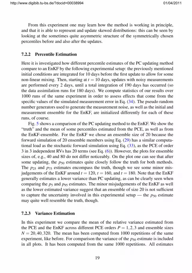
7.2.2 Percentile Estimation

Here it is investigated how different percentile estimates of the PC updating methodcompare to an EnKF by the following experimental setup: the previously mentionedinitial conditions are integrated for 10 days before the first update to allow for somenon-linear mixing. Then, starting at t = 10 days, updates with noisy measurementsare performed every 2 days, until a total integration of 190 days has occurred (sothe data assimilation runs for 180 days). We compute statistics of our results over1000 runs of the same experiment in order to assess effects that come from thespecific values of the simulated measurement error in Eq. (34). The pseudo randomnumber generators used to generate the measurement noise, as well as the initial andmeasurement ensemble for the EnKF, are initialized differently for each of theseruns, of course.

Fig. 5 shows a comparison of the PC updating method to the EnKF. We show the“truth” and the mean of some percentiles estimated from the PCE, as well as fromthe EnKF-ensemble. For the EnKF we chose an ensemble size of 20 because theforward simulation of 20 ensemble members using Eq. (29) has a similar computa-tional load as the stochastic forward simulation using Eq. (33), as the PCE of order3 in 3 independent RVs has 20 terms (see Eq. (6)). However, the plots for ensemblesizes of, e.g., 40 and 80 do not differ noticeably. On the plot one can see that aftersome updating, the p50 estimates quite closely follow the truth for both methods.The p25 and p75 estimates encompass the truth, though we see some minor mis-judgements of the EnKF around t = 120, t = 160, and t = 180. Note that the EnKFgenerally estimates a lower variance than PC updating, as can be clearly seen whencomparing the p5 and p95 estimates. The minor misjudgements of the EnKF as wellas the lower estimated variance suggest that an ensemble of size 20 is not sufficientto capture the uncertainty involved in this experimental setup — the p50 estimatemay quite well resemble the truth, though.

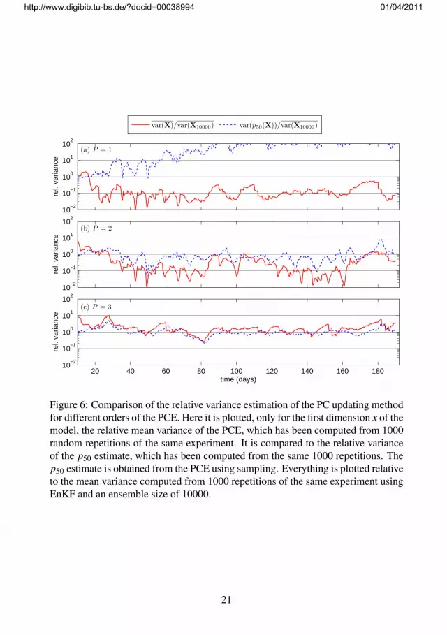
7.2.3 Variance Estimation

In this experiment we compare the mean of the relative variance estimated fromthe PCE and the EnKF across different PCE orders P = 1,2,3 and ensemble sizesN = 20,40,320. The mean has been computed from 1000 repetitions of the sameexperiment, like before. For comparison the variance of the p50 estimate is includedin all plots. It has been computed from the same 1000 repetitions. All estimates

19


−0.2

−0.1 0

0.1

0.2

logit((x−x+ 3.5)/7.0)

2040

6080

100120

140160

180−

0.2

−0.1 0

0.1

0.2

logit((x−x+ 3.5)/7.0)

time (days)

truth

p5 (X

),p95 (X

)p25 (X

),p75 (X

)p50 (X

)

(a)PC

updatin

g,P

=3

(b)EnKF,N

=20

Figure5:

Com

parisonof

thePC

updatingm

ethodto

theE

nKF,applied

toL

orenz-84.H

ereitis

plotted,onlyfor

thefirst

dimension

xofthe

model,the

“truth”and

them

eanofsom

epercentiles

estimated

fromthe

(a)PCE

and(b)E

nKF-ensem

bleX

(p5 ,p

25 ,p50 ,p

75and

p95 ).T

hem

eanhas

beencom

putedover1000

runsofthe

same

experiments.T

heverticalaxis

hasbeen

centredto

xand

scaledw

iththe

logitfunctionfor

clarity.N

otethatthe

plottingstarts

with

thefirstupdate

att=

10days.

20


10−2

10−1

100

101

102

rel.

varia

nce

10−2

10−1

100

101

102

rel.

varia

nce

20 40 60 80 100 120 140 160 18010

−2

10−1

100

101

102

rel.

varia

nce

time (days)

var(X)/var(X10000) var(p50(X))/var(X10000)

(a) P = 1

(b) P = 2

(c) P = 3

Figure 6: Comparison of the relative variance estimation of the PC updating methodfor different orders of the PCE. Here it is plotted, only for the first dimension x of themodel, the relative mean variance of the PCE, which has been computed from 1000random repetitions of the same experiment. It is compared to the relative varianceof the p50 estimate, which has been computed from the same 1000 repetitions. Thep50 estimate is obtained from the PCE using sampling. Everything is plotted relativeto the mean variance computed from 1000 repetitions of the same experiment usingEnKF and an ensemble size of 10000.

21


10−2

10−1

100

101

102

rel.

varia

nce

10−2

10−1

100

101

102

rel.

varia

nce

20 40 60 80 100 120 140 160 18010

−2

10−1

100

101

102

rel.

varia

nce

time (days)

var(X)/var(X10000) var(p50(X))/var(X10000)

(a) N = 20

(b) N = 80

(c) N = 320

Figure 7: Comparison of the relative variance estimation of the EnKF for differentensemble sizes. Here it is plotted, only for the first dimension x of the model,the relative mean variance of the ensemble, which has been computed from 1000random repetitions of the same experiment. It is compared to the relative varianceof the p50 estimate, which has been computed from the same 1000 repetitions. Thep50 estimate is obtained directly from the ensemble. Everything is plotted relativeto the mean variance computed from 1000 repetitions of the same experiment usingEnKF and an ensemble size of 10000.

22


in this experiment are plotted relative to a reference variance obtained from 1000repetitions of an EnKF run with 10000 ensemble members. This we consider “largeenough”, as the variance estimates obtained from the same experimental setup, butwith “just” 640 ensemble members, are almost the same.

One may see in Fig. 6 (a) that for polynomial order 1, PC updating is unable tomaintain a stable p50 estimate — it even goes out of the plotted scale. This is tobe expected, as the PCE has only 4 terms (see Eq. (6)) and not enough variance iscaptured. The variance estimate is also quite unstable and is occasionally two ordersof magnitude smaller than the reference variance. For polynomial order 2, shown inFig. 6 (b), the estimated variance is not much different, except for the time intervalt ∈ [120,170] days. The variance of the p50 estimate is significantly reduced andcomes much closer to the estimated variance. Thus, the results for polynomial order2 are better than for 1 but not what one would call reliable. However, already forpolynomial order 3, shown in Fig. 6 (c), the variance estimate is significantly higher,more stable, and much closer to the reference variance estimate. Additionally, thevariance of the p50 is almost never underestimated.

To compare these results with the EnKF, Fig. 7 shows the same plots as Fig. 6 forselected ensemble sizes. In Fig. 7 (a) one may see the often mentioned behaviour ofthe EnKF to underestimate the variance after some updating: for 20 ensemble mem-bers the variance of the p50 estimate is quite well estimated up to 40 days, whereit starts to drop. Remember that Fig. 7 (a) loosely corresponds to Fig. 6 (c) from acomputational load perspective. There, the variance is not dropping after some timeand is generally larger than for the EnKF. Even quadrupling the ensemble size to80, shown in plot Fig. 7 (b), does not change the variance estimate significantly. In-terestingly, the variance of the p50 estimate drops to almost precisely the estimatedvariance over the whole assimilation period. Finally, Fig. 7 (c) shows a “huge” en-semble of 320, where we can see the start of the convergence to the 10000 ensemblemember run. The variance is still consistently underestimated, but much less thanin the other cases. Additionally, the variance of the p50 estimate drops consistentlybelow the mean variance estimate.

Comparing Fig. 6 (c) with the other plots in Fig. 6 and Fig. 7, we can see thatthe PC updating estimates a variance that is closer to the 10000-member EnKF runthan all other experiments — except the “huge” 320-member EnKF run, which is,of course, to be expected. Over most of the assimilation period it is even quiteconsistently larger than the reference variance. This may be a result of the factthat the PC updating, due to the orthogonality of the involved expansion, is moreeasily able to handle non-Gaussian RVs. The EnKF ensemble is not orthogonal— though some promising approaches have been made in, for example, Evensen(2004) — and the initial span is even getting smaller during the forward integrationand updating as the ensemble members become more and more dependent (e.g. see

23


(a) Polynomial order P = 1

−1 0 1 2 3x

p(x)

(b) Polynomial order P = 2

−1 0 1 2 3x

p(x)

(c) Polynomial order P = 3

−1 0 1 2 3x

p(x)

Figure 8: Probability density estimates for the first PC update at t = 10 days of thefirst dimension x of Lorenz-84. The dashed, black line is the prior; the solid, redline is the posterior; the blue × symbol is the value of the truth; the green + symbolis the value of the noisy measurement.

Houtekamer & Mitchell (2001)). Thus, the EnKF needs a comparably large amountof ensemble members to span and maintain spanning the same subspace as PC up-dating. There, no special steps to maintain orthogonality have to be taken as it isinherent to the method. Following this argumentation, the updating and mainten-ance of non-Gaussian RVs in the context of the Lorenz-84 model is investigatednext.

However, it is important to point out that the reference of a set of EnKF runswith 10000 ensemble members is not representing “the best we can do” in termsof Bayesian updating, so it is not possible to say which method is “better” by thisdirect comparison. All that can be done is to point out differences.

24


(a) N = 50 ensemble members

−1 0 1 2 3x

p(x)

(b) N = 100 ensemble members

−1 0 1 2 3x

p(x)

(c) N = 1000 ensemble members

−1 0 1 2 3x

p(x)

Figure 9: Probability density estimates for the first EnKF update at t = 10 days ofthe first dimension x of Lorenz-84 (legend: see Fig. 8).

25



−1 0 1 2 3x

p(x)


−1 0 1 2 3x

p(x)


−1 0 1 2 3x

p(x)

Figure 10: Probability density estimates for the last PC update at t = 188 days ofthe first dimension x of Lorenz-84 (legend: see Fig. 8).

26



−1 0 1 2 3x

p(x)


−1 0 1 2 3x

p(x)


−1 0 1 2 3x

p(x)

Figure 11: Probability density estimates for the last EnKF update at t = 188 days ofthe first dimension x of Lorenz-84 (legend: see Fig. 8).

27



−1 0 1 2 3x

p(x)


−1 0 1 2 3x

p(x)


−1 0 1 2 3x

p(x)

Figure 12: Probability density estimates for the PC update at t = 110 days of thefirst dimension x of Lorenz-84, with a lower assimilation frequency (legend: seeFig. 8).

28



−1 0 1 2 3x

p(x)


−1 0 1 2 3x

p(x)


−1 0 1 2 3x

p(x)

Figure 13: Probability density estimates for the EnKF update at t = 110 days of thefirst dimension x of Lorenz-84, with a lower assimilation frequency (legend: seeFig. 8).

29


7.2.4 Probability Densities and Updates

Figs. 8 – 11 show pdf estimates for the prior and posterior for both the PC updatingmethod and the EnKF, across different polynomial orders/ ensemble sizes, respect-ively. For the PCE we have again used Monte Carlo sampling to obtain a continuousestimate of the pdf; for the EnKF, the ensemble itself is the required sample which isused in the mentioned kernel density estimation technique. Note that for this exper-iment we change the initial conditions to σ1 = σ2 = σ3 = 0.5 in Eq. (30) so that theprior in Fig. 8 and Fig. 9 is a bit more pronounced. Note that we perform exactly thesame assimilation experiment for both methods, including the specific samples usedto disturb the measurements of the truth. Thus, the plots may be directly compared.

In Fig. 8 and Fig. 9 we compare the pdfs for t = 10 days, which is the firstupdate. For the PCE representation in Fig. 8, we can see how the prior obtainedfrom integrating the initial conditions for 10 days is quite skewed for polynomialorders 2 and 3. This is to be expected as a PCE of total polynomial order 1 can onlyrepresent multivariate Gaussian RVs. For the ensemble representation in Fig. 9, theprior is quite symmetric for 50 ensemble members. For 100 and 1000 memberswe can see a slighly skewed structure — it is not as pronounced as for the PCErepresentation with polynomial order 2 or 3, though, and looks more like the oneobtained from a polynomial order of 1. The update for both the EnKF and the PCupdating is, as expected, moving the mean and reducing the variance. However, thePC updating of orders 2 and 3 is clearly able to retain the skewed structure of theprior. One can also see the convergence of the PCE: with increasing polynomialorder more and more details are added. The posterior of the EnKF, on the otherhand, looks quite Gaussian, even for an ensemble size of 1000.

At the end of the assimilation period, at t = 188 days, one can see in Fig. 10and Fig. 11 that both methods have almost lost all non-Gaussian structure. Both theprior and the posterior are more or less Gaussian — only for polynomial orders 2and 3, as well as the ensemble of size 1000, one may percieve a slight skewness. Forpolynomial order P = 1 we can see that the RV has effectively converged to a Diracdelta — which suggests that all variance has been lost and the polynomial order isclearly not sufficient for this experimental setup. However, this loss of non-Gaussianstructure may be due to the amount and frequency of Gaussian measurements whichhave been assimilated into the model.

To investigate the non-Gaussian updating a bit closer we ran the same exper-iment with a decreased assimilation frequency: data is assimilated only every 10days, starting at day 10. This results in a longer non-linear mixing between theupdates and thus should create pdfs which are more non-Gaussian. The rest of theexperiment stays the same. In Fig. 12 and Fig. 13 one may clearly see how thePC updating method retains the non-Gaussian structure of the prior when doing theupdate, whereas the EnKF eliminates most of it even for a quite large ensemble of

30


size 1000, where the prior is clearly non-Gaussian. Thus, from an uncertainty quan-tification perspective, the PC updating analysis contains more information, hintingat possible advantages of this method. Whether the PCE-based method is in somesense superior to the EnKF or not cannot be judged conclusively from this simpleexperiment, though, and requires further investigation.

Remark Most of the computation operations done in the update procedure arebased on standard matrix algebra (BLAS, LAPACK packages). However, in orderto speed-up certain computations we have used a tensorial algebra as it is providedin Bader & Kolda (2006).

8 Conclusions

We have developed a method which combines Bayesian updating of uncertaintywith the representation of random variables by PCE. The resulting update equationis fully deterministic and thus does not involve any sampling error, as opposed toMonte Carlo methods. However, it involves a truncation error from the truncatedPC expansion. The original Kalman filter has been shown to be a low order specialcase of the new method. The presented method has been employed for the identific-ation of a bi-modal truth. In an additional experiment, the PC updating method hasbeen applied to the recursive identification of uncertain initial values for a chaoticdynamic system, the Lorenz-84 model. On this example it has been compared to arelated sequential Monte Carlo technique, the ensemble Kalman filter. Differencesand similarities have been pointed out.

The method has shown some appealing mathematical properties, as well as ex-perimental capabilities. It is a promising combination of Bayesian inversion anduncertainty quantification techniques based on the PCE. By numerical experimentswe have shown that it is able to handle RVs which have a skewed or even bimodaldistribution. However, the update equation is simple and, as the necessary covari-ance estimates can be directly computed from the PC representation, quite efficient.As the method does not involve any closure assumptions besides the PCE truncation,it is easily applicable to non-linear systems.

It is clear that there are still some problems to solve on the path towards realapplications, e.g., to complex geophysical systems. But there is one more thing toconsider: the method is fully deterministic, which brings applications in areas intoreach which have strong security restrictions or severe real time requirements. Theresequential Monte Carlo methods, but also linearity and/or Gaussian assumptions ofthe original (extended) Kalman filter, may be inadequate.

31


Acknowledgment

The support of SPT Group GmbH in Hamburg, the Deutsche Forschungsgemeinsch-aft (DFG) and the German Luftfahrtforschungsprogramm of the Federal Ministry ofEconomics (BMWA) is gratefully acknowledged.

The following appendices collect some basic properties of the polynomial chaosexpansion (PCE), the connected Hermite algebra, and the use of the Hermite trans-form.

A Multi-IndicesIn the PCE formulation, the need for multi-indices of arbitrary length arises. Form-ally they may be defined by

α = (α1, . . . ,α j, . . .) ∈J := N(N)0 , (A.1)

which are sequences of non-negative integers, only finitely many of which are non-zero. As by definition 0! := 1, the following expressions are well defined:

|α| :=∞

∑j=1

α j,

α! :=∞

∏j=1

α j!, (A.2)

`(α) := max j ∈ N |α j > 0.

B Hermite PolynomialsAs there are different ways to define — and to normalise — the Hermite polynomi-als, a specific way has to be chosen. In applications with probability theory it seemsmost advantageous to use the following definition (Hida et al., 1999; Holden et al.,1996; Janson, 1997; Malliavin, 1997):

hk(t) := (−1)ket2/2(

ddt

)k

e−t2/2; ∀t ∈ R, k ∈ N0, (B.1)

where the coefficient of the highest power of t — which is tk for hk — is equal tounity.

32


The first five polynomials are

h0(t) = 1, h1(t) = t, h2(t) = t2−1,h3(t) = t3−3t, h4(t) = t4−6t2 +3,

and the recursion relation for these polynomials is

hk+1(t) = t hk(t)− k hk−1(t); k ∈ N. (B.2)

These are orthogonal polynomials w.r.t. the standard Gaussian probability meas-ure Γ, where Γ(dt) = (2π)−1/2e−t2/2 dt — the set hk(t)/

√k! |k ∈ N0 forms a

complete orthonormal system (CONS) in L2(R,Γ) — as the Hermite polynomialssatisfy ∫

∞

−∞

hm(t)hn(t)Γ(dt) = n!δnm. (B.3)

Multi-variate Hermite polynomials will be defined right away for an infinitenumber of variables, i.e. for ttt = (t1, t2, . . . , t j, . . .) ∈ RN, the space of all sequences.This uses the multi-indices defined in Appendix A: For α = (α1, . . . ,α j, . . .) ∈Jremember that except for a finite number all other α j are zero; hence in the definitionof the multi-variate Hermite polynomial

Hα(ttt) :=∞

∏j=1

hα j(t j); ∀ttt ∈ RN, α ∈J , (B.4)

except for finitely many factors all others are h0, which equals unity, and the infiniteproduct is really a finite one and well defined.

The space RN can be equipped with a Gaussian (product) measure (Hida et al.,1999; Holden et al., 1996; Janson, 1997; Malliavin, 1997), again denoted by Γ. Thenthe set Hα(ttt)/

√α! | α ∈J is a CONS in L2(RN,Γ) as the multivariate Hermite

polynomials satisfy ∫RN

Hα(ttt)Hβ (ttt)Γ(dttt) = α!δαβ , (B.5)

where the Kronecker symbol is extended to δαβ = 1 in case α = β and zero other-wise.

C The Hermite AlgebraConsider first the usual univariate Hermite polynomials hk as defined in AppendixB, Eq. (B.1). As the univariate Hermite polynomials are a linear basis for thepolynomial algebra, i.e. every polynomial can be written as linear combination of

33


Hermite polynomials, this is also the case for the product of two Hermite polyno-mials hkh`, which is clearly also a polynomial:

hk(t)h`(t) =k+`

∑n=|k−`|

c(n)k` hn(t) (C.1)

The coefficients are only non-zero for integer g = (k + `+ n)/2 ∈ N and if g ≥k∧g≥ `∧g≥ n (Malliavin, 1997). They can be explicitly given

c(n)k` =k!`!

(g− k)!(g− `)!(g−n)!, (C.2)

and are called the structure constants of the univariate Hermite algebra.For the multivariate Hermite algebra, analogous statements hold Malliavin

(1997):Hα(ttt)Hβ (ttt) = ∑

γ

cγ

αβHγ(ttt). (C.3)

with the multivariate structure constants

cγ

αβ=

∞

∏j=1

cγ jα jβ j

, (C.4)

defined in terms of the univariate structure constants Eq. (C.2).From this it is easy to see that

E(Hα Hβ Hγ

)= E

(Hγ ∑

ε

cε

αβHε

)= cγ

αβγ!. (C.5)

Products of more than two Hermite polynomials may be computed recursively,we here look at triple products as an example, using Eq. (C.3):

Hα Hβ Hδ =

(∑γ

cγ

αβHγ

)Hδ

= ∑ε

(∑γ

cε

γδcγ

αβ

)Hε . (C.6)

D The Hermite TransformA variant of the Hermite transform maps a random variable onto the set of expansioncoefficients of the PCE (Holden et al., 1996). Any random variable r ∈ L2(Ω) whichmay be represented with a PCE

r(ω) = ∑α∈J

rα Hα(θ(ω)) (D.1)

34


is mapped ontoH (r) := (rα)α∈J =: (r) ∈ RJ . (D.2)

This way r := E(r) = r0 and H (r) = (r0,0,0, ...), as well as r(ω) := r(ω)− r andH (r) = (0,(rα)α∈J ,α>0).

These sequences may be seen also as the coefficients of power series in infinitelymany complex variables z ∈ CN, namely by

∑α∈J

rα zα ,

where zα := ∏ j zα jj . This is the original definition of the Hermite transform (Holden

et al., 1996).It can be used to easily compute the Hermite transform of the ordinary product

like in Eq. (C.3), asH (Hα Hβ ) = (cγ

αβ)γ∈J . (D.3)

With the structure constants Eq. (C.4) one defines the matrices Qγ

2 := (cγ

αβ) with

indices α and β . With this notation the Hermite transform of the product of tworandom variables r1(ω) = ∑α∈J rα

1 Hα(θ) and r2(ω) = ∑β∈J rβ

2 Hβ (θ) is

H (r1r2) =((r1)Q

γ

2(r2)T ))

γ∈J . (D.4)

Each coefficient is a bilinear form in the coefficient sequences of the factors, and thecollection of all those bilinear forms Q2 = (Qγ

2)γ∈J is a bilinear mapping that mapsthe coefficient sequences of r1 and r2 into the coefficient sequence of the product

H (r1r2) =: Q2((r1),(r2))

= Q2 (H (r1),H (r2)) . (D.5)

Products of more than two random variables may now be defined recursivelythrough the use of associativity. e.g. r1r2r3r4 = (((r1r2)r3)r4):

∀k > 2 : H

(k

∏j=1

r j

):= Qk((r1),(r2), . . . ,(rk)) :=

Qk−1(Q2((r1),(r2)),(r3) . . . ,(rk)). (D.6)

Each Qk is again composed of a sequence of k-linear forms Qγ

kγ∈J , which defineeach coefficient of the Hermite transform of the k-fold product.

35


E Higher Order MomentsConsider RVs rrr j(ω) = ∑α∈J rrrα

j Hα(θ(ω)) with values in a vector space V , thenrrr j, rrr j(ω), as well as rrrα

j are in V . Any moment may be easily computed knowingthe PCE. The k-th centred moment is defined as

MMMkrrr1...rrrk

= E(⊗k

j=1rrr j

), (E.1)

a tensor of order k. Thus it may be expressed via the PCE as

MMMkrrr1...rrrk

= ∑γ1,...,γk 6=0

E

(k

∏j=1

Hγ j(θ)

)⊗k

m=1 rrrγm

m , (E.2)

and in particular:

CCCrrr1rrr2 = MMM2rrr1rrr2

= E(rrr1⊗ rrr2)

= ∑γ,β>0

E(Hγ Hβ

)rrrγ

1⊗ rrrβ

2 (E.3)

= ∑γ>0

γ!rrrγ

1⊗ rrrγ

2,

as E(Hγ Hβ

)= δγβ γ!. The expected values of the products of Hermite polynomials

in Eq. (E.2) may be computed analytically, by using the formulas from AppendixC.

ReferencesAlspach, D. & Sorenson, H. (1972). Nonlinear Bayesian estimation using Gaussian

sum approximations. IEEE Transactions on Automatic Control, 17(4), 439–448.

Anderson, J. L. (2001). An ensemble adjustment Kalman filter for data assimilation.Monthly Weather Review, 129, 2884–2903.

Arnst, M., Ghanem, R., & Soize, C. (2010). Identification of Bayesian posteriorsfor coefficients of chaos expansions. Journal of Computational Physics, 229(9),3134–3154.

Bader, B. W. & Kolda, T. G. (2006). Algorithm 862: MATLAB tensor classes forfast algorithm prototyping. ACM Transactions on Mathematical Software, 32(4),635–653.

36


Balakrishnan, S., Roy, A., Ierapetritou, M. G., Flach, G. P., & Georgopoulos, P. G.(2003). Uncertainty reduction and characterization for complex environmentalfate and transport models: An empirical Bayesian framework incorporating thestochastic response surface method. Water Resources Research, 39(12), 1350.

Bergemann, K., Gottwald, G., & Reich, S. (2009). Ensemble propagation and con-tinuous matrix factorization algorithms. Quarterly Journal of the Royal Meteor-ological Society, 135(643), 1560–1572.

Bishop, C. H., Etherton, B. J., & Majumdar, S. J. (2001). Adaptive samplingwith the ensemble transform Kalman filter. Part I: Theoretical aspects. MonthlyWeather Review, 129(3), 420–436.

Blanchard, E. D. (2010). Polynomial Chaos Approaches to Parameter Estimationand Control Design for Mechanical Systems with Uncertain Parameters. PhDthesis, Department of Mechanical Engineering, VirginiaTech University.

Botev, Z. I., Grotowski, J. F., & Kroese, D. P. (2010). Kernel density estimation viadiffusion. Annals of Statistics, 38(5), 2916–2957.

Burgers, G., van Leeuwen, P. J., & Evensen, G. (1998). Analysis scheme in theensemble Kalman filter. Monthly Weather Review, 126, 1719–1724.

Christen, J. A. & Fox, C. (2005). MCMC using an approximation. Journal ofComputational and Graphical Statistics, 14(4), 795–810.

Engl, H. W., Hanke, M., & Neubauer, A. (2000). Regularization of inverse prob-lems. Kluwer, Dordrecht.

Ephraim, Y. & Merhav, N. (2002). Hidden Markov processes. IEEE Transactionson Information Theory, 48(6), 1518–1569.

Evensen, G. (1992). Using the extended Kalman filter with a multilayer quasi-geostrophic ocean model. Journal of Geophysical Research, 97(C11), 17,905–17,924.

Evensen, G. (1994). Sequential data assimilation with a non-linear quasi-geostrophic model using Monte Carlo methods to forecast error statistics. Journalof Geophysical Research, 99(C5), 10,143–10,162.

Evensen, G. (2003). The ensemble Kalman filter: theoretical formulation and prac-tical implementation. Ocean Dynamics, 53(4), 343–367.

Evensen, G. (2004). Sampling strategies and square root analysis schemes for theEnKF. Ocean Dynamics, 54(6), 539–560.

37


Evensen, G. (2009a). Data Assimilation — The Ensemble Kalman Filter. Springer-Verlag, Berlin, 2nd edition.

Evensen, G. (2009b). The ensemble Kalman filter for combined state and parameterestimation. IEEE Control Systems Magazine, 29, 82–104.

Ghanem, R. & Spanos, P. D. (1991). Stochastic finite elements — A spectral ap-proach. Springer-Verlag, Berlin.

Goldstein, M. & Wooff, D. (2007). Bayes Linear Statistics - Theory and Methods.Wiley Series in Probability and Statistics. John Wiley & Sons, Chichester.

Golub, G. H. & van Loan, C. F. (1996). Matrix Computations. Johns HopkinsUniversity Press, Baltimore, 3rd edition.

Gordon, N., Salmond, D., & Smith, A. (1993). Novel approach to nonlinear/non-Gaussian Bayesian state estimation. In IEE Proceedings F Radar and SignalProcessing, volume 140, (pp. 107–113).

Hastings, W. K. (1970). Monte Carlo sampling methods using Markov chains andtheir applications. Biometrika, 57(1), 97–109.

Hida, T., Kuo, H. H., Potthoff, J., & Streit, L. (1999). White Noise-An InfiniteDimensional Calculus. Kluwer, Dordrecht.

Holden, H., Øksendal, B., Ubøe, J., & Zhang, T.-S. (1996). Stochastic PartialDifferential Equations. Basel: Birkhauser Verlag.

Houtekamer, P. L. & Mitchell, H. L. (2001). A sequential ensemble Kalman filterfor atmospheric data assimilation. Monthly Weather Review, 129(1), 123–137.

Janson, S. (1997). Gaussian Hilbert spaces. Cambridge Tracts in Mathematics,129. Cambridge University Press, Cambridge.

Jazwinski, A. H. (1970). Stochastic Processes and Filtering Theory. AcademicPress, Inc., New York.

Julier, S. & Uhlmann, J. (2004). Unscented filtering and nonlinear estimation. Pro-ceedings of the IEEE, 92(3), 401–422.

Kucerova, A. & Matthies, H. G. (2010). Uncertainty updating in the description ofheterogeneous materials. Technische Mechanik, 30(1-3), 211–226.

Li, J. & Xiu, D. (2009). A generalized polynomial chaos based ensemble Kalmanfilter with high accuracy. Journal of Computational Physics, 228(15), 5454–5469.

38


Lorenz, E. N. (1984). Irregularity: a fundamental property of the atmosphere. TellusA, 36(2), 98–110.

Lorenz, E. N. (2005). A look at some details of the growth of initial uncertainties.Tellus A, 57(1), 1–11.

Luenberger, D. G. (1969). Optimization by Vector Space Methods. John Wiley &Sons, New York, London, Sydney, Toronto.

Ma, X. & Zabaras, N. (2009). An efficient Bayesian inference approach to inverseproblems based on an adaptive sparse grid collocation method. Inverse Problems,25(3), 035013.

Malliavin, P. (1997). Stochastic Analysis. Springer: Springer-Verlag, Berlin.

Marzouk, Y. & Xiu, D. (2009). A stochastic collocation approach to Bayesian in-ference in inverse problems. Communications in Computational Physics, 6(4),826–847.

Marzouk, Y. M., Najm, H. N., & Rahn, L. A. (2007). Stochastic spectral methodsfor efficient Bayesian solution of inverse problems. Journal of ComputationalPhysics, 224(2), 560–586.

Matthies, H. G. (2005). Computational aspects of probability in non-linear mechan-ics. In A. Ibrahimbegovic & B. Brank (Eds.), Engineering Structures under Ex-treme Conditions. Multi-physics and multi-scale computer models in non-linearanalysis and optimal design of engineering structures under extreme conditions,volume 194 of NATO Science Series III: Computer and System Sciences. Ams-terdam: IOS Press.

Matthies, H. G. (2007). Encyclopedia of Computational Mechanics, chapter Uncer-tainty Quantification with Stochastic Finite Elements. John Wiley & Sons, NewYork.

Matthies, H. G. (2008). Stochastic finite elements: Computational approaches tostochastic partial differential equations. Zeitschrift fur Angewandte Mathematikund Mechanik, 88(11), 849–873.

Pence, B., Fathy, H., & Stein, J. (2010). A maximum likelihood approach to recurs-ive polynomial chaos parameter estimation. In American Control Conference(ACC), (pp. 2144–2151).

Segal, I. E. & Kunze, R. A. (1978). Integrals and Operators. Springer-Verlag,Berlin.

39


Shen, C. Y., Evans, T. E., & Finette, S. (2010). Polynomial chaos quantification ofthe growth of uncertainty investigated with a Lorenz model. Journal of Atmo-spheric and Oceanic Technology, 27(6), 1059–1071.

Skorokhod, A. V. (1982). Studies in the Theory of Random Processes. Dover Pub-lications, New York.

Snyder, C., Bengtsson, T., Bickel, P., & Anderson, J. (2008). Obstacles to high-dimensional particle filtering. Monthly Weather Review, 136(12), 4629–4640.

Stuart, A. M. (2010). Inverse problems: A Bayesian perspective. Acta Numerica,19, 451–559.

Tarantola, A. (2004). Inverse Problem Theory and Methods for Model ParameterEstimation. SIAM, Philadelphia.

Tippett, M. K., Anderson, J. L., & Bishop, C. H. (2003). Ensemble square rootfilters. Monthly Weather Review, 131, 1485–1490.

Whitaker, J. S. & Hamill, T. M. (2002). Ensemble data assimilation without per-turbed observations. Monthly Weather Review, 130(7), 1913–1924.

Wiener, N. (1938). The homogeneous chaos. American Journal of Mathematics,60(4), 897–936.

Øksendal, B. (1998). Stochastic Differential Equations, An Introduction with Ap-plications. Springer-Verlag, Berlin, 5th edition.

40


Informatikberichte2009-05 A. Rausch, U. Goltz,

G. Engels,M. Goedicke,R. Reussner

LaZuSo 2009: 1. Workshop furlanglebige und zukunftsfahigeSoftwaresysteme 2009

2009-06 T. Muller,M. Lochau,S. Detering, F. Saust,H. Garbers,L. Martin, T. Form,U. Goltz

Umsetzung eines modellbasiertendurchgangigenEnwicklungsprozesses furAUTOSAR-Systeme mitintegrierter Qualitatssicherung

2009-07 M. Huhn, C. Knieke Semantic Foundation andValidation of Live ActivityDiagrams

2010-01 A. Litvinenko andH. G. Matthies

Sparse data formats and efficientnumerical methods foruncertainties quantification innumerical aerodynamics

2010-02 D. Grunwald,M. Lochau,E. Borger, U. Goltz

An Abstract State Machine Modelfor the Generic Java Type System

2010-03 M. Krosche,R. Niekamp

Low-Rank Approximation inSpectral Stochastic Finite ElementMethod with Solution SpaceAdaption

2011-01 L. Martin,M. Schatalov,C. Knieke

Entwicklung und Erweiterungeiner Werkzeugkette im Kontextvon IT-Okosystemen

2011-02 B. V. Rosic,A. Litvinenko,O. Pajonk,H. G. Matthies

Direct Bayesian update ofpolynomial chaos representations

2011-03 H. G. Matthies White Noise Analysis forStochastic Partial DifferentialEquations

2011-04 O. Pajonk,B. V. Rosic,A. Litvinenko,H. G. Matthies

A Deterministic Filter fornon-Gaussian Bayesian Estimation

41


Documents

A deterministic filter for non-Gaussian Bayesian estimation— Applications to dynamical system estimation with noisy measurements