Embed Size (px)
Citation preview
HAL Id: tel-00598914https://tel.archives-ouvertes.fr/tel-00598914
Submitted on 27 Jul 2011
HAL is a multi-disciplinary open accessarchive for the deposit and dissemination of sci-entific research documents, whether they are pub-lished or not. The documents may come fromteaching and research institutions in France orabroad, or from public or private research centers.
L’archive ouverte pluridisciplinaire HAL, estdestinée au dépôt et à la diffusion de documentsscientifiques de niveau recherche, publiés ou non,émanant des établissements d’enseignement et derecherche français ou étrangers, des laboratoirespublics ou privés.
Compilation infrastructure for dataflow programsMatthieu Wipliez
To cite this version:Matthieu Wipliez. Compilation infrastructure for dataflow programs. Modeling and Simulation. INSAde Rennes, 2010. English. �tel-00598914�
Thèse
THESE INSA Rennessous le sceau de l’Université européenne de Bretagne
pour obtenir le titre deDOCTEUR DE L’INSA DE RENNES
Spécialité : Traitement du signal et des images
présentée par
Matthieu WipliezECOLE DOCTORALE : MATISSELABORATOIRE : IETR
Infrastructure decompilation pour desprogrammes f ux de
données
Thèse soutenue le 09.12.2010devant le jury composé de :François BodinProfesseur des Universités à l’Université de Rennes 1 / PrésidentMarco MattavelliProfesseur des Universités à l’EPFL / RapporteurJean-Philippe DiguetChercheur CNRS HDR au LAB-STICC / RapporteurJulien DuboisMaître de conférences à l’Université de Bourgogne / ExaminateurMickaël RauletDocteur à l’INSA de Rennes / Co-encadrantOlivier DéforgesProfesseur des Universités à l’INSA de Rennes / Directeur de thèse

2
Acknowledgments
First, I would like to thank my advisors Pr Olivier Deforges and Dr Mickael Raulet
for their help, their advice, and their support. Three years is a long time, for
the student and the advisors alike, so thank you for guiding me for all this time.
Mickael, thank you for our discussions about RVC, RVC-CAL, and dataflow more
generally, including dataflow programming, scheduling of dataflow programs, and
code generation from dataflow programs. You showed me the dataflow way starting
with SynDEx, and I would not have done this work and this thesis if you had not
been there to teach me about the merits of dataflow, and I thank you for that.
I would also like to thank the other members of the jury, Pr Marco Mattavelli, Pr
Jean-Philippe Diguet, Pr Francois Bodin, and Dr Julien Dubois. You were all there
in early December in spite of the snow that brought France to its knees, disturbing
air traffic and road traffic alike. Thank you Marco and Jean-Philippe for reviewing
the thesis. Thank you Francois for presiding the jury, and thank you Julien for being
a member of the jury. Marco, you have been a proponent of (then) Cal2C and (now)
Orcc, and I thank you for that.
I extend my thanks to the various people that I have had the pleasure to work
with, Pr Jean-Francois Nezan for his advice on writing articles, and his patience for
reading them, my “friends in misery”, all the PhD students of the team that have
defended a thesis, or will defend one: Ghislain Roquier, Jonathan Piat, Maxime
Pelcat, Jerome Gorin, Nicolas Siret, Herve Yviquel, Khaled Jerbi, and finally to
Aurore Gouin and Jocelyne Tremier for managing administrative tasks seamlessly.
My special thanks go to Damien de Saint Jorre, whom has been a great support by
believing so much in RVC-CAL and in Orcc.
I am grateful to all my friends, and my family for believing in me. Thank you
Dad for all the technical discussions that we had during those three years, and thank
you for your advice more generally. Thank you Mom for bearing with me when I
was talking to you about my work, and still showing support. Thanks to my brother
Bastien and my sister Laurie, with whom I’ve had a lot of fun over the years.
Of course, these acknowledgments would not be complete without thanking Delia,
who still loves me after all these nights when you were on your own because I was
3

4
working (too) late to finish this thesis on time! Thank you for loving me, and even
if you get sleepy when I talk to you about my work for too long, I love you.
I dedicate this thesis to my beloved and regretted grandmother Alfreda.
Contents
Acknowledgments 3
1 Introduction 9
1.1 Context . . . . . . . . . . . . . . . . . . . . . . . . . . . . . . . . . . 9
1.2 Overview . . . . . . . . . . . . . . . . . . . . . . . . . . . . . . . . . . 11
1.3 Contributions . . . . . . . . . . . . . . . . . . . . . . . . . . . . . . . 12
1.4 Outline . . . . . . . . . . . . . . . . . . . . . . . . . . . . . . . . . . . 13
2 Background 17
2.1 Reconfigurable Video Coding . . . . . . . . . . . . . . . . . . . . . . 18
2.1.1 Limitations of the Existing Standardization Process . . . . . . 18
2.1.2 Definition of Video Standards with RVC . . . . . . . . . . . . 20
2.2 Dataflow Models of Computation . . . . . . . . . . . . . . . . . . . . 21
2.2.1 Overview . . . . . . . . . . . . . . . . . . . . . . . . . . . . . 21
2.2.2 Dataflow Process Networks . . . . . . . . . . . . . . . . . . . . 22
2.2.3 Synchronous Dataflow . . . . . . . . . . . . . . . . . . . . . . 23
2.2.4 Cyclo-static Dataflow . . . . . . . . . . . . . . . . . . . . . . . 24
2.2.5 Quasi-static Dataflow . . . . . . . . . . . . . . . . . . . . . . . 24
2.3 RVC-CAL Programming . . . . . . . . . . . . . . . . . . . . . . . . . 25
2.3.1 RVC-CAL Language . . . . . . . . . . . . . . . . . . . . . . . 26
2.3.2 Representation of Different MoCs in RVC-CAL . . . . . . . . 31
2.3.3 Support tools . . . . . . . . . . . . . . . . . . . . . . . . . . . 36
2.4 Compilation Process . . . . . . . . . . . . . . . . . . . . . . . . . . . 36
2.4.1 Parsing and Validation . . . . . . . . . . . . . . . . . . . . . . 37
2.4.2 Control Flow Graph (CFG) . . . . . . . . . . . . . . . . . . . 38
2.4.3 Data Flow Analysis (DFA) . . . . . . . . . . . . . . . . . . . . 40
2.4.4 Generic Optimizations . . . . . . . . . . . . . . . . . . . . . . 42
2.5 Conclusion . . . . . . . . . . . . . . . . . . . . . . . . . . . . . . . . . 42
5
6 CONTENTS
3 Intermediate Representation 43
3.1 Motivations for the Use of a Custom IR . . . . . . . . . . . . . . . . . 43
3.1.1 Analysis and Transformation . . . . . . . . . . . . . . . . . . . 43
3.1.2 Code Generation . . . . . . . . . . . . . . . . . . . . . . . . . 45
3.2 Related Work . . . . . . . . . . . . . . . . . . . . . . . . . . . . . . . 45
3.2.1 GIMPLE Intermediate Representation . . . . . . . . . . . . . 46
3.2.2 Low-Level Virtual Machine (LLVM) . . . . . . . . . . . . . . . 46
3.2.3 XLIM . . . . . . . . . . . . . . . . . . . . . . . . . . . . . . . 48
3.2.4 C Intermediate Language . . . . . . . . . . . . . . . . . . . . . 48
3.2.5 Conclusion . . . . . . . . . . . . . . . . . . . . . . . . . . . . . 49
3.3 Structure of the IR of an actor . . . . . . . . . . . . . . . . . . . . . . 50
3.3.1 Serialization Format . . . . . . . . . . . . . . . . . . . . . . . 50
3.3.2 Priorities . . . . . . . . . . . . . . . . . . . . . . . . . . . . . . 50
3.3.3 Finite State Machine . . . . . . . . . . . . . . . . . . . . . . . 51
3.3.4 Actions . . . . . . . . . . . . . . . . . . . . . . . . . . . . . . 54
3.4 Semantics of the IR . . . . . . . . . . . . . . . . . . . . . . . . . . . . 57
3.4.1 Statements . . . . . . . . . . . . . . . . . . . . . . . . . . . . 57
3.4.2 Expressions and Type System . . . . . . . . . . . . . . . . . . 60
3.5 Conclusion . . . . . . . . . . . . . . . . . . . . . . . . . . . . . . . . . 61
4 Front-end 63
4.1 Overview . . . . . . . . . . . . . . . . . . . . . . . . . . . . . . . . . . 63
4.2 Syntax Parsing . . . . . . . . . . . . . . . . . . . . . . . . . . . . . . 64
4.2.1 Parsing with the Xtext Framework . . . . . . . . . . . . . . . 64
4.2.2 Meta-model Inference . . . . . . . . . . . . . . . . . . . . . . . 64
4.2.3 Resolution of References . . . . . . . . . . . . . . . . . . . . . 66
4.3 Expression Evaluation . . . . . . . . . . . . . . . . . . . . . . . . . . 67
4.4 Typing the AST . . . . . . . . . . . . . . . . . . . . . . . . . . . . . . 68
4.4.1 Type Conversion . . . . . . . . . . . . . . . . . . . . . . . . . 68
4.4.2 Type Inference . . . . . . . . . . . . . . . . . . . . . . . . . . 69
4.4.3 Type Checking . . . . . . . . . . . . . . . . . . . . . . . . . . 70
4.5 Structural Transformations . . . . . . . . . . . . . . . . . . . . . . . . 71
4.5.1 Tag Association Table . . . . . . . . . . . . . . . . . . . . . . 71
4.5.2 Priority Resolution . . . . . . . . . . . . . . . . . . . . . . . . 71
4.5.3 Finite State Machine . . . . . . . . . . . . . . . . . . . . . . . 72
4.5.4 Actions . . . . . . . . . . . . . . . . . . . . . . . . . . . . . . 73
4.6 Semantic Transformations . . . . . . . . . . . . . . . . . . . . . . . . 74
4.6.1 Translation of Statements and Expressions . . . . . . . . . . . 74
4.6.2 Translation to SSA form . . . . . . . . . . . . . . . . . . . . . 76
CONTENTS 7
4.7 Conclusion . . . . . . . . . . . . . . . . . . . . . . . . . . . . . . . . . 77
5 Analysis and Transformation 79
5.1 Overview . . . . . . . . . . . . . . . . . . . . . . . . . . . . . . . . . . 79
5.2 Detection of Unclassifiable Actors . . . . . . . . . . . . . . . . . . . . 83
5.3 Abstract Interpretation of Actors . . . . . . . . . . . . . . . . . . . . 84
5.3.1 Rules of Abstract Interpretation . . . . . . . . . . . . . . . . . 85
5.3.2 Example of Abstract Interpretation . . . . . . . . . . . . . . . 86
5.4 Classification of Dynamic Dataflow Actors . . . . . . . . . . . . . . . 87
5.4.1 Classification of a static actor . . . . . . . . . . . . . . . . . . 87
5.4.2 Classification of a cyclo-static actor . . . . . . . . . . . . . . . 88
5.4.3 Classification of a quasi-static actor . . . . . . . . . . . . . . . 88
5.5 Transformation of Classified Actors . . . . . . . . . . . . . . . . . . . 90
5.5.1 Transformation to SDF and PSDF . . . . . . . . . . . . . . . 90
5.5.2 Loop Rerolling . . . . . . . . . . . . . . . . . . . . . . . . . . 91
5.5.3 Reduction of the Number of Accesses to FIFOs . . . . . . . . 92
5.6 Conclusion . . . . . . . . . . . . . . . . . . . . . . . . . . . . . . . . . 93
5.6.1 Comparison to Related Approaches . . . . . . . . . . . . . . . 93
5.6.2 Conclusion . . . . . . . . . . . . . . . . . . . . . . . . . . . . . 95
6 Code Generation 97
6.1 Overview . . . . . . . . . . . . . . . . . . . . . . . . . . . . . . . . . . 97
6.2 Printing Code . . . . . . . . . . . . . . . . . . . . . . . . . . . . . . . 100
6.2.1 Approaches to Code Printing . . . . . . . . . . . . . . . . . . 100
6.2.2 The StringTemplate Template Engine . . . . . . . . . . . . . . 101
6.2.3 Printing Code with Templates . . . . . . . . . . . . . . . . . . 104
6.3 Transformations of the IR . . . . . . . . . . . . . . . . . . . . . . . . 108
6.3.1 Generic transformations . . . . . . . . . . . . . . . . . . . . . 108
6.3.2 Language-Specific Transformations . . . . . . . . . . . . . . . 110
6.4 Network Code Generation . . . . . . . . . . . . . . . . . . . . . . . . 111
6.4.1 Instantiation and Semantic Checking . . . . . . . . . . . . . . 112
6.4.2 Flattening a Network . . . . . . . . . . . . . . . . . . . . . . . 112
6.4.3 Adding Broadcasts . . . . . . . . . . . . . . . . . . . . . . . . 113
6.5 Conclusion . . . . . . . . . . . . . . . . . . . . . . . . . . . . . . . . . 115
7 Implementation and Results 117
7.1 Development Tools . . . . . . . . . . . . . . . . . . . . . . . . . . . . 117
7.1.1 Eclipse Platform . . . . . . . . . . . . . . . . . . . . . . . . . 117
7.1.2 Graphiti Editor . . . . . . . . . . . . . . . . . . . . . . . . . . 119
8 Contents
7.1.3 Open RVC-CAL Compiler . . . . . . . . . . . . . . . . . . . . 121
7.2 Video Coding Applications . . . . . . . . . . . . . . . . . . . . . . . . 124
7.2.1 Video Coding . . . . . . . . . . . . . . . . . . . . . . . . . . . 124
7.2.2 Normative Decoders . . . . . . . . . . . . . . . . . . . . . . . 125
7.2.3 Proprietary Decoders . . . . . . . . . . . . . . . . . . . . . . . 126
7.3 Implementation of a Dynamic Scheduler . . . . . . . . . . . . . . . . 127
7.3.1 Ptolemy Scheduler . . . . . . . . . . . . . . . . . . . . . . . . 128
7.3.2 Threads . . . . . . . . . . . . . . . . . . . . . . . . . . . . . . 128
7.3.3 SystemC Scheduler . . . . . . . . . . . . . . . . . . . . . . . . 129
7.3.4 Round-Robin Scheduler . . . . . . . . . . . . . . . . . . . . . 129
7.4 Performance of Generated Code . . . . . . . . . . . . . . . . . . . . . 132
7.4.1 Code Generated by the C back-end . . . . . . . . . . . . . . . 132
7.4.2 Results with Other Back-ends and Tools . . . . . . . . . . . . 133
7.4.3 Classification and Transformation of Actors . . . . . . . . . . 134
7.5 Conclusion . . . . . . . . . . . . . . . . . . . . . . . . . . . . . . . . . 134
8 Conclusion 137
8.1 Summary . . . . . . . . . . . . . . . . . . . . . . . . . . . . . . . . . 137
8.2 Perspectives . . . . . . . . . . . . . . . . . . . . . . . . . . . . . . . . 139
A French Annex 141
A.1 Resume de la these . . . . . . . . . . . . . . . . . . . . . . . . . . . . 141
A.1.1 Contexte . . . . . . . . . . . . . . . . . . . . . . . . . . . . . . 141
A.1.2 Programmes flux de donnees . . . . . . . . . . . . . . . . . . . 144
A.1.3 Contributions . . . . . . . . . . . . . . . . . . . . . . . . . . . 145
A.2 Poursuite des travaux sur le flux de donnees . . . . . . . . . . . . . . 148
A.2.1 Prise en compte de l’architecture . . . . . . . . . . . . . . . . 148
A.2.2 Modifications et ameliorations de la RI . . . . . . . . . . . . . 149
A.2.3 Classification et transformation d’acteurs . . . . . . . . . . . . 150
A.2.4 Amelioration des FIFOs . . . . . . . . . . . . . . . . . . . . . 151
A.2.5 Amelioration du nouvel ordonnanceur . . . . . . . . . . . . . . 153
Chapter 1
Introduction
1.1 Context
More than ever, people are watching video content. The good old days where the
only way one could watch video at home was black and white low-resolution analog
television are long gone. The progress made in the last fifteen years or so has been
no less than formidable, for this period has simply revolutionized the way we watch
video. This started with the Digital Versatile Disc (DVD), before DivX and XviD
codecs became available. Later, video broadcasting websites have again radically
changed how people watch video on a daily basis. More recently, the introduction
of smartphones has made video watching shift to a portable and more personal
watching experience.
This increase in video broadcasting has been made possible by a large increase
in bandwidth available for consumers. Asymmetric Digital Subscriber Line (ADSL)
has brought broadband Internet access to hundreds of millions of people. Contrary
to ADSL and other types of DSLs that are based on existing copper telephone lines,
the next generation of landline technology will use optical fiber to offer ultra-fast
broadband Internet access, with rates in the order of hundreds of megabits per
second.
In the meantime, wireless technology has increasingly improved from the initial
data rate offered by the second generation of mobile telephony (2G) based on GSM
(Global System for Mobile Communications, originally from Groupe Special Mobile)
to later generations (2.5G, 2.75G) that used General packet radio service (GPRS)
and Enhanced Data rates for GSM Evolution (EDGE) to offer rates between 80
and 100 kilobits per second (kbps) and around 180 kbps respectively. The third
generation (3G) is now the de facto standard for the latest mobile phones, and uses
the Universal Mobile Telecommunications System (UMTS) to support data rates
between a few hundred kbps and a few megabits per second (Mbps). While still
9
10 Introduction
being technically 3G (more exactly 3.9G), the Long Term Evolution (LTE) will
enable data rates of up to one hundred Mbps.
With both common landline and wireless systems allowing a bandwidth of several
Mbps, and an explosion of video broadcasting, consumed bandwidth has grown
exponentially. As an example, it has been measured that in 2007 YouTube has
consumed as much bandwidth as the whole Internet seven years before. As a matter
of fact, consumed bandwidth has grown even faster than the number of transistors
per die as predicted by Moore’s law. In other words, the quantity of information
transmitted is growing faster than the capacity of routers in the network to treat the
information. This, and the demand for higher resolution necessary for home cinema,
has prompted the Moving Picture Experts Group (MPEG) and the Video Coding
Experts Group (VCEG) of the International Telecommunication Union (ITU-T) to
announce the development of a new coding standard named High Efficiency Video
Coding (HEVC).
Since the first widespread MPEG standard, MPEG-2/H.262 (H.262 being the
name in ITU-T nomenclature), used on DVDs and for digital television, following
standards have attempted to reduce the number of bits necessary to encode video.
MPEG-4 Part 2/H.263 did not provide a significant compression advantage over
MPEG-2, but was a success on Personal Computers with the release of DivX and
XviD codecs, which are used to encode the majority of videos available on peer-to-
peer networks. MPEG-4 Part 10/H.264, or Advanced Video Coding (AVC), was a
major success in that it provides a 50% bitrate reduction over MPEG-2 at the same
quality. HEVC intends to further reduces bitrate by 50% compared to H.264 at the
same quality.
Better video compression is achieved by using more sophisticated algorithms,
which means that video decoding demands more computational power. This was
not a problem until recently, since each new generation of processors was faster than
the previous one. Most of the time, “faster” simply meant “higher clock rate”, and
it was at the time a common belief that processor speed will steadily increase for
evermore. This belief is actually derived from a famous observation called Moore’s
law made by Intel co-founder Gordon E. Moore that the number of transistors that
can be placed inexpensively on an integrated circuit doubles approximately every two
years. Nowhere does this law say that speed or performance must increase, although
it is a consequence of the miniaturization of transistors in that more transistors allow
more complex designs, and smaller transistors allow a higher frequency per watt.
Clock rates stopped increasing when engineers could no longer design faster chips
because power dissipation became an issue, something known as the power wall.
In order to keep providing more computing power (in number of instructions
Overview 11
per second), the semiconductor industry switched to multi-core designs for desktop
computers first, with now most processors, desktop or otherwise, being multi-core.
Symmetrical multiprocessing (SMP) had been around for decades, so the idea of
having several processing units in parallel is hardly new. The two main differences
between multi-core and SMP, though, is that cores communicate faster than separate
processors do, and cores share cache. The latter becomes increasingly important as
we advance towards the memory wall, where memory latency is lagging behind
processor speed [WM95].
However, writing efficient programs for multi-core processors is not easy, and will
be even less so for many-core processors and processors with heterogeneous comput-
ing units (cores, one GPU, various accelerators). Heavily-threaded applications like
Database Management Systems (DBMS) and web servers were “multi-core ready”
since data centers and server machines were already using multi-processors. For all
other computationally-intensive applications, there is not really a single program-
ming model. Between threaded applications, message passing (MPI [GLS99]), multi-
core dedicated API (MCAPI), fine-grain automatic parallelization (i.e. paralleliza-
tion at the instruction level), compiler directives (OpenMP [DM02], Cilk [BJK+95]),
and others, there is plethora of possibilities. Most of these techniques do not even
apply to other types of chips like GPUs or programmable logic (FPGAs and ASICs).
1.2 Overview
This thesis presents a compilation infrastructure for dataflow programs. The concept
of dataflow program was first described by Dennis in 1974 [Den74] as a directed graph
where edges represent the flow of data between vertices, and vertices do not share
state, so it is possible to execute concurrently subsets of a dataflow graph. There are
many languages that can be called dataflow languages, such as Lustre [HCRP02],
Signal [BGJ91], VHDL [IEE93], as well as languages used by tools like Simulink
or LabVIEW.
The dataflow programs we consider in this thesis are dynamic dataflow programs
that behave according to the Dataflow Process Networks model [LP95]. The ver-
tices in a DPN are called actors and are written with a Domain-Specific Language
(DSL) called RVC-CAL. RVC-CAL is a language that was standardized by the Re-
configurable Video Coding (RVC) standard, and with which video coding tools are
defined. The language is a restricted subset of the CAL Actor Language [EJ03]
dedicated to video coding.
The research problems associated with dynamic dataflow programs in general
and RVC-CAL in particular include the following:
12 Introduction
• generate and execute efficient sequential software code from an inherently par-
allel description,
• generate and execute efficient parallel software code,
• generate software that can be dynamically (on-the-fly) reconfigured,
• generate efficient parallel hardware code that can be dynamically reconfigured.
Each of these problems is complex, for instance generating sequential software
code from a dataflow program and executing it in an efficient manner requires anal-
ysis, transformation, optimization, code generation, runtime scheduling.
1.3 Contributions
We show in this thesis how dataflow programs can be compiled to an Intermedi-
ate Representation (IR) so as to facilitate the analysis, transformation, and code
generation for these programs. The thesis makes the following contributions:
• an Intermediate Representation (IR) of dynamic dataflow actors that can be
used for analysis, transformation, and code generation to software and hard-
ware target languages,
• a method to analyze the behavior of a dynamic dataflow actor and check it
against well-known Models of Computation,
• a method to transform actors in a way that reduces the amount of scheduling
that needs to be performed at runtime, and makes merging actors easier,
• a simple template-based system to generate software and hardware code from
the IR,
• a simple, scalable, and efficient scheduling method for dynamic dataflow pro-
grams.
In addition to the research problems we listed, there are practical implementation
problems to consider to allow people to use the RVC standard as well as to describe
their applications with dynamic dataflow. Indeed, we believe it is crucial to build
“tools of the trade” for developers of dataflow applications, for the simple reason
that the more applications developed, the more applications we can experiment on,
and writing an application in a Domain-Specific Language without a domain-specific
editor is painful and tedious.
As a result, we present in this thesis the following contributions we made,
implementation-wise:
Outline 13
• a reconfigurable graphical editor called Graphiti for directed multi-graphs that
can be used to describe, among others, dataflow graphs,
• a complete tool set for RVC-CAL dataflow programs called the Open RVC-
CAL Compiler (Orcc) that includes an RVC-CAL textual editor, a compilation
infrastructure, a simulator and a debugger.
1.4 Outline
Chapter 2 presents the context in which the work presented in this thesis takes
place, as well as many concepts that form the basis for our work. The chapter starts
by a section dedicated to the Reconfigurable Video Coding (RVC) that details the
motivations behind it and the key aspects of the standard. We then present dataflow
programming and the different properties of dataflow models that we deal with
in this thesis, including the question of termination, the existence of a bounded
schedule, and scheduling algorithms. The RVC-CAL language is explained in the
following section. The chapter ends with a section that gives an overview of the
different steps in the compilation process.
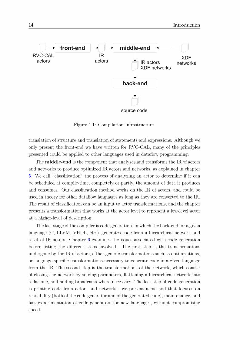
The subsequent chapters detail our compilation infrastructure for RVC-CAL
dataflow programs, shown on Fig. 1.1, which is in essence a three-stage compiler for
dataflow programs. The aim of this infrastructure is three-fold:
1. to allow the seamless compilation of dataflow programs into any language,
including a combination of hardware/software languages and the possibility of
generating multi-core-ready code.
2. to provide developers of RVC applications with a real Integrated Development
Environment (IDE), which is necessary for the success of RVC.
3. to facilitate research about dataflow by providing a stable architecture with a
clean API and integrated tools.
The originality of our approach is that we expose a simple, high-level Interme-
diate Representation (IR) that is specific to dataflow models, and is used for analysis,
transformation, and code generation. Chapter 3 begins by examining related work
and motivations for having an IR specific to dataflow programs. We then detail the
IR, how it is structured, and the semantics of the different instructions it contains.
The first stage of the compiler, called front-end, is responsible for creating
an IR of RVC-CAL actors, the resulting actors being called IR actors. Chapter 4
explains how the front-end creates the IR of an RVC-CAL actor through a series
of transformations including parsing, expression evaluation, typing, type checking,
14 Introduction
front-end middle-end
RVC-CAL
actors
IR
actorsXDF
networks
back-end
IR actors
XDF networks
source code
Figure 1.1: Compilation Infrastructure.
translation of structure and translation of statements and expressions. Although we
only present the front-end we have written for RVC-CAL, many of the principles
presented could be applied to other languages used in dataflow programming.
The middle-end is the component that analyzes and transforms the IR of actors
and networks to produce optimized IR actors and networks, as explained in chapter
5. We call “classification” the process of analyzing an actor to determine if it can
be scheduled at compile-time, completely or partly, the amount of data it produces
and consumes. Our classification method works on the IR of actors, and could be
used in theory for other dataflow languages as long as they are converted to the IR.
The result of classification can be an input to actor transformations, and the chapter
presents a transformation that works at the actor level to represent a low-level actor
at a higher-level of description.
The last stage of the compiler is code generation, in which the back-end for a given
language (C, LLVM, VHDL, etc.) generates code from a hierarchical network and
a set of IR actors. Chapter 6 examines the issues associated with code generation
before listing the different steps involved. The first step is the transformations
undergone by the IR of actors, either generic transformations such as optimizations,
or language-specific transformations necessary to generate code in a given language
from the IR. The second step is the transformations of the network, which consist
of closing the network by solving parameters, flattening a hierarchical network into
a flat one, and adding broadcasts where necessary. The last step of code generation
is printing code from actors and networks: we present a method that focuses on
readability (both of the code generator and of the generated code), maintenance, and
fast experimentation of code generators for new languages, without compromising
speed.
Outline 15
Chapter 7 begins with a presentation of support tools for RVC-CAL dataflow
programs, including a graphical editor called Graphiti and an implementation of the
infrastructure described in this document called Open RVC-CAL Compiler (Orcc).
The chapter then describes the video coding applications written with these tools.
Finally, we show results obtained with these applications concerning classification,
transformation, and dynamic scheduling on uniprocessors, multi-core processors,
and programmable hardware.
Finally, Chapter 8 concludes this thesis. The conclusion sums up the work pre-
sented in the document, identifies current limitations in our approach, and lists
perspectives for future work.

16 Introduction
Chapter 2
Background
The work presented in this thesis, a compilation infrastructure for dataflow pro-
grams, is mainly targeted at — although not restricted to — dataflow programs writ-
ten using the RVC-CAL language within the Reconfigurable Video Coding (RVC)
framework. RVC is the first standard to define a Domain-Specific Language (DSL)
with dataflow semantics and use it to describe video coding tools. This makes RVC
the perfect source of free, open-source, real-world dataflow programs. Consequently,
the results presented in Chapter 7 were obtained on normative RVC video decoders
and lower-level and higher-level non-normative video decoders written with RVC-
CAL. Additionally, many examples throughout this document reference actors that
are either defined by the RVC standard or are custom RVC-CAL implementations
of video coding tools.
This chapter aims to give the reader the necessary knowledge on the rationale
behind, and theoretical and practical aspects of, dataflow programming in general
and RVC dataflow programs in particular. This chapter naturally begins by a pre-
sentation of the Reconfigurable Video Coding standard in section 2.1, why it was
created and the advantages it has over existing approaches. We then define dataflow
programming in section 2.2 with the different models that define the behavior of
dataflow programs, and their associated properties such as existence of a bounded
schedule and compile-time scheduling. Section 2.3 provides an insight about the
RVC-CAL language, its model of computation, and support tools for the language.
This section also presents examples of the main constructs of RVC-CAL that are
useful to understand the examples shown later in this document. The last section of
this chapter gives an overview of the compilation steps that we use in our compilation
infrastructure.
17
18 Background
2.1 Reconfigurable Video Coding
2.1.1 Limitations of the Existing Standardization Process
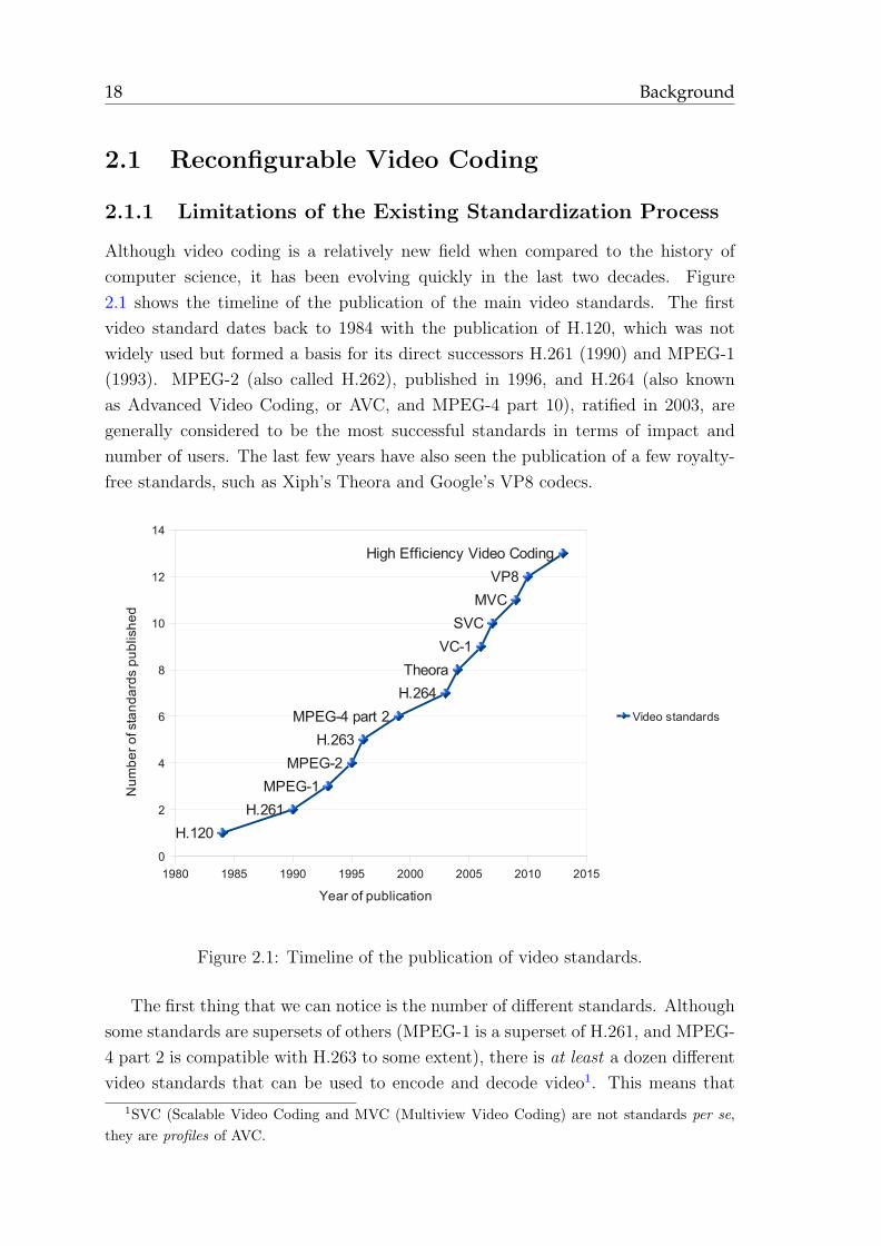
Although video coding is a relatively new field when compared to the history of
computer science, it has been evolving quickly in the last two decades. Figure
2.1 shows the timeline of the publication of the main video standards. The first
video standard dates back to 1984 with the publication of H.120, which was not
widely used but formed a basis for its direct successors H.261 (1990) and MPEG-1
(1993). MPEG-2 (also called H.262), published in 1996, and H.264 (also known
as Advanced Video Coding, or AVC, and MPEG-4 part 10), ratified in 2003, are
generally considered to be the most successful standards in terms of impact and
number of users. The last few years have also seen the publication of a few royalty-
free standards, such as Xiph’s Theora and Google’s VP8 codecs.
1980 1985 1990 1995 2000 2005 2010 2015
0
2
4
6
8
10
12
14
H.120
H.261
MPEG-1
MPEG-2
H.263
MPEG-4 part 2
H.264
Theora
VC-1
SVC
MVC
VP8
High Efficiency Video Coding
Video standards
Year of publication
Nu
mb
er
of sta
nd
ard
s p
ub
lish
ed
Figure 2.1: Timeline of the publication of video standards.
The first thing that we can notice is the number of different standards. Although
some standards are supersets of others (MPEG-1 is a superset of H.261, and MPEG-
4 part 2 is compatible with H.263 to some extent), there is at least a dozen different
video standards that can be used to encode and decode video1. This means that
1SVC (Scalable Video Coding and MVC (Multiview Video Coding) are not standards per se,
they are profiles of AVC.
Reconfigurable Video Coding 19
embedded systems such as set-top boxes, video players, and handheld devices cannot
provide low-consumption hardware acceleration for all these standards because it
would take too much time and space on the component to implement them. The
situation can only worsen for two reasons: (1) once published a standard is never
“deleted”, and (2) the number of standards increases in a quasi-linear manner.
Generally speaking, a video standard defines many algorithms, or coding tech-
niques. These techniques have different goals and requirements, e.g. some techniques
are more computationally expensive, others are oriented towards professional usage,
etc. Since a standard is implemented on many different devices with different use-
cases, it is often not interesting nor possible to implement all techniques in a given
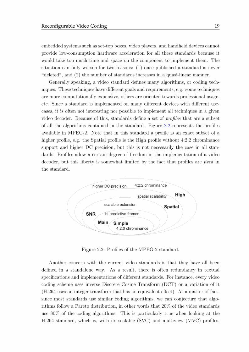
video decoder. Because of this, standards define a set of profiles that are a subset
of all the algorithms contained in the standard. Figure 2.2 represents the profiles
available in MPEG-2. Note that in this standard a profile is an exact subset of a
higher profile, e.g. the Spatial profile is the High profile without 4:2:2 chrominance
support and higher DC precision, but this is not necessarily the case in all stan-
dards. Profiles allow a certain degree of freedom in the implementation of a video
decoder, but this liberty is somewhat limited by the fact that profiles are fixed in
the standard.
bi-predictive frames
scalable extension
4:2:2 chrominance
Simple4:2:0 chrominance
High
Main
SNR
spatial scalability
Spatial
higher DC precision
Figure 2.2: Profiles of the MPEG-2 standard.
Another concern with the current video standards is that they have all been
defined in a standalone way. As a result, there is often redundancy in textual
specifications and implementations of different standards. For instance, every video
coding scheme uses inverse Discrete Cosine Transform (DCT) or a variation of it
(H.264 uses an integer transform that has an equivalent effect). As a matter of fact,
since most standards use similar coding algorithms, we can conjecture that algo-
rithms follow a Pareto distribution, in other words that 20% of the video standards
use 80% of the coding algorithms. This is particularly true when looking at the
H.264 standard, which is, with its scalable (SVC) and multiview (MVC) profiles,
20 Background
the most complex standard ever published.
Finally, since MPEG-2, organizations have been providing reference software
accompanying the textual reference of standards. The problem of existing reference
software is that they are monolithic descriptions of the standards implemented in
C/C++ most of the time. This has the unfortunate effect that it is almost impossible
to derive a hardware implementation from these.
2.1.2 Definition of Video Standards with RVC
The Reconfigurable Video Coding (RVC) [ISO09, MAR10] standard aims to ad-
dress all the issues listed above. First of all, RVC defines a set of standard coding
techniques called Functional Units (FUs). This removes the redundancy between
standards by representing an algorithm that is common to several standards as a
single FU. FUs form the basis of existing and future video standards, and are stan-
dardized as the Video Tool Library (VTL). A FU is described with a portable,
platform-independent language called RVC-CAL, defined in section 2.3.
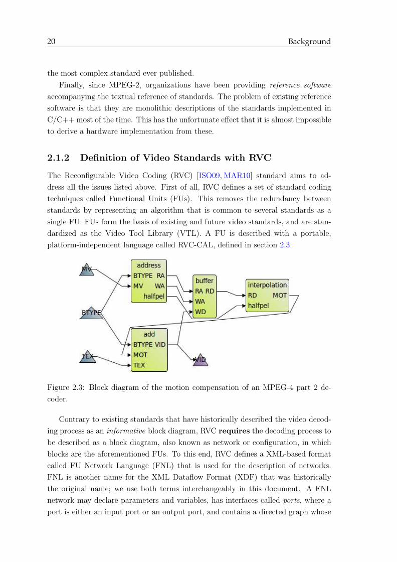
Figure 2.3: Block diagram of the motion compensation of an MPEG-4 part 2 de-
coder.
Contrary to existing standards that have historically described the video decod-
ing process as an informative block diagram, RVC requires the decoding process to
be described as a block diagram, also known as network or configuration, in which
blocks are the aforementioned FUs. To this end, RVC defines a XML-based format
called FU Network Language (FNL) that is used for the description of networks.
FNL is another name for the XML Dataflow Format (XDF) that was historically
the original name; we use both terms interchangeably in this document. A FNL
network may declare parameters and variables, has interfaces called ports, where a
port is either an input port or an output port, and contains a directed graph whose
Dataflow Models of Computation 21
vertices may be instances of FUs from the VTL or ports. At the time of this writing,
RVC has defined the FUs and FNL networks for MPEG-4 part 2 and MPEG-4 part
10 Constrained Baseline Profile.
Figure 2.3 shows an example of the FNL network that represents motion compen-
sation in the normative RVC description of an MPEG-4 part 2 decoder. A triangle
represents either an input port (MV, BTYPE, TEX) or an output port (VID).
Ports allow block diagrams to be composed in a hierarchical way. The rectangles
are instances, for example “buffer” refers to Mgnt Framebuf, a FU that manages a
buffer of frames, and “interpolation” refers to Algo Interpolation halfpel, which
performs half-pixel interpolation. Edges carry data between a source port of the
diagram or of an instance to a target port of the diagram or of another instance.
Describing a video decoder as a network of FUs rather than a monolithic C or
C++ program has several advantages. First of all, it is no longer necessary to define
profiles, rather a decoder may use any arbitrary meaningful combination of FUs.
Additionally, this allows a video decoder to be reconfigured at runtime by changing
the structure of the network that defines the decoding process. This is especially
interesting for hardware and memory-constrained devices. Finally, this makes RVC
more “hardware-friendly” because dataflow is a natural way of describing hardware
architectures.
2.2 Dataflow Models of Computation
2.2.1 Overview
A dataflow Model of Computation (MoC) defines the behavior of a program de-
scribed as a dataflow graph. A dataflow graph is a directed graph whose vertices are
actors and edges are unidirectional FIFO channels with unbounded capacity, con-
nected between ports of actors. The networks of FUs described by the RVC standard
are dataflow graphs. Dataflow graphs respect the semantics of Dataflow Process Net-
works (DPNs) [LP95], which are related to Kahn Process Networks (KPNs) [Kah74]
in the following ways:
• Those models contain blocks (processes in a KPN, actors in a DPN) that com-
municate with each other through unidirectional, unlimited FIFO channels.
• Writing to a FIFO is non-blocking, i.e. a write returns immediately.
• Programs that respect one model or the other must be scheduled dynamically
in the general case [LP95,Par95,HSH+09].
22 Background
The main difference between the two models is that DPNs adds non-determinism
to the KPN model, without requiring the actor to be non-determinate, by allowing
actors to test an input port for the absence or presence of data [LP95]. Indeed, in a
KPN process, reading from a FIFO is blocking : if a process attempts to read data
from a FIFO and no data is available, it must wait. Conversely, a DPN actor will only
read data from a FIFO if enough data is available, and a read returns immediately.
As a consequence, an actor need not be suspended when it cannot read, which in
turn means that scheduling a DPN does not require context-switching nor concurrent
processes. We show an example of a non-determinate merge that can be described
as a DPN actor written in RVC-CAL in section 2.3.2.
SDF
CSDF
PSDF
DPN
expressiveness analyzability
-
+-
+
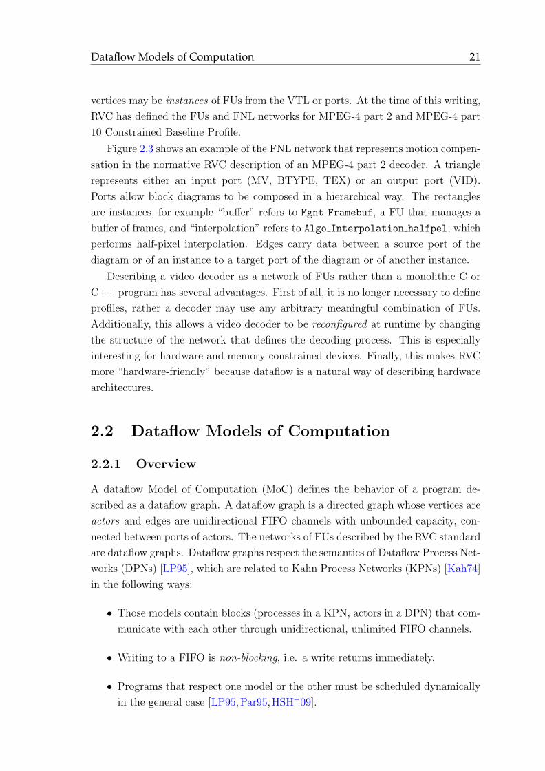
Figure 2.4: Dataflow Models of Computation.
This section presents a taxonomy of Models of Computation (MoCs) (Fig. 2.4)
that can model the different types of behavior that a DPN can exhibit. Figure
2.4 reflects the fact that MoCs are progressively restricted from the most general
DPN model towards the most restricted Synchronous Dataflow (SDF) model [LM87]
with respect to expressiveness, but at the same time they become more amenable to
analysis. The literature defines many different MoCs, and we voluntarily present a
small subset of MoCs that is sufficient to model the different types of behavior that
can be modeled with RVC-CAL as shown in section 2.3. We first study the rules of
DPN, and then present the models that can be used to model static, cyclo-static,
quasi-static, and dynamic actors.
2.2.2 Dataflow Process Networks
We define here the formal notations for Dataflow Process Networks (DPNs)2. Each
FIFO channel in a DPN carries a sequence of tokens X = [x1, x2, ...], where each
xi is called a token. The sequence of unconsumed (or available) tokens on the pth
input port is Xp. An empty FIFO corresponds to the empty sequence, noted ⊥. If
2The notations used below are based on the notations that Lee uses in [LP95].
Dataflow Models of Computation 23
a sequence X precedes a sequence Y , for instance X = [x1, x2] and Y = [x1, x2, x3],
we can write X ⊑ Y .
The set of all possible sequences is noted S, and Sp is the set of p-tuples of
sequences, in other words [X1, X2, ..., Xp] ∈ Sp. Examples of elements of S2 are
s1 = [[x1, x2, x3],⊥], s2 = [[x1], [x2]]. The length of a sequence is given by |X|,
similarly the length of an element s ∈ Sp is in turn noted as |s| = [|X1|, |X2|, ..., |Xp|].
For instance, |s1| = [3, 0] and |s2| = [1, 1].
Executing a DPN boils down to executing repeatedly the actors in the graph,
possibly ad infinitum. An actor executes (or fires) when at least one of its firing
rules is satisfied. Each firing consumes and produces tokens. An actor can have N
firing rules:
R = [R1,R2, ...,RN ] (2.1)
A firing rule Ri is a finite sequence of patterns, one for each of the p input ports of
the actor:
Ri = [Pi,1, Pi,2, ..., Pi,p] ∈ Sp (2.2)
A pattern Pi,j defines an acceptable sequence of tokens: It is satisfied iff Pi,j ⊑ Xj,
the sequence of unconsumed (or available) tokens on the pth input port. If Pi,j = ⊥,
the pattern is satisfied for any sequence, which is different from Pi,j = [∗] that
defines a pattern satisfied for any sequence containing at least one token. When an
actor fires it applies a firing function f that consumes sequences of tokens on p input
ports and produces sequences of tokens on q output ports, and is defined as:
f : Sp → Sq (2.3)
2.2.3 Synchronous Dataflow
Synchronous Dataflow (SDF) [LM87] is the least expressive DPN model, but it
is also the model that can be analyzed more easily. Schedulability and memory
consumption of SDF graphs can be determined at compile-time, and algorithms
exist that can map and schedule SDF graphs onto multi-processors in linear time
with respect to the number of vertices and processors [PPW+09]. Any two firing
rules Ra and Rb of an SDF actor must consume the same amount of tokens:
|Ra| = |Rb| (2.4)
All firings must produce the same amount of tokens on the output ports:
∀sa ∈ Sp, ∀sb ∈ Sp, |f(sa)| = |f(sb)| (2.5)
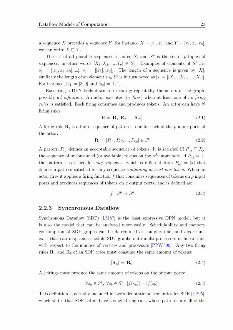
This definition is actually included in Lee’s denotational semantics for SDF [LP95],
which states that SDF actors have a single firing rule, whose patterns are all of the
24 Background
form [∗, ∗, ..., ∗], although our definition explicitly allows SDF actors to have several
firing rules as long as they have the same production/consumption rate. In practice,
this makes it easier to describe SDF actors that have data-dependent computations.
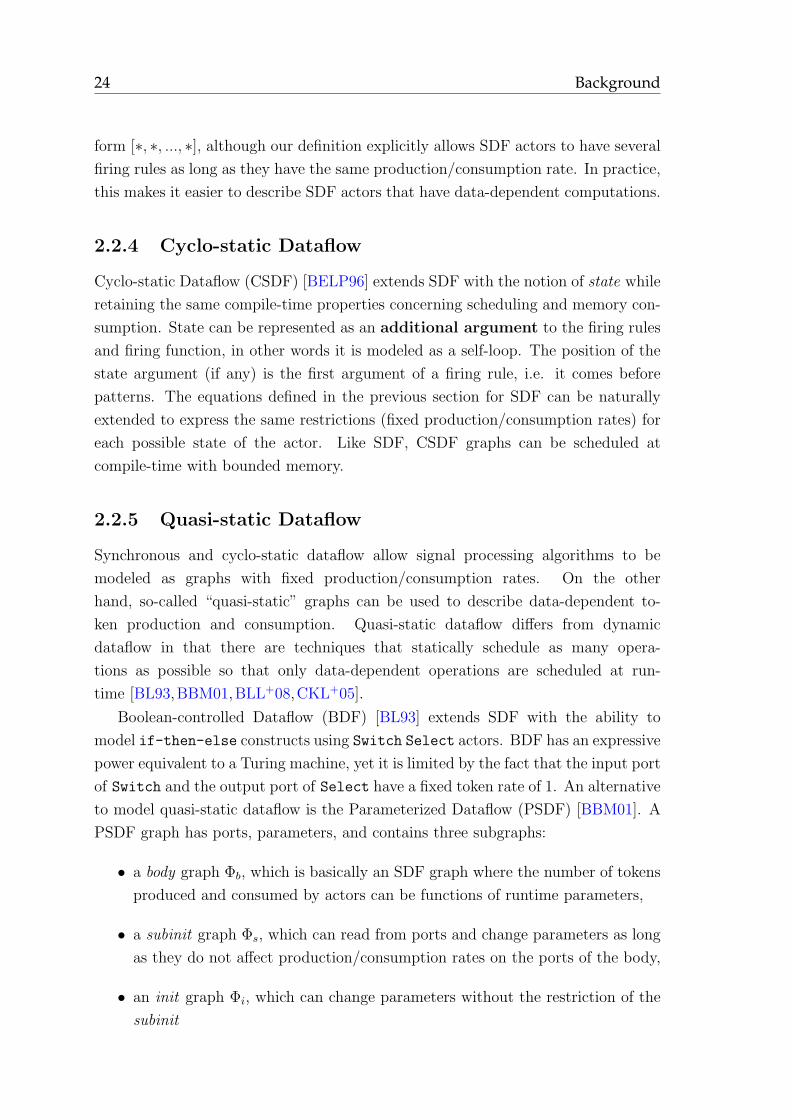
2.2.4 Cyclo-static Dataflow
Cyclo-static Dataflow (CSDF) [BELP96] extends SDF with the notion of state while
retaining the same compile-time properties concerning scheduling and memory con-
sumption. State can be represented as an additional argument to the firing rules
and firing function, in other words it is modeled as a self-loop. The position of the
state argument (if any) is the first argument of a firing rule, i.e. it comes before
patterns. The equations defined in the previous section for SDF can be naturally
extended to express the same restrictions (fixed production/consumption rates) for
each possible state of the actor. Like SDF, CSDF graphs can be scheduled at
compile-time with bounded memory.
2.2.5 Quasi-static Dataflow
Synchronous and cyclo-static dataflow allow signal processing algorithms to be
modeled as graphs with fixed production/consumption rates. On the other
hand, so-called “quasi-static” graphs can be used to describe data-dependent to-
ken production and consumption. Quasi-static dataflow differs from dynamic
dataflow in that there are techniques that statically schedule as many opera-
tions as possible so that only data-dependent operations are scheduled at run-
time [BL93,BBM01,BLL+08,CKL+05].
Boolean-controlled Dataflow (BDF) [BL93] extends SDF with the ability to
model if-then-else constructs using Switch Select actors. BDF has an expressive
power equivalent to a Turing machine, yet it is limited by the fact that the input port
of Switch and the output port of Select have a fixed token rate of 1. An alternative
to model quasi-static dataflow is the Parameterized Dataflow (PSDF) [BBM01]. A
PSDF graph has ports, parameters, and contains three subgraphs:
• a body graph Φb, which is basically an SDF graph where the number of tokens
produced and consumed by actors can be functions of runtime parameters,
• a subinit graph Φs, which can read from ports and change parameters as long
as they do not affect production/consumption rates on the ports of the body,
• an init graph Φi, which can change parameters without the restriction of the
subinit
RVC-CAL Programming 25
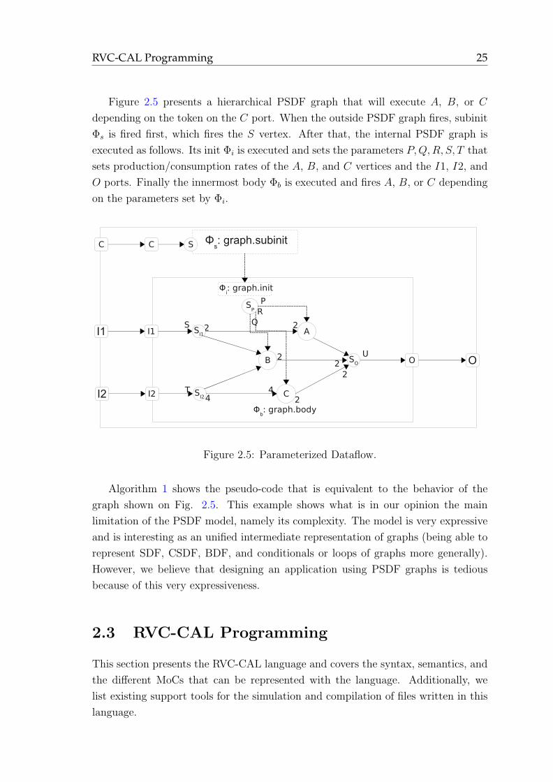
Figure 2.5 presents a hierarchical PSDF graph that will execute A, B, or C
depending on the token on the C port. When the outside PSDF graph fires, subinit
Φs is fired first, which fires the S vertex. After that, the internal PSDF graph is
executed as follows. Its init Φi is executed and sets the parameters P,Q,R, S, T that
sets production/consumption rates of the A, B, and C vertices and the I1, I2, and
O ports. Finally the innermost body Φb is executed and fires A, B, or C depending
on the parameters set by Φi.
Φi: graph.init
Φb: graph.body
A
B
Φs: graph.subinitC
I1
I2 C
I1
I2
SC
OO2
2
44
2
2
2
2
SP
P
R
QS
I1
SI2
SO
S
T
U
Figure 2.5: Parameterized Dataflow.
Algorithm 1 shows the pseudo-code that is equivalent to the behavior of the
graph shown on Fig. 2.5. This example shows what is in our opinion the main
limitation of the PSDF model, namely its complexity. The model is very expressive
and is interesting as an unified intermediate representation of graphs (being able to
represent SDF, CSDF, BDF, and conditionals or loops of graphs more generally).
However, we believe that designing an application using PSDF graphs is tedious
because of this very expressiveness.
2.3 RVC-CAL Programming
This section presents the RVC-CAL language and covers the syntax, semantics, and
the different MoCs that can be represented with the language. Additionally, we
list existing support tools for the simulation and compilation of files written in this
language.
26 Background
Algorithm 1: Pseudo-code equivalent to the PSDF graph of Fig. 2.5.
let c be the result of Φs(C);
if c = 1 thenread 2 tokens on I1;
fire A;
write 1 token to O;
else if c = 2 thenread 1 token on I1 and 1 token on I2;
fire B;
write 2 tokens to O;
else if c = 3 thenread 4 tokens on I2;
fire C;
write 2 tokens to O;
2.3.1 RVC-CAL Language
RVC-CAL is a Domain-Specific Language (DSL) that has been standardized by RVC
as a restricted version of CAL (Cal Actor Language). CAL was invented by Eker
and Janneck and is described in their technical report [EJ03].
Actor Structure
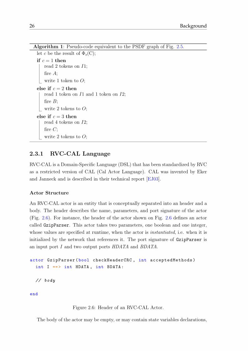
An RVC-CAL actor is an entity that is conceptually separated into an header and a
body. The header describes the name, parameters, and port signature of the actor
(Fig. 2.6). For instance, the header of the actor shown on Fig. 2.6 defines an actor
called GzipParser. This actor takes two parameters, one boolean and one integer,
whose values are specified at runtime, when the actor is instantiated, i.e. when it is
initialized by the network that references it. The port signature of GzipParser is
an input port I and two output ports HDATA and BDATA.
actor GzipParser(bool checkHeaderCRC , int acceptedMethods)
int I ==> int HDATA , int BDATA:
// body
end
Figure 2.6: Header of an RVC-CAL Actor.
The body of the actor may be empty, or may contain state variables declarations,
RVC-CAL Programming 27
functions, procedures, actions, priorities, and at most one Finite State Machine.
Type System
RVC-CAL, like hardware description languages, has integers with an arbitrary bit
width. Integers can be signed (declared with the int keyword) or unsigned (declared
with uint keyword). The bit width may be omitted, in which case the type has
a default bit width, or it can be specified by an arbitrary expression. The RVC
standard does not specify the default bit width, nor does it restrict the expression
that defines the bit width. We proposed in [RWJ09] that the bit width should
evaluate to a compile-time constant, and as such it should not depend on parameters.
The reason behind this is that the values of parameters are specified at runtime,
which is hardly compatible with static typing.
The other types supported by RVC-CAL are booleans (bool), floating-point real
numbers (float), strings (String) and lists (List). The list type behaves more like
an array type, in other words it has a fixed type and a fixed size. Floating-point
and string types are not used at the moment by FUs in the VTL.
Expressions
RVC-CAL has side-effect free expressions, i.e. an expression cannot modify vari-
ables or write to memory, as opposed to imperative languages such as C where an
expression can increment a pointer or call a procedure that changes a state variable.
The language of expressions includes references to variables (possibly with indexes
when referring to a list), binary and unary operations, as well as calls to side-effect
free functions (see below section 2.3.1). Expressions also borrow constructions from
functional languages, like if/then/else conditional expressions, and list generators.
A list generator is similar to the map function found in many functional program-
ming languages, and is a kind of inline for loop that creates a list whose members
are described by an expression. RVC-CAL currently does not define an operator
similar to the reduce or fold function, although it could be useful to add it to the
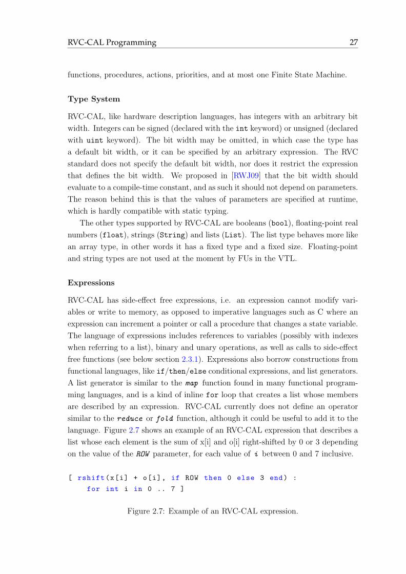
language. Figure 2.7 shows an example of an RVC-CAL expression that describes a
list whose each element is the sum of x[i] and o[i] right-shifted by 0 or 3 depending
on the value of the ROW parameter, for each value of i between 0 and 7 inclusive.
[ rshift(x[i] + o[i], if ROW then 0 else 3 end) :
for int i in 0 .. 7 ]
Figure 2.7: Example of an RVC-CAL expression.
28 Background
State Variables
State variables can be used to define constants and to store the state of the actor
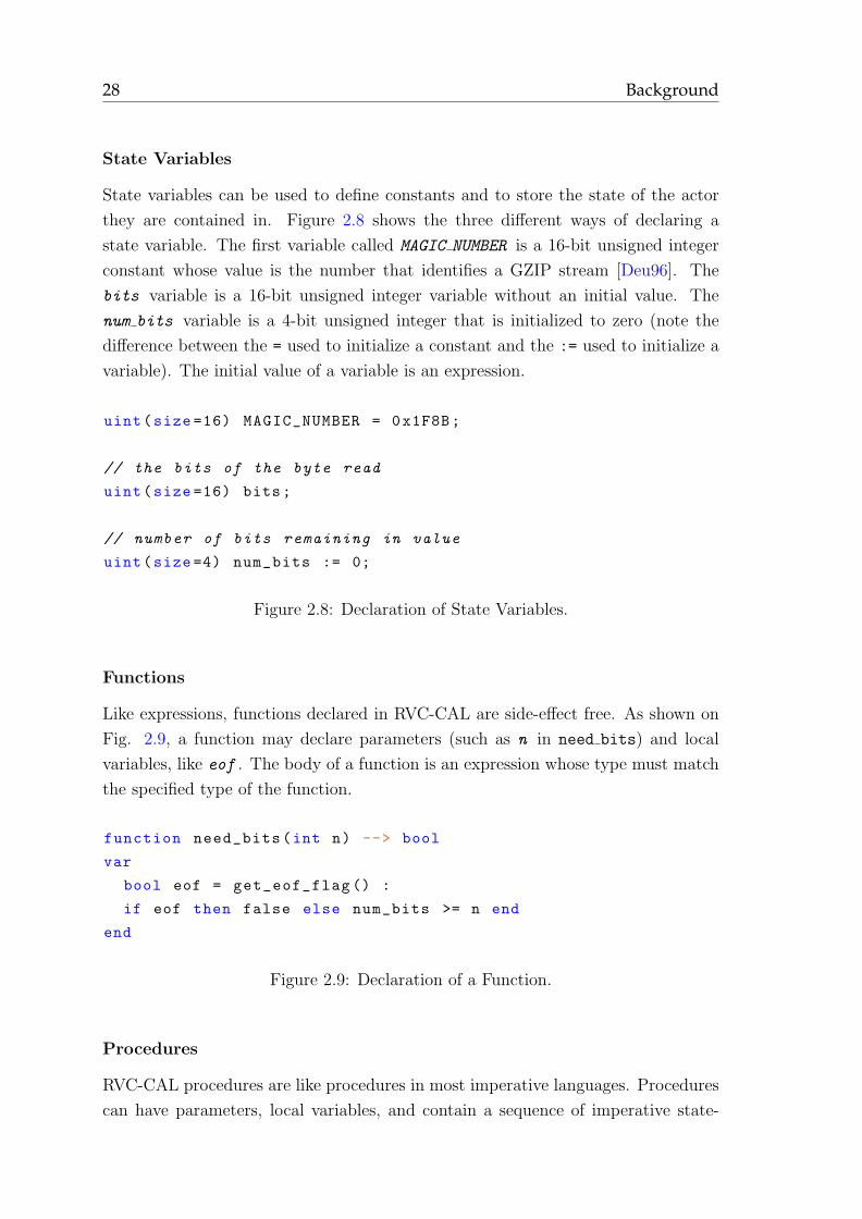
they are contained in. Figure 2.8 shows the three different ways of declaring a
state variable. The first variable called MAGIC NUMBER is a 16-bit unsigned integer
constant whose value is the number that identifies a GZIP stream [Deu96]. The
bits variable is a 16-bit unsigned integer variable without an initial value. The
num bits variable is a 4-bit unsigned integer that is initialized to zero (note the
difference between the = used to initialize a constant and the := used to initialize a
variable). The initial value of a variable is an expression.
uint(size =16) MAGIC_NUMBER = 0x1F8B;
// the bits of the byte read
uint(size =16) bits;
// number of bits remaining in value
uint(size =4) num_bits := 0;
Figure 2.8: Declaration of State Variables.
Functions
Like expressions, functions declared in RVC-CAL are side-effect free. As shown on
Fig. 2.9, a function may declare parameters (such as n in need bits) and local
variables, like eof . The body of a function is an expression whose type must match
the specified type of the function.
function need_bits(int n) --> bool
var
bool eof = get_eof_flag () :
if eof then false else num_bits >= n end
end
Figure 2.9: Declaration of a Function.
Procedures
RVC-CAL procedures are like procedures in most imperative languages. Procedures
can have parameters, local variables, and contain a sequence of imperative state-
RVC-CAL Programming 29
ments that have side-effects. RVC-CAL defines five kinds of statements:
1. assignment of an expression to a local variable or a state variable, possibly
with indexes when the target is a list.
2. call to a procedure or a function; the result of a function call can be assigned
to a local variable or a state variable.
3. execution of statements a finite number of times with a foreach loop that
resembles the generator expression, except its body is a sequence of statements:
it defines an index variable and executes the statements it contains for each
value of the index within defined bounds.
4. conditional execution of statements with an if/then/else construct.
5. execution of statements an unknown number of times with a while loop.
Actions
The only entry points of an actor are its actions; functions and procedures can only
be called by an action. An action may read tokens from input ports, compute data,
and write tokens to output ports. The patterns of tokens read and written by a
single action are called input pattern and output pattern respectively. Apart from
these specific features, the body of an action is like a procedure in most imperative
programming languages, with local variables and imperative statements. Examples
of actions are given below in section 2.3.2.
An action may be identified by a tag, which is a list of identifiers separated by
colons, where ta denotes the tag of action a. |ta| is the length of ta, with the empty
tag ǫ having a null length: |ǫ| = 0. The set of non-empty tags of an actor is denoted
T . There is a prefix relation, noted ⊑, between tags: t ⊑ t′ means that t is a prefix
of t′. For instance with tags a and a.x, we have a ⊑ a.x and a ⊑ a. A set of actions
that start with the same tag as an action a is described as follows:
ta = {ax ∈ A| ta ⊑ tax} (2.6)
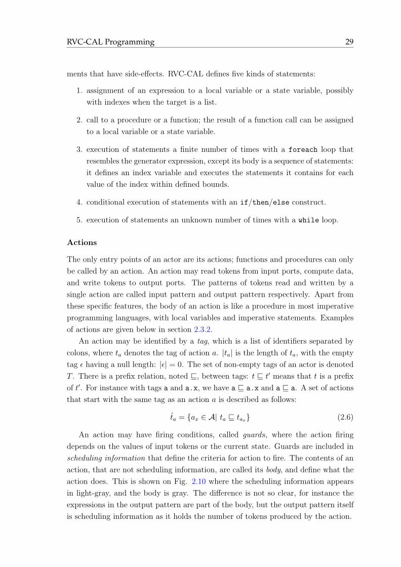
An action may have firing conditions, called guards, where the action firing
depends on the values of input tokens or the current state. Guards are included in
scheduling information that define the criteria for action to fire. The contents of an
action, that are not scheduling information, are called its body, and define what the
action does. This is shown on Fig. 2.10 where the scheduling information appears
in light-gray, and the body is gray. The difference is not so clear, for instance the
expressions in the output pattern are part of the body, but the output pattern itself
is scheduling information as it holds the number of tokens produced by the action.
30 Background
read . immediate : action RUN :[ r ], VALUE :[ v ], LAST :[ l ] ==> OUT :[ v ]guard r = 0, count != BLOCK_SIZEdo last := l; count := count + 1;end
Scheduling information
Body
Figure 2.10: Scheduling information and body of an action.
When an actor fires, an action has to be selected based on the number and values
of tokens available and whether its guards are true. Action selection may be further
constrained using a Finite State Machine (FSM), to select actions according to the
current state, and priority inequalities, to impose a partial order among action tags.
Section 2.3.2 gives complete examples including FSM and priorities.
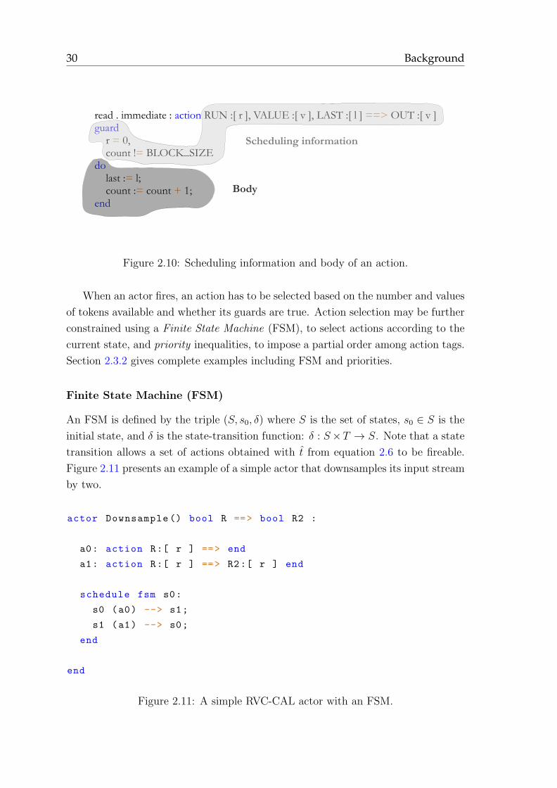
Finite State Machine (FSM)
An FSM is defined by the triple (S, s0, δ) where S is the set of states, s0 ∈ S is the
initial state, and δ is the state-transition function: δ : S×T → S. Note that a state
transition allows a set of actions obtained with t from equation 2.6 to be fireable.
Figure 2.11 presents an example of a simple actor that downsamples its input stream
by two.
actor Downsample () bool R ==> bool R2 :
a0: action R:[ r ] ==> end
a1: action R:[ r ] ==> R2:[ r ] end
schedule fsm s0:
s0 (a0) --> s1;
s1 (a1) --> s0;
end
end
Figure 2.11: A simple RVC-CAL actor with an FSM.
RVC-CAL Programming 31
Priorities
Priorities establish a partial order between action tags. They have the form t1 >
t2 > ... > tn. These inequalities induce a binary relation on actions as follows:
a1 > a2 ⇔ ∃ t1, t2 : t1 > t2 ∧ a1 ∈ t1 ∧ a2 ∈ t2
∨ ∃ a3 : a1 > a3 ∧ a3 > a2(2.7)
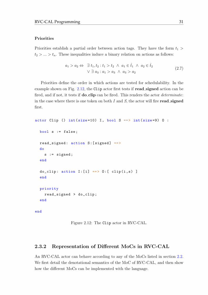
Priorities define the order in which actions are tested for schedulability. In the
example shown on Fig. 2.12, the Clip actor first tests if read signed action can be
fired, and if not, it tests if do clip can be fired. This renders the actor determinate:
in the case where there is one token on both I and S, the actor will fire read signed
first.
actor Clip () int(size =10) I, bool S ==> int(size =9) O :
bool s := false;
read_signed: action S:[ signed] ==>
do
s := signed;
end
do_clip: action I:[i] ==> O:[ clip(i,s) ]
end
priority
read_signed > do_clip;
end
end
Figure 2.12: The Clip actor in RVC-CAL.
2.3.2 Representation of Different MoCs in RVC-CAL
An RVC-CAL actor can behave according to any of the MoCs listed in section 2.2.
We first detail the denotational semantics of the MoC of RVC-CAL, and then show
how the different MoCs can be implemented with the language.
32 Background
Dynamic MoC
RVC-CAL places no restrictions whatsoever about the firing rules nor firing function
of an actor. An RVC-CAL actor can thus have a behavior that is data-independent
and state-independent (SDF), cyclo-static state-dependent (CSDF), quasi-static
data-dependent (PSDF), or data-dependent and state-dependent (dynamic). A dy-
namic actor can be further categorized as time-independent or time-dependent. A
time-independent actor, also known as monotonic or determinate, will produce the
same results regardless of the time at which tokens are present on input ports; it
also means the actor can be represented as a Kahn process using blocking reads.
Conversely, a time-dependent actor does not necessarily produce the same results
depending on the time at which tokens arrive. The Clip actor presented in Fig.
2.12 of section 2.3.1 is an example of a time-dependent actor.
A time-dependent actor is not necessarily non-determinate (Clip is determinate
for example), but it cannot be implemented using the KPN model regardless. If we
use a Kahn process with blocking reads to implement the Clip actor, the behavior
of the actor becomes (1) read data from S (2) read data from I, write data to O,
etc. If the actor is used in a network where no data is ever available on S (in other
words the s flag is never set, which is possible), the network deadlocks. If less data
is available on S than on I 3, the actor quickly deadlocks if using FIFOs of finite
capacity, and if using unbounded FIFOs the actor produces wrong results.
The RVC-CAL language extends the DPN MoC by adding a notion of guard
to firing rules. Formally the guards of a firing rule are boolean predicates that may
depend on the input patterns, the actor state, or both, and must be true for a
firing rule to be satisfied. We define the guards of a firing rule with predicates that
return a set of valid sequences. Predicates are associated to the patterns of the rule
so that Gi,j is the guard predicate associated to the jth pattern of Ri. The firing
rule of the read signed action can then be written as follows:
G1,1 : {[n, ∗] | n < 0} (2.8)
R1 = [X ∈ G1,1, [∗],⊥] (2.9)
An actor is executed (or fired) by selecting a fireable action and firing it. An
action is fireable iff: (1) the current FSM state allows the action to fire (or there
is no FSM and this condition is always true), (2) there are enough tokens for the
action to fire, (3) the guards of the action evaluate to true .
3A variant of this actor is actually in the RVC VTL, and one token is available on S every 64
tokens consumed on I.
RVC-CAL Programming 33
Modeling of the Static MoC
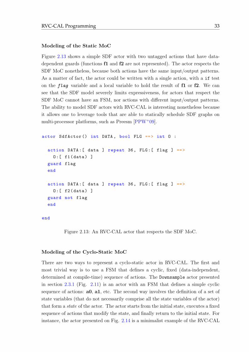
Figure 2.13 shows a simple SDF actor with two untagged actions that have data-
dependent guards (functions f1 and f2 are not represented). The actor respects the
SDF MoC nonetheless, because both actions have the same input/output patterns.
As a matter of fact, the actor could be written with a single action, with a if test
on the flag variable and a local variable to hold the result of f1 or f2. We can
see that the SDF model severely limits expressiveness, for actors that respect the
SDF MoC cannot have an FSM, nor actions with different input/output patterns.
The ability to model SDF actors with RVC-CAL is interesting nonetheless because
it allows one to leverage tools that are able to statically schedule SDF graphs on
multi-processor platforms, such as Preesm [PPW+09].
actor SdfActor () int DATA , bool FLG ==> int O :
action DATA:[ data ] repeat 36, FLG:[ flag ] ==>
O:[ f1(data) ]
guard flag
end
action DATA:[ data ] repeat 36, FLG:[ flag ] ==>
O:[ f2(data) ]
guard not flag
end
end
Figure 2.13: An RVC-CAL actor that respects the SDF MoC.
Modeling of the Cyclo-Static MoC
There are two ways to represent a cyclo-static actor in RVC-CAL. The first and
most trivial way is to use a FSM that defines a cyclic, fixed (data-independent,
determined at compile-time) sequence of actions. The Downsample actor presented
in section 2.3.1 (Fig. 2.11) is an actor with an FSM that defines a simple cyclic
sequence of actions: a0, a1, etc. The second way involves the definition of a set of
state variables (that do not necessarily comprise all the state variables of the actor)
that form a state of the actor. The actor starts from the initial state, executes a fixed
sequence of actions that modify the state, and finally return to the initial state. For
instance, the actor presented on Fig. 2.14 is a minimalist example of the RVC-CAL
34 Background
representation of a CSDF actor using this method.
The first method is more restrictive because expressing an actor with a fixed
sequence of n actions using solely an FSM means the FSM needs to have n transi-
tions. Adding more iterations requires altering the structure of the FSM. In practice,
the second method is very useful to model loops so that they can be translated to
hardware, and it can be found in several actors in the RVC VTL that were origi-
nally written by Dave Parlour from Xilinx, a manufacturer of programmable logic
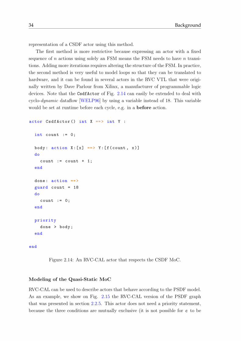
devices. Note that the CsdfActor of Fig. 2.14 can easily be extended to deal with
cyclo-dynamic dataflow [WELP96] by using a variable instead of 18. This variable
would be set at runtime before each cycle, e.g. in a before action.
actor CsdfActor () int X ==> int Y :
int count := 0;
body: action X:[x] ==> Y:[f(count , x)]
do
count := count + 1;
end
done: action ==>
guard count = 18
do
count := 0;
end
priority
done > body;
end
end
Figure 2.14: An RVC-CAL actor that respects the CSDF MoC.
Modeling of the Quasi-Static MoC
RVC-CAL can be used to describe actors that behave according to the PSDF model.
As an example, we show on Fig. 2.15 the RVC-CAL version of the PSDF graph
that was presented in section 2.2.5. This actor does not need a priority statement,
because the three conditions are mutually exclusive (it is not possible for c to be
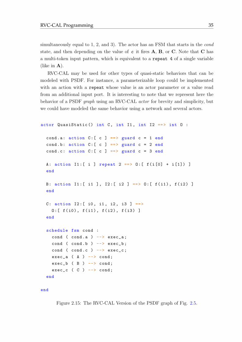
RVC-CAL Programming 35
simultaneously equal to 1, 2, and 3). The actor has an FSM that starts in the cond
state, and then depending on the value of c it fires A, B, or C. Note that C has
a multi-token input pattern, which is equivalent to a repeat 4 of a single variable
(like in A).
RVC-CAL may be used for other types of quasi-static behaviors that can be
modeled with PSDF. For instance, a parameterizable loop could be implemented
with an action with a repeat whose value is an actor parameter or a value read
from an additional input port. It is interesting to note that we represent here the
behavior of a PSDF graph using an RVC-CAL actor for brevity and simplicity, but
we could have modeled the same behavior using a network and several actors.
actor QuasiStatic () int C, int I1, int I2 ==> int O :
cond.a: action C:[ c ] ==> guard c = 1 end
cond.b: action C:[ c ] ==> guard c = 2 end
cond.c: action C:[ c ] ==> guard c = 3 end
A: action I1:[ i ] repeat 2 ==> O:[ f(i[0] + i[1]) ]
end
B: action I1:[ i1 ], I2:[ i2 ] ==> O:[ f(i1), f(i2) ]
end
C: action I2:[ i0, i1, i2, i3 ] ==>
O:[ f(i0), f(i1), f(i2), f(i3) ]
end
schedule fsm cond :
cond ( cond.a ) --> exec_a;
cond ( cond.b ) --> exec_b;
cond ( cond.c ) --> exec_c;
exec_a ( A ) --> cond;
exec_b ( B ) --> cond;
exec_c ( C ) --> cond;
end
end
Figure 2.15: The RVC-CAL Version of the PSDF graph of Fig. 2.5.
36 Background
2.3.3 Support tools
The Open Dataflow environment, or OpenDF4, is a simulator and code generator for
the CAL language [BBJ+08]. Historically, the codebase of the OpenDF simulator
originated from the simulator present in Ptolemy [EJL+03] and later in Moses [ETH].
The simulator supports all the features of CAL, including lambda functions, dynamic
typing, and object-oriented programming with calls to Java classes. The latter is
possible because the simulator is itself running in Java, so it defers calls to Java
classes to the JVM using reflection. Discrete Event simulation [ZPK00] is used by
the simulator to schedule networks.
The OpenDF code generator transforms a hierarchical network and a set of
parameterizable actors into a flattened network and closed actors in a low-level
Intermediate Representation called XLIM. This representation can then be trans-
lated to Verilog by a tool called OpenForge, or to C by another tool unsurprisingly
called Xlim2C. Xlim2C5 is a compiler developed by Ericsson as part of the Actors
project. OpenForge6 is a behavioral hardware synthesizer developed by Xilinx. Un-
til OpenForge was open-sourced on SourceForge, it did not have an official name,
and therefore it is often referred to as “Cal2HDL” in various articles referenced by
this document.
2.4 Compilation Process
This section describes key concepts of compilation, and in particular the concepts
that are necessary to understand our work. Compilation is the process by which a
program in a source language is transformed to another semantically-equivalent pro-
gram in a target language. The source program is generally written by a programmer
in a high-level language, while the target language is often assembly language or ob-
ject code, but this is by no means a sine qua non condition, and there are compilers
for the lowest-level languages (like “brainfuck” [Mu93]) and compilers that generate
C code or byte code rather than assembly or object code. Note that we differentiate
compilation from source-to-source transformation in which tools parse, transform,
and re-generate a program in a given language according to a set of transformation
rules, like TXL [CHHP91].
A modern full-fledged optimizing compiler compiles a language to another lan-
guage following these steps:
4OpenDF is available at http://opendf.sf.net/.5Xlim2C is available in the contrib folder of the OpenDF repository.6OpenForge is available at http://openforge.sf.net/.
Compilation Process 37
1. parsing the program in the source language, checking it is syntactically and
semantically correct (including type checking),
2. transforming the program to an Intermediate Representation (IR) that makes
analysis and optimizations easier,
3. analyzing and optimizing the IR of the program,
4. transforming the IR to an abstract representation of the target language,
5. optimizing the abstract representation using target-specific rules,
6. printing the abstract representation to the target language.
This section presents the first three items of the above list, because the other items
involve details and techniques that we do not need to consider. For more insight,
the reader might refer to the reference book on compilation, the so-called “Dragon
Book” [ASU86].
2.4.1 Parsing and Validation
The first step of any compiler is to obtain an abstract representation of the source
program it is given. A source program is expected to respect the syntax of the
programming language in which it is written. This syntax is defined by a context-free
grammar, from which a lexer and a parser can be automatically generated. A lexer
transforms the source program into a sequence of meaningful tokens, or lexemes,
like identifiers, parentheses, operators, etc. The parser is then able to interpret
the resultant sequence of lexemes as meaningful language constructs that form the
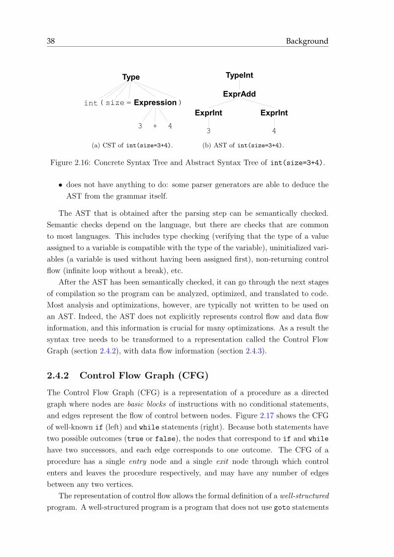
Concrete Syntax Tree (CST) (Fig. 2.16(a)), and informs the user of any errors he
or she might have made. There are lexer/parser generators for several classes of
context-free grammars, e.g. LALR(1) [GH98,Joh76], LL(k) [Kod04], LL(*) [PQ95].
It is also possible to write hand-made lexers and parsers, although it is not probably
worth the effort for complex languages.
The abstract representation that is best suited for manipulation of the source
program is the Abstract Syntax Tree (AST) (Fig. 2.16(b)). Indeed the CST contains
too much information such as grammar rule invocations and separators (commas,
semi-colons, etc.). Depending on the parser generator, the programmer:
• has to write code that creates a part of the AST for each parsing rule; that
code is executed each time the parser enters a parsing rule,
• describes the AST associated with each parsing rule; the parser then generates
these fragments of AST instead of executing arbitrary code,
38 Background
(int
Type
size )=
3 4+
Expression
(a) CST of int(size=3+4).
TypeInt
ExprAdd
ExprInt ExprInt
3 4
(b) AST of int(size=3+4).
Figure 2.16: Concrete Syntax Tree and Abstract Syntax Tree of int(size=3+4).
• does not have anything to do: some parser generators are able to deduce the
AST from the grammar itself.
The AST that is obtained after the parsing step can be semantically checked.
Semantic checks depend on the language, but there are checks that are common
to most languages. This includes type checking (verifying that the type of a value
assigned to a variable is compatible with the type of the variable), uninitialized vari-
ables (a variable is used without having been assigned first), non-returning control
flow (infinite loop without a break), etc.
After the AST has been semantically checked, it can go through the next stages
of compilation so the program can be analyzed, optimized, and translated to code.
Most analysis and optimizations, however, are typically not written to be used on
an AST. Indeed, the AST does not explicitly represents control flow and data flow
information, and this information is crucial for many optimizations. As a result the
syntax tree needs to be transformed to a representation called the Control Flow
Graph (section 2.4.2), with data flow information (section 2.4.3).
2.4.2 Control Flow Graph (CFG)
The Control Flow Graph (CFG) is a representation of a procedure as a directed
graph where nodes are basic blocks of instructions with no conditional statements,
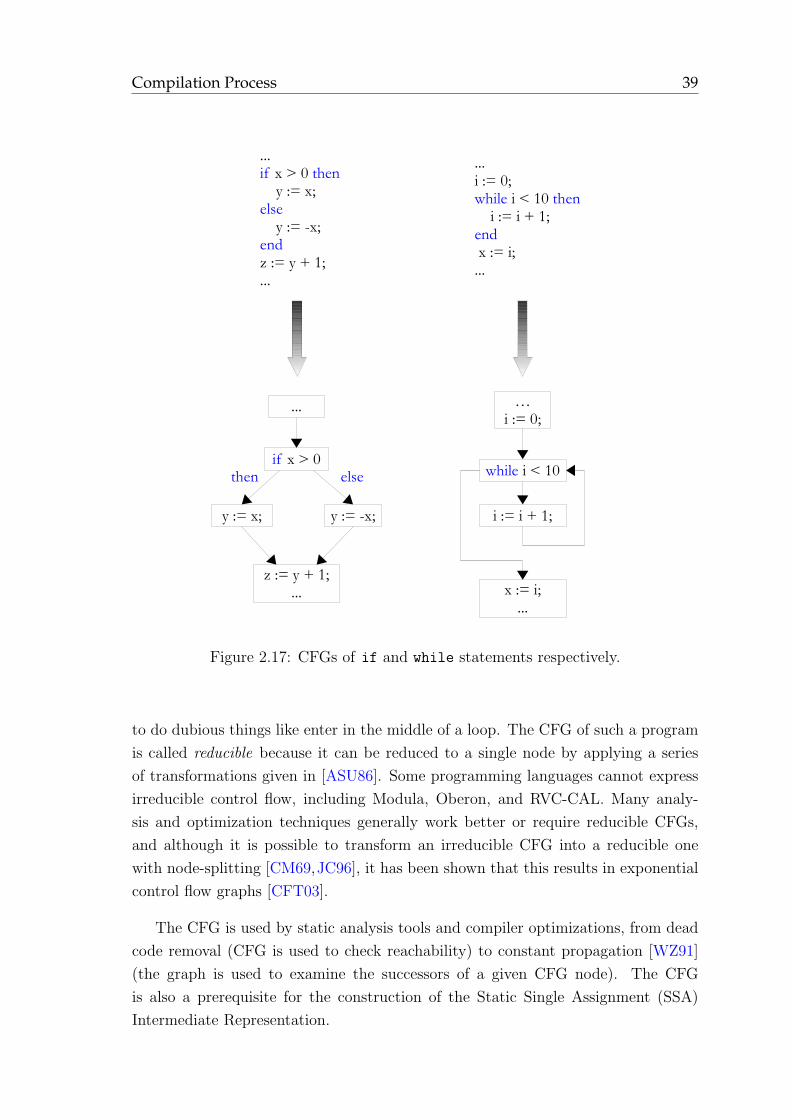
and edges represent the flow of control between nodes. Figure 2.17 shows the CFG
of well-known if (left) and while statements (right). Because both statements have
two possible outcomes (true or false), the nodes that correspond to if and while
have two successors, and each edge corresponds to one outcome. The CFG of a
procedure has a single entry node and a single exit node through which control
enters and leaves the procedure respectively, and may have any number of edges
between any two vertices.
The representation of control flow allows the formal definition of a well-structured
program. A well-structured program is a program that does not use goto statements
Compilation Process 39
if x > 0
y := x; y := -x;
...if x > 0 then y := x;else y := -x;endz := y + 1;...
then else
z := y + 1;...
...
...i := 0;while i < 10 then i := i + 1;end x := i;...
while i < 10
i := i + 1;
x := i;...
…i := 0;
Figure 2.17: CFGs of if and while statements respectively.
to do dubious things like enter in the middle of a loop. The CFG of such a program
is called reducible because it can be reduced to a single node by applying a series
of transformations given in [ASU86]. Some programming languages cannot express
irreducible control flow, including Modula, Oberon, and RVC-CAL. Many analy-
sis and optimization techniques generally work better or require reducible CFGs,
and although it is possible to transform an irreducible CFG into a reducible one
with node-splitting [CM69,JC96], it has been shown that this results in exponential
control flow graphs [CFT03].
The CFG is used by static analysis tools and compiler optimizations, from dead
code removal (CFG is used to check reachability) to constant propagation [WZ91]
(the graph is used to examine the successors of a given CFG node). The CFG
is also a prerequisite for the construction of the Static Single Assignment (SSA)
Intermediate Representation.

40 Background
2.4.3 Data Flow Analysis (DFA)
Data Flow Analysis (DFA) denotes the analysis of the behavior of a program based
on the analysis of the values of its variables. Many compiler optimizations can be
described in terms of DFA [Kil73], including constant propagation, common subex-
pression elimination [Coc70], liveness analysis. DFA is based on the specification of
data flow equations that are generally solved at the boundaries of basic blocks.
Def-use Information
DFA involves the construction of a data-flow graph that encodes information about
the definitions and uses of each variable. Unlike in traditional languages, a def-
inition is actually an assignment, not a variable declaration. An assignment to a
variable is said to kill all previous assignments. The data flow information of a given
variable is generally encoded as two lists:
1. def-use (Definition-Use) is the list of instructions that use this variable, for
each definition D.
2. use-def (Use-Definition) contains for each use U the list of instructions that
define (assign to) this variable before U .
The following example (Fig. 2.18) is adapted from an example given by Wegman
and Zadeck in [WZ91]. The corresponding def-use information is shown on Fig. 2.19.
The variable i has a list of def-use that has two definitions, each of them having three
uses.
Static Single Assignment (SSA)
Static Single Assignment (SSA) [CFR+91] is an Intermediate Representation that
make many optimizations easier to implement, faster, or both by enforcing a single
constraint: each variable must only be assigned once. The first reason for this is
that data flow information is simpler to encode with SSA: use-def chains point to
the only assignment to (or definition of) the variable, and similarly def-use chains
are a unidimensional list since there is a single definition of the variable. Figure 2.20
shows the def-use information of the code in Fig. 2.18 encoded with SSA.
It is possible for a variable to be defined in different branches, like i in our
example. Since a variable must only be defined once, SSA transforms each definition
of the same variable in n different branches to n different variables, which must be
merged when the branches are joined. This is done by a φ-function that creates a
new variable that takes the value of one of the definitions depending on the path
taken in the CFG.
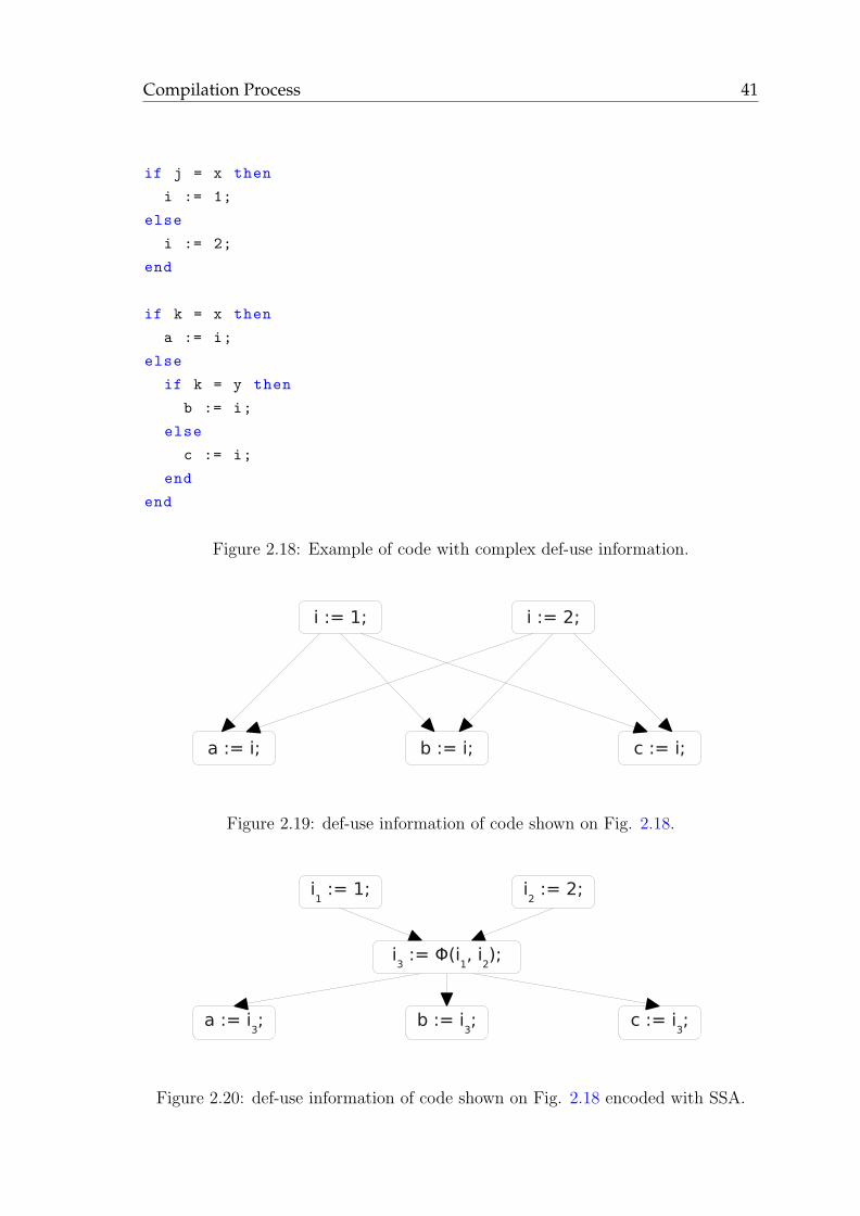
Compilation Process 41
if j = x then
i := 1;
else
i := 2;
end
if k = x then
a := i;
else
if k = y then
b := i;
else
c := i;
end
end
Figure 2.18: Example of code with complex def-use information.
i := 1; i := 2;
a := i; b := i; c := i;
Figure 2.19: def-use information of code shown on Fig. 2.18.
i1 := 1; i
2 := 2;
a := i3; b := i
3; c := i
3;
i3 := Φ(i
1, i
2);
Figure 2.20: def-use information of code shown on Fig. 2.18 encoded with SSA.
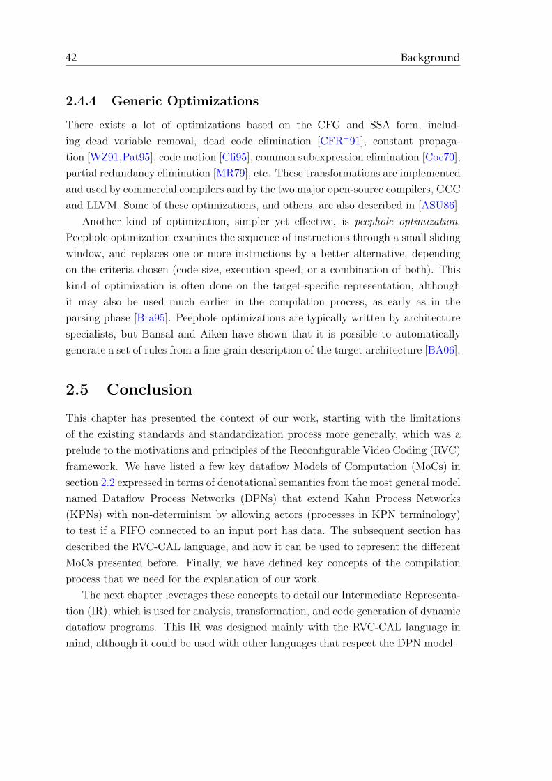
42 Background
2.4.4 Generic Optimizations
There exists a lot of optimizations based on the CFG and SSA form, includ-
ing dead variable removal, dead code elimination [CFR+91], constant propaga-
tion [WZ91,Pat95], code motion [Cli95], common subexpression elimination [Coc70],
partial redundancy elimination [MR79], etc. These transformations are implemented
and used by commercial compilers and by the two major open-source compilers, GCC
and LLVM. Some of these optimizations, and others, are also described in [ASU86].
Another kind of optimization, simpler yet effective, is peephole optimization.
Peephole optimization examines the sequence of instructions through a small sliding
window, and replaces one or more instructions by a better alternative, depending
on the criteria chosen (code size, execution speed, or a combination of both). This
kind of optimization is often done on the target-specific representation, although
it may also be used much earlier in the compilation process, as early as in the
parsing phase [Bra95]. Peephole optimizations are typically written by architecture
specialists, but Bansal and Aiken have shown that it is possible to automatically
generate a set of rules from a fine-grain description of the target architecture [BA06].
2.5 Conclusion
This chapter has presented the context of our work, starting with the limitations
of the existing standards and standardization process more generally, which was a
prelude to the motivations and principles of the Reconfigurable Video Coding (RVC)
framework. We have listed a few key dataflow Models of Computation (MoCs) in
section 2.2 expressed in terms of denotational semantics from the most general model
named Dataflow Process Networks (DPNs) that extend Kahn Process Networks
(KPNs) with non-determinism by allowing actors (processes in KPN terminology)
to test if a FIFO connected to an input port has data. The subsequent section has
described the RVC-CAL language, and how it can be used to represent the different
MoCs presented before. Finally, we have defined key concepts of the compilation
process that we need for the explanation of our work.
The next chapter leverages these concepts to detail our Intermediate Representa-
tion (IR), which is used for analysis, transformation, and code generation of dynamic
dataflow programs. This IR was designed mainly with the RVC-CAL language in
mind, although it could be used with other languages that respect the DPN model.
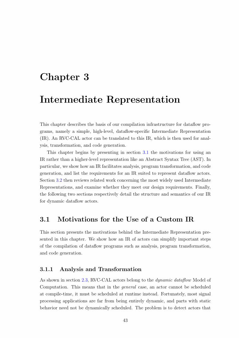
Chapter 3
Intermediate Representation
This chapter describes the basis of our compilation infrastructure for dataflow pro-
grams, namely a simple, high-level, dataflow-specific Intermediate Representation
(IR). An RVC-CAL actor can be translated to this IR, which is then used for anal-
ysis, transformation, and code generation.
This chapter begins by presenting in section 3.1 the motivations for using an
IR rather than a higher-level representation like an Abstract Syntax Tree (AST). In
particular, we show how an IR facilitates analysis, program transformation, and code
generation, and list the requirements for an IR suited to represent dataflow actors.
Section 3.2 then reviews related work concerning the most widely used Intermediate
Representations, and examine whether they meet our design requirements. Finally,
the following two sections respectively detail the structure and semantics of our IR
for dynamic dataflow actors.
3.1 Motivations for the Use of a Custom IR
This section presents the motivations behind the Intermediate Representation pre-
sented in this chapter. We show how an IR of actors can simplify important steps
of the compilation of dataflow programs such as analysis, program transformation,
and code generation.
3.1.1 Analysis and Transformation
As shown in section 2.3, RVC-CAL actors belong to the dynamic dataflow Model of
Computation. This means that in the general case, an actor cannot be scheduled
at compile-time, it must be scheduled at runtime instead. Fortunately, most signal
processing applications are far from being entirely dynamic, and parts with static
behavior need not be dynamically scheduled. The problem is to detect actors that
43
44 Intermediate Representation
behave statically or quasi-statically, since dynamic dataflow has an expressive power
equivalent to a Turing machine [BL93], which means it is not possible to prove the
termination of a dynamic dataflow program in general.
Detecting actors that behave according to more restricted MoCs (than RVC-
CAL) is a process called “classification”. Classification classifies the behavior of an
RVC-CAL actor in terms of number of tokens it receives and sends, patterns that
may govern token exchanges, and possibly acceptable token values. In the simplest
case, structural information of an actor is enough to classify it, for instance the rules
for an actor to be considered static only depend on the input and output patterns
of actions. In more complicated case, it is necessary to gather information from an
actual execution of the actor.
The structural information necessary for classification is not directly expressed
in the AST of an RVC-CAL actor, and the AST must be annotated with precom-
puted information first. For instance, token production/consumption rates for an
action must be computed from the rules of input/output patterns, which depends
on the number of tokens and repeat clause, or the type of tokens and repeat clause.
Likewise, priorities only express a partial order on action tags, so one must compute
the topological sort of the priority graph whose vertices are actions from each t set
used in priorities. The FSM uses action tags too, so a transition from one state to
another may in fact become several possible transitions if the tag associated with
the transition refers to several actions.
In cases when the structural information is not enough, the actor needs to be in-
terpreted so its behavior can be properly analyzed. It is possible to execute the actor
by interpreting the AST directly, but this is cumbersome. For example, RVC-CAL
has a generator expression, a foreach construct, and a while construct. Writing
an interpreter for the RVC-CAL AST means implementing these three separately,
although they can all be transformed to while loops.
Additionally, using the AST needlessly complicates several program transforma-
tions, because transformations need to handle all the constructs of the AST, and
we have just seen that there is redundancy among these constructs. This means
that when writing a transformation, a programmer is going to spend time worrying
about the details of the AST rather than spending time writing the transformation
itself. Again, tag resolution in the FSM and transformation of priorities to a total
order would unnecessarily complicate transformations.
To sum up, on the one hand the AST misses information and needs to be anno-
tated, and on the other hand it contains redundant information for interpretation
and transformation. It is simply not suited for the analysis and transformation of
actors. We need a representation that is simpler to analyze and transform while
Related Work 45
containing all the necessary information.
3.1.2 Code Generation
In the context of co-design and heterogeneous computing more generally, it is desir-
able to be able to compile RVC-CAL actors to several more traditional languages,
hardware or software alike (C, Java, VHDL, etc.), to execute them on hardware
and software architectures. We would like to emphasize that we want to generate
source code and not assembly code. Assembly is inherently platform-specific and
architecture-specific, and there are already plenty of great compilers that are ca-
pable of producing excellent assembly code from higher-level languages, which also
have the advantage of being much easier to generate. As an example C code may
be used on virtually any platform, from high-end desktops and servers to embedded
platforms or even on Systems-on-Chip (SoCs), which is not the case for Intel’s 8086
assembly with AT&T syntax for instance.
Compiling an actor to a target language requires the code of the actor to undergo
several transformations. Indeed, several high-level functional constructs in RVC-
CAL have no direct equivalent in lower-level languages like C and VHDL. RVC-CAL
does not distinguish between assignments to local and state variables, but Hardware
Description Languages (HDLs) generally do. The language also has concepts that
are orthogonal to some languages, e.g. Finite State Machines (FSMs) must be
expressed using specific constructs (such as gotos or switchs) in most software
languages, while FSMs are described with built-in constructs in mainstream HDLs.
The transformations applied to an actor to compile it to a given target language
fall into two categories, either generic or target-specific. Examples of generic trans-
formations include dead variable removal, dead code elimination, constant propaga-
tion, etc. Note that we use the term statements as opposed to instructions to clearly
mark the difference between elements of source code and elements of assembly code.
The goal of an Intermediate Representation (IR) for a given source language is to
minimize the number of target-specific transformations that must be programmed to
compile code to different target languages by providing a sort of “common ground”
between these languages.
3.2 Related Work
This section presents related work about existing Intermediate Representations
(IRs). There has been extensive research on the use of IRs for various purposes,
particularly in the domain of compilation. An IR can have certain properties like
46 Intermediate Representation
SSA (and its many variants [CFR+91, CCF91, BCHS98,KS98, SVKW07] and oth-
ers) or three-address code [ASU86, LA04], or it can be an abstraction of a spe-
cific language, like C [NMRW02,WFW+94]. Additionally, many tools have their
own intermediate representation, such as GCC (an IR called GIMPLE derived from
SIMPLE [HDE+93]), LLVM [LA04], the Glasgow Hashkell Compiler (GHC) (an IR
called C– [JRR99]).
As far as hardware synthesis tools are concerned, it is our impression that there is
not really an open-source alternative to proprietary synthesis tools made by FPGA
manufacturers, in the sense that no open-source synthesis tool has been adopted by
a significant part of users. Consequently, there is no IR that we could produce and
which could then be given to existing synthesis tools.
GCC (GNU Compiler Collection) and LLVM (Low-Level Virtual Machine) are
among the largest open-source compilers available and the most widely used. We
examine in this section their intermediate representations, before presenting the
XLIM representation produced by the OpenDF front-end from CAL code. The last
IR presented is the C Intermediate Language (Cil) that we have used in our previous
work [WRR+08] and has been an inspiration for the IR described in this chapter.
3.2.1 GIMPLE Intermediate Representation
GCC (GNU Compiler Collection) has front-ends for C, C++, Fortran, Java, Objec-
tive C, and back-ends for several architectures, including ARM, MIPS, SPARC, x86,
x86-64. Front-ends manipulate an Intermediate Representation called GENERIC,
which is then lowered to another IR named GIMPLE. GIMPLE is in SSA form,
and is derived from an IR called SIMPLE [HDE+93]. This IR is the IR that the
optimizer (or middle-end) manipulates. After optimization GIMPLE is translated
to the Register Transfer Language (RTL) for target-specific optimizations and code
generation by back-ends.
GIMPLE is a generic IR in the sense that it is possible to obtain a GIMPLE
equivalent of about any program (GCC has front-ends for C, C++, Objective-C,
Fortran, Java, and Ada). The IR is geared towards imperative, sequential program-
ming languages, and it has no dataflow-specific constructs. Additionally, the API
is fairly complex, and it is not clear whether or how the IR could be extended with
dataflow-specific mechanisms.
3.2.2 Low-Level Virtual Machine (LLVM)
The Low-Level Virtual Machine (LLVM) is a project that provides:
Related Work 47
• a clean, target-independent, well documented IR1 called LLVM or LLVM IR,
• a library that contains many optimization passes for the IR, and back-ends for
architectures such as x86, x86 64, PowerPC, ARM, and others,
• a set of command-line tools, from a tool that displays the IR in a textual
form (llvm-dis) to an optimizing compiler (opt) implemented with the LLVM
library,
• a Just-in-time (JIT) engine that loads IR files, optimizes them, translates them
to native code, and executes the resulting code.
The LLVM IR is a typed three-address code assembly language in SSA form. Like
RVC-CAL, the LLVM type system has integer types with an arbitrary bit width.
The IR has 52 instructions, which is a relatively small number of instructions for
an assembly-like language, especially given the fact that this includes support for
high-level features like vectors, switch statements, va arg, and exceptions. This is
possible because many instructions can be overloaded to take arguments of several
types, e.g. add can be used to add integers or vectors.
Since version 2.7, LLVM includes a feature called metadata, which allows arbi-
trary data to be represented within an LLVM file. The IR also supports intrinsics,
which are predefined functions with precise semantics. For example, intrinsics in-
clude llvm.memcpy to copy a block of memory, llvm.atomic.cmp.swap that per-
forms a Compare & Swap, which can be used to implement lock-free data struc-
tures [Val95]. New intrinsics can be added to the LLVM IR without affecting the
existing optimizers. LLVM being under BSD license, one can add their own intrinsics
to the language in their own locally-maintained version of LLVM.
Despite all these features, we did not use LLVM as an Intermediate Representa-
tion of dynamic dataflow programs for several reasons. First of all, LLVM is, like its
name indicates, low-level, and we do not need such a low-level IR. Analysis of the
behavior of dynamic dataflow programs is easier to write with a simpler and higher-
level IR, and the transformations we are interested in are structural transformations,
i.e. transformations of the structure of actors.
The LLVM compiler can optimize code thoroughly, and a low-level IR is not a
problem when generating assembly code or object code (as the majority of back-
ends in LLVM do). However, the IR is not very interesting for the generation of
source code, because the generated code is cryptic. Moreover, we have chosen a
rapid prototyping approach in our compilation infrastructure: we want people to be
able to quickly try out a new approach to generate code in a different manner, and
1The language reference for the IR is available online at http://llvm.org/docs/LangRef.html.
48 Intermediate Representation
this is hardly compatible with the heavy infrastructure typically used in back-ends.
As a conclusion, it is our opinion that in our case, LLVM is more appropriate as a
target for code generation from dataflow programs, than as an IR of the programs
themselves.
3.2.3 XLIM
XLIM (XML Language Independent Model) is a low-level IR in SSA form generated
by the Open Dataflow (OpenDF) environment from CAL actors. This IR was created
to target a hardware synthesizer called OpenForge that generates low-level Verilog
code [JMP+08]. We deliberately chose to design another IR rather than using XLIM
because it failed to meet several of our requirements.
XLIM was designed with hardware in mind, and as such it is ridiculously low-
level. For instance, incrementing a variable is represented with four operations:
one operation to produce the integer “1”, one operation to add the integer to the
source variable, one operation to cast the result, and one operation to store the
result in the target variable. Not only is this extremely verbose (by contrast this
is represented in our IR with an assignment of an addition to a variable, with the
same type information as expressed in XLIM), but this makes the representation
even more complicated to manipulate than an AST.
XLIM removes any form of structure from scheduling information (guards, FSM,
priorities). The action scheduler is expressed as an infinite while loop that starts
by computing the guards of all actions indiscriminately, before entering a gigantic
tree of nested if statements to determine which action should be fired. An FSM
with n states is transformed to a set of n boolean variables, which always contains
exactly one variable whose value is true, and which is the current state. All this
makes it unnecessarily hard to retrieve the structure of the original actor, as well as
making it difficult to design other implementations of an action scheduler.
Finally, contrary to what the name suggests, XLIM is not a language-independent
IR. There are two flavors of XLIM, one hardware-oriented (that was originally
present in OpenDF) and one software-oriented, created for the needs of the Xlim2C
code generator. The hardware-oriented representation supports a small subset of
RVC-CAL, and the software-oriented representation only recently started to sup-
port the most advanced features of RVC-CAL (list generators, foreach statements).
3.2.4 C Intermediate Language
The C Intermediate Language (CIL) [NMRW02] (not to be confused with the Com-
mon Intermediate Language of the Common Language Infrastructure [Ecm06]) is an
Related Work 49
IR that can be seen as a subset of C with clean semantics. Like LLVM, CIL means
several things: an IR; a library that contains an implementation of the CIL IR, a C
to CIL parser, a CIL to C pretty-printer, and several analysis and transformation
passes performed on CIL; a set of tools based on the CIL library. The CIL IR re-
moves many of the quirks and ambiguities typically present in C programs by making
explicit many implicit constructs, such as memory references and side-effects. CIL
is traditionally used to perform analysis and source-to-source transformations of C
programs, such as merging C source files together, adding buffer overrun defense
mechanisms, or ensuring memory safety [NCH+05].
We have used CIL in some of our previous work [WRR+08] in a prototype that
generated C directly from CAL (at the time the RVC standard had not been ratified
yet). CIL has influenced the design of our IR in three ways:
• As a high-level representation and source-to-source transformation tool, CIL
tries its best to produce code that is as faithful as possible to the original code.
We have found this valuable in practice, especially for debugging purposes of
the generated code, e.g. to trace bugs back into the RVC-CAL source. The
IR has been designed to be a canonic representation of RVC-CAL while being
as close to the language as possible.
• Rather than representing loops using a conditional branch statement (in other
words, a if and a goto) like LLVM, CIL lowers all loop constructs to a single
while loop. This makes it easier to produce code for targets that do not
have the notion of a goto, namely programmable logic, as well as simplifying
code generation for target languages (including those that do not have goto
statements, like Oberon [Wir88], Modula [Wir83], and RVC-CAL).
• CIL separates instructions with side-effects from side-effect free expressions,
which facilitates analysis and transformation without obfuscating code like
three-address code does.
3.2.5 Conclusion
We have presented the IRs used by the two major open-source compilers, GCC, and
LLVM, as well as two others IRs related to our work, namely XLIM and CIL, and
have shown why XLIM was poorly suited to be a good IR of RVC-CAL actors. The
rest of this chapter presents the structure and semantics of our IR of RVC-CAL
actors.
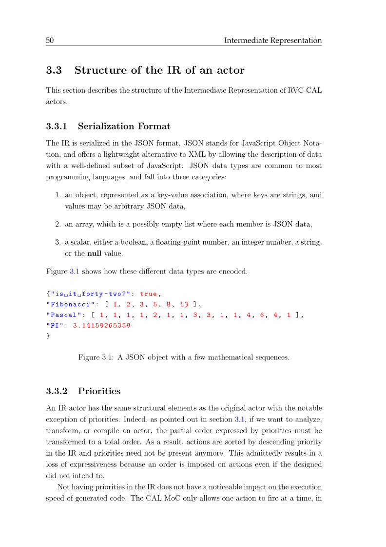
50 Intermediate Representation
3.3 Structure of the IR of an actor
This section describes the structure of the Intermediate Representation of RVC-CAL
actors.
3.3.1 Serialization Format
The IR is serialized in the JSON format. JSON stands for JavaScript Object Nota-
tion, and offers a lightweight alternative to XML by allowing the description of data
with a well-defined subset of JavaScript. JSON data types are common to most
programming languages, and fall into three categories:
1. an object, represented as a key-value association, where keys are strings, and
values may be arbitrary JSON data,
2. an array, which is a possibly empty list where each member is JSON data,
3. a scalar, either a boolean, a floating-point number, an integer number, a string,
or the null value.
Figure 3.1 shows how these different data types are encoded.
{"is it forty -two?": true,
"Fibonacci": [ 1, 2, 3, 5, 8, 13 ],
"Pascal": [ 1, 1, 1, 1, 2, 1, 1, 3, 3, 1, 1, 4, 6, 4, 1 ],
"PI": 3.14159265358
}
Figure 3.1: A JSON object with a few mathematical sequences.
3.3.2 Priorities
An IR actor has the same structural elements as the original actor with the notable
exception of priorities. Indeed, as pointed out in section 3.1, if we want to analyze,
transform, or compile an actor, the partial order expressed by priorities must be
transformed to a total order. As a result, actions are sorted by descending priority
in the IR and priorities need not be present anymore. This admittedly results in a
loss of expressiveness because an order is imposed on actions even if the designed
did not intend to.
Not having priorities in the IR does not have a noticeable impact on the execution
speed of generated code. The CAL MoC only allows one action to fire at a time, in
Structure of the IR of an actor 51
other words two or more actions cannot be fired in parallel, so we only lose the abil-
ity to evaluate the schedulability of actions in parallel. Since scheduling information
is generally computationally-inexpensive and with a few conditional branches, it is
not clear how this information could be computed in parallel on software processors.
This kind of fine-grain parallelism is more suited to Programmable Logic Devices
(PLDs), but if we generate code to compute schedulability information as shown on
Fig. 3.2, synthesizers are capable of analyzing data-dependencies and schedule the
tests in parallel.
Figure 3.2 shows a VHDL process that is sensitive to two signals, the classic
reset signal and a Add TEX send signal that is activated when data is available on
the TEX input port. For the reader not familiar with VHDL, reset is always true
unless the device is reset, in which case the signal becomes false. The assignments
“:=” and “<=” denote assignments to local variables (that we have omitted here
for the sake of brevity) and signals respectively.
3.3.3 Finite State Machine
The Finite State Machine (FSM) of an RVC-CAL actor is transformed in our IR to an
FSM in a form that is easier to manipulate and to generate code from while keeping
the same information (initial state and list of transitions). Contrary to RVC-CAL,
the FSM in the IR explicitly lists the states of the FSM to allow the generation
of switch-based implementations in software languages as well as to describe an
FSM type in Hardware Description Languages (HDLs). Rather than having several
transitions departing from a single state as in RVC-CAL (Fig. 3.3), transitions are
grouped by starting state (Fig. 3.4). Enumerating transitions this way facilitates
analysis (finding dead-end states isO(1) for instance) and code generation: whatever
the target language is, different cases must be distinct, and when using gotos, labels
must be distinct too.
Figure 3.4 shows the IR of the FSM of Fig. 3.3 as serialized with JSON. Note
that action tags are represented as a list of strings, e.g. the tag “cmd.tex” is a
list [‘‘cmd’’, ‘‘tex’’]. Another difference between the original RVC-CAL FSM
and its IR is that action tags are developed, which is why the transition “cmd” to
“cmd” becomes two transitions because the tag “cmd.other” actually denotes two
actions with respective tags “cmd.other.mot” and “cmd.other.mix”. Once again this
facilitates analysis and code generation, but this is not the only reason behind this
difference. Tags used in transitions may be affected by priorities, yet we have seen
that priorities are absent from the IR. As a consequence, tags must be developed
according to the priority order so that their interpretation is no longer dependent
on priorities.
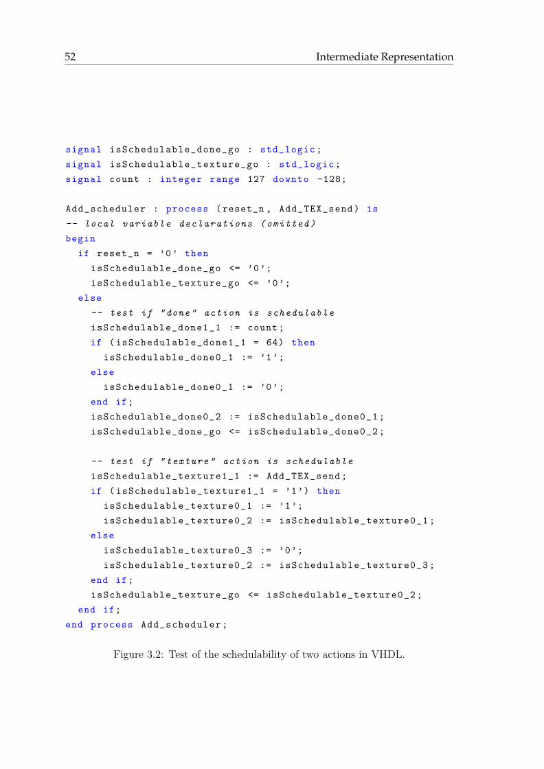
52 Intermediate Representation
signal isSchedulable_done_go : std_logic;
signal isSchedulable_texture_go : std_logic;
signal count : integer range 127 downto -128;
Add_scheduler : process (reset_n , Add_TEX_send) is
-- local variable declarations (omitted)
begin
if reset_n = ’0’ then
isSchedulable_done_go <= ’0’;
isSchedulable_texture_go <= ’0’;
else
-- test if "done" action is schedulable
isSchedulable_done1_1 := count;
if (isSchedulable_done1_1 = 64) then
isSchedulable_done0_1 := ’1’;
else
isSchedulable_done0_1 := ’0’;
end if;
isSchedulable_done0_2 := isSchedulable_done0_1;
isSchedulable_done_go <= isSchedulable_done0_2;
-- test if "texture" action is schedulable
isSchedulable_texture1_1 := Add_TEX_send;
if (isSchedulable_texture1_1 = ’1’) then
isSchedulable_texture0_1 := ’1’;
isSchedulable_texture0_2 := isSchedulable_texture0_1;
else
isSchedulable_texture0_3 := ’0’;
isSchedulable_texture0_2 := isSchedulable_texture0_3;
end if;
isSchedulable_texture_go <= isSchedulable_texture0_2;
end if;
end process Add_scheduler;
Figure 3.2: Test of the schedulability of two actions in VHDL.
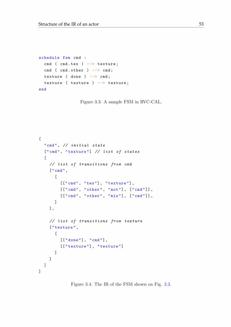
Structure of the IR of an actor 53
schedule fsm cmd :
cmd ( cmd.tex ) --> texture;
cmd ( cmd.other ) --> cmd;
texture ( done ) --> cmd;
texture ( texture ) --> texture;
end
Figure 3.3: A sample FSM in RVC-CAL.
[
"cmd", // initial state
["cmd", "texture"] // list of states
[
// list of transitions from cmd
["cmd",
[
[["cmd", "tex"], "texture"],
[["cmd", "other", "mot"], ["cmd"]],
[["cmd", "other", "mix"], ["cmd"]],
]
],
// list of transitions from texture
["texture",
[
[["done"], "cmd"],
[["texture"], "texture"]
]
]
]
]
Figure 3.4: The IR of the FSM shown on Fig. 3.3.
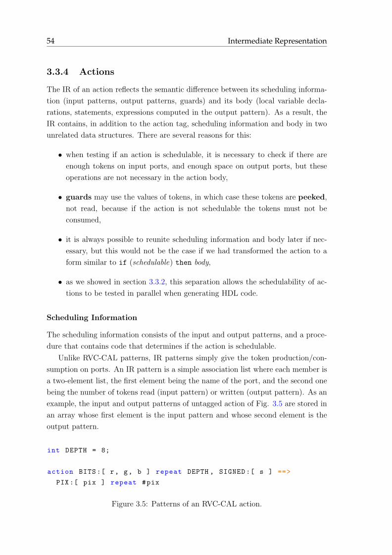
54 Intermediate Representation
3.3.4 Actions
The IR of an action reflects the semantic difference between its scheduling informa-
tion (input patterns, output patterns, guards) and its body (local variable decla-
rations, statements, expressions computed in the output pattern). As a result, the
IR contains, in addition to the action tag, scheduling information and body in two
unrelated data structures. There are several reasons for this:
• when testing if an action is schedulable, it is necessary to check if there are
enough tokens on input ports, and enough space on output ports, but these
operations are not necessary in the action body,
• guards may use the values of tokens, in which case these tokens are peeked,
not read, because if the action is not schedulable the tokens must not be
consumed,
• it is always possible to reunite scheduling information and body later if nec-
essary, but this would not be the case if we had transformed the action to a
form similar to if (schedulable) then body,
• as we showed in section 3.3.2, this separation allows the schedulability of ac-
tions to be tested in parallel when generating HDL code.
Scheduling Information
The scheduling information consists of the input and output patterns, and a proce-
dure that contains code that determines if the action is schedulable.
Unlike RVC-CAL patterns, IR patterns simply give the token production/con-
sumption on ports. An IR pattern is a simple association list where each member is
a two-element list, the first element being the name of the port, and the second one
being the number of tokens read (input pattern) or written (output pattern). As an
example, the input and output patterns of untagged action of Fig. 3.5 are stored in
an array whose first element is the input pattern and whose second element is the
output pattern.
int DEPTH = 8;
action BITS:[ r, g, b ] repeat DEPTH , SIGNED :[ s ] ==>
PIX:[ pix ] repeat #pix
Figure 3.5: Patterns of an RVC-CAL action.
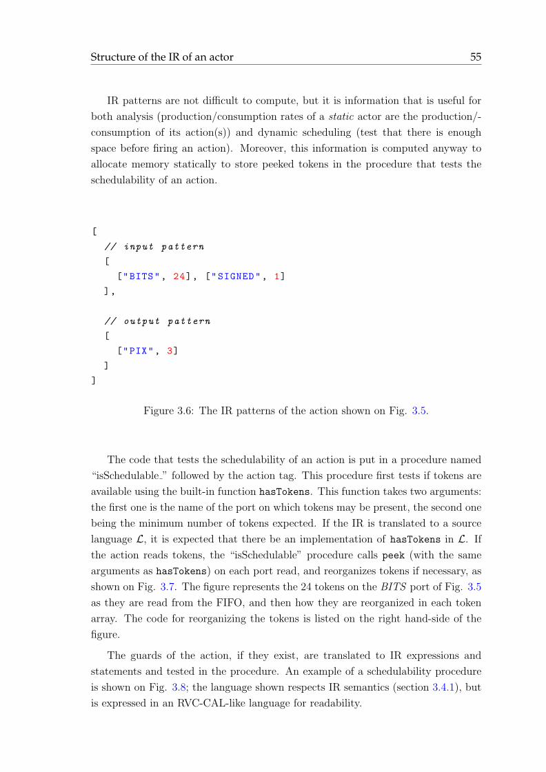
Structure of the IR of an actor 55
IR patterns are not difficult to compute, but it is information that is useful for
both analysis (production/consumption rates of a static actor are the production/-
consumption of its action(s)) and dynamic scheduling (test that there is enough
space before firing an action). Moreover, this information is computed anyway to
allocate memory statically to store peeked tokens in the procedure that tests the
schedulability of an action.
[
// input pattern
[
["BITS", 24], ["SIGNED", 1]
],
// output pattern
[
["PIX", 3]
]
]
Figure 3.6: The IR patterns of the action shown on Fig. 3.5.
The code that tests the schedulability of an action is put in a procedure named
“isSchedulable ” followed by the action tag. This procedure first tests if tokens are
available using the built-in function hasTokens. This function takes two arguments:
the first one is the name of the port on which tokens may be present, the second one
being the minimum number of tokens expected. If the IR is translated to a source
language L, it is expected that there be an implementation of hasTokens in L. If
the action reads tokens, the “isSchedulable” procedure calls peek (with the same
arguments as hasTokens) on each port read, and reorganizes tokens if necessary, as
shown on Fig. 3.7. The figure represents the 24 tokens on the BITS port of Fig. 3.5
as they are read from the FIFO, and then how they are reorganized in each token
array. The code for reorganizing the tokens is listed on the right hand-side of the
figure.
The guards of the action, if they exist, are translated to IR expressions and
statements and tested in the procedure. An example of a schedulability procedure
is shown on Fig. 3.8; the language shown respects IR semantics (section 3.4.1), but
is expressed in an RVC-CAL-like language for readability.
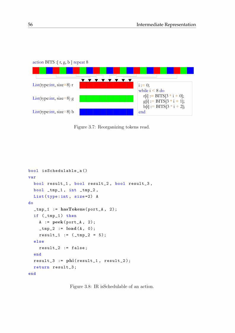
56 Intermediate Representation
action BITS :[ r, g, b ] repeat 8
List(type:int, size=8) r
List(type:int, size=8) g
List(type:int, size=8) b
i := 0;while i < 8 do r[i] := BITS[3 * i + 0]; g[i] := BITS[3 * i + 1]; b[i] := BITS[3 * i + 2];end
Figure 3.7: Reorganizing tokens read.
bool isSchedulable_a ()
var
bool result_1 , bool result_2 , bool result_3 ,
bool _tmp_1 , int _tmp_2 ,
List(type:int , size =2) A
do
_tmp_1 := hasTokens(port_A , 2);
if (_tmp_1) then
A := peek(port_A , 2);
_tmp_2 := load(A, 0);
result_1 := (_tmp_2 = 5);
else
result_2 := false;
end
result_3 := phi(result_1 , result_2 );
return result_3;
end
Figure 3.8: IR isSchedulable of an action.
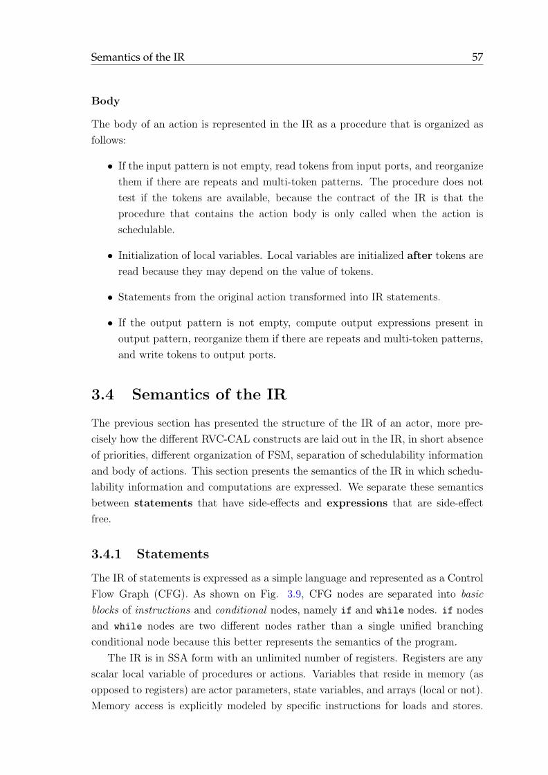
Semantics of the IR 57
Body
The body of an action is represented in the IR as a procedure that is organized as
follows:
• If the input pattern is not empty, read tokens from input ports, and reorganize
them if there are repeats and multi-token patterns. The procedure does not
test if the tokens are available, because the contract of the IR is that the
procedure that contains the action body is only called when the action is
schedulable.
• Initialization of local variables. Local variables are initialized after tokens are
read because they may depend on the value of tokens.
• Statements from the original action transformed into IR statements.
• If the output pattern is not empty, compute output expressions present in
output pattern, reorganize them if there are repeats and multi-token patterns,
and write tokens to output ports.
3.4 Semantics of the IR
The previous section has presented the structure of the IR of an actor, more pre-
cisely how the different RVC-CAL constructs are laid out in the IR, in short absence
of priorities, different organization of FSM, separation of schedulability information
and body of actions. This section presents the semantics of the IR in which schedu-
lability information and computations are expressed. We separate these semantics
between statements that have side-effects and expressions that are side-effect
free.
3.4.1 Statements
The IR of statements is expressed as a simple language and represented as a Control
Flow Graph (CFG). As shown on Fig. 3.9, CFG nodes are separated into basic
blocks of instructions and conditional nodes, namely if and while nodes. if nodes
and while nodes are two different nodes rather than a single unified branching
conditional node because this better represents the semantics of the program.
The IR is in SSA form with an unlimited number of registers. Registers are any
scalar local variable of procedures or actions. Variables that reside in memory (as
opposed to registers) are actor parameters, state variables, and arrays (local or not).
Memory access is explicitly modeled by specific instructions for loads and stores.
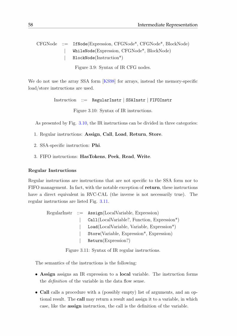
58 Intermediate Representation
CFGNode ::= IfNode(Expression, CFGNode*, CFGNode*, BlockNode)
| WhileNode(Expression, CFGNode*, BlockNode)
| BlockNode(Instruction*)
Figure 3.9: Syntax of IR CFG nodes.
We do not use the array SSA form [KS98] for arrays, instead the memory-specific
load/store instructions are used.
Instruction ::= RegularInstr | SSAInstr | FIFOInstr
Figure 3.10: Syntax of IR instructions.
As presented by Fig. 3.10, the IR instructions can be divided in three categories:
1. Regular instructions: Assign, Call, Load, Return, Store.
2. SSA-specific instruction: Phi.
3. FIFO instructions: HasTokens, Peek, Read, Write.
Regular Instructions
Regular instructions are instructions that are not specific to the SSA form nor to
FIFO management. In fact, with the notable exception of return, these instructions
have a direct equivalent in RVC-CAL (the inverse is not necessarily true). The
regular instructions are listed Fig. 3.11.
RegularInstr ::= Assign(LocalVariable, Expression)
| Call(LocalVariable?, Function, Expression*)
| Load(LocalVariable, Variable, Expression*)
| Store(Variable, Expression*, Expression)
| Return(Expression?)
Figure 3.11: Syntax of IR regular instructions.
The semantics of the instructions is the following:
• Assign assigns an IR expression to a local variable. The instruction forms
the definition of the variable in the data flow sense.
• Call calls a procedure with a (possibly empty) list of arguments, and an op-
tional result. The call may return a result and assign it to a variable, in which
case, like the assign instruction, the call is the definition of the variable.
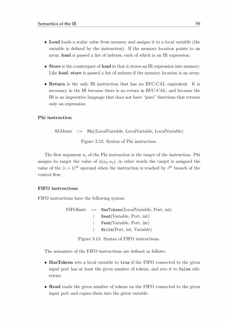
Semantics of the IR 59
• Load loads a scalar value from memory and assigns it to a local variable (the
variable is defined by the instruction). If the memory location points to an
array, load is passed a list of indexes, each of which is an IR expression.
• Store is the counterpart of load in that it stores an IR expression into memory.
Like load, store is passed a list of indexes if the memory location is an array.
• Return is the only IR instruction that has no RVC-CAL equivalent. It is
necessary in the IR because there is no return in RVC-CAL, and because the
IR is an imperative language that does not have “pure” functions that returns
only an expression.
Phi instruction
SSAInstr ::= Phi(LocalVariable, LocalVariable, LocalVariable)
Figure 3.12: Syntax of Phi instruction.
The first argument a1 of the Phi instruction is the target of the instruction. Phi
assigns its target the value of φ(a2, a3), in other words the target is assigned the
value of the (i + 1)th operand when the instruction is reached by ith branch of the
control flow.
FIFO instructions
FIFO instructions have the following syntax:
FIFOInstr ::= HasTokens(LocalVariable, Port, int)
| Read(Variable, Port, int)
| Peek(Variable, Port, int)
| Write(Port, int, Variable)
Figure 3.13: Syntax of FIFO instructions.
The semantics of the FIFO instructions are defined as follows:
• HasTokens sets a local variable to true if the FIFO connected to the given
input port has at least the given number of tokens, and sets it to false oth-
erwise.
• Read reads the given number of tokens on the FIFO connected to the given
input port and copies them into the given variable.
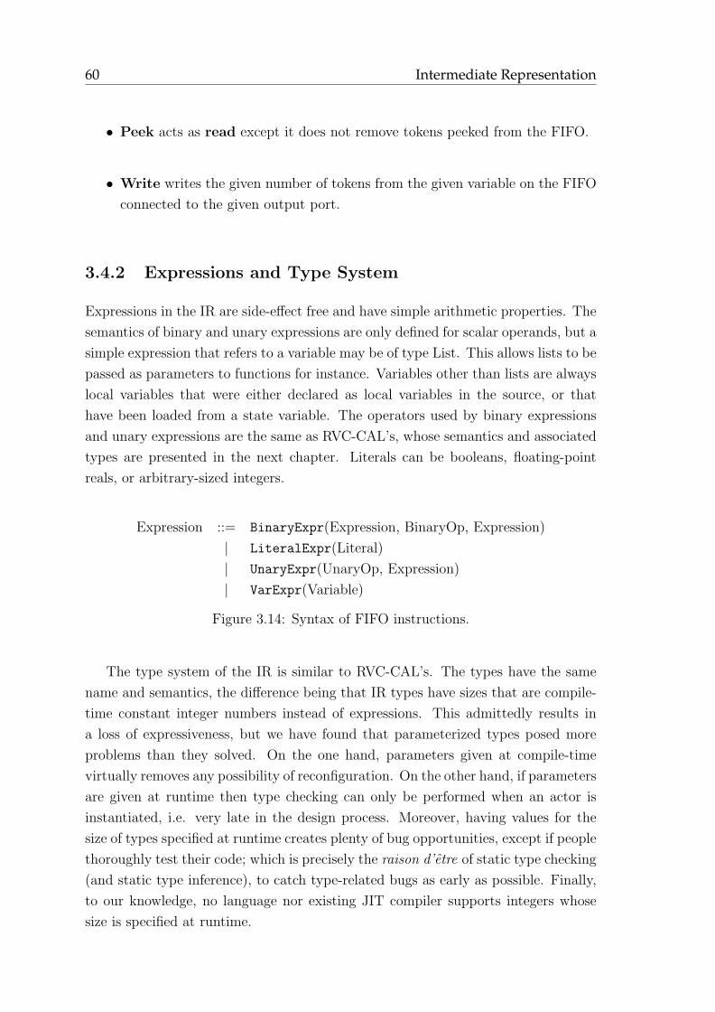
60 Intermediate Representation
• Peek acts as read except it does not remove tokens peeked from the FIFO.
• Write writes the given number of tokens from the given variable on the FIFO
connected to the given output port.
3.4.2 Expressions and Type System
Expressions in the IR are side-effect free and have simple arithmetic properties. The
semantics of binary and unary expressions are only defined for scalar operands, but a
simple expression that refers to a variable may be of type List. This allows lists to be
passed as parameters to functions for instance. Variables other than lists are always
local variables that were either declared as local variables in the source, or that
have been loaded from a state variable. The operators used by binary expressions
and unary expressions are the same as RVC-CAL’s, whose semantics and associated
types are presented in the next chapter. Literals can be booleans, floating-point
reals, or arbitrary-sized integers.
Expression ::= BinaryExpr(Expression, BinaryOp, Expression)
| LiteralExpr(Literal)
| UnaryExpr(UnaryOp, Expression)
| VarExpr(Variable)
Figure 3.14: Syntax of FIFO instructions.
The type system of the IR is similar to RVC-CAL’s. The types have the same
name and semantics, the difference being that IR types have sizes that are compile-
time constant integer numbers instead of expressions. This admittedly results in
a loss of expressiveness, but we have found that parameterized types posed more
problems than they solved. On the one hand, parameters given at compile-time
virtually removes any possibility of reconfiguration. On the other hand, if parameters
are given at runtime then type checking can only be performed when an actor is
instantiated, i.e. very late in the design process. Moreover, having values for the
size of types specified at runtime creates plenty of bug opportunities, except if people
thoroughly test their code; which is precisely the raison d’etre of static type checking
(and static type inference), to catch type-related bugs as early as possible. Finally,
to our knowledge, no language nor existing JIT compiler supports integers whose
size is specified at runtime.
Conclusion 61
3.5 Conclusion
This chapter has presented the foundation on which our compilation infrastructure
is built, namely a simple, high-level Intermediate Representation (IR) of dynamic
dataflow programs. We have listed our motivations for using a dataflow-specific IR,
and examined related work concerning a few existing IRs that have inspired the
design of our IR, whose structure and semantics were then presented.
The next three chapters are dedicated to the three components of our infrastruc-
ture that respectively produce, analyze and transform, and generate code from the
IR of actors.

62 Intermediate Representation
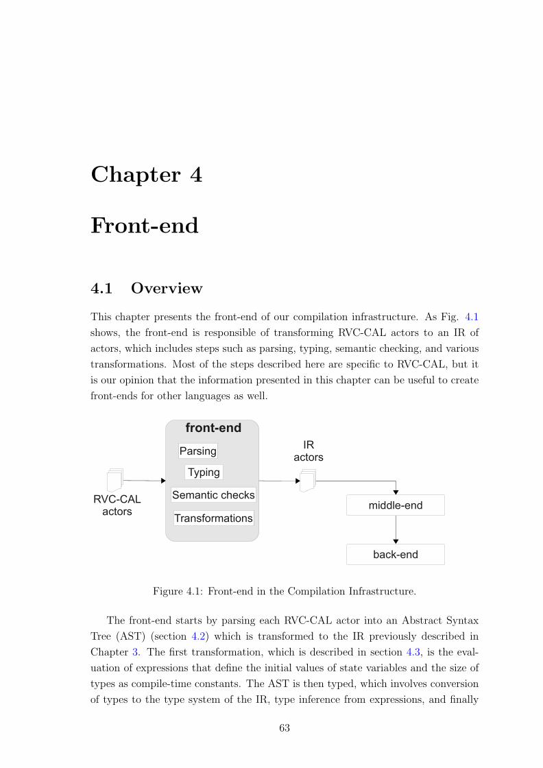
Chapter 4
Front-end
4.1 Overview
This chapter presents the front-end of our compilation infrastructure. As Fig. 4.1
shows, the front-end is responsible of transforming RVC-CAL actors to an IR of
actors, which includes steps such as parsing, typing, semantic checking, and various
transformations. Most of the steps described here are specific to RVC-CAL, but it
is our opinion that the information presented in this chapter can be useful to create
front-ends for other languages as well.
middle-endRVC-CAL
actors
IRactors
back-end
front-end
Parsing
Typing
Semantic checks
Transformations
Figure 4.1: Front-end in the Compilation Infrastructure.
The front-end starts by parsing each RVC-CAL actor into an Abstract Syntax
Tree (AST) (section 4.2) which is transformed to the IR previously described in
Chapter 3. The first transformation, which is described in section 4.3, is the eval-
uation of expressions that define the initial values of state variables and the size of
types as compile-time constants. The AST is then typed, which involves conversion
of types to the type system of the IR, type inference from expressions, and finally
63
64 Front-end
type checking to catch type errors (section 4.4).
The annotated AST can then be transformed to the IR. Section 4.5 presents the
structural transformations from the AST to the IR. These transformations include
the creation of a tag association table, creation of a total order of actions from the
partial order on action tags expressed by the priorities, translation of the FSM, and
transformation of each action to a procedure that contains scheduling information
(guards, input pattern) and a procedure that contains the computations of the ac-
tion. Finally, section 4.6 details the semantic transformations from the AST to the
IR. Semantic transformations aim to express the behavior described by the body of
actions, functions, and procedures with the statements and expressions of the IR.
4.2 Syntax Parsing
4.2.1 Parsing with the Xtext Framework
The Xtext1 framework [EV06] generates an ANTLR-based syntax parser automati-
cally from a grammar description, but also a meta-model of the AST, as well as code
that transforms the concrete syntax to the AST. The AST meta-model generated
from the grammar may be post-processed if necessary to include additional informa-
tion by linking to other meta-models. Xtext takes advantage of the meta-modeling
infrastructure and Java code generation capabilities of the Eclipse Modeling Frame-
work (EMF) [Ecl].
Figure 4.2 shows the grammar rule for an RVC-CAL actor. The grammar de-
scription syntax is read as follows. Strings enclosed in quotes are lexical tokens, e.g.
an actor must begin with the keyword actor. The number of times a rule is invoked
is expressed using the same syntax as regular expressions, namely the number of
invocations can be any number of times (star sign), at least once (plus sign), at
most once (question mark), or exactly one time (no suffix present). The result of a
grammar rule is assigned to a scalar using the equal sign (like “name” and “sched-
ule”). If a rule may be executed more than once, the plus-equal sign must be used
to obtain a list (“parameters”, “inputs”, etc.). When a rule is not called (e.g. an
actor without a Finite State Machine causes the AstSchedule rule to be skipped),
its result is nil.
4.2.2 Meta-model Inference
The part of the meta-model generated for the AstActor rule is shown on Fig. 4.3.
The meta-model is inferred by Xtext from the grammar description using the fol-
1Xtext is available at http://www.eclipse.org/Xtext/.
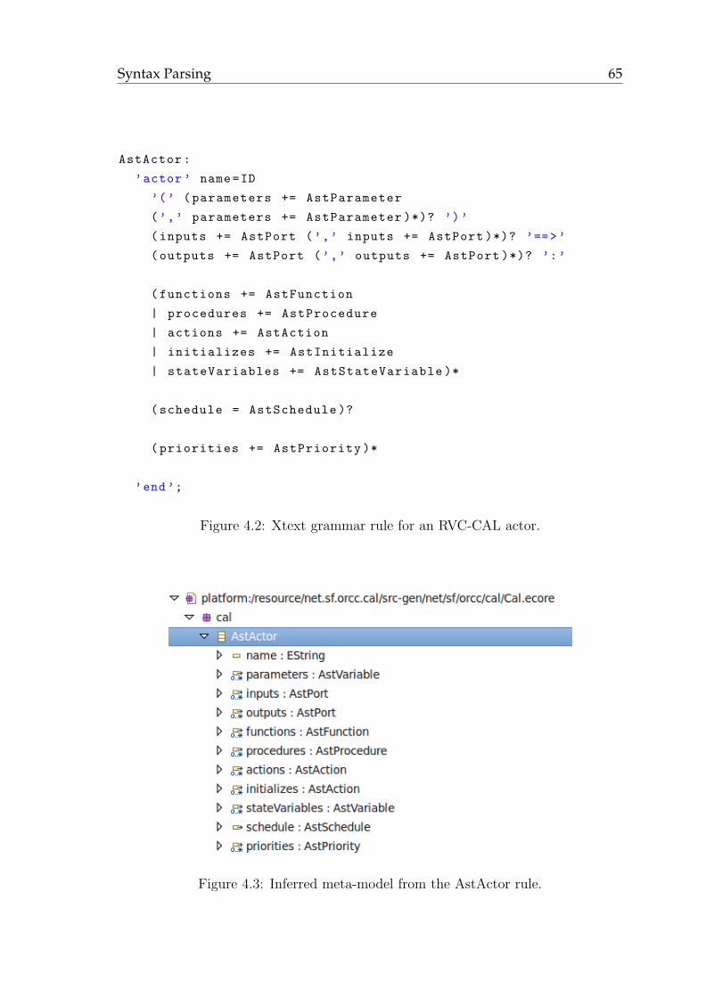
Syntax Parsing 65
AstActor:
’actor ’ name=ID
’(’ (parameters += AstParameter
(’,’ parameters += AstParameter )*)? ’)’
(inputs += AstPort (’,’ inputs += AstPort )*)? ’==>’
(outputs += AstPort (’,’ outputs += AstPort )*)? ’:’
(functions += AstFunction
| procedures += AstProcedure
| actions += AstAction
| initializes += AstInitialize
| stateVariables += AstStateVariable )*
(schedule = AstSchedule )?
(priorities += AstPriority )*
’end’;
Figure 4.2: Xtext grammar rule for an RVC-CAL actor.
Figure 4.3: Inferred meta-model from the AstActor rule.
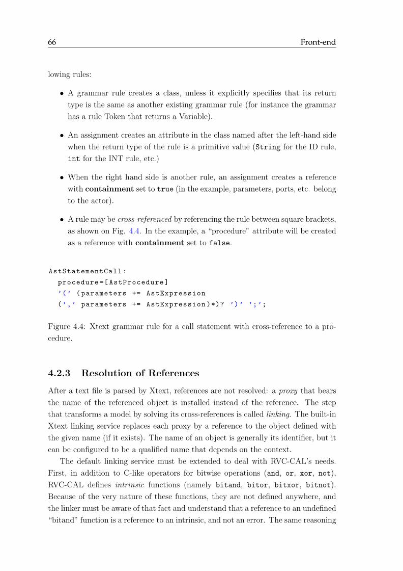
66 Front-end
lowing rules:
• A grammar rule creates a class, unless it explicitly specifies that its return
type is the same as another existing grammar rule (for instance the grammar
has a rule Token that returns a Variable).
• An assignment creates an attribute in the class named after the left-hand side
when the return type of the rule is a primitive value (String for the ID rule,
int for the INT rule, etc.)
• When the right hand side is another rule, an assignment creates a reference
with containment set to true (in the example, parameters, ports, etc. belong
to the actor).
• A rule may be cross-referenced by referencing the rule between square brackets,
as shown on Fig. 4.4. In the example, a “procedure” attribute will be created
as a reference with containment set to false.
AstStatementCall:
procedure =[ AstProcedure]
’(’ (parameters += AstExpression
(’,’ parameters += AstExpression )*)? ’)’ ’;’;
Figure 4.4: Xtext grammar rule for a call statement with cross-reference to a pro-
cedure.
4.2.3 Resolution of References
After a text file is parsed by Xtext, references are not resolved: a proxy that bears
the name of the referenced object is installed instead of the reference. The step
that transforms a model by solving its cross-references is called linking. The built-in
Xtext linking service replaces each proxy by a reference to the object defined with
the given name (if it exists). The name of an object is generally its identifier, but it
can be configured to be a qualified name that depends on the context.
The default linking service must be extended to deal with RVC-CAL’s needs.
First, in addition to C-like operators for bitwise operations (and, or, xor, not),
RVC-CAL defines intrinsic functions (namely bitand, bitor, bitxor, bitnot).
Because of the very nature of these functions, they are not defined anywhere, and
the linker must be aware of that fact and understand that a reference to an undefined
“bitand” function is a reference to an intrinsic, and not an error. The same reasoning
Expression Evaluation 67
applies for built-in procedures like print and println. Another feature that requires
custom linking is the definition of FSM transitions. Transitions reference a source
state and a target state, but these states are never defined. Our custom linking
service must therefore define a state the first time it is encountered when linking
the FSM, and other cross-references to this state will simply point to this state as
usual.
4.3 Expression Evaluation
Many transformations from the AST to the IR need to evaluate expressions as
compile-time constants for various purposes. To this end, an expression is given to
an evaluator, which either returns a compile-time constant, or reports an error. We
define in this section the evaluator that is present in the front-end.
The set of values that the evaluator can return is a union of the set of real
numbers R, signed integer numbers Z, and booleans B (which is an admittedly
small set compared to the other two). The front-end internally represents signed
integer numbers as integers with an arbitrary size, so the value of a signed number
is only limited by the available memory. However, since the RVC standard does not
currently define the size or behavior of real numbers, we currently use 32-bit float
types.
The evaluator has the following properties:
• The value a variable may be assigned belongs to the set:
V alues = R ∪ B ∪ {⊥}
The value ⊥ is used for variables whose value is unknown: uninitialized vari-
ables and variables whose value could not be evaluated as a compile-time
constant.
• Each variable that has been evaluated is present in the environment that as-
sociates a variable and its value:
Env : Idents→ V alues
The evaluation rules for RVC-CAL expressions are shown on Table 4.1. The
table is to be read as the rule named n is applied if the condition c is true, in which
case it returns the value v. Rules are separated in sections, in the following order:
scalars, list expression, if expression, unary operations, binary operations. In each
section, rules are listed sequentially from top to bottom, i.e. if the first rule does
not apply, we try the second one, and so on until we find a rule that can be applied.
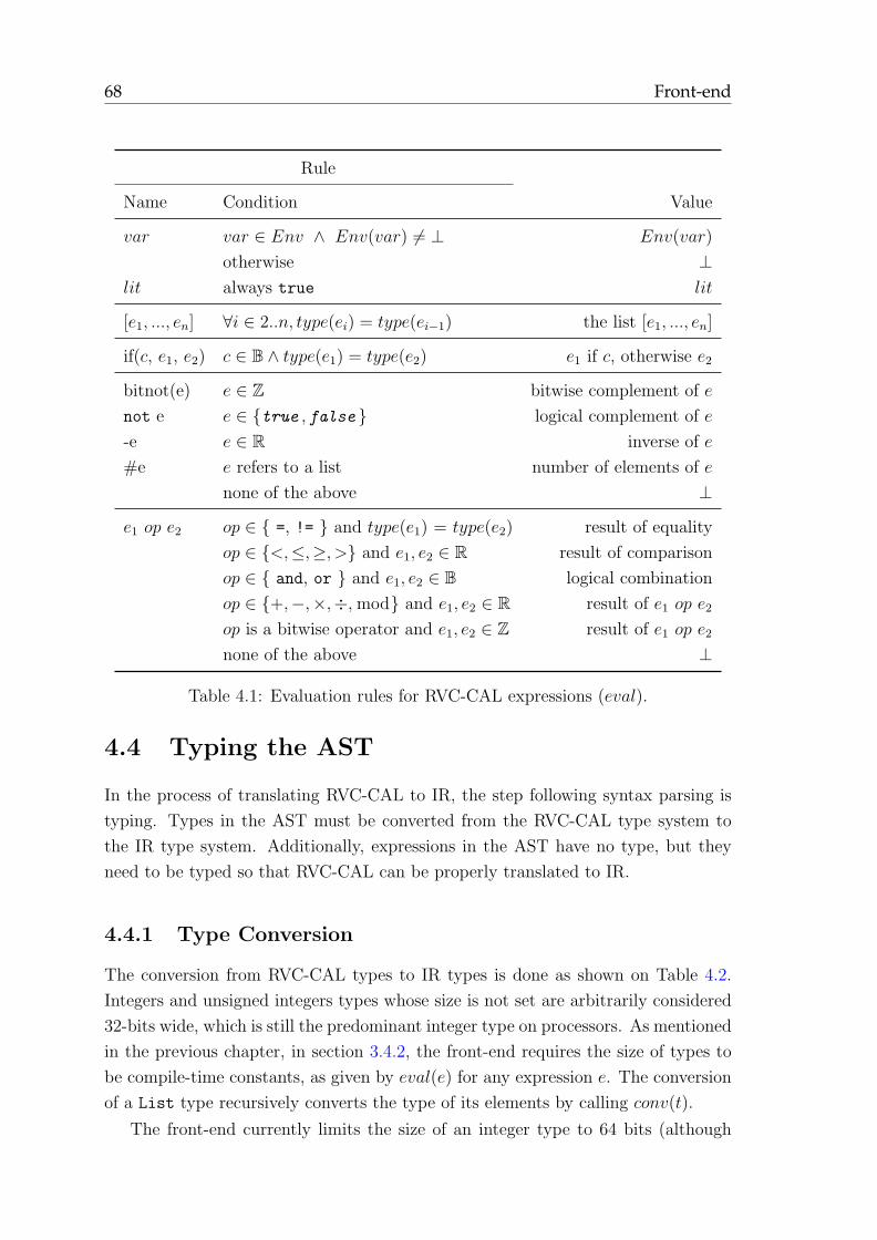
68 Front-end
Rule
Name Condition Value
var var ∈ Env ∧ Env(var) 6= ⊥ Env(var)
otherwise ⊥
lit always true lit
[e1, ..., en] ∀i ∈ 2..n, type(ei) = type(ei−1) the list [e1, ..., en]
if(c, e1, e2) c ∈ B ∧ type(e1) = type(e2) e1 if c, otherwise e2
bitnot(e) e ∈ Z bitwise complement of e
not e e ∈ {true , false } logical complement of e
-e e ∈ R inverse of e
#e e refers to a list number of elements of e
none of the above ⊥
e1 op e2 op ∈ { =, != } and type(e1) = type(e2) result of equality
op ∈ {<,≤,≥, >} and e1, e2 ∈ R result of comparison
op ∈ { and, or } and e1, e2 ∈ B logical combination
op ∈ {+,−,×,÷,mod} and e1, e2 ∈ R result of e1 op e2
op is a bitwise operator and e1, e2 ∈ Z result of e1 op e2
none of the above ⊥
Table 4.1: Evaluation rules for RVC-CAL expressions (eval).
4.4 Typing the AST
In the process of translating RVC-CAL to IR, the step following syntax parsing is
typing. Types in the AST must be converted from the RVC-CAL type system to
the IR type system. Additionally, expressions in the AST have no type, but they
need to be typed so that RVC-CAL can be properly translated to IR.
4.4.1 Type Conversion
The conversion from RVC-CAL types to IR types is done as shown on Table 4.2.
Integers and unsigned integers types whose size is not set are arbitrarily considered
32-bits wide, which is still the predominant integer type on processors. As mentioned
in the previous chapter, in section 3.4.2, the front-end requires the size of types to
be compile-time constants, as given by eval(e) for any expression e. The conversion
of a List type recursively converts the type of its elements by calling conv(t).
The front-end currently limits the size of an integer type to 64 bits (although
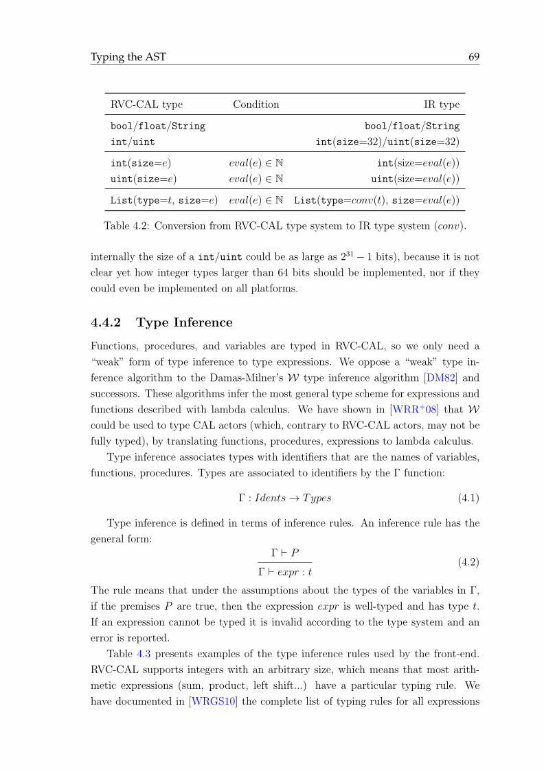
Typing the AST 69
RVC-CAL type Condition IR type
bool/float/String bool/float/String
int/uint int(size=32)/uint(size=32)
int(size=e) eval(e) ∈ N int(size=eval(e))
uint(size=e) eval(e) ∈ N uint(size=eval(e))
List(type=t, size=e) eval(e) ∈ N List(type=conv(t), size=eval(e))
Table 4.2: Conversion from RVC-CAL type system to IR type system (conv).
internally the size of a int/uint could be as large as 231 − 1 bits), because it is not
clear yet how integer types larger than 64 bits should be implemented, nor if they
could even be implemented on all platforms.
4.4.2 Type Inference
Functions, procedures, and variables are typed in RVC-CAL, so we only need a
“weak” form of type inference to type expressions. We oppose a “weak” type in-
ference algorithm to the Damas-Milner’s W type inference algorithm [DM82] and
successors. These algorithms infer the most general type scheme for expressions and
functions described with lambda calculus. We have shown in [WRR+08] that W
could be used to type CAL actors (which, contrary to RVC-CAL actors, may not be
fully typed), by translating functions, procedures, expressions to lambda calculus.
Type inference associates types with identifiers that are the names of variables,
functions, procedures. Types are associated to identifiers by the Γ function:
Γ : Idents→ Types (4.1)
Type inference is defined in terms of inference rules. An inference rule has the
general form:
Γ ⊢ P
Γ ⊢ expr : t(4.2)
The rule means that under the assumptions about the types of the variables in Γ,
if the premises P are true, then the expression expr is well-typed and has type t.
If an expression cannot be typed it is invalid according to the type system and an
error is reported.
Table 4.3 presents examples of the type inference rules used by the front-end.
RVC-CAL supports integers with an arbitrary size, which means that most arith-
metic expressions (sum, product, left shift...) have a particular typing rule. We
have documented in [WRGS10] the complete list of typing rules for all expressions
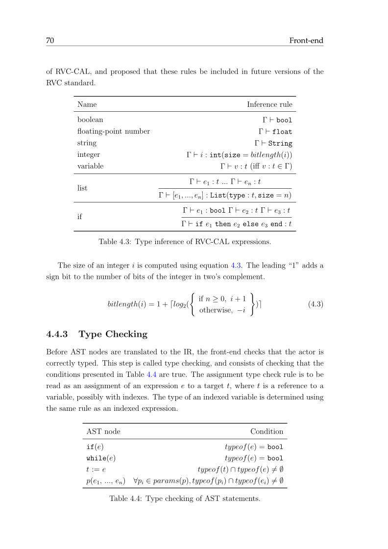
70 Front-end
of RVC-CAL, and proposed that these rules be included in future versions of the
RVC standard.
Name Inference rule
boolean Γ ⊢ bool
floating-point number Γ ⊢ float
string Γ ⊢ String
integer Γ ⊢ i : int(size = bitlength(i))
variable Γ ⊢ v : t (iff v : t ∈ Γ)
listΓ ⊢ e1 : t ... Γ ⊢ en : t
Γ ⊢ [e1, ..., en] : List(type : t, size = n)
ifΓ ⊢ e1 : bool Γ ⊢ e2 : t Γ ⊢ e3 : t
Γ ⊢ if e1 then e2 else e3 end : t
Table 4.3: Type inference of RVC-CAL expressions.
The size of an integer i is computed using equation 4.3. The leading “1” adds a
sign bit to the number of bits of the integer in two’s complement.
bitlength(i) = 1 + ⌈log2(
{
if n ≥ 0, i+ 1
otherwise, −i
}
)⌉ (4.3)
4.4.3 Type Checking
Before AST nodes are translated to the IR, the front-end checks that the actor is
correctly typed. This step is called type checking, and consists of checking that the
conditions presented in Table 4.4 are true. The assignment type check rule is to be
read as an assignment of an expression e to a target t, where t is a reference to a
variable, possibly with indexes. The type of an indexed variable is determined using
the same rule as an indexed expression.
AST node Condition
if(e) typeof(e) = bool
while(e) typeof(e) = bool
t := e typeof(t) ∩ typeof(e) 6= ∅
p(e1, ..., en) ∀pi ∈ params(p), typeof(pi) ∩ typeof(ei) 6= ∅
Table 4.4: Type checking of AST statements.
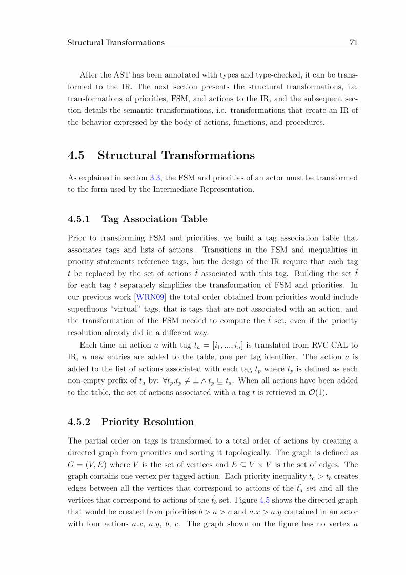
Structural Transformations 71
After the AST has been annotated with types and type-checked, it can be trans-
formed to the IR. The next section presents the structural transformations, i.e.
transformations of priorities, FSM, and actions to the IR, and the subsequent sec-
tion details the semantic transformations, i.e. transformations that create an IR of
the behavior expressed by the body of actions, functions, and procedures.
4.5 Structural Transformations
As explained in section 3.3, the FSM and priorities of an actor must be transformed
to the form used by the Intermediate Representation.
4.5.1 Tag Association Table
Prior to transforming FSM and priorities, we build a tag association table that
associates tags and lists of actions. Transitions in the FSM and inequalities in
priority statements reference tags, but the design of the IR require that each tag
t be replaced by the set of actions t associated with this tag. Building the set t
for each tag t separately simplifies the transformation of FSM and priorities. In
our previous work [WRN09] the total order obtained from priorities would include
superfluous “virtual” tags, that is tags that are not associated with an action, and
the transformation of the FSM needed to compute the t set, even if the priority
resolution already did in a different way.
Each time an action a with tag ta = [i1, ..., in] is translated from RVC-CAL to
IR, n new entries are added to the table, one per tag identifier. The action a is
added to the list of actions associated with each tag tp where tp is defined as each
non-empty prefix of ta by: ∀tp.tp 6= ⊥ ∧ tp ⊑ ta. When all actions have been added
to the table, the set of actions associated with a tag t is retrieved in O(1).
4.5.2 Priority Resolution
The partial order on tags is transformed to a total order of actions by creating a
directed graph from priorities and sorting it topologically. The graph is defined as
G = (V,E) where V is the set of vertices and E ⊆ V × V is the set of edges. The
graph contains one vertex per tagged action. Each priority inequality ta > tb creates
edges between all the vertices that correspond to actions of the ta set and all the
vertices that correspond to actions of the tb set. Figure 4.5 shows the directed graph
that would be created from priorities b > a > c and a.x > a.y contained in an actor
with four actions a.x, a.y, b, c. The graph shown on the figure has no vertex a
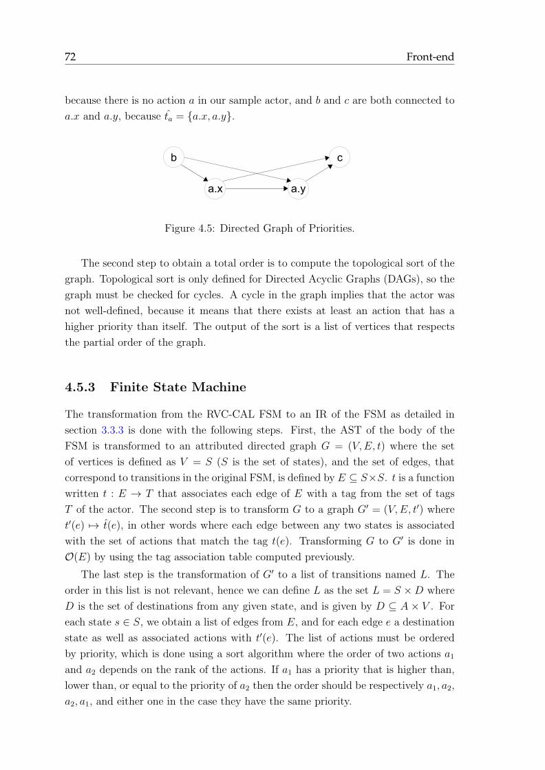
72 Front-end
because there is no action a in our sample actor, and b and c are both connected to
a.x and a.y, because ta = {a.x, a.y}.
b c
a.x a.y
Figure 4.5: Directed Graph of Priorities.
The second step to obtain a total order is to compute the topological sort of the
graph. Topological sort is only defined for Directed Acyclic Graphs (DAGs), so the
graph must be checked for cycles. A cycle in the graph implies that the actor was
not well-defined, because it means that there exists at least an action that has a
higher priority than itself. The output of the sort is a list of vertices that respects
the partial order of the graph.
4.5.3 Finite State Machine
The transformation from the RVC-CAL FSM to an IR of the FSM as detailed in
section 3.3.3 is done with the following steps. First, the AST of the body of the
FSM is transformed to an attributed directed graph G = (V,E, t) where the set
of vertices is defined as V = S (S is the set of states), and the set of edges, that
correspond to transitions in the original FSM, is defined by E ⊆ S×S. t is a function
written t : E → T that associates each edge of E with a tag from the set of tags
T of the actor. The second step is to transform G to a graph G′ = (V,E, t′) where
t′(e) 7→ t(e), in other words where each edge between any two states is associated
with the set of actions that match the tag t(e). Transforming G to G′ is done in
O(E) by using the tag association table computed previously.
The last step is the transformation of G′ to a list of transitions named L. The
order in this list is not relevant, hence we can define L as the set L = S ×D where
D is the set of destinations from any given state, and is given by D ⊆ A × V . For
each state s ∈ S, we obtain a list of edges from E, and for each edge e a destination
state as well as associated actions with t′(e). The list of actions must be ordered
by priority, which is done using a sort algorithm where the order of two actions a1
and a2 depends on the rank of the actions. If a1 has a priority that is higher than,
lower than, or equal to the priority of a2 then the order should be respectively a1, a2,
a2, a1, and either one in the case they have the same priority.
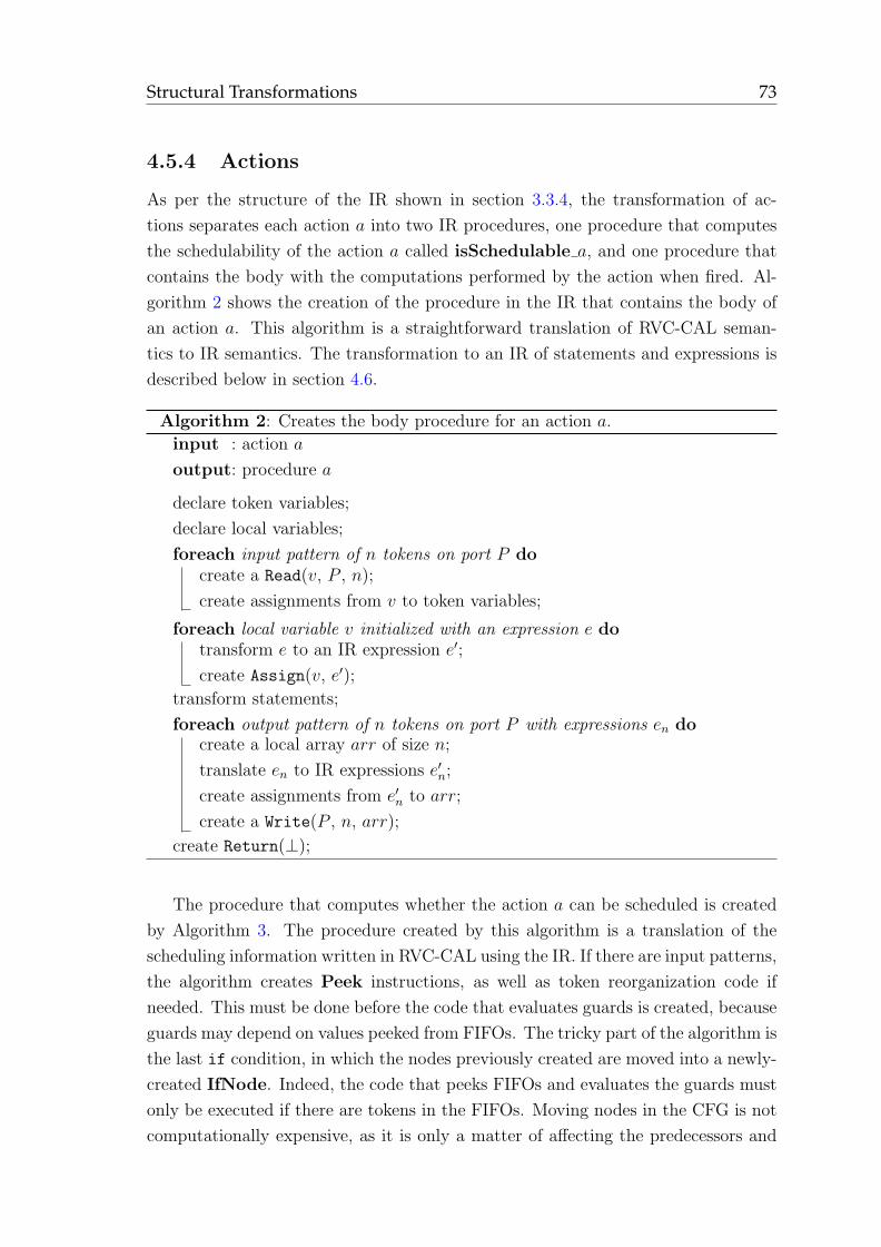
Structural Transformations 73
4.5.4 Actions
As per the structure of the IR shown in section 3.3.4, the transformation of ac-
tions separates each action a into two IR procedures, one procedure that computes
the schedulability of the action a called isSchedulable a, and one procedure that
contains the body with the computations performed by the action when fired. Al-
gorithm 2 shows the creation of the procedure in the IR that contains the body of
an action a. This algorithm is a straightforward translation of RVC-CAL seman-
tics to IR semantics. The transformation to an IR of statements and expressions is
described below in section 4.6.
Algorithm 2: Creates the body procedure for an action a.
input : action a
output: procedure a
declare token variables;
declare local variables;
foreach input pattern of n tokens on port P docreate a Read(v, P , n);
create assignments from v to token variables;
foreach local variable v initialized with an expression e dotransform e to an IR expression e′;
create Assign(v, e′);
transform statements;
foreach output pattern of n tokens on port P with expressions en docreate a local array arr of size n;
translate en to IR expressions e′n;
create assignments from e′n to arr;
create a Write(P , n, arr);
create Return(⊥);
The procedure that computes whether the action a can be scheduled is created
by Algorithm 3. The procedure created by this algorithm is a translation of the
scheduling information written in RVC-CAL using the IR. If there are input patterns,
the algorithm creates Peek instructions, as well as token reorganization code if
needed. This must be done before the code that evaluates guards is created, because
guards may depend on values peeked from FIFOs. The tricky part of the algorithm is
the last if condition, in which the nodes previously created are moved into a newly-
created IfNode. Indeed, the code that peeks FIFOs and evaluates the guards must
only be executed if there are tokens in the FIFOs. Moving nodes in the CFG is not
computationally expensive, as it is only a matter of affecting the predecessors and
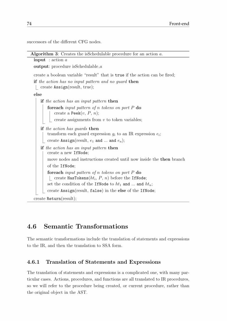
74 Front-end
successors of the different CFG nodes.
Algorithm 3: Creates the isSchedulable procedure for an action a.
input : action a
output: procedure isSchedulable a
create a boolean variable “result” that is true if the action can be fired;
if the action has no input pattern and no guard thencreate Assign(result, true);
else
if the action has an input pattern then
foreach input pattern of n tokens on port P docreate a Peek(v, P , n);
create assignments from v to token variables;
if the action has guards thentransform each guard expression gi to an IR expression ei;
create Assign(result, e1 and ... and en);
if the action has an input pattern thencreate a new IfNode;
move nodes and instructions created until now inside the then branch
of the IfNode;
foreach input pattern of n tokens on port P docreate HasTokens(hti, P , n) before the IfNode;
set the condition of the IfNode to ht1 and ... and htn;
create Assign(result, false) in the else of the IfNode;
create Return(result);
4.6 Semantic Transformations
The semantic transformations include the translation of statements and expressions
to the IR, and then the translation to SSA form.
4.6.1 Translation of Statements and Expressions
The translation of statements and expressions is a complicated one, with many par-
ticular cases. Actions, procedures, and functions are all translated to IR procedures,
so we will refer to the procedure being created, or current procedure, rather than
the original object in the AST.
Semantic Transformations 75
Loading and Storing Global Variables
The front-end produces a code that contains a number of loads and stores that is as
small as possible. Indeed, in the IR a global variable (parameter or state variable)
cannot be used as-is in expressions and needs to be explicitly loaded. Similarly,
when a global variable is assigned in the RVC-CAL source code, this translates to
a store in the IR. However, at most one action can be executed at any given time,
so we have exclusive access to the global variables of the actor, and as a result it is
not necessary to eagerly load or store variables. This simplifies the IR of the code as
well as code generation for hardware targets: during one cycle, programmable logic
can store several global variables, but it cannot store any of them more than once
during the cycle.
To minimize the number of loads and stores, the front-end maintains a set of
variables that need to be loaded, and another set of variables that need to be stored.
These sets are associated to the current procedure, and are initialized to the empty
set. The simplest case is when the procedure does not call another procedure: after
the IR procedure has been fully translated, loads are added at the beginning and
stores at the end. When the procedure does contain calls, however, we need to make
sure that the callee procedure has an up-to-date view of the global variables, and the
front-end inserts spill code around the call. Before the call, this code stores modified
variables that the procedure may load, and after the call, the code re-loads global
variables that the callee procedure may store. If an inline transformation is applied,
this spill code can be identified easily and removed.
Translation of Expressions
The difficulty in the translation of RVC-CAL expressions to the IR lies in the trans-
lation of the functional if and list constructs, and in the fact that the front-end
tries to produce the smallest code for these constructs. For instance the assignment
of a list [e1, e2, ..., en] to a target variable v can be naively translated as the creation
of a temporary list, and a copy of this list to v. However, in most cases2 v can
be assigned the values directly, saving the creation of a copy loop. Similarly, it is
possible for a variable v to be assigned an if that returns a list [e1, e2, ..., en]. In this
case, a naive translation would create code that in each branch of the if, computes
values, copies them into a temporary list, and after the if, copies the temporary
list to v.
To create code that is as small (and hopefully, fast) as possible for assignments
of lists to variables requires the front-end to maintain a current target. When a
2As long as v does not appear on the right hand-side, because the list may reorganize values in
a different order, and assigning v directly will produce wrong results.
76 Front-end
variable is assigned an expression, the target is the variable and indexes used in
the assignment. When an expression is not assigned to anything, for example in
conditions, a temporary variable is created to hold the result and becomes the target.
This target is directly assigned when if and list expressions are translated.
Apart from these considerations, the translation of expressions is done as follows.
Unary and binary expressions have a direct equivalent in the IR, so translating them
is done by translating their operand(s) and creating an equivalent IR expression
with the same operator. Calls to built-in bitwise functions become unary or binary
expressions depending on the function called. A list is translated as a sequence of
stores, surrounded by a WhileNode that corresponds to each generator (if any).
Translation of Statements
The translation of statements is pretty straightforward compared to the translation
of expressions. Calls, if statements, foreach and while loops are transformed to
Call, IfNode, and WhileNode respectively. The only trick is the translation of an
assignment to a variable. If the variable is a list, then the variable becomes the target
in the translator of expressions, which creates the necessary nodes and instructions.
Otherwise, if the variable is a global variable, a temporary local variable is created
to hold the result, and an Assign is created.
4.6.2 Translation to SSA form
The IR created from RVC-CAL statements and expressions does not have the SSA
property initially. As explained in section 2.4.3, Static Single Assignment (SSA)
is a property that makes many optimizations easier to implement, faster, or both,
and reduces memory used to store dataflow information. There are many variants of
SSA: vanilla SSA, semi-pruned SSA, array SSA, interprocedural SSA, etc. [CFR+91,
BCHS98,KS98,SVKW07], and many algorithms that can transform code to minimal
SSA form (with no superfluous φ assignments), using a variety of data structures
and approaches [CFR+91,BM94,CF95,PB95,SG95,AH00].
Of the different strains of SSA, we found that vanilla SSA was the best suited
for our purpose. First, two of the languages we wanted to generate from our IR
(namely LLVM and XLIM) are in vanilla SSA form. Second, the aim of our work
is not to create yet another optimizing compilation infrastructure; we perform a
handful of trivial optimizations in order to produce cleaner and smaller code, but
“true” optimizations should be performed by the compiler specific to the language
in which source code is generated from the IR, therefore we did not feel the need for
more complicated forms of SSA.
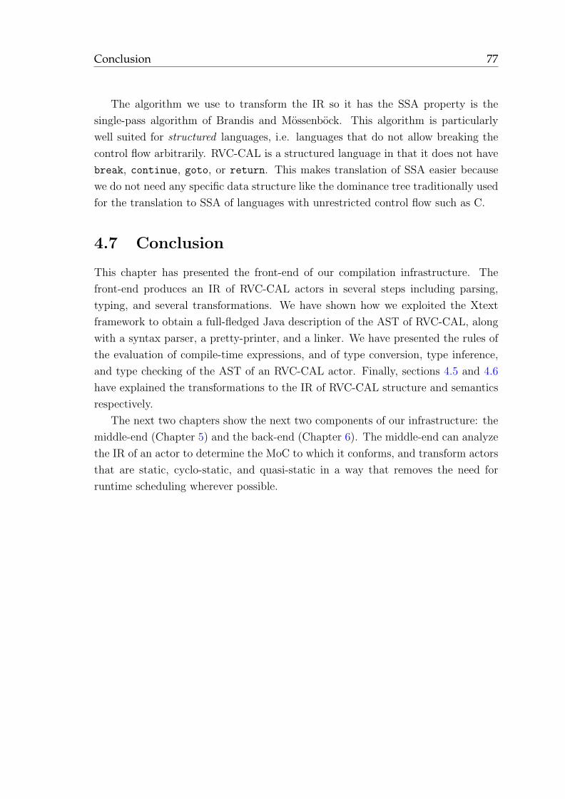
Conclusion 77
The algorithm we use to transform the IR so it has the SSA property is the
single-pass algorithm of Brandis and Mossenbock. This algorithm is particularly
well suited for structured languages, i.e. languages that do not allow breaking the
control flow arbitrarily. RVC-CAL is a structured language in that it does not have
break, continue, goto, or return. This makes translation of SSA easier because
we do not need any specific data structure like the dominance tree traditionally used
for the translation to SSA of languages with unrestricted control flow such as C.
4.7 Conclusion
This chapter has presented the front-end of our compilation infrastructure. The
front-end produces an IR of RVC-CAL actors in several steps including parsing,
typing, and several transformations. We have shown how we exploited the Xtext
framework to obtain a full-fledged Java description of the AST of RVC-CAL, along
with a syntax parser, a pretty-printer, and a linker. We have presented the rules of
the evaluation of compile-time expressions, and of type conversion, type inference,
and type checking of the AST of an RVC-CAL actor. Finally, sections 4.5 and 4.6
have explained the transformations to the IR of RVC-CAL structure and semantics
respectively.
The next two chapters show the next two components of our infrastructure: the
middle-end (Chapter 5) and the back-end (Chapter 6). The middle-end can analyze
the IR of an actor to determine the MoC to which it conforms, and transform actors
that are static, cyclo-static, and quasi-static in a way that removes the need for
runtime scheduling wherever possible.

78 Front-end
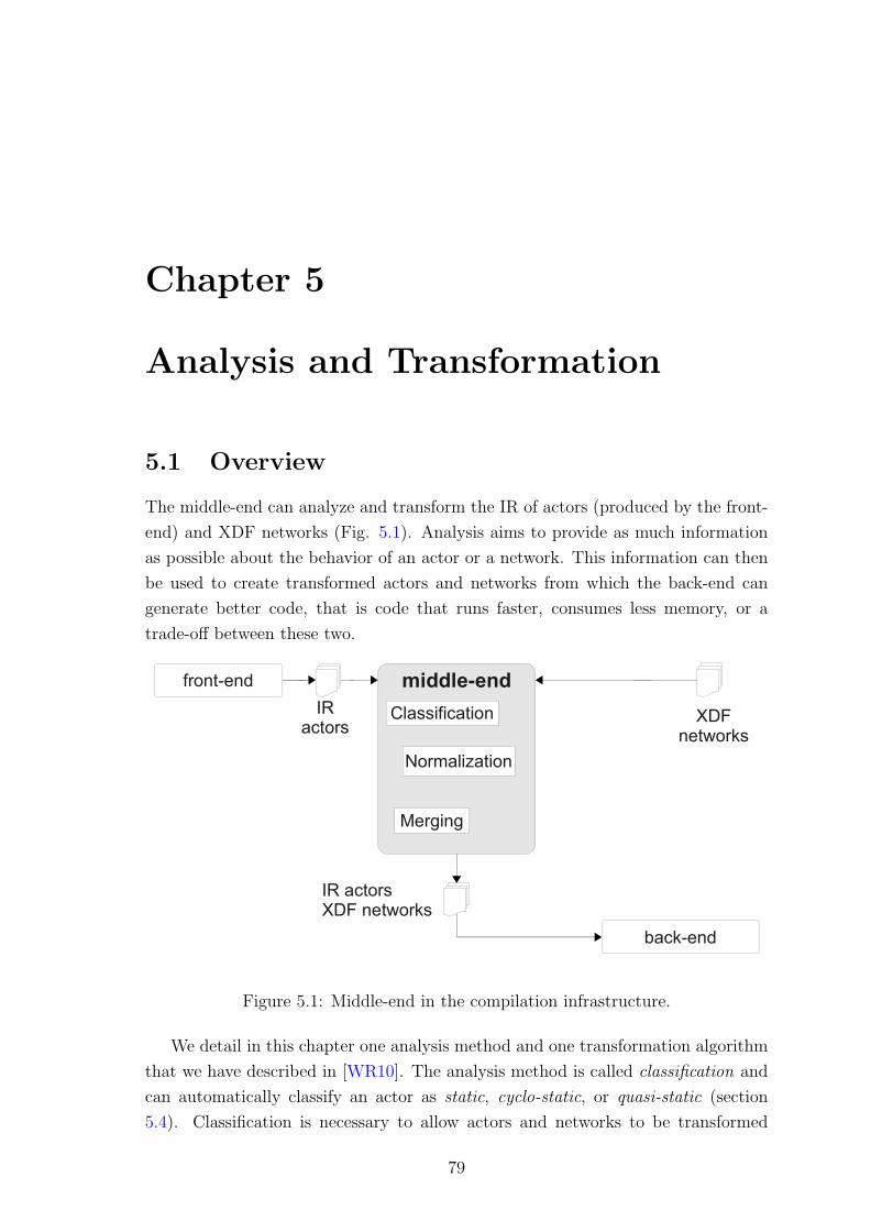
Chapter 5
Analysis and Transformation
5.1 Overview
The middle-end can analyze and transform the IR of actors (produced by the front-
end) and XDF networks (Fig. 5.1). Analysis aims to provide as much information
as possible about the behavior of an actor or a network. This information can then
be used to create transformed actors and networks from which the back-end can
generate better code, that is code that runs faster, consumes less memory, or a
trade-off between these two.
Classification
Normalization
Merging
middle-endfront-end
IRactors
XDFnetworks
back-end
IR actorsXDF networks
Figure 5.1: Middle-end in the compilation infrastructure.
We detail in this chapter one analysis method and one transformation algorithm
that we have described in [WR10]. The analysis method is called classification and
can automatically classify an actor as static, cyclo-static, or quasi-static (section
5.4). Classification is necessary to allow actors and networks to be transformed
79
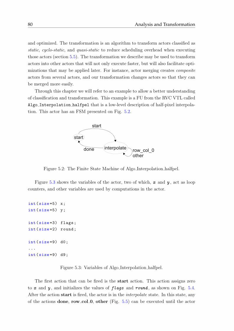
80 Analysis and Transformation
and optimized. The transformation is an algorithm to transform actors classified as
static, cyclo-static, and quasi-static to reduce scheduling overhead when executing
those actors (section 5.5). The transformation we describe may be used to transform
actors into other actors that will not only execute faster, but will also facilitate opti-
mizations that may be applied later. For instance, actor merging creates composite
actors from several actors, and our transformation changes actors so that they can
be merged more easily.
Through this chapter we will refer to an example to allow a better understanding
of classification and transformation. This example is a FU from the RVC VTL called
Algo Interpolation halfpel that is a low-level description of half-pixel interpola-
tion. This actor has an FSM presented on Fig. 5.2.
start
interpolatedone
start
row_col_0other
Figure 5.2: The Finite State Machine of Algo Interpolation halfpel.
Figure 5.3 shows the variables of the actor, two of which, x and y , act as loop
counters, and other variables are used by computations in the actor.
int(size =5) x;
int(size =5) y;
int(size =3) flags;
int(size =2) round;
int(size =9) d0;
...
int(size =9) d9;
Figure 5.3: Variables of Algo Interpolation halfpel.
The first action that can be fired is the start action. This action assigns zero
to x and y , and initializes the values of flags and round , as shown on Fig. 5.4.
After the action start is fired, the actor is in the interpolate state. In this state, any
of the actions done, row col 0, other (Fig. 5.5) can be executed until the actor
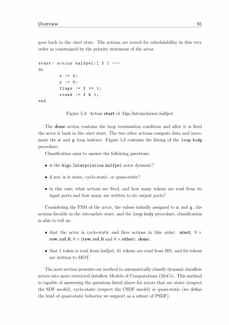
Overview 81
goes back to the start state. The actions are tested for schedulability in this very
order as constrained by the priority statement of the actor.
start: action halfpel :[ f ] ==>
do
x := 0;
y := 0;
flags := f >> 1;
round := f & 1;
end
Figure 5.4: Action start of Algo Interpolation halfpel.
The done action contains the loop termination condition and after it is fired
the actor is back in the start state. The two other actions compute data and incre-
ment the x and y loop indexes. Figure 5.6 contains the listing of the loop body
procedure.
Classification aims to answer the following questions:
• is the Algo Interpolation halfpel actor dynamic?
• if not, is it static, cyclo-static, or quasi-static?
• in this case, what actions are fired, and how many tokens are read from its
input ports and how many are written to its output ports?
Considering the FSM of the actor, the values initially assigned to x and y , the
actions fireable in the interpolate state, and the loop body procedure, classification
is able to tell us:
• that the actor is cyclo-static and fires actions in this order: start, 9 ×
row col 0, 8× (row col 0 and 8× other), done,
• that 1 token is read from halfpel, 81 tokens are read from RD, and 64 tokens
are written to MOT.
The next section presents our method to automatically classify dynamic dataflow
actors into more restricted dataflow Models of Computations (MoCs). This method
is capable of answering the questions listed above for actors that are static (respect
the SDF model), cyclo-static (respect the CSDF model) or quasi-static (we define
the kind of quasi-static behavior we support as a subset of PSDF).
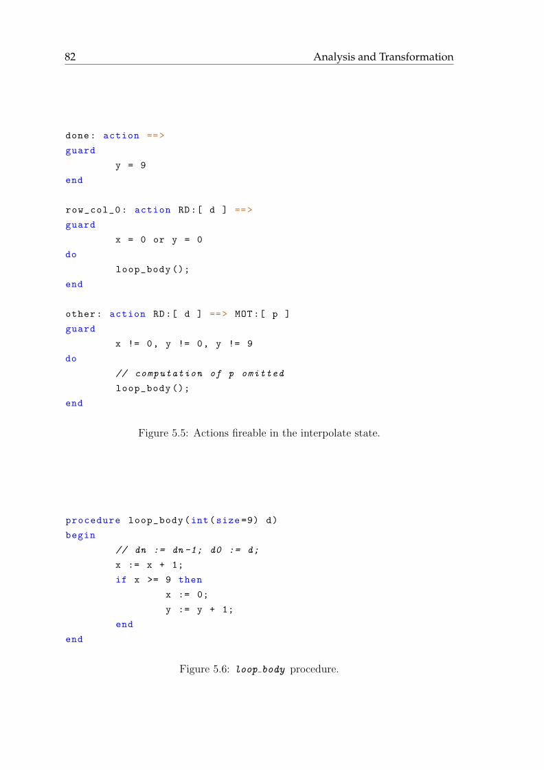
82 Analysis and Transformation
done: action ==>
guard
y = 9
end
row_col_0: action RD:[ d ] ==>
guard
x = 0 or y = 0
do
loop_body ();
end
other: action RD:[ d ] ==> MOT:[ p ]
guard
x != 0, y != 0, y != 9
do
// computation of p omitted
loop_body ();
end
Figure 5.5: Actions fireable in the interpolate state.
procedure loop_body(int(size =9) d)
begin
// dn := dn -1; d0 := d;
x := x + 1;
if x >= 9 then
x := 0;
y := y + 1;
end
end
Figure 5.6: loop body procedure.
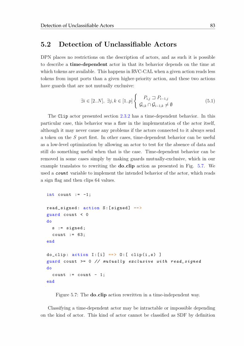
Detection of Unclassifiable Actors 83
5.2 Detection of Unclassifiable Actors
DPN places no restrictions on the description of actors, and as such it is possible
to describe a time-dependent actor in that its behavior depends on the time at
which tokens are available. This happens in RVC-CAL when a given action reads less
tokens from input ports than a given higher-priority action, and these two actions
have guards that are not mutually exclusive:
∃i ∈ [2..N ], ∃j, k ∈ [1..p]
{
Pi,j ⊐ Pi−1,j
Gi,k ∩ Gi−1,k 6= ∅(5.1)
The Clip actor presented section 2.3.2 has a time-dependent behavior. In this
particular case, this behavior was a flaw in the implementation of the actor itself,
although it may never cause any problems if the actors connected to it always send
a token on the S port first. In other cases, time-dependent behavior can be useful
as a low-level optimization by allowing an actor to test for the absence of data and
still do something useful when that is the case. Time-dependent behavior can be
removed in some cases simply by making guards mutually-exclusive, which in our
example translates to rewriting the do clip action as presented in Fig. 5.7. We
used a count variable to implement the intended behavior of the actor, which reads
a sign flag and then clips 64 values.
int count := -1;
read_signed: action S:[ signed] ==>
guard count < 0
do
s := signed;
count := 63;
end
do_clip: action I:[i] ==> O:[ clip(i,s) ]
guard count >= 0 // mutually exclusive with read_signed
do
count := count - 1;
end
Figure 5.7: The do clip action rewritten in a time-independent way.
Classifying a time-dependent actor may be intractable or impossible depending
on the kind of actor. This kind of actor cannot be classified as SDF by definition
84 Analysis and Transformation
(equation 5.1 is incompatible with equation 2.4), but it could still be considered
a valid cyclo-static or quasi-static actor, in which case we would need to record
the sequences of tokens that lead to this cyclo-static or quasi-static behavior. The
intractability of classifying such an actor lies just there.
We showed in [WR10] that the time-dependent version of the Clip actor could be
considered cyclo-static with a period of 65 tokens, because we supposed that tokens
would arrive in the correct order. Even knowing the period of a time-dependent
actor, an automatic classification would still need to explore all the possible input
patterns, from [⊥,⊥] to [[∗, ..., ∗], [∗, ..., ∗]], which means at most 265 combinations in
this case, with no clear heuristic to prune useless sequences. Worse, if an actor were
entirely dynamic, there would be no criterion as to when to stop the enumeration of
possible tokens.
Therefore our classification method must detect and discard time-dependent ac-
tors to prevent enumerating the universe of possible token sequences. Detecting
actions that read less tokens from input ports than higher-priority actions is trivial.
However, such actions may not render the actor time-dependent if their guards are
exclusive, which must be mechanically verified. To this end we feed the guards to a
constraint solving system, which either gives the values of tokens and state variables
that satisfy both guards (guards not mutually exclusive), or else finds no solution
(guards mutually exclusive).
Constraints are created from the guards of an action as follows. The guards of
an action are boolean expressions that must be simultaneously true for the action to
be fired, so we translate each guard of any two actions to a constraint. Suppose an
action has a guard x > 0 and the other action has a guard x 6= 1, then the constraint
solver will find values of x that satisfy the constraints, such as x = 2. If there is
such a solution, this means the guards are not mutually exclusive.
5.3 Abstract Interpretation of Actors
Classifying an actor within a MoC is based on checking that a certain number of
MoC-dependent rules hold true for any execution of this actor. Some of these rules
are verified solely from the structural information of the actor, for instance the rules
for a static actor only depends on the input and output patterns of actions. In
more complicated cases, we need to be able to obtain information from an actual
execution. The actor must be executed so that the information obtained is valid
for any execution of the actor, whatever its environment (the values of the tokens
and the manner in which they are available). As a consequence it is not possible to
simply execute the actor with a particular environment supplied by the programmer.
Abstract Interpretation of Actors 85
To circumvent this problem we use abstract interpretation [CC77].
5.3.1 Rules of Abstract Interpretation
Abstract interpretation is an interpretation of the computations performed by a
program in an abstract universe of objects rather than on concrete objects. Our
abstract interpretation of an actor has the following properties:
• The set of values that can be assigned to a variable is
V alues = Z ∪ {true , false } ∪ {⊥}
The value ⊥ is used for variables whose value is unknown, e.g. for uninitialized
variables.
• The environment is defined as an association of variables and their values:
Env : Idents→ V alues
Env initially contains the state variables of the actor associated with their
initial value if they have one, otherwise with ⊥.
• When the interpreter enters an action, the environment is augmented with
bindings between the name of the tokens in the input pattern and ⊥. In other
words, a token read has an unknown value by default.
The abstract interpreter interprets an actor by firing it repeatedly until either
one of the conditions is met:
1. The interpreter is told to stop because analysis is complete as determined by
the classification algorithm.
2. The interpreter cannot compute if an action may be fired because this infor-
mation depends on a variable whose value is ⊥.
To fire the actor, the interpreter starts by selecting one fireable action, that is
an action that meets the criteria defined section 2.3. The abstract interpretation
of an RVC-CAL actor is the same as its concrete interpretation with the following
exceptions. Any expression that references a variable v where Env(v) = ⊥ has the
value ⊥. Conditional statements and loops that test an expression whose value is ⊥
are not executed. However, guards evaluated as ⊥ cause the abstract interpreter to
stop as per condition 2.
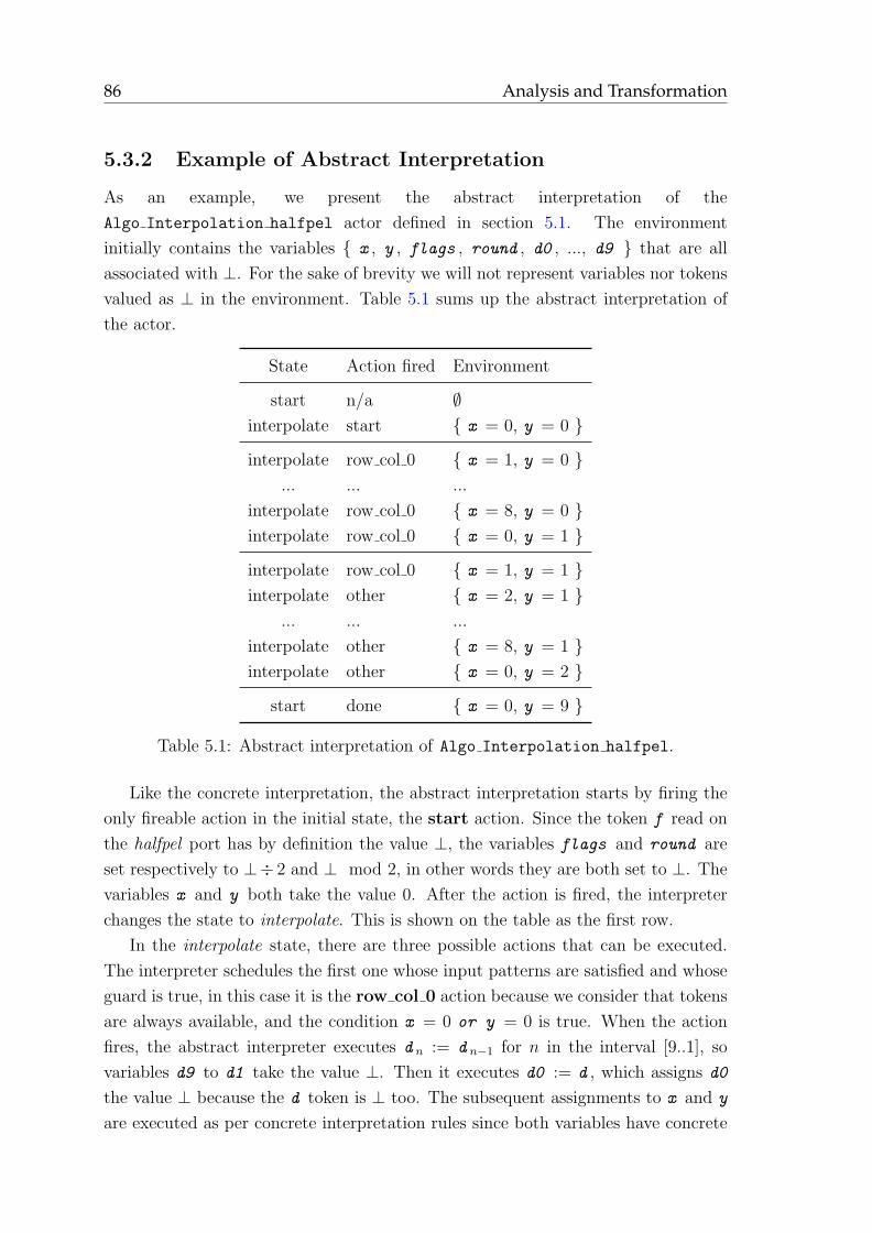
86 Analysis and Transformation
5.3.2 Example of Abstract Interpretation
As an example, we present the abstract interpretation of the
Algo Interpolation halfpel actor defined in section 5.1. The environment
initially contains the variables { x , y , flags , round , d0 , ..., d9 } that are all
associated with ⊥. For the sake of brevity we will not represent variables nor tokens
valued as ⊥ in the environment. Table 5.1 sums up the abstract interpretation of
the actor.
State Action fired Environment
start n/a ∅
interpolate start { x = 0, y = 0 }
interpolate row col 0 { x = 1, y = 0 }
... ... ...
interpolate row col 0 { x = 8, y = 0 }
interpolate row col 0 { x = 0, y = 1 }
interpolate row col 0 { x = 1, y = 1 }
interpolate other { x = 2, y = 1 }
... ... ...
interpolate other { x = 8, y = 1 }
interpolate other { x = 0, y = 2 }
start done { x = 0, y = 9 }
Table 5.1: Abstract interpretation of Algo Interpolation halfpel.
Like the concrete interpretation, the abstract interpretation starts by firing the
only fireable action in the initial state, the start action. Since the token f read on
the halfpel port has by definition the value ⊥, the variables flags and round are
set respectively to ⊥÷ 2 and ⊥ mod 2, in other words they are both set to ⊥. The
variables x and y both take the value 0. After the action is fired, the interpreter
changes the state to interpolate. This is shown on the table as the first row.
In the interpolate state, there are three possible actions that can be executed.
The interpreter schedules the first one whose input patterns are satisfied and whose
guard is true, in this case it is the row col 0 action because we consider that tokens
are always available, and the condition x = 0 or y = 0 is true. When the action
fires, the abstract interpreter executes d n := d n−1 for n in the interval [9..1], so
variables d9 to d1 take the value ⊥. Then it executes d0 := d , which assigns d0
the value ⊥ because the d token is ⊥ too. The subsequent assignments to x and y
are executed as per concrete interpretation rules since both variables have concrete
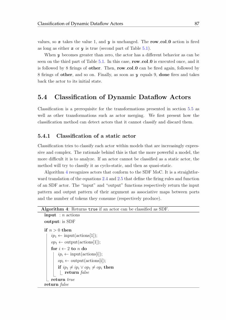
Classification of Dynamic Dataflow Actors 87
values, so x takes the value 1, and y is unchanged. The row col 0 action is fired
as long as either x or y is true (second part of Table 5.1).
When y becomes greater than zero, the actor has a different behavior as can be
seen on the third part of Table 5.1. In this case, row col 0 is executed once, and it
is followed by 8 firings of other. Then, row col 0 can be fired again, followed by
8 firings of other, and so on. Finally, as soon as y equals 9, done fires and takes
back the actor to its initial state.
5.4 Classification of Dynamic Dataflow Actors
Classification is a prerequisite for the transformations presented in section 5.5 as
well as other transformations such as actor merging. We first present how the
classification method can detect actors that it cannot classify and discard them.
5.4.1 Classification of a static actor
Classification tries to classify each actor within models that are increasingly expres-
sive and complex. The rationale behind this is that the more powerful a model, the
more difficult it is to analyze. If an actor cannot be classified as a static actor, the
method will try to classify it as cyclo-static, and then as quasi-static.
Algorithm 4 recognizes actors that conform to the SDF MoC. It is a straightfor-
ward translation of the equations 2.4 and 2.5 that define the firing rules and function
of an SDF actor. The “input” and “output” functions respectively return the input
pattern and output pattern of their argument as associative maps between ports
and the number of tokens they consume (respectively produce).
Algorithm 4: Returns true if an actor can be classified as SDF.
input : n actions
output: is SDF
if n > 0 thenip1 ← input(actions[1]);
op1 ← output(actions[1]);
for i← 2 to n doipi ← input(actions[i]);
opi ← output(actions[i]);
if ip1 6= ipi ∨ op1 6= opi thenreturn false
return truereturn false
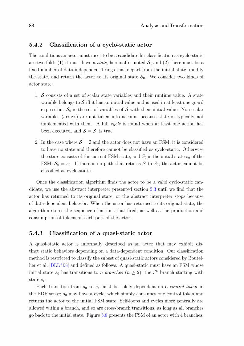
88 Analysis and Transformation
5.4.2 Classification of a cyclo-static actor
The conditions an actor must meet to be a candidate for classification as cyclo-static
are two-fold: (1) it must have a state, hereinafter noted S, and (2) there must be a
fixed number of data-independent firings that depart from the initial state, modify
the state, and return the actor to its original state S0. We consider two kinds of
actor state:
1. S consists of a set of scalar state variables and their runtime value. A state
variable belongs to S iff it has an initial value and is used in at least one guard
expression. S0 is the set of variables of S with their initial value. Non-scalar
variables (arrays) are not taken into account because state is typically not
implemented with them. A full cycle is found when at least one action has
been executed, and S = S0 is true.
2. In the case where S = ∅ and the actor does not have an FSM, it is considered
to have no state and therefore cannot be classified as cyclo-static. Otherwise
the state consists of the current FSM state, and S0 is the initial state s0 of the
FSM: S0 = s0. If there is no path that returns S to S0, the actor cannot be
classified as cyclo-static.
Once the classification algorithm finds the actor to be a valid cyclo-static can-
didate, we use the abstract interpreter presented section 5.3 until we find that the
actor has returned to its original state, or the abstract interpreter stops because
of data-dependent behavior. When the actor has returned to its original state, the
algorithm stores the sequence of actions that fired, as well as the production and
consumption of tokens on each port of the actor.
5.4.3 Classification of a quasi-static actor
A quasi-static actor is informally described as an actor that may exhibit dis-
tinct static behaviors depending on a data-dependent condition. Our classification
method is restricted to classify the subset of quasi-static actors considered by Boutel-
lier et al. [BLL+08] and defined as follows. A quasi-static must have an FSM whose
initial state s0 has transitions to n branches (n ≥ 2), the ith branch starting with
state si.
Each transition from s0 to si must be solely dependent on a control token in
the BDF sense; s0 may have a cycle, which simply consumes one control token and
returns the actor to the initial FSM state. Self-loops and cycles more generally are
allowed within a branch, and so are cross-branch transitions, as long as all branches
go back to the initial state. Figure 5.8 presents the FSM of an actor with 4 branches:
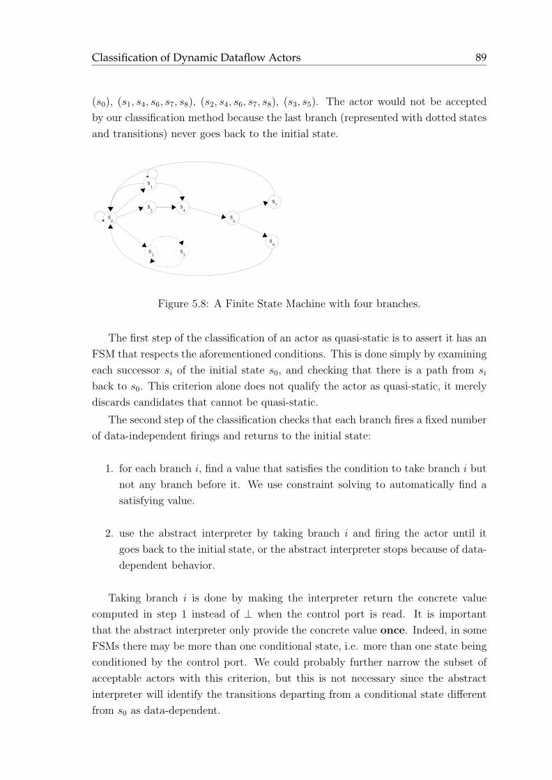
Classification of Dynamic Dataflow Actors 89
(s0), (s1, s4, s6, s7, s8), (s2, s4, s6, s7, s8), (s3, s5). The actor would not be accepted
by our classification method because the last branch (represented with dotted states
and transitions) never goes back to the initial state.
s0
s1
s2
s4
s6
s3
s5
s7
s8
Figure 5.8: A Finite State Machine with four branches.
The first step of the classification of an actor as quasi-static is to assert it has an
FSM that respects the aforementioned conditions. This is done simply by examining
each successor si of the initial state s0, and checking that there is a path from si
back to s0. This criterion alone does not qualify the actor as quasi-static, it merely
discards candidates that cannot be quasi-static.
The second step of the classification checks that each branch fires a fixed number
of data-independent firings and returns to the initial state:
1. for each branch i, find a value that satisfies the condition to take branch i but
not any branch before it. We use constraint solving to automatically find a
satisfying value.
2. use the abstract interpreter by taking branch i and firing the actor until it
goes back to the initial state, or the abstract interpreter stops because of data-
dependent behavior.
Taking branch i is done by making the interpreter return the concrete value
computed in step 1 instead of ⊥ when the control port is read. It is important
that the abstract interpreter only provide the concrete value once. Indeed, in some
FSMs there may be more than one conditional state, i.e. more than one state being
conditioned by the control port. We could probably further narrow the subset of
acceptable actors with this criterion, but this is not necessary since the abstract
interpreter will identify the transitions departing from a conditional state different
from s0 as data-dependent.
90 Analysis and Transformation
5.5 Transformation of Classified Actors
This section presents a method to automatically transform actors that were classified
as static, cyclo-static, or quasi-static, to higher-level SDF and PSDF graphs. This
transformation improves execution speed of the resulting actors, and makes merging
actors of the same kind easier.
5.5.1 Transformation to SDF and PSDF
The classification of actors gives information about the sequence of actions that were
fired:
• in the case of static behavior, there may only be one action by definition;
actors that have several actions with similar input/output patterns must be
transformed to single-action actors.
• in the case of cyclo-static behavior, the sequence is a list of actions with fixed
production/consumption rates that start from an initial state and eventually
return to this initial state.
• in the case of quasi-static behavior, there are several sequences of actions;
each sequence is a concatenation of a first conditional action and a sequence
of actions with fixed production/consumption rates.
To allow actors to be merged later, these sequences must be transformed to
respect appropriate MoCs. They can be trivially transformed from cyclo-static to
CSDF and from quasi-static to PSDF, by transforming an action invocation to a
vertex and setting production and consumption to zero on every edge (since the
actions do not consume the data of one another). Sadly, this sort of graphs are
useless:
• They do not represent the behavior of the actors.
• They are not suitable for merging, in particular merging SDF graphs together
when each graph is composed of up to a few hundred vertices can quickly result
in huge graphs, especially if the repetitions of vertices are not multiple of one
another (see [LM87] for additional explanations).
• They cannot be efficiently mapped and scheduled because optimally scheduling
a SDF graph is an NP-complete problem [PPW+09].
A better representation is a graph where a sequence of actions is transformed to
a single higher-level action that fires all the actions in the sequence consecutively,
Transformation of Classified Actors 91
this way edges can carry the proper production/consumption rates and the graph
accurately represents the actor’s behavior. The contents of higher-level actions can
be factorized with loop rerolling.
5.5.2 Loop Rerolling
Loop rerolling is the exact opposite of the well-known loop unrolling transformation.
It has been used by Stitt and Vahid to recover loop structures from compiled code
[SV05]. In the context of this work, we used this transformation to find loops of
actions within an initially flat sequence of actions.
The general algorithm to perform loop rerolling is as follows:
1. recognize common sequences within an input sequence
2. form loops around consecutive repetitions of common sequences
We used the Sequitur [NMW97] algorithm to recognize common sequences of
actions from the initially flat list of actions. Sequitur works by deriving a hierarchical
structure in the form of a Context-Free Grammar from a sequence of symbols. For
instance the grammar G1 derived from the sequence of symbols ababc is:
• S → A A c
• A → a b
In our case, the initial input is a sequence of actions. Action tags cannot be used
directly however, as Sequitur may group components from different tags together.
For example, the grammar G2 derived from a.b a.c a.b a.c x.y is:
• S → A B C B ’ ’ x . y
• A → a .
• B → b C c
• C → ’ ’ A
This grammar is of no use, because it cannot be exploited to find repetitions of
actions. On the other hand, if we replace a.b by a, a.c by b, and x.y by c, we
obtain the sequence ababc. As shown above, this leads to the grammar G1, which
is clearly more amenable to analysis of loop patterns.
To obtain loops from the hierarchical structure, we walk through the hierarchical
structure by counting the number of rule invocations and developing the rules. For
92 Analysis and Transformation
instance, suppose we have a sequence1 composed of four repetitions of a sub-sequence
composed of five as followed by three bs, noted 4(5(a) 3(b)). The corresponding
grammar is:
• S → A B C C C D
• A → a a
• B → A a
• C → D B A
• D → b b b
The grammar is gradually transformed as follows:
• S1 → A B 3(C) D
• S2 → 2(a) A a 3(D B A) 3(b)
• S3 → 2(a) 2(a) a 3(3(b) A a 2(a)) 3(b)
• S4 → 2(a) 2(a) a 3(3(b) 2(a) a 2(a)) 3(b)
Finally we group consecutive actions together, which gives us 5(a) 3(3(b) 5(a)) 3(b).
Sequitur works in linear time, so the hierarchical structure it derives is not optimal,
which explains why the result is not minimal in terms of number of loops.
Figure 5.9 shows what the output of loop rerolling looks like on the
Algo Interpolation halfpel actor. As mentioned above, Sequitur may not al-
ways derive the optimal grammar, which is why there is an additional loop on other
that would not have been necessary should the first loop include one less row col 0.
5.5.3 Reduction of the Number of Accesses to FIFOs
Before classification, all actors are considered dynamic. This means that to fire an
action an action scheduler must check that there are enough tokens in the input
FIFOs and enough space in the output FIFOs, read tokens, compute data, and
write tokens. After classification we know that some actors have a behavior that is
static, cyclo-static, or quasi-static. As a consequence, we have information about
the number of tokens and the space needed for several actions to fire, not just one.
A static actor is transformed to an actor with a single action, so it is not possible
to reduce the number of read and write operations. Conversely, after loop rerolling
1The developed sequence is “aaaaabbbaaaaabbbaaaaabbbaaaaabbb”.
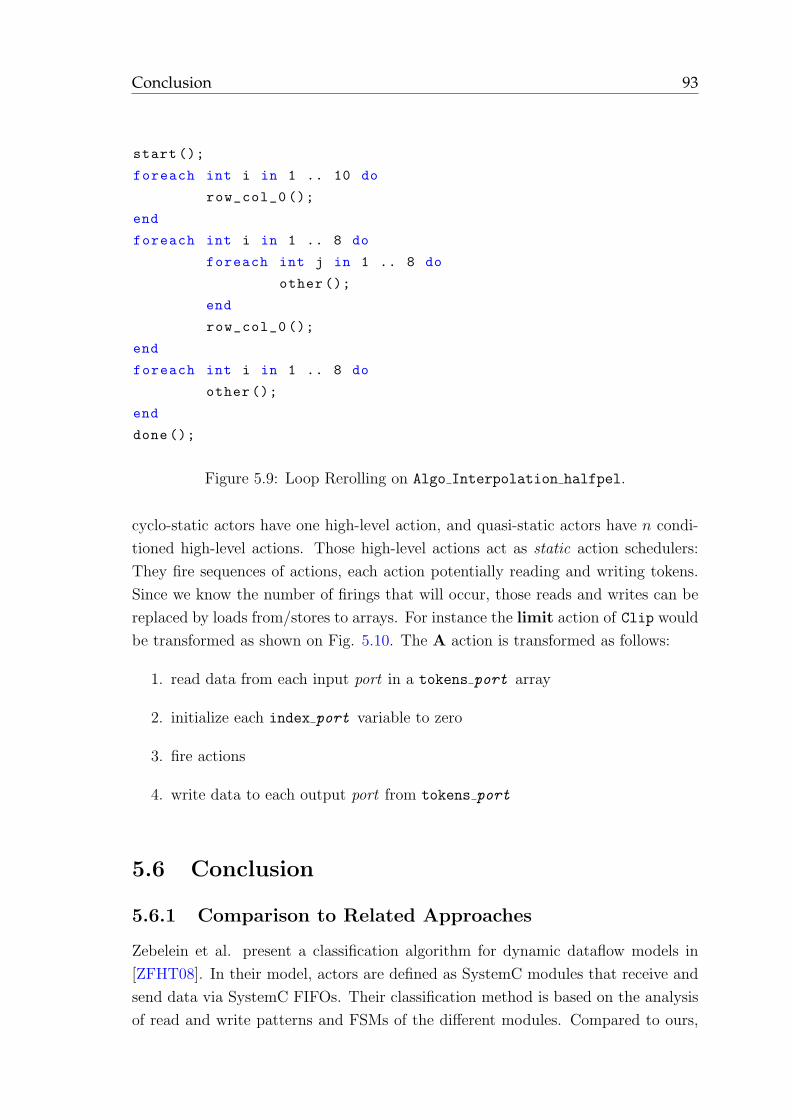
Conclusion 93
start ();
foreach int i in 1 .. 10 do
row_col_0 ();
end
foreach int i in 1 .. 8 do
foreach int j in 1 .. 8 do
other ();
end
row_col_0 ();
end
foreach int i in 1 .. 8 do
other ();
end
done ();
Figure 5.9: Loop Rerolling on Algo Interpolation halfpel.
cyclo-static actors have one high-level action, and quasi-static actors have n condi-
tioned high-level actions. Those high-level actions act as static action schedulers:
They fire sequences of actions, each action potentially reading and writing tokens.
Since we know the number of firings that will occur, those reads and writes can be
replaced by loads from/stores to arrays. For instance the limit action of Clip would
be transformed as shown on Fig. 5.10. The A action is transformed as follows:
1. read data from each input port in a tokens port array
2. initialize each index port variable to zero
3. fire actions
4. write data to each output port from tokens port
5.6 Conclusion
5.6.1 Comparison to Related Approaches
Zebelein et al. present a classification algorithm for dynamic dataflow models in
[ZFHT08]. In their model, actors are defined as SystemC modules that receive and
send data via SystemC FIFOs. Their classification method is based on the analysis
of read and write patterns and FSMs of the different modules. Compared to ours,
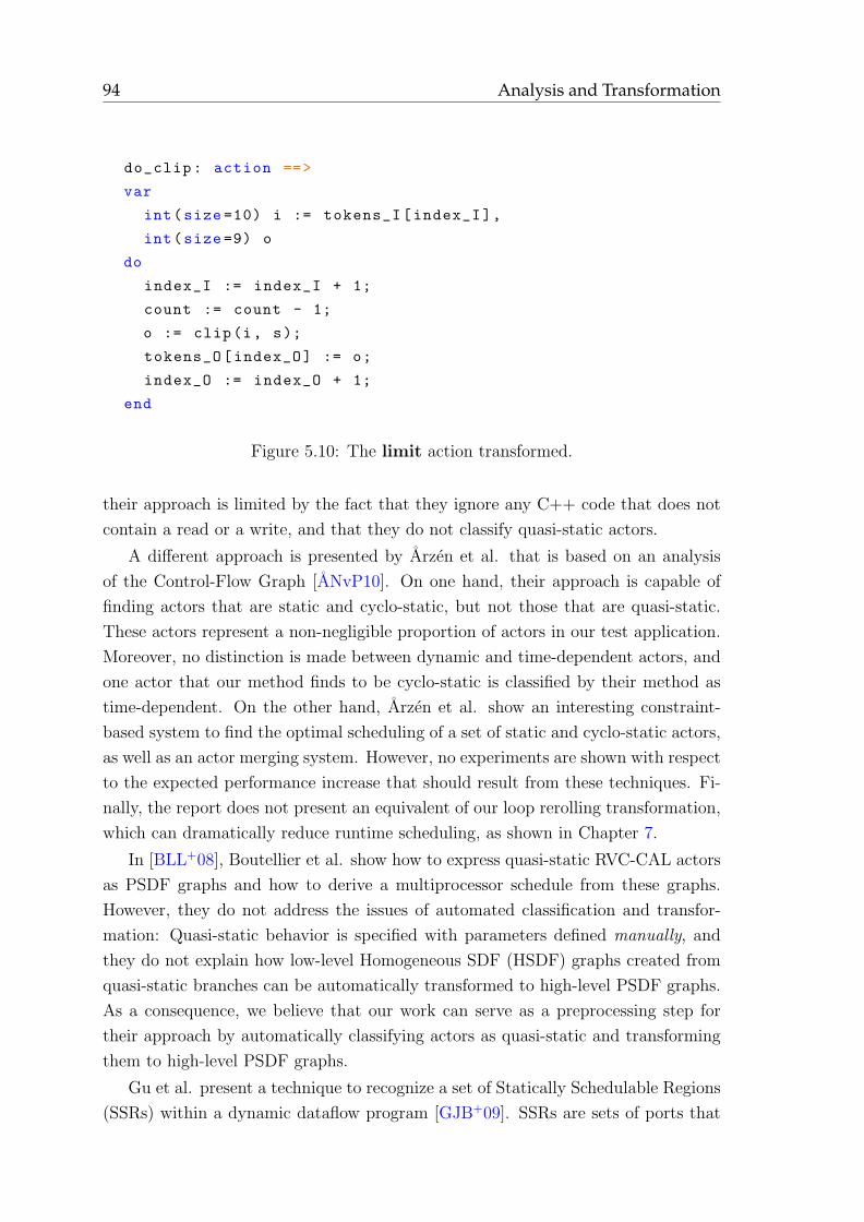
94 Analysis and Transformation
do_clip: action ==>
var
int(size =10) i := tokens_I[index_I],
int(size =9) o
do
index_I := index_I + 1;
count := count - 1;
o := clip(i, s);
tokens_O[index_O] := o;
index_O := index_O + 1;
end
Figure 5.10: The limit action transformed.
their approach is limited by the fact that they ignore any C++ code that does not
contain a read or a write, and that they do not classify quasi-static actors.
A different approach is presented by Arzen et al. that is based on an analysis
of the Control-Flow Graph [ANvP10]. On one hand, their approach is capable of
finding actors that are static and cyclo-static, but not those that are quasi-static.
These actors represent a non-negligible proportion of actors in our test application.
Moreover, no distinction is made between dynamic and time-dependent actors, and
one actor that our method finds to be cyclo-static is classified by their method as
time-dependent. On the other hand, Arzen et al. show an interesting constraint-
based system to find the optimal scheduling of a set of static and cyclo-static actors,
as well as an actor merging system. However, no experiments are shown with respect
to the expected performance increase that should result from these techniques. Fi-
nally, the report does not present an equivalent of our loop rerolling transformation,
which can dramatically reduce runtime scheduling, as shown in Chapter 7.
In [BLL+08], Boutellier et al. show how to express quasi-static RVC-CAL actors
as PSDF graphs and how to derive a multiprocessor schedule from these graphs.
However, they do not address the issues of automated classification and transfor-
mation: Quasi-static behavior is specified with parameters defined manually, and
they do not explain how low-level Homogeneous SDF (HSDF) graphs created from
quasi-static branches can be automatically transformed to high-level PSDF graphs.
As a consequence, we believe that our work can serve as a preprocessing step for
their approach by automatically classifying actors as quasi-static and transforming
them to high-level PSDF graphs.
Gu et al. present a technique to recognize a set of Statically Schedulable Regions
(SSRs) within a dynamic dataflow program [GJB+09]. SSRs are sets of ports that
Conclusion 95
are statically coupled, which essentially means that the production of an output port
matches the consumption of the input port(s) it is connected to (additional criteria
are developed in [GJB+09]). On the one hand, SSR classification has potentially
more knowledge about static behavior because it looks at connected actors rather
than just inside actors. On the other hand, by considering an actor as a whole our
classification can discover its behavior (cyclo-static and quasi-static) and transform
it into a high-level SDF or PSDF graph that will make merging easier. Using SSRs to
obtain additional information as an input to our classification algorithm is a possible
direction for future work.
5.6.2 Conclusion
This chapter has presented one analysis method called classification that can auto-
matically classify an actor as static, cyclo-static or a restricted form of quasi-static
behavior. Classification annotates an actor with an MoC, token production/con-
sumption rates, and a sequence of actions (or sequences of actions in the case of
quasi-static behavior). This information can then be used by a transformation
method that reduces scheduling overhead and can facilitate other transformations
of dynamic dataflow programs, such as actor merging or the quasi-static scheduling
method of Boutellier et al. [BLL+08].
The next chapter details the back-end of our compilation infrastructure that gen-
erates code in several languages from networks and the IR of actors. Chapter 7 will
then present applications on which we have tested our classification and transforma-
tion methods, and results in terms of the number of actors that can be successfully
classified with our method, as well as the speedup given by our transformation.

96 Analysis and Transformation
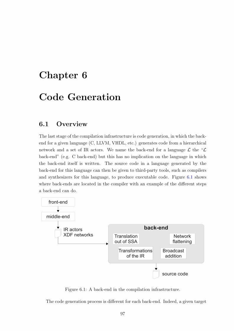
Chapter 6
Code Generation
6.1 Overview
The last stage of the compilation infrastructure is code generation, in which the back-
end for a given language (C, LLVM, VHDL, etc.) generates code from a hierarchical
network and a set of IR actors. We name the back-end for a language L the “L
back-end” (e.g. C back-end) but this has no implication on the language in which
the back-end itself is written. The source code in a language generated by the
back-end for this language can then be given to third-party tools, such as compilers
and synthesizers for this language, to produce executable code. Figure 6.1 shows
where back-ends are located in the compiler with an example of the different steps
a back-end can do.
front-end
middle-end
IR actorsXDF networks
source code
back-end
Transformationsof the IR
Networkflattening
Translationout of SSA
Broadcastaddition
Figure 6.1: A back-end in the compilation infrastructure.
The code generation process is different for each back-end. Indeed, a given target
97
98 Code Generation
language and the associated tools and architecture generally do not have the same
capabilities as another target language and its tools. For instance, VHDL natively
supports the description of hierarchical architectures, while most popular software
languages do not have anything specific for this. Additionally target languages do
not have the same expressiveness, for instance C code is higher-level than VHDL, and
even more than Intermediate Representations like LLVM or XLIM. As a result, many
steps in the general code generation process are optional, and back-ends execute
these steps as needed.
There exists a myriad of programming languages, as well as many intermediate
representations and several hardware description languages, but it is not necessary
to write a back-end for each of these. First of all, the first language one thinks of
generating is unequivocally the C language. Although it was invented forty years ago,
it is still the second most popular language1 for writing software. Most languages
can use C code via a Foreign Function Interface (FFI): Java has the Java Native
Interface (JNI), C++ simply requires the programmer to declare C functions in
extern "C" namespace, and major dynamic languages (such as Python and PHP)
have a well-defined C FFI.
The only architecture that C is not well-adapted to is programmable logic. Al-
though high-level synthesizers are capable of transforming C code into Register
Transfer Level (RTL) description (a description of the flow of signals between hard-
ware registers and the operations performed on these signals), they require the C
code to be written using a strict subset of C (no pointers, no memory allocation).
Additionally, the synthesized RTL code is inherently sub-optimal (in terms of speed
and occupation) because C code is sequential, whereas hardware descriptions are typ-
ically parallel, and the language does not allow the description of integers with an
arbitrary size. Conversely, dataflow networks are a natural abstraction of hardware
architectures by providing hierarchical, inherently parallel descriptions. Actors writ-
ten in RVC-CAL, with arbitrary-sized integers and atomic actions, are well-suited
to be translated to hardware.
Another interesting target is the Low-Level Virtual Machine (LLVM). LLVM is
a platform-neutral, low-level IR, which can be executed on the fly on many archi-
tectures by a Just-In-Time (JIT) engine. Consequently, it is possible to generate a
portable LLVM representation of a Video Tool Library (VTL) [GWPR10a], and to
load actors from this portable VTL on demand when instantiating a network. This
is the purpose of a tool called Jade (JIT Adaptive Decoder Engine) [GWPR10c].
Using the portable VTL in LLVM, Jade is capable of truly reconfiguring a video
decoder dynamically.
1According to the Tiobe index, see http://www.tiobe.com
Overview 99
Our earlier work had focused on generating C code from CAL [WRR+08,
RWR+08,WRN09], and as a consequence the first back-end I wrote in our com-
pilation infrastructure was a C back-end. I have also written a Java back-end, and
have participated in several back-ends written by other people:
• A C++ back-end written by Ghislain Roquier that generates C++ code for
actors and networks; this back-end can be used in a co-design context where
parts of a network are executed by programmable logic.
• An LLVM back-end written by Jerome Gorin that generates LLVM code for
actors; actors in LLVM form can then be loaded on-demand along with an XDF
network by the Just-in-time Adaptive Decoder Engine (Jade) [GWPR10c].
• A VHDL back-end written by Nicolas Siret that generates VHDL code for
actors and networks [SWNR10].
At the time of this writing, other back-ends are work in progress. The first is
a promela back-end whose aim is to allow RVC-CAL dataflow programs to be
checked by the spin model checker (see [HL91] for more details on promela and
spin). The other one is an XLIM back-end to allow the use of other CAL-oriented
tools, like Xlim2C or OpenForge.
The back-end for a given language can perform any or all of the following steps:
1. actor code generation
• transform the Intermediate Representation so that it forms a subset of
the target language and there exists a valid representation in the target
language for each IR instruction and node,
• print code in the target language directly from the transformed IR.
2. network code generation
• close each network in the hierarchy, starting from the top network, by
replacing parameters by their concrete value,
• flatten the network,
• add broadcast where necessary,
• serialize the networks to XDF or print code for each network.
The next section presents how code is printed, and how this influences the data
structure and transformations of the IR. The two subsequent sections present the
transformations of the IR and the transformations of the network respectively.
100 Code Generation
6.2 Printing Code
Printing code is the one step that is common to actor code generation and network
code generation. It produces textual output from a model, where in our case the
model is either an IR actor or a network.
6.2.1 Approaches to Code Printing
There are two kinds of approaches to transform an IR to a target language L: pro-
grammatic approaches or the template approach. Programmatic approaches print
code according to a program, while in the template approach the code is printed
according to a template, which can be informally described as chunks of text inter-
leaved with code or references to data.
Programmatic Approaches
The two most used programmatic approaches are the following:
1. pretty-print an IR to L using visitors, print statements, explicitly specifying
indentation/“dedentation” e.g. at the entry/exit of a block,
2. translate an IR to the AST of L, and pretty-print the resulting AST.
The first approach allows the highest degree of control since everything is done
manually, but this is at the expense of productivity and maintainability. The code
mainly consists of calls to print the text, thus obfuscating the textual representation
of each element. Code written by hand (for instance to prototype a new way of
generating code) cannot be copied/pasted as-is, but instead must be formatted with
a print by line.
The second approach has several advantages over the first one. First of all, we are
not concerned with the textual representation, but with the abstract representation,
which means a productivity a lot higher. The translation from the IR to the AST of L
makes it impossible to produce L code that is not syntactically-correct. Translating
the IR to an AST is relatively easy, an AST being a superset of the IR in most cases.
The main drawback of this approach is that it is necessary to have a description
of the AST and a pretty-printer for it for each language. There are libraries available
for many languages, but not necessarily all, and describing the AST of a language
from scratch is not trivial. Additionally, libraries are not necessarily all written in
the same language, which means you need to write code in this language or use
bindings to it to use the library. Finally, describing a chunk of manually-written
Printing Code 101
code (like a wrapper or initialization code) by constructing an AST is a lot more
verbose than textual code, and the code is painful to write and read2.
The Template Approach
The template approach focuses on describing the textual representation of each ele-
ment of the IR with templates. Contrary to programmatic approaches, the template
approach is text-centric: most of the contents of a template is text. Using templates
has several advantages other programmatic approaches. The visual representation
(in our case generated source code) is independent from the model (IR actor) and
is no longer hard-coded. It is a lot faster to write a template for a language than to
describe the AST constructs in the target language, not to mention the time that
may be necessary to describe the AST or write bindings to an existing library. It is
also very easy to print code differently, like switching from K&R style in C to ANSI
style or Java-like style, whereas changing the style of a pretty-printer can be tricky.
Templates are mostly used by web designers to isolate design from model, and
by programmers who write code generators. Perhaps one of the most early form
of template engine is the m4 macro-processor, used by the Autoconf tools to create
the famous configure scripts. A more recent template engine is the JavaServer
Pages (JSP), which make writing a dynamic website in Java in a similar way to
PHP. The Eclipse Modeling Framework (EMF) uses Java Emitter Templates (JET)
within the Eclipse platform to produce Java code from models. Another example of
what can be considered a template engine is XSLT (Extensible Stylesheet Language
Transformations). XSLT is an XML-based language that creates a new document
(in XML, HTML, or text) from an original XML document by applying template
rules to XML nodes.
6.2.2 The StringTemplate Template Engine
The compilation infrastructure uses the StringTemplate [Par06] to print code with
templates. StringTemplate (ST) is a template engine that strictly enforces sep-
aration of model and view [Par04]. The Model-View-Controller (MVC) [KP88]
paradigm states that an application be described as three connected components:
1. the model manages the behavior and state of the application
2. the view manages the visual representation of the model
3. the controller may update the view and the model when appropriate.
2As a matter of fact, this has been our experience with our Cal2C code generator, which
constructed C code chunks with CIL.
102 Code Generation
MVC is a popular way of implementating a GUI, but can also be applied to other
situations. In particular, we can see a template system as conforming to MVC, where
the View is the template, the Model is the model, and the Controller is the template
engine.
The strict separation of model and view enforced by StringTemplate reduces
the likelihood of having bugs in the printer, or ending up with bloated templates.
This is advocated by Terrence Parr, StringTemplate’s author, in [Par04], and I have
found empirical support that computations in a template are an important source of
hard-to-track bugs in my previous experience with both code generation with m4 and
web design with PHP. Because you can only do so much in a template, in particular
you cannot write code that computes something, you have to do all computations
once and for all in the model. This has two consequences: (1) never will there be
some code hidden inside a template that has an unanticipated side-effect, and (2)
a ST template will contain some control (if/then/else) and loops to iterate on
lists and maps, but most of the contents of the template are the chunks of text it
produces.
Comparison to Related Template Engines
We use EMF technology in the front-end, thus making JET a good candidate for a
template engine, yet JET resembles JSP (without the dependence on Java Enterprise
Edition), which means that code is allowed in the template, which is something that
should be avoided. XSLT was a candidate, but first the IR was not serialized in XML
(although admittedly it would have been possible to remedy that), and second, XSLT
is heavy and complex (it is Turing complete after all), and allows computations to
be performed in the view — although its declarative nature makes it somehow less
error-prone.
Another interesting feature not necessarily found in template engines is on-the-
fly compilation of templates. Many template engines generate code from a template
that must be compiled and linked for the template to be callable by client code.
Instead, ST compiles the templates when they are first loaded, and interprets them.
On-the-fly compilation allows templates to be corrected, improved, and tested much
faster. This is particularly useful when trying a new approach in generated code,
something that typically requires many rounds of trial and error. The disadvantage
of interpretation, as opposed to off-line compilation, is that the template engine
is not as fast. In practice, however, we tackled this problem by leveraging the
concurrent Java API to apply n templates in parallel, with n being the number of
cores of the machine.
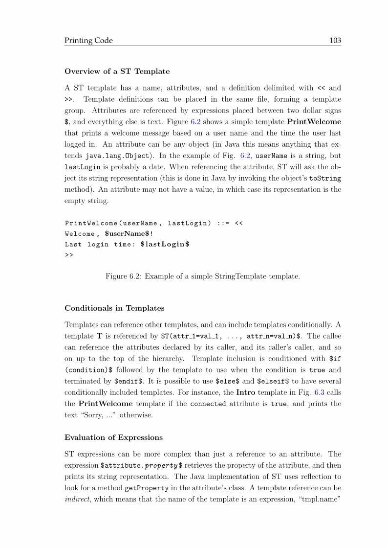
Printing Code 103
Overview of a ST Template
A ST template has a name, attributes, and a definition delimited with << and
>>. Template definitions can be placed in the same file, forming a template
group. Attributes are referenced by expressions placed between two dollar signs
$, and everything else is text. Figure 6.2 shows a simple template PrintWelcome
that prints a welcome message based on a user name and the time the user last
logged in. An attribute can be any object (in Java this means anything that ex-
tends java.lang.Object). In the example of Fig. 6.2, userName is a string, but
lastLogin is probably a date. When referencing the attribute, ST will ask the ob-
ject its string representation (this is done in Java by invoking the object’s toString
method). An attribute may not have a value, in which case its representation is the
empty string.
PrintWelcome(userName , lastLogin) ::= <<
Welcome , $userName$!
Last login time: $ lastLogin$
>>
Figure 6.2: Example of a simple StringTemplate template.
Conditionals in Templates
Templates can reference other templates, and can include templates conditionally. A
template T is referenced by $T(attr 1=val 1, ..., attr n=val n)$. The callee
can reference the attributes declared by its caller, and its caller’s caller, and so
on up to the top of the hierarchy. Template inclusion is conditioned with $if
(condition)$ followed by the template to use when the condition is true and
terminated by $endif$. It is possible to use $else$ and $elseif$ to have several
conditionally included templates. For instance, the Intro template in Fig. 6.3 calls
the PrintWelcome template if the connected attribute is true, and prints the
text “Sorry, ...” otherwise.
Evaluation of Expressions
ST expressions can be more complex than just a reference to an attribute. The
expression $attribute.property $ retrieves the property of the attribute, and then
prints its string representation. The Java implementation of ST uses reflection to
look for a method getProperty in the attribute’s class. A template reference can be
indirect, which means that the name of the template is an expression, “tmpl.name”
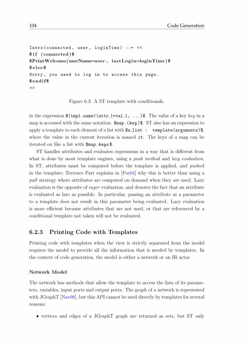
104 Code Generation
Intro(connected , user , loginTime) ::= <<
$ i f ( connected )$
$PrintWelcome(userName=user , lastLogin=loginTime)$
$ e l se $
Sorry , you need to log in to access this page.
$endif$
>>
Figure 6.3: A ST template with conditionals.
in the expression $(tmpl.name)(attr 1=val 1, ...)$. The value of a key key in a
map is accessed with the same notation: $map.(key )$. ST also has an expression to
apply a template to each element of a list with $a list : template(arguments)$,
where the value in the current iteration is named it. The keys of a map can be
iterated on like a list with $map.keys $.
ST handles attributes and evaluates expressions in a way that is different from
what is done by most template engines, using a push method and lazy evaluation.
In ST, attributes must be computed before the template is applied, and pushed
in the template; Terrence Parr explains in [Par04] why this is better than using a
pull strategy where attributes are computed on demand when they are used. Lazy
evaluation is the opposite of eager evaluation, and denotes the fact that an attribute
is evaluated as late as possible. In particular, passing an attribute as a parameter
to a template does not result in this parameter being evaluated. Lazy evaluation
is more efficient because attributes that are not used, or that are referenced by a
conditional template not taken will not be evaluated.
6.2.3 Printing Code with Templates
Printing code with templates when the view is strictly separated from the model
requires the model to provide all the information that is needed by templates. In
the context of code generation, the model is either a network or an IR actor.
Network Model
The network has methods that allow the template to access the lists of its parame-
ters, variables, input ports and output ports. The graph of a network is represented
with JGraphT [Nav08], but this API cannot be used directly by templates for several
reasons:
• vertices and edges of a JGraphT graph are returned as sets, but ST only
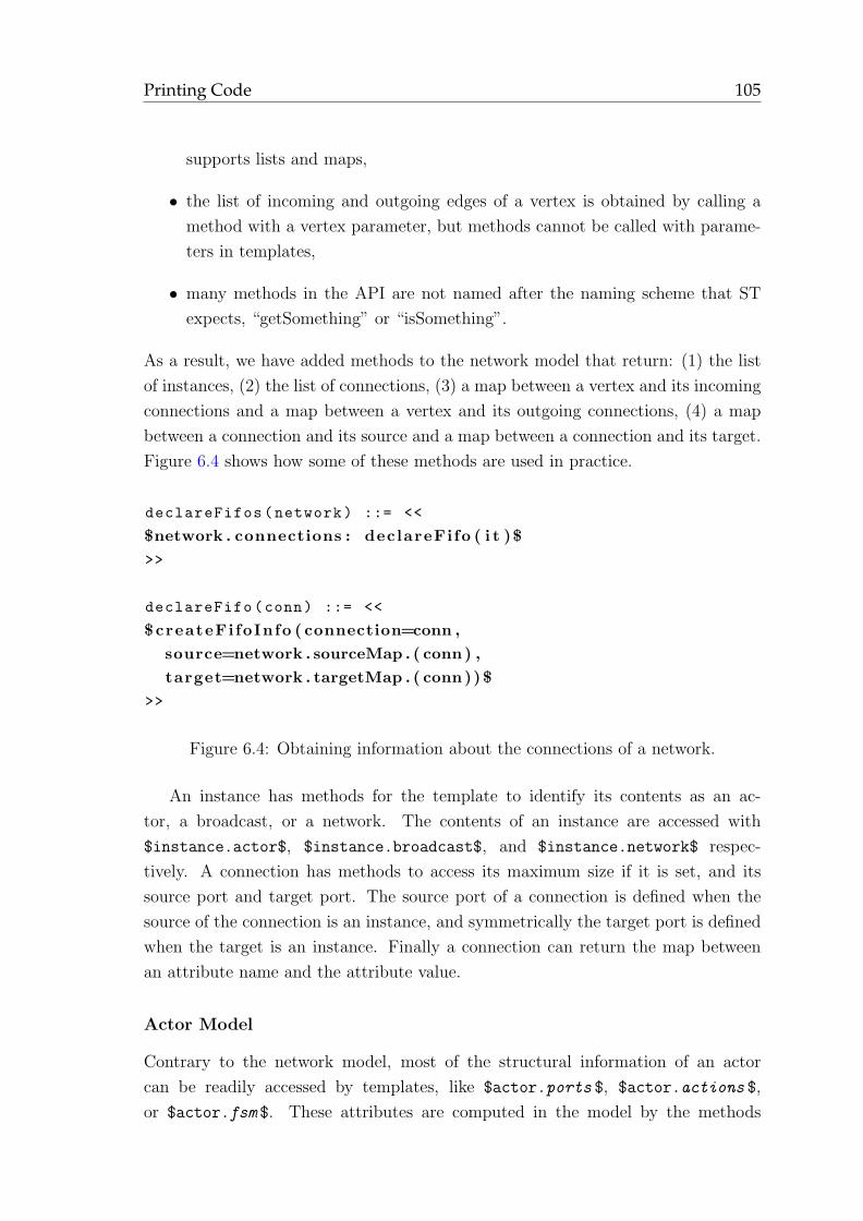
Printing Code 105
supports lists and maps,
• the list of incoming and outgoing edges of a vertex is obtained by calling a
method with a vertex parameter, but methods cannot be called with parame-
ters in templates,
• many methods in the API are not named after the naming scheme that ST
expects, “getSomething” or “isSomething”.
As a result, we have added methods to the network model that return: (1) the list
of instances, (2) the list of connections, (3) a map between a vertex and its incoming
connections and a map between a vertex and its outgoing connections, (4) a map
between a connection and its source and a map between a connection and its target.
Figure 6.4 shows how some of these methods are used in practice.
declareFifos(network) ::= <<
$network . connections : declareFifo ( i t )$
>>
declareFifo(conn) ::= <<
$createFifoInfo ( connection=conn ,
source=network . sourceMap . ( conn) ,
target=network . targetMap . ( conn))$
>>
Figure 6.4: Obtaining information about the connections of a network.
An instance has methods for the template to identify its contents as an ac-
tor, a broadcast, or a network. The contents of an instance are accessed with
$instance.actor$, $instance.broadcast$, and $instance.network$ respec-
tively. A connection has methods to access its maximum size if it is set, and its
source port and target port. The source port of a connection is defined when the
source of the connection is an instance, and symmetrically the target port is defined
when the target is an instance. Finally a connection can return the map between
an attribute name and the attribute value.
Actor Model
Contrary to the network model, most of the structural information of an actor
can be readily accessed by templates, like $actor.ports $, $actor.actions $,
or $actor.fsm $. These attributes are computed in the model by the methods
106 Code Generation
getPorts, getActions, getFsm, which return the ports, actions, and FSM respec-
tively. The IR of statements and expressions is significantly lower-level than struc-
tural information, and there are cases where a naive utilization of templates is not
simple, efficient, or even possible. As a result, specific “tricks” or techniques are
required to handle the following cases gracefully:
• templates of instructions
• printing casts
• printing code for expressions
• template-specific data
As described in Chapter 3, the IR represents the body of an action or a procedure
as a Control-Flow Graph (CFG) where nodes can be basic blocks of instructions or
conditional nodes, namely if and while nodes. There are ten instruction kinds, from
Assign to Write. The API closely reflects this, and adds another instruction kind
called SpecificInstruction to model instructions that are specific to one or more
back-ends. The different node kinds and instruction kinds are subclasses of generic
Node and Instruction interfaces respectively. These interfaces have methods that
test the nature of a node (respectively an instruction), like isIfNode or isAssign,
which can be used in templates. However, using these methods in templates is
verbose and not scalable, because each time a specific instruction Ii is added to the
API a method isIi must be added to the Instruction interface. An alternative is
shown on Fig 6.5, by using the “simple name” of the class of the instruction as the
template name.
Some languages require that when a variable is assigned an expression with a
different type, the expression be casted to the type of the variable. The IR does
not have a built-in representation for casts because the rules that govern the need
for type-casting are language-specific. Languages with arbitrary-sized integers (like
LLVM or VHDL) are quite strict in this regard, whereas C/C++ code generated
from the IR does not even require casting; Java somehow falls in the middle. Us-
ing casts in templates is pretty straightforward: every instruction that assigns a
value to a variable (in the general sense, including loads and stores) has a getCast
method that returns a Cast object if a cast is needed. The class has the properties
$cast.truncated $, $cast.extended $, and $cast.signed $ that respectively in-
dicate if the cast truncates the value, extends the value, and if the value is signed.
If the cast is extended and signed, the value will be extended and its sign bit kept.
As mentioned above, there are things that cannot be done with a template, and
printing readable arithmetic expressions from the expression tree of the IR is one of
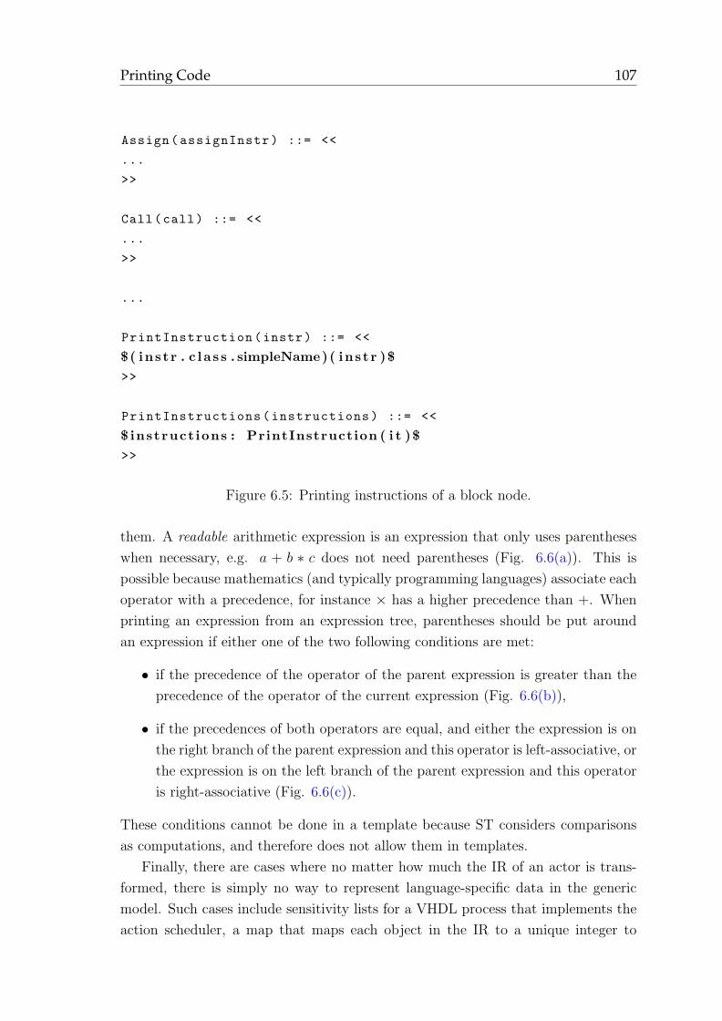
Printing Code 107
Assign(assignInstr) ::= <<
...
>>
Call(call) ::= <<
...
>>
...
PrintInstruction(instr) ::= <<
$( instr . c l a s s . simpleName)( instr )$
>>
PrintInstructions(instructions) ::= <<
$ instruct ions : PrintInstruction ( i t )$
>>
Figure 6.5: Printing instructions of a block node.
them. A readable arithmetic expression is an expression that only uses parentheses
when necessary, e.g. a + b ∗ c does not need parentheses (Fig. 6.6(a)). This is
possible because mathematics (and typically programming languages) associate each
operator with a precedence, for instance × has a higher precedence than +. When
printing an expression from an expression tree, parentheses should be put around
an expression if either one of the two following conditions are met:
• if the precedence of the operator of the parent expression is greater than the
precedence of the operator of the current expression (Fig. 6.6(b)),
• if the precedences of both operators are equal, and either the expression is on
the right branch of the parent expression and this operator is left-associative, or
the expression is on the left branch of the parent expression and this operator
is right-associative (Fig. 6.6(c)).
These conditions cannot be done in a template because ST considers comparisons
as computations, and therefore does not allow them in templates.
Finally, there are cases where no matter how much the IR of an actor is trans-
formed, there is simply no way to represent language-specific data in the generic
model. Such cases include sensitivity lists for a VHDL process that implements the
action scheduler, a map that maps each object in the IR to a unique integer to
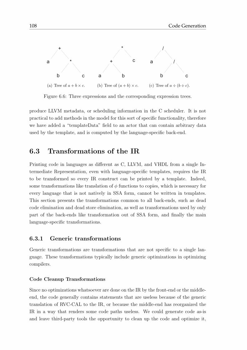
108 Code Generation
a
b c
*
+
(a) Tree of a+ b× c.
a
c
b
+
*
(b) Tree of (a+ b)× c.
a
b c
/
/
(c) Tree of a÷ (b÷ c).
Figure 6.6: Three expressions and the corresponding expression trees.
produce LLVM metadata, or scheduling information in the C scheduler. It is not
practical to add methods in the model for this sort of specific functionality, therefore
we have added a “templateData” field to an actor that can contain arbitrary data
used by the template, and is computed by the language-specific back-end.
6.3 Transformations of the IR
Printing code in languages as different as C, LLVM, and VHDL from a single In-
termediate Representation, even with language-specific templates, requires the IR
to be transformed so every IR construct can be printed by a template. Indeed,
some transformations like translation of φ functions to copies, which is necessary for
every language that is not natively in SSA form, cannot be written in templates.
This section presents the transformations common to all back-ends, such as dead
code elimination and dead store elimination, as well as transformations used by only
part of the back-ends like transformation out of SSA form, and finally the main
language-specific transformations.
6.3.1 Generic transformations
Generic transformations are transformations that are not specific to a single lan-
guage. These transformations typically include generic optimizations in optimizing
compilers.
Code Cleanup Transformations
Since no optimizations whatsoever are done on the IR by the front-end or the middle-
end, the code generally contains statements that are useless because of the generic
translation of RVC-CAL to the IR, or because the middle-end has reorganized the
IR in a way that renders some code paths useless. We could generate code as-is
and leave third-party tools the opportunity to clean up the code and optimize it,
Transformations of the IR 109
but many compilers print warnings whenever there is unused code or variables. As
a result, the code generator does a few transformations on the IR to clean it up,
namely dead store elimination [CFR+91], dead globals elimination, and a simple
form of dead code elimination (e.g. conditionals always true or always false).
The dead store elimination takes the semantics of FIFO operations into account.
For instance, it is possible to remove useless Peek instructions, but Reads must not
be removed because it would change the semantics of the actor.
Translation out of SSA
Contrary to the IR, most target languages are not in SSA form. The IR must thus be
transformed to a non-SSA form so that code does not have φ functions anymore. This
transformation is called “out-of-SSA translation” and the literature proposes several
methods for this [CFR+91, BCHS98, SJGS99, BDR+09]. The method proposed by
Cytron et al. in [CFR+91] for translation out of SSA is simple but can exhibit
subtle errors in some cases, as pointed out by Briggs et al. in [BCHS98], who thus
describe algorithms that produces correct code after the translation out of SSA.
Sreedhar et al. [SJGS99] later present a method that is simpler and more efficient
than the previous algorithms of Briggs et al. Finally, Boissinot et al. [BDR+09]
show an approach that aims at being a “provably-correct method, generic, simple to
implement”, even in cases where the previous methods can be “incorrect, incomplete,
overly pessimistic, or too expensive”.
Fortunately, the method of Cytron et al. works in our case. Their approach
consists of replacing a φ-function in a block b by one copy in each predecessor block
of b. This results in numerous copies in the CFG, which can then be removed by
register allocation using methods such as described in [CAC+81,CH84,BCT94,PS99].
This approach stops working when optimizations such as code motion [Cli95], copy
propagation, partial redundancy elimination [MR79, BC94, CCK+97] increase the
live ranges of variables or break the assumption that a φ-function merges definitions
of the same variable.
Our compiler does not provide these sophisticated optimizations, for the simple
reason that compilers for the target languages we generate are optimizing compilers
and will perform these optimizations, and many others. The simple optimizations
we have implemented allow us to use the naive out of SSA translation method. The
code generator does not use a coalescing register allocator though, which means it
generates many useless copies, but again the tools that are fed the generated code
are expected to take care of that.
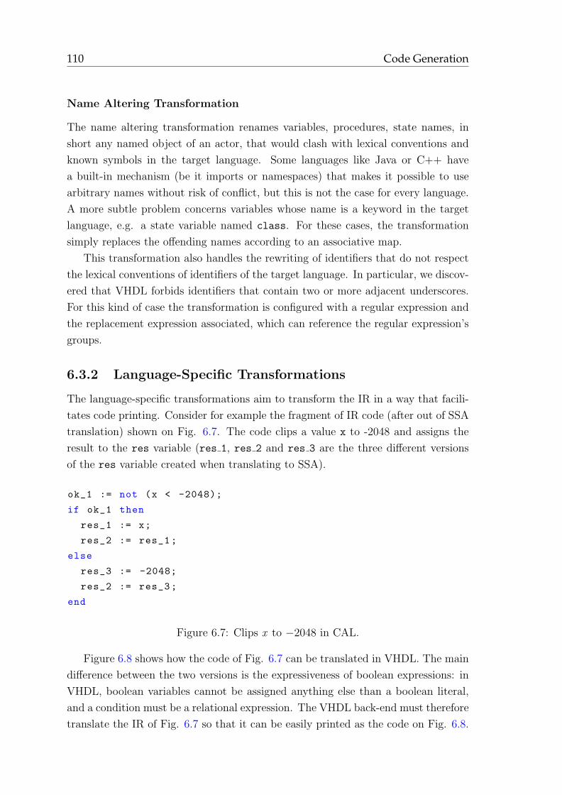
110 Code Generation
Name Altering Transformation
The name altering transformation renames variables, procedures, state names, in
short any named object of an actor, that would clash with lexical conventions and
known symbols in the target language. Some languages like Java or C++ have
a built-in mechanism (be it imports or namespaces) that makes it possible to use
arbitrary names without risk of conflict, but this is not the case for every language.
A more subtle problem concerns variables whose name is a keyword in the target
language, e.g. a state variable named class. For these cases, the transformation
simply replaces the offending names according to an associative map.
This transformation also handles the rewriting of identifiers that do not respect
the lexical conventions of identifiers of the target language. In particular, we discov-
ered that VHDL forbids identifiers that contain two or more adjacent underscores.
For this kind of case the transformation is configured with a regular expression and
the replacement expression associated, which can reference the regular expression’s
groups.
6.3.2 Language-Specific Transformations
The language-specific transformations aim to transform the IR in a way that facili-
tates code printing. Consider for example the fragment of IR code (after out of SSA
translation) shown on Fig. 6.7. The code clips a value x to -2048 and assigns the
result to the res variable (res 1, res 2 and res 3 are the three different versions
of the res variable created when translating to SSA).
ok_1 := not (x < -2048);
if ok_1 then
res_1 := x;
res_2 := res_1;
else
res_3 := -2048;
res_2 := res_3;
end
Figure 6.7: Clips x to −2048 in CAL.
Figure 6.8 shows how the code of Fig. 6.7 can be translated in VHDL. The main
difference between the two versions is the expressiveness of boolean expressions: in
VHDL, boolean variables cannot be assigned anything else than a boolean literal,
and a condition must be a relational expression. The VHDL back-end must therefore
translate the IR of Fig. 6.7 so that it can be easily printed as the code on Fig. 6.8.
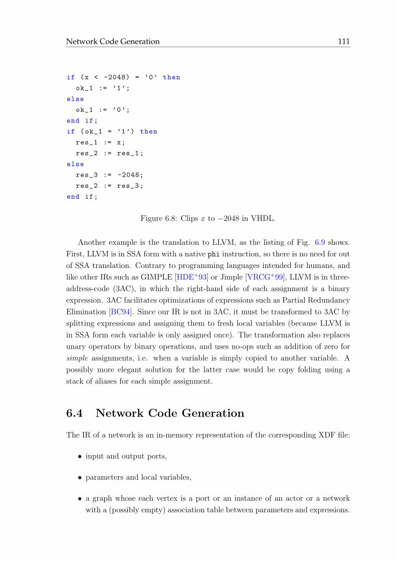
Network Code Generation 111
if (x < -2048) = ’0’ then
ok_1 := ’1’;
else
ok_1 := ’0’;
end if;
if (ok_1 = ’1’) then
res_1 := x;
res_2 := res_1;
else
res_3 := -2048;
res_2 := res_3;
end if;
Figure 6.8: Clips x to −2048 in VHDL.
Another example is the translation to LLVM, as the listing of Fig. 6.9 shows.
First, LLVM is in SSA form with a native phi instruction, so there is no need for out
of SSA translation. Contrary to programming languages intended for humans, and
like other IRs such as GIMPLE [HDE+93] or Jimple [VRCG+99], LLVM is in three-
address-code (3AC), in which the right-hand side of each assignment is a binary
expression. 3AC facilitates optimizations of expressions such as Partial Redundancy
Elimination [BC94]. Since our IR is not in 3AC, it must be transformed to 3AC by
splitting expressions and assigning them to fresh local variables (because LLVM is
in SSA form each variable is only assigned once). The transformation also replaces
unary operators by binary operations, and uses no-ops such as addition of zero for
simple assignments, i.e. when a variable is simply copied to another variable. A
possibly more elegant solution for the latter case would be copy folding using a
stack of aliases for each simple assignment.
6.4 Network Code Generation
The IR of a network is an in-memory representation of the corresponding XDF file:
• input and output ports,
• parameters and local variables,
• a graph whose each vertex is a port or an instance of an actor or a network
with a (possibly empty) association table between parameters and expressions.
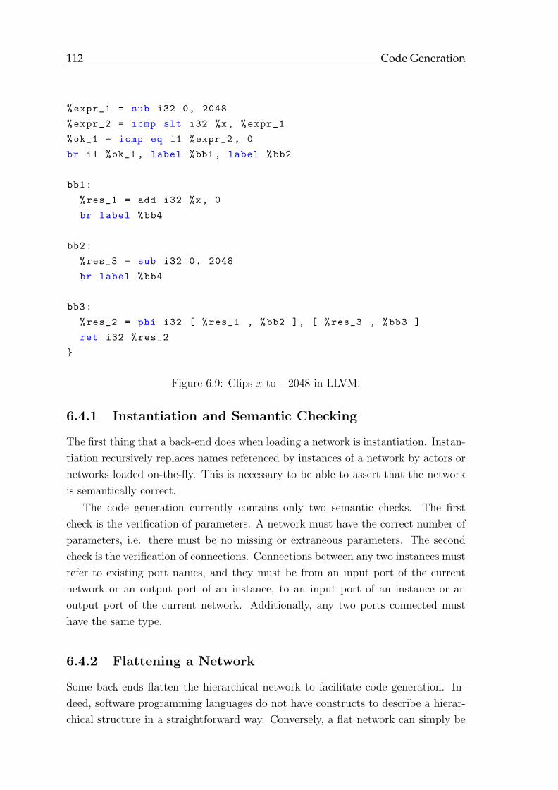
112 Code Generation
%expr_1 = sub i32 0, 2048
%expr_2 = icmp slt i32 %x, %expr_1
%ok_1 = icmp eq i1 %expr_2 , 0
br i1 %ok_1 , label %bb1 , label %bb2
bb1:
%res_1 = add i32 %x, 0
br label %bb4
bb2:
%res_3 = sub i32 0, 2048
br label %bb4
bb3:
%res_2 = phi i32 [ %res_1 , %bb2 ], [ %res_3 , %bb3 ]
ret i32 %res_2
}
Figure 6.9: Clips x to −2048 in LLVM.
6.4.1 Instantiation and Semantic Checking
The first thing that a back-end does when loading a network is instantiation. Instan-
tiation recursively replaces names referenced by instances of a network by actors or
networks loaded on-the-fly. This is necessary to be able to assert that the network
is semantically correct.
The code generation currently contains only two semantic checks. The first
check is the verification of parameters. A network must have the correct number of
parameters, i.e. there must be no missing or extraneous parameters. The second
check is the verification of connections. Connections between any two instances must
refer to existing port names, and they must be from an input port of the current
network or an output port of an instance, to an input port of an instance or an
output port of the current network. Additionally, any two ports connected must
have the same type.
6.4.2 Flattening a Network
Some back-ends flatten the hierarchical network to facilitate code generation. In-
deed, software programming languages do not have constructs to describe a hierar-
chical structure in a straightforward way. Conversely, a flat network can simply be
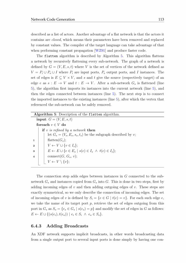
Network Code Generation 113
described as a list of actors. Another advantage of a flat network is that the actors it
contains are closed, which means their parameters have been removed and replaced
by constant values. The compiler of the target language can take advantage of that
when performing constant propagation [WZ91] and produce faster code.
The flatten algorithm is described by Algorithm 5. This algorithm flattens
a network by recursively flattening every sub-network. The graph of a network is
defined by G = (V,E, s, t) where V is the set of vertices of the network defined as
V = Pi ∪ Po ∪ I where Pi are input ports, Po output ports, and I instances. The
set of edges is E ⊆ V × V , and s and t give the source (respectively target) of an
edge e as s : E → V and t : E → V . After a sub-network Gs is flattened (line
5), the algorithm first imports its instances into the current network (line 5), and
then the edges connected between instances (line 5). The next step is to connect
the imported instances to the existing instances (line 5), after which the vertex that
referenced the sub-network can be safely removed.
Algorithm 5: Description of the flatten algorithm.
input: G = (V,E, s, t)
foreach v ∈ V do
if v is refined by a network thenlet Gs = (Vs, Es, ss, ts) be the subgraph described by v;
flatten(Gs);1
V ← V ∪ {v ∈ Is};2
E ← E ∪ {e ∈ Es | s(e) ∈ Is ∧ t(e) ∈ Is};3
connect(G, Gs, v);4
V ← V \ {v};
The connection step adds edges between instances in G connected to the sub-
network Gs and instances copied from Gs into G. This is done in two steps, first by
adding incoming edges of v and then adding outgoing edges of v. These steps are
exactly symmetrical, so we only describe the connection of incoming edges. The set
of incoming edges of v is defined by Si = {e ∈ G | t(e) = v}. For each such edge e,
we take the name of its target port p, retrieve the set of edges outgoing from this
port in Gs as So = {es ∈ Gs | s(es) = p} and modify the set of edges in G as follows:
E ← E ∪ {(s(ei), t(eo)) | ei ∈ Si ∧ eo ∈ So}.
6.4.3 Adding Broadcasts
An XDF network supports implicit broadcasts, in other words broadcasting data
from a single output port to several input ports is done simply by having one con-
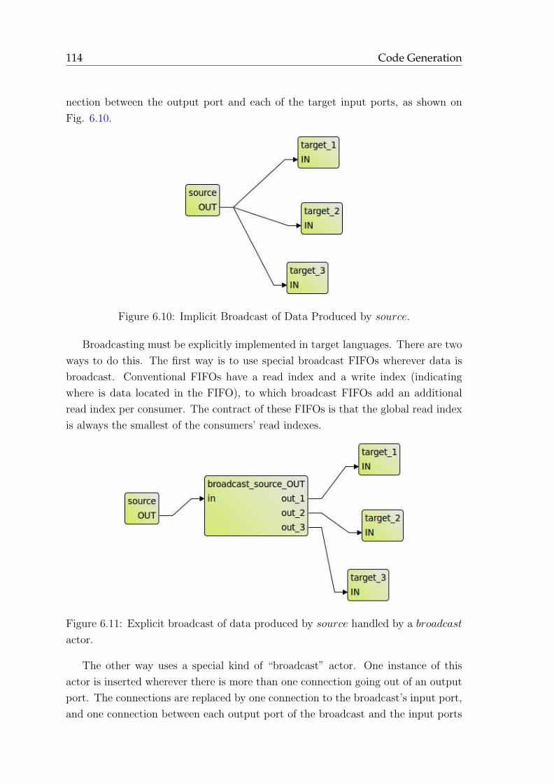
114 Code Generation
nection between the output port and each of the target input ports, as shown on
Fig. 6.10.
Figure 6.10: Implicit Broadcast of Data Produced by source.
Broadcasting must be explicitly implemented in target languages. There are two
ways to do this. The first way is to use special broadcast FIFOs wherever data is
broadcast. Conventional FIFOs have a read index and a write index (indicating
where is data located in the FIFO), to which broadcast FIFOs add an additional
read index per consumer. The contract of these FIFOs is that the global read index
is always the smallest of the consumers’ read indexes.
Figure 6.11: Explicit broadcast of data produced by source handled by a broadcast
actor.
The other way uses a special kind of “broadcast” actor. One instance of this
actor is inserted wherever there is more than one connection going out of an output
port. The connections are replaced by one connection to the broadcast’s input port,
and one connection between each output port of the broadcast and the input ports
Conclusion 115
of the target as shown on Fig. 6.11. When fired, the broadcast actor simply copies
data coming on its input port to each of its output ports.
6.5 Conclusion
This chapter has presented the last stage of our compilation infrastructure that
generates code from networks and the IR of actors. A back-end is specific to a
language, and may generate code in this language for actors, networks, or both.
The code generation process is different for each back-end, with the exception of the
last step called code printing.
We devote an entire section to code printing that starts by examining existing
approaches commonly employed by code generators. The section explains why these
approaches are not very well suited in our case because we want to be able to
generate many different languages, and present an alternative that uses templates
to define a “view” of the model that is the code. We give key features and semantics
implemented by the StringTemplate template engine that back-ends use to print
code, and show some techniques that handle cases that cannot be easily expressed
with templates. Finally, two sections show the steps that are performed to transform
actors and networks respectively so code can be printed from them.
The next chapter starts by presenting the implementation of support tools for
RVC-CAL dataflow programs. These tools include a graphical editor and an imple-
mentation of the infrastructure described in this document, which have been (and
are still being) used for the development of RVC decoders that are described in the
next chapter. After these decoders are presented, the chapter shows results of the
classification and transformation methods we have presented in the previous chapter,
and the scheduling algorithms and techniques we have implemented.

116 Code Generation
Chapter 7
Implementation and Results
This chapter begins with section 7.1 that presents support tools for RVC-CAL
dataflow programs, among which the Open RVC-CAL Compiler, which is an im-
plementation of the compilation infrastructure for dataflow programs described in
this document. The next section starts with an overview of video coding before
presenting the two normative RVC decoders as well as lower-level and higher-level
non-normative decoders. Section 7.3 lists different runtime scheduling techniques
for dynamic dataflow programs. Finally, the chapter concludes by a section that
presents the performance of the code generated from the given test applications on
a multi-core processor and on programmable logic. This section also shows how our
transformation of actors presented earlier can improve speed of the generated code.
7.1 Development Tools
This section lists the development tools that were used to write the applications
detailed later in this chapter. These tools can only be used within the Eclipse
platform, presented in the next subsection.
7.1.1 Eclipse Platform
Eclipse [DRW04] is best described as an open-source, extensible infrastructure for
writing Integrated Development Environments (IDEs). Eclipse is written in Java
and leverages the OSGi [OSG05] framework to offer a dynamic component-based
system. A component is both a bundle in OSGi terminology and a plug-in in Eclipse
terminology. Apart from the core constituted of the platform runtime and the OSGi
implementation, all functionalities are available as plug-ins. As such it is possible
to write arbitrary applications based on a dynamic plug-in model with a minimal
set of plug-ins known as Rich Client Platform (RCP). RCP helps developers to
117
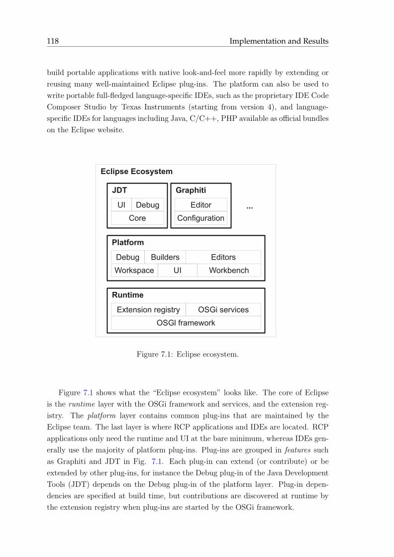
118 Implementation and Results
build portable applications with native look-and-feel more rapidly by extending or
reusing many well-maintained Eclipse plug-ins. The platform can also be used to
write portable full-fledged language-specific IDEs, such as the proprietary IDE Code
Composer Studio by Texas Instruments (starting from version 4), and language-
specific IDEs for languages including Java, C/C++, PHP available as official bundles
on the Eclipse website.
OSGl framework
Extension registry OSGi services
Runtime
UI
Debug Editors
Platform
Builders
Workspace Workbench
UI
JDT
Debug
Core
Eclipse Ecosystem
Graphiti
Editor
Configuration
...
Figure 7.1: Eclipse ecosystem.
Figure 7.1 shows what the “Eclipse ecosystem” looks like. The core of Eclipse
is the runtime layer with the OSGi framework and services, and the extension reg-
istry. The platform layer contains common plug-ins that are maintained by the
Eclipse team. The last layer is where RCP applications and IDEs are located. RCP
applications only need the runtime and UI at the bare minimum, whereas IDEs gen-
erally use the majority of platform plug-ins. Plug-ins are grouped in features such
as Graphiti and JDT in Fig. 7.1. Each plug-in can extend (or contribute) or be
extended by other plug-ins, for instance the Debug plug-in of the Java Development
Tools (JDT) depends on the Debug plug-in of the platform layer. Plug-in depen-
dencies are specified at build time, but contributions are discovered at runtime by
the extension registry when plug-ins are started by the OSGi framework.
Development Tools 119
7.1.2 Graphiti Editor
Graphiti [Gra] is a generic graph editor that I wrote with Jonathan Piat. We believe
Graphiti has a combination of features that makes it unique and invaluable: Graphiti
is an Eclipse plug-in, it is lightweight, dynamically reconfigurable, easily extensible,
and has a nice and standard user interface. We have written an MPEG contribution
to show how the editor could be used to edit RVC dataflow descriptions [WPR08].
Related Work
Most of the approaches to generic visual editors are generative in the sense that they
provide methods to generate a visual editor tailored to a given model and visual
syntax from a specification. The most well-known example within the Eclipse world
is the Graphical Modeling Framework (GMF). GMF generates a graphical editor
based on the Graphical Editor Framework (GEF) from two meta-models defined
with the Eclipse Modeling Framework (EMF), namely the domain model and the
visual model, and the mapping between the two models. The generated editor is fully
customizable and can be updated when the models or the mapping change. Ehrig et
al. present another method to generate visual editors as GEF-based Eclipse editors
from a specification of a Visual Language (VL) and graph transformation techniques
[EEHT05]. Two other well-known approaches for generating editors with a tailor-
made UI (i.e. not using GEF) are DiaGen [MV95] by Minas and Viehstaedt and
GenGED [Bar98] by Bardohl. Another interesting generative method is presented
by West and Kahl in [WK09] using a Haskell framework instead of yet another DSL
for the definition of the model and the VL.
The alternative to generative approaches is to have a generic editor that is con-
figured on-the-fly. The Moses project [ETH] provides a generic graph editor whose
behavior and VL syntax for a given graph are defined by a description of the model
and visual syntax for this graph. The description is written in a DSL called Graph
Type Definition Language (GTDL) [Jan97]. Janneck and Esser detail in [JE01] their
method to define a domain-specific VL syntax in GTDL as is implemented in Moses.
Description of Graphiti
Graphiti combines the elegance and simplicity of the approach of Janneck and Esser
with the flexibility of the Eclipse plug-in system and the power of well-established
frameworks and technologies, namely GEF, XML, XSLT, and ANTLR [PQ95]. The
fact that our approach is similar to theirs is not surprising since Janneck himself
convinced us of the benefit of creating a generic graph editor. Graphiti stems from
the observation that graph editors generally support only a few file formats, and
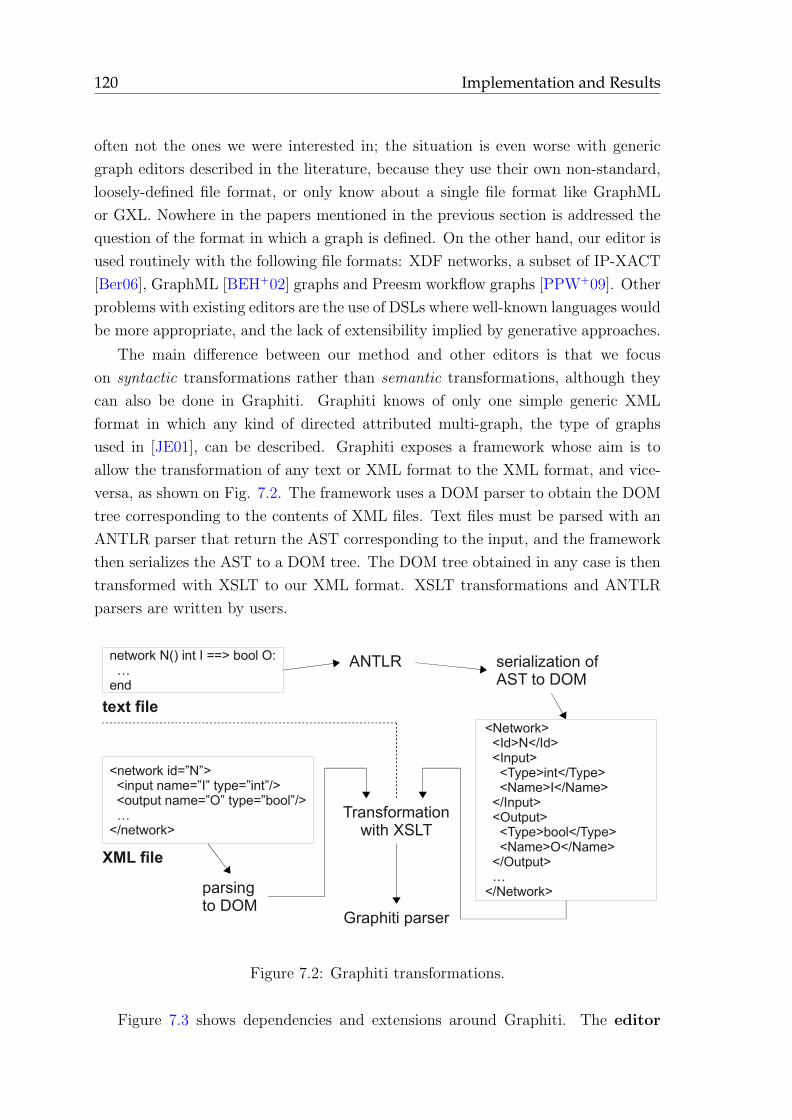
120 Implementation and Results
often not the ones we were interested in; the situation is even worse with generic
graph editors described in the literature, because they use their own non-standard,
loosely-defined file format, or only know about a single file format like GraphML
or GXL. Nowhere in the papers mentioned in the previous section is addressed the
question of the format in which a graph is defined. On the other hand, our editor is
used routinely with the following file formats: XDF networks, a subset of IP-XACT
[Ber06], GraphML [BEH+02] graphs and Preesm workflow graphs [PPW+09]. Other
problems with existing editors are the use of DSLs where well-known languages would
be more appropriate, and the lack of extensibility implied by generative approaches.
The main difference between our method and other editors is that we focus
on syntactic transformations rather than semantic transformations, although they
can also be done in Graphiti. Graphiti knows of only one simple generic XML
format in which any kind of directed attributed multi-graph, the type of graphs
used in [JE01], can be described. Graphiti exposes a framework whose aim is to
allow the transformation of any text or XML format to the XML format, and vice-
versa, as shown on Fig. 7.2. The framework uses a DOM parser to obtain the DOM
tree corresponding to the contents of XML files. Text files must be parsed with an
ANTLR parser that return the AST corresponding to the input, and the framework
then serializes the AST to a DOM tree. The DOM tree obtained in any case is then
transformed with XSLT to our XML format. XSLT transformations and ANTLR
parsers are written by users.
network N() int I ==> bool O: …end
<network id=”N”> <input name=”I” type=”int”/> <output name=”O” type=”bool”/> …</network>
ANTLR
<Network> <Id>N</Id> <Input> <Type>int</Type> <Name>I</Name> </Input> <Output> <Type>bool</Type> <Name>O</Name> </Output> …</Network>
serialization ofAST to DOM
parsing to DOM
Transformationwith XSLT
XML file
text file
Graphiti parser
Figure 7.2: Graphiti transformations.
Figure 7.3 shows dependencies and extensions around Graphiti. The editor
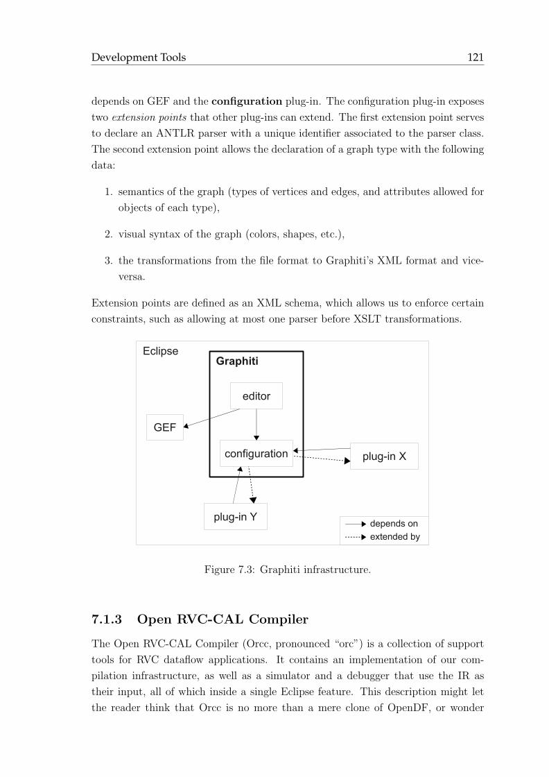
Development Tools 121
depends on GEF and the configuration plug-in. The configuration plug-in exposes
two extension points that other plug-ins can extend. The first extension point serves
to declare an ANTLR parser with a unique identifier associated to the parser class.
The second extension point allows the declaration of a graph type with the following
data:
1. semantics of the graph (types of vertices and edges, and attributes allowed for
objects of each type),
2. visual syntax of the graph (colors, shapes, etc.),
3. the transformations from the file format to Graphiti’s XML format and vice-
versa.
Extension points are defined as an XML schema, which allows us to enforce certain
constraints, such as allowing at most one parser before XSLT transformations.
editor
configuration
Graphiti
GEF
plug-in X
plug-in Y
Eclipse
depends on
extended by
Figure 7.3: Graphiti infrastructure.
7.1.3 Open RVC-CAL Compiler
The Open RVC-CAL Compiler (Orcc, pronounced “orc”) is a collection of support
tools for RVC dataflow applications. It contains an implementation of our com-
pilation infrastructure, as well as a simulator and a debugger that use the IR as
their input, all of which inside a single Eclipse feature. This description might let
the reader think that Orcc is no more than a mere clone of OpenDF, or wonder
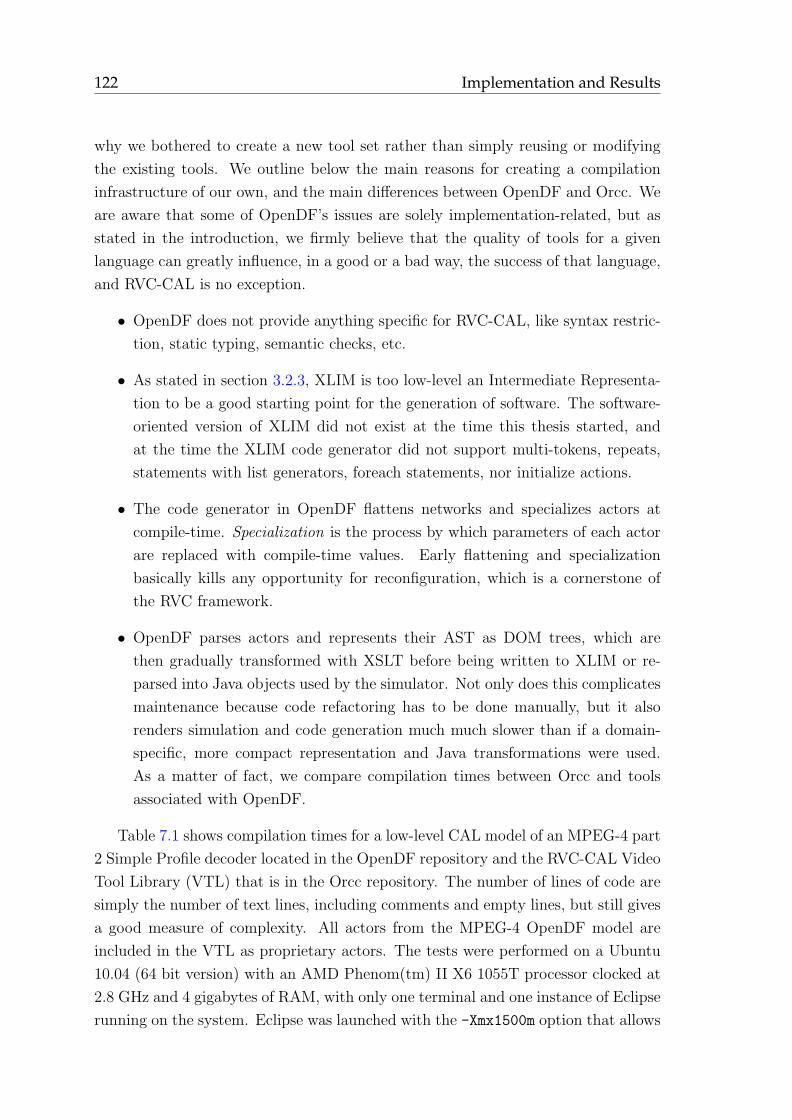
122 Implementation and Results
why we bothered to create a new tool set rather than simply reusing or modifying
the existing tools. We outline below the main reasons for creating a compilation
infrastructure of our own, and the main differences between OpenDF and Orcc. We
are aware that some of OpenDF’s issues are solely implementation-related, but as
stated in the introduction, we firmly believe that the quality of tools for a given
language can greatly influence, in a good or a bad way, the success of that language,
and RVC-CAL is no exception.
• OpenDF does not provide anything specific for RVC-CAL, like syntax restric-
tion, static typing, semantic checks, etc.
• As stated in section 3.2.3, XLIM is too low-level an Intermediate Representa-
tion to be a good starting point for the generation of software. The software-
oriented version of XLIM did not exist at the time this thesis started, and
at the time the XLIM code generator did not support multi-tokens, repeats,
statements with list generators, foreach statements, nor initialize actions.
• The code generator in OpenDF flattens networks and specializes actors at
compile-time. Specialization is the process by which parameters of each actor
are replaced with compile-time values. Early flattening and specialization
basically kills any opportunity for reconfiguration, which is a cornerstone of
the RVC framework.
• OpenDF parses actors and represents their AST as DOM trees, which are
then gradually transformed with XSLT before being written to XLIM or re-
parsed into Java objects used by the simulator. Not only does this complicates
maintenance because code refactoring has to be done manually, but it also
renders simulation and code generation much much slower than if a domain-
specific, more compact representation and Java transformations were used.
As a matter of fact, we compare compilation times between Orcc and tools
associated with OpenDF.
Table 7.1 shows compilation times for a low-level CAL model of an MPEG-4 part
2 Simple Profile decoder located in the OpenDF repository and the RVC-CAL Video
Tool Library (VTL) that is in the Orcc repository. The number of lines of code are
simply the number of text lines, including comments and empty lines, but still gives
a good measure of complexity. All actors from the MPEG-4 OpenDF model are
included in the VTL as proprietary actors. The tests were performed on a Ubuntu
10.04 (64 bit version) with an AMD Phenom(tm) II X6 1055T processor clocked at
2.8 GHz and 4 gigabytes of RAM, with only one terminal and one instance of Eclipse
running on the system. Eclipse was launched with the -Xmx1500m option that allows
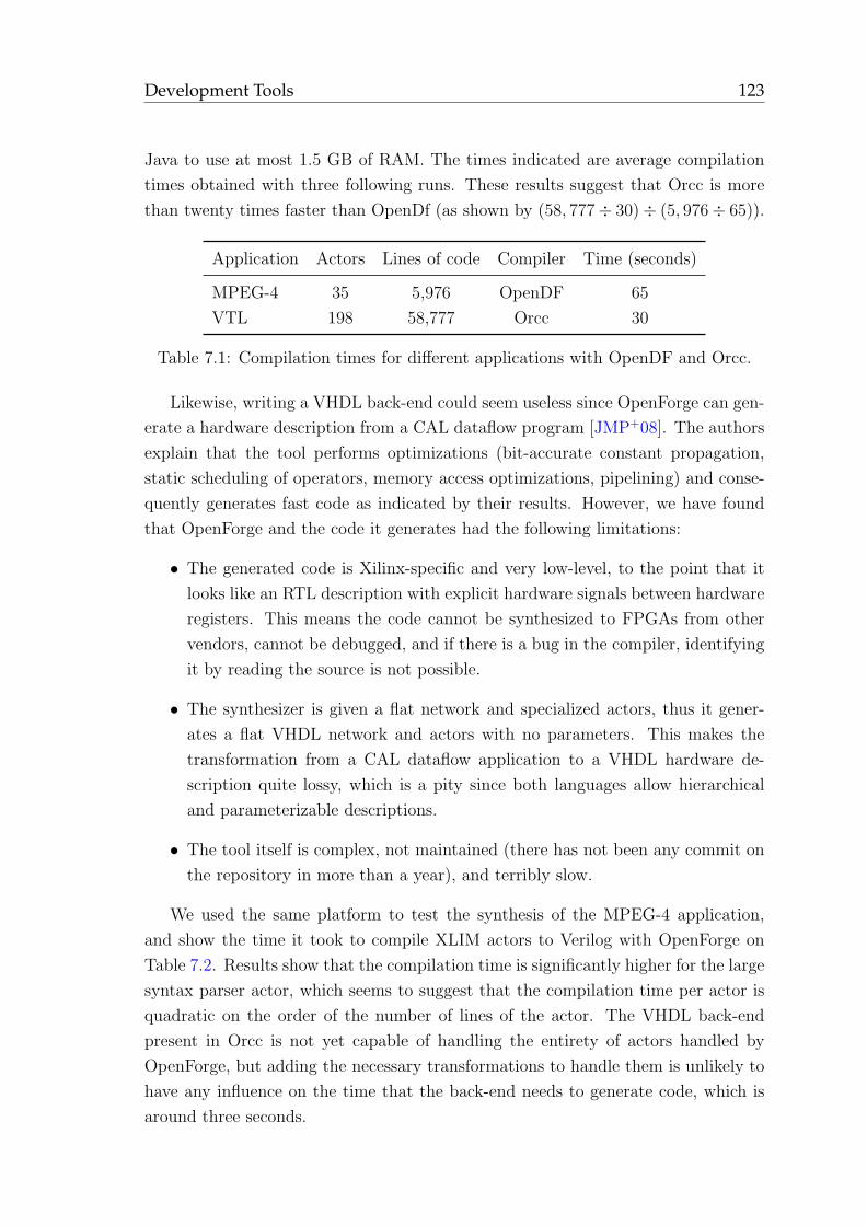
Development Tools 123
Java to use at most 1.5 GB of RAM. The times indicated are average compilation
times obtained with three following runs. These results suggest that Orcc is more
than twenty times faster than OpenDf (as shown by (58, 777÷ 30)÷ (5, 976÷ 65)).
Application Actors Lines of code Compiler Time (seconds)
MPEG-4 35 5,976 OpenDF 65
VTL 198 58,777 Orcc 30
Table 7.1: Compilation times for different applications with OpenDF and Orcc.
Likewise, writing a VHDL back-end could seem useless since OpenForge can gen-
erate a hardware description from a CAL dataflow program [JMP+08]. The authors
explain that the tool performs optimizations (bit-accurate constant propagation,
static scheduling of operators, memory access optimizations, pipelining) and conse-
quently generates fast code as indicated by their results. However, we have found
that OpenForge and the code it generates had the following limitations:
• The generated code is Xilinx-specific and very low-level, to the point that it
looks like an RTL description with explicit hardware signals between hardware
registers. This means the code cannot be synthesized to FPGAs from other
vendors, cannot be debugged, and if there is a bug in the compiler, identifying
it by reading the source is not possible.
• The synthesizer is given a flat network and specialized actors, thus it gener-
ates a flat VHDL network and actors with no parameters. This makes the
transformation from a CAL dataflow application to a VHDL hardware de-
scription quite lossy, which is a pity since both languages allow hierarchical
and parameterizable descriptions.
• The tool itself is complex, not maintained (there has not been any commit on
the repository in more than a year), and terribly slow.
We used the same platform to test the synthesis of the MPEG-4 application,
and show the time it took to compile XLIM actors to Verilog with OpenForge on
Table 7.2. Results show that the compilation time is significantly higher for the large
syntax parser actor, which seems to suggest that the compilation time per actor is
quadratic on the order of the number of lines of the actor. The VHDL back-end
present in Orcc is not yet capable of handling the entirety of actors handled by
OpenForge, but adding the necessary transformations to handle them is unlikely to
have any influence on the time that the back-end needs to generate code, which is
around three seconds.
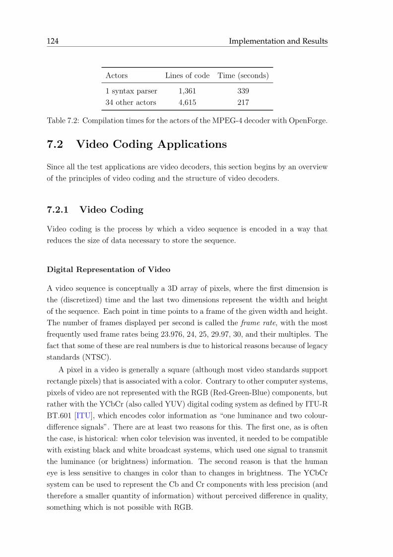
124 Implementation and Results
Actors Lines of code Time (seconds)
1 syntax parser 1,361 339
34 other actors 4,615 217
Table 7.2: Compilation times for the actors of the MPEG-4 decoder with OpenForge.
7.2 Video Coding Applications
Since all the test applications are video decoders, this section begins by an overview
of the principles of video coding and the structure of video decoders.
7.2.1 Video Coding
Video coding is the process by which a video sequence is encoded in a way that
reduces the size of data necessary to store the sequence.
Digital Representation of Video
A video sequence is conceptually a 3D array of pixels, where the first dimension is
the (discretized) time and the last two dimensions represent the width and height
of the sequence. Each point in time points to a frame of the given width and height.
The number of frames displayed per second is called the frame rate, with the most
frequently used frame rates being 23.976, 24, 25, 29.97, 30, and their multiples. The
fact that some of these are real numbers is due to historical reasons because of legacy
standards (NTSC).
A pixel in a video is generally a square (although most video standards support
rectangle pixels) that is associated with a color. Contrary to other computer systems,
pixels of video are not represented with the RGB (Red-Green-Blue) components, but
rather with the YCbCr (also called YUV) digital coding system as defined by ITU-R
BT.601 [ITU], which encodes color information as “one luminance and two colour-
difference signals”. There are at least two reasons for this. The first one, as is often
the case, is historical: when color television was invented, it needed to be compatible
with existing black and white broadcast systems, which used one signal to transmit
the luminance (or brightness) information. The second reason is that the human
eye is less sensitive to changes in color than to changes in brightness. The YCbCr
system can be used to represent the Cb and Cr components with less precision (and
therefore a smaller quantity of information) without perceived difference in quality,
something which is not possible with RGB.
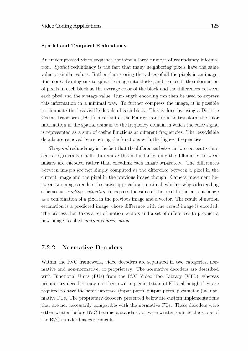
Video Coding Applications 125
Spatial and Temporal Redundancy
An uncompressed video sequence contains a large number of redundancy informa-
tion. Spatial redundancy is the fact that many neighboring pixels have the same
value or similar values. Rather than storing the values of all the pixels in an image,
it is more advantageous to split the image into blocks, and to encode the information
of pixels in each block as the average color of the block and the differences between
each pixel and the average value. Run-length encoding can then be used to express
this information in a minimal way. To further compress the image, it is possible
to eliminate the less-visible details of each block. This is done by using a Discrete
Cosine Transform (DCT), a variant of the Fourier transform, to transform the color
information in the spatial domain to the frequency domain in which the color signal
is represented as a sum of cosine functions at different frequencies. The less-visible
details are removed by removing the functions with the highest frequencies.
Temporal redundancy is the fact that the differences between two consecutive im-
ages are generally small. To remove this redundancy, only the differences between
images are encoded rather than encoding each image separately. The differences
between images are not simply computed as the difference between a pixel in the
current image and the pixel in the previous image though. Camera movement be-
tween two images renders this naive approach sub-optimal, which is why video coding
schemes use motion estimation to express the value of the pixel in the current image
as a combination of a pixel in the previous image and a vector. The result of motion
estimation is a predicted image whose difference with the actual image is encoded.
The process that takes a set of motion vectors and a set of differences to produce a
new image is called motion compensation.
7.2.2 Normative Decoders
Within the RVC framework, video decoders are separated in two categories, nor-
mative and non-normative, or proprietary. The normative decoders are described
with Functional Units (FUs) from the RVC Video Tool Library (VTL), whereas
proprietary decoders may use their own implementation of FUs, although they are
required to have the same interface (input ports, output ports, parameters) as nor-
mative FUs. The proprietary decoders presented below are custom implementations
that are not necessarily compatible with the normative FUs. These decoders were
either written before RVC became a standard, or were written outside the scope of
the RVC standard as experiments.
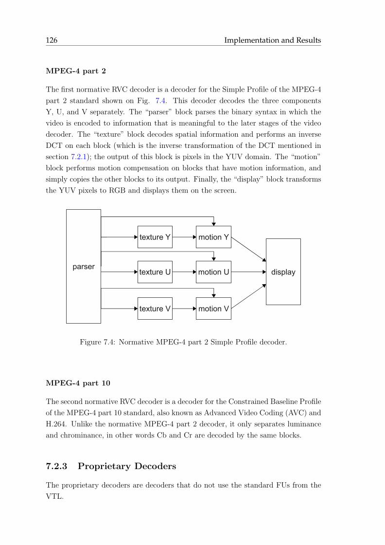
126 Implementation and Results
MPEG-4 part 2
The first normative RVC decoder is a decoder for the Simple Profile of the MPEG-4
part 2 standard shown on Fig. 7.4. This decoder decodes the three components
Y, U, and V separately. The “parser” block parses the binary syntax in which the
video is encoded to information that is meaningful to the later stages of the video
decoder. The “texture” block decodes spatial information and performs an inverse
DCT on each block (which is the inverse transformation of the DCT mentioned in
section 7.2.1); the output of this block is pixels in the YUV domain. The “motion”
block performs motion compensation on blocks that have motion information, and
simply copies the other blocks to its output. Finally, the “display” block transforms
the YUV pixels to RGB and displays them on the screen.
parser
texture Y
texture U
texture V
motion Y
motion U
motion V
display
Figure 7.4: Normative MPEG-4 part 2 Simple Profile decoder.
MPEG-4 part 10
The second normative RVC decoder is a decoder for the Constrained Baseline Profile
of the MPEG-4 part 10 standard, also known as Advanced Video Coding (AVC) and
H.264. Unlike the normative MPEG-4 part 2 decoder, it only separates luminance
and chrominance, in other words Cb and Cr are decoded by the same blocks.
7.2.3 Proprietary Decoders
The proprietary decoders are decoders that do not use the standard FUs from the
VTL.
Implementation of a Dynamic Scheduler 127
Hardware-oriented Description
The hardware-oriented description of an MPEG-4 part 2 Simple Profile decoder was
the first video decoder to be written in CAL. It was written by Dave Parlour from
Xilinx as a test application for OpenForge [JMP+08]. As opposed to the normative
RVC version, this decoder is not compliant with the MPEG-4 part 2 standard, as it
does not respect the requirements of the ISO/IEC 23002-2:2007 standard [ISO07].
The structure of the decoder is shown on Fig. 7.5.
parser texture motion display
Figure 7.5: Proprietary description of an MPEG-4 part 2 Simple Profile decoder.
This description decodes the Y, Cb, Cr components serially, i.e. first the lu-
minance and then the two chrominance components. The texture block contains
a low-level iDCT described as a hierarchical network that contain six actors and a
network that contains five actors itself. In comparison, the normative RVC decoder
implements an ISO/IEC 23002-2 compliant inverse DCT in one actor.
Software-oriented Descriptions
Other researchers working on RVC-CAL have derived proprietary descriptions from
the normative and hardware-oriented descriptions. One description has the same
structure as the hardware description, with the exception of the inverse DCT, which
uses the same as the normative decoder. Another description uses the same structure
as the normative decoder. The main difference with the descriptions presented
previously is that these software-oriented descriptions use a few actors that have
been rewritten to be higher-level. As a matter of fact, some of these actors resemble
the actors produced by of our transformation method presented in Chapter 5.
7.3 Implementation of a Dynamic Scheduler
Dynamic dataflow programs, such as dataflow programs whose actors are defined
with RVC-CAL, behave according to the Dataflow Process Network (DPN) Model
of Computation (MoC) that was detailed in section 2.2. The DPN MoC does not
impose a particular scheduling technique, as long as it is respects the semantics of
the model:
128 Implementation and Results
1. reading from a FIFO is non-blocking and actors are allowed to test an input
port for the absence or presence of data.
2. writing to a FIFO is non-blocking, i.e. a write always returns immediately.
Although it somehow seems unusual, the fact that writes are non-blocking (re-
quirement 2) poses no problem since theoretically FIFOs have an unbounded capac-
ity. In practice, Parks has shown that it is possible to find a bounded schedule for
many process networks and dynamic dataflow applications [Par95]. Additionally,
the implementation of FIFOs must take into account requirement 1: it must be
possible to query the state of the FIFO and peek tokens.
This section describes different scheduling methods that can be used to schedule
dynamic dataflow programs that respect the DPN MoC. The first two methods are
from the state of the art, and the last two are methods we have implemented.
7.3.1 Ptolemy Scheduler
The earliest implementation of a code generator and scheduler for CAL dataflow
programs is described by Wernli [Wer02]. The author presents a compiler that
transforms CAL actors to Java classes that use the Ptolemy API to implement
the behavior of actors. Using this API, a dynamic dataflow actor is represented
as a Java class that extends ptolemy.actor.TypedAtomicActor. The actors can
be used in Ptolemy and scheduled using an approach based on Parks’s scheduling
technique as described by Zhou in [Zho04]. This is different from our approach since
the generated actors are not standalone, rather they must be scheduled within the
Ptolemy framework. Although we have not tested the speed of the Ptolemy simulator
per se, our experience with simulators of CAL dataflow programs — Moses [ETH]
and OpenDF that are both based on a fork of the simulator implemented in Ptolemy,
as well as the simulator implemented in Orcc — allows us to say that the speed
achieved by the Ptolemy CAL simulator cannot compare to the speed of generated
code.
7.3.2 Threads
A possible solution to schedule a dynamic dataflow program is to use one thread
per actor, and let the kernel schedule these threads. This was the first approach
we tried, although we never published our results. The limitation of this approach
is that it is not possible to use traditional FIFOs with blocking reads as per the
requirements of the DPN model (as mentioned above and detailed in section 2.3.2).
The Xlim2C compiler written by Ericsson first generated code with one thread per
Implementation of a Dynamic Scheduler 129
actor. The results they report in the technical report [vP10] is that they obtained
3.5 frames per second on a QCIF video (176x144 pixels) using the hardware-oriented
MPEG-4 part 2 description.
7.3.3 SystemC Scheduler
SystemC [IEE05] is an industry standard for system-level modeling, design and
simulation. Any system that may be implemented in hardware, software, or a com-
bination of both, can be modeled with the set of macros, C++ classes and templates
provided by the SystemC framework. Within this framework, a design is composed
of a set of modules that are connected with channels via ports. Modules can be
parameterized and can contain other modules, in other words hierarchy is allowed.
Each module contains a process that is the computational kernel of the module. Pro-
cesses are not preemptible, but they can be suspended by the SystemC scheduler
when reading from empty FIFOs, writing to full FIFOs, or by calling wait explicitly.
Roquier et al. present an automatic translation (implemented in the Cal2C tool)
of hierarchical networks and actors to SystemC modules, and leverage the TLM
framework (Transaction Level Modeling) to implement peekable FIFOs [RWR+08].
They use their technique to obtain a SystemC model of an earlier version of the
normative MPEG-4 part 2 SP decoder. The results obtained are in the order of
2,000 macroblocks per second, which represents 20 frames per second on a QCIF
video. However, the method presented cannot be used with other schedulers because
actions and action schedulers have an explicit dependency on SystemC. Moreover,
although the generated SystemC model behaves correctly, it does not respect DPN
semantics because actors are suspended whenever they cannot read or write.
I explained in [WRN09] how to separate the scheduler from the actors by using
an interface, and list the requirements the interface needs to meet to guarantee
the DPN semantics are respected by the generated model. The paper presents
comparable results to those shown in [RWR+08], and also presents results for the
low-level proprietary version (which could not be generated before by Cal2C). I also
sketch in this paper that a better scheduler for DPN would make “no use of threads”
and would provide “direct access to peekable FIFOs via pointers”.
7.3.4 Round-Robin Scheduler
The actor scheduler used in software code generated by Orcc uses a single-thread
round-robin scheduler with hand-written specialized FIFOs that minimize the num-
ber of memory copies. I implemented this scheduler in an early version of Orcc,
and we wrote an MPEG contribution about it [RW09] which was presented at the
130 Implementation and Results
89th MPEG meeting. The code generated with this scheduler runs about five times
faster than the code that uses the SystemC scheduler. This speed increase lies in
the implementation of the scheduler and of the FIFOs.
Implementation of the Scheduler
The majority of actors are very fine-grain, especially when compared to software
traditionally implemented with threads. As a result, the time spent in the scheduler
can be quite large compared to the amount of computations performed by actors.
Traditionally, a scheduler will try hard to be fair, i.e. allocate time fairly to active
tasks. A round-robin scheduler is fair by nature, and has zero overhead, since it
simply calls tasks in a pre-determined circular order. This is implemented as an
infinite while loop whose body contains calls to the action scheduler of each actor.
The action scheduler of an actor is implemented as a function that fires as many
actions in a row as possible. If the actor has an FSM, the action scheduler starts
by jumping to the current state of the actor (with a goto). Then the first fireable
action in the state fires and jumps to the target state it is associated with. When no
more actions can be fired, the action scheduler returns. If the actor does not have
an FSM, the action scheduler simply fires actions in an infinite while loop. When
no actions can be fired any more, the function returns.
As an example, Figure 7.6 presents the C implementation of the Downsample
actor that was presented in section 2.3.1 in Fig. 2.11. This figure illustrates why
this implementation respects DPN semantics. Indeed, if an action is not schedulable
because it has no tokens, the scheduler does not wait, instead it simply returns.
Likewise, if an action is schedulable but there is no space in output FIFOs, the
scheduler does not fire the action, and returns. As a matter of fact, this simple
example shows why we currently require that repeat constructs be compile-time
constants. Indeed, if an action is schedulable, and fires, but there is no space in
output FIFOs, the action scheduler must somehow store the tokens produced (whose
number may vary, so this requires dynamic memory allocation), record the fact that
these tokens are to be written later, return, and the next time it is fired, if there
is space, it will send the tokens. This is complicated, and it is likely to be a severe
performance hit for all but coarse-grain actors.
Implementation of FIFOs
The FIFOs are circular buffers implemented as a structure with an array that con-
tains the contents of the FIFO, a size, and a read and write index. We use macros
to produce a template-like definition of FIFOs to provide implementations for 8,
16, 32, and 64-bit integer types (signed or unsigned). For instance, in the example
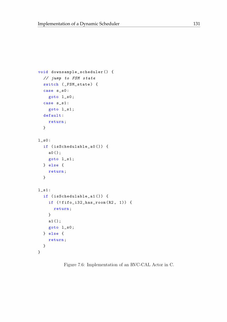
Implementation of a Dynamic Scheduler 131
void downsample_scheduler () {
// jump to FSM state
switch (_FSM_state) {
case s_s0:
goto l_s0;
case s_s1:
goto l_s1;
default:
return;
}
l_s0:
if (isSchedulable_a0 ()) {
a0();
goto l_s1;
} else {
return;
}
l_s1:
if (isSchedulable_a1 ()) {
if (! fifo_i32_has_room(R2 , 1)) {
return;
}
a1();
goto l_s0;
} else {
return;
}
}
Figure 7.6: Implementation of an RVC-CAL Actor in C.
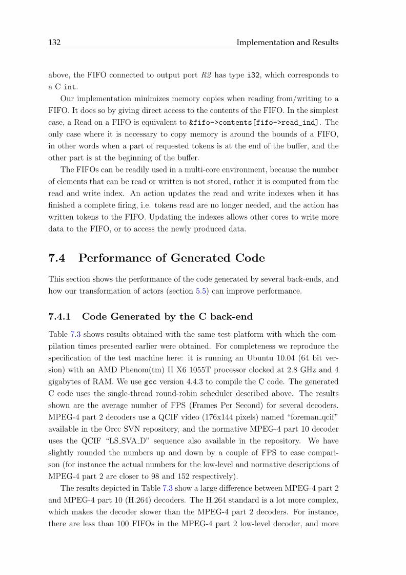
132 Implementation and Results
above, the FIFO connected to output port R2 has type i32, which corresponds to
a C int.
Our implementation minimizes memory copies when reading from/writing to a
FIFO. It does so by giving direct access to the contents of the FIFO. In the simplest
case, a Read on a FIFO is equivalent to &fifo->contents[fifo->read_ind]. The
only case where it is necessary to copy memory is around the bounds of a FIFO,
in other words when a part of requested tokens is at the end of the buffer, and the
other part is at the beginning of the buffer.
The FIFOs can be readily used in a multi-core environment, because the number
of elements that can be read or written is not stored, rather it is computed from the
read and write index. An action updates the read and write indexes when it has
finished a complete firing, i.e. tokens read are no longer needed, and the action has
written tokens to the FIFO. Updating the indexes allows other cores to write more
data to the FIFO, or to access the newly produced data.
7.4 Performance of Generated Code
This section shows the performance of the code generated by several back-ends, and
how our transformation of actors (section 5.5) can improve performance.
7.4.1 Code Generated by the C back-end
Table 7.3 shows results obtained with the same test platform with which the com-
pilation times presented earlier were obtained. For completeness we reproduce the
specification of the test machine here: it is running an Ubuntu 10.04 (64 bit ver-
sion) with an AMD Phenom(tm) II X6 1055T processor clocked at 2.8 GHz and 4
gigabytes of RAM. We use gcc version 4.4.3 to compile the C code. The generated
C code uses the single-thread round-robin scheduler described above. The results
shown are the average number of FPS (Frames Per Second) for several decoders.
MPEG-4 part 2 decoders use a QCIF video (176x144 pixels) named “foreman qcif”
available in the Orcc SVN repository, and the normative MPEG-4 part 10 decoder
uses the QCIF “LS SVA D” sequence also available in the repository. We have
slightly rounded the numbers up and down by a couple of FPS to ease compari-
son (for instance the actual numbers for the low-level and normative descriptions of
MPEG-4 part 2 are closer to 98 and 152 respectively).
The results depicted in Table 7.3 show a large difference between MPEG-4 part 2
and MPEG-4 part 10 (H.264) decoders. The H.264 standard is a lot more complex,
which makes the decoder slower than the MPEG-4 part 2 decoders. For instance,
there are less than 100 FIFOs in the MPEG-4 part 2 low-level decoder, and more
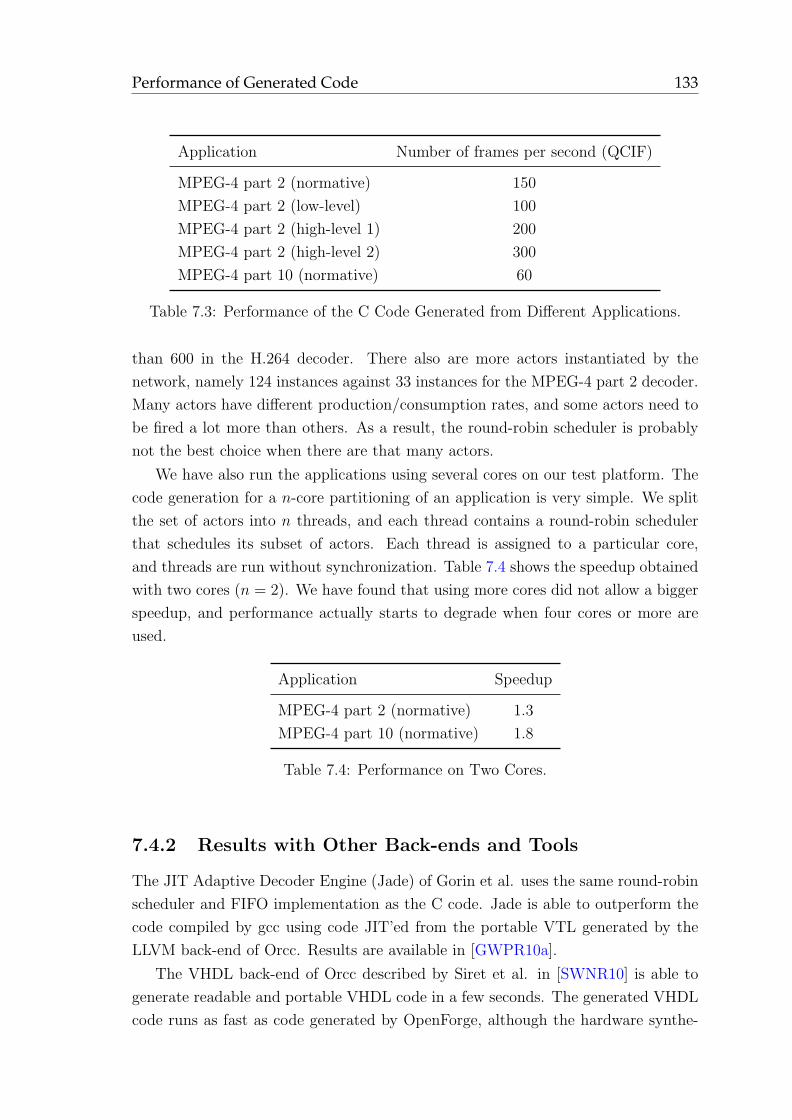
Performance of Generated Code 133
Application Number of frames per second (QCIF)
MPEG-4 part 2 (normative) 150
MPEG-4 part 2 (low-level) 100
MPEG-4 part 2 (high-level 1) 200
MPEG-4 part 2 (high-level 2) 300
MPEG-4 part 10 (normative) 60
Table 7.3: Performance of the C Code Generated from Different Applications.
than 600 in the H.264 decoder. There also are more actors instantiated by the
network, namely 124 instances against 33 instances for the MPEG-4 part 2 decoder.
Many actors have different production/consumption rates, and some actors need to
be fired a lot more than others. As a result, the round-robin scheduler is probably
not the best choice when there are that many actors.
We have also run the applications using several cores on our test platform. The
code generation for a n-core partitioning of an application is very simple. We split
the set of actors into n threads, and each thread contains a round-robin scheduler
that schedules its subset of actors. Each thread is assigned to a particular core,
and threads are run without synchronization. Table 7.4 shows the speedup obtained
with two cores (n = 2). We have found that using more cores did not allow a bigger
speedup, and performance actually starts to degrade when four cores or more are
used.
Application Speedup
MPEG-4 part 2 (normative) 1.3
MPEG-4 part 10 (normative) 1.8
Table 7.4: Performance on Two Cores.
7.4.2 Results with Other Back-ends and Tools
The JIT Adaptive Decoder Engine (Jade) of Gorin et al. uses the same round-robin
scheduler and FIFO implementation as the C code. Jade is able to outperform the
code compiled by gcc using code JIT’ed from the portable VTL generated by the
LLVM back-end of Orcc. Results are available in [GWPR10a].
The VHDL back-end of Orcc described by Siret et al. in [SWNR10] is able to
generate readable and portable VHDL code in a few seconds. The generated VHDL
code runs as fast as code generated by OpenForge, although the hardware synthe-
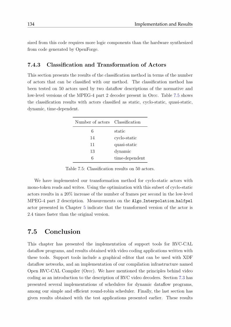
134 Implementation and Results
sized from this code requires more logic components than the hardware synthesized
from code generated by OpenForge.
7.4.3 Classification and Transformation of Actors
This section presents the results of the classification method in terms of the number
of actors that can be classified with our method. The classification method has
been tested on 50 actors used by two dataflow descriptions of the normative and
low-level versions of the MPEG-4 part 2 decoder present in Orcc. Table 7.5 shows
the classification results with actors classified as static, cyclo-static, quasi-static,
dynamic, time-dependent.
Number of actors Classification
6 static
14 cyclo-static
11 quasi-static
13 dynamic
6 time-dependent
Table 7.5: Classification results on 50 actors.
We have implemented our transformation method for cyclo-static actors with
mono-token reads and writes. Using the optimization with this subset of cyclo-static
actors results in a 20% increase of the number of frames per second in the low-level
MPEG-4 part 2 description. Measurements on the Algo Interpolation halfpel
actor presented in Chapter 5 indicate that the transformed version of the actor is
2.4 times faster than the original version.
7.5 Conclusion
This chapter has presented the implementation of support tools for RVC-CAL
dataflow programs, and results obtained with video coding applications written with
these tools. Support tools include a graphical editor that can be used with XDF
dataflow networks, and an implementation of our compilation infrastructure named
Open RVC-CAL Compiler (Orcc). We have mentioned the principles behind video
coding as an introduction to the description of RVC video decoders. Section 7.3 has
presented several implementations of schedulers for dynamic dataflow programs,
among our simple and efficient round-robin scheduler. Finally, the last section has
given results obtained with the test applications presented earlier. These results

Conclusion 135
include performance of the code generated by several back-ends on a multi-core
processor and on programmable logic.
The next and final chapter of this thesis concludes this document by a summary
of the work we have presented, before identifying current limitations in our approach.
Finally, we list perspectives for future work that can take advantage of our compi-
lation infrastructure to perform more sophisticated analyses and transformations.

136 Implementation and Results
Chapter 8
Conclusion
8.1 Summary
The work presented in this thesis takes place in a context of growing demand for bet-
ter video quality (High-Definition TV, home cinema...) and unprecedented concern
for power consumption. Video quality can be improved simply by compressing less,
in other words by transmitting more information. However, bandwidth consumption
is growing in an exponential fashion, driven by the increasing number of embedded
systems with video playing capabilities and Internet access, such as smartphones and
set-top boxes. Another way to improve video quality is to use better video compres-
sion, with more complex algorithms that demand more computational power, which
is conflicting with the goal of lower power consumption. Additionally, the current
process for standardization of video coding methods provides standards with little
flexibility, and no room for arbitrary configuration of a video decoder depending
on the type of the user device. This slows down the adoption of new standards
because it is increasingly long and complicated to implement standards on systems
with restricted capabilities and heterogeneous computing platforms.
The Reconfigurable Video Coding (RVC) MPEG standard attempts to solve
many of these problems. Previous video standards have historically described video
coding features in terms of a fixed set of profiles, with each profile suited to a
particular use of the standard (for instance, low-resolution display, higher error
resilience, the latter and high-resolution display, etc.). In contrast, within RVC a
video decoder is described with a block diagram (or network) whose blocks are called
Functional Units (FUs) or actors and implement different decoding algorithms. This
is a paradigm shift in video coding in that it renders the concept of profile obsolete,
since within RVC a profile is equivalent to a given network of FUs. Another way of
seeing this is that it is possible to have many more configurations of a video decoder
than the existing number of profiles in a typical video standard.
137
138 Conclusion
Furthermore, RVC networks are a lot more flexible than reference software pro-
vided by previous standards as monolithic C/C++ descriptions. An RVC network is
formally described as a Dataflow Process Network (DPN) [LP95], an extension of the
Kahn Process Network (KPN) model [Kah74]; we also refer to a DPN as a dynamic
dataflow program. A DPN connects actors with FIFOs that have non-blocking read
semantics, and actors are described as a set of firing rules that may read/write data
from/to FIFOs. Actors in an RVC network are written in a platform-neutral lan-
guage called RVC-CAL (presented in section 2.3.1) which respects DPN semantics.
The DPN model is the most general dataflow model, and there are many models
that are defined as a restricted subset of DPN semantics. We have shown in section
2.3.2 how some of these models could be described in RVC-CAL.
RVC decoders are abstract descriptions that can be simulated, but they must be
transformed to a hardware or software description to be efficiently executed. In order
to facilitate the analysis, transformation, and code generation for dynamic dataflow
programs, we have defined an Intermediate Representation (IR) of dynamic dataflow
actors in Chapter 3. As we show in section 3.2, to our knowledge there is no IR in
the state of the art that can represent the structure and semantics of an actor in
a simple and high-level way. After the description of the structure and semantics
of our IR, Chapter 4 describes the front-end of our compilation infrastructure that
compiles RVC-CAL to an IR of actors. Along with networks, this IR of actors can be
analyzed and transformed by the middle-end as explained in Chapter 5. Finally, we
explain in Chapter 6 how back-ends generate code in many languages from networks
and the IR of actors.
We have implemented the compilation infrastructure described in this document
in a tool called Orcc (Open RVC-CAL Compiler). In addition to an RVC-CAL front-
end, a middle-end with classification and transformation capabilities, and C, C++,
Java, LLVM, VHDL, and XLIM back-ends, Orcc includes an RVC-CAL textual ed-
itor, a simulator and a debugger. We have also written a generic graph editor called
Graphiti that can be used to edit RVC networks. As pointed out in Chapter 7, Orcc
and Graphiti are available as Eclipse features. This chapter also presents results ob-
tained with RVC video coding applications and several implementations of dynamic
scheduling techniques for dataflow programs, including our round-robin scheduler.
As mentioned in section 7.1.3 these applications represent tens of thousands of lines
of RVC-CAL code. A CABAC parser described as a single actor accounts for more
than 9,000 lines alone [BMR10].
Perspectives 139
8.2 Perspectives
Our compilation infrastructure is the first to use a simple, high-level, unified Interme-
diate Representation (IR) of dynamic dataflow programs that can be easily analyzed,
transformed, and from which we can generate code in many languages from hardware
description languages to high-level software languages. This opens many interesting
perspectives for future work, the first of which is to use the infrastructure to gen-
erate a mixed hardware/software description, also known as a hardware/software
co-design system. Previous works, including ours [RLM+09], have described the im-
plementation of co-design systems from an RVC-CAL program. However, most of
the time software and hardware are generated by different tools (in our case, Cal2C
and OpenForge). Using the C and VHDL back-ends implemented in Orcc, it would
be possible to generate a co-design system with a single tool. This would offer the
user more flexibility to describe the mapping of actors to components.
Another area for future work concerns our classification method presented in
Chapter 5 and the associated transformations. We have seen that we are able to
recognize SDF, CSDF, but only a subset of PSDF, and it would be interesting to rec-
ognize a larger set of quasi-static behaviors. Additionally, based on the results given
by the classification, we could implement many transformations that would allow
faster code to be generated. Indeed, there are many techniques and algorithms in the
literature that can efficiently schedule static, cyclo-static, or quasi-static graphs. We
could benefit from using these techniques whenever possible to reduce the amount
of scheduling that needs to be performed at runtime. Furthermore this would al-
low us to generate an efficient mapping and scheduling of non-dynamic parts of an
application.
Although improving the code generated for statically schedulable actors is im-
portant, it is equally important to improve the speed of code generated for dynamic
actors. The FIFOs we have implemented are multi-core ready, in the sense that they
can be used readily with any arbitrary mapping of actors to several cores. Because of
that, the FIFO implementation is sub-optimal, and we have seen that this approach
to multi-core does not scale at all: using more than three cores even tends to decrease
performance. Each call to check the number of tokens or the space available, or to
read or write data, uses the read (or write) index modulo the size of the FIFO. This
results in a large overhead because FIFOs are the only means of communication that
an actor has: in a simple test, we have noticed that using arrays was 3.5 times faster
than using the current FIFOs. This leads us to believe that by not allowing FIFOs
to be shared between cores, and by reducing the number of modulo operations, we
could obtain a similar speedup in parts of low-level descriptions where FIFO access
is a limiting factor (like the iDCT of the low-level MPEG-4 part 2 description).
140 Conclusion
Likewise, although the current round-robin scheduler is simple and works well
on most applications, there are certain applications where it is grossly inefficient,
and would need to be replaced. In particular, the parser of the MPEG-4 part
10 description was recently rewritten so that the bit-level decoding is described in
a client-server fashion. More precisely, every time a “client” actor wants a syntax
element, it sends a request (with tokens) to a bit-level decoding “server” actor, which
decodes the syntax element and then sends a response with the decoded element to
the client. With the round-robin scheduler, all actors are scheduled once between
each request and the corresponding response, which stalls the client and generally
performs a good deal of useless work. Using a more sophisticated scheduler1 can
dramatically improve the situation (on this particular application the speedup is
around 7), while bringing no significant difference on other applications. We believe
that this experimental scheduler can be further improved to reduce as much as
possible the number of times actors are scheduled in vain.
1Also known as “experimental scheduler” in Orcc.
Appendix A
French Annex
Conformement a la loi n◦94-665 du 4 aout 1994 relative a l’emploi de la langue
francaise, le manuscrit etant redige dans une langue etrangere au francais, il doit
contenir un resume en francais, reproduit ci-apres. Ce resume est suivi par une
synthese du travail effectue autour des programmes flux de donnees RVC-CAL depuis
la fin de la redaction de cette these en octobre 2010.
A.1 Resume de la these
A.1.1 Contexte
Les systemes embarques sont aujourd’hui presents dans la majorite des equipements
du quotidien et dans la quasi-totalite des secteurs d’activite. En 2004, le profit
genere par l’industrie micro-electronique etait d’environ 40 milliards de dollars dans
le monde et, malgre la crise economique mondiale de 2008, il atteint 79 milliards
de dollars en 2009 soit une augmentation de 14,2% par an ; pour l’ensemble du
domaine des systemes embarques, logiciel et materiel, le profit genere est de l’ordre
de 3,488 millions de dollars (Information Society Technology). Ainsi, la consom-
mation des produits de haute technologie est en hausse, notamment l’electronique
grand public. Le nombre de ”smartphones”, ces telephones intelligents combinant
a la fois les fonctions de telephone, d’agenda electroniques, de lecteur video, et de
navigateur Web, par exemple a explose. Precisement, l’institut GfK a mesure une
augmentation du volume des ventes de ce type de telephone de 138%, en France.
D’autre part, il s’est vendu plus de 7 millions de televiseurs a ecran plat en 2009 et
plus de 8 millions en 2010. De la meme maniere, les ventes d’ordinateurs personnels
augmentent regulierement, notamment pour les micro-portables (connus sous le nom
de ”netbooks”), qui offrent des fonctionnalites similaires a un ordinateur portable
classique pour un prix moindre.
142 French Annex
Ces produits ont en commun une offre multimedia importante, notamment
une capacite a lire du contenu video et audio, que celui-ci soit stocke au sein du
peripherique (memoire flash, cartes SD, disque dur, etc.) ou diffuse via des ser-
vices de diffusion de video a la demande (Youtube, Dailymotion, box, etc.). A
l’heure actuelle, un produit type smartphone ne proposant pas une offre multimedia
suffisante ne se vendrait pas, ou peu. Ce point sous-tend que tout produit ”high-
tech” dispose d’une connexion Internet et que la bande passante disponible au sein
du reseau est suffisante. Il y a encore dix ans, une eternite dans le domaine des
hautes technologies, ce point aurait ete juge irreel. En effet, on comptait alors
moins d’un million de foyers ayant un acces Internet haut debit en France ; ils
sont aujourd’hui plus de vingt millions. Par ailleurs, les technologies de transport
de donnees pour telephone portable ont largement evolue, autorisant des taux de
transfert de quelques megabits par seconde (Mbps) grace a la 3G et au protocole
Universal Mobile Telecommunications System (UMTS) contre quelques centaines de
kilobits par seconde (kbps) quelques annees plus tot. Il est a noter que le standard
Long Term Evolution (LTE), en cours de de developpement, permettra des taux de
transferts de donnees jusqu’a 100 Mbps.
Un probleme bloquant apparaıt cependant : la quantite d’information trans-
mise augmente plus rapidement que la capacite qu’ont les routeurs dans le reseau a
traiter cette information. En effet, entre l’augmentation du nombre d’equipements
capables de lire du contenu video diffuse, et l’augmentation de la bande passante
disponible, la bande passante consommee connaıt une croissance exponentielle. Par
exemple, en 2007, il a ete mesure que le site de diffusion video le plus connu, Youtube,
avait consomme autant de bande passante qu’Internet tout entier sept ans plus tot.
Concretement, la bande passante consommee augmente plus vite que le nombre
de transistors disponibles dans les composants electroniques utilises par les rou-
teurs. Ce constat, ainsi que celui de la demande croissante du marche pour des
videos plus hautes resolutions type Haude definition (720p, 1080i, 1080p, voir le 4k
et la Ultra High Definition), a pousse le Moving Picture Experts Group (MPEG)
et le Video Coding Experts Group (VCEG) de l’International Telecommunication
Union (ITU-T) a annoncer le developpement d’une nouvelle norme de codage nomme
High Efficiency Video Coding (HEVC). Cette norme vise a diminuer la quantite
d’informations necessaire pour coder une video de 50% par rapport au precedent
standard MPEG AVC (Advanced Video Coding). Lors du meeting MPEG de jan-
vier 2011, le nombre d’experts et de chercheurs participant aux reunions sur HEVC
representait plus de la moitie du nombre total d’experts participant au meeting, une
indication tres claire de l’interet porte a HEVC.
Afin d’obtenir une compression plus elevee, il est indispensable d’utiliser des al-
Resume de la these 143
gorithmes plus pousses et de facto, plus complexe, ce qui engendre une augmentation
de la puissance de calcul necessaire pour l’encodage et le decodage de video. Ainsi,
l’encodage de sequences video de reference (relativement complexe), avec l’encodeur
de reference HEVC, dans sa version disponible de janvier 2011, necessitait plusieurs
heures de calcul pour quelques centaines d’images. Cette augmentation n’etait pas
problematique jusqu’a present puisque obtenir plus de puissance de calcul reve-
nait a mettre a jour les dispositif de codage et decodage via l’utilisation d’une
nouvelle generation de processeurs plus rapide que la precedente. Autrement dit,
”plus rapide” signifiait concretement ”a une frequence d’horloge plus elevee”, et il
etait commun de penser que la vitesse des processeurs allait continuer a augmenter
lineairement. Ceci decoule d’une affirmation bien connue appelee loi de Moore.
Cette loi definie par le co-fondateur d’Intel : Gordon E. Moore, dit que le nom-
bre de transistors pouvant etre places a peu de frais sur un circuit integre double
approximativement tous les deux ans.
L’interpretation de la loi de Moore doit etre realise avec soin. En effet, elle
ne dit nullement que la frequence ou les performances des processeurs augmentent
lineairement tous les deux ans mais bien que le nombre de transistors double approx-
imativement. Bien que l’augmentation de la frequence soit une des consequences de
la miniaturisation des transistors, celle-ci n’est nullement infinie. La miniaturisation
reduit la consommation energetique, donc la resistance thermique ce qui permet
d’augmenter la frequence de fonctionnement mais il existe une barriere physique au
procede. Ainsi les frequences d’horloge ont arrete d’augmenter quand les ingenieurs
ne pouvaient plus reduire la taille des transistors et, de fait, ne pouvait plus reduire
la dissipation thermique, ce probleme a ete appele le power wall, le mur de la puis-
sance. L’augmentation des performance en terme de puissance de calcul (nombre
d’instructions par seconde) est depuis realise par la fabrication de processeurs ap-
peles ”multi-core”, ou multi-coeurs (i3, i7, par exemple) compose de plusieurs cœurs
de traitement (de 2 a 2n). Ces processeurs, d’abord disponibles pour les ordinateurs
de bureau, sont desormais presents dans divers systemes embarques. Il est a noter
que l’idee d’avoir des processeurs en parallele n’est pas recente, les architectures de
type ”symmetrical multiprocessing” (SMP), par exemple, sont disponibles depuis
des annees. Ceci dit, les deux differences majeures entre les processeurs multi-core
et les architectures classiques SMP (c’est-a-dire disponibles avant le multi-core), sont
que les cœurs d’un processeur communiquent plus rapidement que des processeurs
separes, et que d’autres part les cœurs partagent un cache commun. Ce dernier
point prend de plus en plus d’importance au fur et a mesure que nous avancons vers
le memory wall, le mur de la memoire, qui est caracterise par le fait que la latence
memoire n’augmente pas aussi vite que la vitesse processeur [WM95].
144 French Annex
Le principal probleme des processeurs multi-cœurs est qu’il n’est pas facile de
creer des programmes qui soient efficaces sur ce type d’architecture. Program-
mer les futurs processeurs “many-core” (plusieurs centaines de cœurs) et des pro-
cesseurs heterogenes (comportant des cœurs generalistes, un ou plusieurs GPU,
divers accelerateurs) sera encore plus difficile. Certaines applications etaient deja
pretes pour le multi-core, typiquement les applications fortement multi-threadees
comme les Systemes de Gestion de Bases de Donnees (SGBD) ou les serveurs Web,
qui de toute facon etaient deja deployees sur des serveurs multi-processeurs. Cepen-
dant, pour toutes les autres applications demandeuses de puissance de calcul, il n’y
a pas vraiment de modele de programmation unifie. Entre l’utilisation de threads,
de passage de message (MPI [GLS99]), d’API dedie au multi-core (MCAPI), de
parallelisation automatique (c’est-a-dire extraction automatique de parallelisme au
niveau instruction), de directives pour les compilateurs (OpenMP [DM02], Cilk
[BJK+95]), et autres, il existe tout un panel de possibilites. Notons par ailleurs
qu’aucun des modeles precites n’est adapte a la description de composants (FPGA
et ASIC).
A.1.2 Programmes flux de donnees
Cette these presente une infrastructure de compilation pour des programmes flux
de donnees, appeles “dataflow programs” en anglais. Le concept de programme flux
de donnees a ete decrit pour la premiere fois par Dennis en 1974 [Den74] comme
un graphe dirige dont les arcs representent le flux de donnees entre les sommets.
Le fait que les sommets ne puissent pas partager de variables permet d’executer
des sous-ensembles du graphe de maniere concurrentes. Historiquement il y a eu de
nombreux langages qu’on a qualifies de flux de donnees, tels que Lustre [HCRP02],
Signal [BGJ91], VHDL [IEE93], ainsi que des langages utilises dans des outils
proprietaires comme Simulink ou LabVIEW.
Les programmes flux de donnees que nous considerons dans cette these sont des
programmes flux de donnees qui se comportent selon le model Dataflow Process
Networks [LP95]. Les sommets d’un DPN sont appeles des acteurs, et sont ecrits
dans un langage dedie a un domaine (Domain-Specific Language or DSL) appele
RVC-CAL. RVC-CAL est un langage qui fut standardise par le standard RVC (Re-
configurable Video Coding), et avec lequel sont definis des outils de codage video.
Le language est un sous-ensemble restreint du CAL Actor Language [EJ03] optimise
pour le codage video.
Les problemes de recherche associes avec les programmes flux de donnees dy-
namiques en general, et avec RVC-CAL en particulier incluent les problemes suiv-
ants:
Resume de la these 145
• generation et execution efficace de code logiciel sequentiel a partir d’une de-
scription intrinsequement parallele,
• generation et execution de code logiciel parallele,
• generation de code logiciel qui puisse etre dynamiquement (a la volee) recon-
figure,
• generation de descriptions materielles portables et efficaces,
• reconfiguration partielle d’une description materielle correspondant a un
ajout/suppression de sommets dans le graphe flux de donnees initial,
• creation de programmes pour des architectures heterogenes (materiel/logiciel,
avec differents types de processeurs et liens de communications).
Chacun de ces problemes est complexe en soi, par exemple la generation de
code logiciel sequentiel depuis un programme flux de donnees, et son execution de
maniere efficace demande de l’analyse, de la transformation, de l’optimisation, de la
generation de code, et de l’ordonnancement dynamique, tout ceci dedies a ce type
de programme.
A.1.3 Contributions
Nous montrons dans cette these comment des programmes flux de donnees peuvent
etre compiles dans une Representation Intermediaire (RI) afin de faciliter l’analyse,
la transformation, et la generation de code de ces programmes. La these fait les
contributions suivantes :
• une Representation Intermediaire (RI) d’acteurs flux de donnees dynamiques
qui peut etre utilisee pour l’analyse, la transformation, et la generation de code
vers des langages cibles materiels et logiciels.
• une methode pour analyser le comportement d’un acteur flux de donnees dy-
namique afin de determiner s’il se comporte conformement a des Modeles de
Calcul (MoC) connus,
• une methode qui transforme des acteurs d’une maniere qui reduise
l’ordonnancement a l’execution et facilite la reunification d’acteurs,
• un systeme base sur des templates pour generer du code materiel et logiciel
depuis la RI de maniere simple,
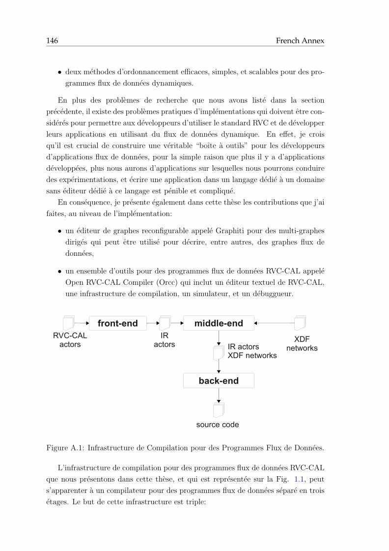
146 French Annex
• deux methodes d’ordonnancement efficaces, simples, et scalables pour des pro-
grammes flux de donnees dynamiques.
En plus des problemes de recherche que nous avons liste dans la section
precedente, il existe des problemes pratiques d’implementations qui doivent etre con-
sideres pour permettre aux developpeurs d’utiliser le standard RVC et de developper
leurs applications en utilisant du flux de donnees dynamique. En effet, je crois
qu’il est crucial de construire une veritable “boıte a outils” pour les developpeurs
d’applications flux de donnees, pour la simple raison que plus il y a d’applications
developpees, plus nous aurons d’applications sur lesquelles nous pourrons conduire
des experimentations, et ecrire une application dans un langage dedie a un domaine
sans editeur dedie a ce langage est penible et complique.
En consequence, je presente egalement dans cette these les contributions que j’ai
faites, au niveau de l’implementation:
• un editeur de graphes reconfigurable appele Graphiti pour des multi-graphes
diriges qui peut etre utilise pour decrire, entre autres, des graphes flux de
donnees,
• un ensemble d’outils pour des programmes flux de donnees RVC-CAL appele
Open RVC-CAL Compiler (Orcc) qui inclut un editeur textuel de RVC-CAL,
une infrastructure de compilation, un simulateur, et un debuggueur.
front-end middle-end
RVC-CAL
actors
IR
actorsXDF
networks
back-end
IR actors
XDF networks
source code
Figure A.1: Infrastructure de Compilation pour des Programmes Flux de Donnees.
L’infrastructure de compilation pour des programmes flux de donnees RVC-CAL
que nous presentons dans cette these, et qui est representee sur la Fig. 1.1, peut
s’apparenter a un compilateur pour des programmes flux de donnees separe en trois
etages. Le but de cette infrastructure est triple:
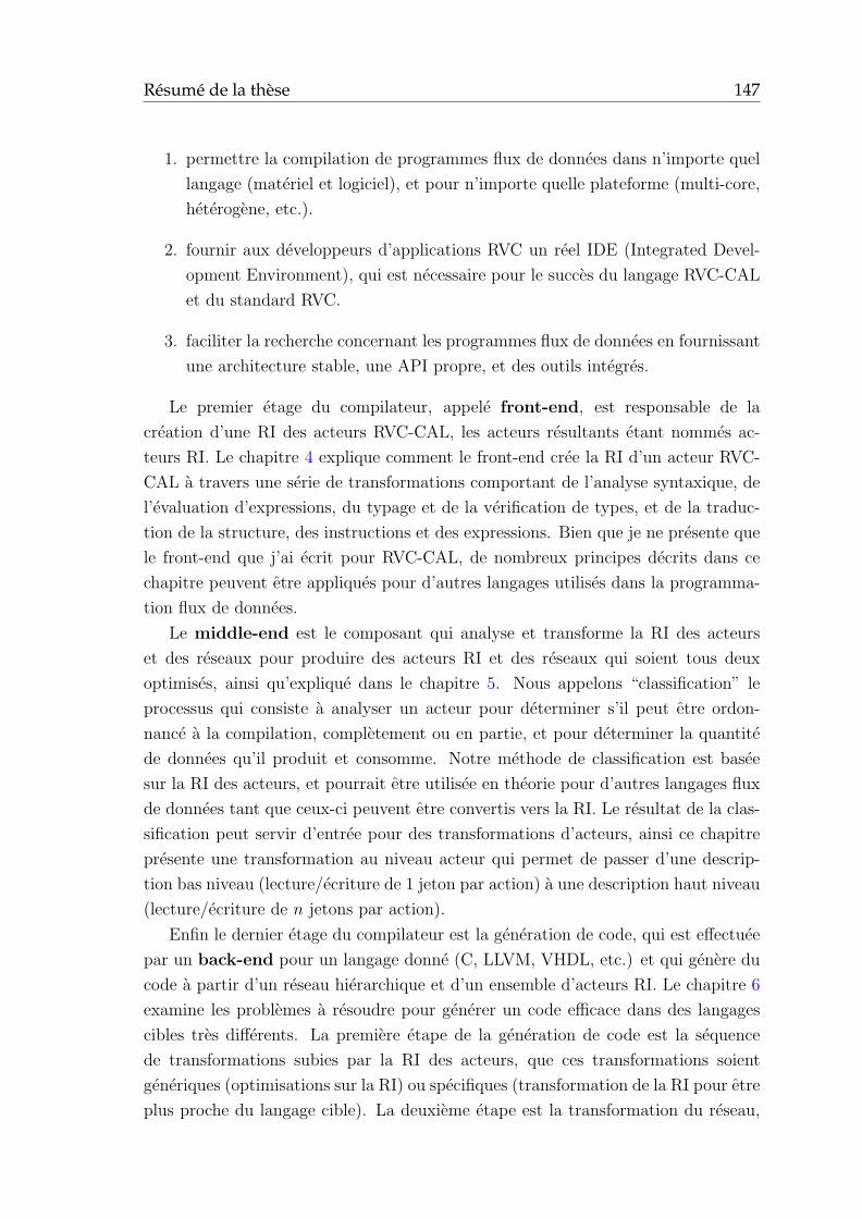
Resume de la these 147
1. permettre la compilation de programmes flux de donnees dans n’importe quel
langage (materiel et logiciel), et pour n’importe quelle plateforme (multi-core,
heterogene, etc.).
2. fournir aux developpeurs d’applications RVC un reel IDE (Integrated Devel-
opment Environment), qui est necessaire pour le succes du langage RVC-CAL
et du standard RVC.
3. faciliter la recherche concernant les programmes flux de donnees en fournissant
une architecture stable, une API propre, et des outils integres.
Le premier etage du compilateur, appele front-end, est responsable de la
creation d’une RI des acteurs RVC-CAL, les acteurs resultants etant nommes ac-
teurs RI. Le chapitre 4 explique comment le front-end cree la RI d’un acteur RVC-
CAL a travers une serie de transformations comportant de l’analyse syntaxique, de
l’evaluation d’expressions, du typage et de la verification de types, et de la traduc-
tion de la structure, des instructions et des expressions. Bien que je ne presente que
le front-end que j’ai ecrit pour RVC-CAL, de nombreux principes decrits dans ce
chapitre peuvent etre appliques pour d’autres langages utilises dans la programma-
tion flux de donnees.
Le middle-end est le composant qui analyse et transforme la RI des acteurs
et des reseaux pour produire des acteurs RI et des reseaux qui soient tous deux
optimises, ainsi qu’explique dans le chapitre 5. Nous appelons “classification” le
processus qui consiste a analyser un acteur pour determiner s’il peut etre ordon-
nance a la compilation, completement ou en partie, et pour determiner la quantite
de donnees qu’il produit et consomme. Notre methode de classification est basee
sur la RI des acteurs, et pourrait etre utilisee en theorie pour d’autres langages flux
de donnees tant que ceux-ci peuvent etre convertis vers la RI. Le resultat de la clas-
sification peut servir d’entree pour des transformations d’acteurs, ainsi ce chapitre
presente une transformation au niveau acteur qui permet de passer d’une descrip-
tion bas niveau (lecture/ecriture de 1 jeton par action) a une description haut niveau
(lecture/ecriture de n jetons par action).
Enfin le dernier etage du compilateur est la generation de code, qui est effectuee
par un back-end pour un langage donne (C, LLVM, VHDL, etc.) et qui genere du
code a partir d’un reseau hierarchique et d’un ensemble d’acteurs RI. Le chapitre 6
examine les problemes a resoudre pour generer un code efficace dans des langages
cibles tres differents. La premiere etape de la generation de code est la sequence
de transformations subies par la RI des acteurs, que ces transformations soient
generiques (optimisations sur la RI) ou specifiques (transformation de la RI pour etre
plus proche du langage cible). La deuxieme etape est la transformation du reseau,
148 French Annex
tout d’abord en “fermant” le reseau (resolution des parametres), en mettant a plat
la hierarchie, et en ajoutant des sommets de diffusion la ou ils sont necessaires. Fi-
nalement, la derniere etape de la generation de code consiste a ecrire du code textuel
depuis la RI des acteurs et des reseaux. Pour ce faire, nous presentons une methode
qui se concentre sur la lisibilite (a la fois celle du generateur de code et du code
genere), la maintenance, et l’experimentation rapide de generateurs de code pour
des nouveaux langages, sans compromettre la vitesse d’execution du generateur de
code
Le chapitre 7 commence par presenter les outils de support pour les programmes
flux de donnees RVC-CAL, ceci incluant un editeur de graphes nomme Graphiti, et
une implementation de l’infrastructure decrite dans ce document appelee Open RVC-
CAL Compiler (Orcc). Le chapitre decrit ensuite les applications de codage video qui
ont ete decrites, en partie ou totalement, avec ces outils. Finalement, nous montrons
les resultats obtenus sur ces applications avec la classification, la transformation
d’acteurs, et l’ordonnancement dynamique sur mono-processeur, processeur multi-
cœurs, et logique programmable.
Pour finir, le chapitre 8 conclut cette these. La conclusion fait le bilan du tra-
vail presente dans le document, identifie les limitations de notre approche a l’heure
actuelle, et liste des perspectives pour des travaux futurs.
A.2 Poursuite des travaux sur le flux de donnees
Cette section decrit les travaux qui ont ete effectues autour des programmes flux de
donnees RVC-CAL, par moi ou par d’autres, au sein du laboratoire ou j’ai effectue
ma these, ainsi que dans d’autres laboratoires, mais egalement des directions qui
semblent interessantes, qu’elles aient ete proposees par moi ou par d’autres.
A.2.1 Prise en compte de l’architecture
Ainsi que j’identifiais dans la conclusion de ma these, l’avantage considerable de se
baser sur une infrastructure de compilation avec une Representation Intermediaire
simple, haut-niveau, et portable, est que l’on peut generer du code materiel et logi-
ciel a partir d’une seule et meme RI d’un programme au sein de l’infrastructure.
Cependant, il n’est pas realiste de pouvoir penser generer une application qui soit
mi-hardware/mi-software sans prendre en compte l’architecture cible.
Un outil appele Preesm, developpe par Maxime Pelcat et Jonathan Piat (et
auquel j’ai contribue un peu de code) a l’IETR, est oriente vers la generation de
code optimisee a partir de modeles flux de donnees statiques pour DSP multi-cœurs,
dont l’architecture (moyens de communications entre cœurs, entre DSPs, entre DSP
Poursuite des travaux sur le flux de donnees 149
et memoire(s), entre DSP et PC...) est decrite a l’aide d’un modele nomme S-LAM
(System-Level Architecture Model). Ce modele est serialise en IP-XACT, ce qui per-
met de garantir l’interoperabilite avec d’autres outils. Afin de mutualiser les efforts,
Maxime et moi avons recemment cree un projet nomme DFTools (pour DataFlow
Tools) dans lequel seront regroupes tous les composants utiles a des outils manipu-
lant des graphes flux de donnees, et ceci inclut notamment un modele d’architecture.
Damien de Saint-Jorre, ingenieur a l’IETR, a d’ailleurs commence une generation
de code multi-plateformes basee sur ce modele d’architecture.
A.2.2 Modifications et ameliorations de la RI
La Representation Intermediaire (RI) sur laquelle est basee l’infrastructure de com-
pilation presentee dans le document a ete construite de maniere incrementale en
fonction des besoins de differents back-ends. Elle n’est donc en aucune maniere
figee, bien au contraire. Par exemple, a une epoque la RI ne contenait pas de CFG,
parce que les analyses que nous voulions faire n’avait pas besoin de cette information,
et le seul back-end existant a l’epoque, le back-end C, n’en avait pas besoin non plus
; j’ai rajoute plus tard la notion de CFG pour les besoins du back-end LLVM ecrit
par Jerome Gorin. Un autre exemple est qu’il y avait auparavant une instruction
HasRoom qui faisait partie de la RI, et qui devait etre traduite par les back-ends
par une verification de la place restante dans la FIFO. La place restante dans une
FIFO n’est pas une condition qui entre en jeu dans l’ordonnancement d’une action,
et n’etait donc pas utilisee par la classification ou l’interpreteur, mais uniquement
traduite par les back-ends. Apres avoir rajoute l’information des motifs d’entree
et de sortie des actions, l’instruction HasRoom etait devenue redondante, et fut
supprimee.
Apres l’ecriture de la these, j’ai realise que l’instruction HasTokens etait
egalement redondante, puisque l’information de lecture peut egalement se deduire
des patterns d’entree et de sortie. D’autre part, ne pas utiliser cette instruction rend
l’ecriture de certains back-ends plus simples, et donne plus de souplesse dans cer-
tains cas (mise a jour de la l’implementation des FIFOs par exemple). On pourrait
argumenter que finalement les autres instructions d’acces aux FIFOs, Peek, Read,
et Write ne sont pas necessaires puisque tout l’information est enregistree dans
les motifs des actions. La difference est cependant que ces instructions definissent
des variables contenant des jetons, ce qui permet de traiter ces variables comme
les autres. Suite a une suggestion de Jerome Gorin, j’ai change la maniere dont
est representee l’information des motifs d’entree et de sortie d’une action. Ces
motifs comportent toute l’information necessaire (dont la definition des variables
contenant les jetons), et ont permis de supprimer les instructions Peek, Read, et
150 French Annex
Write. L’utilisation de motifs rend beaucoup plus simple certaines transformations
d’acteurs, telles que la fusion d’acteurs ou la division d’actions.
Une autre amelioration de la RI a ete proposee par Herve Yviquel, qui effectue
une these a l’IRISA en cotutelle avec l’IETR/INSA. Bien que cet aspect ne soit pas
mentionne dans la these, il n’existe pas reellement de modele de la RI, seulement une
implementation. Definir un modele de la RI aurait un certain nombre d’avantages:
• permettre aux nouveaux developpeurs une reference claire et precise quant a
l’organisation et au contenu de la RI,
• formaliser et uniformiser les relations entre instructions, expressions, nœuds
du CFG, etc. Cela permettra de repondre a des questions comme “quel objet
contient quel autre(s) objet(s)”, “quel objet reference tel autre(s) objet(s)”.
Cela permettra egalement d’offrir les memes possibilites a tous les niveaux,
ce qui n’est pas le cas aujourd’hui, par exemple il est possible de connaıtre le
bloc auquel appartient une instruction, mais il n’est pas possible de connaıtre
facilement le nœud auquel appartient une expression...
• faciliter la traduction depuis et vers la RI a partir de et vers d’autres RI qui
ont deja ete modelisees.
Orcc etant developpe sous Eclipse, le framework de modelisation utilise serait EMF.
A.2.3 Classification et transformation d’acteurs
Un besoin identifie lors du meeting MPEG qui s’est deroule a Daegu, en Coree, fin
janvier 2011, concerne la caracterisation des acteurs dont le comportement depend
du temps. La methode que j’ai proposee dans la these permet de trouver les acteurs
qui ont un comportement time-dependent en verifiant si les gardes d’actions avec
des motifs d’entree dependants du temps sont mutuellement exclusives. J’avais
utilise pour verifier l’exclusion mutuelle un solveur de contraintes. Cependant, le
probleme de prouver l’exclusion mutuelle (ou la non-exclusion mutuelle) est plutot
un probleme de satisfaisabilite qu’un probleme de resolution de contraintes. Cela
fait qu’un solveur de satisfaisabilite (appele solveur SAT ou solveur SMT selon le
type de probleme) sera potentiellement plus performant pour resoudre le probleme.
De plus, le pouvoir d’expression de solveurs SMT est plus important que celui des
solveurs de contraintes typiques, notamment ils peuvent raisonner sur des concepts
de plus haut niveau, tels les tableaux, les fonctions, etc. Il est donc envisage, pour la
classification, de mettre en place une interface avec un solveur SMT afin de diminuer
le nombre de faux-positifs (en effet toutes les gardes d’un acteur potentiellement
Poursuite des travaux sur le flux de donnees 151
time-dependent ne pouvant etre exprimees sous forme de contraintes font que l’acteur
est automatiquement considere time-dependent).
D’autres pistes sont en cours concernant l’analyse et la transformation d’acteurs.
On peut citer par exemple les travaux de Johan Ersfolk, de l’Abo Academy Univer-
sity, qui a commence l’ecriture d’un back-end dans Orcc pour generer du Promela
a partir d’un modele RVC-CAL, afin de pouvoir utiliser l’outil Spin pour analyser
le comportement du modele. D’autres travaux sont en cours par Jerome Gorin pour
fusionner des acteurs dont le comportement est statique, cyclo-statique, ou quasi-
statique.
A.2.4 Amelioration des FIFOs
Comme nous l’avons decrit dans la these, il existe au sein d’un programme flux de
donnees dynamique un certain nombre d’acteurs qui peuvent se comporter selon
des modeles de calcul plus restreints, tels SDF (Synchronous Dataflow), CSDF
(Cyclo-Static Dataflow), ou encore PSDF (Parameterized Synchronous Dataflow).
La litterature mentionne plusieurs techniques pour tirer profit des proprietes de ces
modeles afin de minimiser voir de supprimer le besoin d’ordonnancer ces acteurs
a l’execution en faveur d’un ordonnancement a la compilation. Cependant, il est
rare que tous les acteurs d’une application se comportent selon ces modeles. Dans
certaines applications, la proportion d’acteurs respectant le modele de calcul flux
de donnees dynamique le plus general (DPN) est meme plus grande que la propor-
tion d’acteurs SDF, CSDF, ou PSDF ; c’est ainsi le cas de la description RVC d’un
decodeur MPEG AVC (Advanced Video Coding). Il est donc vital de diminuer au-
tant que faire se peut le surcout lie a l’execution de ce type d’acteurs, notamment
au niveau de l’ordonnanceur d’acteurs et des FIFOs.
Le surcout de l’execution d’acteurs dynamiques par rapport a l’execution
d’acteurs statiques se retrouve a deux niveaux:
1. utilisation de FIFOs, contrairement a de simples tableaux pour des acteurs
statiques,
2. ordonnancement a l’execution plutot qu’a la compilation pour des acteurs sta-
tiques.
Interessons-nous tout d’abord au surcout lie a l’utilisation de FIFOs telles qu’elles
etaient implementees dans le back-end C de Orcc. Les instructions Peek,
Read, Write de la RI sont traduites en C par des appels a des fonctions
d’une librairie implementant des FIFOs avec des buffers circulaires, respectivement
fifo <type> peek, fifo <type> read, fifo <type> write (type etant le type
152 French Annex
de la FIFO, parmi i8, u8, i16, etc.). Afin de pouvoir utiliser ces FIFOs dans un
contexte multi-cœur, le generateur de code C ajoute a la fin de chaque action des
appels aux fonctions fifo <type> read end et fifo <type> write end pour sig-
naler que l’action a fini de lire (respectivement d’ecrire) dans les FIFOs concernees.
Toujours dans ce contexte, une FIFO est une simple structure contenant un tableau,
un indice de lecture, un indice d’ecriture, et un entier contenant la taille de la FIFO.
Les fonctions read end et write end mettent a jour respectivement l’indice de lec-
ture et d’ecriture de la FIFO passee en parametre. Ceci permet de garantir que les
donnees lues et utilisees par une action ne soient pas remplacees par des donnees
produites par un autre acteur tant que l’action n’est pas terminee.
Le probleme inherent a ce modele est qu’a chaque operation sur une FIFO,
que ce soit calcul du nombre de tokens presents, de la place restante, lecture ou
ecriture, les fonctions doivent comparer les indices de lecture et d’ecriture
pour savoir si la FIFO est vide ou pleine. En effet, dans un buffer circulaire
il est possible d’avoir un indice d’ecriture inferieur a l’indice de lecture, dans le cas
ou il y a des donnees entre l’indice de lecture et la fin du buffer, et entre le debut
du buffer et l’indice d’ecriture. Ce surcout est constant quel que soit le nombre de
jetons lus ou ecrits en un appel a read ou write. Autrement dit, si l’on nomme c
le surcout, faire n read(1) entraıne un surcout total de c × (n − 1) par rapport a
un seul read(n). C’est l’une des raisons pour lesquelles un design dit “bas-niveau”,
qui lit/ecrit au plus un jeton par port par action, est plus lent qu’un design plus
haut-niveau qui va lire/ecrire plus de tokens a la fois par action.
Pour remedier a ce probleme, le code genere par le back-end C n’appelle
desormais plus les fonctions de lecture/ecriture de FIFOs. Au debut de l’execution
d’un acteur, l’acteur fait une copie locale des indices de lecture/ecriture. Les ap-
pels aux fonctions de lecture/ecriture sont remplaces par des references de la forme
jetons[indice % TAILLE] ou jetons est le tableau contenant les jetons presents
dans la FIFO, indice est l’indice de lecture (le cas echeant, d’ecriture) local, et
TAILLE est la taille (constante) de la FIFO. Bien entendu, pour que ce remplacement
soit avantageux, il faut que l’operation modulo utilisee soit plus rapide a executer
que les fonctions des FIFOs. Ces fonctions, dans le meilleur des cas, en admettant
qu’elles soient inlinees dans le code appelant, font une addition, une comparaison, et
un saut conditionne. Sur un processeur tel que l’AMD Phenom II, ceci prend 1 + 1 +
1 = 3 cycles. A noter que ce nombre donne un ordre d’idee plutot qu’un temps reel,
puisque les nombres sur lesquels nous nous basons sont la latence des instructions,
et le processeur execute plusieurs instructions a un cycle donne. L’utilisation d’un
saut conditionnel peut occasionner une latence supplementaire lorsque le processeur
predit mal un branchement et doit alors recharger son “pipeline” d’instructions. Une
Poursuite des travaux sur le flux de donnees 153
division sur le processeur decrit ci-dessus, quant a elle, prend au meilleur cas autour
de 20 cycles, et jusqu’a environ 40 cycles au pire cas en 32 bits, et 70 cycles au pire
cas en 64 bits !
L’operation modulo peut etre optimisee pour ne prendre qu’un seul
cycle dans la quasi-totalite des cas. En effet, la taille de la FIFO est constante
et definie a la generation de code par l’utilisateur. Si cette taille est multiple de
2, alors l’operation indice % TAILLE est equivalente a un “et” binaire indice &
(TAILLE - 1), qui ne prend qu’un cycle.
Une autre source de surcout lie a l’ordonnancement d’acteurs dynamiques
provient des sommets de diffusion de donnees. Jusqu’alors, ces sommets etaient
transformes en des acteurs dont le seul but etait de copier les donnees lues depuis
leur port d’entree pour les ecrire sur n ports de sortie. Or il est possible de sup-
primer ces copies memoire en permettant a une FIFO d’avoir plusieurs lecteurs
(et donc plusieurs indices de lecture) pour un ecrivain (un seul indice d’ecriture). Les
FIFOs ont donc ete modifiees par Herve Yviquel pour autoriser plusieurs lecteurs et
supprimer ces sommets de diffusion de donnees.
Application Number of frames per second (QCIF)
MPEG-4 part 2 (normative) 153
MPEG-4 part 2 (low-level) 160
Table A.1: Performance of the C Code Generated from Different Applications.
La table A.1 montre les resultats obtenus sur deux descriptions du decodeur
MPEG-4 part 2 disponible dans Orcc avec les ameliorations mentionnees
precedemment. En comparant ces resultats avec ceux donnes dans la these (table
7.3), on constate une amelioration de 60% sur la description bas-niveau,
alors que l’application haut-niveau n’est quasiment pas affectee. Nous avons obtenu
une augmentation des performances supplementaire en utilisant une taille de FIFO
par defaut plus importantes (4096) et en supprimant les contraintes sur la taille des
FIFOs. Le gain en performance est de l’ordre de 20 fps sur une resolution CIF, qui
amene le design bas-niveau a 80 images par seconde sur une resolution CIF. Nous
poursuivons notre travail sur l’amelioration des FIFOs, notamment pour supprimer
les copies memoire qui sont encore effectuees a la lecture et a l’ecriture de donnees
quand le nombre de jetons a lire/ecrire est superieur a 1.
A.2.5 Amelioration du nouvel ordonnanceur
Nous prevoyons de travailler ensuite a l’amelioration du nouvel ordonnanceur men-
tionne dans la conclusion de la these. Cet ordonnanceur ordonnance les acteurs en
154 French Annex
fonction de leurs besoins, en d’autres termes lorsqu’un acteur ne peut plus s’executer
parce que la FIFO connectee a un de ses ports d’entree I est vide, l’ordonnanceur
va executer l’acteur dont un port de sortie est connecte a I. Si un acteur ne peut
plus s’executer parce que la FIFO connectee a un de ses ports de sortie O est pleine,
alors l’ordonnanceur execute le ou les acteurs dont un port d’entree est connecte a
O. Cet ordonnanceur est tres interessant dans les cas ou les acteurs d’une application
ont des rythmes differents. En effet, l’algorithme de l’ordonnanceur ne va activer
des acteurs que lorsque cela est necessaire, contrairement a l’ordonnanceur Round-
Robin, qui lui ordonnance tous les acteurs de maniere indiscriminee. Le probleme
est que pour l’instant ce nouvel ordonnanceur a un surcout qui le rend plus lent que
l’ordonnanceur Round-Robin dans les cas ou les acteurs d’une application ont des
rythmes homogenes.
Il y a plusieurs sources de surcout dans le nouvel ordonnanceur. Tout d’abord,
les acteurs ne font pas directement aux fonctions de l’ordonnanceur quand ils ne
peuvent plus s’executer. A la place, ils mettent a jour une structure en construisant
un nombre qui identifie les ports dont les FIFOs sont vides ou pleines. Par exemple,
soit un acteur avec quatre ports d’entree P1, P2, P3, P4, s’il manque des donnees sur
les ports 1 et 3, on a un nombre en binaire 0101 (bits 1 et 3 actives). L’ordonnanceur
doit ensuite lancer les predecesseurs (ou successeurs) pour chaque port dont le bit
correspondant dans ce nombre est a 1. Pour cela il fait une boucle sur les ports
d’entree (ou de sortie le cas echeant). On pourrait supprimer la construction de
ce nombre et la boucle de l’ordonnanceur si les acteurs appelaient directement les
fonctions d’ajout et de suppression des predecesseurs.
Une autre source de surcout vient du fait que l’ordonnanceur maintient une liste
des acteurs a ordonnancer, cependant il n’est pas toujours necessaire de passer par
cette liste, notamment dans le cas ou il ne manque des donnees que sur un seul
port. Par ailleurs, l’ordonnanceur execute un acteur en faisant appel a sa fonction
“scheduler”. Il est possible d’eliminer ces deux sources de surcout en declarant les
schedulers d’acteurs en-ligne, et en utilisant des sauts vers ces schedulers plutot que
des appels de fonctions. Toujours sur le processeur mentionne plus tot, un saut con-
ditionnel prend 1 cycle, un appel de fonction en prend 3. A cela vient s’ajouter les
differentes instructions utilisees habituellement dans une fonction : enter (sauve-
garde du pointeur de base et reservation d’espace sur la pile, 10 cycles), leave
(restauration du pointeur de base et liberation de l’espace reserve, 3 cycles), sauve-
gardes de divers registres avec push (4 cycles), etc.
Dans la plupart des langages sequentiels, le cout d’un appel de fonction est
generalement considere negligeable des que cette fonction depasse un certain seuil
(dans son guide pour l’optimisation, AMD suggere de ne pas “inliner” une fonction

Poursuite des travaux sur le flux de donnees 155
qui contient 500 instructions ou plus). En revanche, le code genere a partir d’un
modele CAL a la particularite d’appeler de petites fonctions tres (tres !) souvent.
Bien que le compilateur soit capable d’optimiser les fonctions a l’interieur d’un ac-
teur, il ne peut pas supprimer les appels a des fonctions situees dans des modules
differents. Declarer les fonctions scheduler des acteurs en-ligne devrait permettre
d’eliminer ce surcout.

156 French Annex
List of Figures
1.1 Compilation Infrastructure. . . . . . . . . . . . . . . . . . . . . . . . 14
2.1 Timeline of the publication of video standards. . . . . . . . . . . . . . 18
2.2 Profiles of the MPEG-2 standard. . . . . . . . . . . . . . . . . . . . . 19
2.3 Block diagram of the motion compensation of an MPEG-4 part 2
decoder. . . . . . . . . . . . . . . . . . . . . . . . . . . . . . . . . . . 20
2.4 Dataflow Models of Computation. . . . . . . . . . . . . . . . . . . . . 22
2.5 Parameterized Dataflow. . . . . . . . . . . . . . . . . . . . . . . . . . 25
2.6 Header of an RVC-CAL Actor. . . . . . . . . . . . . . . . . . . . . . . 26
2.7 Example of an RVC-CAL expression. . . . . . . . . . . . . . . . . . . 27
2.8 Declaration of State Variables. . . . . . . . . . . . . . . . . . . . . . . 28
2.9 Declaration of a Function. . . . . . . . . . . . . . . . . . . . . . . . . 28
2.10 Scheduling information and body of an action. . . . . . . . . . . . . . 30
2.11 A simple RVC-CAL actor with an FSM. . . . . . . . . . . . . . . . . 30
2.12 The Clip actor in RVC-CAL. . . . . . . . . . . . . . . . . . . . . . . 31
2.13 An RVC-CAL actor that respects the SDF MoC. . . . . . . . . . . . 33
2.14 An RVC-CAL actor that respects the CSDF MoC. . . . . . . . . . . . 34
2.15 The RVC-CAL Version of the PSDF graph of Fig. 2.5. . . . . . . . . 35
2.16 Concrete Syntax Tree and Abstract Syntax Tree of int(size=3+4). . 38
2.17 CFGs of if and while statements respectively. . . . . . . . . . . . . 39
2.18 Example of code with complex def-use information. . . . . . . . . . . 41
2.19 def-use information of code shown on Fig. 2.18. . . . . . . . . . . . . 41
2.20 def-use information of code shown on Fig. 2.18 encoded with SSA. . . 41
3.1 A JSON object with a few mathematical sequences. . . . . . . . . . . 50
3.2 Test of the schedulability of two actions in VHDL. . . . . . . . . . . . 52
3.3 A sample FSM in RVC-CAL. . . . . . . . . . . . . . . . . . . . . . . 53
3.4 The IR of the FSM shown on Fig. 3.3. . . . . . . . . . . . . . . . . . 53
3.5 Patterns of an RVC-CAL action. . . . . . . . . . . . . . . . . . . . . 54
3.6 The IR patterns of the action shown on Fig. 3.5. . . . . . . . . . . . . 55
157
158 List of Figures
3.7 Reorganizing tokens read. . . . . . . . . . . . . . . . . . . . . . . . . 56
3.8 IR isSchedulable of an action. . . . . . . . . . . . . . . . . . . . . . . 56
3.9 Syntax of IR CFG nodes. . . . . . . . . . . . . . . . . . . . . . . . . . 58
3.10 Syntax of IR instructions. . . . . . . . . . . . . . . . . . . . . . . . . 58
3.11 Syntax of IR regular instructions. . . . . . . . . . . . . . . . . . . . . 58
3.12 Syntax of Phi instruction. . . . . . . . . . . . . . . . . . . . . . . . . 59
3.13 Syntax of FIFO instructions. . . . . . . . . . . . . . . . . . . . . . . . 59
3.14 Syntax of FIFO instructions. . . . . . . . . . . . . . . . . . . . . . . . 60
4.1 Front-end in the Compilation Infrastructure. . . . . . . . . . . . . . . 63
4.2 Xtext grammar rule for an RVC-CAL actor. . . . . . . . . . . . . . . 65
4.3 Inferred meta-model from the AstActor rule. . . . . . . . . . . . . . . 65
4.4 Xtext grammar rule for a call statement with cross-reference to a
procedure. . . . . . . . . . . . . . . . . . . . . . . . . . . . . . . . . . 66
4.5 Directed Graph of Priorities. . . . . . . . . . . . . . . . . . . . . . . . 72
5.1 Middle-end in the compilation infrastructure. . . . . . . . . . . . . . . 79
5.2 The Finite State Machine of Algo Interpolation halfpel. . . . . . . . . 80
5.3 Variables of Algo Interpolation halfpel. . . . . . . . . . . . . . . . . . 80
5.4 Action start of Algo Interpolation halfpel. . . . . . . . . . . . . . . . 81
5.5 Actions fireable in the interpolate state. . . . . . . . . . . . . . . . . . 82
5.6 loop body procedure. . . . . . . . . . . . . . . . . . . . . . . . . . . 82
5.7 The do clip action rewritten in a time-independent way. . . . . . . . 83
5.8 A Finite State Machine with four branches. . . . . . . . . . . . . . . 89
5.9 Loop Rerolling on Algo Interpolation halfpel. . . . . . . . . . . . 93
5.10 The limit action transformed. . . . . . . . . . . . . . . . . . . . . . . 94
6.1 A back-end in the compilation infrastructure. . . . . . . . . . . . . . 97
6.2 Example of a simple StringTemplate template. . . . . . . . . . . . . . 103
6.3 A ST template with conditionals. . . . . . . . . . . . . . . . . . . . . 104
6.4 Obtaining information about the connections of a network. . . . . . . 105
6.5 Printing instructions of a block node. . . . . . . . . . . . . . . . . . . 107
6.6 Three expressions and the corresponding expression trees. . . . . . . . 108
6.7 Clips x to −2048 in CAL. . . . . . . . . . . . . . . . . . . . . . . . . 110
6.8 Clips x to −2048 in VHDL. . . . . . . . . . . . . . . . . . . . . . . . 111
6.9 Clips x to −2048 in LLVM. . . . . . . . . . . . . . . . . . . . . . . . 112
6.10 Implicit Broadcast of Data Produced by source. . . . . . . . . . . . . 114
6.11 Explicit broadcast of data produced by source handled by a broadcast
actor. . . . . . . . . . . . . . . . . . . . . . . . . . . . . . . . . . . . . 114
List of Figures 159
7.1 Eclipse ecosystem. . . . . . . . . . . . . . . . . . . . . . . . . . . . . 118
7.2 Graphiti transformations. . . . . . . . . . . . . . . . . . . . . . . . . 120
7.3 Graphiti infrastructure. . . . . . . . . . . . . . . . . . . . . . . . . . . 121
7.4 Normative MPEG-4 part 2 Simple Profile decoder. . . . . . . . . . . 126
7.5 Proprietary description of an MPEG-4 part 2 Simple Profile decoder. 127
7.6 Implementation of an RVC-CAL Actor in C. . . . . . . . . . . . . . . 131
A.1 Infrastructure de Compilation pour des Programmes Flux de Donnees. 146

160 List of Figures
List of Tables
4.1 Evaluation rules for RVC-CAL expressions (eval). . . . . . . . . . . . 68
4.2 Conversion from RVC-CAL type system to IR type system (conv). . . 69
4.3 Type inference of RVC-CAL expressions. . . . . . . . . . . . . . . . . 70
4.4 Type checking of AST statements. . . . . . . . . . . . . . . . . . . . . 70
5.1 Abstract interpretation of Algo Interpolation halfpel. . . . . . . . 86
7.1 Compilation times for different applications with OpenDF and Orcc. . 123
7.2 Compilation times for the actors of the MPEG-4 decoder with Open-
Forge. . . . . . . . . . . . . . . . . . . . . . . . . . . . . . . . . . . . 124
7.3 Performance of the C Code Generated from Different Applications. . 133
7.4 Performance on Two Cores. . . . . . . . . . . . . . . . . . . . . . . . 133
7.5 Classification results on 50 actors. . . . . . . . . . . . . . . . . . . . . 134
A.1 Performance of the C Code Generated from Different Applications. . 153
161

Personal Publications
[GJB+09] R. Gu, J.W. Janneck, S.S. Bhattacharyya, M. Raulet, M. Wipliez, and
W. Plishker. Exploring the concurrency of an MPEG RVC decoder
based on dataflow program analysis. IEEE Transactions on Circuits
and Systems for Video Technology, 19(11), 2009.
[GWPR10a] Jerome Gorin, Matthieu Wipliez, Francoise Preteux, and Mickael
Raulet. A portable Video Tool Library for MPEG Reconfigurable
Video Coding using LLVM Representation. In Design and Architec-
tures for Signal and Image Processing (DASIP), 2010.
[GWPR10b] Jerome Gorin, Matthieu Wipliez, Francoise Preteux, and Mickael
Raulet. An LLVM-based decoder for MPEG Reconfigurable Video
Coding. In IEEE workshop on Signal Processing Systems (SiPS), 2010.
[GWPR10c] Jerome Gorin, Matthieu Wipliez, Francoise Preteux, and Mickael
Raulet. LLVM-based and scalable MPEG-RVC decoder. Journal of
Real-Time Image Processing, pages 1–12, 2010. 10.1007/s11554-010-
0169-2.
[JMP+08] J.W. Janneck, I.D. Miller, D.B. Parlour, G. Roquier, M. Wipliez,
and M. Raulet. Synthesizing hardware from dataflow programs: An
MPEG-4 simple profile decoder case study. In IEEE workshop on Sig-
nal Processing Systems (SiPS), pages 287–292. IEEE, 2008.
[JMP+09] Jorn W. Janneck, Ian D. Miller, David B. Parlour, Ghislain Roquier,
Matthieu Wipliez, and Mickael Raulet. Synthesizing Hardware from
Dataflow Programs. Journal of Signal Processing Systems, 07 2009.
[JMRW10] J.W. Janneck, M. Mattavelli, M. Raulet, and M. Wipliez. Reconfig-
urable video coding: a stream programming approach to the specifi-
cation of new video coding standards. In Proceedings of the first an-
nual ACM SIGMM conference on Multimedia systems, pages 223–234.
ACM, 2010.
163
[JWR+10] K. Jerbi, M. Wipliez, M. Raulet, O. Deforges, M. Babel, and M. Abid.
Fast Hardware implementation of an Hadamard Transform Using RVC-
CAL Dataflow Programming. In 5th IEEE International Conference
on Embedded and Multimedia Computing, August 2010.
[LMW+08] Christophe Lucarz, Marco Mattavelli, Matthieu Wipliez, Ghislain
Roquier, Mickael Raulet, Jorn W. Janneck, Ian D. Miller, and David B.
Parlour. Dataflow/Actor-Oriented language for the design of complex
signal processing systems. In Design and Architectures for Signal and
Image Processing (DASIP), Bruxelles, Belgique, 2008.
[PPW+09] M. Pelcat, J. Piat, M. Wipliez, S. Aridhi, and J.F. Nezan. An
open framework for rapid prototyping of signal processing applications.
EURASIP Journal on Embedded Systems, 2009:3, 2009.
[RLM+09] G. Roquier, C. Lucarz, M. Mattavelli, M. Wipliez, M. Raulet, J.W.
Janneck, I.D. Miller, and D.B. Parlour. An integrated environment for
HW/SW co-design based on a CAL specification and HW/SW code
generators. In IEEE International Symposium on Circuits and Systems
(ISCAS), page 799. IEEE, 2009.
[RWR+08] G. Roquier, M. Wipliez, M. Raulet, J.W. Janneck, I.D. Miller, and
D.B. Parlour. Automatic software synthesis of dataflow program: An
MPEG-4 simple profile decoder case study. In IEEE workshop on
Signal Processing Systems (SiPS), pages 281–286, 2008.
[SWNR10] Nicolas Siret, Matthieu Wipliez, Jean-Francois Nezan, and Aimad
Rhatay. Hardware code generation from dataflow programs. In Design
and Architectures for Signal and Image Processing (DASIP), 2010.
[WR10] Matthieu Wipliez and Mickael Raulet. Classification and Transforma-
tion of Dynamic Dataflow Programs. In Design and Architectures for
Signal and Image Processing (DASIP), 2010.
[WRN09] Matthieu Wipliez, Ghislain Roquier, and Jean-Francois Nezan. Soft-
ware Code Generation for the RVC-CAL Language. Journal of Signal
Processing Systems, 2009.
[WRR+08] Matthieu Wipliez, Ghislain Roquier, Mickael Raulet, Jean-Francois
Nezan, and Olivier Deforges. Code generation for the MPEG Recon-
figurable Video Coding framework: From CAL actions to C functions.
In IEEE International Conference on Multimedia and Expo (ICME),
pages 1049–1052, 2008.
MPEG Contributions
[DRRW08] Florian Decologne, Mickael Raulet, Ghislain Roquier, and Matthieu
Wipliez. M15420: RVC Conformance Testing of a Functional Unit us-
ing Open Dataflow and TCP/IP. ISO/IEC JTC1/SC29/WG11, 84th
MPEG Meeting Document Register, Archamps, France, April 2008.
[GWR+10] Jerome Gorin, Matthieu Wipliez, Mickael Raulet, Marco Mattavelli, and
Francoise Preteux. M17318: Demo : An MPEG RVC decoder based on
LLVM. ISO/IEC JTC1/SC29/WG11, 91st MPEG Meeting Document
Register, Kyoto, Japan, January 2010.
[JPM+08] Jorn W. Janneck, David Parlour, Ian Miller, Matthieu Wipliez, Mickael
Raulet, Ghislain Roquier, Christophe Lucarz, and Marco Mattavelli.
M15386: CAL profile for HW/SW code generators of the RVC frame-
work. ISO/IEC JTC1/SC29/WG11, 84th MPEG Meeting Document
Register, Archamps, France, April 2008.
[LRWM10] Pierre-Laurent Lagalaye, Mickael Raulet, Matthieu Wipliez, and Marco
Mattavelli. M17839: Debug and development support tools for RVC-
CAL. ISO/IEC JTC1/SC29/WG11, 93th MPEG Meeting Document
Register, Geneva, Switzerland, July 2010.
[RPR+07] Ghislain Roquier, Maxime Pelcat, Mickael Raulet, Matthieu Wipliez,
Jean-Francois Nezan, and Olivier Deforges. M14457: A scheme for
implementing MPEG-4 SP codec in the RVC framework. ISO/IEC
JTC1/SC29/WG11, 80th MPEGMeeting Document Register, San Jose,
USA, April 2007.
[RRW+08] Mickael Raulet, Ghislain Roquier, Matthieu Wipliez, Jean-Francois
Nezan, and Olivier Deforges. M15167: Update of CAL2C code gen-
eration. ISO/IEC JTC1/SC29/WG11, 83rd MPEG Meeting Document
Register, Antalya, Turkey, January 2008.
165

[RW09] Mickael Raulet and Matthieu Wipliez. M16700: Extension of Cal2C in a
new compiler infrastructure called ORCC. ISO/IEC JTC1/SC29/WG11,
89th MPEG Meeting Document Register, London, England, June 2009.
[RWJ09] Mickael Raulet, Matthieu Wipliez, and Jorn W. Janneck. M16333: FU
Parametrization and FU code generation. ISO/IEC JTC1/SC29/WG11,
88th MPEG Meeting Document Register, Maui, USA, April 2009.
[WLRG10] Matthieu Wipliez, Pierre-Laurent Lagalaye, Mickael Raulet, and Jerome
Gorin. M17841: Development status of Open RVC-CAL compiler.
ISO/IEC JTC1/SC29/WG11, 93th MPEG Meeting Document Regis-
ter, Geneva, Switzerland, July 2010.
[WPR08] Matthieu Wipliez, Jonathan Piat, and Mickael Raulet. M15680: DDL
graphical editor. ISO/IEC JTC1/SC29/WG11, 85th MPEG Meeting
Document Register, Hannover, Germany, July 2008.
[WR10] Matthieu Wipliez and Mickael Raulet. M18346: Automatic classification
of FUs. ISO/IEC JTC1/SC29/WG11, 94th MPEG Meeting Document
Register, Guangzhou, China, October 2010.
[WRGS10] Matthieu Wipliez, Mickael Raulet, Jerome Gorin, and Nicolas Siret.
M18345: Addendum: Specification of typing rules for RVC-CAL.
ISO/IEC JTC1/SC29/WG11, 94th MPEG Meeting Document Regis-
ter, Guangzhou, China, October 2010.
[WRN09] Matthieu Wipliez, Mickael Raulet, and Jean-Francois Nezan. M16145:
Proposed changes for RVC-CAL annex A of ISO-IEC 23001-4. ISO/IEC
JTC1/SC29/WG11, 87th MPEG Meeting Document Register, Lau-
sanne, Switzerland, February 2009.
[WRP08] Matthieu Wipliez, Mickael Raulet, and Jonathan Piat. M15870:
Editing a RVC FU network using a GUI called Graphiti. ISO/IEC
JTC1/SC29/WG11, 86th MPEG Meeting Document Register, Busan,
Korea, October 2008.
[WRR+07] Matthieu Wipliez, Ghislain Roquier, Mickael Raulet, Jean-Francois
Nezan, Marco Mattavelli, and Ian Miller. M14981: Status of CAL2C
code generation. ISO/IEC JTC1/SC29/WG11, 82nd MPEG Meeting
Document Register, Shenzhen, China, November 2007.
[WRR+08] Matthieu Wipliez, Mickael Raulet, Ghislain Roquier, Jean-Francois
Nezan, and Olivier Deforges. M15382: A fast simulation of

RVC MPEG4 SP decoder using Cal2C code generation. ISO/IEC
JTC1/SC29/WG11, ISO/IEC JTC1/SC29/WG11, 84th MPEG Meet-
ing Document Register, April 2008.

Bibliography
[AH00] J. Aycock and N. Horspool. Simple generation of static single-
assignment form. In Compiler Construction, pages 110–125. Springer,
2000.
[ANvP10] K.E. Arzen, A. Nilsson, and C. von Platen. Model Compiler, 2010.
[ASU86] A.V. Aho, R. Sethi, and J.D. Ullman. Compilers: principles, tech-
niques, and tools. Reading, MA,, 1986.
[BA06] S. Bansal and A. Aiken. Automatic generation of peephole superopti-
mizers. ACM SIGOPS Operating Systems Review, 40(5):394–403, 2006.
[Bar98] R. Bardohl. A Generic Graphical Editor for Visual Languages based on
Algebraic Graph Grammars. In Proc. IEEE Symp. Visual Languages,
pages 48–55. Citeseer, 1998.
[BBJ+08] Shuvra S. Bhattacharyya, Gordon Brebner, Jorn W. Janneck, Johan
Eker, Carl von Platen, Marco Mattavelli, and Mickael Raulet. OpenDF:
a dataflow toolset for reconfigurable hardware and multicore systems.
SIGARCH Comput. Archit. News, 36(5):29–35, 2008.
[BBM01] Bishnupriya Bhattacharya, Shuvra S. Bhattacharyya, and Senior Mem-
ber. Parameterized Dataflow Modeling for DSP Systems. IEEE Trans-
actions on Signal Processing, 49:2408–2421, 2001.
[BC94] P. Briggs and K.D. Cooper. Effective partial redundancy elimination.
ACM SIGPLAN Notices, 29(6):159–170, 1994.
[BCHS98] P. Briggs, K.D. Cooper, T.J. Harvey, and L.T. Simpson. Practical im-
provements to the construction and destruction of static single assign-
ment form. Software: Practice and Experience, 28(8):859–881, 1998.
[BCT94] P. Briggs, K.D. Cooper, and L. Torczon. Improvements to graph color-
ing register allocation. ACM Transactions on Programming Languages
and Systems (TOPLAS), 16(3):455, 1994.
169
[BDR+09] B. Boissinot, A. Darte, F. Rastello, B.D. de Dinechin, and C. Guillon.
Revisiting out-of-SSA translation for correctness, code quality and ef-
ficiency. In Proceedings of the 2009 International Symposium on Code
Generation and Optimization, pages 114–125. IEEE Computer Society,
2009.
[BEH+02] U. Brandes, M. Eiglsperger, I. Herman, M. Himsolt, and M. Marshall.
GraphML Progress Report Structural Layer Proposal. In Graph Draw-
ing, pages 109–112. Springer, 2002.
[BELP96] G. Bilsen, M. Engels, R. Lauwereins, and J. Peperstraete. Cyclo-
static dataflow. IEEE Transactions on signal processing, 44(2):397–408,
1996.
[Ber06] V. Berman. Standards: The P1685 IP-XACT IP Metadata Standard.
IEEE Design & Test of Computers, 23(4):316–317, 2006.
[BGJ91] Albert Benveniste, Paul Le Guernic, and Christian Jacquemot. Syn-
chronous programming with events and relations: the SIGNAL lan-
guage and its semantics. Science of Computer Programming, 16(2):103–
149, 1991.
[BJK+95] R.D. Blumofe, C.F. Joerg, B.C. Kuszmaul, C.E. Leiserson, K.H. Ran-
dall, and Y. Zhou. Cilk: An efficient multithreaded runtime system. In
Proceedings of the fifth ACM SIGPLAN symposium on Principles and
practice of parallel programming, pages 207–216. ACM, 1995.
[BL93] J.T. Buck and E.A. Lee. Scheduling dynamic dataflow graphs with
bounded memory using the token flow model. Acoustics, Speech, and
Signal Processing, IEEE International Conference on, 1:429–432, 1993.
[BLL+08] J. Boutellier, C. Lucarz, S. Lafond, V.M. Gomez, and M. Mattavelli.
Quasi-static scheduling of CAL actor networks for reconfigurable video
coding. Journal of Signal Processing Systems, pages 1–12, 2008.
[BM94] M.M. Brandis and H. Mossenbock. Single-pass generation of static
single-assignment form for structured languages. ACM Transactions on
Programming Languages and Systems (TOPLAS), 16(6):1698, 1994.
[BMR10] Endri Bezati, Marco Mattavelli, and Mickael Raulet. RVC-CAL
dataflow implementations of MPEG AVC/H.264 CABAC decoding. In
Design and Architectures for Signal and Image Processing (DASIP),
2010.
[Bra95] M.M. Brandis. Optimizing compilers for structured programming lan-
guages. PhD thesis, ETH Zurich, 1995.
[CAC+81] G.J. Chaitin, M.A. Auslander, A.K. Chandra, J. Cocke, M.E. Hopkins,
and P.W. Markstein. Register allocation via coloring. In Computer
Languages, volume 6, pages 47–57. Elsevier, 1981.
[CC77] P. Cousot and R. Cousot. Abstract interpretation: a unified lattice
model for static analysis of programs by construction or approximation
of fixpoints. In Proceedings of the 4th ACM SIGACT-SIGPLAN sym-
posium on Principles of programming languages, pages 238–252. ACM
New York, NY, USA, 1977.
[CCF91] J.D. Choi, R. Cytron, and J. Ferrante. Automatic construction of
sparse data flow evaluation graphs. In Proceedings of the 18th ACM
SIGPLAN-SIGACT symposium on Principles of programming lan-
guages, pages 55–66. ACM, 1991.
[CCK+97] F. Chow, S. Chan, R. Kennedy, S.M. Liu, R. Lo, and P. Tu. A new
algorithm for partial redundancy elimination based on SSA form. In
Proceedings of the ACM SIGPLAN 1997 conference on Programming
language design and implementation, page 286. ACM, 1997.
[CF95] R.K. Cytron and J. Ferrante. Efficiently computing Φ-nodes on-
the-fly. ACM Transactions on Programming Languages and Systems
(TOPLAS), 17(3):487–506, 1995.
[CFR+91] R. Cytron, J. Ferrante, B.K. Rosen, M.N. Wegman, and F.K. Zadeck.
Efficiently computing static single assignment form and the control de-
pendence graph. ACM Transactions on Programming Languages and
Systems (TOPLAS), 13(4):490, 1991.
[CFT03] L. Carter, J. Ferrante, and C. Thomborson. Folklore confirmed: re-
ducible flow graphs are exponentially larger. In Proceedings of the 30th
ACM SIGPLAN-SIGACT symposium on Principles of programming
languages, pages 106–114. ACM, 2003.
[CH84] F. Chow and J. Hennessy. Register allocation by priority-based col-
oring. In Proceedings of the 1984 SIGPLAN symposium on Compiler
construction, pages 222–232. ACM, 1984.
[CHHP91] J.R. Cordy, C.D. Halpern-Hamu, and E. Promislow. TXL: A rapid
prototyping system for programming language dialects. Computer Lan-
guages, 16(1):97–107, 1991.
[CKL+05] J. Cortadella, A. Kondratyev, L. Lavagno, C. Passerone, and Y. Watan-
abe. Quasi-static scheduling of independent tasks for reactive systems.
IEEE Transactions on Computer-Aided Design of Integrated Circuits
and Systems, 24(10):1492–1514, 2005.
[Cli95] C. Click. Global code motion/global value numbering. ACM SIGPLAN
Notices, 30(6):246–257, 1995.
[CM69] J. Cocke and R.E. Miller. Some analysis techniques for optimizing
computer programs. In Proc. 2nd Hawaii International Conference on
System Sciences, pages 143–146, January 1969.
[Coc70] John Cocke. Global common subexpression elimination. SIGPLAN
Not., 5(7):20–24, 1970.
[Den74] J. Dennis. First version of a data flow procedure language. In Program-
ming Symposium, pages 362–376. Springer, 1974.
[Deu96] P. Deutsch. RFC 1952: GZIP file format specification version 4.3.
Internet Engineering Task Force (IETF), 1996.
[DM82] Luis Damas and Robin Milner. Principal type-schemes for functional
programs. In Proceedings of POPL ’82, pages 207–212, 1982.
[DM02] L. Dagum and R. Menon. OpenMP: an industry standard API for
shared-memory programming. Computational Science & Engineering,
IEEE, 5(1):46–55, 2002.
[DRW04] J. Des Rivieres and J. Wiegand. Eclipse: A platform for integrating
development tools. IBM Systems Journal, 43(2):371–383, 2004.
[Ecl] Eclipse Foundation. Eclipse Modeling Framework (EMF).
[Ecm06] Ecma. ISO/IEC 23271/ECMA-335: Common Language Infrastructure
(CLI), 2006.
[EEHT05] K. Ehrig, C. Ermel, S. Hansgen, and G. Taentzer. Generation of visual
editors as eclipse plug-ins. In Proceedings of the 20th IEEE/ACM in-
ternational Conference on Automated software engineering, page 143.
ACM, 2005.
[EJ03] J. Eker and J. Janneck. CAL Language Report. Technical Report
ERL Technical Memo UCB/ERL M03/48, University of California at
Berkeley, December 2003.
[EJL+03] J. Eker, J.W. Janneck, E.A. Lee, J. Liu, X. Liu, J. Ludvig, S. Neuen-
dorffer, S. Sachs, and Y. Xiong. Taming heterogeneity-the Ptolemy
approach. Proceedings of the IEEE, 91(1):127–144, 2003.
[ETH] ETH Zurich. Moses project: http: // www. tik. ee. ethz. ch/
~ moses/ .
[EV06] S. Efftinge and M. Volter. oAW xText: A framework for textual DSLs.
In Workshop on Modeling Symposium at Eclipse Summit, 2006.
[GH98] E.M. Gagnon and L.J. Hendren. SableCC, an object-oriented com-
piler framework. In tools, page 140. Published by the IEEE Computer
Society, 1998.
[GLS99] W. Gropp, E. Lusk, and A. Skjellum. Using MPI: portable parallel
programming with the message passing interface. MIT Press, 1999.
[Gra] Graphiti. Graphiti Editor: http: // graphiti-editor. sf. net/ .
[HCRP02] N. Halbwachs, P. Caspi, P. Raymond, and D. Pilaud. The synchronous
data flow programming language LUSTRE. Proceedings of the IEEE,
79(9):1305–1320, 2002.
[HDE+93] L. Hendren, C. Donawa, M. Emami, G. Gao, and B. Sridharan. De-
signing the McCAT compiler based on a family of structured intermedi-
ate representations. Languages and Compilers for Parallel Computing,
pages 406–420, 1993.
[HL91] G.J. Holzmann and Staff AT&T Bell Laboratories. Design and valida-
tion of computer protocols. Prentice hall Englewood Cliffs, New Jersey,
1991.
[HSH+09] W. Haid, L. Schor, K. Huang, I. Bacivarov, and L. Thiele. Efficient
execution of Kahn process networks on multi-processor systems using
protothreads and windowed FIFOs. In Proc. IEEE Workshop on Em-
bedded Systems for Real-Time Multimedia (ESTIMedia), pages 35–44,
2009.
[IEE93] IEEE Std 1076-1993. IEEE Std 1076 - IEEE Standard VHDL Language
Reference Manual, 1993.
[IEE05] IEEE Std 1666-2005. IEEE Std 1666 - IEEE Standard SystemC Lan-
guage Reference Manual, 2005.
[ISO07] ISO/IEC FDIS 23002-2:2007(E). Information technology – MPEG
video technologies – Part 2: Fixed-point 8x8 inverse discrete cosine
transform and discrete cosine transform, 2007.
[ISO09] ISO/IEC FDIS 23001-4. MPEG systems technologies – Part 4: Codec
Configuration Representation, 2009.
[ITU] ITU-R. ITU-R Recommendation BT.601-4.
[Jan97] J.W. Janneck. Graph-type definition language (GTDL)—specification.
Moses project, 1997.
[JC96] J. Janssen and H. Corporaal. Controlled node splitting. In Compiler
Construction, pages 44–58. Springer, 1996.
[JE01] Jorn W. Janneck and Robert Esser. A predicate-based approach to
defining visual language syntax. In HCC ’01: Proceedings of the IEEE
2001 Symposia on Human Centric Computing Languages and Environ-
ments (HCC’01), page 40, Washington, DC, USA, 2001. IEEE Com-
puter Society.
[Joh76] S.C. Johnson. YACC-yet another compiler-compiler, 1976.
[JRR99] S. Jones, N. Ramsey, and F. Reig. C– –: A Portable Assembly Lan-
guage that Supports Garbage Collection. Principles and Practice of
Declarative Programming, pages 1–28, 1999.
[Kah74] G. Kahn. The semantics of a simple language for parallel programming.
In Proceedings of IFIP’74, pages 471–475, August 1974.
[Kil73] G.A. Kildall. A unified approach to global program optimization. In
Proceedings of the 1st annual ACM SIGACT-SIGPLAN symposium on
Principles of programming languages, pages 194–206. ACM, 1973.
[Kod04] V. Kodaganallur. Incorporating language processing into Java applica-
tions: A JavaCC tutorial. IEEE software, pages 70–77, 2004.
[KP88] G.E. Krasner and S.T. Pope. A cookbook for using the model-view
controller user interface paradigm in Smalltalk-80. Journal of Object-
oriented programming, 1(3):49, 1988.
[KS98] K. Knobe and V. Sarkar. Array SSA form and its use in parallelization.
In Proceedings of the 25th ACM SIGPLAN-SIGACT symposium on
Principles of programming languages, pages 107–120. ACM, 1998.
[LA04] Chris Lattner and Vikram Adve. Llvm: A compilation framework
for lifelong program analysis & transformation. Code Generation and
Optimization, IEEE/ACM International Symposium on, 0:75, 2004.
[LM87] E.A. Lee and D.G. Messerschmitt. Synchronous data flow. Proceedings
of the IEEE, 75(9):1235–1245, 1987.
[LP95] Edward A. Lee and Thomas M. Parks. Dataflow Process Networks.
Proceedings of the IEEE, 83(5):773–801, May 1995.
[MAR10] M. Mattavelli, I. Amer, and M. Raulet. The Reconfigurable Video Cod-
ing Standard [Standards in a Nutshell]. Signal Processing Magazine,
IEEE, 27(3):159 –167, may 2010.
[MR79] E. Morel and C. Renvoise. Global optimization by suppression of partial
redundancies. Communications of the ACM, 22(2):96–103, 1979.
[MV95] M. Minas and G. Viehstaedt. DiaGen: a generator for diagram ed-
itors providing direct manipulation and execution of diagrams. In
11th IEEE International Symposium on Visual Languages, Proceed-
ings., pages 203–210, 1995.
[Mu93] U. Muller. brainfuck – an eight-instruction turing-complete pro-
gramming language. Available at the Internet address http: // en.
wikipedia. org/ wiki/ Brainfuck , 1993.
[Nav08] B. Naveh. JGraphT: http: // jgrapht. sourceforge. net , 2008.
[NCH+05] G.C. Necula, J. Condit, M. Harren, S. McPeak, and W. Weimer.
CCured: Type-safe retrofitting of legacy software. ACM Transactions
on Programming Languages and Systems (TOPLAS), 27(3):477–526,
2005.
[NMRW02] G. Necula, S. McPeak, S. Rahul, and W. Weimer. CIL: Intermediate
language and tools for analysis and transformation of C programs. In
Compiler Construction, pages 209–265. Springer, 2002.
[NMW97] C.G. Nevill-Manning and I.H. Witten. Identifying hierarchical structure
in sequences: A linear-time algorithm. Journal of Artificial Intelligence
Research, 7(1):67–82, 1997.
[OSG05] OSGi Alliance. OSGi Service Platform Release 4, 2005.
[Par95] Thomas M. Parks. Bounded Scheduling of Process Networks. PhD
thesis, Berkeley, Berkeley, CA, USA, 1995.
[Par04] Terence John Parr. Enforcing strict model-view separation in template
engines. InWWW ’04: Proceedings of the 13th international conference
on World Wide Web, pages 224–233, New York, NY, USA, 2004. ACM.
[Par06] T. Parr. A functional language for generating structured text. URL
http://www. cs. usfca. edu/˜ parrt/papers/ST. pdf, 2006.
[Pat95] J.R.C. Patterson. Accurate static branch prediction by value range
propagation. ACM SIGPLAN Notices, 30(6):67–78, 1995.
[PB95] K. Pingali and G. Bilardi. APT: A data structure for optimal control
dependence computation. In Proceedings of the ACM SIGPLAN 1995
conference on Programming language design and implementation, pages
32–46. ACM, 1995.
[PQ95] T.J. Parr and R.W. Quong. ANTLR: A predicated-LL (k) parser gen-
erator. Software: Practice and Experience, 25(7):789–810, 1995.
[PS99] M. Poletto and V. Sarkar. Linear scan register allocation. ACM
Transactions on Programming Languages and Systems (TOPLAS),
21(5):895–913, 1999.
[SG95] V.C. Sreedhar and G.R. Gao. A linear time algorithm for placing
&phgr;-nodes. In Proceedings of the 22nd ACM SIGPLAN-SIGACT
symposium on Principles of programming languages, pages 62–73.
ACM, 1995.
[SJGS99] V. Sreedhar, R. Ju, D. Gillies, and V. Santhanam. Translating out of
static single assignment form. Static Analysis, pages 849–849, 1999.
[SV05] G. Stitt and F. Vahid. New decompilation techniques for binary-level
co-processor generation. In IEEE/ACM International Conference on
Computer-Aided Design, 2005. ICCAD-2005, pages 547–554, 2005.
[SVKW07] S. Staiger, G. Vogel, S. Keul, and E. Wiebe. Interprocedural Static Sin-
gle Assignment Form. In Proceedings of the 14th Working Conference
on Reverse Engineering, pages 1–10. Citeseer, 2007.
[Val95] J.D. Valois. Lock-free linked lists using compare-and-swap. In Pro-
ceedings of the fourteenth annual ACM symposium on Principles of
distributed computing, page 222. ACM, 1995.
[vP10] C. von Platen. CAL ARM Compiler, 2010.
[VRCG+99] R. Vallee-Rai, P. Co, E. Gagnon, L. Hendren, P. Lam, and V. Sundare-
san. Soot - a Java bytecode optimization framework. In Proceedings of
the 1999 conference of the Centre for Advanced Studies on Collaborative
research, page 13. IBM Press, 1999.
[WELP96] P. Wauters, M. Engels, R. Lauwereins, and JA Peperstraete. Cyclo-
dynamic dataflow. In pdp, page 0319. Published by the IEEE Computer
Society, 1996.
[Wer02] L. Wernli. Design and implementation of a code generator for the CAL
actor language. Technical report, Technical Memo UCB/ERL M02,
2002.
[WFW+94] R.P. Wilson, R.S. French, C.S. Wilson, S.P. Amarasinghe, J.M. Ander-
son, S.W.K. Tjiang, S.W. Liao, C.W. Tseng, M.W. Hall, M.S. Lam,
et al. SUIF: An infrastructure for research on parallelizing and opti-
mizing compilers. ACM Sigplan Notices, 29(12):31–37, 1994.
[Wir83] N. Wirth. Programming in MODULA-2. Springer Berlin;, 1983.
[Wir88] N. Wirth. The programming language Oberon. Software: Practice and
Experience, 18(7):671–690, 1988.
[WK09] S. West and W. Kahl. A Generic Graph Transformation, Visualisa-
tion, and Editing Framework in Haskell. In 8th International Workshop
on Graph Transformation and Visual Modeling Techniques, volume 18,
2009.
[WM95] W.A. Wulf and S.A. McKee. Hitting the memory wall: Implications of
the obvious. ACM SIGARCH Computer Architecture News, 23(1):20–
24, 1995.
[WZ91] M.N. Wegman and F.K. Zadeck. Constant propagation with conditional
branches. ACM Transactions on Programming Languages and Systems
(TOPLAS), 13(2):181–210, 1991.

[ZFHT08] C. Zebelein, J. Falk, C. Haubelt, and J. Teich. Classification of General
Data Flow Actors into Known Models of Computation. Proc. MEM-
OCODE, Anaheim, CA, USA, pages 119–128, 2008.
[Zho04] G. Zhou. Dynamic dataflow modeling in Ptolemy II. Master’s thesis,
University of California, 2004.
[ZPK00] B.P. Zeigler, H. Praehofer, and T.G. Kim. Theory of modeling and
simulation. Academic press New York, NY, 2000.
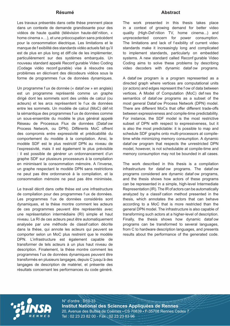
Institut National des Sciences Appliquées de Rennes20, Avenue des Buttes de Coëmes CS 70839 F-35708 Rennes Cedex 7Tel : 02 23 23 82 00 - Fax : 02 23 23 83 96
N° d’ordre : D10-33
Résumé
Les travaux présentés dans cette thèse prennent placedans un contexte de demande grandissante pour desvidéos de haute qualité (télévision haute-déf nition, «home cinema »…), et une préoccupation sans précédentpour la consommation électrique. Les limitations et lemanque de f exibilité des standards vidéo actuels fait qu’ilest de plus en plus long et diff cile de les implémenter,particulièrement sur des systèmes embarqués. Unnouveau standard appelé Reconf gurable Video Coding(Codage vidéo reconf gurable) vise à résoudre cesproblèmes en décrivant des décodeurs vidéos sous laforme de programmes f ux de données dynamiques.
Un programme f ux de donnée (« dataf ow » en anglais)est un programme représenté comme un graphedirigé dont les sommets sont des unités de calcul (ouacteurs) et les arcs représentent le f ux de donnéesentre les sommets. Un modèle de calcul (MoC) déf nitla sémantique des programmes f ux de données commeun sous-ensemble du modèle le plus général appeléRéseau de Processus Flux de données (Dataf owProcess Network, ou DPN). Différents MoC offrentdes compromis entre expressivité et prédicabilité ducomportement du modèle à la compilation. Ainsi, lemodèle SDF est le plus restrictif DPN au niveau del’expressivité, mais il est également le plus prévisible: il est possible de générer un ordonnancement d’ungraphe SDF sur plusieurs processeurs à la compilationen minimisant la consommation mémoire. A l’inverse,un graphe respectant le modèle DPN sans restrictionsne peut pas être ordonnancé à la compilation, et laconsommation mémoire ne peut pas être minimisée.
Le travail décrit dans cette thèse est une infrastructurede compilation pour des programmes f ux de données.Les programmes f ux de données considérés sontdynamiques, et la thèse montre comment les acteursde ces programmes peuvent être représentés avecune représentation intermédiaire (RI) simple et hautniveau. La RI de ces acteurs peut être automatiquementanalysée par une méthode de classif cation décritedans la thèse, qui annote les acteurs qui peuvent secomporter selon un MoC plus restreint que le modèleDPN. L’infrastructure est également capable detransformer de tels acteurs à un plus haut niveau dedescription. Finalement, la thèse montre comment lesprogrammes f ux de données dynamiques peuvent êtretransformés en plusieurs langages, depuis C jusqu’à deslangages de description de matériel, et présente desrésultats concernant les performances du code généré.
Abstract
The work presented in this thesis takes placein a context of growing demand for better videoquality (High-Def nition TV, home cinema...) andunprecedented concern for power consumption.The limitations and lack of f exibility of current videostandards make it increasingly long and complicatedto implement standards, particularly on embeddedsystems. A new standard called Reconf gurable VideoCoding aims to solve these problems by describingvideo decoders with dynamic dataf ow programs.
A dataf ow program is a program represented as adirected graph where vertices are computational units(or actors) and edges represent the f ow of data betweenvertices. A Model of Computation (MoC) def nes thesemantics of dataf ow programs as a subset of themost general Dataf ow Process Network (DPN) model.There are different MoCs that offer different trade-offsbetween expressiveness and compile-time predictability.For instance, the SDF model is the most restrictivesubset of DPN with respect to expressiveness, but itis also the most predictable: it is possible to map andschedule SDF graphs onto multi-processors at compile-time while minimizing memory consumption. A dynamicdataf ow program that respects the unrestricted DPNmodel, however, is not schedulable at compile-time andmemory consumption may not be bounded in all cases.
The work described in this thesis is a compilationinfrastructure for dataf ow programs. The dataf owprograms considered are dynamic dataf ow programs,and the thesis shows how actors of these programscan be represented in a simple, high-level IntermediateRepresentation (IR).The IRof actors canbeautomaticallyanalyzed by a classif cation method presented in thethesis, which annotates the actors that can behaveaccording to a MoC that is more restricted than thegeneral DPN model. The infrastructure is also capable oftransforming such actors at a higher-level of description.Finally, the thesis shows how dynamic dataf owprograms can be transformed to several languages,from C to hardware description languages, and presentsresults about the performance of the generated code.


