Embed Size (px)
Citation preview

Stf Zyd MASTER COPY KEEP THIS COPY FOR REPRODUCTION PURPOSES
REPORT DOCUMENTATION PAGE Form Approved
OMB NO. 0704-0188 Public reporting burden for ttiis collection of information is estimated to average 1 hour per response, including the time for reviewina instructions searrhinn »«*/, *«,. gathering and maintaining me data needed, and comoleunn and rov^inn *2~,IIJiL.^ llXZLZL, S„H^_„;.„.!:.„ ??Jn.s.'Lu"™J/J?.arch'n0- exu »^ dat«
1. AGENCY USE ONLY (Leave blank)
4. TITLE AND SUBTITLE
REPORT DATE
April 1996
Washington, DC 20503. Jefferson
3. REPORT TYPE AND DATES COVERED Final 26 May 95 - 2S Nnv QS
Structural Dynamics and Control
6. AUTHOR(S)
Leonard Meirovitch (principal investigator)
5. FUNDING NUMBERS
DAAH04-95-1-0411
PERFORMING ORGANIZATION NAMES(S) AND ADDRESS(ES)
Virginia Polytechnic Inst & State Univ Blacksburg, VA 24061
9. SPONSORING / MONITORING AGENCY NAME(S) AND ADDRESS(ES)
U.S. Army Research Office P.O.Box 12211 Research Triangle Park, NC 27709-2211
11. SUPPLEMENTARY NOTES
8. PERFORMING ORGANIZATION REPORT NUMBER
10. SPONSORING / MONITORING AGENCY REPORT NUMBER
ARO 34101.1-EG-CF
The v|ews> opinions and/or findings contained in this report are those of the author(s) and should not be construed as an official Department of the Army position, policy or decision, unless so designated by other documentation.
12a. DISTRIBUTION /AVAILABILITY STATEMENT
Approved for public release: distribution unlimited.
13. ABSTRACT (Maximum 200 words)
12 b. DISTRIBUTION CODE
The Tenth Blacksburg Symposium must be regarded as the most successful to date in many respects It has achieved the broadest coverage of the fields of structural dynamics and control, with applications from earthquake engineering, smart structures, robotics, aeroelasticitv of aircraft and rotorcraft large space structures, etc., as well as a good balance between theoretical and experimental papers Also en- couraging was the increasing participation of young researchers bringing new vitality and contributing fresh ideas. °
14. SUBJECT TERMS
17. SECURITY CLASSIFICATION OR REPORT
UNCLASSIFIED NSN 7540-01-280-5500
18. SECURITY CLASSIFICATION OF THIS PAGE
UNCLASSIFIED
19. SECURITY CLASSIFICATION OF ABSTRACT
UNCLASSIFIED
15. NUMBER IF PAGES
16. PRICE CODE
20. LIMITATION OF ABSTRACT
UL Standard Form 298 (Rev. 2-89) Prescribed by ANSI Std. 239-18 298-102

STRUCTURAL DYNAMICS AND CONTROL
Proceedings of the Tenth VPI&SU Symposium Held in Blacksburg, Virginia
May 8-10, 1995
Edited by L. MEIROVITCH
19960503 085 B.-.-.I.0 C^AJZT'a n~E^iluiii!

PREFACE
The Tenth Blacksburg Symposium must be regarded as the most successful to date in many respects. It has achieved the broadest coverage of the fields of structural dynamics and control, with applications from earthquake engineering, smart structures, robotics, aeroelasticity of aircraft and rotorcraft, large space structures, etc., as well as a good balance between theoretical and experimental papers. Also en- couraging was the increasing participation of young researchers bringing new vitality and contributing fresh ideas.
Very much appreciated was the support from Dr. G. L. Anderson, Army Research Office, and Drs. K. P. Chong and S. C. Liu, National Science Foundation.
Special thanks are due to Norma B. Guynn for her significant help in putting this volume together.
Blacksburg, Virginia L. Meirovitch December 1995 Symposium Chairman
and Proceedings Editor
m

TABLE OF CONTENTS
Optimal Nonlinear Polynomial Control for Seismic-Excited Nonlinear or Hysteretic Structures
J. N. Yang, A. K. Agrawal and S. Chen 1
Active Structural Controllers with Amplitude and Actuator Constraints
C.-H. Chuang and D.-N. Wu 13
Saturation Constrained LQR
R. J. Helgeson and P. W. Szustak : 25
Design and Test of a Self Compensating Piezoelectric Actuator for LSS Active Damping
F. Bernelli-Zazzera, R. Biasi and P. Mantegazza 37
Dynamic Boundary Control of Beams Using Active Constrained Layer Damping
A. Baz 49
Errors and Accuracy in Modeling Piezoelectric Stack Actuators
J. A. Main and E. Garcia 65
Independent Modal-Space Control - 15 Years After - Theory and Realization with Distributed Piezoelectric Actuators and Sensors
H. Öz 77
Modeling for Control Design and Validation of Flexible Robot Systems
J. Haug and W. Schiehlen 93
Nonlinear Control Law for a Flexible Robot
B. Yachou and M. Pascal 103
Friction Control in Multibody Systems
H. Bremer 115
Simulation and Testing of a Robotic Manipulator Testbed
R. C. Montgomery, P. A. Tobbe J. M. Weathers and T. Lindsay 127
Design of a Space-Based Electrostatic Antenna with Variable Directivity and Power Density
L. Silverberg and R. Stanley 145

Structural Control by Eigenstructure Assignment Using Inverse Theory
D. J. Inman 157
i?oo Robust Controller Design for an Expendable Launch Vehicle Using Normalized Coprime Factor Plant Description
G. Q. Xing and P. M. Bainum ..-- 171
An Unproven Theorem About Orthogonal Functions
L. Silverberg 183
Frequency Domain Characteristics for a DC Linear Force Actuator for Structural Control
B. Dunn and H. Waites 191
Modeling and Active Vibration Control of Rotor Blades
D. Dinkier and F. Doengi 203
Aeroservoelastic Characteristics of All-Moving Adaptive Flight Control Surfaces
R. Barrett 215
Issues in the Design and Experimentation of Induced-Strain Actuators for Rotor Blade Aeroelastic Control
V. Giurgiutiu, Z. Chaudhry and C. A. Rogers 227
Robust Controller Design of a Wing with Piezoelectric Materials for Flutter Suppression
C. Nam and J.-S. Kim 239
Control of Oscillatory Motions of Cantilevers via Structural Tailoring and Adaptive Materials Technology
L. Librescu, L. Meirovitch and S. S. Na 251
Base-Isolation Control of Structures in Earthquakes
L. Meirovitch and T. J. Stemple 263
Control Algorithm for Flutter Suppression of Low-Aspect Ratio Composite Wings
R. Morris and L. Meirovitch 275
Stability of a Compressible Viscous Fluid Between Coaxial Rotating Cylinders with a Flexible Support
V. Mehl and J. Wauer 287
VI
Peak Stress Control in the Presence of Uncertain Dynamic Loads
G. G. Zhu and R. E. Skelton 299
Methods to Compute Probabilistic Stability Measures for Controlled Systems
R. V. Field, Jr., P. G. Voulgaris and L. A. Bergman 311
Hybrid Sliding Mode Control of Civil Structures
M. P. Singh and E. E. Matheu 323
An Adaptive Fuzzy Controller for Damping Wind-Induced Building Oscillations
N. Tripathi, A. Nerves, H. VanLandingham and R. Krishnan 335
A Crash Avoidance System Based Upon the Cockroach Escape Response
C.-T. Chen, R. D. Quinn and R. E. Ritzmann 345
Modeling a Superconducting Maglev Vehicle/Guideway System
M. Nagurka and S.-K. Wang 355
Advances in Active Vibration Isolation Technology
D. C. Hyland and D. J. Phillips 367
Damage Assessment of a Precision Truss Using Identified Modal Parameters
G. C. Kirby III, A. B. Bosse, S. Fisher and D. K. Lindner 379
Comparison of Error Localisation Techniques for Model Updating
M. G. Smart, M. I. Friswell and J. E. Mottershead 391
Nonlinear Design Technique for Flexible Structures
X. Song, M. J. Schulz, P. F. Pai 403
The Choice of Master Coordinates in the Model Reduction of Structures with Local Nonlinearities
M. I. Friswell, J. E. T. Penny and S. D. Garvey 415
Reflection and Transmission of Elastic Waves in Rods and Beams with a Sudden Change in Cross-Section
P. Hagedorn and W. Seemann 427
Modified Discrete-Time Velocity Feedback for Vibration Suppression of a LSS Laboratory Model
F. Bernelli-Zazzera, A. Ercoli-Finzi, F. Casella, A. Locatelli and N. Schiavoni 439
vn

Dynamics and Control of Flexible Tethered Systems: Analysis and Ground Based Experiments
V. J. Modi, S. Pradhan and A. K. Misra 451
The Use of Boundary Masses in Modal Analysis and Correlation of Large Space Structures
S. Ricci and M. Karpel 463
Deployment Dynamics of a Flexible Dumbbell Satellite
A. K. Amos and B. Qu 475
Laboratory Results on System Identification for Flexible Spacecraft
T. Hong, K. A. Carroll and P. C. Hughes 487
Design of a Sliding Mode Controller for Vibration Suppression of a LSS Laboratory Model
F. Bernelli-Zazzera 501
vni

OPTIMAL NONLINEAR POLYNOMIAL CONTROL FOR
SEISMIC-EXCITED NONLINEAR OR HYSTERETIC STRUCTURES
J. N. Yang, A. K. Agrawal University of California
Irvine, CA 92715 and
S. Chen The World College of Journalism and Communication
Taipei, TAIWAN
Abstract
Under strong earthquakes, the peak response quantities of civil engineering structures should be limited to an acceptable level in order to avoid excessive damages. For this purpose, hybrid protective systems, consisting of active control devices and passive base isolation system, have been shown to be quite effective. However, base isolation systems, such as lead-core rubber bearings and frictional-type sliding bearings, are either nonlinear or hysteretic in nature. In this paper, we present an optimal nonlinear polynomial controller for reducing the peak response quantities of seismic-excited nonlinear or hysteretic building systems. A performance index, that is quadratic in control and polynomial of any order in nonlinear states, is considered. The performance index is minimized based on the Hamilton-Jacobi-Bellman equation using a polynomial function of nonlinear states, which satisfies all the properties of a Lyapunov function. The resulting optimal controller is a summation of polynomials in nonlinear states, i.e., linear, cubic, quintic, etc. Gain matrices for different parts of the controller are determined from Riccati and Lyapunov matrix equations. Numerical simulation results demonstrate that the performance of the proposed controller is remarkable and the percentage of reduction for the selected peak response quantity increases with the increase of the earthquake intensity. Such load adaptive properties are very desirable, since the intensity of the earthquake ground acceleration is stochastic in nature.
1. Introduction
Aseismic hybrid protective systems, consisting of a combination of active control devices and passive base isolation systems, have been shown to be quite effective. Since the dynamic behavior of most base isolation systems, such as lead-core rubber bearings or frictional-type sliding bearings, is highly nonlinear or inelastic, hybrid protective systems involve control of nonlinear or hysteretic structural systems. Likewise, under strong earthquakes, yielding may occur even if the fixed-base building is equipped with active control systems. As a result, control of nonlinear or hysteretic civil engineering structures has attracted considerable attraction recently. Various control methods have been investigated, including pulse control [e.g., Reinhom et al 1987], polynomial control [Spencer et al 1992], acceleration control [Nagarajaiah et al 1993, Reinhorn et al 1993, Riley et al 1993], instantaneous optimal control [Yang et al 1992b], dynamic linearization [Yang et al 1994b, Reinhorn et al 1993], nonlinear control [Yang et al 1992a, 1994a], sliding mode control [Yang et al 1994c, 1995a], etc.
Under strong earthquakes, the main objective of active/hybrid control is to reduce the peak (maximum) response quantities of the structure, such as peak interstory drifts, in order to minimize the damage. Unfortunately, it is extremely difficult to obtain a controller that minimizes the peak (maximum) response quantities of either linear or nonlinear structures. For linear structures, it has been shown by Wu, Gattuli, Lin and Soong (1994), Tomasula, Spencer and Sain (1994) and Agrawal and Yang (1995) that the polynomial controller is more effective than the classical linear controller in suppressing the peak response, because of its ability to apply bigger control force under strong earthquakes. For nonlinear or hysteretic structures, it has been shown by Yang et al (1992a, 1994a) that a controller, having the same nonlinear

J. N. YANG AND A. K. AGRAWAL
characteristics as that of the structure, performs better than a linear controller. In fact, the sliding mode controller [e.g., Yang et al 1994c, 1995a] also has such characteristics.
In this paper, we present an optimal nonlinear polynomial controller for the peak response reduction of seismic-excited nonlinear or hysteretic structures. The performance index to be minimized is quadratic in control and polynomial of any order in nonlinear states. Based on the Hamilton-Jacobi-Bellman equation and the optimality conditions derived by Bernstein (1993) for nonlinear optimal control problem, the performance index is minimized. The resulting optimal control law is a summation of polynomials of different orders in nonlinear states, i.e., linear, cubic, quintic, etc. Gain matrices for different parts of the controller are computed easily from Riccati and Lyapunov matrix equations.
Numerical simulations have been conducted for control of a base-isolated building using lead-core rubber bearings to investigate the performance of the optimal nonlinear controller with respect to various control objectives, including the peak (maximum) response quantities, peak control force and required control effort. The advantages of the proposed optimal nonlinear controller are demonstrated by numerical simulation results.
2. Problem Formulation and Main Results
Consider an n degree-of-freedom nonlinear building structure subjected to a one-dimensional earthquake ground acceleration XQ (t). The vector equation of motion is given by
MX(t) + CX(t)+Fs fX(t)] = HU(t) + Tix0 (t) (1)
in which X(t) = [xx, x2,..., xn]T is an n vector with Xj(t) being the drift of a designated ith story unit;
U(t)= [u i, u 2,. ■ •, u r (t)]T is a r-vector consisting of r control forces; superscript T denotes the transpose of a vector or a matrix; and rj is an n-vector denoting the influence of the earthquake excitation. In Eq.(l), M and C are (nxn) mass and damping matrices, respectively, where linear viscous damping is assumed for the structure; H is a (nxr) matrix denoting the location of r controllers; and Fs[X(t)] is an n-vector denoting the
nonlinear stiffness that is assumed to be a function of X(t). In the state space, Eq.(l) becomes Z(t) = q(Z(t)) + BU(t) + E(t) (2)
where Z(t) = [X(t), X(t)]T is a 2n state vector; q(Z(t)) is a 2n nonlinear vector; B is (2nxr) controller location matrix; and E(t) is a 2n excitation vector, respectively, given by,
q(Z(t)) = X(t) 0 0
; B = M_1H
; E(t) = i •• .. -M-1FS [X(t)] - M_1CX(t) [M V0(t)J
(3)
A general class of nonlinear performance index J is expressed as follows T
J = J(Z0,U(t),t0) = S(ZT,T)+ J L(Z(t),U(t),t)dt (4) to
where Z0 =Z(0) is the initial state, ZT =Z(T) is the terminal state, S(ZT,T) is the terminal cost, and
L(Z(t),U(t),t) is a general nonquadratic non-negative cost function. The minimization of the general performance index in Eq.(4) is not amenable to analytical solutions. In the present study, we present the minimization of a nonquadratic performance index, which is a subclass of the general performance index in Eq.(4), for the infinite time regulator problem given by
k qTQq + Xa
TQaXa + UTRU + i(qTMiq)i-1qTQiq +h(q) i=2
dt (5)
where the implicit dependence of U(t) and q(Z(t)) on t has been dropped and q=q(Z) has been used for simplicity. In Eq.(5), Q is a (2nx2n) positive semi-definite weighting matrix for nonlinear states q of the system; Xa(t) is an n vector consisting of absolute accelerations for all floors; Qa is a diagonal positive
semi-definite weighting matrix; R is a (rxr) positive-definite control weighting matrix; Qj, i=2,3,...,k are

NONLINEAR OPTIMAL CONTROL OF SEISMIC-EXCITED STRUCTURES
(2nx2n) positive semi-definite weighting matrices, Mj, i=2, 3 ,..., k are (2nx2n) appropriate positive-definite
matrices; and h(q) is defined such that simple analytical solution can be obtained,
h(q) = h1(q) = KqTMiqrVMiA i=2
BR V KqTMiq)1-^^^ (6)
In Eq.(6), R will be defined later, and A = A(Z) is the gradient matrix of q(Z) defined as, A(Z) = 3q(Z)/3Z (7)
The first three terms in the performance index of Eq.(5) are quadratic performance indices in terms of the nonlinear states q(Z), absolute acceleration Xa(t), and the control vector U(t). An optimal nonlinear control
law, based on such a quadratic performance index of nonlinear states q(Z), was presented by Yang et al (1992a, 1994a). In this paper, we generalize the performance index to include the fourth term which is the summation of polynomial of nonlinear states q(Z) of different orders higher than the quadratic term. Weighting matrices Q, R, Qaand Qj, i=2,3,...,k, can be chosen in an arbitrary manner to penalize certain
desirable quantities. However, matrices Mj, i=2,3,..., k, are implicit functions of the weighting matrices Qj, i=2,3,..., k. The relation between Mj and Qj will be defined later.
The penalty on Xa has been included in the performance index, Eq.(5), in order to reduce the
absolute acceleration of each floor to an acceptable level. From the equation of motion, Eq.(l), the absolute acceleration vector Xa(t) can be expressed as,
Xa(t) = -LM-1[CX(t)+Fs(X)] + LM_1HU(t) (8)
in which L is a (nxn) transformation matrix. For a shear-beam type building, L(i,j) = 1 for j < i and L(i,j) = 0 for j > i. Substituting Eq.(8) into Eq.(5), one obtains a transformed performance index as follows [Yang et al 1992a]
k q, - = . = =-,
0 ^T Qq + TJ TRU + i^Miq^-VQiq + h(q)
where R, Q and U are
To T =
0 LTQaL
i=2
R = R + BTTaB; Q = Q + Ta -TaBR_1BTTa
U = U + R-1BTTaq(Z)
dt (9)
(10)
(11)
(12)
(13)
Substituting Eq.(ll) into Eq.(2), one obtains the transformed state equation as, Z=Xq + BU + E(t)
where, X = [I-BR-1BTTa]
The minimization of the performance index in Eq.(9) by classical conditions of optimality is very difficult and hence an alternative approach has been developed. This approach is based on the solution of the Hamilton-Jacobi-Bellman (H-J-B) equation using a function which is polynomial in terms of nonlinear states q(Z) of the system. This function is required to satisfy all the properties of a Lyapunov function. Following the derivation presented in the next section, an optimal nonlinear controller, U(t), is obtained,
_1BT X(qTMiq)i_1ATMiq (14) i = 2
in which positive definite matrices P and Mj are obtained by solving algebraic Riccati and Lyapunov matrix equations, respectively,
U(t) = -R_1BT(Ta + ATP)q
PAnA + AT
AIP l0 0* PA0BR-1
BT
A5P + Q = 0 (15)

J. N. YANG AND A. K. AGRAWAL
MiA0(A-BR"1BTA0TP) + (A-BR"1BTA0
TP)TA0TMi + Qj =0 (16)
where A0 = A(Z)L_0 denotes the linearized form of A(Z) at the initial equilibrium point Z=0, that is
stable for civil engineering structures. Note that the second part of the controller in Eq.(14) is the sum of polynomials of various orders in terms of nonlinear states q of the system, i.e., cubic, quintic, etc. Matrices P and Mj in Eq.(15) and (16), respectively, can be solved easily on MATLAB.
Further, if matrices Mj's in Eq.(14) are determined from the solution of matrix Riccati equations
instead of Lyapunov equations, i.e., MiA0(Ä-BR"1BTA0
TP)+(Ä-BR_1BTA0TP)TA0
TMi -I^AQ^T1^AQ"
1^ +QJ =0 (17)
then, the performance index J used to be minimized is given by Eq.(5) where
h(q) = h2(q) = h!(q) - £ (qTMiq)i-1(qTMiABR-1BTATMiq) (18) i=2
in which h-^q) is given by Eq.(6).
3. Derivation of Nonlinear Optimal Control
Let us consider a general time-dependent system, Z(t) = f(Z,Ü,t); Z(t0) = Z0 (19)
and a general performance index J(Z0,U,t0) defined in Eq.(4) in which U is replaced by U. The
minimization of J(Z0,Ü,t0) in Eq.(4) for the system in Eq.(19) results in the well known Hamilton-Jacobi-
Bellman (H-J-B) equation
^r^ = - min[H(Z,Ü, V'(Z),t)l (20) dt u L J
where a prime indicates the differentiation with respect to Z, V(Z) is the optimal cost function, and
H(Z,Ü,V',t) = L(Z,Ü,t) + [V'(Z)]Tf(Z,Ü,t) (21)
is the Hamiltonian function. The necessary condition for the minimization of the right hand side of Eq.(20) is _
3H(z,ü,v,t) = auzji.t) dt(z,y,t) = Q (22) au au au
The solution of Eq.(22) will yield the minimum control Ü (t) = <KZ) if 32H(Z,Ü,V',t)/aÜ2 > 0. For the
optimal control, Ü = <|>(Z), obtained from Eq.(22), the H-J-B equation in Eq.(20) can be expressed as,
^^ + H(Z,<KZ), V'(Z),t) = 0 (23) at
Then, for an optimal cost function V(Z) which satisfies all the properties of a Lyapunov function, if there exists an optimal control Ü =<KZ), which satisfies Eqs.(22) and (23), the closed-loop system is asymptotically stable and the minimum value of the performance index in Eq.(4) is obtained as J(Z0,<t>(Z),to) = V(Z0).
Furthermore, the feedback control U=<KZ) minimizes J(Z0,U,t0) in the sense that
J(Z0,<KZ),t0) = jnin[j(Z0,Ü,t0)l. The asymptotic stability of the closed-loop system is guaranteed UeßL J
through the Lyapunov theorem of stability, i.e., V(Z) < 0. A comparison of the state equation in Eq.(12) with the general state equation in Eq.(19) leads to
f (Z,U, t) = Xq(Z) + BU(t) (24)
Now, we consider a cost function L(Z, U) and a Lyapunov function V(Z) as follows
L(Z, Ü) = qTQq+ÜTRÜ + h(q) (25)

NONLINEAR OPTIMAL CONTROL OF SEISMIC-EXCITED STRUCTURES
V(Z) = qTPq + g(q) (26) where g(q) is some positive definite multinomial of q. Our aim is to determine the nonquadratic cost function, h(q), such that simple analytical solution for the control law U can be derived. Substituting Eq.(24) - (26) into Eq.(21), one obtains the Hamiltonian function
H(q,Ü,V',t) = qTQq+ÜTRÜ + h(q) + [2qTPA + g'(q)T] (Äq(Z) + BÜ) (27) in which A is given by Eq.(7). Substituting Eqs.(25)-(27) into the necessary condition .in Eq.(22), one obtains
2RÜ + 2BTATPq + BTg'(q)T = 0 (28)
From Eq.(28), the optimal nonlinear controller, U(t), is obtained as
Ü(t) = -R_1BTATPq(Z) - |R_1BTg'(q) (29)
It can be verified easily that 32H(Z,Ü,V',t)/3Ü2 =2R>0, since R is a positive-definite matrix. Substituting Eqs.(24)-(26) and Eq.(29) into the H-J-B equation in Eq.(23) and separating quadratic terms in q and terms containing g'(q), one obtains,
-P = PAÄ+ÄTATP-PABR_1BTATP + Q (30)
_M£) = h(q)-Ig'(q)TBR-1BTg'(q) + g'T(Ä-BR-1BTATP)q (31) dt 4
in which the scalar identity 2ql PAAq = qi PAAq + q A A1 Pq has been used to obtain Eq.(30). Equation
(30) is the well-known Riccati matrix equation. Since A(Z) is dependent on the states Z of the system, the matrix P cannot be calculated off-line
without the knowledge of the earthquake ground acceleration, x0(t). Hence A(Z) in Eq.(7) is linearized at
the initial equilibrium point Z=0 that is stable for civil engineering structures, i.e., A0 = A(Z)|Z=Q . Then,
for any time-invariant system with constant A0 and B matrices, P -» 0 as t -»<=». Hence, Eq.(30) becomes
an algebraic Riccati matrix equation, PA0X + ÄTA^P - PA0BR"
1B
TA'5P + Q = 0 (32)
To express the controller in Eq.(29) as an explicit functional of multinomials in q(Z), we choose g(q) in the following form,
g(q) = I -(qTMiq)i (33) i=2 1
such that
g'(q) = 2 I (q^qr^M^q (34) i=2
where k is any integer greater than 2 indicating the order of the multinomials g(q), and Mj 's are positive-
definite matrices. Substitution of g'(q) in Eq.(34) into Eq.(29) leads to the optimal nonlinear controller U
as,
Ü = -R_1BTATPq(Z) - R_1BT I (qTMiq)i_1ATMiq(Z) (35) i=2
We note that for any value of k greater than 2, the maximum order of the controller in terms of nonlinear states q(Z) is (2k+l).
Now, let us choose h(q) as follows
h(q) = hi(q) + I (qTMiq)i-1qTQiq (36) i=2

J. N. YANG AND A. K. AGRAWAL
in which h^q) is given by Eq.(6). Substituting Eqs.(34) and (36) into Eq.(31), one obtains Mj for i=2, 3..k,
as follows, -Mj =MiA(Ä-BR"1BTATP) + (Ä-BR~1BTATP)TATMi +Q; (37)
Again the matrix A will be linearized at the initial equilibrium point Z=0, i.e., A = AQ . Hence, for any
time-invariant system with constant A0 , B and P matrices, Mj -> 0 as t -» «=, and Eq.(37) becomes an
algebraic Lyapunov equation, MiA0(Ä-BR_1BTA0
TP) + (Ä-BR_1BTA0TP)TA0
TMi + Qj =0 (38)
In a similar manner, if h(q) in Eq.(36) is chosen to be,
h(q) = h2(q) + 2 (qTMiq)i-1qTQiq (39) i=2
where h2(q) is given by Eq.(18), then it follows from Eq.(31) that MA 's are determined, for the steady- state solution, from the following algebraic Riccati equation,
MiA0(Ä-BR-1BTA0TP)+(Ä-BR-1BTA0
TP)TA0TMi -MjAoBR^B^TMi +Qj =0 (40)
Finally, substituting Eq.(35) into Eq.(ll), one obtains U(t) given by Eq.(14). It is observed from Eqs.(26), (32), (33) and (38) that the function V(Z) satisfies all the properties of the Lyapunov function.
4. Response of Hysteretic Structures
In order to evaluate the effectiveness and performance of the proposed optimal nonlinear polynomial controller, simulations for the response of the controlled structure will be conducted. The nonlinearity for both the structure and passive protective systems is reflected by the stiffness restoring force Fs[X(t)] in
Eq.(l). The ith element, F^Xi), of the vector Fs[X(t)] is modelled as
Fsi[xi(t)] = aikixi +(l-ai)kiDyivi (41)
in which kj= elastic stiffness of the ith story unit, 04= ratio of the post yielding to pre-yielding stiffness, Dy; = yield deformation = constant, and vj is the nondimensional hysteretic component of the deformation,
with Vj <1, where
-1 D yi
in; I. II in; —1 . 1 in, Aixi-ßi|xi|vi| Vi-Yixi|vi| = fi(xi,vi) (42)
In Eq.(42), Ai, ßj, Yi and n^are parameters characterizing the hysteresis loop of the inelastic behavior. Substituting Eq.(41) into Eq.(l), one obtains the vector equation of motion as follows
MX + CX + KeX(t) + Kj V(t) = HU(t) + r|X0 (t) (43)
where Ke and Kj are the elastic and inelastic stiffness matrices, assembled for each story unit according to
Eq.(41); V(t) = [v1,v-7,...,vn]T is an n vector denoting the hysteretic component of each story unit given by Eq.(42). Derivative matrices, A(Z) and A0, appearing in the control law, Eqs.(14)-(16), are given by
A(Z) Onn
_i 9V -M ^Ke+Kr— ] -M_1C
; A0 = -M_1K -M_1C (44)
in which 0nn and Inn are (nxn) null and identity matrices, respectively, and dV/dX is a diagonal matrix
with the ith diagonal element 9VJ/3XJ given by, 14-I
Ai-ßiSgn(xi) vj Vj-YjVi (45) 9vL_3vL_ 1 axj'axi" y1
For numerical simulations, the hysteretic vector V can be augmented in Eqs.(42) and (43). A detailed description of the procedures for numerical simulations can be found in Yang et al (1992a).

NONLINEAR OPTIMAL CONTROL OF SEISMIC-EXCITED STRUCTURES
5. Other Controllers for Nonlinear or Hysteretic Structures
The performance of the optimal nonlinear polynomial controller presented in this paper will be compared with other controllers available in the literature. These control methods include the LQR method based on linearized structures, the nonlinear controller presented by Yang et al (1992a, 1994a) and the continuous sliding mode controller (Yang et al 1994c, 1995a) to be described briefly in the following.
5.1 Nonlinear Controller: If we choose the weighting matrices Qi =0 for i= 2, 3 ,..., k in the performance
index given by Eq.(5), then the controller in Eq.(14) becomes U(t) = -R-1BT(Ta + ATP)q. This special
nonlinear controller, consisting of only the first term of our polynomial controller, was proposed by Yang et al (1992a, 1994a).
5.2 LQR with Acceleration Penalty: If the nonlinear or hysteretic structure is linearized first at the equilibrium point Z=0, the linearized state equation becomes Z = A0Z(t) + BU(t) + E(t). Then, for the
quadratic performance index
0 the linear optimal control law is obtained as
Z'QZ+XjQaXa+U'RU dt (46)
U(t) = -R_1BT (Ta + P)Z(t) (47)
where P is an appropriate Riccati matrix [see Yang et al 1992a for details].
5.3 Sliding Mode Control: The method of sliding mode control was developed for control of uncertain nonlinear systems. Applications of continuous sliding mode control, that has no undesirable chattering effect, to civil engineering structures was presented by Yang et al (1994c, 1995a). In this approach, a sliding surface
S = PZ(t) = 0 (48) T is designed such that the motion on the sliding surface is stable. In Eq.(48), S = [Si,S2,...,Sr] is a r-vector
consisting of sliding variables Sj, where r is the total number of controller, and P is a (rx2n) matrix to be
determined either by the method of pole assignment or the classical LQR method. Design of various controllers were given in Yang et al (1994c).
6. Numerical Simulations
To demonstrate the performance of the optimal nonlinear polynomial controller, numerical simulations have been conducted for an elasto-plastic eight-story building equipped with a hybrid control system consisting of rubber-bearing isolators and actuators, Fig. 1. The performance of the proposed controller will be compared with that of various controllers described previously.
An eight-story building that exhibits bilinear elasto-plastic behavior is considered. The properties of the building are as follows: (i) the mass of each floor is identical with mj =345.6 metric tons; (ii) preyielding stiffnesses kj (i=l,2..8) of eight-story units are 340400, 325700, 284900, 268600, 243000, 207300, 168700 and 136600 kN/m, respectively, and postyielding stiffnesses are 0.1 kj for i=l,2,...,8, i.e., ccj =0.1 in Eq.(41); and (iii) the viscous damping coefficients for each story unit are Cj =490, 467, 410, 386, 348, 298, 243 and 196 kN.sec/m, respectively. The damping coefficients given above results in a damping ratio of 0.38 % for the first vibrational mode. The fundamental frequency of the unyielded building is 5.24 rad/sec. The yielding level for each story unit varies with respect to the stiffness; with the results, Dyj = 2.4, 2.3, 2.2, 2.1,
2.0, 1.9, 1.7 and 1.5 cm, Eq.(41). The bilinear elasto-plastic behavior can be described by the hysteretic model, Eq. (42), with Aj=1.0, ßi=1.0, nj=95 and Yj=1.0 for i=l,2..8. The El Centra NS (1940) earthquake with a maximum ground acceleration of 0.3g, as shown in Fig. 2, is used for the input excitation.

J. N. YANG AND A. K. AGRAWAL
Without any control system, it has been observed that the deformation of the unprotected building is excessive and that yielding takes place in the upper five stories [Yang et al, 1992a, 1994a]. Hence, a lead- core rubber bearing isolation system is used to reduce the response of the building. The stiffness of the lead- core rubber-bearing is modelled by Eq.(41) with Fsb = abkbxb +(l-ab)kbDybvb in which subscript b
stands for the base-isolation system. The hysteretic component, vb, is modelled by Eq.(42). Properties of
the base-isolation system are: mb=450 metric tons, stiffness kb =18050 kN/m, damping cb =26.17
kN.sec/m, ab= 0.6, Dyb=4 cm, Ab=1.0, ßb=0.5, nb=3 and Yb=°-5< Eq.(42). The hysteresis loop of
such a base-isolation system, i.e., xb versus vb, is shown in Fig. 3. For the building with the base-isolation system, the first natural frequency of the preyielded structure
is 2.21 rad/sec and the damping ratio for the first vibrational mode is 0.16 %. Within 30 seconds of the earthquake episode, the peak interstory drifts, x^, and peak absolute accelerations, x^, of different floors of
the base-isolated building are shown in columns (3) and (4) of Table 1, designated as "With BIS". The results of xb and xb for rubber bearings are shown in the row denoted by B. It is observed from Table 1
that the interstory drifts are within the elastic range. However, the peak drift of the base-isolation system is excessive and should be protected during strong earthquakes.
In order to reduce the drift of the base-isolation system, actuators are attached to the base isolation system, referred to as the hybrid control system, as shown in Fig. 1. We first consider the use of sliding mode control presented by Yang et al (1994c, 1995a). The sliding surface P in Eq.(48) is a row vector with P = [Pj, P2] and it is designed as follows
^=[0.0707 -90.533 -49.462 2.919 10.396 7.596 3.053 3.340 1.796]
P2= [0.795 -0.205 -3.054 -3.198 -2.518 -1.859 -1.423 -0.974 -0.474]
The controller in Eq.(6.19) of Yang et al (1994c) with 51 = 5 x 10⁵ kN.ton.cm/s is used. The peak interstory drifts and absolute floor accelerations are shown in Columns (13) and (14) of Table 1, designated as "Sliding Mode". Also shown in Table 1 are the peak control force U and the required control effort (energy)
TJ2, that is the integral of the square of the control force U(t) over the duration of 30 seconds of the earthquake. We observe that sliding mode control is very effective in reducing the response quantities of the entire system. In particular, the drift of rubber bearings has been reduced by 49%.
Next, we consider the LQR control law, Eq.(47), in which the structural system is linearized first at Z=0. Two cases of weighting matrices for this controller have been considered. In the first case, we choose
the scalar control weighting matrix R = 7.3 x 10~10, and all elements of Q and Qa are zero except
Qa(l,l) = 200 and Q(l,l)=78. The peak response quantities are shown in Columns (5) and (6) of Table 1,
designated as "Linear 1". These weighting matrices have been chosen such that the peak response quantities and the peak control force are as close as possible to those associated with the sliding mode controller. It is
observed that the drift of the rubber bearing and the required control effort u2 are larger than that based on the sliding mode controller. To emphasize more on the reduction of the drift of the rubber bearing, nonzero elements of the weighting matrices are chosen to be Qa(l,l) = 10 and Q(l,l)=130 for the second case. With
R = 7.3 x 10"11, the peak response quantities are presented in Columns (7) and (8), respectively, of Table 1, designated as "Linear 2". It is observed that, although the drift of the rubber bearing and the peak control force are reduced, the building response quantities increase.
For optimal nonlinear controllers presented in this study, we first consider the special case in which Qj =0, i=2, 3,..., k. Such a special controller was proposed by Yang et al (1992a, 1994a). In this case, we
choose R=1.0xl0~7 , andQa and Q are diagonal matrices with: Qa(i,i) =[10, 15, 15, 20, 20, 30, 50, 50,
50], Q(l,l)=100, Q(i,i)=10 for i=2, 3,.., 9, and Q(i,i)=0 for i=10, 11, ..., 18. The peak response quantities based on this controller are shown in Columns (9) and (10) of Table 1, designated as "Nonlinear 1". We

NONLINEAR OPTIMAL CONTROL OF SEISMIC-EXCITED STRUCTURES
observe that the overall performance of this controller is better than that of linear controllers. Next, we consider a general case where Q2 * 0 and Qi = 0 for i=3, 4,..., k. Diagonal weighting matrices are chosen
as follows: R= 1.0 x 1(T3, Qa (i,i) =[4, 6, 6, 8, 8, 12, 35, 35, 35]xl03, Q(l,l)=2, Q(i,i)=l for i=2, 3, .., 9,
Q(i,i)=0 for i=10, 11,..., 18, Q2(l,l)=8, Q2(i,i)=l for i=2, 3,.., 9, andQ2(i,i) =0 for i=10, 11,..., 18. The peak response quantities based on this controller are shown in Columns (11) and (12), respectively, of Table 1, designated as "Nonlinear 2". It is observed that, while the overall performance is similar to that of "Nonlinear 1", the peak control force has been decreased by 5%. In particular, the overall performance of "Nonlinear Controller 2" is comparable with that of the sliding mode controller.
With hybrid control, the building response quantities are well within the elastic range except the drift of rubber bearings. Hence, the reduction for the drift of rubber bearings will be compared for different controllers. The results presented in Table 1 are based on the El Centra earthquake with a peak ground acceleration (PGA) of 0.3g. Since the PGA is stochastic in nature, numerical simulations have been conducted for the same earthquake with different peak ground accelerations. Based on the same design of various controllers presented in Table 1, simulation results for the percentages of reduction for the peak drift of rubber bearings as a function of PGA are shown in Fig. 4. It is observed from Fig. 4 that the peak drift reduction in percentage (%) for linear controllers decreases with the increase of PGA. However, the percentages of the peak drift reduction for both Nonlinear 1 and sliding mode controllers remain almost constant with the increase of PGA. On the other hand, the percentage of the response reduction for rubber bearings for Nonlinear 2 increases as the PGA increases. Because of such a load adaptive property, Nonlinear 2 controller is more effective in limiting the peak response of rubber bearings under strong earthquakes. It should be mentioned that the trend for the percentage of the response reduction for the superstructure is quite different from that for rubber bearings. In fact, as PGA increases, the percentage of the response reduction for the superstructure decreases for Nonlinear 2 controller, whereas it increases for Linear 1 controller. However, since these response quantities are well within the elastic range, they are not presented.
The corresponding peak control force, U, and the required control energy, TJ2 »are presented in Fig.
5 and 6, respectively. These quantities have been normalized, respectively, by the corresponding results for Linear 1 controller subjected to a 700 gal of PGA input. As observed from Figs. 5 and 6, the peak control force and the control energy required by all the controllers in Table 1 are almost the same except the Linear 1 controller. These quantities are significantly higher for the case of the Linear 1 controller. The advantages of the nonlinear optimal controller proposed in this study in terms of the peak response reduction for rubber bearings, peak control force and required control energy are demonstrated in Figs. 4-6.
7. Conclusions
An optimal nonlinear polynomial controller is presented for peak response control of seismic-excited nonlinear or hysteretic structures. A performance index, that is quadratic in control and polynomial in any order of nonlinear states, is minimized based on the solution of the Hamilton-Jacobi-Bellman equation using a polynomial function of nonlinear states, which satisfies all the properties of a Lyapunov function. The resulting optimal controller is polynomial in nonlinear states of the system. Gain matrices for different parts of the controller are computed easily by solving Riccati and Lyapunov matrix equations. Numerical simulations have been conducted for an elasto-plastic eight-story building equipped with a hybrid control system consisting of actuators and lead-core rubber bearings. Simulation results indicate that the performance of the optimal nonlinear polynomial controller presented is quite remarkable. The main advantage of such an optimal controller is its ability to increase the percentage of reduction for the peak response of rubber bearings with the increase of the earthquake intensity. Such a load adaptive capability is very desirable in protecting seismic-excited buildings, in particular when the magnitude of earthquakes exceeds the design one.
Acknowledgement
This research is supported by the National Science Foundation through grant numbers BCS-91- 22046 and the National Center for Earthquake Engineering Research, NCEER-94-5105B.

J. N. YANG AND A. K. AGRAWAL
8. References
1. Agrawal, A.K. and Yang, J.N. (1995), " Nonlinear Optimal Control of Seismic-Excited Linear Structures", Proc. 10th Engr. Mech. Specialty Conf., ASCE, pp. 1223-1226, Colorado.
2. Bernstein, D.S.(1993)," Nonquadratic Cost and Nonlinear Feedback Control", Int'l J. of Robust and Nonlinear Control, Vol. 3, pp. 211-229.
3. Nagarajaiah, S.M., Riley, M.A. and Reinhom, A.M. (1993), " Hybrid Control of Sliding Isolated Bridges", J. Ens. Mech.. ASCE, Vol. 119, No. 11, pp. 2317-2332.
4. Reinhorn, A.M., Soong, T.T. and Yen, C.Y. (1987), "Base-Isolated Structures With Active Control", Recent Advances in Design. Analysis. Testing and Qualification Methods. ASME, PVP-Vol. 127, pp. 413-419.
5. Reinhorn, A.M., Subramaniam, R., Nagarajaiah, S., Riley, M.A. (1993), "Study of Hybrid Systems for Structural and Nonstructural Systems", Proc. Int'l Workshop on Structural Control and Intelligent System, pp. 405-416, edited by G.W. Housner and S.F. Masri, December, Honolulu, Hi.
6. Riley, M.A., Subramaniam, R., Nagarajaiah, S., and Reinhorn, A.M. (1993), "Hybrid Control for Sliding Base-Isolated Structures", Proc. ATC-17-1 Seminar on Seismic Isolation. Passive Energy Dissipation and Active Control. San Francisco, CA, pp. 799-810.
7. Spencer, B.F. Jr., Suhardjo, J. and Sain, M.K.(1992)," Nonlinear Optimal Control of a Duffing", InO J. Nonlinear Mechanics. Vol. 27, No. 2, pp. 157-172.
8. Tomasula, D.P., Spencer, B.F. Jr. and Sain, M.K.(1994)," Limiting Extreme Structural Responses Using an Efficient Nonblinear Control Law", Proceedings of the First World Conference on Structural Control, Pasadena, CA., August 1994, FP4, pp. 22-31.
9. Wu, Z., Gattulli, V., Lin, R.C. and Soong, T.T. (1994)," Implementable Control Laws For Peak Response Reduction", Proc. of the First World Conference on Structural Control. Pasadena, CA., TP2, pp. 50-59.
10. Yang, J.N., Li, Z. and Vongchavalitkul, S. (1992a), " A Generalization of Optimal Control Theory: Linear and Nonlinear Control", National Center for Earthquake Engineering Research Technical Report. NCEER-92-0026.
11. Yang, J.N., Li. Z. and Liu, S.C. (1992b), " Stable Controllers for Instantaneous Optimal Control", I Engineering Mechanics. ASCE, Vol. 118, pp. 1612-1630.
12. Yang, J.N., Li, Z. and Vongchavalitkul, S. (1994a), " A Generalization of Optimal Control Theory: Linear and Nonlinear Control", J. Engineering Mechanics, ASCE, Vol. 120, No. 2, pp. 266-283.
13. Yang, J.N., Li, Z. and Wu, J.C. and Hsu, I.R.(1994b), "Dynamic Linearization for Sliding Isolated Building", J. Engineering Structures. Vol. 16, No. 6, pp. 437-444.
14. Yang, J.N., Wu, J.C, Agrawal, A.K., and Li, Z. (1994c), "Sliding Mode Control of Seismic-Excited Linear and Nonlinear Civil Engineering Structures", National Center for Earthquake Engineering Research, Technical Report NCEER-94-0017.
15. Yang, J.N., Wu, J.C, and Agrawal, A.K. (1995a)," Sliding Mode control For Nonlinear and Hysteretic Systems", to appear in J. Engineering Mechanics. ASCE, Dec. issue, 1995.
16. Yang, J.N. and Agrawal, A.K. (1995b), "Optimal Polynomial Control for Seismic-Excited Linear and Nonlinear Structures", to be submitted for publication as Technical Report, NCEER, SUNY, Buffalo.
10

NONLINEAR OPTIMAL CONTROL OF SEISMIC-EXCITED STRUCTURES
Table 1: Maximum Rest jonse Quantities of an Eig ht Story Building Equipp e with Hybrid Control System.
F L Dv Linear 1 Linear 2 Nonlinear 1 Nonlinear 2 Sliding 0 With BIS U=1491kN U=1031kN U=1437kN U=1350kN Mode 0
U2=1047kN2 U2 =226 kN2 U2 =689 kN2 U2=711kN2 U = 1494 kN
U2 =651
R
kN2
N xi xai xi xai
xi xai xi xai • xi xai xi xai
0 cm cm cm/s2 cm cm/s2 cm cm/s2 cm cm/s2 cm cm/s2 cm cm/s2
(1) (2) (3) (4) (5) (6) (7) (8) (9) (10) (11) (12) (13) (14)
B 4.0 21.35 130 14.4 45 10.7 70 10.7 38 10.7 46 10.8 77 1 2.4 0.62 123 0.15 43 0.22 71 0.20 39 0.18 48 0.14 42 2 2.3 0.59 113 0.16 40 0.25 66 0.20 36 0.18 43 0.14 37 3 2.2 0.65 111 0.19 33 0.29 53 0.22 30 0.21 34 0.16 38 4 2.1 0.63 102 0.21 29 0.30 46 0.23 30 0.22 30 0.15 31 5 2.0 0.65 91 0.22 32 0.30 49 0.22 38 0.21 40 0.14 38 6 1.9 0.65 103 0.23 39 0.31 66 0.22 46 0.20 46 0.18 39 7 1.7 0.60 135 0.22 50 0.34 68 0.20 47 0.20 51 0.20 42 8 1.5 0.41 163 0.16 64 0.27 105 0.15 60 0.16 64 0.15 60
Fig. 1 : A Base-Isolated Structural Model
10 20
Time (sec.)
Fig. 2 : El Centro Earthquake (NS Component).
11

J.N. YANG AND A.K. AGRAWAL
-10 0 10
Displacement (cm) 20 100 200 300 400 500 600 700
Peak Ground Acceleration (gal)
Fig. 3: Hysteresis Loop of Lead-Core Rubber Bearings.
Fig. 4: Peak Drift Reduction vs. Peak Ground Acceleration.
1.0
0.8
s o U 0)
I 0.2
0.0
0.6 ■
0.4 "
Linear 1
Linear 2
Nonlinear 1
Nonlinear 2
Sliding Mod
100 200 300 400 500 600 700
Peak Ground Acceleration (gal)
1.0
120-8 m V a
o 0.6 - B o U ■a 0.4 a)
"3 | 0.2 z
0.0
" Linear 1
" Linear 2
Nonlinear 1
" Nonlinear 2
Sliding Mode
100 200 300 400 500 600 700
Peak Ground Acceleration (gal)
Fig. 5: Normalized Peak Control Force vs. Peak Ground Acceleration.
Fig. 6: Normalized Peak Control Energy vs. Peak Ground Acceleration.
12

ACTIVE STRUCTURAL CONTROLLERS WITH AMPLITUDE
AND ACTUATOR CONSTRAINTS
C.-H. Chuang and D.-N. Wu Georgia Institute of Technology
Atlanta, GA 30332
ABASTRACT
To prevent structural damages, it is safer to bound the vibration amplitude at any instant rather than to minimize the total vibration energy over a time period. In this paper, we consider a nonlinear optimization method for the design of bounded-state controllers which minimize the bound of the vibration amplitude at any instant This method is based on calculation of the exact maximum worst-case bound of system output The effectiveness of the method is demonstrated for a two mass-spring system example. The nonlinear optimization method is then applied to an active tendon control of a five-story building with two actuators. The effect of the actuator dynamics on the system performance is investigated by using a simplified hydraulic actuator model.
1. Introduction The stability and performance requirements are important for a conventional control system design.
For vibration control, the performance requirement is usually expressed in terms of the total vibration energy over a time period. However, if active vibration control is to prevent structures from damage due to large external excitation, reduction of the maximum oscillation amplitude at some instant may be more critical than reduction of the sum of the squares of the amplitude over a period of time. For example, small and prolonged oscillations may not damage the structure as long as the oscillation amplitude is inside a prescribed limit determined mainly by structure property.
Several main bounded-state control methods in the literature are: the pulse control method (Masri, et al, 1981; Udwadia and Tabaie, 1981; Prucz, et al, 1985; Reinhom et al, 1987; Soong, 1990), the set-theoretic method (Schweppe, 1973; Uroso et al, 1982; Parlos et al, 1988), the linear quadratic stabilization method (Chen, 1986), the .^-optimal control method (Vidyasagar, 1986; Dahleh and Pearson, 1987,1988; McDonald and Pearson, 1991), the two-stage LQR control scheme (Chuang and Wang, 1990). Among these methods, only the set-theoretic method and the il -optimal control method employ linear feedback control and consider the constraints on control force magnitude. The set-theoretic method is in fact a method based on Lyapunov funtion which tends to be conservative. The ^'-optimal control method addresses the problem of minimizing the magnitude of the regulated output of a linear time-invariant system subject to magnitude bounded disturbances in a fairly general formulation. It determines an optimal disturbance rejection controller among all possible stabilizing controllers for the system. The controller design problem is formulated as a linear programming problem which gives a global minimum solution to the disturbance rejection problem. However, the order of the optimal controller may be very high and the initial condition is assumed to be zero.
Recently, a nonlinear optimization method (Chuang and Wu, 1994) has been proposed for design of a fixed-order controller for bounded-state control. Both constraints on control force magnitude and uncertainty in initial condition are considered in this method. The nonlinear optimization procedure is based on calculation of the worst-case maximum magnitude of oscillation. This method numerically minimizes the worst-case maximum magnitude of the oscillation. Although a global minimum solution is not guaranteed, local minimum solutions have been determined.
Since large control force is needed in the active control of a building structure, electro-hydraulic actuators are usually used in the control system. In previous research work on active control of civil structures, actuator dynamics is not often considered in the design. However, the actuator dynamics may significanüy affect the system performance under some conditions. In this paper, the nonlinear optimization method is applied to active tendon control of a five-story building while actuator dynamics is included.
13

C.-H. CHUANG AND D.-N. WU
The nonlinear optimization method is also compared to the ^'-optimal control method by studying their effectiveness to a two mass-spring example. It is shown that the bound on the system output achieved by the state feedback control via the nonlinear optimization method is close to that achieved by a 139th order controller via the ^-optimal control method. The controller order for the ^-optimal control method is quite high for this example.
The paper is organized as follows. Problem formulation and the nonlinear optimization method are presented in Section 2. A two mass-spring system is considered for the application of the nonlinear optimization method and the ^-optimal control method in Section 3. In Section 4, a simplified model of hydraulic systems is included. An application of the active tendon control to a five-story building structure is studied in Section 5. Finally, conclusions are given in Section 6.
2. Problem Statement and the Nonlinear Optimization Method for Structural Control Consider the following linear system which has inputs from an active controller and an external
excitation: x(t) = Ax(t) + Bu(t)+Bww(t) (1) y(t) = Cx(t) (2)
where t e R is time, x e Rn denotes the state vector, u € Rm the control vector, w € Rp a vector representing the external disturbance, and yeR' the output vector. Matrices A, B, Bw, and C are system matrices of appropriate dimensions.
Note that the equation of motion of a general linear structure system can always be converted to the first-order ordinary differential equation system described by Eq.(l) and Eq.(2).
Assumption 1: The pair (A,B) is assumed to be completely controllable. Assumption 2: The disturbance signal is assumed to be norm bounded by
W<W (3) where W e Rp is a constant vector. Eq.(3) implies that the absolute value of each component of w is less than the corresponding component of W.
In order to simplify the use of active controllers in practice, the control is selected to be a linear state feedback:
u(t)=Kx(t) (4)
The objective of this controller is to reduce the output response to satisfy |y|^Y (5)
where Y e R* is a constant vector, subject to control constraints
|u|<Ü (6)
where U e Rm is a constant vector. Note that it is important to impose the bound on the control magnitude since a controller with unreasonable size is useless in practice. This is particularly true for building structures since the massive structures of a building require high power actuators. For different actuators, the elements in U can be selected differently to bound the control. For simplicity, the control variables are scaled to make all the elements in Ü equal. The same procedure can be applied to W and Y also. Therefore, without loss of generality, the bounds on w, y, and u are written as:
IML^W, ByL^Y, lu|L<U (7) where |xL denotes the infinity norm of vector x and where WeR.YeR.andUeR.
After applying the feedback control in Eq.(4) to the system in Eq.(l), the closed-loop system becomes:
x(t) = Xx(t) + Bww(t) (8) where A = A+BK.
Define
fsi(t) = ||cieA(t-t')s|[, gi(t) = £"ti|cie
AtBw|Ldx (9)
14

ACTIVE STRUCTURAL CONTROLLERS
where |(#)||„ is the infinity-norm, Cj is the ith row of matrix C, S is a weighting matrix used to introduce different weights on different state variables. In damage control, the displacement is more critical than the velocity since the relative displacement between different parts of the structure is more likely to damage the structure. Therefore, the output y usually consists of the displacement only. Usually S can be chosen to scale down the velocity by a factor.
Uncertainty in the initial states is an important factor in active structure control. Suppose the initial states are arbitrary but lie inside the set
Q={x|||x|l5M<XI} (10)
where Xx e R is a constant and |x(ti)|si>o = |s-1x(ti)L • We have *e folIowmS result.
Theorem 1 (Chuang and Wu, 1994). Suppose the disturbance is bounded by W and the initial point is arbitrary but bounded by Q. Then the worst-case magnitude of the system output response is
> S»P, Jy(C = maxaip[fli(t)XI +gi(t)W] (11)
|w|_£W
Similarly, the worst-case control magnitude is
sup ||u(t)L = maxsup[fusi(t)XI + gui(t)W] (12) |w|_SW
where
f^t^lke^-^sl , gui(t) = Plke^Bj <* (13) II lloo JO II II»
and K; is the ith row of the feedback gain matrix K. An optimization design problem based on the above results can be formulated as:
(OPTF) J=X 1) sup[fsi(t)XI+gi(t)W]<X, i=l, .... e
2) sup^O^ + g^OW^U, i=l, ..., m
3)Re^(A + BK)<0, i=l, .... n
If the optimal J obtained is less than the desired bound Y, the design objective is achieved. If J is greater than Y, then it is impossible to reduce the magnitude of the output to be within the given bound using the given control effort. Either the power of the actuator or the desired bound Y must be increased.
Y There are also other alternatives. For example, the bound of the excitation can be reduced to — W or the
Y bound of the initial point uncertainty can be reduced to — Xx. It should be noted that Theorem 1 can also be
extended to output feedback control by simply replacing A with Ac = A+BKC in OPTF. Then the same optimization procedure follows.
In active building structure control, for some cases, it is important to control the modes of the structure. Therefore, it is straightforward to use eigenvalues and eigenvectors of the system as the optimization parameters instead of using the feedback gain matrix. However, the assignment of eigenvectors of the closed-loop system is not independent from the assignment of the eigenvalues of the closed-loop system. Moreover, the computation of g£(t) does not have to cover the infinite time-interval. Since the closed-loop system is stable, an finite time-interval will be suffice to get the value of g;(t) within a given accuracy.
The fact that the objective function involves the evaluation of the sumpremum of fsi(t)XI +gj(t)W over all times tj < t<°° may cause some difficulties in numerical computation. But since the closed-loop system subject to an active controller must be stable, in practical applications, it is not
15
C.-H. CHUANG AND D.-N. WU
necessary to consider infinite time interval in evaluating the worst-case magnitude in Eq.(3.11). For a given e > 0, we can always find a T>0 such that the difference between the supremums of fäCOXj + gi(t)W over
[t, T] and the supremums of f^OXj + gj(t)W over [tj «>] is less than e. One may notice that the constraints in (OPTF) may not be differentiable since they involve
supremum operation. Therefore, nondifferentiable optimization methods will have to be used in general. Differentiable optimization algorithms may be used directly, but those minimums occur on the corner points might not be obtainable. Local minimums that do not occur at corner points can be obtained using the differentiable optimization algorithms if initial guess is appropriate. Since most available numerical algorithms of nonlinear constrained optimization assume the differentiability of the objective function and that non-differentiable optimization algorithms are usually less efficient than the differentiable optimization algorithms, we will use differentiable optimization algorithm.
3. A Two Mass-spring System In this section, a mass-spring system is used to compare the design results of the tl -optimal control
method and the nonlinear optimization method. It is shown that the bound on system output achieved by the state feedback control obtained via the nonlinear optimization method is close to that achieved by a 139th order controller via the t1 -optimal control method.
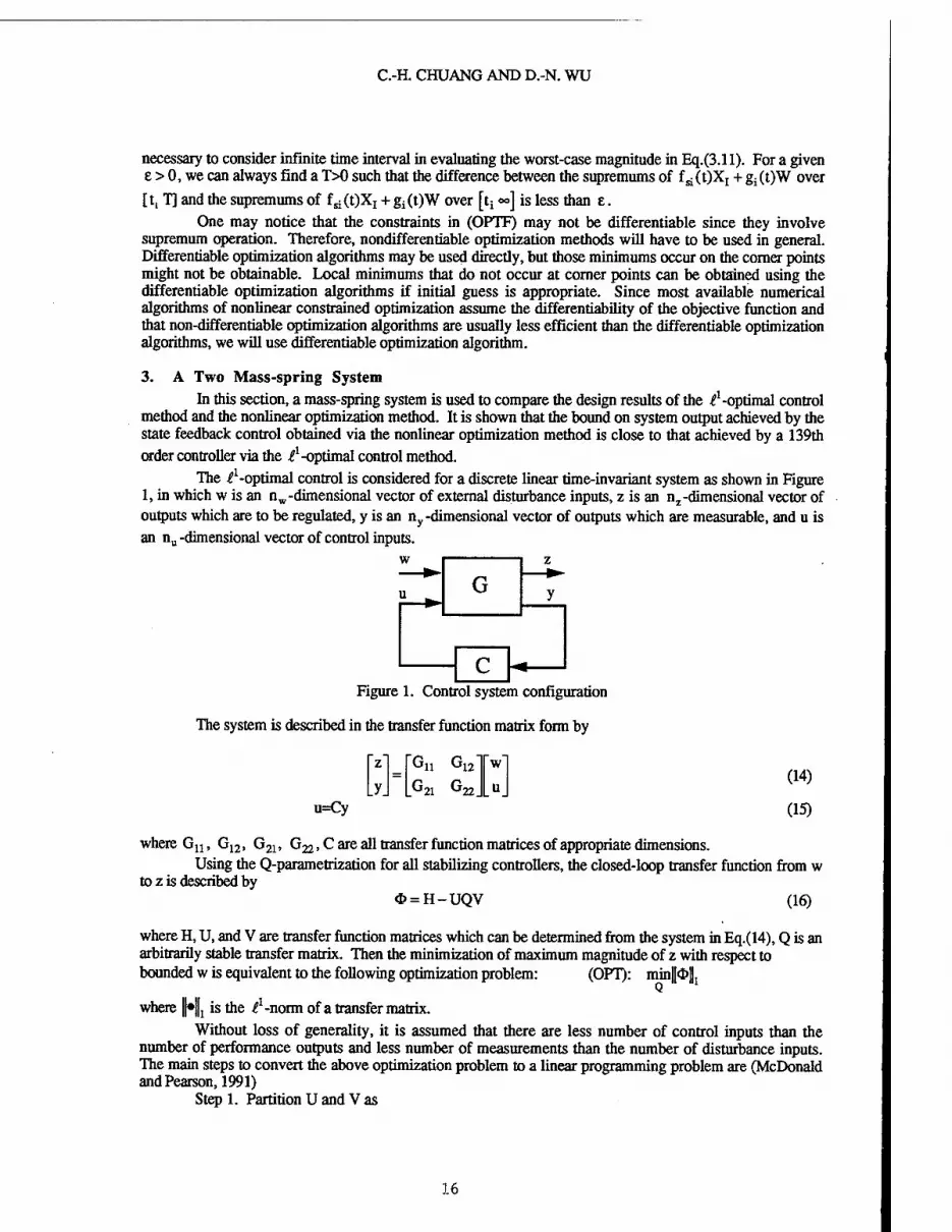
The ll -optimal control is considered for a discrete linear time-invariant system as shown in Figure 1, in which w is an nw -dimensional vector of external disturbance inputs, z is an nz-dimensional vector of outputs which are to be regulated, y is an ny-dimensional vector of outputs which are measurable, and u is an nu -dimensional vector of control inputs.
w
u G z
y
- C - m Figure 1. Control system configuration
The system is described in the transfer function matrix form by
li G12Tw'
2i GJU, u=Cy
(14)
(15)
where Gn, G12, G2i, G22, C are all transfer function matrices of appropriate dimensions. Using the Q-parametrization for all stabilizing controllers, the closed-loop transfer function from w
to z is described by <D = H-UQV (16)
where H, U, and V are transfer function matrices which can be determined from the system in Eq.(14), Q is an arbitrarily stable transfer matrix. Then the minimization of maximum magnitude of z with respect to bounded w is equivalent to the following optimization problem: (OPT): mini«!»!
where fl»||j is the ^-norm of a transfer matrix. Without loss of generality, it is assumed that there are less number of control inputs than the
number of performance outputs and less number of measurements than the number of disturbance inputs. The main steps to convert the above optimization problem to a linear programming problem are (McDonald and Pearson, 1991)
Step 1. Partition U and V as
16

ACTIVE STRUCTURAL CONTROLLERS
U =
where U and V are invertible.
U
LU2. , V = [V V2], H =
H H12
H2i H22J (17)
Step 2. Do coprime factorization for U2U ! and V lV2
7-^2 = NvDv1
(18)
(19)
where Nu, Dy, Nv, Dv are polynomial matrices.
Step 3. Find the transmission zeros of Ü and V. Transfer Ü and V into Smith-Macmillan form as
U = LuMuRu V = LVMVRV
(20) (21)
Let cCi(z) denotes the ith row of Lj , ßj(z) denotes the jth column of Rv\ Z denotes the set of
transmission zeros of U or V in the unit disc. Step 4. Form the linear constraints. The closed-loop transfer function matrix must satisfy for any
z0 G Z, i=l, ..., n2, j=l, ..., nw
1) (aiHßj)k(z0) = (ai*ßj)
k(z0), k=l,..., m0 (22)
2) [-Nu DU]* = TUH (23)
3) [* <fr12] -Nv = [H H12]
-Nv (24)
where m0 is the multiplicity of z0, <& is partitioned similarly as H in Eq.(17)
<& = *21 ^22.
(25)
Assume that the closed-loop transfer function matrix O is a polynomial matrix of a finite order M, the above three constraints can be reduced to three sets of linear equality constraints on <&.
Step 6. Formulate the linear programming problem. In terms of the impulse response coefficients <&ij(k) of the closed-loop system and the auxiliary variable O^(k), *^(k) and X, (OPT) can be approximated by the following linear programming problem which has finite number of variables and finite number of constraints (LPM): inf X
subject to: 1) <D^(k)-<&n(k) = <&ij(k), i=l, ..., nz, j=l, ..., nw,k=l, ...M
2) *i(k), 4>^(k)>0, i=l, ..., n2, j=l,..., nw> k=l, ...M
n. M
3) £]£[*J(k) + *:j(k)]<SX,i=l,..., nz j=l k=l
17

C.-H. CHUANG AND D.-N. WU
4) Eqns.(22)-(25). Under some conditions, as M goes to infinity, the value of the objective function of (LPM) will converge to the value of the objective function of (OPT). Therefore, the optimal problem of (OPT) can be solved by iteratively solving the linear programming problem (LPM).
In the case that there are as many control inputs as performance outputs or as many measurements as disturbance inputs, U2 or V2 in Eq.(17) will not appear and the partition of matrix H and <& will become simpler.
Now we will design the controller for the following two mass spring system (see Figure 2) using both the ^'-optimal control method and the nonlinear optimization method.
Figure 2. A two mass-spring system
The equation of motion of this system is
x2
0 0 1 0
ki+k2 0 0
Ci+C2
"»i m1 mi
h. _j£2_ Ü2. m2 m2 m2
0
1 Si.
m2
r*ii ' 0 " " 0 "
Xo 0 0
x3 + 0
1 u + 1
m, w m2 0
w (26)
where xx and x2 are displacements of mass mj and m2 x3 and x4 are the velocities of nq and m2, u is the control on m2, and w is the disturbance on m1. kl5 k2, Cj, and c2 are the stiffness and damping coefficients respectively. It is assumed that n^ = m2 = 1.0kg, kx =k2 = 1.0N/m, q =c2 = 2N.s/m,and all the displacements and velocities are measurable. The reason to use large damping coefficient is to simplify the use of ^-optimal control method, since poles near origin may increase the complexity of the t1 -optimal control design.
Assuming initial condition is zero, we want to know how large the disturbance can be so that the maximum displacement and the maximum control force are less than one. Therefore, the regulated output z=.
Assume all states are measurable, then y=[xj x2 jq x2] . In the framework of the/-optimal control
method, one can first determine the minimum ^-norm of the closed-loops system for w to z. The inverse of the minimum .^-norm is the largest magnitude of disturbance the system can tolerate.
In order to apply the £ '-optimal method, the system described by Eqns.(26) is first discretized with a sampling time O.lsec. Applying the standard procedure (Maciejowsky, 1989) we can get the matrix H, U, V in Eq.(16). Following the previous steps, the results of linear programming method (LPM) for different order M of the closed-loop transfer function matrix are listed as follows:
M=40, X =3.325 M=60, X =0.8834 M=100, X =0.4132 M=140, X =0.3728 M=180, X =0.3680 M=220, X =0.3677
Therefore, the maximum magnitude of disturbance the system can tolerate is 2.682 and 2.705 for M=140 and M=220, respectively.
18

ACTIVE STRUCTURAL CONTROLLERS
Now we assume that in the nonlinear optimization method, the control force is bounded by one and the disturbance is bounded by 2.682 (corresponding to M=140). The maximum worst-case magnitude of x2
is computed to be 0.9914. This implies that the solution using the nonlinear optimization is very close to the global optimal solution. The control used in nonlinear optimization is just a full state feedback while the order of the dynamic controller using the £l -optimal control method is 139.
Although the il -optimal control method leads to a linear programming problem, the complexity of the resulting linear programming problem increases as the order of closed-loop transfer matrix increases. It is still unknown what is the minimum order such that the optimal value of linear programming problem is within a given accuracy of the global optimal value. For the case M=140, for example, the number of constraints involved in the linear programming is 995 and the number of variables is 846. The system considered here is just a simple two degree-of-freedom mechanical system. For a more complicated system, the resulting linear programming problem may become much more complicated.
4. Hydraulic Actuator Dynamics and the Augmented System Consider a hydraulic control system shown in Figure 3. Neglecting the mass m and viscous
damping D, the block diagram of the position control servo is shown in Figure 4, where Kv is the open loop gain, K, ax and a2 are constants. The closed-loop system then becomes
6n=- K„ -9 | (ais + a2)
(l + ct^s + Coz + Ko) r (l+a!)s+(a2 + K0)
where K0 = KKV. The force acting on the wall is then
F = S(90-z)
where S is the stiffness coefficient of the spring connected to the wall.
(27)
(28)
^=3NME=] m**m
■V-g Wall m
Figure 3. A hydraulic control system
-a-x* n-
> Kv
' + JL (l + qQs+a,
-►e0
Figure 4. Block diagram of the hydraulic position control servo
Suppose there are m such hydraulic actuators involved in the control system. Define
6o=[eoi 802 — %m) ör = [0rf 8r2 ... Qm]
19

C.-H. CHUANG AND D.-N. WU
Z = [Zl z2... ZmZ! z2... zm]
u = [u1u2...umf
the state-space representation of the actuators can be written as
e0 = Aae0+Baer+Ez u=cae0+cbz
where Aa = diag{-
Ba=diag{
a22 + ^02 a21 + ^01
l+an ' l + a12
KQI KQ2 K0m
a2m + Kpm 1+a lm
1+a l+au l+a12
Ca=diag{S!, S2, ...,Sm}
cb = [-ca 0m] E = [Ei E2],
El = diag{-^- ^2^h E2 = diag{-^1 «i.
1+a 11 l+«in 1+a li 1+a
(29) (30)
(31)
(32)
(33) (34)
(35)
(36) lm
Assume that Z is a linear function of state variables of the structure system, i.e. Z=Gx. Combining system (1), (2) and the actuator dynamics (29), (30), we get the augmented system as
x
y = [C 0]
A + BCbG BCä
EG A, x
X [01 [R"l + H,+ «oj W [ 0 J w
®o.
u = [CbG Ca] x
(37)
(38)
(39)
5. Active Control of Building Structure
In this section we consider the active tendon control of a five-story building structure as shown in Fig.5. There are two actuators installed in the building, one on the first floor and the other on the second floor. Suppose that each floor-unit is identically constructed, the equation of motion of the building structure
is then
where
X = AX + Bu + B„,x wA0
y = CX
X = [Xj, X2, ..., Xj, Xj, X2, ..., XjJ
A= . . , B = [02l5 B12f
(40)
(41)
v21 rt22.
20

A21 —
-54 54 0 0 •
54 -254 54 o • 0 54 ~^%i 7m
0 54
0 0 0 ...
ACTIVE STRUCTURAL CONTROLLERS
A22 —
Bi2 = 34
"1 -1" -1 2
0 -1 0 0 0 0
•• 54 0 54 -254
. BW=[0U5 -1 0lx4]T, C=[I5 05]
-54 54 0 0 -
54 -254 54 0 • 0 54 ""£/m 7m
0 54
0 0
0 ■• 54
0 54 -254
xt denotes the relative displacement of ith floor with respect to (i-l)th floor, ut is the horizontal force acting on the building from the ith actuator, and m, k, and c are the mass , elastic stiffness of the shear walls, and the internal damping coefficients of each story unit, respectively. The structure parameters are taken as m=1.728xl05kg, k=1.702xl08N/m, c=1.469xl06kg/sec. x0 is the ground acceleration. The maximum
value of x0 is assumed to be 2.0m / sec2, or approximately 0.2g. Constraint on control force magnitude is assumed to be lOOOkN.
The two actuators are also assumed identical with a^O.05 and a2=3.67. To investigate the bandwidth or the time constant of the actuator on the system performance, different values of K0 from 10 to 400 are used.
The uncertainty in initial condition is assumed to be |SXj 1^=0. lcm, where the weighting matrix is assumed to be S=diag{l,l, 1,1,1,25,25,25,25,25}.
We first design state feedback control using the nonlinear constrained optimization procedure (OPTF). Then the state feedback control is redesigned by including the dynamics of the actuators. The maximum worst-case magnitudes of displacement of each floor unit for different K0 after redesign using the nonlinear optimization method are given in Table 1 below. The ideal case means the case in which actuator dynamics is not considered.
From Table 1, we see that as K0 increases, the worst-case magnitude of displacement of each floor decreases. This implies the larger the bandwidth of the actuator dynamics, the smaller the maximum worst- case magnitude of displacement The coupling between the actuator and the structure increase the stiffness of the building structure. However, this coupling is not considered in the ideal case. Therefore, the maximum displacement is greater than the corresponding values in the cases for K0=100 and 400.
Table 1 Worst-case magnitude of displacement for U=1000kN after redesign
xl(cm) x2(cm) x3(cm) x4(cm) x5(cm) K0=10 9.58 8.98 7.29 5.12 2.64
Ko=100 9.48 8.81 7.22 5.09 2.63
K0=400 9.44 8.79 7.19 5.07 2.62
Ideal case 9.52 8.83 7.22 5.09 2.63
Suppose we apply the feedback controller designed without considering the dynamics of the actuators to the building structure. We would like to see how the existence of the actuator dynamics will affect the system performance. For different values of K0, Table 2 lists the worst-case magnitude of displacement for each floor and the worst-case magnitude of control force for each actuator. The deviation of worst-case magnitudes of displacement and control force from the ideal case is large when K0 is small. As K0
21

C.-H. CHUANG AND D.-N. WU
becomes large, the deviation becomes very small. It seems that the effect of actuator dynamics on system performance can be ignored if the actuator bandwidth is sufficiently large.
Table 2 Worst-case magnitudes of displacement and control force for U=1000kN before redesign
xl(cm) x2(cm) x3(cm) x4(cm) x5(cm) ul(kN) u2(kN) K0=10 11.53 10.55 8.86 6.26 3.24 820 791
K0=100 9.63 8.94 7.35 5.18 2.68 991 984
K0=400 9.53 8.85 7.26 5.12 2.64 996 995
Id<?al case 9.52 8.83 7.22 5.09 2.63 1000 1000
In order to investigate the time response of the closed-loop system, we assume that the earthquake ground acceleration is a non-stationary random process described by (Yang and Li, 1983)
x0(t) = a(t)x(t) (42) where a(t) is a deterministic non-negative envelope function used to describe the nonstationary property of the ground acceleration, x(t) is a stationary stochastic process with zero mean and a power spectral density Sx(co) as
1 + 4^ r v
CO
Sx(co) = D2 (43)
1- \*
■- +4d- KJJ KJ where %&, wg, and D are parameters depending on the intensity and the characteristics of earthquake at a particular location. The envelope function to be used is in the following specific form
— I for0<t£t,
1 for 0 <. t < t,
e^"*' fort>t2
a(t) = (44)
in which tj, t2, c are parameters selected appropriately to reflect the shape and the duration of the earthquake ground acceleration. A simulated earthquake ground acceleration is obtained in Figure 6 assuming that £g=0.65, (og=8.85rad/sec, t!=3sec, t2=13sec and using D to scale the maximum magnitude of ground
acceleration to 2m/s2. We noted from simulation that 1) after the redesign the differences in the time responses of
displacements for different values of are very small; 2) the time responses of displacements with the ideal case feedback control are very close to the time responses of the closed-loop systems with K0=100 and K0 =400. 3) the difference is relatively larger between time responses of displacements for the ideal case and the case in which K0=10.
Since maximum displacement of the first floor is greater than the maximum displacements of other floors, we only plotted the time response of the first floor displacement. In Figure 7, the uncontrolled time response of first floor and the time response of first floor for K0=10 are plotted. Time responses of the first floor for the ideal case and for the case where K0=10 are plotted in Figure 8. Time responses of first actuator for the ideal case and for the case where K0=10 are plotted in Figure 9.
In the case where K0=10, maximum displacement of first floor is reduced to 2.50cm from 3.12cm in open-loop response, which accounts for about 36% reduction. If we applied the controller designed without considering the actuator dynamics, the maximum displacement of the first floor is 2.65cm, which is about 6% greater than the maximum displacement in the case where K0=10. From Figure 9 we see that the difference in control force between ideal case and the case where K0=10 is significant The maximum control force in the ideal case is 300kN, while in the case K0 =10 is 219kN.
22

ACTIVE STRUCTURAL CONTROLLERS
6. Conclusions A nonlinear optimization method for the worst-case control design is considered. From the two-
mass-spring example we have shown that the nonlinear optimization design method can be effective in some situations. In particular, the order of control is smaller compared to the order of control from i1 -optimal control method. In the application of active control of a five-story building structure, the feedback control obtained using nonlinear optimization design reduced the maximum worst-case displacement to 9.58cm from the uncontrolled value 17.3cm using a control force not greater than lOOOkN. Based on a simplified model of a hydraulic actuator, it has been shown that the effect of the actuator dynamics on system performance can be significant when the time constant of the actuator is large. When the time constant is small, the effect of actuator dynamics on system performance is small and may be negligible.
References [I] Chen, Y. H., " On the deterministic performance of uncertain dynamical systems", International Journal of Control, vol.43, no.5, pp.1557-1579, 1986. [2] Chuang, C.-H., Wang, Q., "Active Controllers for Reducing Vibration Amplitude," 1990 American Control Conference, 1990. P] Chuang, C.-H. and Wu, D.-N., "An Optimal Bounded-State Controller for Flexible Structures," Proc. 1994 AIAA Conf. on Guidance, Navigation and Control, 1994. [4] Chuang, C.-H., Wu, D.-N. and Wang, Q, LQR for State-Bounded Structural Control, ASME J. of Dynamic Systems, Measurement and Control, to appear. [5] Dahleh M.A., and Pearson J.B., " t1 -optimal rejection of persistent disturbance," IEEE Trans, on Automatic Control, vol.31, no.4, pp.314-323, 1987. [6] Dahleh M.A., and Pearson J.B., "L1-optimal compensators for continuous-time systems," IEEE Trans, on Automatic Control, vol.32, no. 10, 1987. [7] Dahleh M.A., and Pearson J.B., "Optimal rejection of persistent disturbances: Robust stability and mixed sensitivity minimization," IEEE Trans, on Automatic Control, vol.32, no.8,1988. [8] Dransfield P., Hydraulic Control Systems-Design and Analysis of Their Dynamics, Springer-Verlag, 1981. [9] Maciejowski J.M., Multivariable Feedback Design, Addison-Wesley Publishing Company, 1989. [10] Mastri S.F., Bekey G.A., and Caughey T.K., "Optimal pulse control of flexible structures," ASME Journal of Applied Mechanics, vol.48, pp619-626,1981. [II] McDonald J.S., and Pearson J.B., ".^-optimal control of multivariable systems with output norm constraints," Automatica, vol.27, no.2, pp.317-329,1991. [12] H. E. Merritt, Hydraulic Control Systems, John Wiley & Sons Inc, 1967. [13] Pruce.A, Soong, T.T. and Reinhorn, A.M., An analysis of pulse control for simple mechanical systems, ASME J. of Dynamical Systems, Measurement and Control, vol.107, pp.123-131. [14] Reinhorn, A.M., Manolis, G.D., Wen, C.Y., Active Control of Inelastic Structures, ASCE J. of Engineering Mechanics, vol.113, pp.315-333,1987. [15] Soong, T.T., Active Structural Control: Theory & Practice, Longman, 1990. [16] Uroso P.B. Schweppe F,C, and Gould L.A., 'Ellipsoidal set-theoretic control synthesis," Journal of Dynamical Systems, Measurement and Control, vol.104, pp.331-336,1982. [17] Udwadia R.E. and Tabaie S., "Pulse control of a single-degree-of freedom system," ASCE Journal of Engineering Mechanics, vol.107, pp.997-1010,1981. [18] Vidyasagar M., "Optimal rejection of persistent bounded disturbances," IEEE Trans, on Automatic Control, vol.31, no.6, pp.527-534, 1986. [19] Yang, J.N., Akbarpour, A. and Ghaemmaghami, P., New control algorithms for structure control, ASCE Journal of Engineering Mechanics, vol.113, pp.1369-1386. [20] Yang J.N., Lin M.J., "Building critical-mode control: nonstationary earthquake," Journal of Engineering Mechanics, vol.109, no.6,1983.
23

C.-H. CHUANG AND D.-N. WU
—^-rJ .^«Oa.
04 E-l
vmdk ground acc*teration
Figure 5 Active tendon control of a five-story building structure
Figure 6. Simulated earthquake ground acceleration Figure 8. Displacement of first floor, dotted line: without considering actuator dynamics, solid line: K0=10
Figure 7. Time response of first floor, dotted line: without considering the solid line: K0=10
Figure 9. Control force of first actuator, uncontrolled response, dotted line: actuator dynamics, solid line: K0=10
24
SATURATION CONSTRAINED LQR
R. J. Helgeson and P. W. Szustak State University of New York
Buffalo, NY 14260
Abstract Implementation of active control in civil engineering structures usually requires very large control forces. In some situations the required control force can exceed the force output capability of the actuator. These design conditions can be accommodated by reducing the control gains to insure linear operation, or by allowing the actuator to simply saturate. In this paper, the optimal linear quadratic regulator (LQR) controller is obtained for the case in which there is an explicit force limitation on the actuator. Using Pontryagin's minimum principle, the optimal controller is obtained for both the unsaturated and saturated regions of the actuator force output characteristic. The performance cost index function incorporates both state and control cost terms, in which it is desirable to maximize the control performance in both regions. The resulting algorithm is applied to a computer simulated 1DOF system using an earthquake acceleration record as excitation. The displacement, velocity, and acceleration performance is compared to normal LQR and a modified bang-bang approach. For each case the maximum structural dynamic parameter values are determined. The values of the state and control costs as a function of maximum control force for each of the three approaches is presented. The new approach provides substantial control force reduction when compared to optimal LQR, and results in substantial reduction in control effort when compared to bang-bang control, at the expense of larger state cost.
1. Introduction
The application of the linear quadratic regulator (LQR) to civil engineering structures has been investigated by various researchers in the past decade [Soong, 1990]. The approach has been attractive since it represents optimal performance based on a particular cost function in which both the states and the control effort are included, and the closed form solution is readily available. The performance of optimal LQR has also served as a benchmark to which other control techniques may be conveniently compared. Designers of civil engineering structures are often concerned with design parameters not explicitly taken into account in the optimal LQR approach. These might include maximum acceleration at a critical location in the structure, or maximum deflection which may not be exceeded. Other constraints which may typically apply are limitations on either the stroke displacement or maximum force output from the actuator used to apply the control effort.
25

R. J. HELGESON AND P. W. SZUSTAK
For civil engineering structures the required control force is typically orders of magnitude larger than those required in other disciplines. Situations may arise in which the commanded force exceeds the capability of the actuator. One approach to deal with this is to linearly scale the LQR gains such that the maximum force required by the controller will not exceed the actuator maximum force output. Another approach which has been investigated [Indrawan and Higashihara, 1993] requires that the actuator provide either maximum positive or negative output force when optimal control conditions are met, and provides no control force when the optimal conditions are not met. This is termed modified bang-bang control in this paper. This technique provides good control of the system states, but requires a controller which has the dynamic response required for bang-bang implementation. In addition there is no attention paid to the control effort, since it is most often fully on. Finally this approach is difficult to implement in the laboratory.
This current study develops the optimal controller for the case in which the actuator has a force limited output. Rather than reducing gains to accommodate this constraint, the actuator limitation is explicitly addressed in the optimal control derivation. The Liapunov stability of the control algorithm as applied to a single degree of freedom system is then examined, showing global asymptotic stability. Simulation results for application of the method to a simple 1DOF structure excited by a seismic disturbance is then presented. The resulting performance is compared to both the optimal LQR and the modified bang-bang approach.
2. Saturation Constrained Optimal Control
We will consider systems defined by the state equations
i(r) = Az(0+Bo(/) (1)
The performance cost functional to be used places penalty on both the state response and the control effort, as reflected by constant matrices Q and R respectively. The cost function is given as
' = -jj[zT(0Q*(0 + «T(0Rn(0]* (2) •a
To reflect the control force limitation on the actuator, the commanded control outputs must satisfy the inequality,
KOl^Umax for t[t0,t„] (3)
where the condition applies to each controller if there is more than one. The Hamiltonian for this system is given as
H(z,uA,r) = I{zT(OQz(r) + uT(f)Ru(r)}+XT(r){Az(0 + Bu(f)} (4)
Because of the control constraint given in (3), the optimal controller is obtained from Pontryagin's minimum principle [Gopal, 1993]. The approach requires that two distinct optimal controls be obtained. The first applies to the region in which the maximum control is not exceeded, referred to as the unsaturated region. The second optimal control is obtained from the region in which the control exceeds the maximum, termed the saturated region. Following Pontryagin's minimum principle for unsaturated control we require that
26

SATURATION CONSTRAINED LQR
du — = Ru(t) + BTl(t) = 0 (5)
In addition, the differential equation for the states is given as
r) H i(t) = j^ = Az(t)+Bu(t) (6)
and the differential equation for the costates is
M') = -ff = -Qz«-ATMr) (7)
Solving (5) for u(t), the optimal control law when the controller is unsaturated is
u'(0 = -R-,BT^(r) (8)
which is the same control force expression obtained from the optimal LQR derivation with no control constraint. Following the standard solution approach for the optimal LQR [Soong, 1990], a solution of the costate is assumed to be of the form
X(t) = P(t)x(t) (9)
Differentiation of (9) obtains
i(t)=i>(t)z(t)+p(t)z(t) (10)
Substituting (7) and (6) into the left hand and right hand sides of (10) respectively, and using equations (8) and (9), one obtains the matrix Riccati equation
P(r) = -P(r)A + P(f)BR-1BTP(f)-Q-ATP(f) (11)
Assuming that P(t) remains constant during the period of control, the derivative becomes zero and the algebraic Riccati equation is obtained. It can be solved to yield a constant P matrix. Substituting (9) into (8), the optimal controller for the unsaturated control actuator is obtained as
u*(0 = -R-,BTPzW (12)
which from equations (3) and (8) is valid for
\-R~lBT Ht)\<u^ (13)
For saturated control we are unable to guarantee that equation (5) can be satisfied. Rather when the control constraint given by equation (3) applies, we require that the control force be that which minimizes the partial derivative of the Hamiltonian with respect to the admissible controls. That is
r) H —— = Ru(r)+BTA,(/) = minimum (14)
27

R. J. HELGESON AND P. W. SZUSTAK
Examination of the this requirement implies that
«*(0 = -"n„ for R-*BTX (t)>um (15a)
and
«•(0 = +"™, for R-1BT^(f)<-«max (15b)
To obtain the required optimal control it is again necessary to solve for the costate vector 5l(t). If a solution of the form of (9) is assumed, no progress is made.
Assuming that the control is in the saturated region and equations (15a) or (15b) apply, the coupled state and costate equations are given as
z(f) = Az(f) + Bumx (16)
and
X(t) = -ArX(t)-Qz(t) (17)
where A,(tf)=0.
Equation (16) can be easily solved, but equation (17) potentially requires solution backward in time, due to the final condition. However, a recursive solution to the coupled equations can be obtained by taking advantage of the fact that the costate equation applies for both saturated and unsaturated control regions. In addition, when the saturated region is entered from the unsaturated region, the value of the costate is known from equation (9). If we assume that the controller begins operation in the linear region when the earthquake excitation is applied, then the optimal control force can be determined throughout the control period. This is a reasonable assumption. Thus the saturated region can only be initially reached from the linear control region. In this region the costates are linearly related to the measured states, and are given by equation (9). At each sample time, the unsaturated-saturated transition condition given by (13) is checked. At the transition boundary from the saturated to the saturated region, the current value of the costates from (9) are used as the initial conditions for the solution of (17) which applies in the saturated region. While in the saturated region, the appropriate condition (15a) or (15b) is used to pass algorithm control back to the unsaturated region. This approach continues as control passes between the unsaturated to saturated regions. This technique allows implementation of the optimal controller for both the unsaturated and saturated regions of the actuator.
3. Application to 1DOF System
To investigate the performance of this technique a simple single degree of freedom system was examined. The equation of motion for this 1DOF system is given as
mx + cx + kx = u + mxs (18)
where m is the mass, c is the damping coefficient, k is the stiffness, u is the control effort, and xg is the
earthquake acceleration. Equation (18) can be placed in the state variable form of equation (1) to obtain
-co2 -2$4 x2 +1 yu/m+^) <i9>
28

SATURATION CONSTRAINED LQR
where co2 = k I m , "t, = c/2m(0 , x{ = x, and x2=x. The optimal controller for the unsaturated region is given by
u*(r) = -R-IBTPz(0 (20)
where for a single control force R is a scalar, the control location matrix is given as
BT=[0 1] (21)
the state vector is defined as
z(t) = [Xl(t) x2(t)]r (22)
and P is the solution to the Riccati equation, which in this case will be of the form
Pi Pi
Pi Pi. (23)
The optimal control for the saturated region is given by equations (15a) and (15b). The performance of the algorithm for particular system parameters will be examined for various maximum control force limitations. The stability of the system is examined first.
4. Stability of 1DOF System in the Sense of Liapunov
The direct method of Liapunov [Slotine and Li, 1991] is a powerful technique for showing stability of both linear and nonlinear systems. The technique involves generating a scalar energy-like function for the dynamic system, and examining the time variation of the scalar function. In this case there is a nonlinearity of the saturation type, and an approach leading to the formulation of a candidate Liapunov function is not obvious. To facilitate the analysis, equations (21), (22), and (23) are substituted into (20), and the required control force for the linear region becomes
"(0 = -Pi *i - Pi x2 (24)
which is linear in the state variables. Without loss in generality, we assume that the maximum control force in the saturated region is given as
"™x(0 = ±l (25)
The control force characteristic defined by (24) and (25) can be approximated by
u(t) = tanh (-/>3 xy -p4x2) (26)
Using equation (19), with the control defined by (26), the second order differential equation of motion for the system with control is given as
x + 2^(Ox + (ü2x tanh(-/>3 x-p4x) = 0 (27) m
29

R. J. HELGESON AND P. W. SZUSTAK
An approach which sometimes leads to the required positive definite Liapunov function for simple systems is the variable gradient approach [Slotine and Li, 1991], in which the general form of the gradient of an unknown Liapunov function is assumed, and the gradient is then integrated to obtain the Liapunov function. Unfortunately the form of the gradient is difficult to obtain. For systems which can be modeled as an n' order differential equation, a technique is available which is sometimes successful for obtaining the required Liapunov function for simple nonlinear systems [Ingwerson, 1962]. This approach has been applied to equation (27). Following this approach, the resulting positive definite Liapunov function for this system is obtained as
to2 x2 \ x1
V(x) = —^-+—logcosh(p3J:1)+^- (28)
which is a function of both states, as required. The stability of a system is determined by examining the first derivative of the Liapunov function. Taking the time derivative of equation (28), and after some algebraic manipulation, we obtain
V(x) = -2^(ax22-^-
m
tanh(/?4 x2 )(l - tanh2 (p3 x{))
1 + tanh(p4 x2 )tanh(/?3 xx) (29)
It can be shown that equation (29) is negative semi-definite, due to x2 appearing as a factor in each term. Liapunov theory requires that the derivative of the candidate Liapunov function is negative definite to show global asymptotic stability. When the derivative is negative semi-definite the system is only locally stable. To show global stability, invariant set theory is invoked. This theory identifies the set of coordinates G in state space for which each system trajectory which starts in G remains in G. Since the candidate Liapunov function satisfies
V(x) < 0 over the whole state space (30)
V(X)H>°° as |x||-»°o (3!)
the Global Invariant Set theorem [LaSalle and Lefschetz, 1961] is satisfied. This theorem states that for the above conditions all solutions globally asymptotically converge to the largest invariant set in the set of all points where V(x) = 0. In this case this later set is defined by the line x2=0, and the largest invariant
set within this set is the origin X]=x2=0. Therefore the system is globally asymptotically stable.
5. Simulation Performance of 1DOF System
To examine the performance of the proposed control algorithm, we have examined a 1DOF system with the same system parameters as that examined in the modified bang-bang approach [Indrawan and Higashihara, 1991]. Specifically the mass, damping, and stiffness are lNs2/mm, 0.316 Ns/mm, and 10 N/mm respectively. The earthquake excitation is 2% El Centro (NS component). In the reference a maximum control force of +/-10 N was applied, resulting in a maximum displacement of 1.1 mm. The performance was compared to an LQR implementation in which the control weight R in the cost function was adjusted until the same maximum displacement of 1.1 mm was obtained. The required value of R is 0.065, and the value for the cost weighting Q matrix is the identity matrix.
For the current study, we have simulated the optimal LQR using R=0.065 and Q=I, the modified bang-bang control approach [Indrawan and Higashihara, 1991] with the same R value, and the new saturation constrained LQR approach, also with the same weightings. Typical time histories for a
30

SATURATION CONSTRAINED LQR
maximum control force of 10 N are shown in Figure 1. Figure la shows the earthquake excitation, which for this 1DOF system is 2% El Centra NS. A comparison of the displacement responses is shown in Figures lb and lc.
Figure lb shows uncontrolled displacement as well as optimal LQR displacement response. Figure lc shows the bang-bang displacement response and the saturation constrained displacement response. It can be seen that the maximum displacement for saturation constrained is somewhat larger than both optimal LQR and modified bang-bang (1.4 mm versus 1.1 mm). However, as will be seen shortly, a small increase in the maximum control force yields comparable performance with better overall performance if both state and control costs are considered. Figures Id and le show the acceleration response for optimal LQR and saturation constrained LQR. The maximum acceleration of 69.3 mm/s2 compares favorably with a maximum of 66.1 mm/s2 obtained from the modified bang-bang approach. In addition, it is doubtful that an experimental implementation of the bang-bang approach would produce accelerations this low. Finally, Figures If and lg shows the time history of the applied control force by the saturation constrained LQR method and the optimal LQR method.
The maximum displacement, velocity, and acceleration response for each approach is summarized in Table 1, along with the corresponding values for the uncontrolled response.
Control Method Displmnt (mm) Velocity (mm/s) Accel (mm/s2) Cntrl Force (N) Uncontrolled 3.4 12.0 71.6 na
LQR 1.1 6.7 76.0 25.4 Modified bang-bang 1.1 6.4 66.1 10.0 Sat Constrained LQR 1.4 6.5 69.3 10.0
Table 1. Maximum Response for Various Control Approaches
To gain more insight into the performance of the saturation constrained LQR method, the performance of the three control approaches were examined as a function of the maximum control force available from the actuator. For each control approach the saturation of the control force was varied from a minimum of 0 N, corresponding to uncontrolled response, to a maximum of 25.4 N, corresponding to that required by normal LQR to produce a maximum displacement of 1.1 mm. Figure 2 shows the maximum observed displacement corresponding to each level of control force for the three approaches. It is significant to observe that the maximum displacement for the saturation constrained LQR approach matches that provided by the LQR approach with only half the required control force. The performance for the normal LQR control presented in Figure 2 is obtained by reducing the LQR gain until the desired maximum control force is observed, and reporting the corresponding maximum displacement for that maximum control.
The cost function defined by equation (2) has been determined as a function of maximum available control force for the three techniques. Specifically, for each control approach the cost due to states (first term in equation (2)), the cost due to control (second term in (2)), and the total cost was determined. For the modified bang-bang approach the control cost weight Q=I in equation (2). It is pointed out that in the derivation of the controller for that approach, there was no control cost included in the performance cost index. We have included it in this analysis for comparison purposes. Figures 2, 3, and 4 show the three costs as a function of control force for optimal LQR, modified bang-bang, and saturation constrained LQR respectively. Comparing Figures 2 and 4, it can be seen that the total cost for both normal LQR and saturation constrained LQR compare very favorably. However, if the state and control cost components
31

R. J. HELGESON AND P. W. SZUSTAK
100
CM <
-100
2
0
-2h -4
Figure 1a. Earthquake Input - El Centra NS
5 10 15 20 25
Figure 1 b. LQR & Uncontrolled Displacement Response
30
LQR Uncontrolled
w V " s>
0 5 10 15 20 25 30
Figure 1c. Mod. Bang-Bang & Sat. Constr. LQR Displacement Response
-2-
Bang-Bang Sat. Constr. LQR
" <S mi-
10 15 Time [sec]
20 25 30
32

SATURATION CONSTRAINED LQR
Figure 1 d. LQR Acceleration Response
CM <
5 10 15 20 25
Figure 1e. Sat. Constr. LQR Acceleration Response
CM
5 10 15 20 25
Figure 1f. Sat. Constr. LQR Control Force
0 5 10 15 20 25 31
Figure 1g. LQR Control Force
20 0
20
i 1 1 i
1 1 1 i
10 15 Time [sec]
20 25 30
33

R. J. HELGESON AND P. W. SZUSTAK
Figure 2. Optimal LQR Cost Indices
10 15 20
Figure 3. Modified Bang-Bang Cost Indices
25
5 10 15 20 25
Figure 4. Saturation Constrained LQR Cost Indices
10 15 20 Maximum Actuator Force [N]
■Total Cost State Cost Control Cost
25
30
30
30
34
SATURATION CONSTRAINED LQR
are examined, it can be seen that the saturation constrained LQR provides consistently better state cost performance.
An examination of Figure 4 indicates that there is no improvement in the saturation constrained LQR performance as the control is increased above 12 N. More importantly, the LQR performance has been achieved with half the control force. It is believed that this apparent performance improvement is due primarily to the earthquake used in the simulation. In the El Centra record there are only a few large acceleration input excursions, and reducing the control output has only a small effect on the maximum displacement observed. The bumpy characteristic in the saturation constrained cost performance seen in Figure 4 is believed due to the error in estimating the unsaturated-saturated transition time in the algorithm. An examination of Figure 3 shows that the modified bang-bang approach provides the best state cost performance, at the expense of a significantly higher control cost. Thus, if the actuator is limited in dynamic response, or if the control energy is to be conserved, then the new approach provides improved performance.
6. Considerations and Future Work
The performance of the proposed control algorithm relies on the ability to identify the time at which the required control force transitions between the unsaturated the unsaturated regions. Most importantly, as the transition from unsaturated to saturated output occurs, the values of the state variables at the transition time are used as the initial conditions on the costate equation. In a sampled data system for civil engineering applications, the sampling frequency will typically be low (several hundred Hz). Thus the actual transition time will normally not coincide with a sampling instant. This effect results in the bumpy characteristic evident in Figures 4. To better estimate the transition time, a simple linear predictor-estimator is being incorporated into the algorithm. Following this improvement, the algorithm will be tested on a scaled 3-story structure on the shake table at SUNY at Buffalo. The resulting performance will be subsequently reported.
7. Summary and Conclusions
The optimal LQR controller in which a maximum force constraint is explicitly included in the optimal control derivation has been obtained. The resulting control has an optimal control force for the unsaturated region, and one for the saturated region. The solution requires that, at the transition from unsaturated to saturated control force, the values of the state variables are used to initialize the costate equation, which is subsequently required to determine re-entry to the unsaturated region. The algorithm has been applied to a 1DOF system. Using an approximation to the control force nonlinearity, the stability of the system has been examined. Specifically, global asymptotic stability in the sense of Liapunov has been shown. The control algorithm has been simulated for a 1DOF structure, and the resulting performance has been compared to the optimal LQR as well as a modified bang-bang control approach. By comparing maximum displacement as a function of maximum available control force, it has been shown that the new approach yields performance comparable to normal LQR with only half the required force for this particular earthquake. Additional earthquake records must be studied. An examination of performance cost indices show that the new approach provides an alternative to the modified bang-bang approach. That technique yields excellent state cost performance at the expense of using an actuator high linear dynamic response. The saturation constrained LQR approach yields performance which is comparable to LQR for somewhat lower control forces. Recognizing that many actuators have this lower dynamic response capability, it is believed that the new approach warrants further examination and test evaluation.
35

R. J. HELGESON AND P. W. SZUSTAK
8. Acknowledgments
The authors would like to thank Professors T. Singh and T.T. Soong, both of the State University of New York at Buffalo, the former for initially sparking our interest in this control problem, and the latter for providing guidance and encouragement throughout the work.
9. References
1. Gopal, 1991, Control Theory, John Wiley & Sons, Inc., New York. 2. Indrawan and Higashihara, 1993. "Active Vibration Control with Explicit Treatment of Actuator's
Limit", Proceedings of Seminar on Seismic Isolation, Passive Energy Dissipation, and Active Control, Volume 2, Applied Technology Council, ATC 17-1.
3. Ingwerson, D. R., 1961. A Modified Lyapunov Method for Nonlinear Stability Problems, Stanford University, Ph.D., Engineering Mechanics, University Microfilms Inc., Ann Arbor, Michigan.
4. LaSalle, J. and S. Lefschetz, 1961. Stability by Liapunov's Direct Method, Academic Press. 5. Slotine, J.E. and W. Li, 1991. Applied Nonlinear Control, Prentice-Hall Inc., Englewood Cliffs,
New Jersey. 6. Soong, T.T., 1990. Active Structural Control, Theory & Practice, Longman Scientific & Technical,
John Wiley & Sons, Inc. New York.
36

DESIGN AND TEST OF A SELF COMPENSATING PIEZOELECTRIC
ACTUATOR FOR LSS ACTIVE DAMPING
F. Bernelli-Zazzera, R. Biasi and P. Mantegazza Politecnico di Milano
Milano, ITALY
Abstract The paper presents the design phase and experimental test of an active member to be used for control of
lattice trusses. The active element is a linear piezoelectric device, and the complete actuator includes also a load cell and a displacement transducer. The overall length is then adjusted to allow it to substitute a rod of the truss structure to be controlled. The use of a load cell and displacement transducer allows to adaptively compensate the intrinsic hystheresis of the piezoelectric device, by means of an on-line identification, so the actuator acts as ideal. The experiments performed on a relatively small laboratory truss structure demonstrate the performance improvements achieved via the hystheresis compensation.
1. Introduction Active control of lattice trusses is a research field of growing interest, due to the numerous possible
applications in space and on Earth. In particular, space applications focus on the suppression of vibrations of slender trusses, comparable to the one designed for the future International Space Station. Among many well known actuator families, e.g. proof-mass [1], gas jets [2], reaction wheels [3], tendon actuators [4], active members [5], the latter seem to possess many desirable characteristics for space applications. In fact, they can be relatively light weight, of compact design and they need only electrical power. On the other hand, they can not be used to control rigid body motion, since they provide only internal forces; this seems a minor disadvantage, since at the moment any space vehicle includes a primary orbit and attitude control system.
The design of an active member can be carried out using totally different conceptual approaches, but the use of linear piezoelectric devices as primary elements appears the most appropriate with the available up-to- date technologies. Other possibilities could rely on hydraulic actuators, linear motors, voice coil motors, shape memory alloys or magnetostrictive materials. However piezoelectric actuators can withstand heavy loads, are of simple design, highly efficient and have a high operating bandwidth.
The above mentioned reasons are the basis of many experiments performed in which a piezoelectric element is the core of an actuator used to damp vibrations of a truss structure. Among others, at least three experiments deserve a brief presentation dictated by the peculiar use of the piezoelectric element. A linear piezoceramic actuator has been used at the Free University of Brussels in Belgium [6] as force actuator; the control law imposes a direct proportionality between the commanded voltage and the derivative of the load measured by a load cell mounted between the actuator and the structure. At ISAS in Japan [7] the piezoelectric element is used to vary the stiffness of an active member, by regulating the friction between two concentric cylinders. In this application then the actuator can be regarded as a semi-active element. At the Massachusetts Institute of Technology [8] the piezoelectric element is not used as active member, but as passive damper: the internal strain generates a tension which is dissipated in a suitable electric circuit.
The present experiment aims at enhancing the performances of piezoelectric active members. To do so, the active element is coupled to a load cell and a displacement transducer, whose outputs are used to identify the state of the actuator via a recursive least squares estimation algorithm. The estimated parameters are used to compensate the natural hystheretical behavior of piezoelectric materials, with a sensible effect on the performances of the actuator. This design can be truly considered as a smart active member, whose output
37

F. BERNELLI-ZAZZERA, R. BIASI, P. MANTEGAZZA
force is always equal to the desired commanded force, regardless of the control strategy adopted to evaluate the required control force. This could be an advantage when small uncertainties in the control forces could generate severe performance degradation, calling for application of robust control technology which, as well known, is computationally consuming and not always practicable.
The design of the active element is based on the performances required to control the TESS large laboratory truss structure [9] using six actuators. The prototype actuator is then verified on a smaller structure, having the same topology and comparable dynamic characteristics.
2. Test structure(s) The TESS experiment [9], consists in a 54 bay truss structure, shown in fig.l, suspended by 3 pairs of
soft springs which do not modify the dynamics of the "free-free" structure, apart from the introduction of six rigid body modes, disregarded in this study since they are not controlled by active members. The natural bending modes are essentially either in the vertical or in the horizontal plane, and are always present in couples closely spaced in frequency, due to the almost symmetric topology.
The positions of the active members is based on the consideration that they act primarily by modifying their stiffness. So the best locations correspond to the most deformed elements. Obviously each natural mode has its own optimal locations, so the global optimum is found using a blending of the controllability of the first 4 bending modes in the horizontal plane. This choice leaves the vertical bending and torsional modes uncontrolled, but determines the performance requirements for the active element. The three best positions are at about 30%, 50% and 70% of the overall length; the control efficiency can then be doubled by placing three additional active elements in symmetric locations with respect to the longitudinal axis, as represented in fig.l.
active members
Figure 1: TESS structure with locations of active members
Numerical simulations of the performances of this controller layout show that the modal damping can be increased up to 10% (it is about 1% in open loop), if each active member has a stroke of 70 microns, an axial force capability of 100 N in tension and compression, an operating bandwidth of at least 100 Hz [10]. These requirements are used to design the actuator and also the smaller test structure on which the prototype has been tested. In fact, being it useless to control the large structure with a single active member since its effects would be negligible, it is decided to assemble an auxiliary truss easily controlled by just one actuator.
The smaller structure is made of the same elements as TESS, i.e., PVC tubes of the Meroform series. It is an 8 bay vertical truss clamped to the ground, 2.8 meters tall, with triangular cross section, as sketched in fig.2. A tip mass of 15 kg can be optionally fixed at the top, in order to lower the first natural frequency from 5.23 to 2.28 Hz, thus allowing to verify the behavior of the active member under high loads, lower frequencies and higher deformations. The lack of diagonals on one side of the truss causes a poor torsional stiffness, so the second mode, closely coupled to the first, is a torsional mode, and occurs at 7.28 Hz (3.08 Hz with the tip mass). The location of the active member at the base of the truss in vertical position (see fig.2), has no effect on the torsional mode, allowing a clearer understanding of the results, and represents the optimal location to control the first bending mode, either with or without tip mass.
38

DESIGN AND TEST OF A SELF COMPENSATING PIEZOELECTRIC ACTUATOR
accelerometer
2.8 m
optional mass (15 kg)
accelerometer amplifier
personal computer
extensometer amplifier
active member
Figure 2: sketch of the test experiment
3. Actuator design
3.1 Constitutive equations and actual behavior of the discrete piezoelectric actuator
The active truss element is based on a commercially available high stroke piezoelectric actuator. In these devices, a stack of piezoceramic disks is connected electrically in parallel, in order to obtain higher stroke and to lessen the required driving voltage. From the constitutive equations of piezoelectric materials, a scalar equation that relates the applied force, the extension and the driving voltage for the discrete actuator, can be easily obtained [11]:
F = KAx+DV (1)
x= KAlF + ev with 0 =
where 0 is the extension/voltage characteristic of the actuator.
Extension (micron)
70
60
50
40
30
20
10
0
Fi£
■^<£*\- - /- '
y
D 50 100 150 200 2 Driving voltage
;ure 3: extension/voltage characteristic of the actuator experimental results with constant applied force
50
where F is the applied force, x is the displacement with respect to the reference position (zero applied force and voltage), and V is the applied voltage. KA is the actuator stiffness and D is the force/voltage characteristic. Equation 1 can be solved for x, that leads to the following complementary equation: D
-~T (2)
From eqs. 1 or 2 the driving voltage that should be applied to the actuator in order to obtain a desired force with known displacement can be calculated straightforwardly. Unfortunately, KA , D and 0 can not be considered constant in actual devices, due to the non-linearity that affects the actuators behavior. The actual quasi- static relationship between extension and driving voltage has been measured by means of a suitable test facility. The results confirmed the presence of hysteresys, that strongly depends on the frequency and the amplitude of the driving cycles, as can be noticed from fig.3.
Therefore, if the calculation of the driving voltage to obtain a desired displacement and force is performed considering KA and 0 as constants, major inaccuracies could occur.
39

F. BERNELLI-ZAZZERA, R. BIASI, P. MANTEGAZZA
I F, structure
: Load cell, F
:
Actuator F=Kx+Dv
:
Displacement transducer. 4 Real time identification of K e D
Kid
-4* ^ Did
V.
Two different ways for taking into account the non-linearity can be considered. In a typical approach, a clos_ed loop control system would be implemented, where a suitable compensator (either analog or digital) calculates in real time the driving voltage from the error between the desired and the actual force acting on the actuator. The compensator control law can not be designed neglecting the dynamics of the structure where the active element is embedded. As a consequence, every change in the operating conditions of the structure could affect heavily the response of the active truss member. Therefore, a better approach seems to be a self compensating control, that is able to. follow in real time the variation of the actuator and structure characteristics.
Following this approach, an identification algorithm for the real
time estimation of the values of KA and D has been implemented. The calculation of the driving voltage is performed in open loop, by applying eq.l with the estimated values of KA and D. Notice that the control loop is 'closed' by the identification process, as shown in the scheme of fig.4.
-e v = (Fdes-Kid x)/Did
7fr
Fdes
T :
Figure 4: scheme of identification and control loops
3.2 On line estimation Before describing the estimation algorithms implemented, some general concepts about parametric
identification are briefly recalled. Let consider a linear system described by the equation yi=9i* (3)
where y; is the output at discrete time i, ft=[/i/2 /n]T is a vector of known measurements, ■& is the vector of
parameters under estimation. If eq.3 is considered at N time steps, it becomes in matrix notation
y = <M where Y = [y! y2 •••JN] > $ =
Of
.®TN
(4)
The least squares estimate of the parameters d is defined as the vector $ that minimizes the quadratic error function
E{6) = -ZT
E where e = Y - <W (5)
Trivial matrix calculations show that the solution is given by
ö =[&Ttf1 QT Y (6)
The identification criterion presented takes in account all the sampled data to perform the estimation; therefore it is not applicable in real time estimation. In order to improve the dynamic performances of the estimator, the error function can be modified by introducing a weight. With reference to the error for the sample at time i, we have
Ei^) = -Wief Wi is the weight function at time step i (7)
40

DESIGN AND TEST OF A SELF COMPENSATING PIEZOELECTRIC ACTUATOR
The weight function can be written in several ways in order to achieve different performances of the system. If
ty=A*M, where As [0,l] (8) the weight function decreases asymptotically from 1 to 0, depending on the value of X; called therefore forgetting factor. It is rather obvious that the dynamic response and the noise rejection characteristics of the estimator are strongly affected by the forgetting factor. The lower it is, the faster will be the estimator in following the parameters variations, but higher noise has to be taken in account. When the weighting function takes the discrete form
Jl,ifre [N-m,N] wi=) (9) [0 elsewhere
the estimation process involves only a batch of the last m+1 samples, with unit weight {moving window least squares estimate). Hence, m becomes the parameter that can be adjusted in order to obtain either faster response or better noise rejection. Unlike the algorithm based on forgetting factor, the moving window estimate actually completely forgets the past samples. Due to this property, it is expected to give better performances in time-varying systems where the present response is nearly uncorrelated to the previous one.
For both the identification procedures presented above, recursive algorithms have been implemented in order to speed up the calculation of the estimation updates. For the forgetting factor least squares estimate, referring to the symbols in eq.4, we have the following iteration:
2. pN = r1 T
PN-IVN^NPN-X
ä-<PN
PN-I<PN J
PN-\ —
1 V - P ,n P
N-\9N i.AN - rN(pN
(10)
h-<PNPN-\<PN
4.1} N =&N_i + KNeN
For the moving window least squares estimate, the recursive algorithm subtracts from the least square system (6) the first equation of the previous step, and adds to the same linear system the last acquired equation. This can be accomplished in a recursive way by using a technique to subtract and add to the Cholesky factorization any line of the matrix <E> [12].
3.3 Control laws As already underlined, the increase in the damping of the structure is obtained by varying the internal
force in the active truss element. With respect to the concept of active structural element, only co-located control laws were implemented. In particular, the 'direct velocity feedback' strategy was adopted in different ways. As a consequence, the main input parameter is the relative velocity of the structural nodes to which the active member is connected. The measure of this quantity is not directly available, but it can be substituted by the 'velocity' of the internal reaction; this substitution is correct if the control bandwidth is far below the typical dynamic response of the single truss member. Moreover, it should be noticed that the use of the actuator extension velocity instead of the nodes velocity would lead to great inaccuracies. In fact, the low stiffness of the Meroform rod connected to the actuator determines a tangible difference between the measured displacement and the relative displacement of the structural nodes. As a consequence, in all the considered tests the following equation applies:
AF = T (11) where T is a general function, depending on the particular control law.
For the coulomb friction control, the control force switches between two opposites values with respect to the sign of input velocity, that is:
\v = + K for F<-Fmin
(12) [T = -K for F> + Fmin
Fmin is a constant introduced in order to switch off the control when the input variable falls inside a specified range (dead band).
41

F. BERNELLI-ZAZZERA, R. BIASI, P. MANTEGAZZA
In the viscous friction, the control strength is proportional to the relative speed of the truss nodes, that is:
r = KjF (13) For every control law, the final aim is to evaluate the driving voltage of the actuator. As already
explained, this task is accomplished by solving eq.l with the estimated values of KA and D. In real time control, this equation has to be evaluated at discrete time steps, therefore
V) = Fi ~ KAixi
(14)
Unfortunately, there is no actual knowledge of the values of Kj, Dj and xj (the value is affected by the same voltage that will be applied). By defining a parameter p that represents the contribution in force due to the voltage (p e [0,1]), we have
F = (l-p)F+ pF where KAx = (l-p)F and DV = pF (15)
Considering that p is constant, the following equation is obtained for the calculation of the actuator driving voltage
^Ir"-1 (16)
Dimensions 1 = 100 mm, <)> = 32 mm Stiffness K& 8*107 Nm-i Extension per unit drive voltage 6 0.1 pmV-l Maximum applied voltage 800 V Maximum stroke 80 um Electrical capacitance 800 nF Maximum applied load compression: 5000 N
traction: 1000 N Preload 1000 N Rise time (step input, 500 V) 0.1ms
Table 1: main characteristics of PXE HP A3 piezoelectric actuator
4. Practical realization and experimental setup The piezoelectric actuator (Philips PXE HPA 3) [13] used in the actual active truss member was
chosen after extensive numerical simulations (minimum stroke requirement of 70 urn). The main characteristics are given in tab. 1
It is important to underline that this actuator does not operate with a negative driving voltage (negative extension). Therefore the actual maximum stroke is ± 40 urn. A load cell and an accurate displacement transducer have been embedded in the active truss element, in order to obtain an unique self-sensing 'smart' structural element. Both the load cell and the displacement transducer, as well as the low-noise amplification circuits, were designed ad hoc for this application.
The active truss element has the same joints and the same length of the passive one (a short piece of Meroform rod is connected directly to the actuator); therefore the two parts can be easily substituted.
With reference to fig.5, the load cell measures the strain on the thin wall of a hollow cylinder coaxial with the actuator, by means of four strain- gauges. A final sensitivity of about 0.25 N/bit was obtained, with excellent linearity.
The displacement transducer is based on the strain measurement on two thin strips made of ergal,
positioned on opposite sides of the actuator and subjected to the same extension. This design has been preferred to other displacement transducers (capacitive, inductive or optical sensors) for its simplicity. The strips need to be preloaded in order to operate properly, therefore two adjusting screws have been provided. The design aims to lessen the effect of the sensor on the actuators response. To do this, the sensor stiffness is about l/80th of the actuators one. A good sensitivity of about 30 nanometers/bit was obtained. The complete actuator mounted on the truss is represented in fig.6.
terminal
, . piezoelectric elastic element displacement joint \ transducer.
Figure 5: active member design
42

DESIGN AND TEST OF A SELF COMPENSATING PIEZOELECTRIC ACTUATOR
The high voltage driving circuit for the piezoelectric actuator is limited to 260V maximum output voltage, in order to simplify the supply circuits. Nevertheless, the stroke of ± 13 urn that can be obtained with this voltage guarantees an effective control on the small structure, as it results from the numerical simulations.
The accelerometer positioned on the top of the test structure in used only as reference sensor, and not for control purposes.
A plug-in acquisition board provides the interface from the analog inputs (sensors) and outputs (high voltage driver circuit) to a personal computer. This performs all the calculations for the identification and control processes in real-time, by means of interrupt driven routines. The acquisition frequency was set about 20 times greater than the first structural frequency, i.e. 116 Hz for the structure without mass and 45 Hz with the mass on the top.
An interactive program has been written to control easily all the parameters and the test execution. By means of the same program, the actuator can be used as harmonic exciter.
5. Experimental verification Many experimental tests have been carried out on the smaller, vertical structure, to evaluate the
effectiveness of the different control laws and identification algorithms. All the tests were performed after applying the same excitation history to the structure. The excitation
last long enough to reach a stationary response. Therefore the results can be compared directly. The results presented hereafter refer to the structure without mass on the top (conceptually similar
results were obtained with the 15 Kg mass on the top). Unless different labels are shown on the plot, the control law is the proportional one (viscous friction). Figure 7 shows the internal force on the active element. This is proportional to the acceleration on the top of the structure (not shown here), as should be expected when only one mode is excited. The power spectral densities and the envelopes of the different responses are plotted. Table 2 reports the damping achieved with different identification and control strategies. The calculation of the damping values has been performed following two different criteria: • exponential interpolation of the time history envelope (only for linear control laws) • direct calculation from the Power Spectral Density, from the definition of the q-factor.
1 Mpeuk $=-Z- q = ~ — (17)
where (Opeak refers to the frequency of maximum PSD, and co1/2high and (ol/2t„w are the frequencies at which PSD=PSDpea]</2
43

F. BERNELLI-ZAZZERA, R. BIASI, P. MANTEGAZZA
Free response Constant K and D
2 4 6 Time (s)
Moving window, 10 samples
-0.5
-1 0 2 4 6 8
Power spectral density (norm.)
5.5 6 6.5 Frequency (Hz)
2 4 6 Time (s)
Forgetting factor = 0.715
2 4 6 8 Time (s)
Internal reaction envelope free response
\'\ Constant K and D
.'\ Moving window, 10 samples
>'\- — Forgetting factor = 0.715
0.5 1 1.5 Time (s)
Figure 7: internal reaction on the active truss element (normalized)
Control law and identification
Free response
Constant KandD
Mov.win. 10 samp.
Forg.fact. 0.715
Peak frequency Damping, l/(2*q)
Damping (expon.interp.)
5.8906 0.0120 0.0127
5.9756 0.0166 0.0230
6.0322 0.0258 0.0276
6.0322 0.0258 0.0269
Table 2: damping values obtained with different identification and control strategies
44

DESIGN AND TEST OF A SELF COMPENSATING PIEZOELECTRIC ACTUATOR
300
200
100
Actuator voltage (V)
0
-Moving window, 2 samples ■ Moving window, 8 samples
0.2 0.4 Time (s)
x 107 K parameter (N/m)
-Moving window, 2 samples ■ Moving window, 8 samples
0.6
0.2 0.4 Time (s)
x i o'4 Extension (m)
0.2 0.4 Time (s)
D parameter (N/V)
0.2 0.4 Time (s)
0.6
0.6
100
50
0
-50
-100.
Force ident. error (N)
—Moving window, 2,samples Moving window,8 .samples
100
50
0
-50
-100
0 0.2 0.4 0.6 Time (s)
Moving window, 2 samples 1
■
—Acquired force - Identified force
■
0 0.2 0.4 Time (s)
0.6
1
0.8
0.6
0.4
0.2
p=1 -Kx/F parameter
0 K/\J n/u 0 0.2 0.4 0.6
Time (s) Moving window, 8 samples
0.2 0.4 Time (s)
0.6
Figure 8: moving window estimates
45

F. BERNELLI-ZAZZERA, R. BIASI, P. MANTEGAZZA
300
200
100
Actuator voltage (V)
—Forgetting factor = 0.34 Forgetting factor = 0.75
6
5
4
3
2 I
100
50
0
-50
0.2 0.4 Time (s)
x 107 K parameter (N/m)
—Forgetting factor = 0.34 Forgetting factor = 0.75
0.2 0.4 Time (s)
Force ident. error (N)
-100
-Forgetting factor = 0.34 Forgetting factor = 0.75
0.6
0.6
100
50
0
-50
-100
0 0.2 0.4 Time (s)
Forgetting factor = 0.34
0.6
■
—Acquired force - Identified force
0.2 0.4 Time (s)
0.6
x 1 o"4 Extension (m)
-100
0.2 0.4 Time (s)
D parameter (N/V)
0.2 0.4 Time (s)
p=1 -Kx/F parameter
0.6
0.6
0.2 0.4 Time (s)
Forgetting factor = 0.75
0.6
0.2 0.4 Time (s)
0.6
Figure 9: forgetting factor estimates
46

DESIGN AND TEST OF A SELF COMPENSATING PIEZOELECTRIC ACTUATOR
Figures 8 and 9 show some comparisons between different identification algorithms and parameters. In the first six plots the following data are presented for two different identifications: actuator driving voltage, actuator extension, K and D parameters, error between identified and acquired force.
The last two plots on the bottom show the acquired and identified force histories for the two identification algorithms considered.
In order to compare directly the results of the moving window and forgetting factor identification algorithms, an heuristic, but nevertheless effective law has been considered, i.e.:
„ (i' + -) A* moving window samples = 2*intX (18)
'=o £A!'
From the experimental results, some conclusions can be drawn: • the control is effective with respect to the free response for all the control laws considered, even at reduced
driving voltage • the on-line identification causes a slight but tangible improvement of the damping • the moving window least squares estimation algorithm is most effective when the number of samples used
for the identification covers about half a structural oscillation period. This result can be understood considering that, due to the hysteresys, two singular point for the values of K and D are reached during each cycle.
• the higher is the number of identification samples, the bigger becomes the error between identified and acquired force, especially near the singular points, as it can be expected
• there is no substantial differences between the effectiveness of the two identification algorithms proposed • the best performances are obtained with the non linear control law (coulomb friction). This is probably due
to the higher energy transfer between actuator and structure
6. Concluding remarks The experiment designed allows to conclude that piezoelectric actuators are a valid solution for the
realization of active members, which in turn are suitable to control flexible lattice trusses. The actual design of the actuator embeds a force and a displacement sensor, but does not incorporate the signal conditioning electronics; this could be done with the care needed to manipulate medium/high voltages. The co-located and self adaptive control strategy implemented make the actuator a fully autonomous system, adaptable to any structure. In this sense, it can be considered as a smart structural element. The results obtained encourage to verify, from the experimental point of view, the numerical results obtained when controlling a multi-mode flexible truss, using more than one actuator.
Acknowledgments This research has been supported by ASI - Agenzia Spaziale Italiana, under contract ASI1992 RS 82
References [1] Mantegazza P., Ricci S. and Vismara A., "Design and Test of a Proof-Mass Actuator for Active
Vibration Control", Proceedings of the 9th VPI&SU Symposium on Dynamics and Control of Large Structures, Blacksburg - Virginia, 1993, pp.543-557;
[2] Bernelli-Zazzera F. and Mantegazza P., "Control of Flexible Structures by Means of Air Jet Thrusters: Experimental Results", Proceedings of the 9th VPI&SU Symposium on Dynamics and Control of Large Structures, Blacksburg - Virginia, 1993, pp.231-242;
[3] Hallauer W.L. and Lamberson S., "Experimental Active Vibration Damping of a Plane Truss Using Hybrid Actuation", Proceedings of the 30th Structures, Structural Dynamics and Materials Conference, Mobile - Alabama, 1989, pp.80-90;
[4] Okudo H., Murotsu Y., Mitsuya A. and Terui F., "Research on Tendon Control System for Flexible Structures", in Distributed Parameter Systems: Modeling and Simulation, Elsevier Science Publishers, Holland, 1989, pp.417-424;
47

F. BERNELLI-ZAZZERA, R. BIASI, P. MANTEGAZZA
[5] Edberg D.L., Bicos A.S., Fuller CM., Tracy JJ. and Fetcher J.S., "Theoretical and Experimental Studies of Truss Incorporating Active Members", Journal of Intelligent Materials Systems and Structures, Vol.3, 1992, pp.334-347;
[6] Preumont A., Dufour J.P. and Malekian C, "Active Damping by a Local Force Feedback with Piezoelectric Actuators", Journal of Guidance Control and Dynamics, Vol.15, n.2, 1992, pp.390-395;
[7] Onoda J., and Minesugi K., "Semi-Active Vibration Suppression of Truss Structures by Coulomb Friction", Proceedings of the 33rd Structures, Structural Dynamics and Materials Conference, 1992, pp.2141-2155;
[8] Hagood N.W. and Crawley E.F., "Experimental Investigation of Passive Enhancement of Damping for Space Structures", Journal of Guidance Control and Dynamics, Vol.14, n.6, 1991, pp.1100-1109;
[9] Ercoli-Finzi A., Gallieni D. and Ricci S., "Design, Modal Testing and Updating of a Large Space Structure Laboratory Model", Proceedings of the 9th VPI&SU Symposium on Dynamics and Control of Large Structures, Blacksburg - Virginia, 1993, pp.409-420;
[10] Biasi R., "Sistemi di Controllo Attivo per Strutture Aerospaziali", PhD thesis, Politecnico di Milano, 1995;
[11] IEEE Standards on Piezoelectricity, ANSI IEEE Std.176, 1987; [12] Gill P.E., Murray W. and Wright M.H., Practical Optimization, Academic Press, New York, 1981; [13] Unknown author(s), "PXE High Power Actuator", Technical Publication 165, Philips Electronic
Components and Materials.
48

DYNAMIC BOUNDARY CONTROL OF BEAMS
USING
ACTIVE CONSTRAINED LAYER DAMPING
A. Baz The Catholic University of America
Washington, DC 20064
Abstract
A globally stable boundary control strategy is developed to damp out the vibration of beams fully-treated with Active Constrained Layer Damping (ACLD) treatments. The devised boundary controller is compatible with the operating nature of the ACLD treatments where the strain induced, in the active constraining layer, generates a control force and moment acting at the boundary of the treated beam. The development of the boundary control strategy is based on a distributed-parameter model of the beam/ACLD system in order to avoid the classical spillover problems resulting from using "truncated" finite element models. Such an approach makes the boundary controller capable of controlling all the modes of vibration of the ACLD-treated beams and guarantees that the total energy norm of the system is continuously decreasing with time.
The control strategy is provided also with a dynamic compensator in order to shape the vibration damping characteristics of the ACLD in the frequency domain. The effectiveness of the ACLD in damping out the vibration of cantilevered beams is determined for different controller parameters and compared with the performance of conventional Passive Constrained Layer Damping (PCLD). The results obtained demonstrate the high damping characteristics of the boundary controller particularly over broad frequency bands.
1. Introduction
Active Constrained Layer Damping (ACLD) treatments have been recognized as effective means for damping out the vibration of flexible structures (Agnes and Napolitano 1993, Azvine et.al. 1994, Baz 1933a-b, Baz and Ro 1993a-d, 1994 and 1995a-b, Edberg and Bicos 1992, Plump and Hubbard 1986, Shen 1993 and Van Nostrand et.al. 1994). Such effectiveness is attributed to the high energy dissipation characteristics
49

A. BAZ
of the ACLD treatments as compared to conventional constrained damping layers.
The effectiveness of the ACLD treatments is demonstrated using either finite element methods (Agnes and Napolitano 1993, Baz and Ro 1994 and 1995 and Van Nostrand et.al. 1994) or distributed-parameter methods (Azvine et.al. 1994, Baz 1993b, Baz and Ro 1993-1995, Plump" and Hubbard 1986, Shen 1993) which are based on the shear models of Mead and Markus (1969) and DiTaranto (1965). In all these methods, the ACLD treatments are controlled by simple proportional and/or derivative feedback of the transverse deflection or the slope of the deflection line. The control gains have generally been selected arbitrarily to be small enough to avoid instability problems. In 1994, Shen developed the stability bounds for full ACLD treatments and Baz and Ro (1995b) devised optimal control strategies for selecting the gains.
In the present study, the focus is placed on developing a globally stable dynamic boundary control strategy which is compatible with the operating nature of the ACLD treatments. Such control strategy is based on the distributed-parameter variational model developed by Baz (1995) for beams which are fully treated with ACLD treatments. In this manner, the instability problems associated with the simple proportional and/or derivative controllers are completely avoided. Furthermore, as the control strategy is based on a distributed-parameter model, hence the classical spillover problems resulting from using "truncated" finite element models are eliminated. Accordingly, the devised boundary controller will be able to control all the modes of vibration of the ACLD-treated structures. Also, the dynamic nature of the controller makes it suitable for shaping the vibration damping characteristics of the ACLD in the frequency domain.
This paper is organized in six sections. In Section 1 a brief introduction is given. The concept of the active constrained layer damping is presented in Section 2. The variational model of the ACLD is presented in Section 3. In Section 4, the structures of static and dynamic stabilizing boundary control algorithms are developed and their performance characteristics arepresented in Section 5 in comparison to that of conventional constrained layer damping. Section 6 gives a brief summary of the conclusions.
2. The Concept of the Active Constrained Layer Damping
The ACLD treatment consists of a conventional passive constrained layer damping which is augmented with efficient active control means to control the strain of the constrained layer, in response to the structural vibrations as shown in Figure (1). The visco-elastic damping layer is sandwiched between two piezo-electric layers. The three-layer composite ACLD when bonded to the beam acts as a smart constraining layer damping treatment with built-in sensing and actuation capabilities. The sensing, as indicated by the sensor voltage Vs, is provided by the piezo-electric
50

DYNAMIC BOUNDARY CONTROL OF ACLD
layer which is directly bonded to the beam surface. The actuation is generated by the other piezo-electric layer which acts as an active constraining layer that is activated by the control voltage Vc. With appropriate strain control, through proper manipulation of Vs, the structural vibration can be damped out.
as a E a o. S ■4
CONTROL ,Vn\ / v VOLTAGE {}lc) V)
SENSOR VOLTAGE (Vs)
ACTIVE PIEZO-ELECTRIC CONSTRAINING LAYER
VISCO-ELASTIC LAYER '/>//;///>;/;;;/;//;;//;/;////77
BEAM
PIEZO-ELECTRIC SENSOR
Figure (1) - Active Constrained Layer Damping
In this manner, the ACLD provides a practical means for controlling the vibration of massive structures with the currently available piezo-electric actuators without the need for excessively large actuation voltages. This is due to the fact that the ACLD properly utilizes the piezo-electric actuator to control the shear in the soft visco-elastic core which is a task compatible with the low control authority capabilities of the currently available piezo-electric materials.
3. Variational Modeling of the Active Constrained Layer Damping
3.1. Main Assumptions of the Model
Figure (2) shows a schematic drawing of the ACLD treatment of a sandwiched beam. It is assumed that the shear strains in the piezo-electric sensor/actuator layers and in the base beam are negligible. It is also assumed that the longitudinal stresses in the visco-elastic core are negligible. The transverse displacements w of all points on any cross section of the sandwiched beam are considered to be equal. Furthermore, the piezo-electric sensor/actuator layers and the base beam are assumed to be elastic and dissipate no energy whereas the core is assumed to be linearly visco-elastic. In addition, the piezo-electric sensor and the base beam are considered to be perfectly bonded together such that they can be reduced to a single equivalent layer. Accordingly, the original four-layer sandwiched beam reduces to an equivalent three-layer beam. Also, it is assumed that the thickness and elasticity of the sensor are negligible as compared to those of the base beam.
51

A. BAZ
he
(T) PIEZO-CONSTRAINING LAYEK
X\\\\\\\\\^K\\\\\\\\\\\\l\\\\\\\\1
G2 • (2) V7SCO-ELASTIC IAYEP.
PIEZO-ELECTRIC STRAIN
x=0 (3) BEAM/P1EZO-SENSOE LAYER
L
x=L
Figure (2) - Schematic drawing of the geometrical parameters of the ACLD
3.2. Kinematic Relationships
From the geometry of Figure (2), the shear strain y in the core is:
r = [h wx + (uj-Ug)]/^, (1) where h = h2 + hx/2 + h3/2 (2)
where ux and u3 are the longitudinal deflections of the piezo-actuator layer and beam/sensor layer respectively. Also, w denotes the transverse deflection of the beam system. Subscript x denotes partial differentiation with respect to x and hx, h2 and h3 define the thicknesses of the piezo-actuator, the visco-elastic layer, the piezo-sensor/base beam system respectively.
3.3. Energies of Beam/ACLD system
3.3.1. Potential Energies
The potential energies associated with the extension Ult bending U2 and shearing U3 of the different layers of the beam/ACLD system are:
1- JL
Ui = 1/2 Kj b f Ujx dx + 1/2 K3 b f u3x dx, (3)
i- L
U2 = 1/2 Dtb| wxx dx, (4) and U3 = 1/2 G2' h2 b f y2 dx. (5)
o o
where Ka= Ex hx, K3= E3 h3, E1 and E3 denote Young's modulus of the piezo-actuator layer and beam/sensor system. Also, Dt = (E^ + E3I3)/b,
52

DYNAMIC BOUNDARY CONTROL OF ACLD
with Ejlj and E3I3 denoting the flexural rigidity of piezo-actuator and the beam/sensor layer respectively. The storage shear modulus of the visco-elastic layer is G2' and the beam width is b.
3.3.2. Kinetic Energy
The kinetic energy T associated with the transverse deflection w is given by:
T = 1/2 m b f w? dx (6)
o
where m is the mass/unit width and unit length of the sandwiched beam.
3.4. Work Done on Beam/ACLD system
The work done Wx by the piezo-electric control forces is given by:
L
Wx = Ki b J ep ulx dx (7)
o
where ep is the strain induced in the piezo-electric constraining layer. In this study, ep is assumed constant over the entire length of the constraining layer in order to maintain and emphasize the simplicity and practicality of the ACLD treatment.
The work W2 dissipated in the visco-elastic core is given by:
W2 = - h2 b J xd r dx (8)
where xd is the dissipative shear stress developed by the visco-elastic core. It is given by:
Td = (G2' 7} /a) zt = (G2# I'ri (9)
where TJ, W and i denote the loss factor of the visco-elastic core, the frequency and v^T respectively.
In equation (9), the behavior of the visco-elastic core is modeled using the common complex modulus approach which is a frequency domain - based method (Nashif, Jones and Henderson 1985). Adoption of this approach results in a variational model of the ACLD which can be easily reduced to the classical models of Mead and Markus (1969) and DiTaranto (1973) when the piezo-electric strain ep is set equal to zero. However, other visco-elastic models such as Golla-Hughes-McTavish (GHM) method are being considered as viable means for describing the transient behavior of the ACLD (Lam, Saunders and Inman 1995).
53

A. BAZ
3.5. The model
The equations and boundary conditions governing the operation of the beam/ACLD system are obtained by applying Hamilton's principle (Meirovitch 1967):
3 2
f 5(T- £ Uj) dt + f S(£ Wj) dt = 0 (10)
where 6(. ) denotes the first variation/in the quantity inside the parentheses. The resulting equations and boundary conditions are:
Wi i = A w "tt " "xxxxxx " wxxxx + ^ wxxtt
at x=0 w
w„
= 0, (12-a) wx = 0,
(11)
(12-b)
(12-c) xxxxx 8* wxxx "■"
at x=L A wxxxx + C wtt - (A g Y/h) ep = 0 (12-d)
(12-e) wxx = °
A Wxxxxx - B wxxx + C Wxtt = 0 (12-f)
where A = Dt/mg, B = A(l+Y)g and C = 1/g
It is important here to note that the sixth order partial differential equation describing the beam/ACLD system (equation (11)) is the same as that describing a beam treated with conventional Passive Constrained Layer Damping (PCLD) as obtained by Mead and Markus (1969). However, the boundary condition given by equation (12-d) is modified to account for the control action generated by the strain ep induced by the Active Constraining Layer at the free end of the beam (i.e. at x=L).
Therefore, the particular nature of operation of the beam/ACLD system implies the existence of boundary control action ep. In Section 4, a boundary control strategy is devised to capitalize on this inherent operating nature of the beam/ACLD system in such a manner that ensures global stability of all the vibration modes of the system.
4. Boundary Control Strategies
4.1. Overview
Distributed-parameter control theory is used to devise static and dynamic boundary control strategies that generate the boundary control action ep in order to ensure global stability of all the vibration modes
54

DYNAMIC BOUNDARY CONTROL OF ACLD
of the beam/ACLD system. These control strategies are devised to ensure that the total energy of the beam/ACLD system is a strictly non-increasing function of time.
4.2. Control strategies
4.2.1. Static boundary control
The total energy En of the beam/ACLD system is obtained using equations (3) through (6) as follows:
En = Ü! + U2 + U3 + T
or L- 1. L
En/b = 1/2 [K^ u2x dx + K3J u3x dx + Dt[ wxx dx
+ G2 h2 j y2 dx + m F w2 dx 1 (13)
Equation (13) gives the energy norm of the beam/ACLD system which is quadratic and strictly positive. This norm is equal to zero if and only if ux, u3, w, wx, wxx and wt are all zeros for all the points along the beam between [0,L]. This condition is ensured only when the beam/ACLD system reverts back to its original undeflected equilibrium position.
Differentiating the different components of equation (13) with respect to time and integrating by parts gives:
L
En/b = KlUlt(L) ep - (G2' 7} h2/u) f yt2 dx (14)
o
As the second term is strictly negative, hence a globally stable boundary controller with a continuously decreasing energy norm (i.e. En<0) is obtained when the control action ep takes the following form:
ep = - Kg ult(L) (15)
where Kg is the gain of the boundary controller.
Equation (15) indicates that the control action is a velocity feedback of the longitudinal displacement of the piezo-electric constraining layer.
It is important also here to note that when the active control action ep ceases or fails to operate for one reason or another (i.e. when e = 0),
55

A. BAZ
the beam system remains globally stable as indicated by equation (14). Such inherent stability is attributed to the second term in the equation which quantifies the contribution of the Passive Constrained Layer Treatment (PCLD). Hence, the two terms of equations (14) provide quantitative means for weighing the individual contributions of the ACLD and the PCLD to the total rate of energy dissipation of the beam system.
4.2.2. Dynamic boundary control
In the above static boundary controller; the control action e is generated directly by multiplying the longitudinal velocity ult ofP the piezo-electric constraining layer by a static control gain constant K . However, in the case of the dynamic boundary controller; the multiplier is a dynamic function that can be tailored to shape the damping characteristics of the ACLD in order to target particular modes of vibration. Such dynamic function is described, in the time domain, as follows:
v = ä v + b ult(L)
and -Ki ep = cT v + d ult(L) (16)
where v e RPxl, a" e RP*P, b e RPX1, C e R1XP and d is a scalar. In the Laplace domain, the dynamic function is given by:
-K: ep = H(s) Ul(L) (17)
where H(s) = - [cT (s Ipxp - a)"1 b + d] s and I is identity matrix of
order p.
The dynamic transfer function H(s) is selected to be strictly positive real (SPR) fuction satisfying the following Kalman-Yakubovitch lemma (Narendra and Annaswamy 1989):
aT P + P ä = -q qT - e Q
and P b - cT/2 = /d - a q (18)
where P and Q € Rpxp are symmetric positive definite matrices, q e Rpxl, e>0 is sufficiently small, and a>0 such that d > a.
Using the above dynamic transfer function, one can easily show that the resulting dynamic boundary controller is globally stable. In order to proof the stability of the dynamic controller, consider the following total energy Ed of the beam/ACLD/controller system:
Ed = U2 + U2 + U3 + T + vT P v (19)
where the last term is a measure of the energy of the dynamic controller.
56

DYNAMIC BOUNDARY CONTROL OF ACLD
Differentiating equation (19) with respect to time gives:
L
Ed/b = KlUlt(L) ep - (G2' TJ h2A>) J n2 dx
o
+ vT (äT P + P ä) v + 2 vT Pb ult
= - a ult2 - e vTQv - |/d - a ult - vTq]2]
L
- (G2' 7) h2/w) f yt2 dx (20)
Hence, Ed < 0 and the dynamic boundary controller ensures global stability. In equation (20), the terms between brackets define the energy decay rate resulting from the active dynamic boundary controller. If this rate vanishes, Ed is still <0 becuase of the last integral term which quantifies the energy dissipation by the passive visco-elastic core.
4.3. Implementation of the boundary contro11ers
4.3.1. Static boundary control
The globally stable boundary controller can be implemented using one of the following two strategies:
a. in terms of longitudinal displacement u, of the piezo-actuator
In this case, the control action e is given by:
ep = - Kg s ux(L) (21)
where K is the gain of the boundary controller, s is the Laplace operator and UjlL) is the longitudinal displacement of the free end of the piezo-actuator.
b. in terms of the longitudinal displacement u3 of the base beam
The control action ep is generated as follows:
eP = <Kg K3/Ki) s / (1+Kg L s) u3(L) (22)
where u3(L) is the longitudinal displacement of the free end of the beam/sensor system.
57

A. BAZ
4.3.2 Dynamic boundary control
The globally stable dynamic boundary controller can be implemented using one of the following two strategies:
a. in terms of longitudinal displacement ua of the piezo-actuator
In this case, the control action ep is given by:
ep = -[HCsVKj] u^L) (23)
where H(s) is the transfer function of the boundary controller defined in equation (17) and ux(L) is the longitudinal displacement of the free end of the piezo-actuator.
b. in terms of the longitudinal displacement u3 of the base beam
The control action ep is generated as follows:
ep = [(^/Ki) H(s)]/ [Kx+ L H(s)] u3(L) (24)
where u3(L) is the longitudinal displacement of the free end of the beam/sensor system.
In all the above control strategies, the control voltage Vc sent to the piezo-actuator is calculated from (Crawley and de Luis 1987):
Vc = (h^dgj) ep (25)
where d31 is the piezo-electric strain constant resulting from the application of the voltage Vc across the piezo-actuator layer.
Implementation of the control strategies a requires that the actuator must be designed as an actuator with self-sensing capabilities using the approaches suggested by Dosch, Inman and Garcia (1992). In the control strategies b, the operation can be based directly on the system configuration shown in Figure (2-a). It is important to note that the temporal derivatives of ut and u3 can be determined by monitoring the current of the piezo-sensor rather than its voltage as described, for example, by Miller and Hubbard (1987).
The effectiveness of the boundary controller, given by equations (21) and (23), in suppressing the vibration of a beam treated with ACLD treatment is determined in Section 5 when the beam is subject to sinusoidal transverse load acting at its free end.
5. Performance of Beams with ACLD and PCLD Treatments
5.1 Materials
The effectiveness of the ACLD treatment is demonstrated using a cantilevered steel beam which is 1.0 m long, 1.25 cm thick and 10 cm wide.
58

DYNAMIC BOUNDARY CONTROL OF ACLD
The beam is treated with an acrylic base visco-elastic material which is 2.50 cm thick and has a complex shear modulus G2 =3.5 (1+1. 5i) MN/m2.
The visco-elastic core is sandwiched between two ceramic piezo-electric films (PTS-1195, Piezo-electric Products, Meutchen, NJ) whose thickness hlt Young's modulus Ex and piezo-electric strain constant are 0.625 cm, 63 GN/m2 and 18. 6xl0"n m/V.
5.2 Performance of the Beam/ACLD System
The effectiveness of the devised boundary controller in damping out the vibration of the steel beam under consideration is determined by subjecting the beam to sinusoidal transverse load acting at its free end and computing the compliance at the same location using the mechanical compliance approach described by Douglas and Yang (1978) and Baz (1993b).
Figure (3-a) shows the compliance of the beam/ACLD system when static and dynamic boundary controllers are used. The static controller has a gain Kg=0.05 and the_dynamic controller is a second order controller with a=[0 1.-1E6 -2E3], b=[0 2E4]T, d=5E8, q=[l 0.5]T and e=0.005. Shown also in the figure is the compliance of the uncontrolled beam which is treated with the Passive Constrained Layer Damping (PCLD) treatment. In that case, the control loop that regulates the interaction between the piezo-sensor and the piezo-actuator is maintained open, i.e. K = 0. It is evident that the static and dynamic boundary controllers of the ACLD treatment have effectively attenuated the vibration of the beam over the frequency band under consideration as compared to the conventional PCLD treatment. It is also evident that the second order dynamic controller has provided more attenuation at low excitation frequencies as compared to the static controller. However, at higher frequencies the two controllers behave similarly.
The corresponding control voltage used to activate the piezo-constraining layer is shown in Figure (3-b) for the static and dynamic controllers. Note that effective vibration attenuation can be achieved by the devised boundary controllers without the need for excessively high control voltages.
Comparison between the performance of the globally stable static controller and a third order dynamic controller is shown in Figure (4). In the figure, the static controller has a gain K=0.05 and the dynamic controller has a=[0 1 0,0 0 1,-3.3E5 0 -2E2], b=[0 0 120]T, d=0, q=[l 0.75 0.5]T and e=0.005. It is evident that the third order dynamic controller is more effective in attenuating the structural vibration than the static controller over the considered frequency band provided that the maximum control voltage is maintained the same for both cases. Note also that the effectiveness of the dynamic controller becomes more evident at high excitation frequencies.
6. Conclusions
This paper has presented a variational formulation of the dynamics of beam which are fully-treated with Active Constrained Layer Damping
59

A. BAZ
w -7
p
o u
10
rf 10 ,
-9 10 J
— Uncontrolled — Static — Dyn. 2nd Order
■ i i 111
10 10
FREQUENCY (Hz)
<
-2 10
Static Dyn. 2nd Order
"i -i 1 r—i—r-rn
10 10 10 10
FREQUENCY (Hz)
Figure (3) - Comparisons between the performance of static and second order dynamic boundary controllers
a. Compliance and b - Actuator voltage.
60

DYNAMIC BOUNDARY CONTROL OF ACLD
10 10"
FREQUENCY (Hz)
5* Static Dyn. 3rd order
10 10
-T
10 10
FREQUENCY (Hz)
10
Figure (4) - Comparisons between the performance of static and third order dynamic boundary controllers a. Compliance and b - Actuator voltage.
61

A. BAZ
treatments. The equations and the boundary conditions governing the performance of this class of surface treatment are presented using Hamilton's principle. These equations are used to devise static and dynamic boundary control strategies which are compatible with the operating nature of the ACLD treatment. The developed control strategies ensure global stability for all the vibration modes of the beam/ACLD system and guarantees that the total energy norm of the system is continuously decreasing with time. The performance of the boundary controllers is shown to produce higher vibration attenuation for all the modes over a broad frequency band as compared to conventional passive constrained layer damping treatments. Also, the dynamic boundary controller is found to be more effective than the static controller particularly when the controller order is increased. Such effectiveness stems from the ability of the dynamic controller to shape the damping characteristics of the ACLD in the frequency domain.
It is important here to note that although the analysis, control strategies and the numerical results presented are for cantilevered beams, the procedures developed in this paper can be readily extended to beams subject to other boundary conditions. However, the proposed boundary controllers become inappropriate for beams with fixed-fixed boundaries because of the controllability and observability issues raised by Miller and Hubbard (1987). Extension of the present study to the control of vibration of plates and rotating beams, treated with ACLD treatments, using boundary controllers is now in progress theoretically and experimentally.
It is worth mentioning here also that although the boundary controller presented is shown to be theoretically stable for all the modes of vibrations, the stability bounds are practically not infinite because of the actuator and sensor dynamics.
Acknowledgements
This work is funded by The U.S. Army Research Office (Grant number DAAH-04-93-G-0202). Special thanks are due to Dr. Gary Anderson, the technical monitor, for his invaluable technical inputs.
References
Agnes, G.S. and K. Napolitano, "Active Constrained Layer Viscoelastic Damping", Proc. of 34th SDM Conference, pp. 3499-3506, April 1993.
Azvine, B., G. Tomlinson and R. Wynne, "Initial Studies into the Use of Active Constrained-Layer Damping for Controlling Resonant Vibrations", Proc. of Smart Structures and Materials Conference on Passive Damping, ed. C. Johnson, Vol. 2193, pp. 138-149, Orlando, Florida, 1994.
Bailey, T. and J. Hubbard, "Distributed Piezo-electric Polymer Active Vibration Control of A Cantilever Beam", Journal of Guidance and Control, Vol. 8, pp.606-611, 1985.
Baz, A., "Active Constrained Layer Damping", U.S.Patent application, 1993a. Baz, A., "Active Constrained Layer Damping", DAMPING'93 Conference, San
62

DYNAMIC BOUNDARY CONTROL OF ACLD
Francisco, CA , pp. IBB 1-23, February 1993b. Baz, A., "Boundary Control of Beams Using Active Constrained Layer
Damping", Trans of ASME, J. of Vibration and Acoustics, 1995. Baz, A. and J. Ro, "Partial Treatment of Flexible Beams with Active
Constrained Layer Damping", Conference of Engineering Sciences Society, ASME-AMD- Vol. 167, pp. 61-80, Charlottesville, VA, June 1993c.
Baz, A. and J. Ro, "Finite Element Modeling and Performance of Active Constrained Layer Damping", Ninth VPI & SU Conference on Dynamics & Control of Large Structures, pp. 345-358, Blacksburg, VA , May 1993d.
Baz, A. and J. Ro, "Actively-Controlled Constrained Layer Damping", Sound ( Vibration Magazine, Vol.28, No.3, pp. 18-21, March 1994.
Baz, A. and J. Ro, "Performance Characteristics of Active Constrained Layer Damping", Shock and Vibration Journal, Vol.2, No.1, pp.33-42, 1995a.
Baz, A. and J. Ro, "Optimum Design and Control of Active Constrained Layer Damping", ASME J. of Vibration and Acoustics, Vol. 117B, pp. 135-144, 1995b.
Butkovskiy, A. G., Distribute Control Systems, American Elsevier Publishing Co., Inc., New York, 1969.
Crawley, E. and J. De Luis, "Use of Piezoelectric Actuators as Elements in Intelligent Structures" Journal of AIAA, Vol. 25, No. 10, pp. 1373-1385, 1987.
DiTaranto, R. A., "Static Analysis of A Laminated Beam", ASME J. of Engineering for Industry, Vol. 95, No. 3, pp. 755-761, 1973.
DiTaranto, R. A., "Theory of Vibratory Bending for Elastic and Viscoelastic Layered Finite Length Beams", ASME J. of Applied Mechanics, Vol. 87, No. 4, pp. 881-886, 1965.
Dosch, J.J., D.J.Inman and E. Garcia, "A Self-Sensing Piezoelectric Actuator for Collocated Control", J. of Intelligent Material Systems and Structures, Vol. 3, pp. 166-184, 1992.
Douglas, B. E. and Yang, J., "Transverse Compressional Damping in the Vibratory Response of Elastic-Viscoelastic-Elastic Beams", AIAA Journal, Vol. 16, No. 9, pp. 925-930, 1978.
Edberg, D. and A. Bicos, "Design and Development of Passive and Active Damping Concepts for Adaptive Structures", Conference on Active Materials and Adaptive Structures, ed. by G. Knowles, IOP Publishing Ltd., Bristol, UK, pp. 377-382, 1992.
Lam, M. J., Saunders W. R. and Inman, D. J., "Modeling Active Constrained Layer Damping using Finite Element Analysis and GHM Damping Approach", Smart Structures and Materials Conference, Paper number 2445-09, San Diego, CA, March 1995.
Mead, D. J. and Markus, S., "The Forced Vibration of a Three-Layer, Damped Sandwich Beam with Arbitrary Boundary Conditions", J. of Sound and Vibration, Vol. 10, No. 1, pp. 163-175, 1969.
Meirovitch, L., Analytical Methods in Vibrations, MacMillan Pub. Co., Inc. , New York, 1967.
Miller, S. and J. Hubbard, Jr., "Observability of a Bernoulli-Euler Beam using PVF2 as a Distributed Sensor", Seventh Conference on Dynamics S Control of Large Structures, VPI & SU, Blacksburg, VA, pp. 375-930, May
63

A. BAZ
1987. Narendra, K. and Annaswamy, A. M., Stable Adaptive Systems, Prentice Hall, Englewood Cliffs, New Jesrey, 1989.
Nashif, A., Jones D. I., and Henderson J. P., Vibration Damping. J. Wiley & Sons, New York, 1985.
Plump, J. and J. E. Hubbard, "Modeling of An Active Constrained Layer Damper", Twelves Intl. Congress on Acoustics, Paper # D41, Toronto, Canada, July 24-31, 1986.
Shen, I. Y., "Hybrid Damping Through Intelligent Constrained Layer Treatments", ASME J. of Vib. and Acoust., Vol.116, No.3, pp. 341-349, 1994.
Van Nostrand, W., G. Knowles and D. Inman, "Finite Element Modeling for Active Constrained-Layer Damping" Proc. of Smart Structures and Materials Conference on Passive Damping, ed. C. Johnson, Vol. 2193, pp. 126- 137, Orlando, Florida, 1994.
64

ERRORS AND ACCURACY IN MODELING
PIEZOELECTRIC STACK ACTUATORS
J. A. Main and E. Garcia Vanderbilt University
Nashville, TN
Abstract Presented in this study is an evaluation of two control strategies for piezoelectric stack actuators:
voltage feedback control and charge feedback control. The study consists of two principal parts: an experimental determination of the nonlinearities inherent in piezoelectric actuators using different control strategies, and an analysis of how those nonlinearities would effect the stability and performance of a hypothetical feedback control system.
Voltage control of the piezoelectric actuator tested in this study was demonstrably more nonlinear than the same actuator with charge feedback circuitry. Nyquist design analysis reveals that these nonlinearities translate into lower stability margins and potential system performance for voltage control of piezoelectric actuators as compared to charge control.
Introduction Due to their size and ability to apply significant forces over a small displacement range,
piezoelectric actuators have entered the mainstream of mechanical system design in applications where their unique properties provide a design solution. They are commonplace as positioners in scanning- tunneling microscopes, vibration dampers, and focusing elements in adaptive optical systems. This increasing use of piezoelectric actuators indicates that they have reached a critical point in the evolution of a mechanical component: Piezoelectric actuators are now sufficiently reliable and available, making them a practical design option for application of controlled forces and motions in mini- and micro-devices.
A key issue in incorporation of components in the design mainstream is the ability of the system engineer to predict performance at both the component and system levels so that intelligent and informed design decisions can be made. Accurate system models are critical to project success in an environment where the length of product design cycles is decreasing and product testing takes place in virtual environments. In modern engineering accurate component models are a necessity, not a luxury, therefore a critical look needs to be taken at the models of piezoelectric actuators. The goal of this investigation is to specifically look at the accuracy of models of piezoelectric stack actuators ("stacks").
There are many different models for piezoelectric actuators in the literature (see for example Cross 1991, Tzou 1991, Damjanovic et al. 1992, Jones et al. 1994). Fundamentally, though, they fall into two categories, those that are based on a voltage-proportional constitutive relationship and those that are based on a charge-proportional constitutive relationship (Main et al. 1995). The purpose of this paper is to examine the two available constitutive-based models and examine how stack behavior deviates from model predictions in each case. The overall purpose is not to develop a new model or improve an old one, but to examine how the deviations of the behavior of the actuator from the model can impact design decisions in systems that include piezoelectric stacks.
65

MAIN AND GARCIA
Method This investigation was undertaken to answer the question "How good are the models for
piezoelectric stacks, and how might deviations from those models effect design decisions in systems that include stack actuators?" It is evident that there are two distinct tasks involved in answering this question. The first is largely an experimental task-determination of the differences between a physical system (the stack) and its analytical model. The second is a theoretical exercise-predicting how the discrepancies will impact the overall design of some other system that incorporates piezoelectric stacks..
The physical "system" examined in this case is shown in Figure 1. It is a simple stack actuator with an aluminum tip mass securely mounted to an optical table. The purpose of the mass is to provide a conductive target for a capacitance displacement sensor. This particular system was chosen so mat tie characteristics of the stack actuator would predominate, and so that any deviations from the analytical models that might be noted during system testing would be due to the stack only. Since the only other component in the physical system is a mass, and the dynamic characteristics of mass are well known, any deviations of the physical system from the model predictions can be safely assumed to be characteristics of the stack.
In a previous investigation (Main et al. 1995) two strategies for the control of piezoelectric stack actuators were presented. These two strategies are derived through different approximations of the piezoelectric constitutive equations, but fundamentally the difference is that one relies upon control of the voltage applied to a stack, the other the charge applied to a stack. The relationship for controlling the load/deflection characteristics of a piezoelectric stack with applied voltage can be derived from one of the standard forms of the piezoelectric constitutive relationships (IEEE 1987),
Tp=cEpqSq-ekpEk (1),
where T is the stress applied to the piezoelectric stack, c& the material modulus at constant electric field E, S the strain in the piezoelectric material, and e the piezoelectric constant. The constant e is not the piezoelectric constant that is typically supplied, so the substitution
is used to put the equation in terms of the more familiar piezoelectric constant d. In addition, if the actuator has a geometry similar to Figure 2, where all stresses, strains, and fields are limited to the 3-direction, the constitutive relationship can be accurately approximated by
Figure 1. Photo of stack-mass positioning system test setup.
66

ERRORS AND ACCURACY IN MODELING PIEZOELECTRIC STACK ACTUATORS
Materi il. Hjg 3-Direction
Electrodes
Figure 2. Sketch of a piezoelectric stack actuator.
E c J r& E1
(3)
where contributions from directions other than the 3-direction are neglected. For a particular stack actuator the strain in the 3-direction can be written as
S -- nt
(4)
where x is the actuator tip deflection, and n and t the number and thickness of the actuator layers, respectively.
Controlling the piezoelectric actuator with voltage is based on the assumption that the field applied to a piezoelectric material is equivalent to the total field present in the material. This is not strictly true (Main et al. 1995), but it is a useful approximation because it relates the field term E to an easily controllable quantity, namely a voltage (V) applied to two electrodes on either side of a wafer of piezoelectric material.
^7 (5)
Making the above substitution and noting that Tß=F/A, where F is the actuator applied force and A the cross-sectional area, a control relationship for piezoelectric stacks is found that describes the relationship between the applied voltage and the output force and deflection.
Ar"
nt x-
Ad33cn (6)
The practical implementation of this control scheme can be accomplished with a simple inverting amplifier (gain=-G) as shown in Figure 3. If the output of the system is taken to be the displacement of the tip mass, the equation of motion can be derived by examining the free-body diagram of the system in Figure 4
Ac- Ad?. mx = —
33 ^M*33C33( •V;„
nt (7)
67

MAIN AND GARCIA
Piezoactuator
Figure 3. Typical voltage-feedback amplifier driving a stack actuator.
where m is the mass, Vyj is the input voltage to the amplifier, and the coordinate x is as defined in Figure 4. Taking Vin as the system input and x as the system output results in the block diagram shown in
Figure 5 that describes the dynamic behavior of this simple system. Note that the stack is assumed to be massless in this simple 1 degree-of-freedom model. The transfer function equivalent to this diagram is
x
V~
l\ClyiCySj
ms2+^- (8).
nt
A similar line of reasoning can be used to develop a stack control relationship and system transfer function that relies fundamentally on charge applied to the actuator. The piezoelectric constitutive relationship in equation (1) can be equivalently written in terms of different state variables as
r^cft-y),. (9)
where <P is now the modulus of the material at constant electric displacement, h is the piezoelectric constant, and D is the electric displacement. As in the voltage control case, A is a value that is not generally supplied by manufacturers, so the substitution
% 8igCqp (10)
is used to switch to the more common piezoelectric constant g.
Target Mass c
Piezoelectric Stack
;
A
vxss^
Figure 4. Free body diagram of the stack-mass positioning system.
68

ERRORS AND ACCURACY IN MODELING PIEZOELECTRIC STACK ACTUATORS
in A<*33C33G -N 1 *fc ? 2 ms
AcE
nt
Figure 5. Block diagram of the stack-mass positioning system under voltage control.
The constitutive relationship can be approximated by
1 3 — C33O3 — ^33^331/3 (ID
where again only the 3-direction contributions are assumed to be significant. The electric displacement in the 3-direction (D3) can be expressed in terms of the charge applied
to the stack by applying Gauss's Law for dielectrics. This results in the relationship
nA (12)
where Qt is the total amount of the charge applied to the stack (Main et al. 1995). Applying this substitution as well as those for stress and strain results in the following control relationship for the charge- activated piezoelectric actuator.
A D D F = Äx_<?33£33_ßr
nt n (13)
Applying a known amount of charge to a stack requires a different amplifier configuration than in the voltage control case. One configuration that can be used to perform charge control is shown in Figure 6 (Comstock 1981). Circuit analysis shows that the charge applied to the piezoactuator is
a=cv* (14)
where C is the value of the series capacitance and Vin is the amplifier input voltage. Using these results the equation of motion for the tip mass in the charge control case can be written
mx = & x I #33C33^ y
nt n (15)
and the system block diagram drawn as shown in Figure 7. The system transfer function that is equivalent to this diagram is
g33c33C
X n
ms2+^ (16).
nt
69

MAIN AND GARCIA
Piezoactuator
Figure 6. Amplifier configuration to control charge applied to a piezoelectric actuator.
■> 1 *fc ? ms2
AcZ nt
Figure 7. Block diagram of the stack-mass positioning system using charge control.
Equations (8) and (16) represent single degree-of-freedom dynamic models of the stack-mass system under voltage and charge control, respectively. The stated purpose of this investigation is to quantify the accuracy of these models and determine how any inaccuracies will affect system design decisions. This requires some sort of methodology to catalog the differences between the models and actual system behavior.
A method employed by Ogata (1990) to analytically evaluate the stability of nonlinear systems is used here to reduce experimental data and provide a framework for a similar stability analysis. The basis of the method is the addition of a nonlinear block, labeled N, to the system block diagrams (See Figure 8). In Ogata's stability analysis method, this block was used to add a known nonlinear effect, such as gear backlash or static friction, to an otherwise linear system. Here N will be used as an arbitrary complex gain that describes the differences between the system model predictions and the true system behavior. Obviously, if the system and model agree completely, N will always equal 1. Similarly, if the difference between the model and the physical system is some unmodeled linear phenomenon, such as viscous damping, or a lag in the actuator response, N will have a constant complex value or may vary only with frequency.
Values for N are calculated by equating experimental test results for x/Vin to the transfer functions from the block diagrams in Figure 8. Solving for N yields
/
N(f,X) = ( x^
\V»J experimental
ms +- Ac E \
33
nt ■**■ ^33^33^-^
(17)
in the voltage control case and
70

ERRORS AND ACCURACY IN MODELING PIEZOELECTRIC STACK ACTUATORS
-Ad33c£G .ivN Vin N - l
ms2 x^
t -i j
AcE
nt
(a)
n Vin N -
■i
\ 1 ms2
x^ )
Ac* nt
(b)
Figure 8. Block diagrams for the stack-mass positioning system for voltage control (a) and charge control (b) including the arbitrary block N.
N{f,X) = ( x^
\V*) experimental
nt D r g33c33c
n
(18)
in the charge control case, where N is assumed to be both a function of frequency/and amplitude X. Calculating the differences between the models and the experimental data in this fashion allows the results to be analyzed in a manner similar to a Nyquist system design exercise, revealing system stability and performance limits. This will be shown in detail in the following sections.
Experimental The behavior of the amplifier-stack-mass system was evaluated in both the voltage and charge
control configurations by applying a sinusoidal input signal and recording the cyclic displacement output of the mass with a capacitance displacement gage. System tests were performed at frequencies of 1,100,200, 300,400, 500, and 600 Hz and at mass displacement amplitudes of 1,2,3,4, 5, and 6 (im, resulting in a total of 42 tests with each amplifier configuration. Raw time histories of the system input and output were digitized and recorded under each set of test conditions.
The frequency range was selected to keep the excitation signal in the quasi-static regime; that is, well below the first natural frequency of the stack-mass system. The amplifiers were also tested to assure that all tests were within the linear range. Finite element analysis indicated that the lowest natural frequency of the stack-mass system was greater than 10 kHz. This was experimentally confirmed by applying broadband voltage noise to the stack-mass system and recording the displacement/input voltage transfer function shown in Figure 9. To avoid any system dynamics the maximum test frequency was chosen to be 600 Hz, well below the system resonance.
The amplitude range was limited by the maximum amount of voltage (or charge) that could be applied to the stack without permanently depoling the piezoceramic. Since piezoceramics can generally withstand greater positive voltages and charges than negative ones, a displacement offset of +3.75 pm was applied to the stack in all the tests by adding an appropriate DC offset to the input signal to put the stack in the middle of the allowable operating range.
71

MAIN AND GARCIA
10
51 '0.1
_ 200 v> I 100
-100
-200
i
Test Frequency Range
^^^^^^^^^^^^^~ ^^^^^^^^—^^—^ ^^^^^M
o o o o o o o o o o in
Frequency (Hz)
Figure 9. Transfer function of the stack-mass positioning system under voltage control showing the test frequency range relative to the resonance peak of the system.
The experimental data from each test was acquired and stored in the form of amplifier input- displacement output hysteresis loops. An example of the digitized raw data is shown in Figure 10. In order to perform the calculation outlined in equations (17) and (18) for each set of test conditions it was necessary to convert the raw hysteresis loop data into a transfer function representation. Following the method of Ogata, the experimental curves were approximated by finding the magnitude and phase of the fundamental harmonic. This was accomplished by directly calculating the magnitude of the transfer function from the peak-to-peak magnitude of the hysteresis loops, and basing the phase of the transfer function on the width of the hysteresis loop at the x-axis. An example of the resulting curve fit is also shown in Figure 10. In this fashion an experimental response curve is approximated by a complex transfer function, allowing the experimental data to be substituted into equations (17) and (18). This process was repeated for every set of test conditions and each amplifier configuration, effectively mapping N as a function of frequency and amplitude over the range of the test conditions.
The magnitudes of the resulting JVs are shown for voltage and charge control in Figures 11 and 13, respectively, which have identical axes for ease of comparison. In both the charge control and voltage control cases the value used for the appropriate piezoelectric constant in the model QI33 or #33) yielded an N with magnitude near 1 in the quasistatic-small amplitude tests (1 Hz frequency-1 (jm amplitude).
a -'
Q. F
2
1.5
1
0.5
0
0.5
-1
1.5
' ^ S N k^ \ •
\ \ 1
■
> N ■ \ N \
\ \ \ rv
• ^ &
-3 -2-10 1 Amplifier Input Voltage (V)
Figure 10. Example of a digitized input-output hysteresis loop and the fundamental harmonic curve fit.
72

ERRORS AND ACCURACY IN MODELING PIEZOELECTRIC STACK ACTUATORS
The difference in behavior of the stack-mass positioning system between voltage and charge control is immediately apparent when Figures 11 and 13 are compared. The fact that N displays some frequency dependence under both voltage and charge control is not surprising since the stack models presented here do not include any damping. The truly surprising result is the dramatic amplitude dependence in the voltage control tests. As discussed earlier, if the model accurately reflects the characteristics of the physical system, the value for JV should stay near 1+Oi in the complex plane. This is generally true in the charge control case, where the magnitude of N does show a slight upward trend, but varies approximately only 5% over the range of amplitudes tested. This is in stark contrast to the voltage control case, where the magnitude of N varies fully 45% over the same range of stack displacement amplitudes. The identical result can be seen when comparing the phase of N, plotted as a function of amplitude in Figures 12 and 14. In the voltage control cases the phase is larger and more variable than in the charge control cases. These results generally agree with the earlier work of Duong and Garcia (in press) and Spangler (1994), but it is important to note that the voltage control discrepancies are not variations in piezoelectric constants, but exist because the applied electric field is not equal to the total electric field in the piezoelectric material (Main et al. 1995).
1.5
1.4
1.3 Z
I1"2 TJ 3
1,1-1 CO
2 1
0.9
0.8 0 1 2 3 4 5 6
Input Amplitude (V)
Figure 11. Plot of the magnitude of Nasa, function of input voltage amplitude at each test frequency under voltage control.
; y 1 o 1 Hz
A 100 Hz
0 200 Hz
D 300 Hz
0 400 Hz
V 500 Hz
# 600 Hz
\
;
;
; 4 ;
;
.
• 0 1Hz
A 100 Hz . ■ 0 200 Hz ■ D 300 Hz
0 400 Hz
■ V 500 Hz
* 600 Hz
■
' ] —o-
-12
0 1 2 3 4 5 6 Input Amplitude (V)
Figure 12. Plot of the phase of Nasa function of input voltage amplitude at each test frequency under voltage control.
1.5
1.4
1.3
;i.2 i i
1
0.9
0.8
0 1 Hz
A 100 Hz
0 200 Hz
□ 300 Hz
0 400 Hz
V 500 Hz
« 600 Hz -—&-
I
z -8
-12
-16
O 1 Hz
A 100 Hz
O 200 Hz
□ 300 Hz
O 400 Hz
V 500 Hz
0 600 Hz
:
012345678 012345678 Input Amplitude (V) Input Amplitude (V)
Figure 13. Plot of the magnitude of N as a function Figure 14. Plot of the phase of N as a function of of input voltage amplitude at each test frequency input voltage amplitude at each test frequency under charge control. under charge control.
These results dramatically illustrate the errors inherent in the approximation used in equation (5) as well as the complete unsuitability of voltage control of stacks in open loop systems. It is not clear,
73

MAIN AND GARCIA
however, what effect that these system variations, which are clearly unmodeled nonlinear effects as demonstrated by their amplitude dependence, will have on a closed-loop control system. In the following section the results of the experimental investigation will be used to predict how these unmodeled nonlinearities will affect the stability and performance of a feedback control system that includes a piezoelectric stack actuator.
Table 1. Geometric and material properties of the piezoelectric stack actuator. Material PZT-5H Number of Layers n 130 Cross-sectional area A 3.46xl0"5 m2
Layer thickness t 120xl0"6m d33 568xlO-12m/V
C33E 6.75x10¹⁰ Pa g33 23.3xl0-3 V-m/N C33° ll.lxl010Pa Tip mass m 8.08 g
Feedback Control Considerations One common application of piezoelectric stack actuators is in microposition control. A typical
system diagram for position feedback control using stacks is shown in Figure 15, where Kc represents the controller transfer function, Km the combined transfer function of the stack and the mechanism it is driving, and Kfthe transfer function of the position feedback component. The transfer function equivalent of this block diagram is
x
V~ {Kc+l)Km
l + KcKmKf (19)
so the characteristic equation of the system is
-1 - KcKmKf (20).
In a typical Nyquist stability analysis, the quantity KcKmKf would be plotted on the complex plane and phase and gain margins calculated from the position of the characteristic curve relative to -l+0i. However, it is clear from the experimental data presented previously that there can be significant differences between models of stack actuators and the behavior of the physical system, potentially resulting in erroneous stability analyses.
' ►Q Kc —*0— Km Vi
Kf
Figure 15. Block diagram of a typical feedback position control system using piezoelectric actuators.
74

ERRORS AND ACCURACY IN MODELING PIEZOELECTRIC STACK ACTUATORS
The point is that the true physical system behavior over the range of test conditions was not accurately described by the models of the systems shown in Figures 5 and 7 in all cases. The true system behavior is best described by the product of the system models (Equations 8 and 16) and the appropriate N(X,f), since N by definition embodies the differences between the model and physical system. By analogy, the true behavior of the stack mechanism in this feedback control case is not Km, but is assumed to be NKm, where the appropriate N is used depending on the control quantity chosen. The characteristic equation can now be written as
-1
N = KKK f (21)
where the quantity -1/N now takes the place of the -1+Oi point in the Nyquist stability analysis. The -1/N loci are plotted in the complex plane in Figures 16 and 17 for the voltage control and
charge control cases, respectively. Also shown in these figures is a curve representing the composite KcKmKf for a hypothetical feedback control system. Since the -1/N loci are serving the purpose that the -1+Oi point serves in normal Nyquist control system analysis, the relationship between the loci and the characteristic curve can be used to determine gain and phase stability margins for the system.
The determination of the gain and phase margins is also shown in Figures 16 and 17. The unit circle is replaced by a circle that is expanded about the origin in the complex plane until it intersects with points from the -1/N loci. The role of the negative real axis in Nyquist analysis is played by a radial line that is rotated clockwise until it also intersects points from the -1/N loci. Gain margins are calculated from the radius of the "unit" circle and the distance from the origin to the intersection of the characteristic equation and the "negative real axis" line according to the relationship
a + b (22) *,=■
where Kg is the resulting gain margin and a and b are as defined in Figures 16 and 17. The phase margin (<!>) is the angle between the "negative real axis" line and a radial line drawn through the intersection of the characteristic equation and the "unit" circle.
In the case of the hypothetical characteristic equation presented here, the gain margin is calculated to be 4.35dB for voltage control and 8.11dB for charge control. Phase margins present the same trend, where the 25° stability margin for voltage control is less than the 45° margin for charge control. These results are significant in two ways. First, larger gain and phase margins indicate greater system stability and reliability for charge control of piezoelectric actuators than voltage control. Second, larger stability margins means higher controller gains are possible, potentially increasing system performance and decreasing sensitivity to parameter variation.
0.2-
-0.2
-0.4
-0.6
-0.8
Figure 16. Calculation of gain and phase margins for a hypothetical feedback control system using voltage-controlled piezoelectric stack actuators.
Figure 17. Calculation of gain and phase margins for a hypothetical feedback control system using charge-controlled piezoelectric stack actuators.
75

MAIN AND GARCIA
It is important to note that the amplitude dependence of the voltage control system has a major impact on this stability analysis. The -1/N loci from the voltage control tests move toward the origin as the amplitude of the input voltage, and thus the stack displacement, increases. This means that a system could be tested and appear perfectly stable at low amplitudes, but if driven at higher amplitudes could exhibit instabilities. Moreover, if phase and gain margins are calculated from constitutive models they may be overly optimistic in both voltage and charge control, and the case of voltage control, potentially grossly optimistic.
Conclusions Both voltage control and charge control of piezoelectric stack actuators were investigated over a
range of frequencies and amplitudes. Some frequency dependence was observed using both control schemes, likely due to unmodeled damping. Clearly nonlinear behavior in the form of amplitude dependence was also evident using both control schemes, but it was particularly conspicuous with voltage control. Discrepancies between the response magnitude predicted by the model and experimental results approached 45% for voltage control over the range of stack amplitudes tested. This compares unfavorably with the less than 5% variation in the charge control case.
These system nonlinearities can be masked by closing the loop with feedback control, but there is still a cost since there are lower stability margins in voltage control than charge control because of the higher degree of nonlinearity.
Acknowledgments The authors gratefully acknowledge the support of the National Science Foundation (contract
#MSS9350269) with Dr. Dev Garg of the Dynamic Systems and Controls Program serving as monitor and NASA (contract #NAG11484) with Dr. Gamett Homer serving as monitor. The Army Research Office also supported this effort with equipment obtained through the University Research Initiative.
References Comstock, R., 1981, "Charge Control of Piezoelectric Actuators to Reduce Hysteresis Effects", United
States Patent #4,263,527, Assignee: The Charles Stark Draper Laboratory. Cross, L.E., 1991, "Polarization Controlled Ferroelectric High Strain Actuators," J. of Intell. Mater. Syst.
and Struct., Vol. 2, pp. 241-260. Damjanovic, D. and Newnham, R.E.,1992, "Electrostrictive and Piezoelectric Materials for Actuator
Applications," J. of Intell. Mater. Syst. and Struct., Vol. 3, pp. 190-208. Duong, K. and Garcia, E., "Open Loop Compensation of a Stack-Mass Positioning System," J. of Intell.
Mater. Syst. and Struct., in press. IEEE Standard on Piezoelectricity, ANSI/IEEE Std. 176-1987. Jones, L., Garcia, E. and Waites, H., 1994, "Self-sensing control as applied to a PZT stack actuator used as
a micropositioner," Smart Mater. Struct., Vol. 3, pp.147-156. Main, J.A., Garcia, E., and Newton, D., 1995, "Precision position control of a piezoelectric stack using
charge feedback," Proceedings of the 1995 SPIE North American Conference on Smart Structures and Materials, 26 February-3 March 1995, San Diego, CA.
Spangler, R., 1994, Broadband Control of Structural Vibration Using Simultaneous Sensing and Actuation with Nonlinear Piezoelectric Elements, Ph.D. Dissertation, MIT.
Tzou, H.S., 1991, "Design of a piezoelectric exciter/actuator for micro-displacement control: theory and experiment," Precision Engineering, Vol. 13, No. 2, pp.104-109.
Ogata, K., 1990, Modem Control Engineering, Prentiss Hall, Inc., pp. 645-676.
76

INDEPENDENT MODAL-SPACE CONTROL - 15 YEARS AFTER
THEORY AND REALIZATION WITH
DISTRIBUTED PIEZOELECTRIC ACTUATORS AND SENSORS
Hayrani Oz Ohio State University Columbus, OH 43210
Abstract
In view of the recent advances and published literature on the control of structures by distributed piezoelectric elements, the concept of independent control and sensing of the structural modes has reemerged. In particular, to this end, piezoelectric orthogonal actuators and sensors have been introduced. On the other hand, Independent Modal-Space control (IMSC) of distributed-parameter- systems (DPS) is a well-known approach advocated by the author and his associates throughout the past two decades. It has been shown by its proponents that the IMSC method ultimately represents a globally optimal distributed-control and distributed-sensing approach to structural control. Piezoelectric elements are no exception to the general theoretical concepts of distributed control of DPSs via the IMSC method. By a constructive theoretical approach, it is shown why the recent emergence of the phrases "independent modal control" and "orthogonal actuators and sensors" constitute precise piezoelectric realizations of the IMSC method of the author and his past associates, fifteen years after its introduction.
1. Introduction
The concept of Independent Modal-Space Control (IMSC) was originally proposed in 1976 as a control method by modal synthesis for structural systems (Meirovitch, Van Landingham and Öz, 1976, 1977; Meirovitch and Öz, 1977) and later rephrased by Meirovitch and öz in 1979 as the IMSC method (Meirovitch and Öz, 1979; Öz and Meirovitch 1979,1980b)and has been known as such since then. The IMSC method has been the subject of many papers by its proponents and opponents. The major criticism of IMSC was that it could not be implemented because it required too many actuators (to affect distributed control). In the early 1980s, IMSC has been recognized as a globally optimal distributed control approach for Distributed Parameter Systems (DPS). Associated with it, Meirovitch and Baruh introduced the spatial modal filters in 1982 (Meirovitch and Baruh, 1982), and subsequently, Öz and Meirovitch (1983) used the (independent) spatial modal filters (ISMF) in conjunction with Independent Modal Space Control for Independent Modal-Space Kaiman Filtering (IMSKF) to affect genuine distributed control and sensing of structures. In the meantime, in 1985, Crawley proposed the use of piezoelectric elements for structural control bringing in the prospects of realizing distributed actuation and sensing (Crawley and de Luis, 1985, 1986, 1987). Recently, independent modal space control of DPSs formed the foundation of a general approach for approximation of spatially continuously distributed actuation and sensing by patched (piecewise) actuators (Öz, 1993). Piezoelectric elements are no exception to the general theoretical concepts of distributed control of DPSs by the IMSC method. On the other hand, because genuine distributed actuation and sensing can now be implemented by piezoelectric elements, it is inevitable that the connection between the IMSC method and the piezoelectric structural control systems should be established.
The concepts of independent control and sensing of the modes of distributed-parameter structures have re-emerged recently in conjunction with control by using piezoelectric actuators and sensors (Tzou and Hollkamp, 1994; Tzou, Zhong, and Hollkamp, 1994). Tzou refers to the distributed
77

H. OZ
piezoelectric actuators and sensors that make independent actuation and sensing of the modes possible as orthogonal actuators and orthogonal sensors (Tzou and Tseng, 1991; Tzou, Zhong, and Natori, 1993; Tzou, Zhong, and Hollkamp, 1994). These recent advances in the area of Adaptive Structures via piezoelectric elements represent practical physical realizations of the original IMSC and ISMF concepts (Lee, 1992) advocated by Meirovitch and öz, Baruh, and Silverberg (Meirovitch and Öz, 1977,1979, 1980; Öz and Meirovitch, 1980 a,b; Meirovitch and Baruh, 1982; Meirovitch and Silverberg, 1983). In this paper, by a constructive theoretical approach, we show why the recent emergence of the phrases "independent modal (space) control" and orthogonal actuators/sensors constitute precise physical realization of the IMSC method of Meirovitch and Öz, fifteen years after its introduction. However, due to limited space, only the basic steps and results are presented. For further details and illustration of the concepts for electroelastic systems, the reader is referred to (Öz, 1996).
2. Eigenvalue Problem of a Distributed-Parameter Structure: Modal Representation
The equations of motion (EOM) of a nongyroscopic, undamped, self-adjoint distributed-parameter structural system which can be obtained by the distributed-Lagrangean approach (Öz, 1996) has the general form given by
/T7(p)ÜHM + äs(u(pi0) = f{pt) (1a)
dt2
with the boundary conditions
{ßs(u(p,f))}=0 (1b)
where u(p,t) is the displacement field and f(p,t) is the input field per domain of p. m(p) is the positive definite mass operator per domain of p and 9E, is the positive semi-definite self-adjoint structural stiffness operator. {BJ denotes the set of equilibrium conditions on the boundary of the domain of p. In the above EOM, the domain of p can be one-, two- or three-dimensional in which case u(p,t), f(p,t) would be vectors, and m(p) and i£s(u) would be mass and stiffness operator matrices of compatible dimensions. Hence, the form of Eq. (1) describes a large class of problems in one-, two- and three-dimensional structural systems. The generic input field vector f (p, t) could be due to electrical fields or due to mechanical control inputs, disturbances, other sources, or any combination of these effects.
The eigenvalue problem associated with Eqs. (1) has the form
a. (<t> (P)) =Arm (P) fr (P) r = 1, 2,..., <*> (2)
where Ap <j>, are the r-th eigenvalue and the r-th three-dimensional distributed eigenvector (eigenfunctions vector), respectively. For the self-adjoint system, the distributed eigenvectors can be orthonormalized to satisfy
J4>: & (4>J dp = a>? dn , f ft (p)m(p) fr (p)dp = <5ra, w,2 = A, (3)
where integrations are over the domain of p and ur is the r-th structural natural frequency.
In terms of eigenfunctions vector, the following modal expansions can be written for both the displacement field and the input field vectors:
u(p,t) = E<D,GW) ■ fW) = X>(P)<tV(P)>r(') (4a,b)
where ^(t) and fr(t) are the scalar modal displacement and modal input coordinates, respectively. The modal quantities, in turn, can be obtained from the distributed quantities by the spatial weighting (projection) operations
78

INDEPENDENT MODAL-SPACE CONTROL
S,{t) = f<bTrm(p)u(p,t)dp, fr(t) = ftff(p,t)dp (5a,b)
The «-dimensional partial differential system of Eq. (1) is equivalent to the infinite set of ordinary differential equations in the modal space described by
lr(t)+u%(t) =fr(t) r=1,2 - (6)
In modal response analysis of structural systems, the modal EOMs are decoupled for arbitrary modal input coordinates fr(t). But the situation is different when fr represent control inputs as external recoupling of the modal dynamics can occur through the feedback control inputs (Meirovitch and Oz, 1979).
Since our focus is on structural control, f(p,t) or its modal coordinates fr(t) (r=1,2,...~) will be considered to represent only the action of control loads on the structural system. It will be assumed that a (modal) state feedback control law is to be used to control the modal system of Eq. (6). Thus, introducing the «-dimensional vector of modal coordinates given by
5 = p, ^ - ^ sn+1... qr
the functional form of the resulting feedback modal control inputs becomes:
fr(t) = frß,9 , r=1,2,...,~
MO-piW- W) fnAt) - L(t)]T
The form of Eq. (7) implies that the control law, at least theoretically, involves infinitely many connections or gain functions/coefficients from the «»-dimensional J;to the infinite dimensional modal input vector fM(t). Design of such infinitely many gain connections is not deemed practical and almost invariably one resorts to model-reduction to retain only a subset of n modal coordinates for control law design. Thus one deals with a finite-dimensional (modal) control design model (CDM):
rVL?'= tf(f> , [w2]n=d/ag[<..ü)2J (8)
where
z,n = [t,^...?,n]T,fZ = [f,(t)....fn(t)]T
are the n-dimensional truncated modal displacement and modal input vectors. The modal feedback control inputs fM
n designed for n-modes will have the functional form
W) = ffc, 5") M.2 n (9)
which involves only a finite number of gain connections from the 2n modal states to the effective n-modal control inputs. The practical consequence of this finite dimensionalization is that the finite number of control gains can be designed within the available state-of-the-art and be implemented. The resulting closed-loop modal dynamics for the CDM is
l,+w% = frfc, ?) r=1,2 n (10)
79
H. OZ
3. Distributed-lndependent Modal-Space Control (IMSC) and Independent Spatial Modal Filtering (ISMF)
Independent Modal-Space Control (IMSC) is a genuine modal-space control approach first proposed by (Meirovitch, Van Landingham, and Öz, 1976, 1977; Meirovitch and Öz, 1977) and further studied by (Meirovitch and Baruh, 1981,1982,1983; Meirovitch and Silverberg, 1983, .1985) and by (Öz, 1983 a,b, 1985, 1988, 1990, 1993). In that, the control design is done first for the modal control inputs in the modal-space. In other words, the control law is designed directly for the control gain functions between the modal control inputs fr(r=1,...,°°) and the modal states. Furthermore, in the IMSC approach, the unique feature of the independency of the modal dynamics in the open-loop system is preserved in the closed-loop system by designing.each modal control input fr, r= 1,2,...,<*> as a feedback function of the corresponding modal states \r\r only, independently of the other modal inputs. Hence, in IMSC the modal control inputs have the unique functional form of
fr = ffoX) M.2,...,» (11)
which is the trademark for the concept. In contrast to the general functional forms of Eqs. (6) and (9) which is referred to as coupled-control (CC), where an r-th modal input is a feedback function of all modal states, the functional form of Eq. (11) is what distinguishes a control approach uniquely as an independent modal control. Originally, the IMSC functional form of the modal control inputs, Eq. (11), was proposed to avoid the curse of high-dimensionality («-dimensionality) encountered in the computation of control gains in a typical CC approach, which due to the nature of its design philosophy results in external coupling of the modal dynamics in the closed-loop system. Thus, in CC, the control law must by necessity be computed for an =°- or very large n-dimensional coupled system of equations. If the IMSC philosophy is adopted, the counterpart of Eqs. (10) for the closed-loop system is:
l+ü)% = fr<Z,\) r=1,2 » (12)
Accordingly, in the IMSC approach control laws are designed only for second-order modal dynamics independently regardless of the »-dimensionality of the system. In the general linear time- invariant modal state feedback form, the IMSC laws are described by:
W = 9rt**+9£ r=1.2 " (13) where grd, g„ represent modal displacement and modal velocity gains.
One of the features of the IMSC approach as noted above is that it yields modal-control laws even for the entire -»-dimensional system virtually without any computational effort. However, since the design philosophy obtains the modal control laws fr(t) first, this must then be followed by a second procedure to obtain the physical control inputs f(p,t) from the computed modal control laws. This second step constitutes a modal synthesis procedure for the physical control field distribution. Indeed, because of this feature, the articles by Meirovitch, Öz and Van Landingham (1976, 1977) which introduced the concept of independent control of the modes of the system was presented as a "Modal Synthesis" technique. The modal synthesis procedure is straightforward and directly available from the modal expansion expression for the input distribution given by Eq. (4b). Thus, the physical control inputs for the IMSC of the «»-dimensional DPS are synthesized from the designed modal control inputs of the form of Eq. (11) according to:
f(P.t) = £>(P)<MP)W (14) /■-1
Another important feature of the IMSC approach becomes evident from Eq. (14). Since the distributed eigenvectors 4>r(p) are spatially continuous functions, the synthesized physical control input f(p,t) for the IMSC represents a spatially continuous distributed control field. Therefore, in the IMSC philosophy no apriori assumption or restriction is placed on the physical control input field by forcing it
80

INDEPENDENT MODAL-SPACE CONTROL
to be a spatially known discrete input field of a finite number m of (point) inputs, the locations of which are specified apriori to solve the control problem. In the IMSC approach, the spatial distribution of the control input is not known or assumed apriori but becomes known explicitly as a result of the solution for the modal control inputs via the modal synthesis in Eq. (14).
Although the articles which first introduced the IMSC concept did not appear to dwell on the implied theoretically «-dimensional distributed-control aspect of the IMSC solutions^ a result of the modal synthesis procedure, the subsequent publications by Meirovitch, Öz, Baruh and Silverberg soon recognized and highlighted the IMSC technique in closed-form as an ideal globally optimum distributed- control solution for the DPS (Meirovitch and Silverberg, 1983; Öz, 1983 a,b 1988, 1990, 1993). The distributed-control feature of the IMSC also forms the foundation to develop the concept of power efficiency for structural control systems (Öz, Farag and Venkayya, 1990; Öz, 1993,1994; Öz and Khot, 1994). However, from the published literature to date by other researchers, it is evident that the basic distributed-control feature of the IMSC method is not recognized.
As in any state feedback control approach, the implementation of the IMSC distributed control field requires exact knowledge of the modal states whose eigenvalues are altered by control. Typically, following the estimation theory, one may wish to obtain these modal states via dynamic state estimators! In particular, consistent with its philosophy, in the IMSC approach independent modal state estimators have been considered (Meirovitch and Öz , 1977, 1979, 1980). The dynamic state estimators constitute temporal filters to obtain the modal coordinates or modal states in general. However, it turns out that the modal coordinates can also be obtained by a spatial weighting/filtering process. In conjunction with the studies concerning the implementation of the IMSC for distributed-parameter systems, Meirovitch and Baruh (1982) introduced the concept of spatial modal filters. Subsequently, Öz and Meirovitch (1983) demonstrated the implementation of spatial modal filters by a finite number of sensor outputs. In a modal-space design philosophy, the form of theoretical spatial modal filters are readily recognized to be the weighted inner product over the structural domain that extracts the modal coordinates, as given by Eq. (5a). Hence, a spatial modal filter is described by the operation
W) = fö(p)m(p)u(p,f)dp
m =fö(P)m(p)ü{p,t)dP r=1,2,...,» (15a,b)
By using the modal expansion Eq. (4a) for the displacement field and the mass orthonormality relations Eq. (3), one recognizes the validity of the result of the weighted spatial integration operations on the displacement field described by Eqs. (15). Operations (15) that yield the modal states are referred to as spatial modal filters. They have the following self-evident features: i- to implement the spatial modal filters, sensing of the complete distributed displacement and velocity fields are required which theoretically necessitates spatially continuous distributed-sensors, ii- spatial modal filters are independent of each other since the r-th modal states are obtained by weighting the sensor signals by the r-th distributed eigenfunctions vector alone. Hence, the operations described by Eq. (15) are also referred to as Independent Spatial Modal Filtering (ISMF). Thanks to the orthogonality of the modes, no observation spillover exists in ISMF for mode rfrom the measured field quantities.
If one assumes that distributed measurements of the displacement and velocity profiles can be affected so that independent spatial modal filtering can be carried out to obtain the modal states, one can then readily implement the IMSC laws, Eq. (13), through the distributed-control input obtained via the modal synthesis procedure of Eq. (14). Therefore, the concepts of independent modal control and independent modal sensing are inherently and naturally intertwined. Complete independency of the modal dynamics both in control and sensing renders the IMSC to be a globally optimal distributed parameter control of the DPS both in regards to a quadratic distributed performance functional and the control gain norms (Meirovitch and Silverberg, 1983; Öz, 1983a,b, 1988, 1990). From a distributed- parameter system perspective, the modal control gains grd and g„ in the IMSC control law of Eq. (13) represent the unknown coefficients in the expansions of distributed displacement feedback and velocity
81

H. OZ
feedback control influence/gain functions between the actuation and sensing operations given by
"1 r=7,2,...~ (16)
GM P 0 = E gnStPWrWtitP >(P')
It can be shown that combination of the ISMF's, Eqs. (15), and the IMSC control laws, Eq. (13), through the modal synthesis procedure given by Eq. (14) ultimately yields the explicit form of the distributed- parameter-control field (Öz, Farag and Venkayya, 1990; Öz, 1993) as
f(p,t) = fGd(p,p')u{p',t)dp'+fGv{p,p,)ü{p',t)dp'
f{p,t) = Cd{p,u{p/,t))+Cv{P,ü{p',t)) (17)
where Cd and Cv are linear distributed-feedback control operators for displacement feedback and velocity feedback giving the required control input at position p, due to sensing of the displacement and velocity at point p', where p and p' denote the control and sensing points, respectively. The control gain coordinates grt, gn can be obtained by minimizing a control design performance index or by direct eigenvalue allocation or by any other control design approach. If eigenvalues of only n modes are affected via direct eigenvalue allocation or via optimal control, in this case, the distributed-control influence functions are obtained as a finite sum r=1,2 n from Eq. (16) since gMy will be computed to be zero for the truncated dynamics (Öz, 1996).
Finally, it is easy to see that the distributed-parameter control synthesized according to Eq. (14) from the IMSC laws, again thanks to orthonormality properties, will yield from Eq. (5b), f/t) - 0 forr = n+1,..., °°. Hence, no control spillover exists in distributed-IMSC solutions.
Although a distributed-control f(p,t) can be designed theoretically by the IMSC, the state-of-the-art until the early 1990's has been such that distributed inputs could only be implemented approximately by means of a finite number of spatially discrete controls over finite subdomains of the structure. In practice, this meant the use of point control inputs almost exclusively. Hence, a large number of such point inputs would have to be used to approximate the theoretical IMSC solution for the f(p,t) described by Eqs. (16) and (17). Similarly, the state-of-the-art in sensor technology could allow implementation of distributed sensing only approximately by a finite but large number of spatially discrete point sensors to affect the spatial modal filtering to extract the modal state information needed in the control laws, Eq. (13). Hence, via IMSC, although a theoretical solution for control of all modes was possible, it could only be implemented approximately by using spatially discrete actuators and sensors. In turn, this meant that in the approximate implementation of the IMSC control and observation spillover problems could resurface theoretically; the degree and significance of which ultimately depends on the number of discrete actuators and sensors used.
Therefore, originally, recognizing such practical limitations, Meirovitch, Öz and Baruh presumed that the modal synthesis procedure had to be realized by a finite number of point control inputs. Consequently, a Galerkin approximation which is reviewed in (Öz, 1996) implied that «-point inputs would be required to control «-modes exactly as the theoretical solution indicates. More practically, given only a finite number of n-point control inputs, only n-modes could be controlled independently exactly as proposed in the theory, while leaving the rest of the modes susceptible to control spillover as a consequence of finite-dimensionalization (approximation) of the input profile. Conversely, it was viewed that n actuators would be needed to control n-modes, which is prohibitive for large n. Hence, in the literature, the phrase IMSC incorrectly has been interpreted strictly as an "n-mode, n-input" control approach and the theoretically distributed-control and distributed-sensing features of the method have been mostly overlooked.
82

INDEPENDENT MODAL-SPACE CONTROL
The apparent disadvantage of the approximate n-mode/n-input version of the distributed-IMSC solutions requiring many actuators for large n, and the ability of the technique to produce «-mode or very large order globally optimal control laws free of computational difficulties, and mechanically well- posedness of its concepts in contrast to the CC approaches, have also caused arguments in the scientific community interested in the control of flexible structures (Meirovitch, Baruh, and Öz, 1983; Öz, 1985, 1987; Lindberg and Longman, 1984; Floyd, 1984; Lindberg, 1984; Lyons, 1984).
In the meantime, Meirovitch, Öz, Baruh and Silverberg have emphasized the distributed-control of a DPS via IMSC and addressed ways of approximate implementation of the technique by using spatially piecewise continuous control input fields and affecting distributed-sensing by interpolating discrete measurements to implement the spatial modal filters (Meirovitch and Baruh, 1982; Meirovitch and Silverberg, 1983,1985; Meirovitch and Öz, 1983; Öz, 1983 a, b; Öz, Baruh, Silverberg, 1986; Öz, 1993).
4. Independent Modal-Space Control and Sensing of Distributed Electroelastic Systems
While limitations of the actuator and sensor technology have influenced the way the IMSC was received and perceived, these limitations have not been regarded by the proponents of the technique as an obstacle to advance and strengthen the theoretical foundation and understanding of the approach necessitating breakthroughs in the actuator and sensor technologies to make distributed actuation and sensing a reality.
In 1985, at the 26th Structures, Structural Dynamics, and Materials Conference in Orlando, Florida, Crawley presented the use of piezoelectric elements for vibration control of (large space) structures for the first time, demonstrating the prospects of a breakthrough in the actuation and sensor technology (Crawley and de Luis, 1985, 1986, 1987). The implication of this new development for realizing the distributed-IMSC approach was immediately evident to its proponents. Then, although one could not exactly anticipate how the theory of application of piezoelectric elements to structural control would develop, it was clear that a large number of piezoelectric elements could actually be utilized towards practical realization of distributed sensing and distributed-control evermore closely approximating the theoretical distributed-control results, specifically those based on the IMSC. In light of the developments during the last ten years, in this section, we present realization of the distributed-IMSC and distributed-ISMF by using piezoelectric elements.
4.1 General Electroelastic Control Problem
We use the phrase "electroelastic" to categorize an elastic system forced or sensed by piezoelectric material elements embedded within it or bonded to it. The structural dynamic EOM of the structural material domain including the piezoelectric elements material domain still conform to the general operator form given by Eq. (1a), repeated here for convenience:
m(p) ^M + äs(i/(p,0) = Up A (18a) dt
with similar structural boundary conditions also involving electrical variables, and with the same qualifications described following Eq. (1a). In the case of electroelastic systems, it is to be understood that the mass and structural stiffness operators m(p), äs are now derived for the composite domain of the elastic structural material and the piezoelectric material. f(p,t) is the input field distribution regardless of the nature of the actuators that produce it. However, for electroelastic control, the structural stiffness operator must be assumed to be positive-definite (or not allow any rigid body modes) since rigid body modes are piezoelectrically uncontrollable and unobservable. In the literature, the above form of equations are dealt with and derived in an explicit form by using classical advanced strength of materials approach for composite plates/beams (Lee, 1992). Alternatively, variational approaches are used (Tzou, 1993). In both approaches, piezoelectric action of the actuators on the structure are obtained in explicit
83

H. OZ
form. Most recently, a distributed-Lagrangean formulation that yields the electroelastic EOM was presented (Öz, 1996). However, regardless of the particular formulations, if the input field f(p, t) is due to piezoelectric elements on/within the structure, the structural dynamics can always be written in the following operator form
m(p)ü(p,r) +%{u(p,t))=<gE{E(p,t)) (18b)
where äs and s£E are the 2scMh and sd-th order differential operators on their respective arguments, s and d denote the order of the strain derivative and the dimensionality of the problem, respectively. The eigenvalue problem of the electroelastic system (Eq. (18b)) is still given by Eq. (2) with the orthonormality relationships of Eqs. (3). Designing the electric input field E(p, t) to elicit a desired response for the displacement field u(p, t) in Eq. (18b) constitutes the electroelastic control problem. The operator s£E
acting on the electric field E(p, t) in Eq. (18b) produces the input load field f(p, t) in the generic structural dynamic form of Eq. (18a)
f(p,t)=äE(E(p,t)) (18c)
in which sfE will be referred to as the piezoelectric control influence operator and E(p, t) denotes the applied electric field distribution in the piezoelectric domain. It will be assumed that the electric field induced in the piezoelectric actuator domains due to the direct piezoelectric effect is negligible in comparison to the applied electric field. For our purposes in this paper, the derivation of the specific forms of the operators m(p), s£s(p), and äE (p, t) is not of interest, but an understanding of their physical origin, significance, and mathematical forms is essential.
In general, the effect of the electric-field on the structure is realized through spatial polarity strength distribution vectors Pk(p) and the effective electrode shape functions ^"k(p) corresponding to the k-th component Ek(p,f) k = 1, 2, 3 of the electric field vector E(p,t) together with the associated temporal strength ek(t) of E,,. In the most general case, the polarity strength distribution vector (PDV) Fj| (p) can have six components for each electric field component Ek. Each element of Pk corresponds to an element of stress or strain tensor for the problem. Hence, the spatial dependence of the E(p,t) is embodied in the polarization distribution vectors Pk(p) and the electrode shape functions &~k(p). Therefore, the effective control input distribution can be represented alternately in the following form:
f(p,f) = ^E(p,t)) = £ ^Pk2-k)ek(f) (19)
where the reader should not equate the electric field E(p,t) to the summation of the products P^ as arguments of the piezoelectric actuator influence operator äE.
For the purpose of designing specific piezoelectric actuators, representation of the inverse piezoelectric effect in terms of the PDV's Pk is more illuminating than the electric field vector E(p,t). Whereas E(p,t) can have at most three components, the available vectors Pk can have up to eighteen components in total depending on the nature of the ferroelectric behavior exhibited by a chosen piezoelectric material (Fatuzzo and Merz, 1967; Zaky and Hawley, 1970). Thus the effect of the electric field E(p,t) can be realized by changing the strengths of the polarities spatially as elements of the vectors Pk and/or by shaping the electrode areas ^ . With this design freedom available, one can tailor the products Pk 9~y to realize various piezoelectric controller configurations and control approaches, as we shall show next to obtain modal actuators and modal sensors.
4.2 Realization of Distributed-IMSC via Piezoelectric Modal Actuators
The electric-field vector E(p,t) can be represented in the form of an expansion in terms of the three-dimensional vector of distributed electric support/basis functions #;(p) and the expansion coefficients eft) representing temporal signal strengths or electrical input coordinates for the bases ^r(p):
84

INDEPENDENT MODAL-SPACE CONTROL
m
E(P,f) = E W*,» (2°)
where m is an arbitrary number of basis functions. Conceptually, expansion (20) is a mathematically valid expression, although it may not be always possible to identify ^r(p) as explicit functions. However, the actions of ^r(P) are realized by the PDV's Pk which are always explicitly obtainable, and.this is sufficient for implementation purposes.
Let us assume that the E(p,t) is such that it satisfies the following equation
E^W/O , etf-etf , * = 1,2,3^=1,2.. (21)
Therefore
ä^fr(p)) = E ^dPk^r = apJAJlP)) ,k*1.2,3 (22) k
and the temporal strengths ek(t), k = 1,2,3 of all three possible electric field components are taken to be the same and equal to er(t) and a is a scalar proportionality constant. Considering the structural eigenvalue problem Eq. (2), Eq. (22) becomes
syW) = E ^dPk^ür = aßJiW) = afi/nmjiP) (23) k
Substituting Eqs. (20 - 23) back into Eq. (18c) for the control input, the particular form of the electric-field distribution yields
r r
= E">(P)<l>r(P)a,V?r(0 (24)
Comparing Eq. (24) with the modal synthesis, Eq. (14), we recognize that the assumed form of the E(p,t) given by Eqs. (20 - 23) yields the distributed control input field f(p,t) and the associated modal inputs fr(t) as
f(p,f) = E mmfrm ; W =aM(0 (25) r
which is precisely in the form of modal expansion, Eq. (14), for the input field and fr (t) are the modal control inputs. We conclude that by proper choices of electric support functions %, proportional to an operation on the eigenfunctions as described by Eqs. (22) and (23), one can realize the modal synthesis expression Eq. (25) in which the modal control inputs are the scaled physical temporal signal strengths of the respective electric support functions.
With the above result, the control problem now reduces to designing the modal control inputs, that is the temporal electric field strengths as feedback functions of the (modal) states. If one assumes
fffi =f^rg = aM(f) = aM(U) =e£Ä) (26> one obtains the IMSC precisely by the piezoelectric actuators and as stated in its original generic form given byEq. (11).
Combining the electrically generated independent modal-space control laws of Eq. (26) with Eqs.
85

H. OZ
(24) and (25), one finally realizes the distributed-IMSC solution presented in Sec. 3. Note that by choosing ar = Ar"1 the electric-field coordinate e/f) is identically the modal input fjf) . Referring back to expansion (20), we identify each term in the expansion as the r-th modal actuator Er
M(p,t)
E(p,0 = £ ErM(p,0 ■ E,V0 = We/0 (27)
r
where #XP) satisfies the distributed differential equation given by Eq. (22) or (23). However, the solution for realizing ^.(P) Yet remains to be obtained.
For any input distribution f(p, t), the structural modal inputs are always given by Eq. (5b) fr(t)=/4>r
T(p)f(p,t)dp
regardless of the physical nature of the inputs. If f(p, t) is realized by piezoelectric actuators as per Eq. (18), the modal inputs are
fr (t) = ftf (P) Sfe (E)dp r = 1, 2,... (28)
for any arbitrary electric field distribution E(p, t). In particular if s£E is affected via the special form of modal actuators, Eq. (24), then substituting them into Eq. (28) we obtain the modal inputs
W=E/te(^(p))e//)c/p=EaAe/f)|(|)>(p)^ r,y = 1, 2,...
^)=ayV;(0ö5=arArer(0=^0 j, r-% 2,...
It can be thought that the distributed-IMSC for all modes would require an infinite number of such piezoelectric modal actuator layers.
On the other hand, if we desire to realize distributed control of only n -modes, one then can use only m = n piezoelectric modal actuators corresponding to the n -modes considered. Thus, taking j = 1, 2 n and r = 1, 2 <=° in Eq. (29) we obtain
fffi=effi . r=1,2,..., n fr(t) = 0 , r = n +1,..., <*
Therefore, n -modes can be considered independently exactly as discussed in Sec. 3 without causing any control spillover to the modes beyond n. In particular, if the electric-field input consists of a single modal actuator j, for a single term expansion in Eq. (20), Eq. (27) yields
W=aAe/H" r-1,2... ;j'J fß-afteß ,fß=0 r=1,2...*y
Hence the j-th modal actuator provides modal control input only to the j-th mode and does not cause control spillover to the other modes. Because this feature of a modal actuator is brought about by taking advantage of the orthogonality properties of the modes as emerges in Eq. (23), the modal actuators are independent of or orthogonal to each other. Recently, such modal actuators have been referred to as orthogonal actuators (Tzou and Hollkamp, 1994; Tzou, Zhong, and Hollkamp, 1994). We showed that the concept is inherent in the generic modal synthesis procedure (Eq. (14)) of the distributed-parameter IMSC approach as realized by piezoelectric modal actuators in the form of Eqs. (23-25).
Next, we turn to satisfying the requirement of Eq. (23) or (24) for creating a piezoelectric modal actuator. For brevity, here we present only the end result and refer the reader to Öz (1996) for details. Noting the form of Eq. (23) it is implied that the spatial distribution of the electric field is affected by the polarization profile functions P(p) which appear in the indirect piezoelectric constitutive equation that generates the piezoelectric control influence operation äE. Theoretically, depending on the ferroelectric behavior of the piezoelectric material, up to eighteen such functions Pkj (p), k- 1,2,3;;' = 1-6 can exist for tailoring where k and j refer to the polarization field direction and the element of the piezoelectric strain
86

INDEPENDENT MODAL-SPACE CONTROL
tensor, respectively. Defining the aggregate polarization vector P(p) as the column array of all relevant functions P^ the elements of P constitute the unknowns to realize a modal actuator. A unique solution to design the r-th modal actuator is given by (Öz, 1996).
Pr=ar/f;r1K4.re = ar/f;r
1ä;U) forNp=s' (30)
where kp and K denote the A/pdimensional cross-sectional polarization stiffness and the cross-sectional structural stiffness matrices, respectively. ä~s is an s*-component vector readily identifiable by an anti- straining operation denoted by the superscript "-s" on the structural stiffness operator s£s. Alternately, the resulting vector ä~s is obtainable as the product of the cross-sectional structural stiffness matrix K with the vector 4>re of all strain derivatives in the r-th mode shape as described by the middle term in Eq. (30), which also means that its elements are the generalized internal loads corresponding to the elements of the vector array of all straining derivatives of all displacement field variables. The solution, Eq. (30), requires that there must be as many polarization profile functions PJp) available in the vector P as the number of total relevant strain derivatives s* for the specific problem. Hence, realization of a specific modal actuator depends upon the ability to tailor the necessary number of polarization distribution profiles P^.for a specific polarization direction as well as choosing and/or orienting the piezoelectric layers of ferroelectric behavior to yield a nonsingular piezoelectric (global) cross-sectional polarization stiffness matrix kp. The reader is referred to (Öz, 1996) for illustrative examples.
4.3 Realization of Independent Spatial Modal Filters via Piezoelectric Modal Sensors
As discussed in Sec. 3, the modal states required to implement the IMSC could theoretically be obtained from independent spatial modal filters (ISMF) by using continuous distributed-sensing of the displacement and velocity fields.
For ready reference, we restate the forms of the ISMF's from Eq. (15)
Zr=fä(p)m(p)u(p,f)dP , ?,rft>Tr(p)m(p)ü(p,f)dp
Equivalently, using the eigenvalue problem Eq. (2) in the above, one has
Z,r=K'[ur(PMs®r)dp , K*X?füT(pMJLtydp (31)
These alternate forms of the ISMF will be useful in recognizing the equivalency of the piezoelectric modal sensors to the realization of the ISMF's.
Let us consider a piezoelectric domain to be used as a motion sensor. For ease of visualization, we shall assume that the sensor domain has six faces with electrode covers. The domain is assumed to be polarizable in three coordinate directions. The function of the piezo domain as a sensor is based on its ability to convert mechanical strain energy to electrical energy of polarization resulting in depositing of capacitive surface-bound charges on its faces. Measurement of these charges serves as a means of quantitatively sensing the portion of the mechanical deformation whose energy has been converted to polarization energy. Hence, piezoelectric sensors which will sense only the desired deformations instead of sensing all deformations, can be designed . In principle, then, a modal sensor will sense the strain energy of deformation due to a particular mode of deformation.
It is assumed that six faces are paired with each other along each coordinate direction. The motion can be sensed by measuring the charge QENk deposited on each face due to polarization where an equal amount of opposite charge is deposited on the opposite surface along the k-th coordinate direction. To obtain a piezoelectric modal sensor, we shall use an energy approach.
The electrical polarization energy U which leads to the build-up of the bound surface charge
87

H. OZ
density on the k-th surfaces is given by
Up= ±[e%dVE - -±fDeTEpdVE - IfO^dV, (32)
where we recognized the equivalency of the polarization energy 1/ to internal piezoelectric coupling energy Upz (Öz, 1996). VE denotes the piezoelectrically active volume and Ep(f) i&the electric-field vector induced due to polarization. P and De are the polarization field and electric displacement field vectors due to mechanical strain, respectively. The pair of surfaces along the pk-th coordinate direction each with equal and opposite amount of charge QENk effectively represents a k-th capacitor capable of storing electrical energy due to polarization in the k-th direction. Hence along the orthogonal coordinate directions, the total capacitive energy stored due to the external work done by the mechanical strain can be written as
WC=£I^4EC;1QL4C~1Q< fc-1 2 k 2
where W0 is the capacitative energy stored and Q is a generalized capacitance in the k -th direction. Regardless of this concept, the total capacitive energy can be represented by a single total capacitance C and the total charge QEN deposited on the surface electrodes of the sensor. Since this capacitive energy is due to polarization caused by mechanical strain, we have Wc = Up:
^Q^-lf^E^V,
In general, a piezoelectric sensor can be designed to sense a particular component of deformation if we require that its stored energy We or Up or Upz mimic the strain energy due to the desired component of deformation. Denoting the desired component of strain energy by Ue\ the sensor realization equation must be
jc-^Q^-lf^Edv.-äu;
where i is a proportionality constant signifying the fraction of the desired strain energy converted into capacitive energy via direct piezoelectric action.
Suppose that we wish to realize an ISMF by a piezoelectric sensor to sense/filter the r-th mode of motion only. The strain energy Uer for the r-th mode is
U; = Uer=l[uT2s®r)dpW=l<ü2r?r(f) (34)
Hence combining Eqs. (33) and (34) we must have
C-1 Q^=[9TEpdVE = ärfu T2s(WdpW (35a)
=äh\?{[uT2Jitydp? = i>2r#Q (35b)
Qe, = (ärCKry%1 ju %(fydp (35c)
We used Eq. (31) for ^(t) in Eq. (35a) to obtain Eq. (35b). Then in the resulting expression, Eq. (35c), we recognize that measurement of charge will simply be the piezoelectric realization of the r-th spatial

INDEPENDENT MODAL-SPACE CONTROL
modal filter expression Eq. (31) through a proportionality constant. It now remains to obtain the particular polarization field that the piezoelectric sensor domain must have to satisfy Eqs. (35). This time considering the polarization strength distribution profile functions Pkj that appear in the direct piezoelectric constitutive equations, in an analogous manner to the case of modal actuators, it is shown in (Öz, 1996) that the following equation must be satisfied to realize an Independent Spatial Modal Filter for the r-th mode
Pr=ar/c;r1K|re=ar/c;;ä;U) .ZV** (36)
where all quantities are exactly as defined for Eq. (30).. Equation (36) yields the required sensor polarization strength profile functions P^(p) represented in P to realize a modal sensor for mode r. Note that ä and a are different proportionality constants which can be related to each other (Öz, 1996). The same form of the solutions given by Eqs. (30) and (36) establish the duality of piezoelectric modal actuators and sensors.
In concluding the developments above, we point out that the equality of the capacitive energy stored and the direct piezoelectric coupling energy is tantamount to the electrostatic EOM generally identified as the sensor equation for an r-th piezolayer (Öz, 1996). From the duality of the piezoelectric modal actuators and modal sensors, we conclude that the same modal piezoelectric layer designed according to Eq. (30) or (36) can perform both as a modal actuator and a modal sensor. These are referred to as self-sensing actuators (Tzou and Hollkamp, 1994).
5. Concluding Remarks
Recently, Lee and Moon (1990) presented concepts and experiments on designing modal sensors and actuators. Lee (1992) specifically points out the connection between the IMSC technique and control and sensing by using modal piezoelectric actuator and sensor distributions. More recently, Tzou and Hollkamp (1994), and Tzou, Zhong, and Hollkamp (1994) presented the concepts and experimental realization for one-dimensional systems of independent modal control and orthogonal piezoelectric modal actuators and modal sensors. In this paper, we showed for multi-dimensional systems that these recent developments in independent control of the modes of a DPS with orthogonal piezoelectric actuators and sensors indeed represent the practical implementation of the general theory of distributed-IMSC presented and advocated by Meirovitch, Öz, Baruh, and Silverberg during the last fifteen years. The results presented in this paper imply that the modal actuators and modal sensors represent continuous layers of piezoelectric elements. The reader is referred to (Öz, 1996) for the cases where multiple piezoelectric patch actuators and patch sensors are to be used to affect the distributed- IMSC.
6. Acknowledgment
Part of this work was performed at the Phillips Laboratory, Kirtland Air Force Base, Albuquerque, NM, during the summer of 1994, sponsored by the Air Force Office of Scientific Research, Boiling, AFß| Washington, D.C. under Summer Faculty Research Program. The contents of this paper do not necessarily imply the position, policy, and endorsement of the government.
7. References
Crawley, E. F., and de Luis, J., 1985, "Use of Piezoceramics as Distributed Actuators in Large Space Structures", AIAA Paper No. 85-0626, Procs. of the 26th AIAA Structures. Structural Dynamics. and Materials Conference. Orlando, FL, pp. 126-133.
1986, "Experimental Verification of Distributed Piezoelectric Actuators for Use in Precision Space Structures", Procs. Of the 27th AIAA Structures. Structural Dynamics, and Materials Conference. San Antonio, TX, pp. 116-124.
89

H. OZ
_, 1987, "Use of Piezoelectric Actuators as Elements of Intelligent Structures", AIAA Journal, Vol. 25, No. 10, pp. 1373-1385.
Fatuzzo, E., and Merz, W. J., 1967, Ferroelectricity, North-Holland Publishers, Amsterdam.
Floyd, M. A., 1984, "Comment on 'A Comparison of Control Techniques for Large Flexible Systems'", Journal of Guidance, Control, and Dynamics, Vol. 7, No. 5, pp. 634-635.
Lee, C. K., 1992, "Piezoelectric Laminates: Theory and Experiments for Distributed Sensors and Actuators", Intelligent Structural Systems, (Ed. H. S. Tzou and G. L. Anderson), Kluwer Publishers, pp. 75-167.
Lee, C. K., and Moon, F. C, 1990, "Modal Sensors/Actuators", ASME Journal of Applied Mechanics, No. 57, pp. 434-441.
Lindberg, R. E„ 1984, "Comment on 'A Comparison of Control Techniques for Large Flexible Systems", Journal of Guidance, Control, and Dynamics, Vol. 7, No. 5, pp. 635-637.
Lindberg, R. E., and Longman, R. W., 1984, "On the Number and Placement of Actuators for Independent Modal Space Control", Journal of Guidance, Control, and Dynamics, Vol. 7, No. 2, pp. 215- 221.
Lyons, M. G., 1984, "Comment on 'A Comparison of Control Techniques for Large Flexible Systems", Journal of Guidance, Control, and Dynamics, Vol. 7, No. 5, pp. 637-640.
Meirovitch, L, and Silverberg, L, 1985, "Control of Non-Self-Adjoint Distributed-Parameter Systems", Journal of Optimization Theory and Application, Vol. 47, No. 1, pp. 77-90.
Meirovitch, L, Baruh, H., Montgomery, R. C, and Williams, J., 1984, "Nonlinear Natural Control of an Experimental Beam", Journal of Guidance, Control, and Dynamics, Vol. 7, No. 4, pp. 437-442.
., 1983, "A Comparison of Control Techniques for Large Flexible Systems", Journal of Guidance, Control, and Dynamics, Vol. 6, No. 4, pp. 302-310.
Meirovitch, L, and Silverberg, L, 1983, "Globally Optimal Control of Self-Adjoint Distributed Systems", Procs. Of the 4th VPI and SU/AIAA Symposium on Dynamics and Control of Large Structures. Blacksburg, VA. Also, Optimal Control Applications and Methods, Vol. 4, pp. 365-386.
Meirovitch, L, and Baruh, H., 1983a, "On the Robustness of the Independent Modal-Space Control Method", Journal of Guidance Control and Dynamics, Vol. 6, No. 1, pp. 20-25.
, 1983b, "On the Problem of Observation Spillover in Self-Adjoint Distributed-Parameter Systems", Journal of Optimization Theory and Applications, Vol. 39, No. 2, pp. 269- 291
_, 1982, "Control of Self-Adjoint Distributed-Parameter Systems", Journal of Guidance, Control and Dynamics, Vol. 5, pp. 60-66.
Meirovitch, L, and Öz, H., 1980, "Modal-Space Control of Distributed Gyroscopic Systems", Journal of Guidance and Control, Vol. 3, No. 2, pp. 140-150.
, 1979, "Computational Aspects of the Control of Large Flexible Structures", Procs. Of the 18th IEEE Conference on Decision and Control. Ft. Lauderdale, FL.
90

INDEPENDENT MODAL-SPACE CONTROL
, 1977, "Observer Modal Control of Dual-Spin Spacecraft", Procs. Of the 1st VPI & SU/AIAA Symposium on Dynamics and Control of Large Flexible Spacecraft, Blacksburg, VA. Also, 1979, Journal of Guidance and Control, Vol. 2, No. 2, pp. 101-110.
Meirovitch, L, Van Landingham, H. F., and Öz, H., 1976, "Control of Spinning Flexible Spacecraft by Modal Synthesis", Paper 76-022, XXVIIth International Astronautical Congress of the IAF, Anaheim, CA; Also, 1977, Ada Astronautica, Vol. 4, No 9-10, pp. 984-1010.
Öz, H., 1996, "Distributed Modal-Space Control and Estimation with Electroelastic Applications", Dynamics and Control of Distributed Systems (Ed. H.S. Tzou and LA. Bergman), Cambridge University Press, 1996.
" , "Efficiency Modes Analysis of Structure Control Systems", Journal of Guidance, Control, and Dynamics, Vol. 17, No. 5, pp. 1028-1036.
, 1993, "Optimal Approximations to Distributed-Parameter-Closed-Loop Structures", AIAA Paper No. 93-1656, Procs. of the 34th Structures, Structural Dynamics, and Materials Conference, pp. 3096-3107.
1985, "Fundamental Aspects of Structural Control", Procs. Of the International Symposium on Structural Control, University of Waterloo, Canada. Also, 1987, Structural Control (Ed. H. H. E. Leipholz), Martinus Nijhoff Publishers.
_, 1983b, "Another View of Optimality for Control of Flexible Systems", Procs. Of the 4th VPI and SU/AIAA Symposium on Dynamics and Control of Large Structures. Blacksburg, VA.
_, 1983a, "Dynamically Similar Control Systems and a Globally Minimum Gain Control Technique: IMSC", Procs. of the 4th VPI & SU/AIAA Symposium on Dynamics and Control of Large Structures, Blacksburg, VA. Also, 1988, Journal of Optimization Theory and Applications, Vol. 59, No. 2, pp. 183-207.
Öz, H., and Khot, N., 1994, "Optimization for Efficient Structure Control Systems", Journal of Guidance, Control, and Dynamics, Vol. 17, No. 6, pp. 1366-1369.
Öz, H., Farag, K., and Venkayya, V. B., 1990, "Efficiency of Structure-Control Systems", Journal of Guidance, Control, and Dynamics, Vol. 12, No. 3, pp. 545-554.
Öz, H., Baruh, H., and Silverberg, L, 1986, "Approximations to Distributed Controllers in Structural Dynamic Systems", Procs. Of the International Acoustical Conterence. University of Toronto, Canada.
Öz, H., and Meirovitch, L, 1983, "Stochastic Independent Modal-Space Control of Distributed- Parameter Systems", Journal of Optimization Theory and Applications, Vol. 40, No. 1, pp. 121-154.
, 1980b, "Modal-Space Control of Large Flexible Spacecraft Possessing Ignorable Coordinates", Journal of Guidance and Control, Vol. 3, No. 6, pp. 569-577. Also, 1979, Procs. Of the 2nd VPI&SU/AIAA Symposium on Dynamics and Control of Large Flexible Spacecraft. Blacksburg, VA.
_, 1980a, "Optimal Modal-Space Control of Flexible Gyroscopic Systems, Journal of Guidance and Control, Vol. 3, No. 2, pp. 218-226.
Tzou, H. S., 1993, Piezoelectric Shells, Distributed Sensing, and Control of Continua, Kluwer Publishers, Dordrecht, The Netherlands.
91

H. OZ
Tzou, H. S., and Fu, H., 1994a, "A Study of Segmentation of Distributed Sensors and Actuators, Part I: Theoretical Analysis", Journal of Sound and Vibration, 172, pp. 247-260.
., 1994b, "A Study of Segmentation of Distributed Sensors and Actuators, Part II: Parametric Study and Vibration Controls", Journal of Sound and Vibration, 172, pp. 261-276.
Tzou, H. S., and Hollkamp, J. J., 1994, "Collocated Independent Modal Control with Self-Sensing Orthogonal Piezoelectric Actuators (Theory and Experiment)", Smart Materials and Structures Vol 3 No 3, pp. 277-284.
Tzou, H. S., Zhong, J. P., and Hollkamp, J. J., 1994, "Spatially Distributed Orthogonal Piezoelectric Shell Actuators: Theory and Applications", Journal of Sound and Vibration, 177 (3), pp. 363- 379.
Tzou, H. S., Zhong, J. P., and Natori, M., 1993, "Sensor Mechanics of Distributed Shell Convolving Sensors Applied to Flexible Rings", ASME Journal of Vibration and Acoustics Vol 115 pp 40-46.
Tzou, H. S., and Anderson, G. L, Editors, 1992, Intelligent Structural Systems, Kluwer Publishers, Dordrecht, The Netherlands.
Tzou, H. S., and Tseng, C. I., 1991, "Distributed Vibration Control and Identification of Coupled Elastic/Piezoelectric Systems: Finite Element Formulation and Applications", Mechanical Systems and Signal Processing, 5(3), pp. 215-231.
Zaky, A. A., and Hawley, R., 1970, Dielectric Solids, Dover Publishers, Inc., NY.
92

MODELING FOR CONTROL DESIGN AND VALIDATION
OF FLEXIBLE ROBOT SYSTEMS
J. Haug and W. Schiehlen University of Stuttgart Stuttgart, GERMANY
Abstract
In the last two decades, several models have been developed for the simulation of gross nonlinear motions of multibody systems which incorporate elastic members with small deformations. Although these models represent the real system sufficiently well for simulation, a closed-loop controller designed on the basis of such models may result in instability if applied to the real system.
In this paper, the value of a model consisting of superelements for control synthesis is investigated. The superelements approximating flexible bodies with beam-like structures are composed of a series of rigid bodies interconnected by joints and springs. As an example, the nonlinear equations of motion of a plane flexible robot with two links are derived and linearized for control synthesis. A first controller is synthesized by using the pole placement method. Applied to the 'real system' represented by a highly accurate finite element model, the controller leads to instability. Therefore, a second controller is synthesized by using left coprime factorization and Hoo-minimization resulting in robust behavior.
1 Introduction
Industrial robot manipulators have to serve conflicting goals: Demands on high velocities lead to large dynamical forces, whereas energy efficiency requires light weight constructions. Both requirements can only be met by allowing flexible deformations at normal working conditions. However, to guarantee safety and accuracy, open and closed loop controllers have to be applied to such systems.
A basic requirement for control synthesis is a mathematical model of the system to be controlled. For the above mentioned structures the method of elastic multibody systems has been established which takes into consideration a gross nonlinear reference motion as well as small deformations. For describing small elastic deformations different approaches are available:
• finite elements,
• continuous systems,
• rigid bodies interconnected by joints and springs.
A controller designed with these models may fail if applied to the real system due to modeling errors and spillover effects, see Engell [1] and Czaijkowski et al. [2].
In this paper, the third approach will be considered in more detail. A plane two-link flexible robot, known from Kleemann [3], Fig. 1, is modeled by 6 rigid bodies interconnected by auxiliary joints and
93

J. HAUG AND W. SCHIEHLEN
springs. On the basis of this model, called design model in the following, controllers will be designed using two different methods, the pole placement method and Hoo-minimization. To check the influence of modeling errors and the performance of the controlled system, a second, highly, accurate model on the basis of a finite element approach is generated. This will be called the plant model and is used as a representation of the real system. In Table 1 the physical properties of the flexible robot are given, see Kleemann [3].
w,(t)
w2(t)
Figure 1: Flexible robot
body 1 body 2
geometry:
left joint of the beam M 0.115 0.075 right joint of the beam [m] 0.1 0.05 flexible beam [m] 0.535 0.625 mass:
left joint of the beam [kg] 3.33 1.1 right joint of the beam [kg] 4.44 1.13 flexible beam [kg/m] 2.51 1.12
moment of inertia:
left joint of the beam [kg m2] 13 • 10-3 1.6-10-3
right joint of the beam [kg m2] 11.5-10-3 0.51 • 10-3
drive [kg m2] 0.45 -10"3 0.14 • 10~3
stiffness:
beam [Nm2] 1215 218
transmission:
ratio 105 161
Table 1: Physical properties of the flexible robot
94

CONTROL DESIGN AND VALIDATION OF FLEXIBLE ROBOT SYSTEMS
2 Equations of motion
The equations of motion for the design model can be found from the well-known multibody systems approach. The equations of motion for the plant model may be generated either from a multibody systems approach extended by finite elements with small displacements or from a pure finite element approach including gross nonlinear motion. In the following, the first approach will be used.
2.1 Design Model
In rigid multibody systems, flexibility is represented by so-called superelements. A superelement con- sists of three rigid bodies connected by revolute joints and springs, Fig. 2. For plane motion, a free superelement has two internal and three external degrees of freedom. The parameters for stiffness, inertia and geometry have been identified by Rauh [5].
The model for the plane robot consists of two superelements and two main joints, one for each elastic arm, resulting in 6 degrees of freedom. By formulating Newton's and Euler's equations for each body and applying d'Alembert's principle, the equations of motion can be found as
M(q)q + k(q,q)=h(q,q,t) (1)
where M is the mass matrix, k is the vector of the gyroscopic forces, h is the vector of generalized applied forces, and q is the vector of generalized coordinates describing the motion of the robot.
Figure 2: Superelement of a two dimensional beam
For control synthesis, the equations of motion may be linearized with respect to the final position. The resulting equations can be written in state space form:
x = Ax + Bu , y = Cx (2)
where x is the state vector summarizing coordinates q and velocities q. The vector u contains the two inputs, which are the two torques acting at the joint of each body and the vector y contains the four outputs, assuming that the joint angles and the tip displacements of each body can be measured Fig. 1:
[l T r T n T2 J , y = [ fa fa wi w2 ] . (3)
2.2 Plant Model
Following the approach used by Melzer [6], the equations of motion for a multibody system with elastic members are derived using d'Alembert's principle, too:
J2 I j 6rT(pa - fa)dV + J 6eT<TadV - f SrTtadA j = 0 (4)
95
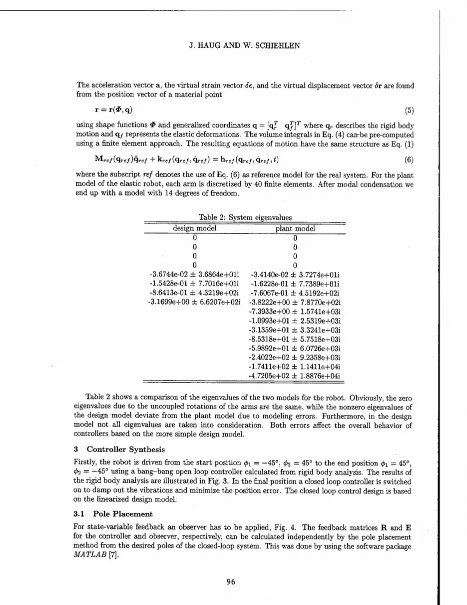
J. HAUG AND W. SCHIEHLEN
The acceleration vector a, the virtual strain vector 6e, and the virtual displacement vector <5r are found from the position vector of a material point
r = r(#,q) (5)
using shape functions «P and generalized coordinates q = [qjT qT]T where qr describes the rigid body motion and q/ represents the elastic deformations. The volume integrals in Eq. (4) can-be pre-computed using a finite element approach. The resulting equations of motion have the same structure as Eq. (1)
Mre/(qre/)qre/ + kre/(qre/,qre/) = hre/(qre/,qre/,f) (6)
where the subscript ref denotes the use of Eq. (6) as reference model for the real system. For the plant model of the elastic robot, each arm is discretized by 40 finite elements. After modal condensation we end up with a model with 14 degrees of freedom.
Table 2: System eigenvalues
design model plant model 0 0 0 0 0 0 0 0
-3.6744e-02 ± 3.6864e+01i -3.4140e-02 ± 3.7274e+01i -1.5428e-01 ± 7.7016e+01i -1.6228e-01 ± 7.7389e+01i -8.6413e-01 ± 4.3219e+02i -7.6067e-01 ± 4.5192e+02i -3.1699e+00 ± 6.6207e+02i -3.8222e+00 ± 7.8770e+02i
-7.3933e+00 ± 1.5741e+03i -1.0993e+01 ± 2.5319e+03i -3.1359e+01 ± 3.3241e+03i -8.5318e+01 ± 5.7518e+03i -5.9892e+01 ± 6.0726e+03i -2.4022e+02 ± 9.2358e+03i -1.7411e+02 ± 1.1411e+04i -4.7205e+02 ± 1.8876e+04i
Table 2 shows a comparison of the eigenvalues of the two models for the robot. Obviously, the zero eigenvalues due to the uncoupled rotations of the arms are the same, while the nonzero eigenvalues of the design model deviate from the plant model due to modeling errors. Furthermore, in the design model not all eigenvalues are taken into consideration. Both errors affect the overall behavior of controllers based on the more simple design model.
3 Controller Synthesis
Firstly, the robot is driven from the start position fa = -45°, fa = 45° to the end position fa = 45°, fa = -45° using a bang-bang open loop controller calculated from rigid body analysis. The results of the rigid body analysis are illustrated in Fig. 3. In the final position a closed loop controller is switched on to damp out the vibrations and minimize the position error. The closed loop control design is based on the linearized design model.
3.1 Pole Placement
For state-variable feedback an observer has to be applied, Fig. 4. The feedback matrices R and E for the controller and observer, respectively, can be calculated independently by the pole placement method from the desired poles of the closed-loop system. This was done by using the software package MATLAB [7].
96

CONTROL DESIGN AND VALIDATION OF FLEXIBLE ROBOT SYSTEMS
c r^fNm] T [Nm]
0
2.5-
OH
2.5-
-5- i ■
4 0,t[rad] ^.t2[rad]
1 ... \ ^-" \ /
O.b- \ / - \ /
0- y / \ / \
0.5- / \ __^/ \
'~—■ -■■ ■■ i—- mi. ,.,—
-1 -I 1 ■ 1 1
2 4 t[&] 6
4 f[s] 6
n ^ 0, [rad/s2] - - 0,2 [rad/s2]
0.25- |
0-
0.25-
-0 5- i ■ i '
2 4 r[s] 6
Figure 3: Torques, rSl, rS2! angles, <f>ai, (j>S2 velocity of the angles 4>tl, <j>S2 and acceleration of the angles 4>Sr, <pS2 using rigid body dynamics
Figure 4: State-variable feedback controller and observer
97

J. HAUG AND W. SCHIEHLEN
Applying the resulting controller and observer to the plant model leads to instability due to positive eigenvalues, Table 3. Additionally, this result is illustrated for the first 8 eigenvalues of the closed loop plant model in Fig. 5. A detailed error investigation shows that this instability effect is not only due to truncation of modes but also due to errors in the eigenvalues of the design model. Therefore, a robust controller will be designed in the following section.
<D
100
90
80
70
60
50
40
30
20
10
s-plane •
, © •
®- desired observer ®- desired conti •- closed loop
(plant model
oiler 1 ©
)
• ®
■ « ' ©«B « 0 -100-90 -80 -70 -60 -50 -40 -30 -20 -10 0 10 20 30 . 40
o
Figure 5: Poles of the open and closed loop system
3.2 Robust Controller
Using a normalized left coprime factorization description of the model a controller can be designed giving maximal robustness against unstructured model errors, see McFarlain and Glover [8]. The controller is computed by performing H^ minimization.
The matrix of transfer functions corresponding to Eq. (2) is
G(s) = C(I6s-A)-1B, (7)
where I6 is a 6 x 6 idendity matrix. A normalized left coprime factorization can be written as
G = B~^ (8)
where
N = C(I6s-(A + HC))-1B and D = C(I6 s - (A + HC))-XH + I4 . (9)
The matrix H is computed by solving the generalized filtering algebraic Riccati equation [8]. With the factorized transfer function the controller K can be calculated from the following minimization problem
inf K stabilizing
(Jj)(I4 + GK)-1D-1
oo Pmax
where the maximal stability margin pmax is calculated as
pmax = y/l-\\\N D]fH
(10)
(11)
98

CONTROL DESIGN AND VALIDATION OF FLEXIBLE ROBOT SYSTEMS
using the Hankel Norm. This problem can be solved by using standard Hoo minimization [7]. Therefore, the system has to be arranged in form of a generalized feedback representation shown in Fig. 6 where the matrix for the augmented plant P is given as
(12)
-D-1
0 -G
X2
-D-1 -G
w
1 P
+ y
r i
1 w D1 14 ^^
12
n U
G
\ ,
L
) j - u 1
j
e'
K
Figure 6: Generalized feedback arrangement
In order to receive a good performance of the closed loop system, a desired shape of the singular value plot of Q = GK has to be obtained. This can be accomplished by open loop shaping, i.e. weighting the matrix of transfer functions G as
Gw = W0GW/
where for the given example the weighting matrices are chosen to be constant:
W0
100 0 0 0 0 100 0 0 0 0 300 0 0 0 0 300
w7 100 0
0 200
(13)
(14)
In Fig. 7 the singular values of the design plant G(s), the weighted design plant Gw{s) and the matrix of transfer functions Gw(s)Kw(s) which represents the quantitative performance of the closed loop system are shown. After computing the controller Kw using Eq. (10) on the basis of the weighted plant Gw the final solution for the original plant can be obtained:
K = WjKwWo (15)
Applying the resulting controller to the plant model leads to a stable closed loop system, Table 3. In addition, this result is illustrated for the first 7 only negative eigenvalues of the closed loop system in Fig. 8 in contrast to the first controller, which has shown some positive eigenvalues, Fig. 5. Figure 9 shows the time behavior of the system without closed loop controller, characterized by strong vibrations. Figure 10 represents the time behavior of the plant with bang-bang open loop and the robust controller. Obviously, the behavior is stable.
99

J. HAUG AND W. SCHIEHLEN
Ö(G) [dB] ä(Gw)[dB] — ä(GwKw)[dB] -
100
-100
-200
o(G)[äB) o(G w)[dB) o(GwK-w)[dB)
103 ct>[rad/s] 104
Figure 7: Singular values of the design plant G(s), the weighted design plant Gw(s) and the matrix of transfer functions Gw{s)Kw{s)
0) 100
90
80
70
60
50
40
30
20
10
0 -100-90 -80 -70 -60 -50 -40 -30 -20 -10 0
Figure 8: Poles of the open and closed loop system
s-plane o •
c o •
•- closed loop (plant model
. o-closed loop ) •»' ■
(design mod« d)
°:0*
■—•— 6 •
100

CONTROL DESIGN AND VALIDATION OF FLEXIBLE ROBOT SYSTEMS
wjio-Vl w2[10 3m] jjClO-4!!!] y2[10-4m] 6 ■
-0.5-
Figure 9: Time response of the flexible deformations wi, w2 and the displacement of the end effectors from the desired position yu y2 after open loop control
10
5
0
-5
-10
1
0.5
0-1
-0.5-
-1
TjfNm]-- — r2[Nm]
■SilSIIIISIII
k ■
■
i
,.
0j[rad] 02[rad]
WjflO-^]
4 t[s] 6
-w2[10_3m]
4 5 f[s]
6
3
0
-3
-6
y,[10-4m]--
5 t[s)
Figure 10: Torques TU T2, angles fa, <f>2 and displacement of the end effectors from the desired position yu y2 for combined open and closed loop control
4 Conclusions
In this paper, a flexible robot is modeled for control design by a rigid multibody systems approach using superelements for approximating elastic beams. Such a rough model simplifies control design but it may result in erroneous eigenvalues compared to an accurate plant model. A classical state feedback controller designed on the basis of such a simple model may then result in instability if it is applied to the real system, whereas a robust control design yields satisfactory results.
101

J. HAUG AND W. SCHIEHLEN
Table 3: System eigenvalues
poleplacement controller Ifoo-controller
design model plant model design model plant model
-llil.OOOi
-35±1.000i -9 ±2.0001
-30±12.00i -28±32.19i -7±36.19i
-25 ± 68.851 -5±76.85i
-20±372.2i -3±432.2i
-20±592.1i -2±662.1i
-2.69655±1.35220i
-1.05965±1.88077i -2.98403 ±1.57787i -26.4449±32.1089i 1.09867±59.7810i
-25.0116±69.1325i 38.7776±75.1259i
-97.4938±87.3932i -19.8063±385.126i -1.26790 ±449.7931 -20.4332 ±598.4441 -5.23938 ±775.0891 -758.149±1574.08i 1.46803±2532.67i 865.039±3324.26i 3508.09±5751.34i 290.554±6074.10i 39070.5±9238.93i 167.051 ±11412.4i 54678.2±18881.8i
-50.1419 -292.469
-8.74732±13.3253i -12.1852±15.1144i -26.9174±29.3775i -140.185±53.7447i -37.7267±55.0028i -40.7346±72.6638i -66.8500±86.9316i -3.55750±432.495i -3.62259±432.932i -13.6105±662.148i -13.5747±862.374i
-85.0004 -279.327 .
-16.5779±8.37190i -44.6019±15.7678i -6.16580±16.7730i -26.6622±48.8267i -32.5240±81.8415i -160.570±84.7682i -37.4280±85.4585i -4.38792±436.967i -1.44847±450.238i -5.16786±664.929i -5.67702±786.447i -7.38658±1574.13i -11.1672±2531.84i -31.3682±3324.07i -85.3200±5751.82i -59.9052±8072.62i -240.219±9235.84i -174.11H£11411.0i -472.054±18875.9i
References
[1] Engell, S., Modelgüte und Regelgüte, VDI Berichte Nr. 925, VDI-Verlag, 1989.
[2] Czaijkowski, E.A., and Preumont, A., and Hafka, R.T., "Spillover Stabilization of Large Space Structures", Journal of Guidance and Control 13 (1990) 1000-1007.
[3] Kleemann, U., Regelung elastischer Roboter, VDI Fortschritt-Berichte, Reihe 8, Nr. 191, VDI- Verlag, 1989.
[4] Schiehlen, W.O., Technische Dynamik, Teubner, 1986.
[5] Rauh, J., Ein Beitrag zur Modellierung elastischer Balkensysteme, VDI Fortschritt-Berichte, Reihe 18, Nr. 37, VDI-Verlag, 1987.
[6] Melzer F., "Semi-Symbolic Equations of Motion for Flexible Multibody Systems", Proceedings of the 1993 ASME International Computers in Engineering Conference, San Diego, August 8-12, 1993.
[7] The Math Works Inc., MATLAB User's Guide, Natick, MA, 1992.
[8] McFarlain D.C. and Glover K., Robust Controller Design Using Normalized Coprime Factor Plant Description, Springer-Verlag, 1990.
102

NONLINEAR CONTROL LAW FOR A FLEXIBLE ROBOT
B. Yachou Universite d'Evry Val d'Essonne
Evry, FRANCE
and
M. Pascal Universite P. et M. Curie
Paris, FRANCE
Abstract
In this paper, a control command for flexible robots is elaborated by using a non linear decoupling technics. The dynamical model is obtained by a modal synthesis method and a feed back on the elastic variables is also considered. The control law takes into account the dynamical model after removing the Lagrange multipliers. An example of the control of a flexible arm is investigated and shows the efficiency of this non linear control law.
1. Introduction
Weight minimization and large accelerations in many robotics applications lead to an increasing tendancy for elastic vibrations. Light structures in robotics allow a better ratio payload/weight of the robots and energetic reduction for the motors in the joints. In space applications, the very long and slender geometric dimensions induce important vibrations. Manipulators arms require a reasonable accuracy in the end-point positioning of the arm. This accuracy is deteriorated by structural deformations. For improving the performance of these flexible robots, the elastic deflections must be taken into account in the control law, in order to damp their motion. Classical control laws defined for rigid robots can be extended for flexible robots but they will not have the same ideal performance as the number of actuators is less than the number of variables to control. Several different methods have been proposed in the last few years in order to solve this problem : Inverse dynamics and computed torque applied to the position control multilinks elastic robots (Ref. 1), L Q R method based on a linearized behavior model and a state feed back (Ref. 2), singular perturbation methods where the elastic and the rigid motions are supposed to be time separable (Ref. 3), non linear decoupling methods based on the dynamical model of the robots (Refs. 4 - 5). In this work, the last method is used because the non linearity in the behavior of the robots seems to be a predominant effect.
2. Modelisation of the robot
Let us consider a multibody open chain robot composed of NB bodies S},.. SNB articulated by (NB-1) joints L],..Lm_l. Each component (S(.) can undergo small elastic deformations and large displacements. In the past, several methods has been proposed for the dynamical analysis of flexible multibody systems : Analytical methods (Refs. 6 - 7), approximated methods using non linear finite elements discretisation (Ref. 8) ; resolution of the motion of each flexible component into a large rigid body motion and a small elastic displacement (Ref. 9). In this work, this last method is used, together with a modal synthesis method giving for each flexible components an approximate value of the (small) displacements field (Ref. 10).
2.1. Dynamical model of one flexible component
For each flexible components {Si) of the robot, the motion is resolved into a rigid motion of a reference configuration (J&r) and a small elastic displacement Q (Fig. 1).
103

B. YACHOU and M. PASCAL
The inertial position u of every material point Mis given by :
ü = OinerO0+O0 0+OM'+ M'M = a+ üref + x + g (i)
where Q=Cf(x,t) is the elastic displacement field related to an undeformed reference, configuration
(<!hr) and X = 0 M gives the position of the point M which is assumed to be rigidly connected to the reference configuration ((/£>,.)■ üref gives the rigid body translation motion, or is a constant vector. The
choice of the reference configuration will be given later. Let us introduce the orthogonal matrix P giving the position of the local frame (Rt) rigidly connected to the reference configuration (Ul?r) with respect to the
inertial frame (Rj„er). ( 'P = P~l).P defines the rigid rotationnal motion of the body.
The column matrix of the inertial components of vector v. is given by :
u = a+uref + P(xe + g) (2)
where x and Q are the column matrices of the local components of vectors x and ö The local motion equations of the flexible component are :
div(VS)+p0f = poü in (u%0) (3)
where (fjk0) is the initial configuration of the body, p0 is the initial mass density, j> is the second Piola- Krichoff stress tensor, if is the strain gradient defined by dü = ft'dx.
\f = />( §f+ V. g() ( £ unitarian tensor)
V is the gradient operator with respect to the local components of vector X, f is the body applied force. Assuming small strains, the Lagrangian strain tensor is approximated by :
Jjfr =i/2(W-IF)s£=i/2(v.£'+ 'V.g'O
and assuming linear constitutive law, the stress tensor is given by :
£ =A(trace£)ifc+2// £,
It results for the motion equation projected in the local reference frame (Re) the following expression :
\=Pof'~-p'opür
ür = üref + Px gives the inertial components of the rigid body acceleration.
k, is a linear differential operator.
By application of the virtual works principle, with a virtual displacement S Qe, we obtain :
104

NONLINEAR CONTROL LAW FOR A FLEXIBLE ROBOT
+ J 'SgtkL[gt]iv= j* lSQ((p0f~p0-pür)dv
dir c4jr
A spacial discretisation of the reference domain (<&r) is performed by means of finite elements method :
where q is the column matrix of the local components of the displacements of the nodes and N(xe) is the interpolating matrix.
Assuming a virtual displacement of the body in the form 8 Qe = NSq, the virtual works principle gives the following dynamical equations:
Mq + Cq + Kq = Fe-FK (6)
where M = I . p0 'NN dv is the (constant) mass matrix ;
C = J . 2p0 'N 'PPN dv is the gyroscopic matrix ;
K = Ks + Kd, Ks = J » 'M^[N] dv is the (constant) structural stiffness matrix ;
Kd = J . /90 'N 'PPN dv is the dynamical stiffness matrix ;
^c ~ J A ^ '^-^' ^V 's re'atec*t0 tne aPP"ed forces ;
^R ~ J L ^° '^ '^ ^r ^V lS related t0 tne inertiai forces produced by the motion of the reference
configuration ((#,.).
The matrices C, Kd and FR are time variant.
2.2 Incremental motion of the flexible component
The motion of the flexible component is defined by an incremental method (Ref. 10) : in each time
interval [f„,f„+1], the reference configuration (ußr) is the rigid configuration reached at the time tn and the
motion equations are linearized with respect to the increment of displacement q>: of this time interval (Fig. 2).
The increment qn is splitted into a rigid increment q" and a flexible increment«^ :
Let us consider the matrix X giving the modes shapes of the body assuming that the reference configuration ((fbr) is fixed. Xh a constant matrix defined by :
105

B. YACHOU and M. PASCAL
X = (Xl...X,)
where N is the total degrees of freedom of the nodes, X. is the mode shape associated with the pulsation
COj. The modal matrix X is splitted into the matrix Xr of rigid body mode shapes and the matrix Xd of
deformation mode shapes. Assuming that the increment qn is small, this increment is expressed as a linear combination of the rigid modes and the deformation modes :
6 nd
q^Y^y-Xrj + YsYZjX^XrV + X.Y^XY" (7) >1 y=i
Y = Y.
gives the modal amplitude of the modes, n d is the number of deformation modes chosen : in most
cases, only few deformation modes are used, namely low frequencies modes. The new generalized variables of the dynamical model are defined by the equations
(8)
where ^n = 'X Kn X is the generalized stiffness matrix ; £„ = 'X CnX is the generalized damping
matrix ; m-'XMX is the (constant) generalized mass matrix ; 3e"—XF" and 3"R~l='X F£~l are
related to the applied forces and to the residual inertia forces respectively.
2.3 Dynamical model of the whole system
The dynamical model of the robot is deduced from Eq. (6) (Ref. 10):
lMq+C t + K q=Fe-FR + r+'P['JA] (/) [g(U) = 0 00
(9)
q is the column matrix of the local components of the displacements increments of the whole system, F is the
column matrix of the local components of the forces or torques produced by the actuators, Fe and FR are
the column matrices of the applied forces and residual inertia forces for the whole system, M S\K and P
are block-diagonal matrices defined from M■,C., Kj and P ( ]' = 1,.. NR) by :
M =
Mn
M, i •
'Mm
At last X is the column matrix of the Lagrange multipliers associated with the constraint equations (/'/) in which
U is the column matrix of the inertial components of the nodes of the whole system and J is the Jacobian matrix of the function g.
The constraint equation (9) (/'/') is linearized on the time interval U„,t„+] J :
106

NONLINEAR CONTROL LAW FOR A FLEXIBLE ROBOT
^7"+1) = ^7")+f#] AU+4*Uf) = o Wh
JnAÜ=Jn{Ü"+x-Ü") = 0
From the incremental motion of the system (Fig. 3), we deduce
\u_^ = u>; +_pn q —«+i
Ur is the column matrix of the inertial components of the reference motion of the nodes for the whole system, qd is the column matrix of the local components of the flexible increments of the nodes. By projection of the constraint equations (//') on the modal basis of the whole system, we obtain
JnPn'XY"*=JnPn_xXYZ
where Yd is the column matrix of the modal amplitudes of the deformations modes
(10)
Yd =
O
Y d\
o Y dNB
Y. is of the same size as Y
The relation between Pn and Pn_x can be written in the following form
P = P AP
where A P„ gives the small rigid rotation increments of the system. It results that the constraint equations (10) take the form :
V 7"+] = n. Y'J (11)
"n xd
** = J.P,,X
On the other hand, the generalization of the equation (8) to the whole system gives the following equation :
V'TIX" (12)
2.4 Numerical integration
The numerical code used is the PLEXUS Software (Ref. 11) in which a Newmark semi-explicit scheme is chosen for the integration of the motion equations :
107

B. YACHOU and M. PASCAL
At1
Y" Y"+l = Y"+AtY" + 2
y~n _ y~n-l , _£[_£_ | ~y~n-l . TT« |
From these formulas and from the constraint equations (11), we obtain
1
(13)
v., Y" At
M., 2 A"n Y"-Y"-AtY"-1-— Y"-1 (14)
The acceleration Y " is computed from the dynamical equations (10) in which Y " is estimated by its value in the middle of the step (Ref. 11):
Yn = W„+nrl 'x„r+m-x 'XT
Wm=nTx (3;-3/-'-F„ Y"- „ f-"2) (15)
Y «-1/2 _ y n-l A t y-„_)
2
From formulas (13) and (14), we deduce the Lagrange multipliers :
-l
■"" ld J At
-[H?]-1 x„wxtxr
Y"-Y"-AlY"-x At2 - n-l
(16)
where H" - 7tnm~ 'nn is a square matrix of dimensions («,, xn() (n( is the number of scalar constraints) which is supposed to be non-singular. From formulas (14) and (15), we deduce the incremental acceleration at time t :
Y" = zn + (P"x r
Z" = (E-H"2) Wn+-%\Yd"-Yn-At t"-' -— f"-' At' (17)
<P' = (E-H^)m •^r-l
where H"2 - m'1 ' nn [H" ] nn is a square matrix of dimensions (NXN)(N total number of degrees
of freedom of the whole system); E is the (N x N) Unitarian i i matrix.
3. Dynamical control laws in the joint space
The aim is to choose the control forces or torques produced by the motors at the joints in order to obtain a desired trajectory defined in the joint space and to damp the elastic vibrations. The main difficulty to solve this problem is that the actuators act only on the rigid body degrees of freedom.
108

NONLINEAR CONTROL LAW FOR A FLEXIBLE ROBOT
To design the control laws, we use the dynamical model (17) in which a split of the rigid variables and the deformation variables are done in order to obtain the rigid body accelerations :
V = z; + (0ir'x, + <r,d'xd)r (0
Z" = z;+(<tr,r % + &dd %) r (io
We define the following control vector at each time /
v- = üC"+G; (ü:-u,"yG;{v:-eur")-Gf U;-G; eU'd
(18)
(19)
In this formula, the notations U and U give the relative velocities and the relative accelerations (in local reference frames) of the components of matrix U .
The desired trajectory is defined by
%=lü„ , eUdc = o
At last, Gp , Gyr , Gp and Gv are gains matrices. These matrices are chosen in order to
minimize the rigid error er=U-''Ur and the flexible error Sd = - ' Ud and their first and second
derivatives with respect to time. If the dynamical model (17) is used, we assume the following relation :
from which the control torque is obtained :
Ä" = {xrfrr% + xrfrd%)
Hence the obtained torque depend on the control vector and on the dynamical model and includes a feed back of the rigid and elastic variables.
For practical implementation of the obtained control command, only some special nodes will occur in the expression (19) of the control vector, namely the nodes where the actuators lie and some nodes where the
deformations have to be damped. It results that in the feed back gains matrices Gvr, G r, G/, Gd, only the
terms related to these nodes are not equal to zero.
By substitution in the dynamical model, the errors on the rigid and flexible variables are given by :
109

B. YACHOU and M. PASCAL
^+G;^+G;^ = -GV^-G;V,
L'{ = (xdcfdrX+xdafdd'xd)jn
il = L>{(ur]+xrz>;)-xdz"d
(20)
In terms of the error on the state vector A X= (!er, 'ed, 'sr, 'ed), the formula (20) takes the form
AXn=&{AXn) + fy(AX„)\n
IV /" _ J" TJn
\L2 L\ Uc J
G =
(OOIO \ OOOI I I I I T" J" T" I"
fGrpO 00 ^
OGdpOO
o o G;O [O O O Gd)
(21)
The obtained equation is a non-linear equation.
The gains matrix G, which have to be chosen in order to minimize the rigid error Sr and the magnitude of the elastic variables, can be obtained by linearization of equation (21) in the vicinity of a point of the desired trajectory (Ref. 4) and by using standard technics of computation of the gains matrix for linear systems.
4. Test example
This control command is applied to a single planar flexible robotic arm (Fig. 3). At one end of the arm, there is a rotational joint acted by a motor. At the other end, a concentrated mass m is rigidly connected to the' robotic arm. The numerical data of the system are the following :
Lenght:/. = \m
Crossed section :S = 1,510"4/»2
Concentrated mass : m = 5,9 kg
Mass density : p0 = 7,8103 kg/w3
Young modulus : E = 2101' N Im2
Poisson ratio: v=0,35
We use the two first vibrations modes of the link with clamped-free boundaries conditions. The associated frequencies are /, = 0,26H, and f2 = 1,1 Iff.. In this simple model, there is only one rigid variable 9, acted by the torque r; the desired trajectory is denned by
110

NONLINEAR CONTROL LAW FOR A FLEXIBLE ROBOT
& n ( , A
VmJ 15 + 10
\lm J
where tm — 8s.
For the elastic variables, we choose to control the tip of the link, namely the transverse deflection uv and the slope Rr.
The corresponding feedback gains are Grp = lO0, Gr
v=20, G, =[-20,20], Gdv ='[20,-20].
The results of the simulation are shown on the Figures 5 - 8. The curve (Fig. 5) shows that for the risid variable, the desired trajectory is well followed. The curve (Fig. 6) shows the behavior of the flexible arm controlled by a linear PID law corresponding to the control gains : G = 9, Gv = 6, G- = 4. The
simulation shows that in this case, the desired trajectory is not well-followed.
The curves (Fig. 7 and 8) show that with the non-linear control law chosen, the elastic deformations at the tip of the arm are very quickly damped. The computational time necessary to obtain the control torque at each time step takes about 3.5 ms. The damping of the elastic variables is obtained from the feed back of these variables in the control command.
5. Conclusions
In this work, a dynamical model for flexible robots is used to design a non-linear control law in order to follow a desired trajectory in the joints space and to damp the structural vibrations of the links. As test example, a one single flexible robotic arm is chosen ; the numerical simulation shows the efficiency of this non- linear control law.
6. References
1. Bayo, E.. Papadopoulos. P., Stubbe. J. and Serna. M. A.. Inverse Dynamics and Kinematics of Multilink Elastic Robots: An Iterative Frequency Domain Approach, Int. J. ofRobotics Research Vol 8 No 6 1989, pp. 49-62.
2. Chaloub, N. G. and Ulsoy, A. G.. Control of a Flexible Arm : Experimental and Theoretical Results, J. Dyn. Syst. Meas. Control ASME, Vol. 109, 1987, pp. 299-310.
3. Siciliano. B. and Book. W. J., A Singular Perturbation Approach to Control of Lightweight Flexible Manipulators, Int. J. of Robotics Research, Vol. 7, No. 4, 1988, pp. 79-90.
4. Chedmail. P., Aoustin. Y. and Chevallereau. C. Modelling and Control of Flexible Robots, Int. J. For Num. Meth. in Eng., Vol. 32, 1991, pp. 1595-1619.
5. Modi, V. I, Karray, F. and Chan, J. K.. On the Control of a Class of Flexible Manipulators Using Feed hack Linearization Approach, 42nd Congress of the Int. Astr. Fed., October 5-11, 1991, Montreal. Canada.
6. Pascal. M., Dynamics Analysis of a System of Hinge-Connected Flexible Bodies, Celestials Mechanics Vol. 41, 1988, pp. 253-274.
7. Pascal, M., Dynamical Simulation of a Flexible Manipulator Arm, Acta Astronautica, Vol 21 1990 pp. 161-169.
8. Cardonna. A. and Geradin. M., Modelling of Superelements in Mechanism Analyis, Int. J. for Num. Meth. In Eng., Vol. 32, 1991, pp. 1565-1593.
9. De Veubeke, F. B„ The dynamics of Flexible Bodies, J. of Eng. Sei., Vol. 14, 1976, pp. 895-913. 10. Azouz, N.. Joli, P. and Pascal. M., Dynamic Analysis of General Flexible Multibody Systems, Euromech
320 : Multibody Systems : Advanced Algorithm and Software Tools, Prague, 6-8 June 1994. 11. Barraco. A.. Cuny. B„ Hoffmann, A.. Jamet. P., Combescure. A., Lepareux, M. and Bung, H„ Plexus-
Software for - the Numerical Analysis of the Dynamical Behavior of Rigid and Flexible Mechanisms in Multibody Systems Handbook, Berlin - Springer - Verlag. 1990.
.11

B. YACHOU and M. PASCAL
Fig. 1 : Decomposition of the displacement
NON-LINEAR CONTROL LAW FOR A FLEXIBLE ROBOT
Fig.2 : Description of the displacement increment
Fig.3: FLEXIBLE ARM
112

NONLINEAR CONTROL LAW FOR A FLEXIBLE ROBOT
Fig.4: DEFINITION OF PARAMETERS
CONTROL LAM I (S)
RIGID DECREE OF FREEDOM
-1- Desired trajectory
ruzm-cum
Fig. S -2- Real behaviour
T. 5T
Flg. 7
DISPLACEHEHT OF TEKKODU. SECTIOB
RIGID DEGREE OF FREEDOM -1- Desired trajectory
Fig. 6
-2- Real behaviour
NOULIHEAR CONTROL LAM TT
Fig. 8
ROTATION OF TERMINAL SECTION
<•■, 7, 2.
113

114

FRICTION CONTROL IN MULTIBODY SYSTEMS
H. Bremer Technical University of Munich
Munich, GERMANY
Abstract: Friction is an important factor in most mechanical engineering applications. It may either cause undesired behaviour like, for instance, stick-slip vibrations in a mechanical clutch, or control inaccuracies in fine point robot control. Or it may directly be used for energy dissipation like in turbine blade dampers or in mechanical brakes. The main difficulty hereby is the fact that friction depends on actual parameters like temperature, humidity and aging, just to mention the most important ones. Since the first experimental results from the 17th and 18th century (Amonton, Euler, Coulomb) many attempts have been made to derive a mathematical theory of frictional processes. However, general mathematical mo- dels which include every important parameter have not yet been found. It is, therefore, more convenient to get information on the friction by on-line measurement instead of numerical precalculations. The necessary measurement data is already available in actively controlled systems.
1 Introduction
Friction forces in general depend on normal pressure and relative velocity at the contacts points. In case of dry friction it is known by experience, that sliding friction has lower values than the maximum possible sticking forces, which causes in some cases stick-slip vibrations. Howe- ver, using special paper lining between the contacting bodies may also lead to smaller sticking than sliding force coef- ficients. This is commonly used in au- tomatic changeover gears which operate with a mechanical clutch. In any case, the amount of friction may be charac- terized by a velocity dependent coeffi- cient ix. Assuming smooth transition from stiction to sliding friction may be represented by
d/i
V = f*o
= -Tfi
A/x(l -T\V ') CD
o o
o
0) 3 £ I ' ' M ' ' ' 1
200 400 600
♦ 10 ";
Fig. 1: Friction coefficient over relative velocity
115

H. BREMER
(Afx may be positive or negative). The common way to describe the friction coefficient is by curve fitting. One corresponding result was given by
(J. = Ho — Afi- Vrel
Vrel +- (2)
(see [1]) which represents a first order Taylor expansion of eq.(l). However, such an experimental result can only be valid for a given set of actual parameters which may alter during operational processes. Eq.(2) is therefore used as an input for numerical calculations but treated as unknown for control calculations.
2 Feedforward Control and Reference Path
The equations of motion of a mechanical system read
M(z)z + g(z, z) = B~u + f
'dvf\T . . "^T/öw/
dz OZ / i=i i=l
*in J2'
Control
Path o o
9 CM
>,8 CM
I
1 I I | I I I I | I 1 I I |
1.0 1.5 2.0
M
Fig. 2: Scara straight line (below), control (above)
J\ + misj + m.2l2 rri2S2h cos(a — ß)
m2S2h cos(a — ß) J2 + rri2S2
? = E dvd
dz d,i (3)
where index in denotes input forces and torques while d represents disturbances (friction in the actual case).
Equation (3) yields directly the open loop control input for the desired path z0 when z0 (and derivatives) is inser- ted. In the absence of friction one gets
M{z0)z0 + g(z0, z0) = Bu0 (4)
2.1 Scara Robot
The simplest representation of a Scara robot is given by a double pendulum with z = (a ß)T being absolute coordi- nates. The equations of motion read
M(z) 'z + g(z,z) = Bu + f
Bu = ( ta ~tß \ V tß J
1=- l«l\dz)
fdv
\dz )»
+ß2
g = m2hs2sm(a- ß)[ .„ -a (5)
116

FRICTION CONTROL IN MULTIBODY SYSTEMS
The maneuver considered is drawing a straight line beginning with (a0 ß0) = (20° 160°) and ending with (aeße) = (70° 110°). The results are, in the ab- sence of friction, given in Fig. 2.
2.2 Automated Clutch
In case of a sliding clutch the equation of motion of the motor coordinate sim- ply reads
Clutch Pressure
(pM = a<PM + f + JM'
/ = JM
p(6)
where JM'- motor moment of inertia, a = K/JM- K is assumed known from a characteristic field and R is a charac- teristic length. For a known fi one gets an optimized clutch torque (not shown here) with clutch pressure time history according to Fig. 3. The pressure is achieved by digital control with AT = 10 [ms] as sampling rate. During this time, M0 is assumed to be constant.
2.3 Influence of Friction
320
Coeff. Needed
320
Fig. 3: Optimized clutch pressure time history
It is obvious that the automated clutch cannot operate with unknown friction. It was shown by numerical calculation that the changeover process gets unstable if the real input value changes too much compared to the nominal input value.
Path o o 9 w
>> o I I I I I I 1 I I I I 1 I I I
1.0 1.5 2.0 I
Fig. 4: Scara maneuver with friction Fig. 5: Path deviation for the elastic robot, compa- rison of reference and measured strain gauge signals (dashed)
In case of the considered scara robot a straight line cannot be achieved if friction (with p=const.) occurs, Fig. 4.
117

H. BREMER
Finally, to mention a more realistic robot case, the simulation of a flexible robot (two elastic links) has been proven by experiments [2]: In case of friction the desired path could of course not be realized, Fig. 5.
It ist therefore a demanding question to estimate friction. This can be achieved adapting classical observer theory, which in the following will be discussed briefly.
3 Friction Observer
3.1 General Theory
Observer theory will here be discussed for linear plant representation (deviation from reference state, first order Taylor expansion), [3]. Aim of the minimum dimension observer is to estimate nonmeasured state variables. Here we assume that every state variable is available. Observer theory is then applied to the augmented state which includes friction input. Corresponding equations are represented by
x = Ax + feJRn, y=Cx, C = EeMn. (7)
(E: unit matrix). The unknown disturbance / is represented by a combination of basic functions e, which are solutions of the first order linear differential equation
f = He, e = Feemr, (8)
yielding
D=(o ?)(:)«*■ A={£3C)6K" w y
The estimated state vector x € IRn,n — n + r is assumed proportional to an estimation £ G IRr
corrected by a measurement input Szy:
#■ = Sii + s2y, Si e ntn'r, s2 e nn,n
Z = DZ + Ly, DGlRr'r.£eIRr'n. (10)
118

FRICTION CONTROL IN MULTIBODY SYSTEMS
Using a (still unknown) transformation T G IRr'n, which transforms x into the subspace denned by £, yields the following condidions:
/IS, (« - 5) — 0, ,'iS, (£ - Tx) -H. 0 (11)
leading, for the limiting values, to
COND 1:1;- 5iT - S2C = 0 e IRn,n
COND 2: TA-DT-LC = 0e JRs'n
(12)
(13)
Inserting these into (£ — Tx) shows that for
A (£ - Tx) = D(£ - Tx) (14)
it is a necessary condition for eq.(ll) that matrix D is asymptotically stable. Following [4] one may chose
T=[-T*Er], T* GlRr'n, Sx 0 , s2 = En
(15)
(Ea = E £ IRa'aVa: identity matrix). Condition 1 (eq.(12)) is then fullfilled, while T* is still arbitrary. From condition 2 (eq.(13)) one obtains
D = TASi,
L = TAS2. (16)
The estimation then reads, with eq.(7), eq.(10), eq.(15)
E 0 ' /Tl* E
A 0 L D 'Mi
(17)
(18)
D = -[T*H - F], L = -[T*(A+HT*)-FT*]
119

H. BREMER
Transforming eq.(18)with eq.(17) yields
A 0 0 -T*H + f
T*f (19)
3.2 Basic Disturbance Functions
The estimation £ according to eq.(10) basicly depends on eq.(8). Chosing F as
F =
/ 0 1
\0 1
€lRr (20)
for only one disturbance input yields an arbitrary time dependent polynomial vector eT = (c1t
r-1/(r — 1)! c2tr jr\ ■ ■ -cr)
T with coefficients c* which are on-line adjusted by the estimation procedure. With this statement, any disturbance can be represented. The necessary condition for correct disturbance estimation is
A = A H 0 F
(H, F) observable. (21)
The observability condition
Rank[JTT FTHT ■ • • Fr~lTHT) = (22)
assures observability for every dimension r, especially r = 1 yielding F = F = 0 i.e. e = e = const. Augmenting for several independent disturbance inputs, one may chose F = 0. This means that every disturbance is reconstructed with constants, which are adjusted to the real disturbance time history by the observer input, mainly due to the feedback of real and estimated measurement. Although F = 0 seems to be a quite rough approach, most applications showed a very good disturbance estimation (which of course depends on T*), see for instance [5], [6]. Hence, using F = 0 yields
D = -[T*H], L = -[T*(A + HT*)] (23)
and demonstrates the asymptotic approach of e in eq.(19) with —T*H = D being asymptotical stable according to eq.(14) et sequ.
120

FRICTION CONTROL IN MULTIBODY SYSTEMS
4 Friction Control
4.1 Automated clutch
To start with the simplest case, the automated gear is considered with eq.(6). Using x = <PM + M0/JM
yields the onedimensional state equation x = ax + f. Along with h = 1, e = /, e = 0 one has, according to eq.(9)
;i)(:)-»=^(: Chosing T* - T* = A yields for eq.(15)
(25)
T = (-A1)
0 Si = 1 , s2
With correspondig D and L from eq.(23),
D = -A, L=-\(a + X),
one gets for eq.(19)
d_ x di[ f
a 0 0 -A
(26)
/J + U W
a X
►
<
+ I
) V +
A
f
Fig. 6: Estimation scheme
(24)
yielding
x(t)
f(t) x0e" \
f0e.
eatff(r)e-ai
7V(r)e (28)
I.e. for / = const for instance, the real disturbance is asymptotically estimated with / = f+f0exp(-Xt) (A sufficienty high). For the real case, fi is recalculated from eq.(6) for every sampling rate Ar in which the clutch pressure p is held constant, yielding results according to Fig. 7
121

H. BREMER
Coeff. Needed
240 280 320
♦ 10
Coeff. Estimated o 05
•a £ m "5 <n E
i i i | i ' i | i i i | i i i |
240 280 320
+ 10 "3
Fig. 7: Real (left) and estimated friction coefficient (right) versus time
4.2 Scara Robot
Using u0 from open loop control yields along with x = Xd + Aa; a linear (time dependent) state equation, which can be treated with eq.(18) in order to obtain the unknown friction torques. This means for friction control, to superimpose u —*■ u0 — /. Here, for H = E G IR2,2 => f = e £ IR2 the result is depicted in Fig. 8.
Path Estimation Error o o
Q I I I | I 1 I I |
1.0 1.5 2.0
o-fc.
J I I L
0
t
J L
Fig. 8: Friction torque rejection for drawing a straight line
The two friction torques for the a and ß direction are estimated separately, although only one of them would have been sufficient to recalculate the friction coefficient \i. However, in this special case \i itself is not of interest.
122

FRICTION CONTROL IN MULTIBODY SYSTEMS
5 PD-Control
5.1 Slipping Friction
The usual way to control (in particular flexible) robots, is to off-line calculate an open loop control for the desired reference, which is augmented by suitable corrections (see [7] for instance) and then to superimpose an on-line linear (PD-)control. Friction estimation as described above, however, is an on-line procedure and can therefore not be calculated in advance. On the other hand, because the magnitude of friction is not directly of interest in case of robot control, one can get rid of it by a simple on-line PD-control: u = u0 - D(z - z0) - K(z - z0). The results are shown in Fig. 9.
Control
3
Coordinates
18 *-> a -°. o
a, •3
0
t
Friction Torque o
n O I N
I I | I I I I | I I I I ^8
0
t
I I I I I I I I ]'''■)
Path Deviation o O -r-
a -L-H-
Path o o
>,8 I
I I I I I I I
Relative Velocities
1.0 1.5 2.0
Fig. 9: PD-friction-control for drawing a straight line
Once using linear on-line control schemes, one can even neglect the open loop part: Linearizing for the end position (z = zen(j+Az) assures asymptotic stability for the end point with u = —DAz-KAz due to Lyapunov's stability theorems. The path between the initial and the end position is then somewhat arbitrary. The straight line considered here, however, can be achieved without much loss of accuracy, see Fig. 10.
123
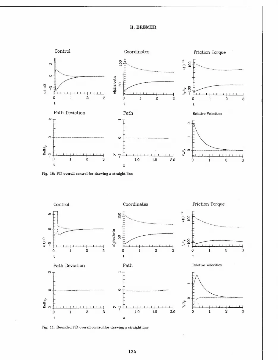
H. BREMER
Control Coordinates Friction Torque
I o o 2
^8 i i i I i i i i I i i i i I J< i ' | i i i ' | i ' ' i |
Path Deviation
o t
Relative Velocities
I l l | I ' I I | i i i ' |
0 1
t
' ' ' | i ' ' i | ' ' ' i
1.0 1.5 2.0
Fig. 10: PD overall control for drawing a straight line
Control Coordinates Friction Torque
3 .; ml 3 ' i i i | i i i i i i i i i
"S3 ■° o to m a
"3 I ' I I | I I I I [ I I ! I |
SH O --
»r o J? I I I I I I I I I I I I I ' ' ' ' I
0 1
t
0 1
t 0 1
t
Path Deviation Path Relative Velocities
01
I I I I I I I I I I I I I I I I I I I I I I I I I I I I I I
0 1
t
1.0 1.5 2.0
Fig. 11: Bounded PD overall control for drawing a straight line
124

FRICTION CONTROL IN MULTIBODY SYSTEMS
The main drawback of the direct linear control without open loop support is, that much energy is needed when the maneuver starts. If the control input is bounded, then asymptotic stability is still guaranteed, but path tracking becomes inaccurate, see Fig. 11.
5.2 Stiction
As a matter of fact, control becomes ineffective when no measurement signal is available. This may occur in case of stiction. The relative velocity is then equal to zero and the actual friction force is anywhere on the vertical axis in Fig. 1, according to the actual balance of generalized forces. A common procedure for this case is to superimpose high frequency signals to the control input in order to change from stiction to sliding. A comparable procedure is the following: In case of actively controlled systems one may look for nonzero measurement signals from anywhere else and feed these back. This means to pass over from local to non-local feed back. Of course, stability then has to be carefully investigated, see [9], [8]. An example is shown in Fig. 12: Strain gauge signals demonstrate joint sticking after an impact on the tip of an elastic link robot for local joint feedback. Augmentig PD-control by non-local measurements avoids sticking, see Fig. 13. With this concept sticking will only occur when all available signals become zero at once - a very unusual case.
t[s]
K [1/m]
0,00-
i\ -0,01",",
-0,02
-0,03
-0,04
-0,05
i i ■ i ■ \
Vv- 0
t[s]
Fig. 12: Elastic robot: strain gauge measurements near shoulder (solid) and near ellbow (dashed) after an impact at the tip, joint PD-control
Fig. 13: Same case: joint PD-control augmented by curvature feedback (strain gauge signals)
6 Conclusions
Mechanical multibody Systems with friction may be treated in various manners. The preceeding chap- ters demonstrate a simplification from case to case. Main differences hereby are: if friction itself is needed for control, like in case of automatic gears, the observer theory is a powerful tool. The presen- ted example is furthermore useful in antiskid brake systems for instance: Here, no "motor dynamics" arise at the wheel (i.e. a = 0) yielding a very simple and robust procedure for determination of actual friction (independent of aging, temperature etc.). On the other hand, if the amount of friction is not
125

H. BREMER
explicitely needed,, then a PD-control should preferably be used to cancel disturbances. Even stiction does not cause severe problems using a dislocated PD-control.
The PD-control may be regarded in two ways: the first one is to superimpose open loop control by PD-feedback in order to cancel out whatever disturbs the desired path. Because these disturbances are small in general, this kind of control does not need much energy.
Regarding basic stability considerations, the feedforward-feedback combination can be reduced to over- all PD-feedback only. However, the differences are significant: Overall PD-control needs high power at the beginning of every maneuver. This is a basic quality of simple PD controls: Starting with conside- ribly high control input the trajectory approaches the objective position exponentially. Furthermore, a desired path can not be guaranteed but is somewhat arbitrary.
Thus, in case friction is not needed itself but only friction rejection is wanted, preference should be given to an off-line precalculated open loop control superimposed by linear feed back. If, however, the maneuver path is not of interest but only the end position, then a simple bounded PD-control works satisfacory.
References
[1] H.Bremer: Clutch Friction Measurement. J. Guidance, Vol. 15, Nr. 3, 615 - 620, 1992
[2] F.Pfeiffer, H.Bremer, J. Figueiredo: Surface Polishing with Flexible Link Manipulator. To appear
[3] D.G.Luenberger: Observers for Multivariable Systems. IEEE Trans. Automatic Control, Vol. AC 11, Nr.2, 190 - 197, 1966
[4] G.Grfibel: Beobachter zur Reglersynthese. Schriftenreihe des Lehrstuhls für Meß- und Rege- lungstechnik, Abt. Maschinenbau, Ruhr-Universität Bochung, Heft 9, 1977
[5] P.C.Müller, J. Ackermann: Nonlinear Control of Elastic Robots. VDI-Ber. 598, 321 - 333, 1986
[6] H.Bremer: Dynamik und Regelung mechanischer Systeme. Stuttgart: Teubner 1988
[7] H.Bremer, F.Pfeiffer: Experiments with Flexible Manipulators. Proc. IFAC Robot Control, Capri/Italy, 515-522, 1994
[8] H.Bremer, F.Pfeiffer: Elastische Mehrkörpersysteme. Stuttgart: Teubner 1992
[9] S.Fürst, K.Richter: Nichtlokale Rückführung bei der Regelung elastischer Strukturen. ZAMM 71, Nr.4, T173 - T176, 1991
126

SIMULATION AND TESTING OF
A ROBOTIC MANIPULATOR TESTBED
R. C. Montgomery NASA Langley Research Center
Hampton, VA 23681
P. A. Tobbe and J. M. Weathers Control Dynamics, a Division of bd Systems
Huntsville, AL 35802
T. Lindsay Rockwell International
Downey, CA 90241
Abstract
A testbed to study attitude control of two manipulator coupled spacecraft has been developed at the Marshall Space Flight Center (MSFC). This testbed currently consists of a single vehicle that represents an actively controlled spacecraft. The base of the manipulator is rigidly attached to the wall of the MSFC flat-floor facility. Design and development of the testbed is presented herein including the tuning of the testbed simulators. Selected experimental results are used to illustrate the use of the testbed for component development. Plans call for a second vehicle to be added to the testbed. A simulator incorporating this second vehicle is described and simulation results for that case are presented.
1. Introduction
The handling of a large controlled spacecraft using a robotic manipulator is an important technol- ogy for future space missions and is presently planned for early Space Station assembly missions. The operations planned require precision telerobotic maneuvering of large payloads by the astronauts using the Remote Manipulator System (RMS) of the Space Shuttle. The focus of this research is aimed at controlling the motions of large payloads (on the order of the size of the Space Shuttle itself) during the start-up and stopping transients that result from the flexibility of the manipulator-coupled system.
During start-up and stopping, the direction of motion of a large payload is difficult to predict because of start-up transients and subsequent vibration in the system. One fix for this problem
is to conduct the operation slowly, in steps, and minimize the excitation. If objectional vibrations do occur, then, extra time is required for them to settle out. This solution, although immediately implementable with no new technology, carries with it the penalty of extending the time required for
127

R. C. MONTGOMERY, P. A. TOBBE, J. WEATHERS, AND T. S. LINDSAY
operations. As long as the time required to accomplish the maneuvers is not an issue, this solution is adequate, barring frustration of the human operator. However, the cost of orbit time is high and, if multiple launches are required, an entire launch may possibly be avoided if mission time lines can be accelerated and the utility of the current RMS can be expanded to include additional precision operations. Hence, NASA continues to develop telerobotic technology that addresses these problems.
Both simulation and hardware testbeds have been developed for advancing telerobotic technol- ogy. In simulation, batch and man-in-the-loop simulators with realistic display and control interfaces are used. Concerning hardware testbeds, ground testing of hardware is necessarily compromised since providing the zero-gravity of space is not possible. To overcome this difficulty, techniques have been developed using hybrid simulators wherein the interface loads to specific hardware components are computer driven to simulate the external space environment of the component!"!]. Additionally, NASA facilities have been developed for planar motion that allow testing hardware in essentially a frictionless, free-free environment. One such facility is located at the G. C. Marshall Space Flight Center (MSFC). Using the MSFC facility, a testbed for developing hardware components and control system techniques for manipulator technology has been developed [2]. At this time the testbed con- sists of an anthropomorphic manipulator with the shoulder attached to a wall of the facility and the wrist attached to a large payload. The payload and the elbow joint of the manipulator are supported using air bearings. The next phase of the testbed evolution calls for construction of another payload to replace the wall attachment so that free-free operation can be evaluated. This paper is a progress report which discusses overall problems of the telerobotic control of space robots, overviews the development of the testbed, and presents results of hardware component testing accomplished to this time and results of simulation studies on the planned free-free testbed.
2. Problems Addressed and Solution Concepts
Two problems are addressed herein. One is the precision maneuvering problem alluded to in the Introduction. This is depicted on the left side of figure (1). On many telerobotic systems, the payload can be viewed from the teleoperator's location and, additionally, from other perspectives using television displays. Hand controls and switches provide the operator inputs to the system. With extensive training the operator can master the mapping of the motion of the payload to his inputs. Uniformity and predictability of payload motions with respecct to operator inputs is a key to a teleoperator's competence and satisfaction with the system and short training cycles. System designs strive to accomplish this result. Generally, it is possible, given precise control of each joint in angular position and velocity and adequate geometric information, to precisely control the position and velocity of the payload using inverse kinematics. Unfortunately, flexibility of the structural members and realistic motor responses lead to small errors in positioning and velocity of the payload. These errors cannot be compensated for in a system that has no feedback of payload position or velocity with simple control schemes, e.g. PID of joint servos with inputs based on inverse kinematics. In large manipulator arms, attempts to derive these variables from joint position and rate sensors are frustrated by structural flexibility. Thus, to null these errors requires an advanced distributed modelling capability and an accompanying complex control scheme, or other more advanced hardware devices that can remove these small errors at the payload interface, e.g. a high bandwidth, dextrous end effector.
Load control is another problem addressed herein and indicated on right side of figure (1). The figure depicts docking of a large payload to the Space Shuttle using the RMS. This operation is to
128

SIMULATION AND TESTING OF A ROBOTIC MANIPULATOR TESTBED
PRECISION PAYLOAD MANEUVERS
Vibratory Response
LOAD CONTROL
0 Kh Desired
,f Motion
Correct Input
Figure 1- Problems addressed in this paper.
be attempted on STS-74 in September 1995. The current plan is to position the payload in close proximity and align the docking ports. The reaction control system (RCS) on the Space Shuttle will then be fired to provide the closure velocity and forces required for capture and latching of the docking mechanism. When large objects come into contact with each other, extremely large loads may be transmitted through the interface mechanisms. These loads may jam or otherwise damage the interface mechanisms, grapple fixtures, and end effectors. As with prrecision maneuvers, these problems may also be solved by augmenting the system with necessary sensors and by using advanced control schemes that depend on complex modelling or by incorporating an advanced end effector that has load control capability.
Thus, an active inertial device that will allow precision payload positioning, active monitoring, and control of loads transmitted to the payload is desirable. The device should be designed to solve the problems of figure (1) with little or no impact on the existing RMS. A potential hardware solution to the problem was proposed in reference [3], see figure (2). This proposed solution involves an independent device called an End-Point Control Unit (EPCU) that interfaces the payload and the end-effector of the RMS and actively controls loads transmitted to the payload using active compliance and/or inertial load relief. Vibration isolation is provided through active compliance and/or inertial load relief through inertia devices such as control moment gyros (CMGs), reaction wheels, or reaction mass actuators. The EPCU would be a tool, stored in the payload bay until needed, picked up by the RMS or other compatible telerobotic manipulators, and used to grapple the payload. Astronaut inputs would be provided via a Power/Data Grapple Fixture (PDGF) which would return appropriate signals so that the astronaut can monitor safe operation of the unit.
Active compliance was also proposed as a potential solution to the problem in [4]. Since inertial load control devices carry a heavy weight penalty, if active compliance alone can solve the problem, that is the most attractive of the EPCU options. Active compliance was investigated in [4] using a simulation of the MSFC testbed [2]. The results of [4] were promising, so, it was decided to test an active compliance EPCU in hardware on the MSFC testbed. The next section overviews development of the testbed.
129

R. C. MONTGOMERY, P. A. TOBBE, J. WEATHERS, AND T. S. LINDSAY
VIBRATION ISOLATION ACTIVE COMPLIANCE
INERTIAL DEVICES AND/OR REACTION JETS
Figure 2.- EPCU concept.
FIXED BASE SHOULDER MOUNT
MSFC FLAT FLOOR FACILITY
Figure 3- Schematic diagram of the current testbed.
3. Testbed Development
The testbed and its software support tools consists of the physical apparatus at MSFC and simulators available for component and control law preliminary design. The physical apparatus was assembled from existing components and stock items available at MSFC and consists of a payload and a two-link arm with the shoulder attached to the wall of the flat floor facility as illustrated in figure (3). The payload was an existing vehicle, referred to herein, as air bearing vehicle 1 (ABV1). Features of ABV1 which made it ideal for this application are: a 3 point air bearing mechanical support; a sensor set which includes 1 rate gyro, 2 accelerometers, 2 laser scanners; a propulsion and attitude control system which includes 24 cold gas thrusters and 1 CMG; an onboard 48 VDC power supply using 10 NiCd Batteries; and radio communication to the onboard 486-based computer control system. The unit is about 2 m square by 1.5 m high with a mass of approximately 2000 kg.
Available joint motors had been purchased earlier by MSFC. Hence, the preliminary design consisted of selecting the manipulator arm design characteristics to achieve control responses and
130

SIMULATION AND TESTING OF A ROBOTIC MANIPULATOR TESTBED
system frequencies of interest.
Testbed Preliminary Design and NASTRAN Modelling
The preliminary design of the testbed employed elementary analysis models, NASTRAN models, and two simulators. The first simulator, the Multibody Simulator, includes the effects of flexibility in the linkages using component mode analysis. It uses modes and frequencies obtained from a NASTRAN model of the testbed. The second simulator, the Closed-loop Control Simulator, was intended primarily for development and checkout of control laws and operates in an interactive workstation environment. This simulator was also used in the preliminary design of the facility, see [5]. For the Closed-loop Control Simulator the linkages are assumed rigid with flexibility lumped at the joint locations. The following subsections describe elements of the preliminary design studies, the NASTRAN model, and the two simulators.
A NASTRAN model of the two link manipulator, flexible joints, motors, and rigid air bearing vehicle was constructed from the overall system model illustrated in figure (3). The arm linkages were modeled using CBEAM elements. The joints were modeled as shown in figure (4) to produce the appropriate load paths between the arm linkages, motors, and harmonic drives.
A series of models were then studied for preliminary design with varying linkage lengths, cross sections, and joint angles. In these models, the system was either cantilevered to the wall or free floating, attached to a second identical air bearing vehicle. The motor rotors were either locked to the motor housings or free to rotate. The following trends were observed. The system natural frequencies were lower when the rotors were free than when locked. In reality, the joint controllers will act as springs between the rotors and housings. The system natural frequencies were also lower for the cantilevered system than the free floating two body system.
The target first system bending mode was on the order of 0.05 Hz for the cantilevered system with the rotors locked. This was to provide a margin to allow frequency to increase when the joint controllers are installed and the facility evolves into a two body system. The CMGs will also be improved to raise the current gimbal rate limits.
The preliminary design resulted in an arm linkage consisting of two 2.74 m long aluminum I- beams. The flanges are 0.076 m by 0.0032 m and the webs are 0.1 m by 0.0032 m. Table 1 lists the cantilevered system natural frequencies of the final design for various joint configurations indicated in figure (5). The label fixed pertains to the locked rotors while the label pinned refers to the free rotor conditions. The true system frequencies will depend on the joint control laws.
The preliminary design called for a single air bearing support at the middle joint. This air bearing would be about 12 inches below the arm centerline. An early NASTRAN model was modified to add the offset mass of the air bearing to the middle joint. As a result of this modification, the first torsional mode dropped from 11.7 Hz to 2.04 Hz. The top view of this mode is shown in figure (6). Note the motion of the air bearing in comparison to the elbow of the arm. A three point air bearing support was selected to provide additional torsional resistance. In this configuration, if the air gap of one bearing increases due to torsion such that it loses functionality, the resulting decreasing air gap on the other bearings will cause a force imbalance resulting in a restoring torque. This restoring torque will re-seat the raised bearing. By imposing these boundary conditions in the NASTRAN model, the first torsion mode was increased to 12 Hz.
131

R. C. MONTGOMERY, P. A. TOBBE, J. WEATHERS, AND T. S. LINDSAY
TM+TK(1/N-1)
a) < INNER LINK
OUTER LINK
GEAR BOX HOUSING
Figure 4.- Joint model free body diagram.
Table 1. System analytical natural frequencies.
Model Frequencies, Hz.
Conf 0 fixed .04 .048 2.25 12.03 18.38 24.1
pinned 3 Rigid 2.88 4.29 5.99 12.03 18.73 24.43
Conf 1 fixed .04 .24 .6 18.37 22.9 pinned 3 Rigid 2.78 4.12 5.7 18.72 23.26
Conf 2
fixed .05 .18 .6 18.37 22.93
pinned 3 Rigid 2.78 4.11 5.71 18.72 23.28
Conf 3
fixed .06 .17 .64 18.36 22.93
pinned 3 Rigid 2.77 4.11 5.72 18.7 23.28
ConfO -TM- ■o
Conf 1 Ti
Conf 2
Conf 3
Figure 5- Configuration identification and nomenclature.
132

SIMULATION AND TESTING OF A ROBOTIC MANIPULATOR TESTBED
elbow wrist
-0 O - shoulder Y ABV1 *
air bearing
Figure 6- Configuration 0, 2.04 Hz. torsion mode
Multibody Simulation Description and Results
A multibody simulation of the planned testbed in configuration 1 was constructed using a public domain simulation tool [6]. Figure (7) is a block diagram of the simulation. Joint commands are produced from a desired tip trajectory using an inverse kinematics algorithm. The joint servos operate in a current command mode, generating torque from a control law based on joint position error. The joint controllers and CMG function independently in this study. Since the system state model was made of finite dimension and had all stable poles for the CMG gimbal rate command to angular rate sensor transfer function open loop characteristics, it is expected that there is a finite range of CMG gain that will produce stability. The CMG on the mobility base is driven by a vehicle control law to dampen out vibrations.
In the model, the arm linkages, air bearing vehicle, motor rotors and harmonic gear drives are treated as separate bodies that are connected through constraint forces and moments derived from free body diagrams. The model has six rigid body degrees of freedom representing joint rotations and motor rotor rotations. The gear box flexibility was modeled as torsional springs placed in the appropriate load paths as shown for a typical joint in figure (4). The inner link is attached to both the rotor and the gear box housing so that the torque reflected back to the inner link is comprised of the motor torque, the torque from the gear box housing, and the torque transmitted to the outer link, but reduced by the gear ratio. Note that, consulting figure (4), the torque output of the rotational spring between the gear box housing and outer link is
TK = KR(0j - 0m/N)
where, TK is the spring torque developed between the outer link and the gear box, 6j is the joint rotation and 0m is the rotor rotation.
Initially, the arm linkages are modeled as flexible bodies using the assumed modes technique [7]. Free-free modal data generated from NASTRAN models was used in that early model. Later, constrained and fixed-interface normal modes (Craig-Bampton) were used to lower the number of modes required in the simulation. The arm linkages are 2.743 m long with a mass of 11.135 kg. Lumped masses and inertias were attached to the beams to simulate the various brackets, air bearings, motor housings, etc. The shoulder and elbow joint motors have a torque gain of .407 N-m/amp and a peak torque of 6.5 N-m. For this model the air bearing vehicle mass was 1694.35 kg and the moment of inertia about the vertical axis through the center of mass was 802.63 kg-m2. The CMG was modelled with a maximum gimbal rate of 50 deg/s and a peak torque of 39.72 N-m.
The joint angles initial conditions for configuration 0 were used and the rotors were locked to the motor housings on the inner bodies. Excitation was by firing air thrusters on ABV1 to generate a lateral force perpendicular to the arm of 177.93 N for .5 s. The simulation was run with and without the CMG to damp out the motion of the mobility base. Figure (8) is a graph of the simulated angular
133

R. C. MONTGOMERY, P. A. TOBBE, J. WEATHERS, AND T. S. LINDSAY
velocity of ABV1 with and without CMG control. The CMGs did not exceed their rate limit in the simulation. For the CMG closed loop control case, feedback is from the ABV1 rate gyro to command torques to CMG steering law software. These results show that the CMG has.adequate control authority to suppress vibrations seen by the mobility base.
1 MOTOR TORQUE
SIRED AJECTORY
INVERSE KINEMATICS *>
JOINT CONTROLLER
PLANT
ROTOR DYNAMICS
FLEXIBLE ARM
DYNAMICS
JOINT DYNAMICS
CMG DYNAMICS
J J
RATE COMMAND
VEHICLE CONTROL
LAW "\
CMG STEERING
LAW
RATE CMG RATE
SERVO
GIMBAL TORQUE
Figure 7.- Block diagram of the multibody simulation.
with CMG contra! without CMG control
Figure 8- Payload angular velocity vs. time.
Closed-loop Control Simulator
This simulator was developed using a symbolic manipulator [8] to generate the equations of motion of the testbed. Joint motors located at the shoulder, elbow and wrist joints are simulated using electrical characteristics provided by the manufacturer of the motors. The armature is attached to a harmonic gear drive that is modeled as a spring and damper. The torque output of the CMG is modeled by projecting rate of change of the angular momentum vector of its spinning rotor onto the vertical. The spin axis of the rotor is controlled by a gimbal servo motor which was represented by a second order transfer function with a damping ratio of 0.7 and a natural frequency of 3 rad./s. These gimbal servo motor output characteristics were assumed to be achievable by the servo in the preliminary design. The dynamics of the system, comprised of the arms, payload, motors and the control moment gyro, were simulated on a commercially available software package [9].
134

SIMULATION AND TESTING OF A ROBOTIC MANIPULATOR TESTBED
4. Initial Testbed Operation and Simulator Tuning
The facility was fabricated and assembled using beam characteristics determined in the section III and initial testing was undertaken in December 1992. These tests were designed to examine the control authority of the controllers and the quality of the sensor set. Selected results from these tests are reported here. Four configurations were tested as shown in figure (5). For each configuration, two joint motor feedback cases were tested. One was for the free condition (no feedback) on all joints except the one being tested and the other was for maximum spring stiffness effect provided by proportional feedback from the joint angle sensors. The spring stiffness effects of the motors were empirically adjusted to their maximum values obtainable without visible self-excited bending motion of the arms. The feedback gains determined by this process were 16.27, 8.14 and 6.78 N-m per degree for the shoulder, elbow and wrist motors respectively. These were limited because of noise in the angular position sensor electronics. This noise exceeded 1 degree at a frequency that was dependent on the value of the feedback gain.
Figure (9) shows y accelerometer outputs for configuration 1. For excitation common to both time histories, the y-axis jets were fired. First, the system was quiescent for 2 seconds. Then, the y-axis reaction jets were fired for 2 seconds, in the positive y-axis direction and then fired in the negative y-axis jets for next 2 seconds. The jets were turned off for the remainder of the run. The free response seen on the left side of figure (9) shows a residual oscillation after the jets were turned off with a measured frequency of .1429 rad/s. When maximum joint angle feedback was used, the right side of figure (9), this oscillation is suppressed but, at the expense of a oscillation at about 6.3 rad/sec. found to be caused by the noise in the angular position sensor electronics.
Redesign of the sensor electronic lowered sensor noise characteristics to below the acceptable 5 parts in a 1000 of full range. Also the joint motor control law was redesigned to incorporate derived joint angular velocity feedback to simulate the tachometer feedback on the Space Shuttle RMS. The redesign used a simple rs/(1+rs), discretized for the sample rate of the onboard computer, to derive angular velocity from the joint angle measurement. Experiments were performed to determine the best time constant in the differentiator based on obtaining the highest gain on the rate term of the proportional/estimated derivative (PED) controller. A value of .05 s was selected based on these studies. Thus, in the current joint PED controller, a torque command to each of the joints is computed using a control law with position feedback coming from resolvers on each of the joints.
Free Response Joint Angle Feedback
a o 3
a
—
N.
123456789 10 01234567
time, s time, s
Figure 9- Y-accelerometer outputs for a y-jet firing for configuration 1.
135

R. C. MONTGOMERY, P. A. TOBBE, J. WEATHERS, AND T. S. LINDSAY
The simulator was tuned to the testbed so that control laws could be developed and initially tested using it with some hope that they would perform properly on the testbed. Results from the initial tests in conjunction with additional data from hardware data sheets were employed in tuning the simulator.
Aerodynamic damping coefficient of .15 s"1, was estimated from free-vehicle acceleration data by fitting an exponential curve to the acceleration time history. Also, the nonlinear variation of gear box torque output with angular displacement was modeled as a piecewise linear variation suggested in the data sheets from the manufacturer. Harmonic-gear efficiency was another important factor taken into account. Since gear efficiency data on the harmonic drives used were not readily available without conducting detailed component tests, they were estimated using output matching from test data. For this purpose, the test data were post-processed, digitally, using a two-pass fourth order low-pass Butterworth filter, see [10], to remove noise above 2 Hz while maintaining zero phase distortion.
Figure (10) presents results from two simulation runs (with and without air damping of the payload included) of configuration 0 and two test runs. As in the tests, simulations were run with torque command to one motor at a time and assume a gear efficiency of 50% for harmonic drive gear boxes. The tests were set up for the initial conditions of the simulation runs to the accuracy achievable on the system readout display. However, noise in the joint angle sensor system resulted in some error in the initialization of the configuration. A doublet torque command to the wrist motor of 100 N-m for 2 seconds was followed by -100 N-m for the next 2 seconds with null commands for the remaining 4 seconds. As seen in the figure, the predicted motion is in general agreement with test data. Inclusion of estimated damping lowered the peak response by about 15% to yield a closer agreement with the test data. Unfortunately, for this case, configuration 0, the signal to noise ratio of shoulder and elbow angle encoders was so unfavorable that a meaningful comparison with simulation for those joint motors was not possible.
c * a c Ö 2
Damping from free-vehicle /'""'N Undamped acceleration data ^^^ / \ /
!./ "\ "■ /^--^ *\ *
/;/ V\ \ .'/ N \ • '>/ ^\ \ /"/ N\ //'/ N\\ \ ■<'/ **\ N ill \ \ \ ■'/ Vv»
Test Data / v \\\ \ i\ // \\\\
- / \ * \^
•' \v "j ' "i V / \ \\ \ vv
- / >\ v* '>\\\
• \ \\ \ *■
\\\ / ■^ ^fc> / X^£""
\ i i i i
4 6
time, s
Figure 10 Wrist Joint Torque Input Gear Efficiency = 50%Wrist Joint Angle
5. Component Testing up to This Time
The EPCU concept offered promise as indicated by the results in [4]. This promise was confirmed when the one degree-of-freedom EPCU was simulated using the closed-loop control simulator. Figure
136

SIMULATION AND TESTING OF A ROBOTIC MANIPULATOR TESTBED
(11) shows the nomenclature and the geometry of the installation as simulated. The line of action of the EPCU is from the wrist joint motor center through the geometric center of ABV1. A shoulder- torque doublet was used to obtain the results of figure (12). A proportional control law was used with a gain of 1000 N/m on the axial force Fa from the displacement L. Since ABV1 was modelled as a rigid body, the displacement L is representative of the stroke required of the EPCU. The axial force and stroke of the EPCU was ±4 N and ±10 mm respectively for the run. Compare the vibratory motion of the wrist on the left with the smooth motion of the payload, ABV1, on the right. This and other results led us to believe that stable operation of a one degree-of-freedom EPCU could be achieved and vibratory wrist motions could be effectively isolated from the payload. Consequently, a one degree-of-freedom active compliance EPCU was designed for testing on the testbed at the MSFC. The goals of the testing were restricted to seeing if the device could improve tracking performance and reduce interface loads. This limitation in the scope of the testing was necessary since the testbed did not have the displays and controls needed to study precision positioning in detail. Hence, fully automated maneuver sequences were planned.
V \ P \ N
W AA \ i,
' Y
M ►■
X
Figure 11.- EPCU installation simulated.
WRIST MOTION PAYLOAD MOTION
Y, m Y, m
06 ^^^^
04 ^\
02 J ^^^
t = Os
X, m X, m.
Figure 12- An X-Y plot of the simulated wrist and payload motions with an EPCU active.
The EPCU design consists of four subcomponents: a drive mechanism, a linear motion constraint system, feed back-sensors, and digital control hardware and software. Figure (13) is a schematic diagram of the device. The drive mechanism consists of a motor controller and a 5-phase stepper
137
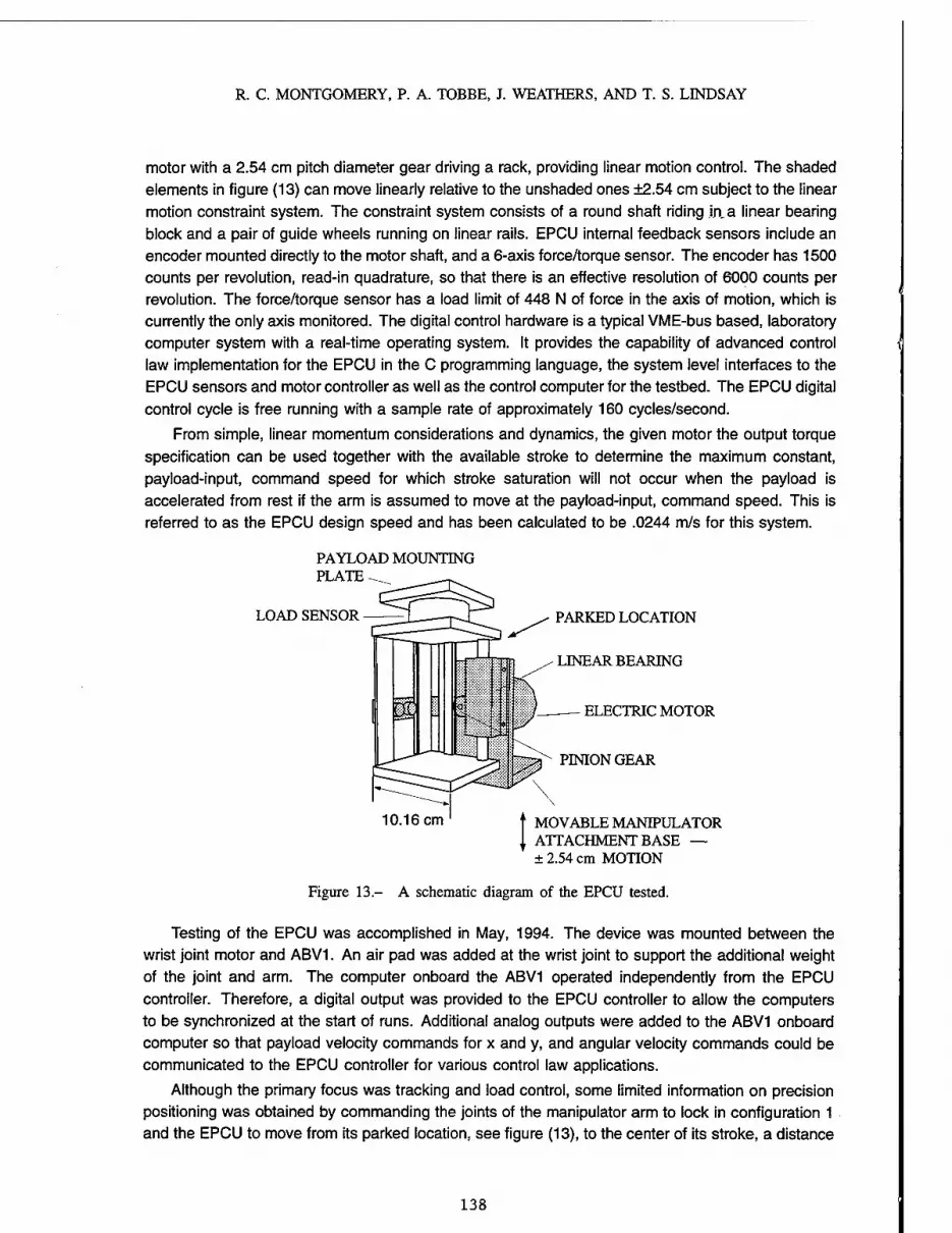
R. C. MONTGOMERY, P. A. TOBBE, J. WEATHERS, AND T. S. LINDSAY
motor with a 2.54 cm pitch diameter gear driving a rack, providing linear motion control. The shaded elements in figure (13) can move linearly relative to the unshaded ones ±2.54 cm subject to the linear motion constraint system. The constraint system consists of a round shaft riding in. a linear bearing block and a pair of guide wheels running on linear rails. EPCU internal feedback sensors include an encoder mounted directly to the motor shaft, and a 6-axis force/torque sensor. The encoder has 1500 counts per revolution, read-in quadrature, so that there is an effective resolution of 6000 counts per revolution. The force/torque sensor has a load limit of 448 N of force in the axis of motion, which is currently the only axis monitored. The digital control hardware is a typical VME-bus based, laboratory computer system with a real-time operating system. It provides the capability of advanced control law implementation for the EPCU in the C programming language, the system level interfaces to the EPCU sensors and motor controller as well as the control computer for the testbed. The EPCU digital control cycle is free running with a sample rate of approximately 160 cycles/second.
From simple, linear momentum considerations and dynamics, the given motor the output torque specification can be used together with the available stroke to determine the maximum constant, payload-input, command speed for which stroke saturation will not occur when the payload is accelerated from rest if the arm is assumed to move at the payload-input, command speed. This is referred to as the EPCU design speed and has been calculated to be .0244 m/s for this system.
PAYLOAD MOUNTING PLATE
LOAD SENSOR
10.16 cm
PARKED LOCATION
LINEAR BEARING
ELECTRIC MOTOR
PINION GEAR
MOVABLE MANIPULATOR ATTACHMENT BASE — ± 2.54 cm MOTION
Figure 13- A schematic diagram of the EPCU tested.
Testing of the EPCU was accomplished in May, 1994. The device was mounted between the wrist joint motor and ABV1. An air pad was added at the wrist joint to support the additional weight of the joint and arm. The computer onboard the ABV1 operated independently from the EPCU controller. Therefore, a digital output was provided to the EPCU controller to allow the computers to be synchronized at the start of runs. Additional analog outputs were added to the ABV1 onboard computer so that payload velocity commands for x and y, and angular velocity commands could be communicated to the EPCU controller for various control law applications.
Although the primary focus was tracking and load control, some limited information on precision positioning was obtained by commanding the joints of the manipulator arm to lock in configuration 1 and the EPCU to move from its parked location, see figure (13), to the center of its stroke, a distance
138

SIMULATION AND TESTING OF A ROBOTIC MANIPULATOR TESTBED
of 0.0254 m in approximately 2 seconds. No instabilities were observed during this operation which was always smooth and predictable except for one instance when the set screw locking the pinion gear to the motor shaft was loose and needed to be tightened.
For each of the tracking and load control tests, the initial configuration of the testbed was configuration 1. The first step in the test procedure was to unpark the EPCU. Then, the arm was commanded to retract at a constant rate along the negative x-axis, figure (14). The retracted position was held for 10 seconds and then the arm was commanded to return to the initial position at the same rate at which it was retracted. The final position was again held for 10 seconds. Data gathering was terminated and the EPCU was parked. Both long and short test runs were made since several minutes were required for a full retraction and many conditions and several control schemes had to be evaluated. For short runs the retraction distance was 0.305 m. For long runs the arm was retracted to the maximum retraction configuration shown in figure (14) and then returned to the initial conditions of configuration 1. The total retraction distance was 2.134 m for this case. Long runs covered most of the useful configurations of the arm. Speed of maneuvers was also studied. Runs with constant retraction rates between 0.0244 m/s, the design speed, and 0.0457 m/s were made. In no case was an instability detected or did the EPCU hit its stops, saturating its the deflection limits. Selected results, taken at and above the design speed, are discussed below.
Figure 14.- Maximum retraction configuration for long test runs.
Testing of the EPCU was limited to a one week time period because of the expense of bringing together the equipment and personnel. Five control laws, briefly described in [11] were used. These control laws ranged, in simplicity of implementation, from simple active spring control laws to a more modern fuzzy logic controller designed using Allen-Bradley's Fuzzy Logic Explorer, A-B FLEX, [12]. Only the control laws corresponding to data presented herein are described. Both tracking performance and a load control results are presented. For all runs, by rigidly clamping it at the EPCU's center position, the hardware easily accommodated comparison runs for cases with and without the EPCU active.
Figure (15) is a comparison of the tracking performance for the EPCU "clamped" vs. the EPCU active using one of the control laws tested, the "meanfz" control law. The speed for this run was the design speed of 0.0244 m/s. The "meanfz" control law is an active spring controller, force command proportional to deflection measured from the center position, except that the force feedback signal is conditioned by subtracting the current value from the mean value of the past N readings. N is chosen to obtain stable operation without oscillatory force output. The value of N=75, corresponding to a mean value time base of approximately 0.47 s, was used. This was designed to eliminate the effects of constant offset forces caused by gravity, air pad thrust misalignment, and the effects of drift in the force sensor reading. It is difficult to see any tracking performance improvement from this data. However, the standard deviation, a, of the x displacement error is 0.02527 m for the
139

R. C. MONTGOMERY, P. A. TOBBE, J. WEATHERS, AND T. S. LINDSAY
CLAMPED MEANFZ
a = 0.02601 m
too
Time, s
100
Time,!
Figure 15.- EPCU value added in tracking.
"meanfz" control law case and 0.02601 m for the "clamped" case indicating that some improvement was actually obtained.
A load control result is presented in figure (16). Here, a V-input controller is used and the speed for the run was increased to .0366 m/s. The V-input controller augments active stiffness control with a feedforward signal computed from the desired velocity of the manipulator arm, to provide for future telerobotic operation. A change in feedforward signal produces a pulse in velocity proportional to the change which is designed to load the EPCU with the desired change in linear momentum, modulated by the peak force output of the EPCU motor. For the load control run of figure (16) the standard deviation of the x position error was 0.02969 m and peak force was 45 N for the V-input controller. For the "clamped" case it was 0.03005 m and peak force was 75 N. The difference in the standard deviation for the "clamped" case runs is attributed to the speed difference in the runs. Thus, almost a 50% reduction in load was obtained while simultaneously providing a modest improvement in tracking performance. This result is contrary to the proposition that improved tracking performance can be obtained only at the expense of increased interface load. This shows that the EPCU is capable of simultaneously increasing the precision of tracking and reducing interface loads and that the concept warrants further development.
6. Free-free Testbed Simulations
The next step in the evolution of the testbed is to add another vehicle and make the testbed free-free in the horizontal plane. Thus, another vehicle is to be installed and has been sized to be approximately 455 kg. It will be placed at the payload end of the testbed. ABV1 will be moved to the shoulder joint. The configuration is illustrated in a sketch, figure (17). The closed-loop control simulator has been modified to simulate this testbed configuration. Again a symbolic manipulator, [8], was use to derive the equations of motion using a Lagrangian formulation and to generate Fortran code for the simulation which ran on a workstation using different commercially available simulation software system, [13]. This process was selected since the code generation option of the symbolic manipulator is not provided by the commercially available simulation software package used. The testbed was modelled as two rigid vehicles coupled by a two-link, manipulator arm. The arm links were assumed rigid. Simulation runs were made using doublet torque inputs at the shoulder, elbow,
140

SIMULATION AND TESTING OF A ROBOTIC MANIPULATOR TESTBED
CLAMPED V-INPUT
150 150
Figure 16.- EPCU value added in load control.
MSFC FLAT FLOOR FACILITY
ABV1
ARM LINKS
Figure 17- Sketch of the planned free-free testbed.
and wrist joints to examine the range of motions (translations and rotations of the two payloads and arms) that need be provided for on the testbed. The magnitude of the doublet was the maximum allowable for each individual joint motor.
Figure (18) shows the simulated testbed configuration and nomenclature used for presentation of results. Figure (19) displays time histories of the variables, x, y, 02, and a,. These are typical of the other torque input cases. The range of variables covering by all simulations are: x and y, ±.1 m; 01, -20° to 5°; 02, +45° to -8°; au -8° to 15°; and a2, ±8°. In addition to providing for the range of motions listed, because of the masses involved, some means of arresting testbed is recommended other than stopping air flow to the air pads which would damage the precision flat floor..
7. Conclusions and Future Plans
Because of the high cost operator training, orbit time, and the possibility of expanding the operational utility of current space systems, NASA continues to develop telerobotic technology directed at improving telerobotic operations in space. This report has overviewed one such activity — the use of a development testbed at the Marshall Space Flight Center. The design history of the testbed, simulation and hardware testing and analysis, has been summarized including plans for
141

R. C. MONTGOMERY, P. A. TOBBE, J. WEATHERS, AND T. S. LINDSAY
Figure 18- The simulated testbed configuration and symbols used.
1.012
x, m
2.008
y, m
2.004
e2, deg.
a, deg
30.6
Figure 19- Simulated responses due to a 51 N-m doublet at the wrist.
adding another vehicle to the current testbed to make it free-free in the spring of 1996. A simulation study of the resulting free-free testbed configuration has been made. Simulation results from the study have been presented that identify travel limits for step doublet response of the free-free testbed joint motors.
The testbed can be used, over the next several years, for the advancement of telerobotic and robotic automation technology. In this report we have presented the current output of one productive use of the testbed — a preliminary evaluation of an EPCU component. This test activity was conducted to get a quick look at the capabilities of the EPCU. Because of the desire to get an early evaluation, the unit was assembled from laboratory parts and a simplified design was selected
142

SIMULATION AND TESTING OF A ROBOTIC MANIPULATOR TESTBED
providing only one degree of freedom. Testing was also limited to three days because of the cost. Nevertheless, results were encouraging and suggest that a more detailed look at the concept is warranted. Hence, additional development and testing is planned.
References
[I] W. G. Sutton and P. A. Tobbe. The MSFC Space Station/Space Operations Testbed. NASA Automated Rendezvous and Capture Review. NASATM 108598. pp. 83-83-IL, November, 1991.
[2] R. C. Montgomery, P. A. Tobbe, J. Weathers, D. Ghosh, and J. L. Garrison. A Testbed for Research on Manipulator Coupled Active Spacecraft. AIAA Guidance, Navigation, and Control Conference, AIAA paper No. 93-3712, August 9-11, 1993.
[3] R. C. Montgomery, S. P. Kenny, D. Ghosh, and Joram Shenhar. Evaluation of Inertial Devices for the Control Of Large, Flexible, Space-Based Telerobotic Arms. Proc. Fifth Annual NASA/DOD CSI Technology Conference, March 3-5, 1992.
[4] Davoud Manouchehri, Thomas Lindsay, and Dave Ghosh. Hardware Interface for Isolation of Vibrations in Flexible Manipulators — Development and Application. Space Operations, Applications, and Research Symposium, August 3-5, 1993.
[5] J. L. Garrison and R. C. Montgomery:. Space Shuttle to Space Station Freedom Berthing Dynamics Research at the NASA Langley Research Center. Proc. Fourth Conference on Intelligent Robotic Systems for Space Exploration, Rensselaer Ploytechnic Institute, Troy, NY., September 30 - October 1, 1992.
[6] Dynacs, Inc., Clearwater, Florida. Users Manual for TREETOPS, rev. 8, 1990.
[7] Patrick Tobbe and W. Schonberg. A Comparison of Ritz Vectors for Use in Flexible Multibody Simulations. 9th VPI&SU Symposium on Dynamics and Control of Large Structures, Blacksburg, Virginia, May 10-12, 1993.
[8] B. W. Char et al. MAPLE Reference Manual, 5th Edition. Department of Computer Science, University of Waterloo, Waterloo, Ontario, CANADA N2L 3G1, March 1988.
[9] Integrated Systems, Inc., Palo Alto, California. MatrixX Core Users Manual and System Build V2.4 Users Guide, Edition 8, June 1991.
[10] John N. Little and Loren Shure. Signal Processing Toolbox for Use with MATLAB. The Math Works, Inc., Natick, Mass., 1992.
[II] R. C. Montgomery, P. A. Tobbe, J. Weathers, D. Manouchehri, and T. S. Lindsay. Testing of an End-Point Control Unit Designed to Enable Precision Control of Manipulator-Coupled Spacecraft. AIAA Space Programs Technologies Conference and Exhibit, AIAA Paper No., Huntsville, AL, September 27-29, 1994.
[12] Allen-Bradley Company, Milwaukee, Wl. A-B FLEX Version 2.0 User's Guide, April 1992.
[13] Anon. MATLAB Users Guide. The Math Works, Inc., Natick, Mass., 1992.
143

144
DESIGN OF A SPACE-BASED ELECTROSTATIC ANTENNA WITH VARIABLE DIRECTIVITY AND POWER DENSITY
Larry Silverberg* and Robert Stanley* North Carolina State University
Raleigh, NC 27695-7910
Abstract
This paper describes a new type of adaptable antenna, wherein directivity is varied over a 6° range and power density is varied over a 6.5db range in experimental tests. The electrostatic antenna concept presented here can be regarded as a compromise between the low performance mechanical method of adapting the far field beam pattern and the high performance, but often prohibitively complex method of carrying out the adaptations electronicly. The electrostatic antenna described in this paper is shown to be well-suited for space- based applications.
Introduction
The concept of deforming a thin membrane into a curved reflecting surface using electrostatic forces is old. However, until 1978 the art consisted of using a single integral electrode to generate the electrostatic field. On June 6,1978 a patent entitled "Controlled Flexible Membrane Reflector" was issued to Charles W. Perkins [1]. The patent presented the possibility of controlling an optical surface reflector by means of multiple electrostatically charged electrodes. It also employed a supporting structure which consisted of a large ring on which the membrane was stretched, like a circular trampoline. Perkin's supporting structure became a standard design over the next decade. The membrane tension forces had the adverse effect of requiring voltages up to 400,000 volts. In addition, due to malformities in the rim, servo actuators were installed for mechanical compensation. Perkin's electrostatic antenna was later studied by Lang [2] and Goslee [3] (see Fig. 1). The feasibility of an electrostatically controlled membrane diminished as the complexities grew and by the late 1980's all known research had ceased.
The concept of harnessing electrostatic forces for membrane shaping surfaced again in the early 1990's at NCSU. Dr. Silverberg, along with a team of graduate students, independent of the a priori work, envisioned an electrostatically shaped membrane that differed from Perkin's electrostatic membrane in one important feature. Silverberg's electrostatically shaped membrane contained no supporting structure. This concept variation was significant enough to warrant a new patent in April of 1994 entitled "Electrostatically Shaped Membranes'* [4]. The research conducted by Silverberg's team was carried out in the following progression: They were first concerned with how reliable one could predict electrostatically induced deformations [5]. The next step was a general formulation for predicting the dynamic behavior of structures subjected to electrostatic fields [6]. Once the dynamics of electrostatic structures was understood, their effort turned toward investigating control issues. One study developed a modal control technique for shaping the antenna surface to maximize the far field power density [7,8].
This paper focuses on the basic principles that govern the overall design of electrostatic antennas. The next section describes the performance characteristics that are achievable with the electrostatic antenna described in this paper and how these differ from a fixed shape antenna. In particular we review the abilities of the electrostatic antenna to control directivity, power density and more generally the beam pattern distribution.
The third section provides detailed descriptions of the experimental set-up. This covers geometry, the membrane, power requirements, type of feed, pinned boundary conditions, back plates, measurement system, and a photo of the experiment.
In the fourth section empirical relationships that collectively govern antenna performance are developed. Surface deflections are expressed as a function of applied voltages, and the far field beam pattern of the transmitted antenna signal is then calculated. Voltage resolution and surface accuracy are then expressed as functions of the transmission wavelength.
t Professor, Department of Mechanical and Aerospace Engineering, Box 7910. * Graduate Research Assistant, Department of Mechanical and Aerospace Enginering, Box 7910.
145

SILVERBERG AND STANLEY
The fifth section gives experimental results that demonstrate the performance characteristics of the electrostatic antenna. This section shows how well the antenna beam can be directed, its power density varied, and its surface resolution maintained in addition to other engineering performance characteristics. In keeping with tradition the paper closes with a summary and some suggestions for the future.
?:'■"■ 1 MODIFIED BACK. ELECTRODE WITH 3 CONTROL AREAS!
Figure 1. Goslee's electrostatic antenna [3]
Antenna Performance
The earliest human made far-field antennas date back to the 1920' s with the ability to transmit and receive short wavelength signals for radio detection. Monopole and dipole antennas were first used and later directional antennas were designed to yield desirable beam patterns. The next level of sophistication in antenna design arose with the introduction of adaptable antennas wherein the beam pattern is adapted in real time. Adaptable antennas are currently one of two types; mechanical or electronic (phased-array). This paper describes another type of adaptable antenna, called an electrostatic antenna, that is particularly well suited for space-based applications.
Unlike the mechanical and electronic types, the electrostatic antenna's beam pattern is adapted by varying the shape of the antenna's surface, specifically, its modes of deformation. The first mode of deformation is called the directivity mode. This mode is responsible for beam directivity. The directivity mode enables the antenna to scan and to function as a surveillance or mapping satellite. The second mode of deformation controls the'power density of the beam pattern. In space applications, the power density mode controls the ground swath illuminated on the Earth by the antenna. The power density mode is useful in communication satellites and in certain military applications. Higher modes of deformation control the power distribution of the beam pattern.
Within the context of space-based adaptable antennas, the mechanical types tend to suffer from the following limitations. Their beam pattern adaptability is restricted to directivity (mode one deformation), and the associated beam pattern time constants are relatively large (T > 500s). On the other hand, the electronic types can control the beam pattern rapidly (T < 1 millisec), but the manufacturing complexities have inhibited
146

DESIGN OF A SPACE-BASED ELECTROSTATIC ANTENNA
their use. The electrostatic antenna, as this paper demonstrates, is capable of controlling the first two modes of the beam pattern (directivity and power density). The control of the higher modes has not yet been demonstrated although it is feasible, in principle. The associated time constants are smaller than for the mechanical type and larger than for the electronic type. The relatively small beam pattern time constants associated with the electrostatic antenna (T < lOsec) are achievable because the aperture is composed of a low mass membrane that is weakly coupled to the satellite dynamics.
Setup
An electrostatic antenna works on the basic principle that like charges repel. When two electrodes are charged, with one fixed and one free to move, the free electrode will move apart from the fixed electrode so as to balance the elastic restoring force and the electrostatic force. By controlling the applied voltages the position of the free electrode can be prescribed. On this basis, an electrostatic antenna is designed here to control its first two modes of deformation which in turn control directivity and power density (see Fig. 2).
In the following experiment the fixed electrodes (see 2 and 4 in Fig. 3) are referred to as back plates and the free electrodes (see 3 and 5 in Fig. 3) are electrically segmented regions on a 7 mil metalized Mylar membrane. Metalized Mylar was chosen because it is elastic, conductive and easily segmented. Metal between segments was removed using a liquid solution of sodium hydroxide (NaOH) (see Fig. 4).
r^ßäS^t'i^
i.'timju^Mtaife-'wtiii*''' inn
'<•£*;•:■ Sliä&iiisäwS ■ MI
l«&|8ß?^£-*" *•■&
f~ pi '$0 ■ ■ lewVs^lgEi ä*aÜ.":*J ' f^--5*"'" "»** >(ljä|S
•.":i- SPZ10: •i# iiili •' »&*&?& <&i
Figure 2: Electrostatic antenna
The membrane is physically constrained by a magnetically levitated pinned boundary condition (see 6 in Fig. 3). The boundary condition is comprised of two semi-cylinders that form a cylinder when brought together (1 inch diameter, 13 inches long). Attracting magnets secure the membrane along the interproximal surface (see Fig. 5). Along the long axis of the cylinder there exist alternating regions of insulative and conductive material (see 7 and 8 in Fig. 5, respectively). These regions provide a conductive pathway along which the membrane segments are charged. The boundary condition is constrained in the horizontal plane by means of high precision ball bearings (see 9 in Fig. 5). In the vertical direction the boundary condition is levitated by neodymium-iron-boron magnets. This combination produces a near frictionless pinned boundary condition. '
The back plates are composed of thin aluminum rectangular plates however just about any conductive material would work. The number of back plates is governed by the number of controlled modes of deformation; in this experiment two. As a general rule, the number of independently controlled back plates is not less than the number of controlled modes of deformation. In optical applications, the surface tolerance requirements are not met with the minimum number of back plates. In such cases more back plates are used until the desired surface accuracy is reached. In microwave applications, the number of controlled back plates
147

SILVERBERG AND STANLEY
is on the order of the number of controlled modes of deformation. This is the case treated in this paper. Also note that the fixed back plates may be eliminated in some designs by instead using attached back plates [4].
The back plates along with the boundary condition are mounted on a multi-purpose high voltage test block. The test block consists of nothing more than an 18* x 12' x 4" block of acrylic with uniformly spaced holes that accept spring loaded RJ-8 coaxial cables from 0-30 kV direct current power supplies.
Antenna surface test measurements where gathered with a linear positioning device and an analog distance sensor with a resolution of .034 in. The analog distance sensor rides broadside to the aperture on the
1. High voltage test block 2. Left side back plate 3. Left side of electrically segmented
metalized Mylar 4. Right side back plate 5. Right side of electrically
segmented metalized Mylar
6. Magnetically levitated pinned boundary conditions
Figure 3: Test block and membrane apparatus
11. 12.
Left side of electrically segmented metalized Mylar Right side of electrically segmented metalized Mylar
Figure 4: Electrically segmented metalized Mylar
148

DESIGN OF A SPACE-BASED ELECTROSTATIC ANTENNA
linear positioner via a carriage. By recording the 0-5V analog output signal from the sensor at specified intervals, the antenna surface is recorded (see Fig. 6).
7. Insulative material 8. Conductive material 9. High precision ball bearing and magnet
well 10. High voltage test block mounting slots
Figure 5: Magnetically levitated pinned boundary conditions
©
«JKKSWKWWS
© »s»»i!i8^»»«»»^»t»»»SKK8»MtM8aMt8iSy8»i
13. Stepper motor 14. SAID Analog distance
sensor 15. Drive belt 16. Slider rods 17. SAID Sensor line-of-sight 18. Metalized Mylar membrane 19. High voltage test block
Figure 6: Test set-up overview
149

SILVERBERG AND STANLEY
Engineering Curves
The engineering performance of the electrostatic antenna is described by relationships (curves) between the applied voltages, the surface deformations, and the beam pattern. First, the surface deformations are expressed as a function of the applied voltages. Next, beam pattern parameters are expressed as functions of the surface deformations. Finally, surface rms values, and resolution issues are discussed.
The deformation of a surface cross section is assumed in the polynomial form
where
y(x,V1,V2)=^ar(V1,V2)xr, X!<=x<xN
r=0
ar(Vi, V2) = br + Vi cr + V2 dr + V? er + V* fr + V! V2 gr
(1)
(2)
in which bf, Cf, dj-, er, fr, and gr are undetermined coefficients, and Vi and V2 denote the applied voltage pairs to the left of center and to the right of center, respectively (see Fig. 4). The previously described measurement system scans the membrane and records surface deformations at xs (s = 1,2 N). The measurement system scans the membrane M = 11 times; each time the applied voltages Vi and V2 are updated (see Table 1). Deformation curves are obtained from
Table 1. Applied voltages for each scan (M = 11) V2(KV)
0 5 10 15 20 0 X 5 X
Vi(KV) 10 X X 15 X X X 20 X X X X
the data in two steps. The first step determines ar (r = 0,1,.... 4) in Eq. (1) for each scan. The second step determines br, Cr, dr, %, fr, and &■ (r = 0,1 4) as a function of Vi and V2. The first step yields from Eq. (1) for each scan the set of linear algebraic equations
Xa = y (3)
inwhicha = [a0ai...a4]1, y = [y(xi)y(x2)...y(xN)]T and
X =
1 Xl Xj Xj Xj
I x2 X^ X^ X<7
1 Xj>J Xj^ XJ,J XJ,J
The least square estimate of a is given by
a = (XTX)_1XTy (4)
The second step yields from Eqs. (2) and (4) the set of linear algebraic equations
J.DV

DESIGN OF A SPACE-BASED ELECTROSTATIC ANTENNA
Vzr=ar, (r = 0,l,...,4) (5)
in which ar = [ar(l) ar(2)... ar (M)]T, zr = [br cr dr er fr gr]T and
V =
1 VjQ) V2(2) V2(l) v|(l) V^DVzd)
1 Vj(2) V2(2) V2(2) V2(2) V!(2)V2(2)
1 Vi(3) V2(3) V2(3) V2(3) V!(3)V2(3)
1 Vi(M) V2(M) V2(M) V|(M) V!(M)V2(M)
Finally, the least squares estimates of zr (r = 0,1,..., 4) are given by
?r = (VTV)-1VTar, (r = 0,l,...,4) (6)
The surface defonnations described above were obtained empirically rather than predicted from a physical model of the system. The surface deformations of electrostatic structures in general have been predicted in other works [6].
Having expressed deformations as functions of the applied voltages, the next step is to determine the far-field beam pattern and its associated performance parameters (directivity, power density, etc.) as a function of the surface deformations. This is accomplished using physical optics by one of several commercially available computer subroutines; in our study we used POMESH (Ref. 9).
Another useful set of parameter curves governs surface deformation sensitivity. The rms value of the difference between the actual surface deformation and the desired surface deformation is determined in several steps. The surface deformations are first translated to a set of axis who's origin ties on the vertex of the membrane. A weighted average of the directivity of the surface defonnations are then determined by
j N/2 N/2
8=2X(y(xi>-y(-xi))xi/Xx? i=l
N/2 N/2
i=l i=l
(7)
in which 6j = (y(xj) - y(- xi))/2xi denotes the direction angle associated with xi and - XJ (xi > 0). Note that 9 also represents the least squares solution obtained by minimizing the error functional
N/2 U/2 E= 2(y(xi)_y(_xi> -2exi)2= XKy(xi)-6xi)-(y(-Xi) + 6xi)]2. The translated coordinates are
i=l i=l now rotated an amount B. The desired surface deformatons in the rotated frame are given by the general
parabolic form yd =^x2, and the associated rms value of the difference between the actual surface
deformation and the desired surface deformation is given by
151

SILVERBERG AND STANLEY
nnsi: 1 N
£ £ M*r. Vi, V2) - yd(xr, Vlf V2))2
r=l
-|l/2
(8)
in which y<j(x, Vj, V2) denotes the desired surface deformation as a function of x, Vi and V2 in the rotated coordinate system. Another rms value of importance is associated with the error introduced by the limiting resolution of the applied voltages Vi and V2. The resolution of the applied voltages are denoted by AVi and AV2, respectively. We obtain
rms2 = N 1E ay(x,,Vi,v2)
dVx AVj + 3y(xr,Vi,v2) AV2
1/2
(9)
in which the inner parenthetic term denotes the change in the surface deformation Ay(xr, Vi, V2). Both rms errors given in (8) and (9) contribute independently to the total rms error
rms = nnsi + rms2 (10)
The transmitted or received signal that coherently reflects off of the aperture bounds the total rms by
rms< — 10 (11)
in which X denotes the signal wavelength. Equation (1) determines the surface deformations as functions of the applied voltages, which in turn are related to the beam pattern as previously described, and the surface deformations are related to acceptable rms levels as indicated by Eq. (11).
Performance Tests
The electrostatic antenna described in this paper was designed to undergo the first two modes of deformation; the directivity mode and the power density mode. Upon completing M=ll scans, the antenna deformations (Eqs. 1 and 2) were computed. The results are given in Table 2. The antenna transmitted at a frequency of 1 GHz (A. = 11.80 in), and employed a dipole feed. We first evaluate the directivity mode. As shown in Fig. 7 and referring to Table 1, the rotation of the antenna is proportional to the difference between the applied voltage to the left of center (Vi) and the applied voltage to the right of center (V2), denoted by 8V = Vi - V2. From Fig. 7 the antenna rotates approximately 1° every 8V = 5KV. The associated beam pattern is shown in Fig. 8. As shown, the directivity also increases approximately 1° every 8V = 5KV. This corresponds to the best parabolic fit to the unchanged preshaped membrane (Vi = V2 = 0). The desired antenna surface was assumed to be parabolic with a focal length of fo = 15.84 in. The rms values corresponding to Fig. 7 are nnsi = (0.47, 0.54, 0.58, 0.62). The rms values for the other test cases were similar. The rms values associated with the voltage resolution determined from Eq. (8), were small compared to the rms values associated with the parabolic fit The implication is that the performance of the power source met the antenna requirements. From Eq. (10) the useful transmitting or receiving wavelengths are bounded below by XQUQ = 6.2 inches
Table 2: Deflection coefficients versus r (r = 0,1,2, 3,4) 0 12 3 4
br 1.3449e+01 3.0670e-01 -4.7906e-02 3.8650e-03 -1.4097e-04 cr -1.3185e-02 4.1077e-03 -7.8032e-05 -5.6697e-05 3.2718e-06 dr -1.9472e-03 7.6749e-04 -5.4300e-04 9.4436e-05 -4.6386e-06 er -8.7081e-04 2.1771e-04 -3.0525e-05 3.3055e-06 -1.3254e-07 fr 1.6006e-03 -2.6937e-04 -5.5771e-06 2.9624e-06 -1.6797e-07 gr -1.3268e-03 6.9404e-05 7.9863e-05 -1.2268e-05 5.0688e-07
152

DESIGN OF A SPACE-BASED ELECTROSTATIC ANTENNA
I
14.5
14
13.5
13
115
■ f*" ~" *^til **^
«L* #
/
4*, it: 'i:
/
t 0
■ »
V1-V?
■
0 0-0 —a -10-5 -♦- -15-5 --X--20-5
-8-6-4-2 0 2 X-axis (Inches)
Figure 7 Directivity mode
; i
V1-V2 : 04 — —a -10-5 — ♦- -15-5 --X--20-5
\
;\ \ \£ \ % :
; \i * V
" * v\i \ \ V-
'■
; y- \ ' .
'■
■
25
20
15
I 10
I 5
0
-5
-10 -20 -15 -10 -5 0 5 10 15 20
Theta in degrees
Figure 8 Beam pattern (directivity mode)
The evaluation of the power density mode is now described. As shown in Fig. 9, and referring to Table 1, the focal length is inversely proportional to the uniformly applied voltage V = Vi = V2. From Fig. 10, the power density increased by approximately 6.5db as the applied voltage increased by 20KV. As before, the desired surface was assumed to be the best parabolic function that fit the uncharged surface of the membrane. The associated rms values were rmsi = (0.47,0.51,0.54,0.70,0.76). Once again rms2 « rmsi and the power density mode met the antenna wavelength requirements bounded below by Xntin = 7-6 inches.
Summary
This paper described the design of an experimental electrostatic antenna and tested its performance. The experimental antenna was shown to be capable of adapting the directivity of the beam over a 6° range and the power density over a 6.5 db range. The experimental antenna surface was sufficiently accurate to accommodate wavelengths bounded below by approximately 7.6 inches.
Future efforts could extend the results presented here to the design and testing of electrostatic antennas that are paraboloidally preshaped, and to increase the number of independently applied voltages along with an increase in the number of modes of deformation that are shaped.
153

SILVERBERG AND STANLEY
References
14.5
14
13.5
13
1X5
• ?r ~t*a^
■
f4,' / *
'1 * V1-V2
■
o 0-0 —B -5-5 - «- -10-10 --X--15-15 --+--20-20
"t
-8-6-4-2 02468
X-axis (Inches)
Figure 9 Power density mode
Figure 10 Beam pattern (power density mode)
1. Perkins, C. W., Controlled Flexible Membrane Reflector, U. S. Patent No. 4,093,351, June 6,1978. 2. Lang, J. H., "Electrostatically Figured Membrane Reflectors: An Overview," presented at the Large
Space Antenna Systems Technology Meeting, November 30-December 3,1982. 3. Goslee, J. W. and Hinson, W. F., "Measurement of Electrostatically Formed Antennas Using
Photogrammetry and Theodolites," presented at the 1984 American Congress on Surveying and Mapping, March 11-16,1984, Washington, D. C.
4. Silverberg, L., Electrostatically Shaped Membranes, U.S. Patent No. 5,307,082, April 16,1994. 5. Silverberg, L. and Doggett, W. O., "Planar Electrodynamics of Interconnected Charged Particles,"
American Physical Society Bulletin, Series II, Vol. 36, Nov. 10,1991. 6. Silverberg, L. and Weaver, L., "Dynamics and Control of Electrostatic Structures," Journal of Applied
Mechanics, to appear. 7. Silverberg, L. and Washington, G., "Modal Control of Reflector Surfaces Using Far-Field Power
Measurements," Microwave and Optical Technology Letters, Vol. 7, No. 12, August 20,1994.
154

DESIGN OF A SPACE-BASED ELECTROSTATIC ANTENNA
8. Washington, G. and Silverberg, L., "Modal Control of a Comer Reflector to Maximize Far-Field Power," Microwave and Optical Technology Letters, Vol. 8, No. 5, April 5,1995.
9. "POMESH", Computer Software Management and Information Center (COSMIC), The University of Georgia, 382 East Broad Street, Athen, GA 30602-4272.
155

156

STRUCTURAL CONTROL BY EIGENSTRUCTURE
ASSIGNMENT USING INVERSE THEORY
D. J. Inman Virginia Polytechnic Institute and State University
Blacksburg, VA 24061
Abstract This manuscript points out the relationship between eigenstructure assignment methods for second
order mechanical systems and the inverse eigenvalue problem for second order matrix polynomials. The inverse method for matrix polynomials is then used to derive a new eigenstructure assignment method. This method is shown, by example to yield feedback gains numerically equivalent to a previously published method but at some computational advantage via an alternate matrix manipulation.
1. INTRODUCTION The purpose of this effort is to point out the natural connection between the inverse eigenvalue problem of second order matrix polynomials and the eigenstructure assignment prob- lem for second order structural models, common to structural control of linear systems. This effort rests on several assumptions. First, it is assumed that examination of structural control in a second order mass-damping and stiffness coordinate system (rather than the usual state space form) will result in computational savings as well as reveal physical insight. Secondly, it is assumed that making a strong connection between two unrelated fields - inverse matrix polynomials and eigenstructure assignment theory, will encourage others to find more fruitful results than those discussed in the following. Eigen- structure assignment methods have received substantial theoretical development as well as practical applications. Andry, et al. (Ref. 1) provided both a literature survey (prior to 1983) and an adaptation of eigenstructure assignment methodology to an important subclass of control problems consisting of mechanical systems (Ref. 2). Mechanical systems are those which are naturally represented in the form
Mx + £>x + Kx = f (t) (1)
where M, D and K are nxn, symmetric, real value, positive definite (or semi definite) matrices repre- senting a system mass, damping, and stiffness matrix respectively, x is an n x 1 vector of displacement with time derivatives x (the velocity vectors) and x (the acceleration vector). Equation (1) is usefull describing the open loop response of a variety of devices, machines and structures.
Equation (1) forms the basis for the eigenstructure assignment methods presented here. The objective of eigenstructure assignment is to develop a control law to apply to the right hand side of equation (1), based on measurement, that will move the eigenvalues and eigenvectors (together referred to as eigenstructure) to more desirable values. The thought being that the closed loop response of the system is shaped by the system's natural frequencies, mode shapes and damping ratios contained in the system eigenstructure. Many approaches to eigenstructure assignment have been proposed in the literature and successfully used in practice. The approach presented here makes use of the matrix theory associated with inverse eigenvalue problems (Ref. 3).
The following sections review three eigenvalue problems associated with equation (1), the inverse eigenvalue problems for each, formulates the eigenstructure assignment method as applied to mechanical systems and then combines inverse eigenvalue theory with the eigenstructure assignment formulation to produce a new method of calculating feedback gain matrices to achieve a desired eigenstructure. These sections are followed by examples and conclusion sections.
2. THREE EIGENVALUE PROBLEMS The eigenvalue problem associated with equation (1) becomes (after multiplying by M_1)
L(A)x = (A2/ + XH2 + £T3)x = 0 (2)
* Samuel Herrick Endowed Professor, Department of Engineering Science and Mechanics
157

DANIEL J. INMAN
where the complex scalar A is called an eigenvalue, and x a right eigenvector (possible complex but never zero). The matrix polynomial L(A) is referred to as a lambda matrix. Here it is important to note the difference between the eigenvalues and eigenvectors of a system (2), and eigenvalues and eigenvectors of a single matrix.
Equation (1) is written in the standard physical coordinate system which is a second order vector differential equation in n dimensions. Two other formulations are used as mathematical models of vibrating structures: the standard state space formulation common to control theory and a first order formulation in pencil form, both of dimension 2n. These two forms are summarized next.
To examine these first order forms, multiply equation (1) by M~l (assumed to be nonsingular) and let zi(i) = x(t) and z2(t) = x(£). Then equation (2) can be written as the two equations
(3)
(4)
where f(t) = M_1F(£), H2 = M~XD and H3 = M^K. These two equations are combined to yield the standard state space form.
z1{t) = z2{t)
z2(t) = -H2z2(t) - H3*i(t) + f(i)
*(*) = 0
-H3
I -H2
z(t)
or
where
i(t) = Az(t) + Bu(t)
*(*) = L*a(*) x(t)
U(t) = f (t) B : A =
f(t) (5)
(6)
0 -H3
I -H2
Here z(t) is called the state vector, A is the state matrix and B is the input matrix. Here u(t) is the applied force, or control vector.
Finally, premultiply equation (5) by the matrix
N ■ H2 I I 0
This yields a first order matrix pencil
Nir{t) - Pv(i) = g(t) (7)
where
v(*) = x(«) , g(*) = f(t)
0 P =
-H3 0 0 I
Next consider solutions of equations (5) and (7) of the form z(t) = zext and v(t) = veAt, respectively, for the homogeneous case f (t) = 0. Then equations (5) and (7) yield the two eigenvalue problems:
(A - \I)z = 0
(P - XN)v = 0
(8)
(9)
where the constant vectors z and v must of course be nonzero, and are possibly complex valued. Equations (2), (8) and (9) result in the same set of 2n eigenvalues A», which contain the system's
natural frequencies and damping ratios, and the complex vectors Xj, Z{ and v* corresponding to each
158

STRUCTURAL CONTROL BY INVERSE THEORY
eigenvalue Aj. Each of these three different eigenvectors are in some way related to the system's mode shapes.
Each of these three eigenvalue problems can be restated as a matrix equation by defining the matrices (the dimensions are listed paranthetically):
X = [xi x2 ... x2„] (n x 2n)
Z = [zi z2 ... z2„] (2n x 2n)
V = [vi v2 ... v2„] (2n x 2n)
whose columns are the associated eigenvectors and
A =
Ai 0 0 . . 0 0 A2 0 . . 0
0 0 0 . . 0 0 0 0 . • Afc
(2n x 2n)
consisting of the system eigenvalues. The matrix A is upper triangular. Each Jordan block Aj is of the form
■Aj a 0 ... 0
A* 0 Ai a .
0 0 0 0 0 0
0
a
Here a = 1 if a particular Ai is not simple (i.e., repeated eigenvalue and dependent eigenvectors); otherwise, a = 0. Using this matrix notation the eigenvalue problem stated by equations (2), (8) and (9) can be expressed as the following three matrix equations:
XA2 + H2XA + H3X = 0
AZ - ZA = 0
PV - NVA = 0
Note that the vectors Zi are related to the eigenvectors x» by
Zi = Xi
AiXi
for each i(i = 1,2,..., 2n) or, collecting these in augmented matrix form
Z = X
XA
(10)
(11)
(12)
(13)
(14)
The Jordan form of the state matrix A is given by the usual 2n x 2n matrix
A = Z~XAZ
which follows directly from equation (11) which can also be rewritten as
AZ = ZA (15)
159

DANIEL J. INMAN
The left eigenvectors Wj can be computed from the right eigenvectors by
W = (Z-1)7 (16)
where W = [wx w2...w2„]
The matrix W is 2n x In (same dimension as Z). Now WTZ = Z~XZ — 1. The corresponding statement to equation (15) in terms of W is
WTA = AWT (17)
These three related eigenvalue problems and their matrix equation relationships are used in the following section to discuss the inverse eigenvalue problem.
3. THE INVERSE EIGENVALUE PROBLEMS This section introduces the results of the inverse eigenvalue problem using the three eigenvalue
problems of the previous section. A more complete account can be found in Ref. 3. To this end a 2n x In nonsingular matrix Q is introduced which satisfies
QNZ = I
The following product can be used to calculate the matrix Q:
B1=NAN-1=\HI
2 I
which can be expressed in terms of Q by
Bi = NAN-1 = NZAZ~lN-1 = Q~lAQ
0 I r° 11 '0 -ffsl -H3 -H2\ i -H2\ I -H2\
(18)
(19)
(20)
The matrix Q can be partitioned into Q = [<pi Q2], where both Qi and Q2 are 2n x n matrices. Solving for the partition Qi yields
Qi = Q = Z^N'1 = Z -l = yJ (21)
Here the matrix Y consists of the left eigenvectors yj of the physical system, yfL(X) = 0, where L(X) as defined in equation (2), i.e.,
Y = [yi y2... y2„]
Equation (20) can be now solved for the partition Q2, i.e.
QBX = AQ
"0 J
-M- -M- lD J 0 = AQ
J" 0
Q 0 I = AQi
Q2 = AQi
Hence, Q can now be represented in the partitioned form
Q = [YT AYT]
(22)
(23)
160

STRUCTURAL CONTROL BY INVERSE THEORY
Next, formulas are derived which specify the coefficient matrices K and D in terms of the spectral matrices, X, Y and A for the system in second order form. Recall that the matrix A can be represented as
A = ZAZ'1 = X
XA AZ~
XAZ-1
XAiZ-1 0 I
-H2
Substituting
7—1 _ QN = [YTAYT] H2 I I 0
-WT [YTH2 + AYJ YT]
(24)
(25)
(note: here a relation between the left eigenvectors W — {Z~l)T of the state matrix A and the left eigenvectors Y of the physical system is given) into (24) yields the inverse formulas
XA(YTH2 + AYT) XAYT
XA2(YTH2 + AYT) XA2YT
or, upon equating the 4 partitions of each matrix:
0 / —Hz —H2
(26)
XA(YTH2 + AYT) = 0
XAYT = I
XA2(YTH2 + AYT) = -H3
XA2YT = -H2
Rearranging the last three equations yields the inverse formulas
H2 = -XA2YT
and the normalization condition
H3 = H\ - XA3YT
XAYT = I
(27)
(28)
(29)
Thus, the coefficient matrices H2 and J?3 can be specified in terms of normalized modal vectors (i.e., X, Y such that XAYT = I) and sets of natural frequencies and damping ratios (A). Equations (27), (28) and (29) represent the solution to the inverse eigenvalue problem as detailed in Ref. 3 and are in agreement with those originally developed in Ref. 4 for the case of nonsingular coefficients. Here however, the inverse of the matrix A does not have to be calculated in order to compute H2 or H3. In particular, systems with rigid body modes (for which A is singular) can be treated using equations (27), (28) and (29). In fact, the solution to the inverse eigenvalue problem presented here does not require calculation of the inverse of any matrix.
Equations (27)-(29) can be partitioned to render them useful for eigenstructure assignment pro- viding a connection between the two fields of study. To this end, rearrange A and define
Ai
Ai ai2
0 A2
0(m-l)m Am
(30)
and
A2 =
Am+i 0(m+l)(m+2) 0 Am+2
0 0
0 0
0 0
a(2n-l)2n A2n
(31)
161

DANIEL J. INMAN
where aj(i+1) = 0 or 1 depending on whether or not a particular eigenvalue is simple. Hence A is partitioned as
[Ai 0 0 A2
(31) A =
Likewise, the matrices X and Y are partitioned as
X = [Xl X2) (32)
Y = [Y1 Y2] (33)
Substitution of these partitioned matrices into equations (27), (28) and (29) yields
H2 = -(X1A2
1Y1T + X2AlY2
T) (34)
H3 = Hi - (XtAlY? + X2A3
2Y2T) (35)
I = XxktY? + X2A2Y? (36)
which represent a partitioned form of the solution of the inverse eigenvalue problem. These expressions render the inverse eigenvalue problem compatible with the eigenstructure assignment problem where Xi, Ai, and Y\ are considered to be that part of the eigenstructure which is acceptable and X2, A2 and Y2 will become the desired eigenstructure.
4. THE EIGENSTRUCTURE ASSIGNMENT PROBLEM The eigenstructure assignment method presented here is taken from Andry et al.1. The method
was derived for a general control system, however it is applied specifically to vibrating structures described in second order vector differential equations of interest here. There are a variety of different eigenstructure assignment methods available in the literature. The method of Andry et al.1 is chosen because is represents that eigenstructure assignment method which appears to be most comparable to the method proposed here. Those readers familiar with eigenstructure assignment may wish to skip this section and proceed to the next section.
The control formulation is the standard linear time invariant system described by the equations
x = Ax(t) + Bu(t) (37)
y(t) = Cx(t) (38)
where x(t) is the 2n x 1 state vector, u(i) is the nxn control input vector and, y(i) is the r x 1 output vec- tor. The matrices, B and C are real constant matrices of the appropriate dimension such that rank(B) = m 7^ 0, rank(C) =r^0. The system is assumed to be controllable; rank([2? AB... A2n~lB}) = In and observable, rank([CT ATCT... {AT)2n-lCT)) = 2n.
Simply stated the eigenstructure assignment problem is (see for instance Ref. 1). Given a self- conjugate set of scalars {Xf}, i = 1,2,..., r and a corresponding self-conjugate set of vectors {vf}, i = 1,2,..., r, find a real (m x r) matrix G such that r of the eigenvalues of (A + BGC) are precisely those of the set {Xf}, with corresponding eigenvectors {vf}.
Here G is the feedback gain matrix and the control law for output feedback is of the form
u(«) = Gy(t) (39)
First consider the case where the desired eigenvector \f is completely specified. Consider the closed loop system
x = (A + BGC)x(t) (40)
Assume the desired closed loop eigenvalues {Xf}i=1 are given and v» is the closed loop eigenvector corresponding to.Aj. Then we have for an eigenvalue/eigenvector pair, Aj and v»,
{A + BGC)vi = Xw (41)
162

STRUCTURAL CONTROL BY INVERSE THEORY
or
Define a vector IEU as
vi = (AiJ-A)-1BGCvi
mi = GCvi
Combining equation (42) and (43) yields
Vi = (XJ - A)'1 Bin.
(42)
(43)
(44)
This implies that the eigenvectors Vj must be in the subspace spanned by the columns of (\{I — A)_1B, an important restriction.
Since in general, a desired eigenvector vf will not be in the prescribed subspace, a "best possible" choice for an achievable eigenvector is made: this best possible eigenvector is the projection of vf onto the subspace spanned by the columns of (AjJ- A)~lB. Thus an achievable eigenvector v;^ is computed by
wiA = LiiLjL^Ljvf (45)
where Li = (\iI-A)~1B
In many situations, an eigenvector is only partially specified, e.g.
(46)
vf =
x X
Vij X
(47)
where Vij are designer specified components and x is an unspecified component. In this case reorder vf in the following way
d\Ri _ Kr Ti (48)
where the symbol {-}Ri denotes the reordered vector, T{ is a vector of specified components of vf and di is a vector of unspecified components of vf. Reorder the rows of the matrix (Aj/ - A)_1.B in the same way and write
{{\iI-A)-1B}Rt = t^ Di
(49)
Following the same steps as before (to obtain z») with rj replacing vf and Li replacing Li, yields
viA = Li{LjLi)-lL?Ti (50)
For an output feedback law of the form u(i) = Gy(t), the closed loop system is
x = (A + BGC)x{t) (51)
Here it is necessary to transform the input matrix B into the following form:
B-> im 0
(52)
where Im is the nx n identity, m being the number of control inputs. Define a transformation matrix T
T = [B P] (53)
163

DANIEL J. INMAN
where P is any matrix such that rank(T) = n. Consider the change of coordinates.
x = Tx
Thus the open loop system is transformed to
x(i) = Äx(f) + Bu(t)
y(t) = Cx(t)
(54)
(55)
(56)
where Ä = T~XAT
B = T~XB =
C = CT
The eigenvalues of the original system are identical to the eigenvalues of the transformed system and the eigenvectors of the two systems are related by
r-1^ = (57)
In the following is assumed that all matrices and eigenvectors have been transformed to obtain the necessary structure of the matrix B so that the specified components of the desired eigenvectors appear first, and the (T) notation will be suppressed for convenience.
For a closed loop eigenvalue Aj and its associated eigenvector Vj, the following must hold:
(A + BGC)vi = XiVi, i = l,2,...,r
or (Xil - A)vi = BGCvi
Partition equation (59), using the special structure of the B matrix:
Xilm — An —Ai2 —A21 Aj7n_m — A22 0
GC
(58)
(59)
(60)
where
Vi =
A = Au A12 A21 A22
are partitioned appropriately, and J„_m is the identity matrix of dimension n — m. Consider the first matrix equation from the partitioned form
[Aj Im - An - A12] Zt
Wj = GC
Zj
Wj (61)
Expanding this expression yields
(Aj/m - An)zi - Ai2-Wi = Aj/mZj - (Anzi + Ai2Wj) = AjZj - Aw = GCVJ (62)
where Ai = [An A12]. Equation (62) can be rewritten as
(Ai + GC)vi = AjZj (63)
164

STRUCTURAL CONTROL BY INVERSE THEORY
This equation holds for each desired eigenvalue/achievable eigenvector pair, and can be written as the matrix relation
{Ai + GC)V = Z (64)
where V — [vi v2 ... vr], is (n x r)
Z = [AjZi A2Z2 ... Arzr], is (m x r)
The feedback gain matrix G can be calculated from equation (64) to be
G = (Z - AXV){CV) -1 (65)
which is the appropriate gain matrix as calculated in Ref. 1, written in notation compatible with the results presented here. A MATLAB program for implementing this gain calculation appears in Ref. 5.
5. EIGENSTRUCTURE ASSIGNMENT VIA INVERSE METHODS In this section the inverse method is used to develop an eigenstructure assignment method and an
outline of the algorithm is provided. Recall that the state matrix used in the inverse model is
0 -H3
I -H2
(66)
where H3 and H2 are denned in partitioned form by equations (34) and (35) respectively. If Xi, Ai, and Yi are viewed as that portion of the eigenstructure which is acceptable and X2, A2 and I2 is that eigenstructure which is to be assigned the matrices H2 and H3 can be described in terms of their corresponding matrices of the original system, M~XD and M-1K, respectively, plus an incremental matrix:
H2 = M~XD + AH2 (67)
H3 = M~XK + AH3 (68)
where AH2 and AH3 represent the changes in the mass weighted damping and stiffness matrices as calculated using the inverse eigenvalue theory. The question of interest here is how to apply this inverse eigenvalue problem formulation to create a feedback system of the structure
k(t) = Acex(t) = (A + BGC)x(t) (69)
where Ace is the closed loop state matrix, A, B, and C are the open loop state matrix, the input matrix, and the output matrix, respectively, and G is the feedback gain matrix. In this section the inverse eigenvalue formulas of equations (34) and (35) subject to equation (36) are manipulated to determine the matrix expression BGC and hence the matrix Ac( in a control formulation compatible to eigenstructure assignment.
Consider the closed loop system of the form
Ix(t) + H2x(t) + i?3x(t) = B0u(t)
and its corresponding state space formulation
*(*) = 0 I
—H3 —H2 *(*) + 0
Bo u(t)
(70)
(71)
where z(t) = [x T(t) xT(t)] . Next, define the ixl vector of outputs y(t) of the system as
y(t) = Cz(t) = [Co d] X(«) = C0x(t) + Cix(i) (72)
165

DANIEL J. INMAN
where Co and C\ represent position and velocity measurements respectively. Consider output feedback of the form
u(t) = Gy(t) = GCz{t)
After some rearrangement the closed loop system becomes
i(t) = Auz(t)
with the closed loop state matrix is now
Act = 0 I
—H3 + BQGCQ —H2 + BQGCI
Now the inverse eigenvalue approach yields
*(*) =
where H3 and H2 and defined by
0 -H3
I -H2
z(t)
H3 = M~lK - B0GC0
H2 = M~lD - B0Gd
Solving this for the unknown terms yields
B0GCo = M~XK -Hs = M-XK - H* + X^Y? + X2k\Y2T
B0GC1 = M~lD -H2 = M~XD + Xlh\Y? + X2k2
2Y?
Alternately, using equations (67) and (68) yields
AH3 = —BQGCO
A/22 = —BQGCI
or
and
[A#3 &H2] = -B0G[Co d]
B0GC = [-AH3 -AH2]
(73)
(74)
(75)
(76)
(77)
(78)
(79)
(80)
(81)
(82)
(83)
(84)
In order to solve for the feedback gain matrix G, the matrices Bo and C have to be defined. In general, for output feedback the matrices Bo and C are not square matrices, so that the inverses of these matrices, required to solve for G, do not exist. However, a left generalized inverse, defined by
Bo ~ (Bo Bo) B0
and a right generalized inverse, defined by
cI = cT(c C1)-1
can be used to solve (84) for G using the generalized inverse, the gain matrix becomes
G = -B^[AH3 AH^C1
(85)
(86)
(87)
where AH3 and AH2 are denned by the partitions given in equations (34), (35), (77) and (78). Thus, a closed loop system can be constructed that uses the results from inverse eigenvalue formulas discussed earlier.
166

STRUCTURAL CONTROL BY INVERSE THEORY
Since, in general, the matrices Bo and C are non-square matrices, the pseudo-inverses give only a best possible result. That means that if Bo and C are non-square matrices, G in equation (87) can't be solved exactly such that (A + BQGC) = Ac(. In other words: the problem that arises is that GQGC
won't be fully populated. This implies that the eigenvalues and eigenvectors of a-elosed loop system where J?o and C are non-square matrices won't be equal to the desired closed loop system values and the other (supposedly unchanged) ones will be shifted as well.
A major problem in adopting inverse eigenvalue problem methods to eigenstructure assignment is to find an effective output feedback method. One approach is to use smart structures (Ref. 6) to force the matrices C and Bo to be square. The control theory problem remains to adopt output feedback methodologies such as those suggested by Datta (Ref. 7) and Datta et al. (Ref. 8) to capitalize on the inverse eigenvalue problem formulation and solutions.
A comparison between the inverse approach and other approaches to eigenstructure assignment is made for the case that Bo and C are square matrices. For J50 and C being nonsingular square matrices, equation (87) simplifies to
G=-Bö1[AH3 AH2JC-1 (88)
For the special case that Bo and C are identity matrices, this equation can be further simplified to the partitioned matrix
G = -[AH3 AH2] (89)
In either case the closed loop state matrix is then calculated to be Aci = (A + B0GC). A MATLAB code for computing G can be found in Ref. 4.
6. EXAMPLES For the sake of comparing the proposed "inverse" approach with existing approaches consider two
examples. First, a 3 degree of freedom system shall have the following mass, damping and stiffness matrices, respectively
Af = 3 0 0 5 -2 0 0 2 0 , D = -2 3 -1 0 0 1 0 -1 1
= K
The eigenvalues of this system are
"-1.2817 ±0.9595i" Aopen loop = -0.6521 ± 0.9375i
[ -0.1496 ± 0.5261i
A closed loop controller will be designed such that the last two eigenvalues and their corresponding eigenvectors are changed to
A4/6C/ = -0.5 ± 0.5i, [v5ci v6cl]
while the other eigenvalues and eigenvectors remain unaffected. First, coefficient matrices are determined from the inverse eigenvalue formulation. This yields
[0.5 0.5] 0.5 0.5 1.0 1.0
H2 = 5.0000 -2.0000 0.0000
-1.3054 3.9500 -0.3223 0.2315 -0.6833 1.2259
H3 = 4.6527 -2.4750 -0.3388
-1.5369 3.6333 -0.5482 0.0000 -1.0000 1.0000
The system described by these matrices has the desired eigenvalues and eigenvectors. Next, a closed loop system is constructed that contains the same eigenvalues and eigenvectors as
the corrected system. The input and output matrices are square matrices defined by
B0 = 1 0 -1 0 1 0 0 0 1
rl 0 0 0 0 0-1 0 10 0 -1 0
, c = 0 0 10 0 0 0 1
0 0 0 0
0 0 0 0 1 0 Lo 0 0 0 0 lJ
167

DANIEL J. INMAN
Calculating G from equation (88) and by using AÄ2 — M lD - H2 and AÄ3 — M 1K — H% yields
G = 0.1158 0.1583 0.1129 -0.2315 -0.1583 -0.2259
-0.2315 -0.3167 -0.2259 -0.3473 -0.7916 -0.3388- 0.0000 0.0000 0.0000 -0.2315 -0.3167 -0.2259
Now the closed loop state matrix Aci = A + BQGC can be calculated. A comparison between the eigenvalues of the closed loop system shows that they are exactly as assigned:
A = AC
-1.2817 ±0.9595* -0.6521 ± 0.9375* -0.5000 ±0.5000*
The same is true for the closed loop eigenvectors: the set of closed loop eigenvectors consists of the two assigned eigenvectors and the open loop eigenvectors that were not supposed to be changed.
As a second example consider a four degree of freedom system having the following mass, damping and stiffness matrices
M =
1 0 0 0l 0 10 0 0 0 10 0 0 0 u
, D =
3-2 0 -2 5 -3 0-3 7 0 0-4
0 0
-4 4,
, K =
10-5 0 0 -5 10 -5 0
0 -5 10 -5 0 0-5 5.
This open loop system has eigenvalues:
A =
-9.2009 -2.7115 ± 1.9926* -1.2893 ±2.1265* -0.1110 ±0.7768*
L-1.5755
The eigenvalues Ai and As and their corresponding eigenvectors shall be changed to a pair of complex conjugate eigenvalues and eigenvectors. The new eigenvalues and eigenvectors will have the following values
^1 + * I-*-
Anew — 3.5 ± ±2.l)l, [Vineu) VgnetlIJ —
The inverse algorithm yields the following coefficient matrices
1-i 1 *
1 + i 1
—* .
A2 =
3.4736 -4.5842 -1.3321 1.6515 0.1254 -3.6209 0.5991 -3.2051
3.5695 -1.4021 3.7567 -4.0419 8.3151 -4.8145 0.8846 1.7835.
A3 =
12.0537 -6.5454 -5.8406 5.5284 -2.4501 2.4368 5.9787 -5.6044 0.4695 -6.5649 12.5778 -6.4124 2.5232 -3.1102 -8.2628 9.1160.
which has the desired eigenvalues and eigenvectors. Now a closed loop system will be constructed that will contain the same eigenvalues and eigenvectors
as the corrected system. The input and output matrices are square matrices; define Bo and C as 4 x 4 and 8x8 identity matrices, respectively. Then equation (87) simplifies to (88)
G = [AH3 AH2]
168

STRUCTURAL CONTROL BY INVERSE THEORY
AH3 and AH2 can be determined from AH2
gain matrix G can be determined M~lK - H2 and AH3 = M~XK - Hz and the feedback
G =
-2.0537 1.5454 -2.5499 7.5632 -0.4695 1.5649 -2.5232 3.1102
5.8406 -5.5284 -10.9787 5.6044 -2.5778 1.4124 3.2628 -4.1160
-0.4736 2.5842 -3.5695 - 1.4021 -0.6679 3.3485 -6.7567 4.0419 -0.1254 0.6209 -1.3151 0.8145 -0.5991 3.2051 -4.8846 --2.2165.
Finally, the closed loop state is calculated matrix and a A comparison between the specified eigenvalues and those of the closed loop system shows that they are exactly the same (this applies also for the eigenvectors):
T-2.7115 ±1.9926r -1.2893 ±2.1265* -0.1110 ±0.7768*
L -3.5000 ± 2.000* .
A = Aw =
In both examples the reader can verify that exactly the same gain matrix results from the method of Andry et al.1 given by equation (65) for both examples but about 1/3 the computational time as measured by MATLAB'S flops command.
7. CONCLUSION An eigenstructure assignment method has been presented based on using the matrix manipulation
for inverse eigenvalue problems. The resulting gain matrix calculation derived by inverse methods does not resemble that obtained by conventional eigenstructure assignment, but appears to produce the same numerical values for several different example problems. The computation using inverse eigenvalue methods is faster than that of Ref. 1 when programmed in MATLAB for these examples. In addition, the proposed method allows both the open loop structure and the closed loop system to have rigid body modes often useful in aerospace structures. The remaining modes are stable because of the partitioning offered by the inverse eigenvalue approach. In fact, if the inverse approach is used with full state feedback the unassigned eigenstructure is the same in the closed loop system as it is in the open loop system.
Often in eigenstructure assignment it is not possible to replace a specific eigenvalue or a pair of eigenvalues. The method proposed here allows specific eigenvalues to be changed, leaving the others unchanged. See Ref. 8 for an alternative approach. Some traditional eigenstructure assignment methods do not guarantee that the closed loop system is stable, i.e. it is possible that some closed loop eigenvalues are unstable. This is certainly undesired.
It is not claimed that the method proposed here is superior than that of Ref. 1 or even some other recent approaches (Ref. 8), but rather is a different approach which may lead to better understanding or improved computational performance. An important point in Ref. 1 is the understanding gained by analyzing equation (59) which implies that the desired eigenvector "must lie in the subspace spanned by the columns of (AjJ - A)~xBn, where A* is the desired eigenvalue and in particular that not every eigenvector can be assigned. This condition applies for output feedback and collapses in the full state feedback case considered here (i.e. B, and C are nonsingular) allowing all elements of an eigenvector to be assigned. A related statement can be made by examining equations (84), i.e.
B0Gd = M~XD + XiAlY? + X2A2
2Y?
B0GC2 = M~lK - Hi + X2k\YT + X2A\Y2T
Andry's et al.1 result implies that there exists desired values X2, A2 and Y2 such that these equations have no solution for specific nonsingular Bo, Ci and C2. No such direct restriction exists in inverse eigenvalue problem, but rather the normalization stated by equation (36) must hold which implies a relationship between the (open loop) original systems eigenstructure and the desired eigenstructure. The major difference here being that the restriction on achievable eigenvectors using the inverse approach is not as transparent because the left eigenvector is also assigned.
169

DANIEL J. INMAN
Three differences appear to hold between conventional eigenstructure assignment as summarized by Andry et al.1 and the inverse eigenvalue approach proposed here in the full state feedback case. First the eigenvalues and eigenvectors not assigned by the inverse method are not changed by the closed loop control. Secondly, the inverse method appears to compute the gain matrix G in about 1/3 the time. Thirdly, both the open loop and closed loop system may contain rigid body modes. It is also important to note that the eigenvectors assigned in the inverse approach are those from the physical, coordiante system in the second order form, while the theory forming the results of Ref. 1 is the assignment of state space eigenvectors. Also the inverse eigenvalue approach to eigenstructure assignment uses both the left and right eigenvectors of the physical system (i.e. of the lambda matrix). These differences may render the proposed approach more suitable for use with vibrating structures.
A short version of the above result appears as Ref. 9. The significance of an inverse eigenvalue problem approach to feedback control may be in the adoptation to control of the method of Ref. 10 which ensures that the resulting inverse solution is symmetric and positive definite. This would render a quarantee of closed loop stability if applied to the eigenstructure assignment problem. However, the method still requires full state feedback while others (Ref. 8) do not.
8. ACKNOWLEDGEMENTS The author was supported in part by AFOSR Grant Number F49620-93-1-0280 and ARO Grant
Number DAAL 03-92-G-0180, for which he is thankful.
REFERENCES
1. Andry, A. N., Shapiro, E. Y., and Chung, J. C, "Eigenstructure Assignment for Linear Systems," IEEE Transactions on Aerospace and Electronic Systems, Vol. 19, No. 5, September 1983, pp. 711-729.
2. Andry, A. N., Shapiro, E. Y., and Chung, J. C, "Modal Control for a Class of Linear, Discrete, Vi- brating Mechanical Systems," Proceedings 1st International Modal Analysis Conference, November 1982, pp. 430-435.
3. Starek, L., and Inman, D. J., "On the Inverse Vibration Problem with Rigid-Body Modes," ASME Journal of Applied Mechanics, December 1991, Vol. 50, pp. 1101-1104.
4. Lancaster, P. and Maroulas, J., "Inverse Eigenvalue Problems for Damped Vibrating Systems," Journal of Mathematical Analysis and Applications, Vol. 123, No. 1, pp. 238-261, 1987.
5. Kress, A., Model Correction and Control by Inverse Problems, Masters Thesis, Department of Mechanical and Aerospace Engineering, State University of New York at Buffalo, October 1991.
6. Leo, D. J. and Inman, D. J., "Modeling and Control of a Slewing Frame Containint Self-Sensing Active Members," Smart Materials and Structures, Vol. 2, pp. 82-95, 1993.
7. Datta, B. N., "Linear and Numerical Albebraic Control Theory: Some Research Problems", Linear Algebra and Its Application, 1993.
8. Datta, B. N., Elhay, S. and Ram, Y. M., "Biorthogality, and Partial Pole Assignment for the Symmetric Definite Quadratic Pencil," preprint Feb. 1995.
9. Inman, D. J. and Kress, A., "Eigenstructure Assignment via Inverse Eigenvalue Methods," AIAA Journal of Guidance, Control and Dynamics, Vol. 18, No. 3, pp. 625-627, May, June, 1995.
10. Starek, L. and Inman, D. J., "A Symmetric, Positive Definite Inverse Vibration Problem," Pro- ceedings ASME 15th Biennial Vibration and Noise Conference, Symposium on Inverse Problems ed. G. Gladwell and H. Cudney, 1995 to appear.
170

H„ ROBUST CONTROLLER DESIGN FOR AN
EXPENDABLE LAUNCH VEHICLE USING NORMALIZED
COPRIME FACTOR PLANT DESCRIPTION^
G. Q. Xing* and P. M. Bainum** Department of Mechanical Engineering
Howard University Washington DC 20059
Abstract The H. robust controller of the expendable launch vehicle in the presence of system parameter uncertainty and wind gust disturbance is studied using the Normalized Left Coprime Factorization(NLCF) plant description. In order to meet the design requirements of both the robust stability and performance objectives, the 'loop shaping' procedure is introduced within the H. robust controller design of the NLCF framework.The system performance and robustness are compared in the frequency domain and the time domain for different H„ robust controllers due to the different shaping functions. The comparisons indicate that the performance and robustness of the H. robust controller with a one order zero-pole points shaping function is much better than that of the H. robust controller with a PID shaping function or with no shaping function.
1. Introduction
In order to achieve the zero steady error for the control system of the expendable launch vehicle, the popular design method we can think of at first is to use the PID controller. But if we have to consider the effect of the flexibility and parameter uncertainty of the large launch vehicle on the vehicle stability, the robust controller in the presence of system parameter uncertainty and system unmodelled dynamics should be considered for the expendable launch vehicle.
The robust stabilization problem of finding a single feedback controller can be solved using the H„ optimization methods. The solution to H„ optimization problems are typically iterative in nature. It has been shown that[1>2] the use of normalized coprime factor plant descriptions, in which the plant perturbations are defined as additive modifications to the coprime factors, lead to a closed-form expression for the maximum perturbation radius. The maximum radius can be computed directly in terms of the design model, thus allowing optimal and suboptimal robust compensators to be found without the usual y iteration of the H. controller design.
The paper describes an application of the Glover-McFarlane theory11'21 to the robust control of the expendable launch vehicle system. In order to meet the design requirements of both the robust stability and performance objectives, the well know 'loop shaping' procedure is introduced within the H„ robust controller design of the Normalized Left Coprime Factorization(NLCF) framework. In this approach the loop shaping principle is used to introduce performance/robustness trade-offs, while the application of the NLCF robust stabilization method is to guarantee closed-loop stability.
2. Review of H„ Robust Controller Design Using Normalized Coprime Factor Descriptions 2.1 The statement of the problem
It is assumed that the system transfer function marrix(stable or not), G(s), is given. As we know now that any (stable or not) transfer function matrix G(s) can be represented in terms of a pair of asymptotically stable, real-rational, proper transfer function matrices that are left(or right) coprime. For a left-coprime factor form with (M, e RH., N,e RH.), we have
Supported by Howard University/NASA Lewis Cooperative Research Studies, Grant NO. NAG3-1445, Donald F. Noga, Technical Officer. Senior Research Associate. Distinguished Professor of Aerospace Engineering, Fellow AI A A, Fellow AAS.
i71

G. Xing and P. Bainum
G = M;W
with
AG - [AM, , AAg e RHm
(1)
(2)
(3)
This uncertainty model can be represented as an upper linear-fractional transformation( Fig. 1).
1— 1
AP
p GA I
y u K
Fig.l Feedback control of uncertainty model
GA - Fu(P,AP) - P22+PnAP(I-PuAPyPl2 (4)
where det(I-Pn AP) * 0, and
p p 1 11 * 12
P P _ 21 22_
=
0 I i
\G
M< \G
(5)
AP - [AN, ,-AM,] (6)
The closed-loop transfer function matrix for the normal plant, G , and compensator, K, can be given by the lower linear fractional transform, i.e.,
FfPJK) - P^PJXJ-PJV^ {I-GK)-lM-] (7)
By employing Fig.l, the robust stabilization problem can be posed. From viewing Ga perturbed models for a given class of perturbations, AP, one can seek a single compensator K(s) that stabilizes not only G but all members of the GL family. If AP belongs to a class of admissible perturbations defined as the union of the set of stable bounded perturbations(RH„) and the set of perturbations in RL„ for which G and G^ have an equal number of closed right half plane poles, then the following theory can be established[1,2].
Robust Stabilization Theorem For any P^ of P given by equation (5) with stabilizable and detectable state-variable realization, the compensator K(s) of Fig.l stabilizes G4=FU (P, AP) for all admissible values of AP such that M APIL £■ e if, only if,
(1) K stabilizes G
172

üfoo Robust Controller Design for ELV
(2) nF^Kkse-1
The parameter e in the theorem can be viewed as a measure of robust stability for a given closed-loop system. The problem of finding the largest level of robust stability is termed the optimal robust stabilization problem and is formally stated as follows.
Optimal and Suboptimal Robust Stabilization Problem Find the largest strictly positive number e=emax such that for all admissible AP values satisfying n APIL <; e, a single controller exists that stabilizes FU(P, AP). From the robust stabilization theorem,
IW*)L - Y^ (8)
where K is chosen from all controllers that stabilize G. The suboptimal robust stabilization problem can be posed as follows: if a y (>Ymin) is given, it is
required to find the controller K such that (1) K stabilizes G (2) ,IF,(P,K).LSY
for all admissible values AP such that n APIU <. Y'1 ■
2.2 The solution for the optimal and suboptimal H. robust controller (1) The maximum robust stability margin emax is
e„ - Y! - [HliV^r > 0 (9)
where |.||H denotes the Hankel norm. An alternative formula for emav is
e max =(ukjiXY)y* (io)
As we know that if G has stabilizable and detectable realization (A,B,C,D), the state-variable realization of the N] M, are given by (11)
M A-HC B-HD H
-R'mC RmD R1'2 (11)
he X and Y are the solutions of the generalized control algebraic Riccati equation(GCARE)(12) and the generalized filter algebraic Riccati equation(GFARE)(13), respectively.
(A-BS lD TC?X+X{A-BS lD TQ-XBS "IB TX+C TR 'C = 0 (12)
(A-BS'D TC)Y+Y(A-BS-lD TQT-YC TRlCY+BS-lB T = 0 (13)
where
S-Im+DTD R^DDT (14)
173

G. Xing and P. Bainum
H=(YC T*BD *)R-1 FS'XB TX+D TQ (15)
(2) The suboptimal controller which satisfies the following norm criterion for y 2-Y-,
WfP&M (I-GKylM-\iy (16)
and its construction is
K - (Ln4+L12)(Lj+L22y (17)
where
^21 -^22
A-BF y2WlBS-m -y2(y2-\ymWlYCTR-m
-F SAn (y2-iyll2DTRU2
C-DF DSm -(y2-\yV2R-112
(18)
and <£ is arbitrary in RH«as long as ||$||. z 1.
W = (y2-\)I-YX
When $ = 0, (17) gives the lowest order suboptimal controller which is also called the a controller always satisfies the norm criterion (15), but it is a stabilizing controller if and When Y=Ymin it corresponds to the optimal controller. The construction of the optimal c in[l-3].
3.
(19)
oiler. This 'min*
n be found
Loop-Shaping Design Procedure The Normalized Left Coprime Factorization(NLCF) robust stabilization problem I in section
2 is a particularly simple approach to robust controller design. The trade-off for this simp] :ver, is that there is no scope for design inputs and, in particular, performance objectives cannot be included.
The loop-shaping design will introduce a procedure which allows performance requirements to be specified within the NLCF framework, and allows the designer to trade-off between performance and robust stability objectives.
The NLCF robust stabilization method with loop-shaping design procedure(NLCF/LSDP) uses the well known 'loop shaping' principles to introduce performance/robustness trade-offs, while using the NLCF robust stabilization method as a means of guaranteeing closed-loop stability.This approach is similar in philosophy to the Loop Transfer Recovery approach to LQG problem. The procedure is briefly outlined below:
(1) Loop Shaping: Select an open-loop pre and/or post compensation weighting function(W, and/or Wj), the singular values of the nominal plant G are shaped so that the singular values of the Gs = W2GW, give a desired open-loop shape. If this is not possible, adjustments will have to be made to the specifications, to the
174

Hoc Robust Controller Design for ELV
plant, or to both. (2) Robust Stabilization: A feedback controller which robustly stabilizes NLCF of the shaped plant
W2GW, is synthesized. The synthesis procedure, in fact, is to determine the optimal stability margin ymin or suboptimal stability margin y^y™. - If the resulting value of ymin is too high, modify the shaping functions W, or W2 and repeat until a satisfactory compromise is found. Once a loop shape that produces an acceptable ymir
has been obtained, compute the corresponding optimal or suboptimal controller, Ks, from (.16). (3) Weight Absorption: Because W2 or W, are not part ofthe plant, they must be absorbed into the
controller by replacing Ks with K= W,KSW2. The final controller degree will be bounded above by the degree ofthe plant plus twice that ofthe weight.
4. The Mathematical Model of the Expendable Launch Vehicle The vehicle is treated as a long slender beam, only the pitch plane motion and the transverse bending
are considered, and both booster as well as sustainer engines can be gimbaled for the guidance and control during the ascent and the sustainer engine is assumed to be gimbaled at a ratio of 0.6 of that of the booster engine(Fig.2).The dynamical equations ofthe vehicle are given in [4].
AY- *B.VB _ ÖOÖy Fi«tO F'»w« T3 - Suatuner Engm« Thru«! T - 600ft«r Engirt« Thruit
k|- Norm«! Fo'C« •! i
6 • G'fl»D«! Angi«
CU - C»M*r o' Uttl RS - ß«t« S«mof pS ' pQnuon S«naor VA/V' VilOCüy 01 A*f/V»hlcl« WQ- wkno Gwil
Ot - Angi« o' Attack
4.1
Fig.2 Simplified two-dimensionl model ofthe Expendable Launch Vehicle
The state equations
The state equations are given by
x = Ax + 56., ♦ G W BS g g
where
0 10 0 0
«41 0 aA2 0 fl43
0 0 0 10
«SI 0 fl52 S55 «53
«3. 0 fl32 0 fl33
o] 0 *1 0
K «43 X2 e B = 0
Gg- 0 X = *3 = 9
*,. «53 \ 9
h\ a33. X\ *,.
(20)
175

G. Xing and P. Bainum
4.2 Observation output and measurement equations It is assumed that a position gyro and two rate gyros are used to measure vehicle attitude. The two rate
gyros are located at the forward and aft body of the vehicle. The information from the two rate gyros will be mixed according to the ratio cc:(l-a). Therefore the rotational position at the position gyro location, es, and the rotational rate at the two rate gyro locations, 6S, can be written
y* - C*sx
(21) 0 S
6 c* - ais
1 0 0
0 a (1-a]
1 0 0' 0 0 p
0 1 0 $'0 >7
0 10$' 0 ra
where <t>p' is the slope at the position sensor, fa and fa are the slopes at the foward and aft body rate sensor locations, respectively.
Considering the sensor dynamics'41
(0
8, S2+2E, o> S+u>2 s v p p
8 co„
Ö. ^«^W W(s) -
e o
(22)
and measurement error
sen sen^ ' ' sen sen^ ' lsen
w 0.0003 W0.01
W0.5
0.0003 W0.01 Usl0.5
KJ2 * 1 (23)
The measurement outputs of the position gyro and rate gyros can be written as follows:
y (s) - W {s)yAs) * W (s)r\ senK ' lsen (24)
4.3 Actuator dynamics It is assumed that the actuator dynamics can be described by the following transfer function141
K, CBS 'BS
bF S+KCBS (25)
176

-ffoo Robust Controller Design for ELV
where 6BS =gimbal angle, KcBS = booster and sustainer control gain, also,
tor
&CBS S^l^ptojß+Vif (26)
where 6CBS =the output of the controller.
W (s) 'BS (_s£)(_L) bCBS 6F 6CBS
(27)
4.4 Wind gust disturbance The disturbance due to the wind gust is modelled according to the following periodic function[4]
Wg(s) - AJl-cosuf) (28)
where Ag =amplitude of the wind gust(ffsec), o> g=the frequency of the wind gust(rad/sec). 4.5 The parameter uncertainty model by using Internal Feedback Loop technique
It is assumed that the perturbed system can be represented by the additive parameter pertubation as
x = (A+Aä)X * (5+A5)6 + G W BS *" g (29)
LA -
0 0 0 0 0 0
aaAXbaAl 0 aa426a42 0 aa436«43 »4,**4,
0 0 0 0 0 A5 = 0
aa5l6a51 0 aa526a52 aa556a55 aa5i6a53 bb5l6b51
aazMi 0 aa32öai2 0 aa33Öa33 bb,fibn
(30)
where the aay are the maximum amplitude of the parametric uncertainty ay, the bby are the maximum amplitude of the parametric uncertainty by.
The AA and AB can be written by using the ntemal feedback technique as follows:
LA - Wt A WM AB - W, A Wm (31)
where
177

G. Xing and P. Bainum
W,=
0 0 0 0 0 0 0 0 0 0 0 0 0 aan aa*i aa42 0 0 0 0 0 0 0 w« 0 0
0 0 0 0 0 0 0 0 0 0 0 0 0 0 0 0 aa51 aa52 aa55 aa53 0 0 0 0 M« 0
0 0 0 0 0 0 0 aa31 aazl aav 0 0 w,
(32)
W AR
10 0 0 0 0
0 0 10 0 0
0 0 0 0 1 0
10 0 0 0 0
0 0 10 0 0
0 0 0 10 0
0 0 0 0 1 *»- o 10 0 0 0 0
0 0 10 0 0
0 0 0 0 1 0
0 0 0 0 0 1
0 0 0 0 0 1
0 0 0 0 0 1
(33)
Fig3 The interconnection structure of the ELV control system
A - diag[öa4Vba42,6aA3,6asl,baS2,öa55, 6aS3,öa3l,6a32,6a3i,6bn,6b51,M3l]
(34)
The system equations can be written as follows:
x=Ax + Bbss + G+ Wu (35)
The perturbed output equation is
(36)
while the open-loop transfer matrices are as follows:
Yper{l-13}
Ydis{14-15}
Ymea{16-17}
Upg{l-13}
GA
Udis{14-16}
Ume»{17)
Fig.4 Feedback control of »certaiaty model
178

HQO Robust Controller Design for ELV
per
■ ~\ r i
Pn ?n Pn U per
P« P* P* dis
?3. P* P* U mea
(37) The Plant and Shaped Plant
where
P =
W
W
w w 12 gsl
w w 22 gsl
0
0
w w 13 act
w w 23 act
w w www w www ms 22 gst ms 23 act
(38)
A w. A G r . W--
g
W "AR 0 12 K oj
w„ A B
w-.= A W,
W "AR W " BR
21 C 0
(39)
(41)
o 10'f z A- : c
llO":
"->..^ \ .. \ \
: Plant \ 'x
io2r -. PID Shaping Plant
- T Shaping Plant
\
10'3r V.
10"" 10-1
1°" 10° 10' Fre<|uency(Rad/Sec)
Fig.S The plant and shaped pint
- r
W := "22*
A G g
C 0 W := r,23"
A B
C 0
The Open-Loop of H-inf Controller for Different Shaping
(40)
Fig. 3 shows the interconnection structure of the expendable launch vehicle control system. The feedback control of the uncertainty model for the expendable launch vehicle is shown in Fig. 4.
5. Numerical Design and Results 5.1 Plant frequency properties
The frequency property of the launch vehicle plant is shown in Fig.5 . It is evident that the gain in the low frequency region is too low so that the system performance will not be satisfactory. In order to improve system performance and system robustness,the loop-shaping procedure is used 5.2 The selection of the loop- shaping functions
io r ■» x
£10":-'
No Shaping
. .3 Shaping
T Shaping
10 10 10 Frequency(Rad/Sec)
Fig.6 The open-loop frequency property for different shaping plant
179

G. Xing and P. Bainum
Two kinds of shaping weighting function are selected to shape the frequency property of the plant.
(1) PID shaping weighting function: W1=I,W2=[KA(S+K,)/S,KAKR]
(2) Forward/lag phase shaping function: W, =1, W2
[KA.CS+KUVCS+O.OOIXK^CS+K^/CS+O.OOOI)] The shaped plant by the PID or T
function(i.e. forward/lag phase weighting function) is shown in Fig.5. It is indicated that the best is the plant shaped by T weighting function. 5.3. The calculation of the controller parameters
Three kinds of controllers, i.e., PID shaping, T function shaping, and no shaping controllers are designed. First of all the stability margin of the system for each shaped plant is calculated. The stability margin can be adjusted by the selection of the parameters for shaping the weighting functions, until the stability margin is satisfied. The open-loop frequency properties are shown in Fig. 6. It is seen that the best open-loop frequency property is associated with the system for which the plant is shaped by the T function. 5.4 The sensitivity and complementary sensitivity for three kinds of H„ robust controllers
The sensitivity and complementary sensitivity for three kinds of H. robust controllers are shown in Fig.7 and Fig.8, respectively. Fig.7 and Fig.8 show that the best one of the three kinds of H. robust controllers for both system performance and robustness is the system for which the plant is shaped by the T function . 5.5 Simulations
Simulations are used to certify the validity of the system design. The transient time responses of the H„ robust control system with parameter uncertainty( 10% parameter error assumed in all parameters) and wind gust disturbance are simulated for three kinds of H. robust controllers in Figs.9-11. Fig.9 shows that the theta angle response of the launch vehicle system when the system is disturbed by 10% parameter uncertainty and wind gust (wind gust frequency is assumed as the rigid body frequency, 3.25 rad/sec, wind gust amplitude is 15ft/sec). It is evident from Fig.9 that the time response vibration amplitude labeled by the solid line is much less than that of the other two kinds of H„
The Sensitivity S(s)
-■-s^S
io° !■
1 ■s r 1 i x | /
•
10 'r v
• . - No Shaping
-. PID Shaping
\ i
- T Shaping
IG'' 10'' 10° Frequency(Rad/Sec)
10' MO2
Fig.7 The sensitivity for different H. robust controllers
The Complementary Sensitivity T(s)
- No Shaping
PID Shaping
T Shaping
10 10 10 Frequency! Rad/Sec)
Fig.8 The complementary sensitivity for different H. robust controllers
180

Hoo Robust Controller Design for ELV
robust controllers. This indicates that the robust performance of the H. robust controller for which the plant is shaped by the T function is much better than that of the other two kinds of robust controllers.
In order to test the robust stability, the time responses of the launch vehicle system attitude when the system is disturbed by the wind gust and various different error ratios of the parameter uncertainty are simulated in Fig. 10. It is shown in Fig. 10 that the stability margin of the three kinds of controllers are different. The controller with no plant shaping only allows the parametric uncertainty error to be less than 8% of the normal parametric values. The controller with PID plant shaping allows the parametric uncertainty error to be less than 12% of the normal parametric values. The controller with the T function plant shaping can allow the parametric uncertainty error to be more than 12% of the normal parametric values.
Finally the robust stability of the H„ robust controller with the T function plant shaping is compared with that of the classic PID controller in Fig.l 1. This shows that the PID controller can allow a parametric uncertainty error less thant 20% of the nominal values, but that the H„ robust controller with T function plant shaping can tolerate a parametric uncertainty error more than 40%. Fig. 11 also shows that the robust performance of the H„ robust controller with the T function plant shaping is much better than that of the PID controller.
6. Conclusions
1. The H. robust controller for expendable launch vehicles using the Normalized Coprime Factor Plant Description theory has been designed without the usual y iteration of the H. controller design. The validity of the design is certified by simulations.
2. The design process indicates that the loop-shaping procedure for the H. robust control system design is a very important step. The selection of the shaping weighting function is directly and closely related with the system performance and robustness. Three kinds of various weighting shaping functions are compared. Their sensitivity/complementary sensitivity and simulations in the time domain show that the differences in performance and robustness for the three kinds of
1.2(
I 0.8r.
0.6r •
i
4 Or
Theta Angle Response of the Perturbed System for the Wind Gust Dis
: No Shaping
-. PID Shaping
• T shaping
Wind gust frequency = 3.25rad./sec
d. I ¥ 0.2h
-o.2r .,'..-i;; v
"°'4! -o.6r
A .*.■ A A- A- „ ■'"'
0 5 10 15 20 25 30 35 Time(Sec)
Rg.9 Theta angle of the system disturbed by parametric error and wind gust
No Shaping(5% error) x 1(/8% enor
I»s
PID Shaping(5% error) 2,
0 50 100
T Shaping(5% error)
0 50 100 Time(sec)
0 50 100 Time(sec) 0 50 100
Time(sec)
Fig.10 Theta angle responses of .he various H. robust control system for different parametric error
181

G. Xing and P. Bainum
controllers due to different shaped plants can be significant. 3. Simulations show that both the robust performance and robust stability of the H„ robust
controller with the T function plant shaping-are much better than those of the other two different weight shaping H„ robust controllers. The stability margin of the H. robust controller with the T function plant shaping can tolerate a parametric uncertainty error more than 40%, but the stability margin of the other two H„ robust controllers and the PID controller are less than 8%, 12%, and 20%, respectively.
References 1.
2.
3. 4.
Glover, Keith (1984): All Optimal Hankel-Norm Approximations of Linear Multivariable Systems and Their L" -Error Bounds. Int. J. Control, Vol. 39, No.6, ppl 115-1193. Glover, Keith and MacFarlance, Duncan (1989): Robust Stabilization of Normalized Coprime Factor Plant Descriptions with H„ -Bounded Uncertainty, IEEE Trans. Autom. Control, Vol. 34, No. 8, pp821- 830. Maciejowski, Jan Marian (1989): Multivariable Feedback Design, Addison Wesley. Pai, Rajendra V., Bainum, Peter M., Li, Feiyue and Porada, Theodore : Control Structure Interaction associated with Flexible Expendable Launch Vehicles, AAS/AIAA Spaceflight Mechanics Meeting, Albuquerque, New Mexico, February 13-16, 1995, Paper AAS 95-162.
PID(10% error)
0 50 100
LQG(10% error)
S °
-2
^«««.
0 50 100
H-inf(10% error)
0 50 100 Time(sec)
20% error
0 50 100
20% error
Q
-2
WAYffMWMMW
50 100
20% error
0 50 100 Time(sec)
x10 3W% error
rS°
0 50 100
40% error
0 50 100
40% error
0 50 100 Time(sec)
Fig.l 1 Theta angle response of the PID, LQG and H. robust controllers for different parametric error
182

AN UNPROVEN THEOREM ABOUT ORTHOGONAL FUNCTIONS Larry Silverberg*
North" Carolina State University Raleigh, NC 27695-7910
Introduction
I first came upon this result in my work in the area of control of distributed systems. I was studying the manner in which the natural modes of vibration of simple beams are altered by attaching to them concentrated spring and damping elements. The result has since been distilled into an unproven theorem, presenfly being called the orthogonal function theorem.
Orthogonal Function Theorem1
Let <t>r(x), (r = 1,2,.... n+1) be an ordered set of real orthonormal functions defined over the interval [a b]. The zeros of the n+l-th orthonormal functions are x^r = 1,2,.... n). Then an orthonormal set ofn real n- dimensional orthonormal vectors can be constructed from the orthonormal functions by evaluating the lowest n orthonormal functions at the zeros of the n+l-th orthonormal function. The orthonormal vectors are yrr = [wi Q/xi) w2 $AX2)... wn <Mxn)l
T> (r = 12,.... n), in which w/r = 1,2,.... n) are positive numbers. The above described orthogonal function theorem is both unusual and a paradox. It is unusual because
the zeros of the n+l-th orthonormal function influence the construction of orthonormal vectors from the lowest n orthonormal functions. The orthogonal function theorem is a paradox for reasons described in the next section.
The Paradox
Let us now more closely examine the orthogonal function theorem. The orthonormality conditions that the functions <j>r(x) satisfy are given by
J <|)r(x)<|)s(x)dx = 8rs, (r,s = l,2,...,n + l) (1)
where 8rS is the Kronecker-delta function (5« = 0 when r * s and 5n- = 1) and where x is defined over the interval [0,1]. The zeros of <t»n+i(x) satisfy
<t>n+l(xt) = 0, (t = 1,2 n) (2)
It is implied by (2) that <|>n+l(x) has n zeros. The n-dimensional orthonormal vectors are stated in the theorem to satisfy the orthonormality conditions
V?Vs=8is' (r,s = l,2 n) (3)
t Professor, Department of Mechanical and Aerospace Engineering, Box 7910. 1 Since the orthogonal function theorem is unproven, the use of the term theorem in this context is strictly a contradiction, but the author was unsatisfied with the alternatives so the term is being used with some reluctance. Furthermore, as an unproven theorem, it is incomplete in that its restrictive conditions have not been given in the statement of the theorem. An intelligent list of restrictive conditions has not yet been compiled.
183

SILVERBERG
where Yr = [wjij^xi) W2<t>r(x2) ... wn(()i(xn)]T in which wr shall be referred to as weighting constants. The paradox arises when we recognize that (3) represents a set of linear algebraic equations in terms of the
unknowns wr (r = 1, 2,..., n). The number of equations is equal to n2 and the equation corresponding to the pair of indices (r,s) is identical to the equation corresponding to the pair of indices (s,r). Therefore the number
of independent equations is N = ^_ '. The paradox lies in that the number of equations is larger than the
number of unknowns (when n > 1). Indeed, the existence of an exact solution to an overdetermined set of linear algebraic equations is all together unexpected. Without an available explanation, the presence of an exact solution can be regarded as a paradox.
The Sine Functions
Without a proof of the orthogonal function theorem, we now resort to verifying the theorem. The verification is given in order to provoke insight that could lead to a proof of the theorem at a later date. The verification could also illuminate restrictive conditions to which the theorem is subject. We first consider the orthonormal set of sine functions
4>r(x) = V2sinncx, (r = l,2 n + 1) (4)
The zeros of <t>n+i(x) are
xt = -^-, (t = U n) (5) n+l
The weights wr (r = 1, 2,..., n) associated with the orthonormal vectors xyx, (r = 1, 2,..., n) are obtained by letting r = s in (3). This yields the set of n linear algebraic equations
n ]£<|>2(xt)w
2=l, (r = l,2 n) (6) t=l
Letting r * s in (3) yields the unproven identities
n XMxtHs^Wt^O, (r*s = l,2,...,n) (7) t=l
Substituting (4) and (5) into (6) and (7), we get
£2sm2(^Llw2 = l, (r = l,2,.„,n)
and
(8) v n+ii •
t=l
]Tsm(^sin^_)w2=0, (r*s = l,2 n) (9)
As an illustration, let n = 3, in which case (8) and (9) reduce to
184

AN UNPROVEN THEOREM ABOUT ORTHOGONAL FUNCTIONS
"1 2 1" K l 2 0 2 H .=. l ' >
1 2 1 H l
V2 0 -V2] r 2i wi 0
1 -2 1 H . = . 0 V2 0 -V2_ MJ p
(10a,b)
Observe that the first and third equations in (10a) are identical to each other. The general solution to (10a) is 22222112 then expressed in terms of Wj as (wj w2 w3) = (w, 7 r -Wj). Substituting the general solution to (10a) into
(10b) verifies (10b) when wi = 1/2. The verification of (9) for values of n ranging from 1 to 10 was carried out elsewhere (Refs. 1,2).
At this point in the verification, one might speculate that the satisfaction of (9) is peculiar to the sine functions given in (4). Lets look at another orthonormal set of sine functions, given by
2(B2 + Y )
^rW = Jn2r 2 sinßrx, ßrcotßr + y = 0, (r = l,2,...,n + l)
Vßr +y +y (lla,b)
in which y> 0 (Ref. 3). The zeros of 4>n+l(x) satisfy
*t = 2ßn+l
(2t-l), (t = l,2,...,n) (12)
in which ßn+i is obtained from (lib). Substituting (11a) and (12) into (6) and (7) yields
X|r^A-2f ^f (21-1)1 w? = l. (r = l,2 n), £jßr+Y +Y Vßn+1 2 )
(14a)
and
4(ßZ + y2)(ß2 + Y2) SKß2+Y2 + Y)(ßs+Y2+Y)
sin ßr %
ßn+l 2 (2t -1) sin
%
lßn+l 2 (2t -1) wf=0, (14b)
(r*s=l,2, ...,n)
As an illustration, let n = 5 and y = 2. From (lib) we obtain ßi = 2.2889, ß2 = 5.0870, ß3 = 8.0962, ß4 = 11.1727, ßs = 14.2764 and ßö = 17.3932. From (12) the zeros of <|>6 are given by xi = 0.1806, x2 = 0.3612, X3 = 0.5419, X4 = 0.7225 and X5 = 0.9031. By inversion of (14a) we obtain the weighting constants wi = 0.5158, w2 = 0.4950 W3 = 0.4700, W4 = 0.4433, and W5 = 0.4144. Substituting these values into the left side of the unproven identities (14b) completes the verification of the orthogonal function theorem for the sine functions given by (lib) restricted to n = 5. The verification of (14b) for values of n ranging from 1 to 15 was carried out elsewhere (Ref. 3).
The verification given above considered two orthonormal sets of sine functions. A list of the sets of orthonormal functions for which the orthogonal function theorem has been verified is given in Table 1. The orthogonal function theorem was violated when the set of orthonormal functions was associated with free-free beams (Ref. 1). This set is a mixed set of two polynomial functions and the remaining are transcendental func- tions. Observe in Table 1, that the orthogonal function theorem was satisfied for another mixed set (case 4).
185

SILVERBERG
Table 1. Verification of Orthogonal Function Theorem
Transcendental Functions
1. (|>r(x) = V2sinna, 0<x<l, (r = l,2,„.,n + l;n = l,2,...,10) (Refs. 1,2)
2. <))r(x) = V2sinf^Y^\o<x<l,(r = l,2,...,n + l;n = l,2,...,10)
J2(B2 + Y2) , r o sinßrx, ßrcotßr+Y = 0,Y = 2)0<x<l,
ßr+Y +Y
(r = 1,2,..., n+1; n = 1,2,..., 10) (Ref. 3)
4. <t>o(x)=l,<|>r(x) = V2cos(ntx),0<x<l>(r = l,2 n + l;n = l,2,...,10)
»2^ „2-, J2(ßz+Y ) 7
r ,'—cosßrx,0<x<l,ßrtanßr = Y,Y = l/5, ßr+YZ + Y
(r = 1,2,..., n+1; n = 1,2 10) (Ref. 3)
6. <(>, (x) = ^ z1- (sin ßrx - sänh ßrx) + cosh ßrx - cos ßrx, ^ sin ßr + sinh ßr )
l + cosßrcoshßr = 0, 0<x<l,(r=l,2,...,n+l;n = l,2,...,10) (Ref. 1)
Polynomial Functions
7. «t.1(x) = l,4>2(x) = 2V3x,<t>3(x) = 6V5(x2-l/12),<t.4(x) = 20V7x(x2-3/20)
(|>5(x) = 210(x4 - 3x2 /14 + 3/560),..., -1 /2 < x < 1 /2(Legandre polynomials),
(n = l,2,...,10) (Ref.l)
Node Control Theorem2
We now restate an application of the orthogonal function theorem to the control of distributed systems in the form of the node control theorem. The node control theorem was first presented in Ref. 1 and is presented again here to show how the orthogonal function theorem can be used to determine control gains and to determine control input locations in direct state feedback control of one-dimensional systems.3
2Those readers uninterested in the application of the orthogonal function theorem may wish to skip this section. 3The node control theorem has been used to control transient temperatures in conducting media in Ref. 3 and to control vibration in two-dimensional plates and membranes in unpublished woik by the authors of Ref. 2.
186

AN UNPROVEN THEOREM ABOUT ORTHOGONAL FUNCTIONS
Consider the partial differential equation that governs the transient vibration of a one-dimensional uniformbar
m^uM_AE3Vx1t) = f(xt) (15)
dr <fcr
where u(x, t) is a longitudinal displacement at 0 < x < 1 and time t > 0, f(x, t) is the controrforce distribution, m is the mass distribution and AE is the stiffness distribution. Both m and AE are positive constants. The uniform bar is subject to the boundary conditions
_klu(0,t)+Ä)=o, k2uat)+^M=o (i6) ox ox
in which ki and k.2 are nonnegative constants. The control force distribution is
f(x,t) = -^giu(x,t) + hi^|^J8(x-xi) (17)
in which 5(x - Xj) is a spatial impulse at the undetermined location XJ and gi and hi are undetermined control gains. The eigenfunctions of the uniform bar solve the eigenvalue problem
X2m<t>(x)-AE^-^ = -Y(gi + Ahi)(t)(x)8(x-xi) (18)
subject to the homogeneous boundary conditions
_kl(f)(0) + ^(0) = o and k2<Kl) + ^ = 0 dx dx
There exists a countably infinite number of eigenfunctions <t>r(x) (r = 1, 2,...,) and associated eigenvalues Ar which solve (18). In the absence of feedback control (letting gj = hj = 0, (i = 1, 2, ..., n) in (18)) the eigensolutions are
<t>r)(x) = Nr(k1sinßrx + ßrcosßrx), A° = iß ß£, (r = l,2,...) (19)
V m
in which ßr satisfy the characteristic equation 0 = (kik2 - (f) tan ßr + Qn + k2)ßr, the normaliza-tion constants
\l 2 2, r-k?+ßr2>| kA X'1 are Nr = T (kt + ßp +1 —Tg-— sin 2ßr+-r- (1 - cos 2ßr) , and the superscript 0 designates quantities
associated with the uncontrolled system. The eigenfunctions of the uncontrolled system are also referred to as natural modes of vibration. The eigenfunctions of the controlled system are also called controlled modes of vibration. The locations of the forces xi, (i = 1, 2,.... n) and the control gains gj and hi (i = 1, 2,.... n) are determined on the basis of the following Node Control Theorem:
Node Control Theorem
A uniform bar with homogeneous boundary conditions in which the lowest n natural modes of vibration participate significantly in the system response, when subject to n direct state feedback forces placed at the zeros of the n+l-ih natural mode, can be controlled in a manner that satisfies the following three properties:
187

SILVERBERG
(1) Mode invariance. The n controlled modes of vibration are identical to the natural modes of vibration.
(2) Frequency invariance. The frequencies of oscillation of the n controlled modes of vibration are identical to the natural frequencies of oscillation.
(3) Uniform damping. The damping rates of the n controlled modes of vibration are identical to each other.
The desirability associated with these three properties was described in detail in Ref. 4. In short, the first two properties minimize the magnitude of the direct feedback control forces. Control forces increase in magnitude when tasked to effectively change the bar's natural modes of vibration and to change the bar's natural frequencies of oscillation. We can see that the third property is desirable when we consider the alternatives. The allowance of one decay rate to be lower than the others yields a response that in time is dominated by that mode. Furthermore, the magnitude of a control force increases with the decay rate. It follows that me control forces will be unnecessarily large when one decay rate is either smaller or larger than the rest The level of uniform damping is then selected on the basis of how much overall effort associated with the control forces the designer is willing to expend.
Let us now show how the node control theorem follows from the orthogonal function theorem. We first express the n lowest controlled modes in terms of the lowest n natural modes as
<Mx) = 5>s0(x)Crs, 0- = l>2,...,n) s=l
(20)
in which c^ (r,s = 1,2,..., n) are called coupling coefficients. Equation (20) is tantamount to assuming that n modes participate in the system response and that the participation of the remaining modes is negligible.
Substituting (20) into (18), premultiprying by — f 6r (x)( )dx and applying the orthonormality conditions m J0
(1) yields the eigenvalue problem
s=l a.r8st + Xr —
m
/
Xhitf(xi)tf(xi) U=l
+ *?Sst + 1
m Sgi^cxiWjcxi)
U=i
N
fC«, (21)
(r,t=l,2 n)
It follows from the orthogonal function theorem that the parenthetic summations in (21) can be reduced to the form
2hi(t)0(xi)<t)0(xi) = h5st, igi<l)?(xi)(t)0(xi) = g8st, (s,t = l,2,...,n) (22) i=l i=l
Substituting (22) into (21) we get
0 = (x2r+Xt- + Xf+-^]cn=0, (r,t = l,2,...,n)
V m my (23)
Solving (23) yields
crt = 8rt (r,t = l,2,...,n) and Xr=-a±ic0r (24)
188

AN UNPROVEN THEOREM ABOUT ORTHOGONAL FUNCTIONS
in which a =T— is the uniform decay rate and <} = \ - \ is the r-th natural frequency of oscillation.
Indeed, (24) is a statement of the three properties predicted by the Node Control Theorem.
Summary
This paper introduced an unproven theorem about orthogonal functions. The theorem leads to a paradox that is currently unresolved. The application of the theorem to the control of distributed systems is also presented in the form of a node control theorem.
References
1. Weaver, L., Jr., and Silverberg, L., "Node Control of Uniform Beams Subject to Various Boundary Conditions", Journal of Applied Mechanics, Vol. 59, December 1992, pp. 983-990.
2. Rosetti, D. J. and Sun, J. Q„ "Uniform Modal Damping of an Elastic Ring by an Extended Node Control Theorem", Journal of Guidance, Control and Dynamics, in press.
3. Bokar, J., Silverberg, L„ Özisik, M. N., "An Engineering Foundation for Controlling Heat Transfer in One-Dimensional Transient Heat Conduction Problems", Journal of the Franklin Institute, in review.
4. Silverberg, L., "Uniform Damping Control of Spacecraft", Journal of Guidance, Control and Dynamics, Vol. 9, No. 2, March-April 1986, pp. 221-227.
189

190
FREQUENCY DOMAIN CHARACTERISTICS FOR A DC LINEAR FORCE ACTUATOR FOR STRUCTURAL CONTROL
B. Dunn Vanderbilt University
Nashville, TN
and
H. Waites Marshall Space Flight Center
Huntsville, AL
Abstract
Equations of motion are developed for a DC voice-coil type force actuator. Typically, the dynamics of a typical force actuator are assumed to be those of a linear second order system. This paper derives the complete set of actuator equations for a prototype force actuator. Included are the effects of a localized PD (Position Derivative) control loop which provides a user desired actuator break (natural) frequency and damping characteristics. The model also takes into account the effects of viscous friction and coil characteristics such as back emf voltage and inductance. The resulting fourth order system can then be shown to reduce to a simpler second order system with careful assumptions.
For control purposes the effects of the actuator break frequency is examined for a single mode model. The effects of actuator dynamics are included with a PPF (Positive Position Feedback) control law to show the significance of actuator dynamics for the combined system model.
Experimentally, the linear actuator model is used in conjunction with a tendon controlled flexible structure. Using a PPF control scheme, the first two bending modes in two orthogonal planes of the structure show damping increases from approximately 500% to 1100%.
1. Introduction
The equations of motion for a simple linear voice-coil type electro-mechanical actuator are developed fully by including all of the inherit properties of the actuator including the viscous damping and inductance. This formulation also includes a PD controller in the forward loop and examines the resultant 4th order system and a simplified 2nd order model which has similar response up to the actuator break frequency.
PPF is used in conjunction with voice-coil type linear actuators and rigid spreaders to form a tendon actuated truss-like structure which is controlled in 2 orthogonal planes. Tendon actuation schemes have been shown to be an effective means of structural control using various types of state-feedback (Murotsu, Okubo, and Term 1989; Murotsu, Okubo, Senda 1991; Lu et aL, 1994) for controlling multiple modes of beam-like structures. This truss was used as a proof of concept model for the ACES (Active Control Evaluation for Structures) boom located at NASA's Marshall Spaceflight Center.
191

BJXJNN, E.GARCIA, and H.WATTES
Positive Position Feedback has been shown to be an effective means of vibration control (Dosch, Inman, and Garcia, 1992; Fanson and Caughey, 1987) for complex structural systems. However these works have not addressed the issue of control for larger more flexible structures with low modes of vibration such as Large Space Structures (LSS). The original paper on PPF (Goh and Caughey, 1985> states that actuator dynamics can be neglected for circumstances such as high actuator bandwidth. Hence the successful use of piezoelectric elements, with their high-bandwidth, allow the actuator dynamics to be insignificant in the model formulation. This paper concerns itself with the case in which electromechanical actuators are implemented in a PPF control scheme and the actuator dynamics interact with system dynamics.
2. Actuator Dynamics
Consider the electro-mechanical representation shown in Fig. 1 which models a typical DC linear actuator or rotary motor.
va(t)
x,x,x(t)
Ft«)
Figure 1
For this system Kirchoffs law yields for the circuit loop,
M=lv,(,Aft»-> (1)
where Va is the actuator voltage, Vb is back-emf voltage, Ra is resistance of the coil, and La is the coil's inductance. The force developed in the actuator is proportional to the current by,
F. (0 = ^1.(1) (2)
and the back-emf voltage by,
Vb(t) = K, dx(t)
dt (3)
Applying Newton's law for the moving actuator mass gives,
d2x(t) 1 = -^-F.(t)- C, dx(t) 1
dt2 M, "%"' M, dt M. Ft(t) (4)
where Ca is the viscous damping coefficient and Ft is the force due to external loading or the transmitted force. Converting Eqs. (l)-(4) into the Laplace domain, with zero initial conditions, the transfer function between actuator voltage and movement of the mass becomes (Kuo, 1991);
K: X(s)= V,(s) as3 + ßs2+7s (5)
192

FREQUENCY DOMAIN CHARACTERISTICS FOR A DC LINEAR FORCE ACTUATOR
where a = M.L., ß = M.R, + C.L., and y = KsKb + C.R.. Now consider the same system with closed loop position and derivative control as shown in Fig. 2, where the position X(s), can be measured experimentally by means of an LVDT (Linear Variable Displacement Transducer) or other position transducer. The KLVDT is the associated LVDT gain, Kp is the position gain, Kd is the derivative gain, and Vc(s) is a command voltage.
V,(s) ^ Ws) V»(S)
Figure 2
For the system shown the transfer function between command voltage and position is now,
X(s) _ Kds + Kp
Vc(s) as3+ßs2 + y/s + 8 (6)
whereK^KpK^Ki, K^K.K^K^ y' = y+ KdKLVOT, and 8 = 1^^^. For many electro-
mechanical servo applications, it should be noted that La«l (i.e. a«l). Thus the effective damping and stiffness of the actuator can be approximated by the relation,
s2+ys+- = s2 + 2C.a>ts + a>,2 (7)
and therefore the associated gains can be specified for a desired £, and (Dt within limitations of the hardware. To find the force available externally, Ft(s), let the open loop transfer function Eq. (5) be NJ/DJ and the closed loop equation Eq. (6) be NJD2. By rearranging Eq. (1), the actuator force becomes,
K;(V.(s)-Vb(s)) F'(S)- L,s + R,
(8)
With the addition of PD control and considering the forces on the actuator (Fig. 2), Eq. (4) becomes,
(9) (as3 + ßs2 + rs+8)X(s)= Ki(V/(s) DVb(s))-Ft(s)
L.s + R.
Now let the transfer function between command signal voltage, Vc(s), and actuator voltage, V,(s), become,
Vc(s) X(s)Vc(s) N,D2
-. Therefore,
DN Va(s) = ^2-Vc(s)
NA 'c (10)
and similarly,
193

B.DUNN, E.GARCIA, and H.WATTES
Vb(s) = KbS^-Vc(s) (11)
Substituting Eq. (10) and (11) into Eq. (9), substituting forNi, N2,Di, and T>2, and solving for the transfer function between command voltage and transmitted force gives;
v „2 Ft(s) (ccs^ + ßs^+TsXKdS + Kp) KjK^K^ + KpS)
Vc(s) (Las + Ra)(as3 + ßs2 + y's + 8) (Las + Ra)(as3 + ßs2+Y's+8)
(as3 + ßs2 + y's+8)(Kds+Kp)(Las + Ra)
(Las+Ra )(as3 + ßs2 + y's + 8) (12)
If expanded, the third term in Eq. (12) gives the 5th order term KdL.ass. It becomes obvious when considering the small value of the inductance squared (Le. Lma), that this term can be neglected. It should be noted that Eq. (12) gives a DC force (i.e. s=0) which equals - Kp. In other words, the applied force at DC is proportional to the electronic spring force provided by the closed loop actuator control. This is expected since an applied voltage produces a force with this actuator in contrast to reaction mass actuators whose force output depends on the acceleration of the actuator mass (Zimmerman and Inman, 1990).
Typically when considering a system for control purposes the models are reduced to a lower order by neglecting the "fast" poles of the system. These are the roots which have steady state responses which die out quickly and have negligible influence upon the dominate poles' responses. Generally when a system has a characteristic equation similar to Eq. (12), the time constant, L/R,, is small giving credence to neglecting the effects of the motor or actuator inductance. Also the viscous damping coefficient, Ca, can usually be neglected in the case of an actuator with small "pumping" losses due to movement of the armature within the magnet assembly. Also another simplification can be made by considering the DC force produced by this actuator in conjunction with the relationship, F(s)=KDCX(s), where KDC is found from Eq. (12) when s=0. This simplification gives KJX; = -KLVürKp reducing the force equation to:
-K LVDTKp Ft(s) Vc(s) ßs2+ys + 8
(13)
It is important to note that this simplification eliminates the effects of the zeros in the closed loop transfer function whose effect is to smooth out the response of the actuator near the break frequency.
Consider a prototype linear actuator whose characteristics are given in Table I.
Table I - Prototype Actuator Constants
wn=27C 30 Hz Ca=0.17 Klvdt =196.85 V/m Ra=2.68Q Kamp =3.5 Volts/Volt La =0.782 mH Ki=4.45N/amp Ca=0N-s/m Kb=4.45V-sec/m Ma =0.2 kg
For these values the simulated frequency responses for the original fourth order system and the reduced second order system are shown in Fig. 3. Up to the break frequency of the actuator, the magnitudes and phases of the two systems are similar giving confidence in neglecting the terms from Eq. (12) when the actuator is to be used under it's break frequency.
194

FREQUENCY DOMAIN CHARACTERISTICS FOR A DC LINEAR FORCE ACTUATOR
Force/Commend Voltage Transfer Function Comparison
= 10' =:: = :::::: = : = = :ä
10'
200
ISO
>100-
50
20 — Full Model '-Reduced Model
30 FreqHi
40 50
: : j\ ;
20 30 FmqHz
Figure 3
40 50
3. Structural Modeling
A popular way to represent distributed parameter systems is as a discrete model by using the finite element method with equations in the form:
Mx + Dx + Kx = BfF(t) (14)
where M, D, K are the nxn mass, damping, and stiffness matrices, and Bf an nxl input matrix, withx being the nxl degrees of freedom of the structure. The stiffness matrix K= KM+KA+KQ, where KM reflects the structure's stiffness, KA= f(F(t)) the destabilizing effect of axial loading, and KG the stiffening effect of a uniform gravity field. Eq. (14) can be rewritten in modal coordinates as,
Iq + ADq + AKq = SmTBfF(t) (15)
Where I is the identity matrix, A0 = l^mj)-, and AK = to?5y where the £ and con are the modal
damping ratio and natural frequencies corresponding to the modal coordinates, q. Letting zx = q and %2 = Zj = q and rewriting Eq. (15) in matrix form gives the state space representation,
kh -V u(t)
+ Du(t) (16)
Now consider the discrete system with a set of rigid spreaders and inextendable tendons which now apply two point loads (one at XL and one at Xs) and a moment, M(t), due to the effects of a time dependent applied tension (Ti(t)-T2(t)) in the tendon as in Fig. 4. Note that this representation would now include a time varying axial load, P(t), which consequently would produce a time dependent stiffness matrix, KA.
195
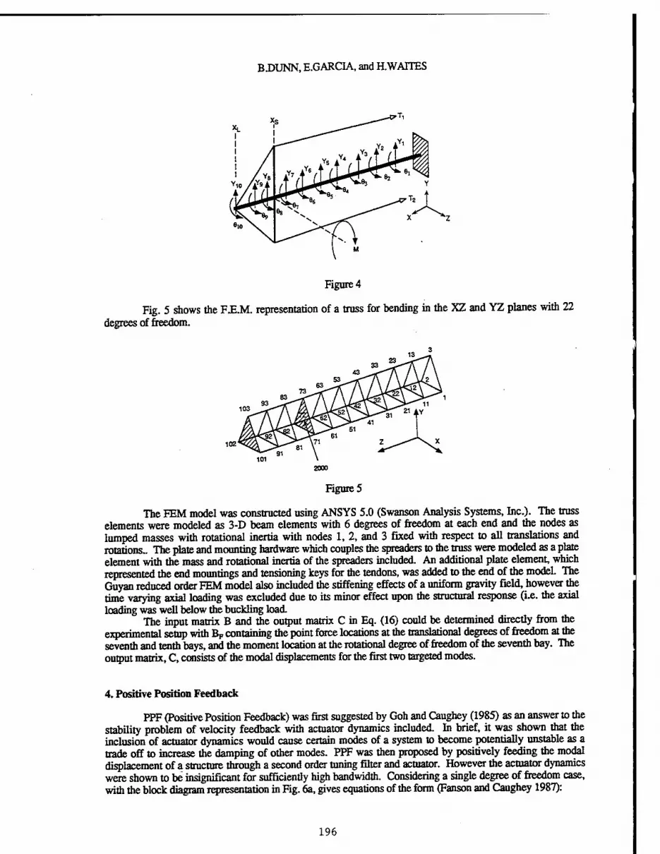
BDUNN, E.GARCIA, and H.WATTES
Figure 4
Fig. 5 shows the FJE.M. representation of a truss for bending in the XZ and YZ planes with 22 degrees of freedom.
2000
Figure 5
The FEM model was constructed using ANSYS 5.0 (Swanson Analysis Systems, Inc.). The truss elements were modeled as 3-D beam elements with 6 degrees of freedom at each end and the nodes as lumped masses with rotational inertia with nodes 1, 2, and 3 fixed with respect to all translations and rotations.. The plate and mounting hardware which couples the spreaders to the truss were modeled as a plate element with the mass and rotational inertia of the spreaders included. An additional plate element, which represented the end mountings and tensioning keys for the tendons, was added to the end of the model. The Guyan reduced order FEM model also included the stiffening effects of a uniform gravity field, however die time varying axial loading was excluded due to its minor effect upon the structural response (i.e. the axial loading was well below the buckling load.
The input matrix B and the output matrix C in Eq. (16) could be determined directly from the experimental setup with BF containing the point force locations at the translational degrees of freedom at the seventh and tenth bays, and the moment location at the rotational degree of freedom of the seventh bay. The output matrix, C, consists of the modal displacements for the first two targeted modes.
4. Positive Position Feedback
PPF (Positive Position Feedback) was first suggested by Goh and Caughey (1985) as an answer to the stability problem of velocity feedback with actuator dynamics included. In brief, it was shown that the inclusion of actuator dynamics would cause certain modes of a system to become potentially unstable as a trade off to increase the damping of other modes. PPF was then proposed by positively feeding the modal displacement of a structure through a second order tuning filter and actuator. However the actuator dynamics were shown to be insignificant for sufficiently high bandwidth. Considering a single degree of freedom case, with the block diagram representation in Fig. 6a, gives equations of the form (Fanson and Caughey 1987):
196

FREQUENCY DOMAIN CHARACTERISTICS FOR A DC LINEAR FORCE ACTUATOR
| + 2Cco| + (ö2 = gQ)2Tl
<n + 2£fC0fT| + C02=CD2£
(17)
(18)
where £ and TJ denote structural and filter coordinates, respectively. By observing the root-locus for this system as in Fig. 6b, it becomes obvious that as the filter loses damping the structural poles move farther into the left half plane with a corresponding gain in damping.
H(S)
No Actual» «0:
200
s2+ECfi»fS+<Bf2 KSH
$
-230
•*». -50 0 RaalAxfc
Figure 6a,b
For comparison of a case with the addition of actuator dynamics, different effects can be seen depending on values of actuator break frequency. Consider the block diagram representation of a combined actuator-structural mode-PPF filter in Fig. 7.
R(s) -=<H Actuator Dynamics
Structural Mode
<D~ PPF Fitter Mode
-C(s)
Figure 7
A generic single degree of freedom model was constructed and combined with an actuator with a set damping ratio of 0.17 and the natural frequency was varied to allow it's effects to be studied for cases when the actuator's natural frequency is far above, close to, or far below that of the controlled mode. The actuator model was the 4th order model created as per the Actuator Modeling section of this paper, although only the dominant poles are shown in the root-loci.
Now consider the root-loci for different actuator frequencies in Fig. 8. For the 50 Hz case notice that the interaction between filter and structural poles are nearly identical to those of the system with no actuator dynamics. For this case, referring to Table II, observe that the stability of the filter is the limiting factor with one filter pole quickly moving into the right half plane for a small loop gain. However there are several obvious changes when the actuator is changed to 20 Hz. First the root-loci for the structural poles move to the real axis as opposed to the idealized PPF and 50 Hz cases and instability ultimately results. Second the actuators go into the right-half briefly, but looking at Table n, it can be seen that the actuator goes unstable well before the structure. In the 10 Hz case there are other noticeable changes. First the structural poles move slightly into the left half and then move toward the imaginary axis and instability. Second the actuator can once again become unstable and in fact does so before the structural mode. Last it can be seen that lowering the actuator frequency to 5 Hz causes no appreciable increase in the structural damping before instability occurs and once again the actuator goes unstable. Obviously from these observations an actuator with a natural frequency well above the structural mode will result in the best case situation of increased control of the structural mode while allowing global stability for the combined actuator-filter-structure system.
197

B.DUNN, E.GARCIA, and H.WAITES
50HZ 20Hz 400
-200
400
-50 0 Real Axis
10Hz
-200
200
-200
-50 Real Axis
Figure 8
Table n - Destabilizing Gain Values, g
Structure Filter Actuator 50 Hz RS 0.003 0.83 20 Hz 0.23 RS 0.10 10 Hz 2.37 RS 0.09 5Hz 0.31 RS 0.37
RS: Remained Stable
Now reconsider the multi-degree of system shown in Fig. 5. Writing the structure, filters, and actuators in state-space form and combining gives the system shown in Fig. 9. Where there are now frequencies above and below the bandwidth of the actuator.
vc(t) +
-§ * Aa.Ba.Ca.Da As.Bs.Cs.Os Z(t)
Zi(t)
Z2(t)
Af.Bf.Cf.Df
Figure 9
The s, a, and Fs refer to the structure, actuator, and filters respectively. The Cs matrix assumes perfect filtering to allow modal displacements as outputs from the structural states. The Cf matrix of tuning filter outputs are already in modal coordinates due to one filter per mode and the 2 position states of the filters are multiplied by the gains gl and g2.
Setting the gain g2 equal to zero for the first mode the effects of increasing the closed loop gain are shown in Fig. 10, where bom plots are for the same system and gains but the second shows more detail of the first mode poles. There are obvious similarities to the SDOF model showing that for gains past a critical threshold, the filter loses stability and its closed loop poles move into the right half plane. Also notice that
198

FREQUENCY DOMAIN CHARACTERISTICS FOR A DC LINEAR FORCE ACTUATOR
since the actuator's bandwidth was chosen to be well beyond that of the first mode, there is for all practical purposes no influence of the actuator dynamics upon the structural modes, i.e. the idealized PPF case is approached. Now consider the case in which the first 2 modes are now controlled with independent PPF filters and independent loop gains, gl and g2, but a single actuator where the filter outputs, Cf, are added together to form the single actuator input as in Fig. 9.
200
100
i o -100
-200
Pola Mgrelkin for g1 wth p2-0 j—' r-
-IsN-
40 R»
Pola Mlgmkn for g1 wWi g2-0
20 1 10
£ o i
-10 i
-20
-20 Ha
Figure 10
The new pole migration can be seen in Fig. 11. showing that as the second mode loop gain is increased, initially there is an increase in damping for both modes. However as the gain is increased further to a point of maximum second mode damping, the first mode begins to lose a small amount of damping ultimately achieving almost the original £ but with a small increase in the natural frequency.
Pole hBgratJon for g2 «Ah g1 Fixed Pole MtgraBon for g2wtthg1 Fixed
. 200 o— 1
1 50
I 1
100
M o
-100
1
£ 0 o >f<
1
o >fc
-200 □
1 ■
-50 1
-«0 -20 Re
-40 -20 Re
Figure 11
5. Experimental
The actuators used for this paper are voice-coil type linear actuators with rare earth magnet assemblies and copper coils obtained from Applied Engineering. All mounting hardware, except for 2 inch travel ball-slides, was fabricated on site. Fastar LVDTs (Linear Voltage Displacement Transducers) from Data Instruments, were used to obtain a position signal from the actuator's moving components. The PD control for the electronic damping and spring force giving a damping ratio of 0.17 and frequency of 30 Hz was provided by a Comdyna GP-6 analog computer with the final actuator voltage and current from Kepco BOP-36-6M bipolar power amplifiers. The transfer functions of command voltage/position were verified experimentally by using a random signal input and the position output of the LVDTs and then comparing the magnitude and phase against theoretical models from MATLAB using the derived functions from the Actuator Dynamics section.
The 2 meter truss gave first bending modes of 2.3 Hz and 7 Hz in the YZrplane and 2.3 Hz and 6.9 Hz respectively in the XZ-plane. The addition of the spreaders, tendons, and mounting plate caused the first mode frequencies to drop to 1.98 Hz and the second mode to increase to 7.35 Hz for both planes of vibration and the appearance of torsional mode at approximately 7 Hz. Frequency transfer functions were taken with a Techtronix 2642 digital FFT analyzer. The spreader lengths were checked experimentally to determine whether or not their natural frequencies were near any of the controlled structural modes. The damping ratios were found from the experimental transfer functions and the frequency domain version of OKID (Juang, et al, 1993) for the modes to be controlled and 1 % damping assumed in the other modes.
199

BDUNN, E.GARCIA, and H. WATTES
The PPF filters were constructed from OP-07 op-amps and precision resisters and capacitors. The position signals for each mode were obtained from electronically integrated Kistler 8630 accelerometer signals. The accelerometers were placed at the nodes corresponding to 41 and 43 in Fig. 5. Their outputs were then band-passed through Sallen-Key second order filters (Malmstadt, Enke, and Crouch 1981) whose cutoff frequencies were chosen as those of the modes to be controlled. This allowed "modal" displacements to be determined for 4 bending modes of the structure (i.e. 2 in the XZ and 2 in the YZ planes). As with the actuators, the modal signals and PPF filters were experimentally verified against theoretical models. Recalling that the PPF filters would sacrifice damping in order to increase that of the structure, the damping ratios for the PPF filters were prescribed at 0.5 since the objective of the active control experiment was to increase the modal damping ratios.
Openvs Closed Loop Responses YZ Plan»
2 3 4 5 6 7 FreqHz
Open vs Closed Loop Responses XZ Plane
^X^rrr^^—_J \ y^\. *s^~^^ lär ^\rf '
0 " , 1
10'
gMO2
5 €io'
10°
10-i[ , , ,—I 0123456789 10
Freq H2
Figure 12a,b
Shown in Fig. 12a,b are experimental transfer functions showing the open and closed loop comparisons for the first 2 modes in the XZ and YZ-bending planes. Using OKID this results in an increases of modal damping shown in Table m. However it must be noted that due to the large increase in damping of the second modes, OKID was unable to extract a modal damping ratio and the second mode values in Table m are estimated from the structures decay times. Note that even though the torsional modes were not targeted for control due to the low modal participation of the input forces and moment, the PPF control scheme was able to slightly decrease the magnitude of these modes at approximately 7 Hz.
Table Ill-Open Vs Closed Loop % Damping
Open Loop Closed Loop % Increase ModelXZ 1.5% 92% 513 ModelYZ 1.3% 9.9% 661 Mode2XZ 0.78% 10% 1182 Mode2YZ 0.83% 10% 1100
The optimum gain for the first mode closed loop mode was set in hardware then the second mode gain was increased to achieve the best transient response while maintaining stability in the structure and filters. As was seen in the resulting eigenvalues of the system matrix in the PPF section, with 1 actuator for the 2 target modes an increase in the damping was possible while global stability was maintained (see Fig. 11).
200

FREQUENCY DOMAIN CHARACTERISTICS FOR A DC LINEAR FORCE ACTUATOR
6. Conclusions
Positive Position Feedback has been shown to be an effective means of control when used in conjunction with linear actuators and a tendon control scheme for a light-flexible structurewith low modes of vibration. The 4th order actuator model combined with PPF and structure showed similar behavior to that of the predicted performance giving large increases in damping while maintaining stability for all the modeled modes.
A complete actuator model was provided and then a simplified version was given which could be used when the actuator is operated below its break frequency.
7. Acknowledgments
This work was done under the NASA G.S.R.P program with grant NGT-51044. The authors also wish to thank Lowell Jones and Robert Carlin at the Smart Structures Laboratory, Vanderbilt University, and David Newton of Garman Systems Inc.
8. References
Dosch, J., Inman, D., Garcia, E., 1992, "A Self-Sensing Piezoelectric Actuator for Collocated Control," Journal of Intelligent Materials. Systems, and Structures, vol. 3, pp. 167-185
Fanson, J., Caughey, T., 1987, "Positive Position Feedback Control for Large Space Structures," AIAA /ASME/ ASCE /AHS/ ASC 28th Structures, Structural Dynamics, and Materials Conference, paper number 87-902, pp. 588-598
Goh, C, Caughey, T., 1985, "On the Stability Problem Caused by Finite Actuator Dynamics in the Collocated Control of Large Space Structures", International Journal of Control, vol. 41, no. 3, pp. 787-802
Juang, J. Phan, M., Horta, L., Longman, R., 1993, "Identification of Observer/Kalman Filter Markov Parameters: Theory and Experiments, "Journal of Guidance. Control, and Dynamics, vol. 16, no. 2, pp. 320- 329
Kuo, B., 1991," Automatic Control Systems." Prentice Hall Inc., Englewood Cliffs, New Jersey, pp. 170-173
Lu, J., Thorp, J., Aubert, B., Larson, L., 1994, "Optimal Tendon Configuration of a Tendon Control System for a Flexible Structure," Journal of Guidance. Control, and Dynamics, vol. 17, no. 1, January-February, pp. 161-169
Malmstadt, H., Enke, C, Crouch, S., 1981, "Electronics and Instrumentation for Scientists." The Benjamin/Cummings Publishing Company, Inc., Menlo Park, California, pp. 208-210
Murotsu, Y., Okubo, H., Senda, K., 1991, "Identification of a Tendon Control System for Flexible Space Structures, "Journal of Guidance. Control, and Dynamics, vol. 14, no.4, July-August, pp. 743-750
Murotsu, Y., Okubo, H, Terui, F., 1989, "Low-Authority Control of Large Space Structures by Using a Tendon Control System, "Journal of Guidance. Control, and Dynamics, vol. 12, no. 2, March-April, pp. 264- 272
Zimmerman, D., Inman, D., 1990, "On the Nature of the Interaction Between Structures and Proof-Mass Actuators, "Journal of Guidance. Control, and Dynamics, vol. 13, no. 1, pp. 82-88
201

202

MODELING AND ACTIVE VIBRATION
CONTROL OF ROTOR BLADES
D. Dinkier* and F. Doengi* University of Stuttgart Stuttgart, GERMANY
Abstract
The paper discusses the stabilization of pitch-flap flutter and the vibration attenuation of flexible hingeless rotor blades in forward flight. Mathematical models for the geometrically nonlinear struc- ture and the aerodynamic loads are derived. Using the Finite Element Method, the discrete equa- tions of motion are obtained. Dynamic simulations are presented for a rotor blade model. Robust state feedback controllers are designed for various configurations and flight states using the Linear Quadratic Gaussian / Loop Transfer Recovery (LQG/LTR) and the Normalized Left Coprime Factor- ization (NLCF) design methods. Conclusions are drawn regarding the feasibility of smart rotors.
1. Introduction
In forward flight helicopters experience high vibratory loads, aeroelastic instabilities and strong noise impact. Transonic effects on the advancing blade, dynamic stall at the retreating blade as well as blade-vortex interaction (BVI) of preceding and following blades are the main sources of vibration and noise. These phenomena put limits on the flight performance. They reduce passenger comfort and can lead to structural fatigue failure.
Despite the complex flow field and load distribution on the rotor in forward flight the vibratory loads transferred to the helicopter fuselage via the rotating hub consist of well-defined frequencies. This is due to the filtering characteristics of the hub. It is a well-known fact7'8 that for a rotor with ra& identical blades the hub transfers only loads of multiple blade passage frequency n&fi, where Q denotes the rotor angular velocity. As an example, a four-bladed rotor will lead to fuselage vibration frequencies 4f2, 8fi, etc. For most helicopters the largest components are the vertical shears and the pitch and roll moments at Tifcft due to nt,Q blade flap shears and (rib — 1) fi blade flap and torsion moments, respectively8'11.
Two general approaches are discussed in the literature for active vibration control, the Higher Harmonic Control (HHC) and the Individual Blade Control (IBC). Friedmann and Hodges4 give an extensive overview of the work carried out in this field. HHC has been investigated both theoretically and experimentally in a large number of studies. The idea is to use the swash-plate not only for conventional primary pitch control at Ü but also to superimpose a higher-harmonic signal with contributions from the frequencies (nj - 1) fi, ri^fi, and (rib + 1) fi- In a closed-loop control configuration this concept uses accelerometers attached to the fuselage and an adaptive controller to adjust the swash-plate input
•Professor, Head of Aeroelasticity and Dynamics Group tPhD student
203

D. DINKLER, F. DOENGI
to varying flight states. In experiments good results were obtained in reducing the vibration level at the hub or at selected fuselage positions. However, HHC failed to suppress both hub and airframe vibrations in the presence of airframe-rotor coupling11. Wind tunnel tests showed that BVI noise reduction by HHC could result in higher vibration levels and vice versa14.
It is hoped that some of these disadvantages can be overcome by using IBC. This approach applies vibration control in the rotating frame. It is independent of the hub filtering characteristics and can also account for individually different blade properties. However, implementation using conventional hydraulic servo tabs leads to bulky and heavy systems like the one designed for wind tunnel tests of the Bo 105 hingeless rotor13.
With the advent of smart structural concepts in the late 80's new actuators were investigated for IBC of rotor blades. Surveys are given by Narkiewicz10 or Strehlow and Rapp15. Among the concepts proposed are bending and torsion actuators at the blade root as well as twist control rods based on piezoceramic actuators. Shape adaptivity of blades covers adaptive twist, bending and section cam- ber. Nose drooping is discussed in order to attenuate dynamic stall on the retreating blade5. For most of these applications actuator materials must be significantly improved. Piezoceramics are lim- ited to very low strains. While shape memory alloy (SMA) actuators offer large strain capability they are constricted to frequencies less than 10 Hz due to slow heating-cooling cycles. Recent trends are therefore based on smart mechanisms such as control flaps at the trailing edge of the outer blade region1,15'17. Actuated via the swash-plate and a mechanical linkage servo flaps have been used by Kaman for primary pitch control9. In the present paper they are investigated as means for pitch-flap flutter suppression and vibration reduction of a blade with conventional swash-plate primary control.
2. Structural model of elastic rotor blades
In order to describe the kinematics of a flexible rotor blade two frames of reference are introduced. For helicopters which fly with constant forward speed an inertially fixed reference frame {x0,yo,zo} is connected to the airframe such that the x0 axis points along the tail boom. A second frame {x, y, z} is fixed to the rotating hub. Its x axis points along the rotating blade to be considered subsequently. The z and z0 axes are equivalent. The rotor moves with angular velocity Cl, leading to a time-varying azimuth angle ip = Qt mod 2n measured from the x0 axis towards the x axis. It is assumed that the undeflected rotor blade lies in the hub plane, i.e. there is no pre-cone angle. Furthermore, the flow velocity C/0 due to helicopter forward motion is assumed to be parallel to the x0 axis.
Fig.l: Blade deflections Fig.2: Blade section with flap
Deflections of the flexible rotor blade are measured in the {x,y,z} frame. The model includes radial elongations u, lagwise and flapwise bending, v and w, respectively, as well as torsion or twist angle a, see Fig. 1. Note that the x axis is equivalent to the elastic axis of the blade. For blade sections with a control flap at the trailing edge, the position of the flap hinge is denoted by yj and the control flap angle by ß, see Fig. 2. The position of a mass element dm measured in the hub-fixed frame {x, y, z}
204

MODELING AND ACTIVE VIBRATION CONTROL OF ROTOR BLADES
is given by the vector sum of its undeflected position and the deflection vector:
r(f) = R + d(t) = Rx
Ry
Rz
+ u - yv,x -zw,x
V
w + ya + Sf(y - yf)ß
_ f 0 -if y-
l 1 if V- y/<o Vf>0
The expression for the deflection vector is valid for small rotations. Note that for Hapless sections Sf = 0. The time derivatives of r are given by r = d and r = d, its first variation by Or — 6d. The position of the deflected mass element in the inertial reference frame {xo,yo,z0} is found by the transformation
ro Tr, T = c\ -s\ 0 si Ci 0 0 0 1
where Cn = cos (nüt);, sn = sin(nQ.t) (2)
Its time derivatives are f = Tr + Tf and r0 = Tr + 2Tf + Tr.
The virtual work SWm of the mass inertia forces is given by
-SWn = f 6rTr0 dm = f SdTTT[f{K +d) + 2Td + Td]pdV Jm JV
(3)
where m and V are the total mass and volume of the blade, respectively, and p denotes the local mass density. The matrix terms are evaluated and reordered with respect to the variables v = [ a, u, v, w, ß ]T. Integration over the blade sections leads to planar first-order and second-order inertia moments. The approach yields a one-dimensional formulation of the virtual work of mass inertia forces:
-6W„ fix
Jo SvT [OMV + 2fiOGv - fi2Ocv - Q20Q]dx (4)
The terms in brackets represent, from left to right, the inertia forces, the gyroscopic or Coriolis forces, the centripetal forces dependent on the deflections, and the centripetal forces on the undeflected blade, respectively. The length of the blade is denoted by lx.
The rotor blade is modeled as a geometrically nonlinear beam structure. Flapwise and lagwise bending are coupled with the radial deflection via higher-order terms. The Bernoulli hypothesis is assumed to be valid. For moderate rotations von Kärmän strains can be used to model the longitudinal strain at the elastic axis (y = z = 0):
e = u,x +-(w,l +v,2x ) (5)
Let MT, N, My, and Mz be the internal reaction torque, longitudinal force, lagwise and flapwise bending moments, respectively. The internal virtual work of the elastic forces is then given by
- 5Wi = j [ Sa,x MT + SeN - 6v,xx My - 6w,xx Mz]dx Jo
(6)
Substitution of linear material laws and equations of static equilibrium and reordering of terms with respect to the variables v yields the following matrix formulation of the inner virtual work,
-5Wi -/ Jo 6vT Os v dx , (7)
where Os is the absolute or secant stiffness operator matrix. In the incremental formulation of the static equilibrium the tangent stiffness operator matrix Or replaces O5. Gravitation exerts both a
205

D. DINKLER, F. DOENGI
force in negative w direction and, in the case of a centre of gravity (C.G. in Fig. 2) offset from the elastic axis, a torque. The external virtual work due to gravitation is
SW0 [ [ Say + Sw] pdV = f 6vT Og dx Jv Jo
(8)
3. Modeling of aerodynamic loads
The flow field around a rotor blade in forward flight is extremely complex, although the resulting loads are periodic and can be expressed by Fourier series. Modeling of transonic effects, of dynamic stall or BVI are demanding tasks in computational fluid dynamics. Inclusion of aeroelastic coupling between structure and flow-field leads to large and time-consuming numerical problems. However, in order to design IBC systems an efficient model of small dimension must be available for a preliminary dynamic analysis of the plant to be controlled. Since aeroelastic coupling substantially influences the dynamic characteristics of such a system it must be taken into account for feedback control design. As a first approach this work employs classical aeroelastic strip theory for sections with control flaps as derived by Theodorsen16. Time histories of loads and deformations are assumed to be harmonic. The aerodynamic model is simplified for inviscid, incompressible, quasi-stationary, linearized potential flow. For each strip perpendicular to the rotor blade axis the flow velocity is computed from the contributions of rotor motion and forward flight motion of the helicopter. The influence of the flow component along the rotor blade is known to be small and can be neglected. Fig. 3 shows a section of the rotor blade with control flap.
z,w
U
y.v
«/ ---^ "öp ^r—^^t" ^^
^ yf<° , 5ß
Fig.3: Aerodynamic loads on a section with flap
In Theodorsen's formulation, the blade section is approximated by a oscillating flat plate. Lift I and drag d per unit length act on the elastic axis. The pitch torque ma per unit length is positive nose up. The flap moment mp per unit length acts about the pivot hinge of the control flap. In undeflected position, the rotor blade possesses an initial pitch angle ao which varies with the radial position. Its aerodynamic centre (A.C.) is at position yn, see Fig. 2. The aerodynamic loads on a harmonically oscillating plate with flap are formulated under the assumption of quasi-stationary flow:
I =
ma = —
77 pb2
4 Uä-w-(yn- j)ä- i^Uß-T^ß
IT pUb Ua-w- (yn- -)ä + -T10Uß + Tu^-ß I 7T 47T
+ npU2ba0 (9)
d — TrpU2bc*D(a0 + a) , where c*D = —- dCL
(10)
pb2 " 4
i b \ TT ■ / 2 b 3&2 . .. -*(yn ~ ^)Ua + n(y'n - -yn + —)a + TT (I
+ (r4 + r10)f/2/3 + (r1
+ TTpUbyn
Ts - lyfT4 + ±Tn)^Uß + 2T13jß1
Ua-w - (yn - -)d + -T10Uß + Tu^-ß 2 IT 47T
+ itpU2byna0 (11)
206

MODELING AND ACTIVE VIBRATION CONTROL OF ROTOR BLADES
nip pb2
4 -T8 -Ua + T13 b-ä + Tt \w + - (T5 -T4TW)U2 ß - T4TU^-Uß -T3^ß
' Z Z ft 47T 47T
4
2
Ua w-(yn- r)<* + -T10Uß + Tu^-ß 2 n 47T
-T12^ü2a0 (12)
Here, p denotes the mass density of the surrounding air, and b is the chord length of the blade section. The lift and drag coefficients of the section are CL and cp, respectively. The Tt constants contain geometric information about the control flap. They are listed in Ref. 16. The effective flow velocity at a section with radial position x contains the constant contribution from the rotor angular velocity fi and a harmonic part from the helicopter forward speed UQ:
U = fix + U0 sin (fit) (13)
Analogously, the squared effective flow velocity can be divided into constant and time-varying parts:
U2 = n2x2 + ^ + 2ÜxUo sin(fii) - ^2- cos(2fii)
The virtual work due to aerodynamic loads is
ÖWa = / [ 6w I - 5v d + öa ma + öß m,ß ] dx . Jo
(14)
(15)
Substitution of the above equations for the aerodynamic loads and reordering terms with respect to the variables v yield
6Wa = I'* 6vT [Oa2v + UOalir + U2Oa0v + U2 Oa] dx . Jo
(16)
Here, Oo2, Oai and Oa0 are the aerodynamic mass, damping and stiffness operator matrices, re- spectively, and U2Oa denotes the aerodynamic forces due to the initial pitch angle a0- With the abbreviations cn = cos (nüt) and sn = sin (nüt) one obtains from Eqs. (13) and (14)
6Wa = [ Jo
ÖV? Oa2v + (Qx + t/os1)Oalv + (fi222 + ^ + 2fiz[/0si-^c2)Oaov
+(tfx* + Vl + 2{lxUos1-^c2)00 dx . (17)
4. Equations of motion
After collecting the terms of virtual work derived in the previous sections the principle of virtual work is formulated as follows,
6Wm + SWi + 6Wg + 6Wa + 6Wb =0, (18)
where 6Wm, SW{, SWg, and SWa are given in Eqs. (4), (7), (8) and (17), respectively, and SWb represents the virtual work due to boundary terms. The above weak formulation of the equations of motion is discretized using the Finite Element Method. The blade is divided into ne elements of length ru
i = l,...,ne. For the interpolation of the deflection variables in each element first-order # and third-order * Hermitian shape functions are applied:
a $Q, U = $Ü, U = 'J,V, IU=:\I>W (19)
The vectors a,ü,v, and w contain the DOFs at the two nodes of an element. Note that the control flap angle ß is treated as a discrete quantity which is constant over the whole flap length. For the aero- dynamic terms root cut-out as well as tip loss effects are implemented by suppressing the aerodynamic
207
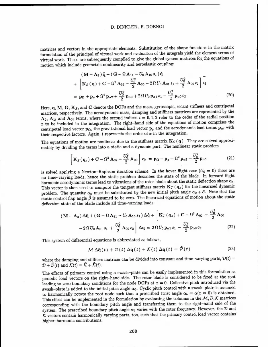
D. DINKLER, F. DOENGI
matrices and vectors in the appropriate elements. Substitution of the shape functions in the matrix formulation of the principal of virtual work and evaluation of the integrals yield the element terms of virtual work. These are subsequently compiled to give the global system matrices for the equations of motion which include geometric nonlinearity and aeroelastic coupling:
+
(M-A2)q+(G-fiAii-tfoAi0Si)q
Ks(q) + C r/2 £/2
fl2 A02 - -£ Aoo - 2 Ü U0 Aoi sx + -£■ A00 c2
tfl = pn + ps + ft2Pc2 + -^-Pao + 2fiE/op1
U% aSi r- PaO C2 (20)
Here, q, M, G, Ks, and C denote the DOFs and the mass, gyroscopic, secant stiffness and centripetal matrices, respectively. The aerodynamic mass, damping and stiffness matrices are represented by the A2, An and A0i terms, where the second indices i = 0,1,2 refer to the order of the radial position x to be included in the integration. The right-hand side of the equations of motion comprises the centripetal load vector pa, the gravitational load vector pp and the aerodynamic load terms pai with their respective factors. Again, i represents the order of x in the integration.
The equations of motion are nonlinear due to the stiffness matrix Ks (q). They are solved approxi- mately by dividing the terms into a static and a dynamic part. The nonlinear static problem
Ks(qs) + C-fi2A( •02 U%
M)0 <ls = PQ+Pg + ft2 P<*2 + U$
PaO (21)
is solved applying a Newton-Raphson iteration scheme. In the hover flight case (U0 = 0) there are no time-varying loads, hence the static problem describes the state of the blade. In forward flight harmonic aerodynamic terms lead to vibrations of the rotor blade about the static deflection shape q«. This vector is then used to compute the tangent stiffness matrix KT (qs) for the linearized dynamic problem. The quantity a0 must be substituted by the new initial pitch angle a0 + ä. Note that the static control flap angle ß is assumed to be zero. The linearized equations of motion about the static deflection state of the blade include all time-varying loads:
(M - A2) Aq + (G - ft An - Uo A« si) Aq +
U2
2ft[/0AoiSi + -yA00c2
U2
Kr(qs) + C-ft2A02 - -^-Aoo
t/n2
Aq = 2 ft Uo Pal «I IT PaO C2 (22)
This system of differential equations is abbreviated as follows,
M Aq(t) + V(t) Aq(i) + K{t) Aq(f) = V (t) (23)
where the damping and stiffness matrices can be divided into constant and time-varying parts, V(t) =
V + V{t) and K(t) = £ + K{t).
The effects of primary control using a swash-plate can be easily implemented in this formulation as periodic load vectors on the right-hand side. The rotor blade is considered to be fixed at the root leading to zero boundary conditions for the node DOFs at x = 0. Collective pitch introduced via the swash-plate is added to the initial pitch angle a0. Cyclic pitch control with a swash-plate is assumed to harmonically rotate the root node such that a prescribed twist angle ab = a(x = 0) is obtained. This effect can be implemented in the formulation by evaluating the columns in the M,V,K matrices corresponding with the boundary pitch angle and transferring them to the right-hand side of the system. The prescribed boundary pitch angle ab varies with the rotor frequency. However, the V and K, vectors contain harmonically varying parts, too, such that the primary control load vector contains higher-harmonic contributions.
208

MODELING AND ACTIVE VIBRATION CONTROL OF ROTOR BLADES
For low forward flight velocities, the blade response to harmonic aerodynamic loads and cyclic pitch control concentrates on the Ü and 2fi frequencies. A good approximation can be obtained by us- ing Fourier expansion restricted to these two frequencies. For larger advance ratios \x = Uo/(Qlx) higher-harmonic terms can significantly influence the blade response. Since such cases are investi- gated regarding feedback control numerical time integration of modally reduced systems is applied in this work. Modal reduction of the unsymmetric system with non-Rayleigh damping is carried out in an approximate manner by evaluation of the left and right eigenvectors of the M,JC constant matrix pair. Transformation of the constant damping matrix V as well as of the time-varying matrices leads to coupling terms in the state matrix. When designing feedback control for a reduced system with selected modes this implies dynamic spillover. The advantage of this simplified reduction approach is to avoid conjugate complex eigenvectors.
5. Dynamic analysis of a model rotor blade
A basic mathematical model of a flexible, hingeless helicopter rotor blade has been developed in order to investigate the feasibility of IBC systems and their performance with respect to suppression of aeroelastic instability effects and vibration attenuation. The model named RB3 is shown in Fig. 4. The flap and lag hinges are replaced by an elastic neck, primary pitch control is applied via a pitch bearing at the blade root. A detailed documentation of the geometrical, stiffness and inertia properties of the' RB3 blade is given in Ref. 3. The aerodynamic properties of the blade sections are assumed constant along the blade length, the lift slope coefficient has been chosen as dci/da = 5.7, and dco/dcL = 0.1. The blade is assumed to possess a linear washout of 9°. For the simulations, ao was set to 12° at the blade root, which includes collective pitch.
ä & w accelerometers elastic axis /
flap control moment Mß
#=l 250 *—»■
Fig.4: Rotor blade model RB3 (dimensions given in [mm])
For IBC, the control input is modeled as an external torque Ma at the outer end of the blade neck which represents actuation by hydraulic servo tabs or piezoelectric torque actuators such as ±45° patches on the neck or control rods10'15. Optionally, the blade may be equipped with a control flap of 0.25 m length as shown in Fig. 4. Control input is then chosen as the external control flap moment Mß exerted by some servo or smart mechanism like hinged piezo-bars10'15. Accelerometers are used as sensors measuring the flapwise bending and twist angular accelerations, w and ä, respectively, at the location of the Ma input. These signals may be electronically integrated to yield w, w, and a time histories. As an alternative, modal sensors manufactured of piezopolymer material are considered. By shaping the width of such piezofoils placed along the blade length the sensors can be tuned to measure specified aeroelastic modes. Assuming perfect performance of such sensors it is possible to directly feed the signals back to a state controller without the need of an observer or other filter12.
The blade has been discretized with 20 finite elements of equal length leading to a model with 120 DOFs plus the optional ß DOF. Static and dynamic simulations as well as eigenanalyses have been performed for varying rotor angular velocities2. In Fig. 5 the eigenvalues and eigenvectors of the aeroelastic system are given for varying rotor angular velocity. The eigenfrequency diagram shows that there is resonance
209

D. DINKLER, F. DOENGI
for the first torsion mode (Ti) when excited with 4fi-periodic loads at ti « 36.1 rad/s and when excited with 3ft-periodic loads at ti « 43.3 rad/s. The situation is aggravated by low damping as shown in the damping diagram below. For a four-bladed rotor assumed here, both 3ti and 4ti loads are transmitted via the hub to the helicopter airframe. Therefore, the resonance peaks shall be reduced by applying active vibration control.
200
D) 'E 50
1 1 1 1 ' 1 ' ^
4fi^^^ F,
- —- F2 -^"^ T,
3n^-^^ -p*
2Q_--—-*
^_____~-—■ ^—^
^_____^~—~~~^^ __JL_———
I.I, 1
_ 150 = __
100
1.0
--. 0.5 - o z <D
E °-° E D> E -0.5 Q. Q. a
-1.0
- ** — " *" "* ^f"0*'^
-
- - £2=0 rad/s £2 = 30 rad/s £2 = 45 rad/s
i i , i i
0.0 1.0 2.0 3.0 4.0 rotor blade x coordinate [m]
5.0
30 35 40 45 rotor angular velocity £2 [rad/s]
50
0.0
E CO
10
0
-10
-20
-30
-40
————————^ *
1.0
^r 0.5 6 Z ■S 0.0
o -0.5
1.0 2.0 3.0 4.0 rotor blade x coordinate [m]
5.0
30 35 40 45 rotor angular velocity £2 [rad/s]
50 -1.0
-
I I 1 1 / *^
£2 = 0 rad/s - £2 = 30 rad/s - -
I
£2 = 45 rad/s - 1 1 1
0.0 1.0 2.0 3.0 4.0 rotor blade x coordinate [m]
5.0
Fig.5: Aeroelastic eigenvalues and eigenvectors in hovering flight
For rotor angular velocities greater than 40 rad/s the diagrams exhibit interaction of the first and sec- ond flapping (Fi,F2) and the first torsion mode which leads to very low damping of Ti about ti = 44 rad/s and to instability of F2 for ti > 48.3 rad/s. The appropriate eigenvectors, given in Fig. 5 on the right hand side, indicate an increasing similarity of the F2 and Ti modes. The results presented in Fig. 5 are valid for hover only. From numerical simulations of the dynamic blade response in forward flight one observes instability from ti > 38.5 rad/s for U0 = 70 m/s. The RB3 model which has been designed on purpose to exhibit pitch-flap flutter shall be subsequently stabilized using active control.
6. Robust feedback control design methods
In order to directly address eigenmodes state feedback control is used for system stabilization and vibration attenuation. Control designs are based on time-invariant, modally reduced models of the rotor blade. Modal sensors yield signals which can be directly fed back without the need of a state observer. In this case linear optimal control (LQR) is used to find a time-invariant control law. If accelerometers are applied for sensing, a state observer has to estimate the modal states of the system.
210

MODELING AND ACTIVE VIBRATION CONTROL OF ROTOR BLADES
It is then necessary to account for the spillover problem by using robust control design methods. In this work, the Linear Quadratic Gaussian / Loop Transfer Recovery (LQG/LTR) design method by Doyle and Stein 3 and Äoo-optimal Normalized Left Coprime Factorization (NLCF) control theory by Glover and MacFarlane 6 are used to find suitable control laws.
Consider a state representation of the reduced modal system to be given by
x = Ax + Bu, y = Cx. (24)
Provided the modal states x are known from measurements direct state feedback is applied:
u = -JCcx (25)
The linear quadratic regulator (LQR) is obtained by solving the controller algebraic Riccati equation,
SCA + ATSC-SCBR-1BTSC + QC = 0 -»■ Kc = Rj1 BTSc, (26)
where Qc and Rc are the state and input weighting matrices. The LQR possesses good robustness properties which are in general lost when estimating the state variables for feedback, u = - Kc x, with a state observer
x = Ax + Bn + JCf[y - Cx] (27)
The LQG/LTR method3 presents an approach to recover the robustness properties of the LQR by computing the filter gain matrix Kf with the following filter algebraic Riccati equation:
SfAT + ASf--SfCTCSf+BBT = 0 -> Kf = -SfCT, (28)
where p -> 0 is a positive real tuning parameter. In the present work, the LQG/LTR method is used as a design tool without explicitly letting p -*• 0 because undesired observer dynamics result. This is due to the fact that the observer poles converge to the plant zeroes which are poorly damped in the case of the aeroelastic system. The stability of the full-dimensional closed-loop system is checked with an eigenanalysis of the time-invariant model and with numerical time integration of the periodic model.
As an alternative to LQG/LTR control the ifoo-optimal NLCF method 6 is applied. In contrast to other iJoo-optimal control design methods, NLCF control offers open-loop weighting and avoids iteration to find the optimal control law. The controller and filter gain matrices are found from generalized controller and filter algebraic Riccati equations:
SCA + ATSC - SCBBTSC + CTC = 0 -»• Kc = BTSc , (29)
SfAT + ASf - SfCTCSf + BBT = 0 -> Kj = -7
2 [(1 ~72)I + ScSf]-TSfCT, (30)
where I is the identity matrix and 7 is a parameter chosen slightly greater than the inverse maximum stability margin 7min
6:
7 « 1.057mi„ = y/l + Amax(S/Sc) (31)
Here, A denotes the eigenvalues of the matrix in brackets.
7. Vibration control of the RB3 model blade
Applying active vibration control at the RB3 model blade two aims are pursued. First, the higher- harmonic (3ft, 4ft) vibration response of the rotor blade shall be attenuated at ft = 35 rad/s and Uo = 70 m/s. Second, the aeroelastic system shall be stabilized at ft = 45 rad/s and UQ = 70 m/s. Both Ma and Mp control inputs are to be used with suitable sensors. For vibration control design the influence of primary control is neglected in a first approach. The most important features of all IBC systems designed are summarized in the table below. All designs are based on modally reduced, time-invariant rotor blade plants which comprise the Fi, F2, and Ti modes. The input and output matrices contain the appropriate modal participation factors for actuators and sensors chosen.
211

D. DINKLER, F. DOENGI
Q 1 objective 35 rad/s -> vibration attenuation actuator type Ma Mß
controller LQR LQG/LTR NLCF LQR LQG/LTR NLCF sensor type modal w w modal a
Zmin uncontr. (mode) 2.0 (TO 3.3 (TO £,min specified (mode) 15.2 (TO 14.9 (Tlf) 9.8 (Tic) 15.0 (TO 15.0 (Tic-) 11.1 (Tlc) £,min checked (mode) 15.2 (TO 3.6 (Tlf) 6.3 (Tic) 14.3 (TO 12.6 (Tic) 10.1 (Tic)
\Ma/0\max [Nm] 387 409 4470 7.97 8.43 7.27
Q 1 objective 45 rad/s -» system stabilization
actuator type Ma Mß
controller LQR LQG/LTR NLCF LQR LQG/LTR NLCF sensor type modal w modal a
£min uncontr. (mode) 1.7 (TO 2.9 (TO £.min specified (mode) 14.1 (F2) 14.1 (F2c) 8.0 (Tic) 16.2 (F2) 16.2 (F2c) 12.2 (Tic)
(,min checked (mode) 14.3 (F2) 14.1 (Tlc) 8.8 (Tic) 17.7 (F2) 14.3 (F2/) 11.4 (Tlc) \Ma/0\max [Nm] 882 833 999 35.0 39.6 52.8
The types of actuators and sensors listed in the above table are as shown in Fig. 4. In all cases, the uncontrolled plant has lowest damping in the Ti mode. The percentage of damping £ of an eigenvalue S ± iw is defined as
£ = _ — . 100 [%] where w0 = V w2 + <52 . (32)
The table gives both the minimum damping specified in the control design and the values obtained when checking the eigenvalues of the full-dimensional closed-loop system. Here, the indices c and / indicate the regulator and observer poles, respectively. The difference between specified and ob- tained eigenvalues in the LQR case is due to dynamic spillover from the approximate modal reduction discussed in Section 4. Much worse effects on the minimum damping obtained are observed for the LQG/LTR and NLCF compensators where in addition to dynamic spillover both control and observa- tion spillover occur. Especially in the ft — 35 rad/s case with Ma actuation damping of the Ti mode turns out to be very low for the closed-loop systems with observers.
Comparison of the Ma and Mß actuation concepts show that the required control moments are much lower in the latter case. This is due to the fact that Ma must act on the structural torsion stiffness whereas Mß moves a control flap about a hinge without structural but only aerodynamic stiffness. This clearly points out that application of smart material actuators is more promising in connection with some kind of smart control flap than for inducing structural twist.
Dynamic simulations using reduced numerical time integration with ten modes are shown for the n = 35 rad/s, UQ = 70 m/s case in Fig. 6. The left diagrams refer to Ma actuation, the right ones to Mß actuation. The control objective is to add damping to the Ti mode which is known to be poorly damped and near resonance with 4fi loads, see Fig. 5 and the uncontrolled a tip displacement in Fig. 6. Since the Fi mode is essential for primary control it should not be affected by vibration control. In the NLCF control case with Ma actuation this is not achieved as becomes apparent in the diagrams of the tip flapwise displacement. Furthermore, the required control moment becomes extremely large, see the above table (not shown in Fig. 6). This is due to the fact that the NLCF controller has been designed with pure gain weighting leading to unwanted additional damping in the Fi mode. In principal, single mode weighting is feasible in the NLCF design, but it leads to additional observer states. This is a general drawback of the NLCF design method when aiming at control of single modes. However, good results have been achieved with NLCF control for the Mß actuation cases. Note that in the presence of the control flap the a amplitudes of the uncontrolled system are higher than in the MQ case. As
212

MODELING AND ACTIVE VIBRATION CONTROL OF ROTOR BLADES
mentioned before, the control moments are much lower than with twist actuation at the blade neck. Maximum control flap angles ßmax have been found from numerical simulation to be 3.3° at Q, = 35 rad/s and between 4.4° with LQG/LTR and 7.0° with NLCF control at Q = 45 rad/s.
15
o> m o> T>
Ö b <1>
c 0 10
to -S < a. -10
-15
. I i I
- - - ■
— / / \ f~ X .
»\ _<r_;j ̂ \y— - uncontrolled
- LQR - LQG/LTR -
i i NLCF i 1
0.0 0.5 1.0 azimuth angle y [it]
1.5 2.0 1.0 azimuth angle y [it]
0.8
0.4 -
m 0.0 "o •o Q. ™ -0.4
-0.8
. I I 1
- - -
Jf ^•^* \\
v£ uncontrolled LQR LQG/LTR NLCF
I ' I
0.8
0.4
2 0.0
•o a. ™ -0.4
0.0 0.5 1.0 1.5 azimuth angle y [it]
2.0
400
1" 5. 200
£° „ 0 CD
o -200
-400 -
-600
. -I- I l
^^~"=^ / - /
\ / s\_^/
- - LQR . LQGA.TR
- I l 1
0.0 0.5 1.0 1.5 azimuth angle y [it]
2.0
-0.8 (
10.0
E z 5 5.0 c CD
£ o E 0.0 Q C o
-5.0
r i i
- uncontrolled LQR LQG/LTR NLCF
\^-/ _
1 1 1
0.0 0.5 1.0 1.5 azimuth angle y [it]
2.0
-
I
I II
h
jft \\ // \\ v A // \\
/' A // A
I 1
- LQR LQG/LTR NLCF
\ // :--^ ft
I 1 1
^X """
"0.0 0.5 1.0 1.5 azimuth angle y [it]
2.0
Fig.6: Tip displacements and control moments for system at O = 35 rad/s, U0 = 70 m/s
In the case of pitch-flap flutter suppression at fi = 45 rad/s and U0 = 70 m/s good results were obtained with the LQR and LQG/LTR control systems. Here, too, NLCF control is less efficient in Ti mode weighting. Similar to control-configured flight of inherently unstable aircraft future smart rotor blades have the potential to extend the limits of helicopter flight performance by suppression of aeroelastic instabilities.
8. Conclusions and outlook
The mathematical modeling of the aeroelastic behaviour of flexible helicopter rotor blades has been discussed. Using the Finite Element Method the discrete equations of motion have been derived. For a model rotor blade an eigenanalysis was presented pointing out regions of resonance and pitch- flap flutter. Both vibration attenuation and system stabilization were investigated as control objectives using the LQR, the LQG/LTR and NLCF control design methods. Compared to linear optimal control NLCF was found more difficult to deal with regarding single mode weighting. Both twist actuation at the blade neck and control flap actuation have been considered, the latter being much more promising for application of smart materials due to lower control moments required.
213

D. DINKLER, F. DOENGI
However, smart flaps will have to cover an angular range of about ±5°. An important future task is to find smart mechanisms which are able to provide such maneuverability over a wide frequency range.
The IBC systems in this paper have been designed for specified flight states. Their-stability robustness is not guaranteed regarding parameter variations. In future work it will be indispensible to account for adaptivity of control in order to cover realistic state variations occuring in helicopter flight.
References
1. Chopra, I., "Development of a smart rotor", Proc. 19th European Rotorcraft Forum, Cernobbio (Como), Italy, September 14-16, 1993
2. Doengi, F. and Dinkier, D.: "Dynamics and control of flexible helicopter rotor blades", ISD Report No. 95/2, Institute for Statics and Dynamics of Aerospace Structures, University of Stuttgart, Stuttgart, Germany, 1995
3. Doyle, J.C. and Stein, G., " Multivariable feedback design: Concepts for a classical / modern syn- thesis", IEEE Trans. Autom. Contr., Vol. AC-26, 1981, pp. 4-16
4. Friedmann, P.P., and Hodges, D.H., "Rotary-wing aeroelasticity with application to VTOL vehi- cles", in A.K. Noor and S.L. Venneri (Eds.): Flight Vehicle Materials, Structures and Dynamics, Vol. 5, pp. 299-391, ASME, New York, 1993
5. Geissler, W. and Raffel, M., "Dynamic stall control by airfoil deformation", Proc. 19th European Rotorcraft Forum, Cernobbio (Como), Italy, September 14-16, 1993
6. Glover, K. and MacFarlane, D., "Robust stabilization of normalized coprime factor plant descrip- tions with Foo-bounded uncertainty", IEEE Trans. Autom. Contr., Vol.34, 1989, pp.821-830
7. Johnson, W., Helicopter Theory, Princeton University Press, Princeton, NJ, 1980
8. King, S.P., "The minimisation of helicopter vibration through blade design and active control", Aeronautical Journal, August / September 1988, pp. 247-263
9. Lemnios, A.Z. and Jones, R., "The servo flap — An advanced rotor control system", Proc. AHS Design Specialist Meeting on Vertical Lift Aircraft Design, San Francisco, CA, January 17-19,1990
10. Narkiewizc, J. and Done, G.T.S., "Overview of smart structure concepts for helicopter rotor con- trol", Proc. Second European Conf. on Smart Structures and Materials, pp. 242-245, Glasgow, UK, October 12-14, 1994
11. Nitzsche, F. and Breitbach, E., "A study on the feasibility of using adaptive structures in the attenuation of vibration characteristics of rotary wings", Proc. AIAA / ASME / ASCE / AHS / ASC 33rd Structures, Structural Dynamics and Materials Conference, pp. 1391-1402, Dallas, TX, April 13-15, 1992
12. Nitzsche, F., "Modal sensors and actuators for individual blade control", Proc. AIAA/ASME/ ASCE/AHS/ASC 34rd Structures, Structural Dynamics and Materials Conference, pp. 3507- 3516, La Jolla, CA, April 19-22, 1993
13. Richter, P. and Schreiber, T., "Theoretical investigations and windtunnel tests with HHC-IBC", Proc. 20th European Rotorcraft Forum, Amsterdam, The Netherlands, October 4-7, 1994
14. Splettstoesser, W.R., Lehmann, G., and van der Wall, B., "Higher harmonic control of a helicopter model rotor to reduce blade/vortex interaction noise", Z. Flugwiss. Weltraumforsch., Vol. 14,1990, pp.109-116
15. Strehlow, H. and Rapp, H., "Smart materials for helicopter active control", AGARD Conference Proceedings 531: Smart Structures for Aircraft and'Spacecraft, Lindau, Germany, 1992
16. Theodorsen, T., "General theory of aerodynamic instability and the mechanism of flutter", NACA Report No. 496, 1935
17. Yillicki, Y.,-Hanagud, S., Schräge, D.P., and Higman, J.P., "Aeroelastic analysis of rotor blades with flap control", Proc. 18th European Rotorcraft Forum, Avignon, France, September 15-18,1992
214

AEROSERVOELASTIC CHARACTERISTICS OF
ALL-MOVING ADAPTIVE FLIGHT CONTROL SURFACES
R. Barrett* Auburn University Auburn, AL 36849
Abstract
The aeroservoelastic properties of a new class of adaptive aeronautical surfaces are detailed. These new active surfaces use the newly invented Flexspar configuration which employs a high strength main spar around which an aerodynamic shell is pivoted. Within the aerodynamic shell, a piezoelectric actuator is mounted with one end bonded rigidly to the spar and the other attached to a point on the shell. As the piezoelectric element is energized, the pitch angle of the shell is changed. Adjacent to the piezoelectric element, a sensor is used to determine the position of the shell. A simple feedback loop connecting the sensor and actuator provides a high degree of stability. Inertial and aerodynamic coupling are minimized by collocating the pitch axis, aerodynamic center and center of gravity. Laminated plate theory estimations are used with basic kinematic expressions for relating piezoelectric flexure to shell pitch angle change. Wind tunnel test results demonstrate that stable deflections up to +11° are possible. By using an adaptive positioning system, the aerodynamic shell may be moved with respect to the main spar. This modification lends aeroservoelastic characteristics to the system. Accordingly, as the quarter-chord of the shell is moved forward of the pitch axis, small pitch deflections are effectively magnified with increasing airspeed. Experimental testing of an aeroservoelastically coupled wing specimen showed magnification of pitch deflections from ±11° to ±16° and good correlation with theory.
1. Introduction Flight control has been one of the major concerns of aviation enthusiasts since the invention of the
first aircraft. The dawn of controlled flight saw early aviators shifting weight and pulling wires to steer their crafts. These early days had various types of twisting, all-moving and flapped wing devices which manipulated air-loads. As time progressed, the control surfaces became more sophisticated and today, aircraft designers have an impressive array of actuators, materials and surface designs which may be used. One of the newer types of control surface actuators uses adaptive materials. In many ways, adaptive flight control surfaces are novel, modern devices which are unique and new; however, such structures have been flying for more than 270 million years. Because the adaptive actuators and the aircraft structure are intimately integrated, flight control by using camber and twist changes (as with bird wings) are possible. In 1989, the first of these adaptive aerodynamic studies were conducted on a series of bending-twist and extension-twist coupled aerodynamic plates. Crawley, Lazarus and Warkentin successfully showed that piezoelectric elements could actively bend or actively twist these coupled plates.1 As a result, twist motions would be generated which would, in turn, alter the loading across the span of the plate. Following this early work, a number of experimenters showed that piezoelectric actuators could be integrated into aerodynamic surfaces to actively induce twist and camber changes. Many of these studies were centered on vibration amelioration and flutter suppression. However, many technologists continued to explore different types of aeroelastic control.2"5 Various control schemes were devised for using skin- bonded elements to change the camber and twist of wings. The effects of wing sweep on active aeroservoelastic performance were included by Ehlers and Weisshaar.6 At about the same time, a new manufacturing method for piezoelectric elements was discovered which would lend highly orthotropic characteristics to otherwise isotropic piezoelectric sheets. These directionally attached piezoelectric (DAP) elements were shown to have orthotropy ratios in excess of 50. Accordingly, several experiments were conducted to show that inherent structural or geometric coupling (as was the case with the bending-twist or extension-twist aerodynamic surfaces) was no longer necessary to induce active twist deflections
*Assistant Professor, Aerospace Engineering Department
215

R. BARRETT
in flight control surfaces. Instead, the DAP elements could be arranged so as to directly generate a torsional shear flow which would result in a twist deflection. The first of these studies were conducted on helicopter rotor blades.7'9 Although only small static twist deflections were generated (±0.1° @ 600 V/mm), the principles of active blade twist manipulation were proved. Six years of follow-on work have since been conducted in the area of active helicopter rotor blade twist manipulation.10-12 The culmination of this tireless endeavor has been an improvement in static twist deflection to nearly ±0.2° at 600 V/mm.13 Because these twist levels are so low, a host of investigators have looked into high authority actuators for a greater degree of control. One of the most common high authority devices has been the active servoflap. Conceived in 1989 by Spangler and Hall, the active servoflap has demonstrated high lift coefficient changes in a small package.14 This device performs admirably in attached flow as is found in helicopters; however, at high angles of attack, like those experienced by missiles, the surface locks in a hard-over deflection. Accordingly, flight control devices for missiles and other vehicles which use low aspect ratio surfaces need another type of adaptive surface design for flight control.
In early 1991, a new type of missile flight control surface was invented. This device employed a twist-active DAP torque-plate which was bonded to a structurally stiff main spar. Tests showed that relatively large static pitch deflections (±4.5°) could be generated.15'16 Although deflections of this order of magnitude are fine for many types of flight control, still higher deflection levels are needed for many applications. Accordingly, an initial study into aeroservoelastic tailoring of torque-plate fins was made in 1992.17-18 This early study demonstrated that airloads could successfully be used to magnify pitch deflections. Unfortunately, along with pitch angle magnification came divergence. As a result, all of the subsequent torque-plate research has been on control surfaces which are not aeroservoelastically coupled. Still, significant advances have been made without coupling.
Among these advances have been the invention of the free-spar torque-plate fin and the Flexspar fin. The free-spar design has shown the highest pitch deflection levels of any torque-plate configuration, up to ±8° with a break frequency in excess of 50 Hz. This prototype 5" span by 2" chord graphite-epoxy fin exhibited stable deflections with airspeed and no flutter, buffet or divergence tendencies.19'21 Because still greater pitch deflections are necessary for many types of missiles, a new type of actuator configuration dubbed the Flexspar was invented. This design is a simpler arrangement than the torque-plate as only two active elements are needed for actuation. This design was originally proven in a series of laboratory bench tests which showed deflections up to +11°.22 After the initial concept was proven, a series of Flexspar wings were manufactured for a l/3rd scale TOW missile. These wings were shown to pitch up to ±14°.23
By using this wind tunnel test data, it was estimated that the missile turn radius could be effectively reduced by an order of magnitude. The most recent study conducted on Flexspar fins demonstrated full flight control on a remotely piloted vehicle.24 Although these studies have proven the basic utility of the torque-plate and Flexspar configurations, much work has yet to be done. Because there is a constant design compromise between deflection level and dynamic deflection bandwidth, high stiffness, high deflection actuators are needed. One method of maintaining the high structural stiffness and improving the deflection levels is to call upon aeroservoelastic effects. These have been shown to work well, but rapidly lead to divergence difficulties. However, with an active shell positioning system, it is now possible to move the aerodynamic shell with respect to the flexural axis so as to optimize the system performance. Accordingly, this paper will lay out the fundamentals of the Flexspar configuration and present data on a new type of active aeroservoelastic tailoring method.
2. Tip-Joint Flexspar Design and Modeling The Flexspar design is based on a single bimorph actuator which drives an aerodynamic shell in
pitch. Within the aerodynamic shell, a structurally stiff main spar provides support for a pair of pivots which form a rotational axis. For subsonic applications, the main spar, center of gravity and aerodynamic center are usually collocated along the quarter-chord of the aerodynamic shell. The base of the bimorph bender is rigidly fixed to the main spar, while the tip is joined to the shell. Figure 1 shows a typical main spar and bimorph actuator prior to structural integration.
216

AEROSERVOELASTIC CHARACTERISTICS OF ADAPTIVE CONTROL SURFACES
Fig. 1 Typical Flexspar Main Spar and Active Element (from TOW missile of Ref. 23)
There are two main configurations of Flexspar fins. The first, the shell-joint Flexspar has a bimorph bender element which is rigidly bonded to the main spar and connects to the shell in a chordwise direction This configuration is generally used for high stiffness, low deflection applications. The second configuration is the tip-joint Flexspar. This uses a bimorph bender element which is mounted at the root of the fixed base and connects to the tip of the movable shell. Much larger deflections are attainable from the shell-joint configuration. Figure 2 shows a typical shell-joint configuration with nomenclature for analysis.
aerodynamic shell main spar end pivot
flexure end pivot
graphite end extension
bimorph bender element
rigid root mount with root protector
Fig. 2 Shell-Joint Flexspar Configuration
217

R. BARRETT
Tip-Joint Flexspar Laminated plate theory has been used to successfully analyze adaptive plate structures for several
decades. Using the conventional laminated plate theory assumptions laid out by Jones20 the element curvature may be estimated. Assuming that a finite bond line with low stiffness connects a pair of piezoceramic sheets to an isotropic substrate, then the curvature KJI is as follows:
4 Ea v«+2v»+t;A !k 12 a !^^+(ts + 2tb)t^K
(1)
If the geometry of Figure 2 is used in conjunction with the above estimation, then the shell pitch angle may be determined.
<i> = 2 sin
l-cos(id0) lotot
»K)l »fa)
21, (2)
Shell-Joint Flexspar Borrowing the dimensional notation from Fig. 2, and using the bimorph curvature estimation of
equation 1, the shell joint pitch angle may be solved for.
0 = tan
l-cos(id0) lotot
sinjido)' iin(Kl0)
(3)
An examination of equation 3 shows that the deflections will be considerably smaller than those obtained by the tip-joint Flexspar configuration.
3. Control Surface Design and Construction
As with earlier torque-plate and Flexspar investigations, PZT-5H piezoceramic sheets were used to power the aerodynamic surface. Figure 3 shows the overall geometry of the stabilizer with the internal layout of the components. The piezoelectric bender was constructed from a pair of 7.5 mil PZT sheets bonded to a 2 mil brass substrate with Scotchweld™ adhesive tape in a 350° cure under approximately 8 psi of pressure. The actuator element is 2.5" long with root of the actuator element measuring 0.4" and the tip 0.3" wide. Masterbond conducting epoxy was used to make electrical contact with the nickel electroded faces of the PZT sheets. After the cure, the element was removed from curing jigs, deflashed and trimmed to tolerance. A protective root section made of style #120 fiberglass was added to provide protection for the leads and the base of the element. A graphite-epoxy extender measuring 1.8" was bonded to the tip of the actuator bimorph and the end of the shell. The main spar was constructed with a flexible nylon hinge sandwiched between the structural material. The tip of the shell had a positioning barrel which could move the aerodynamic shell up to 20%c. The fully contracted position of the barrel collocated the fin aerodynamic center and the pitch axis. As the barrel was extended, the shell moved forward with respect to the pitch axis. This lent adaptive aeroservoelastic characteristics to the system. The shell positioning barrel was constructed from a 10 mil diameter Tinel alloy K shape-memory alloy coil which was balanced by a conventional spring-steel coil. The position of the barrel was determined by a helical position sensor which was connected to a closed-loop controller.
218.

AEROSERVOELASTIC CHARACTERISTICS OF ADAPTIVE CONTROL SURFACES
aerodynamic shell
shell positioning barrel-
main spar flexure
bimorph piezoceramic element
Fig. 3 Adaptive Shell-Positioning Flexspar Arrangement
The aerodynamic shell of Fig. 3 was constructed with a fiberglass leading-edge shell up to 30%c and tip shell from 85% to 100% of the span. Aft of the leading-edge shell a series of graphite ribs made from Ik tows are connected to the trailing-edge stiffener. The internal shell structure was covered with Micafilm aerodynamic skinning material.
4. Control Surface Testing and Aeroelastic Tailoring
The driving element of the Flexspar fin was tested for tip-bending deflection. A laser-mirror was mounted on the end of the member and the deflections were measured. Figure 4 shows the test results as compared to the laminated plate theory estimations.
a £ 3 £ "Sk W Ä
la OS *
■* <u a u Si 3 ft« 'S s I «8 U i>
ft-
4.0 - - predicted
y^O
3.0 - O measured .^O
2.0 - ^^o
1.0 -
0 -—-~~"°T 1 1 h 1 1 i h— 1 4 6 8 10 12 14 16
Static Half-Amplitude Actuation Potential, E3 (volts/mil) 18
Fig. 4. Actuator Beam Flexural Test Results
After the flexural characteristics of the actuator were verified, basic bench and wind tunnel tests were conducted on the entire fin. The mass moment of inertia of the fin structure was determined to be 0.0132 lbm-in2 by performing a series of tests in a rotational spring rig. Dynamic testing showed that the low- deflection, passive rotational stiffness is approximately 0.0040 in-lbf/deg. Figure 5 shows the results of the dynamic bench testing.
219

R. BARRETT
an
a o
at
60 -|-
50 —
40 --
30 --
20 --
10 ± 19 V/mil
+ + 0 18
—I 20 2 4 6 8 10 12 14 16
Excitation Frequency, / (Hz)
Fig. 5 Flexspar Fin Pitch Angle as a Function of Actuation Frequency
Bench testing demonstrated a natural frequency of approximately 13 Hz. From Fig. 5, the peak was flattened out, not by structural damping, but from the shell encountering the rotation stops at the base of the structure.
A series of aerodynamic tests were conducted on the Flexspar fin in the 1 ft x 1 ft model scale wind tunnel at Auburn University. The static deflection of the fin was measured by a position measurement bar mounted within the structure and by correlating the electrical measurements with laser-rotation data. An estimate of the static deflection was made using equations 1 and 2 with no aeroelastic coupling (pitch axis and aerodynamic center were collocated). The testing was conducted in a pseudostatic condition with a 0.5 Hz sine signal driving the shell in pitch. Figure 6 shows the analytical estimations of pitch deflection and the experimental aerodynamic data.
u <
— 0.8 S
-- 0.6
-- 0.4 3
0.2
6 8 10 12 14 Applied Potential, E3 (V/mil)
16 18
a
I
Fig. 6 Active Aerodynamic Characteristics of the Uncoupled Flexspar Fin
From Fig. 6, it can be seen that the linear lift curve slope is approximately 0.041/deg. Because the aerodynamic profile is symmetric (modified NACA 0012), there is no zero-lift pitching moment about the quarter-chord. Further, the bench and wind tunnel test data are sufficient for prediction of the aeroservoelastic characteristics. Through a simple moment balance, the aeroservoelastic angle of attack increment, cte may be determined.
220

AEROSERVOELASTIC CHARACTERISTICS OF ADAPTIVE CONTROL SURFACES
<x„ Ktot<l»a-<lSceCiac
(4) qSceCLa-Ktot
Equation 4 shows that the pitch axis - quarter chord eccentricity, e, active pitch angle, 0a, dynamic pressure, q, and base angle of attack, OQ, have a profound effect on the aeroservoelastic angle of attack increment, ote. Using equation 4 it can be seen that large eccentricity induces rapid divergence.
^ 6 T 60 •e 5 +
CD a c I t-i
Q
_2 "5 o
3
2 ■•
1 ■■
14
ea o
"3> 12
™ 10 8 6
4
2 0
ceo = 6°
20 40 60 Wind Tunnel Speed, V (ft/s)
10 9 8 7 6 5 4 3 2 1 0
20 lg 16 14 12 10
g 6 4 t 2 0
ceo = 4'
oo = 8°
20 40 60 Wind Tunnel Speed, V (ft/s)
Fig. 7 Aeroservoelastic Angle of Attack Increment as a Function of Geometry, Base Conditions and Aerodynamic Forces
From Fig. 7, it can be seen that stable aeroservoelastic deflections cannot be attained by using a conventional approach to fin design. Accordingly, a specialized adjusting barrel was used to position the aerodynamic shell with respect to the pitch axis which is aligned with the main spar. This shell manipulation barrel may be contracted or extended so as to manipulate the fin eccentricity. Because aerodynamic control comes from the active pitch deflection, 0a, it is desirable to magnify this value to increase the control power of the system. The control effectiveness ratio, R can be defined as: R = oce/<|>a. Because me eccentricity may now be scheduled to hold a constant aeroservoelastic angle of attack increment, equation 4 may be rearranged to find e.
e = - Ktot(R+i)
qScCL R + % (5)
From equation 5, it can be easily seen that at low airspeed, the ideal eccentricity goes to infinity. Because there are physical limitations in the system, the actual eccentricity of a given system will be truncated at a fixed level until the dynamic pressure increases.
A series of experiments were ran with the shell positioning system activated. Because the uncoupled active deflections range up to ±11° and the onset of stall starts at around ±16° deflection, the control effectiveness ratio may be fixed at R = 1.45. Figure 8 shows actual and ideal eccentricity scheduling as a function of wind tunnel speed.
221

R. BARRETT
S> 50% o
| 40%
| 30%--
o ja U
1 3 a CO
J3
20%
10%
0%
ideal eccentricity scheduling
0a =11° R=1.45
□ □ o. □>
actual eccentricity scheduling
10 20 30 Wing Tunnel Speed, V (ft/s)
40 50
Fig. 8 Eccentricity Scheduling for a Maximum Aeroelastic Angle of Attack Range of ±16°
With the proper eccentricity scheduling in hand, the wing was tested to demonstrate the amount of stable aeroservoelastic magnification that may be obtained through the active positioning system. Figure 9 shows the aeroservoelastic angle of attack of the fin with a fixed 5% eccentricity and an appropriately scheduled offset
T3
a
< o
Ja "BO
3
20
18 16 14 12 10
8 6
4 + 2 0
controlled active aeroelastic wing with eccentricity scheduling
uncontrolled aeroelastic wing at e = 5%c
45 o 10 20 30 Wing Tunnel Speed, V (ft/s)
—i—
40 50
Fig. 9 Comparison of Steady Aeroservoelastic Angle of Attack for a 5% Offset and a Scheduled Offset as per Fig. 8
Throughout the wind tunnel testing, the fin exhibited no flutter tendency as it was mass balanced about the quarter-chord of the aerodynamic shell. Also, the fin experienced no buffet as the flow over the fin was extremely smooth. The tunnel turbulence factor was determined to be less than 0.04. Figure 10 shows the static and dynamic Flexspar fin during wind tunnel testing.
5. Conclusions This study has shown that laminated plate theory and kinematics can successfully predict the
deflections generated by Flexspar flight control surface actuators with aeroservoelastic tailoring. Experimental model testing showed that pitch deflections up to ±11° may be achieved with Flexspar control surfaces measuring 4" in span with a 3.33" mean geometric chord. Using a shell offset of up to 20%, the deflection magnitudes may be increased to and held at ±16° at speeds greater than 25 ft/s.
222

AEROSERVOELASTIC CHARACTERISTICS OF ADAPTIVE CONTROL SURFACES
Fig. 10. Static and Dynamic Flexspar Fin During Wind Tunnel Testing
6. Acknowledgments The author would like to acknowledge the Auburn University School of Engineering and Aerospace
Engineering Department for supporting this research along with Dr. Brian Chin and the Auburn University Materials Engineering Program. The author would also like to thank Mr. Fred Brozoski, Clifton Minter, Steven Williams and Steven Rose for helping with the construction and testing of Flexspar fins.
7. References
1. Crawley, E.F., Lazarus, K.B., and Warkentin, D. J., "Embedded Actuation and Processing in Intelligent Materials," 2nd Int. Workshop on Comp. Mat'ls and Struct. Troy, NY.
2. Lazarus, K. B., Crawley, E. F., Bohlmann, J. D., "Static Aeroelastic Control Using Strain Actuated Adaptive Structures," proceedings of the First Joint U.SJJapan Conference on Adaptive Structures, Maui, Hawaii, October, 1990.
3. Song, O., Librescu, L. and Rogers, C. A., "Static Aeroelasticity Behavior of Adaptive Aircraft Wing Structures Modeled as Composite Thin-Walled Beams," presented at the International Forum on Aeroelasticity and Structural Dynamics, Aachen, Germany, June, 1991.
4. Ehlers, S. M., "Aeroelastic Behavior of an Adaptive Lifting Surface," Ph. D. Thesis, Purdue University, August, 1991.
5. Lazarus, K. B., Crawley, E. F., and Lin, C. Y., "Fundamental Mechanisms of Aeroelastic Control with Control Surface and Strain Actuation," AIAA-91-0985-CP, April 1991, pp. 1817-1831.
6. Ehlers, S. M. and Weisshaar, T. A., "Static Aeroelastic Behavior of an Adaptive Laminated Piezoelectric Composite Wing" AIAA Journal, Vol. 28, No. 4 , April, 1990, pp. 1611-1623.
7. Barrett, R. M., "Intelligent Rotor Blade and Structures Development Using Directionally Attached Piezoelectric Crystals," M.S. Thesis, University of Maryland, College Park, MD, May, 1990.
8. Barrett, R. M., "Intelligent Rotor Blade Actuation through Directionally Attached Piezoelectric Crystals," Presented at the AHS National Forum, Washington, D.C., May 1990.
223

R. BARRETT
9. Barrett, R. M., "Method and Apparatus for Structural Actuation and Sensing in a Desired Direction," U. S. Patent Application 485,599/07, 1990.
10. Chen, P.C., and Chopra, I., "A Feasibility Study to Build a Smart Rotor: Induced-Strain Actuation of Airfoil Twist Using Piezoceramic Crystals," proceedings of the SPIE North American Conference on Smart Structures and Materials, Albuquerque, NM, Feb. 1993.
11. Park, C, Walz, C, and Chopra, I., "Bending and Torsion Models of Beams with Induced Strain Actuators," proceedings of the SPIE North American Conference on Smart Structures and Materials, Albuquerque, NM, Feb. 1993.
12. Chen, P. C, and Chopra, I., "Induced Strain Actuation of Composite Beams and Rotor Blades with Embedded Piezoceramic Elements," proceedings of the SPIE North American Conference on Smart Structures and Materials, Orlando, FL, Feb. 1994.
13. Chen, P. C, and Chopra, I., "Hover Testing of a Smart Rotor with Induced-Strain Actuation of Blade Twist," proceedings of the 36th AIAA/ASME/ASCE/AHS/ASC Structures, Structural Dynamics and Materials Conference and AIAA/ASME Adaptive Structures Forum, New Orleans, LA, April, 1995.
14. Spangler, R. L., and Hall, S. R., "Piezoelectric Actuators for Helicopter Rotor Control," Paper proceedings of the 31st AIAA/ASME/ASCE/AHS/ASC Structures, Structural Dynamics and Materials Conference, Long Beach, California, April, 1990.
15. Barrett, R., "Active Plate and Missile Wing Development Using EDAP Elements," Journal of Smart Materials and Structures, Institute of Physics Publishing, Ltd., Techno House, Bristol, UK, Vol.1, No. 3, ISSN 096, pp. 214-226.
16. Barrett, R., "Active Plate and Missile Wing Development Using DAP Elements," AIAA Journal, Vol. 32, No. 3, March, 1994, pp. 601 - 609.
17. Barrett, R., "Aeroservoelastic DAP Missile Fin Development," Journal of Smart Materials and Structures, Institute of Physics Publishing, Ltd., Techno House, Bristol, UK, Vol. 2, No. 2, ISSN 0964- 1726, June 1993, pp. 55-65.
18. Barrett, R., "Modeling Techniques and Design Principles of a Low Aspect Ratio Active Aeroservoelastic Wing," proceedings of the North American Conference on Smart Materials and Structures, Albuquerque, New Mexico, 1993, pp. 107 -118.
19. Barrett, R., "Active Composite Torque-Plate Fins for Subsonic Missiles," paper presented at the Dynamic Response of Composite Structures Conference, New Orleans, Louisiana, August 30 - September 1, 1993.
20. Barrett, R., "Advanced Low-Cost Smart Missile Fin Technology Evaluation," Final Report to Wright Laboratory, USAF Armament Directorate, contract number F08630-93-C-0039 Eglin AFB, December, 1993.
21. Barrett, R., "All-Moving Active Aerodynamic Surface Research," proceedings of the 31st Annual Technical Meeting of the Society of Engineering Science, College Station, TX, October 10 - 12, 1994, pp. 2-15.
22. Barrett, R., "A Solid State Apparatus for Controlling Pitch Deflections of Aerodynamic Right Control Surfaces," Auburn University invention disclosure, October, 1994 (patent pending).
224

AEROSERVOELASTIC CHARACTERISTICS OF ADAPTIVE CONTROL SURFACES
23. Barrett, R., Gross, R. S., and Brozoski, F., "Missile Flight Control using Active Flexspar Actuators," proceedings of the 1995 Smart Structures and Materials Conference, February 26 - March 3, San Diego, California.
24. Barrett, R., Gross, R. S., and Brozoski, F. T., "Design and Testing of Subsonic All-Moving Smart Flight Control Surfaces," proceedings of the 36th AIAA Structures, Structural Dynamics and Control Conference, New Orleans, LA, April, 1995, pp. 2289 - 2296, AIAA paper no. AIAA-95-1081.
25. Jones, R. M. "Micromechanical Behavior of a Lamina," Mechanics of Composite Materials* Hemisphere Publishing Corporation, New York, 1975.
8. Nomenclature
A,B,D extensional, coupling and bending stiffness matrices CL lift coefficient CLOC lift curve slope e pitch axis - quarter chord eccentricity E3 through thickness electric field EL,ET longitudinal and transverse element stiffness 1 length of Flexspar component q dynamic pressure R control effectiveness ratio t thickness V airspeed a0 base angle of attack ae aeroservoelastic angle of attack Kij ijth laminate curvature Ai ith direction actuator free strains 0a active pitch angle (with no aeroservoelastic magnification)
subscripts a actuator b bond 0 original or base conditions s substrate
225

226

ISSUES IN THE DESIGN AND EXPERIMENTATION
OF INDUCED-STRAIN ACTUATORS FOR
ROTOR BLADE AEROELASTIC CONTROL
V. Giurgiutiu Virginia Polytechnic Institute and State University
Blacksburg, VA 24061-0261
Z. Chaudhry UTRC
East Hartford, CT 06108
C. A. Rogers Virginia Polytechnic Institute and State University
Blacksburg, VA 24061-0261
ABSTRACT
The basic concepts and some innovative ideas associated with the analysis, design and experimentation of induced-strain actuators for rotor blade aeroelastic vibration control are presented and discussed. A trailing-edge servo-flap principle actuated by a hydraulically-amplified large-displacement induced- strain actuator is considered. Design requirements based on extensive literature review are proposed and utilized. The principle of high-power induced-strain actuation, and the energy and energy-density of several commercially-available induced-strain actuators are presented. A full-scale proof-of-concept demonstrator was designed and built, and is currently being tested. Results from static and dynamic tests are presented. In spite of the power limitations of the existing laboratory equipment, good frequency response of the full-scale proof-of-concept demonstrator was proven in the range of 1 to 20 Hz. Further tests with full-power equipment are envisioned.
DESIGN REQUIREMENTS FOR INDUCED-STRAIN ACTUATED ROTOR BLADE ACTIVE CONTROL
Rotor blade vibration reduction based on higher harmonic control - individual blade control (HHC-IBC) principles is a very attractive area of application for induced-strain actuators (ISA). Recent theoretical and experimental work on achieving HHC-IBC through conventional and ISA means was reviewed by Giurgiutiu, Chaudhry and Rogers (1995). Several concepts were investigated. The servo-flap principle appeared to offer the most promising avenue for short-term implementation (Figure 1). Several servo- flap (or servo-tab) proposals were found in the literature, with different geometric configurations, resulting in different ratios between flap and blade areas, chords, and spans. Hence, the force and displacement (moment and angle) requirements for the servo-flap actuation were found to be widely different.
227

GIURGIUTIU, CHAUDHRY, AND ROGERS
partial span flap
Figure 1 Rotor blade servo-flap principle for aeroelastic vibration control (Millot and Friedmann, 1992).
Table 1 General design requirements for an active servo-flap to produce aeroelastic vibration control on a typical helicopter rotor blade (Giurgiutiu, Chaudhry, and Rogers, 1995a)
Parameter Value and units Notes
Flap deflection
Hinge moment
Frequency
Maximum instantaneous energy transmitted to the airstream
Maximum instantaneous power transmitted to the airstream
ISA actuator weight budget
ISA system weight budget (including power supply, lead
wires, controls, etc.)
Overall power consumption budget
Specific transmitted energy
Specific transmitted power
Specific power consumption
±1/30 rad («±2°)
±75 Nm
25 - 30 Hz
1.25 J/blade
0.5 kW
10 kg/blade
80 kg / 4-blade helicopter
10-12 kW / 4-blade helicopter
0.125 J/kg
25W/kg
<140 W/kg
simultaneous with flap deflection
(zero steady force is assumed)
« 10% of typical blade weight
K1% of typical helicopter weight
«1% of typical rotor power
including all losses
228
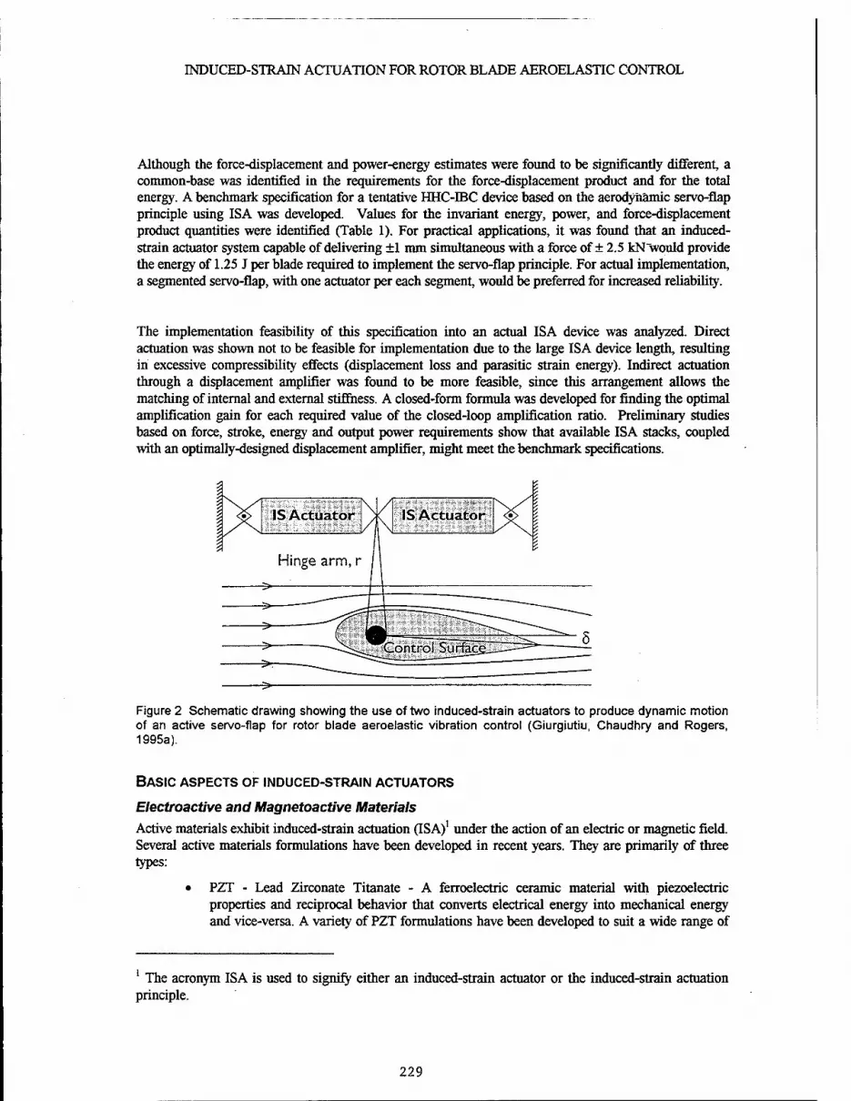
INDUCED-STRAIN ACTUATION FOR ROTOR BLADE AEROELASTIC CONTROL
Although the force-displacement and power-energy estimates were found to be significantly different, a common-base was identified in the requirements for the force-displacement product and for the total energy. A benchmark specification for a tentative HHC-IBC device based on the aerodynamic servo-flap principle using ISA was developed. Values for the invariant energy, power, and force-displacement product quantities were identified (Table 1). For practical applications, it was found that an induced- strain actuator system capable of delivering ±1 mm simultaneous with a force of ± 2.5 kN would provide the energy of 1.25 J per blade required to implement the servo-flap principle. For actual implementation, a segmented servo-flap, with one actuator per each segment, would be preferred for increased reliability.
The implementation feasibility of this specification into an actual ISA device was analyzed. Direct actuation was shown not to be feasible for implementation due to the large ISA device length, resulting in excessive compressibility effects (displacement loss and parasitic strain energy). Indirect actuation through a displacement amplifier was found to be more feasible, since this arrangement allows the matching of internal and external stiffness. A closed-form formula was developed for finding the optimal amplification gain for each required value of the closed-loop amplification ratio. Preliminary studies based on force, stroke, energy and output power requirements show that available ISA stacks, coupled with an optimally-designed displacement amplifier, might meet the benchmark specifications.
Figure 2 Schematic drawing showing the use of two induced-strain actuators to produce dynamic motion of an active servo-fiap for rotor blade aeroelastic vibration control (Giurgiutiu, Chaudhry and Rogers, 1995a).
BASIC ASPECTS OF INDUCED-STRAIN ACTUATORS
Electroactive and Magnetoactive Materials Active materials exhibit induced-strain actuation (ISA)1 under the action of an electric or magnetic field. Several active materials formulations have been developed in recent years. They are primarily of three types:
• PZT - Lead Zirconate Titanate - A ferroelectric ceramic material with piezoelectric properties and reciprocal behavior that converts electrical energy into mechanical energy and vice-versa. A variety of PZT formulations have been developed to suit a wide range of
1 The acronym ISA is used to signify either an induced-strain actuator or the induced-strain actuation principle.
229

GIURGIUTIU, CHAUDHRY, AND ROGERS
signal transmission and reception qualities. PZT-5 is one of the most widely used formulations for actuator applications.
• PMN - Lead Magnesium Niobate - An electrostrictive ceramic material with piezoelectric properties and reciprocal behavior that converts electrical energy into mechanical energy and vice-versa. Numerous PMN formulations have been developed to suit a wide range of signal transmission and reception qualities.
• TERFENOL - TER (Terbium) FE (Iron) NOL (Naval Ordinance Laboratory) - A magnetostrictive alloy consisting primarily of Terbium, Dysprosium, and Iron. This magnetostrictive material does not exhibit reciprocal behavior since it only converts electro- magnetic energy into mechanical energy. Various TERFENOL formulations have been developed. A commonly-used formulation is TERFENOL-D.
Construction of a PZT or PMN Stack Actuator An electroactive solid-state actuator consists of a stack of many layers of electroactive material (PZT or PMN) alternatively connected to the positive and negative terminals of a high-voltage source (Figure 1). Such a PZT or PMN stack behaves like an electrical capacitor. When activated, the electroactive material expands and produces output displacement. Typical strains for electroactive materials are in the range of 750-1200 urn/m.
The PZT or PMN stacks are manufactured by two methods. In the first method, the layers of active material and the electrodes are mechanically assembled and glued together using a structural adhesive. The adhesive layer stiffness is at least an order of magnitude lower than the stiffness of the ceramic. Since this effect lowers significantly the final stiffness of the stack, special care is given to obtaining as thin an adhesive layer as possible. In the second method, the ceramic layers and the electrodes are assembled in the "green" state, and then fired together (co-fired) under a high isostatic pressure (HTP process) in the processing oven. This process ensures a much suffer final product and, hence, a better actuator performance. However, the processing limitations, such as oven and press size, etc., limit the applicability of this process to small stacks only.
The stacks are surrounded by a protective polymeric or elastomeric wrapping. Lead wires protrude from the wrapping for electrical connection. Steel washers, one at each end, are also provided for distributing the load into the brittle ceramic material. When mounted in the application structure, these stacks must be handled with specialized knowledge. Protection from accidental impact damage must be provided. Adequate structural support and alignment are needed. Mechanical connection to the application structure must be such that tension stresses are not induced in the stack since the active ceramic material has very low tension strength. Hence, the load applied to the stack must always be compressive and perfectly centered. If tension loading is also expected, adequate pre-stressing must be provided through springs or other means.
Construction of a TERFENOL Actuator A magnetoactive solid-state actuator consists of a TERFENOL bar inside an electric coil and enclosed into an annular magnetic armature (Figure 2). When the coil is activated, the TERFENOL expands and produces output displacement. The TERFENOL material has been shown to be capable of strains up to 2000 pm/m, but with high nonlinear and hysteresis penalties. Practical strains employed by the manufacturers of TERFENOL actuators are in the range of 750-1000 um/m.
The TERFENOL-D bar, the coil, and the magnetic armature are assembled between two steel-washers and put inside a protective wrapping. This forms, according to manufacturer's terminology, a "drive motor actuator without pre-stress housing".
230
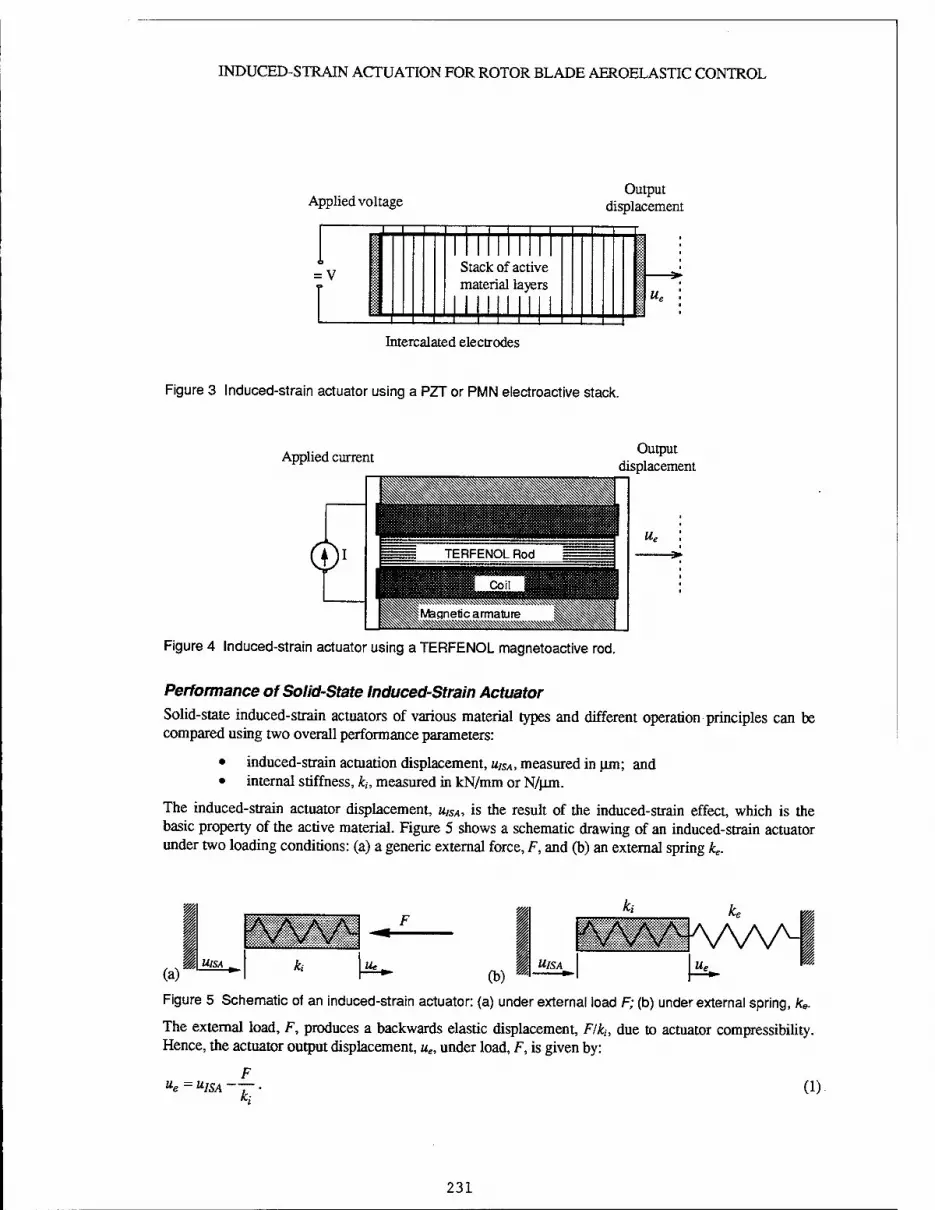
INDUCED-STRAIN ACTUATION FOR ROTOR BLADE AEROELASTIC CONTROL
Applied voltage Output
displacement
= V Stack of active material layers
JÜ Intercalated electrodes
Figure 3 Induced-strain actuator using a PZT or PMN electroactive stack.
Applied current Output
displacement
Figure 4 Induced-strain actuator using a TERFENOL magnetoactive rod.
Performance of Solid-State Induced-Strain Actuator
Solid-state induced-strain actuators of various material types and different operation principles can be compared using two overall performance parameters:
• induced-strain actuation displacement, UISA, measured in um; and • internal stiffness, kh measured in kN/mm or N/jxm.
The induced-strain actuator displacement, uISA, is the result of the induced-strain effect, which is the basic property of the active material. Figure 5 shows a schematic drawing of an induced-strain actuator under two loading conditions: (a) a generic external force, F, and (b) an external spring ke.
(a)' UlSA k K (b)
h
KVWW\AA UlSA I
Figure 5 Schematic of an induced-strain actuator: (a) under external load F; (b) under external spring, ke.
The external load, F, produces a backwards elastic displacement, F/ki, due to actuator compressibility. Hence, the actuator output displacement, ue, under load, F, is given by:
F "£="/SA-
ki (1)
231

GIURGIUnU, CHAUDHRY, AND ROGERS
If the external load, F, varies linearly with the output displacement, ue, one can assume an external spring, ke, as shown in Figure 5b. Thus:
F = ke-ue. (2)
After substitution and simplification, one gets an expression for the output displacement, ue, in terms of the stiffness ratio, r = kjkt, i.e.,
1 1+r «ISA- (3)
Output Energy of an Induced-Strain Actuator Under quasi-static conditions, the output energy is:
&e = 2e 'Ue ' (4)
0.75
Output energy 0 5 coefficient,£'e
0.25
1 1 1
A 11 III 1 1 1 1 1 1 Ml
1/ II / / 1 II 1 1 / üü\AA ,', II / — kj ke
/ ^Uv, y II
Stiffness mach
* ' point
II ^ i •*** —.-, .1
0.01 0.1 1 10
Stiffness ratio, r = kjki
100
Figure 6 Stiffness match principle for peak energy delivery from an induced-strain actuator.
Substitution of (3) into (4) yields the expression of output energy in terms of stiffness ratio, r;.
Ee(r) = - (1 + r)"
-(i*/«ZSO- (5)
A plot of the variable part of Equation (5), called the output energy coefficient E 'e (r) is given in
Figure 6. The function E 'e (r) is zero for both "free" (/•= 0) and "blocked" (r ) conditions, and has a maximum at r = 1. The r = 1 condition, with ke = kh is called "stiffness match", and identifies the maximum value of the output energy that can be delivered by an induced-strain actuator:
Eemax=j(2kiU!SA) (6)
Output Energy and Energy Density Comparison of Induced-Strain Actuators Figure 7a shows a plot of the output energy capabilities of various commercially-available induced-strain actuators of different sizes and operating principles. In order to attain a meaningful performance comparison, allowance for differences in volume and mass must be made. Dividing the actuator output energy by the actuator volume, one gets the volume-based output energy density (Figure 7b). Similar calculations made in terms of mass and cost give a complete perspective of the induced-strain actuators'
232

INDUCED-STRAIN ACTUATION FOR ROTOR BLADE AEROELASTIC CONTROL
performance for application in rotor blade solid actuation design (Giurgiutiu, Chaudhry, and Rogers, 1995b).
0.7000 -
o
CL :
_, 0.6000 -
tput
En
erg
y,
o
o
O 0.3000 •
E
1 0.2000 'S S 0.1000 •
o.oooo ■
s o i 2 •"•
, S o _ z ■? T o
!! : '. 1 E i 1111
Induced Strain Actuator Model Number (a*
Figure energy;
o*
5
■J E
11000 T
10.000
8.000
6.000
4.000 4R | §
2.000
0.000
5 3 i & o a J s 1 i g § E - "■
» K K d o.
X CM CM X 3
Induced Strain Actuator Model Number
7 Performance comparison for 15 commercially-available induced-strain actuators: (a) output (b) volume-based output energy density
HAHDIS SERIES ACTUATORS FOR ROTOR BLADE ACTIVE SERVO-FLAP CONTROL
The output displacement of present-day solid-state induced-strain actuators does not exceed the order of 100 um. To use such a small output in actual rotor blade servo-flap actuation, some means of displacement amplification is necessary. After considering several options, we found that the hydraulic amplification principle offers the best opportunities for achieving large output displacements, while satisfying the stiffness and irreversibiliry requirements for aeroelastic control. A device based on the hydraulic amplification principle also offers versatility for rotor blade installation, since the induced- strain hydraulic drive and the hydraulic output actuator, can be connected through conventional hydraulic lines, and can be placed in different locations inside the blade section to accommodate the geometric constraints. In our vision, such an induced-strain actuation system, based on hydrostatic principles, would be a self-contained sealed module, independent from the main aircraft hydraulic system.
To test the viability of our analysis, a full-scale proof-of-concept demonstrator, called a "Hydraulically amplified high displacement induced-strain" (HAHDIS) actuator, was designed and built in the Center for Intelligent Material Systems and Structures (CIMSS) at Virginia Tech (Figure 8). The HAHDIS proof-of-concept demonstrator was configured around a pair of high-power ISA devices with large free strain displacement, U!SA = 0.120 mm, and internal stiffness kt = 370 kN/mm, capable of delivering a maximum output energy, Ee = 0.666 J. To produce an output resistance to the actuator and to simulate real-life external stiffness, a load simulator was also designed and built. The load simulator consisted of a double-leaf spring connected to a movable airfoil. The linear displacement of the HAHDIS actuator was transformed in angular displacement through a hinge arm of 28 mm. This arrangement was expected to produce an angular motion of around ±2°, satisfying the initial requirements for an aeroelastic vibration control application1-2.
233

GIURGIUTIU, CHAUDHRY, AND ROGERS
Small output
piston Hydraulic
Ampllfl Leaf-Spring
Load Simulator
Dummy P247.70
ISA drivers
Large-piston
block
Small-piston
block
fffffjif^^
mmm asp W^^^mW^^^i mBBt't jMHNMfflfli mm ifmmJF^^Xi^^^m mM llili
WmmSSSStHfiiffl^^ .MMHIIIIIIIIIII(?HM
/ / \ Dummy P247.70
ISA drivers Connecting Rod 1:1 Scale
servo-tab
Figure 8 Layout and internal construction of the hydraulically-amplified high-displacement induced-strain (HAHDIS) actuator.
TESTING OF THE HAHDIS ACTUATOR
Testing of the HAHDIS actuator is currently underway in CIMSS laboratory. The HAHDIS actuator was fully instrumented with force, displacement, and pressure transducers, and was subjected to static and dynamic tests. In the static tests, ISA input to the actuator was simulated by the turning of screws placed on dummy ISA devices. The predicted behavior was observed. Angle output measurements of ±2° were obtained with ± turn of a d-24 UNF screw. These initial results confirmed the soundness of our design, and its capability for full scale applications. However, the existence of displacement losses was also identified. These losses appeared even under no-load conditions due to Coulomb friction between the piston seals and the cylinder bore, and due to compressibility of the conventional rubber seal construction. These losses produced an effective amplification ratio under no-load condition of about 14 times, which is only 87.5% of the 16 times design ratio.
For dynamic testing, four E300-P4 PMN stacks were acquired from EDO Corp. and installed in pairs at the reciprocal-acting input cylinders of the HAHDIS device. The PMN stacks were energized with a pair of high-voltage sinusoidal signals (400±400 V) produced by a dual-channel model 50/750 TREK high- voltage amplifier. The two signals are in opposite phase, though maintaining the same bias. This arrangement permits that as one stack expands, the other retreats, and vice-versa. The hydraulic fluid is sent back-and-forth to the "in" and "out" chambers of the output cylinder, thus producing alternating motion.
During dynamic tests, a frequency range between 1 Hz and 20 Hz was explored. Discrete frequencies of 1 Hz, 2 Hz, 3 Hz, 5 Hz, 10 Hz, 15 Hz, 18 Hz, and 20 Hz, were sampled. At each frequency, data collection was done with the VTDEE software using a sampling rate of 100 Hz. The data was stored in the computer memory into an MS-EXCEL 5.0 file. For quick reference, captures and print-outs of the data screen were also performed. The sampled data consisted of the input and output displacements, u ,u , and u , and of the pressures in the two chambers, pj and p2. Figure 9 presents an example of the
displacement and pressure data captured at 1 Hz over the 2-second time period. The effects of the approximately 14 times displacement amplification are clearly illustrated: the small input displacement signals shown at the bottom of the graph are amplified into the very large output signal shown in the upper portion of the graph. It should be noted that the same displacement calibration factor of 1.3089
234
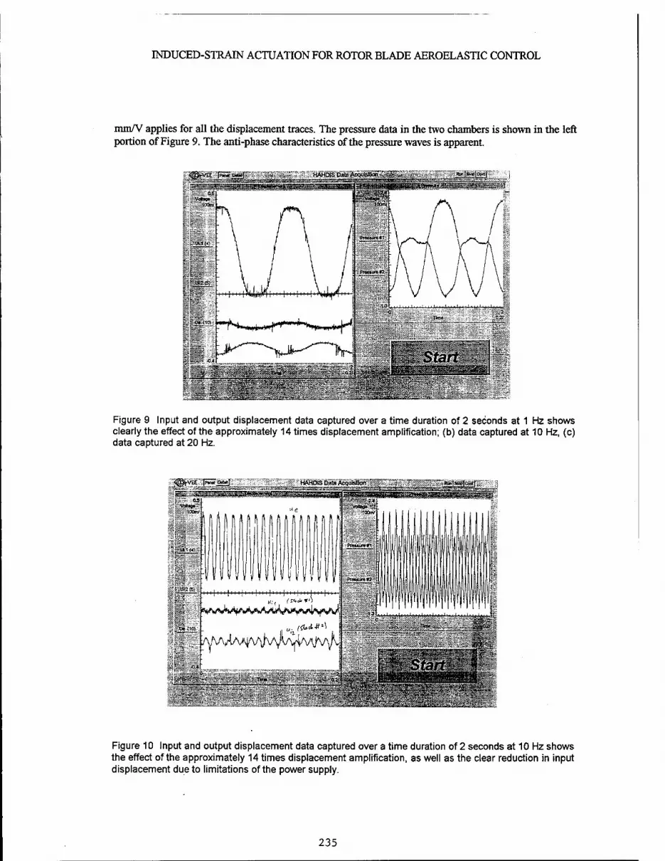
INDUCED-STRAIN ACTUATION FOR ROTOR BLADE AEROELASTIC CONTROL
mm/V applies for all the displacement traces. The pressure data in the two chambers is shown in the left portion of Figure 9. The anti-phase characteristics of the pressure waves is apparent.
"(Si"auj HAIHJiS Data Acquc'lion iZJ^Ll*!.
"»■'-
i7apsaa^aw«HC^BjBray7i»«w-?-ya;r:.-'--' ■■: ■-: ■■: ■■.i
!*'>_■ ."'Ä-llaiiy "IMJ
»«F
PrawurefS?»
Figure 9 Input and output displacement data captured over a time duration of 2 seconds at 1 Hz shows clearly the effect of the approximately 14 times displacement amplification; (b) data captured at 10 Hz, (c) data captured at 20 Hz.
trvit' |SMM»|:
HAHDiS Data Acqufefilon
l-"l'"i"'l'
Figure 10 Input and output displacement data captured over a time duration of 2 seconds at 10 Hz shows the effect of the approximately 14 times displacement amplification, as well as the clear reduction in input displacement due to limitations of the power supply.
235

GIURGIUTIU, CHAUDHRY, AND ROGERS
The pressure calibration factor was 200 psi/V. The pressure in the hydraulic chambers #1 and #2 has static-bias components of 292 psi and 331 psi, and dynamic components of 78 psi and 95 psi, respectively. The fact that the dynamic components of the hydraulic pressures are similar in magnitude and of opposite phase illustrates the satisfactory operation of the device.
Figure 10 presents an example of the displacement and pressure data captured at 10 Hz over a 2-second time period. It is noted that the input displacements have decreased considerably due to the power limitations of the model 50/750 TREK high-voltage power amplifier. However, the effect of the displacement amplification is clearly illustrated: the very small input displacement signals shown at the bottom of the graph are amplified into the very large output signal shown in the upper portion of the graph. At this frequency, the displacement amplification ratio was found to be approximately 15.5 times, which is very close to the design value of 16 times. It is believed that this good response is partly due to the beneficial effect from a possible external system resonance, which clearly reduces the effective output load. However, the stable and controllable behavior of the device under resonance conditions is an added merit of the HAHDIS concept.
Figure 11 presents an example of the displacement and pressure data captured at 20 Hz over a 2-second time period. It is noted that, due to the power limitations of the model 50/750 TREK high-voltage power amplifier, the input displacements have decreased so much that they have become a mere ripple, as shown at the bottom of the graph. However, due to the powerful displacement amplification, a sizable output displacement is still observed. This illustrates once again the benefits of the HAHDIS design concept.
<^VEE [S*a~|
Figure 11 Input and output displacement data captured over a time duration of 2 seconds at 20 Hz shows that the approximately 14 times displacement amplification can produce sizable output waveform from almost imperceptible input displacement.
Figure 12 shows the frequency response curve for the interval 1 to 20 Hz. The output displacement response amplitude, ue, has a moderate decrease up to 10 Hz, and a very rapid decrease afterwards. Examination of the average input displacement curve, «,- ? shows that it is also decreasing.
236

INDUCED-STRAIN ACTUATION FOR ROTOR BLADE AEROELASTIC CONTROL
Additional examination of the oscilloscope data during the experiment showed that the high-voltage signal provided by the model 50/750 TREK amplifier started to become angular below 10 Hz, indicating that the upper limit of the amplifier performance has been reached. Above 10 Hz, the "amplifier signal deteriorated much faster, and its amplitude rapidly decreased. Thus, the decreased input voltage resulted in decreased input displacement to the device, and explains the observed decrease in output amplitude. When we compensated for the loss of input displacement, the output displacement curve"l>ecame almost
flat, with a peak at 10 Hz (curve ue in Figure 12). This proves the effectiveness of the HAHDIS principle. It is also clear that, with higher power stacks and high-voltage amplifiers, a flat frequency response will be attained up to the design frequency of 25-30 Hz.
0.8
0.6
u, mm
0.4
0.2
o
o ©
1 I Compensated output
displacement, u* e
\..
Output displacement, u
Averaged input displacement, u ; 0 » s " D n ..
0 O
_L f g s s e % On*
10 f.Hz
15 20
Figure 12 Frequency response curves of the HAHDIS actuator, showing its good performance over the frequency range 1-20 Hz in spite of the input displacement decrease due to limitations in the high-voltage power supply.
CONCLUSIONS
The feasibility of solid-state actuation of a helicopter servo-flap for rotor blade active control was studied theoretically and experimentally. Induced-strain actuators and hydrostatic amplification principles were adopted. A full-size hydraulically-amplified high-displacement induced-strain (HAHDIS) proof-of- concept demonstrator was designed and built. The HAHDIS demonstrator has undergone static and dynamic tests in CMSS laboratory. Due to the high cost of the induced-strain equipment, reduced-power induced-strain stacks and ancillary electronics were employed, and no external load was applied. In spite of the power limitations of the equipment, the signal captured and the frequency response curve in the
237

GIURGIUTIU, CHAUDHRY, AND ROGERS
range 1-20 Hz showed excellent confirmation of the theoretical analysis, and irrevocably proved the feasibility of the HAHDIS concept. Further dynamic tests are proposed with full-power equipment to prove a flat dynamic response curve up to the design frequency of 25-30 Hz, with realistic external loading. In parallel, an improved design, HAHDIS Mk2, is underway. HAHDIS Mk2 will be free from internal friction losses, and will adopt a modular design. The HAHDIS Mk2 design will be configured for rotor blade installation and will fit into the space and geometry constraints of a typical helicopter blade.
ACKNOWLEDGMENTS
The authors gratefully acknowledge the support of the Army Research Office - University Research Initiative Program, Grant No. DAAL03-92-O181, Dr. Gary Anderson, Program Manager.
REFERENCES
Ben-Zeev, O., Chopra, I., "Development of an Improved Helicopter Rotor Model with Smart Trailing Edge Flaps for Vibration Suppression", 1995 SPIE North American Conference on Smart Structures and Materials, Smart Structures and Integrated Systems, 26 February - 3 March 1995, San Diego, CA, Paper # 2443-01 (in press).
Giurgiutiu, V., Chaudhry, Z., Rogers, CA., 1995a, "Stiffness issues in the Design of ISA Displacement Amplification Devices: Case Study of a Hydraulic Displacement Amplifier", Smart Structures and Materials '95, San Diego, CA, 26 February -3 March 1995, Paper # 2443-12 (in press).
Giurgiutiu, V., Chaudhry, Z., Rogers, C.A., 1995b, "Effective Use of Induced-strain Actuators in Aeroelastic Vibration Control", Proceedings of the Adaptive Structures Forum, 35th AIAA/ASME/ASCE/AHS/ASC Structures, Structural Dynamics, and Materials Conference, New Orleans, LA, April 13-14, 1995, Paper # AIAA-95-1095.
Giurgiutiu, V., Chaudhry, Z., Rogers, CA., 1995c, "Engineering Feasibility of Induced-Strain Actuators for Rotor Blade Active Vibration Control", Journal of Intelligent Material Systems and Structures, Technomic Pub. Co., September 1995.
Giurgiutiu, V., Chaudhry, Z., Rogers, C. A., 1995d, Energy-Based Comparison of Solid-State Actuators, Micro- Integrated Smart Materials and Structures Conference, Williamsburg, VA, October 11-12, 1995.
Giurgiutiu, V., Chaudhry, Z., Rogers, CA., 1994c, "The Analysis of Power Delivery Capability of Induced-strain Actuators for Dynamic Applications", Proceedings of the Second International Conference on Intelligent Materials, ICIM'94, June 5-8, 1994, Colonial Williamsburg, VA, Technomic Pub. Co., Inc., 1994, pp. 565-576.
Hall, S. R., and Prechtl, E. F., 1995, "Development of a Piezoelectric servoflap for helicopter rotor control", in Active Materials and Smart Structure, Proceedings of the Symposium, Texas A&M University, College Station, TX, October 10-12, 1994 (A95-23026 05-39), Bellingham, WA, SPIE Proceedings Vol. 2427, 1995, pp. 16-19.
Librescu, L., Rogers, CA., and Song, O, 1992, "Static and Dynamic Behavior of Adaptive Aircraft Wing Structures Modeled as Composite Thin-Walled Beams", Proceedings of the 6th Japan-US Conference on Composite Materials, Grosvenor Resort, Orlando, Florida, June 22-24, 1992, Technomic Pub. Co., Inc., 1992, pp. 713-724.
Millott, T. A., and Friedmann, P.P., 1992, " Vibration Reduction in Helicopter Rotors Using an Active Control Surface Located on the Blade", Proceedings of the AIAA/ASME/ASCE/AHS/ASC 33rd Structures, Structural Dynamics, and Materials Conference, Dallas, TX, April 1992, paper AIAA-92-2451-CP, pp. 1975-1988.
Song, O., Librescu, L., 1993, "Vibration Behavior of Rotating Helicopter Blades Incorporating Adaptive Capabilities", Proceedings of SPIE 1993 North American Conference on Smart Structures and Materials, Albuquerque, 1-4 Feb., 1993, pp. 354-365
Straub, F. K., and Merkley, D. J., 1995, "Design of a Smart Material Actuator for Rotor Control", 1995 SPIE North American Conference on Smart Structures and Materials, Smart Structures and Integrated Systems, 26 February - 3 March 1995, San Diego, CA, Paper # 2443-10 (in press).
238

ROBUST CONTROLLER DESIGN OF A WING
WITH PIEZOELECTRIC MATERIALS FOR FLUTTER
SUPPRESSION
C. Nam and J.-S. Kim Hankuk Aviation Universit;
Kyung-gi, KOREA
Abstract
Active flutter suppression system is designed of a composite plate wing model using the reduced or- der model. The analysis for a laminated composite wing with segmented piezoelectric sensor /actuator pairs is conducted by Ritz solution technique. Unsteady aerodynamic forces calculated by Doublet lattice method are approximated as the transfer functions of the Laplace variable by Minimum State method. Among the aerodynamic states obtained from rational function approximation, only one aerodynamic state is included in the plant model for feedback purpose. The neglected aerodynamic states are regarded as the modeling error. The control system uses the integrated and collocated piezo- electric self-sensing actuator pairs so as to prohibit the non-minimum phase model and the spillover due to the unmodeled dynamics. Based on the mixed-sensitivity H^ control method, the control parameters are determined. Using a simple wing model, the performance of the controlled system is shown in the frequency and time domain, respectively. The electric current and the power requirement for aeroelastic control are also predicted.
1. Introduction There has been a considerable amount of research activity to use piezoelectric materials as sen-
sor/actuators for the response control of structures. The piezoelectric materials generate an electrical charge(direct effect) in proportion to the applied mechanical forces and vice versa(converse effect). Due to the direct and converse effects of piezoelectric materials, the intelligent structure which is defined as a structure with the integrated sensor/actuator system is possible. The application of the intelligent structure by the use of sensor/actuator shows the potential to enhance the structural performance as well as reliability. Recently, Zhou at al.[l] developed a theoretical model to predict and analyze the power requirement and power consumption of the system. They also conducted the experiment and verified their analytical results.
A lot of investigators[2, 3, 4, 5] have studied the static and dynamic aeroelastic control of wing structure with piezo actuators and demonstrated the feasibility of the application of piezoelectric ma- terials. The application of piezoelectric materials to aeroelastic control may provide a new dimension in design to eliminate the instability by changing wing configuration to cause lift distribution varia- tion. The optimization technique was applied to find the best geometry of the piezo actuators for the aeroelastic control[6, 7, 8].
Based on the results of our previous study[6, 8], a robust controller is designed for active flut- ter suppression using the reduced order model. The analysis for a laminated composite wing with segmented piezoelectric sensor/actuator pairs is conducted by Ritz solution technique. The active control system design for flutter suppression requires the equation of motion to be expressed in a linear time-invariant state-space form. Doublet lattice method is used to compute unsteady aerodynamic forces, which are approximated as the transfer functions of the Laplace variable by Minimum State method combined with optimization technique. In order to design an active control system efficiently,
239

C. Nam & J. Kim
the plant should be modeled accurately. However, this requires to increase the number of state vari- ables for the rational function approximation of the unsteady aerodynamic forces. There is always a trade-off between the cost for real-time implementation and performance of the controlled system. Among the aerodynamic states obtained from rational function approximation, only one aerodynamic state is included in the plant model for feedback purpose. The neglected aerodynamic states are regarded as the modeling error. The control system uses the integrated and collocated piezoelectric self-sensing actuator pairs so as to prohibit the non-minimum phase model as well as the spillover due to the unmodeled dynamics. Based on the mixed-sensitivity i?«, control method, the control parameters are determined. This method enables not only the disturbance attenuation specification but also the stability margin specification with the unstructured modeling error, which are combined into a single infinity norm specification^, 10]. Using a simple wing model, the performance of the controlled system is shown in the frequency and time domain, respectively. The electric current and the input control voltage which are required for aeroelastic control are also examined.
2. Modeling of the wing structure Based on the classical laminated plate theory, the equations of motion of a model with piezo
actuators are formulated. For the design of the flutter suppression system, a composite wing model which has four pairs of the self-sensing piezoelectric actuators on the surface is considered as shown in Fig. 1. Model is assumed to be a symmetric laminated plate and has the same size of the surface bonded piezoelectric materials on the top and bottom of plate at the same location.
The linear coupled electromechanical constitutive relations of a piezoelectric materials can be written as;
{D} = [d]T{T}+[£T]{E} (La)
{S}=[sE}{T} + [d]{E} (1.6)
{5} is the strain, {T} is the stress, {£>} is the electric displacement, and {E} is the electric field intensity, [d], [eT], [sE] denote the piezoelectric constant, dielectric constant, and elastic compliance matrix, respectively. It is assumed that the "3" axis is associated with the direction of poling and the mechanical property of the piezoelectric materials is modeled as an isotropic material. For the thin plate shape of the piezoelectric materials, we can rewrite Eq. (1).
D3 = [d31 d32 OJ [axx CTyy axy\T + elzE3 (2.o)
(2.6) «11 «12 0
«12 «22 0 0 0 S66
where «fei = dw The electric charge which is the output signal can be obtained by integrating the electric displacement D3 with respect to the area of piezo actuators. The electric current is calculated by taking derivative of the charge with respect to time.
Strain energy and kinetic energy of the composite wing model with piezoelectric actuators can be expressed as;
° - uLy4äS]{I}**-/JOM'-}*■* (3>
p(u2 + v2 + w2)dx dy (4) 2 J A,> where A, Av represent area of composite plate and piezoelectric actuator, respectively, {e}, {K} are the midplane strain and curvature. [As], [Ds], and [Bs] are extension, bending, and extension/bending coupling stiffness matrices, respectively. {N\} and {MA} are inplane forces and moments due to actuator strain. u,v,w are displacements in x, y, z direction. The virtual work due to aerodynamic forces is
6WA= / / p(x,y)6w(x,y,t)dxdy (5)
240

Robust Controller Design of a Wing with Piezoelectric Materials
where p(x, y) is the pressure. The aerodynamic force is calculated using the doublet-lattice method[ll] for Mach 0.8 and 15 reduced frequencies ranging from 0 to 1.5. For calculation of the pressure distribution on an oscillating plate wing undergoing simple harmonic motion, the plate wing is divided into total 50 panels arranged 10 in the spanwise direction and 5 in the chordwise direction.
The Ritz solution technique assumes the deflection shapes for the wing structure. In this paper, it is assumed that the same magnitude but the opposite direction of electric field is applied to the piezoelectric material so as to create a pure bending moment for flutter control. With this assumption, the inplane displacements can be neglected. The out-of-plane displacement w(x, y, t) on the model is represented as a set of polynomial functions and written as;
n
w(x,y,t)=y£2zk{x,y)qk(t) (6) fe=i
The displacement functions Zk(x,y) are assumed as products of polynomial in x and y directions. The assumed displacement functions are chosen to satisfy the geometric boundary conditions for a wing clamped at the root.
Zk(x,y) = (1^—)i(Tr-)j, i = 0,l,2,3,..., j = 2,3,4,5,... (7) ■A-max * max
where Xmax and Ymax are constant normalization length. These are defined as the root chord and span, respectively. Using these displacement expressions, the strain energy and kinetic energy are written in matrix form;
U = \{q}T[Ks]{q}-[QA\{q} (8)
T = \{q}T[Ms){q} (9)
where {QA} is [Fj,]{u}. [Fp] is the control force matrix due to unit electric voltage, and {u} is the applied voltage. The virtual work in the generalized coordinate is 8WA = QA^II The generalized aerodynamic force {QA} is expressed as gd[.A]{g}. <jy is the dynamic pressure, [A] is the unsteady aerodynamic force matrix.
Lagrange's equation results in a set of ordinary differential equations of motion. After the vibration analysis, a model reduction is performed using first 6 vibration modes to obtain a set of equations of motion in modal coordinates. Then, the reduced equations of motion is as following form;
[Ms}{q} + [Ks]{q} = [Fp]{u} + qd[Ä]{q} (10)
[Ms](= [Mcomposite. + Mpie.zo]) and [Ks](= \Kcomposite. + KpiRZ0\) are respectively the generalized mass and stiffness matrices including the effect of the piezoelectric actuators placement.
The output vector {J/Q} is written as;
{VQ} = ks I D3 dx dy = ks [Fp]T {q} + ks [D] {u} (11) JApi
where ks is the gain of the charge amplifier. From Eq. (2), the observation matrix is proportional to the transpose of the control matrix. [D] is the diagonal matrix and the components of [D] are given as;
Du = ¥* (&-¥*&)> d3! = d32 (12) tpi \ 1 fp J
where vv and Ep are the poisson's ratio and Young's modulus of the piezoelectric materials, APi, tPi is the area, thickness of the i — th piezoelectric actuator. The electric currents flowing through the piezoelectric actuators can be obtained by taking time derivative of the electric charge stored due to
241

C. Nam & J. Kim
the direct effect of the piezoelectric materials. Since /, JAvi
'3 dx dy, the current vector is written
as; ■ft -\T {I}=[Fp]1{q} + [D}{ü} (13)
For aeroservoelastic analysis and design, it is necessary to transform the equations of motion into the state space form. This requires approximating the unsteady aerodynamic forces in terms of rational functions of the Laplace variable. There are several methods for the rational function approximation(RFA), but RFA always causes an increase in the total number of states due to the addition of augmented aerodynamic states to represent unsteady aerodynamic forces accurately. In this study, Minimum State method[12] combined with optimization technique is adopted for the rational function approximation, since the increase in the size of the augmented aerodynamic state is smaller than any other methods.
Minimum State method[12] approximates the aerodynamic force matrix by
[Äap(S)) = [Äo] + [Ä,]s + [Ä2]S2 + [D'a][sl - RT'iEa}* (14)
where the nondimensionalized Laplace variable s = (sb/V), V is the airspeed, b is the semi chord, and s is the Laplace variable. The components of the diagonalized matrix [R'a] are negative constants which are selected arbitrarily. For given [R'a] matrix, [Äo], [Äi], [Ä2], [D'a], and [Ea] are determined by using repeated least-square fit.
Using Eq. (14) for the RFA and the state vector {xf}T = [q q qa\, the state equation (full model) which includes the effects of piezoelectric control forces is expressed as follows;
{i/}=[i/]{x/}
iVf} = [Cf] {*/}
+
+ Df
{«}
{«}
where
M- [o] [/]
[0] [Ea]
[0]
[Ra]
[Da
B,
Cf
[0]
[0]
fe.fö]T[o][o]]
Dt = [0]
(15)
(16)
(17.o)
(17.6)
(17.c)
(17.d)
The detailed expressions for [M], [B], [K], [Da], and [Ra] can be found in Ref. [8]. qa is the aerodynamic state vector. If [R'a] is set to be a m x m matrix, the total number of states is 12 + m. A total of 6 components of [JR^J matrix are used for the RFA. Therefore, the dimension of the state vector is 18.
3. The robust controller design 3.1 Reduced order model
Since the system matrix is a function of the dynamic pressure, it is necessary to choose the design air speed for designing control system. The approximation of high order plant and controller models by models of lower order is an integral part of control system design. Complicated plant models lead to high order controllers and the difficulties associated with implementing them. The reduced order models simplify the process of understanding the design limitations. Also, the controller synthesis computations will be faster and require less memory. In this study, model reduction is performed to truncate unimportant states from the full state model. The aerodynamic stiffness, damping, mass
242
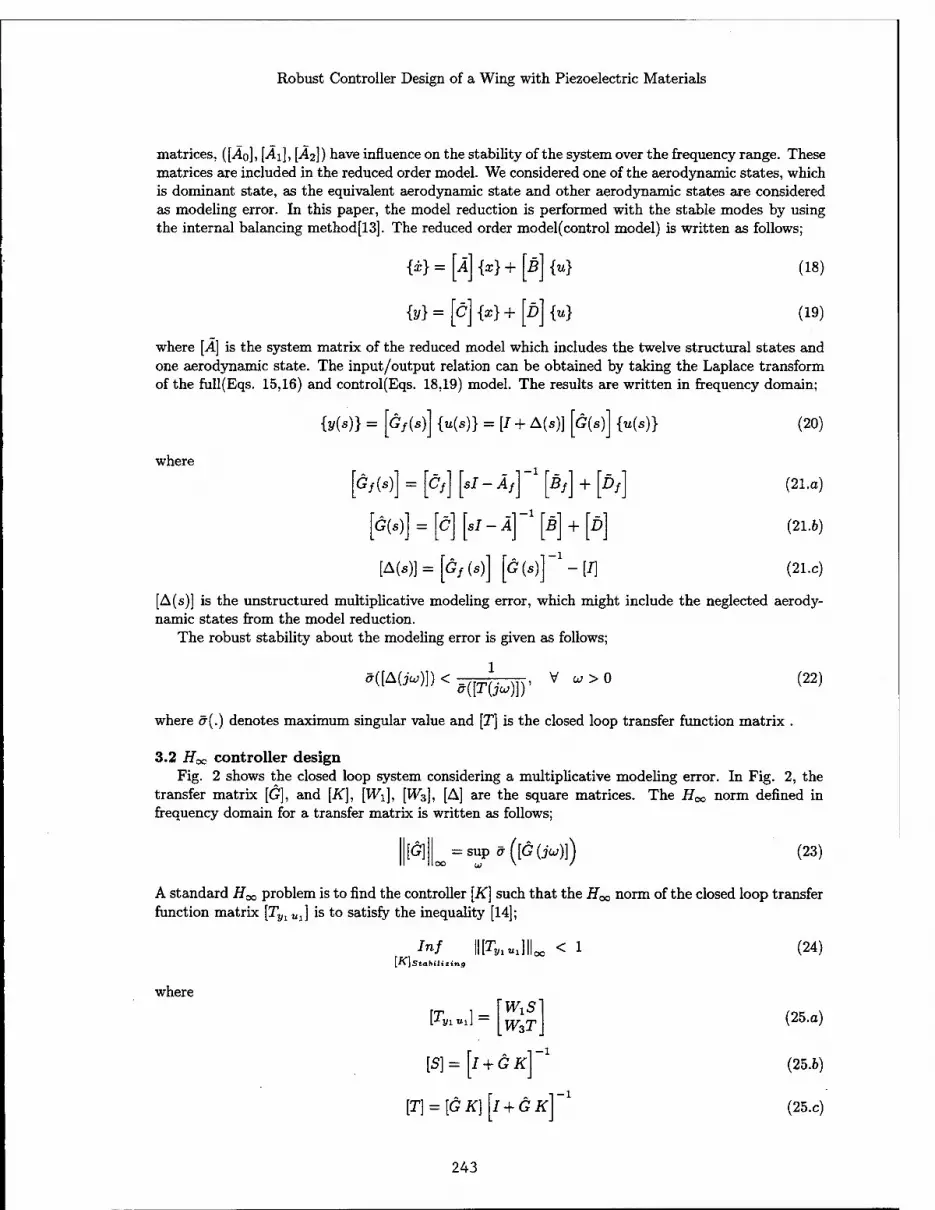
Robust Controller Design of a Wing with Piezoelectric Materials
matrices, ([ÄQ], [ÄI], [Ä2]) have influence on the stability of the system over the frequency range. These matrices are included in the reduced order model. We considered one of the aerodynamic states, which is dominant state, as the equivalent aerodynamic state and other aerodynamic states are considered as modeling error. In this paper, the model reduction is performed with the stable modes by using the internal balancing method[13]. The reduced order model(control model) is written as follows;
{i}=[i]{x}+[s]M
{y}=[c] {*}+[£]{«}
(18)
(19)
where [A] is the system matrix of the reduced model which includes the twelve structural states and one aerodynamic state. The input/output relation can be obtained by taking the Laplace transform of the full(Eqs. 15,16) and control(Eqs. 18,19) model. The results are written in frequency domain;
{y(s)}= Gf(s) {u(s)} = [I + A(s)} G(s) {u(s)}
where
[<?,(*)] = [c,][5J-i/]~ [£/] + [£/]
[ö(*)] = [c'][5J-i]"1[ß] + [ö]
{A(s)}=[Gf(s)] [6(s)]~ -[/]
(20)
(21.a)
(21.6)
(21.c)
[A(s)] is the unstructured multiplicative modeling error, which might include the neglected aerody- namic states from the model reduction.
The robust stability about the modeling error is given as follows;
c([A(jw)}) < 1
V a; >0 *(PW1)
where ä{.) denotes maximum singular value and [T] is the closed loop transfer function matrix
(22)
3.2 Hx controller design Fig. 2 shows the closed loop system considering a multiplicative modeling error. In Fig. 2, the
transfer matrix [G], and [K], [Wi], [W3], [A] are the square matrices. The Hoc norm defined in frequency domain for a transfer matrix is written as follows;
[G]\ =supff([G(jw)]) (23)
A standard H^, problem is to find the controller [K] such that the H^ norm of the closed loop transfer function matrix [Tyi Ul] is to satisfy the inequality [14];
Inf ||[TBlBl]||e [K]stabilixing
< 1
where
l-*!/i«iJ — W3T
[S} = I + GK -1
[T] = [GK] I + GK
(24)
(25.0)
(25.6)
(25.c)
243

C. Nam & J. Kim
The infimum is chosen over all stabilizing controllers [K]. [Wx] and [W3] are the weighting matrices for the performance and robustness. [S] is the sensitivity matrix, [T] is the closed loop complementary sensitivity matrix. The singular values of [S] determine the disturbance attenuation as well as the tracking performance about the reference input. The singular values of [T] denote the robustness of the closed loop system about the modeling error. Since [S] and [T] should satisfy the following equation;
[S(s)] + [T(s)] = [I\, (26)
the weighting matrices [W\], [W3] are to be chosen to satisfy the following;
äilWiiJwT^+ädWsiJu)}-1) > 1, Vw>0 (27)
In this paper, [Wi] 1 and [W3] 1 are selected to take account of not only the disturbance attenuation performance at low frequency region but also the robust stability at high frequency region;
»»•'ME'-TtOT WM"?"* i = w'i (28)
where 7, ki, k3, rd, rn are the constants which are given arbitrarily. The augmented plant [P](see Fig. 2) with the weighting functions can be written as the following by applying appropriate similar transformation;
A(j B\ Z?2 Ci Du Du C2 D21 D22
[P(s)} =
where [Du] = {D22} = [0], [D{2] = [D2l] = [0 /], [D&d] = [0], lBiDl2] = [0]
The 2-Riccati method[14] is used to find a stabilizing feedback control law;
{u2(S)} = [K(s)}{y2(s)}
The controller transfer function [.fir(s)] is written;
[K(s)} = Ac
Cc
Bc
Dc
(29)
(30)
(31)
(32)
where
[Ac] = [A0] + ([Bi] [Bf - [B2] [B2)T) [P] + ([/] - [Q] [P])"1 [Q] [C2\T [C2]
m = ([I}-[Q}[P})-l[Q}[C2]
[CC\ = -[B2]T[P]
[Dc] = [0]
[P] [Ao] + [A0f [P] - [P] ([B2] [B2]T - m [Brf) [P] - [d]T [d] = [0]
[Q] [A0]T + [A0] [Q] - [Q] {[C2]T [C2] - [CX]T [C,]) [Q] - [B,] [B.f = [0]
Amax([Q][P]) < 1
[P], [Q] are the positive semidefinite matrices. The MATLAB Toolbox is used to solve this problem. The electric currents required for aeroelastic control are calculated in this paper. When the voltage
{u} applied to the actuators and the measured current {/} are
{u} = {V0}sin(wt), {/} = {I0}sin(wt + <j>),
the admittance matrix [Y] of the model can be written as
PW]=J« Cf\ [jul - Äf] 1 \BS + Dt /ks=jv[Gf{ju)]/ks
(33.o,6)
(34)
244

Robust Controller Design of a Wing with Piezoelectric Materials
For the calculation of the electric current, it is assumed that the forces {ur} are exerted on the surface of self-sensing actuator as the following;
{ur} = {Vr}sin(u)t) (35)
The required electric current can be obtained as;
{/o} = [I+G}{ju)K{ju)\-l\Y{3w)\{Vr} (36)
4. Numerical examples A simple wing model is used to design the control system for flutter suppression. Wing is idealized
as a laminated plate model with four sets of the segmented piezoelectric materials as shown in Fig. 1. The laminate has six symmetric layers, [105/±45]s and each layer has uniform thickness, which is 0.02 inch. It is assumed that a set of actuators is bonded on both top and bottom surfaces of the laminated plate to generate a pure bending force for control. Each piezo sensor/actuator is sized 1.5 x 3.0 inches. Thickness of the piezoelectric materials is 0.005 inch, which is about 4.2% of the plate thickness. The material properties of the composite materials and piezoelectric materials are given in Table 1. In this paper, two models with different locations of the piezo sensors/actuators are considered. In the first model(CASE 1), the piezoelectric materials are placed at pzx(i) =0.5, 0.5, 3.5, 3.5 inches and pzy(i) =1.0, 7.0, 1.0, 7.0 inches, respectively. A model with the actuator locations which have been obtained through the optimization technique subject to minimize the control performance index is considered as a second model(CASE 2) [8]. The x and y coordinates of the second model are pzx{i) =0.000, 0.003, 4.496, 2.354 inches and pzy(i) = 0.000, 9.000, 0.000, 8.192 inches. For CASE 1, open loop flutter analysis is conducted and flutter is occurred at about 615fps(feet/sec) by the torsional mode, w/ = 57J?z[8]. CASE 2 model also has almost the same open loop flutter speed as CASE 1. The design airspeed required for the control system design is set to be VDBSIGN = 800/ps.
Fig. 3 shows the maximum and minimum singular values of the different models, which are the full model(18 states), reduced model with one aerodynamic state(13 states), and reduced model without aerodynamic states(12 states), respectively. As shown in figure, the differences between the full model(18 states) and the reduced model(13 states) are negligible over all the frequency range. However, when the aerodynamic states are neglected for the model reduction(12 states), the error becomes larger. The reduced model with 12 states is not adequate for the control system design.
The parameters in weighting matrices [Wi] and [W3] are chosen to meet the given design specifica- tion. These are kx = 0.1, rd = 5.305 x 10⁻³, rn = 2.653 x 10~4, k3 = 3.142 x 10³. 7 is the parameter on which we iterate for design. The frequency response of [Wi]-1 and [W3]-1 are shown in Fig. 4. The imposed design specifications are;
1. The error due to disturbance should be attenuated at least 1/10 in the specified frequency range from 0 to 30 Hz after feedback loop is closed.
2. The control loop bandwidth should be 500 Hz with -20db/decade roll-off above the specified frequency range.
The singular values of the sensitivity function [5] and the complementary sensitivity function [T] of the closed loop system are shown in Fig. 5. For this plot, 7 is set to be 1.1. Those are nearly coincident with their associated weighting functions [Wi]_1 and [W3]-1, respectively. That means that the specified value of 7 is close to the optimal value.
Fig. 6(a) and 7(a) show the step response when the unit step reference input is exerted on the actuator 1 (placed at inboard & leading edge direction of the model) for each case. In both cases, the outputs track the reference inputs without excessive overshoot. The result of CASE 2(Fig. 7) shows better response characteristics than those of CASE l(Fig. 6). In order to see the required power for control, the electric voltages and currents are calculated and the results are also shown in Fig. 6 and 7((b),(c)). There is a substantial amount of difference in applied voltages between two models,
245

C. Nam & J. Kim
although the difference in the electric currents is negligible. Therefore, the second model(CASE 2) needs less electric power and also shows better control performance.
When the force of the unit magnitude {Vr}j which is equivalent to 1 Volt actuation is exerted harmonically on the j — th actuator, the required electric currents are equal to the frequency response functions which represent the relations between the disturbance forces and the electric currents. The magnitude of the frequency response function matrix(Eq. (36)) is plotted in Fig. 8. Note that Fig. 8 represents the apparent value of {Io}i/{Yr}j- Therefore, the real dissipative currents are less than the presented values. The diagonal elements are somewhat larger than the off-diagonal terms due to the dielectric terms. The currents become larger at near natural frequency. But the magnitudes are less than —60 db in the frequency range from 0 to 400 Hz. Therefore, the required power per actuator will be less than 10 Watts, if the disturbance forces are 100 Volts in magnitude.
Fig. 9 shows the root loci for the closed loop when the control system is designed by using H^ theory with design velocity VQESIGN = 800/ps. Figure indicates that the system is stable up to the speed of 1000/ps. The increase in the nutter speed compared with the open loop system is remarkable. The figure also show that the control system is robust on the unmodeled dynamics although only one aerodynamic state is included in the reduced order control model.
5. Summary In this paper, a control system is designed for flutter suppression of a composite wing using seg-
mented piezoelectric self-sensing actuators. The control system uses the integrated and collocated piezoelectric self-sensing actuator pairs so as to prohibit the non-minimum phase model and the spillover due to the unmodeled dynamics. The reduced order model is developed in order to design active flutter suppression system. One of the aerodynamic states, which is dominant state, is consid- ered as the equivalent aerodynamic state and other aerodynamic states are considered as modeling error. In this paper, the model reduction is performed with the stable modes by using the internal balancing method. Based on the mixed-sensitivity fT«, control method, the control parameters are determined. For a given simple wing model, the performance of the controlled system is shown in the frequency and time domain. Although the optimization is not performed to find the geometry of the piezoelectric materials in this paper, it was found that CASE 2 which has been found from the previ- ous optimization study has better response characteristics. The electric current and the electric power which are required for aeroelastic control are predicted. Further study might be needed concerning the power requirement for aeroelastic control using the realistic wing structures.
References
1 Zhou, S., Liang, C, Rogers, C.A., "Coupled Electro-mechanical Impedence Modeling to Predict Power Requirement and Energy Efficiency of Piezoelectric Actuators Integrated with Plate-like Structures," AIAA Paper No. 94-1762, Proceedings of the AIAA/ASME Adaptive Structures Forum, SC, April 1994.
2 Ehlers, S.M., Weisshaar, T.A., "Effects of Adaptive Material Properties on Static Aeroelastic Control," AIAA Paper No. 92-2526, Proceedings of the 33th Structures, Structural Dynamics and Material Conference, TX, April 1992.
3 Lin, C.Y., Crawley, E.F., "Towards Optimal Aeroelastic Control Using Elastic and Induced Strain Anisotropy," AIAA Paper No. 94-1547, Proceedings of the 35th Structures, Structural Dynam- ics and Material Conference, SC, April 1994.
4 Leeks, T.J., Weisshaar, T.A., "Optimizing Induced Strain Actuators for Maximum Panel Deflec- tion," AIAA Paper No. 94-1774, Proceedings of the AIAA/ASME Adaptive Structures Forum, SC, April 1994.
246
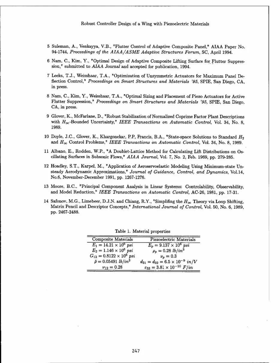
Robust Controller Design of a Wing with Piezoelectric Materials
5 Suleman, A., Venkayya, V.B., "Flutter Control of Adaptive Composite Panel," AIAA Paper No. 94-1744, Proceedings of the AIAA/ASME Adaptive Structures Forum, SC, April 1994.
6 Nam, C, Kim, Y., "Optimal Design of Adaptive Composite Lifting Surface for Flutter Suppres- sion," submitted to AIAA Journal and accepted for publication, 1994.
7 Leeks, T.J., Weisshaar, T.A., "Optimization of Unsymmetric Actuators for Maximum Panel De- flection Control," Proceedings on Smart Structures and Materials '95, SPIE, San Diego, CA, in press.
8 Nam, C, Kim, Y., Weisshaar, T.A., "Optimal Sizing and Placement of Piezo Actuators for Active Flutter Suppression," Proceedings on Smart Structures and Materials '95, SPIE, San Diego, CA, in press.
9 Glover, K., McFarlane, D., "Robust Stabilization of Normalized Coprime Factor Plant Descriptions with iJoo-Bounded Uncertainty," IEEE Transactions on Automatic Control, Vol. 34, No. 8, 1989.
10 Doyle, J.C., Glover, K., Khargonekar, P.P, Francis, B.A., "State-space Solutions to Standard H2
and He*, Control Problems," IEEE Transactions on Automatic Control, Vol. 34, No. 8, 1989.
11 Albano, E., Rodden, W.P., "A Doublet-Lattice Method for Calculating Lift Distributions on Os- cillating Surfaces in Subsonic Flows," AIAA Journal, Vol. 7, No. 2, Feb. 1969, pp. 279-285.
12 Hoadley, S.T., Karpel, M., "Application of Aeroservoelastic Modeling Using Minimum-state Un- steady Aerodynamic Approximations," Journal of Guidance, Control, and Dynamics, Vol.14, No.6, November-December 1991, pp. 1267-1276.
13 Moore, B.C., "Principal Component Analysis in Linear Systems: Controlability, Observability, and Model Reduction," IEEE Transactions on Automatic Control, AC-26, 1981, pp. 17-31.
14 Safonov, M.G., Limebeer, D.J.N. and Chiang, R.Y., "Simplifing the Hoc Theory via Loop Shifting, Matrix Pencil and Descriptor Concepts," International Journal of Control, Vol. 50, No. 6, 1989, pp. 2467-2488.
Table 1. Material properties
Composite Materials Piezoelectric Materials Ei = 14.21 x 10e psi Ep = 9.137 x 10b psi E2 = 1.146 x 10⁶ psi pp = 0.28 lb/in3
Gi2 = 0.8122 x 10⁶ psi vp = 0.3 p = 0.05491 lb/in3 d31 = d32 = 6.5 x 10~9 in/V
vyi = 0.28 e33 = 3.81 x IP"10 F/in
247

C. Nam & J. Kim
10 100 1000 Frequency (Hz)
Fig. 1. Laminated plate model with self-sensing actuators.
Fig. 4. Singular value specifications of weighting functions.
AUGMENTED PLANT P(s)
{u,l I
—f»®—
——li
M H ra-HAsflL^WjwJO-Hy,,,,-!
w
CONTROLLER
PWT
Fig. 2. Block diagram of robust control system.
10 100 1000 Frequency(Hz)
10000
(a) 10 100 1000
Frequency (Hz)
(b)
10 100 1000 Frequency (Hz)
10000
Fig. 5. Performance of the closed loop systems, (a) Sensitivity function [S] and weighting function [Wi]-1. (b) Complementary sensitivity function [T] and weighting function [Wb]-1-
Fig. 3. Singular value plots of the full model and the reduced order model, (a) Maximum singular values, (b) Minimum singular values.
•248

Robust Controller Design of a Wing with Piezoelectric Materials
CASE1 CASE 2
0.025 0.03
600
o a.
o >
a. ■ <
i 2 i : :
0.025 0.03
i
0.005 0.01
(b)
0.015 Time
0.02 0.025 0.03
0 0.005 0.01 0.015 0.02 0.025 0.03
(c) Tme 0.005 0.01 0.015 0.02 0.025 0.03
(c) Tane
Fig. 6. Step response of the controlled system, Fig. 7. Step response of the controlled system CASE 1. CASE 2.
249

C. Nam & J. Kim
CASE 2
200 400 600 800 1000 Frequency(Hz)
(a)
200 400 600 800 1000 Frequency(Hz)
(b)
5000
u <u w 4000
CO
^3000 CO a. >2000 cs c g> 1000 E
Closed Loop Root Loci
• t
0 r >■> *ltl> llllhlil4—I»*MIMIW««<»
-800 -600 -400 -200 Real Part
200
Fig. 9. The closed loop root loci, CASE 2.
l/v o '-75 Hj»=--
200 400 600 800 1000 Frequency(Hz)
(c)
200 400 600 S00 1000 Frequency(Hz)
(d) Fig. 8. Electric current due to the unit distur- bance input voltage, CASE 2.(unit:db)
250

CONTROL OF OSCILLATORY MOTIONS OF CANTILEVERS VIA STRUCTURAL TAILORING AND
ADAPTIVE MATERIALS TECHNOLOGY*
L. Librescu*, L. Meirovitch** and S.S. Nat Virginia Polytechnic Institute and State University
Blacksburg, VA 24061-0219
Abstract
A dual approach integrating structural tailoring and adaptive materials technology and designed to control the dynamic response of cantilever beams subjected to external excitations is presented. Whereas structural tailoring uses the anisotropy properties of advanced composite materials, adaptive materials technology exploits the actuating capabilities of piezoelectric materials bonded or embedded into the host structure. A dynamic control law relating the piezoelectrically induced boundary bending moment with the velocity at given points of the structure is implemented and its effect on the closed- loop eigenfrequencies and dynamic response to harmonic excitations is investigated. The combination of structural tailoring and control by means of adaptive materials proves very effective in damping out vibration. This methodology offers great possibilities also in preventing wing nutter instability.
1. Introduction
As the requirements for higher flexibility on high speed aircraft increase, so do the challenges of developing innovative design solutions. Whereas the increased flexibility is likely to provide enhanced aerodynamic performance, the aircraft must be able to fulfill a multitude of missions in complex environmental conditions and to feature an expanded operational envelope and longer operational life. To achieve such ambitious goals, advanced concepts resulting in the enhancement of static and dynamic response of the multimission, highly flexible aircraft must be developed and implemented. One way of achieving such goals consists of the integration of advanced composite materials in the aircraft structure. In this regard, it should be stated that the directionality property featured by anisotropic composite materials is capable of providing the desired elastic couplings through the proper selection of the ply-angle. However, such a technique is passive in nature in the sense that, once the design is in place, the structure cannot respond to the variety of conditions in which it must operate.
The above situation can be mitigated by incorporating into the host structure adaptive materials able to respond actively to changing conditions. In a structure with adaptive capabilities, the natural frequencies, damping and mode shapes can be tuned to reduce the vibration so as to avoid structural resonance and nutter instability, and in general to enhance the dynamic response characteristics. The adaptive capability is achieved through the converse piezoelectric effect, which consists of the generation of localized strains in response to an applied voltage. This induced strain field produces, in turn, a change in the dynamic response characteristics of the structure. It is proposed here to enhance the free vibration and dynamic response to external excitations of wing structures by incorporating the adaptive capability referred to as induced strain actuation in conjunction with structural tailoring. Under consideration is a cantilevered aircraft wing, modeled as a thin/thick-walled closed cross-section beam of anisotropic material. Implementation of a control law relating the applied electric field to one of the mechanical quantities characterizing the response of the wing according to a prescribed functional relationship results in eigenvalue/boundary-value problems. The solution consists of closed-
t The authors are listed in alphabetical order. * Professor, Department of Engineering Science and Mechanics
** University Distinguished Professor, Department of Engineering Science and Mechanics. t Graduate Student, Department of Engineering Science and Mechanics.
251

L. LIBRESCU, L. MEIROVITCH AND S.S. NA
loop eigenvalues/dynamic response characteristics, which are functions of the applied voltage, i.e., of the feedback control gain.
It should be stated here that investigation of static and dynamic control of aircraft wing structures via the simultaneous implementation of induced strain actuation and structural tailoring is of recent vintage. To these authors' knowledge, the first attempt to study this problem by integrating both techniques was carried out in the Refs. 1 and 2, in the context of an advanced structural wing model. The present study, consistent with the approach in Ref. 2, represents a clear departure from the approach in Refs. 1, 3 and 4, in the sense that here a dynamic feedback control strategy is implemented. This enables us to control the free and forced vibrations and avoid the resonance phenomenon without weight penalties. Moreover, this adaptive strategy promises to be effective also in flutter control.
Although the paper addresses mainly the problem of control of aircraft wings, the concept tran- scends this application. This implies that the methodology developed here can be applied to a number of other advanced structures. Indeed, the approach is applicable to other lightweight structural mod- els, such as helicopter blades and flexible robot arms operating in space.
2. Basic Assumptions and Kinematics
The structural model used here consists of a cantilevered thin-walled, closed-section beam. Its purpose is to simulate the lifting surface of advanced flight vehicles. The model is confined to uniform single-cell beams. Two systems of coordinates, s,z,n and x,y,z, are used to define points of the thin-walled beam. Note that the 2-axis is located so as to coincide with the axis of symmetry of the cross-sectional areas. The beam model incorporates the following nonclassical features: i) anisotropy of the constituent material layers, ii) transverse shear, iii) nonuniform torsion, in the sense that the rate of twist dQ/dz is no longer assumed to be constant (as in the Saint-Venant torsional model) but a function of the spanwise coordinate, and iv) primary and secondary warping effects. As a result, the present beam model is capable of providing results also for thick-walled beams and/or for constituent materials exhibiting high flexibilities in transverse shear. We also postulate the in-plane cross-section nondeformability of the beam (Refs. 5 and 6).
In accordance with the above assumptions, and in order to reduce the three-dimensional problem to an equivalent one-dimensional one, the components of the displacement vector are expressed as (Refs. 1,5 and 6)
u(x, y, z, t) =u0(z, t) - yQ(z, i) (la)
v(x,y,z,t) -v0(z,t)+xQ(z,t) (lb)
y(s) -n- w(x,y,z,t) =wo(z,t)+0x(z,t)
+ 8y(z,t) x(s) + n as
ds
dy -0'(z,O[i?L,(s) + na(s)] (lc)
where
and
ex(z,t) = ly2(z,t)-v'0(z,t), ey(z,t) = lxz{z,t)-u'0{z,t) (2a,b)
a« = -yWg-*(,)§ (2c) in which 9x(z, t) and Oy(z,t) denote the rotations about axes x and y, respectively, and jyz and jxz
denote the transverse shear strains in the planes yz and xz, respectively; primes denote derivatives with respect to the ^-coordinate. When the transverse shear effect is ignored, 6X -*■ —v'0 and 6y -» —u'0. From Eq. (lc) it is apparent that the warping measure is Q'(z,t). Equations (1) and (2) reveal that six kinematic variables, u0(z,t), v0(z,t), w0(z,t), 6x(z,t), 8y{z,t), and ®{z,t) representing three translations in the a;, y, z directions and three rotations about the x, y and z axes, respectively, are used to define the displacement vector of components u, v and w in the x, y and z directions, respectively.
252

CONTROL OF OSCILLATORY MOTION OF CANTILEVERS
The primary warping function has the expression
Fu(s)= fS{rn(s)-rP]ds (3) Jo
where fc[rn(x)/h(s)]ds
W §c[l/h(s)]ds [ }
is the torsional function, in which the quantity h(s) denotes the beam wall thickness, allowed to
vary along the periphery, © (-)ds denotes the integral around the entire periphery C of the mid-line
cross-section of the beam and / rn(s)ds = fi(s) is referred to as the sectorial area. For the case of Jo
uniform h in the circumferential direction, Eq. (4) reduces to ip — 2Ac/ß, where Ac denotes the cross-sectional area bounded by the mid-line while ß denotes the total length of the contour mid-line. Moreover,
rn(s) = x(s)fs-y(s)fs (5)
Using the kinematic relations, Eqs. (1) and (2), we can obtain the strain measures. Their expres- sions are omitted for brevity.
3. Location of Piezoactuator Patches. Global Constitutive Equations We assume that the master structure consists of m layers and the actuator of I piezoelectric
layers. We stipulate that the actuators are distributed over the entire span of the beam. Along the circumferential s and transverse n directions, they are distributed according to
R(k){n) = H(n - n(fc-)) - H(n - n(i+)), £(*)(«) = H(s -*(*-)) - H(s - s(fc+)) (6)
where R is a spatial function and H(-) denotes Heaviside's distribution, in which the subscript k in parentheses identifies the fcth layer. The linear constitutive equations for a three-dimensional piezoelectric continuum, expressed in Voigt's contracted notation, are (Ref. 7)
<Ji = C^Sj — eri£r, Dr = erjSj + erl£i (7a, b)
in which Uj and Sj(i, j = 1,2,..., 6) denote the stress and strain components, respectively, where
*-{ bpr, p — r, j — 1,2,3 /_.. 2Spr, p?r, j=4,5,6 W
Moreover, Cy, erj, and eft are the elastic (measured for conditions of a constant electric field), piezoelectric and dielectric constants (measured under constant strain), and £T and Dr(r = 1,2,3) denote the electric field intensity and electric displacement vector, respectively. In Eqs. (7), summation over repeated indices is implied. Whereas Eq. (7a) describes the converse piezoelectric effect, consisting of the generation of mechanical stress or strain in response to an electric field, Eq. (7b) describes the direct piezoelectric effect, consisting of the generation of an electrical charge under a mechanical force. In piezoelectric adaptive structures, the direct effect is used for sensing and the converse effect is used for active control. Equations (7) are valid for the most general case of anisotropy, i.e., for triclinic crystals. In the following, we restrict ourselves to the case of a transversely-isotropic piezoelectric continuum, the n-axis being a six-fold axis of symmetry, considered to be parallel to the direction of polarization, i.e., in the thickness direction. In this case, the piezoelectric continuum is characterized by five independent elastic coefficients, Cu = C22, C13 = C23 = C^i = C32, C33, C44 = C55, Cee = (C11 — Ci2)/2, three independent piezoelectric coefficients, eis = ^24, e3i = 632 and 633, and two independent dielectric constants, £n = £22, £33 (Ref- 7).
253

L. LIBRESCU, L. MEIROVITCH AND S.S. NA
At this point, we assume that the master structure is made of anisotropic material layers, the anisotropy being of the monoclinic type. We also assume that the electric field vector Si is represented in terms of its component £3 only, implying that £1 = £2 = 0. As a result of the uniform voltage distribution, £3 is independent of space but dependent on time.
Upon invoking the previously stipulated distribution law of piezoactuators, Eqs. (6), and their specific anisotropy properties, the three-dimensional constitutive equations for the actuator layers can be expressed as
0
<TZZ
&SZ (*) 0
C12
C11
0
0 Cu — C: 12
•Jss
szz -
(*) . sz. (*)
eif4k)Rk(n)Rk(s)
0
and o£*>=d?s&>. 44
(9a)
(9b) The last terms in Eq. (9a) identify the actuation stresses induced by the applied electric field.
Integrating the three-dimensional constitutive equations through the thickness of the master struc- ture and actuators and postulating that the hoop stress resultant Nss is negligibly small when com- pared with the remaining stresses, two-dimensional constitutive equations, referred to also as shell- constitutive equations, are obtained. The equations are not displayed here for brevity.
4. The Equations of the Wing Structure Involving Bending-Twist Coupling The great possibilities provided by advanced anisotropic composite materials can be used to en-
hance the response of lifting surfaces. Implementation of structural/aeroelastic tailoring has revealed great promise toward improving static and dynamic response characteristics, preventing vibration resonance and enhancing aeroelastic behavior. For thin-walled composite beams, tailoring was car- ried out in a number of recent papers, (Refs. 8-10), in which the possibility of generating desired elastic couplings beneficial to specific aeronautical problems was examined. Among the possible cou- plings that can be induced via tailoring, the most beneficial for the problem at hand is the bending- twist cross-coupling. This coupling has also been used for the solid beam model to enhance the structural/aeroelastic response behavior of wing structures (Refs. 11-14). As shown in Refs. 8 and 9, the ply-angle distribution with respect to the spanwise z-axis inducing such a cross-coupling is 0(y) = -0(-y). Using such a ply-angle, the equations of motion of the combined host-piezoactuator structure (Refs. 1 and 6) are
a55(v'^ + e'x)+ a56&" +Py = hv0
-a660^" + a77&' - a56 «' + 0£) + a739'^ + mz = (64 + 65) 6 - (610_+ b18) ©"
a330;' + 037©" - 055 K + 8x) ~ a560" = (bj + &14) Ä,
For cantilevered beams, the boundary conditions are
and
v0 = 0, 9X = 0, 0 = 0, 0' = 0 at z = 0.
a55(v'0 + ex)+ a56e" =0, a330x + a37Q' = Mx
(10a)
(106)
(10c)
(11a - d)
-a660'" + a770' - a56 « + 8'x) + a376'x = _ (&10 + &18) ©'
a56« + 0*)+ a660" =0
> at z = L (12a - d)
254

CONTROL OF OSCILLATORY MOTION OF CANTILEVERS
The terms underscored in Eqs. (10)-(12) by single and double dashed lines are associated with warping inhibition and warping inertia effect, respectively, whereas the term underscored by a solid line is associated with the rotatory inertia.
5. The Control Law
Although the structural/aeroelastic tailoring technique was proved effective in enhancing the static and dynamic response behavior of flight vehicle structures (Refs. 11 and 14), its effectiveness is limited by the fact that the technique is passive in nature. This implies that, once the ply-angles and ply- sequence of the laminated construction are fixed, the structure cannot respond adaptively to the variety of external stimuli encountered during flight. For this reason, as a complementary way of controlling the behavior of the structure, the smart structure concept is considered.
For feedback control, the applied electric field £3, on which the piezoelectrically induced moment depends, must be related to one of the mechanical quantities characterizing the wing's response. Thus, a number of control laws can be implemented. Their effectiveness can be measured by the ability to enhance the free vibration behavior, suppress the forced vibration to any time-dependent external excitation and prevent resonance and any instability which may occur during flight.
A number of control laws have been proposed and used (Ref. 1-4, 15 and 16) for inducing strain actuation capability via the boundary control moment, . Among these, we single out velocity feedback
control (Ref. 2), whereby the piezoelectrically induced moment Mx at the wing tip is proportional to the rotational velocity 9X(L) at the wing tip. A more explicit expression of this control law is derived from Eq. (12b) in the form
6x(L) + f3®(L)-kp6x(L) = 0 (13)
where f$ = 037/033 and kp denotes the feedback gain. The advantage of this control law is that it has a dynamic character. This implies that, in contrast
to the previously mentioned ones, damping is adaptively induced and, as such, enhanced dynamic response performances are expected from its application.
6. Problems Considered
The equations derived in this paper are general, in the sense that they are valid for a beam of arbitrary cross section, as well as for piezoelectric actuators arbitrarily located throughout the wall thickness and along the circumference of the beam. However, in the present case, a biconvex profile typical of supersonic wing airplanes is adopted, whose dimensions are identical to the ones in Ref. 10. It is also assumed that the piezoceramic actuators used here are mounted symmetrically on the upper and bottom surfaces of the wing. Being very light, the actuators do not affect the mass or stiffness properties of the original structure in any meaningful way (Ref. 17). The wing structure is assumed to be of a graphite/epoxy composite material whose elastic characteristics are
EL =30 x 106 psi, ET = 0.75 x 10⁶ psi
GLT =0.37 x 10⁶ psi, GTT = 0.45 x 10⁶ psi
ßTT =ßLT = 0.25, p = 14.3 x 10~5 lb sec2 /in4
where subscripts L and T denote directions parallel and transverse to the fibers, respectively. The geometrical wing characteristics are displayed in Fig. 1. The piezoelectric actuators are made of PZT-4 ceramic, whose properties are given in Ref. 18.
The associated differential eigenvalue problem has been discretized in space by the extended Galerkin method (Ref. 19). In parallel to this, an exact solution based on the Laplace transform in the spatial domain (Ref. 20) was obtained and the agreement of the results obtained by the two approaches was excellent. The same solution techniques have been successfully used in Refs. 2 and 10.
Using structural tailoring and the induced strain actuation technology in combination, two prob- lems associated with the dynamics of aircraft wings have been considered, namely Problem I: free
255

L. LIBRESCU, L. MEIROVITCH AND S.S. NA
vibration and Problem II: dynamic response to harmonically time-dependent excitations. In addition, several results related to the dynamic response to arbitrary time-dependent excitations have also been obtained.
In analyzing Problem I, the external loads have been removed from Eqs. (10). Moreover, all the field variables, including the electrical current £3, denoted generically by F(z,t), are written in the form
F{z,t) = F(z)ext (14)
where A is the complex eigenvalue. Because the eigenvalue appears in both the equations of motion and the boundary conditions, the solution of the closed-loop eigenvalue problem is not an easy task.
For dynamic response, Problem II, it is assumed that the wing is excited by a concentrated, harmonic load, arbitrarily located along the span and the chord of the wing. Hence, the load py is written in the form
py(z, t) = FJ(z - z0) eiut (15a)
where S(-) denotes a spatial Dirac delta function, ZQ the spanwise location of the load, Fo the amplitude and w the excitation frequency. Moreover, when py is located off the longitudinal axis of symmetry by an amount x0, then a concentrated moment
mx(z,t) - F0x05{z - z0)e iu>t (156)
must be included as well. Such a load and moment can be generated, among others, by a power system located on the wing at x0, z0. As soon as the frequency response functions V0(Z,UJ),9X(Z,U>)
and Q(z, u) corresponding to a given excitation frequency have been determined, it is possible to obtain their counterparts in the time domain. This conversion is accomplished via the Fourier transform, as follows:
v0(z,i) 0x(z,t) e(z,t)
T- v0(z,u) 9x{z,u) Q(z,w)
_i_ r+oa
~ 2?r y.«
V0(Z,UJ)
0x(z,u) Q(Z,LJ)
Jwt dcj (16)
where T~l denotes the inverse Fourier transform. These quantities enable one to determine the dynamic magnification factors due to simple harmonic force excitation.
These quantities evaluated for different feedback gains and ply-angles are able to reveal the effec- tiveness of combining structural tailoring and adaptive material technology.
7. Numerical Examples The closed-loop eigenvalue problem is obtained by inserting Eq. (14) into Eqs. (10)-(13) with the
external load terms removed and dividing through by ext. Laplace transforming the resulting equations in the spatial domain, it is possible to express the eigenfrequencies as functions of the feedback gains and ply-angles. When the structure is activated, implying that kp ^ 0, the eigenfrequencies A are complex quantities of the form
A = a + iud (17)
For a given A, one can determine the damped frequency aid as the imaginary part of Eq. (17). Moreover, the damping factor £ can be obtained from the real part a = — C,wn in the form
C = -<r/(a2+u$ 1/2 (18)
The ratio Ud/wn of the damped frequency Ud and undamped frequency un, i.e., of the nonactivated structure versus the dimensionless feedback gain kp = kpLü/azz, where w is the natural frequency of the nonactivated structure corresponding to 6 = 0 and M = 16, is plotted for the first mode in Fig. 2 for the ply-angle 6 = 45°. Results (not shown here) reveal that the adaptive capability decays in power with the increase in the mode number.
Figure 3 depicts the damping factor C, versus the ply angle 9 for three different values of the feedback gain for a given aircraft wing defined in terms of its aspect ratio and wall thickness. The
256

CONTROL OF OSCILLATORY MOTION OF CANTILEVERS
plot reveals not only that damping can be induced adaptively, but that tailoring can also be used to enhance damping in the structure.
A number of plots of the steady-state dynamic response to a harmonic load acting at the wing tip versus the excitation frequency u are presented. Figure 4 displays the steady-state deflection amplitude as a function of the excitation frequency for wings of aspect ratios M = 6 with the transverse shear included and with a ply-angle 9 = 45°. Results reveal that for wings including the warping inhibition, resonance shifts toward larger excitation frequencies, a trend diminishing in the case of high aspect ratio wings. Moreover, the difference between the resonance frequency of wings exhibiting free warping and warping inhibition becomes progressively larger as the wing aspect ratio diminishes. The plot also reveals the strong effects of adaptiveness on the deflection. Results (not displayed here) show that resonance frequencies increase dramatically with a decrease of the wing's aspect ratio, as should be expected.
Figure 5 presents the steady-state transverse deflection of shear deformable and infinitely rigid in transverse shear wing models as a function of the excitation frequency for 6 = 60° and free warping. As can be seen, transverse shear flexibility causes a shift in the resonance toward lower frequencies and an increase of the deflection. This goes back to the conclusion that beam models rigid in transverse shear overestimate the resonance frequency and underestimate the deflection. Concerning the influence of wing aspect ratio, the conclusions reached from Figs. 3 and 4 remain valid in this case as well.
From Fig. 6, which depicts the steady-state deflection as a function of the excitation frequency for shear deformable and non-shear deformable wings and for nonactivated and activated wings, one can conclude that, for wings including the warping restraint, shear deformability plays the unique role of shifting resonance toward the lower frequencies. At the same time, the deflection amplitudes are not affected by transverse shear effects.
As the wing aspect ratio decreases, its influence becomes more prominent, in the sense that for small/moderate aspect ratios the shift becomes more prominent than in the case of high-aspect ratio wings. It should also be noted here that for small/moderate aspect ratio wings the deflections of the activated wing are much smaller than for a high aspect ratio wing.
As 9 approaches 90°, at which angle the bending stiffness is the largest, small differences in the deflection amplitudes for the shear deformable and non-shear deformable wings exhibiting free warping can occur. The only effect of ignoring the transverse shear is to shift resonance toward higher frequencies. For the same aspect ratio wing, a dramatic increase in the resonance frequencies are experienced in the case of 9 = 90° (Fig. 7) as compared to 9 = 60° (Fig. 6).
The steady-state twist as a function of the excitation frequency shows similar trends as the trans- verse deflection. Figure 8 depicts the steady-state twist for wings of M = 6 as a function of the excitation frequency for shear deformable and shear nondeformable beam models and for the acti- vated and nonactivated wings. The structure corresponds to the ply-angle 6 = 60°. As in the case of the transverse deflection (see Figs. 6 and 7), it should be noted that inadvertent neglect of the transverse shear can result in an underestimation of the twist and an overestimation of the resonance frequency.
In all previously displayed results, it was assumed that the concentrated load acts on z-axis. However, when there is an eccentricity c = x0/c, both the deflection and twist will be affected.
Figure 9 depicts the normalized steady-state deflection versus the feedback gain for different ec- centricities c. The plot reveals the obvious trend that v increases with c and decays when the wing is activated. The same is true of the twist 0.
In addition to the fact highlighted previously that the steady-state deflection and twist of wing structures can be controlled and the resonance phenomenon inhibited by simultaneous use of tailoring and adaptive materials, the possibility of controlling the steady-state bending moment generated at the wing root becomes also apparent from Fig. 10. This figure shows that i) the bending moment is a maximum for that value of the ply-angle for which the bending stiffness 033 is a minimum, i.e., 0 = 0°, 180, and a minimum for 9 = 90° when 033 is a maximum. This implies that tailoring can be used to reduce as much as possible the bending moment, thus avoiding overdesign of the root region of the wing, and ii) adaptive material technology can be applied toward the same goal. Figure
257

L. LIBRESCU, L. MEIROVITCH AND S.S. NA
10 also reveals that for relatively large values of the feedback gain, tailoring becomes less efficient than for low feedback gains. This suggests that a trade-off between the two techniques can be achieved.
Finally, Figs. 11 and 12 depict the time history of the wing deflection for the ply-angles 0 = 0 and 6 = 90°, respectively, and for shear deformable and non-shear deformable, as well as for activated and nonactivated wings. As 6 increases from 0 to 90°, the bending stiffness increases from a very low value to a maximum value. At the same time, the displacement decreases. Moreover, as Figs. 11 and 12 reveal, for 6 = 0, in a 0.1 s time interval, there is one crossing of the time axis while for 6 = 90°, in the same time interval there are eight such crossings. This is evidently due to the fact that the bending stiffness experiences a dramatic increase when 6 varies from 0 to 90°. In both cases, the effectiveness of the adaptive technique to inhibit steady-state vibration becomes evident. It should also be noted that, with an increase in kp a corresponding decrease of the slope of the deflection curve is experienced. This goes back to the conclusion that in this case the maximum velocity decreases and damping increases.
8. Conclusions
A dual technology based on the use of structural tailoring and adaptive materials for control and aimed at enhancing the dynamic response characteristics of aircraft wing structures was developed. Using the dynamic control law described in this paper in conjunction with tailoring, a significant improvement of the dynamic response of wing structures can be achieved. The same technique is likely to yield good results in more complex problems, such as for flutter control of aircraft wings.
The paper also highlights the importance of a number of nonclassical effects, such as transverse shear, anisotropy and warping inhibition, which can influence the dynamic response of advanced wing structures to a very large degree.
9. References
1. Librescu, L., Meirovitch, L. and Song, O., "Integrated Structural Tailoring and Control Using Adaptive Materials for Advanced Aircarft Wings," Journal of Aircraft (in press).
2. Tzou, H.S., Piezoelectric Shells, Distributed Sensing and Control of Continua, Kluwer Academic Publ, Dordrecht/Boston/London, 1993.
3. Librescu, L., Song, O. and Rogers, C.A., "Adaptive Vibrational Behavior of Cantilevered Struc- tures Modeled as Composite Thin-Walled Beams," International Journal of Engineering Science, Vol. 31, No. 5, 1993, pp. 775-792.
4. Tzou, H.S. and Zhong, J.R, "Adaptive Piezoelectric Structures: Theory and Experiment," Active Materials and Adaptive Structures, Materials and Structures Series, (Ed.) G.J. Knowles, Institut of Physics Publ., 1992, pp. 219-224.
5. Librescu, L. and Song, O., "Behavior of Thin-Walled Beams Made of Advanced Composite Mate- rials and Incorporating Non-Classical Effects," Applied Mechanics Reviews, Vol. 44, No. 11, Part 2, 1991, pp. 174-180.
6. Song, O. and Librescu, L., "Free Vibration of Anisotropie Composite Thin-Walled Beams of Closed Cross-Section Contour," Journal of Sound and Vibration, Vol. 167, No. 1, 1993, pp. 129-147.
7. Maugin, G.A., Continuum Mechanics and Electromagnetic Solids, North-Holland, Amsterdam, The Netherlands, 1988.
8. Rehfield, L.W. and Atilgan, A.R., "Toward Understanding the Tailoring Mechanisms for Thin- Walled Composite Tubular Beams," Proceedings of the First USSR-U.S. Symposium on Mechanics of Composite Materials, 23-26 May, Riga, Latvia SSR, S.W. Tsai, J.M. Whitney, T-W Chou and R.M.Jones (Eds.), ASME Publ. House, 1989, pp. 187-196.
9. Smith, E.C. and Chopra, I., "Formulation and Evaluation of an Analytical Model for Composite Box-Beams," Journal of the American Helicopter Society, Vol. 36, No. 3, 1991, pp. 23-35.
10. Librescu, L., Meirovitch, L. and Song, O., "Refined Structural Modeling for Enhancing Vibrations and Aeroelastic Characteristics of Composite Aircraft Wings," La Recherche Aerospatiale, (in press).
258

CONTROL OF OSCILLATORY MOTION OF CANTILEVERS
11. Weisshaar, T.A., "Aeroelastic Tailoring-Creative Use of Unusual Materials," AIAA Paper 87-0976, AIAA/ASME/ASCE/AHS 28th Structures, Structural Dynamics, and Materials Conference, April 9-10, 1987.
12. Lottati, J., "Aeroelastic Stability Characteristics of a Composite Swept Wing with Tip Weights for an Unrestrained Vehicle," Journal of Aircraft, Vol. 24, No. 11, November 1987, pp. 793-802.
13. Librescu, L. asnd Simovich, J., "General Formulation for the Aeroelastic Divergence of Composite Swept Forward Wing Structures," Journal of Aircraft, Vol. 25, No. 4, 1988, pp. 364-371.
14. Weisshaar, T.A., "Aeroelastic Stability and Performance Characteristics of Aircraft with Advanced Composite Swept Forward Wing Structures," AFFDL-TR-78-118, 1978.
15. Weisshaar, T.A. and Ehlers, S.M., "Adaptive Aeroelastic Composite Wings-Control and Optimiza- tion Issues," Composites Engineering, Vol. 2, Nos. 5-7, 1992, pp. 457-476.
16. Tzou, H.S. and Zhong, J.P., "Adaptive Piezoelectric Structures: Theory and Experiment," Active Materials and Adaptive Structures, Proceedings of the ADPA/AIAA/ASME/SPIE Conference on Active Materials and Adaptive Structures, Ed. G.J. Knowles, 4-8 November 1991, Alexandria, VA, pp. 719-724.
17. Rao, S.S. and Sunar, M., "Piezoelectricity and its Use in Disturbance Sensing and Control of Flexible Structures: A Survey," Applied Mechanics Reviews, Vol. 27, No. 4, 1994, pp. 113-123.
18. Berlincourt, D.A., Curran, D.R., and Jaffe, H., "Piezoelectric and Piezomagnetic Materials and Their Function in Transducers," Physical Acoustics-Principles and Methods, (Eds. W.P. Mason), Vol. 1, Part A, Academic Press, New York, 1964, pp. 169-270.
19. Palazotto, A.N. and Linemann, P.E., "Vibration and Buckling Characteristics of Composite Cylin- drical Panels Incorporating the Effects of a Higher Order Shear Theory," International Journal of Solids and Structures, Vol. 28, No. 3, 1991, pp. 341-361.
20. Librescu, L. and Thangjitham, S., "Analytical Studies on Static Aeroelastic Behavior of Forward- Swept Composite Wing Structures," Journal of Aircraft, Vol. 28, No. 2, 1991, pp. 151-157.
1 = 30 in c= 10 in 6 = 2.68 in h = 0.4 in
0.90
0.80 "—- 0.04 0.08 0.12 0.16
Kr,
Fig. 1 Geometry of the wing structure Fig. 2 The first normalized damped frequency Qdi = Wdi/^ni versus the dimensionless feedback gain for M = 16
259

L. LIBRESCU, L. MEIROVITCH AND S.S. NA
0 30 60 90 120 150 130
ö(deg)
Fig. 3 Damping ratio versus the ply-angle for J2=16
V(m)
0.2
0.16
0.12
V{ia) 0.08
0.04-
T.S. Kf = 0 : i'
- - - vijo T.S. K, = 0.025 i
W.R. \\\ I /''
9 = 60° U ii "
tf„ = 0.05
^SK* = 0.075^^, ' '
» ' * ■
535 540.4 545.8 551.2 556.6 562
w(rad/s)
Fig. 6 Steady-state deflection versus the excita- tion frequency for M = 6 and 9 = 60°
o.s
0.4
0.3
V(in)
0.1
375 237 239.8 242.2 244.8 247.4 250
w(rad/s) 359 362.2 365.4 368.6 371.8
w(rad/s) Fig. 4 Steady-state deflection versus the excita- Fig. 7 Steady-state deflection versus the excita-
tion frequency for M = 6 and 9 = 45° tion frequency for M = 16 and 9 = 90'
10.0
V{m)
0.16 -
0.12 -
0(rad)
0.08 -
0.04
520 526.5 533 539.5
w(rad/s) Fig. 5 Steady-state deflection versus the excita- Fig. 8 Steady-state twist versus the excitation
546
tion frequency for M = 16 and 9 = 60° frequency for M = 6, and 9 = 60°
260

CONTROL OF OSCILLATORY MOTION OF CANTILEVERS
1.000
V 0.8S0
0.775
*-^—1—»..-,—- —I
0 = 60°'
"N •■>
V '•> '••v ' '\. "N "-.N -
\"v '-.N . N
X. ' X ■-. s c = 0.8
c = o\J -
c = 0.4
** / / . ■ \ -
—, , , i__ , —L
0.0003 0.0005 0.0008
Kr,
0.001
Fig. 9 Normalized steady-state deflection versus the feedbackgain for M = 16, 0 = 60° (V = V/V, V corresponds to c=l, Kp = 0)
Fig. 11 Steady-state deflection versus time for M = 16 and 6 = 0
M o.s
0.0011 0.0022 0.0034 0.0045
Fig' 10 ^ZtJerlTttf^ "?rnt/?#
the "** Fig. 12 Steady-state deflection versus time S7 the ^back-gain (M = for JJ = W and * = JW M/M, M corresponds to 9 = 0, Kp = 0)
261

262

BASE-ISOLATION CONTROL OF STRUCTURES IN EARTHQUAKES*
Leonard Meirovitch* and Timothy J. Stemple* Virginia Polytechnic Institute and State University
Blacksburg, VA 24061-0219
Abstract
The objectives of control of structures in earthquakes are to prevent injury to occupants and damage to contents and to protect the integrity of the structure. Both objectives can be achieved through base isolation and feedback control, whereby the structure is stabilized relative to the inertial space. Nonlinear on-off control with deadband has the advantages of economy and simplicity of implementation.
1. Introduction
The basic objectives of control of structures subjected to earthquake excitations are 1) to prevent injury to the occupants and damage to the contents and 2) to protect the integrity of the structure. These objectives can be achieved through control and base isolation. Cost considerations call for hybrid control, a blend of passive and active control. Passive control involves damping materials dispersed throughout the structure. On the other hand, active control implies feedback control forces acting on the base and on the structure. The idea of base isolation is to isolate the structure from the effects of the moving ground. A good strategy is to stabilize the base relative to the inertial space and to suppress the structural vibration relative to the base. Following is a literature survey on the subject of structural control.
The feasibility of modern linear feedback control theory to control the vibration of structures under random loading, such as due to earthquakes, was investigated by Yang [45]. It was assumed that random excitations can be modeled by either a stationary Gaussian white noise or a nonstationary Gaussian shot noise passing through a filter. The use of active tendon control of structures subjected to both deterministic and probabilistic excitations was proposed by Roorda [34,35], who introduced a pair of tendons to generate a control torque at some point on the structure so as to create an active damping effect. A method of active control for tall buildings excited by earthquake ground motion was presented by Yang [46]. The effectiveness of active mass dampers and active tendon systems was investigated. The effect of time delay between sensing the structural motion and applying the control force in active tendon control was analytically and experimentally studied by Abdel-Mooty and Roorda [1]. The fact that earthquake excitations introduce disturbances that are not known a priori has prompted Yang, Akbarpour and Ghaemmaghami [47,48] to propose a method known as instantaneous optimal control. The efficiency of the new control laws was demonstrated through numerical examples. A sensitivity study was conducted by Yang and Akbarpour [50] to investigate the effect of uncertainties in system identification on the performance of the active control system for seismically-excited buildings. Both the active tendon control system and the active mass damper system were considered.
In an attempt to generate vibration cancelation control, a computer algorithm for the optimum selection of a series, or train of force pulses for application to a continuous system was developed by Masri, Bekey and Safford [14]. The optimized pulse train generates oscillations in a system to match within specified error bounds the response which would be produced by a continuous loading of arbitrary nature, such as an earthquake excitation. Masri, Bekey and Udwadia [15] studied the
* Supported by the NSF Research Grant CMS-9423575 monitored by Dr. S.C. Liu. The support is greatly appreciated. t University Distinguished Professor and * Graduate Research Assistant, Department of Engineering
Science and Mechanics.
263

L. MEIROVITCH AND T. J. STEMPLE
feasibility of using pulsed open-loop adaptive control for reducing the oscillations of tall structures subjected to strong ground shaking. A method for active optimum pulse control of flexible structures subjected to arbitrary dynamics environments was proposed by Masri, Bekey and Caughey [16]. The optimal pulse characteristics are determined analytically so as to minimize a nonnegative cost function related to structure energy. The same authors [17] introduced the method of on-line vibration control ol nonlinear flexible structures subjected to arbitrary deterministic and stochastic excitations. The direct method of Liapunov is used to establish stability of the control system. Miller, Masri, Dehghanyar and Caughey [26] provided both numerical and experimental studies demonstrating the feasibility, reliability and robustness of the optimal pulse-control method in active vibration control of large structures. A method for on-line parameter control of linear as well as nonlinear, multi-degree- of-freedom systems provided with adjustable-gap impact dampers responding to arbitrary dynamic loads was presented by Dehghanyar, Masri and Miller [5]. Reinhorn, Manolis and Wen [29] presented a methodology for the shape control of structures undergoing inelastic deformations through the use of an active pulse/force system. The method is based on an active control algorithm derived from standard numerical integration schemes that uses corrective pulses or forces to limit the response of a structure that has already entered the inelastic range. Udwadia and Tabaie [41,42] investigated the feasibility of using open-loop, on-line adaptive pulse control to limit the vibrations of structural and mechanical systems. The technique is illustrated by means of a structure subjected to earthquake-like base excitations.
The use of base isolation in conjunction with active control for suppressing the vibration of structures under earthquake excitation was studied experimentally and analytically by Kelly [9] and Kelly, Leitmann and Soldatos [10], respectively. In the experimental work, a multilayer natural rubber bearing base isolation system was employed and the structure was excited by actual records of earthquake ground motion. Note that in Ref. 10 a linear structure is controlled by nonlinear control. Bhatti, Pister and Polak [2] provided a general formulation for the design of control devices in base isolation systems for structures under seismic excitation. Lin, Tadjbakhsh, Papageorgiou and Ahmadi [12] presented a comparison of the performance of three different base-isolation systems, the laminated rubber bearing system, the New Zealand system and the resilient-friction base isolator system. The possibility of combined passive base isolation control systems and an active control system that exerts control forces only on the base and induces artificial damping without increasing the stiffness to the isolated structure was investigated by Pu and Kelly [28].
In an investigation by Yang, Danielians and Liu [51], two hybrid control systems were proposed for structures against strong earthquakes. Yang, Li, Danielians and Liu [52,53] proposed to reduce the response of structures to earthquake excitations by basing the controls on measurements of the state and obviating the problem of tracking a time-dependent system matrix. The approach represents a refined version of the instantaneous optimal control [47,48] algorithm for nonlinear or hysteretic systems. A systematic way of assigning the weighting matrix Q in conjunction with instantaneous optimal control developed in Refs. 47 and 48 was proposed by Yang, Li and Liu [54]. The approach, based on the Liapunov's direct method, was extended by the same authors [55] to the case in which velocities and accelerations are fed back. Reinhorn, Soong and Wen [30] used two techniques to actively control base-isolated structures, the first using pulses to maintain the response of the structure within prescribed bounds and the second using active tensioning tendons. An optimal frequency-domain approach to active control of wind excited structures was proposed by Suhardjo, Spencer and Kareem [40] in which the Hi norm of the transfer function from the external disturbance to the regulated output is minimized. A hybrid sliding base isolation system using friction-controllable bearings was proposed by Feng, Shinozuka and Fujii [6] and Feng [7]. An optimal control algorithm using acceleration, velocity and displacement feedback was proposed and applied to base-isolated structures by Rofooei and Tadjbakhsh [33].
Wong and Luco [44] examined the effects of soil-structure interaction on the form of the control rule and on the effectiveness of active control on the seismic response of structures.
Control based on the idea of altering the modal characteristics of a system to achieve satisfactory performance is generally known as modal control. The concept of modal control of large and flexible
264

BASE-ISOLATION CONTROL OF STRUCTURES
structures was examined by Martin and Soong [13]. It was shown via numerical examples that in the design of modal control, a great deal of freedom exists in terms of eigenvalue assignments and control policy decision. Soong and Chang [36] proposed a simple criterion for optimal design of the control matrix wiinin the framework of modal control. An analysis of optimal modal control for tall buildings subject to earthquake excitation was presented by Pu and Hsu [27]. Vilnay [43] showed that, in the modal control approach, the effect of the active control mechanism on the structure response can be represented by the so-called influence matrix. The pole assignment method was applied to control the critical modes of large structures by Juang, Sae-Ung and Yang [8]. In the above investigations, the control design was carried in coupled form, in the sense that the equations of motion are simultaneous.
A different type of modal control is one in which the control design is carried out for each mode independently. The method, developed by Meirovitch and Oz [18] and Meirovitch and Baruh [19], is known as the independent modal-space control (IMSC) method. Then, Meirovitch and Silverberg [20] used optimal IMSC for the control of structures subjected to earthquakes.
The formulation of a predictive control law and its implementation in a computer control system for the seismic response of an experimental modal structure was presented by Rodellar and Martin- Sanchez [31]. Experimental results are presented by Rodellar, Chung, Soong and Reinhorn [32] to illustrate the capability of predictive control. The full-scale implementation of active control of structures under seismic excitation was conducted by Soong, Reinhorn, Wang and Lin [38]. An. active bracing system is used in the investigation. Experiments in feedback control of structures were presented by Roorda [35]. It is demonstrated that, in all four experiments, each using a different control device, the vibration levels can be reduced to some degree by suitable control forces. Soong, Reinhorn and Yang [37] proposed a standardized model for structural control experiments and presented some initial experimental results. Chung, Reinhorn and Soong [3] used prestressed tendons connected to a servo-hydraulic actuator to control a single-degree-of-freedom model structure under base excitation generated by a large-scale seismic simulator. Chung, Lin, Soong and Reinhorn [4] extended the experiment to a l:4-scaled model structure simulating a three-story frame building. The IMSC method in conjunction with nonlinear control was verified experimentally by Meirovitch, Baruh, Montgomery and Williams [22].
The literature on structural control includes three books. The first is by Leipholz and Abdel- Rohman [11] and is devoted exclusively to civil engineering applications. The second is by Soong [39] and is also concerned with civil structures, but is more focused. The third is by Meirovitch [24] and is more interdisciplinary in nature than the first two. A review of advances in active control of civil engineering structures was presented by Yang and Soong [49].
2. Problem Formulation The system shown in Fig. 1 represents an elastic structure supported by a base in the form of
a rigid slab capable of moving relative to the ground while restrained by a viscous damper and an elastic spring. For simplicity, we assume that all motions take place in the horizontal direction. From Fig. 1, we conclude that the absolute displacement of the structure at any point P and time t is
u(P,t)=ub(t) + ue(P,t) (1)
where u&(£) is the displacement of the base mass and ue(P, t) the elastic displacement. The equations of motion and associated boundary conditions can be derived by means of the
extended Hamilton's principle, which can be stated as [23]
I, (6T-6V + 5W)dt = 0, 6ub = 6ue = 0, t = tut2 (2)
where T is the kinetic energy, V the potential energy and 6W the virtual work performed by the nonconservative forces. The kinetic energy has the form
265

L. MEIROVTTCH AND T. J. STEMPLE
where mb is the mass of the base, ms = / pdD the mass of the structure, p the mass density of the JD
structure and D the domain of the structure. The potential energy has the form
V = 2kb(ub - Ugf + - I ueCuedD (4)
in which kb is the stiffness of the base spring, ug the ground displacement and £ a stiffness differential operator. Moreover, the virtual work of the nonconservative forces can be written as
OÜb ■± + Fb) Sub - / -gfSuedD + / f(5ub + 8ue)dD
(5)
where
F = Fb+ fdD JfdD (6) in which F is the total force acting on the system, Fb the control force acting on the base and / the distributed force acting on the structure, which includes the wind force fw and the control force fc, and
?b = 7;cb(üb - üg)2, ?e = -üeCeüe (7a, b)
are a Rayleigh's dissipation function for the base damper and a Rayleigh's dissipation function density for the elastic structure, respectively. Inserting Eqs. (3)-(7) into Eq. (2) and carrying out the usual operations, we obtain the equations of motion
müb + püedD + cbüb + kbub = cbüg + kbug + F (8a)
püb + püe + Ceüe + Cue = f (86)
where m = mb + m, is the total mass of the system, and we note that Eq. (8a) is an ordinary differential equation for the motion of the base mass and Eq. (86) is a partial differential equation for the elastic motion of the structure, and is subject to given boundary conditions.
We observe that the equation for the elastic structure, Eq. (86), does not contain any direct input from the motion of the ground; the only motion input is due to the base. Hence, the base provides an isolation system for the structure, protecting the structure from any direct effects of the ground motion. This implies that suitable controls can be designed to keep the acceleration üb of the base relatively small.
Design of controls on the basis of hybrid (ordinary and partial) differential equations is not feasible, so that spatial discretization is a virtual necessity. To this end, we express the elastic displacement in the form
n
ue(P,t) = Y^MP)qei(t) = <t>T(P)qe(t) (9) «=1
where <p = [fa fa ... <j>n]T is an n-vector of admissible functions [23] and qe is an n-vector of generalized coordinates. Introducing Eq. (9) into Eqs. (8), premultiplying both sides of Eq. (86) by <p and integrating over the domain D, we obtain
-T mub + <f> qe + cbüb + kbub = cbug + kbug + F (10a)
^üb + Meqe+Ceqe+Keqe = fw+fc (106)
266

BASE-ISOLATION CONTROL OF STRUCTURES
where Mt = f p<f>4>TdD, Ce= I (f>Ce4>TdD, Ke= f (pCtf
JD JD JD dD
are the mass matrix, damping matrix and stiffness matrix for the structure. Moreover,
0 = / p<t>dD, fw= f <f>fwdD, fc = / <j>fcdD JD JD JD
(11a, M
(12o,b,c)
where f«, is a generalized wind force vector and fc is a generalized control force vector for the structure. Equations (10) can be combined into the single matrix equation
'Mq + Cq + Kq=Qd + Qc
where q = [ub qf ]r is an (n + l)-dimensional generalized displacement vector for the system
M = 771 <f) 7*1
,c = cb 0 0 ce
,K = kb 0 0 Ke
(13)
(14) l<f> Me\
are (n + 1) x (n + 1) system mass, damping and stiffness matrices, respectively,
Qd= [cbüg+kbug fJ]T (15)
is an (n + l)-dimensional persistent displacement vector and
Qc=[Ff?f (16)
is an (n + l)-dimensional generalized control vector. The above discretization process can be carried out by a Rayleigh-Ritz based substructure synthesis or by the finite element method [23].
Assuming that the control is implemented by means of r discrete actuators, the control density function fc can be expressed as
fc = Fi(t)6(P-Pi), i = l,2,...,r (17)
in which F»(i) are the control forces and 8(P - Pi) are spatial Dirac delta functions, where Pi denote the location of the actuators. Inserting Eq. (17) into Eq. (12c), we obtain the generalized control vector
£ = X>(t)<KPi) = BeFe i=l
where Be = [<t>{Pl) <t>{P2) ... <p(Pr)]
(18)
(19)
is a control influence matrix for the structure and Fe is a vector of actual controls acting on the structure. Introducing Eq. (18) into Eq. (16) and recalling Eq. (6), we can express the generalized control vector Qc in terms of actual control forces as follows:
Qc = Bu
where
B = 1 1T
0 Be
is the control influence matrix for the system and
(20)
(21)
(22)
267

L. MEIROVITCH AND T. J. STEMPLE
is the actual control vector for the system. For control purposes, it is convenient to cast the equations of motion, Eq. (13), in the state form
x = Ax + Xd + B'u
where
x = , Xd = 0
are the state vector and associated persistent disturbance vector and
A = - 0 /
-M~XK -M~lC ,B' =
(23)
(24a, b)
(25a, 6)
are coefficient matrices, in which I is the identity matrix.
3. Control Design
The idea of base isolation in earthquakes is to cause the base to remain stationary in an inertial space while the ground moves under the base. This can be achieved under the ideal conditions in which the base lies on frictionless supports, so that the effects of ground motion are not transmitted to the base. But, this leaves the structure exposed to other external forces, such as wind forces. Indeed, when the base lies on frictionless supports, wind forces can move the structure, at least in theory. To prevent motion of the structure due to winds, the base is anchored to the ground through a spring and a dashpot, as shown in Fig. 1. To ensure that the force transmitted to the base due to ground motion is small, the spring stiffness kb and the dashpot coefficient of viscous damping cb are as small as possible, just sufficient to withstand the ordinary wind forces. Disturbances due to larger wind forces are mitigated by the active controls.
We assume that the controls are carried out by means of two actuators, one on the base and one at the top of the structure. The actuator on the base was denoted earlier by Fb. The actuator at the top is denoted by Fe(t), so that in view of Eq. (17) the distributed control on the structure has the explicit form
fc(P,t) = Fe(t)S(P - Px) (26)
where Pi denotes the point at the top of the structure. Inserting Eq. (26) into Eq. (18), we obtain
in which
fc = beFe
be = <f>(Px)
(27)
(28)
is a control influence vector for the structure. It follows that the generalized control vector remains in the form of Eq. (20), but the control influence matrix, Eq. (21), reduces to
B = 1 1T
0 bj (29)
We propose to carry out control by direct feedback control, whereby the sensors and actuators are arranged in collocated pairs, and the actuator at one location reacts to the signal from the sensor at the same location only. In the case at hand, the control pairs are on the base and at the top of the structure. Linear control has the disadvantage that the actuators operate even when the state is relatively small. Moreover, if the force required exceeds the capacity of the actuator, i.e., if the actuator reaches saturation, the control ceases to be linear. Optimal control in the sense that the time, or the fuel is minimized implies bang-bang, which is nonlinear. But, bang-bang can be plagued by chattering [24], so that we consider as an alternative a modified on-off control with a two-tiered deadband for the actuator forces Fb and Fe. A generic control law is best described by considering
268
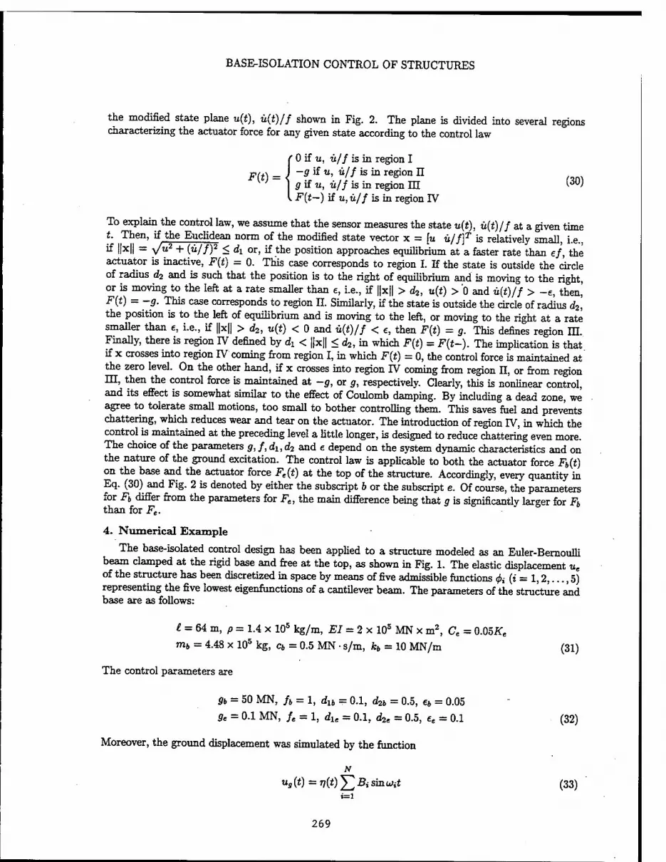
BASE-ISOLATION CONTROL OF STRUCTURES
the modified state plane u(t), ü(t)/f shown in Fig. 2. The plane is divided into several regions characterizing the actuator force for any given state according to the control law
F(t) = I
' 0 if u, ü/f is in region I —g if u, ü/f is in region II g if u, ü/f is in region III (30)
. F(t-) if u, ü/f is in region IV
To explain the control law, we assume that the sensor measures the state u(t), ü(t)/f at a given time t. Then, if the Euclidean norm of the modified state vector x = [u ü/f]T is relatively small, i.e., if ||x|| = y/u2 + (ü/f)2 < di or, if the position approaches equilibrium at a faster rate than ef, the actuator is inactive, F(t) = 0. This case corresponds to region I. If the state is outside the circle of radius d2 and is such that the position is to the right of equilibrium and is moving to the right, or is moving to the left at a rate smaller than e, i.e., if ||x|| > d2, u(t) > 0 and ü(t)/f > -e, then, F(t) = ~9- This case corresponds to region II. Similarly, if the state is outside the circle of radius d2, the position is to the left of equilibrium and is moving to the left, or moving to the right at a rate smaller than e, i.e., if ||x|| > d2, u(i) < 0 and ü(t)/f < e, then F(t) = g. This defines region IH. Finally, there is region IV defined by dx < ||x|| < d2, in which F(t) = F(t-). The implication is that if x crosses into region IV coming from region I, in which F(t) = 0, the control force is maintained at the zero level. On the other hand, if x crosses into region IV coming from region II, or from region m, then the control force is maintained at -g, or g, respectively. Clearly, this is nonlinear control, and its effect is somewhat similar to the effect of Coulomb damping. By including a dead zone, we agree to tolerate small motions, too small to bother controlling them. This saves fuel and prevents chattering, which reduces wear and tear on the actuator. The introduction of region IV, in which the control is maintained at the preceding level a little longer, is designed to reduce chattering even more. The choice of the parameters g, f, dx,d2 and e depend on the system dynamic characteristics and on the nature of the ground excitation. The control law is applicable to both the actuator force Fb(t) on the base and the actuator force Fe(t) at the top of the structure. Accordingly, every quantity in Eq. (30) and Fig. 2 is denoted by either the subscript 6 or the subscript e. Of course, the parameters for Fb differ from the parameters for Fe, the main difference being that g is significantly larger for Fb than for Fe.
4. Numerical Example
The base-isolated control design has been applied to a structure modeled as an Euler-Bernoulli beam clamped at the rigid base and free at the top, as shown in Fig. 1. The elastic displacement ue
of the structure has been discretized in space by means of five admissible functions & (i = 1,2,..., 5) representing the five lowest eigenfunctions of a cantilever beam. The parameters of the structure and base are as follows:
£ = 64 m, p = 1.4 x 10⁵ kg/m, EI = 2x 10s MN x m2, Ce = 0.05tfe
mb = 4.48 x 10⁵ kg, cb = 0.5 MN • s/m, kb = 10 MN/m (31)
The control parameters are
gb = 50 MN, fb = 1, dlb = 0.1, d2b = 0.5, e6 = 0.05 ge = 0.1 MN, fe = 1, dle = 0.1, d2e = 0.5, ee = 0.1 (32)
Moreover, the ground displacement was simulated by the function
N
ug(t)=T}(t)'52Bismuit (33) t=i
269

v(t) =
L. MEIROVITCH AND T. J. STEMPLE
where N = 9, Bi = 0.5, B2 = -0.65, B3 = 0.35, B4 = -0.85, B5 = 1.15, B6 = -1.25, B7 = 1-05, Bs = -1, B9 = 0.95, wi = 1, u>2 = 1.2, o;3 = 2, u/4 = 2.3, w5 = 3, w6 = 3.1, w7 = 4, w8 = 4.3, w9 = 9 and
3(^)2+2(^)': «'" (34> .0 , f 2 < *
in which ti = 20 s, *2 = 40 s. Figures 3 and 4 show the displacement and velocity of the ground for 0 < t < 100 s.
Figures 5 and 6 depict the displacement of the base and of the top of the building, respectively, whereas Figs. 7 and 8 show the corresponding velocities, in which the uncontrolled response is plotted in a dashed line and the controlled one in a solid line. On the other hand, Figs. 9 and 10 display the actuator force on the base and on the top of the structure. These preliminary results appear quite encouraging. Figures 5-8 indicate that the controls reduce the displacement and velocity during the earthquake but increase the residual displacement and velocity somewhat after the termination of the earthquake. The residual displacement and velocity can be reduced further by choosing smaller dead zone parameters, but this is likely to increase chattering.
Conclusions This paper presents a base-isolation control design capable of reducing the motion of structures
relative to the inertial space during earthquakes, thus achieving the basic objectives of preventing injury to occupants and damage to the contents and protecting the integrity of structures. The control law is a modified on-off with deadband, a nonlinear control more economical than linear control and easier to implement. Preliminary results are very encouraging. The performance can be further improved through an optimization of the various control parameters.
6. Bibliography 1. Abdel-Mooty, M. and Roorda, J., "Time-Delay Compensation in Active Damping of Structures,''
ASCE Journal of Engineering Mechanics, Vol. 117, No. 11, 1991, pp. 2549-2570. 2. Bhatti, M.A., Pister, K.S. and Polak, E., "Optimization of Control Devices in Base Isolation System
for Aseismic Design," in Structural Control, H.H.E. Leipholz, ed., North-Hollang Publishing Co., Amsterdam, The Netherlands, 1979, pp. 127-138.
3. Chung, L.L., Reinhorn, A.M. and Soong, T.T., "Experiment on Active Control of Seismic Structures," ASCE Journal of Engineering Mechanics, Vol. 114, No. 2, 1988, pp. 241-256.
4. Chung, L.L., Lin, R.C., Soong, T.T. and Reinhorn, A.M., "Experimental Study of Active Control for MDOF Seismic Structures," ASCE Journal of Engineering Mechanics, Vol. 115, No. 8, 1989, pp. 1609-1627.
5. Dehghanyar, T.J., Masri, S.F., and Miller, R.K., "On-Line Parameter Control of Nonlinear Flexible Structure," in Structural Control, H.H.E. Leipholz, ed., Martinus Nijhoff Publishers, Dordrecht, The Netherlands, 1987, pp. 141-159.
6. Feng, M.Q., Shinozuka, M. and Fugi, S., "Friction-Controllable Sliding Isolation System," ASCE Journal of Engineering Mechanics, Vol. 119, No. 9, 1993, pp. 1845-1864.
7. Feng, M.Q., "Application of Hybrid Sliding Isolation System to Buildings," ASCE Journal of Engineering Mechanics, Vol. 119, No. 10, 1993, pp. 2090-2108.
8. Juang, J.N., Sae-Ung, S. and Yang, J.N., "Active Control of Large Building Structures," in Structural Control, H.H.E. Leipholz, ed., North-Holland Publishing Co., Amsterdam, The Netherlands, 1979, pp. 663-676.
9. Kelly, J.M., "Control Devices for Earthquake-Resistant Structural Design," in Structural Control, H.H.E. Leipholz, ed., North-Holland Publishing Co., Amsterdam, The Netherlands, 1979, pp. 391-413.
10. Kelly, J.M., Leitmann, G. and Soldatos, A.G., "Robust Control of Base-Isolated Structures Under Earthquake Excitation," Journal of Optimization Theory and Applications, Vol. 53, No. 2, 1987, pp. 159-180.
270

BASE-ISOLATION CONTROL OF STRUCTURES
11. Leipholz, H.H.E. and Abdel-Rohman, M., Control of Structures, Martinus Nijhoff Publishers, Dordrecht, The Netherlands, 1986.
12. Lin, B.C., Tadjbakhsh, LG., Papageorgiou, A.S. and Ahmadi, G., "Performance of Earthquake Isolation Systems," ASCE Journal of Engineering Mechanics, Vol. 116, No. 2, 1990, pp. 446-461.
13. Martin, C.R. and Soong, T.T., "Modal Control of Multistory Structures," ASCE Journal of the Engineering Mechanics, Vol. 102, No. EM4, 1976, pp. 613-623.
14. Masri, S.F., Bekey, G.A. and Safford, F.B., "Optimal Response Simulation of Multidegree Systems by Pulse Excitation," Journal of Dynamic Systems, Measurement, and Control, Vol. 97, No. 1 1975, pp. 46-52.
15. Masri, S.F., Bekey, G.A. and Udwadia, F.E., "On-Line Pulse Control of Tall Buildings," in Structural Control, H.H.E. Leipholz, ed., North-Holland Publishing Co., Amsterdam, The Netherlands, 1979, pp. 471-491.
16. Masri, S.F., Bekey, G.A. and Caughey, T.K., "Optimal Pulse Control of Flexible Structures," Journal of Applied Mechanics, Vol. 48, No. 3, 1981, pp. 619-626.
17. Masri, S.F., Bekey, G.A. and Caughey, T.K., "On-Line Control of Nonlinear Flexible Structures," Journal of Applied Mechanics, Vol. 49, No. 4, 1982, pp. 877-884.
18. Meirovitch, L. and Öz, H., "Active Control of Structures by Modal Synthesis," in Structural Control, H.H.E. Leipholz, ed., North-Holland Publishing Co., Amsterdam, The Netherlands, 1979, pp. 505-521.
19. Meirovitch, L. and Baruh, H., "Control of Self-Adjoint Distributed-Parameter Systems," Journal of Guidance and Control, Vol. 5, No. 1, 1982, pp. 60-66.
20. Meirovitch, L. and Silverberg, L.M., "Control of Structures Subjected to Seismic Excitation," ASCE Journal of Engineering Mechanics, Vol. 109, No. 2, 1983, pp. 604-618.
21. Meirovitch, L. and Öz, H., "Digital Stochastic Control of Distributed-Parameter Systems," Journal of Optimization Theory and Applications, Vol. 43, No. 2, 1984, pp. 307-325.
22. Meirovitch L., Baruh, H., Montgomery, R.C., and Williams, J.P., "Nonlinear Natural Control of an Experimental Beam," Journal of Guidance, Control, and Dynamics, Vol. 7, No. 4, 1984 pp. 437-442.
23. Meirovitch, L., Computational Methods in Structural Dynamics, Sijthoff & Noordhoff, The Netherlands, 1980.
24. Meirovitch, L., Dynamics and Control of Structures, Wiley-Interscience, New York, 1990. 25. Meirovitch, L. and Kwak, M.K., "Rayleigh-Ritz Based Substructure Synthesis for Flexible
Multibody Systems," AIAA Journal, Vol. 29, No. 10, 1991, pp. 1709-1719. 26. Miller, R.K., Masri, S.F., Dehghanyar, T.J. and Caughey, T.K., "Active Vibration Control of Large
Civil Structures," ASCE Journal of Engineering Mechanics, Vol. 114, No. 9, 1988, pp. 1542-1570. 27. Pu, J.-P. and Hsu, D.-S., "Optimal Control of Tall Building," ASCE Journal of Engineering
Mechanics, Vol. 114, No. 6, 1988, pp. 973-989. 28. Pu, J.-P. and Kelly, M., "Active Control and Seismic Isolation," ASCE Journal of Engineering
Mechanics, Vol. 117, No. 10, 1991, pp. 2221-2236. 29. Reinhorn, A.M., Manolis, G.D. and Wen, C.Y., "Active Control of Inelastic Structures," ASCE
Journal of Engineering Mechanics, Vol. 113, No. 3, 1987, pp. 315-333. 30. Reinhorn, A.M., Soong, T.T. and Wen, C.Y., "Base Isolated Structures with Active Control," in
Recent Advances in Design, Analysis, Testing and Qualification Methods, ASME PVP-Vol. 127 1987, pp. 413-419.
31. Rodellar, J. and Martin-Sanchez, J., "Predictive Structural Control," in Structural Control, H.H.E. Leipholz, ed., Martinus Nijhoff Publishers, Dordrecht, The Neterlands, 1987, pp. 580-593.
32. Rodellar, J., Chung, L.L., Soong, T.T., and Reinhorn, A.M., "Experimental Digital Control and Structures," ASCE Journal of Engineering Mechanics, Vol. 115, No. 6, 1989, pp. 1245-1261.
33. Rofooei, F.R. and Tadjbakksh, LG., "Optimal Control of Structures with Acceleration, Velocity, and Displacement Feedback," ASCE Journal of Engineering Mechanics, Vol. 119, No. 10, 1993 pp. 1993-2010.
271

L. MEIROVITCH AND T. J. STEMPLE
34. Roorda, J., "Tendon Control in Tall Buildings," ASCE Journal of the Structural Division, Vol. 101, No. ST3, 1975, pp. 505-521.
35. Roorda, J., "Experiments in Feedback Control of Structures," in Structural Control, H.H.E. Leipholz, ed., North-Holland Publishing Col., Amsterdam, The Netherlands, 1979, pp. 629- 661.
36. Soong, T.T. and Chang, M.I.J., "On Optimal Control Configuration in Theory of Modal Control," in Structural Control, H.H.E. Leipholz, ed., North-Holland Publishing Co., Amsterdam, The Netherlands, 1971, pp. 723-738.
37. Soong, T.T., Reinhorn, A.M. and Yang, J.N., "A Standard Model for Structure Control Experiments and Some Experimental Results," in Structural Control, H.H.E. Leipholz, ed., Martinus Nijhoff Publishers, Dordrecht, The Netherlands, 1987, pp. 669-693.
38. Soong, T.T., Reinhorn, A.M., Wang, Y.P. and Lin, R.C., "Full-Scale Implementation of Active Control I: Design and Simulation," ASCE Journal of Engineering Mechanics, Vol. 117, No. 11, 1991, pp. 3516-3536.
39. Soong, T.T., Active Structural Control: Theory and Practice, Longman Scientific and Technical, Essex, England, 1990.
40. Suhardjo, J., Spencer, B.F., Jr. and Kareem, A., "Frequency Domain Optimal Control of Wind- Excited Buildings," ASCE Journal of Engineering Mechanics, Vol. 118, No. 12, 1992, pp. 2463- 2481.
41. Udwadia, F.E. and Tabaie, S., "Pulse Control of Single Degree-of-Freedom System," ASCE Journal of the Engineering Mechanics Division, Vol. 107, No. EM6, 1981, pp. 997-1009.
42. Udwadia, F.E. and Tabaie, S., "Pulse Control of Structural and Mechanical Systems," ASCE Journal of the Engineering Mechanics Division, Vol. 107, No. EM6, 1981, pp. 1011-1028.
43. Vilnay, O. "Design of Modal Control of Structures," ASCE Journal of the Engineering Mechanics Division, Vol. 107, No. EM5, 1981, pp. 907-915.
44. Wong, H.L. and Luco, J.E., "Structural Control Including Soil-Structural Interaction Effects," ASCE Journal of Engineering Mechanics, Vol. 101, No. EM6, 1975, pp. 819-838.
45. Yang, J.N., "Application of Optimal Control Theory to Civil Engineering Structures," ASCE Journal of Engineering Mechanics, Vol. 101, 1975, pp. 819-838.
46. Yang, J.N., "Control of Tall Buildings under Earthquake Excitation," ASCE Journal of the Engineering Mechanics Division, Vol. 108, No. EM5, 1982, pp. 833-849.
47..Yang, J.N., Akbarpour, A. and Ghaemmaghami, P., "New Optimal Control Algorithms for Structural Control," ASCE Journal of Engineering Mechanics, Vol. 113, No. 9, 1987, pp. 1369- 1386.
48. Yang, J.N., Akbarpour, A. and Ghaemmaghami, P., "Optimal Control Algorithms for Earthquake- Excited Building Structure," in Structural Control, H.H.E. Leipholz, ed., Martinus Nijhoff Publishers, Dordrecht, The Netherlands, 1987, pp. 748-781.
49. Yang, J.N. and Soong, T.T., "Recent Advances in Active Control of Civil Engineering Structures," Journal of Probabilistic Engineering Mechanics, Vol. 3, No. 4, 1988, pp. 179-188.
50. Yang, J.N. and Akbarpour, A., "Effect of System Uncertainty on Control of Seismic-Excited Buildings," ASCE Journal of Engineering Mechanics, Vol. 116, No. 2, 1990, pp. 462-478.
51. Yang, J.N., Danielians, A. and Liu, S.C., "Aseimic Hybrid Control Systems for Building Structures," ASCE Journal of Engineering Mechanics, Vol. 117, No. 4, 1991, pp. 836-853.
52. Yang, J.N., Li, Z., Danielians, A. and Liu, S.C., "Aseismic Hybrid Control of Nonlinear and Hysteretic Structures, I," ASCE Journal of Engineering Mechanics, Vol. 118, No. 7,1992, pp. 1423- 1440.
53. Yang, J.N., Li, Z., Danielians, A. and Liu, S.C., "Aseismic Hybrid Control of Nonlinear and Hysteretic Structures, H," ASCE Journal of Engineering Mechanics, Vol. 118, No. 7, 1992, pp. 1441-1456.
54. Yang, J.N., Li, Z. and Liu, S.C., "Stable Controllers for Instantaneous Optimal Control," ASCE Journal of Engineering Mechanics, vol. 118, No. 8, 1992, pp. 1612-1630.
272

BASE-ISOLATION CONTROL OF STRUCTURES
55. Yang, J.N., Li, Z. and Liu, S.C., "Control of Hysteretic System Using Velocity and Acceleration Feedbacks," ASCE Jourard of Engineering Mechanics, Vol. 118, No. 11, 1992, pp. 2227-2245.
Lp.B
— f.
I—<
Fig. 1 - Model of a Base-Isolated Structure Fig. 2 - On-Off Control Regions in a Modified State Plane
Fig. 3 - Displacement of the Ground
I0M3O4O5O6O70S090
t(s) Fig. 4 - Velocity of the Ground
273

L. MEHtOVITCH AND T. J. STEMPLE
o.«
0.6
0.4
I" -—. 0
-o 3 -0.2
-0.4
-0.«
1 ( i s
'!.. 1
\
nil'' '■' iv^\ ■A^f y*\-
ü ifii"^' 1111? ;-
: i 10 20 30 40 50 60 70 K> 90 100
*(s) Fig. 5 - Displacement of the Base
■0 20 30 40 30 60
i(s) Fig. 6 - Velocity of the Base
TO 80 90 100
10 2030405060708090 100
*(s) Fig. 7 - Displacement of the Top of Structure Fig. 8 - Velocity of the Top of Structure
60
Z S
Et, .20- I I i
10 203O4O5O607OSO90I0O
*(s) Fig. 9 - Control Force on Base
0.1
fc, -0.05 ■■
-0.1
-0.15
1 1 | Ji- 1 i i i
i ! i i
ll I0 203040506070J090 100
. t(s) Fig. 10 - Control Force at Top of Structure
274

CONTROL ALGORITHM FOR FLUTTER SUPPRESSION OF
LOW-ASPECT RATIO COMPOSITE WINGS
Russell Morris and Leonard Meirovitch Virginia Polytechnic Institute and State University
Blacksburg, VA 24061
Abstract
A control algorithm has been developed for the flutter suppression of low-aspect ratio composite wings. The control system uses surface-mounted piezoelectric sensors and actuators in conjunction with a linear quadratic regulator design. As a test of the feasibility of the design, the algorithm has been tested on an aircraft model including a trapezoidal composite plate wing as well as rigid-body pitch and plunge degrees of freedom.
1. Introduction
This paper is concerned with the design of a modern adaptive aircraft wing. Such a wing must be capable of sensing its current dynamic state and respond in such a manner as to prevent divergence or body-freedom flutter. Design of such an adaptive, or "smart" structure has become feasible with the advent of adaptive materials, such as piezoelectric ceramics and films, shape memory alloys and fiber optics (Refs. 1, 2 and 3). In particular, piezoelectric materials generate a measurable voltage proportional to the state of strain in the material. This property, together with their light weight and high strength makes piezoelectrics ideal for use as sensing materials in modern aircraft structures. Piezoelectric materials also have a converse property whereby they deform in proportion to an applied voltage field. This converse effect provides the control designer with a means of inducing strains in the host structure and thereby altering its dynamic characteristics. The basic premise behind smart- structure design is that intelligent materials are incorporated into the structure itself, thus giving the structure the ability to sense and react to changes in its dynamic state according to an appropriate control law.
For the flutter suppression problem at hand, it is proposed to incorporate surface-mounted piezo- electric patches into the wing design, which, together with appropriate control methodology, can favorably alter the flutter dynamic characteristics.
2. Aircraft Wing Model
The structural model includes the essential physical characteristics required for flutter analysis of modern low-aspect ratio composite wings. A view of the aircraft model is shown in Fig. 1. The wing is modeled as a trapezoidal, shear-deformable, composite plate with root and tip chords parallel to the flow. There are 2k symmetrically stacked, variable thickness, generally orthotropic plies in the laminate (Fig. 2). The piezoelectric patches are mounted symmetrically on both the upper and lower surfaces of the wing, with those on top playing the role of actuators and those at the bottom serving as collocated sensors. Research has shown that rigid-body motions of an aircraft play an important role in the occurrence of certain types of flutter phenomena (Ref. 4). For this reason, fuselage mass and inertia are included and the model is assumed to undergo rigid-body plunge (translation in the z-direction) and rigid-body pitch (rotation about the y-axis). The control of the rigid-body modes must be carried out separately, as it is not feasible to alter these modes by means of piezoelectric actuation. Rigid-body control can be introduced into the system through the use of thrusters and torquers or through aerodynamic control surfaces. This type of model formulation was first presented in Ref. 10 to study the effects of aeroelastic tailoring on flutter speed.
275

R. MORRIS AND L. MEIROVITCH
3. System Equations of Motion
The equations of motion for the system in Fig. 1 are derived by means of the extended Hamilton's principle. To this end, it is first necessary to derive expressions for the system kinetic.energy, potential energy and the virtual work performed by all nonconservative forces.
i. Kinetic energy The total kinetic energy of the fuselage/plate model includes contributions from rigid-body motions
and elastic plate deformations. The absolute displacement of a point on the fuselage is given by
Wf(x, t) = wc(t) + (x- xc)i>c(t) (1)
where xc is the position of the system center of mass, wc the rigid-body plunge degree of freedom and ij)c the rigid-body pitch angle. The absolute displacement of a point on the flexible plate is given by
u(x,y,z,t)=zipx(x,y,t), v(x,y,z,t) = zif>y{x,y,t)
wp(x,y,t) = wc(t) + (x- xc)ipc{t) + w(x,y,t)
in which u and v are elastic displacements in the x and y directions, ipx and tpy are rotations of a line originally normal to the mid-plane of the undeformed plate and w is the transverse elastic displacement of the plate. Taking the appropriate time derivatives, we obtain the following expression for the system kinetic energy:
T=\ f w}dMf + \ I (Ü2 + v2 + wl)dMp 1 JMf
l JMP
= 2 / [vc + (x- xc)i>c] dMf + -J | z2ipl + z2ipl + [u>c + (x - xc)ipc +1&] \
=- (MCW2
C + Ici>2c) + 2 / [mP^2 + -W* + $)] dAP + üc f
dM„
rripWdAp
i>c f JA
+ ipc mp(x - xc)wdAp
where
Mc = Mf + Mp, Ic= I (x- xcfdMf + f (x - xcf JMf JMP
MP = S / Pidz> 7
P = X! / Pi''
dMr,
jzzdz
(3)
(4a, b)
(4c, d)
in which Mf is the total mass of the fuselage, Mp the total mass of the plate, mp the mass per unit area of plate, pj the mass per unit volume of plate and Ip the mass moment of inertia per unit area of plate. Note that there are 2k stacked plies and hj — hj-i defines the thickness of ply j.
ii. System potential energy The potential energy for the wing/fuselage system consists only of the elastic strain energy in the
flexible wing. Because the plate model is a composite laminate, first-order shear deformation theory is used in the analysis. Essentially, this amounts to relaxing the constraints imposed on the rotation ij)x and tpy by Kirchoff's assumptions. Under the first-order theory, ipx and tj)y remain independent degrees of freedom.
The piezoelectric patches are treated as surface-mounted isotropic plies. The voltage-induced strain is included in the stress-strain relationships from laminate plate theory. For each patch, the stress-strain relationship is
• xy
= [Q \py €x Ax ey ~ h-y
1 }
(5)
276

ACTIVE FLUTTER SUPPRESSION ALGORITHM
where Qp is the reduced stiffness matrix for the piezoelectric material and Ax and Ay are voltage- induced strains given by
A„ &j,
V*{x,y,t) (6)
in which V^a;,^,*) is the voltage applied across the patch, ex and ey are piezoelectric constants and t is the patch thickness.
Using the laminate plate theory with first-order shear deformation (Ref. 11), we can write the expression for the total laminate strain energy in the form
V Ipx ,x
T \DU D12 D 16
= { Wy,y F>\2 D22 D26 JAT \ _Wx,y + Wy,x _ Die Di& Dee
[lpx+WtX
T Au A45 'lpy+W,y
. A45 A55 $x+W,x.
i>x,x T
Fu F12 Fie ~ex~ + Vy,y F12 F22 F26 ey
_1px ,y + '>Py ,x _ _-Fi6 F 26 Fee_ 0
i>x,x Vy,y
_Yx,y + 1py,x
dAj, (7)
in which the total laminate extensional, bending and piezoelectric stiffness coefficients are given re- spectively by
Aab = I>; - hi-l)QJab, Dab = - £(Ä* - h^Qib, Kb = jj>, + Vl)(%)'X3' («O, b, c) i=i i=i 3=1
where hj and hj-i, which are in general functions of a; and y, were defined earlier and m is the number of actuator patches. The last term in Eq. (7) represents the voltage-dependent actuation strain energy of the system.
iii. Virtual work The only nonconservative forces present in this model are due to aerodynamic loading of the wing.
The model under consideration is a trapezoidal wing characterized by a low-aspect ratio and forward sweep. The flight regime for flutter of such a wing is undoubtedly supersonic. For large Mach numbers, there is a weak memory effect, as well as weak three-dimensional effects. These factors suggest the use of piston theory (Ref. 5), in which the pressure difference between the upper and lower surfaces of the plate is related to the absolute displacement of the plate, or by an aerodynamic operator
Ap=-CW(!+[;
1 S \ m ^ 4« 2 ox
(9a, b)
where U is the free-stream airspeed, q the free-stream dynamic pressure, M the free-stream Mach number, 7 the ratio of specific heats and tjf the plate half-thickness. The virtual work performed by the aerodyanmic forces is
6W = / ApSwpdAp = / ]w8wc + W(x - xc)6ipc + W6w\ dAp (10)
in which 5wp is the virtual displacement of the wing and
W = C(x)| i>c + W,x + ff \wc + {x- xc)ipc + w (11)
277

R. MORRIS AND L. MEIROVITCH
The system equations of motion are now derived by means of the extended Hamilton's principle (Ref. 6)
*2
/ *1
(ST -6V + 8W)dt = 0, Swc = öxßc = Sw = 8^x =6i/>y = 0 at h, t2 (12)
Introducing Eqs. (3), (7) and (10) into Eq. (12) we obtain a hybrid system of equations consisting of two ordinary differential equations for the rigid-body motions and three partial differential equations for the elastic plate displacements. Spatial discretization through a series expansion allows reduction of the three partial differential equations to a system of ordinary differential equations in terms of generalized coordinates. The first two generalized coordinates correspond to the rigid-body degrees of freedom
wc(t) = qi(t), i>c{t) = qi{t) (13a,6)
On the other hand, the elastic displacements are expressed as series of trial functions multiplied by generalized coordinates, or
"+2 2n+2 3n+2
w{x,y,t) = ^j<j)i{x,y)qi{t), iffx(x,y,t)= ^ &(*,»)*(*), 1>y(x,y,t) = ^ <t>i{x,y)qi(t) *=3 t=n+3 i=2n+3
(14a, b, c) Substitution of Eqs. (13) and (14), in conjunction with Eqs. (3), (7) and (10) directly into Hamilton's principle results in the discretized equations of motion
Mq{t) + Hq(t) + (K + KA)q(t) = BVp(t) + BVrb(t) (15)
where M is a system mass matrix, K a system elastic stiffness matrix, H an aerodynamic damping matrix, KA an aerodynamic stiffness matrix, Vp(i) a vector of control voltages for the piezoelectric actuators and VTb(i) a vector of control inputs for the rigid-body actuators; B and B are participation matrices corresponding to the piezoelectric and rigid-body actuators respectively. Both KA and H are depend on the free-stream airspeed U. In addition, the aerodynamic stiffness matrix is nonsymmetric, thus rendering the problem non-self-adjoint (Ref. 6).
4. Convergence of the Free-Vibration Solution
The convergence and accuracy of the discretized solution depends on the nature of the trial func- tions used in Eqs. (13). For non-self-adjoint systems, the trial functions (j>i{x,y) are generally from the class of comparison functions, which satisfy all the problem boundary conditions (Ref. 6). The cantilever plate under consideration is subject to natural boundary conditions at the three free edges, which are further complicated by the fact that the leading and trailing edges are functions of both x and y. Hence, comparison functions are not feasible here, so that we do the next best thing and choose the trial functions from the class of quasi-comparison functions, defined as linear combinations of admissible functions (shape functions) capable of satisfying all the problem boundary conditions (Ref. 7). Unlike comparison functions, admissible functions need satisfy only the geometric boundary conditions at the clamped edge of the plate. Quasi-comparison functions have been shown to exhibit faster convergence than both admissible functions and comparison functions for both self-adjoint and non-self-adjoint systems (Refs. 7 and 8). Furthermore, the class of quasi-comparison functions is much broader than the class of comparison functions, and it generally involves linear combinations of several families of admissible functions. For the problem at hand, half of the trial functions are chosen as trigonometric functions and half as power series.
To demonstrate the convergence and accuracy of the solution, natural frequencies were calculated for two different models using increasing numbers of trial functions. The first model is an aluminum rectangular cantilever plate, for which an exact solution is available (Ref. 9). The results are shown
278
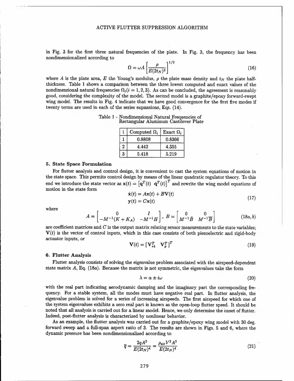
ACTIVE FLUTTER SUPPRESSION ALGORITHM
in Fig. 3 for the first three natural frequencies of the plate, nondimensionalized according to
1'2
In Fig. 3, the frequency has been
(16) E(2tN)2\
where A is the plate area, E the Young's modulus, p the plate mass density and tpt the plate half- thickness. Table 1 shows a comparison between the three lowest computed and exact values of the nondimensional natural frequencies fij(i = 1,2,3). As can be concluded, the agreement is reasonably good, considering the complexity of the model. The second model is a graphite/epoxy forward-swept wing model. The results in Fig. 4 indicate that we have good convergence for the first five modes if twenty terms are used in each of the series expansions, Eqs. (14).
Table 1 - Nondimensional Natural Frequencies of Rectangular Aluminum Cantilever Plate
i Computed fi{ Exact tii 1 0.8808 0.8366 2 4.442 4.355 3 5.418 5.219
5. State Space Formulation
For flutter analysis and control design, it is convenient to cast the system equations of motion in the state space. This permits control design by means of the linear quadratic regulator theory. To this end we introduce the state vector as x(t) = [qT(£) qT(£)] and rewrite the wing model equations of motion in the state form
x(i) = Ax(t) + BV(t)
y(t) = Cx(t)
where 0 I
-M~l{K + KA) -M-XH
are coefficient matrices and C is the output matrix relating sensor measurements to the state variables; V(t) is the vector of control inputs, which in this case consists of both piezoelectric and rigid-body actuator inputs, or
B = 0
M^B 0_
M~YB
(17)
(18a, b)
v(*)=[v£ vj? (19)
6. Flutter Analysis
Flutter analysis consists of solving the eigenvalue problem associated with the airspeed-dependent state matrix A, Eq. (18a). Because the matrix is not symmetric, the eigenvalues take the form
A = Q ± iu> (20)
with the real part indicating aerodynamic damping and the imaginary part the corresponding fre- quency. For a stable system, all the modes must have negative real part. In flutter analysis, the eigenvalue problem is solved for a series of increasing airspeeds. The first airspeed for which one of the system eigenvalues exhibits a zero real part is known as the open-loop flutter speed. It should be noted that all analysis is carried out for a linear model. Hence, we only determine the onset of flutter. Indeed, post-flutter analysis is characterized by nonlinear behavior.
As an example, the flutter analysis was carried out for a graphite/epoxy wing model with 30 deg. forward sweep and a full-span aspect ratio of 3. The results are shown in Figs. 5 and 6, where the dynamic pressure has been nondimensionalized according to
Q = 2qA2
TV2A2
E(2tN)* E{2tNf (21)
279

R. MORRIS AND L. MEIROVITCH
in which pair is the air density and V the free-stream airspeed; all other quantities have been defined previously. In Fig. 5 we see that as the dynamic pressure is increased, the rigid-body pitch mode becomes more stable, while simultaneously the first flexible bending mode tends toward instability. In Fig. 6, we see that the frequencies of the two modes coalesce as the dynamic pressure is increased. Hence, the flutter mechanism for this case is the coalescence of the rigid-body pitch and first flexible bending mode, known as body-freedom flutter.
7. Linear Quadratic Regulator Design A preliminary control design has been carried out to demonstrate the feasibility of increasing the
speed of the wing/fuselage model. This control design assumes that the entire state is available for feedback and amounts to placing all the closed-loop eigenvalues in the left-half of the complex plane at each airspeed. To this end, we use the linear quadratic regulator theory to stabilize the system at each airspeed.
Following the usual procedure, the control law is chosen so as to minimize the quadratic cost functional
J=±f[xTQx + VTRV]dt (22)
in which
R =
rx 0 0 0 r2 0
0 0 '•■ 0 0 0
is a positive definite control weighting matrix and
Q = K 0 0 M
(23)
(24)
is a positive semi-definite state weighting matrix. It should be pointed out that the state weighting matrix Q was chosen so that the first term in the cost functional represents the sum of the system kinetic and potential energies, or
oo oo
\ I [xTQx] dt = \ I [qrMq + q^q] dt (25)
Application of Pontryagin's minimum principle yields a state feedback control law given by
V(t) = -BrlBTKgx{t) (26)
where Kg is the solution to the algebraic matrix Riccati equation
0 = -Q - ATKg - KaA + KgBR-1BTKQ (27)
Because the state matrix depends on the airspeed, a control law must be formulated for a series of increasing airspeeds, resulting in an airspeed-dependent gain schedule. The solution to the linear quadratic regulator problem guarantees asymptotic stability. However, at each airspeed the maxi- mum actuation voltage must be checked for saturation through simulation of the closed-loop system. Naturally, as the airspeed increases, more control effort must be utilized to stabilize the system. The airspeed at which one of the piezoelectric actuators reaches saturation becomes the new maximum airspeed of the system.
As an example, a control design was carried out for control of the bending-torsion flutter of a cantilever graphite/epoxy plate with no forward sweep and a full-span aspect ratio of 6. Ten PZT
280

ACTIVE FLUTTER SUPPRESSION ALGORITHM
actuator pairs were utilized in conjunction with full-state feedback. The control design was carried out beginning at an airspeed slightly below the open-loop flutter airspeed of the model. The results are shown in Fig. 7, which represents a plot of the normalized maximum actuation voltage as a function of the nondimensional dynamic pressure. The maximum actuation voltage has been normalized by dividing it by the saturation voltage of the piezoelectric material, or
V = ^L (28) »'sat
so that saturation occurs when V = 1. It is obvious from this graph that very little control effort is needed below the open-loop nutter speed of the system, as expected. As the dynamic pressure increases, the maximum actuation voltage increases until it eventually reaches saturation. The control design has increased the maximum dynamic pressure of this plate model by approximately 45%. Although a gain matrix was calculated for each increasing airspeed, numerical simulation has shown that the gain matrix calculated at the saturation airspeed is sufficient to stabilize the system at all lower airspeeds. This result simplifies the control implementation significantly and agrees with similar results presented in Ref. 3.
8. Conclusions
An aircraft wing model capable of predicting accurately various forms of flutter phenomena has been developed. Preliminary results indicate that it may be possible to increase the flutter speed of an aircraft wing by means of controls using piezoelectric actuators. Some subjects for future consideration include 1) output feedback utilizing the piezoelectric sensors and 2) model reduction (possibly transforming to modal space) to eliminate the higher frequency modes from the discrete model. The need for model reduction is based on two factors. First, the high frequency modes are not accurate and are causing numerical problems in the control simulation. In addition, only the first few modes participate in any of the flutter mechanisms studied.
9. References
1. Scott, R. C, and Weisshaar, T. A., "Controlling Panel Flutter Using Adaptive Materials," Proceed- ings of the AIAA/ASME/ASCE/AHS/ASC 32nd Structures, Structural Dynamic, and Materials Conference, Baltimore, MD, April 8-10, 1991, pp. 2218-2229.
2. Lazarus, K. B. and Crawley, E. F., "Multivariable High-Authority Control of Plate-Like Active Structures," AIAA Paper No. 92-2529-CP.
3. Lai, Z., Zhou, R. C. and Xue, D., "Suppression of Nonlinear Panel Flutter at Elevated Temperature with Piezoelectric Actuators," AIAA Paper No. 93-1698-CP.
4. Weisshaar, T. A., Zeiler, T. A., Hertz, T. J. and Shirk, M. H., "Flutter of Forward Swept Wings, Analysis and Tests," Proceedings of the AIAA/ASME/ASCE/AHS 23rd Structures, Structural Dynamics and Materials Conference, New Orleans, LA, 1982, pp. 111-121.
5. Bisplinghoff, R. L. and Ashley, H., Principles of Aeroelasticity, Dover Publications, Inc., New York, 1975.
6. Meirovitch, L., Computational Methods in Structural Dynamics, Sijthoff & Noordhoft, The Nether- lands, 1980.
7. Meirovitch, L. and Kwak, M. K., "Convergence of the Classical Rayleigh-Ritz Method and the Finite Element Method," AIAA Journal, Vol. 28, No. 8, 1990 pp. 1509-1516.
8. Hagedorn, P., "The Rayleigh-Ritz Method With Quasi-Comparison Functions in Non-Self-Adjoint Problems," Journal of Vibration and Acoustics, Vol. 115, July 1993, pp. 280-284.
9. Blevins, R. D., Formulas for Natural Frequency and Modeshape, Van Nostrand Reinhold, New York, 1979.
10. Meirovitch, L. and Seitz, T. J., "Structural Modeling for Optimization of Low Aspect Ratio Com- posite Wings, Journal of Aircraft, Vol. 32, No. 5, 1995 (to appear).
11. Whitney, J., Structural Analysis of Laminated Anisotropie Plates, Technomic Publishing, Lan- caster, PA, 1987.
281

Piezoelectric Patches
Air Flow
*c = Pitch Angle Wc = Plunge Direction
Fig. 1 - Aircraft Wing with Surface-Mounted Piezoelectric Patches
Piezoelectric Actuators Laminate Midplane
Piezoelectric Sensors
Fig. 2 - Laminate Cross Section
282

30
25
20
&i 1 5
10
_ ' I I ' I 'l ' ' I I I ' ■<—T 1 ' , i , | i i . i i
" \ \_Q3_
-
9""^V^S-fk •
\. til -e— . L T?T- —©—
-1—i—
i—i—
5 10 15 20 25 30 35
n
Fig. 3 - Nondimensional Natural Frequencies Versus the Number of Trial Functions for Aluminum Rectangular Cantilever Plate
Qi
50
40
30
20
10
10 15 20 25 30 35 n
Fig. 4 - Nondimensional Natural Frequencies Versus the Number of Trial Functions for Graphite/Epoxy Forward-Swept Wing
283

- 5
a -1 0
1 5
"•■-«i»».s.T.... ! >
Flutter Onset
20
——pitch —- bendim
-J 1 1 1 I L_
15 20 25
q
30 35
Fig. 5 - Eigenvalue Real Part Versus Nondimensional Dynamic Pressure for Forward-Swept Wing
2.5 =*—rjf-
fi 1.5
0.5
-"—v; * *fc •
- 1 ! i ■pitch
—- bending : j ;
.
—i—i—i—i—i—,—,—,—,—i ....i..
15 20 25
9 30 35
Fig. 6 - Pitch and Bending Frequencies Versus Nondimensional Dynamic Pressure for Forward-Swept Wing
284

1 4
1.2
1.0
0.8
V 0.6
: Open-loop Flutter *?:::. j\ dynamic » : \
: !. Pressure.' Actuator
0.4 j# Saturation
0.2 *
0 0 : | '
_n o 800 1000 1200 1400 1600 1800
q Fig. 7 - Normalized Maximum Actuation Voltage Versus
Nondimensional Dynamic Pressure
235

286
STABILITY OF A COMPRESSIBLE
VISCOUS FLUID BETWEEN COAXIAL ROTATING
CYLINDERS WITH A FLEXIBLE SUPPORT
V. Mehl and J. Wauer Universität Karlsruhe
Karlsruhe, GERMANY
Abstract
The stability behavior of a compressible viscous fluid flow between two coaxial infinitely-long cylinders with a flexible support is analyzed. The outer cylinder is fixed, and the rotational speed of the inner cylinder is chosen to be sufficiently low so that laminar-turbulent transition or even fully-developed turbulent flow cannot appear. First of all, a correct formulation of the governing boundary value problem in the sense of continuum mechanics - including an accurate description of all boundary and transition conditions - is given. Next, the simplified boundary value problem representing the stationary motion in the form of a laminar shear flow is deduced. Subsequently, the linearized equations of motion for small superimposed perturbations are derived. Finally, the procedure used to solve the formulated equation set approximately is described. It can be recognized that two independent stability problems appear: the first one represents a Taylor-like vortex flow instability still possible for flexibly-supported cylinders; the second one is a real transverse interaction problem without axial perturbations. Attention is focussed on the stability limit in the form of a threshold speed for varying characteristic parameters. In the present paper, the first stability problem is completely analyzed without significant additional restrictions. For the second problem, the results for the special case of a narrow fluid-filled gap are presented.
1. Introduction
The stability behavior of an incompressible viscous fluid flow between two coaxial rotating cylinders is a classical problem in hydrodynamics (Ref. 2, 3). Interesting secondary effects are related to an eccentric mounting of the cylinders (Ref. 5), the presence of an axial flow (Ref. 6) or the influence of the compressibility of the fluid (Ref. 10). A further important modification concerns the support itself, which is assumed to be rigid in all available references. In the present work, a flexible bedding in the radial direction is assumed and the dependence of the critical Taylor number on the stiffness property of the suspension is the main objective. The results for a compressible fluid are compared with those for an incompressible fluid (Ref. 9).
Technical backround includes the interaction of rotating shafts and the surrounding seals, for instance (Ref. 4). But then, different practical facts, e.g., finite length and non-uniform geometry of the seals, and very often such high angular speeds that a fully turbulent flow results, complicate the problem to be solved so extreme that purely numerical investigations are required.
2. Formulation
Consider an elastically supported (foundation stiffness per unit length k), rigid and perfectly balanced cylinder of radius R{ and mass density QC . It rotates at a constant angular speed Q in a centric position within a cylindrical rigid stator of radius Ra. Fig. 1 illustrates the geometry and shows the introduced r,<p,z- coordinate system used in the following. The gap between the two cylinders is filled with a Newtonian compressible fluid of mass density gp at constant temperature (constant dynamic viscosity fi). The purely azimuthal flow field (u0 = u>o = 0) is laminar and rotationally. symmetric with its velocity v0(r) in the circumferential direction <p and pressure po(r). The rotating
287

V. MEHL, J. WAUER
inner cylinder moves due to the small transverse displacements Ax(t), Ay(t) and the state variables of the fluid fluctuate [Au(r,<p,z,t),Av(r,tp,z,t),Aw(r,<p,z,t),Ap(r,<p,z,t)] about their stationary values because of the eccentric motion of the inner cylinder.
\ \ A x *. \ . -W:- :-: ■[:.:'.
■■•..' , • ■ '.:■*.."-
t ~2Ri \ 1 "■y
■ z
\ \ \ \ \ \ \ \
cross section
Fig. 1: Geometry of both cylinders
The problem is described by the continuity equation, the momentum equations in radial, azimuthal and axial directions and the state equation for a perfect gas, then by the dynamic transition conditions at the surface (located at r = Ä,- + Az cosy + Ay sin ip) between fluid and rotating inner cylinder (force balance for this cylinder) and the kinematical boundary and transition conditions (no-slip) at the surface between fluid and stator and between fluid and rotor.
The governing equations of motion are written down in dimensionless form with nondimensional variables
r = r(Ra-Ri), t = f^^L, p = PR*tfeF
x = x(Ra- Ri), y = y(Ra- Ri), z = z(Ra- £,-),
u = ü Äjft, v = v RiQ,, w = w Ri&,
and parameters
d dRitl Qp RiQ . a = —, Ke = , M = , c = sound velocity
Ri u c „ 1 cP Qp kgFR2
KM; Cv Or ITU2 ITU
238

STABILITY OF A COMPRESSIBLE, VISCOUS FLUID BETWEEN ROTATING CYLINDERS
After dropping all overbars for convenience, the boundary value problem reads
9QF , QQF , v öQF 6QF [du u 1 dv dw\ at or r dip dz \drrrdipdzl
(du du v du du v2 \ dt dr r d<p dz r J
dr Re\Zdr2+Zrdr +r*d<p2 +dz2 Zr2 3r* 8<p + 3 drdz + froTfy) '
(dv dv v dv dv uv\ dt dr r dtp dz r J
rdip Re\dri r dr + Zr* dip2 dz* r2 + 3r* dip + Zrd^dl + frdrlfy)'
(dw dw v dw dw \ dt dr r dip dz J
dp 1 fd2w ldw 1 d2w 4d2w 1 d2v 1 d2u l_du\ dz Re \dr*+ rdr+ r* dip2 + 3 dz2 + Zr d<päz + 3 drdz + Zr"dl j '
2JT
d'x bja* Sa [, . -j7~ + 0 x -{ / (—crrr cos ip + <jrit) sin ip) llA , A dip=Q, dt-* Re2 I J v r v r'r=±+Axcostp+Aysmtp ^ «i
0
2TT
d2y 6ja4 Sa f, . ~n? + D -, y / Wrr sin 10 + cv^cos ip) ,,. , A dip — 0, dt1 Re1 T J V ^ ^r=i+Arcos¥>+Aj(sm¥> ^ u'
0
u(l +±,(p,z,t) = «(1 + £,?>,*,*) = t»(l + £,?,*, t) = 0,
..ei 1 A , A ■ ^ rfAx dAy . u{- + Ax cos ip + Ay sin ip, ip, z, t) -—— cos ip + —-£ sin ip, dt dt
v(± + Ax cosip+Ay sin <p, tp, z,t) =1 -^sinip+—lCos<p, dt dt
w(^ + Ax cos ip + Ay sin <p, <p, z, t) = 0
with
a =-v+—(—-if^.A.-^l^lj.^i\\ l (dv v l 9u> rr F^ Re{dr Z\dr + r + rdip+ dz))' ^"&^"+^
for a compressible fluid.
289

V. MEHL, J. WAUER
3. Analysis
In the perturbed state the displacements of the cylinder are given as
x(t) = x0+Ax(t), y(t) = y0 + Ay(t), xo = yo=0,
whereas the state variables Aq(r, tp, z,t) (q G u,v,w,p) about the stationary flow state qo(r) (?o € v0,po ^0,uo = wo = 0) are
v(r, tp, z,t) = v0(r) + Av(r, tp, z, t), p(r, tp, z, t) = p0(r) + Ap(r, tp, z,t),
u(r,tp,z,t)=0 + Au(r,tp,z,t), w(r,tp,z,t) = 0 + Aw{r,tp,z,i).
Considering the stationary state of the boundary value problem first, all A-terms are ignored so that a time-independent boundary value problem
v^_dpo_ d2v0 ldvp vl _ r dr ' dr2 r dr r2 '
t>o(£) = l, «o(l + £) = 0
for vo(r),po(r) remains. Obviously, this describes a circumferential Couette flow unchanged in' comparison with the classical Taylor vortex flow problem and stable for sufficiently low Reynolds numbers. Even for a finite gap, an analytical solution
v0(r) = ' 2 + a
f -2(a + l)2 ] f ar*-l / (cll)M {Eu(a + 2)2a2) . e{2Eu(2 +a)2a2\ a2r2 )] p0(r) = p0i ■ (or)
ßo{r) = -j^r Po(r)
can be given. It is remarkable that the stationary flow field remains the same also for an incompressible fluid (but the pressure changes).
To formulate the variational equations characterizing the superimposed small perturbations, a Taylor expansion of first order
q(± + Ax cos tp + Ay sin tp, tp, z, t) = j(i, tp, z, t) + g ^ *' Or
(Ax cos tp + Ay sin tp)
is used in the transition conditions. Then the stationary quantities go(r) are subtracted and the remaining equations are linearized in the A-quantities. This yields a boundary value problem
fdAu Au I dAv dAw\ 1 dAp . dg0 v0 dAp n Qo ~3 h r —T h -r— + -=—57- + AU-T- + — — = 0, V or r r dtp dz J Eu at or Eu r dtp
I dAu VQ f dAu \ \ ^0 A °^P S0{-W+-{-dV-2Av))-Ef-rAp=-^
1 ( Ad2 Au A_dAu_AAu 1 d2Au d2Au 7 dAv 1 d2Av Id2 Aw' + Re \Z dr2 +3r'~dr~ 3 'r2 + r* dtp2 + dz2 ~ 3^ ~fy + 3r drdtp + 3 drdz ^
I dAv fdvo vo\ 4 t;o <9At;\ 1 dAp fio -^-+I-S- + — Au+ '-
dt \ dr r J r dtp I r dtp
290

STABILITY OF A COMPRESSIBLE, VISCOUS FLUID BETWEEN ROTATING CYLINDERS
+ 1 (d2Av 1 dAv Av 4 d2Av d2Av 7 dAu 1 d2Aw 1 d2Au Re
+ ■ + + + • + ■ + r dr r2 3r2 dip2 dz2 3r2 dp 3r dipdz 3r drdip
'8Aw vodAw Po I -^r- + dt r d<p
dAp
1 (d2Aw 1 dAw 1 d2Aw 4d2Aw 1 d2Av ld2Au l_8Au\
Re [ 8r2 r 8r + r2 dtp2 + 3 dz2 + Zr dipdz + 3 drdz + I7~dz~J '
I* , r <f2Ax 5a47 6a
-/{[( P Re( dr Z\ dr + r * r d<p + dz 1) COS Ip
1 (dAv Av IdAu Re\dr r r dp '
+ or cos
d2Ay 8aA*f 6a
dt2 +~Re~-
ip+Re'\dS' ~ ^(7)) Sin^ i (Azcos^ + Aj/sin^) Lp = 0,
ff / I IA -Re I or 3 V dr ' r + r Op + dz J J J
_1_ (dAv _ Av 1 öAu Re \ dr r r dip
COS ip
+ dpo . ~dr~Sm(p Re\dr2
1 fd2vo d fvos
~ ~d~\—\\cosip (Aa:cos^ + Aysmtp) \dip = 0,
Au(-,p,z,f) = — cosp+—sinp,
M?.^«.<) + dt>0 or
/A , A • \ dAx . dAy ■ {Ax cos tp-\-Ay sm.ip) = — sinp + —r^-cosp, dt at
Au, Av, Aiy, Ap 2ff-periodic in <p.
To separate the t- and ^-dependence, assume the following solution:
Aq(r,ip,z,t) = Q(r,p)-eaXt+i°\ u, v, p U, V, P
Ati)(r, <p, z,t) = -iW(r, ip) ■ eaM+i<7Z,
Ax(t) = X ■ eaXt, Ay{t) = Y ■ eaM.
The resulting boundary value problem is
fdU U 1 dV „A aX „ t,2 öp
\dr r .r dip ) Eu Eur En r dip
291

V. MEHL, J. WAUER
\ r \dtp vl p = _dP
Eu dr
1 U&U_ 4 dU__4U_ 1 &£■_ 2Tj_J_dV- ]_fV_ adW Re \^3 dr2 3r dr 3r2 r2 dtp2 * 3r2 d<p + Sr drdtp + 3 dr
Qo (axv +(^l+^.)u+^—]=-- — \ \ dr r J r dtp) r dip
+ -7T 1 (d2V . 1 dV V_ _4_ (PV__ 2
2 + 3r2 d<p2~r ' 3r2 dy> ' 3r dtp r 3r öröy> ■ + -
Re \ dr2 r dr r . - . aT, 7 dU c dW 1 d2f7
/ ,.,. , v0dW\ _ 1 /d2W 1 ÖW 1 d2W 4cr a dV a dU a\ e0{aXW+7^)=aP+Te[^ + -rl7 + 7>^-TW-Tr^-ZJr--TrU)>
< ^z.^VIv Sa T/lYn 2 (dU l fdU U 1 dV T„\)\
+JL/^_I I^sin 1 eiaz
Re\dr r r d<p)
+ a
ir j| 1 üe^ör 3\9r r r dy> J J
, ,,2 5a47 siny?
J_/öF_y 1017 i?e \ ör r r dtp '
dpo . 1 /d2t>o ö /^o> -— sin 95 f 1 — (X cos tp + Ysintp) >dtp = 0, or""'' ÄeVör2 drij))00^
U(l+±,v) = V(l+};,tp) = W(l + ±;,tp) = 0,
U(^,<p)e^ =a\(X cos tp + Y sintp), W(±p) = 0,
(X cos tp + Y sin tp) = aA(—X sin tp + Y cos tp), v(i,»y+^
{/, V, W, P 2ff-periodic in y>.
Two cases have to be distinguished:
l.c-^0, 2. <T = 0.
If the wave number <r is finite, obviously the kinematical transition conditions between fluid and inner cylinder enforce that the displacements of the inner cylinder vanish: X = Y = 0. As a consequence, the ^-dependence does not occur any longer and the dynamic transition conditions are identically fulfilled. The remaining boundary value problem coincides with the classical one governing the Taylor vortex flow instability which has been analyzed in detail also for a finite fluid gap (Ref. 8).
292

STABILITY OF A COMPRESSIBLE, VISCOUS FLUID BETWEEN ROTATING CYLINDERS
A vanishing wave number a means that all variables U, V, W and P will be independent of the axial space coordinate z. The velocity component W appears only in one equation, which is independent from the other equations. Assuming solutions for the remaining variables Q(Q £ U} V, P) in product form
oo
<2(r> <P) = Y1 (Qn{r) sin n<p + Qn(r) cos n<p), Qe U, P,
oo
^(r>^) = ^2\Vn(r) shiny + V„(r) cosntp) n=0
leads for every ordinal number n(n = 0,1,...,00) to a certain eigenvalue problem. In the dynamic
transition condition, the integral / ...dtp vanishes identically for n ^ 1 because / sin9? smn<pd<p = 0 0 0
for 7i 7^ 1. This leads to Ax, Ay = 0 in these cases. Only for n = 1, coupled fluid-cylinder vibrations" are described, so that in the following, this case is dealt with exclusively. Dropping the index n = 1 and taking notice that ^~- = (.)' yields
JU>+1U-IV) + ^P+JLU_J?_P=0J \ r r ) Eu Eur Eur
Jü'+1-ü+1-v) + ^-P + -ß-ü+^P = o,
V r r I Eu Eur Eur
eo
eo **=-* + -k(F+hV-&v-vr+h^
r+r-MiV-*+hv+fr)
-*+& Y + 6{p'0Y- X + P-HlU' + V'-iV+TrU
= 0,
= 0,
t/(i + i) = t/(i + i) = ni + i) = F(i + i) = o,
U($) = aXY, Ü(^) = aXX , V(I) = a\Y - t*(±) X, 7(£) = -a\X - t/0(l) Y.
Finally, eliminate X, Y and obtain in this way a complicated eigenvalue problem in U, V, P, Ü, V, P with space-dependent coefficients. Only an approximate solution seems to be possible. Galerkin's method using Ritz series expansions fulfilling all boundary conditions is promising. But finding comparison functions for the present problem - especially for the pressure P,~P - is a lengthy pre- calculation.
293

V. MEHL, J. WAUER
An alternative seems to be to consider the stability problem for a narrow gap a < 1. Here, a shifted reference frame using the transformation
1 1 , a I
is appropriate. Applying it, there are several simplifications. On the one hand, the" location of the fluid surfaces in the centered position of the inner cylinder change,
and on the other hand, the derivatives themselves are modified:
Here, the coefficients are constant [using t/0(£) = -1, t# = 0] if the ^-dependence of v0 is neglected because |£| < \ [set v0(£) = v0(0) = |]. So, a further simplification of the governing eigenvalue problem follows:
a(FW + aF) + i!-Z7+fiF+5f-P=o,
(««' + (f -1) v + f K) = -«/> + i (V» + cV + i«cr'),
(A+(2+°+sib)l)^^(2+«)|,(-i)-^n4)-^p(-i)
(A+(s+»+iKj;)s)irH)+P+.)SvH)-^r(-j)+j^j-i,-i)
-rf@+1)'"-i)+"'(^+1),'(-»+«(1+i^j;)7,t-»-0- where %£ = (.)'. This eigenvalue problem in U{£), V(£), P(f) and 17(0,V(0,P(0 possesses constant coefficients and is much easier to solve. The classical solution in exponential form leads to a matrix eigenvalue problem solvable by standard methods.
294
00
Qo
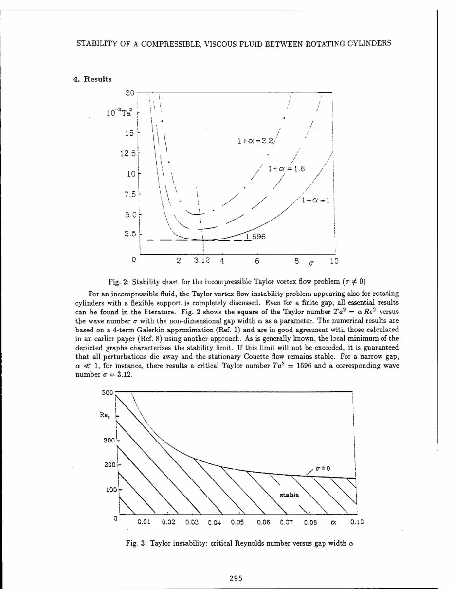
STABILITY OF A COMPRESSIBLE, VISCOUS FLUID BETWEEN ROTATING CYLINDERS
4. Results
20;
10 ~Ta~
5.0
Ü.0
0
i • 15r \\\ 12.5
10
7.5 r - l^c< —1
2 3.12 4 8 10
Fig. 2: Stability chart for the incompressible Taylor vortex flow problem (er ^ 0)
For an incompressible fluid, the Taylor vortex flow instability problem appearing also for rotating cylinders with a flexible support is completely discussed. Even for a finite gap, all essential results can be found in the literature. Fig. 2 shows the square of the Taylor number Ta2 = a Re2 versus the wave number a with the non-dimensional gap width a as a parameter. The numerical results are based on a 4-term Galerkin approximation (Ref. 1) and are in good agreement with those calculated in an earlier paper (Ref. 8) using another approach. As is generally known, the local minimum of the depicted graphs characterizes the stability limit. If this limit will not be exceeded, it is guaranteed that all perturbations die away and the stationary Couette flow remains stable. For a narrow gap, a <C 1, for instance, there results a critical Taylor number Ta2 = 1696 and a corresponding wave number a — 3.12.
500
Re, -
300
200
100
0.01 0.02 0.03 0.04 0.05 0.06 0.07 0.08 £X 0.1C
Fig. 3: Taylor instability: critical Reynolds number versus gap width a
295

V. MEHL, J. WAUER
The influence of compressibility is characterized by a non-vanishing Mach number M(Eu < oo). Fig. 4 shows that the stability limit increases with increasing Mach number, but very slightly for small values of Q. The relationship between Re and M is given by
Re = aRi-M. v
For any fluid with sound velocity c and viscosity v, very small values of a and Ri are necessary to fulfill the equation. But for very small values of a, the stability limit is nearly constant for varying M. Even for a = 1 and M = 1, the stability limit is 3% higher than for M = 0, but with air as fluid a radius of less than Zpm is needed, which does not make sense. There remains the small area (*) of technical interest. Here the influence of compressibility can be neglected (Ref. 10).
Ta2c = aRe2
c
a = 1.0
10,000
a = 0.5
a = 0.1
Fig. 4: Influence of compressibility on the stability limit of the Taylor problem
The eigenvalue problem for a narrow gap (governing the stability behavior in the case of coupled fluid-structure vibrations where a = 0) is solved numerically. Attention is focussed on the stability limit where the real part of A changes from its original negative value to a positive one. But it has to be noticed that the corresponding imaginary part of A cannot be expected to be zero there (9{A} ^ 0). This means (see Fig. 5) that the centre S of the inner cylinder rotates on a circle of constant radius (3fc{A> = 0) about the centre O of the stator. The angular speed is u = Ö{A} Q « |Q. The threshold speed is characterized by the minimum of Re for which this condition is fulfilled as a function of the parameters a, M, 6 and 7 (Fig. 6).
Fig. 5: Coupled fluid-structure vibrations (a — 0) at Re = Rec
296

STABILITY OF A COMPRESSIBLE, VISCOUS FLUID BETWEEN ROTATING CYLINDERS
For the second case this stability chart shows that for a not too small, the influence of M is negligible, too. But for very small values of a, the stability limit jumps up with increasing M, the more evidently the smaller the bedding stiffness 7. It is worth discussing the special case of 7 = 0. For an incompressible fluid, the whole range is unstable, whereas for even a very small value of M the stationary state is possible, only in a small area indeed. The difference is large for small a; a limiting process M —► 0 is not possible. The reason is that the corresponding equation set is degenerate for the case M = 0. This means that here an incompressible fluid must be treated as a compressible fluid with very small M in order to obtain the right results.
0-05 / 7 = 0 (M = 0)
Fig. 6: Stability chart for the coupled fluid-structure vibrations
It is obvious that the threshold speed and the type of instability (a ^ 0 or a = 0) depend on the parameters a (gap width) < 1 and 7 (stiffness), in general. The effective stability limit is therefore given by the lowest branch of the two instability forms. It follows qualitatively that one gets Taylor- vortices for a large gap and high stiffness, but instability with cylinder vibrations for a narrow gap and low stiffness (Fig. 7). If 7 tends to infinity, only Taylor vortices are possible, and the displacements of the inner cylinder are zero.
500
Re. r-
O.Ci 0.02 0.03 0.04 0.05 0.06 0.07 0.08 , ,, 0.10 (X («1)
Fig. 7: Stability chart for a narrow gap
297

V. MEHL, J. WAUER
5. Conclusion
The stability behavior of the fluid flow between coaxial rotating cylinders with a flexible support has been analyzed. Without essential restrictions, the outer cylinder was constructed as a stator, and the inner flexibly supported cylinder rotated at constant speed. The compressible fluid was assumed to have constant temperature and viscosity.
The governing boundary value problem demonstrates that a circumferential Couette flow between the coaxial rotating cylinders is the stationary state also for a flexibly supported inner cylinder. The variational equations lead to two independent eigenvalue problems. The discussion shows that two different types of instability can appear, the Taylor vortex flow instability about a non-oscillating inner cylinder and coupled transverse vibrations of the fluid-cylinder system. The type and onset of instability - the critical Reynolds number - depend on parameters characterizing gap width a (to be small here), stiffness 7 and compressibility (Mach number M).
6. References
1. Breitling, M., Study thesis (Institut für Technische Mechanik, Universität Karlsruhe, 1992).
2. Bühler, K., Coney, J. E. R., Wimmer, M., Zierep, J., Ada Mechanica 62 (1986) 47.
3. Chandrasekhar, S., Eydrodyncmic end Hy drome gnetic Stability, Oxford University Press; Oxford, 1961.
4. Cheng, H. S., Trumpler, P. J-, J. Eng. Industry 85 (1963) 274.
5. Di Prima, R. C, Stuart, J. T., J. Fluid Mech. 67 (1975) 85.
6. Di Prima, R. C, Pridor, A., in First Taylor Vortex Flow Working Party, Leeds, 1979.
7. Hall, P., J. Fluid Mech. 146 (1984) 347.
8. Kirchgässner, K., Z. Angew. Math. Physik 12 (1961) 14.
9. Mehl, V., Wauer, J., in Stability, Vibration and Control of Structures, Vol 1 (A. Guran and D. J. Inman, Eds.), World Scientific Publ., Singapore, 1995, 280.
10. Wassermann, P., Diploma thesis (Institut für Technische Mechanik, Universität Karlsruhe, 1994).
11. Wauer, J., Z. Angew. Math. Mech. 73 (1993) T274.
298

PEAK STRESS CONTROL IN THE PRESENCE OF UNCERTAIN DYNAMIC LOADS
G. G. Zhu Cummins Engine Company, Inc.
Columbus, IN 47203-3005 and
R. E. Skelton Purdue University
W. Lafayette, IN 47907
Abstract This paper outlines a role for covariance control theory in civil structures. Covariance control theory
assigns a specified covariance upperbound to the controlled structural system. It is known that the energy-to-peak gain for a linear system is precisely the maximum singular value of the output covariance matrix. This paper shows that using covariance control theory, and adding base accelerometers (in addition to other sensors on the rest of the structure) enhances the ability to keep the peak stresses (at multiple places throughout the structure) smaller in the presence of energy bounded, but uncertain base accelerations from earthquakes. Some comments are added to show the same technique for redesign of the Hubble Space Telescope controller.
1 Introduction
Civil engineering structures are large, dynamically rich (complex models with many modes of vibration), and therefore presents a challenge for control and structures theory, and presents a substantial test to investigate the true limitations of control theory. A brief summary of the existing results in structure control are in Yang et al (1990b), Abdel and Leipholz (1983), Meirovitch et al (1983), Soong (1990), Tonnasula et al. (1994).
Our approach develops analytical methods which can guarantee upper bounds on each output in the presence of uncertain disturbances with known energy bounds. It is reasonable to assume a limit to the energy of the disturbance, since for any given past earthquake records, the integral of the squared signal (energy) is readily computable. Our design therefore presumes a priori knowledge of an upper bound of the integral squared of the earthquake signals (accelerations) records, rather than the actual earthquake signal itself.
From the literature, the stability guarantees using co-located sensors and actuators require infinite bandwidth actuators and sensors and perfect models. Yet the bandwidth of the control device is not high compared to all the modes of the structure. Hence many stability "guarantees" in the present literature are not realistic or practical, and building safety is definitely not guaranteed with these designs. A Bounded Inpu^Bounded Output (BIBO) type of stability proof is more appropriate, to include the disturbance dynamics in the stability discussions. In fact, because the exact dynamics of the disturbances are not known a priori, existing techniques generally do not guarantee stability of the system. Techniques for control design in the presence of uncertain disturbances have been developed by Johnson et al. (1971). Applying these ideas of "disturbance estimation" to the seismic excitation problem suggests using accelerometer feedback to measure the earthquake excitation and using this signal in feedback. Also in Zhu et al. (1991), we are able to guarantee specific levels of performance in the presence of uncertain disturbances.
We shall combine the ideas of disturbance accommodating control [Johnson et al. (1971)] and the robust control work of [Zhu et al (1991)] to provide a structural controller with stability guarantees and performance upperbounds in the presence of unknown but bounded energy disturbances.
299

G. G. ZHU AND R. E. SKELTON
This paper adds the discrete counterpart to the continuous time problem soved in Zhu et al. (1994).
Output Covariance Constraint Problem With Disturbance Feedback
Consider the following dynamic system
x = Ax + Bu + Diwi + D2w2
yi = Cix; i = l,2,--,m, ; y=[yf,y2r,
Zi = Mx + Vi
Z2 = Wj + v2
• .yi TiT = Cx
(1)
where x is the state vector, wi and w2 are system disturbances, y«(t = 1,2, • • •, m) are the performance output vectors, Z\ the measurement of the system with measurement noise Vi, and finally z2 is the measurement of the system disturbance w2 with measurement noise v2. The system disturbance w2
is measurable in many engineering control problems. For instance, in the building structure control problems, the earthquake disturbance to the building can be measured by imbedding the accelerometers in the building foundation. Later in this section, it will be shown that by feeding back the measured disturbances to the controller the closed loop system performance can be improved significantly. Here we assume that the system noises wj and w2, and measurement noises Vi and v2 are independent zero-mean white noises, that is,
foow1(t) = 0, £oow2(t)=0
focW1(t)wf(t-r) = W15(r) ^ocVi(t)vf(t-r)=V15(r)
£»vi(t) = 0; 5oov2(t) = 0; eoow3(t)w%(t-T) = W26(T); £ooV2(t)vn*-T) = V2$(T),
(2a) (2b) (2c)
where £<»[•] = lime-«» £[■], and £ is an expectation operation. We shall consider the full order dynamic feedback with disturbance feedback.
2.1. Full Order Dynamic Controller.
Consider the following dynamic controller
Xc = ACXC + FiZi + F2Z2
U = GXe (3)
The resulting closed loop system has the form
where
ACL
x = Acxx + DCLWCI,
ycL — Cc£,X + HcZ,WcfX, (4)
A-FjM A-Ac + BG-FiM FiM Ae + FiM
Di D2 — F2 — Fi —F2
0 F2 Fi F2
;CCL ■[S c c
G
*CL = X-Xc
Xc
= [wi".w2,.vr,v^] T1T
(5)
(6)
300

PEAK STRESS CONTROL FOR UNCERTAIN DYNAMIC LOADS
Let C„ = [0, G] and CCL = [C, C]. Now we are ready to define the Output Covariance Constraint problem.
2.2. Output Covariance Constraint Problem with Disturbance Feedback.
The Output Covariance Constraint problem with Disturbance feedback (OCCD) is" defined as fol- lows:
Find a full order dynamic feedback controller (3) to minimize
JOCCD = £«,uT(i)Ru(<)
subject to
Y< ^ Sx.ttWyftt) < Yi(« = 1,2, • • •, m
where Yj = [CCLXC^] .. and X satisfies
0 = XA£t + AcLX + DCLWCLDZL , ™CL = block diag [W,, W2) Vi, V2] (7)
The OCCD problem reduces to the Output Covariance Constraint (OCC) problem in [Zhu et al (1991)] when z2 = 0, w2 = 0, W2 = 0, V2 = 0. The closed loop system can be written in the form of (4), where the closed loop system matrices ACL, Bex, and CCL are defined in (5). The following Theorem provides the necessary and sufficient conditions for the OCCD problem.
Theorem 1 Suppose that the proposed OCCD problem is regular (the solution of the problem depends on the choice of the cost function). Assume that the triples (A, B, C) and (A, Di, M.) are stabilizable and detectable. Then the following statements are equivalent:
(i) the matrices (Ac,Fi,F2,G) describe the optimal OCCD controller.
(Ü) Ft = XN^Vr1 ; F2 = D2W2(W2 + V2)-J ;
G = -RT^K; AC = A + BG-F1M; 0 = XAT + AX - XMrV^MX
+ FaVjF^ + (Fa - D2)W2(F2 - D2)T + DiWiD? ;
0 = ATK + KA-KBR-1BTK-|-CTQC;
0 = XetA + BG^tA + BGJXc + PiViPf + PaOBVa + VaJFT; 0 = Q<[CiXCf-Y<])X = X + Xc;
Q = block diag[QuQ2,--,Qm] > 0 . (8)
Proof of Theorem 1 The necessity of the proof is similar to the OCC problem treated in Zhu et al. (1991). One only needs to form the closed loop cost function, and apply the Khun-Tucker conditions. Then the resulting necessary conditions are the consequence of the partial derivatives. Note from the eqs. for G, K, in (8) that G is the optimal LQ control gain for some choice of weighting matrix Q. We will show that the OCCD controller is an LQG controller for a slightly modified estimator to account for the measured distrurbances.
The proof of the sufficiency will be divided into parts: i) the conditions of the optimal estimation problem, ii) the separation principle of the LQG problem with disturbance feedback. Then, combine
301

G. G. ZHU AND R. E. SKELTON
the results of steps i) and ii), and apply the procedure in Zhu et al (1993), to complete the proof.
i) Optimal Estimator
Consider the following estimator to estimate the state of (1), given u(t), Zi(i), and z2(t).
Xc = AeXc + Bu + F2z2 + Fi (zi - Mxc) (9)
The error covariance X = £oo(x - xc)(x - x<.)r, satisfies the following Lyapunov equation
0 = X(A-P1M)r + (A-.PiM)X + P1V1Pj, + DiW1Df +F2V2F2
r + (D2-F2)W2(D2-F2)r. (10)
For any Fi such that A - FiM is asymptotically stable, let X (Xo) denote the solution of (10) with the choice F2 (F2), where
P° = D2W2(W2 + V2)-1. (11)
Now for any F2, we have X > Xo . (12)
A well-known property of Lyapunov equations is the following:
Lemma 1 Given 0 = PiA* + AP4 + Q<, onJAu stable, then Pt > P2 t/Qi > Q2.
Now, to prove (12) we only need to show that for any F2 with proper dimension,
F3VaFj + (D2 - F2)W2(D2 - F2)r > F^Ff + (D2 - Fg)W2(Da - F°)r . (13)
Consider that
[F2 - D2W2(V2 + W2)-1](V2 + W2)[F2 - D0W2(V2 + Wj)"1]7"
= F2(V2 + W2)F^ - F2D2W2 - D2W2Ff/ + D^D^
= F2V2Fj + (D2-F2)W2(Do-F2)T-D2[W2-*]D|' . (14)
where $ = W2(V2 + W2)~1W2. Hence, we obtain
F2V2F2r + (Da - F2)W2(Dj - F2)
r = D2[W2 - SJD7* (15) +[F2 - D2W2(V2 + Wj)-1]^ + W2)[F2 - D2W2(V2 + Wa)"1]7".
Note that
F5V2F° + (Da - Fg)Wa(Da - F°2f = D2[W2 -W2(V2 + W2)"1W2]D2
r (16)
and the fact that
[F2 - D2W2(V2 + Wj)"1]^ + W2)[F2 - D2W2(V2 + Wj)"1]7" > 0
leads to (13). Now that we must choose the smallest forcing term in (10) relative to P2. The smallest Frobenious norm of these terms is given by F2 = D2W2(V2 + W2)
_1. The problem of finding the Fj yielding the smallest X is a standard problem yielding the Fj, as follows
Pi = XMVJ-1;F2 = D2W2(V2-|-W2)-1; (17)
0 = XA7' + AX-XMTVJ-1MX + F2V2F7'
+(F2 - D2)W2(F2 - D2)T + DiWiDf .
302

PEAK STRESS CONTROL FOR UNCERTAIN DYNAMIC LOADS
ii) Separation Principle
One can prove a separation principle, by following the same procedure as that in Kwakernaak and Sivan (1972). Then we have the conclusion that the best full order LQG controller with disturbance feedback is the combination of the optimal estimator (17) and the standard state feedback LQG gain,
G = -R-^K (18)
where K satisfies
0 = ATK + KA-KBR-1BTK + CTQC. (19)
Note that the corresponding LQG cost is
JLQG = £oc[yTQy + uTRu], Q > 0 . (20)
Combining the optimal estimator gain and state feedback gain, we know that for a fixed output weighting matrix Q, the controller minimizing the above LQG cost satisfies (8) with fixed Q = Q.
The sufficiency of (ii) now follows similarly to the procedure as in Zhu et al. (1993), concluding that any controller (Ac, G, Fu F2) described by (3) is an optimal OCCD controller. D
Theorem 1 establishes the fact that the solution to the OCCD problem is the solution to a standard LQG problem (when W2 = 0, V2 = 0, z2 = 0, v2 = 0), and to a modified LQG problem otherwise. The weighting matrix Q is not known a priori, however, note that the estimation error (»variance, without disturbance feedback, satisfies
0 = XAr + AX - XMrVJ-xMX + DiWxDl" + D2W2D3r , X > 0 , (21)
and with disturbance feedback X > 0 satisfies
0 = XAr + AX-XMTVr1MX + D1W1Df + D2W2D|'
-D2W2(W2 + V2)-1W2D2
r. (22)
Since the forcing term of Riccati equation (21) minus that of (22) is
D2W2(W2 + Vs^WaDj > 0 ,
we have x>x,
which proves the following Lemma.
Lemma 2 The full order OCCD controller reduces the optimal estimation error, hence, improves the maximal achievable performance in the LQG problem.
Remark: The maximum achievable performance of the OCC problem with disturbance feedback is always better or equal to that without disturbance feedback. This is obvious because the OCC controller is a feasible solution of the OCCD problem.
The optimal controller satisfying (8) can be designed by the following OCCD algorithm with guar- anteed optimality and convergence, see Zhu et al (1993).
303

G. G. ZHU AND R. E. SKELTON
2.3. The OCCD Algorithm.
1. Given system matrices (A,B,Di,D2,M, C), input noise intensity matrices (Vi,.V2, W1,W2), weighting matrix R, initial output weighting matrix Q(0), output variance bound of (i = 1,2, • • •, m), 0 < ß < 1, error bound e > 0, and free parameter a > 0.
2. Compute the optimal estimate gains Fi and F2, where
Fx = XMTVJ-1;F2 = D2W2(W2 + V2)-1 (23)
0 = XAr + AX-XMrVjf1MX + F2V2F2r
+(D2 - F2)W2(D2 - F2)T + DiWjDf (24)
3. Compute the state feedback LQG gain with fixed Q{j)
GO) = -R-^Kfj), (25)
where 0 = K(j)A + ATK(j) - K{j)-BBTlBTK{j) + CTQ(i)C . (26)
4. Compute m
«rrÜ) = £ HQ*0')[Ci (X + XeÜ)) Cf - Y«M (27)
where XdJ) satisfies
0 = X^(A + BGjf + (A + BGJXcj + PxVxPf + F2(W2 + V3)Ff (28)
5. If err(j) < e, stop. Else, let
Q<(i + l)=y3Qi(i) + (l-/3)EA+ET, (29)
where Qi(j) + a [Ci[X + XijlCT - Yt] = EA+Er + EA_ET, (30)
and A+ (A_) contains zeros and all positive (negative) eigenvalues of the left hand side, and E is the unitary matrix of eigenvectors. Go to Step 3.
Remark 1 The controller can be designed to constrain the output £«, norms, using the fact in Zhu et al. (1989) that
IWßo<W]l|wcL|ß, (31) where CT[] is the maximum singular value of .[•], and || • H*, and || • ||| are defined by
11*11» = wpyf(*)y«(*); IKOLIIS = f°° wgtww-lwa(t)*,w > o (32) t>0 Jo
and W is defined in (9). By designing the OCCD controller so that Y* < a^, one can guarantee I |y» I loo ^ /*»in tne presence of any disturbance with the property ||WCL||§ < mjoi.
304

PEAK STRESS CONTROL FOR UNCERTAIN DYNAMIC LOADS
3 Discrete Time OCC Problem With Disturbance Feedback
Consider the following discrete time system
x(Jb + l) = Ax(jfc) + Bu(k) + D1w1(A) + D2w2(ifc)
y(*) = Cx(*)
»i(A) = Mx(k) + Vi(k)
Z2(k) = W2(*) + v2(fc)
where twi, iu2, vi, and t>2 are independent zero mean white noises with (»variances Wi, W2, Vi, and V2. Let the closed loop system with the state feedback controller
u(jfc) = Gix(fc) + G2z2(fc)
and the full order dynamic controller
in the following form
where
Xe(*+1) = AeXe(*)+Pi«i(*) + Pa»a(A) u(fc) = G!Xc(k) + G2z2(k)
xcUk) = Acz,xcx,(A;) + DcLWCL(fc)
yCL(k) = CcLXCL(k) + HcL*rCL(k)
Wci =
and for the state feedback
w2
Vl v2
; YCL -[;]-[
XCL = X
XCL + H» H„ wci(fc)
and full order dynamic feedback
XCL =
Now we can define the OCC problem with Disturbance feedback (OCCD).
X-Xc Xc
(33)
(34)
(35)
(36)
(37)
(38)
(39)
3.1. The discrete OCCD problem.
Find a state feedback controller (34) and full order dynamic feedback controller (35) to minimize the following OCCD cost
JOCCD = £» nT(k) R u(*), R > 0 (40)
subject to
and
X = ACLXACJ + DCL Wei BcJ; WCL = block diag [Wj, Wa, V,, V2] (41)
Sac y«(i) yjT(A:) = Ci XCL CiT < = Yi, t = 1, 2, •■-, m (42)
305

G. G. ZHU AND R. E. SKELTON
where R and Y< (» = 1, 2, • • •, m) are given, y = [yiT, yaT, • • •, yn
T]; y< = QXCL € »m<
{Soo [■] = (limfc_oo£ [•]]) and £ is an expectation operator.
The physical meaning of the discrete time OCCD problem is similar to the continuous time case: Minimizing the control effort subject to output performance requirements on each output group. The following Lemma provides the connection between stochastic and deterministic OCCD problem for discrete systems.
Lemma 3 For the discrete time closed loop system (36), suppose that the closed loop system is asymp- totically stable. Let the input £2 norm
I|WCL()I|2 =
and the output I« norm
U=o
|yCL(0lloo = supyci(*)ycL(fc) fc>0
-1*
(43)
(44)
Define the input £2 disturbance set
Slw = {WCL : k - «—.+«-*+«*.+»«, || ^ (-) ||2 < 1 } , (45)
then
*[Y] = sup HYciO)«« (46)
where
Y = CcrXC^i and X satisfies
X = AciXAcn, + DCLWCLDCZ,
Using the equation (46), the stochastic OCCD problem can be interpretted into the following assuming that R = diag [rir2 • ■ • rnu ] > 0 and Yj = <*I > 0 (t = 2, • • •, m).
3.2. The deterministic interpretation of the OCCD problem.
Find a state feedback controller (34) or full order dynamic controller (35) to minimize the deter- ministic OCCD cost
nti
JOCCD = Y\ri sup || tt< (•) H«,2 (47) i=1 wo. € n«,
subject to
II * (Oil?» < eli = l,2,-m. (48)
Hence, the OCCD controller minimizes a worst case weighted control bound subject to the worst case £oo output constraints. Over the given l-x disturbance set Qw.
306
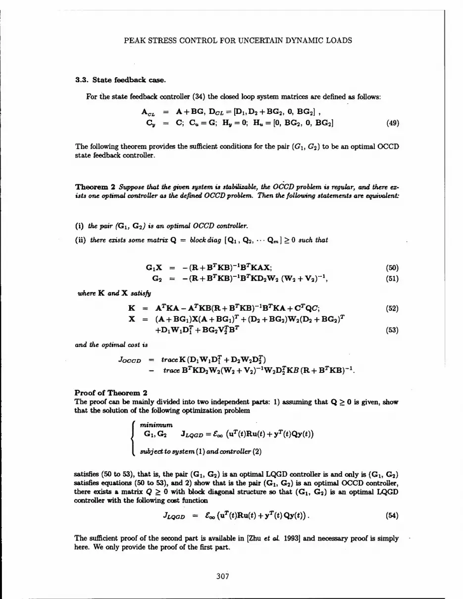
PEAK STRESS CONTROL FOR UNCERTAIN DYNAMIC LOADS
3.3. State feedback case.
For the state feedback controller (34) the closed loop system matrices are denned as follows:
ACL = A + BG, BCL = Pi, D2 + BG2, 0, BG2] , C„ = C; C„ = G; H„ = 0; Hu = [0, BG2, 0, BG2] (49)
The following theorem provides the sufficient conditions for the pair (G\, G2) to be an optimal OCCD state feedback controller.
Theorem 2 Suppose that the given system is stabilizable, the OCCD problem is regular, and there ex- ists one optimal controller as the defined OCCD problem. Then the following statements are equivalent
(i) the pair (Gi, G2-) is an optimal OCCD controller.
(ii) there exists some matrix Q = blockdiag [Qi, Q2, •• ■ Qm] > 0 such that
dX = -(R + BTKB)-1BTKAX; (50) G2 = -(R + BTKB)-1BTKD2W2 (W2 + V2)-\ (51)
where K and X satisfy
K = ArKA-ATKB(R + BTKB)-1BTKA + CrQC; (52) X = (A + BG1)X(A + BGi)T + (D2 + BG2)W2(D2 + BG2)
T
+DiWiDf + BG2V2rBT (53)
and the optimal cost is
JOCCD = trace K (DiWiDf + D2W2D2r)
- trace BrKD2W2(W2 + V2)-1W2D2
rKß(R+ BTKB)-1.
Proof of Theorem 2 The proof can be mainly divided into two independent parts: 1) assuming that Q > 0 is given, show that the solution of the following optimization problem
minimum Gi, G2 JLQGD = So* (uT(t)Ru(t) + yT(t)Qy(*))
subject to system (1) and controller (2)
satisfies (50 to 53), that is, the pair (Gi, G2) is an optimal LQGD controller is and only is (Gi, G2) satisfies equations (50 to 53), and 2) show that is the pair (Gi, G2) is an optimal OCCD controller, there exists a matrix Q > 0 with block diagonal structure so that (Gi, G2) is an optimal LQGD controller with the following cost function
JLQGD = £co(uT(t)Ru(t) + yT(t)Qy(t)). (54)
The sufficient proof of the second part is available in [Zhu et al. 1993] and necessary proof is simply here. We only provide the proof of the first part.
307

G. G. ZHU AND R. E. SKELTON
To prove the first part, consider the following weighted Frobenius norms with expection operator £„.
ATi = 50O||[G1 + (R + BTKB)-1BrKA]x(f)||2(R+BrKB) (55)
and
Ni = ^||[Gj + (R + BTKB) 1BrKD2W2(W2 + V2)-1]x(t)||2(R+BTKB) (56)
where K is the positive semidefinite solution of equation (52) whose positive semidefinite solution exists under the stabilizability assumption in Theorem 2.
Note that
and
Ni = <roceBrKI>2W2(W2+V2)-1W2D2rKB(R + BrKB)"1
+ trace (R + BrKB)G2(W2 + V2) 6^ + 2 trace BTKD2W2G2 (57)
N2 = trace BTKAXATKB(R+BTKB)"1
+ traceG1XGi(R+BTKB)+2traceBTKXx GiT, (58)
where X satisfying (53) is the closed loop state covariance matrix. The LQGD cost (54) can be rewritten into the following format:
JLQGD = trace RGi JTGi7* + trace RG2(W2 + V2)G^ + trace QCXCT. (59)
Using equations (57 to 58), we can obtain that
JLQGD = Nx + N2 -trace BrKBG2(W2 + V2)G2T -2 trace BrKD2W2G2
-trace BTKD2W2(W2 + V2)_1W2D2
TKB(R + BTKB)_1
-trace G1XG1TBTKB+ tracex|crQC - ATKB(R + BrKB)_1BTKA]
-2 trace BTK AXGiT. (60)
Substituting the Riccati equation into (60) yields
JLQGD = Nx+N2- trace BTKBG2(W2 + V2)G^ - 2 trace BrKD2W2G2
- trace BTKD2W2(W2 + V2)-1W2D2
rKB(R + BTKB)_1
- trace G1XG1BrKB + trace X [K - AKAT]
- 2 trace BTKAXGiT (61)
or equivalently
JLQGD = Ni + Ni- trace KD2W2Bf - traceBTKD2W2(W2 + V2)_1
W2D2rKB(R + BTKB)_1 + trace K [X - (A + BGi)X(A + BG{f]
- BG2V2G^Br - (Da + BG2)W2(D2 + BG). (62)
Using the Lyapunov equation (54), equation (55) becomes
JLQGD = Nx + N2+trace K[DxWiDj+ D3W2D2r]
- trace BTKD2W2(W2 + V2)_1 W2D2
rKB(R + BTKB)_1 (63)
308

PEAK STRESS CONTROL FOR UNCERTAIN DYNAMIC LOADS
Hence, the minimum can be obtained by setting
Ni = 0 and AT2 = °.
that is
trace [d + (R + BTKB) 1BTKA]x[d + (R + BTKB) 1B
TKA]
T = 0
and
trace
or equivalently,
and
G2 + (R + BTKB) 1B
TKD2W2(W2 + V2)
_1
G2 + (R + BTKB)_1BTKD2W2(W2 + V2)_1
[G1 + (R+BT
KB)~1B
TKA]X = 0
G2 + (R + BrKB) 1BTKD2W2(W2 + V2)"1 = 0
(W2+V2).
= 0,
(64)
which completes the theorem.
(65)
(66)
(67)
a
4 Conclusions
Earthquake accelerations can be measured by accelerometers embedded in the foundation. Using these sensors in a feedback scheme can improve the dynamic response considerably. An algorithm is given to guarantee that the peak response is bounded below a specified number in the presence of unknown earthquake accelerations with known energy bounds.
309

G. G. ZHU AND R. E. SKELTON
References
1. Abdel-Rohman, M. and H.H. Leipholz. "Active Control of Tall Building," ÄSME J. Struct Engr., 1983, 107(7).
2. Chang, C. Hybrid Control of Civil Structures, Ph.D. Dissertation, Purdue University, May, 1993.
3. Johnson, CD. and R.E. Skelton. "Optimal Desaturation of Momentum Exchange Control Sys- tems,'' AI A A Journal, 1971, 9(1).
4. Kobori, T., N. Koshika, K. Yarnada and Y. Ikeda. "Seismic-response-controlled Structure with Active Mass Driver System, Part 1. Design," Earthquake Engineering and Structural Dynamics, 1991, 22:133-149.
5. Kwakernaak, H. and R. Sivan. Linear Optimal Control Systems, 1972, Wiley, New York.
6. Meirovitch, L. and L.M. Silverberg. "Control of Structure Subjected to Seimic Excitation," ASME J. Engrg. Mech., 1983, 109(2).
7. Sakamota, M., K. Sasaki, and T. Kobori. "Active Structural Response Control System,'' Mecha- tronics, 1992, 2(5):503-519.
8. Soong, T.T. Active Structural Control Theory and Practice, 1990, Longman, London, U.K., and Wiley, New York.
9. Wilson, D.A. "Convolution and Hankel Operator Norms for Linear Systems," IEEE Thms. Au- tomat. Contr., 1989, 34(1).
10. Yang, J.N., A. Akbarpour, and P. Ghaemmaghami. "New Optimal Control Algorithm for Struc- tural Control," ASME J. Engrg. Mech.,, 1987, 113.
11. Yang, J.N., A. Danielians, and S.C. Liu. Aseimic Hybrid Control System for Building Structure Under Strong Earthquake," J. of Intell. Mater. Syst. and Structure, 1990, 1.
12. Zhu, G., M. Corless, and R. Skelton. "Robustness Properties of Covariance Controllers," In. Proceedings of Allerton Conf., 1989, Monticello, IL.
13. Zhu, G., M. Rotea, and R. Skelton. "A Convergent Feasible Algorithm for the Output Covariance Constraint Problem," In 1993 American Control Conference, 1993, San Francisco, California.
14. Zhu, G. and R.E. Skelton. "Mixed Lj and L,» Problems by Weight Selection in Quadratic Optimal Control," Int. J. Control, 1991, 53(5).
15. Zhu, G. and R. Skelton. "Output Covariance Constraint Problem with Disturbance Feedback," Proceedings, 1st World Conference on Structural Control, Pasadena CA, August 1994, pp. FP4- 32-41.
16. Tonnasula, D., B. Spencer, and M. Sain, "Limiting Extreme Structural Responses Using an Effi- cient Nonlinear Control Law," Proceedings 1st World Conference on Structural Control, Pasadena CA, August 1994, pp. FP4-22-31.
310
METHODS TO COMPUTE PROBABILISTIC STABILITY MEASURES
FOR CONTROLLED SYSTEMS
R. V. Field, Jr., P. G. Voulgaris, and L. A. Bergman University of Illinois
Urbana,IL 61801
Abstract Model uncertainty, if ignored, can seriously degrade the performance of an otherwise well-designed
control system. If the level of this uncertainty is extreme, the system may even be driven to instability. In the context of structural control, performance degradation and instability imply excessive vibration or even struc- tural failure. Robust control has typically been applied to the issue of model uncertainty through worst-case analyses. These traditional methods include the use of the structured singular value, as applied to the small gain condition, to provide estimates of controller robustness. However, this emphasis on the worst-case scenario has not allowed a probabilistic understanding of robust control. Because of this, an attempt to view controller robustness as a probability measure is presented. As a result, a much more intuitive insight into controller robustness can be obtained. In this context, the joint probability distribution is of dimension equal to the number of uncertain parameters, and the failure hypersurface is denned by the onset of instability of the closed-loop system in the eigenspace. A computed measure of system reliability is then used to estimate controller robust- ness. It is demonstrated via an example that this method can provide accurate results on the probability of failure. Moreover, a comparison of this method to a suitably modified structured singular value robustness anal- ysis in a probabilistic framework is performed. It is shown that the method is superior despite the qualitative accuracy of the structured singular value analysis.
1. Introduction The distribution of eigenvalues in uncertain dynamical systems and its relationship to the robustness of
structural systems have been topics of some interest in recent years, as discussed, for example, by Field et al. (Ref. 4), Spencer et al. (Refs. 9-11), and Stengel and Ray (Refs. 7,12). Stengel and Ray (Ref. 12) were among the first to use large-scale Monte Carlo simulation to estimate the robustness of uncertain controlled structural systems. Using this approach, one constructs a distribution of root loci simulating the stochastic behavior of the closed-loop pole locations. Because this is a graphical method, one gains an intuitive understanding of system robustness. The results reported were quite promising, but the large number of realizations required to attain a high degree of accuracy in the distribution of the tails of the closed-loop poles may render this approach compu- tationally unattractive.
In a recent series of papers, however, Spencer et al. (Refs. 9-11), and coworkers have introduced a "systematic approach for determining the probability that instability will result from the uncertainties inherently present in a controlled structure". This probability measure is a direct indication of the robustness of the closed- loop system. In addition, as opposed to the more "brute-force" Monte Carlo simulation approach, this method provides a means of evaluating the reliability of the system directly.
As described in Spencer (Ref. 11), this investigation into the probability of failure of controlled struc- tures has led to a method for characterizing the stability of a system based upon an eigenvalue criterion, namely the probability that the real part of every eigenvalue will be contained strictly in the left-half plane. First and second order reliability methods (FORM/SORM), shown to be accurate for series-type system reliability prob- lems by Madsen (Ref. 6), were used for estimating the probability of system instability. A series of numerical examples were constructed in which the stability of a controlled single degree-of-freedom system with four uncertain parameters was analyzed.
Traditional methods used to assess controller robustness, involving the use of the singular value of some mapping as applied to a small gain condition, are often conservative in nature. Therefore, the focus of this work involves comparing robustness estimates using the FORM methodology with those estimates obtained using
311

R.V. FIELD, JR., P.G. VOULGARIS, AND L.A. BERGMAN
more traditional techniques. In particular, a method is introduced herein to reformulate the robustness measure gained from the structured singular value analysis {e.g., Ref. 3) into a probabilistic framework. Upon applying these techniques, one then has two different methods to intuitively assess the robustness of-the system.
One realistic application of these methods involves the control of a single-story building constrained to a single degree-of-freedom, subject to seismic excitation. In order to provide more realism, the example includes the effects of controller time delay, a significant contributor to system instability Utilizing both methods of assessing controller robustness, an attempt is made to individually characterize the robustness qual- ities of several control law designs. Modern controller designs based on procedures such as LQR, optimal H2, and optimal H^ are considered to facilitate comparisons with other results in the literature. Furthermore, upon comparison to simulation results, one can conclude which assessment method is more effective for this partic- ular class of problems.
2. Problem Definition Consider the equation of motion for an n -dimensional structure subject to controller time delay and
including a multiplicative model of the uncertainty in the structure and delay,
M, (I+ Am) #0 + C, (I + Ac) q(t) + K, (I + Aj) q(t) = Bsu(t - x (1 + 8T)). (1)
Here, Am, Ac, and Ak represent the uncertainty in the mass, damping, and stiffness matrices, respectively, and 5T represents the scalar uncertainty in the time delay of the control input. Note that, in general, the A. 's are completely populated and each element can be modeled as an independent random variable, with mean m- and standard deviation <y..
When applying active control strategies to the structure described above, the robustness of individual control designs can be assessed by considering the various pole locations of the closed-loop system. This is illustrated in Fig. 1.
B(f-T(l+8t)) Structure Measured Output -►
Delay -ST(l+8t)
Controller -K(5)
y(t)
Fig. 1 Closed-loop system including uncertainty.
Herein, the robustness of several control designs will be assessed using two different methods, each to be described in the following sections.
3. The FORM Method A method to assess the robustness of the closed-loop system using first-order reliability methods
(FORM) is introduced. The dynamics of the closed-loop system shown in Fig. 1 can be represented by
*CL = Act(A)*CL> (2)
where A is used to represent the uncertainty of the entire closed-loop system. A stability analysis can be completed by examining the eigenvalues of
det [si -ACL(A)] =0. (3)
Stability requires that the real part of every eigenvalue be contained in the open left-half plane (OLHP) or, alter- natively, that no one eigenvalue have real part contained in the closed right-half plane (CRHP). This notion of stability can be posed in terms of the probability of instability or probability of failure, pf, as (Refs. 6,9,10)
N
Pf = P VRe[ij(A)] >0 (4)
where \j is the j th eigenvalue of Eq. (3) and N denotes the order of the closed-loop system. Since this expres- sion cannot, in general, be evaluated directly (Ref. 11), an alternative approach is to recognize that Eq. (4) is, in
312

METHODS TO COMPUTE PROBABILISTIC STABILITY MEASURES
fact, the failure condition for a series-type system. The problem can thus be approximated by a series of "components" with limit state functions defined as
gj(A) = -Re[Xj(A)\,j 1,2,..„AT. (5)
If any one of the components fails (i.e., g (A) < 0), then the entire system is considered failed. The notion of system failure is illustrated graphically in Fig. 2 for a three mode system with two random parameters. As illus- trated, the system failure region is the union of all modal failure regions, and the number of random quantities defines the dimension of the parameter space.
6o <£
Re[XA = 0
SAFE Re [Xj] < 0
Re [X,] = 0
Re[Xß >0 FAILED
Re[XJ = 0
■**«,
Fig. 2 Stability region of three-mode system with two uncertain parameters.
The problem can be reformulated in a normalized probability space, assuming p degrees-of-random- ness, through the transformation given by Spencer (Ref. 11)
zs = T(8,.),f = \,2,...,p, (6)
where T is a nonlinear operator defined as
T:2>-><A£. (7)
This transformation is always possible for continuous random variables with invertible distribution functions. Here, 8; represents the variate in the original parameter space, fP, and z-t is the variate in the normalized proba- bility space, 3\£, normally distributed with zero mean and unit variance. Assuming that the variates are mutually independent, this transformation can be performed on each independently using
Z|. = T(8;) = <&-'[FA.(5,.)], (8)
where <&(■) represents the standard unit normal distribution function and FA (•) is the marginal cumulative distribution function of the / th random variable. Likewise,
GfZ) = g/r'(A)),j= 1,2,..„AT, (9)
represents the set of identical limit state functions, where Z depicts the normalized random uncertainties, mapped to X.-
Conceptually, the reliability index, ß, is the minimum Euclidean distance from the origin to the design point, z* , in 9{,, provided that the design point defines a limit state surface. This can be stated mathematically as the solution to the constrained optimization problem (Ref. 11),
ß FORM = min ßy where ß. = min \Z\, j = 1, 2, ..., N.
G,(Z) = 0
This leads directly to a first-order approximation to the probability of instability, or failure, given by
FORM ,. a FORM. Pf-Pf = ^(Tß ),
(10)
(11)
313

R.V. FIELD, JR., P.G. VOULGARIS, AND L.A. BERGMAN
where the location of the failure surfaces in N determines the sign of ß . Note that the solution to Eq. (10) is the global minimum contained in 3\£. For an N -dimensional problem, there will, in theory, be N reliability indices.
When applying Eq. (11) to determine p,, it is imperative to consider the shape of these limit state func- tions in sy£. Highly dependent failure boundaries tend to overlap or nest, causing the failure probabilities of higher-order modes to tend to be subsets of the lower-order modes. In addition, and quite frequently when considering structural problems, one mode can dominate the contributions of the others {i.e., ßj« ß2 < ... < ßw). In these situations, Eq. (11), with ßj = ß, provides an adequate approximation to pf
(Ref. 6). Two scenarios of this type are depicted in Fig. 3.
GZ{Z) = 0
FAILED
*L
G2(Z) = 0
Fig. 3 Illustrations of the FORM approximation for multiple-mode systems.
However, when confronted with a multiple-mode system that does not behave as illustrated in the figure, Eq. (11) may not provide an adequate estimate of pf. Other FORM and SORM methods are available to combine reliability information for several modes in a system reliability analysis. For example, reliability index results and design-point coordinates can be used to estimate correlation between modes, bimodal intersection probabilities, and the probability of the union of failure events, i.e., system failure (Ref. 6). As previously stated, the procedure used herein selects only the minimum of single-mode reliability indices. Therefore, by neglecting the contributions from other failure modes, it may sometimes overestimate the system reliability.
4. The [i -Analysis Method An alternative route in assigning a probabilistic measure of robustness utilizes some of the tools of deter-
ministic robust control. In particular, analysis based on the notion of the structured singular value, herein termed u. -analysis, can be utilized in a probabilistic manner to provide estimates to the probability of failure.
To perform a n -analysis, the closed loop dynamics are represented so that the uncertainty block, A, that contains all of the uncertainties present, is extracted as shown in Fig. 4 (Refs. 1,3).
I
A Wr zr
ns)aug
u y K(s)
] H Fig. 4 Augmented structure used in structured singular value (\i) analysis.
The A block is in feedback with the (stable) nominal closed loop system H, where the latter is produced by the interconnection of the nominal plant, P(s), and the controller, K(s). The nominal plant, however, can be repre- sented in an augmented form, notated as Paug(s) and given by
x = Ax + B^ + BjK (12)
314

METHODS TO COMPUTE PROBABILISTIC STABILITY MEASURES
zr = C1JC + DnH'r + Dj2K
y = C2x + D21 wr + D22K ,
(13)
(14)
where the matrices A, B2, C2, and D22 are the state-space description of the original plant, P(s), and x and u are the state and input vectors, respectively. The vectors wr and zr, connect the nominal closed-loop system, H, with the uncertainty block, A. The remaining matrices B,, C,, Dn, D12, and D2I are required to augment the original plant to be compatible with these additional inputs and outputs.
Robust stability of the closed-loop system depends on the size of H(/co). For the structural system given by Eq. (1), the uncertainty block can be represented as
A =
K 0 0 0
0 Ac 0 0
0 0 \ 0
0 0 0 \
(15)
where AT in Eq. (15) is a (stable) error due to the uncertainty in the time delay. For the framework presented herein, this delay uncertainty can be extracted as
(Ref. 3)
AT0'CO) = e-H5<l _ !. (16)
The structured singular value of a complex matrix M, associated with the structure of A, is defined as
u[M] =
inf{a[Q]: det(I-QM) = 0} Q
if inf{ö[Q]: det(I-QM) = 0} = 0
else (17)
where Q is any complex matrix with structure identical to that of A (i.e., block diagonal of the same dimen- sions), and 5 [Q] is the maximum singular value of Q. Assuming that the nominal closed-loop system, H, is stable, a condition for robust stability can be given as
sup {|i [HO'©)] a [AO'co)] } < 1, (18)
where u. is the structured singular value of HQco). This structured singular value analysis can be reformulated in a probabilistic framework. A probability
estimate of the stability of the closed-loop system is simply the probability that Eq. (18) is satisfied. Hence, the probability of instability, or failure, in this |l -analysis framework, can be given as
p) = \-P ( sup{[i[HU(o)]G[AUoi)]} <1) (19)
This method may provide conservative estimates of controller robustness for several reasons (Ref. 1). If Eq. (18) is satisfied, the closed-loop system is stable for all admissible uncertainty. Violation of Eq. (18), however, does not imply that the system is unstable since it is only a sufficient condition for stability. It can be shown that violation of Eq. (18) does imply that there exists a perturbation system, A(s), possibly dynamic, with size HAll^ at most equal to (u. [H(j'co*)]) , where CO* is that frequency where violation of Eq. (18) occurs. Nonetheless, it is not specified how probable this destabilizing A(s) may be in the operating space of the system, leading to a "worst-case" assessment of the robustness of the closed-loop system. In addition, such an uncer- tainty may be totally dynamic, which is immediately excluded here since mixed (i.e., real parametric and dynamic) uncertainty is considered. Finally, the computation of Ji, as shown in Eq. (17), can be done, in general, only approximately by computing an upper bound (Refs. 1,3),
\i[M]< m/0[DMD -l
(20)
315

R.V. FIELD, JR., P.G. VOULGARIS, AND L.A. BERGMAN
where D is any stable, invertible matrix that commutes with the uncertainty block, A. Hence, the presence of these concepts will contribute to the conservativeness of the \i -analysis method.
5. Control Design The robustness of several different optimal control strategies for the nominal system is to be assessed.
This section provides a brief overview of the various controller designs used. The first two designs assume that state feedback is available for measurement and they result in a constant gain control law- A second set of designs operates on the more realistic assumption that only output feedback is available, and noise signals are present in the loop.
To begin, consider the nominal closed-loop system shown in Fig. 5.
Fig. 5 Block diagram of closed-loop system to be controlled.
Here, d{i) is an exogenous disturbance {e.g., a seismic excitation), n(t) models any sensor noise, y{t) is the measured output vector, and u{t - x) is the input, subject to controller time delay. In addition, let the input vector, w(t), and the regulated output vector, z(t), be given by
w{t) = gj \ andz« = 1 Qx(t) i
R5«(r) (21)
where Q and R are positive semidefinite and positive definite matrices that weight the state of the structure and control input, respectively. The Wd(s) and Wn(s) blocks in Fig. 5 represent weighting filters that can be used to model the generation of the disturbance and noise. In general, they can be dynamic filters, but for all the cases considered herein, they are assumed static and fixed.
To apply state feedback techniques, assume that state information is directly available, y(t) = x(t) (and hence n(t) = 0). With the additional assumptions that x = 0 and d(t) is unit intensity white noise, the Linear- Quadratic (LQ) design goal is to minimize the expectation of a specific quadratic cost function
lim E (x)z(x)dx (22)
This cost function can be shown to be equivalent to the H2 norm of the transfer function from d{t) to zit), i.e.,
lim E if -i i
2
— | z (x)z(x)dx \\d->z\\ 2- (23)
The optimal controller for this problem is the Linear Quadratic Regulator; i.e., a state feedback gain matrix, K, that is obtained from a solution of a standard algebraic Riccati equation. Note that this controller is the same one that is obtained for the more usual (deterministic) system, where d(i) = 0 and the objective is to minimize
■I [*r(x)Qx(x) + «r(x)Rw(x)] dx, (24).
316

METHODS TO COMPUTE PROBABILISTIC STABILITY MEASURES
for some initial defined state, i.e., x(0) = x0. Herein, this design is referred to as the nominal LQR control. In the presence of time delay, a simple modification of the optimal LQR gains can be introduced to
account for any phase additions introduced by the delay (Refs. 8,11). The corresponding solution is simply a revised gain set attempting to correct for phase additions due to controller delay and is herein termed the phase- corrected LQR control (LQRPC).
Usually in structural systems, state information is unavailable for direct measurement. In addition, measurement noise signals are generally present and tend to degrade the performance of the closed-loop. Modeling these added terms provides a much more realistic control problem. Herein, the authors consider two optimal output feedback design methods for the nominal system of Fig 5. The notion of optimality should be related to the particular assumptions on the system inputs as well as the cost objectives.
The first is the H2 optimal design (or LQG), where it is assumed that both d(t) and n{t) are unit inten- sity, uncorrelated white noise processes. The objective is to minimize the steady-state variance of the output
lim E 1 IT
(x)z(x)d% \w->z\ 2- (25)
The second is the H„ optimal design, where it is assumed that both d(f) and n{f) are energy bounded signals. The design goal is to minimize the "worst case" amplification of the energy of the output, i.e.,
sup w*0
00
I z (/c)z(x)Jx
Oc
J w (%)w(x)dz
= W-»Z (26)
Ä, There are two important things to note at this time. First, in order to apply the usual finite-dimensional
^ and H„ design methods, the time delay must be approximated by a rational transfer function (Ref. 8). Second, the input/output pair given by Eq. (21) is identical for all the control designs considered. This allows the best comparison of the robustness characteristics of each individual design since, in each case, an identical closed-loop transfer function is used.
6. Examples A model simulating a three-story building has been braced to allow only a single degree-of-freedom
(SDOF). The control is applied to the structure using prestressed active tendons connected to a servocontrolled hydraulic actuator. Figure 6 illustrates the SDOF model, as first reported by Chung et at. (Ref. 2).
m
m; v. v. i
Fig. 6 Single degree-of-freedom structure with active tendon control
The equation of motion of this system is
mq(t) + cq(t) + kq(f) = - (4* cos a) u(t - T) + md(t), (27)
317

R.V. FIELD, JR., P.G. VOULGARIS, AND L.A. BERGMAN
where m, c, and k are the mass, damping, and stiffness values, respectively, of the SDOF structure and q, q, and q are the acceleration, velocity, and position, respectively, associated with the floor of the structure. Addi- tionally, kc and a are deterministic parameters associated with the structure of the control.law, u is the position of the controlling actuator, and d(f) represents the acceleration of the ground. In addition, when utilizing output feedback, the measurement signal is corrupted by noise
y(t) = q(t) + n(t). (28)
Herein, both d(t) and n(t) are modeled as white noise processes with zero mean and unit intensity. Some statis- tical information for the parameters is presented in Table 1.
Parameter Mean, m
m (lb-s2/in) 16.69
c (lb-s/in) 9.02
k (lb/in) 7,934
X (ms) 20
kc (lb/in) 2,124
a (degrees) 36
Table 1: Model parameters for SDOF structure. To assess the robustness of the closed-loop system, consider the expression
mm(l + 8m)q(t) + mc(l + Sc)q(t) + mk(l + 8k)q(t) = - (4*ccoscx) u(t - mx(l + ö\)), (29)
where the 8; 's and mi 's represent the uncertainties and mean values, respectively, of the mass, damping, stiff- ness, and time delay parameters. Utilizing the FORM approach, it can be shown that the constrained optimization problem for this application, as introduced in Eq. (10), is given by
.FORM = minßm + Z2
c + zl + Z2x
Re(k{) = 0 Re(Xk)<0
,k = 2,3, ...N m<\X2\<...N. (30)
Here, the zt 's are the random quantities, mapped to the normalized probability space, and the Xk 's are the closed-loop eigenvalues, sorted by magnitude. The probability of failure is then given by Eq. (11). Note that the uncertainties, 6,-, can take on any definable probability distribution since that information is used in the transfor- mation to the normalized probability space. Herein, however, only identical uniform variates will be considered.
To assess controller robustness using the (i-analysis method, recall Eq. (18), where the condition for robust stability was stated with respect to the mapping H. In a probabilistic framework, the probability of stability is
P: =P ( sM/>{n[H(;co)]0 [AC/co)] } < 1) . (31)
Since all 5,- are assumed to be mutually independent, the probability of stability is simply the product of two independent events, given by
pSj = P ( suj> {n [HO'co)] o [Ak c Jja)] } < 1) , where Ak
"«* 0 0
0 8C 0
0 0 m
(32)
and
318

METHODS TO COMPUTE PROBABILISTIC STABILITY MEASURES
pSi = P ( 5«p{n[H(jco)] |\(/a»|} < !) (33)
In the previous expression, AT(jffi) is a function of the time delay and its uncertainty. Assuming positive uncer- tainty in the delay (i.e., 8T > 0), 8X can be extracted as a multiplicative stable error, as shown in Fig. 7.
tu Fig. 7 Equivalent model of time delay assuming positive uncertainty.
Likewise, if 8X < 0, the uncertainty in the time delay can be extracted as a stable division error, shown in Fig. 8.
-*8.
Fig. 8 Equivalent model of time delay assuming negative uncertainty.
The uncertainty block given by Eq. (32) is static for this example, so an equivalent expression for the first stability condition is given by
p. =P ( 5«p{ji[H0-a»]}o[AfcaJ <1)
In addition, Ak c m has nonzero elements on the diagonal only. Hence
pti = P[max[\^] < £) = p(|6j4n|6j<jLn|8J<i),
where
(i = sup {fi[H(jco)]} •
(34)
(35)
(36)
To further evaluate Eq. (35), the distributions of m, c, and k must be specified. While any combination of distribution functions may be used here, only identical uniform distributions will be considered, since it makes the computation of ps easier. Therefore, when formulating the A block, the actual parameter uncertainty is weighted so that each f8;| is independent and uniformly distributed on [-1,1].
Continuing, since Eq. (35) involves independent events, it can be rewritten as
Note that each event of Eq. (37) is of equal probability. Hence,
Ps, =
1 if 0<ix<l
(37)
(38)
To estimate ps , recall that 8X is uniformly distributed over a specified range (i.e. [-8T ,8T ]). For any arbitrary 8T, the corresponding (multiplicative) modeling error, AT, can be bounded by-a (frequency) enve- lope, given by
|AT0©)|<|W50'co)| V©, (39)
where
319

R.V. FIELD, JR., P.G. VOULGARIS, AND L.A. BERGMAN
Ws(j<o) = _ 2.1 jco
(40)
jeo+H Note that, when 8X is negative, the corresponding (division) modeling error, AT, can also be bounded by the expression given in Eq. (40).
Assume for the moment that 8T is positive, and let H represent the nominal closed-loop system. Then a simple estimate of p can be given by
P J^{^[HO-CO)]|W60-CO)|} <1 (41)
This probability measure can be obtained by finding the critical delay uncertainty, 8t' , for which the plots of u\ [H(/co)] and the upper bound vs. frequency just touch. Hence, the simplified probability estimate for ps , assuming 8T > 0, can be given as
P(0<8T<8, ) = 2\ 1 2
tn
else
(42)
Similarly, if Sx is negative, let H represent the nominal closed-loop system, and
n = sup {u[H(/<ö)]} . (43)
One can again find a critical value of the delay uncertainty, 8T , for which the plots of (X [H(/(o)] and the upper bound vs. frequency just touch. The simplified probability estimate for ps , assuming 8T < 0, can be now given as
P(8T <8T<0) =
-crtt -OT
28T max
1 2
if 5, >-8T m
else
(44)
Combining the above arguments for positive and negative 8T, it is easy to show that a probability of failure estimate for this SDOF structure, assuming fl, p, > 1, can be given as
/f=l =Jp(0<8T<8f) + frfp(8r<8T<0) H-
(45)
The controller design techniques described earlier were applied to the SDOF structure. Similar to previous work by Spencer et cd. (Ref. 11), the weighting matrices of z(t), as given by Eq. (21), were selected to be
Q = Jt 0
00 and R = kc, (46)
where k and kc are set to their mean values, as given in Table 1. In addition, to prescribe an external distur- bance-to-noise ratio of 25:1, the filters shown in Fig. 5 were set to
W. = 1 and Wn = ^. d n 25 (47)
320

METHODS TO COMPUTE PROBABILISTIC STABILITY MEASURES
From the previous discussion, it is obvious that the addition of the time delay as a random quantity complicates the jo. -analysis method. Therefore, first consider the robustness of the system subject to a determin- istic time delay, i = 20 ms. FORM and \i -analysis robustness estimates of the four controllers are presented in Table 2, where m, c, and k are modeled as independent uniform random variables with a specified coefficient of variation (COV).
Controller V- p'f „FORM FORM
Pf MCS
Pf
LQR 1.151 0.3450 oo 0.0 0.0
LQRPC 0.7937 0.0 oo 0.0 0.0
H2 1.920 0.8586 0.6171 0.2686 0.2683
ff. 9.074 0.9987 1.1710 0.8792 0.8788
Table 2: Robustness estimates (X = 20 ms) using FORM and \i, COVm c k = 25%.
FORM The conservative nature of the u. -analysis method is readily apparent from the data since, in all cases,
pf <p^. However, while the two assessment methods do provide different estimates of robustness, they do predict a similar pattern. The data clearly illustrates the high level of accuracy encountered when using the FORM method.
With the addition of the random time delay, the robustness estimates using the p. -analysis method become even more conservative as indicated in Table 3. Again, although both methods predict similar trends, the robustness estimates using the FORM method are clearly superior to those utilizing the |j, -analysis method. This leads to the general observation that, when considering systems of this type and in this framework, the well- established reliability methods are more useful.
In regard to the individual controller robustness, it is clear from the data that the LQR and LQRPC control are the most robust to the presence of model uncertainty. This can be attributed to the inherently good robustness properties of LQ regulators (e.g., guaranteed phase and gain margins, etc.; see Ref. 5 for more details). None of the nominal output feedback designs can match the robustness of the LQ designs. Hence, the need for output feedback techniques that can directly incorporate uncertainty into the design process is apparent.
Controller & £ Pf „FORM FORM
Pf MCS
Pf
LQR 1.559 1.613 0.8575 2.598 4.69e-3 0.0
LQRPC 1.391 L426 0.6395 CO 0.0 0.0
"2 7.719 8.054 0.9987 0.9709 0.8342 0.8339
H„ 43.813 43.061 1.0 2.7589 0.9971 0.9968
Table 3: Robustness estimates using FORM and \i, random i, COVm k = 25%.
7. Conclusions Traditional methods used to assess controller robustness may sometimes have precluded a probabilistic
understanding of robust control. In this paper, methods to assess robustness as a probability measure have been presented. In addition to the valuable insight gained concerning robust stability of the closed-loop, with the use of these methods, one can classify the robustness characteristics of various control designs for the specific problem at hand.
The first-order reliability method (FORM), as used herein to estimate robustness, is an approximation that relies upon two assumptions. First, the failure surface defining the onset of instability must be fairly linear.
321

R.V. FIELD, JR., P.G. VOULGARIS, AND L.A. BERGMAN
If it is not, the first-order curve fit to the failure surface may become inadequate. Second, the most probable failure condition must be sufficiently governed by a single mode. Highly uncorrelated failure modes may lead to inaccuracy of the FORM approximation, and more sophisticated FORM/SORM methods may be needed. However, for the problem considered herein, robustness estimates using the FORM method are quite adequate. This may be attributed to the high level of correlation between failure modes, typical of a structural system.
The use of the structured singular value, (j., to assess controller robustness proved -to be conservative when applied in a probabilistic framework. The main premise of this method operates only upon the maximum structured singular value and, hence, evaluates the "worst-case" scenario only. In addition, the fundamental robust stability criterion used is valid for uncertainty that may contain much more than the class of uncertainty considered here. The examples considered assumed only real parametric uncertainty, a small subclass. As a result, the analysis gave, although qualitatively accurate, quite conservative results. That is, |X -analysis can correctly predict which controller is more robust probabilistically, yet the predicted probability of failure can be quite conservative. Therefore, it is possible to conclude that the FORM method provides superior robustness estimates when applied to structural control problems.
When considering the control schemes, the obvious choice is one that utilizes state feedback, provided the state vector is available, which rarely occurs in structural applications. In all cases, the LQR design possessed very good robustness qualities. In addition, the mapping used to adjust the control gains for controller delay purposes further improved the robustness of the system. However, when output feedback is required for implementability, the robustness of the closed-loop generated by the nominally optimal Hm and H2 controllers may be poor, particularly if there exists any uncertainty in the time delay. Future work is needed to investigate techniques that can incorporate robustness directly into the design process. Based on the qualitative accuracy of the u\ -analysis in a probabilistic framework, \i -synthesis design techniques can provide the tools to improve the robustness qualities of the closed-loop system.
8. References 1. Balas, G., J. Doyle, K. Glover, A. Packard and R. Smith, u. -Analysis and Synthesis Toolbox, MUSYN
Inc. and The MathWorks, Inc., 1991. 2. Chung, L., A. Reinhorn and T. Soong, "Experiments on Active Control of Seismic Structures," Journal of
Engineering Mechanics, Vol. 114, No. 2, pp. 241-256, 1988. 3. Doyle, J., A. Packard and K. Zhou, "Review of LFT's, LMFs, and u.," Proceedings of the 30th IEEE
Conference on Decision and Control, England, pp. 1227-1232, 1991. 4. Field, R.V. Jr., W. Hall and L. Bergman, "A MATLAB®-Based Approach to the Computation of Probabi-
listic Stability Measures for Controlled Systems," Proceedings of the First World Conference on Structural Control, Los Angeles, CA, Vol. 2, pp. 13-22, August 4-6, 1994.
5. Maciejowski, J., Multivariable Feedback Design, Addison-Wesley Publishing, New York, NY, 1989. 6. Madsen, H., S. Krenk and N. Lind, Methods of Structural Safety, Prentice Hall, Englewood Cliffs, NJ,
1986. 7. Ray, L. and R. Stengel, "A Monte Carlo Approach to the Analysis of Control System Robustness," Auto-
matica, Vol. 29, No. 1, pp. 229-236, 1993. 8. Sain, P., B. Spencer, M. Sain and J. Suhardjo, "Structural Control Design in the Presence of Time Delay,"
Proceedings of the 9th ASCE Engineering Mechanics Conference, College Station, TX, May 25-27, 1992.
9. Spencer, B., M. Sain, J. Kantor and C. Montemagno, "Probabilistic Stability Measures for Controlled Structures Subject to Real Parameter Uncertainties," Smart Materials and Structures, Vol. 1, pp. 294- 305, 1992.
10. Spencer, B., M. Sain and J. Kantor, "Reliability-Based Measures of Stability for Actively Controlled Structures," Structural Safety and Reliability, Schueller, Shinozuka and Yao (eds.), Balkema, Rotterdam, pp. 1591-1598,1994.
11. Spencer, B., M. Sain, C-H. Won, D. Kaspari and D. Sain, "Reliability-Based Measures of Structural Control Robustness," Structural Safety, Vol 15, 1994.
12. Stengel, R. and L. Ray, "Stochastic Robustness of Linear Time-Invariant Control Systems," IEEE Trans- actions on Automatic Control, Vol. 36, No. 1, pp. 82-87,1991.
322

HYBRID SLIDING MODE CONTROL OF CIVIL STRUCTURES
M. P. Singh and E. E. Matheu Virginia Polytechnic Institute and State University
Blacksburg, VA 24061-0219
Abstract
The research for non-passive strategies for seismic response reduction has been the subject of many efforts, and active control schemes are being intensively investigated for practical implementation. The main concerns arising from active control approaches are the large control forces and power require- ments associated with response reduction of massive civil structures under strong earthquakes. Some alternative ways, such as semi-active control approaches, are currently being considered to achieve the desired performance without the need of such a large external power sources. In this paper a hybrid strategy involving both active and semi-active control is investigated. The proposed method is based on the sliding mode control approach and its feasibility is evaluated by numerical simulations.
1 Introduction
Although a large majority of civil structures are being currently designed such that they can withstand the forces and accommodate the deformation that are likely to be imposed by a design level earthquake, the methods are also being sought whereby one can reduce these imposed forces and deformations so that more economical and safer designs can be achieved. These methods are of passive and active kind. In the passive methods, one tries to reduce the response either by installing devices such as dampers which can dissipate vibration energy or by installing base isolators which filter out the input energy such that the filtered input does not excite the dominant structural modes. A combination of the two types of passive devices can also be used. The active methods for reducing the response, on the other hand, apply counteractive forces to reduce the response. In the civil engineering community, the active methods are further classified as active control and semi-active control methods. The methods in which the counteractive forces are applied by an external device such as an actuator usually operated by a large energy source are being referred to active control methods. The semi-active control methods, on the other hand, are those which actively regulate the reactive forces inside a structure by temporally manipulating installed devices such as dampers and stiffeners by simple closing and opening of fluid passages or by regulation of electric current or magnetic flux. Since civil structures are usually massive, the active control methods may need a very large capacity actuator with a large power source which can apply a large force very swiftly to achieve a desired level of control. The high level of peak power and force can limit the practical application of active methods to civil structures. One can, however, supplement the active control method with a semi-active devices to reduce the peak power and force level requirements to acceptable levels. This paper examines the possibility of using such a hybrid combination of the two methods. The sliding mode control approach (Utkin, 1992) is used to develop the controllers for the active and semi-active methods. Numerical results are presented to examine the effectiveness of the proposed hybrid method in reducing the response and the power and force demand placed on an actuator.
323

M.P. SINGH AND E.E. MATHEU
2 System Equations
The equations of motion of a n/-degree-of-freedom shear building model subjected to a seismic excita- tion xg{t) and control actions u can be written as:
M z + [C + Cv(z, z)] z + [K + Kv(z, z)] z = -M ri} + Du (1)
in which z € 3Jn/ designates the relative displacements of each degree-of-freedom and where M, C, K € sjjn/xn^ represent the structural mass, damping and stiffness matrices, respectively. The vector r 6 3?n/
denotes the influence of the ground motion on each degree-of-freedom. The vector u € 9ftmc contains the mc control actions whose locations are identified through the matrix D € sRn/xm<=. The matrices Cv and Kv represent the contributions of variable damping and stiffness devices, respectively. Each one of these devices is characterized by variable stiffness and damping coefficients kVi and cVi which we assume can be changed independently. We consider also that the number of such semi-active devices is at most equal to the number of degrees-of-freedom, that is msa < nj.
We introduce an appropriate change of coordinates defined by
z = Tdd (2)
where the matrix Td € $lnfxnf is a transformation matrix from relative displacements to interstory drifts. Td is chosen such that it diagonalizes the matrices Cv and Kv. In terms of the new variables d the equations of motion (1) take the form
Md + C + Cv d + K + Kv d = -Tj Mrfj+TjDu
where the transformed structural matrices are given by
M^TjMTd ; C = T2,CTd ; K = TjKTd
and the variable damping and stiffness contribution is represented, respectively, by
Cv = Td Cv Td ; Kv = Td Kv Td
(3)
(4)
(5)
With this transformation , the only nonzero diagonal elements of the variable damping and stiffness contributiont matrices are the coefficients cVi and kVi, respectively.
The equations of motion (3) can be written in state space form as follows
77 = A rf + AVT7 +Bxu +exg
where the state vector i) € SRn is given by
with
n -{1} 0 In/
-M-1«: -M-1C ! A-v = 0 0
-M^Kv -M^Cv
B1 = 0
M^TjD '-{ - ° \ -M-^TdMr /
(6)
(7)
(8)
(9)
where we assume that the columns of the input matrix Bi are linearly independent, that is, rank(B) mc.
The contribution of the semi-active devices to the state equations is given by the term
AVJ? = 0
-M-1 [Kv Cv ] 77 (10)
324

HYBRID SLIDING MODE CONTROL OF CIVIL STRUCTURES
The degrees-of-freedom associated with a semi-active action can be identified by using a location matrix L e sft"/x™»» such that
£ = LTd and £ = LTd (11)
then we can write
AVT? = 0
[-KJ ]{!} (12)
where both K£ and Cy are reduced size (Sftm<">xm<"») diagonal matrices containing only the coefficients of the semi-active devices, that is K£ = diag{kVi) and C^ = diag(cVi).
Considering equation (12) we can write the state equations (6) in the following form
where the control action v is defined as
v = -[K' &v ]{!}
and the input matrix B2 € sRnxm3a is defined as
B2= 0
M~JL
(13)
(14)
(15)
3 Sliding Surface Design
To develop a control algorithm for the system (13), it is proposed to use the sliding mode control approach. The main idea of this method consists of enforcing a set of ms pre-defined relationships between the state variables 77. These constraints could have either linear or nonlinear functional form. For the linear case, they can be expressed as follows:
s(T7) = Cs 77 = 0 (16)
where the constant matrix Cs has dimensions ms x n. This defines a (n — ms )-dimensional manifold in the state space and it is called the sliding surface. Here we will consider the case in which the number of active control actions is equal to the number of constraints represented by the sliding surface; that is, ms = mc = m.
The matrix Cs is selected in such a way that the system (13), constrained to satisfy (16), shows desirable characteristics. This constrained motion is known as sliding motion. In order to select a suitable surface we must first describe the resulting sliding motion. Since the definition of the sliding surface can be interpreted as a set of constraints on the state variables, it is natural to look for the description of the sliding motion in terms of a reduced number of variables. We will obtain such description through an appropriate transformation of the state equations (13). The objective of such a transformation is to obtain a representation where the active control actions do not explicitly appear in the equations of the sliding motion.
To build this transformation we consider the singular value decomposition (Strang, 1988) of the active control input matrix Bi, given by
Ba VxRV£ (17)
where the square matrices Vi €$Knx" and V2 GSR" the following structure
R =
are orthogonal, and the matrix R s5Rraxm has
S 0
(18)
325

M.P. SINGH AND E.E. MATHEU
■where S = diagfa) with Ci > 0, i — 1,2, ...,m. We use this factorization to define a matrix T as follows
T = ViEp (19)
where Ep isanxn permutation matrix which when premultiplied to a matrix will simply interchange the top m rows with the bottom n-m rows. We use this matrix T to define a new set of state variables y in the following form
*7 = Ty (20)
In terms of the new set of variables, the state equations are written as
where
y = Ay + Biu + B2v + exg
A = T 'AT ; B^T^Bi ; B2= T^Bz ; 5 = T_1.
(21)
(22)
in which the transformed input matrix Bi shows a block structure, with a null matrix corresponding to the first n — m rows whereas the remaining m rows define the non-singular matrix £2 = £ V£.
Bi 0
(23)
The sliding surface definition (16) can also be written in terms of the new state variables as follows
s(y) = Csy = 0
where CS = CST
We now partition the system equations (21) in the following form
(U An Ai2 A21 A22 {£} + 0
n u+ B21 B22
v+ Hh
(24)
(25)
(26)
where the transformed state variables y have been separated into a set of n — m variables in the vector yi, and the remaining m variables in the vector y2. Similarly, equations (24) defining the sliding surface can be written as follows
s(y) = Cslyi + Cs2y2 = 0 (27)
wherein Csi and CS2 are appropriate submatrices of Cs. Without any loss of generality, we can also select
Cs2 = Im (28)
We will now obtain the description of the motion when constrained to the sliding surface. Consider that the system hits the sliding manifold at some time th and it is forced to stay there by some active control action ü while the semi-active devices are turned off, that is v = 0. Therefore,
s(y) = Csy = 0 \/t>th
s(y) |u=ü= Csy = 0 Vi > th v=0
In view of equations (37) and (28), these two conditions imply that
Y2 = -Csi yi
Y2 = -Csi yi
(29)
(30)
(31)
(32)
326

HYBRID SLIDING MODE CONTROL OF CIVIL STRUCTURES
To obtain the control action which enforces the condition (30), we substitute (21) into (30) and obtain the following
s(y) |u=ü=Cs{Äy + B1ü + exff } = 0 (33) v=0
from which the control ü is obtained as the solution of the following equation
CsBj ü = -CSÄ y - Cse xg (34)
The matrix Cs must be selected such that the rank of the product matrix CgB^ is equal to m. This will assure the nonsingularity of the coefficient matrix in equation (39), which can be solved uniquely to obtain ü as follows
ü = ueq + lift (35)
where ueg = -fi-1CsÄy and uh =-n_1Csexff (36)
in which we have used the fact that CSB = ft. The term ueg is the so-called equivalent control (Utkin,1971) whereas the second term uh represents the feedforward term required to counteract the effect of the external disturbance on the sliding motion.
Using the control defined in (35) in the partitioned state equations (26), and considering the condi- tion v = 0, we obtain
yi y2
_An_ _Aj2 -Csi An —CsiAi2 li W -&. >*• (37)
We notice here that under the control actions {u = ü, v = 0}, the dynamic behavior of the m variables y2 is totally determined by equation (32). If we know take equation (31) into account, from equation (37) we conclude that the description of the system dynamics under sliding motion can be defined in terms of the n — m variables yi as follows
yi = [An - Äi2Csi] yi + ei xg (38)
Equation (38) offers a very convenient framework to perform the design of the sliding surface. Considering that we have already assigned CS2 = Im, the selection of the sliding surface may now be completed by choosing the matrix Csi such that we obtain some desirable characteristics for the reduced order dynamics described by (38).
Several approaches are available in the literature to obtain Csi. If we neglect the presence of the external disturbance §i xg and the variables y2 are regarded as the control input in the reduced order system given by
yi = An yi + Äi2 y2 (39)
then the problem of selecting the matrix Csi can be solved by using any standard technique rendering a linear feedback law of the form y2 = -Csiyi. Two of the most commonly used approaches are the eigenstructure assignment techniques and the minimization of a quadratic functional, and several examples of applications of these methods in the context of sliding mode control can be found in Utkin & Young (1978), Dorling & Zinober (1986), and Yang <fe al (1993), among others.
4 Control System Design
Having established the sliding surface, we must now define the control actions required to force the system state to move towards this sliding surface. In standard sliding mode control, the active control action will force the system state to remain on the sliding surface once it reaches there. To achieve this objective, this control will involve some form of discontinuity with respect to this surface, needed to
327*
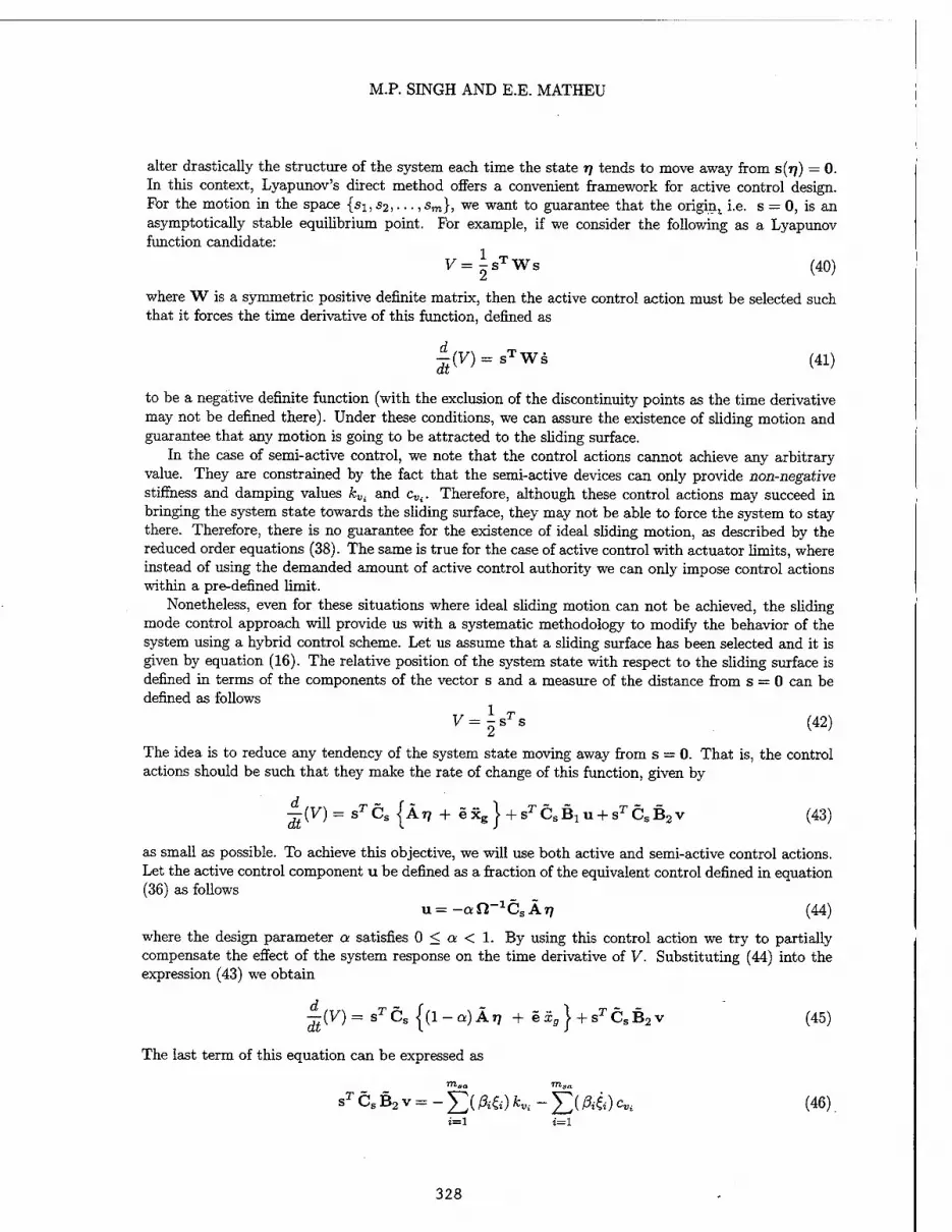
M.P. SINGH AND E.E. MATHEU
alter drastically the structure of the system each time the state r\ tends to move away from s(?7) = 0. In this context, Lyapunov's direct method offers a convenient framework for active control design. For the motion in the space {si, S2,..., sm}, we want to guarantee that the origin^ i.e. s = 0, is an asymptotically stable equilibrium point. For example, if we consider the following as a Lyapunov function candidate:
V=isTWs (40)
where W is a symmetric positive definite matrix, then the active control action must be selected such that it forces the time derivative of this function, defined as
|(V) = sTWs (41)
to be a negative definite function (with the exclusion of the discontinuity points as the time derivative may not be defined there). Under these conditions, we can assure the existence of sliding motion and guarantee that any motion is going to be attracted to the sliding surface.
In the case of semi-active control, we note that the control actions cannot achieve any arbitrary value. They are constrained by the fact that the semi-active devices can only provide non-negative stiffness and damping values kVi and cVi. Therefore, although these control actions may succeed in bringing the system state towards the sliding surface, they may not be able to force the system to stay there. Therefore, there is no guarantee for the existence of ideal sliding motion, as described by the reduced order equations (38). The same is true for the case of active control with actuator limits, where instead of using the demanded amount of active control authority we can only impose control actions within a pre-defined limit.
Nonetheless, even for these situations where ideal sliding motion can not be achieved, the sliding mode control approach will provide us with a systematic methodology to modify the behavior of the system using a hybrid control scheme. Let us assume that a sliding surface has been selected and it is given by equation (16). The relative position of the system state with respect to the sliding surface is defined in terms of the components of the vector s and a measure of the distance from s = 0 can be defined as follows
1 V=-s Js (42)
The idea is to reduce any tendency of the system state moving away from s = 0. That is, the control actions should be such that they make the rate of change of this function, given by
— (V)= sTCs {Ä77 + exg} + sTCsB1u + srCsB2v (43)
as small as possible. To achieve this objective, we will use both active and semi-active control actions. Let the active control component u be defined as a fraction of the equivalent control defined in equation (36) as follows
u= -aß-1CsÄ»7 (44)
where the design parameter a satisfies 0 < a < 1. By using this control action we try to partially compensate the effect of the system response on the time derivative of V. Substituting (44) into the expression (43) we obtain
jt{V)= sTCs {(l-a)Ä77 +eiä}+sTCsB2v (45)
The last term of this equation can be expressed as
sr ""3a "'aa
Cs B2 v = - J2( Ä6) K - ]T( ßdi) cVi (46) i=\
328

HYBRID SLIDING MODE CONTROL OF CIVIL STRUCTURES
where the coefficient ßi represent a component of the vector ß defined as follows
/3T = sTCsB2 (47)
Under the assumption that the devices are designed to perform in a bi-state regime, the semi-active control actions can be defined by considering equation (46). It is immediately apparent that whenever the terms (/%&) and (/%&) are negative, we should zero out their contribution to the function (45), and whenever these terms are positive we should choose the largest values of the coefficients for the corresponding coefficients kVi and cVi. Therefore, the control algorithm becomes
kmax
K^^f-il + sgnißS)) (48)
cmax / • \ Cüi = "i2~(1 + S5n(/3Ä)) (49)
This algorithm is used to obtain the following numerical results.
5 Numerical Results
We will consider a 10 story shear building model for the numerical simulations. The values of the floor weights correspond to those of a typical medium size office building. The floor mass and stiff- ness values are shown in Figure (1). The structural damping was assumed to be proportional, with a first modal damping ratio of 3.10%. The active control force is provided through a system of ac- tive tendons installed at first floor level. The semi-active devices are modelled as variable stiffness and damping mechanisms mounted along diagonal braces. These devices are installed on the first four floors of the structure, and we assume they can be attached and detached to provide addi- tional stiffness and damping when required. The values of the added stiffness coefficients are given by {O.Skref ,Q.3kref ,0.2krej ,0.1kref} for the devices from the first up to the fourth floor, respectively. The reference value kref is the story stiffness, that is 654.98 [MN/m]. Similarly, the added damping co- efficients have values of {0.3cre/, 0.3cre/, 0.2cre/, 0.1cre/} for the devices from the first up to the fourth floor, respectively. The adopted reference value cref is 6.15[MN.sec/m]. The numerical results have been obtained using the El Centro ground acceleration record, with a maximum acceleration level of 0.3g.
Figure (2) shows the time histories of the top floor relative displacement for the controlled and uncontrolled cases, comparing two different types of control schemes. In Figure (2.a) the controlled response was obtained by using the proposed hybrid control approach, where the active control compo- nent was implemented as defined by equation (44) with a value of a equal to 0.10. Figure (2.b) allows the comparison with a fully active control scheme. In this figure, the controlled response was obtained by using the active tendon system according to a sliding mode control law, while the devices were disconnected. The maximum displacement is reduced to 68% and 52% with respect to the uncontrolled case for the hybrid and fully active control cases, respectively.
Figure (3) shows the time histories of the top floor absolute acceleration, comparing the uncontrolled case with the two controlled cases. We notice that the hybrid scheme reduces the response to 72% with respect to the uncontrolled case, while the fully active control approach achieves a reduction of 74%
For any fully or partially active control system, the maximum requirements of force and power are critical from the point of view of its practical feasibility. Therefore, in Figure (4) we compare these requirements for the two controlled cases. Figure (4.a) shows the time histories for the control forces, normalized with respect to the floor weight. We notice that the hybrid scheme demands a maximum control force which is approximately 50% of the force required in the fully active case. Figure (4.b) shows the instantaneous power for the two cases. The maximum power demand for the hybrid control is approximately 80% of the peak power corresponding to the fully active control.
329

M.P. SINGH AND E.E. MATHEU
Floor Mass: 357.24 [kN.sec2/m]
Natural Freqs. [rad/sec]
1 6.40
Floor Stiffness: 654.98 [MN/m]
2 19.06 3 31.29 4 42.82
5 53.39
6 62.78 7 7076
8 77.16
9 81.83 10 84.68
Semi-Active Devices
Active Tendon System
FIGURE 1:10-STORY BUILDING MODEL USED FOR NUMERICAL SIMULATIONS.
330

HYBRID SLIDING MODE CONTROL OF CIVIL STRUCTURES
Displacement [m] 0.20
0.15
0.10
0.05
0.00
-0.05
-0.10 h
-0.15
-0.20
Uncontrolled
Hybrid Control
0 1
Displacement [m] 0.20
6 7 8 9
Time [sec]
0.15
0.10
0.05
0.00
-0.05
-0.10
-0.15
-0.20
10 11 12 13 14 15
r"t7
V i , i
Uncontrolled
Active Control
_L 0 1 6 7 8 9
Time [sec]
10 11 12 13 14 15
FIGURE 2: UNCONTROLLED AND CONTROLLED TOP FLOOR DISPLACEMENT, (a) HYBRID CONTROL (b) FULLY ACTIVE TENDON SYSTEM.
331
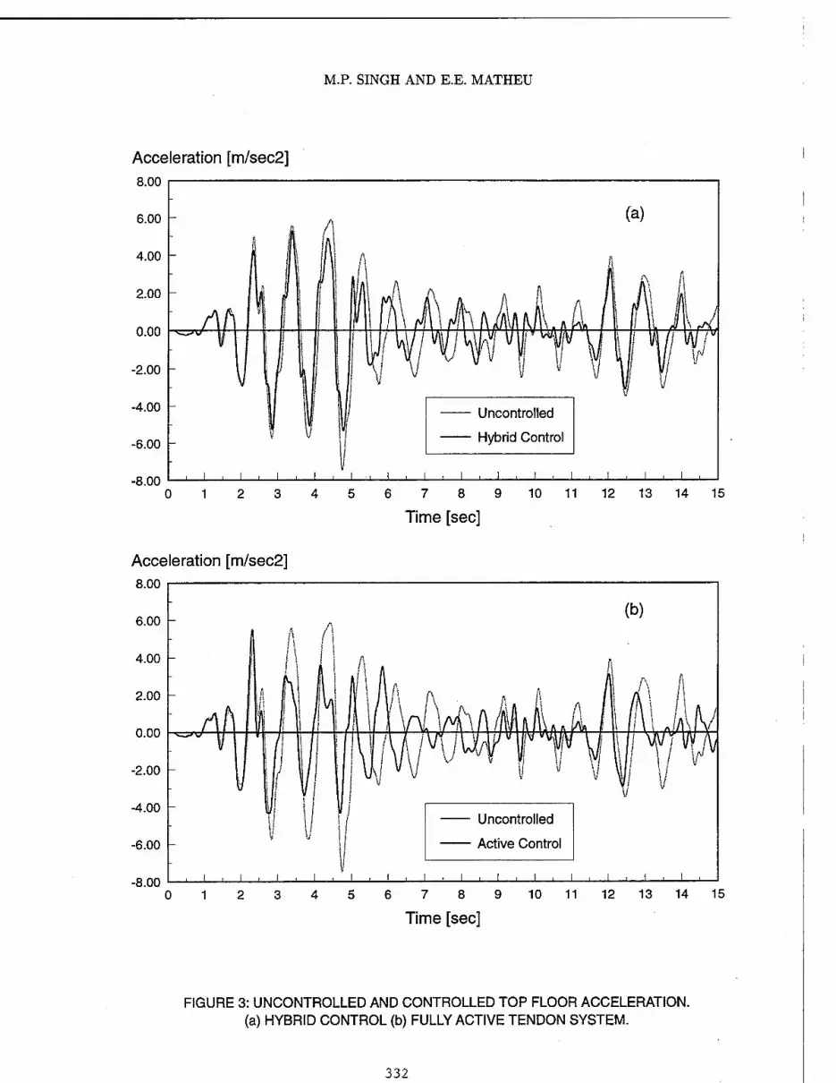
M.P. SINGH AND E.E. MATHEU
Acceleration [m/sec2] 8.00
6 7 8 9
Time [sec]
Acceleration [m/sec2] 8.00
6.00
4.00
2.00
0.00
-2.00
-4.00
-6.00
-8.00
1 A C (b)
Uncontrolled
Active Control
_i i i_ j_
6 7 8 9
Time [sec]
10 11 12 13 14 15
FIGURE 3: UNCONTROLLED AND CONTROLLED TOP FLOOR ACCELERATION, (a) HYBRID CONTROL (b) FULLY ACTIVE TENDON SYSTEM.
332

HYBRID SLIDING MODE CONTROL OF CIVIL STRUCTURES
Control Force / Floor Weight 4.00
(a) Control Force
Fully Active Control
Hybrid Control
5 6 7 8 9 10 11 12 13 14 15
Time [sec]
Power [kW] 700
6 7 8 9
Time [sec]
FIGURE 4: CONTROL FORCE AND INSTANTANEOUS POWER.
333

M.P. SINGH AND E.E. MATHEU
6 Concluding Remarks
The paper presents the formulation and numerical results for a hybrid control approach where active and semi-active response control strategies are combined. The sliding mode control approach is used to design the controller. If one employs only the active method to control the response, the peak power and maximum force requirements can be very high to achieve a desired reduction in the response. On the other hand, if only the semi-active method is used then not enough control "authority may be available to achieve a desired reduction in the response. A combination of the two methods, however, can be used with advantage to obtain a balanced performance with acceptable power and force demand. The numerical results indicate that the use of semi-active devices can, indeed, be utilized to reduce the maximum force and peak power required by the active control method.
7 Acknowledgments
This research is sponsored by the National Science Foundation through Grant No. BCS-9301574. This support is gratefully acknowledged.
8 References
Dorling, C. M. and Zinober, A., "Two approaches to hyperplane design in multivariable variable struc- ture control systems," International Journal of Control, No. 44, pp. 65-82, 1986.
Strang, G-, Linear Algebra and its Applications, Harcourt Brace Jovanovich, FL, 1988.
Utkin V. I., "Equations of the sliding regime in discontinuous systems," Automation and Remote Control, No. 12, pp. 42-54, 1971.
Utkin, V. I. and Young, K. D., "Methods for constructing discontinuous planes in multidimensional variable structure systems," Automation and Remote Control, No. 31, pp. 1466-1470, 1978.
Utkin, V. I., Sliding Modes in Control and Optimization, Springer-Verlag, Berlin, 1992.
Yang J. N, Li, Z., Wu, J. C. and Young, K. D., "A discontinuous control method for civil engineering structures," Dynamics and Control of Large Structures, edited by L. Meirovitch, pp. 167-180, Proc. 9th VPI <fe SU Symposium on Dynamics and Control of Large Structures, VA, 1993.
334

AN ADAPTIVE FUZZY CONTROLLER FOR DAMPING WIND-INDUCED
BUILDING OSCILLATIONS
N. Tripathi, A. Nerves, H. VanLandingham and R. Krishnan Virginia Polytechnic Institute and State University
Blacksburg, VA 24061
Abstract
When tall buildings are subjected to environmental loads such as wind and earthquake, large deflection and acceleration responses result. Hence, passive, semi-active and active vibration control schemes are becoming an integral part of the structural system of the next generation of tall buildings. This paper presents an adaptive fuzzy logic controller (FLC) which works in conjunction with a tuned mass damper (TMD) system. The FLC can cope with the nonlinearities associated with the structural system and adapt itself to dampen wind-induced oscillations. It is assumed that a controller already exists which can control amplitude of the oscillations to certain extent. The FLC learns the functioning of the existing controller and tries to improve the performance by adapting its parameters. The FLC approach is a model-free approach since only the measured variables are used in deriving and adapting the FLC without any a priori knowledge of the system model. The paper indicates that the FLC is one of the good candidates as an active controller for damping wind-induced building oscillations.
1. Introduction
Dynamic loads that act on large civil structures can be classified into two main types: environmental, such as wind, wave, and earthquake loads; and man-made, such as vehicular and pedestrian traffic and those caused by reciprocating and rotating machinery. The response of these structures to dynamic loads will depend on the intensity and duration of the excitation, the structural system, and the ability of the structural system to dissipate the excitation energy. The shape of the structure also has a significant effect on the loading and resulting response from wind excitation.
The advent of high-strength, lighter, and more flexible construction materials has created a new generation oftall buildings. Due to the smaller amount of damping provided by these modern structures, large deflection and acceleration responses result when they are subjected to environmental loads. Such large responses, in turn, can cause human discomfort or illness and, sometimes, unsafe conditions. Passive, semi- active, and active vibration control schemes are becoming an integral part of the structural system of the next generation of tall buildings. This paper addresses the problem of providing active control to a building structure being subjected to wind excitation.
It has been shown in field studies that tall buildings subjected to wind-induced oscillations usually oscillate at the fundamental frequency of the building. In some cases this is coupled with torsional motion when the torsional and lateral oscillation frequencies are close. One of the most common control schemes used to correct these oscillations is a tuned mass damper (TMD) system. Basically, a TMD consists of a mass attached to the building, such that it oscillates at the same frequency as the structure but with a phase shift. The mass is attached to the building via a spring-dashpot system and the energy is dissipated by the dashpot
335

N. •nUPATTfl, A. NERVES, H. VANLANDINGHAM AND R. KRISHNAN
as relative motion develops between the mass and the structure. To provide active control, a hydraulic or electric actuator is connected between the building and the TMD. A controller issues the appropriate command signal to the actuator to provide the desired control force. The active control system essentially regulates an external force to counteract the dynamic response of the building or structure. - A variety of control schemes have been proposed, each showing varying degrees of effectiveness. Earlier approaches to the problem included classical feedback control [1], optimal control [2], pole-assignment control [3], and modal control [4]. More recently, methods like independent modal space-control [5] and bounded-state control [6] have been proposed. To take into consideration the nonlinear characteristics of a structures, sliding-mode control ([7], [8]), Newmark-Beta-based control [9], and instantaneous optimal control [10] have been considered. Intelligent control using neural networks ([11], [12]) have also been proposed.
There has been a rapid growth in the use of fuzzy logic in a wide variety of consumer products and industrial systems. Fuzzy logic represents one of the model-free approaches to the problems of system identification and control. The control of the vibrations can be viewed as a problem of mapping between the controller inputs and controller output Fuzzy logic systems have been proved to be universal approximators [13] and hence are good candidates for solving complex control problems. Several advantages of fuzzy logic are that they can be nonlinear, can be adaptive, can admit high degree of parallel implementation, and can tolerate uncertainty in the system. More importantly, human experience and expertise about the system and its performance can be incorporated into the design of a fuzzy controller. Section 2 describes the model of a building used for simulation. Section 3 explains the development of an adaptive FLC. Section 4 presents the results. Finally, Section 5 summarizes the paper and hints at future work.
2. System Model
The basic idea of fuzzy control for structural systems is illustrated for a building equipped with a tuned mass damper. The building-TMD system is being subjected to wind excitation. Since the TMD is used primarily to suppress the first fundamental mode in wind-induced motion, a single-degree-of-freedom, but nonlinear model, of the building gives a good approximation to first-mode structural motion. Figure 1 shows a schematic diagram of the building-TMD system. It is a shear-beam model of the structure represented by a damped spring-mass system.
«
kDf] \AA _[Q_
u u mD
0 0
1 —*l
«B 1
Figure 1. Building-TMD Model
The building is modeled by a first-mode modal mass mB and a damping constant bß. The spring kB can become inelastic with a restoring force given by [14]
Fk = a k yB + (l - a) k v (1)
336
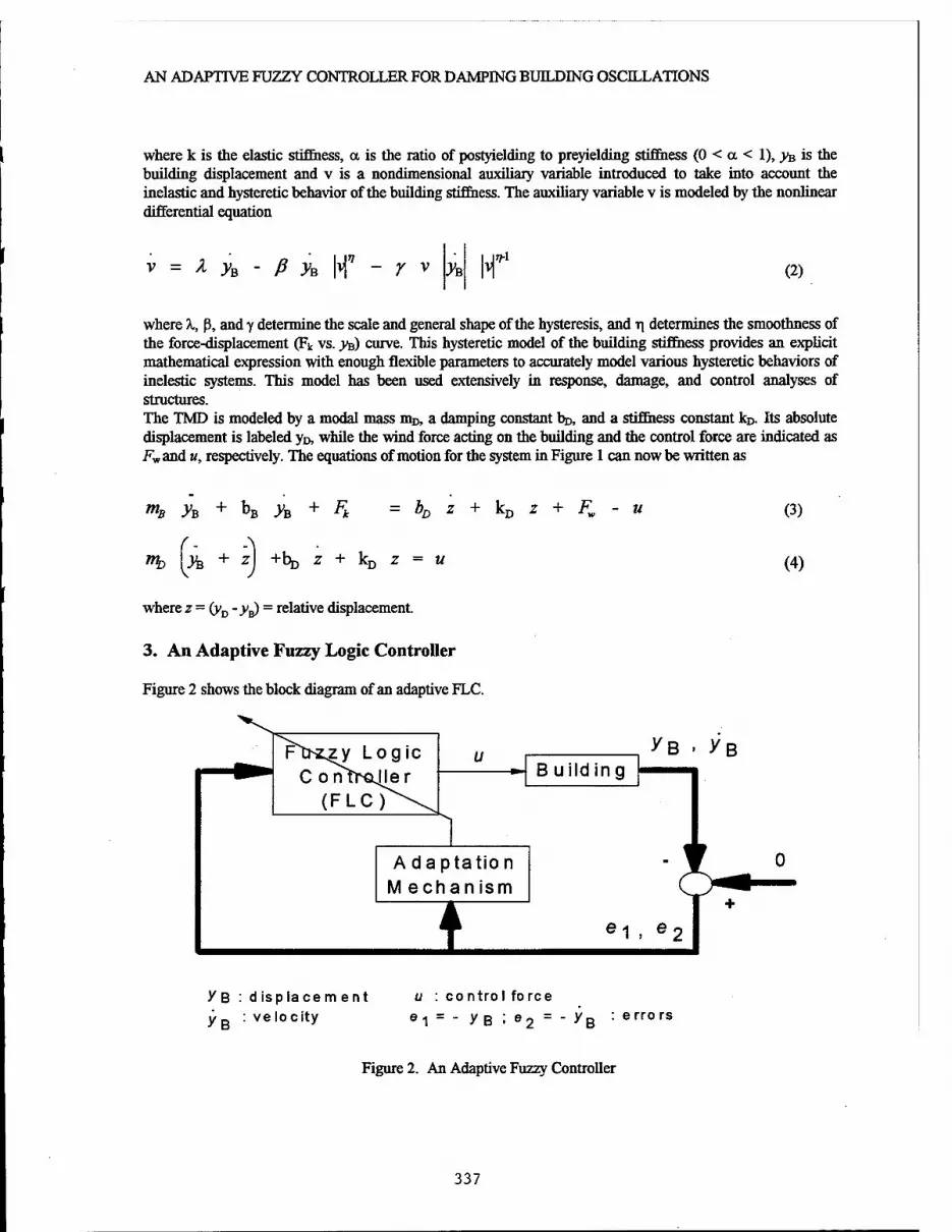
AN ADAPTIVE FUZZY CONTROLLER FOR DAMPING BUILDING OSCILLATIONS
where k is the elastic stiffness, a is the ratio of postyielding to preyielding stiffness (0 < a < 1), VB is the building displacement and v is a nondimensional auxiliary variable introduced to take into account the inelastic and hysteretic behavior of the building stiffness. The auxiliary variable v is modeled by the nonlinear differential equation
v = X yB - ß yB Y v Ä >7-l
(2)
where "k, ß, and y determine the scale and general shape of the hysteresis, and r\ determines the smoothness of the force-displacement (Fk vs. ys) curve. This hysteretic model of the building stiffness provides an explicit mathematical expression with enough flexible parameters to accurately model various hysteretic behaviors of inelestic systems. This model has been used extensively in response, damage, and control analyses of structures. The TMD is modeled by a modal mass mD, a damping constant ho, and a stiffness constant kD. Its absolute displacement is labeled yD, while the wind force acting on the building and the control force are indicated as Fv and «, respectively. The equations of motion for the system in Figure 1 can now be written as
mB JB + bB yB + Fk = bD z + kD z + Fw - u
"b [ä + z) +bD z + kD z = "
where z = (yD -y^ = relative displacement.
3. An Adaptive Fuzzy Logic Controller
Figure 2 shows the block diagram of an adaptive FLC.
(3)
(4)
Fü^zy Logic C onfrajler
(FLC)
u
A daptation M echan ism
I
B uild ing yß • YB
e-i , e2
y B : d isplacem ent y R : ve locity
u : control force e1 = - yB : e2
= ■ -^B : errors
Figure 2. An Adaptive Fuzzy Controller
337

N. TREPATHI, A. NERVES, H. VANLANDINGHAM AND R KRISHNAN
Fuzzy Rule Base
RVV Fuzzifier
FV Fuzzy Inference
Engine
FV *- Defuzzifier
RVV
Form of the FLC
RVV: real-valued variables
FV: fuzzy variables
Figure 3 Form of the Fuzzy Logic Controller Shown in Figure 2
The building displacement and velocity are measured. The errors between desired displacement and velocity (zero) and the actual displacement and velocity (measured values) are provided to the FLC. The FLC itself consists of a fuzzifier, a rule base, an inference engine and a defuzzifier as shown in Figure 3 [15]. The fuzzifier is the plant (or building)-to-fuzzy logic system interface and performs a mapping from real-valued variables into fuzzy variables. The fuzzy rule base consists of a collection of fuzzy rules. Fuzzy rules can be developed by using IF-THEN rules based on the knowledge and can be fine tuned by training the fuzzy logic system to match the input-output pairs. Alternatively, a few data can be selected as input-output pairs to determine the parameters of the FLC. In the fuzzy inference engine, fuzzy logic principles are used to combine the fuzzy IF-THEN rules in the fuzzy rule base into a certain mapping. The defuzzifier is the fuzzy logic system-to-plant (or building) interface and performs a mapping from fuzzy variables to real-valued variables (Eq. (7) in the Appendix). The control force determined by the FLC drives the TMD system to control the oscillations. The adaptation mechanism modifies the parameters of the system by observing the errors in displacement. The basic steps for obtaining above configuration shown in Figure 2 are discussed briefly.
* Step 1: First, obtain a nonadaptive FLC based on the functioning of an existing controller.
* Step 2: Modify the parameters of the FLC to get an improvement over the existing controller. Some intuition
might help in determining the direction in which certain parameters should be varied. In the worst case (where no such intuition is forthcoming), run several simulation tests to observe the effect of varying different parameters on the performance of the controller.
* Step 3: Adapt the FLC parameters based on some performance criterion. The current value of the performance
criterion can be attributed to different parameters of the FLC by relating the FLC parameters to the performance criterion.
338

AN ADAPTIVE FUZZY CONTROLLER FOR DAMPING BUILDING OSCILLATIONS
The execution of above mentioned steps is described next.
* Step 1:
To get a nonadaptive FLC, the existing controller (proportional controller) was put on-line and several variables such as building displacement building yB, velocity yB and control force u (determined by the existing controller) were recorded. Inputs to the FLC are yB and yB and output of the FLCis control force. Some of the data were selected as input and output pairs, which determined the centers of the membership functions of inputs and output. Fifty rules were selected. This method of determining centers of input membership functions is not unique. If the knowledge of behavior of the system is known, some linguistic rules can be formed rather than relying completely on the available data. The widths of membership functions were chosen randomly as 0.1. If the widths of membership functions are adjusted properly and the selected training pairs are representative of the operation of the overall system, the FLC would function almost as good as the existing controller.
* Step 2:
By judiciously modifying the output and widths of input membership functions, the FLC can be made to perform better than the existing controller to a certain degree. Centers of the output membership functions were modified according to the following equation:
ü(k + \) = M(Jt)+0.05 sign(ü(k)) (5) where sign is the signum function. When the argument is positive, its value is 1 and when the argument is negative, its value is -1.
In other words, 5% change in the location of the centers of output membership functions in proper direction was made. If the center value is positive, the magnitude of the center will be increased in a positive direction. If the center value is negative, the magnitude of the center will be increased in a negative direction. Also, some simulation tests were run for different values of spreads of the input membership functions. The combination of changes in the center locations of output membership functions and the changes in the spreads of input membership functions could result in better performance of the controller.
* Step 3:
Furthermore, if the parameters of the FLC are modified on-line based on some performance criterion, even better performance can be obtained. The adaptation mechanism shown in Figure 2 was based on gradient descent algorithm. The adaptation equations are derived in the Appendix. The centers of the input membership functions and the output membership functions were adapted on-line.
4. Results
Simulation tests were carried out for the duration of 100 seconds, with a step size of 0.1. Figure 4 shows the response of a building in the absence of any control force.
339
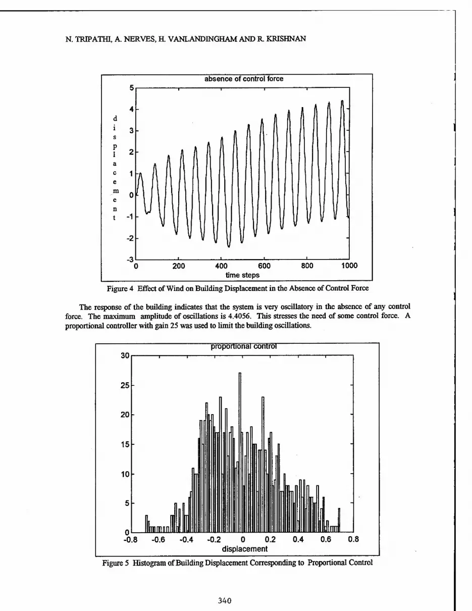
N. TRIPATHI, A. NERVES, H. VANLANDINGHAM AND R KRISHNAN
absence of control force
-3 200 400 600
time steps 800 1000
Figure 4 Effect of Wind on Building Displacement in the Absence of Control Force
The response of the building indicates that the system is very oscillatory in the absence of any control force. The maximum amplitude of oscillations is 4.4056. This stresses the need of some control force. A proportional controller with gain 25 was used to limit the building oscillations.
proportional control •9U
25
1 1 1
20
15 -
10 -
5 - Flnfl HI II 1
-
0 -0
In min ill jj .8 -0.6 -0.4 -0.2 0 0.2
displacement 0.4 C .6 0 8
Figure 5 Histogram of Building Displacement Corresponding to Proportional Control
340

AN ADAPTIVE FUZZY CONTROLLER FOR DAMPING BUILDING OSCILLATIONS
Figure 5 presents the histogram of the building displacement when proportional control is used. The proportional control is effective in limiting the amplitude of oscillations and the maximum amplitude of oscillations was observed to be 0.7033. The sum-squared-error over the certain simulation period was 9.3482. An FLC based on the proportional controller performance gave a maximum amplitude of 1.0002 and the sum- squared error was 9.6264. Some changes in spreads of the input membership functions and output centers, as suggested in step 2 in section 3, led to the maximum amplitude of 0.6543 and the sum=squared-error of 9.1832. This corresponds to 6.9 % improvement in the amplitude reduction and 4.0% improvement in the sum-squared-error.
20
18
16
14
12
10
8
6
4
2
-0.8
adaptive fuzzy control
-0.2 0 displacement
0.6
Figure 6 Histogram of Building Displacement for an Adaptive Fuzzy Control
Figure 6 presents the histogram of the building displacement when an adaptive fuzzy control is used. The maximum amplitude of oscillations was observed to be 0.5508 and the sum-squared-error was 8.7368. Thus it gave an improvement of 21.6835% in terms of amplitude of oscillations and 13.19 % improvement in terms of the sum-squared-error. Figure 7 shows time history of the building displacement when an adaptive fuzzy control was used.
5. Conclusions
A problem of damping wind-induced oscillations in tall structures was addressed. An adaptive FLC was designed which works in conjunction with a TMD system. It was assumed that there exists a controller which can reduce the effect of wind on the building oscillations. An FLC was designed based on the functioning of a proportional controller. A marginal improvement in controller performance was obtained by varying parameters of an FLC off-line. Then, an adaptive FLC was developed which tried to minimize the amplitude of building oscillations by using a gradient descent algorithm to adapt the parameters of the FLC. The adaptive FLC performed better than the existing proportional controller. If the building is severely nonlinear, the FLC may provide a more extreme improvement over a standard controller. The advantage of such an approach is that the adaptive FLC would perform at least as good as the existing controller since it has already
341

N. TRIPATffl, A. NERVES, H. VANLANDINGHAM AND R KRISHNAN
learned the functioning of the existing controller. If the learning rate is not too high, the adaptive FLC would outperform the existing controller. The price paid for the improved performance is computational efforts. It might take some time to arrive at the proper learning rate.
0.2
0.6
d °'4
i s P 1 a c 0 e m e -0.2 n t
-0.4
adaptive fuzzy control
-0.6
- I
ll h
200 400 600 time steps
800 1000
Figure 7 Time History of Building Displacement Corresponding to An Adaptive Fuzzy Control
A constant learning rate with momentum was used to adapt the parameters of the FLC. A natural extension of the approach considered here would be to use an adaptive learning rate instead of a constant learning rate. Also, different learning rates can be used for different parameters. A neural network can be used to identify the plant and hence its prediction can be used one step ahead to predict the effect of the application of the control force calculated by the adaptive FLC. This information can be utilized to further adapt the parameters of the FLC or to modify the output of the adaptive FLC in a certain way.
References
[1] Leipholz, H.H.E. and Abdel-Rohman,M., Control of Structures, Martinus Nijhoff Publishers, The Netherlands, 1986.
[2] Yang, J.N., "Application of Optimal Control Theory to Civil Engineering Structures," ASCE Journal of Engineering Mechanics, Vol. 101, No. 6, 1975, pp. 819-838.
[3] Abdel-Rohman,M. anf Leipholz, H.H., "Structural Control by Pole Assignment Method," ASCE Journal of Engineering Mechanics, Vol. 104, No. 5, 1978, pp. 1159-1175.
[4] Abdel-Rohman, M. and Leipholz, H.H., "General Approach to Active Structural Control," ASCE Journal of Engineering Mechanics, Vol. 104, No. 6,1979, pp. 1007-1023.
[5] Meirovitch, L. and Oz, H., "Active Control of Structures by Modal Synthesis," In Leipholz, H.H.E. (ed.), Structural Control, North Holland, Amsterdam, 1980, pp.505-521.
[6] Lee, S.K. and Kozin, F., "Bounded-State Control of Linear Structures," In Leipholz, H.H.E. (ed.), Structural Control, Martinus Nijhoff, Amsterdam, 1987, pp. 387-407.
342

AN ADAPTIVE FUZZY CONTROLLER FOR DAMPING BUILDING OSCILLATIONS
[7] Krishnan, R, Singh, M.P., and Nerves, A.C., "Mitigation of Wind and Earthquake Effects on Structures by Sliding Mode Control," Proceedings of the First World Conference on Structural Control, Los Angeles, CA, August 3-5,1994. n
[8] Yang, J.N., Li, Z., and Wu, J.C., "Discontinuous Nonlinear Control of Base-Isolated Buildings, In Housner, G.W. and Masri, S.F. (eds.), Proceedings of the International Workshop on Structural Control, Honolulu, Hawaii, August 5-7,1993.
[9] Reinhorn, A.M., Manolis, G.D., and Wen, C.Y., "Active Control of Inelastic Structures, _ASCE Journal of Engineering Mechanics, Vol. 113, No. 3, March 1987, pp. 315-333.
[10] Yang, J.N., Li, Z., and Vongchavalitkul, S., "Generalization of Optimal Control Theory: Linear and Nonlinear Control," ASCE Journal of Engineering Mechanics, Vol. 120, No. 2, February 1994, pp. 266-283.
[11] Nerves, A.C. and Krishnan, R, "Active Control of Wind-Induced Vibrations in Tall Buildings using NeuralNetworks," Proceedings of the IEEE Industrial Electronics Conference, Bologna, Italy, September 9-14,1994.
[12]Nerves, A.C., Krishnan, R, and Singh, M.P., "Modeling, Simulation and Analysis of Active Control oi Structures with Nonlinearities using Neural Networks," Proceedings of the ASCE Engineering Mechanics Conference, Boulder, CO, May 22-24,1995.
[13] Wang., L X., Adaptive Fuzzy Systems and Control, PTR Prentice Hall Inc., Englewood Cliffs, NJ 07632, 1994.
[14] Wen, Y.K.,"Methods of Random Vibration for Inelastic Structures," Journal of Applied Mechanics Review, Vol. 42, No. 2, pp.39-52.
[15]Mamdani, E. H., "Applications of Fuzzy Algorithms for Simple Dynamic Plant," Proc. IEE, 121, No. 12 (1974), 1585-1588.
Appendix
The performance measure to be minimized is „ i » (6)
where e is the negative of the building displacement. The FLC parameters which can be adapted are:
Ij (center of output membership function for rule i) jCj (center of inputl membership function for rule i) Xg (centerof input2 membership function for ruleO a^ (spread of inputl membership function for rule 0 a2i (spread of input 2 membership function for rule D
There are M rules (i=[l,M]). The relationship among these parameters is represented by:
M _
tiMu)0h.) where
(8)
343

N. TRIPATHI, A. NERVES, H. VANLANDINGHAM AND R. KRISHNAN
fe=expj-- ^2 — X2i (9)
(l^ and (ijj are degrees of membership of first and second input respectively for rule i. Here, Xi and x2 are the inputs to the FLC and u is the output of the FLC. The update equations, based on the gradient descent algorithm are:
dE W + D^W-r/—— (10)
dE xJi(k + l)=xJi(k)-r}—— j=[l,2] (11)
vAk + V-CTjM-tj-^— j=[l,2] (12)
where r\ is the learning rate. Since the learning rate can be chosen carefully, the exact partial derivatives are not required. If the signs of these partial derivatives are determined, the gradient descent algorithm can try to reach the niinima by "traveling" in proper direction.
InEq. (10),
dE dE de du (13) dät(k) de du düt(k)
From Eq. (6)
^ = e (14) de
dz Also, it was found from a crude linear approximation of the plant that —is positive.
du flu
Moreover, is positive (from (7)). Hence, Eq. (10) becomes dJt(k)
M,(/fc + l) = M,(Jt)-77'e (15)
where r\' is the modified learning rate. Similarly, it was found that
x„(k + 1) =xli(k)-Tiesign((x, -xB)ü) «, L ™ -A H1,2],HW (16) crjj(k + 1)=aji(k)-Tiesign(M)
where sign is the Signum function.
344
A CRASH AVOIDANCE SYSTEM BASED UPON THE COCKROACH ESCAPE RESPONSE
C.-T. Chen, R. D. Quinn and R. E. Ritzmann Case Western Reserve University
Cleveland, OH 44106
Abstract A crash avoidance system for automobiles is developed based upon a distributed network of artificial neurons that mimic the neural organization of the escape system in the American cockroach. The escape system in the cockroach is shown to be an excellent source of inspiration for the development of a crash avoidance system. The equations of motion for a four-wheeled vehicle with front wheel steering are derived to model the dynamics of the vehicle for the purpose of simulation. The crash avoidance system is implemented in an artificial neural network which is trained off-line, but then is shown to produce real- time performance in an unknown dynamic environment. A novel crash avoidance scheme is derived for training the crash avoidance system. Simulation results show that the well-trained crash avoidance system results in a reflexive crash avoidance behavior in an environment without a priori information.
1. Introduction A crash avoidance system for four-wheeled vehicles is developed based upon a distributed network of
artificial neurons that mimic the neural organization of the escape system in the cockroach, Periplcmeta americana. The goal of a crash avoidance system is to faithfully detect a threat from within numerous benign stimuli, identify where the threat is coming from and evoke appropriate avoidance maneuvers in the context of the vehicle's internal state and its environment. The system must do all of this in a very short period of time. These are also the goals of escape systems found in animals.
The escape response circuit in the cockroach is an excellent source of inspiration for the development of a crash avoidance system. Ritzmann [8] provided a comprehensive discussion of the present state of knowledge about this circuit. It accurately identifies rapidly accelerating wind stimuli as arising from predators. Wind information is gathered by mechanoreceptive hairs and is conducted to the thorax by giant interneurons. There it is integrated by a distributed population of interneurons, called type A thoracic interneurons (TIAs). The TIAs direct turning movements away from the lunging predator via both direct and indirect connections to the leg motor neurons. All of this is accomplished in approximately 60ms.
A crash avoidance system that only factored in the most immediate threat might cause more harm than good. For instance, a system that automatically steers the vehicle away from an obstacle, could cause a collision with a wall or another passing vehicle. The cockroach solves this problem by incorporating context dependence into its system. In addition to monitoring wind inputs from predators, the TIAs receive input from exteroceptive cues such as antennal contact, auditory responses and ambient light and proprioceptive cues on the state and position of the legs. The distributed network of TIAs interprets the data on wind direction in the context of everything else the cockroach is experiencing at the moment of the attack. The context dependent nature of the cockroach escape system permits a very short reaction time because a suitable response need not be planned at the time of a particular threat, but is continuously updated based upon the animal's physiological state and its environment. Thus, the cockroach escape circuit satisfies all of the requirements for a successful crash avoidance system.
345

C. T. CHEN, R. D. QUINN and R. E. RITZMANN
The neural circuit that comprises the cockroach escape system has been previously documented by intracellular analysis and modeled on a computer as a distributed network of artificial neurons[2-4]. In this paper, a crash avoidance system is developed for four-wheeled vehicles based upon this circuit. A dynamic simulation of a four-wheeled vehicle is developed and the crash avoidance is implemented and tested. The crash avoidance circuit incorporates sensory structures that detect an approaching threat- and then evokes appropriate avoidance maneuvers to be carried out by the vehicle's wheels. The avoidance maneuvers include turning, braking and accelerating. The results will be compared to some related works [1,5-6].
2. Vehicle Dynamics The vehicle's motion is defined with reference to a right-hand orthogonal coordinate system o-xyz
which originates at the center of mass (CM.) and moves with the vehicle. The inertial frame denoted by O- XYZ describes the position of this vehicle in the world coordinates.
Assuming this vehicle has front wheel steering(FfT5), the corresponding kinematics are shown in Fig. 1, where wheel i with radius rw is represented by i, i=l ~ 4. The wheel base is 2a and track is 2b. The mass of the vehicle is denoted by m, the moment of inertia about the z-axis is Iz; <]), and <|>2 denote the steering angle of wheel 1 and wheel 2 respectively, and <j) is the steering wheel angle. The steering wheel angle <|) results from an applied torque on the steering wheel, it may also be considered the angle of a " virtual wheel" which is attached to the middle point between wheel 1 and wheel 2.
Assuming no tire side slip, the Ackerman steering constraint may be expressed as
(tan<|)2-tan(t)1) + — tan,tan<}>2 =0 (1) a
Introducing the steering wheel angle <J>, the steering angles for wheel 1 and wheel 2 are expressed as
^ , 2atan$ , , 2atan<j> „ , N
2a-btan<)> 2a+btan<}> During a turning maneuver, the vehicle is in translation and rotation; the rotation is expressed in terms
of yaw rate 0 = 9k, and its translation can be represented by the velocity of the vehicle's CM. as
Yo = v.!+v,J (3) where v„ is the forward component speed and vy is the lateral component speed.
The motion of these four wheels are described by the individual wheel-fixed coordinate O-x^z^ where the subscript i denotes the wheel i, i=l ~ 4. Since there is no side-slip or skidding, the velocity v,
with respect to the wheel-fixed frame is y> = vi ii (4)
The position vectors with respect to the vehicle-fixed frame for these four wheels are r, = rG + ai+bj; r2=rG + ai-bj (5a,b)
r3 =rG-ai+bj; r4=r0-ai-bj (5c,d)
where rG is the position vector of the CM. of the vehicle in the global coordinate system. The velocities of
the wheel centers can be expressed as
y, =yG-b8i+a8j = v1i,; v2 = yG + b8i+a6j = v2i2 (6a,b)
v3 = yG-b8i-a8j = v3i3; v, = vG + b8i-a8j = v4i4 (6c,d)
From Eq. (6) a set of nonholonomic constraints based on no wheel slip can be expressed as
<*>vx=a8; vy=a8 (7a,b)
where <£ = — tan(b. 2
Substituting these two nonholonomic constraints into Eq. (6), the virtual displacements of the wheels can be expressed as
5s1=8sIj(l-^<&)2+(2<&)2; 8s2=8s,j(l+^<I>)2 + (24>)2 (8a,b)
346

CRASH AVOIDANCE SYSTEM
8s, = 8s, 1-** 1-3* a
8s4 = 8s,
The virtual work 8ww done on these four wheels by shaft torques is
8Ww = £&*, =[f1(<t>)T1 +f1(<t»)x2+f3((J))T3 + f4(<t))Tj6sx=f15si 1=1
where
iw V a r. V a <f>)2+(24>)2;
(8c,d)
(9a)
(9b,c)
a f,=-
a
f.^t^tj+fo+ta
(9d,e)
(9f) Let the virtual work 8w, done by the steering torque t, applied through the steering linkage be defined
as 5ws=xs5<t); the total virtual work can be expressed as 8w = 8ww +8ws =fx8sx+T,8<|> (10)
Neglecting the rotational kinetic energy of the wheels, the kinetic energy can be expressed as
r=Im(v,+v;)+Ii2e2+!i.(e+<j))3 (ii)
where I, is the moment of inertia of the front steering system. Lagrange's equations in quasi-coordinates and in true coordinates, respectively, can be expressed as
( ) + o)T — = f+Cv dt dv dv
d_ dT_ 3T_
dt 9q 3q " "
where
v = v,
; Ö)T = 0 -e
; q = e
v y e 0 <t>
(12a)
(12b)
(12c,d,e)
and f is the generalized external applied force vector; cv is the constraint force vector; T is the
generalized external applied torque; c, is the constraint torque vector.
Substituting the energy Tinto Eq. (12) and cancelling the Lagrange multipliers, the dynamic equations of motion augumented with the differentiated nonholonomic constraints become
M,(4>)2+Gr(4>) = Ur(4>)Ü (13a)
where ü = [t, x2 x3 xt T,] ; (13b)
M = rD,i V [XI fB 1
; z = ~ ; Gr = ; u = ; D = kj q Oc L°^J 4> 0 -a 0]
; Gc = 0 1 -a 0J
1(1 + 4*2)<K 0
and D = m mO O 4>
0 0 I. I. B =
(13c,d,e,f,g,h)
(13ij) f f f f 0
0 0 0 0 1
Let the sideslip angle a be defined as the angle between the tangential velocity direction of the CM. and the vehicle forward heading direction, the velocity vector v, its derivative v and time derivative of yaw
rate can be expressed, respectively, as
v = s cos a
since v =
scosa-sa since
s sin a + sä cos a 6 = - (s sin a + sä cos a)
a where
since = — = $
p Vi+o2' cosa = •
L,+b 1
Vl+3>2
(14a,b,c)
(14d,e)
347

C. T. CHEN, R. D. QUINN and R. E. RITZMANN
and p is a signed curvature radius of the vehicle's path at this moment. 6c can be solved through algebraic manipulation as
1+402 ■ a = — d>
2(1+<D2) (140
1 Substituting Eq. (14) into Eq. (13), and assuming that the applied torque on each wheel is xi = —Te, i=l
~ 4, where Te is the total applied torque from engine torque or braking, the equations of motion can be
expressed as D,z.+G.(z.,z.) = u (15a)
where
zs = ; DS =
m+mtf + fl. + IJO'/a' 1,4»
f(<|>)Vl + 3>2
aVl + 4>2
af(<t>)
I. ; G.=
(II + IJ)<l>(l+4<D2)
2a2V(l+4>2)3f(<t>) I,(l+4<£>2)
2aV(l + *2)3
S(j); u =
(15b,c,d,e)
and the function f(<(>) is defined as f = - (f+ f2 + f3 + f4) 4
Note that if <j> is a constant, then <j> = ^ = 0, the system is reduced to one degree-of-freedom, and Eq. (15) becomes
G(4>)s = T« (16a) where
G(<(.)= f(<t>)Vl + *2
(16b)
3. Performance Limits Due to the limits from the engine and braking torque, Te must satisfy
mm — c max
Substituting Eq. (16) into Eq. (17), the constraint on S is T . ..x mm < c < max
(17)
(18) G(«>) GW)
The constraint on speed is 0<s<s_ (19)
The pure rolling assumption for the tire model remains valid if the available frictional forces are not saturated by the inertial forces; therefore, the friction force required by the vehicle motion is
f,2 + f2<(umg)2 (20) where f, = ms and fB = m(s)2 / |p|. Substituting these expressions for the friction components into Eq. (20),
the constraint on s is
■M^'S + nV (21)
(22) Because the square root in Eq. (21) must be positive, the constraint on speed is
s2 2 lig|p| It is assumed that the limit of the steering wheel angle is the only constraint for the steering system:
<L.£«>£4>» (23)
4. Controller Design A control law referred to as the computed torque method is applied in a straightforward manner as
u = D,ü(Zs,z!)+Gs(z„z,) (24)
348

CRASH AVOIDANCE SYSTEM
Eq. (24) is substituted into Eq. (15), the nonlinearity is canceled and the closed-loop dynamics are obtained as
zs = u(Zs,zs) (25)
where ü" is a new control vector and permits the application of a smooth state feedback.
For our task involving the stabilization of the desired outputs, this new control vector takes the following form
ü = zd-K!(zs-Zo)-K2(zs-Zd) (26)
where the subscript 'd' represents the desired action for crash avoidance, and the (2X2) gain matrices K, and K2 may be selected so that this system has independent actuators. That is K, = diag[k1
s,k*] and
K2 = diag[k2 ,k* ]. Therefore, Eq. (25) will be decoupled into independent error dynamics e+K,e+K2e = 0 (27)
where e = zs - zd = [es ,e^ ]T = [s - sd ,<|> - <|>d ]T. The elements of the gain matrices are positive and chosen so
as to guarantee the eigenvalues assignment corresponding to the design specification.
5. Biologically-Inspired Crash Avoidance System A crash avoidance system is developed based on the cockroach escape response. The system
incorporates simulated sensory structures that detect an approaching threat and then evokes appropriate avoidance movements to be carried out by the wheels of the vehicle. Exteroceptors include sonar proximity detectors to monitor the presence of objects around the vehicle. Proprioceptive sensors include tachometers to monitor the speeds of the wheels and potentiometer to monitor the steering wheel angle. The avoidance maneuvers may include turning, braking and accelerating to respond to a crash threat.
The crash avoidance circuit for a four-wheeled vehicle is shown in Fig. 2. The architecture of this neural network is based on a model of the cockroach escape circuit [2]. A sigmoidal function with bias is used to model the input-output relation of a neuron. The simulated vehicle is equipped with 8 sonar sensors that are mounted on a horizontal ring around the vehicle such that its environment can be scanned. A range reading can be measured through an echo from an object; the measurements of all sonar sensors are fed forward to the ventral giant neurons and exteroceptive neurons. Apart from the measured information at current moment t, the radial measure of distance to an obstacle at the last sampling moment t-At is also recorded to infer the relative velocity and relative heading direction expressed with respect to the vehicle. The outputs of the exteroceptive neurons are the normalized relative distance and orientation of an obstacle.
Proprioceptive neurons receive wheel speed data from simulated tachometers; the steering wheel angle is also fed into the proprioceptive neurons. The outputs of the proprioceptive neurons are the normalized speed of the vehicle and the normalized steering wheel angle.
The observed threat field, which is represented by the normalized magnitude of the velocity and normalized forward heading direction of an obstacle relative to the vehicle, is constructed by the outputs of ventral giant neurons(vGI). Ventral giant neurons receive the signals from the outputs of proprioceptive neurons and sensor neurons at the last sampling moment t-At and the current moment t.
Eighteen neurons reside in the thoracic layer and twelve neurons reside in the local layer. These numbers were chosen arbitrarily. The outputs of the motor neurons are the desired avoidance commands expressed in the normalized tangential acceleration s„ and normalized steering wheel angle tyt. The actual
commands will be recovered by Sa = s.«(2sa-1); 4>4 = 4>„(2$,-l) (28a,b)
The desired tangential speed s„ is sd = s+s„At, and the desired steering wheel angle speed and
acceleration are set to zero in correspondance to the desired steady state after At. The neural network was trained using backpropagation to make the vehicle respond appropriately to
potential crashes. The learning of this system was confined to varying the connection weights. In order to find the appropriate connection weights given the known structure of the circuit, sufficient data are needed to train this system. These data were developed from a theoretical crash avoidance scheme.
6. Crash Avoidance Scheme (Off-line')
349

C. T. CHEN, R. D. QUINN and R. E. RITZMANN
The crash avoidance scheme in the path-time space(s,t) is shown in Fig. 3, where the vehicle is treated as a particle moving at constant speed v" over a planned path sv which is function of time t; the moving obstacle travelling over s° at constant speed v° is enlarged proportionally as a circle with radius R.
Suppose that the vehicle arrives at the point s," at time t,", and passes through the intersection to the
point s2 at t2; similarly, the center of the moving obstacle reaches position 1 and position 2 at time t°, t°,
and this enlarged circle is tangent to the trajectory sv of the vehicle at these moments. A crash alarm set will be defined in terms of the following inequalties,
crash alarm set:= {(vv,s\ v°,s°,R)|t; < tj < t° with t,Y > 0 or t," < t2v < t°2 with t2
v > 0} (29)
When there is a crash alarm, avoidance action must be taken to elude a possible collision. The first option is acceleration or deceleration. The acceleration scheme implies that the vehicle must pass through
the intersection to sv2 before the time t° by applying driving torque to the wheels. The condition with a
minimum acceleration for crash avoidance is s; = sv(t;) (30a)
For the deceleration scheme, the vehicle just arrives at sjr at t > t° by applying a braking torque, and the condition with a minimum deceleration is
s,v=sv(t°) (30b) Sometimes, the acceleration or deceleration scheme fails due to the vehicles performance limits, speed,
or terrain conditions, etc.; so replanning other paths becomes necessary to avoid a collision. Path replanning involves the application of steering torque to achieve the desired steering wheel angle.
In fact, there is no preexisting knowledge of the obstacles' path in the real world. Only observations of the obstacles motion are available through the sensory systems. Therefore, each prediction according to the current situation of the world at any instant expresses an inferrance of the future motions of the obstacles. This prediction is referred to as an inertia cue whose inputs are from the current sensing. Whether a crash alarm occurs and whether a crash avoidance is needed depend on the usage of inertia cues which are inferred corresponding to the steady state assumption We will treat the vehicle as following a straight path or a circular path at constant speed v", and we will treat the moving obstacle as following a straight path with a constant speed v° as inertia cues to predict the likelihood of a crash.
The desired deceleration sd or acceleration s* used for crash avoidance with the corresponding tangential speed sd,s* at point s,v,s2 must satisfy the constraint Eqs. (18) and (21) on s , and the speed
must satisfy Eqs. (19) and (22). If there exists a feasible deceleration V and acceleration s* simultaneously, the desired tangential acceleration s, will be chosen corresponding to the equation
s" if's* <-sd
(31) otherwise
If all of these constraints are not satisfied, avoidance by acceleration/ deceleration is not possible along the preplanned path; therefore, the path replanning for collision avoidance must be made, and the desired steering wheel angle <)>„ must be found which satisfies the corresponding constraints. The most desirable
steering wheel angle <J>d is denoted as the value which is closest to the current steering wheel angle <j>.
7. Simulation and Results Given this vehicle is travelling over a straight path at a constant velocity vs = s=14 m/sec in the heading
direction 9V = n/2. The properties and performance limits of the vehicle are: mass m= 1400 kg; moment of inertia about the z-axis I2= 2000 kgm2; moment of inertia of front steering system I,= 10 kgm2; wheel
base 2a= 2.5 m; track 2b= 2 m; radius of the four wheels r„= 0.3 m; the speed limit s„„= 20 m/sec; the maximum torque on wheels xrax= 1200 Nm; the minimum torque on wheels Traill= -1200 Nm; the
maximum steering wheel angle <)>„„= rc/6 rad; the minimum steering wheel angle ^^,= -n/6 rad; the available distance the sonar can reach is D= 50m; the sampling time At= 0.5 sec. For the controller design, the diagonal feedback gain matrices K, and K2 are determined as K, = diag[100,40] and K2 = diag[0,800] corresponding to the design specifications.
350

CRASH AVOIDANCE SYSTEM
In an unknown environment, a moving obstacle appears at constant speed v°=14m/sec along a straight path. The moving obstacle is modeled as a circle with radius R°=1.5 m. The obstacle is enlarged to have a radius of 3.2 m for the purpose of the crash avoidance scheme. The initial positions of the vehicle and the moving obstacle are located on a circumference with radius 20m.
The training patterns on cases which are composed of different invariant heading direction 8° will be obtained by the simulation of this crash avoidance scheme. Here, 14 different heading directions for the moving obstacle are used, these directions are 0, n/6, n/4, n/3, 2rc/3, 3JI/4, 5n/6, n, 7JC/6, 5K/A, 4n/3, 5n/3, 7n/4 and 1 lxc/6. Using the crash avoidance scheme, the data used to train the crash avoidance system can be gathered through simulation. Note that in this paper the friction coefficient u. between the wheels and ground is assumed to be infinite.
Through a series of simulations using the 14 different cases, the data which represent the output of ventral giant interneurons, exteroceptive neurons, and proprioceptive neurons in this crash avoidance system constitute the training inputs; the desired commands are the outputs of motor neurons from the training outputs. The backpropagation method is applied to determine the synaptic weights.
After finishing the training, the same 14 training cases are excuted to test this crash avoidance system. Collisions still occured in a few cases. The reason is that the neural network is a function mapping in the view point of mathematics; so the synaptic weights solution is the coordination of all training patterns. When a collision happened, the second sensed data to the last are collected and fed into the crash avoidance scheme to result in more training patterns. Then this system was trained again to enhance the avoidance capibility on those cases for which crashes still occured.
After this enhanced training, the performance of the system was tested again. All 14 crash situations were successfully avoided. For 8° = 0, Fig. 4 is the crash avoidance trajectory performed by a vehicle with this crash avoidance system installed. Fig. 5 shows this vehicle state during crash avoidance maneuver for 8° = 0; In this case, after the maneuver, the crash avoidance commands cause the vehicle to have a positive steering wheel angle and decreasing speed. The minimum relative distance between the vehicle and the obstacle is 3.54 m in the real-time simulation whereas the desired distance is 3.92m in the off-line scheme.
In order to test the flexibility of this system for an untrained case, the case for 8°=67c/5 was used. Fig. 6 shows the avoidance trajectory. The crash avoidance system was successful for this untrained case. Fig. 7 shows the vehicle state corresponding to this case.
8. Conclusions In this paper, the equations of motion for a vehicle moving on a plane were derived using a form of
Lagrange's equations for quasi-coordinates. Corresponding to the assumption of no tire slip, two nonholonomic constraints were generated. The constraints were incorporated into the dynamics and the equations of motion were reduced to two, one governing the translation of the vehicle and the other governing the steering mechanism. Because the reduced nonlinear dynamics model is in a controllable canonical form, a feedback linearization can be applied to design a controller for the vehicle motion. The characteristics of the outputs of the vehicle state corresponded to the desired response, so the feedback gains were assigned in response to the desired outputs. A neural network crash avoidance system similar in architecture to the escape system of the cockroach was developed to achieve the crash avoidance objective. A crash avoidance scheme was developed to gather training data. The scheme generated the desired commands for crash avoidance in response to a moving obstacle. The training data were fed into the crash avoidance system to train the neural network. With the trained crash avoidance system installed in the vehicle, the simulation showed that the crash avoidance system can react rapidly to an oncoming crash. The cockroach escape circuit proved to be an excellent model for a crash avoidance system. This reflexive control mimics the biological behavior.
Natural systems provide an excellent source of inspiration for solving engineering problems. This paper provides an approach for such interactions between engineering and biology. Concepts extracted from the cockroach escape system are successfully applied to the vehicle to avoid the crash reflexively. Practical technological devices can benefit from biological inspiration.
351

C. T. CHEN, R. D. QUINN and R. E. RITZMANN 9. References 1. Arkin, R. C, "Modeling Neural Function at the Schema Level: Implications and Results for Robotic
Control," In Biological Neural Networks in Invertebrate Neuroethology and Robotics. R.D. Beer, R.E. Ritzmann and McKenna eds. Academic Press, Chapter XVII., 1993.
2. Beer, R. D., and Chiel, H. J., "Simulations of Cockroach Locomotion and Escape," In Biological Neural Networks in Invertebrate Neuroethology and Robotics. R.D. Beer, R.E. Ritzmann and McKenna eds. Academic Press, Chapter XII., 1993.
3. Beer, R. D., Chiel, H. J. and Sterling, L.S., "Heterogeneous Neural networks for Adaptive Behavior in Dynamic Environments," In Advances in Neural Information Processing Systems I. D.S. Touretzky eds. Morgan Kaufmann, 1990.
4. Beer, R. D., Kacmarcik, R.E., Ritzmann, R,E. and Chiel, H. J., "A Model of Distributed Sensorimotor control in the Cockroach Escape Turn," In Advances in Neural Information Processing Systems 3. R.P. Lippmann, J. Moody and D.S. Touretzky eds. Morgan Kaufmann, 1990.
5. Brooks, R A., "A robust Layered Control System for a Mobile Robot," IEEE Journal of Robotics and Automation, Vol. RA-2, No. 1, March, 1986.
6. Khatib, O., "Real-Time Obstacle Avoidance for Manipulators and Mobile Robots," Proc. IEEE Int. Conf. Robotics and Automation, pp.500, St. Louis, 1985.
7. Quinn, R D., "Equation of Motion for Structures in Terms of Quasi-Coordinates," Journal of Applied Mechanics, Vol. 57, September, 1990.
8. Ritzmann, R.E., "The Neural Organization of Cockroach Escape and Its Role in Context Dependent Orientation," In Biological Neural Networks in Invertebrate Neuroethology and Robotics. R.D. Beer, R. E. Ritzmann and T. Mckenna eds. Academic Press, 1993.
9. Wong, J. Y., "Theory of Ground Vehicles," John Wiley & Sons, 1978.
virtual wheel fc ••
T.C.
":m Motor Nnroti
Local Nevroaj
Fig. 1 A simplified four-wheeled vehicle model with front wheel steering
point vehicle
Utramk Rnfc-FIadlai SnurNntMi
■t la« tint t-41
Fig. 2 Crash avoidance system based on the neural network of a cockroach escape system
-»x
Fig. 3 Crash alarm in a dynamic environment
352
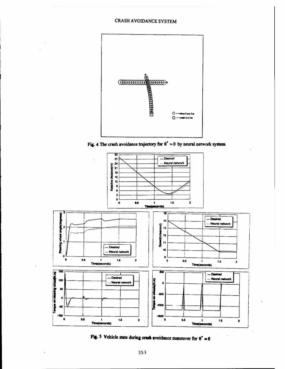
CRASH AVOIDANCE SYSTEM
Fig. 4 The crash avoidance trajectory for 9* =0 by neural network system
■ Desired
. Neural network
Flg. 5 Vehicle state during crash avoidance maneuver for 8* «0
353

C. T. CHEN, R. D. QUINN and R. E. RITZMANN
Fig. 6 The crash avoidance trajectory for untrained case 0* = 6x/5 by neural network system
39 36 33
E 30
I27 I 24 5 21
319 ee 9
e 3 o
! \ —uearea i
■— Neural network ] ~^— —^r 1 1
^ i
\ ! i
y y s
0.5 \S TimefMoand*)
Fig.7 Vehicle state during crash avoidance maneuver for untrained case 9* = 6% IS
354
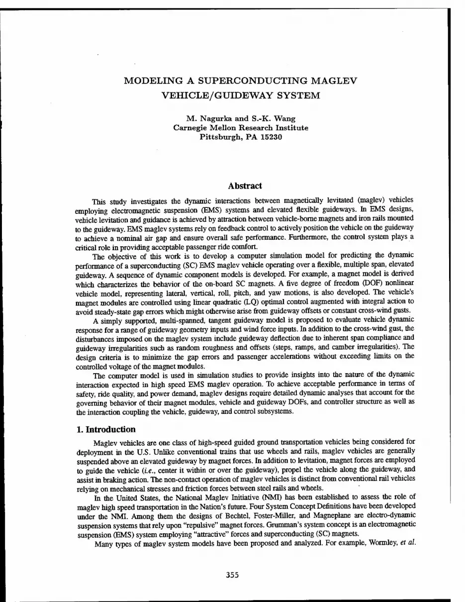
MODELING A SUPERCONDUCTING MAGLEV
VEHICLE/GUIDEWAY SYSTEM
M. Nagurka and S.-K. Wang Carnegie Mellon Research Institute
Pittsburgh, PA 15230
Abstract
This study investigates the dynamic interactions between magnetically levitated (maglev) vehicles employing electromagnetic suspension (EMS) systems and elevated flexible guideways. hi EMS designs, vehicle levitation and guidance is achieved by attraction between vehicle-bome magnets and iron rails mounted to the guideway. EMS maglev systems rely on feedback control to actively position the vehicle on the guideway to achieve a nominal air gap and ensure overall safe performance. Furthermore, the control system plays a critical role in providing acceptable passenger ride comfort.
The objective of this work is to develop a computer simulation model for predicting the dynamic performance of a superconducting (SC) EMS maglev vehicle operating over a flexible, multiple span, elevated guideway. A sequence of dynamic component models is developed. For example, a magnet model is derived which characterizes the behavior of the on-board SC magnets. A five degree of freedom (DOF) nonlinear vehicle model, representing lateral, vertical, roll, pitch, and yaw motions, is also developed. The vehicle's magnet modules are controlled using linear quadratic (LQ) optimal control augmented with integral action to avoid steady-state gap errors which might otherwise arise from guideway offsets or constant cross-wind gusts.
A simply supported, multi-spanned, tangent guideway model is proposed to evaluate vehicle dynamic response for a range of guideway geometry inputs and wind force inputs. In addition to the cross-wind gust, the disturbances imposed on the maglev system include guideway deflection due to inherent span compliance and guideway irregularities such as random roughness and offsets (steps, ramps, and camber irregularities). The design criteria is to minimize the gap errors and passenger accelerations without exceeding limits on the controlled voltage of the magnet modules.
The computer model is used in simulation studies to provide insights into the nature of the dynamic interaction expected in high speed EMS maglev operation. To achieve acceptable performance in terms of safety, ride quality, and power demand, maglev designs require detailed dynamic analyses that account for the governing behavior of their magnet modules, vehicle and guideway DOFs, and controller structure as well as the interaction coupling the vehicle, guideway, and control subsystems.
1. Introduction Maglev vehicles are one class of high-speed guided ground transportation vehicles being considered for
deployment in the U.S. Unlike conventional trains that use wheels and rails, maglev vehicles are generally suspended above an elevated guideway by magnet forces. In addition to levitation, magnet forces are employed to guide the vehicle (i.e., center it within or over the guideway), propel the vehicle along the guideway, and assist in braking action. The non-contact operation of maglev vehicles is distinct from conventional rail vehicles relying on mechanical stresses and friction forces between steel rails and wheels.
In the United States, the National Maglev Initiative (NMI) has been established to assess the role of maglev high speed transportation in the Nation's future. Four System Concept Definitions have been developed under the NMI. Among them the designs of Bechtel, Foster-Miller, and Magneplane are electro-dynamic suspension systems that rely upon "repulsive" magnet forces. Grumman's system concept is an electromagnetic suspension (EMS) system employing "attractive" forces and superconducting (SC) magnets.
Many types of maglev system models have been proposed and analyzed. For example, Wormley, et cd.
355

M. NAGURKA and S.-K. WANG
(1992) used simplified one-dimensional vehicle models for providing initial guidelines and overall directions for maglev design and development. Dynamic interactions between a maglev vehicle and a flexible guideway were studied in (Cai, et al, 1994) using a two DOF vehicle model. More sophisticated vehicle models were developed for maglev systems in (Daniels, et al, 1992) to evaluate vehicle/guideway interactions for various guideway structures. The vehicle/guideway interactions of a maglev system with a multi-car, multi-load vehicle were investigated in (Cai, et al, 1993).
An objective of this study is to develop a detailed mathematical model for evaluating-the dynamics of a SC EMS-type maglev vehicle with a combined lift and guidance system. The aim of the mathematical model is to simulate the maglev vehicle over a multi-span flexible guideway at full speed under the influence of guideway irregularities and aerodynamic loading. The overall system can be decomposed into four main components: vehicle model, magnet model, guideway model, and controller. The purpose of this paper is to describe detailed mathematical models of these subsystems.
2. System Models
2.1 Vehicle Model
In order to facilitate the development of the vehicle model, two coordinate systems, an inertial coordinate frame and a carbody coordinate frame, are first established. The carbody motion is then described by the translational and rotational transformations between these two coordinate systems. The carbody coordinate frame is fixed in the vehicle carbody with principal axes Xc, Yc, and ZQ and origin located at the vehicle center of gravity identified as CG. The inertial coordinate frame, XJYJZI, moves along the guideway longitudinal direction (i.e., Xj direction) at a constant vehicle speed, V^
The vehicle motion is characterized by the lateral and vertical displacements of the carbody CG and the roll, pitch, and yaw angles which describe the orientation of the carbody coordinate frame with respect to the inertial frame. The lateral and vertical displacements of the carbody CG are denoted by yc and zc, respectively. It is assumed that the carbody axes are initially aligned with the inertial reference axes. Then, the orientation of the carbody frame can be reached by successive rotations as follows: (i) a rotation y/c (yaw) about the Zc axis, (ii) a rotation 9C (pitch) about the resulting Yc axis, and (Hi) a rotation tj>c (roll) about the resulting Xc axis.
Amaglev vehicle model is developed based on the Grumman system concept (Proise, et al, 1993). Figure 1 shows the vehicle in its nominal position. There are Nm magnet modules on each side, inclined at angle ß from vertical. (Nm is an even number.) The magnets are arranged in such a way that the magnet forces pass through the longitudinal axis of the vehicle when the vehicle is in its nominal position. Each module contains several magnets controlled by the same power supply. The magnet force at each magnet module is assumed to be distributed uniformly along the module length, lm. The vehicle carbody is assumed to be rigid. The vehicle length and height are denoted by Ly and h^ respectively. Also shown in the figure are the nominal air gap, Ä0, and the height and width between the module and the carbody CG, denoted by hc and wc, respectively.
K- Nm magnet modules
i i ' i i
guideway
Figure 1. Grumman-Type Vehicle Configuration
356

MODELING A SUPERCONDUCTING MAGLEV VEHICLE/GUIDEWAY SYSTEM
f>
'2Nm ■trnri rri'rrw
^ Af„
l.t.M.t i^ 71 14 ,1 , t , t, f
rJV_+ 1
••/,
Top View
4Z,
9-
t ■ t ,t , T,t ,t Lt,t Lt,t tt Lt i ' i i i ' i i i ' i ' i i i ' i ' r-i-r
+ ZT
S-
i^TJ •Yi
Side View Front View
Figure 2. Free-Body Diagram of Vehicle Carbody
The free-body diagram of the vehicle carbody is shown in Figure 2. The vehicle is supported by magnet forces from the two rows of magnet modules. In addition to the magnet forces, the vehicle model described here may be disturbed by a cross-wind gust represented by an aerodynamic force, Fw in the lateral direction and an aerodynamic moment, Mw in the yaw direction. The vehicle model equations of motion can be written as
Fz-Mvg = Mvz
M. /A-(/,-7Pfflyfl,z
My = /A-(/z_/*)<öA Mz + Mw = Izäz-(Ix-Iy)coxC0y
<t>C = ^X+(^y<t>c+Ü)Z^9C yrc
ö„ = 0) -CO <t>
(1)
(2)
(3)
(4)
(5)
(6)
(7)
(8)
where Mv is the vehicle mass, g is the acceleration due to gravity, Ix, IT and Iz are the roll, pitch, and yaw moments of inertia of the vehicle, respectively, and ctXp a>y and az are the roll, pitch, and yaw angular velocities, respectively, in the carbody coordinate frame. Equations (1) and (2) are the translational equations of motion given by Newton's second law, where Fy and Fz are the total magnet force components in the lateral and vertical directions, respectively, applied to the carbody CG. Equations (3)-(5) are the rotational equations of motion from Euler's equations, where M^ My and Mz are the resultant roll, pitch, and yaw moments due to the magnet forces. Equations (6)-(8) are the angle-angular velocities relations which couple the vehicle angular velocities to the roll, pitch, and yaw angles, where small angles are assumed. The magnet forces, Fy and Fz, and the corresponding moments, Mx, My, and Mz, have been derived in (Wang, 1995).
2.2 SC Magnet Model
The proposed Grumman vehicle design contains forty-eight EMS-type SC magnets, twenty-four magnets on each side (Proise, et ed., 1993). In this study, the vehicle magnets are grouped into 2Nm magnet modules. All magnets in a module are controlled by a single power supply. The number of magnet modules is a design variable and can be specified based on the required dynamic performance.
357

M. NAGURKA and S.-K. WANG
(guideway longitudinal direction)
iron rail
f/2
NJ1 turns
R,
pathC
normal coil
f/2 ■ Am (face area).
NJ2 turns
Nsc turn
SCcoil
71 iron core
he
~=r U (controlled voltage)
Figure 3. SC Magnet Configuration
The SC magnet system, shown schematically in Figure 3, consists of a guideway iron rail, an iron-core magnet, a SC coil wrapped on the back leg of the iron core, and a set of normal coils, which are serially connected, attached to both pole ends of the iron core. N$c and Nn are the numbers of turns in the SC coil and the normal coils, respectively. The current in the SC coil, /5c, is provided by a constant current source, and the resulting magnet force provides the lifting capability to balance the total weight in static equilibrium. The trim current, i, in the normal coils is driven by a controlled voltage,«, to maintain the air gap, h, at its nominal value. The total magnet force provided by the magnet is/. The total resistance of the normal coils is denoted by Rc and the face area of each magnetic pole is denoted by Am.
By applying Ampere's law along path C in Figure 3 and using the law of conservation of energy for the magnetic energy stored in the air gap, the attractive magnet force at magnet module; can be represented as
fr VoA
4h: WsJsc + NJP ' J = l>->™„ (9)
where J/Q is the permeability of air, nm is the number of magnets in each magnet module, and hj and ij are the air gap and trim current at module;', respectively. From Kirchhoff 's voltage law, the trim current/voltage relation in magnet module; can be derived as
Uj = Rcij- PoAjfaij M N (N SCJSC + N i.)dh. " r J
2h. dt 2h: dt' j=l,...,2N„ (10)
In summary, the dynamics of the SC magnet model are described by the voltage equation (10) for each module and can be represented by 2Nm first-order ODEs. The resulting trim current and the constant SC current in each magnet module produce a magnetic flux which set up the attractive magnet force between the iron core and the iron rail. The magnet force at each module, described by Equation (9), is a nonlinear function of the trim current, SC current and air gap between the magnet and the rail.
2.3 Guideway Model
The guideway deviations at the magnet modules can be attributed to vehicle dynamic loading on the flexible guideway spans and to guideway geometry irregularities. The guideway model, developed here, relates the magnet force and the corresponding guideway deflection for each magnet module. A multi-span, elevated guideway is considered. Figure 4 shows the guideway configuration for a single span. The guideway span consists of the track slab which contains the iron rails and a box beam which is simply supported. The box beam selected in this study is the narrow, hollow-box beam (Phelan, 1993). A benefit of the narrow beam design for vehicles with inclined magnets is that it reduces the distance between the right- and left-side magnets and thus a smaller cant angle is allowed for providing levitation with a smaller magnet force.
358

MODELING A SUPERCONDUCTING MAGLEV VEHICLE/GUIDEWAY SYSTEM
track slab
h rail
wb
\
\ narrow box beam —*
Figure 4. Guideway Span Configuration
A Bernoulli-Euler beam with simply supported ends is assumed to model each guideway span. The equation of motion for a span can be expressed as
ox at (11)
where xs is the axial coordinate of the beam, t is time, El is the bending rigidity, c is the viscous damping coefficient, yis the mass per unit length of the beam, ws(xs, t) is the vertical deflection of the beam, and / (xs, t) is the loading force per unit length due to the moving vehicle acting on the beam. (The use of the superscript - denotes functional dependence on both space and time.)
To determine the solution of Equation (11), a modal analysis method is utilized in which the deflection of the beam is expressed as
w. (xs, t) = £ a-(t) sin (jitx/Ls) (12)
where aft) is the time-varying modal amplitude, Ls is the span length, sm(jnxJLs) is the mode shape of the simply supported beam, and ns is the number of mode shapes included in the solution. Substituting Equation (12) into Equation (11) and then multiplying by sia(kKxs/Ls) and integrating from jCy=0 to xs=Ls gives the resulting differential equation for the modal amplitude aft) as
c. .^ HJfJKY ,^ 2
s s 0
sm 'jnx ^
dx. (13)
with initial condition, a/(0)=a/0. for ;'=l,...,n5. From Equation (13), the circular frequency and the modal damping ratio can be identified as
.2 2 J ft
COj=2
'£/ Zj = 2ya. (14)-(15)
for;'= l,...,ns. The beam deflection can be determined by Equation (12) after solving Equation (13). The vehicle is assumed to negotiate a multi-span guideway as depicted in Figure 5. The vehicle/guideway
interaction is considered in the time interval [fy, tfl. At r=r0, the vehicle is completely located on Span I and just about to enter Span II. As time increases, the vehicle excites both Span I and Span II simultaneously. In this study, it is assumed that the vehicle length, L^ is less than the guideway span length, Ls. As a result, the vehicle is completely located on Span II at t=tf. For multi-span configurations, additional spans can be "daisy-chained" (i.e., at t=tf, the clock is reset to t=t0 and the same algorithm for the following span is applied).
The dynamic interaction between a moving vehicle and a flexible guideway has been studied intensively (e.g., Kortum and Wormley, 1981; Smith and Wormley, 1974). The process of deriving the vehicle/guideway
359
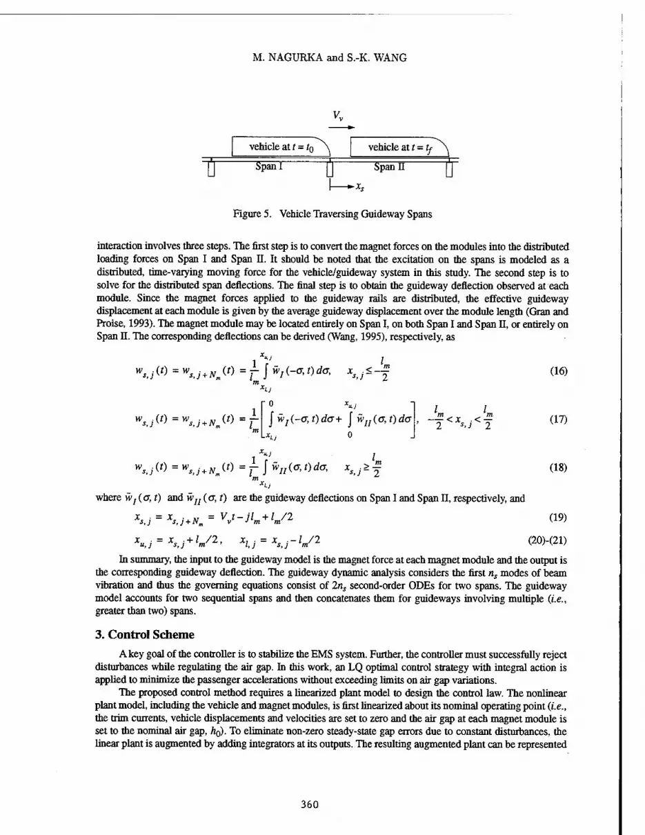
Tr
M. NAGURKA and S.-K. WANG
vehicle at t = t$ \ vehicle at t = t f Span I U TF SpanH
Figure 5. Vehicle Traversing Guideway Spans
interaction involves three steps. The first step is to convert the magnet forces on the modules into the distributed loading forces on Span I and Span II. It should be noted that the excitation on the spans is modeled as a distributed, time-varying moving force for the vebicle/guideway system in this study. The second step is to solve for the distributed span deflections. The final step is to obtain the guideway deflection observed at each module. Since the magnet forces applied to the guideway rails are distributed, the effective guideway displacement at each module is given by the average guideway displacement over the module length (Gran and Proise, 1993). The magnet module may be located entirely on Span I, on both Span I and Span II, or entirely on Span n. The corresponding deflections can be derived (Wang, 1995), respectively, as
w.
wsj(t)=wsJ+Na(t) = r
0
J Wj (-a, t)da+ \ WJJ (a, t) da
"■I.J
1 I -™<x .<J?
2 *>J 2
w rj('> = Ws,j + Nm^ = f J *Il(*»d« Xs,j*J
(16)
(17)
(18)
where w^a, t) and wu (a, t) are the guideway deflections on Span I and Span n, respectively, and
x . = x ■ „ = V t-jl +1/2 s, j s,j + Nm v -I'm m
x ■ = x +1/2, x, ■ = x -1/2 u,j s,j m ' l,j s,j m
(19)
(20M21)
hi summary, the input to the guideway model is the magnet force at each magnet module and the output is the corresponding guideway deflection. The guideway dynamic analysis considers the first ns modes of beam vibration and thus the governing equations consist of 2ns second-order ODEs for two spans. The guideway model accounts for two sequential spans and then concatenates them for guideways involving multiple (i.e., greater than two) spans.
3. Control Scheme
A key goal of the controller is to stabilize the EMS system. Further, the controller must successfully reject disturbances while regulating the air gap. hi this work, an LQ optimal control strategy with integral action is applied to minimize the passenger accelerations without exceeding limits on air gap variations.
The proposed control method requires a linearized plant model to design the control law. The nonlinear plant model, including the vehicle and magnet modules, is first linearized about its nominal operating point (i.e., the trim currents, vehicle displacements and velocities are set to zero and the air gap at each magnet module is set to the nominal air gap, AQ). To eliminate non-zero steady-state gap errors due to constant disturbances, the linear plant is augmented by adding integrators at its outputs. The resulting augmented plant can be represented
360

MODELING A SUPERCONDUCTING MAGLEV VEHICLE/GUIDEWAY SYSTEM
as (Wang, 1995)
x = Ax + Bu + Ev (22)
y = Cx + Dv (23)
where the augmented state vector, x, control vector, u, output vector y, and disturbance vector, v, can be identified as
x = [yc, zc, 0C, 6C, yc, (Ox, <ay, a>z, iv ..., i^, yn,..., v/(2Arj]
u= [uv...,uwf
y = {hx-h0,...,h1Nm-hQ]T
V = lygV ■ ■ •> yg (2NJ' ZgV ■■■'Zg (2Nm)' ygV —>fg (2Nm)' ZgV ■■■>Zg (2NJ' FW MJ
(24)
(25)
(26)
(27)
where y/y (/"= l,...,2N^) is the integral of the air gap error at module ;'. The LQ optimal control law results from the minimization of the performance index,
= j(xrQx + urRuJ<# (28)
subject to x = Ax + Bu. When applied to the augmented plant model the optimal control law can be shown to be
u = -R_1BrPx (0 (29)
where P is a unique, symmetric, semi-positive definite matrix solved from the algebraic Riccati equation
PA + ATP - PBR-1BrP + Q = O (30) provided system (A, B) is stabilizable and system (A, H), where HrH=Q, is detectable. In Equations (29) and (30), Q and R are two weighting matrices which can be adjusted to achieve desired closed-loop behavior.
4. Simulation Study The complete maglev system, consisting of the vehicle model, guideway model, SC magnet system, and
controller, is represented in the block diagram of Figure 6. The inputs to the overall system are the aerodynamic force and moment, Fw and Afw due to the cross-wind gust, and the irregularity, w^, due to the guideway. The
(Plant Model)
Magnet Modules
Guideway w
Vehicle
FWMW
Feedback Controller
: h
Figure 6. Block Diagram of Complete Maglev System
361

M. NAGURKA and S.-K. WANG
LATERAL GUIDEWAY IRREGULARITIES (RIGHT & LEFT RAILS)
| 0.5
!-0.5 -
.._
7 At ̂
'n/ 1
If- X^
A 1 \
v\\ /
i i i i i " right rail
left rail ~i
§4
E 2
S- 0 O
10 20 30 40 50 60 70 80 90 Distance (m)
VERTICAL GUIDEWAY IRREGULARITIES (RIGHT & LEFT RAILS) !
right rail - - left rail
;rrr r<p V; ^C^ry^
i
- X
i i i 0 10 20 30 40 50 60 70 80
Distance (m)
Figure 7. Combined Guideway Irregularities
90
outputs of the system are the air gap, h, and the vehicle state, xv In the simulation model, the cross-wind gust is assumed to be a wind profile perpendicular to the guideway with constant velocity. As the vehicle enters the wind zone, the vehicle responds to a sharp discontinuity, such as might occur when the vehicle exits a tunnel. Four types of irregularity characteristics for an elevated guideway have been modeled, including surface roughness, step, ramp, and camber. The simulation model accepts any combination of these guideway irregularities. Since these irregularities result from a wide variety of effects including construction practice and environmental conditions, it is assumed that the amplitudes of each type of irregularity (except for the surface roughness which is described by a power spectral density function) are normally distributed random numbers. With prescribed mean values and standard deviations, the guideway irregularities may represent the tolerance requirements of the guideway structure.
A number of safety-, power- and comfort-related performance measures can be identified for the maglev system developed in this work. The maglev system is required to (0 maintain each magnet module/iron rail air gap between 30 mm and 50 mm (i.e., 40 mm nominal gap with ±10 mm maximum gap error), (ii) ensure that the control voltages are within a feasible limit of ±300 V, and (Hi) maximize ride comfort where the ride comfort is measured by comparing carbody accelerations at the car front and rear to the ISO ride quality criteria (ISO, 1978).
In the simulation study, the maglev vehicle was simulated at 500 kph on a 4-span flexible guideway with combined guideway irregularity, consisting of guideway roughness, step, ramp, and camber geometry errors, as shown in Figure 7. The guideway random roughness is described by the power spectral density, ä>(Q)=A,Ä22, with a roughness parameter, Ar=6.1xl0-8 m, representing a high quality welded rail. The step deviation, column height, and camber amplitude for each span are generated randomly with a zero mean and a 2 mm standard deviation. We assume no aerodynamic loading in this simulation case. The parameter values for the vehicle model, SC magnet model, and guideway model are summarized in Tables 1,2, and 3, respectively. The weighting matrices Q and R used to determine the controller parameters are selected as
= diag(^ •2
■^max''
-2
.-2 _-2 -2 -2 -2 -2 -2 -2 0 ,8 ,W ,V ,Z , CO , (0 , CO rmax' max' ~max'-'max' max' x,max' y,max' z,max'
l.max' •"' l2N„, max' ■yn, -2
•'>'/(2JVm),max
= &*{%« 2Nm, max . U
(31)
(32)
where the estimated limits in Q and R are listed in Table 4.
362

MODELING A SUPERCONDUCTING MAGLEV VEHICLE/GUIDEWAY SYSTEM
Table 1. Parameters of Vehicle Model
Parameter Symbol Value Unit
vehicle mass Mv 30,600 kg
vehicle length Lv 18 m
vehicle height K 3.9 m
vehicle width wv 3.8 m
nominal air gap ho 0.04 m
height, magnet centroid to vehicle CG hc 1.09 m
width, magnet centroid to vehicle CG wc 0.76 m
roll moment of inertia Ix 7.4xl04 kg-m2
pitch moment of inertia h 8.0xl05 kg-m2
yaw moment of inertia h 9.6X10⁵ kg-m2
magnet cant angle ß 35 deg
number of modules on each side Nm 2 None
number of magnets in each module nm 12 None
Table 2. Parameters of SC Magnet Model
Parameter Symbol Value Unit
number of turns in SC coil NSc 1020 None
number of turns in normal coils Nn 96 None
face area of each magnetic pole "■m 0.04 m
total resistance of normal coils Re 1.0 ohm
permeability of air rt> 47CX10-7 weber/A-m
Table 3. Parameters of Guideway Model
Parameter Symbol Value Unit
narrow box beam width Wb 1.2 m
narrow box beam height h 1.8 m
span length h 21.3 m
span mass per unit length r 4777 kg-m2
bending rigidity EI 1.84xl010 N-m2
first-mode span damping ratio f 0.03 None
363

M. NAGURKA and S.-K. WANG
Table 4. Estimated Limits in Weighting Matrices
Parameters Value Unit
"max' max 0.01 m
rmax' max' rmax 0.01 rad
"max' max 1.0 m/s
(0 , Ö) ,6) x, max' y, max' z, max 1.0 rad/s
V.max <fcl,~WJ 300 A
)W (P1.-.2AW 0.001 m-s
";,max (pl,...,2WJ 300 V
The magnet input voltages at each module are shown in Figure 8. The peak voltage is -49.8 V at module 3 which is substantially less than the limit of -300 V. Figure 9 shows that all the air gap deviations are below the allowable 10 mm safety margin. Figures 10 and 11 depict the vehicle accelerations for the car front and car rear in the lateral and vertical directions, respectively. To evaluate ride comfort, the reduced comfort boundaries of the ISO one hour ride quality criterion are also shown. The results indicate that both the lateral and vertical acceleration levels are below the ISO criterion.
In summary, this simulation study evaluates the maglev system performance under disturbances including guideway flexibility and guideway irregularity. The behavior of the maglev system when exposed to combined disturbances can be determined. For the case studied, the simulation results indicate that the requirements on the air gap safety margin, the control voltage limit, and the ride quality can be satisfied.
5. Conclusions This paper describes a nonlinear simulation model that was developed to represent the governing behavior
of a SC EMS maglev vehicle with a combined lift and guidance system. The simulation model predicts vehicle behaviors under the influence of guideway flexibility, guideway irregularities, and cross-wind gust An example simulation case of a high-speed vehicle on a guideway with flexibility and a combination of guideway irregularities demonstrates the effectiveness of the LQ optimal controller in satisfying the desired performance specifications.
_ 40
a 20
1 ° 1-20 « S-40
-60
(0
I o ■5 £-20
,-40
-60
MAGNET INPUT VOLTAGE FOR RIGHT-SIDE MODULES
• A ../../.A. - - / \ y >'■ Y^- / ~^7: ; v s \ v '/: \L^> "*:
\ / ^ ' | module 1
\ / ■""''
\Jy ■ ! , : i
0.1 0.2 0.S 0.3 0.4 Time (sec)
MAGNET INPUT VOLTAGE FOR LEFT-SIDE MODULES
0.6 0.7
V--': ^T/ '_
V \
. V :..,\ \ : N
\ ■ - ^/
/ '. —v
module 3 — module 4
] i i i
0.1 0.2 0.3 0.5 0.6 0.7 Time (sec)
Figure 8. Magnet Input Voltages
364
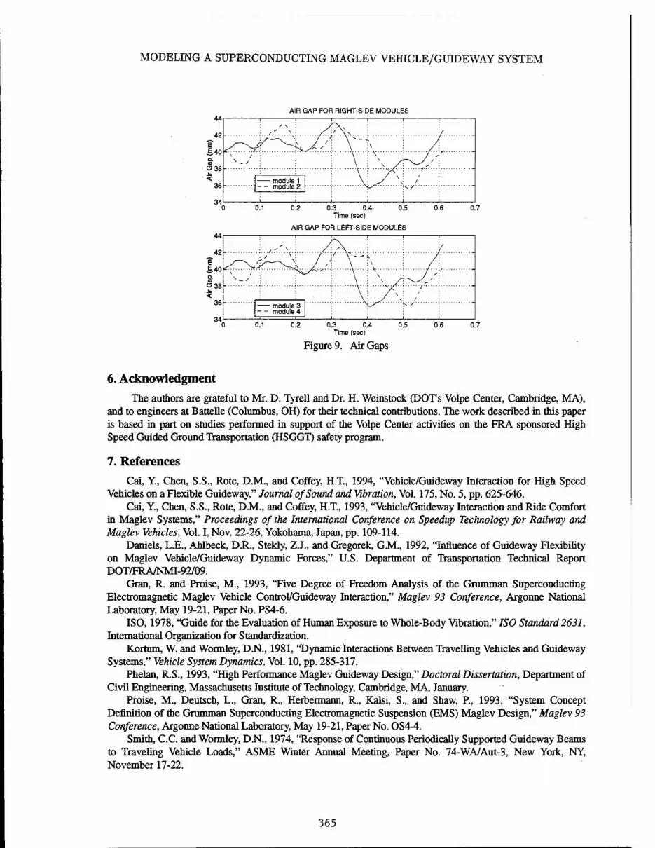
MODELING A SUPERCONDUCTING MAGLEV VEHICLE/GUIDEWAY SYSTEM
AIR GAP FOR RIGHT-SIDE MODULES
0.1 0.3 0.4 Time (sec)
AIR GAP FOR LEFT-SIDE MODULES
0.7
Figure 9. Air Gaps
6. Acknowledgment The authors are grateful to Mr. D. Tyrell and Dr. H. Weinstock (DOTs Volpe Center, Cambridge, MA),
and to engineers at Battelle (Columbus, OH) for their technical contributions. The work described in this paper is based in part on studies performed in support of the Volpe Center activities on the FRA sponsored High Speed Guided Ground Transportation (HSGGT) safety program.
7. References Cai, Y., Chen, S.S., Rote, D.M., and Coffey, H.T., 1994, "Vehicle/Guideway Interaction for High Speed
Vehicles on a Flexible Guideway," Journal of Sound and Vibration, Vol. 175, No. 5, pp. 625-646. Cai, Y, Chen, S.S., Rote, D.M., and Coffey, H.T., 1993, "Vehicle/Guideway Interaction and Ride Comfort
in Maglev Systems," Proceedings of the International Conference on Speedup Technology for Railway and Maglev Vehicles, Vol. I, Nov. 22-26, Yokohama, Japan, pp. 109-114.
Daniels, L.E., Ahlbeck, D.R., Stekly, Z.J., and Gregorek G.M., 1992, "Influence of Guideway Flexibility on Maglev Vehicle/Guideway Dynamic Forces," U.S. Department of Transportation Technical Report DOT/FRA/NMI-92/09.
Gran, R. and Proise, M., 1993, "Five Degree of Freedom Analysis of the Grumman Superconducting Electromagnetic Maglev Vehicle Control/Guideway Interaction," Maglev 93 Conference, Argonne National Laboratory, May 19-21, Paper No. PS4-6.
ISO, 1978, "Guide for the Evaluation of Human Exposure to Whole-Body Vibration," ISO Standard 2631, International Organization for Standardization.
Kortum, W. and Wormley, D.N., 1981, "Dynamic Interactions Between Travelling Vehicles and Guideway Systems," Vehicle System Dynamics, Vol. 10, pp. 285-317.
Phelan, R.S., 1993, "High Performance Maglev Guideway Design," Doctoral Dissertation, Department of Civil Engineering, Massachusetts Institute of Technology, Cambridge, MA, January.
Proise, M., Deutsch, L., Gran, R., Herbermann, R., Kalsi, S., and Shaw, P., 1993, "System Concept Definition of the Grumman Superconducting Electromagnetic Suspension (EMS) Maglev Design," Maglev 93 Conference, Argonne National Laboratory, May 19-21, Paper No. OS4-4.
Smith, C.C. and Wormley, D.N., 1974, "Response of Continuous Periodically Supported Guideway Beams to Traveling Vehicle Loads," ASME Winter Annual Meeting, Paper No. 74-WA/Aut-3, New York, NY, November 17-22.
365

M. NAGURKA and S.-K. WANG
Wang, S.-K., 1995, "Levitation and Guidance of a Maglev Vehicle Using Optimal Preview Control," Doctoral Dissertation, Department of Mechanical Engineering, Carnegie Mellon University, Pittsburgh, PA, May.
Wormley, D.N., Thornton, RX>., Yu, S.-H., and Cheng, S., 1992, "Interactions Between Magnetically Levitated Vehicles and Elevated Guideway Structures," U.S. Department of Transportation Technical Report DOT/FRA/NMI-92/23.
LATERAL ACCELERATION (with 1 Hr ISO)
10" 10' Frequency (Hz)
10'
Figure 10. Lateral RMS Accelerations
VERTICAL ACCELERATION (with 1 Hr ISO)
10" 10' Frequency (Hz)
10'
Figure 11. Vertical RMS Accelerations
366

ADVANCES IN ACTIVE VIBRATION ISOLATION TECHNOLOGY
D. C. Hyland* and D. J. Phillips** Harris Corporation GASD Melbourne, FL 32902-9400
Abstract
Operation of microgravity, space-station attached payloads and protection of sensitive equipment aboard multi-sensor platforms requires active vibration isolation technology. In response to these needs, the Active Isolation Fitting (AIF) was developed to replace passive mechanical end fittings and joints in truss structures. The AIF combines intrastructural and inertial devices to cancel vibration transmission into a vibration-sensitive subsystem. This paper discusses the AIF principles of operation, details its robust performance characteristics and reviews the extensive experimental results that have been accumulated over the past several years. Test results show 20 to 30 dB of broadband isolation tor both single AIF tests and six degree-of-freedom isolation systems demonstrated on two major, Government-supplied testbeds.
1. Introduction
One of the most pressing needs in all applications of vibration control is the refinement of self- contained, modular vibration suppression hardware. A key component in any overall vibration suppression strategy is the technology to either isolate sensitive equipment from a vibrating structure or to isolate structure from a source of disturbances. Moreover, the vibration isolation strategy lends itself well to self- contained, modular hardware solutions. This was the inspiration for the invention of the Harris Active Isolation Fitting (AIF) that is described in this paper.
To understand why the active control approach was taken, Figure 1 illustrates the distinction between intrastnictual damping approaches to isolation and active isolation. We concentrate on the simplest case in which it is desired to modify a uniaxial member connecting a base body (wherein vibration disturbances originate) to an isolated body so as to reduce the isolated body's vibration. The intrastructural approach (left hand side of Figure 1), essentially inserts a damper between the two bodies so as the dissipate energy. This can be implemented passively (e.g., viscoelastic material treatment, fluid dampers, etc.) or actively (e.g., a piezoelectric actuator with collocated strain sensor closing a strain rate feedback loop). In any case, because the isolator member not only damps but also transmits vibrational energy, it is possible to reduce the resonance peaks of the isolated body response but not to appreciably reduce the broadband, nonresonant response (see PSD sketch on lower left of Figure 1). This results in significant performance limitations.
In contrast (see the right side of Figure 1), an active approach, perhaps combining inertial sensing with mtrastructual actuation, has the potential to prevent vibration transmission into the isolated body. As indicated in the lower right of Figure 1, the effect on the isolated body is equivalent to reducing the overall disturbance input Thus, both resonant and nonresonant response can be suppressed over a broad frequency band.
To fully realize the potential of active isolation, we conducted a multi-year search for a self- contained, modular device that:
1. interfaces cleanly with existing structure and, itself, has structural functionality - i.e. can be used to replace passive struts and end fittings in truss structures
2. provides high levels of vibration isolation while retaining high mechanical stiffness at low frequency (so that a sensor, for example, can be tightly coupled to a spacecraft bus for precision pointing while being isolated from bus-generated vibration)
* Senior Scientist ** Staff Engineer
367

D.C. HYLAND AND DJ. PHILLIPS
liitrnstructural Damping (active or passive)
Active Isolation
Isolated Body
Damper attenuates
vibration, does not
prevent its transmission
Isolated Body
HWPf
WKSsmmfKm IT
_K , Active Isolator Strut
• Mix of inertial and intrastructural devices
• Synergy of active and passive approaches
v\ • Cancels vibration transmission (as well as damps)
v2 PSD Resonance peaks squashed
Peaks squashed and overall level
reduced
10-20 dB rms attenuation 30-40 dB rms attenuation
Figure 1 Both Resonant and Nonresonant Response is Suppressed Using Active Isolation
3. uses, local, nonadaptive control systems to provide reliable isolation without requiring a detailed design knowledge of the dynamics of the remainder of the system
4. reverts to a stiff, passive structural component upon failure or disengagement of the active elements
5. involves low power, inexpensive components without need for exotic hardware or materials
6. can provide the basic building block from which increasingly complex active isolation structures can be built up in a transparent way
Over the past four years, our research efforts performed an exhaustive search for the correct sensor and actuator types and the appropriate control architecture to meet the above requirements. The finally accepted Active Isolation Fitting (AIF) design is an active uniaxial connector device for vibration cancellation that replaces passive mechanical end fittings and joints in structures. The device is low power, consists of inexpensive components and fails gracefully by reverting to a stiff mechanical member when active components are disabled.
Section 2 describes the underlying principles of AIF operation and elaborates its robust performance characteristics. These are corroborated by numerous experimental results. Data obtained in uniaxial tests are discussed in Section 3. The AIF is the basic module of our isolation technology, from which more complex multi-degree-of-freedom systems can be built up. Section 4 reviews experimental results for six degree-of-freedom isolation systems composed of six independent AEF modules.
2. Principles of Operation and Robustness Properties
Figure 2 shows the essential mechanical and control aspects of the AIF design. This is a uniaxial connector device having an intrastructural actuator (a piezoelectric stack is the preferred embodiment but other types of prime-movers can be utilized, depending on stroke and bandwidth requirements) and two high bandwidth accelerometers, one near each end. The control strategy involves the interplay of two nonadaptive control loops. The "inboard loop" involves the base-body-end accelerometer and the piezo
368

ADVANCES IN ACTIVE VIBRATION ISOLATION TECHNOLOGY
Isolated Payload
Payload . ^ Interface \^Z j\s^
Top Accelerometer
Accelerometer
Base Interface
AIF Commands Piezo to Generate a Force Opposing the Position Changes of the
Payload
AIF Commands Piezo to Accomodate Motion
of Bast-
Vibrating Base
Figure 2 Active Isolation Fitting (AIF) Principle of Operation
stack and provides feedforward cancellation of incoming disturbances. The "outboard loop" uses the isolated-body-end accelerometer and the piezo stack to inertially stabilize the isolated-body or payload end of the fitting. These two loops work synergistically to achieve high performance isolation.
With the conventions shown in Figure 3 we can give a simple result that sheds some light on the robustness properties of the AIF control design. Here xl and x2 sat the displacements of the inboard and outboard substructures, respectively, along the AIF axis at the two attachment points. These quantities are modelled in the frequency domain as:
*, =tf (*2/+2ThOi'+Oi)'1 (♦, /+♦,*■) (1)
x2 =<£(*2'+2TI2Q2J + Q^)"
1 4>2(-/)
where fy eIRN\§2 eIRNl and(|>d are modal influence coefficient vectors and T)k,Qk(k = l,2) are nonnegative diagonal matrices containing, respectively the modal damping coefficients and modal frequencies. We assume:
Qi>0, a.
b.
c.
ß2+e<t>2<l>I>0V€>0
T|„T12>0
An idealized form of the AIF constitutive relation is: . f = K{x2-Xl-KvV)
K = mechanical stiffness > 0
KV > 0 is the voltage/strain constant of the actuator
V = drive voltage to the piezo actuator
(2)
(3)
369

D.C. HYLAND AND D.J. PHILLIPS
F= External Disturbances
Figure 3 Basic Nomenclature and Kinematic Conventions for AIF Analysis
The actuator drive from the combined inboard and outboard loops takes the form: V = -GI4-LI(s)al-G04-L0(s)a0 (4)
Go>0,G,e[0,l) where a, and a0 are the outputs of the inboard and outboard accelerometers, respectively and
Lj (s) and L0 (s) are rational, stable and proper compensation filters.
Preparatory to the proof of the following result, recall that a square transfer function G(s) is
positive real [1] if 1) all poles of G(s) are either in the closed left half plane or, if on the imaginary axis,
they are simple with positive semi-definite residue matrix and 2) G(s) + G (s) is nonnegative definite for
all Re[.s]>0. Here GH denotes the complex conjugate transpose. If, in addition to the above,
G(lO)) + GH(iCd) is positive definite for real 0), G(s) is strictly positive real [2-4]. The interconnection, through a unity feedback configuration, of a strictly positive real plant and a positive real controller is stable [2].
The following result illustrates the consequences when L; and L0 can be so chosen as to render
Lj dj, and L0 a0 ideal estimates of the displacements xl and x2, respectively.
370

ADVANCES IN ACTIVE VIBRATION ISOLATION TECHNOLOGY
Proposition: With the above assumptions and for all §keIR '(k = l,2) and for all values of
T[k,Qk(k = 1,2), G0 and G, subject to the restrictions in (2) and (4), if: L,a,=xv L0a0=x2 (5)
then the closed-loop system (1) - (4) is stable. Proof. Defining y - xx, system (1), (3) and (4) can be written in the form:
y = -^{sA-l%u + s^A-ll^F <6>
u = K{l-G1)^[l-K{l + G0)^2A-2l^2]yAG(s)y
where A, A s2I+2TI1£V+£2I (7)
A2 A s2/+2T|2 Q2* + fi^ + tf (l + G0 )<t>2 <|>2
Because of (2. a, d), the plant, §J (s AJ"1 )((>, is obviously strictly positive real. Also, the controller transfer
function G(s) has all its poles in the closed left half plane with the exception of a simple pole at the origin with positive residue. Moreover,
G(/co) + G*(ico) = AK2(l - G,) (l + G0) <£ A"1 TI2 Q2 A2'" <>2
>0 Hence G is positive real. Being the interconnection of a strictly positive real plant and positive real controller, system (6) is stable. D
Note that x2 is given by:
x2=^2[s2I+2r\2Cl2s + Q22+K{l + G0)^2^]~1 Kil-Gj) ^Xl
(8)
Evident from this expression is that the outboard loop augments the stiffness of substructure 2. Thus the function of the outboard loop is to stabilize the isolated structure relative to inertia! space. In place of position feedback, it is also possible to feed back rate, x2, in the outboard loop. In this case much the same stability results are achieved except that the damping of substructure 2 is augmented. Ideally, after calibration and measurement of the constants A" and Kv, it is desirable to set Gt = 1. In this case, as (8) shows, substructure 2 is entirely decoupled from substructure 1. Thus the inboard loop is a feedforward controller that serves to cancel the outward propagating disturbances, jl — C^y [ establishes the degree to
which x2 is reduced relative to the open-loop (G7 = o). Of course, the idealized position estimate conditions (5) can only be approximately realized over a
finite frequency band because of (1) accelerometer dynamics, (2) high frequency dynamics of the piezoelectric stack actuator (3) the use of realizable low pass filters to form position estimates from accelerometer estimates and (4) the desire to reduce the gains G, Lt{s) and G0 L0(s)lo negligible levels (via high pass filters) below a lower cutoff frequency, Q.L, below which high stiffness, but not isolation, are desired. The last item is actually a design requirement to ensure that the ATF behaves as a stiff, passive structural component at low frequency. The gains L, and L0 contain low-pass and lead-lag elements that compensate for all of the above nonidealities so as to recover the above robustness properties within the desired isolation frequency band. These compensator designs depend only upon dynamic characteristics intrinsic to the AIF device itself and not on the adjoining substructures. Thus, the inherently stable AIF design needs no special "tuning" to adjust to the detailed dynamic characteristics of the base-or isolated bodies.
As a corollary to Proposition 1, we note that because of the combinatorial properties of positive real systems, similar robustness can be deduced for systems involving several ATF units connecting the two substructures. In general, stability and performance of one ATF are not sensitive to the presence of other AIFs in the system, so that more complex isolators can be readily built up from independent AIF units.
371

D.C. HYLAND AND D.J. PHILLIPS
3. Uniaxial Test Results
From the outset of AIF development down to the present, individual AIF units were evaluated for further integration by use of the uniaxial test stand shown in Figure 4. The AIF unit being tested connects one of several different types of isolated body with the base plate. Disturbances are injected into the system by a proof-mass actuator mounted under the base plate. Isolated bodies that are typically used are either a rigid mass or star shaped body (shown in Figure 4) with complex modal dynamics in the frequency band of interest Both sine sweep and random disturbances are injected. Data from accelerometers mounted on the isolated body is used to obtain frequency response functions (FRFs) from the disturbance input to isolated body displacement AIF performance is characterized by comparison of the magnitudes of the closed-versus open-loop FRFs.
Figure 5 shows such a comparison for both a rigid mass and the star-shaped flexible body. For both cases, we show the magnitude of the shaker disturbance input to isolated body position transfer functions for open- and closed-loop operation. 10 to 35 dB attenuation is obtained over 10 to 100 Hz. These results also illustrate that performance is not sensitive to the dynamic characteristics of the isolated body.
Furthermore the AIF design can be adapted to a variety of applications. For example Figure 6 shows uniaxial test results for a higher bandwidth design. This design achieves 30 dB nns vibration reduction over the 10 to 200 Hz frequency band. Finally, even more impressive isolation results can be achieved by stacking AIFs into multi-stage isolators. Test results for a two-stage configuration are shown in Figure 7. This configuration attains 42 dB nns attenuation over the 10 to 200 Hz band. We should again note that all of the above isolation results are obtained without reducing the static mechanical stiffness of the AIF.
4. Multi Degree-of-Freedom Isolation System Test Results
The AIF can be packaged to serve as an end fitting or joint in truss structures. Several basic AIF modules (each, as in Figure 2, being uniaxial) are combined to carry out more complex isolation tasks. For example, multi-degree-of-freedom isolators are built of several AIFs and passive strut members. The simplest such assembly is a six-member (hexapod) mount which provides six degrees of freedom (d.o.f.) isolation for sensitive equipment mounted outboard.
Since its original conception on the Defense Meteorological Satellite Vibration Damping Study conducted by Harris for Phillips Lab in 1992,6 d.o.f. isolators of various sizes have been built and tested on in-house and Government-supplied test facilities.
For example, as part of a Cooperative Technology Development Agreement with NASA/LaRC, Harris fabricated a 6 d.oi. unit and in February 1994, installed and tested it on the NASA/LaRC CEM Phase 3 spacecraft control testbed. As Figure 8 illustrates, the 6 d.o.f. assembly replaced the instrument support truss, connecting the gimballed sensor package with the main CEM structure. Test results illustrated in the right-hand portion of Figure 8 show excellent broadband isolation performance. Details are reported in [5],
To-date, the most challenging tests of AIF capabilities occurred on the ACTs program. The ACTS structural control testbed, Figure 9, is one of the most complex and traceable in existence. Disturbances injected at the base have constant PSDs from 10 to 200 Hz. Stringent performance requirements are levied on line-of-sight (LOS) errors, defocus errors and wavefront errors. In all, the response of over 150 modes must be attenuated by 20 to 40 dB in order to meet these requirements. Six AIFs were mounted as end fittings on each of the six struts supporting the structure on the experiment base. Test data (Figures 10.a, b, c) shows over 40 dB attenuation of the modes principally contributing to LOS error, nearly 50 dB peak attenuation of defocus and nearly 40 dB peak attenuation of wavefront error, rms attenuation of LOS, defocus and wavefront errors over the entire 10 to 200 Hz disturbance band are over 20 dB, 30 dB and 20 dB, respectively.
The above test results are but a sample of the 6 d.oi. isolator experimental findings obtained to-date on ground-based facilities. Isolator performance has been determined to be insensitive to the gravity vector. Moreover, these 6 D.OF. isolation trusses are composed of six AIFs operating independently — for isolation, global multivariable control is not needed. For isolation combined with precision pointing, a pointing controller is readily incorporated in order to coordinate the several AIFs using isolated body attitude information.
372
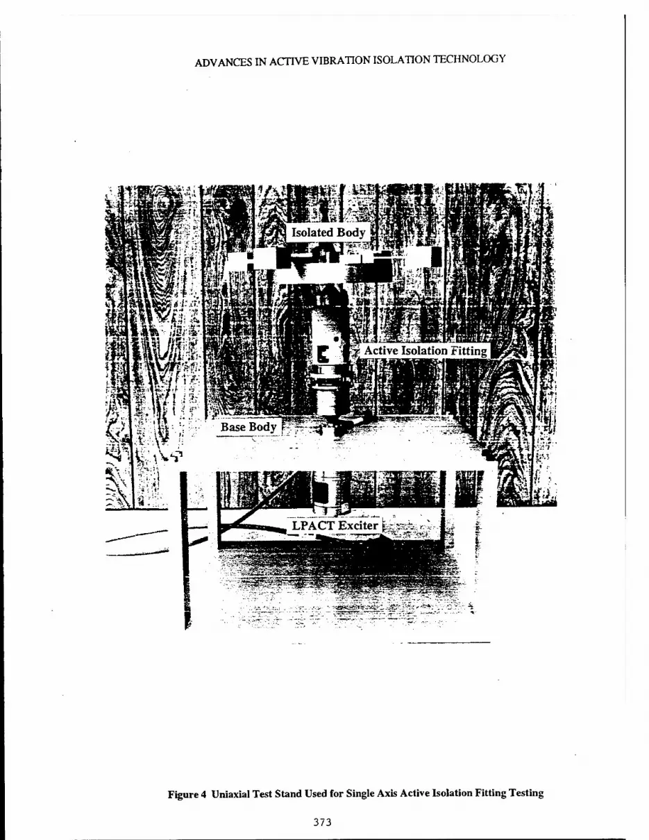
ADVANCES IN ACTIVE VIBRATION ISOLATION TECHNOLOGY
Figure 4 Uniaxial Test Stand Used for Single Axis Active Isolation Fitting Testing
373

Rigid Mass Test Body:
D.C. HYLAND AND DJ. PHILLIPS
mass isolation: open vs closed loop (#1)
~ -10 as ■D
I -15 .£
Urn V
1 -20:
"3
f -25 E.
f -30-
-35
-40 10' 10:
frequency (Hz)
Star-Shaped Flexible Body:
iS
•i o
o D.
0
-5
-10
-15
-20
-25
-30
-35
-40
-45 10»
star isolation: open vs closed loop (#1)
: : : i
\ ..-''"' " i™'"' * T\--'''"*S~-*'''i\/" *» » *
frequency (Hz) 10^
No Isolation Isolator Loops Closed
Overall disturbance input is reduced. 10-35 dB attenuation shown in these test results over broad frequency band. Performance not sensitive to dynamic characteristics (flexibility of isolated body).
Figure 5 Broadband Isolation Capabilities of the AIF are Demonstrated by Uniaxial Test Results
374

ADVANCES IN ACTIVE VIBRATION ISOLATION TECHNOLOGY
Active Fining: One DOF Test Stand: OL & CL: Top & Bottora FB
C3
s C
C 10-2!
10-3
10-4
■— | ^/».vz-v-i-» I • v„v7 » j : :.\x::: t::::!:::::^::^::::^:!-;::^:::::::::::;^: h£\ ; f\- '** riif * ■ ? ■ Äiijf: ^igi v:::::::::::;:Kä:::::::::::i:*.*r's^""";:::":::::::::::"::::::?,::X!^»>;w-J.*.S:::iS
■■RMSJCL/RMSIÖL!="-'iö'dB"
J 3
50 100 150
Frequency (Hz)
200 250
Figure 6 Active Fitting: One DOF Test Stand Isolation Results for a High Bandwidth IVsign
Single DOF Test Stand: Two Stacked Fittings: OL & CL
s o
o D. O
102
10»
10°
10-'
10-2
10-J
10-4
10-5 50 200 250 100 150
Frequency (Hz)
Figure 7 Single DOF Test Stand: Two Stacked Fittings, Open-Versus Closed-Loop Performance
375

D.C. HYLAND AND D.J. PHILLIPS
VAM
•Random disturbances at SWIR and CERES
•Responses measured at MISR boresight
-Closed-Loop - Open-Loop
MSIR Instrument
32 48
Frequency ft+z)
Figure 8 An AD? 6 d.o.f. Isolation System (called the Vibration Attenuation Module, VAM) was Successfully Demonstrated on EOS-AM 1 Laboratory Testbed
Large. Representative Testbed 3 Year Program Started December 1991 Disturbance PSD's Basically Flat Over 10-200 Hz Band Over 150 Modes In Disturbance BandMust Be Suppressed Both LPACTs and AIFs Used
vimii&ujuiumnmim wi."
■-&-£ o IB
24 LPACTs Installed on Payload Provide High Bandwidth Damping
Six AIFs Tnstwllrd in Support Truss Mem- bers Provide High Bandwidth Isolation From Base Disturbances
Tzr Tzr
Figure 9 The ACTS Testbed was Used to Demonstrate Six Degree-of-Freedom A1F Isolation Performance
376

10%
ADVANCES IN ACTIVE VIBRATION ISOLATION TECHNOLOGY
Controller STM7 0 Ro Results
10'
10"
c
\
:$:;•• ...ty.... ...r...
üiif::;: :J:I:::: v-i ••••
U-.-.i-.:::
:itj:::::::::::::|: :J:V::::::::::J:C:
•»•*
!!!!!l!rtl!!J!!!!!Jiimii!!! ::::R::S::j::^^;:::|:
<L:::::::4y::l ipiii!!jitai»3;S$i!
;:::§:::
frequency (Hz)
Figure 10.a AIF's Dramatically Reduced Line-of-Sight Jitter on the ACTS Testbed
Controller STM7 D Ro Results 10
10"- ::::open:to<jRTms=:a.T.5Si:::::::::::::;:::: ... .closed loop rms = 0.005668 : * :!!!!röSreyüc:fiböl«28iStldB!!l:::!:!::3!!J:
10"
N -4
I1 < C
<o 10 a V) 3
|io- ■D
10
10"
10"
.u.U.
:j::i:::::=!::¥::::::»:::*i!::f
:!::::::S:?::S:::S ||!!!^!!!!!!M!|!!P|!!!!
i^jimiimiijliilliumm
10' frequency (Hz)
10*
Figure lO.b ADJ's Reduced ACTS Defocus Errors by Nearly 30 dB rms Over the Entire 10-200 Hz Disturbance Band
377

10° .
D.C. HYLAND AND DJ. PHILLIPS
Controller STM7 D Ro Results
10
5 f
i
1 »pert loop:rros:=0:8912::•::::: ::::■::::::::::: closed-looprms = 0.07917 ?■*{"':
HI n: Tim. : :•••!:■
: I I : M...
:i:» 1 :fc::
:£::::y::\-::«::::**£:::5:S""St^Fl
^.^ = : = ::««::A:::k::J:V^=::l •-■•»'1:1:::
frequency (Hz)
Figure 10.c ACTS Surface Errors were Reduced by More than 20 dB rms Over the 10-200 Hz Band
5. Concluding Remarks
This paper has described a compact, modular active isolation device, the Active Isolation Fitting (AIF), that combines intiastructural actuation with inertial sensing to cancel vibration transmission into vibration-sensitive subsystems. While providing high levels of vibration isolation, the device retains high mechanical stiffness at low frequencies and fails gracefully by reverting to a stiff mechanical member when active components are disabled. Predicated robustness properties indicate that performance is insensitive to the detailed dynamic properties of the base body or isolated body-either or both may be highly resonant structures with vibration modes in the isolation band. Moreover, the same properties suggest that several independent AIF modules may be robustly combined to carry out more complex, multi-degree-of-freedom isolation tasks. These features together with the predicated high levels of isolation have been abundantly confirmed by numerous single axis and six degree-of-freedom isolation experiments involving both in-house and Government-supplied structural control testbeds.
6. References
1. Anderson, B.D.O., and Vongpanitlerd, S., Network Analysis and Synthesis: A Modern Systems Theory Approach, Prentice-Hall, Englewood Cliffs, NJ, 1973.
2. Benhabib, R.M., Iwens, R.P., and Jackson, R.L., "Stability of Large Space Structure Control Systems Using Positivity Concepts," Journal of Guidance and Control, Vol. 4,1981, pp. 487—494.
3. Lozano-Leal, R, and Joshi, S., "Strictly Positive Real Transfer Functions Revisited," IEEE Transactions on Automatic Control, Vol. 35, November 1990, pp. 1243—1245.
4. Wen, J.T., "Time Domain and Frequency Domain Conditions for Strict Positive Realness," IEEE Transactions on Automatic Control, Vol. 33, October 1988, pp. 988—992.
5. D.C. Hyland, J.A. King and DJ. Phillips, "Streamlined Design and Self Reliant Hardware for Active Control of Precision Space Structures," NASA Contractor Report 4637, NAS1-19372, NASA Langley Research Center, December 1994.
378

DAMAGE ASSESSMENT OF A PRECISION TRUSS
USING IDENTIFIED MODAL PARAMETERS
G. C. Kirby III, A. B. Bosse and S. Fisher Naval Research Laboratory
Washington, D.C. 20375-5355
and
D. K. Lindner Virginia Polytechnic Institute and State University
Blacksburg, VA 24061
Abstract This paper compares the application of two damage detection algorithms to a 3.74 meter
aluminum laboratory truss. The precision space truss is composed of 52 nodes and 161 elements, and has 11 modes in the range 0-128 Hz. The reference model for the undamaged structure was obtained using finite-elements, and damage was estimated using modal parameters that were identified from measured frequency response functions. Damage was inflicted on the structure by the removal of a single tube element. The two algorithms used to successfully locate the damage include the best achievable eigenvector approach and another based on redistribution of strain energy. An interesting feature of this work is that it involved a "blind" test of the damage detection algorithms, in that the analyst was told only that a single tube element had been removed. The most important lesson learned is that the damage detection algorithms should only be expected to give a set of candidate damage elements, which must be verified by inserting the damage into the analytical model for each candidate and comparing to the measured response of the damaged structure.
1. Introduction Over the past decade a considerable amount of effort has been invested in developing
algorithms that can detect, locate and estimate damage for structures. These techniques have not been successful for massive stiff structures, for example, the Interstate 40 bridge test in New Mexico (Ref. 1) and offshore oil and gas platforms (Ref. 2). However, for light flexible structures such as spacecraft they have shown promise (Ref. 2) and have been an area of active investigation.
One class of algorithms for damage detection is based on optimal updating of the mass and stiffness matrices to match the test frequencies and mode shapes (Ref. 3). Another class of algorithms is model-based, requiring measured modal parameters and a finite element model of the structure (Refs. 2, 4-10). A subclass of these algorithms rely upon the determination of a damage vector (Refs. 4,5) indicating degrees of freedom affected by the damage. The angle between the measured damage vector and the analytical damage vector is minimized either through a subspace rotation (Ref. 4) or minimum rank perturbation (Ref. 5), and damage extent is determined by eigenstructure assignment. Another subclass of model-based algorithms assumes damage in every mass and stiffness element in the structure, and generates damage parameters for each (Refs. 6-9).
379

G. KIRBY, A. BOSSE, S. FISHER AND D. LINDNER
Lindner et al. (Refs. 7,8) calculate a damage parameter for each element/mode pair separately. Damage location and estimation are determined by examining consistency over all the modes. Elements with low standard deviation for their damage estimates over all modes are candidates for further investigation. Lim (Ref. 9) uses the same formulation, but includes all elements and modes in the solution for the damage parameters. Lim and Kashangaki address sensitivity to modal parameter measurement errors in a subsequent paper by reformulating the problem using the method of best achievable eigenvector (Ref. 10).
In this paper, we apply the best achievable eigenvector method, as well as another model-based approach based on the strain energy redistribution caused by damage, to a single-element failure in a laboratory truss. The solution is a two-step process, whereby damage is first located and then damage magnitude is estimated using experimental modal parameters. The removed element was selected by screening the modal strain energies of the healthy truss members. The analyst was informed only that one member had been removed from the truss, but not told which one. Verification of damage detection was done by removing each candidate element identified by the algorithms from the finite element model and comparing model response with the test data. Orthogonality between modeshapes was also used to estimate the extent of the damage.
2. Damage Location
For model based damage detection algorithms, the structure can be idealized with a finite element model. The finite element model is characterized by its mass and stiffness matrices M and K. For a structure with n degrees of freedom these matrices will be of dimension n x n. The equations of motion for the free response of the system are given by
Mx+Kx = 0 (1) where x is a n dimensional vector representing the physical displacements at each node. Assuming that the motion of each node is harmonic, the eigenvalue problem for Eq. (1) can be expressed as
KO=M$Q (2) where <E> is a n x r modal matrix whose columns contain r modeshapes and Q. is a diagonal matrix containing the r eigenvalues. Both O and & can be estimated through modal testing and one of many modal parameter identification algorithms (Ref. 11).
2.1 Best Achievable Eigenvector (BAE)
The concept of best achievable eigenvector was introduced by Andry et al. (Ref. 12) and expanded by Lim and Kashangaki (Ref. 10) for damage location and estimation. The procedure seeks to minimize the distance between the measured eigenvector <|>ti and the best achievable
eigenvector §- by assigning a damage parameter to each structural stiffness and mass element of a
finite element model. The following mathematical development has been taken largely from Lim and Kashangaki (Ref. 10).
Damage to the structure is characterized by scaling factors on the structural stiffness and mass elements so that the damaged global stiffness and mass matrices (Kd, Md) can be expressed as a linear combination of the element stiffness and mass matrices (K, M|) and the healthy global stiffness and mass matrices (Kh, Mh)
380

DAMAGE ASSESSMENT OF A PRECISION TRUSS USING IDENTIFIED MODAL MODELS
Kd=Kh + iaiKi
(3)
i Substitution of Eqs. (3) into the eigenvalue problem Eqs. (2) for r modes yields the set of equations
Md=Mh +
SajKj^ - ibjMj*^ MhOtQ- Kh<Dt (4) i=l i=l
where the subscript t is used to denote a particular measured mode. All quantities on the right hand side of Eq. (4) are available from the finite element model and modal survey. Implicit in Eq. (4) is the requirement for the displacements to be available either through complete measurement of the degrees of freedom (dof) at each node or expansion from a reduced set of measurements.
Thus, the measured modeshape can be written as a linear combination of the scaling factors, element matrices and measured modeshapes. For the jm test mode
ta^K^-ib^M^^^ (5) i=l i=l
where the vector ^ corresponds the jth column of <£,, COt-is the j'h eigenvalue and
Ej=(%Mh-Kh) <6>
For modes with small changes in the eigenvalues, the matrix Ej will be ill-conditioned. This would imply that inaccurate predictions of damage location will be obtained for these modes and only modes with significant changes in the eigenvalues should be used for damage detection.
The fundamental equation for damage location then becomes
L..y..=d)t. (7) ij'y Ytj v
where
j Ej Kj fori = l,...,p ij [-cofjE^Mj fori = p + l,...,p + q (8)
y..=Si(|>tj fori = l,...,p + q
and s is a vector containing the scaling factors
s = {a, - ap b, ■•• aq} (9) It should be emphasized that Eq. (7) is solved for every element for each mode of interest. For a
three dimensional structure Ly will in general have 12 nonzero columns, 6 due to the element stiffness matrix and 6 due to the element mass matrix. An exact solution exists only if <j>tj is a linear combination of these 12 columns. When the measured modeshape <J>tj does not lie in the subspace spanned by the nonzero columns of Lj, the best achievable eigenvector in a least squares sense for the particular element and mode is given by
381

G. KIRBY, A. BOSSE, S. FISHER AND D. LINDNER
f=LL> (10) U 'j Ü ti
where for computational efficiency L is the matrix obtained by eliminating the zero columns of Ly ■j
and the superscript + denotes the pseudoinverse.
Damage location can now be determined by selecting elements corresponding to the best achievable eigenvectors closest to the measured modeshapes. The distance between the two vectors can be obtained using the Euclidean norm
d = v*; en)
Thus, a low value of d indicates for that mode the element in question produces a best achievable eigenvector close to the measured modeshape and is a candidate for further investigation.
2.2 Redistribution of Strain Energy (RSE) Examination of redistribution of the strain energy can also be used to determine location of
damage in the structure. Previous researchers Kashangaki et al. (Ref. 13) and Lim and Kashangaki (Ref. 10) have suggested the use of element strain energy as a means to determine which elements' damage can be successfully detected. These arguments followed from Chen and Garba (Ref. 2) in which changes in the kinetic energy distribution at each degree of freedom were equated with the potential energy to locate damage.
The procedure for using redistributed strain energy for location of damage begins by determining strain energy
fness matrix fo mode is given by
the strain energy for each element using healthy and damaged mode shapes with the element stiffness matrix for the healthy structure. The redistributed strain energy for the i,h element and the j,h
S =(J)TK(() (12) ü j ' j
and for the damaged structure
S =(J)TK<t) (13) dij T dj iT dj
where the d subscript refers to the modeshape corresponding to the damaged case and Kj is the stiffness matrix for the i1h element. RSE for the damaged elements will be unusually large due to the inconsistency between the displacements at the nodes defining the damaged elements and the assumption of no stiffness variation. For mass normalized eigenvectors, the sum of the elements' strain energy is equal to the eigenvalue. This would suggest using modes for damage detection whose frequencies are significantly altered by the damage, consistent with the requirements on Ej of Eq. (6). This procedure is much less computationally intensive than the method of best achievable eigenvector.
2.3 Estimation of Damage Magnitude Once candidate elements are selected for possible damage, the extent of damage for each
element can be estimated by one of two methods. The first method estimates the damage magnitude by solving the set of equations
s = L+r (14)
where
382

DAMAGE ASSESSMENT OF A PRECISION TRUSS USING IDENTIFIED MODAL MODELS
L =
A •• A B 11 pi n
A.
A ■■ A B 12 P2 12
/v ' A • •• A B
L lr pr lr
B q
B qi
qi
B qr
(15)
The vector s represents the scaling factors of the candidate p damaged stiffness elements and q mass elements
s = |a ••• a b ••• b | [i pi qJ
The vectors A and B represent the j,h columns of the matrices A. and B associated with the
ith element obtained from
ÄlS=K,*t , B^-M^A The right hand side of Eq. (14) is
where
'={*; - Rif
R = M<DQ -K<D h t t h t
(16)
(17)
(18)
Although, in theory, Eq. (14) can be solved in a least squares sense for the scaling factors, noise in the measured modeshapes and frequencies will give inaccurate results. This may be avoided by the use of filtered modeshapes. The filtered modeshape for each mode is obtained from
<bf = L L+ $ mj j mj mj
where
with A« and By given by
L = j
A L lj
B B
(19)
(20)
A^EJ'K, , B^-ffljEj'M,
A second method estimates the damage magnitude by minimizing the ratio between the magnitude of the largest and smallest diagonal elements of the modal assurance criterion (MAC) matrix. The MAC matrix, an orthogonality measure between two sets of modeshapes, is given by
MAC = <£?<!> (22)
where <t>i and <&m are matrices whose columns are either analytical or measured modeshapes of unit length. Perfect agreement between these two sets of modeshapes results in a MAC matrix equal to the identity matrix. As corresponding columns of the measured and model modeshape matrices become less correlated, off diagonal terms appear in the MAC matrix as well as non unity diagonal elements. For r measured modes, p is defined as the ratio between the largest magnitude diagonal element d(1) and the smallest magnitude diagonal element d(r)
383

G. KIRBY, A. BOSSE, S. FISHER AND D. LINDNER
P = d(l) d(r)
We therefore seek reduction factors which minimize p or
min p
(23)
(24)
It should be emphasized that this technique is slower than using Eq. (14) due to re-computation of the eigensolution for the finite element model for each step in the optimization. For this study, both methods were used.
3. Experiment Description
3.1 Truss Structure The test article used in this study is the Naval Center for Space Technology's 3.74 Meter
Precision Truss, which is located in the Payload Checkout Facility at the Naval Research Laboratory in Washington, DC and pictured in Figure 1. Its design is based on drawings provided by the NASA Langley Research Center for its CSI Evolutionary Model (Ref. 14) and it is composed of aluminum and stainless steel piece parts. There are 12 cubic bays, 13.4 in on a side, and the total weight is 29.9 lb. Due to its precision joints, and because the aluminum tube elements (0.3125 in outer diameter, 0.035 in wall thickness) are bonded and pinned to their end-fittings, the assembled structure has little slop and exhibits extremely linear dynamics.
«fr\-•'--;* ,>M Sllafeilii '
Figure 1: Naval Center for Space Technology 3.74 Meter Precision Truss
3.2 Finite-Element Model A finite element model (FEM) consisting of rod elements and utilizing a lumped mass matrix
(85% of the total structural weight is at the nodes) adequately characterizes the structural modes, with mode frequency prediction errors on the order of 1% (see Table 1, column 3). The total weight of the FEM was 29.8 Ib., giving a weight error of 0.3%. In addition, stiffness errors were minimized through the use of a dynamic stiffness test which characterizes the effective stiffness of the tube assemblies, consisting of tubes, end-fittings and node balls (Refs. 15,16). Conventional quasi-static tensile tests gave stiffness values that varied as much as 20% from the dynamic stiffness values, and their use in the FEM resulted in mode frequency prediction errors on the order of 5%.
The Modal Assurance Criterion provides another way to assess model fidelity by checking orthogonality of the modeshapes between the FEM and healthy test data. The MAC shown in Figure
384

DAMAGE ASSESSMENT OF A PRECISION TRUSS USING IDENTIFIED MODAL MODELS
3 indicates a good match between model and test modeshapes. Comparing this format to that of Figure 7, the diagonal terms are large values and off diagonal terms are projected onto these. Ultimately, though, a system model is only as good as its ability to predict system response (referred to as synthesis), which requires not only good pole values, but accurate modeshapes as well. Figure 4 shows a typical frequency response function from the modal test, along with a frequency response function (FRF) synthesized from the FEM modal parameters and identified modal damping ratios. The match between this FEM and the measured truss responses is very good. Figure 4 also shows the eleven modes active in the analysis band, 0-128 Hz, whose modal damping ratios range from 0.2 to 1.0 percent.
M)TJA*i AcoiwrofMnra
Mode f„(Hz) fFEM(Hz) AFBA(%) f< (HZ) Ad(%)
1 12.52 12.61 +0.72 12.44 -0.64
2 14.26 14.10 -1.12 14.13 -0.91
3 26.47 26.45 -0.08 26.32 -0.57
4 29.57 29.55 -0.07 27.44 -7.20
5 54.93 54.59 -0.62 47.84 -12.9
6 64.78 64.33 -0.69 55.88 -13.7
7 72.09 69.33 -3.83 68.62 -4.81
8 87.65 87.37 -0.32 86.57 -1.23
9 109.3 109.7 +0.31 98.56 -9.83
10 116.0 118.1 +1.85 109.5 -5.60
11 119.4 122.4 +2.47 118.0 -1.19
Figure 2: Schematic Showing Impact and Damage Locations
Table 1: Mode Frequencies for Healthy Test (//,), FEM (/F£M) and Damage Test (fd) Models (A's computed relative to fh)
0.8
0.7
0.6
1° 0.4
0.3
0.2
0.1
-10- rn ■a O-20-
-30 \
-40-
-50-
1, ; 11 il '! II r\ i/l
11
1 <
i\ J\ \ 1 \\J A «1 il \i .
1 y r ''u V I
Test
I' -- FEM
i
60 FREO (Hz)
Figure 3: Modal Assurance Criterion for FEM versus Healthy Test Modeshapes
Figure 4: Typical Healthy System FRF versus Synthesized FRF using Finite Element Model
3.3 Modal Testing and Modal Parameter Identification Two modal surveys were carried out on the truss, one survey for the healthy structure and
another for the case where a single diagonal tube was removed (see note in Figure 2 for damage location). A GenRad 2515 modal test system was used to compute and store 288 single-reference FRF's for each test. A single measurement involved applying an impulsive input to one node point using an impact hammer, while four tri-axial accelerometers recorded the system response. Five
385

G. KIRBY, A. BOSSE, S. FISHER AND D. LINDNER
averages were made for the first impact point, and then this was repeated for the second impact location. Next, the accelerometers were moved to four new node points and the process repeated until all 48 nodes were tested. Because the weight of the accelerometers could not be ignored, mass simulators were installed at the other 44 nodes. Thus, the 288 FRFs per survey resulted from 2 input locations times 48 node points times 3 dof per node.
The Polyreference Time Domain modal parameter estimation algorithm (Ref. 1t, pp. 18-50) was used to estimate modes and modeshapes from the test data. A normal mode model was employed to estimate frequencies, damping ratios and (real) modeshapes for 11 modes in the range 0-128 Hz. Since the identified model is estimated directly from test data, as long as the model is consistent with the physical system under test and the quality of the test data is good, it is unmatched by any analytical model in its ability to predict system response, as evidenced by Figure 5. Although no synthesized FRFs have been shown for the damage truss identified model nor for other response locations, their quality is similar to that shown in Figure 5. Thus, the modal parameters used in this damage detection study were of high fidelity.
0.8
0.7
0.6
Ü | 0.5
0.4
0.3-
Figure 5: Typical Healthy System FRF versus Synthesized FRF using Identified Model
Figure 6: Modal Assurance Criterion for Healthy versus Damage Test Modeshapes
3.4 Damage Detection Data
A unique feature of this work is that it involved a "blind" test of the damage detection algorithms, in that the analyst was provided with
• Physical parameters such as masses and stiffnesses for constructing a FEM
• Identified modal parameters (i.e., frequencies, damping ratios and modeshapes) for both the healthy and damaged test configurations, and
• Knowledge that one tube element was removed for the damage case
Only one damage case was investigated, for which a single element was removed which had modal strain energy rankings in the upper one-third. Figure 2 shows the location of the missing member, a diagonal in the front face. The percent modal strain energies (MSE's) for the removed are shown in Table 2, along with their rankings among the entire set of 161 truss elements. The elements with the highest MSE's are those in the middle two bays near the attachment to a 15,000 lb. test plate.
386

DAMAGE ASSESSMENT OF A PRECISION TRUSS USING IDENTIFIED MODAL MODELS
Mode» 1 2 3 4 5 6 7 8 9 10 77
%MSE Rank
0.10 47
0.27 36
0.05 67
1.41 18
0.74 28
3.52 4
4.36 3
0.39 53
0.04 85
5.43 1
6.85 2..
Table 2: Modal Strain Energies for Removed Element
The MAC between the healthy and damage test modeshapes is shown in Figure 6, and indicates that the damage inflicted on the structure causes significant changes in the higher modes. This is completely consistent with the frequency shifts recorded in Table 1, column 6 and also with the modal strain energies reported in Table 2.
4. Application of Algorithms Prior to application of the algorithms, the analyst was not informed that element 52 was removed
from the structure. Initially, measured damage vectors were determined using the right hand side of Eq. (4). The non-zero structure of the damage vectors suggested dof associated with element 40 had changed. Based upon these results and screening of best achievable eigenvectors for elements with modal strain energies greater than 1% for the first four modes, element 40 was incorrectly identified as being removed. After learning the first prediction was incorrect, redistributed strain energies were computed for all modes. These results also indicated that element 40, in addition to element 52, were candidates for damage. The MAC matrix for simulations with these elements removed from the FEM were computed and the diagonal spread, p, corresponding to element 52 was lower. Hence, element 52 was correctly identified as the missing member. It was then postulated by the analyst that there were measurement errors associated with a particular node attached to element 40.
A closer inspection of the experimental modeshapes verified that, indeed, a tri-axial accelerometer attached to that node had incorrectly labeled channels, due to the sensor being rotated during the roving-response modal survey. Thus, not only was the analyst able to detect the damage, but also to make judgments about a misplaced sensor during a test conducted two months prior. After receiving the corrected modeshapes, the removed member was promptly identified by both the BAE and RSE methods.
The top five candidates for the damaged element are given in Table 3, along with the Euclidean distances, using best achievable eigenvectors for 11 measured modes. The ranking for removed element 52 is listed in the last column of the table. Table 4 shows the top five candidates using redistribution of strain energy, along with the percent redistributed strain energies using the measured modeshapes. Again, the ranking for element 52 is listed in the last column of the table. For both methods, modes 4, 5, 6 and 9, which had significant frequency changes (see %Ad in Table 1), can be used to detect the damaged member. However, modes 7 and 10, whose frequencies also exhibited a large shift, did not identify the missing element. One can see that neglecting elements with low percent modal strain energies in the healthy structure can cause erroneous damage predictions. Consider the consequences of eliminating element 52 from consideration by screening the modal strain energies given in Table 2. While the fifth mode gives a clear indication of damage (see Figures 7 and 8), the modal strain energy for this particular case was less than 1 percent. Similar results can be seen for modes 8 and 9.
It is clear that clustering of the Euclidean distances occurs for some of the modes (see mode 2 Euclidean distances in Table 3), resulting in ambiguities and false positives. Similarbehavior is seen in the redistributed modal strain energies. For these reasons, candidate elements must be selected from tabulated results, as given by Tables 3 and 4. Examination of the MAC matrix obtained from Eq. (22) can be used to make a determination of damage from a set of candidates. Figures 9 and 10 are mesh plots of the MAC matrix between test modeshapes for the damaged structure and those obtained by removal of candidate elements 52 and 149 from the finite element model. Element 52 was chosen for obvious reasons. Element 149 was chosen as a candidate because it was ranked first for modes 7 and 11. Comparison of the MAC matrices obtained by the removal of each of these
387

G. KIRBY, A. BOSSE, S. FISHER AND D. LINDNER
elements from the model indicates element 149 can be eliminated from the candidate set. Table 6 shows the diagonal spread, d(1)/d(11), of the MAC matrix obtained for 7 candidate elements. It is seen that removal of element 52 produces the smallest diagonal spread and hence the replication of the modeshapes is nearly uniform over all the modes.
Using Eqs. (14) with the filtered modeshapes given by Eqs. (19) and the minimum diagonal spread given by Eq. (23), estimation of the damage magnitudes using modes 4,5,6,9 were -0.9438 and -0.9435, respectively. These estimates compare favorably with the actual complete loss of stiffness, which is -1.00.
Table 3: Best Achievable Eigenvector, Integers are Element Numbers, Reals are Euclidean Distances
MODE 1 2 3 4 5 E52 MODE 1 2 3 4 5 E52
1 107
0.069
125
0.069
149
0.069
150
0.069
157
0.069 99
0.078 1 125
15.6
108
11.8
2 6.79
102
6.32
110
6.14
36
0.61
2 52
0.052
133
0.052
137
0.053
139 0.054
74
0.057
1
0.052 2
96
6.24
123
5.95
72
5.44
77
3.96
52
3.77 5
3.76
3 52
0.070
45 0.078
50 0.085
137 0.087
149
0.089
1 0.070
3 125 10.6
2
8.47 108 8.39
52
6.24
14
4.90
4
6.24
4 52
0.051
45 0.063
34
0.101
137 0.102
133 0.103
1 0.051
4 52 35.2
71
6.18 63 3.08
77
2.70
123 2.38
1
35.2
5 52
0.120 45
0.160
49
0.192
135 0.193
50 0.204
1
0.120 5
52 33.6
23
5.68
15 5.06
1 4.95
34 3.77
1 33.6
6 52
0.075 45
0.081
49 0.084
48 0.088
135 0.089
1
0.075 6
52 12.0
161 9.29
160 8.27
152 5.94
149
4.45
1 12.0
7 149 0.149
150 0.149
160
0.149
73 0.149
75 0.155
11
0.161 7 111
8.47 122 5.49
89 5.39
127 5.28
103
4.75
10 3.36
8 133 0.127
52
0.135
150 0.157
157 0.157
160 0.157
2 0.135
8 52 6.52
157 5.78
158 4.92
108 3.56
138 3.47
1 6.52
9 52
0.215
46 0.222
50 0.224
49 0.224
48
0.225
1 0.215
9 2
16.95
52 11.12
1
8.53
46 7.79
37
5.57 2
11.1
10 155 0.154
156 0.154
2
0.154
50 0.154
68
0.155
80 0.164
10 90
5.58
37
4.18
138
3.88
2 3.69
141 3.33
89 0.17
11 149 0.402
150 0.402
160 0.402
73 0.402
75 0.404
38 0.424
11 90 15.7
81 11.34
125 11.2
102 8.38
148 5.97
56
0.06
Table 4: Redistribution of Strain Energy, Integers are Element Numbers, Reals are %RSE's
K * « * • » « V*
mac m MMC
■ »«
"\ » »
m
x K x * xx
X Element 52 *
' 0 20 40 60 60 100 120 140 160 160 Element Number
Figure 7: Euclidean Distances for 5th Mode
Element 52
0.3 •
0.25
c
•
= 0-2
E
i 0.1
0.05 I
1L.1I ll UL -*,!(... j| . . 0 20 40 60 80 100 120 140 160 180 200
Element Number
Figure 8: Damaged Structure's Strain Energy Redistribution, 5th Mode
388

DAMAGE ASSESSMENT OF A PRECISION TRUSS USING IDENTIFIED MODAL MODELS
Candidate Modes 4,5,6,9 Modes 1-11 52 1.02 1.09
133 1.63 2.27
149 10.38 10.63
45 3.63 98.89
125 3.73 27.75
90 3.73 24.24
2 3.67 28.57
Table 5: Damage Candidates' MAC Diagonal Ratios, p
Figure 9: MAC matrix for Element 52 Figure 10: MAC matrix for Element 149 Removed From Model, y=1.09 Removed From Model, y=10.63
5. Summary Damage detection on a precision laboratory truss was performed using two different classes of
algorithms. The first algorithm is based upon the concept of best achievable eigenvector and requires experimental modal parameters as well as a finite element model of the structure. The second method computes the redistribution of strain energy for each element of the truss, where elements exhibiting large changes in strain energy are candidates for further investigation. Damage was inflicted on the structure by the removal of one element, whose location was withheld from the analyst. Both algorithms not only detected the damage location and extent, but also helped to identify an error during the modal testing, namely, a rotated accelerometer. The measure of the diagonal spread of the MAC matrix, which is the ratio between the largest and smallest magnitude diagonal elements, was found to be a useful measure of model fidelity for verification of damage location and extent.
Valuable lessons were learned for locating and estimating damage using experimental modal parameters. First of all, modes exhibiting high percent changes in frequency were found to give incorrect predictions of damage location, even though the actual damaged element had high percent modal strain energies for the healthy structure. For example, see BAE results for modes 7 and 10 in Table 3. It must be understood that these algorithms can only be expected to yield a set of candidate damaged elements, which must be verified by inserting the damage into the analytical model and comparing to the measured response of the damaged structure. As necessary, one should examine frequency changes, orthogonality of modeshapes, or synthesized frequency response functions for each candidate.
389

G. KIRBY, A. BOSSE, S. FISHER AND D. LINDNER
6. Acknowledgments
The authors wish to express their deep gratitude to Mr. Rob Waner for providing the FEM mass and stiffness values and to Tae Lim, who provided valuable insight to application of damage detection algorithms.
7. References 1. Martinez, D. R., Sandia National Laboratories, Private Communication.
2. Chen, J. C. and Garba, J. A., "On-Orbit Damage Assessment for Large Space Structures", AIAA Journal, Vol26. No. 9, pp. 1119-1126, Sept 1988.
3. Kim, H. M. and T. J. Bartkowicz, "A Two-Step Structural Damage Detection Approach With Limited Instrumentation", AIAA/ASME 35th SDM Conference, Hilton Head, SC, April 1994.
4. Zimmerman, D. C. and Kaouk, M., "Structural Damage Detection Using a Subspace Rotation Algorithm", Proc. of the AIAA/ASME/ASCE/AHS/ACS 33rd Structures, Structural Dynamics and Materials Conf., pp. 2341-2350, 1992.
5. Zimmerman, D. C, and Kaouk, M., "Structural Damage Assessment Using a Generalized Minimum Rank Perturbation Theory", AIAA Journal, Vol. 32 No. 4, pp. 836-842, 1994.
6. Baruh, H. and Ratan, S., "Damage Detection in Flexible Structures", J. of Sound and Vibration Vol. 166, No. 1, pp. 21-30, 1993.
7. Lindner, D. K. and Kirby, G. C, "Location and Estimation of Damage in a Beam Using Identification Algorithms", Proc. of the AIAA/ASME Adaptive Structures Forum, AIAA, Washington, DC, 1994, pp. 192-198 (AIAA Paper 94-1755).
8. Lindner, D. K., Twitty, G. and Goff, R., "Damage Detection, Location and Estimation for Large Truss Structures", Proc. of the AIAA/ASME/ASCE/AHS/ACS 34th Structures, Structural Dynamics and Materials Conf., pp. 1539-1548,1993.
9. Lim, T. W., "Analytical Model Improvement Using Measured Modes and Submatrices", AIAA Journal, Vol. 29, No. 6, pp. 1015-1018,1991.
10. Lim, T. W. and Kashangaki, T. A. L, "Structural Damage Detection of Space Truss Structures Using Best Achievable Eigenvectors", AIAA Journal, Vol. 32 No. 5, pp. 1049-1057.
11. Allemang, R. J. and Brown, D. L., "Experimental Modal Analysis and Dynamic Component Synthesis: Modal Parameter Estimation," Vol. 3, Final Technical Report for Air Force Wright Laboratories, AFWAL-TR-87-3069, December 1987.
12. Andry, A. N., Shapiro, E. Y. and Chung, J. C, "Eigenstructure Assignment for Linear Systems", IEEE Trans, on Aerospace and Electronic Systems, Vol. AES-19, No. 5, pp. 711-729,1983.
13. Kashangaki, T. A. L, Smith, S. W. and Lim, T. W., "Underlying Modal Data Issues for Detecting Damage in Truss Structures", Proc. of the AIAA/ASME/ASCE/AHS/ASC 33rd Structures, Structural Dynamics and Materials Conference, AIAA, Washington, DC, 1992, pp. 1437-1446 (AIAA Paper 92-2264).
14. Gronet, M. J. et al., "Design, Analysis and Testing of the Phase 1 CSI Evolutionary Model Erectable Truss," NASA Contractor Report 4461, NASA LaRC Contract No. NAS1-19241, August 1992.
15. Lim, T. W. and Waner, R. C, "System Identification, Control and Health Monitoring of the NRL Space Truss Structure, " Final Report for Naval Research Laboratory ASEE Summer Faculty Fellowship, Contract No. N00173-95-P-4529, University of Kansas Flight Research Laboratory, Lawrence, KS, August 1995.
16. Hallauer, W. L. and Lamberson, S. E., "A Laboratory Planar Truss for Structural Dynamics Testing," Experimental Techniques, Vol. 13, No. 9,1989, pp. 24-27.
390
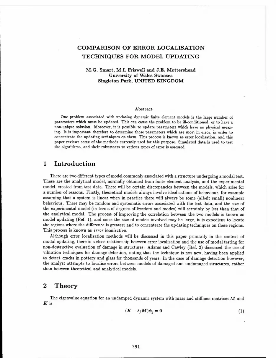
COMPARISON OF ERROR LOCALISATION
TECHNIQUES FOR MODEL UPDATING
M.G. Smart, M.I. Friswell and J.E. Mottershead University of Wales Swansea
Singleton Park, UNITED KINGDOM
Abstract
One problem associated with updating dynamic finite element models is the large number of parameters which must be updated. This can cause the problem to be ill-conditioned, or to have a non-unique solution. Moreover, it is possible to update parameters which have no physical mean- ing. It is important therefore to determine those parameters which are most in error, in order to concentrate the updating techniques on them. This process is known as error localisation, and this paper reviews some of the methods currently used for this purpose. Simulated data is used to test the algorithms, and their robustness to various types of error is assessed.
1 Introduction
There are two different types of model commonly associated with a structure undergoing a modal test. These are the analytical model, normally obtained from finite-element analysis, and the experimental model, created from test data. There will be certain discrepancies between the models, which arise for a number of reasons. Firstly, theoretical models always involve idealisations of behaviour, for example assuming that a system is linear when in practice there will always be some (albeit small) nonlinear behaviour. There may be random and systematic errors associated with the test data, and the size of the experimental model (in terms of degrees-of-freedom and modes) will certainly be less than that of the analytical model. The process of improving the correlation between the two models is known as model updating (Ref. 1), and since the size of models involved may be large, it is expedient to locate the regions where the difference is greatest and to concentrate the updating techniques on these regions. This process is known as error localisation.
Although error localisation methods will be discussed in this paper primarily in the context of modal updating, there is a close relationship between error localisation and the use of modal testing for non-destructive evaluation of damage in structures. Adams and Cawley (Ref. 2) discussed the use of vibration techniques for damage detection, noting that the technique is not new, having been applied to detect cracks in pottery and glass for thousands of years. In the case of damage detection however, the analyst attempts to localise errors between models of damaged and undamaged structures, rather than between theoretical and analytical models.
2 Theory
The eigenvalue equation for an undamped dynamic system with mass and stiffness matrices M and ÜTis
(ÜT-AjM)^. =0 (1)
391

SMART, FRISWELL AND MOTTERSHEAD
where A^ and <j>j are the eigenvalues and eigenvectors for the j-th mode. The orthogonality conditions (given mass normalised eigenvectors) are
$TK$ = A #TM<P = I (2)
where S? is the matrix whose columns are the eigenvectors and A the matrix with the eigenvalues on the leading diagonal.
It is possible to parameterize models both in terms of physical parameters, or in terms of substruc- tures. If analytically derived and experimentally obtained matrices are available, then the difference between them may be expressed as a Taylor's expansion
h~^ h~^r~ ()
where Ok are the parameters, Kx is the experimental stiffness matrix, and KA is the analytical stiffness matrix. Similar expressions apply for the mass matrix. Neglecting higher order terms
KX*KA + AK where AK = £ ^A0k (4)
In the case of substructure parameterisation, the difference between analytical and experimental matrices is expressed as
Kx*KA + AK where AK = j^ A0kKk (5) jfc=i
Kk is the stiffness matrix of the k-th substructure, and is equal to dKA/dOk. Some error localisation techniques either work directly on models which have not been parameterised, and hence give results in terms of the degrees-of-freedom (DoF) of the models, whilst other methods require parameterisation of the model.
2.1 Degree-of-Freedom Algorithms using Modal Data
2.1.1 Use of Mode Shapes Alone
Pandey et al. (Ref. 3) considered the use of mode shapes for damage detection, specifically the Modal Assurance Criterion (MAC) and Coordinate Modal Assurance Criterion (COMAC). The MAC is a global measure of the difference between two mode shapes, denned as (Ref. 4)
MAT- \YLi=i^Xi-<t>Ai 1 ((., MAO - =5j - 5-=^ —-—- (6) l^i=l<t>Xi<PXi ■l^i=l<PAi<PAi
where fa is the ith coordinate of the eigenvector, the subscripts X and A refer to experimental and analytical models respectively and the * refers to the complex conjugate. The COMAC is denned as (Ref. 5)
COMACW = -^=1l^'ll^^2
E£=l [^AijJ EjL=l {<t>Xij) (7)
where <j>ij 1S the ith coordinate of the jth eigenvector, and L is the number of mode shapes being correlated. The COMAC is a measure of the difference between a set of modes at a particular coordinate.
Pandey et al. found that neither of these quantities was sensitive to damage, but they quoted the values only to two significant figures, which may have obscured the results. It was not possible to decide whether the MAC and COMAC were insensitive to the presence of damage, or merely unable to locate it. They also considered the use of "curvature mode shapes", obtained by numerically differentiating the
392

ERROR LOCALISATION
displacement mode shapes, and concluded that these were more reliable locators of damage. However experimental verification was undertaken, and thus the possible amplification of noise introduced by differentiation was not considered. Furthermore, damage was simulated by the removal of 90% of an element stiffness, and this is clearly not a realistic scale of "damage" to use in the context of error localisation routines.
2.1.2 Force residual method
The eigenvalue equation for the experimental model is
[KA + AK}$x - [M + AM]$XAX = 0 (8)
A localisation matrix L is defined as (Ref. 6)
L = AM$xAx - AK$x = KA$X - MA$XAX (9)
This matrix contains the errors corresponding to the DoF for the various modes. Localisation indicators may be defined as
m
qi = Y^Wj\Lij\ (10)
where Wj is a weighting factor for the jth mode.
2.2 Parameter-based Routines using Modal Data
2.2.1 Substructure energy functions
Link (Refs. 7,8) devised a localisation function based on the elastic and kinetic energy contained in each mode
m m
AEk = Y, WjA^jKkA^j AT«, = ^ WjAfyMtAfyXj (11) j=i j=i
where A<£- is the difference between analytical and experimental eigenvectors, and Wj is a weighting factor for the jth mode. The above equations are for substructure parameterization, similar expressions would apply when using physical parameters. It will be seen from the results, presented later, that an effective weighting factor is the inverse of the eigenvalue, as this takes into account the fact that the mode shapes for the higher modes are less well characterized than those for the lower modes.
2.2.2 Error matrices
Ewins (Ref. 9) suggested the use of the inverse mass and stiffness matrices, given by
ÜT1 = *A_1#T M_1 = ##T (12)
for error localisation, by examining the difference between analytical and experimental inverse ma- trices. Pandey and Biswas (Ref. 10) adopted this approach for damage location, and used the method to detect damage to a beam in the laboratory. Some researchers have proposed inverting the matrices in Eq. (12). Obviously when the number of measured modes or measured coordinates are less than those of the actual model, a normal inverse cannot be found. Mannan and Richardson (Ref. IT) and Lieven and Ewins (Ref. 12) suggest the use of the pseudo-inverse for this purpose. Zhang and Lallemant (Ref. 13) followed a different approach to inversion by expanding the matrices in a binomial series. Following Eqs. (4) and (5), we may write
Kx-l = (KA + AKYl (13)
= KA-y - KA-
lAKKA~l + KA-xAKKA-
xAKKA~l + ■■■ (14)
393

SMART, FRISWELL AND MOTTERSHEAD
The first-order approximation is
AK RS KA \KA — Kx ) KA
whilst if second-order effects are included
AK ta KA {KA~l - Kxl) KA + AKKA~lAK
(15)
(16)
Similar expressions apply for the mass matrix. The inverse matrices for the analytical model may obviously be obtained through calculation. Those
for the experimental model can be approximated as follows. The mode shape matrix is partitioned:
&x = &RL $RH (17)
where the subscripts R and 5 refer to the retained (master) and slave coordinates, and L and H to the lower, measured modes and higher, unmeasured modes respectively.
K-
since the second term should be small.Although there is no similar criterion for accuracy, the mass matrix is approximated as
&RL [AL]-
1 [$RL$SL] +
&RH [AH]
1[$RH&SH] (18)
' $RL [AL]-
1 [$RL$SL] (19)
M~l §RL [$RL$SL] (20)
The slave DoF are initially approximated by using the corresponding elements from the analytical mode shapes. Then, Eq. (15) is used to calculate AK which is used in turn to update KA and and to obtain better estimates for the slave DoF by solving
[{KA + AK) - {MA + AM)AL] ( ^ ) = 0 (21)
in a least-squares sense. Park et al. (Ref. 14) used eigenvalue sensitivity to weight the error matrices from Eq. (15) for
damage location, and stated that better results were achieved. The theory is unsuitable for model updating however, and this will be discussed further in the following section.
2.2.3 Eigensensitivity
Adams and Cawley appear to be amongst the first authors to use the sensitivity of the eigenvalues to locate damage (Refs. 15-17), employing the ratio of eigenvalue changes to this end. Since then a large number of papers have appeared in the literature using similar methods. Friswell ei al. (Ref. 18) used statistical techniques to improve the Adams and Cawley approach so that measurement noise would not trigger false damage location. Ricles and Kosmatka (Ref. 19) derived what_appears to be the most complete eigensensitivity-based error localisation equations, including the effect both of eigenvalue and eigenvector changes. The eigenvalues and eigenvectors of the experimental model expressed as a first-order Taylor's series around the analytical values are
Ax - AA
dA
l dö
A6 (22)
394

ERROR LOCALISATION
The derivatives of the eigenvalues and eigenvectors may be calculated via a number of established methods (Refs. 20,21). Returning to the weighted matrix method of Park et al. (Ref. 14) mentioned in the previous section, the change in the jth eigenvalue due to kth parameter change is
^ = £|&«. <23> 4=1
where d\j/dek is given by (Ref. 20).
sf=*<sr*sr*' (24)
The ratio ajk = a£fyek is constant for a11 3 if damage has occurred at location k. Therefore, the
variance of ctjk can be used as an inverse weighting factor for the error matrices given in Eqs. (15) and (16). A necessary assumption however is that damage occurs in one place, since ocjk is constant for all j only if this condition is fulfilled. Where there are errors in more than one place, the method will fail and hence it would not be useful for the purposes of model updating.
2.3 FRF method
The equation for the frequency response matrix is
H{W) = (K-UJ2M)~
1 (25)
The sensitivity of the FRF matrix with respect to a parameter 6k is
9H - H Wk--H lk(K-SM) H (26)
A first-order Taylor's series may be used to express the change in FRF in terms of the change in structural parameters
^AÖ = AÜ (27) dB
Eq. (27) may be used to locate damage, in the same manner as for Eq. (22). Lin and Ewins (Refs. 22,23) used this technique (but with a slightly different expression for Eq. (27)) to locate damage in simple structures.
Using FRF's directly offers several advantages over the use of eigenvalues and eigenvectors. Because information on all modes is contained in each FRF, modal truncation is not a problem. Furthermore, every frequency line of the FRF is a potential equation, increasing the size of the system greatly. Finally, there is no need to perform curve-fitting, which reduces the effect of problems such as repeated or close eigenvalues.
On the other hand, it is not practical to use all the frequency lines which are measured, since the resulting system of equations becomes too large to solve. The FRF equations do not really contain more information than the modal model because (in theory at least) FRFs may be constructed from the modal model. Also it is crucial to select points that are well away from the resonances to prevent ill-conditioning of the equations, and these points are less sensitive than those near resonances. Furthermore, the fact that curve fitting is not performed means that the data may be noisy.
2.4 Solution of sensitivity equations
Eqs. (22) and (27) are of the form of Ax = b. In general, matrix A, of dimension n x m and with rank r is not square, and there are a number of solution methods depending on the size of A.
If n < TO there are more parameters than equations and the problem is underdetermined. If r ='n then there are an infinite number of "exact" solutions (in the sense that || Ax - b ||2 is zero to working
395

SMART, FRISWELL AND MOTTERSHEAD
13 5 7 9 11 13 15 17 19
\
. . , , , . .
'i. 2 3 4 V7/7
VW, 6 7 8 9 10
'', ] D D D D D D D D D / <■ 3 ^ t f 5 i \ 10 12 14 16 18 20
Figure 1: Ten noded beam element with damage
precision). If r < n then there are an infinite number of least-squares solutions (in other words solutions which minimise || Ax — 6 H2).
If n > m then there are more equations than parameters and the problem is overdetermined. If r = m and the equations are consistent, then there is a unique least-squares solution. If r < m then there are an infinite number of least-squares solutions.
Lallemant and Piranda (Ref. 6) suggested a "best sub-basis" method for error localisation. That is, the column of A which best represents the vector b is selected. Then, this column is retained and the next best column selected and so on. This method enables the selection of those parameters which provide the best basis for the solution 6, and can ostensibly be used for error location. However, the best sub-basis will provide different results depending on the size of A. If the equations are overdetermined, then the best sub-basis method chooses those parameters to which the solution is most sensitive. If the equations are underdetermined, then there is no unique solution, and the solution obtained will depend on the algorithm employed.
2.5 Testing error localisation
A ten element cantilever beam model, shown in Figure 1, was used to test and compare the lo- calisation routines. Two noded beam elements with one translational and one rotational DoF at each node were used. The material properties of the beam were: E=70GPa, L=lm, b=25mm, b=50mm, />=2800kg/m3. The "experimental" data was obtained by reducing the stiffness of one element, shown hatched in Figure 1, by 50%. The methods were tested in four ways. Firstly, all modes and coordinates were included. Secondly, the first five modes were used, again with complete coordinates. Thirdly, the first five modes were used with only the translational coordinates included. These were expanded to the full set of coordinates using the analytical mode shapes (Ref. 24)
#xs = [*AS\T T = [$AR]+
$XR (28)
where + denotes the pseudo-inverse. Finally, systematic error was introduced by calculating the "experimental" data from a beam with
twenty elements. Complete coordinates were used in this case. The results are shown in Figures 2 to 23. The binomial series method did not converge with a 50% reduction in stiffness, even with complete modes and coordinates, so for this method the stiffness of the element was reduced by 10%. Also, even at 10% it did not converge when systematic error was introduced, therefore no figure for systematic error is shown for the binomial method.
2.6 Discussion
From Figures 2 to 23, a number of results are plain. Firstly, it can be seen that the COMAC is not a reliable indicator of error location. This can be understood intuitively if damage at the root of
396

ERROR LOCALISATION
a cantilever is considered. Clearly, the displacement of all modes is zero at the root, and hence cannot reveal any difference here. Mode shapes by themselves will not necessarily exhibit the greatest changes at the position of greatest error.
Both the force residual and substructure energy methods successfully locate the error, but the results are worse when all modes are included as opposed to including only the first five modes. This suggests that the higher modes, whilst affected more by error, are in fact less well characterised, and should therefore be weighted against. The results of the energy method weighted by the inverse of the eigenvalues are shown in Figures 12, 13 and 14. The error has been more sharply defined by this weighting.
The best sub-basis method also selects the initial parameter correctly (using either eigendata or FRF data) and engineering judgement could be applied to choose those other parameters which are considered important in locating error. It should be noted that when using FRF data the selection of which frequency points to use is crucial to the success of the method. In this case, points were arbitrarily chosen far from the resonances, since at resonances the magnitudes of the FRFs are strongly influenced by damping, which is normally an ill-defined quantity. Also, when using sensitivity methods it may be necessary to weight certain measurements to reflect greater certainty or uncertainty as their reliability. However, no weighting was employed in this research.
Finally, it is clear that all the methods fail when discretisation error is introduced. In order to ascertain the extent of discretisation error caused by the method used here, the first five frequencies for the beam, calculated using ten and twenty elements respectively, are shown in Table 1. These results clearly demonstrate that the discretisation error considered in this example is very conservative and that in practice worse effects are to be expected. This failure is a serious one, since systematic error will occur in practice no matter how carefully measurements are made. More thought needs to be given to making methods robust against this form of error.
Table 1: Change in frequencies due to discretisation
/io (Hz) /20 (Hz) A/ (%) 20.19 20.19 -0.0001 126.55 126.54 -0.0031 354.42 354.33 -0.0238 695.00 694.38 -0.0890 1150.69 1147.99 -0.2345
3 Conclusions and recommendations
A number of different approaches to error localisation have been examined. These range from direct degree-of-freedom based methods to techniques which require parameterisation of the structure and are often based on a first-order Taylor series. The methods which seem to show most promise are sensitivity-based techniques, but all the methods examined here fail when a small systematic error is introduced into the results. There is a paucity of papers which have tested the methods outlined in a rigorous experimental manner, which is not surprising considering the weaknesses inherent to them. It is necessary to improve the robustness of error localisation techniques to systematic error before they can be confidently used in practice.
References [1] Mottershead, J. E. and Friswell, M. I. Model updating in structural dynamics: a survey. Journal
of Sound and Vibration 167(2), 1993, pp. 347-375. [2] Adams, R. D. and Cawley, P., Nondestructive Testing, vol. 8 Elsevier, London, 1985.
397

SMART, FRISWELL AND MOTTERSHEAD
[3] Pandey, A. K., Biswas, M., Samman, M. M. Damage detection from changes in curvature mode shapes. Journal of Sound and Vibration 145(2), 1991, pp. 321-332.
[4] Allemang, R. J. and Brown, D. L. A Correlation coefficient for modal vector analysis. In Proceedings of the 1st International Modal Analysis Conference. Orlando, Florida, 1982, pp. 110-115.
[5] Lieven, N. A. J. and Ewins, D. J. Spatial correlation of mode shapes, the Coordinate Modal Assurance Criterion (COMAC). In Proceedings of the 6th International Modal Analysis Conference. Kissimmee, Florida, 1988, pp. 690-695.
[6] Lallemant, G. and Piranda, J. Localization methods for parametric updating of finite element models in elastodynamics. In Proceedings of the 8th International Modal Analysis Conference. Kissimmee, Florida, 1990, pp. 579-585.
[7] Link, M. Localisation of errors in computational models. In Eurodyn '90: Proceedings of the 1st European Conference on Structural Dynamics. Rotterdam, 1990, pp. 305-313.
[8] Link, M. and Santiago, O. F. Updating and localizing structural errors based on minimization of equation errors. In Proceedings of the International Conference on Spacecraft Structures and Mechanical Testing. Noordwijk, Holland, 1991.
[9] Ewins, D. J., Modal Testing: Theory and Practise Research Studies Press, Letchworth, England, 1985.
[10] Pandey, A. K. and Biswas, M. Damage detection in structures using changes in flexibility. Journal of Sound and Vibration 169(1), 1994, pp. 3-17.
[11] Mannan, M. A. and Richardson, M. H. Detection and location of structural cracks using FRF mea- surements. In Proceedings of the 8th International Modal Analysis Conference. Kissimee, Florida, 1990, pp. 652- 657.
[12] Lieven, N. A. J. and Ewins, D. J. Error location and updating of finite element models using SVD. In Proceedings of the 8th International Modal Analysis Conference. Kissimmee, Florida, 1990, pp. 769-773.
[13] Zhang, Q. and Lallemant, G. Dominant error localisation in a finite element model of a mechanical structure. Mechanical Systems and Signal Processing 1(2), 1987, pp. 141-149.
[14] Park, Y. S., Park, H. S., Lee, S. S. Weighted-error-matrix application to detect stiffness damage dynamic characteristic measurement. International Journal of Analytical and Experimental Modal Analysis 3(3), 1988, pp. 101-107.
[15] Adams, R. D. et al. A Vibration technique for nondestructively assessing the integrity of structures. Journal of Mechanical Engineering Science 20(2), 1978, pp. 93-100.
[16] Cawley, P. and Adams, R. D. The location of defects in structures from measurement of natural frequencies. The Journal of Strain Analysis 14(2), 1979, pp. 49-57.
[17] Cawley, P. and Adams, R. D. A Vibration technique for nondestructively assessing the integrity of fibre composite structures. Journal of Composite Materials 13(4), 1979, pp. 161-175.
[18] Friswell, M. I., Penny, J. E. T., Wilson, D. A. L. Using vibration data and statistical measures to locate damage in structures. Modal Analysis 9(4), 1994, pp. 239-254.
[19] Ricles, J. M. and Kosmatka, J. B. Damage detection in elastic structures using vibratory residual forces and weighted sensitivity. AIAA Journal 30(9), 1992, pp. 2310-2316.
[20] Fox, R. L. and Kapoor, M. P. Rates of change of eigenvalues and eigenvectors. AIAA Journal 6(12), 1968, pp. 2426-2429.
[21] Nelson, R. B. Simplified calculation of eigenvector derivatives. AIAA Journal 14(9), 1976, pp. 1201-1205.
[22] Lin, Y. and Ewins, D. J. Model updating using FRF data. In Proceedings of the 15th International Seminar on Modal Analysis. Leuven, Belgium, 1990, pp. 141-162.
[23] Lin, R. and Ewins, D. J. Analytical model improvement using frequency response functions. Me- chanical Systems and Signal Processing 8(4), 1994, pp. 437-458.
[24] O'Callahan, J., Avitabile, P., Riemer, R. System Equivalent Reduction Expansion Process. In Proceedings of the 7th International Modal Analysis Conference. Las Vegas, Nevada, 1989, pp. 29-37.
398

ERROR LOCALISATION
°'85 1 3 5 7 9 11 13 15 17 1 Error position: translational DoF
5 7 9 11 13 15 17 Error position: translational DoF
6 8 10 12 14 16 18 20 Error position: rotational DoF
Figure 2: COMAC: all modes, complete coordi- nates
6 8 10 12 14 16 18 Error position: rotational DoF
Figure 5: COMAC: systematic error
O0.95-
0.9
1 3 5 7 9 11 13 15 17 19 Error position: translational DoF
5 7 9 11 13 15 17 19 Error position: translational DoF
8 10 12 14 16 18 20 Error position: rotational DoF
6 8 10 12 ■ 14 16 18 20 Error position: rotational DoF
Figure 3: COMAC: 1st 5 modes, complete coordi- nates
Figure 6: Force residual: all modes, complete co- ordinates
6 8 10 12 14 16 18 20 Error position: rotational DoF
Figure 4: COMAC: 1st 5 modes, incomplete coor- dinates
2 4 6 8 10 12 14 16 18 20 Error position: rotational DoF
Figure 7: Force residual: 1st 5 modes, complete coordinates
399

SMART, FRISWELL AND MOTTERSHEAD
6 8 10 12 14 16 18 20 Error position: rotational DoF
Figure 8: Force residual: 1st 5 modes, incomplete coordinates
23456789 10 Error position: element no
Figure 11: Link's energy: 1st 5 modes, complete coordinates
4 6 8 10 12 14 16 18 20 Error position: rotational DoF
Figure 9: Force residual: systematic error
2 3 4 5 6 7 8 Error position: element no
Figure 12: Link's weighted energy: 1st 5 modes, complete coordinates
4 5 6 7 8 Error position: element no
4 5 6 7 8 9 10 Error position: element no
Figure 10: Link's energy: all modes, complete co- ordinates
Figure 13: Link's weighted energy: 1st 5 modes, incomplete coordinates
400

ERROR LOCALISATION
1 1 ' ' ' ' 1 1 1
0.9 -
0.8 -
0.7 - o 5 0.6 . <D
J?0.5 re g £0.4
•
0.3 •
0.2 -
0.1
0
-
1 2 3 4 5 6 Error position
7 8 element no
9 10
Figure 14: Link's weighted energy: systematic er- ror
4 5 6 7 8 Error position: node number
4 5 6 7 8 Error position: node number
Figure 15: Binomial series: all modes, complete Figure 17: Binomial series: 1st 5 modes, incom- coordinates plete coordinates
23456789 10 Error position: node number
Figure 16: Binomial series: 1st 5 modes, complete coordinates
401

SMART, FRISWELL AND MOTTERSHEAD
6 8 7 3 Error position: Element no
Figure 18: Best sub-basis (eigenvalues): all modes
2 1 8 10 Error position: Element no
Figure 21: Best sub-basis (FRF)
4 2 7 3 Error position: Element no 2 10 8 7
Error position: Element no
Figure 19: modes
Best sub-basis (eigenvalues): 1st 5 Figure 22; Begt sub.basis (FRF): incomplete coor-
dinates
Figure 20: Best sub-basis (eigenvalue): systematic error Figure 23: Best sub-basis (FRF): systematic error
402

NONLINEAR DESIGN TECHNIQUE FOR FLEXIBLE STRUCTURES
Xubin Song, Mark J. Schulz, P. Frank Pai North Carolina A&T State University
Greensboro, NC 27411
Abstract A Computational Nonlinear Design technique to optimize the design of advanced actively controlled
flexible structures is presented. The technique uses explicit time integration to transform nonlinear differential equations into sparse linear algebraic discrete-time equations and analytic gradient equations that can be efficiently solved. A multi-variable design optimization adjusts structural parameters and control gains to minimize system vibration. This solution approach is nearly exact, uses a minimum number of matrix inversions, and provides gradient sensitivities of any variable in the system equations without recursion or approximation. Also, any type of structural nonlinearity, forcing function and initial conditions can be modeled. Furthermore, a new nonlinear feedback control law that mimics the characteristics of a passive isolator is proposed to improve stability of the nonlinear system. Since full second order sparse equations are used in the control design, all difficulties of imprecise eigenvalue/vector calculations, reduced basis approximations, and spillover effects present in linear modeling techniques are eliminated. An initial result using the technique is presented in which vibration of a four bay 16 degree-of-freedom cantilever truss is controlled using a single actuator near the support.
1. Introduction Advanced structures such as the space station, high speed civil transport aircraft, fuel-efficient
automobiles, and high altitude long endurance aircraft are designed for minimum weight to improve performance and reduce operating costs over the life of the product. These light-weight designs, however, are more flexible than traditional structures and behave nonlinearly and often are designed to operate beyond buckling. Flexible structures are also designed to have a finite fatigue life that is governed by the stress to number of cycles to failure curves (S/N curves) for the structural material. For aerospace materials, these curves state that large stresses cause logarithmically greater damage than lower stresses and show the criticality of analyzing for and preventing large displacements and stresses in the structural response. Therefore, to design the most efficient structure and to accurately predict structural life, highly flexible structures are most appropriately modeled and analyzed using nonlinear structural theory.
The increased flexibility of light-weight structures also increases vibration. This requires that lightweight structures often have some type of passive or active control device to suppress vibration [1] to ensure the safety, reliability and performance of the structure. An active control system can also be used to quench dangerous characteristics unique to nonlinear structures, such as bifurcations to a higher response level, internal resonances, limit cycling, and chaotic behavior. Nonlinear control is proposed for the active structure as it potentially can give better performance than linear control for linear and nonlinear structures.
It is apparent that nonlinear design is needed to develop lighter-weight and lower cost advanced structures. Presently, however, there are no general techniques available to simultaneously design the structure and controller for nonlinear systems — existing techniques apply only to linear systems. Analytical techniques to handle nonlinear structures problems are not well developed principally because exact closed- form solutions to general large order systems of nonlinear differential equations are unobtainable. Thus, this paper addresses the need to develop an analytical technique that can design nonlinear actively controlled flexible structures with improved performance and reliability.
403

X. SONG, M. SCHULZ, F. PAI
Existing techniques for nonlinear control such as feedback linearization, describing functions, sliding control, adaptive control [2], model referenced adaptive control [3], neural network control [4], and nonlinear modal control [5] have serious limitations when applied to the control of large flexible structures. These include restriction to certain classes of nonlinear systems, requiring full state feedback, errors due to truncating sub-harmonic and super-harmonic Fourier terms, linearization errors, application only to tracking control or uncertain systems, restriction to very small order or single input or decoupled systems, or being heuristically based. These techniques also obscure the relationship between the structural response and the structural and control design parameters when performing a multi-disciplinary optimization. Direct Optimal Control of Nonlinear Systems via Hamiltons Law of Varying Action [6] using assumed time modes is probably the most similar method to the method we propose, but it does not efficiently handle the steady- state response computation for large systems, cannot use output feedback control, and the optimal control formulation is not suited to constrained structural optimization.
The innovation of the technique proposed herein is that the highly nonlinear dynamic and control equations are transformed into sparse linear algebraic discrete-time equations and analytic gradient equations that can be solved efficiently, especially by using parallel computing. A nearly exact solution is obtained, the number of matrix inversions is minimized, gradients sensitivities of any variable in the system matrices can be obtained without recursion or approximation, and any types of structural nonlinearities, forcing functions, and initial conditions can be handled. Thus a standard multivariable optimization routine can design the multi-degree-of-freedom nonlinear system, that is, adjust structural parameters and control gains to minimize the mean-square response of the system. The mean-square control forces and any other desired parameters of the design, such as structural weight, can also be minimized. Since full system sparse equations in second order form are used in the control design, all the difficulties of imprecise and expensive eigenvalue/vector calculations, reduced basis approximations, and spillover effects present in other techniques are eliminated. Furthermore, a new nonlinear control law that mimics the characteristics of a passive isolator is proposed to improve stability robustness for the optimized nonlinear system.
2. Nonlinear Design Technique The general structure-control design approach taken here is to use explicit time integration, and
optionally parallel computing, to obtain a nearly exact solution to the simultaneous second-order nonlinear differential equations describing the closed loop system. The nonlinear structural model could be generated from a nonlinear finite element code. With this approach only the mass matrix that is often diagonal needs to be inverted in the integration solution. The remaining computations in the integration only involve addition and multiplication of sparse matrices and can be done extremely fast using parallel-vector sparse matrix solvers [7]. The optimization computations are streamlined by computing the gradients or sensitivities of the design variables in closed form, or semi-analytically depending upon the type of finite elements used in the model. Matrix inversion is needed to compute the gradients, but the matrices are very sparse and easy to invert. Choosing a larger time step to eliminate the less important higher frequency portions of the response can also reduce computations, but stability cannot be guaranteed for nonlinear systems. The integration solution is made robust to instability by assuming constant acceleration over each time step and by performing an equilibrium balance at the end of each time step.
Nonlinear structural optimization is computationally intensive due to the recomputation of the solution at each iteration of the optimization. However, since the sparsity of the structural matrices is preserved in this approach, the new sparse matrix solvers recently available can be used to greatly reduce this computational burden. New parallel algorithms also exist to perform general matrix computations [8], assemble finite element matrices from the elemental level [9], compute design sensitivities [10], and perform large scale design optimization [11,12]. Therefore the method proposed here should be able to handle realistic size engineering problems when the algorithm is developed for parallel computing.
The structure and control optimization is performed by defining an objective function to try to drive the forced nonlinear system to its zero equilibrium solution using the minimum control force. Constant gain output feedback control is used, which is the simplest and most practical technique for active structural control. No observer or dynamic compensator is needed and time delay in computing the control action is minimized. The control gains are actually the coefficients of some polynomial function of the nonlinear displacements and velocities of the system. The technique can also be used to study the dynamic behavior and control order characteristics of nonlinear systems. Gain suppression can be used to identify the best out
404

NONLINEAR DESIGN TECHNIQUE
of a group of candidate locations to take feedback measurements and to place actuators. Any type of forcing functions can be used and chaotic responses can also be computed.
Also to be investigated using this technique is whether active nonlinear damping can effectively suppress detrimental nonlinear structural effects for multi-degree-of-freedom systems. Nonlinear damping on single- degree-of-freedom systems has been shown to delay the point of bifurcations to a higher response level, prevent period doubling leading to chaotic behavior, reduce sensitivity to small variations in system and excitation parameters and initial conditions, and limit the amplitude or prevent catastrophic internal resonances from occurring.
2.1 Integration Solution The general form of the differential equations of motion that describe an n dimensional second order
closed-loop nonlinear dynamic system subject to a general forcing function is
Mx + fv(x) + f</(x) = F(0-uv(x)-u</(x) (i)
where x is the displacement vector, M is the mass matrix, f v (x), f d (x) are the nonlinear damping and
stiffness force vectors, respectively, F(f) is the external force vector, and -uv(x) - u^(x) are the nonlinear control force vectors. The external force can be of any form, transient or steady-state. The Newmark-Beta explicit time integration technique is used to solve (1). The solution is shown below
xr+1 = x, + xrAt + [(0.5 - ß)xr + ßxr+1 ]A/2 (2a)
*r*l = *r + [0 " *)*r + **r*l ^ (2b)
xr+1 =M-1[F((r + l)AO-uv(xr+1)-u,(xr+I)-fv(xf+1)-f(/(xf+1)] (2c)
where r+1 denotes the current solution point, r denotes the last solution point, At is the time step, and X,ß are constants. The integration solution is carried out only long enough to represent the essential characteristics of the response, which may be only four cycles of response. An iteration of (2a-c) is done each timestep to obtain an equilibrium force balance that greatly improves the accuracy of the solution. The equilibrium balance is done by taking the first estimate of xf+I = xr and using (2a,2b) to get an updated estimate of xr+1 in (2c). Note that all terms with the r subscript do not change in this iteration. The value of xr+1 usually converges within about five iterations.
With this formulation, the only inversion is the mass matrix and the sparsity of the structural matrices is preserved. Thus the computations can be carried out very fast for a large number of time steps using parallel-sparse matrix solvers. A larger time step can also be used to eliminate the high frequency portion of the response to reduce computations. The explicit Newmark-Beta integration method used is more accurate than Euler finite difference type methods, and it is simpler to derive analytic gradients and preserve the sparsity of the structural matrices than in the Runge-Kutta or implicit Newmark-Beta methods.
Note that this form of integration is different than the implicit Newmark-Beta method typically used in finite element codes that perform direct integration solutions. Here, only the mass matrix needs to be inverted. Since M is often diagonal or constant, the inversion is either trivial or only needs to be done once. In most nonlinear models the stiffness matrix is nonlinear and recursion is necessary to -integrate the nonlinear equations. No repeated inversion is needed using the solution procedure presented here. Thus this approach may also be useful to solve general nonlinear structures problems.
2.2 Objective Function An objective function that minimizes the mean square vibration displacement of the system and the mean
square control forces is
405
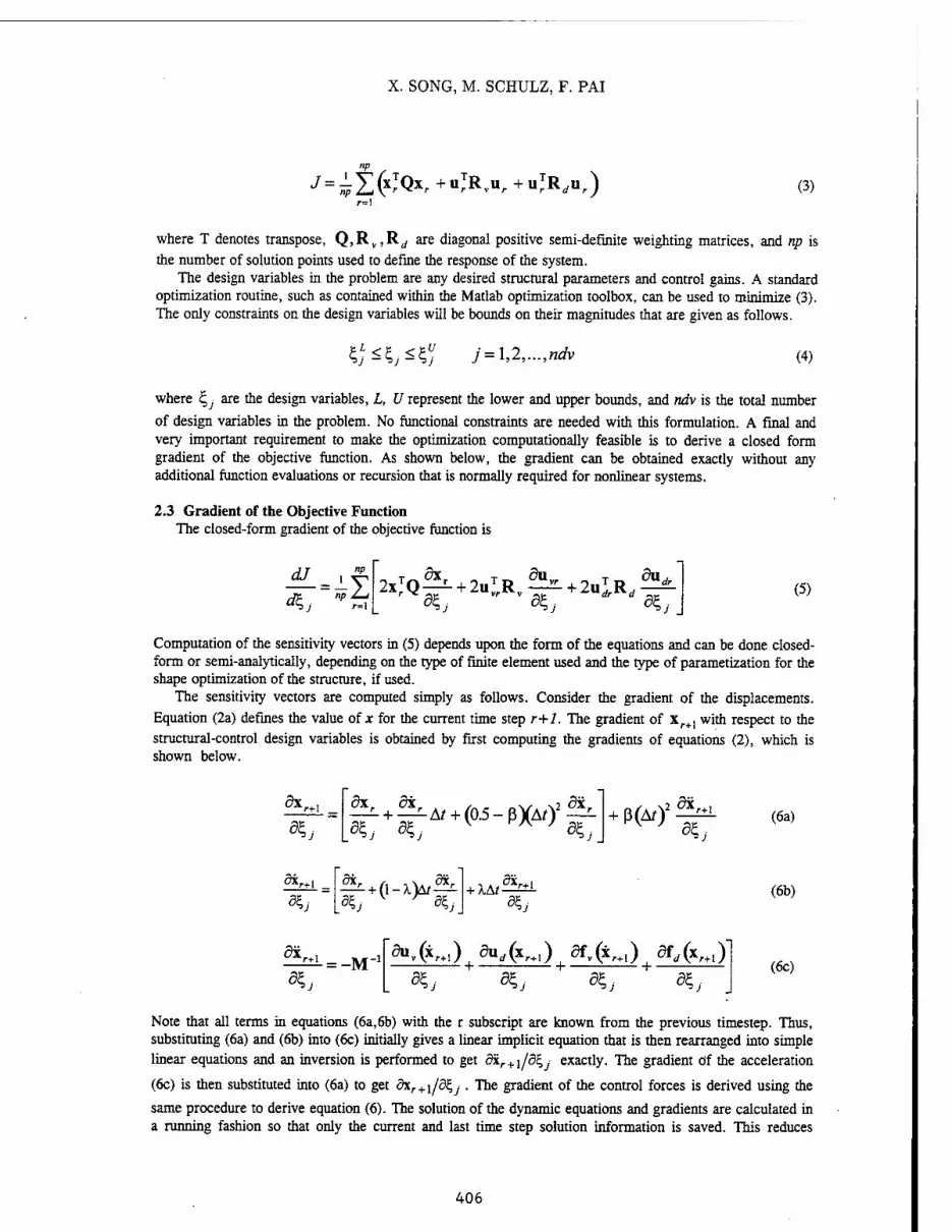
X. SONG, M. SCHULZ, F. PAI
np
(3)
where T denotes transpose, QjR^R^ are diagonal positive semi-definite weighting matrices, and np is the number of solution points used to define the response of the system.
The design variables in the problem are any desired structural parameters and control gains. A standard optimization routine, such as contained within the Matlab optimization toolbox, can be used to minimize (3). The only constraints on the design variables will be bounds on their magnitudes that are given as follows.
^<^,<^ j = l,2,...,ndv (4)
where £,j are the design variables, L, U represent the lower and upper bounds, and ndv is the total number
of design variables in the problem. No functional constraints are needed with this formulation. A final and very important requirement to make the optimization computationally feasible is to derive a closed form gradient of the objective function. As shown below, the gradient can be obtained exactly without any additional function evaluations or recursion that is normally required for nonlinear systems.
2.3 Gradient of the Objective Function The closed-form gradient of the objective function is
dJ np
np Z_i
„ T~ 3xP „ T- da 2xjQTr^- + 2uLR
%j **>j
+ KRrf du dr
*J
(5)
Computation of the sensitivity vectors in (5) depends upon the form of the equations and can be done closed- form or semi-analytically, depending on the type of finite element used and the type of parametization for the shape optimization of the structure, if used.
The sensitivity vectors are computed simply as follows. Consider the gradient of the displacements. Equation (2a) defines the value of x for the current time step r+1. The gradient of xr+1 with respect to the structural-control design variables is obtained by first computing the gradients of equations (2), which is shown below.
dx r+\
%J
dxr dx.
*j d*>J
A/ + (0.5-ßXAr): + ß(A/> (6a)
dk r+l
%J ^ + (1-^ + XAt^^
%j
(6b)
dx r+\
%J = -M -i d».(*«i) du„(xr+1) 5fv(xr+1) dfd(xr+{)
*j *j
+ ■
*>j *j
(6c)
Note that all terms in equations (6a,6b) with the r subscript are known from the previous timestep. Thus, substituting (6a) and (6b) into (6c) initially gives a linear implicit equation that is then rearranged into simple linear equations and an inversion is performed to get dxr+l/dE,j exactly. The gradient of the acceleration
(6c) is then substituted into (6a) to get dxr+l/d£,j . The gradient of the control forces is derived using the
same procedure to derive equation (6). The solution of the dynamic equations and gradients are calculated in a running fashion so that only the current and last time step solution information is saved. This reduces
406

NONLINEAR DESIGN TECHNIQUE
computations and memory requirements. As stated, the gradient equations are initially linear equations in an implicit form, but they are rearranged and solved by inversion rather than recursion that is normally needed when using a harmonic balance type solution for nonlinear differential equations. This is possible because the displacements are known and can be directly substituted into the nonlinear terms thus eliminating recursion.
The formulation presented above represents a general approach to analyze nonlinear actively controlled practical engineering structures. Other nonlinear control approaches that we have found in the literature would be either computationally intractable, restricted to small scale problems, or would produce an approximate solution when applied to an optimization problem.
3. Control Law Design Nonlinear control potentially improves performance over linear control, but it may also be particularly
appropriate for systems that undergo large displacements or have varying or uncertain parameters. Nonlinear control may be able to operate over wide frequency and amplitude ranges using a simple nonlinear active damping control law. This may eliminate system identification and adaptive control necessary in linear systems, and, moreover, cannot destabilize the plant. This approach can also be used to design a passive nonlinear vibration suppression system.
The general control approach taken here is to consider any type of nonlinear control function that uses constant gain output feedback control. Feedback control using constant gains is much simpler than using a dynamic compensator, and output feedback is appropriate for large structures where only a small number of sensors is practical. We are investigating general polynomial control schemes but stability is not guaranteed, except possibly for collocated active damping. A new approach being investigated assures stability based on the idea that adding a simple spring-damper system between two coordinates on the structure cannot destabilize the system. This nonlinear feedback control law uses the absolute value of a polynomial function multiplied by the sign of the velocity or displacement at the actuator location. This means that the control forces act as if they were produced from a spring-damper system with time-varying coefficients. The damper can only extract energy and the spring can only store/release energy when stretched or compressed. Thus, with slowly varying coefficients, this control law is stable and robust to system parameter variations, forcing function type, and modeling errors, but it may have somewhat reduced performance from a controller that is not constrained to this form.
From previous structural vibration and control studies on linear systems, we have found that additive damping is often the most effective way to reduce wide band vibration using minimum control forces. This is because wide band disturbing forces acting on a system always have components in phase with the structural velocity, and velocity feedback control, which is active damping, can most directly alter this phase coincidence. Active damping tends to distort and couple and distribute energy among the complex mode shapes of a structure, whereas position feedback changes the stiffness and hence significantly changes the actual mode shapes and frequencies of the closed-loop structure. Changing the mode shapes of a structure usually requires large control forces, and generally does not produce a commensurate reduction in vibration amplitude. Active damping versus position feedback nonlinear control laws are being studied to determine the most effective algorithm to suppress vibration for nonlinear structures.
4. Example Problem An initial result is presented in which a four bay 16 degree-of-freedom cantilever truss with a transverse
harmonic force at its end is controlled using a single actuator near the support. Testing of the technique is being done using a 90 MHz pentium PC with 16MB RAM and the sparse matrix functions in Matlab. This setup is easily powerful enough to solve the nonlinear truss structure without using parallel computing. The truss structure is shown in Figure 1. The truss has a linear stiffness matrix and a diagonal nonlinear stiffness matrix. The nonlinear stiffness matrix is comprised of small nonlinear terms proportional to the linear diagonal terms and a term from a light nonlinear spring at the top of the truss. All members of the truss are pin connected and the two offset members at the actuator are designed to produce a transverse force on the truss, that is, only the y direction component of the force in the actuator is transferred to the truss.
407

X. SONG, M. SCHULZ, F. PAI
\ \ \ Nonlinear Spring
Disp. Sensor 2 4 6
Transverse Force Actuator f (t)
Figure 1. Nonlinear Active Truss
The mass matrix and the linear and nonlinear stiffness matrices for the truss are given below. The mass and stiffness coefficients were chosen to obtain a desired truss frequency and do not represent any particular system dimensions or material properties.
M = diag$6 5.6 5.6 5.6 5.6 5.6 5.6 5.6 5.6 5.6 5.6 5.6 55 55 5.3 5.3]*!%
K/ =
984 0 0 0 -363 0 0 0 0 0 0 0 0 0 0 0 790 0 -725 0 0 0 0 0 0 0 0 0 0 0 0
984 -130 -259 130 -363 0 0 0 0 0 0 0 0 0
790 130 -65 0 0 0 0 0 0 0 0 0 0
984 -130 0 0 -363 0 0 0 0 0 0 0
790 0 -725 0 0 0 0 0 0 0 0
984 -130 -259 130 -363 0 0 0 0 0
790 130 -65 0 0 0 0 0 0 984 -130 0 0 -363 0 0 0
790 0 -725 0 0 0 0
Symm. 984 -130
790
-259
130
622
130
-65
-130
790
-363
0
0
0
363
0.
0
0
-725
0
725
'10J
:a^ Knl = diad9S4 790 984 2*10* 984 790 984 790 984 790 984 790 622 790 363 725*10
The vector of displacements is x(f) = [xl y\ x2 y2 . . xS ySj . The nonlinear stiffness terms are
coefficients that multiply cubic displacements of the associated coordinates, and were chosen arbitrarily to test the technique. Future work is to use a fully nonlinear geometrically exact truss model [13] and other types of nonlinear elements.
The mass matrix contains about 90% non-structural mass at each node of the truss. Proportional linear damping (D=0.0002K/) is assumed to simplify the example. The design goal is to reduce the cantilever type bending of the truss. A sinusoidal force /(/) = 40sin(4Trt) acts at the end of the truss (DOF y7). The uncontrolled truss exhibits a beating response that is shown in Figure 2.
408

NONLINEAR DESIGN TECHNIQUE
DOF:1,5, 9,13 DOF:2, 6,10, 14
2 4 6
DOF:4, 8, 12,16
Figure 2. Truss Vibration (Disp. vs Time) Uncontrolled
Integration parameters corresponding to constant acceleration over each time step (ß = 025, a = 03) are used in the integration. The time step required to ensure stability was 0.001 second and the response was computed for 2.6 seconds to optimize the system. Initial conditions were zero. The external spring coefficient was optimized and bounded within the range 10,000 to 40,000. A cubic polynomial control law is used with feedback of the velocity and position of only one point at the end of the truss (x,6 = yt). The proposed control law is shown below,
"v = C;v **16 +C2v **16 "M + C3v **\6
ud = c\d *xu + °id **i6 *he| + cid *X\6
where the Cj„,cw values are coefficients to be determined by the optimization. The weighting matrices chosen
are Q = 200* I,RD = 10"8,RV = 4 * 10-8. This particular weighting puts almost all emphasis on minimizing the displacements of the truss with little penalty for control force magnitude. The optimization was done in two steps with different values of the weighting matrix Q. The initial value weighted the displacements near the actuator more heavily to help convergence. The objective function at the start of the optimization was J=3943 and at the end J=213.2. The optimization took about 40 minutes wall time and 20 iterations on a 90MHz PC and drove the stiffness of the nonlinear external spring to its upper bound, 40,000, and set the control gains for the cubic displacement and all the velocity feedback gains to be negligibly small (for a multi-frequency input the opposite could occur and the velocity gains could overshadow the position gains). The optimal control law determined by the optimization thus consisted of only the position feedback terms, as shown below.
ud = 6.9682 * 104 * xI6 -12.68 * 104 * x16 * |*16| + 0.0062 * 104 * x,36
This is a significantly different type of control action than could occur with linear control, and this particular result depends on the amplitude and frequency content of the forcing function, the nonlinearity of the structure,
409

X. SONG, M. SCHULZ, F. PAI
and the weighting parameters. The vibration response of the truss using this control law is shown in Figure 3. Note that the beating is nearly eliminated and that the vibration amplitudes at the actuator and at the end of the truss are about the same. Further reducing the vibration at the end would increase the vibration at the actuator and this is a limiting condition in suppressing vibration of the truss. The control force is shown in Figure 4.
DOF: 1,5, 9, 13
x1CT
2 4 6 8
DOF: 3, 7, 11, 15
DOF: 2, 6, 10, 14
Figure 3. Truss Vibration (Disp. vs Time) with Nonlinear Control
-400
Figure 4. Control Force (Transverse Force vs Time) with Nonlinear Control
This example shows that active control and the small effect of increasing the stiffness of the nonlinear spring reduces the peak vibration amplitude of the truss by about 80 percent.
Nonlinear control laws may have more than one solution and this example was re-run with a different starting point for the optimization. The nonlinear spring was fixed at the upper bound of 40,000, velocity gains were set to zero, and a slightly different scaling of the design variables was used. The starting value of the
410

NONLINEAR DESIGN TECHNIQUE
objective function is unchanged, J=3943, and the optimization found a minimum J=212.71. The response and control forces are similar to the first case and the optimal control law is shown below.
ud = 6.8609 * 104 * x,6 + 0.4692 * 104 * x16 * |x16| + 0.0360 * 104 * 4
A linear control case was also run for a comparison to nonlinear control results above. Here, the external spring was set to its upper value and the optimization re-run with only the linear position feedback control term remaining. The optimization drove the objective function from the same starting point as the nonlinear cases, J=3943, to a minimum value of J=216.7. The linear control gain is given below.
ud = 6.0739 *104*x16
The response and control forces for the linear case are different than for the nonlinear case and are shown in Figures 5 and 6, respectively. For this example the nonlinear control produced a very slightly better performance, as defined by the smaller J value, than the linear control. However, for larger amplitudes of the forcing function, or different weighting factors, or a strongly nonlinear structure, the nonlinear control may have a more significant advantage.
In the truss configuration studied here the peak transverse control forces are high, approximately 37 times larger than the disturbing force at the end of the truss (also, peak actuator force is 2.23 times greater than transverse force). A static analysis without the nonlinear terms was performed to verify the reasonableness of the dynamic solution and to determine the best position for the actuator. The static analysis showed that for the actuator at node 1, as in the above examples, the transverse force required to reduce deflection at the end of the truss to zero was 34.5 times greater than the end force. This verifies the large control forces determined in the dynamic analysis. With the actuator positioned at bays 3,5 and then 7, the peak transverse force reduced, respectively, to 3.9, 1.7, and 1 times the end force. This result shows that a static analysis is useful to determine optimal positioning of actuators and emphasizes intuition that the actuator should be as close to the disturbing force as possible. Changing the angles of the actuator link configuration also reduces the actuator force required, but to a much lesser extent than repositioning the actuator.
5. Continuing Work The problem presented herein has verified the integration algorithm and gradient derivation for a simple
assumed structural nonlinearity. Currently, a geometrically exact nonlinear truss element has been programmed with the exact closed-form gradient, and the static deflection analysis has been used to determine a better actuator position. This model is being tested and initial results show that the nonlinear element formulation and gradient are much longer and require much more computation than the example presented. A nonlinear beam finite element has been derived by Pai based on the theory in [14] and will be programmed and tested next. Nonlinear active damping will be studied using the nonlinear beam model.
6. Conclusion The example problem showed that the technique presented herein is an effective tool to design nonlinear
structures to suppress structural vibration. Also, nonlinear design as well as nonlinear control are new fields to be developed that promise significant improvements in structural designs. In particular, control system stability and new types of nonlinear control laws need to be investigated. Safer and more economical designs for engineering applications such as large flexible space structures, high speed aircraft, tall buildings, commercial aircraft, and almost any lightweight/highly flexible structure may be possible by nonlinear design and nonlinear control.
Parallel-vector sparse matrix equation-solvers and optimization techniques are also needed to apply the present technique to large scale structures. This would be an important step toward developing a New Generation of Nonlinear Structural Analysis Tools For Shared and Distributed Memory High-Performance Computers.
7. Acknowledgment This work was supported by the NASA CORE Program (Grant No. NAGW-2924).
411

X. SONG, M. SCHULZ, F. PAI
x10 -3 DOF: 1, 5,9, 13
0 2 4 6
x10 -3 DOF: 3, 7, 11,15
DOF: 2, 6, 10, 14
2 4 6
DOF: 4, 8, 12, 16
Figure 5. Truss Vibration (Disp. vs Time) with Linear Control
FEEDBACK:Udr
12 3 4 5 6 7 8
Figure 6. Control Force (Transverse Force vs Time) with Linear Control
412

NONLINEAR DESIGN TECHNIQUE
8. References 1. Venkayya, V.B., Tischler, V.A., and Knot, N.S., "Dynamics and Control of Space Structures,"
AFWAL/FIBRA, Design and Analysis Methods Group, Analysis and Optimization Branch, Structures and Dynamics Division.
2. Slotine, J. and Li, W., "Applied Nonlinear Control," 1991, Prentice-Hall. 3. Sardar, H.M. and Ahmadian, ML, "A Modified Model Referenced Adaptive ControUTechnique for
Nonlinear Dynamic Systems", Journal of Vibration and Acoustics, Vol. 114, 154-160, 1992. 4. Goh, C.J., "Model Referenced Control of Non-linear Systems via Implicit Function Emulation",
International Journal of Control, Vol. 114, No.l, 91-115, 1994. 5. Slater, J.C., "Nonlinear Modal Control," Ph.D. Thesis, State University of New York at Buffalo,
New York, 1993. 6. Adiguzel, E. and Oz, H., "Direct Optimal Control of Nonlinear Systems via Hamilton's Law of
Varying Action", AIAA Guidance, Navigation and Control Conference, August 12-14, 1991, New Orleans, LA.
7. Nguyen, D.T., "Parallel-Vector Methods for Computational Mechanics", Short Course, Greensboro, NC, Dec. 1-2, 1994.
8. Agarwal, T.K., Storaasli, O.O., and Nguyen, D.T., "A Parallel-Vector Algorithm for Rapid Structural Analysis on High-Performance Computers", AIAA Paper 90-1149, Presented at the AIAA/ASME/ASCE/AHS 31st Structures, Structural Dynamics and Materials Conference, Long Beach California, April 2-4, 1990.
9. Baddourah, M.A., Storaasli, O.O., Carmona, E.A., and Nguyen, D.T., "A Parallel Algorithm for Generation and Assembly of Finite Element Stiffness and Mass Matrices", AIAA -91-1006-CP.
10. Nguyen, D.T., Storaasli, O.O., Qin, J., and Qamar, R., "Automatic Differentiation for Design Sensitivity Analysis of Structural Systems Using Multiple Processors", Multidisciplinary Parallel- Vector Computation Center, 135 KDH Building, Old Dominion University, Norfolk, VA 23529.
11. Nguyen, D.T, Storaasli, O.O., Carmona, E.A., Al-Nasra, Zhang.Y., Baddourah, M.H., and Agarwal, T.K., "Parallel-Vector Computation for Linear Structural Analysis and Nonlinear Unconstrained Optimization Problems," Computing Systems in Engineering, Vol. 2, No. 3, September 1991.
12. Belvin, W.K., Maghami, P.G., and Nguyen, D.T., "Efficient Use of High-Performance Computers for Integrated Controls and Structures Design," Computing Systems in Engineering Journal, Vol. 3, No. 1-4, pp. 181-188, 1992.
13. P. F. Pai and A. H. Nayfeh, "A New Method for the Modeling of Geometric Nonlinearities in Structures," Computers & Structures, Vol 53, pp. 877-895, 1994.
14. P. F. Pai and A. H. Nayfeh, "A Fully Nonlinear Theory of Curved and Twisted Composite Rotor Blades Accounting for Warpings and Three-Dimensional Stress Effects," Int. J. Solids and Structures 31, 1309-1340, 1994.
413

4H

THE CHOICE OF MASTER COORDINATES IN THE MODEL
REDUCTION OF STRUCTURES WITH LOCAL NONLINEARITIES
M. I. Friswell University of Wales
Swansea, UNITED KINGDOM
J. E. T. Penny and S. D. Garvey Aston University
Birmingham, UNITED KINGDOM
Abstract
This paper considers the application of model reduction methods, which are popular for linear systems, to systems with local nonlinearities, modelled using finite element analysis. In particular these methods are demonstrated by obtaining the receptance of a continuous system with cubic stiffening discrete springs, using the harmonic balance method. The model reduction methods available and the choice of master coordinates are considered. In the IRS method there is a conflict in the choice of master coordinates between the demands of the nonlinearity and the linear reduction. Other reduction methods considered are the reduction to modal coordinates and a balanced realisation approach. Reduction to modal coordinates is easy to apply and gives acceptable results, although a more accurate reduced model may be obtained with IRS and the best choice of master coordinates. Reduction based on observability and controllability considerations, via balanced realisations, gives the most accurate reduced model.
1. Introduction
The analysis of nonlinear models with a large number of degrees of freedom requires considerable computational effort and therefore models of nonlinear systems are generally restricted to a low number of degrees of freedom. In structural dynamics finite element analysis is often used to obtain accurate discretised models of continuous systems, usually with hundreds if not thousands of degrees of freedom. If a nonlinear component, for example a joint or a crack (Refs. 1 and 2), is added to the finite element model, then the calculation of the system response will require considerable computation. Nonlinearities in these large models are often local in the sense that the forces in the nonlinear components may be determined by a small number of degrees of freedom. This paper will reduce the number of degrees of freedom in the model using a variety of methods and thus speed up the computation. Friswell et al. (Ref. 3) introduced the idea of using reduction based on the linear model but did not discuss the choice of retained coordinates in any detail.
Model reduction has considerable potential in substructuring. In linear systems, substructuring has been used to replace the solution of a large eigenproblem with the solutions of several smaller eigenproblems. Substructuring methods have been used to some extent in nonlinear analysis (Refs. 4
415

M. I. FRISWELL, J. E. T. PENNY AND S. D. GARVEY
and 5), although the number of degrees of freedom in the linear parts of the substructures will have to be reduced to fully realise the potential of substructuring.
2. Using Model Reduction For Nonlinear Equations
To obtain the receptance for a structure modelled with a large number of degrees of freedom requires the solution of a large number of nonlinear differential equations. If a structure has only local nonlinearities then it is possible to restrict the number of nonlinear equations that need to be solved and obtain the receptance for the generalised coordinates from the reduced transformation.
Suppose the ordinary differential equation for the nonlinear structure may be written in terms of the n degrees of freedom x as
Mx + Dx + Kx + HN(x) = Bf(f) (1)
y = Cx
where M, D and K are the usual mass, damping and stiffness matrices, f is the applied force and N contains the nonlinear terms. The matrices H and B distribute the nonlinear terms and the applied force to the correct degrees of freedom. These matrices are not strictly necessary but their inclusion means that the nonlinear force vector, N, and the forcing vector, f, have smaller dimensions. The measured degrees of freedom, y, are determined by the matrix C. Note that D is used for damping to allow control notation to be applied to the input and output matrices. If the nonlinearity is local then it may be written in terms of a limited number of the generalised coordinates. Let
N(x) = n(zi,Z2,...,Zp) = N(z) (2)
where the z-t are linear combinations of the elements of x, so that for some (p,n) transformation matrix, TJJ,
z = TNx. (3)
The number of these coordinates, p, should be as small as possible, in which case TN will be full rank.
The next step is to reduce the order of the model using a reduction transformation derived from the linear part of the model. The transformation will be of the form
x = T q (4)
where q is a vector of the r reduced coordnates and T is a transformation matrix of size (n, r), the form of which will be discussed later. Applying this transformation to Eq. (1), and premultiplying by the transpose of the transformation matrix, produces a set of r equations in the r generalised coordinates q,
TTMTq + TTDTq + TTKTq + TTHN(z) = TTBf(/) (5)
y = CTq
or writing the transformed matrices and vectors with an overbar
416

MODEL REDUCTION IN NONLINEAR STRUCTURES
Mq + Dq + Kq + HN(z) = Bf(r)
y = Cq. (6)
The coordinates used to specify the nonlinearity may be obtained from the reduced set of coordinates by combining Eqs. (3) and (4) to give
z = TNTq= TN q. (7)
3. The Model Reduction Techniques
Four model reduction techniques will be used to reduce the number of degrees of freedom in the linear system. It is assumed that the number of reduced degrees of freedom is greater than the number of degrees of freedom required to calculate the nonlinearity, p. All the methods produce a reduced model that approximates the full model at the lower excitation frequencies. The first three reduction methods, described in this section, are based on the undamped part of the linear model; the reduction based on a balanced realisation, described in the next section, includes damping. The methods chosen apply the transformations once; methods that produce separate reduced models at different excitation frequencies in the Harmonic Balance method are not considered
3.1. Improved Reduced System (IRS)
O'Callahan (Ref. 6) introduced this improvement on static reduction. The method provides a perturbation to the transformation from the static case by including the inertia terms as pseudo static forces. The IRS transformation is based on choosing a subset of the coordinates as masters, to be retained, while the remaining coordinates are slaves which are eliminated. Thus
x = •, where q = xm (8)
and the subscripts m and s denote master and slave coordinates. The mass and stiffness matrices are partitioned based on the master and slave coordinates. The transformation, Tj, is then given by
-1-
where S =
by,
0 0 0 K -1
ss .
Tj = Ts + SMTgMjpKR (9)
and Ts is the transformation obtained from static reduction (Ref. 7), given
Ts = ~KSS Ksm. (10)
MR and KR are the following reduced mass and stiffness matrices, obtained from static reduction,
MR = T1 M Ts KR = T1 K Ts (ID
417

M. I. FRISWELL, J. E. T. PENNY AND S. D. GARVEY
Automatic methods to choose the master degrees of freedom are available based on static reduction, for example, the method of Henshell and Ong (Refs. 8 and 9). Friswell et al. (Ref. 10) outlined an iterated IRS method, which uses the improved reduced matrices MR and KR in Eq. (9). On convergence the reduced model produces the SEREP transformation described below.
3.2. System Equivalent Reduction Expansion Process (SEREP)
This reduction (Ref. 11) uses the computed eigenvectors to produce the transformation between the master and slave coordinates. The matrix containing the first r analytical eigenvectors, O, is partitioned into the master and slave coordinates. When the number of master coordinates are greater than the number of modes then
Tu = O m
Oe
<Dm+ where Om+ = (om
TOm) OmT (12)
and G>m and Os are the parts of the analytical eigenvectors associated with the master and slave coordinates respectively. Using this method the reduced model will exactly reproduce the lower natural frequencies of the full linear model.
3.3. Modal Coordinates
The SEREP reduction method reproduces the lower modes of the linear system. An alternative is to transform the equations into modal coordinates. The reduced coordinates are now modal participation factors rather than specified physical coordinates. The tranformation matrix is the first r columns of the eigenvector matrix
Tm = 0. (13)
4. Controllability, Observability and Balanced Realisations
The concepts of controllability and observability originated in Control Engineering. In simple terms, a system is controllable if an input exists that enables the states of the system to attain any arbitrary value. Similarly a system is observable if the states of the system may be deduced from the output. The determination of system controllability and observability is usually based on the state space representation of the system although it is possible to work direcüy with the second order equations of motion (Ref. 12). Equation (1) may be written as
_d_fx
öt\±
0 I
-M^K -M_1D
fxl r o " r o i u+ -M_1H
N(z) + M_1B f(<)
y -[c »]{*} (14)
where z = [TN 0]\ . L
Equation (14) may be rewritten in terms of the state vector, w, as
418

MODEL REDUCTION IN NONLINEAR STRUCTURES
w = Aw + HN(z) + Bf(r)
y = Cw (15)
where z = T^ w, w = < . ^ and the matrix definitions may be deduced by comparing Eqs. (14)
and (15). The controllability and observability grammians for the linear part of Eq. (15), Wc and W0 respectively, are defined for a stable, time invariant system as
Wf f Jo eAtBBT eAT dT, W0 = f
Jo /TCTC^ dr. (16,17)
These grammians are conveniently calculated from the algebraic Lyapunov equations (Refs. 12-14),
AT AWC + WcA1 + BB1 = 0, A1W0 + W0A + C'C = 0. (18,19)
The grammians are positive semi-definite, and for a controllable and observable system are positive definite. If a system is controllable and observable then a useful measure is how close the grammians are to being rank deficient, that is how close the system is to being uncontrollable or unobservable. This measure takes the form of the ratio of the largest to the smallest singular value of the grammians.
Moore (Ref. 14) introduced the idea of a balancing transformation. The state of the system is transformed so that the controllability and observability grammians are diagonal and equal. Laub (Ref. 13) gave an efficient method for the calculation of this transformation, which is implemented in MATLAB (Ref. 15). If Tb is the balancing transformation then Eq. (15) becomes
v = Äv + HN(z) + Bf(r)
y = Cv (20)
where w = Tbv, Ä = T^ATb, H = T^H, B = T^B, C = CTb.
The model may be reduced by eliminating those transformed states that are least controllable and observable (Ref. 12 and 14). The reduced matrices are calculated using a similar approach to static reduction in dynamics. If vm represents those states which are retained, vs those that are eliminated,
and the matrices Ä, H, B and C are partitioned accordingly, then the reduced model is
^nm -^ms^ss^sm |vm vm = [ + [Hm-Ä^Ä^HsjNW + [Bm-Ä^Ä-^BgJfW
vm - csÄ;*Bsf(r) (21)
where v = -j *" J-, A = ^mm •^ms , H = Hm , B =
Bm , c = "sm ^ss . LHsJ LBSJ
*-m ^sj-
419

M. I. FRISWELL, J. E. T. PENNY AND S. D. GARVEY
In Eq. (21), vs is assumed to be zero, and the reduction is similar to that for a linear system, except
that the nonlinear distribution matrix, H, must also be reduced. For lightly damped linear, elastic structures the resulting transformation is often very similar to the reduction to modal coordinates. One difficulty is that the coordinates specifying the nonlinearity, z, must be calculated. The transformation given by Eq. (21) suggests that this estimator should be given by
z = TN Tb -A-1 A vm + TNTb
0 f + TNTb
0 N(z). (22)
Equation (22) is an implicit function in z, which complicates the analysis of the reduced system. Also the results using this estimator are poor, and far better results are obtained using the simplified estimator
z = TNTb (23)
The reduction transformation is based on the observability and controllability of the linear part of the model. To allow for a local nonlinearity, the coordinates used to specify the nonlinearity, given by the transformation Eq. (3), should be included in the output matrix, C. Generally the force produced by the local nonlinearity will only occur at a limited number of combinations of degrees of freedom, given by the matrix H in Eq. (1). These force locations should be included in the input matrix, B. For example, a nonlinear translational spring will produce a force which is a function of the spring extension. The force produced by the spring will occur at its two ends, and the forces will equal in magnitude but opposite in direction. Therefore in the computation of the reduction transformation one extra input and one extra output is specified. Once the reduction transformation has been calculated, these extra inputs and outputs are neglected.
5. Using The Reduced Model To Calculate The Receptance
The receptance will be calculated using the harmonic balance method. The response of each degree of freedom is assumed to be at the excitation frequency only, although not necessarily in phase with the force or with the response of any other degree of freedom. Other more accurate methods are available to estimate the structure's receptance (Refs. 16-21), although this form of the harmonic balance method will serve our purpose here to look at the inaccuracies introduced by the model reduction. Near resonance the errors introduced by only considering the fundamental frequency are small. Friswell and Penny (Ref. 22) showed that, for a single degree of freedom system with a cubic nonlinearity, the error in jump frequency is at most 0.3% and the error in the magnitude just before the jump is at most 2% for a large range of forcing magnitudes and damping values.
The approximate response at the excitation frequency is obtained by neglecting terms that are harmonics of the excitation frequency. For a single degree of freedom system this produces a cubic polynomial for the response magnitude (Refs. 22 and 23). For a multi degree of freedom case each degree of freedom JCj, is written as
x-t = Ai cos cot + B[ sin cot (24)
for some constants A; and 5/. Substituting these expressions for the system response into the equations of motion for a cubic stiffening nonlinearity gives a set of simultaneous cubic polynomials
420

MODEL REDUCTION IN NONLINEAR STRUCTURES
in the constants A; and Z?;. These nonlinear simultaneous equations may be solved using the Newton Raphson method with the initial values taken to be the parameters from the previous frequency. Using this choice of initial values simulates an experiment where the excitation frequency is either swept up or down.
6. The Receptance Of A Cantilever Beam System
Figure 1 shows the example of two cantilever beams whose free ends are joined by a discrete linear and cubic stiffening spring and also by a damper. Each cantilever is discretised into six elements, giving 12 degrees of freedom per beam, or 24 altogether. The structure is assumed to be forced at degree of freedom 7 and the response measured at degree of freedom 17, as marked on Figure 1. The system is excited with a sinusoidal force of 250 N around the second resonance at approximately 301 rad/s. Note that the second linear natural frequency is approximately 262 rad/s.
6 Vr* Vh 6m VK 1(& 12m v ■ ■ ■ i -■ 1 V thickness =15 mm i force
T
,t response A thickness = 20 mm y
111% nl3 A15 A17 A19 A 21 A23 ^
ff\ f\\ ft\ fT\ fT\ fh 6 14 16 18 20 22 24 "^
fc=10kN/m B = 2MN/m3 c = 10Ns/m
E = 70 GN/m2 p = 2700 kg/m3
Figure 1. The Twin Cantilever Beam Example (24 Degrees of Freedom)
6.1. IRS Reduction
Figure 2 shows the receptance of the full model during an upward frequency sweep between 270 rad/s and 330 rad/s. Also shown are the effects of using the reduced models with 4 degrees of freedom, based on the IRS method with different sets of reduced coordinates. The quality of the receptance depends on the choice of master coordinates, and clearly demonstrates the need to choose these coordinates very carefully. Table 1 shows the estimated jump frequencies for each seLof degrees of freedom. Also shown in Table 2 are the natural frequencies of the linear part of the reduced model, to give some idea of the accuracy of the IRS reduction. The set of coordinates 5, 9, 15, 19 is the one chosen by the automatic selection procedure based on static reduction, where all the degrees of freedom are possible master coordinates (Ref. 9). The results follow the expected trend; as the retained, or master degrees of freedom, become more remote from the nonlinearity, the resulting receptance becomes less accurate. The results for degrees of freedom 5, 6,11,12 and 1, 2, 3,4 are particularly
421

M. I. FRISWELL, J. E. T. PENNY AND S. D. GARVEY
bad because the master coordinates are located on only one beam. The estimation of the extension in the nonlinear spring is likely to be poor in these cases. In the case of degrees of freedom 1, 2, 3, 4, even the estimate of the response at the tip of the thinner beam is likely to be poor.
no reduction
DoF 11,12,13,14
DoF 7,11,13,17
DoF 5,9,15,19
DoF 5,6,19,20
DoF 5,6, 11,12
DoFl,2,3,4
I I I I I 1—T-
290 300 310 320 Frequency (rad/s)
330
Figure 2. Twin Cantilever Beam Example using IRS Reduction - the Effect of the Choice of Master DoFs on the Receptance Near the Second Resonance
Reduced DoF Set Jump Frequency
(rad/s)
Natural Frequencies (rad/s)
1 2 3 4
No Reduction 300.6 92.714 261.97 536.65 682.68
11, 12, 13,14 299.1 92.714 261.82 539.01 683.03
7,11,13,17 298.5 92.714 261.77 537.45 681.65
5, 9, 15, 19 297.1 92.714 261.65 535.82 681.15
5, 6, 19, 20 295.4 92.714 261.40 538.40 688.01
5, 6, 11, 12 297.2 92.714 261.79 540.37 1401.86
1, 2, 3,4 308.2 92.734 279.31 819.64 3960.76
Table 1. Twin Cantilever Beam Example using IRS Reduction - Jump Frequencies and Linear Natural Frequencies
422

MODEL REDUCTION IN NONLINEAR STRUCTURES
6.2. Reduction to Modal Coordinates and SEREP
Figure 3 shows the results of reducing the model to 4, 5 or 6 modal coordinates. The results for SEREP are identical, providing a really poor choice of coordinates is not chosen (which would result in a poorly conditioned pseudo inverse in Eq. (12)). The results follow the expected trend, in that the more modes that are used, the more accurate the reduced model. Interestingly, using 4 modal coordinates is not as accurate as model reduction based on the IRS method and the best choice of master coordinates.
290 300 310 Frequency (rad/s)
320 330
Figure 3. Twin Cantilever Beam Example using Reduction to Modal Coordinates - the Effect of the Number of Modes Retained on the Receptance near the Second Resonance
No. of Modes Jump Frequency (rad/s)
No Reduction 300.6
7 300.4
6 300.0
5 299.5
4 297.3
Table 2. Jump Frequencies for the Twin Cantilever Beam Example using Reduction to Modal Coordinates
423

M. I. FRISWELL, J. E. T. PENNY AND S. D. GARVEY
6.3. Reduction via a Balanced Realisation
Figure 4 shows the results of reducing the model using observability and controllability, via the balanced realisation approach. Reduction to 14,12,10 and 8 states is performed, which is equivalent to 7, 6, 5 and 4 modes in the reduction to modal coordinates method. Table 3 shows the jump frequencies and the first four natural frequencies of the reduced model. The results follow the expected trend, in that the more states that are used, the more accurate is the reduced model. Using 8 states produces a more accurate receptance than either reduction to 4 modal coordinates, or reduction by IRS with the best choice of master coordinates.
0.18
290 300 310 Frequency (rad/s)
Figure 4. Twin Cantilever Beam Example using Reduction Based on Observability, Controllability and Balanced Realisations - the Effect of the Number of States Retained on the Receptance near the Second Resonance
7. Conclusions
This paper has considered the application of model reduction techniques for linear systems to structures with nonlinear components. The methods have been tested by calculating the receptance of a system consisting of two cantilever beams joined with a cubic spring. Using the IRS method the master degrees of freedom should be chosen carefully to produce an accurate reduced model. Better quality results are obtained if the coordinates required to specify the nonlinearity are retained after the reduction. Reduction to modal coordinates is easy to apply and gives acceptable results, although a more accurate reduced model may be obtained with IRS and the best choice of master coordinates. Reduction based on observability and controllability considerations, via balanced realisations, gives the best results, although implementing such a reduction method requires more computation initially.
424

MODEL REDUCTION IN NONLINEAR STRUCTURES
No. of States Jump Frequency
(rad/s)
Natural Frequencies (rad/s)
1 2 3 "' 4
No Reduction 300.6 92.714 261.97 536.65 682.68
14 300.7 92.714 261.97 536.65 682.71
12 300.8 92.714 261.97 536.66 682.77
10 300.9 92.714 261.98 536.71 683.19
8 301.4 92.714 261.99 537.07 685.07
Table 3. Jump Frequencies for the Twin Cantilever Beam Example using Reduction Based on Observability, Controllability and Balanced Realisations
8. References
1. Dimarogonas, A.D. and Papadopoulos, CA., "Vibration of Cracked Shafts in Bending," Journal of Sound and Vibration, Vol. 91, No. 4,1983, pp. 583-593.
2. Changhe, L., Bernasconi, O. and Xenophontidis, N., "A Generalised Approach of the Dynamics of Cracked Structures," Transactions oftheASME, Journal of Vibration, Acoustics, Stress and Reliability in Design, Vol. Ill, 1989, pp. 257-263.
3. Friswell, M.I., Penny, J.E.T. and Garvey, S.D., "Using Linear Model Reduction to Compute the Receptance of Structures with Local Cubic Nonlinearities," 19th International Seminar on Modal Analysis, Leuven, Belgium, September 1994, pp. 79-90.
4. Wu, S-C. and Haug, E.J., "Geometric Non-linear Substructuring for Dynamics of Flexible Mechanical Systems," International Journal for Numerical Methods in Engineering, Vol. 26, No 10, 1988, pp. 2211-2226.
5. Sheu, C-H., De Roeck, G., Van Laethem, M. and Geyskens, P., "Application of the Substructuring Technique to Non-linear Dynamic Structural Analysis," Computers and Structures, Vol. 35, No. 5, 1990, pp. 593-601.
6. O'Callahan, J.C., "A Procedure for an Improved Reduced System (IRS) Model," Proceedings of the 7th International Modal Analysis Conference, Las Vegas, January 1989, pp. 17-21.
7. Guyan, R.J., "Reduction of Stiffness and Mass Matrices," AZAA Journal, Vol. 3, No. 2,1965 p.380.
8. Henshall, R.D. and Ong, J.H., "Automatic Masters for Eigenvalue Economisation," International Journal of Earthquake Structural Dynamics, Vol. 3,1975, pp. 375-383.
9. Penny, J.E.T., Friswell, M.I. and Garvey, S.D., "The Automatic Choice of Measurement Locations for Dynamic Tests," AIAA Journal, Vol. 32, No. 2, 1994, pp. 407-414.
10. Friswell, M.I., Garvey, S.D. and Penny, J.E.T., "Model Reduction using an Iterated IRS Technique," 5th International Conference on Recent Advances in Structural Dynamics, Southampton, UK, July 1994, pp. 879-889.
425

M. I. FRISWELL, J. E. T. PENNY AND S. D. GARVEY
11. O'Callahan, J., Avitabile, P. and Riemer, R., "System Equivalent Reduction Expansion Process," Proceedings of the 7th International Modal Analysis Conference, Las Vegas, January 1989, pp. 29-37.
12. Skelton, R.E., Dynamic Systems Control, Linear Systems Analysis and Synthesis, John Wiley & Sons, 1988.
13. Laub, A. J., "Computation of 'Balancing' Transformations," Proceedings of the 1980 ASME Joint Automatic Control Conference, 1980, Paper FA8-E.
14. Moore, B., "Principal Component Analysis in Linear Systems: Controllability, Observability, and Model Reduction," IEEE Transactions on Automatic Control, Vol. AC-26, No. 1,1981, pp. 17-32.
15. Mathworks Inc., Control System Toolbox User's Guide, 1994.
16. Tamura, H., Kondou, T. and Sueoka, A., "Higher Approximate Solutions of the Duffing Equation (Odd Order Superharmonic Resonances in the Hard Spring System)," Bulletin of the Japanese Society of Mechanical Engineers, Vol. 29, No. 249,1986, pp. 894-901.
17. Tsuda, Y., Inoue, J., Tamura, H. and Sueoka, A., "On the 1/2-th Subharmonic Vibrations of a Non-linear Vibrating System with a Hard Duffing Type Restoring Characteristic," Bulletin of the Japanese Society of Mechanical Engineers, Vol. 27, No. 228,1984, pp. 1280-1287. .
18. Lau, S.L. and Cheug, Y.K., "Amplitude Incremental Variational Principle for Nonlinear Vibration of Elastic Systems," Journal of Applied Mechanics, Vol. 48, No. 4,1981, pp. 959- 964. .
19. Ferri, A.A., "On the Equivalence of the Incremental Harmonic Balance Method and the Harmonic Balance-Newton Raphson Method," Transactions of the ASME, Journal of Applied Mechanics, Vol. 53, 1986, pp. 455-457.
20. Cheung, Y.K. and Iu, V.P., "An Implicit Implementation of Harmonic Balance Method for Nonlinear Dynamic Systems," Engineering Computations, Vol. 5,1988, pp. 134-140..
21. Budak, E. and Özgüven, H., "Iterative Receptance Method for Determining Harmonic Response of Structures with Symmetrical Non-linearities," Mechanical Systems and Signal Processing, Vol. 7, No. 1, 1993, pp. 75-87.
22. Friswell, M.I. and Penny, J.E.T., "The Accuracy of Jump Frequencies in Series Solutions of the Response of a Duffing Oscillator," Journal of Sound and Vibration, Vol. 169, No. 2,1994, pp. 261-269.
23. Jordan, D.W. and Smith, P., Nonlinear Ordinary Differential Equations, Oxford University Press, 1977.
426

REFLECTION AND TRANSMISSION OF
ELASTIC WAVES IN RODS AND BEAMS WITH A SUDDEN
CHANGE IN CROSS-SECTION
P. Hagedorn and W. Seemann Technische Hochschule Darmstadt
Darmstadt, GERMANY
Abstract
In this paper we examine the complex coefficients of reflection and transmission of elastic waves in rods at the location of a sudden change in cross-section. Their knowledge is useful for example in the insulation of structure-borne sound. The values given in literature for these coefficients are usually determined using simple theories for longitudinal or transverse vibrations in elastic rods, where the cross-sections are assumed to remain uniform. In the present paper, we restrict our attention to longitudinal waves in rods; bending waves in beams will be considered in another paper. The vibrations are then described by the one-dimensional linear wave equation for which the transition relations are formulated at the point of discontinuity of the cross-section. Although this one-dimensional wave equation can give an excellent approximation to waves obtained from the theory of three-dimensional elasticity, this is certainly not true in the immediate neighborhood of a sudden change of cross-section. The coefficients of reflection and transmission computed in this manner are therefore of questionable value. In this paper we show how the coefficients of reflection and transmission can be computed using standard finite element codes designed for the solution of eigenvalue rather than wave propagation problems. The values of the coefficients computed using the three-dimensional theory of elasticity are then compared to the values obtained via the elementary one-dimensional theory.
1 Introduction
The knowledge of transmission and reflection coefficients in rods and beams with a sudden change in cross-section is important in many technical applications. With such coefficients, for instance, the propagation, radiation and insulation of structure-borne sound in buildings or in machines can be determined. Structural elements such as beams or rods are of particular importance in this context. In the present paper we restrict our attention to longitudinal waves in rods; bending waves in beams will be considered in another paper. For the case of purely longitudinal waves, the coefficients may be found using the one-dimensional wave equation and the transition conditions of equilibrium and continuity of displacement at the discontinuity in'
427

P. HAGEDORN AND W. SEEMANN
the cross-section. Such ideal transmission and reflection coefficients are given for instance in [1]. The results may be valid if the change in cross-section is small. For large changes in cross-section experimental data may differ significantly from these theoretical predictions.
Normally, vibration problems of elastic structures are solved numerically using commercial finite element codes. The computation of travelling wave problems using FEM packages is however often not possible. If standing waves or vibrations are considered, jn other words, if the vibration is described in terms of modes, finite element methods are a good tool to achieve accurate results. Therefore, in this paper we show how the transmission and reflection coefficients of a rod with a sudden change in cross-section can be computed by a combination of analytical considerations and finite element modal results.
2 Formulation of the Problem
We consider a system consisting of two semi-infinite rods with constant but different cross- sections A\ and A2, see figure 1. The geometric and material parameters in the left rod are characterized by an index 1, those in the right rod by an index 2. For simplicity we assume identical mass densities (p) and Young's moduli (E) in both rods. The equations of motion for the longitudinal vibrations are
EAiu'l-pAiüx = 0, z<0, (1)
EA2u2 - pA2ü2 = 0 , x > 0, (2)
where u = u(x,t) denotes the longitudinal displacement and ()' and () indicate the partial
®
T E,Aup t
9 "" * E,A2,P
Figure 1: System of two rods with different cross-sections
derivatives with respect to the spatial co-ordinate x and the time t. We are interested in solutions in the form of travelling harmonic waves with a given circular
frequency u. They can be written as
«i(M) = £e{tf1+fi>'('"-*7) + J7i_e^i+fcf)} , (3)
u2(x,t) = Re{U2+ej^-k^ + U2-e^t+kf^} (4)
with an arbitrary reference length / and the nondimensional wave number
k = lu)y/p/E . (5)
This parameter is equal in both beams since it does not depend on A\ and A2. It is related to the wavelength A through k — 2irl/X.
The four complex amplitudes C/1+, U\-, U2+ and U2- are not independent but are related through the reflection and transmission coefficients r, t, f and i, which are implicitly defined
428

REFLECTION AND TRANSMISSION COEFFICIENTS
black box
Figure 2: Transition zone as a black box
by
J7i_
U2+
rUi+ + t U2-
tUi+ + f U2- (6)
(7)
The interpretation of these coefficients is as follows. If there is an incoming wave (i.e. travelling towards the discontinuity in the cross-section at x = 0) in beam 1 of amplitude U\+ it will produce a reflected wave of complex amplitude r • J71+ as well as a wave transmitted into beam 2 with complex amplitude t • U\+. The reflection and transmission coefficients r and t may be complex, which means that there are phase shifts. In a similar way f and i are defined. For an incoming wave of amplitude U2- in beam 2 the reflected wave in beam 2 has the complex amplitude f ■ U2- while the wave transmitted to beam 1 has the complex amplitude t ■ U2-.
If we assume certain specific transition conditions, the reflection and transmission coeffi- cients can easily be computed. Those idealised transition conditions are: equal displacements u\ and u2 and equal normal forces N\ and N2 at x = 0 for any time t. Note that these conditi- ons implicitely assume that the cross sectional displacements and normal stresses are constant over the cross-section, which clearly is not true. Additionally, expressions for the reflection and transmission coefficients will be given in section 3.1 for the case in which additional discrete masses and springs are present at the transition.
The one-dimensional wave equations (1), (2) give a good description of the longitudinal waves far away from the discontinuity at x = 0. We know from the theory of elasticity that in the neighborhood of this discontinuity the vibrations are qualitatively quite different from the planar motion assumed in the derivation of (1), (2). The deviations from the planar waves do however decay exponentially with \x\, so that even in three-dimensional elasticity there are motions of the type (3), (4) with the exception of a certain 'transition zone' or boundary layer. In many applications one may not be interested in a detailed description of the vibrations in the transition zone. In this case the longtudinal waves away from the transition zones can still be described by (l)-(4) and the complex amplitudes are related through (6), (7). The coefficients r, t, f and t will however differ from the ones obtained in the manner described above. Here, the transition zone for a real system will be regarded as a black box. Purely longitudinal harmonic waves as described by (3), (4) are assumed to enter and to leave the black box. No transition conditions will be assumed on the level of u\,u2 and N\,N2. The relations between the complex amplitudes will be calculated using three-dimensional finite element models. The reflection and transmission coefficients will then be computed by a combination of analytical and finite element results.
Due to the fact that it is not easily possible to model infinite rods and travelling waves in commercial finite element codes, we have to consider a finite system, see figure 3. This has important consequences for the determination of our reflection and transmission coefficients.
429

P. HAGEDORN AND W. SEEMANN
We now have the boundary conditions that the normal forces are zero at the free end of each beam (in the 3D model: stress free end surfaces). This leads to reflections at these boundaries and therefore to standing waves. Note that the boundary condition N = 0 will not cause boundary layers which have to be studied via three-dimensional elasticity, as is the case in the transition zone.
Instead of a wave-propagation problem we now have an eigenvalue problem. Free harmonic vibrations of this system are possible only for discrete frequencies w, the eigenfrequencies, which can easily be computed using a finite element code.
3 Determination of the Coefficients
3.1 Ideal Transition Conditions
3.1.1 System with Discrete Mass
In this section we analytically compute the reflection and transmission coefficients for a system with a discrete mass m at x = 0, assuming ideal transition conditions. This may be a good approximation for cases in which a part of the rod is almost not deformed and plays the role of an additional mass, see figure 4. The ideal transition conditions imply that the displacements ui(0,t) and u2(0,t) are equal and that the sum of the normal forces JV^O,*), N2(0,t) and the inertia force -mii(0, t) is zero. The solution therefore has to satisfy the equations
ui(0,t) - u2(0,t) = 0,
EA!u[(0, t) - EA2u'2(0, t) - mii(0, t) = 0 ,
or, after substituting (3) and (4):
U1++ Ü!-- u2+- u2- = .o
jjEA1{-U1+ + Ui-)-jjEA2(-U2+ + U2-) + miü2(U1+ + U1.) = 0
(8)
(9)
(10)
(11)
Dividing the second equation by kEA\jl and introducing the abbreviations S = A2/Ai and ß = moj2l/(kEAi) we can rewrite it in the form
(ß - j)U1+ + (ß + j)Ü!- + j6(U2+ -U2-) = 0 (12)
For the determination of r and t we consider a wave in beam 1 travelling towards the transition zone. We can achieve this by setting C/1+ = 1 and U2- = 0. The resulting amplitudes J7i_ and U2+ are then equal to the reflection and transmission coefficients r and t, as can be seen
u h
Figure 3: Finite system of two rods with given lengths Zx and l2
430

REFLECTION AND TRANSMISSION COEFFICIENTS
from (6) and (7). With the transition conditions (10) and (12) we obtain the simple system of linear equations
3+ß jt){tJ = {j-ß), (13)
and solving for r, t results in
_l-ß2-6* + 2jß 4_2(l + S) + 2jß ß2 + {i + 6f ' *~ ßi + (i + sy ■ (14)
We calculate the reflection and transmission coefficients f and i in analogous manner by considering a wave in beam 2 travelling towards x = 0, so that we set U2- = 1 and U1+ = 0. This leads to
-l-ß2 + 63 + 2jßS -_ 2(1 + 6)6 + 2jß6 ß2 + {l + 6f ' l- ßt + (l + 6f ■ (15>
3.1.2 General Case
In this section we consider the more general case with a discrete mass at the end of each beam and a spring between them at x = 0, see figure 6. If we denote the masses by ma and m2 and the stiffness of the spring by c, the transition conditions read
mi«i(0,t) = JBA1wi(0,0 + c(w2(0,/)-«1(0,f)), (16)
TO2ä2((M) = -EA2u'2(0:t) + c(u1(0,t)-u2(0,t)). (17)
Substituting (3), (4) we obtain
(-j + fh1-c)U1+ + (j + m1-c)U1- + cU2+ + cU2- = 0, (18)
cUl+ + CU-L- + (j6 +m2- c)U2+ + (-j6 + fh2 - c)U2- = 0 (19)
with the abbreviations 6 = A2/A-L, fhn = mnluj2/(kEA1) (n = 1,2) and c = clftkEAi). The coefficients of reflection and transmission can then be determined by the previously described way.
3.2 Nonideal Transition Conditions
Now, we show explicitly how the reflection and transmission coefficients can be computed with the finite system of figure 3, using the finite element results and the boundary conditions at x = -l-y and x = +l2. In equations (3) and (4) we have as unknowns the amplitudes Ui+, f/i_,
"Additional" mass
^W///^
WMftr«
Figure 4: Part of beam 2 as additional mass
431

P. HAGEDORN AND W. SEEMANN
771
Figure 5: System with a discrete mass at x = 0
U2+ and U2- and the wave number k, which is directly related to the frequency u through equation (5).
As we handle our finite system by a finite element code we can easily compute the ei- genfrequencies and the corresponding mode shapes. From the large variety of eigenmodes we consider only those which correspond to the 'longitudinal vibrations'. We obtain the wave number k for each of these eigenmodes from the corresponding eigenfrequency using (5). One of the four complex amplitudes can be assumed as given, since the mode shapes are only determined up to a multiplicative factor. For this reason we consider U\+ as given from now on.
For the rod of figure 3 we have vanishing normal forces at both ends (stress free surfaces). If we assume that (in contrast to the transition region) the one-dimensional rod theory is valid at x = -li, then A^ = EAiu\ and with the nondimensional length lx = l-y/l this yields
EAijj[-U1+ej^+kT^ + Ui-e^*-^} = 0 .
After dividing by EAijjejUJi this leads to the simple relation
-U1+ejkT* + U!-e-ikTl = 0 .
As the amplitude U1+ is given, we can determine the amplitude U\- as
U1- = e2>kT*U1+,
(20)
(21)
(22)
which is a simple relation between the incoming and the reflected wave at x = -lx. In a similar way, we can formulate the boundary condition at x = l2, which leads to the relation
Uo- -2jkT2 JJI 2+ (23)
a) thin elastic layer
b)
i Qvw£ 771« 771,
Figure 6: System with a thin elastic layer at the joint (a) and the corresponding model with two discrete masses and a spring (b)
432

REFLECTION AND TRANSMISSION COEFFICIENTS
with the dimensionless length l2 = hjl and the two unknown amplitudes U2- and U2+. So far we have only used the eigenfrequencies u obtained from the FEM computations (to
calculate k). Now we make use also of the eigenforms obtained from the numerical compu- tation. At the rods' ends, the stress free cross-sections remain planar (to an extremely high degree of accuracy). From the numerically computed mode shape we calculate the ratio of the amplitudes of the axial displacements at both ends, which we denote by a. If we fall back upon the one-dimensional rod theory, from (3), (4) we obtain a = «2(M)M(-/i,*), and using (22), (23) we get
a U2+e-'kT* + U2-e
jkh 2U2+e-ikT* U1+e&i + J7j i-e' -jkh 2U1+e^
or
U2+ = aejk^+T^U1+
(24)
(25)
All the four complex amplitudes in (22), (23) are therefore known, since a and u; follow from the numerical computations and üi_, U2+ and U2- can be calculated from (22), (23), (25) for a given arbitrary value of £/1+.
The four reflection and transmission coefficients still have to be computed. For their determination we can only use the definitions (6) and (7), since these are the only means to describe the longitudinal waves entering and leaving the black box. This means that we have only two equations for four unknowns. The trick now is to compute the eigenfrequency u first for a given length ratio l2/h. If we use a second rod system with a different length /\, and adjust l2 such that the eigenfrequency is the same as in the original system, we obtain two more equations of the type (6), (7). We therefore now have four linear independent equations for our four coefficients forming a linear, inhomogeneous system of equations, which can be solved easily:
(26)
It has to be assured that the difference h - lt is not a multiple of the wavelength A = 2wl/k, since this would lead to the same amplitudes and therefore to linear dependent equations. Also, it is necessary to have the same eigenfrequency in both rod systems, because the reflection and transmission coefficients are functions of u> in general.
Instead of using free end boundaries in the rod system we could also have fixed end boun- daries. In the finite element model the corresponding boundary condition would be zero displacement over the whole end surface. The equations (22), (23) and (25) would then be substituted by equations to be found by similar considerations as before (the coefficient a would have to be defined in a different way).
With the knowledge of the reflection and transmission coefficients we can now proceed the other way round and solve the eigenvalue-problem without using the ideal transition conditions. As already shown, the boundary conditions at the free ends yield the relations
/ u1+ 0 0 U2- \ (r \ (Ul-\ 0 Ui+ U2- 0 t u2+
Ui+ 0 0 U2- r Ü!- V o Ui+ U2- o ) \t ) \ u2+ 1
u2+
e2jkJiUi e - -U1+
e2jkl2U2-
(27)'
(28)
433

P. HAGEDORN AND W. SEEMANN
Inserting these formulas into the definitions of the reflection and transmission coefficients
J7i_ = rUi+ + tU2-, (29)
U2+ = tUl+ + f U2- (30)
leads to the system of equations
( r-e2^ t \[U1+\ /0\ V t r-e**r* ) [U2- ) = {0 ) ■ (31)
For non-trivial solutions the determinant of the coefficient matrix has to be zero so that we obtain the characteristic equation
rf-tt- re2jkh - fe2jkJl + e2jk^+'^ = 0 (32)
which can be solved for the wave number k (respectively for the eigenfrequency u) if the coefficients are known as functions of this variable.
4 Relations Between the Coefficients
In order to be able to check the coefficients calculated from (26), we formulate relations to be fulfilled by the reflection and transmission coefficients. If we assume that no energy is dissipated nor transformed into other types of wave motions within the transition zone, the energy transported by an incoming wave is the same as the sum of the energies in the reflected and the transmitted waves. For an incoming wave in rod 1 this leads to
I r\2 +6 \t \2= 1 (33)
with the abbreviation 6 = A2/Ai. Similarly, for the case of an incoming wave in rod 2 we have
\r\2+\\i\2=l. (34)
In addition, if time is reversed, this leads to inverse phase shifts. Therefore, for the wave propagation in reverse time, the complex conjugates of the reflection and transmission coeffi- cients have to be taken. This implies
tfi_ = rU1+ + tU2-, (35)
U2+ = tU1+ + fU2- (36)
for the direct situation and
U1+ = r*^_+Pi72+, - (37)
U2- = t*U!- + r*U2+ (38)
for the reverse situation in which r*,t*, r* and i* denote the complex conjugates of r, t, f and t. Substituting (37), (38) into (35), (36) leads to
[l_rr*_tf*]^1_ + [_ri*_tf*]^2+ = o, (39)'
[-tr* -ft*]U!- + [l-ti* -ff*]U2+ = 0, (40)
434

REFLECTION AND TRANSMISSION COEFFICIENTS
so that
' 1- rr* -it* -ri* -if* det
tr* -ft* l-tt* -ff* I (41)
has to be fulfilled. The relations (33), (34) and (41) are completely general. All other relations found in literature, see for example [1], like ti- rf = 1, are only valid in speeial cases.
At this point it should be mentioned that even with the help of (33), (34) and (41) the coefficients r, t, f and i cannot be determined with only one single finite element calculation. The reason is that all coefficients are complex so that there are four unknown real and four unknown imaginary parts to be found. Equations (6) and (7) also have real and imaginary parts and thus correspond to four real equations. Equations (33) and (34) are real and (41) can also be shown to be real. As a result, there are only seven equations for eight unknowns, so that one equation is missing.
5 Results
5.1 Ideal Transition Conditions
In section 3.1 the reflection and transmission coefficients were determined assuming ideal tran- sition conditions. The results (14) and (15) show that normally the reflection and transmission coefficients are not real. Even for the simple case considered in section 3.1.1 they do not fulfill the relation ti - rf = 1 mentioned in the preceeding section, but they do fulfill a similar equation | ti - rf |= 1. This new relation is still valid for the more general case including springs in addition to the discrete mass in the transition zone.
We now will use these results to test the procedure described in section 3.2. In doing this we will not use finite element computations but we assume that the finite rod of figure 4 can be described by the wave equation even in the immediate neighborhood of x = 0.
The given parameters are Young's modulus E, the mass density p and the reference length /. Furthermore, we have to choose the ratio between the cross-sections 6 — A2/Ai, the di- mensionless mass ß = mui2l/\kEA{) and the wave number k. First, we analytically compute a ratio l2/h so that the frequency u (given by (5)) is an eigenfrequency of the system. This means that we can choose for example any dimensionless length h = h/l and then compute a dimensionless length l2 = hi I, so that the characteristic equation
det
/ 1 1 -1 -1 \ ß-j ß + j jS -jS _ejkh e-jkh o o
\ 0 0 -e-ikh ejkh )
(42)
is fulfilled. This equation follows from the transition and boundary conditions^ With one given amplitude, for example {71+, we now can compute the corresponding eigen-
form to this eigenfrequency and therefore the ratio of the amplitudes a = u2(h,t)/ui(-li,t). Next we determine a different ratio h/h and the corresponding a in the same way.
We now have all the data needed to apply the calculation method for the reflection and transmission coefficients developed in section 3.2. We set the amplitudes Ui+ — Üi+ = 1 and can compute all other amplitudes from (22), (23) and (25). The coefficients r, t, f, i obtained in this manner from (26) are identical to those given in (14) and (15).
435

(43)
P. HAGEDORN AND W. SEEMANN
For a numerical example we set
E = 2.1 -1011 N/m2, p = 7800 kg/m3, I = lm, 6 = 0.25,
ß = 0.01.
The formulas (14) and (15) yield the reflection and transmission coefficients
r = ...0.5999 + 0.0128;', t_ = 1.5999 + 0.0128./, f = -0.6000 + 0.0032;', t = 0.4000 + 0.0032;'.
For the application of the method developed in this paper we set furthermore
k = 1, h = 20 , h = 20.5.
Possible dimensionless lengths of beam 2 which fulfill the condition that the frequency u corresponding to k = 1 is an eigenfrequency are
l2 = 29.9569 , l2 = 20.4004 .
The eigenforms yield the ratios between the amplitudes in beam 2 and beam 1
a = 3.6582, a = -3.9913 .
Setting Ui+ = Ui+ — 1 we can calculate the amplitudes by using the formulas (22), (23) and (25)
J7i_ = -0.6669 + 0.7451 j, U2- = -3.1524 + 1.8561;', U2+ = 3.9842 + 0.2382;,
Inserting these values into the system of equations (26) and solving for the reflection and transmission coefficients leads again to the results (43).
5.2 Test of Accuracy
As a test of the accuracy of the different models we consider a rod with constant cross section. In addition to the 3D FEM-model and the description via elementary rod theory we also use Love's rod theory. In this theory also the kinetic energy due to the transverse contraction is taken into account. Of course each of the three descriptions and pertaining numerical computations contains errors, if compared to an exact solution of the equations of linear elasticity for quasi-longitudinal vibrations. We respectively use the eigenfrequencies for the comparison of the three models.
Let n be the number of the eigenmode and / the length of the rod, then the eigenfrequencies resulting from simple rod theory are given by
Applying Love's theory the equivalent formula reads
FE 1
U2+ = 3.4855 - - l.moj, Ü!- = -0.9873 - - 0.1586;', (44)
U2- = -3.9715 - - 0.3968;'.
P Jl + v2ijn2ir2/P' (46)
436

REFLECTION AND TRANSMISSION COEFFICIENTS
n=l n=2 n=3 n=4 n=5 FEM 16.2139 32.4220 48.6188 64.7998 80.9639
rod 16.2148 32.4297 48.6445 64.8593 81.0741
Love 16.2139 32.4220 48.6186 64.7979 80.9543
Table 1: Eigenfrequencies for a rod with constant cross-section
jL. J±L / / /
Figure 7: Detail of the finite element model of the beam under consideration
where v is the Poisson number and i2 = Ip/A the ratio between the polar moment of inertia and the area of cross section.
As a numerical example we consider a beam with
E = v
,"2
2.1-10nN/m2. 0.3,
p = 7800 kg/nr / = 160 m,
12 m
The resulting eigenfrequencies in Hz obtained from the different approaches are given in table 1.
The results listed in table 1 give an indication of the accuracy of the different descriptions. This is of relevance if we compare the values of the coefficients of reflection and transmission calculated by means of the one-dimensional wave equation and ideal transition conditions with the 'corrected' values from the 'black box' approach.
5.3 Ideal and Real Coefficients
In this subsection we compare the ideal and real coefficients of reflection and transmission for 6 = 0.5. In figure 7 a detail of the finite element model is shown. The first five longitudinal mode shapes were used. Therefore, we have five different frequencies for which we obtain the nonideal coefficients. For ideal transmission conditions the coefficients of reflection and transmission do not depend on the frequency and should therefore be equal for all longitudinal mode shapes.
In all results the magnitudes of the coefficients are almost equal to those predicted for ideal transmission conditions, the differences being of the order of the accuracy of the finite element computation. Nevertheless, there are significant differences in the imaginary part of the coefficients, which are zero for ideal conditions. The imaginary part of the coefficients relative to the absolute values are shown in figure 8. The magnitude of the imaginary part increases with frequency. An extrapolation of the curves towards zero frequency shows that for to —> 0 the imaginary parts also tend to zero. This may be explained by the fact that part of the transition zone is not deformed and plays thus the role of an additional mass, which has more influence for high frequencies.
437

P. HAGEDORN AND W. SEEMANN
0.08
0.06
XI
5 0.04
S 0.02
20 40
f[Hz]
60
j
0
-0.005
-0.01 - <
I -0.015 i
-0.02
-0.025 0 20 40
f[Hz]
60
Figure 8: Imaginary parts of the coefficients in relation to the absolute values
Acknowledgement All the computations were done by Rainer Oberle the help of whom we greatly acknowledge.
References
[1] Cremer, L.; Heckl, M.: Structure-Borne Sound, 1988, Springer, Berlin, Heidelberg, New York.
[2] Hagedorn, P.: Technische Schwingungslehre - Band 2, 1989, Springer, Berlin, Heidelberg, New York.
[3] Mace, B.R.: Reciprocity, Conservation of Energy and some Properties of Reflection and Transmission Coefficients, Journal of Sound and Vibration, 155, 1992, 375-381.
438

MODIFIED DISCRETE-TIME VELOCITY FEEDBACK FOR VIBRATION
SUPPRESSION OF A LSS LABORATORY MODEL
F. Bernelli-Zazzera, A. Ercoli-Finzi F. Casella, A. Locatelli, N. Schiavoni
Politecnico di Milano Milano, ITALY
Abstract
This paper deals with the problem of active vibration suppression in a large flexible truss structure, representative of a very large space structure, using air jet thrusters as actuators. A very simple controller based on direct velocity feedback is initially presented; its shortcomings, mainly due to delays in the control loop and to the structure of the control law, are highlighted and eliminated using a Kaiman state prediction filter and a modified control law. Finally, significant experimental results obtained with this controller are given.
1. Introduction
Active control of Large Space Structures (LSS) represents a vast field of research and has encouraged many theoretical and experimental works all over the world. In this context, a research work is being conducted at the Politecnico di Milano for the development and experimental verification of active controls for a laboratory model of a LSS, a large modular truss suspended by soft springs [1].
439

F. BERNELLI-ZAZZERA, F. CASELLA, A. ERCOLI-FINZI, A. LOCATELLI, N. SCHIAVONI
Figure 1 - The laboratory structure
At the moment, only air jet thrusters (AJT) are available as actuators on this structure; control systems using other kinds of actuators (e.g. active members) have been investigated theoretically [2], but their experimental verification is left for future research. The purpose of this work is to obtain the best possible performance of the control system with the current configuration of sensors and actuators, i.e. accelerometers and AJT's.
2. Experimental facility
The laboratory structure (Figure 1) is a modular truss having a mass of 75 Kg and a total length of 19 m, built with commercial PVC elements [1]. The truss is suspended by 3 pairs of soft springs assuring an acceptable decoupling of rigid and elastic vibration modes; it has been designed so that bending modes are either in the horizontal or in the vertical plane; this permits to apply the control in the horizontal plane only, without any loss of generality. The natural frequencies and damping coefficients of the first eight horiziontal plane modes are shown in Table 1.
Six AJT actuators are mounted on the tips and near the middle of the structure, as shown in Figure 2. Each of them consists of a pair of electrovalves and nozzles, mounted back-to-back, that can generate a transverse thrust of 2 N in either direction in the horizontal plane. Thrust is generated with a delay of approximately 12 ms after the application of the control command; moreover these actuators do not operate properly at switching frequencies greater than 40 Hz. Actuator locations have been chosen in a previous work [3] as a compromise between maximization of structure controllability and minimization of static deformation; in this research they are considered as given and not subject to change.
Structure motion is measured by 6 piezoresistive accelerometers, measuring the horizontal transverse acceleration. These instruments, co-located with the actuators, have a band ranging from 0 to 500 Hz and a rms noise level, after the anti-aliasing filter, of 20 mm/s2. Particular care must be taken not to induce rolling
▲A ▲ A
Figure 2 - Actuator positions - top view
440

MODIFIED DISCRETE TIME VELOCITY FEEDBACK FOR VIBRATION SUPPRESSION...
movements in the truss, as the component of the gravity acceleration along the axis of the sensors could be misinterpreted as a transverse acceleration.
An electro-mechanical shaker is available for structure excitation at its natural frequencies; after the desired initial conditions have been reached, it is automatically disconnected from the structure before the control experiment begins.
The linear mathematical model of the structure, obtained with a finite element analysis program, is the following:
x = Or| (1)
rj + 2aQf) + Q2r| = <D'Mau (2)
y = Msx = -Msc&Q2r| - 2Ms(£>EQ.f] + Ms<DO'Mau (3)
where x is the vector of the physical coordinates of the truss nodes, <& is the matrix of the modal shape vectors, r\ the vector of the mode amplitudes, Q and E the diagonal matrices of natural frequencies and damping coefficients, u the normalized control variable vector (i.e. ut e {-1; 0; 1}); Ms depends on the position and orientation of the sensors, while Ma
depends on the position and thrust intensity of the actuators; y is the vector of the acceleration measurements. The equations (l)-(3) can be easily rearranged in the standard form
Mode f(Hz) %
Rigid Rot 0.293 0.0032
Rigid Transl. 0.312 0.0085
I bending 1.032 0.0139
II bending 2.930 0.0110
III bending 5.536 0.0110
IV bending 8.781 0.0100
V bending 12.880 0.0100
VI bending 17.699 0.0100
Table 1 - Natural frequencies and damping coefficients
z(t) = Az(t) + Bu(t) y(t) = Cz(t) + Du(t) (4)
where
O -Q2
I -2HQ B =
O -O'M,
C = | -MsOQ2 -2MsOSQ
from which a discrete time model
z(k+l) = Fz(k) + Gu(k) y(k) = Cz(k) + Du(k)
D = MoOO'Ma
(5)
can be obtained through the sampling transformation. The model used for control system simulation comprises the first 28 modes, with frequencies up to 32 Hz,
while controller design is carried out on a model which considers the first 8 horizontal plane modes only.
3. Direct velocity feedback
The particular nature of the AJT actuators, whose thrust cannot be regulated in amplitude, suggests using a bang-bang control law. Moreover, it is desirable to limit the switching frequency as much as possible, to prevent actuator wear and malfunctioning.
A simple solution that seems to fulfil these requirements is to fire each actuator in the opposite direction with respect to the local velocity, emulating friction of the actuator on a horizontal plane. Since friction is a dissipative phenomenon, this kind of control has stabilizing properties (this fact can be formally proved, see [4]). In order to avoid persistent control switching near the equilibrium condition, we can introduce a suitable dead band in the control law, delimited by a velocity threshold v,. For each actuator, if the local velocity is v,-, the corresponding value for the control variable is:
441

F. BERNELLI-ZAZZERA, F. CASELLA, A. ERCOLI-FINZI, A. LOCATELLI, N. SCHIAVONI
Ui = 0 N<vt
-sign(vi) |v;| > vt (6)
Tip velocity (m/s)
Time (s)
Figure 3 - Control system instability
The threshold v, determines the residual velocity, so it should be taken as low as possible, provided that the control system remains stable and does not show limit cycles near the equilibrium position.
Since the acceleration sensors are co-located with each actuator, we can obtain the local velocity v,- simply by filtering the local acceleration with a low pass filter, that approximates an integrator in the band of interest.
This controller seems very attractive for its simplicity, decentralization and robustness (it does not explicitly depend on the model of the structure). However, it suffers two rather severe limitations [3].
The first is due to control loop delays, introduced by the actuators and by the anti-aliasing filters, that can destabilize higher frequency bending modes. For instance, Figure 3 shows tip velocity in a simulated control experiment, in which the second bending mode is excited so as to have an initial tip velocity of 25 cm/s and the velocity threshold is set to 2 cm/s. This unsatisfactory behavior, confirmed by experimental results (see section 6), can be eliminated by further increasing the threshold; however this would imply having unacceptably high residual velocities.
The second limitation arises from the very structure of the control law: even if we could eliminate the control loop delays, the controller would not behave properly near the equilibrium. This is apparent if we consider Figure 4, that shows tip velocity, position and control in a simulated control experiment, in which actuator velocities are directly fed to the control law without any delay. The velocity threshold can be lowered to only 2 mm/s; however, control chattering appears in the last seconds. This happens because the control forces try to keep v = 0, thus holding the whole structure bent out of the equilibrium position. This is undesirable, since it causes unnecessary excitation of higher frequency modes, wasting of thrust and lengthening of the control transient.
These limitations have been overcome by introducing a Kaiman state predictor, to compensate for delays, and using an appropriately modified control law, such that the stabilizing properties of the controller are maintained for large perturbations, and dramatically improved near equilibrium.
Tip control
Figure 4 - Control chattering
442

h Actuators -* - -► Sensors
_
Control State law estimator
Figure 5 - Control system structure
MODIFIED DISCRETE TIME VELOCITY FEEDBACK FOR VIBRATION SUPPRESSION...
4. State variable estimator
The block diagram of the control system is sketched in Figure 5. The state estimator should feed the control law with the appropriate variables (e.g. actuator velocities or modal amplitudes and rates), compensating for the various control loop delays. A fundamental problem arises here: the estimator has a reduced order with respect to the plant, that is substantially a resonant system having many (in principle infinite) closely spaced natural frequencies; however, the contribution of high frequency unmodeled modes on the sensors' output is not negligible, because of the high frequency spectral components of the input signal, that makes sharp on-off transitions. It is therefore desirable to suppress these components, that could have unpredictable or even destabilizing effects on the control system.
This task can be accomplished with the system of Figure 6. The idea is to use a high order lowpass filter to eliminate the acceleration components of the unmodeled modes. This filter introduces a phase lag that is roughly equivalent to that of a pure time delay of n sample periods for the lower frequency modes; in other words, the output y of this filter closely resembles the delayed output y* of an equivalent plant in which higher order modes have been removed. This signal can now be safely used as input for the reduced order state estimator, that should provide a suitable predictive action to compensate for this delay, along with the delay of« sample periods introduced by the anti-aliasing filter and by the actuators.
If we use a standard, time- invariant Kaiman predictor [5], we can also take into account the deterministic input to the system, i.e. the control variables. However, for consistency reasons, this signal must be filtered with the same filter used for the acceleration signals and delayed by the same time delay of the actuators, as shown in the diagram. This means that the last values of the control variables are not actually used in the state predictions; it is then possible to add a feed-forward term that takes into account their effect on the plant's state.
u(k) Actuators Truss Sensors
y(k)
V*(k-n)
Actuator model
Low pass
Low pass
KP x(k+m|k-n) —-+Q-
Feedforward correction
x(k+m) —►
State estimator
Figure 6 - State estimator
As a compromise between accuracy and computational burden, a time invariant Kaiman predictor with 16 state variables (modal amplitudes and rates for the first 8 horizontal plane modes) has been used. The incoming acceleration signals are processed by a sixth order Butterworth filter, with a cutoff frequency of 15 Hz. This filter introduces a phase lag that, for the first 6 modes, is roughly equivalent to that of a pure time delay of 40 ms; the signals relative to the 7th and 8th modes suffer heavier distortion, while further modal components are almost completely attenuated. This system then provides accurate estimations of the motion components of the 2 rigid and the first 4 bending modes and can be implemented on a standard PC with a sampling frequency of 200 Hz.
443
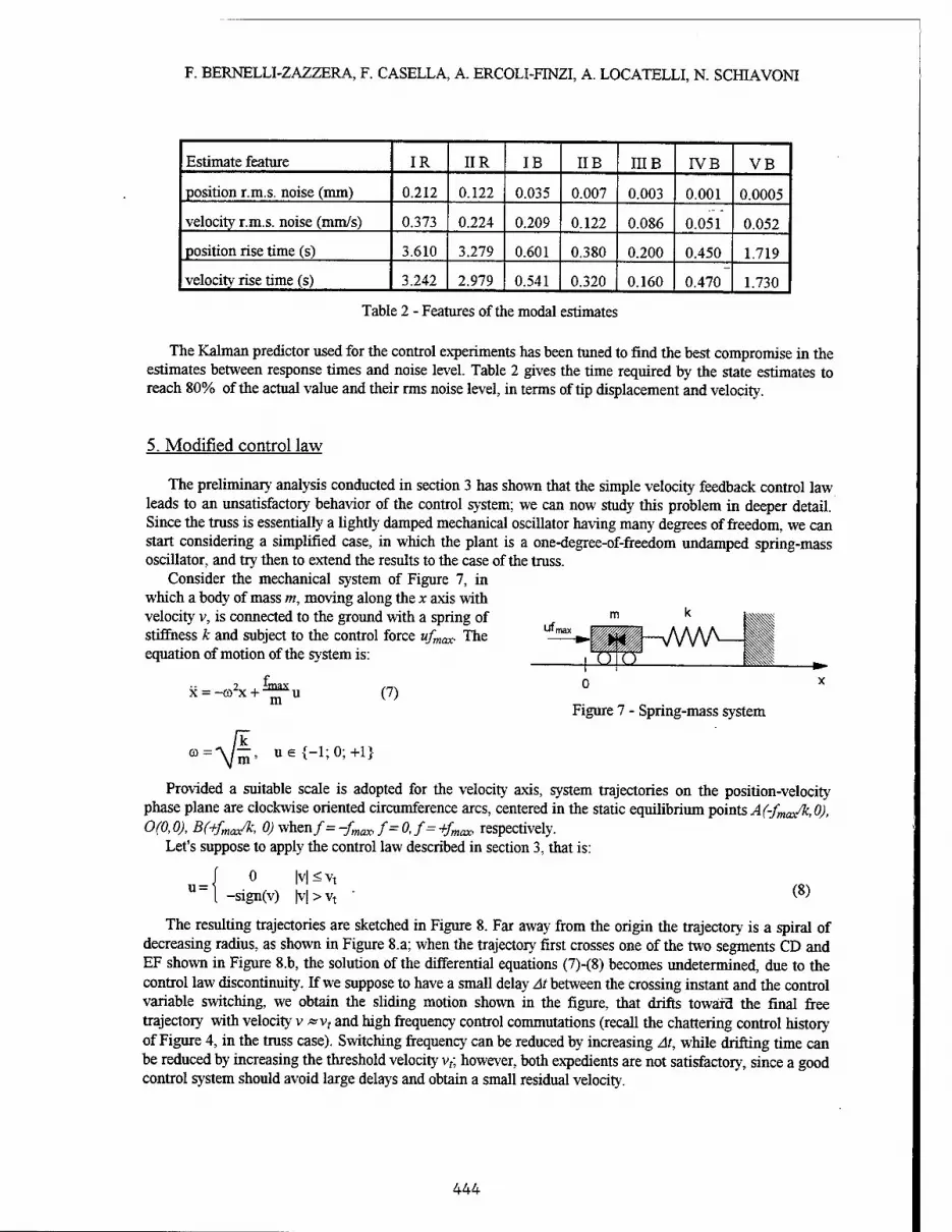
F. BERNELLI-ZAZZERA, F. CASELLA, A. ERCOLI-FINZI, A. LOCATELLI, N. SCHIAVONI
Estimate feature IR IIR IB IIB IIIB IV B VB
position r.m.s. noise (mm) 0.212 0.122 0.035 0.007 0.003 0.001 0.0005
velocity r.m.s. noise (mm/s) 0.373 0.224 0.209 0.122 0.086 0.051 0.052
position rise time (s) 3.610 3.279 0.601 0.380 0.200 0.450 1.719
velocity rise time (s) 3.242 2.979 0.541 0.320 0.160 0.470 1.730
Table 2 - Features of the modal estimates
The Kaiman predictor used for the control experiments has been tuned to find the best compromise in the estimates between response times and noise level. Table 2 gives the time required by the state estimates to reach 80% of the actual value and their rms noise level, in terms of tip displacement and velocity.
5. Modified control law
The preliminary analysis conducted in section 3 has shown that the simple velocity feedback control law leads to an unsatisfactory behavior of the control system; we can now study this problem in deeper detail. Since the truss is essentially a lightly damped mechanical oscillator having many degrees of freedom, we can start considering a simplified case, in which the plant is a one-degree-of-freedom undamped spring-mass oscillator, and try then to extend the results to the case of the truss.
Consider the mechanical system of Figure 7, in which a body of mass m, moving along the x axis with velocity v, is connected to the ground with a spring of stiffness k and subject to the control force ufmax. The equation of motion of the system is:
ufm
1 ff
x = -co2x + %su m (7) Figure 7 - Spring-mass system
© = m' ue{-l;0;+l}
Provided a suitable scale is adopted for the velocity axis, system trajectories on the position-velocity phase plane are clockwise oriented circumference arcs, centered in the static equilibrium points A(-fmco/k,0), O(0,0), B(+fmax/k, 0) whenf=-fmax,f=0,f=+fmax, respectively.
Let's suppose to apply the control law described in section 3, that is:
u = 0 M<vt
-sign(v) |v| > vt (8)
The resulting trajectories are sketched in Figure 8. Far away from the origin the trajectory is a spiral of decreasing radius, as shown in Figure 8.a; when the trajectory first crosses one of the two segments CD and EF shown in Figure 8.b, the solution of the differential equations (7)-(8) becomes undetermined, due to the control law discontinuity. If we suppose to have a small delay At between the crossing instant and the control variable switching, we obtain the sliding motion shown in the figure, that drifts toward the final free trajectory with velocity v «vr and high frequency control commutations (recall the chattering control history of Figure 4, in the truss case). Switching frequency can be reduced by increasing At, while drifting time can be reduced by increasing the threshold velocity vf; however, both expedients are not satisfactory, since a good control system should avoid large delays and obtain a small residual velocity.
444

MODIFIED DISCRETE TIME VELOCITY FEEDBACK FOR VIBRATION SUPPRESSION...
Figure 8 - Phase-plane trajectories of the spring-mass system
Some simple considerations about the physical motivations of this control behavior suggest a suitable modification of the control law. For example, let x > 0 and v < 0, so that -kx < 0 and f=fmax > 0: the elastic force of the spring is pushing the body towards the origin, while the control force is directed away from the origin. When the body passes through the equilibrium point x - fmax/k, the control force becomes predominant, so that the vector sum of the two is directed away from the origin. If the velocity towards the origin is low enough, it can become lower than the threshold before the origin has been reached, thus starting the high frequency control commutations. The simplest way to avoid that is to inhibit the activation of the control force whenever it is greater and opposite to the elastic force acting on the body.
The resulting control law and control system trajectory are shown in Figure 9; far away from the origin the trajectory is again a sort of spiral, while it can be easily proved that, once it has crossed the segment AB, further intersections with the x axis will occur at a distance from the origin
x(k+l) = (Vd2+x(k)2 - d), d = AO = OB (9)
Equation (9) describes a non-linear discrete time system, for which the origin is a globally stable equilibrium point, since x(k+l) <x(k) for the triangular inequality. In the neighborhood of the origin, eq. (9) can be approximated with the first non-zero term of its McLaurin expansion, that is
x(k+l)*x(k)^; |x(k)|«d (10)
showing how the trajectory asymptotically converges to the origin. The control law of Figure 9 should then
Figure 9 - Phase-plane trajectories of the spring-mass system
445

M V
u=-1 u=0 ■■' u=-1
-a„ vt ac c
-vt
U=+1 u=0 u=+1
F. BERNELLI-ZAZZERA, F. CASELLA, A. ERCOLI-FINZI, A. LOCATELLI, N. SCHIAVONI
be modified adding a velocity dead band, to avoid persistent control action in the neighborhood of the origin.
Figure 10 shows the resulting control law on the aei-v plane instead of the x-v plane, where aei = -kx/m is the acceleration term due to the spring force and ac = fmcJm is the acceleration that the control force can impress to the body. The reason of this particular representation will be clarified in the ael following.
This control law is the starting point for the derivation of the modified control law for the truss case. The basic idea is that each control section of the truss (i.e. each section on which an actuator is installed) is a body of a certain mass, subject to two kinds of forces: the local actuator thrust and the elastic force exerted by the remaining part of the structure, which is a function of its deformation state. If we are able to calculate the accelerations caused by these two forces, we can think of applying the control law of Figure 10 to each actuator. A theoretical analysis of the truss dynamics under this kind of control is not feasible, because there are many degrees of freedom and many independent actuators; however this extension seems reasonable, since the underlying physical motivations are the same of the spring-mass case.
The above considerations can be formalized as follows: consider the dynamical model of the truss
rj + 2Efif] + Q2n = <&'Mau (H)
x = Ms*r| ; v = Ms<Df) (12)
where x is the vector of the transverse displacements of the control sections and v the vector of the corresponding velocities. The term 2EQf| can be ignored, since, due to the low damping coefficients of the structure, it is at least one order of magnitude smaller than the control term. The dynamics of the control sections is therefore:
Figure 10 - The modified control law
x = -Ms$Q2r| + Ms<DO'Mau (13)
In other words, the instantaneous acceleration of each control section is the sum of two terms: the first one is a function of the modal amplitudes r\, i.e. of the state of deformation, the other one is a function of the control variables. Provided that the actuators are sufficiently spaced one from each other, the matrix M/b$>'Ma is almost diagonal: this means that the instantaneous acceleration of a control section depends mainly on its corresponding control variable and not on the others. We can therefore write that, for each actuator:
XJ =-kjT] + ajUj (14)
where kt is the i-th row of the matrix Ms<bQ? and at is the i-th diagonal element of the matrix Ms®Q>'Ma. At this point, we can think of using the same control law we obtained in the spring-mass case, that is the
one of Figure 10, in which ae! = -£;r| and ac = a{.
For each i ael = -km if (v; > -vt and 0 < ag] < a,) or (v; < vt and -a; < a^ < 0)
Uj = 0
else Uj = -sign(vi).
The actually used algorithm is slightly more complex, because some actuators are not widely spaced from each other, so that Mß>®'Ma is only block diagonal, but the underlying philosophy is exactly the same.
446

MODIFIED DISCRETE TIME VELOCITY FEEDBACK FOR VIBRATION SUPPRESSION...
0.4
Tip velocity °-2
(m/s) 0
-0.2 -0.2
Tip control
0 12 3 0 Time (s)
Figure 11 - Bending mode control system response
This control law has the same dissipative properties of the direct velocity feedback control law (6), since each control force is either zero or opposite to the actuator's velocity, thus subtracting energy from the structure. However, due to the heuristic derivation of the truss case, it's not possible to guarantee a priori that the control transient won't show high frequency commutations.
Extensive simulation of the control system, supposing accessible state information and lack of non- idealities such as delays in the control loop, has shown excellent performance when the first four bending modes only are controlled (i.e. the velocity components of the rigid modes are eliminated); as an example, Figure 11 shows the values of the tip velocity and of the corresponding control values when the first mode only (left - compare with Figure 4) and all the first four modes (right) are excited. Residual velocities as low as 1.5 mm/s can be obtained.
If we control the two rigid and the first four 0.4 r bending modes, instead, the behavior of the control system is not so good: for example, if we excite the first rigid mode only, unwanted oscillations arise on the bending modes, thus limiting control effectiveness (see Figure 12). In a real "free-free" truss, control of the rigid modes by velocity feedback would not be possible, but in the actual truss the rigid motion corresponds to a pendulum mode, which in principle should be easily controlled by a lateral force.
These oscillations can be explained if we consider that, for typical truss motion, rigid modes elastic forces correspond to accelerations not greater than 0.1-0.2 m/s2, much lower than those corresponding to the bending modes. The application of the control force causes the structure to bend, thus generating a reactive elastic acceleration that builds up very rapidly,
Tip velocity (m/s)
Tip control Q
2 3 4 Time (s)
Figure 12 Rigid and bending mode control system response
447

F. BERNELLI-ZAZZERA, F. CASELLA, A. ERCOLI-FINZI, A. LOCATELLI, N. SCHIAVONI
due to the higher frequency modes, to around 0.4 m/s2. The elastic acceleration term can therefore easily change sign, causing the control force to switch off; the elastic acceleration consequently decreases as rapidly as it had increased and changes sign again, so that high-frequency oscillations arise. In principle, we could avoid these oscillations by substantially lowering the actuators' thrust intensity; however this would unacceptably reduce the control system effectiveness on the bending mode vibration suppression.
From a conceptual point of view, the suppression of the rigid mode oscillations in the laboratory structure is not very significant, since their dynamics (suspension spring induced oscillations) is completely different from that of the real space environment (free inertial motion); we can therefore limit ourselves to bending mode vibration suppression, supposing that in space there will be an independent attitude control system. However, it is possible that, with a different choice of LSS geometric configuration, building materials and actuator thrust intensities, these unwanted oscillations arise not only when controlling the rigid modes, but also when controlling the lower frequency bending modes. This should be verified, for instance, using structural data from various proposed space-bom structure designs.
6. Experimental results
Experimental results are given for the above-mentioned controllers [6]. For each experiment, the truss tip velocity and the corresponding actuator's control variable are shown. Tip velocity has been calculated by processing the output of the accelerometers with the same Kaiman filter used for the controller; the low pass filter has been removed, so that the motion of the first two uncontrolled modes (5th and 6th) can be observed. Since the rigid modes are uncontrolled, we are not interested in their velocity components: the use of a Kaiman filter permits us to suppress them from the measurements simply by setting to zero the corresponding columns in the filter's output matrix; on the other side, the filter needs a certain settling time to give accurate results, expecially for the first bending mode (see Table 2). Initial conditions for the experiments are as follows: either a single bending mode is excited, so as to have a tip velocity of 25 cm/s, or all the first four bending modes are simultaneously excited, with tip velocities of 12, 12, 12, 4 cm/s respectively.
Figure 13 shows the response of the simple controller described in section 3, in which the second bending mode has been excited so as to have a tip velocity of 0.25 m/s and the velocity threshold has been set to 20 mm/s: the control system's response is clearly unstable.
If we use the state variable estimator, described in section 4, to obtain the velocity of the control sections, instead of the pseudo-integrators, we obtain the results shown in Figure 14.a from the top to the bottom, when the first, the second and all the first four bending modes are excited, respectively. The velocity threshold can be lowered to 4 mm/s without the system going unstable; however,
Figure 13 - Simple controller response
control chattering appears at the end of the control transient, in particular when exciting the first bending mode.
The introduction of the modified control law described in section 5 eliminates this problem, as can be seen in Figure 14.b; in addition it allows us to further reduce the residual velocity to 2.5 mm/s and to cut the air consumption of the actuators by 15-30%, depending on the initial conditions. The control spikes that sometimes appear in the end of the control transitories are caused by disturbances induced by the suspension springs, that are nearly resonant with the fourth bending mode of the structure.
448

MODIFIED DISCRETE TIME VELOCITY FEEDBACK FOR VIBRATION SUPPRESSION...
0.2 Tip 0.1
velocity 0
(m/s) -0.1 -0.2
a) Direct velocity feedback v, = 4 mm/s
Tip
control
1
0.5
-0.5
-1
4 6 Time (s)
10
lillllll ;
U ; ; ; | 10
-0.2
b) Modified velocity feedback v, = 2.5 mm/s
2 3 4 Time (s)
1
0.5
n PU i ■ "i i ' j ■■■■■—
0.5
-1 i II ; i : :
Tip
control
2 3 4
Time (s)
12 3 4 5 6
1
0.5
U If i
III ;i ■
-0.5 1 -1 LI U LI. u U 1
0.2 0.1
0
-0.1
1
0.5
0
-0.5r
-1
3 4
Time (s)
lllll III : : ! :
■ll : ;
Tip
1
0.5
control -0,i
||] pin ; 11- ; : : 2 3 4 5 6
Time (s)
Figure 14 - Experimental response of the bending mode control systems
449

F. BERNELLI-ZAZZERA, F. CASELLA, A. ERCOLI-FINZI, A. LOCATELLI, N. SCHIAVONI
7. Conclusions
A control system for vibration suppression in a laboratory model of a LSS, based on on-off air jet actuators, has been presented. Each actuator is activated according to a control law, that depends on the actuator's velocity and on the deformation state of the whole structure; both are obtained with a state estimator based on a discrete time, time-invariant Kaiman predictor. Experimental results in the control of the first four bending modes of the structure have been quite promising, and have largely confirmed the results of simulation studies. The proposed control law can however induce transient oscillations when trying to control vibration modes having very different intrinsic stiffness, in this case the rigid and the bending modes. Its applicability to other large flexible structures should therefore be subject to further study.
8. Acknowledgements
The authors are grateful to Marco Gruppi, who performed some work on the topic as a part of his graduation thesis.
9. References
[1]
[2]
[3]
[4]
[5] [6]
Ercoli-Finzi A., Gallieni D., Ricci S., "Design, Modal Testing and Updating of a Large Space Structure Laboratory Model (TESS)", Proceedings of the 9th VPI&SU Symposium on Dynamics and Control of Large Structures, Blacksburg-Virginia, 1993, pp.409-420; Bernelli-Zazzera F., Cristiani D., Ercoli-Finzi A., Guidotti A.,Locatelli A., Schiavoni N., "A Study on Nonlinear Control of Space Structures Using Active Members and Jet Thrusters", Proceedings of the 9th VPI&SU Symposium on Dynamics and Control of Large Structures, Blacksburg-Virginia, 1993 pp 505- 516; Bernelli-Zazzera F., Mantegazza P., "An Experiment on Active Control of Large Space Structures by Means of Jet Thrusters", Proceedings of the UthAlDAA Conference, Como-Italy, 1993, pp.1139-1147; Balas M.J., "Direct Velocity Feedback Control of Large Space Structures", Journal of Guidance and Control, Vol.2 n.3, 1979, pp.252-253; Anderson B. D. O., Moore J. B., "Optimal Filtering", Prentice-Hall 1979, pp. 105-115 Casella F., Gruppi M., "Progetto e Sperimentazione di un Sistema di Conrrollo Mediante Attuatori a Getto delle Vibrazioni di una Grande Struttura Flessibile", graduation thesis, Politecnico di Milano 1994.
450

DYNAMICS AND CONTROL OF FLEXIBLE TETHERED SYSTEMS: ANALYSIS AND GROUND BASED EXPERIMENTS
V. J. Modi* and S. Pradhan** The University of British Columbia
Vancouver, B.C., CANADA V6T 1Z4
and
A. K. Misra* McGill University
Montreal, Quebec, CANADA H3A 2K6
Abstract
A mathematical model is developed to study dynamics and control of a class of two-body systems, consisting of a flexible tether connecting a rigid platform with a point mass subsatellite, undergoing planar motion in a Keplerian orbit. The model incorporates translation of the tether attachment point and deployment/retrieval of the subsatellite. The governing equations of motion are obtained using the Lagrangian procedure. The offset control strategy, which involves movement of the tether attachment point, is used to regulate the attitude dynamics of the tether. The controller for the time varying rigid body dynamics is designed using the Feedback Linearization Technique (FLT). Finally, an experimental setup is described to validate effectiveness of the FLT based offset controller for regulating the attitude motion.
1. Introduction
With the advent of the Space Shuttle and the U.S. proposed Space Station, interest in the concept of Tethered Satellite Systems (TSS) has increased considerably due to a number of potential applications. These include scientific experiments in the microgravity environment, upper atmospheric research, generation of electricity, cargo transfer between orbiting bodies, collection of planetary dust without landing (Ref. 1), expansion of the geostationary orbit resource by having tethered chain satellites (Ref. 2) to name a few.
The potential of the tethered systems has led to many investigations on its dynamics and control during stationkeeping (constant tether length), deployment, and retrieval. The large body of literature generated over years has been reviewed by Misra and Modi (Refs. 3,4). Different control strategies have been developed to regulate the complex dynamics of these systems. They can be classified as: the tension or length rate control (Refs. 5, 6); the thruster control (Ref. 7); and the offset control (Ref. 8). Because of relative advantages and disadvantages of these methods for different tether lengths, it is desirable to use a hybrid strategy where the offset law can be used for shorter tethers and the thruster scheme for longer ones (Ref. 9). The studies by Modi et al. (Refs. 8,9) consider the tether as a rigid body and the offset strategy is used to control the libration of the tether. The present study extends this research to systems with a flexible tether, a rigid platform and a pointmass subsatellite. The main objective of this study is to validate the offset strategy for a system with a flexible tether. To that end, the equations of motion for planar dynamics are obtained by the Lagrangian procedure.
The attitude controller for the time varying tether dynamics is designed by the Feedback Lin- earization Technique (FLT). The control inputs are the moments applied by the momentum gyros for the platform pitch angle and the offset acceleration along the local horizontal for the tether swing. It is shown that a relatively simple control structure is sufficient to regulate the dynamics without implementing a gain scheduling procedure, which is normally used for time varying systems.
* Professor; Fellow AIAA, AAS; Academy Member IAA; Department of Mechanical Engineering ** Post Doctoral Fellow; Department of Mechanical Engineering
t Professor; Associate Fellow AIAA, Senior Member AAS; Department of Mechanical Engineering
451

V.J. MODI, S. PRADHAN AND A.K. MISRA
Finally, a ground based experiment is described to validate the offset strategy for control of the tether attitude. The FLT based controller, which is implemented in real time, is able to regulate the motion of the ground based tethered system quite successfully during the stationkeeping, deployment and retrieval modes of operation.
2. Mathematical Model
The TSS under consideration (Fig. 1) consists of four subsystems : platform; offset mechanism; tether; and subsatellite. As shown in Fig. 1, the frame Fp (Xp, Yp, ZP) is located at the center of mass of the platform and defines the librational motion of the platform. It is oriented along any arbitrary body fixed directions. The origin of the frame Ft (Xt, Yt, Zt) is fixed to the tether at the platform end and is used to define the motion (both rigid and flexible) of any elemental mass of the tether. The axis Yt is along the line joining the tether end points and is directed towards the subsatellite. Xt is parallel to the orbit normal X0, and Zt completes the right-handed triad.
Two additional reference frames are required to define the kinematics of any mass element in the system: inertial frame Fi (Xi, Yi, Z{) located at the center of Earth; and the orbital frame F0 (X„, Y0, Z0). The origin of the orbital frame is located at the instantaneous center of mass of the system and follows a Keplerian orbit. The orbital frame is so oriented that the Y0-axis is along the local vertical and points away from the Earth; the Z0-axis is along the local horizontal and points towards the direction of motion of the system; and the X0-axis is along the orbit normal completing the right-handed triad.
The platform is considered a rigid body free to undergo rotational motion and the subsatellite is modelled as a point mass. The offset mechanism, which moves the tether attachment point, is also considered to be a point mass. All the motions are restricted to the plane of the orbit. The relative orientation of different coordinate systems are expressed using the modified Euler rotations. The flexibility of the tether is modelled by the assumed mode method (Ref. 10). The effect of structural damping is incorporated by introducing Rayleigh's dissipation function (Ref. 11). Application of the Lagrangian procedure results in the nonlinear, nonautonomous and coupled equations of motion governing the system dynamics.
As can be expected, the complete set of equations are indeed extremely lengthy and hence are not presented here for brevity. The generalized coordinate vector of this system contains the platform
pitch angle (ap), the tether pitch (at), the modes for the longitudinal tether oscillation {Bi}^, and
the modes for the lateral vibration of the^tether {Ci}^- Here N\ and 2V2 represent number of modes for the transverse and longitudinal oscillations of the tether, respectively, used in the simulation. The vector of generalized forces is dependent on the control strategy used. It is obtained using the principle of virtual work.
3. Design of the Attitude Controller As mentioned before, it is advantageous to use the offset strategy for attitude control when the
tether length is small. This section presents the design procedure for the offset control for a class of tethered systems. For highly time varying systems, which is the case in this study, the commonly used control algorithms are: gain scheduling; adaptive/self-tunning control; simultaneous stabiliza- tion of multiple plants; and Feedback Linearization Technique (FLT). Particularly for systems whose mathematical model can be represented with a reasonable degree of accuracy, FLT controller is quite effective and does not have the disadvantages of other strategies. The disadvantages include design and implementation of controllers at multiple operating points in the gain scheduling approach; numerical problems associated with adaptive and self-tunning algorithms; and lack of simultaneous controllability of multiple plants over the operating domain. In the present study, the attitude dynamics of the system can be modelled quite accurately and hence the FLT is used for the controller design.
The purpose of the attitude controller is to regulate the rigid body rotation of the platform and tether. The dominant characteristics, which governs the system dynamics, is the time varying length of the tether during deployment and retrieval. The tether response is not significantly influences by the
452

DYNAMICS AND CONTROL OF FLEXIBLE TETHERED SYSTEMS
platform dynamics. However, with nonzero offset, the platform motion is strongly affected by the tether swing. Therefore design of the controller for the tether dynamics is based on the model decoupled from the platform motion. On the other hand, the model for the platform controller includes the effect of tether libration.
The pitch (at) equation for the tether dynamics is decoupled from the platform motion. The resulting equation is linearized about the quasi-equilibrium trajectory (öt) and the specified offset motion. The total offset position {dp} is the sum of the specified value {Dp} and" the controller coordinate {£>}. It should be pointed out that the prime objective of the design is to get a single controller expression applicable during deployment as well as retrieval of the tether. To that end, the linear equations were found to be sufficient. The resulting dynamic equations for the controller design are:
map(ap,x,t)äp + fap(ap,äp,x,x,t) = Qap;
ät = aiat + a,2Dx + a3ät + ait>z +b + cDz;
i>z = ut;
(1)
(2)
(3)
where as = {at, Dz, at, DZ}T■ Here Dz is the offset along the local horizontal required to control the
attitude motion (2—component of {£>}). The coefficients of the above equations are defined in Ref.(12). In the model for controller design, Eq.(3) is used to regulate the offset position and velocity.
For the platform pitch controller, the generalized force Qap can be selected as
Qap = map(ap,z,t)vp + fap(ap,äp,x,x,t). (4)
where vp is the secondary control input. It is selected to place the closed loop eigenvalues of the transformed system at some desired locations,
vp = kPl(aPd - ap) + kP2(äPd - at,) + äPd, (5)
where kPl and kP2 are the position and velocity feedback gains, respectively; and ap ., 6tp, and äp, represent the desired trajectory.
The model used for the tether controller design, Eqs. (2) and (3), can be expressed as
x = f(x) + g(x)ut, (6)
where: f(x) — <
X3
Xi aiXi + 02X2 + 03S3 + 04X4 + b
0
and g(x)
Here X{, i=l-4, are the elements of vector x. With quasi-static assumption, the functions /(x) and g(x) satisfy the feedback linearizability conditions (Ref. 13) and hence can be transformed to the canonical form. The state transformation, which achieves this specific form, is
z = T(x) = [tij]x, (7)
where:
*n = «2 + o-ic + 03(04 + 03c); tis = —04 — 03c;
*12 = -c(a2 + oic) + o4(o4 + a3c); *X4 = c(o4 + 03c);
453

V.J. MODI, S. PRADHAN AND A.K. MISRA
and for i = 2, 3,4
tu — oii(i_1)3; Uz = *(i-i)i + a3t(i_!)3;
The transformed system can be expressed as
d dT<
til —0-2t(i-l)3', tiA = %-l)2 + 04*(x-l)3-
r*i] f*2] f °) Z2
23 » = , zz > +«
0 0
. 24 j I 0 J ll J >«<• (8)
The control input (vt) of the transformed system is related to the original input (ut) by the expression
vt - P(x) ut =
Q{x) (9)
where: P(x) = oit43si + 02*4322 + (Ui + 03*43)33 + (t42 + 04*43)34; and Q(x) = ct43 + t44. Eq.(9) is referred to as the primary controller. The secondary controller, i.e. the controller for the system in Eq.(8), is designed to place the closed loop eigenvalues at some desired locations. This leads to the following expression for the transformed control input, vt,
vt = *tl(*i - *id) + M*2 - *2d) + kt3(z3 - zzd) + kt4(Zi - zid), (10)
where: kti and Zi&, i=l-4, are the coefficients of the desired closed loop polynomial and the desired values for Zi's, respectively. 2,d's can be computed from Eq.(7) with the knowledge of the desired x. Though this approach uses the quasi-static assumption where the system is treated as time invariant over small time-intervals, it avoids gain scheduling by obtaining a closed-form expression for the controller.
4. Results and Discussion
The nonlinear coupled differential equations governing the system dynamics were integrated numerically. Results were obtained for a wide range of system parameters involving the tether length, deployment/retrieval rates, arbitrarily fixed and moving tether attachment point in different directions, etc. Only a few typical results are presented here. The inertia and elastic parameters considered in the analysis are:
Ip = Inertia matrix of the platform,
'8,646,050 -8,135 328,108 1 -8,135 1,091,430 27,116 kg-m2; 328,108 27,116 8,286,760 J
nip = mass of the platform = 90,000 kg;
m0 = mass of the offset mechanism = 10 kg;
Pt = mass of the tether per unit length = 4.9 x 10⁻³ kg/m;
ms = mass of the subsatellite = 500 kg;
EA = 61, 645 N.
Here, E is the Young's modulus of the tether material and A, the cross-sectional area of the tether. The system negotiates a circular trajectory with a period of 90.3 minutes. The structural damping considered in the simulation corresponds to a damping ratio of 0.5% based on the first natural frequency of the longitudinal oscillation of the tether. In the simulation, the Xp and Xj-axes are oriented parallel to the orbit normal (X0). The platform and tether pitch angles (ap, at) are the angles between the local
454

DYNAMICS AND CONTROL OF FLEXIBLE TETHERED SYSTEMS
vertical (i.e. Y0-axis), and Yp and Yt-axes, respectively. The longitudinal and lateral elastic motions of the tether are measured with respect to the frame Ft. In these definitions, the subscript 'p' and 'f' refer to the platform and tether, respectively.
Typical dynamic simulation results for operations at a shorter tether length {L) where the offset control strategy is more efficient are shown in Fig. 2. It considers a case of retrieval from L =200 m to L =50 m with an exponential velocity profile. The negative value of L during retrieval makes the system unstable. The tether pitch angle (at) grows upto ±50°. The transverse mode (Ui) grows and eventually oscillates between ±3 cm even without any initial disturbance. The mean value of the Bi response decreases with the tether length. As expected, for zero offset, the platform pitch response is not affected by the retrieval maneuver.
The controllers designed for the platform and tether pitch angles were implemented on the com- plete flexible, nonlinear and coupled model. Intentional modelling errors are introduced by neglecting the shift in the center of mass terms from the controller model, but the corresponding terms are retained in the simulation. For controlled simulation during stationkeeping at a tether length of 200 m, the rigid modes are stabilized to some steady state value, but the performance of the system is not satisfactory (plot not shown). The desired steady state value for ap and dpZ are 0 and 1 m, respectively. The controller does not achieve these steady state requirements. When the shift in the center of mass terms were included in the controller model, the steady state value of ap became zero. However, the steady state value of dpZ still remained less than the required magnitude of 1 m.
It was decided to introduce, an outer integral loop to reduce the steady state error. The schematic diagram of the controllers with the integral loop is shown in Fig. 3. With this, the structure of the primary controller in Eq.(9) becomes
vt - P(x) y* Ui = Q(x) + Kl j0
DAt + KpDz' <U)
where Kj and Kp are the integral and proportional gains, respectively. The secondary control input vt
was obtained as before using Eq.(10). In the present simulation, the gains are: Kj = —1.5 x 10~9; and Kp = 1.0 x 10⁻⁶. The response of the system with the integrator loop is presented in Fig. 4. Now, the steady state offset is 1.0 m as commanded.
The response of the system during the controlled retrieval from tether length of 200 m to 50 m in 1 orbit is shown in Fig. 5. An exponential velocity profile is used for the retrieval. The generalized coordinate for the transverse vibration (Ci) grows close to 2 cm even with zero initial condition. The initial disturbance in the first longitudinal mode (J5X) decays quite rapidly due to the structural damping, however there is a steady oscillation with a relatively small amplitude due to coupling with the transverse vibration (inset in Ux plot). The platform pitch response settles down to zero within 0.4 orbit. The tether pitch angle is stabilized about the quasi-equilibrium position which is zero after the retrieval. The moment (Mx) required to control ap is only 4 Nm. The offset position required to control the tether swing is between +12 m and -5 m. This is well within the limit of ±15 m for the present study.
5. Experimental Procedure
Numerical simulation results show effectiveness of the offset control strategy to regulate the attitude dynamics of the tether. This section describes a ground based experiment carried out to demonstrate effectiveness of the attitude controller. The feasibility of the offset control strategy by experimental simulation was first shown by Modi et al. (Ref. 8). An LQR based algorithm was used to control tethered satellite oscillations. The main problem with this form of controller is that of gain scheduling for time varying systems. In the present study, a controller based on the FLT is implemented in real time. As mentioned earlier, this algorithm does not involve any gain scheduling during deployment or retrieval of the subsatellite.
455

V.J. MODI, S. PRADHAN AND A.K. MISRA
c o a x v G
V
d v
>> 13 M _H a a >» V -1-3
l-l O
tf > M
V (H
3 M
T3
u
5 >> CÖ 03
S) M -■3
-a a u ^
■s ° (S o E ü
S. 3 bo
Es*
456

DYNAMICS AND CONTROL OF FLEXIBLE TETHERED SYSTEMS
pz
KPo FLT controller for tether
». \
. 4- n . .
J Plant
~p2 -rA
'o —►
+ " Dz U Output
►-
Qrv aP FLT controller for platform
Figure 3 Schematic diagram of the closed-loop system with outer integral loop controller.
The experimental setup consists of a spherical mass, representing the subsatellite, which can be deployed or retrieved from a carriage (Fig. 6). The carriage can be moved in a horizontal plane thus permitting motion of the tether attachment point to implement the offset control strategy. A Nylon thread, 1 mm in diameter, served as tether. The tether can have a maximum length of 2.25 m. The angular deviation of the tether from the vertical position is measured by a pair of optical potentiometers. In the original setup (Ref. 8), a pair of resistance potentiometers were used and the sensing mechanism was not dynamically balanced. In the present study, a better sensor and sensing mechanism have been designed to improve the system output by having a dynamically balanced system.
5.1 Controller Design and Implementation
The linearized governing equations representing the laboratory model of the tethered satellite system can be written as:
ä = OiQ + a3ä + cda;
7 = ai7 + 037 + cdy;
(12)
(13)
where: ai = —g/L; a.3 = —2L/L; c = l/L; L is the instantaneous tether length; g, the acceleration due to gravity; a and 7 are the tether angles in two orthogonal vertical planes; and da and cLy are the accelerations of the offset point for controlling a and 7, respectively. The a and 7 equations are independent of each other and hence the controllers can be designed separately. They were obtained using the FLT procedure described earlier (Eqs. 7, 9 and 10).
The continuous time controller is implemented as a sampled data system with zero order hold. The sampling period (At) is a critical parameter governing the system performance. At has to be sufficiently large so that the computations required in the control loop can be completed. In the present
457

V.J. MODI, S. PRADHAN AND A.K. MISRA
1 y co y- ^ , . J3
orb
.-■>
in o in ■ä
! '" V. "- "3 ■£ E 1 ei ! / /
> C^
~" >
1 O II I ^_^^, ^ -*3 V
tn ~ ! (, 1 SO i - Efc- !
\ f-sl LEI \ LEJ<C^ o
ö
c o in
s
~a V
"o CO O c
^ ° o £W 11 o o o
0 0°. in o o 9 in d y CG
T- - O O i- er D
8~ 1 a o 60 O
.5 a o co
o E | 3 >>
O N u ii © u 0 in Ja
C f O x ! / O >
CO c l .. i- q , \ / "'■§ <M ö ö ;
Sys
tem
ex
pone
li ll II ;
o o o aa co" o": fe; 1<^:
E! / r) j /
x! / !E: o —' ^^ O . o
in O O CM o o o o o o o T- O *- o
CM O O o ■* o CM O o o o 4)
3 a 1
W - tüO m
o o CM
£ o
_i II
D> n C a. CD E CD o c o
1 .2 II CO
55 a
Q
o E 'CM ~
II °
O X
co E o- T o CM O o II II II
o o o
a m O
J=l
ja
c o a m
S ä •« § "o "3
ü .S
u S U)
458
DYNAMICS AND CONTROL OF FLEXIBLE TETHERED SYSTEMS
setup, as found from the experimental results, the time required to perform sensing, computation, actuation and data storage, was less than 2 ms. So the above mentioned factors do not have any importance in selection of the sampling time. The governing factor requires the frequency of the sampled data system to be higher than the Nyquist frequency. For better performance of the system, the sampling time should be less than one sixth of the minimum period of the system (Ref. 14), which is 1.45 s in the present case. From this consideration, the sampling time (At) is taken to be 100 ms.
The computer program to implement the controller was written in MicroSoft C language. The real time implementation begins with the initialization and calibration of the potentiometers. Appli- cation of any disturbance starts the control loop. Each loop consists of measurement of the angles; computation of the offset position, velocity and acceleration; checking for the steady state and safety conditions; and recording the data into the output file. After the data are written, the program waits till the time reaches At and then the loop continues. The controller operation can be stopped at any time by a keyboard command. The flow chart for the controller operation is shown in Fig. 7.
5.2 Results and Discussion
The controller based on the FLT was found to be quite effective in real time with the experimental tethered satellite model. A series of tests were carried out during different phases of tether operations. Only a small sample of representative data is recorded here. It should be pointed out that the energy dissipation in the real system due to aerodynamic drag and Coulomb friction in the potentiometers are very difficult to model mathematically or eliminate from the experiment. The other characteristics which may cause discrepancy between the controlled experimental and numerical results are:
(i) missing pulses in the stepper motor;
(ii) noise in the measurement due to residual dynamic imbalance of the sensing mechanism;
(iii) nonlinearities of the real system due to backlash in the sensor and actuator drive systems, and friction at the linear bearings.
During the experiment, the system was subjected to a large disturbance of around 10° to assess the controller effectiveness under a demanding situation. In practice, an external disturbance would seldom result in deviation larger than a few degrees. The experimental results for stationkeeping at a tether length of 2 m are compared with the numerical result in Fig. 8. The numerical results match with the experimental data quite closely, implying that the mathematical equations represent the experimental model quite accurately. The small discrepancy can be attributed to the sources of error mentioned earlier. A single FLT based controller was used to regulate the system during deployment, retrieval and stationkeeping phases. A sample plot for retrieval of the subsatellite, from L = 2 m to L = 0.5 m in 10 s, is shown in Fig. 9. The instability of the uncontrolled system is quite evident from the growth of amplitude during retrieval. The controller is indeed quite effective in damping both the inplane and out-of-plane tether oscillations. The angles a and 7 settle to zero within 6 s with the offset requirement of around 20 cm. The controller was found to be quite successful even with faster retrieval and different rates of deployment (not shown).
6. Conclusions
The equations of motion are obtained for a class of orbiting systems consisting of a flexible tether connecting a rigid platform with a point mass subsatellite. The formulation includes deploy- ment/retrieval of the subsatellite and translation of the tether attachment point at the platform end. The Lagrangian procedure is used to obtain the equations of motion. The attitude controller, for de- ployment, retrieval and stationkeeping modes, is designed using the Feedback Linearization Technique (FLT). The controller based on the rigid body model is implemented on the complete flexible nonlinear dynamics. An outer PI control loop is introduced to improve the system performance. Simulation re-
459

V.J. MODI, S. PRADHAN AND A.K. MISRA
tfl
Qi CD h ttl
a X3 03
> <D F
Sa a> Ä
c ?.a F U) 0
H^\ o Q.
oc \ < h*- "O <n 1- i- / <ü -J 01/ T3 IÄ"-
n a> —~
v> ?s c <° h
o. 0 c
7 o o
<
03
'S Q 15
p 7-
ß
S V
6
u -*J
tm ;Z3 a O
o e o cn
V -4J TJ (rt 3
XI -*^> ^J
£ id O u
fc X5
t- u u 3 UJ
et LU X h- LU (-
er 0,r-2 t- fF, co °K§ 5Lu< .,21
ui<0° <iu 5 2
AR
R
ETR
O
TE
ING
Ott a. et
er LU
LU I- co
-ja-co
i- er O zaE Rar« QHO LU O ü COS < <c ^ CD 0. <
LU H ÜH< CLUlO
\ -\ ülh
V 5°| J \ vjy
^11
BO td
g 43
CO
V u 3 b0
460

DYNAMICS AND CONTROL OF FLEXIBLE TETHERED SYSTEMS
o
c 2
U cti
H
05
1)
3
en r 0) F
E CD n OJ X
_j
, Ö) i c , Q.
<D . d> 1 J£
i £Z i O
CO
en
o O
CD o II
0) S a H ?- = 3 . 2
■?* O £ ■r- O 1 II u
ab l a u-
Ü
o d
o ö
?-
o Ö
60
c o
3 -a
c o
a o
a E o Ü
00
<0 u 3
461

V.J. MODI, S. PRADHAN AND A.K. MISRA
suits show the effectiveness of the offset strategy in controlling the attitude dynamics of a flexible tether. A simple FLT based controller is shown to be quite effective during all the three operational phases, i.e. deployment, stationkeeping and retrieval. The ground based experimental results substantiate the attitude control law in real time.
7. References
1. Pasca, M., and Lorenzini, E., "Collection of Martian Atmospheric Dust with a low Altitude Tethered Probe," AAS/AIAA Spaceflight Mechanics Meeting, Houston, Texas, U.S.A., February 1991, Paper No. AAS-91-178.
2. Yasaka, T., "Geostationary Chain Satellite - Expanding Orbit Resource," 36th Congress of the International Astronautical Federation, October 1985, Paper No. IAA-85-483.
3. Misra, A. K., and Modi, V. J., "Dynamics and Control of Tether Connected Two-Body System - A Brief Review," 33rd Congress of the International Astronautical Federation, France, 1982, Paper No. IAF-82-315; also Space 2000, Editor: L.G. Napolitano, AIAA Publisher, pp.473-514.
4. Misra, A. K., and Modi, V. J., "A Survey on the Dynamics and Control of Tethered Satellite Sys- tems," NASA/AIAA/PSN International Conference on Tethers, Arlington, VA, U.S.A., September 1986, Paper No. AAS-86-246; also Advances in the Astronautical Sciences, Editors : P. M. Bainum et al., American Astronautical Society, 62, pp.667-719.
5. Rupp, C. C, "A Tether Tension Control Law for Tethered Sub-satellite Deployed along Local Vertical," NASA TM X-64963, September 1975.
6. Bainum, P. M., and Kumar, V. K., "Optimal-Control of the Shuttle-Tethered System," Ada Astronautica, 7, 1980, pp.1333-1348.
7. Banerjee, A. K., and Kane, T. R., "Tethered Satellite Retrieval with Thruster Augmented Con- trol," Journal of Guidance, Control and Dynamics, 7, 1984, pp.45-50.
8. Modi, V. J., Lakshmanan, P. K., and Misra, A. K., "Offset Control Strategy for the Space Station Based Tethered Payload," The Journal of the Astronautical sciences, 39, 1991, pp.205-232.
9. Modi, V. J., Lakshmanan, P. K., and Misra, A. K., "On the Control of Tethered Satellite Systems," Proceedings of the AIAA/ ASME/ ASCE/ AHS/ ASC 32nd Structures, Structural Dynamics, and Materials Conference, Baltimore, Maryland, U.S.A., April 1991, Paper No. AIAA-91-1002, AIAA Publisher, Part 4, pp. 2865-2876; also Ada Astronautica. 26, 1992, pp. 411-423.
10. Xu, D. M., The Dynamics and Control of the Shuttle Supported Tethered Subsatellite System, Ph.D. Thesis, Department of Mechanical Engineering, McGill University, 1984, pp. 67-70.
11. Greenwood, D. T., Principles of Dynamics, Prentice Hall Inc., New-Jersy, 1965, p.490.
12. Pradhan, S., Modi, V.J. and Misra, A.K., "Control of Tethered Satellite Systems using Thruster and Offset Strategies," International Journal of Control, in press.
13. Su, R., "On the Linear Equivalents of Nonlinear Systems," Systems and Control Letters, 2, 1982, pp.48-52.
14. deSilva, C. W., Control Sensors and Actuators. Prentice Hall, Englewood Cliffs, New Jersey, U.S.A., 1989, pp.5-30.
462

THE USE OF BOUNDARY MASSES IN MODAL ANALYSIS AND CORRELATION OF LARGE SPACE STRUCTURES
Sergio Ricci Politecnico di Milano
Milano, ITALY
and
Mordechay Karpel Technion-Israel Institute of Technology
Haifa, ISRAEL
Abstract
The paper presents a methodology, based on the use of fictitious masses, for the analysis and the modal synthesis of structural components. The applicability of the methodology has been experimentally verified by tests of a space-like truss performed at the Dipartimento di Ingegneria Aerospaziale of Politecnico di Milano. Some results of numerical simulations, showing the advantages of this methodology during the finite element model updating, are also reported.
1. Introduction
During the last years, many significant experimental facilities reproducing most of the dynamic and environmental characteristics of Large Space Structures (LSS) have been developed. The main interest in this activity is the need to study and solve the many problems typical of LSS; the most notable are low weight and modular topology (for ease of transportation and assembly), lack of ground support, almost null effect of gravity loads, and the very high pointing accuracy required in the nominal operating conditions and during attitude acquisition maneuvers. For these reasons ground vibration tests are essential for the verification of the dynamic properties of the LSS, desirably in their operational configuration. On the other hand, practical and economic considerations suggest not to perform full scale ground vibration tests, because obvious environmental difficulties like size, high flexibility, assembly and support, make it very difficult, expensive and sometimes risky. A potential solution to this problem is to divide the structure into several substructures and to perform the test by parts. This approach is valid only if the tests on individual parts provide enough information to adequately predict the dynamic properties of the assembled structure. Since during the modal analysis only a small set of low natural frequencies and modes are identified, the properties near the boundaries between different components might not be adequately represented in these low-frequency component modes.
Many methods are reported in the literature for accelerating convergence in substructure coupling, mainly based on the use of the so called "fixed-end" or "free-end" adjoint modes [1-4]. In the "fixed-end" case, for example, the modal basis of the structural components are composed by a limited number of rigid and flexible modes plus a certain number of static modes, obtained by loading the boundaries by elementary forces. These static modes are used to take into account the behavior of the structure close to the boundaries. This approach is not so easily applicable during the experimental modal testing because of difficulty in generating and measuring the adjoint static modes, especially in the case of very flexible structures, such as the LSS.
An alternative approach appears to be one based on the use of "fictitious masses." This approach, suggested during the 70s by Newman and Karpel [5], has shown a good efficiency in many numerical applications, including aeroelastic, dynamic response and active control problems. In this method, the dynamic properties of the separate components are computed with their boundaries loaded with rigid heavy
463

SERGIO RICCI AND MORDECHAY KARPEL
dummy masses. Using these large masses, the low frequency modes contain local deformations directly related to the structural behavior near the interfaces. These boundary modes are fundamental in order to obtain the dynamic properties of the components when combined with others, and to accurately tune the finite element (fem) model on the basis of modal testing results, mainly in presence of near-boundary modeling errors.
The two main purposes of this paper are : first to demonstrate the applicability of fictitious-mass method in experimental modal analysis and the second is an evaluation of the advantages related to the use of this method during the correlation and model updating phase. For this purpose, both numerical and experimental results are presented.
2. The Fictitious Mass Method
We present here only the main bases of the fictitious mass method. For a full description see Refs. 5 and 9. The main difference between the original formulation of the method and one used to extend its application to experimental modal analysis is the use of a fictitious stiffness as well. In reality, the large fictitious mass cannot be directly connected to the structure being tested, especially in the case of very flexible structures, but must be supported by an "ad hoc" suspension system, modeled here by means of springs. The term "fictitious mass" is inappropriate in the case of experimental applications, because this mass is not quite "fictitious", having a comparable value to that of the entire structure. In the following, the terms boundary mass (BM) and stiffness are adopted. The equation of motion of a structural component loaded by boundary mass and stiffness can be expressed as:
M,.
Ml Mbb + Mt f\\.ub +
Kib Kbb Kf ■0 (1)
where the mass and stiffness matrices [M] and [K] (of order n) are partitioned with respect to the internal i and boundary b degrees of freedom, used to connect the component to the others, [Mfl and [Kfl are the boundary mass and stiffness matrices respectively. The solution of Eq. (1) gives the eigenvalues [cofl and eigenvectors [§fl, with generalized mass :
[GMf] = [*f]T[M] M+[*fbf[Mf] [^] (2)
where [<jtyj,] includes the rows of [<jy] related to the boundary d.o.f. {ub}. Let consider now the same equation for the structural component without boundary mass and stiffness :
rM, Mih~ J*L r*,v %ib
Mjb Mbb_ kr ßib Kbb. ub
= 0 (3)
The basis of the method consists of the hypothesis that the displacements of the structural component without boundary mass and stiffness can be represented as a linear combination of the first tif modes [((y], with n-f« n, and thus :
ub fc/}
The substitution of Eq. (4) into Eq. (3), and the use of Eq. (2) yield :
W/]-[^]lM/][^]]fe}+fK]1GM/]-K]^/][^]]fe/}=w
(4)
(5)
Equation (5) can be solved for the rif eigenvalues [co„] and eigenvectors [v)f„] that are approximations of the eigenvalues and eigenvectors of the unloaded structural component : the natural modes can be then expressed as :
464

THE USE OF BOUNDARY MASSES IN MODAL ANALYSIS AND CORRELATION ...
M (6)
and the generalized mass by :
[GM] = [V„f[[GM/]-[v]r[M/][^])[¥„] (7)
The low frequency eigenvalues of [co„] and the corresponding eigenvectors [((>] are identical to those of the unloaded structural component : the high frequency ones reflect the local structural behavior close to the boundaries, and do not represent necessarily natural modes of the unloaded structure. For the sake of simplicity in the following the term Modal Coupling will be used to indicate the solution of Eqs.(5-6).
Based on the previous assumptions, it's possible to formulate the equation of motion of a structural component as a part of free vibrations of a complex structure. The modal coupling of the different structural components can be performed by imposing boundary displacements and forces compatibility.
3. Application to the TESS Structure
We would like to recall here the main results reported in [11], concerning the application of the Modal Coupling to a real test case, as part of the Truss Experiment for Space Structures (TESS). The structure was a space-type truss 20 m long, developed at the Dipartimento di Ingegneria Aerospaziale of Politecnico di Milano. This truss, loaded at one end with a 105 Kg cross-shaped steel mass hang on suspension springs, was tested using a standard modal survey equipment. While statically hung the truss and the BM show the same deflection so as to avoid local loads when connected together. Because of the configuration of the diagonal elements, the horizontal plane (x-z) is plane of symmetry. In this way, the lateral and axial natural modes are decoupled by the vertical and torsional ones, so we can apply the Modal Coupling procedure on the lateral modes only, without any loss of generality.
Fig.l - The TESS structure.
465
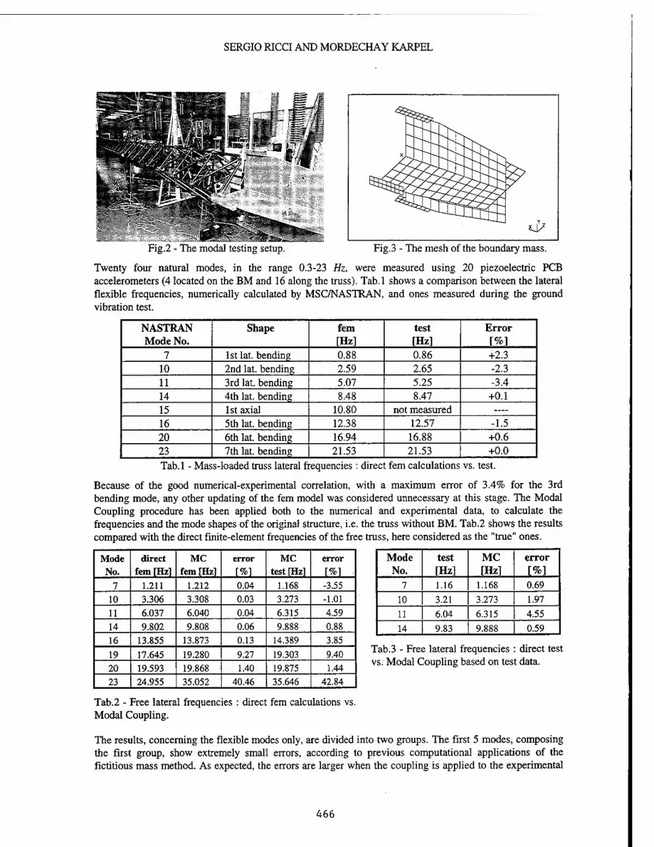
SERGIO RICCI AND MORDECHAY KARPEL
xX~^ ~^"^~-
u> Fig.2 - The modal testing setup. Fig.3 - The mesh of the boundary mass.
Twenty four natural modes, in the range 0.3-23 Hz, were measured using 20 piezoelectric PCB accelerometers (4 located on the BM and 16 along the truss). Tab.l shows a comparison between the lateral flexible frequencies, numerically calculated by MSC/NASTRAN, and ones measured during the ground vibration test.
NASTRAN Mode No.
Shape fern [Hz]
test [Hz]
Error [%]
7 1st lat. bending 0.88 0.86 +2.3 10 2nd lat. bending 2.59 2.65 -2.3 11 3rd lat. bending 5.07 5.25 -3.4 14 4th lat. bending 8.48 8.47 +0.1 15 1st axial 10.80 not measured —
16 5th lat. bending 12.38 12.57 -1.5 20 6th lat. bending 16.94 16.88 +0.6 23 7th lat. bending 21.53 21.53 +0.0 Tab.l - Mass-loaded truss lateral frequencies : direct fern calculations vs. test.
Because of the good numerical-experimental correlation, with a maximum error of 3.4% for the 3rd bending mode, any other updating of the fern model was considered unnecessary at this stage. The Modal Coupling procedure has been applied both to the numerical and experimental data, to calculate the frequencies and the mode shapes of the original structure, i.e. the truss without BM. Tab.2 shows the results compared with the direct finite-element frequencies of the free truss, here considered as the "true" ones.
Mode No.
direct fem[Hz]
MC fern [Hz]
error [%]
MC test [Hz]
error [%]
Mode No.
test [Hz]
MC [Hz]
error [%]
7 1.211 1.212 0.04 1.168 -3.55 7 1.16 1.168 0.69 10 3.306 3.308 0.03 3.273 -1.01 10 3.21 3.273 1.97 11 6.037 6.040 0.04 6.315 4.59 11 6.04 6.315 4.55 14 9.802 9.808 0.06 9.888 0.88 14 9.83 9.888 0.59 16 13.855 13.873 0.13 14.389 3.85
jquencies ised on tes
19 17.645 19.280 9.27 19.303 9.40 lab.ä - rree lateral tr vs. Modal Coupling b*
direct test t data.
20 19.593 19.868 1.40 19.875 1.44 23 24.955 35.052 40.46 35.646 42.84
Tab.2 - Free lateral frequencies : direct fern calculations vs. Modal Coupling.
The results, concerning the flexible modes only, are divided into two groups. The first 5 modes, composing the first group, show extremely small errors, according to previous computational applications of the fictitious mass method. As expected, the errors are larger when the coupling is applied to the experimental
466

THE USE OF BOUNDARY MASSES IN MODAL ANALYSIS AND CORRELATION .
modes, but even in this case they are under 5 %. The second group contains the modes showing high errors (modes 19 and 23). It must be emphasized that these high errors are almost equal when the coupling is applied to the numerical and the experimental modes. Thus these errors are not simply related to incorrect measures. In fact these errors mean that the modes 19 and 23 (1st axial and 7th bending mode, respectively) are not natural modes of the free truss, but represent the so called "boundary modes" , i.e. modes with large deformations near the boundary point, as demonstrated in Fig. 4, where comparisons between the test coupling and the directly calculated mode shapes are shown. The plots concern the lateral bending modes only, and the reported deflections are ones at the measurement points. The near-boundary large distortion of the mode 23 is typical of boundary modes resulting from the mass-loaded truss. The accuracy of the obtained results is also demonstrated in Tab.3 where the coupled frequencies are compared to the experimentally measured ones (for the first 4 bending modes only), obtained during a previous test on the original truss. It can be observed that the modal coupling yielded frequency errors of less than 5 %.
1st bending mode (No.7 Nastran) 1.21 [Hz] 5th bending mode (No. 16 Nastran) 13.86 [Hz]
0 10 20 3D 40 SO
2nd bending mode (No. 10 Nastran) 3.31 [Hz]
10 20 30 40 50
6th bending mode (No.20 Nastran) 19.59 [Hz]
0 10 20 30 40 SO
3rd bending mode (No. 11 Nastran) 6.04 [Hz]
0 10 20 30 40 SO
7th bending mode (No.23 Nastran) 24.95 [Hz]
0 10 20 30 40 SO
4th bending mode (No. 14 Nastran) 9.80 [Hz]
20 30 Bays
Direct Nastran
Modal Coupling
Fig.4 - Modes of the free unloaded truss : nominal vs. Modal Coupling based on test data.
4. The Model Updating
The presence of the boundary modes in the modal basis is very important during the updating of the finite element model in order to correlate its frequencies to the measured ones, mainly in presence of modeling errors close to the near boundary zone. In order to investigate this aspect, as the. available mesh results already well correlated, some modeling errors have been numerically simulated, and the model updating has then been performed using MSC/NASTRAN Sol.200, on the basis of the following hypotheses :
• The considered mesh is composed of ROD elements with the cross sectional area constitutes the design variables during the updating process ;
• Only the lateral modes have been considered ;
467

SERGIO RICCI AND MORDECHAY KARPEL
• Only errors in the stiffness modeling have been simulated ;
• The modal basis is composed by 11 modes : 3 rigid, 7 bending and 1 axial mode ;
• The structural mass has been constrained to be constant during the computation.
The updating problem has been stated as a classical structural optimization problem, using the DEQATN cards, allowing the Sol.200 of MSC/NASTRAN user-defined functions to be considered as constraint and/or objective functions during the optimization [12]. Particularly, the normalized errors between the eigenvalues of a baseline structure, here considered the "real structure" to which the modal testing has been performed, and those of an initial structure, on which modeling errors have been introduced, are considered as constraint functions. The objective function is constituted by a quadratic sum of these errors. Having limited the problem to the horizontal plane only, seven constraint functions have been considered, as many as the identified bending modes. The axial mode was included in the modal basis, but has not been explicitly considered during the updating. The model updating has then been formulated as a classical structural optimization problem:
\2
min 7
I; 1
Eigrii -Eigni B\
\\ Eignf
subject to
= 100.0
-0.K Eign;-Eign}
Eignf
B\
* 100.0 <+0.1 i= 1,7
where Eignt = i - th eigenvalue
Eigni = i - th eigenvalue of the baseline structure
Since the considered truss is composed of 54 bays, a variable linking operation is necessary, to group many structural elements in the same design variable, so as to avoid a highly over determined problem, requiring a least square solution. Two configurations have been analyzed, coming from two different linking operations. In the first configuration the 54 bays are divided into 9 modules, each one composed of 6 bays and related to the same design variable, the cross section area of the ROD elements of the lateral longerons (Fig.5).
Modules 123456789
, X=0.
1-6 7-12 13-18 19-24 25-30 31-36 37-42 43-48 49-54 Bays
Fig.5 - Configuration 1 : 9 design variables.
In the second configuration, in order to evaluate the influence of localized modeling errors, the original structure has been divided into 12 not uniform modules, composed respectively by 1-2-3-5-7-9 bays and so on symmetrically along the X axis, as shown in Figure 6.
, Modules 6 7 10 11-*2
1 2-3 4-6 7-11 12-18 19-27 _, 28-36 Bays 37-43 44-48 49-51 52-53 54
Fig.6 - Configuration 2 : 12 design variables.
468

THE USE OF BOUNDARY MASSES IN MODAL ANALYSIS AND CORRELATION ...
Updated elements
horizontal longerons .... Constant elements
Fig.7 - Variable and constant structural elements.
The optimization processes have been performed on two meshes at the same time, with and without Boundary Mass. The structural elements different from ones composing the lateral longerons have been constrained to be constant "(Fig.7). Two optimization cases will be reported, concerning errors in the stiffness modeling, uniformly and not uniformly distributed along the truss.
4.1 The Sensitivity Analysis
Before discussing the optimization results it is very interesting to analyze the constraint sensitivities (DSCM2 matrices), i.e. the derivatives of the eigenvalue errors with respect to the design variables. Figures 8 shows in a 3D block diagram format these matrices in the case of 9 design variables (configuration 1), without and with boundary mass : the i-th row reports the derivatives of the constraint on the i-th eigenvalue and so on. Figure 9 reports the same values, but in a contour plot format.
s
12 3 4 5 6 7
Design Variables
25
20
7 1 15
5 1«9 10
3 TSJ 5 1 l?U\JsJniQ 0
s
2 3 4 5 6 7
Design Variables
8 9
Fig.8 - The eigenvalues errors derivatives for the configuration 1 : without vs. with BM.
a) DSCM2 matrix (without BM) 7
b) DSCM2 matrix (with BM)
2 4 6 8 Design Variables
2 4 6 8 Design Variables
Fig.9 - Isosensitivity curves without (a) and with Boundary Mass (b).
The contour representation is quite unusual and maybe unrealistic in this case, since the problem does not involve continuous variables. Nevertheless, this kind of representation offers an immediate explanation of what happens when boundary modes are included in the modal basis during the updating process. The plot concerning the structure without BM is obviously symmetric, since the structure is homogeneous along the
469

SERGIO RICCI AND MORDECHAY KARPEL
X axis, and shows a sensitivity close to zero at the ends of the truss. On the other hand the plot concerning the structure with BM appears distorted : in particular the modes 6 and 7 show very high sensitivity values close to the left end of the truss, one loaded by the BM. As previously demonstrated these are the so called boundary modes : when included inside the modal basis they play the role of local sensitivity amplifier.
4.2 First Case : Uniform Truss
The first case considered is very simple : the main goal is to optimize the finite element models (with and without BM) to match their eigenvalues to those of the corresponding baseline structures considered as uniform, i.e. having the stiffness constant along the X axis and equal to the original value. The hypothesis on the basis of this test case is that the real structure has a uniformly distributed stiffness, so that the modeling errors are only generated by an erroneous evaluation of this parameter. Two initial designs are then considered, dealing with a 30% uniform under/over estimation of the stiffness (identified in the Tables as K -30% and K +30%). Tab.4 reports the eigenvalue errors, normalized with respect to the baseline structures. Since these errors are considered as constraint functions, it can be seen that the initial constraint
violation in both optimizations are around 28%. Tabs.5 and 6 present the normalized errors of the design variables after the optimization. Looking at the results it appears that for configuration 1 there is not a significant difference between the final structures obtained with and without BM, with errors between the final design variables and the ones corresponding to the baseline structure close to zero. This is not the case of configuration 2, where the design variables 1 and 2 are related to 1 and 2 bays respectively. In this case the
-r u >i T •*• i .u • , local sensitivity generated by the BM is Tab.4 - Initial errors on the eigenvalues. A,„J„^„ ,„I A ■ *u A I- " fundamental during the updating process to
recover the initial errors. The final design without BM is obviously symmetric, such as the sensitivity matrix, and shows big errors corresponding to the design variables N.l and N.12. The final model with BM has negligible errors in design variable N.l, close to the BM, but still large errors close to the free end.
:o:;::X';':':':-.::':::':--x-::>>::.^: Without BM With BM
ss:w:>;*sss;-s;Ss:: Initial
K-30% Initial
K +30% Initial
K-30% Initial
K +30% Mode % Err. % Err. % Err. % Err.
l°h.bend. -27.93 +27.81 -26.26 +26.17 2° h.bend. -29.25 +28.84 -29.17 +28.81 3° h.bend. -28.89 +28.06 -29.01 +28.29 4° h.bend. -28.22 +26.88 -28.46 +27.29 5° h.bend. -27.34 +25.43 -27.71 +26.11 6° h.bend. -26.31 +24.02 -26.98 +24.96 7° h.bend. -25.47 +22.56 -25.83 +23.24
Without BM With BM
t:\iwm Final K-30%
Final K +30%
Final K -30%
Final K +30% äS:-::S:?:::
DV % Err. % Err. % Err. % Err. 1 +0.00 +0.00 +0.08 +0.17 2 +0.00 +0.00 +0.00 +0.00 3 +0.00 +0.00 +0.00 -0.08 4 +0.00 -0.08 +0.00 -0.17 5 +0.00 +0.08 +0.00 +0.08 6 +0.00 -0.08 +0.00 +0.08 7 +0.00 +0.00 +0.00 +0.00 8 +0.00 +0.00 +0.00 +0.00 9 +0.00 +0.00 -0.08 -0.35
Tab.5 - Configuration 1 : final errors on the design variables after the optimization, without vs. with BM.
Without BM With BM Final
K -30% Final
K +30% Final
K -30% Final
K +30% DV % Err. % Err. % Err. %Err.
1 -34.33 +30.03 +0.00 -0.44 2 -0.09 -1.66 +0.09 +0.52 3 -0.35 +0.09 +0.00 -0.17 4 +0.00 +0.00 +0.00 -0.26 5 +0.00 +0.00 -0.09 -0.35 6 +0.00 +0.00 +0.00 -0.09 7 +0.00 +0.00 +0.00 0.26 8 +0.00 +0.00 +0.00 +0.17 9 +0.00 +0.00 +0.09 +0.09 10 +0.35 +0.09 +0.00- -0.35 11 -0.09 -1.66 -0.17 -1.31 12 -34.33 +30.03 -34.33 +22.33
Tab.6 - Configuration 2 : final errors on the design variables after the optimization, without vs. with BM.
470

THE USE OF BOUNDARY MASSES IN MODAL ANALYSIS AND CORRELATION ...
4.3 Second Case : non Uniform Truss
This second case deals with the problem of updating the model of a supposed uniform structure that actually has an unknown local change in its stiffness. The baseline structures are now obtained changing the nominal value of the design variable N.l by ±30%. The goal of the optimization is to match the eigenvalues of the new baseline structures starting from uniform trusses. Tabs. 7 and 8 show the initial eigenvalues errors for both configurations. It must be emphasized that while in the case of the configuration 1 the errors, though small, are meaningful, in the case of the configuration 2 the errors without BM are practically null. It means that even a 30% change of the stiffness of the design variable N.l, does not affect the seven lowest lateral eigenvalues. This can be well understood remembering that the variable N.l, for the configuration 2, it related to the first bay only, which is not distorted significantly in the lowest natural modes. Therefore its influence on the eigenvalues without BM is negligible. This is not the case of the truss with BM, where the eigenvalue errors, though small, result still again capable of driving the optimization process.
Without BM With BM Without BM With BM DVN.l -30%
DVN.l +30%
DVN.l -30%
DVN.l +30%
DVN.l -30%
DVN.l +30%
DVN.l -30%
DVN.l +30%
Mode % Err. % Err. % Err. % Err. Mode % Err. % Err. % Err. %Err. 1 -0.062 +0.028 -0.730 +0.395 1 -0.000 +0.000 -0.018 +0.010 2 -0.410 +0.224 -2.739 +1.524 2 -0.000 +0.000 -0.090 +0.051 3 -1.150 +0.626 -4.090 +2.348 3 -0.002 +0.001 -0.194 +0.110 4 -2.193 +1.194 -5.850 +3.563 4 -0.006 +0.003 -0.457 +0.255 5 -2.745 +1.558 -5.816 +3.809 5 -0.010 +0.006 -0.822 +0.450 6 -3.267 +1.487 -8.395 +6.455 6 -0.017 +0.009 -2.207 +1.232 7 -3.479 +2.080 -5.535 +4.893 7 -0.026 +0.014 -2.160 +1.303
Tab.7 - Configuration 1 : initial errors on the eigenvalues, without vs. with BM.
Tab.8 - Configuration 2 : initial errors on the eigenvalues, without vs. with BM.
Tabs.9-10 report the final errors of the design variables after the optimizations. Without the BM, the errors on the design variable N.l cannot be recovered for both configurations. They range from a minimum value of 13% (configuration 1) to a maximum of 42% (configuration 2). The same errors can be recovered using the BM, to a maximum value of 3 % (configuration 2), which is quite acceptable.
Without BM With BM DVN.l -30%
DVN.l +30%
DVN.l -30%
DVN.l +30%
DV % Err. % Err. % Err. % Err. 1 +18.0 -13.0 +0.12 -2.36 2 -0.09 +0.00 -0.09 +0.61 3 +0.09 +0.00 -0.52 +0.09 4 -0.09 +0.00 -0.17 +0.70 5 +0.09 +0.00 +0.26 -0.61 6 -0.09 +0.00 +0.44 -0.52 7 +0.09 +0.00 -0.09 +0.35 8 -0.09 +0.00 +0.00 -0.61 9 -17.4 +13.1 -0.17 +7.71
Tab.9 - Configuration 1 : final errors on the design variables after the optimization, without vs. with BM.
Without BM With BM DVN.l -30%
DVN.l +30%
DVN.l -30%
DVN.l +30%
DV % Err. % Err. % Err. % Err. 1 +42.9 -23.1 -0.25 -3.16 2 +0.00 +0.00 +0.17 +0.61 3 -0.17 +0.00 -0.17 +0.52 4 +0.00 +0.00 -0.09 -0.52 5 +0.00 +0.00 +0.00 -0.52 6 +0.00 +0.00 +0.00 -0.09 7 +0.00 +0.00 +0.09 +0.43 8 +0.00 +0.00 +0.09 +0.43 9 +0.00 +0.00 -0.09_ -0.43 10 -0.17 +0.00 -0.17 +0.61 11 +0.00 +0.00 -0.52 +0.61 12 +0.00 +0.00 -0.17 +0.17
Tab. 10 - Configuration 2 : final errors on the design variables after the optimization, without vs. with BM.
471

SERGIO RICCI AND MORDECHAY KARPEL
It's important to emphasize that after the optimizations all the constraints are satisfied and the value of the objective function is close to zero, for both meshes with and without BM, meaning that the final structures show the same eigenvalues as the corresponding baseline ones. Therefore, there is nothing to do to improve the optimization process, since all the convergence checks are already satisfied. The residual errors, in the case without BM, are only determined by a lack of sensitivity information about the structural behavior close to the end of the truss, as shown in 4.1. Even if both final structures, resulting from the optimizations with and without BM mass, show the same eigenvalues, they will yield different eigenvalues when the boundary conditions are changed, for example when they are used to calculate the eigenvalues of the clamped structure," where the residual errors assume great importance. This indicates an important advantage of the fictitious mass method when applied to the experimental modal analysis. It allows testing a structure in more convenient boundary condition than those of the operational configuration.
5. Summary and Conclusions
In this work the applicability of the Dynamic Coupling procedure, based on the use of boundary masses, to the experimental modal analysis of a structural component, in order to synthesize an accurate modal basis, has been demonstrated. The obtained modal basis contains boundary modes able to describe the local behavior of the structure near to its connections to other components. This methodology allows one to generate and measure the boundary modes directly during the modal testing, so avoiding the need to numerically add static modes to the modal model. The practical insensitivity of the method to the value of the mass makes its design very simple and the method itself applicable not only to the dynamic analyses of structures by means of substructuring techniques, but also to a variety of problems which require the performance of modal tests with the boundary conditions different from those of the real environment.
The advantages of the boundary masses during the finite element model updating has been pointed out. The increase of the derivatives of the eigenvalues with respect to local structural changes close to the mass-loaded boundaries, allows more efficient applications of the standard tools used in the model updating phase, that are mainly gradient-based methods, to recover even localized modeling errors.
6. Acknowledgments
The authors wish to thank Mrs. D. Raveh for her fundamental contribution in the application of the fictitious mass method to the modal testing of the TESS structure.
7. References
[1] Hurty, W.C., "Dynamic Analysis of Structural Systems by Component Modes", AIAA Journal, Vol.3, No. 4, 1965, pp. 678-685.
[2] Craig, R.R.Jr. and M.C.C. Bampton, "Coupling of Substructures for Dynamic Analyses", AIAA Journal, Vol. 6, No 7, 1968, pp. 1313-1319.
[3] Benfield, W.A. and Hruda, R.F., "Vibration Analysis of Structures by Component Mode Substitution", AIAA Journal, Vol. 9, No. 7 1971, pp. 1255-1261.
[4] Girard, A., "Modal Effective Mass Models in Structural Dynamics", Presented at IXth International Modal Analysis Conference, Firenze, Aprile 1991.
[5] Karpel, M. and Newman, M., "Accelerated Convergence for Vibration Modes Using the Substructure Coupling Method and Fictitious Coupling Masses", Israel Journal of Technology, Vol. 13, Feb. 1975, pp. 55-62.
[6] Karpel, M.," Efficient Vibration Mode Analysis of Aircraft with Multiple External Store Configurations", Journal of Aircraft, Vol. 25, No. 8, 1988, pp. 747-751.
[7] Karpel, M. and Wieseman, C. D.,"Modal Coordinates for Aeroelastic Analysis with Large Local Structural Variations", Journal of Aircraft, Vol. 31, No. 2, 1994, pp. 396-403.
[8] Karpel, M. and Wieseman, C. D.,"Time Simulation of Flutter with Large Stiffness Changes", Journal of Aircraft, Vol. 31, No. 2, 1994, pp. 404-410.
[9] Karpel, M. and Raveh, D.,"The Fictitious Mass Element in Structural Dynamics", presented at 36th AIAA/ASME/ASCE/AHS/ASC Structures, Structural Dynamics and Material Conference, New Orleans, Aprile 1995.
472

THE USE OF BOUNDARY MASSES IN MODAL ANALYSIS AND CORRELATION.
[10] Bernelli Zazzera, F., D. Gallieni and S. Ricci, "Modal Testing of a Large Space Structure Laboratory Model", Proceedings of the 17th International Seminar on Modal Testing, Leuven, Belgium, Settembre 1992, pp. 1177-1190.
[11] Karpel, M., Raveh, D. and Ricci, S.,"Ground Vibration Tests of Space-Structure Components Using Boundry Masses", presented at 45th Congress of the International Astronautical Federation, IAF-94- 1.2.185, Jerusalem, Israel, Ottobre 1994.
[12] Moore, G. J.,"MSC/NASTRAN V.67 User's Guide - Design Sensitivity and Optimization", The MacNeal Schwendler Corp., Aprile 1992.
473

474

DEPLOYMENT DYNAMICS OF A FLEXIBLE DUMBBELL
SATELLITE
Anthony K. Amos and Benhe Qu Pennsylvania State University
University Park, PA 16802
A telescopically deployable dumbbell earth satellite undergoing in-plane attitude librations and linkage vibrations with and without deployment motions is studied analytically. The equations of motion are derived from application of Hamilton's Principle and are used in parametric studies involving attitude orientation at orbit insertion, deployment motions, and linkage flexibility.
Results for the rigid dumbbell previously reported are briefly summarized. Additional results when linkage flexibility is included are reported in the present paper. These show that the orbital and attitude motions are not significantly different from the rigid case. The linkage vibrations reveal patterns of both linear and nonlinear couplings with the orbital and attitude dynamics. Linear coupling occurs at low amplitude librations and produces forced response vibrations of the linkage at the orbital and attitude frequencies. Large amplitude librations give rise to nonlinear couplings resulting in linkage vibrations at frequencies much higher than those of the attitude and orbital dynamics, and which exhibit bifurcation among three attractors.
Coriolis forces generated by deployment motion deform the linkage into a steady deflected configuration about which vibrations occur. This bias deflection feeds on itself through interaction with the orbital rate and increases or decreases with flexibility changes due to linkage length variations accompanying deployment.
INTRODUCTION The flight mechanics of a spacecraft entails complex interactions among several types of dynamic
response, including orbital, attitude or librational, and vibrational motions as well as configurational evolution from appendage deployment. For safe effective utilization of the space environment, a good understanding of these interactions is necessary. Analytical simulation is the only viable means towards this goal, since the microgravity environment of space cannot be simulated on the ground for meaningful experimentation. Thus the last four or five decades of space exploration and utilization have been accompanied by several efforts at analytical simulation of spacecraft flight mechanics. Spacecraft configurations used in these studies vary widely from a single rigid body with or without appendages, to multibody flexible systems. One configuration that has received considerable attention is the dumbbell: two mass points interconnected by a slender linkage, which may or may not be flexible. It is particularly useful for providing insight into the dynamics of multi-flexible body systems in microgravity without undue
475

A. K. AMOS & B. QU
complexity of the analytical modeling. A special version of the dumbbell, one with a tether linkage, provided a convenient model for early studies of tethered satellite operations in the eighties and beyond. Studies with these models provide the background and motivation for the present investigation.
Early dumbbell model studies [1-11] focussed on the small amplitude librations of a rigid dumbbell in circular orbits. Later tethered satellite studies, introduced flexibility and deployment dynamics and their couplings with the orbital and attitude motions. Liu and Bainum[12] considered only the vibrations of the tether while Martinez-Sanchez and Gavit [13], Morana and Quadrelli [14], Stuiver and Bainum [15] studied the deployment dynamics of the tether without considering its flexibility. Modi and Misra [16,17] included both flexibility and deployment dynamics in their study but ignored the coupling between the orbital and the attitude dynamics. Cherchas and Gossain [18] examined the dynamics of a large flexible solar array as it deploys from a spinning spacecraft without considering the orbital motion. Equations considering orbital, attitude, and flexibility couplings were derived by Amos, Melton and Thompson [19] and extended in subsequent studies to include orbital eccentricity (Cohrac and Amos [20]), and linkage flexibility effects (Bell and Amos [21]; Bell, [22]). The effects of deployment on the orbital and attitude dynamics of the rgid dumbbell have recently been reported (Qu and Amos [23]). The present study provides additional information on deployment effects when flexibility of the telescopic linkage is considered.
The model for the present study is a telescopically deploying dumbbell, illustrated in Figure 1. The derivation of the equations of motion for the planar dynamics of the model and the simulation results for various initial attitudes with and without deployment are presented in this paper.
EQUATIONS OF MOTION
The equations of motion governing the orbital, attitude, vibrational, and deployment motions of the dumbbell earth satellite are developed through application of Hamilton's principle, namely
f'f (ÖT-ÖV +bWnc)dt = 0 (1)
where T, V, and Wnc are respectively the kinetic energy, potential energy and virtual work of non- conservative external forces. The satellite model is idealized on the basis of the following assumptions: (a) the earth is spherically symmetric and homogeneous, (b) the perturbations of other celestial bodies, atmospheric drag, and solar pressure are negligible, (c) the two end masses are point masses and rigidly attached to the linkage, (d) the two tubes making up the telescopic linkage can slide freely with respect to each other without any friction, (e) the two tubes have the same flexural rigidity El, cross-section area A, and mass per unit length m, (f) the deployment speed vd is constant. The deployment process is treated as the motion of one linkage segment - the sliding segment - relative to the other - the reference segment. Figure 1 shows the analytical model.
c % Point Mass
wf. .
Telescopic Linkage
c j) Point Mass J^aj' Attitude Reference Datum Nf
Figure 1. Deployable Dumbbell Satellite Configuration
476

DEPLOYMENT DYNAMICS OF A FLEXIBLE DUMBBELL SATELLITE
The position vectors of end masses m1 and m2 are defined by Rt and R2 respectively. Angle 0 is the orbital angular position of m1 with respect to a reference datum, and angle ij> defines the in-plane attitude of the satellite relative to the local vertical. The vectors Ä, and /?, locate the positions of arbitrary points Pr and P, on the deformed linkage, where subscripts r and s denote the reference and the sliding segments respectively.
Ri, B,p R, and R, are given by äi~Ri£v R2 = (R1+Lcosy)e1+Lsmtye2 (2)
Rr = (/?! + Xr cosip - wr simj» ^ + (Xr sinij» + wr cos-ijj) e2 (3)
Rs = (^i+ Xs cosij) — ws sinip )gj + (Xs sinij> + ws cos-ty) e2 (4)
where
I = X3+«2: u2=ues(L3)+ftvddt-±tf(dWs/dls)2d%s (5)
X, = xr +ur: ur = u„{xr)--/*'(dwr ld\rfd%r (6)
Xs=xs+us: us=ua(xs)+£vddt-jf^(dws/d%s)2di-s (7)
uer> ues an<^ Wr > w* are tne elastic axial aE>d lateral deflections of Pr and Ps respectively; u2, ur and My are axial displacements of m2, Pr andi^ respectively;
t0 is the time at deployment initiation; \r and 1-s are dummy integration variables; L0, Lt, L2 and Z,3 are lengths of linkage segments, as indicated in Figure 1, at
initial time.
From these the kinetic energy, potential energy and increment of the virtual work of non- conservative forces are obtained as follows:
I = I/2L& «Ä! +OT2Ä2 'R2 +m^Rr *Rrdxr +mtf äS^A) (8)
2J0 El '*Vf+EA\dU'
dxt dxr +1 f If13
2^0 El
'lo
'd2ws
dx2 + EA
dxr
dxr
(9)
(10)
^{R, R2 J0 Rr Jl0Rs
where \i is the gravitational parameter of the earth; p and p are transverse distributed contact forces
acting on the two segments of the linkage. These are zero everywhere except in the overlap region where they are equal and opposite to each other.
Use of these in the Hamilton's principle produces the desired equations of motion. They are of the integro-differential form because of the mixed set of discrete and distributed state variables. They are next simplified by ignoring all contributions due to axial elastic deformations, since these are small and of high frequency. The resulting equations representing the discrete orbital and attitude variables (/?!, 6 and op) are given by:
M0 Mx
M, M2
MA A M3 e M4_ m -/>dßr*- (ii)
477

A. K. AMOS & B. QU
where M0 = mT=ml +OT2 +^1^ +L2)
Mx = -(s2 simp +IX cosip)
M2 = rtij-Rl+J1+TajRy cosip - 2/^ simp Af3 = 7X +S2ÄJ cosip —/j/?! simp
—simp —simp
Ms=m -Rj COS1p + Xr Äj cosip + A',
*r X, .
F - M 2 5- TWJ. (s2 cosip-Jj simp) -!
L Ri
• \2 (s2 cosip - Ix simp )(ö' +ip)
+mTRß'2 +2m2(Ms2vd simp +/2 cosip )(e +ip)
F2 = (S2 simp + 7X cosip )JR1t|i2+2(s2 simp + Ix cosip ^Bip
- 2(mTR1 + S2 cosip - ^ simp )_R]8
~2(Vrf + ^2*i^ cosip - J2ÄlSimp)(9' +ip)
=• _ I* 3"R7
S2simp +/} cosip +3—simp cosip Ri
-(S2simp +J1cosip)Ä162-2(S2 cosip -7Xsinip)Rfi -2SyJp -Mp)
3^ =»»2+«1^2
S2 = «2(13+1^)+|»£2 + j«[(ls+%)2 " (A) +«ü)2]
Ji = /^(Zg +"<* )2 + 3 «*? + ^C^+"<i)3-(^o +"d)3]
7i = /M/o wrdxr^L\dxs I2 = mf^wrdxr+mf^wsdxs
The equations governing the in-plane vibrations are obtained separately for the two segments as: f*i] w +-MD-V w.
where
F4=m \
—— sinip +w/ cosip -3—-simp cosip R R,
-(simp +w'r costp)/?^'
~(xrwr -wr){e+vT -2(cosip -w'r simple J-EAv* +pr
(12)
(13)
(14) (15) (16)
(17)
(18)
(19)
(20)
(21)
(22)
(23)
478

DEPLOYMENT DYNAMICS OF A FLEXIBLE DUMBBELL SATELLITE
F5=m K
simp + w's cosij) —3—-sinij* cosip Ri
-(sinij) +w's cos^Rfi' (24)
~{x,wt' - w,)(e +i|i )2 - 2(cosil> - w's sinij,)^' -2vrf(e +i|5)]-£/wf +ps
SAMPLE PROBLEM
The sample problem of these studies is a telescopically deployable dumbbell in earth orbit. The specific properties of the vehicle are: m1 = m2= 5,000 kg, m = 0.05 kg / m, Lx = L2 = 5 Ä7M, and
El = 45xl06 N—m2. Orbit insertion occurs at <5,9ÖÖ /fern radius of mass mi with an angular velocity 6(0) = 0.00110153 rad/s and radial velocity R1(o) = 0 km/s. The radial direction at orbit insertion is
taken as the reference datum for true anomaly; i.e. 8 (0) = 0°. The attitude of the vehicle at insertion is parametrically varied, but the initial rate is fixed at aj5 (o) = 0 rod I s.
For the rigid dumbbell the applicable equations of motion are obtained from the above by setting the flexibility variables and their time derivatives to zero, leading to pure ordinary differential equations in the time variable. They are integrated using the Runge-Kutta fourth order algorithm for a given set of initial conditions. Several sets of initial conditions are used to generate the following parametric studies: (a) attitude positioning, (b) attitude positioning with extensional deployment, (c) attitude positioning with contracting deployment.
The flexible dumbbell equations of motion are first discretized in the spatial coordinate by means of finite central difference relations. The resulting ordinary differential equations are then integrated numerically.
RESULTS AND DISCUSSION
Rigid Dumbbell:
Results for the rigid dumbbell have been reported in [23]. The major findings are briefly summarized here, and illustrated in figures 2-6.
Figure 2 is a composite of the attitude phase planes for various insertion orientations and in the absence of any deployment motion. It is evident that: • The local vertical orientation is the only equilibrium configuration. • The local horizontal is unstable and produces periodic tumbling. • All other orientations result in limit cycle oscillations about the local vertical. The orbit corresponding to all orientations other the local horizontal is elliptical. It is nominally circular for the horizontal orientation. These are depicted in Figure 3.
s. ■'■
Figure 2: Attitude Phase Planes for Various Initial Orientations
479

A. K. AMOS & B. QU
6915- "AAAAAAAAA
J 6910 - ^ 6905- 1MWW 6900- LvVVvvvvv
6895- 1_—1 1 1
10 20 30 40
Time (sec X10"3)
Vertical Orientation
50
oaua - 6902-
g" 6901 - i 6900- Of 6899 -
6898- 6897-1 1 1 1 1
10 20 30 40 50
Time (sec X10"3)
Horizontal Orientation Figure 3: Orbital Motions
During extensional deployment for non-horizontal orientations, the attitude motion is lightly damped by coriolis effects accompanying the deployment motion. This effect is reversed (negatively damped) during retraction resulting in a gentle divergence in the amplitude of the librational motion. These are depicted in Figure 4.
Time (sec xlO"3) Extension
10 20 30 40
Time (sec X10"3) Retraction
50
Figure 4: Librational Motions During Deployment
The altitude of the reference mass (m,) is seen in Figure 5 to drift with deployment, in order to maintain the center of mass at a fixed orbit in the absence of external torques. The drift is downward for extension and upward for retraction deployment.
6915
Time (sec xlO"3)
10 20 30 40
Time (sec xlO"3)
50
Figure 5: Orbital Motions During Deployment
For the initially horizontal attitude configuration, extensional deployment has a stabilizing effect resulting in lightly damped librational motion about the local vertical. Retraction deployment produces continuous tumbling of the vehicle. Figure 6 shows these effects.
480

DEPLOYMENT DYNAMICS OF A FLEXIBLE DUMBBELL SATELLITE
Time (sec X10"3) Extension
50.0 100.0 150.0 200.0
\|/(rad)
Rfltraotinn. Figure 6: Attitude Motions During Deployment - Horizontal Initial Orientation
Flexible DnmruVll;
Results from inclusion of linkage flexibility are portrayed in Figures 7 through 14 In general the orbital and attitude motions are not significantly affected by the linkage flexibility. However, the vibrational dynamics of the linkage are highly dependent on the orbital and attitude dynamics. This dependence arises from linear and nonlinear couplings among the system variables in the linkage deformation equations.
Figure 7 presents the attitude librations for a local vertical initial orientation. Figure 8 presents the vibrational response of the linkage at a point near its center, for the same flight condition. The similarity in the profiles of the two clearly identifies a linear coupling effect in which the linkage vibration is a forced response to the attitude librations: There is a one-to-one frequency correspondence between the linkage motions and the attitude forcing function. Nonlinear coupling effects are negligible at the small librational amplitudes involved.
Figure 7: Attitude Motion Vertical Init. Orientation
Figure 8: Linkage Vibration Vertical Init. Orientation
Increasing the initial orientation to 30° increases the librational amplitude as indicated by Figure 9 Nonlinear coupling effects are significant at these amplitudes, as is evident in Figure 10-representing the vibrational response of the linkage for this flight configuration. The frequency of this response is higher foan the forcing function, and the motion is periodic but clearly non harmonic. The motion appears to bifurcate among three attractors of the motion represented by the undeformed linkage configuration, and a deflected configuration to either side of the undeformed (central and side attractors)
481

A. K. AMOS & B. QU
As the amplitude of the librational motion increases with increasing initial attitude of the vehicle, so does the amplitude of the linkage vibrations. The attractors do not appear to change much in position but the side ones seem to weaken in strength so that the vibrations are centered more about the central attractor. Figures 11 and 12 depict the vibrational motions for 60° and 90° initial orientations. For the horizontal orientation the side attractors do not manifest themselves. The amplitude of vibration remains constant between the periodic tumbling stages, but varies significantly from one stage to another.
10 20 30 40 50
Time (sec x 10"3) Figure 9: Attitude Motion
30° IniL Orientation
E E
Time (sec X10-3)
■2? E E
-150 -100 -50 0 50 100 150
Wc (mm)
Figure 10: Linkage Vibrations - 30° IniL Orientation
400
10 20 30 40
Time (sec xlO"3)
50
Figure 11: Linkage Vibrations 60° Init. Orientation
E E
100 ■
0 -
-100 -
-200-
-300 ■ 1 1 1 1
10 20 30
Time (sec x 10^
40
-3\
50
Figure 12: Linkage Vibrations 90° Init. Orientation
Figures 13 and 14 present results from simulations that include both flexibility and deployment The primary effect of deployment is through the coriolis forces it produces. Under constant deployment speed the steady coriolis force distribution deforms the linkage into a steady deflected state about which all vibrations occur. The amplitude of this bias deflection increases with extensional deployment as the flexibility of the linkage increases with length growth. The opposite effect occurs with retraction deployment. This bias deflection further feeds on itself by interacting with the orbital rate to generate additional linkage deforming forces. The two sources of deformation reinforce each other for extensional deployment, but oppose each other for retraction. These effects are demonstrated by the results for a vertical and a 30° initial orientation shown in Figures 13 and 14.
482
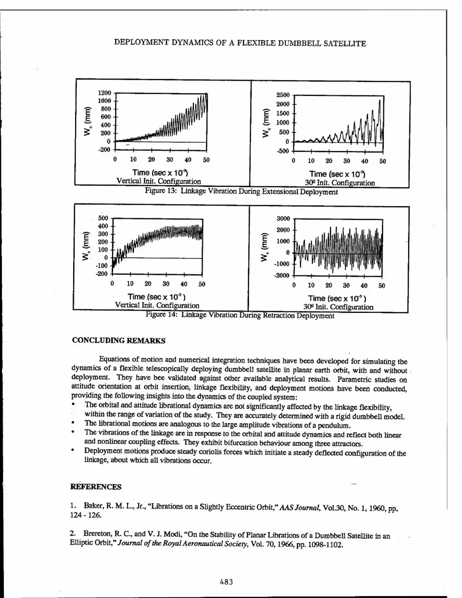
DEPLOYMENT DYNAMICS OF A FLEXIBLE DUMBBELL SATELLITE
E E
E E
Time (sec X10"3) Vertical Init. Configuration
Figure 13: Linkage Vibration During Extensional Deployment
Time (sec x 10'3) 30s Init. Configuration
3000
2000 ■ ■
1000 - -.
Time (sec x103) Vertical Init. Configuration
Figure 14: Linkage Vibration During Retraction Deployment
Time (sec x10'3) 30° Init. Configuration
CONCLUDING REMARKS
Equations of motion and numerical integration techniques have been developed for simulating the dynamics of a flexible telescopically deploying dumbbell satellite in planar earth orbit, with and without deployment. They have bee validated against other available analytical results. Parametric studies on attitude orientation at orbit insertion, linkage flexibility, and deployment motions have been conducted, providing the following insights into the dynamics of the coupled system: • The orbital and attitude librational dynamics are not significantly affected by the linkage flexibility,
within the range of variation of the study. They are accurately determined with a rigid dumbbell model. • The librational motions are analogous to the large amplitude vibrations of a pendulum. • The vibrations of the linkage are in response to the orbital and attitude dynamics and reflect both linear
and nonlinear coupling effects. They exhibit bifurcation behaviour among three attractors. • Deployment motions produce steady coriolis forces which initiate a steady deflected configuration of the
linkage, about which all vibrations occur.
REFERENCES
1. Baker, R. M. L., Jr., "Librations on a Slightly Eccentric Orbit," AAS Journal, Vol.30, No. 1,1960, pp. 124-126.
2. Brereton, R. C, and V. J. Modi, "On the Stability of Planar Librations of a Dumbbell Satellite in an Elliptic Orbit," Journal of the Royal Aeronautical Society, Vol. 70,1966, pp. 1098-1102.
+83

A. K. AMOS & B. QU
3. Klemperer, W. B., and R. M. Baker, Jr., "Satellite Librations," ActaAstronautica, Vol. 3, 1957, pp. 16- 27.
4. Klemperer, W. B., "Satellite Librations of Large Amplitude," ARS Journal, Vol. 30, No. 1,1960, pp. 123-124.
5. Modi, V. J., and R. C. Brereton, "Libration Analysis of a Dumbbell Satellite Using the WKBJ Method," Journal of Applied Mechanics, Vol. 33, No. 3,1966, pp. 676-678.
6. Moran, J. P., "Effects of Plane Librations on the Orbital Motion of a Dumbbell Satellite," ARS Journal, Vol. 31, No. 8,1961, pp. 1089-1096.
7. Rosner, H. R., "Motion of a Dumbbell Satellite," Advances in Astronomical Sciences, Vol. 7,1961, pp. 125-137.
8. Schechter, H. B., "Dumbbell Librations in Elliptic Orbit," AIAA Journal, Vol. 2, No. 6,1964, pp. 1000- 1003.
9. Schindler, G. M., "On Satellite Librations," ARS Journal, Vol. 29, No. 5,1959, pp. 368-370.
10. Schindler, G. M., "Satellite Librations in the Vicinity of Equilibrium Solutions," Astronautica Acta, Vol. 6, No. 5,1960, pp. 233-240.
11. Stocker, T. A. J., and R. F. Vachino, "The Two-Dimensional Librations of a Dumbbell-Shaped Satellite in a Uniform Gravitational Field," Advances in Astronautical Sciences, Vol. 3,1958, pp. 37-1 to 37-20.
12. Liu, L., and P. M. Bainum, "Effect of Tether Flexibility on the Tethered Shuttle Subsatellite Stability and Control," Journal of Guidance, Control and Dynamics, Vol. 12, No. 6,1987, pp. 866-873.
13. Martinez-Sanchez, M., and S. A. Gavit, "Orbital Modifications Using Forced Tether-Length Variations," Journal of Guidance, Control and Dynamics, Vol. 10, No. 3,1987, pp. 233-241.
14. Morana, M., and M. B. Quadrelli, "Orbit Circularization Using a Tether of Varying Length," Dynamics of Flexible Structures in Space -Proceedings of the First International Conference, Cranfield, UK, 1990, pp. 603-615.
15. Stuiver, W, and P. M. Bainum, "A Study of Planar Deployment Control ad Libration Damping of a Tethered Orbiting Interferometer Satellite," The Journal of the Astronautical Sciences, Vol. XX, No. 6, 1973, pp. 321-346.
16. Modi, V. J., and A. K. Misra, "Deployment Dynamics and Control of Tethered Satellite Systems," AIAA/AAS Astrodynamics Conference, Palo Alto, California, 1978
17. Modi, V. J., and A. K. Misra, "On the deployment Dynamics of Tether Connected Two-Body Systems," ActaAstronautica, Vol. 6,1979, pp.1183-1197.
18. Cherchas, D. B., ad D. M. Gossain, "Dynamics of a Flexible Solar Array During Deployment from a Spinning Spacecraft," CASI Transactions, Vol. 7, No.l, 1974, pp.10-18.
484

DEPLOYMENT DYNAMICS OF A FLEXIBLE DUMBBELL SATELLITE
19. Amos, A. K., R. G. Melton, and R. C. Thompson, "Orbital Equations of a Flexible Dumbbell Satellite - Part 1," Proceedings oftheAIAA/AASAstrodynamics Conference, Portland, Oregon, 1990, pp. 690 - 697.
20. Cohrac, J. R, and A. K. Amos, "Orbital Eccentricity Effects in Satellite Librations," Proceedings of the Eighth VPI&SU Symposium on Dynamics and Control of Large Structures, 1991, pp. 691-702.
21. Bell, E. I, and A. K. Amos, "Response of a Flexible Dumbbell Satellite to an Orbit Circularization Maneuver," Proceedings of the Ninth VPI&SU Symposium on Dynamics and Control of Large Structures, Blacksburg, Virginia, 1993, pp. 433-444.
22. Bell, E. J., "Interactions of Orbital, Attitude, and Vibrational Dynamics of a Flexible Dumbbell," M.S. Thesis, The Pennsylvania State University, University Park, Pennsylvania, 1993.
23. Qu, B. and A. K. Amos, "Deployment Dynamics of a Dumbbell Satellite," Paper AAS-95-206, AAS/AIAA Spaceflight Mechanics Meeting, Albuquerque, NM, Feb. 1995.
24. Thompson, J. M. T., and H. B. Stewart, "Nonlinear Dynamics and Chaos," Wiley, New York, 1986.
485

486

LABORATORY RESULTS ON SYSTEM IDENTIFICATION FOR
FLEXIBLE SPACECRAFT
T. Hong University of Toronto
Ontario CANADA
K. A. Carroll Dynacon Enterprises Ltd
Ontario CANADA
P. C. Hughes University of Toronto
Ontario CANADA
Abstract
Most of the many clever methods that have been proposed in the last two decades for controlling flexible spacecraft rely on an accurate mathematical model for the structural dynamics. This makes sense: the better one knows what one is controlling, the better one can control it. The assumption of accurate math models, however, may not always be valid for certain kinds of complex structures, particularly if there are significant nonlinearities, or time-variable parameters, or both. This paper examines an approach to system identification for a complex laboratory structure in which both the mentioned complexities exist. In addition, both "rigid" and "flexible" degrees of freedom (DOF) are present. A type of "augmented nonlinear feedforward" identification scheme is examined, first in simulation and then experimentally. Although the system identification performance improvement is marginal for the rigid DOF, it is significant for the flexible DOF.
1. Introduction
It is generally accepted that there is a long-term trend to larger, and therefore more stracturally flexible, spacecraft. This is true despite the current renewed emphasis on SmallSats, where economic constraints have led to doing more with less whenever possible. Looking a decade or two into the future, predictions of large space structures, either deployed or possibly erected, still seem reasonable. As an important example, Space Station must for many purposes be viewed as a large flexible spacecraft. One of the challenges posed by large space structures is in the area of system identification ("system ID," for brevity). Many factors combine to make system ED a challenge. There are often a large number of significant modes; sometimes, these modes are 'clustered' together; and, since large space structures
487

T. HONG, K. A. CARROLL AND P. C. HUGHES
electro-opticaljMSitioning system (deops) rib-tip accelerometers (20)
5m-
Figure 1: The Daisy facility: Emulating the dynamics of large flexible spacecraft.
frequently will consist of periodic lattices (cartesian or polar), the prospect of localized behavior as a consequence of slight imperfections is also likely.
Accurate system ID is often a precursor to sophisticated control algorithms, which assume that the 'plant' to be controlled is known. Many of the best current system ID methods are rooted in linear time-invariant theory and thus may stumble when used for a structure that possesses either some nonlinearities, or some time-variable parameters, or both. The laboratory structure used in this research has both these complications and thus provides a system ID challenge. How this challenge is met is the theme of this paper.
2. The Daisy Facility
Over the past decade, the Daisy facility (Figure 1) has been developed at the University of Toronto's Institute for Aerospace Studies, as described by, for example, Crocker, Hong and Hughes [1990]. The purpose of this facility is to study system identification and control of flexible space structures, and to provide a testbed for sensor and actuator development. Such ground-test facilities are not cheap (compared to paper studies and computer simulations) but they cost only a fraction of the expense of experiments in
488

LABORATORY RESULTS ON SYSTEM IDENTIFICATION FOR FLEXIBLE SPACECRAFT
space. Thus, although one must in the end conduct investigations in the environment and weightlessness of space, much can be learned from ground tests on a structure with as many realistic features as possible.
2.1 System Description
The Daisy structure consists of ten ribs forming a cone, each rib free to rotate about its pivot in two mutually perpendicular directions— "in cone" and "out of cone." This presents 20 degrees of freedom and hence 20 modes of vibration. To emulate the dynamics of large space structures of the future, these modes have been designed to have low natural frequencies (wi «0.1 Hz), light damping (C < 1%), and clustered modal frequencies. The ribs are mounted on a rigid hub which itself has three rigid rotations (pitch, roll, yaw) with respect to its support pillar.
For system ED and control purposes, motion is sensed via attitude and attitude-rate encoders on the hub, accelerometer clusters on all the ribs, and an optical deflection sensing system for measuring rib deflections relative to the hub. Called DEOPS, the optical sensing system has been described by Laurin et al. (1993). In the present paper, only the hub sensors and DEOPS will be used; the accelerometers are not used. Actuation is provided by three mutually orthogonal reaction wheels on the hub. The Daisy structure (which control engineers would want to call the 'plant') consists of a rigid hub- representative of the 'main body' of a satellite—which has three rotational degrees of freedom (roll, 6X; pitch, 02; and yaw, 03) aligned with the principal axes. Attached to the hub are 10 slender rigid ribs, each attached at its mass center to the hub via universal joints. Each joint, in turn, contain coil springs that provide a slight restoring force when rotated, and off-loading springs that are adjusted to bear the weight of the rib to reduce friction and lower damping in the joint. Coupling springs also connect each rib to its two neighboring ribs. In total. Daisy has three rigid DOF and 20 nonrigid, coupled DOF. The fact that the ribs have discrete elasticity instead of distributed elasticity is important in coping with gravity effects, and has no drawbacks since the salient dynamic characteristics of large flexible spacecraft are successfully represented.
Daisy's sensing system currently comprises three hub angular-position sensors to measure {91, 62, 93] and three hub angular-rate sensors to measure {0\, 92, e3}. In addition, DEOPS gives an additional 20 measurements of relative deflection. Deflection rates are calculated by (carefully) differentiating the deflection signals (Figure 2). Note that all these sensors are spacecraft-like—no cheating by 'measuring the distance from the ceiling,' etc!
Daisy's current actuator complement consists of three mutually orthogonal reaction wheels on the hub (with axes parallel to the principal axes) and quartets of thrusters on the tip of each rib. The latter are not used in this paper. Note that, here too, all these actuators are spacecraft-like—no cheating by 'pushing against the wall,' etc!
In summary, Daisy possesses 23 degrees of freedom, 46 sensors and 43 actuators. Some of Daisy's computer control components are been described in more detail by Crocker, Hong & Hughes [1990].
2.2 Daisy Dynamics Model
The dynamical model of Daisy can be written in the standard matrix-second-order form, viz.,
Mq(t) + {V + g)ci(t)+Kq(t)=Bu(t) ___ (1)
where {M., V, G, K} are respectively the mass matrix, the damping matrix, the gyricity matrix, and the stiffness matrix. The only source of gyricity is the set of hub reaction wheels; normally the magnitude of this term is relatively small, and its effects on system ID are studied as part of this paper. The displacement vector (coordinate vector) for the system is designated q, which contains the three hub angles 6 = col{0i, 02,03} and the two deflection angles for each of the 10 ribs. Nominally, the ribs lie in a cone (Figure 1). Their deflection components are called "in cone" and "out of cone" (by analogy
489

T. HONG, K. A. CARROLL AND P. C. HUGHES
to in-plane and out-of-plane) and are designated a,/ and aj0, respectively, for j = 1,..., 10. Together, (Xj = col{c*jo, a,-/}. Then we define
q= =col{0,a1,...,aio} (2)
Various math models of Daisy have been developed (these will not be reviewed here) and all are of the form (1). Finite-element-based models have been developed and, because of the nature of Daisy, models derived from first principles have also been successful.
2.3 Open-Loop Structural Characteristics
The dynamical characteristics of the Daisy structure are different in significant ways from a linear structure in space. There are two reasons for this. The first is that the Daisy structure is not linear (but then no real structure is). The second is that the Daisy structure is not in space. Both these bothersome facts are, unfortunately, intrinsic to a real ground-test facility, and the first of them exactly reflects the reason why a ground-test facility is of engineering interest.
A certain degree of pendulosity must be tolerated, especially if one wishes to study hub and rib deflections that are nonnegligibly nonlinear. The period of this oscillation is Tpen « 22 sec. In addition, a slight damping torque is provided by the pivot on which Daisy is mounted. Thus the 'rigid' modes are almost, but not quite, at the origin in the complex plane.
3. System ID Background
As a precursor to many modern control system designs, it is often necessary to have an accurate model of the plant dynamics. As well, system ID can be very important in reconciling the difference between experimental and theoretical performance. Previous system ID efforts on Daisy by Guccione [1993] and Boulet et al. [1994] were narrowly focused and did not attempt to produce a general model.
3.1 Choice of Algorithm
In an attempt to remedy this and to possibly improve the control performance of Daisy, a series of system ID tests were performed on Daisy using the OKID algorithm [Juang, 1994]. The OKID method is one of several schemes recently developed to perform input-output system ID in a 'black box' manner [Liu & Miller, 1994]. OKID was chosen because of its widespread use and acceptance. The initial test results were very disappointing. Several problems were identified in the original test proce- dures, including poor data quality and nonlinear and extraneous dynamics due to friction and mechanical interaction problems. In preparation for another round of system identification tests, solutions were found for most of the original problems. The data quality was improved and the mechanical interactions were minimized but it was not possible to eliminate certain inherent nonlinearities (such as hub friction) and time dependences (such as wheel gyricity).
3.2 Hub Friction and Wheel Gyricity
Hub friction arises in the pitch and roll directions due to rolling friction in the ball bearings that support Daisy's weight, while allowing Daisy to rotate about these axes. (Daisy is supported by a low-friction air bearing about the yaw axis.) The friction torque about each axis is a nonlinear function of angular speed. Hub friction must be modeled by (at least) Coulomb damping or some more sophisticated model of static and dynamic friction effects [Haessig & Friedland, 1991]; it can not, however, be modeled by the exponential damping assumed by the all of the more modern linear system ID algorithms.
490

LABORATORY RESULTS ON SYSTEM IDENTIFICATION FOR FLEXIBLE SPACECRAFT
Wheel gyricity arises due to rotation of the reaction wheels relative to the hub. Accounting for gyricity requires adding three extra time varying inputs corresponding to the form of the gyric torque:
-g(t)q(t) = h£(t)e(0 (3)
where hw(t) is the angular momentum stored in the reaction wheels. Although gyricity does not make a linear system nonlinear, it does make it time varying. This is not readily handled in system ID routines.
3.3 Level of Excitation
For a linear system, the amplitude of excitation does not theoretically matter. Since we are dealing with an admittedly somewhat nonlinear system, the excitation level does matter. If one tests with very low excitation levels, one has friction problems with the hub and with the reaction wheels. On the other hand, if one increases the excitation magnitude, other nonlinear effects come into play—including restriction of movement caused by the support wiring, the motion limits of the hub bearing, and a more prominent role for gyricity.
By directly instrumenting and measuring the reaction wheel output and modeling hub friction in conjunction with the linear system ED we can account for all the effects occurring in low-excitation testing. Lowering the magnitude of the disturbance signals greatly improved the quality of the results. The levels of excitation expected in the target application (spacecraft) are not normally likely to be large.
4. Extending Linear System ID
On simulations using both linear and nonlinear models of the Daisy structure (built using MatLab's SimuLink environment), the OKID identification algorithm did very well in identifying the linear system models—but did not do very well on the nonlinear system models. For a given nonlinear system response, in general no linear model will produce the same outputs given the same inputs. While the OKTD identification algorithm or any comparable method attempts to produce a system model that minimizes the error when compared to the original input and output measurements, the match will never be particularly good for systems with significant nonlinearities.
4.1 Incorporating Nonlinearities
Needed is a way to take into account the effect of simple nonlinearities in the identification process while allowing the linear system ID method to operate exclusively on the linear components of the test system. Examining Figure 2, the current Daisy system model consists of embedded linear and nonlinear com- ponents. This model can be separated into a main linear component and equivalent nonlinear feedback blocks. Once separated from the nonlinear subsystems, it should be possible to perform system ID on the linear subsystem if the nonlinearity is sufficiently well characterized. There is the trivial case of a completely identified nonlinearity. If one knows the exact magnitude of the nonlinear disturbances, and they can be expressed as a function of the measured test inputs and outputs, then it is possible to subtract this effect from the original measurements. In effect it becomes a modeled disturbance to the linear system. A similar example is time-varying parameters associated with gyricity. If the commanded reaction wheel torques were used as system inputs and the reaction wheel angular momentum and the hub angular velocity were measured, then the gyric torque can simply be subtracted from the commanded torque. In general, however, all the above conditions cannot be met. In the case of friction, the form of the nonlinearity is known but the magnitude of the dynamic friction force parameter is not. For the case of gyricity, the system ID tests performed on Daisy used the reaction wheel speeds as system inputs rather
491
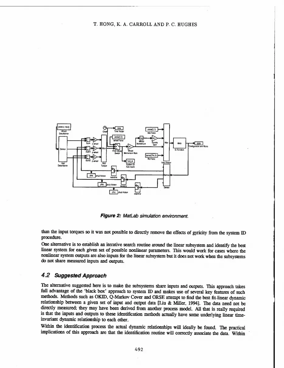
T. HONG, K. A. CARROLL AND P. C. HUGHES
[«lime, hdisf]
Wheel Disturbance
f=Hi>^» Sum xjtfiee)
Hub Dislurbance
ConSguralion and Rates
Sum1 y wheel
S»"2 2 »heel
| «fe |x>
I yft I
Figure 2: MatLab simulation environment.
than the input torques so it was not possible to directly remove the effects of gyricity from the system ID procedure.
One alternative is to establish an iterative search routine around the linear subsystem and identify the best linear system for each given set of possible nonlinear parameters. This would work for cases where the nonlinear system outputs are also inputs for the linear subsystem but it does not work when the subsystems do not share measured inputs and outputs.
4.2 Suggested Approach
The alternative suggested here is to make the subsystems share inputs and outputs. This approach takes full advantage of the 'black box' approach to system ID and makes use of several key features of such methods. Methods such as OKID, Q-Markov Cover and ORSE attempt to find the best fit-linear dynamic relationship between a given set of input and output data [Liu & Miller, 1994]. The data need not be directly measured; they may have been derived from another process model. All that is really required is that the inputs and outputs to these identification methods actually have some underlying linear time- invariant dynamic relationship to each other.
Within the identification process the actual dynamic relationships will ideally be found. The practical implications of this approach are that the identification routine will correctly associate the data. Within
492

LABORATORY RESULTS ON SYSTEM IDENTIFICATION FOR FLEXIBLE SPACECRAFT
Inputs
GyricHy
Linear Components
Outputs
Hub Friction
Figure 3: Augmented system ID model.
reason one can add inputs and outputs that one believes have real physical meaning. The identification routine will also properly scale the inputs. There is no need to iterate around the linear identification procedure to determine unknown time-invariant scaling factors. The procedure used thus consists of augmenting the identification of the original linear system model with additional inputs representing the effects of nonlinearities and letting the system ID algorithm (OKID in our case) scale and associate input and output data (Figure 3) as it sees fit. This approach can be extended for as many nonlinear terms as desired and is not dependent on the method of system ID used. It can be done either online or (as here) offline. It can also be used to evaluate the relative merits of various models for nonlinearities. This approach should have many uses where an identified linear model is either not accurate enough or not possible due to nonlinear effects. Both situations occurred in the original identification tests on Daisy.
Possible disadvantages of this approach include increased complexity of the identified system. This may have numerical consequences that offset the advantages from providing more system information. There is also an inability to determine whether the additional information being provided for system ID is being used properly. Care must be used to not just add more inputs of dubious or unknown physical meaning to the identification procedure to see if they improve the identified results.
493

T. HONG, K. A. CARROLL AND P. C. HUGHES
0.05 System ID Simulations: Performance Comparison Rigid DOFs
6- o
-0.05 100 150
time (s)
— Simulated Response --■ Linear Model,
RMS Error=0.0007976 — Friction Model,
RMS Error=0.0004869
200 250
0.02
-0.02 100 150
time (s) 200
Simulated Response Linear Model,
RMS Error=0.000151 Friction Model,
RMSError=7.91e-05
250
0.01
50
— Simulated Response — Linear Model,
RMS Error=5.38e-05 — Friction Model,
RMS Error=0.0004052
200 250 100 150 time (s)
Figure 4: System ID simulations: performance comparison, rigid DOF.
5. Simulation Results
To test the feasibility of this approach, a nonlinear Daisy simulator was built in MatLab, containing hub friction and all the flexible degrees of freedom. This was used to generate output data in response to bandwidth-limited random inputs. These outputs were then fed into an OKID-based system ID program along with the original inputs. These results were then compared the identification results produced with augmented friction inputs.
The friction model used in the simulation is the reset integrator model of Haessig and Friedland [1991]. It approximates both dynamic and static friction terms, producing an estimate of the friction force using only output velocity data. There is one undetermined parameter within this model: the magnitude of the dynamic friction. This parameter will be determined in the system ID step. For the system simulations a value for the dynamic friction was assigned. For the system ID tests the friction foree inputs were normalized to a value of 1, before being fed into OKID.
The system ID results (Figures 4 and 5) showed that the augmented friction terms greatly improve the accuracy of me identified models. Both identified models have been model order reduced to order eight, the number of modes actually generated by the simulator. The unaugmented identification results are quite good for the rigid degrees of freedom but are not as good for the flexible degrees of freedom. The augmented identification results show much better performance in recreating the motion of the Daisy's
494

LABORATORY RESULTS ON SYSTEM IDENTIFICATION FOR FLEXIBLE SPACECRAFT
System ID Simulations: Sample Performance Comparison Rib DOFs 0.03 r
a 0.02
2 0.01
■ -0.01 •
-0.02 100 150
time (s)
— Simulated Response — Linear Model,
RMS Error=0.008063 — Friction Model,
RMS Error=0.0006699
0.05
-0.05
- Simulated Response — Linear Model,
RMS Error=0.008069 -• Friction Model,
RMS Error=0.001777
50 100 150 200 time (s)
250
Figure 5: System ID simulations: performance comparison, flexible (rib). DOF.
ribs compared the unaugmented model. Its performance is almost ideal.
6. Experimental System ID Results: Rigid Daisy
Next, a very simple experimental system ID test was performed using just the hub degrees of freedom, the ribs being locked down rigidly to the hub. Daisy was excited using its reaction wheels with magnitude- and bandwidth-limited random signals. For the two slightly pendulous degrees of freedom (roll and pitch) the magnitude of the signal had to be limited to prevent the hub motion from encountering the limits of the supports. For the yaw direction, for which the air bearing permitted a much larger degree of travel, the excitation magnitude was increased and the bandwidth decreased (to prevent the reaction wheel from saturating).
The measured hub positions serve as the system outputs while the measured reaction wheel rates serve as system inputs. The system outputs and inputs were also processed to produce normalized friction and gyricity estimates. The reset integrator model was used for the friction estimates. For one identification test, the system inputs consisted of the reaction wheel rates. Two other identification tests were performed with the system inputs augmented first by the friction vector from the reset integrator model (for a total of 6 inputs and 3 outputs) then by both the friction and gyricity model outputs (for a total of 9 inputs 3 outputs)
495

T. HONG, K. A. CARROLL AND P. C. HUGHES
0.04 Daisy Rigid System ID: Performance Comparison
Actual Response Linear Model,
RMS Error=0.003363 Friction Model,
RMS Error=0.003368 Friction & Gyricity Model,
RMS Error=0.004463
Actual Response Linear Model,
RMS Error=0.001785 Friction Model,
RMS Error=0.00173 Friction & Gyricity Model,
RMS Error=0.003385
- Actual Response - Linear Model, RMS Error=0.1092 Friction Model, RMS Error=0.05075 Friction & Gyricity Model, RMS Error=0.02219
100 150 time (s)
200 250
Figure 6: Daisy rigid system ID: performance comparison.
All the experimental system ID used OKID as the identification algorithm. As with the simulation, for the rigid test the number of modes expected from the system ID is known. All the experimentally identified models were reduced reduced in order down to the three modes expected before being compared. The results are surprisingly very good for all three cases (Figure 6). Quantitatively, the best results are given by the augmented friction model but the results are not too much different from the results of the unaugmented model. The augmented friction and gyricity model produces results that are actually poorer than the other two. It is possible that the gyricity term is not a major effect, or that the system is so small and simple with such small nonlinearities that the inclusion of extra terms is not numerically justified. We note that for the simulations, the true test of the value of augmenting the system ID inputs was displayed in the modeling of the ribs not the hub. This was also true experimentally.
7. Experimental System ID Results: Flexible Daisy
The same experimental procedure was used for the flexible Daisy test as for the rigid Daisy test This included using exactly the same set of reaction wheel excitations and then model order reducing the resultant identified systems to the same size (in this case, order 46). The big difference between these two tests is the size of the two systems involved. The unaugmented system identification problem has
496


