Embed Size (px)
Citation preview

Imperial College LondonDepartment of Physics
Constraining theories of modified gravity withatom interferometry
Dylan Owusu Achiew Banahene-Sabulsky
Submitted in part fulfillment of the requirements for the degree ofDoctor of Philosophy in Physics of Imperial College London
London, United KingdomMay 2018


Abstract
Matter-wave interferometry is ideal for detecting small forces, being able to sense changes of
acceleration as small as 1 nm s−2 as a result of quantum interference. In this thesis, I prepare
a cloud of ultracold 87Rb atoms and measure the force between an atom and a cm-sized source
mass using atom interferometry. The interferometer uses a sequence of optical Raman pulses to
split, reflect, and recombine the atomic wavefunction. The force that is measured is consistent
with standard Newtonian gravity. Some theories that have been advanced to explain the
accelerating expansion of the universe - otherwise known as dark energy - predict a departure
from the Newtonian force in my experiment. I use my result to constrain the parameters
of these theories. The sensitivity of the experiment is sufficient to probe physics at energies
approaching the Planck scale.
i

Declaration
I declare that the contents of this thesis are entirely my own doing; contributions from other
sources are acknowledged and cited.
The copyright of this thesis rests with the author and is made available under a Creative
Commons Attribution Non-Commercial No Derivatives license. Researchers are free to copy,
distribute or transmit the thesis on the condition that they attribute it, that they do not use it
for commercial purposes and that they do not alter, transform or build upon it. For any reuse
or redistribution, researchers must make clear to others the license terms of this work
ii

Contents
Abstract i
Declaration i
List of Tables vii
List of Figures ix
1 Introduction 1
2 Atom interferometer theory 7
2.1 Principle of the atom interferometer . . . . . . . . . . . . . . . . . . . . . . . . . 7
2.2 Description of the proposed acceleration . . . . . . . . . . . . . . . . . . . . . . 16
3 The apparatus 20
3.1 The vacuum system . . . . . . . . . . . . . . . . . . . . . . . . . . . . . . . . . . 20
3.1.1 3D MOT Chamber . . . . . . . . . . . . . . . . . . . . . . . . . . . . . . 23
3.2 The Laser system . . . . . . . . . . . . . . . . . . . . . . . . . . . . . . . . . . . 26
3.2.1 The MOT laser system . . . . . . . . . . . . . . . . . . . . . . . . . . . . 27
iii

iv CONTENTS
3.2.2 The Interferometer laser system . . . . . . . . . . . . . . . . . . . . . . . 34
3.3 Optics, Imaging and Detection . . . . . . . . . . . . . . . . . . . . . . . . . . . . 37
3.3.1 2D and 3D MOT optics . . . . . . . . . . . . . . . . . . . . . . . . . . . 37
3.3.2 Interferometer beam collimator and optics . . . . . . . . . . . . . . . . . 38
3.3.3 CCD camera and optics . . . . . . . . . . . . . . . . . . . . . . . . . . . 39
3.3.4 Photodetector, noise limits and optics . . . . . . . . . . . . . . . . . . . . 40
3.4 The 3D MOT and Sisyphus cooling . . . . . . . . . . . . . . . . . . . . . . . . . 42
3.4.1 Shim electromagnets and field control . . . . . . . . . . . . . . . . . . . . 42
3.4.2 Temperature and number measurements . . . . . . . . . . . . . . . . . . 43
3.5 The Honeywell QA-750 MEMS Accelerometer and vibration isolation . . . . . . 46
3.5.1 Electronics . . . . . . . . . . . . . . . . . . . . . . . . . . . . . . . . . . . 46
3.5.2 Vibration isolation . . . . . . . . . . . . . . . . . . . . . . . . . . . . . . 47
3.6 The source mass . . . . . . . . . . . . . . . . . . . . . . . . . . . . . . . . . . . 48
3.6.1 Light scatter tests . . . . . . . . . . . . . . . . . . . . . . . . . . . . . . . 51
3.7 Computer control system, sequencing and pattern generation . . . . . . . . . . . 54
4 Setting up the interferometer 60
4.1 Studies with Co-propagating Raman beams . . . . . . . . . . . . . . . . . . . . 62
4.1.1 Rabi flops and Raman Spectroscopy . . . . . . . . . . . . . . . . . . . . . 62
4.1.2 Ramsey Interferometry . . . . . . . . . . . . . . . . . . . . . . . . . . . . 68
4.1.3 Ramsey’s method with frequency and phase scanning . . . . . . . . . . . 70
4.1.4 Spin Echo Interferometry . . . . . . . . . . . . . . . . . . . . . . . . . . . 73

4.2 Studies with Counter-propagating Raman beams . . . . . . . . . . . . . . . . . . 74
4.2.1 Velocity selection . . . . . . . . . . . . . . . . . . . . . . . . . . . . . . . 74
4.2.2 Checking the applied phase accuracy with the atom interferometer . . . . 76
4.2.3 Calibrating the MEMS accelerometer with the atom interferometer . . . 80
5 Primary experiment 85
5.1 Explanation of the experiment and the run pattern . . . . . . . . . . . . . . . . 85
5.2 The primary result . . . . . . . . . . . . . . . . . . . . . . . . . . . . . . . . . . 89
5.3 Constraints on Chameleon Gravity . . . . . . . . . . . . . . . . . . . . . . . . . 98
6 Conclusion 107
6.1 Summary of achievements . . . . . . . . . . . . . . . . . . . . . . . . . . . . . . 107
6.2 Improvements for future work . . . . . . . . . . . . . . . . . . . . . . . . . . . . 108
A Magnetic field sensitivity 112
B SI to GeV conversion 114
C Symmetron constraints 116
Bibliography 117
v

vi

List of Tables
5.1 MEMS accelerometer voltages for the primary experiment. . . . . . . . . . . . . 91
B.1 SI to GeV conversions . . . . . . . . . . . . . . . . . . . . . . . . . . . . . . . . 114
vii

viii

List of Figures
2.1 Principle of the interferometer . . . . . . . . . . . . . . . . . . . . . . . . . . . . 8
2.2 Energy level scheme for Raman transitions . . . . . . . . . . . . . . . . . . . . . 9
2.3 Light shifts in kHz versus detuning of ω1 from the interval g ↔ 5P3/2(F ′ = 3) . . 14
2.4 Light shift ∆eg of the hyperfine interval versus detuning of ω1 from the interval
g ↔ 5P3/2(F ′ = 3) . . . . . . . . . . . . . . . . . . . . . . . . . . . . . . . . . . . 15
2.5 Intensity ratio as a function of the frequency at which the light shift of the
hyperfine interval is zero . . . . . . . . . . . . . . . . . . . . . . . . . . . . . . . 15
2.6 Probability of spontaneous scattering by an atom during the time of a π pulse . 16
2.7 Experiment schematic . . . . . . . . . . . . . . . . . . . . . . . . . . . . . . . . 19
3.1 Schematic representation of the vacuum system and surrounding optical elements 21
3.2 In-vacuum 3D MOT Electromagnet profile . . . . . . . . . . . . . . . . . . . . . 25
3.3 In-vacuum 3D MOT electromagnet . . . . . . . . . . . . . . . . . . . . . . . . . 26
3.4 Laser system for cooling, trapping, and detection . . . . . . . . . . . . . . . . . 27
3.5 Acousto-optical modulator and fiber splitting tray . . . . . . . . . . . . . . . . . 30
3.6 Colinear Polarization Spectrometer and the reference laser . . . . . . . . . . . . 31
ix
x LIST OF FIGURES
3.7 Repump laser 6.6 GHz frequency offset lock for addressing the dark hyperfine
ground state . . . . . . . . . . . . . . . . . . . . . . . . . . . . . . . . . . . . . . 32
3.8 Cooling laser 220 MHz frequency offset lock for laser cooling and trapping . . . 33
3.9 Schematic view of the commercial µQuans UKUS . . . . . . . . . . . . . . . . . 35
3.10 Raman laser intensity ratio and phase noise trials . . . . . . . . . . . . . . . . . 37
3.11 Interferometer and detection optics . . . . . . . . . . . . . . . . . . . . . . . . . 40
3.12 Femto photodiode noise figures . . . . . . . . . . . . . . . . . . . . . . . . . . . 41
3.13 Electronics for controlling the magnetic field . . . . . . . . . . . . . . . . . . . . 43
3.14 Shim field trials . . . . . . . . . . . . . . . . . . . . . . . . . . . . . . . . . . . . 44
3.15 TOF temperature measurements for the 3D MOT and Sisyphus cooling . . . . . 45
3.16 QA750 MEMS vibration trials . . . . . . . . . . . . . . . . . . . . . . . . . . . . 48
3.17 Source mass geometry . . . . . . . . . . . . . . . . . . . . . . . . . . . . . . . . 49
3.18 Source mass angles and the force projection factor . . . . . . . . . . . . . . . . . 50
3.19 Light scatter near the source mass . . . . . . . . . . . . . . . . . . . . . . . . . . 53
3.20 Schematic experiment run pattern . . . . . . . . . . . . . . . . . . . . . . . . . . 56
3.21 Detection scheme . . . . . . . . . . . . . . . . . . . . . . . . . . . . . . . . . . . 57
3.22 Experiment control and block diagram . . . . . . . . . . . . . . . . . . . . . . . 59
4.1 Co- and counter- propagating geometry . . . . . . . . . . . . . . . . . . . . . . . 61
4.2 Co-propagating Rabi Flop and Raman Spectroscopy . . . . . . . . . . . . . . . . 64
4.3 Co-propagating Raman Spectroscopy of F=1 . . . . . . . . . . . . . . . . . . . . 65
4.4 Scalar, vector and tensor total light shift schematic . . . . . . . . . . . . . . . . 66

LIST OF FIGURES xi
4.5 Doppler-insensitve Raman Spectroscopy of F=1 at different magnetic fields . . . 67
4.6 Transitioning from Lin⊥Lin to circular polarization . . . . . . . . . . . . . . . . 67
4.7 Preparing the cloud in |1, 0〉 . . . . . . . . . . . . . . . . . . . . . . . . . . . . . 69
4.8 Clearing of states . . . . . . . . . . . . . . . . . . . . . . . . . . . . . . . . . . . 69
4.9 Co-propagating Rabi flops at multiple fall times . . . . . . . . . . . . . . . . . . 70
4.10 Ramsey’s method: scanning the frequency of both pulses . . . . . . . . . . . . . 71
4.11 Ramsey’s method: scanning the phase between the pulses . . . . . . . . . . . . . 72
4.12 Velocity-insensitive spin echo interferometry . . . . . . . . . . . . . . . . . . . . 73
4.13 Counter-propagating Raman spectroscopy and Rabi flopping with two velocity
classes . . . . . . . . . . . . . . . . . . . . . . . . . . . . . . . . . . . . . . . . . 75
4.14 Single velocity selection . . . . . . . . . . . . . . . . . . . . . . . . . . . . . . . . 76
4.15 Atom interferometry with two velocity classes and circularly polarized light . . . 77
4.16 Single velocity class atom interferometry . . . . . . . . . . . . . . . . . . . . . . 78
4.17 Comparison of velocity selection techniques . . . . . . . . . . . . . . . . . . . . . 79
4.18 Velocity selection sensitivity comparison . . . . . . . . . . . . . . . . . . . . . . 80
4.19 Response of MEMS electronics . . . . . . . . . . . . . . . . . . . . . . . . . . . . 81
4.20 Atom interferometer correlation with MEMS accelerometer . . . . . . . . . . . . 82
4.21 Big tilt trial . . . . . . . . . . . . . . . . . . . . . . . . . . . . . . . . . . . . . . 83
5.1 Experiment strategy . . . . . . . . . . . . . . . . . . . . . . . . . . . . . . . . . 86
5.2 Experiment run pattern . . . . . . . . . . . . . . . . . . . . . . . . . . . . . . . 86
5.3 Raw data from one run of the primary experiment . . . . . . . . . . . . . . . . . 89

5.4 Sample of primary experiment data . . . . . . . . . . . . . . . . . . . . . . . . . 90
5.5 Determining aball . . . . . . . . . . . . . . . . . . . . . . . . . . . . . . . . . . . 92
5.6 Source mass magnetism test . . . . . . . . . . . . . . . . . . . . . . . . . . . . . 95
5.7 Size limit for size parameter L . . . . . . . . . . . . . . . . . . . . . . . . . . . . 100
5.8 Contour plot showing the size-limited regime versus pressure-limited regime for
φbg . . . . . . . . . . . . . . . . . . . . . . . . . . . . . . . . . . . . . . . . . . . 101
5.9 Contour plot showing φbg and the screening regimes of λ1, λ2 . . . . . . . . . . . 102
5.10 Chameleon constraints on Λ versus M from this thesis, n = 1 model . . . . . . . 103
5.11 Constraints on Chameleon gravity . . . . . . . . . . . . . . . . . . . . . . . . . . 104
6.1 Delay time trials . . . . . . . . . . . . . . . . . . . . . . . . . . . . . . . . . . . 109
C.1 Constrained symmetron parameter space . . . . . . . . . . . . . . . . . . . . . . 116
xii

Chapter 1
Introduction
“Cosmologists are often in error, but never in doubt.”
and
“It is important to do everything with passion, it embellishes life enormously.”
Lev Landau
Motivation and Objectives
In this thesis, I describe an experiment to measure the force between a neutral atom and a
test mass. The motivation is to place constraints on theories of modified gravity that aim to
explain the accelerating expansion of the universe and the uneven distribution of light and
matter within it - dark energy.
A new scalar field provides a natural explanation, but that should produce a new “fifth” force;
experiments ranging from the laboratory to the solar-system find no such force. This apparent
contradiction can be understood if the properties of the scalar field vary with the local mass
density so that the force becomes weak in regions of high mass density. The field would then
go undetected in terrestrial and solar system experiments [1, 2] using macroscopic test masses,
while still allowing the pressure associated with the field to drive the accelerating expansion of
1

2 Chapter 1. Introduction
the universe. It is now known [3] that individual atoms are small and light enough that they
do not suppress this force and can therefore be used to detect the field. To accomplish this, I
design and build an atom interferometer and use it to search for small accelerations of rubidium
atoms in the scalar field gradient near a test mass.
I present 5 chapters detailing my work with my advisor Prof. E. A. Hinds FRS; I first need
to motivate how an atom interferometer is sensitive to accelerations, presented in chapter 2.
I also briefly discuss the supposed scalar fields and how they can be measured. Following
this, I begin to present the results of my thesis. In chapter 3, I describe the experimental
setup. I demonstrate my ability to make an acceleration-sensitive interferometer by starting
with spectroscopy using co-propagating Raman beams in chapter 4. In chapter 5, I present
the primary experiment and my result. I conclude with chapter 6 and comment on how the
experiment could be improved.
The author worked alone on the topics presented in this thesis; the use of ‘I’ in this thesis
expresses this. All optical components used in the figures of this work were supplied by the
GW optics component library [4].
Atom interferometry
In this thesis I use atom interferometry where the internal energy states are coupled to the
external momentum states through a Raman transition [5]. Atom interferometry with internal
energy states was a consequence of high-resolution spectroscopy insomuch that it was discov-
ered from a search for an optimal combination of sub-Doppler [6] and Ramsey [7] techniques.
Traditionally, the external motion of atoms was successfully treated by classical physics; the
exchange of momentum during emission and absorption of photons by atoms and molecules is
a coupling between the internal and external degrees of freedoms that has required a quantum
mechanical treatment to understand [8,9]. I address the interferometric technique explicitly in
chapter 2 and demonstrate the steps leading to my experimental realization in chapter 4.
After the first experimental realization of a cold atom gravimeter using atom interferometry in

3
the 1990s [5], this high-sensitivity technique was usefully applied to measurements of the fine
structure constant [10], the gravitational constant G [11,12], and higher order terms associated
with general relativity [13,14]. The experiment in this thesis is an addition to this list of precise,
fundamental tests.
Aside from fundamental physics applications, atom interferometry has demonstrated measure-
ments of rotations and acceleration with high precision and accuracy, which can lead the way to
a new generation of gyroscopes, gravity gradiometers and absolute gravimeters [15–17]. Once
incorporated into navigation suites, these devices could make dead-reckoning navigation viable.
This technology is currently being commercialized. The author acknowledges generous funding
from both the European Union through the Marie Sklodowska Curie Early Stage Researcher
program, the Action-Initial Training Network: Frontiers in Quantum Technology (FP7/2007-
2013), and the Dstl.
A brief introduction to dark energy
The direct evidence for the existence of dark energy [18] is observational. There are three points
of observational evidence that have led to the conclusion there is a dark energy. (i) Luminosity
distance and constraints from supernovae: In 1998, two groups pointed out the accelerating
expansion of the universe based on the observation of luminosity distances of redshifted Type
Ia supernovae [19, 20]. The use of the luminosity distance as a standard was born out of the
need to measure distances in an expanding universe; one way of defining distance is through
the luminosity of a stellar object. Type Ia supernovae are observed when white dwarf stars
exceed the Chandrasekhar mass limit and explode. It is believed that these supernovae form in
the same way irrespective of their location in the universe, so they should have some common
absolute magnitude independent of redshift; this has led to their treatment as an ideal standard
for luminosity. After examining low and high redshift supernovae in the late 1990s, an anomaly
was found; to explain the observed redshifts, the universe had to be dominated by an energy
density other than matter [18]. In 1998, Perlmutter et al. of the supernova cosmology project

4 Chapter 1. Introduction
(SCP) found that about 70% of the energy density in the present universe consists of dark
energy [19]. In 2004 Riess et al. [21] found that the universe exhibited a transition from
deceleration to acceleration at the > 99% confidence level using data from the Hubble Space
Telescope.
(ii) Age of the universe and the cosmological constant: Comparing the age of the universe and
the age of the oldest stellar population presents evidence for a dark energy. First, the age of the
oldest stellar objects has been constrained [22–24] to 12.7 ± 0.7 Gyr, implying the age of the
universe need satisfy the lower bound: > 11−12 Gyr. Assuming a ΛCDM model, the standard
model of cosmology where the equation of state of dark energy is assumed constant, WMAP3
data produces a best fit value for the age of universe of 13.73+0.13−0.17 Gyr [25]. Calculating the
age of the universe from the Friedmann equation [18] with the cosmological constant absent
gives 2/(3H0), where H0 is the present Hubble parameter. This parameter is constrained to be
H−10 = 9.776h−1 Gyr for 0.64 < h < 0.80 from the observations of the Hubble Space Telescope
Key project [26]. While this Hubble parameter is consistent with the conclusions of the cosmic
microwave background or CMB [25] and redshift studies of large scale structures or galaxy
clustering [27, 28], it produces an age of the universe in the range 8 − 10 Gyr, which fails to
satisfy the stellar age bound; a flat universe without a cosmological constant suffers from an
age hierarchy problem! This problem can be solved in a flat universe model by the addition
of a cosmological constant [18]. The essential idea is that the age of the universe increases
as the proportion of energy density in the universe from matter decreases. If one takes 70%
of the energy density in the present universe to consist of dark energy [19] and a choice of
h = 0.72 [18], one obtains an age of the universe of 13.1 Gyr, entirely consistent with the lower
bound set by the oldest stellar populations. The presence of a cosmological constant and a
dark energy can solve the universe age crisis.
(iii) The CMB and large scale structure constraints: The observations of the CMB [25] and
large scale structure [27, 28] independently support a dark energy dominated universe. The
CMB anisotropies exhibit a nearly scale-invariant spectra of primordial perturbations; this
agrees with the predictions of inflationary cosmology. Large scale structure redshift surveys
find that a dark energy just like that required by the CMB and supernova data is required to

5
explain their findings. These datasets rule out a flat universe without a cosmological constant
and support a dark energy.
This cosmological constant, Λ, was introduced by Einstein in 1917 as a simple solution to
achieve a static universe. Later, in 1929, with Hubble’s discovery of the expanding universe,
Einstein dropped the term as it was no longer required. However, the cosmological constant
arises naturally as an energy density of the vacuum in particle physics. If it originates from the
vacuum energy density, the energy scale of Λ should be much larger than that of the present
Hubble constant H0. This is the cosmological constant problem [29] and was well known before
the discovery of the accelerating expansion of the universe in 1998. There have been a number of
theoretical attempts to solve this problem; a short and incomplete list of attempts, with an eye
towards the focus of this thesis, include: changing gravity [30], quantum gravity [31], higher-
dimensional gravity [32], super gravity [33], and space-time foam [34]. In this thesis, I test
two theories from one particular class of scalar field model of dark energy. Scalar fields occur
naturally in particle physics, including string theory; these can act as dark energy candidates.
I focus on a class of model called Quintessence [18] that is described by a scalar field minimally
coupled to gravity but that can lead to the present inflation. Astrophysical bounds discussed
above imply such that the simplest theories with scalars must have matter couplings irrelevant
on cosmological scales. Further, the ΛCDM model may not be correct. If a scalar field is
responsible for dark energy, the equation of state for dark energy can be dynamical instead of
a constant. It is then critical to distinguish between the cosmological constant and dynamical
dark energy models in order to understand the origin of this energy density. The link between
cosmological scalar theories and astrophysical bounds can be broken by the introduction of
what are called screening mechanisms.
These screening mechanisms employ non-linear dynamics to decouple solar system scale tests
from cosmological scale tests of gravity. The key is in order of magnitude comparison of density:
there are 29 orders of magnitude that separate terrestrial and cosmological densities. Further,
there are 20 orders of magnitude separating their distance scales! As a result, the scalar field
properties can vary significantly in different environments. The classic example of a screening
mechanism is the chameleon mechanism [1] where the mass of the scalar is an increasing function

6 Chapter 1. Introduction
of the ambient density, allowing it to have a sub-micron Compton wavelength in the solar system
but remain light on cosmological scales. A closely related model was discovered, the symmetron
mechanism [35], which maintains a light mass on all scales. It screens by driving the coupling
to matter to zero when the ambient density exceeds a certain threshold.
Burrage et al. [3] proposed a method of measuring a force coming from the gradient of these
theoretical scalar fields; their realization was that individual atoms are small and light enough
that they are not entirely screened and can therefore be used to detect the presence of a field.
In chapter 2, I present a schematic for the measurement I perform and how it is sensitive to the
scalar fields. I outline how an acceleration measurement constrains the two primary parameters
of the field theories. In chapter 5, I present my result that is in agreement with Newtonian
gravity. I apply this result to the chameleon field theory, which allows me to directly constrain
the two parameters of the theory. I compare to other measurements, in the parameter space
I’ve considered. I briefly comment on the symmetron at the end of chapter 5 and provide
constraints that I place on that theory in appendix C.

Chapter 2
Atom interferometer theory
In this chapter, I provide a theoretical description of the atom interferometer I operate in this
thesis. Following this, I discuss the polarization selection rules, the light shift, and spontaneous
emission. I conclude with a brief discussion of the scalar field theories that I probe with this
experiment.
2.1 Principle of the atom interferometer
In Fig. 2.1, I illustrate the principle of the 87Rb atom interferometer I use in this thesis. I label
the two 5S1/2 hyperfine ground states of 87Rb as |g〉 for F = 1 and |e〉 for F = 2. The atom
starts in the state |g〉 at a position z1, where I apply a π/2 optical Raman pulse that splits the
atomic wavefunction into an equal superposition of |g〉 and |e〉. This Raman transition is driven
by counter-propagating light beams with frequencies ω1 and ω2; the absorption of a photon at
frequency ω1 together with a stimulated emission at frequency ω2 drives the transition to state
|e〉. This process transfers momentum ~keff = ~c(ω1 + ω2) to the wavefunction component in
state |e〉, but there is no momentum transferred from the light to the component that remains
in state |g〉. After propagating freely for a time T , the atom arrives with the |g〉 component
at position z2 and the |e〉 component at position z3. At this point I apply a Raman π pulse
that swaps the internal states and exchanges their momenta. After waiting for another free
7

8 Chapter 2. Atom interferometer theory
propagation time T , the two parts of the wavefunction overlap at position z4. Then, a second
π/2 pulse closes the interferometer to produce interference fringes in the populations of |g〉 and
|e〉. These fringes are sensitive to the acceleration of the atom along the direction of the Raman
beams, and in this thesis I use that sensitivity to look for a non-Newtonian attraction between
an atom and a test mass.
time
Z
ω1ω1ω1
ω2 ω2 ω2
π/2 π/2π
T T
z1
z3
z2
z4
Figure 2.1: Principle of the interferometer. The interferometer evolves in time and space fromleft to right and top to bottom.
This scheme was first developed by Kasevich and Chu [5]. Critically, all the atoms participate
in the interferometer regardless of their initial momentum p, so it is not necessary to resolve
the recoil splitting that makes the interferometer sensitive to acceleration. Despite this, it is
useful to make the atom cloud cold in order to minimize the Doppler broadening of the Raman
transition.
In Fig. 2.2, I show the two hyperfine ground states with energies ~ωg and ~ωe which are
separated by 6.8 GHz. The upper state, which I denote |i〉, represents the electronically excited
5P3/2 states. The laser light fields E1 and E2 are traveling waves propagating along the z
direction,
E1 = E1 cos (k1z − ω1t+ ϕ1)
E2 = E2 cos (k2z − ω2t+ ϕ2).
(2.1)

2.1. Principle of the atom interferometer 9
|e , ωe
|g ,ωg
E1,ω1 E2,ω2
ωHFS
δ
Δ
Figure 2.2: Energy level scheme for Raman transitions.
For now, I will write k1z + ϕ1 = φ1 and k2z + ϕ2 = φ2. I define the two Rabi frequencies as
Ω1 =1
~〈i|d|g〉 · E1
Ω2 =1
~〈i|d|e〉 · E2.
(2.2)
The light fields are at optical frequencies. In this thesis I have a detuning ∆ ≈ −1 GHz and a
δ in the kHz range. The Rabi frequencies are less than 1 MHz; thus a frequency hierarchy is
established: ω1,2 (ωe − ωg) ∆ δ, Ω1,2. With this hierarchy in place, the rotating wave
and adiabatic approximations [36] allow me to eliminate the intermediate state |i〉 and consider
only the two level system of |g〉 and |e〉, where transitions between the states are being driven
by an effective Rabi frequency
Ω =Ω1Ω2
2∆(2.3)
as discussed by Kasevich and Chu [37].
I write the state of the two level system in an interaction picture as
|ψ〉 = age−iωgt|ψg〉+ aee
−i(ωe+δ)t|ψe〉 (2.4)

10 Chapter 2. Atom interferometer theory
with the initial state vector at time t ae(t)ag(t)
, (2.5)
and let the Raman light be applied for a time τ . The state vector at a time t+ τ is [7]
ae(t+ τ)
ag(t+ τ)
= eiτδ/2·
cos (aτ/2)− i δa
sin (aτ/2) −iΩaeiφ sin (aτ/2)
−iΩae−iφ sin (aτ/2) cos (aτ/2) + i δ
asin (aτ/2)
ae(t)
ag(t)
,
(2.6)
where a =√
Ω2 + δ2 and φ = φ2 − φ1. For simplicity, I assume that the Raman transition is
tuned to be exactly resonant, so δ = 0. I then have
ae(t+ τ)
ag(t+ τ)
=
cos (A/2) −ieiφ sin (A/2)
−ie−iφ sin (A/2) cos (A/2)
ae(t)
ag(t)
, (2.7)
where A = Ωτ is known as the pulse area. The first pulse of the interferometer has duration
τ/2 and pulse area A = π/2. So,
Q1 =1√2
1 −ieiφ(z1)
−ie−iφ(z1) 1
. (2.8)
Here, φ(z1) indicates the phase difference φ evaluated at the position z1 of the atom. Following
this is a period of free flight time of duration T with pulse area A = 0:
Q2 =
1 0
0 1
. (2.9)
The second Raman pulse has a duration of τ and a pulse area A = π, giving me
Q3 =
0 −ieiφ(z2)
−ie−iφ(z3) 0
(2.10)

2.1. Principle of the atom interferometer 11
where the component of the wavefunction in state |g〉 interacts with the second laser pulse at
position z2 but the component in state |e〉 interacts at position z3, see Fig. 2.1. A second free
flight time gives
Q4 = Q2. (2.11)
The final π/2 pulse gives
Q5 =1√2
1 −ieiφ(z4)
−ie−iφ(z4) 1
. (2.12)
If I start with the atom in state |g〉, the final state vector is described by
ae
ag
= Q5Q4Q3Q2Q1
0
1
. (2.13)
Evaluation produces |ae|2|ag|2
=
sin2 (Φ/2)
cos2 (Φ/2)
, (2.14)
where Φ = φ(z1)− φ(z2)− φ(z3) + φ(z4). Recall that
φ(z) = φ2(z)− φ1(z) = (k2z + ϕ2)− (k1z + ϕ1) = z(k2 − k1) + (ϕ2 − ϕ1). (2.15)
Using the same value ϕ2−ϕ1 throughout and writing keff = k2−k1, then Φ = keff(z1−z2−z3+z4).
In the absence of acceleration, z1 − z3 = z2 − z4, and so Φ = 0. If an atom has a constant
acceleration az along the z direction, the additional differences are
z1 − z3 = −1
2azT
2 and
z4 − z2 =1
2az(2T )2 − 1
2azT
2 =3
2azT
2,
(2.16)
where I have neglected the small time 2τ taken up by the laser pulses. This gives Φ = keffazT2.
A simple way to scan through the fringe pattern is to change the phase difference φ2 − φ1 on
one of the laser pulses. For example, if the first and second pulses have φ2 − φ1 = 0 but the

12 Chapter 2. Atom interferometer theory
third pulse has φ2 − φ1 = θ, then the fringe pattern in state |g〉 is described by
|ag|2 = cos2(1
2
[keffazT
2 + θ])
(2.17)
and I can access any part of the pattern by adjusting θ.
Polarization selection rules
A small magnetic field (on the order of 1 G) is applied parallel to z, the direction of propagation
of the light beams that drive the Raman transitions. This is done to ensure that the magnetic
substates mF are not appreciably mixed by any stray magnetic field along x or y. The Raman
light is delivered from the laser system on a polarization-maintaining fiber, with frequency ω1
being polarized linearly along x and ω2 being linearly polarized along y. The two beams emerge
from the fiber, co-propagating with this polarization which I call Lin⊥Lin.
To consider the polarization selection rules, I note that the two dipole operators that couple to
these two light beams can form tensors of rank 2, 1, or 0. I will call them T (k), where k = 2, 1, 0.
The Raman transition matrix elements have the form 〈F = 2, m2|T (k)q |F = 1, m1〉. By the
Wigner-Eckart theorem, this is proportional to 〈F = 2||T (k)||F = 1〉, which vanishes when k =
0. By uncoupling the nuclear spin, I obtain 〈F = 2||T (k)||F = 1〉 ∝ 〈J = 1/2||T (k)||J = 1/2〉,
which vanishes when k = 2. The only allowed Raman transition is then the one described by
the vector operator T (1). Since the two light fields have Lin⊥Lin polarization, the transition
is driven by the vector combination (d1x) × (d2y) = d1d2z, described by T(1)0 . This drives the
∆mf = 0 transitions 〈F = 2, mF |T (1)0 |F = 1, mF 〉.
I introduce a quarter-wave plate, allowing me to convert the polarizations of the co-propagating
beams to right-hand circularly polarized light at frequency ω1 and left-hand circularly polarized
light at frequency ω2, which I write as RHCP and LHCP. Absorption from one beam together
with emission into another changes mF by ±2, corresponding to the operator T(2)±2 , which is
forbidden from driving transitions as previously established. In the experiment, I retro-reflect
the laser beams through a second quarter-wave plate to form counter-propagating beams with

2.1. Principle of the atom interferometer 13
RHCP-LHCP and LHCP-RHCP, (details in chapter 4). This now drives ∆mF = 0 transitions
with the operator having the allowed vector character T(1)0 .
In summary, the allowed transitions that I drive use either co-propagating beams with Lin⊥Lin
polarization (section 4.1) or counter-propagating beams with RHCP-LHCP and LHCP-RHCP
(section 4.2, driving σ+σ+ and σ−σ− transitions). The former are not useful for measuring
acceleration by interferometry because the transition imparts a negligible momentum to the
atom, ~c(ω1 − ω2), so the primary experiment I present in chapter 5 uses the latter, where the
recoil momentum is ~c(ω1 + ω2).
The light shift
The electric dipole interaction of the atom with the laser light drives the Raman transitions,
as discussed in the last two sections. This same interaction is also responsible for an AC Stark
shift, usually referred to as the light shift, which perturbs the energies of the hyperfine levels
and affects the detuning of δ.
The light shift of level |g〉 is given by standard second-order perturbation theory as
∆g =∑i
( Ω21
4(ω1 − ωig)+
Ω22
4(ω2 − ωig)
), (2.18)
where ωig means ωi − ωg. The sum is taken over all the hyperfine levels of the upper 5P3/2
manifold; I ignore the 5P1/2 upper levels because they are ∼ 7 THz away. With 100 W/m2
of circularly polarized light in each laser frequency, in a) of Fig. 2.3 I show the shift ∆g in
kHz for the state |F = 1, mF = 0〉 as a function of the detuning of ω1 from the interval
5S1/2(F = 1) → 5P3/2(F ′ = 3) (as ω1 is varied, I also change ω2 to keep the transition
resonant). I observe resonant light shifts that come from the coupling to the upper levels
F ′ = 2 and F ′ = 1. There is no coupling to F ′ = 3 because it is dipole-forbidden. There
is also no coupling to F ′ = 0 because the light is circularly polarized in this calculation and
F ′ = 0 has no mF ′ = ±1 states. I use circularly polarized light for this calculation because it
the polarization I will use in the primary experiment in chapter 5.

14 Chapter 2. Atom interferometer theory
a) b)
-1.5 -1.0 -0.5 0.0 0.5
-400
-200
0
200
400
Detuning from 5P3/2(F'=3), [GHz]
Lightshift,
e[kHz]
-1.5 -1.0 -0.5 0.0 0.5
-400
-200
0
200
400
Detuning from 5P3/2(F'=3), [GHz]
Lightshift,
g[kHz]
Figure 2.3: Light shifts in kHz versus detuning of ω1 from the interval g ↔ 5P3/2(F ′ = 3).The Raman beams have 100 W/m2 each of circularly polarized light. a) Shift of the state|F = 1,mf = 0〉. b) Shift of the state |F = 2,mf = 0〉.
The light shift of level |e〉 is
∆e =∑i
( Ω21
4(ω1 − ωie)+
Ω22
4(ω2 − ωie)
), (2.19)
where ωie means ωi − ωe. This is plotted in b) of Fig. 2.3 versus the detuning ω2 from the
interval 5S1/2(F = 2) − 5P3/2(F ′ = 3), where I observe resonances in the light shift from
F ′ = 1, 2, 3. The light shift of the hyperfine interval ∆eg = ∆e − ∆g goes to zero near the
F ′ = 1 and F ′ = 3 resonances, shown in a) of Fig. 2.4, but these frequencies are not useful
for driving the two photon Raman transitions because the one photon scattering rate is high.
With laser beams of equal intensity, there are no useful zeros of ∆eg. A useful zero appears at
a detuning of approximately -2 GHz when the beam of frequency ω1 is half the intensity of the
beam of frequency ω2, shown in b) of Fig. 2.4.
In Fig. 2.5, I show the intensity ratio as a function of the frequency at which the light shift of
the hyperfine interval goes to zero. Close to the maximum of this curve, the intensity ratio for
vanishing light shift is least sensitive to variations in the detuning. At the maximum, the de-
tuning is -1.13 GHz and the corresponding intensity ratio is 0.583. I operate the interferometer
under that condition. The light shift is then calculated to be 1.6 Hz/(W/m2) if the intensity
ratio changes by 1% of itself.

2.1. Principle of the atom interferometer 15
-4 -3 -2 -1 0 1-30
-20
-10
0
10
20
30
Detuning from intermediate state, [GHz]
Lightshift,
eg[kHz]
-4 -3 -2 -1 0 1-30
-20
-10
0
10
20
30
Detuning from intermediate state, [GHz]
Lightshift,
eg[kHz]
a) b)
Figure 2.4: Light shift ∆eg of the hyperfine interval versus detuning of ω1 from the intervalg ↔ 5P3/2(F ′ = 3). a) Both beams have 100 W/m2 and b) 50 W/m2 in ω1 and 100 W/m2 atω2. In b) I observe a useful zero at a detuning of approximately -2 GHz.
-3.0 -2.5 -2.0 -1.5 -1.0 -0.5
0.30
0.35
0.40
0.45
0.50
0.55
Detuning, Δ [GHz]
Intensityratio
Figure 2.5: Intensity ratio as a function of the frequency at which the light shift of the hyperfineinterval is zero. The red lines denote the maximum intensity ratio of .583 at -1.13 GHz.
Spontaneous scattering
The Raman pulses induce only a small population in the excited states |i〉, but still this is not
entirely negligible; there is some probability that the atom will scatter a photon by spontaneous
emission during a π pulse. Such a scattering randomizes the phase of the interferometer and
results in a loss of visibility of the fringes. I plot the probability that an atom in the state
|F = 2, mF = 0〉 or |F = 1, mF = 0〉 will scatter a photon spontaneously during a π pulse
in Fig. 2.6. This probability is proportional to the intensity of the light and the duration of

16 Chapter 2. Atom interferometer theory
the pulse, but the same product determines the pulse area A; it is sufficient to specify that the
pulse is a π pulse. The plot shows how this probability depends upon the detuning. This is
calculated with the intensity ratio being re-evaluated to give zero light shift at each detuning.
The scatter is about 2% over the range of detunings considered. In total, the three pulses of
the interferometer give a pulse area of 2π, so for my detuning of -1.13 GHz I expect a net
spontaneous scattering probability of approximately 5%.
-1.4 -1.3 -1.2 -1.1 -1.0 -0.91.5
2.0
2.5
3.0
Detuning, Δ [GHz]
Spontaneousemission
probability
[%] |2, 0⟩
|1, 0⟩
Figure 2.6: Probability of spontaneous scattering by an atom during the time of a π pulse.This is plotted versus the detuning from the excited state with the intensity ratio of the twolight beams optimized at each frequency to give zero light shift. I show |F = 2, mf = 0〉 in redand |F = 1, mf = 0〉 in blue.
This calculation and those leading to Figs. 2.3, 2.4, 2.5, and 2.6 were done using a program
written by Prof. E. A. Hinds FRS.
2.2 Description of the proposed acceleration
In order to explain the growing expansion rate of the universe, cosmologists have proposed a
“dark energy”. This might simply be a non-zero cosmological constant, but it could also be a
result of negative pressure caused by a light scalar field. In order to avoid conflicting with fifth
force experiments on Earth, it is proposed that the new field φ be sensitive to the density of
the surrounding matter. This gives rise to the name “chameleon”.

2.2. Description of the proposed acceleration 17
While the field φ is fully described by relativistic quantum field theory, the non-relativistic
steady-state is simple enough:
∇2φ = −Λ5
φ2+
ρ
M, (2.20)
where ρ is the local matter density, Λ sets the strength of the field self interaction, M determines
the coupling between the field and matter, and where c = ~ = 1 (the units are in GeV, see
appendix B). A small test particle placed in a gradient of the scalar field φ would be subjected
to a force
~F ∝ ~∇φ. (2.21)
Such a gradient is found outside a dense spherical object [3]. The acceleration of a test object
(labelled 2) towards the center of a source object (labelled 1) from equation (2.21) is given by
aχ =1
M
∂φ
∂r= 2λ1λ2
(MPl
M
)2 Gm1
r2, (2.22)
where MPl =√
18πG
is the reduced Planck mass, m1 is the mass of the source mass, and G is
the Newtonian gravitational constant. The coefficients λ1 and λ2, sometimes called screening
factors, describe how the field is screened by each object. These screening factors are given by
λi =
1, ρiR
2i < 3Mφbg
3MφbgρiR2
i, ρiR
2i > 3Mφbg,
(2.23)
where ρi and Ri are the density and radius respectively of object i and φbg is the vacuum
expectation value of φ in the absence of the source and test masses. When ρiR2i > 3Mφbg,
the field is suppressed inside the object bar a thin shell near to the surface. In the case when
ρiR2i < 3Mφbg, the field is unsuppressed even at the center of the object, so λi → 1. For
λ2 = 1, the force on the test object takes the form −m2
M~∇φ; one can think about m2
Mφ as a
potential energy for the interaction. Notably, this force should resemble gravity in that it is a
1/r2 attraction - which leads to these scalar field theories being classified as screened modified
gravity.
This leaves φbg to be evaluated. Consider a spherical vacuum vessel of radius L, with solid walls

18 Chapter 2. Atom interferometer theory
and at UHV pressures (≤ 10−9 mbar): the field φ rises from zero near the dense walls to some
value φbg at the center. If the chamber is sufficiently large, φbg reaches some equilibrium value
φeq =√
Λ5M/ρvac determined by the gas density ρvac. For small vessels, φbg = 0.693√
Λ5L2 [3].
This expression is valid for φbg < φeq. If this condition is not satisfied, φbg = φeq.
The basic idea of the experiment
It is in this way that measuring an acceleration aχ constrains Λ and M . Based on equation
(2.22), I designed an experiment similar to what was proposed in Burrage et al. [3], see Fig.
2.7. First, I create a vacuum can with dimensions sufficiently large to satisfy the conditions
necessary for the scalar field to reach the vacuum value φbg = 0.693√
Λ5L2, namely that the
can maintain a sufficiently large open space L in good vacuum, see dark red curve in Fig. 2.7.
When perturbed by a cm scale source mass, the field creates a large gradient across the center
of the chamber, see the dashed light blue curve. I place an ensemble of atoms at this point and
use atom interferometry to measure their acceleration towards the ball, see the inset in Fig. 2.7.
I move the source mass between two positions on opposite sides of the atom cloud. Through
subtraction, this allows me to distinguish the attraction toward the source mass from other
external forces. In describing this experiment, I present three chapters: first, the construction
of the apparatus in chapter 3. In chapter 4, I setup the interferometer. In chapter 5, I perform
the experiment discussed here and constrain the possible values of Λ and M , which are the two
free parameters of the theory.

2.2. Description of the proposed acceleration 19
π/2
π/2 π
t
x
ϕ ϕbg
z
Figure 2.7: Experiment schematic. Dark red curve: unperturbed scalar field inside the vacuumchamber. Dashed blue curves: perturbed scalar field, depending on the position of the sourcemass. The atoms are at the center of the chamber. The source mass can take a series of positionsthat are equal but opposite. Inset: I measure the acceleration using an atom interferometer.

Chapter 3
The apparatus
In this chapter, I describe the experimental apparatus. First, I describe the vacuum system
including the pumping arrangements and the electromagnets inside the vacuum can. Next, I
discuss the lasers and describe the two parallel systems in operation: one at 780.2 nm that
provides light for cooling and trapping and another, frequency-doubled, starting at 1560.4
nm for the interferometer. Shorter sections follow, describing the 2D/3D MOT optics, the
interferometer optics, the CCD camera, the photodetector, and the MEMS accelerometer that
I use, initially, for vibration measurements. I move on to discussions about the source mass
and the installation geometry, with some focus on initial light scatter tests. Last, I describe
the control system, timing, sequencing, and pattern generation for the experiment.
3.1 The vacuum system
The vacuum system for this experiment, displayed in Fig. 3.1, is composed of two smaller
vacuum systems separated by a differential pumping section and a gate valve. The first system
is for the 2D MOT, comprising a long, uncoated glass cell (25mm × 25 mm × 120 mm), two
natural abundance electrochemical rubidium dispensers (SAES, RB/NF/4.8/17 FT10+ 10), a 2
l/s ion pump (Agilent), an all-metal angle valve, a 2 mm diameter aperture made from a copper
conflat gasket, and a metal gate valve to separate it from the main chamber. The optics deliver
20

3.1. The vacuum system 21
over 100 mW of combined cooling and repump power to the 2D MOT. The main vacuum system
contains the 3D MOT capture region, the source mass, the interferometer region, and the 3D
MOT electromagnets. The lower section of this chamber contains a combination Pirani/hot
cathode gauge (Leybold, ITR-200), a combination diode ion pump/non-evaporable getter with
µmetal shielding around the magnets (SAES, NEXTorr D-300), and a viton-sealed angle valve
(MDC, good to 1 × 10⁻¹¹ mbar). There are also two flanges on this chamber for electrical
connections to the electromagnets. In the following subsections, I describe key parts and
concepts of the vacuum system.
v
Rb
x2
ix)
ix)
i) ii)
iii)
iv) v) viii)
v) viii)
x)
vii)
xii)
vi)
vi)
a)
b)
xi)
iv)
2D MOT
xi)
x)
Figure 3.1: Schematic representation of the vacuum system and surrounding optical elements.a) A top down view. i) 2D MOT electromagnets, ii)2 l/s ion pump, iii) rubidium dispensers, iv)2 mm diameter copper aperture, v) glass cell, vi) 2D MOT power splitting optics, vii) 2D MOTCCTV camera for monitoring, viii) Rb-87 MOT of ≈ 1010 atoms, ix) 3D MOT electromagnets,x) 3D MOT beam collimation tubes, xi) photodiode for detection. b)A side view of the samevacuum system. xii) SAES NEXTorr D-300 combination ion pump and NEG. The source masshas been left out of the schematic here but see Fig. 3.17 for where it fits in.

22 Chapter 3. The apparatus
Rubidium dispensers
I use natural abundance rubidium dispensers from SAES as the source of rubidium-87 (87Rb)
vapor in my system, see iii) in a) of Fig 3.1. Atom interferometry with Raman transitions is
more favorable with 87Rb due to the magnitude of the hyperfine splitting and fewer Zeeman
sublevels. While 87Rb is only 28% of the vapor, a single dispenser provides sufficient vapor
pressure to keep the 2D MOT loaded; the differential pumping aperture, see iv) in a) of Fig.
3.1, ensures the main chamber can maintain a low pressure of 2 × 10⁻¹⁰ mbar versus the 2D
MOT cell at 2× 10⁻⁷ mbar. The dispensers consist of an anhydrous rubidium salt of chromic
acid, with the formula Rb2CrO4. The reducing agent is the ST 101 getter material, made of
zirconium and aluminum (84% and 16%, respectively). This is critical to the pure dispensing
of alkali metal vapor, as the ST 101 irreversibly sorbs almost all the chemically active gases
produced during the reduction reaction [38]. The dispensers I installed have 4.8 mg of natural
abundance rubidium each. The two dispensers are heat-sunk and electrically connected a
DN16 flange that contains four copper wire feedthroughs that are rated to 12 A each. After
activation, I dispense rubidium vapor at 2.5 A, continuous operation, which gives a pressure of
approximately 2× 10⁻⁷ mbar.
Differential pumping
There is 750 mm of separation from the center of the 2D MOT to the center of the 3D MOT. I
aim to understand the flow of background gas from the 2D MOT cell (background loading with
rubidium vapor) into the main vacuum chamber. The limiting conductance is the orifice iv) in
a) and b) of Fig. 3.1, which has a radius of r = 1 mm. The gas is in the regime of molecular
flow, where the conductance is [39]
Cor = πr2
√kBT
2πm= .21 l/s, (3.1)
where kB is Boltzmann’s constant, T is the mean temperature of the gas and m is the mass
of a 87Rb atom. This conductance is reduced by the tubing connecting the 2D MOT cell to

3.1. The vacuum system 23
the main chamber; the tube has a length of l = 240 mm and a diameter of d = 16 mm. The
conductance of a long tube is
Clong tube =d3
3l
√kBT
2πm= .38 l/s, (3.2)
but for my application the ratio l/d ≈ 8. When this ratio is below 50 equation (3.2) requires
significant correction. I correct for the short length of the tube; the entrance of the duct can
be considered not unlike a circuit element with resistance Z1 = 1/C1 in series with the long
duct calculated above, of resistance Z2 = 1/C2, making the net conductance
1
Cshort tube
=1
Clong tube
+1
Clong tube aperture
→ Cshort tube ≈ 7× 10⁻⁴ l/s. (3.3)
Combining these two, I expect a net conductance of .14 l/s between the 2D MOT and the main
chamber. The pumping speed in the main chamber is about a thousand times higher than this
conductance. With the 2D MOT ion pump off during experimental operation, I expect a ratio
of order 103, corresponding to a partial pressure of rubidium in the main chamber of order
2× 10⁻¹⁰ mbar. This is consistent with the unobservable pressure increase when the rubidium
dispenser is turned on.
3.1.1 3D MOT Chamber
Here I describe the 3D MOT chamber and the interior layout of the vacuum can. See Section
3.6 for information about the source mass and movement in vacuum.
UHV MOT electromagnets
In designing the 3D MOT electromagnets, I struck a balance between: (i) small electromagnets
in terms of physical size and number of windings, which offer low inductance and fast switching
and (ii) large electromagnets, which can leave a large open volume for the scalar field φ0 to
develop. To accomplish this, I had to install the 3D MOT electromagnets inside the vacuum

24 Chapter 3. The apparatus
chamber. This added an additional concern; I had to minimize the power dissipated to ensure
that resistive heating would not significantly increase out-gassing.
The Biot-Savart law describes the magnetic field on the cylindrical symmetry axis z of a single
circular loop of radius r carrying a current I,
d~B =µ0
4π
Id~s× r
r2→ Bz =
µ0I
2
r2
(r2 + (z − z0)2)3/2, (3.4)
where z0 is the axial position. Each MOT electromagnet is a sum of circular loops
Bz,coil =nz∑i=1
nr∑j=1
(Bz
)i,j, (3.5)
where i, j label the axial positions and radii of the nth loops, respectively. I convert this to the
magnetic field gradient,
Gz,coil =nz∑i=1
nr∑j=1
(∂Bz
∂z
)i,j. (3.6)
I can now consider physical and geometric constraints. I opted to use polyamide-imide enamel
insulated copper wire with a rectangular cross-section of 2.7 mm × 4 mm. The copper wire,
without insulation, has a cross section of 2.54 mm × 3.8 mm. The maximum diameter is
constrained to 160 mm by the requirement of fitting within the chamber wall boundary. The
minimum radius is set at 55 mm by the need for optical access as well as source mass manip-
ulation. This limits the electromagnet to 9 turns in the radial direction, from the outer wall
moving inwards. The spacing between the MOT electromagnets was chosen to be 11 cm to
roughly optimize the field gradient value and shape. This left an open space defined by a sphere
of radius r = 65 mm in which scalar fields could rise to a significant value. Fig. 3.2 shows the
power dissipation as a function of the number of axial turns for an electromagnet that produces
the required field gradient, for the maximum number of radial turns constrained by geometry.
With 9 radial turns, the minimum power required for this field gradient is when there are 13
axial layers, dissipating only 11 W. The geometry of the chamber is convenient for in vacuum
MOT electromagnets, as evidenced by b), c), and e) of Fig. 3.2; The field passes through zero
near the center of the chamber. The field gradient, while it does suffer a dip near the center of

3.1. The vacuum system 25
the chamber due to deviation from anti-Helmholtz configuration, see d) of Fig 3.2, reaches the
designed field gradient. Over the trapping volume of ± .01 m, I can see the fluctuation is under
30 G/m; this is not problematic for a MOT. These MOT electromagnets will make a trap.
5 10 15 20 25 3010
11
12
13
14
15
16
17
Axial turns
Powerdissipated
[W]
-0.3 -0.2 -0.1 0.0 0.1 0.2 0.3
-60000
-40000
-20000
0
20000
40000
60000
Axial coordinate, z [m]
MagneticFieldCurvature
[G/m
2 ]
-0.4 -0.2 0.0 0.2 0.4
-100
-50
0
50
100
Axial coordinate, z [m]
MagneticField[G]
-0.3 -0.2 -0.1 0.0 0.1 0.2 0.3-1500
-1000
-500
0
500
1000
1500
Axial coordinate, z [m]
MagneticFieldGradient[G/m
]
-0.03 -0.02 -0.01 0.00 0.01 0.02 0.031500
1550
1600
1650
a) b)
d)
c) e)
Figure 3.2: In-vacuum 3D MOT Electromagnet profile. a) Power dissipation for 1500 G/mas a function of axial turns for maximum radial turns, the red lines show the minimum at 13axial turns and 11 W. b) Magnetic field versus deviation from the center of the chamber. Theelectromagnets are oriented in anti-Helmholtz configuration along z and share the midpoint oftheir separation distance with the center of the chamber. c) The magnetic field gradient as afunction of distance from the center of the chamber. d) A closer look at the gradient near thecenter. e) The magnetic field curvature versus distance from the center of the chamber.
The MOT electromagnets were tested before installation, see b) in Fig. 3.3. They are 200 mΩ
each with 9 radial and 13 axial turns for a total of 117 turns. The electromagnets have an in-
ductance of 30±3 µH each. To ensure good thermal conductance from the electromagnet to the
vacuum chamber and the environment, I needed a solution similar to groove grabbers (Kimball
Physics, electron gun mounting) but with a larger contact surface, see a) in 3.3. During contin-
uous operation at 11 W, a time constant of τ = 90 min was measured for the electromagnets.
The asymptote was 85 C. I was particularly interested in their out-gassing characteristics. A
similar vacuum can to the main chamber was brought down to 10−8 mbar with an electromagnet

26 Chapter 3. The apparatus
installed. During the same heating test previously mentioned, the vacuum quality degraded by
a few 10−10 mbar; in the main chamber, this effect is only observed after 7 hours of operation, as
the experiment vacuum can is a larger heat sink and the electromagnets are presumed cleaner.
During interferometer operation, 10 W was used and continuous operation is rarely needed in
practice.
a) b)
Figure 3.3: In-vacuum 3D MOT electromagnet. a) The aluminum former of the electromagnet.Also on display is one of two cooling flanges which slot directly into the grooves on the mainvacuum can. b) A wound electromagnet at the conclusion of testing the profile. Note the slotin the former for eddy current suppression.
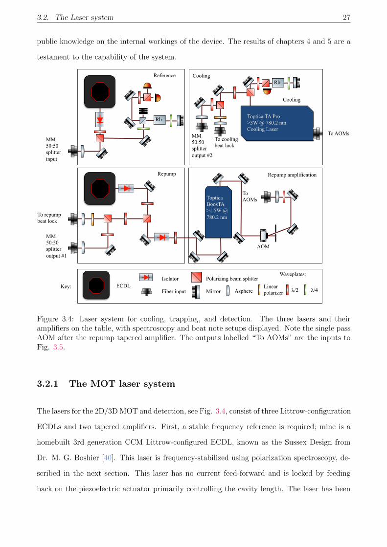
3.2 The Laser system
Here I describe the two independently referenced laser systems, Fig. 3.4 and Fig. 3.9. First,
I start with the optics layout of the laser system that I assembled for cooling, trapping, and
detecting the atoms. This system comprises three agile frequency-stabilized external-cavity
diode lasers (ECDL) and their attendant amplifiers, all lasing on the D2 line of 87Rb at 780.24
nm. This is followed by descriptions of the spectroscopy and beat note lock loops. I conclude
the section by describing the unified laser system bought from µQuans, a set of four telecom
C-band ECDLs lasing at 1560.48 nm. These lasers, after amplification through fiber amplifiers,
are frequency-doubled via PPLN (periodically-poled Lithium-Niobate) waveguides to 780.24
nm. This is a closed commercial device; I provide information on how I used it and discuss
3.2. The Laser system 27
public knowledge on the internal workings of the device. The results of chapters 4 and 5 are a
testament to the capability of the system.
Rb
Reference
MM 50:50 splitter input
Rb
Toptica TA Pro >3W @ 780.2 nm Cooling Laser
Cooling
MM 50:50 splitter output #2
To cooling beat lock
To AOMs
Toptica BoosTA >1.5W @ 780.2 nm
Repump
MM 50:50 splitter output #1
To repump beat lock
To AOMs
Cooling
Repump amplification
ECDL Isolator Fiber input
Polarizing beam splitter Mirror Asphere
Waveplates:
λ/2 λ/4 Linear polarizer
Key:
AOM
Figure 3.4: Laser system for cooling, trapping, and detection. The three lasers and theiramplifiers on the table, with spectroscopy and beat note setups displayed. Note the single passAOM after the repump tapered amplifier. The outputs labelled “To AOMs” are the inputs toFig. 3.5.
3.2.1 The MOT laser system
The lasers for the 2D/3D MOT and detection, see Fig. 3.4, consist of three Littrow-configuration
ECDLs and two tapered amplifiers. First, a stable frequency reference is required; mine is a
homebuilt 3rd generation CCM Littrow-configured ECDL, known as the Sussex Design from
Dr. M. G. Boshier [40]. This laser is frequency-stabilized using polarization spectroscopy, de-
scribed in the next section. This laser has no current feed-forward and is locked by feeding
back on the piezoelectric actuator primarily controlling the cavity length. The laser has been

28 Chapter 3. The apparatus
upgraded and moved into a 4th generation box. The control electronics consist of a homebuilt
piezostack controller as well as commercial temperature and current controllers (Wavelength
Electronics). The maximum power output is 20 mW.
The second laser in the system, another Sussex Design, functions as the repump laser. This
laser’s function is to pump all atoms that fall into the 52S1/2(F = 1) ground state into the (F=2)
ground state via the 52P3/2(F = 2) state. It is part of a homebuilt master oscillator power
amplifier (MOPA) with a commerical tapered amplifier from Toptica Photonics, providing up
to 1.5 W at 780 nm with maximum operating current and saturated optical input (20 mW).
This laser can only provide 11 mW to the TA; it produces 15 mW at full current. This laser
has no current feed-forward and is locked by feeding back on a piezoelectric actuator primarily
controlling the cavity length. The laser has been upgraded and moved into a 4th generation
box as well. The control electronics consist of a homebuilt piezostack controller and commercial
temperature and current controllers. After the TA, the repump light is sent through a single-
pass AOM (Gooch+Housego, M080-2B/F-GH2), see Fig. 3.4, before being fiber coupled and
sent to the next stage of light management, see Fig.3.5.
The third laser is a commercial MOPA from Toptica Photonics. This device contains a Littrow
configured ECDL coupled into a tapered amplifier (TA). The output of this device is fiber
coupled using an additional device from the manufacturer, manually installed (please note
this fiber coupler is not matched to the TA output profile, the coupler was intended for a
different Toptica laser). With maximum operating current applied to the TA and saturated
optical input power (40 mW), optical powers exceeding 3 W at 780.24 nm are available; the
fiber coupling has been found to be 65% efficient. There is a side output from the ECDL (15
mW) for spectroscopy and locking. Full power output from the TA does not endanger the
fiber, given the polarization-maintaining fiber is well coupled (from Schafter+Kirchhoff, with
metalized fiber tips). Please note that significant power couples to the fast axis of the fiber; it
is dumped with polarization cleaning optics, see the input from the cooling laser in a) of Fig.
3.5. This laser is run using control electronics from the manufacturer. The original laser diode
passed away early in 2016, after giving it’s life gallantly in the service of science; the current
feed-forward on this laser was turned off upon installation of a new diode and remains off. This

3.2. The Laser system 29
device provides the cooling force in the MOT.
The light management stage, see Fig. 3.5, consists of three AOMs (AA Opto-Electronics,
MT110-A1-IR) for the cooling light, beam combining optics, and fiber coupler inputs. The
AOMs are in double pass configuration for beam position stability and high extinction. They
use an analog radio-frequency (RF) chain, see b) of Fig. 3.5. The AOMs are used for the
following, starting from the left in a) of Fig. 3.5: (i) produces resonant 52S1/2(F = 2) →
52P3/2(F = 3) light for the 2D MOT push beam, (ii) produces light 13 MHz red-detuned of the
52S1/2(F = 2) → 52P3/2(F = 3) transition for the 2D MOT and (iii) produces light 15 MHz
red-detuned of the 52S1/2(F = 2)→ 52P3/2(F = 3) transition for the 3D MOT. After AOM (ii)
and (iii), repump light is combined with the cooling light before being fiber coupled.
The 87Rb reference laser
The reference laser is frequency stabilized by deriving an error signal from a polarization spec-
trometer, see a) of Fig. 3.6, where birefringence is induced in an atomic vapor cell using a
pump/probe interrogation technique [41]. This error signal is fed into a homemade lock loop
(proportional and integral gain only) which controls the cavity length via a piezoelectric ac-
tuator. I use a rubidium vapor cell containing natural abundances of 85Rb and 87Rb. When
the lock loop is open and the laser is set scanning near transitions in 85Rb/87Rb, a series of
dispersive lines are observed, see b) Fig. 3.6; the lineshape is ideal for stabilizing the laser to
the center of the transition. I lock to the cooling transition, colored gray in Fig. 3.6.
The polarization spectroscopy optical setup differs slightly [42] from a typical polarization
spectrometer using alkali vapor cells; I do not spatially separate the pump and probe beam and
then attempt to obtain good beam overlap in the cell. Instead, I employ a colinear method
similar to saturated absorption setups, which suppresses sensitivity to beam misalignments.
This method does not eliminate the Doppler-broadened absorption feature; instead, it creates
the polarization dispersions within the larger absorption feature, see b) Fig. 3.6 and note the
similarity to a typical saturated absorption spectrum for D2 85Rb/87Rb, see c) in Fig. 3.9 for
comparison.

30 Chapter 3. The apparatus
3D MOT X
2D MOT
Push beam 3D MOT Y
3D MOT +Z
3D MOT -Z
Input from Cooling laser
Input from Repump a)
b)
+2Δ
Δ
+1Δtowardmirror
0th order +1Δ
Input from Cooling laser
50:50 PM splitter 50:50 PM splitter
Mirror PBS AOM λ/2 plate λ/4 plate Aperture/iris and beam block Fiber collimator
c)
i) ii) iii)
Figure 3.5: Acousto-optical modulator and fiber splitting tray. a) Layout of optics in thesplitting stage. AOMs: (i) 2D MOT push beam, (ii) 2D MOT, (iii) 3D MOT. b) Schematicrepresentation of a double-passage AOM setup. The frequency chain driving the AOMs con-sists of, in order of connection, a voltage-controlled oscillator (Minicircuits, ZX95-200+), avoltage-controlled attenuator (Minicircuits, ZX73-2500+), a high isolation switch (Minicircuits,ZASWA-2-50DR+), a low pass filter (Minicircuits, BLP-150+) and a power amplifier (Minicir-cuits, ZHL-3A+). c) A component key.
The observed zero crossings of the polarization spectrum are sensitive to magnetic fields. For
this reason, the spectroscopy setup is far away (1.5 m) from the 3D MOT electromagnets and
encased in a soft iron shield with only a small aperture for the light to pass through. To reduce
the effects of air currents and stray light, the spectrometer is enclosed in an opaque acrylic
case. It has been checked that when the electromagnets switch, no change to the error signal
can be observed.

3.2. The Laser system 31
2000 3000 4000 5000 6000
-0.15
-0.10
-0.05
0.00
0.05
0.10
0.15
Time Division [s]
PhotodiodeSignal[V
]a)
b)
50:50
i)
ii)
To beat note photodiodes
F = 3
CO23 CO13
Rb vapor cell in soft iron shield
87Rb: 52S1/2 (F = 2) è 52P3/2 (F = 3)
Mirror
PBS
λ/2 plate λ/4 plate Photodiode
Laser
85Rb: 52S1/2 (F = 3) è 52P3/2 (F = 4)
Subtracter
PID loop and lock circuit
HV amplifier
Figure 3.6: Colinear Polarization Spectrometer and the reference laser a) Schematic layout ofpolarization spectrometer. The PBS cube before the photodetectors splits the polarizationsinto i) and ii). b) A sample scan of the piezostack showing the relevant dispersion feature ingray.
The repump laser
The repump laser is frequency stabilized to the reference laser with a frequency offset beat note
lock loop at 6.49 GHz. I know the frequencies of the various transitions in the D2 manifold
to tens of hertz [43]; a direct microwave beat note is a suitable way to frequency stabilize the
laser. A schematic of the frequency offset lock and the beat note lock loop appears in a) of
Fig. 3.7. I create the beat note with 3 mW picked off from the output of the repump laser
and mixed with 1 mW of light from the reference laser. The light is directed onto a fixed gain,
amplified InGaAs detector (Thorlabs, PDA8GS), see the left side of a) in Fig. 3.7. While the
bandwidth of this device is sufficient for the application, the sensitivity to 780 nm is low. This
small signal is then inserted into two RF amplifiers chained together (Minicircuits, ZRON-

32 Chapter 3. The apparatus
1000 2000 3000 4000 5000 6000 7000
-0.05
0.00
0.05
Time Divison [s]
PhotodiodeSignal[V
]a)
Spectrum Analyzer
b)
c)
R1
R2
Output error signal
Input
-3 dB -6 dB
High-pass filter
R1
R3
R1
R1
R1
R2
R3
Note: R2>R1>R3
C C
C C CO12
Near 87Rb: 52S1/2 (F = 1) è52P3/2 (F = 2)
To spectroscopy To amplifier
Reference Repump
50:50 Splitter
ESC
Sampler
Oscilloscope
MM fiber Mixer
6.6 GHz VCO
Linear Polarizer
Limiter
50:50 Splitter
Figure 3.7: Repump laser 6.6 GHz frequency offset lock for addressing the dark hyperfine groundstate. a) Schematic layout of the repump offset lock. b) Piezostack scan of the cross-over, lockpoint in black. c) The error signal board passive component layout [44].
8G+ and then ZVA-183-S+) before entering a mixer (ZMX-7GR). A frequency quadrupled
voltage controlled oscillator (Minicircuits, ZX95-6640C-S+) amplified by a single RF amplifier
(Minicircuits, ZRON-8G) feeds the other input of the mixer. The output of the mixer feeds
into an amplifier (Minicircuits, ZFL-1000GR) before entering a cautionary limiter (Minicircuits,
VLM-52-S+) and a splitter (Minicircuits, ZFRSC-42-S+). One splitter output goes to a 1 GHz
spectrum analyzer, the other goes to the error signal card (ESC) [44], see c) of Fig. 3.7. When
the piezostack of the repump laser is scanned, the dispersion signal shown in b) of Fig. 3.7 is
observed.
This dispersion signal is the crossover transition 52S1/2(F = 1) → 52P3/2(F = 1 → F =
2). This crossover transition is 80 MHz away from the repump transition 52S1/2(F = 1) →
52P3/2(F = 2); I use an 80 MHz AOM to shift the frequency before application to the atoms.

3.2. The Laser system 33
The cooling laser
0 200 400 600 800 1000 1200 1400
0
1
2
3
4
5
6
Frequency [MHz]
PhotodiodeSignal[V
]
b)
a) To spectroscopy
Reference
Saturated Absorption Spectrometer with Unshielded Rb vapor cell
Offset Lock
CO23 CO13
220 MHz
212 MHz
52P3/2 (F=3) CO12
52P3/2 (F=2)
Toptica TA Pro >3W @ 780.2 nm Cooling Laser
Toptica fiber output to AOM board
52P3/2 (F=1)
Linear Polarizer
Figure 3.8: Cooling laser 220 MHz frequency offset lock for laser cooling and trapping. a)Schematic layout of the cooling offset lock and the attendant saturated absorption spectrometerfor monitoring. b) Saturated absorption and error signal showing cross-over features, lock pointand the relevant transition.
The cooling laser, whose function is to drive the D2 cycling transition 52S1/2(F = 2) →
52P3/2(F = 3), is frequency stabilized with a similar frequency offset beat note lock loop with
one key difference; the VCO was chosen to have a relatively linear response between tuning
voltage and frequency output. Unlike the repump beat note lock, this lock requires a range of
offset frequencies to allow sub-Doppler cooling. The beat note lock is operated at 220 MHz; it

34 Chapter 3. The apparatus
was designed to be used in conjunction with a double-pass AOM, center frequency 110 MHz.
The VCO (Minicircuits, ZOS-300+) allows 160 MHz of tuning.
The master oscillator has a third of the power from the ECDL picked off and sent to an auxiliary
output; I use this for spectroscopy and the beat note lock, see a) of Fig. 3.8. The beam, once
split, is directed into a saturated absorption spectrometer and onto a fast photodetector after
overlap with the reference laser. I compare the beat note signal with saturated absorption
spectrum, see b) of Fig. 3.8. The saturated absorption spectrometer produces the top of b) in
Fig. 3.8 when the piezo voltage is scanned. Simultaneously, I look at the error signal from the
offset lock, observing a dispersion signal symmetric about the cooling transition. Highlighted
in red is the zero-crossing I use, 220 MHz below the cooling transition.
3.2.2 The Interferometer laser system
I used a Raman laser system composed of two frequency doubled, phase-locked C-band ECDLs
supplied by µQuans. The µQuans Raman laser system, see a) in Fig. 3.9, consists of three
1560.4 nm ECDLs, two Erbium-doped fiber amplifiers (EDFAs), three periodically poled Lithium-
Niobate frequency doubling crystals (PPLNs) and an AOM.
The output of the reference laser (at 1560.4 nm), see i) in b) of Fig. 3.9, is injected directly into
the PPLN waveguide and fed into a saturated absorption spectrometer, where it is frequency
stabilized to the peak of the largest crossover transition in the 85Rb spectrum via lock-in
amplifier, see c) in Fig. 3.9. The first interferometer laser, ii) in b) of Fig. 3.9, is frequency
offset locked to the reference laser; this laser is stabilized 750 MHz red of the 52S1/2(F =
2) → 52P3/2(F = 1) transition, see ii) in d) of Fig. 3.9. After power amplification and
frequency doubling, a small amount of light is picked off for the phase lock. The second
interferometer laser, see iii) in b) of Fig. 3.9, is phase locked to the first laser with a small
pickoff after amplification and frequency doubling; it is frequency offset by 6.834 GHz, spanning
the hyperfine splitting. The Raman laser delivers the light linearly polarized, with the slow
axis containing frequency ii) and the fast axis containing frequency iii) from d) of Fig. 3.9. The
power ratio of the interferometer frequencies is controlled with the EDFA settings. I found that

3.2. The Laser system 35
a) b)
Offset Lock
Not used in this experiment Offset Lock
Φ EDFA
PPLN
PPLN MOT output
EDFA PPLN
EDFA PPLN Raman output ϕ -lock Multiplexer
Raman Laser System
c)
384.228 384.228 384.229 384.230 384.230
-1
0
1
2
Frequency [THz]
Volts
[V] Lock point
52S1/2 (F = 2) è52P3/2 (F = 3)
52S1/2 (F = 3) è52P3/2 (F = 4)
85Rb 87Rb
i)
ii)
iii)
|2 |1
iii) ii)
ωHFS
d)
Figure 3.9: Commercial and schematic view of the commercial µQuans UKUS. a) the formfactor of the device. b) Schematic of the laser setup inside the device, where i) is the referencelaser, ii) is one Raman frequency and iii) the other. c) saturated absorption spectrum fromthe reference laser. d) Raman laser transitions and their laser label. Note, I only use threeof the four lasers, the reference laser and the bottom two lasers, known as the Raman orinterferometer lasers, and their attendant frequency and phase locks. I control these lasersthrough serial communication (for frequency and phase), TTLs and analog voltages (pulses,power and shutters).
the power ratio set by the EDFAs is not maintained across the range of AOM tuning voltages,
see a) and b) of Fig. 3.10. To ensure this didn’t affect the experiment, I leave the AOM on full
RF power for the interferometer sequence, having previously set the intensity ratio. Laser phase
noise is also a concern for the interferometer, see c) and d) of Fig. 3.10. C-band fiber amplifiers
paired with doubling crystals helps reduce noise by comparison to a tapered amplifier; tapered
amplifiers have amplified spontaneous emission over a range of frequencies, a pedestal, that
is not suppressed when the amplifier is seeded. This leaves only the RF chain for the phase
lock as the culprit for any observed phase noise larger than that listed for the phase frequency

36 Chapter 3. The apparatus
detector. The phase noise, as a power spectral density, for the whole phase lock loop is shown
in c) of Fig. 3.10. Pulse times of interest are between 20 µs (50 kHz) and 5 µs (200 kHz). The
interferometer samples this power spectrum according to the transfer function [45],
|Hφ(2πf)|2 ≈
16 sin4(ωT/2), 2πf Ω
4 Ω(2πf)2
sin2(ωT ), 2πf Ω,
(3.7)
where Ω is from equation (2.3). This is shown for a typical interferometer time of 2T = 32 ms,
in d) of Fig. 3.10. The data sheet for the device says, for an interferometer with 2T = 50 ms
and a π-pulse of 20 µs, a three pulse sequence produces 19.75 mrad of phase noise. For the
parameters I use in chapter 5, I expect a larger phase noise due to my application of a shorter
π-pulse; with 2T = 32 ms and a π-pulse of 5 µs, a three pulse sequence produces 36.17 mrad
of phase noise. The shorter pulse samples the higher frequencies in c) of Fig. 3.10, increasing
the laser phase noise. To come to a phase noise, I must integrate the power spectral density
convolved with the transfer function up to the frequency of the pulse. While the pulse times
I am interested in have larger contributions at high frequency, the transfer function does not
weight those frequencies heavily by comparison to contributions below 10 kHz, where the phase
lock performs well. This noise is dwarfed by the uncertain from vibrations, shown in section
3.5. This allows me to apply short pulses without worrying that laser phase noise will dominate
above vibration noise.
The device is controlled via analog voltages, 5V TTL and RS232 over Ethernet. Analog voltages
control an attenuator that feeds the RF amplifier for the internal AOM, allowing for variable
output power. TTLs control the pulse length and internal shutter; the device only supports
square pulses (there is a low-pass filter on the amplitude control that prevents pulse shaping but
also ensures that voltage jitter on the user supplied voltage input does not translate to intensity
noise). The RS232 commands, over Ethernet, communicate frequency and phase information
to the phase lock and offset lock of the Raman system.

3.3. Optics, Imaging and Detection 37
a) b)
0.0 0.2 0.4 0.6 0.8 1.0 1.2 1.40
100
200
300
400
500
600
VCA tuning on AOM [V]
Ramanlaseroutputpower
[mW]
EDFA1 = 2.1 [V] and EDFA2 = 3 [V]
0.0 0.2 0.4 0.6 0.8 1.0 1.2 1.4
1.45
1.50
1.55
1.60
1.65
1.70
VCA tuning on AOM [V]
IntensityRatio
1 10 100 1000 104 105 106
10-11
10-10
10-9
10-8
10-7
Frequency [Hz]
PLLphasenoise[rad2/Hz]
10 100 1000 104 10510-14
10-9
10-4
10
106
Frequency [Hz]
Transferfunction,
|H(2f)2
c) d)
Figure 3.10: Raman laser intensity ratio and phase noise trials. a) AOM RF power as a tuningvoltage on a VCA versus output laser power for an EDFA setting that nominally produces anintensity ratio that cancels the light shift. b) Tuning voltage on Raman AOM VCA versusthis intensity ratio (I1/I2); note, at high powers there is a dip in this power ratio makingthese settings unusable. c) Frequency versus PLL phase noise. d) Transfer function of theinterferometer accounting for the laser phase data in c). The data in c) was provided by thecompany µQuans and is used with their permission.
3.3 Optics, Imaging and Detection
3.3.1 2D and 3D MOT optics
2D MOT optics
The 2D MOT, i) through vii) in figure 3.1, is a cigar-shaped trap made with elliptical laser
beams and two pairs of anti-Helmholtz electromagnets. The beams have an aspect ratio of
about 3:1. A beam containing 90 mW of cooling and 10 mW of repump light is first made into
a collimated 24 mm 1/e2 intensity radius beam from a 780 nm PM fiber. It then passes through
polarization optics that split the power between a vertical and horizontal beam. This light is

38 Chapter 3. The apparatus
then passed through two cylindrical lenses, plano-concave and plano-convex, and finally two
zero-order quarter-wave plates (the light is right-hand circularly polarized) before entering the
glass cell (see v) in figure 3.1). The light is retro-reflected back into the glass cell after passing
through another set of quarter-wave plates.
3D MOT optics
I used a six beam configuration for the 3D MOT, see x) in Fig. 3.1. I implemented the
AOM and laser frequency recombination such that all six MOT beams are controlled by a
single double-pass AOM, see iii) in Fig. 3.5, allowing a smooth transition from 3D MOT to
far-detuned molasses cooling. The light is brought into the chamber over four polarization-
maintaining fibers; the X and Y beams are coupled into two 50:50 polarization-maintaining
fiber splitters (Thorlabs, PMC780-50B-APC), see x) in a) of Fig. 3.1 and the right hand side
of a) of 3.5. Each fiber output illuminates a 25 mm diameter, f = 50 mm plano-convex lens
that creates a collimated 1/e2 intensity diameter of 12 mm. Repump light is coupled into all
four fibers and comes out over all six beams; the largest intensity of repump light comes out
of the vertical axes. The 3D MOT beams produce an intensity of 12 W/m2 with the 3D MOT
AOM at full RF power. Note, the beams denoted Z that are parallel to gravity are the beams
that go through the electromagnets. The Z beams are left-hand circularly polarized and the
XY beams are right-hand circularly polarized. The power balance is monitored after the 3D
MOT beam is separated into horizontal/vertical beams and at the fiber outputs. A horizontal
power imbalance of 1 mW between the pairs of counter-propagating beams is enough to ruin
the molasses.
3.3.2 Interferometer beam collimator and optics
The Raman axis, the axis sensitive to acceleration, is horizontal. The atomic cloud falls through
the beam; this, in combination with the vacuum window size, limits the interferometer time
2T < 50 ms. The beam collimator (Schafter+Kirchhoff, 60FC-T-4-M200-37) is AR coated, has

3.3. Optics, Imaging and Detection 39
a lens of f = 200 mm, and gives a beam waist of w = 20.9 mm at 780.nm, see part a) of Fig.
3.11. I tested the device to ensure that I understood the collimator and to check for any defect
in the fiber or the collimator; curves x) and y) in the figure are the horizontal and vertical
Gaussian intensity profiles of the beam and give a beam waist of w = 20.9 mm. I use two
apertures on the input side of the chamber to remove the tails of the beam, one just after the
beam collimator and another after the steering mirror but before the λ/4; another aperture is
located on the retro-reflection side to ensure all the beam passes through the 25 mm PBS. The
first two irises reduce the beam diameter to 22 mm. I use a 50 mm diameter zero-order quarter
waveplate to set the input polarization to circularly polarized. After passing in and out of the
vacuum chamber through two AR-coated vacuum windows, the beam travels a distance d = 400
mm to the aperture in front of an identical zero-order quarter waveplate. This returns the light
to linear polarization so I can dump one frequency into a beam stop. This gives me the ability
to allow only one set of beams to be resonant. The PBS, with a polarization extinction ratio
(PER) of 1:3000, dumps frequency iii) of d) in Fig. 3.9 into a beamstop. The retro-reflection
mirror is a λ/20 flatness, protected silver mirror (Edmunds, 48017) with a navigation grade
MEMS accelerometer (Honeywell, QA750) epoxied flat to the back.
3.3.3 CCD camera and optics
I use the free expansion of the atom cloud to measure the temperature of the MOT and molasses;
this requires a CCD camera. I opted for a device (Allied Vision, Pike 505B) which works well
at 780 nm. Each pixel is 3.45 µm square and the SONY CCD chip is 9.3 mm × 8.7 mm. The
camera is mated with a 2X - 40X variable focus lens system. I fix the pixel to length conversion
by taking calibration shots of a ruler placed at the same distance as the camera is to the atoms.
A typical snap of a cold cloud, see b) in Fig. 3.11, using our camera software takes 106 ms total.
First, a 3 ms exposure is taken of the atom cloud. After a wait time of 100 ms, another 3 ms
exposure is taken of the background; this background is subtracted from the image of the atom
cloud, producing an image like b) in Fig. 3.11. The CCD camera is not orthogonal to any axis
of the 3D MOT. The camera is located 150 mm away from the cloud; It is 13 deg below the

40 Chapter 3. The apparatus
2D MOT
d
MEMS accelerometer
Pike 505B CCD Camera
b)
c)
a)
0 100 200 300 400 500 6000
10
20
30
40
50
60
70
x)
0 100 200 300 400 500 6000
20
40
60
80
y)
a)
b)
c)
µQuans Laser
PM fiber Beam collimator
Iris #1
Iris #2
λ/4
λ/4
Steering mirror
Iris #3
Beam stop
PBS Retro-reflector mirror
Lens system
PD Iris
780 line filter
Photodetector
XY 3D MOT beam collimators
3D MOT and Interferometer volume
Figure 3.11: Interferometer and detection optics. On the left, labeled interferometer anddetection optics discussed in the text: a) A CCD camera snap of the beam produced by thebeam collimator. Both x) and y) show the beam is Gaussian with the expected 1/e2 intensitydiameter of w = 20.9 mm. b) CCD camera for imaging the MOT and molasses. This is a snapfrom the CCD during a molasses time-of-flight trial, showing one snap in a series describing aslowly expanding cloud. c) Photodetector optics for atom number measurements. The earlyacquisition program in action. The acquisition program shows the voltages measured, see Fig.3.21 for details.
plane of the XY MOT beams and 22.5 deg off the X MOT axis. Temperature measurements
with this CCD camera position samples the temperature of all the 3D MOT axes. I call these
axes X and Y, but the Y axis has a greater projection along the MOT electromagnet axis than
the X axis.
3.3.4 Photodetector, noise limits and optics
I use a low-noise silicon photodiode with an integrated ultra-low-noise amplifier (Femto, LCA-
S-400K-SI) to detect the atom cloud. This device has an active diameter of 3 mm. Fluorescence
is collected perpendicular to the Raman axis. First, there is a 50 mm diameter iris to reduce
background light from the detection beams, followed by a pair of 50 mm diameter achromatic

3.3. Optics, Imaging and Detection 41
doublets with focal lengths f = 150 mm and f = 75 mm for a magnification of -2. After
the lens pair, I placed another iris for fine control of the background light. This is followed
by a laser line band pass filter and the photodetector. The photodiode measures through an
AR-coated vacuum window with a clear aperture of 32 mm. I collect 1% of the light emitted
during fluorescence. The maximum conversion gain around 780 nm is 5.3× 10⁶ V/W.
10 100 1000 104 10510-15
10-14
10-13
10-12
10-11
10-10
10-9
Frequency [Hz]
PowerSpectralDensity
[mV/Hz]
10 100 1000 104 105
10-14
10-13
10-12
10-11
10-10
10-9
Frequency [Hz]
PowerSpectralDensity
[mV/Hz]
a) b)
Figure 3.12: Femto photodetector noise figures. a) Power spectrum up to 100 kHz; the onlymajor features are peaks from the op amps in the amplifier, starting around 20 kHz. Note theroll off. This is from an integrator with τ = 10.8 µs, installed before the acquisition card. b)Power spectrum up to 100 kHz with the detection light on and uncontrolled light scatter. Notethe increase in noise below 100 Hz.
I performed a series of trials with the photodetector to measure the noise when no light is falling
on the photodetector versus when the system measures atoms. I want to see that the noise I
measure is consistent with the data sheet. First, I completely cover the photodetector to allow
no light to reach it and take a 2 second dataset sampled at 200 kHz; the output noise with no
light on the detector is listed as 1.6 mVRMS over the entire bandwidth. I measured the voltage
output, obtaining 1.602 mVRMS, consistent with the data sheet. I am most interested in an
equivalent power of light falling on the device so I can compare to atom fluorescence through
a solid angle: the measured result comes to 302 pW over 400 kHz. I want to compare to a
measurement at 1 kHz; I expect to measure around 15 pW/√
kHz, based on information from
the data sheet, and obtain 11 pW/√
kHz, slightly better than expected. The power spectrum
of the data, on display as a) in Fig. 3.12, shows no features other than the spikes from the
op-amps of the photodiode amplifier.
A measurement with cold atoms, see b) in Fig. 3.12, gave 40 pW/√
kHz, which included noise
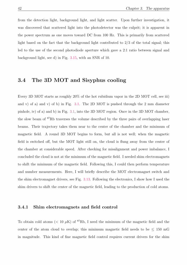
42 Chapter 3. The apparatus
from the detection light, background light, and light scatter. Upon further investigation, it
was discovered that scattered light into the photodetector was the culprit; it is apparent in
the power spectrum as one moves toward DC from 100 Hz. This is primarily from scattered
light based on the fact that the background light contributed to 2/3 of the total signal; this
led to the use of the second photodiode aperture which gave a 2:1 ratio between signal and
background light, see d) in Fig. 3.15, with an SNR of 10.
3.4 The 3D MOT and Sisyphus cooling
Every 3D MOT starts as roughly 20% of the hot rubidium vapor in the 2D MOT cell, see iii)
and v) of a) and v) of b) in Fig. 3.1. The 2D MOT is pushed through the 2 mm diameter
pinhole, iv) of a) and b) in Fig. 3.1, into the 3D MOT region. Once in the 3D MOT chamber,
the slow beam of 87Rb traverses the volume described by the three pairs of overlapping laser
beams. Their trajectory takes them near to the center of the chamber and the minimum of
magnetic field. A round 3D MOT begins to form, but all is not well; when the magnetic
field is switched off, but the MOT light still on, the cloud is flung away from the center of
the chamber at considerable speed. After checking for misalignment and power imbalance, I
concluded the cloud is not at the minimum of the magnetic field. I needed shim electromagnets
to shift the minimum of the magnetic field. Following this, I could then perform temperature
and number measurements. Here, I will briefly describe the MOT electromagnet switch and
the shim electromagnet drivers, see Fig. 3.13. Following the electronics, I show how I used the
shim drivers to shift the center of the magnetic field, leading to the production of cold atoms.
3.4.1 Shim electromagnets and field control
To obtain cold atoms (< 10 µK) of 87Rb, I need the minimum of the magnetic field and the
center of the atom cloud to overlap; this minimum magnetic field needs to be ≤ 150 mG
in magnitude. This kind of fine magnetic field control requires current drivers for the shim

3.4. The 3D MOT and Sisyphus cooling 43
electromagnets; I will also discuss the switch for the MOT electromagnet briefly, see a) of Fig.
3.13.
Vin1
Vin1
Vin2
Vin2
a)
OPA549
- +
V-
V+
B
I
X, Y, Z
Ilimit and Ref Vin
b)
Figure 3.13: Electronics for controlling the magnetic field. a) H-bridge for fast switching ofthe 3D MOT electromagnet. A single current source (Delta Elektronika, SM 7.5-80) was usedto power both electromagnets. b) OPA549 current driver for shim electromagnet operation.Additional electronics allowed for the switching of the current direction and for current limitedoperation.
A one-chip circuit based on the OPA549 was devised to operate the shim electromagnets with
a simple linear voltage control, see b) of Fig. 3.13. I was then able to profile the magnetic field
inside the chamber with parameter scan trials. I scanned the X,Y and Z shim electromagnets,
one at a time and in that order, fixed the reading that gave the most compact cloud size as
imaged by the CCD camera, and reiterated, see Fig. 3.14. I plot sigma, the cloud size from
the 2D Gaussian fit. This method is placing the center of the quadrupole at the center of the
MOT beams using the shim magnets. This left a cloud in the middle of the chamber upon
release, after controlling for beam alignment and power imbalance.
I used an H-bridge for the 3D MOT switch, see a) Fig. 3.13, that enables a voltage to be
applied across the electromagnets in opposite directions. The idea was to be able to tune the
switching time to a minimum. In testing I found that the switch could shut a magnet off in
a 1/e2 time of 1.5 ms. Installed in the vacuum can and using the atoms as the judge of an
appropriate switching time, I found that 3 ms was less lossy and gave a lower temperature.
3.4.2 Temperature and number measurements
I measure the temperature using the time-of-flight technique, where a cloud is dropped and
allowed to expand freely for a time T. This expansion is monitored on a CCD camera. I use

44 Chapter 3. The apparatus
-0.2 -0.1 0.0 0.1 0.2 0.3400
500
600
700
800
900
1000
Applied voltage control [V]
2[mm2 ]
X shim, x X shim, y Y shim, x Y shim, y Z shim, x Z shim, y
-0.2 -0.1 0.0 0.1 0.2 0.3400
500
600
700
800
900
1000
Applied voltage control [V]
2[mm2 ]
X shim, x X shim, y Y shim, x Y shim, y Z shim, x Z shim, y
Figure 3.14: Shim field trials. Starting with the X shim electromagnets, I scan the voltageof applied to the driver to realize a small shift in the magnetic field for each shot. I find theminimum for the X shim scan and set the value. I iterate over Y shim and Z shim and repeatall three one more time. Note, as I set the shim values, the next scan leads to a more compactcloud; scan order X, Y, and then Z.
a 2D Gaussian fit to give the size of the cloud, σ, see a) and b) of Fig. 3.15. The method
of Fig. 3.14 produces an oval-shaped cloud of atoms, see b) in Fig. 3.11 as well as a) and c)
in 3.15. To obtain the temperature, I plot the ballistic expansion time t, squared, against the
cloud diameter from the 2D Gaussian fit σ, squared, and fit a line to
σ2 = σ20 +
kBT
mt2, (3.8)
where σ20 is the initial cloud size, kB is Boltzmann’s constant, T is the temperature, and m
is the mass of the 87Rb atom. For the MOT, I obtain a geometric mean temperature of 170
µK. This temperature is not cold enough to perform atom interferometry in our geometry for
more than a few ms, so I opt for cooling the atoms further via the Sisyphus mechanism [46],
also known as molasses or polarization-gradient cooling. I know the recoil temperature, the
theoretical limit of sub-Doppler cooling, is 348.7 nK [43] but that in practice, with Sisyphus
cooling, Foot says the best one hope for is about an order of magnitude higher [47].
I release the cloud by switching the 3D MOT electromagnets; this takes 3 ms during which
time the MOT light is left on. After this, the detuning of the light is ramped over 500 µs from

3.4. The 3D MOT and Sisyphus cooling 45
0 20 40 60 80 100
0.5
1.0
1.5
2.0
2.5
Ballistic expansion time, t 2 [ms2]
Clouddiameter,
2[mm2 ]
X: Tx = 179 ± 2 K Y: TY = 156 ± 2 K
0 20 40 60 80 100
0.5
1.0
1.5
2.0
2.5
Ballistic expansion time, t 2 [ms2]
Clouddiameter,
2[mm2 ]
X: Tx = 179 ± 2 K Y: TY = 156 ± 2 K
0 50 100 1500.05
0.10
0.15
0.20
0.25
0.30
Ballistic expansion time, t 2 [ms2]
Clouddiameter,
2[mm2 ]
X: Tx = 5 ± 2 K Y: TY = 5 ± 2 K
0 50 100 1500.05
0.10
0.15
0.20
0.25
0.30
Ballistic expansion time, t 2 [ms2]
Clouddiameter,
2[mm2 ]
a) b)
c)
d) Figure 3.15: TOF temperature measurements for the 3D MOT and Sisyphus cooling. a) The3D MOT is oval shaped and too hot for atom interferometry for more than a few ms. b) Coldatoms after the conclusion of Sisyphus cooling. c) A 3D MOT forming in the main chamber.
-15 MHz to -150 MHz by the cooling laser offset lock. At the conclusion of the frequency ramp,
the intensity is ramped to extinction over 500 µs via the VCA in the RF chain leading to the
AOM. These clouds have temperatures consistent with Foot’s assertion [47], see b) in Fig. 3.15;
I obtain clouds with a geometric mean temperature of 5 µK, cold enough to not disperse while
performing interferometry with tens of ms interrogation time.
I measure the particle number in two ways: (i) I use the CCD to estimate the particle number
during MOT and Sisyphus cooling trials and (ii) I use the Femto photodetector, see c) in
Fig. 3.11, to measure the particle number. The photodetector has a gain from the trans-
impedance amplifier of 107 V/A and the efficiency at 780 nm is .53 A/W. A single atom,
driven on resonance, delivers 2.75 fW incident on the detector; this is smaller than expected
from geometry (11 fW per atom) because the solid angle is clipped by changing the limiting
aperture from the window to the second iris in front of the photodetector. This is for background
removal. For V = 100 mV of signal, typical of a number measurement after Sisyphus cooling,
I obtain
Atom number =V
107 V/A× .53 A/W× (2.75× 10⁻¹⁵) W/atom≈ 7× 10⁶ atoms. (3.9)

46 Chapter 3. The apparatus
3.5 The Honeywell QA-750 MEMS Accelerometer and
vibration isolation
Here I discuss the micro-electro-mechanical system (MEMS) navigation-grade accelerometer
(Honeywell, QA750). This device is used to track table tilting, vibrations and other accelera-
tions. I perform a series of trials to test the electronics, understand noise sources, and probe
the vibration spectrum near the experiment platform, see all of Fig. 3.16. The vacuum can
rests on an 310 mm thick, stainless steel optical table (Thorlabs, Nexus series) and four 700
mm tall active vertical and horizontal vibration isolating support legs (Thorlabs, PTS603), see
i) of a) in Fig. 3.16. To reach the height of the vacuum windows, the Raman interferometer
retro-reflection mirror and the MEMS accelerometer, epoxied flat to the back, must rest on a
platform, see ii) in a) of Fig. 3.16. This stand is 240 mm from the table top to the center of
the mirror. The outer casing and base are both aluminum. Inside, the stand is filled with sand
up to the last 3 cm, where a steel rod protrudes into the stand to lock the top platform in
place. The top platform is constructed out of two aluminum plates sandwiching a 5 mm layer
of damping foam (α-gel), held tight with nylon screws, see iii) in a) of Fig. 3.16. The mirror
and accelerometer are held in a 50 mm diameter mirror mount (Thorlabs, POLARIS-K2F1)
epoxied to a ceramic pedestal held firmly via three point contact atop a 1 mm layer of paper,
see iv) of a) in Fig. 3.16. The paper and ceramic serve to dampen the transmission of high
frequency vibrations from the aluminum stand and table to the retro-reflection mirror, and so
the MEMS accelerometer.
3.5.1 Electronics
The MEMS accelerometer is connected to the electronics on the vibration isolation platform
through cables that are not stretched taut; this minimizes vibration transfer through the ca-
bling. The Honeywell QA750 MEMS accelerometer used in this experiment outputs a current
proportional to the acceleration with a calibration from the manufacturer listing 1.349122 ×
10−3 A/g, where g is taken as 9.80665 m s−2. Across this output I connected a 10 kΩ resistor

3.5. The Honeywell QA-750 MEMS Accelerometer and vibration isolation 47
(measured, 9.9195 ± .0003 kΩ), in parallel with two capacitors in series (measured, each 330
nF). The accelerometer is listed on the datasheet to have bandwidth exceeding 300 Hz, up to
500 Hz; my particular device goes to 430 Hz. I add the capacitors to create a roll off. This
creates a time constant τ = 1.726 ms with a 3 dB point at 579 Hz, just past the bandwidth of
the accelerometer; this is to suppress any noise not coming from the accelerometer. The ground
of the accelerometer case is that of the table top, 2) in a) of Fig. 3.16. This is not the ground
of the voltage measurement, 1) in a) of Fig. 3.16.
Understanding the correlation between the sign of the voltage and the direction of the accel-
eration is the first step in determining whether any force I detect is attractive or repulsive.
When the MEMS accelerometer has the non-connectorized side face down on the table (the
side epoxied to the back of the retro-reflector), the device delivers a positive voltage, see vi)
in b) of Fig. 3.16. The accelerometer is used in the orientation shown in vii) of b) in Fig.
3.16, where the angle θ is exaggerated for display. The table has a slight tilt, and while it does
oscillate about some mean tilt angle, it never changes sign.
3.5.2 Vibration isolation
With the accelerometer in the orientation shown in iv) of a) and vii) of b) in Fig. 3.16, I measure
the vibration spectrum in m2s−4/Hz up to 500 Hz under various conditions at midday during
a weekday, typical hours for experimental trials, see c) of Fig. 3.16. The flat orange line across
the frequency bands is white noise equivalent to 5 nm s−2 when integrated over the frequency
bands; I present it for reference. The gray spectrum is the pick-up over the electronics and
cabling, which appears as a false acceleration of 2.2 µm s−2. Major contributors to this are the
frequency band below 1 Hz and the peak at 50 Hz; when powered and part of the power supply
ground, the harmonics of 50 Hz are suppressed. With the accelerometer on and the optical
table grounded around midday, the accelerometer measures vibrations totaling 1.6 mm s−2.
The accelerometer was placed atop the isolation platform and the optical table was floated;
this produced the red spectrum, vibrations totaling 712 µm s−2. The atom interferometer
geometry provides a filtering effect dependent upon the interferometer time T . For T = 16 ms,

48 Chapter 3. The apparatus
a)
0.5 5 50 50010-16
10-14
10-12
10-10
10-8
10-6
Frequency [Hz]
PSD[m
2s-4 /Hz]
Isolation platform, midday
Unfloated table, midday
Line noise
= 1 [mrad] with white noise spectrum
i)
ii)
iii)
iv)
v) To NI PXI-4462, 1 MΩ and 217 pF
R C
1)
2)
R: 9.9195 kΩ C: 174 nF τRC: 1.73 ms
b)
g
+V vi) vii)
g +V
θ
c)
Figure 3.16: QA750 MEMS vibration trials. a) Schematic layout of the MEMS accelerometerand the Raman retro-reflection mirror on the vibration isolation platform. From the floor up: i)Optical table, ii) stand, iii) sandwich of two aluminum plates and a wedge of damping foam, iv)the accelerometer, the mirror and the ceramic pedestal, and v) the circuit diagram of turningthe accelerometer current into a voltage. b) Correlation of the sign of the voltage and thedirection of acceleration is critical. Determining which way it goes: vi) with gravity and vii) inthe orientation (exaggerated) of iv). c) Vibration spectrum over 500 Hz in the setup of a) forvarious conditions.
this covers a bandwidth of about 63 Hz; the atoms will be sensitive to vibrations totaling 90
µm s−2.
3.6 The source mass
This section describes the source mass installation and geometry. A UHV rotary feed-through
is installed in the larger flange containing the MOT window, see i) of a) in Fig. 3.17. This
comes with a stepper motor and controller that interface through a Windows computer with
a GUI. This rotates a rod inside the vacuum, which extends down into a small ball bearing

3.6. The source mass 49
a)
d ωlas
i)
ii) iii)
iv)
b)
ϑ
0°
Right Left
i)
iii)
iv)
Raman
Z
Y
X
Raman
θ
Figure 3.17: Source mass geometry. a) The vacuum feed-through for moving the source mass,side view: i) The UHV compatible rotary feed-through and stepper motor, ii) the ball bearingand stability support, iii) the two rods that bring the source mass into close proximity of theatoms and iv) the source mass, covered in a layer of MH2200 optical coating. b) Vacuumfeed-through for moving the source mass, top view: i) the rotary feed-through is positionedjust outside the edge of the top 3D MOT electromagnet former. iii) the rod extends into thechamber to allow the source mass access to the interferometer region. iv) The source mass has arange of usable angles, see a) in Fig. 3.19. The orientation convention adopted is the following:when the source mass is past 0 degrees towards +30 degrees, the orientation is referred to as“left” and if the orientation is towards -30 degrees it is “right”.
specially lubricated for UHV use, see ii) in a) of Fig. 3.17, held in place by an aluminum brace.
An aluminum arm extends out into the chamber, see iii) of a) and b) of Fig. 3.17, where it is
attached to an aluminum rod holding the source mass. The source mass, a sphere of aluminum
of radius 19 mm, see iv) of a) and b) in Fig. 3.17, sits above the plane of the XY MOT beams
and the Raman beam. It is covered in a coat of Alion MH2200 optical absorber coating. This
is a black coating that has a high absorption in infrared with very low out-gassing, < 10−12
(mbar liter)/(s cm2), comparable to stainless steel.
The Raman beam is reduced to 22 mm diameter beam using two irises. The nearest approach
of the source mass to the axis of the Raman beam is at d = 25 mm, see a) in Fig. 3.18,
placing the source mass in the shadow of the aperture. The Cartesian coordinates of the ball
are determined by
d = x, y, z =R cos (θ)− x0, y0, R sin (θ)
, (3.10)

50 Chapter 3. The apparatus
where I set the origin of Cartesian coordinates to be the center of the cloud, x, y, z = 0, 0, 0.
I need to know the positioning of the source mass relative to the atoms. The vertical axis of
rotation and a vertical axis through the center of the ball are separated by R = 72.79 mm, the
extension rod iii) in b) of Fig. 3.17. The vertical axis of rotation and a vertical axis through
center of the cloud are separated by x0 = 55.00 mm. The vertical separation, y0, between the
horizontal plane through the center of the ball and the horizontal plane through the center of
the atom cloud is 12.7(2) mm. The XY plane is horizontal. The Raman axis is ±45 degrees
off the Y and X axes, also the MOT axes, respectively. The Z axis is parallel with gravity.
The axis of rotation and the vertical through the center of the cloud both lie on the X axis,
separated by x0. Using equation (3.10), I can calculate the distance d of the center of the atom
cloud to the center of the source mass as a function of angle, see Fig. 3.18. The full angle
available to move the source mass is ϑ = 50 degrees, shown in b) of Fig. 3.18.
-20 -10 0 10 20
22
24
26
28
30
32
34
Source mass angle [deg]
Distancefromcloudtosourcemass[mm]
-20 -10 0 10 20-10
-5
0
5
10
Source mass angle [deg]
Forceprojectionfactor
a) b)
Figure 3.18: Source mass angles and the force projection factor.
Barriers to further movement of the source mass, see thin red lines in Fig. 3.18, prevent the
source mass from hitting the electromagnet former. These barriers are designed into the ball
bearing mount, see ii) in a) of Fig. 3.17. The red region around 0 degrees, while accessible to
the source mass, blocks the top 3D MOT beam. Further, from -5 to 5 degrees, the source mass
clips the solid angle of the photodetector, making this region of space thoroughly unusable.
The thin blue lines at ±14 degrees are the angles used in the experiment.
Based on geometry I can define a force projection factor, scaled to one, as a function of the
angle the source mass has with respect to the atomic cloud, see b) in Fig. 3.18. This factor

3.6. The source mass 51
helped in the design of the experiment and can help inform the design of future experiments.
This factor uses geometry to parameterize how sensitive the atoms are to a 1/r2-style force,
F ∼ 1
d2; (3.11)
the projection onto the Raman axis is
Fz =1
d2
z
|d|=
z3√x2 + y2 + z2
, (3.12)
This force projection, scaled to numbers of order 1, is plotted as a function of the source mass
angle θ, see Fig. 3.18, in angles read from the stepper motor assembly. The thin red thin
lines and shaded areas are restricted regions. The blue lines for ±14 degrees are shown to be
near the maximum extent of the force projection factor’s range, around a projection factor of
±9.2; these are the positions I used for the source mass to create the largest possible 1/r2-style
force. In the theoretical work supporting this experiment, the atom ensemble was considered
at the surface of the source mass [3]; the acceleration calculated was the acceleration along
the line joining the center of the source mass and that of the atom cloud. This force needs
modification by the factors above: (i) the separation is larger than the radius of the mass, so
a reduction factor of ( rballd
)2 is required, where rball = 19 mm and d is the distance from the
atom cloud to the source mass center, as shown in a) of Fig. 3.17. (ii) The interferometer
only measures the component along the Raman axis. To account for this, I require a reduction
factor of cos (θ). The total force reduction factor has a value ±0.332. A point of improvement
to future experiments would be to enhance the factor or improve the experiment in other ways
to counteract this.
3.6.1 Light scatter tests
In this experiment, I am concerned with three light scatter problems: (i) First, I want to ensure
that no leakage light from the 3D MOT setup makes its way into the chamber. (ii) Second, I
want to ensure that the source mass does not scatter Raman light through the interferometer

52 Chapter 3. The apparatus
volume. (iii) And finally, I want to control the background light during detection. In this
section, I address (i) and (ii). I leave (iii) for discussion about the primary experiment in
Chapter 5.
A few µW of resonant or near resonant leakage light from the 3D MOT beams can provide
enough photons to optically pump the atoms, creating a false signal. The cooling light going
into the 6 3D MOT beams is controlled by a single double-pass AOM; when the RF switch is
triggered and the VCA tuned to allow no RF power through, all light through the AOM shines
on a beam block. Only a few µW travel down the beam line leading to the 6 fiber couples, see
iii) in a) of Fig. 3.5, from the cooing laser and is 220 MHz red-detuned; it is not coupled into
the fibers and can not be measured at the output of any fibers. The repump laser is controlled
by a single pass AOM located two fiber couples before the experiment, see Fig. 3.4; triggering
the RF switch and tuning the VCA on the repump AOM passes no light into the first fiber
couple. No light passes in the next stage, and none onto the experiment. After these checks
were complete, a cold cloud could be dropped for > 40 ms undisturbed; the distribution of
atoms in the F=2 ground state, after Sisyphus cooling, remained unaltered for this time.
Scattered Raman light can be parameterized by an electric field ε. This field could cross scatter
back through the main Raman beam axis, denoted by a field E; at worst, this could change
the phase by δφ = ε/E, leading to the measurement of a false acceleration. I want to keep this
false acceleration below the 10 nm s−2 level. To do this, I need to control this phase shift to
δφ = ε/E ≤ 4 × 10⁻⁵. It is critical that this light scatter be kept to a minimum; when the
source mass is moved, I want to ensure the light scatter through the atom cloud is less than
2× 10⁻⁹ of the peak Raman intensity. To do this I performed light scatter trials on a 1:2 scale
system.
By geometry, I have eliminated the possibility of blocking the Raman beam with the source
mass. By clipping the beam with an iris, the Gaussian tail is prevented from diffracting around
the edge of the window and the source mass. Despite this, light is still diffracted into angles
that will land on the source mass. To test this, a scale model was created, see a) of Fig. 3.19. A
780 nm test laser (Thorlabs, S1FC780) was coupled to a fiber collimator (Schafter+Kirchhoff,

3.6. The source mass 53
δ
La)
b)
x
y
z y
Figure 3.19: Light scatter near the source mass. a) The scale test setup. I used a low power780 nm fiber laser and a beam collimator as a test Raman beam. I passed this beam through aniris and used a CCD camera to examine the diffraction around the edge of iris, paying particularattention to the region occupied by the source mass. b) Long exposure (.5 s) snapshot of thescatter past the iris edge.
60FC-Q780-4-M100-37), passed through an iris and onto a CCD camera (Allied Vision, Merlin
F-033C) at various positions along the light beam path, including through optics detailed in
iv) of a) in Fig. 3.16. The CCD camera used no optics and was modified to prevent scatter
around the CCD chip and electronics for this measurement; reflective surfaces were covered
with black vinyl tape and coated metal foil. A 1:2 scale source mass of polished steel was used.
This setup was constructed in a box shielded from background light. I applied low powers (150
µW), producing images like b) of 3.19 for an exposure time of .5 s, where the CCD camera
was scanned across the iris edge and into the shadow created by the iris. The beam waist
was 10.5 mm. This shows scattered photon count across the CCD chip, where the chip is set
downstream, behind the source mass by a distance L parallel to the aperture edge. In a typical
π-pulse, 1.5× 10⁵ photons scatter off the source mass. To put a bound on the phase shift from
scattered light, I take the worst case scenario in which all the light scattered from the ball goes
through a solid angle subtending the entire interferometer volume and that these photons are
as effective as driving transitions as the photons that are not scattered. This gives a power ratio

54 Chapter 3. The apparatus
of the peak beam intensity versus the worst case scatter through the interferometer region as
ε/E → 8× 10⁻¹⁰; this is a factor 2 below the required intensity to create a systematic of order
10 nm s−2, as the worst case scenario. Regardless, I took caution before installation; the source
mass, of machined aluminum, was coated in a layer of the NIR absorbing, UHV-compatible
paint MH2200.
3.7 Computer control system, sequencing and pattern
generation
In the following subsections I describe the hardware that enabled this experiment to function
and the work that went in to ensuring precise timing. I then describe the pattern generation
and acquisition software.
PXI case and cards
National Instruments PXI instrumentation is used in this experiment. A small chassis (NI,
PXI-1072) contained three output cards and one input card. First, the PXI-6723 (13-Bit, 32-
Channel, 800 kS/s) provides analog outputs to the experiment. Next, the PXI-6541 (50 MHz,
32-Channel) high-speed digital card controls digital communication to the MOT laser system
and AOMs. Last, the PXIe-6341 (16 AI (16-Bit, 500 kS/s), 2 AO, 24 DIO) controls digital
communication to the Raman laser system. The PXI-4462 (204.8 kS/s, 4-Input) is used to log
the MEMS and photodetector voltages.
Variable time based functionality through an FPGA
The timing sequence for the experiment involves slow processes like loading the MOT and fast
processes like the Raman pulses. I opt to use a variable frequency clock, where clock pulses are
generated dynamically, changing when the card outputs need to change timebase. I use the Opal

3.7. Computer control system, sequencing and pattern generation 55
Kelly XEM3001 FPGA module (400,000-gate Xilinx Spartan-3 FPGA, XC3S400-4PQ208C) for
this purpose.
In brief, a hardware server sends the FPGA a list of variable timebase segments to be used in
a run. The segments specify the clock frequency and the number of clock pulses needed for the
segment. The FPGA generates the clock frequency from dividing down the master clock (300
MHz).
Cicero and Atticus - pattern generation and timing
I make use of Cicero Word Generator and Atticus Hardware Server software [48] for pattern
generation and hardware communication. Cicero, designed to use National Instruments output
hardware, is compatible with any output hardware that uses the NIDaqMx driver library. The
hardware layer consumes substantial memory for generation of the output buffers; a large
amount of memory located on the computer communicating with the output cards is critical to
ensure smooth running. The user interface allows for separating an experiment into individual
time blocks, with individual timing, supporting analog output, digital output, GPIB and RS232
communication. See an experimental run on Cicero in Fig. 3.22. I show a schematic version of
the run pattern shown in Fig. 3.22 in Fig. 3.20.
Labview CVI
The acquisition software was designed in Labview CVI. The program acquires two voltages,
the voltage from the MEMS accelerometer and the voltage from the photodetector. For all
experiments presented, the detection is clocked at 200 kHz and triggered by the FPGA. I
briefly describe how these signals are acquired below.

56 Chapter 3. The apparatus
3D MOT and source mass movement
Sisyphus cooling to 5 µK
Velocity selection and blow away
Interferometer Detection
Start
End
3D MOT Freq.
3D MOT intensity
Repump Intensity
Raman Intensity
3D MOT Electromagnets
Raman electromagnets
Time
-15 MHz -3 MHz
-150 MHz
12 W/m2
off Isat Isat
Full
off
off
on
off
π/2
on
off
π π/2 T T
40 ms
π
+6 MHz
Isat
Figure 3.20: Schematic experiment run pattern. Here I display the most dynamic channels:the 3D MOT frequency (controlled by the VCO in the offset lock of the cooling laser) andintensity (tuning applied RF power to the 3D MOT AOM), the repump intensity (tuningapplied RF power to the AOM), the Raman light intensity (tuning applied RF power to theAOM in the µQuans laser), and the electromagnet switches for the 3D MOT and Raman axiselectromagnets. I discuss velocity selection and blow away sequencing in sections 4.1.2 and4.2.1.

3.7. Computer control system, sequencing and pattern generation 57
MEMS voltage
The MEMS voltage acquired by the NI PXI-4462 card is positive. In a typical experiment, the
voltage is acquired every 5 µs over the interferometer time 2T. The mean of this is given as
an output. The triangularly weighted mean is another output . Here, the weighting increases
linearly to 1, starting at 0 over the interval 0 < t < T , the decreases to 0 over T < t < 2T [49].
Photodetector voltage
Figure 3.21: Detection scheme. A snapshot of the photodetector acquisition taking place duringa typical interferometer run. The atomic signal is in red and the background light is in blue.See Fig. 3.20 for the detection sequence in the pattern.
The photodetector voltage, also acquired by the NI PXI-4462 card, is a positive voltage, see Fig.
3.21. The detection sequence is broken into two sections, atomic signal acquisition (red) and
background determination (blue). The background, superimposed on the atomic signal acquisi-
tion for comparison, occurs 40 ms after the interferometer output is measured. The background
determination uses the same detection sequence as the atomic signal acquisition, the only dif-
ference being that I have waiting until all the atoms have left the measurement volume. The
sequences are identical and obtain voltage values corresponding to N2, Ntot, N2,bg and Ntot,bg,
the atom number in |2, 0〉, the total number of atoms in |2, 0〉 and |1, 0〉, the background light
of the |2, 0〉 atom number measurement and the background of the total atom number mea-
surement, respectively. First, the cooling light is turned on for 750 µs, measuring N2. Next,
the repump is turned on for a 750 µs measurement of Ntot. I make small cuts to remove the rise
time and fall time associated with changing the light intensity. I can then take these voltages

58 Chapter 3. The apparatus
and produce a mean value which can be used to construct the probability
P =N2 −N2,bg
Ntot −Ntot,bg
. (3.13)
These four mean voltages are exported, as well as the probability P .

3.7. Computer control system, sequencing and pattern generation 59
Com
pute
r H
P 67
0
FPG
A
PXI-
1072
Cha
ssis
: PX
I-44
62
PXI-
6723
PX
I-65
41
PXIe
-634
1
AO
M
Freq
. C
hain
MuQ
uans
La
ser
Coo
ling
Lase
r
Phot
odet
ecto
r +
MEM
S
Expe
rimen
t
Inpu
t
Out
put
Elec
trom
agne
t Sw
itchi
ng/C
ontro
l
Fig
ure
3.22
:E
xp
erim
ent
contr
olan
dblo
ckdia
gram
.T
op:
The
exp
erim
ent
contr
olco
mpute
rdoi
ng
wor
kon
16N
ov,
2017
wit
ha
range
ofso
ftw
are
invie
w.
Fro
mle
ftto
righ
t,th
est
epp
erm
otor
contr
olG
UI
and
the
Ram
anla
ser
lock
mon
itor
.B
ehin
dth
ese
win
dow
sar
ete
rmin
als
mon
itor
ing
the
har
dw
are
serv
eran
dco
mm
ands
sent
toit
.M
ovin
gri
ght,
the
Lab
vie
wC
VI
acquis
itio
npro
gram
isbusy
takin
gdat
a.B
elow
itis
are
cent
phot
odet
ecto
rac
quis
itio
n.
Furt
her
righ
tis
Cic
ero,
hav
ing
just
succ
essf
ully
outp
ut
the
nex
tpat
tern
.B
otto
m:
Blo
ckdia
gram
ofth
eex
per
imen
t.Sta
rtin
gw
ith
aW
indow
sm
achin
e,th
epat
tern
gener
ator
sends
clock
info
rmat
ion
toth
eF
PG
Aan
dth
epat
tern
toth
eP
XI
chas
sis.
The
FP
GA
then
star
tsth
ese
quen
ce,
sendin
ga
dynam
iccl
ock
sign
alto
all
the
card
s.T
hes
eca
rds
outp
ut
tova
riou
ssy
stem
s;th
eM
OT
lase
rs,
AO
Ms,
elec
trom
agnet
s,an
dth
eR
aman
lase
r.A
shor
tti
me
late
r,ou
tput
from
the
phot
odet
ecto
ran
dM
EM
Sis
acquir
edan
dse
nt
toth
eco
mpute
r.

Chapter 4
Setting up the interferometer
With the apparatus on the table, my goal turned to setting up the interferometer. First,
using a co-propagating beam configuration, see a) in Fig. 4.1, I checked that I understood
the Rabi frequency, the separation of magnetic sub-levels and the light shift. Following this, I
began Ramsey interferometry to check the quality of my state selection and the timing between
pulses. I add in a third pulse to realize spin echo experiments. These tests were useful in that
they allowed me to use a simpler system to check my understanding without the additional
concern of vibrations or the initial velocity distribution of the atoms.
In the section following, I retro-reflect the Raman beam to begin counter-propagating studies.
I make a velocity selection from the cold cloud and perform 3 pulse, acceleration-sensitive
interferometry using configuration b) in Fig. 4.1. The method pursued has both pairs of light
beams resonant, driving two atom interferometers simultaneously. I use these data to check the
accuracy of my laser phase commands. Using this method of two simultaneous interferometers
does not produce high fringe contrast in my experiment. I resolve to move on to configuration
c) in Fig. 4.1. I realize Kasevich-Chu style atom interferometry and focus the rest of the section
on investigating the correlation with the MEMS accelerometer, concluding with a calibration
of the MEMS accelerometer to the atom interferometer. All data presented are representative,
single scans. If averaging is used, it is explicitly mentioned.
60

61
Co-propagating versus counter-propagating and conventions
In the two sections below, I use three optical geometries on the way to acceleration-sensitive
atom interferometry, see Fig. 4.1. In the first section, I use co-propagating Raman light with
the two frequencies in perpendicular Linear polarizations, see a) in Fig. 4.1. I block the retro-
reflection for tests in this configuration. After discussing Raman spectroscopy, I confirm that
changing the incoming polarization from perpendicular linear to circularly polarized no longer
drives the Raman transition, in agreement with the selection rules discussed in chapter 2.
Lin ⊥ Lin
c)
a)
g
vL
ω1
ω2Doppler-insensitive
Bea
m B
lock
vR I0
γI0
b)
ω1
ω2
ω1
ω2Doppler-sensitive Double Single Diffraction
I0
γI0
g
vL
ω1
ω2
ω1
ω2Doppler-sensitive Single Diffraction
I0
γI0
Beam Block
ω1
We throw out slave 1.
g
vL vR σ+
σ-
σ-
σ+
σ+
σ-
σ-
vL: σ- σ- transition vR: σ+ σ+ transition
Figure 4.1: Co- and counter- propagating geometry. a) Co-propagating method: this configu-ration is important as it allows for testing without the addition of acceleration noise. b) Firstcounter-propagating method: both σ+σ+ and σ−σ− transitions are allowed which can opentwo interferometers simultaneously. c) Second counter-propagating method: I dump a singlefrequency before the retro-reflector using polarization optics. This allows me to choose σ+σ+
or σ−σ−. This is the setup for the primary experiment, where I have selected σ−σ− transitions.The factor γ=.583 for the detuning I have chosen.
In the section following, I start studies using counter-propagating beams using b) of Fig. 4.1;
with the incoming beam circularly polarized, I retro-reflect the beam through a λ/4-plate, which
flops the polarizations of the frequencies. This allows me to drive σ+σ+ and σ−σ− transitions
as well as conferring velocity sensitivity. I make an acceleration-sensitive atom interferometer

62 Chapter 4. Setting up the interferometer
in this setting and show that utilizing two simultaneous interferometers does not confer the
best acceleration sensitivity in my experiment. Finally, I add a polarizing beam-splitter after
the second λ/4-plate, see c) in Fig. 4.1, which allows me to select one frequency and extinguish
it. By this method, I can drive σ+σ+ or σ−σ− transitions. I choose to drive σ−σ− transitions
and proceed to investigate correlations with my MEMS accelerometer.
4.1 Studies with Co-propagating Raman beams
4.1.1 Rabi flops and Raman Spectroscopy
At the end of Sisyphus cooling, the cold atom cloud is left distributed across the 8 Zeeman
sub-levels of the F=1 and F=2 ground states. The quality of the cooling and repump AOM
extinction and the inhomogeneity in the applied magnetic field determine the exact distribution
of atoms across these states. I begin the studies of co-propagating transitions by performing a
simple manifold selection; I load all the atoms into the Zeeman sub-levels of the F=1 ground
state. I do this by turning off the repump light for the last 2 ms of the Sisyphus cooling.
To begin driving the Raman transition from F=1 to F=2, parameters had to be given to the
µQuans laser; the detuning, power ratio, and overall output power. In accordance with the
magic ratio calculation in chapter 2, the offset lock of the two lasers was set to a detuning -1.13
GHz from the cycling transition, 52S1/2(F = 2) → 52P3/2(F = 3). To cancel the AC Stark
shift, this detuning requires an intensity ratio of .583 between ii) and iii) of b) and d) in Fig.
3.9. This was done by setting a fixed RF power for AOM at the output ii) and iii) in b) of Fig.
3.9 and varying the power ratios of EDFA 1 and EDFA 2. I found that scanning the RF power
applied to the AOM, for fixed EDFA ratios, did not maintain the intensity ratio, see a) and b)
of Fig. 3.10. To ensure I used a stable intensity ratio, I would choose a fixed RF power for the
AOM and change the amplifier settings. For my first test to drive the |1, 0〉 → |2, 0〉 transition,
I selected an output power corresponding to a π-pulse time of 23.4 µs or a Rabi frequency of
20.4 kHz. A small magnetic field was applied to lift the degeneracy of the Zeeman sub-levels.
The frequency of the phase lock between Raman laser 1 and 2 was scanned around 6.834 GHz,

4.1. Studies with Co-propagating Raman beams 63
the hyperfine splitting, and I monitored the transition probability P of atoms being in the F=2
manifold at these frequencies. In this chapter, all frequencies are referenced to the hyperfine
splitting (HFS) and are denoted by the shorthand “Difference Frequency from HFS.” I applied
a square pulse of 23 µs and scanned the 200 kHz around the hyperfine splitting, see Fig. 4.2.
I expected to observe a sinc function with a maximum probability near to .33 of the atoms
present, with the assumption that I had filled all three Zeeman sub-levels equally. I fit a sinc
function to the data in Fig. 4.2, the red line, [7]:
P =1
3
Ω2(Ω2 + (2πδf)2
) sin2[τ
2
√Ω2 + (2πδf)2
], (4.1)
where P is the transition probability, Ω is the Rabi frequency, δf is the difference frequency
from the hyperfine splitting and τ is the pulse time. The fit tells me I applied a square pulse in
time of 23.2± .3 µs and that the center of the peak is -2 kHz off the hyperfine frequency. The
peak of the sinc went to P = .32 of the total population present. This implies my assumption
that the states are loaded equally may be correct, but I press on to confirm my suspicions that
the rest of the atoms are distributed amongst the two magnetically sensitive states, |1, 1〉 and
|1,−1〉. Immediately following this, I looked for Rabi oscillations where I scan the pulse time,
see inset in Fig. 4.2, confirming the π-time was indeed 23 µs.
An investigation of the entire F=1 manifold is warranted to study the distribution of the atoms
across internal states, polarization quality of the light and control of the magnetic field. A
small magnetic field induces a shift between the three Zeeman sub-levels of F=1. Scanning
the frequency difference between the Raman lasers, I expect the Lin⊥Lin polarization to drive
the transitions to |1, 1〉 → |2, 1〉 and |1,−1〉 → |2,−1〉. A scan of 2 MHz around the mF = 0
transition reveals the transitions, see a) in Fig. 4.3.
The mF = ±1 peaks are approximately equidistant δf ≈ ±670 from the mF = 0 transition.
The Breit-Rabi formula is
E|J=1/2mjImI〉 = − ∆EHFS2(2I + 1)
+ gIµBmB ±∆EHFS
2
(1 +
4mx
2I + 1+ x2
)1/2, (4.2)

64 Chapter 4. Setting up the interferometer
-100 -50 0 50 1000.0
0.1
0.2
0.3
0.4
Difference frequency from HFS [kHz]
Probability,
10 20 30 40 50 600.000.050.100.150.200.250.30
Square pulse, time applied [s]
Probability,
Figure 4.2: Co-propagating Rabi Flop and Raman Spectroscopy. A 23 µs square pulse drivesthe atoms in |1, 0〉 to |2, 0〉. The red line is a fit to equation (4.1). Inset: Rabi flopping byscanning the pulse time at the center frequency of the peak, confirming the π-time (demarcatedby vertical red line).
wherem = mI±mJ , x = (gJ−gI)µBB∆EHFS
, gI is the nuclear g-factor, and µB is the Bohr magneton [43].
This equation gives the Zeeman shift of the energy levels. Knowing the frequency of the
mF = ±1 transitions allows me to calculate that the magnetic field at the position of the
cloud is 480 mG. Closer inspection of i) and iii) in b) of Fig. 4.3 indicate that the applied
magnetic field is homogeneous at the position sampled by the cold cloud; the line widths of
all three pulses are the same, where I would expect the the magnetically sensitive sub-levels
to have suffered inhomogeneous broadening in the presence of large gradients. The mF = ±1
transitions are not exactly equidistant from the mF = 0 transition in Fig. 4.3, but off by some
30 kHz; from Equation (4.2), I expect them to be off by only 33 Hz. This led to a study of
what this shift might be, see Fig. 4.4.
I consider the scalar, vector, and tensor components of the light shift. They all produce a shift
to the states as shown in a), b), and c) of Fig. 4.4. Only the tensor shift could supply such
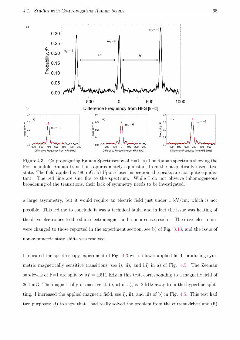
4.1. Studies with Co-propagating Raman beams 65
scale vec ten
-500 0 500 1000
0.00
0.05
0.10
0.15
0.20
0.25
0.30
Difference Frequency from HFS [kHz]
Probability,
mF = -1
mF = 0
mF = +1
δf δf
a)
b)
-900 -800 -700 -600 -500 -400 -3000.0
0.1
0.2
0.3
0.4
Difference Frequency from HFS [kHz]
Probability,
-200 -100 0 100 200 3000.0
0.1
0.2
0.3
0.4
Difference Frequency from HFS [kHz]
Probability,
400 500 600 700 800 9000.0
0.1
0.2
0.3
0.4
Difference Frequency from HFS [kHz]
Probability,
mF = -1 mF = 0
mF = +1 i) ii) iii)
Figure 4.3: Co-propagating Raman Spectroscopy of F=1. a) The Raman spectrum showing theF=1 manifold Raman transitions approximately equidistant from the magnetically-insensitivestate. The field applied is 480 mG. b) Upon closer inspection, the peaks are not quite equidis-tant. The red line are sinc fits to the spectrum. While I do not observe inhomogeneousbroadening of the transitions, their lack of symmetry needs to be investigated.
a large asymmetry, but it would require an electric field just under 1 kV/cm, which is not
possible. This led me to conclude it was a technical fault, and in fact the issue was heating of
the drive electronics to the shim electromagnet and a poor sense resistor. The drive electronics
were changed to those reported in the experiment section, see b) of Fig. 3.13, and the issue of
non-symmetric state shifts was resolved.
I repeated the spectroscopy experiment of Fig. 4.3 with a lower applied field, producing sym-
metric magnetically sensitive transitions, see i), ii), and iii) in a) of Fig. 4.5. The Zeeman
sub-levels of F=1 are split by δf = ±511 kHz in this test, corresponding to a magnetic field of
364 mG. The magnetically insensitive state, ii) in a), is -2 kHz away from the hyperfine split-
ting. I increased the applied magnetic field, see i), ii), and iii) of b) in Fig. 4.5. This test had
two purposes: (i) to show that I had really solved the problem from the current driver and (ii)

66 Chapter 4. Setting up the interferometer
10 15 20 25 30
-2000
-1000
0
1000
2000
Laser Power [mW]
ShiftsofmfstatesinF=1[Hz]
Vector shifts to energy levels
mf = +1mf = 0mf = -1
10 15 20 25 30
-2000
-1000
0
1000
2000
Laser Power [mW]
ShiftsofmfstatesinF=1[Hz]
Vector shifts to energy levels
mf = +1mf = 0mf = -1
10 15 20 25 30
-2000
-1000
0
1000
2000
Laser Power [mW]
ShiftsofmfstatesinF=1[Hz]
Vector shifts to energy levels
mf = +1mf = 0mf = -1
10 15 20 25 30-2000
-1000
0
1000
2000
3000
10 15 20 25 30
-2000
-1000
0
1000
2000
10 15 20 25 30
-2000
-1000
0
1000
2000a) b) c)
Figure 4.4: Scalar, vector and tensor shifts. a) Scalar shift: A shift of all the mF statestogether, equally. This could be caused by Raman laser 1 at a sub-optimal frequency or themagic ratio being off. b) Vector shift: A shift in which the magnetically-sensitive states shiftsymmetrically from the unperturbed magnetically-insensitive state; since the insensitive stateis actually affected to second order, a small shift is realized. This shift has a linear relationshipwith total beam intensity. c) Tensor shift: Moves the magnetically-sensitive states together.
to investigate how far I could split the Zeeman sub-levels. The µQuans laser offers large power
outputs (in excess of 1 W), which gave me the opportunity to use very short π-pulses. Short
pulse times lead to larger frequency widths that would allow me to select large momentum
distributions from the cold cloud in counter-propagating configurations. This is not possible
with small applied magnetic fields and so small Zeeman sub-level splitting, as a short pulse will
inadvertently drive the |1, 1〉 → |2, 1〉 and |1,−1〉 → |2,−1〉 transitions. I found that I could
apply a magnetic field up to 2 G. I show a high field test in i), ii), and iii) of b) in Fig. 4.5; the
Zeeman sub-levels are split by δf = ±2180 kHz, or 1.551 G. Before this test, I had realigned the
loading of the 2D MOT into the 3D MOT which involved tweaking the position of the 3D MOT.
While this did not change the temperature of the cloud, it changed the distribution of atoms
among the three Zeeman sub-levels of F=1. For the rest of this section using co-propagating
Raman beams, the field is set to 1 G.
Next, I checked the polarization dependence of the transitions. In co-propagating beam configu-
rations, the ∆mf = 0 transitions have maximum transition strength with Lin⊥Lin polarization
and are forbidden with circular polarization. I took spectra like a) in Fig. 4.3 where I changed
the waveplate angle in 5 degree steps, as shown in a) and b) of Fig. 4.6. Each turn of the
waveplate toward circularly polarized light decreased the transition probability across all Zee-
man sub-levels in the F=1 manifold. The peak transition probability goes like cos2 (θ), where

4.1. Studies with Co-propagating Raman beams 67
-3000 -2500 -2000 -1500 -10000.0
0.1
0.2
0.3
0.4
Difference Frequency from HFS [kHz]
Probability,
-1000 -500 0 500 10000.0
0.1
0.2
0.3
0.4
Difference Frequency from HFS [kHz]
Probability,
1500 2000 2500 30000.0
0.1
0.2
0.3
0.4
Difference Frequency from HFS [kHz]
Probability,
-700 -600 -500 -400 -3000.0
0.1
0.2
0.3
0.4
Difference Frequency from HFS [kHz]
Probability,
-200 -100 0 100 2000.0
0.1
0.2
0.3
0.4
Difference Frequency from HFS [kHz]
Probability,
300 400 500 600 7000.0
0.1
0.2
0.3
0.4
Difference Frequency from HFS [kHz]
Probability,
mF = -1
mF = -1
mF = 0
mF = 0
mF = +1
mF = +1
a)
b)
i)
ii) iii) i)
ii) iii)
Figure 4.5: Doppler-insensitive Raman Spectroscopy of F=1 at different magnetic fields. Thedata is in black, fits are in red. a): i), ii), and iii): Spectroscopy following Fig. 4.3 to ensure thatthe magnetically sensitive states and their separation is understood. b): i),ii), and iii): Largerapplied magnetic field leads to larger splitting. This series was scanned with less resolution.
θ is the waveplate angle referenced to the fast axis, shown in c) of Fig. 4.6; the rotation mount
used was not aligned with the waveplate’s fast axis making the wave plate angle axis arbitrary.
mF = +1 mF = 0
mF = -1 mF = 0
a) b)
-500 0 500
0.00
0.05
0.10
0.15
0.20
0.25
Difference frequency from HFS [kHz]
Probability,
-100 -50 0 50 100
0.00
0.05
0.10
0.15
0.20
0.25
Difference frequency from HFS [kHz]
Probability,
LinLin@ 140°175°180°185°
±-± @ 190°
-100 -50 0 50 100
0.00
0.05
0.10
0.15
0.20
0.25
Difference frequency from HFS [kHz]
Probability,
150 160 170 180 1900.00
0.05
0.10
0.15
0.20
0.25
0.30
0.35
Wave plate angle [deg]
Probabilityofpeak
c)
Figure 4.6: Transitioning from Lin⊥Lin to circular polarization. a) The spectra show thetransition probability decreasing equally across the states as the waveplate is rotated. b) Closerinspection of |1, 0〉 → |2, 0〉 transition. c) The peak probability P of the magnetically-insensitivestate in co-propagating configuration as a function of λ/4 waveplate angle.
In this subsection, starting with tests of the π-pulse time and power, I was able to scan the fre-
quency difference between the Raman lasers and resolve the splitting of the Zeeman sub-levels
of F=1 by my applied magnetic field. I was able to solve problems related to the Zeeman split-
ting, test larger applied fields, and demonstrate the polarization dependence of the transition
strength.

68 Chapter 4. Setting up the interferometer
4.1.2 Ramsey Interferometry
A natural progression from this point is to add another pulse. This is Ramsey’s method [7,50].
First, I must develop a state selection scheme that is more restrictive than selecting the entire
manifold, as in the previous subsection. I need to select atoms in only the mF = 0 Zeeman
sub-level of either F=1 or F=2; I select |1, 0〉, as described next. This state selection technique
also lends itself to selecting a velocity distribution of the cold cloud, which I discuss at the
beginning of the next section on counter-propagating studies.
State preparation
I need to employ a state preparation scheme. I no longer allow the atom to fill the F=1
manifold but instead leave the repump light on when I extinguish the Sisyphus cooling beams.
This leaves all the atoms in the F=2 manifold. I use a Raman π-pulse to move atoms from F=2,
mF=0 to F=1, mF=0 and then blow away the rest of the atoms populating the F=2 manifold.
To blow away the atoms in F=2, I apply blue-detuned (+1Γ) cooling light near the saturation
intensity to the atoms over all 6 3D MOT beams for 1 ms. This heats the atoms left in F=2,
causing them to leave the interferometer region well before detection. This method of state
preparation is simple in execution but severe in terms of atom loss, see Fig. 4.7. I perform two
checks to ensure no Zeeman sub-level other than |1, 0〉 is populated. First, I perform detection,
as detailed in previously in Fig. 3.21, and observe no atoms in the F=2 manifold. I then ensure
the mF = ±1 Zeeman sub-levels are clear by scanning the frequency of a second Raman π-pulse
(π-time of 50 µs), see Fig. 4.8.
I want to perform interferometry at different free propagation times T. My atoms are falling
through the intensity profile of the beam and I need to ensure that I can drive a Rabi flop
for all times T of interest and availability. Fig. 4.9 shows damped Rabi oscillations after
different fall times. At fall times past 20 ms, like in c) of Fig. 4.9, the Rabi oscillations begin
to show decreased Rabi frequency. As the cloud expands the atoms sample a larger range of
intensities; atoms in different parts of the cloud see increasingly different Rabi frequencies and
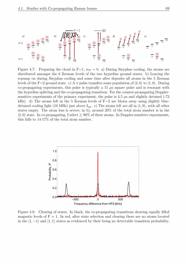
4.1. Studies with Co-propagating Raman beams 69
F=1
F=2
a)
0
0 -1
-1 +1
+1
-2
+2
b)
0 -1
+1
-2
+2
c)
0
0 -1
-1 +1
+1
-2
+2
d)
0
0 -1
-1 +1
+1
-2
+2
F’ = 2
e)
0
0 -1
-1 +1
+1
-2
+2
Figure 4.7: Preparing the cloud in F=1, mF = 0. a) During Sisyphus cooling, the atoms aredistributed amongst the 8 Zeeman levels of the two hyperfine ground states. b) Leaving therepump on during Sisyphus cooling and some time after deposits all atoms in the 5 Zeemanlevels of the F=2 ground state. c) A π pulse transfers some population of |2, 0〉 to |1, 0〉. Duringco-propagating experiments, this pulse is typically a 15 µs square pulse and is resonant withthe hyperfine splitting and the co-propagating transition. For the counter-propagating Doppler-sensitive experiments of the primary experiment, the pulse is 4.5 µs and slightly detuned (-72kHz). d) The atoms left in the 5 Zeeman levels of F=2 are blown away using slightly blue-detuned cooling light (10 MHz) just above Isat. e) The atoms left are all in |1, 0〉, with all otherstates empty. The atom loss is severe; in b), around 20% of the total atom number is in the|2, 0〉 state. In co-propagating, I select ≥ 90% of these atoms. In Doppler-sensitive experiments,this falls to 14-17% of the total atom number.
-500 0 5000.0
0.2
0.4
0.6
0.8
1.0
Frequency difference from HFS [kHz]
Probability,
Figure 4.8: Clearing of states. In black, the co-propagating transitions showing equally filledmagnetic levels of F = 1. In red, after state selection and clearing there are no atoms locatedin the |1,−1〉 and |1, 1〉 states as evidenced by their being no detectable transition probability.

70 Chapter 4. Setting up the interferometer
the oscillation loses coherence faster than at fall times closer to the peak intensity and smallest
cloud size.
0 50 100 150 2000.0
0.1
0.2
0.3
0.4
0.5
0.6
0.7
Applied pulse time [s]
Probability,
0 50 100 150 2000.0
0.1
0.2
0.3
0.4
0.5
0.6
0.7
Applied pulse time [s]Probability,
0 50 100 150 2000.0
0.1
0.2
0.3
0.4
0.5
0.6
0.7
Applied pulse time [s]
Probability,
a) b) c)
Figure 4.9: Co-propagating Rabi oscillations at multiple fall times. As time goes on, the cloudflops at a longer frequency, especially at later fall times, as the cloud travels through the Ramanbeam intensity profile and expands. The nominal pulse time is 18 µs. Fall time: a) 0 ms, b)16 ms, and c) 32 ms.
4.1.3 Ramsey’s method with frequency and phase scanning
Having shown that I could prepare a cloud in |1, 0〉 and with Rabi oscillations mapped out
throughout fall times up to 40 ms, it was the ideal time to add another pulse. First, I scanned
the frequency of the two π/2-pulses, of duration τ , with a fixed free-propagation time T. I show
an example with T = 1 ms and τ = 12 µs, see Fig. 4.10. The red line is a fit to the function [7],
P = AΩ2
δ2 + Ω2sin[τ
2
√δ2 + Ω2
]∣∣∣i(ei(0.5δ0T−(φ+(τ+T )(δ+δ0))) − e−i(0.5δ0T+τ(δ+δ0)))×(cos[τ
2
√δ2 + Ω2
]+
iδ√δ2 + Ω2
sin[τ
2
√δ2 + Ω2
])∣∣∣2 +B
(4.3)
where Ω is the Rabi frequency, δ is the frequency difference from the hyperfine splitting, δ0 is the
frequency offset from the hyperfine splitting, φ is the phase difference between the two pulses,
and A is an amplitude scaling factor and B is the background. The equation was derived from
the same method used to determine the probability for the three pulse interferometer, equation
(2.13), with only three interaction matrices Q5Q2Q1; it includes two π/2 pulses sandwiching
a free propagation time interaction matrix. For this test, the value of φ was set to 0. I found
A = .85 and B = .07. The data in this scan under-samples the fringe pattern, with about one
point per fringe. I look at the center 20 kHz, a) of Fig. 4.10, to illustrate more clearly that the
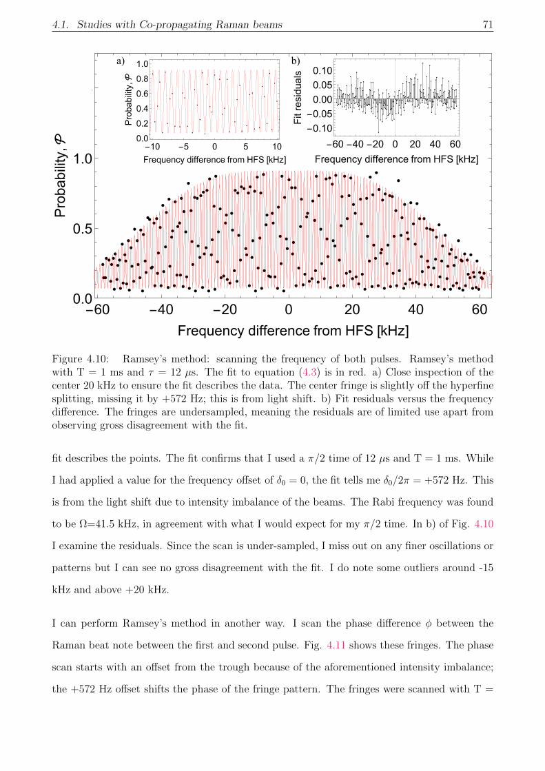
4.1. Studies with Co-propagating Raman beams 71
-60 -40 -20 0 20 40 600.0
0.5
1.0
1.5
Frequency difference from HFS [kHz]
Probability,
a) b)
redo
-60 -40 -20 0 20 40 60-0.10-0.050.000.050.10
Frequency difference from HFS [kHz]
Fitresiduals
-10 -5 0 5 100.0
0.2
0.4
0.6
0.8
1.0
Frequency difference from HFS [kHz]
Probability,
Figure 4.10: Ramsey’s method: scanning the frequency of both pulses. Ramsey’s methodwith T = 1 ms and τ = 12 µs. The fit to equation (4.3) is in red. a) Close inspection of thecenter 20 kHz to ensure the fit describes the data. The center fringe is slightly off the hyperfinesplitting, missing it by +572 Hz; this is from light shift. b) Fit residuals versus the frequencydifference. The fringes are undersampled, meaning the residuals are of limited use apart fromobserving gross disagreement with the fit.
fit describes the points. The fit confirms that I used a π/2 time of 12 µs and T = 1 ms. While
I had applied a value for the frequency offset of δ0 = 0, the fit tells me δ0/2π = +572 Hz. This
is from the light shift due to intensity imbalance of the beams. The Rabi frequency was found
to be Ω=41.5 kHz, in agreement with what I would expect for my π/2 time. In b) of Fig. 4.10
I examine the residuals. Since the scan is under-sampled, I miss out on any finer oscillations or
patterns but I can see no gross disagreement with the fit. I do note some outliers around -15
kHz and above +20 kHz.
I can perform Ramsey’s method in another way. I scan the phase difference φ between the
Raman beat note between the first and second pulse. Fig. 4.11 shows these fringes. The phase
scan starts with an offset from the trough because of the aforementioned intensity imbalance;
the +572 Hz offset shifts the phase of the fringe pattern. The fringes were scanned with T =
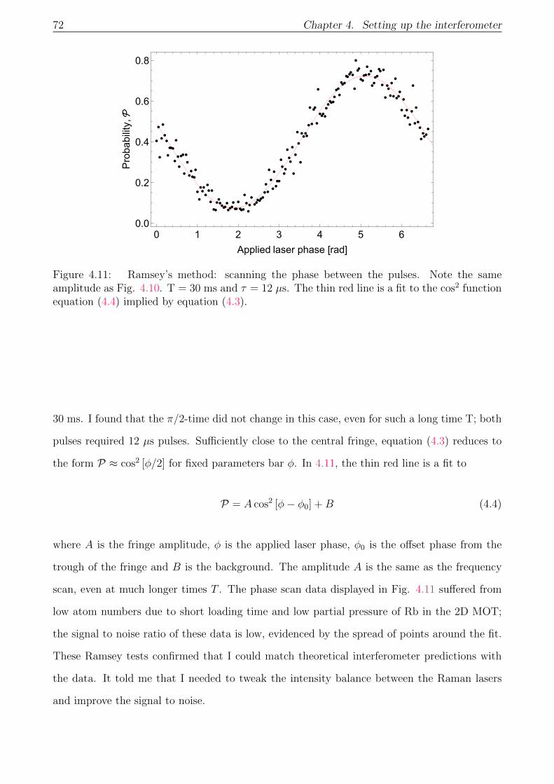
72 Chapter 4. Setting up the interferometer
0 1 2 3 4 5 60.0
0.2
0.4
0.6
0.8
Applied laser phase [rad]
Probability,
Figure 4.11: Ramsey’s method: scanning the phase between the pulses. Note the sameamplitude as Fig. 4.10. T = 30 ms and τ = 12 µs. The thin red line is a fit to the cos2 functionequation (4.4) implied by equation (4.3).
30 ms. I found that the π/2-time did not change in this case, even for such a long time T; both
pulses required 12 µs pulses. Sufficiently close to the central fringe, equation (4.3) reduces to
the form P ≈ cos2 [φ/2] for fixed parameters bar φ. In 4.11, the thin red line is a fit to
P = A cos2 [φ− φ0] +B (4.4)
where A is the fringe amplitude, φ is the applied laser phase, φ0 is the offset phase from the
trough of the fringe and B is the background. The amplitude A is the same as the frequency
scan, even at much longer times T . The phase scan data displayed in Fig. 4.11 suffered from
low atom numbers due to short loading time and low partial pressure of Rb in the 2D MOT;
the signal to noise ratio of these data is low, evidenced by the spread of points around the fit.
These Ramsey tests confirmed that I could match theoretical interferometer predictions with
the data. It told me that I needed to tweak the intensity balance between the Raman lasers
and improve the signal to noise.

4.1. Studies with Co-propagating Raman beams 73
4.1.4 Spin Echo Interferometry
I now added a third pulse to the interferometer to make a spin echo. The same parameters were
used as the Ramsey phase scan in Fig. 4.11 with the two noted improvements added; I increased
the atom number and tweaked the intensity ratio. The pulses times were (π/2 − π − π/2) →
(12 µs− 24 µs− 14 µs) and the time between the pulses was T = 15 ms.
0 10 20 30 40
0.2
0.4
0.6
0.8
1.0
1.2
1.4
Applied laser phase [rad]
Probability,
0 10 20 30 40
0.2
0.4
0.6
0.8
1.0
1.2
1.4
Applied laser phase [rad]
Probability,
0 10 20 30 40
-0.10-0.050.000.050.10
Applied laser phase [rad]
Fitresiduals
0 10 20 30 40
-0.10-0.050.000.050.10
Applied laser phase [rad]
Fitresiduals
a)
b)
Figure 4.12: Velocity-insensitive spin echo interferometry. a) A phase scan for 2T = 30 msshowing 6 fringes up to 40 radians. The thin red line is the fit to equation (4.4). Note thefringes start at the trough instead of half way up the fringe like in Fig. 4.11, after adjusting theintensity ratio. b) Fit residuals versus the applied laser phase; far from being undersampled,these fringes show good agreement with the fit.
The phase scan, see a) in Fig. 4.12, shows fringes with the same peak probability as 4.11
but with a larger background. This is probably due to dephasing resulting from spontaneous
scattering. The fit, from equation (4.4), is the thin red line. The data displays improved signal
to noise and starts at the trough for φ = 0. The residuals, see b) in Fig. 4.12, show increased
dispersion at the peaks of the fringe pattern. This effect is primarily due to variations in
the total atom number in the interferometer due to variations in the atom loading. The full

74 Chapter 4. Setting up the interferometer
amplitude from peak to trough of the phase scan in Fig. 4.12 is 0.575.
The spin echo interferometer concluded my studies of co-propagating Raman transitions. Hav-
ing demonstrated my ability to make a three-pulse interferometer, I now want to make the
interferometer acceleration-sensitive; this requires counter-propagating Raman beams.
4.2 Studies with Counter-propagating Raman beams
4.2.1 Velocity selection
Removing the beam block gave the possibility of driving a Raman transition with counter-
propagating laser beams, see b) and c) in Fig. 4.1. Experiments performed in this configuration
are sensitive to the finite velocity distribution of the atom cloud [51]. For my first spectroscopy
test, I use the configuration of b) in Fig. 4.1, but with the polarization Lin⊥Lin. I use a 10 µs
π-pulse for the velocity selection step, c) of Fig. 4.7, which corresponds to a velocity selection
width of ±1 cm/s; the frequency of this pulse was detuned by -78 kHz which corresponds to a
velocity selection centered around -3 cm/s. It is useful to understand the width of the velocity
selection in terms of temperature. The pulse time corresponds to Fourier width of νf = (τ)−1
of about 27 kHz. I can convert this to a velocity,
v =νfc
2νlas, (4.5)
where c is the speed of light and νlas is the transition frequency. The temperature selection
width of the 10 µs pulse is then
T =mv2
kB≈ 1.1µK (4.6)
where m is the mass of the 87Rb atom and kB is Boltzmann’s constant. In the configuration
where both pairs of beams are resonant, b) of Fig. 4.1, I expect to observe two peaks despite
my laser being detuned to -78 kHz; the opposite beam pair will be resonant with the equal but
opposite velocity class along the beam axis. To observe my velocity selection, I apply a second

4.2. Studies with Counter-propagating Raman beams 75
π-pulse of 50 µs. The Fourier width of this pulse is narrower than the velocity selection pulse,
offering improved resolution.
The spectrum presented in Fig. 4.13 is a scan of the Raman difference frequency around the
hyperfine splitting of the second pulse. The inset is a Rabi flop on the selection frequency,
-78 kHz. The outermost peaks are the velocity selected atoms, shifted due to the Doppler
effect, and the center peak is the co-propagating transition, resonant irrespective of velocity.
The atoms have zero center-of-mass motion and are cold (5 µK, 0±2.2 cm/s); fewer atoms
are selected the further I move the selection frequency away from the hyperfine splitting. The
Fourier width of the selection pulse is sufficiently wide that the selection centered on -78 kHz
selects atoms in the class centered at +78 kHz. To ensure the magnetically sensitive transitions
were suppressed while using short Raman pulses, I set the applied magnetic field to 1.5 G for
this entire section.
-200 0 200 400 6000.00
0.05
0.10
0.15
0.20
0.25
0.30
Frequency difference from HFS [kHz]
Probability,
0 10 20 30 400.00
0.05
0.10
0.15
0.20
Applied pulse time [s]
Probability,
Figure 4.13: Counter-propagating Raman spectroscopy and Rabi flopping with two velocityclasses. The velocity selection pulse, a 10 µs π-pulse, was detuned by −78 kHz. The spectrumwas resolved with a 50 µs π-pulse. Note the two velocity classes, one to each side of the co-propagating transition, marked by gray lines. The center black line marks the co-propagatingtransition. Inset: a Rabi flop on the velocity selected atoms, in preparation for Fig. 4.15.
I change the optics, c) of Fig. 4.1, and test my ability to select a single velocity selection, Fig.
4.14. I make a velocity selection with a 4.5 µs π-pulse detuned by -72 kHz with respect to the

76 Chapter 4. Setting up the interferometer
hyperfine splitting. It is probed by a 50 µs π-pulse. This selection addresses a Fourier width of
about 58 kHz, equivalent to a velocity spread of ±2.3 cm/s around the detuning of -72 kHz or -3
cm/s. The equivalent temperature is 5.4 µK. I had changed the waveplate orientation to circular
to drive the σ−σ− transition for this test; my failure to tweak the waveplate appropriately
resulted in a reduced co-propagating peak still appearing. It was subsequently corrected. Fig.
4.14 shows the result of this scan; a large velocity peak centered around -72 kHz and no peak
on the opposite side at +72 kHz.
-150 -100 -50 0 50 100 1500.00
0.02
0.04
0.06
0.08
0.10
0.12
Frequency difference from HFS [kHz]
Probability,
Figure 4.14: Single velocity selection. Doppler-sensitive two-pulse Raman spectroscopy inves-tigating the momentum class selection. The polarization was improperly set, showing a reducedco-propagating transition.
4.2.2 Checking the applied phase accuracy with the atom interfer-
ometer
Using these velocity selections, I started out at small times 2T to observe interference patterns,
see Fig. 4.15. I show a fringe pattern with 2T = 1 ms, using pulse times (π/2 − π − π/2) →
(7 µs−14 µs−7 µs). I scanned the applied laser phase on the third pulse, out to 200 rad. This
data serves a purpose beyond demonstrating acceleration-sensitive fringes; this dataset is a
calibration of the applied laser phase. It is critical before continuing that I know how accurate

4.2. Studies with Counter-propagating Raman beams 77
my phase commands are. Later, I flop the applied laser phase between φ0 and φ0 + π and
perform a subtraction to suppress any amplitude and background fluctuations. The accuracy
of the phase command is crucial when performing this subtraction (φ0 + π) − (φ0). The red
line is a fit to
P = A cos2 [q(φ+ φ0)] +B, (4.7)
0 50 100 150 200
0.20
0.25
0.30
0.35
0.40
Applied laser phase [rad]
Probability,
0 5 10 15 20 25 300.15
0.20
0.25
0.30
0.35
Applied laser phase [rad]
Probability,
0 50 100 150 200-3-2-10123
Applied laser phase [rad]
Fitresiduals
Dsd fringes and prooving 4 multiplier is four
a) b)
Figure 4.15: Atom interferometry with two velocity classes and circularly polarized light. Theparameters for this trial are as follows: 2T = 1 ms and pulse lengths of (π/2 − π − π/2) →(7 µs− 14 µs− 7 µs). The velocity selection π-pulse was 13 µs. The fit, in red, is to equation(4.7). This Raman beams were circularly polarized; there was no co-propagating componentpresent. a) The fit residuals versus the applied laser phase. The points are well described bythe fit. b) A closer look at the first few fringes.
where A is the amplitude, B is the background, φ0 is the offset phase and q is my parameter of
interest, the phase command calibration which I expect to be 1. I measure the same background
as in Fig. 4.12, but I observe a reduced fringe amplitude. The peak to trough contrast is 0.06.
The fit gives me a value for the calibration of q = 1.0001±0.0004; this is sufficient to ensure my
phase commands do not add error to the subtraction. In a) of Fig. 4.15 I show the residuals.
The residuals show this data is noisier than Fig. 4.12, probably due to vibrations and sensitivity
to the initial position and velocity distribution of the atoms. To illustrate the data follows an
oscillatory pattern, I zoom in on a selection of the dataset in b) of Fig. 4.15, where I show the
first 30 rad.

78 Chapter 4. Setting up the interferometer
Fringe pattern comparison for different velocity selections
2 4 6 8 10 120.2
0.3
0.4
0.5
0.6
0.7
0.8
Applied laser phase [rad]
Probability,
0 2 4 6 8 10 12-3-2-1012
Applied laser phase [rad]
Fitresiduals
Figure 4.16: Single velocity class atom interferometry. Demonstrated here with a time 2T =32 ms, the pulse times are short, (π/2 − π − π/2) → (2.05 µs − 4.7 µs − 3.2 µs). The insetshows the fit residuals versus applied laser phase.
This method of making acceleration-sensitive fringes, using two velocity classes, proved difficult
to realize at larger 2T times. The fringe contrast produced using this method was also limited.
These limitations directly affected the prospective acceleration sensitivity. To see if I could get
around these problems, I choose to extinguish a frequency at the retro-reflection, see c) in Fig.
4.1, and use a single velocity class, Fig. 4.14. Having extinguished a pair of beams, I leave only
the σ−σ− transition resonant. This beam polarization, in conjunction with my velocity selection
around -72 kHz, selects an atom cloud that is moving toward the retro-reflection mirror. Using
this cloud I make a Kasevich-Chu style atom interferometer, see Fig. 4.16.
I started with interferometers at small times 2T. I was able to increase the 2T time up to the
point when the atom cloud leaves the beam cross section capable of driving Rabi flops, around
43 ms. The interferometer with the best contrast occurred with 2T = 32 ms; this is just after
the point when the last π/2 time starts to differ from the first. The pulse times used are very
short, almost as short as the 4.5 µs velocity selective pulse: in order of (π/2 − π − π/2), the
times are (2.05 µs − 4.7 µs − 3.2 µs). This limits the contrast, but was required in order to

4.2. Studies with Counter-propagating Raman beams 79
select enough atoms. The last π/2 time is 1 µs different from the first at 2T = 32 ms due to the
atoms falling through the intensity profile of the Raman beam, changing the Rabi frequency;
moving to times larger than 2T = 32 ms resulted in a loss of contrast due to the changing
efficiency of the final pulse. These are the pulse times in the primary experiment described in
the next chapter. I show a phase scan of 4π at 2T = 32 ms in Fig. 4.16. The red line is a fit to
equation (4.7). The pattern displays a trough at zero phase and a full amplitude of 19%. The
residuals displayed in the top inset of Fig. 4.16 are less noisy than Fig. 4.15 at significantly
longer 2T time.
0 2 4 6 8 10 12
-0.10
-0.05
0.00
0.05
0.10
Applied laser phase [rad]
Shiftedprobability,
-0
Figure 4.17: Comparison of velocity selection techniques. With a time 2T = 5 ms, the disparityin contrast and noise is readily apparent between the single velocity selection (black) and thedouble velocity selection (red).
I show a comparison between double and single velocity selection configurations. The fringe
patterns have different backgrounds; to compare them, I modify the probability P by subtract-
ing the mean probability from each fringe. I create the mean probability P0 = B + A, the
background plus half the peak to trough amplitude. I show this in Fig. 4.17, where I display
the double velocity selection case (red) and the single velocity selection case (black). These
fringe patterns have the same pulse times and 2T time. The single-diffraction case (black) is
higher contrast and less noisy than the same double single-diffraction case (red). I perform this
test over a series of 2T times for both the double and single velocity selection fringe patterns
and compare their peak to trough amplitude, see Fig. 4.18. The conclusion is clear; I will use
the single velocity selection for maximum acceleration sensitivity.

80 Chapter 4. Setting up the interferometer
0 5 10 15 20 25 300.00
0.01
0.02
0.03
0.04
0.05
0.06
0.07
Free propagation time 2T [ms]
Fullfringeamplitude,
max-min
Figure 4.18: Velocity selection comparison. As the 2T time increases, the contrast shrinks asvibration and decreasing Rabi frequency of the last pulse smear out the fringe pattern. Clearlyshown is the performance difference between the double velocity selection (red) and the singlevelocity selection (black) in this system.
4.2.3 Calibrating the MEMS accelerometer with the atom interfer-
ometer
The atom interferometer measures background accelerations as well as the small anomalous
signal I seek. The MEMS accelerometer on the retro-reflector could separate all background
accelerations from my signal because it is not sensitive to the anomalous acceleration while the
atom interferometer is. Previously, I scanned the applied laser phase on the last π/2-pulse to
observe a fringe pattern. Now, I simply let a combination of vibrations and table wallowing,
the unrestricted and small tilting of the floated optical table, scan out a fringe pattern.
The MEMS accelerometer comes with a given calibration of Ξ = 1.37572 × 10⁻⁴ A/(m s−2);
this means there is a calibration value I can expect from the MEMS accelerometer. The
current from the accelerometer is converted to a voltage reading of the ADC in the computer
interface, see Fig. 3.16. The resistor there has been calibrated by injecting a known current,
measured by a high-precision ammeter (Keysight 34461A, 6.5 digit), and recording the voltage,
see Fig. 4.19. The values of multiple readings are plotted in Fig. 4.19; they give me a linear
fit V = 9816.68(18)I + 150(17) × 10−6. Combining the slope, R, of this fit and the specified

4.2. Studies with Counter-propagating Raman beams 81
-100 -50 0 50 100-1.0
-0.5
0.0
0.5
1.0
Appplied current [μA]
Acquiredvoltage
[V]
Figure 4.19: Response of MEMS electronics. The linear relationship between a known, appliedcurrent to the electronics of v) of a) in Fig. 3.16 and the acquired voltage, allowing me todetermine the resistance R.
sensitivity Ξ of the MEMS accelerometer, I obtain the an expected calibration
ξ =1
ΞR= 0.74046± .00001
m s−2
V, (4.8)
where the error is dominated by the error in the measured value of the resistance.
I want to empirically measure this calibration using the atom interferometer, see Fig. 4.20.
Before a data run, a phase scan allows me to establish a value for φlas = φ0 such that the
interferometer is most sensitive to changes of acceleration, a scan which looks like Fig. 4.16.
I measure the MEMS voltage for each shot as established in section 3.7, see a) in Fig. 4.20.
I switch the phase from φlas = φ0 to φlas = φ0 + π between shots and subtract, obtaining a
fringe pattern with the background suppressed, see b) and c) in Fig. 4.20. In Fig. 4.20, this
subtraction is performed on the atom accelerometer running near midday on August 28, 2017;
c) shows a fringe pattern scanned out by the table tilting. I plot this data versus the MEMS
accelerometer voltage reading. I use this to calibrate the MEMS accelerometer.
I fit the data of c) in Fig. 4.20, the red line, to
P∗ = A cos(β(V0 + VMEMS)
), (4.9)

82 Chapter 4. Setting up the interferometer
0.254 0.255 0.256 0.257-0.2
-0.1
0.0
0.1
0.2
MEMS signal [V]
Probabilitywith
subtraction,
*
0 500 1000 1500 2000 25000.2490.2500.2510.2520.2530.254
Shot
MEMSsignal
[V]
0 500 1000 1500 2000 25000.150.200.250.300.350.400.450.50
Shot
Probability,
*
a)
b)
c)
Figure 4.20: Atom interferometer correlation with MEMS accelerometer. a) MEMS voltageacquired during the run. The table is slowly tilting. b) The atom interferometer signal, fedsome fixed φlas = φ0, flops between φ0 (black) and φ0 + π (blue), scanning fringe patterns asthe table tilts. c) Correlating the atom interferometer and the MEMS. The red line is a fit toequation (4.9). This is data around midday. I have not removed any data points, evidenced bythe occasional uncorrelated shot (all of which are from the laboratory door being slammed; theauthor notes, wryly, that other laboratory users fail to read clear signage/instruction when itdoesn’t involve their experiment).
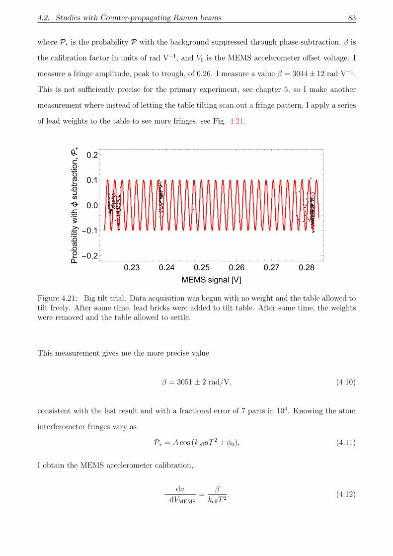
4.2. Studies with Counter-propagating Raman beams 83
where P∗ is the probability P with the background suppressed through phase subtraction, β is
the calibration factor in units of rad V−1, and V0 is the MEMS accelerometer offset voltage. I
measure a fringe amplitude, peak to trough, of 0.26. I measure a value β = 3044± 12 rad V−1.
This is not sufficiently precise for the primary experiment, see chapter 5, so I make another
measurement where instead of letting the table tilting scan out a fringe pattern, I apply a series
of lead weights to the table to see more fringes, see Fig. 4.21.
0.23 0.24 0.25 0.26 0.27 0.28
-0.2
-0.1
0.0
0.1
0.2
MEMS signal [V]
Probabilitywith
ϕsubtraction,
*
Figure 4.21: Big tilt trial. Data acquisition was begun with no weight and the table allowed totilt freely. After some time, lead bricks were added to tilt table. After some time, the weightswere removed and the table allowed to settle.
This measurement gives me the more precise value
β = 3051± 2 rad/V, (4.10)
consistent with the last result and with a fractional error of 7 parts in 104. Knowing the atom
interferometer fringes vary as
P∗ = A cos (keffaT2 + φ0), (4.11)
I obtain the MEMS accelerometer calibration,
da
dVMEMS
=β
keffT 2. (4.12)
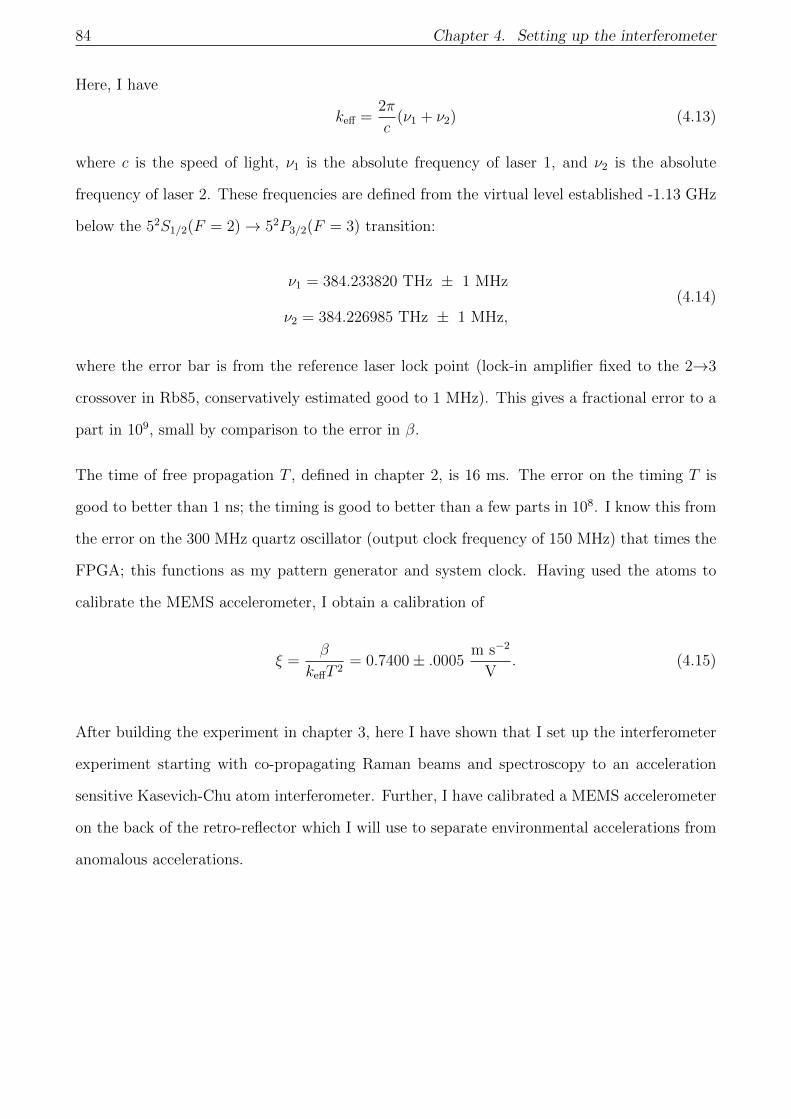
84 Chapter 4. Setting up the interferometer
Here, I have
keff =2π
c(ν1 + ν2) (4.13)
where c is the speed of light, ν1 is the absolute frequency of laser 1, and ν2 is the absolute
frequency of laser 2. These frequencies are defined from the virtual level established -1.13 GHz
below the 52S1/2(F = 2)→ 52P3/2(F = 3) transition:
ν1 = 384.233820 THz ± 1 MHz
ν2 = 384.226985 THz ± 1 MHz,
(4.14)
where the error bar is from the reference laser lock point (lock-in amplifier fixed to the 2→3
crossover in Rb85, conservatively estimated good to 1 MHz). This gives a fractional error to a
part in 109, small by comparison to the error in β.
The time of free propagation T , defined in chapter 2, is 16 ms. The error on the timing T is
good to better than 1 ns; the timing is good to better than a few parts in 108. I know this from
the error on the 300 MHz quartz oscillator (output clock frequency of 150 MHz) that times the
FPGA; this functions as my pattern generator and system clock. Having used the atoms to
calibrate the MEMS accelerometer, I obtain a calibration of
ξ =β
keffT 2= 0.7400± .0005
m s−2
V. (4.15)
After building the experiment in chapter 3, here I have shown that I set up the interferometer
experiment starting with co-propagating Raman beams and spectroscopy to an acceleration
sensitive Kasevich-Chu atom interferometer. Further, I have calibrated a MEMS accelerometer
on the back of the retro-reflector which I will use to separate environmental accelerations from
anomalous accelerations.

Chapter 5
Primary experiment
5.1 Explanation of the experiment and the run pattern
The scientific aim of this thesis, to look for deviations from Newtonian gravity, was now possible
with the conclusion of chapter 4. Here, I present the results of this experiment. First, I describe
the experiment run pattern, where I explain which parameters were switched, how fast and why.
Following this, I describe the data and the 36 independent datasets that comprise the result.
This leads to a brief discussion of some of the systematics and limitations of the experiment.
Last, I discuss how my result places constraints on theories of screened modified gravity.
The experiment strategy is shown in Fig. 5.1. The source mass can be placed in two positions,
“Left” or “Right”, defined in section 3.6. Viewed from the side, a) in Fig. 5.1, the source mass
perturbs the scalar field from its background value φbg, which is determined by the chamber
dimensions and the vacuum quality. I change the source mass position, changing the sign of the
acceleration. The source mass does not block the raman beam, which can be seen more clearly
when viewed from the top, b) in Fig. 5.1. It is also off axis, so I measure a projection of the
force onto the Raman axis which I will treat in a section considering systematic corrections.
The experiment parameters are as previously established in the preceding chapter. In brief,
starting with an ensemble of a few 106 atoms at 5 µK, all in the |1, 0〉 ground state, I operate
85

86 Chapter 5. Primary experiment
ϕ ϕbg
+z -z
Left Right
Right Left a) b)
Figure 5.1: Experiment strategy. a) Perturbations induced by the presence of a source mass.The gradient direction changes with the switching of the source mass position. b) Top downview showing the source mass in relation to the atoms.
a Kasevich-Chu atom interferometer with 2T = 32 ms and pulse times (π/2 − π − π/2) →
(2.05 µs − 4.7 µs − 3.2 µs) at cm distances from a cm-sized source mass. I switch some
parameters to mitigate the effects of drift [52, 53] and to suppress systematic errors, see Fig.
5.2. First, I switch the phase of the Raman beat note, on the third interferometer pulse, between
φ0 and φ0 +π (see section 4.2.3). Second, I switch the source mass between the positions “Left”
and “Right”, see Fig. 5.1. Last, I flop the direction of the applied magnetic field. This was
a precautionary measure; I will show there was no measured effect. A full experiment pattern
requires 16 shots, shown in time order in Fig. 5.2.
L
R
ϕ0 ϕ0+π
ϕ0
ϕ0
ϕ0
ϕ0
ϕ0
ϕ0
ϕ0
1 2
3 4
5 6
7 8
9 10
12 11
13 14
15 16 ϕ0+π ϕ0+π
ϕ0+π
ϕ0+π
ϕ0+π
ϕ0+π
ϕ0+π
Add in time blocks loke 10, 110 and 1100 etc like ed and I discussed
-B0 +B0 +B0
Figure 5.2: Experiment run pattern. A total of 16 shots make a single run pattern. Thephase of the Raman beat note applied to the third pulse is changed every shot between φ0 andφ0 +π. The source mass changes position every two shots. The magnetic field is switched, as aprecaution, in a more complicated pattern; the first 4 shots are +B0, the next 8 shots are −B0,and the last four are +B0. Each shot took 1.2 seconds, limited by the loading time of MOT.There was a dead time of about 1 second related to pattern generation and moving the sourcemass; the time between shots was 2.2 seconds.
A summary of how the measurement works helps dissect the run pattern. The atom interfer-
ometer has two outputs:
N1 = A sin2 [Φ/2] and N2 = A cos2 [Φ/2], (5.1)

5.1. Explanation of the experiment and the run pattern 87
where Φ = keffaT2 is the total phase difference along the two interferometer paths and A is the
amplitude of the fringe pattern. I can rewrite these outputs as
N2 =A
2(1− cos [Φ]) and N1 =
A
2(1 + cos [Φ]). (5.2)
I introduce an additional contribution to Φ by changing the phase of the Raman beat note just
before application of the third pulse. I apply a π phase flip, changing the fringe pattern to
N2 =A
2(1 + cos [Φ]) and N1 =
A
2(1− cos [Φ]). (5.3)
The experiment uses the photodetector voltage to measure N2 and Ntot = N2 + N1 with their
respective backgrounds,
V2 = q(N2 + b2) and Vtot = q(Ntot + btot), (5.4)
where q converts voltage to atom number and q b is the background light. The ratio of these
voltages is
P =V2
Vtot
=q(N2 + b2)
q(Ntot + btot)=
N2 + b2
Ntot + btot
. (5.5)
From equations (5.2) and (5.3), I have
Pπ0
=A2
(1± cos (Φ)
)+ b2
A+ btot
, (5.6)
where the sign is determined by the phase shift (0 or π) applied on the third laser pulse. I take
the difference:
P∗ = Pπ − P0 =( A
A+ btot
)cos (Φ) = C cos (Φ). (5.7)
This is a fringe symmetrical around P∗ = 0 with an amplitude dependent upon the background.
It might seem natural to subtract the background before constructing the ratio P ; I found em-
pirically that this subtraction adds unwanted noise. Since a background-dependent amplitude
does not compromise the measurement, I refrain from subtracting the background. For each
pair of time bins in Fig. 5.2, I subtract the φ0 + π interferometer signal from the φ0 signal to

88 Chapter 5. Primary experiment
give a value of P∗; I average the corresponding MEMS accelerometer signals.
The experiment runs with the source mass in either the “Left” or “Right” position. Switching
the position will change the sign of the attractive force between the atom cloud and the source
mass, resulting in an acceleration ±aball. It may also change the acceleration due to the tilting
of the table between a0 ± δg. I expect a PL∗ ,
PL∗ = CL cos (ΦL), (5.8)
where ΦL = keffT2(a0 + δg + aball), and similarly a PR∗ ,
PR∗ = CR cos (ΦR), (5.9)
where ΦR = keffT2(a0 − δg − aball). Here, δg allows for the possibility that the table may tilt
when the source mass moves. Critically, the MEMS accelerometer measures δg but not aball,
allowing me to separate δg from aball. If the calibration of the MEMS accelerometer voltage were
inaccurate, there could be a residual systematic error as the method would not fully remove
δg. I investigate this in the next section and find the calibration is good enough to avoid such
an error.
Equations (5.8) and (5.9) can be re-written as
PR∗ (V RM ) = CR cos
(β(V R
M − Vbias − Vball)),
PL∗ (V LM) = CL cos
(β(V L
M − Vbias + Vball)),
(5.10)
where β converts voltage to phase, V LM (V R
M ) is the MEMS voltage for when the source mass
is in the left (right) position, Vbias accounts for the tilt of the table as well as offset bias and
Vball is the offset associated with aball. By fitting the left (right)-position fringe pattern as a
function of V LM (V R
M ), I distinguish the acceleration of interest, aball, from the uninteresting δg.
Last, I switched the sign of the applied magnetic field, so B± = ±1.685 G, just to check that
this did not reveal any systematic effect.

5.2. The primary result 89
To summarize, the run pattern has three modulations, each with its own orthogonal switching
pattern. First, the applied laser phase φ0 is changed between φ0 and φ0+π every shot (every 2.2
s). I take the difference, allowing me to suppress backgrounds and amplitude fluctuations. Next,
I change the source mass position every two shots (4.4 s), the primary experiment. Finally, I
changed the sign of the applied magnetic field.
5.2 The primary result
0 2000 4000 6000 8000 100000.0
0.1
0.2
0.3
0.4
0.5
0.6
Shot index
Probability,
Figure 5.3: Raw data from one run of the primary experiment. The only data processingperformed here was to create the probability P , see equation (3.13), and to remove shots whena laser unlocked.
The apparatus was set to take data in multiples of 12000 shots. Fig. 5.3 shows the values
of P measured in a typical run. These 12000 data points constitute 1500 run patterns giving
750 values for V LM , P
L∗ and 750 values for V R
M , PR∗ . Half of these values have the applied
magnetic field B+ and the other half B−.
Fig. 5.4 shows the PL∗ (V LM) and PR∗ (V R
M ) obtained from the data in Fig. 5.3. Please note, for
display purposes in Fig. 5.4, I have inverted the sign of the “left” points so that they can be
distinguished from the “right” points. Further, for ease of comparison to the fit, I have binned
the data in bins of 135 µV. Without this last step, the data resembles that of Fig. 4.20. The

90 Chapter 5. Primary experiment
fit is to the data, before binning. I fit each fringe to the equation
PL,Rfit = C cos(β(V L,RM + V L,R
0
)), (5.11)
where C is the same for both source mass positions. Here, V L,R0 = Vbias ± Vball so aball =
ξ2(V L
0 − V R0 ), where ξ is defined in equation (4.15). I acquired 36 datasets like Fig. 5.4, from
which I obtain the values of V L0 and V R
0 , see column 2 and 3 of Table 5.1. The mean of the
left V 0L and right V 0
R voltages, column 4, corresponds to the offset voltage Vbias of the MEMS
accelerometer, as shown in equation (5.11). The value of Vball is given in column 5. The variation
in the bias is very large, the standard deviation is 299 µV, compared with the value of Vball.
This bias variation corresponds to a bias noise of 221 µm s−2, where I have used the conversion
ξ. The data sheet for the MEMS accelerometer (Honeywell QA-750) specifies a bias change of
< 60 µg/C; the standard deviation I observe in Vbias is consistent with a standard deviation
in the laboratory temperature of order 1/2C. The heating, ventilation, and air conditioning
system for this experiment is rated for temperature variations up to 2 C, but the temperature
logs report a standard deviation in the laboratory temperature consistent with the bias change
of the measured MEMS accelerometer bias change, about 1/2C. The author and his advisor
note, for posterity, that the Honeywell QA750 MEMS accelerometer has performed admirably
as the world’s most elaborate thermometer.
0.21 0.211 0.212 0.213
-0.1
0
0.1
MEMS signal, VM [V]
*
Figure 5.4: Sample of primary experiment data. Data taken in the “right” source mass positionis denoted by the black diamonds and the “left” position by the lavender triangles. Taken overabout 12 hours, this set is typical of the fringe patterns. The noise is reduced here by binning;Fig. 4.20, a similar dataset bar the binning, displays this noise. This pattern began on the left,near VM = 0.21 V. Over the course of the measurement, the table tilted toward VM = 0.214 V.

5.2. The primary result 91
Table 5.1: MEMS accelerometer voltages for the primary experiment.
Run V L0 [µV] V R
0 [µV] 12
(V0
R + V0L) [µV] 1
2
(V0
R − V0L) [µV]
1 88.427 90.419 89.423 -0.996± 0.9312 -225.172 -228.175 -226.674 1.501±1.6503 174.98 172.551 173.766 1.215 ±0.8994 -387.892 -387.626 -387.759 -0.133±0.6965 -263.586 -264.139 -263.862 0.276 ±0.9296 482.588 480.665 481.627 0.962±1.3627 -224.137 -222.523 -223.33 -0.807±1.4008 -138.433 -132.999 -135.716 -2.717±1.4899 245.717 244.479 245.098 0.619± 1.35410 453.448 453.587 453.517 -0.069±1.26711 -245.572 -246.986 -246.279 0.707±1.24112 425.547 425.068 425.308 0.239 ±0.67713 -399.578 -400.224 -399.901 0.323±1.17914 -97.296 -92.783 -95.0395 -2.257±1.04715 -420.431 -421.344 -420.888 0.456±2.17116 278.323 279.585 278.954 -0.631±1.09417 185.738 186.466 186.102 -0.364 ±1.05418 571.298 570.71 571.004 0.294 ± 0.65619 30.218 28.745 29.482 0.736±0.78520 -329.507 -328.537 -329.022 -0.485±0.96721 125.525 128.913 127.219 -1.694±0.89522 -128.808 -131.236 -130.022 1.214±1.25923 80.814 80.044 80.429 0.385±1.43424 67.671 66.125 66.8982 0.773±1.95325 234.78 231.159 232.969 1.810±1.87426 -156.536 -153.57 -155.053 -1.483± 0.78327 193.041 195.936 194.489 -1.447±0.49228 435.774 432.925 434.349 1.425 ±0.73229 616.171 617.848 617.009 -0.838± 0.69930 279.021 283.67 281.346 -2.324± 0.49831 -378.129 -376.76 -377.444 -0.684± 0.43432 393.232 392.377 392.805 0.428± 0.50833 243.155 243.876 243.516 -0.360± 0.51634 343.014 346.5 344.757 -1.743± 1.16135 177.633 178.189 177.911 -0.278± 1.34036 236.898 237.225 237.062 -0.164± 1.697

92 Chapter 5. Primary experiment
Throughout all datasets, the most stable in terms of table wallowing covered only half a fringe
while the least stable covered 10 fringes. Not all datasets contain 12000 shots; various conditions
led some sets to be stopped early or to significant cuts being made. Some issues were as simple
as lasers unlocking due to a change of lab temperature. Set 7 through 15 were high vibration
tests where I slipped paper dampeners underneath various table legs in an attempt to reduce
table wallowing while increasing vibrations. There was no evident change in the quality of the
data, which showed the MEMS accelerometer was effective at removing the vibration noise.
Set 26 through set 33 were full sets with minimal cuts.
For each of the 36 measurements I determine Vball = (V R0 −V L
0 )/2, shown in column 5 of Table
5.1. These have a weighted mean and standard error of
Vball = +28± 193 nV. (5.12)
After multiplying by ξ, given in equation (4.15), this gives
aball = +20± 143stat nm s−2. (5.13)
I plot the individual values of aball in Fig. 5.5. Next, I interpret the sign of aball as indicating
an attractive force. I follow this with a discussion of systematic corrections and uncertainties
before stating the result for aχ.
5 10 15 20 25 30 35-4-2024
Sequence index
aball[μms-2]
Figure 5.5: Determining aball. Here are the 36 independent measurements of aball. The meanand standard error of these values is given in equation (5.13). The gray line is through aball = 0µm s−2, for reference.

5.2. The primary result 93
Determination of an attractive or repulsive result
Before I can apply systematic corrections and interpret my result, I must be clear on whether
my result, aball, is an attractive or repulsive force. I use the correlation between the sign of
the MEMS accelerometer voltage and the MEMS orientation, see Fig. 3.16, to determine the
attractive or repulsive nature. When oriented like vi) in b) of 3.16, parallel with the force of
gravity, I measure a positive voltage much larger than any possible bias error. With the MEMS
accelerometer attached to the mirror, see vii) of b) in Fig. 3.16, I measure strictly positive
voltages through all measured tilt angles of the experiment. The table is always tilted such
the MEMS accelerometer measures a small component along gravity, strictly positive voltages
V L,RM . This means a positive voltage is a force whose direction goes from “Left” to “Right”,
see Fig. 3.17. I performed a simple check by placing weights on the “right” side of the optical
table, which made the MEMS accelerometer voltage more positive. If the force is attractive, I
expect V R0 to be a larger positive voltage than V L
0 , which is to say I expect an attractive force
to produce a positive voltage for V R0 −V L
0 . The mean of column 5 in Table 5.1, equation (5.12),
is a positive voltage. I have measured an attractive force.
Systematic corrections
There are two systematic corrections I need to apply to the value of aball, equation (5.13). First,
the aball I have measured is the component of the whole acceleration toward the source mass,
projected onto the Raman beam axis. I must divide my result by cos (θ), where θ = 48.8 Deg is
the angle between the line linking the center of the atom cloud and the source mass and a line
through the center of the atom cloud and parallel to Raman beam axis, see section 3.6. Second,
I must remove the contribution of the normal Newtonian gravitational acceleration between the
atom cloud and the source mass from aball. The atom cloud has a center of mass velocity of
3 cm/s along the Raman beam, toward the “left” position. They fall under gravity from their
starting point. The distance d, see a) in Fig. 3.17, from the center of the atom cloud to the
center of the source mass, after following the trajectory for 2T = 32 ms, is 30.1 mm in the case
of the “right” position and 28.9 mm for the “left” position; this position difference is sufficiently

94 Chapter 5. Primary experiment
small as to not require a separate treatment of the gravitational acceleration of the two mass
positions. The cloud expands during the interferometer time 2T = 32 ms. Some atoms move
closer to the mass and some further away. I measure the acceleration averaged over the cloud;
the force over a spherical cloud is the same as the force on an atom at the centre of the cloud,
in that the gravitational attraction to a sphere is as though the mass is all concentrated at the
center. Knowing this, I can state the Newtonian gravitational acceleration due to the presence
of the source mass as ag = +7 nm s−2 for both positions, where the sign is from determining
whether the force is attractive or repulsive. Having determined that an attractive force is a
positive voltage, I subtract this gravitational acceleration from aball. Applying both of these
corrections to my result, I obtain
aχ =aball
cos (θ)− ag = +24± 210 nm s−2, (5.14)
the anomalous acceleration between the source mass and the atomic cloud.
Systematic uncertainties
Here, I discuss systematic uncertainties in this experiment. I measure the change of interfer-
ometer phase when the source mass moves from “left” to “right”. Aside from the effect of the
Newtonian attraction and the proposed scalar field, there is also the possibility of an interfer-
ometer phase shift if the table tilts when the source mass is moved. This has been anticipated
in the way the experiment is performed in that I remove this contribution δg with the MEMS
accelerometer. The movement of the source mass could produce real or apparent phase shifts
through other mechanisms - these potential systemic errors are considered here.
Magnetic field gradients from the source mass do not accelerate the atom when it is in the
superposition |1, 0〉 + eiφ|2, 0〉, but can create a systematic error as described in Appendix
A. Movement of the atoms through a magnetic field gradient creates a phase shift in the
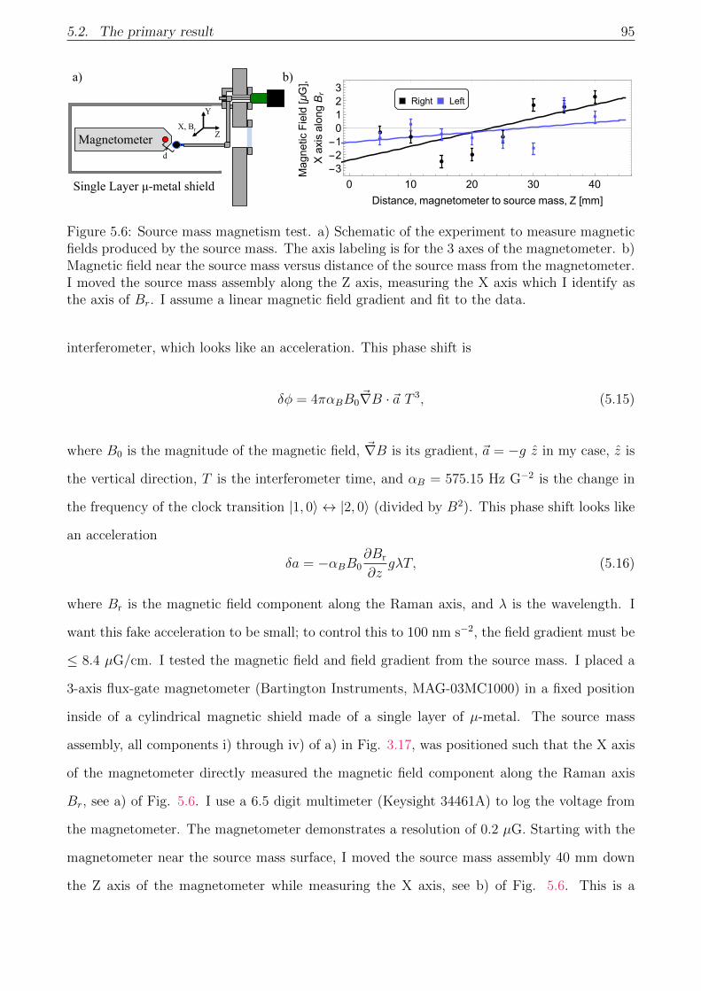
5.2. The primary result 95
X, Br
Y
Magnetometer d
Single Layer µ-metal shield
Z
a)
0 10 20 30 40-3-2-10123
Distance, magnetometer to source mass, Z [mm]
MagneticField[G],
XaxisalongBr
Right Left
b)
Figure 5.6: Source mass magnetism test. a) Schematic of the experiment to measure magneticfields produced by the source mass. The axis labeling is for the 3 axes of the magnetometer. b)Magnetic field near the source mass versus distance of the source mass from the magnetometer.I moved the source mass assembly along the Z axis, measuring the X axis which I identify asthe axis of Br. I assume a linear magnetic field gradient and fit to the data.
interferometer, which looks like an acceleration. This phase shift is
δφ = 4παBB0~∇B · ~a T 3, (5.15)
where B0 is the magnitude of the magnetic field, ~∇B is its gradient, ~a = −g z in my case, z is
the vertical direction, T is the interferometer time, and αB = 575.15 Hz G−2 is the change in
the frequency of the clock transition |1, 0〉 ↔ |2, 0〉 (divided by B2). This phase shift looks like
an acceleration
δa = −αBB0∂Br
∂zgλT, (5.16)
where Br is the magnetic field component along the Raman axis, and λ is the wavelength. I
want this fake acceleration to be small; to control this to 100 nm s−2, the field gradient must be
≤ 8.4 µG/cm. I tested the magnetic field and field gradient from the source mass. I placed a
3-axis flux-gate magnetometer (Bartington Instruments, MAG-03MC1000) in a fixed position
inside of a cylindrical magnetic shield made of a single layer of µ-metal. The source mass
assembly, all components i) through iv) of a) in Fig. 3.17, was positioned such that the X axis
of the magnetometer directly measured the magnetic field component along the Raman axis
Br, see a) of Fig. 5.6. I use a 6.5 digit multimeter (Keysight 34461A) to log the voltage from
the magnetometer. The magnetometer demonstrates a resolution of 0.2 µG. Starting with the
magnetometer near the source mass surface, I moved the source mass assembly 40 mm down
the Z axis of the magnetometer while measuring the X axis, see b) of Fig. 5.6. This is a
96 Chapter 5. Primary experiment
measurement of the field gradient; I approximate the field gradient as linear and fit to the data
from the magnetometer. I obtain a field gradient of 1.0 ± 0.4 µG/cm for the “right” position
and 0.4 ± 0.3 µG/cm for the “left”; my experiment is sensitive to the difference between the
positions, δa ∼ 12
(∂BR
r
∂z− ∂BL
r
∂z
). This corresponds to a false acceleration +4±3 nm s−2, note the
positive sign from “right” - “left” makes for an attractive acceleration. I conclude the source
mass makes negligible contributions to the systematic uncertainty due to the second-order
Zeeman effect.
An electric field gradient would accelerate the atoms by
δaE′ = αEE′E0/m, (5.17)
where αE is the ground state DC polarizability, and m is the mass of a 87Rb atom. The
aluminum source mass is electrically grounded to the same potential as the vacuum chamber.
However, aluminum forms a stable oxide layer upon exposure to air, called alumina (Al2O3),
that is ∼4 nm thick. This makes it possible for the surface of the layer to become charged.
The alumina film breaks down at electric fields above a few MV/cm, so the source mass cannot
hold potentials more than ∼ 1 V. With the atoms placed 27 mm from the center of the source
mass (of radius 19 mm), and the source mass charged up to 1V, this acceleration is 2 nm s−2.
This is small enough to neglect.
There is an electric analogue to the false acceleration given by equation (5.16), caused by the
(changing) Stark shift of the clock transition, which goes like kE2. I replace αB is equation
(5.16) with the Stark shift coefficient k = −1.23× 10⁻¹⁰ Hz/(V/m)2 [54]; this coefficient shows
the clock transition is exceedingly insensitive to electric fields, making this effect much smaller
than the second-order Zeeman shift. For the electric field previously considered, the electric
analogue to equation (5.16) produces false accelerations below 1 nm s−2. This shift can be
dismissed.
If the calibration of the MEMS accelerometer voltage were inaccurate, there could be a residual
systematic error as the method would not fully remove δg. To ensure this was not a problem

5.2. The primary result 97
for my experiment, I measured 〈V RM − V L
M〉 of the data. I obtain 〈V RM − V L
M〉 = −6.615 µV.
Therefore,
δg =ξ
2〈V R
M − V LM〉 = −2.447± 0.002 µm s−2, (5.18)
where the error bar is from the uncertainty in the calibration ξ. The calibration is good enough
to avoid such an error, as the uncertainty in the determination of δg is negligible.
Last, related to the switching of all waveforms in Fig. 5.2, I wanted to investigate the possibility
of a systematic error arising from a correlation between the MEMS accelerometer voltage and
the phase switching of the beat note between the Raman lasers. Such a correlation could
produce a false acceleration aχ; this problem of unwanted crosstalk, see section 6.1 of [55], is
well studied. I performed a simple test of the MEMS accelerometer acquisition channel where I
switched the phase of the Raman beat note between φ0 +π and φ0 while monitoring the MEMS
accelerometer voltage for a switch dependent shift. I find that the mean shift due to switching
of the Raman beat note phase is 〈V π−0M 〉 ≤ 0.4±1 nV. Using the calibration ξ, this corresponds
to an acceleration 0.3± 0.7 nm s−2. This is negligible.
Noise from the background
I found that the background subtraction adds noise to the data. This is due to low voltage
signal from the small atom numbers used in the experiment, a consequence of the lossy state
and velocity selection technique I employ, see Fig. 4.7. I allude to this problem in my treatment
of equations (5.4) to (5.7), where I conclude that without background removal, the amplitude
of the fringe pattern becomes a function of the background. The data displayed in Fig. 5.4
and all the datasets in Fig. 5.5 have the background included. I record the background voltage
btot of every shot in a measurement and found that it is constant over the duration of every
measurement, so the fringe amplitude did not vary. That is important as one could imagine
a systematic variation of amplitude might produce a systematic error in the measurement.
Clearly, it would be desirable to have a more efficient optical pumping scheme, in which case
it may make sense to reintroduce the background subtraction.
98 Chapter 5. Primary experiment
Conclusions about aχ
First, and before discussion of how my result applies to the scalar fields discussed in chapter
2, I must set an upper bound for my result. Having considered the systematic uncertainties
above, I arrive at the result aχ = +16± 4syst ± 210stat nm s−2. I can say, with 90% confidence
that aχ < +285 nm s−2, where the positive sign means an attractive acceleration. I take this
as my upper limit.
5.3 Constraints on Chameleon Gravity
I seek to apply my result to one of the central mysteries of cosmology - dark energy. I focus
on the chameleon gravity discussed in chapter 2. I ended my discussion on the origin of the
proposed anomalous acceleration with equation (2.22). There, I give the acceleration aχ of the
atom toward the center of the source mass. I will now use this expression for aχ, together with
my experimental upper limit, to constrain the parameters Λ, the field self-coupling, and M ,
the field coupling to matter. First I will restate equation (2.22) in a slightly different form for
ease of discussion:
aχ = λ1λ2ρ1R
31
3M2r2, (5.19)
where ρ1 is the density of the source mass. Here, I have replaced the Planck mass MPl =
1/√
8πG, the mass of source m1 = 43πR3
1ρ1. The parameter λ1, for the source mass and given by
equation (2.23), is equal to 3Mφbg/(ρ1R21) up to a maximum value of one. Here, φbg is the value
of the field far from the source mass, which I take as the value near the center of the empty
vacuum can. Similarly, λ2, for the test mass - the atom - is characterized by 3Mφbg/(ρ2R22)
up to a maximum value of one. I must first evaluate φbg to find the functional relationship
between Λ, M , and aχ.

5.3. Constraints on Chameleon Gravity 99
Determining φbg
Simply put, the background field φbg has two regimes: the first being where φbg is dominated
by the background pressure inside the vacuum can, parameterized by the residual background
pressure ρ of H2, and a second where φbg is limited by the dimensions of the can, parameterized
by the radius L.
The density of the wall of the vacuum can is high, so the scalar field has a low value. The
density of background gas ρ inside the vacuum can is much lower than the density of the walls,
so φbg has a higher equilibrium value. The field φbg can, however, be less than that if the size
L of the vacuum can does not allow sufficient room for the field to become that large. Burrage
et. al. [3] have shown that
φbg = 0.693√
Λ5L2 (5.20)
at the center of an evacuated spherical vacuum vessel, where L is the radius of the vacuum can.
I can conclude then that φbg is size-limited if 0.693√
Λ5L2 <√
Λ5M/ρ, which I rewrite as
Λ5( M
MPl
)3
> (0.69)6L4ρ3/M3Pl. (5.21)
To determine whether φbg is pressure or size limited, I must establish what ρ and L are for my
system.
The pressure, according to the ion pump current, is 4.4 × 10⁻¹⁰ mbar, calibrated to nitrogen;
see xii) in b) of Fig. 3.1 for the placement of the ion pump. To adjust to the corresponding
pressure of hydrogen, this value needs to be divided by 0.46 [56]; so a pressure of 9.6 × 10⁻¹⁰
mbar. This pressure corresponds to a mass density of ρ = 8.6 × 10⁻¹⁴ kg/m3 or 3.7 × 10⁻³⁴
GeV4 (see Appendix B for conversion from SI units to GeV).
The open volume in my experiment is not spherical; there is no analytical form for φbg in my
case. However, φbg will not be smaller than that of a sphere inscribed within my vacuum can
that just touches the MOT electromagnet formers, as shown in a) in Fig. 5.7, where L = 6.5
cm or 3.3× 10¹⁴ GeV−1. I would expect φbg to be larger than this and L = 8 cm or 4.1× 10¹⁴

100 Chapter 5. Primary experiment
SECTION A-ASCALE 1 : 1
A
A
1
1
2
2
3
3
4
4
5
5
6
6
7
7
8
8
A A
B B
C C
D D
SHEET 1 OF 1
DRAWN
CHECKED
QA
MFG
APPROVED
DBANAHEN 11/05/2018
DWG NO
TITLE
SIZE
DSCALE
REV
1 : 1
SECTION A-ASCALE 1 : 1
A
A
1
1
2
2
3
3
4
4
5
5
6
6
7
7
8
8
A A
B B
C C
D D
SHEET 1 OF 1
DRAWN
CHECKED
QA
MFG
APPROVED
DBANAHEN 11/05/2018
DWG NO
TITLE
SIZE
DSCALE
REV
1 : 1
a) b)
L = 6.5 cm L = 8 cm
Figure 5.7: Size limit for size parameter L. a) a sphere with an open volume defined by L = 6.5cm, where no mass is present other than the atoms and source mass. b) a larger volume definedby L = 8 cm.
GeV−1 is a more reasonable choice of L. The radius of the spherical octagon is 9 cm. Taking
L = 6.5 and 8 cm together with the mass density ρ of the background gas, I now know that
(0.69)6L4ρ3/M3Pl is between 0.5× 10−98 and 1.6× 10−98 GeV5.
In Fig. 5.8, I show contours of φbg as a function of Λ and M , taking L = 8 cm. I use the range
of Λ and M established in Burrage et al [3]: from the observed accelerating expansion of the
universe, Λ is expected to be of order 1 meV, so I take the range 10−2 < Λ < 102 meV. M ,
however, is much less constrained. A lower bound of 104 GeV is established by the measured
1S − 2S transition in hydrogen [57–59]. A lack of clarity about physics above the Planck scale
creates an upper bound defined by the reduced Planck mass, MPl ≈ 2× 10¹⁸ GeV. The dashed
red line, b), shows the boundary between the pressure-limited and size-limited regime. The
dotted orange line, a), shows where this boundary would be for L = 6.5 cm. Note that, with
this wide parameter space, it makes little difference whether I take L = 6.5 cm or 8 cm. With
the value of φbg established, I am ready to determine λ1 and λ2, the screening factors of the
source mass and the atom respectively.
Screening of the source mass, λ1
Up to a maximum value of one, the screening factors λi are given by λi = 3MρiR2
iφbg, see equation
(2.23). Starting with the the size-limited regime for φbg, and knowing that R1 = 19 mm and

5.3. Constraints on Chameleon Gravity 101
-14 -12 -10 -8 -6 -4 -2 0-2
-1
0
1
2
Log10 [M/MPl]
Log 10
10-3eV
a) b)
Pressure-limitedregime,
Size-limited regime, L
Log10 [bg /GeV]
-15.48-14.62-13.76-12.90-12.04-11.18-10.32-9.46-8.60-7.74
Figure 5.8: Contour plot showing the size-limited regime versus pressure-limited regime for φbg.This is the field at the center of my spherical vacuum chamber as a function of Λ and M . Inthe bottom left corner of the plot, φbg is limited to
√Λ5M/ρ by the residual gas pressure, here
taken to be 9.6 × 10⁻¹⁰ mbar of hydrogen (H2). Outside of that corner, φbg is limited by the
size of the vacuum can to 0.693√
Λ5L2. a) This boundary, orange and dotted, is for L = 6.5 cm.b) For L = 8 cm, red and dashed. The boundary shift is negligible by comparison to the openparameter space.
ρ1 = 2700 kg/m3 for the aluminum source mass, I find
λ1 = 2.6× 10¹⁷Λ5/3(M/MPl), (5.22)
where Λ is in GeV. The blue line in the upper right hand corner of Fig. 5.9 is where λ1 = 1;
over nearly all this parameter space, λ1 < 1. This is often referred to as a screened source mass
in the literature [3]. The entire pressure-limited regime is contained below the line λ1 = 1.
Screening of the atoms, λ2
The atom is composed of two parts, the electron cloud and the nucleus. Neither part is uniformly
dense, but it is useful to note that 3M/ρ2R22 for a uniformly dense sphere of mass m2 simplifies
to 4πMR2/m2. The nuclear mass of 87Rb is ∼ 4300 times larger than that of the electrons and
the nuclear radius is ∼ 10000 times smaller so it is the nucleus that limits λ2 < 1.
I show λ2 = 1 as the black line in Fig. 5.9, where I have estimated the nuclear radius of a 87Rb

102 Chapter 5. Primary experiment
-14 -12 -10 -8 -6 -4 -2 0-2
-1
0
1
2
Log10 [M/MPl]
Log 10
10-3eV
2=1,Rb87 electrons
1=1, Source mass
2=1, Rb87
Log10 [bg /GeV]
-15.48-14.62-13.76-12.90-12.04-11.18-10.32-9.46-8.60-7.74
Figure 5.9: Contour plot showing φbg and the screening regimes of λ1, λ2. The blue line showsλ1 = 1. The black line displays λ2 = 2 when considering the entire 87Rb atom. The red line isλ2 = 1 when considering only the electron cloud of 87Rb.
atom from the liquid drop model, so rnuc = 1.25 × 10⁻¹⁵ A1/3 m, where A is the atomic mass
number. Above the line, the atom is unscreened, so the factor is unity, and below the line it is
screened, so the screening factor falls below unity.
As a point of comparison, the red line in Fig. 5.9 shows λ2 = 1 calculated using parameters
from the electron cloud. For R2 I take the measured covalent radius of the 87Rb atom, so 235±5
pm [60].
Plotting the constraints together
Now, having investigated the terms in equation (5.19), I am able to show how my measurement
of aχ constrains Λ and M . The contours in Fig. 5.10 show the anomalous acceleration in
units of gravity on Earth g. Shaded in gray is the parameter space excluded by the experiment
presented in this thesis. The solid black line is for Λ0 = 2.4 meV, the the value corresponding
to the universal acceleration measured by the Planck Collaboration [61, 62], see appendix B.
In this plot, I show the regimes discussed above: a) is the pressure (left) versus size (right)
boundary for φbg, b) is the line λ2 = 1, the screening of the atoms (to the left is screened and
to the right is unscreened), and c) is the line λ1 = 1, the screening of the source mass (to the

5.3. Constraints on Chameleon Gravity 103
left is screened and to the right is unscreened). All these regimes shape how my measurement
constrains the two parameters. There is an M -insensitive region between a) and b) due to
the value λ2 < 1 below b) until it lifts off at a) due to changing φbg at low M/MPl, the
pressure ρ versus size L boundary. In the upper right hand corner, at M/MPl nearing unity,
my measurement stops covering parameter space; this is due to the source mass being screened
past λ1 = 1 and so aχ becomes independent of Λ. This can be observed in the straight line
turning up in the contours. This means that my experiment has a nearest approach to the
planck scale, M/MPl = 1, exactly at this point when aχ becomes insensitive to Λ. For my
experiment, this is Log10[M/MPl] = −0.647, the black vertical line labelled d) in Fig. 5.10.
The calculations and program that led to figures 5.8, 5.9, and 5.10 were made by Prof. E. A.
Hinds FRS, for reference [3].
-14 -12 -10 -8 -6 -4 -2 0-2
-1
0
1
2
Log10 [M/MPl ]
Log 10
10-3eV
0=2.4 meV
c)
b)a)
Covered in this experiment, shaded
d)
Log10 [acceleration/g]
-14
-12
-10
-8
-6
-4
-2
0
2
Figure 5.10: Chameleon constraints on Λ versus M from this thesis, n = 1 model. Using the90% confidence bound on aχ, I place constraints on Λ and M . Shaded in gray is the parameterrange tested by the experiment presented in this thesis. The dark energy scale, the cosmologicalconstant i.e. the energy density of the vacuum of space, Λ0 = 2.4 meV, is the black line cuttingacross. a) Coming from φbg, this is the pressure ρ versus vacuum can size L boundary. b) Thisliftoff is from the λ2 = 1 line, where to smaller values of M/MPl, λ2 < 1 and to higher valuesof M/MPl, λ2 = 1. c) This boundary is from λ1 = 1; λ1 < 1 over almost the entire parameterspace. d) this is the closest approach to the reduced Planck mass MPl in my experiment, dueto screening of the source mass: Log10[M/MPl] = −0.647.

104 Chapter 5. Primary experiment
Comparison with other tests
In Fig. 5.11, I show how my experiment, in lavender, compliments other experiments to con-
strain the parameter space available to the chameleon theory. I use the range of parameters
previously established. The black line is Λ = Λ0 ≈ 2.4 meV [61, 62] (see appendix B), and
could drive the observed cosmological expansion today.
-14 -12 -10 -8 -6 -4 -2 0-2
-1
0
1
2
Log10 [M/MPl ]
Log 10Λ
10
-3eV
Λ0=2.4 meV
Eöt-Wash,
UWash 2007
Atom accelerometer, Imperial 2017
Figure 5.11: Constraints on Chameleon gravity. In lavender is my atom accelerometer exper-iment. The Eot-Wash torsion balance experiment is shown in green. Gravitational resonancespectroscopy with ultra-cold neutrons and neutron interferometry constraints are shown in lightred. The black line is the energy density of the vacuum of space. Note the small parameterspace left open around Λ0, between Log10[M/MPl] ∼ −1.6→ −3.4.
State-of-the-art torsion balance experiments, namely those of the Eot-Wash group, consist
of a mass that acts as a pendulum that is suspended above a another mass that sources a
gravitational field, acting as an attractor [63–65]. The two masses are arranged in a manner
that cancels the inverse-square contribution to the total force so that the experiment is sensitive
to any deviations. The experiment uses two circular disks as the test masses. These disks have
holes bored into them to remove mass. This creates a net torque due to dipole (and higher-
order multipole) moments. By rotating the upper disk at an angular velocity such that the
contribution from any inverse-square force to the torque is zero, any measured residual force

5.3. Constraints on Chameleon Gravity 105
is non-Newtonian. The group has measured no such force, which places strong constraints on
non-inverse-square law modifications of gravity. This includes any scalar-tensor theory where
the field is massive, including Yukawa interactions. Constraints due to these tests are wide
ranging and shown in light green with a forest green border in Fig. 5.11. Assuming the Planck
value of Λ = Λ0, Neutron interferometry [67,68] places a lower limit on M/MPl (shown in light
red straddling the black line in Fig. 5.11), but my experiment places a more stringent lower
limit of -3.4 on Log10(M/MPl), while the torsion balance experiment places an upper limit of
-1.6. This leaves only a small region unconstrained between Log10[M/MPl] ∼ −1.6→ −3.4. A
different type of atom interferometer experiment has been proposed [69] which might be able
to probe this region. This proposed experiment involves using asymmetric parallel plates as
the source mass; the plates being asymmetric in terms of their thickness.
During the production of this thesis, the author was made aware of an attempt to constrain
these same theories using a different atom interferometer technique, that of a cavity gravimeter
[70–72]. That experiment excludes almost exactly the same parameter space as the experiment
presented in this thesis, though the boundary line differs in detail due to differences in the
chamber geometry, gas pressure, and atom species.
A comment on the symmetron
In this thesis, I focus on chameleon gravity. Closely related to the chameleon scalar field is the
symmetron model, with its own screening mechanism [3, 35, 73]. A symmetron scalar field has
an effective potential symmetric under φ→ −φ. The simplest effective symmetron potential is
of the form
Veff(φ) =λ
4φ4 +
1
2
( ρ
M− µ2
), (5.23)
where λ is the field self-coupling, M is the suppression scale for the matter coupling, and µ is
the potential mass scale; M and µ are in GeV while λ is dimensionless.
At low densities ρ, V has a double minimum; the field picks one of the minima and breaks
the symmetry. It is in this asymmetric phase, with a non-zero field value, that the symmetron

106 Chapter 5. Primary experiment
sources a fifth force. At high densities, ρ > µ2M , the potential has a single minimum at φ = 0
and no fifth force is sourced. I show the constraints placed on the symmetron parameter space
by my experiment in Appendix C; this plot was created by Dr. Clare Burrage.
Chapter 6
Conclusion
6.1 Summary of achievements
I designed and built a complete cold atom experiment that created 5 µK ensembles of 87Rb.
After this, I investigated the Raman transition, first with co-propagating beams and, after
observing interference fringes, with velocity-sensitive counter-propagating beams. Building up
from single pulses to triple pulses, I came to a working acceleration-sensitive atom interferom-
eter. I used it to calibrate a MEMS accelerometer on the back of the retroreflector. I then
pressed on to the main experiment, where I made a series of measurements looking for anoma-
lous accelerations. My result was consistent with no anomalous acceleration. This allowed me
to exclude most of the parameter space in chameleon theories of modified gravity, and some of
the parameter space of symmetron theories.
Applications
This experiment, while primarily scientific, was part of a program to develop atom interferom-
etry for the purpose of measuring accelerations with high sensitivity. This program, funded by
the Dstl, aims to integrate an atom interferometer into navigation suites for inertial navigation.
Some of the advances made in this work were helpful to this navigation project.
107

108 Chapter 6. Conclusion
6.2 Improvements for future work
There are several ways in which the experiment could be improved in the future.
(i) [High importance I] Improving the number of atoms participating in the interferometer.
My state preparation scheme is inefficient. While the state is pure, as shown in Fig. 4.8, the
scheme throws most of the atoms away. A factor of 5 improvement in atom number would
be gained by optical pumping to drive more atoms into the |1, 0〉 or |2, 0〉 ground state before
starting the interferometer. Moving the 2D MOT closer to the 3D MOT chamber could produce
an improvement greater than or equal to a factor of four. Having more atoms would open the
option of selecting a narrower velocity distribution; for interferometer pulse times presented in
chapter 5, this would increase my interferometer contrast and so, for the same amount of data,
the acceleration sensitivity.
(ii) [High importance II] There can be a time lag between the acceleration and the signal
registered by the MEMS accelerometer. These time delays can range up to 10 ms [74–76],
depending on the placement of the accelerometer/seismometer; in my system, the accelerometer
is directly attached to the retro-reflector. In the experiment I performed in chapter 5, I did
not account for any time delay. Subsequently, I checked to see if the noise could be reduced by
compensating for a delay. Fig. 6.1 shows the noise measurements of 200 shot fringe patterns,
resembling Fig. 4.20, taken with delay times ranging from no delay to 500 µs. The standard
error versus delay time exhibits a minimum at a delay of 100 µs. This suggests that the noise
in my experiment could be reduced by about 35% if it were run again.
(iii) [Modified technique I] Launching the atoms can increase the 2T time and so the acceler-
ation sensitivity. In my interferometer time of 2T = 32 ms, the atoms fall 5 mm. The distance
the atoms move is proportional to T 2 and so is the acceleration sensitivity. To double the
sensitivity, I must double the distance covered; to keep the atoms within range of the source
mass, this would require an increasingly larger mass which will then begin to interfere with
Raman beam and producing a significant φbg. If the atoms were launched in an arc against
gravity, as originally specified in [3], the time would be doubled but the distance travelled folds

6.2. Improvements for future work 109
0 100 200 300 400 5000
10
20
30
40
Delay time [μs]
StdErr[μms-2]
Figure 6.1: Delay time trials. Small datasets similar to Fig. 4.20 were taken for varying delaytimes. Fitting these fringes and considering the standard error on the offset acceleration createsthe trend shown.
on top of itself; doubling the time 2T with launching would give me a factor 4 improvement in
sensitivity.
(iv) [Modified technique II] Another way to improve the sensitivity of the interferometer is
to increase the number of momentum recoils received. While this scales linearly with keff by
comparison to quadratically for the time T , it is still useful for increasing sensitivity. One way
to do this is to use multiple π and π/2 Raman pulses in the interferometer sequence.
(v) [Small technical point] Laboratory temperature stability drift in the lock point of the
reference and repump lasers for the MOT, limiting datasets to 4000 to 15000 shots before a laser
would unlock. Improvements to the temperature stability of the lab is one solution. Another
would be to improve the technique that frequency stabilizes the lasers.
These improvements, (i) through (v), would readily allow the experiment to reach nm s−2
sensitivity.

110 Chapter 6. Conclusion
Acknowledgements
I would be remiss to not thank the following for their contributions to my thesis, in no particular
order:
• Jon Dyne, professional mechanical engineer: for machining, vacuum know-how, the occa-
sional and often warranted kick in the rear, and all the hard and clever work you put in
to this project. You have my undying gratitude and respect. I really look up to you.
• Sanja Maricic, my co-advisor: You kept it all together for me. Thank you a thousand
times over for putting up with the nightmare that was taking care of me; without your
undying support, I would have either quit or been dragged out by immigration... I loved
every celebration, every afternoon spent helping you, and will miss our chats. Take care,
I’ll see you soon!
• Steve Maine, David Williams and Giovanni Marinaro, all of the mechanical workshop:
for their machining assistance on various jobs, major and minor. Good times!
• Valerijus Gerulis, professional electronics engineer: for help with electronics and power
supplies... good fun talking to you. I’ll miss you! Expect emails from me on occasion,
asking for designs and advice!
• Judith Baylis, coordinator: Thank you for your help guiding me through everyday busi-
ness with the EU... your help was invaluable in bringing me to the UK and keeping me
here. Loved our morning chats!
• Dr. Clare Burrage, cosmologist and collaborator: for being so passionate, interested and
helpful. You helped make this entire thesis possible and I’m indebted to you. I’ll be in
touch, we can’t let these theories slip past us without proper tests!
• Tobias Rechberger, Dr. Tobias Jenke, and Prof. Dr. Hartmut Abele of the reactor squad:
for letting me anywhere near your fascinating experiment... I had the time of my life
working with you all at the ILL in Grenoble. I hope to be back soon to contribute more!

6.2. Improvements for future work 111
• Dr. Indranil Dutta, postdoc and friend: We had some great times. Thanks for being
there and keeping me sane.
• The venerable Prof. E. A. Hinds FRS, my advisor: It was all good fun. Of particular
note is how regularly we realized I was probably the luckiest graduate student in CCM.
I’ve learned so much from you I could fill a book. I hope this thesis will suffice, for now.

Appendix A
Magnetic field sensitivity
In chapter 5, equation (5.15), I give an expression for the phase shift to the interferometer due
to a magnetic field gradient. I will show here how one arrives at this result. This is based on
the work of Prof. E. A. Hinds FRS.
In the rest frame of the atom an applied magnetic field of magnitude B(~r), where ~r the position
of the atom. I will Taylor expand the field and consider terms up to the gradient,
B(~r) = B0 + ~∇B · ~r. (A.1)
I describe the position of the atom by ~r(t) = ~v0t+ 12~at2. I use states that are only sensitive to
the second-order Zeeman shift (mf = 0). The hyperfine interval has a Zeeman frequency shift,
given as a function of time by
f(t) = α(B0 + ~∇B · ~r(t)
)2
' αB20 + 2αB0
~∇B · ~r(t). (A.2)
For the first free propagation time T , the corresponding accumulated phase shift is−2π∫ T
0f(t)dt.
The application of a π pulse swaps the population in states F = 1 and F = 2, giving a sign
flip. The phase accumulated over the second time T is 2π∫ 2T
Tf(t)dt. The total phase shift of
112

113
the interferometer is therefore,
δφ = 4παB0~∇ ·(∫ 2T
T
~r(t)dt−∫ T
0
~r(t)dt)
= 4παB0~∇B · (~v0T
2 + ~aT 3), (A.3)
The magnitude of B is only sensitive (in first order) to changes of Br, the field component along
the Raman beam axis, allowing me to replace ~∇B with ~∇Br. The acceleration ~a is vertical, so
along gravity, allowing me to replace ~a by −gz. The initial velocity is ~v0 = 0. Therefore,
δφ = −4παB0∂Br
∂zgT 3. (A.4)
I want to know how this phase shift due to the magnetic field gradient equates to a false
acceleration δa measured by the interferometer along the Raman beam axis. Using the relation
φ = keff δa T2 ' 4π
λδa T 2, I can write
4π
λδa T 2 = −4παB0
∂Br
∂zgT 3, (A.5)
and solving for δa,
δa = −αB0∂Br
∂zgλT, (A.6)
This is equation (5.16).

Appendix B
SI to GeV conversion
It is useful, for section 5.3, to establish how to convert SI units to GeV.
Table B.1: SI to GeV conversions
SI GeVMeters ( e
~c × 109) GeV−1
Seconds ( e~ × 109) GeV−1
Kilograms ( c2
e× 10−9) GeV
Kelvins (kBe× 10−9) GeV
Joules (1e× 10−9) GeV
The Planck mass, expressed in GeV: MPl → 1.22√8π× 1019 GeV. One can calculate Λ0 = 2.4
meV, the physical scale that could describe the accelerating expansion of the universe, using
the above. This is calculated from the the dark energy density required to completely explain
the present rate of expansion [62].
ρDE ∼ 10−29 g/cm3 ≈ (2.4 meV)4. (B.1)
Interestingly enough, using the above numbers one can obtain a length scale that clearly explains
114

115
the interest in sub-millimeter forces,
λDE = 4
√~cρDE
≈ 0.085 mm. (B.2)

Appendix C
Symmetron constraints
In this thesis, I focus my attention on the chameleon field. This experiment is also a test of
similar scalar field theories; of particular note is the symmetron theory. The plot below shows
the constraints placed on the parameter space open to the symmetron by this experiment. This
has been provided by Dr. Clare Burrage.
Astrophysics
Atom
Interferometry
Eo..t-Wash
-10 -5 0 5 10 15 20
-70
-60
-50
-40
-30
-20
-10
0
log MsGeV
log(10)
log()
log(10
)
Astrophysics
Atom
Interferom
etry
Eo..t-Wash
-10 -5 0 5 10 15 20
-70
-60
-50
-40
-30
-20
-10
0
log MsGeV
log(10)
log()
log(10
)
Inte
rfer
omet
ry
Figure C.1: Constrained symmetron parameter space, MS vs λ for different values of µ. Forthe atom interferometer constraints, the different dashed lines correspond to choices of µ =10−4, 10−4.5, 10−5, 10−6, 2.4 × 10⁻³ eV from top to bottom [73]. The Eot-Wash bounds arefor values µ = 10−4, 10−3, 10−2 eV, displayed by the solid, dashed and dotted green linesrespectively. The astrophysical bounds are insensitive to the value of µ.
116

Bibliography
[1] J. Khoury and A. Weltman. Phys. Rev. D 69, 044026 (2004).
[2] D. F. Mota and D. J. Shaw. Phys. Rev. D 75, 063501 (2007).
[3] C. Burrage, E. J. Copeland, and E. A. Hinds. JCAP 03, 042 (2015).
[4] Alexander Franzen, GW Optics component library.
[5] M. Kasevich and S. Chu. Phys. Rev. Lett. 67, 181-184 (1991).
[6] P. D. Lett, R. N. Watts, C. I. Westbrook, W. D. Phillips, P. L. Gould, and H. J. Metcalf.
Phys. Rev. Lett. 61, 169172 (1988).
[7] N. F. Ramsey. ”Molecular Beams”, Oxford University Press, Oxford (1956).
[8] Ch. Borde. Phys. Lett. A, 140 10 (1989).
[9] Ch. Borde and J. L. Hall. ”Laser Spectroscopy”, Plenum Press, New York (1973).
[10] D. S. Weiss, B. C. Young and S. Chu. Appl. Phys. B, 59, 217 (1994).
[11] A. Bertoldi, G. Lamporesi, L. Cacciapuoti, M. De Angelis, M. Fattori, T. Petelski, A.
Peters, M. Prevedelli, J. Stuhler, and G. M. Tino. Eur. Phys. J. D 40, 271 (2006).
[12] F. Sorrentino, Y.-H. Lien, G. Rosi, L. Caccoapuoti, M. Prevedelli, and G. M. Tino. New
J. Phys. 12 095009 (2010).
[13] S. Dimopoulos, P. W. Graham, J. M. Hogan, M. A. Kasevich, Phys. Rev. D. 78, 042003
(2008).
117

118 BIBLIOGRAPHY
[14] S. Dimopoulos, P. W. Graham, J. M. Hogan, and M. A. Kasevich. Phys. Rev. Lett. 98,
111102 (2007).
[15] A. Louchet-Chauvet, T. Farah, Q. Bodart, A. Clairon, A. Landragin, S. Merlet, and F. P.
D. Santos. New J. Phys. 12, 065025 (2011).
[16] A. Peters, K. Y. Chung, and S. Chu. Metrologia 38, 25 (2001).
[17] T. Muller, M. Gilowski, M. Zaiser, P. Berg, C. Schubert, T. Wendrich, W. Ertmer, and
E.M. Rasel. Eur. Phys. J. D 53, 273 (2009).
[18] E.J. Copeland, M. Sami, and S. Tsujikawa. Int. J. Mod. Phys. D 15, 1753-1936 (2006).
[19] S. Perlmutter et al. Astrophys. J. 517, 565 (1999).
[20] A. G. Riess et al. Astron. J. 116, 1009 (1998); Astron. J. 117, 707 (1999).
[21] A. G. Riess et al. [Supernova Search Team Collaboration], Astrophys. J. 607, 665 (2004).
[22] R. Jimenez, P. Thejll, U. Jorgensen, J. MacDonald, and B. Pagel. MNRAS 282, 926
(1996).
[23] H. Richer et al. Astrophys. J. 574, L151 (2002).
[24] B. Hansen et al. Astrophys. J. 574, L155 (2002).
[25] D. N. Spergel et al. [WMAP Collaboration], arXiv:astro-ph/0603449.
[26] W. L. Freedman et al. Astrophys. J. 553, 47 (2001).
[27] M. Tegmark et al. [SDSS Collaboration], Phys. Rev. D 69, 103501 (2004).
[28] U. Seljak et al. Phys. Rev. D 71, 103515 (2005).
[29] S. Weinberg. Rev. Mod. Phys. 61, 1 (1989).
[30] Van der Bij, J. J. H. Van Dam, and Y. J. Ng. Physica 116A, 307 (1982) and
W. Buchmuller and N. Dragon. Phys. Lett. B 207, 292 (1988).

BIBLIOGRAPHY 119
[31] E. Baum. Phys. Lett. B 133, 185 (1983); S.W. Hawking. Phys. Lett. B 134, 403 (1984);
S. R. Coleman. Nucl. Phys. B 310, 643 (1988).
[32] S. Kachru, M. Schulz, and E. Silverstein. Phys. Rev. D 62, 045021 (2000); N. Arkani-
Hamed, S. Dimopoulos, N. Kaloper, and R. Sundrum. Phys. Lett. B 480, 193 (2000);
S.-H. Tye and I. Wasserman. Phys. Rev. Lett. 86, 1682 (2001); H. T. Cho, C. L. Ho and
K. W. Ng. arXiv:hep-ph/0508018.
[33] P. Fre, M. Trigiante and A. Van Proeyen. Class. Quant. Grav. 19, 4167 (2002); M. de Roo,
D. B. Westra and S. Panda. JHEP 0302, 003 (2003); Y. Aghababaie, C. P. Burgess, S. L.
Parameswaran and F. Quevedo. Nucl. Phys. B 680, 389 (2004).
[34] R. Garattini. Nucl. Phys. Proc. Suppl. 88, 297 (2000); Int. J. Mod. Phys. D 4, 635 (2002).
[35] K. Hinterbichler and J. Khoury. Phys. Rev. Lett. 104, 231301 (2010).
[36] K. Moler, D. S. Weiss, M. Kasevich, and S Chu. Phys. Rev. A 45 (1992).
[37] M. Kasevich and S. Chu. Appl. Phys. B 54, 321 (1992).
[38] SAES Alkali dispenser catalog
[39] Vacuum Technology, Pfeiffer Vacuum (2017).
[40] A. S. Arnold, J. S. Wilson, and M. G. Boshier. Rev. Sci. Instrum. 69, 1236 (1998).
[41] C. P. Pearman, C. S. Adams, S. G. Cox, P. F. Griffin, D. A. Smith, and I. G. Hughes.
Journal of Physics B 35, 24 5141 (2002).
[42] Samuel Pollock. Integration of Magneto Optical Traps in Atom Chips. PhD thesis, Imperial
College London (2010).
[43] D. A. Steck. Rubidium 87 D Line Data Version 2.1.5, (2015).
[44] G. Ritt, G. Cennini, C. Geckeler and M. Weitz. Appl. Phys. B 79, 363 (2004).
[45] Benjamin Canuel. Etude d’un gyrometre a atomes froids, PhD thesis. Universite Paris Sud
- Paris XI, 2007. French.

120 BIBLIOGRAPHY
[46] H. J. Metcalf and P. van der Straten. ”Laser Cooling and Trapping” Springer-Verlag, New
York (1999).
[47] C. J. Foot. ”Atomic Physics”, Oxford University Press, Oxford (2005).
[48] Aviv Keshet, Cicero Word Generator and Atticus Hardware Server, (2008).
[49] P. Cheinet, B. Canuel, F.P.D. Santos, A. Gauguet, F. Yver-Leduc and A. Landragin. IEEE
Transactions on Instrumentation and Measurement 57 (2008).
[50] N. F. Ramsey. Physical Review 78 (1950).
[51] M. Kasevich, D. S. Weiss, E. Riis, K. Moler, S. Kasapi, S. Chu. Phys. Rev. Lett. 66, 2297
(1991).
[52] G. E. Harrison, M. A. Player, and P. G. H. Sandars. J. Phys. E: Sci. Instrum. 4, 750
(1971).
[53] J. J. Hudson, M. R. Tarbutt, B. E. Sauer, and E. A. Hinds. New J. Phys. 16, 013005
(2014).
[54] M. S. Safronova, D. Jiang, B. Arora, C. W. Clark, M. G. Kozlov, U. I. Safronova, and W.
R. Johnson. IEEE Transactions on Ultrasonics, Ferroelectrics and Frequency Control 57
(2010).
[55] D. M. Kara, I. J. Smallman, J. J. Hudson, B. E. Sauer, M. J. Tarbutt, and E. A. Hinds.
New Journal of Physics 14, 103051 (2012).
[56] MKS instruments, Gas Correction Factors for Ionization Vacuum Gauges, Technical infor-
mation, 2018.
[57] J. Jaeckel and S. Roy. Phys. Rev. D 82, 125020 (2010).
[58] C. Schwob, L. Jozefowski, B. de Beauvoir, L. Hilico, F. Nez, L. Julien, F. Biraben, O.
Acef, J.J. Zondy, and A. Clairon. Phys. Rev. Lett 82, (1999).
[59] G. Simon, C. Schmitt, F. Borkowski, and V.H. Walther. Nucl. Phys. A 333, (1980).

BIBLIOGRAPHY 121
[60] J. C. Slater. J. Chem. Phys. 41, 3199 (1964).
[61] Planck Collaboration. Planck 2013 results. arxiv: 1303.5076
[62] P. J. Steinhardt and N. Turok. Science 312, 1180-1183 (2006)
[63] D. J. Kapner, T. S. Cook, E. G. Adelberger, J. H. Gundlach, B. R. Heckel, C. D. Hoyle,
and H. E. Swanson. Phys. Rev. Lett. 98 021101 (2007).
[64] E. G. Adelberger, B. R. Heckel, S. A. Hoedl, C. D. Hoyle, D. J. Kapner, and A. Upadhye.
Phys. Rev. Lett. 98, 131104 (2007).
[65] A. Upadhye. Phys. Rev. D 86, 102003 (2012).
[66] A. D. Rider, D. C. Moore, C. P. Blakemore, M. Louis, M. Lu, and G. Gratta. Phys. Rev.
Lett. 117, 101101 (2016).
[67] H. Lemmel, P. Brax, A. N. Ivanov, T. Jenke, G. Pignol, M. Pitschmann, T. Potocar, M.
Wellenzohn, M. Zawisky, and H. Abele. Phys. Lett. B 743 (2015)
[68] K. Li, M. Arif, D. G. Cory, R. Haun, B. Heacock, M. G. Huber, J. Nsofini, D. A. Pushin,
P. Saggu, D. Sarenac, C. B. Shahi, V. Skavysh, W. M. Snow, and A. R. Young. Phys. Rev.
D 93 062001 (2016).
[69] C. Burrage, E. J. Copeland, and J. A. Stevenson. JCAP 08, 070 (2016).
[70] P. Hamilton, M. Jaffe, J. M. Brown, L. Maisenbacher, B. Estey, and H. Muller. Phys. Rev.
Lett. 114, 100405 2015.
[71] P. Hamilton, M. Jaffe, P. Haslinger, Q. Simmons, H. Muller, and J. Khoury. Science 349,
849-851 (2015).
[72] M. Jaffe, P. Haslinger, V. Xu, P. Hamilton, A. Upadhye, B. Elder, J. Khoury, and H.
Muller. Nature Physics 13, 938942 (2017).
[73] C. Burrage and J. Sakstein. Living Rev. Relativity 21, 1 (2018).

122 BIBLIOGRAPHY
[74] J. Lautier, L. Volodimer, T. Hardin, S. Merlet, M. Lours, F.P.D. Santos, A. Landragin.
Appl. Phys. Lett. 105, 144102 (2014).
[75] S. Merlet, J. Le Gouet, Q. Bodart, A. Landragin, F.P.D. Santos and P. Rouchon. Metrologia
46, 87-94 (2009).
[76] Indranil Dutta. Stability improvement of a sagnac cold atom interferometer : towards con-
tinuous operation, PhD thesis. Universite Pierre et Marie Curie - Paris VI, 2015. English.