Continuous GPS measurements of postglacial adjustment in Fennoscandia 1. Geodetic results

Durham Research Online

Deposited in DRO:

06 October 2008

Version of attached file:

Published Version

Peer-review status of attached file:

Peer-reviewed

Citation for published item:

Milne, G. A. and Mitrovica, J. X. and Davis, J. L. and Scherneck, H. G. and Johansson, J. M. andKoivula, H. and Vermeer, M. (2004) ’Continuous GPS measurements of postglacial adjustment inFennoscandia, 2 : modeling results.’, Journal of geophysical research : solid earth., 109 . B02412.

Further information on publisher’s website:

http://dx.doi.org/10.1029/2003JB002619

Publisher’s copyright statement:

2004 American Geophysical Union. Milne, G. A., Mitrovica, J. X., Davis, J. L., Scherneck, H. G., Johansson, J.M., Koivula, H., Vermeer, M. (2004) ’Continuous GPS measurements of postglacial adjustment in Fennoscandia, 2 :modeling results.’, Journal of geophysical research: solid earth, 109, B02412, 10.1029/2003JB002619 (DOI). To viewthe published open abstract, go to http://dx.doi.org and enter the DOI.

Use policy

The full-text may be used and/or reproduced, and given to third parties in any format or medium, without prior permission orcharge, for personal research or study, educational, or not-for-profit purposes provided that:

• a full bibliographic reference is made to the original source

• a link is made to the metadata record in DRO

• the full-text is not changed in any way

The full-text must not be sold in any format or medium without the formal permission of the copyright holders.

Please consult the full DRO policy for further details.

Durham University Library, Stockton Road, Durham DH1 3LY, United KingdomTel : +44 (0)191 334 3042 — Fax : +44 (0)191 334 2971

http://dro.dur.ac.uk

http://www.dur.ac.uk

http://dx.doi.org/10.1029/2003JB002619

http://dro.dur.ac.uk/2098/

http://dro.dur.ac.uk/policies/use.pdf


Durham Research Online

Deposited in DRO: 23 March 2010

Peer-review status: Peer-reviewed

Publication status: Published version

Citation for published item: Milne, G. A., Mitrovica, J. X., Davis, J. L., Scherneck, H. G., Johansson, J. M., Koivula, H., Vermeer, M. (2004) 'Continuous GPS measurements of postglacial adjustment in Fennoscandia, 2 : modeling results.', Journal of geophysical research : solid earth., 109 . B02412.

Further information on publisher’s website: http://www.agu.org/pubs/crossref/2004/2003JB002619.shtml

Publisher’s copyright statement: © 2004 American Geophysical Union

Additional information: Milne, G. A., Mitrovica, J. X., Davis, J. L., Scherneck, H. G., Johansson, J. M., Koivula, H., Vermeer, M. (2004) 'Continuous GPS measurements of postglacial adjustment in Fennoscandia, 2 : modeling results.', Journal of geophysical research: solid earth, 109, B02412, 10.1029/2003JB002619 (DOI). To view the published open abstract, go to http://dx.doi.org and enter the DOI.

Use policy The full-text may be used and/or reproduced, and given to third parties in any format or medium, without prior permission or charge, for personal research or study, educational, or not-for-profit purposes provided that :

a full bibliographic reference is made to the original source a link is made to the metadata record in DRO the full-text is not changed in any way

The full-text must not be sold in any format or medium without the formal permission of the copyright holders. Please consult the full DRO policy for further details.

Durham University Library, Stockton Road, Durham DH1 3LY, United Kingdom Tel : +44 (0)191 334 2975 | Fax : +44 (0)191 334 2971


http://dx.doi.org/

http://dro.dur.ac.uk/dropolicy.pdf

Continuous GPS measurements of postglacial adjustment in

Fennoscandia:

2. Modeling results

Glenn A. Milne,1 Jerry X. Mitrovica,2 Hans-Georg Scherneck,3 James L. Davis,4

Jan M. Johansson,3 Hannu Koivula,5 and Martin Vermeer6

Received 10 June 2003; revised 28 October 2003; accepted 21 November 2003; published 28 February 2004.

[1] Data collected under the auspices of the BIFROST GPS project yield a geographicallydense suite of estimates of present-day, three-dimensional (3-D) crustal deformation rates inFennoscandia [Johansson et al., 2002]. A preliminary forward analysis of these estimates[Milne et al., 2001] has indicated that models of ongoing glacial isostatic adjustment (GIA)in response to the final deglaciation event of the current ice age are able to provide anexcellent fit to the observed 3-D velocity field. In this study we revisit our previous GIAanalysis by considering amore extensive suite of forward calculations and by performing thefirst formal joint inversion of the BIFROST rate estimates. To establish insight into thephysics of the GIA response in the region, we begin by decomposing a forward predictioninto the three contributions associated with the ice, ocean, and rotational forcings. From thisanalysis we demonstrate that recent advances in postglacial sea level theory, in particular theinclusion of rotational effects and improvements in the treatment of the ocean load in thevicinity of an evolving continental margin, involve peak signals that are larger than theobservational uncertainties in the BIFROST network. The forward analysis is completed bypresenting predictions for a pair of Fennoscandian ice histories and an extensive suite ofviscoelastic Earth models. The former indicates that the BIFROST data set provides apowerful discriminant of such histories. The latter yields bounds on the (assumed constant)upper and lower mantle viscosity (nUM, nLM); specifically, we derive a 95% confidenceinterval of 5 � 1020 � nUM � 1021 Pa s and 5 � 1021 � nLM � 5 � 1022 Pa s, with somepreference for (elastic) lithospheric thickness in excess of 100 km. The main goal of the(Bayesian) inverse analysis is to estimate the radial resolving power of the BIFROST GPSdata as a function of depth in the mantle. Assuming a reasonably accurate ice history, wedemonstrate that this resolving power varies from �200 km near the base of the uppermantle to �700 km in the top portion of the lower mantle. We conclude that the BIFROSTdata are able to resolve structure on radial length scale significantly smaller than a singleupper mantle layer. However, these data provide little constraint on viscosity in the bottomhalf of the mantle. Finally, elements of both the forward and inverse analyses indicate thatradial and horizontal velocity estimates provide distinct constraints on mantle viscosity.INDEX TERMS: 1208 Geodesy and Gravity: Crustal movements—intraplate (8110); 1236 Geodesy and Gravity:

Rheology of the lithosphere and mantle (8160); 8107 Tectonophysics: Continental neotectonics;

KEYWORDS: glacial isostasy, space geodesy, mantle viscosity

Citation: Milne, G. A., J. X. Mitrovica, H.-G. Scherneck, J. L. Davis, J. M. Johansson, H. Koivula, and M. Vermeer (2004),

Continuous GPS measurements of postglacial adjustment in Fennoscandia: 2. Modeling results, J. Geophys. Res., 109, B02412,

doi:10.1029/2003JB002619.

1. Introduction

[2] Baseline Inferences for Fennoscandian ReboundObservations Sea Level and Tectonics (BIFROST)[BIFROST Project, 1996] is a project initiated in 1993 todirectly measure the present-day, three-dimensional (3-D)crustal deformation in Fennoscandia. A dense array ofcontinuously operating GPS (Global Positioning System)receivers was deployed between 1993 and 1997 to achievethis objective. The BIFROST GPS network is composedof two subnetworks, the Swedish SWEPOS

TMnetwork

JOURNAL OF GEOPHYSICAL RESEARCH, VOL. 109, B02412, doi:10.1029/2003JB002619, 2004

1Department of Earth Sciences, University of Durham, Durham, UK.2Department of Physics, University of Toronto, Toronto, Ontario,

Canada.3Onsala Space Observatory, Chalmers University of Technology,

Onsala, Sweden.4Harvard-Smithsonian Center for Astrophysics, Cambridge, Massachu-

setts, USA.5Finnish Geodetic Institute, Masala, Finland.6Institute of Geodesy, Helsinki University of Technology, Espoo,

Finland.

Copyright 2004 by the American Geophysical Union.0148-0227/04/2003JB002619$09.00

B02412 1 of 18

(21 receivers) and the Finnish FinnRefTMnetwork (12 re-

ceivers) which, together, provide a relatively uniform andcomplete spatial sampling of crustal motion in Sweden andFinland (see Figure 1a for site locations).[3] The companion paper by Johansson et al. [2002]

(hereinafter referred to as paper 1) focused on data analysisprocedures adopted to obtain the geodetic estimates of crustaldeformation and on the primary sources of error associatedwith the GPS data analysis. The site velocities resulting fromthe BIFROST standard solution (see paper 1) are plotted inFigures 1b and 1c. The vertical rates (Figure 1b) map into abroad, ellipsoidal region of uplift with an axis of symmetrylying approximately southwest to northeast. The maximum,site-specific, rate of 11.2 mm/yr is recorded at Umea. Thehorizontal deformation field is characterized by motionsdirected outward from the zone of maximum crustal uplift.The amplitude of these horizontal motions exceeds 2 mm/yrat several sites (e.g., Tromsø, Arjeplog).[4] The 3-D crustal velocities estimated from the

BIFROST network exhibit geometries that are consistentwith numerical models of glacial isostatic adjustment (GIA)[e.g., James and Lambert, 1993; Mitrovica et al., 1994b]. Apreliminary modeling analysis in paper 1 showed that pre-

dictions based on a single ice-Earth model pair tuned to fit aregional sea level database yields a good fit to the BIFROSTresults, suggesting that GIA is the dominant contribution tothe observed signal. This was confirmed by Milne et al.[2001], who provided an overview of the application ofBIFROST constraints to the problems of inferring mantleviscosity, estimating ongoing regional sea level rise andbounding neotectonic motions in Fennoscandia.[5] Models of the GIA process in Fennoscandia have

traditionally been constrained using relative sea level obser-vations obtained from sea level markers within the geolog-ical record or from the regional tide gauge network. Thesesea level data have been used in a large number of analysesto infer GIA model parameters relating to subsurfaceviscosity structure [e.g., Haskell, 1935; Veining Meinesz,1937; McConnell, 1968; Wolf, 1987; Fjeldskaar, 1994;Mitrovica, 1996; Lambeck et al., 1998a; Davis et al.,1999; Wieczerkowski et al., 1999] and the deglaciationhistory of the most recent Fennoscandian ice sheet [e.g.,Tushingham and Peltier, 1991; Lambeck et al., 1998a].Unfortunately, while the Fennoscandian database of sealevel observations is relatively large, it remains insufficientto uniquely constrain either the loading history or the Earth

Figure 1. (a) Map showing the locations of 34 GPS receiver sites in the BIFROST GPS network. Thenetwork comprises 21 SWEPOS

TM stations (triangles) and 12 FinnRefTM stations (circles). Data fromthe IGS (International GPS Service) site Tromsø (diamond) are also employed in the analysis.Note that the sites are distributed uniformly over most of Sweden and Finland. (b) Contour mapof the present-day vertical velocity field. The locations of the GPS sites are shown by grey circlesand the site-specific 1s uncertainty is superimposed at each location (error scale at top). (c) Thepresent-day horizontal velocity determined for each site. The 1s error ellipses are shown (scalevector at bottom). Site locations are marked by grey circles. The observational errors shown arescaled values of the formal uncertainties determined for each site. The scaling factor is computedas part of the GPS data processing analysis to quantify the contribution of a number of potentialerror sources (see paper 1). It is important to note that the errors shown in Figures 1b and 1c areestimates of the true uncertainty [see, e.g., Makinen et al., 2003; Scherneck et al., 2003].

B02412 MILNE ET AL.: FENNOSCANDIAN GPS MODELING RESULTS

2 of 18

B02412

model for the region or, in fact, to completely separate thesensitivities of the observations to these two fundamentalinputs to the GIA problem.[6] These obstacles are common to all GIA analyses, and

efforts to overcome them involve one of two approaches.First, one can seek parameterizations of the data that exhibita reduced sensitivity to the uncertain ice history [e.g.,McConnell, 1968; Nakada and Lambeck, 1989; Mitrovicaand Peltier, 1993]. Second, one can introduce new datatypes with complementary sensitivities. In regards to GIAanalysis within Fennoscandia, the BIFROST data setsprovide a novel route toward the latter. For example, akey limitation of sea level data, both geological and tidegauge, is their relatively poor spatial distribution [see, e.g.,Lambeck et al., 1998a, Figure 20]; in particular, these dataare confined to coastal regions and so provide a relativelysparse sampling of the region of uplift. The BIFROST data,in contrast, provide an improved spatial coverage that moreuniformly samples the Fennoscandian deformation field. Inaddition, while sea level data constrain only the verticalcomponent of GIA, the GPS network yields estimates of thefull 3-D deformation field. The horizontal component ofGIA-induced deformation has been shown to have sensitiv-ities to variations in the Earth model and ice history that aredistinct from those of the vertical component [Mitrovica etal., 1994a, 1994b].[7] The present study is motivated by the unique con-

straints on GIA models provided by the BIFROST network,and our goal is to revisit, in detail, the ‘‘excellent fit’’ to theGPS data described in previous numerical GIA studies. Webegin by decomposing forward analyses of the present-dayFennoscandian deformation field into contributions associ-ated, for example, with ice and ocean loading, rotationaleffects, etc., in order to clarify the physics of the GIAresponse in this region. We next explore the potential of theBIFROST data to constrain models of the GIA process byconsidering predictions based on forward analyses of theBIFROST data involving two regional ice models and alarge sequence of Earth models distinguished on the basis ofthe thickness of the (elastic) lithosphere and the (assumedconstant) viscosity within either the upper or lower mantle.Forward analyses are a relatively crude method for explor-ing constraints on Earth structure provided by the GPSestimates of 3-D crustal velocity. Accordingly, we completethe paper by providing the first multilayer formal inversionof the BIFROST data. The primary goal of the inversion isto generate estimates of the detailed, depth-dependentresolving power of the GPS data.

2. Forward Model

[8] In general, numerical models of the GIA processrequire two inputs: A representation of the GIA forcingand a rheological model of the solid Earth that governs theresponse to the forcing. Following the vast majority ofprevious GIA studies, we adopt a Maxwell viscoelasticrheology in our modeling. The extent to which a simplelinear rheology of the Maxwell type is valid for the Earth’smantle on GIA timescales remains a matter of ongoingdiscussion [e.g., Karato and Wu, 1993; Wu, 1999]. How-ever, there is also broad consensus that the Maxwellviscoelastic rheology has proven to be the simplest model

that can provide acceptable fits to a variety of GIA datatypes.[9] The Earth models we adopt are spherically symmetric

(i.e., physical properties are invariant with longitude andlatitude), and self-gravitating. The models are compressiblein the elastic limit and incompressible in the (long time-scale) fluid limit (see Wu and Peltier [1982] for completedetails). The elastic and density structure, which is the samefor each model, of the models has a depth discretization of25 km throughout the mantle and is taken from the seismicmodel PREM [Dziewonski and Anderson, 1981]. The radialprofile of viscosity, which is more crudely depth parame-terized into three layers, is a free parameter of the modeling(see section 3).[10] Computing the response of such an Earth model to a

forcing that includes a surface (ice plus ocean) mass loadand perturbations in the rotational state is a relativelycomplex undertaking [e.g., see Peltier, 1974; Mitrovica etal., 1994a; Milne et al., 1999; Mitrovica et al., 2001]. Themain elements of the mathematical formalism are brieflydescribed in Appendix A. In the following, we outline thegeneral steps in the calculation, paying particular attentionto new developments that are relevant to results described insection 3.[11] Our calculation of present-day 3-D crustal motions

proceeds as follows. First, with the viscoelastic Earth modelspecified, we compute all the parameters defining the Lovenumbers (equations (A1) to (A4)), using the approachspecified by Peltier [1974] and Wu [1978]. Second, for agiven model of the late Pleistocene ice history we solve thesea level equation recently derived by Milne [1998] andMilne et al. [1999]. The new sea level theory incorporates aseries of improvements to the traditional approach describedby Farrell and Clark [1976], including a revised treatmentof the sea level response in the vicinity of an evolvingocean-continent margin and the incorporation of consistentGIA-induced perturbations to the model Earth’s rotationvector. This sea level equation provides, on output, thespherical harmonic decomposition of the ocean load, andthus at this stage the total surface mass load as a function oftime, L‘,m(t) in equations (A8) and (A9), is completelyspecified. A second output of the theory is a time-dependentperturbation in the rotation vector.[12] Perturbations to the rotation vector are computed

within the sea level theory by solving a linearized versionof the Euler equation [e.g., Sabadini et al., 1982; Wu andPeltier, 1984; Mitrovica and Milne, 1998; Mitrovica et al.,2001]. Expressions required to map these perturbations intospherical harmonic coefficients of the change in the rota-tional potential, L‘,m(t) in equations (A8) and (A9), are givenby Mitrovica and Milne [1998] and Mitrovica et al. [2001].To produce accurate predictions of the present rate of changeof the rotation vector, and the associated rotational potential,this aspect of the computation is performed over seven fullglacial cycles [e.g., Sabadini and Vermeersen, 1997]. Theresulting time series,L‘,m(t), provides the final component ofthe GIA-forcing required in our expressions (A8) and (A9)that give the spherical harmonic coefficients of the 3-Dcrustal displacement response.[13] The computation of 3-D crustal motions is, at this

stage, straightforward. The Love number parameters (equa-tions (A1)–(A4)) are used to establish the impulse response


3 of 18

B02412

of the Earth model and these, together with the sphericalharmonic coefficients of the surface mass load, L‘,m, androtational potential, L‘,m, are applied to equations (A8) and(A9). Solving these equations yields, following equations(A5) and (A6), the coefficients in the spectral decomposi-tions of the vertical and horizontal components of thecrustal motion, respectively.

3. Modeling Results

3.1. Forward Analysis

[14] In previous work we were concerned solely with theability of the numerical predictions to fit the BIFROSTestimates of 3-D deformation in Fennoscandia. To begin thissection we decompose a specific prediction that provides agood fit to these data into the contributions associated witheach of the three GIA forcings (ice load, ocean load, androtational potential). The three-layer radial viscosity modelincludes a top layer of thickness 96 km in which theviscosity is set to very large values in order to simulate anelastic lithosphere. The viscosity in the upper mantle,extending from the base of the lithosphere to the 670 kmseismic discontinuity, is 5 � 1020 Pa s, and the viscositywithin the lower mantle, the region from 670 km to thetop of the core, is set to 5 � 1021 Pa s. This viscositymodel provides a good fit to the BIFROST data [e.g., Milneet al., 2001]; it is also compatible with a number ofrecent inferences, based on various parameterizations ofFennoscandian sea level data, which are relatively insensi-tive to details of the ice sheet history [Mitrovica, 1996;Wieczerkowski et al., 1999].[15] In regard to a global ice model, we adopt the ICE-3G

history of Tushingham and Peltier [1991] but replace theFennoscandian and Barents Sea component of this historywith the regional model proposed by Lambeck et al. [1998a](hereafter referred to as the LSJ model). The latter has beenshown to provide a good fit to the Fennoscandian databaseof relative sea level histories [Lambeck et al., 1998a,1998b]. The complementary ocean load is computed bysolving several versions of the so-called sea level equation(see below); in all cases, the sea level response is computedby employing the pseudospectral technique [Mitrovica andPeltier, 1991; Milne et al., 1999] with a spherical harmonictruncation at degree and order 256.[16] Figure 2 shows a series of predictions of radial crustal

velocity. Figure 2a shows the total response generated usingthe ice history and Earth model specified above, togetherwith an ocean load computed using the nonrotating form ofthe new sea level formalism derived by Milne [1998] andMilne et al. [1999]. In Figures 2b and 2c this signal isdecomposed into the ice and ocean load signals, respectively.The total signal (Figure 2a) peaks at 10–11 mm/yr near thesites Skelleftea and Umea. It is clear that the ice loadingdominates the magnitude and geometry of the present-dayradial deformation response. The local ocean load, in com-parison, contributes 10–20% of the total signal with peakamplitudes that are localized, not surprisingly, in the Gulf ofBothnia. The magnitude of the ocean-load-induced signalvaries from 0.05 to 1.2 mm/yr at the GPS receiver locations.Given that the uncertainties in the vertical rates are generallysubmillimeters per year (see Figure 1 and paper 1) and thatthese errors will continue to improve as the GPS time series

are extended, the signal from the ocean load, though rela-tively small, is certainly significant.[17] The sea level theory described by Milne [1998]

incorporates, among other things, a significant improvementin the treatment of the water load in the vicinity of regionsvacated by ablating ice relative to the original equationderived by Farrell and Clark [1976]. This improvement isillustrated in Figure 3 for the period in which ice retreatsfrom the Gulf of Bothnia.[18] Figure 3 (left) shows the ice thickness in three

snapshots from 11.6 to 8.8 ka, during which time theFennoscandian region becomes ice free. Figure 3 (middle)shows the variation in the ocean load predicted using thenew sea level theory of Milne [1998]. As an example,

Figure 2. Forward predictions of the radial component ofpresent-day crustal velocity due to different components ofthe GIA surface loading: (a) both ice and ocean components;(b) ice component only; (c) ocean component only; and(d) ocean component predicted by solving the original sealevel equation of Farrell and Clark [1976]. GPS receiverlocations are indicated in accordance with Figure 1a.


4 of 18

B02412

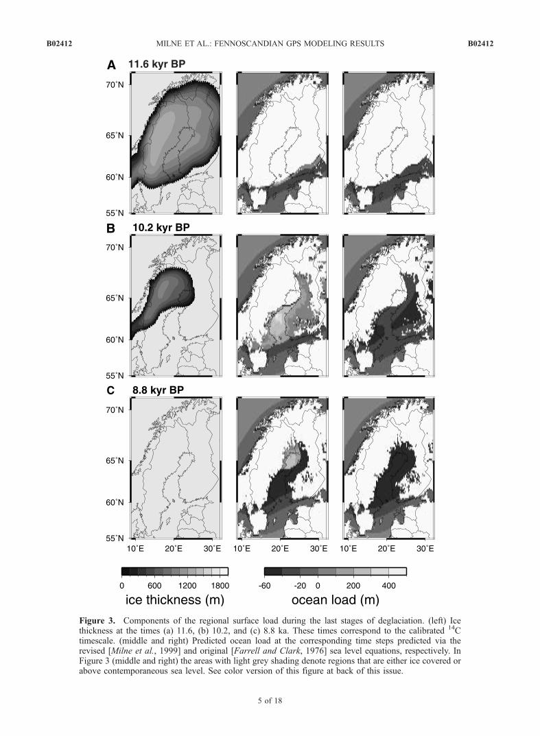
Figure 3. Components of the regional surface load during the last stages of deglaciation. (left) Icethickness at the times (a) 11.6, (b) 10.2, and (c) 8.8 ka. These times correspond to the calibrated 14Ctimescale. (middle and right) Predicted ocean load at the corresponding time steps predicted via therevised [Milne et al., 1999] and original [Farrell and Clark, 1976] sea level equations, respectively. InFigure 3 (middle and right) the areas with light grey shading denote regions that are either ice covered orabove contemporaneous sea level. See color version of this figure at back of this issue.


5 of 18

B02412

Figure 3b represents the ocean load change predicted overthe preceding time step (from 11.6 to 10.2 ka), and so on.Between 11.6 and 10.2 ka, a large section of the gulfbecomes ice free (Figure 3, left), and the new sea leveltheory correctly predicts an inundation of water into thisregion. The color contours on Figure 3 indicate that inun-dation extends over a broad swath of Finland and a portionof Sweden, indicating that these areas were below sea level(due to the crustal lowering caused by the ice load) at thetime of ice retreat. The amplitude of the inundation reachesin excess of 400 m in the central portion of the gulf. Overthe same period, the Baltic Sea to the south experiences areduction in the ocean load of amplitude tens of meters.This region became ice free at an earlier stage in the model;hence, from 11.6 to 10.2 ka the predicted reduction in oceanload is primarily a consequence of continuing postglacialuplift of the local crust. In the next time slice, from 10.2 to8.8 ka, the ice sheet disappears, and the northern tip of theGulf of Bothnia is finally exposed. The correspondingocean load prediction (Figures 3c, middle) shows an influxof water into this small area of �200 m amplitude. During

the same period the remainder of gulf (i.e., the region thatbecame ice free in the penultimate time step) experiences asignificant reduction in the ocean load. This reduction islargely due to the postglacial uplift of the region; however,there is also a significant contribution from the fall in theocean surface associated with the decreasing gravitationalattraction of the ablating ice mass.[19] The inundation of water into a region vacated by

ablating ice is governed by the total distance between thegeoid and solid surfaces in the region exposed by the iceretreat. In traditional postglacial sea level theory, the localwater load is governed not by the total distance between thegeoid and solid surfaces, but rather by changes in the heightof each of these surfaces over the previous time step; hencethe inundation process cannot be modeled. To illustrate this,Figure 3 (right) shows a sequence of predictions analogousto Figure 3 (middle), with the exception that the traditionaltheory for ocean load changes is applied. In this case,regions subject to recent ice retreat do not show an influxof water load. Instead, both crustal uplift and the changinggravitational attraction of the ablating ice mass lead to areduction in the distance between the geoid and solidsurfaces and thus a reduction in the local ocean load. Notethat the two theories (Figures 3, middle, and 3, right) showrelatively consistent predictions in regions that are notvacated by ice in the most recent time step.[20] The results in Figure 3 indicate that the original sea

level theory yields a considerably larger negative water loadfor the region compared to the revised theory. Figure 2dshows the ocean load signal in radial crustal velocitypredicted on the basis of the original sea level equation.The predicted uplift signal is 2–3 times greater than thatpredicted using the revised theory in the vicinity of the Gulfof Bothnia (see Figure 2c). The error incurred by adoptingthe original sea level theory is as high as 1.6 mm/yr at theBIFROST sites, a discrepancy which exceeds the typicalobservational error.[21] Figure 4 shows results that are analogous to those in

Figure 2, with the exception that we now treat the horizontaldeformation field. The total predicted signal (Figure 4a)displays the characteristic pattern of divergent motioncentered near the location of the peak present-day uplift(and peak ice height at Last Glacial Maximum). Thisprediction is in accord with the general form of theobservations (Figure 1c). The asymmetry in the predicteddeformation pattern is largely a result of the deformationassociated with the deglaciation of the distant Laurentide icecomplex [Mitrovica et al., 1994b]. As in Figure 2, the ice-load-induced signal generally dominates the total field. Anexception to this rule is evident in southern Finland, wherethe magnitude of the ocean load signal is comparable to thehorizontal motions produced by the ice loading. The errorincurred by adopting the traditional sea level theory is mostpronounced in the same region.[22] Next we focus on deformation driven by GIA-in-

duced perturbations in Earth rotation. The geometry of theperturbation to the centrifugal potential is described (tobetter than �1%) by a degree 2 order one surface sphericalharmonic [e.g., Han and Wahr, 1989; Mitrovica et al.,2001]. The orientation of this potential forcing is governedby the GIA-induced polar wander path during the postgla-cial period, which lies, approximately, on the great circle

Figure 4. Analogous to the predictions shown in Figure 2except that the present-day horizontal deformation rate fieldis shown. The GPS site locations are not shown. The scalevector is shown at the bottom left.


6 of 18

B02412

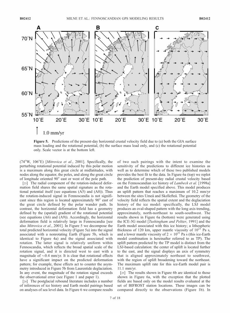
(74�W, 106�E) [Mitrovica et al., 2001]. Specifically, theperturbing rotational potential induced by this polar motionis a maximum along this great circle at midlatitudes, withnodes along the equator, the poles, and along the great circleof longitude oriented 90� east or west of the pole path.[23] The radial component of the rotation-induced defor-

mation field shares the same spatial signature as the rota-tional potential itself (see equations (A5) and (A8)). Thusthe rotation-induced signal in Fennoscandia is not signifi-cant since this region is located approximately 90� east ofthe great circle defined by the polar wander path. Incontrast, the horizontal deformation field has a geometrydefined by the (spatial) gradient of the rotational potential(see equations (A6) and (A9)). Accordingly, the horizontaldeformation field is relatively large in Fennoscandia [seealso Mitrovica et al., 2001]. In Figure 5 we decompose thetotal predicted horizontal velocity (Figure 5a) into the signalassociated with a nonrotating Earth (Figure 5b, which isidentical to Figure 4a) and the signal associated withrotation. The latter signal is relatively uniform withinFennoscandia, which reflects the broad spatial scale of therotation signal, and it is directed west to east with amagnitude of �0.4 mm/yr. It is clear that rotational effectshave a significant impact on the predicted deformationpattern; for example, these effects act to counter the asym-metry introduced in Figure 5b from Laurentide deglaciation.In any event, the magnitude of the rotation signal exceedsthe observational error (see Figure 1 and paper 1).[24] The postglacial rebound literature includes a number

of inferences of ice history and Earth model pairings basedon analyses of sea level data. In Figure 6 we compare results

of two such pairings with the intent to examine thesensitivity of the predictions to different ice histories aswell as to determine which of these two published modelsprovides the best fit to the data. In Figure 6a (top) we replotthe prediction of present-day radial crustal velocity basedon the Fennoscandian ice history of Lambeck et al. [1998a]and the Earth model specified above. This model producesan uplift pattern that reaches a maximum of 10.2 mm/yrbetween the sites Umea and Skelleftea. The geometry of thevelocity field reflects the spatial extent and the deglaciationhistory of the ice model: specifically, the LSJ modelproduces an oval-shaped pattern with the long axis trending,approximately, north-northeast to south-southwest. Theresults shown in Figure 6a (bottom) were generated usingthe ICE-3G model [Tushingham and Peltier, 1991] and theEarth model associated with this ice history; a lithosphericthickness of 120 km, upper mantle viscosity of 1021 Pa s,and a lower mantle viscosity of 2 � 1021 Pa s (this ice-Earthmodel combination is hereinafter referred to as TP). Theuplift pattern predicted by the TP model is distinct from theLSJ-based calculation: the center of uplift is located furtherto the east, and the signal displays an axis of symmetrythat is aligned approximately northeast to southwest,with the region of uplift broadening toward the northeast.The maximum uplift rate for this ice-Earth model pair is11.1 mm/yr.[25] The results shown in Figure 6b are identical to those

shown in Figure 6a, with the exception that the plottedfields are based only on the model results evaluated at theset of BIFROST station locations. These images can becompared directly to the observations (Figure 1b). In

Figure 5. Predictions of the present-day horizontal crustal velocity field due to (a) both the GIA surfacemass loading and the rotational potential, (b) the surface mass load only, and (c) the rotational potentialonly. Scale vector is at the bottom left.


7 of 18

B02412

general, the pattern shown in Figure 1b (top) more closelymatches the observations. The greatest misfit between theobservations and the LSJ model is apparent in the northeastsection of the plotted region (Figure 6c, top), where the

observed radial rates are underpredicted. However, note thatthe observations in this region exhibit the largest uncertainty.The TP model produces uplift contours that are orientedmore east-west than north-south and so it does not, in

Figure 6. (a) Predictions of the present-day radial velocity field based on the (top) LSJ and (bottom) TPice-model pairs (see text for details). (b) Same as in Figure 6a except that the predicted deformation fieldis sampled at GPS site locations only. These maps can be compared directly to observational results inFigure 1a. (c) Residual vertical deformation field calculated by subtracting the predicted rates from theobserved rates. The zero contour is marked by a white line.


8 of 18

B02412

general, produce a good match to the observations(Figure 6c, bottom). These qualitative comments are sup-ported by the normalized c2 misfit computed for thesemodels: 5.94 and 10.3 for the LSJ and TP models, respec-tively. The c2 values are computed by evaluating theobserved rate minus the predicted rate divided by theobserved error at each site, squaring this value and thensumming the contributions for each site. This sum is thennormalized by the number of observations minus one.[26] Figure 7 shows an analogous plot of the predicted

horizontal rates. Once again, the patterns of present-dayhorizontal velocity generated for the two models are distinct.

These differences aremost apparent in the lower section of themap. For example, the TP model produces larger southwardmotion in southern Finland and southern Sweden. Compar-ison of the predictions in Figure 7b with the observations(Figure 1c) indicates that the latter is better matched by theLSJ model (see also column Figure 7c). Thec2 values for theLSJ and TP models are 16.8 and 30.6, respectively.[27] It is interesting to note that the c2 values for the fits

to the horizontal rates are �3 times larger than those for thevertical rates. As discussed previously by Milne et al.[2001], this could be a result of limitations in the forwardmodel due to, for example, a simplified 1-D Earth structure

Figure 7. As in Figure 6, except that results for horizontal rates are shown. The vector magnitude scaleis shown at bottom left.


9 of 18

B02412

or inaccuracies in the adopted ice model. These limitationshave been shown to impact the predictions of horizontalrates more so than vertical rates [Mitrovica et al., 1994b;Wahr and Davis, 2002]. With regard to the suggestion ofuncertainties in the ice model, it is important to note thatboth of the ice models we have adopted were constrainedusing observations of relative sea level changes, which aredirectly affected by vertical crustal motion but are indepen-dent of horizontal motion. This suggests that inaccuracies inthe ice models may be an important source of this variationin the c2 values. Of course, the poorer fit to the horizontalrates could also be attributed to an underestimation of thetrue uncertainty in the horizontal rates.[28] We next present the results of a detailed forward

modeling analysis based on the LSJ ice history. In partic-ular, we have predicted the Fennoscandian 3-D crustaldeformation using this history and a large suite of Earthmodels in which the lithospheric thickness, upper mantleviscosity (nUM) and lower mantle viscosity (nLM) werevaried over the ranges shown in Figure 8. For each of theseruns we computed the normalized c2 statistic and the resultsare shown in Figure 8.[29] Figure 8a shows the results for the case in which

only the vertical component of the rates is considered. Thereis significant trade-off between viscosity values in the upperand lower mantle. Consider, for example, the results for thecase of a 120 km thick lithosphere: c2 values of less thanfive can be achieved with an approximately isoviscousmantle of �2–3 � 1021 Pa s or with a two layer structurecharacterized by an order of magnitude jump in viscosityacross the 670 km interface (nUM � 5 � 1020 Pa s, nLM �5–10 � 1021 Pa s). A similar trade-off has been identified ininferences based on relative sea level data [e.g., Lambeck etal., 1990; Mitrovica, 1996]. An important feature of theresults for vertical rates is the rapid increase in the misfitas the upper mantle viscosity is reduced below about 5 �1020 Pa s for lower mantle viscosity values ranging from 3 to50 � 1021 Pa s. This gradient is a consequence of themarked decrease in the predicted present-day uplift rates asthe upper mantle viscosity is reduced below this threshold.For such viscosity models, the relatively rapid isostaticuplift has yielded relatively small levels of remnant (i.e.,present-day) disequilibrium.[30] Figure 8b shows the c2 results when only the

horizontal component of the rates is taken into account.Since the GIA model does less well in predicting thehorizontal rates compared to the vertical rates (see Figure 7and related discussion), the error bars for these data werescaled by a factor of 1.8 to produce a minimum c2 valuethat matches that for the vertical rates. This scaling of theerror in the horizontal rates was performed as a preliminaryattempt to account for the influence of uncertainties in theice model. In Figure 8b the region of viscosity space wherethe best fit is achieved is significantly different from thelocation of the minimum in Figure 8a. In particular, uppermantle viscosities greater than �1021 Pa s, and lower mantleviscosities less than �3 � 1021 Pa s are excluded on thebasis of the horizontal velocities. Thus, when consideringmisfit for the combined horizontal and vertical motions(Figure 8c), a relatively small region of acceptable viscositymodel space is isolated. We conclude that horizontalmotions provide constraints on viscosity which are distinct

from those provided by observations which reflect verticaldeformation (radial crustal uplift rates, sea level changes).[31] Figures 8 (top), 8 (middle), and 8 (bottom) refer to a

different value for the adopted lithospheric thickness. (Ourcalculations were extended to include lithosphere thick-nesses of 146 km and 171 km, but these results are notshown.) The model with a lithospheric thickness of 120 kmwas found to produce the minimum c2 value (for nUM = 8 �1020 Pa s and nLM = 1022 Pa s).[32] Applying an F test to the results shown in Figure 8c

(bottom), yields the following 95% confidence interval:5 � 1020 � nUM � 1021 Pa s; 5 � 1021 � nLM � 5 �1022 Pa s.[33] In Figure 9 the c2 results are plotted as a function of

lithospheric thickness and nUM for a fixed nLM value of1022 Pa s. In this case, the radial rates show a relatively weakcorrelation between lithospheric thickness and upper mantleviscosity, while a strong trade-off is evident in the fits to thehorizontal rates. In regard to the latter, the quality of fit canbe maintained by increasing or decreasing both parameterssimultaneously within a given parameter range. As anexample, a good fit can be obtained for either a relativelythick lithosphere (�140 km) and high nUM (�1021 Pa s), ora relatively thin lithosphere (�80 km) and low nUM (�5 �1020 Pa s). As we noted in the context of Figure 8, thevertical rates cannot be fit for nUM less than �5 � 1020 Pa s(regardless of the value adopted for lithospheric thickness)and the 3-D rates prefer a relatively thick lithosphere, with a95% confidence interval of 90 to 170 km.[34] The optimum parameter ranges cited above are

broadly consistent with other inferences of mantle viscos-ity based on GIA data from Fennoscandia. Using geo-logical records of postglacial sea level change, Lambecket al. [1998a] inferred values of lithospheric thickness(65–85 km) and upper mantle viscosity (3–4 � 1020 Pa s)which lie at the lower bound of our ranges. A companionstudy based on instrumented sea level records [Lambecket al., 1998b] yielded slightly higher values for boththese parameters (80–100 km and (4–5) � 1020 Pa s).Wieczerkowski et al. [1999] have used their newlyderived estimate of the Fennoscandian relaxation spec-trum to infer a mean viscosity within the bulk of thesublithospheric upper mantle of �5 � 1020 Pa s; this isalso near the lower bound of our inferred range. Mostrecently, Kaufmann and Lambeck [2002] inverted a widesubset of GIA data, including relative sea level historiesfrom Fennoscandia, and derived bulk upper and lowermantle values (7 � 1020 Pa s, 2 � 1022 Pa s, respec-tively) near the center of our preferred ranges.[35] We next investigate the influence of the choice of

ice model on the inference of Earth model parameters. InFigure 10 we repeat the calculations of Figure 8 (for alithospheric thickness of 120 km) using the ICE-3Gdeglaciation history discussed above. The general locationand structure of the c2 minimum in viscosity space issimilar to that obtained with the LSJ model, although thec2 values are consistently higher for the ICE-3G predic-tions. We conclude that our choice between these two icemodels does not significantly influence the inferred rangeof optimum Earth model parameters. It is interesting tonote that the specific Earth model used in the derivation ofthe ICE-3G load history (LT = 120 km, nUM = 1021 Pa s,


10 of 18

B02412

nLM = 2� 1021 Pa s) does not yield a good fit to the 3-D ratesin Fennoscandia.[36] The forward modeling analysis presented above and

the inverse analysis presented below are based on single-site

position estimates for each of the BIFROST stations. Therates based on these time series may be systematicallybiased due to perturbations in both the reference framerealizations and the satellite orbits during the monitoring

Figure 8. Normalized c2 contour plots for a variety of Earth models characterized by an elasticlithosphere of thickness 71, 96 or 120 km (see label at bottom left) and a two-layer sublithospheric mantleviscosity with a range of uniform values within the upper mantle (nUM) and lower mantle (nLM) regions.Results are shown for (a) vertical rates only, (b) horizontal rates only, and (c) all three rate components.


11 of 18

B02412

period. The error would appear as a long-wavelength featurein the observed 3-D velocity field. A related point in thisregard is the difficulty in separating long-wavelength con-tributions to the horizontal motion associated with GIA(e.g., the rotation-induced signal (Figure 5c) or that due tothe distant Laurentide ice sheet [Mitrovica et al., 1994b])from that associated with the rigid component of tectonicplate motion.[37] We have performed a regional strain rate analysis

using the BIFROST data to investigate the influence of

these issues on the accuracy of our viscosity inference(S. Bergstrand et al., Upper mantle viscosity from continu-ous GPS baselines in Fennoscandia, submitted to Journal ofGeodynamics, 2003). This type of analysis is less sensitiveto long-wavelength signals in the observed velocity field.The results based on the strain rate analysis give a 95%confidence range for nUM of 3–10 � 1020 Pa s and an

Figure 9. Normalized c2 values plotted as a function oflithospheric thickness and upper mantle viscosity (nUM) fora fixed lower mantle viscosity of 1022 Pa s. As in Figure 8,results are shown for (a) vertical rates only, (b) horizontalrates only, and (c) all three rate components.

Figure 10. Normalized c2 contour plots based on the ICE-3G deglaciation model for a variety of Earth modelscharacterized by an elastic lithosphere of thickness 120 kmand a two-layer sublithospheric mantle viscosity with arange of uniform values within the upper mantle (nUM)and lower mantle (nLM) regions. Results are shown for(a) vertical rates only, (b) horizontal rates only, and (c) allthree rate components.


12 of 18

B02412

optimum lithospheric thickness of 120 km, in agreementwith our present results.

3.2. Inverse Analysis

[38] The forward analyses summarized in Figures 8–10,although an extension of earlier work [Milne et al., 2001],provide a rather coarse measure of the sensitivity of theBIFROST data to variations in mantle viscosity. As a simpleexample, the correlation between values of nUM and nLM inFigure 8 preferred on the basis of radial velocity datasuggest that these data do not independently resolve thebulk upper and lower mantle viscosity. This point is part ofa broader question that serves as the focus of the presentsection; namely, what is the radial resolving power of theBIFROST data set?[39] To answer this question, we perform a joint inversion

of the BIFROST data set of present-day 3-D crustal veloc-ities. For this purpose we adopt a Bayesian inferenceprocedure. As in previous work on the viscosity problem,we parameterize the inversion in terms of the logarithm ofviscosity in a set of discrete layers [e.g., Mitrovica andForte, 1997]. In this regard, the ‘‘model’’ to be inverted foralso includes a final parameter equal to the thickness of theelastic lithosphere, and we can thus write

X ¼ log n rj� �

for j ¼ 1;N � 1;LT� �

; ð1Þ

where j denotes the radial layer (j = 1 is the layer above thecore-mantle boundary, and j = N � 1 is the layer below theelastic lithosphere) and LT is the lithospheric thickness(nondimensionalized using the radius of the Earth, a). Themodel X has a total of N parameters.[40] We have chosen to discretize the mantle viscosity

into a set of 22 uniform layers, with 9 residing within thelower mantle. Thus N = 23. The inverted model isspecified by both the a posteriori model and covariancematrix. The diagonal elements of the latter provide thevariances of the 23 individual model parameters. TheBIFROST data will not be capable of resolving structureon the length scale of the individual viscosity modellayers, and therefore the a posteriori variances for thesemodel estimates will not be substantially smaller than theprior variances adopted in the inversions (we have foundthat the greatest reduction is of the order 30–40%). Wewill estimate the resolving power of the BIFROST data byexamining the posterior covariance matrix. The spread ofthe off-diagonal elements for, say, the jth row of thismatrix provides a measure of the radial resolving power ofthe data for an estimate of viscosity at a depthcorresponding to the jth radial layer [e.g., Tarantola andValette, 1982]. As we note below, the a posteriori uncer-tainty for an estimate of the average viscosity over thisresolving width will, in contrast to the uncertainty for anindividual model value, be significantly smaller than theprior uncertainty.[41] The prior and starting model for our inversion

corresponds to an Earth model with an elastic lithosphereof 96 km, an upper mantle viscosity of 5 � 1020 Pa s, and alower mantle viscosity of 5 � 1021 Pa s. The Frechet kernelsare computed numerically using a suite of models in whichthe viscosity in the 22 mantle layers and the lithosphericthickness are perturbed from the values defining this starting

model. As an illustration, we show, in Figure 11, Frechetkernels for the prediction of the three components of crustalvelocity for a set of eight sites lying (south to north) alongthe major axis of the Fennoscandian deformation region(see Figure 1a for site locations). To account for differencesin the thickness of the radial layers, each plotted value of thekernels has been normalized by the (nondimensional) thick-ness of the associated radial layer. Since the predictionshave a nonlinear dependence on mantle viscosity, thekernels will be a function of the model; nevertheless, thestarting model was adopted because it provides a near bestfit to the BIFROST-derived estimates of 3-D crustal velocity(Figure 8c).[42] The Frechet kernels provide a measure of the de-

tailed depth-dependent sensitivity of a particular datum tovariations in the radial profile of mantle viscosity. Predic-tions of radial velocity for sites within central Fennoscandia(Martsbo to Sodankyla) based on the starting model show abroad sensitivity to bulk upper mantle viscosity. Significantchanges in this pattern of sensitivity are evident as oneconsiders sites closer to the perimeter of the Fennoscandianice complex at Last Glacial Maximum, Hassleholm to thesouth and Kevo to the north. With the possible exception ofHassleholm, all predictions of radial velocity show a mod-erate, but nonnegligible sensitivity to variations in lowermantle viscosity (at least in the shallowest portions of thisregion), and this explains the trade-off evident in Figure 8a.[43] The predictions of horizontal velocity show a distinct

sensitivity to variations in the mantle viscosity profile.These predictions have a sensitivity that tends to peak nearthe top of the mantle. Furthermore, while there is littlesensitivity to variations in viscosity within the top half ofthe lower mantle, a nonzero sensitivity is apparent at somesites (e.g., Jonkoping) near the base of the mantle.[44] Figure 12 shows the results of two inversions of the

BIFROST data set. For each of these inversions the dottedline on Figure 12 represents the prior (and starting) viscositymodel. The dashed line is the posterior model for apreliminary inversion in which the viscosity in layers withinthe lower and, independently, the upper mantle, are assumedto be perfectly correlated; this assumption yields a two-layer viscosity model characterized by nLM � 1022 Pa s andnUM � 5.5 � 1020 Pa s, and lithospheric thickness of�116 km. We note, in reference to Figure 8c, that thismodel falls close to the best fit model determined by ourforward analysis.[45] The solid line on Figure 12 shows the radial viscosity

profile generated from a multilayer inversion of theBIFROST data set. In the upper mantle, this model oscil-lates around the starting/prior model (with the exception ofa thin layer of low viscosity at the base of the lithosphere).In addition, the model trends toward values in excess of1022 Pas in the top half of the lower mantle before returningto a viscosity close to the prior value near the base of themantle. (The posterior estimate of lithospheric thickness inthis inversion is 104 ± 6 km.)[46] The question arises as to whether these variations

in the viscosity are actually resolved by the BIFROSTdata set. To answer this question, we turn to Figure 13,which provides plots of the off-diagonal elements ofthe covariance matrix for eight target depths (i.e., depthscorresponding to a specific layer of the model) ranging


13 of 18

B02412

from the shallow upper mantle to 1225 km depth. Theindividual plots are normalized by the largest off-diagonalvalue and the diagonal element (i.e., the variance) is notshown. Below target depths of �1300 km we have notedthat the location of the peak off-diagonal element is gener-ally widely displaced from the target and this indicates thatthe BIFROST data do not provide significant radial resolu-tion of mantle viscosity in this region of the lower mantle.

In contrast, at progressively shallower depths, Figure 13indicates a resolving power which gradually improves.[47] Let us, for the purpose of illustration, define the

resolving width as the radial range of the off-diagonalelements having values equal to or greater than 50% ofthe peak off-diagonal value (i.e., width at half max). In thiscase, the radial resolving power of the BIFROST data at thetarget depth of 230 km is �200 km. This resolving power

Figure 11. Frechet kernels (see text) as a function of radius for predictions of the three components ofpresent-day crustal velocity: solid line, radial; dashed line, horizontal south; dotted line, horizontal east.Each panel refers to a different site in the BIFROST GPS network (see Figure 1). Each value of the kernelis normalized by the (nondimensional) thickness of the associated radial layer in order to remove anysensitivity to layer thickness. The kernels each have 22 values, nine within the lower mantle and theremainder in the sublithospheric upper mantle. A 23rd value (not plotted or shown) used in the inversionsrefers to changes in the thickness of the elastic lithosphere. The kernels were computed for a startingmodel defined as having a lithosphere of thickness 96 km, nUM = 5 � 1020 Pa s, and nLM = 5 � 1021 Pa s.


14 of 18

B02412

reduces to �380 km at a target depth of 468 km and�640 km at 652 km depth. We can conclude, for example,that both the low-viscosity layer of thickness �50 km atthe base of lithosphere and the high viscosity hump at�1400 km depth (solid line, Figure 12) are not resolvableby the BIFROST data. Furthermore, while target depthsranging from 800 to 1300 km show relatively little covari-ance with upper mantle viscosity values, some sensitivity toupper mantle structure is always evident; this is in accordwith the forward results in Figure 8c.[48] In Figure 12 we show three radial regions (bottom

right) which are, according to Figure 13, resolvable by theBIFROST data. From deepest to shallowest, the weighted(by the resolving kernel) mean of the viscosity profilewithin these regions is: 8.9 � 1021 Pa s, 5.4 � 1020 Pa s,and 5.9 � 1020 Pa s, respectively. Over depth rangesresolvable by the BIFROST data, the observational con-straints lead to an order of magnitude reduction in thevariance of the averages.

4. Final Remarks

[49] The BIFROST Fennoscandian GPS network was thefirst to produce maps of the present-day, 3-D crustalvelocity field associated with GIA. In a general sense, thesemaps confirmed the basic postglacial deformation patternfirst predicted theoretically in the early 1990s [James andLambert, 1993; Mitrovica et al., 1993, 1994b], namely,ongoing radial rebound of previously glaciated regions

and horizontal motions directed outward from the zone ofmaximum uplift. After roughly a decade of GPS datacollection, the observational uncertainties in the rate esti-mates are now sufficiently small (Figure 1) that increasinglyaccurate theoretical predictions must be brought to bear toanalyze the data. We have demonstrated, for example, thatthe signal associated with recent improvements in the GIAtheory, for example the inclusion of crustal deformationsdriven by perturbations in the Earth’s rotation vector and arefined treatment of the water load in the vicinity of anablating ice margin and evolving shoreline, exceed thecurrent observational uncertainty.[50] The ability of modern numerical models of the GIA

process to accurately reconcile the BIFROST rate estimatespermits a wide number of geophysical applications [e.g.,Milne et al., 2001]. The forward analyses described hereintouch upon two of the classic GIA analyses; namely,constraining the space-time history of late Pleistocene icecover and the radial profile of mantle viscosity. Our resultsindicate that the BIFROST data provide a potentiallypowerful test for models of the ice history (Figures 6 and7) and permit bounds to be placed on the bulk upper and(shallow) lower mantle viscosity and the lithospheric thick-ness (Figure 8).[51] Our analysis was completed by performing the first

formal inversion of the BIFROST data set. The main goal ofthis inversion was a determination of the resolving power ofthe GPS estimates of 3-D crustal velocities. In this regard,the results in Figure 13 have several important implications

Figure 12. Results of a Bayesian inversion of the BIFROST GPS data set. The dotted line representsthe starting and prior (two layer) viscosity model adopted in the inversion (nUM = 5 � 1020 Pa s, nLM =5 � 1021 Pa s); the starting lithospheric thickness is 96 km. The dashed line is the inverted profilegenerated by assuming that the layers in the upper and (independently) the lower mantle are perfectlycorrelated (posterior LT = 106 km). The solid line shows the results for a full multilayer inversion of theGPS data set (posterior LT = 103 ± 8 km). The off-diagonal elements for a subset of rows in theassociated posterior covariance matrix is given in Figure 13. The three horizontal lines at bottom rightillustrate three of the radial regions which are resolved by the BIFROST data set (see text and Figure 13).


15 of 18

B02412

for the forward analyses of mantle viscosity summarized inFigure 8. First, the inference of lower mantle viscosityimplied by the analysis in Figure 8 is more accuratelyinterpreted as a constraint on the viscosity in the top�800 km of this region. This limitation should not besurprising given the size of the Fennoscandian ice complexthat covered the region at Last Glacial Maximum (seeMitrovica [1996] for a discussion). Furthermore, theBIFROST data are able to resolve structure on radial scalesfiner that the entire width of the upper mantle. Specifically,this resolution ranges from �200 km just below the litho-sphere to �300 km near the base of the upper mantle.Accordingly, a significant improvement in the fit of theforward models may be achievable by considering a suite ofmodels with two or three isoviscous layers within the uppermantle.

[52] As we have discussed, our inferences of viscositywithin the upper mantle and the top portion of the lowermantle are reasonably consistent with previous studiesbased (at least in part) on the GIA record within Fenno-scandia. We have inferred lower bounds of �5 � 1020 Pa son the bulk upper mantle viscosity below Fennoscandia and�90 km on the elastic thickness of the Fennoscandiancraton. The resolving power of the data is not sufficient torule out a thin low-viscosity region below the lithosphere;however, any region of significant weakness extending�200 km or more from the lithosphere does appear to beruled out on the basis of the 3-D rates. The resolving powerof the observations to depths of �1300 km will continue toimprove as the BIFROST time series are extended and theobservational error reduced further. Future analyses maytherefore be able to provide more robust constraints on the

Figure 13. Plot of the off-diagonal elements for a set of eight rows in the posterior covariance matrixgenerated by Bayesian inversion of the BIFROST data set (the associated inverted model is given by thesolid line in Figure 12). The values are normalized by the largest off-diagonal (i.e., covariance) in eachcase. The target depth (TD) is specified by the label on each panel, and it is located at the center of thelayer whose value is not shown on the plot. The up-pointing arrow on the abscissa of each panel indicatesthe radius of the 670 km discontinuity marking the boundary between the upper and lower mantle.


16 of 18

B02412

possible existence of a thin low viscosity region immedi-ately below the Fennoscandian craton.[53] In future work we plan to extend the above forward

and inverse modeling analyses in three important ways.First, we will consider a revised GPS data set in which therates will be based on time series that are several yearslonger than those considered here. Second, we will employa series of ice histories that are generated from a realisticglaciological model and are validated with observationalevidence from the regional geological record. Third, we willincorporate independent data sets in the inversions. Thesewill include the so-called Fennoscandian relaxation spec-trum [McConnell, 1968; Wieczerkowski et al., 1999] and aset of postglacial decay times determined from centralFennoscandia [e.g., Mitrovica and Forte, 1997].[54] The incorporation of lateral variations in Earth struc-

ture will also serve as a focus for future work. Thesevariations, whether in the form of heterogeneities in litho-spheric strength or mantle structure, are an area of activeinterest in GIA research [e.g., Kaufmann and Wu, 2002],and they will no doubt impact the prediction (and analysis)of the BIFROST GPS-determined rates. Members of theBIFROST Project have completed the development of afinite element numerical formulation of GIA on asphericalEarth models (K. Latychev et al., Glacial isostatic adjust-ment on 3-D earth models: A finite-volume formulation,submitted to Geophysical Journal International, 2003). Thefuture application of this formulation to the present-dayFennoscandian deformation field will be an importantextension of the work presented here.

Appendix A: Theoretical Formalism forComputing 3-D Surface Deformation

[55] In the following, we provide a brief sketch of thespectral theory developed to calculate the three componentsof surface deformation associated with GIA. Computationof the impulse response of the (Maxwell) viscoelastic Earthmodel is based on a normal mode theory developed byPeltier [1974], Peltier and Andrews [1976], and Wu [1978].This response is represented in terms of so-called visco-elastic Love numbers which, in the time domain, have thefollowing form [Peltier and Andrews, 1976]:

hL‘ tð Þ ¼ hL;E‘ d tð Þ þ

XJj¼1

r‘;Lj exp �s‘j t

� �; ðA1Þ

lL‘ tð Þ ¼ lL;E‘ d tð Þ þ

XJj¼1

r0‘;Lj exp �s‘j t

� �; ðA2Þ

hT‘ tð Þ ¼ hT ;E‘ d tð Þ þ

XJj¼1

r‘;Tj exp �s‘j t

� �; ðA3Þ

lT‘ tð Þ ¼ lT ;E‘ d tð Þ þ

XJj¼1

r0‘;Tj exp �s‘j t

� �; ðA4Þ

where the superscripts L and T represent Love numbers forthe case of a surface mass load (load Love numbers) and

gravitational potential forcing (tidal or tidal-effective Lovenumbers), respectively. The first term on the right-hand sideof equations (A1)–(A4) denotes the instantaneous elasticresponse (hence the superscript E) to the associated forcing,while the second term is the nonelastic response. The latteris composed of a set of J modes of pure exponential decay.The h and l Love numbers govern the radial and tangentialdisplacement response, respectively, at spherical harmonicdegree ‘. The adopted viscoelastic structure of the Earthmodel is embedded within these Love numbers.[56] With these expressions in hand we can proceed

toward a spectral formulation of the radial and horizontalcrustal displacement responses due to GIA. Let us denotethese responses as R(q, y, t) and V(q, y, t), respectively,where q is the colatitude, y is the east longitude, and t is thetime. A spherical harmonic decomposition of these fieldsmay be written as [Mitrovica et al., 1994a, 2001]

R q;y; tð Þ ¼X1‘¼0

X‘

m¼�‘

R‘;m tð ÞY‘;m q;yð Þ ðA5Þ

V q;y; tð Þ ¼X1‘¼0

X‘

m¼�‘

V ‘;m tð ÞrY‘;m q;yð Þ; ðA6Þ

where m is the spherical harmonic order, r is the two-dimensional gradient operator, and Y‘,m is the surfacespherical harmonic basis function. We adopt the specificnormalization

Z ZWYy‘0;m0 q;yð ÞY‘;m q;yð Þ sin q dqdy ¼ 4pd‘0;‘dm0 ;m; ðA7Þ

where the dagger denotes the complex conjugate and Wrepresents the unit sphere.[57] The GIA forcing is composed of contributions from

the surface mass load and a gravitational potential pertur-bation (the so-called rotational potential) arising from GIA-induced changes in the planetary rotation vector. We denotethe spherical harmonic coefficients of the former by L‘,mand of the latter by L‘,m, respectively. The harmoniccoefficients in the spectral decompositions (A5) and (A6)are then [e.g., Mitrovica et al., 2001]

R‘;m tð Þ ¼Z t

�1

L‘;m t0ð Þg

hT‘ t � t0ð Þ

þ 4pa3

2‘þ 1ð ÞMe

L‘;m t0ð Þ

hL‘ t � t0ð Þdt0 ðA8Þ

V‘;m tð Þ ¼Z t

�1

L‘;m t0ð Þg

lT‘ t � t0ð Þ

þ 4pa3

2‘þ 1ð ÞMe

L‘;m t0ð ÞlL‘ t � t0ð Þdt0; ðA9Þ

where a and Me are the Earth’s radius and mass,respectively, and g is the surface gravitational acceleration.

[58] Acknowledgments. We thank Kurt Lambeck and Tony Purcellfor providing us with their Fennoscandian ice model SCAN-2. We alsothank Erik Ivins, Giorgio Spada, and Isabella Velicogna for constructive


17 of 18

B02412

reviews. This research was funded by the Natural Environment ResearchCouncil of the United Kingdom and the Natural Sciences and EngineeringResearch Council of Canada. We also acknowledge the support given bythe Swedish Research and Testing Institute, the Swedish Natural ScienceResearch Council, the Swedish Research Council, the Swedish NationalSpace Board, and the Swedish Research Council for Engineering Sciences.Some figures were generated with the Generic Mapping Tools softwarepackage [Wessel and Smith, 1991].

ReferencesBIFROST Project (1996), GPS measurements to constrain geodynamicprocesses in Fennoscandia, Eos Trans. AGU, 77, 337, 341.

Davis, J. L., J. X. Mitrovica, H.-G. Scherneck, and H. Fan (1999), Inves-tigations of Fennoscandian glacial isostatic adjustment using model sealevel records, J. Geophys. Res., 104, 2733–2747.

Dziewonski, A. M., and D. L. Anderson (1981), Preliminary ReferenceEarth Model (PREM), Phys. Earth Planet. Inter., 25, 297–356.

Farrell, W. E., and J. A. Clark (1976), On postglacial sea level, Geophys. J.R. Astron. Soc., 46, 647–667.

Fjeldskaar, W. (1994), Viscosity and thickness of the asthenosphere de-tected from the Fennoscandian uplift, Earth Planet. Sci. Lett., 126,399–410.

Han, D., and J. Wahr (1989), Post-glacial rebound analysis for a rotatingEarth, in Slow Deformations and Transmission of Stress in the Earth,Geophys. Monogr. Ser., vol. 49, edited by S. Cohen and P. Vanıcek,pp. 1–6, AGU, Washington, D. C.

Haskell, N. A. (1935), The motion of the fluid under a surface load, 1,Physics, 6, 265–269.

James, T. S., and A. Lambert (1993), A comparison of VLBI data with theICE-3G glacial rebound model, Geophys. Res. Lett., 20, 871–874.

Johansson, J. M., et al. (2002), Continuous GPS measurements of postgla-cial adjustment in Fennoscandia: 1. Geodetic results, J. Geophys. Res.,107(B8), 2157, doi:10.1029/2001JB000400.

Karato, S., and P. Wu (1993), Rheology of the upper mantle: A synthesis,Science, 260, 771–778.

Kaufmann, G., and K. Lambeck (2002), Glacial isostatic adjustment and theradial viscosity profile from inverse modeling, J. Geophys. Res.,107(B11), 2280, doi:10.1029/2001JB000941.

Kaufmann, G., and P. Wu (2002), Glacial isostatic adjustment on a three-dimensional laterally heterogeneous earth: Examples from Fennoscandiaand the Barents Sea, in Ice Sheets, Sea Level and the Dynamic Earth,Geodyn. Ser., vol. 29, edited by J. X. Mitrovica and L. L. A. Vermeersen,pp. 293–309, AGU, Washington, D. C.

Lambeck, K., P. Johnston, and M. Nakada (1990), Holocene glacialrebound and sea-level change in NW Europe, Geophys. J. Int., 103,451–468.

Lambeck, K., C. Smither, and P. Johnston (1998a), Sea-level change,glacial rebound and mantle viscosity for northern Europe, Geophys. J.Int., 134, 102–144.

Lambeck, K., C. Smither, and M. Ekman (1998b), Tests of glacial reboundmodels for Fennoscandinavia based on instrumented sea- and lake-levelrecords, Geophys. J. Int., 135, 375–387.

Makinen, J., H. Koivula, M. Poutanen, and V. Saaranen (2003), Verticalvelocities in Finland from permanent GPS networks and from repeatedprecise levelling, J. Geodyn., 35, 443–456.

McConnell, R. K. (1968), Viscosity of the mantle from relaxation timespectra of isostatic adjustment, J. Geophys. Res., 73, 7089–7105.

Milne, G. A. (1998), Refining models of the glacial isostatic adjustmentprocess, Ph.D. thesis, Univ. of Toronto, Toronto, Ont., Canada.

Milne, G. A., J. X. Mitrovica, and J. L. Davis (1999), Near-field hydro-isostasy: The implementation of a revised sea-level equation, Geophys. J.Int., 139, 464–482.

Milne, G. A., J. L. Davis, J. X. Mitrovica, H.-G. Scherneck, J. M. Johansson,M. Vermeer, and H. Koivula (2001), Space-geodetic constraints on glacialisostatic adjustment in Fennoscandia, Science, 291, 2381–2385.

Mitrovica, J. X. (1996), Haskell [1935] revisited, J. Geophys. Res., 101,555–569.

Mitrovica, J. X., and A. M. Forte (1997), Radial profile of mantle viscosity:Results from the joint inversion of convection and postglacial reboundobservables, J. Geophys. Res., 102, 2751–2769.

Mitrovica, J. X., and G. A. Milne (1998), Glaciation-induced perturbationsin the Earth’s rotation: A new appraisal, J. Geophys. Res., 103, 985–1005.

Mitrovica, J. X., and W. R. Peltier (1991), On postglacial geoid subsidenceover the equatorial oceans, J. Geophys. Res., 96, 20,053–20,071.

Mitrovica, J. X., and W. R. Peltier (1993), A new formalism for inferringmantle viscosity based on estimates of postglacial decay times: Applica-

tion to RSL variations in N.E. Hudson Bay, Geophys. Res. Lett., 20,2183–2186.

Mitrovica, J. X., J. L. Davis, and I. I. Shapiro (1993), Constraining pro-posed combinations of ice history and Earth rheology using VLBI deter-mined baseline length rates in North America, Geophys. Res. Lett., 20,2387–2390.

Mitrovica, J. X., J. L. Davis, and I. I. Shapiro (1994a), A spectral formalismfor computing three dimensional deformations due to surface loads:1. Theory, J. Geophys. Res., 99, 7057–7073.

Mitrovica, J. X., J. L. Davis, and I. I. Shapiro (1994b), A spectral formalismfor computing three dimensional deformations due to surface loads:2. Present-day glacial isostatic adjustment, J. Geophys. Res., 99,7075–7101.

Mitrovica, J. X., G. A. Milne, and J. L. Davis (2001), Glacial isostaticadjustment on a rotating Earth, J. Geophys. Int., 147, 562–578.

Nakada, M., and K. Lambeck (1989), Late Pleistocene and Holocene sea-level change in the Australian region and mantle rheology, Geophys. J.Int., 96, 497–517.

Peltier, W. R. (1974), The impulse response of a Maxwell Earth, Rev.Geophys., 12, 649–669.

Peltier, W. R., and J. T. Andrews (1976), Glacial isostatic adjustment-I. Theforward problem, Geophys. J. R. Astron. Soc., 46, 605–646.

Sabadini, R., and B. Vermeersen (1997), Ice-age cycles: Earth’s rotationinstabilities and sea-level changes, Geophys. Res. Lett., 24, 3041–3044.

Sabadini, R., D. A. Yuen, and E. Boschi (1982), Polar wander and theforced responses of a rotating, multilayered, viscoelastic planet, J. Geo-phys. Res., 87, 2885–2903.

Scherneck, H.-G., J. M. Johansson, H. Koivula, T. van Dam, and J. L.Davis (2003), Vertical crustal motion observed in the BIFROST project,J. Geodyn., 35, 425–441.

Tarantola, A., and B. Valette (1982), Generalized non-linear inverse pro-blems solved using the least squares criterion, Rev. Geophys., 20, 219–232.

Tushingham, A. M., and W. R. Peltier (1991), ICE-3G: A new globalmodel of late Pleistocene deglaciation based on geophysical predic-tions of postglacial relative sea level change, J. Geophys. Res., 96,4497–4523.

Veining Meinesz, F. A. (1937), The determination of the Earth’s plasticityfrom the post-glacial uplift of Scandinavia: Isostatic adjustment, K. Akad.Wet., 40, 654–662.

Wahr, J. M., and J. L. Davis (2002), Geodetic constraints on glacial isostaticadjustment, in Ice Sheets, Sea Level and the Dynamic Earth, Geodyn.Ser., vol. 29, edited by J. X. Mitrovica and L. L. A. Vermeersen, pp. 3–32, AGU, Washington, D. C.

Wessel, P., and W. H. F. Smith (1991), Free software helps map and displaydata, Eos Trans. AGU, 72, 441, 445–446.

Wieczerkowski, K., J. X. Mitrovica, and D. Wolf (1999), A revised relaxa-tion spectrum for Fennoscandia, Geophys. J. Int., 139, 69–86.

Wolf, D. (1987), An upper bound on lithospheric thickness from glacio-isostatic adjustment in Fennoscandia, J. Geophys., 61, 141–149.

Wu, P. (1978), The response of a Maxwell earth to applied surface massloads: Glacial isostatic adjustment, M.Sc. thesis, Univ. of Toronto, Tor-onto, Ont., Canada.

Wu, P. (1999), Modelling postglacial sea levels with power-law rheologyand a realistic ice model in the absence of ambient tectonic stress, Geo-phys. J. Int., 139, 691–702.

Wu, P., and W. R. Peltier (1982), Viscous gravitational relaxation, Geophys.J. R. Astron. Soc., 70, 435–485.

Wu, P., and W. R. Peltier (1984), Pleistocene deglaciation and the Earth’srotation: A new analysis, Geophys. J. R. Astron. Soc., 76, 753–792.

��J. L. Davis, Harvard-Smithsonian Center for Astrophysics, 60 Garden

Street, MS-42, Cambridge, MA 02138, USA. ( [email protected])J. M. Johansson and H.-G. Scherneck, Onsala Space Observatory,

Chalmers University of Technology, SE-439 92, Onsala, Sweden.([email protected])H. Koivula, Finnish Geodetic Institute, Geodeetinrinne 2, Masala,

FIN-02431, Finland. ([email protected])G. A. Milne, Department of Earth Sciences, University of Durham,

Science Labs, Durham, DH1 3LE, UK. ([email protected])J. X. Mitrovica, Department of Physics, University of Toronto, 60 St.

George St., Toronto, Ontario, Canada M5S 1A7. ( [email protected])M. Vermeer, Institute of Geodesy and Cartography, Helsinki University

of Technology, P.O. Box 1200, Hut, FIN-02015, Finland. ([email protected])


18 of 18

B02412

Figure 3. Components of the regional surface load during the last stages of deglaciation. (left) Icethickness at the times (a) 11.6, (b) 10.2, and (c) 8.8 ka. These times correspond to the calibrated 14Ctimescale. (middle and right) Predicted ocean load at the corresponding time steps predicted via therevised [Milne et al., 1999] and original [Farrell and Clark, 1976] sea level equations, respectively. InFigure 3 (middle and right) the areas with light grey shading denote regions that are either ice covered orabove contemporaneous sea level.

B02412 MILNE ET AL.: FENNOSCANDIAN GPS MODELING RESULTS B02412

5 of 18

Documents

Continuous GPS measurements of postglacial adjustment in Fennoscandia 1. Geodetic results