arX

iv:1

101.

1517

v1 [

astr

o-ph

.CO

] 7

Jan

201

1Draft version January 10, 2011Preprint typeset using LATEX style emulateapj v. 11/10/09

CORRELATIONS IN THE (SUB)MILLIMETER BACKGROUND FROM ACT× BLAST

Amir Hajian1,2,3, Marco P. Viero4,5, Graeme Addison6, Paula Aguirre7, John William Appel3, Nick Battaglia1,James J. Bock8,4, J. Richard Bond1, Sudeep Das9,3,2, Mark J. Devlin10, Simon R. Dicker10, Joanna Dunkley6,3,2,

Rolando Dunner3, Thomas Essinger-Hileman3, John P. Hughes24, Joseph W. Fowler11,3, Mark Halpern12,Matthew Hasselfield12, Matt Hilton16,17, Adam D. Hincks3, Renee Hlozek6, Kent D. Irwin11, Jeff Klein10,

Arthur Kosowsky13, Yen-Ting Lin23, Tobias A. Marriage2,14, Danica Marsden10, Gaelen Marsden12,Felipe Menanteau24, Lorenzo Moncelsi15, Kavilan Moodley16, Calvin B. Netterfield5,18,

Michael D. Niemack11,3, Michael R. Nolta1, Lyman A. Page3, Lucas Parker3, Douglas Scott12,Neelima Sehgal19, Jon Sievers1, David N. Spergel2, Suzanne T. Staggs3, Daniel S. Swetz10,11,

Eric R. Switzer20,3, Robert Thornton10,21, Ed Wollack22,

Draft version January 10, 2011

ABSTRACT

We present measurements of the auto- and cross-frequency correlation power spectra of the cosmic(sub)millimeter background at: 250, 350, and 500µm (1200, 860, and 600 GHz) from observationsmade with the Balloon-borne Large Aperture Submillimeter Telescope, BLAST; and at 1380 and2030 µm (218 and 148 GHz) from observations made with the Atacama Cosmology Telescope, ACT.The overlapping observations cover 8.6 deg2 in an area relatively free of Galactic dust near the southecliptic pole (SEP). The ACT bands are sensitive to radiation from the CMB, the Sunyaev-Zel’dovich(SZ) effect from galaxy clusters, and to emission by radio and dusty star-forming galaxies (DSFGs),while the dominant contribution to the BLAST bands is from DSFGs. We confirm and extend theBLAST analysis of clustering with an independent pipeline, and also detect correlations between theACT and BLAST maps at over 25σ significance, which we interpret as a detection of the DSFGs inthe ACT maps. In addition to a Poisson component in the cross-frequency power spectra, we detect aclustered signal at 4σ, and using a model for the DSFG evolution and number counts, we successfullyfit all our spectra with a linear clustering model and a bias that depends only on redshift and not onscale. Finally, the data are compared to, and generally agree with, phenomenological models for theDSFG population. This study represents a first of its kind, and demonstrates the constraining powerof the cross-frequency correlation technique to constrain models for the DSFGs. Similar analyses withmore data will impose tight constraints on future models.Subject headings: cosmology: cosmic microwave background, cosmology: cosmology: observations,

submillimeter: galaxies – infrared: galaxies – galaxies: evolution – (cosmology:)large-scale structure of universe

1 Canadian Institute for Theoretical Astrophysics, Universityof Toronto, Toronto, ON M5S 3H8, Canada

2 Department of Astrophysical Sciences, Peyton Hall, Prince-ton University, Princeton, NJ 08544, USA

3 Joseph Henry Laboratories of Physics, Jadwin Hall, Prince-ton University, Princeton, NJ 08544, USA

4 California Institute of Technology, 1200 E. California Blvd.,P asadena, CA 91125, USA

5 Department of Astronomy & Astrophysics, University ofToronto, 50 St. George Street, Toronto, ON M5S 3H4, Canada

6 Department of Astrophysics, Oxford University, Oxford,OX1 3RH, UK

7 Departamento de Astronomıa y Astrofısica, Facultad deFısica, Pontificıa Universidad Catolica, Casilla 306, Santiago 22,Chile

8 Jet Propulsion Laboratory, Pasadena, CA 91109, USA9 Berkeley Center for Cosmological Physics, LBL and Depart-

ment of Physics, University of California, Berkeley, CA 94720,USA

10 Department of Physics and Astronomy, University of Penn-sylvania, 209 South 33rd Street, Philadelphia, PA 19104, USA

11 NIST Quantum Devices Group, 325 Broadway Mailcode817.03, Boulder, CO 80305, USA

12 Department of Physics and Astronomy, University ofBritish Columbia, Vancouver, BC V6T 1Z4, Canada

13 Department of Physics and Astronomy, University of Pitts-burgh, Pittsburgh, PA 15260, USA

14 Deptartment of Physics and Astronomy, The Johns HopkinsUniversity, 3400 N. Charles St., Baltimore, MD 21218, USA

15 Department of Physics & Astronomy, Cardiff University, 5

The Parade, Cardiff, CF24 3AA, UK16 Astrophysics and Cosmology Research Unit, School of

Mathematical Sciences, University of KwaZulu-Natal, Durban,4041, South Africa

17 School of Physics & Astronomy, University of Nottingham,NG7 2RD, UK

18 Department of Physics, University of Toronto, 60 St.George Street, Toronto, ON M5S 1A7, Canada

19 Kavli Institute for Particle Astrophysics and Cosmology,Stanford University, Stanford, CA 94305, USA

20 Kavli Institute for Cosmological Physics, 5620 South EllisAve., Chicago, IL 60637, USA

21 Department of Physics , West Chester University of Penn-sylvania, West Chester, PA 19383, USA

22 Code 553/665, NASA/Goddard Space Flight Center,Greenbelt, MD 20771, USA

23 Institute for the Physics and Mathematics of the Universe,The University of Tokyo, Kashiwa, Chiba 277-8568, Japan

24 Department of Physics and Astronomy, Rutgers, The StateUniversity of New Jersey, Piscataway, NJ USA 08854-8019

2 Hajian, Viero, et al.

1. INTRODUCTION

Roughly half of all the light in the extragalactic skywhich originated from stars appears as a nearly uniformcosmic infrared background (CIB; Puget et al. 1996;Fixsen et al. 1998). This background peaks in intensityat around 200µm (Dole et al. 2006), and results fromthermal re-radiation of optical and UV starlight by dustgrains, meaning that half of all the light emitted by starsis hidden by a veil of dust.Following its discovery, stacking analyses have statis-

tically resolved most of the CIB shortward of 500µminto discrete, dusty star-forming galaxies (DSFG), andto a lesser extent radio galaxies, at z ≤ 3 (e.g.,Dole et al. 2006; Devlin et al. 2009; Marsden et al. 2009;Pascale et al. 2009). Longward of 500µm, the contribu-tion from radio galaxies and higher-redshift DSFG to theCIB increases dramatically with increasing wavelength(e.g., Bethermin et al. 2010), and as a result, the CIB atthese wavelengths has yet to be fully resolved into dis-crete sources (e.g., Zemcov et al. 2010). At wavelengthslongward of ∼ 1 mm, while both radio sources and DS-FGs (e.g., Weiß et al. 2009; Vieira et al. 2010) are stillpresent, signal from the cosmic microwave background(CMB) becomes visible and dominates the power on an-gular scales larger than ∼ 7 arcmin (ℓ ∼ 3000) at λ = 2mm.To fully realize the cosmological information encoded

in the CMB power spectrum, contributions to it fromsources must be removed. At current mm-wave detec-tion and resolution levels, the radio sources are primarilydiscrete (Poisson) while the DSFGs are confusion limitedand clustered. For example, at 148 GHz the power spec-trum of DSFGs roughly equals the CMB power spectrumat ℓ ≈ 3000. Thus knowledge of DSFGs is important forunderstanding the scalar spectral index of the primordialfluctuations and other parameters encoded in the high–ℓCMB power spectrum.Because CMB maps contain signal from multiple con-

tributors, determining precisely the level at which galax-ies contribute to the CMB power spectra is non-trivial.Submillimeter (submm) maps, on the other hand, forthe most part contain signal from dusty galaxies, sothat cross-frequency correlations of submm and mm-wave maps provide a unique way to isolate the contri-bution of DSFGs to the CMB maps. However, submmmaps of adequate area and depth have until now not ex-isted.Here we present the first measurement of the cross-

frequency power spectra of submm and mm-wave maps.We use mm-wave data from the Atacama CosmologyTelescope (ACT; Fowler et al. 2007; Swetz et al. 2010) at1380 and 2030 µm (218 and 148 GHz), collected duringthe 2008 observing season, and submm wave data fromthe Balloon-borne Large Aperture Submillimeter Tele-scope (BLAST; Pascale et al. 2008; Devlin et al. 2009) at250, 350, and 500µm (1200, 860, and 600 GHz), whichwere collected during its 11 day flight, at ∼ 40 km al-titude, in Antarctica in 2006. We use these to mea-sure the power from DSFGs, both Poisson and clustered.These results will complement those anticipated fromthe Planck mission (Tauber et al. 2010) by extending tohigher resolution in the mm-wave regime.This paper is organized as follows: In § 2 we briefly

overview the sources of signal in the submm and mm-wave sky, their spectral signatures, and the models weadopt to describe them. In § 3 and 4 we describe thedata and detail the techniques used to measure the powerspectra. We present our results in § 5, and interpret themin terms of a linear clustering model in § 6. We discussand conclude in § 7 and 8.

2. THE (SUB)MILLIMETER BACKGROUND

The dominant contribution to the cosmic submillime-ter and millimeter-wave background, referred to here-after as the CSB, depends strongly on wavelength andangular scale. One map may have contributions fromgalaxies, CMB, and the Sunyaev-Zel’dovich (SZ) effectsimultaneously.

2.1. Power Spectra

The beam-corrected power spectrum of the sky is asuperposition, depending on wavelength, of the followingterms:

Cskyℓ =Ccirrus

ℓ + CCMBℓ + Cradio

ℓ

+CDSFGℓ + CSZ

ℓ + Cffℓ +Nℓ, (1)

where Cℓ represents the angular power spectrum in mul-tipole space, ℓ, and Nℓ is the noise. Here “cirrus” refersto emission from Galactic dust (§ 2.6), “ff” refers tofree-free emission, and “radio” refers to radio sources,whose flux increases at longer wavelengths (§ 2.4). It isassumed that diffuse synchrotron emission is negligible.For the purposes of this paper we consider GHz-peakedsources and similar objects as radio sources. Equation 1assumes that the various components are uncorrelated,when in reality, correlations among various componentslikely exist. Typically, however, these correlations shouldbe small and can be reasonably neglected. Further-more, we define the power from the extragalactic sky as

CCSBl ≡ Csky

l −Ccirrusl −Cff

ℓ . The Cffℓ component is neg-

ligible for the area of the sky we are dealing with and weignore it. In what follows we report cross power spectraas both Cℓ and P (kθ), with kθ the angular wavenum-ber. To convert from multipole ℓ to kθ, or from µK2 toJy2 sr−1, see Appendix A.In order to isolate the spectra of one or more contrib-

utors to the background requires removal, or adequatemodeling, of the unwanted power. Since the contributorshave distinct spectral signatures (i.e., their flux densitiesvary from band to band differently), multi-frequency ob-servations make decomposition of the signal possible. Fordiscrete sources, the ratio of flux densities from band toband is

Sν1

Sν2

=

(

ν1ν2

)αν1−ν2

, (2)

where αν1−ν2 is the “spectral index”, and is a functionof the rest-frame spectral energy distributions (SEDs)of the sources that make up the galaxy population, andtheir redshift distributions. Consequently, measurementsof the spectral indices can place powerful constraintson source population models (e.g., Marsden et al. 2010;Bethermin et al. 2010).

2.2. CMB

Correlations in the CSB from ACT× BLAST 3

At wavelengths longer than ∼ 1 mm (ν =350 GHz) the CMB dominates the power spec-trum on scales greater than ∼ 8′. Multiplepeaks in the spectrum have been measured mostrecently by: Brown et al. (2009); Friedman et al.(2009); Reichardt et al. (2009b,a); Sayers et al. (2009);Lueker et al. (2010); Sharp et al. (2010); Fowler et al.(2010); Das et al. (2010); and Nolta et al. (2009). Sec-ondary anisotropies include: CMB lensing, which acts tosmooth out the peaks and add excess power to the damp-ing tail; and the SZ effect, which distorts the primordialCMB signal.In the present analysis, the CMB power in ACT maps,

which dominates on large scales, does not correlate withsignal in the BLAST maps; however, it does act to in-crease the noise on those scales (see Appendix B).

2.3. Dusty Star-Forming Galaxies

DSFGs, as their name implies, are galaxies undergo-ing vigorous star formation, much of which is opticallyobscured by dust. They have average flux densities of5 mJy (at 250µm; Marsden et al. 2009), star-formationrates (SFRs) of ∼ 100 – 200 M⊙yr

−1 (Pascale et al.2009; Moncelsi et al. 2010), number densities of ∼ 2 ×10−4 Mpc−3 (e.g., van Dokkum et al. 2009), and typ-ically lie at redshifts 0 – 4, with the peak in thedistribution at z ∼ 2 (Amblard et al. 2010). Theyare distinguished from “submillimeter galaxies” (SMGs)discovered by SCUBA (Smail et al. 1997; Hughes et al.1998; Eales et al. 1999), which are ten times less abun-dant (Coppin et al. 2006), lie at slightly higher redshifts(Chapman et al. 2005), have SFR ∼ 1000 M⊙yr

−1, andare thought to be triggered largely by major mergers(Engel et al. 2010). They are of course related: SMGscomprise the extreme, high-redshift end of the DSFGpopulation.The dust in DSFGs absorbs starlight and re-emits it

in the IR/submm, with a spectral energy distribution(SED) phenomenologically well approximated by a mod-ified blackbody,

Sν ∝ νβB(ν), (3)

where B(ν) is the Planck function, and β is the emis-sivity index (whose value typically spans 1.5 – 2; e.g.,Draine & Lee 1984). The SED of a typical DSFG withtemperature ∼ 30 K and β = 2 (Chapin et al. 2010)peaks at rest-frame λ ≃ 100µm (which redshifts into thesubmillimeter at z ∼ 1 − 10). A property of this shapeis that with increasing redshifts, observations in the(sub)mm bands continue to sample at a rest-frame wave-length close to the peak of the SED, so that even thoughsources become more distant, their apparent flux remainsroughly constant. This so-called negative K-correctionmakes observations at longer wavelengths more sensitiveto higher redshift sources (Blain et al. 2003). As a result,sources at z >∼ 1 have a significant impact on the power

spectrum at (sub)mm bands.The cross-power spectrum between frequency bands 1

and 2 arising from unclustered sources is related to thenumber counts, i.e., the surface density N as a functionof flux density (S) as follows

CPoissonℓ =

∫ Scut1

0

∫ Scut2

0

S1S2d2N

dS1dS2dS1dS2, (4)

where dN/dS ∆S is the number of sources per unit solidangle in a flux bin of width ∆S, at frequency bands 1and 2, and Scut is the flux density at which the countsare truncated. When the slope of the counts is steeperthan −3, the power diverges at low flux densities, and thepower spectrum is dominated by the contribution to thebackground from faint sources. In the case of DSFGs, thestrong evolution of the source counts with redshift resultsin a steep slope at the faint end (Devlin et al. 2009), sothat after masking local sources (with Scut

<∼ 500 mJy)

the DSFG component of the CIB at λ > 250µm is dom-inated by faint sources and remains finite.Since galaxies are spatially correlated (being biased

tracers of the underlying dark matter field), the DSFGpower spectrum has both Poisson and clustered compo-nents:

CDSFGℓ = CDSFG,Poisson

ℓ + CDSFG,clusteredℓ . (5)

The measured strength of the clustered componentis such that it dominates over the Poisson onscales >∼ 3′ (Viero et al. 2009, hereafter V09) and

(Marsden et al. 2009; Hall et al. 2010; Dunkley et al.2010; Shirokoff et al. 2010), with the exact value depend-ing on frequency and flux cut. How the strengths of thePoisson and clustering terms scale with wavelength, andif they evolve together or independently, remain an openquestions.We compare to the models of Bethermin et al. (2010,

hereafter B10) and Marsden et al. (2010, hereafter M10)for DSFGs at the BLAST and ACT wavebands. Theseare phenomenological models which are specifically tai-lored to constrain the evolution of the rest-frame far-infrared peak of galaxies at redshifts up to z ∼ 4.5. Themodels use similar Monte Carlo fitting methods but dif-fer in a few ways, e.g. the B10 model is fit using data(predominantly number counts) from a very wide rangeof IR wavelengths (15µm to 1.1mm) while M10 uses onlydata that constrains the evolution of the FIR peak andwas not fit to any observations with λ < 70µm. B10also divides galaxies into two distinct populations basedon luminosity and attempts to account for the stronglensing of high-redshift galaxies; M10 does neither of theabove.

2.4. Radio Galaxies

Synchrotron and, to a lesser extent free-free emis-sion dominates the SEDs of radio galaxies at rest-frameλ >∼ 1 mm. Thus radio galaxies become an increas-

ingly important contribution to the CSB at wavelengthsgreater than ∼ 1.5 mm (ν <∼ 200 GHz). Their number

counts are relatively shallow (e.g., de Zotti et al. 2010),meaning that their contribution to the power spectrumis dominated by the brighter sources, resulting in pri-marily Poisson noise, with the clustered term being sub-dominant.While radio sources are a significant source of power

at 2030 and 1380µm, they do not feature prominentlyin the cross-frequency correlation of ACT and BLASTmaps. They only contribute to the uncertainties in thecross-power spectrum, so we do not include them in ourmodels for the cross spectra.

4 Hajian, Viero, et al.

04h 30m04h 40m04h 50m05h 00m

R.A. (J2000)

-55

-54

-53

-52

Dec.

(J2

000)

500 m

04h 30m04h 40m04h 50m05h 00m

R.A. (J2000)

-55

-54

-53

-52D

ec.

(J2

000)

350 m

04h 30m04h 40m04h 50m05h 00m

R.A. (J2000)

-55

-54

-53

-52

Dec.

(J2

000)

2030 m

04h 30m04h 40m04h 50m05h 00m

R.A. (J2000)

-55

-54

-53

-52

Dec.

(J2

000)

1380 m

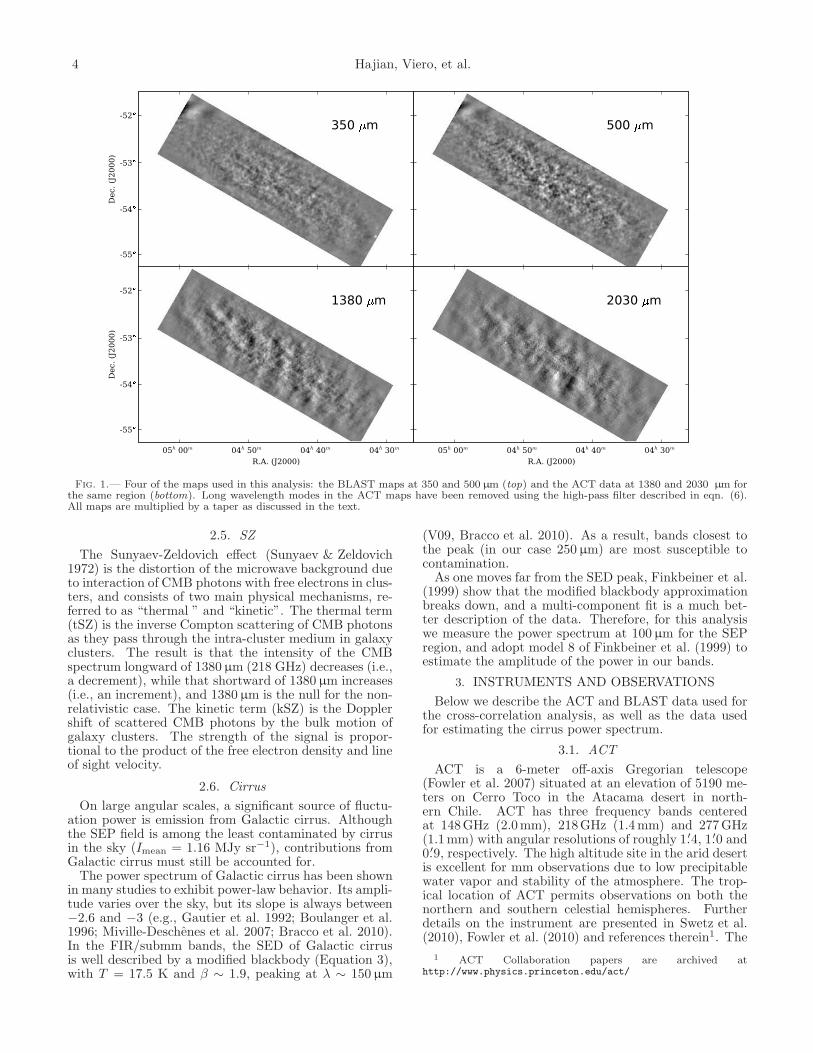
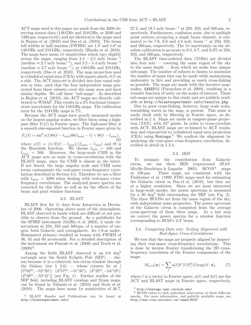
Fig. 1.— Four of the maps used in this analysis: the BLAST maps at 350 and 500µm (top) and the ACT data at 1380 and 2030 µm forthe same region (bottom). Long wavelength modes in the ACT maps have been removed using the high-pass filter described in eqn. (6).All maps are multiplied by a taper as discussed in the text.

2.5. SZ

The Sunyaev-Zeldovich effect (Sunyaev & Zeldovich1972) is the distortion of the microwave background dueto interaction of CMB photons with free electrons in clus-ters, and consists of two main physical mechanisms, re-ferred to as “thermal ” and “kinetic”. The thermal term(tSZ) is the inverse Compton scattering of CMB photonsas they pass through the intra-cluster medium in galaxyclusters. The result is that the intensity of the CMBspectrum longward of 1380µm (218 GHz) decreases (i.e.,a decrement), while that shortward of 1380µm increases(i.e., an increment), and 1380µm is the null for the non-relativistic case. The kinetic term (kSZ) is the Dopplershift of scattered CMB photons by the bulk motion ofgalaxy clusters. The strength of the signal is propor-tional to the product of the free electron density and lineof sight velocity.

2.6. Cirrus

On large angular scales, a significant source of fluctu-ation power is emission from Galactic cirrus. Althoughthe SEP field is among the least contaminated by cirrusin the sky (Imean = 1.16 MJy sr−1), contributions fromGalactic cirrus must still be accounted for.The power spectrum of Galactic cirrus has been shown

in many studies to exhibit power-law behavior. Its ampli-tude varies over the sky, but its slope is always between−2.6 and −3 (e.g., Gautier et al. 1992; Boulanger et al.1996; Miville-Deschenes et al. 2007; Bracco et al. 2010).In the FIR/submm bands, the SED of Galactic cirrusis well described by a modified blackbody (Equation 3),with T = 17.5 K and β ∼ 1.9, peaking at λ ∼ 150µm

(V09, Bracco et al. 2010). As a result, bands closest tothe peak (in our case 250µm) are most susceptible tocontamination.As one moves far from the SED peak, Finkbeiner et al.

(1999) show that the modified blackbody approximationbreaks down, and a multi-component fit is a much bet-ter description of the data. Therefore, for this analysiswe measure the power spectrum at 100µm for the SEPregion, and adopt model 8 of Finkbeiner et al. (1999) toestimate the amplitude of the power in our bands.

3. INSTRUMENTS AND OBSERVATIONS

Below we describe the ACT and BLAST data used forthe cross-correlation analysis, as well as the data usedfor estimating the cirrus power spectrum.

3.1. ACT

ACT is a 6-meter off-axis Gregorian telescope(Fowler et al. 2007) situated at an elevation of 5190 me-ters on Cerro Toco in the Atacama desert in north-ern Chile. ACT has three frequency bands centeredat 148GHz (2.0mm), 218GHz (1.4mm) and 277GHz(1.1mm) with angular resolutions of roughly 1.′4, 1.′0 and0.′9, respectively. The high altitude site in the arid desertis excellent for mm observations due to low precipitablewater vapor and stability of the atmosphere. The trop-ical location of ACT permits observations on both thenorthern and southern celestial hemispheres. Furtherdetails on the instrument are presented in Swetz et al.(2010), Fowler et al. (2010) and references therein1. The

1 ACT Collaboration papers are archived athttp://www.physics.princeton.edu/act/

Correlations in the CSB from ACT× BLAST 5

ACT maps used in this paper are made from the 2008 ob-serving season data (148GHz and 218GHz, or 2030 and1380µm, respectively) and are identical to the maps usedin Hajian et al. (2010) and Das et al. (2010). The beamfull widths at half maxima (FWHM) are 1.4′ and 1.0′ at148GHz and 218GHz, respectively (Hincks et al. 2010).The maps have mean 1σ sensitivities which vary slightlyacross the maps, ranging from 2.4 − 3.5 mJy beam−1

(median ≈ 2.7 mJy beam−1), and 3.2− 5.4 mJy beam−1

(median ≈ 3.7 mJy beam−1), at 148GHz and 218GHz,respectively (Das et al. 2010). The map projection usedis cylindrical equal area (CEA) with square pixels, 0.5′ ona side. The ACT data-set is divided into four equal sub-sets in time, such that the four independent maps gen-erated from these subsets cover the same area and havesimilar depths. We call these “sub-maps”. As describedin Hajian et al. (2010), the ACT maps are directly cali-brated to WMAP. This results in a 2% fractional temper-ature uncertainty for the 148GHz maps. The calibrationerror for the 218GHz maps is 7%.Because the ACT maps have poorly measured modes

on the largest angular scales, we filter them using a high-pass filter Fc(ℓ) in Fourier space. The high-pass filter isa smooth sine-squared function in Fourier space given by

Fc(ℓ) = sin2 x(ℓ)Θ(ℓ− ℓmin)Θ(ℓmax − ℓ) + Θ(ℓ− ℓmax),(6)

where x(ℓ) = (π/2)(ℓ − ℓmin)/(ℓmax − ℓmin) and Θ isthe Heaviside function. We choose ℓmin = 100 andℓmax = 500. Moreover, the large-scale CMB in theACT maps acts as noise in cross-correlations with theBLAST maps, since the CMB is absent in the latter.If not ltered, the large angular scale and CMB noiseterms contaminate the real-space cross-frequency corre-lations described in Section 3.4. Therefore we use a filterwith ℓmax = 2200 when dealing with real-space cross-frequency correlations. The analyzed power spectra arecorrected for this filter as well as for the effects of thebeam and pixel window functions.

3.2. BLAST

BLAST flew for 11 days from Antarctica in Decem-ber of 2006. Operating above most of the atmosphere,BLAST observed in bands which are difficult or not pos-sible to observe from the ground. As a pathfinder forthe SPIRE instrument (Griffin et al. 2003), it made ob-servations at 250, 350 and 500µm, of a number of tar-gets, both Galactic and extragalactic. Its 1.8-m under-illuminated primary resulted in beams with FWHM of36, 45 and 60 arcseconds. For a detailed description ofthe instrument see Pascale et al. (2008) and Truch et al.(2009)2.Among the fields BLAST observed is an 8.6 deg2

rectangle near the South Ecliptic Pole (SEP) — cho-sen because it is a relatively low-cirrus window throughthe Galaxy (see § 2.6) — whose corners lie at [(5h02m,−5250′); (4h57m,−5135′); (4h25m,−5419′);(4h30m,−5541′)] (see Fig. 1). Further studies of theSEP field, including BLAST catalogs and 24µm maps,can be found in Valiante et al. (2010) and Scott et al.(2010). The maps have mean 1σ sensitivities of 36.7,

2 BLAST Results and Publications can be found athttp://blastexperiment.info/

27.2, and 19.1 mJy beam−1 at 250, 350, and 500µm, re-spectively. Furthermore, confusion noise, due to multiplepoint sources occupying a single beam element, is esti-mated to be 7.6, 6.0 and 4.4 mJy beam−1 at 250, 350,and 500µm, respectively. The 1σ uncertainty on the ab-solute calibration is accurate to 9.5, 8.7, and 9.2% at 250,350, and 500µm, respectively.The BLAST time-ordered data (TODs) are divided

into four sets — covering the same region of the skyto the same depth — from which we make four uniquesub-maps. The number of subsets is chosen to maximizethe number of maps that can be made while maintaininguniformity in hits and providing as much cross-linkingas possible. The maps are made with the iterative map-maker, SANEPIC (Patanchon et al. 2009), resulting in atransfer function of unity on the scales of interest. Thesesub-maps are unique to this study and are publicly avail-able at http://blastexperiment.info/results.php.Due to poor cross-linking, however, large scale noise,

resembling waves in the map, is present. This noise iseasily dealt with by filtering in Fourier space, as de-scribed in § 4. Maps are made in tangent-plane projec-tion (TAN), with 10′′ pixels. In order to cross-correlatewith ACT, BLAST maps are re-binned to ACT resolu-tion and reprojected to cylindrical equal-area projection(CEA) using Montage.3 We confirm the alignment byanalyzing the real-space cross-frequency correlation, de-scribed in detail in § 3.4.

3.3. IRIS

To estimate the contribution from Galacticcirrus, we use three IRIS (reprocessed IRAS :Miville-Deschenes & Lagache 2005) HCON4 mapsat 100µm. These maps are consistent with theFinkbeiner et al. (1999, FDS) maps used for estimatingthe Galactic cirrus in Das et al. (2010), but they areat a higher resolution. Since we are most interestedin large-scale modes, the power spectrum is measuredfor a 30 deg2 field surrounding the SEP (see Fig. 2).The three HCONs are from the same region of the sky,with independent noise properties. The power spectrumof the Galactic cirrus is computed from the averagecross-spectrum of these three maps. As a last stepwe correct the power spectra for a window functioncorresponding to IRAS’s 4.3′ beam.

3.4. Comparing Data sets: Testing Alignment withReal-Space Cross-Correlations

We test that the maps are properly aligned by inspect-ing their real-space cross-frequency correlations. Thisis done by inverse Fourier transforming the 2D cross-frequency correlation of the Fourier components of themaps:

Ma×b(x) =∑

ℓ

a(ℓ)b∗(ℓ)F 2c (ℓ)exp(iℓ ·x), (7)

where ℓ is a vector in Fourier space, a(ℓ) and b(ℓ) are theACT and BLAST maps in Fourier space, respectively,

3 http://montage.ipac.caltech.edu/4 HCON refers to each individual observation at three different

epochs. For more information, and publicly available maps, seehttp://www.cita.utoronto.ca/~mamd/IRIS/

6 Hajian, Viero, et al.

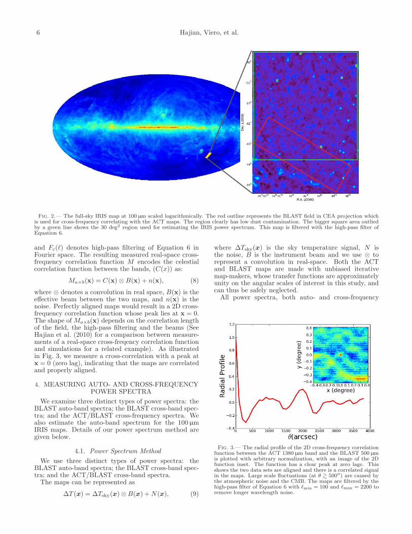
Fig. 2.— The full-sky IRIS map at 100µm scaled logarithmically. The red outline represents the BLAST field in CEA projection whichis used for cross-frequency correlating with the ACT maps. The region clearly has low dust contamination. The bigger square area outliedby a green line shows the 30 deg2 region used for estimating the IRIS power spectrum. This map is filtered with the high-pass filter ofEquation 6.

and Fc(ℓ) denotes high-pass filtering of Equation 6 inFourier space. The resulting measured real-space cross-frequency correlation function M encodes the celestialcorrelation function between the bands, (C(x)) as:

Ma×b(x) = C(x) ⊗B(x) + n(x), (8)

where ⊗ denotes a convolution in real space, B(x) is theeffective beam between the two maps, and n(x) is thenoise. Perfectly aligned maps would result in a 2D cross-frequency correlation function whose peak lies at x = 0.The shape of Ma×b(x) depends on the correlation lengthof the field, the high-pass filtering and the beams (SeeHajian et al. (2010) for a comparison between measure-ments of a real-space cross-freqency correlation functionand simulations for a related example). As illustratedin Fig. 3, we measure a cross-correlation with a peak atx = 0 (zero lag), indicating that the maps are correlatedand properly aligned.

4. MEASURING AUTO- AND CROSS-FREQUENCYPOWER SPECTRA

We examine three distinct types of power spectra: theBLAST auto-band spectra; the BLAST cross-band spec-tra; and the ACT/BLAST cross-frequency spectra. Wealso estimate the auto-band spectrum for the 100µmIRIS maps. Details of our power spectrum method aregiven below.

4.1. Power Spectrum Method

We use three distinct types of power spectra: theBLAST auto-band spectra; the BLAST cross-band spec-tra; and the ACT/BLAST cross-band spectra.The maps can be represented as

∆T (x) = ∆Tsky(x)⊗B(x) +N(x), (9)

where ∆Tsky(x) is the sky temperature signal, N isthe noise, B is the instrument beam and we use ⊗ torepresent a convolution in real-space. Both the ACTand BLAST maps are made with unbiased iterativemap-makers, whose transfer functions are approximatelyunity on the angular scales of interest in this study, andcan thus be safely neglected.All power spectra, both auto- and cross-frequency

Fig. 3.— The radial profile of the 2D cross-frequency correlationfunction between the ACT 1380µm band and the BLAST 500µmis plotted with arbitrary normalization, with an image of the 2Dfunction inset. The function has a clear peak at zero lage. Thisshows the two data sets are aligned and there is a correlated signalin the maps. Large scale fluctuations (at θ & 500′′) are caused bythe atmospheric noise and the CMB. The maps are filtered by thehigh-pass filter of Equation 6 with ℓmin = 100 and ℓmax = 2200 toremove longer wavelength noise.

Correlations in the CSB from ACT× BLAST 7

6000 4000 2000 0 2000 4000 6000

x

6000

4000

2000

0

2000

4000

6000

y

6.0

5.4

4.8

4.2

3.6

3.0

2.4

1.8

1.2

0.6

0.0

6000 4000 2000 0 2000 4000 6000

x

6000

4000

2000

0

2000

4000

6000

y

6.0

5.4

4.8

4.2

3.6

3.0

2.4

1.8

1.2

0.6

0.0

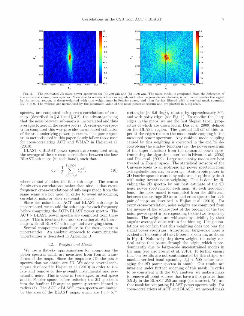
Fig. 4.— The estimated 2D noise power spectrum for (a) 250 µm and (b) 1380 µm. The noise model is computed from the difference ofthe auto- and cross-power spectra. Noise due to scan-synchronous signals and other large-scale correlations, which contaminates the signalin the central region, is down-weighted with this weight map in Fourier space, and then further filtered with a vertical mask spanning|ℓx| < 500. The weights are normalized by the maximum value of the noise power spectrum and are plotted in a log-scale.

spectra, are computed using cross-correlations of sub-maps (described in § 3.1 and § 3.2), the advantage beingthat the noise between sub-maps is uncorrelated and thusaverages to zero in the cross-spectra. A cross-power spec-trum computed this way provides an unbiased estimatorof the true underlying power spectrum. The power spec-trum methods used in this paper closely follow those usedfor cross-correlating ACT and WMAP in Hajian et al.(2010).BLAST × BLAST power spectra are computed using

the average of the six cross-correlations between the fourBLAST sub-maps (in each band), such that

Cℓ =1

6

1≤β≤4∑

α,β;α<β

Cαβℓ , (10)

where α and β index the four sub-maps. The reasonfor six cross-correlations, rather than nine, is that cross-frequency cross-correlations of sub-maps made from thesame scans are not used, in order to avoid introducingcorrelated noise or other systematic effects.Since the noise in all ACT and BLAST sub-maps is

uncorrelated, we co-add the sub-maps for each frequencybefore computing the ACT×BLAST power spectra. TheACT× BLAST power spectra are computed from thesemaps. This is identical to cross-correlating all ACT sub-maps with all BLAST sub-maps and averaging them.Several components contribute to the cross-spectrum

uncertainties. An analytic approach to computing theuncertainties is described in Appendix B.

4.2. Weights and Masks

We use a flat-sky approximation for computing thepower spectra, which are measured from Fourier trans-forms of the maps. Since the maps are 2D, the powerspectra that we obtain are 2D. We adopt several tech-niques developed in Hajian et al. (2010) in order to iso-late and remove or down-weight instrumental and sys-tematic noise. This is done in two stages, in real spaceand in Fourier space, before reducing the 2D spectruminto the familiar 1D angular power spectrum binned inradius (ℓ). The ACT×BLAST cross-spectra are limitedby the area of the BLAST maps, which are 1.5 × 5.7

rectangles (∼ 8.6 deg2), rotated by approximately 30,and with noisy edges (see Fig. 1). To apodize the sharpedges in the maps, we use the first Slepian taper (prop-erties of which are described in Das et al. 2009) definedon the BLAST region. The gradual fall-off of this ta-per at the edges reduces the mode-mode coupling in themeasured power spectrum. Any residual mode couplingcaused by this weighting is corrected in the end by de-convolving the window function (i.e. the power spectrumof the taper function) from the measured power spec-trum using the algorithm described in Hivon et al. (2002)and Das et al. (2009). Large-scale noisy modes are besttreated in Fourier space. The statistical isotropy of theUniverse leads to an isotropic 2D power spectrum fromextragalactic sources, on average. Anisotropic power in2D Fourier space is caused by noise and is optimally dealtwith using inverse noise weighting. This is done by di-viding the 2D spectra by our best estimate of the 2Dnoise power spectrum for each map. At each frequencyband, the noise model is computed from the differencebetween the average 2D auto- and cross-spectra for eachpair of maps as described in Hajian et al. (2010). Forevery cross-correlation, noise weights are computed fromthe inverse of the square root of the product of the twonoise power spectra corresponding to the two frequencybands. The weights are whitened by dividing by theirangular averaged value with a fine binning. Using simu-lations we confirm that this weighting does not bias thesignal power spectrum. Anisotropic, large-scale noise isevident at the center of the 2D power spectrum, as shownin Fig. 4. Noise-weighting down-weights the noisy ver-tical stripe that passes through the origin, which is pre-dominantly due to large-scale unconstrained modes inthe map (see also Fowler et al. 2010). To further ensurethat our results are not contaminated by this stripe, wemask a vertical band spanning |ℓx| < 500 before aver-aging the 2D power spectra in annuli. Our results areinvariant under further widening of this mask. In orderto be consistent with the V09 analysis, we make a maskto remove all point sources that have a flux greater than0.5 Jy in the BLAST 250µm map (six sources). We usethat mask for computing BLAST power spectra only. Forcross-correlations of ACT and BLAST, we instead mask

8 Hajian, Viero, et al.

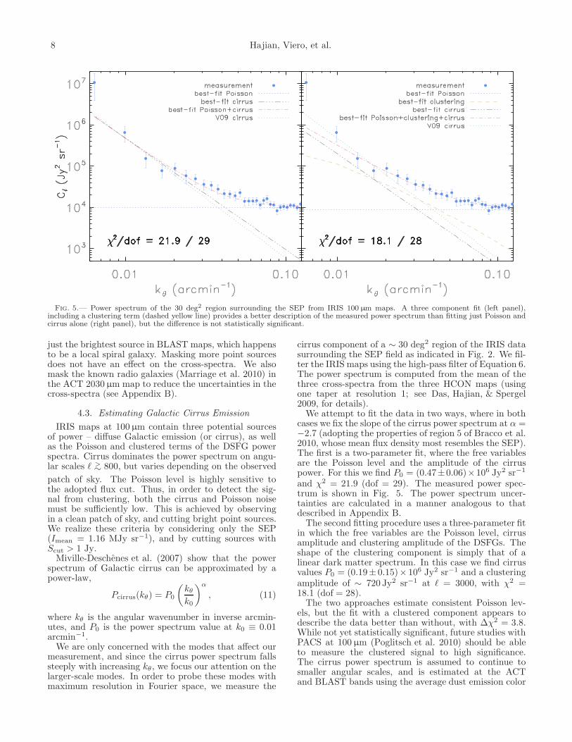
Fig. 5.— Power spectrum of the 30 deg2 region surrounding the SEP from IRIS 100µm maps. A three component fit (left panel),including a clustering term (dashed yellow line) provides a better description of the measured power spectrum than fitting just Poisson andcirrus alone (right panel), but the difference is not statistically significant.

just the brightest source in BLAST maps, which happensto be a local spiral galaxy. Masking more point sourcesdoes not have an effect on the cross-spectra. We alsomask the known radio galaxies (Marriage et al. 2010) inthe ACT 2030µm map to reduce the uncertainties in thecross-spectra (see Appendix B).

4.3. Estimating Galactic Cirrus Emission

IRIS maps at 100µm contain three potential sourcesof power – diffuse Galactic emission (or cirrus), as wellas the Poisson and clustered terms of the DSFG powerspectra. Cirrus dominates the power spectrum on angu-lar scales ℓ >∼ 800, but varies depending on the observed

patch of sky. The Poisson level is highly sensitive tothe adopted flux cut. Thus, in order to detect the sig-nal from clustering, both the cirrus and Poisson noisemust be sufficiently low. This is achieved by observingin a clean patch of sky, and cutting bright point sources.We realize these criteria by considering only the SEP(Imean = 1.16 MJy sr−1), and by cutting sources withScut > 1 Jy.Miville-Deschenes et al. (2007) show that the power

spectrum of Galactic cirrus can be approximated by apower-law,

Pcirrus(kθ) = P0

(

kθk0

)α

, (11)

where kθ is the angular wavenumber in inverse arcmin-utes, and P0 is the power spectrum value at k0 ≡ 0.01arcmin−1.We are only concerned with the modes that affect our

measurement, and since the cirrus power spectrum fallssteeply with increasing kθ, we focus our attention on thelarger-scale modes. In order to probe these modes withmaximum resolution in Fourier space, we measure the

cirrus component of a ∼ 30 deg2 region of the IRIS datasurrounding the SEP field as indicated in Fig. 2. We fil-ter the IRIS maps using the high-pass filter of Equation 6.The power spectrum is computed from the mean of thethree cross-spectra from the three HCON maps (usingone taper at resolution 1; see Das, Hajian, & Spergel2009, for details).We attempt to fit the data in two ways, where in both

cases we fix the slope of the cirrus power spectrum at α =−2.7 (adopting the properties of region 5 of Bracco et al.2010, whose mean flux density most resembles the SEP).The first is a two-parameter fit, where the free variablesare the Poisson level and the amplitude of the cirruspower. For this we find P0 = (0.47±0.06)×106 Jy2 sr−1

and χ2 = 21.9 (dof = 29). The measured power spec-trum is shown in Fig. 5. The power spectrum uncer-tainties are calculated in a manner analogous to thatdescribed in Appendix B.The second fitting procedure uses a three-parameter fit

in which the free variables are the Poisson level, cirrusamplitude and clustering amplitude of the DSFGs. Theshape of the clustering component is simply that of alinear dark matter spectrum. In this case we find cirrusvalues P0 = (0.19± 0.15)× 106 Jy2 sr−1 and a clusteringamplitude of ∼ 720 Jy2 sr−1 at ℓ = 3000, with χ2 =18.1 (dof = 28).The two approaches estimate consistent Poisson lev-

els, but the fit with a clustered component appears todescribe the data better than without, with ∆χ2 = 3.8.While not yet statistically significant, future studies withPACS at 100µm (Poglitsch et al. 2010) should be ableto measure the clustered signal to high significance.The cirrus power spectrum is assumed to continue tosmaller angular scales, and is estimated at the ACTand BLAST bands using the average dust emission color

Correlations in the CSB from ACT× BLAST 9

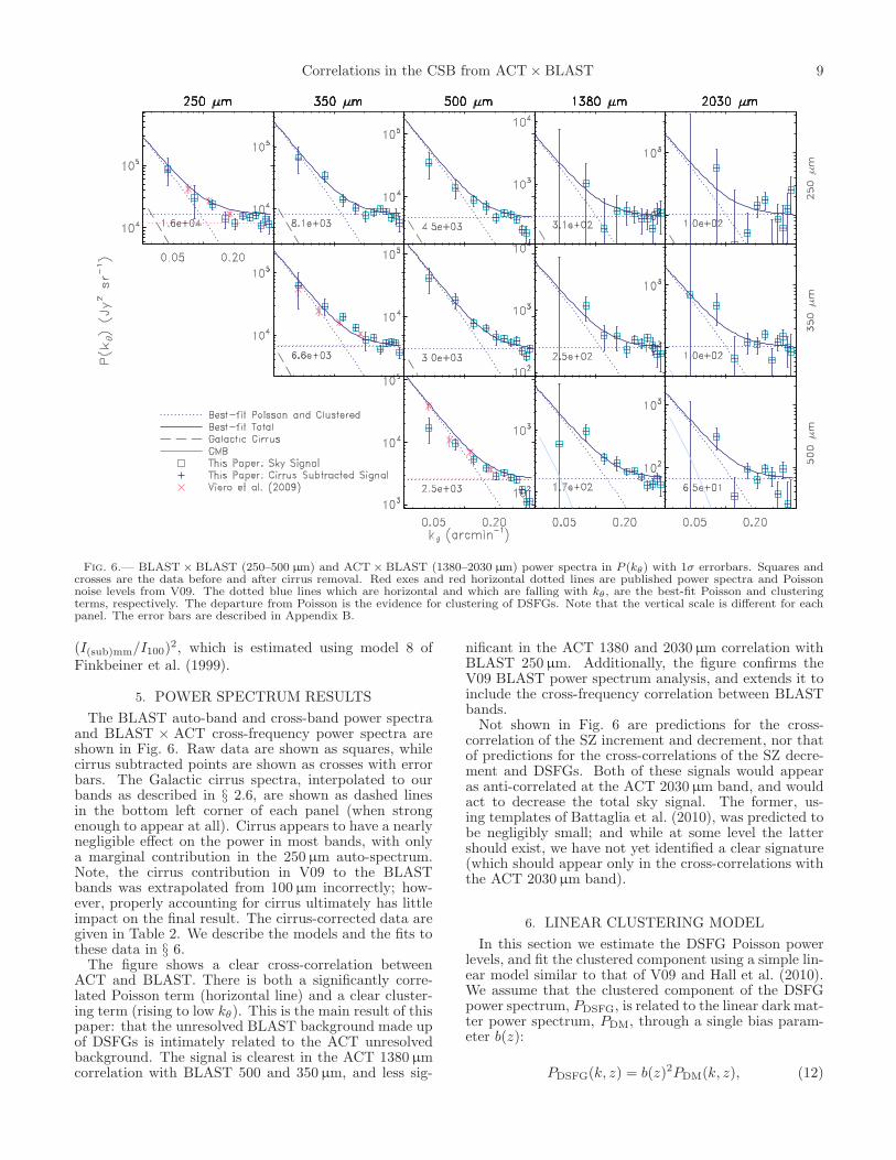
Fig. 6.— BLAST × BLAST (250–500µm) and ACT× BLAST (1380–2030µm) power spectra in P (kθ) with 1σ errorbars. Squares andcrosses are the data before and after cirrus removal. Red exes and red horizontal dotted lines are published power spectra and Poissonnoise levels from V09. The dotted blue lines which are horizontal and which are falling with kθ, are the best-fit Poisson and clusteringterms, respectively. The departure from Poisson is the evidence for clustering of DSFGs. Note that the vertical scale is different for eachpanel. The error bars are described in Appendix B.

(I(sub)mm/I100)2, which is estimated using model 8 of

Finkbeiner et al. (1999).

5. POWER SPECTRUM RESULTS

The BLAST auto-band and cross-band power spectraand BLAST × ACT cross-frequency power spectra areshown in Fig. 6. Raw data are shown as squares, whilecirrus subtracted points are shown as crosses with errorbars. The Galactic cirrus spectra, interpolated to ourbands as described in § 2.6, are shown as dashed linesin the bottom left corner of each panel (when strongenough to appear at all). Cirrus appears to have a nearlynegligible effect on the power in most bands, with onlya marginal contribution in the 250µm auto-spectrum.Note, the cirrus contribution in V09 to the BLASTbands was extrapolated from 100µm incorrectly; how-ever, properly accounting for cirrus ultimately has littleimpact on the final result. The cirrus-corrected data aregiven in Table 2. We describe the models and the fits tothese data in § 6.The figure shows a clear cross-correlation between

ACT and BLAST. There is both a significantly corre-lated Poisson term (horizontal line) and a clear cluster-ing term (rising to low kθ). This is the main result of thispaper: that the unresolved BLAST background made upof DSFGs is intimately related to the ACT unresolvedbackground. The signal is clearest in the ACT 1380µmcorrelation with BLAST 500 and 350µm, and less sig-

nificant in the ACT 1380 and 2030µm correlation withBLAST 250µm. Additionally, the figure confirms theV09 BLAST power spectrum analysis, and extends it toinclude the cross-frequency correlation between BLASTbands.Not shown in Fig. 6 are predictions for the cross-

correlation of the SZ increment and decrement, nor thatof predictions for the cross-correlations of the SZ decre-ment and DSFGs. Both of these signals would appearas anti-correlated at the ACT 2030µm band, and wouldact to decrease the total sky signal. The former, us-ing templates of Battaglia et al. (2010), was predicted tobe negligibly small; and while at some level the lattershould exist, we have not yet identified a clear signature(which should appear only in the cross-correlations withthe ACT 2030µm band).

6. LINEAR CLUSTERING MODEL

In this section we estimate the DSFG Poisson powerlevels, and fit the clustered component using a simple lin-ear model similar to that of V09 and Hall et al. (2010).We assume that the clustered component of the DSFGpower spectrum, PDSFG, is related to the linear dark mat-ter power spectrum, PDM, through a single bias param-eter b(z):

PDSFG(k, z) = b(z)2PDM(k, z), (12)

10 Hajian, Viero, et al.

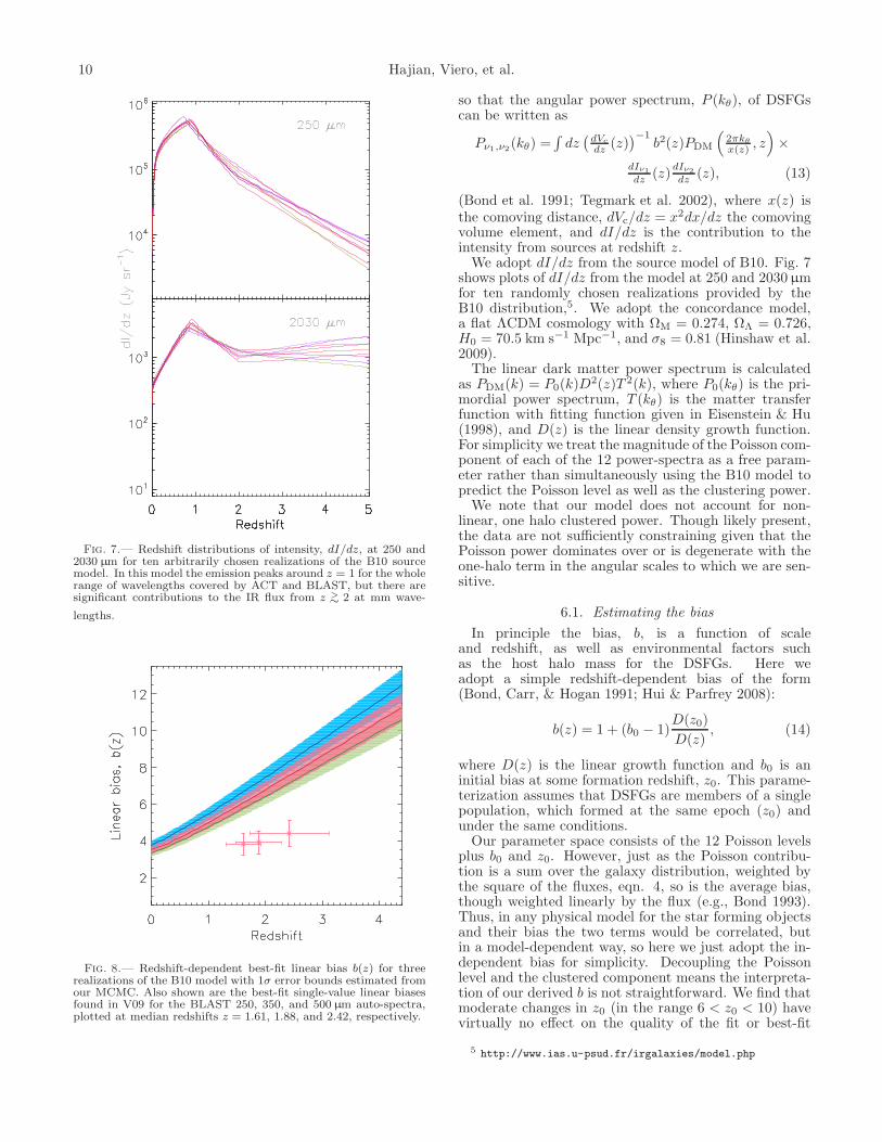
Fig. 7.— Redshift distributions of intensity, dI/dz, at 250 and2030µm for ten arbitrarily chosen realizations of the B10 sourcemodel. In this model the emission peaks around z = 1 for the wholerange of wavelengths covered by ACT and BLAST, but there aresignificant contributions to the IR flux from z >∼ 2 at mm wave-

lengths.

Fig. 8.— Redshift-dependent best-fit linear bias b(z) for threerealizations of the B10 model with 1σ error bounds estimated fromour MCMC. Also shown are the best-fit single-value linear biasesfound in V09 for the BLAST 250, 350, and 500µm auto-spectra,plotted at median redshifts z = 1.61, 1.88, and 2.42, respectively.

so that the angular power spectrum, P (kθ), of DSFGscan be written as

Pν1,ν2(kθ) =∫

dz(

dVc

dz (z))−1

b2(z)PDM

(

2πkθ

x(z) , z)

×dIν1dz (z)

dIν2dz (z), (13)

(Bond et al. 1991; Tegmark et al. 2002), where x(z) isthe comoving distance, dVc/dz = x2dx/dz the comovingvolume element, and dI/dz is the contribution to theintensity from sources at redshift z.We adopt dI/dz from the source model of B10. Fig. 7

shows plots of dI/dz from the model at 250 and 2030µmfor ten randomly chosen realizations provided by theB10 distribution,5. We adopt the concordance model,a flat ΛCDM cosmology with ΩM = 0.274, ΩΛ = 0.726,H0 = 70.5 km s−1 Mpc−1, and σ8 = 0.81 (Hinshaw et al.2009).The linear dark matter power spectrum is calculated

as PDM(k) = P0(k)D2(z)T 2(k), where P0(kθ) is the pri-

mordial power spectrum, T (kθ) is the matter transferfunction with fitting function given in Eisenstein & Hu(1998), and D(z) is the linear density growth function.For simplicity we treat the magnitude of the Poisson com-ponent of each of the 12 power-spectra as a free param-eter rather than simultaneously using the B10 model topredict the Poisson level as well as the clustering power.We note that our model does not account for non-

linear, one halo clustered power. Though likely present,the data are not sufficiently constraining given that thePoisson power dominates over or is degenerate with theone-halo term in the angular scales to which we are sen-sitive.

6.1. Estimating the bias

In principle the bias, b, is a function of scaleand redshift, as well as environmental factors suchas the host halo mass for the DSFGs. Here weadopt a simple redshift-dependent bias of the form(Bond, Carr, & Hogan 1991; Hui & Parfrey 2008):

b(z) = 1 + (b0 − 1)D(z0)

D(z), (14)

where D(z) is the linear growth function and b0 is aninitial bias at some formation redshift, z0. This parame-terization assumes that DSFGs are members of a singlepopulation, which formed at the same epoch (z0) andunder the same conditions.Our parameter space consists of the 12 Poisson levels

plus b0 and z0. However, just as the Poisson contribu-tion is a sum over the galaxy distribution, weighted bythe square of the fluxes, eqn. 4, so is the average bias,though weighted linearly by the flux (e.g., Bond 1993).Thus, in any physical model for the star forming objectsand their bias the two terms would be correlated, butin a model-dependent way, so here we just adopt the in-dependent bias for simplicity. Decoupling the Poissonlevel and the clustered component means the interpreta-tion of our derived b is not straightforward. We find thatmoderate changes in z0 (in the range 6 < z0 < 10) havevirtually no effect on the quality of the fit or best-fit

5 http://www.ias.u-psud.fr/irgalaxies/model.php

Correlations in the CSB from ACT× BLAST 11

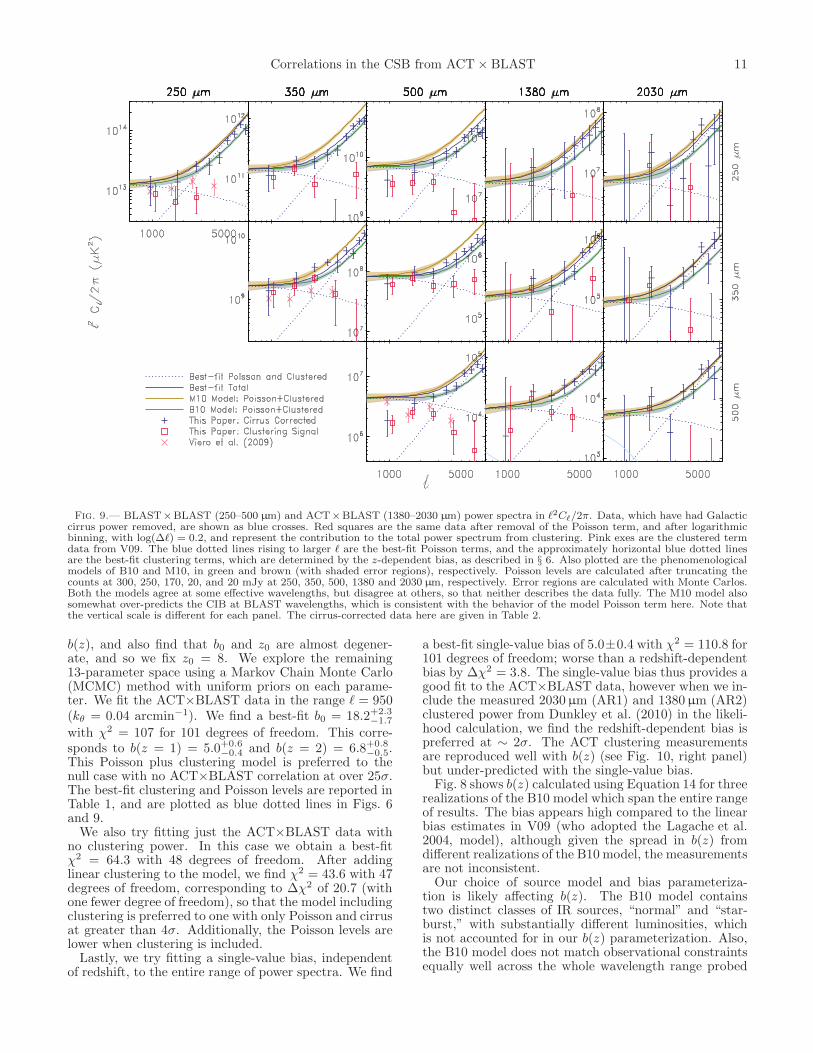
Fig. 9.— BLAST×BLAST (250–500µm) and ACT×BLAST (1380–2030µm) power spectra in ℓ2Cℓ/2π. Data, which have had Galacticcirrus power removed, are shown as blue crosses. Red squares are the same data after removal of the Poisson term, and after logarithmicbinning, with log(∆ℓ) = 0.2, and represent the contribution to the total power spectrum from clustering. Pink exes are the clustered termdata from V09. The blue dotted lines rising to larger ℓ are the best-fit Poisson terms, and the approximately horizontal blue dotted linesare the best-fit clustering terms, which are determined by the z-dependent bias, as described in § 6. Also plotted are the phenomenologicalmodels of B10 and M10, in green and brown (with shaded error regions), respectively. Poisson levels are calculated after truncating thecounts at 300, 250, 170, 20, and 20 mJy at 250, 350, 500, 1380 and 2030µm, respectively. Error regions are calculated with Monte Carlos.Both the models agree at some effective wavelengths, but disagree at others, so that neither describes the data fully. The M10 model alsosomewhat over-predicts the CIB at BLAST wavelengths, which is consistent with the behavior of the model Poisson term here. Note thatthe vertical scale is different for each panel. The cirrus-corrected data here are given in Table 2.

b(z), and also find that b0 and z0 are almost degener-ate, and so we fix z0 = 8. We explore the remaining13-parameter space using a Markov Chain Monte Carlo(MCMC) method with uniform priors on each parame-ter. We fit the ACT×BLAST data in the range ℓ = 950(kθ = 0.04 arcmin−1). We find a best-fit b0 = 18.2+2.3

−1.7

with χ2 = 107 for 101 degrees of freedom. This corre-sponds to b(z = 1) = 5.0+0.6

−0.4 and b(z = 2) = 6.8+0.8−0.5.

This Poisson plus clustering model is preferred to thenull case with no ACT×BLAST correlation at over 25σ.The best-fit clustering and Poisson levels are reported inTable 1, and are plotted as blue dotted lines in Figs. 6and 9.We also try fitting just the ACT×BLAST data with

no clustering power. In this case we obtain a best-fitχ2 = 64.3 with 48 degrees of freedom. After addinglinear clustering to the model, we find χ2 = 43.6 with 47degrees of freedom, corresponding to ∆χ2 of 20.7 (withone fewer degree of freedom), so that the model includingclustering is preferred to one with only Poisson and cirrusat greater than 4σ. Additionally, the Poisson levels arelower when clustering is included.Lastly, we try fitting a single-value bias, independent

of redshift, to the entire range of power spectra. We find

a best-fit single-value bias of 5.0±0.4 with χ2 = 110.8 for101 degrees of freedom; worse than a redshift-dependentbias by ∆χ2 = 3.8. The single-value bias thus provides agood fit to the ACT×BLAST data, however when we in-clude the measured 2030µm (AR1) and 1380µm (AR2)clustered power from Dunkley et al. (2010) in the likeli-hood calculation, we find the redshift-dependent bias ispreferred at ∼ 2σ. The ACT clustering measurementsare reproduced well with b(z) (see Fig. 10, right panel)but under-predicted with the single-value bias.Fig. 8 shows b(z) calculated using Equation 14 for three

realizations of the B10 model which span the entire rangeof results. The bias appears high compared to the linearbias estimates in V09 (who adopted the Lagache et al.2004, model), although given the spread in b(z) fromdifferent realizations of the B10 model, the measurementsare not inconsistent.Our choice of source model and bias parameteriza-

tion is likely affecting b(z). The B10 model containstwo distinct classes of IR sources, “normal” and “star-burst,” with substantially different luminosities, whichis not accounted for in our b(z) parameterization. Also,the B10 model does not match observational constraintsequally well across the whole wavelength range probed

12 Hajian, Viero, et al.

by ACT and BLAST; for instance it under-predicts Pois-son power and number counts compared to BLAST andSPT measurements at 500 and 1360µm (see § 5.6 ofBethermin et al. 2010, as well as Fig. 9 of this paper).An under-prediction of dI/dz would result in a higherbias to compensate.

7. DISCUSSION

We compare the models of B10 and M10 (described in§ 2.3,) to our results. Poisson levels are calculated fromthe number counts using Equation 4, where the valuesof Scut are chosen to mimic those used in the analysis,i.e., Scut = 500, 250, 170 mJy at 250, 350, and 500µm,respectively.Model predictions of B10 and M10 are shown in Fig. 9

as green and brown lines with shaded error regions, re-spectively. Both models agree at some effective wave-lengths, but disagree at others, so that neither appearsto fully describe the data. The M10 model also somewhatover-predicts the CIB at BLAST wavelengths, which isconsistent with the behavior we see for the model Poissonterm. On the other hand, as already mentioned, the B10model under-predicts Poisson power and number countscompared to BLAST and SPT measurements at 500 and1360µm, which again is consistent with the behavior ofthe Poisson term of the model in Fig. 9.The Poisson and clustered power amplitudes are plot-

ted as a function of effective wavelength, defined asλeff =

√λ1λ2, in Fig. 10. Also included are mea-

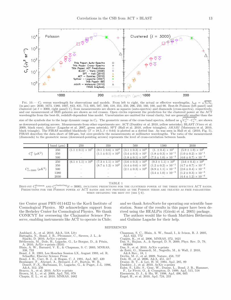
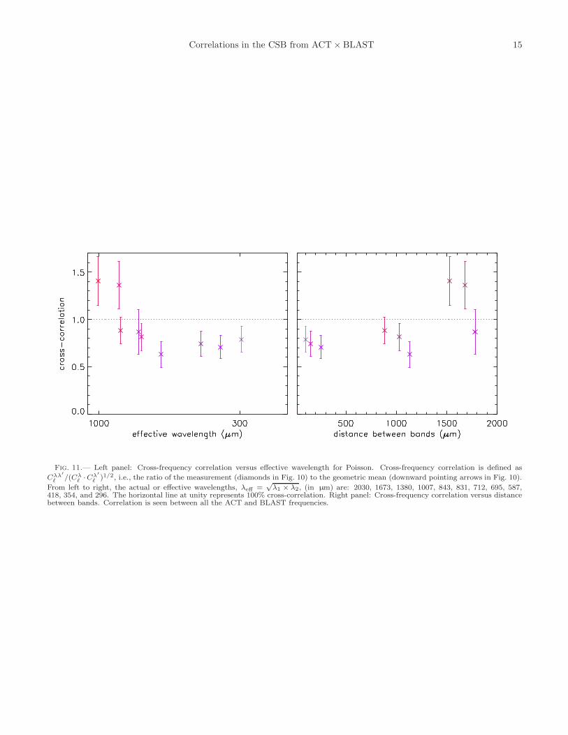
surements made by the following experiments: AKARIat 90µm (Matsuura et al. 2010); Spitzer at 160µm(Lagache et al. 2007); BLAST at 250, 350, and 500µm(Viero et al. 2009); ACT at 1380, 1673, and 2030µm(Dunkley et al. 2010); SPT at 1363, 1629, and 1947µm(Hall et al. 2010); and the FIRAS modified blackbody(T = 18.5, β = 0.64), which is shown as a dotted line.The degree of correlation between widely spaced wave-

lengths is of interest both in determining the redshiftdistribution of sources, and for modeling the IR sourcepower as a CMB contaminant. To assess the correla-tion, the geometric means at each effective cross-band

wavelength, defined as√

Cλℓ ·Cλ′

ℓ , are shown as a down-

ward pointing arrows. Since we do not measure Cλℓ at

λ = 1380 and 2030µm, we rely on measurements byDunkley et al. (2010) for those bands when calculatingthe geometric means. The ratios of the measurements tothe geometric means, Cλλ′

ℓ /(Cλℓ ·Cλ′

ℓ )1/2, then representthe levels of cross-correlation between bands. These areshown in Fig. 11 for the Poisson power as a function bothof effective wavelength and of distance between bands.Correlation is seen between all the frequencies, and doesnot fall significantly as a function of increased band sep-aration, suggesting a tight redshift distribution for theoverlapping population. This behavior is consistent withthe findings of e.g., Hall et al. (2010) and Dunkley et al.(2010): that the 1000− 2000µm bands are correlated atclose to the 100% level, and extends the range of wave-lengths probed.

8. CONCLUSION

We present measurements of the auto- and cross-frequency correlations of BLAST (250, 350 and 500µm)

and ACT (1380 and 2030µm) maps. We find signifi-cant levels of correlation between the two sets of maps,indicating that the same DSFGs that make up the un-resolved fluctuations in BLAST maps are also present inACT maps. Furthermore, we confirm previous BLASTanalyses (Viero et al. 2009) for a different field and withan independent pipeline, and extend the analysis by in-cluding BLAST× BLAST cross-frequency correlations.We fit Poisson and clustered terms at each effective

wavelength simultaneously, which we achieve by adopt-ing a model for the sources (Bethermin et al. 2010), as-suming a parameterized form for the z-dependent biasand using an MCMC to minimize the χ2. Using thismodel we detect a clustered signal at 4σ, in addition toa Poisson component. The best-fit bias is one that in-creases sharply with redshift, and is consistent with whatwas found by Viero et al. (2009).We compare phenomenological models by

Bethermin et al. (2010) and Marsden et al. (2010)to the data and find rough agreement at numerouseffective wavelengths. But we also find that neithermodel quite reproduces the data faithfully. Thus,we expect this measurement and others like it willultimately provide powerful constraints for the redshiftdistribution and SEDs of future versions of the models.Though we find convincing evidence for correlated

Poisson and clustered power from DSFGs, the levels ofprecision needed to robustly remove these signals fromCMB power spectra demand better measurements still.This is particularly true of the clustering term, whosecontribution to the power spectrum in ℓ2Cℓ peaks atℓ ∼ 800 – 1000, which is also the region in ℓ-space typ-ically targeted in searches for the SZ power spectrum.Since the clustered term should scale independently ofthe Poisson term, the measurement becomes increasinglyimportant to determine precisely. Future studies combin-ing Herschel/SPIRE with ACT, SPT, and Planck willgo a long way towards solidifying this much needed mea-surement.

BLAST was made possible through the support ofNASA through grant numbers NAG5-12785, NAG5-13301, and NNGO-6GI11G, the NSF Office of Polar Pro-grams, the Canadian Space Agency, the Natural Sciencesand Engineering Research Council (NSERC) of Canada,and the UK Science and Technology Facilities Council(STFC). CBN acknowledges support from the CanadianInstitute for Advanced Research.ACT was supported by the U.S. National Science

Foundation through awards AST- 0408698 for the ACTproject, and PHY-0355328, AST- 0707731 and PIRE-0507768. Funding was also provided by Princeton Uni-versity and the University of Pennsylvania. Compu-tations were performed on the GPC supercomputer atthe SciNet HPC Consortium. SciNet is funded by: theCanada Foundation for Innovation under the auspices ofCompute Canada; the Government of Ontario; OntarioResearch Fund – Research Excellence; and the Universityof Toronto. JD acknowledges support from an RCUKFellowship. SD, AH, and TM were supported throughNASA grant NNX08AH30G. AK was partially supportedthrough NSF AST-0546035 and AST-0606975 for workon ACT. ES acknowledges support by NSF Physics Fron-

Correlations in the CSB from ACT× BLAST 13

Fig. 10.— Cℓ versus wavelength for observations and models. From left to right, the actual or effective wavelengths, λeff =√λ1λ2,

(inµm) are: 2030, 1673, 1380, 1007, 843, 831, 712, 695, 587, 500, 418, 354, 350, 296, 250, 160, 100, and 90. Best-fit Poisson (left panel) andclustered (at ℓ = 3000, right panel) Cℓ from measurements are shown as squares (auto-spectra) and diamonds (cross-spectra), respectively,and our measurement of IRIS galaxies are shown as red crosses. Open circles represent the prediction for the clustered power at the ACTwavelengths from the best-fit, redshift-dependent bias model. Uncertainties are omitted for visual clarity, but are generally smaller than the

size of the symbols due to the large dynamic range in Cℓ. The geometric mean of the cross-band spectra, defined as√

Cλ1

ℓ ·Cλ2

ℓ , are shown

as downward-pointing arrows. Measurements from other experiments are: ACT (Dunkley et al. 2010, yellow asterisks); BLAST (Viero et al.2009, black exes); Spitzer (Lagache et al. 2007, green asterisk); SPT (Hall et al. 2010, yellow triangles); AKARI (Matsuura et al. 2010,black triangle). The FIRAS modified blackbody (T = 18.5, β = 0.64) is plotted as a dotted line. As was seen in Hall et al. (2010, Fig. 5),FIRAS describes the data short of 500µm, but over-predicts the measurements at millimeter wavelengths. The ratio of the measurement(diamonds) to the geometric mean (downward-pointing arrows) represents the level of cross-correlation between bands.

band (µm) 250 350 500 1380 2030

250 (1.1 ± 0.1) × 107 (9.1 ± 0.6) × 104 (3.1 ± 0.3) × 103 (1.± 0.4) × 101 (5.9± 1.9)× 100

Cpℓ (µK2) 350 – (1.1 ± 0.1) × 103 (3.4 ± 0.3) × 101 (1.8 ± 0.3)× 10−1 (1.0± 0.2)× 10−1

500 – – (1.8 ± 0.1) × 100 (7.3 ± 1.0)× 10−3 (4.6± 0.7)× 10−3

250 (6.1 ± 1.1) × 106 (7.3 ± 1.1) × 104 (3.6 ± 0.3) × 103 (9.3 ± 1.1)× 100 (3.6± 0.4)× 100

350 – (8.7 ± 1.2) × 102 (4.4 ± 0.6) × 101 (1.2 ± 0.2)× 10−1 (4.7± 0.7)× 10−2

Ccℓ=3000

(µK2) 500 – – (2.1 ± 0.3) × 100 (6.9 ± 1.1)× 10−3 (2.6± 0.4)× 10−3

1380 – – – (3.4 ± 1.0)× 10−5 (1.2± 0.3)× 10−5

2030 – – – – (4.4± 1.2)× 10−6

TABLE 1Best-fit CPoisson

ℓ and Cclusteringℓ (ℓ = 3000), including predictions for the clustered power at the three effective ACT bands.

Predictions for the Poisson power at ACT bands are not provided as the Poisson terms are treated as free parameterswhen obtaining the best fit (see § 6).

tier Center grant PHY-0114422 to the Kavli Institute ofCosmological Physics. SD acknowledges support fromthe Berkeley Center for Cosmological Physics. We thankCONICYT for overseeing the Chajnantor Science Pre-serve, enabling instruments like ACT to operate in Chile;

and we thank AstroNorte for operating our scientific basestation. Some of the results in this paper have been de-rived using the HEALPix (Gorski et al. 2005) package.The authors would like to thank Matthieu Bethermin

and Guilaine Lagache for their help.

REFERENCES

Amblard, A., et al. 2010, A&A, 518, L9+Battaglia, N., Bond, J. R., Pfrommer, C., Sievers, J. L., &

Sijacki, D. 2010, ArXiv e-printsBethermin, M., Dole, H., Lagache, G., Le Borgne, D., & Penin,

A. 2010, ArXiv e-prints (B10)Blain, A. W., Barnard, V. E., & Chapman, S. C. 2003, MNRAS,

338, 733Bond, J. R. 1993, Les Houches Session LX, August 1993, ed. R.

Schaeffer, Elsevier Science PressBond, J. R., Carr, B. J., & Hogan, C. J. 1991, ApJ, 367, 420Boulanger, F., Abergel, A., Bernard, J.-P., Burton, W. B.,

Desert, F.-X., Hartmann, D., Lagache, G., & Puget, J.-L. 1996,A&A, 312, 256

Bracco, A., et al. 2010, ArXiv e-printsBrown, M. L., et al. 2009, ApJ, 705, 978Chapin, E. L., et al. 2010, MNRAS, 1682

Chapman, S. C., Blain, A. W., Smail, I., & Ivison, R. J. 2005,ApJ, 622, 772

Coppin, K., et al. 2006, MNRAS, 372, 1621Das, S., Hajian, A., & Spergel, D. N. 2009, Phys. Rev. D, 79,

083008Das, S., et al. 2010, ArXiv e-printsde Zotti, G., Massardi, M., Negrello, M., & Wall, J. 2010,

A&A Rev., 18, 1Devlin, M. J., et al. 2009, Nature, 458, 737Dole, H., et al. 2006, A&A, 451, 417Draine, B. T., & Lee, H. M. 1984, ApJ, 285, 89Dunkley, J., et al. 2010, ArXiv e-printsEales, S., Lilly, S., Gear, W., Dunne, L., Bond, J. R., Hammer,

F., Le Fevre, O., & Crampton, D. 1999, ApJ, 515, 518Eisenstein, D. J., & Hu, W. 1998, ApJ, 496, 605Engel, H., et al. 2010, ApJ, 724, 233

14

Hajian,Viero,et

al.

ℓ 950 1750 2650 3550 4450 5350 6250 7150 8050

250 × 250 (8.4± 4.8)×1013 (1.2± 0.8)×1014 (1.6± 0.7)×1014 (1.9± 0.9)×1014 (2.9± 0.8)×1014 (4.2± 1.1)×1014 (5.2± 1.1)×1014 (6.5± 1.2)×1014 (6.6± 1.5)×1014

250 × 350 (4.2± 1.9)×1011 (8.3± 1.9)×1011 (8.7± 2.2)×1011 (1.3± 0.3)×1012 (1.3± 0.2)×1012 (2.8± 0.3)×1012 (2.8± 0.3)×1012 (3.7± 0.4)×1012 (3.9± 0.6)×1012

250 × 500 (2.3± 0.8)×1010 (1.9± 0.7)×1010 (2.3± 0.6)×1010 (3.1± 1.1)×1010 (4.5± 0.8)×1010 (5.1± 0.8)×1010 (6.7± 1.2)×1010 (8.4± 1.1)×1010 (8.3± 1.5)×1010

250 × 1400 — (1.9 ± 5.1)×107 (1.3 ± 2.1)×107 (4.2 ± 5.6)×107 (6.7 ± 4.5)×107 (9.7 ± 3.8)×107 (1.1 ± 0.7)×108 (1.2 ± 0.7)×108 (1.1 ± 1.0)×108

250 × 2000 — (3.6 ± 2.2)×107 (1.1 ± 1.9)×107 (1.1 ± 0.9)×107 (3.0 ± 1.8)×107 (4.6 ± 2.7)×107 (2.5 ± 2.8)×107 (6.6 ± 4.0)×107 (1.4 ± 6.4)×107

350 × 350 (9.1± 33.9)×108 (6.8 ± 3.4)×109 (6.7 ± 2.8)×109 (1.0± 0.2)×1010 (1.0± 0.5)×1010 (1.9± 0.2)×1010 (1.8± 0.3)×1010 (3.1± 0.4)×1010 (3.7± 0.6)×1010

350 × 500 (8.0± 6.7)×107 (1.7 ± 0.8)×108 (1.9 ± 0.5)×108 (2.6 ± 0.4)×108 (2.8 ± 0.7)×108 (3.3 ± 0.5)×108 (5.0 ± 0.8)×108 (6.8 ± 0.9)×108 (6.5 ± 1.6)×108

350 × 1400 — (3.6 ± 3.0)×105 (3.5 ± 1.9)×105 (4.9 ± 4.0)×105 (4.8 ± 2.4)×105 (1.0 ± 0.3)×106 (1.2 ± 0.4)×106 (2.3 ± 0.5)×106 (2.0 ± 1.1)×106

350 × 2000 — (2.4 ± 1.6)×105 (1.5 ± 1.0)×105 (2.1 ± 1.0)×105 (3.7 ± 1.3)×105 (6.7 ± 1.8)×105 (4.6 ± 2.7)×105 (9.8 ± 3.9)×105 (1.2 ± 0.6)×106

500 × 500 (3.7± 0.8)×106 (3.9 ± 1.0)×106 (5.3 ± 1.0)×106 (8.1 ± 1.0)×106 (1.0 ± 0.1)×107 (1.1 ± 0.2)×107 (1.4 ± 0.2)×107 (2.3 ± 0.3)×107 (2.5 ± 0.5)×107

500 × 1400 — (2.1 ± 1.2)×104 (1.8 ± 0.7)×104 (2.8 ± 1.3)×104 (2.9 ± 0.8)×104 (4.7 ± 1.0)×104 (5.8 ± 1.5)×104 (4.9 ± 2.0)×104 (6.9 ± 3.1)×104

500 × 2000 — (1.3 ± 0.5)×104 (6.7 ± 3.2)×103 (1.3 ± 0.4)×104 (1.5 ± 0.5)×104 (2.7 ± 0.7)×104 (3.5 ± 1.1)×104 (2.3 ± 1.6)×104 (5.9 ± 2.7)×104

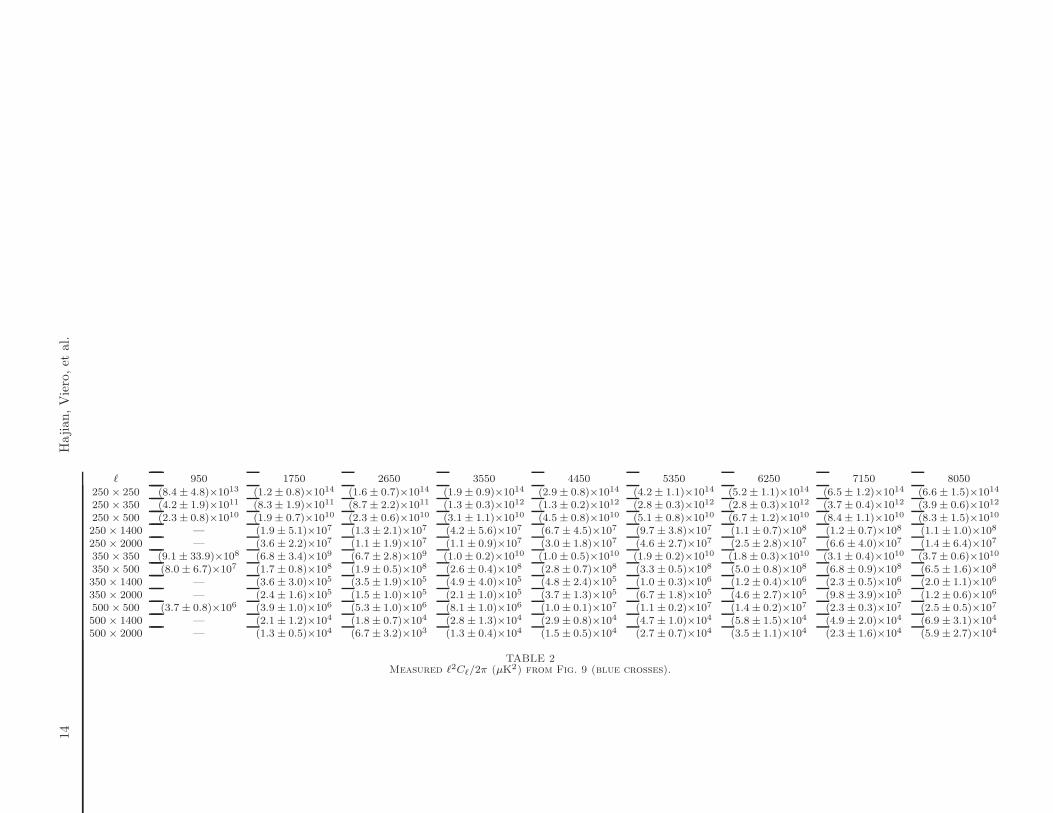
TABLE 2Measured ℓ2Cℓ/2π (µK2) from Fig. 9 (blue crosses).

Correlations in the CSB from ACT× BLAST 15

Fig. 11.— Left panel: Cross-frequency correlation versus effective wavelength for Poisson. Cross-frequency correlation is defined as

Cλλ′

ℓ /(Cλℓ ·Cλ′

ℓ )1/2, i.e., the ratio of the measurement (diamonds in Fig. 10) to the geometric mean (downward pointing arrows in Fig. 10).

From left to right, the actual or effective wavelengths, λeff =√λ1 × λ2, (in µm) are: 2030, 1673, 1380, 1007, 843, 831, 712, 695, 587,

418, 354, and 296. The horizontal line at unity represents 100% cross-correlation. Right panel: Cross-frequency correlation versus distancebetween bands. Correlation is seen between all the ACT and BLAST frequencies.

16 Hajian, Viero, et al.

Finkbeiner, D. P., Davis, M., & Schlegel, D. J. 1999, ApJ, 524,867

Fixsen, D. J. 2009, ApJ, 707, 916Fixsen, D. J., Dwek, E., Mather, J. C., Bennett, C. L., & Shafer,

R. A. 1998, ApJ, 508, 123Fowler, J. W., et al. 2007, Appl. Opt., 46, 3444—. 2010, ApJ, 722, 1148Friedman, R. B., et al. 2009, ApJ, 700, L187Gautier, III, T. N., Boulanger, F., Perault, M., & Puget, J. L.

1992, AJ, 103, 1313Gorski, K. M., Hivon, E., Banday, A. J., Wandelt, B. D., Hansen,

F. K., Reinecke, M., & Bartelmann, M. 2005, ApJ, 622, 759Griffin, M. J., Swinyard, B. M., & Vigroux, L. G. 2003, in

Presented at the Society of Photo-Optical InstrumentationEngineers (SPIE) Conference, Vol. 4850, IR Space Telescopesand Instruments. Edited by John C. Mather . Proceedings ofthe SPIE, Volume 4850, pp. 686-697 (2003)., ed. J. C. Mather,686–697

Hajian, A., et al. 2010, ArXiv e-printsHall, N. R., et al. 2010, ApJ, 718, 632Hincks, A. D., et al. 2010, ApJS, 191, 423Hinshaw, G., et al. 2009, ApJS, 180, 225Hivon, E., Gorski, K. M., Netterfield, C. B., Crill, B. P., Prunet,

S., & Hansen, F. 2002, ApJ, 567, 2Hughes, D. H., et al. 1998, Nature, 394, 241Hui, L., & Parfrey, K. P. 2008, Phys. Rev. D, 77, 043527Lagache, G., Bavouzet, N., Fernandez-Conde, N., Ponthieu, N.,

Rodet, T., Dole, H., Miville-Deschenes, M.-A., & Puget, J.-L.2007, ApJ, 665, L89

Lagache, G., et al. 2004, ApJS, 154, 112Lueker, M., et al. 2010, ApJ, 719, 1045Marriage, T. A., et al. 2010, arXiv:1007.5256Marsden, G., et al. 2009, ApJ, 707, 1729—. 2010, ArXiv e-prints (M10)

Matsuura, S., et al. 2010, ArXiv e-printsMiville-Deschenes, M.-A., & Lagache, G. 2005, ApJS, 157, 302Miville-Deschenes, M.-A., Lagache, G., Boulanger, F., & Puget,

J.-L. 2007, A&A, 469, 595Moncelsi, L., et al. 2010, ArXiv e-printsNolta, M. R., et al. 2009, ApJS, 180, 296Pascale, E., et al. 2008, ApJ, 681, 400—. 2009, ApJ, 707, 1740Patanchon, G., et al. 2009, ApJ, 707, 1750Poglitsch, A., et al. 2010, A&A, 518, L2Puget, J.-L., Abergel, A., Bernard, J.-P., Boulanger, F., Burton,

W. B., Desert, F.-X., & Hartmann, D. 1996, A&A, 308, L5+Reichardt, C. L., et al. 2009a, ApJ, 701, 1958—. 2009b, ApJ, 694, 1200Sayers, J., et al. 2009, ApJ, 690, 1597Scott, K. S., et al. 2010, ApJS, 191, 212Sharp, M. K., et al. 2010, ApJ, 713, 82Shirokoff, E., et al. 2010, ArXiv e-printsSmail, I., Ivison, R. J., & Blain, A. W. 1997, ApJ, 490, L5+Sunyaev, R. A., & Zeldovich, Y. B. 1972, Comments on

Astrophysics and Space Physics, 4, 173Swetz, D. S., et al. 2010, ArXiv e-printsTauber, J. A., et al. 2010, A&A, 520, A1+Tegmark, M., et al. 2002, ApJ, 571, 191Truch, M. D. P., et al. 2009, ApJ, 707, 1723Valiante, E., et al. 2010, ApJS, 191, 222van Dokkum, P. G., et al. 2009, PASP, 121, 2Vieira, J. D., et al. 2010, ApJ, 719, 763Viero, M. P., et al. 2009, ApJ, 707, 1766 (V09)Weiß, A., et al. 2009, ApJ, 707, 1201Zemcov, M., Blain, A., Halpern, M., & Levenson, L. 2010, ApJ,

721, 424

Correlations in the CSB from ACT× BLAST 17

APPENDIX

A. UNIT CONVERSION

The flux density unit of convention for infrared, (sub)millimeter, and radio astronomers is the Jansky, defined as:

Jy = 10−26 W

m2 Hz, (A1)

and is obtained by integrating over the solid angle of the source. For extended sources, the surface brightness isdescribed in Jy per unit solid angle, for example, Jy sr−1, (as adopted by BLAST), or Jy beam−1 (e.g., SPIRE).Additionally, the power spectrum unit in this convention is given in Jy2 sr−1

CMB unit convention is to report a signal as δTCMB; the deviation from the primordial 2.73 K blackbody. To convertfrom Jy sr−1 to δTCMB in µK, as a function of frequency:

δTν =

(

δBν

δT

)

, (A2)

whereδBν

δT=

2k

c2

(

kTCMB

h

)2x2ex

(ex − 1)2=

98.91 Jy sr−1

µK

x2ex

(ex − 1)2, (A3)

and x=hν

kνTCMB=

ν

56.79 GHz, (A4)

(Fixsen 2009). Because the BLAST bandpasses have widths of ∼ 30% (Pascale et al. 2008), and because the CMBblackbody at these wavelengths is particularly steep (falling exponentially on the Wien side of the 2.73 K blackbody),the integral of δBν/δT over the bands is weighted towards lower frequencies; an effect that becomes dramatically morepronounced at shorter wavelengths. Thus, the effective BLAST band centers in δT are ∼ 264, 369, and 510µm, leadingto factors of conversion from nominal of ∼ 2.46, 1.75, and 1.13, respectively.Lastly, the CMB power spectrum is conventionally reported versus multipole ℓ, while in the (sub)millimeter the

convention is to report it versus angular wavenumber, kθ = 1/θ, which is also known as σ in the literature, and istypically expressed in arcmin−1. In the small-angle approximation the two are related by ℓ = 2πkθ.

B. POWER SPECTRUM UNCERTAINTIES

The contents of each map used for cross-frequency correlations can be considered as a sum of two parts: one with afinite cross-correlation; and the other with vanishing cross-power spectrum. The former contributes to the signal in thecross-power spectrum, while the latter contributes to the uncertainties. Therefore three terms contribute to the powerspectrum uncertainties: sample variance in the signal due to limited sky coverage; the noise; and a non-Gaussian termdue to the Poisson distributed compact sources and galaxy clusters. The diagonal component of the ACT × BLASTcross-spectrum variance can be written as the sum of these terms, in order:

σ2(CA×Bb ) =

2

nb

(

CA×Bb

)2

+Cb(N

(1)b + N

(2)b ) + N

(1)b N

(2)b

nb+

σ2P

fsky, (B1)

where Nb, estimates the average power spectrum of the noise; the superscripts (1) and (2) label the maps (1 for ACT,2 for BLAST); nb counts the number of Fourier modes measured in bin b (that is, the number of pixels falling in the

appropriate annulus of Fourier space); fsky is the patch area divided by the full-sky solid angle, 4π sr; and Cb is themean cross-spectrum. The last term, σ2

P, arises from the Poisson-distributed components in the maps (i.e., unresolvedcompact sources and clusters of galaxies) and is given by the non-Gaussian part of the four-point function as describedin Fowler et al. (2010) and Hajian et al. (2010). For purposes of the covariance calculation, we assume that the spatialdistribution of these objects is uncorrelated. This term is constant with ℓ.The noise terms in the ACT and BLAST maps are given by

N(1)b =CCMB

b + CRGb +NA

b ,

N(2)b =NB

b , (B2)

where CRGb is the power spectrum of the radio galaxies in the ACT maps and NA

b and NBb are the noise spectra in

ACT and BLAST respectively. The noise terms, Nb, are dominated by the atmospheric noise on large angular scalesand by detector noise on the smallest scales (Das et al. 2010). The CMB is a major source of noise for this studyout to ℓ ∼ 2500, especially for the 148GHz data. Radio galaxies only contribute to the uncertainties through thefourth moment of the field. They do not bias the signal. The effect of the radio galaxies is stronger at 148GHz and isnegligible at 218GHz. Therefore we mask the brightest radio galaxies in the 148GHz map to reduce the uncertaintyon the cross-power spectra.The uncertainties on BLAST × BLAST power spectra are computed using a similar analytic estimate, given in

Eqn.(9) of Fowler et al. (2010) with nw = 6 cross-spectra per map.

18 Hajian, Viero, et al.

As a sanity check, we compare our analytic estimate of the error bars with the standard deviation of the powerspectra computed from patches of the sky. We divide the data into four patches of equal area and with them computefour independent cross-power spectra. We use the variance of the measurements at each ℓ bin as a measure of the erroron the power spectrum. This method agrees well with the analytic estimate of the errors; however, due to the smallarea of the sky used in this analysis, both analytic and patch-variance estimates of the error bars have uncertaintieswhich are limited by fsky. Thus, we conservatively use the greater of the analytic and patch-variances as an estimateof the uncertainty of the power spectrum. We test the effect that this choice of error bars has on our results in section6.1.When fitting parameters, we take the joint likelihood function to be diagonal as the off-diagonal elements are small

(Das et al. 2010).