Coupled buoyancy and Marangoni convection in acetone: experiments and comparison with numerical simulations

J . Fluid Mech. (1992), vol. 234, p p . 487-510 Printed in Great Britain

487

Coupled buoyancy and Marangoni convection in acetone : experiments and comparison with

numerical simulations

By D. VILLERS AND J. K. PLATTEN Universitd de Mons - Hainaut, Department of Thermodynamics, B-7000 Mons, Belgium

(Received 21 June 1990 and in revised form 16 July 1991)

This paper presents a study of the convection in acetone due jointly to the thermocapillary (Marangoni) and thermogravitational effects. The liquid (acetone) is submitted to a horizontal temperature difference. Experiments and numerical simulations both show the existence of three different states : monocellular steady states, multicellular steady states and spatio-temporal structures. The results are discussed and compared with the linear stability analysis of Smith & Davis (1983).

1. Introduction When a layer of fluid is submitted to a horizontal temperature difference, as

sketched on figure 1, convection results from density differences and surface tension forces, due to the variation of the surface tension u with the temperature T . The thermocapillary effect, usually referred to as Marangoni convection, is directly related to the surface tension gradient

We have already presented some results (Villers & Platten 1985, 1987) when surface tension increases with temperature, a very complex case since the surface and gravitational forces produce two superposed convective cells.

In this paper, we focus our attention on the classical case of negative au/aT. Then, the two forces act in the same direction. The parameters which allow to describe convection are :

the Prandtl number P r = v /K, (2)

the Rayleigh number gaATh3

Ra = -, KV

(au/aT) ATh the Marangoni number Mu = - 9

Po KV

(3)

(4)

the aspect ratio A = L/h, ( 5 )

where g is the gravitational acceleration, a the thermal expansion coefficient, AT the temperature difference imposed between the lateral walls, h the thickness of the layer, K the thermal diffusivity, po the density of the fluid a t the mean temperature, v the kinematic viscosity, and L the length of the cavity. One can find in the literature other definitions of Ra and Ma, namely Ra* = gaATh4/KvL and

488 D . Villers and J . K . Platten

- L + FIGURE 1. Two-dimensional description of the model cavity used for the numerical and

experimental work.

Ma* = - (acr/aT) ATh2/p, KVL ; the ratio of the two definitions is simply A . The second set of definitions (containing the aspect ratio L / h ) is usually adopted by researchers more implied in numerical analysis. However, we have found in our experimental study that the points corresponding to steady states or to oscillatory states are more separated in phase space using Ma and Ra than when using Ma* and Ra*. Clearly, gravitational forces dominate for large h (the Rayleigh number is proportional to h3) whereas the thermocapillary effect is dominant for small h (the Marangoni number is proportional to h) . I n the literature, the ratio Ra/Ma is sometimes referred to as the dynamic Bond number.

The parallel-flow solution valid for an infinite layer yields a simple cubic polynomial expression for the horizontal velocity profile V,(z) taking into account both the thermocapillary and the thermogravitational processes (Birikh 1966 ; Kirdyashkin 1984; Villers & Platten 1987). Obviously a simpler parabolic profile is obtained when thermocapillarity acts alone (Smith & Davis 1983). These expressions are very useful when one is interested in the basic convective states for low values of the control parameter, namely the temperature difference.

The scope of this paper is a first insight in the flow pattern when the basic state becomes unstable, in a layer of finite extension. First we present numerical simulations in order to describe the expected flow pattern and next show some experiments confirming the transitions between monocellular steady flow, multicellular flow and, for higher values of the control parameter, spatio-temporal behaviour. These will be compared and discussed in the last two sections in the light of numerical simulations and the existing stability analysis of Smith & Davis (1983).

2. Steady convection : numerical simulations The goal of these simulations is to show the basic velocity field in a cavity of finite

extension, and to describe the first ' instability ' of this profile. Numerically, we consider the problem of transient natural convection in a rectangular enclosure using the stream function-vorticity formulation of the two-dimensional NavierStokes and energy equations, assuming the Boussinesq approximation. The numerical finite differences method we use is the classical second-order alternating-direction implicit method (Peaceman & Rachford 1955) on a rectangular grid (129 x 33 or 257 x 65) (see also Villers & Platten 1990). This method was implemented in Fortran on a standard microcomputer. The two lateral isothermal walls and the bottom (supposed to be

Coupled buoyancy and Marangoni convection 489

conducting) are rigid. The thermocapillary effect (for a flat interface) introduces the Levich boundary condition (Levich 1962)

from which follows in dimensionless form the Marangoni number given by (4). Since the main goal of these numerical experiments is to show different convective regimes rather than to simulate accurately the laboratory experiments, we shall not take into account heat and mass transfer in the gas phase, themselves influenced by the experimental devices used to avoid evaporation, etc. Therefore, as we have done previously, we use an adiabatic condition as the boundary condition for the temperature on the top.

The simulations presented in this section are performed with a Prandtl number Pr = 4. This small value is chosen because it corresponds in order of magnitude to many low-viscosity and transparent organic liquids which can be used in experiments and because the computation time is an increasing function of Pr. Figure 2 shows the streamlines and isotherms obtained in a rectangular cavity of aspect ratio A = 4, with Ma = 1000 and Ra = 0 (case a ) and with Ma = 2000 and Ra = 0 (case b). We clearly observe a single convective cell, with the streamlines approximately horizontal in the central part of the cavity. In these conditions, we expect that the flow in this region corresponds to the parabolic solution occurring when thermocapillarity is the only cause of motion in an infinite cavity :

V,(z) = z(z-8) with 0 < z < 1. (7)

This is evident from figure 2 (c ) which shows the simulated profile V,(z) on the vertical median (Ma = 2000, Ra = 0) together with the parabola of equation (7).

Fig. 3 (case a : A = 4, Ma = 3000, Ra = 0 and case b : A = 4, Ma = 4000 and Ra = 0) shows situations with higher values of the control parameter. In both cases, we observe the existence of a perturbation (of finite amplitude) superposed on the original monocellular regime, which corresponds to two stationary convective cells with the same direction of rotation. We can also see from the shape of the isotherms that locally there exist negative horizontal temperature gradients aT/ax, instead o f the global positive mean temperature gradient ATIL, together with local vertical stratifications aT/az < 0 (unstable when gravity acts). With fluids of Prandtl number much greater than one, temperature fluctuations constitute a ‘dangerous ’ source of instability.

The instability of the monocellular state remains when gravity acts together with thermocapillarity. For example, we observe the monocellular state when A = 4, Ma = 1000, Ra = 1000, but also a bicellular steady state when A = 4, Ma = 4000, Ra = 4000 or A = 4, Ma = 6000, Ra = 6000. Figure 4 shows the stationary state obtained withMa = Ra = 6000. Streamlines and isotherms look very much like those obtained with Ra = 0, Ma = 4000 in figure 3(b). The V, ( z ) profile on the vertical median is clearly different from a parabola, because of the action of gravity.

The number (and to a lesser extent the size) of the convective cells quite naturally changes with the aspect ratio. Suppose that the lateral extension of one cell is more or less constant, as an extrapolation to finite systems of the results of a normal mode analysis with the appearance of a unique wavelength (Smith & Davis 1983; Laure & Roux 1989). Therefore, in a finite layer, we expect the number of convective cells to depend on the available space, namely A . To confirm this hypothesis, we have


- 12 -8 - 4 0 4

VSZ)

FIQURE 2. (u, b ) Streamlines and isotherms of two numerical simulations with Pr = 4, Ru = 0, A = 4: (a) Mu = 1000; (b ) Mu = 2000; (c) V&) profile on the vertical median compared with the parabolic profile of equation (7) (Ma = 2000).

Coupled buoyancy and Marangoni convection 49 1

FIGURE 3. Streamlines and isotherms of two numerical simulations with Pr = 4, Ra = 0, A = 4: (a) Ma = 3000; ( b ) M u = 4000.

FIQURE 4. Streamlines and isotherms of a numerical simulation with Pr = 4, Ru = 6000, Ma = 6000 and A = 4.

performed simulations at R a = 0 and Mu = 8000, varying A with the succession values, 2, 3, 4, 6 (see figure 5u-d). A variation of the number of cells is, in fact, observed. When A = 2, it seems impossible to have more than one cell, whereas a second cell is possible for A = 3 and A = 4. In a still larger cavity (A = 6), we see the appearance of a third cell. Thus, from these few simulations, we propose that the length of a cell is approximately two times its thickness. This crude approximation


FIQURE 5 . Influence of the aspect ratio on the convective motions with Pr = 4, Ra = 0, Ma = 8000 and (a) A = 2, ( b ) A = 3, (c) A = 4, ( d ) A = 6.

is not too far from the critical wavelength resulting from the theory of Smith & Davis (1983) which predicts a value close to 2.5.

Other simulations will be shown in the next section, devoted to comparisons with experiments.

3. Steady convection : experiments 3.1. Experimental conditions

The experimental technique used to record velocity profiles, e.g. VJz) , is laser Doppler velocimetry (LDV). As explained elsewhere (Platten, Villers & Lhost 1988), our LDV equipment is specially dedicated to the measurements of small velocities in liquids, rangiong from 5 pm/s to a few mm/s. We choose acetone as test fluid for several reasons.

(i) It is a transparent liquid, which thus allows the use of LDV. (ii) It has a low value of the surface tension and so, combined with its good properties as solvant, we can avoid problems of surface contamination by surface-active substances more easily than in water or in aqueous solutions. (iii) For acetone, Pr w 4.24 at a mean temperature of 20 "C. This small value allows faster numerical simulations than for other organic liquids (alcohols, etc.) having a greater Pr. (iv) We estimate the coefficients as - (acr/aT) A T / p , KV w 38 x lo3 cm-' and gaAT/Kv w 344 x lo3 cm-3 for


mm

I I - L = 3 0 m m -I

FIGURE 6. Sketch of the experimental cell.

AT = 1 K and at T = 20 "C. Thus, the flow is primary due to thermocapillarity for thickness of the order of 1 mm and length of the order of 1 cm. It is, however, possible to obtain R a and M a of the order of 103-105, the range which corresponds to transition in the flow structure, and for which it is still possible to perform numerical simulations without computational problems (such as numerical divergence, excessive CPU time or memory). On the other hand, one small disadvantage in using acetone is that it is a rather volatile liquid. We thus have to carefully limit the evaporation, to avoid problems due to the latent heat of evaporation together with a small decrease of the thickness.

The experimental cell used for the present experiments is schematically depicted on figure 6. The lateral walls and the conducting bottom are made out of stainless steel. The length L is 30 mm and the two front and back transparent glass sides are separated by 10mm. We hope that this short distance favours a flow without a horizontal velocity component normal to the glass plates, so that a two-dimensional model would be sufficient for comparisons. We have verified experimentally in a few cases that the flow in the middle of the cavity is just slightly slowed because of the effect of the lateral boundaries ; in the worst cases, the boundary-layer effect along the lateral wall is only observed over a distance of about 2 mm. The temperature gradient is imposed using two water-thermostated copper pieces in good thermal contact with the lateral stainless steel walls. The two temperatures are measured using thermocouples. A Teflon block is inserted a few millimetres above the upper surface, in order to avoid evaporation problems. Probably this Teflon block will influence the thermal boundary condition at the free surface but this is ignored in the numerical model as already explained. Therefore quantitative comparison between numerical simulations and experiences is not expected to be completely satisfactory.

3.2. Monocellular convection We first perform experiments with low R a and Ma (that is with thin layers and small AT), to obtain monocellular states. Figure 7 shows three horizontal velocity profiles, V,(z) on the vertical median of the cavity, a t the following conditions: ( a ) h = 1.75 mm, AT = 1.2 K (thus R a = 2212 andMa = 7980); ( b ) h = 2.5 mm, AT = 0.8 K (thus R a = 4300 and Ma = 7600); (c) h = 2.5 mm, AT = 1.2 K (thus R a = 6450 and Ma = 11 400). Comparing the surface velocity of the first and third cases, where only the thickness of the acetone layer is modified, we verify that the ratio of velocities (-5.881 - 3.91 = 1.48) is equal to the ratio of the thicknesses (2.5/1.75 = 1.43). This


2.0 -J

z (mm) 1.0 i O

0.5 1 0

0 0

0 0

0

0 0

0 0 0

0

1:: 1 1.5

0

0

0

0

0

0

0

0.5 0 -6 3 - 5 - 4 - 3 -2 - I 0 I 2

V , (mm/s)

FIGURE 7 . Horizontal velocity profiles V , ( z ) on the vertical median of the cavity: (a)h=1.75mm,AT=1.2K;(b)h=2.Fjmm,AT=0.8K;(c)h=2.5mm,AT=1.2K.

is in agreement with the analytical two-dimensional model (Villers & Platten 1987) which predicts that the velocities are proportional to h and AT when thermocapillary convection dominates (and this is the case for thin layers). For the second and third profiles, only AT is changed, and the ratio of the surface velocities (-5.88/ -3.61 = 1.63) is also comparable to the ratio of the temper;tture differences (1.2/0.8 = 1.5).

Coupled buoyancy and Marangoni convection

2.5 - -

2.0 -

1.5 - z(mm) :

1.0 -

0.5 -

0 -4

495

0 0 (4

-3.5mm/s O

(ExP. -3.6) 0 0

0 0

0 0

0 0

0 0

0 0

0 0 0 0 0 0 0 1.15mm/s o (Exp. 1.1)

0 0

0 0

0 0

. . . . . . . . . . . . . . . . . . . . . . . . . . . . . . - 3 -2 - 1 0 1 2

We have performed a numerical simulation for the conditions of the second profile, that is h = 2.5 mm and AT = 0.8 K. The corresponding dimensionless numbers are Pr = 4.24, Ra = 4300, Ma = 7600 and A = 12. The streamlines and isotherms obtained for the steady state are presented in the figure 8(a ) . We see that in the central part of the cavity, where experimental measurements are made, the streamlines are horizontal and parallel ; the convection is in the form of a monocellular cell, with the exception of a little vortex appearing near the hot wall. The horizontal velocity profile (deduced from the stream function and converted in a dimensional form) is shown on figure 8 (b) , and is in quantitative agreement with experiments : - 3.5 mm/s for the surface velocity compared to - 3.6 mm/s found experimentally, and 1.15 mm/s as the maximum bulk velocity, compared to the measured value of 1.1 mm/s.


0

0

0.5

0 -6 - 5 - 4 - 3 - 2 - 1 0 1 2

V , (mmls)

FIGURE 9. Horizontal velocity profile on the vertical median of the cavity: h = 2.5 mm, AT = 1.6 K.

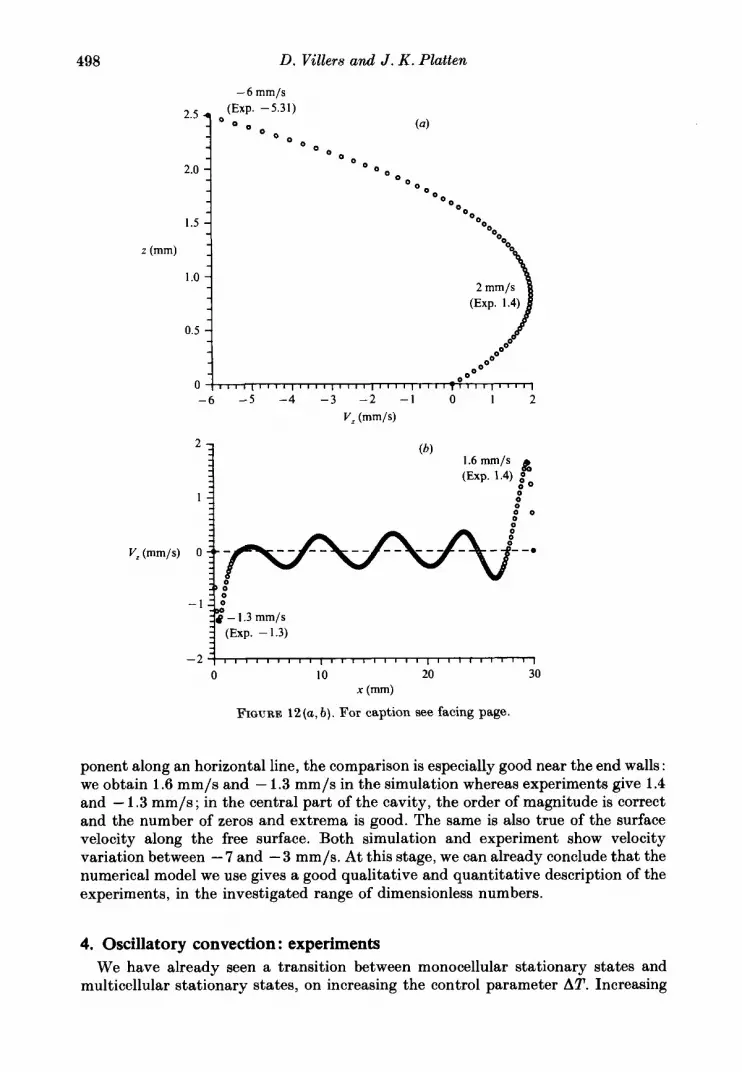
3.3. Multicellular convection We describe in this subsection an experiment performed in an acetone layer of thickness h = 2.5 mm, submitted to a temperature difference of AT = 1.6 K, that is twice that for the profile shown on figure 7 ( b ) . The new profile is presented on figure 9. We immediately see that the surface velocity (-5.31 mm/s) is not twice the velocity obtained with AT = 0.8 K ( - 3.61 mm/s) and even is less than that obtained with the lower AT = 1.2 K (-5.88 mm/s, see figure 7c) . Thus it seems that the experiment a t AT = 1.6 K is not an extrapolation of those a t AT = 0.8 K and 1.2 K. Therefore, we have measured other velocity components. Figures 10(a) and 10(b) give the vertical velocity component along an horizontal line (V,(z) at z = 1.35 mm above the bottom of the cavity) and the horizontal velocity component along the surface V,(s). We clearly observe that V , oscillates in the central part of the cavity, as it should when the flow is multicellular ; indeed, besides the two boundary layers near the hot and cold walls, we also observe in the central part successive alternation of rising and sinking liquid, with relatively small vertical velocities (of the order of one-fifth of the velocities in the boundary layers). In addition, the horizontal velocity component along the surface V,(z) indicates that the motion in the surface is still from the hot to the cold side, but there are important variations of the velocity, between -4 and -7 mm/s. From these two profiles, we may conclude that the flow is multicellular and, particularly from figure lO(u), that there must be five vortices inside the basic convective cell.

We have performed a second numerical simulation for the conditions of this last experiment, h = 2.5 mm and AT = 1.6 K. The corresponding dimensionless numbers are Pr = 4.24, Ra = 8600, Mu = 15200 and A = 12. The streamlines and isotherms obtained for the steady state are presented in figure 11. We clearly see the multicellular pattern, with five vortices (although the fifth near the cold wall is less visible). Also, the isotherms show some inversions in the horizontal gradient aT/ax along the horizontal coordinate. Figure 12 (a-c) gives the three computed dimensional profiles which correspond to the three experimental profiles shown on figures 9 and 10(u, b ) . The comparison between the experiment and the simulation is not only correct as far as the number of vortices is concerned, but also from a quantitative point of view : the surface velocity on the vertical median is - 6 mm/s numerically compared to - 5.31 mm/s experimentally. Concerning the vertical velocity com-


-2:

V,(mm/s) -4 i

-6

497

I

I

;

00 0 0

0 ' 0 0 0 0 0

o o o 8 %

0 0 0 0 . 0 0

. . ' .

0 o o o . . o o o 0

'0'

'1 1 P.

I ,

!: . I

0 10 20 30

FIGURE 11. Streamlines and isotherms of a numerical simulation of the flow field at Pr = 4.24, Ra = 8600, Ma = 15200 and A = 12; these conditions correspond to the experiment shown on figures 9 and 10.

498

1 '

D. Villers and J . K . Platten

c 1.6 mm/s (Exp. 1.4)

(b)

0"0 0 0

0 0

0

- 6 mm/s

: :$ - I .3 mm/s

(Exp. -1.3)

- 2 - , , , , , 1 , , 1 1 , , , , 1 1 1 1 1 ~ , , , , , ~ ~ ~ 1 ~

FIGURE 12(a, b ) . For caption see facing page.

ponent along an horizontal line, the comparison is especially good near the end walls : we obtain 1.6 mm/s and - 1.3 mm/s in the simulation whereas experiments give 1.4 and - 1.3 mm/s ; in the central part of the cavity, the order of magnitude is correct and the number of zeros and extrema is good. The same is also true of the surface velocity along the free surface. Both simulation and experiment show velocity variation between - 7 and - 3 mm/s. At this stage, we can already conclude that the numerical model we use gives a good qualitative and quantitative description of the experiments, in the investigated range of dimensionless numbers.

4. Oscillatory convection : experiments We have already seen a transition between monocellular stationary states and

multicellular stationary states, on increasing the control parameter AT. Increasing


-2

-4

-6

-8

FIQURE 12. (a) Horizontal velocity profile V , ( z ) on the vertical median of the cavity, ( b ) vertical velocity component V,(s) along an horizontal line at z = 1.35 mm, and (c) horizontal velocity component V&) along the surface. The three profiles are obtained from the numerical simulation of the flow field at Pr = 4.24, Ra = 8600, Ma = 15200 and A = 12; these conditions correspond to the experiment shown on figures 9 and 10.

AT (or h) still further, we expect another transition towards spatio-temporal states. This is the object of this section.

4.1. Detection of the oscillations Determination of periodic states is not easy, in the absence of some knowledge of the conditions for their appearance, i.e. the values of the control parameters, the region of the cavity where the amplitude of oscillations is sufficient to be detected, the order of magnitude of the time period (a few seconds, minutes, etc.). It appears from preliminary measurements of periodic behaviour that the period is of the order of I0 s, and that the most important variations of the horizontal component of velocity (the amplitude of the oscillations) are recorded a few tenths of a millimeter below the surface. Figure 13 shows a few detailed oscillations recorded by our signal analyser. The thickness h of the layer for this experiment was 4.0 mm and the temperature difference A T = 3.4 K ; the optical LDV probe was focused 0.4 mm below the surface, on the vertical median of the cavity. The figure is composed from 59 successive Fourier transforms of the LDV signal, taken at regular time intervals (the time between each FFT is 0.744 s). Regarding the shape of an individual spectrum, each one is itself an average of Fourier transforms of 8 time samples of 0.1 s, with overlaps, taken over about 0.7 s. As the arrival times and the sizes of the incoming particles in the optical probe are variable, the corresponding Fourier transforms have different amplitudes. We can observe different typical situations : for example, many particles of about the same size cross the measuring volume a t approximately equally spaced times and then the average FFT is broad ; in other cases, if two particles cross at the beginning and at the end of the time span, we finally observe two peaks in the average spectrum. Thus the global average Fourier transforms have maximum peaks corresponding to different values of the instantaneous velocities at the measuring


15000 15700 16 400

(Hz)

4 19000

FIQURE 13. Example of some oscillations of an horizontal component of the velocity at one point in the cavity, h = 4.1 mm, AT = 3.4 K.

point over the entire time of the averaging procedure. However, we are interested in the global variation with time of the frequency corresponding to maximum amplitude. From the result shown on figure 13, we clearly observe that the signal oscillates between 20 KHz4300 Hz and 20 KHz-3600 Hz with a period of 11.0 s. Since the fringe spacing of the LDV system is 1.7 pm and the 20 KHz corresponds to the frequency shift used to resolve the sign ambiguity using double Bragg cells, then the horizontal velocity oscillates between -7.3 mm/s and -6.1 mm/s. Of course, the oscillations are recorded over several minutes (typically 10 to 15 min), in order to be sure they are not transient, and to obtain a precise value of the period.

4.2. Velocity measurements in periodic conditions

It should be pointed out that LDV is not well suited for the study of time-dependent velocity fields since we can perform only a local measurement of one velocity component a t one time. Consequently, it is hard to determine phase relations between values of the velocity obtained at different positions. It would be possible to look a t the whole velocity field, as a function of time, using other techniques such as particle image displacement velocimetry (Dudderar & Simpkins 1977). Figure 14 shows the profile V,(z) along the vertical median with h = 3.3 mm and AT = 4.1 K. For each z, the graph gives the two extreme values of the velocity and the arrow indicates the amplitude of the velocity variation. The period has the same constant value everywhere and is equal to 9.3 s. We see that the amplitude of the oscillations is important in the upper part of the layer, near the surface where thermocapillarity is the principal cause of motion. On the other hand, in the region of positive horizontal velocities (near the bottom of the cavity), oscillations are not visible.

I n another experiment characterized by h = 5.70 mm and AT = 6.0 K, we have measured the profile V,(z) along an horizontal line a t z = 2.5 mm above the bottom (see figure 15). Once again, the two dots indicate the minimum and maximum values of K ( t ) . From this profile, we deduce that the spatio-temporal flow structure is not


- 4 -

- 5

0.0

ob

0

0

0

0

. . . . . . . . . . . . . . . . . . . . . . . . . . . . . . .

0

0

0

50 1

0

I , , , , , , , , , , , , , , , I , , T , , , , , , , , , j

- 10 - 5 0 5

FIGURE 14. VJz) profile measured on the vertical median of the cavity (h = 3.3 mm and AT = 4.1 K), showing the minimum and maximum values of the measured velocities during the oscillations.

v, (mm/s) _ _

simply of the form of travelling waves. We would see in that case in the central part an oscillation of V, between negative and positive values, corresponding to a continuous translation of convective rolls; this is not the case, except at some particular positions.

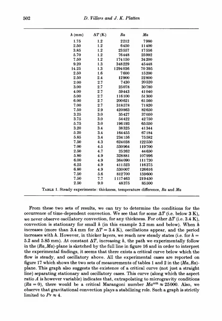
4.3. Steady and oscillatory cases as a function of h and AT We have repeated these experiments many times, changing the thickness h and the temperature difference AT. Depending on the experimental conditions, we have obtained stationary or oscillatory regimes. Table 1 lists the parameters for steady experiments (i.e. when oscillations are not detected) whereas table 2 lists the oscillatory experiments, giving for each the measured values of the period l7.

502 D. Villers and J . K . Platten

h(mm) AT(K)

1.75 1.2 2.50 1.2 3.85 1.2 5.70 1.2 7.50 1.2 9.20 1.3

14.25 1.3 2.50 1.6 2.50 2.4 2.00 2.7 3.00 2.7 4.00 2.7 5.00 2.7 6.00 2.7 7.00 2.7 7.50 2.9 3.25 3.0 3.75 3.0 5.75 3.0 3.20 3.4 5.20 3.4 5.85 3.4 7.50 4.3 7.00 4.5 2.50 4.7 5.80 4.9 6.00 4.9 6.25 4.9 6.80 4.9 7.50 5.6 7.50 7.7 2.50 9.0

Ra

2212 6 450

23 557 76448

174150 348 229

1 294 036 7 600

12900 7 430

25078 59 443

116 100 200 62 1 318578 420 863 35 427 54422

196 193 38 325

164 455 234 156 624038 530 964 25262

328881 364090 41 1523 530007 812700

1117463 48 375

Ma

7 980 11 400 17556 25 992 34 200 45 448 70 395 15200 22 800 20 520 30 780 41 040 51 300 61 560 71 820 82 650 37 050 42 750 65 550 41 344 67 184 75 582

122 550 119700 44 650

107 996 111720 116375 126616 159 600 219450 85 500

TABLE 1. Steady experiments : thickness, temperature difference, Ra and Ma

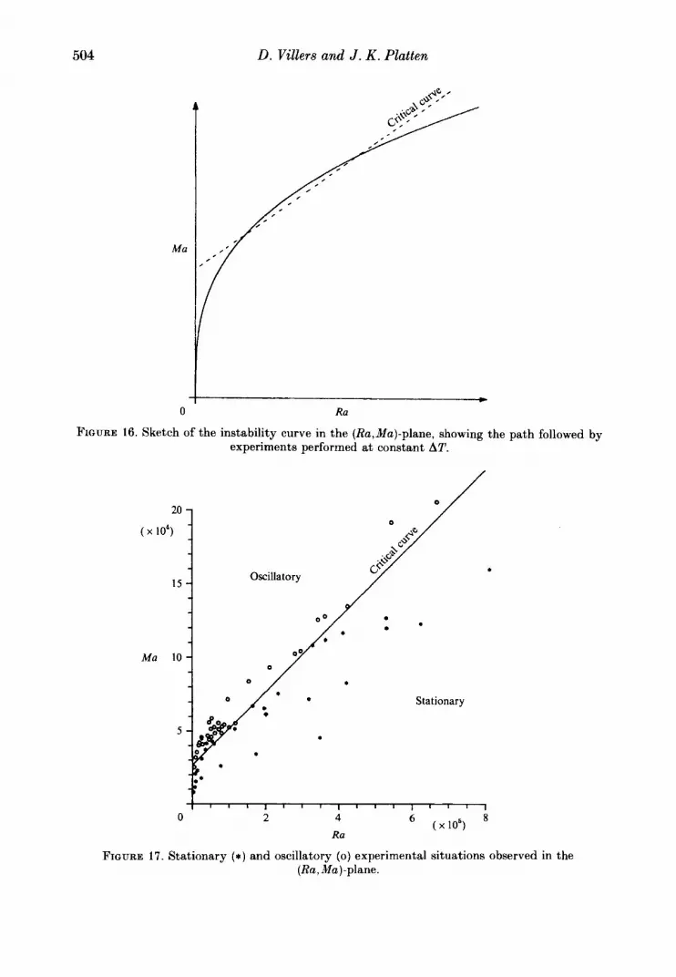
From these two sets of results, we can try to determine the conditions for the occurrence of time-dependent convection. We see that for some AT (i.e. below 3 K), we never observe oscillatory convection, for any thickness. For other AT (i.e. 3.4 K), convection is stationary for small h (in this example 3.2 mm and below). When h increases (more than 3.4 mm for AT = 3.4 K), oscillations appear, and the period increases with h. However, in thicker layers, we reach new steady states (i.e. for h = 5.2 and 5.85 mm). At constant AT, increasing h, the path we experimentally follow in the (Ra,Ma)-plane is sketched by the full line in figure 16 and in order to interpret the experimental findings, it seems that there exists a critical curve below which the flow is steady, and oscillatory above. All the experimental cases are reported on figure 17 which shows the two sets of measurements of tables 1 and 2 in the (Ma, Ra)- plane. This graph also suggests the existence of a critical curve (not just a straight line) separating stationary and oscillatory cases. This curve (along which the aspect ratio A is however variable) indicates that, extrapolating to microgravity conditions (Ra = 0 ) , there would be a critical Marangoni number Mucrit w 25000. Also, we observe that gravitational convection plays a stabilizing role. Such a graph is strictly limited to Pr w 4.


h(mm) AT(K) R a Ma

4.25 3.0 99222 ' 48 450 4.60 4.85 3.40 3.55 3.75 3.95 4.10 4.20 2.75 3.15 3.55 3.75 3.30 1.35 1.70 1.90 2.15 2.25 2.45 3.00 3.15 5.60 5.50 5.60 5.90 5.60 6.00

3.0 3.0 3.4 3.4 3.4 3.4 3.4 3.4 3.9 3.9 3.9 3.9 4.1 4.9 4.9 4.9 4.9 4.9 4.9 4.9 4.9 4.9 6.0 6.0 6.0 9.0 9.0

100451 117735 45 970 52 327 61 678 72 082 80610 86 653 27 901 41 933 60022 70 748 50 686 4 147 8281

11 562 16752 19200 24 789 45511 52 685

296018 343 398 362 47 1 423 902 543 707 668 736

52 440 55 290 43 928 45 866 48 450 51 034 52 972 54 264 40 755 46 683 52611 55575 51 414 25 137 31 654 35378 40033 41 895 45619 55 860 58653

104272 125400 127 680 134 520 191 520 205 200

(6)

10.5 11.5 13.0 9.8

10.0 9.4

11.0 11.2 11.4 8.0 8.5 9.2 9.4 9.3 4.7 5.1 5.5 7 .O 6.6 5.6 7.0 8.0

13.7 12.0 12.5 13.0 13.6 13.9

TABLE 2. Oscillatory experiments : thickness, temperature difference, Ra, Ma and measured values of the period l7

We are also interested in the dependence of the period 17 on h and AT, or on Ra and Ma. Experimentally, l7 does not seem to depend on AT, but varies considerably with the thickness h. For example, at h = 1.35 mm and AT = 4.9 K, the measured period is 4.7 s whereas with h = 5.6 mm (and the same AT) 17 = 13.7 s, it is about three times greater. At constant h (e.g. h = 5.6 mm), 17 = 13.6 and 13.7 s for respectively AT = 9 and 4.9 K. In view of these findings, we have plotted the dimensionless period (with the timescaling h2/v) as a function of the ratio Ma/Ra which is independent of the temperature difference AT. Figure 18 suggests a simple monotonic relation between 17/(h2/v) and Ma/Ra (e.g. linear). The choice of the timescaling can be criticized, but it appears that the viscous time h2/v corresponds in order of magnitude to the measured period (say 1 s). The thermal time hZ/K could also be used since Pr is not too far from 1. A scaling time incorporating surface properties has been tried; indeed, -pvh/(AT&/aT) has the dimension of time, but a typical order of magnitude of this timescale is 2.5ms, very different from the measured periods. It will now be interesting to see if these experimentally recorded oscillations can be reproduced by numerical simulations, and that is the goal of the last two sections.


0 Ra

FIGURE 16. Sketch of the instability curve in the (&,Ma)-plane, showing the path followed by experiments performed at constant AT.

.

20

( x lo4)

15

Ma 10

Stationary

5

8 ( x 105)

0 2 4

Ra

FIGURE 17. Stationary (*) and oscillatory (0) experimental situations observed in the (Ra, Ma)-plane.


v)

B

5 0.4 { E

- E .-

6

505

0

0

0

0 q o

4QOo

1 .o

0.8 1 -0

'E: & 0.6

, , , , , , , , ~ ~ ~ ~ l l [ i l ~ , ~ , l , , ~ ~ , l l ~

0

0 0

MalRa.

Ra Ma Ma/Ra I7 (dimensionless)

10000 10000 1 Stationary state 15000 15000 1 0.34 20 OOO 20 000 1 0.33 30 OOO 30 000 1 0.34 40 000 30 OOO 0.75 0.24

TABLE 3. Parameters of the numerical simulations performed in order to observe oscillatory convection

5. Oscillatory convection : numerical simulation Most of the numerical simulations presented in the literature, concerning this kind

of problem, are performed with low Pr, because, essentially, of the interest in crystal growth of semiconductors or in melt motion of metals. Moreover, just a few papers (Ben Hadid & Roux 1990; Villers & Platten 1990) consider the influence of thermocapillarity. At Pr greater than 1, the numerical procedure implies large computational times. Therefore we have not tried to obtain extensive results for the transition between stationary and oscillatory convection, as this has been done by Ben Hadid & Roux (1990) for Pr = 0.015. However, we present in this section the results of a few simulations of convection in a cavity of aspect ratio A = 9, with Pr = 4.24 and for some pairs of Ra and Ma (see table 3).

We observe oscillatory convection with Ra and Ma equal to or greater than 15000. This crude estimation of the critical limit has the same order of magnitude as the experimental onset presented on figure 17 (Ra = 15000, Mucrit = 30000). Of course comparison is not as significant as for the steady state. We have not tried to refine the numerical solution owing to the prohibitive CPU time on the microcomputer and the boundary conditions used in the model. The non-dimensional numerical period seems to be a function of the ratio Ma/Ra only, as has been suggested by the


t = O

c

1917142

i 23IT7/42

3817142

4017142

FIGURE 19. Streamlines at different times during one period of oscillation, obtained by numerical simulation with Ra = 20000. Ma = 20000, Pr = 4 and A = 4.

experiments. For the two numerically investigated ratios, the dimensionless periods agree with the experimental data of figure 18.

From the numerical simulations, it is interesting to describe the temporal behaviour of the flow pattern. Figure 19 illustrates the variation of the streamlines


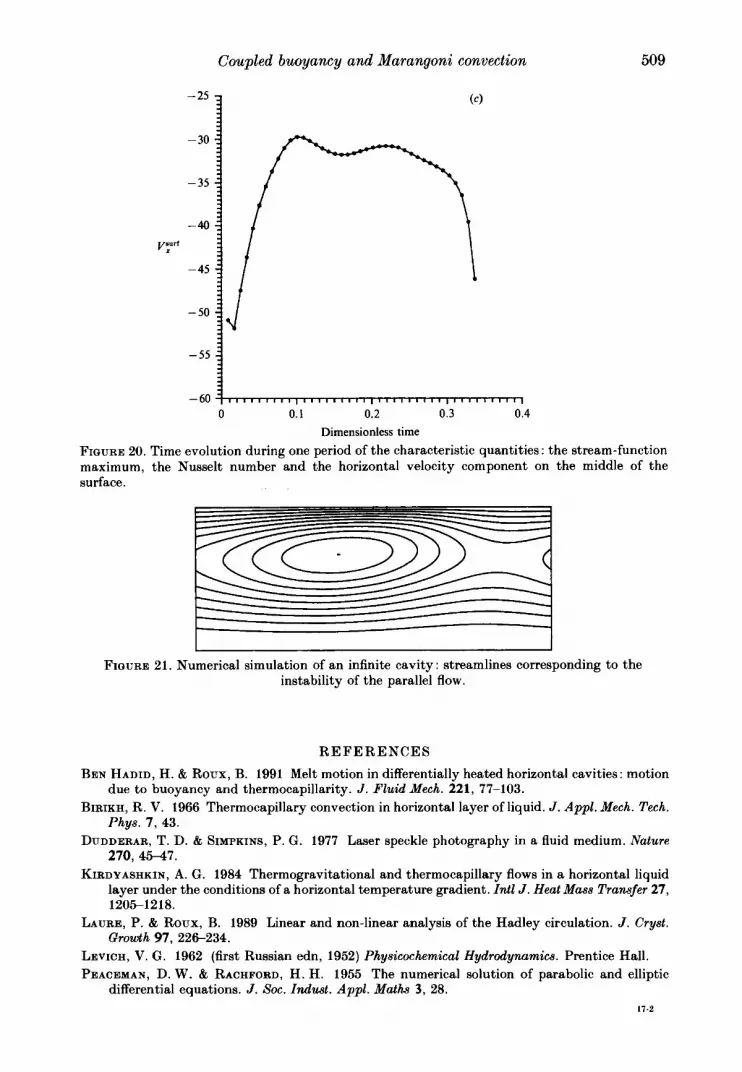
at different times during one period of oscillation (with Ra = M a = 20000). We observe a first stage (between t = 0 and 12 l7/42) characterized by an ‘emission’ of a vortex travelling from the hot wall towards the cold wall, whereas the first well- formed vortex remains almost at a fixed position. Afterwards, the flow seems stabilized (at t = 23Z7/42) with three vortices of gradually decreased intensity, still moving from hot to cold. This very regular pattern of convection is then rapidly destroyed : there is a slowing down in the largest (cold) part of the cavity, benefitting the hot vortex which reaches its maximum amplitude (at t = 4017/42). Figure 20 shows the evolution over time of some characteristic quantities : the maximum of the stream function Ym,,, the Nusselt number, and the horizontal velocity component at the middle of the surface during one period. Their non-sinusoidal character demonstrates the nonlinear nature of the evolution of the perturbative pattern.

6. Discussion and conclusions The results presented in §$2-5 show, for the experimental and numerical

approaches, the same scenario (successive transitions between three flow patterns) when Ra and Ma increase : a monocellular steady state, a multicellular steady state and a time-dependent flow. Moreover, quantitative agreement is achieved regarding stationary states. For the oscillatory cases, it is impracticable (due to CPU time and memory requirements in our equipment) to perform numerical simulations for the conditions of an experiment. However, experiments and simulations give almost the same periods and have a common feature: we never observe travelling waves with the appearance of rolls near one wall and the corresponding disappearance near the opposite wall.

The travelling wave state was expected because it is predicted by the theory of Smith & Davis (1983) in an infinite cavity and by Laure & Roux (1989) in a cavity of large extent. Both contributions show rolls travelling from the cold side to the hot side (with return flow conditions and Pr > 1). For example, Smith & Davis predict an instability of the parallel flow at a critical value Ma*Crit = 220 for Pr = 4 (i.e. for Ma = 550 in our definition, since A = 2.5), with a mode of instability characterized by a dimensionless wavelength 2.5 and a dimensionless frequency 1.23. We have performed a supplementary numerical simulation using periodic lateral boundary conditions with a periodic length fixed at 2.5, in order to simulate an infinite cavity. At Ma = 1000 ( >550), Ra = 0 and Pr = 4, we have observed travelling rolls, as we can see on figure 21 with the streamlines given at an arbitrary time. The numerical frequency of these travelling waves ia about 0.61. Despite the divergence from 1.23 (the value predicted by Smith & Davis) we consider that our ‘nonlinear’ simulation confirms their linear stability results.

There thus remains a discrepancy between the instability in an infinite or large cavity and the time-dependent flow we observe in a cavity of low aspect ratio (say with A between 5 and 10). We suppose that lateral walls prevent or delay the translation of rolls, because it could be difficult when A is small to create or suppress rolls near these lateral walls. For large or infinite layers, it seems that when the parallel flow becomes unstable, we directly observe a time-dependent periodic structure. In a finite (and small) cavity, we observe a first instability to a steady multicellular pattern, followed by a second instability towards a very complex time- dependent flow.

At this stage, we need fundamental theoretical work taking into account the role of the lateral walls, incorporating the aspect ratio A in a linear or nonlinear theory,

17 FLM 234

508

12.0

11.5

11.0

10.5

ymax

10.0

9.5

9.0

8.5

30

28

26

Nu

24

22

D . Villers and J . K . Platten

(a)

0 0.1 0.2 0.3 Dimensionless time

(b)

0.4

20 0 0.1 0.2 0.3 0.4

Dimensionless time

FIQURE 20.(a,b) . For caption see facing page.

together with the usual parameters like Pr, Ra and Ma. Also, it has already been shown that three-dimensional effects can be very important, especially in low-Pr fluids (Smith & Davis 1983). Nevertheless, even though our results are restricted to one Pr and their general validity cannot be asserted, we believe that our experimental work constitutes a preliminary study to eventually validate these expected new theories.

This work is partially supported by the FNRS (Fonds National de la Recherche Scientifique) Brussels by grant No. 1.50101.89F.


FIGURE 20. maximum, surface.

-25 3

- 30

- 35

-40

- 45

- 25

- 30

- 35

-40

- 45

- 50

- 55

-60 I r r n r 8 t I n 1 8 i n 8 5 r n I I I I I I I I I 1 I 8 I I I I I I I I

0 0.1 0.2 0.3 0.4

Dimensionless time

Time evolution during one period of the characteristic quantities : the stream-function the Nusselt number and the horizontal velocity component on the middle of the

- 5 0 y

- 55

- 60 I 0 0.1 0.2 0.3 0.4

Dimensionless time

Time evolution during one period of the characteristic quantities : the stream-function the Nusselt number and the horizontal velocity component on the middle of the

~ ~~~

FIQURE 21. Numerical simulation of an infinite cavity : streamlines corresponding to the instability of the parallel flow.

REFERENCES

BEN HADID, H. & Roux, B. 1991 Melt motion in differentially heated horizontal cavities: motion due to buoyancy and thermocapillarity. J. Fluid Mech. 221, 77-103.

BIRIKH, R. V. 1966 Thermocapillary convection in horizontal layer of liquid. J. Appl. Mech. Tech. Phys. 7, 43.

DUDDERAR, T. D. & SIMPKINS, P. G. 1977 Laser speckle photography in a fluid medium. Nature 270, 45-47.

KIRDYASHKIN, A. G. 1984 Thermogravitational and thermocapillary flows in a horizontal liquid layer under the conditions of a horizontal temperature gradient. Intl J . Heat Mass Transfer 27, 1205-1 2 18.

LAURE, P. & Roux, B. 1989 Linear and non-linear analysis of the Hadley circulation. J. Cryst. Growth 97, 226-234.

LEVICH, V. G. 1962 (first Russian edn, 1952) Phyeicochemical Hydrodynamics. Prentice Hall. PEACEMAN, D. W. & RACHFORD, H. H. 1955 The numerical solution of parabolic and elliptic

differential equations. J. SOC. Indust. Appl . Math 3 , 28. 17-2

510

PLATTEN, J. K., VILLERS, D. & LHOST, 0. 1988 LDV study of some free convection problems a t extremely slow velocities : Soret driven convection and Marangoni convection. In Laser Anemomtry in Fluid Mechanics, Vol. I11 (ed. R. J. Adrian, T. Asanuma, D. F. G. Durao, F. Durst & J. H. Whitelaw), p. 245. Ladoan, Instituto Superior Technico, Lisbon.

SMITH, M. K. & DAVIS, S. H. 1983 Instabilities of dynamic thermocapillary liquid layers. Part 1. Convective instabilities. J. Fluid Mech. 132, 119.

VILLERS, D. &, PLATTEN, J. K. 1985 Marangoni convection in systems presenting a minimum in surface tension. PhysicoChem. Hydrodyn. 6, 435.

VILLERS, D. & PLATTEN, J. K. 1987 Separation of Marangoni convection from gravitational convection in earth experiments. PhysicoChem. Hydrodyn. 8 , 173.

VILLERS, D. & PLATTEN, J. K. 1990 Influence of thermocapillarity on the oscillatory convection in low P r fluids. In Notes on Numerical Fluid Mechanics, Vol. 27 (ed. B. Roux), p. 108. Vieweg, Braunschweig.

D . Villers and J . K . Platten

Documents

Coupled buoyancy and Marangoni convection in acetone: experiments and comparison with numerical simulations