Embed Size (px)
Citation preview

JOURNAL OF GEOPHYSICAL RESEARCH, VOL. 100, NO. D7, PAGES 14,269-14,289, JULY 20, 1995
Coupled energy-balance/ice-sheet model simulations of the glacial cycle: A possible connection between terminations and terrigenous dust
W. Richard Peltier and Shawn Marshall
Department of Physics, University of Toronto, Toronto, Ontario, Canada
Abstract. We apply a coupled energy-balance/ice-sheet climate model in an investigation of northern hemisphere ice-sheet advance and retreat over the last glacial cycle. When driven only by orbital insolation variations, the model predicts ice-sheet advances over the continents of North America and Eurasia that are in good agreement with geological reconstructions in terms of the timescale of advance and the spatial positioning of the main ice masses. The orbital forcing alone, however, is unable to induce the observed rapid ice-sheet retreat, and we conclude that additional climatic feedbacks not explicitly included in the basic model must be acting. In the analyses presented here we have parameterized a number of potentially important effects in order to test their relative influence on the process of glacial termination. These include marine instability, thermohaline circulation effects, carbon dioxide variations, and snow albedo changes caused by dust loading during periods of high atmospheric aerosol concentration. For the purpose of these analyses the temporal changes in the latter two variables were inferred from ice core records. Of these various influences, our analyses suggest that the albedo variations in the ice-sheet ablation zone caused by dust loading may represent an extremely important ablation mechanism. Using our parameterization of "dirty" snow in the ablation zone we find glacial retreat to be strongly accelerated, such that complete collapse of the otherwise stable Laurentide ice sheet ensues. The last glacial maximum configurations of the Laurenfide and Fennoscandian complexes are also brought into much closer accord with the ICE-3G reconstruction of Tushingham and Peltier (1991, 1992) and the ICE-4G reconstruction of Peltier (1994) when this effect is reasonably introduced.
1. Introduction
An increasing body of observational evidence amassed over the past two decades has demonstrated an inextricable link between late Pleistocene glaciation cycles and quasi- periodic variations in surface insolation caused by the changing geometry of the Earth's orbit around the Sun due to many body effects in the solar system. Whether these Milankovitch cycles constitute the primary forcing respon- sible for the extreme perturbations to global climate that accompany ice age cycles is still a subject of active debate, a debate in which our ability to comprehend the extremely complex nonlinear climate system is being severely tested. Nevertheless, the signature of the astronomical variations is clearly etched into the paleoclimatic record, especially that component of the record that consists of oxygen isotope ratios measured in the tests of foraminifera found in deep-sea sediments [i,e., Broecker and yon Donk, 1970; Hays et al., 1976]. The fundamental link between the deep-sea foramin- ifera record and the astronomical variations lies in the fact
that the dominant frequencies of the Milankovitch cycles are also evident in oceanic 180/160 concentration variations through geologic time, as these are preserved in the CaCO3
Copyright 1995 by the American Geophysical Union.
Paper nember 95JD00015. 0148-0227/95/95JD-00015505.00
tests of both benthic and planktonic species. Because atmospheric water vapor becomes progressively more highly enriched in the lighter oxygen isotope as it moves from the site of evaporation to the site of precipitation on an incipient ice sheet, this ratio is an excellent proxy for the volume of continental ice [Shackleton, 1967]. During times of intense glaciation the oceans are isotopically heavier than average and •5180 is high in foraminiferal tests extracted from deep- sea sedimentary cores.
The recent success of the Milankovitch theory of astro- nomically driven glacial cycles has resulted in increasing interest in the development of explicit paleoclimate models that may be employed to test earth system sensitivity to orbital insolation variations [Hyde and Peltier, 1985, 1987; Gallde et al. 1991, 1992; Neeman et at., 1988a,b; Deblonde and Peltier, 1990a,b; 1991a,b, 1993; Deblonde et al., 1992]. A consistent feature in all of these analyses has been the problem encountered in explaining ice age terminations. Continental ice sheets have been found to nucleate readily over the 80-100 kyr timescale of the most recent Pleistocene glaciation when the system is forced only by the Milankov- itch signal, but the rapid retreat of the ice sheets, known to have occurred over a much shorter period of approximately 10 kyr, has never been adequately explained. The simula- tions of Gallge et al. [1991, 1992], however, are perhaps unique, in that they do predict ice-sheet collapse on the appropriate time-scale, though the main mechanism forcing the retreat in their model of this process is a reduction of
14,269

14,270 PELTIER AND MARSHALL: COUPLED ENERGY-BALANCE/ICE-SI•ET MODEL
albedo associated with "snow aging," an effect that is sufficiently subtle as to suggest that the search for alternative mechanisms may be warranted.
The difficulty of effectively modeling glacial terminations has led to the general conclusion [Hyde and Peltier, 1985, 1987; Gal!de et al., 1991, 1992; Broecker and Denton, 1989; Deblonde and Peltier, 1991a,b, 1993; Deblonde et al., 1992] that orbital forcing alone cannot account for these epochal events; rather, a number of interrelated feedbacks such as glacial isostatic adjustment, atmospheric greenhouse gas concentrations, oceanic heat transport, and variations in the hydrological cycle may be collectively responsible. In addition, the dynamics of marine-based, temperate and nonequilibrium ice sheets are not well known or described in the basic ice-sheet model (B ISM) that has been employed in the previous analyses of Deblonde and Peltier, for example. It is quite possible that ablation mechanisms related to these unique conditions, for which there is no modem analog, may also contribute to the acceleration of collapse; subglacial hydrology is surely one example of an unmodeled physical influen6e through which a plausible feedback mechanism for the initiation of collapse could be acting.
This paper discusses an extension of the model of Deblon- de and Peltier [1991b, 1993] to an exploration of the physics of termination. The model elements consist of a global two- dimensional (2D) one-level seasonal energy balance model, essentially that developed by North et al. [1983], that is asynchronously coupled to vertically integrated 2D ice-sheet models over North America and Eurasia. However, unlike the energy-balance model (EBM) of North et al., which was linear, we employ the nonlinear version discussed by Deblo- nde et al. [1992] that was employed in a series of prelimi- nary analyses reported by Deblonde and Peltier [1993]. The physics of this model will be summarized in section 2. The model has been designed to study the cryospheric response to astronomical forcing, and includes the associated lithosp- heric feedback associated with the glacial isostatic adjustment process [e.g., Peltier, 1974, 1976, 1985]. In developing this model, our philosophy has been to keep the structure one of minimum complexity that is nevertheless sufficient to provide an adequate representation of climate state in the extratropics.
Previous paleoclimate simulations of the last glacial cycle with the basic model were presented by Deblonde and Peltier [1991b], while an initial exploration of CO2 and thermohaline circulation feedbacks has been recently pro- vided by Deblonde and Peltier [1993]. These results will be briefly reviewed and extended in section 3.1. The remainder of section 3 explores various parameterizations that we have tested to help account for glacial retreat following the last glacial maximum (LGM). Deblonde and Peltier [1993], for example, found that simplified representations of the North Atlantic heat flux and global atmospheric CO2 variations were sufficient to entirely explain the collapse of the Eur- asian ice sheet, but had little or no effect on the North American ice sheet, which remained essentially impervious to the increase of orbital forcing at LGM, even when these feedbacks were added.
In the continuing search for a mechanism adequate to deliver complete terminations we first postulate in the new work to be reported herein that a marine-based instability triggered by the collapse of the Fennoscandian ice complex into the North Atlantic may have led to massive calving of
the Laurentide ice sheet via Hudson Strait. This would be
expected to create an ice-free region in Hudson Bay, the core area of the Laurentide ice sheet, leading perhaps to inward collapse and accelerated retreat of the residual ice. This process will be mimicked in a new series of experiments by artificially removing all of the ice from the Hudson Strait and Hudson Bay. In the first approximation, this was implemented as a step change following Fennoscandian retreat during a period of already high ablation of the Laurentide ice sheet. Results of these simulations, which lead to the conclusion that even this drastic representation of the effect of a marine instability is unable to induce termina- tion, are presented in section 3.3 below.
In the final series of experiments to be reported here we explore an alternative mechanism that could underlie the physics of termination by parameterizing the radiative impact of the low-albedo (dirty) snow/ice that would undoubtedly exist due to high influxes of terrigenous dust that are known to have occurred episodically during the last glaciation cycle [De Angelis et al., 1987; Lorius, 1991]. As discussed in detail in section 3.4, we postulate that the ablation zones of the ice sheets that existed during periods of high sedimen- tation would have markedly reduced albedo, thus greatly increasing solar absorption and accelerating meltback. This accelerated mass loss in the ablation zone, a very narrow band of ice that lies just inside the ice sheet margin, does in fact lead to complete deglaciation. This is in striking contrast to the net effect of the removal of ice from the core
of the sheet via marine instability (section 3.3), which fails to precipitate termination. Our conclusions following discussion of this sequence of analyses are presented in section 4.
2. Model Physics
The basic climate model that we have developed consists of coupled energy-balance and ice-sheet components that are asynchronously coupled. These ingredients are discussed in the following subsections.
2.1. The Energy Balance Model
The (EBM) used in the study is essentially that of North et al. [1983], with modifications made by Hyde et al. [1989] to introduce a nonlinear temperature-dependent albedo feedback and as previously employed in the context of ice age cycle analyses by Deblonde et al. [1992] and Deblonde and Peltier [1993]. It is a 2D one-level model with realistic land-sea geography and topography. The main rationale for our choosing this model is that explicit 2D geography is believed critical to paleoclimate modeling, given the funda- mental importance of continentality to the correct representa- tion of the seasonal cycle [North et al., 1983]. Hyde et al. [1989] have also demonstrated very favorable comparisons in the extratropics with GCM paleoclimate simulations by Kutzbach and Guetter [1986] at a sequence of times through the last deglaciation event.
The precise form of the model to be employed in the present work is embodied in the energy-balance equation:
i}T + A + BT (r,t) Q a(r,t)S (0,t) -'- C(r).•. •- o (1)
- Vh'[D (x)V h T (r,t)]

PELTIER AND MARSHALL: COUPLED ENERGY-BALANCE/ICE-SHEET MODEL 14,271
The left-hand side of this equation represents the short-wave energy absorbed by the Earth, Q being the solar constant and S representing the solar distribution function, incorporating both latitudinal variations and orbital variations over the
geologic timescale of interest. The co-albedo field a(r,t) is a function of both position and surface type, with temporal and spatial variations in ice cover introducing a nonlinear feedback to the temperature equation (i.e., a temperature- dependent coalbedo field). Constant coalbedo values of 0.3 and 0.5 will be used in all that follows to distinguish land- Q and sea-ice, respectively, an approximation which, being Ao zenith angle independent, is admittedly crude. At all points B not covered by ice, surface-atmosphere absorption was Cw modeled with a smooth latitudinally varying co-albedo field, ao+a2P2(x ), in which P2 is the Legendre polynomial of degree 2. This parameterization is identical to that introduced by C,i North et al. [1983] based on present-day satellite observa- C• tions [Stephens et al., 1981 ].
The first term on the right-hand side of the energy-balance equation represents local energy absorption, C(r,t) being the surface-dependent heat capacity, while the terms Ao+BT(r,t) Dj, model local infrared emission, with Ao and B empirically Do determined based on a fit to global satellite data [Short and D2 North, 1984]. The final term on the right-hand side of (1) Dn represents horizontal heat transport that is assumed to be representable in the form of a smooth meridional linear diffusion. This representation of the highly nonlinear transports associated with baroclinic eddies in the atmosphere a0 has been argued to be valid for the long temporal and large oa spatial scales that are the only scales of interest in the a•i present context [Lorenz, 1979]. A summary of the constants asi employed in the model is provided in Table 1.
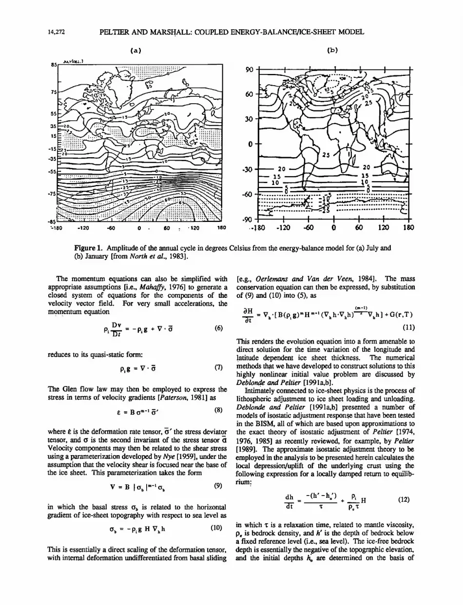
In all of the analyses to be discussed herein, as in the above referenced previous work, all of the fields will be truncated to spherical harmonic degree and order 11. The energy balance model is solved iteratively for the geography dependent annual cycle in the global temperature field. While the spatial resolution is quite coarse, the model has nevertheless been shown to generate a very reasonable facsimile of the present-day annual cycle (e.g., as shown in Figure 1).
2.2. The Ice-Sheet Model
The BISM is derived from the vertically integrated continuity equation for ice mass, with individual fields that appear in the mass balance relation represented on a 1' latitude-longitude grid, with individual domains being employed to represent the evolution of the ice field over the North American and Eurasian continents. The ice sheet
physics is empirically simplified from the equations of motion, based on laboratory study and observations of present-day alpine glaciers and the Greenland and Antarctic ice sheets.
Approximating the ice substance as incompressible, the continuity equation simplifies to
V. v = 0 (2)
in which v is ice velocity. This can be vertically integrated over the height of the ice sheet (H) to give
i)H = _Vh(HV ) (3) -37
Table 1. Constants Employed in Coupled Energy- Balance/Ice-Sheet Model
Para- Value Units Source/ meter Comments
Energy-Balance Model
1360 W m '2 203.3 W m '2
2.094 W m '2 øC'l
9.7 W yr m '2 øC'l 0.97 W yr m '2 øC'1
1.5 W yr m '2 øC4 0.08 W yr m '2 øC4
North et al. [1983] North et al. [1983] North et al. [1983] Deep ocean Shallow seas in N.
Pacific
D(x) = Dj, [ DoPo(X) + D2P2(x) + D4P4(x) ]
0.945 0.7971428 W m '2 øC4
-0.587756 W m '2 øC4 0.1763264 W m '2 øC4
ab(x) = ao + a2P2(x)
0.7
-0.09
0.30
0.50
Ice-Sheet Model/Coupling
T,n -2.0 øC Tsi -4.0 øC ¾ 6.5 øC km 4 a 10.0 m s 4 øC4
b 0.2 kg m s 4 c -70
0 3000 years Di 920 kg m '3 Pe 3300 kg m '3 B• 3.0 m '3a yr 4 m 2.5
Pollard [1983] Pollard [1983] Pollard [1983] Pollard [ 1983 ]
Oerlemans [ 1981] Oerlemans [ 1981]
in which Vh is the horizontal gradient operator and V is the vertical average of the horizontal component of flow veloc- ity:
H
V -' 1 0fVhdz (4) H
It has been assumed in deriving the above expressions that the vertical velocity at the bottom of the ice sheet is negli- gible relative to the horizontal components of velocity. Including an external source/sink term G(r,T) for net accumulation or ablation, we obtain the conventional mass balance equation:
i)H = -V•(HV) + G(r T) (5) -5'i- '
14,272 PELTIER AND MARSHALL: COUPLED ENERGY-BALANCE/ICE-SI-•ET MODEL
(a) (b)
75
55
35
15
.• 0 -35
-,55 '30
-?s -60
-es -90 '-•80 -120 -60 0 - 60 - ß •20 •80 -'l gO
20 20 ].5 15
.120 -60 0 60 120 180
Figure 1. Amplitude of the annual cycle in degrees Celsius from the energy-balance model for (a) July and (b) January [from North et al., 1983].
The momentum equations can also be simplified with appropriate assumptions [i.e., Mahaffy, 1976] to generate a closed system of equations for the components of the velocity vector field. For very small accelerations, the momentum equation
Dv = Pi'-•' -Pig + V' • (6)
reduces to its quasi-static form:
Pig = V'• (7)
The Glen flow law may then be employed to express the stress in terms of velocity gradients [Paterson, 1981] as
e = B .om-' •' (8)
where t; is the deformation rate tensor, c•' the stress deviator tensor, and c• is the second invariant of the stress tensor ci Velocity components may then be related to the shear stress using a parameterization developed by Nye [1959], under the assumption that the velocity shear is focused near the base of the ice sheet. This parameterization takes the form
v = B Io,, ! m-' or, (9)
in which the basal stress ob is related to the horizontal gradient of ice-sheet topography with respect to sea level as
IJt, = - Pig H V,, h (10)
This is essentially a direct scaling of the deformation tensor, with internal deformation undifferentiated from basal sliding
[e.g., Oerlemans and Van der Veen, 1984]. The mass conservation equation can then be expressed, by substitution of (9) and (10) into (5), as
(m-l)
: Va'[B(p•g)mH m*• (Vah'Vah)•Vah] +G(r,T) (11)
This renders the evolution equation into a form amenable to direct solution for the time variation of the longitude and latitude dependent ice sheet thickness. The numerical methods that we have developed to construct solutions to this highly nonlinear initial value problem are discussed by Deblonde and Peltier [1991a,b].
Intimately connected to ice-sheet physics is the process of lithospheric adjustment to ice sheet loading and unloading. Deblonde and Peltier [1991a,b] presented a number of models of isostatic adjustment response that have been tested in the B ISM, all of which are based upon approximations to the exact theory of isostatic adjustment of Peltier [1974, 1976, 1985] as recently reviewed, for example, by Peltier [1989]. The approximate isostatic adjustment theory to be employed in the analysis to be presented herein calculates •e local depression/uplift of the underlying crust using the following expression for a locally damped rerum to equilib- rium:
dh -(h' -ho') Pi = , + H (12) dt x pox
in which 'c is a relaxation time, related to mantle viscosity, p, is bedrock density, and h' is the depth of bedrock below a fixed reference level (i.e., sea level). The ice-free bedrock depth is essentially the negative of the topographic elevation, and the initial depths h• are determined on the basis of

PELTIER AND MARSHALL: COUPLED ENERGY-BALANCE/ICE-SHEET MODEL 14,273
present-day topographic data [e.g., Gates and Nelson, 1975a,b]. Further extension of the model to include the complete theory of glacial isostatic adjustment of Peltier [1974, 1976, 1985, 1994] will be reported in due course.
2.3. The Coupled Model
The above described ice-sheet and energy-balance models are asynchronously coupled, using a coupling algorithm similar to that discussed by Hasselmann [1988]. The EBM is run to obtain a converged solution for the annual cycle at discrete time intervals separated by At,=100-1000 years in the current sequence of experiments. This temperature field is then employed as input to the ice-sheet model, which is integrated employing smaller time steps, At,, from time t to t+ Ate For all results reported here, the ice sheets were updated at At,=25 year intervals as in the work by Deblonde and Peltier [1991b]. This asynchronous coupling scheme is justified on the basis of the fact that the climate state will be essentially in equilibrium with the ice sheets for the period Ats, due to the long timescale over which the ice sheets evolve.
Coupling between the EBM and B ISM occurs primarily through the accumulation/ablation term G(r,T) introduced above. This net balance function is assumed to be directly dependent on the temperature field, with an additional position dependence determined by the global precipitation field. Put simply, accumulation of snow/ice is assumed to occur over the continents as long as the average daily temperature remains below a critical value, assumed to be - 2øC by tuning to today's climate [Deblonde and Peltier, 199 lb, 1993]. The net accumulation is then given by
G.• --- pre(r). fpre.AT• ha2 km
unknown and more important, the geographical distribution may have varied widely. Furthermore, some present-day dry regions, such as southwestern North America, almost certainly experienced an increase in precipitation relative to today's levels.
In the model, ice-sheet ablation rates are also determined from the average monthly temperature, with net ablation assumed to occur when temperatures exceed 0øC for both land and sea ice. The net ablation is calculated using a parameterization similar to that first introduced by Pollard [ 1980, 1983] that takes the form
max (0. aT,,, + bQ", + c) (14)
where Qm is the average monthly insolation at the top of the atmosphere and a, b and c are
a -- b --- (15) OT
empirically determined constants. The net mass balance is then
O (r, T),,, -- G,, - G,, (16)
Further coupling between the EBM and ISM occurs through the temperature-elevation feedback and seasonal snow-ice albedo feedback. In the former, a constant lapse rate ¾ is assumed in order to correct the predicted sea-level temperatures for the topographic elevation at the ice sheet surface as:
T -- T (r,t) - ¾(H-h'-h'o) (17)
--- pre(r). fpre h> 2 km 2 rh-2) AT,,
(13) This corrected temperature is input to the longwave emission term of the EBM. The lapse rate used and all other con- stants employed in the model are listed in Table 1.
Here, AT., is the monthly averaged temperature difference from the critical value of-2øC. The second equation is employed to represent the elevation desert effect observed in present-day alpine regions. The precipitation field that we employ, pre(r), is taken from present-day observations, discretized over a 1 ø grid corresponding to the resolution of the "windows" within which we choose to explicitly solve the evolution equation for the ice sheets. A precipitation factor fpre of 0.9 was used throughout the investigation, again corresponding to that employed by Deblonde and Peltier [199 lb, 1993]. This implies that precipitation was set to 90% of today's values, while maintaining the same spatial distribution. It is doubtful that either of these assumptions is entirely valid, but insufficient paleoclimatic evidence is available to justfly an alternative choice. Ice-core studies in Greenland and Antarctica indicate that glacial-period precipi- tation may have been reduced by as much as 60% [Jouzel et al., 1989; Raisbeck et al., 1987]. This figure has been inferred from løBe data and the deuterium-temperature record, which yield an estimate of water vapor pressure. However, these ice-core records may represem local effects, confined to the polar regions. While it is likely that precipi- tation fell in temperate regions also, the reduction factor is
3. Results
In presenting the results of our new analyses in this section, we will discuss a number of different feedback mechanisms that could be involved in the termination
process, including [CO2] variations, oceanic heat transport changes due to modulation of the strength of the thermoha- line circulation, marine ice-sheet instabilities, and finally and most importantly, the feedback due to variations in the atmospheric concentration of terrigenous dust. All of these feedbacks will be assessed by comparing their impacts against an appropriate control simulation that we first discuss in the following subsection.
3.1. Control Case
The control model is similar to that described by Debl- onde and Peltier [1993]; it incorporates only the physics discussed above. Two significant changes, however, have been made from the control analysis employed by Deblonde and Peltier [ 1993], in an attempt to correct for the previously inadequate treatment of the North Pacific and shallow sea regions dividing Alaska and eastern Siberia. In our previous analyses, model ice sheets developed over Alaska and

14,274 PELTIER AND MARSHALL: COUPLED ENERGY-BALANCE/ICE-SHEET MODEL
extreme eastern Siberia, despite geological evidence suggest- ing that the cominental ice sheets did not in fact extend into these regions [CLIMAP, 1981; Porter et al., 1983]. While large alpine glaciers and ice fields were most certainly present, it is believed that these glaciers did not merge to form a continuous ice sheet.
The first change to the Deblonde and Peltier [1993] control case involved the heat capacity assigned to the shallow-water regions of the Bering Sea and Sea of Okhotsk off eastern Siberia. These regions are essentially cominental shelves, with presem-day ocean depths as small as 100 m. Given the estimated 120-m eustatic sea level drop at LGM [Fairbanks, 1989; Chappell-Shackleton, 1986] or more accurately, the 105-m eustatic fall inferred on the basis of gravitationally self-consistent rsl calculations [Peltier, 1994], much of this region was certainly exposed land surface at that time. As a result, the heat capacity in this shallow-sea region will have varied greatly over the glacial period, and would certainly be much less than that of the deep ocean.
Deblonde and Peltier [1993] set the value of the surface heat capacity in this region to one third that of the deep ocean heat capacity, which was calculated based on the assumption of a 75-m mixed layer. This value has been further reduced in the present analyses, to C•/10, an inter- mediate value which is still an order of magnitude larger than the cominental heat capacity. This change increases the amplitude of sununer warming, partially offsetting the erroneous prediction of ice sheet advance over eastern Siberia.
In addition to the warming effected by the shallow seas of this region, considerable present-day waxming is caused by heat transport from the Kuroshio current, a transport that is clearly not represemed in the climate model. After the Gulf Stream and North Atlantic drift, this is the second largest region of oceanic heat transfer to the atmosphere [Hsiung, 1986]. Yet another physical consideration that may be critical to seasonal melt on the Alaskan peninsula is deriva- tive of the alpine topography of this region, with high glaciated peaks separated by broad valleys. These alpine valleys are simply not resolved by our 1 ø topographic data set, implying that a relatively high average topographic height is assigned over the region. As these alpine valleys do drive extensive summer melt, our model, which fails to resolve them, provides a poor simulation of local ablation effects. It is likely that high seasonal meltback in the valleys played a major role in preventing the merging of the alpine glaciers into a continuous ice sheet. Rather than attempting to model both this topographic effect and the warming of the region by the Kuroshio current, we have chosen in the presem analyses to inhibit the growth of an ice sheet over the Alaskan peninsula in an ad hoc manner. This was done by setting ablation equal to accumulation at all times, so that the region remained perpetually ice free. The primary reason that this was done was to remove any erroneous effects of Alaskan ice cover on the developmere of the Lauremide ice sheet that might otherwise occur.
With the above modifications incorporated, the control case was run for a full glacial cycle, from t= 122 kyr B.P. to present day. Initial conditions for the last interglacial at 122 ka B.P. were assumed to be idemical to those that obtain at
present. The summer seasonal insolation anomaly time series employed to force the model was computed on the
basis of the new time series for the orbital elements recently computed by Quinn et al. [1991]. A sequence of time slices through the predicted history of ice-sheet evolution from the last interglacial to the present, for both the Laurentide and the Fennoscandian complexes, are shown in Figures 2 and 3, respectively, for this control simulation. Both ice sheets nucleated rather quickly at about 110 kyr B.P. after the integration commenced at 122 kyr B.P. In North America, ice is predicted to flood over the continent from nucleation points over Baffin Island and the St. Elias mountain range near the Yukon-Alaskan border (Figure 2b). These individ- ual centers merge at about 80 kyr B.P. in this control simula- tion to form the Laurentide ice sheet, with a single dome establishing itself over Hudson Bay by 50 kyr B.P. The ice sheet thereafter is predicted to continue to thicken and spread further southwards (Figures 2d and 2e).
While the predicted areal extent of the ice sheet at last glacial maximum (LGM) is very close to that observed (e.g., as represented by the ICE-3G model of Tushingham and Peltier [1991, 1992]), the maximum thickness of ice over Hudson Bay is predicted to have reached more than 4000 m, about 25% greater than the most accurate existing estimate from ICE-3G. In terms of total volume, the ice sheet is predicted to have reached its maximum near 17 kyr B.P., somewhat later than the presently accepted date of LGM (-21 ka) based upon the Barbados relative sea level history of Fairbanks [ 1989] with timescale determined by U/Th dating [Bard et al., 1990]. However, only a minor meltback is predicted to occur between LGM and the presem (Figure 2f). This is the fundamental flaw in the predictions of this model, which it is our propose to address in the remainder of the present paper.
The Eurasian ice sheet, meanwhile, is predicted to nucleate over the mountains of Norway and the northern Barems Sea, with significant advances and retreats occurring over the next 60 kyr in response to orbital forcing. The higher continemality makes the Fennoscandian complex more responsive to orbital variations than the North American complex, and efficiently inhibits ice-sheet development over the Asian continent. Hence, ice-sheet growth occurs primar- ily through steady thickening from 60 kyr B.P. until LGM (Figure 3e). The maximum volume of the Fennoscandian ice complex is achieved near 20 kyr B.P., and this is followed by a sharp meltback of about 50% of ice-sheet volume by 10 kyr B.P. Rather than a cominued collapse, however, the ice sheet recovers somewhat and thickens slightly from -10 kyr to presem (Figure 3f). This is again quite clearly at odds with the observational evidence as represented, for example, by the ICE-3G model.
Plots of ice volume history over the full simulation for both ice sheets are presented in Figure 4. The maximum ice volume reaches about 35 x 106 km 3 in North America and 22 x 10 • km 3 in Eurasia. This compares to geological recon- structions by Hughes et al. [1981] which estimate the maximum volumes at 31.2-36.7 x 10⁶ km 3 and 8.2-14.3 x 10⁶
km 3 for these two respective regions. Fischer et al. [1985] have estimated a Laurentide ice sheet volume of 18.0-25.9
x10 • km 3 using a multidomed reconstruction rather than a single dome structure as assumed by Hughes et al. [1981] and predicted by the model. The more accurate ICE-3G reconstruction of Tushingham and Peltier [1991, 1992] has a maximum ice volume much closer to the estimate of
Fischer et al. than to that of Hughes et al. [see also Peltier, 1994].

9O
80 •!• ^ • ,. .......
?::•'..'•.v,•.•:.',?• :•::.-':'•'::.•'?::>:::::4 K•'"• "'•:• ' •: • •:'• :::•;•'t:•.;:::.•:t• •' :.•:'
30
80
70
•)
50
40
30
9O
8O
7O
5O
3O
(c)
9O
8O
7O
6O
50
4O
3O
80
7O
60-
5O
4O
30 -175 -156 -136 -117 -98 -79 -59 -40
Figure 2. Ice-sheet thickness contours over North America for the control simulation at (a) 120 ka, (b) 100 ka, (c) 70 ka, (d) 40 ka, (e) 18 ka, and (f) 0 ka.

-15 13 41 69 96 124 152 180 -15 13 41 69 96 124 152 18C
Figure 3. Ice sheet thickness contours over Eurasia for the control simulation at (a) 120 ka, (b) 100 ka, (c) 70 ka, (d) 40 ka, (e) 18 ka, and (f) 0 ka.

PELTIER AND MARSHALL: COUPLED ENERGY-BALANCE/ICE-SHEET MODEL 14,277
5.00E+16
4.00E+16'
3.00E+16'
2.00E+16.
1.00E+16' /'"x •'•-•x J -i ! 0 00E+00 • •'••'•1' • I • I • I ' I '
ß -1.2'0•+0s -•.00•+0s -a.oo•+04 -4.00E+04 -2.00E+04 0.00E+00 -6.00E+04
Figure 4. Ice volume variations over the last 120 kys for the control simulation. Solid line (North American ice), dashed line (Eurasian ice).
3.2. Influence of [CO2] and Oceanic Heat Flux Variations
In order to correct the predictions of the climate model so as to better represent the termination process it was con- cluded that additional feedback mechanisms must be acting in concert with orbital forcing, either independently or triggered by LGM climate conditions. The first of these additional mechanisms that we shall attempt to incorporate is that associated with variations in the concentration of
atmospheric greenhouse gases. Changes of atmospheric carbon dioxide and methane
concentrations through the last glacial cycle are very well established from ice core records, both in Amarctica [Barnola et al., 1987; Neftel et al., 1988] and Greenland [Stauffer et al., 1988]. Due to the rapid, homogeneous mixing of CO2 and CH 4 in the atmosphere, these ice-core records are accepted as representative of global levels. The records demonstrate very significant variations over the last 160 kyr, as shown in Figure 5. Greenhouse gases exhibit well-known and important radiative effects in the atmos- phere, being highly absorbent of infrared radiation and almost transparent to short-wave radiation. The influence of these gases clearly alters the energy balance and influences surface temperatures; it is therefore important that the influence of these variations be incorporated into the model so as to test the hypothesis that it might be through their influence that the additional forcing required to effect complete termination of the ice age might be obtained.
We have investigated the plausibility of the importance of this feedback by introducing a correction factor A in the infrared emission term in the EBM, such that the long-wave emission becomes Ao+ A + BT(r,t) where Ao is the same factor as that in equation (1) and is obtained by empirically fitting to the modem climate with its presem concentrations of greenhouse gases. For the purposes of this investigation, carbon dioxide will be considered to be the only critical greenhouse gas, and is the only constituent to be modeled. As a reference concentration we will choose [CO21o=320 ppm. The perturbation to the factor Ao, that is A, is calcu- lated using an extrapolation of the available logarithmic formula for radiative effects of CO2 increases [e.g., Marshall et al., 1988; Ramanathan et al., 1987], i.e.;
For the decrease in [COx], observed at LGM, AA is positive, representing greater infrared emission to space and inbreased cooling. This correction for paleoclimatic C02 levels has been introduced into the EBM in four discrete stages, corresponding to the Barnola et al. [1979] observation of essentially two different lower levels of CO2 between the last and present interglacial [Deblonde and Peltier, 1993]. During the interglacials from -122 to -115 kyr and from -14 kyr to present, [CO2] t was assumed to be equal to the present level, giving AA=0. This was considered valid because glacial [CO2] changes are of the order of 120 ppm while preindustrial to present-day changes are about 20 ppm. The glacial period was divided into intermediate and full glacial conditions, with CO2 concentrations of 250 and 200 ppm, respectively. The intermediate conditions obtain from -115 kyr to -80 kyr, and correspond to a radiative cooling of AA=i W/m 2. Full glacial conditions are assumed to prevail from -80 kyr to -14 kyr, with AA=2 W/m 2. A discussion of the global temperature decreases corresponding to these changes is provided by Deblonde and P•ltier [1993].
Also introduced into the EBM by Deblonde and Peltier [1993] was a simple parameterization of North Atlantic heat transport. As ocean dynamics are not explicitly included in the model, there is no physical representation of the signifi- cant high-latitude warming generated by the poleward transport of tropical surface waters. Observations of these heat fluxes have been made by ship measurements, and are documented in recent reports by Hsiung [1986], Hsiung et al. [1989], and Hakkinen and Cavalieri [1989]. From a 30-year data set, Hsiung [1986] found that the largest center of oceanic heat loss is the North Atlantic, associated with the Gulf Stream and the North Atlantic Drift. Hakkinen and
Cavalieri [1989] have reported heat fluxes of up to 400 W/m 2 in the Greenland, Norwegian, and Barems Seas.
Interest in the impact of variations of the North Atlantic heat transport has recently intensified due to the suggestion by B roecker et al. [1985] that the North Atlantic thermoha- line circulation may have switched off during glacial times [Broecker and Denton, 1989]. Results from simple meri/:li- onal cell models of the thermohaline circulation [Bryan,
-420
•' -440 .-
-7.5 • -490 -10.0 -500[
0 40 80 120 160
Age ( kyr B P )
280
260 ;; 240 •.
220 • 200 L)
180
AA = -k $n [C02], k = 6 W/m 2 (18) [CO21o
Figure 5. Carbon dioxide variations (upper curve) and the deuterium temperature record (lower curve) from the Vostock ice core over the last 160 kyr [from Barnola et al., 1987].

14,278 PELTIER AND MARSHALL: COUPLED ENERGY-BALANCE/ICE-SHeET MODEL
1986; Marotzke et al., 1988; Wright and Stocker, 1991; Sakai and Peltier, 1995] and coupled atmosphere-ocean global circulation models (GCMs) [i.e., Manabe and Stouffer, 1988] have indicated that present-day mean ocean currents may indeed have varied in this way under ice age conditions. In particular, the North Atlantic response to increased fresh- water influx may have been such as to switch off the process of deep-water formation in the North Atlantic and thus markedly reduce the strength of the thermohaline circulation. The impact of such a shutdown of the thermohaline circula- tion has been assessed in paleoclimate studies; Rind et al. [1989], in particular, found using the Goddard Institute for Space Studies GCM that no ice sheets could be supported in the model when the North Atlantic heat flux was fully active.
Observational evidence supporting this possibility has been provided by Boyle [1988a,b], who has studied cadmium levels in the shells of foraminifera from deep-sea cores. Cadmium is thought to be proxy for oceanic productivity, with Cd content varying with nutrient level (phosphates, nitrates). The present-day North Atlantic deep water has very low Cd levels, as a result of nutrient removal during its relatively recent presence at the surface. In glacial times, however, there were much higher levels of deep water Cd, suggesting a reduced turnover of North Atlantic surface waters. This has been interpreted as a possible indication of thermohaline circulation shutdown.
It should be noted that this interpretation of the Cd data is not universally accepted, as other factors are involved in oceanic productivity. For example, a glacial-period reduction in North Atlantic surface-water temperatures might also limit productivity. The evidence is nevertheless indicative of some reorganization of North Atlantic heat transfer, if not a complete shutdown of the therrnohaline overturning. As this may be important to the process of ice age termination, a parameterization of the impact of variations in the North Atlantic heat flux was incorporated into the model following Deblonde and Peltier [1993] in order to provide a further assessment in terms of the new control model employed here. This was done by simply adding a local heat flux to the energy balance equation, centered over the Norwegian Sea as shown in Figure 6. The magnitude and position of the flux were based on the observations and calculations of
Hsiung [1986] and Hakkinen and Cavalieri [1989]. By adding this term to the energy-balance model without compensation, energy is no longer conserved. We expect this approximation to be acceptable, since the perturbation to the globally averaged heat flux is less than 1 W/m 2. We estimate timing and extent of the postulated shutdown of the heat flux on the basis of arguments presented by Broecker and Denton [1989], who hypothesize a reduction in oceanic transport coincident with the known CO2 variations discussed above. This link is suggested on the basis of the important role of the oceans as a carbon dioxide sink. The glacial cycle was therefore split into four phases identical with those employed to represent the [CO2] variation, with full modem heat flux present in the interglacial periods from - 122 to - 115 kyr and -14 kyr to present. The heat flux was reduced by 25% in intermediate glacial conditions from -115 kyr to -80 kyr, and reduced by 50% under full glacial conditions from - 80 kyr to- 14 kyr.
In the absence of any quantitative estimate of the actual reduction in heat flux that may have occurred during glacial times, these values were chosen by Deblonde and Peltier
90 • ! • I • I • I • I •
30
•.o
o
-30
..
-60 • •••• i i••1 ir ' • -90 • I • I • -180 -120 -60 0 60 120 180
Figure 6. North Atlantic heat flux distribution and intensity employed in the parameterization of the climate impact of variability in the strength of the thermohaline circulation.
[1993] based on their ability to model the full glacial cycle in conjunction with the CO2 variations. Deblonde and Peltier's "best fit" case was rerun here with the
aforementioned changes made to Alaska and the shallow seas east of Siberia. A full glacial simulation from -122 kyr to present was performed, with predicted ice volume variations shown in Figure 7. The warming effect of the North Atlantic heat flux tends to dominate the radiative cooling, from reduced CO2 levels during interglacial and intermediate glacial conditions from 122 to 80 kyr B.P. As a result, the North American and Eurasian ice sheets are much slower to nucleate than in the control case. The two ice sheets were
initiated over the same centers as in Figures 2a, 2b and 3a, but exhibit only small fluctuations until 80 kyr B.P. They then begin to advance over the continents, following quite different growth histories than in the control case.
The Laurentide ice sheet advances slowly and continuous- ly over North America, reaching a maximum extent near 17 kyr B.P. once again. The maximum volume predicted is 34 x 106 km 3, again within the range of the reconstruction by
3.00E+16
2.00E+16
1.00E+16
0.00E+00 • , I • • ' I • I , I i .... -1.20E+05 -1.00E+05 -8.00E+04 -6.00E+04 -4..00E+04 -2.00E+04 0.00E+00
Figure 7. Ice volume variations over the last 120 kyr for the simulation including both oceanic heat flux and atmospheric carbon dioxide variations. Solid line (North America), dashed line (Eurasia).

PELTIER AND MARSHALL: COUPLED ENERGY-BALANCE/ICE-SHEET MODEL 14,279
Hughes et al. [1981] but considerably higher than in the. more accurate ICE-3G model of Tushingham and Peltier [1991, 1992]. The ice sheet then undergoes a sharp collapse until about 8 kyr B.P., losing over 40% of the LGM ice volume. The meltback levels off at this point, with little change from -8 kyr to present. Figure 8 depicts ice-sheet thickness contours during the meltback period from LGM to presem. The predicted LGM ice volume is slightly less than the control case prediction, although the ice thickness over
8O
7O
the core of the ice sheet is still almost 4000 m. The areal
extent of the ice sheet is very well modeled once again. The ice sheet predicted to remain at the present time has retreated above the Great Lakes, but still covers most of Canada (Figure 8d).
The Fennoscandian complex, meanwhile, grows quickly into its full glacial configuration, approaching its maximum extent by 68 kyr B.P. (Figure 7). It then remains fairly stable at this volume, advancing with minor retreats and
8O
7O
3O
-175 -156 -136 -117 -98 -79 -59 -40 -175 -156 -136 -117 -98 -79 -59 -40
Figure 8. Ice-sheet thickness contours over North America for the case that includes both CO2 and oceanic heat flux variations. The individual frames correspond to the times (a) 18 ka, (b) 12 ka, (c) 10 ka, and (d) 0 ka.

14,28o PELTIER AND MARSHALL: COUPLED ENERGY-BALANCE/ICE-SHEET MODEL
peaking at 18 kyr B.P. The maximum volume predicted is 17 x 106 km 3, closer to the Hughes et al. [1981] estimation than the base case prediction and again excessive compared with the ICE-3G reconstruction. Immediately following LGM, a rapid collapse is predicted over the next 8-10 kyr. This deglaciated state is maintained from -10 kyr until present and is clearly in accord with modem observations. This termination is illustrated in Figure 9. By 10 kyr B.P. (Figure 9c), small ice fields remain over eastern Siberia and the Barems Sea. The Siberian ice sheet collapses completely by present (Figure 9d), while the ice over the Barems Sea
thickens slightly and some ice returns to northern Scandinavia.
It is interesting that the CO2 reductions and oceanic heat flux variations have completely changed the nature of the predicted Eurasian ice cover. Instead of a southwards advance over Great Britain and central Europe, the ice now extends much further eastward. A second ice sheet nucleates
over eastern Siberia, and by the LGM this ice sheet has merged with the Scandinavian mass to form a continuous band of ice over northern Asia. From a circumpolar view, this Eurasian complex, along with the Greenland and
8O
7O
3O
(b)
eo
8O
7O
5O
30
-1:5 13 41 69 96 124 152 180 -15 13 41 69 96 124 152 180
Figure 9. Same as Figure 8 but for Eurasia.

PELTIl•R AND MARSHALL: COUPLED ENERGY-BALANCE/ICE-SHEET MODEL 14,281
Laurenfide ice sheets, forms an almost continuous ring about the pole. The significant eastward migration of this Eurasian ice sheet relative to the control case results from the COc induced cooling; central and eastern Asia are sufficiently removed from the North Atlantic heat flux that the CO: effects dominate. This scenario is not in accord with the
best available a priori information, which suggests that no significant continental ice sheet existed in eastern Siberia [e.g., Tushingham and Peltier, 1991, 1992].
One further test that is of interest in the context of the
simulations under discussion here was an investigation of model sensitivity to the EBM time step employed. In the analyses by Deblonde and Peltier [1993], the energy-balance equation was solved for a new equilibrium annual cycle every 1000 years, with the calculated surface temperature field assumed to be maintained for the next millennium.
However, glacial collapse is known to have occurred over a period less than 10 kyr, and it is clear that the boundary conditions associated with ice sheet position change consider- ably over 1000 years during this period (e.g., V.L. Blette, personal communication, 1991). By employing smaller EBM time steps during the period of glacial retreat, we might better ensure that the temperature field was in an appropriate equilibrium with the ice sheets.
Initial tests of 100- to 500-year EBM time steps over the past 20 kyr did indeed indicate that a choice of Atp1000 years was too long to keep pace with the process of glacial retreat. Shorter time steps actually resulted in higher ablation, associated with the positive warming feedbacks due to glacial retreat (i.e., reduced snow cover leading to albedo decreases). Shorter EBM time steps were therefore run over the entire glacial cycle, with ice volume variations for Atp250 and 500 years shown in Figure 10.
[ (') North American ice sheet
•,00E+ 16 1 2,00E+16 1,00E+16
O, OOE+Oo • i ...... V"--• •"•1 •- , I * I -120 -100 -80 -60 -40 -20 0
5,00œ+16
4.00•+16
(b) Eurasian ice sheet
3.00E+ 16
2,00E+16
ß .;•'=':•
1.00E+16 - •.• ......... '2 "2"•"•"•'"/ • 0,00E+00 , • .....
-120 o100 '•0 -•0 '•0 '•0 0 kyears
Figure 10. Ice volume variations over the past 120 kyr illustrat- ing the sensitivity of the model results to variation of the time step employed in the numerical integration. Solid line (time step 1000 years), dashed line (500 years), dotted line (250 years).
The 1000-year time steps as used by Deblonde and Peltier [1993] provide an adequate treatment of the Laurentide ice sheet, with only small deviations from the cases that employed finer time steps. However, the Eurasian ice sheet is seen to significantly diverge in the different cases, with less than 50% of the ice developing in the models with higher time resolution than in the model with At, = 1000 years. This large difference results from the reduced sensitivity of the ice sheet when overly large time steps are employed. When sufficiently short time steps are employed, ice volume does not reach as large a peak at -68 kyr, and this prevents the merging of the Scandinavian and Siberian ice sheets across northern Asia and leads to a much better fit
to a priori expectations. These results suggest that a time step less than 1000 years
is necessary to give a converged solution. Since we observed only small differences in the simulations that employed time steps of 500 and 250 years, suggesting that the solution has converged to the physical solution when a time step of At•=500 years is employed, this reduced time step was therefore employed in all of the further analyses to be discussed herein.
3.3. Forced Collapse of the Core of the Laurentide Ice Sheet: The Impact of Marine Instability
The resilience of the Laurentide ice sheet discussed above, to both oceanic heat flux and [CO2] variations, has led us to the conclusion that additional processes must be responsible for its collapse. It is suspected that marine-based ice-sheet calving and ice stream dynamics may constitute critical ablation mechanisms, and these processes are unrepresented in the model. Observations of the Greenland ice sheet, arguably the best analog available for the Laurentide com- plex, suggest that over 80% of Greenland ablation occurs through calving into the ocean. Due to the complexities involved in the construction of a sufficiently sophisticated model of marine-based ice-sheet dynamics, we have been led to conclude that the best way to test the sensitivity of the Laurentide complex to marine instabilities might be to introduce what we expect would be the result of an intense marine instability into the model in an ad hoc way and to employ the model to investigate its subsequent impact. Consideration of the previously described results led to the notion that a marine instability might have been triggered by an influx of freshwater into the North Atlantic from the
collapse of the Fennoscandian ice mass. Combined with warm climatic conditions, increases in sea level may have precipitated massive calving of the core of the Laurentide ice sheet into Hudson Bay, with ice flowing out to open water via the Hudson Strait. This hypothesis is supported some- what by geomorphological reconstructions [Hughes et al., 1981] and relative sea level data [Tushingham and Peltier, 1991], which suggest interior downdraw through marine instability as a possible termination mechanism. Ruddlman [1987] has presented arguments stressing that further glaciological study into marine-based and floating ice-sheet behavior will be necessary to verify the effectiveness of this mechanism, and we certainly concur with this conclusion. It was suspected that collapse of the core of the Laurentide ice sheet through this mechanism would greatly accelerate retreat. To test this possibility, we have simply removed ice entirely from Hudson Bay and Hudson Strait instantaneously

14,282 PELTIER AND MARSHALL: COUPLED ENERGY-BALANCE/ICE-SHEET MODEL
at 14 kyr B.P., a time of high ablation of the Laurentide complex which lags Fennoscandian collapse and which therefore could conceivably be tied to this event. As simply setting ice thickness to zero causes computational difficulties in the model, ice removal was rather accomplished by assuming "infinite" ablation to occur over the target region. A simulation of glacial retreat was then performed over the period from 20 kyr B.P. to the present, using a start-up file from the case previously described in which both carbon dioxide and heat flux variations were included.
Interestingly, the Laurentide ice sheet proved to be rather robust even to this abrupt removal of its core. The expected accelerated meltback and downdraw into the center of ice-
free Hudson Bay did not occur, even with the Hudson Bay and Hudson Strait regions maintained ice-free from -14 kyr to present. This parameterization of the influence of an extreme marine instability did induce some further northward retreat of the residual ice domes, but substantial ice persisted both to the east and to the west of Hudson Bay to the present day. These domes were essentially isolated masses of significant thickness, with the Cordilleran dome extending as far as 45 ø south. This result demonstrates the extraordinary resilience of the Laurentide ice sheet, even to such an extreme alteration of its interior. We must conclude from
this experiment that the mechanism of marine instability does not appear to offer a satisfactory explanation of the observed rapidity of the termination of glaciation on the North Ameri- can continent. Although the introduction of subglacial hydrological processes into the model could help to further increase sensitivity and perhaps thereby to accelerate retreat, we choose in what follows to investigate an equally interest- ing altemative.
3.4. Atmospheric Aerosols and Glacial Terminations
The persistence of Laurentian ice, even following extreme alteration by removal of the entire ice-sheet core, leads us to the (apparently inescapable) conclusion that still further alternative mechanisms must be responsible for its complete collapse. Possible further feedbacks that could be relevant might involve variations of precipitation levels and distribu- tion, and atmospheric aerosol load. Unfortunately, only very limited information can be inferred from the paleoclimatic record concerning the nature of the atmospheric circulation local to major ice sheets while they remained in place. While some assessment of the variations in precipitation amount, for example, has been made from ice core records and from local geological evidence (i.e., continental lake levels), realistic temporal and spatial distributions cannot be reliably estimated.
Atmospheric aerosol concentrations, on the other hand, are well known to have undergone severe fluctuations over the last glacial period, with the record preserved in both Antarc- tic [de Angelis et al., 1987; Legrand et al., 1988] and Greenland [Dansgaard et al., 1984; Thompson and Mosley- Thompson, 1981] ice cores. These aerosol variations include both continental and marine components, which are assumed to precipitate from the atmosphere into the snow cover through a variety of deposition mechanisms. Aluminum content in the ice is normally considered to be proxy for continental dust, while sodium levels are indicative of marine-salt input.
De Angelis et al. [ 1987] reported continental dust levels at
LGM up to 30 times greater than interglacial levels based upon analyses of the Vostock core, concurring with earlier estimates of amounts up to 27 times greater than modern at Dome C. Marine aerosols showed similar but more modest
variability, with LGM levels 3-5 times greater than during the present or previous interglacial. Time series of dust in the Vostock core over the past 160 kyr are shown in Figure 11 based upon the analysis of De Angelis et al. Two periods of high atmospheric loading are readily identified therein, centered respectively in those intervals at 60 kyr and 20 kyr B.P., the latter being the more intense and clearly preceding the onset of termination, making this event an interesting candidate for the source of additional deglacial feedback on causality grounds.
These high atmospheric dust levels have been attributed both to increased meridional atmospheric circulation and to the exposure of arid continental shelf regions during periods of maximum glacier extent [Peltier, 1994]. Although aerosol levels in Vostock ice are not necessarily characteristic of the northern hemisphere, similar results have been found to be characteristic of this hemisphere by analysis of Greenland and Canadian Arctic cores from Camp Century and Devon Island, which indicate dust levels 12-30 times greater at LGM than through the Holocene [Dansgaard et al., 1984].
An increase in low- or mid-latitude atmospheric aerosol levels at the LGM has also been previously inferred on the basis of loess deposition records [e.g., Zhang, 1982]. These parallel observations provide a strong argument for pro- nounced changes of global atmospheric composition over the last glacial cycle. The importance of the aerosol variations is sufficient to have warranted their recent inclusion in GCM
simulations of past climate states [COHMAP, 1988]. Atmospheric aerosol loading also plays a significant but
controversial role in radiative transfer. As aerosols such as
continental dust are optically reflective and thermally transparent to a high degree of approximation, it is generally believed that an increase in aerosol levels would cause a net
radiative cooling [Coakley et al., 1983; Charlson et al., 1987]. Not considered in this conventional notion, however, are the surface radiative effects of sediment deposition and their dependence on temporal surface variations. Over low-
Age 103 yr BP 10 50 100 150
AI_i , , •, ,, ,, • ,, ! ,, •, ,, I ,• ,,• , ,, ,, • •1,,
ng g f c•]80%• ' © ]
[ ,,, ,,' ', -60 ,"• ,. -' /•-• • • ,• ]
50
0 0 500 1000 1500 2000
Depth m
Figure 11. Continental sediment loading (solid line) and oxygen isotope ratio (dashed line) as measured in the Vostok ice core over the last 160 kyr [from de Angelis et al., 1987].

PELTIER AND MARSHALL: COUPLED ENERGY-BALANCE/ICE-SHEET MODEL 14,283
albedo continental or oceanic surfaces, continental and marine sediments would not be expected to play an important role, and dry deposition might lead to higher albedos as is observed in desert regions. In the present-day climate, therefore, atmospheric and surface effects would be of the same sign.
At LGM, however, much of the northern hemisphere continental surface is covered by high-albedo snow and ice, and heavy sedimentation would clearly lead to albedo reductions in these regions. Put simply, "dirty" snow would absorb much more solar radiation than fresh snow. This
would lead to a local radiative warming, opposing the atmospheric cooling. The net radiative balance therefore requires careful consideration of both atmospheric and surface effects, and the sign of the radiative effects from atmospheric aerosol loading is unclear. This has been recognized, for example, by Harvey [1988] in EBM simula- tions of glacial-period aerosol influences. Incorporating multiple scattering from surface, clouds, and Rayleigh scatterers, Harvey's simple analysis suggested a net global cooling at the LGM, but an increase of radiative forcing in high latitudes. He found high-latitude cooling to be signifi- cantly less than that reported by Coakley et al. [1983] and Potter and Cess [1984] for present climate conditions.
The position that we shall adopt here is that high sedimen- tation of terrigenous dust over the ice sheets could play a critical role in initiating collapse. High influxes of dust could well cause increased solar absorption in regions where the ice sheet surface is not being regenerated with fresh snow, i.e., in the ablation zones. Although the ablation zone is a very narrow margin along the fringe of the ice sheets (e.g., see Figure 12 of Deblonde and Peltlet [1991a,b]), the accelerated meltback due to the direct radiative effect of the
dust would be amplified by positive feedbacks such as further decreases in albedo associated with melt ponds and loss of ice surface area. It is this type of nonlinear ice sheet retreat that we suggest might be ultimately responsible for termination.
Rather than introducing an explicit treatment of local albedo variations, this idea has been tested in the model through a direct modification of the ablation rates that are normally computed using (14). During periods of high sedimentation, any loss of ice mass in the ablation zones is assumed to be magnified over that delivered by the previous- ly discussed Pollard parameterization by some factor. The ablation zones are defined as before as regions in which the net monthly loss of ice mass exceeds the net monthly gain (i.e., G(r,T•< 0). As stated above, this corresponds to a narrow strip along all but the northern boundaries of the ice
Peltlet [1991a,b]). The intervals over which this parameterization was applied
were taken to be controlled by measurements from the Vostock ice core (Figure 11), which shows dramatic increases of aerosol load in the time intervals from 65 to 55
kyr B.P. and 22 to 12 kyr B.P. Ablation levels were left unadjusted at all other times. Simulations using this parame- terization are presented below for dust ablation factors of 2, 2.5, and 3 above the ablation rates delivered by the standard parameterization. All cases were run in models that also contained the CO• and oceanic heat flux variations previous- ly discussed.
Ice volume variations over the full glacial cycle are shown
in Figure 12 for each of the three ablation factors, along with that for the standard case. The timing of the dust flux is very evident in the plots, with the initial peak at-65 kyr curbing ice sheet growth and the LGM peak precipitating extremely rapid retreat.
The Laurentide ice sheet does not experience significant ablation from 65 to 55 kyr B.P., as it is then in a stage of high accumulation and the ablation zone is extremely narrow. Ice sheet advance is temporarily checked, then continues with little variation between the three ablation factors. The
maximum volume reached is 26-28 x 106 km 3, intermediate between the reconstructions of Hughes et al. [1981] and Fischer et al. [1985] and closer to the most accurate avail- able model ICE-3G of Tushingham and Peltier [1991, 1992] but still somewhat high. Different ablation histories are pre- dicted for the different test cases following LGM. With-an ablation factor of 3, the maximum volume occurs at 20 kyr B.P. in accord with observations, followed by an almost complete collapse by 8 kyr B.P., again in accord with observations. Test cases with lower ablation factors predict slightly later glacial maxima, at -19 kyr and -18 kyr; and significant but incompletely enhanced retreats are simulated in each of these cases.
Figure 13 displays ice sheet thickness contours over the last 18 kyr for the high ablation test case. At 18 kyr B.P., the maximum ice sheet thickness is about 3500 m, still about
5.00E+16
4.00E+16-
3.00E+16
2.00E+16
1.00E+16
0.00E+00
- 1.20E+05
North American ice sheet
/ .(:' ;.i• / ,:-?' !\• I
/ . .,?' '•'.
,...,. , I '•klf !••"•'1 -1.00E+05 -8.00E+04 -6.00E,04 -4.00E+04 -2.00E+04 0.00EtO0
5.00E+16
4.00E+ 16,
3.00E+16 -
2.00E+16
{•,> Eurasian ice sheet
0.00E+00 I' '-'- -'----'- ' I ' I ' ,, X¬___X•_•.• - 1.20E+05 - 1.00E+05 -8.00E+04 -6.00E+04 -4.00E+04 -2.00E+04 0.00E+00
year
Figure 12. Ice volume variations over the last 120 kyr for a sequence of analyses which differ from one another only with respect to the intensity of the dust forcing that is applied to the ice-sheet ablation zones during the periods of high terrigenous dust load revealed in Figure 11. For the North American and Eurasian ice sheet complexes the individual simulations are solid line (no dust forcing), dashed line (ablation factor of 2, i.e. standard ablation rate doubled), dotted line (ablation factor of 2.5), dash-dotted line (ablation factor of 3).

14,284 PELTIER AND MARSHALL: COUPLED ENERGY-BALANCE/ICE-SHEET MODEL
8O
7O
3O
8O
7O
30 -175 -156 -136 -117 -98 -79 -59 -40 -175 -156 -136 -117 -98 -79 -59 -40
Figure 13. Ice-sheet thickness contours over North America for the high ablation rate test case with an ablation factor of 3. The times for which the thickness distribution is shown are (a) 18 ka, (b) 12 ka, (c) 10 ka, and (d) 0 ka.
15% high according to the ICE-3G reconstruction of Tushin- gham and Peltier [1991, 1992]. The southward extent of the ice sheet is slightly reduced from the case without dust flux and again is in closer accord with the observational record. The ice sheet retreats rapidly following LGM, with residual ice predicted over Baffin Island and the St. Elias Mountains for the present day. This is not unreasonable, as large ice fields do currently exist in both regions.
The Eurasian ice sheet is more sensitive to the influence
of the dust flux than is the Laurentian ice sheet, in conse-. quence of its already higher sensitivity to both orbital forcing and oceanic heat flux; these influences generate larger ablation zones in Eurasia, with correspondingly higher amplification of the meltback. The ablation rate in the case without dust forcing at 65 kyr B.P., resulting from a warm orbital period, increases with the dust flux (Figure 12). This

PELTIER AND MARSHALL: COUPLED ENERGY-BALANCE/ICE-SHEET MODEL 14,285
actually prevems the union of the Scandinavian and East Siberian ice sheets and leads to a divergent ice volume history. Similar to the large time step case of section 3.2, growth of the Eurasian ice sheet is suppressed when the western and eastern ice sheets remain isolated and this is in
close accord with most imerpretations of the observational record. This results in reduced maximum ice volumes of
8-10 x 106 km 3 predicted between 22 and 21 kyr B.P. and this is within the range of the reconstruction by Fischer et al. [ 1985] and ICE-3G both with respect to ice volume and with respect to the timing of LGM, as this has been recently
redetermined on the basis of the Barbados record of relative
sea level change obtained by Fairbanks [1989] when the U/Th recalibration of the •4C dates provided by Bard et al. [1990] is employed to fix the timescale. The Fennoscandian ice-sheet collapse is rapid and complete in all cases; the ablation amplification here is clearly unnecessary, as the Eurasian ice sheet fully retreats even in the absence of the additional radiative forcing that we have suggested should arise in consequence of the aerosol load.
The LGM extent and subsequent collapse of the Fennosca- ndian ice sheet are shown in Figure 14 with an ablation
80
70
(d)
•.'?•I•.'.'.•5•:•:•::• •;]•'k.':•.:::k]:•:•:•::':.• :•::- $i::i:]::: ::::::::::::::::::::::::::::::::::::::::::::::::::::::::::::::::::::::::::::::::::::::::::: :•:•:•::]:•::5:•:•:•]•:5:]•.•'•
30
-15 13 41 69 96 124 152 180 -15 13 41 69 96 124 152 180
Figure 14. Same as Figure i3 but for Eurasia.

14,286 PELTmR AND MARSHALL: COUPLED ENERGY-BALANCE/ICE-SHEET MODEL
factor of 3. It should be noted that Figure 14a represents ice extent at 18 kyr B.P., well into the retreat period. Present- day residual ice is predicted over Svalbard and the Barents Sea, as well as a small amount over Scandinavia. The increased ablation parameterization for periods of high atmospheric deposition has given predictions of ice-sheet retreat over this time period that are in quite reasonable accord with those estimated from the geological record. Ice- sheet advance and retreat are very well modeled in both time and space, with maximum ice sheet volume and position in close agreement with the most accurate ICE-3G reconstruc- tion.
It should be noted that in spite of its evident success in delivering acceptably abrupt terminations, there are certainly issues remaining concerning the legitimacy of the strategy that we have adopted in introducing the aerosol effect. Consider, for example, a "dirty" snow albedo reduction from 0.7 to 0.1-0.4; this is equivalent to a snowpack absorbing two to three times as much incident radiation as would be
normal. In the current pararneterization, this surplus energy is all assumed to be convened into the latent heat of melting. This may not be a realistic assumption, however, as some of the absorbed energy could be lost through sensible heat fluxes and diffusive heat transport away from the ablation zone. Changing the local snow/ice albedo values in the EBM would allow these effects to be incorporated. How- ever, the applicability of the EBM to the evaluation of the temperature field on the steeply inclined ice-sheet margins is itself questionable. The diffusion parameterization employed to represent the horizontal advection of heat is designed for long timescales and large spatial scales of the order of 2000 km or greater, an order of magnitude larger than the typical width of the ablation zone. It is unlikely that the diffusive transport scheme employed in the EBM could provide an accurate treatment of the local energy balance.
Our parameterization of low-albedo snow effects through a simple rescaling of the predicted ablation rates may also be questionable. Pollard's [1980] empirical ablation formula, G•b= max(O,aT,•+bQm+c), is essentially a linearized energy balance model which assumes no heat storage. Inspection of this ablation formula shows that mass loss due to ablation is
a function of T,• and Q,• only, Q,• being the insolation at the top of the atmosphere at a given position. Since this insolation is independent of the atmospheric or surface characteristics, ablation variations due to high aerosol levels must be introduced through the temperature. A simple tripling of the locally calculated ablation is equivalent to an increase of the temperature by more than a factor of 3. The dirty-snow parameterization may not be reasonable from this ,perspective, particularly for high ablation zone temperatures (i.e., T,•> 10øC). The only way to justify the parameteri- zation is to assume that Pollard's ablation formula is inappro- prime for the unique set of conditions existing along the temperate ice-sheet margins that are of concern to us here.
This is a distinct possibility, since the empirical constants in the model have been based on observations of present-day alpine glaciers and polar ice sheets. Of these, Greenland may be the best analog for the continental ice sheets of interest to us here, based on size and climatic environment. However, both Greenland and Antarctica are polar ice sheets, which are in equilibrium states so far as the most recent analyses have been able to determine [Van der Deen, 1991; Warrick and Oerlemans, 1990]. In contrast, the Laurentide
and Fennoscandian ice sheets at the LGM were in temperate climate zones with much longer and more intense ablation seasons. In addition, the ice sheets were far from equilib- rium states during retreat. There may in fact be no present- day analog which properly captures these features of LGM continental ice sheets and it would therefore not be sensible
to insist that their physics was obliged to adhere to the empirical Pollard parameterization.
4. Discussion
A number of new paleoclimate simulations of the last glacial cycle have been presented in this paper in an attempt to simulate the growth and retreat of the northern hemisphere ice sheets over the last glacial cycle of the present ice age. Starting with a very simple coupled energy-balance and ice- sheet model, driven by orbital variations, successive physical effects have been introduced in an attempt to simulate the process of ice sheet collapse. The inclusion of these addi- tional physical affects has proven critical, in the context of this model, to development of an improved understanding of the physics of termination. These analyses suggest that it is in consequence of the action of a number of climatic forcings acting in concert that rapid collapse of the continental ice sheets occurs. The current investigation has demonstrated that oceanic heat fluxes, carbon dioxide levels, and snow albedo variations may all be important factors in global climate sensitivity and ice-sheet evolution. Further work on the detailed elaboration of these physical effects will doubt- less be required, however, in order to more fully understand them in detail.
The accurate representation of snow albedo variations based on snow age, type, and sediment content, the main new effect that we have investigated here, is clearly very difficult given the present state of our knowledge. The questions of snow/ice albedo variations with age and during heavy ablation are unresolved and controversial. Gallde et al. [1991, 1992], for example, have simulated ice-sheet terminations using a snow age albedo feedback based on recrystallization processes discussed by Danard et al. [ 1984]. Recrystallization occurs as a result of radiative heat applied to the snow cover, and results in a decrease in the facets of fresh snow crystals. This reduces scattering of incident radiation in the uppermost snow layer, lowering the albedo. Old snowpacks therefore undergo a continual decrease in albedo with age, with a minimum of 0.4 employed in the analyses of Gallde et al. [1991, 1992]. Their parameteriz- ation is applied over the entire surface of the ice sheet.
The invocation of this recrystallization process to defend the reduction of albedo over the entire ice sheet has met with
some objection, particularly in light of present-day observa- tions. Gallde et al. [1991, 1992] point out that the current snow albedo over central Antarctica remains very high (above 0.8) all year, despite very low accumulation rates which result in "old" snow in the uppermost snow layer. Furthermore, Barry et al. [1984] have presented reports of ice albedo increases with age over an annual cycle; they postulate internal freezing and melting of the surface layer in the summer months, resulting in greater bubble density and more scattering surfaces. Barry et al. [1984] quote measured ice albedo values of 0.5 for melting first-year ice, 0.69 for melting multiyear ice, and 0.72 for old frozen ice.

PELTIER AND MARSHALL: COUPLED ENERGY-BALANCE/ICE-SHEET MODEL 14,287
Controversy over the impact of sediment deposition that we have tentatively investigated here is of a similar level, as previously noted. Melt ponds in the ablation zone may play a more significant role than dust in increasing the local energy absorption. Barry et al. [1984] measured melt pond albedos of 0.2-0.4, and estimated a melt pond coverage of 70% in the ablation zone. This effect would certainly couple with the high "dirty snow" absorption to increase the radiative forcing and therefore the local temperature field in the ablation zone. The analyses presented in this paper might be construed to show that such processes would be similarly effective in accelerating deglaciation.
Quite apart from recrystallization and melting processes, an improved treatment of snow/ice albedo variations would clearly require the application of a much more derailed hydrological model. Spatially and temporally resolved cloud cover would also be necessary to justify a treatment of second-order radiative effects from aerosol levels or surface type.
What we have established here, at minimum, is that modest increases of ablation zone ablation rates, such as might be expected in association with increases in the atmospheric concentration of terrigenous dust, are quite capable of amplifying the rate of ice-sheet termination so as to very accurately mimic geological observations. We therefore suggest that this mechanism deserves very detailed further examination. This is a subject of ongoing research.
Acknowledgments. This paper is publication number CSHD 8- 5 of the Climate System History and Dynamics Collaborative Special Project that is funded by the Natural Sciences and Engineering Research Council of Canada and the Atmospheric Environment Service of Canada. Additional research support has been provided through NSERC grant A9627.
References
Bard, E., B. Hamelin, R. Fairbanks, and A. Zindler, Calibration of the •nC timescale over the past 30,000 years using mass spectrometric U-Th ages from Barbados corals, Nature, 345, 405-410, 1990.
Barnola, J.M., D. Raynaud, Y.S. Korotkevitch, and C. Lorius, Vostock ice core provides 160,000 year record of atmos- pheric CO 2, Nature, 329, 408-414, 1987.
Barry, R.G., A. Henderson-Sellers, and K.P. Shine, Climate sensitivity and the marginal cryosphere, in Climate Processes and Climate Sensitivity, Geophys. Mon. Set. vol. 29, edited by J.E. Hansen, and T. Takahashi, pp. 221-237, AGU Washington, D.C., 1984.
Boyle, E.A., Cadmium: Chemical tracer of Deepwater pale- oceanography, Paleoceanography 3, 471-489, 1988a.
Boyle, E.A., The role of vertical fractionation in controlling late Quaternary atmospheric carbon dioxide, J. Geophys. Res., 93, 15,701-15,714, 1988b.
Broecker, W.S. and G.H. Denton, The role of ocean-Atmosphere reorganizations in glacial cycles, Geochim. Cosmochim. Acta, 53, 2465-2501, 1989.
Broecker, W.S., and J. van Donk, Insolation changes, ice volumes, and O •8 record in deep sea cores, Rev. Geophys., 8, 169-198, 1970.
Broecker, W.S., D.M. Peteet, and D. Rind, Does the ocean- atmosphere system have more than one stable mode of oper- ation?, Nature 315, 21-25, 1985.
Bryan, F., High-latitude salinity effects and interhemispheric thermohaline circulations, Nature, 323, 301-304, 1986.
Chappell, J., and N.J. Shackleton, Oxygen isotopes and sea level, Nature, 324, 137-140, 1986.
Charlson, R.J., J.E. Lovelock, M.O. Andreae, and S.G. Warren, Oceanic phytoplankton, atmospheric sulphur, cloud albedo and climate, Nature, 326, 655-661, 1987.
CLIMAP Project Members, Seasonal reconstructions of the Earth's surface at the last glacial maximum, Geol. Soc. Am. Map Chart Ser., MC-36, 1981.
Coaldey, J.A., R.D. Cess, and F.B. Yurevich, The effect of tropospheric aerosols on the Earth's radiation budget: A parameterization for climate models, J. Atmos. Sci. 40, 116- 138, 1983.
COHMAP Project Members, Climatic changes of the last 18,000 years: Observations and model simulations, Science, 241, 1043-1052, 1988.
Danard, M., M. Gray, and G. Lyv, A model for predicting ice accretion and ablation in water bodies, Mon. Weather Rev., 112, 1160-1169, 1984
Dansgaard, W., S.J. Johnsen, H.B. Clausen, D. Dahl-Jensen, Gundestmp, N., C.U. Hammer, and H. Oesdger, North- Atlantic climatic oscillations revealed by deep Greenland ice cores, in Climate Processes and Climate Sensitivity, Geoph- ys. Monogr. Ser., vol. 29, edited by J.E. Hansen, and T. Takahashi, pp. 228-298, AGU, Washington, D.C. 1984,
De Angelis, M., N.I. Barkov, and V.N. Petroy, Aerosol concen- trations over the last climatic cycle (160 kyr) from an Antarc- tic ice core, Nature, 325, 318-321, 1987.
Deblonde, G., and W.R. Peltier, A one dimensional model of continental ice volume fluctuations through the Pleistocene: Implications for the origin of the mid-Pleistocene climate transition, J. Climate, 4, 18-34, 1991a.
Deblonde, G., and W.R. Peltier, Simulations of continental ice sheet growth over the last glacial-interglacial cycle: Experi- ments with a one level seasonal energy balance model including realistic geography, J. Geophys. Res. 96, 9189- 9216, 1991b.
Deblonde, G., and W.R. Peltier, Pleistocene ice age scenarios based upon observational evidence, J. Climate, 6, 709-727, 1993.
Deblonde, G., W.R, Peltier, and W.T. Hyde, Simulations of continental ice sheet growth over the last glacial-interglacial cycle: Experiments with a one level seasonal energy balance model including seasonal ice-albedo feexlback, Global Planet. Change, 98, 37-55, 1992.
Fairbanks, R.G., A 17,000 year glacio-eustatic sea-level Record: Influence of glacial melting rates on the younger dryas event and deep-ocean circulation, Nature 342,637-642, 1989.
Fischer, D.A., N. Reeh, and K. Langley, Objective reconstmc tions of the late Wisconsinan Laurentide ice sheet and the
significance of deformable beds, Geogr. Phys. Quaternaire, 39(3), 229-238, 1985.
Gal16e, H. van Ypersele, J.P. Fichelet, Th., Tricot, Ch. and Berger, A., Simulation of the last glacial cycle by a coupled 2-D climate-ice sheet model. Part (1): The Climate model, J. Geophys. Res., 96, 13139-13161, 1991.
Gal16e, H. van Ypersele, J.P., Marisat, I., Fichefet, Th., Tricot, Ch., and Berger, A., Simulation of the last glacial cycle by a coupled 2-D climate-ice sheet model. Part (2): Response to insolation and CO2 variations, J. Geophys. Res., 97, 15713- 15740, 1992.
Gates, W.L., and A.B. Nelson, A new (revised) tabulation of the Scripps topography on a 1 ø global grid, Part I., Terrain heights, Rep. R-1276-ARPA, 132 pp, Rand Corp., Santa Monica, Calif. 1975a.
Gates, W.L., and A.B. Nelson, A new (revised) tabulation of the Scripps topography on a 1 ø global grid., Part 11., Ocean depths, Rep. R-1277-1-ARPA, 132 pp., Rand Corp., Santa Monica, Calif., 1975b.
Hakkinen, S., and D.J. Cavalieri, A study of oceanic surface
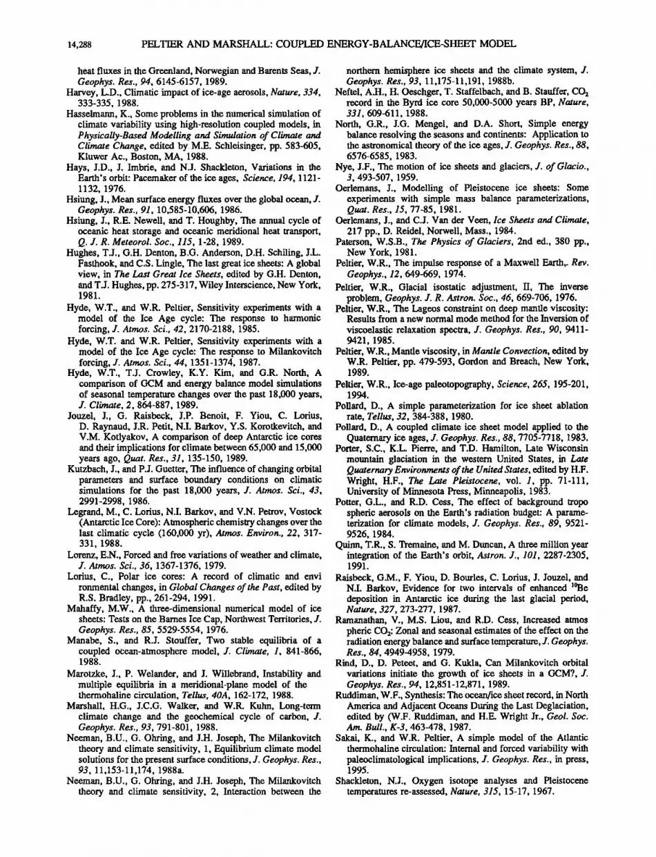
14,288 PELTIER AND MARSHALL: COUPLED ENERGY-BALANCE/ICE-SHEET MODEL
heat fluxes in the Greenland, Norwegian and Barents Seas, J. Geophys. Res., 94, 6145-6157, 1989.
Harvey, L.D., Climatic impact of ice-age aerosols, Nature, 334, 333-335, 1988.
Hasselmann, K., Some problems in the numerical simulation of climate variability using high-resolution coupled models, in Physically-Based Modelling and Simulation of Climate and Climate Change, edited by M.E. Schleisinger, pp. 583-605, Kluwer Ac., Boston, MA, 1988.
Hays, J.D., J. Imbrie, and N.J. Shackleton, Variations in the Earth's orbit: Pacemaker of the ice ages, Science, 194, 1121- 1132, 1976.
Hsiung, J., Mean surface energy fluxes over the global ocean, J. Geophys. Res., 91, 10,585-10,606, 1986.
Hsiung, J., R.E. Newell, and T. Houghby, The annual cycle of oceanic heat storage and oceanic meridional heat transport, Q. J. R. Meteorol. Soc., 115, 1-28, 1989.
Hughes, T.J., G.H. Denton, B.G. Anderson, D.H. Schiling, J.L. Fasthook, and C.S. Lingle, The last great ice sheets: A global view, in The Last Great Ice Sheets, edited by G.H. Denton, and T.J. Hughes, pp. 275-317, Wiley Interscience, New York, 1981.
Hyde, W.T., and W.R. Peltlet, Sensitivity experiments with a model of the Ice Age cycle: The response to harmonic forcing, J. Atmos. Sci., 42, 2170-2188, 1985.
Hyde, W.T. and W.R. Peltlet, Sensitivity experiments with a model of the Ice Age cycle: The response to Milankovitch forcing, J. Atmos. Sci., 44, 1351-1374, 1987.
Hyde, W.T., T.J. Crowley, K.Y. Kim, and G.R. North, A comparison of GCM and energy balance model simulations of seasonal temperature changes over the past 18,000 years, J. Climate, 2,864-887, 1989.
Jouzel, J., G. Raisbeck, J.P. Benoit, F. Yiou, C. Lorius, D. Raynaud, J.R. Petit, N.I. Barkov, Y.S. Korotkevitch, and V.M. Kotlyakov, A comparison of deep Antarctic ice cores and their implications for climate between 65,000 and 15,000 years ago, Quat. Res., 31, 135-150, 1989.
Kutzbach, J., and P.J. Guetter, The influence of changing orbital parameters and surface boundary conditions on climatic simulations for the past 18,000 years, J. Atmos. Sci., 43, 2991-2998, 1986.
Legrand, M., C. Lorius, N.I. Barkov, and V.N. Petrov, Vostock (Antarctic Ice Core): Atmospheric chemistry changes over the last climatic cycle (160,000 yr), Atmos. Environ., 22, 317- 331, 1988.
Lorenz, E.N., Forced and free variations of weather and climate, J. Atmos. Sci., 36, 1367-1376, 1979.
Lorius, C., Polar ice cores: A record of climatic and envi tonmental changes, in Global Changes of the Past, edited by R.S. Bradley, pp., 261-294, 1991.
Mahaffy, M.W., A three-dimensional numerical model of ice sheets: Tests on the Barnes Ice Cap, Northwest Territories, J. Geophys. Res., 85, 5529-5554, 1976.
Manabe, S., and R.J. Stouffer, Two stable equilibria of a coupled ocean-atmosphere model, J. Climate, 1, 841-866, 1988.
Marotzke, J., P. Welander, and J. Willebrand, Instability and multiple equilibria in a meridional-plane model of the thermohaline circulation, Tellus, 40A, 162-172, 1988.
Marshall, H.G., J.C.G. Walker, and W.R. Kuhn, Long-term climate change and the geochemical cycle of carbon, J. Geophys. Res., 93, 791-801, 1988.
Neeman, B.U., G. Ohring, and J.H. Joseph, The Milankovitch theory and climate sensitivity, 1, Equilibrium climate model solutions for the present surface conditions, J. Geophys. Res., 93, 11,153-11,174, 1988a.
Neeman, B.U., G. Ohring, and J.H. Joseph, The Milankovitch theory and climate sensitivity, 2, Interaction between the
northern hemisphere ice sheets and the climate system, J. Geophys. Res., 93, 11,175-11,191, 1988b.
Neftel, A.H., H. Oeschger, T. Staffe!bach, and B. Stauffer, CO2 record in the Byrd ice core 50,000-5000 years BP, Nature, 331,609-611, 1988.
North, G.R., J.G. Mengel, and D.A. Short, Simple energy balance resolving the seasons and continents: Application to the astronomical theory of the ice ages, J. Geophys. Res., 88, 6576-6585, 1983.
Nye, J.F., The motion of ice sheets and glaciers, J. of Glacio., 3, 493-507, 1959.
Oerlemans, J., Modelling of Pleistocene ice sheets: Some experiments with simple mass balance parameterizations, Quat. Res., 15, 77-85,1981.
Oerlemans, J., and C.J. Van der Veen, Ice Sheets and Climate, 217 pp., D. Reidel, Norwell, Mass., 1984.
Paterson, W.S.B., The Physics of Glaciers, 2nd ed., 380 pp., New York, 1981.
Peltlet, W.R., The impulse response of a Maxwell Earth,. Rev. Geophys., 12,649-669, 1974.
Peltlet, W.R., Glacial isostatic adjustment, H, The inverse problem, Geophys. J. R. Astron. Soc., 46, 669-706, 1976.
Peltier, W.R., The Lageos constraint on deep mantle viscosity: Results from a new normal mode method for the Inversion of
viscoelastic relaxation spectra, J. Geophys. Res., 90, 9411- 9421, 1985.
Peltlet, W.R., Mantle viscosity, in Mantle Convection, edited by W.R. Peltlet, pp. 479-593, Gordon and Breach, New York, 1989.
Peltier, W.R., Ice-age paleotopography, Science, 265, 195-201, 1994.
Pollard, D., A simple parameterization for ice sheet ablation rate, Tellus, 32, 384-388, 1980.
Pollard, D., A coupled climate ice sheet model applied to the Quaternary ice ages, J. Geophys. Res., 88, 7705-7718, 1983.
Porter, S.C., K.L. Pierre, and T.D. Hamilton, Late Wisconsin mountain glaciation in the western United States, in Late Quaternary Environments of the United States, edited by H.F. Wright, H.F., The Late Pleistocene, vol. 1, pp. 71-111, University of Minnesota Press, Minneapolis, 1983.
Potter, G.L., and R.D. Cess, The effect of background tropo spheric aerosols on the Earth's radiation budget: A parame- terization for climate models, J. Geophys. Res., 89, 9521- 95 26, 1984.
Quinn, T.R., S. Tremaine, and M. Duncan, A three million year integration of the Earth's orbit, Astron. J., 101, 2287-2305, 1991.
Raisbeck, G.M., F. Yiou, D. Bourles, C. Lorius, J. Jouzel, and N.I. Barkov, Evidence for two intervals of enhanced •øBe deposition in Antarctic ice during the last glacial period, Nature, 327, 273-277, 1987.
Ramanathan, V., M.S. Liou, and R.D. Cess, Increased atmos pheric CO:: Zonal and seasonal estimates of the effect on the radiation energy balance and surface temperature, J. Geophys. Res., 84, 4949-4958, 1979.
Rind, D., D. Peteet, and G. Kukla, Can Milankovitch orbital variations initiate the growth of ice sheets in a GCM?, J. Geophys. Res., 94, 12,851-12,871, 1989.
Ruddiman, W.F., Synthesis: The ocean/ice sheet record, in North America and Adjacent Oceans During the Last Deglaciation, edited by (W.F. Ruddiman, and H.E. Wright Jr., Geol. Soc. Am. Bull., K-3, 463-478, 1987.
Sakai, K., and W.R. Peltier, A simple model of the Atlantic thermohaline circulation: Internal and forced variability with paleoclimatological implications, J. Geophys. Res., in press, 1995.
Shackleton, N.J., Oxygen isotope analyses and Pleistocene temperatures re-assessed, Nature, 315, 15-17, 1967.

PELTIER AND MARSHALL: COUPLED ENERGY-BALANCE/ICE-SHEET MODEL 14,289
Short, D.A., and G.R. North, Infrared parameterization and simple climate models, J. Clim. Appl. Meteorol., 23, 1222- 1233, 1984.
Stauffer, B., E. Lockbronner, H. Oeschger, and J. Schwander, Methane concentration in the global atmosphere was only half that of the preindustrial Holocene, Nature, 332, 812- 814, 1988.
Stephens, G.L., G.C. Campbell, and T.H. Vonder Haar, Earth radiation budgets, J. Geophys. Res., 86, 9739-9760, 1981.
Thompson, L.G., and E. Mosley-Thompson, Microparticle concentration variations linked with climatic change: Evi- dence from polar ice cores, Science, 212, 812-815, 1981.
Tushingham, A.M., and W.R. Peltier, ICE-3G: A new global model of late Pleistocene deglaciation based upon geo- physical predictions of post-glacial relative sea level changes, J. Geophys. Res., 96, 4497-4523, 1991.
Tushingham, A.M., and W.R. Peltier, Validation of the ICE-3G model of W'tirm-Wisconsin deglaciation using a data base of relative sea level histories, J. Geophys. Res., 97, 3285-3304, 1992.
Van der Deen, C.J., Land ice and climate, in Climate System
Modelling, edited by K.E. Trenberth, Cambridge University Press, New York, in press, 1995.
Warrick, R.A., and J. Oerlemans, Sea level rise, in Climate Change, The IPCC Scientific Assessment, edited by J.T. Houghton, G.J. Jenkins, and J.T. Ephraums, Cambridge University Press, New York, 1990.
Wright, D.G., and T.F. Stocker, A zonally averaged ocean model of the thermohaline circulation, Part I, Model devel- opment and flow dynamics, J. Phys. Oceanogr., 21, 1713- 1724, 1991.
Zhang, D., Meteorological characteristics of dust fall in China since historic times, in Quaternary Geology and Environment of China, edited by T.S. Liu., p.p. 161-166, China Ocean Press, Beijing, 1982.
S. Marshall and W.R. Peltier, Deprtment of Physics, Univer- sity of Toronto, Toronto, Ontario, Canada M5S 1A7. (e-mail: [email protected])
(Received May 10, 1994; revised October 10, 1994; accepted December 29, 1994.)


