Embed Size (px)
Citation preview
DETERMINATION OF GLACIAL-ICE TEMPERATURE
PROFILES USING RADAR AND AN ANTENNA-GAIN
ESTIMATION TECHNIQUE
BY
Mike Hughes
Submitted to the graduate degree program in Electrical Engineering
and the Graduate Faculty of the University of Kansas School of Engineering
in partial fulfillment of the requirements for the degree of
Master of Science
______________________
Dr. Kenneth Demarest
Chairperson
Committee Members* ______________________
Dr. Chris Allen*
______________________
Dr. Carl Leuschen*
Date defended: ______________

- 2 -
The Thesis Committee for Mike Hughes certifies
That this is the approved Version of the following thesis:
DETERMINATION OF GLACIAL-ICE TEMPERATURE PROFILES USING RADAR AND AN ANTENNA-GAIN ESTIMATION TECHNIQUE
Committee:
______________________ Dr. Kenneth Demarest
Chairperson
______________________ Dr. Chris Allen
______________________ Dr. Carl Leuschen
Date defended: ______________
- 3 -
ABSTRACT
Knowledge of glacial ice temperature profiles is important to the study of
glaciology. Currently, the only method of obtaining ice temperature profiles is by
drilling ice cores, which is a long and arduous process. Fortunately, ice-penetrating
radar can be used to obtain temperature profiles without the need of ice cores. A radar
technique incorporating common mid-point geometries is presented for measuring ice
temperature. However, in order for this technique to work, accurate estimates of the
far-zone antenna gain within glacial ice are necessary. Currently, commercial
electromagnetics software packages utilizing the finite element method (FEM) are
used by academia and industry to accurately characterize antennas in free space, and
near finite dielectric and conductive materials. Unfortunately, these commercial
packages are incapable of accurately determining the far-zone antenna gain near a
dielectric half-space such as glacial ice. Therefore, to solve this problem, a routine for
determining the far-zone gain of an antenna located near glacial ice was developed,
which utilizes an FEM package in conjunction with a near-to-far-field transformation
(NFFT). Additionally, glacial ice imposes another complication to estimating far-
zone antenna gain: the dielectric constant is a function of depth. Therefore the far-
zone antenna gain within glacial ice changes as a function of depth due to increased
ray bending resulting from refraction. To solve this problem, the geometric optics
technique (GO) was used to propagate the far-zone antenna gain determined within
the relatively shallow upper region of glacial ice, dubbed the quasi-far-zone, to any
depth within glacial ice. Results are presented showing that this technique is capable
of accurately determining the far-zone gain at any depth within glacial ice for an
arbitrary antenna located near glacial ice. Additionally, results are presented showing
that with the aid of this numerical antenna gain estimation software, ice-penetrating
radar can be used to determine glacial ice temperature profiles at all depths.

- 4 -
ACKNOWLEDGEMENT
I would like to thank Dr. Demarest for being my adviser and committee chair.
His support and vast knowledge of electromagnetics made this work possible. I would
also like to thank Dr. Allen and Dr. Leuschen for serving on my committee, and
providing their invaluable support and insight. Also, while at CReSIS, I had the
fortune of being exposed to numerous areas of remote-sensing. Therefore, I wish to
thank all the faculty, staff, and students at CReSIS for their support in furthering my
development as an electrical engineer.
- 5 -
TABLE OF CONTENTS
LIST OF FIGURES ............................................................................................................... - 7 -
LIST OF TABLES ................................................................................................................. - 9 -
CHAPTER 1: INTRODUCTION .......................................................................................... - 10 -
1.1 MOTIVATION ................................................................................................................... - 10 - 1.2 RADAR SET-UP FOR ATTENUATION PROFILING .............................................................. - 11 - 1.3 THE IMPORTANCE OF PREDICTING ANTENNA GAIN ........................................................ - 13 - 1.4 COMPLICATIONS IN DETERMINING ANTENNA GAIN WITHIN GLACIAL ICE ...................... - 15 - 1.5 A SOLUTION FOR DETERMINING FAR-ZONE ANTENNA GAIN IN GLACIAL ICE ................ - 16 - 1.6 THESIS ORGANIZATION ................................................................................................... - 18 -
CHAPTER 2: ANTENNA ANALYSIS USING HFSS ......................................................... - 19 -
2.1 THE FINITE ELEMENT METHOD....................................................................................... - 19 - 2.2 FREE-SPACE ANTENNA MODELING ................................................................................. - 20 -
2.2.1 The Solution Space .................................................................................................... - 21 - 2.2.2 Boundary Conditions ................................................................................................. - 22 - 2.2.3 Port Excitation .......................................................................................................... - 22 - 2.2.4 Solution Set-Up .......................................................................................................... - 25 -
2.3 FAR-ZONE FIELD CALCULATIONS USING HFSS ............................................................. - 25 - 2.4 MODELING ANTENNAS ABOVE A HALF-SPACE OF GLACIAL ICE ..................................... - 30 -
2.4.1 HFSS Modeling Adjustments for Antennas Near Glacial Ice .................................... - 30 - 2.4.2 What HFSS Will Let You Do Even Though It Is Incorrect! ....................................... - 32 -
2.5 HFSS MODELING SUMMARY .......................................................................................... - 34 -
CHAPTER 3: FAR-ZONE FIELD PATTERNS IN GLACIAL ICE ...................................... - 35 -
3.1 BACKGROUND FOR THE FEM-NFFT-GO TECHNIQUE .................................................... - 35 - 3.1.1 Far-Zone Fields within Uniform Glacial Ice ............................................................. - 36 - 3.1.2 Far-Zone Fields within Non-Uniform Glacial Ice ..................................................... - 41 -
3.1.2.1 Glacial Ice Empirical Density Model ............................................................................. - 41 - 3.1.2.2 Geometric Optics Ray Tracing ....................................................................................... - 44 -
3.2 USING THE FEM-NFFT-GO TECHNIQUE TO DETERMINE FAR-ZONE ELECTRIC FIELDS . - 48 - 3.2.1 Sampling and Exporting Near-Zone Fields ............................................................... - 48 - 3.2.2 Running the FEM-NFFT-GO Routine ....................................................................... - 52 -
3.2.2.1 HFSS Requirements ....................................................................................................... - 52 - 3.2.2.2 The Master.m Matlab File .............................................................................................. - 53 -
CHAPTER 4: FAR-ZONE FIELD RESULTS FOR ICE-MOUNTED ANTENNAS ............ - 58 -
4.1 FEM-NFFT VALIDATION TESTS ..................................................................................... - 58 - 4.1.1 The Null Field Test .................................................................................................... - 58 - 4.1.2 The Hertzian Dipole Test ........................................................................................... - 63 - 4.1.3 Effects of Sampling Location ..................................................................................... - 66 - 4.1.4 Comparing FEM-NFFT Results with HFSS Near-Zone Results ............................... - 70 -
4.2 COMBINED FEM-NFFT-GO RESULTS ............................................................................ - 73 -
CHAPTER 5: GLACIAL ICE TEMPERATURE EXTRACTION FROM ATTENUATION MEASUREMENTS .............................................................................................................. - 79 -
5.1 CAUSES OF ATTENUATION IN GLACIAL ICE..................................................................... - 79 - 5.2 CONDUCTIVITY IN GLACIAL ICE ..................................................................................... - 81 - 5.3 MEASURED GLACIAL TEMPERATURE PROFILES .............................................................. - 83 - 5.4 RELATION OF ATTENUATION TO ICE PERMITTIVITY AND TEMPERATURE ........................ - 87 -

- 6 -
5.5 ATTENUATION EXTRACTION FROM RADAR ECHOES ....................................................... - 89 - 5.6 TEMPERATURE EXTRACTION FROM MEASURED ATTENUATION ...................................... - 92 - 5.7 SIMULATED TEMPERATURE PROFILE RESULTS ............................................................... - 94 -
5.7.1 Simulated Temperature Extraction under Ideal Conditions ...................................... - 97 - 5.7.2 Effect of Neglecting Refractive Gain on Temperature Extraction ........................... - 100 - 5.7.3 Effect of Ice Density Profile Error on Temperature Extraction .............................. - 103 - 5.7.4 Effect of Using a Free-Space Hertzian Dipole as Estimated Antenna Gain ............ - 109 -
5.8 CHAPTER 5 RESULTS SUMMARY ................................................................................... - 111 -
CHAPTER 6: SUMMARY/CONCLUSIONS/FUTURE WORK ......................................... - 114 -
6.1 ANTENNA-GAIN ESTIMATION SUMMARY ...................................................................... - 115 - 6.2 EFFECTS OF ANTENNA-GAIN ESTIMATION ON ICE-TEMPERATURE EXTRACTION SUMMARY
…………………………………………………………………………………………- 115 - 6.3 CONCLUSIONS ............................................................................................................... - 116 - 6.4 FUTURE WORK .............................................................................................................. - 117 -
APPENDIX A: QUASI-FAR-ZONE FIELD DERIVATION ................................................ - 118 -
APPENDIX B: FEM-NFFT-GO MATLAB CODE CONTRACTS...................................... - 133 -
APPENDIX C: ICETEMP.M MATLAB CODE .................................................................. - 143 -
REFERENCES .................................................................................................................. - 153 -

- 7 -
LIST OF FIGURES FIGURE 1.1 – ICE-PENETRATING RADAR SYSTEM .............................................................................. - 10 - FIGURE 1.2 − BISTATIC-RADAR COMMON M IDPOINT CONFIGURATIONS ........................................... - 12 - FIGURE 1.3 − THE THREE FIELD REGIONS .......................................................................................... - 17 - FIGURE 2.1 − GENERIC HFSS MODELING .......................................................................................... - 21 - FIGURE 2.2 – WAVEPORT USAGE IN COAX-TO-STRIPLINE HFSS MODEL .......................................... - 23 - FIGURE 2.3 – LUMPED PORT USAGE IN DIPOLE HFSS MODEL ........................................................... - 24 - FIGURE 2.4 − FREE-SPACE EQUIVALENCE .......................................................................................... - 26 - FIGURE 2.5 – GEOMETRY FOR A Z-DIRECTED HERTZIAN DIPOLE ....................................................... - 27 - FIGURE 2.6 – NFFT SUPERPOSITION FROM A SINGLE SURFACE OF CURRENT SEGMENTS .................. - 29 - FIGURE 2.7 − HFSS MODELING NEAR A HALF-SPACE ....................................................................... - 31 - FIGURE 2.8 − FAR-ZONE E-PLANE FOR HORIZONTAL HERTZIAN DIPOLE MOUNTED ABOVE GLACIAL ICE
FROM HFSS (DB) ..................................................................................................................... - 33 - FIGURE 3.1 − THE THREE FIELD REGIONS .......................................................................................... - 36 - FIGURE 3.2 − EQUIVALENCE FOR A HALF-SPACE OF GLACIAL ICE ..................................................... - 37 - FIGURE 3.3 − RECIPROCITY FOR A HALF-SPACE OF GLACIAL ICE ...................................................... - 38 - FIGURE 3.4 − GLACIAL ICE DENSITY VS. DEPTH: EMPIRICAL MODELS .............................................. - 42 - FIGURE 3.5 − GLACIAL ICE DIELECTRIC CONSTANT VS. DEPTH: EMPIRICAL MODELS ....................... - 43 - FIGURE 3.6 − GEOMETRIC OPTICS RAY TRACING – CONSTANT ENERGY TUBES ................................ - 45 - FIGURE 3.7 − HFSS V. 10 FIELDS CALCULATOR ................................................................................ - 49 - FIGURE 3.8 − HFSS V. 10 FIELDS CALCULATOR EXPORT SOLUTION WINDOW .................................. - 50 - FIGURE 3.9 – HFSS HALF-SPACE MODELING CONVENTION .............................................................. - 52 - FIGURE 4.1 − THE NULL-FIELD TEST ................................................................................................. - 59 - FIGURE 4.2 − THE NULL-FIELD TEST: FOUR TEST CASES .................................................................. - 62 - FIGURE 4.3 − HORIZONTAL HERTZIAN DIPOLE .................................................................................. - 63 - FIGURE 4.4 − E-PLANE OF HORIZONTAL HERTIZAN DIPOLE FAR-ZONE FIELDS (DBI): FEM-NFFT,
EXACT, AND FREE SPACE ......................................................................................................... - 65 - FIGURE 4.5 − H-PLANE OF HORIZONTAL HERTZIAN DIPOLE FAR-ZONE FIELDS (DBI): FEM-NFFT,
EXACT, AND FREE SPACE ......................................................................................................... - 66 - FIGURE 4.6 − VERTICAL HERTZIAN DIPOLE ....................................................................................... - 67 - FIGURE 4.7 − FAR-ZONE E-PLANE OF VERTICAL HERTZIAN DIPOLE ABOVE ICE (DBI): NEAR-ZONE
FIELDS SAMPLED AT 2Λ ............................................................................................................ - 68 - FIGURE 4.8 − FAR-ZONE E-PLANE OF VERTICAL HERTZIAN DIPOLE ABOVE ICE (DBI): NEAR-ZONE
FIELDS SAMPLED AT Λ .............................................................................................................. - 69 - FIGURE 4.9 − FAR-ZONE E-PLANE OF VERTICAL HERTZIAN DIPOLE ABOVE ICE (DBI): NEAR-ZONE
FIELDS SAMPLED AT 0.5Λ ......................................................................................................... - 70 - FIGURE 4.10 − E-PLANE OF HORIZONTAL HERTZIAN DIPOLE FAR-ZONE FIELDS (DBI): FROM HFSS
NEAR-FIELD CALCULATOR....................................................................................................... - 71 - FIGURE 4.11 − H-PLANE OF HORIZONTAL HERTZIAN DIPOLE FAR-ZONE FIELDS (DBI): FROM HFSS
NEAR-FIELD CALCULATOR....................................................................................................... - 72 - FIGURE 4.12 − TAPERED SLOT ANTENNA (V IVALDI ) ......................................................................... - 74 - FIGURE 4.13 − VIVALDI FREE-SPACE PATTERN (DBI) – E-PLANE ...................................................... - 74 - FIGURE 4.14 − VIVALDI FEM-NFFT RESULT – E-PLANE GAIN (DBI) ............................................... - 76 - FIGURE 4.15 − GAIN PATTERN AT VARIOUS DEPTHS FOR V IVALDI ANTENNA (E-PLANE) ................. - 77 - FIGURE 4.16 − GAIN PATTERN AT VARIOUS DEPTHS FOR HERTZIAN DIPOLE (E-PLANE) ................... - 78 - FIGURE 5.1 − GLACIAL ICE CONDUCTIVITY CONTRIBUTIONS [28] (FOR FREQUENCIES BETWEEN 0.1 TO
300 MHZ) ................................................................................................................................. - 82 - FIGURE 5.2 − GLACIAL ICE TEMPERATURE AT 10 M DEPTH VS. ELEVATION [41] ............................... - 84 - FIGURE 5.3 − MEASURED TEMPERATURE PROFILES FROM ANTARCTICA ........................................... - 85 -
- 8 -
FIGURE 5.4 − MEASURED TEMPERATURE PROFILE FROM GREENLAND .............................................. - 86 - FIGURE 5.5 − BISTATIC-RADAR COMMON M IDPOINT CONFIGURATIONS ........................................... - 89 - FIGURE 5.6 – COMMON MID-POINT RADAR SET-UPS FOR LAYER 1 ................................................... - 90 - FIGURE 5.7 – MEASURED TEMPERATURE PROFILES USED FOR SIMULATION ...................................... - 94 - FIGURE 5.8 –MEASURED/SIMULATED TEMPERATURE PROFILES (IDEAL CASE) ................................. - 98 - FIGURE 5.9 – TEMPERATURE EXTRACTION ERROR (IDEAL CASE) ...................................................... - 98 - FIGURE 5.10 – MEASURED/SIMULATED ATTENUATION PROFILES (IDEAL CASE) ............................... - 99 - FIGURE 5.11 – ATTENUATION EXTRACTION ERROR (IDEAL CASE) .................................................. - 100 - FIGURE 5.12 – ERROR BETWEEN SIMULATED /MEASURED TEMPERATURE PROFILES (IGNORING
REFRACTIVE GAIN) ................................................................................................................ - 101 - FIGURE 5.13 – MEASURED/SIMULATED TEMPERATURE PROFILES (IGNORING REFRACTIVE GAIN).. - 102 - FIGURE 5.14 – ANTENNA-GAIN ESTIMATION ERROR IN DB (IGNORING REFRACTIVE GAIN) ............ - 103 - FIGURE 5.15 – DENSITY PROFILES ................................................................................................... - 104 - FIGURE 5.16 – TEMPERATURE EXTRACTION ERROR (PROFILE 2 DENSITY MODEL) ......................... - 105 - FIGURE 5.17 – MEASURED/SIMULATED TEMPERATURE PROFILES (PROFILE 2 DENSITY MODEL) .... - 105 - FIGURE 5.18 - TEMPERATURE EXTRACTION ERROR (PROFILE 1 DENSITY MODEL) .......................... - 106 - FIGURE 5.19 – MEASURED/SIMULATED TEMPERATURE PROFILES (PROFILE 1 DENSITY MODEL) .... - 107 - FIGURE 5.20 – ANTENNA-GAIN ESTIMATION ERROR IN DB (INCORRECT DENSITY PROFILE)........... - 108 - FIGURE 5.21 – TEMPERATURE EXTRACTION ERROR (FREE-SPACE HERTZIAN DIPOLE) ................... - 109 - FIGURE 5.22 – MEASURED/SIMULATED TEMPERATURE PROFILES (FREE-SPACE HERTZIAN DIPOLE)
....................................................................................................................... ………………- 110 - FIGURE 5.23 – ANTENNA-GAIN ESTIMATION ERROR IN DB (FREE-SPACE HERTZIAN DIPOLE) ........ - 111 - FIGURE 5.24 – ANTENNA-GAIN ESTIMATION ERROR IN DB (ALL ERROR SOURCES) ........................ - 112 - FIGURE A.1 − RECIPROCITY ............................................................................................................. - 118 - FIGURE A.2 - CASE 1 RECIPROCITY DERIVATION ............................................................................ - 120 - FIGURE A.3 – FIELDS PRODUCED BY Θ-DIRECTED OBSERVER ELECTRIC TEST CURRENT ................ - 122 -

- 9 -
LIST OF TABLES TABLE 1.1 − RADAR SYSTEM KEY PARAMETERS ............................................................................... - 13 - TABLE 2.1 − HFSS MODELING REQUIREMENTS NEAR GLACIAL ICE ................................................. - 31 - TABLE 3.1 -- ICE DENSITY EMPIRICAL CONSTANTS ........................................................................... - 42 - TABLE 3.2 – HFSS VECTOR CARTESIAN FIELD VALUE OUTPUT FILE FORMAT ................................. - 51 - TABLE 3.3 – HFSS POINTS FILE FORMAT .......................................................................................... - 51 - TABLE 3.4 − HFSS MODEL NAMING CONVENTIONS .......................................................................... - 53 - TABLE 3.5 − FEM-NFFT-GO INPUT PARAMETERS ............................................................................ - 54 - TABLE 3.6 − FEM-NFFT OUTPUT PARAMETERS ............................................................................... - 57 - TABLE 3.7 − GO OUTPUT PARAMETERS ............................................................................................. - 57 - TABLE 4.1 – THE NULL-FIELD TEST CASES ....................................................................................... - 59 - TABLE 4.2 − HORIZONTAL HERTIZAN DIPOLE TEST PARAMETERS .................................................... - 64 - TABLE 4.3 − VERTICAL DIPOLE MODELING PARAMETERS ................................................................. - 67 - TABLE 4.4 − HFSS NEAR-ZONE FIELD PARAMETERS ........................................................................ - 71 - TABLE 4.5 − VIVALDI MODELING PARAMETERS ................................................................................ - 75 - TABLE 5.1 - IDEAL TEMPERATURE PROFILE EXTRACTION SIMULATION PARAMETERS ...................... - 97 - TABLE 5.2 – DENSITY PROFILE EMPIRICAL CONSTANTS .................................................................. - 103 - TABLE 5.3 – GAIN ESTIMATION ERROR COMPARISON ..................................................................... - 113 - TABLE A.1 – THE FOUR RECIPROCITY CASES .................................................................................. - 120 - TABLE A.2 – DUALITY [18] .............................................................................................................. - 130 -
- 10 -
CHAPTER 1: Introduction
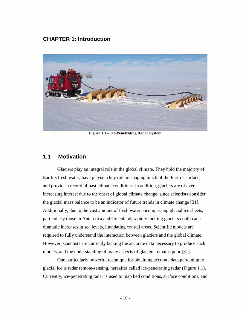
Figure 1.1 – Ice-Penetrating Radar System
1.1 Motivation
Glaciers play an integral role in the global climate. They hold the majority of
Earth’s fresh water, have played a key role in shaping much of the Earth’s surface,
and provide a record of past climate conditions. In addition, glaciers are of ever
increasing interest due to the onset of global climate change, since scientists consider
the glacial mass balance to be an indicator of future trends in climate change [31].
Additionally, due to the vast amount of fresh water encompassing glacial ice sheets,
particularly those in Antarctica and Greenland, rapidly melting glaciers could cause
dramatic increases in sea levels, inundating coastal areas. Scientific models are
required to fully understand the interaction between glaciers and the global climate.
However, scientists are currently lacking the accurate data necessary to produce such
models, and the understanding of many aspects of glaciers remains poor [31].
One particularly powerful technique for obtaining accurate data pertaining to
glacial ice is radar remote-sensing, hereafter called ice-penetrating radar (Figure 1.1).
Currently, ice-penetrating radar is used to map bed conditions, surface conditions, and

- 11 -
internal layers of glacial ice, allowing such calculations as ice thickness and annual
snow accumulation. However, with accurate knowledge of the far-zone antenna
radiation pattern within glacial ice, the full power of ice-penetrating radar can be
utilized. With this knowledge, the attenuation as a function of depth can be accurately
determined. Then, since it is directly related to attenuation, temperature as a function
of depth can be obtained.
Glacial ice temperature profiles are invaluable to the study of glaciers and
climate. In particular, “ice temperature is important for a variety of glacial processes,
including glacial flow, meltwater drainage, and subglacial erosion and deposition,”
[31]. Currently however, obtaining ice temperature profiles is a long and difficult
process, since it requires the drilling of ice cores, a process that can take years to
complete. The ability to use ice-penetrating radar in obtaining temperature profiles
would eliminate the need for drilling ice cores to obtain temperature measurements.
This would make temperature profiles much easier to obtain over much broader areas
of the Antarctica and Arctic ice sheets, which should greatly improve the science of
studying glaciers and climate. Next, the proposed radar set-up for measuring ice
temperature is presented.
1.2 Radar Set-Up for Attenuation Profiling
The proposed radar set-up for determining glacial ice attenuation as a function
of depth involves placement of both transmit and receive antennas directly on the ice-
cap surface in common midpoint (CMP) geometry. Two separate CMP configurations
are utilized to achieve two separate signals off of each resolution layer [27], as shown
in Figure 1.2. The resolution layer shown in Figure 1.2 is 100 meters, and indicates
the depth-range for which a single attenuation value is obtained. Also, the use of two
separate CMP configurations is desirable since it reduces some of the uncertainties
associated with attenuation profile extraction [32].
- 12 -
(a) (b)
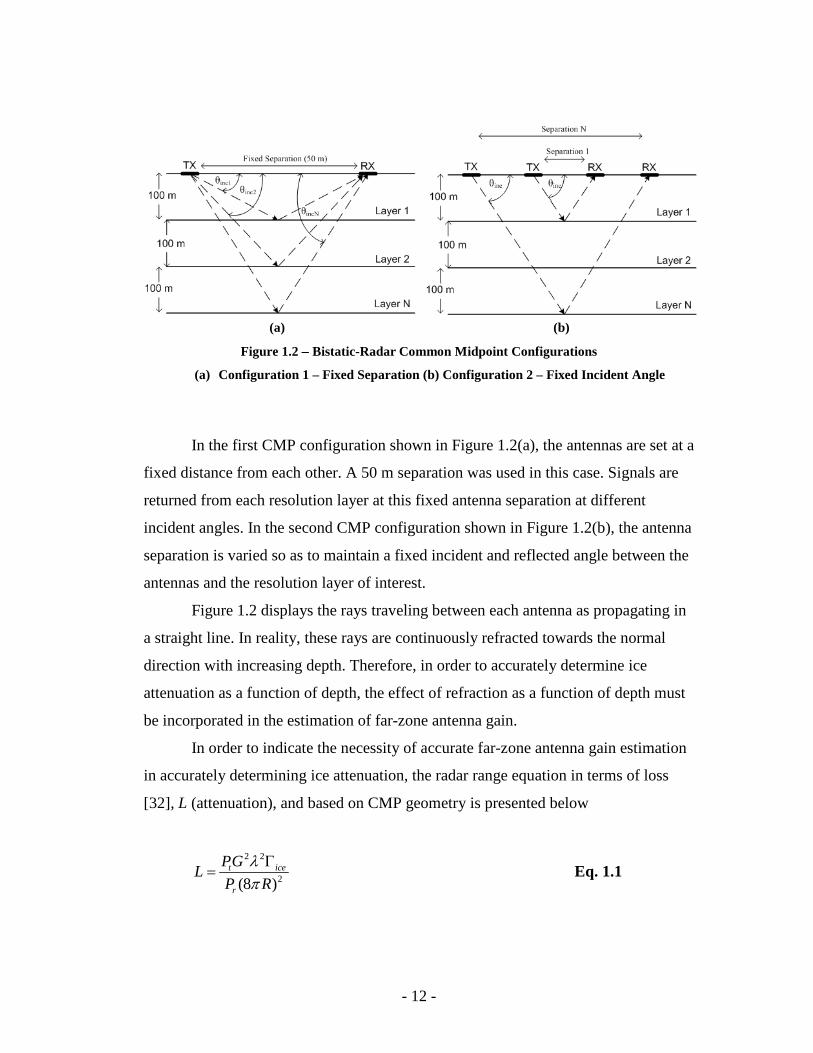
Figure 1.2 −−−− Bistatic-Radar Common Midpoint Configurations
(a) Configuration 1 – Fixed Separation (b) Configuration 2 – Fixed Incident Angle
In the first CMP configuration shown in Figure 1.2(a), the antennas are set at a
fixed distance from each other. A 50 m separation was used in this case. Signals are
returned from each resolution layer at this fixed antenna separation at different
incident angles. In the second CMP configuration shown in Figure 1.2(b), the antenna
separation is varied so as to maintain a fixed incident and reflected angle between the
antennas and the resolution layer of interest.
Figure 1.2 displays the rays traveling between each antenna as propagating in
a straight line. In reality, these rays are continuously refracted towards the normal
direction with increasing depth. Therefore, in order to accurately determine ice
attenuation as a function of depth, the effect of refraction as a function of depth must
be incorporated in the estimation of far-zone antenna gain.
In order to indicate the necessity of accurate far-zone antenna gain estimation
in accurately determining ice attenuation, the radar range equation in terms of loss
[32], L (attenuation), and based on CMP geometry is presented below
2 2
2(8 )t ice
r
PGL
P R
λπ
Γ= Eq. 1.1
- 13 -
The parameters Pr and Pt are the power received and transmitted which are accurately
known. Also, R is the range to the target which is determined by the round-trip transit
time of the radar signal. Additionally, iceΓ is the internal ice specular reflection
coefficient which can be assumed to be -80 dB. However, any uncertainties
associated with iceΓ are eliminated through use of the two combined radar CMP
configurations (see Chapter 4). Therefore, the only unknown in Equation 1.1 required
in determining the loss L is the antenna gain G. Equation 1.1 assumes the transmit
and receive antennas are identical, which is the case for the two proposed CMP
geometries.
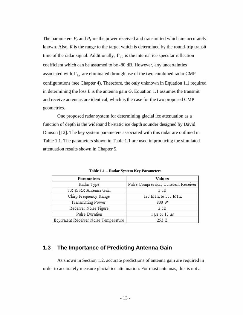
One proposed radar system for determining glacial ice attenuation as a
function of depth is the wideband bi-static ice depth sounder designed by David
Dunson [12]. The key system parameters associated with this radar are outlined in
Table 1.1. The parameters shown in Table 1.1 are used in producing the simulated
attenuation results shown in Chapter 5.
Table 1.1 −−−− Radar System Key Parameters
1.3 The Importance of Predicting Antenna Gain
As shown in Section 1.2, accurate predictions of antenna gain are required in
order to accurately measure glacial ice attenuation. For most antennas, this is not a
- 14 -
simple task. Due to the complexity of most modern antennas (and other electronic
devices), their analysis does not lead to closed form solutions of Maxwell’s equations.
Therefore, numerical methods for approximating these solutions while maintaining
engineering accuracy is required [39]. A number of numerical techniques exist for
approximating solutions to Maxwell’s equations, each of which differ in the way they
discretize the problem from the continuous domain. One means of categorizing these
techniques is to separate them into those based on partial differential equation
formulations, and those based on integrodifferential equation formulations.
The two most popular techniques within the partial differential equation
category are the finite difference (FD) and finite element method (FEM). Either of
these techniques can be exploited in the time or frequency domain. However, FD is
usually exploited in the time domain, and called the FDTD (finite-difference time-
domain) technique [26]. Both of these techniques are similar in that they directly
solve for the near-zone electric and magnetic fields within a finite solution space.
Also, since both of these techniques solve for fields within a finite space, boundary
conditions and hybrid methods are required for analyzing open structures to transform
the infinite region to a finite one [39]. Although both the FDTD and FEM techniques
are well-suited for arbitrary and versatile materials and geometries, and considered
computational efficient, the FEM is considered to be slightly superior to the FDTD in
these categories [39]. In particular, the FEM technique is much better suited for
arbitrary geometries than the FDTD [7].
The most popular technique within the integrodifferential equation category is
the method of moments (MoM) [19]. Rather than solving directly for the fields within
a finite solution space, as with the FEM and FDTD techniques, the MoM works by
determining the currents on individual segments of the antenna structure resulting
from the antenna excitation [19]. Also, unlike the FEM and FDTD techniques, the
MoM is best suited for open structures [39]. Therefore, the MoM can directly
determine far-zone patterns in an open region without the requirement of hybrid
techniques. Two major drawbacks of the MoM however, are its inability to analyze
- 15 -
problems of arbitrary materials (i.e. dielectrics) or geometries. But, although the
MoM is not generally well-suited for antennas that contain dielectrics, some
formulations, such as the Numerical Electromagnetic Code (NEC) [8] can model wire
antennas on or near a dielectric half-space, and provide far-zone patterns within that
half-space using a near-to-far-field transformation. Although glacial ice is a dielectric
half-space, it presents other difficulties discussed in the next section.
1.4 Complications in Determining Antenna Gain within Glacial Ice
Glacial ice significantly alters the gain pattern of antennas relative to their
free-space counterparts. The alteration is initially caused by the permittivity of ice
being greater than that of free space, leading to increased radiation in glacial ice
relative to the free-space pattern. This initial alteration of the gain pattern can be
determined by modeling the antenna above an infinite dielectric half-space of ice with
a dielectric constant equal to that at the ice surface.
In reality, the dielectric constant of glacial ice is not constant, but increases
with increasing depth to a maximum value, which is that of pure ice. This dielectric
constant gradient is caused by increasing pressure with depth yielding an increased
density with depth, which is related to the dielectric constant. Therefore, the energy
propagating from the antenna within glacial ice is continuously refracted towards the
normal with increasing depth, which further modifies the far-zone antenna gain.
West and Demarest [46] handled the problems associated with determining
far-zone antenna gain within glacial ice for simple wire antennas. They used the NEC
in conjunction with geometric optics ray tracing (GO) to develop a two-step hybrid
technique for finding the far-zone gain of wire-type antennas mounted on or near
glacial ice with depth-dependant density profiles. Due to the depth-dependant density
profile of glacial ice, the hybrid technique was required. The NEC code was used to
calculate the electromagnetic fields within the upper-surface of the ice. Then, GO was
- 16 -
used to calculate the antenna gain increase over the antenna gain determined in the
upper-surface of the ice, resulting form the focusing effect of the ice density profile.
The MoM-GO technique proposed by West and Demarest proved useful for
wire-type antennas mounted above glacial ice. But, due to the inability of the MoM to
analyze complex materials and geometries, the MoM is unsuitable for analyzing the
complex antennas often used in modern ice-penetrating radars. Therefore, a technique
capable of analyzing modern complex antennas, as well as dealing with the
complicated material properties of glacial ice is required, which is presented next.
1.5 A Solution for Determining Far-Zone Antenna Gain in Glacial Ice
Accurate far-zone antenna gain estimations are required in order to accurately
measure ice attenuation as a function of depth. However, from Section 1.4, it is
apparent that glacial ice complicates the far-zone gain estimation. With the exception
of the MoM-GO technique, none of the previously discussed antenna analysis
techniques are capable of dealing with the far-zone gain altering effects of glacial ice.
However, the MoM-GO technique is only capable of modeling simple wire-type
antennas above glacial ice. Therefore, a technique capable of handling both
complicated antennas and the gain-altering effects of glacial ice is required.
As discussed in Section 1.3, the FEM technique is the best at handling
complicated structures, but on its own is incapable of modeling infinite structures
such as an antenna in the presence of a glacial ice. In order to analyze radiating
structures in the presence of a very large problem domain using rigorous methods
such as FEM, it is necessary to use hybrid techniques [13]. In fact even in the
presence of an infinite homogeneous background, the commercial FEM code HFSS
requires the combination of FEM and an NFFT (near-to-far-field transformation)
algorithm to determine far-zone fields. However, electrically large inhomogeneous
- 17 -
backgrounds are more difficult and each specific problem requires its own technique
[9, 13, 24, and 45].
Figure 1.3 −−−− The Three Field Regions
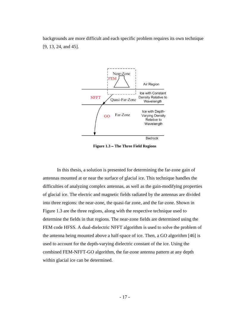
In this thesis, a solution is presented for determining the far-zone gain of
antennas mounted at or near the surface of glacial ice. This technique handles the
difficulties of analyzing complex antennas, as well as the gain-modifying properties
of glacial ice. The electric and magnetic fields radiated by the antennas are divided
into three regions: the near-zone, the quasi-far zone, and the far-zone. Shown in
Figure 1.3 are the three regions, along with the respective technique used to
determine the fields in that regions. The near-zone fields are determined using the
FEM code HFSS. A dual-dielectric NFFT algorithm is used to solve the problem of
the antenna being mounted above a half-space of ice. Then, a GO algorithm [46] is
used to account for the depth-varying dielectric constant of the ice. Using the
combined FEM-NFFT-GO algorithm, the far-zone antenna pattern at any depth
within glacial ice can be determined.

- 18 -
1.6 Thesis Organization
The overall goal of this work is to determine the ice attenuation, and thus ice
temperature, at any depth within glacial ice from radar returns. As stated previously,
precise knowledge of the far-zone antenna gain is necessary to accurately determine
the radar signal attenuation at each depth. Therefore, the majority of this work is
devoted to determination of the far-zone antenna gain. A three-part hybrid technique
was developed to determine the far-zone antenna gain, involving FEM, a near-to-far-
field transformation (NFFT), and GO. FEM modeling using HFSS is discussed on its
own in Chapter 2. Next, the FEM-NFFT-GO hybrid technique is discussed in Chapter
3. Results from both the FEM-NFFT and combined FEM-NFFT-GO technique are
presented in Chapter 4. The proposed technique for determining temperature from
radar returns and simulated results are discussed in Chapter 5. Finally, Chapter 6
discusses conclusions and future work. A full derivation of the dual-dielectric NFFT
routine is presented in Appendix A. Also, the code used to implement the FEM-
NFFT-GO routine is discussed in Appendix B. The code used for performing ice
temperature extraction simulations in presented in Appendix C.
- 19 -
CHAPTER 2: Antenna Analysis Using HFSS
Full characterization of radar systems requires antenna analysis. One of the
most popular antenna analysis tools is the commercial software Ansoft HFSS. Among
other things, it is useful for determining input impedance, scattering parameters, and
both near-zone and far-zone antenna patterns in free space. The code directly solves
for the electric and magnetic near-zone field values in a solution space surrounding
the geometry of interest (Figure 2.1) using the finite element method (FEM). The
FEM is discussed in Section 2.1. Since field values determined within the solution
space are often still in the near-zone, a near-to-far-field transformation (NFFT),
performed in post-processing, is necessary to determine the free-space far-zone field
values. Free-space antenna modeling using HFSS is presented in Section 2.2, and the
HFSS NFFT for obtaining free-space far-zone field values is presented in Section 2.3.
With some modeling adjustments, HFSS can also be used to determine near-
zone parameters for antennas located above glacial ice. Unfortunately, for reasons
discussed in Section 2.4, the HFSS NFFT can not be used to transform these near-
zone field values to the far-zone.
2.1 The Finite Element Method
The finite element method is a useful tool for solving vector electromagnetic
wave equation boundary problems for complex radiating structures. Within a given
solution space surrounding the radiating structure of interest, the FEM [39] code
solves the 3D vector wave equations with given boundary conditions for a finite
number of 3D elements, often tetrahedrons, which fill the solution space. Due to the
relative accuracy and speed of the FEM for a variety of radiating structures [40], the
method has found much commercial success in products such as Ansoft HFSSTM
(high frequency structure simulator), a product often used by the Center for Remote
- 20 -
Sensing of Ice Sheets (CRESIS) for modeling antennas radiating in free space. In free
space, the software provides accurate values for scattering parameters and input
impedance. Also, through the use of a near-to-far-field transformation, HFSS is
capable of generating far-zone radiation patterns in free-space. Additionally, due to
the software’s ability to model an arbitrary variety of materials, it is capable of
accurately calculating near-field parameters for radiating structures located above
glacial ice. However, even with the many post-processing features of HFSS, it is
incapable of accurately determining far-zone radiation patterns for antennas located
above a dielectric half-space such as glacial ice.
Although it is possible to have multiple materials within the software’s finite
solution space, it is impossible to model multiple materials outside of the solution
space. When enclosing the solution space with any of the available boundary
conditions (usually radiating boundary conditions are used), the code assumes the
medium outside of the solution space is a homogeneous medium of the users choice.
Therefore, since a dielectric half-space is infinite relative to the antenna, it is
impossible to determine the far-zone radiation pattern of antennas located near a
dielectric half-space, such as glacial ice.
Even though HFSS is incapable of determining far-field radiation patterns for
antennas located near a dielectric half-space, it is still capable of determining accurate
electric and magnetic near-field values, provided the modeled dielectric medium
within the solution space is large enough relative to the antenna. Therefore, HFSS can
be utilized in determining the electric and magnetic near-field values, a key step in
solving the overall far-zone antenna gain determination problem.
2.2 Free-Space Antenna Modeling
When modeling antennas in free-space (or any homogeneous medium) with
HFSS, the antenna is embedded in a finite solution space in which the wave equation
- 21 -
derived from the differential form of Maxwell’s Equations is solved. In addition to
other parameters, the size and material properties of the solution space require user
specification. Other parameters requiring using specification are boundary conditions,
port excitation, and solution set-up. Each of these specification requirements are
discussed next.
2.2.1 The Solution Space
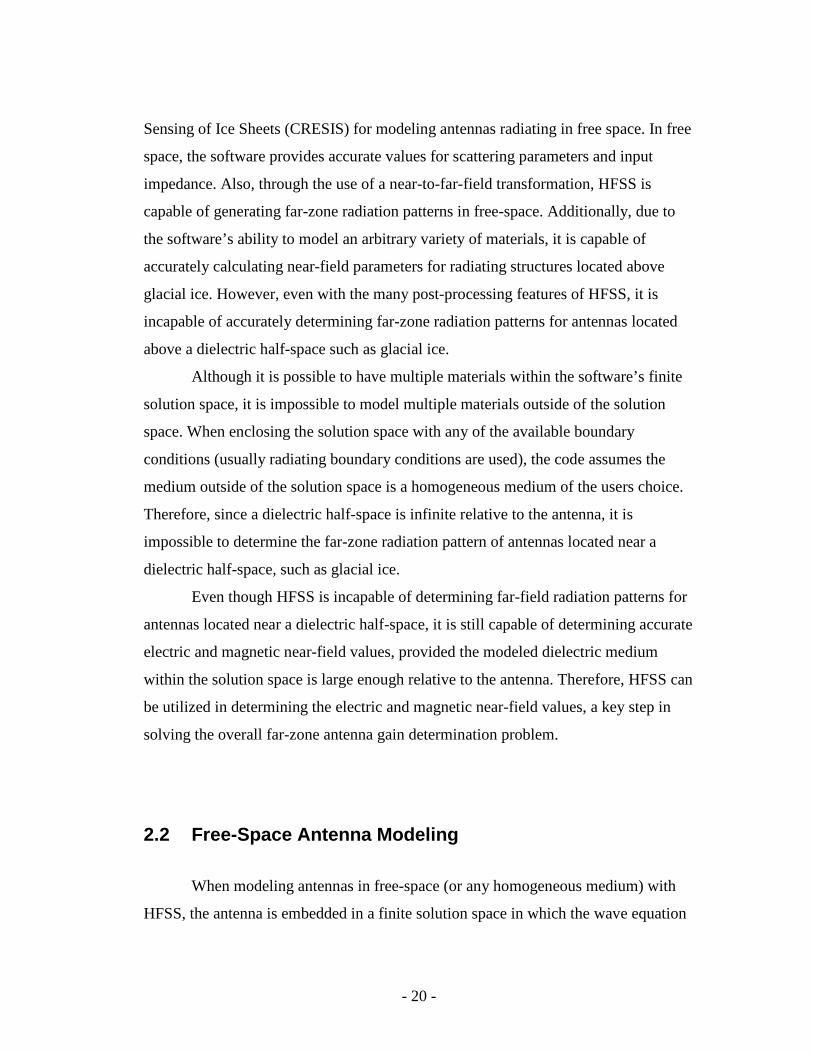
The antenna being modeled is embedded in the solution space and enclosed
by a solution box as shown in Figure 2.1. The user can specify the solution space to
have any material properties, including such parameters as permittivity, permeability,
and loss tangent. Even anisotropic materials can be modeled in HFSS. Also, the
solution space can be set to any geometry and size, but analysis time is directly linked
to the size of the solution space. Usually, the solution space is rectangular, with a
minimum size of a quarter wavelength at the frequency of interest [21].
Figure 2.1 −−−− Generic HFSS Modeling
- 22 -
2.2.2 Boundary Conditions
Due to discontinuities associated with the finite solution space, boundary
conditions are required. This is because the fields are discontinuous along the
boundaries, so the spatial derivatives can not be calculated directly. Therefore, user-
specified boundary conditions are used to define the field behavior at the solution
space boundaries [21].
For the case of a structure open to infinite space, two different types of
boundaries are often utilized: radiation and PML (perfectly matched layer)
boundaries. Although implemented differently, both radiation and PML boundaries
achieve the same end result: making a finite solution space behave as if it were
infinite. However, only radiation boundaries are discussed here, since due to ease of
implementation, they are used more frequently. Figure 2.1 shows a generic HFSS
simulation setup, utilizing a radiation boundary.
Radiation boundary conditions are also referred to as absorbing boundary
conditions since the “system absorbs the wave at the radiation boundary, essentially
ballooning the boundary infinitely far away form the structure and into space” [21].
Therefore, the radiation boundary is non-reflecting and enables a finite space to be
treated as an infinite space.
2.2.3 Port Excitation
When using HFSS, antenna feeds are modeled as ports. A port is “a unique
type of boundary condition that allows energy to flow into and out of a structure”
[21]. HFSS uses an arbitrary port solver to determine the natural modes that can exist
inside of a transmission structure having the same cross section as the port. Two types
of ports are used in HFSS: wave ports and lumped ports.
With wave ports, the port is assumed to be connected to an infinitely long
waveguide having the same cross-section and properties as the port. The wave port
- 23 -
solver determines the characteristic impedance, complex propagation constant,
associated s-parameters of the port, and supports multiple modes. By default, the
outer edge of a wave port is defined to have a “Perfect E boundary,” meaning that the
port is enclosed inside of a perfect conductor, such as a waveguide. The perfect E
boundary forces the electric field to be perpendicular to the boundary surface.
Additionally, wave ports must always be directly connected to the solution box
boundary, and lie on a planar surface. When specifying a wave port, the port location
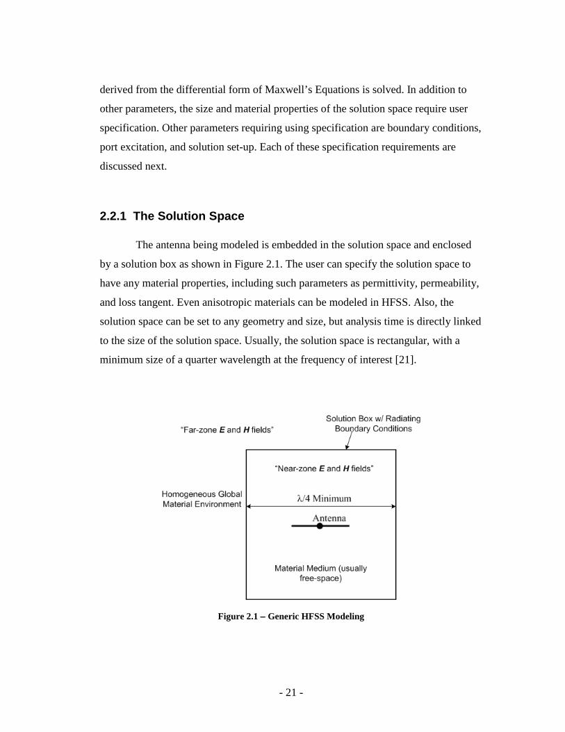
must overlap a 3-dimensional object. Figure 2.2 shows a picture of a waveport
feeding a coaxial line. Also shown in Figure 2.2 is an integration line, which defines
the positive direction at each port.
Figure 2.2 – Waveport Usage in Coax-to-Stripline HFSS Model
Lumped ports are used for driving sources internal to the solution box
boundary. Unlike wave ports, lumped ports only support a single mode (TEM) and
can be considered to be an ideal current source. Also, lumped ports use a perfect E
boundary only along port edges that interface with conductors. All other edges of the
port utilize “Perfect H boundaries,” which force the electric field to be tangential to
- 24 -
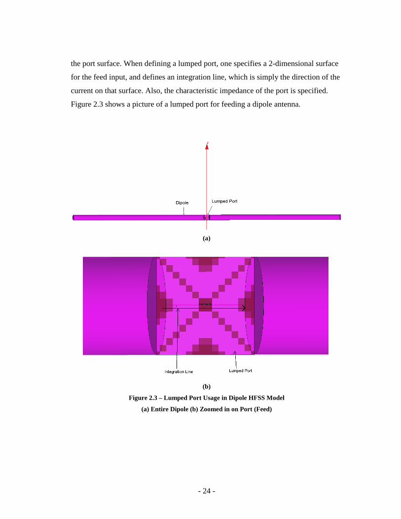
the port surface. When defining a lumped port, one specifies a 2-dimensional surface
for the feed input, and defines an integration line, which is simply the direction of the
current on that surface. Also, the characteristic impedance of the port is specified.
Figure 2.3 shows a picture of a lumped port for feeding a dipole antenna.
(a)
(b)
Figure 2.3 – Lumped Port Usage in Dipole HFSS Model
(a) Entire Dipole (b) Zoomed in on Port (Feed)
- 25 -
2.2.4 Solution Set-Up
The last required specification for analyzing structures using HFSS is the
solution set-up. The minimum items required in the solution set-up are the solution
frequency, maximum number of adaptive passes, and the parameter Delta S. The
maximum number of adaptive passes and Delta S are both features of the adaptive
solution process of HFSS.
HFSS uses adaptive meshing to analyze structures, where the mesh is a grid of
tetrahedrons. Adaptive meshing works by searching for the largest gradients in the E-
field throughout a region in the solution box, and adjusting the mesh accordingly with
each subsequent adaptive pass. With each adaptive pass, HFSS compares the S-
parameters from the current pass to those of the previous pass. If the maximum
change in the S-parameters has changed by less than the user-defined “Delta S,” or
the maximum number of adaptive passes has been exceeded, the solution has
converged. The default Delta S setting is 2%, and is recommended as sufficient by
HFSS.
A useful optional input when adding a solution set-up is the frequency sweep,
which allows for results to be determined for a range of frequencies in addition to the
solution frequency. The converged mesh at the solution frequency is used to solve for
the fields at the frequencies specified in the frequency sweep.
2.3 Far-Zone Field Calculations Using HFSS
The field values determined within the solution space are typically in the near
zone, since the solution box is usually too small for fields to reach the far-zone.
Therefore, HFSS incorporates a NFFT (near-to-far-field transformation) to determine
far-zone field values. In order for HFSS to calculate meaningful far-zone field values,
non-reflecting boundaries such as radiation or PML must be specified at the solution
- 26 -
box. This allows HFSS to make the finite solution space appear as an infinite one,
since the non-reflecting boundaries absorb all incident radiation. Otherwise, any
radiation incident on the boundaries would be reflected back, invalidating the near-
zone field values. With this NFFT algorithm, near-zone field values sampled on the
solution space boundary are converted to far-zone field values.
(a) (b)
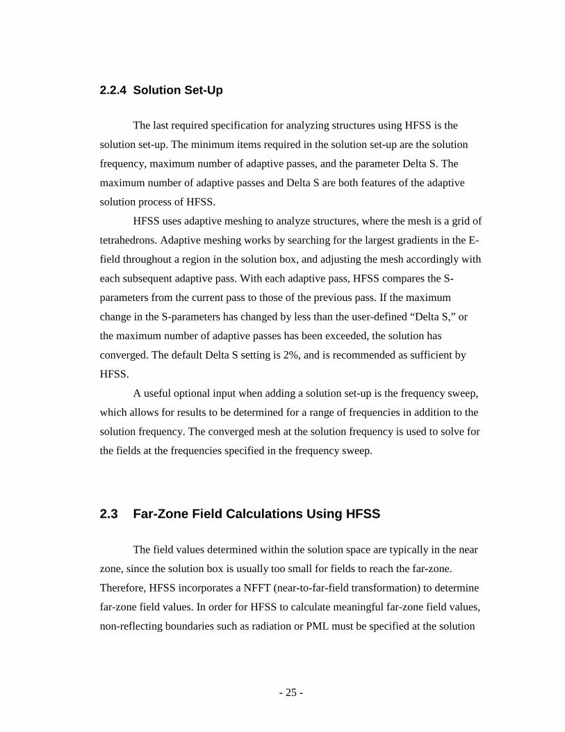
Figure 2.4 −−−− Free-Space Equivalence
(a) Original Problem (b) Equivalent Problem
The HFSS NFFT algorithm makes use of the Schelkunoff Equivalence
Principle [18] to replace the complicated geometry and associated near-zone fields
inside the solution box with an equivalent structure that radiates the same far-zone
fields external to the solution box as did the original geometry. Figure 2.4(a) shows
an antenna residing in free-space. This figure shows the solution box surrounding the
antenna on which the near-zone fields were calculated by HFSS, along with the (yet
to be determined) far-zone pattern that the antenna radiates external to the solution
- 27 -
box. Figure 2.4(b) shows an electrically equivalent geometry. Here the radiating
source (antenna) within the sampling surface is removed, and electric and magnetic
surface currents are placed on the solution box, with values given by:
n= ×J H Eq. 2.1
n= ×M E Eq. 2.2
where E and H are the electric and magnetic fields originally present on the solution
box surface, respectively, and the unit vector n is directed outward from the surface.
According to the Schelkunoff Equivalence Principle [18], these currents generate the
same fields outside the solution box as did the original radiating structure, and zero
(null) fields inside the solution box.
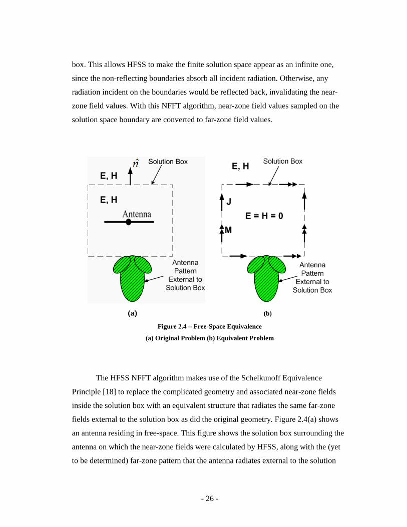
Figure 2.5 – Geometry for a z-Directed Hertzian Dipole
HFSS implements the NFFT by first sampling the electric and magnetic near-
zone fields on the solution box boundary. Then, the near-zone fields are converted to
- 28 -
equivalent surface currents on a rectangular grid located on the solution box
boundary. Each electric and magnetic current segment behaves as an infinitesimal
(Hertzian) electric and magnetic dipole, respectively which radiates into a
homogeneous environment.
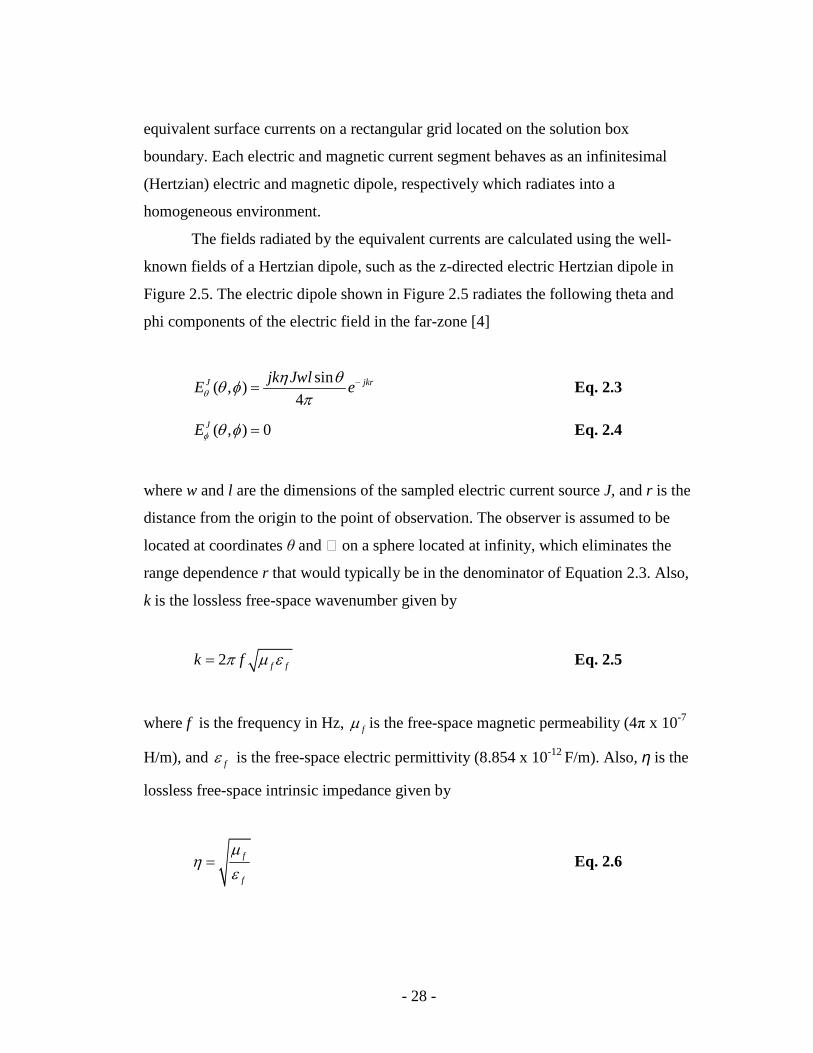
The fields radiated by the equivalent currents are calculated using the well-
known fields of a Hertzian dipole, such as the z-directed electric Hertzian dipole in
Figure 2.5. The electric dipole shown in Figure 2.5 radiates the following theta and
phi components of the electric field in the far-zone [4]
sin
( , )4
J jkrjk JwlE eθ
η θθ φ
π−= Eq. 2.3
( , ) 0JEφ θ φ = Eq. 2.4
where w and l are the dimensions of the sampled electric current source J, and r is the
distance from the origin to the point of observation. The observer is assumed to be
located at coordinates θ and ϕ on a sphere located at infinity, which eliminates the
range dependence r that would typically be in the denominator of Equation 2.3. Also,
k is the lossless free-space wavenumber given by
2 f fk fπ µ ε= Eq. 2.5
where f is the frequency in Hz, fµ is the free-space magnetic permeability (4π x 10-7
H/m), and fε is the free-space electric permittivity (8.854 x 10⁻¹² F/m). Also, η is the
lossless free-space intrinsic impedance given by
f
f
µη
ε= Eq. 2.6
- 29 -
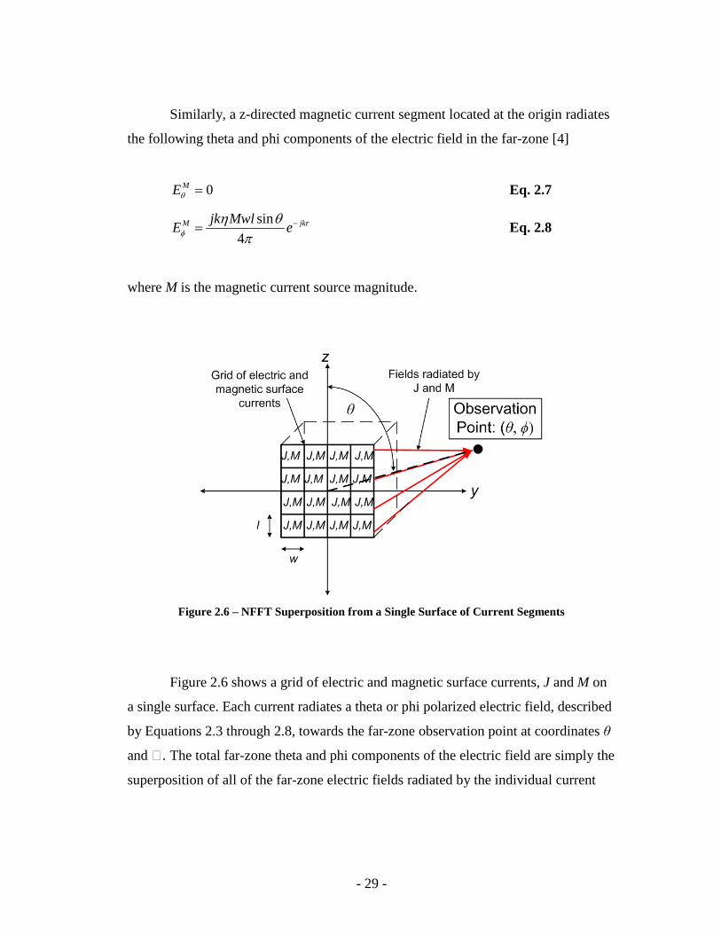
Similarly, a z-directed magnetic current segment located at the origin radiates
the following theta and phi components of the electric field in the far-zone [4]
0MEθ = Eq. 2.7
sin
4M jkrjk Mwl
E eφ
η θπ
−= Eq. 2.8
where M is the magnetic current source magnitude.
Figure 2.6 – NFFT Superposition from a Single Surface of Current Segments
Figure 2.6 shows a grid of electric and magnetic surface currents, J and M on
a single surface. Each current radiates a theta or phi polarized electric field, described
by Equations 2.3 through 2.8, towards the far-zone observation point at coordinates θ
and ϕ. The total far-zone theta and phi components of the electric field are simply the
superposition of all of the far-zone electric fields radiated by the individual current
- 30 -
segments. For a surface such as that shown in Figure 2.6, the total field is calculated
by
( )1 1
, ( , , , ) ( , , , )M N
T J M
m n
E E n m E n mθ θ θθ φ θ φ θ φ= =
= + ∑∑ Eq. 2.10
( )1 1
, ( , , , ) ( , , , )M N
T J M
m n
E E n m E n mφ φ φθ φ θ φ θ φ= =
= + ∑∑ Eq. 2.11
where the indexes N and M represent the number of rows and columns for which the
surface has been discretized into surface currents J and M.
2.4 Modeling Antennas above a Half-Space of Glacial Ice
The procedure presented in Sections 2.2 and 2.3 is sufficient to model
radiating structures in free-space or some other homogeneous medium. However, in
remote sensing of polar ice sheets, antennas radiate into a half-space of glacial ice.
This affects all characteristics of the antenna, including its input impedance, near-
zone fields, and far-zone fields. With some modeling adjustments (Section 2.4.1),
near-zone fields and input impedance can still be obtained. In fact, these HFSS
modeling adjustments have been routinely performed at CRESIS for obtaining the
input impedance of ice-mounted antennas. However, true far-zone fields can not be
obtained using HFSS alone.
2.4.1 HFSS Modeling Adjustments for Antennas Near Glacial Ice
The process of modeling antennas near a dielectric half-space in HFSS is
similar to the generic modeling described in Sections 2.2. However, now, some of the
material representing the half-space must be placed within the solution box in order to
- 31 -
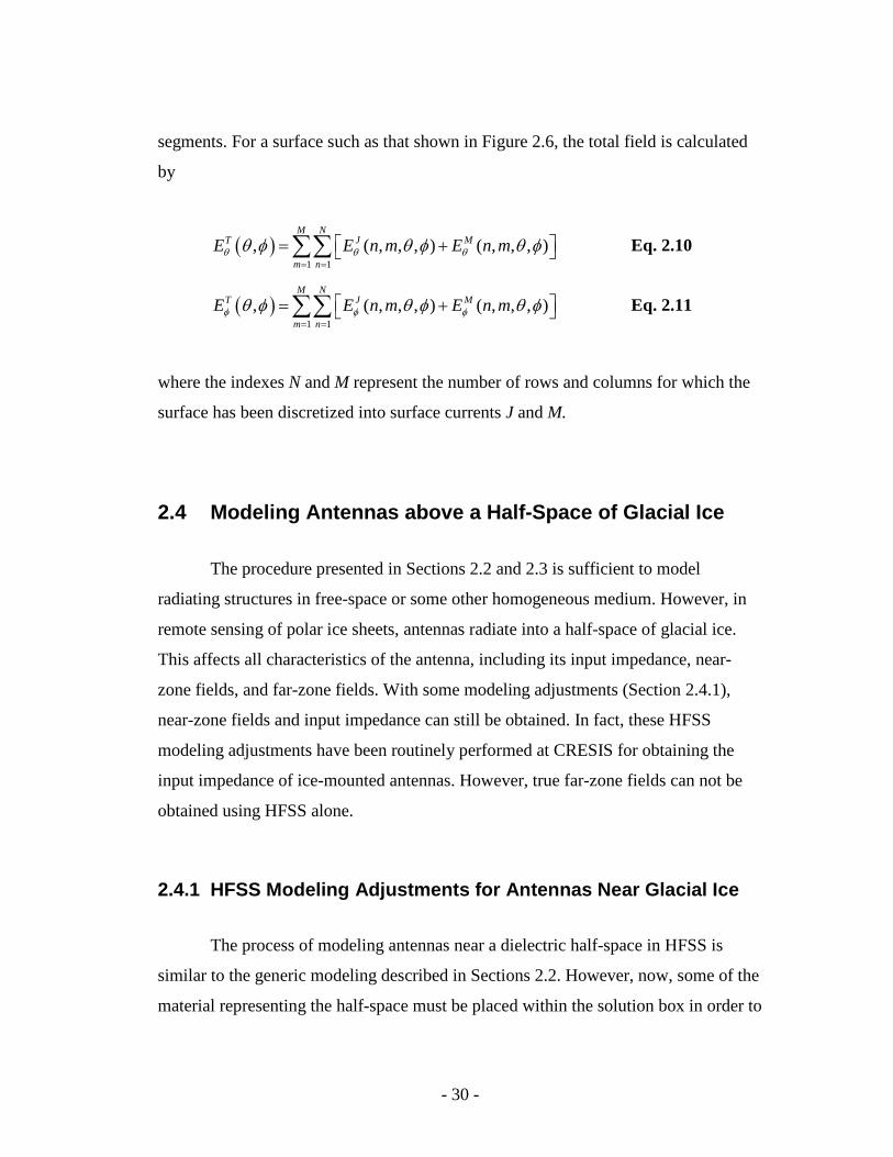
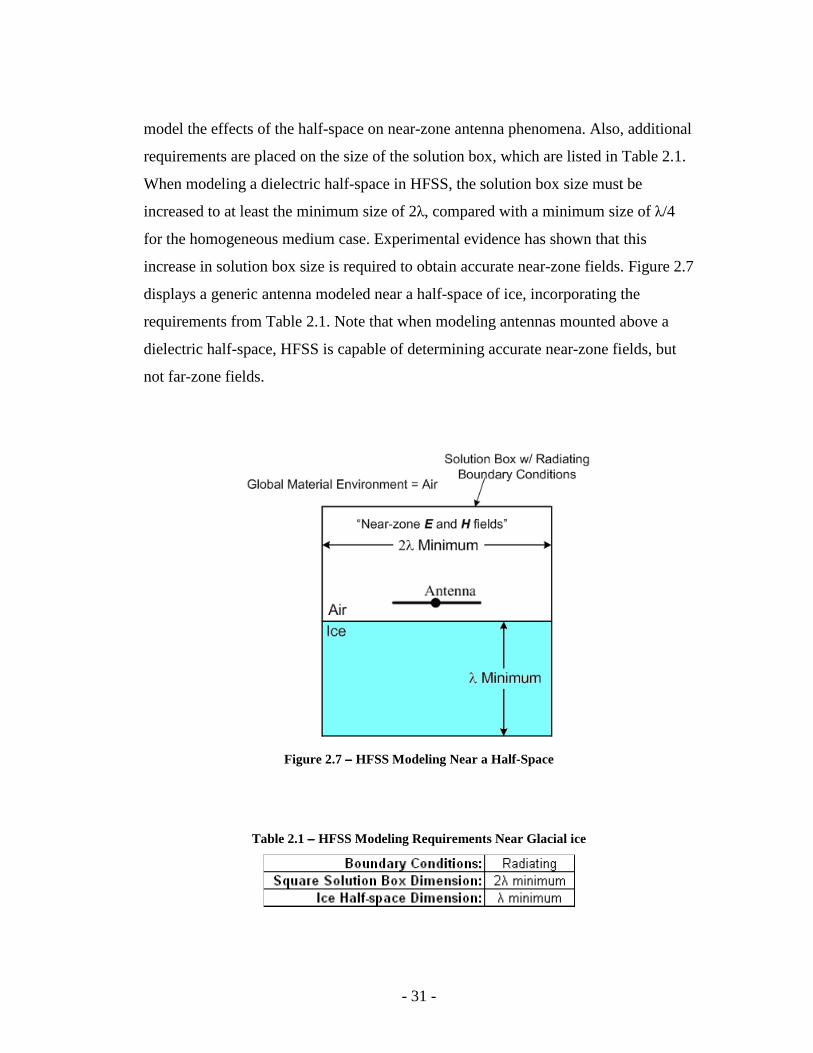
model the effects of the half-space on near-zone antenna phenomena. Also, additional
requirements are placed on the size of the solution box, which are listed in Table 2.1.
When modeling a dielectric half-space in HFSS, the solution box size must be
increased to at least the minimum size of 2λ, compared with a minimum size of λ/4
for the homogeneous medium case. Experimental evidence has shown that this
increase in solution box size is required to obtain accurate near-zone fields. Figure 2.7
displays a generic antenna modeled near a half-space of ice, incorporating the
requirements from Table 2.1. Note that when modeling antennas mounted above a
dielectric half-space, HFSS is capable of determining accurate near-zone fields, but
not far-zone fields.
Figure 2.7 −−−− HFSS Modeling Near a Half-Space
Table 2.1 −−−− HFSS Modeling Requirements Near Glacial ice

- 32 -
2.4.2 What HFSS Will Let You Do Even Though It Is Incorrect!
Although it is impossible to obtain correct far-zone antenna patterns for ice-
mounted antennas using HFSS alone, HFSS will not prevent users from trying. As
discussed in Sections 2.2 and 2.3, HFSS can only correctly perform its NFFT
algorithm into a homogeneous infinite medium, specified by the global material
environment (GME). Therefore, the NFFT algorithm used by HFSS is useless for far-
zone radiation into anything other than a homogeneous medium. That being said,
HFSS will not prevent the user from generating incorrect far-zone field results.
A theory proposed by an HFSS employee for possibly obtaining nearly correct
far-zone fields within air or ice involved adjustment of the GME. He suggested that
modeling the antenna above glacial ice, but setting the GME to air or ice, depending
on the observer’s location, would produce nearly correct far-zone fields within air or
ice, respectively.
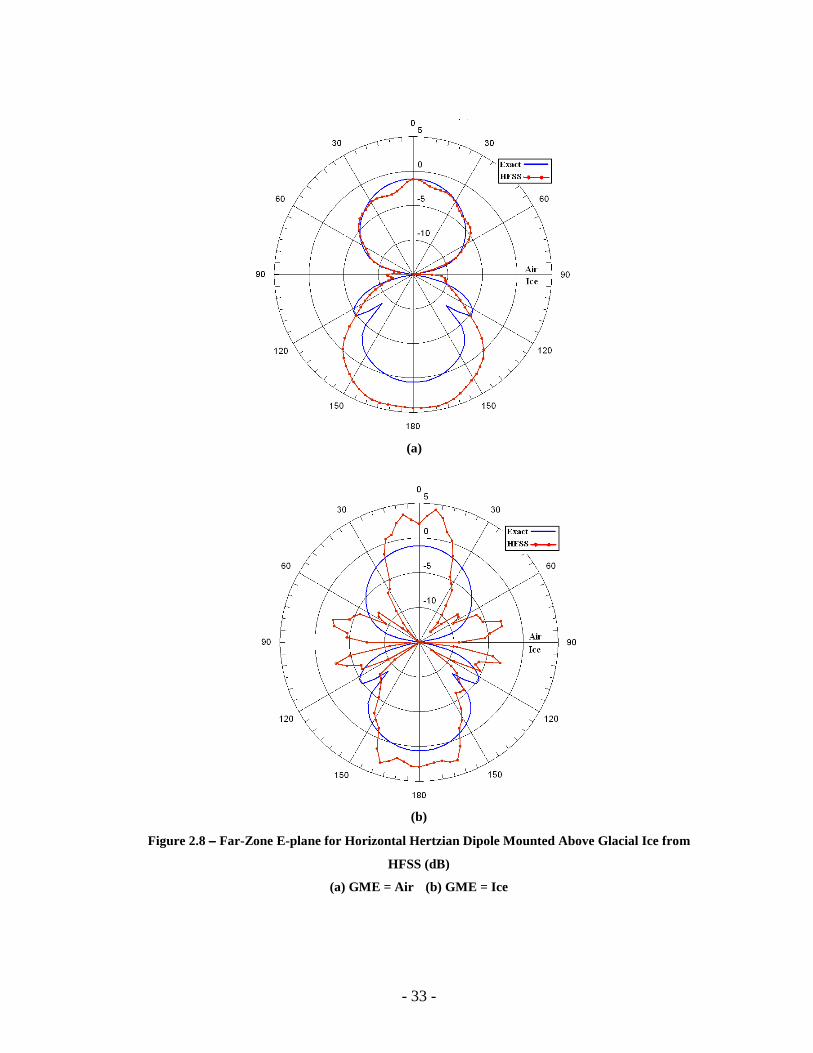
The E-plane far-zone fields resulting from such a procedure are presented in
Figure 2.8, for an ice-mounted horizontal Hertzian dipole. In Figure 2.8(a), the GME
is air, and Figure 2.8(b), the GME is ice. Also shown in Figure 2.8 is the exact result
[40] for a horizontal Hertzian dipole located above a half-space of glacial ice. Both of
the results obtained from HFSS disagree dramatically with the true result, indicating
that true far-zone fields for ice-mounted antennas can not be obtained using HFSS
alone.
- 33 -
(a)
(b)
Figure 2.8 −−−− Far-Zone E-plane for Horizontal Hertzian Dipole Mounted Above Glacial Ice from
HFSS (dB)
(a) GME = Air (b) GME = Ice
- 34 -
2.5 HFSS Modeling Summary
In the context of modeling antennas near glacial ice, HFSS is only useful for
determining near-zone fields and input impedances, and this requires the modeling
technique discussed in Section 2.4. Also, although HFSS allows the calculation of
far-zone fields, these results are incorrect for ice-mounted antennas. The inability of
HFSS to determine far-zone fields for ice-mounted antennas is due to the HFSS
NFFT only being capable of transforming near-zone fields to a homogeneous far-
zone. In order to determine true far-zone fields, a custom NFFT is required, which is
discussed in Chapter 3. In this custom NFFT, the near-zone fields calculated in HFSS
are sampled and exported to memory. These near-zone fields are then converted to a
series of equivalent radiating current filaments. The NFFT algorithm allows the
currents to radiate essentially in an infinite half-space, allowing for the determination
of accurate Green’s functions associated with the current filaments.
- 35 -
CHAPTER 3: Far-Zone Field Patterns in Glacial Ice
In order to accurately determine glacial ice temperature profiles from radar
returns, accurate far-zone antenna gain estimation is required. Typically, far-zone
antenna gain is determined using commercial software such as HFSS. However, due
to the complicated properties of glacial ice, these commercial software packages are
incapable of determining the far-zone gain for ice-mounted antennas (see Chapter 2).
This chapter presents a new hybrid technique for determining the far-zone gain of
glacial ice-mounted antennas, which addresses the problem by dividing the geometry
into three regions: the near-zone, the quasi-far-zone, and the far-zone. Fields in the
near-zone are determined using the finite element method (FEM) via HFSS. In the
quasi-far-zone, which is the region just below the surface of the ice where the
wavefronts are planar, the fields are determined using a near-to-far-field
transformation (NFFT). In the far-zone, which is the region starting just below the
quasi-far-zone and ending at bedrock, fields are determined using geometric optics
ray tracing (GO). The combined three-part non-iterative hybrid technique is called the
FEM-NFFT-GO technique.
The basic theory of this technique is presented in Section 3.1. Also, the
practical aspects of the technique, as well as the operation of the FEM-NFFT-GO
software are presented in Section 3.2.
3.1 Background for the FEM-NFFT-GO Technique The FEM-NFFT-GO technique involves three steps: the FEM modeling of the
antenna above the upper layer of glacial ice to obtain electric and magnetic near-zone
field values, the transformation (NFFT) from the near-zone to the quasi-far-zone (a
few wavelengths below the air/ice interface), and the projection of the quasi-far-zone
fields to any depth within the non-uniform glacial ice (GO). The three regions (near-
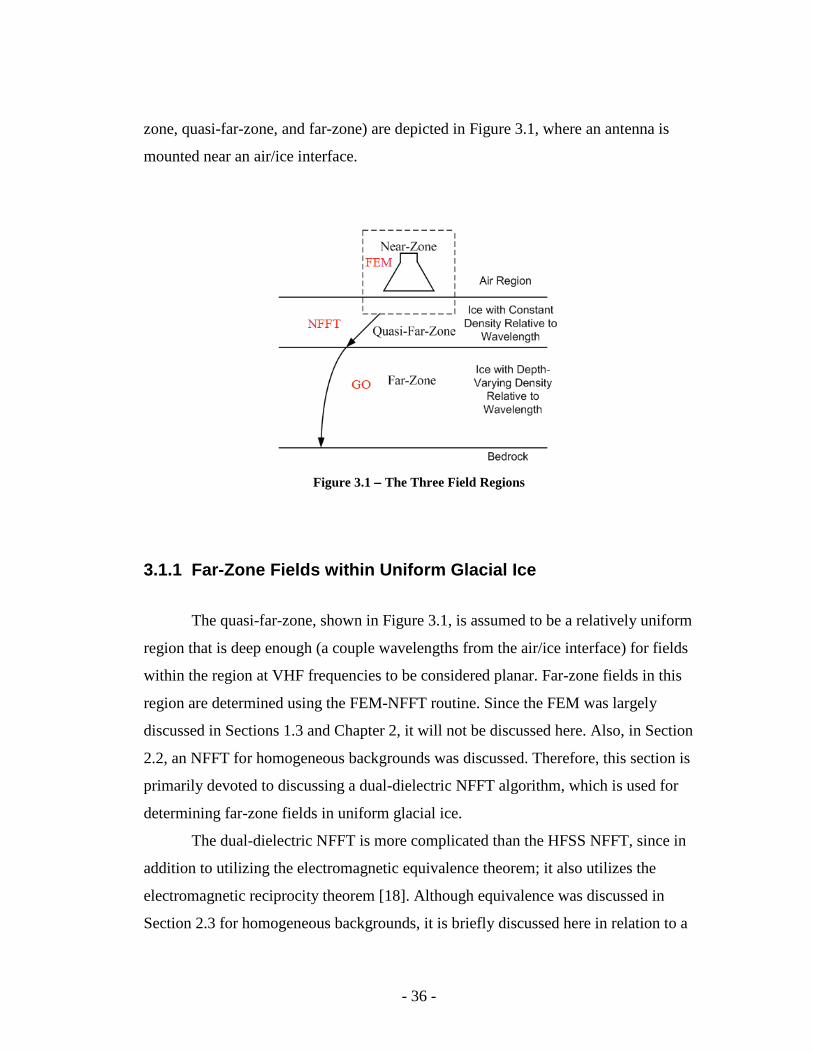
- 36 -
zone, quasi-far-zone, and far-zone) are depicted in Figure 3.1, where an antenna is
mounted near an air/ice interface.
Figure 3.1 −−−− The Three Field Regions
3.1.1 Far-Zone Fields within Uniform Glacial Ice
The quasi-far-zone, shown in Figure 3.1, is assumed to be a relatively uniform
region that is deep enough (a couple wavelengths from the air/ice interface) for fields
within the region at VHF frequencies to be considered planar. Far-zone fields in this
region are determined using the FEM-NFFT routine. Since the FEM was largely
discussed in Sections 1.3 and Chapter 2, it will not be discussed here. Also, in Section
2.2, an NFFT for homogeneous backgrounds was discussed. Therefore, this section is
primarily devoted to discussing a dual-dielectric NFFT algorithm, which is used for
determining far-zone fields in uniform glacial ice.
The dual-dielectric NFFT is more complicated than the HFSS NFFT, since in
addition to utilizing the electromagnetic equivalence theorem; it also utilizes the
electromagnetic reciprocity theorem [18]. Although equivalence was discussed in
Section 2.3 for homogeneous backgrounds, it is briefly discussed here in relation to a
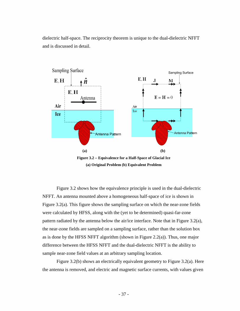
- 37 -
dielectric half-space. The reciprocity theorem is unique to the dual-dielectric NFFT
and is discussed in detail.
(a) (b)
Figure 3.2 −−−− Equivalence for a Half-Space of Glacial Ice
(a) Original Problem (b) Equivalent Problem
Figure 3.2 shows how the equivalence principle is used in the dual-dielectric
NFFT. An antenna mounted above a homogeneous half-space of ice is shown in
Figure 3.2(a). This figure shows the sampling surface on which the near-zone fields
were calculated by HFSS, along with the (yet to be determined) quasi-far-zone
pattern radiated by the antenna below the air/ice interface. Note that in Figure 3.2(a),
the near-zone fields are sampled on a sampling surface, rather than the solution box
as is done by the HFSS NFFT algorithm (shown in Figure 2.2(a)). Thus, one major
difference between the HFSS NFFT and the dual-dielectric NFFT is the ability to
sample near-zone field values at an arbitrary sampling location.
Figure 3.2(b) shows an electrically equivalent geometry to Figure 3.2(a). Here
the antenna is removed, and electric and magnetic surface currents, with values given
- 38 -
by Equations 2.1 and 2.2, are placed on the sampling box. As was shown in Section
2.3, the superposition of the fields radiated by these currents generates the same total
electric and magnetic fields outside the sampling box as did the original radiating
structure, and zero (null) fields inside the sampling box.
The calculation of the fields radiated by these equivalent electric and magnetic
surface currents is straightforward when the background medium is free space, but
the presence of the air/ice boundary presents a more difficult problem. A general
solution involves the decomposition of the spherical waves emanating from the
currents into a spectrum of plane waves, whose reflections from and transmission
through the dielectric interface can be determined from the Fresnel reflection and
transmission coefficients. However, when the observer is electrically far from the
boundary (as in the case of the quasi-far-zone), the reciprocity principle can be used
to simplify the analysis [38]. For this case, only the geometric optics waves – those
obeying Snell’s law – need be considered.
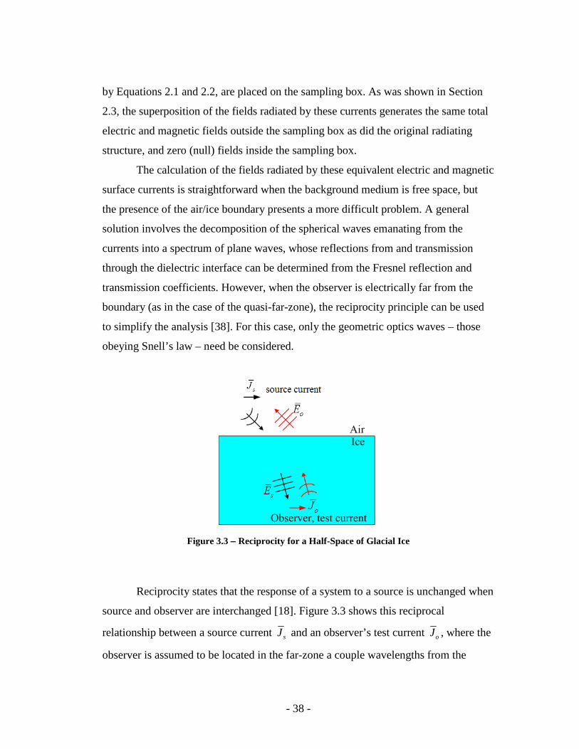
Figure 3.3 −−−− Reciprocity for a Half-Space of Glacial Ice
Reciprocity states that the response of a system to a source is unchanged when
source and observer are interchanged [18]. Figure 3.3 shows this reciprocal
relationship between a source current sJ and an observer’s test current oJ , where the
observer is assumed to be located in the far-zone a couple wavelengths from the
- 39 -
air/ice interface. Fields transmitted by the source current are in black, and those fields
transmitted by the observer’s test current are in red. The field transmitted by the
observer’s test current is planar within the vicinity of the air/ice interface, whereas the
field transmitted by the source antenna is not yet planar in the vicinity of the air/ice
interface. Therefore, reciprocity can be used to describe sE (electric field due to the
source current at the point of observation) in terms of the field oE (electric field due to
the observer test current near the air/ice interface), which is a plane wave. The
derivation and presentation of these plane wave formulas is presented in Appendix A.
Also, Appendix A provides a thorough description of all the supplementary formulas
and variable descriptions necessary for coding the dual-dielectric NFFT routine.
The total quasi-far-zone electric field at any pair of observation angles θ and
ϕ is the superposition of the electric fields radiated by each electric and magnetic
current source along the sampling box, determined by the formulas presented in
Appendix A. Recalling that the near-zone field sampling box is rectangular, there are
six two-dimensional surfaces on which electric and magnetic current sources exist.
When the source and observer are in different mediums, the sum of total parallel and
perpendicular polarized electric fields radiated from a surface are found by
( )1 1
, , ( , , , ) ( , , , )M N
T Ti TiSurf E M
m n
E i E m n E m nθ θ θθ φ θ φ θ φ= =
= + ∑∑ Eq. 3.1
( )1 1
, , ( , , , ) ( , , , )M N
T Ti TiSurf E M
m n
E i E m n E m nφ φ φθ φ θ φ θ φ= =
= + ∑∑ Eq. 3.2
where i is index representing the surface, M and N are the number of surface currents
in each of the two dimensions of the surface, and TSurfEθ and T
SurfEφ are the parallel
and perpendicular components of the transmitted electric field radiated by the surface
i. When the source and observer are located in the same medium, the sum of total
parallel and perpendicular polarized electric fields radiated from a surface are
- 40 -
( )1 1
, , ( , , , ) ( , , , ) ( , , , ) ( , , , )M N
RI Ii Ri Ii RiSurf E E M M
m n
E i E m n E m n E m n E m nθ θ θ θ θθ φ θ φ θ φ θ φ θ φ= =
= + + + ∑∑ Eq. 3.3
( )1 1
, , ( , , , ) ( , , , ) ( , , , ) ( , , , )M N
RI Ii Ri Ii RiSurf E E M M
m n
E i E m n E m n E m n E m nφ φ φ φ φθ φ θ φ θ φ θ φ θ φ= =
= + + + ∑∑
Eq. 3.4
where RISurfEθ and RI
SurfEφ are the parallel and perpendicular components of the
combined incident and reflected electric fields radiated by the surface i. Finally, the
total electric far-fields at each pair of observation angles due to the contribution of all
sampled surfaces are
( ) ( ) ( )6
1
, , , , ,Total T RISurf Surf
i
E E i E iθ θ θθ φ θ φ θ φ=
= + ∑ Eq. 3.5
( ) ( ) ( )6
1
, , , , ,Total T RISurf Surf
i
E E i E iφ φ φθ φ θ φ θ φ=
= + ∑ Eq. 3.6
Antenna patterns are often presented as gain relative to an isotropic radiator,
which is given by the following expressions
( )
22 ,
( , )Total
oo
EG
θθ
π θ φθ φ
η= Eq. 3.7
( )
22 ,
( , )Total
oo
EG
φφ
π θ φθ φ
η= Eq. 3.8
where oη is the intrinsic impedance of the medium containing the observer. For
antenna patterns located above the air/ice interface, the intrinsic impedance is that of
free-space (377 Ω), whereas for antenna patterns located below the air/ice interface,
the intrinsic impedance is that of the upper-layer of ice (280 Ω).
- 41 -
3.1.2 Far-Zone Fields within Non-Uniform Glacial Ice
The non-uniform region of glacial ice, called the far-zone, is shown in Figure
3.1. This region extends from the quasi-far-zone to bedrock. As shown in Figure 3.1,
rays propagating toward the bedrock are continuously refracted towards the normal
direction in this region due to the depth-dependent density of glacial ice. This
refractive gain must be accounted for if ice attenuation is to be accurately measured
from radar sounding. Fortunately, the GO (geometric-optics ray tracing) technique
can be used to determine the refractive gain. But, to be useful, the GO technique
requires knowledge of the density profile causing the refractive gain.
Ice core data taken from Greenland and Antarctica have resulted in empirical
ice density models that agree well with measured results [3, 10, and 43]. Combining
the empirical ice density model with GO allows for the effect of depth-varying ice
density on the far-zone antenna gain to be determined. Since the GO technique
depends on both glacial ice density modeling and geometric optics, both are presented
in this section.
3.1.2.1 Glacial Ice Empirical Density Model
Generally, ice density (and other constitutive parameters) varies as a function
of depth only [20]. Near the surface, the ice is intermixed with air bubbles yielding a
density less than that of pure ice [34], where the density of pure ice P is 0.92 g/cm3.
As the depth increases, the pressure due to the mass of ice above compresses the ice,
thus reducing the volume of the air bubbles until the pure ice density is achieved. This
compression occurs for roughly the first 100 meters of ice. An accurate model for the
ice density is given by the following relation [37]
RzP Veρ = − Eq. 3.9
- 42 -
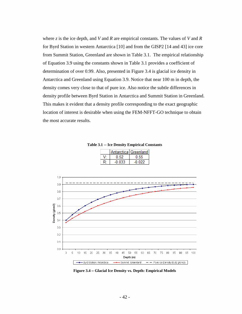
where z is the ice depth, and V and R are empirical constants. The values of V and R
for Byrd Station in western Antarctica [10] and from the GISP2 [14 and 43] ice core
from Summit Station, Greenland are shown in Table 3.1. The empirical relationship
of Equation 3.9 using the constants shown in Table 3.1 provides a coefficient of
determination of over 0.99. Also, presented in Figure 3.4 is glacial ice density in
Antarctica and Greenland using Equation 3.9. Notice that near 100 m in depth, the
density comes very close to that of pure ice. Also notice the subtle differences in
density profile between Byrd Station in Antarctica and Summit Station in Greenland.
This makes it evident that a density profile corresponding to the exact geographic
location of interest is desirable when using the FEM-NFFT-GO technique to obtain
the most accurate results.
Table 3.1 -- Ice Density Empirical Constants
Figure 3.4 −−−− Glacial Ice Density vs. Depth: Empirical Models
- 43 -
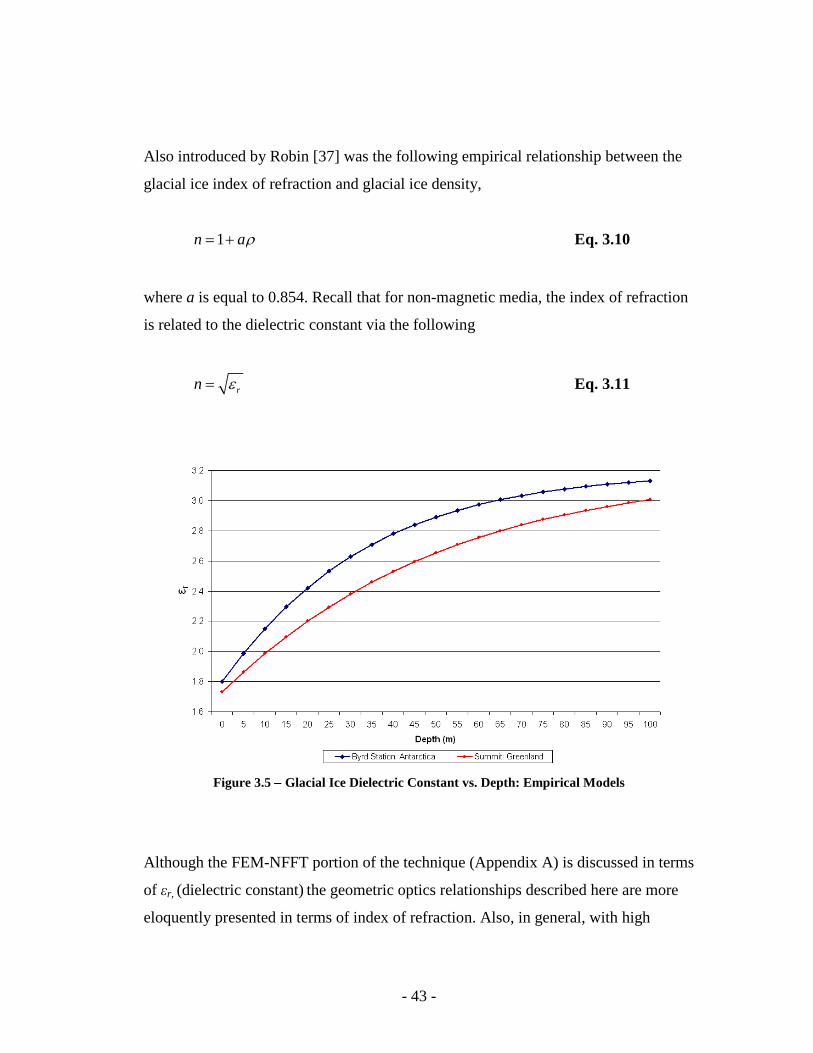
Also introduced by Robin [37] was the following empirical relationship between the
glacial ice index of refraction and glacial ice density,
1n aρ= + Eq. 3.10
where a is equal to 0.854. Recall that for non-magnetic media, the index of refraction
is related to the dielectric constant via the following
rn ε= Eq. 3.11
Figure 3.5 −−−− Glacial Ice Dielectric Constant vs. Depth: Empirical Models
Although the FEM-NFFT portion of the technique (Appendix A) is discussed in terms
of εr, (dielectric constant) the geometric optics relationships described here are more
eloquently presented in terms of index of refraction. Also, in general, with high
- 44 -
frequency approximations such as geometric optics ray tracing, the index of refraction
is used. Figure 3.5 shows the relationship between εr and depth using Equation 3.10
and 3.11. Notice that in both Antarctica and Greenland, the change in εr with depth
begins to level off near 100 m in depth.
3.1.2.2 Geometric Optics Ray Tracing
Although geometric optics ray-tracing is often thought of at optical
frequencies, it can also be used at the VHF frequencies used by ice-penetrating
radars. The key point to consider when applying geometric optics is the relation of
size and curvature of wavefronts to wavelength [36]. The electromagnetic fields a
couple wavelengths into the upper-ice region (i.e. the quasi-far-zone) can be
considered locally as propagating rays with planar wavefronts [46], indicating
essentially no wavefront curvature, and the size of the wavefront is much larger than
the wavelength. At greater depths, the ice density increases slowly compared to
wavelength for VHF radars, so reflections are minimal [25], and the ray paths are
bent increasingly toward the normal direction. From these ray trajectories the antenna
gain at any depth can be determined.
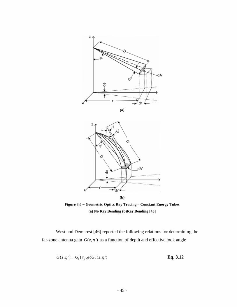
The geometric depiction of ray bending occurring within the ice is presented
in Figure 3.6. In Figure 3.6(a), a constant energy ray tube extending from a point
source is propagating in a continuous medium, where the ray tube energy is focused
on the area dA, at a distance D from the source. Figure 3.6(b) depicts the case where
the mediums refractive index increases gradually with depth, and the constant energy
ray tube is focused on the area dA’, located at the same distance D from the source.
The area dA’ in Figure 3.6(b) is less than the area dA in Figure 3.6(a). Therefore, the
energy per unit area is increased for the case of gradually increasing dielectric
constant, leading to an increased far-zone antenna gain in the medium having the
dielectric constant-gradient.
- 45 -
(a)
(b)
Figure 3.6 −−−− Geometric Optics Ray Tracing – Constant Energy Tubes
(a) No Ray Bending (b)Ray Bending [45]
West and Demarest [46] reported the following relations for determining the
far-zone antenna gain ( , ')G z η as a function of depth and effective look angle
0 0( , ') ( , ) ( , ')fG z G G zη γ φ η= Eq. 3.12
- 46 -
where Go is the quasi-far-zone gain in the upper region of glacial ice (relative to a
free-space isotropic radiator), which is the result of the FEM-NFFT technique. Also,
Gf is the gain factor improvement due to ray bending. The effective look angle 'η is
given by
1 '' tan
r
zη − =
Eq. 3.13
where r’ is the radial distance traveled by the ray beginning at the surface, as shown
in Figure 3.6(b) and z is the depth within the ice. From geometric optics [46], the gain
improvement factor is given by
2
0
0
sin( , ')
'' ' cos 'f
DdAG z
drdA rd
γη
γγ
= = Eq 3.14
Here, 0γ is the angle the ray makes with the normal as it is launched at the surface, D
is the direct distance from the ray location at depth z from the starting location, and 'γ
is the angle the ray makes with the normal at any depth. The parameters D and 'γ are
given by
2 2( ')D r z= + Eq. 3.15
10' sin sinin
nγ γ−
=
Eq. 3.16
Another key parameter found in Equation 3.14 is
2 2
0
'( )
z cr dz
n z c=
+∫ Eq. 3.17
- 47 -
which is the radial distance traveled by a ray beginning at the surface, where ( )n z is
the refractive index as a function of depth, and
0 0sinc n γ= Eq. 3.18
As stated in Section 3.1.2.1, glacial ice density profiles are often described by the
following exponential relationship [37],
( ) Rzz P Veρ = − Eq. 3.19
( ) 1 ( )n z a zρ= + Eq. 3.20
where the ice density ρ is now presented as a function of depth.
Making use of the exponential density profile described in Equations 3.19 and
3.20, and integrating Equation 3.17 yields the following result for the radial distance
traveled by a ray at any depth
( )0 0
2 2' log
2 2Rz
c WY W Xr
R W e WY W X
− + + = + +
Eq. 3.21
Differentiating Equation 3.21 with respect to 0γ and then integrating with respect to z
yields the following result
2 20
0 00 0
0 0
2 2cos' 1 2 2' cos
XXW c W cndr c
r nd c W RW Y Y
γγ
γ
+ + + + = + + −
Eq. 3.22
where,
2 2 21 2W aP a P c= + + − Eq. 3.23
- 48 -
( )22 2 RzX a PV aV e= − − Eq. 3.24
2 2 2RzY a V e X W= + + Eq. 3.25
20 2 2X a PV aV= − − Eq. 3.26
2 20Y a V X W= + + Eq. 3.27
Although an exponential density profile was assumed in the derivation of Equation
3.21 and 3.22, any density profile could be used in conjunction with the geometric
optics ray tracing technique. However, this would require either numerical calculation
of 'r and 0
'dr
dγ, or another closed form derivation of these parameters.
3.2 Using the FEM-NFFT-GO Technique to Determine Far-Zone Electric Fields
In this section, the practical aspects of running the FEM-NFFT-GO technique
are presented, as well as some of the practical aspects used in creating the routine.
Regarding the FEM-NFFT procedure, these include near-zone-field sampling,
sampling location, and sampling resolution. Also presented is the procedure for
actually running the FEM-NFFT-GO routine using the Master.m Matlab script. The
Matlab script keeps most of the inner-workings of the routine hidden from the user,
so these inner-workings are left for Appendix B.
3.2.1 Sampling and Exporting Near-Zone Fields
HFSS has a useful built-in feature called the vector field calculator. This
allows for the performance of mathematical operations, as well as exportation of data,
on all saved field data in the modeled geometry [22]. It also allows for certain types
of data to be imported into HFSS. The Fields Calculator is easily accessed from the
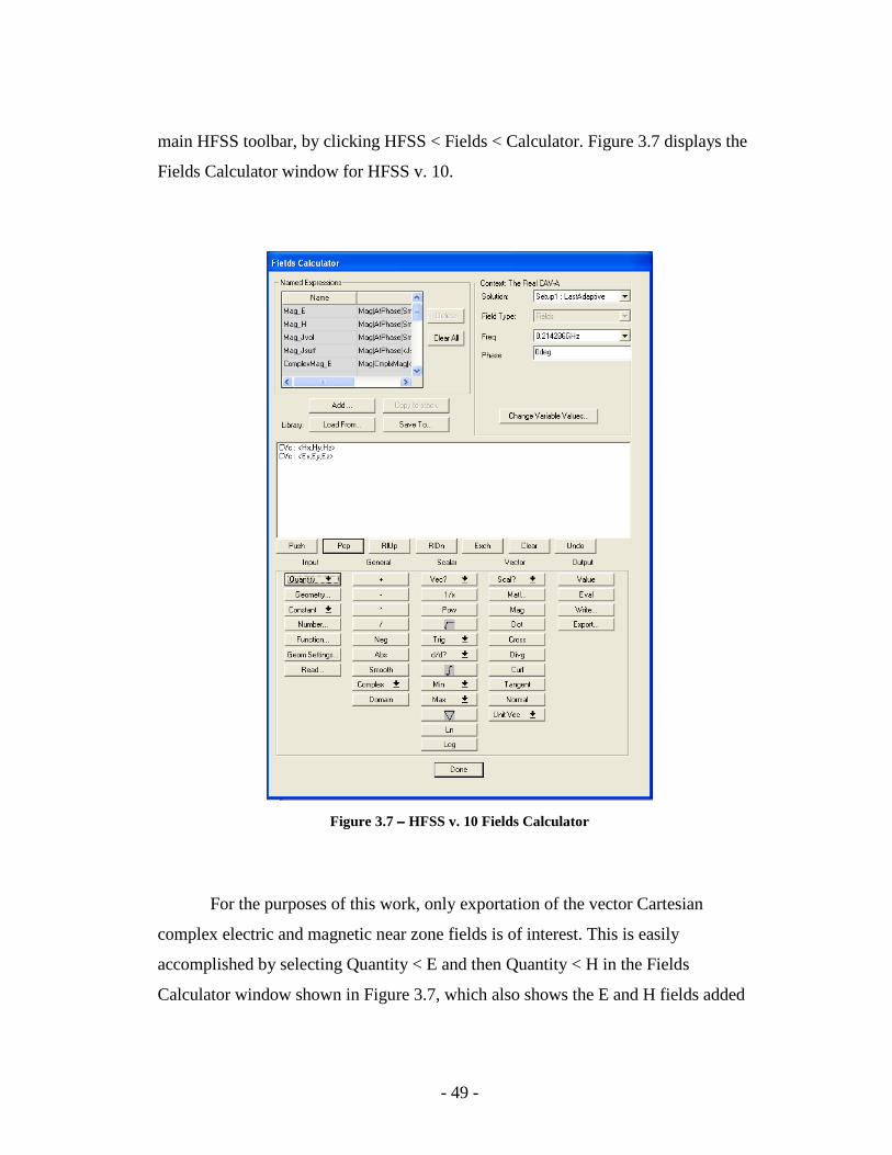
- 49 -
main HFSS toolbar, by clicking HFSS < Fields < Calculator. Figure 3.7 displays the
Fields Calculator window for HFSS v. 10.
Figure 3.7 −−−− HFSS v. 10 Fields Calculator
For the purposes of this work, only exportation of the vector Cartesian
complex electric and magnetic near zone fields is of interest. This is easily
accomplished by selecting Quantity < E and then Quantity < H in the Fields
Calculator window shown in Figure 3.7, which also shows the E and H fields added
- 50 -
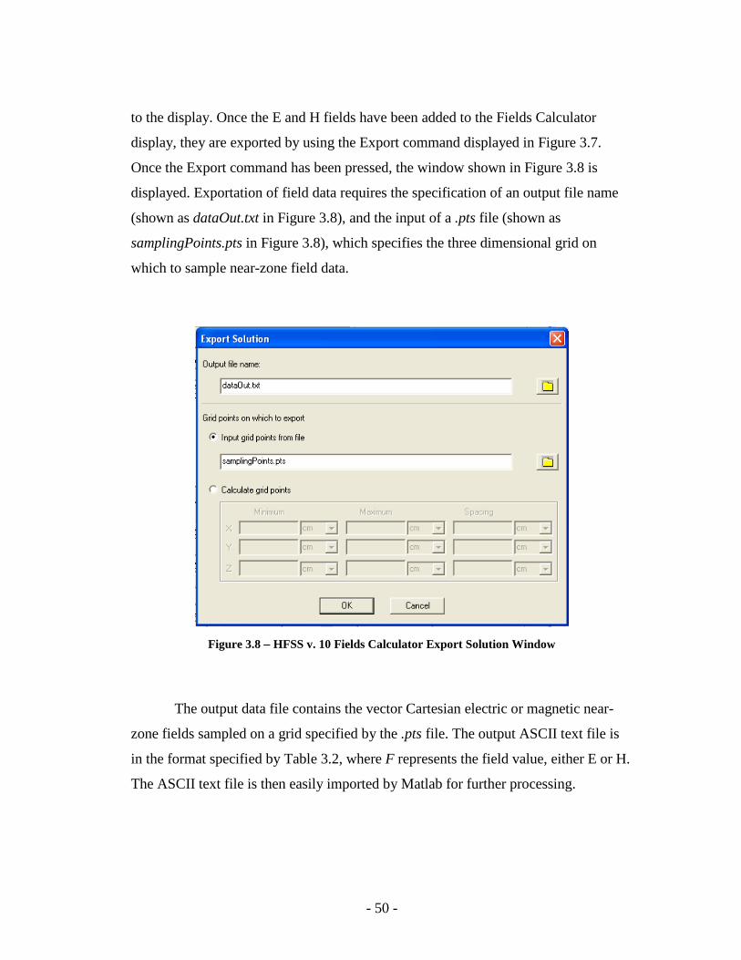
to the display. Once the E and H fields have been added to the Fields Calculator
display, they are exported by using the Export command displayed in Figure 3.7.
Once the Export command has been pressed, the window shown in Figure 3.8 is
displayed. Exportation of field data requires the specification of an output file name
(shown as dataOut.txt in Figure 3.8), and the input of a .pts file (shown as
samplingPoints.pts in Figure 3.8), which specifies the three dimensional grid on
which to sample near-zone field data.
Figure 3.8 −−−− HFSS v. 10 Fields Calculator Export Solution Window
The output data file contains the vector Cartesian electric or magnetic near-
zone fields sampled on a grid specified by the .pts file. The output ASCII text file is
in the format specified by Table 3.2, where F represents the field value, either E or H.
The ASCII text file is then easily imported by Matlab for further processing.
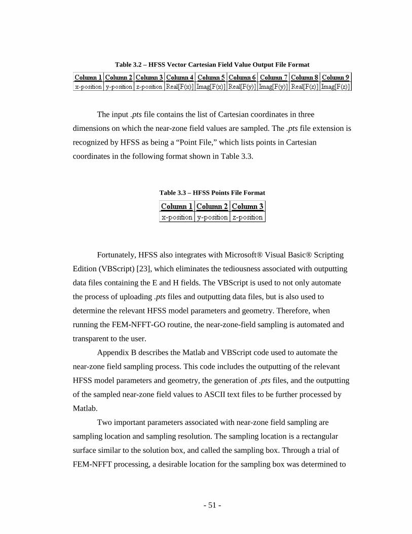
- 51 -
Table 3.2 – HFSS Vector Cartesian Field Value Output File Format
The input .pts file contains the list of Cartesian coordinates in three
dimensions on which the near-zone field values are sampled. The .pts file extension is
recognized by HFSS as being a “Point File,” which lists points in Cartesian
coordinates in the following format shown in Table 3.3.
Table 3.3 – HFSS Points File Format
Fortunately, HFSS also integrates with Microsoft® Visual Basic® Scripting
Edition (VBScript) [23], which eliminates the tediousness associated with outputting
data files containing the E and H fields. The VBScript is used to not only automate
the process of uploading .pts files and outputting data files, but is also used to
determine the relevant HFSS model parameters and geometry. Therefore, when
running the FEM-NFFT-GO routine, the near-zone-field sampling is automated and
transparent to the user.
Appendix B describes the Matlab and VBScript code used to automate the
near-zone field sampling process. This code includes the outputting of the relevant
HFSS model parameters and geometry, the generation of .pts files, and the outputting
of the sampled near-zone field values to ASCII text files to be further processed by
Matlab.
Two important parameters associated with near-zone field sampling are
sampling location and sampling resolution. The sampling location is a rectangular
surface similar to the solution box, and called the sampling box. Through a trial of
FEM-NFFT processing, a desirable location for the sampling box was determined to
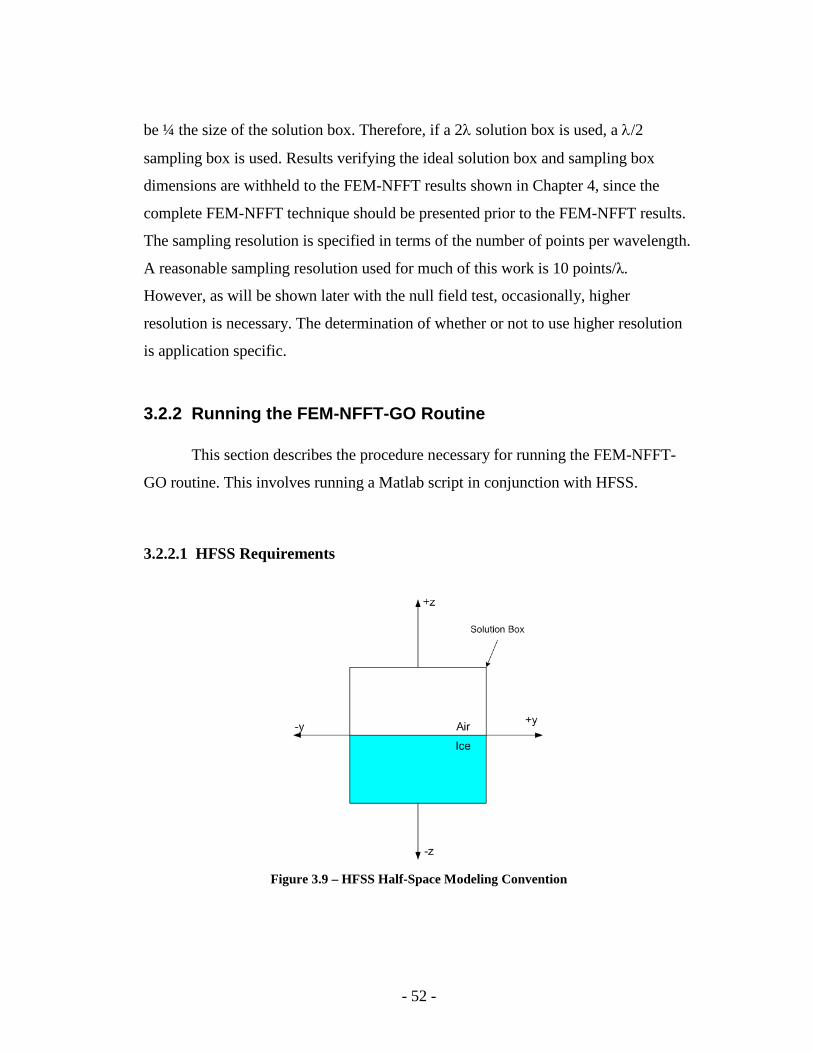
- 52 -
be ¼ the size of the solution box. Therefore, if a 2λ solution box is used, a λ/2
sampling box is used. Results verifying the ideal solution box and sampling box
dimensions are withheld to the FEM-NFFT results shown in Chapter 4, since the
complete FEM-NFFT technique should be presented prior to the FEM-NFFT results.
The sampling resolution is specified in terms of the number of points per wavelength.
A reasonable sampling resolution used for much of this work is 10 points/λ.
However, as will be shown later with the null field test, occasionally, higher
resolution is necessary. The determination of whether or not to use higher resolution
is application specific.
3.2.2 Running the FEM-NFFT-GO Routine This section describes the procedure necessary for running the FEM-NFFT-
GO routine. This involves running a Matlab script in conjunction with HFSS.
3.2.2.1 HFSS Requirements
Figure 3.9 – HFSS Half-Space Modeling Convention

- 53 -
In order for HFSS to interface properly with the FEM-NFFT-GO routine,
some modeling and naming conventions are required when modeling antennas in
HFSS. When modeling ice-mounted antennas in HFSS, the Matlab code assumes that
the half-space of ice extends from z=0 towards negative values of z, and the half-
space of air extends from z=0 towards positive values of z. This is shown in Figure
3.9.
Table 3.4 −−−− HFSS Model Naming Conventions
Due to the VBScript used in automatically sampling the near-zone electric and
magnetic fields, some naming conventions are required for building the HFSS model.
These naming conventions are outlined in Table 3.4. As discussed previously, the
“Solution Box” is the box enclosing the solution space, on which radiating boundary
conditions are specified. The “Solution Setup” was discussed in Section 2.1, and
“Setup1” is in fact the default name.
The only other requirement of HFSS when running the FEM-NFFT-GO
routine is that the desired HFSS model with solved near-zone field values be open
while running the NFFT portion of the routine, which accomplishes the near-zone
field sampling. Also, only one HFSS model at a time should be open while running
the routine.
3.2.2.2 The Master.m Matlab File
In this section, the operation of the Master.m Matlab script file is discussed,
which is the only code with which the user is required to interface. The Master.m
script is divided into three sections: inputs to specify for the FEM-NFFT-GO routine,
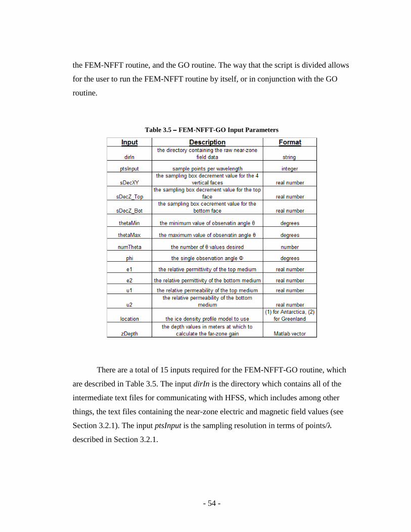
- 54 -
the FEM-NFFT routine, and the GO routine. The way that the script is divided allows
for the user to run the FEM-NFFT routine by itself, or in conjunction with the GO
routine.
Table 3.5 −−−− FEM-NFFT-GO Input Parameters
There are a total of 15 inputs required for the FEM-NFFT-GO routine, which
are described in Table 3.5. The input dirIn is the directory which contains all of the
intermediate text files for communicating with HFSS, which includes among other
things, the text files containing the near-zone electric and magnetic field values (see
Section 3.2.1). The input ptsInput is the sampling resolution in terms of points/λ
described in Section 3.2.1.
- 55 -
Three of the more complicated input parameters are sDecXY, sDecZ_Top, and
sDecZ_Bot. Each of these inputs are used to specify the sampling box size. The
sDecXY input specifies the reduction in size of the sampling box relative to the
solution box in the X and Y dimensions. The sDecZ_Top input specifies the reduction
in size of the sampling box relative to the solution box in the positive Z dimension.
Finally, the sDecZ_Bot input specifies the reduction in size of the sampling box
relative to the solution box in the negative Z dimension. The formulas for determining
the size of the sampling box from the decrement factors are as follows
( ) 2*XYsampBox solution box size sDecXY= − Eq. 3.28
( ) _ _ZsampBox solution box size sDecZ Top sDecZ Top= − − Eq. 3.29
where sampBoxXY is the size of the sampling box in wavelengths in the X and Y
dimensions and sampBoxZ is the size of the sampling box in wavelengths in the Z
dimension.
The reason for differentiating the sampling box size in the X, Y, and Z
dimensions has to do with the variability in HFSS antenna modeling. As discussed in
Section 2.2, waveport excitation requires that the port be connected to the solution
box boundary. If uniform reduction in the sampling box relative to the solution box
occurred in each dimension, this could cause overlap of the sampling box and the
antenna, which may be undesirable. Therefore, the option for non-uniform sampling
box size allows for the sampling box to be kept from overlapping with the antenna
location, if desired.
The observation angles are specified by four variables, thetaMin, thetaMax,
numTheta, and phi. Therefore, the far-zone fields determined by the FEM-NFFT-GO
routine are always computed through a range of θ values at a constant value of φ.
The material parameters for the dielectric half-space are specified by four
variables. The relative permittivity and relative permeability of the upper half-space
(air for purposes of ice-penetrating radar) are specified by e1 and u1, respectively.
- 56 -
For the lower half-space (glacial ice for purposes of ice-penetrating radar), the
relative permittivity and relative permeability are specified by e2 and u2,
respectively.
The final two input variables are only relevant for the GO routine. The input
location specifies the empirical constants to use for the glacial ice-density model (see
Section 3.1.2.1). A value of “1” specifies usage of the Antarctic empirical constants,
and a value of “2” specifies usage of the Greenland empirical constants (see Table
3.1). The last input zDepth is a one-dimensional Matlab row-vector specifying the
various depths in meters, within the ice, at which to determine the far-zone electric
field gain.
The FEM-NFFT section of the Matlab.m function contains calls to two sub-
functions, Equivalent_Currents and NFFT. Equivalent_Currents performs the
sampling of the near-zone electric and magnetic fields and their conversion to
equivalent surface currents, and basically implements the equivalence theorem. NFFT
performs the near-to-far-field transformation, and basically implements the
reciprocity theorem. Since Equivalent_Currents is an intermediate step, its outputs
are not listed here. However, the separation of the implementation of the equivalence
and reciprocity theorems eliminates the need for re-sampling the near-zone electric
and magnetic fields and converting them to equivalent currents unnecessarily.
Descriptions of the Equivalent_Currents outputs are described in the source code.
The outputs from the NFFT sub-function are listed in Table 3.6. These outputs
include the observation angles, intrinsic impedances of the upper and lower mediums,
and the theta and phi components of the quasi-far-zone electric field in both complex
and magnitude format (relative to an isotropic radiator). The variables EthetaIN and
EphiIN are in magnitude format which is required for input to the sub-function that
performs the GO routine.
The GO section of the Matlab.m function contains a call to the
Gain_Factor sub-routine which implements the geometric-optics ray-tracing
calculations. The outputs of Gain_Factor are listed in Table 3.7. The primary outputs

- 57 -
of concern are GthetaAD and GphiAD which are the theta and phi components of the
far-zone electric gain. GthetaAD and GphiAD are 2D matrices that are a function of
the effective look angle aidaPrime in the row dimension, and a function of zDepth in
the columns dimension.
Table 3.6 −−−− FEM-NFFT Output Parameters
Table 3.7 −−−− GO Output Parameters
- 58 -
CHAPTER 4: Far-Zone Field Results for Ice-Mounted Antennas
Far-zone field results obtained using the FEM-NFFT-GO techniques are
presented in this chapter (Section 4.4). But, prior to their presentation, results
validating the accuracy of the FEM-NFFT routine are presented in Section 4.1. Recall
that the FEM-NFFT procedure is useful on its own for determining far-zone fields for
antennas mounted above a homogeneous half-space.
4.1 FEM-NFFT Validation Tests
Four tests were performed to validate the FEM-NFFT technique for obtaining
the far-zone electric fields above a dielectric half-space. The first two of these tests
check the accuracy of the FEM-NFFT routine by comparing the FEM-NFFT results
to theoretical predictions. The third test validates the choice of near-zone field
sampling location when using the FEM-NFFT routine. The fourth test determines
whether or not similar far-zone field results could have been obtained using HFSS
alone, by substantially increasing the solution box size to several wavelengths.
4.1.1 The Null Field Test
A null field test was the first devised to validate the FEM-NFFT algorithm. In
this test, a plane wave was incident from a source located far from the sampling box.
Figure 4.1(a) depicts the original geometry and the equivalent geometry is depicted in
Figure 4.1(b). Here, the fields located some distance from the air/ice interface are Eb
and Hb, and those near the air/ice interface are Ea and Ha. In Figure 4.1(b), Ea and Ha
are sampled and converted to equivalent electric and magnetic source currents using
Equations 2.1 and 2.2. According to the equivalence principle, the observer senses the
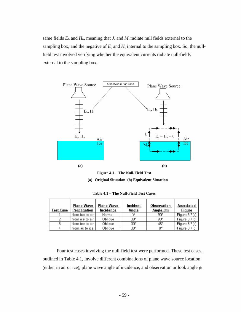
- 59 -
same fields Eb and Hb, meaning that Js and Ms radiate null fields external to the
sampling box, and the negative of Ea and Ha internal to the sampling box. So, the null-
field test involved verifying whether the equivalent currents radiate null-fields
external to the sampling box.
(a) (b)
Figure 4.1 −−−− The Null-Field Test
(a) Original Situation (b) Equivalent Situation
Table 4.1 – The Null-Field Test Cases
Four test cases involving the null-field test were performed. These test cases,
outlined in Table 4.1, involve different combinations of plane wave source location
(either in air or ice), plane wave angle of incidence, and observation or look angle φ.
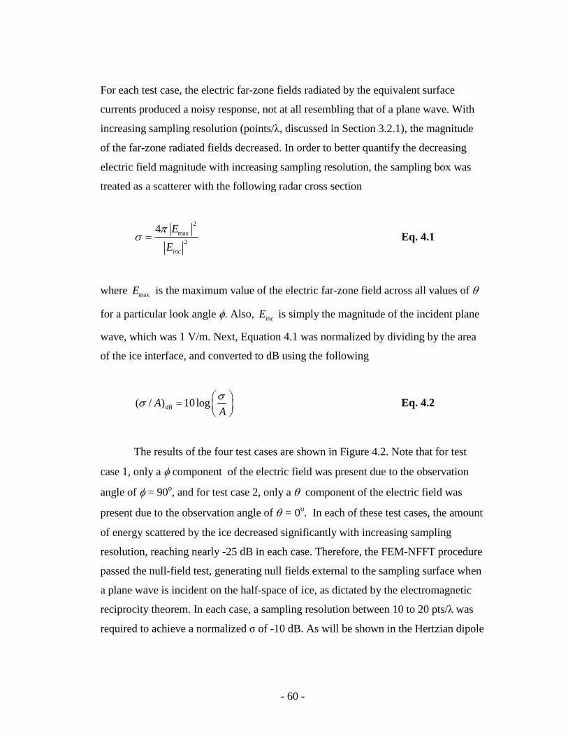
- 60 -
For each test case, the electric far-zone fields radiated by the equivalent surface
currents produced a noisy response, not at all resembling that of a plane wave. With
increasing sampling resolution (points/λ, discussed in Section 3.2.1), the magnitude
of the far-zone radiated fields decreased. In order to better quantify the decreasing
electric field magnitude with increasing sampling resolution, the sampling box was
treated as a scatterer with the following radar cross section
2
max2
4
inc
E
E
πσ = Eq. 4.1
where maxE is the maximum value of the electric far-zone field across all values of θ
for a particular look angle φ. Also, incE is simply the magnitude of the incident plane
wave, which was 1 V/m. Next, Equation 4.1 was normalized by dividing by the area
of the ice interface, and converted to dB using the following
( / ) 10 logdBAA
σσ =
Eq. 4.2
The results of the four test cases are shown in Figure 4.2. Note that for test
case 1, only a φ component of the electric field was present due to the observation
angle of φ = 90o, and for test case 2, only a θ component of the electric field was
present due to the observation angle of θ = 0o. In each of these test cases, the amount
of energy scattered by the ice decreased significantly with increasing sampling
resolution, reaching nearly -25 dB in each case. Therefore, the FEM-NFFT procedure
passed the null-field test, generating null fields external to the sampling surface when
a plane wave is incident on the half-space of ice, as dictated by the electromagnetic
reciprocity theorem. In each case, a sampling resolution between 10 to 20 pts/λ was
required to achieve a normalized σ of -10 dB. As will be shown in the Hertzian dipole
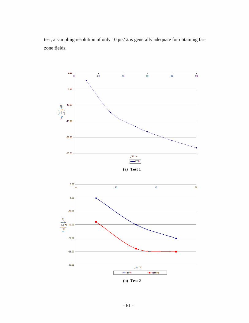
- 61 -
test, a sampling resolution of only 10 pts/ λ is generally adequate for obtaining far-
zone fields.
(a) Test 1
(b) Test 2
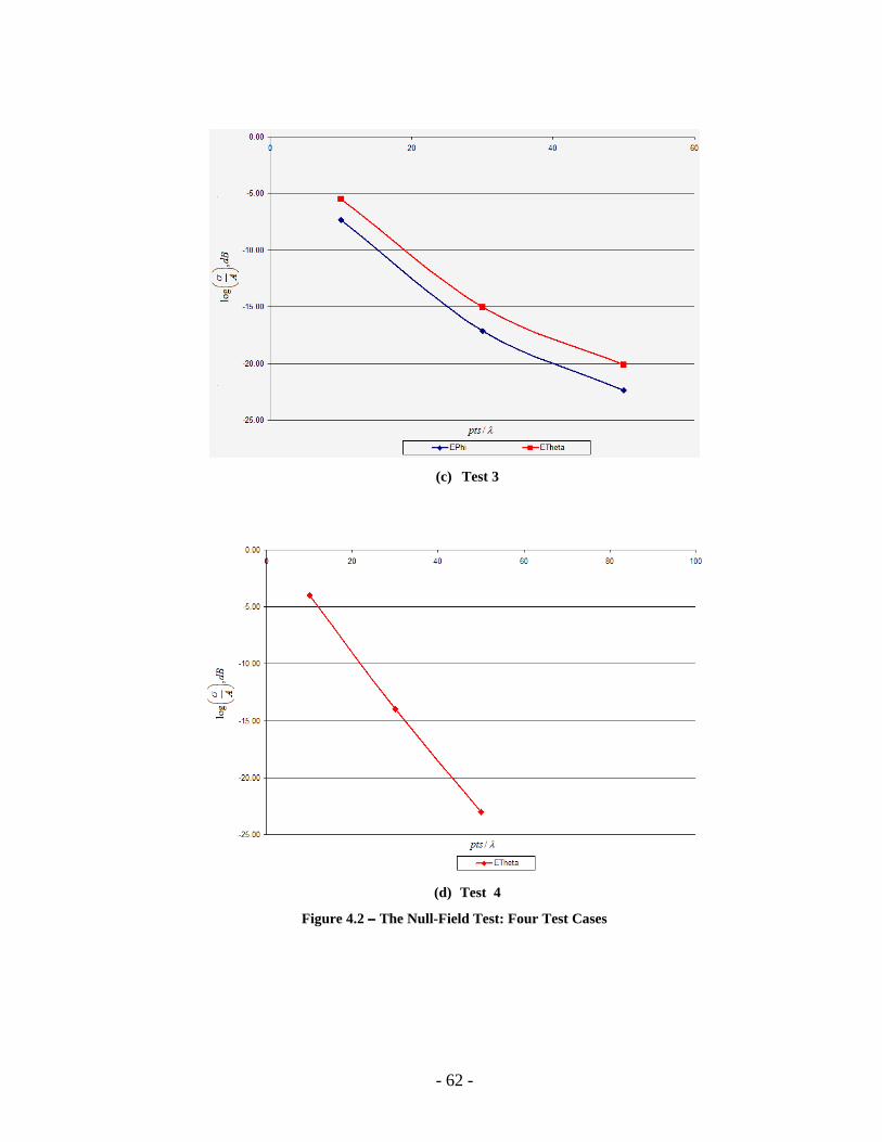
- 62 -
(c) Test 3
(d) Test 4
Figure 4.2 −−−− The Null-Field Test: Four Test Cases
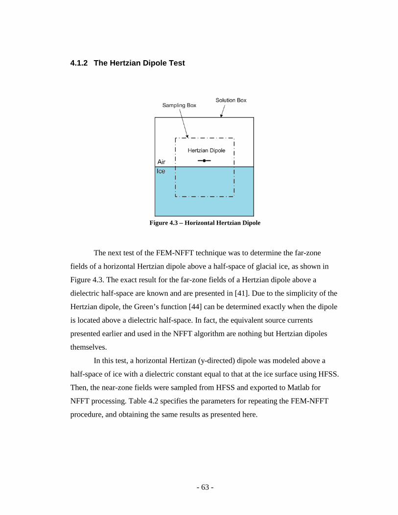
- 63 -
4.1.2 The Hertzian Dipole Test
Figure 4.3 −−−− Horizontal Hertzian Dipole
The next test of the FEM-NFFT technique was to determine the far-zone
fields of a horizontal Hertzian dipole above a half-space of glacial ice, as shown in
Figure 4.3. The exact result for the far-zone fields of a Hertzian dipole above a
dielectric half-space are known and are presented in [41]. Due to the simplicity of the
Hertzian dipole, the Green’s function [44] can be determined exactly when the dipole
is located above a dielectric half-space. In fact, the equivalent source currents
presented earlier and used in the NFFT algorithm are nothing but Hertzian dipoles
themselves.
In this test, a horizontal Hertizan (y-directed) dipole was modeled above a
half-space of ice with a dielectric constant equal to that at the ice surface using HFSS.
Then, the near-zone fields were sampled from HFSS and exported to Matlab for
NFFT processing. Table 4.2 specifies the parameters for repeating the FEM-NFFT
procedure, and obtaining the same results as presented here.
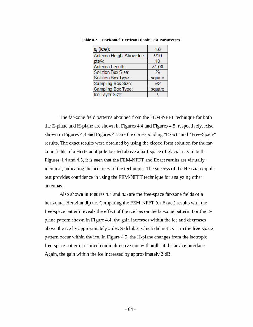
- 64 -
Table 4.2 −−−− Horizontal Hertizan Dipole Test Parameters
The far-zone field patterns obtained from the FEM-NFFT technique for both
the E-plane and H-plane are shown in Figures 4.4 and Figures 4.5, respectively. Also
shown in Figures 4.4 and Figures 4.5 are the corresponding “Exact” and “Free-Space”
results. The exact results were obtained by using the closed form solution for the far-
zone fields of a Hertzian dipole located above a half-space of glacial ice. In both
Figures 4.4 and 4.5, it is seen that the FEM-NFFT and Exact results are virtually
identical, indicating the accuracy of the technique. The success of the Hertzian dipole
test provides confidence in using the FEM-NFFT technique for analyzing other
antennas.
Also shown in Figures 4.4 and 4.5 are the free-space far-zone fields of a
horizontal Hertzian dipole. Comparing the FEM-NFFT (or Exact) results with the
free-space pattern reveals the effect of the ice has on the far-zone pattern. For the E-
plane pattern shown in Figure 4.4, the gain increases within the ice and decreases
above the ice by approximately 2 dB. Sidelobes which did not exist in the free-space
pattern occur within the ice. In Figure 4.5, the H-plane changes from the isotropic
free-space pattern to a much more directive one with nulls at the air/ice interface.
Again, the gain within the ice increased by approximately 2 dB.
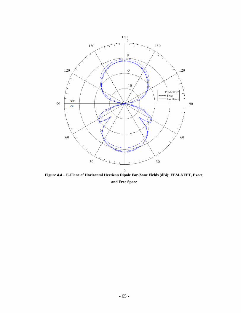
- 65 -
Figure 4.4 −−−− E-Plane of Horizontal Hertizan Dipole Far-Zone Fields (dBi): FEM-NFFT, Exact,
and Free Space
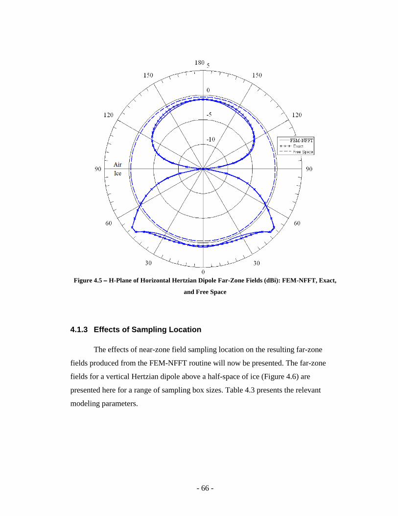
- 66 -
Figure 4.5 −−−− H-Plane of Horizontal Hertzian Dipole Far-Zone Fields (dBi): FEM-NFFT, Exact,
and Free Space
4.1.3 Effects of Sampling Location
The effects of near-zone field sampling location on the resulting far-zone
fields produced from the FEM-NFFT routine will now be presented. The far-zone
fields for a vertical Hertzian dipole above a half-space of ice (Figure 4.6) are
presented here for a range of sampling box sizes. Table 4.3 presents the relevant
modeling parameters.
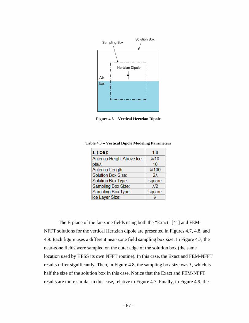
- 67 -
Figure 4.6 −−−− Vertical Hertzian Dipole
Table 4.3 −−−− Vertical Dipole Modeling Parameters
The E-plane of the far-zone fields using both the “Exact” [41] and FEM-
NFFT solutions for the vertical Hertzian dipole are presented in Figures 4.7, 4.8, and
4.9. Each figure uses a different near-zone field sampling box size. In Figure 4.7, the
near-zone fields were sampled on the outer edge of the solution box (the same
location used by HFSS its own NFFT routine). In this case, the Exact and FEM-NFFT
results differ significantly. Then, in Figure 4.8, the sampling box size was λ, which is
half the size of the solution box in this case. Notice that the Exact and FEM-NFFT
results are more similar in this case, relative to Figure 4.7. Finally, in Figure 4.9, the
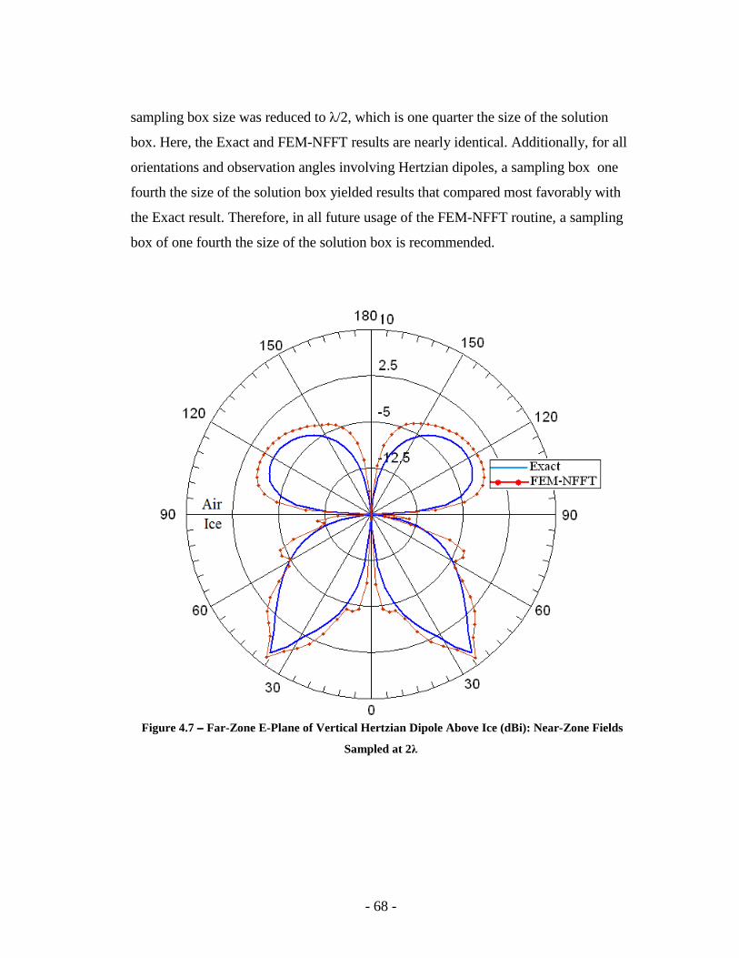
- 68 -
sampling box size was reduced to λ/2, which is one quarter the size of the solution
box. Here, the Exact and FEM-NFFT results are nearly identical. Additionally, for all
orientations and observation angles involving Hertzian dipoles, a sampling box one
fourth the size of the solution box yielded results that compared most favorably with
the Exact result. Therefore, in all future usage of the FEM-NFFT routine, a sampling
box of one fourth the size of the solution box is recommended.
Figure 4.7 −−−− Far-Zone E-Plane of Vertical Hertzian Dipole Above Ice (dBi): Near-Zone Fields
Sampled at 2λ
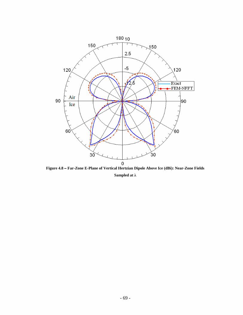
- 69 -
Figure 4.8 −−−− Far-Zone E-Plane of Vertical Hertzian Dipole Above Ice (dBi): Near-Zone Fields
Sampled at λ
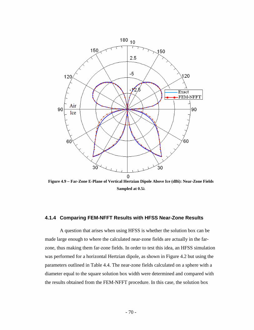
- 70 -
Figure 4.9 −−−− Far-Zone E-Plane of Vertical Hertzian Dipole Above Ice (dBi): Near-Zone Fields
Sampled at 0.5λ
4.1.4 Comparing FEM-NFFT Results with HFSS Near-Zone Results
A question that arises when using HFSS is whether the solution box can be
made large enough to where the calculated near-zone fields are actually in the far-
zone, thus making them far-zone fields. In order to test this idea, an HFSS simulation
was performed for a horizontal Hertzian dipole, as shown in Figure 4.2 but using the
parameters outlined in Table 4.4. The near-zone fields calculated on a sphere with a
diameter equal to the square solution box width were determined and compared with
the results obtained from the FEM-NFFT procedure. In this case, the solution box
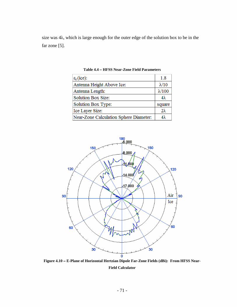
- 71 -
size was 4λ, which is large enough for the outer edge of the solution box to be in the
far zone [5].
Table 4.4 −−−− HFSS Near-Zone Field Parameters
Figure 4.10 −−−− E-Plane of Horizontal Hertzian Dipole Far-Zone Fields (dBi): From HFSS Near-
Field Calculator
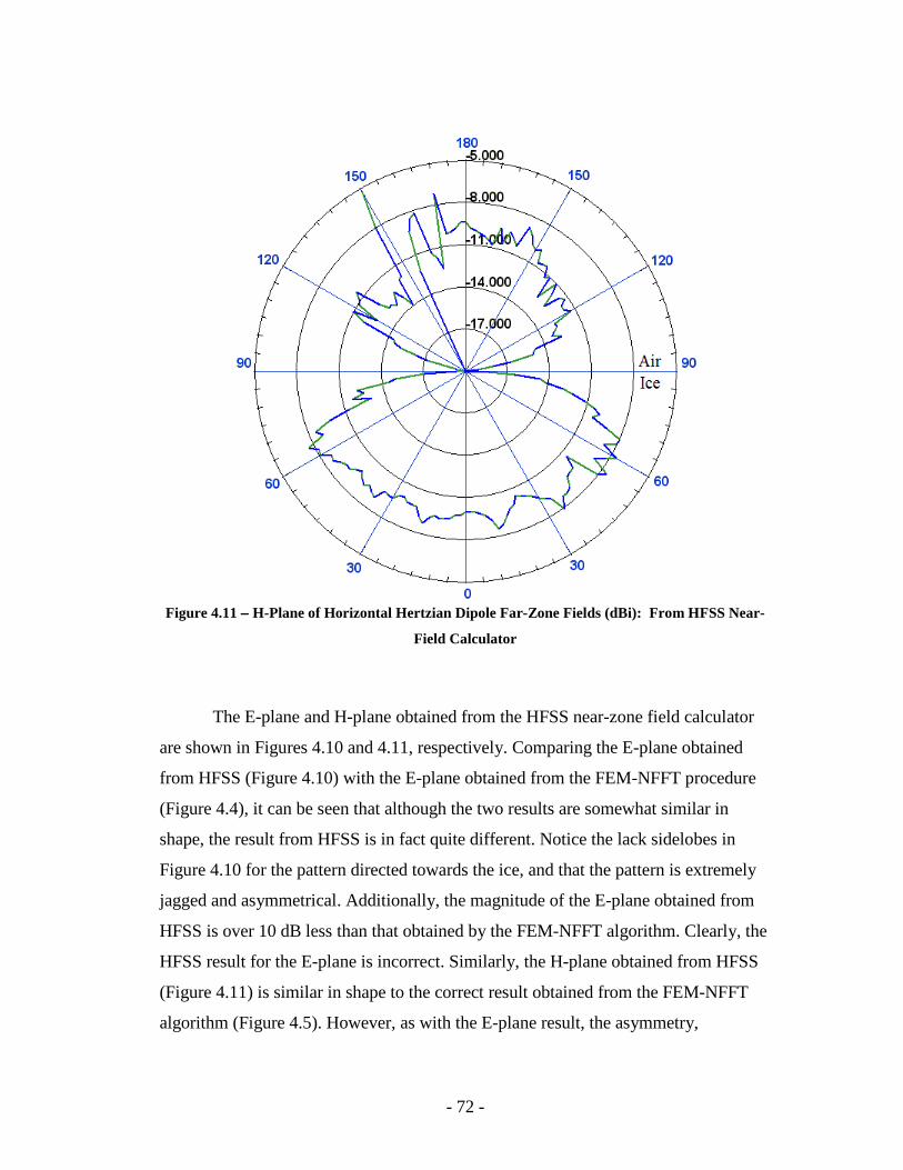
- 72 -
Figure 4.11 −−−− H-Plane of Horizontal Hertzian Dipole Far-Zone Fields (dBi): From HFSS Near-
Field Calculator
The E-plane and H-plane obtained from the HFSS near-zone field calculator
are shown in Figures 4.10 and 4.11, respectively. Comparing the E-plane obtained
from HFSS (Figure 4.10) with the E-plane obtained from the FEM-NFFT procedure
(Figure 4.4), it can be seen that although the two results are somewhat similar in
shape, the result from HFSS is in fact quite different. Notice the lack sidelobes in
Figure 4.10 for the pattern directed towards the ice, and that the pattern is extremely
jagged and asymmetrical. Additionally, the magnitude of the E-plane obtained from
HFSS is over 10 dB less than that obtained by the FEM-NFFT algorithm. Clearly, the
HFSS result for the E-plane is incorrect. Similarly, the H-plane obtained from HFSS
(Figure 4.11) is similar in shape to the correct result obtained from the FEM-NFFT
algorithm (Figure 4.5). However, as with the E-plane result, the asymmetry,
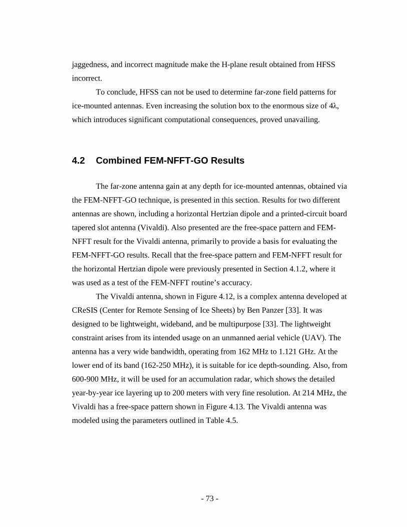
- 73 -
jaggedness, and incorrect magnitude make the H-plane result obtained from HFSS
incorrect.
To conclude, HFSS can not be used to determine far-zone field patterns for
ice-mounted antennas. Even increasing the solution box to the enormous size of 4λ,
which introduces significant computational consequences, proved unavailing.
4.2 Combined FEM-NFFT-GO Results
The far-zone antenna gain at any depth for ice-mounted antennas, obtained via
the FEM-NFFT-GO technique, is presented in this section. Results for two different
antennas are shown, including a horizontal Hertzian dipole and a printed-circuit board
tapered slot antenna (Vivaldi). Also presented are the free-space pattern and FEM-
NFFT result for the Vivaldi antenna, primarily to provide a basis for evaluating the
FEM-NFFT-GO results. Recall that the free-space pattern and FEM-NFFT result for
the horizontal Hertzian dipole were previously presented in Section 4.1.2, where it
was used as a test of the FEM-NFFT routine’s accuracy.
The Vivaldi antenna, shown in Figure 4.12, is a complex antenna developed at
CReSIS (Center for Remote Sensing of Ice Sheets) by Ben Panzer [33]. It was
designed to be lightweight, wideband, and be multipurpose [33]. The lightweight
constraint arises from its intended usage on an unmanned aerial vehicle (UAV). The
antenna has a very wide bandwidth, operating from 162 MHz to 1.121 GHz. At the
lower end of its band (162-250 MHz), it is suitable for ice depth-sounding. Also, from
600-900 MHz, it will be used for an accumulation radar, which shows the detailed
year-by-year ice layering up to 200 meters with very fine resolution. At 214 MHz, the
Vivaldi has a free-space pattern shown in Figure 4.13. The Vivaldi antenna was
modeled using the parameters outlined in Table 4.5.
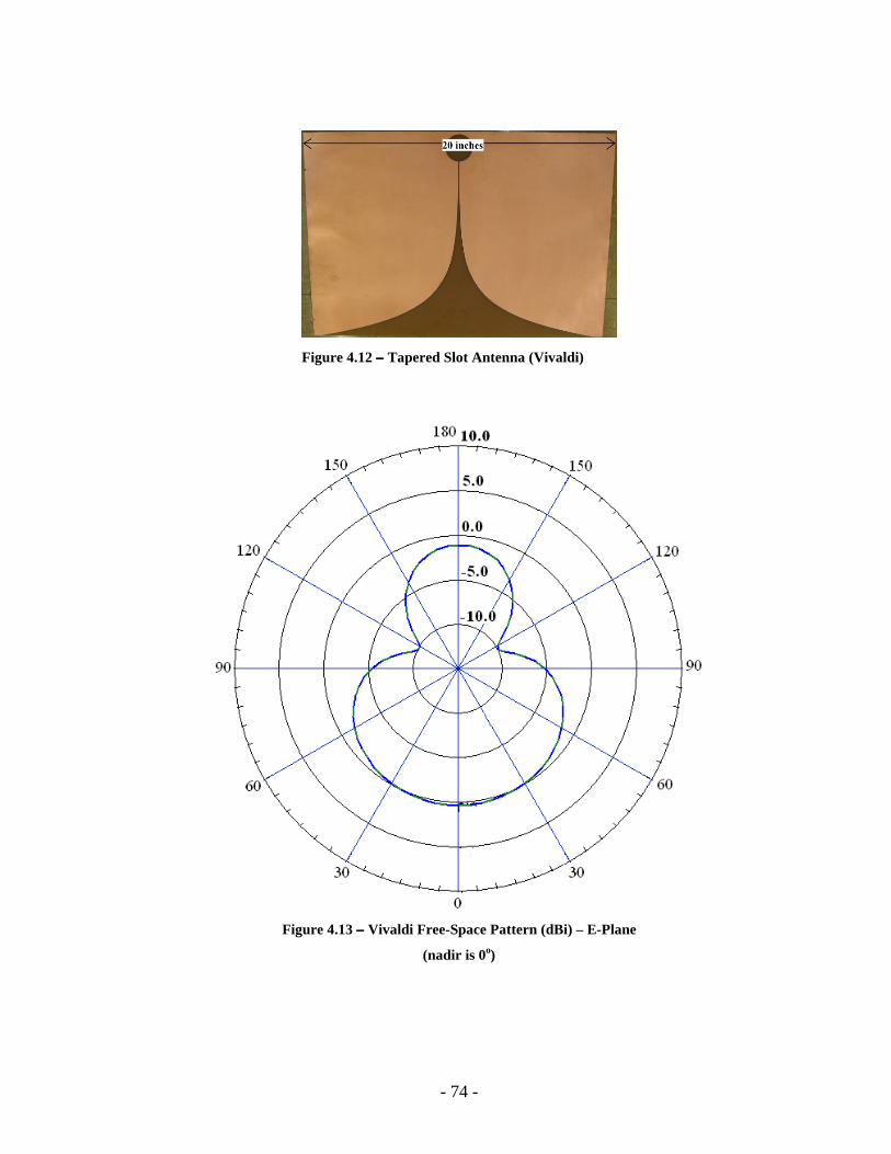
- 74 -
Figure 4.12 −−−− Tapered Slot Antenna (Vivaldi)
Figure 4.13 −−−− Vivaldi Free-Space Pattern (dBi) – E-Plane
(nadir is 0o)
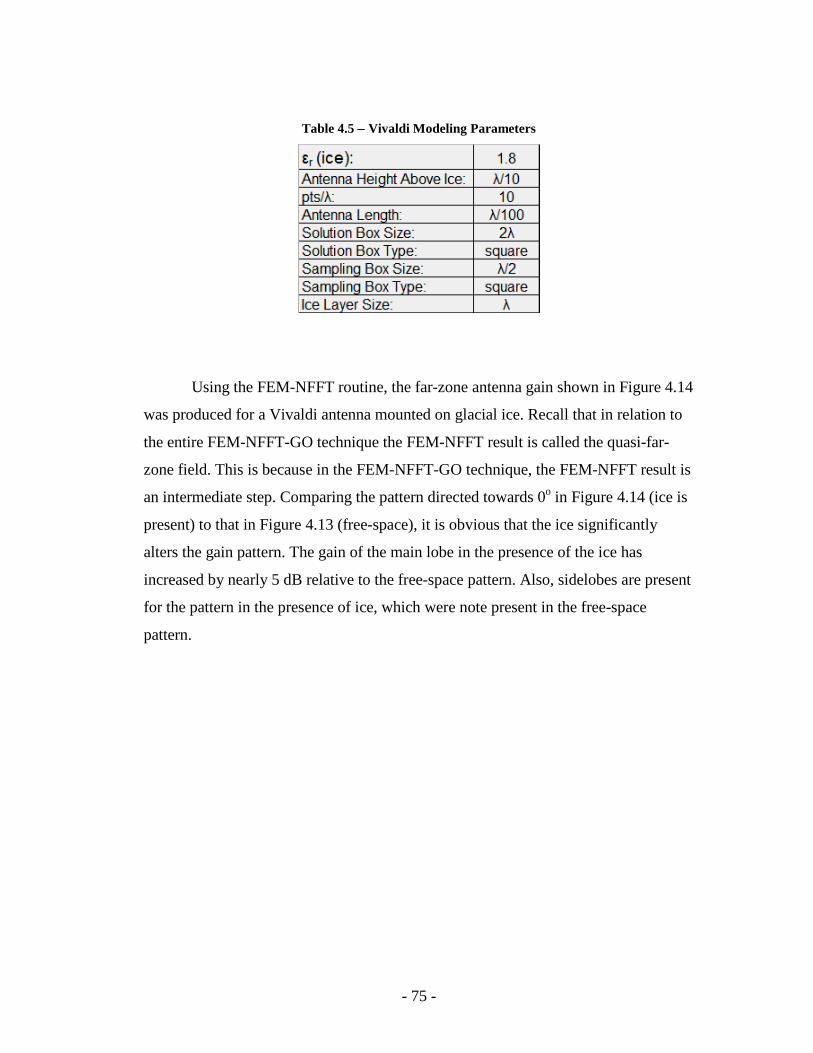
- 75 -
Table 4.5 −−−− Vivaldi Modeling Parameters
Using the FEM-NFFT routine, the far-zone antenna gain shown in Figure 4.14
was produced for a Vivaldi antenna mounted on glacial ice. Recall that in relation to
the entire FEM-NFFT-GO technique the FEM-NFFT result is called the quasi-far-
zone field. This is because in the FEM-NFFT-GO technique, the FEM-NFFT result is
an intermediate step. Comparing the pattern directed towards 0o in Figure 4.14 (ice is
present) to that in Figure 4.13 (free-space), it is obvious that the ice significantly
alters the gain pattern. The gain of the main lobe in the presence of the ice has
increased by nearly 5 dB relative to the free-space pattern. Also, sidelobes are present
for the pattern in the presence of ice, which were note present in the free-space
pattern.
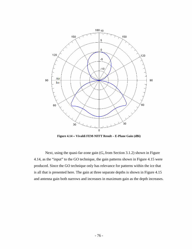
- 76 -
Figure 4.14 −−−− Vivaldi FEM-NFFT Result – E-Plane Gain (dBi)
Next, using the quasi-far-zone gain (Go from Section 3.1.2) shown in Figure
4.14, as the “input” to the GO technique, the gain patterns shown in Figure 4.15 were
produced. Since the GO technique only has relevance for patterns within the ice that
is all that is presented here. The gain at three separate depths is shown in Figure 4.15
and antenna gain both narrows and increases in maximum gain as the depth increases.
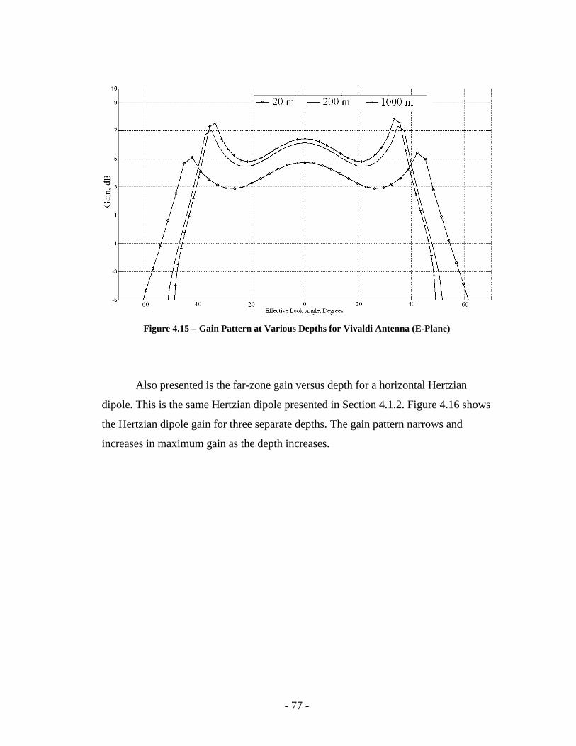
- 77 -
Figure 4.15 −−−− Gain Pattern at Various Depths for Vivaldi Antenna (E-Plane)
Also presented is the far-zone gain versus depth for a horizontal Hertzian
dipole. This is the same Hertzian dipole presented in Section 4.1.2. Figure 4.16 shows
the Hertzian dipole gain for three separate depths. The gain pattern narrows and
increases in maximum gain as the depth increases.
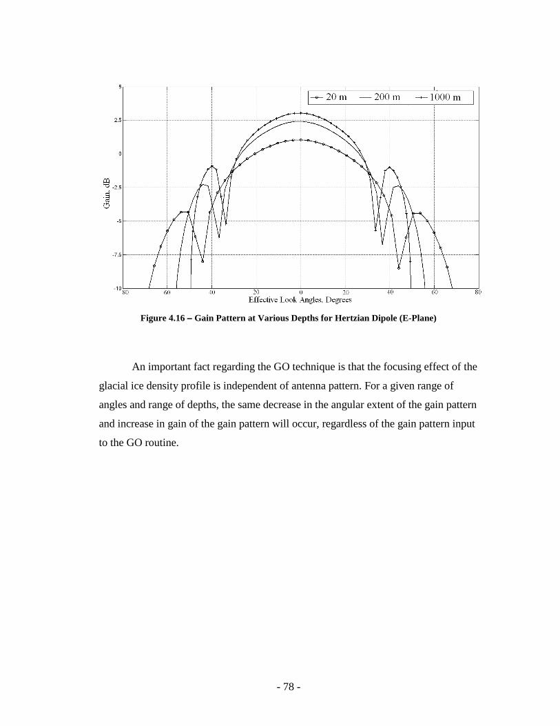
- 78 -
Figure 4.16 −−−− Gain Pattern at Various Depths for Hertzian Dipole (E-Plane)
An important fact regarding the GO technique is that the focusing effect of the
glacial ice density profile is independent of antenna pattern. For a given range of
angles and range of depths, the same decrease in the angular extent of the gain pattern
and increase in gain of the gain pattern will occur, regardless of the gain pattern input
to the GO routine.
- 79 -
CHAPTER 5: Glacial Ice Temperature Extraction from Attenuation Measurements
Ice attenuation can be measured from radar returns using a surface-based
bistatic radar system, such as that presented in Section 1.2. Two common mid-point
(CMP) antenna configurations are utilized in the data attainment: one where transmit
and receive antennas are at a fixed distance from each other, and another where the
transmit and receive antennas are at a fixed incident and reflected angle with respect
to each other. Results from these two arrangements are then combined to measure
attenuation as a function of depth.
The ultimate goal of obtaining ice attenuation as a function of depth is to
determine the ice temperature as a function of depth. However, prior to relating
attenuation to ice temperature, the basic causes of attenuation within glacial ice must
be considered, which are presented in Sections 5.1 and 5.2. Also, in Section 5.3
existing temperature profile data is presented for glaciers in Antarctica and
Greenland. These data reveal the range of temperatures typically encountered in
glacial ice. Next, in Section 5.4, the relationship between loss mechanisms and the
attenuation constant is presented. The method for measuring glacial ice attenuation
from radar echoes is presented in Section 5.5. Then, the algorithm for extracting
temperature from attenuation measurements is presented in Section 5.6. Finally, in
Section 5.7, simulated results are presented that highlight the capabilities of the
technique for extracting glacial ice temperature from radar echoes.
5.1 Causes of Attenuation in Glacial Ice
Two loss (attenuation) mechanisms can occur in glacial ice: conduction loss,
and polarization loss. Conduction losses occur when the conductivity σ is greater than
zero, and results in conduction current defined by the following
- 80 -
CJ Eσ= Eq. 5.1
The conduction current causes some of the energy transmitted from the radar to be
converted to heat within the ice.
Polarization losses are due to displacement current within lossy media.
Displacement current results within any dielectric exposed to a time-varying electric
field, and is described by the following
DJ j Eωε= Eq. 5.2
where ω is the frequency in radians per second. For materials with a real permittivity
(i.e. lossless dielectric), equal amounts of energy are stored and released upon each
cycle, meaning that DJ results in no loss. However, when the permittivity is complex,
as with glacial ice, DJ causes some of the incident energy to be converted to heat.
Therefore, the causes of loss in glacial ice are due to conductivity σ and a
complex permittivity. Generally, these two loss mechanisms are combined into a
single imaginary component of the permittivity, where
' ''( )j σε ε ε ω= − + Eq. 5.3
Equation 5.3 can be simplified to the following
' ''( )o r rjε ε ε ε= − Eq. 5.4
where oε is the free-space permittivity (8.854 x 10⁻¹² F/m), the real part of the
permittivity is
- 81 -
'
'r
o
εε
ε= Eq. 5.5
and the imaginary part is
''
''r
o
σε ωεε
+= Eq. 5.6
At depth-sounding frequencies in glacial ice, the loss is dominated by σ [28] and
therefore, the imaginary part of ε can be simplified to
''r
o
σωε
ε= Eq. 5.7
which neglects contributions to loss arising from ''ε . However, Equation 5.7 is only
applicable for frequencies below 700 MHz, since above this frequency, ''ε
(polarization loss term) increases with frequency and becomes very large. Equation
5.7 allows the conductivity and loss within ice to be entirely described by the
permittivityε . Since σ is the primary cause of loss in glacial ice, a further discussion
of the causes of conductivity is warranted.
5.2 Conductivity in Glacial Ice
Radar signal attenuation within glacial ice is proportional to conductivity,
which in turn depends on a number of factors, including impurity concentrations as
well as the ice temperature [28]. Pure ice conductivity is due to the polarization of
individual water molecules (H2O), hydronium (H3O+) and hydroxyl (OH-) ionic
defects, and Bjerrum defects in the presence of high-frequency (0.1 to 300 MHz)
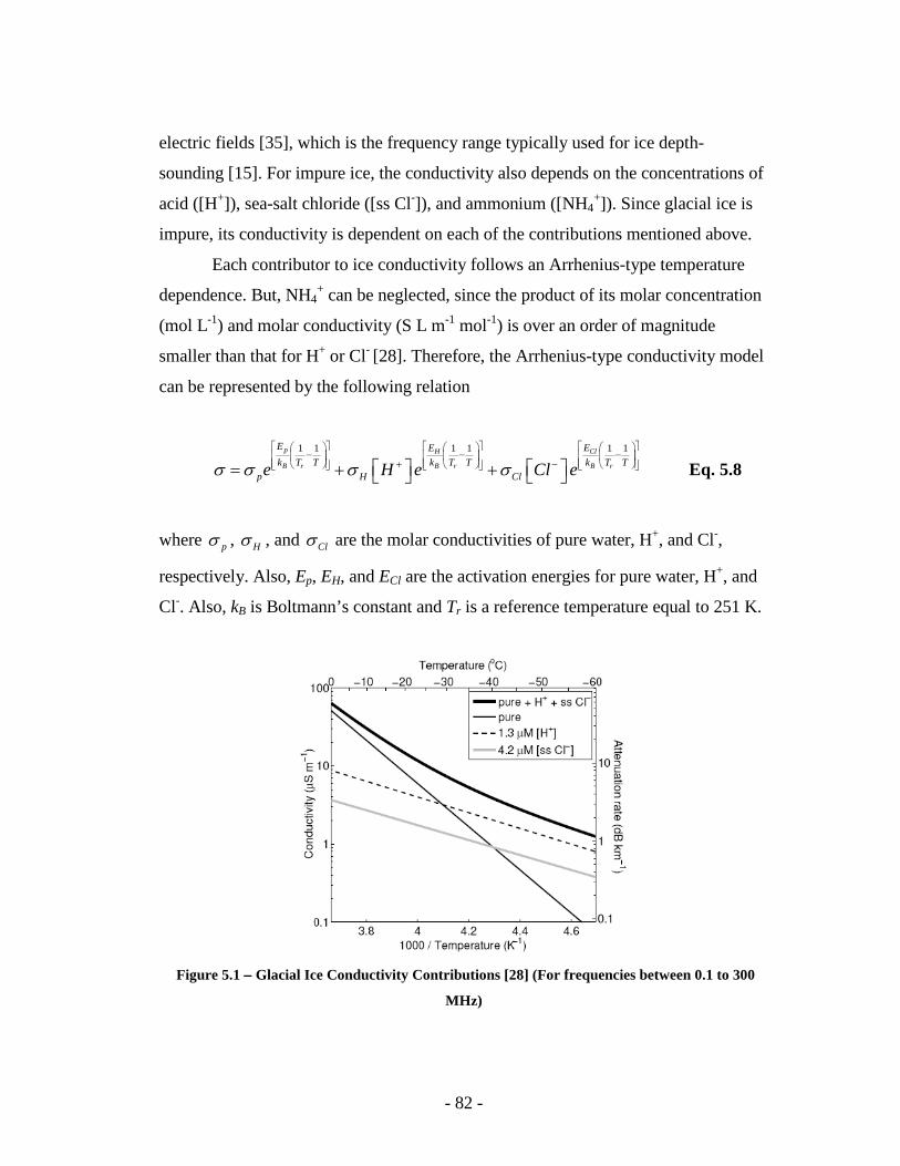
- 82 -
electric fields [35], which is the frequency range typically used for ice depth-
sounding [15]. For impure ice, the conductivity also depends on the concentrations of
acid ([H+]), sea-salt chloride ([ss Cl-]), and ammonium ([NH4+]). Since glacial ice is
impure, its conductivity is dependent on each of the contributions mentioned above.
Each contributor to ice conductivity follows an Arrhenius-type temperature
dependence. But, NH4+ can be neglected, since the product of its molar concentration
(mol L-1) and molar conductivity (S L m-1 mol-1) is over an order of magnitude
smaller than that for H+ or Cl- [28]. Therefore, the Arrhenius-type conductivity model
can be represented by the following relation
1 1 1 1 1 1p ClH
B r B r B r
E EE
k T T k T T k T T
p H Cle H e Cl eσ σ σ σ
− − − + − = + + Eq. 5.8
where pσ , Hσ , and Clσ are the molar conductivities of pure water, H+, and Cl-,
respectively. Also, Ep, EH, and ECl are the activation energies for pure water, H+, and
Cl-. Also, kB is Boltmann’s constant and Tr is a reference temperature equal to 251 K.
Figure 5.1 −−−− Glacial Ice Conductivity Contributions [28] (For frequencies between 0.1 to 300
MHz)
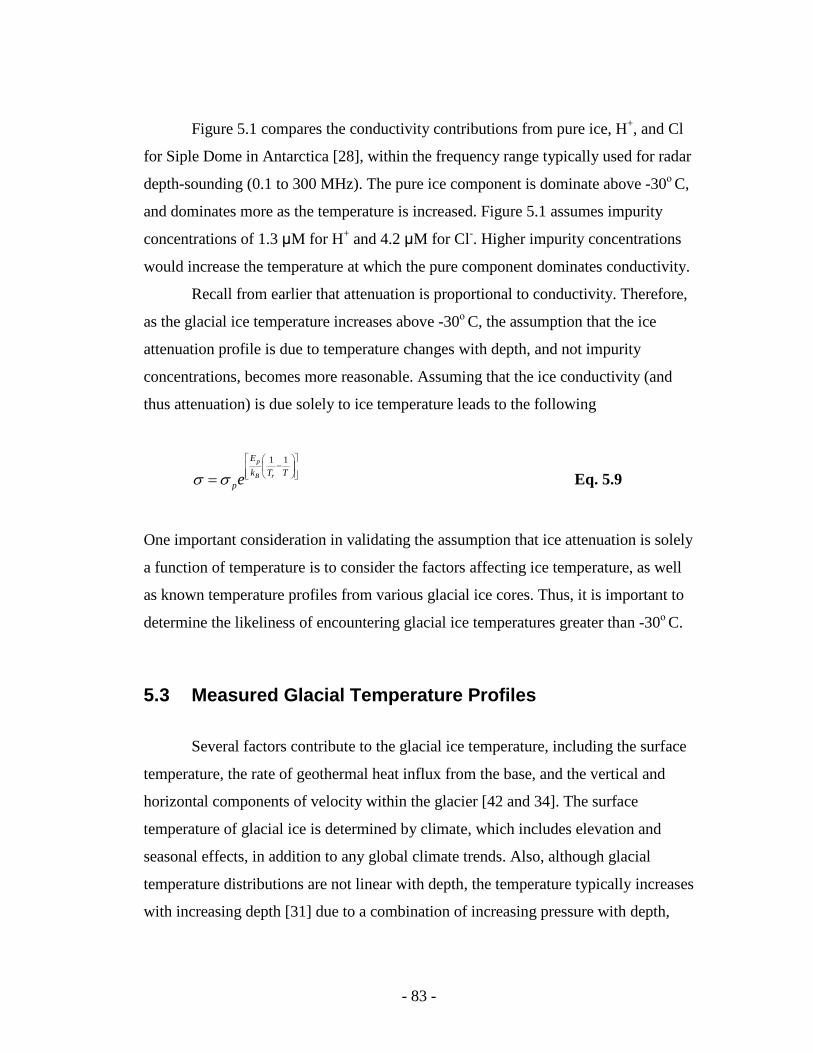
- 83 -
Figure 5.1 compares the conductivity contributions from pure ice, H+, and Cl
for Siple Dome in Antarctica [28], within the frequency range typically used for radar
depth-sounding (0.1 to 300 MHz). The pure ice component is dominate above -30ο C,
and dominates more as the temperature is increased. Figure 5.1 assumes impurity
concentrations of 1.3 µM for H+ and 4.2 µM for Cl-. Higher impurity concentrations
would increase the temperature at which the pure component dominates conductivity.
Recall from earlier that attenuation is proportional to conductivity. Therefore,
as the glacial ice temperature increases above -30ο C, the assumption that the ice
attenuation profile is due to temperature changes with depth, and not impurity
concentrations, becomes more reasonable. Assuming that the ice conductivity (and
thus attenuation) is due solely to ice temperature leads to the following
1 1p
B r
E
k T T
peσ σ
− = Eq. 5.9
One important consideration in validating the assumption that ice attenuation is solely
a function of temperature is to consider the factors affecting ice temperature, as well
as known temperature profiles from various glacial ice cores. Thus, it is important to
determine the likeliness of encountering glacial ice temperatures greater than -30ο C.
5.3 Measured Glacial Temperature Profiles
Several factors contribute to the glacial ice temperature, including the surface
temperature, the rate of geothermal heat influx from the base, and the vertical and
horizontal components of velocity within the glacier [42 and 34]. The surface
temperature of glacial ice is determined by climate, which includes elevation and
seasonal effects, in addition to any global climate trends. Also, although glacial
temperature distributions are not linear with depth, the temperature typically increases
with increasing depth [31] due to a combination of increasing pressure with depth,
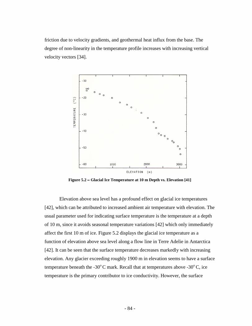
- 84 -
friction due to velocity gradients, and geothermal heat influx from the base. The
degree of non-linearity in the temperature profile increases with increasing vertical
velocity vectors [34].
Figure 5.2 −−−− Glacial Ice Temperature at 10 m Depth vs. Elevation [41]
Elevation above sea level has a profound effect on glacial ice temperatures
[42], which can be attributed to increased ambient air temperature with elevation. The
usual parameter used for indicating surface temperature is the temperature at a depth
of 10 m, since it avoids seasonal temperature variations [42] which only immediately
affect the first 10 m of ice. Figure 5.2 displays the glacial ice temperature as a
function of elevation above sea level along a flow line in Terre Adelie in Antarctica
[42]. It can be seen that the surface temperature decreases markedly with increasing
elevation. Any glacier exceeding roughly 1900 m in elevation seems to have a surface
temperature beneath the -30ο C mark. Recall that at temperatures above -30ο C, ice
temperature is the primary contributor to ice conductivity. However, the surface
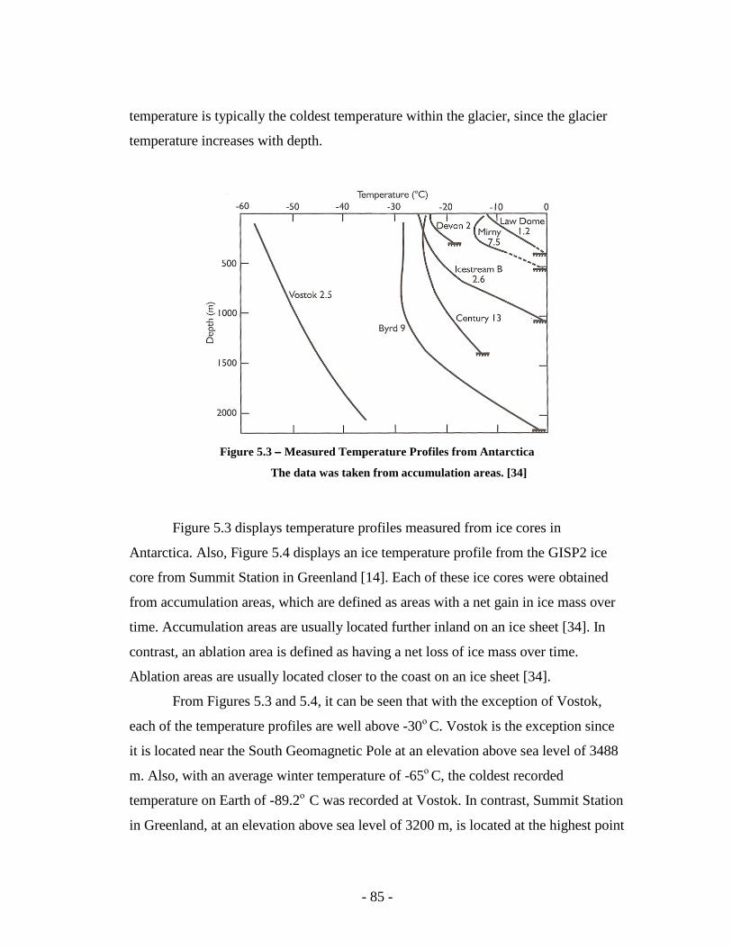
- 85 -
temperature is typically the coldest temperature within the glacier, since the glacier
temperature increases with depth.
Figure 5.3 −−−− Measured Temperature Profiles from Antarctica
The data was taken from accumulation areas. [34]
Figure 5.3 displays temperature profiles measured from ice cores in
Antarctica. Also, Figure 5.4 displays an ice temperature profile from the GISP2 ice
core from Summit Station in Greenland [14]. Each of these ice cores were obtained
from accumulation areas, which are defined as areas with a net gain in ice mass over
time. Accumulation areas are usually located further inland on an ice sheet [34]. In
contrast, an ablation area is defined as having a net loss of ice mass over time.
Ablation areas are usually located closer to the coast on an ice sheet [34].
From Figures 5.3 and 5.4, it can be seen that with the exception of Vostok,
each of the temperature profiles are well above -30ο C. Vostok is the exception since
it is located near the South Geomagnetic Pole at an elevation above sea level of 3488
m. Also, with an average winter temperature of -65ο C, the coldest recorded
temperature on Earth of -89.2ο C was recorded at Vostok. In contrast, Summit Station
in Greenland, at an elevation above sea level of 3200 m, is located at the highest point
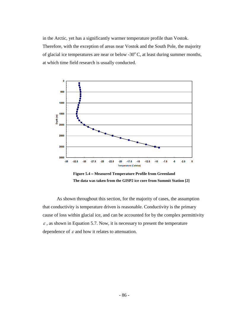
- 86 -
in the Arctic, yet has a significantly warmer temperature profile than Vostok.
Therefore, with the exception of areas near Vostok and the South Pole, the majority
of glacial ice temperatures are near or below -30ο C, at least during summer months,
at which time field research is usually conducted.
Figure 5.4 −−−− Measured Temperature Profile from Greenland
The data was taken from the GISP2 ice core from Summit Station [2]
As shown throughout this section, for the majority of cases, the assumption
that conductivity is temperature driven is reasonable. Conductivity is the primary
cause of loss within glacial ice, and can be accounted for by the complex permittivity
ε , as shown in Equation 5.7. Now, it is necessary to present the temperature
dependence of ε and how it relates to attenuation.
- 87 -
5.4 Relation of Attenuation to Ice Permittivity and Temperature
The majority of the material in Section 5.4 was originally presented by Li,
Xie, and Dobbs in [27].
The attenuation (loss) within glacial ice can be entirely accounted for by the
complex permittivity ε as shown in Equation 5.7. Both the real and imaginary parts
of ε exhibit temperature dependence. Based on the work in [29],
' ( ) 3.1884 (0.00091)r T Tε = + Eq. 5.10
where T is the temperature in degrees Celsius. Also, as shown in [1]
'' 2.02 0.0251( , ) 10
10T
r f Tf
ε − += Eq. 5.11
where f is the operating frequency of the radar system in GHz.
Generally, for lossy media, the wavenumber is complex and is represented by
( )k j jωµ σ ωε= − + Eq. 5.12
where µ equals the free-space magnetic permeability (4π x10-7 H/m), since glacial
ice is non-magnetic. However, since conductivity was accounted for by ''rε in
Equation 5.7, k can be simplified to
k ω µε= Eq. 5.13
The complex propagation constant is related to k via the following
- 88 -
jk jγ α β= = + Eq. 5.14
where α is the attenuation constant (Np/m) and β is the phase constant (rad/m).
Taking the real and imaginary parts of jk and doing some rearrangement results in
( )1
' 222 1 tan 1
2o o rf
µ ε εα π δ
= − −
Eq. 5.15
and
( )1
' 222 1 tan 1
2o o rf
µ ε εβ π δ
= − +
Eq. 5.16
where tanδ is the loss tangent described by
''
'tan r
r
εδ
ε=
Eq. 5.17
Equation 5.15 relates the attenuation α to the complex permittivity ε of the
ice, which is itself a function of temperature. Therefore, the ability to measure
attenuation at each depth within glacial ice should enable the determination of
temperature at each depth. The measurement of attenuation at each depth using radar
echoes from the two CMP configurations is discussed next.
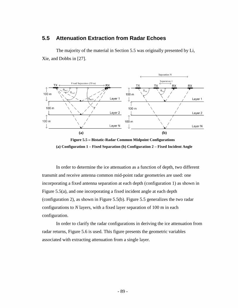
- 89 -
5.5 Attenuation Extraction from Radar Echoes
The majority of the material in Section 5.5 was originally presented by Li,
Xie, and Dobbs in [27].
(a) (b)
Figure 5.5 −−−− Bistatic-Radar Common Midpoint Configurations
(a) Configuration 1 – Fixed Separation (b) Configuration 2 – Fixed Incident Angle
In order to determine the ice attenuation as a function of depth, two different
transmit and receive antenna common mid-point radar geometries are used: one
incorporating a fixed antenna separation at each depth (configuration 1) as shown in
Figure 5.5(a), and one incorporating a fixed incident angle at each depth
(configuration 2), as shown in Figure 5.5(b). Figure 5.5 generalizes the two radar
configurations to N layers, with a fixed layer separation of 100 m in each
configuration.
In order to clarify the radar configurations in deriving the ice attenuation from
radar returns, Figure 5.6 is used. This figure presents the geometric variables
associated with extracting attenuation from a single layer.
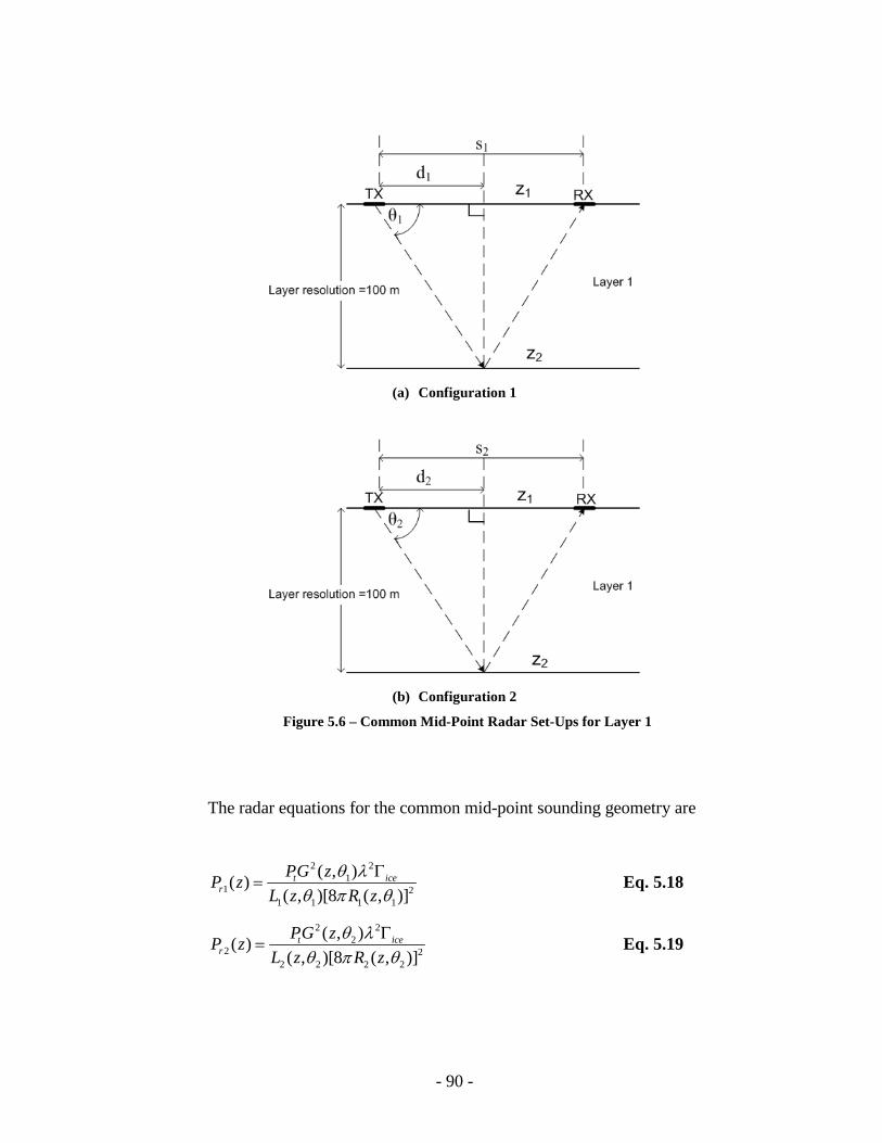
- 90 -
(a) Configuration 1
(b) Configuration 2
Figure 5.6 – Common Mid-Point Radar Set-Ups for Layer 1
The radar equations for the common mid-point sounding geometry are
2 21
1 21 1 1 1
( , )( )
( , )[8 ( , )]t ice
r
PG zP z
L z R z
θ λθ π θ
Γ= Eq. 5.18
2 22
2 22 2 2 2
( , )( )
( , )[8 ( , )]t ice
r
PG zP z
L z R z
θ λθ π θ
Γ= Eq. 5.19
- 91 -
where Equation 5.18 is associated with configuration 1 and Equation 5.19 is
associated with configuration 2. The loss incurred by the received signal in each
configuration is related to the attenuation ( )zα by
10
2 ( ')sec '
1 1( , )z
z dzL z e
α θθ ∫= Eq. 5.20
20
2 ( ')sec '
2 2( , )z
z dzL z e
α θθ ∫= Eq. 5.21
Also, the incident angles and ranges shown in Figure 5.6 are determined by
1 11 1( , ) tan
dz d
zθ − =
Eq. 5.22
1 22 2( , ) tan
dz d
zθ − =
Eq. 5.23
1 11
( , )cos
zR zθ
θ= Eq. 5.24
2 22
( , )cos
zR zθ
θ= Eq. 5.25
Dividing Equation 5.19 by 5.18, assuming Γice is specular, and doing some
rearrangement results in
2 2 2 2
1 1 1 2 2 2 1 2 12 2 2 2
2 2 2 1 1 1 2 1 2
( , ) ( , ) ( ) ( , ) ( , ) ( )cos
( , ) ( , ) ( ) ( , ) ( , ) ( )cosr r
r r
L z G z P z R z G z P z
L z G z P z R z G z P z
θ θ θ θ θθ θ θ θ θ
= = Eq. 5.26
Next, dividing Equations 5.20 by 5.21 results in
1 20
2 ( ')(sec sec ) '1 1
2 2
( , )
( , )
zz dzL z
eL z
α θ θθθ
−∫= Eq. 5.27
- 92 -
Equation 5.27 can be rearranged to the following
1 1
2 2 1 20
( , ) 1( ') ' ln
( , ) 2(sec sec )
z L zz dz
L z
θα
θ θ θ
= − ∫ Eq. 5.28
Plugging Equation 5.26 into Equation 5.28 yields a relationship between the
accumulated attenuation over a depth z and the power received from that depth
2 2
1 2 12 2
2 1 2 1 20
( , ) ( )cos 1( ') ' ln
( , ) ( )cos 2(sec sec )
zr
r
G z P zz dz
G z P z
θ θα
θ θ θ θ
= − ∫ Eq. 5.29
The ice attenuation over a single resolution layer z∆ at a depth zi can be obtained by
subtracting the contributions from all layers previous to zi from the accumulated
attenuation
1
10
( ) ( ') ' ( )iz i
i kk
z z dz z zα α α−
=
= − ∆ ∑∫ Eq 5.30
Equations 5.30 and 5.29 can be used to determine the attenuation at any depth within
glacial ice from knowledge of the received power, incident angles, and far-zone
antenna gain. The next section deals with relating the measured attenuation to
temperature.
5.6 Temperature Extraction from Measured Attenuation
The majority of the material in Section 5.6 was originally presented by Li,
Xie, and Dobbs in [27].
Extraction of temperature from measured attenuation involves representing
( )zα from Equation 5.15 in terms of the temperature-dependent complex
- 93 -
permittivityε . However, prior to doing so, for low-loss dielectrics (tan 1δ << ), the
following simplification can be made for ( )zα [11]
' ''
'
tan( ) r r
r
f fz
c c
π ε δ π εα
ε= = Eq. 5.31
To see if the low-loss approximation of Equation 5.31 is acceptable for glacial ice,
consider σ of 0.00001 S/m [2] at a frequency f of 200 MHz (frequency used in ice-
penetrating radar), and a dielectric constant 'rε of 3.2 (that of fully compressed ice).
Determining ''rε using the above information and Equation 5.7 yields a loss
tangenttanδ of 0.00028, which is much less than 1.
Plugging Equations 5.11 and 5.12 into 5.31 yields
( )
2.02 0.025
12
10( )
3 3.1884 (0.00091)
T
zT
πα
− +
=+
Eq 5.32
Rearranging Equation 5.32 and squaring both sides results in the following
transcendental equation relating temperature T(z) to attenuation ( )zα
[ ]2
4.04 0.05 ( )3 ( )3.1884 (0.00091) ( ) 10 0T zz
T zαπ
− + + − = Eq. 5.33
Equation 5.33 can be solved numerically to determine the temperature as a function
of depth within glacial ice. The next section presents resulting temperature profiles
obtained using Equation 5.33 and simulated data.
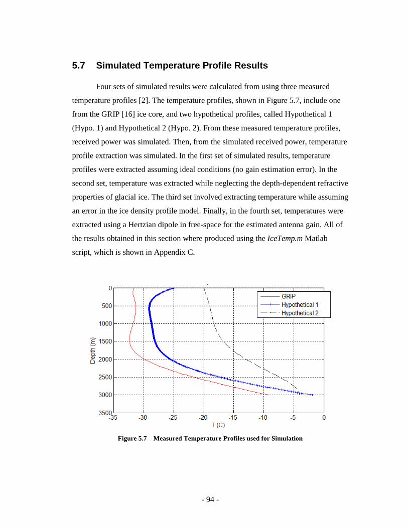
- 94 -
5.7 Simulated Temperature Profile Results
Four sets of simulated results were calculated from using three measured
temperature profiles [2]. The temperature profiles, shown in Figure 5.7, include one
from the GRIP [16] ice core, and two hypothetical profiles, called Hypothetical 1
(Hypo. 1) and Hypothetical 2 (Hypo. 2). From these measured temperature profiles,
received power was simulated. Then, from the simulated received power, temperature
profile extraction was simulated. In the first set of simulated results, temperature
profiles were extracted assuming ideal conditions (no gain estimation error). In the
second set, temperature was extracted while neglecting the depth-dependent refractive
properties of glacial ice. The third set involved extracting temperature while assuming
an error in the ice density profile model. Finally, in the fourth set, temperatures were
extracted using a Hertzian dipole in free-space for the estimated antenna gain. All of
the results obtained in this section where produced using the IceTemp.m Matlab
script, which is shown in Appendix C.
Figure 5.7 – Measured Temperature Profiles used for Simulation
- 95 -
Each of the three simulated sets of results involved an identical procedure for
simulating received power. The equations used for simulating received power are
presented in Section 5.6, but are repeated here for clarity. First, from the measured
temperature profiles, real and imaginary permittivites were calculated for each depth
using the following
' ( ) 3.1884 (0.00091) ( )r z T zε = + Eq. 5.34
'' 2.02 0.025 ( )1( ) 10
10T z
r zf
ε − += Eq. 5.35
Then, from the calculated values of ' ( )r zε and '' ( )r zε , the attenuation at each depth
was calculated using
( )1
' 22( )
( ) 2 1 tan ( ) 12
o o r zz f z
µ ε εα π δ
= − −
Eq. 5.36
The attenuation is related to the total loss incurred by the received power from each
depth by
1
02 ( ')sec '
1 1( , )z
z dzL z e
α θθ ∫= Eq. 5.37
20
2 ( ')sec '
2 2( , )z
z dzL z e
α θθ ∫= Eq. 5.38
Knowing the accumulated loss at each depth from Equations 5.37 and 5.38, and using
the appropriate formulas from Section 5.6 for describing the geometries of radar
configurations 1 and 2, allows the received power to be simulated using
- 96 -
2 21
1 21 1 1 1
( , )( )
( , )[8 ( , )]t ice
r
PG zP z
L z R z
θ λθ π θ
Γ= Eq. 5.39
2 22
2 22 2 2 2
( , )( )
( , )[8 ( , )]t ice
r
PG zP z
L z R z
θ λθ π θ
Γ= Eq. 5.40
Once the received power is known and the antenna gain at each depth is estimated,
the attenuation at each depth can be extracted using
2 21 2 1
2 22 1 2 1 20
( , ) ( )cos 1( ') ' ln
( , ) ( )cos 2(sec sec )
zr
r
G z P zz dz
G z P z
θ θα
θ θ θ θ
= − ∫ Eq. 5.41
1
10
( ) ( ') ' ( )iz i
i kk
z z dz z zα α α−
=
= − ∆ ∑∫ Eq. 5.42
Note that the Vivaldi antenna (Chapter 4) was used for calculating antenna gain in
Equations 5.39, 5.40, and 5.41. Once the attenuation at each depth has been extracted,
the temperature at each depth can be extracted using
[ ]2
4.04 0.05 ( )3 ( )3.1884 (0.00091) ( ) 10 0T zz
T zαπ
− + + − = Eq. 5.43
The purpose of the simulations in Section 5.7 was to explore the effect of
antenna-gain estimations on the ability to extract glacial-ice temperature profiles.
There are other possible sources of error in determining glacial-ice temperature
profiles that are not investigated in this work. These include possible inaccuracies in
the temperature extraction algorithm, the possibility of the internal ice reflectivity
being a function of polarization and incident angle, and the signal to noise ratio. Since
in these temperature profile extraction simulations, the same algorithm was used to
simulate received power, as was used to extract temperature, inaccuracies in the
temperature extraction algorithm could not be explored in this work. The effect of
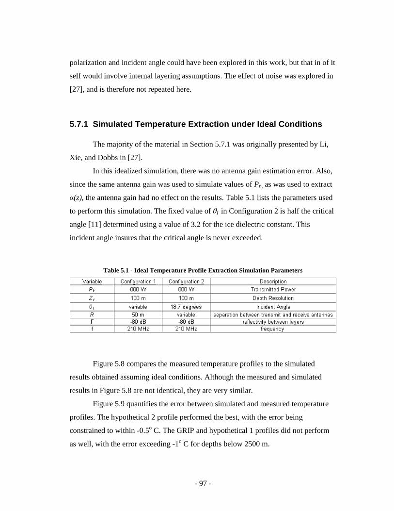
- 97 -
polarization and incident angle could have been explored in this work, but that in of it
self would involve internal layering assumptions. The effect of noise was explored in
[27], and is therefore not repeated here.
5.7.1 Simulated Temperature Extraction under Ideal Conditions
The majority of the material in Section 5.7.1 was originally presented by Li,
Xie, and Dobbs in [27].
In this idealized simulation, there was no antenna gain estimation error. Also,
since the same antenna gain was used to simulate values of Pr , as was used to extract
α(z), the antenna gain had no effect on the results. Table 5.1 lists the parameters used
to perform this simulation. The fixed value of θI in Configuration 2 is half the critical
angle [11] determined using a value of 3.2 for the ice dielectric constant. This
incident angle insures that the critical angle is never exceeded.
Table 5.1 - Ideal Temperature Profile Extraction Simulation Parameters
Figure 5.8 compares the measured temperature profiles to the simulated
results obtained assuming ideal conditions. Although the measured and simulated
results in Figure 5.8 are not identical, they are very similar.
Figure 5.9 quantifies the error between simulated and measured temperature
profiles. The hypothetical 2 profile performed the best, with the error being
constrained to within -0.5o C. The GRIP and hypothetical 1 profiles did not perform
as well, with the error exceeding -1o C for depths below 2500 m.
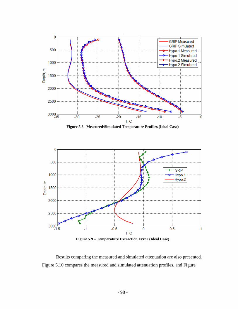
- 98 -
Figure 5.8 –Measured/Simulated Temperature Profiles (Ideal Case)
Figure 5.9 – Temperature Extraction Error (Ideal Case)
Results comparing the measured and simulated attenuation are also presented.
Figure 5.10 compares the measured and simulated attenuation profiles, and Figure
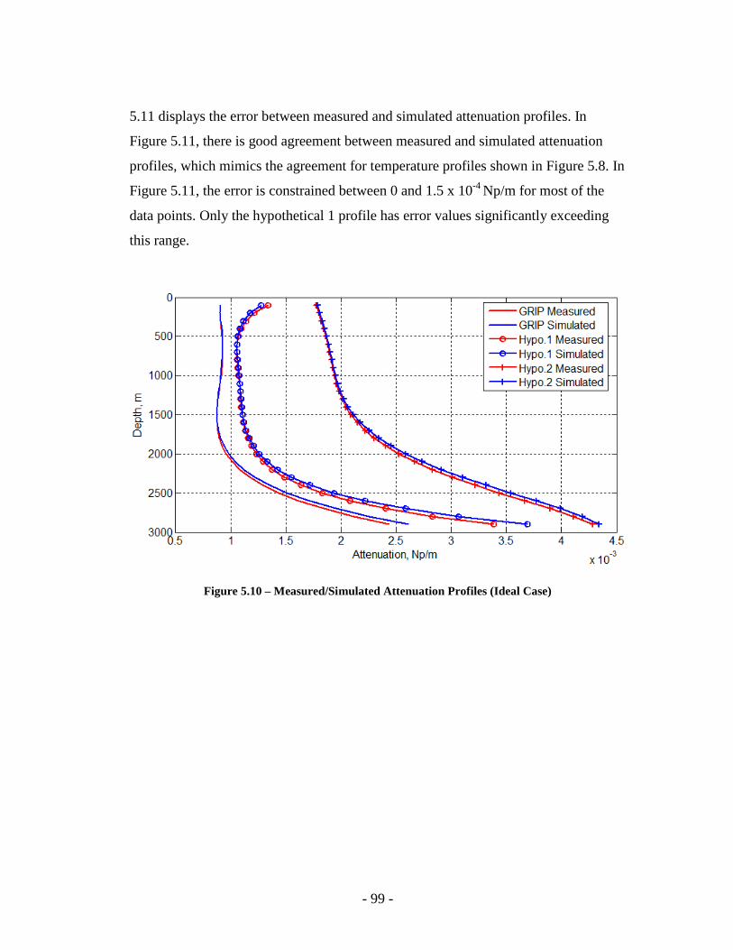
- 99 -
5.11 displays the error between measured and simulated attenuation profiles. In
Figure 5.11, there is good agreement between measured and simulated attenuation
profiles, which mimics the agreement for temperature profiles shown in Figure 5.8. In
Figure 5.11, the error is constrained between 0 and 1.5 x 10⁻⁴ Np/m for most of the
data points. Only the hypothetical 1 profile has error values significantly exceeding
this range.
Figure 5.10 – Measured/Simulated Attenuation Profiles (Ideal Case)
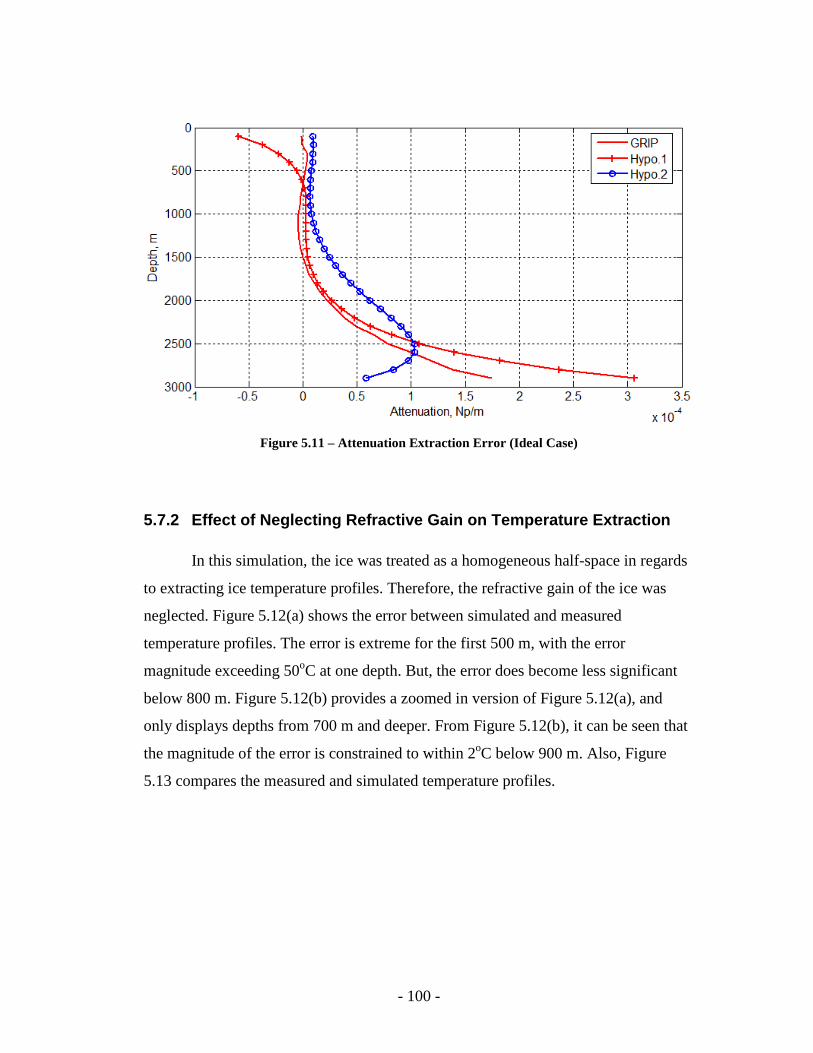
- 100 -
Figure 5.11 – Attenuation Extraction Error (Ideal Case)
5.7.2 Effect of Neglecting Refractive Gain on Temperature Extraction
In this simulation, the ice was treated as a homogeneous half-space in regards
to extracting ice temperature profiles. Therefore, the refractive gain of the ice was
neglected. Figure 5.12(a) shows the error between simulated and measured
temperature profiles. The error is extreme for the first 500 m, with the error
magnitude exceeding 50oC at one depth. But, the error does become less significant
below 800 m. Figure 5.12(b) provides a zoomed in version of Figure 5.12(a), and
only displays depths from 700 m and deeper. From Figure 5.12(b), it can be seen that
the magnitude of the error is constrained to within 2oC below 900 m. Also, Figure
5.13 compares the measured and simulated temperature profiles.
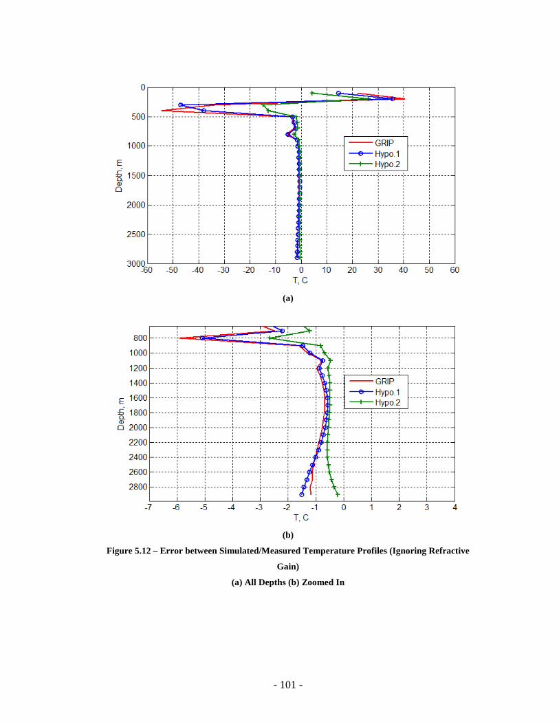
- 101 -
(a)
(b)
Figure 5.12 – Error between Simulated/Measured Temperature Profiles (Ignoring Refractive
Gain)
(a) All Depths (b) Zoomed In
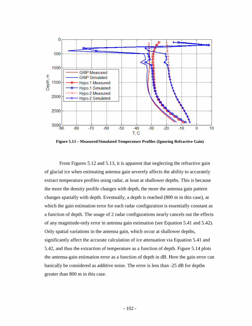
- 102 -
Figure 5.13 – Measured/Simulated Temperature Profiles (Ignoring Refractive Gain)
From Figures 5.12 and 5.13, it is apparent that neglecting the refractive gain
of glacial ice when estimating antenna gain severely affects the ability to accurately
extract temperature profiles using radar, at least at shallower depths. This is because
the more the density profile changes with depth, the more the antenna gain pattern
changes spatially with depth. Eventually, a depth is reached (800 m in this case), at
which the gain estimation error for each radar configuration is essentially constant as
a function of depth. The usage of 2 radar configurations nearly cancels out the effects
of any magnitude-only error in antenna gain estimation (see Equation 5.41 and 5.42).
Only spatial variations in the antenna gain, which occur at shallower depths,
significantly affect the accurate calculation of ice attenuation via Equation 5.41 and
5.42, and thus the extraction of temperature as a function of depth. Figure 5.14 plots
the antenna-gain estimation error as a function of depth in dB. Here the gain error can
basically be considered as additive noise. The error is less than -25 dB for depths
greater than 800 m in this case.
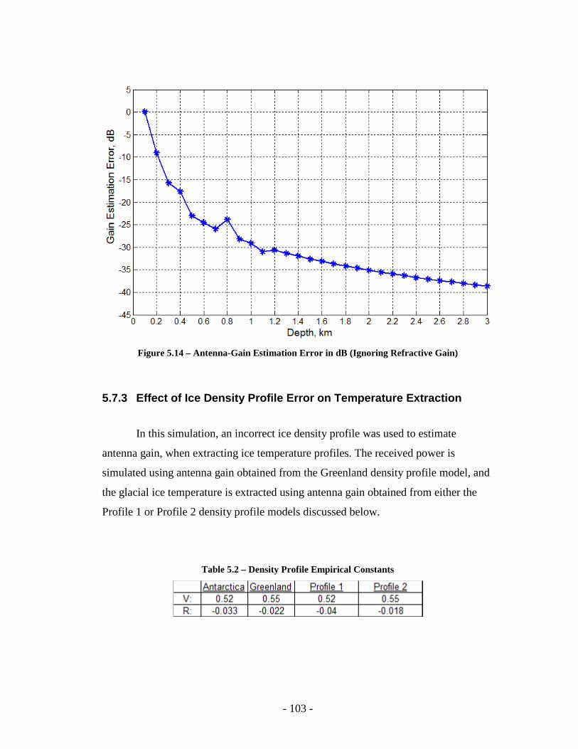
- 103 -
Figure 5.14 – Antenna-Gain Estimation Error in dB (Ignoring Refractive Gain)
5.7.3 Effect of Ice Density Profile Error on Temperature Extraction
In this simulation, an incorrect ice density profile was used to estimate
antenna gain, when extracting ice temperature profiles. The received power is
simulated using antenna gain obtained from the Greenland density profile model, and
the glacial ice temperature is extracted using antenna gain obtained from either the
Profile 1 or Profile 2 density profile models discussed below.
Table 5.2 – Density Profile Empirical Constants
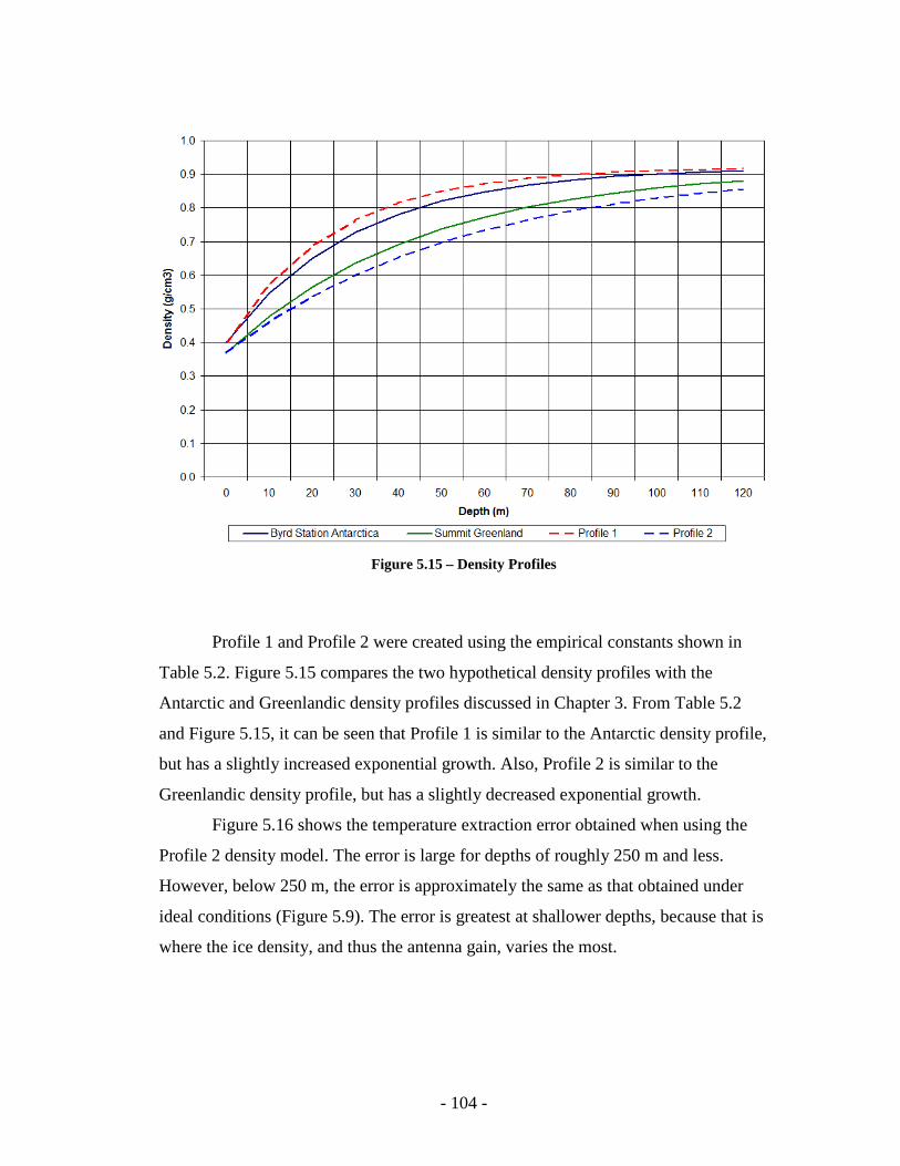
- 104 -
Figure 5.15 – Density Profiles
Profile 1 and Profile 2 were created using the empirical constants shown in
Table 5.2. Figure 5.15 compares the two hypothetical density profiles with the
Antarctic and Greenlandic density profiles discussed in Chapter 3. From Table 5.2
and Figure 5.15, it can be seen that Profile 1 is similar to the Antarctic density profile,
but has a slightly increased exponential growth. Also, Profile 2 is similar to the
Greenlandic density profile, but has a slightly decreased exponential growth.
Figure 5.16 shows the temperature extraction error obtained when using the
Profile 2 density model. The error is large for depths of roughly 250 m and less.
However, below 250 m, the error is approximately the same as that obtained under
ideal conditions (Figure 5.9). The error is greatest at shallower depths, because that is
where the ice density, and thus the antenna gain, varies the most.
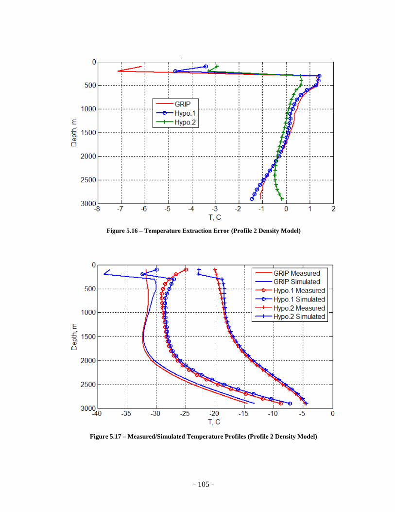
- 105 -
Figure 5.16 – Temperature Extraction Error (Profile 2 Density Model)
Figure 5.17 – Measured/Simulated Temperature Profiles (Profile 2 Density Model)
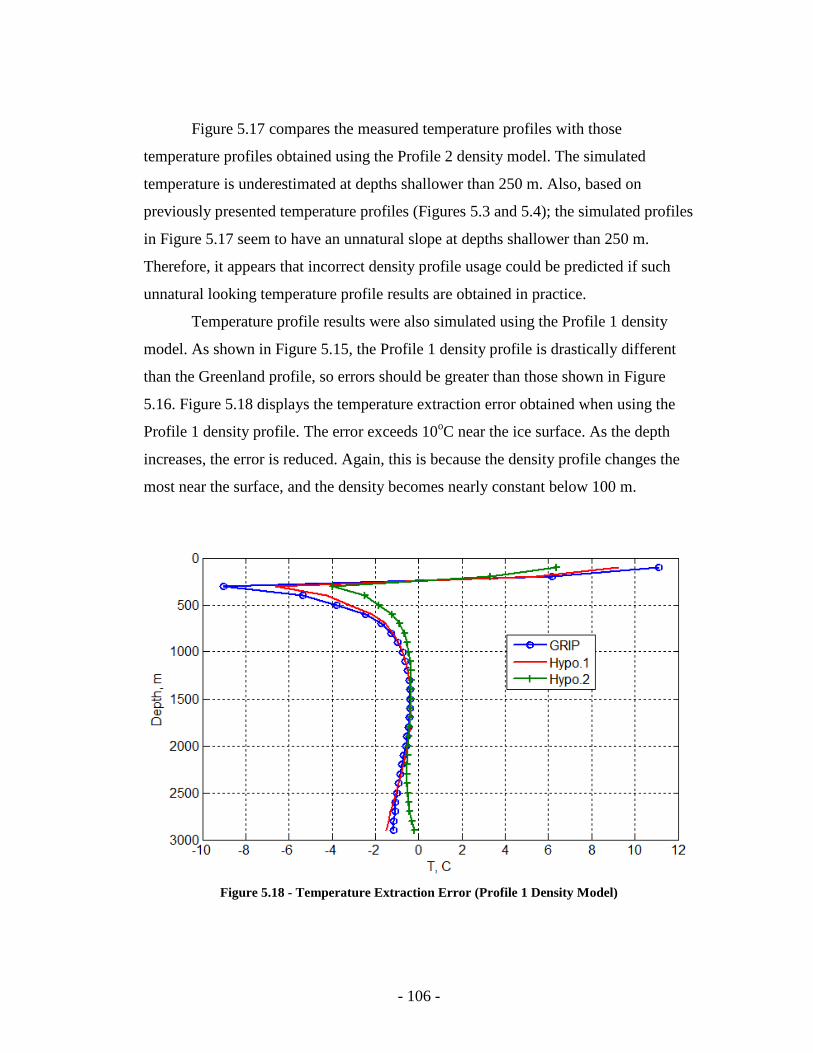
- 106 -
Figure 5.17 compares the measured temperature profiles with those
temperature profiles obtained using the Profile 2 density model. The simulated
temperature is underestimated at depths shallower than 250 m. Also, based on
previously presented temperature profiles (Figures 5.3 and 5.4); the simulated profiles
in Figure 5.17 seem to have an unnatural slope at depths shallower than 250 m.
Therefore, it appears that incorrect density profile usage could be predicted if such
unnatural looking temperature profile results are obtained in practice.
Temperature profile results were also simulated using the Profile 1 density
model. As shown in Figure 5.15, the Profile 1 density profile is drastically different
than the Greenland profile, so errors should be greater than those shown in Figure
5.16. Figure 5.18 displays the temperature extraction error obtained when using the
Profile 1 density profile. The error exceeds 10oC near the ice surface. As the depth
increases, the error is reduced. Again, this is because the density profile changes the
most near the surface, and the density becomes nearly constant below 100 m.
Figure 5.18 - Temperature Extraction Error (Profile 1 Density Model)
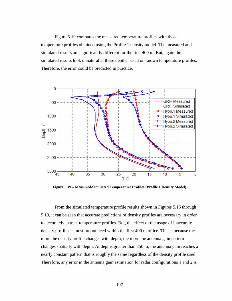
- 107 -
Figure 5.19 compares the measured temperature profiles with those
temperature profiles obtained using the Profile 1 density model. The measured and
simulated results are significantly different for the first 400 m. But, again the
simulated results look unnatural at these depths based on known temperature profiles.
Therefore, the error could be predicted in practice.
Figure 5.19 – Measured/Simulated Temperature Profiles (Profile 1 Density Model)
From the simulated temperature profile results shown in Figures 5.16 through
5.19, it can be seen that accurate predictions of density profiles are necessary in order
to accurately extract temperature profiles. But, the effect of the usage of inaccurate
density profiles is most pronounced within the first 400 m of ice. This is because the
more the density profile changes with depth, the more the antenna gain pattern
changes spatially with depth. At depths greater than 250 m, the antenna gain reaches a
nearly constant pattern that is roughly the same regardless of the density profile used.
Therefore, any error in the antenna gain estimation for radar configurations 1 and 2 is
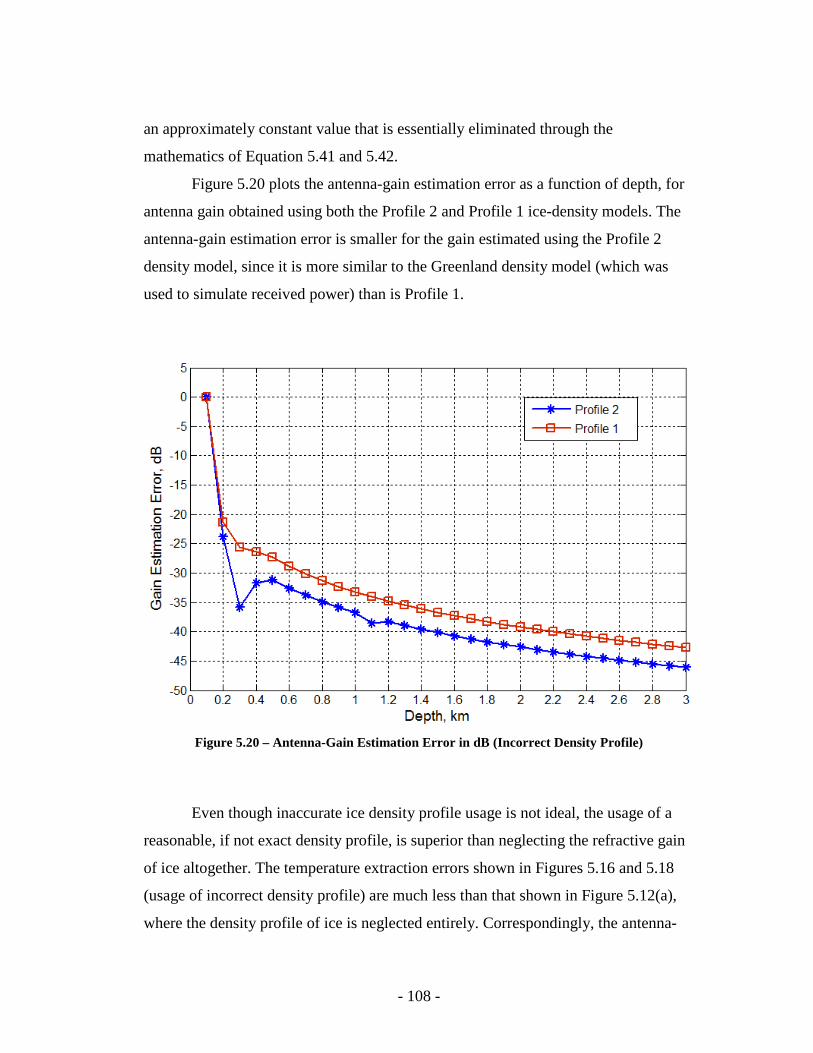
- 108 -
an approximately constant value that is essentially eliminated through the
mathematics of Equation 5.41 and 5.42.
Figure 5.20 plots the antenna-gain estimation error as a function of depth, for
antenna gain obtained using both the Profile 2 and Profile 1 ice-density models. The
antenna-gain estimation error is smaller for the gain estimated using the Profile 2
density model, since it is more similar to the Greenland density model (which was
used to simulate received power) than is Profile 1.
Figure 5.20 – Antenna-Gain Estimation Error in dB (Incorrect Density Profile)
Even though inaccurate ice density profile usage is not ideal, the usage of a
reasonable, if not exact density profile, is superior than neglecting the refractive gain
of ice altogether. The temperature extraction errors shown in Figures 5.16 and 5.18
(usage of incorrect density profile) are much less than that shown in Figure 5.12(a),
where the density profile of ice is neglected entirely. Correspondingly, the antenna-
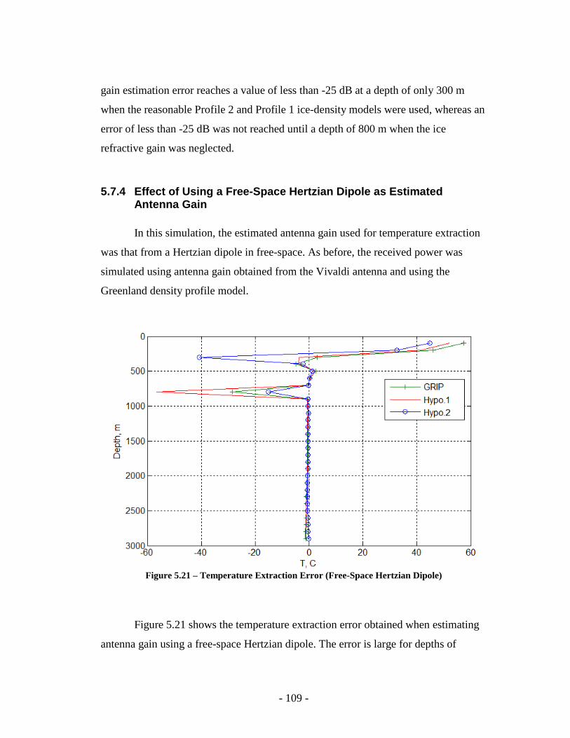
- 109 -
gain estimation error reaches a value of less than -25 dB at a depth of only 300 m
when the reasonable Profile 2 and Profile 1 ice-density models were used, whereas an
error of less than -25 dB was not reached until a depth of 800 m when the ice
refractive gain was neglected.
5.7.4 Effect of Using a Free-Space Hertzian Dipole as Estimated Antenna Gain
In this simulation, the estimated antenna gain used for temperature extraction
was that from a Hertzian dipole in free-space. As before, the received power was
simulated using antenna gain obtained from the Vivaldi antenna and using the
Greenland density profile model.
Figure 5.21 – Temperature Extraction Error (Free-Space Hertzian Dipole)
Figure 5.21 shows the temperature extraction error obtained when estimating
antenna gain using a free-space Hertzian dipole. The error is large for depths of
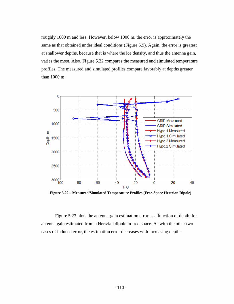
- 110 -
roughly 1000 m and less. However, below 1000 m, the error is approximately the
same as that obtained under ideal conditions (Figure 5.9). Again, the error is greatest
at shallower depths, because that is where the ice density, and thus the antenna gain,
varies the most. Also, Figure 5.22 compares the measured and simulated temperature
profiles. The measured and simulated profiles compare favorably at depths greater
than 1000 m.
Figure 5.22 – Measured/Simulated Temperature Profiles (Free-Space Hertzian Dipole)
Figure 5.23 plots the antenna-gain estimation error as a function of depth, for
antenna gain estimated from a Hertzian dipole in free-space. As with the other two
cases of induced error, the estimation error decreases with increasing depth.
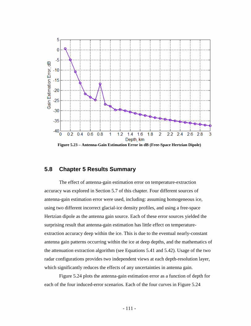
- 111 -
Figure 5.23 – Antenna-Gain Estimation Error in dB (Free-Space Hertzian Dipole)
5.8 Chapter 5 Results Summary
The effect of antenna-gain estimation error on temperature-extraction
accuracy was explored in Section 5.7 of this chapter. Four different sources of
antenna-gain estimation error were used, including: assuming homogeneous ice,
using two different incorrect glacial-ice density profiles, and using a free-space
Hertzian dipole as the antenna gain source. Each of these error sources yielded the
surprising result that antenna-gain estimation has little effect on temperature-
extraction accuracy deep within the ice. This is due to the eventual nearly-constant
antenna gain patterns occurring within the ice at deep depths, and the mathematics of
the attenuation extraction algorithm (see Equations 5.41 and 5.42). Usage of the two
radar configurations provides two independent views at each depth-resolution layer,
which significantly reduces the effects of any uncertainties in antenna gain.
Figure 5.24 plots the antenna-gain estimation error as a function of depth for
each of the four induced-error scenarios. Each of the four curves in Figure 5.24
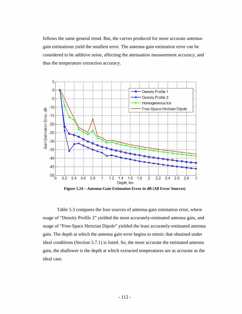
- 112 -
follows the same general trend. But, the curves produced for more accurate antenna-
gain estimations yield the smallest error. The antenna-gain estimation error can be
considered to be additive noise, affecting the attenuation measurement accuracy, and
thus the temperature extraction accuracy.
Figure 5.24 – Antenna-Gain Estimation Error in dB (All Error Sources)
Table 5.3 compares the four sources of antenna-gain estimation error, where
usage of “Density Profile 2” yielded the most accurately-estimated antenna gain, and
usage of “Free-Space Hertzian Dipole” yielded the least accurately-estimated antenna
gain. The depth at which the antenna gain error begins to mimic that obtained under
ideal conditions (Section 5.7.1) is listed. So, the more accurate the estimated antenna
gain, the shallower is the depth at which extracted temperatures are as accurate as the
ideal case.

- 113 -
Table 5.3 – Gain Estimation Error Comparison
- 114 -
CHAPTER 6: Summary/Conclusions/Future Work
The thesis work began under the assumption that accurate far-zone antenna-
gain estimates are required in order to use ice-penetrating radar to accurately measure
glacial ice temperature profiles. Therefore, this work set out to determine a method of
accurately estimating the antenna-gain of ice-mounted antennas. First, the possible
usage of commercial codes was explored, but it was found that although commercial
codes are often used to determine far-zone antenna gain in free-space, these codes are
incapable of doing so for ice-mounted antennas, due to the inhomogeneous dielectric
constant of glacial ice. So, after some deliberation, a three-part hybrid numerical
technique, called the FEM-NFFT-GO, was devised for accurately estimating the far-
zone antenna gain within glacial ice. The FEM-NFFT-GO technique uses the FEM
(finite element method) to calculate near-zone fields of the antenna, a dual-dielectric
NFFT (near-to-far-field transformation) to determine the far-zone fields in the upper
region of glacial ice, and the GO (geometric optics ray-tracing) technique to
determine the far-zone fields at any depth within glacial ice. Results were presented
that both validate the FEM-NFFT-GO technique, and highlight its ability to determine
far-zone gain for complex ice-mounted antennas. Then, the glacial-ice temperature
extraction algorithm was presented, as well as results relating the effects of antenna-
gain estimation error on temperature profile extraction accuracy. Surprisingly, it was
found that antenna-gain estimation errors only have a significant effect on
temperature extraction at shallow depths within the ice. Regardless of the necessity of
accurate antenna-gain estimations to extract glacial-ice temperatures, a powerful
antenna-gain estimation technique was developed that should prove useful in many
applications.
- 115 -
6.1 Antenna-Gain Estimation Summary
The FEM-NFFT-GO technique provides an invaluable tool with which to
estimate far-zone antenna gain for ice-mounted antennas. This ability should prove to
be a huge benefit to future glaciological research. The technique is easy to use, and is
essentially a post-processing feature on top of the widely used HFSS antenna-analysis
software.
Also, the FEM-NFFT-GO antenna gain estimation technique is useful for
analyzing radiating structures in general, regardless of whether glacial ice is involved.
The FEM-NFFT technique can be used alone to analyze radiating structures above an
arbitrary half-space, which may be useful for ground-penetrating radar. Also, the GO
portion of the technique can be adjusted to use refractive indexes following any
mathematical trend.
The FEM-NFFT-GO technique relies on two assumptions in order to predict
far-zone antenna gain accurately. First, this technique assumes that far-zone fields
within the ice are planar prior to the ice dielectric constant changing significantly.
Although this is a good approximation, it may not be entirely accurate. Field
experiments will be required to determine the accuracy of this assumption. Second,
the technique assumes that the glacial ice density profile is known with a high degree
of accuracy. However, a reasonable approximation will suffice in most cases.
6.2 Effects of Antenna-Gain Estimation on Ice-Temperature Extraction Summary
As shown in Chapter 5, antenna-gain estimation error was shown to only have
a significant effect on temperature extraction accuracy at shallow depths, where the
definition of shallow depended upon the accuracy of the antenna-gain estimation.
When the most accurate antenna-gain estimation error was used (a slight alteration to
the glacial-ice density profile), the extracted temperatures were found to be nearly as

- 116 -
accurate as the ideal case for depths below 250 m. When the least accurate antenna-
gain estimation error was used (gain estimated from free-space Hertzian dipole), the
extracted temperatures were found to be nearly as accurate as the ideal case for depths
below 1000 m.
The most probable source of error explored in Chapter 5 was the usage of an
incorrect ice density profile for estimating far-zone antenna. This was found to
adversely affect the temperature extraction accuracy, but again, only at shallow
depths. Even when a significantly different density profile was used, the results were
still favorable, and the extracted temperatures were found to be nearly as accurate as
the ideal case for depths below 400 m.
6.3 Conclusions
The combination of the FEM-NFFT-GO antenna gain estimation technique
along with the bistatic radar configurations discussed in Chapter 5 should enable
glacial ice temperature profiles to be measured using ice-penetrating radar.
Depending on the accuracy of the antenna-gain estimation, extracted temperatures
will be accurate throughout most or all of the ice depth. However, if accurate ice
temperatures are required only at very deep depths, accurate antenna-gain estimations
are unnecessary.
This ability to measure glacial ice temperature via radar will make obtaining
these profiles much easier, since ice-core drilling will no longer be required. The
resulting potential increase in the availability of such data should further the science
of glaciology, since ice temperature is fundamental in a variety of glacial processes
[31]. An increased understanding of glacial processes will further science’s
understanding of how glaciers relate to the global climate.

- 117 -
6.4 Future Work
There is some future work to be carried out regarding both antenna-gain
estimation for ice-mounted antennas and glacial-ice temperature extraction. To verify
the accuracy of the FEM-NFFT-GO technique, field experiments need to be
conducted to measure actual antenna patterns within glacial ice. This could be
accomplished using a bistatic system and a calibration target.
Regarding temperature extraction, the effect of non-specular reflectivity and
the accuracy of the temperature-extraction algorithm need to be investigated. As for
non-specular reflectivity, the use of two independent measurements (combination of
two radar configurations) at each depth-resolution layer should reduce any errors
associated with non-specular reflectivity, provided the incident angles at the depth of
interest are roughly the same for both radar configurations. This error reduction
associated with non-specular reflectivity would be similar to what occurred with the
antenna-gain estimation error.
The accuracy of the temperature-extraction algorithm can only be investigated
by taking field measurements, using the temperature-extraction radar set-up, in
regions with known temperature profiles. Then, the extracted temperature profiles
from radar measurements can be compared with the known temperature profiles to
investigate the accuracy of the technique.
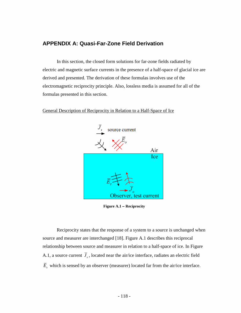
- 118 -
APPENDIX A: Quasi-Far-Zone Field Derivation
In this section, the closed form solutions for far-zone fields radiated by
electric and magnetic surface currents in the presence of a half-space of glacial ice are
derived and presented. The derivation of these formulas involves use of the
electromagnetic reciprocity principle. Also, lossless media is assumed for all of the
formulas presented in this section.
General Description of Reciprocity in Relation to a Half-Space of Ice
Figure A.1 −−−− Reciprocity
Reciprocity states that the response of a system to a source is unchanged when
source and measurer are interchanged [18]. Figure A.1 describes this reciprocal
relationship between source and measurer in relation to a half-space of ice. In Figure
A.1, a source current sJ , located near the air/ice interface, radiates an electric field
sE which is sensed by an observer (measurer) located far from the air/ice interface.

- 119 -
The observer has a hypothetical test current oJ that radiates an electric field oE ,
which is planar near the air/ice interface. Since sJ is located near the air/ice interface,
sE is not yet planer near the air/ice interface, and therefore can not be described
directly in terms of planar transmission and reflection coefficients. However, the
reciprocal relationship between source and observer will be taken advantage of to
describe sE in terms of the planar oE near the air/ice interface.
Using the notation in Figure A.1, reciprocity can be stated mathematically for
electric sources via the following relation.
, ,o s s oE J E J= Eq. A.1
The brackets in Equation A.1 indicate the inner product, which expands to the
following
( ) ( )o s s o
S S
E J dS E J dS⋅ = ⋅∫∫ ∫∫ Eq. A.2
Equation A.2 directly relates the source and observer in Figure A.1, and shows that
switching the role of source and observer has no effect on the problem solution. The
“observer current” oJ can be considered to be a hypothetical test current. Although
oJ is useful in the quasi-far-field formula derivation, it disappears in the final result.
The Four Cases to Consider when Deriving Quasi-Far-Zone Field Formulas
There are four cases to consider when deriving the quasi-far-zone electric
fields radiated by surface currents in the presence of a half-space of ice. These four
cases, which involve different combinations of field polarization (parallel or
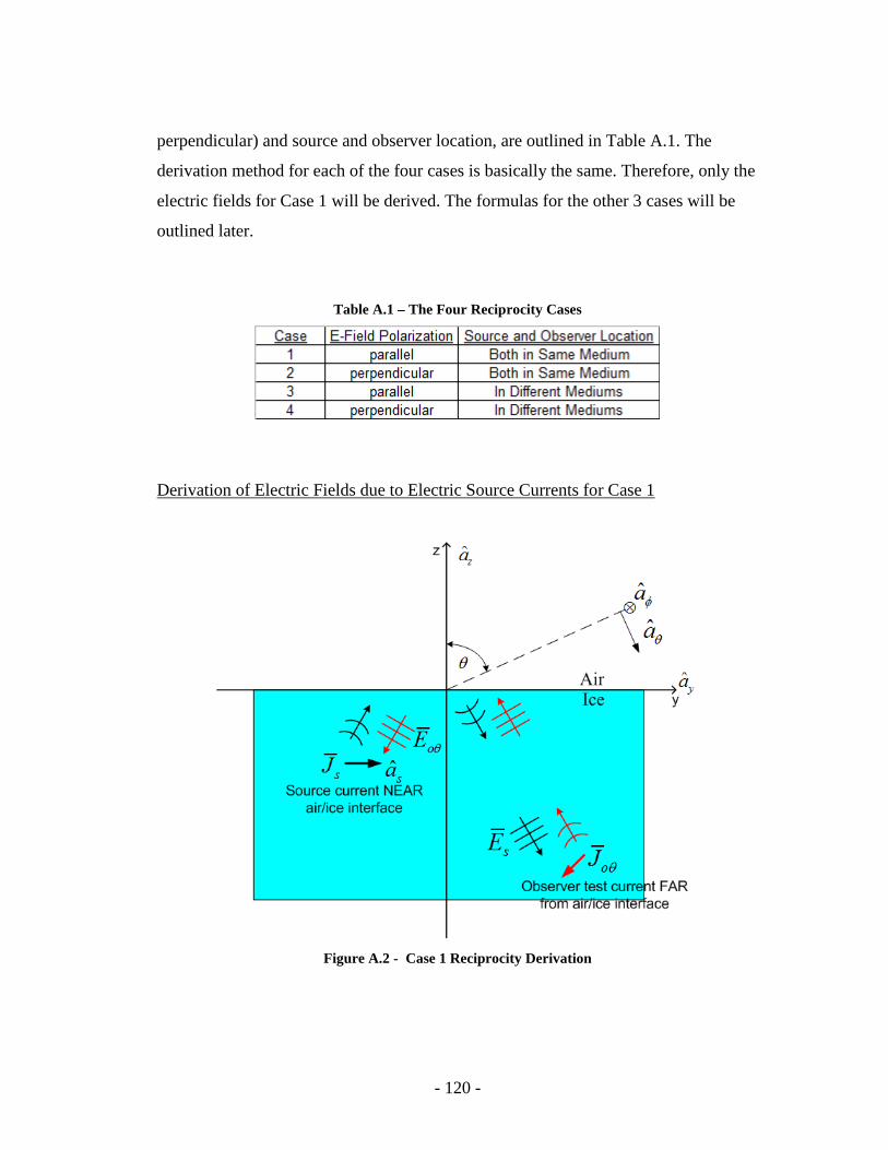
- 120 -
perpendicular) and source and observer location, are outlined in Table A.1. The
derivation method for each of the four cases is basically the same. Therefore, only the
electric fields for Case 1 will be derived. The formulas for the other 3 cases will be
outlined later.
Table A.1 – The Four Reciprocity Cases
Derivation of Electric Fields due to Electric Source Currents for Case 1
Figure A.2 - Case 1 Reciprocity Derivation
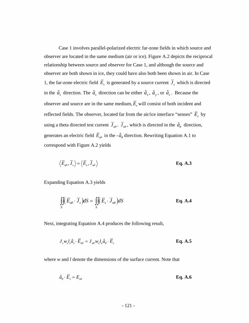
- 121 -
Case 1 involves parallel-polarized electric far-zone fields in which source and
observer are located in the same medium (air or ice). Figure A.2 depicts the reciprocal
relationship between source and observer for Case 1, and although the source and
observer are both shown in ice, they could have also both been shown in air. In Case
1, the far-zone electric field sE is generated by a source current sJ which is directed
in the ˆsa direction. The sa direction can be either ˆxa , ˆya , or ˆza . Because the
observer and source are in the same medium,sE will consist of both incident and
reflected fields. The observer, located far from the air/ice interface “senses” sE by
using a theta directed test current oJ θ . oJ θ , which is directed in the aθ direction,
generates an electric field oE θ in the -aθ direction. Rewriting Equation A.1 to
correspond with Figure A.2 yields
, ,o s s oE J E Jθ θ= Eq. A.3
Expanding Equation A.3 yields
( ) ( )o s s o
S S
E J dS E J dSθ θ⋅ = ⋅∫∫ ∫∫ Eq. A.4
Next, integrating Equation A.4 produces the following result,
ˆ ˆs s s s o o o o sJ w l a E J w l a Eθ θ θ⋅ = ⋅ Eq. A.5
where w and l denote the dimensions of the surface current. Note that
ˆ s sa E Eθ θ⋅ = Eq. A.6
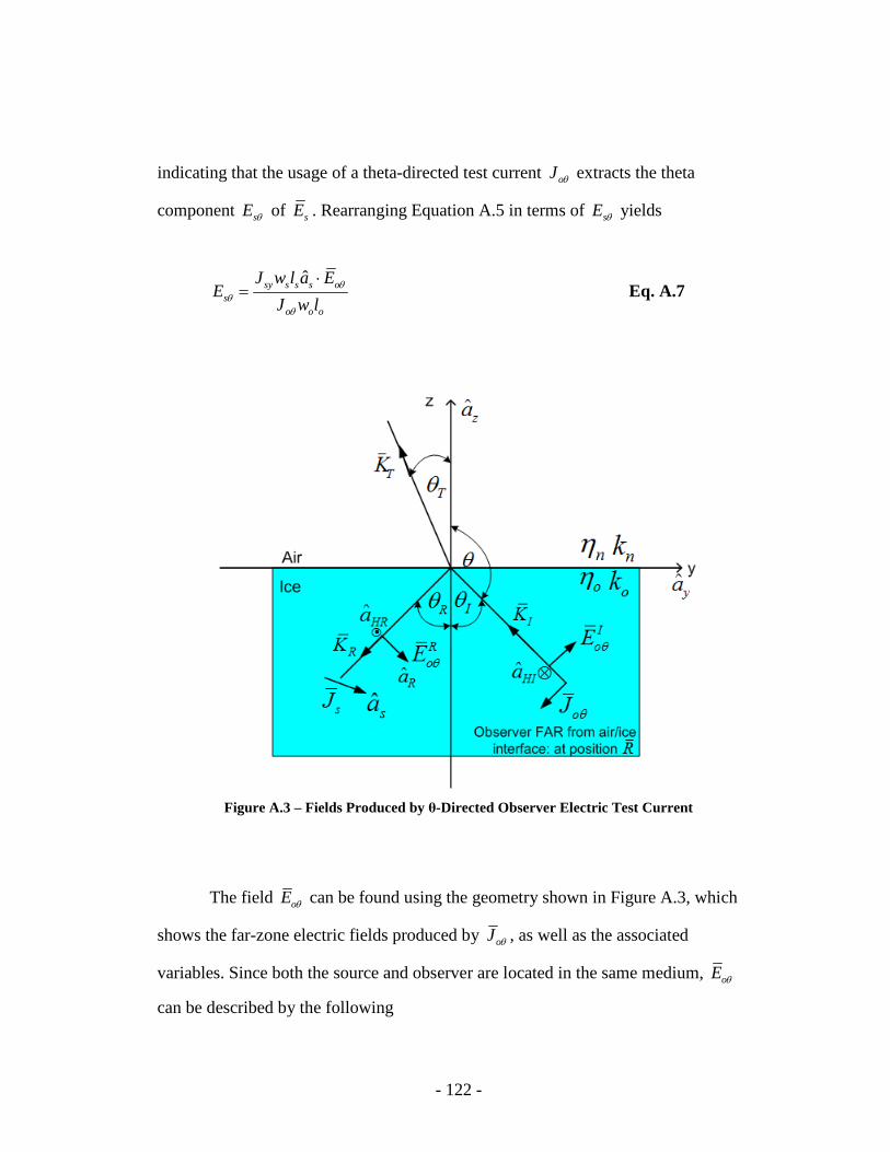
- 122 -
indicating that the usage of a theta-directed test current oJ θ extracts the theta
component sE θ of sE . Rearranging Equation A.5 in terms of sE θ yields
ˆsy s s s os
o o o
J w l a EE
J w lθ
θθ
⋅= Eq. A.7
Figure A.3 – Fields Produced by θ-Directed Observer Electric Test Current
The field oE θ can be found using the geometry shown in Figure A.3, which
shows the far-zone electric fields produced by oJ θ , as well as the associated
variables. Since both the source and observer are located in the same medium, oE θ
can be described by the following
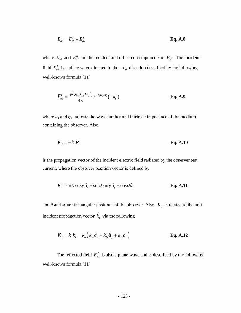
- 123 -
I Ro o oE E Eθ θ θ= + Eq. A.8
where IoE θ and R
oE θ are the incident and reflected components of oE θ . The incident
field IoE θ is a plane wave directed in the aθ− direction described by the following
well-known formula [11]
( )( ) ˆ4
Ij K RI o o o o oo
jk J w lE e aθ
θ θ
ηπ
− ⋅= − Eq. A.9
where ko and ηo indicate the wavenumber and intrinsic impedance of the medium
containing the observer. Also,
I oK k R= − Eq. A.10
is the propagation vector of the incident electric field radiated by the observer test
current, where the observer position vector is defined by
ˆ ˆ ˆsin cos sin sin cosx y zR a a aθ φ θ φ θ= + + Eq. A.11
and θ and φ are the angular positions of the observer. Also, IK is related to the unit
incident propagation vector Ik via the following
( )ˆ ˆ ˆ ˆI o I o Ix x Iy y Iz zK k k k k a k a k a= = + + Eq. A.12
The reflected field RoE θ is also a plane wave and is described by the following
well-known formula [11]
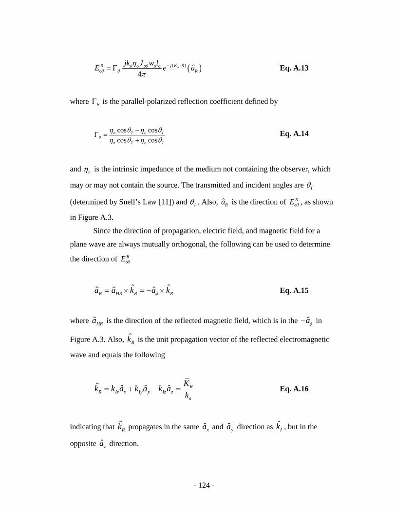
- 124 -
( )( ) ˆ4
Rj K RR o o o o oo R
jk J w lE e aθ
θ θ
ηπ
− ⋅= Γ Eq. A.13
where θΓ is the parallel-polarized reflection coefficient defined by
cos cos
cos cosn T o I
n T o Iθ
η θ η θη θ η θ
−Γ =
+ Eq. A.14
and nη is the intrinsic impedance of the medium not containing the observer, which
may or may not contain the source. The transmitted and incident angles are Tθ
(determined by Snell’s Law [11]) and Iθ . Also, ˆRa is the direction of RoE θ , as shown
in Figure A.3.
Since the direction of propagation, electric field, and magnetic field for a
plane wave are always mutually orthogonal, the following can be used to determine
the direction of RoE θ
ˆ ˆˆ ˆ ˆR HR R Ra a k a kφ= × = − × Eq. A.15
where ˆHRa is the direction of the reflected magnetic field, which is in the aφ− in
Figure A.3. Also, Rk is the unit propagation vector of the reflected electromagnetic
wave and equals the following
ˆ ˆ ˆ ˆ RR Ix x Iy y Iz z
o
Kk k a k a k a
k= + − = Eq. A.16
indicating that Rk propagates in the same ˆxa and ˆya direction as Ik , but in the
opposite za direction.

- 125 -
Equation A.7 can be solved for sE θ , the electric field produced by the source
current. By inspection of Equation A.7, since oE θ (defined by Equations A.8, A.9,
and A.13) consists of incident and reflected fields, so must sE θ . Therefore, the
parallel-polarized electric field produced by sJ can be described by
I Rs s sE E Eθ θ θ= + Eq. A.17
The incident field is
ˆ I
I s s s s os
o o o
J w l a EE
J w lθ
θθ
⋅= Eq. A.18
and the reflected field is
ˆ R
R s s s s os
o o o
J w l a EE
J w lθ
θθ
⋅= Eq. A.19
Substituting Equation A.9 into Equation A.18 results in
( ) ˆ ˆ4
Ij K RI o o s s ss s
jk J w lE e a aθ θ
ηπ
− ⋅= ⋅− Eq. A.20
and substituting Equation A.13 into Equation A.19 results in
( )( ) ˆˆ ˆ4
Rj K RR o o s s ss R s
jk J w lE e a k aθ θ φ
ηπ
− ⋅= Γ − × ⋅ Eq. A.21
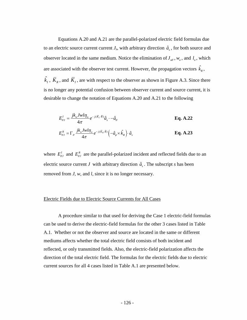
- 126 -
Equations A.20 and A.21 are the parallel-polarized electric field formulas due
to an electric source current current Js, with arbitrary direction sa , for both source and
observer located in the same medium. Notice the elimination of oJ θ , ow , and ol , which
are associated with the observer test current. However, the propagation vectors ˆRk ,
Ik , RK , and IK , are with respect to the observer as shown in Figure A.3. Since there
is no longer any potential confusion between observer current and source current, it is
desirable to change the notation of Equations A.20 and A.21 to the following
( ) ˆ ˆ4
Ij K RI o oJ s
jk JwlE e a aθ θ
ηπ
− ⋅= ⋅− Eq. A.22
( )( ) ˆˆ ˆ4
Rj K RR o oJ R s
jk JwlE e a k aθ θ φ
ηπ
− ⋅= Γ − × ⋅ Eq. A.23
where IJEθ and R
JEθ are the parallel-polarized incident and reflected fields due to an
electric source current J with arbitrary direction sa . The subscript s has been
removed from J, w, and l, since it is no longer necessary.
Electric Fields due to Electric Source Currents for All Cases
A procedure similar to that used for deriving the Case 1 electric-field formulas
can be used to derive the electric-field formulas for the other 3 cases listed in Table
A.1. Whether or not the observer and source are located in the same or different
mediums affects whether the total electric field consists of both incident and
reflected, or only transmitted fields. Also, the electric-field polarization affects the
direction of the total electric field. The formulas for the electric fields due to electric
current sources for all 4 cases listed in Table A.1 are presented below.
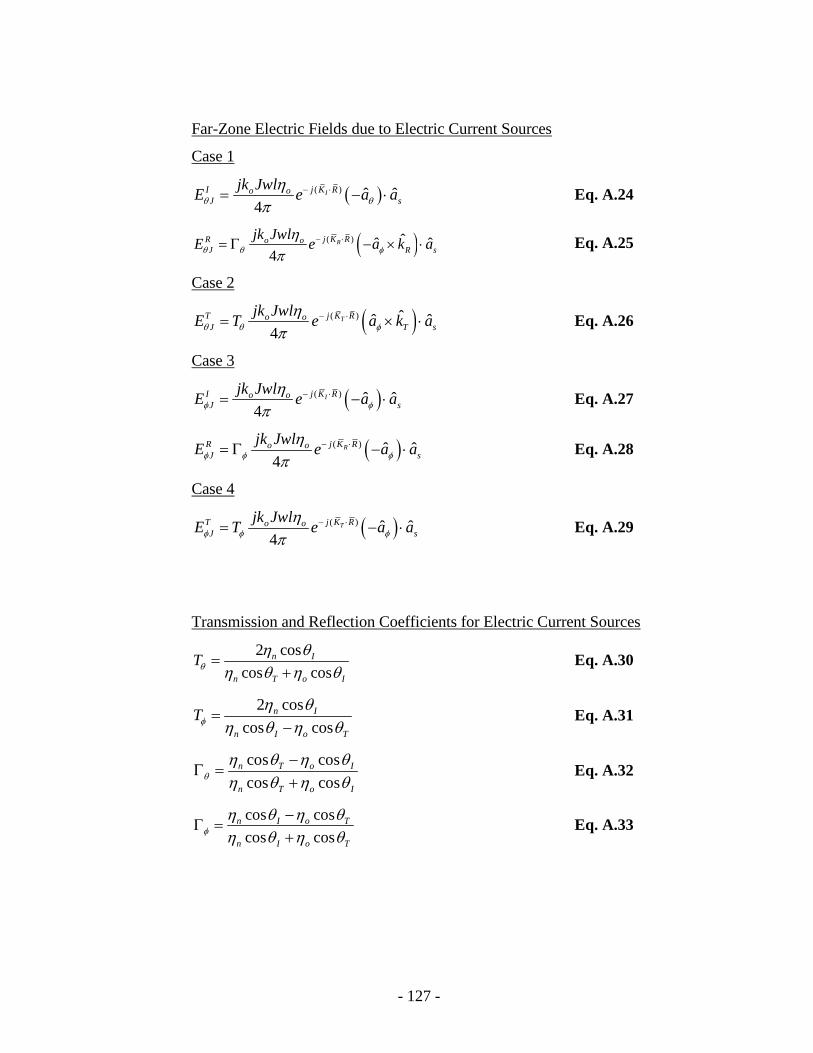
- 127 -
Far-Zone Electric Fields due to Electric Current Sources
Case 1
( )( ) ˆ ˆ4
Ij K RI o oJ s
jk JwlE e a aθ θ
ηπ
− ⋅= − ⋅ Eq. A.24
( )( ) ˆˆ ˆ4
Rj K RR o oJ R s
jk JwlE e a k aθ θ φ
ηπ
− ⋅= Γ − × ⋅ Eq. A.25
Case 2
( )( ) ˆˆ ˆ4
Tj K RT o oJ T s
jk JwlE T e a k aθ θ φ
ηπ
− ⋅= × ⋅ Eq. A.26
Case 3
( )( ) ˆ ˆ4
Ij K RI o oJ s
jk JwlE e a aφ φ
ηπ
− ⋅= − ⋅ Eq. A.27
( )( ) ˆ ˆ4
Rj K RR o oJ s
jk JwlE e a aφ φ φ
ηπ
− ⋅= Γ − ⋅ Eq. A.28
Case 4
( )( ) ˆ ˆ4
Tj K RT o oJ s
jk JwlE T e a aφ φ φ
ηπ
− ⋅= − ⋅ Eq. A.29
Transmission and Reflection Coefficients for Electric Current Sources
2 cos
cos cosn I
n T o I
Tθ
η θη θ η θ
=+
Eq. A.30
2 cos
cos cosn I
n I o T
Tφ
η θη θ η θ
=−
Eq. A.31
cos cos
cos cosn T o I
n T o Iθ
η θ η θη θ η θ
−Γ =
+ Eq. A.32
cos cos
cos cosn I o T
n I o Tφ
η θ η θη θ η θ
−Γ =
+ Eq. A.33
- 128 -
Propagation Vectors, Wavenumbers, and Intrinsic Impedances
ˆ ˆ ˆ ˆI Ix x Iy y Iz zk R k a k a k a= − = + + Eq. A.34
ˆ ˆ ˆ ˆR Ix x Iy y Iz zk k a k a k a= + − Eq. A.35
2 2 2ˆ ˆ ˆ ( )T Ix x Iy y Iz n Ix Iyk k a k a sign k k k k= + + − − Eq. A.36
ˆ ˆ ˆsin cos sin sin cosx y zR a a aθ φ θ φ θ= + + Eq. A.37
ˆI o IK k k= Eq. A.38
ˆR o RK k k= Eq. A.39
ˆT n IK k k= Eq. A.40
2o f o f ok fπ µ µ ε ε= Eq. A.41
2n f n f nk fπ µ µ ε ε= Eq. A.42
f oo
f o
µ µη
ε ε= Eq. A.43
f nn
f n
µ µη
ε ε= Eq. A.44
Note, in Equations A.41 through A.44, fµ and fε are the free-space magnetic
permeability and electric permittivity, respectively. Also, oε and nε are the dielectric
constants of the medium containing and not containing the observer, respectively.
The relative magnetic permeabilitiesoµ and nµ are both equal to 1 for since glacial
ice and air are both non-magnetic mediums.
- 129 -
Required Formula Adjustments for Incident Angles Exceeding the Critical Angle
For cases involving transmission from a medium with a high dielectric
constant to one with a lower dielectric constant (i.e. transmission from ice to air), the
possibility for an evanescent wave exists. An evanescent wave is a surface wave that
decays exponentially in the ˆza direction, and is therefore a non-propagating wave.
This occurs then the incident angle Iθ is greater than the critical angle cθ , making the
transmission angle Tθ imaginary. The critical angle is determined via the following
1sin nc
o
εθ
ε−
=
Eq. A.45
For the case of evanescent waves, the following adjustments are required for the
transmission and reflection coefficients, and transmission vector [11].
2 cos
cosn I
n o I
TjAθ
η θη η θ
=− +
Eq. A.46
2 cos
cosn I
n I o
TjAφ
η θη θ η
=−
Eq. A.47
cos
cosn o I
n o I
j A
j Aθ
η η θη η θ
− −Γ =
− + Eq. A.48
cos
cosn o I
n o I
j A
j Aθ
η η θη η θ
− −Γ =
− + Eq. A.49
2 2 2ˆ ˆ ˆ( )T Ix x Iy y Iz n Ix Iy zK k a k a jsign k k k k a= + − − + + Eq. A.50
where
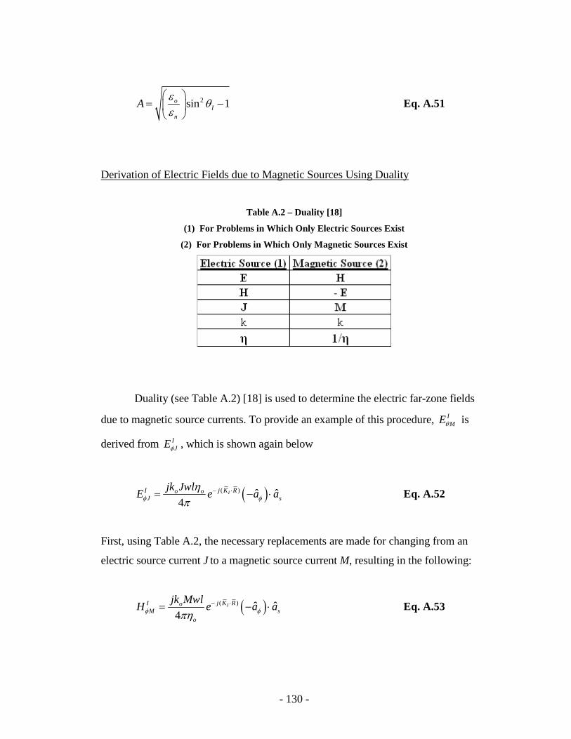
- 130 -
2sin 1oI
n
Aε
θε
= −
Eq. A.51
Derivation of Electric Fields due to Magnetic Sources Using Duality
Table A.2 – Duality [18]
(1) For Problems in Which Only Electric Sources Exist
(2) For Problems in Which Only Magnetic Sources Exist
Duality (see Table A.2) [18] is used to determine the electric far-zone fields
due to magnetic source currents. To provide an example of this procedure, IMEθ is
derived from IJEφ , which is shown again below
( )( ) ˆ ˆ4
Ij K RI o oJ s
jk JwlE e a aφ φ
ηπ
− ⋅= − ⋅ Eq. A.52
First, using Table A.2, the necessary replacements are made for changing from an
electric source current J to a magnetic source current M, resulting in the following:
( )( ) ˆ ˆ4
Ij K RI oM s
o
jk MwlH e a aφ φπη
− ⋅= − ⋅ Eq. A.53
- 131 -
where ˆsa is now the direction of M. Notice that whereas a φ-directed electric current
produces a φ-directed electric field, a φ-directed magnetic current produces a φ-
directed magnetic field. Now, using the following relation, the electric field
associated with IMHφ can be determined
E Hη= Eq. A.54
So, the parallel-polarized incident electric field due to a magnetic source current is
( )( ) ˆ ˆ4
Ij K RI oM s
jk MwlE e a aθ φπ
− ⋅= − ⋅ Eq. A.55
Electric Fields due to Magnetic Source Currents for All Cases
Restating Equation A.55 and using duality to derive all of the parallel and
perpendicular electric field components due to magnetic source currents results in the
following
Far-Zone Electric Fields due to Magnetic Current Sources
Case 1
( )( ) ˆ ˆ4
Ij K RI oM s
jk MwlE e a aθ φπ
− ⋅= − ⋅ Eq. A.56
( )( )ˆ ˆ ˆ4
Rj K RR oM s
jk MwlE e a aθ θ φπ
− ⋅= Γ − ⋅ Eq. A.57
Case 2
( )( )ˆ ˆ ˆ4
Tj K RT oM s
jk MwlE T e a aθ θ φπ
− ⋅= − ⋅ Eq. A.58

- 132 -
Case 3
( )( ) ˆ ˆ4
Ij K RI oM s
jk MwlE e a aφ θπ
− ⋅= ⋅ Eq. A.59
( )( ) ˆˆ ˆ ˆ4
Rj K RR oM R s
jk MwlE e a k aφ φ φπ
− ⋅= Γ × ⋅ Eq. A.60
Case 4
( )( ) ˆˆ ˆ ˆ4
Tj K RT oM T s
jk MwlE T e a k aφ φ φπ
− ⋅= − × ⋅ Eq. A.61
Duality also causes a change in the reflection and transmission coefficients for fields
produced by magnetic source currents resulting in the following formulas.
Transmission and Reflection Coefficients for Magnetic Current Sources
ˆ o
n
T Tθ θ
ηη
=
Eq. A.62
ˆ o
n
T Tφ φ
ηη
=
Eq. A.63
ˆθ θΓ = −Γ Eq. A.64
ˆφ φΓ = −Γ Eq. A.65

- 133 -
APPENDIX B: FEM-NFFT-GO Matlab Code Contracts
There are a total of 25 Matlab and VBS functions used to carry out the FEM-
NFFT-GO routine. Since this is an enormous amount of code, only the contracts
describing the purpose of each function, the functions assumptions, and its inputs and
outputs are presented here. The function contracts are presented in alphabetical order.
AnglePos.m
%%%%%%%%%%%%%%%%%%%%%% ---Purpose---%%%%%%%%%%%%%%%%%%%%%%%%%%%%% %%This function creates an angular position matrix from the point of %view of the observer %INPUTS: % 1. thetaMin,thetaMax; min and max values of theta look % 2. numTheta; the number of theta values to have % 3. phi; a specific value of phi % The inputs are given in units of degrees and conv erted to radians %%OUTPUTS: % 1. lookAngles; a matrix containing both theta and phi values of %the observer
AngleVectors.m
%%%%%%%%%%%%%%%%%%%%%% ---Purpose---%%%%%%%%%%%%%%%%%%%%%%%%%%%%% % Converts the angular theta and phi directions int o x,y,z %coordinates %%INPUTS: % 1. lookAngles; the theta and phi angles of the ob server %%OUTPUTS: % 1. aHatTheta; the theta directed unit vector conv erted to x,y,z % 2. aHatPhi; the phi directed unit vector converte d to x,y,z AParameter.m
%%%%%%%%%%%%%%%%%%%%%% ---Purpose---%%%%%%%%%%%%%%%%%%%%%%%%%%%%% %%This function determines the parameter A, as defi ned in %Engineering Electromagnetics (Demarest, p. 500). T he A parameter is %used within transmission and reflection coefficient formulas if the %critical angle has been exceeded. It is necessary to maintain the %proper sign and phase of the coefficients. %INPUTS: % 1. nA,nB; the indexes of refraction for each medi um, where n1 is % % the incident medium, and n2 is the transmission m edium % 2. thetai; the incident theta angle %%OUTPUTS:

- 134 -
% 1. A; the A parameter
AutomateFieldCalc.vbs
'----------------- AutomateFieldCalc.vbs ---------- ----------------' ' Assumptions: ' 1. a .pts file containing the points for which E and H are desired is available ' 2. The .pts file contains points in units of mete rs, as required by HFSS. ' 3. The geometry must have one box surrouding the entire geometry ' 4. The outputs desired are complex E and H in rec tangular coordinates ' 5. OUTPUTS: E_Field_Results.txt and H_Field_Resul ts.txt ' 6. INPUTS: fieldDataPoints.pts ' NOTE: This code requires use of dirIN, but must b e manually typed into the code ' ------------------------------------------------- ----------------' AutomatePropertyOutput.vbs
'------------------- AutomatePropertyOutput.vbs --- ---------------' ' Assumptions: ' 1. The boundary surrounding the geometry is a rec tangular box ' 2. The boundary box is named exactly "BoundaryBox " ' 3. The geometry must have one box surrouding the entire geometry ' 4. The analysis setup is named exactly "Setup1" ' 5. The geometry is oriented so that the dielectri c (ice) half space is pointing in the negative z direction ' 6. The ice box is assumed to start at the origin and continue in the negative z direction until the BoundaryBox is r eached ' NOTE: This code requires use of dirIN, but must b e manually typed into the code ' ------------------------------------------------- ----------------' currentDimensions.m
%%%%%%%%%%%%%%%%%%%%%% ---Purpose---%%%%%%%%%%%%%%%%%%%%%%%%%%%%% %%This function determines the length, width, and d irection of a %surface current, J or M %%INPUTS: % 1. faceID; the boundary box face identification % 2. stepX,stepY,stepZ; the size of the increments in x,y,z % dimensions %%OUTPUTS: % 1. length,width; the dimensions of the current s egment % 2. curDir1,curDir2; the direction of the current segment, either % x,y,z

- 135 -
EDifferentMedium_J.m
%%%%%%%%%%%%%%%%%%%%%% ---Purpose---%%%%%%%%%%%%%%%%%%%%%%%%%%%%% %%Determines the theta and phi component of the ele ctric field due %to an electric surface current, Js, for the case o f the source and %observer being in different mediums. %%INPUTS: % 1. Js; electric surface current magnitude % 2. pos; position matrix of Js % 3. k; the wavenumber % 4. kT; the transmitted propagation vector % 5. kHatT; the transmitted unit propagation vector % 6. length, width; dimensions of Js % 7. impdanceA; the impedance of the medium % 8. aHatJ; the direction of Js % 9. transC; transmission coefficient % 10. aHatPhi; the phi unit direction %%OUTPUTS: % 1. EthetaJ; Etheta due to an electric surface cur rent % 2. EphiJ; Ephi due to an electric surface current EDifferentMedium_M.m
%%%%%%%%%%%%%%%%%%%%%% ---Purpose---%%%%%%%%%%%%%%%%%%%%%%%%%%%%% %%Determines the theta and phi component of the ele ctric field due %to a magnetic surface current, Ms, for the case of the s ource and %observer being in different mediums. %%INPUTS: % 1. Ms; the surface current M % 2. pos; the source position vector relative to th e origin % 3. k; the incident field wavenumber % 4. KT; transmitted propagation vectors % 5. kHatT; the transmission unit vector % 6. length,width; the surface current step size di mensions % 7. impedanceA; the impedance for the incident med iums % 8. aHatM; the source unit vector. % 9. transC; the transmission coefficient % 10. aHatphi; the phi direction unit vector %%OUTPUTS: % 1. EthetaM; Etheta due to a magnetic surface curr ent % 2. EphiM; Ephi due to a magnetic surface current
EfarField.m
%%%%%%%%%%%%%%%%%%%%%% ---Purpose---%%%%%%%%%%%%%%%%%%%%%%%%%%%%% %%This function determines the far field theta and phi components of %E based on both the electric surface current Js an d magnetic %surface currents Ms. Primarily, this function simp ly determines %which situation is in effect based on the source/o bserver %locations, polarization, and source type % %%%%%%%% 4 source/observer possibilities: % a. source/observer = top/bottom medium

- 136 -
% b. source/observer = bottom/top medium % c. source/observer = top/top medium % d. source/observer = bottom/bottom medium % %%%%%%%% 2 polarization possibilities: % a. parallel polarization (theta component) % b. perpendicular polarization (phi component) % %%%%%%%% 2 source type possibilities: % a. electric current % b. magnetic current %%INPUTS: % 1. Js,Ms; matrix of electric surface currents and magnetic surface % currents respectively % 2. pos; matrix of source position vectors % 3. k1,k2; wavenumbers for top and bottom media % 4. KI; incident propagation vectors % 5. KR; reflected propagation vectors % 6. KT; transmission propagation vectors % 7. kHatR; reflected unit vector % 8. kHatT; transmission unit vector % 9. length; length of the current segment % 10. width; width of the discrete sampled value % 11. curDir1; direction of the 1st current vector on a face % 12. curDir2; direction of the 2nd current vector on a face % 13. impedance1,impedance2; impedances of top and bottom media % 14. lookAngles; the theta and phi angles of the o bserver % 15. reflectC; reflection coefficient array % 16. transC; transmission coefficient array % 17; aHatPhi; phi direction unit vector array % 18; aHatTheta; theta direction unit vector array %%OUTPUTS: % 1. Etheta; the parallel polarized E field % 2. Ephi; the perpendicularly polarized E field %%Note: postscript 1 on inputs represents medium re siding in %positive z axis (top medium), and postscript 2 represents medi um %residing in negative z axis (bottom medium)
EIncMag.m
%%%%%%%%%%%%%%%%%%%%%% ---Purpose---%%%%%%%%%%%%%%%%%%%%%%%%%%%%% %%This function produces the Ei value which is the E field magnitude %value of the incident field with zero phase. This function can also %be used to determine Hi. However, this requires dividing the result %of this function by the impedance, impedance1, whi ch is handled in %the calling code. %%INPUTS: % 1. k1; the incident field wavenumber % 2. Source; the current segment value (usually den oted J or M) % 3. length; the length dimension of the discrete c urrent values % 4. width; the width dimension of the discrete cur rent values % 5. impedance1; the impedance value of the inciden t medium %%OUTPUTS: % 1. Ei; the E field magnitude

- 137 -
Equivalent_Currents.m
%%%%%%%%%%%%%%%%%%%%%% ---Purpose---%%%%%%%%%%%%%%%%%%%%%%%%%%%%% %Equivalent_Current samples near E and H fields fro m HFSS and then %converts those fields to equivalent currents. %%INPUTS: % 1. dirIn: the input directory of the raw data fil es % 2. ptsInput: the near field sampling interval % 3. sDecXY: the sampling box decrement factor in t he XY dimensions % 4. sDecZ_Top: the sampling box decrment factor in the upper z % plane % 5. sDecZ_Bot: the sampling box decrment factor in the lower z % plane %%OUTPUTS: % 1. Frequncy % 2. stepX,stepY,stepZ: the sampling size dimension % 3. Js"": the electric current matrix for each fac e % 4. Ms"": the magnetic current matrix for each fac e % 5. pos"": the current position matrix for each fa ce %%NOTE: The faces are divided into left, right, top , bottom, front, %and back
ESameMedium_J.m
%%%%%%%%%%%%%%%%%%%%%% ---Purpose---%%%%%%%%%%%%%%%%%%%%%%%%%%%%% %%Determines the theta and phi component of the ele ctric field due %to an electric surface current, Js, for the case o f the source and %observer being in the same medium. %%INPUTS: % 1. Js; the surface current J % 2. pos; the source position vector relative to th e origin % 3. k; the incident field wavenumber % 4. KI; the incident field vector % 5. KR; the reflected field vector % 6. kHatR; the reflection unit vector % 7. length,width; the surface current step size di mensions % 8. impedanceA; the impedance for the incident med iums % 9. aHatJ; the source unit vector. % 10. reflectC; the reflection coefficient % 11. aHatphi; the phi direction unit vector % 12. aHatTheta; the theta direction unit vector %%OUTPUTS: % 1. EthetaJ; Etheta due to an electric surface cur rent % 2. EphiJ; Ephi due to an electric surface current ESameMedium_M.m
%%%%%%%%%%%%%%%%%%%%%% ---Purpose---%%%%%%%%%%%%%%%%%%%%%%%%%%%%% %%Determines the theta and phi component of the ele ctric field due %to a magnetic surface current, Ms, for the case of the s ource and %observer being in the same medium. %%INPUTS:

- 138 -
% 1. Ms; the surface current M % 2. pos; the source position vector relative to th e origin % 3. k; the incident field wavenumber % 4. KI; the incident field vector % 5. KR; the reflected field vector % 6. kHatR; the reflection unit vector % 7. length,width; the surface current step size di mensions % 8. impedanceA; the impedance for the incident med iums % 9. aHatM; the source unit vector. % 10. reflectC; the reflection coefficient % 11. aHatphi; the phi direction unit vector % 12. aHatTheta; the theta direction unit vector %%OUTPUTS: % 1. EthetaJ; Etheta due to a magnetic surface curr ent % 2. EphiJ; Ephi due to a magnetic surface current
GainFactor.m
%%%%%%%%%%%%%%%%%%%%%% ---Purpose---%%%%%%%%%%%%%%%%%%%%%%%%%%%%% %Determines the gain factor improvement in the E fi elds due to the %focusing effect arising from increasing dielectric constant with %increasing depthin glacial ice. %%INPUTS: % 1. EthetaIN; the total theta directed E field, ca lculated from % previous code % 2. EphiIN; the total phi directed E field, calcul ated from % previous code % 3. lookAngles; the angles associated with EthetaT otal and % % EphiTotal % 4. location; 1 = Antarctia, 2 = Greenland % 5. z; the depth vector %%OUTPUTS: % 1. GthetaAD; Etheta as a function of aidaPrime (r ows) % and depth (columns) - in magnitude gain % 2. GphiAD; Ephi as a function of aidaPrime (rows) and % depth (columns) - in magnitude gain % 3. g0; The incident angles at the surface directe d towards the % ice, ranging only from 0 to 90 degrees (double sided). % 4. g02; The incident angles at the surface direct ed towards the % ice, ranging only from 90 to 270 degrees. % 5. aidaPrime; the effective look angle at each de pth -- 0 degrees % at nadir (goes from 0 to 90 and 0 to -90 degre es) % 6. Gf; The gain factor improvement matrix
Generate_PTS_File.m
%%%%%%%%%%%%%%%%%%%%%% ---Purpose---%%%%%%%%%%%%%%%%%%%%%%%%%%%%% %creates a .pts file for each of the six boundary b ox faces given %x,y,z minimum and maxium values %%INPUTS: % 1. xMin,yMin,zMin; the minimum boundary box dimen sions % 2. xMax,yMax,zMax; the maximum boundary box dimen sions

- 139 -
% 3. Frequency; the frequency of antenna operation % 4. ptsInput; the number of sample points taken pe r wavelength % 5. sDecXY; the sample box decrement factor in X a nd Y dimensions % 6. sDecZ_TOP; the sample box decrement factor in positive Z % 7. sDecZ_Bot; the sampel box decrement facotr in negative Z % 8. dirIn; the directory containing the data files %INPUT ASSUMPTIONS: Assume that the boundary box is rectangular; the %input dimensions are in units of meters; the frequ ency is in units %of Hz; the ptsInput is in units of points/waveleng th %NOTE: HFSS requires that the .pts file be in units of meters. %OUTPUTS: outputs 6 .pts files, one for each bounda ry box face; % 1. stepX,stepY,stepZ; the x,y,z sample increment values. %comments assume positive z pointing upward, positi ve y pointing to %the right, and poitive x pointing out of the screeen KVectors.m
%%%%%%%%%%%%%%%%%%%%%% ---Purpose---%%%%%%%%%%%%%%%%%%%%%%%%%%%%% %%This function produces the K vectors. The K vectors describe the %propagation of incident, reflected, or transmitted waves %%INPUTS: % 1. lookAngles; the look angles, theta and phi of the observer % 2. k1,k2; the wavenumbers of the top and bottom m edia %%OUTPUTS: % 1. KI; the incident propagation vectors for media 1 and 2 % 2. KR; the reflected propagation vectors for medi a 1 and 2 % 3. KT; the transmitted propagation vectors for me dia 1 and 2
Master.m
%%%%%%%%%%%%%%%%%%%%%% ---Purpose---%%%%%%%%%%%%%%%%%%%%%%%%%%%%% %Master_Output runs either the FEM-NFFT by itself o r in combination %with the GO algorithm. This code is divided into three s ection with %necessary comments listed below % 1. INPUTS TO SPECIFY % 2. The FEM-NFFT Procedure % 3. The GO Procedure
NFFT.m
%%%%%%%%%%%%%%%%%%%%%% ---Purpose---%%%%%%%%%%%%%%%%%%%%%%%%%%%%% %NFFT performs the near to far field transformation s %%INPUTS: % 1. thetaMin: the minimum desired value of the ang le theta % 2. thetaMax: the maximum desired value of the ang le theta % 3. numTheta: the number of theta values desired f or angular % resolution % 4. phi: the value of phi desired % 5. e1,e2: the relative permittivity of the top an d bottom mediums % 6. u1,u2: the relative permeability of the top an d bottom mediums % 7. Frequncy
- 140 -
% 8. stepX,stepY,stepZ: the sampling size dimension % 9. Js"": the electric current matrix for each fac e % 10.Ms"": the magnetic current matrix for each fac e % 11.pos"": the current position matrix for each fa ce %%OUTPUTS: % 1. EthetaTotal: the total complex E-field in thet a % 2. EphiTotal: the total complex E-field in phi % 3. lookAngles: the matrix in radians containing t heta and phi % values % 4. impedance1: the intrinsic impedance of the top medium % 5. impedance2: the intrinsic impedance of the bot tom medium ObtainHFSS_Properties.m
%%%%%%%%%%%%%%%%%%%%%% ---Purpose---%%%%%%%%%%%%%%%%%%%%%%%%%%%%% %Obtains outer boundary data from HFSS_DataOut.txt %Determines box dimensions and frequency and conver t dimensions to %meters %%%%% -- Assumptions -- %%%%%% % 1. Assumes that the boundary is a rectangular box % 2. Assumes HFSS units of nm,um,mm,meter,cm,km,ft, in,mil,uin % 3. Code converts all units to meters %%INPUT ASSUMTIONS: The input file contains text of the following %form: % XSize 10mm % YSize 10mm % ZSize 2.5mm % Position -5 ,-5 ,0 %position can contain units % Frequency 50000000000 %%INPUT: % 1. HFSSInputFile; a file containing the data show n above %%OUTPUT: % 1. xMin,yMin,zMin; the minimum dimensions of boun dary box % 2. xMax,yMax,zMax; the maximum dimensions of boun dary box % 3. Frequency; the frequency of the HFSS simulatio n in Hz reflectCoeff.m
%%%%%%%%%%%%%%%%%%%%%% ---Purpose---%%%%%%%%%%%%%%%%%%%%%%%%%%%%% %%This function produces the reflection coefficient , which is either %parallel or perpendicular depending on the polariz ation %INPUTS: % 1. lookAngles; matrix of theta and phi of the obs erver % 2. thetaI; the incident angle % 3. thetaT; the transmission angle % 4. impedance1; the impedance value of the inciden t medium % 5. impedance2; the impedance value of the transmi ssion medium % 6. n1,n2; the indexes of refraction for each medi um %%OUTPUTS: % 1. reflectC; the reflection coefficient

- 141 -
SourceVector.m
%%%%%%%%%%%%%%%%%%%%%% ---Purpose---%%%%%%%%%%%%%%%%%%%%%%%%%%%%% % Converts the curDir1 and curDir2 direction indexe s to actual % vector direction %%NOTES: curDir'' = 1 indicates x directed current % curDir'' = 2 indicates y directed current % curDir'' = 3 indicates z directed current %%INPUTS: % 1. curDir1, curDir2; the direction of each type o f current on the % data sample face %%OUTPUTS: % 1. aHatS1, aHatS2; the unit vector of each type o f current on the % data sample face SurfCurrents.m
%%%%%%%%%%%%%%%%%%%%%% ---Purpose---%%%%%%%%%%%%%%%%%%%%%%%%%%%%% %%This function takes in the E and H field data fro m a face of the %boundary box, and computes the electric and magnet ic surface %currents Js and Ms. %%INPUTS: % 1. Efilename; the data file containing the near-z one electric % field data for a surface % 2. Hfilename; the data file containing the near-z one electric %field data for a surface % 3. faceID; a value identifying which face of the sampling box has % been input %%OUTPUTS: % 1. Js; the electric surface currents on the face % 2. Ms; the magnetic surface currents on the face % 3. pos; the position of each surface current on t he face
ThetaAngles.m
%%%%%%%%%%%%%%%%%%%%%% ---Purpose---%%%%%%%%%%%%%%%%%%%%%%%%%%%%% %%This function produces a matrix of the incident a nd transmission %angles theta %%INPUTS: % 1. lookAngles; matrix of theta and phi of the obs erver % 2. nA,nB; the refractive indexes of the incident and transmission % media. %%OUTPUTS: % 1. thetaI; the incident angle % 2. thetaT; the transmitted angle

- 142 -
transCoeff.m
%%%%%%%%%%%%%%%%%%%%%% ---Purpose---%%%%%%%%%%%%%%%%%%%%%%%%%%%%% %%This function produces the transmission coefficie nt, which is %either parallel or perpendicular depending on the polariza tion %%INPUTS: % 1. lookAngles; matrix of theta and phi of the obs erver % 2. thetaI; the incident angle % 3. thetaT; the transmission angle % 4. impedance1; the impedance value of the inciden t medium % 5. impedance2; the impedance value of the transmi ssion medium % 6. n1,n2; the indexes of refraction for each medi um %%OUTPUTS: % 1. transC; the reflection coefficient
WaveNumber.m
%%%%%%%%%%%%%%%%%%%%%% ---Purpose---%%%%%%%%%%%%%%%%%%%%%%%%%%%%% %%This function produces the wavenumbers, impedance s, and index of %refraction from each medium in the half-space %%INPUTS: % 1. Frequency; the operating frequency % 2. e1,e2; the dielectric constant of top and bott om media % 3. u1,u2; the relative permeavility of the top an d bottom media %%OUTPUTS: % 1. k1,k2; wavenumbers of top and bottom media % 2. impedance1,impedance2; impedances of top and b ottom medium % 3. n1,n2; indexes of refraction of top and bottom media

- 143 -
APPENDIX C: IceTemp.m Matlab Code
This section contains the temperature profile extraction code, called
IceTemp.m, which is a modified version of original code presented by Lie, Xie, and
Dobbs in [27]. This code was used to perform the temperature profile extraction
simulations shown in Chapter 5.
%%%%%%%%%%%%%%%%%%%%%%%%%%%%%%%%%%%%%%%%%%%%%%%%%%%%%%%%%%%%%%%%%%%% %PART 1: obtain Temperature profiles from the Exce l Spreadsheet %Data % 1.) Read the temperature vs. depth profile for pu re ice % 2.) Enter in constants % 3.) Produce layer depth matrix % 4.) Load the Antenna Gain Data % 2.) Calculate the real and imaginary parts of the permittivity % 3.) Calculate the wavenumber, loss tangent, and a ttenuation % 4.) Calculate the Total Attenuation %%%%%%%%%%%%%%% Read in the Temperature Profiles %% %%%%%%%%%%%%%%%%% % GRIP Temperature Profile T1 = xlsread ( 'Ice_temp_profile' , 'Hypothetical profiles' , 'B4:B304' ); % Hypothetical 1 Profile T2 = xlsread ( 'Ice_temp_profile' , 'Hypothetical profiles' , 'C4:C304' ); % Hypothetical 2 Profile T3 = xlsread ( 'Ice_temp_profile' , 'Hypothetical profiles' , 'D4:D304' ); % read the depth profile d = xlsread ( 'Ice_temp_profile' , 'Hypothetical profiles' , 'A4:A304' ); % plot temperature profiles in terms of depth figure (1); plot(T1, d, 'r' );hold on plot(T2, d, 'b' );hold on plot(T3, d, 'm' );hold off grid; h = gca; set (h, 'YDir' , 'reverse' ); legend ( 'GRIP' , 'Hypothetical_1' , 'Hypothetical_2' , 'Location' , 'NorthEast' ); title ( 'Ice Temperature Profiles' ); xlabel ( 'T (C)' ); ylabel ( 'Depth (m)' ); %%%%%%%%%%%%%%%%%%%%%%%%%%%%%%%%%%%%%%%%%%%%%%%%%%%%%%%%%%%%%%%%%%%% %%%%%%%%%%%%%%%%%%%%%%% Constants %%%%%%%%%%%%%%%%%%%%%%%%%%%%% %depth of each layer (depth-resolution)
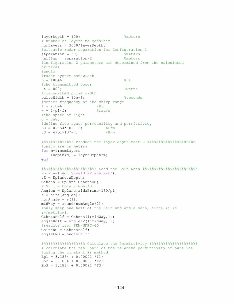
- 144 -
layerDepth = 100; %meters % number of layers to consider numLayers = 3000/layerDepth; %bistatic radar separation for Configuration 1 separation = 50; %meters halfSep = separation/2; %meters %Configuration 2 parameters are determined from the calculated critical %angle %radar system bandwidth B = 180e6; %Hz %the transmitted power Pt = 800; %watts %transmitted pulse width pulseWidth = 10e-6; %seconds %center frequency of the chirp range f = 210e6; %Hz w = 2*pi*f; %rad/s %the speed of light c = 3e8; %define free space permeability and permittivity E0 = 8.854*10^-12; %F/m u0 = 4*pi*10^-7; %H/m %%%%%%%%%%%%%% Produce the layer depth matrix %%%%%%%%%%%%%%%%%%%%% %units are in meters for m=1:numLayers zDepth(m) = layerDepth*m; end %%%%%%%%%%%%%%%%%%%%%%%% Load the Gain Data %%%%%%%%%%%%%%%%%%%%%%%% Eplane=load( 'VivaldiEPlane.mat' ); zE = Eplane.zDepth; Gtheta = Eplane.GthetaAD; % Gphi = Eplane.GphiAD; Angles = Eplane.aidaPrime*180/pi; s = size(Angles); numAngle = s(1); midWay = round(numAngle/2); %only keep one half of the Gain and angle data, sin ce it is symmetrical. GthetaHalf = Gtheta(1:midWay,:); angleHalf = angles2(1:midWay,:); %results from FEM-NFFT-GO GainFNG = GthetaHalf; angleFNG = angleHalf; %%%%%%%%%%%%%%%%%%% Calculate the Permittivity %%%%%%%%%%%%%%%%%%%%% % calculate the real part of the relative permittiv ity of pure ice %using the constant Er method Ep1 = 3.1884 + 0.00091.*T1; Ep2 = 3.1884 + 0.00091.*T2; Ep3 = 3.1884 + 0.00091.*T3;
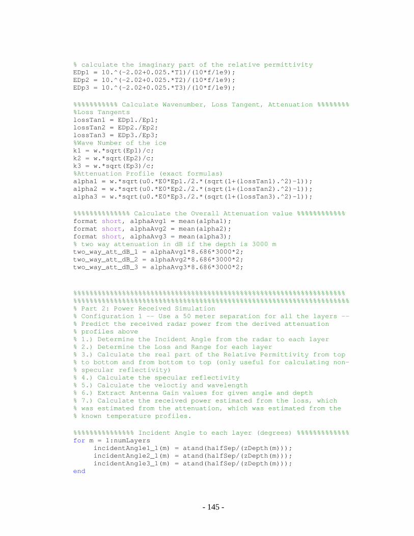
- 145 -
% calculate the imaginary part of the relative perm ittivity EDp1 = 10.^(-2.02+0.025.*T1)/(10*f/1e9); EDp2 = 10.^(-2.02+0.025.*T2)/(10*f/1e9); EDp3 = 10.^(-2.02+0.025.*T3)/(10*f/1e9); %%%%%%%%%%% Calculate Wavenumber, Loss Tangent, Att enuation %%%%%%%% %Loss Tangents lossTan1 = EDp1./Ep1; lossTan2 = EDp2./Ep2; lossTan3 = EDp3./Ep3; %Wave Number of the ice k1 = w.*sqrt(Ep1)/c; k2 = w.*sqrt(Ep2)/c; k3 = w.*sqrt(Ep3)/c; %Attenuation Profile (exact formulas) alpha1 = w.*sqrt(u0.*E0*Ep1./2.*(sqrt(1+(lossTan1). ^2)-1)); alpha2 = w.*sqrt(u0.*E0*Ep2./2.*(sqrt(1+(lossTan2). ^2)-1)); alpha3 = w.*sqrt(u0.*E0*Ep3./2.*(sqrt(1+(lossTan3). ^2)-1)); %%%%%%%%%%%%%% Calculate the Overall Attenuation va lue %%%%%%%%%%%% format short , alphaAvg1 = mean(alpha1); format short , alphaAvg2 = mean(alpha2); format short , alphaAvg3 = mean(alpha3); % two way attenuation in dB if the depth is 3000 m two_way_att_dB_1 = alphaAvg1*8.686*3000*2; two_way_att_dB_2 = alphaAvg2*8.686*3000*2; two_way_att_dB_3 = alphaAvg3*8.686*3000*2; %%%%%%%%%%%%%%%%%%%%%%%%%%%%%%%%%%%%%%%%%%%%%%%%%%%%%%%%%%%%%%%%%%% %%%%%%%%%%%%%%%%%%%%%%%%%%%%%%%%%%%%%%%%%%%%%%%%%%%%%%%%%%%%%%%%%%%%% Part 2: Power Received Simulation % Configuration 1 -- Use a 50 meter separation for all the layers -- % Predict the received radar power from the derived attenuation % profiles above % 1.) Determine the Incident Angle from the radar t o each layer % 2.) Determine the Loss and Range for each layer % 3.) Calculate the real part of the Relative Permi ttivity from top % to bottom and from bottom to top (only useful for calculating non- % specular reflectivity) % 4.) Calculate the specular reflectivity % 5.) Calculate the veloctiy and wavelength % 6.) Extract Antenna Gain values for given angle a nd depth % 7.) Calculate the received power estimated from t he loss, which % was estimated from the attenuation, which was est imated from the % known temperature profiles. %%%%%%%%%%%%%%% Incident Angle to each layer (degre es) %%%%%%%%%%%%% for m = 1:numLayers incidentAngle1_1(m) = atand(halfSep/(zDepth(m) )); incidentAngle2_1(m) = atand(halfSep/(zDepth(m) )); incidentAngle3_1(m) = atand(halfSep/(zDepth(m) )); end
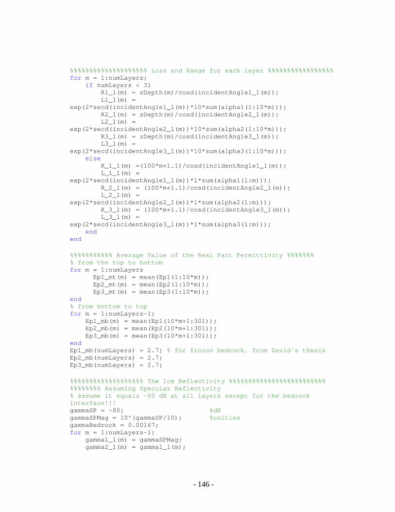
- 146 -
%%%%%%%%%%%%%%%%%%%% Loss and Range for each layer %%%%%%%%%%%%%%%%% for m = 1:numLayers; if numLayers < 31 R1_1(m) = zDepth(m)/cosd(incidentAngle1_1(m )); L1_1(m) = exp(2*secd(incidentAngle1_1(m))*10*sum(alpha1(1:10* m))); R2_1(m) = zDepth(m)/cosd(incidentAngle2_1(m )); L2_1(m) = exp(2*secd(incidentAngle2_1(m))*10*sum(alpha2(1:10* m))); R3_1(m) = zDepth(m)/cosd(incidentAngle3_1(m )); L3_1(m) = exp(2*secd(incidentAngle3_1(m))*10*sum(alpha3(1:10* m))); else R_1_1(m) =(100*m+1.1)/cosd(incidentAngle1_1 (m)); L_1_1(m) = exp(2*secd(incidentAngle1_1(m))*1*sum(alpha1(1:m))) ; R_2_1(m) = (100*m+1.1)/cosd(incidentAngle2_ 1(m)); L_2_1(m) = exp(2*secd(incidentAngle2_1(m))*1*sum(alpha2(1:m))) ; R_3_1(m) = (100*m+1.1)/cosd(incidentAngle3_ 1(m)); L_3_1(m) = exp(2*secd(incidentAngle3_1(m))*1*sum(alpha3(1:m))) ; end end %%%%%%%%%%% Average Value of the Real Part Permitti vity %%%%%%% % from the top to bottom for m = 1:numLayers Ep1_mt(m) = mean(Ep1(1:10*m)); Ep2_mt(m) = mean(Ep2(1:10*m)); Ep3_mt(m) = mean(Ep3(1:10*m)); end % from bottom to top for m = 1:numLayers-1; Ep1_mb(m) = mean(Ep1(10*m+1:301)); Ep2_mb(m) = mean(Ep2(10*m+1:301)); Ep3_mb(m) = mean(Ep3(10*m+1:301)); end Ep1_mb(numLayers) = 2.7; % for frozon bedrock, from David's thesis Ep2_mb(numLayers) = 2.7; Ep3_mb(numLayers) = 2.7; %%%%%%%%%%%%%%%%%%% The Ice Reflectivity %%%%%%%%%%%%%%%%%%%%%%%%% %%%%%%%% Assuming Specular Reflectivity % assume it equals -80 dB at all layers except for the bedrock interface!!! gammaSP = -80; %dB gammaSPMag = 10^(gammaSP/10); %unitles gammaBedrock = 0.00167; for m = 1:numLayers-1; gamma1_1(m) = gammaSPMag; gamma2_1(m) = gamma1_1(m);
- 147 -
gamma3_1(m) = gamma2_1(m); end gamma1_1(numLayers) = gammaBedrock; gamma2_1(numLayers) = gammaBedrock; gamma3_1(numLayers) = gammaBedrock; %%%%%%%%%%%%%%%%% Velocity and Lambda %%%%%%%%%%%%%%%%%%%%%%%%%%%%%% %calculate the velocity for each temp profile vp1 = c/sqrt(Ep1_mb(1)); %m/s vp2 = c/sqrt(Ep2_mb(1)); %m/s vp3 = c/sqrt(Ep3_mb(1)); %m/s %calculate the wavelength in ice for each temp prof ile lambda1 = vp1/f; %m lambda2 = vp2/f; %m lambda3 = vp3/f; %m %%%%%%%%%%%%%%%%%%%%% Antenna Gain %%%%%%%%%%%%%%%%%%%%%%%%%%% %determine the gain at each incident angle and each depth %%%% Assuming constant gain, not using Gain from FE M-NFFT-GO %%%%%%% % 3 dB gain assumed % for m=1:numLayers % for n=1:numLayers % GainMag(m,n)=10^0.3; % end % end %%%% Extracting Relevant Gain Values form FEM-NFFT- GO Code %%%%%% for m=1:numLayers %the incident angle at z angleInc = incidentAngle1_1(m); %the difference between the incident angle at z and angles in gain %pattern at z diFF = abs(angleFNG(:,m)-angleInc); %the index where the two angles agree most index = find(diFF == min(diFF)); GainMag(m) = GainFNG(index,m); %dB end %%%%%%%%%%%%%%%%%%%%%%% Received Power %%%%%%%%%%%%%%%%%%%%%%%%%%%%% %units are in Watts for m=1:numLayers Pr1_1(m) = Pt * GainMag(m)^2*lambda1^2*gamma1_1(m)/((8*pi*R1_1(m))^ 2*L1_1(m)); Pr2_1(m) = Pt * GainMag(m)^2*lambda2^2*gamma2_1(m)/((8*pi*R2_1(m))^ 2*L2_1(m)); Pr3_1(m) = Pt * GainMag(m)^2*lambda3^2*gamma3_1(m)/((8*pi*R3_1(m))^ 2*L3_1(m)); end %%%%%%%%%%%%%%%%%%%%%%%%%%%%%%%%%%%%%%%%%%%%%%%%%%%%%%%%%%%%%%%%%%% %%%%%%%%%%%%%%%%%%%%%%%%%%%%%%%%%%%%%%%%%%%%%%%%%%%%%%%%%%%%%%%%%%%%% Part 2: Power Received Simulation % Configuration 2 -- Use a separation defined by th e incident angle
- 148 -
% that is half of the critical angle % Predict the received radar power from the derived attenuation % profiles above % 1.) Determine the Incident Angle from the radar t o each layer % 2.) Determine the Loss and Range for each layer % 3.) Calculate the real part of the Relative Permi ttivity from top % to bottom and from bottom to top % 4.) Calculate the specular reflectivity % 5.) Calculate the received power estimated from t he loss, which % was estimated from the attenuation, which was est imated from the % known temperature profiles. %%%%%%%%%%%%%%%%%%%%%%% Critical Angle %%%%%%%%%%%%%%%%%%%%%%%%%%%% %the critical angle only exists for propagation fro m ice to air %the index of refraction for air nAir = 1; %ice dielectric constant for pursposes of calculati ng critical angle Eice = 3.2; %fixed critical angle and halfSepMax cTheta = asind(nAir/sqrt(Eice)); halfSepMax = zDepth.*tand(cTheta); %factor for determing the antenna separation to use based on the %maximum possible antenna separation factor = 2; halfSep1 = halfSepMax./factor; halfSep2 = halfSepMax./factor; halfSep3 = halfSepMax./factor; %%%%%%%%%%%%%%%% Incident Angle, Range, and Depth %%%%%%%%%%%%%%%%% for m=1:numLayers incidentAngle1_2(m) = atand(halfSep1(m)/(zDepth( m))); incidentAngle2_2(m) = atand(halfSep2(m)/(zDepth( m))); incidentAngle3_2(m) = atand(halfSep3(m)/(zDepth( m))); R1_2(m) = zDepth(m)/cosd(incidentAngle1_2(m)); R2_2(m) = zDepth(m)/cosd(incidentAngle2_2(m)); R3_2(m) = zDepth(m)/cosd(incidentAngle3_2(m)); if numLayers < 31 L1_2(m) = exp(2*secd(incidentAngle1_2(m))*10*sum(alpha1(1:10* m))); L2_2(m) = exp(2*secd(incidentAngle2_2(m))*10*sum(alpha2(1:10* m))); L3_2(m) = exp(2*secd(incidentAngle3_2(m))*10*sum(alpha3(1:10* m))); else L1_2(m) = exp(2*secd(incidentAngle1_2(m))*1*sum(alpha1(1:1*m) )); L2_2(m) = exp(2*secd(incidentAngle2_2(m))*1*sum(alpha2(1:1*m) )); L3_2(m) = exp(2*secd(incidentAngle3_2(m))*1*sum(alpha3(1:1*m) )); end end
- 149 -
%%%%%%%%%%%%%%%%%%%%% The Ice Reflectivity %%%%%%%%%%%%%%%%%%%%%%%% % for specular case, use same as Part 1 gamma1_2 = gamma1_1; gamma2_2 = gamma2_1; gamma3_2 = gamma3_1; %%%%%%%%%%%%%%%%%%%%% Antenna Gain %%%%%%%%%%%%%%%%%%%%%%%%%%% %determine the gain at each incident angle and each depth %%%% Assuming constant gain, not using Gain from FE M-NFFT-GO %%%%%%% %GainMag2 = GainMag; %%%% Extracting Relevant Gain Values form FEM-NFFT- GO Code %%%%%% for m=1:numLayers %the incident angle at z angleInc = incidentAngle1_2(m); %the difference between the incident angle at z and angles in %gain pattern at z diFF = abs(angleFNG(:,m)-angleInc); %the index where the two angles agree most index = find(diFF == min(diFF)); GainMag2(m) = GainFNG(index,m); %dB end %%%%%%%%%%%%%%%%%%%% Received Power %%%%%%%%%%%%%%%%%%%%%%%%%%%% %These are all basically for a constant incident an gle for m=1:numLayers Pr1_2(m) = Pt*GainMag2(m)^2*lambda1^2*gamma1_2(m)/((8*pi*R1_2( m))^2*L1_2(m)); Pr2_2(m) = Pt*GainMag2(m)^2*lambda2^2*gamma2_2(m)/((8*pi*R2_2( m))^2*L2_2(m)); Pr3_2(m) = Pt*GainMag2(m)^2*lambda3^2*gamma3_2(m)/((8*pi*R3_2( m))^2*L3_2(m)); end %%%%%%%%%%%%%%%%%%%%%%%%%%%%%%%%%%%%%%%%%%%%%%%%%%%%%%%%%%%%%%%%%%%% %%%%%%%%%%%%%%%%%%%%%%%%%%%%%%%%%%%%%%%%%%%%%%%%%%%%%%%%%%%%%%%%%%%% % Part 3: Derive Attenuation from Power %%%%%% %%%%%%%%%%%%%%%%% % 1.) Estimate the Antenna Gain for Temperature Ext raction % 2.) Calculate total attenuation from z=0 to each depth % 3.) Determine the attenuation at each depth % 4.) Extract Temperature from Attenuation %%%%%%%%%%%%%%%%%% Estimated Antenna Gain %%%%%%%%%%%%%%%%%%%%%%%% % Normal: Assume estimated gain is the same as that used for Pr % simulations GainMag_E = GainMag; GainMag2_E = GainMag2; % Assume a uniform dB error in the gain estimation %error_dB = 30.0; %GainMag_EdB = 10*log10(GainMag) - error_dB; %GainMag2_Edb = 10*log10(GainMag2) - error_dB; %GainMag_E = 10.^(GainMag_EdB/10); %GainMag2_E = 10.^(GainMag2_Edb/10);
- 150 -
%%%%%%%% Calculate total attenuation from z=0 to ea ch depth %%%%%%%% for m=1:numLayers alphaAccum1(m) = log((GainMag_E(m)^2*Pr1_2(m)*cosd(incidentAngle1_1( m))^2)/(GainMag2_E(m)^2*Pr1_1(m)*cosd(incidentAngle1_2(m))^2))/(2*(s ecd(incidentAngle1_1(m))-secd(incidentAngle1_2(m)))); alphaAccum2(m) = log((GainMag_E(m)^2*Pr2_2(m)*cosd(incidentAngle2_1( m))^2)/(GainMag2_E(m)^2*Pr2_1(m)*cosd(incidentAngle2_2(m))^2))/(2*(s ecd(incidentAngle2_1(m))-secd(incidentAngle2_2(m)))); alphaAccum3(m) = log((GainMag_E(m)^2*Pr3_2(m)*cosd(incidentAngle3_1( m))^2)/(GainMag2_E(m)^2*Pr3_1(m)*cosd(incidentAngle3_2(m))^2))/(2*(s ecd(incidentAngle3_1(m))-secd(incidentAngle3_2(m)))); end %%%%%%%%%%%%%% Determine Attenuation at Each Depth %%%%%%%%%%%%%%%% % the incremental z layer deltaZ = layerDepth; %determine the individual attenuation across each i ndividual layer %the sum of the previous attenuations sumAlpha1 = 0; sumAlpha2 = 0; sumAlpha3 = 0; for m=1:numLayers alphaInd1(m) = alphaAccum1(m)/deltaZ - sumAlpha 1; sumAlpha1 = sumAlpha1 + alphaInd1(m); alphaInd2(m) = alphaAccum2(m)/deltaZ - sumAlpha 2; sumAlpha2 = sumAlpha2 + alphaInd2(m); alphaInd3(m) = alphaAccum3(m)/deltaZ - sumAlpha 3; sumAlpha3 = sumAlpha3 + alphaInd3(m); end %%%%%%%%%%%%%%%%%%%%%% Extract Temperature %%%%%%%%%%%%%%%%%%%%%%%% for m = 1:numLayers-1 f1 = @(T)(3*alphaInd1(m)/pi)^2*(3.1884+0.00091* T)-10^(-4.04+0.05*T); T_1(m) = fzero(f1,T1(10*m)); dT1(m) = T_1(m) - T1(10*m); f2 = @(T)(3*alphaInd2(m)/pi)^2*(3.1884+0.00091* T)-10^(-4.04+0.05*T); T_2(m) = fzero(f2,T2(10*m)); dT2(m) = T_2(m) - T2(10*m); f3=@(T)(3*alphaInd3(m)/pi)^2*(3.1884+0.00091*T) -10^(-4.04+0.05*T); T_3(m)=fzero(f3,T3(10*m)); dT3(m)=T_3(m)-T3(10*m); end %%%%%%%%%%%%%%%%%%%%%%%%%%%%%%%%%%%%%%%%%%%%%%%%%%%%%%%%%%%%%%%%%%%% %%%%%%%%%%%%%%%%%%%%%%%%%% Plots %%%%%%%%%%%%%%%%%%%%%%%%%%%%%%%%% %plot indexes
- 151 -
s1=1; s2=290; I=10; figure(2) %compare measured and extracted temperatures plot(T1(1:I:290), zDepth(1:numLayers-1), 'r' );hold on plot(T_1, zDepth(1:numLayers-1), 'b' ) plot(T2(1:I:290), zDepth(1:numLayers-1), 'r' );hold on plot(T_2, zDepth(1:numLayers-1), 'b' ) plot(T3(1:I:290), zDepth(1:numLayers-1), 'r' );hold on plot(T_3, zDepth(1:numLayers-1), 'b' ) grid; h = gca; set (h, 'YDir' , 'reverse' ); legend ( 'GRIP Measured' , 'GRIP Simulated' , 'Hypo.1 Measured' , 'Hypo.2 Simulated' , 'Hypo.3 Measured' , 'Hypo.3 Simulated' ); title ( 'Ice Temperature Profiles' ); xlabel ( 'T, C' ); ylabel ( 'Depth, m' ); figure(3) %compare measured and extracted temperatures plot(dT1, zDepth(1:numLayers-1), 'r' );hold on plot(dT2, zDepth(1:numLayers-1), 'r' );hold on plot(dT3, zDepth(1:numLayers-1), 'r' );hold on grid; h = gca; set (h, 'YDir' , 'reverse' ); legend ( 'GRIP' , 'Hypo.1' , 'Hypo.2' ); title ( 'Temperature Profile Estimation Error' ); xlabel ( 'T, C' ); ylabel ( 'Depth, m' ); figure(4) %compare measured and extracted attenuation plot(alpha1(1:I:290), zDepth(1:numLayers-1), 'r' );hold on plot(alphaInd1(1:numLayers-1), zDepth(1:numLayers-1 ), 'b' ) plot(alpha2(1:I:290), zDepth(1:numLayers-1), 'r' );hold on plot(alphaInd2(1:numLayers-1), zDepth(1:numLayers-1 ), 'b' ) plot(alpha3(1:I:290), zDepth(1:numLayers-1), 'r' );hold on plot(alphaInd3(1:numLayers-1), zDepth(1:numLayers-1 ), 'b' ) grid; h = gca; set (h, 'YDir' , 'reverse' ); legend ( 'GRIP Measured' , 'GRIP Simulated' , 'Hypo.1 Measured' , 'Hypo.2 Simulated' , 'Hypo.3 Measured' , 'Hypo.3 Simulated' ); title ( 'Ice Attenuation Profiles' ); xlabel ( 'Attenuation, Np/m' ); ylabel ( 'Depth, m' ); figure(5) %compare measured and extracted temperatures
- 152 -
plot(-(alpha1(1:I:290)-transpose(alphaInd1(1:numLay ers-1))), zDepth(1:numLayers-1), 'r' );hold on plot(-(alpha2(1:I:290)-transpose(alphaInd2(1:numLay ers-1))), zDepth(1:numLayers-1), 'r' );hold on plot(-(alpha3(1:I:290)-transpose(alphaInd3(1:numLay ers-1))), zDepth(1:numLayers-1), 'r' );hold on grid; h = gca; set (h, 'YDir' , 'reverse' ); legend ( 'GRIP' , 'Hypo.1' , 'Hypo.2' ); title ( 'Attenuation Profile Error' ); xlabel ( 'Attenuation, Np/m' ); ylabel ( 'Depth, m' );
- 153 -
REFERENCES
[1] Allen, C, Gandhi, M., Gogineni, P., and K. Jezek, “Feasibility Study for
Mapping Polar Ice Bottom Topography using Interferometric Synthetic-
Aperture Radar Technique,” Information Telecommunication and Technology
Center, University of Kansas, Lawrence, KS, Tech. Rep. RSL 11680-1, Jan.
1997.
[2] Allen, C., “Fall 2006 Project Background Information, Scope, and
Expectation,” EECS 823 Remote Sensing Class, The University of Kansas,
Lawrence, KS, Fall 2006.
[3] Alley, R. “Personal Communication” "Richard Alley" [email protected]
[4] Balanis, C.A., “Antenna Theory: Analysis and Design”, 3rd Ed., John Wiley &
Sons, Inc. 2006.
[5] Bansal, R., “The Far-Field: How Far is Far Enough?,” Applied Microwave
&Wireless, November, 1999.
[6] Bogorodsky, V.V., Bentley, C.R., and P. Gudmansen, “Radioglacicology”, Kiewer, 1985.
[7] Booton, R.C., “Computational Methods for Electromagnetics and Microwaves”,
Wiley Interscience, 1992.
[8] Breakal, J.K., Burke, G.J., and E.K. Miller, “The Numerical Electromagnetics Code
(NEC)”, 6th Symposium and Tech Exhibition on Electromagnetic Compatibility,
Zurich, 1985.

- 154 -
[9] Chen, M., Zhang, Y., Zhao, W., and C.H. Liang, “Analysis of Antennas Around
NURBS Surface with Hybrid MoM-PO Technqiue,” IEEE Transactions on Antennas
and Propagation, 2007, vol. 55, pp. 407-413.
[10] Clough, J.W., “Radio Wave Propagation in Antarctic Ice sheet,” Ph.D. Thesis,
University of Wisconsin, 1974.
[11] Demarest, K., “Engineering Electromagnetics”, Prentice Hall, 1997.
[12] Dunson, D., “A Wideband Synthetic Aperture Radar for Ice Sheet Basal
Measurements,” Master’s Thesis, The University of Kansas, Lawrence, KS, 2006.
[13] Fernandez-Recio, R., Garcia-Castillo, L.E., Gomez-Revuelto, I., and M. Salazar-
Palma, “Fully Coupled Hybrd FEM-UTD Method for Analysis of NURBS Radiation
Problems,” IEEE Transactions on Antennas and Propagation, 2008, vol. 56, pp. 774-
783.
[14] GISP II Ice Core, http://www.gisp2.sr.unh.edu/
[15] Gogineni, P., Chulah, T., Allen, C., Jezek, K., and R. Moore, “An Improved Coherent
Radar Depth Sounder,” J. Glaciol., Vol. 44, pp. 659-669.
[16] GRIP Ice Core,
http://www.ncdc.noaa.gov/paleo/icecore/greenland/summit/document/
[17] Haldar, M.K., “Introducing the Finite Element Method in Electromagnetics to
Undergraduates Using Matlab,” International Journal of Electrical Engineering
Education, 2006.
[18] Harrington, R.F., “Tim-Harmonic Electromagnetic Fields”, McGraw-Hill, Inc.,
1961.

- 155 -
[19] Harrington, R.F., “Field Computation by Moment Methods”, Krieger, 1968.
[20] Harrison, C.H., “Radio Echo Sounding of Horizontal Layers in Ice,” Journal of
Glaciology, Vol. 12, No. 66, 1973, pp. 383-397.
[21] HFSS Version 10 Manual,
ftp://ftp.ansoft.com/techsup/download/web/primg/hfss_v10.zip
[22] HFSS Vector Field Calculations,
http://www.ansoft.com/hfworkshop02/HFSS_Vector_Field_Calculations.pdf
[23] Introduction to Scripting in HFSS, ftp://162.105.247.210/incoming/aa/scripting.pdf
[24] Jin, J.M. and X.Z. Sheng, “A Hybrid FEM/SBR Method to Compute Scattering by
Large Bodies with Small Protruding Scatterers,” Microwave Optical Technology
Letters, 1997., vol. 15, pp. 78-84.
[25] Kravstov, Yu.A, and Yu.I. Orlov, “Geometrical Optics of Inhomogeneous Media”,
Springer-Verlag, 1990.
[26] Kunz, K.S. and R.J. Luebbers, “Finite Difference Time Domain Method for
Electromagnetics”, CRC-Press, 1993.
[27] Li, J, Xie, T. and K.E. Dobbs, “Ice Temperature Profile Estimation by Using a
Wideband Ice Depth Sounder,” EECS 823 Final Project, The University of Kansas,
Lawrence, KS, 2006.
[28] MacGregor, J.A., “Development and Applications of a Radar-Attenuation Model for
Polar Ice Sheets,” Ph.D. Thesis, University of Washington, 2008.

- 156 -
[29] Matzler, C. and U. Wegmuller, “ Dielectric Properties of Fresh-water Ice at
Microwave Frequencies,” Journal of Physics D: Applied Physics, 1987, Vol. 20, pp.
1623-1630.
[30] Moore, J.C. and S. Fujita, “Dielectric Properties of Ice Containing Acid and Salt
Impurity at Microwave and Low Frequencies,” Journal of Geophysical Research,
Vol. 98, No. B6, June 1993.
[31] Nesje, A., and S.O. Dahl, “Glaciers and Environmental Change,” Arnold Publishing,
London, 2000.
[32] Paden, J., Allen, C., Gogineni, P., Jezek, K., Dahl-Jensen, D., and L. Larsen,
“Wideband Measurements of Ice Sheet Attenuation and Basal Scattering,” IEEE
Geoscience and Remote Sensing Lett., Vol. 2., No. 2, Apr 2005.
[33] Panser, B., “Development of an Electrically Small Vivaldi Antenna: The CReSIS
Aerial Vivaldi (CAV-A),” M.S. Thesis, University of Kansas, 2007.
[34] Paterson, W.S.B., “The Physics of Glaciers”, Pergamon Press, 1981.
[35] Petrenko, V. and R. Whitworth, “Physics of Ice”, 1st Ed., Oxford University Press,
Oxford, 1999.
[36] Ramo, S, Whinnery, J.R., and Theodore Van Duzer, “Fields and Waves in
Communication Electronics,” 3rd Ed., John Wiley & Sons, Inc., 1994.
[37] Robin, G., Evan, S., and J.T. Bailey, “Interpretations of Radio Echo Sounding in
Polar Ice Sheets,” Phl. Trans. Roy. Soc. Of London, vol. A-265, pp. 437-505, 1969.
[38] Rutledge, D.B. and M.S. Muha, “Imaging Antenna Arrays,” IEEE Trans. Antennas
Propag., Vol. 30, pp. 535-540, 1982.
- 157 -
[39] Salazar-Palma, M., Sarkar, T.K., Garcia-Castillo, L.E., Roy, T., and A. Djordjevic,
“Iterative and Self-Adaptive Finite-Elements in Electromagnetic Modeling” , Artech
House, 1998.
[40] Sharawi, M.S. and Aloi, D.N., “Design of a Linearly Polarized Rectangular Patch
Antenna Using MoM, FDTD, and FEM,” IEEE Antennas and Propagation
Symposium, June 2007, pp. 3916-1919.
[41] Smith, G. S., “Directive Properties of Antennas for Transmission into a Material
Half-Space,” IEEE Transactions on Antennas and Propagation, 1984, vol. 32, pp.
232-246.
[42] Souchez, R.A. and R.D. Lorrain, “Ice Composition and Glacier Dynamics”,
Springer-Verlag, New York, 1991.
[43] Sowers, T. “Personal Communication”, "Todd Sowers" [email protected]
[44] Stakgold, I., “Green’s Functions and Boundary Value Problems”, John Wiley
& Sons, Inc., 1979.
[45] Wang, Y., Chaudhuri, S.K., and S. SafevNaeini, “An FDTD/Raytracing Analysis
Method for Wave Penetration through Inhomogeneous Walls,” IEEE Transactions on
Antennas and Propagation,” 2002., vol. 50,. pp. 1598-1604.
[46] West, J.W., and K.R. Demarest, “The Radiation Characteristics of an Arbitrary
Antenna Positioned on a Polar Ice Sheet”, Geophysics, 1987


