Coupled fluid-flow and magnetic-field simulation of the Riga dynamo experiment

Coupled fluid-flow and magnetic-field simulationof the Riga dynamo experiment

S. Kenjereš, K. Hanjalić, and S. RenaudierDepartment of Multi Scale Physics and J.M. Burgerscentre for Fluid Dynamics,Delft University of Technology, Lorentzweg 1, 2628 CJ Delft, The Netherlands

F. Stefani and G. GerbethForschungszentrum Rossendorf, P.O. Box 510119, 01314 Dresden, Germany

A. GailitisInstitute of Physics, University of Latvia, LV-2169 Salaspils 1, Riga, Latvia

�Received 16 June 2006; accepted 13 November 2006; published online 26 December 2006�

Magnetic fields of planets, stars, and galaxies result from self-excitation in movingelectroconducting fluids, also known as the dynamo effect. This phenomenon was recentlyexperimentally confirmed in the Riga dynamo experiment �A. Gailitis et al., Phys. Rev. Lett. 84,4365 �2000�; A. Gailitis et al., Physics of Plasmas 11, 2838 �2004��, consisting of a helical motionof sodium in a long pipe followed by a straight backflow in a surrounding annular passage, whichprovided adequate conditions for magnetic-field self-excitation. In this paper, a first attempt tosimulate computationally the Riga experiment is reported. The velocity and turbulence fields aremodeled by a finite-volume Navier-Stokes solver using a Reynolds-averaged-Navier-Stokesturbulence model. The magnetic field is computed by an Adams-Bashforth finite-difference solver.The coupling of the two computational codes, although performed sequentially, provides animproved understanding of the interaction between the fluid velocity and magnetic fields in thesaturation regime of the Riga dynamo experiment under realistic working conditions.© 2006 American Institute of Physics. �DOI: 10.1063/1.2404930�

I. INTRODUCTION

Magnetic-field generation in cosmic bodies such as plan-ets, stars, and galaxies, originates from the homogeneous dy-namo effect in moving conductors.1–3 As a typical bifurca-tion phenomenon, this effect occurs only when a criticaldimensionless number is reached. The relevant number fordynamos is the magnetic Reynolds number Remª�0�lv,where �0 denotes the magnetic permeability of the fluid, �its electrical conductivity, l a typical length scale, and v atypical velocity scale of the flow. The critical value dependson the flow pattern, which is controlled by the hydrodynamicReynolds number Reªv · l /� �where � is the kinematic vis-cosity of the fluid�.

The first experimental demonstration of the homoge-neous dynamo effect traces back to the 1960s, when Lowesand Wilkinson carried out experiments with two cylindersrotating around inclined axes within a block of iron �see Ref.4 for the history of these experiments�. Besides the fact thatthese experiments were strongly dominated by the high per-meability of the used materials, their mechanical stiffnessmade them unsuitable for the investigation of nontrivial satu-ration effects.

Dynamos of genuine hydromagnetic character were firstrealized in laboratory in 1999, when the liquid sodium facili-ties in Riga and Karlsruhe became operative.5,6 Since then, anumber of experiments have been carried out at both placesproviding a wealth of data on the dynamo behavior in thekinematic and the saturation regime.7–18 Further dynamo-related experiments are being prepared or carried out at vari-

ous places in the world.19–23 Although, up to present, theyhave not yet reached the self-excitation condition, they havebrought about many interesting results, in particular concern-ing the role of turbulence in flows with large Rem.

The present paper is exclusively devoted to the Rigadynamo experiment. As a follow up of a preceding paper,14

we aim at an improved numerical simulation of the interac-tion of velocity and magnetic field. In contrast to Ref. 14,where the velocity field was assumed to be known by pre-ceding measurements in a water test facility, our first goal isnow to simulate the fluid flow numerically. With the givenReynolds number of Re�3.5�106 this cannot be done �atpresent� by a direct numerical simulation �DNS�. The centralpart of the paper is, therefore, devoted to a Reynolds-averaged-Navier-Stokes �RANS� model for the flow in therealistic geometry of the Riga dynamo.

At this point, we would like to underline the increasingimportance of turbulence modeling for the simulation of hy-dromagnetic dynamos in general, and of the geodynamo inparticular. It is certainly true that impressive numerical re-sults, including the occurrence of polarity reversals, havebeen achieved by a number of fully coupled three-dimensional �3D� geodynamo models during the pastdecade.24 However, most of these models are still working inparameter regions far away from those of the Earth and/orwith rather oversimplified models of turbulence, such as ar-tificial hyperviscosities. Only recently has more effort beenspent on applying up-to-date methods of subgrid scale mod-eling to the geodynamo, including large-eddy-simulation�LES� models25,26 and RANS models.27 A central problem

PHYSICS OF PLASMAS 13, 122308 �2006�

1070-664X/2006/13�12�/122308/14/$23.00 © 2006 American Institute of Physics13, 122308-1

Downloaded 25 Aug 2010 to 131.180.130.114. Redistribution subject to AIP license or copyright; see http://pop.aip.org/about/rights_and_permissions

http://dx.doi.org/10.1063/1.2404930

http://dx.doi.org/10.1063/1.2404930

http://dx.doi.org/10.1063/1.2404930

for turbulence modeling of magnetohydrodynamics �MHD�flows at large Rem �with and without strong rotation� is thatthere are not many experiments on which they could bechecked. This present paper is a first approach to do exactlythis by validating an existing MHD RANS model on theRiga dynamo experiment.

A significant part of the paper is devoted to the RANSsimulation of the pure hydrodynamic loop of the Riga dy-namo. At the relevant Reynolds number this is already aformidable problem which must be successfully solved be-fore the very MHD regime can be entered. We will see thatthe used RANS model gives a good description of the veloc-ity profiles that were measured at a 1:2 water test loop of theRiga dynamo facility.

As for the coupled MHD problem, our work represents acompromise in the form of the coupling of a RANS modelwith an older Adams–Bashforth finite-difference solver thatwas described in Refs. 14 and 28. The reason is twofold:First, as the ratio Rem /Re�10−5, the effective length scalesof the magnetic field are much larger than for the velocityfield. This means that only a comparably coarse grid isneeded to get a physically correct picture of the magneticfield �a similar argument can be found in Ref. 29�.

Second, the correct implementation of the nonlocalboundary conditions for the magnetic field is a notoriousproblem in nonspherical geometries. In the employed finite-difference solver this problem was overcome by solving theLaplace equation in the exterior and using matching condi-tions at the interface to the dynamo domain.14,28 A similarapproach, although based on the finite element method, waspresented by Guermond et al.30 Other methods of handlingthis boundary condition problem are the integral equationapproach31–33 and a hybrid boundary element/finite volumemethod.34 For the Riga experiment, we also checked the useof simplified boundary conditions �so-called vertical fieldconditions35� which led, however, to a significant 20% errorin the determination of the critical Rem. Hence, such simpli-fied boundary conditions should not be used in the simula-tion of a real experiment.

Consequently, in order to concentrate on the RANSmodeling, and not to be distracted by the intricacies of theboundary condition problem for the magnetic field, we de-cided to use a coupling of two codes for the determination ofthe fluid flow and the magnetic field. Of course, a simulta-neous simulation of both quantities in one common codewould certainly be desirable, since an obvious disadvantageof such a coupling is the necessity to project the result ofeither code to the different geometry of the other, whichneeds some additional effort. Such a simultaneous simulationis left for future work.

One of the most interesting questions of dynamo re-search is the understanding of the saturation mechanism.This relies basically on Lenz’s rule stating that the generatedmagnetic field acts �via the Lorentz force� against the sourceof its own generation. In a first attempt to quantify the mainsaturation effect, we had developed a very simple one-dimensional back-reaction model that relies on the accumu-lative braking of the azimuthal velocity component along thevertical axis of the dynamo.11,14 This simple model, which

gave already a reasonable self-consistent picture ofmagnetic-field strength, Joule excess power, growth rate, andfrequency in the saturation regime, will be refined in thepresent paper.

II. EXPERIMENTAL BACKGROUND

The “heart” of the Riga dynamo experiment consists ofthree concentric cylinders with different flow structures �Fig.1�. In the central cylinder the liquid sodium is pumped by apropeller on a helical path with a carefully adjusted relationof the axial and azimuthal velocity components.28,36,37 Theoptimization of the radial dependence of both componentsaimed at maximization of the flow helicity.28 Evidently, inthe real experiment the demanded Bessel function profilescan never be realized exactly. Nevertheless, a maximum ofthe axial velocity at the center, and a maximum of the azi-muthal velocity close to the inner wall, are well realizable bya suitable configuration of prepropeller and postpropellervanes.

The propeller, in turn, is driven by two electric motorswith a power that can reach up to 100 kW each. After theswirl is removed by guide vanes placed in the lower bend ofthe rig, the flow becomes basically rotationless in the back-flow annular passage. However, the back reaction of the self-

FIG. 1. �Color online� The Riga dynamo experiment. �a� Central module ofthe facility. �b� Snapshot of the “double-helix” magnetic-field structure re-sulting from the undisturbed velocity field. The color scale of the magnetic-field lines indicates the axial component of the field.

122308-2 Kenjereš et al. Phys. Plasmas 13, 122308 �2006�


excited magnetic field is supposed to induce some rotationwithin this tube. The same holds for the outermost cylinderwhere the sodium is stagnant at the beginning of the experi-ment, but where the Lorentz forces are also expected to drivesome flow when the magnetic field has become strongenough. The total volume of the used sodium is 2 m3. Thevelocity reaches values up to 20 m/s. Needless to say, spe-cial care is necessary to run a sodium facility of that size ina safe manner. During the experiment, the magnetic field ismeasured by flux-gate sensors, Hall sensors, and inductioncoils.

III. NUMERICAL CODES

A. Summary of previous numerical efforts

The idea of the Riga dynamo experiment traces back to1973, when Ponomarenko38 had proved dynamo action for aconducting rod moving on a helical path through a conduct-ing medium of infinite extension. The kinematic regime ofthe Riga dynamo experiment has been extensively studied byvarious one-dimensional �in r� �Refs. 39–41� and two-dimensional �2D� �in r−z� codes14,28 for the solution of theinduction equation,

�B

�t= � � �v � B� +

1

�0��B . �1�

The two-dimensional code, which is essentially a finite-difference solver using Adams-Bashforth method for thetime integration, will be used in the following to obtain themagnetic field and Lorentz force structure which enter theRANS model for the velocity.

In a first attempt to elucidate the basic physical mecha-nism of the saturation, we restricted ourselves to the brakingand accelerating effect of the Lorentz forces on the azimuthalvelocity field.11,14 In doing so, the pressure increase due tothe axial Lorentz force component is taken into account bycalibrating the magnetic-field amplitude in such a way as tofit the resulting Joule losses to the measured excess power ofthe motors. Adopting the weak-field dynamo concept, usingthe inviscid approximation, and considering only the m=0mode of the Lorentz force, we ended up with the ordinarydifferential equation for the perturbation �v�,

v̄z�

�z�v� =

1

�0�� B� � B��, �2�

which describes the downward braking of the azimuthal ve-locity in the central channel and the upward acceleration inthe backflow channel. This equation can easily be solvedwhen the azimuthal Lorentz force component is known.

This simple saturation model serves us in the followingas the basis with which we will compare the results of theRANS model.

B. RANS model

1. Mathematical rationale and turbulence models

The fluid flow in the Riga dynamo experiment exhibitssome features that are very challenging for numerical simu-lations. Because of the very high Re number �Re�3.5

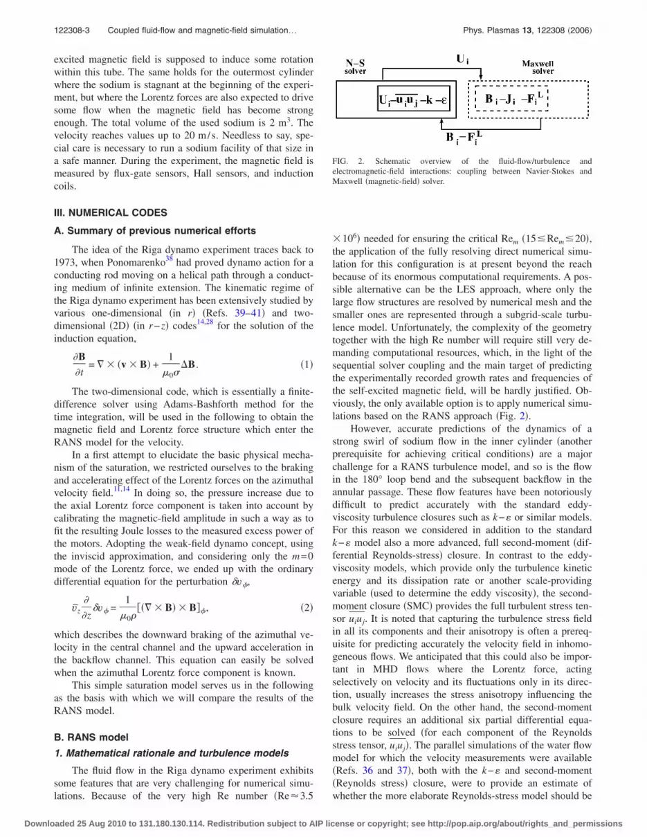
�106� needed for ensuring the critical Rem �15Rem20�,the application of the fully resolving direct numerical simu-lation for this configuration is at present beyond the reachbecause of its enormous computational requirements. A pos-sible alternative can be the LES approach, where only thelarge flow structures are resolved by numerical mesh and thesmaller ones are represented through a subgrid-scale turbu-lence model. Unfortunately, the complexity of the geometrytogether with the high Re number will require still very de-manding computational resources, which, in the light of thesequential solver coupling and the main target of predictingthe experimentally recorded growth rates and frequencies ofthe self-excited magnetic field, will be hardly justified. Ob-viously, the only available option is to apply numerical simu-lations based on the RANS approach �Fig. 2�.

However, accurate predictions of the dynamics of astrong swirl of sodium flow in the inner cylinder �anotherprerequisite for achieving critical conditions� are a majorchallenge for a RANS turbulence model, and so is the flowin the 180° loop bend and the subsequent backflow in theannular passage. These flow features have been notoriouslydifficult to predict accurately with the standard eddy-viscosity turbulence closures such as k− or similar models.For this reason we considered in addition to the standardk− model also a more advanced, full second-moment �dif-ferential Reynolds-stress� closure. In contrast to the eddy-viscosity models, which provide only the turbulence kineticenergy and its dissipation rate or another scale-providingvariable �used to determine the eddy viscosity�, the second-moment closure �SMC� provides the full turbulent stress ten-sor uiuj. It is noted that capturing the turbulence stress fieldin all its components and their anisotropy is often a prereq-uisite for predicting accurately the velocity field in inhomo-geneous flows. We anticipated that this could also be impor-tant in MHD flows where the Lorentz force, actingselectively on velocity and its fluctuations only in its direc-tion, usually increases the stress anisotropy influencing thebulk velocity field. On the other hand, the second-momentclosure requires an additional six partial differential equa-tions to be solved �for each component of the Reynoldsstress tensor, uiuj�. The parallel simulations of the water flowmodel for which the velocity measurements were available�Refs. 36 and 37�, both with the k− and second-moment�Reynolds stress� closure, were to provide an estimate ofwhether the more elaborate Reynolds-stress model should be

FIG. 2. Schematic overview of the fluid-flow/turbulence andelectromagnetic-field interactions: coupling between Navier-Stokes andMaxwell �magnetic-field� solver.

122308-3 Coupled fluid-flow and magnetic-field simulation… Phys. Plasmas 13, 122308 �2006�


used for the simulation of the real Riga experiment with amagnetic field, or the simpler and more economical k−model could still suffice.

We present now a short outline of both models consid-ered, which were used to close the RANS mean momentumequation. Together with the continuity equation �Uj /�xj =0,the RANS momentum equation describing turbulent flow ofan incompressible fluid subjected to a magnetic field can bewritten as

�3�

The turbulent stress tensor uiuj is provided by a turbulencemodel. The SMC requires the solution of the model equa-tions for the turbulent stress tensor uiuj and the dissipationrate of the turbulent kinetic energy k �see the Appendix�. Itis noted that when the second-moment turbulence closure isapplied, the production terms �Pij� are treated exactly. Theadditional source/sink terms in the uiuj and equations, Sij

M

and SM, respectively, representing effects of the fluctuating

Lorentz force on turbulence, must be included, according toKenjereš and Hanjalić42,45 �see, also, Hanjalić andKenjereš43,44,47�. The redistributive terms ��ij�, the slow��ij

S � and rapid contributions��ijR� are modeled using the

model of Speziale et al.48 �RSM_SSG�, extended to accountfor the magnetic effect by an additional rapid term ��ij

M�proposed by Kenjereš et al.46

In this study, we adopted a new extended variant ofthe previously proposed MHD Reynolds stress model ofKenjereš et al.,46 where the MHD terms have been added tothe linear version of the pressure-strain correlation togetherwith the wall-reflection terms according to Gibson andLaunder.49 The choice of the Speziale et al.48 model is pri-marily motivated by its ability to reasonably reproduce thenear-wall stress anisotropy without introducing any specialwall-reflection term. This is compensated by the nonlinearrepresentation of the rapid redistributive term.

For industrial MHD problems, Kenjereš and Hanjalićproposed an extension of the standard two-equation k−model to account for the effects of magnetic field. With thismodel the turbulent stress is computed from the conventionaleddy-viscosity stress-strain relationship where the turbulentviscosity �t=c�k2 / is obtained from the solution of equa-tions for the turbulence kinetic energy k and its dissipationrate . We note that the k− model is in principle recoveredby contracting the uiuj equation and the stress tensor in the equation of the above second-moment closure, withk=0.5uiui. However, some small differences exist. So, in the equation the turbulent diffusion is now expressed via thesimple-gradient diffusion instead of the general-gradient hy-pothesis. The Lorentz force effects are incorporated throughadditional source/sink terms as proposed in Kenjereš andHanjalić.42,45,47 The coefficients for this k- MHD model aregiven in Table II of the Appendix.

2. Numerics for the RANS approach

The transport equations discussed above can be writtenin a general form as

��

�t+ Uj

��

�xj=

�

�xj��

��

�xj� + S�, �4�

where � is dependent variable ��=Ui or uiuj or , etc.� and�� is characteristic transport coefficient of the dependentvariable and S� represents all source/sink terms. In the finite-volume approach that is applied in this study, all terms arepreintegrated over a computational cell �elementary controlvolume� as

�V

��

�tdV + �

S�Uj� − ��

��

�xj�njdS = �

V

S�dV , �5�

where the volume integration of convective and diffusiveterms is replaced by a surface integration over the controlvolume faces by employing the Gauss-Ostrogradski diver-gence theorem, i.e., Vdiv� dV=S� ·n dS, where n is theunit normal vector of the cell-face surface. The solver canhandle three-dimensional structured multidomain, multi-block, nonorthogonal geometries. The local grid refinementis possible for predefined blocks �i.e., specific block refine-ment�. The solver can be run in serial �single processor� orparallel mode utilizing the domain decomposition messagepassing interface �MPI� directives �in our case, domain de-composition is defined in the form of decomposition overmultiblocks which can be part of different domains, i.e.,parts belonging to fluid flow, wall domains, or external elec-tromagnetic layers�. The collocated variable arrangement andCartesian vector and tensor components are applied for allvariables. This collocated variable arrangement requires onlya single set of geometrical information to be stored in con-trast with the staggered variable arrangement. In order toprevent decoupling of the velocity and pressure fields theRhie-Chow interpolation is used. The SIMPLE algorithm isused for linking iteratively corrected velocity and pressurefields. The diffusive term �the third term in Eq. �4�� of equa-tions set is discretized by the second-order accurate centraldifference scheme �CDS�. The monotonicity preserving totalvariation diminishing �TVD� scheme is used for the convec-tive term �the second term in Eq. �4�� with the UMISTlimiter.50 Integration of the time-dependent term �the firstterm in Eq. �4�� is performed by the fully implicit three con-secutive time-steps method with second-order accuracy al-lowing significantly larger time steps to be used when com-pared to explicit time integration methods.

3. Simulations of the 1:2 scale-down experimentalsetup with water

In order to test the performance of the two turbulencemodels, we performed first the fluid-flow and turbulencesimulations for the 1:2 scale-down setup with water as theworking fluid for which a detailed experimental databaseexist.36,37 The flow is characterized with very high Re�1.25�106 �based on the mean axial velocity and diameterof the inner cylinder�. The results of numerical simulationsare compared with the laser-Doppler anemometer �LDA�



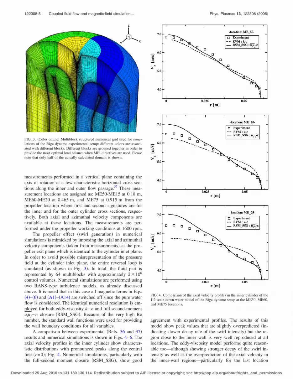
measurements performed in a vertical plane containing theaxis of rotation at a few characteristic horizontal cross sec-tions along the inner and outer flow passage.37 These mea-surement locations are assigned as: ME50-ME15 at 0.18 m,ME60-ME20 at 0.465 m, and ME75 at 0.915 m from thepropeller location where first and second signatures are forthe inner and for the outer cylinder cross sections, respec-tively. Both axial and azimuthal velocity components areavailable at these locations. The measurements are per-formed under the propeller working conditions at 1600 rpm.

The propeller effect �swirl generation� in numericalsimulations is mimicked by imposing the axial and azimuthalvelocity components �taken from measurements� at the pro-peller exit plane which is identical to the cylinder inlet plane.In order to avoid possible misrepresentation of the pressurefield at the cylinder inlet plane, the entire reversal loop issimulated �as shown in Fig. 3�. In total, the fluid part isrepresented by 64 multiblocks with approximately 2�106

control volumes. Numerical simulations are performed usingtwo RANS-type turbulence models, as already discussedabove. It is noted that in this case all magnetic terms in Eqs.�4�–�6� and �A1�–�A14� are switched off since the pure waterflow is considered. The identical numerical resolution is em-ployed for both eddy-viscosity k− and full second-momentuiuj − closure �RSM_SSG�. Because of the very high Renumber, the standard wall functions were used for providingthe wall boundary conditions for all variables.

A comparison between experimental �Refs. 36 and 37�results and numerical simulations is shown in Figs. 4–6. Theaxial velocity profiles in the inner cylinder show character-istic distributions with pronounced peaks along the centralline �r=0�; Fig. 4. Numerical simulations, particularly withthe full-second moment closure �RSM_SSG�, show good

agreement with experimental profiles. The results of thismodel show peak values that are slightly overpredicted �in-dicating slower decay rate of the swirl intensity� but the re-gion close to the inner wall is very well reproduced at alllocations. The eddy-viscosity model performs quite reason-able too—although showing stronger decay of the swirl in-tensity as well as the overprediction of the axial velocity inthe inner-wall regions—particularly for the last location

FIG. 3. �Color online� Multiblock structured numerical grid used for simu-lations of the Riga dynamo experimental setup: different colors are associ-ated with different blocks. Different blocks are grouped together in order toprovide the most optimal load balance when MPI directives are used. Pleasenote that only half of the actually calculated domain is shown.

FIG. 4. Comparison of the axial velocity profiles in the inner cylinder of the1:2 scale-down water model of the Riga dynamo setup at the ME50, ME60,and ME75 locations.



�ME75�. For locations in the outer passage, both modelsshow good agreement with experiments �Fig. 5�. The azi-muthal velocity distributions in the inner cylinder have thecharacteristic shape with zero values along the central line�r=0� and peak values in the wall proximity �Fig. 6�. It canbe seen that both models produced good agreement with ex-periments. The peak values are, in contrast to the axial ve-locity, very well predicted at all locations. The only differ-ence is in the locations of the peaks, which are againpredicted by the second-moment closure in better agreementwith experiments. A small underprediction in comparisonwith experiments is observed in the near-wall region wherethe eddy-viscosity model surprisingly shows slightly betteragreements for the last two locations �ME60 and ME75�.

It is important to mention that the azimuthal velocitycomponent proved to be very sensitive to the applied numeri-cal resolution and used numerical schemes. Application ofthe lower-level accuracy schemes �like upwind deferredschemes� produced significantly reduced values of the peakazimuthal velocity �approximately 50%�. These discrepan-cies are eliminated by using the TVD differencing schemewith the UMIST limiter for all variables.50

It can be concluded that for the 1:2 scale-down watermodel good agreements are obtained between numericalsimulations and measurements of the velocity field in thebulk of the inner and outer passage. The second-momentclosure predictions were shown to be generally superiorwhen compared with the simpler k- model, and presumably,the superiority will be even more visible in the bend area andwhen comparing variables. But we note that the eddy-

FIG. 5. Comparison of the axial velocity profiles in the outside passage ofthe 1:2 scale-down water model of the Riga dynamo setup at the ME15 andME20 locations.

FIG. 6. Comparison of the azimuthal velocity profiles in the inside cylinderof the 1:2 scale-down water model of the Riga dynamo setup at the ME50,ME60, and ME75 locations.



viscosity results are not much inferior especially when con-sidered in light of satisfactory predictions of the azimuthalvelocity component �Fig. 6�, which has the most profoundeffect on the self-excitation phenomenon. The success of thek- model can be explained by its tendency to produce asolid-body-rotation type of azimuthal velocity in swirlingflow irrespective of the swirl origin, which has been regardedas an illustration of its inaptitude for swirling flows in gen-eral. However, in the present situation the imposed swirl ismade on purpose to be close to solid-body rotation, thussuited for eddy-viscosity models. Then the problem remains,of course, if the back reaction of the magnetic field couldalter significantly the solid-body-like profile to another pro-file for which the k- model might not be appropriate. Thisscenario is rather unlikely since quite a number of experi-mental data �growth rates, frequencies, axial field depen-dence� support the general picture that the basic saturationeffect comes from the downward braking of the azimuthalvelocity component rather than from a radial redistributionof the flow. If the main saturation effect were due to a sig-nificant change of the radial profile of the azimuthal compo-nent, this would not result in the observed change of theaxial dependence of the magnetic field as it was documentedin Refs. 7 and 11–13. Moreover, since the main task of thesenumerical simulations is to provide the velocity perturbationin the saturated regime for the magnetic-field solver, the im-provements achieved with the second-moment closure do notseem to be of crucial importance. Recalling also that theinclusion of the electromagnetic effects in second-momentclosures requires substantial modeling and computational ef-fort, it was decided that the simple two-equation k− eddy-viscosity model can serve the purposes of mimicking thesaturation regime by using two separate numerical codes.

4. Simulations of the full-scale experimental setupwith sodium

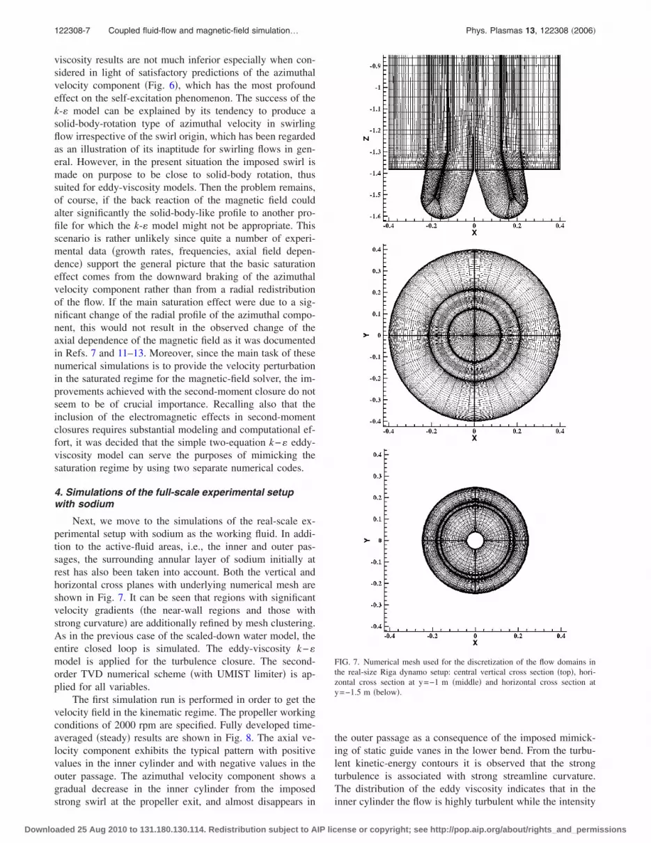
Next, we move to the simulations of the real-scale ex-perimental setup with sodium as the working fluid. In addi-tion to the active-fluid areas, i.e., the inner and outer pas-sages, the surrounding annular layer of sodium initially atrest has also been taken into account. Both the vertical andhorizontal cross planes with underlying numerical mesh areshown in Fig. 7. It can be seen that regions with significantvelocity gradients �the near-wall regions and those withstrong curvature� are additionally refined by mesh clustering.As in the previous case of the scaled-down water model, theentire closed loop is simulated. The eddy-viscosity k−model is applied for the turbulence closure. The second-order TVD numerical scheme �with UMIST limiter� is ap-plied for all variables.

The first simulation run is performed in order to get thevelocity field in the kinematic regime. The propeller workingconditions of 2000 rpm are specified. Fully developed time-averaged �steady� results are shown in Fig. 8. The axial ve-locity component exhibits the typical pattern with positivevalues in the inner cylinder and with negative values in theouter passage. The azimuthal velocity component shows agradual decrease in the inner cylinder from the imposedstrong swirl at the propeller exit, and almost disappears in

the outer passage as a consequence of the imposed mimick-ing of static guide vanes in the lower bend. From the turbu-lent kinetic-energy contours it is observed that the strongturbulence is associated with strong streamline curvature.The distribution of the eddy viscosity indicates that in theinner cylinder the flow is highly turbulent while the intensity

FIG. 7. Numerical mesh used for the discretization of the flow domains inthe real-size Riga dynamo setup: central vertical cross section �top�, hori-zontal cross section at y=−1 m �middle� and horizontal cross section aty=−1.5 m �below�.



of turbulence is gradually decreasing in the outer passage.Despite the high Reynolds number simulated �Re�3.5�106� and the very complex geometry, simulations provedto be numerically very stable and high convergence criteria� ��10−6� is achieved without difficulties for all variables.For this particular simulation, we used multiblock decompo-sition with 32 CPUs and almost ideal load balancing betweenprocessors is achieved at the SGI Origin 3800 system with1024 CPUs.

IV. THE COUPLING OF THE CODES

A. Exchange of calculated fields between solvers

Now, after completing the first set of the RANS-basedfluid-flow and turbulence simulations, the coupling of thefluid-flow and magnetic-field solvers will be discussed. Themagnetic-field code is used to get values of the electromag-netic parameters, including the magnetic field and Lorentzforce components. Here it is important to note that exchangeof the information between solvers is not a trivial task. Thedifference in definitions of local coordinate systems �the rect-angular 2D polar cylindrical for the magnetic-field solverand the 3D nonorthogonal with Cartesian components� re-quires that additional effort must be put into this two-wayindirect coupling of the solvers. In addition, the collocatedlocations of variables requested by the fluid-flow solver donot coincide with the discretized locations for variables usedby the magnetic-field solver. The principles of the interpola-tion are demonstrated in Fig. 9, where the value of the arbi-trary variable �f� located in the center of the 3D nonorthogo-nal control volume are estimated as

f =z2 − z

z2 − z1� r2 − r

r2 − r1f11 +

r − r1

r2 − r1f21�

+z − z1

z2 − z1� r2 − r

r2 − r1f12 +

r − r1

r2 − r1f22� . �6�

This approach is applied for all electromagnetic variables,i.e., Bi, Fi

L. Since a very fine numerical mesh was used forboth numerical solvers �225�44 rectangular nodes for themagnetic-field solver and the previously defined numericalmesh for the fluid-flow solver, Fig. 7�, it was possible toobtain smooth interpolated fields without significant loses in

FIG. 8. �Color online� Axial and azimuthal velocity components �in �m/s��above, turbulent kinetic energy �in �m2/s2�� and eddy viscosity �in �m2/s��below contour distributions in the central vertical plane of the real-size Rigadynamo setup: Re=3.5�106 �propeller working conditions of 2000 rpm� allbefore a magnetic field is generated.

FIG. 9. Schematic of the interpolation between the 2D rectangular polar-cylindrical magnetic-field solver �domain defined by dashed lines and acontrol volume defined by the dashed area� and the 3D nonorthogonal fluid-flow solver �defined by solid lines�.



the divergency free magnetic-field condition. In order todemonstrate the accuracy of the presented interpolationmethod, contours of the axial and radial magnetic field, aswell as the axial and azimuthal Lorentz force components inthe central vertical plane, are shown in Fig. 10. It can be seenthat all variables exhibit smooth distributions without anydiscontinuities confirming accuracy and reliability of the in-terpolation method. Such exported electromagnetic fields arenow ready to be used by the fluid-flow solver. It is importantto note that in this second step of solvers coupling theLorentz force components are active in the momentum equa-tions �Eq. �3�� as well as all additional electromagnetic con-tributions in the turbulence parameters, i.e., SM and S

M �Eq.

�A16��. It should be stressed, however, that in the presentrealization of the coupling only the azimuthal average �them=0 mode� over the Lorentz force has been taken into ac-count while the m=2 mode has been neglected. This m=2mode, which results from the quadratic appearance of themagnetic-field m=1 mode in the Lorentz force, would beneeded to explain nonaxisymmetric velocity perturbations.This is also left for future simulations.

B. An improved saturation model

In this section we show how the coupling of both codescan be employed for a refinement of the former saturationmodel that was based on a simple one-dimensional back-reaction model.11,14 Let us start by saying what a saturationmodel is. A dynamo is in a saturated state when the Lorentzforces, according to the self-excited magnetic field, modifythe flow in such a way that the resulting growth rate of themagnetic field is just zero. Translated to the concrete Rigadynamo experiment, this means the following: for a certainsupercritical rotation rate of the propeller, we measure theJoule excess power and infer from that the magnetic-fieldamplitude which cannot be obtained from purely kinematicsimulation. This magnetic eigenfield is then plugged into theRANS solver for the velocity field, and the resulting flowmodification is evaluated if it really leads to a zero growthrate. In addition, the eigenfield structure resulting from themodified velocity field can also be compared with the mea-sured one.

Actually, this simple back-and-forth method representsonly the first step of a perturbation method. The next stepwould be to compute again the magnetic field and Lorentzforces from the modified velocity, and so on.

Even such a simple-seeming back-reaction model is notwithout intricacies, in particular concerning a reliable deter-mination of the Joule excess power. These problems werediscussed in Ref. 14, where we have finally obtained a linearmodel of the form PJoule= ��−1840 rpm� / �1840 rpm��48.4 kW, which fits reasonably to the available excesspower data. It is worthwhile to note the very flat increase ofthe excess power with the rotation rate, particularly whencompared with the steep power �i.e., pressure� increase in theKarlsruhe experiment �Ref. 15, inset of Fig. 4�. The reasonfor this behavior is the freedom of the azimuthal velocitycomponent to be braked by the Lorentz force. Now, havingcalibrated the magnetic field at a given propeller rotationrate, we use the RANS model to compute the flow modifi-cation due to the Lorentz force corresponding to this field.

In order to demonstrate the back-reaction effects of theimposed Lorentz force on the fluid flow, characteristic veloc-ity profiles are shown in Figs. 11–13. For all figures, theJoule dissipation was chosen as 10 kW. The profiles of theaxial velocity components along the inner cylinder undergosignificant changes when the effects of the imposed Lorentzforce are taken into account. Note that the locations at whichthe profiles are extracted are defined with respect to the dis-tance from the vertical center of the experimental setup sothat all locations above the center have a positive sign�+950, +786, +321 mm� and those below this plane have a

FIG. 10. �Color online� Snapshots of the axial �left� and radial �right� mag-netic field �above� �both in �T�� and axisymmetric part of the axial �left� andazimuthal �right� Lorentz force components �below� �both in �N/m3��. Con-tour distributions in the central vertical plane of the real-size Riga dynamosetup at Re=3.5�106 �propeller working conditions of 2000 rpm�.



negative sign �−143,−607,−1071 mm�. In addition to astronger suppression in the central region close to the axis�indicating a faster rate of decay of the swirling intensity�,the Lorentz force produces the characteristic “M”-shapedprofiles with distinct peaks in the wall proximity for the lasttwo positions �−607,−1071 mm�; Fig. 11. The azimuthal ve-locity profiles along the inner cylinder are more monotonicwith characteristic peak values at the wall side �Fig. 12�.Again, due to the active Lorentz force, the maximum valuesare significantly reduced.

The profiles of the axial velocity in the outer passagewith and without the Lorentz force are significantly different�Fig. 13�. These changes are caused both by different ap-proaching profiles, which are particularly sensitive to thestrong 180° bend curvature, and the direct Lorentz force ef-fects in the outer passage.

In the following step we have taken the computed veloc-ity differences resulting from either the one-dimensional orthe RANS model. Actually, this has been done for four dif-ferent propeller rotation rates: 2000, 2200, 2400, and2600 rpm. The amplitudes of the velocity changes were fixedin such a way that they corresponded to a Joule dissipation of4.3 kW for 2000 rpm, of 9.5 kW for 2200 rpm, of 14.7 kW

for 2400 rpm, and of 20 kW for 2600 rpm. The velocity per-turbations for a Joule dissipation of 9.5 kW are shown in Fig.14 for the central cylinder, and in Fig. 15 for the backflowannular passage. In the inner channel, it is remarkable thatthe profiles of v� in the one-dimensional and in the RANSmodels are very close to each other. In the outer channel thisdifference is a bit larger, but not dramatic. The RANS modelmakes also checkable predictions on the deformation of theaxial velocity, which was not possible by the simple one-dimensional model that did not include any change of vz.

For each of the propeller rotation rates, 2000, 2200,2400, and 2600 rpm, we have computed the growth rates andthe frequencies �see Fig. 16� with the two back-reactionmodels �1D and RANS�. What can we learn from Fig. 16?When looking at the growth rate curve we see that the maineffect �i.e., going down from the kinematic curve to the satu-rated curve� is already included in the one-dimensionalmodel. The RANS model brings the curve even closer to thezero line, improving therefore the saturation model. In con-trast to the growth rate, the frequency does not decrease. Iteven increases slightly in comparison to what would be ex-pected from extrapolating the kinematic regime. Althoughnot documented here, the saturation model is also in good

FIG. 11. Profiles of the axial velocity component along the inner cylinderwithout �above� and with �below� Lorentz force effects: propeller workingconditions of 2000 rpm and Joule dissipation of 10 kW.

FIG. 12. Profiles of the azimuthal velocity component along the inner cyl-inder without �above� and with �below� Lorentz force effects �identicalworking conditions as in previous figure�.



agreement with the observed shift of the magnetic-fieldstructure towards the propeller region.11 This change in thefield structure mirrors the deteriorated excitation ability inthe lower part of the dynamo due to the braked azimuthalvelocity. The effect of the RANS model on the frequency isnot significantly different from that of the one-dimensionalmodel.

V. CONCLUSIONS AND OUTLOOK

We studied numerically the mechanism of the magnetic-field generation in the Riga dynamo experiment, aimed atgaining further insight into the velocity and magnetic fieldand their interaction in the saturation regime. This regime,characterized by the zero growth rate of the generated mag-netic field, was simulated by using a coupled RANS solverfor the fluid flow �Navier-Stokes� and a finite-differencesolver for the magnetic field.

First, we have obtained the velocity and turbulence fieldsin the kinematic regime, i.e., without magnetic field. Thefields and Lorentz forces resulting from the magnetic-fieldsolver were exported to the fluid solver where all additionalmodel terms associated with electromagnetic effects are ac-tivated. Then, the velocity perturbations obtained under theinfluence of the Lorentz force were exported back into the

magnetic-field solver in order to capture the differences be-tween the kinematic and the saturated regimes. The exchangeof fields between solvers was done by multidimensionalinterpolation/extrapolation technique, which provided accu-

FIG. 13. Profiles of the axial velocity component in the outer annular pas-sage without �above� and with �below� Lorentz force effects.

FIG. 14. Differences of velocity profiles with and without Lorentz forces:inner cylinder.



rate projections with smooth fields. These computations wereperformed for different propeller rotation rates, and thegrowth rates and frequencies of the self-excited magnetic-field components are compared with the experimental re-

sults. The predicted growth rates with the RANS model showan improvement over the simple one-dimensional saturationmodels. In contrast, the predicted frequencies are just mar-ginally different from these predicted by the one-dimensionalmodel.

Despite significant simplification and approximation, es-pecially in treating the magnetic field and sequential interuseof two solvers, the simulations have reproduced the majorparameters—the growth rate and frequencies of the Riga ex-periment in close accord with measurements. Useful newinformation about the fluid flow and magnetic fields and theirinteraction have also been obtained. A main novelty of theRANS model compared with the former one-dimensionalmodel is that a radial restructuring of the axial velocity pro-file has been predicted. It would certainly be interesting todetect this effect by flow measurements. Of course, morecomprehensive information, especially about the self-excitation dynamics, could be expected only from the simul-taneous time solutions for both fields accounting for directtwo-way coupling, which is currently in progress.

FIG. 15. Differences of velocity profiles with and without Lorentz forces:outer cylinder.

FIG. 16. Growth rates �a� and frequencies �b� in the kinematic and thesaturated regime of the Riga dynamo experiment. For the saturation regime,the simple 1D model of braking and the RANS has been used. The numeri-cal results for the saturated regime are obtained under the rough assumptionthat 4.3, 9.5, 14.7, and 20 kW Ohmic losses occur at rotation rates of 2000,2200, 2400, and 2600 rpm, respectively. �, p, and f at the temperature Twere scaled to ��c , pc , fc�=��T� /��157 °C��T� , p�T� , f�T�� as requiredby the scaling properties of the induction equation.



ACKNOWLEDGMENTS

Access to the supercomputing facilities at the SARAComputing and Networking Services in Amsterdam has beenprovided by the National Computing Facilities Foundation�NCF� and sponsored by the Nederlandse Organisatie voorWetenschappelijk Onderzoek �NWO�. We thank MichaelChristen �TU Dresden� for providing velocity data from thewater test facility. The results presented in this paperemerged from the research project “MAGDYN: MagneticField Dynamos—Laboratory Studies based on the Riga Dy-namo Facility” sponsored by the European Commission un-der Contract No. HPRI-CT-2001-50027. The research ofS.K. has been made possible through a fellowship of theRoyal Netherlands Academy of Arts and Sciences �KNAW�.This work was supported by Deutsche Forschungsgemein-schaft in the framework of SFB 609 and Grant No. GE 682/14-1.

APPENDIX

1. Second-moment „Reynolds-stress… model for MHD

This model includes the solving of all turbulent-stresscomponents �uiuj� together with an equation for the dissipa-tion rate of the turbulent kinetic energy ��,

�uiuj

�t+ Ul

�uiuj

�xl=

�

�xl��lm + Cs

k

ulum� �uiuj

�xm� + Pij

+ �ijS + �ij

R + �ijM − ij + Sij

M , �A1�

�

�t+ Ul

�

�xl=

�

�xl��lm + C

k

ulum� �

�xm� + C1

kP

− C22

k+ S

M , �A2�

where

Pij = − uiul�Uj

�xl− ujul

�Ui

�xl, P = − uiuj

�Ui

�xj�A3�

are the production of turbulent stresses and of turbulent ki-netic energy, respectively, and �lm is the Kronecker delta.The additional “MHD” terms are included in their exactform,

SijM = Sij

M1 + SijM2, �A4�

where

SijM1 = −

�

�� ilmBmuj

��

�xl+ jlmBmui

��

�xl� , �A5�

SijM2 =

�

��BiBlujul + BjBluiul − 2Bl

2uiuj� . �A6�

The correlation between fluctuating velocity components andgradients of the electric potential is modeled as

ui��

�xj= C� jlmBmuiul, �A7�

where jlm is the permutation tensor. Finally, slow, rapid, andelectromagnetic parts of the pressure-strain correlation aremodeled as

�ijS = − �C1 + C1

*Pbij� , �A8�

�ijR = C2�bij

2 −1

3bll

2�ij� + Sijk�C3 − C3*�bijbji�1/2�

+ C4k�Silblj + Sljbil −2

3Slmbml�ij�

+ C5k��ilblj − �ljbil� , �A9�

�ijM = − C3

M�SijM −

2

3SM�ij� , �A10�

where

SM =1

2Sii

M, bij =uiuj

2k−

1

3�ij ,

�A11�

Sij =1

2� �Ui

�xj+

�Uj

�xi�, �ij =

1

2� �Ui

�xj−

�Uj

�xi�

are the magnetic turbulent kinetic-energy production, the an-isotropy, the mean rate of strain, and the mean vorticity ten-sors, respectively. This final version of the model is essen-tially a combination of the Speziale et al.48 second-momentclosure with MHD extensions proposed by Kenjereš et al.46

Finally, all model coefficients are given in Table I.

2. The k−� model with MHD effects

The simplified version of the above model can be ob-tained by contracting indices, i.e., k=0.5uiui and by introduc-ing the turbulent viscosity ��t� as

TABLE II. Specification of coefficients in k and equations in the presenceof the imposed electromagnetic fields for simplified eddy-viscosity modelwith MHD terms.

�k � c� C1 C2 C1M

1. 1.3 0.09 1.44 1.92 0.025

TABLE I. Specification of coefficients in uiuj and equations in the presence of the imposed electromagneticfields for Speziale et al. �Ref. 48� and Kenjereš et al. �Ref. 45� second-moment closure with MHD terms.

C1 C1* C2 C3 C3

* C3M C4 C5 CS C C1 C2 C�

3.4 1.8 4.2 0.8 1.3 0.6 1.25 0.4 0.22 0.18 1.44 1.83 0.6



uiuj =2

3k�ij − �t� �Ui

�xj+

�Uj

�xi�, �t = c�k2/ , �A12�

�k

�t+ Uj

�k

�xj=

�

�xj�� +

�t

�k� �k

�xj� + P − + SM , �A13�

�

�t+ Uj

�

�xj=

�

�xj�� +

�t

��

�xj� + C1

kP − C2

2

k

+ SM , �A14�

where the production of turbulent kinetic energy is modeledas

P = �t S 2, S = �2SijSij , �A15�

and additional MHD terms are included as

SM = −�

�B0

2k exp�− C1M �

�B0

2 k

�, S

M = SM

k. �A16�

This final version of the model is a combination of the stan-dard two-equation k− eddy-viscosity model with MHD ex-tensions proposed in Kenjereš and Hanjalić.42 The coeffi-cients for this k- MHD model are given in Table II.

1H. K. Moffatt, Field Generation in Electrically Conducting Fluids �Cam-bridge University Press, Cambridge, London, New York, Melbourne,1978�.

2F. Krause and K.-H. Rädler, Mean-field Magnetohydrodynamics and Dy-namo Theory �Pergamon, Oxford, 1980�.

3G. Rüdiger and R. Hollerbach, The Magnetic Universe: Geophysical andAstrophysical Dynamo Theory �Wiley, Weinheim, 2004�.

4I. Wilkinson, Geophys. Surv. 7, 107 �1984�.5A. Gailitis, O. Lielausis, S. Dement’ev, E. Platacis, A. Cifersons, G. Ger-beth, Th. Gundrum, F. Stefani, M. Christen, H. Hänel, and G. Will, Phys.Rev. Lett. 84, 4365 �2000�.

6R. Stieglitz and U. Müller, Phys. Fluids 13, 561 �2001�.7A. Gailitis, O. Lielausis, E. Platacis, S. Dement’ev, A. Cifersons, G.Gerbeth, Th. Gundrum, F. Stefani, M. Christen, and G. Will, Phys. Rev.Lett. 86, 3024 �2001�.

8A. Gailitis, O. Lielausis, E. Platacis, G. Gerbeth, and F. Stefani, Magne-tohydrodynamics 37, 71 �2001�.

9A. Gailitis, O. Lielausis, E. Platacis, G. Gerbeth, and F. Stefani, Dynamoand Dynamics, a Mathemetical Challenge, edited by D. Armbruster and I.Oprea �Kluwer, Dordrecht, 2001�, pp. 9–16.

10A. Gailitis, O. Lielausis, E. Platacis, S. Dement’ev, A. Cifersons, G.Gerbeth, Th. Gundrum, F. Stefani, M. Christen, and G. Will, Magnetohy-drodynamics 38, 5 �2002�.

11A. Gailitis, O. Lielausis, E. Platacis, G. Gerbeth, and F. Stefani, Magne-tohydrodynamics 38, 15 �2002�.

12A. Gailitis, O. Lielausis, E. Platacis, G. Gerbeth, and F. Stefani, Rev. Mod.Phys. 74, 973 �2002�.

13A. Gailitis, O. Lielausis, E. Platacis, G. Gerbeth, and F. Stefani, Surv.Geophys. 74, 973 �2002�.

14A. Gailitis, O. Lielausis, E. Platacis, G. Gerbeth, and F. Stefani, Phys.Plasmas 11, 2838 �2004�.

15R. Stieglitz and U. Müller, Magnetohydrodynamics 38, 27 �2002�.16U. Müller and R. Stieglitz, Nonlinear Processes Geophys. 9, 165 �2002�.17U. Müller, R. Stieglitz, and S. Horanyi, J. Fluid Mech. 498, 31 �2004�.18U. Müller, R. Stieglitz, and S. Horanyi, J. Fluid Mech. 552, 419 �2006�.19N. L. Peffley, A. B. Cawthorne, and D. P. Lathrop, Phys. Rev. E 61, 5287

�2000�.20F. Pétrélis, M. Bourgoin, L. Marié, J. Burguete, A. Chiffaudel, F. Daviaud,

S. Fauve, P. Odier, and J. F. Pinton, Phys. Rev. Lett. 90, 174501 �2003�.21E. J. Spence, M. D. Nornberg, C. M. Jacobson, R. D. Kendrick, and C. B.

Forest, Phys. Rev. Lett. 96, 055002 �2006�.22P. Frick, V. Noskov, S. Denisov, S. Khripchenko, D. Sokoloff, R.

Stepanov, and A. Sukhanowsky, Magnetohydrodynamics 38, 143 �2002�.23H.-C. Nataf, T. Alboussiére, D. Brito, P. Cardin, N. Gagniére, D. Jault,

J.-P. Masson, and D. Schmitt, Geophys. Astrophys. Fluid Dyn. �unpub-lished�; http://arxiv.org/abs/physics/0512217.

24G. A. Glatzmaier, Annu. Rev. Earth Planet. Sci. 30, 237 �2002�.25B. A. Buffett, Geophys. J. Int. 153, 753 �2003�.26M. Matsushima, Phys. Earth Planet. Inter. 153, 74 �2005�.27F. Hamba, Phys. Plasmas 11, 5316 �2004�.28F. Stefani, G. Gerbeth, and A. Gailitis, in Transfer Phenomena in Magne-

tohydrodynamic and Electroconducting Flows, edited by A. Alemany, Ph.Marty, and J. P. Thibault �Kluwer, Dordrecht, 1999�, pp. 31–44.

29Y. Ponty, H. Politano, and J.-F. Pinton, Phys. Rev. Lett. 92, 144503�2004�.

30J.-L. Guermond, J. Léorat, and C. Nore, Eur. J. Mech. B/Fluids 22, 555�2003�.

31F. Stefani, G. Gerbeth, and K.-H. Rädler, Astron. Nachr. 321, 65 �2000�.32M. Xu, F. Stefani, and G. Gerbeth, J. Comput. Phys. 196, 102 �2004�.33M. Xu, F. Stefani, and G. Gerbeth, Phys. Rev. E 70, 056305 �2004�.34A. B. Iskakov, S. Descombes, and E. Dormy, J. Comput. Phys. 197, 540

�2004�.35A. Brandenburg, A. Nordlund, R. F. Stein, and U. Torkelsson, Astrophys.

J. 446, 741 �1995�.36M. Christen, H. Hänel, and G. Will, in Beiträge zu Fluidenergiemaschinen

4, edited by W. H. Faragallah and G. Grabow �Faragallah-Verlag undBildarchiv, Sulzbach/Ts., 1998�, pp. 111–119.

37M. Christen �private communication�.38Yu. B. Ponomarenko, J. Appl. Mech. Tech. Phys. 14, 775 �1973�.39A. Gailitis and Ya. Freibergs, Magnetohydrodynamics �N.Y.� 12, 127

�1976�.40A. Gailitis and Ya. Freibergs, Magnetohydrodynamics �N.Y.� 16, 116

�1980�.41A. Gailitis, Magnetohydrodynamics �N.Y.� 32, 58 �1996�.42S. Kenjereš and K. Hanjalić, Int. J. Heat Fluid Flow 21, 329 �2000�.43K. Hanjalić and S. Kenjereš, J. Turbul. 1, 1 �2000�.44K. Hanjalić and S. Kenjereš, Flow, Turbul. Combust. 66, 427

�2001�.45S. Kenjereš and K. Hanjalić, Int. J. Heat Fluid Flow 25, 559 �2004�.46S. Kenjereš, K. Hanjalić, and D. Bal, Phys. Fluids 16, 1229 �2004�.47K. Hanjalić and S. Kenjereš, Trans. ASME, J. Appl. Mech. 73, 430

�2006�.48C. G. Speziale, S. Sarkar, and T. B. Gatski, J. Fluid Mech. 227, 245

�1991�.49M. M. Gibson and B. E. Launder, J. Fluid Mech. 86, 491 �1978�.50F. S. Lien and M. A. Leschziner, Int. J. Numer. Methods Fluids 19, 527

�1994�.



Documents

Coupled fluid-flow and magnetic-field simulation of the Riga dynamo experiment