Seediscussions,stats,andauthorprofilesforthispublicationat:https://www.researchgate.net/publication/1898775

SolarActivityForecastwithaDynamoModel

ARTICLEinMONTHLYNOTICESOFTHEROYALASTRONOMICALSOCIETY·JULY2007

ImpactFactor:5.11·DOI:10.1111/j.1365-2966.2007.12267.x·Source:arXiv

CITATIONS

90

READS

21

3AUTHORS,INCLUDING:

J.Jiang

ChineseAcademyofSciences

32PUBLICATIONS460CITATIONS

SEEPROFILE

PiyaliChatterjee

IndianInstituteofAstrophysics

41PUBLICATIONS744CITATIONS

SEEPROFILE

Allin-textreferencesunderlinedinbluearelinkedtopublicationsonResearchGate,

lettingyouaccessandreadthemimmediately.

Availablefrom:PiyaliChatterjee

Retrievedon:05February2016

arX

iv:0

707.

2258

v1 [

astr

o-ph

] 1

6 Ju

l 200

7

Mon. Not. R. Astron. Soc. 000, 000–000 (0000) Printed 1 February 2008 (MN LATEX style file v2.2)

Solar activity forecast with a dynamo model

Jie Jiang1 ⋆, Piyali Chatterjee2 and Arnab Rai Choudhuri1,21National Astronomical Observatories, Chinese Academy of Sciences, Beijing 100012, China.2Department of Physics, Indian Institute of Science, Bangalore- 560012, India.

ABSTRACT

Although systematic measurements of the Sun’s polar magnetic field exist only frommid-1970s, other proxies can be used to infer the polar field at earlier times. Theobservational data indicate a strong correlation between the polar field at a sunspotminimum and the strength of the next cycle, although the strength of the cycle isnot correlated well with the polar field produced at its end. This suggests that theBabcock–Leighton mechanism of poloidal field generation from decaying sunspots in-volves randomness, whereas the other aspects of the dynamo process must be reason-ably ordered and deterministic. Only if the magnetic diffusivity within the convectionzone is assumed to be high (of order 1012 cm2 s−1), we can explain the correlationbetween the polar field at a minimum and the next cycle. We give several independentarguments that the diffusivity must be of this order. In a dynamo model with diffusiv-ity like this, the poloidal field generated at the mid-latitudes is advected toward thepoles by the meridional circulation and simultaneously diffuses towards the tachocline,where the toroidal field for the next cycle is produced. To model actual solar cycleswith a dynamo model having such high diffusivity, we have to feed the observationaldata of the poloidal field at the minimum into the theoretical model. We develop amethod of doing this in a systematic way. Our model predicts that cycle 24 will be avery weak cycle. Hemispheric asymmetry of solar activity is also calculated with ourmodel and compared with observational data.

Key words: Sun: activity, magnetic fields, sunspots

1 INTRODUCTION

During the last few decades, solar physicists have attemptedto predict the strength of every solar cycle a few years beforeits onset. When such attempts were made to predict the lastcycle 23 in the mid-1990s, there did not yet exist sufficientlysophisticated and detailed models of the solar dynamo. Somost of the attempts were primarily based on various pre-cursors which were expected to give an indication of the nextsolar cycle. Solar dynamo theory has progressed enormouslyin the last few years and first attempts are now made topredict the next cycle 24 from dynamo models. Dikpati etal. (2006) and Dikpati & Gilman (2006) have predicted thatthe cycle 24 will be the strongest cycle in 50 years. On theother hand, Choudhuri et al. (2007) have used a differentmodel and different methodology to conclude that the cy-cle 24 will be the weakest in 100 years. Irrespective of whichprediction turns out to be correct, the next cycle 24 shouldbe regarded as a historically important cycle in the evo-lution of solar dynamo theory—as the first cycle for whichdetailed dynamo predictions could be made. In view of these

⋆ E-mail: jiangjie@ourstar.bao.ac.cn

contradictory predictions, it is clear that cycle prediction isa fairly model-dependent affair. Since there are still manyuncertainties in solar dynamo models (Choudhuri 2007a), itmay be worthwhile to analyze the physical basis of the solarcycle prediction carefully, rather than having too much faithon predictions from any particular model.

Amongst the so-called precursor methods, the mostpopular method first proposed by Schatten et al. (1978) is touse the polar magnetic field at the preceding minimum as athe precursor for the next maximum. Since the polar field isweak at the present time, Svalgaard et al. (2005) and Schat-ten (2005) have predicted a weak cycle 24. This prediction isin agreement with the dynamo-based prediction of Choud-huri et al. (2007), but not with the prediction of Dikpatiet al. (2006). One important question before us is whetherthis polar field method is reliable. The next important ques-tion is whether dynamo models provide any support for thismethod.

Since systematic polar field measurements are availableonly from mid-1970s, we so far have only 3 data points indi-cating a strong correlation between the polar field at a min-imum and the next maximum, as we discuss in the §2. Evenif the correlation may appear good, it can be argued that

2 J. Jiang, P. Chatterjee and A. R. Choudhuri

3 data points do not constitute a good statistics. However,we can use various other proxies like polar faculae (Sheeley1991) and positions of filaments (Makarov et al. 2001) to in-fer polar fields from the beginning of the 20th century, andwe argue in §2 that there are good reasons to have faith onthe polar field method for predicting solar cycles.

We now come to the question whether the polar fieldmethod can be justified from dynamo theory. Both the pre-dictions of Dikpati et al. (2006) and Choudhuri et al. (2007;hereafter CCJ) are based on flux transport dynamo mod-els. In these models, the main source of poloidal field is theBabcock–Leighton process in which tilted bipolar regions onthe solar surface give rise to a poloidal field after their decay.This poloidal field is advected by the meridional circulationtowards the pole, to create a strong (i.e. of order 10 G) po-lar field at the time of the solar minimum. The conventionalwisdom is that this polar field is then advected downwardby the meridional circulation to bring it to the tachocline,where it is stretched by the differential rotation to createthe toroidal field, ultimately leading to active regions due tomagnetic buoyancy. The correlation between the polar fieldat the minimum and the strength of the next maximum canbe explained if this polar field can be brought to the mid-latitude tachocline by the time of the next maximum. Sincea maximum comes about 5 years after a minimum, the ad-vection time from the pole to the mid-latitude tachoclinehas to be of order 5 years if this explanation is to work. Al-though we do not have any direct observational data on thenature of the meridional circulation in the lower half of theconvection zone, the time scale of this circulation seems toset the period of the dynamo (Dikpati & Charbonneau 1999;Hathaway et al. 2003) and we cannot vary the amplitude ofthe meridional circulation at the bottom of the convectionzone too much if we wish to reproduce various observed fea-tures of the solar cycle, especially its period. Charbonneau& Dikpati (2000) pointed out that the advection time intheir model was of order 20 years and led to a correlationof the polar field at the end of cycle n with the strengths ofthe cycles n + 2 and n + 3 rather than the cycle n + 1. Thesame is presumably true for the simulations of Dikpati et al.(2006) and Dikpati & Gilman (2006).

In the CCJ model, a sudden change in the polar fieldat the time of a minimum has a prominent effect on thenext maximum coming only after 5 years, as can be seenin Fig. 2 of CCJ. In the caption of Fig. 2, CCJ offered anexplanation by suggesting that the advection time in theirmodel was shorter than that in the models of Dikpati andco-workers. We now feel that this explanation was erroneous.When we find two phenomena A and B correlated, our firstguess usually is that the earlier phenomenon is the causeof the later phenomenon. But an alternative explanation isalso possible. If both A and B are caused by C which tookplace earlier than both A and B, then also it is possiblefor A and B to appear correlated. We now believe that thepolar field at the minimum and the strength of the nextmaximum are correlated not because the polar field was thedirect cause of the next maximum by being advected fromthe pole to the tachocline. Rather, they appear correlatedbecause both of them arise from the poloidal field producedby the Babcock–Leighton process in the mid-latitudes. Letus explain this point with Fig. 1.

During a maximum, the poloidal field is created by the

P

C

T

Figure 1. A sketch indicating how the poloidal field produced atC during a maximum gives rise to the polar field at P during thefollowing minimum and the toroidal field at T during the nextmaximum.

Babcock–Leighton process primarily in the region C indi-cated in Fig. 1. This field is advected by the meridionalcirculation to the polar region P to produce the polar fieldat the minimum. If diffusion is important, then the poloidalfield produced at C also keeps diffusing. The diffusion inour dynamo model is stronger than in the model of Dikpatiand co-workers, as pointed out by Chatterjee et al. (2004)and Chatterjee & Choudhuri (2006). So, in a few years, thepoloidal field diffuses from C to reach the tachocline at T inour model, which will not happen in the model of Dikpati &Gilman (2006) where the poloidal field will be swept awayfrom C to P completely by the meridional circulation beforeit has any chance to reach the tachocline due to the low dif-fusivity of that model. Thus, in our model, the poloidal fieldat C produced during a maximum gives rise to the polarfield at P during the next minimum and also the toroidalfield at T which is the cause of active regions during thesubsequent maximum. The polar field at the minimum andthe strength of the next maximum appear correlated not be-cause one is the cause of the other, but because both of themhave the poloidal field of the previous cycle as their cause. Ifthe poloidal field produced in the previous cycle was strong,then both of these will be strong, and vice versa.

This brings us to the crucial question as to what de-termines the strength of the poloidal field produced by theBabcock–Leighton process. CCJ argued that this processinvolves some randomness and the actual poloidal field pro-duced in the Sun at the end of a cycle will in general bedifferent from the polar field produced in a theoretical meanfield dynamo model. The polar field of the theoretical modelat the solar minimum will be characteristic of a typical ‘av-erage’ cycle. To model actual cycles, CCJ proposed thatthe theoretical model should be ‘corrected’ by feeding in-formation about the observed poloidal field at the minimuminto the theoretical model in some suitable fashion. CCJ haddone this by using the values of DM (Dipole Moment, whichis a good measure of the polar field) at the minima computedby Svalgaard et al. (2005). Since values of DM are availableonly from mid-1970s, this method could be applied to modelonly the last few solar cycles. While this method yielded re-

Solar activity forecast with a dynamo model 3

sults agreeing reasonably well for cycles 21–23, using onlyone number like the DM value to characterize the poloidalfield at a minimum may seem like a drastic simplification.Especially, if the poloidal field produced all over the surfacediffuses through the convection zone to reach the tachocline,then we ought to feed information about poloidal field at alllatitudes into our dynamo model rather than feeding onlythe DM value. One of the aims of this paper is to develop aformalism to do this.

We first discuss in §2 whether the polar fields at minimaseem sufficiently well correlated with the strengths of thenext maxima on the basis of the observational data. Thena brief description of our dynamo model is provided in §3.Then in §4 we present some calculations done by introduc-ing stochastic fluctuations at the minima in dynamo modelswith high and low diffusivities to show that a high-diffusivitymodel provides a better fit with observational data. Severalindependent arguments in favour of a high magnetic diffusiv-ity are put together in §5. Then in §6 we discuss our method-ology of processing the observational data from Wilcox SolarObservatory (WSO) and feeding them into the theoreticaldynamo model. Our results based on calculations with moredetailed data of poloidal field are presented in §7. We closein §8 with concluding remarks.

2 THE IMPLICATIONS OF OBSERVATIONAL

DATA

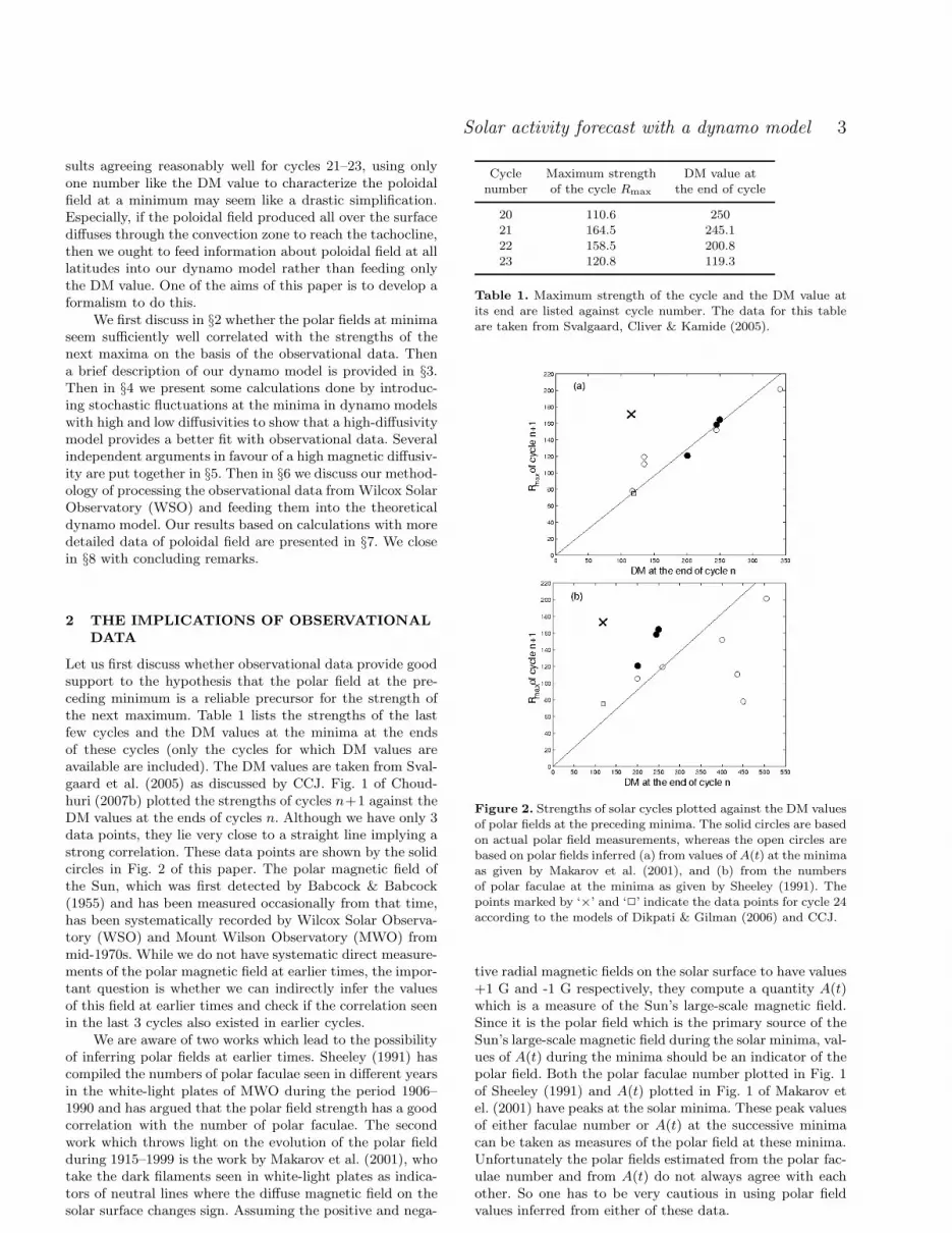
Let us first discuss whether observational data provide goodsupport to the hypothesis that the polar field at the pre-ceding minimum is a reliable precursor for the strength ofthe next maximum. Table 1 lists the strengths of the lastfew cycles and the DM values at the minima at the endsof these cycles (only the cycles for which DM values areavailable are included). The DM values are taken from Sval-gaard et al. (2005) as discussed by CCJ. Fig. 1 of Choud-huri (2007b) plotted the strengths of cycles n+1 against theDM values at the ends of cycles n. Although we have only 3data points, they lie very close to a straight line implying astrong correlation. These data points are shown by the solidcircles in Fig. 2 of this paper. The polar magnetic field ofthe Sun, which was first detected by Babcock & Babcock(1955) and has been measured occasionally from that time,has been systematically recorded by Wilcox Solar Observa-tory (WSO) and Mount Wilson Observatory (MWO) frommid-1970s. While we do not have systematic direct measure-ments of the polar magnetic field at earlier times, the impor-tant question is whether we can indirectly infer the valuesof this field at earlier times and check if the correlation seenin the last 3 cycles also existed in earlier cycles.

We are aware of two works which lead to the possibilityof inferring polar fields at earlier times. Sheeley (1991) hascompiled the numbers of polar faculae seen in different yearsin the white-light plates of MWO during the period 1906–1990 and has argued that the polar field strength has a goodcorrelation with the number of polar faculae. The secondwork which throws light on the evolution of the polar fieldduring 1915–1999 is the work by Makarov et al. (2001), whotake the dark filaments seen in white-light plates as indica-tors of neutral lines where the diffuse magnetic field on thesolar surface changes sign. Assuming the positive and nega-

Cycle Maximum strength DM value atnumber of the cycle Rmax the end of cycle

20 110.6 25021 164.5 245.122 158.5 200.823 120.8 119.3

Table 1. Maximum strength of the cycle and the DM value atits end are listed against cycle number. The data for this tableare taken from Svalgaard, Cliver & Kamide (2005).

Figure 2. Strengths of solar cycles plotted against the DM valuesof polar fields at the preceding minima. The solid circles are basedon actual polar field measurements, whereas the open circles arebased on polar fields inferred (a) from values of A(t) at the minimaas given by Makarov et al. (2001), and (b) from the numbersof polar faculae at the minima as given by Sheeley (1991). Thepoints marked by ‘×’ and ‘2’ indicate the data points for cycle 24according to the models of Dikpati & Gilman (2006) and CCJ.

tive radial magnetic fields on the solar surface to have values+1 G and -1 G respectively, they compute a quantity A(t)which is a measure of the Sun’s large-scale magnetic field.Since it is the polar field which is the primary source of theSun’s large-scale magnetic field during the solar minima, val-ues of A(t) during the minima should be an indicator of thepolar field. Both the polar faculae number plotted in Fig. 1of Sheeley (1991) and A(t) plotted in Fig. 1 of Makarov etel. (2001) have peaks at the solar minima. These peak valuesof either faculae number or A(t) at the successive minimacan be taken as measures of the polar field at these minima.Unfortunately the polar fields estimated from the polar fac-ulae number and from A(t) do not always agree with eachother. So one has to be very cautious in using polar fieldvalues inferred from either of these data.

4 J. Jiang, P. Chatterjee and A. R. Choudhuri

For the minima at the ends of cycles 20, 21 and 22, wehave DM values available as well as values of A(t) computedby Makarov et al. (2001). If we divide DM by the peak valuesof A(t) at these minima, we get 19.2, 15.8 and 19.1 respec-tively. Since the average of these is 18.0, we assume that wecan multiply peak values of A(t) at the earlier minima to getthe DM values (in µT) at these minima. We estimate DMvalues at the ends of cycles 15–19 in this way. Strengths ofcycles n + 1 plotted against these DM values are shown byopen circles in Fig. 2(a). The solid circles are based on theactual magnetic field measurements at the ends of cycles 20–22. It seems that there is a very good correlation betweenthe polar field at the end of a cycle and the strength of thefollowing cycle. The points marked by ‘×’ and ‘2’ indicatethe data points for cycle 24 according to the models of Dik-pati & Gilman (2006) and CCJ. Dikpati & Gilman (2006)predict that cycle 24 will be 30-50% stronger than cycle 23.Since cycle 23 had Rmax = 120.8, this gives a range 157-181for the Rmax value of cycle 24, with an average of 169. Wehave used this value in Fig. 2(a).

If we use the peak polar faculae numbers as given inFig. 1 of Sheeley (1991) to estimate the polar fields at theminima, then the correlation turns out to be considerablyworse. This is shown in Fig. 2(b). The open circles in thisfigure are obtained by assuming that the DM values (in µT)at the minima are given by multiplying the total numberof polar faculae (i.e. the sum of north and south polar fac-ulae) by a factor 4.55. This is done for the minima at theends of cycles 14–19, whereas the solid circles are based onactual polar field measurements at the ends of cycles 20–22. The correlation would have looked considerably betterif two data points at the bottom right did not exist. Thesetwo data points correspond to the minima around 1923 and1964. These minima were followed by the two weakest cyclesin the past century. According to Fig. 1 of Sheeley (1991),the polar faculae counts during these minima were reason-ably high, suggesting that the polar fields would have beenstrong and thus offsetting the two data points in Fig. 2(b).On the other hand, values of A(t) at these minima, as shownin Fig. 1 of Makarov et al. (2001), were quite low. This sug-gests weaker magnetic fields at these minima, which wouldbring the two data points much closer to the correlation line.We shall probably never know for sure whether the polarfields at these minima were actually weak or strong. Thisshows that using other parameters as proxies of the polarfield can be problematic. Only when we have reliable polarmagnetic measurements for several cycles, we shall be ableto determine really how good a correlation exists betweenthe polar fields at the minima and the strengths of the nextcycles. Errors in the polar field estimate probably make thecorrelation look worse than what it actually is. For example,if we had actual polar field measurements for the two datapoints at the bottom right of Fig. 2(b), probably these pointswould lie closer to the correlation line. In spite of various un-certainties, Figs. 2(a) and 2(b) suggest that the correlationbetween the polar field at a minimum and the strength ofthe next maximum is reasonably good. It may be noted thatMakarov et al. (1989) found a correlation between the polarfaculae number and the sunspot number about 6 years later.

Fig. 3 plots the DM values of the polar field at theends of cycles against the strengths of those cycles. Again,the 4 solid circles are based on actual polar field measure-

60 80 100 120 140 160 180 200 220100

150

200

250

300

350

Rmax

of cycle n

DM

at t

he e

nd o

f cyc

le n

Figure 3. DM values of polar fields at the minima plotted againstthe strengths of the previous solar cycles. The solid circles arebased on actual polar field measurements, whereas the open cir-cles are based on polar fields inferred from values of A(t) at theminima as given by Makarov et al. (2001).

ments, whereas the 5 open circles are based on DM valuesinferred from A(t) peak values. Neither the solid circles, northe open circles show much correlation. It is clear that thestrength of a cycle does not determine the polar field pro-duced at the end of the cycle, implying that the generationof the poloidal field involves randomness. The lack of cor-relation in Fig. 3 can be taken as a justification behind theassumption of CCJ that the polar field at the end of a cy-cle cannot be inferred from the sunspot data of the cycleand has to be fed into the theoretical model by using actualobservational data. On the other hand, Dikpati & Gilman(2006) have used the sunspot area data as the completelydeterministic source of poloidal field in their model. Accord-ing to our judgment, it is wrong to assume a process whichclearly involves randomness and is poorly correlated to bedeterministic. Using suitably averaged sunspot area data,Cameron & Schussler (2007) found a rather intriguing cor-relation between the theoretically computed magnetic fluxcrossing the equator at the minimum and the strength ofthe next maximum, for the last few cycles. They suggestedthis as a possible reason how Dikpati & Gilman (2006) “pre-dicted” the past cycles. However, this correlation virtuallydisappeared when Cameron & Schussler (2007) used moredetailed sunspot data rather than the smoothed data.

3 THE STANDARD DYNAMO MODEL

The toroidal field of the dynamo is universally believed tobe produced in the tachocline. A very influential idea forthe generation of the poloidal field is the α-effect, which as-sumes that the toroidal field is twisted by helical turbulenceto give rise to the poloidal field (Parker 1955; Steenbecket al. 1966). When flux tube rise simulations establishedthat the toroidal field at the bottom of the solar convec-tion zone (hereafter SCZ) has to be much stronger than theequipartition field (Choudhuri & Gilman 1987; Choudhuri1989; D’Silva & Choudhuri 1993; Fan et al. 1993), it becameclear that the traditional α-effect will be suppressed. Thishas led several dynamo theorists in recent years to invokean alternative idea of poloidal field generation from the de-cay of tilted active regions proposed by Babcock (1961) and

Solar activity forecast with a dynamo model 5

Leighton (1969). The meridional circulation, which is pole-ward near the surface and equatorward at the bottom ofSCZ, has to play an important role in such dynamo modelscalled ‘flux transport dynamos’ (Wang et al. 1991). Two-dimensional flux transport dynamo models were first con-structed by Choudhuri et al. (1995) and Durney (1995).

Most of our calculations are based on the dynamo modelpresented by Nandy & Choudhuri (2002) and Chatterjee etal. (2004). The readers are advised to consult either Chat-terjee et al. (2004) or Choudhuri (2005) for the full detailsof the model. Here we present only the salient features. Thebasic equations for the standard axisymmetric αΩ solar dy-namo model are

∂A

∂t+

1

r sin θ(v · ∇)(r sin θA) = ηp(∇

2 −1

r2 sin2 θ)A + αB,

(1)

∂B

∂t+

1

r[∂

∂r(rvrB) +

∂

∂θ(vθB)] = ηt(∇

2 −1

r2 sin2 θ)B

+r sin θ(Bp · ∇)Ω +1

r

dηt

dr

∂

∂r(rB), (2)

where B(r, θ, t)eφ and ∇ × [A(r, θ, t)eφ] respectively corre-spond to the toroidal and poloidal components. Here v is themeridional flow, Ω is the internal angular velocity and α de-scribes the generation of poloidal field from the toroidal field.The turbulent diffusivities for the poloidal and toroidal fieldare denoted by ηp and ηt. Since turbulence has less effect onthe stronger toroidal field, we in principle allow ηp and ηt

to be different. Magnetic buoyancy is treated by removinga part of B from the bottom of SCZ to the top wheneverB exceeds a critical value, as discussed by Chatterjee et al.(2004, §2.6). Such a treatment of magnetic buoyancy cou-pled with α concentrated at the top of SCZ captures theessence of the Babcock–Leighton process of poloidal fieldgeneration (Nandy & Choudhuri 2001). Although the pe-riod of a flux transport dynamo is determined mainly bythe meridional flow speed (Dikpati & Charbonneau 1999;Hathaway et al. 2003) and this flow speed is known to vary,the detailed time variation is known only since 1996 (Gi-zon 2004). Hence, we adopt a steady meridional flow speed.Chatterjee et al. (2004, §2) and Choudhuri (2005) describehow the various parameters v, Ω, ηp, ηt and α were specifiedto produce what they called their standard model, of whichthe solution was presented in §4 of Chatterjee et al. (2004).The period of this standard model was about 14 years. Wechange v along with some other parameters to get a periodof 10.8 years. The old values and the changed values of theparameters are listed in Table 1. The dynamo model withthe changed values giving a period of 10.8 years is referredto our standard1 model. Most of our high-diffusivity calcu-lations in this paper are done with this Standard1 model.

Since the diffusion of the poloidal field is going to playa very important role, we write down the expression of ηp

which we use, although the reader is referred to Chatterjeeet al. (2004) or Choudhuri (2005) for the expressions of theother parameters. We take ηp to be given by

ηp(r) = ηRZ +ηSCZ

2

»

1 + erf

„

r − rBCZ

dt

«–

. (3)

Here ηSCZ is the turbulent diffusivity inside the convectionzone, which is taken as 2.4× 1012 cm2 s−1 in the Standard1

model. The diffusivity ηRZ below the bottom of SCZ is as-

Table 2. The original values of the parameters in the standardmodel (§4 of Chatterjee et al. 2004) along with the changed valueswe use now. The first four parameters control the amplitude, pen-etration depth, equatorial return flow thickness and the positionof the inversion layer of the meridional circulation, respectively.The half width of tachocline is denoted by dtac.

Parameter Standard Model This Model

v0 −29 m s−1 −35 m s−1

Rp 0.61R⊙ 0.63R⊙

α0 25 ms−1 22.5 ms−1

β2 1.8 × 10−8m−1 1.3 × 10−8 m−1

r0 0.1125R⊙ 0.1184R⊙

dtac 0.025R⊙ 0.015R⊙

sumed to have a rather value of 2.2 × 108 cm2 s−1. A plotof ηp can be seen in Fig. 4 of Chatterjee et al. (2004).

We carry on our calculations with the solar dynamocode Surya developed at the Indian Institute of Science. Thiscode and a detailed guide (Choudhuri 2005) for using it aremade available to anybody who sends a request to ArnabChoudhuri (e-mail address: arnab@physics.iisc.ernet.in).This code has not only been used for doing several dynamocalculations (Nandy & Choudhuri 2002; Chatterjee et al.2004; Choudhuri et al. 2004; Chatterjee & Choudhuri 2006;CCJ), a modified version of the code has also been used tostudy the magnetic field evolution in neutron stars (Choud-huri & Konar 2002; Konar & Choudhuri 2004).

A flux transport dynamo combines three basic process:(i) the strong toroidal field B is produced by the stretch-ing of the poloidal field by differential rotation Ω in thetachocline; (ii) the toroidal field generated in the tachoclinerises due to magnetic buoyancy to produce sunspots (activeregions) and the decay of tilted bipolar sunspots producesthe poloidal field A by the Babcock–Leighton mechanism;(iii) the meridional circulation v advects the poloidal fieldfirst to high latitudes and then down to the tachocline atthe base of the convection zone, although we are now sug-gesting that diffusivity may play a more significant role thanmeridional circulation in bringing the poloidal field to thetachocline in high-diffusivity models. CCJ argued that theprocesses (i) and (iii) are reasonably ordered and determin-istic, whereas the process (iii) involves an element of ran-domness, which presumably is the primary cause of solarcycle fluctuations. Firstly, although active regions appear ina latitude belt at a certain phase of the solar cycle, whereexactly within this belt the active regions appear seems ran-dom. Secondly, there is considerable scatter in the tilts ofbipolar active regions around the average given by Joy’s law(Wang & Sheeley 1989). The action of the Coriolis forceon the rising flux tubes gives rise to Joy’s law (D’Silva &Choudhuri 1993), whereas convective buffeting of the fluxtubes in the upper layers of the convection zone causes thescatter of the tilt angles (Longcope & Fisher 1996; Longcope& Choudhuri 2002). Since the poloidal field generated froman active region by the Babcock–Leighton process dependson the tilt, the scatter in the tilts introduces a randomnessin the poloidal field generation process. We suggest that thepoloidal field at the solar minimum produced in a mean fielddynamo model is some kind of ‘average’ poloidal field dur-

6 J. Jiang, P. Chatterjee and A. R. Choudhuri

ing a typical solar minimum. The poloidal field during aparticular solar minimum may be stronger or weaker thanthis average field. By feeding the observational data intothe model, we have to correct the ‘average’ poloidal field tomake the prediction of the next cycle.

CCJ corrected the average poloidal field at a minimumby the very simple method of changing the values of A above0.8R⊙ in accordance with the DM value at that minimum.The advantage of this method is that it is extremely easyto implement. It is, however, a drastic over-simplification torepresent the poloidal field at the minimum by a single num-ber. Especially, in the high-diffusivity models, if the poloidalfield diffuses downward at different latitudes instead of be-ing advected to the pole first, then it may be important todevelop a methodology of feeding values of poloidal field atdifferent latitudes into the theoretical model instead of us-ing only the value of DM. Wilcox Solar Observatory (WSO)has regularly measured the line-of-sight component of themagnetic field using the 5250 A Fe I line since the later partof 1976. This component can be taken as a simple projec-tion of the radial field. We will discuss in §6 how to analysisWSO data and connect them with our dynamo model. Wewould like to point out that the quality of the data shouldbe sufficiently high to ensure that our methodology givesmeaningful results. In §7 we shall present our results ob-tained with WSO data. When we tried to use the data fromNational Solar Observatory (NSO), we were completely un-able to model the past cycles properly. Before we presentthe results obtained with detailed poloidal field data, weuse the simpler method of CCJ for updating the poloidalfield in the next section to highlight the differences betweendynamo models with high and low diffusivities.

Even before the development of realistic flux trans-port dynamo models, Choudhuri (1992) suggested that thestochastic fluctuations around the mean values of variousquantities may be the source of irregularities in the solarcycle. This idea was further explored by several other au-thors (Moss et al. 1992; Hoyng 1993; Ossendrijver et al. 1996;Mininni & Gomez 2002). Now we identify the randomnessin the Babcock–Leighton process as the source of stochasticfluctuations in the solar dynamo.

4 CONTRASTING BEHAVIOURS OF

DYNAMOS WITH HIGH AND LOW

DIFFUSIVITIES

In §2 we have seen that there is reasonably convincing ob-servational evidence that the strength of the polar fieldat a minimum plays an important role in determining thestrength of the next maximum coming about 5 years later.The results of CCJ reproduce this observed pattern. Fig. 1 ofthe present paper and the accompanying text explains howthis happens. It is the poloidal field cumulatively generatedduring the declining phase of the cycle which is responsiblefor both the polar field at the end of the cycle (produced bypoleward advection of this poloidal field from mid-latitudes)and the maximum of the next cycle (since the toroidal fieldis generated from this poloidal field which has diffused tothe bottom of the convection zone). To support our asser-tion, the left column of Fig. 4 shows how the poloidal fieldlines evolve in our Standard1 model with diffusivity on the

t = 3 T / 8

t = T / 8

t = T / 4

t = 0

Figure 4. Evolution of the poloidal field. The left column corre-sponds to our high-diffusivity Standard1 model. The right columncorresponds to the low-diffusivity of model of Dikpati & Charbon-neau (1999), except that we have taken u0 = 20 m s−1.

higher side. For the sake of comparison, the right side ofFig. 4 shows the poloidal field evolution in a low-diffusivitymodel, which we shall discuss later. Since we are not con-cerned with parity issue here, most of the calculations in thisSection are done in a hemisphere with boundary conditionsat the equators appropriate for a dipolar solution.

We have seen in Fig. 2 of CCJ that, if the poloidalfield above 0.8R⊙ is suddenly changed at a minimum, thenthe maximum coming soon after that and the subsequentmaximum are both affected. From this, we expect that thestrength of a maximum should depend on the polar fieldstrengths at the two preceding minima. Thus, while the po-lar field at the immediately preceding minimum should notdetermine the strength of the maximum completely, we ex-pect our theoretical model to show a good correlation be-tween the polar field of a minimum and the strength of thenext maximum, as we see in the observational data discussedin §2. Since the poloidal field generated at the surface hasto diffuse to the tachocline in a few years to produce thiscorrelation, we expect that the correlation will get worseif the diffusivity is reduced. We carry out some numericalexperiments to test this.

We run our dynamo code for several cycles, stopping itat every minimum and changing the value of A above 0.8R⊙

in the following fashion. We use a random number generat-ing programme to generate random numbers between 0.5and 1.5. We take one of these random numbers as the factorγ for a minimum and multiply A above 0.8R⊙ by a con-

Solar activity forecast with a dynamo model 7

Figure 5. The strength of the maximum of cycle n + 1 plottedagainst the randomly chosen value of γ at the end of cycle n.Standard1 model is used to generate this plot.

Figure 6. The strength of the maximum of cycle n + 1 plottedagainst the randomly chosen value of γ at the end of cycle n. Thediffusivity ηP is made half its value used in the Standard1 modelto generate this plot.

stant number such that the amplitude of the poloidal fieldbecomes γ times the amplitude of the poloidal field pro-duced in an average cycle (i.e. when the code is run withoutany interruptions). Fig. 5 plots the strengths of the nextmaxima against values of γ chosen in the preceding minima(which can be regarded as indicative of the strengths of thepolar field at the minima). We see a very good correlationas we see in the observational data of Fig. 2. Then we re-peat this numerical experiment by reducing the diffusivityof the poloidal field within the convection zone to half itsvalue, i.e. ηSCZ is changed from the value 2.4 × 1012 cm2

s−1 used in our Standard1 model to the value 1.2×1012 cm2

s−1. All the other parameters are kept the same, except wechange α0 to 9 m s−1 to make sure that the solutions re-main oscillatory. The run with this reduced diffusivity givesFig. 6, where we find the correlation to be worse than whatit is in Fig. 5. It is thus clear that reducing the diffusivity inthe theoretical model leads to worsening of the correlationbetween the polar field at the minimum and the strength ofthe next maximum. However, Fig. 6 still represents a case inwhich the poloidal field reaches the tachocline by diffusingfrom the surface in a few years. If we really want to makediffusion inefficient such that the poloidal field cannot reach

0 5 10 15 20 25 30 35 400

10

20

30

40

50

60

70

80

90

t (years)

Latitu

de

Figure 7. The theoretical butterfly diagram obtained with ourcode Surya for the low-diffusivity of model of Dikpati & Char-

bonneau (1999), except that we have taken u0 = 20 m s−1.

the tachocline by diffusion and has to be advected there bythe meridional circulation, then we have to reduce the diffu-sivity of the poloidal component in our model by at least oneorder of magnitude. As it happens, our model does not giveoscillatory solutions if the diffusivity of the poloidal field inthe convection zone is reduced by a factor of 10 while keep-ing the other parameters unchanged. We, therefore, carry onsome tests on the model of Dikpati & Charbonneau (1999)to study the behavior of a dynamo with low diffusivity.

Dikpati & Charbonneau (1999) present what they calla ‘reference solution’ in §3 of their paper. The turbulent dif-fusivity within the convection zone in this solution is takento be 5×1010 cm2 s−1, which is about 50 times smaller thanthe value we use in our Standard1 model. We try to repro-duce this reference solution with our dynamo code Surya

by changing the various parameters to what are given inthe paper of Dikpati & Charbonneau (1999). Especially, wechange the form of the meridional circulation to the fromproposed by van Ballegooijen & Choudhuri (1988), whichhas been used by Dikpati & Charbonneau (1999). We alsotreat the magnetic buoyancy in the non-local way as theyhave done. We found that our solution had a longer periodand looked somewhat different from the solution presentedin Fig. 3 of Dikpati & Charbonneau (1999). However, whenwe take the amplitude of the meridional circulation to beu0 = 20 m s−1 rather than u0 = 10 m s−1 as quoted byDikpati & Charbonneau (1999), we get the theoretical but-terfly diagram shown in Fig. 7, which very closely resemblesFig. 3 of Dikpati & Charbonneau (1999). The evolution ofthe poloidal field in this model has been shown on the rightside of Fig. 4. This can be compared with the plots given onthe right side of Fig. 2 of Dikpati & Charbonneau (1999).Again we find that our plots look very similar to theirs. Itthus appears that our code Surya is capable of reproducingthe results of Dikpati & Charbonneau (1999).

Comparing with the high-diffusivity solution shown onthe left side of Fig. 4, we find that the poloidal field in thislow-diffusivity solution is not able to diffuse to the tachoclinefrom the surface, but is advected there by the meridional cir-culation. Taking the diffusion time to be L2/η where L isthe depth of the convection zone, the diffusion time in thelow-diffusivity model is larger than 250 years, but is of or-der 5 years in the high-diffusivity Standard1 model. In thelow-diffusivity solution, when the poloidal field producedin a cycle is being brought to the tachocline, the poloidalfield produced in the earlier cycles are still present at the

8 J. Jiang, P. Chatterjee and A. R. Choudhuri

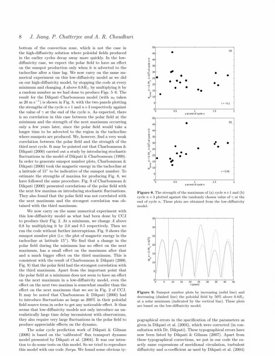
bottom of the convection zone, which is not the case inthe high-diffusivity solution where poloidal fields producedin the earlier cycles decay away more quickly. In the low-diffusivity case, we expect the polar field to have an effecton the sunspot production only when it is advected to thetachocline after a time lag. We now carry on the same nu-merical experiment on this low-diffusivity model as we didon our high-diffusivity model, by stopping the code at everyminimum and changing A above 0.8R⊙ by multiplying it bya random number as we had done to produce Figs. 5–6. Theresult for the Dikpati–Charbonneau model (with u0 takenas 20 m s−1) is shown in Fig. 8, with the two panels plottingthe strengths of the cycle n+1 and n+3 respectively againstthe value of γ at the end of the cycle n. As expected, thereis no correlation in this case between the polar field at theminimum and the strength of the next maximum occurringonly a few years later, since the polar field would take alonger time to be advected to the region in the tachoclinewhere sunspots are produced. We, however, find a very weakcorrelation between the polar field and the strength of thethird next cycle. It may be pointed out that Charbonneau &Dikpati (2000) carried out a study by introducing stochasticfluctuations in the model of Dikpati & Charbonneau (1999).In order to generate sunspot number plots, Charbonneau &Dikpati (2000) took the magnetic energy in the tachocline ata latitude of 15 to be indicative of the sunspot number. Toestimate the strengths of maxima for producing Fig. 8, wehave followed the same procedure. Fig. 9 of Charbonneau &Dikpati (2000) presented correlations of the polar field withthe next few maxima on introducing stochastic fluctuations.They also found that the polar field was not correlated withthe next maximum and the strongest correlation was ob-tained with the third maximum.

We now carry on the same numerical experiment withthis low-diffusivity model as what had been done by CCJto produce their Fig. 2. At a minimum, we change A above0.8 by multiplying it by 2.0 and 0.5 respectively. Then werun the code without further interruptions. Fig. 9 shows thesunspot number plot (i.e. the plot of magnetic energy in thetachocline at latitude 15). We find that a change in thepolar field during the minimum has no effect on the nextmaximum, has a small effect on the maximum after thatand a much bigger effect on the third maximum. This isconsistent with the result of Charbonneau & Dikpati (2000,Fig. 9) that the polar field had the strongest correlation withthe third maximum. Apart from the important point thatthe polar field at a minimum does not seem to have an effecton the next maximum in a low-diffusivity model, even theeffect on the next two maxima is somewhat smaller than theeffect on the next maximum that we see in Fig. 2 of CCJ.It may be noted that Charbonneau & Dikpati (2000) hadto introduce fluctuations as large as 200% in their poloidalfield source term in order to get any noticeable effect. It thusseems that low-diffusivity models not only introduce an un-realistically large time delay inconsistent with observations,they also require very large fluctuations in the polar field toproduce appreciable effects on the dynamo.

The solar cycle prediction work of Dikpati & Gilman(2006) is based on the ‘calibrated’ flux transport dynamomodel presented by Dikpati et al. (2004). It was our inten-tion to do some tests on this model. So we tried to reproducethis model with our code Surya. We found some obvious ty-

0 0.5 1 1.5 20

5

10

15

20

25

30

35

40

45

50

γ at end of cycle n

Bφ

max

(r

= 0

.7R

s, λ=

10o )

of c

ycle

n+

1

r = −0.1

(a)

0 0.5 1 1.5 20

5

10

15

20

25

30

35

40

45

50

γ at end of cycle n

Bφ

max

(r

= 0

.7R

s, λ=

10o )

of c

ycle

n+

3

(b)

r = 0.56

Figure 8. The strength of the maximum of (a) cycle n+1 and (b)cycle n +3 plotted against the randomly chosen value of γ at the

end of cycle n. These plots are obtained from the low-diffusivitymodel.

0 5 10 15 20 25 30 35 40 450

5

10

15

20

25

30

35

t (years)

|Bφ (

r =

0.7

Rs, λ

=10

o )|

Figure 9. Sunspot number plots by increasing (solid line) anddecreasing (dashed line) the poloidal field by 50% above 0.8R⊙

at a solar minimum (indicated by the vertical line). These plotsare based on the low-diffusivity model.

pographical errors in the specification of the parameters asgiven in Dikpati et al. (2004), which were corrected (in con-sultation with Dr. Dikpati). These typographical errors havenow been listed by Dikpati & Gilman (2007). Apart fromthese typographical corrections, we put in our code the ex-actly same expressions of meridional circulation, turbulentdiffusivity and α-coefficient as used by Dikpati et al. (2004)

Solar activity forecast with a dynamo model 9

with the same values of different parameters. We also ran thecode in a full sphere rather than in a hemisphere as done inthe case of the other calculations in this section, to make surethat all the conditions (after correcting the typographical er-rors) were identical with the conditions used by Dikpati etal. (2004) to produce their ‘calibrated’ solution. We founda decaying solution, in contrast to the oscillatory solutionwhich Dikpati et al. (2004) reported. Although our code re-produces the results of Dikpati & Charbonneau (1999), theresults reported in Dikpati et al. (2004) are not reproduced.That is the reason why we had to use the model of Dikpati& Charbonneau (1999) when we wanted to do some tests ona low-diffusivity model.

It may be noted that Nandy & Choudhuri (2002) arguedthat a meridional circulation penetrating slightly below thetachocline is needed to produce solar-like butterfly diagramsand we are using such a circulation. Dikpati & Charbonneau(1999) and Charbonneau & Dikpati (2000) also used suchpenetrating circulation (see Fig. 2 in Choudhuri et al. 2005).Dikpati et al. (2004) are the only authors to claim that theycan get solar-like butterfly diagrams, with sunspots confinedto low latitudes, even with a non-penetrating meridional cir-culation. This result has so far not been reproduced by anyother group. Other groups using non-penetrating circulationhave always obtained butterfly diagrams extending to fairlyhigh latitudes (Bonanno et al. 2002; Guerrero & de GouveiaDal Pino 2007). It remains to be seen whether any other dy-namo group is able to reproduce the model of Dikpati et al.(2004), which we cannot reproduce with our dynamo codeand on which the predictions of Dikpati & Gilman (2006)are based.

5 ARGUMENTS IN FAVOUR OF HIGH

DIFFUSIVITY OF THE POLOIDAL FIELD

From the results presented in the previous section, it shouldbe clear that the diffusivity in the convection zone has to behigh if the polar field at the minimum has to be correlatedwith the strength of the next maximum as seen in the obser-vational data. This is a very compelling argument that theturbulent diffusivity of the convection zone is probably highlike 2 × 1012 cm2 s−1 as taken in our model (Chatterjee etal. 2004; CCJ) and not low like 5 × 1010 cm2 s−1 as takenin the models of Dikpati and her collaborators (Dikpati &Charbonneau 1999; Charbonneau & Dikpati 2000; Dikpatiet al. 2004; Dikpati & Gilman 2006). We now list severalother arguments in support of a high diffusivity.

(i) Even if we assume the turbulent velocities withinthe SCZ to have rather low values like v ≈ 10 m s−1 andthe convection cells to be have rather small sizes like l ≈30, 000 km, still the turbulent diffusivity ≈ (1/3)vl wouldturn out to be not less than 1012 cm2 s−1. Thus simple order-of-magnitude estimates favour the high values of diffusivitythat we use rather than the low values used by Dikpati andher co-workers. Parker (1979, p. 629) used the convectionzone model of Spruit (1974) to conclude that the turbulentdiffusivity should be of order 1–4 × 1012 cm2 s−1 withinthe convection zone. It may be noted that convection zonedynamo models developed in the early years of solar dynamoresearch gave best results when the turbulent diffusivity wastaken to be of order 1012 cm2 s−1 (Kohler 1973; Moffatt

1978, §9.12). Interface dynamos, however, required smallerdiffusivities of order 1010 cm2 s−1 to match the observedperiod of the solar cycle (Choudhuri 1990).

(ii) Wang et al. (1989) studied the evolution of the dif-fuse magnetic field on the solar surface under the joint influ-ence of diffusion and meridional circulation. They concludedthat theory fits observations best if diffusivity at the solarsurface is taken to be 1012 cm2 s−1 or larger, comparableto the diffusivity within convection zone used in our model.While the surface value of diffusivity inferred by Wang et al,(1989) may not necessarily imply that diffusivity inside theconvection zone also has to be comparable, it is still worthnoting that the value of diffusivity used by us is so compa-rable to what is needed to match surface observations. Thissurface value of turbulent diffusion also follows from the factthat the granules at the surface have sizes of the order of afew hundred km, whereas convective velocities are of theorder of 1 km s−1.

(iii) The solar magnetic field is of dipolar nature. Ahigh diffusivity allows the poloidal field lines to get con-nected across the equator and establish a dipolar parity.Yoshimura et al. (1984) pointed out that a high diffusivityhelped in establishing a dipolar parity even in the tradi-tional αΩ dynamo models without meridional circulation.This effect becomes more important in flux transport dy-namos (Chatterjee et al. 2004). If the diffusivity is low, thenthe dynamo solutions tend to be quadrupolar and one needssome additional ad hoc assumption like an extra α-effectat the bottom of the convection zone to make the solutionsdipolar (Dikpati & Gilman 2001; Bonanno et al. 2002; Chat-terjee et al. 2004). While we observe the generation of thepoloidal field on the solar surface by the Babcock–Leightonprocess (Wang et al. 1989), there is no strong observationalevidence for an additional source of poloidal field in thetachocline. A high diffusivity within the convection zone al-lows us to build models of the solar dynamo with the cor-rect parity without invoking an α-effect in the tachocline.Dikpati & Gilman (2007) admit that the tachocline α is a“noise-amplifier”. On using mean field equations, they findthat transients take very long time to die out. Within thereal Sun, there are always fluctuations around the mean anda noise-amplifier would not allow the system to relax to aregular behaviour, especially when the diffusivity is low.

(iv) The irregularities in the solar cycle remain highlycorrelated in both the hemispheres. In other words, stronger(weaker) solar cycles tend to be stronger (weaker) in boththe hemispheres and longer (shorter) solar cycles tend tobe longer (shorter) in both the hemispheres. Chatterjee &Choudhuri (2006) studied this problem and concluded thata high diffusivity forces the cycles in the two hemispheres toremain locked with each other even in the presence of asym-metries between the hemispheres. We expect that stochas-tic fluctuations without having any correlation between thetwo hemispheres would lead to irregularities correlated inthe two hemispheres if the diffusivity is high, but not if thediffusivity is low. This, however, has to be substantiated bydetailed simulations, which we are carrying out now. Theobserved strong correlation of cycle irregularities betweenthe two hemispheres will be impossible to explain with amodel having low diffusivity.

All the above arguments taken together suggest a highvalue of turbulent diffusivity within the solar convection

10 J. Jiang, P. Chatterjee and A. R. Choudhuri

zone. The turbulent diffusivity seems to have a value suchthat the diffusion time of the poloidal field across the convec-tion zone turns out to be comparable to the advection timeby the meridional circulation. At the first sight, it may seemlike a coincidence that these two time scales seem to be socomparable. However, the meridional circulation is supposedto be driven by the turbulent stresses in the convection zone.So both of these two time scales arise from the same physicsof turbulence in the convection zone and it may not be sosurprising that they are comparable.

It is usually assumed that the meridional circulationplays a very important role in flux transport dynamos. Onemay wonder if a high diffusivity will reduce the importanceof meridional circulation. The poloidal and toroidal fields influx transport dynamo models are produced at the surfaceand in the tachocline respectively. These fields are clearlyadvected by the meridional circulation poleward and equa-torward respectively. Since the toroidal field is confined ina narrow layer at the bottom of the SCZ, it is essential toassume a low diffusivity there so that advective effects aremore important there than diffusive effects (Choudhuri etal. 2005). A substantially lower diffusivity at the base ofthe SCZ is assumed both by us (Nandy & Choudhuri 2002;Chatterjee et al. 2004) and by the HAO group (Dikpati &Charbonneau 1999; Dikpati et al. 2004). If diffusive effectswere more important than the advective effects, then thedynamo wave at the bottom of SCZ would propagate pole-ward (Choudhuri et al. 1995), in accordance with the dy-namo propagation sign rule (see, for example, Choudhuri1998, §16.6). In spite of the assumed high diffusivity of ourmodel within the SCZ, there is no doubt that the meridionalcirculation is responsible for the equatorward propagation ofthe dynamo wave at the bottom of SCZ and for the pole-ward advection of the poloidal field at the surface. In thelow-diffusivity model of the HAO group, the meridional cir-culation additionally advects the poloidal field from the solarsurface to the tachocline. On the other hand, the poloidalfield in our model reaches the tachocline by diffusing fromthe surface where it is generated.

If cycle 24 turns to be very strong as predicted by Dik-pati & Gilman (2006), then that will provide a very con-vincing argument in favour of low diffusivity, since a highdiffusivity will not allow a strong solar cycle just after aweak polar field in the preceding minimum. On the otherhand, a weak cycle 24 as predicted by us will make the casefor high diffusivity considerably more compelling.

6 THE CONNECTION OF THE

THEORETICAL MODEL WITH THE

OBSERVATIONAL INPUT

In the previous two sections, we have argued that the dif-fusivity of the poloidal field should be high. With such dif-fusivity, we expect that the poloidal field generated at thesolar surface by the Babcock–Leighton process would dif-fuse towards the tachocline at all latitudes. Consequently,the approach followed by CCJ of updating the theoreticalmodel with a single number (the value of DM) at the mini-mum is a drastic simplification. We now discuss how we canfeed the observed magnetic field values at different latitudesto update the poloidal field at the minimum.

The code Surya calculates the time evolution ofA(r, θ, t), whereas the observations provide the line-of-sightcomponent of B = ∇ × [A(r, θ, t)eφ] at the solar surface.The first step is to use the observational data to calculateA(r = R⊙, θ, t) at the solar surface during the minimum.The relation B = ∇ × [A(r, θ, t)eφ] implies that the mag-netic field has to be divergence-free, which requires thatR π

0Br(r = R⊙, θ, t) sin θdθ integrated from one pole to the

other must be zero. If errors in magnetic field data makeR π

0Br(r = R⊙, θ, t) sin θdθ non-zero, then some special care

has to be exercised when calculating A(r = R⊙, θ, t). Weshall discuss this and then point out how we update A(r, θ, t)underneath the solar surface.

Following Svalgaard et al. (2005), we operationally de-fine the solar polar field as the net magnetic line-of-sightcomponent measured through the polarmost apertures atWSO along the central meridian on the solar disk. We thankTodd Hoeksema for providing line-of-sight magnetic fieldvalues averaged over the Carrington Rotation (CR) obtainedat WSO for 30 points equally spaced in sine latitude from−14.5/15 to +14.5/15 for each rotation from mid 1976 to2006 (CR1642-CR2045). The following operations have tobe performed to obtain the “real” radial magnetic field fromthe WSO data (as explained to us by Todd Hoeksema andLeif Svalgaard): (1) the raw data are divided by the cosineof the latitude, (2) a constant scaling factor 1.85 is multi-plied to correct the saturation effect, (3) another constantnumber 1.25 is multiplied to the data of the first two yearsto correct the scattered light. Thus we may obtain the ra-dial magnetic field for latitude -75 to +75. What we need isthe value from the north pole to the south pole. Svalgaardet al. (1978) pointed out that the variation with latitude ofaverage magnetic flux density between the pole and the po-lar cap boundary obey the relation of cos8 θ near the northpole and cos8(π − θ) near the south pole. With this inter-polation, we finally obtain the values of Br between the twopoles. Fig. 10 is the contour of Br between latitudes ±90from the middle of 1976 to the end of 2006.

The Sun’s polar field reverses near the maximum ofone cycle and then begins its growth toward a new peakwith opposite polarity. The polar field becomes strong andwell established about three years before the sunspot min-imum (Svalgaard et al. 2005). To get Br at the minimaat the ends of cycles 21, 22 and 23, we average the rawdata for the following 3-year periods just before the minima:CR1737–CR1777 (1983:07:10–1986:06:26), CR1871–CR1911(1993:07:03–1996:06:28) and CR2006–CR2045 (2003:08:02–2006:07:01). For the minimum at the end of cycle 20, how-ever, we only have the data since CR1642 (1976:05:27).Hence, for this case, we average the data for 8 CarringtonRotations, i.e. CR1642–CR1649(1976:05:27–1976:12:31).

Fig. 11 shows Br as a function of latitude at the minimaat the ends of cycles 20, 21, 22 and 23. Because of the aver-aging over 3-year periods, the data look reasonably smooth.However, Br does not appear very symmetric at some ofthe minima. For example, for the minimum at the end of cy-cle 21, the south polar field is clearly stronger than the northpolar field. Since the magnetic field cannot have a monopolecomponent, the flux must be distributed in such a way thatR π

0Br(r = R⊙, θ, t) sin θdθ turns out to be zero. The ob-

servational data give the following values of this quantity atthe ends of the 4 successive minima we are considering: 0.14,

Solar activity forecast with a dynamo model 11

Figure 10. Contours of longitude-averaged photospheric mag-netic fields from the middle of 1976 to the end of 2006 from WSOpolar field data. The values between ±75 latitude are given bythe observation. The values in the polar regions are extrapolatedbased on cos8 θ near the north pole and cos8(π−θ) near the southpole. During the interval Nov. 2000 - Jul. 2002, there were someproblems with instrument sensitivity and the real fields are likelyto be stronger than that what was recorded (Schatten 2005). How-ever, this does not pose a problem for our theoretical modelingbecause we require polar field data only during the solar minima.

Figure 11. The radial magnetic field Br for the minima at theends of cycles 20 (solid line), 21 (dotted line), 22 (dashed line)

and 23 (dot-dashed line). This plot is obtained from the WSOdata shown in Fig. 10.

-0.001, 0.09 and 0.011 G. These values give an estimate ofthe monopole component introduced due to the errors in thedata. Since this monopole component is not divergence-free,it causes problems when we try to go from Br(r = R⊙, θ, t)to A(r = R⊙, θ, t). To have an idea how large the monopolecomponents are at the various minima, keep in mind thata uniform radial field of 1 G over the entire solar surfacewould make

R π

0Br(r = R⊙, θ, t) sin θdθ equal to 2 G.

To calculate A(r = R⊙, θ, t) from Br, we use the rela-tion

Br =1

r sin θ

∂

∂θ(sin θA). (4)

If A is non-zero on any of the poles, then some terms in (1)would become singular. To ensure that A remains zero atboth the poles, we use the following relations to obtain the

surface values of A in the two hemispheres:

A(R⊙, θ, t) sin θ =

(

R θ

0Br(R⊙, θ′, t) sin θ′dθ′ 0 < θ < π

2R θ

πBr(R⊙, θ′, t) sin θ′dθ′ π

2< θ < π.

(5)We take R⊙ as the unit of length in the above expressionsgiving the numerical value of A sin θ. Only if there is nomonopole contribution, we expect A(R⊙, θ, t) calculated inthe two hemispheres to match across the equator. Otherwise,we have to connect across the equator by the polynomial fit.

Fig. 12 shows the plots of A sin θ as a function of latitudeat the four minima we are considering. The plots beforesmoothing and after smoothing at the equator are shown inFigs. 12(a) and (b) respectively. Both Br plots in Fig. 11 andA sin θ plots in Fig. 12 indicate that the polar field duringthe minima at the ends of cycles 20 and 21 had nearly thesame strength and they were larger than that at the endof cycle 22. The minimum at the end of cycle 23 has theweakest strength. It may be noted that the integrands in(5) have Br multiplied by sin θ, which is very small in thepolar regions. Hence uncertainties in the value of magneticfield in the polar regions do not have much effect in thecomputation of A sin θ. In spite of the errors in the data, wefind in Fig. 12(a) that the jumps in the plots at the equatorare not very large.

We now discuss how the observational data can be fedinto the theoretical model to correct for the poloidal fieldproduced at the end of a cycle. We already pointed out thatthe poloidal field at the minimum produced in our dynamocode corresponds to an average cycle. CCJ identified cycle 23as an average cycle and took the poloidal field at its begin-ning as indicative of a poloidal field of average strength inthat phase of the dynamo cycle. From the dashed curve inFig. 11 giving the poloidal field at the end of cycle 22, wefind that A sin θ averaged over latitude is 0.66. Now, in ourdynamo code, the only source of nonlinearity is the mag-netic buoyancy and the actual value of A sin θ depends onthe critical magnetic field Bc above which B is supposed tobe buoyant. On setting Bc = 108 G in Surya, we find thatA sin θ at the solar surface averaged over latitude turns outto be equal to 0.66 at the time of minimum in a regularrun (taking R⊙ as the unit of length when calculating A). Itmay be noted that this value of Bc can be taken as a meanvalue of the toroidal field beyond which magnetic buoyancysets in. Flux tube simulations suggest a value of 105 G in-side flux tubes (D’Silva & Choudhuri 1993; Fan et al. 1993),implying a filling factor of order 10−3 for the flux tubes. Asomewhat larger filling factor of order 10−2 was estimatedin §3 of Choudhuri (2003). We put Bc = 108 G and run thedynamo code from a minimum to the next minimum, whenthe poloidal field has to be updated. After stopping the codeat a minimum, we check the values of A at all the grid pointson the solar surface. We denote these by Acode(R⊙, θ). Wehave already discussed how to obtain A at a minimum fromthe observational data and have shown the plots in Fig. 11.Suppose Acode(R⊙, θ) has to be multiplied by γ(θ) to makethe product equal to A obtained from observational data atthat latitude. Fig. 13 shows γ(θ) as a function of latitude forthe four minima we are considering. To avoid the numericalproblem of dividing one small number by another, we donot calculate γ(θ) within 5 degrees of the poles where bothAcode(R⊙, θ) and A become very small. We take γ(θ) to be 1

12 J. Jiang, P. Chatterjee and A. R. Choudhuri

Figure 12. Poloidal field A(R⊙, θ) sin θ inferred from the WSOdata (a) before smoothing and (b) after smoothing, for the min-ima at the ends of cycles 20 (solid line), 21 (dotted line), 22(dashed line) and 23 (dot-dashed line). It may be noted thatA(R⊙, θ) sin θ during the minima at the ends of cycles 21 andcycle 23 is negative. We have plotted the absolute values.

Figure 13. γ(θ) at different latitudes for the minima at the endsof cycles 20, 21, 22, 23. The line styles are the same as in Figs. 11and 12. We do not change values of A in the polar regions (within5 degrees of the poles). Hence, there are no values near the poles.

Figure 14. (a) The contours of toroidal field and (b) the poloidalfield lines, at the solar minimum in an undisturbed run of ourStandard1 model. The solid lines indicate positive values of B

and A, whereas dotted lines indicate negative values.

within these regions. We now feed the observational data inour theoretical model stopped at the minimum in the follow-ing way. At all grid points above 0.8R⊙, we multiply A bythe factor γ(θ) appropriate for that latitude. We do not makeany changes in the values of A below 0.8R⊙. This ensuresthat the poloidal field in the upper layers, which has beencreated by the Babcock–Leighton mechanism operating dur-ing the previous cycle, gets corrected to the observed values,whereas the poloidal field at the bottom of the convectionzone, which may have been created during the still earliercycles, is left unchanged. Later when we plot the poloidalfield lines just after updating, we shall see discontinuitiesat 0.8R⊙. However, the discontinuities in the field lines in-troduced by the discontinuity in γ(θ) at 5 degrees from thepoles are completely insignificant and are not visible in theplots of field lines.

7 PREDICTION RESULTS

We have described in the previous section how the obser-vational data of the poloidal field can be fed into the theo-retical dynamo model stopped at a minimum, to correct forthe randomness in the poloidal field generation process. Weobtain a relaxed solution of our Standard1 model with ourcode Surya and stop it at a minimum. Identifying this asthe minimum at the end of cycle 20, we update the poloidalfield by feeding observational data appropriate for this mini-mum. Then we run the code in successive steps of one cycle,stopping at the consecutive minima to update the poloidalfield by feeding the observational data. The run after theminimum at the end of cycle 23 generates the prediction forcycle 24.

Fig. 14 gives the contours of toroidal field and thepoloidal fields lines at a minimum during a regular run ofSurya for the Standard1 model. Since the diffusivity is lowwithin the tachocline where the toroidal field is produced,we find that the toroidal fields from the previous cycles arestill present. It will be seen that our theoretical butterflydiagrams show eruptions from the previous cycle even aftera new cycle has begun. Our best theoretical models for thesolar cycle still suffer from this defect. On the other hand,the high diffusivity of the poloidal field within the convec-tion zone makes the poloidal fields produced in earlier cy-cles decay away and we predominantly have the poloidalfield produced in the previous cycle present at the time ofthe minimum. Fig. 15 shows poloidal field lines at the fourminima just after they have been updated by feeding theobservational data. It is clear that the poloidal field tendsto be asymmetric between the hemispheres. For example,the poloidal field at the end of cycle 20 appears strongerin the northern hemisphere. This is consistent with Fig. 11,where we see that the north polar field was stronger than thesouth polar field during the minimum at the end of cycle 20.We see discontinuities in poloidal field lines at r = 0.8R⊙

Solar activity forecast with a dynamo model 13

Figure 15. The poloidal field lines given by constant contoursof Ar sin θ just after correcting by the observational data duringthe minima at the ends of cycles (a) 20, (b) 21, (c) 22 and (d) 23.The dashed lines correspond to r = 0.8R⊙.

in Fig. 15. These discontinuities get smoothed as our codeadvances the magnetic field for a few weeks and cause noproblems. An alternative procedure is to multiply A at alldepths by γ(θ). We have checked that this gives very similarresult for our high-diffusivity model, where we do not havepoloidal fields created in the earlier cycles stored at the bot-tom of SCZ. However, one gets considerably different resultsif these different procedures are followed in a low-diffusivitymodel. A very careful comparison of the poloidal field linesin Fig. 14 with the field lines above 0.8R⊙ in the four plotsin Fig. 15 shows that the field lines connect across the equa-tor more smoothly in Fig. 15 (i.e. the field lines appear morebent in Fig. 14). In other words, poloidal field lines recon-structed from observational data suggest slightly more dif-fusion between the two hemispheres compared to the fieldlines from the pure theoretical model shown in Fig. 14. Thiscan be taken as another evidence that the magnetic diffu-sivity assumed by us is not unreasonable. If anything, thecomparison of field lines in Figs. 14 and 15 suggests thatthe actual diffusivity may even be higher than what we areusing in our theoretical model.

Fig. 16 now presents our results for cycles 21-24 gen-erated by our methodology. The top panel superposes themonthly sunspot number generated from our model (solidline) on the observational data (dashed line). We may pointout that the absolute value of the theoretical sunspot num-ber from our numerical code does not have any particularsignificance, since a finer grid would make B buoyant at alarger number of grid points and will increase the numberof eruptions in our method of treating magnetic buoyancy.To generate the top panel of Fig. 16, we scaled the theo-retical sunspot number suitably to make it fit the observa-tional plot. The bottom panel shows the butterfly diagramproduced by our model. We see in the top panel that thetheoretical plot is in quite good agreement with the obser-vational data for cycles 22–23. The fit is not so good forcycle 21. One possible reason for this is the incompletenessof the poloidal field data at the end of cycle 20. The dataare available only from the middle of that minimum andthere were some calibration problems in the first 2 years.The other possibility is that, after we initialize the code byfeeding observational data at a minimum, it may take abouta cycle before the code starts giving really reliable outputs.The cycle 24 comes out as the weakest cycle in a long time.The relative total sunspots numbers for cycles 21–24 pro-duced by the model are 3866, 3862, 3300 and 2292, respec-tively. Hence, the coming cycle 24 should be 30.5% weakerthan cycle 23, which makes cycle 24 a little stronger thanwhat it was in the earlier calculation of CCJ, who foundcycle 24 to be about 35% weaker compared to cycle 23. Wedo believe that the methodology adopted in this paper isa more realistic, thorough and reliable methodology. How-ever, the advantage of the methodology of CCJ is that thismethodology, based on using a single number like the valueof DM to update the poloidal field at the minimum, is ex-

Figure 16. The upper panel shows the theoretical monthlysmoothed sunspot number (solid line) superposed on the monthlysmoothed sunspot numbers from observation (dashed line). Forcycles 22 and 23, the two lines match quite well. But for cycle21, the result from the model is slightly weaker than the obser-vational result. Incomplete observational data at the end of cycle20 might be the reason. The cycle 24 is clearly very weak. Thelower panel shows the theoretical butterfly diagram of sunspotssuperimposed on the contours of radial field for the cycles 21–24.The solid and dashed curves in the lower panel indicate positiveand negative values of Br at the surface. (Note that the solid anddashed curves got accidentally interchanged in Fig. 3 of CCJ.)

tremely easy and straightforward to implement in a dynamomodel. The fact that the two methodologies give reasonablysimilar results suggests that the simple method of CCJ canbe used for a quick first calculation of solar cycles, to givereasonably reliable results.

One additional advantage of our present methodologyover the methodology of CCJ is that the present method-ology allows us to study the asymmetry between the twohemispheres, which was not possible with the methodologyof CCJ. The North-South asymmetry can be defined as

AS =N − S

[N + S]ave

, (6)

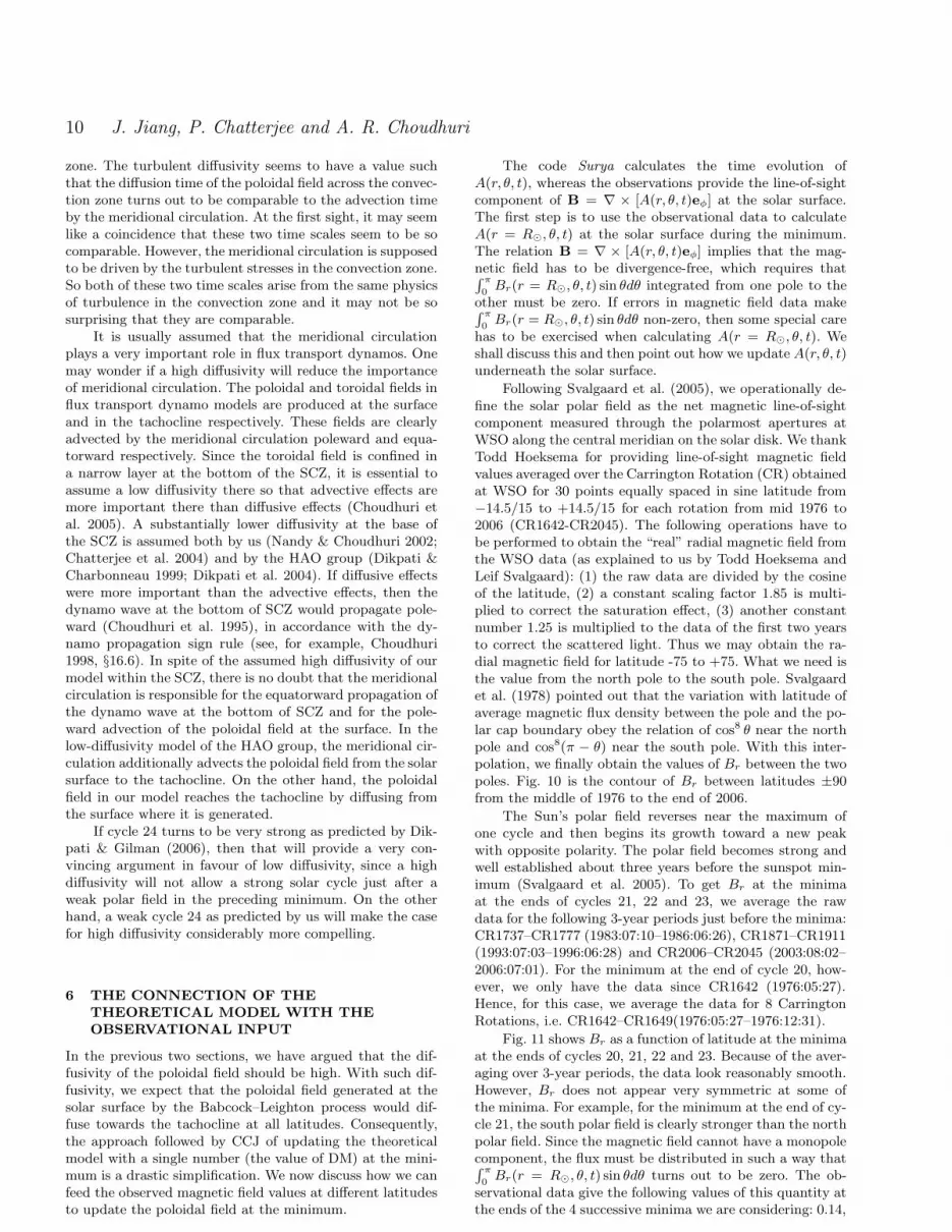
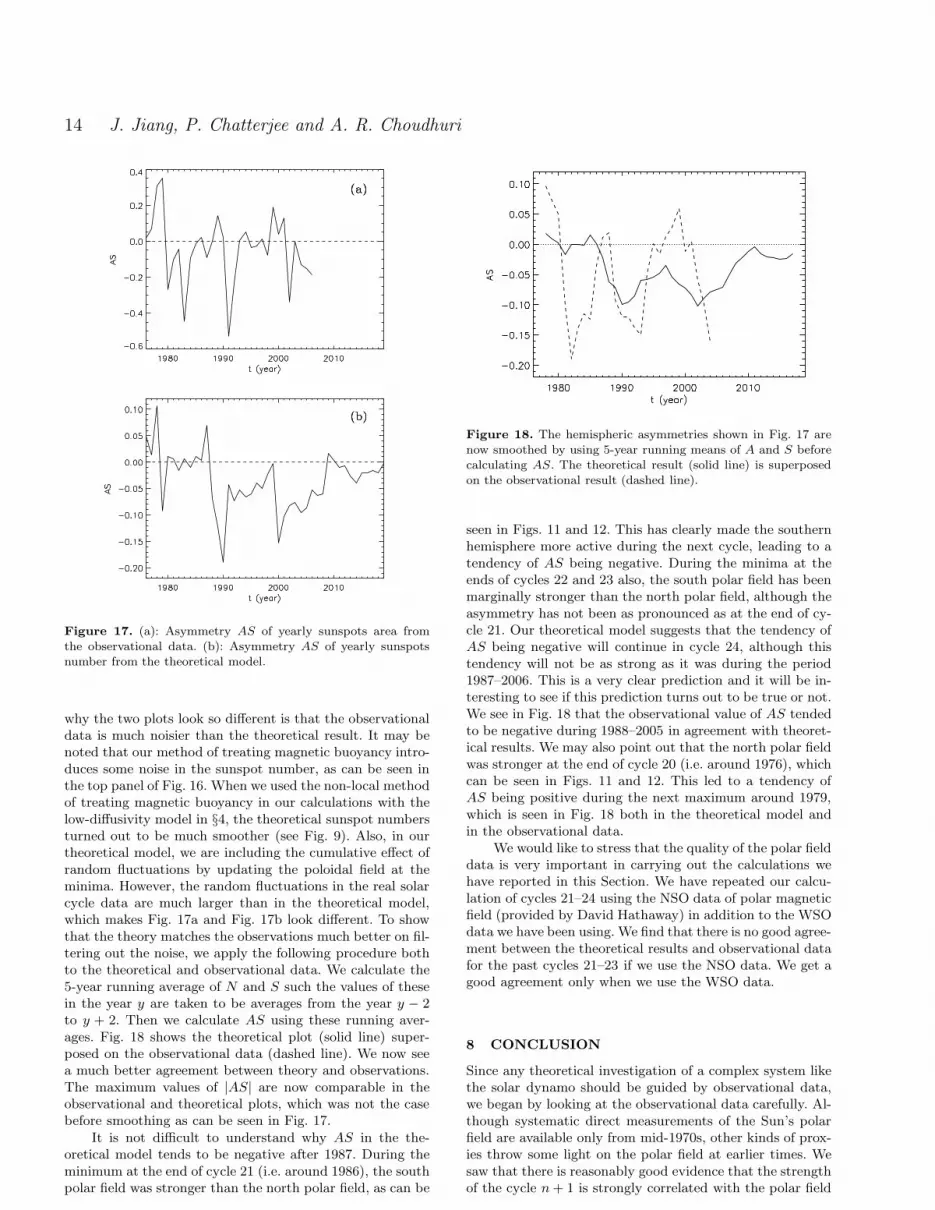
where N and S stand for the annual sunspot group numbersin northern and southern hemisphere respectively (Li et al.2002), and [N + S]ave is the value of N + S averaged overcertain interval, which we take here to be 1976–2006. Dif-ferent observational manifestations of solar activity, such asmajor flares, sunspot numbers, sunspot area data and so on,indicate that the solar activity can be asymmetric about theequator. Fig. 17a shows the asymmetry AS of yearly sunspotarea during 1976–2006. Fig. 17b gives the asymmetry fromour theoretical model. At the first sight, it may seem that thetheory does not match observations well. The main reason

14 J. Jiang, P. Chatterjee and A. R. Choudhuri

Figure 17. (a): Asymmetry AS of yearly sunspots area fromthe observational data. (b): Asymmetry AS of yearly sunspotsnumber from the theoretical model.

why the two plots look so different is that the observationaldata is much noisier than the theoretical result. It may benoted that our method of treating magnetic buoyancy intro-duces some noise in the sunspot number, as can be seen inthe top panel of Fig. 16. When we used the non-local methodof treating magnetic buoyancy in our calculations with thelow-diffusivity model in §4, the theoretical sunspot numbersturned out to be much smoother (see Fig. 9). Also, in ourtheoretical model, we are including the cumulative effect ofrandom fluctuations by updating the poloidal field at theminima. However, the random fluctuations in the real solarcycle data are much larger than in the theoretical model,which makes Fig. 17a and Fig. 17b look different. To showthat the theory matches the observations much better on fil-tering out the noise, we apply the following procedure bothto the theoretical and observational data. We calculate the5-year running average of N and S such the values of thesein the year y are taken to be averages from the year y − 2to y + 2. Then we calculate AS using these running aver-ages. Fig. 18 shows the theoretical plot (solid line) super-posed on the observational data (dashed line). We now seea much better agreement between theory and observations.The maximum values of |AS| are now comparable in theobservational and theoretical plots, which was not the casebefore smoothing as can be seen in Fig. 17.

It is not difficult to understand why AS in the the-oretical model tends to be negative after 1987. During theminimum at the end of cycle 21 (i.e. around 1986), the southpolar field was stronger than the north polar field, as can be

Figure 18. The hemispheric asymmetries shown in Fig. 17 arenow smoothed by using 5-year running means of A and S beforecalculating AS. The theoretical result (solid line) is superposedon the observational result (dashed line).

seen in Figs. 11 and 12. This has clearly made the southernhemisphere more active during the next cycle, leading to atendency of AS being negative. During the minima at theends of cycles 22 and 23 also, the south polar field has beenmarginally stronger than the north polar field, although theasymmetry has not been as pronounced as at the end of cy-cle 21. Our theoretical model suggests that the tendency ofAS being negative will continue in cycle 24, although thistendency will not be as strong as it was during the period1987–2006. This is a very clear prediction and it will be in-teresting to see if this prediction turns out to be true or not.We see in Fig. 18 that the observational value of AS tendedto be negative during 1988–2005 in agreement with theoret-ical results. We may also point out that the north polar fieldwas stronger at the end of cycle 20 (i.e. around 1976), whichcan be seen in Figs. 11 and 12. This led to a tendency ofAS being positive during the next maximum around 1979,which is seen in Fig. 18 both in the theoretical model andin the observational data.

We would like to stress that the quality of the polar fielddata is very important in carrying out the calculations wehave reported in this Section. We have repeated our calcu-lation of cycles 21–24 using the NSO data of polar magneticfield (provided by David Hathaway) in addition to the WSOdata we have been using. We find that there is no good agree-ment between the theoretical results and observational datafor the past cycles 21–23 if we use the NSO data. We get agood agreement only when we use the WSO data.

8 CONCLUSION

Since any theoretical investigation of a complex system likethe solar dynamo should be guided by observational data,we began by looking at the observational data carefully. Al-though systematic direct measurements of the Sun’s polarfield are available only from mid-1970s, other kinds of prox-ies throw some light on the polar field at earlier times. Wesaw that there is reasonably good evidence that the strengthof the cycle n + 1 is strongly correlated with the polar field

Solar activity forecast with a dynamo model 15

at the end of cycle n, giving credence to the method of pre-dicting solar cycles by using the polar field at the precedingminimum as a precursor (Svalgaard et al. 2005, Schatten2005). On the other hand, the polar field at the end of acycle is not correlated with the strength of the cycle. Theseobservational facts guide us in developing our theoreticalapproach.

We suggest that the lack of correlation of the polar fieldat the end of a cycle with the strength of the cycle, as seenin Fig. 3, is a compelling evidence that the generation of thepoloidal field involves randomness. Since the poloidal field isproduced by the Babcock–Leighton mechanism, the physicalorigin of this randomness is not difficult to understand. Thetilts of bipolar sunspots on the solar surface have a largescatter around the mean given by Joy’s law, presumablycaused by the interaction of the rising flux tubes with theconvective turbulence in the uppermost layers of SCZ (Long-cope & Choudhuri 2002). Since the poloidal field producedin the Babcock–Leighton process depends on the tilt, thisscatter in tilts undoubtedly would introduce a randomness.CCJ proposed that the theoretical dynamo model should becorrected by feeding the actual data of poloidal field pro-duced at the end of a cycle when we want to model actualsolar cycles. We have followed this procedure in the presentwork as well.

As for the strong correlation between the polar field ata minimum and the strength of the next cycle, the theoret-ical explanation depends on the fact that the poloidal fieldis transported to the tachocline and then stretched by dif-ferential rotation to produce the toroidal field responsiblefor the strength of the cycle. Since these are regular anddeterministic processes, we expect a causal link to persist.However, in low-diffusivity dynamo models (η ≈ 1010 cm2

s−1), the polar field can be transported to the tachoclineonly by meridional circulation and the advection time is toolarge to explain the correlation between the polar field andthe immediate next cycle. Only in high-diffusivity models(η ≈ 1012 cm2 s−1), the poloidal field created in the pre-vious cycle gets advected to the pole and simultaneouslydiffuses to the tachocline, leading to the observed correla-tion. We have provided several other arguments that thesolar dynamo has to be a high-diffusivity dynamo.

CCJ had used a single number (the value of DM) tofeed the polar field at the minimum into the theoreticalmodel. We now have developed a methodology of feedingthe detailed information of the poloidal field at different lat-itudes. While this a much more satisfactory method thanthe method used by CCJ, we find that the method of CCJalso gives results in qualitative agreement with the more de-tailed method. Since the method of CCJ is much easier toimplement, it can be used to obtain a quick first result. Itshould be kept in mind that the prediction of the sunspotmaximum at the beginning of the cycle is possible only be-cause the rising phase is dominated by fairly ordered anddeterministic processes like the advection/diffusion of thepoloidal field and the generation of the toroidal field by dif-ferential rotation. The declining phase of the cycle, whenthe poloidal field is produced by the Babcock–Leighton pro-cess, involves randomness and is not predictable. If this viewis correct, then we can think of predicting a cycle only af-ter the declining phase of the previous cycle is over and weknow from observations how much poloidal field has been

produced. It may thus never be possible to make a realis-tic prediction of the strength of a sunspot maximum morethan 7–8 years ahead in time. Bushby & Tobias (2007) havegiven several other arguments to show the impossibility oflong-term prediction in the solar dynamo.

A high-diffusivity dynamo certainly has a shorter mem-ory compared to a low-diffusivity dynamo. Additionally,when the poloidal field information is fed into the theoret-ical model at the time of the minimum, that also tries toerase the memory of the dynamo. One important questionis whether the memory of the dynamo is restricted to beless than 11 years in our model, since the poloidal field isupdated after every 11 years. Fig. 2 of CCJ showed that thememory of a disturbance can persist for at least 2 cycles ifthe dynamo is not disturbed any more after giving a sin-gle kick. Will the introduction of randomness after a cycleerase this memory completely? The answer will depend onreally how random the next kick is. There is no doubt thatthe Babcock–Leighton process introduces randomness in thegeneration of the poloidal field. However, the limited datashown in Fig. 3 is insufficient for us to conclude whetherthe randomness is serious enough to erase the memory com-pletely or whether some weak correlation still exists betweenthe strength of a cycle and the poloidal field produced at itsend.

Svalgaard et al. (2005) suggested a simple relation thatthe maximum International Sunspot Number Rmax of cyclen will be proportional to the value of DM at the end of cyclen − 1, i.e.

(Rmax)n = k(DM)n−1. (7)

This implies a complete loss of memory of the previous cy-cles. If the randomness introduced in the Babcock–Leightonprocess does not completely erase the memory of the im-mediately preceding cycle, then, on the basis of Fig. 2 ofCCJ showing that the memory of the polar field can persistfor a couple of cycles, we would expect a more complicatedfunctional relationship

(Rmax)n = f [(DM)n−1, (DM)n−2]. (8)

For the last few cycles, the results obtained with our dy-namo model are roughly in agreement with what one wouldexpect on the basis of (7). However, if two preceding cycleshave been of very unequal strengths and (8) is the correctrelation rather than (7), then it is possible that a detailedcalculation based on a dynamo model may give a result sig-nificantly different from what one would get from (7). Thetheoretical sunspot number shown in Fig. 16 also indicatesthat (8) may be a more correct relation. Since we had notfed any information about the minimum at the end of cy-cle 19 into our theoretical model, the theoretical cycle 21does not match observations so well as the cycles 22–23 forwhich data for the 2 previous minima had been fed.

One important question is whether observational datacan help us in deciding about the memory of the dynamoprocess. We see in Fig. 2 that the solid circles based onactual polar field measurements lie close to a straight line,suggesting that (7) may actually be true. However, the opencircles based on more uncertain data show a scatter. We can-not be sure whether this scatter is due to the errors in thedata or whether there is an inherent scatter in the data. Ifthere is an inherent scatter, one possible explanation is that

16 J. Jiang, P. Chatterjee and A. R. Choudhuri

(8) is the correct relation and that is why we do not ex-pect all data points in a (Rmax)n versus (DM)n−1 plot tolie on a straight line or a curve. An alternative explanation,however, is also possible. We have been tacitly assumingthat the transport of the poloidal field to tachocline and itsstretching by differential rotation there are ordered and de-terministic processes. As argued by Choudhuri (2003), themagnetic field has to become intermittent at some stage toaccount for the existence of flux tubes. This also may in-troduce some randomness, making a departure from a strictcausal relationship between (Rmax)n and (DM)n−1.

Sometimes the so-called ‘even-odd rule’ is forwarded asan argument in favour of the dynamo having a memory last-ing for at least 2 cycles. There have been 6 consecutive pairsof cycles in which the odd cycle was stronger than the pre-ceding even cycle. The cycle 23 broke this ‘even-odd rule’after more than a century. It is difficult to be sure whetherthe ‘even-odd rule’ really exists or whether this apparent ef-fect was caused by the accident of statistics. Charbonneauet al. (2007) have made the provocative suggestion that thiseffect is caused by the period doubling in the dynamo, whichis a nonlinear chaotic system. If this theoretical explanationis correct, then the randomness introduced in the Babcock–Leighton process should not erase the memory of the pre-ceding cycle completely.

To sum up, there is no doubt that the Babcock–Leighton process of poloidal field generation introduces asignificant amount of randomness in the dynamo processand this has to be corrected in a theoretical model by us-ing actual observational data. Whether this process erasesall the memory of previous cycles or whether some memorystill persists is a question which cannot be settled on the ba-sis of currently available limited observational data. Perhapswe should keep our minds open and allow for the possibil-ity that the dynamo retains some memory even after theBabcock–Leighton process introduces a significant elementof randomness.

Our model makes a very clear prediction that cycle 24will be a rather weak cycle. This is a quite robust predictioneven if the memory of the dynamo persists for a few yearsbeyond one cycle, since the polar fields at the ends of bothcycles 22 and 23 have been weak. In our high-diffusivity dy-namo model, it would be completely impossible to have aweak polar field (like what we have now) to be followed by avery strong cycle as predicted by Dikpati & Gilman (2006).Apart from the fact our two dynamo models used diffusiv-ities differing by a factor of 50, the second main differenceis that Dikpati & Gilman (2006) have taken the sunspotarea data as the source of the poloidal field. In our view,the poloidal field generation involves randomness and can-not be calculated deterministically from sunspot number orarea data of previous cycles. We now have to wait for a ver-dict on this debate from the Sun-god himself in about 4–5years’ time.

ACKNOWLEDGMENTS

We are grateful to Dirk Callebaut, David Hathaway, ToddHoeksema, Ken Schatten, Leif Svalgaard and Andrey Tla-tov for explaining various aspects of observational data. Wethank Axel Brandenburg, Paul Charbonneau and Dibyendu

Nandy for valuable discussions. We also acknowledge dis-cussions with Mausumi Dikpati during our efforts in repro-ducing her low-diffusivity model. Suggestions from the ref-eree, Leif Svalgaard, and the Editor helped in improving thepresentation. This work began when A.R.C. was a VisitingProfessor at the National Astronomical Observatories in Bei-jing. He would like to thank Jingxiu Wang, Jun Zhang andother members of the group for the very warm hospitality.J.J. acknowledges financial support from National Basic Re-search Program of China through grant nos. 2006CB806303,10573025 and 10603008. P.C. acknowledges financial supportfrom C.S.I.R through grant no. 9/SPM-20/2005-EMR-I.

REFERENCES

Babcock H. W., 1961, ApJ, 133, 572Babcock H. W., Babcock H. D., 1955, ApJ, 121, 349Bonanno A., Elstner D., Rudiger G., Belvedere G., 2002, A&A,

390, 673Bushby P. J., Tobias S. M., 2007, arXiv:0704.2345v1Cameron R., Schussler M., 2007, ApJ, 659, 801Charbonneau P., Beaubien G., St-Jean C., 2007, ApJ, 658, 657Charbonneau P., Dikpati M., 2000, ApJ, 543, 1027Chatterjee P., Choudhuri A. R., 2006, Sol. Phys., 239, 29Chatterjee P., Nandy D., Choudhuri A. R., 2004, A & A, 427,

1019Choudhuri A. R., 1989, Sol. Phys., 123, 217Choudhuri A. R., 1990, ApJ, 355, 733

Choudhuri A. R., 1992, A&A, 253, 277Choudhuri A. R., 1998, The Physics of Fluids and Plasmas: An

Introduction for Astrophysicists, Cambridge University PressChoudhuri A. R., 2003, Sol. Phys., 215, 31Choudhuri A. R., 2005, The User’s Guide to the Solar Dynamo

Code Surya (available on request)Choudhuri A. R., 2007a, Adv. Space Res. (in press)Choudhuri A. R., 2007b, J. Astrophys. Astron. (submitted)Choudhuri, A. R., Chatterjee, P., Jiang, J., 2007, Phys. Rev.

Lett., 98, 131101Choudhuri A. R., Chatterjee P., Nandy D., 2004, ApJ, 615, L57Choudhuri A. R., Gilman P. A., 1987, ApJ, 316, 788Choudhuri A. R., Konar S., 2002, MNRAS, 332, 933Choudhuri A. R., Nandy D., Chatterjee P., 2005, A&A, 437,703Choudhuri A. R., Schussler M., Dikpati M., 1995, A&A, 303, 29Dikpati M, Charbonneau P., 1999, ApJ, 518, 508

Dikpati M., de Toma G., Gilman P., 2006, Geo. Res. Lett., 33,L05102

Dikpati M., de Toma G., Gilman P. A., Arge C. N., White O. R.,2004, ApJ, 601, 1136

Dikpati M., Gilman P. A., 2001, ApJ, 559, 428Dikpati M., Gilman P. A., 2006, ApJ, 649, 498Dikpati M., Gilman P. A., 2007, Sol. Phys., 241, 1D’Silva S., Choudhuri A. R., 1993, A&A, 272, 621Durney B. R., 1995, Sol. Phys., 160, 213Fan Y., Fisher G. H., Deluca E. E., 1993, ApJ, 405, 390Gizon L., 2004, Sol. Phys., 224, 217Guerrero G., de Gouveia Dal Pino E. M., 2007, A&A, 461, 341Hathaway D. H., Nandy D., Wilson R. M., Reichmann E. J., 2003,

ApJ, 589, 665Hoyng P., 1993, A&A, 272, 321Kohler H., 1973, A & A, 25, 407

Konar S., Choudhuri A. R., 2004, MNRAS, 348, 661Leighton, R. B., 1969, ApJ, 156, 1Li K. J., Liu X. H., Yun H. S., et al., 2002, Publ. Astron. Soc.

Japan., 54, 629Longcope D. W., Choudhuri A. R., 2002, Sol. Phys., 205, 63Longcope D. W., Fisher G. H., 1996, ApJ, 458, L380

Solar activity forecast with a dynamo model 17

Makarov V. I., Makarova V. V., Sivaraman K. R., 1989, Sol. Phys.,

119, 45Makarov V. I., Tlatov A. G., Callebaut D. K., Obridko, V. N.,

Shelting, B. D., 2001, Sol. Phys., 198, 409Mininni P., Gomez D. O., 2002, ApJ, 573, 454Moffatt H. K., 1978, Magnetic Field Generation in Electrically

Conducting Fluids, Cambridge University PressMoss D., Brandenburg A., Tavakol R., Tuominen I., 1992, A& A,

265, 843Nandy D., Choudhuri A. R., 2001, ApJ, 551, 576Nandy D., Choudhuri A. R., 2002, Sci, 296, 1671Ossendrijver A. J. H., Hoyng P., Schmitt D., 1996, A&A, 313, 938Parker E. N., 1955, ApJ, 122, 293Parker E. N., 1979, Cosmical Magnetic Fields, Oxford University

PressSchatten K., 2005, Geo. Res. Lett., 32, L21106Schatten K. H., Scherrer P. H., Svalgaard, L., Wilcox, J. M., 1978,

Geo. Res. Lett., 5, 411Sheeley N. R. Jr., 1991, ApJ, 374, 386Spruit H. C., 1974, Sol. Phys., 34, 277Steenbeck M., Krause F., Radler K. H., 1966, Z Naturforsch, 21,

369Svalgaard L, Cliver E. W., Kamide Y., 2005, Geo. Res. Lett., 32,

L01104Svalgaard L, Duvall, T. L., Scherrer, P. H., 1978, Sol. Phys., 58,

225van Ballegooijen A. A., Choudhuri A. R., 1988, ApJ, 333, 965Wang Y.-M., Nash A. G., Sheeley N. R. Jr, 1989, ApJ, 347, 529Wang Y.-M., Sheely, N. R., Jr., 1989, Sol. Phys.,124, 81Wang Y.-M., Sheeley N. R. Jr, Nash A. G., 1991, ApJ, 383, 431Yoshimura H., Wang Z., Wu F., 1984, ApJ, 280, 865