Critical assessment of high-throughput standalone methods for secondary structure prediction

Critical assessment of high-throughputstandalone methods for secondarystructure predictionHua Zhang, Tuo Zhang, Ke Chen, Kanaka Durga Kedarisetti, Marcin J. Mizianty, Qingbo Bao,Wojciech Stachand Lukasz KurganSubmitted: 13th September 2010; Received (in revised form): 20th December 2010

AbstractSequence-based prediction of protein secondary structure (SS) enjoys wide-spread and increasing use for the analy-sis and prediction of numerous structural and functional characteristics of proteins.The lack of a recent comprehen-sive and large-scale comparison of the numerous prediction methods results in an often arbitrary selection of a SSpredictor. To address this void, we compare and analyze 12 popular, standalone and high-throughput predictors ona large set of 1975 proteins to provide in-depth, novel and practical insights. We show that there is no universallybest predictor and thus detailed comparative studies are needed to support informed selection of SS predictorsfor a given application. Our study shows that the three-state accuracy (Q3) and segment overlap (SOV3) of the SSprediction currently reach 82% and 81%, respectively.We demonstrate that carefully designed consensus-based pre-dictors improve the Q3 by additional 2% and that homology modeling-based methods are significantly better by1.5% Q3 than ab initio approaches.Our empirical analysis reveals that solvent exposed and flexible coils are predictedwith a higher quality than the buried and rigid coils, while inverse is true for the strands and helices.We also showthat longer helices are easier to predict, which is in contrast to longer strands that are harder to find. The currentmethods confuse 1^6% of strand residues with helical residues and vice versa and they perform poorly for residuesin the b- bridge and 310 -helix conformations. Finally, we compare predictions of the standalone implementations offour well-performing methods with their corresponding web servers.

Keywords: secondary structure; protein structure; secondary structure prediction

INTRODUCTIONThe secondary structure (SS) of proteins, which was

first postulated over 50 years ago by Pauling and

Corey [1,2], is defined as a consecutive fragment of

protein sequence that corresponds to a spatially local

region in the associated tertiary structure that has dis-

tinct geometrical shape. About half of amino acids

(AAs) in protein chains fold into the a-helix and

Hua Zhang is a Lecturer in College of Computer and Information Engineering, Zhejiang Gongshang University, Hangzhou,

Zhejiang, P.R. China. His research interests are focused on machine learning and bioinformatics.

Tuo Zhang is a post-doctoral fellow in the School of Informatics at the Indiana University-Purdue University Indianapolis. He is

conducting research related to protein structure and function.

Ke Chen is a PhD student at the University of Alberta, Canada. His research interests are in structural bioinformatics.

Kanaka Durga Kedarisetti is a PhD candidate holding M.Sc. degree in Software Engineering from the University of Alberta. Her

work focuses on data mining, machine-learning and their applications in computational biology.

Marcin Mizianty is a research assistant and a PhD student at the University of Alberta, Canada. His work focuses on structural

bioinformatics, rational drug-design, knowledge discovery and machine learning.

Qingbo Bao is a graduate student who holds MSc in Bioinformatics from the Nankai University, P.R. China. He specializes in data

mining and machine learning.

Wojciech Stach has recently obtained his PhD in Computer Engineering from the University of Alberta, Canada. He specializes in

systems modeling, computational intelligence and data mining.

Lukasz Kurgan is an Associate Professor at the University of Alberta, Canada. The web site of his laboratory is located at http://

biomine.ece.ualberta.ca/.

Corresponding author. Lukasz Kurgan, Department of Electrical and Computer Engineering, ECERF, 9107 116 Street, University of

Alberta, Edmonton, AB, Canada T6G 2V4. Tel: þ1-780-492-5488; Fax: þ1-780-492-1811; E-mail: [email protected]

BRIEFINGS IN BIOINFORMATICS. VOL 12. NO 6. 672^688 doi:10.1093/bib/bbq088Advance Access published on 20 January 2011

� The Author 2011. Published by Oxford University Press. For Permissions, please email: [email protected]

by guest on May 14, 2016

http://bib.oxfordjournals.org/D

ownloaded from

http://bib.oxfordjournals.org/

b-strand SSs and the remaining residues are more

irregularly structured. Methods for the assignment of

the SS depend on the experimentally derived tertiary

structure and they include DSSP [3], STRIDE [4],

P-SEA [5], XTLSSTR [6], SECSTR [7] and KAKSI

[8]. DSSP is often the method of choice since this

approach is used to annotate depositions to PDB [9]

and was used to evaluate SS predictions in the critical

assessment of techniques for protein structure predic-

tion (CASP) [10] competitions and the EValuation of

Automatic protein structure prediction (EVA) [11]

continuous benchmarking project. The DSSP anno-

tates each AA in a sequence with one of eight SS types:

H (a-helix), G (310-helix), I (p-helix), B (isolated b-

bridge), E (b-sheet), T (hydrogen bonded turn), S

(bend) and ‘_’ (any other structure). These eight

types are often reduced to the three SS states, a-

helix (which includes types H, G and I), b-strand

(E and B) and coil (T, S and _).

Since the tertiary structure is known for a rela-

tively small number of proteins, i.e. only about

60 000 proteins are included in the PDB, several

past decades observed development of numerous

methods that predict the SS from the protein

sequence. The quality of these predictions has

improved considerably when compared with the

first method, which was proposed almost 50 years

ago [12] and which took advantage of correlations

between particular AA types and SS types. A rela-

tively low prediction quality obtained by methods

that were developed until mid-1990s is due to the

fact that they used only local, with respect to the

sequence, information, i.e. a segment of 3–51 con-

secutive residues. Such local information is estimated

to account for about 65% of the SS formation [13]. A

major breakthrough was achieved by inclusion of the

multiple alignment profiles, which are utilized by

virtually all current prediction methods. This infor-

mation together with availability of larger databases

and more advanced prediction algorithms resulted in

a significant increase of the prediction accuracies

[14]. Modern predictors achieve accuracy, which is

measured using the Q3 index, of over 75% [11,15]

and certain algorithms such as PROTEUS [16] and

SSpro [17], which incorporate alignments to known

structures in the PDB obtain accuracies of about

80%. Gradually, the prediction accuracy is approach-

ing the estimated theoretical limit of 88–90%

[15,18,19]. The SS predicted from a protein

sequence is widely used for the analysis and predic-

tion of numerous structural and functional

characteristics of proteins, including target selection

in structural genomics, multiple alignment, predic-

tion of protein–ligand interactions and prediction of

higher dimensional aspects of protein structure

including the tertiary structure, solvent accessibility,

residue contacts, etc. [13,20]. The importance and

popularity of the SS predictors is demonstrated by

the massive workloads that they handle. For instance,

in 2005, the PSIPRED web server was reported to

receive over 15 000 requests per month [21]. The

development and applications of the SS prediction

methods enjoy a steady growth over the past 20

years; Supplementary Figure S1.

The predictive quality of the SS predictors was

evaluated and compared within the frameworks

of several initiatives including CASP, Critical

Assessment of Fully Automated Structure

Prediction (CAFASP) and EVA. Only the early

CASP and CAFASP experiments, including

CASP3 in 1998, CASP4 and CAFASP2 in 2000

and CASP5 and CAFASP3 in 2002, evaluated the

SS predictions. Later on, the evaluations were carried

out using the EVA platform [11,22]. Its most recent

release monitored 13 SS predictors, including PHD

[23], PORTER [24], PSIPRED [25], SABLE [26],

SSpro [27] and YASPIN [28] that are considered in

this study. Since April 2008 EVA is no longer being

updated. One of the drawbacks of this service is that

individual methods were tested on often different

and a relatively small, between 73 and 232,

number of chains. The sizes of the protein sequence

sets that are common to multiple methods range

between 80 (with results for six predictors) and 212

chains (with results for three predictors). This does

not allow for an in-depth and comprehensive com-

parative analysis. In spite of these limitations, the two

contributions that introduced EVA received rela-

tively significant attention; as one measure of their

impact, they received close to 200 citations accord-

ing to the ISI Web of Science as of August 2010.

Both CASP and EVA performed evaluations on rela-

tively small protein sets that include up to a few

hundred chains, which do not allow for a more

detailed analysis of various aspects of the SS predic-

tions. Additionally, a few new SS predictors, such as

SPINE [29], SPINEX [30] and PROTEUS [16,31]

were developed in recent years and some of the older

solutions such as PSIPRED [21], SSpro [17] and

JNET [32] were recently upgraded and modified.

These methods were never comprehensively com-

pared against each other and other existing solutions.

Assessment of standalone secondary structure prediction methods 673 by guest on M

ay 14, 2016http://bib.oxfordjournals.org/

Dow

nloaded from


We present results of a comprehensive assessment

of the quality of the sequence-based SS prediction.

We compare results generated by 12 fully auto-

mated, high-throughput SS predictors on a datasets

with 1975 proteins. We consider standalone methods

that can be incorporated into local predictive pipe-

lines. We concentrate on practical aspects that would

help practitioners to select the right tools and devel-

opers to focus their efforts on addressing unresolved

problems. We compare the overall performance of

each of the methods, evaluate the significance of the

differences in their predictive quality and also con-

sider a number of novel dimensions to provide in-

depth insights. This is motivated by a few recent

works that analyze the relation between the quality

of the SS predictions and the position in the

sequence [33] and the size of the input protein

chain [34]. We analyze a wider range of other factors

including localization of errors with respect to the

native SS segments, the quality of the prediction of

the eight SS defined by DSSP and the accuracy of

the SS predictions in relation to the native solvent

accessibility and residue flexibility. We also analyze

complementarity between different predictors and

we investigate feasibility of building ensembles that

would provide improved prediction rates. Similar to

the prior evaluation efforts, our work primarily con-

centrates on predictions for globular proteins, i.e.

we evenly sample the sequence space of proteins

deposited to the PDB, since these proteins are

well-represented in the PDB and the knowledge of

their structures is necessary to generate the ground

truth to perform evaluations. Recent reviews of

methodologies designed specifically for membrane

proteins, which are underrepresented in the PDB,

can be found in [35,36]. These methods focus on

the prediction of certain SS elements of the mem-

brane proteins, including the transmembrane helices

[37–39] and strands [40].

MATERIALSANDMETHODSDatasetThe evaluation was performed on a dataset that was

extracted from PDB using protein sequence culling

server [41] as of 31 March 2008. We selected the

culled chains characterized by pairwise identity of

<25% (computed using local alignment) and which

were solved using high quality crystals, i.e. with the

resolution cutoff at 2 A and the R-factor cutoff at

0.25. The original culled list included 3643 chains.

We removed short peptide sequences with less than

20 residues and chains that included singular residues,

such as ‘X’. We run the SS predictors on the remain-

ing 3289 chains. Our preliminary analysis revealed

that chains that were deposited into PDB before

2004 could not be used for the evaluation since

the homology-based SSpro overfitted these chains;

Supplementary Figure S2. The SSpro was published

in 2005 [17] and these older chains were likely

included in its template library. Consequently,

1975 chains that were deposited between 2004 and

2008 were used to benchmark the SS predictors.

Empirical evaluationWe measure predictive quality at the residue and the

SS segment levels. We use the quality measures that

were reported in the EVA platform [11,22]. Given

that Nij denotes the number of residues in the native

SS state i which are predicted in state j where i, j 2{helix H, strand E, coil C} and N denotes number of

all residues in the dataset, the residue-level measures

include:

QHpre ¼NHHP

i2fH,E,CgNiH� 100%;

QEpre ¼NEEP

i2fH,E,CgNiE� 100%;

QCpre ¼NCCP

i2fH,E,CgNiC� 100%;

QHobs ¼NHHP

j2fH,E,CgNHj� 100%;

QEobs ¼NEEP

j2fH,E,CgNEj� 100%;

QCobs ¼NCCP

j2fH,E,CgNCj� 100%;

Q3 ¼

P

i2fH,E,CgNii

N� 100%

and

QHEerror ¼NHE þNEH

N� 100%

674 Zhang et al. by guest on M


Dow

nloaded from


The QHpre, QEpre and QCpre quantify the number of

the correctly predicted helix, strand and coil residues

among all predicted helix, strand and coil residues,

respectively. Similarly, QHobs, QEobs and QCobs,

quantify the number of the correct helix, strand

and coil predictions among all native helix, strand

and coil residues, respectively. The Q3 gives the

overall rate of correct predictions for the three SS

states. The QHEerror measures the amount of signifi-

cant mistakes where a native helix residue is pre-

dicted as a strand and vice versa. We also compute

the segment overlap values that quantify the amount

of overlap between the native and the predicted

helix (SOVH), strand (SOVE) and coil (SOVC) seg-

ments, including the overall segment overlap that

consider the three SSs (SOV3) [42]. We compute

SOV values for each chain and we average them

over all proteins. In the cases where we evaluate

predictive performance for a subset of residues in

our benchmark dataset, i.e. when considering resi-

dues in a specific native SS state, in a specific range of

their native RSA and with specific values of their

native B-factor, we only compute the per-residues

measures since the per-segment measures require

that the predictions have no breaks.

We run statistical tests to verify significance of the

differences in the predictive quality between all pairs

of the considered SS predictors. Our tests aim to

show how likely it is for a given method to be

significantly better than another method when con-

sidering an application to predict the SS for an aver-

age-sized dataset with 500 chains. We performed

these tests for the Q3, SOV3, SOVH and SOVE

measures. We first verified whether the values of

these measures are normal for each predictor using

the Shapiro–Wilk test [43] with 0.05 significance

level. The tests have revealed that none of the mea-

surements is normal and therefore we used the non-

parametric Wilcoxon rank-sum test [44] with 0.05

significance level. For each pair of the SS predictors

we compared paired values of the quality measures

computed per chain for randomly selected 500

chains from the benchmark dataset. We repeated

that 1000 times, each time annotating whether and

which method is statistically significantly better

according to a given quality index. We report the

corresponding probability of significance, which is

defined as the number of tests where a method A

is significantly better than a method B minus the

number of times where B is significantly better

than A, divided by 1000.

Considered prediction methodsWe considered several well-known mature SS pre-

dictors and a selection of new methods that were

published in high-impact venues. The necessary con-

dition for the considered methods was that they have

to offer a standalone implementation that allows for

high throughput and fully automated batch predic-

tions and which can be incorporated into local pre-

dictive pipelines. We permitted one exception since

majority of the predictors that satisfy this condition

were based on neural networks (NNs); a recent

Hidden Markov Model (HMM)-based method, the

P.S.HMM [45], which does not provide a standalone

version, was included. This allowed us to include

two different HMM-based predictors. We consid-

ered total of 12 predictors including PHD [23,46],

PSIPRED [21,25], JNET [32,47], SSpro [17,27],

SABLE [26], YASPIN [28], PORTER [24],

OSSHMM [48], PROTEUS [16], SPINE [29],

P.S.HMM [45] and SPINEX [30]; Table 1. The

selected predictors include most of the key SS pre-

diction methods which were identified by Rost [13],

such as PHD, PSIPRED, SSpro, PORTER, SABLE

and YASPIN and most of the methods recently

reviewed by Pirovano and Heringa [20], including

PHD, PSIPRED, SSpro, PORTER and YASPIN.

RESULTSOverall prediction qualityFigure 1 compares the overall prediction quality of

the considered 12 SS predictors on the entire bench-

mark dataset with 1975 proteins. We observe that

most of the NN-based methods, except for the

older JNET and PHD, outperform the HMM-

based solutions. The two best performing methods

according to both Q3 and SOV3 measures, SSpro

and PROTEUS, use homology modeling. The top

two ab initio methods are PSIPRED and SPINEX.

Although the inclusion of the homology modeling is

helpful, the margin of improvement is relatively

narrow, about 1.5% Q3 and 2.5% SOV3. The best

Q3 values for the homology-based predictors are at

about 82%, while Q3 of the best ab-initio methods are

around 80.5%. While these results are quite encoura-

ging, the values of the QHEerror, which quantifies the

amount of errors where a native helix residue is pre-

dicted as a strand and vice versa, are relatively high

and range between 0.6%, 1.2%, 1.6% and 1.8% for

the best performing PROTEUS, SPINEX, SSpro

and PSIPRED, respectively and 6.3% for the worst



Dow

nloaded from


Table1:

Summaryof

the12

SSpredictio

nmetho

dsconsidered

inthisstud

y.The

metho

dsaresorted

bythedate

oftheirpu

blication

Nam

e(version

)No.

ofcitation

saPredictionmetho

dsURLof

thestan

daloneim

plem

entation

Web

serv

eravailable

Total

Per

year

Classifier

type

Architectur

eHom

ology

mod

eling

PHD

(PRO

Fphd

)958

68NN

bTw

o-levelfeed-forw

ardNNs

No

www.predictprotein.org/do

wnload.ph

pYes

PSIPRED

(2.5)

1492

136

NN

Ensembleof

4tw

o-levelfeed-forw

ardNNs

No

bioinf.cs.ucl.ac.uk

/psip

red/

Yes

JNET

370

37NN

Two-levelfeed-forw

ardNNs

No

www.com

pbio.dun

dee.ac.uk/So

ftware/JN

et/jn

et.

htmlc

Yes

SSpro(4.03)

282

35NN

Ensembleof11bidirectionalrecurrent

NNs

Yes

scratch.proteo

mics.ics.uci.edu/

Yes

SABL

E(2.0)

5210

NN

Two-levelensemble

of18

Elman-type

recursive

NNs

No

sable.cchm

c.org/sable_do

c.html

Yes

YASPIN

6212

NN

and

HMM

hybrid

Two-levelhybrid

withafeed-fo

rwardNN

inthe

first

leveland

seven-stateHMM

inthesecond

level

No

www.ibi.vu.nl/program

s/yaspinwww/d

Yes

PORT

ER90

18NN

Two-levelensembleof

45bidirectionalrecurrent

NNs.

Noe

distill.ucd.ie/por

ter/

Yes

OSSHMM

72

HMM

f36

hidd

enstates

(15forH,9

forE,12

forC)

No

migale.jouy.inra.fr/outils/m

ig/oss-hmm/

No

PROTEU

S27

7NN

Feed

-forw

ardNN

that

uses

outputsof

PSIPRED

,JNET

andTR

ANSEC

Yes

wks16338.biolog

y.ualberta.ca/proteus/contact.jsp

Yes

SPINE(1.0)

176

NN

Ensembleof

2tw

o-levelfeed-forw

ardNNs

No

sparks.in

form

atics.iupu

i.edu/SPINE/spine.htmld

Yes

P.S.HMM

41

NN

and

HMM

hybrid

Ensembleof

3tw

o-levelh

ybrids

withHMM

infirst

leveland

afeed-fo

rwardNN

inthesecond

level

No

Not

availableg

No

SPINEX

00

NN

Ensemble

oftw

ofeed-fo

rward

NNswith

two

hidden

layers

No

http://sparks.in

form

atics.iupu

i.edu/SPINE-XI/spine

-xi.h

tmld

Yes

a Citations

intheISIW

ebof

Kno

wledgeas

ofMay

2010.bNeuralnetwork,NN.cWeused

implem

entatio

ninclud

edin

thePR

OTEU

S.d A

vailablefrom

theauthorsup

onrequ

est.

e Weused

thestandalone

version

which

does

notinclude

theho

molog

ymod

eling.

f HiddenMarkovMod

el.gNostandalone

implem

entatio

n(predictions

wererunby

theauthorsof

themetho

ds).



Dow

nloaded from


performing PHD and P.S.HMM. The segment

overlap values for helices are quite high and reach

close to 82% for the SSpro and PROTEUS and over

80% for the PSIPRED and SPINEX. The segment

overlap values for the strands are lower in the

75–77% range for a few well-performing predictors;

this is expected since strands form sheets that

involve long-range interactions. One exception is

PROTEUS that obtains 81.1% SOVE but, as dis-

cussed below, this method over-predicts the strand

residues.

PROTEUS offers accurate predictions for the

helices, with the highest QHpre, the second highest

QHobs and the highest SOVH. It also obtains the

highest SOVE with the highest QEobs but as a

trade-off for a relatively low QEpre, which means

that it over-predicts the strand residues. The SSpro

generates high quality predictions for the coils with

the highest SOVC and QCobs and the second highest

QCpre. It also obtains the best QEpre with a relatively

low (when compared with PROTEUS) QEobs,

which means that it under-predicts the strand resi-

dues. This suggests that these two methods comple-

ment each other and thus they would be good

candidates to build a consensus-based SS predictor.

The top two ab initio methods, PSIPRED and

SPINEX, have Q3 values higher by 1–1.5% when

compared with the other ab initio predictors.

PSIPRED has a relatively high SOV3 that equals

78.5%, which is about 1% higher than the SOV3

of the runners up SPINEX and PORTER. The

main reason for the lower SOV3 of SPINEX is

Figure 1: The quality of the SS prediction of the 12 considered predictors (x-axis) on the benchmark dataset with1975 protein chains. (A) The values of the Q3, QHpre, QEpre and QCpre using solid lines and QHobs, QEobs, QCobs

using dotted lines. (B) The values of the SOV3, SOVH, SOVE and SOVC.The methods are sorted by their Q3 values.



Dow

nloaded from


that it performs weaker for the strand segments, i.e. it

has a relatively low SOVE, although it performs on a

par with the PSIPRED for the helix segments.

We investigate significance of the differences

between all pairs of the considered SS predictors.

We performed 1000 repetitions of a non-parametric

Wilcoxon test by comparing the paired sequence-

level results on sets of 500 chains that were randomly

chosen from the benchmark dataset; Table 2. The

probabilities above 0.95 and below �0.95 corre-

spond to significant differences and the positive/

negative values indicate that a method in a given

row in Table 2 is better/worse than a method in

the corresponding column. The tests that are based

on the Q3 reveal that the two homology-based pre-

dictors, SSpro and PROTEUS, are not significantly

different and that PROTEUS is significantly better

than all ab initio predictors. Among the ab initio meth-

ods, SPINEX and PSIPRED generate comparable

Q3 values and the former predictor is significantly

better than the remaining eight ab initio methods

and comparable with the SSpro. Similarly, the

SOV3 values of PROTEUS and SSpro are compar-

able and PROTEUS is significantly better than the

other 10 considered approaches. Among the ab-initiomethods, the best performing PSIPRED is compar-

able to the SSpro, PORTER and SPINEX and sig-

nificantly better than the other seven predictors that

do not use the homology modeling. The helical seg-

ments are predicted with the highest SOVH by

PROTEUS which is shown not to be significantly

better than only SSpro, SPINEX and PSIPRED.

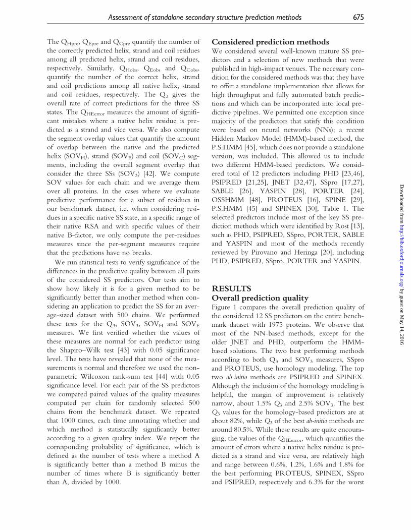
Table 2: Results of 1000 repetitions of a non-parametric Wilcoxon test with 0.05 significance which comparespaired sequence-level results of all pairs of the considered12 SS predictors on1000 sets of 500 chains that were ran-domly chosen from the benchmark dataset

A PHD PSIPRED YASPIN SPINE JNET SSpro SABLE PROTEUS OSSHMM P.S.HMM PORTER SPINEX

PHD �1.00 �1.00 �1.00 �1.00 �1.00 �1.00 �1.00 �1.00 �0.01 �1.00 �1.00PSIPRED 1.00 1.00 0.93 1.00 �0.64 1.00 �1.00 1.00 1.00 0.79 �0.01YASPIN 1.00 �1.00 �1.00 1.00 �1.00 �0.76 �1.00 1.00 1.00 �1.00 �1.00SPINE 1.00 �0.96 0.75 1.00 �1.00 0.99 �1.00 1.00 1.00 0.00 �1.00JNET 1.00 �1.00 �1.00 �1.00 �1.00 �1.00 �1.00 �0.01 1.00 �1.00 �1.00SSpro 1.00 0.23 1.00 1.00 1.00 1.00 �0.17 1.00 1.00 1.00 0.15SABLE 1.00 �1.00 0.05 �0.01 1.00 �1.00 �1.00 1.00 1.00 �0.98 �1.00PROTEUS 1.00 1.00 1.00 1.00 1.00 0.50 1.00 1.00 1.00 1.00 0.99SSHMM 1.00 �1.00 �1.00 �1.00 �0.04 �1.00 �1.00 �1.00 1.00 �1.00 �1.00P.S.HMM �0.01 �1.00 �1.00 �1.00 �1.00 �1.00 �1.00 �1.00 �1.00 �1.00 �1.00PORTER 1.00 �0.18 1.00 0.04 1.00 �0.93 0.61 �1.00 1.00 1.00 �1.00SPINEX 1.00 �0.49 0.99 0.01 1.00 �0.97 0.36 �1.00 1.00 1.00 0.00

B PHD PSIPRED YASPIN SPINE JNET SSpro SABLE PROTEUS OSSHMM P.S.HMM PORTER SPINEX

PHD �1.00 �1.00 �1.00 �1.00 �1.00 �1.00 �1.00 �1.00 0.00 �1.00 �1.00PSIPRED 1.00 1.00 0.66 1.00 �0.17 0.97 �0.88 1.00 1.00 0.07 0.00YASPIN 1.00 0.00 �0.43 1.00 �1.00 �0.03 �1.00 0.77 1.00 �0.94 �1.00SPINE 1.00 �0.06 0.00 1.00 �0.99 0.00 �1.00 1.00 1.00 �0.01 �0.73JNET 1.00 �1.00 �1.00 �1.00 �1.00 �1.00 �1.00 �0.13 1.00 �1.00 �1.00SSpro 1.00 0.20 0.65 0.97 1.00 1.00 �0.06 1.00 1.00 0.90 0.15SABLE 1.00 �0.74 �0.09 0.00 1.00 �1.00 �1.00 1.00 1.00 �0.10 �0.98PROTEUS 1.00 1.00 1.00 1.00 1.00 0.96 1.00 1.00 1.00 1.00 0.87OSSHMM 1.00 �1.00 �1.00 �1.00 �0.97 �1.00 �1.00 �1.00 1.00 �1.00 �1.00P.S.HMM 0.00 �1.00 �1.00 �1.00 �1.00 �1.00 �1.00 �1.00 �1.00 �1.00 �1.00PORTER 1.00 �0.77 �0.14 0.00 1.00 �1.00 0.00 �1.00 1.00 1.00 �0.09SPINEX 1.00 �1.00 �0.93 �0.32 0.76 �1.00 �0.03 �1.00 1.00 1.00 �0.02

The results for Q3 (entries in the upper triangle) and SOV3 (entries in the lower triangle) are shown in upper panel. Lower panel shows results forSOVH (entries in the upper triangle) and SOVE (entries in the lower triangle) measures. For each of the 1000 trials, we annotated whether andwhich method is statistically significantly better and we report the corresponding probability of significance which is defined as the number oftestswhere amethod in a givenrowis significantlybetter than amethod in a given columnminus thenumber of times it is significantly worse dividedby 1000. Positive/negative values mean that that a method in a given row was significantly better/worse with a given probability than a methodin the corresponding column. Underlined bold denotes the methods/probabilities that are not significantly worse than the best performinghomology-basedmethod and bold denotes the samewhen comparedwith the best ab initiomethod.



Dow

nloaded from


The PSIPRED, which has the best SOVH among

the ab initio predictors, is similar to the SPINEX,

PORTER and SPINE and significantly better than

the other six ab initio predictors. The evaluation con-

cerning the strand segments shows that the

PROTEUS has the highest SOVE which is signifi-

cantly better than the results of all other 11 methods.

The best performing ab initio PSIPRED has a com-

parable SOVE when contrasted with the SSpro,

YASPIN, SPINE, SABLE and PORTER and it sig-

nificantly outperforms the SPINEX, both HMM-

based methods and the older NN-based PHD and

JNET.

Comparisonwith web serversWe compare the quality of predictions generated by

the standalone implementations with the corre-

sponding web servers. We include web servers for

the two homology-based methods, SSpro [17] and

PROTEUS [31], the well-performing ab-initioPSIPRED [21] and PORTER [24], for which the

web server includes homology modeling. The web

server for SSpro does not predict chains that are

shorter that 25 residues (the standalone version

does not have this limitation) and thus we compare

both versions of this method on the reduced bench-

mark set that excludes the 22 short chains; the other

methods are compared on the entire benchmark set.

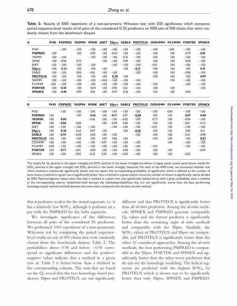
A side-by-side comparison is shown in Figure 2. We

observe that the web server for SSpro is consistently,

i.e. using all quality measures, outperformed by the

standalone version. This is because the standalone

program generates the sequence profiles and per-

forms the homology analysis using a much larger

database than the web server version (personal com-

munication with the authors). On the other hand,

the web server for PROTEUS provides consistently

improved predictions with 0.9% higher Q3 and 1.2%

higher SOV3 when compared with its standalone

version. This is likely due to the updated and

enlarged databases that are utilized by the web

server, i.e. the server [31] implements an updated

version of the original PROTEUS predictor [16].

Although the web server that implements

PSIPRED provides predictions with higher Q3 (by

1.4%) and SOV3 (by 0.5%) when compared with the

standalone program, these improvements are incon-

sistent with respect to different quality measures.

Specifically, although Q3, QCobs, QHpre, QEpre,

SOV3, SOVC and SOVE values are better for the

web server, the remaining measures including

QHobs, QEobs, QCpre and SOVH have higher values

for the standalone program. Finally, we observe that

the web server for PORTER overfits the benchmark

dataset, i.e. all quality measures have values of at least

at 95%, which is likely because this server utilizes

homology modeling and its template library overlaps

with the benchmark set.

We conclude that the user should carefully con-

sider whether to use a web server or a standalone

Figure 2: Comparison of the quality of the SS predictions between the web servers (ws) and the standaloneimplementations for SSpro, PROTEUS, PSIPRED and PORTER.The results for both versions of SSpro are computedon a subset of the benchmark dataset that excludes 22 chains with less than 25 residues; the other methods arecompared using the entire benchmark dataset with 1975 protein chains. The x-axis lists the evaluation measures.The solid bars report results for standalone version and the hollow bars for the corresponding web servers.



Dow

nloaded from


program. The standalone programs allow for high

volume predictions and they can be incorporated

in other predictive pipelines, but they require instal-

lation on a local computer. The web servers are more

convenient in use for predicting a few protein chains

(i.e. they do not need to be downloaded and

installed), but they may pose a challenge when

applied to predict a large set of chains (i.e. some

servers allow submission of one chain at the time

and may have long wait times due to limited com-

putational resources and a long queue of requests

from other users). Moreover, our analysis shows

that the differences in the predictive quality for a

given predictor between its standalone and web

server versions depend on the frequency with

which the underlying databases are updated.

Consensus-based predictionsWe investigate whether building a simple consensus

using the considered SS predictors would lead to

improvements. This is motivated by the work in

[49] which shows that a simple majority vote-based

consensus can outperform individual methods used

in the consensus. Furthermore, the consensus-based

approaches were shown to improve predictive qual-

ity in related areas, including prediction of the pro-

tein fold types [50,51], quaternary structure type

[52], transmembrane helices [37] and disorder

[53–55], to name a few. The authors in [49] con-

clude that any three state-of-the-art SS prediction

methods can be used to build a well-performing

consensus. We extend their work by using a

weighted consensus in which the Q3 values are

used as the weights. In our consensus each SS state

receives a score equal to the sum of the Q3 values of

the base methods that predict this state (0 is assumed

is none of the methods predicts this state) and we

predict the state that has the largest summed Q3

value. When compared with the classical consensus

that does not utilize weights [49], our approach

reduces the number of ties and allows building

ensembles with an even number of the base

predictors.

We have built consensus predictors that include

top k prediction methods that were sorted in

descending order by their Q3 values. We con-

sidered two scenarios, the first one with all 12 meth-

ods where k¼ 3, 4, 5, . . . , 12, (we cannot built

ensembles with k¼ 1, 2) and the second one in

which we use only the ab-initio methods where

k¼ 3, 4, 5, . . . , 10; Figure 3. In both cases, the

consensus-based methods improve the predictions

when contrasted with results from the best base

methods. When including the homology-based

methods, the Q3 and SOV3 values are improved by

2% and 1.5% when compared against the best Q3 of

SSpro and the best SOV3 of PROTEUS, respec-

tively. When considering only the ab initio methods,

the improvements for Q3 and SOV3 equal 1% and

1.2% when compared with the best Q3 of SPINEX

and the best SOV3 of PSIPRED, respectively. In

contrast to the other study [49], the best results are

obtained when combining four methods. This is

likely due to the usage of the weights. Inclusion of

additional methods, beyond the four, worsens the

predictions; this is likely since the subsequently

added predictors introduce more errors than the cor-

rect and complementary predictions. Our analysis

suggest that the consensus of certain combinations

of four predictors, e.g. those with the highest Q3,

that applies the weighted majority voting improves

the prediction quality when compared with the best

performing methods that were considered in this

work. These ensembles obtain Q3¼ 84.4% and

SOV3¼ 82.5% when using the two homology-

based predictors and Q3¼ 81.6% and

SOV3¼ 79.7% when using only the ab-initiopredictors.

Furthermore, we compare the ensemble of the

four methods selected based on their Q3 values

with other ensembles of three and four predictors

to demonstrate that proper selection of the base

methods leads to improvements. We compare

against the consensus of the four and three methods

that were most cited per year since the publication

and the four and three methods that were published

the most recently, Table 1. The ensembles of four/

three of the most cited methods that include the

homology-based SSpro obtain the Q3 equal to

80.6% and 78.6% and the SOV3 equal to 78.3%

and 76.3%, respectively. In the case of the most

recent methods which include the homology-based

PROTEUS, the Q3 values are 82.7% and 82.5% and

the SOV3 are 80.8% and 80.4%, respectively. These

results are lower than the results obtained when

selecting the base methods using their Q3 values.

We also estimate a theoretical upper limit of the

consensus-based methods by using an oracle predic-

tor that always selects a correct prediction if any of

the methods in a given ensemble generates such cor-

rect outcome. The top four predictors, SSpro,

PROTEUS, PSIPRED and SPINEX, correctly



Dow

nloaded from


predict 95% of the residues. We observe a wide

margin between the results of the weighted-majority

based ensemble and the estimated upper limit.

Although it would be unreasonable to expect that

the ensembles could approach the limit values, we

believe that customized designs which consider

window- and chain-level information extracted

from the outputs of the base predictors could lead

to further improvements.

Localization of the errorsWe analyze localization of the prediction errors with

respect to the local native SS arrangements. We use

native SS triplets to annotate the middle residue as

located inside of a SS segment (HHH, EEE and

CCC), at or adjacent to a terminus of a helix or a

strand segment (CEE, CCE, EEC, ECC, CHH,

CCH, HHC and HCC) and in the remaining con-

figurations which include the middle residue in a

helix conformation that is directly adjacent to a

strand or vice versa (CEH, HEC, EEH, HEE,

EHH, HHE and HEH which are denoted by

H/E), middle residue as an isolated coil (HCE,

ECH, HCH and ECE) and an isolated b-bridge

(CEC). The remaining CHC, CHE, EHC and

EHE triplets do not occur in the DSSP annotations

and are never predicted, which is due to the fact that

the shortest helix is three residues long and that all

considered predictors ensure that this constrain is

satisfied.

Over 67% of residues are inside the SS segments,

Figure 4A. These residues are characterized by rela-

tively low error rates (number of incorrect predic-

tions) when compared with the overall number of

these residues. The error rates range between 6.6%

for PROTEUS (out of 18.3% overall error rate of

this predictor) and 17.4% for PHD (out of 32.2%).

Figure 4A reveals that for most of the predictors,

except for the PROTEUS and YASPIN, the

number of errors for the strand and helix residues

is similar, although there are approximately twice

as many helical residues in the native structures.

PROTEUS incorrectly predicts only 7.5% of resi-

dues inside the strand segments and the second best

PSIPRED makes 17.3% of mistakes.

Close to 30% of residues are located at or adjacent

to a terminus of helix and strand segments. On aver-

age the largest fraction of the prediction errors is

made for these positions. These error rates vary

between 8.5% for SSpro (out of 17.7%) and 13.1%

for PHD (out of 32%), Figure 4B. There are no

disproportions in the quantity of the errors between

Figure 3: Comparison of Q3 (hollow markers) and SOV3 (solid markers) values obtained with weighted majority-vote based consensus predictors. The x-axis denotes a consensus of k¼1 (a single predictor), 3, 4, 5,. . ., 12 top-per-forming, with respect to the Q3 reported in Figure 1A, SS predictors. The triangles show a theoretical upper limitfor a given ensemble and they correspond to an oracle ensemble which selects a correct prediction if any of themethods in the consensus generates it.The circles denote ensembles that include all predictors while squares corre-spond to ensembles without the homology-based SSpro and PROTEUS.



Dow

nloaded from


Figure 4: Localization of prediction errors with respect to the native SS triplet configurations. (A) The counts oferrors (on x-axis) for triplets EEE, HHH and CCC and which correspond to positions where the middle residue isinside a SS segment. (B) Counts for triplets CEE, CCE, EEC, ECC, CHH, CCH, HHC and HCC for positions wherethe middle residue is at or adjacent to a terminus of a helix or strand segment. (C) Covers remaining tripletswhere the middle residue is in a helix conformation that is directly adjacent to a strand or vice versa (H/E), is asingle coil (HCE, ECH, HCH and ECE) and an isolated beta-bridge (CEC). The left most bar shows the totalnumber of native triples that were annotated using DSSP and the subsequent bars show the number of errors fora given prediction methods when predicting residues in the middle position of the triplets. The values above thebars are the percentages of the number of residues (for DSSP bar) and the corresponding errors (for other bars)in given set of triplet configurations among all residues in the dataset.



Dow

nloaded from


the N- and C-termini of strands and helices (CEE

and CCE versus EEC and ECC and CHH and CCH

versus HHC and HCC). We note that PROTEUS

over-extends the strand segments, which could be

deduced from larger values for the CCE and ECC

triplets and smaller values for the CEE and EEC

triplets, respectively. Overall, these errors likely

stem from the fact that some SS assignments at the

termini could be ill-defined; the differences that

could shift the termini in either direction could be

subtle and may lead to ambiguities with respect to

which residues at the edge of the segments should be

included, as it was discussed in Ref. [8]. These mis-

takes should have a relatively negligible negative

effect, when compared with the errors made inside

the SS segments, when using these predictions to

find the overall amount of helix and strand residues

in a sequence, which has applications in the predic-

tions of domains [56], contact order [57] and folds

[51], to name a few.

The remaining nearly 3% of residues are located at

the termini of a helix/strand that is directly adjacent

to a strand/helix or they concern single coil residues

flanked by helix/strand residues and b-bridges;

Figure 4C. Between 51% (for SSpro) and 72% (for

JNET) of residues that are at the helix/strand inter-

face are incorrectly predicted. This could be due to

the fact that such conformations are relatively rare

and thus the prediction models tend to assume that

the helix or strand termini are followed by a coil.

Between 30% (for SSpro) and 49% (for PROTEUS)

of the flanked coil residues are predicted as either

strand or helix residues, which means that the major-

ity of these coil residues are correctly predicted. On

the other hand, the predictions of the isolated

b-bridges suffer low success rates. Only between

48% (for PROTEUS) and 12% (for OSSHMM) of

them are correctly predicted. Although the b-bridges

constitute only about 1% of all residues and thus

these errors contribute relatively little towards the

overall error rates, the problem is aggravated by the

fact that the incorrect prediction of one b-bridge

residue means that the corresponding b-bridge resi-

due (even if correctly predicted) cannot be linked

with the hydrogen bond.

Quality of the three-state predictions forthe eight-state SSsWe investigate the quality of the prediction for

each of the eight SS states defined with the DSSP.

We classify a given prediction as correct if the

corresponding three-state SS is predicted correctly,

i.e. the a-helix (H), 310-helix (G) and p-helix (I) are

predicted as the helix (H), the isolated b-bridge (B)

and b-sheet (E) as the strand (E) and the hydrogen

bonded turn (T), bend (S) and other coils (‘_’) as the

coil (C).

Figure 5A shows that although predictions of the

a-helices are quite accurate, the 310-helices are pre-

dicted relatively poorly. The best performing SSpro

correctly predicts only 50% of the 310-helices, while

success rates for the other predictors range between

43.8% (for PSIPRED) and 21.9% (for JNET).

Although this type of the helix occurs relatively

rarely, it accounts for 10% of all helix and 4% of

all residues in our dataset. The low total number of

the p-helix residues does not allow us to formulate

statistically sound conclusions. The p-helix residues

are under-represented in our dataset since they are

common in the membrane proteins for which the

tertiary structure (and consequently DSSP-derived

SS) is very difficult to resolve.

The b-sheet residues are predicted with a reason-

able quality, Figure 5B. The best performing

PROTEUS makes only 11.5% of errors and the

runner up PSIPRED, SPINEX and SSpro make

25%, 25.6% and 25.6% errors, respectively. On the

other hand, predictions of the isolated b-bridges are

relatively poor. The corresponding error rates are at

51.9% for PROTEUS, 65.6% for SSpro, 72.2% for

YASPIN and above 78% for the remaining methods.

This agrees with the observations in the ‘Localization

of errors’ section.

The most accurately predicted coil types are

bends; Figure 5C. The corresponding error rates

range between 12.3% for SSpro and 25.3% for

PHD. To compare, the error rates for turns are

between 18% for SSpro and 28.8% for YASPIN

and for the other coils they are in 15.8% for SSpro

to 25.4% for P.S.HMM range. We hypothesize that

the turns suffer the lowest predictive performance

since they include hydrogen bonds that are also typi-

cal for the helical conformation.

Predictions of long helix and strandsegmentsWe analyze the quality of the predictions for long

helix and strand segments. We assume a given seg-

ment is correctly predicted if at least 50% of its resi-

dues are correctly predicted; similar results can be

obtained for other cutoff values. We compute the

fraction of the segments with increasing minimal



Dow

nloaded from


size that were incorrectly predicted; Supplementary

Figure S3. The results show that it is easier to predict

longer helix segments. The corresponding error rates

decline with the increasing minimal size of the seg-

ment; Supplementary Figure S3A. This is expected as

helices are formed based on local, with respect to the

sequence, interactions. Therefore longer helical

segments should be easier to detect using a

window in a sequence, which is the primary way

to encode inputs to the SS predictors. On the

other hand, Supplementary Figure S3B demonstrates

that longer strand segments are more difficult to pre-

dict. The error rates increase for the longer segment

and this trend is universal for all methods, except for

Figure 5: Evaluation of errors for the eight-state SSs. A given eight-state SS is assumed to be correctly predicted ifthe predicted three-state SS was correct, i.e. if helix was predicted for H, G and I, strand for E and B and coil forT, S and _. (A) The counts of errors (on x-axis) for helices, (B) strands and (C) coils. The numbers at the top of thebars in (A) denote the total numbers (for the left most bar) and the number of correctly predicted pi-helix residues(for the other bars). The left most bar shows the total number of native SS that were annotated using DSSP andthe subsequent bars show the number of errors for a given prediction method.



Dow

nloaded from


the PROTEUS which maintains the lowest error

rates across all segment sizes.

To compare, while about 98% of helices with 10

or more residues have at least 50% of their residues

correctly predicted by the SPINEX, SSpro and

PROTEUS, the corresponding success rates for

strands are 85.1%, 81.5% and 95.7%. For the 1542

strand segment that are at least 10 residues long the

two homology-based predictors, PROTEUS and

SSpro, fail to find at least 50% of their residues for

4.3% and 18.5% of the segments, respectively, the

two best performing ab-initio predictors, SPINEX

and PSIPRED, fail for 14.9% and 15.6%, respec-

tively and in the worst cases the errors are as high

as 46.3% and 49.5% for the two HMM-based meth-

ods. Our analysis also shows that on average (across

all predictors) 23.4% and 14.6% of the helix and

strand segments that are at least three residues long

are entirely missed, i.e. not even one of their residues

is predicted correctly. These rates drop to 7.2% and

9.2% when considering segments with at least five

residues and to 2% and 7.3% for the cutoff of 10

residues.

Quality of predictions for buried andsolvent exposed residuesSome of the applications of the predicted SS, includ-

ing prediction of the solvent accessibility of residues

[58], residue depth [59,60] and binding residues [61],

concentrate on the subset of AAs that are character-

ized by a specific placement with respect to the pro-

tein surface. This motivates our analysis that

compares the quality of the SS predictions for resi-

dues that are exposed to the solvent, i.e. residue with

the native relative solvent accessibility (RSA) com-

puted with the DSSP > 0.25 and residues that are

buried (RSA� 0.25); Supplementary Figure S4.

Although Supplementary Figure S4A shows that

Q3 values for the buried and the exposed residues

are similar, we observe substantial differences for the

prediction of individual SS states. The quality of the

coil predictions, measured using both QCobs and

QCpre, is higher for the exposed residues when com-

pared with the buried AAs. The differences vary

between 5.8% and 14.1% for QCobs and between

8.1% and 16.3% for QCpre. On the contrary, predic-

tions of the exposed helix and strand residues suffer

lower quality. The buried helices are predicted with

QHobs that is better by 1.1 to 7.6% and with QHpre

that is better by 0.3–5.2% when compared with the

exposed helix residues. Similarly, QEobs is higher by

10.9–24.9% and QEpre is higher by 11.7–21.9% for

the buried strands. These differences are consistent

for all SS predictors and they likely stem from the

fact that the buried coil residues are less frequent than

the exposed coil residues (44% versus 56% in the

benchmark dataset) in the native structures, while

residues in the helix and strand conformations are

more frequently buried (58% buried helix residues

versus 42% exposed and 75% buried strand residues

versus 25% exposed). The machine learning models

that are used to predict SSs, which include NNs and

HMMs, are designed to maximize the overall pre-

dictive quality, which means that they could be

biased to focus on the more frequent characteristics

of each SS type.

Quality of predictions with respect toresidue-level flexibilityWe also investigate whether the quality of the SS

prediction varies depending on the native flexibility

of the AAs. The flexibility is measured using the

B-factors, which quantify fluctuations of atoms that

make up residues about their average positions. The

B-factor values are reported in the PDB files and

they were normalized as described in Ref. [62].

The differences in these predictive qualities would

have implications in the applications of the predicted

SS to the prediction of B-factors [63] and disordered

residues [64]. We consider three categories of flex-

ibility where a residue is assumed rigid if its normal-

ized B-factor <�1, neutral if the normalized B-

factor is between �1 and 1 and flexible when the

normalized B-factor >1. This results in about 9% and

9.9% of the helices being rigid and flexible, respec-

tively. The corresponding rates for the strands are

13.8% and 5.2% and for the coils are 4.8% and

22.8%, respectively. For the top five best-performing

SS predictors the overall Q3 values are higher for the

rigid residues by 3–5% when compared with the

flexible residues; Supplementary Figure S5.

Importantly, we observe substantial differences in

the prediction quality for the coils, strands and

helices. The QCobs and QCpre for the flexible residues

are higher by between 6.9% and 21.1% and by

between 14.7% and 33.5%, respectively. This is in

contrast to the helices and strands for which predic-

tions for the flexible residues are worse than for the

rigid residues. More specifically, QHobs and QHpre for

the rigid residues are higher by 6.2–20% and by

11.6–20%, respectively. Similarly, the range of the

increase of the QEobs and QEpre values for the rigid



Dow

nloaded from


residues is between 23.3% and 38.9% and between

27.8% and 40.5%, respectively. Similarly as in the

case of the analysis for the buried and exposed resi-

dues, the variations in the predictive quality between

the flexible and the rigid residues likely can be

explained by the nature of the classification algo-

rithms that focus on the more frequent patterns.

We note that 64% of the flexible residues are coils,

while 78% of the rigid residues are in the strand or

helix conformations.

DISCUSSIONOur analysis reveals that the best Q3 and SOV3

values for the homology-based predictors are at

about 82% and 81%, respectively, while for the

best ab-initio methods they are around 80.5% and

78.5%, respectively. This is consistent with the

recently reported results for the PROTEUS predic-

tor [31]. The best SOVH and SOVE values for the

homology-based and other predictors are at about

82% and 81% and 80% and 75%, respectively. The

homology-based methods are shown to be statisti-

cally significantly better than the ab initio approaches

although the magnitude of the differences is rela-

tively small. We also show that the NN-based solu-

tions outperform the HMM-based methods. Among

the ab initio methods, the PSIPRED and SPINEX

usually significantly outperform other predictors,

although SPINEX perform relatively poorly for the

prediction of the strand segments and PORTER and

SPINE perform comparably well with respect to the

prediction of the SS segments. Further improve-

ments can be obtained by building consensus-based

predictors, but they need to include a carefully

selected set of the best performing methods. We

show that a weighted majority vote consensus of

the four best performing, according to the Q3, pre-

dictors that includes the homology-based methods

obtains Q3¼ 84.4% and SOV3¼ 82.5%. These

results improve over the predictions of the best indi-

vidual methods by 2% for the Q3 and 1.5% for the

SOV3. In case when we use the top four ab-initiomethods the Q3¼ 81.6% and SOV3¼ 79.7%,

which corresponds to 1% and 1.2% improvements

over the best performing ab initio predictor,

respectively.

About a third to a half of all errors concerns resi-

dues located inside the native SS segments and we

believe that these mistakes could be addressed by

future SS predictors. This could lead to relatively

substantial improvements, e.g. the Q3 of the most

accurate SSpro would reach 90.1% assuming that

all of these residues would be correctly predicted.

Most of the errors are made for the positions at or

adjacent to a helix or a strand termini. Between 29%

and 44% of these residues are incorrectly predicted

and this accounts to about 41–56% of all prediction

errors. These mistakes are very difficult to fix since

the SS assignment on this positions tends to be rela-

tively ambiguous [8].

Our analysis reveals that the predictions for the

a-helix residues are the most accurate, with the

lowest and average error rates (across the considered

SS predictors) that equal 6.8% and 13.8%, respec-

tively. The predictions for the three types of coils,

including the turns, bends and other coils, are char-

acterized by the average error rates of 22.4%, 17.4%

and 22.1%, respectively. The b-sheet residues are

predicted with acceptable error levels that for the

best performing methods equal 11.6% and on aver-

age equal 31.2%. On the other hand, the two types

of the SS that suffer relatively low prediction quality

include the 310-helices and the isolated b-bridges.

The corresponding lowest and average error rates

for these structures are 49.9% and 51.8% and

64.6% and 78.7%, respectively. In spite of their rela-

tively small impact on the overall prediction quality,

i.e. the 310-helices and the isolated b-bridges account

for about 1% and 4% of all residues in the benchmark

dataset, respectively, these low prediction rates are a

common problem to all predictors and they motivate

development of specialized methods that would con-

centrate on prediction of these structures.

Our analysis also shows that while, as expected,

longer helix segments are easier to predict, longer

strand segments suffer lower prediction rates. The

long strand segments are harder to predict when

compared with the mid-sized and the long segments.

Specifically, on average about 19% of the strands

with sizes �5 have <50% of their residues correctly

predicted, while the corresponding failure rates for

the strands with �10 and �15 residues equal 25.5%

and 35.2%, respectively.

We found that the prediction quality is affected by

the position with respect to the protein surface and

the flexibility of residues. Our analysis demonstrates

that the solvent exposed and flexible coils are pre-

dicted with a better quality than the buried and rigid

coils. This is reversed for the helices and strands, in

which case the buried and rigid strand/helix residues

are predicted with a higher quality when compared



Dow

nloaded from


with the exposed and flexible strand/helix residues.

These trends are common to all considered SS pre-

dictors and they most likely stem from the fact that

they utilize machine learning-based prediction

algorithms.

SUPPLEMENTARYDATASupplementary data are available online at http://

bib.oxfordjournals.org/.

Key Points

� There is no universally best SS predictor and thus users shouldutilize detailed comparative studies to support informed selec-tion of a predictor for a given application.

� The three-state accuracy (Q3) and segment overlap (SOV3) ofthe SS prediction currently reach 82% and 81%, respectively.

� Weightedmajority vote-based consensus SS predictors improveQ3 by additional 2% reaching Q3 of 84.4%.

� Solventexposed and flexible coils arepredictedwithhigherqual-ity than the buried and rigid coils, while the inverse is true forthe strands and helices.

� Current predictors perform poorly for residues in the betabridge and 310 -helix conformations.

AcknowledgementsThe authors would like to thank the authors of the secondary

structure predictors for making them available for this study.

FUNDINGThis work was supported in part by the National

Natural Science Foundation of China (grant no.

61003187) and the Zhejiang Provincial Natural

Science Foundation of China (grant no.

Y1090688) to H.Z., the NSERC Discovery grant

to L.K., the Alberta Ingenuity and iCORE scholar-

ships to K.C., W.S. and K.D.K. and the Killam

Memorial Scholarship to M.J.M.

References1. Pauling L, Corey RB, Branson HR. The structure of pro-

teins; two hydrogen-bonded helical configurations of thepolypeptide chain. Proc Natl Acad Sci USA 1951;37:205–11.

2. Pauling L, Corey RB. The pleated sheet, a new layer con-figuration of polypeptide chains. Proc Natl Acad Sci USA1951;37:251–6.

3. Kabsch W, Sander C. Dictionary of protein secondarystructure: pattern recognition of hydrogen bonded and geo-metrical features. Biopolymers 1983;22:2577–637.

4. Frishman D, Argos P. Knowledge-based protein secondarystructure assignment. Proteins 1995;23:566–79.

5. Labesse G, Colloc’h N, Pothier J, et al. P-SEA: a new effi-cient assignment of secondary structure from C alpha traceof proteins. Comput Appl Biosci 1997;13:291–5.

6. King SM, Johnson WC. Assigning secondary structure fromprotein coordinate data. Proteins 1999;3:313–20.

7. Fodje MN, Al-Karadaghi S. Occurrence, conformationalfeatures and amino acid propensities for the pi-helix.Protein Eng 2002;15:353–58.

8. Martin J, Letellier G, Marin A, et al. Protein secondarystructure assignment revisited: a detailed analysis of differentassignment methods. BMCStruct Biol 2005;5:17.

9. Berman HM, Westbrook J, Feng Z, et al. The Protein DataBank. Nucleic Acids Res 2000;28:235–42.

10. Moult J, Pedersen JT, Judson R, et al. A large-scale experi-ment to assess protein structure prediction methods. Proteins1995;23(3):ii–v.

11. Koh IY, Eyrich VA, Marti-Renom MA, et al. EVA: evalua-tion of protein structure prediction servers. NucleicAcidsRes2003;31:3311–5.

12. Guzzo AV. The influence of amino-acid sequence on pro-tein structure. BiophysJ 1965;5:809–22.

13. Rost B. Prediction of protein structure in 1D – secondarystructure, membrane regions, and solvent accessibility. In:Bourne PE, Weissig H, (eds). Structural Bioinformatics. 2ndedn. Hoboken, New Jersey, USA: Wiley 2009;679–714.

14. Rost B, Sander C. Third generation prediction of secondarystructure. In: Webster D, (ed). Protein Structure Prediction:Methods and Protocols. Totowa, New Jersey, USA: HumanaPress, 2000;71–95.

15. Rost B, Eyrich VA. Eva: large-scale analysis ofsecondary structure prediction. Proteins 2001;45(Suppl. 5):192–9.

16. Montgomerie S, Sundararaj S, Gallin WJ, et al.Improving the accuracy of protein secondary structureprediction using structural alignment. BMC Bioinformatics2006;7:301.

17. Cheng J, Randall AZ, Sweredoski MJ, et al. SCRATCH: aprotein structure and structural feature prediction server.Nucleic Acid Res 2005;33:W72–6.

18. Rost B. Protein secondary structure continues to rise.J Struct Biol 2001;134:204–18.

19. Kihara D. The effect of long-range interactions on the sec-ondary structure formation of proteins. Protein Sci 2005;14:1955–63.

20. Pirovano W, Heringa J. Protein secondary structure predic-tion. MethodsMol Biol 2010;609:327–48.

21. Bryson K, McGuffin LJ, Marsden RL, etal. Protein structureprediction servers at University College London. NucleicAcid Res 2005;33:W36–8.

22. Eyrich VA, Marti-Renom MA, Przybylski D, et al. EVA:continuous automatic evaluation of protein structure pre-diction servers. Bioinformatics 2001;17(12):1242–3.

23. Rost B. PHD: predicting one-dimensional protein structureby profile-based neural networks. Methods Enzymol 1996;266:525–39.

24. Pollastri G, McLysaght A. Porter: a new, accurate server forprotein secondary structure prediction. Bioinformatics 2005;21(8):1719–20.

25. Jones DT. Protein secondary structure prediction based onposition-specific scoring matrices. J Mol Biol 1999;292:195–202.



Dow

nloaded from


26. Adamczak R, Porollo A, Meller J. Combining prediction ofsecondary structure and solvent accessibility in proteins.Proteins 2005;59:467–75.

27. Pollastri G, Przybylski D, Rost B, et al. Improving the pre-diction of protein secondary structure in three and eightclasses using recurrent neural networks and profiles.Proteins 2002;47:228–35.

28. Lin K, Simossis VA, Taylor WR, et al. A simple and fastsecondary structure prediction algorithm using hiddenneural networks. Bioinformatics 2005;21:152–9.

29. Dor O, Zhou Y. Achieving 80% ten-fold cross-validatedaccuracy for secondary structure prediction by large-scaletraining. Proteins 2007;66:838–45.

30. Faraggi E, Yang Y, Zhang S, et al. Predicting continuouslocal structure and the effect of its substitution for secondarystructure in fragment-free protein structure prediction.Structure 2009;17:1515–27.

31. Montgomerie S, Cruz JA, Shrivastava S, et al. PROTEUS2:a web server for comprehensive protein structure predictionand structure-based annotation. Nucleic Acids Res 2008;36:W202–9.

32. Cole C, Barber JD, Barton GJ. The Jpred 3 secondarystructure prediction server. Nucleic Acid Res 2008;36:W197–201.

33. Saunders R, Deane CM. Protein structure prediction beginswell but ends badly. Proteins 2010;78(5):1282–90.

34. Kurgan L. On the relation between the predicted secondarystructure and the protein size. ProteinJ 2008;24(4):234–9.

35. Punta M, Forrest LR, Bigelow H, et al. Membrane proteinprediction methods. Methods 2007;41(4):460–74.

36. Nam HJ, Jeon J, Kim S. Bioinformatic approaches for thestructure and function of membrane proteins. BMB Rep2009;42(11):697–704.

37. Shen H, Chou JJ. MemBrain: improving the accuracy ofpredicting transmembrane helices. PLoS One 2008;3(6):e2399.

38. Pylouster J, Bornot A, Etchebes TC, de Brevern AG.Influence of assignment on the prediction of transmembranehelices in protein structures. Amino Acids 2010;39(5):1241–54.

39. Ahmed R, Rangwala H, Karypis G. TOPTMH: topologypredictor for transmembrane alpha-helices. J BioinformComput Biol 2010;8(1):39–57.

40. Freeman TC Jr, Wimley WC. A highly accurate statisticalapproach for the prediction of transmembrane beta-barrels.Bioinformatics 2010;26(16):1965–74.

41. Wang G, Dunbrack RL Jr. PISCES: a protein sequenceculling server. Bioinformatics 2003;19:1589–91.

42. Zemla A, Venclovas C, Fidelis K, et al. A modified defini-tion of SOV, a segment-based measure for protein second-ary structure prediction assessment. Proteins 1999;34(2):220–3.

43. Shapiro SS, Wilk MB. An analysis of variance test fornormality (complete samples). Biometrika 1965;52(3–4):P591–611.

44. Wilcoxon F. Individual comparisons by ranking methods.Biometrics Bull 1945;1:80–3.

45. Won KJ, Hamelryck T, Prugel-Bennett A, et al. An evolu-tionary method for learning HMM structure: prediction ofprotein secondary structure. BMCBioinformatics 2007;8:357.

46. Rost B, Yachdav G, Liu J. The PredictProtein Server.Nucleic Acids Res 2004;32:W321–6.

47. Cuff JA, Barton GJ. Application of multiple sequence align-ment profiles to improve protein secondary structure pre-diction. Proteins 2000;40:502–11.

48. Martin J, Gibrat JF, Rodolphe F. Analysis of an optimalhidden Markov model for secondary structure prediction.BMCStruct Biol 2006;6:25.

49. Albrecht M, Tosatto SC, Lengauer T, et al. Simple consen-sus procedures are effective and sufficient in secondarystructure prediction. Protein Eng 2003;16(7):459–62.

50. Shen HB, Chou KC. Ensemble classifier for protein foldpattern recognition. Bioinformatics 2006;22(14):1717–22.

51. Chen K, Kurgan L. PFRES: protein fold classification byusing evolutionary information and predicted secondarystructure. Bioinformatics 2007;23(21):2843–50.

52. Shen HB, Chou KC. QuatIdent: a web server for identify-ing protein quaternary structural attribute by fusing func-tional domain and sequential evolution information.J Proteome Res 2009;8(3):1577–84.

53. Schlessinger A, Punta M, Yachdav G, et al. Improved dis-order prediction by combination of orthogonal approaches.PLoSOne 2009;4:e4433.

54. Mizianty M, Stach W, Chen K, et al. Improved sequence-based prediction of disordered regions with multilayerfusion of multiple information sources. Bioinformatics 2010;26(18):i489–96.

55. Xue B, Dunbrack RL, Williams RW, etal. PONDR-FIT: ameta-predictor of intrinsically disordered amino acids.Biochim Biophys Acta 2010;1804(4):996–1010.

56. Reddy CC, Shameer K, Offmann BO, et al. PURE: awebserver for the prediction of domains in unassignedregions in proteins. BMCBioinformatics 2008;9:281.

57. Shi Y, Zhou J, Arndt D, et al. Protein contact order predic-tion from primary sequences. BMC Bioinformatics 2008;9:255.

58. Garg A, Kaur H, Raghava GP. Real value prediction ofsolvent accessibility in proteins using multiple sequencealignment and secondary structure. Proteins 2005;61(2):318–24.

59. Song J, Tan H, Mahmood K, etal. Prodepth: predict residuedepth by support vector regression approach from proteinsequences only. PLoSOne 2009;4(9):e7072.

60. Zhang H, Zhang T, Chen K, et al. Sequence based residuedepth prediction using evolutionary information and pre-dicted secondary structure. BMCBioinformatics 2008;9:388.

61. Kauffman C, Karypis G. LIBRUS: combined machinelearning and homology information for sequence-basedligand-binding residue prediction. Bioinformatics 2009;25(23):3099–107.

62. Zhang H, Zhang T, Chen K, et al. On the relation betweenresidue flexibility and local solvent accessibility in proteins.Proteins 2009;76(3):617–36.

63. Schlessinger A, Yachdav G, Rost B. PROFbval: predictflexible and rigid residues in proteins. Bioinformatics 2006;22(7):891–3.

64. He B, Wang K, Liu Y, et al. Predicting intrinsic disorder inproteins: an overview. Cell Res 2009;19(8):929–49.



Dow

nloaded from


Documents

Critical assessment of high-throughput standalone methods for secondary structure prediction