arX

iv:0

710.

1771

v1 [

cond

-mat

.sta

t-m

ech]

9 O

ct 2

007

Crystallization and melting of bacteria colonies and Brownian Bugs

Francisco Ramos,1 Cristobal Lopez,2 Emilio Hernandez-Garcıa,2 and Miguel A. Munoz1

1 Departamento de Electromagnetismo y Fısica de la Materia and Instituto de Fısica Teorica y Computacional Carlos I,Facultad de Ciencias, Univ. de Granada, 18071 Granada, Spain.

2Instituto de Fısica Interdisciplinar y Sistemas Complejos IFISC (CSIC-UIB).Campus de la Universidad de las Islas Baleares, E-07122 Palma de Mallorca, Spain.

(Dated: February 5, 2008)

Motivated by the existence of remarkably ordered cluster arrays of bacteria colonies growing inPetri dishes and related problems, we study the spontaneous emergence of clustering and patternsin a simple nonequilibrium system: the individual-based interacting Brownian bug model. We mapthis discrete model into a continuous Langevin equation which is the starting point for our exten-sive numerical analyses. For the two-dimensional case we report on the spontaneous generation oflocalized clusters of activity as well as a melting/freezing transition from a disordered or isotropicphase to an ordered one characterized by hexagonal patterns. We study in detail the analogiesand differences with the well-established Kosterlitz-Thouless-Halperin-Nelson-Young theory of equi-librium melting, as well as with another competing theory. For that, we study translational andorientational correlations and perform a careful defect analysis. We find a non standard one-stage,defect-mediated, transition whose nature is only partially elucidated.

PACS numbers: 02.50.Ey, 05.10.Gg, 05.40.-a, 87.18.Ed

INTRODUCTION

Spontaneous emergence of clustering is a widespreadphenomenon in population biology, ecology, material sci-ence, and other fields [1, 2]. Either passive or active“particles” (trees, bacteria, plankton, etc.) bunch to-gether forming dense localized clusters embedded in an,otherwise, almost empty surrounding space. The patchydistribution of plankton in the ocean surface [3], the spa-tial distribution of vegetation in semi-arid regions [4], orthe fascinating patterns generated by bacteria grown inPetri dishes [5, 6] are some examples. Some simple mech-anisms leading to clustering have been described:

(i) Non-interacting inertial particles moving in a fluc-tuating environment (as a turbulent flow) may becomeclustered [7]. This path coalescence mechanism has beenclaimed to contribute to plankton patchiness.

(ii) Branching and annihilating Brownian particles(also called super-Brownian processes) tend to bunch to-gether. This type of clustering has its roots in the factthat offsprings are created within a local neighborhood oftheir parents and die anywhere, giving rise to an overalltendency to form localized colonies [8].

(iii) In some cases, clustering stems from the inter-action with a second “field” influencing the dynamics(water in models for vegetation patchiness [4], nutrientsor chemicals in models for chemotactic bacteria cluster-ing [2], etc.) through some type of feedback mechanism.Reaction-diffusion equations have proven to be a conve-nient tool to model clustering at a mesoscopic level inthis case [1, 9, 10, 11].

Contrarily to the cases above, there are clustering mod-els in which individuals interact with each other in a di-rect way. For example, their effective interaction can be

such that the reproduction rate (or some other individualdynamical property) is diminished by a factor depend-ing on the relative abundance of neighboring individuals.As a well documented example of this, let us mentionthe empirically observed Janzen-Connell effect in ecol-ogy: owing to various circumstances (presence of special-ized pests or predators, competence for resources, etc.),the effective reproduction rate of an individual decreaseswith the number of conspecific specimens surroundingit [12]. Similar effects appear also in bacteria colonies,social phenomena, and in systems exhibiting collectivemotion [13].

In many of these systems, clusters are distributed inspace in a disordered way but, very remarkably, in someother cases they self-organize forming rather regular pat-

terns. As a simple example to bear in mind, let usfocus on the strikingly ordered patterns self-generatedby Escherichia Coli, Salmonella typhimorium, and otherbacteria grown in Petri dishes. When grown in a sub-strate of nutrients under adequate conditions these bac-teria colonies structure themselves into clusters which, intheir turn, self-organize in spirals, squares, or crystal-likehexagonal arrays (as a beautiful illustration, see Fig.1 in[5] or page 529 of [6]).

How ordered can such two-dimensional patterns be?This question resembles very much the problem of crys-tal ordering in equilibrium solids and the existence of amelting (freezing) solid/liquid (liquid/solid) transition.For two-dimensional systems in thermodynamic equi-librium the Mermin-Wagner-Hohenberg (MWH) theo-rem [14] rules out continuous symmetries to be spon-taneously broken in the presence of fluctuations. Thiscovers the case of translational invariance and, there-fore, two dimensional crystals/solids cannot exhibit truelong-range translational order (destroyed by low-energy

2

Goldstone modes). Indeed, the most popular equilib-rium melting theory (to be described in some detail be-low [15, 16, 17, 18]) predicts the melting transition tooccur in two-stages, and to include an intermediate hex-

atic phase in between a quasi long-range ordered solidphase and the disordered (or isotropic or liquid) phase.Alternatively, a competing theory [19] predicts a uniquediscontinuous transition between such two phases.

Note, notwithstanding, that all the clustering prob-lems described above occur away from thermodynamicequilibrium. Actually, many of them exhibit absorbingstates, a quintessential example of irreversible nonequi-librium dynamics (fluctuations can lead from activity tothe absorbing state, but not the other way around [20]).

Does the MWH theorem applies to nonequilibriumproblems as self-organized bacteria colonies? Do theyexhibit a melting/freezing transition similar to that oc-curring in equilibrium? Do they have an hexatic phase?

Nonequilibrium problems violating the MWH theoremare well known. A notorious example is provided bythe model of self-propelled particles proposed by Vic-sek et al. [13] which illustrates how communities (flocks,schools) of interacting individuals (birds, fishes) move co-herently, with true long-range order, adopting a collectivenon-vanishing velocity (which breaks the continuous ro-tational symmetry). Soon after the introduction of sucha model it was proved in an elegant way that, indeed, truelong-range order emerges owing to inherently nonequilib-rium effects [21] (see also [22] for a related, though dif-ferent, nonequilibrium mechanism leading to true long-range two-dimensional ordering). Is the MWH violatedin a similar way for the clustering problems describedabove?

Aimed at answering the previously posed questions andto scrutinize the role of fluctuations in nonequilibriumclustered systems exhibiting self-organized patterns, weanalyze here a simple model of individual interacting par-ticles [23, 24, 25] exhibiting clustering as well as orderedpatterns.

Our main conclusions are as follows: while we finda solid phase with quasi long-range translational orderand a disordered phase in analogy with equilibrium situ-ations, we do not find any evidence either of the hexaticphase predicted by the most popular theory for equilib-rium melting [15, 16, 17, 18], nor we find the discon-tinuous transition predicted by competing theories [19].Instead, we report on a one-stage continuous transition

analogous to what was reported in numerical investiga-tions of other equilibrium [26] and nonequilibrium [27]melting problems. An explanation justifying our find-ings, supported by the analysis of topological defects andlikely to be valid for other systems, is proposed.

The paper is structured as follows. First we definethe model, describe its basic ingredients and introducea Langevin equation capturing all its relevant traits at acontinuous level. We discuss briefly its main phenomenol-

ogy: emergence of clusters and ordering into hexagonalpatterns. Afterwards, we report on its numerical analy-sis paying attention to the melting transition (includinga careful analysis of topological defects) and compare ourresults with standard equilibrium melting theories. Fi-nally, we discuss our findings from a general perspectiveand present the conclusions.

THE INTERACTING BROWNIAN BUG MODELAND ITS LANGEVIN REPRESENTATION

The individual-based model we study here, the “inter-acting Brownian bug” (IBB) model, was recently intro-duced by two of us [23, 24]. It consists of branching-annihilating Brownian particles (bugs, bacteria) whichinteract with each other within a finite distance, R [23].Particles move off-lattice in a d-dimensional [0, L]d inter-val with periodic boundary conditions, obeying a dynam-ics by which particles can:

• diffuse (at rate 1) performing Gaussian randomjumps of variance 2D,

• dissappear spontaneously (at rate β0),

• branch, creating an offspring at their same spatialcoordinates with a density-dependent rate λ:

λ(j) = max{0, λ0 −NR(j)/Ns}, (1)

where j is the particle label, λ0 (reproduction ratein isolation) and Ns (saturation number) are fixedparameters, and NR(j) stands for the number ofparticles within a radius R from j.

The control parameter is µ = λ0 − β0 while the functionmax() enforces the transition rates positivity. See [28]where similar models in which the death or the diffusionrate are density-dependent are studied.

The main phenomenology of the IBB is as follows[23, 24, 25]. For large values of µ there is a station-ary finite density of bugs (active phase) while for smallvalues the system falls ineluctably into the vacuum (ab-sorbing phase). Separating these two regimes there is acritical point at some value µc, belonging to the directedpercolation (DP) universality class [25] characterizing ina robust way transitions into absorbing states [20].

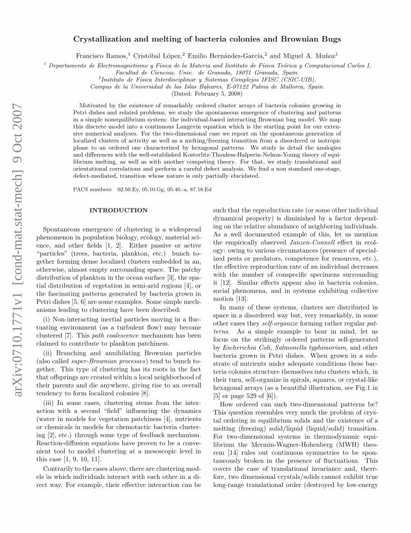
In the active phase, owing to the local-density depen-dent dynamical rules particles group together formingclusters (see Fig. 1 (a) and (b)) provided that the dif-fusion constant is small enough (for large values of D,homogeneous distributions are obtained). Such clustershave a well-defined typical diameter (which can be ana-lytically estimated [29]) and a characteristic number ofparticles within, which depend on the parameters R, Ns,and µ [23, 24]. Well inside the active phase, when theclusters start filling the available space they self-organize

3

(a) (b)

(c) (d)

FIG. 1: Upper panels: Snapshots of two-dimensional IBBmodel in its stationary state (time t = 2 × 105 Monte Carlosteps) in the: (a) disordered active phase, µ = 1.0, and (b)the ordered/patterned active one µ = 2.0; other parametervalues are: Ns = 50, R = 0.1, D = 10−5. Lower panels:Snapshots of the two-dimensional Langevin equation, Eq.(2)in its stationary state for µ = 2.0, D = 0.25, R = 10, Ns =50 in the: (c) disordered active phase σ = 2.5 and (d) theordered/patterned active one, σ = 1.5. Observe that the 2snapshots to the right (b and d) have a crystal-like hexagonalordering, absent in the other two (a and c). Also, the crystal-like packing is more evident in the continuous model for thechosen parameters, but no qualitative difference exist betweenthe upper and the lower panels.

in spatial structures with remarkable hexagonal order(see Fig.1 (b)).

From the theoretical side, an important breakthroughis that the IBB model can be cast into a continuousstochastic equation [23]. Indeed, by applying standardFock-space (Doi-Peliti [30]) techniques, a Langevin equa-tion including the main relevant traits of the problem ina parsimonious way can be derived (see Appendix A in[23] and references therein). The Langevin equation forthe local density [31] of bugs ρ(x, t) reads (in the Itorepresentation)

∂ρ(x, t)

∂t= µρ(x, t) +D∇2ρ(x, t) (2)

−ρ(x, t)

Ns

∫

|x−y|<R

dyρ(y, t) + σ√

ρ(x, t)η(x, t),

where the noise amplitude σ is a function of the micro-scopic parameters and η(x, t) is a normalized Gaussian

white noise. This includes only the leading terms in adensity expansion; for instance, a higher order noise termappear in the mapping [23] but it does not alter the re-sults reported in what follows in any significant way.

Note that, leaving aside the non-local saturation term,this equation coincides with the Reggeon-field theory orGribov process, describing at a coarse-grained level sys-tems with absorbing states in the directed percolation(DP) class (see [20] and references therein). Let us un-derline the presence of a square-root multiplicative noise.Note also that the deterministic part of Eq.(2), includ-ing a non-local saturation term, is identical to the equa-tion proposed by Fuentes et al. [11]. Eq.(2) is thereforea simple (the simplest) stochastic generalization of suchmodel.

The main advantage of the continuous Langevin equa-tion above is that it allows for analytical studies andpermits to scrutinize the effect of fluctuations (by justtuning the noise amplitude). It also constitutes a moregeneral, elegant, and compact formulation of the prob-lem. For these reasons, we choose Eq.(2) as the startingpoint of our forthcoming analyses.

INTEGRATION OF THE LANGEVIN EQUATIONAND FIRST ANALYSES

Analytical studies of the deterministic part of Eq.(2)(i.e. mean field analyses) have already been performedin [11, 23, 24]. They permit, for instance, to understandthe wave-length instability mechanism leading to patternformation, as well as many other aspects. In order to an-alyze the full stochastic Eq.(2) and, in particular, its as-sociated melting/freezing transition, one needs to resortto computational studies.

However, integrating numerically Langevin equationswith square-root noise is a highly non-trivial task; ow-ing to the fact that for small density values the square-root term (with multiplies a random number) becomeslarger in amplitude than the deterministic terms, stan-dard integration schemes (Euler, Runge-Kutta, etc.) leadineluctably to unphysical negative values of the densityfield [32], and this pathology is not easily cured in anynaıve way. Luckily, a very efficient scheme, specificallydevised to overcome such a difficulty, has been recentlyproposed [33].

The method is a split-step algorithm in which the sys-tem is discretized in space and two evolution operationsare performed at each discrete time-step: (i) first, thenoise term is treated in an exact way, by sampling theconditional probability distribution coming out of the(exactly solvable) associated Fokker-Planck equation ateach site. By sampling in an exact way such a distribu-tion an output is produced at each site. (ii) Afterwards,the remaining deterministic terms are integrated usingany standard scheme taking as the input at each site the

4

output of the previous step at each site. More details andapplications can be found in [33].

To implement the split-step scheme to integrate Eq.(2)in two dimensions, we discretize the space, by introducinga lattice of linear size L = 256 or 512 (L ≈ 1024 is al-ready at the limit of our present computational power).We fix the discrete time step to ∆t = 0.25, R = 10,Ns = 50, D = 0.25 (which is small enough to have clus-tering) and use either µ or σ as a control parameter. Forall of the simulations reported here we initialize the sys-tem with a homogeneous initial density, ρ(x, t = 0) = ρ0,leave it relax towards its stationary state (reached typi-cally after 105 Monte Carlo steps), and perform steady-state measurements (averaging over, at least, 105 config-urations).

First of all, we verify that Eq.(2) reproduces qualita-tively all the basic phenomenology of the microscopic IBBmodel: (i) an absorbing phase for small values of µ, (ii)an active disordered phase, encountered by increasing µfor a fixed σ and (iii) an active ordered crystal-like phasewhich is reached by further increasing the value of µ oralternatively, fixing µ and reducing the noise amplitude,σ (see Fig.(1 (c) and (d))).

Separating (i) and (ii) there is a directed-percolation-like phase transition, while our focus here is on the tran-sition from the disordered active phase (ii) to the orderedself-organized one (iii). In order to study the effect of thenoise on such a transition, from now on, we fix µ = 2.0,well into the active phase, and use the noise amplitude,σ, as a tuning parameter. Fig. 1 (plots (c) and (d))shows two snapshots obtained for µ = 2.0 with σ = 2.5and σ = 1.5 respectively. While in both cases clustersof localized activity (ρ(x) 6= 0) exist, only in the secondone clusters are self-organized into an ordered hexagonalarray.

Cluster analyses

A preliminary step towards a systematic cluster anal-ysis is to have an efficient method to detect and labelthem. We have implemented an algorithm, based in theHoshen-Kopelman one [34] as follows. First, to avoidspurious clusters we apply a smoothening filter to thenoisy field ρ(x, t) in our simulations, which removes itsshort wavelength fluctuations:

ρp(x, t) =1

πR2p

∫ |y|=Rp

|y|=0

ρ(x + y, t), dy (3)

where Rp is the cluster average radius (almost constantfor the considered parameter range). Then we define a“smoothened” binary field, ρp(x, t) taking a value 0 (1)wherever ρp(x) < Θ (ρp(x) > Θ). The threshold Θ isfixed to an optimal value Θ = 0.55, found by trial and er-ror, and we verify that an excellent cluster identification

2 2.1 2.2 2.3 2.4 2.52

3

4

5

6

7

8

9

10

σ

m

2 2.1 2.2 2.3 2.4 2.50.12

0.14

0.16

0.18

0.2

0.22

<v c>

<vc>

m

2.2 2.4 2.65.7

5.8

5.9

6

6.1

x 10−3

σ

Nc/N

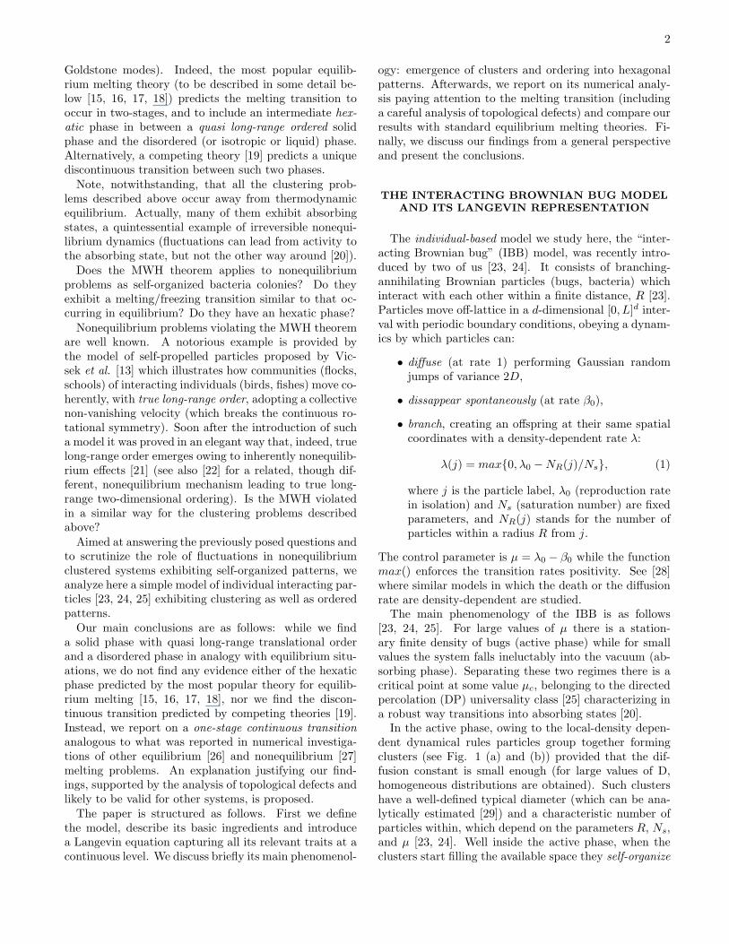
FIG. 2: Main: cluster mobility per unit time (boxes and leftaxis) and mean cluster center of mass velocity (circles andright axis) as a function of σ for L = 256. Inset: Number ofclusters per surface unit versus σ, for L = 256.

(as compared to visual inspection) is obtained. The out-put is not very sensible to the threshold choice althoughsmall variations can be observed. Once the binary dis-cretized field has been constructed, a standard Hoshen-Kopelman algorithm is straightforwardly employed. Itgenerates a list of clusters, together with the list of spa-tial coordinates ascribed to (the center of mass of) eachof them.

Having described the main computational techniques,we now report on various observables characterizing col-lective properties of clusters.

The average cluster mobility, m, is defined as the stan-dard deviation of the excursion of the cluster center ofmass (during a fixed-length time interval), averaged overmany different clusters in the steady state

m =

√

⟨

(xc − 〈xc〉)2⟩

+⟨

(yc − 〈yc〉)2⟩

, (4)

where (xc, yc) are the center of mass cluster coordinatesand 〈·〉 stands for averages in the steady state.

In Fig. 2 we plot m as a function of the noise ampli-tude σ; the mobility exhibits a sharp transition (sharperupon enlarging the system size) from the low-noise phasein which the clusters are almost frozen and localized inspace to the high noise one in which they move morefreely. The change of behavior occurs around σ ≈ 2.39.

Fig. 2 shows also the average velocity (in modulus)of the cluster center of mass (vxc , vyc) versus σ. Whilefor small values of σ we observe a linear dependence be-tween 〈vc〉 and σ [35], this linear dependence is brokenabove certain noise threshold (again around σ ≈ 2.39), atwhich its derivative exhibits a discontinuity. Above thetransition point the velocity increases non-linearly withσ.

5

We have also measured (Fig.2 inset) the number ofclusters per surface unit as a function of σ. While inthe disordered phase the density of clusters increases asthe noise strength is reduced, it remains constant (at avalue corresponding to the maximum capacity) once thethreshold for an ordered structure is reached.

The three described observables provide evidence ofa melting/freezing transition. The change of behavioroccurs in all cases at a unique point, somewhere aroundσ ≈ 2.39. A more detailed finite size scaling analysiswould be required to pin down the critical point withmore accuracy using these observables.

The picture that emerges from these measurements isthat clusters emerge at a mesoscopic scale out of thenonequilibrium microscopic rules and then, upon reduc-ing the noise-amplitude, they self-organize into frozenpatterns with reduced mobility and velocity and with amore compact packing. In this sense, clusters become theequivalent of “particles” in standard liquid/solid transi-tions.

Structure Function Analysis.

In order to obtain an alternative, more direct, estima-tion of the location of the freezing/melting transition notrelying on the (computationally costly) identification ofclusters, we analyze a properly defined structure func-tion. As the overall density varies upon changing pa-rameters and system size, it is convenient to define anormalized version of the structure function as follows

S (k) =⟨

|F(k)|2⟩

k, (5)

where F is the Fourier transform of the normalized den-sity

F(k) =

∫

Ld

ρnorm(x)e−ik·xdx, (6)

k is the momentum, 〈·〉k stands for spherical averagesover all two-dimensional vectors with module k = |k|,and the normalized density ρnorm is

ρnorm (x) =ρ (x)

√

∫

Ld |ρ (x)|2

. (7)

Using this normalized density, and by virtue of the Par-seval’s identity,

∫

L−d |F (k)|2

=∫

Ld |ρnorm (x)|2

= 1, itis guaranteed that S (k) is normalized to unity for allparameter values and system-sizes.

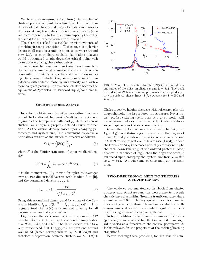
Fig.3 shows the structure-function for a size L = 512as a function of k, for three different noise amplitudes:σ = 2.20, 2.40, and 2.60. The three curves exhibits avery pronounced first Bragg-peak at positions aroundk0L ≈ 43 (which corresponds to k0 ≈ 0.083(9) andtherefore a separation between clusters R0 ≈ 11.9(1).

20 40 60 80 1000

20

40

60

80

100

120

k⋅L

S(k

)

σ=2.002.402.60

1.5 2 2.5 30

50

100

150

200

σ

⟨ S(k

=k 0)

⟩

N=256x256

512x512

FIG. 3: Main plot: Structure function, S(k), for three differ-ent values of the noise amplitude σ and L = 512. The peakaround k0 ≈ 42 becomes more pronounced as we go deeperinto the ordered phase. Inset: S(k0) versus σ for L = 256 andL = 512.

Their respective heights decrease with noise strength: thelarger the noise the less ordered the structure. Neverthe-less, perfect ordering (delta-peak at a given mode) willnever be reached as cluster internal fluctuations enforcesome dispersion in the structure function.

Given that S(k) has been normalized, the height atk0, S(k0), constitutes a good measure of the degree oforder. Actually, an abrupt transition is obtained at aboutσ ≈ 2.39 for the largest available size (see (Fig.3)): abovethe transition S(k0) decreases abruptly corresponding tothe breakdown (melting) of the ordered patterns. Also,observe in the inset of Fig.3 that the degree of order isenhanced upon enlarging the system size from L = 256to L = 512. We will come back to analyze this issuelater.

TWO-DIMENSIONAL MELTING THEORIES:A SHORT REVIEW

The evidence accumulated so far, both from clusteranalyses and structure function measurements, revealsthe existence of a melting/freezing transition, somewherearound σ = 2.39. The key question we face now is:does such a nonequilibrium transition exhibit the well-known universal features of standard equilibrium melt-ing/freezing in two-dimensional systems?

Note, in addition, that here the number of clusters(particles) is not constant but fluctuates, and its averagevalue varies as a function of the control parameter, σ.Is this relevant for the properties at the melting/freezingtransition?

Before tackling these problems, for the sake of com-

6

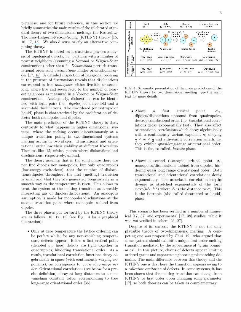
pleteness, and for future reference, in this section webriefly summarize the main results of the celebrated stan-dard theory of two-dimensional melting: the Kosterlitz-Thouless-Halperin-Nelson-Young (KTHNY) theory [15,16, 17, 18]. We also discuss briefly an alternative com-peting theory.

The KTHNY is based on a statistical physics analy-sis of topological defects, i.e. particles with a number ofnearest neighbors (assuming a Voronoi or Wigner-Seitzconstruction) other than 6. Dislocations perturb trans-lational order and disclinations hinder orientational or-der [17, 18]. A detailed inspection of hexagonal orderingin the presence of fluctuations reveals that disclinationscorrespond to free monopoles, either five-fold or seven-fold, where five and seven refer to the number of near-est neighbors as measured in a Voronoi or Wigner-Seitzconstruction. Analogously, dislocations can be identi-fied with tight pairs (i.e. dipoles) of a five-fold and aseven-fold disclinations. The disordered (or isotropic orliquid) phase is characterized by the proliferation of de-fects: both monopoles and dipoles.

The main prediction of the KTHNY theory is that,contrarily to what happens in higher dimensional sys-tems, where the melting occurs discontinuously at aunique transition point, in two-dimensional systemsmelting occurs in two stages. Translational and orien-tational order lose their stability at different Kosterlitz-Thouless-like [15] critical points where dislocations anddisclinations, respectively, unbind.

The theory assumes that in the solid phase there arenor free dipoles nor monopoles, but only quadrupoles(low-energy excitations), that the number of disloca-tions/dipoles throughout the first (melting) transitionis small and that they are generated progressively in asmooth way as the temperature is risen. This allows totreat the system at the melting transition as a weaklyinteracting gas of dipoles/dislocations. An analogousassumption is made for monopoles/disclinations at thesecond transition point where monopoles unbind fromdipoles.

The three phases put forward by the KTHNY theoryare as follows [16, 17, 18] (see Fig. 4 for a graphicalillustration):

• Only at zero temperature the lattice ordering canbe perfect while, for any non-vanishing tempera-ture, defects appear. Below a first critical point(denoted σm here) defects are tight together inquadrupoles, hindering translational order. As aresult, translational correlation functions decay al-gebraically in space (with continuously varying ex-ponents), as corresponds to quasi long-range or-

der. Orientational correlations (see below for a pre-cise definition) decay at long distances to a non-vanishing constant value, corresponding to truelong-range orientational order [36].

FIG. 4: Schematic presentation of the main predictions of theKTHNY theory for two dimensional melting. See the maintext for more details.

• Above a first critical point, σm,dipoles/dislocations unbound from quadrupoles,destroy translational order (i.e. translational corre-lations decay exponentially fast). They also affectorientational correlations which decay algebraicallywith a continuously variant exponent η6 obeying1

4≤ η6 ≤ 1

3and a diverging correlation length, i.e.

they exhibit quasi-long-range orientational order.This is the, so called, hexatic phase.

• Above a second (isotropic) critical point, σi,monopoles/disclinations unbind from dipoles, hin-dering quasi long range orientational order. Bothtranslational and orientational correlations decayexponentially. The associated correlation lengthsdiverge as stretched exponentials of the forma exp(b∆−1/2) where ∆ is the distance to σi. Thisis the isotropic (also called disordered or liquid)phase.

This scenario has been verified in a number of numer-ical [17, 37] and experimental [17, 38] studies, while itwas not verified in others [26, 27].

Despite of its success, the KTHNY is not the onlyplausible theory of two-dimensional melting. A com-peting one was proposed by Chui [19], who argued thatsome systems should exhibit a unique first-order meltingtransition mediated by the appearance of “grain bound-aries”. In this picture, chains of defects appear limitingordered grains and separate neighboring mismatching do-mains. The main difference between this theory and theKTHNY one is that here the transition appears owing toa collective excitation of defects. In some systems, it hasbeen shown that the melting transition can change fromKTHNY to first order upon changing some parameter[17], so both theories can be taken as complementary.

7

−1

0

1

−1

0

1

−1

0

1

0 50 100 150 200 250

−1

0

1

r

g(r)

σ=2.00

σ=2.38

σ=2.42

σ=2.60

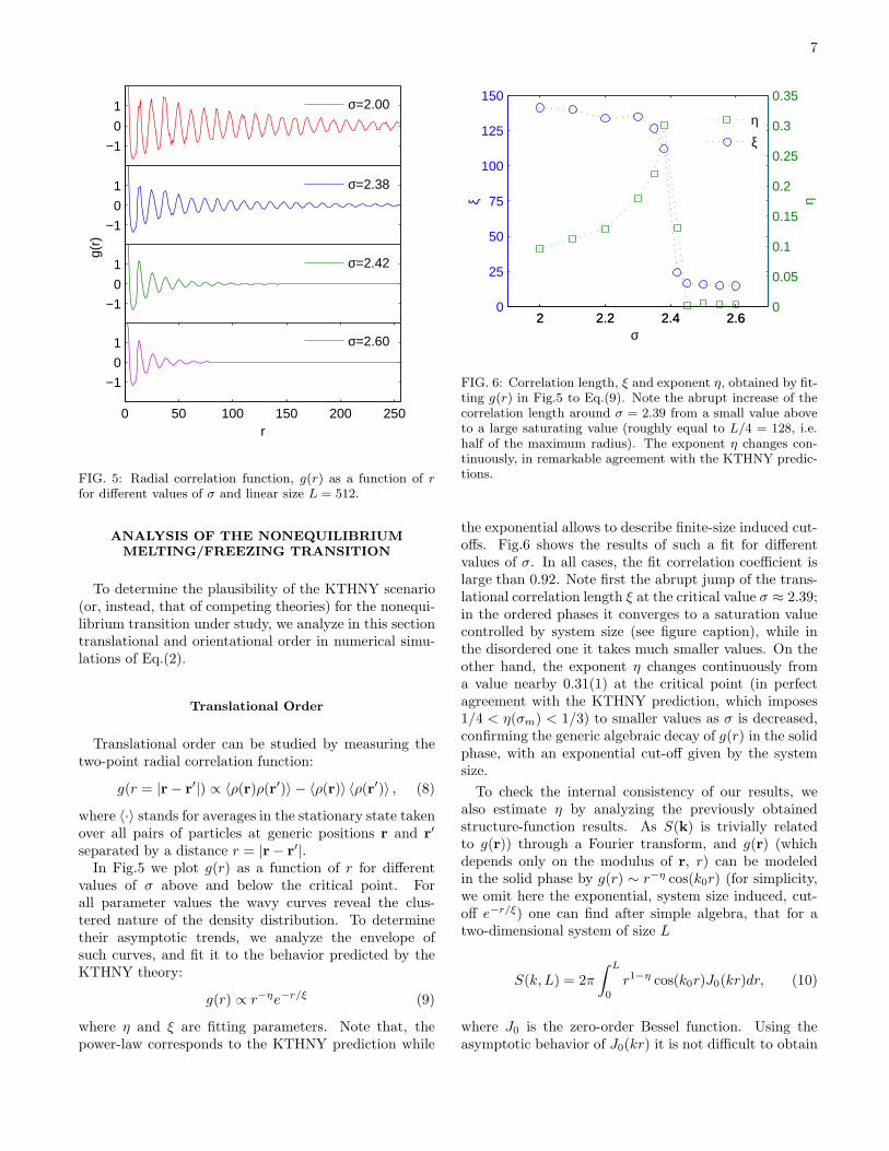
FIG. 5: Radial correlation function, g(r) as a function of rfor different values of σ and linear size L = 512.

ANALYSIS OF THE NONEQUILIBRIUMMELTING/FREEZING TRANSITION

To determine the plausibility of the KTHNY scenario(or, instead, that of competing theories) for the nonequi-librium transition under study, we analyze in this sectiontranslational and orientational order in numerical simu-lations of Eq.(2).

Translational Order

Translational order can be studied by measuring thetwo-point radial correlation function:

g(r = |r − r′|) ∝ 〈ρ(r)ρ(r′)〉 − 〈ρ(r)〉 〈ρ(r′)〉 , (8)

where 〈·〉 stands for averages in the stationary state takenover all pairs of particles at generic positions r and r′

separated by a distance r = |r− r′|.In Fig.5 we plot g(r) as a function of r for different

values of σ above and below the critical point. Forall parameter values the wavy curves reveal the clus-tered nature of the density distribution. To determinetheir asymptotic trends, we analyze the envelope ofsuch curves, and fit it to the behavior predicted by theKTHNY theory:

g(r) ∝ r−ηe−r/ξ (9)

where η and ξ are fitting parameters. Note that, thepower-law corresponds to the KTHNY prediction while

2 2.2 2.4 2.60

25

50

75

100

125

150

ξ

2 2.2 2.4 2.60

0.05

0.1

0.15

0.2

0.25

0.3

0.35

σ

η

η

ξ

FIG. 6: Correlation length, ξ and exponent η, obtained by fit-ting g(r) in Fig.5 to Eq.(9). Note the abrupt increase of thecorrelation length around σ = 2.39 from a small value aboveto a large saturating value (roughly equal to L/4 = 128, i.e.half of the maximum radius). The exponent η changes con-tinuously, in remarkable agreement with the KTHNY predic-tions.

the exponential allows to describe finite-size induced cut-offs. Fig.6 shows the results of such a fit for differentvalues of σ. In all cases, the fit correlation coefficient islarge than 0.92. Note first the abrupt jump of the trans-lational correlation length ξ at the critical value σ ≈ 2.39;in the ordered phases it converges to a saturation valuecontrolled by system size (see figure caption), while inthe disordered one it takes much smaller values. On theother hand, the exponent η changes continuously froma value nearby 0.31(1) at the critical point (in perfectagreement with the KTHNY prediction, which imposes1/4 < η(σm) < 1/3) to smaller values as σ is decreased,confirming the generic algebraic decay of g(r) in the solidphase, with an exponential cut-off given by the systemsize.

To check the internal consistency of our results, wealso estimate η by analyzing the previously obtainedstructure-function results. As S(k) is trivially relatedto g(r)) through a Fourier transform, and g(r) (whichdepends only on the modulus of r, r) can be modeledin the solid phase by g(r) ∼ r−η cos(k0r) (for simplicity,we omit here the exponential, system size induced, cut-off e−r/ξ) one can find after simple algebra, that for atwo-dimensional system of size L

S(k, L) = 2π

∫ L

0

r1−η cos(k0r)J0(kr)dr, (10)

where J0 is the zero-order Bessel function. Using theasymptotic behavior of J0(kr) it is not difficult to obtain

8

that

S(k0, L) ∼ L3/2−η (11)

for the mode k0 (which is the only one for which thereare not destructive interferences).

Actually, in the inset of Fig.(3) we showed that whilethe curves for S(k0, L) overlap for different system sizesabove the critical point, bellow it, they growth with sys-tem size. Indeed they grow algebraically with a slightlyσ-dependent exponent which for all σ values is in theinterval [1.24, 1.36]. Therefore, exploiting Eq.(11) wederive a value for η which is in the interval [0.14, 0.26]in rather good agreement with the direct measurementsabove. Summing up, we have deduced, in two indepen-dent ways, results consistent with algebraically decayingcorrelations as predicted by the KTHNY scenario.

Orientational Order

To quantify the degree of orientational order of a givenconfiguration in the steady state, we first identify theclusters using the algorithm described above. After that,a Voronoi tessellation of the system configuration is con-structed [39]. For each configuration, the correspondingtessellation gives as output the list of clusters and the setof nearest neighbors of each. Finally, for each cluster j,we define [16, 17, 18]

ψ6(j) =1

Nj

Nj∑

k=1

ei6θjk , (12)

where the sum extends over the Nj neighbors of cluster j;θjk is the angle between the centers of mass of clusters jand k and an arbitrary fixed reference axis. The averageof ψ6 over different clusters,

ψ6 =

∣

∣

∣

∣

∣

∣

1

Nc

Nc∑

j=1

ψ6(j)

∣

∣

∣

∣

∣

∣

, (13)

where Nc is the total number of clusters, is a global ori-

entational order parameter. An associated susceptibility

can be also defined, χ6 = Nc

(

⟨

ψ26

⟩

− 〈ψ6〉2)

.

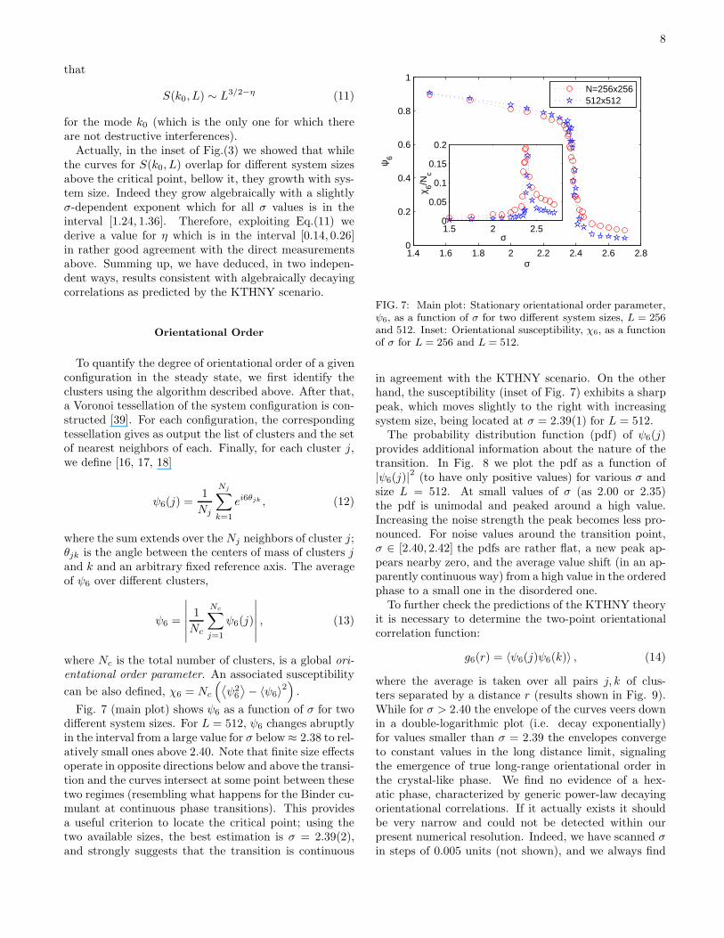
Fig. 7 (main plot) shows ψ6 as a function of σ for twodifferent system sizes. For L = 512, ψ6 changes abruptlyin the interval from a large value for σ below ≈ 2.38 to rel-atively small ones above 2.40. Note that finite size effectsoperate in opposite directions below and above the transi-tion and the curves intersect at some point between thesetwo regimes (resembling what happens for the Binder cu-mulant at continuous phase transitions). This providesa useful criterion to locate the critical point; using thetwo available sizes, the best estimation is σ = 2.39(2),and strongly suggests that the transition is continuous

1.4 1.6 1.8 2 2.2 2.4 2.6 2.80

0.2

0.4

0.6

0.8

1

σ

ψ6

N=256x256512x512

1.5 2 2.50

0.05

0.1

0.15

0.2

σ

χ 6/Nc

FIG. 7: Main plot: Stationary orientational order parameter,ψ6, as a function of σ for two different system sizes, L = 256and 512. Inset: Orientational susceptibility, χ6, as a functionof σ for L = 256 and L = 512.

in agreement with the KTHNY scenario. On the otherhand, the susceptibility (inset of Fig. 7) exhibits a sharppeak, which moves slightly to the right with increasingsystem size, being located at σ = 2.39(1) for L = 512.

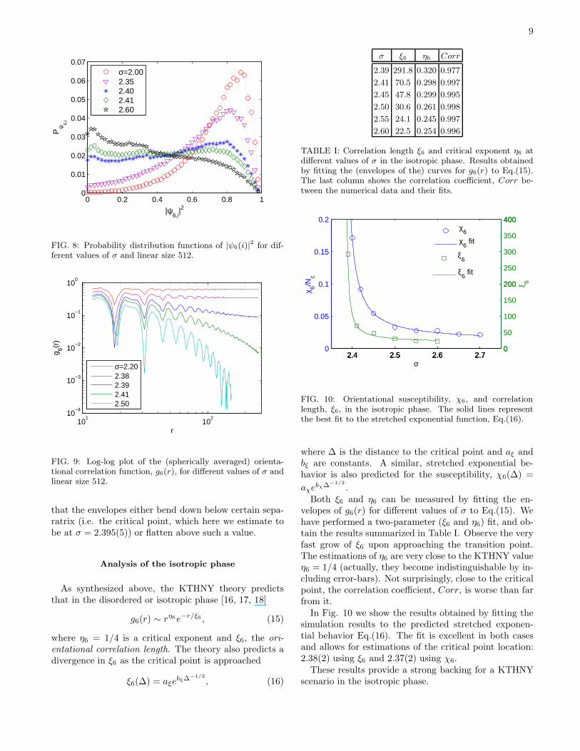
The probability distribution function (pdf) of ψ6(j)provides additional information about the nature of thetransition. In Fig. 8 we plot the pdf as a function of|ψ6(j)|

2(to have only positive values) for various σ and

size L = 512. At small values of σ (as 2.00 or 2.35)the pdf is unimodal and peaked around a high value.Increasing the noise strength the peak becomes less pro-nounced. For noise values around the transition point,σ ∈ [2.40, 2.42] the pdfs are rather flat, a new peak ap-pears nearby zero, and the average value shift (in an ap-parently continuous way) from a high value in the orderedphase to a small one in the disordered one.

To further check the predictions of the KTHNY theoryit is necessary to determine the two-point orientationalcorrelation function:

g6(r) = 〈ψ6(j)ψ6(k)〉 , (14)

where the average is taken over all pairs j, k of clus-ters separated by a distance r (results shown in Fig. 9).While for σ > 2.40 the envelope of the curves veers downin a double-logarithmic plot (i.e. decay exponentially)for values smaller than σ = 2.39 the envelopes convergeto constant values in the long distance limit, signalingthe emergence of true long-range orientational order inthe crystal-like phase. We find no evidence of a hex-atic phase, characterized by generic power-law decayingorientational correlations. If it actually exists it shouldbe very narrow and could not be detected within ourpresent numerical resolution. Indeed, we have scanned σin steps of 0.005 units (not shown), and we always find

9

0 0.2 0.4 0.6 0.8 10

0.01

0.02

0.03

0.04

0.05

0.06

0.07

|ψ6,i

|2

Pψ

6,i

σ=2.002.352.402.412.60

FIG. 8: Probability distribution functions of |ψ6(i)|2 for dif-

ferent values of σ and linear size 512.

101

102

10−4

10−3

10−2

10−1

100

r

g 6(r)

σ=2.202.382.392.412.50

FIG. 9: Log-log plot of the (spherically averaged) orienta-tional correlation function, g6(r), for different values of σ andlinear size 512.

that the envelopes either bend down below certain sepa-ratrix (i.e. the critical point, which here we estimate tobe at σ = 2.395(5)) or flatten above such a value.

Analysis of the isotropic phase

As synthesized above, the KTHNY theory predictsthat in the disordered or isotropic phase [16, 17, 18]

g6(r) ∼ rη6e−r/ξ6 , (15)

where η6 = 1/4 is a critical exponent and ξ6, the ori-

entational correlation length. The theory also predicts adivergence in ξ6 as the critical point is approached

ξ6(∆) = aξebξ∆

−1/2

, (16)

σ ξ6 η6 Corr

2.39 291.8 0.320 0.977

2.41 70.5 0.298 0.997

2.45 47.8 0.299 0.995

2.50 30.6 0.261 0.998

2.55 24.1 0.245 0.997

2.60 22.5 0.254 0.996

TABLE I: Correlation length ξ6 and critical exponent η6 atdifferent values of σ in the isotropic phase. Results obtainedby fitting the (envelopes of the) curves for g6(r) to Eq.(15).The last column shows the correlation coefficient, Corr be-tween the numerical data and their fits.

2.4 2.5 2.6 2.70

0.05

0.1

0.15

0.2

σ

χ 6/Nc

2.4 2.5 2.6 2.70

200

400

2.4 2.5 2.6 2.70

50

100

150

200

250

300

350

400

ξ 6

χ

6

χ6 fit

ξ6

ξ6 fit

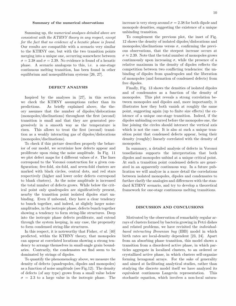
FIG. 10: Orientational susceptibility, χ6, and correlationlength, ξ6, in the isotropic phase. The solid lines representthe best fit to the stretched exponential function, Eq.(16).

where ∆ is the distance to the critical point and aξ andbξ are constants. A similar, stretched exponential be-havior is also predicted for the susceptibility, χ6(∆) =

aχebχ∆

−1/2

.Both ξ6 and η6 can be measured by fitting the en-

velopes of g6(r) for different values of σ to Eq.(15). Wehave performed a two-parameter (ξ6 and η6) fit, and ob-tain the results summarized in Table I. Observe the veryfast grow of ξ6 upon approaching the transition point.The estimations of η6 are very close to the KTHNY valueη6 = 1/4 (actually, they become indistinguishable by in-cluding error-bars). Not surprisingly, close to the criticalpoint, the correlation coefficient, Corr, is worse than farfrom it.

In Fig. 10 we show the results obtained by fitting thesimulation results to the predicted stretched exponen-tial behavior Eq.(16). The fit is excellent in both casesand allows for estimations of the critical point location:2.38(2) using ξ6 and 2.37(2) using χ6.

These results provide a strong backing for a KTHNYscenario in the isotropic phase.

10

Summary of the numerical observations

Summing up, the numerical analyses detailed above are

consistent with the KTHNY theory in any respect, except

for the fact that no evidence of a hexatic phase is found.Our results are compatible with a scenario very similarto the KTHNY one, but with the two transition pointsmerging into a unique one, occurring somewhere betweenσ = 2.38 and σ = 2.39. No evidence is found of a hexaticphase. A scenario analogous to this, i.e. a one-stagecontinuous melting transition, has been found in otherequilibrium and nonequilibrium systems [26, 27].

DEFECT ANALYSIS

Inspired by the analyses in [27], in this sectionwe check the KTHNY assumptions rather than itspredictions. As briefly explained above, the the-ory assumes that the number of dipoles/dislocations(monopoles/disclinations) throughout the first (second)transition is small and that they are generated pro-gressively in a smooth way as the temperature isrisen. This allows to treat the first (second) transi-tion as a weakly interacting gas of dipoles/dislocations(monopoles/disclinations).

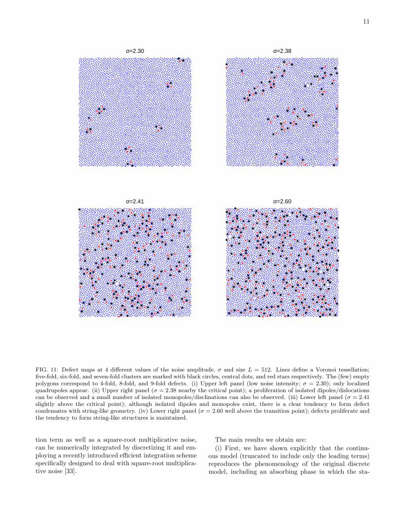
To check if this picture describes properly the behav-ior of our model, we scrutinize how defects appear andproliferate upon rising the noise amplitude. In Fig. 11we plot defect maps for 4 different values of σ. The linescorrespond to the Voronoi construction for a given con-figuration; five-fold, six-fold, and seven-fold clusters aremarked with black circles, central dots, and red starsrespectively (higher and lower order defects correspondto blank clusters). As the noise amplitude is increasedthe total number of defects grows. While below the crit-ical point only quadrupoles are significatively present,nearby the transition point isolated dipoles start un-binding. Even if unbound, they have a clear tendencyto bunch together, and indeed, at slightly larger noise-amplitudes, in the isotropic phase, defects bunch togethershowing a tendency to form string-like structures. Deepinto the isotropic phase defects proliferate, and extendthrough the system keeping, in any case, the propensityto form condensed string-like structures.

In this respect, it is noteworthy that Fisher, et al. [40]predicted, within the KTHNY theory, that monopolescan appear at correlated locations showing a strong ten-dency to arrange themselves in small-angle grain bound-aries. Contrarily, the condensates we find seem to bedominated by strings of dipoles.

To quantify the phenomenology above, we measure thedensity of defects (quadrupoles, dipoles and monopoles)as a function of noise amplitude (see Fig.12). The densityof defects (of any type) grows from a small value belowσ = 2.3 to a large value in the isotropic phase. The

increase is very steep around σ = 2.38 for both dipole andmonopole densities, suggesting the existence of a uniqueunbinding transition.

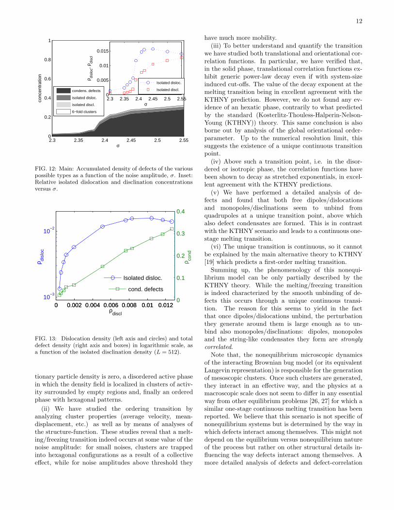
To complement the previous plot, the inset of Fig.12 shows the density of isolated dipoles/dislocations andmonopoles/disclinations versus σ, confirming the previ-ous observations, that the steepest increase occurs atσ ≈ 2.39. Note that the total number of monopoles growscontinuously upon increasing σ, while the presence of arelative maximum in the density of dipoles reflects thecompetition between two conflicting tendencies: the un-binding of dipoles from quadrupoles and the liberationof monopoles (and formation of condensed defects) fromfree dipoles.

Finally, Fig. 13 shows the densities of isolated dipolesand of condensates as a function of the density ofmonopoles. This plot reveals a strong correlation be-tween monopoles and dipoles and, more importantly, itillustrates how they both vanish at roughly the samepoint, suggesting again (up to finite size effects) the ex-istence of a unique one-stage transition. Indeed, if thedipoles unbinding occurred before the monopoles one, theline joining the circles should intersect the vertical axiswhich is not the case. It is also at such a unique tran-sition point that condensed defects appear, being theirdensity (roughly) linearly correlated with the density ofmonopoles.

In summary, a detailed analysis of defects in Voronoitessellations supports the interpretation that bothdipoles and monopoles unbind at a unique critical point.At such a transition point condensed defects are gener-ated in an apparently continuous way. In a future pub-lication we will analyze in a more detail the correlationsbetween isolated monopoles, dipoles and condensates tofurther clarify the analogies and differences with the stan-dard KTHNY scenario, and try to develop a theoreticalframework for one-stage continuous melting transitions.

DISCUSSION AND CONCLUSIONS

Motivated by the observation of remarkably regular ar-rays of clusters formed by bacteria growing in Petri dishesand related problems, we have revisited the individual-

based interacting Brownian bug (IBB) model in whichbirth rates are local-density dependent [23, 24]. Apartfrom an absorbing phase transition, this model shows atransition from a disordered active phase, in which par-ticles aggregate in localized clusters, to an ordered orcrystallized active phase, in which clusters self-organizeforming hexagonal arrays. For the sake of generalityand aimed at facilitating analytical studies, rather thanstudying the discrete model itself we have analyzed itsequivalent continuous Langevin representation. Thisstochastic equation, which involves a non-local satura-

11

σ=2.30 σ=2.38

σ=2.41 σ=2.60

FIG. 11: Defect maps at 4 different values of the noise amplitude, σ and size L = 512. Lines define a Voronoi tessellation;five-fold, six-fold, and seven-fold clusters are marked with black circles, central dots, and red stars respectively. The (few) emptypolygons correspond to 4-fold, 8-fold, and 9-fold defects. (i) Upper left panel (low noise intensity; σ = 2.30); only localizedquadrupoles appear. (ii) Upper right panel (σ = 2.38 nearby the critical point); a proliferation of isolated dipoles/dislocationscan be observed and a small number of isolated monopoles/disclinations can also be observed. (iii) Lower left panel (σ = 2.41slightly above the critical point); although isolated dipoles and monopoles exist, there is a clear tendency to form defectcondensates with string-like geometry. (iv) Lower right panel (σ = 2.60 well above the transition point); defects proliferate andthe tendency to form string-like structures is maintained.

tion term as well as a square-root multiplicative noise,can be numerically integrated by discretizing it and em-ploying a recently introduced efficient integration schemespecifically designed to deal with square-root multiplica-tive noise [33].

The main results we obtain are:

(i) First, we have shown explicitly that the continu-ous model (truncated to include only the leading terms)reproduces the phenomenology of the original discretemodel, including an absorbing phase in which the sta-

12

2.3 2.35 2.4 2.45 2.5 2.550

0.2

0.4

0.6

0.8

1

σ

conc

entr

atio

n

condens. defects

isolated disloc.

isolated discl.

6−fold clusters

2.3 2.35 2.4 2.45 2.5 2.550

0.005

0.01

0.015

σ

ρ disl

oc, ρ

disc

l

Isolated disloc.

Isolated discl.

FIG. 12: Main: Accumulated density of defects of the variouspossible types as a function of the noise amplitude, σ. Inset:Relative isolated dislocation and disclination concentrationsversus σ.

0 0.002 0.004 0.006 0.008 0.01 0.01210

−3

10−2

ρ disl

oc

0 0.002 0.004 0.006 0.008 0.01 0.0120

0.1

0.2

0.3

0.4

ρdiscl

ρ cond

cond. defects

Isolated disloc.

FIG. 13: Dislocation density (left axis and circles) and totaldefect density (right axis and boxes) in logarithmic scale, asa function of the isolated disclination density (L = 512).

tionary particle density is zero, a disordered active phasein which the density field is localized in clusters of activ-ity surrounded by empty regions and, finally an orderedphase with hexagonal patterns.

(ii) We have studied the ordering transition byanalyzing cluster properties (average velocity, mean-displacement, etc.) as well as by means of analyses ofthe structure-function. These studies reveal that a melt-ing/freezing transition indeed occurs at some value of thenoise amplitude: for small noises, clusters are trappedinto hexagonal configurations as a result of a collectiveeffect, while for noise amplitudes above threshold they

have much more mobility.(iii) To better understand and quantify the transition

we have studied both translational and orientational cor-relation functions. In particular, we have verified that,in the solid phase, translational correlation functions ex-hibit generic power-law decay even if with system-sizeinduced cut-offs. The value of the decay exponent at themelting transition being in excellent agreement with theKTHNY prediction. However, we do not found any ev-idence of an hexatic phase, contrarily to what predictedby the standard (Kosterlitz-Thouless-Halperin-Nelson-Young (KTHNY)) theory. This same conclusion is alsoborne out by analysis of the global orientational order-parameter. Up to the numerical resolution limit, thissuggests the existence of a unique continuous transitionpoint.

(iv) Above such a transition point, i.e. in the disor-dered or isotropic phase, the correlation functions havebeen shown to decay as stretched exponentials, in excel-lent agreement with the KTHNY predictions.

(v) We have performed a detailed analysis of de-fects and found that both free dipoles/dislocationsand monopoles/disclinations seem to unbind fromquadrupoles at a unique transition point, above whichalso defect condensates are formed. This is in contrastwith the KTHNY scenario and leads to a continuous one-stage melting transition.

(vi) The unique transition is continuous, so it cannotbe explained by the main alternative theory to KTHNY[19] which predicts a first-order melting transition.

Summing up, the phenomenology of this nonequi-librium model can be only partially described by theKTHNY theory. While the melting/freezing transitionis indeed characterized by the smooth unbinding of de-fects this occurs through a unique continuous transi-tion. The reason for this seems to yield in the factthat once dipoles/dislocations unbind, the perturbationthey generate around them is large enough as to un-bind also monopoles/disclinations: dipoles, monopolesand the string-like condensates they form are strongly

correlated.Note that, the nonequilibrium microscopic dynamics

of the interacting Brownian bug model (or its equivalentLangevin representation) is responsible for the generationof mesoscopic clusters. Once such clusters are generated,they interact in an effective way, and the physics at amacroscopic scale does not seem to differ in any essentialway from other equilibrium problems [26, 27] for which asimilar one-stage continuous melting transition has beenreported. We believe that this scenario is not specific ofnonequilibrium systems but is determined by the way inwhich defects interact among themselves. This might notdepend on the equilibrium versus nonequilibrium natureof the process but rather on other structural details in-fluencing the way defects interact among themselves. Amore detailed analysis of defects and defect-correlation

13

will be investigated in a future work, where we will tryto develop a theoretical framework for one-stage contin-uous melting transitions.

Let us also emphasize that the models we have ana-lyzed are not the best choice to explore with high numer-ical resolution the possibility of one-stage melting from ageneral perspective. Effective models,with a dynamics atthe level of clusters (as opposed to having a microscopicdynamics for particles) would be a much better optionfrom the computational point of view.

In summary, despite of interesting and not fully un-derstood differences, the striking patterns produced bythe biologically inspired Langevin equation (2) resemblevery much the melting/freezing solid/liquid transition inequilibrium systems.

It is our hope that this paper will motivate furtherstudies of (i) the effect of fluctuations on self-organizednonequilibrium patterns and (ii) the analogies and differ-ences between the defect-mediated type of melting tran-sition described here and standard equilibrium meltingscenarios.

ACKNOWLEDGMENTS We acknowledge usefulcomments and discussions with F. de los Santos. Thiswork was supported in part by the Spanish projectsFIS2005-00791 and FIS2004-00953 (Ministerio de Ed-ucacion y Ciencia), FQM-165 (Junta de Andalucıa),and the European Commission through the NEST-Complexity project PATRES (043268).

[1] J. D. Murray, Mathematical Biology, Berlin, Springer-Verlag, 1989.

[2] G. Flierl, D. Grunbaum, S. Levin, and D. Olson, J.Theor. Biol. 196, 397 (1999).

[3] A. P. Martin, Progr. in Oceanography, 57, 125 (2003).[4] Spatial Ecology, Ed. by D. Tilman and P. Kareiva,

(Princeton University Press, Princeton, 1997). J. vonHardenberg et al, Phys. Rev. Lett. 87, 198101 (2001).

[5] E. O. Budrene and H. C. Berg, Nature, 349, 630 (1991);ibid. 376, 49 (1995). D. E. Woodward et al., Biophys. J.68, 2181 (1995).

[6] E. Ben-Jacob, I. Cohen, H. Levine. Adv. Phys. 49, 395(2000).

[7] J. M. Deutsch, J. Phys. A 18, 1449 (1985). M. Wilkinsonand B. Mehlig, Phys. Rev. E 68, 040101(R) (2003). T.Tel, A. de Moura, C. Grebogi, and G. Karolyi, Phys.Rep. 413, 91 (2005).

[8] W. R. Young, A. J. Roberts, and G. Stuhne, Nature,412, 328 (2001). See also, Y-C. Zhang, M. Serva, andM. Polikarpov, J. Stat. Phys. 58, 849 (1990). M. Meyer,S. Havlin, and A. Bunde, Phys. Rev. E 54, 5567 (1996).B. Houchmandzadeh, Phys. Rev. E 66, 052902 (2002). J.Felsenstein, Amer. Natur. 109, 359 (1975).

[9] M. C. Cross and P. C. Hohenberg, Rev. Mod. Phys. 65,851 (1994).

[10] D. Walgraef, Spatio-Temporal Pattern Formation,Springer-verlag, New York, 1997.

[11] M. A. Fuentes, M. N. Kuperman, and V. M. Kenkre,Phys. Rev. Lett. 91, 158104 (2003). Related works are:H. Sayama, M. A. M. de Aguiar, Y. Bar-Yam, and M.Baranger, Phys. Rev. E 65, 051919 (2002); Y. E. Maru-vka and N. M. Shnerb, Phys. Rev. E 73, 011903 (2006).

[12] D. H. Janzen, American Naturalist, 104, 501 (1970). Foran updated review see, Tropical Forest Diversity and Dy-namism, Ed. E. C. Losos and E. G. Leigh, Jr. ChicagoUniversity Press, Chicago, 2004.

[13] T. Vicsek, A. Czirok, E. Ben-Jacob, I. Cohen, and O.Shochet, Phys. Rev. Lett. 75, 1226 (1995). See also,G. Gregoire and H. Chate, Phys. Rev. Lett. 92, 25702(2004). G. Gregoire, H. Chate, and Y. Tu, Physica D181, 157 (2003). E. V. Albano, Phys. Rev. Lett. 77 2129(1996).

[14] N. D. Mermin and H. Wagner, Phys. Rev. Lett. 17, 1133(1966). P. C. Hohenberg, Phys. Rev. 158, 383 (1967). N.D. Mermin, Rev. Mod. Phys. 51, 591 (1979).

[15] J. M. Kosterlitz and D. J. Thouless, J. Phys. C 6, 1181(1973).

[16] B. I. Halperin and D. R. Nelson, Phys. Rev. Lett. 41,121 (1978). D. R: Nelson and B. I. Halperin, Phys. Rev.B 19, 2457 (1979). D. R: Nelson and B. I. Halperin, 21,5312 (1980). A. P. Young, Phys. Rev. B 19, 1855 (1979).

[17] K. J. Strandburg, Rev. Mod. Phys., 60, 161 (1988).[18] D. R. Nelson, Defects and Geometry in Condensed Matter

Physics, Cambridge University Press, Boston (2002).[19] S. T. Chui, Phys. Rev. Lett. 48, 933 (1982); Phys. Rev.

B 28, 178 (1983). See also, M. A. Glaser and N. A. Clark,Adv. Chem. Phys. 83, 543 (1993).

[20] H. Hinrichsen, Adv. Phys. 49, 815 (2000). G. Grinsteinand M. A. Munoz, in Fourth Granada Lectures in Com-putational Physics, Ed. P. L. Garrido and J. Marro,Springer, Berlin, 1997. G. Odor, Rev. Mod. Phys. 76,663 (2004).

[21] J. Toner and Y. Tu, Phys. Rev. Lett. 75 , 4326 (1996).J. Toner, Y. Tu, and S. Ramaswany, Ann. of Phys. 318,170 (2005).

[22] K. E. Bassler and Z. Racz, Phys. Rev. E 52, R9 (1995).[23] E. Hernandez-Garcıa and C. Lopez, Phys. Rev. E 70,

016216 (2004).[24] C. Lopez and E. Hernandez-Garcıa, Physica D 199, 223

(2004). E. Hernandez-Garcıa and C. Lopez, J. Phys.Cond. Matt. 17, S4263 (2005).

[25] C. Lopez, F. Ramos, and E. Hernandez-Garcıa, J.Phys.(Condensed Matter) 19, 065133 (2007 ).

[26] J. F. Fernandez, J. J. Alonso, and J. Stankiewicz, Phys.Rev. Lett. 75, 3477 (1995). Phys. Rev. E 55, 750 (1997).J. J. Ruiz-Lorenzo, E. Moro, and R. Cuerno, Phys. Rev.E 73, 015103(R) (2006).

[27] R. A. Quinn and J. Goree, Phys. Rev. E 64 051404(2001).

[28] B. M. Bolker and S. W. Pacala, Theor. Pop. Biol. 52 179(1997). D. Birch and W. R. Young, J. Theor. Pop. Biol.70, 26 (2006). C. Lopez, Phys. Rev. E 74, 012102 (2006).

[29] Since the only factor impeding unbounded diffusivespreading of particles is their finite lifetime which, in itsturn, is proportional to the inverse of the death rate,1/β0, the average linear size of clusters has to be propor-

tional top

D/β0, as can be numerically verified [23, 24].[30] M. Doi, J. Phys. A 9, 1479 (1976). L. Peliti, J. Physique,

14

46, 1469 (1985). P. Grassberger and M. Scheunert,Fortschr. Phys. 28, 547 (1980). C. J. DeDominicis, J.Physique 37, 247 (1976). H. K. Janssen, Z. Phys. B 23,377 (1976).

[31] Strictly speaking, when employing the Doi-Peliti formal-ism the resulting field is not a density field, but its firstmoment coincide with the density [30].

[32] R. Dickman, Phys. Rev. E 50, 4404 (1994). C. Lopez andM. A. Munoz, Phys. Rev. E 56, 4864 (1997).

[33] I. Dornic, H. Chate, and M. A. Munoz, Phys. Rev. Lett.94, 100601 (2005). See also, L. Pechenik and H. Levine,Phys. Rev. E 59, 3893 (1999). E, Moro, Phys. Rev. E 70,045102(R) (2004).

[34] J. Hoshen and R. Kopelman, Phys. Rev. B 14 3438(1976).

[35] The linear dependence in the ordered phase can be in-terpreted as a direct transfer of the “thermal” energyintroduced by the noise to the kinetic energy of clusters.

[36] Orientational ordering escapes the premises of the MWHtheorem. Indeed, the local hexagonal ordering induces aneffective long-range interaction not covered by the theo-

rem hypotheses.[37] A. Jaster, Phys. Rev. E 59, 2594 (1999); Phys. Lett. A

330, 120 (2004). K. Chen, T. Kaplan, and M. Mostoller,Phys. Rev. Lett. 74, 4019 (1995). K. Bagchi, H. C. An-dersen, and W. Swope, Phys. Rev. Lett. 76, 255 (1996).R. Radhakrishnan, K. E. Gubbins, and M. Sliwinska-Bartkowiak, Phys. Rev. Lett. 89, 076101 (2002). C. H.Mak, Phys. Rev. E 73, 065104(R) (2006). S. Z. Lin, B.Zheng, and S. Trimper, Phys. Rev. E 73, 066106 (2006).

[38] J. D. Brock, R. J. Birgenau, J. D. Lister, and A. Aharony,Phys. Today 42, 52 (1989). C. F. Chou, A. J. Jin, S. W.Hwang, and J. T. Ho, Science 280, 1424 (1998).

[39] A. Okabe, B. Boots, and K. Sugihara, Spatial Tessella-tions, Concepts and Applications of Voronoi diagrams,John Wiley and Sons Ltd. England (1992). J. R. Sackand J. Urrutia, Handbook of Computational Geometry,Elsevier Science, Netherlands (2000).

[40] D. S. Fisher, B. I. Halperin, and R. Morf, Phys. Rev. B20, 4692 (1979).