Damageâviscoplastic consistency model with a parabolic cap for rocks with brittle and ductile behavior under low-velocity impact loading

INTERNATIONAL JOURNAL FOR NUMERICAL AND ANALYTICAL METHODS IN GEOMECHANICSInt. J. Numer. Anal. Meth. Geomech. 2010; 34:1362–1386Published online 14 December 2009 in Wiley Online Library (wileyonlinelibrary.com). DOI: 10.1002/nag.868

Damage–viscoplastic consistency model with a parabolic capfor rocks with brittle and ductile behavior under low-velocity

impact loading

Timo Saksala∗,†

Department of Mechanics and Design, Tampere University of Technology, Tampere, Finland

SUMMARY

This paper presents a damage–viscoplastic cap model for rocks with brittle and ductile behavior underlow-velocity impact loading, which occurs, e.g. in percussive drilling. The model is based on a combinationof the recent viscoplastic consistency model by Wang and the isotropic damage concept. This approachdoes not suffer from ill posedness—caused by strain softening—of the underlying boundary/initial-valueproblem since viscoplasticity provides a regularization under dynamic loading by introducing an internallength scale. The model uses the Drucker–Prager (DP) yield function with the modified Rankine criterionas a tension cut-off and a parabolic cap surface as a compression cut-off. The parabolic cap is smoothlyfitted to the DP cone. The strain softening law in compression is calibrated with the degradation indexconcept of Fang and Harrison. Thereby, the model is able to capture the brittle-to-ductile transition andhardening behavior of geomaterials under highly confined compression, which is the prevailing stressstate under a bit-button in percussive drilling. Rock strength heterogeneity is characterized statisticallyat the structural level using the Weibull distribution. An explicit time integrator is chosen for solvingthe FE-discretized equations of motion. The contact constraints due to the impact of an indenter areimposed with the forward increment Lagrange multiplier method that is compatible with explicit timeintegrators. The model is tested at the material point level with various uniaxial and triaxial tests. At thestructural level confined compression, uniaxial tension tests and a rock sample under low-velocity impactare simulated. Copyright q 2009 John Wiley & Sons, Ltd.

Received 12 February 2009; Revised 6 October 2009; Accepted 8 October 2009

KEY WORDS: viscoplastic consistency model; Drucker–Prager criterion; damage model; cap model; rockfracture; Weibull distribution; contact constraints

1. INTRODUCTION

The major factors affecting the fracture process of rock are the heterogeneity of rock microstructureand the external loading along with its rate. In confined compression, for example, the microscopic

∗Correspondence to: Timo Saksala, Department of Mechanics and Design, Tampere University of Technology, P.O.Box 589, FIN-33101, Tampere, Finland.

†E-mail: [email protected]

Copyright q 2009 John Wiley & Sons, Ltd.

DAMAGE–VISCOPLASTIC CONSISTENCY MODEL 1363

processes involved can be classified as brittle and ductile processes [1]. The former, occurringmainly at the low confinement region, involves a lot of microcracking, whereas in the latter casemicrosliding caused by high confining pressure prevails. An unconfined rock sample fails in axialsplitting mode with one or few contiguous failure planes. Under low confinement, the axial splittingis suppressed and a specimen fails with a shear band formed by highly concentrated interactingmicrocracks. At the high levels of confinement, the shear band formation is suppressed andhomogeneous microcracking and microsliding prevail throughout the sample [2]. This deformation,called cataclastic flow, is characterized by inelastic deformations due to irreversible changes ofthe grain network geometry at the micro structural level [3]. Cataclastic flow results, as the grainsare immobilized and the porosity is minimized, in the rise of the bulk modulus of the material,which is macroscopically observed as a steep rising in the stress–strain curve [3]. In tension theexisting microcracks grow perpendicular to the direction of loading and new microcracks nucleate.The response of the specimen can be perfectly brittle or quasi-brittle depending on whether thepropagation of new and existing microcracks is stable or unstable [3]. The failure mode is thetransverse splitting mode.

A practical problem of considerable importance, where all of these failure modes are involved,is the drill bit–rock interaction in percussive drilling. There the impact-induced stress wave (withamplitude ranging from 200 to 300MPa) is transmitted from the drill bit into the rock by the bit-buttons. The side crack formation therein is due to tensile cracking or mixed tensile-shear cracking.In the region immediately under the drill bit a triaxial stress state prevails and the compressivestrength of rock is exceeded [4, 5]. In this region, called a crushed zone, microcracking is pervasiveand rock behaves in a ductile manner [4, 5]. A detailed description of the fracture mechanisms inrock in quasi-static indentation can be found in [4, 5].

Many continuum-based models using damage mechanics and/or plasticity theory have beendeveloped to account for the complex phenomenona involved in rock fracture during percussivedrilling. Liu et al. studied the bit–rock fragmentation mechanisms numerically with their quasi-staticR-D2D code which is based on a continuum scalar damage model with a double-elliptic strengthcriterion and statistically distributed material parameters [4, 5]. In these studies the indentationproblem was considered quasi-static. The bit–rock indentation in percussive drilling is, however,a dynamic problem where the development of the stress state due to the impact of a bit-buttonand the consequent stress wave propagation are transient events with high local strain rates. Forthis reason, Saksala [6] studied the impact indentation of rock with a rate-independent damage–plasticity model. Other dynamic approaches on the numerical modeling of percussive drilling areby Thuro and Schormair [7] based on PFC and by Rossmanith et al. [8] based on a finite differencescheme. These approaches are, however, either not able to accommodate the strain rate effects,being rate-independent models [4–8], or cannot account for the ductile behavior under a bit-buttonas they have no cap model [6–8].

This paper presents a constitutive model for rock that is, in principle, capable to account forthe above-mentioned failure modes and strain rate effects. The model is based on a combinationof the recent viscoplastic consistency model by Wang et al. [9, 10], the isotropic damage conceptand a cap hardening model the novelty being in the combination of these existing concepts. Othercombinations of damage and plasticity/viscoplasticity in geomaterials modeling are, e.g. [11–15]to mention but only a few. Combinations of damage and viscoplastic consistency models seem,however, rare in the literature.

In dynamic loading conditions, viscoplasticity preserves the well-posedness of the underlyingboundary/initial-value problem (BIVP) by introducing a length-scale effect through inertia [9, 16]

Copyright q 2009 John Wiley & Sons, Ltd. Int. J. Numer. Anal. Meth. Geomech. 2010; 34:1362–1386DOI: 10.1002/nag

1364 T. SAKSALA

and naturally accommodates the strain rate effects as well. Viscoplastic stress states are indicatedby the Drucker–Prager (DP) yield function with the modified Rankine (MR) criterion as a tensioncut-off. The ductile behavior (cataclastic flow) is governed by a parabolic cap surface smoothlyfitted to the DP surface. The softening in tension is due to damaging, while in compression thestrength degradation is governed by a strain softening law calibrated with the degradation index,a material property proposed by Fang and Harrison [17]. At the mesoscopic level the constitutivemodel is kept as simple as possible since the nonlinear response observed in the experiments canbe achieved at the laboratory experiment level by characterizing the rock heterogeneity statisticallyas in the models of Liu [4] and Fang and Harrison [1].

The model is implemented with an explicit time integrator. Contact constraints are imposed withthe forward increment Lagrange multiplier method that is compatible with explicit integrators. Inorder to demonstrate the performance of the present approach, it is tested in various uniaxial andtriaxial tests at the material point (finite element) level. At the structural level, confined compressionand uniaxial tension tests and the impact indentation with a right-angled indenter are simulated inplane strain conditions both with homogeneous and heterogeneous strength properties.

2. THEORY OF THE MODEL

2.1. Viscoplastic consistency model

The viscoplastic consistency model presented by Wang et al. [9, 10] introduces the strain rateeffects into the classical rate-independent plasticity. Accordingly, a trial stress state violating theyield criterion is returned to the yield surface as in the rate-independent plasticity. Moreover, thesplit of the strain tensor in elastic and viscoplastic parts is assumed as in rate-independent plasticity,i.e. e= ee+ evp. The major difference to the rate-independent plasticity is the dependence of theyield function on the rate of the internal variable(s). The basic ingredients of the viscoplasticconsistency model are

fvp = f (r,�, �)

evp = ��gvp�r

fvp � 0, ��0, � fvp=0

(1)

where r is the stress (tensor or matrix), gvp is the viscoplastic potential, � ,� are the internalvariable and its rate, respectively, and � is the viscoplastic increment. The yield function fvpcan be called as a dynamic yield function, as it can expand and shrink in relation to its staticposition (�=0) depending on the strain rate. Moreover, the loading–unloading conditions of theKuhn–Tucker form must hold.

2.1.1. DP viscoplasticy with tension and compression cut-offs. For the present purpose, a three-surface viscoplasticity model consisting of the DP, the MR (tension cut-off), and a parabolic cap(compression cut-off) yield functions is formulated. These functions read in the above-mentioned



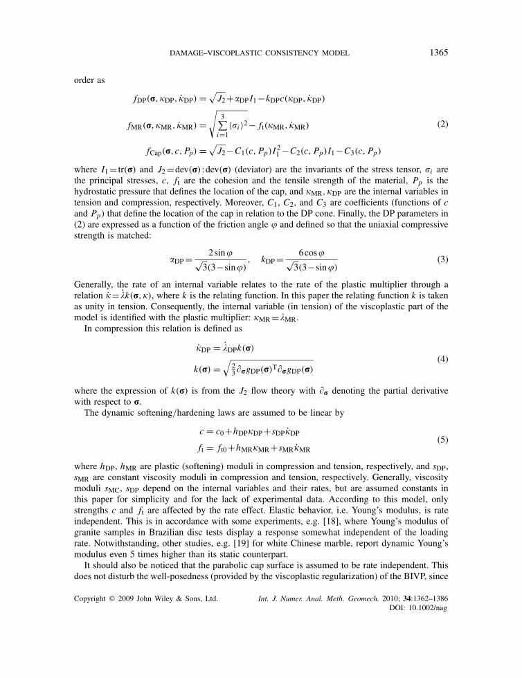
order as

fDP(r,�DP, �DP) =√J2+�DP I1−kDPc(�DP, �DP)

fMR(r,�MR, �MR) =√

3∑i=1

〈�i 〉2− ft(�MR, �MR)

fCap(r,c, Pp) =√J2−C1(c, Pp)I

21 −C2(c, Pp)I1−C3(c, Pp)

(2)

where I1= tr(r) and J2=dev(r) :dev(r) (deviator) are the invariants of the stress tensor, �i arethe principal stresses, c, ft are the cohesion and the tensile strength of the material, Pp is thehydrostatic pressure that defines the location of the cap, and �MR,�DP are the internal variables intension and compression, respectively. Moreover, C1, C2, and C3 are coefficients (functions of cand Pp) that define the location of the cap in relation to the DP cone. Finally, the DP parameters in(2) are expressed as a function of the friction angle � and defined so that the uniaxial compressivestrength is matched:

�DP= 2sin�√3(3−sin�)

, kDP= 6cos�√3(3−sin�)

(3)

Generally, the rate of an internal variable relates to the rate of the plastic multiplier through arelation �= �k(r,�), where k is the relating function. In this paper the relating function k is takenas unity in tension. Consequently, the internal variable (in tension) of the viscoplastic part of themodel is identified with the plastic multiplier: �MR=�MR.

In compression this relation is defined as

�DP = �DPk(r)

k(r) =√

23�rgDP(r)

T�rgDP(r)(4)

where the expression of k(r) is from the J2 flow theory with �r denoting the partial derivativewith respect to r.

The dynamic softening/hardening laws are assumed to be linear by

c = c0+hDP�DP+sDP�DP

ft = ft0+hMR�MR+sMR�MR(5)

where hDP, hMR are plastic (softening) moduli in compression and tension, respectively, and sDP,sMR are constant viscosity moduli in compression and tension, respectively. Generally, viscositymoduli sMC, sDP depend on the internal variables and their rates, but are assumed constants inthis paper for simplicity and for the lack of experimental data. According to this model, onlystrengths c and ft are affected by the rate effect. Elastic behavior, i.e. Young’s modulus, is rateindependent. This is in accordance with some experiments, e.g. [18], where Young’s modulus ofgranite samples in Brazilian disc tests display a response somewhat independent of the loadingrate. Notwithstanding, other studies, e.g. [19] for white Chinese marble, report dynamic Young’smodulus even 5 times higher than its static counterpart.

It should also be noticed that the parabolic cap surface is assumed to be rate independent. Thisdoes not disturb the well-posedness (provided by the viscoplastic regularization) of the BIVP, since


1366 T. SAKSALA

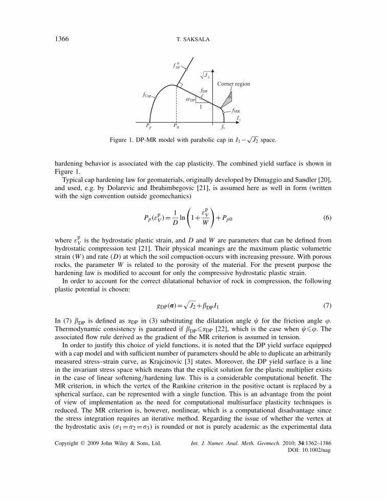
Pp Ptr

Figure 1. DP-MR model with parabolic cap in I1−√J2 space.

hardening behavior is associated with the cap plasticity. The combined yield surface is shown inFigure 1.

Typical cap hardening law for geomaterials, originally developed by Dimaggio and Sandler [20],and used, e.g. by Dolarevic and Ibrahimbegovic [21], is assumed here as well in form (writtenwith the sign convention outside geomechanics)

Pp(εpV )= 1

Dln

(1+ ε

pV

W

)+Pp0 (6)

where εpV is the hydrostatic plastic strain, and D and W are parameters that can be defined from

hydrostatic compression test [21]. Their physical meanings are the maximum plastic volumetricstrain (W ) and rate (D) at which the soil compaction occurs with increasing pressure. With porousrocks, the parameter W is related to the porosity of the material. For the present purpose thehardening law is modified to account for only the compressive hydrostatic plastic strain.

In order to account for the correct dilatational behavior of rock in compression, the followingplastic potential is chosen:

gDP(r)=√J2+�DP I1 (7)

In (7) �DP is defined as �DP in (3) substituting the dilatation angle � for the friction angle �.Thermodynamic consistency is guaranteed if �DP��DP [22], which is the case when ��. Theassociated flow rule derived as the gradient of the MR criterion is assumed in tension.

In order to justify this choice of yield functions, it is noted that the DP yield surface equippedwith a cap model and with sufficient number of parameters should be able to duplicate an arbitrarilymeasured stress–strain curve, as Krajcinovic [3] states. Moreover, the DP yield surface is a linein the invariant stress space which means that the explicit solution for the plastic multiplier existsin the case of linear softening/hardening law. This is a considerable computational benefit. TheMR criterion, in which the vertex of the Rankine criterion in the positive octant is replaced by aspherical surface, can be represented with a single function. This is an advantage from the pointof view of implementation as the need for computational multisurface plasticity techniques isreduced. The MR criterion is, however, nonlinear, which is a computational disadvantage sincethe stress integration requires an iterative method. Regarding the issue of whether the vertex atthe hydrostatic axis (�1=�2=�3) is rounded or not is purely academic as the experimental data



are too scattered to decide this matter definitively [3]. Thus, the choice of the MR criterion isjustified.

2.1.2. Fitting of cap to DP cone and determination of the active surface. In order to regularize thetransition from the DP cone to the parabolic cap, a continuation of the gradient field is imposed.This means that the DP flow rule direction should be equal to the direction of the cap flow rule atthe intersection of these surfaces. Thus, the conditions for fitting the cap to the DP cone are

−�DPPtr+�DP = C1P2tr +C2Ptr+C3

−�DP = 2C1Ptr+C2

0 = C1P2p +C2Pp+C3

(8)

where Ptr is a transition (hydrostatic) pressure at which the transition from DP yield mode to thecap hardening mode (see Figure 1) occurs.

The first of the conditions in (8) guarantees a continuous transition from the DP surface tothe parabolic cap. The second condition ensures that the gradient of the viscoplastic DP potentialequals the gradient of the cap at the transition pressure Ptr. In case of the associated DP flowrule (�DP=�DP), these two conditions provide a smooth transition from the DP failure line to theparabolic cap. The last condition ensures that the cap intersects I1-axis at the pressure Pp. Onsolving the system (8) the coefficients C1, C2, and C3 can be obtained as the functions of Ptr, Pp.

The transition pressure Ptr is usually assumed to move in some relation to Pp. In the parabolic capmodel for Boise sandstone proposed by Carroll [23], the width of the parabola is assumed to stayconstant during hardening. In the present formulation the transition pressure moves proportionatelyto Pp

Ptr= Pp(εpV )

Pp0Ptr0= Pp(ε

pV )kp (9)

where Ptr0 ,Pp0 are the initial values of the pressures Ptr ,Pp, and kp is their ratio. This choicepreserves the aspect ratio of the cap surface.

A check procedure is required in order to determine the active surface. For this end, an additionalcriterion f NDP shown in Figure 1 is introduced and defined as the normal line to the DP cone at thetransition pressure Ptr

f NDP =√J2−�−1

DP I1−�NDP

�NDP = Ptr(�DP+�−1DP)+kDPc(�DP, �DP)

(10)

where �NDP is determined from the geometry in Figure 1. The active surface detection is performedon the basis of a trial elastic state computed at time t as sketched in Table I.

The active surface detection scheme proposed here differs significantly from that used byDolorevic and Ibrahimbegovic [21] in their smooth transition from the DP cone to an elliptic capsurface and linear tension cut-off. Namely, they transform the DP yield function from the stressto the strain space and perform the active surface detection in the strain space while here it isperformed in the stress space. The detection method presented here is thus simpler.

The stress integration (return mapping) is performed with respect to the active surface. Stressupdate algorithms for the viscoplastic consistency model are considered, e.g. in [9, 10, 24]. Here,


1368 T. SAKSALA

Table I. A scheme for active surface detection.

1. f NDP>0

If f trialCap >0→ cap plasticityElse → elastic process

2. f NDP�0

If I trial1 <Ptr and f trialCap >0→ cap plasticity

Elseif f trialDP >0 and f trialMR >0→ MR-DP viscoplasticity

Elseif f trialDP >0 and f trialMR �0→ DP viscoplasticity

Elseif f trialDP �0 and f trialMR >0→ MR viscoplasticityElse → elastic process

these methods are not followed. Instead, the generalized cutting plane method is employed dueto its simplicity (for details, see [25]). Moreover, multisurface plasticity techniques are neededin treating the corner point situation (MR-DP viscoplasticity in Table I and the gray triangle inFigure 1). The standard procedure based on Koiter’s rule is employed here (for details, see [25]).2.2. Calibration of the softening law with the degradation index concept

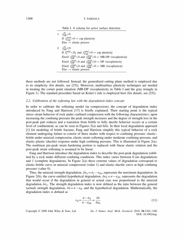
In order to calibrate the softening model (in compression), the concept of degradation indexintroduced by Fang and Harrison [17] is briefly explained. Their starting point is the typicalstress–strain behavior of rock under confined compression with the following characteristics: uponincreasing the confining pressure the peak strength increases and the degree of strength loss in thepost-peak part reduces and a transition from brittle to fully ductile behavior occurs at a certainlevel of confinement, as can be seen in Figures 5(a) and 6(b). In their local degradation approach[1] for modeling of brittle fracture, Fang and Harrison simplify this typical behavior of a rockelement undergoing failure to consist of three modes with respect to confining pressure: elastic–brittle under uniaxial compression, elastic-strain softening under moderate confining pressure, andelastic–plastic (ductile) response under high confining pressure. This is illustrated in Figure 2(a).The nonlinear pre-peak strain hardening portion is replaced with linear elastic relation and thepost-peak strain softening is assumed to be linear.

Fang and Harrison introduce the degradation index to describe the post-peak degradation exhib-ited by a rock under different confining conditions. This index varies between 0 (no degradation)and 1 (complete degradation). In Figure 2(a) these extreme values of degradation correspond toelastic–brittle curve in uniaxial compression (value 1) and elastic–ductile curve at high confiningpressure (value 0).

Thus, the uniaxial strength degradation, �u =�c−�du, represents the maximum degradation. InFigure 2(b), the curve entitled hypothetical degradation, �h =�−�dh, represents the degradationthat would occur if the degradation in general or actual case was proportional to the uniaxialdegradation �u . The strength degradation index is now defined as the ratio between the general(actual) strength degradation, �=�−�d, and the hypothetical degradation. Mathematically, thedegradation index is defined as

rd= �−�d�−�dh

= �

�h(11)



Figure 2. Simplified stress–strain relations of rock under different confining pressures (a) and illustrationof the degradation index (b) (redrawn from [17]).

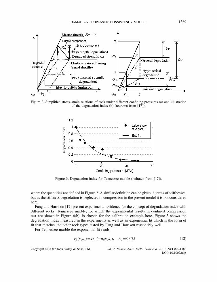
Figure 3. Degradation index for Tennessee marble (redrawn from [17]).

where the quantities are defined in Figure 2. A similar definition can be given in terms of stiffnesses,but as the stiffness degradation is neglected in compression in the present model it is not consideredhere.

Fang and Harrison [17] present experimental evidence for the concept of degradation index withdifferent rocks. Tennessee marble, for which the experimental results in confined compressiontest are shown in Figure 6(b), is chosen for the calibration example here. Figure 3 shows thedegradation index measured in the experiments as well as an exponential fit which is the form offit that matches the other rock types tested by Fang and Harrison reasonably well.

For Tennessee marble the exponential fit reads

rd(�con)=exp(−nd�con), nd=0.075 (12)


1370 T. SAKSALA

The degradation index is now used in calculating the present value of cohesion ct, its residualvalue cres, and the softening modulus as follows:

ct = max(cres,c0+hDP�DP+sDP�DP)

cres = (1−rd(�con))c0

hDP(�conf) = hDP0 ·rd(�con)(13)

where hDP0 is the initial softening modulus. With these choices, the response in compressionof the model is linear elastic until the peak strength after which a linear softening curve untilthe residual strength follows. The softening modulus decreases exponentially (as a function ofconfining pressure) as well. Upon reaching the residual value of cohesion the softening modulusis set to zero.

2.3. Damage formulation and combining the damage and viscoplastic parts

In the damage part of the present model, the standard phenomenological isotropic (scalar) damagemodel is employed with a typical exponential damage function

t=gt(εvpeqvt)=1−(1−At+At exp(−�tε

vpeqvt)) (14)

where At, �t are the parameters controlling the final value and the slope of the damage variable,respectively, and ε

vpeqvt is a cumulative equivalent viscoplastic strain that serves as a history variable.

Within a numerical algorithm it is computed incrementally. The increment is defined so that onlypositive strains contribute to the damage growth:

�εvpeqvt=

√3∑

i=1〈�ε

vpi 〉2 (15)

In (15) �εvpi denote the principal values of the viscoplastic strain increment �evp. As the damage

evolution is driven by (visco) plastic strain, the rate effect affects the damage evolution as well.In the rate-independent plasticity, the coupling of damage and plasticity affects the requirements

for the parameters of the combined model and the implementation as well. Two groups of models,namely those with the plastic part written in terms of the nominal or effective stress, are studiedby Grassl and Jirasek [26]. The effective stress space formulation poses no extra restrictions on themodel parameters while the model formulated with the nominal stress must be strongly hardening.Moreover, the effective space formulation provides a natural means to separate the plasticity anddamage computations so that the robust methods of computational plasticity can be employed inthe stress integration. Jason et al. [27] and Grassl and Jirasek [26] applied this formulation in theirdamage–plastic models for concrete. The effective stress formulation is used here as the argumentdeveloped in [26] applies for consistent viscoplasticity as well.

Deactivation–activation of damage is required when a microcrack closes and opens in cyclicloading. Here, a simple method based on the positive–negative part split of the effective principalstress is employed. Accordingly, the nominal-effective stress relation is

r=(1−t)r++ r− (r= r++ r−) (16)



with r+ =max(r,0) and r− =min(r,0) being the positive and negative parts, respectively, of theprincipal effective stress. This relation preserves the thermodynamic consistency of the viscoplas-ticity part of the model as shown in Appendix A.

2.4. Parameters required by the model

Finally, the parameters required by the present approach are listed. The number of these parametersis still quite decent including the deformation parameters, E , �, �, � , the strength parameters,ft, fc, Weibull modulus mw and the location parameter xu , the cap hardening parameters D, W ,the cap transition and location pressures Ptr, Pp, the viscosity parameters sDP, sMR, parameters �t,At for tensile damage function, and the laboratory data of a rock in triaxial compression for thedetermination of the degradation index parameter nd.

2.5. Solving the equations of motion

2.5.1. Explicit time integration of the equations of motion. The explicit modified Euler timeintegrator is chosen for solving the equations of motion. The response of the system using thismethod is computed as [28]

ut =M−1(ftext−Cut −ftint), ut+�t = ut +�t ut , ut+�t =ut +�t ut+�t (17)

In (17) a dot above the displacement vector u denotes its time derivative. The method has the samecritical time step and the second-order accuracy as the central difference method [28].

2.5.2. Treatment of the impact of indenter. The forward increment Lagrange multiplier methodis employed for the determination of contact forces because it is compatible with explicit timeintegrators. The idea of the method is to refer the kinematic contact constraints one time stepahead of Lagrange multipliers as [29]

Mut +Cu+fint = ftext−GTkt

Gut+�t −b = 0(18)

where b is the vector containing the initial distances between the contact node pairs (which areknown in advance), G is the kinematic contact constraint matrix, and k is the Lagrange multipliervector having the physical interpretation of the contact forces. Substituting (17) into (18) gives,after some algebra,

ut = ˜ut −M−1GTkt

ut+�t = ut +�t ut

ut+�t = ut +�t ut+�t

(19)

where

˜ut = M−1(f text−Cut −ftint)

ut+�t = ut +�t ut +�t2 ˜ut

(�t2GM−1GT)kt = Gut+�t −b→kt(20)


1372 T. SAKSALA

It should be noted that this method is fully explicit only when the node-to-node contact interfaceis used. In this case, with the lumped mass matrix, the equations for solving the Lagrange multipliersin (20) are uncoupled. With more general contact interfaces, a coupled system of equation must besolved. Nevertheless, the contact nodes in the problem of straight impact (non-oblique collision)indentation are known in advance and no excessive relative tangential motion occurs betweenthem. Thus, the node-to-node contact interface can be used in this problem.

3. NUMERICAL EXAMPLES

3.1. Material point-level tests

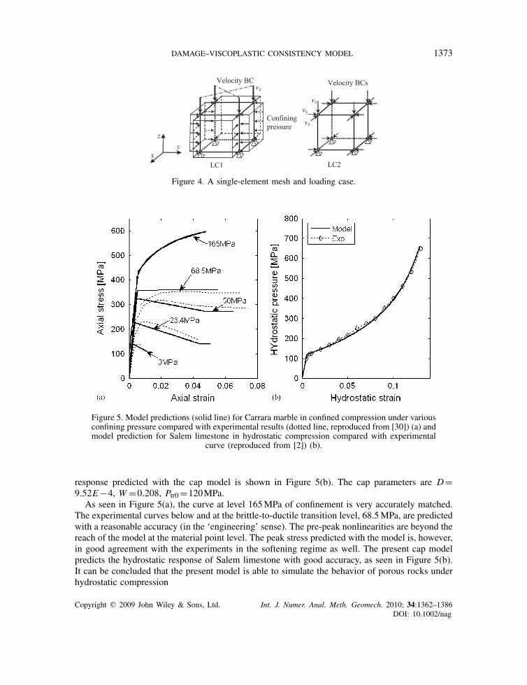
The present constitutive model is now tested in various uni and triaxial tests at the material pointlevel using a computational model consisting of a single 8-node hexahedral element. A single-Gauss point numerical integration scheme is used for stress computation. The element side is0.01m if not otherwise stated.

Results are presented with the sign convention adopted in geomechanics, i.e. compressive stressesand strains are considered positive. The material properties used in the numerical simulations are,if not explicitly otherwise stated, given in Table II.

Perfectly viscoplastic behavior in tension is assumed, i.e. hMR=0. The tensile damage param-eters are set as �t=0.98, �t=5000.

3.1.1. Confined and hydrostatic compression tests. Compressive axial loading is applied in thez-direction in the form of velocity boundary condition with constant velocity 0.25m/s (LC1 inFigure 4). The displacements caused by the confining pressure boundaries are solved from the staticproblem and used as an initial value: u0=K−1fext, where K is the (linear elastic) stiffness matrixfor the static problem and fext is the external equivalent nodal force due to confining pressure�conf. As the constitutive relationships for the strain rate dependancy of the viscosity parameterswere not available, the rocks tested here, constant values sDP=sMR=0.01MPas, are used unlessotherwise stated.

As the data for Tennessee marble under highly confined compression were not available, anothermarble for which the data was found in the literature is chosen for the verification of the capmodel. The response of Carrara marble is predicted and compared with the experimental data inFigure 5(a). The material properties used are E=60GPa, �=0.274, fc0=138MPa, �=35◦, �=5◦.The degradation index parameter is set as nd=0.02 and viscoplastic softening modulus chosenas hDP0=800MPa. Finally, the cap pressure and hardening parameters chosen are Ptr0=3.3 fc,Pp0=10 fc, and D=1.11E−4, W =0.08, respectively.It is also demonstrated that the cap model can reproduce the experimental hydrostatic response

of rocks. The experimental volumetric strain–pressure relationship for Salem limestone and the

Table II. Material properties used in numerical simulations.

Quantity E ft fc � � � �

Value 60GPa 13MPa 130MPa 0.2 30◦ 5◦ 2600kg/m3



Figure 4. A single-element mesh and loading case.

Figure 5. Model predictions (solid line) for Carrara marble in confined compression under variousconfining pressure compared with experimental results (dotted line, reproduced from [30]) (a) andmodel prediction for Salem limestone in hydrostatic compression compared with experimental

curve (reproduced from [2]) (b).

response predicted with the cap model is shown in Figure 5(b). The cap parameters are D=9.52E−4, W =0.208, Ptr0=120MPa.

As seen in Figure 5(a), the curve at level 165MPa of confinement is very accurately matched.The experimental curves below and at the brittle-to-ductile transition level, 68.5MPa, are predictedwith a reasonable accuracy (in the ‘engineering’ sense). The pre-peak nonlinearities are beyond thereach of the model at the material point level. The peak stress predicted with the model is, however,in good agreement with the experiments in the softening regime as well. The present cap modelpredicts the hydrostatic response of Salem limestone with good accuracy, as seen in Figure 5(b).It can be concluded that the present model is able to simulate the behavior of porous rocks underhydrostatic compression


1374 T. SAKSALA

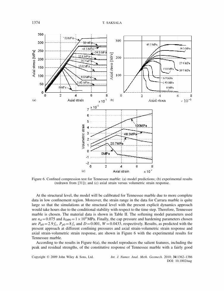
Figure 6. Confined compression test for Tennessee marble: (a) model predictions; (b) experimental results(redrawn from [31]); and (c) axial strain versus volumetric strain response.

At the structural level, the model will be calibrated for Tennessee marble due to more completedata in low confinement region. Moreover, the strain range in the data for Carrara marble is quitelarge so that the simulations at the structural level with the present explicit dynamics approachwould take hours due to the conditional stability with respect to the time step. Therefore, Tennesseemarble is chosen. The material data is shown in Table II. The softening model parameters usedare nd=0.075 and hDP0=1×104MPa. Finally, the cap pressure and hardening parameters chosenare Ptr0=2.9 fc, Pp0=8 fc and D=0.001, W =0.0433, respectively. Results, as predicted with thepresent approach at different confining pressures and axial strain-volumetric strain response andaxial strain-volumetric strain response, are shown in Figure 6 with the experimental results forTennessee marble.

According to the results in Figure 6(a), the model reproduces the salient features, including thepeak and residual strengths, of the constitutive response of Tennessee marble with a fairly good



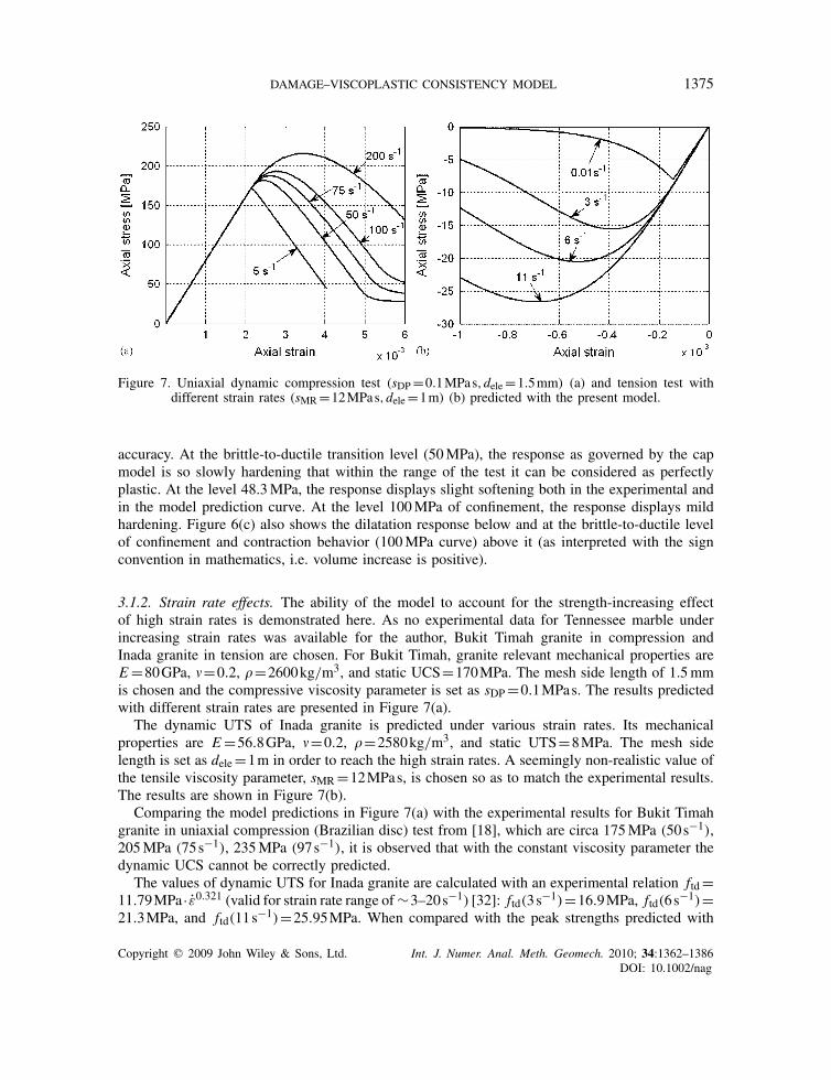
Figure 7. Uniaxial dynamic compression test (sDP=0.1MPas,dele=1.5mm) (a) and tension test withdifferent strain rates (sMR=12MPas,dele=1m) (b) predicted with the present model.

accuracy. At the brittle-to-ductile transition level (50MPa), the response as governed by the capmodel is so slowly hardening that within the range of the test it can be considered as perfectlyplastic. At the level 48.3MPa, the response displays slight softening both in the experimental andin the model prediction curve. At the level 100MPa of confinement, the response displays mildhardening. Figure 6(c) also shows the dilatation response below and at the brittle-to-ductile levelof confinement and contraction behavior (100MPa curve) above it (as interpreted with the signconvention in mathematics, i.e. volume increase is positive).

3.1.2. Strain rate effects. The ability of the model to account for the strength-increasing effectof high strain rates is demonstrated here. As no experimental data for Tennessee marble underincreasing strain rates was available for the author, Bukit Timah granite in compression andInada granite in tension are chosen. For Bukit Timah, granite relevant mechanical properties areE=80GPa, �=0.2, �=2600kg/m3, and static UCS=170MPa. The mesh side length of 1.5mmis chosen and the compressive viscosity parameter is set as sDP=0.1MPas. The results predictedwith different strain rates are presented in Figure 7(a).

The dynamic UTS of Inada granite is predicted under various strain rates. Its mechanicalproperties are E=56.8GPa, �=0.2, �=2580kg/m3, and static UTS=8MPa. The mesh sidelength is set as dele=1m in order to reach the high strain rates. A seemingly non-realistic value ofthe tensile viscosity parameter, sMR=12MPas, is chosen so as to match the experimental results.The results are shown in Figure 7(b).

Comparing the model predictions in Figure 7(a) with the experimental results for Bukit Timahgranite in uniaxial compression (Brazilian disc) test from [18], which are circa 175MPa (50s−1),205MPa (75s−1), 235MPa (97s−1), it is observed that with the constant viscosity parameter thedynamic UCS cannot be correctly predicted.

The values of dynamic UTS for Inada granite are calculated with an experimental relation ftd=11.79MPa· ε0.321 (valid for strain rate range of∼3–20s−1) [32]: ftd(3s−1)=16.9MPa, ftd(6s−1)=21.3MPa, and ftd(11s−1)=25.95MPa. When compared with the peak strengths predicted with


1376 T. SAKSALA

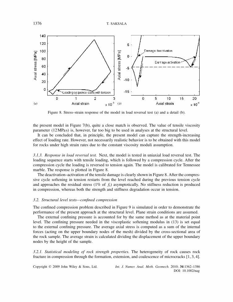
Figure 8. Stress–strain response of the model in load reversal test (a) and a detail (b).

the present model in Figure 7(b), quite a close match is observed. The value of tensile viscosityparameter (12MPas) is, however, far too big to be used in analyses at the structural level.

It can be concluded that, in principle, the present model can capture the strength-increasingeffect of loading rate. However, not necessarily realistic behavior is to be obtained with this modelfor rocks under high strain rates due to the constant viscosity moduli assumption.

3.1.3. Response in load reversal test. Next, the model is tested in uniaxial load reversal test. Theloading sequence starts with tensile loading, which is followed by a compression cycle. After thecompression cycle the loading is reversed to tension again. The model is calibrated for Tennesseemarble. The response is plotted in Figure 8.

The deactivation–activation of the tensile damage is clearly shown in Figure 8. After the compres-sive cycle softening in tension restarts from the level reached during the previous tension cycleand approaches the residual stress (1% of ft) asymptotically. No stiffness reduction is producedin compression, whereas both the strength and stiffness degradation occur in tension.

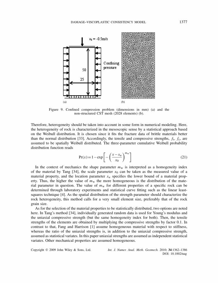
3.2. Structural level tests—confined compression

The confined compression problem described in Figure 9 is simulated in order to demonstrate theperformance of the present approach at the structural level. Plane strain conditions are assumed.

The external confining pressure is accounted for by the same method as at the material pointlevel. The confining pressure needed in the viscoplastic softening modulus in (13) is set equalto the external confining pressure. The average axial stress is computed as a sum of the internalforces (acting on the upper boundary nodes of the mesh) divided by the cross-sectional area ofthe rock sample. The average strain is calculated dividing the displacement of the upper boundarynodes by the height of the sample.

3.2.1. Statistical modeling of rock strength properties. The heterogeneity of rock causes rockfracture in compression through the formation, extension, and coalescence of microcracks [1, 3, 4].



Figure 9. Confined compression problem (dimensions in mm) (a) and thenon-structured CST mesh (2028 elements) (b).

Therefore, heterogeneity should be taken into account in some form in numerical modeling. Here,the heterogeneity of rock is characterized in the mesoscopic sense by a statistical approach basedon the Weibull distribution. It is chosen since it fits the fracture data of brittle materials betterthan the normal distribution [33]. Accordingly, the tensile and compressive strengths, ft, fc, areassumed to be spatially Weibull distributed. The three-parameter cumulative Weibull probabilitydistribution function reads

Pr(x)=1−exp

[−(x−xux0

)mw]

(21)

In the context of mechanics the shape parameter mw is interpreted as a homogeneity indexof the material by Tang [34], the scale parameter x0 can be taken as the measured value of amaterial property, and the location parameter xu specifies the lower bound of a material prop-erty. Thus, the higher the value of mw the more homogeneous is the distribution of the mate-rial parameter in question. The value of mw for different properties of a specific rock can bedetermined through laboratory experiments and statistical curve fitting such as the linear least-squares technique [4]. As the spatial distribution of the strength parameter should characterize therock heterogeneity, this method calls for a very small element size, preferably that of the rockgrain size.

As for the selection of the material properties to be statistically distributed, two options are notedhere. In Tang’s method [34], individually generated random data is used for Young’s modulus andthe uniaxial compressive strength (but the same homogeneity index for both). Then, the tensilestrengths of the elements are obtained by multiplying the compressive strengths by factor 0.1. Incontrast to that, Fang and Harrison [1] assume homogeneous material with respect to stiffness,whereas the ratio of the uniaxial strengths is, in addition to the uniaxial compressive strength,assumed as statistical variates. In this paper uniaxial strengths are assumed as independent statisticalvariates. Other mechanical properties are assumed homogeneous.


1378 T. SAKSALA

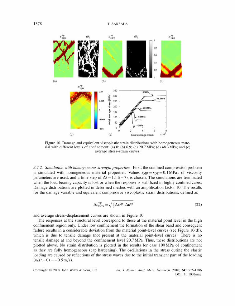
Figure 10. Damage and equivalent viscoplastic strain distributions with homogeneous mate-rial with different levels of confinement: (a) 0; (b) 6.9; (c) 20.7MPa; (d) 48.3MPa; and (e)

average stress–strain curves.

3.2.2. Simulation with homogeneous strength properties. First, the confined compression problemis simulated with homogeneous material properties. Values sMR=sDP=0.1MPas of viscosityparameters are used, and a time step of �t=1.1E−7s is chosen. The simulations are terminatedwhen the load bearing capacity is lost or when the response is stabilized in highly confined cases.Damage distributions are plotted in deformed meshes with an amplification factor 10. The resultsfor the damage variable and equivalent compressive viscoplastic strain distributions, defined as

�εvpeqvc=

√23�e

vp :�evp (22)

and average stress–displacement curves are shown in Figure 10.The responses at the structural level correspond to those at the material point level in the high

confinement region only. Under low confinement the formation of the shear band and consequentfailure results in a considerable deviation from the material point-level curves (see Figure 10(d)),which is due to tensile damage (not present at the material point-level curves). There is notensile damage at and beyond the confinement level 20.7MPa. Thus, these distributions are notplotted above. No strain distribution is plotted in the results for case 100MPa of confinementas they are fully homogeneous (cap hardening). The oscillations in the stress during the elasticloading are caused by reflections of the stress waves due to the initial transient part of the loading(vb(t=0)=−0.5m/s).



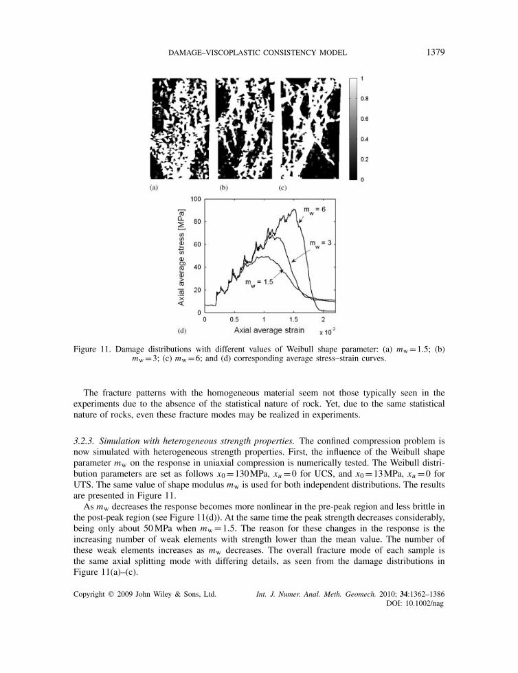
Figure 11. Damage distributions with different values of Weibull shape parameter: (a) mw=1.5; (b)mw=3; (c) mw=6; and (d) corresponding average stress–strain curves.

The fracture patterns with the homogeneous material seem not those typically seen in theexperiments due to the absence of the statistical nature of rock. Yet, due to the same statisticalnature of rocks, even these fracture modes may be realized in experiments.

3.2.3. Simulation with heterogeneous strength properties. The confined compression problem isnow simulated with heterogeneous strength properties. First, the influence of the Weibull shapeparameter mw on the response in uniaxial compression is numerically tested. The Weibull distri-bution parameters are set as follows x0=130MPa, xu =0 for UCS, and x0=13MPa, xu =0 forUTS. The same value of shape modulus mw is used for both independent distributions. The resultsare presented in Figure 11.

As mw decreases the response becomes more nonlinear in the pre-peak region and less brittle inthe post-peak region (see Figure 11(d)). At the same time the peak strength decreases considerably,being only about 50MPa when mw=1.5. The reason for these changes in the response is theincreasing number of weak elements with strength lower than the mean value. The number ofthese weak elements increases as mw decreases. The overall fracture mode of each sample isthe same axial splitting mode with differing details, as seen from the damage distributions inFigure 11(a)–(c).


1380 T. SAKSALA

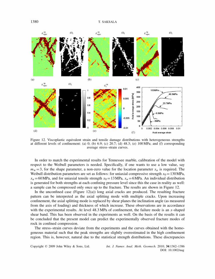
Figure 12. Viscoplastic equivalent strain and tensile damage distributions with heterogeneous strengthsat different levels of confinement: (a) 0; (b) 6.9; (c) 20.7; (d) 48.3; (e) 100MPa; and (f) corresponding

average stress–strain curves.

In order to match the experimental results for Tennessee marble, calibration of the model withrespect to the Weibull parameters is needed. Specifically, if one wants to use a low value, saymw=3, for the shape parameter, a non-zero value for the location parameter xu is required. TheWeibull distribution parameters are set as follows: for uniaxial compressive strength x0=130MPa,xu =60MPa, and for uniaxial tensile strength x0=13MPa, xu =6MPa. An individual distributionis generated for both strengths at each confining pressure level since this the case in reality as well:a sample can be compressed only once up to the fracture. The results are shown in Figure 12.

In the unconfined case (Figure 12(a)) long axial cracks are produced. The resulting fracturepattern can be interpreted as the axial splitting mode with multiple cracks. Upon increasingconfinement, the axial splitting mode is replaced by shear planes the inclination angle (as measuredfrom the axis of loading) and thickness of which increase. These observations are in accordancewith the experimental results. At level 48.3MPa of confinement, the failure mode is an x-shapedshear band. This has been observed in the experiments as well. On the basis of the results it canbe concluded that the present model can predict the experimentally observed fracture modes ofrock in confined compression.

The stress–strain curves deviate from the experiments and the curves obtained with the homo-geneous material such that the peak strengths are slightly overestimated in the high confinementregion. This is, however, natural due to the statistical strength distributions. These discrepancies



Figure 13. Damage distribution in uniaxial tension simulation with a single (a) and multiple macro cracks(b), and corresponding average stress–strain curves (c).

in the stress–strain curves are within the acceptable limits. The final remark is that, despite thesimplified assumptions under which the constitutive model was formulated, the results displaypre-peak nonlinearity, which becomes more pronounced as the confining pressure increases. Thisis due to the statistical strength characterization.

3.3. Structural level tests—uniaxial tension

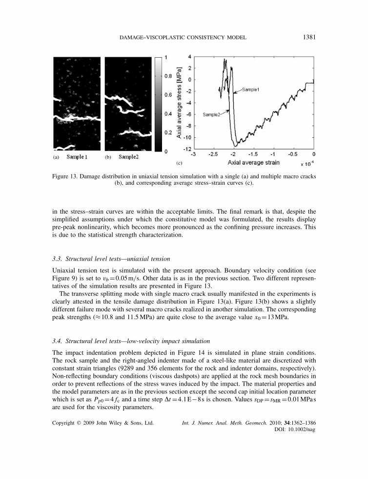
Uniaxial tension test is simulated with the present approach. Boundary velocity condition (seeFigure 9) is set to vb=0.05m/s. Other data is as in the previous section. Two different represen-tatives of the simulation results are presented in Figure 13.

The transverse splitting mode with single macro crack usually manifested in the experiments isclearly attested in the tensile damage distribution in Figure 13(a). Figure 13(b) shows a slightlydifferent failure mode with several macro cracks realized in another simulation. The correspondingpeak strengths (≈10.8 and 11.5MPa) are quite close to the average value x0=13MPa.

3.4. Structural level tests—low-velocity impact simulation

The impact indentation problem depicted in Figure 14 is simulated in plane strain conditions.The rock sample and the right-angled indenter made of a steel-like material are discretized withconstant strain triangles (9289 and 356 elements for the rock and indenter domains, respectively).Non-reflecting boundary conditions (viscous dashpots) are applied at the rock mesh boundaries inorder to prevent reflections of the stress waves induced by the impact. The material properties andthe model parameters are as in the previous section except the second cap initial location parameterwhich is set as Pp0=4 fc and a time step �t=4.1E−8s is chosen. Values sDP=sMR=0.01MPasare used for the viscosity parameters.


1382 T. SAKSALA

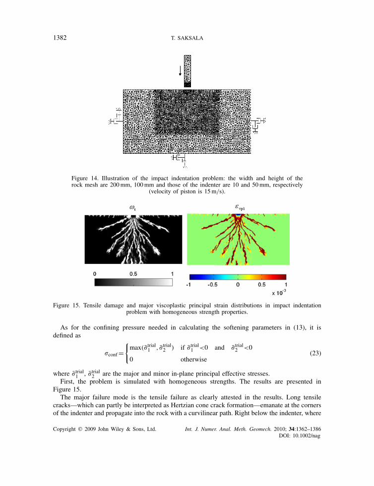
Figure 14. Illustration of the impact indentation problem: the width and height of therock mesh are 200mm, 100mm and those of the indenter are 10 and 50mm, respectively

(velocity of piston is 15m/s).

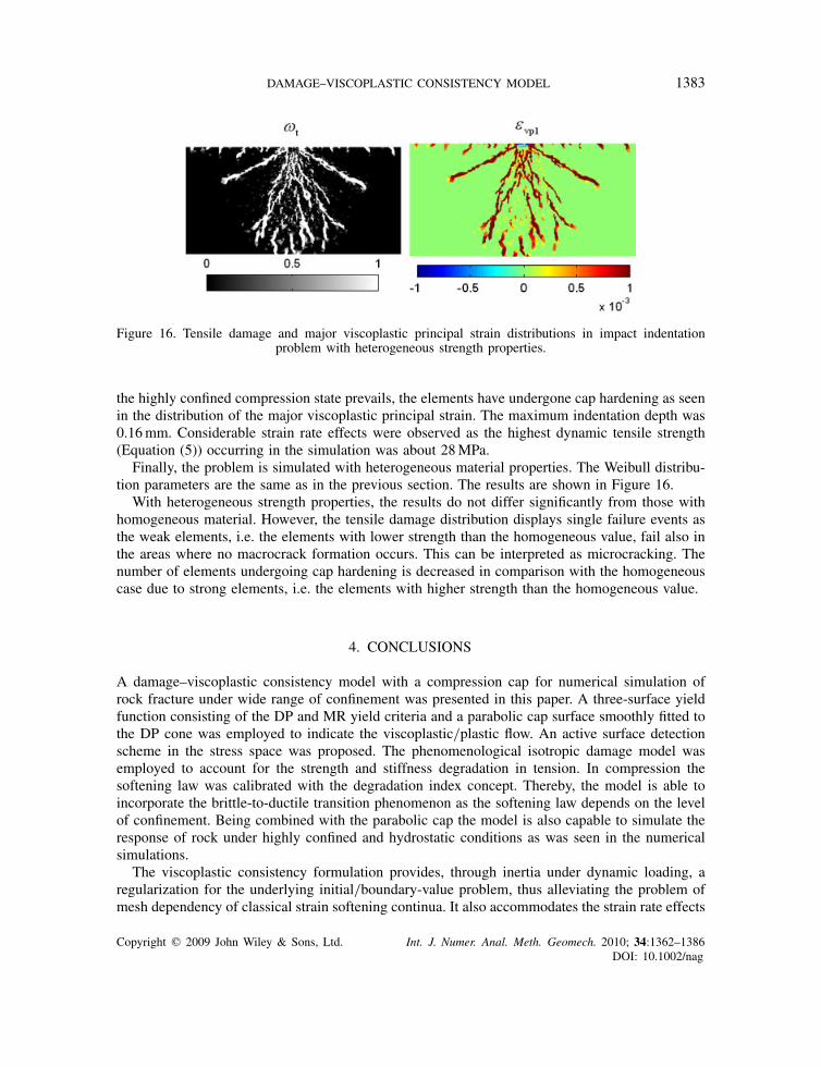
Figure 15. Tensile damage and major viscoplastic principal strain distributions in impact indentationproblem with homogeneous strength properties.

As for the confining pressure needed in calculating the softening parameters in (13), it isdefined as

�conf={max(�trial1 , �trial2 ) if �trial1 <0 and �trial2 <0

0 otherwise(23)

where �trial1 , �trial2 are the major and minor in-plane principal effective stresses.First, the problem is simulated with homogeneous strengths. The results are presented in

Figure 15.The major failure mode is the tensile failure as clearly attested in the results. Long tensile

cracks—which can partly be interpreted as Hertzian cone crack formation—emanate at the cornersof the indenter and propagate into the rock with a curvilinear path. Right below the indenter, where



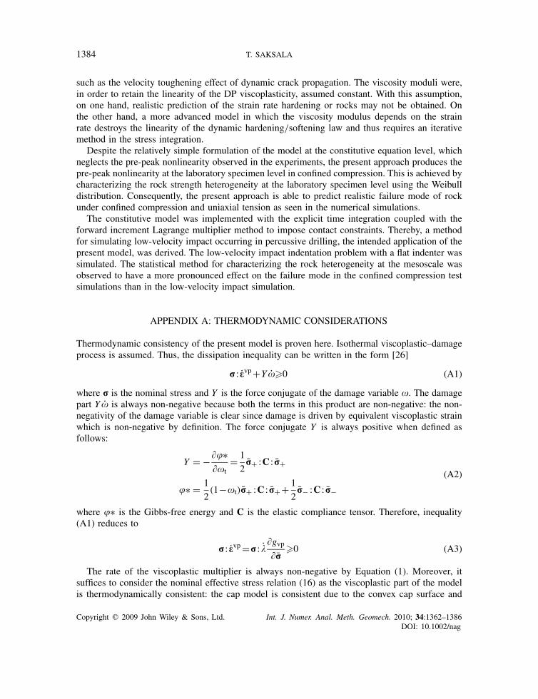
Figure 16. Tensile damage and major viscoplastic principal strain distributions in impact indentationproblem with heterogeneous strength properties.

the highly confined compression state prevails, the elements have undergone cap hardening as seenin the distribution of the major viscoplastic principal strain. The maximum indentation depth was0.16mm. Considerable strain rate effects were observed as the highest dynamic tensile strength(Equation (5)) occurring in the simulation was about 28MPa.

Finally, the problem is simulated with heterogeneous material properties. The Weibull distribu-tion parameters are the same as in the previous section. The results are shown in Figure 16.

With heterogeneous strength properties, the results do not differ significantly from those withhomogeneous material. However, the tensile damage distribution displays single failure events asthe weak elements, i.e. the elements with lower strength than the homogeneous value, fail also inthe areas where no macrocrack formation occurs. This can be interpreted as microcracking. Thenumber of elements undergoing cap hardening is decreased in comparison with the homogeneouscase due to strong elements, i.e. the elements with higher strength than the homogeneous value.

4. CONCLUSIONS

A damage–viscoplastic consistency model with a compression cap for numerical simulation ofrock fracture under wide range of confinement was presented in this paper. A three-surface yieldfunction consisting of the DP and MR yield criteria and a parabolic cap surface smoothly fitted tothe DP cone was employed to indicate the viscoplastic/plastic flow. An active surface detectionscheme in the stress space was proposed. The phenomenological isotropic damage model wasemployed to account for the strength and stiffness degradation in tension. In compression thesoftening law was calibrated with the degradation index concept. Thereby, the model is able toincorporate the brittle-to-ductile transition phenomenon as the softening law depends on the levelof confinement. Being combined with the parabolic cap the model is also capable to simulate theresponse of rock under highly confined and hydrostatic conditions as was seen in the numericalsimulations.

The viscoplastic consistency formulation provides, through inertia under dynamic loading, aregularization for the underlying initial/boundary-value problem, thus alleviating the problem ofmesh dependency of classical strain softening continua. It also accommodates the strain rate effects


1384 T. SAKSALA

such as the velocity toughening effect of dynamic crack propagation. The viscosity moduli were,in order to retain the linearity of the DP viscoplasticity, assumed constant. With this assumption,on one hand, realistic prediction of the strain rate hardening or rocks may not be obtained. Onthe other hand, a more advanced model in which the viscosity modulus depends on the strainrate destroys the linearity of the dynamic hardening/softening law and thus requires an iterativemethod in the stress integration.

Despite the relatively simple formulation of the model at the constitutive equation level, whichneglects the pre-peak nonlinearity observed in the experiments, the present approach produces thepre-peak nonlinearity at the laboratory specimen level in confined compression. This is achieved bycharacterizing the rock strength heterogeneity at the laboratory specimen level using the Weibulldistribution. Consequently, the present approach is able to predict realistic failure mode of rockunder confined compression and uniaxial tension as seen in the numerical simulations.

The constitutive model was implemented with the explicit time integration coupled with theforward increment Lagrange multiplier method to impose contact constraints. Thereby, a methodfor simulating low-velocity impact occurring in percussive drilling, the intended application of thepresent model, was derived. The low-velocity impact indentation problem with a flat indenter wassimulated. The statistical method for characterizing the rock heterogeneity at the mesoscale wasobserved to have a more pronounced effect on the failure mode in the confined compression testsimulations than in the low-velocity impact simulation.

APPENDIX A: THERMODYNAMIC CONSIDERATIONS

Thermodynamic consistency of the present model is proven here. Isothermal viscoplastic–damageprocess is assumed. Thus, the dissipation inequality can be written in the form [26]

r : evp+Y �0 (A1)

where r is the nominal stress and Y is the force conjugate of the damage variable . The damagepart Y is always non-negative because both the terms in this product are non-negative: the non-negativity of the damage variable is clear since damage is driven by equivalent viscoplastic strainwhich is non-negative by definition. The force conjugate Y is always positive when defined asfollows:

Y = −��∗�t

= 1

2r+ :C : r+

�∗ = 1

2(1−t)r+ :C : r++ 1

2r− :C : r−

(A2)

where �∗ is the Gibbs-free energy and C is the elastic compliance tensor. Therefore, inequality(A1) reduces to

r : evp=r : ��gvp�r

�0 (A3)

The rate of the viscoplastic multiplier is always non-negative by Equation (1). Moreover, itsuffices to consider the nominal effective stress relation (16) as the viscoplastic part of the modelis thermodynamically consistent: the cap model is consistent due to the convex cap surface and



associated flow rule, the same applies to the MR model, and the DP plasticity model with non-associated flow rule is consistent when �DP��DP [22]. Finally, the combined DP-MR plasticityprocess is also thermodynamically consistent, which follows from the fact that Koiter’s rulepreserves the consistency of the individual models. Thus, for thermodynamic consistency it issufficient to show that the model verifies (in the principal effective stress space) the inequality (invector notation)

r· �gvp�r

=((1−t)r++ r−) · �gvp�r

�0 (A4)

It is trivial to show that the MR viscoplasticity verifies (A4) due to the construction of the MRcriterion. As for the DP viscoplasticity, a straightforward proof is essentially based on the ordering�1��2��3, which is preserved by the return mapping, and the thermodynamic consistency of theplain DP model, i.e.

r · �gvpDP

�r�0 for all r such that fDP(r)�0 (A5)

Thus, it can be concluded that the entire model is thermodynamically consistent.

REFERENCES

1. Fang Z, Harrison JP. Development of a local degradation approach to the modelling of brittle fracture inheterogeneous rocks. International Journal of Rock Mechanics and Mining Sciences 2002; 39:443–457.

2. Lubarda VA, Mastilovic S, Knap J. Brittle–ductile transition in porous rocks by pressure-dependent cap model.Journal of Engineering Mechanics 1996; 122:633–642.

3. Krajcinovic D. Damage Mechanics. Elsevier: Amsterdam, 1996.4. Liu HY. Numerical modelling of the rock fragmentation process by mechanical tools. Ph.D. Thesis, Lulea

University of Technology, Sweden, 2004.5. Liu HY, Kou SQ, Lindqvist P-A. Numerical studies on bit-rock fragmentation mechanisms. International Journal

of Geomechanics (ASCE) 2008; 45:45–67.6. Saksala T. Damage–plastic model for numerical simulation of rock fracture in dynamic loading. In Proceedings of

the Sixth International Conference on Engineering Computational Technology, Topping BHV (ed.). Civil-CompPress: Stirling, U.K., 2008. Paper 163.

7. Thuro K, Schormair N. Fracture propagation in anisotropic rock during drilling and cutting. Geomechanik andTunnelbau 2008; 1:8–17.

8. Rossmanith HP, Knasmillner RP, Daehnke A, Mishnaevsky Jr L. Wave propagation, damage evolution, anddynamic fracture extension. Part I percussion drilling. Materials Science 1996; 32:350–358.

9. Wang W. Stationary and propagative instabilities in metals—a computational point of view. Ph.D. Thesis, DelftUniversity of Technology, 1997.

10. Wang WM, Sluys LJ, De Borst R. Viscoplasticity for instabilities due to strain softening and strain-rate softening.International Journal for Numerical Methods in Engineering 1997; 40:3839–3864.

11. Salari MR, Saeb S, Willam KJ, Patchet SJ, Carrasco RC. A coupled elastoplastic damage model for geomaterials.Computer Methods in Applied Mechanics and Engineering 2004; 193:2625–2643.

12. Rouabhi A, Tijani M, Moser P, Goetz D. Continuum modelling of dynamic behaviour and fragmentation ofquasi-brittle materials: application to rock fragmentation by blasting. International Journal for Numerical andAnalytical Methods in Geomechanics 2005; 29:729–749.

13. Shao JF, Jia Y, Kondo D, Chiarelli AS. A coupled elastoplastic damage model for semi-brittle materials andextension to unsaturated conditions. Mechanics of Materials 2006; 38:218–232.

14. Abou-Chakra Guery A, Cormery F, Sub K, Shao JF, Kondo D. A micromechanical model for the elasto-viscoplasticand damage behavior of a cohesive geomaterial. Physics and Chemistry of the Earth 2008; 33:S416–S421.


1386 T. SAKSALA

15. Pellet F, Hajdu A, Deleruyelle F, Besnus F. A viscoplastic model including anisotropic damage for the timedependent behaviour of rock. International Journal for Numerical and Analytical Methods in Geomechanics2005; 29:941–970.

16. Sluys LJ. Wave propagation, localization and dispersion is softening solids. Ph.D. Thesis, Delft University ofTechnology, 1992.

17. Fang Z, Harrison JP. A mechanical degradation index for rock. International Journal of Rock Mechanics andMining Sciences 2001; 38:1193–1199.

18. Zhai Y, Ma G, Zhao J, Hu C. Dynamic failure analysis on granite under uniaxial impact compressive load.Frontiers of Architecture and Civil Engineering in China 2008; 2:253–260.

19. Wang QZ, Li W, Song XL. A method for testing dynamic tensile strength and elastic modulus of rock materialsusing SHPB. Pure and Applied Geophysics 2006; 163:1091–1100.

20. DiMaggio FL, Sandler IS. Material models for granular soils. Journal of Engineering Mechanics (ASCE) 1971;97:935–950.

21. Dolarevic S, Ibrahimbegovic A. A modified three-surface elasto-plastic cap model and its numericalimplementation. Computers and Structures 2007; 85:419–430.

22. Ottosen NS, Ristinmaa M. The Mechanics of Constitutive Modeling. Elsevier: Amsterdam, 2005.23. Carroll MM. A critical state plasticity theory for porous reservoir rocks. American Society of Mechanical

Engineering 1991; 117:Book G00617.24. Winnicki A, Pearce CJ, Bicanic N. Viscoplastic Hoffman consistency model for concrete. Computers and

Structures 2001; 79:7–19.25. Simo JC, Hughes TJR. Computational Inelasticity. Springer: Berlin, 1998.26. Grassl P, Jirasek M. Damage–plastic model for concrete failure. International Journal of Solids and Structures

2006; 43:7166–7196.27. Jason L, Huerta A, Pijaudier-Cabot G, Ghavamian S. An elastic plastic damage formulation for concrete:

application to elementary tests and comparison with an isotropic damage model. Computer Methods in AppliedMechanics and Engineering 2006; 195:7077–7092.

28. Hahn GD. A modified Euler method for dynamical analyses. International Journal for Numerical Methods inEngineering 1991; 32:943–955.

29. Carpenter NJ, Taylor RL, Katona MG. Lagrange constraints for transient finite element surface contact.International Journal for Numerical Methods in Engineering 1991; 32:103–128.

30. Jaeger JC, Cook NGW. Fundamentals of Rock Mechanics. Chapman & Hall: Boca Raton, 1971.31. Brady BHG, Brown ET. Rock Mechanics for Underground Mining. Springer: Berlin, 1993.32. Sang HC, Yuji O, Katsuhiko K. Strain-rate dependency of the dynamic tensile strength of rock. International

Journal of Rock Mechanics and Mining Sciences 2003; 40:763–777.33. Lu C, Danzer R, Fischer FD. Fracture statistics of brittle materials: Weibull or normal distribution. Physical

Review E 2002; 65:067102-1-4.34. Tang CA. Numerical simulation of progressive rock failure and associated seismicity. International Journal of

Rock Mechanics and Mining Sciences 1997; 34:249–261.


Documents

Damageâviscoplastic consistency model with a parabolic cap for rocks with brittle and ductile behavior under low-velocity impact loading