Deconstructing blazars: A different scheme for jet kinematics in flat-spectrum AGN

Astronomy & Astrophysics manuscript no. jet˙ridge˙lines˙v4 c© ESO 2011October 25, 2011

Deconstructing blazars: A different scheme for jet kinematics inflat-spectrum AGN

M. Karouzos1,2,?,??, S. Britzen1, A. Witzel1, J.A. Zensus1,3, and A. Eckart3,1

1 Max-Planck-Institut fur Radioastronomie, Auf dem Hugel 69, 53121 Bonn, Germany2 Reimar-Lust Fellow of the Max Planck Society

e-mail: [email protected] I.Physikalisches Institut, Universitat zu Koln, Zulpicher Str. 77, 50937 Koln, Germany

Received / Accepted

ABSTRACT

Context. Recent VLBI studies of the morphology and kinematics of individual BL Lac objects (S5 1803+784, PKS 0735+178, etc.)have revealed a new paradigm for the pc-scale jet kinematics of these sources. Unlike the apparent superluminal outward motionsusually observed in blazars, most, if not all, jet components in these sources appear to be stationary with respect to the core, whileexhibiting strong changes in their position angles. As a result, the jet ridge lines of these sources evolve substantially, at times forminga wide channel-flow.Aims. We investigate the Caltech-Jodrell Bank flat-spectrum (CJF) sample of radio-loud active galaxies to study this new kinematicscenario for flat-spectrum AGN. Comparing BL Lac objects and quasars in the CJF, we look for differences with respect to thekinematics and morphology of their jet ridge lines. The large number of sources in the CJF sample, together with the excellentkinematic data available, allow us to perform a robust statistical analysis in that context.Methods. We develop a number of tools that extract information about the apparent linear and angular evolution of the CJF jet ridgelines, as well as their morphology. In this way, we study both radial and non-radial apparent motions in the CJF jets. A statisticalanalysis of the extracted information allows us to test this new kinematic scenario and assess the relative importance of non-radialand radial motions in flat-spectrum AGN jets, compared to those of quasars. We also use these tools to check the kinematics for(multi-wavelength) variable AGN.Results. We find that approximately half of the sample shows appreciable apparent jet widths (> 10degrees), with BL Lac jet ridgelines showing significantly larger apparent widths than both quasars and radio galaxies. In addition, BL Lac jet ridge lines are foundto change their apparent width more strongly. Finally, BL Lac jet ridge lines show the least apparent linear evolution, which translatesto the smallest apparent expansion speeds for their components. We find compelling evidence supporting a substantially differentkinematic scenario for flat-spectrum radio-AGN jets and in particular for BL Lac objects. In addition, we find that variability isclosely related to the properties of a source’s jet ridge line. Variable quasars are found to show “BL Lac like” behavior, compared totheir non-variable counterparts.

Key words. Galaxies: statistics - Galaxies: active - Galaxies: nuclei - Galaxies: jets - BL Lacertae objects: general

1. Introduction

Although observed in the minority of active galaxies (∼ 5−15%;Kellermann et al. 1989; Padovani 1993; Jiang et al. 2007), ex-tragalactic jets are some of the most pronounced morphologicalfeatures in AGN research. Their presumably direct connectionto the active core and the supermassive black hole (SMBH) re-siding there, makes them invaluable tools in the effort to char-acterize the properties and the underlying physics of activity ingalaxies. VLBI observations enable the direct imaging of AGNjets and thus the study of their properties on parsec scales. Oneof the most prominent discoveries, related to jet kinematics, wasthat of apparent superluminal motion of jet components (e.g.,Whitney et al. 1971; Pearson & Readhead 1981), a combina-tion of relativistic expansion speeds (close to the speed of light)

? Member of the International Max Planck Research School (IMPRS)for Astronomy and Astrophysics at the Universities of Bonn andCologne?? Current affiliation: Center for the Exploration of the Origin of theUniverse, Seoul National University, Gwanak-gu, Seoul 151-742, Korea

and the projected geometry onto the plane of the sky (e.g., Rees1966).

Jet kinematics, as studied through the investigation of dis-tinct components, is usually explained in terms of the shock-in-jet model (e.g., Marscher & Gear 1985), where the observed jetknots are manifestations of shocks propagating down the jet atrelativistic speeds. Beaming and projection effects regulate theobserved properties of the jets. There has been continuous effortto distinguish whether the different types of active galaxies (e.g.,quasars, BL Lacs, Fanarrof-Riley, etc.) are just a result of ori-entation effects, or if additionally these objects have intrinsicallydifferent properties. The current paradigm is that indeed differentjet properties can be attributed to geometrical effects combinedwith factors such as the black hole mass or the accretion rate. Forexample, Ghisellini et al. (1993) for a sample of 39 superluminalsources find no appreciable difference between the distributionof Doppler factors between BL Lacs and flat-spectrum radio-quasars (FSRQs), with RGs showing smaller values. Some indi-cations to the contrary also exist (e.g., Gabuzda 1995; Gabuzdaet al. 2000). Analysis of statistically important samples (largenumber of sources and/or stringent selection criteria) of active

arX

iv:1

110.

5306

v1 [

astr

o-ph

.CO

] 2

4 O

ct 2

011

2 Karouzos et al.: A different scheme for jet kinematics in BL Lacs

galaxies have been of fundamental importance to this end (e.g.,Ghisellini 1993; Vermeulen & Cohen 1994; Vermeulen 1995;Taylor et al. 1996; Hough et al. 2002; Lister & Homan 2005;Britzen et al. 2007b).

Although it is crucial to pursue a statistical approach to theopen problem of AGN jet kinematics, the study of individualsources is indispensable. It has helped to elucidate particularmechanisms or effects that might get smoothed out by the poortemporal or spatial resolution usually available in big statisticalsamples. Such a case of a detailed study of an individual objectis that of S5 1803+784.

1.1. S5 1803+784: A case study

S5 1803+784 is an active galaxy at a moderate redshift of z=0.68(Hewitt & Burbidge 1989). It has been classified as a BL Lac ob-ject. Being a member of the complete S5 sample (Witzel 1987)it has been extensively studied in the radio, at different wave-lengths and with different instruments (see Britzen et al. 2010afor a detailed recounting of the source’s radio observations his-tory). Typical for this class of objects, 1803+784 has been ob-served to be variable in the radio and the optical on both long andshort-timescales (e.g., Wagner & Witzel 1995; Heidt & Wagner1996; Nesci et al. 2002; Fan et al. 2007).

Britzen et al. (2010a), by (re-)analyzing more than 90 epochsof global VLBI and VLBA data, reveal a new kinematic schemefor 1803+784. All components in the inner part of the jet (upto 12 mas) appear to remain stationary with respect to the core.This behavior is seen at all frequencies studied by the authors(1.6 - 15 GHz). In contrast to this, the components show strongchanges in their position angles, implying a prevailing move-ment perpendicular to the jet axis.

Britzen et al. (2010a) also studied the jet ridge line morphol-ogy and evolution of S5 1803+784. A jet ridge line at a givenepoch is defined as the line that linearly connects all compo-nent positions at that epoch. The authors find that the jet ridgeline changes in an almost periodic manner, starting resembling astraight line, evolving into a sinusoid-like pattern, and finally re-turning to its original linear pattern, although slightly displacedfrom its original position. A period of ∼ 8.5 years is calculatedfor the evolution of the jet ridge line.

Finally, the authors find that the jet changes its apparentwidth (in a range between a few and a few tens of degrees) inan almost periodic way with a timescale similar to the one foundfrom the evolution of the jet ridge line. All of the above proper-ties support a new kinematic scheme for 1803+784, where com-ponents follow oscillatory-like trajectories, with their movementpredominantly happening perpendicular to the jet axis ratherthan along it. Moreover, the jet appears at times to form a widechannel of flow, while changing its width considerably acrosstime.

1.2. Motivation

S5 1803+784 is one of several BL objects exhibiting the behav-ior described above. 0716+714 has been shown to behave in asimilar way (Britzen et al. 2009), with most of its componentsbeing stationary with respect to the core while changing theirposition angles considerably. PKS 0735+178 is another exam-ple of a source with similar, but rather more complicated, kine-matic properties (Gomez et al. 2001; Agudo et al. 2006; Britzenet al. 2010b). Under the unification scheme of active galaxies(e.g., Antonucci 1993; Urry & Padovani 1995), both BL Lac ob-

jects and FSRQs are believed to be active galaxies for which theviewing angle to their jets is very small, leading to strong rela-tivistic effects. Given the similar viewing angle distributions, inthe last several years the general classification of blazar has oftenbeen used to describe members of either class, also in terms oftheir jet properties. However, this phenomenological unificationof FSRQs and BL Lacs comes into question in light of the recentinvestigation of sources like S5 1803+784, PKS 0735+178 and0716+714. Is the peculiar kinematic behavior seen in these ob-jects revealed due to the unprecedented richness of the datasetsavailable, and could therefore be relevant for all flat-spectrumradio-AGN, or are BL Lacs characterized by a genuinely differ-ent set of kinematic properties?

This paper focuses on the relevance of this new kinematicscheme for flat-spectrum radio-AGN, while investigating the ap-parent divide between BL Lac and FSRQ jet kinematics. Asvaluable as single source studies are to an in-depth understand-ing of particular phenomena, there are a number of biases orunaccounted factors that alter and ultimately hinder a universalapplication of their results. In this context, we use the CJF sam-ple to statistically investigate and assess the similarity, or diver-gence, of the kinematic and morphological properties betweenthe two distinct sub-samples of FSRQs and BL Lac objects in theCJF. We want to test whether jet components of BL Lac objectsindeed show slower apparent speeds with respect to their corescompared to FSRQs. Furthermore we are interested in the phe-nomenon exhibited in S5 1803+784 of an, at times, very widejet, as well as a strong evolution of that width. For this investi-gation we use tools that extract information from the jet ridgeline of the sources, instead of focusing on individual compo-nents. This allows for a investigation that is mostly independentof component modeling and cross-identification.

The paper is organized as follows: in Sect. 1.1 we introducethe new kinematic scheme for BL Lac objects, as shown for thecase of the source 1803+784, and discuss the motivation of thiswork, in Sect. 2 we describe the CJF sample, in Sect. 3 we de-scribe the data used, in Sect. 4 we present the analysis of our dataand the results, and in Sect. 5 we discuss our results and givesome conclusions. Throughout the paper, we assume the cos-mological parameters H0 = 71 kms−1Mpc−1, ΩM = 0.27, andΩΛ = 0.73 (from the first-year WMAP observations; Spergelet al. 2003).

2. The CJF sample

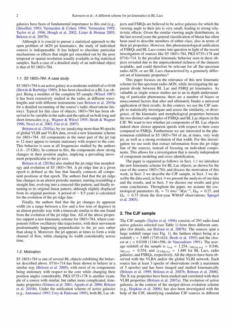
The CJF sample (Taylor et al. 1996) consists of 293 radio-loudactive galaxies selected (see Table 1) from three different sam-ples (for details, see Britzen et al. 2007b). The sources span alarge redshift range (see Fig. 1), the farthest object being at aredshift z = 3.889 (1745+624; Hook et al. 1995) and the clos-est at z = 0.0108 (1146+596; de Vaucouleurs 1991). The aver-age redshift of the sample is zavg = 1.254, zBLLac,avg = 0.546,zRG,avg = 0.554, and zFS RQ,avg = 1.489 for BL Lacs, radiogalaxies, and FSRQs, respectively. All the objects have been ob-served with the VLBA and/or the global VLBI network. Eachsource has at least 3 epochs of observations (with a maximumof 5 epochs) and has been imaged and studied kinematically(Britzen et al. 1999; Britzen et al. 2007b; Britzen et al. 2008).The X-ray properties have been studied and correlated with theirVLBI properties (Britzen et al. 2007a). The evolution of activegalaxies, in the context of the merger-driven evolution scheme(e.g., Hopkins et al. 2006), has also been investigated with thehelp of the CJF, identifying candidate CJF sources in different

Karouzos et al.: A different scheme for jet kinematics in BL Lacs 3

0 1 2 3 4z

0

10

20

30N

Radio GalaxiesBL LacsQuasars

Fig. 1. Redshift distribution of radio galaxies (grey blocks), BLLacs (dashed line), and FSRQs (solid line) in the CJF sample.

evolutionary stages, including new binary black hole candidates(Karouzos et al. 2010).

Table 1. CJF sample and its properties.

Frequency(MHz) 4850Flux lower limit @5GHz 350mJySpectral Index α4850

1400 ≥ −0.5Declination δ ≥ 35Galactic latitude |b| ≥ 10# Quasars 198# BL Lac 32# Radio Galaxies 52# Unclassified 11# Total 293

2.1. Radio emission

The CJF is a flux-limited radio-selected sample of flat-spectrumradio-loud AGN. The sample was originally created to study,among other things, the kinematics of pc-scale jets and apparentsuperluminal motion (see Taylor et al. 1996 for more details).

The CJF sample (Table 1) has been most extensively stud-ied in the radio regime (e.g., Taylor et al. 1996; Pearson et al.1998; Britzen et al. 1999; Vermeulen et al. 2003; Pollack et al.2003; Lowe et al. 2007; Britzen et al. 2007b; Britzen et al. 2008).Britzen et al. (2008) developed a localized method for calculat-ing the bending of the jet associated with individual components.The maximum of the distribution of local angles is at zero de-grees, although a substantial fraction shows some bending (0−40degrees). A few sources exhibit sharp bends of the order of > 50degrees (see Fig. 13 in Britzen et al. 2008).

Although the CJF sample consists mostly of core-dominatedAGN, presumably highly beamed sources, the kinematical studyof the sample identifies a large number of sources with station-ary, subluminal, or, at best, mildly superluminal outward veloc-ities (e.g., see Fig. 15 in Britzen et al. 2008). Combined witha number of sources with inwardly moving components (e.g.,0600+422, 1751+441, 1543+517, Britzen et al. 2007b), these

sources do not fit into the regular paradigm of outward, superlu-minaly moving components in blazar jets. One explanation ofthese peculiar kinematic behaviors is that of a precessing, orhelical jet (e.g., Conway & Murphy 1993) possibly as a resultof a SMBH binary system. Other interpretations include trailingshocks produced in the wake of a single perturbation propagat-ing down the jet (e.g., Agudo et al. 2001; but also see Mimicaet al. 2009), or standing re-collimation shocks (e.g., Gomez et al.1995).

Karouzos et al. (2010) compile a list of all the CJF sourcesthat have been found to show long timescale variability in the ra-dio (as well as in other wavelength regimes). This list comprisesin total 40 CJF sources, 27 of which have been argued to showpossibly periodical variability of their fluxes. The authors do nottake into account intra-day variability.

3. Data

The work presented here is heavily based on the kinematic anal-ysis of the CJF sample (Britzen et al. 2007b; Britzen et al. 2008).An extensive observing campaign of all 293 CJF sources was un-dertaken using both the VLBA and the global VLBI array at 5GHz (see Britzen et al. 2007b for details). We note that five CJFsources were initially excluded from any further analysis dueto problematic observations (0256+424, 0344+405, 0424+670,0945+664, 1545+497) and therefore are also omitted here. Intotal, 288 sources are considered and analyzed in the followingsections. Of these, according to the optical classification fromBritzen et al. (2007b), 196 are classified as quasars, 49 as radiogalaxies, 33 as BL Lac objects , and 10 are not classified.

Due to the scope of the CJF program, the identification andanalysis of pc-scale jet component kinematics has focused onthe part of the jet that is beamed towards us. For a number ofsources, several components belonging to the counter-jet havebeen identified. However, for these sources cross-identificationof the counter-jet components over epochs has not been carriedout. For this reason, and given the nature of the analysis that weundertook (see below), we have excluded all counter-jet compo-nents in the following investigation. In a total number of 2468components identified, 82 (3.32%) counter-jet components havebeen identified and excluded from our analysis. Britzen et al.(2007b) report that on average radio galaxies have 3.6 compo-nents identified per jet, 2.7 components are identified per quasarjet, and 2.9 components per BL Lac jet. This reflects the relativedifference of projected jet length for the different types of objectclasses. This shall be discussed more thoroughly in Sect. 5.

In the following, the tools that we use for the analysis ofthe CJF jet ridge lines, in the context described in Sect. 1.1, aredescribed. In short we used the following measures:

– Monotonicity Index, M.I.– Apparent Jet Width, dP– Apparent Jet Width Evolution, ∆P– Apparent Jet Linear Evolution, ∆`

We note that all the above measures, as their names imply, referstrictly to values projected onto the plane of the sky. Although itis possible to constrain, or in some cases have a specific estimateof the viewing angle of each source and therefore attempt to cal-culate intrinsic jet properties, this is outside the scope of this pa-per. For the following sections, we adopt the basic assumption asdescribed by the AGN unification scheme (e.g., Antonucci 1993,Urry & Padovani 1995) that BL Lacs and FSRQs are seen at thesmallest viewing angles, while radio galaxies have their jet axis


further away from our line of sight. As we are mainly interestedin the comparison between FSRQs and BL Lacs, deprojectionof the jet properties investigated here is not critical. For the fol-lowing analysis, and for the sake of brevity, we shall drop thecharacterization of apparent for each of these values, althoughthis will be implied throughout unless otherwise stated.

3.1. Monotonicity Index, M.I.

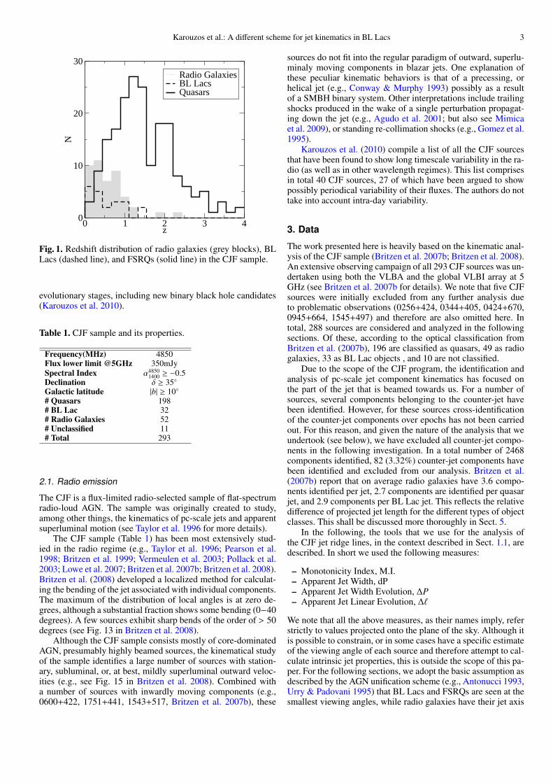
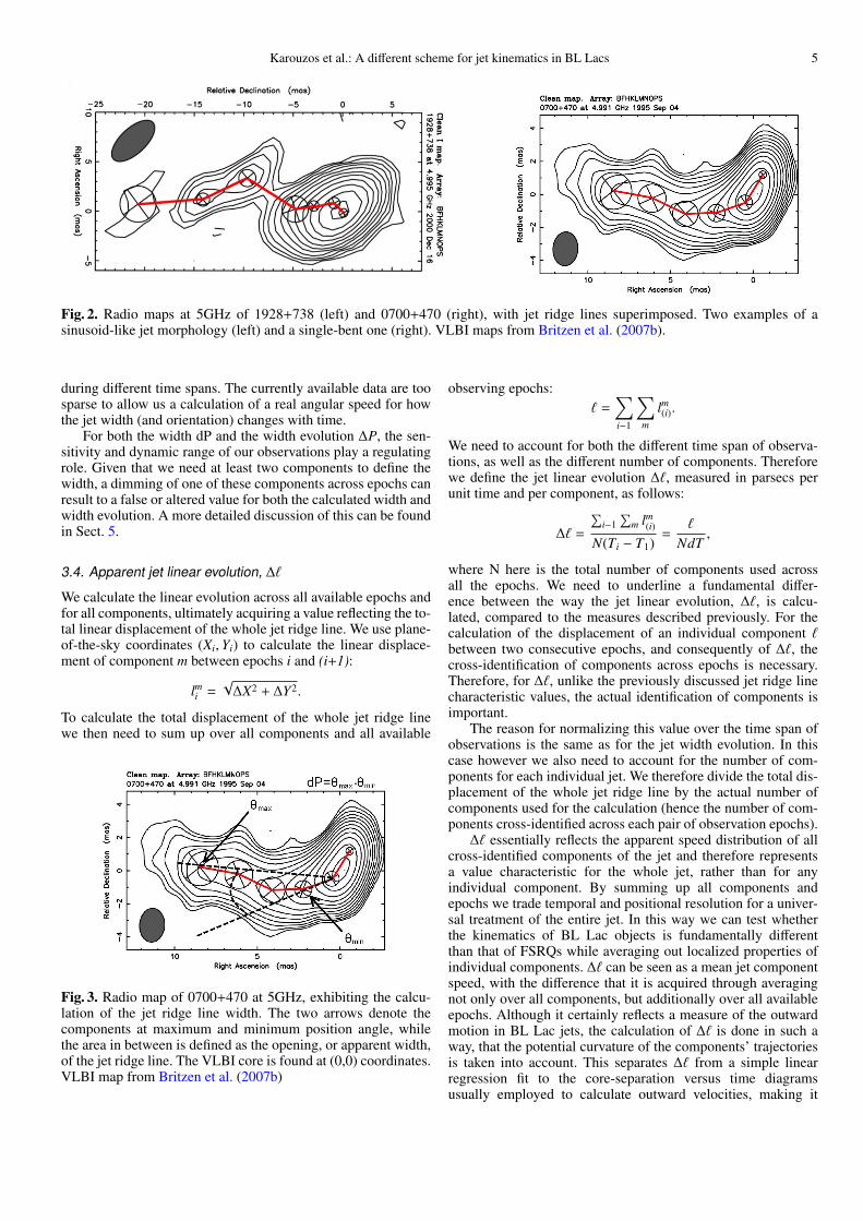
It is known that a large number of active galaxies exhibit bentor otherwise non-linear jet morphologies on various scales.Individual sources like S5 1803+784 and PKS 0735+178 (seereferences above), as well as others (e.g. 3C 345; Lobanov &Zensus 1999; B0605-085; Kudryavtseva et al. 2010), have beenextensively studied to understand the origin of these bends.Britzen et al. (2008) calculate the “bends” between successivecomponents of the pc-scale jet for all CJF sources, finding largelocal variations of the position angles of the sources. In this con-text, we are interested in quantifying the bending of the wholejet ridge line. Moreover, we want to differentiate between a“monotonically-bent” jet, i.e., a jet that is bent in only one di-rection (see Fig. 2, right), as opposed to a more sinusoid-likemorphology (similar to what is seen for some epochs of S51803+784, see Fig. 2, left). This is done by means of the mono-tonicity index, M.I..

We quantify a sinusoid-like morphology of a jet by identify-ing the local extrema in a given jet ridge line, in the core sep-aration - position angle plane. For an epoch i, a component mexhibits a local extremum under the definition

θm;extr : |θm − θm±1| ≥ 10(dθm + dθm±1),

where θm and dθm denote the position angle of component andits uncertainty. θm is calculated as

θm = arctanXY,

where X and Y are cartesian coordinates on the plane of the sky.Having calculated the number of extrema for a given jet ridgeline at an epoch i, we define the M.I. as

M.I. =number o f extrema

N − 1,

where N is the total number of components at that given epoch.This is a crude calculation, but can give us a handle on how thebending of the jet behaves along the jet. For M.I. values close toone, the jet resembles more a sinusoid. An M.I. value close tozero reveals a monotonic, single-bend, jet morphology. We nor-malize for the number of components N to account for longer, orshorter, jets and to enable comparison between different sources.As an example, for the sources shown in Fig. 2, 1928+738 isfound to have an M.I. value of 0.4, compared to 0700+470, thatgives an M.I. value of 0.

As is the case for most of the tools described in this sec-tion, the value of M.I. depends heavily on the resolution of theobservations. Given that the resolution is not the same acrossall epochs and sources, an uncertainty is introduced when com-paring two M.I. values of two different sources. A final remarkpertains to the definition of an extremum. We use a 10σ1 value

1 Here σ is defined as the sum of the position angle errors for θmand θm±1. The choice of this σ reflects an original underestimation (inBritzen et al. 2007b) of the position angle errors during the componentfitting.

as the lower limit for flagging an extremum. A different level ofsignificance (e.g., 5σ) would result in different values of M.I..The choice of the 10σ significance is a conservative approach tothe identification of extrema in the jet ridge line. In the follow-ing, M.I. shall be used as more of a qualitative tool rather than aquantitative measure of the actual jet morphology.

3.2. Apparent jet width, dP

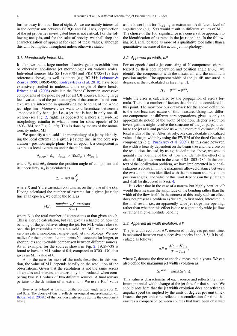
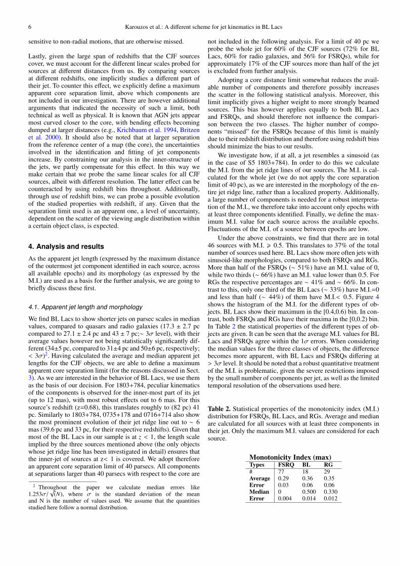
For an epoch i and a jet consisting of N components charac-terized by their core separation and position angle (ri, θi), weidentify the components with the maximum and the minimumposition angles. The apparent width of the jet dP, measured indegrees, is then calculated as (see Fig. 3):

dPi = θmaxi − θmin

i ,

while the error is calculated by the propagation of errors for-mula. There is a number of factors that should be considered atthis point. The most obvious drawback for the above definitionis the non-localized nature of this measure. Using two differ-ent components, at different core separations, gives us only anapproximate notion of the width of the flow. Higher resolutioninvestigations might resolve the structure of the jet perpendicu-lar to the jet axis and provide us with a more real estimate of thelocal width of the jet. Alternatively, one can calculate a localizedvalue of the jet width by using the FWHM of the fitted Gaussiancomponents (e.g., Pushkarev et al. 2009). In this case however,the width is heavily dependent on the beam size and therefore onthe resolution. Instead, by using the definition above, we seek toquantify the opening of the jet flow and identify the effect of achannel-like jet, as seen in the case of S5 1803+784. In the con-text of the localization problem, we have implemented in our cal-culations a constraint in the maximum allowed distance betweenthe two components identified with the minimum and maximumposition angles. The value of this limit depends on the jet lengthand shall be discussed in Sect. 4.

It is clear that in the case of a narrow but highly bent jet, dPwould then measure the amplitude of the bending rather than thewidth of the flow itself. In the context of this study such an effectdoes not present a problem as we are, to first order, interested inthe final result, i.e., an apparently wide jet ridge line opening,rather than whether this effect is due to a genuinely wide jet flowor rather a high-amplitude bending.

3.3. Apparent jet width evolution, ∆P

The jet width evolution ∆P, measured in degrees per unit time,is measured between two successive epochs i and (i-1). It is cal-culated as follows:

∆P =dPi − dPi−1

Ti − Ti−1,

where Ti denotes the time at epoch i, measured in years. We canalso define the maximum jet width evolution as:

∆Pmax = max∆P1...i.

This value is characteristic of each source and reflects the max-imum potential width change of the jet flow for that source. Weshould note here that the jet width evolution does not reflect anangular speed (as implied by the units of degrees per unit time).Instead the per unit time reflects a normalization for time thatensures a comparison between sources that have been observed


Fig. 2. Radio maps at 5GHz of 1928+738 (left) and 0700+470 (right), with jet ridge lines superimposed. Two examples of asinusoid-like jet morphology (left) and a single-bent one (right). VLBI maps from Britzen et al. (2007b).

during different time spans. The currently available data are toosparse to allow us a calculation of a real angular speed for howthe jet width (and orientation) changes with time.

For both the width dP and the width evolution ∆P, the sen-sitivity and dynamic range of our observations play a regulatingrole. Given that we need at least two components to define thewidth, a dimming of one of these components across epochs canresult to a false or altered value for both the calculated width andwidth evolution. A more detailed discussion of this can be foundin Sect. 5.

3.4. Apparent jet linear evolution, ∆`

We calculate the linear evolution across all available epochs andfor all components, ultimately acquiring a value reflecting the to-tal linear displacement of the whole jet ridge line. We use plane-of-the-sky coordinates (Xi,Yi) to calculate the linear displace-ment of component m between epochs i and (i+1):

lmi =√

∆X2 + ∆Y2.

To calculate the total displacement of the whole jet ridge linewe then need to sum up over all components and all available

Fig. 3. Radio map of 0700+470 at 5GHz, exhibiting the calcu-lation of the jet ridge line width. The two arrows denote thecomponents at maximum and minimum position angle, whilethe area in between is defined as the opening, or apparent width,of the jet ridge line. The VLBI core is found at (0,0) coordinates.VLBI map from Britzen et al. (2007b)

observing epochs:` =∑i−1

∑m

lm(i).

We need to account for both the different time span of observa-tions, as well as the different number of components. Thereforewe define the jet linear evolution ∆`, measured in parsecs perunit time and per component, as follows:

∆` =

∑i−1∑

m lm(i)N(Ti − T1)

=`

NdT,

where N here is the total number of components used acrossall the epochs. We need to underline a fundamental differ-ence between the way the jet linear evolution, ∆`, is calcu-lated, compared to the measures described previously. For thecalculation of the displacement of an individual component `between two consecutive epochs, and consequently of ∆`, thecross-identification of components across epochs is necessary.Therefore, for ∆`, unlike the previously discussed jet ridge linecharacteristic values, the actual identification of components isimportant.

The reason for normalizing this value over the time span ofobservations is the same as for the jet width evolution. In thiscase however we also need to account for the number of com-ponents for each individual jet. We therefore divide the total dis-placement of the whole jet ridge line by the actual number ofcomponents used for the calculation (hence the number of com-ponents cross-identified across each pair of observation epochs).

∆` essentially reflects the apparent speed distribution of allcross-identified components of the jet and therefore representsa value characteristic for the whole jet, rather than for anyindividual component. By summing up all components andepochs we trade temporal and positional resolution for a univer-sal treatment of the entire jet. In this way we can test whetherthe kinematics of BL Lac objects is fundamentally differentthan that of FSRQs while averaging out localized properties ofindividual components. ∆` can be seen as a mean jet componentspeed, with the difference that it is acquired through averagingnot only over all components, but additionally over all availableepochs. Although it certainly reflects a measure of the outwardmotion in BL Lac jets, the calculation of ∆` is done in such away, that the potential curvature of the components’ trajectoriesis taken into account. This separates ∆` from a simple linearregression fit to the core-separation versus time diagramsusually employed to calculate outward velocities, making it


sensitive to non-radial motions, that are otherwise missed.

Lastly, given the large span of redshifts that the CJF sourcescover, we must account for the different linear scales probed forsources at different distances from us. By comparing sourcesat different redshifts, one implicitly studies a different part oftheir jet. To counter this effect, we explicitly define a maximumapparent core separation limit, above which components arenot included in our investigation. There are however additionalarguments that indicated the necessity of such a limit, bothtechnical as well as physical. It is known that AGN jets appearmost curved closer to the core, with bending effects becomingdumped at larger distances (e.g., Krichbaum et al. 1994, Britzenet al. 2000). It should also be noted that at larger separationfrom the reference center of a map (the core), the uncertaintiesinvolved in the identification and fitting of jet componentsincrease. By constraining our analysis in the inner-structure ofthe jets, we partly compensate for this effect. In this way wemake certain that we probe the same linear scales for all CJFsources, albeit with different resolution. The latter effect can becounteracted by using redshift bins throughout. Additionally,through use of redshift bins, we can probe a possible evolutionof the studied properties with redshift, if any. Given that theseparation limit used is an apparent one, a level of uncertainty,dependent on the scatter of the viewing angle distribution withina certain object class, is expected.

4. Analysis and results

As the apparent jet length (expressed by the maximum distanceof the outermost jet component identified in each source, acrossall available epochs) and its morphology (as expressed by theM.I.) are used as a basis for the further analysis, we are going tobriefly discuss these first.

4.1. Apparent jet length and morphology

We find BL Lacs to show shorter jets on parsec scales in medianvalues, compared to quasars and radio galaxies (17.3 ± 2.7 pccompared to 27.1 ± 2.4 pc and 43 ± 7 pc;∼ 3σ level), with theiraverage values however not being statistically significantly dif-ferent (34±5 pc, compared to 31±4 pc and 50±6 pc, respectively;< 3σ)2. Having calculated the average and median apparent jetlengths for the CJF objects, we are able to define a maximumapparent core separation limit (for the reasons discussed in Sect.3). As we are interested in the behavior of BL Lacs, we use themas the basis of our decision. For 1803+784, peculiar kinematicsof the components is observed for the inner-most part of its jet(up to 12 mas), with most robust effects out to 6 mas. For thissource’s redshift (z=0.68), this translates roughly to (82 pc) 41pc. Similarly to 1803+784, 0735+178 and 0716+714 also showthe most prominent evolution of their jet ridge line out to ∼ 6mas (39.6 pc and 33 pc, for their respective redshifts). Given thatmost of the BL Lacs in our sample is at z < 1, the length scaleimplied by the three sources mentioned above (the only objectswhose jet ridge line has been investigated in detail) ensures thatthe inner-jet of sources at z< 1 is covered. We adopt thereforean apparent core separation limit of 40 parsecs. All componentsat separations larger than 40 parsecs with respect to the core are

2 Throughout the paper we calculate median errors like1.253σ/

√(N), where σ is the standard deviation of the mean

and N is the number of values used. We assume that the quantitiesstudied here follow a normal distribution.

not included in the following analysis. For a limit of 40 pc weprobe the whole jet for 60% of the CJF sources (72% for BLLacs, 60% for radio galaxies, and 56% for FSRQs), while forapproximately 17% of the CJF sources more than half of the jetis excluded from further analysis.

Adopting a core distance limit somewhat reduces the avail-able number of components and therefore possibly increasesthe scatter in the following statistical analysis. Moreover, thislimit implicitly gives a higher weight to more strongly beamedsources. This bias however applies equally to both BL Lacsand FSRQs, and should therefore not influence the compari-son between the two classes. The higher number of compo-nents “missed” for the FSRQs because of this limit is mainlydue to their redshift distribution and therefore using redshift binsshould minimize the bias to our results.

We investigate how, if at all, a jet resembles a sinusoid (asin the case of S5 1803+784). In order to do this we calculatethe M.I. from the jet ridge lines of our sources. The M.I. is cal-culated for the whole jet (we do not apply the core separationlimit of 40 pc), as we are interested in the morphology of the en-tire jet ridge line, rather than a localized property. Additionally,a large number of components is needed for a robust interpreta-tion of the M.I., we therefore take into account only epochs withat least three components identified. Finally, we define the max-imum M.I. value for each source across the available epochs.Fluctuations of the M.I. of a source between epochs are low.

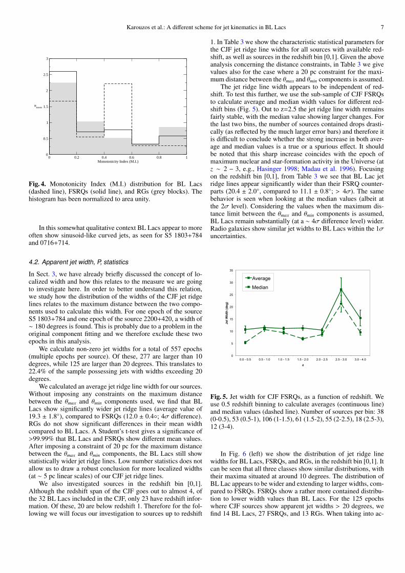
Under the above constraints, we find that there are in total46 sources with M.I. > 0.5. This translates to 37% of the totalnumber of sources used here. BL Lacs show more often jets withsinusoid-like morphologies, compared to both FSRQs and RGs.More than half of the FSRQs (∼ 51%) have an M.I. value of 0,while two thirds (∼ 66%) have an M.I. value lower than 0.5. ForRGs the respective percentages are ∼ 41% and ∼ 66%. In con-trast to this, only one third of the BL Lacs (∼ 33%) have M.I.=0and less than half (∼ 44%) of them have M.I.< 0.5. Figure 4shows the histogram of the M.I. for the different types of ob-jects. BL Lacs show their maximum in the [0.4,0.6) bin. In con-trast, both FSRQs and RGs have their maxima in the [0,0.2) bin.In Table 2 the statistical properties of the different types of ob-jects are given. It can be seen that the average M.I. values for BLLacs and FSRQs agree within the 1σ errors. When consideringthe median values for the three classes of objects, the differencebecomes more apparent, with BL Lacs and FSRQs differing at> 3σ level. It should be noted that a robust quantitative treatmentof the M.I. is problematic, given the severe restrictions imposedby the small number of components per jet, as well as the limitedtemporal resolution of the observations used here.

Table 2. Statistical properties of the monotonicity index (M.I.)distribution for FSRQs, BL Lacs, and RGs. Average and medianare calculated for all sources with at least three components intheir jet. Only the maximum M.I. values are considered for eachsource.

Monotonicity Index (max)Types FSRQ BL RG# 77 18 29Average 0.29 0.36 0.35Error 0.03 0.06 0.06Median 0 0.500 0.330Error 0.004 0.014 0.012


0 0.2 0.4 0.6 0.8 1Monotonicity Index (M.I.)

0

0.5

1

1.5

2

2.5

3

nnorm

Fig. 4. Monotonicity Index (M.I.) distribution for BL Lacs(dashed line), FSRQs (solid line), and RGs (grey blocks). Thehistogram has been normalized to area unity.

In this somewhat qualitative context BL Lacs appear to moreoften show sinusoid-like curved jets, as seen for S5 1803+784and 0716+714.

4.2. Apparent jet width, P, statistics

In Sect. 3, we have already briefly discussed the concept of lo-calized width and how this relates to the measure we are goingto investigate here. In order to better understand this relation,we study how the distribution of the widths of the CJF jet ridgelines relates to the maximum distance between the two compo-nents used to calculate this width. For one epoch of the sourceS5 1803+784 and one epoch of the source 2200+420, a width of∼ 180 degrees is found. This is probably due to a problem in theoriginal component fitting and we therefore exclude these twoepochs in this analysis.

We calculate non-zero jet widths for a total of 557 epochs(multiple epochs per source). Of these, 277 are larger than 10degrees, while 125 are larger than 20 degrees. This translates to22.4% of the sample possessing jets with widths exceeding 20degrees.

We calculated an average jet ridge line width for our sources.Without imposing any constraints on the maximum distancebetween the θmax and θmin components used, we find that BLLacs show significantly wider jet ridge lines (average value of19.3 ± 1.8), compared to FSRQs (12.0 ± 0.4; 4σ difference).RGs do not show significant differences in their mean widthcompared to BL Lacs. A Student’s t-test gives a significance of>99.99% that BL Lacs and FSRQs show different mean values.After imposing a constraint of 20 pc for the maximum distancebetween the θmax and θmin components, the BL Lacs still showstatistically wider jet ridge lines. Low number statistics does notallow us to draw a robust conclusion for more localized widths(at ∼ 5 pc linear scales) of our CJF jet ridge lines.

We also investigated sources in the redshift bin [0,1].Although the redshift span of the CJF goes out to almost 4, ofthe 32 BL Lacs included in the CJF, only 23 have redshift infor-mation. Of these, 20 are below redshift 1. Therefore for the fol-lowing we will focus our investigation to sources up to redshift

1. In Table 3 we show the characteristic statistical parameters forthe CJF jet ridge line widths for all sources with available red-shift, as well as sources in the redshift bin [0,1]. Given the aboveanalysis concerning the distance constraints, in Table 3 we givevalues also for the case where a 20 pc constraint for the maxi-mum distance between the θmax and θmin components is assumed.

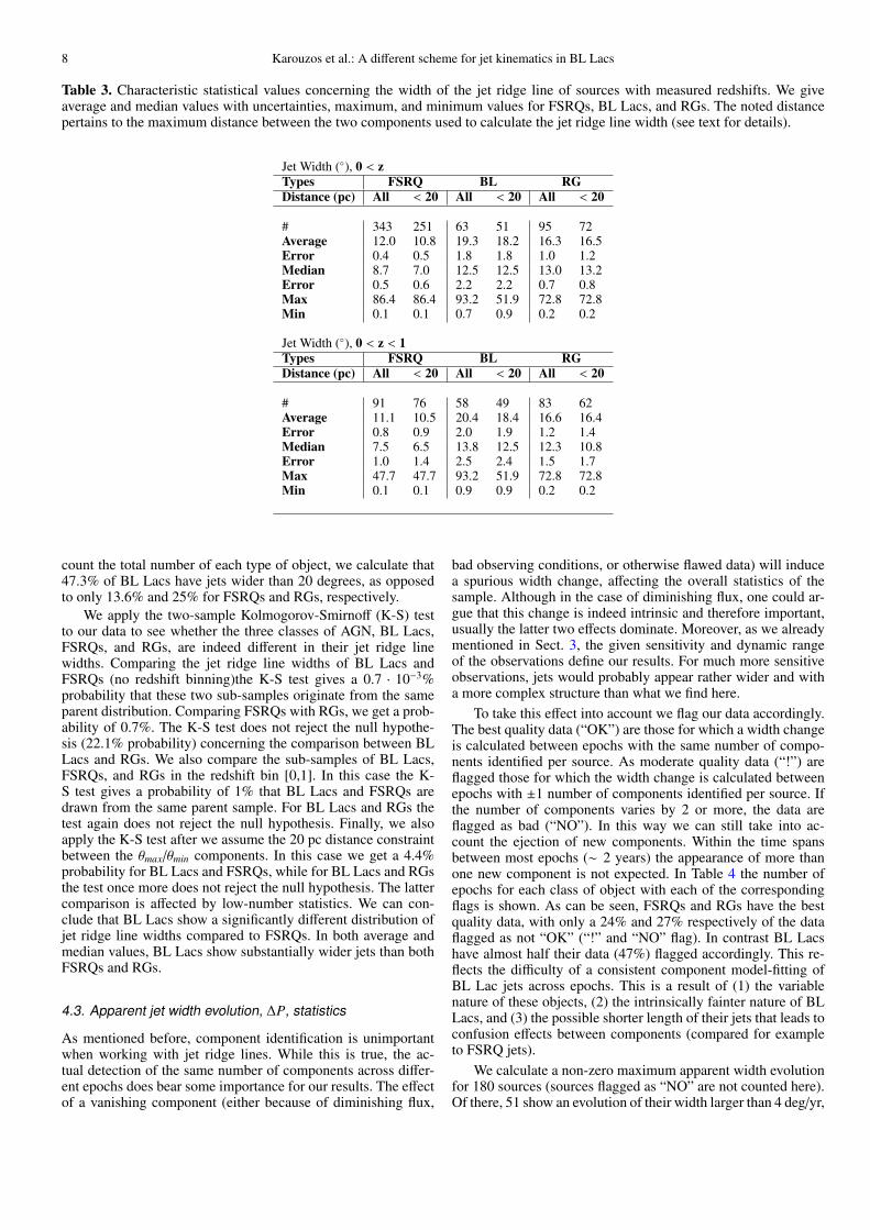
The jet ridge line width appears to be independent of red-shift. To test this further, we use the sub-sample of CJF FSRQsto calculate average and median width values for different red-shift bins (Fig. 5). Out to z=2.5 the jet ridge line width remainsfairly stable, with the median value showing larger changes. Forthe last two bins, the number of sources contained drops drasti-cally (as reflected by the much larger error bars) and therefore itis difficult to conclude whether the strong increase in both aver-age and median values is a true or a spurious effect. It shouldbe noted that this sharp increase coincides with the epoch ofmaximum nuclear and star-formation activity in the Universe (atz ∼ 2 − 3, e.g., Hasinger 1998; Madau et al. 1996). Focusingon the redshift bin [0,1], from Table 3 we see that BL Lac jetridge lines appear significantly wider than their FSRQ counter-parts (20.4 ± 2.0, compared to 11.1 ± 0.8; > 4σ). The samebehavior is seen when looking at the median values (albeit atthe 2σ level). Considering the values when the maximum dis-tance limit between the θmax and θmin components is assumed,BL Lacs remain substantially (at a ∼ 4σ difference level) wider.Radio galaxies show similar jet widths to BL Lacs within the 1σuncertainties.

0

5

10

15

20

25

30

35

0.0 - 0.5 0.5 - 1.0 1.0 - 1.5 1.5 - 2.0 2.0 - 2.5 2.5 - 3.0 3.0 - 4.0

Jet W

idth

(deg

)

z

Average

Median

Fig. 5. Jet width for CJF FSRQs, as a function of redshift. Weuse 0.5 redshift binning to calculate averages (continuous line)and median values (dashed line). Number of sources per bin: 38(0-0.5), 53 (0.5-1), 106 (1-1.5), 61 (1.5-2), 55 (2-2.5), 18 (2.5-3),12 (3-4).

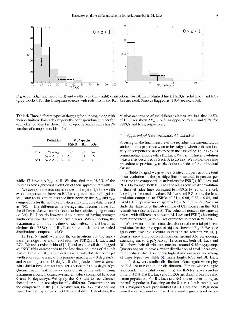
In Fig. 6 (left) we show the distribution of jet ridge linewidths for BL Lacs, FSRQs, and RGs, in the redshift bin [0,1]. Itcan be seen that all three classes show similar distributions, withtheir maxima situated at around 10 degrees. The distribution ofBL Lac appears to be wider and extending to larger widths, com-pared to FSRQs. FSRQs show a rather more contained distribu-tion to lower width values than BL Lacs. For the 125 epochswhere CJF sources show apparent jet widths > 20 degrees, wefind 14 BL Lacs, 27 FSRQs, and 13 RGs. When taking into ac-


Table 3. Characteristic statistical values concerning the width of the jet ridge line of sources with measured redshifts. We giveaverage and median values with uncertainties, maximum, and minimum values for FSRQs, BL Lacs, and RGs. The noted distancepertains to the maximum distance between the two components used to calculate the jet ridge line width (see text for details).

Jet Width (), 0 < zTypes FSRQ BL RGDistance (pc) All < 20 All < 20 All < 20

# 343 251 63 51 95 72Average 12.0 10.8 19.3 18.2 16.3 16.5Error 0.4 0.5 1.8 1.8 1.0 1.2Median 8.7 7.0 12.5 12.5 13.0 13.2Error 0.5 0.6 2.2 2.2 0.7 0.8Max 86.4 86.4 93.2 51.9 72.8 72.8Min 0.1 0.1 0.7 0.9 0.2 0.2

Jet Width (), 0 < z < 1Types FSRQ BL RGDistance (pc) All < 20 All < 20 All < 20


count the total number of each type of object, we calculate that47.3% of BL Lacs have jets wider than 20 degrees, as opposedto only 13.6% and 25% for FSRQs and RGs, respectively.

We apply the two-sample Kolmogorov-Smirnoff (K-S) testto our data to see whether the three classes of AGN, BL Lacs,FSRQs, and RGs, are indeed different in their jet ridge linewidths. Comparing the jet ridge line widths of BL Lacs andFSRQs (no redshift binning)the K-S test gives a 0.7 · 10−3%probability that these two sub-samples originate from the sameparent distribution. Comparing FSRQs with RGs, we get a prob-ability of 0.7%. The K-S test does not reject the null hypothe-sis (22.1% probability) concerning the comparison between BLLacs and RGs. We also compare the sub-samples of BL Lacs,FSRQs, and RGs in the redshift bin [0,1]. In this case the K-S test gives a probability of 1% that BL Lacs and FSRQs aredrawn from the same parent sample. For BL Lacs and RGs thetest again does not reject the null hypothesis. Finally, we alsoapply the K-S test after we assume the 20 pc distance constraintbetween the θmax/θmin components. In this case we get a 4.4%probability for BL Lacs and FSRQs, while for BL Lacs and RGsthe test once more does not reject the null hypothesis. The lattercomparison is affected by low-number statistics. We can con-clude that BL Lacs show a significantly different distribution ofjet ridge line widths compared to FSRQs. In both average andmedian values, BL Lacs show substantially wider jets than bothFSRQs and RGs.

4.3. Apparent jet width evolution, ∆P, statistics

As mentioned before, component identification is unimportantwhen working with jet ridge lines. While this is true, the ac-tual detection of the same number of components across differ-ent epochs does bear some importance for our results. The effectof a vanishing component (either because of diminishing flux,

bad observing conditions, or otherwise flawed data) will inducea spurious width change, affecting the overall statistics of thesample. Although in the case of diminishing flux, one could ar-gue that this change is indeed intrinsic and therefore important,usually the latter two effects dominate. Moreover, as we alreadymentioned in Sect. 3, the given sensitivity and dynamic rangeof the observations define our results. For much more sensitiveobservations, jets would probably appear rather wider and witha more complex structure than what we find here.

To take this effect into account we flag our data accordingly.The best quality data (“OK”) are those for which a width changeis calculated between epochs with the same number of compo-nents identified per source. As moderate quality data (“!”) areflagged those for which the width change is calculated betweenepochs with ±1 number of components identified per source. Ifthe number of components varies by 2 or more, the data areflagged as bad (“NO”). In this way we can still take into ac-count the ejection of new components. Within the time spansbetween most epochs (∼ 2 years) the appearance of more thanone new component is not expected. In Table 4 the number ofepochs for each class of object with each of the correspondingflags is shown. As can be seen, FSRQs and RGs have the bestquality data, with only a 24% and 27% respectively of the dataflagged as not “OK” (“!” and “NO” flag). In contrast BL Lacshave almost half their data (47%) flagged accordingly. This re-flects the difficulty of a consistent component model-fitting ofBL Lac jets across epochs. This is a result of (1) the variablenature of these objects, (2) the intrinsically fainter nature of BLLacs, and (3) the possible shorter length of their jets that leads toconfusion effects between components (compared for exampleto FSRQ jets).

We calculate a non-zero maximum apparent width evolutionfor 180 sources (sources flagged as “NO” are not counted here).Of there, 51 show an evolution of their width larger than 4 deg/yr,


0 10 20 30 40 50 60 70 80 90 100dP (deg)

0

10

20

30

40

50

N

0 < z < 1

0 6 12 18ΔP

max (deg/yr)

0

5

10

15

20

N

0 < z < 1

Fig. 6. Jet ridge line width (left) and width evolution (right) distributions for BL Lacs (dashed line), FSRQs (solid line), and RGs(grey blocks). For this histogram sources with redshifts in the [0,1] bin are used. Sources flagged as “NO” are excluded.

Table 4. Three different types of flagging for our data, along withtheir definition. For each category the corresponding number foreach class of object is shown. For an epoch i, each source has Ninumber of components identified.

Definition # of epochsFSRQ BL RG

OK Nl = Nl+1 173 26 54! Nl = Nl+1 ± 1 53 21 15NO Nl ≥ Nl+1 ± 2 2 2 5

while 17 have a ∆Pmax > 8. We thus find that 28.3% of thesources show significant evolution of their apparent jet width.

We compare the maximum values of the jet ridge line widthevolution per source between BL Lacs, quasars, and radio galax-ies, using no maximum distance limit between the θmax and θmincomponents for the width calculation and excluding data flaggedas “NO”. The differences in average and median values forthe different classes are not found to be statistically significant(< 3σ). BL Lacs do however show a trend of having strongerwidth evolution than the other two classes. When checking themaximum and minimum values of each sub-sample, it becomesobvious that FSRQs and BL Lacs show much more extendeddistributions compared to RGs.

In Fig. 6 (right) we show the distributions for the maxi-mum jet ridge line width evolution for FSRQs, BL Lacs, andRGs. We use a redshift bin of [0,1] and exclude all data flaggedas “NO” (this corresponds to the last three columns of the leftpart of Table 5). BL Lac objects show a wide distribution of jetwidth evolution values, with a primary maximum at 3 degrees/yrand extending out to 18 deg/yr. Radio galaxies show a some-what similar behavior with a plateau between 2 and 4 degrees/yr.Quasars, in contrast, show a confined distribution with a strongmaximum around 3 degrees/yr and all values contained between0 and 10 degrees/yr. We apply the K-S test to see whetherthese distribution are significantly different. Concentrating onthe comparison in the [0,1] redshift bin, the K-S test does notreject the null hypothesis (33.8% probability). Calculating the

relative occurrence of the different classes, we find that 12.5%of BL Lacs show ∆Pmax > 8, as opposed to 4% and 5.7% forFSRQs and RGs, respectively.

4.4. Apparent jet linear evolution, ∆`, statistics

Focusing on the final measure of the jet ridge line kinematics, asstudied in this paper, we want to investigate whether the station-arity of components, as observed in the case of S5 1803+784, iscommonplace among other BL Lacs. We use the linear evolutionmeasure, as described in Sect. 3, to do this. We follow the sameprocedure as previously, to check the statistics of the individualclasses.

In Table 5 (right) we give the statistical properties of the totallinear evolution of the jet ridge line (measured in parsecs perunit time and component) distributions for FSRQs, BL Lacs, andRGs. On average, both BL Lacs and RGs show weaker evolutionof their jet ridge lines compared to FSRQs (∼ 2σ difference).Looking at the median values, BL Lacs and RGs show the leastevolution compared to FSRQs (0.24 ± 0.06, 0.28 ± 0.04, and0.414±0.020 pc/yr/comp respectively; ∼ 3σ difference). We alsostudy the statistics of the sub-sample of CJF sources in the [0,1]redshift bin (also in Table 5). The behavior remains the same asbefore, with differences between BL Lacs and FSRQs becomingmore pronounced (with a ∼ 4σ difference in median values).

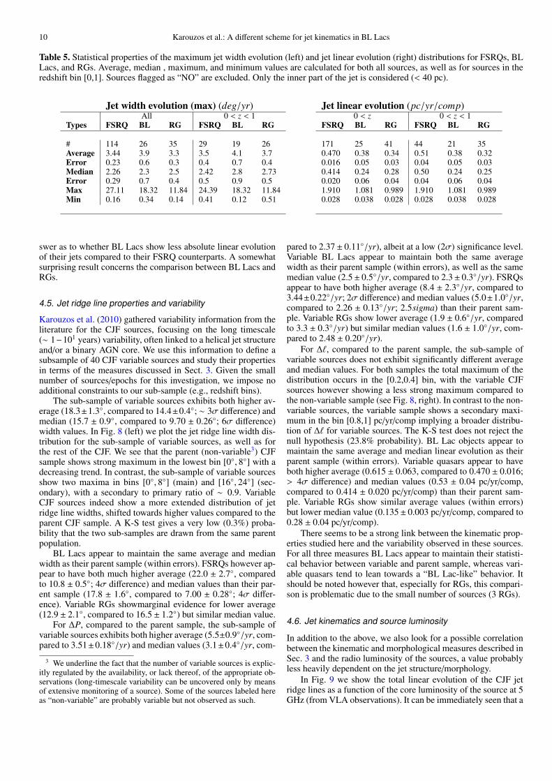
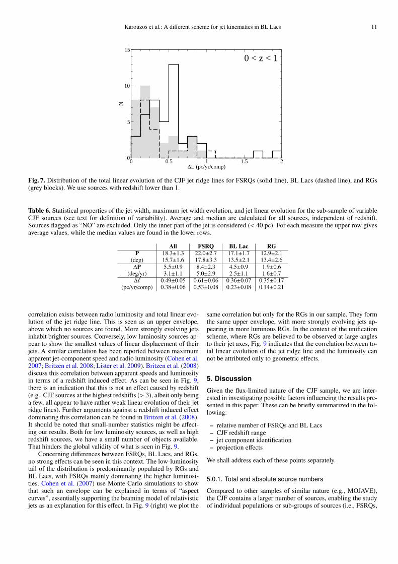
We now turn to the actual distribution of the total jet linearevolution for the three types of objects, shown in Fig. 7. We onceagain only take into account sources in the redshift bin [0,1].Quasars show a pronounced maximum around 0.63 pc/yr/comp,extending out to 2 pc/yr/comp. In contrast, both BL Lacs andRGs show their distribution maxima around 0.25 pc/yr/comp.Quasars appear to have a wider distribution of total linear evo-lution values, also showing the highest maximum values amongall three types (see Table 5). Interestingly, RGs and BL Lacs,in total, show very similar distributions. Once again we employthe K-S test to compare the distributions. For the whole sample(independent of redshift constraints), the K-S test gives a proba-bility of 4.3% that BL Lacs and FSRQs are drawn from the sameparent population. For BL Lacs and RGs the test does not rejectthe null hypothesis. Focusing on the 0 < z < 1 sub-sample, weget a marginal 5.4% probability that BL Lacs and FSRQs stemfrom the same parent sample. These results give a positive an-


Table 5. Statistical properties of the maximum jet width evolution (left) and jet linear evolution (right) distributions for FSRQs, BLLacs, and RGs. Average, median , maximum, and minimum values are calculated for both all sources, as well as for sources in theredshift bin [0,1]. Sources flagged as “NO” are excluded. Only the inner part of the jet is considered (< 40 pc).

Jet width evolution (max) (deg/yr)All 0 < z < 1

Types FSRQ BL RG FSRQ BL RG


Jet linear evolution (pc/yr/comp)0 < z 0 < z < 1

FSRQ BL RG FSRQ BL RG

171 25 41 44 21 350.470 0.38 0.34 0.51 0.38 0.320.016 0.05 0.03 0.04 0.05 0.030.414 0.24 0.28 0.50 0.24 0.250.020 0.06 0.04 0.04 0.06 0.041.910 1.081 0.989 1.910 1.081 0.9890.028 0.038 0.028 0.028 0.038 0.028

swer as to whether BL Lacs show less absolute linear evolutionof their jets compared to their FSRQ counterparts. A somewhatsurprising result concerns the comparison between BL Lacs andRGs.

4.5. Jet ridge line properties and variability

Karouzos et al. (2010) gathered variability information from theliterature for the CJF sources, focusing on the long timescale(∼ 1−101 years) variability, often linked to a helical jet structureand/or a binary AGN core. We use this information to define asubsample of 40 CJF variable sources and study their propertiesin terms of the measures discussed in Sect. 3. Given the smallnumber of sources/epochs for this investigation, we impose noadditional constraints to our sub-sample (e.g., redshift bins).

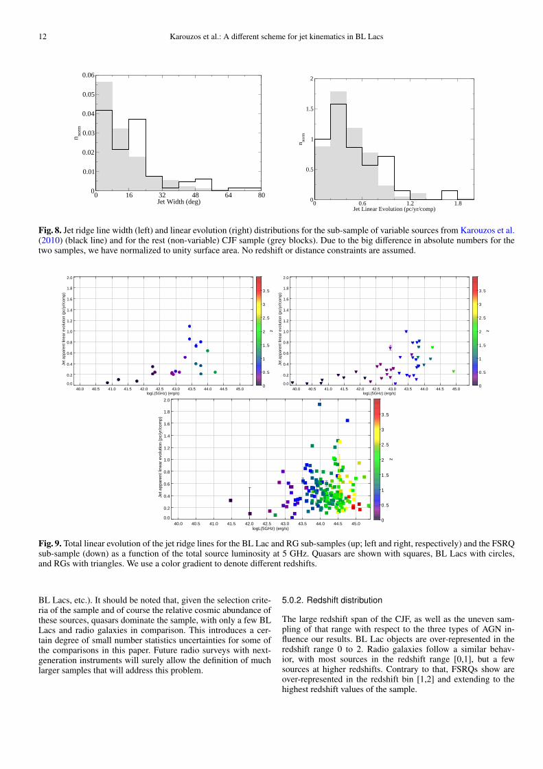
The sub-sample of variable sources exhibits both higher av-erage (18.3±1.3, compared to 14.4±0.4; ∼ 3σ difference) andmedian (15.7 ± 0.9, compared to 9.70 ± 0.26; 6σ difference)width values. In Fig. 8 (left) we plot the jet ridge line width dis-tribution for the sub-sample of variable sources, as well as forthe rest of the CJF. We see that the parent (non-variable3) CJFsample shows strong maximum in the lowest bin [0, 8] with adecreasing trend. In contrast, the sub-sample of variable sourcesshow two maxima in bins [0, 8] (main) and [16, 24] (sec-ondary), with a secondary to primary ratio of ∼ 0.9. VariableCJF sources indeed show a more extended distribution of jetridge line widths, shifted towards higher values compared to theparent CJF sample. A K-S test gives a very low (0.3%) proba-bility that the two sub-samples are drawn from the same parentpopulation.

BL Lacs appear to maintain the same average and medianwidth as their parent sample (within errors). FSRQs however ap-pear to have both much higher average (22.0 ± 2.7, comparedto 10.8 ± 0.5; 4σ difference) and median values than their par-ent sample (17.8 ± 1.6, compared to 7.00 ± 0.28; 4σ differ-ence). Variable RGs showmarginal evidence for lower average(12.9 ± 2.1, compared to 16.5 ± 1.2) but similar median value.

For ∆P, compared to the parent sample, the sub-sample ofvariable sources exhibits both higher average (5.5±0.9/yr, com-pared to 3.51±0.18/yr) and median values (3.1±0.4/yr, com-

3 We underline the fact that the number of variable sources is explic-itly regulated by the availability, or lack thereof, of the appropriate ob-servations (long-timescale variability can be uncovered only by meansof extensive monitoring of a source). Some of the sources labeled hereas “non-variable” are probably variable but not observed as such.

pared to 2.37± 0.11/yr), albeit at a low (2σ) significance level.Variable BL Lacs appear to maintain both the same averagewidth as their parent sample (within errors), as well as the samemedian value (2.5± 0.5/yr, compared to 2.3± 0.3/yr). FSRQsappear to have both higher average (8.4 ± 2.3/yr, compared to3.44±0.22/yr; 2σ difference) and median values (5.0±1.0/yr,compared to 2.26 ± 0.13/yr; 2.5sigma) than their parent sam-ple. Variable RGs show lower average (1.9 ± 0.6/yr, comparedto 3.3 ± 0.3/yr) but similar median values (1.6 ± 1.0/yr, com-pared to 2.48 ± 0.20/yr).

For ∆`, compared to the parent sample, the sub-sample ofvariable sources does not exhibit significantly different averageand median values. For both samples the total maximum of thedistribution occurs in the [0.2,0.4] bin, with the variable CJFsources however showing a less strong maximum compared tothe non-variable sample (see Fig. 8, right). In contrast to the non-variable sources, the variable sample shows a secondary maxi-mum in the bin [0.8,1] pc/yr/comp implying a broader distribu-tion of ∆` for variable sources. The K-S test does not reject thenull hypothesis (23.8% probability). BL Lac objects appear tomaintain the same average and median linear evolution as theirparent sample (within errors). Variable quasars appear to haveboth higher average (0.615 ± 0.063, compared to 0.470 ± 0.016;> 4σ difference) and median values (0.53 ± 0.04 pc/yr/comp,compared to 0.414 ± 0.020 pc/yr/comp) than their parent sam-ple. Variable RGs show similar average values (within errors)but lower median value (0.135± 0.003 pc/yr/comp, compared to0.28 ± 0.04 pc/yr/comp).

There seems to be a strong link between the kinematic prop-erties studied here and the variability observed in these sources.For all three measures BL Lacs appear to maintain their statisti-cal behavior between variable and parent sample, whereas vari-able quasars tend to lean towards a “BL Lac-like” behavior. Itshould be noted however that, especially for RGs, this compari-son is problematic due to the small number of sources (3 RGs).

4.6. Jet kinematics and source luminosity

In addition to the above, we also look for a possible correlationbetween the kinematic and morphological measures described inSec. 3 and the radio luminosity of the sources, a value probablyless heavily dependent on the jet structure/morphology.

In Fig. 9 we show the total linear evolution of the CJF jetridge lines as a function of the core luminosity of the source at 5GHz (from VLA observations). It can be immediately seen that a


0 0.5 1 1.5 2ΔL (pc/yr/comp)

0

5

10

15

N

0 < z < 1

Fig. 7. Distribution of the total linear evolution of the CJF jet ridge lines for FSRQs (solid line), BL Lacs (dashed line), and RGs(grey blocks). We use sources with redshift lower than 1.

Table 6. Statistical properties of the jet width, maximum jet width evolution, and jet linear evolution for the sub-sample of variableCJF sources (see text for definition of variability). Average and median are calculated for all sources, independent of redshift.Sources flagged as “NO” are excluded. Only the inner part of the jet is considered (< 40 pc). For each measure the upper row givesaverage values, while the median values are found in the lower rows.

All FSRQ BL Lac RGP 18.3±1.3 22.0±2.7 17.1±1.7 12.9±2.1

(deg) 15.7±1.6 17.8±3.3 13.5±2.1 13.4±2.6∆P 5.5±0.9 8.4±2.3 4.5±0.9 1.9±0.6

(deg/yr) 3.1±1.1 5.0±2.9 2.5±1.1 1.6±0.7∆` 0.49±0.05 0.61±0.06 0.36±0.07 0.35±0.17

(pc/yr/comp) 0.38±0.06 0.53±0.08 0.23±0.08 0.14±0.21

correlation exists between radio luminosity and total linear evo-lution of the jet ridge line. This is seen as an upper envelope,above which no sources are found. More strongly evolving jetsinhabit brighter sources. Conversely, low luminosity sources ap-pear to show the smallest values of linear displacement of theirjets. A similar correlation has been reported between maximumapparent jet-component speed and radio luminosity (Cohen et al.2007; Britzen et al. 2008; Lister et al. 2009). Britzen et al. (2008)discuss this correlation between apparent speeds and luminosityin terms of a redshift induced effect. As can be seen in Fig. 9,there is an indication that this is not an effect caused by redshift(e.g., CJF sources at the highest redshifts (> 3), albeit only beinga few, all appear to have rather weak linear evolution of their jetridge lines). Further arguments against a redshift induced effectdominating this correlation can be found in Britzen et al. (2008).It should be noted that small-number statistics might be affect-ing our results. Both for low luminosity sources, as well as highredshift sources, we have a small number of objects available.That hinders the global validity of what is seen in Fig. 9.

Concerning differences between FSRQs, BL Lacs, and RGs,no strong effects can be seen in this context. The low-luminositytail of the distribution is predominantly populated by RGs andBL Lacs, with FSRQs mainly dominating the higher luminosi-ties. Cohen et al. (2007) use Monte Carlo simulations to showthat such an envelope can be explained in terms of “aspectcurves”, essentially supporting the beaming model of relativisticjets as an explanation for this effect. In Fig. 9 (right) we plot the

same correlation but only for the RGs in our sample. They formthe same upper envelope, with more strongly evolving jets ap-pearing in more luminous RGs. In the context of the unificationscheme, where RGs are believed to be observed at large anglesto their jet axes, Fig. 9 indicates that the correlation between to-tal linear evolution of the jet ridge line and the luminosity cannot be attributed only to geometric effects.

5. Discussion

Given the flux-limited nature of the CJF sample, we are inter-ested in investigating possible factors influencing the results pre-sented in this paper. These can be briefly summarized in the fol-lowing:

– relative number of FSRQs and BL Lacs– CJF redshift range– jet component identification– projection effects

We shall address each of these points separately.

5.0.1. Total and absolute source numbers

Compared to other samples of similar nature (e.g., MOJAVE),the CJF contains a larger number of sources, enabling the studyof individual populations or sub-groups of sources (i.e., FSRQs,


0 16 32 48 64 80Jet Width (deg)

0

0.01

0.02

0.03

0.04

0.05

0.06n no

rm

0 0.6 1.2 1.8Jet Linear Evolution (pc/yr/comp)

0

0.5

1

1.5

2

n norm

Fig. 8. Jet ridge line width (left) and linear evolution (right) distributions for the sub-sample of variable sources from Karouzos et al.(2010) (black line) and for the rest (non-variable) CJF sample (grey blocks). Due to the big difference in absolute numbers for thetwo samples, we have normalized to unity surface area. No redshift or distance constraints are assumed.

0.0

0.2

0.4

0.6

0.8

1.0

1.2

1.4

1.6

1.8

2.0

40.0 40.5 41.0 41.5 42.0 42.5 43.0 43.5 44.0 44.5 45.0logL(5GHz) (erg/s)

Jet a

ppar

ent l

inea

r ev

olut

ion

(pc/

yr/c

omp)

z

0

0.5

1

1.5

2

2.5

3

3.5

0.0

0.2

0.4

0.6

0.8

1.0

1.2

1.4

1.6

1.8

2.0

40.0 40.5 41.0 41.5 42.0 42.5 43.0 43.5 44.0 44.5 45.0logL(5GHz) (erg/s)

Jet a

ppar

ent l

inea

r ev

olut

ion

(pc/

yr/c

omp)

z

0

0.5

1

1.5

2

2.5

3

3.5

0.0

0.2

0.4

0.6

0.8

1.0

1.2

1.4

1.6

1.8

2.0

40.0 40.5 41.0 41.5 42.0 42.5 43.0 43.5 44.0 44.5 45.0logL(5GHz) (erg/s)

Jet a

ppar

ent l

inea

r ev

olut

ion

(pc/

yr/c

omp)

z

0

0.5

1

1.5

2

2.5

3

3.5

Fig. 9. Total linear evolution of the jet ridge lines for the BL Lac and RG sub-samples (up; left and right, respectively) and the FSRQsub-sample (down) as a function of the total source luminosity at 5 GHz. Quasars are shown with squares, BL Lacs with circles,and RGs with triangles. We use a color gradient to denote different redshifts.

BL Lacs, etc.). It should be noted that, given the selection crite-ria of the sample and of course the relative cosmic abundance ofthese sources, quasars dominate the sample, with only a few BLLacs and radio galaxies in comparison. This introduces a cer-tain degree of small number statistics uncertainties for some ofthe comparisons in this paper. Future radio surveys with next-generation instruments will surely allow the definition of muchlarger samples that will address this problem.

5.0.2. Redshift distribution

The large redshift span of the CJF, as well as the uneven sam-pling of that range with respect to the three types of AGN in-fluence our results. BL Lac objects are over-represented in theredshift range 0 to 2. Radio galaxies follow a similar behav-ior, with most sources in the redshift range [0,1], but a fewsources at higher redshifts. Contrary to that, FSRQs show areover-represented in the redshift bin [1,2] and extending to thehighest redshift values of the sample.


As we briefly discussed before, the fixed sensitivity and res-olution of the arrays used allows us to have a direct comparisonbetween the different CJF sources. On the same time however, italso essentially leads us to observe different scales of the jet forobjects at different redshifts. It is expected that the properties,kinematics, and morphology of a jet are strong functions of theseparation from the core. We therefore adopt redshift bins for allof the comparisons we do. Given the distribution of redshifts forthe CJF the only bin we can use without losing most of the BLLacs is the [0,1] one4.

5.0.3. Component identification

The way that we study the width and width evolution of the jet iscompletely independent of component identification. The linearevolution of the jet ridge line on the other hand is an excep-tion to this. For this measure we are forced to follow the givenidentification of components (from Britzen et al. 2007b) as weneed some reference point to calculate absolute displacements.Despite the inevitable coupling of prior component identifica-tion to our ∆` measure, the fact that we include in this measureall components and all epochs ensures a treatment of the jet asa whole, evening out peculiarities or possible misidentificationsof individual components.

Our measures are however sensitive to the number of compo-nents identified at a certain epoch. This is especially relevant forBL Lacs, given the nature of their jets. As we discussed shortlypreviously, BL Lacs are extremely variable sources. In parts thisowns to the presumably small angle to our line of sight, resultingto beaming effects that change the flux of both the core and thejet. Secondly, we have shown that BL Lacs show indications ofshorter jets than both FSRQs and RGs. This translates to higherdifficulty in consistently model-fitting the jets of BL Lacs, asblending effects become more prominent as the viewing angledecreases. Moreover, given the strong variability of both coreand jet, components might simply vanish as a result of dimin-ishing luminosity or insufficient dynamic range of the observa-tions. A further way to demonstrate this is by using the qualityclassification for jet components used by Britzen et al. (2008).Jet component proper motions are classified as Q1 for the bestquality data, and Q2 and Q3 for diminishing quality. The ratioN(Q1)/(N(Q2) + N(Q3)), where N(x) is the number of x qualitycomponents of that type of source, is 0.63 for FSRQs, 0.80 forRGs, and 0.41 for BL Lacs. Returning to our original point, wesee therefore that the number of components across epochs inBL Lacs jets is more variable than both FSRQs and RGs. Thisintroduces some uncertainty to our results.

5.0.4. Projection effects

The fact that the values calculated here are all projected onto theplane of the sky introduces some uncertainty and consequentlya scatter in this statistical investigation. Although for this analy-sis and for the following discussion we have adopted the generalAGN unification scheme, where BL Lacs and FSRQs are at thesmallest viewing angles and radio galaxies are at larger view-ing angles, the dispersion of the actual angles within each classintroduces the aforementioned scatter in our statistics.

4 It should also be noted that given the featureless spectrum, forwhich BL Lacs are famous, leads to more than 34% of the CJF BLLacs to not have available redshift information. When using redshiftbins these objects are obviously excluded.

An alternative path would be to try and deproject the jet val-ues calculated here. Although certainly possible for a numberof the CJF sources where a Doppler factor has been calculated(e.g., Britzen et al. 2007a, it would introduce further degrees ofuncertainty to our analysis that are not so easily constrained. Aswe are mainly interested in the comparison between FSRQs andBL Lacs rather than the calculation of intrinsic jet properties, thedeprojection is not essential for the results of this paper.

5.1. Possible explanations

It is of great interest to try and explain the kinematic behaviorseen in a large number of the CJF (combining the percentagescalculated from both apparent width and apparent width evolu-tion we get an approximately 30% of the sample showing widejets that change their width strongly) and the apparent preferencefor BL Lacs to show this behavior over FSRQs. One obvious fac-tor that should play a deciding role for the kinematics of jet com-ponents is the viewing angle under which a source is observed. Itis known that BL Lacs and FSRQs are seen jet-on, at the smallestviewing angles, with steeper-spectrum quasars and radio galax-ies being sources observed at progressively larger viewing an-gles (e.g., Antonucci 1993; Urry & Padovani 1995). Could aviewing angle difference explain the kinematic differences seenin some of the CJF sources and in particular observed betweenBL Lacs and FSRQs? Assuming that jet components follow bal-listic, linear paths, one can expect that viewed at smaller view-ing angles (smaller than the critical angle 1/γ, with γ being theLorentz factor of the flow), the components are observed to coversmaller distances, than if seen edge-on. Therefore, the slowerspeeds, and hence smaller total linear evolution of their jet ridgelines, observed for BL Lacs could be explained in terms of asystematically smaller viewing angle for BL Lacs, compared toFSRQs.

However, Hovatta et al. (2009) (based on an investigationinitiated by Lahteenmaki & Valtaoja 1999) used long timescalevariability of AGN, together with jet kinematics, to deriveDoppler factors and consequently viewing angles of a sampleof 87 AGN. They found that FSRQs actually show smallermean viewing angles than BL Lacs (a result also found byLahteenmaki & Valtaoja 1999). Although there are certain limi-tations to the method used by the authors, their results are diffi-cult to reconcile with a viewing-angle-dependent explanation ofour results.

Our results would therefore indicate the need for an addi-tional, potentially geometric, effect in play. This would be inagreement with Cohen et al. (2007), who postulate that low-speed components in FSRQ and BL Lac jets appear so becausetheir pattern Lorentz factor is lower than the bulk Lorentz factorof the jet. Alternatively, it should be considered whether there issome systematic bias in the way Doppler factors are estimated,that would lead to an over- or underestimation of the viewingangles of BL Lacs and FSRQs, respectively.

The large jet widths and jet widths changes are more diffi-cult to explain. An additional mechanism or effect must be in-troduced to produce a wide jet. Precession of the jet axis, or as-suming that the components follow non-ballistic and non-linearpaths can lead to such jet properties (e.g., Steffen et al. 1995;Gong 2008; Roland et al. 2008; Gong et al. 2011). In thesemodels, jet components follow highly curved trajectories, which,viewed face-on, would give the impression of a wider distribu-tion of jet component position angles. A precessing jet, or rathera precessing jet nozzle, would imply that different componentsfollow different trajectories. That would result in a changing


jet component position angle distribution, more pronounced atsmaller viewing angles. That more BL Lacs show M.I. closer toone compared to FSRQs, implying a highly curved, sinusoid-likeridge-line, lends additional support to this scenario. Followingthis train of thought would then lead us to the conclusion that ei-ther (1) there is a sub-set of FSRQs and BL Lacs (∼ 30% in oursample) for which non-ballistic and/or precession effects play animportant role, or more generally that (2) for these sources theviewing angles are below some critical angle θc that allow us towitness and thus characterize the helical or “non-ballistic” struc-ture common in all radio-AGN jets, but which would otherwisebe blended out by the projection effects at viewing angles > θc.

In a following paper, we shall use an expanded version of thehelical jet model of Steffen et al. (1995) to evaluate the statisticalresults presented here, in terms of the viewing angle (and hencebeaming) effect, as well as a possible helical geometry of the jet.

A final scenario that needs to be discussed is whether a sys-tematic difference in the Lorentz factors γ between FSRQs andBL Lacs could produce the effects observed here. It has beenargued that BL Lacs show smaller Lorentz factors than FSRQs(e.g., Morganti et al. 1995; Urry & Padovani 1995; Hovatta et al.2009). If this is true (and not a selection bias in the samples used)then that would naturally explain the slower components in BLLacs. The above in turn ties in to the currently accepted unifi-cation scheme (e.g., Urry & Padovani 1995). In that paradigm,BL Lacs and FSRQs are drawn from two, presumably different,parent samples of Fanaroff-Riley I (low luminosity) and II (highluminosity) galaxies (FR; Fanaroff & Riley 1974; Padovani &Urry 1991; Capetti & Celotti 1999; Xu et al. 2009), respectively.If that is true, then the differences seen in the jet ridge line prop-erties of BL Lacs and FSRQs should then translate to differencesbetween FRI and FRII jet kinematics. Interestingly, studies ofFRI and FRII kinematics have shown that both types have simi-lar parcec-scale jet Lorentz factors (e.g., Giovannini et al. 2001),contradictory to what we find here, as well as in other studiesmentioned above, concerning the parsec-scale jet speeds in BLLacs and FSRQs.

It should be noted however that FRI sources show disruptedjets much earlier (i.e., closer to the core) than FRIIs (e.g., seeLaing 1996 and references therein). Perucho et al. (2010) explainthis in terms of decollimation through the growth of non-linearKelvin-Helmholtz instability modes in FRI jets. In this context,the wider jets seen in BL Lacs could indicate larger amplitudeinstabilities (closer to the non-linear regime) in the jet that, giventhe lower-speed flows observed in these objects, would lead to anearlier disruption of the jet at kpc scales (as expected for FRIs).

It is difficult to offer a single answer concerning an interpre-tation of our results. It is very likely that both viewing angle andLorentz factor effects, as well as flow instabilities that depend onthe latter, influence the appearance of BL Lac and FSRQ jets. Acomparison between the jet ridge lines of FRIs and FRIIs to BLLacs and FSRQs, respectively, would offer further insight on theproblem. A much larger sample than the CJF would be requiredfor such a study.

5.2. Comparison with previous studies

It should be noted that this is the first time the jet ridge lines ofa sample of AGN this size have been explicitly and exclusivelystudied in a statistical manner. While the ridge line of a jet is nota new concept, so far only the jet ridge lines of individual sources(both galactic and stellar) have been studied (e.g., Condon &Mitchell 1984; Steffen et al. 1995; Lister et al. 2003; Lobanovet al. 2006; Britzen et al. 2009; Perucho et al. 2009; Lister et al.

2009; Britzen et al. 2010a). The definition of the jet ridge linecan differ from study to study. We define the ridge line of a jetat a certain epoch as the line that linearly connects the projectedpositions of all components at that epoch. Alternatively, one canuse an algorithm to more directly extract the jet ridge line fromthe VLBI map of each epoch (e.g., Pushkarev et al. 2009). Oneshould however be careful of over-sampling any given map, ineffect extracting information that is not actually there. In thissense, the method followed here, although perhaps simpler, ismore robust in the quality of information used.

The one obvious direct comparison that can be drawn is tothe MOJAVE / 2cm sample (Lister & Homan 2005; Paper I ofa series of 6 papers). As the work presented here is prototypein its conception, it is difficult to draw direct comparisons tothe MOJAVE sample. It is of interest to compare the apparentvelocity distributions for the MOJAVE and the CJF, as the ap-parent velocities are in a sense reflected in our measure of thetotal jet ridge line linear evolution. The CJF sources appear tobe significantly slower than what is seen in the MOJAVE sample(e.g., compare Fig. 7 from Britzen et al. 2008 and Fig. 7 fromLister et al. 2009). In the distribution of apparent speeds, for theCJF there is a maximum at around 4c and then a turn down,with very few sources above 15c. In contrast, the distributionfor the MOJAVE sources shows a maximum at 10c with a fairnumber of sources showing speeds greater than 20c. This canbe explained in terms of the higher temporal resolution of theMOJAVE sample (owning to the larger number of epochs persource) that might allow the detection of such faster motions.It is interesting to note that no clear distinction has been madein the MOJAVE sample between BL Lacs and FSRQs, proba-bly due to the relatively small number of BL Lacs. Lister et al.(2009) however do mention that BL Lacs are more often foundto exhibit “low-pattern speeds”, i.e., components with slow mo-tions, significantly smaller than others in the same jet. Similarevidence has been previously found in different VLBI samples(e.g., Jorstad et al. 2001; Kellermann et al. 2004). Combinedwith the argument that BL Lac jets exhibit lower Lorentz fac-tors, as a result of a possible correlation between intrinsic AGNluminosity and jet Lorentz factor (e.g., Morganti et al. 1995),the above are in agreement with CJF BL Lacs showing on aver-age weaker linear evolution than FSRQs. It should be noted thatthe agreement with previous studies concerning the outward mo-tions of BL Lacs objects supports the robustness and reliabilityof our method.

As was previously mentioned, a correlation between appar-ent speeds and luminosity has been studied for the MOJAVEsample too (Cohen et al. 2007; Lister et al. 2009). A similar cor-relation was observed also for the CJF sample, as was shown inBritzen et al. (2008). It should be noted that for both samples,these correlations were between luminosity and either the max-imum apparent speed per source (in the case of MOJAVE), oronly for the best quality (Q1) data (for the CJF). In this paper wepresented a similar correlation between 5 GHz core luminosity(as derived from VLA measurements) and the total linear evolu-tion of the jet ridge line. In this sense, we include speed infor-mation for all components identified across-epochs and thereforetreat the jet as a whole, rather than singling out the fastest com-ponent. The result is however remarkably similar to what waspreviously found. Cohen et al. (2007) and Lister et al. (2009)discuss possible interpretations of the upper-envelope that is ob-served in this correlation, in terms of the beaming model. Theyconclude that there is no apparent argument as to why such anenvelope should exist. They instead offer an alternative interpre-tation in terms of a link between the energy output of the AGN


and the intrinsic Lorentz factor of a jet. They conclude howeverthat the shallow flux limit of the MOJAVE sample does not allowfor a robust conclusion. The deeper flux-limit of the CJF (andthe resulting more than double number of sources) allow us tore-address the same issue. The fact that this correlation remainsin the CJF sample, both in the sense of a maximum apparent jetspeed, as well as that of the linear evolution measure (in essencea mean jet speed), argues in favor of a link between the intrinsicluminosity and Lorentz factor. A definite answer would come bythe inclusion of low-luminosity sources in such an investigation.It would then become obvious whether this envelope holds andpotentially differentiate between a beaming model signature andthat of an intrinsic connection of the energy output and the jetkinematics.

A final note concerning the comparison between our resultsand these of the MOJAVE sample pertains to the observationsfrequency of each sample. Unlike the CJF, the MOJAVE usesVLBI observations at 15 GHz, meaning that a potentially differ-ent regime of the jet is probed, compared to what is studied inthe CJF. Two-zone models, such as the “two-fluid” model (e.g.,Sol et al. 1989, Pelletier & Roland 1989), predict a fast jet spine,embedded in a slower moving sheath. This would imply that theMOJAVE potentially probes deeper, thus faster, jet layers com-pared to what is seen in the CJF sample. Moreover, higher ob-servation frequency also translates to higher angular resolutionand therefore to probing effects closer to the core and also en-abling the detection of faster moving components. In this case,it would be interesting to apply the methods used in this paperfor the MOJAVE dataset, as it is expected that the curvature ofthe jet (and therefore potentially the angular properties and evo-lution of the jet ridge line) should play an increasingly importantrole at closer core separations.

6. Conclusions

We summarize our results:

– we develop a number of tools to investigate both the mor-phology and kinematics of the CJF jet ridge lines:1. Monotonicity Index2. Apparent jet width3. Apparent jet width evolution4. Apparent jet linear evolution

– Using the M.I., we find that BL Lacs jet ridge lines moreoften resemble a sinusoidal curve compared to both FSRQsand RGs. In contrast, 2/3 of the FSRQs have an M.I. lowerthan 0.5 (indicating fairly monotonic jets).

– 22.4% of the CJF sources have apparent jet widths largerthan 20 degrees. 47.3% of BL Lacs, over 13.6% and 25% forFSRQs and RGs, respectively, have dP > 20 degrees.

– BL Lacs exhibit substantially apparently wider jets. Thiseffect persists under several constraints (e.g., redshift bins,core separation limits). Quasars show the least wide jetsamong the three classes. This supports the effects seen inindividual BL Lac objects (i.e., 1803+784, 0716+714, etc.).

– No indication is found for a change of apparent jet widthwith redshift, at least out to z ∼ 2.

– The distribution of apparent jet ridge line widths for BL Lacsappears to extend towards higher values, with FSRQs mainlycontained at lower values. Radio galaxies show a somewhatwider distribution of widths than FSRQs. A K-S test indi-cates a 0.7 · 10−3% probability that FSRQs and BL Lacs aredrawn from a single parent population.

– 28.3% of the CJF sources exhibit apparent jet width evolu-tion larger than 4 deg/yr. 12.5% of BL Lacs have ∆Pmax > 4,as compared to 4% and 5.7% for FSRQs and RGs, respec-tively.

– When taking into account the maximum values of appar-ent width evolution for the CJF sources, BL Lacs are foundto show marginally stronger evolution of their apparent jetwidths, with FSRQs and RGs showing similar values (withinerrors). This behavior holds for a smaller redshift bin.

– BL Lac objects, on average, show weaker apparent lin-ear evolution of their jet ridge lines compared to FSRQs.Interestingly, RGs show even weaker linear evolution. BLLac objects and radio galaxies show apparent slower movingjets than quasars.

– Variable CJF source are, on average, found to exhibit appar-ent wider jets than the non-variable ones. A K-S test givesa 1% probability that these two sub-samples stem from thesame parent distribution.

– Variable sources in the CJF show, on average, stronger ap-parent angular evolution than the non-variable ones. This isreflected in the fairly wider distribution of apparent jet widthevolution angles compared to the parent (non-variable) sam-ple.

– Variable sources exhibit stronger apparent linear evolution.This is seen also in the distributions of the two sub-samples.

– Variable FSRQs show more “BL Lac-like” behavior withwider jets that also change their width more strongly.

– A correlation, in the form of an upper envelope, is foundbetween total apparent linear evolution of the CJF jet ridgelines and their radio (VLA, 5 GHz) core luminosities.Although partly attributed to relativistic effects, there are in-dications of a further, intrinsic effect additional to the geo-metric one.

In conclusion, by statistically analyzing the CJF sample,we provide detailed insight concerning the morphology andevolution of AGN jet ridge lines. The statistical investigationof the CJF sources lends independent support to the differentkinematic scenario recently seen in a number of BL Lac ob-jects (1803+784, Britzen et al. 2010a; 0735+178, Britzen et al.2010b; etc.). 25%-30% of the CJF sample show apparently con-siderably wide jets and strong apparent width evolution. BLLac objects appear to deviate the strongest from the kinematicparadigm, widely accepted for blazars, of outward superlumi-nally moving jet components. BL Lacs appear to evolve their jetridge lines (with respect to the core) less than the other sourceclasses, hence indicating a slower apparent flow in their jets. Onthe other hand, they show significantly apparent wider jets, witha trend to change their widths more strongly, than both FSRQsand RGs. All these three effects have been already observedin the jets of 1803+784, 0716+714, and 0735+178. ViewingBL Lacs at small angles to their jet axis possibly allows us touncover this peculiar kinematic behavior that would otherwisebe inaccessible at larger viewing angles. However, the picturedoes not remain “simple”. By studying a sub-sample of CJFsources identified as variable, we find that these sources actuallyshow wider, more strongly evolving jet ridge lines, with variableFSRQs exhibiting a more “BL Lac like” behavior. All the above,combined with the significant number of CJF sources showingevidence supporting a different kinematic scheme (independentof their classification), imply a rather universal effect, rather thansomething unique to BL Lacs.

It should therefore be noted that the above results underlinethe fact that the notion of linear, ballistic trajectories for AGN


jet components usually employed until recently is a very crudeapproximation and, more often than not, deviates grossly fromthe reality. It is of great interest to uncover the process that leadsto the properties of AGN jet ridge lines as studied in this paper.In a following paper, we shall use a simple jet model to addressthis point.

Acknowledgements. M. Karouzos was supported for this research through astipend from the International Max Planck Research School (IMPRS) forAstronomy and Astrophysics. M.K. wants to thank Lars Fuhrmann and MarMezcua, as well as an anonymous referee for insightful discussions and com-ments that greatly improved this manuscript. This research has made use ofthe NASA/IPAC Extragalactic Database (NED) which is operated by the JetPropulsion Laboratory, California Institute of Technology, under contract withthe National Aeronautics and Space Administration. This research has made useof NASA’s Astrophysics Data System Bibliographic Services. The Very LongBaseline Array is operated by the USA National Radio Astronomy Observatory,which is a facility of the USA National Science Foundation operated under co-operative agreement by Associated Universities, Inc.

ReferencesAgudo, I., Gomez, J., Martı, J., et al. 2001, ApJ, 549, L183Agudo, I., Gomez, J. L., Gabuzda, D. C., et al. 2006, A&A, 453, 477Antonucci, R. 1993, ARA&A, 31, 473Britzen, S., Brinkmann, W., Campbell, R. M., et al. 2007a, A&A, 476, 759Britzen, S., Kam, V. A., Witzel, A., et al. 2009, A&A, 508, 1205Britzen, S., Kudryavtseva, N. A., Witzel, A., et al. 2010a, A&A, 511, A57+Britzen, S., Vermeulen, R. C., Campbell, R. M., et al. 2008, A&A, 484, 119Britzen, S., Vermeulen, R. C., Taylor, G. B., et al. 2007b, A&A, 472, 763Britzen, S., Vermeulen, R. C., Taylor, G. B., et al. 1999, in Astronomical Society

of the Pacific Conference Series, Vol. 159, BL Lac Phenomenon, ed. L. O.Takalo & A. Sillanpaa, 431–+

Britzen, S., Witzel, A., Gong, B. P., et al. 2010b, ArXiv e-printsBritzen, S., Witzel, A., Krichbaum, T. P., et al. 2000, A&A, 360, 65Capetti, A. & Celotti, A. 1999, MNRAS, 304, 434Cohen, M. H., Lister, M. L., Homan, D. C., et al. 2007, ApJ, 658, 232Condon, J. J. & Mitchell, K. J. 1984, ApJ, 276, 472Conway, J. E. & Murphy, D. W. 1993, ApJ, 411, 89de Vaucouleurs, G. 1991, Science, 254, 1667Fan, J. H., Liu, Y., Yuan, Y. H., et al. 2007, A&A, 462, 547Fanaroff, B. L. & Riley, J. M. 1974, MNRAS, 167, 31PGabuzda, D. C. 1995, Proceedings of the National Academy of Science, 92,

11393Gabuzda, D. C., Pushkarev, A. B., & Cawthorne, T. V. 2000, MNRAS, 319, 1109Ghisellini, G. 1993, Advances in Space Research, 13, 587Ghisellini, G., Padovani, P., Celotti, A., & Maraschi, L. 1993, ApJ, 407, 65Giovannini, G., Cotton, W. D., Feretti, L., Lara, L., & Venturi, T. 2001, ApJ, 552,

508Gomez, J. L., Guirado, J. C., Agudo, I., et al. 2001, MNRAS, 328, 873Gomez, J. L., Marti, J. M. A., Marscher, A. P., Ibanez, J. M. A., & Marcaide,

J. M. 1995, ApJ, 449, L19+Gong, B. 2008, MNRAS, 389, 315Gong, B., Kong, S. W., Xue, F., Li, Y., & Huang, Y. F. 2011, ArXiv e-printsHasinger, G. 1998, Astronomische Nachrichten, 319, 37Heidt, J. & Wagner, S. J. 1996, A&A, 305, 42Hewitt, A. & Burbidge, G. 1989, in A new optical catalog of QSO (1989), 0–+Hook, I. M., McMahon, R. G., Patnaik, A. R., et al. 1995, MNRAS, 273, L63+Hopkins, P. F., Hernquist, L., Cox, T. J., et al. 2006, ApJS, 163, 1Hough, D. H., Vermeulen, R. C., Readhead, A. C. S., et al. 2002, AJ, 123, 1258Hovatta, T., Valtaoja, E., Tornikoski, M., & Lahteenmaki, A. 2009, A&A, 494,

527Jiang, L., Fan, X., Ivezic, Z., et al. 2007, ApJ, 656, 680Jorstad, S. G., Marscher, A. P., Mattox, J. R., et al. 2001, ApJ, 556, 738Karouzos, M., Britzen, S., Eckart, A., Witzel, A., & Zensus, A. 2010, ArXiv

e-printsKellermann, K. I., Lister, M. L., Homan, D. C., et al. 2004, ApJ, 609, 539Kellermann, K. I., Sramek, R., Schmidt, M., Shaffer, D. B., & Green, R. 1989,

AJ, 98, 1195Krichbaum, T. P., Witzel, A., Standke, K. J., et al. 1994, in Compact

Extragalactic Radio Sources, ed. J. A. Zensus & K. I. Kellermann, 39–+Kudryavtseva, N., Britzen, S., Witzel, A., et al. 2010, ArXiv e-printsLahteenmaki, A. & Valtaoja, E. 1999, ApJ, 521, 493Laing, R. A. 1996, in IAU Symposium, Vol. 175, Extragalactic Radio Sources,

ed. R. D. Ekers, C. Fanti, & L. Padrielli, 147–+Lister, M. L., Cohen, M. H., Homan, D. C., et al. 2009, AJ, 138, 1874

Lister, M. L. & Homan, D. C. 2005, AJ, 130, 1389Lister, M. L., Kellermann, K. I., Vermeulen, R. C., et al. 2003, ApJ, 584, 135Lobanov, A. P., Krichbaum, T. P., Witzel, A., & Zensus, J. A. 2006, PASJ, 58,

253Lobanov, A. P. & Zensus, J. A. 1999, ApJ, 521, 509Lowe, S. R., Gawronski, M. P., Wilkinson, P. N., et al. 2007, A&A, 474, 1093Madau, P., Ferguson, H. C., Dickinson, M. E., et al. 1996, MNRAS, 283, 1388Marscher, A. P. & Gear, W. K. 1985, ApJ, 298, 114Mimica, P., Aloy, M., Agudo, I., et al. 2009, ApJ, 696, 1142Morganti, R., Oosterloo, T. A., Fosbury, R. A. E., & Tadhunter, C. N. 1995,

MNRAS, 274, 393Nesci, R., Massaro, E., Maesano, M., et al. 2002, AJ, 124, 53Padovani, P. 1993, MNRAS, 263, 461Padovani, P. & Urry, C. M. 1991, ApJ, 368, 373Pearson, T. J., Browne, I. W. A., Henstock, D. R., et al. 1998, in Astronomical

Society of the Pacific Conference Series, Vol. 144, IAU Colloq. 164: RadioEmission from Galactic and Extragalactic Compact Sources, ed. J. A. Zensus,G. B. Taylor, & J. M. Wrobel, 17–+

Pearson, T. J. & Readhead, A. C. S. 1981, ApJ, 248, 61Pelletier, G. & Roland, J. 1989, A&A, 224, 24Perucho, M., Lobanov, A. P., & Kovalev, Y. Y. 2009, in Astronomical Society of

the Pacific Conference Series, Vol. 402, Astronomical Society of the PacificConference Series, ed. Y. Hagiwara, E. Fomalont, M. Tsuboi, & M. Yasuhiro,349–+

Perucho, M., Martı, J. M., Cela, J. M., et al. 2010, A&A, 519, A41+Pollack, L. K., Taylor, G. B., & Zavala, R. T. 2003, ApJ, 589, 733Pushkarev, A. B., Kovalev, Y. Y., Lister, M. L., & Savolainen, T. 2009, A&A,

507, L33Rees, M. J. 1966, Nature, 211, 468Roland, J., Britzen, S., Kudryavtseva, N. A., Witzel, A., & Karouzos, M. 2008,

A&A, 483, 125Sol, H., Pelletier, G., & Asseo, E. 1989, MNRAS, 237, 411Spergel, D. N., Verde, L., Peiris, H. V., et al. 2003, ApJS, 148, 175Steffen, W., Zensus, J. A., Krichbaum, T. P., Witzel, A., & Qian, S. J. 1995,

A&A, 302, 335Taylor, G. B., Vermeulen, R. C., Readhead, A. C. S., et al. 1996, ApJS, 107, 37Urry, C. M. & Padovani, P. 1995, PASP, 107, 803Vermeulen, R. C. 1995, Proceedings of the National Academy of Science, 92,

11385Vermeulen, R. C., Britzen, S., Taylor, G. B., et al. 2003, in Astronomical Society

of the Pacific Conference Series, Vol. 300, Radio Astronomy at the Fringe,ed. J. A. Zensus, M. H. Cohen, & E. Ros, 43–+

Vermeulen, R. C. & Cohen, M. H. 1994, ApJ, 430, 467Wagner, S. J. & Witzel, A. 1995, ARA&A, 33, 163Whitney, A. R., Shapiro, I. I., Rogers, A. E. E., et al. 1971, Science, 173, 225Witzel, A. 1987, in Superluminal Radio Sources, ed. J. A. Zensus &

T. J. Pearson, 83–93Xu, Y.-D., Cao, X., & Wu, Q. 2009, ApJ, 694, L107

Documents

Deconstructing blazars: A different scheme for jet kinematics in flat-spectrum AGN