arX

iv:1

007.

0900

v1 [

astr

o-ph

.CO

] 6

Jul

201

0

Indicators of Intrinsic AGN Luminosity: a Multi-Wavelength

Approach

Stephanie M. LaMassa1, Tim M. Heckman1, Andrew Ptak2, Lucimara Martins3, Vivienne

Wild4, Paule Sonnentrucker1, Christy Tremonti5

1The Johns Hopkins University, Baltimore, MD, USA 2NASA Goddard Space Flight Center3 NAT - Universidade Cruziero do Sul, Sao Paulo, Brazil 4 Institut d’Astrophysique de

Paris, 75014 Paris, France 5 Department of Astronomy, University of Wisconsin-Madison,

Madison, WI, USA

ABSTRACT

Active Galactic Nuclei (AGN) consist of an accretion disk around a super-

massive black hole which is in turn surrounded by an obscuring torus of dust

and gas. As the resulting geometry of this system affects the observable proper-

ties, quantifying isotropic indicators of intrinsic AGN luminosity is important in

selecting unbiased samples of AGN. In this paper we consider five such proxies:

the luminosities of the [OIII]λ5007 line, the [OIV]25.89µm line, the mid-infrared

(MIR) continuum emission by the torus, and the radio and hard X-ray (E >

10keV) continuum emission. We compare these different proxies using two com-

plete samples of low-redshift type 2 AGN selected in a homogeneous way based

on different indicators: an optically selected [OIII] sample and a mid-infrared

selected 12µm sample. To assess the relative merits of these proxies, we have

undertaken two analyses. First, we examine the correlations between all five

different proxies, and find better agreement for the [OIV], MIR, and [OIII] lumi-

nosities than for the hard X-ray and radio luminosities. Next, we compare the

ratios of the fluxes of the different proxies to their values in unobscured Type

1 AGN. The agreement is best for the ratio of the [OIV] and MIR fluxes, while

the ratios of the hard X-ray to [OIII], [OIV], and MIR fluxes are systematically

low by about an order-of-magnitude in the Type 2 AGN, indicating that hard

X-ray selected samples do not represent the full Type 2 AGN population. In a

similar spirit, we compare different optical and MIR diagnostics of the relative

energetic contributions of AGN and star formation processes in our samples of

Type 2 AGN. We find good agreement between the various diagnostic parame-

ters, such as the equivalent width of the MIR polycyclic aromatic hydrocarbon

features, the ratio of the MIR [OIV]/[NeII] emission-lines, the spectral index of

the MIR continuum, and the commonly used optical emission-line ratios. Finally,

– 2 –

we test whether the presence of cold gas associated with star-formation leads to

an enhanced conversion efficiency of AGN ionizing radiation into [OIII] or [OIV]

emission. We find that no compelling evidence exists for this scenario for the

luminosities represented in this sample (Lbol ≈ 109 - 8 × 1011 L⊙).

1. Introduction

Active galactic nuclei (AGN) are powered by accretion onto a central supermassive

blackhole. According to the unified model (e.g. Antonucci 1993), an optically-thick torus of

dust and gas surrounds this central engine. Hence orientation of the system plays a central

role in determining the observable features of AGN. In Type 1 AGN, the system is oriented

face-on, leaving an unobstructed view of the central engine and the broad line region. In

contrast, Type 2 AGN are oriented edge-on, blocking the accretion disk and the broad line

region. These obscured AGN can be identified by their narrow optical and mid-infrared

emission lines which originate in gas photoionized by accretion disk photons. This narrow

line region (NLR) extends hundreds of parsecs away from the central source and is therefore

not significantly affected by torus obscuration.

The luminosity of emission lines formed in the narrow line region can therefore be

used as isotropic indicators of intrinsic AGN luminosity. The flux of the [OIII]λ5007 line

is commonly used as such a diagnostic (e.g. Bassani et al. 1999, Heckman et al. 2005) as

it is one of the most prominent lines and suffers little contamination from star formation

processes in the host galaxy. This line can be attenuated by dust in the host galaxy, though

this effect can be somewhat remedied by applying a reddening correction using the observed

Balmer decrement (i.e. the observed ratio of the narrow Hα/Hβ emission-lines compared to

the intrinsic ratio) and the extinction curve for galactic dust (Osterbrock & Ferland 2006).

Isotropic indicators of AGN luminosity also exist in the infrared band and are much less

affected by dust extinction than the optical [OIII] line. Recently, the luminosity of the [OIV]

25.89µm line has been shown to be a robust proxy of AGN power (e.g. Melendez et al. 2008,

Rigby et al. 2009, Diamond-Stanic et al. 2009): it is formed in the NLR, so it is not affected

by torus obscuration, and with an ionization potential of 54.9 eV, starburst activity does

not significantly contribute to this line. AGN also emit over 20% of their bolometric flux

in the mid-infrared (MIR), where photons produced by the continuum are absorbed by the

torus and re-radiated (e.g. Spinoglio & Malkan 1989). This MIR emission from the dusty

torus can also be a proxy for the intrinsic AGN luminosity. Two potential issues with the

MIR continuum are contamination by emission from dust heated by stars (e.g. Buchanan et

al. 2006; Deo et al. 2009) and possible anisotropy in the torus emission (e.g. Pier & Krolik

– 3 –

1992, Buchanan et al. 2006, Elitzur & Shlosman 2006, Nenkova et al. 2008).

Radio and hard X-ray (E > 10 keV) flux can serve as proxies of the intrinsic AGN con-

tinuum. Radio emission has been shown to be similar between type 1 and type 2 AGN (e.g.

Giuricin et al. 1990, Diamond-Stanic et al. 2009, Melendez et al. 2010) and correlated with

optical luminosity, in particularly the [OIII] flux (Xu et al. 1999), making high resolution

radio observations that isolate emission from the nucleus another diagnostic of intrinsic AGN

power. Hard X-rays can pierce through the obscuring torus, provided that the object is not

heavily Compton thick (NH < 1025 cm−2), and has therefore been used as a method to select

AGN samples (e.g. Winter et al. 2008, Treister et al. 2009).

Connections have been observed between star formation activity in the host galaxy and

the central AGN (e.g. Kauffmann et al. 2003). Starburst activity can be parametrized by

various IR features, such as the equivalent width (EW) of polycyclic aromatic hydrocarbons

(PAHs). IR and optical data, such as the ratio of fine structure lines and the shape of the

spectral slope, can also reveal the relative amount of AGN to starburst activity. Samples of

Seyfert 2 galaxies (the predominant local class of type 2 AGN) are useful in examining the

relationships among these star formation vs. AGN-to-starburst indicators as the obscuration

of the central engine allows detailed study of the host galaxy.

To address these issues, we will use two complete and homogeneous Sy2 samples selected

based on isotropic indicators of AGN luminosity (one [OIII]-selected sample and one MIR-

selected sample). We will compare the various diagnostics of intrinsic AGN luminosity and

probe for biases resulting from sample selection criteria, starburst contamination, errors

introduced from extinction correction, and scatter due to the various physical mechanisms

producing these emission features. Such biases are likely minimized in the diagnostic ratios

with the smallest dispersion. Where available, we compare these ratios with the Sy1 values to

probe for differences due to the inclination of the system, thus testing to which extent these

indicators of intrinsic AGN luminosity are truly “isotropic.” We will also test the agreement

among mid-infrared and optical star formation indicators. Finally, we will examine the

possibility that the fraction of the AGN ionizing luminosity that is converted into [OIII] and

[OIV] emission is systematically higher in systems in which there is a copious supply of dense

gas associated with starburst activity.

– 4 –

2. The Data

2.1. Sample Selection

The selection of the SDSS [OIII] sample is discussed in detail in LaMassa et al. (2009).

In brief, Type 2 AGN were drawn from a parent sample of approximately 480,000 galaxies in

SDSS Data Release 4 = DR4 (Adelman-McCarthy et al. 2006). The Type 2 AGN with an

observed [OIII] flux greater than 4 × 10−14 erg s−1 cm−2 were selected, providing a complete

sample of 20 Sy2s (hereafter the “[OIII] sample,” listed in Table 1).

The mid-IR sample comprises the Seyfert 2 galaxies from the original IRAS 12µm survey

(Spinoglio & Malkan 1989). This represents a complete sample of Sy2s down to a flux-

density limit of 0.3 Jy at 12 µm, drawn from the IRAS Point Source Catalog (Version 2),

with latitude |b| > 25o to avoid contamination from the Milky Way. We have dropped NGC

1097 from this original sample as it has since been classified as a Type 1 Seyfert (Storchi-

Bergmann et al. 1993), leaving 31 mid-IR selected Sy2s (hereafter the “12µm sample,” listed

in Table 2).

2.2. Optical Data

The optical data for the [OIII]-sample were drawn from SDSS DR4, whereas the optical

data for the 12µm sample were collected from the literature or from SDSS Data Release

7 (DR7) where available. The reddening corrected [OIII] flux (F[OIII],corr) was calculated

using the observed Hα/Hβ ratio and an intrinsic ratio of 3.1 with R=3.1 extinction curve

for galactic dust (Osterbrock & Ferland 2006). Tables 3 and 4 list the optical emission

line fluxes and ratios utilized for this study, as well as the relevant literature sources for

the 12µm sample. The black hole masses (MBH) were derived for the [OIII] sample by the

SDSS velocity dispersion (σ) and the M-σ relation (MBH = 108.13(σ/200 km s−1)4.02 M⊙,

Tremaine et al. 2002). We used literature values for MBH for the 12µm sources, with most of

the masses derived using the M-σ relation cited above. For F04385-0828, F05189-2524 and

TOLOLO 1238-364, the full width half max (FWHM) of the [OIII] line was used as a proxy

for the velocity dispersion (Wang & Ahang 2007, Greene & Ho, 2005), and photometry of

the host galaxy was used to estimate MBH for F08572+3915 (see Veilleux et al. 2009 for

details).

– 5 –

2.3. Infrared Data

The infrared data presented here were obtained from the Infrared Spectrograph (IRS,

Houck et al. 2004) on board the Spitzer Space Telescope. Low-resolution spectra were ob-

tained using the Short-Low (SL, 3.6”×57” aperture size) and the Long-Low (LL, 10.5”×168”

aperture size) modules and high-resolution spectra were provided by the Short-High (SH,

4.7”×11.3” aperture size) and the Long-High (LH, 11.1”×22.3”) modules.

The Sy2s in the [OIII]-sample were observed in IRS staring mode in both high and low

resolution under Program ID 30773. For the 12-µm sample, high resolution data existed for

all 31 Sy2s but low resolution data were only available for 30 galaxies (IRAS 000198-7926

lacked low resolution data). The high resolution data were obtained in IRS staring mode

for 30 of the Sy2s (NGC 5194 had only IRS spectral mapping mode high-resolution data in

the archive). Several galaxies had multiple IRS observations: we analyzed these observations

independently and compared our results between the two observations. For the low-resolution

data, IRS staring mode was used when available with the remainder observed in IRS spectral

mapping mode. The Spectral Modeling Analysis and Reduction Tool (SMART, Higdon et

al. 2004) was used to reduce the staring mode observations for the 12µm-sample to be

consistent with previous IRS analysis of the 12 µm sample (e.g. Tommasin et al. 2008, Wu

et al. 2009, Buchanan et al. 2006), Spitzer IRS Custom Extraction (SPICE) was used to

analyze the staring mode observations for the [OIII]-sample1, and the Cube Builder for IRS

Spectra Maps (CUBISM, Smith et al. 2007a) was utilized to analyze the spectral mapping

observations. Table 5 lists the Program ID(s) for each galaxy, the IRS mode used, and

spectral extraction area for low-resolution spectral mapping mode data (discussed below).

2.3.1. High-Resolution IRS Staring Spectra

We used the basic calibrated data (BCD) pipeline products as the starting point for

our analysis. Rogue pixels were removed using the IDL routine IRSCLEAN MASK and the

rogue pixel mask matching the campaign number of the observation. Dedicated off-source

background observations were taken for all sources in the [OIII]-sample and for most of

the Sy2s in the 12µm sample. Multiple background observations, if present, were coadded

within each nod and subsequently subtracted from the source image. The background-

subtracted source images were then coadded between the two nods. The galaxies in the 12µm

1Though the IRS staring data for the 12µm sample was reduced using SMART and the [OIII]-sample with

SPICE, the effect of the different reduction software is expected to be negligible on the derived parameters

used in this analysis.

– 6 –

sample that had dedicated background observations and thus were background subtracted

are marked with a “b” in Table 5. For sources in the 12µm sample without dedicated

off-source observations, no background subtraction was performed.

Spectra were extracted from these combined observations, using the full aperture ex-

traction mode. The edges of each order were then inspected, removing any data points that

fell outside of the calibrated range for that order (IRS Data Handbook, Version 3.1, Table

5.1). The orders were then combined using a 2.5-σ clipping mean, resulting in a final cleaned

spectrum.

2.3.2. Low-Resolution IRS Staring Spectra

The low-resolution data were processed in a similar fashion as the high-resolution data,

i.e. we started with the BCD products and removed the rogue pixels with IRSCLEAN MASK.

However, for these observations a background data set was built for each nod and order by

coadding the off-source order and nod position. The background-subtracted nods (following

the same procedure as above) were combined for each order and the spectra then extracted

using tapered column extraction. The orders were combined using a 2.5-σ clipping average.

This procedure was executed separately for the SL and LL module. Fourteen of our galaxies

had low resolution IRS staring mode data; the rest were acquired in spectral mapping mode.

We note that IRAS 00198-7926 did not have archival low resolution spectral data.

2.3.3. Spectral Mapping Spectra

The IRS spectral mapping observations were analyzed with CUBISM (Smith et al.

2007a), which uses the BCD data to create 3-D spectral cubes (one spectral dimension and

2 spatial dimensions). For the low resolution data, background observations were built from

the other order of the on-source module (e.g. SL 2 was used as the background for SL 1,

etc.). After the rogue pixels were removed, using the default “autogen bad pixels” option in

CUBISM, a spectral cube was built. Spectra were then extracted using matched apertures

among the detectors and centered on the nucleus. The aperture extraction size for these low-

resolution spectral mapping observations are listed in Table 5. The low resolution spectral

mapping data for NGC 1068 was saturated near the nucleus and consequently not included

in this analysis.

For the IRS spectral mapping high resolution observation of NGC 5194, no background

subtraction was performed. The spectrum was extracted over the full cube, corresponding

– 7 –

to a size of 31.5”×45” in the LH module and 13.8”×27.6” in the SH module.

2.4. Radio and Hard X-ray Data

The radio and hard X-ray data were drawn from the literature; VLA radio data at

8.4 GHz were only available for the 12µm sample (Thean et al. 2000). In several cases,

multiple radio components were analyzed; we included only the flux for the component that

was nearest the published center of the galaxy. Twenty-six of the 31 12µm sources had radio

data, with 3 additional sources having upper limits. The hard X-ray fluxes originated from

the 22-month Swift-BAT Sky Survey (Tueller et al. 2010) and from BeppoSax (Dadina

2007). Only 11 out of the 31 12µm sources and one of the 20 [OIII] sources (IC 0486) have

X-ray detections in the 14-195 keV range. We adopted an upper limit of 3.1×10−11 erg cm−2

s−1, the flux limit of BAT, for the remainder of the sample when an upper limit was not

quoted in either Tueller et al. (2009) or Dadina et al. (2007).

3. Measurements

3.1. IR Emission Line Fluxes

The high resolution spectra were utilized to measure the emission line fluxes: a Gaussian

profile was fit to the emission line feature, with the local continuum, centered on the line’s

rest-frame wavelength, fit by a zero- or first-order polynomial. The errors were estimated

by calculating the root-mean-square (RMS) around this local continuum and measuring the

flux values with the continuum shifted by ± the RMS. In the cases where an emission line

was not present, a 3-σ upper limit was estimated from the RMS around the best-fit local

continuum (where the RMS is assumed to be the 1-σ error). In the cases with multiple

observations per galaxy, we measured the emission line fluxes independently and averaged

the resulting values; these flux measurements agreed within several percent between most

of the individual observations, with at most a factor of ∼1.5 discrepancy, which was only

present in one of the sources.2 Tables 6 and 7 list the emission line flux values for the

[OIII] and 12µm samples, respectively. Comparing our line flux values with Tommasin et

2We note that NGC 1143/4 has two high resolution archival observations, one centered at RA=43.8004,

Dec=-0.1839, and the other at RA=43.7985 and Dec=-0.1807, a distance of ∼13.4”. We present the line

fluxes from the first region as this corresponds to NGC 1144 which is classified as a Sy2 in SIMBAD. The

optical data are for NGC 1144 as well.

– 8 –

al. (2008, 2010), we find that our [OIV] flux values largely agree within a factor of 1.5

(with the exception of NGC 1667 and NGC 7582 where their values are a greater than a

factor of 2 higher than ours). However, their [NeII] flux values are generally systematically

higher by a factor of ∼2.5 - ∼4.5, though we do obtain consistent values for NGC 424,

NGC 5135 and NGC 5506. Despite these differences in the measured [NeII] line strength,

we obtain similar results to Tommasin et al (2010), namely that as the relative contribution

of the AGN to the ionization field increases (parameterized by [OIV]/[NeII]), the starburst

strength (parameterized by the PAH equivalent width) decreases.

3.2. IR Continuum Flux and PAHs

The MIR continuum flux values (FMIR) and PAH equivalent widths (EWs) were mea-

sured using the low resolution spectra. For the galaxies that had multiple observations, we

utilized the observations that had consistent flux values in the overlap region between the

SL and LL modules: Program ID 30572 for For NGC 1386, NGC 4388, NGC 5506 and NGC

7130; Program ID 0086 for NGC 5135; and Program IDs 00086 and 30572 for NGC 5347 (for

this source, the analysis was done separately for each observation and the results averaged

together). The MIR continuum flux was measured at 13.5 µm (rest-frame), averaged over a

3µm window; these flux values are listed in Table 6 for the [OIII]-selected sample and Table

7 for the 12µm sample. This window was chosen as it is free from strong emission line and

PAH features.3 In LaMassa et al. (2009), we included the flux centered at 30µm as part

of the MIR flux diagnostic. However, emission at this higher wavelength can be strongly

affected by star formation processes in the host galaxy (e.g. Deo et al. 2009, Baum et al.

2010), so here we use F13.5µm as FMIR.

We used PAHFIT (Smith et al 2007b) to measure the PAH EWs, a program which uses

a model consisting of several components: a starlight component represented by blackbody

emission at T = 5000 K, a thermal dust continuum constrained to default temperature bins

(35, 40, 50, 65, 135, 200 and 300 K), IR emission lines, PAH (dust) features and extinction

(we used a foreground extinction screen). As PAHFIT requires a single stitched spectrum,

the SL spectrum was scaled to match the LL spectrum, with typical adjustments under 20%

(though several galaxies were adjusted by ∼40% and NGC 7582 by greater than a factor of

6, indicating the presence of extended IR emission in this object). Here we utilize the EW of

the PAH features at 11.3µm and 17µm, which consist of the features within the wavelength

3Though this range does include the [NeII] 12.81µm line, in most cases this comprises less than 1% of

the MIR flux, with the exception of NGC 7582 where the [NeII] line is ∼1.5% of the MIR flux.

– 9 –

range 11.2-11.4µm and 16.4-17.9µm, respectively (Tables 6 and 7). However, we note that

the current version of PAHFIT has a bug which assumes the PAH EW feature to be Gaussian

rather than Drude, which could underestimate the PAH EW by a factor of 1.4. We report

the EWs as reported from PAHFIT, with the caveat that these may be lower limits.

We compared our results with the 11.2µm feature from Wu et al. (2009) and the

11.3µm and 17µm features measured by Gallimore et al. (2010), where in the latter, we

added their published 11.2µm and 11.3µm EW values. Wu et al. employed a spline fit

between 10.8µm and 11.8µm to measure the EW. With this method, the results are widely

influenced by the choice of anchor points for fitting the pseudo-continuum and can result

in an underestimate of the EW compared to a method that utilizes spectral decomposition,

such as PAHFIT (Smith et al 2007b). Of the 28 sources we have in common with Wu

et al. (2009), 12 of them had consistent 11.3µm EW values (within a factor of 2), 6 had

lower values than we obtained (which would be expected from the disagreements between

the spline vs. decomposition methods mentioned above) and 10 had higher values, where

for 6 of these, PAHFIT had obtained an EW value of zero, yet the spline method yielded

a measurement. Comparing our results with Gallimore et al. (2010) gave better results,

though a discrepancy did still exist: of the 23 sources in common, we obtained consistent

EW values (within a factor of 2) for 11 sources at 11.3µm and for 12 sources at 17µm. Though

Gallimore used PAHFIT to measure these features, they modified the code to include more

fine-structure lines, fit silicate emission features, and use the cold dust model from Ossenkopf

et al. (1992); they also generated their own software to build spectral data cubes whereas

we employed CUBISM. Such differences could account for the inconsistencies in our PAH

EW measurements. Though the derived EWs are different from those reported by Wu et al.

and Gallimore et al. for at least half the sources we have in common, our main conclusions

based on PAH EWs agree qualitatively with Wu et al. and Gallimore et al.: PAH features

are associated with other star formation activity indicators (Gallimore et al. 2010, Wu et

al. 2009) and the EWs are inversely correlated to the strength of the ionization field (Wu et

al. 2009 where they use the IRAS colors to parameterize AGN strength).

In the discussion that follows, we divide the 12µm-sample into two classes, those with

weak PAH emission (“PAH-weak” sources) and those with strong PAH emission (“PAH-

strong” sources, galaxies with EW > 1 µm in either the 11.3 µm or 17µm band, with PAH

EWs detected in both bands); the strong PAH emission is likely due to starburst activity in

the host galaxy (see §5.2).

– 10 –

4. Diagnostics of Intrinsic AGN Luminosity

Our goal is to evaluate the relative efficacy of the five different proxies for the AGN

intrinsic luminosity under consideration in this paper. We expect that these different proxies

will not agree perfectly, due to the different physical mechanisms that produce and affect the

emission features as well as biases resulting from sample selection, starburst contamination,

statistical errors and in some cases, uncertain application of extinction corrections. To

address this, we will undertake two kinds of comparions.

First, we will use our two Sy2 samples to inter-compare these proxies in a pair-wise

fashion and measure the amount of scatter in the corresponding flux ratios. Which proxies

agree best with one another? Second, we will compare these pairs of flux ratios to the

corresponding values for unobscured Type 1 AGN to test which proxies are more “isotropic,”

i.e. suffer the least AGN-viewing-angle dependence.

Figures 1 - 10 show the histograms of a subset of ratios for the five proxies. In each plot,

the solid black line represents both samples combined, the red dashed line and green dotted-

dashed line delineate the 12µm sample (“PAH-weak” and “PAH-strong” sources respectively)

and the cyan filled histogram reflects the [OIII]-sample. Adjacent to these histograms are

the luminosity vs. luminosity plots, showing the correlation between these indicators: the

cyan asterisks represent the [OIII] sample, the red diamonds (green triangles) depict the

“PAH-weak” (“PAH-strong”) 12µm sources, and the dashed black line represents the best

fit from multiple linear regression analysis (i.e. the REGRESS routine in IDL), where in the

figure captions, ρ is the linear regression coefficient and Puncorr is the probability that the two

quantities are uncorrelated. Though the distance dependence in luminosity vs. luminosity

plots enhances the correlation compared to flux vs. flux plots, we employed this method as

the 12µm sample lies at a systematically lower redshift, and thus have higher flux values,

than the [OIII] sample. One of our main goals is to examine the dispersion in the flux ratios,

where this distance dependence cancels out. In §4.3, we test if these ratios are affected by

luminosity.

Where available, the values for Sy1s are included in these plots. The results are sum-

marized in Tables 8 and 9 which lists the mean and sigma of each ratio for the combined

sample and the sub-samples separately. In the histograms and luminosity plots, the upper

limits are plotted but not included in the analysis of the mean and sigma (except for the

ratios involving the hard X-ray flux). Since only 12 of the 51 AGN were detected in hard

X-rays, we have employed survival analysis to quantify the correlations among the proxies

and to calculate the mean of the ratios. This approach takes the upper-limits into account

(ASURV Rev 1.2, Isobe and Feigelson 1990; LaValley, Isobe and Feigelson 1992; for uni-

variate problems using the Kaplan-Meier estimator, Feigelson and Nelson 1985; for bivariate

– 11 –

problems, Isobe et al. 1986).

4.1. Inter-Comparison of Proxies

The isotropic luminosity diagnostics that agree best, and therefore may be least subject

to the uncertainties and errors discussed above, are F[OIII],obs, F[OIV ] and FMIR. A wider

spread is present between the radio and hard X-ray fluxes compared with the optical and

MIR values.

In all cases, a wider dispersion is present between all the flux ratios in the 12µm sample

as compared to the [OIII] sample. Below, we examine whether such a scatter could be due

to aperture effects, extinction corrections applied to the [OIII] flux, starburst contamination

to the the MIR flux or if it represents a real difference between AGN selected on the basis

of [OIII] flux versus MIR flux.

Since the 12µm Sy2s are typically more nearby than the [OIII]-selected galaxies, aperture

effects can potentially play a significant role when comparing flux values by either missing

NLR flux or obtaining too much host galaxy contamination. However, we find no evidence

in our data for such an effect (see Appendix). Another possible explanation for this wider

dispersion is that the optical data for the 12µm sample are drawn from the literature, which

can introduce scatter into the optical diagnostics as such data are not taken and reduced

in a uniform matter. The most striking example of this is the comparison of the [OIV] flux

with the observed and extinction corrected [OIII]-flux: de-reddening the [OIII]-flux widens

the dispersion in the 12µm-sample (see Figure 1). This can be an artifact of using literature

Hα and Hβ values and to a lesser extent can be due to large amounts of dust in the host

galaxies of the 12µm sample as evidenced by the wide range of Balmer decrements. Gould-

ing and Alexander (2009) note that galaxies that would not be identified optically as AGN

(i.e. have a low “D” value, see §5.1) tend to have similar Balmer decrements yet higher

F[OIV ]/F[OIII],obs ratios than optically identified AGN. This result suggests that applying a

reddening correction using the Balmer decrement still under-represents the intrinsic [OIII]

flux. However, our 12µm sources with lower “D” values (<1.2) do not show systematically

higher F[OIV ]/F[OIII],obs ratios (see Figure 11), indicating that “extra” extinction that Gould-

ing and Alexander observe in their sources is not present in ours. As expected, the ratio of

F[OIV ]/F[OIII],obs increases with Hα/Hβ, denoting that both quantities trace host galaxy ex-

tinction, though with wide scatter. Comparison with the locus of points for the [OIII] sample

shows that the Balmer decrement is systematically higher for similar 12µm F[OIV ]/F[OIII],obs

values, suggesting that the the 12µm Balmer decrements are over-estimating the amount of

dust present rather than under-estimating. This result indicates that the literature Balmer

– 12 –

decrements, which are not analyzed in a systematic and homogenous way, are introduc-

ing uncertainties that bias the results and do not better recover the truly intrinsic AGN

luminosity.

However, this can not be the only cause of the greater scatter in the 12µm sample, since

the ratio of MIR/[OIV] fluxes shows more scatter in the 12 µm sample (Figure 3), though

these data were analyzed homogeneously. Could the presence of Sy2s in the 12µm sample

that have significant contributions from starburst activity create the wider dispersion in these

diagnostics? To address this issue, we isolated the “PAH-strong” sources, which have greater

amounts of star formation activity (discussed in detail below). The distributions between the

“PAH-strong” and “PAH-weak” sub-samples are similar, suggesting that starburst processes

are not responsible for the wider dispersion. We also focused on sources with a limited

“D” value, which as noted above indicates the relative contribution of AGN to starburst

activity. Repeating the calculation of mean and standard deviations on the flux ratios for

the 12µm sources with 1.2≤ D ≤ 1.7 did not result in a significant decrease (a factor of

2 or more) in the dispersion with the exception of log (FMIR/F[OIII],obs) (σ=0.42 dex), log

(F[OIII],obs/F8.4GHz) (σ=0.60 dex) and log (F[OIII],corr/F8.4GHz) (σ=0.51 dex). For these first

two ratios, this is largely due to the removal of the 3 outliers (F04385-0828, F08572+3914

and Arp 220) with systematically higher (lower) FMIR/F[OIII],obs (F[OIII],obs/F8.4GHz) values

from the full sample. The dispersions for the other ratios were still systematically higher

than the [OIII]-sample. We conclude that there is a real difference between the AGN selected

on the basis of [OIII] emission-lines and MIR continuum.

We also compared our results with two other samples of Seyfert 2 galaxies: one a

complete sample down to a flux limit of (1-3) ×10−11 erg cm−2 s−1 at 14 - 195 keV drawn

from the 3 and 9 month Swift-BAT survey (Melendez et al. 2008 and references therein) and

the other drawn from the revised Shapley-Ames catalog (Shapley & Ames 1932; Sandage &

Tammann 1987), consisting of galaxies with BT ≤ 13 (Diamond-Stanic et al. 2009). Here

we include those radio quiet Seyfert types 1.8 - 2 that have measured [OIII] and [OIV] fluxes,

giving 12 and 56 Sy2s, respectively. The log of the ratios of [OIV] to [OIII],obs for both

samples are higher than our combined sample, 0.60 ± 0.74 dex (Melendez et al. 2008) and

0.57 ± 0.67 dex (Diamond-Stanic et al. 2009) vs. 0.08 ± 0.41 dex, but the differences are

not statistically significant. A wider dispersion is present in these comparison samples than

the [OIII]-selected sample (as was the case for the 12µm sample). This may indicate that

selection based on [OIII] leads to better agreement between between the [OIII] and [OIV] flux

rather than selection based on other methods. This effect could be due to the [OIII]-bright

sources having less extinction in the NLR than Sys selected in other ways.

As the samples in Weaver et al. (2010) and Winter et al. (2010) samples were selected

– 13 –

based on their hard (14-195 keV) X-ray flux from the Swift-BAT 9 month (Winter et al.

(2010) and Weaver et al.(2010)) and 22 month (Weaver et al. (2010)) catalog, we can

compare our Sy2 X-ray flux ratios. Using the values in Winter et al. (2010), we find log

(F14−195keV /F[OIII],obs) = 2.76±0.59 dex and log (F14−195keV /F[OIII],corr)4 = 2.34± 0.69 dex

for Sy2 galaxies. The log (F14−195keV /F[OIV ]) ratio from Weaver et al. (2010) for Sy2s

is 2.38±0.45 dex. All three values are systematically higher than what we obtain for our

samples of Sy2 galaxies by roughly an order of magnitude (see Table 9). This is depicted

graphically in Figure 12. Employing survival analysis, we compared these ratios between

the BAT-selected Sy2s and the [OIII] and 12µm samples separately and find that they differ

significantly (i.e. p <0.05, corresponding to the 2σ level, that they are drawn from the

same parent population), with the caveat that with only one [OIII] Sy2 detected by BAT,

the comparison between BAT and [OIII] selected Sy2s may be less robust. These differences

suggest that the samples selected in hard X-rays do not fairly sample the population of Type

2 AGN selected in the MIR and possibly the optical, however comparisons with BAT-selected

Sy1s reveal mixed results (see §4.2).

4.2. Comparison with Sy1s

In order to determine if the proxies we are considering are affected by the orientation

of the AGN, and evaluate the extent to which they may be considered truly “isotropic,” we

compared our results for Sy2 with the corresponding values for Sy1, using data taken from

the literature. The Sy1 MIR fluxes were calculated from the 14.7µm flux densitites reported

in Deo et al. (2009), where they analyzed a heterogeneous sample of Sy1 and Sy2 galaxies

available in the Spitzer archive, ranging in redshift 0.002 < z < 0.82. The radio flux values

were derived from the high-resolution 8.4-GHz flux density values from Thean et al.(2000),

which presented analysis of the extended 12µm sample.5 The hard X-ray data (14-195 keV)

are drawn from Melendez et al. (2008, sample selection described above), the 22-month

Swift-BAT Catalog (Tueller et al. 2010) and Rigby et al. (2009, same parent sample as

Diamond-Stanic et al. 2009, with X-ray data derived from the 22-month Swift-BAT Catlog,

BeppoSAX (Dadina 2007) and Integral (Krivonos et al. 2007)). The comparison Sy1 [OIII]

4We note that for the cases where the Winter et al. 2010 Balmer decrement was less than the assumed

intrinsic value (3.1), we did not apply a redenning correction, but rather used the observed value, both here

and in §4.2.

5The extended 12µm sample probes to a lower flux density limit than the original 12µm sample: 0.22

Jy vs. 0.30 Jy, giving a total of 118 detected Sys over the 59 detected in the original sample (Rush et al.

1993).

– 14 –

and [OIV] flux values are derived from Melendez et al. (2008) and Tommasin et al. (2008,

2010), which presents high resolution Spitzer spectroscopy of the extended 12µm sample. As

only Winter et al. (2010) quote Balmer decrements, we only have comparison Sy1 F[OIII],corr

values for the samples selected from the BAT catalog (i.e. F14−195keV and F[OIV ] from Weaver

et al. 2010). We utilize both the Kolmogorov-Smirnov test (“K-S” test) and Kuiper’s test

on the detected data points (excluding the three [OIV] and three radio upper limits in the

12µm data) to determine to which extent the flux ratios are significantly inconsistent between

the Sy1 and Sy2 galaxies: a lower Kuiper “D” value indicates that these two populations

are drawn from the same parent population, suggesting that such fluxes are independent

of viewing angle. The Kuiper test is similar to the more often used K-S test but with the

following modification: the “D” statistic of the K-S test represents the maximum deviation

between the cumulative distribution functions (CDFs) of the two samples, whereas the “D”

statistic in Kuiper’s test is the sum of the maximum and minimum deviations between the

CDFs of the two samples, so that this statistic is as sensitive to the tails as to the median

of the distribution. The results of the K-S test and Kuiper test agree in that they do

not lead us to reject the null hypothesis that the two samples are drawn from the same

parent population, with the exception of the F[OIV ]/F[OIII],obs ratio, where the tests lead to

conflicting results. We note that two-sample tests work better for larger data sets, so the

probabilities quoted in Table 10 should be interpreted as approximate.

The comparisons of the Sy2 and Sy1 samples are shown in Figures 1 through 10. In each,

the dotted-dashed and (in the cases of more than one comparison sample) dashed line(s) on

these plots indicate the mean values for the Sy1 diagnostic ratios and the correlations from

linear regression we calculated from the literature values.

A mild disagreement between the average Sy1 and Sy2 F[OIV ]/F[OIII],obs ratio (up to

a factor of ∼2) is evident. Here the comparison Sy1 data come from the Diamond-Stanic

et al. (2009) and the Melendez et al. (2008) samples. We obtain mixed results as to

the significance of this difference based on the statistical test used: according to the K-S

test, the F[OIV ]/F[OIII],obs ratio for the Sy1 and Sy2 populations are statistically significantly

different (D=0.301, p=0.042), but not according to the Kuiper test (D=0.310, p=0.223). We

find similar disparate results when we run these tests on the F[OIV ]/F[OIII],obs ratio for the

detected points between the Sy1s and Sy2s in the Melendez et al. (2008) and Diamond-Stanic

et al (2009) samples, namely that the K-S test implies different parent populations (p=0.005

and p=0.004, respectively) but not the Kuiper test (p=0.097 and p=0.126, respectively).

Melendez et al. (2008) and Diamond-Stanic et al. (2009) (as well has Haas et al. 2005, who

compared seven quasars with seven Fanaroff-Riley II (FRII) radio galaxies) have reported

significant differences between the observed [OIII] and [OIV] flux between Sy1s (quasars for

Haas et al. 2005) and Sy2s (FRIIs for Haas et al. 2005), with the type 2 sources having higher

– 15 –

F[OIV ]/F[OIII],obs ratios. These authors have attributed the diminumtion of [OIII] in type 2

AGN to extinction in the NLR. Baum et al. (2010) suggests that such [OIII] obscuration

results from the AGN torus: using the 12 µm sample, they find a correlation between the

F[OIV ]/ F[OIII],obs ratio and the Sil 10µm feature, which probes torus obscuration.6 In type

1 Sy1s, this silicate feature is in emission, whereas Sy2s exhibit Sil absorption, making the

Sil strength a probe of system orientation. The ratio of F[OIV ] to F[OIII],obs increases with Sil

absorption (parameterized by negative values of the Sil strength) which could suggest that

the torus is extincting part of the [OIII] emission. Our results may confirm these previous

studies as we find that Sy2s tend to have lower observed [OIII] emission as compared to Sy1s

and this may be due to NLR extinction. We note, however, that such extinction affects the

[OIII] line only up to a factor of 2 on average between our Sy2 and comparison Sy1 samples,

albeit with a wide dispersion, and this difference between the two populations may not be

significant.

The average log (FMIR/F[OIII],obs) ratio is consistent between Sy1s (2.56 ± 0.50 dex) and

Sy2s (2.62 ± 0.62 dex), which could seemingly contradict the results cited above where NLR

extinction causes attenuation of the [OIII] flux in Sy2s but not in Sy1s. The clumpy torus

model of Nenkova et al. (2008) and smooth torus model of Pier & Krolik (1992) predicts

a slight anistropy in emission at 12µm depending on viewing angle: as the viewing angle

increases from 0 (Sy1) to 90 (Sy2), the torus flux decreases by a factor of ∼2. The effects of

depressed MIR emission in Sy2s and enhanced MIR emission in Sy1s, assuming [OIII] is more

extincted in the former than the latter, would therefore result in FMIR/F[OIII],obs ratios that

are more consistent than F[OIV ]/F[OIII],obs, which is indeed what we observe. However, the

average differences between FMIR/F[OIII],obs and F[OIV ]/F[OIII],obs are within the scatter of

these ratio values, and we are unable to rule this out as the main driver for the disagreement,

rather than invoking anisotropies in torus emission.

Interestingly, the relationship between LMIR and L[OIV ] is nearly identical for Sy1 and

Sy2 galaxies (Figure 3). Though the MIR flux is not corrected for starburst contamination

(see Appendix), and the Sy2s in the 12µm sample are thought to harbor more star formation

activity than Sy1s (e.g. Buchanan et al. 2006), we see no evidence that star formation

activity is contributing significantly to the MIR emission. As the FMIR/F[OIV ] diagnostic

ratio shows the smallest dispersion for the combined sample, a similar relationship to Sy1

galaxies and no evidence for luminosity bias (see Sectin §4.3), the MIR and [OIV] flux may

be the most robust proxies for the intrinsic AGN luminosity in Type 2 AGN. However, the

KS test and Kuiper’s test indicates a lower probability that the Sy1 and Sy2 samples agree

6They define the Sil strength by the natural logarithm of the observed flux of the feature divided by the

interopolated continuum flux at 10µm.

– 16 –

than the FMIR/F[OIII],obs ratio, though this could be driven by the lower Neff value for

FMIR/F[OIII],obs rather than a robust statistical agreement.

The different slopes between Sy1s and Sy2s in the luminosity plots of the radio data

against other intrinsic AGN flux proxies (Figures 4, 5 and 6) suggest disagreements between

these samples. However, the F[OIV ]/F8.4GHz and FMIR/F8.4GHz flux ratios are consistent

between Sy1 and Sy2 galaxies, indicating that the disparate slopes are perhaps influenced

by scatter due to the wide range of radio loudness in AGN. Results of the KS test and

Kuiper’s test (Table 10) also indicate that the differences in the radio flux ratios between

Sy1s and Sy2s are not statistically significant. Diamond-Stanic et al. (2009) compared the

6 cm radio data between Sy1s and Sy2s and found that for the Sy2s with a measured X-

ray column density, these two samples show no statistically significantly differences, though

they find a higher probability that they are drawn from the same distribution (∼68 - 78%)

than we do (∼55%). Melendez et al. (2010) also found that the 8.4 GHz and [OIV] fluxes

between Sy1 and Sy2 galaxies are not significantly different, though sources dominated by

star formation (i.e. less than 50% of the [NeII] line attributable to AGN ionization) had

statistically different F[OIV ]/F8.4GHz values than AGN dominated sources, indicating that

radio emission may not accurately trace intrinsic AGN power. This latter result may agree

qualitatively with our Figure 5, where the “PAH-strong” sources lie at or below the best-fit

line between L[OIV ] and L8.4GHz.

The hard X-ray proxy performs much more poorly (Figures 7 - 10), based on both the

wider dispersion in the diagnostic flux ratios and the larger disagreement between the Sy1

and Sy2 flux ratios. The mean hard X-ray emission (normalized by other isotropic indicators)

in Sy2s tends to be about an order of magnitude weaker than in Sy1s, though this is driven

largely by the 12µm sample as only one source was detected by BAT in the [OIII] sample.

This disagreement agrees with the results of Rigby et al. (2008) and Weaver et al. (2010),

where the X-ray flux was normalized by the [OIV] emission. Indeed, using survival analysis,

we find that F14−195keV /F[OIV ] disagrees significantly between BAT-selected Sy1s and both

the [OIII] and 12µm sub-samples. Such a large disagreement is not found between the Sy1s

and Sy2s in the Winter et al. (2010) sample (see Table 9), which is driven by the lower [OIII]

flux observed in their Sy2s as compared to their Sy1s. The hard X-ray to [OIII] flux ratios,

both observed and reddening corrected, do not differ significantly between the BAT-selected

Sy1s and the [OIII]-selected Sy2s, but do for the 12µm sample.7 According to the Logrank

7F14−195keV /F[OIII],obs has mixed results for the 12µm sample: according to two of the tests (Logrank

and Peto & Prentice Generalized Wilcoxon Test), the difference is significant though with other tests, the

null hypothesis that the two samples are drawn from the same parent distribution can only be discarded at

the ∼12% confidence level.

– 17 –

and Peto & Prentice Generalized Wilcoxon tests, the hard X-ray flux normalized by the MIR

flux differs signficantly for both Sy2 subsamples and the BAT-selected Sy1s. Consistent

with the results from §4.1, hard X-ray selected AGN do not represent the population of

those selected in the MIR, and there may be some evidence that they do not fully sample

the optically selected sources. Compton scattering may be responsible for weakening the

observed hard X-ray emission in Sy2s, as suggested by Weaver et al. (2010), which indicates

that the 14-195 keV emission is not truly isotropic.

4.3. Luminosity Dependence

As we have seen above, there is significant scatter in the flux ratios of the different

proxies for AGN intrinsic luminosity. Here we examine the possibility that some of this

scatter is caused by systematic differences that correlate with the accretion rate of the black

hole (in units of the Eddington limit).

To make this test, for any pair of luminosity proxies we parameterized LAGN/LEdd by

the square root of the product of the luminosities of the two proxies divided by the mass of

the central black hole (MBH , listed in Tables 1 and 2). Linear regression fits were performed,

with the correlation coefficients and probability of uncorrelation listed in Table 11.

We find three statistically significant anti-correlations (Figure 13): F[OIV ]/F[OIII],obs,

FMIR/F[OIII],obs and FMIR/F8.4GHz. The anti-correlations for the ratios involving F[OIII],obs

are largely driven by those galaxies with a high Balmer decrement. When we exclude the 6

sources with Hα/Hβ ≥ 9, which may be those systems with the most NLR etinction, these

anti-correlations are no longer statistically significant. This may indicate that the bolometric

correction to the observed [OIII] luminosity might have a weak dependence on the Eddington

ratio. However, the observed [OIII] luminosity, which partly parameterizes the Eddington

ratio, does not as accurately trace intrinsic AGN flux for these more dust-obscured sources.

If the Eddington ratio is defined as just LOIV /MBH and LMIR/MBH in these relationships,

the anti-correlations are no longer significant. Hence, the weak trends in Figure 13 a) and b)

is likely driven more by NLR extinction bias on the [OIII] flux rather than the accretion rate

of the black hole. This latter mechanisms could be affecting the FMIR/F8.4GH ratio, albeit

with wide scatter.

– 18 –

5. Starburst Activity in the Host Galaxy

5.1. Comparison of Different Diagnostics

Given the strong connection between Type 2 AGN and star-formation (e.g. Kauffmann

et al. 2003) we expect that the signature of both processes will be present in optical and MIR

spectra of AGN. By analogy to the previous section (where we compared different proxies

for the intrinsic AGN luminosity) we now undertake a comparison of different diagnostics of

the relative energetic significance of a starburst vs. the AGN.

One such diagnostic involves the use of the MIR polycyclic aromatic hydrocarbon (PAH)

features. These have been shown to be correlated with star formation activity (e.g. Smith

et al. 2007) and possibly anti-correlated with the presence of an AGN (O’Dowd et al. 2009;

Voit 1992). More specifically, we used the equivalent width (EW) of the PAH features to

assess the relative amount of starburst activity in the host galaxy (e.g. Genzel et al. 1998).

Another empirical diagnostic of the relative contribution of the starburst in the MIR can

be parametrized by the MIR spectral index: α20−30µm8. Larger values of α20−30µm indicate

the presence of cold dust from starburst activity (Deo et al. 2009 and references therein).

The ratio of the [OIV] to [NeII] 12.81µm MIR emission-lines probes the hardness of ionizing

spectrum and hence the relative importance of the AGN and starburst. A larger ratio (∼1)

implies the dominance of AGN activity whereas a lower ratio (∼0.02) is pure starburst

activity (Genzel et al. 1998). The analogous diagnostic from optical spectra is the distance

a galaxy spectrum lies from the locus of star forming galaxies in the Baldwin, Phillips

& Televich BPT (1981, BPT) diagram (D =√

([NII]/Hα + 0.45)2 + ([OIII]/Hβ + 0.5)2,

Kauffmann et al. 2003). A larger “D” parameter indicates pure AGN activity while a smaller

value implies a mixture of starburst and AGN processes in the host galaxy.

Figures 14 and 15 illustrate the relationship between these AGN and star formation

activity indicators for the Sy2s in our combined sample. The color coding is the same as

in Figures 1 - 10. According to linear regression analysis, α20−30µm and the PAH EWs are

correlated and [OIV]/[NeII] and the PAH EWs are anti-correlated at greater than the 3.5σ

level: PAH EW 11.3 µm vs. α20−30µm has ρ=0.609, Puncorr=1.47×10−5; PAH EW 17 µm

vs. α20−30µm has ρ=0.600, Puncorr=5.26×10−6; PAH EW 11.3mum vs. [OIV]/[NeII] has ρ=-

0.677, Puncorr=2.26×10−6; PAH EW 17µm vs. [OIV]/[NeII] has ρ=-0.515, Puncorr=4.89×10−4.

We also note that the Sy2s with strong PAH emission mostly lie at systematically higher

PAH EW values than the relation found between α20−30µm and the PAH EWs. The majority

of the Sy2s have D values between ∼1.2-2.0, with five of the strong PAH sources at system-

8αλ1−λ2= log(fλ1

/fλ2)/log(λ1/λ2)

– 19 –

atically lower D values, ∼0.5-1.1 (see Figure 169). The Sy2s with lower D values have higher

PAH EW values and lower F[OIV ]/F[NeII] ratios, though they exhibit a weaker trend with

the IR spectral index.

These results indicate that the various MIR and optical indicators of starburst activity

agree both qualitatively and quantitatively.

5.2. The Spatial Scale of the MIR Emission and the Role of the Host Galaxy

The results above refer to measurements of the central region enclosed by the IRS

aperture. However, the 12µm sample was drawn from the IRAS Point Source Catalog, where

the aperture size (0.75 × 4.5’ at 12µm) is much larger and will encompass contributions from

the host galaxy. To quantify the extendedness of the MIR emission in the 12µm sample, we

calculate the ratio of the IRAS flux (at 12µm, Spinoglio & Malkan 1989) to the IRS flux. A

ratio of ∼1 indicates the MIR emission is dominated by the galactic center, whereas higher

ratios imply a greater amount of extended emission. In Figure 17, we plot this ratio against

the PAH EW at 11.3 µm and F[OIV ]/F[NeII]. As expected, the relative amount of extended

MIR emission decreases as the relative energetic importance of the AGN increases.

Comparison of the ratio by which the SL module was rescaled to match the LL module

(see § 4.2) reveals the presence of extended emission on smaller spatial scales. Inspection of

this extendedness factor does not show any significant differences between the “PAH-weak”

and “PAH-strong” sources (with the exception of NGC 7582).

5.3. Are [OIII] and [OIV] Biased by Star Formation?

In this section, we investigate whether the relative fraction of the AGN bolometric

luminosity that emerges in [OIII] and [OIV] line emission is preferentially higher in galaxies

with more star formation. This might be expected if the gas clouds in the NLR that are

photoionized by the AGN and produce these lines are directly related to the gas clouds

responsible for star-formation. If true, this would imply that AGN selected using [OIII] or

[OIV] would be biased towards galaxies with higher star formation rates.

To test this, we have plotted the ratio of both F[OIII],obs and F[OIV ] to FMIR versus

9The two “PAH-weak” sources with low D values are Arp 220 and F08572+3915, which have [OIV] upper

limits and no measureable PAH EW at 11.3µm.

– 20 –

the star formation indicators analyzed above (PAH EWs, IR spectral index and the “D”

parameter). We find no strong trends between the star formation indicators and [OIV] and

[OIII] emission, as illustrated in Figures 18 and 19.

We conclude that there is no convincing evidence that host galaxies with a large star

formation rate have preferentially higher relative luminosities of [OIII] and [OIV] at the

luminosities represented in this sample, where the bolometric luminosity (Lbol) ranges from

Lbol ≈ 109 - 8 × 1011 Lsun, which is ∼3×10−5 to 0.5 of the Eddington luminosity (Ledd)10.

Thus, these proxies of intrinsic AGN power are not biased by star formation activity at these

Eddington ratios.

6. Conclusions

We have taken an empirical approach in analyzing the agreement among the various

indicators of isotropic AGN luminosity for two complete and homogeneously selected sam-

ples of Sy2s, one selected based on observed [OIII] flux and the other on MIR flux. The

diagnostic ratios with the smallest spread are likely those where such biases from sample

selection, starburst contamination, statistical errors, and scatter due to the various physical

mechanisms that produce these emission features, are minimized. Such indicators, as well

as those that agree the most with Sy1 relations, may be the most robust tracers of AGN

activity. Our results on these indicators are summarized below.

- Sample Selection The optically selected sample, picked on the basis of high [OIII] flux,

shows tighter correlations among these diagnostics than the MIR selected sample. We inves-

tigated whether the inclusion of active star forming galaxies in the 12µm sample introduced

the spread in these ratios by dividing the sample into galaxies that have large amounts of

starburst activity (“PAH-strong”) and those that do not (“PAH-weak”). The distribution

of the diagnostic ratios for the two sub-samples are similar. Isolating the 12µm sources with

a limited D range (1.2≤D≤1.7) also results in large scatter that is systematically higher

than that observed in the [OIII] sample for all but three of the flux ratios. A similarly wide

spread between F[OIV ]/F[OIII],obs is present in other samples (i.e. Melendez et al. 2008 and

Diamond-Stanic et al. 2009), indicating that sample selection based on [OIII] is primarily

responsible for the tighter correlations we observe. This may be due to less extinction in the

NLR region which would be expected in sources that have high observed [OIII] flux.

10We estimated Lbol by assuming the observed mid-infrared flux constitutes 20% of the bolometric flux

(Spinoglio & Malkan 1989).

– 21 –

- Extinction Correction Applying an extinction correction to the [OIII] flux tightens the

correlations with the other luminosity indicators for the [OIII]-selected sample, yet broadens

the dispersion for the 12µm sample. It is not clear whether this difference is primarily due to

the different sources of the emission-line data (homogenous SDSS data for the [OIII] sample

and heterogeneous data for the 12µm sample), or whether it simply points out the limitations

of extinction corrections in very dusty AGN. Comparison of the optical vs. MIR properties

of the most dusty AGN in the SDSS suggest that the former effect is important (Wild et al.

2010).

- Agreement Among Sy2s The observed [OIII], [OIV] and MIR luminosities agree the

best in the combined Sy2 sample. The widest spread among the various proxies is seen in the

radio emission. The X-ray data are dominated by upper limits, but also show a significantly

larger dispersion than the optical and IR isotropic flux indicators.

- Comparison with Sy1s The mean ratio of the observed [OIII] flux to the [OIV] flux is

lower in Sy2 than in Sy1s by a factor of 1.5-2, while the mean ratio of the observed [OIII]

flux to MIR is consistent between Sy2s and Sy1s. The former result, which represents a

statistically significant difference between Sy1s and Sy2s according to the KS test but not

Kuiper’s test, agrees with previous findings (e.g. Haas et al. 2005, Melendez et al. 2008,

Diamond-Stanic et al. 2009) and has been interpreted as extinction affecting [OIII] in the

NLR, or even torus obscuration attenuating the [OIII] emission (Baum et al. 2010). However,

the latter result can not be simply explained by a larger amount of dust extinction of [OIII] in

the Sy2s, but it could be due to a slight anisotropy in the MIR emission as predicted by Pier &

Krolik (1992) and Nenkova et al. (2008) where Sy1s could have up to a factor of two higher

MIR flux as compared to Sy2s. The wide scatter in these ratios can also be responsible

for the discrepancy between the F[OIV ]/F[OIII],obs and FMIR/F[OIII],obs values, which may

be the main driver for the mild disagreement rather than torus emission anisotropy. The

F[OIV ]/F8.4GHz and FMIR/F8.4GHz mean values are consistent between Sy1 and Sy2 galaxies

(in agreement with Diamond-Stanic et al. 2009 and Melendez et al. 2010 for the [OIV] and

radio comparison), though the slopes of the luminosity plots show disagreements and there

is wide scatter which is expected due to the wide range of radio loudness observed in AGNs.

- Hard X-ray Selected Samples We find that the hard X-ray flux (relative to the [OIII],

[OIV], and MIR fluxes) is suppressed by about an order-of-magnitude in MIR selected Sy2s

compared to both Sy1s (consistent with Rigby et al. 2008) and to hard X-ray selected Type

2 AGN (Winter et al. 2010 and Weaver et al. 2010). The comparison with the [OIII] sample

is mixed, with statistically significant differences between the Sy2s and Sy1s when the X-

ray flux is normalized by the [OIV] and MIR flux, but not when normalized by the [OIII]

flux. However, hard X-ray selected Sy2s differ significantly from [OIII]-selected Sy2s (though

– 22 –

with only one [OIII] Sy2 detected by BAT, this analysis may be less robust than the 12µm

comparison). These results indicate that hard X-ray emission (E > 10 keV) is anistropic and

hard X-ray selected samples are biased against the more heavily obscured type 2 AGN that

are present in MIR and possibly [OIII] selected samples. As Weaver et al. (2010) note for

sources detected in hard X-rays, Compton scattering could be responsible for the hard X-ray

attenuation observed in Type 2 AGN as compared to Type 1. In more obscured sources,

Compton scattering may be pushing them below the flux sensitivity of BAT.

FMIR and F[OIV ] agree the best, both in comparison with the other indicators in the

combined Sy2 sample (having the least scatter) and in having a nearly identical flux ratio

in Sy2s and Sy1s as well as not suffering from a luminosity bias. Among the indicators we

have considered, they are the best proxies for truly isotropic AGN emission.

We tested the level of agreement of various optical and infrared indicators of star for-

mation activity compared with proxies of AGN activity. Similar to previous works, we find

statistically significant relations among the various indicators of the relative energetic signif-

icance of star formation and an AGN. These include the MIR spectral slope (parametrized

by α20−30µm), the PAH EWs at 11.3µm and 17µm, the ratio of [OIV]/[NeII] fluxes, and the

location of the galaxy in the commonly used diagnostic diagram based on optical emission-

lines. We note that the last two diagnostics are a measure of the relative contribution of

AGN vs. starburst activity to the incident ionizing radiation. As the incident radiation field

becomes more dominated by the AGN activity, the PAHs become weaker relative to the

MIR continuum. In part this is expected because of the“dilution” of the MIR continuum

by AGN-heated dust, but the AGN may also be directly affecting the PAH emission (e.g.

O’Dowd et al. 2009).

We also found that the Sy2s that were clearly starburst/AGN composites based on the

above indicators were systematically those cases in which large-scale MIR emission from the

host galaxy greatly exceeded that from the AGN. We quantified this by comparing the ratio

of the 12µm flux from the large IRAS aperture with the 15.5µm flux from the small IRS

aperture. A smaller aperture is therefore necessary to isolate AGN emission in systems with

high rates of star formation on large scales and/or low AGN luminosities.

The ratios of the [OIII]/MIR and [OIV]/MIR fluxes show little if any evidence for a

correlation with any of the above measures of the relative amount of star formation. This lack

of a relationship suggests that the [OIII] and [OIV] lines are not biased to be a preferentially

higher fraction of the AGN bolometric luminosity in host galaxies with more star formation

activity (more dense gas).

This work is based in part on observations made with the Spitzer Space Telescope, which

– 23 –

is operated by the Jet Propulsion Laboratory, California Institute of Technology under a

contract with NASA. The authors thank the anonymous referee whose insightful comments

improved the quality of this manuscript.

REFERENCES

Adelman-McCarthy, J. et al. 2006, ApJS, 162, 38

Antonucci, R. R. J. 1993, ARA&A, 31, 473

Baldwin, J. A., Phillips, M. M., & Terlevich, R. 1981, PASP, 93, 5

Bassani, et al. 1999, ApJS, 121, 473

Baum, S. A., et al. 2010, ApJ, 710, 289

Bian, W., & Gu, Q. 2007, ApJ, 657, 159

Buchanan, C. L., Gallimore, J. F., O’Dea, C. P., Baum, S. A., Axon, D. J., Robinson, A.,

Elitzur, M., & Elvis, M. 2006, AJ, 132, 401

Dadina, M. 2007, A&A, 461, 1209

Dahari, O., & De Robertis, M. M. 1988, ApJS, 67, 249

de Grijp, M. H. K., Keel, W. C., Miley, G. K., Goudfrooij, P., & Lub, J. 1992, A&AS, 96,

389

Deo, R. P., Richards, G. T., Crenshaw, D. M., & Kraemer, S. B. 2009, ApJ, 705, 14

Diamond-Stanic, A. M., Rieke, G. H. & Rigby, J. R., 2009 ApJ, 698, 623

Elitzur, M., & Shlosman, I. 2006, ApJ, 648, L101

Feigelson, E. D., & Nelson, P. I. 1985, ApJ, 293, 192

Gallimore, J. F., et al. 2010, ApJS, 187, 172

Genzel, R., et al. 1998, ApJ, 498, 579

Giuricin, G., Mardirossian, F., Mezzetti, M., & Bertotti, G. 1990, ApJS, 72, 551

Goulding, A. D., & Alexander, D. M. 2009, MNRAS, 398, 1165

– 24 –

Greene, J. E., & Ho, L. C. 2005, ApJ, 627, 721

Heckman, T. M., Ptak, A., Hornschemeier, A., & Kauffmann, G. 2005, ApJ, 634, 161

Houck et al., 2004, ApJS, 154, 18

Isobe, T & Feigelson, E. D. 1990, BAAS, 22, 917

Isobe, T., Feigelson, E. D., & Nelson, P.I. 1986, AJ, 306, 490

Kauffmann, G., et al. 2003, MNRAS, 346, 1055

Krivonos, R., Revnivtsev, M., Lutovinov, A., Sazonov, S., Churazov, E., & Sunyaev, R.

2007, A&A, 475, 775

LaMassa, S. M., Heckman, T. M., Ptak, A., Hornschemeier, A., Martins, L., Sonnentrucker,

P. & Tremonti, C. 2009, ApJ, 705, 568

LaValley, M. P., Isobe, T. & Feigelson, E. D. 1992, BAAS, 24, 839

Melendez, M., Kraemer, S. B., & Schmitt, H. R. 2010, MNRAS, 649

Melendez et al. 2008, ApJ, 682, 94

Moustakas, J., & Kennicutt, R. C., Jr. 2006, ApJS, 164, 81

Nenkova, M., Sirocky, M. M., Nikutta, R., Ivezic, Z., & Elitzur, M. 2008, ApJ, 685, 160

O’Dowd, M. J., et al. 2009, ApJ, 705, 885

Osterbrock, D. E., & Ferland, G. J. 2006, Astrophysics of gaseous nebulae and active galac-

tic nuclei, 2nd. ed. by D.E. Osterbrock and G.J. Ferland. Sausalito, CA: University

Science Books, 2006

Peng, Z., Gu, Q., Melnick, J., & Zhao, Y. 2006, A&A, 453, 863

Pier, E. A., & Krolik, J. H. 1992, ApJ, 401, 99

Rigby, J. R., Diamond-Stanic, A. M., & Aniano 2009, arXiv:09052956v1

Higdon, S. J. U., et al. 2004, PASP, 116, 975

Rush, B., Malkan, M. A., & Spinoglio, L. 1993, ApJS, 89, 1

Sandage, A., & Tammann, G. A. 1987, A Revised Shapley-Ames Catalog of Bright Galaxies

(2nd e. Washington, DC: Carnegie Institution of Washington)

– 25 –

Schmitt, H. R., Donley, J. L., Antonucci, R. R. J., Hutchings, J. B., & Kinney, A. L. 2003a,

ApJS, 148, 327

Schmitt, H. R., Donley, J. L., Antonucci, R. R. J., Hutchings, J. B., Kinney, A. L., & Pringle,

J. E. 2003b, ApJ, 597, 768

Shapley, H. & Ames, A. 1932, Ann. Harvard College, Obs., 88, 41

Smith, J. D. T., et al. 2007a, PASP, 119, 1133

Smith, J. D. T., et al. 2007b, ApJ, 656, 770

Spinoglio, L. & Malkan, M. A. 1989, ApJ, 342, 83

Storchi Bergmann, T., & Pastoriza, M. G. 1989, ApJ, 347, 195

Storchi-Bergmann, T., Bica, E., & Pastoriza, M. G. 1990, MNRAS, 245, 749

Storchi-Bergmann, T., Baldwin, J. A., & Wilson, A. S. 1993, ApJ, 410, L11

Storchi-Bergmann, T., Kinney, A. L., & Challis, P. 1995, ApJS, 98, 103

Thean, A., Pedlar, A., Kukula, M. J., Baum, S. A., & O’Dea, C. P. 2000, MNRAS, 314, 573

Tommasin, S., Spinoglio, L., Malkan, M. A., & Fazio, G. 2010, ApJ, 709, 1257

Tommasin, S., Spinoglio, L., Malkan, M. A., Smith, H., Gonzalez-Alfonso, E., & Charman-

daris, V. 2008, ApJ, 676, 836

Tran, H. D. 2003, ApJ, 583, 632

Tremaine, S., et al. 2002, ApJ, 574, 740

Tueller, J., et al. 2010, ApJS, 186, 378

Vaceli, M. S., Viegas, S. M., Gruenwald, R., & de Souza, R. E. 1997, AJ, 114, 1345

Veilleux, S., Kim, D.-C., Sanders, D. B., Mazzarella, J. M., & Soifer, B. T. 1995, ApJS, 98,

171

Veilleux, S., Kim, D.-C., & Sanders, D. B. 1999, ApJ, 522, 113

Veilleux, S., et al. 2009, ApJ, 701, 587

Voit, G. M. 1992, MNRAS, 258, 841

– 26 –

Treister, E., Urry, C. M., & Virani, S. 2009, ApJ, 696, 110

Wang, J.-M., & Zhang, E.-P. 2007, ApJ, 660, 1072

Wild, V. et al. 2010 submitted to MNRAS

Winter, L. M., Mushotzky, R. F., Tueller, J. & Markwardt, C. 2008, ApJ, 674, 686

Winter, L. M., Lewis, K. T., Koss, M., Veilleux, S., Keeney, B., & Mushotzky, R. F. 2010,

ApJ, 710, 503

Wu, Y., Charmandaris, V., Huang, J., Spinoglio, L., & Tommasin, S. 2009, ApJ, 701, 658

Xu, C., Livio, M., & Baum, S. 1999, AJ, 118, 1169

This preprint was prepared with the AAS LATEX macros v5.2.

– 27 –

(a) (b)

(c) (d)

Fig. 1.— a) Distribution of log (F[OIV ]/F[OIII],corr). Black solid line shows the combined

sample, filled cyan histogram depicts the [OIII]-sample, and red (green) dashed histogram are

the weak PAH (strong PAH) 12µm sources. b) Log (L[OIV ]) vs log (L[OIII],corr); black dashed

line represents best-fit from linear regression with ρ=0.837 giving Puncorr=1.28×10−13 (slope

= 0.83 ± 0.08 dex with intercept at 6.32 dex). Cyan asterisks represent the [OIII] sample

and red diamonds (green triangles) depict the weak PAH (strong PAH) 12µm Sy2s. The blue

dotted-dashed line in a) and b) reflect the values for Sy1s, with F[OIII],corr from Winter et al.

(2010) and F[OIV ] from Weaver et al. (2010). c) Distribution of log (F[OIV ]/F[OIII],obs). d)

Log(L[OIV ]) vs log(L[OIII],obs); black dashed line represents best-fit from linear regression with

ρ=0.884 giving Puncorr=8.52×10−17 (slope = 0.86 ± 0.07 dex with intercept at 5.92 dex). The

purple dashed line and blue dot-dashed line represent the Sy1 values from Diamond-Stanic

et al. (2009) and Melendez et al. (2008) samples, respectively.

– 28 –

(a) (b)

(c) (d)

Fig. 2.— a) Distribution of log (FMIR/F[OIII],corr). b) Log (LMIR) vs log (L[OIII],corr);

ρ=0.711 giving Puncorr=1.04×10−8 (slope = 0.71 ± 0.10 dex with intercept at 13.8 dex).

c) Distribution of log (FMIR/F[OIII],obs). d) Log (LMIR) vs log (L[OIII],obs); ρ=0.731 giving

Puncorr=2.46×10−9 (slope = 0.68 ± 0.09 dex with intercept at 15.7 dex). The blue dashed-

dotted line represents the Sy1 values, with FMIR from Deo et al. (2009) and F[OIII],obs from

Melendez et al. (2008). Color and linestyle coding same as Figure 1.

– 29 –

Fig. 3.— Left: Distribution of log (FMIR/F[OIV ]). Right: Log (LMIR) vs log (L[OIV ]);

ρ=0.894 giving Puncorr=5.76×10−17 (slope = 0.91 ±0.07 dex with intercept at 6.24 dex).

The blue dashed-dotted line represents the Sy1 values, with FMIR from Deo et al. (2009)

and F[OIV ] from Tommasin et al. (2010) and Melendez et al. (2008). The relationship

between LMIR and L[OIV ] is nearly identical for Sy1s and Sy2s. Color and linestyle coding

same as Figure 1.

– 30 –

(a) (b)

(c) (d)

Fig. 4.— a) Distribution of log (F[OIII],corr/F8.4GHz). b) Log (L[OIII],corr) vs log (L8.4GHz);

ρ=0.667 giving Puncorr=2.00×10−4 (slope = 0.57 ± 0.13 dex with intercept at 20.1 dex). c)

Distribution of log (F[OIII],obs/F8.4GHz). d) Log (L[OIII],obs) vs log (L8.4GHz); ρ=0.57 giving

Puncorr=0.003 (slope = 0.49 ± 0.14 dex with intercept at 22.1 dex). The blue dashed-dotted

line represents the Sy1 values, with the radio data from Thean et al. (2000) and F[OIII],obs

from Diamond-Stanic et al. (2009) and Melendez et al. (2008). Color and linestyle coding

same as Figure 1.

– 31 –

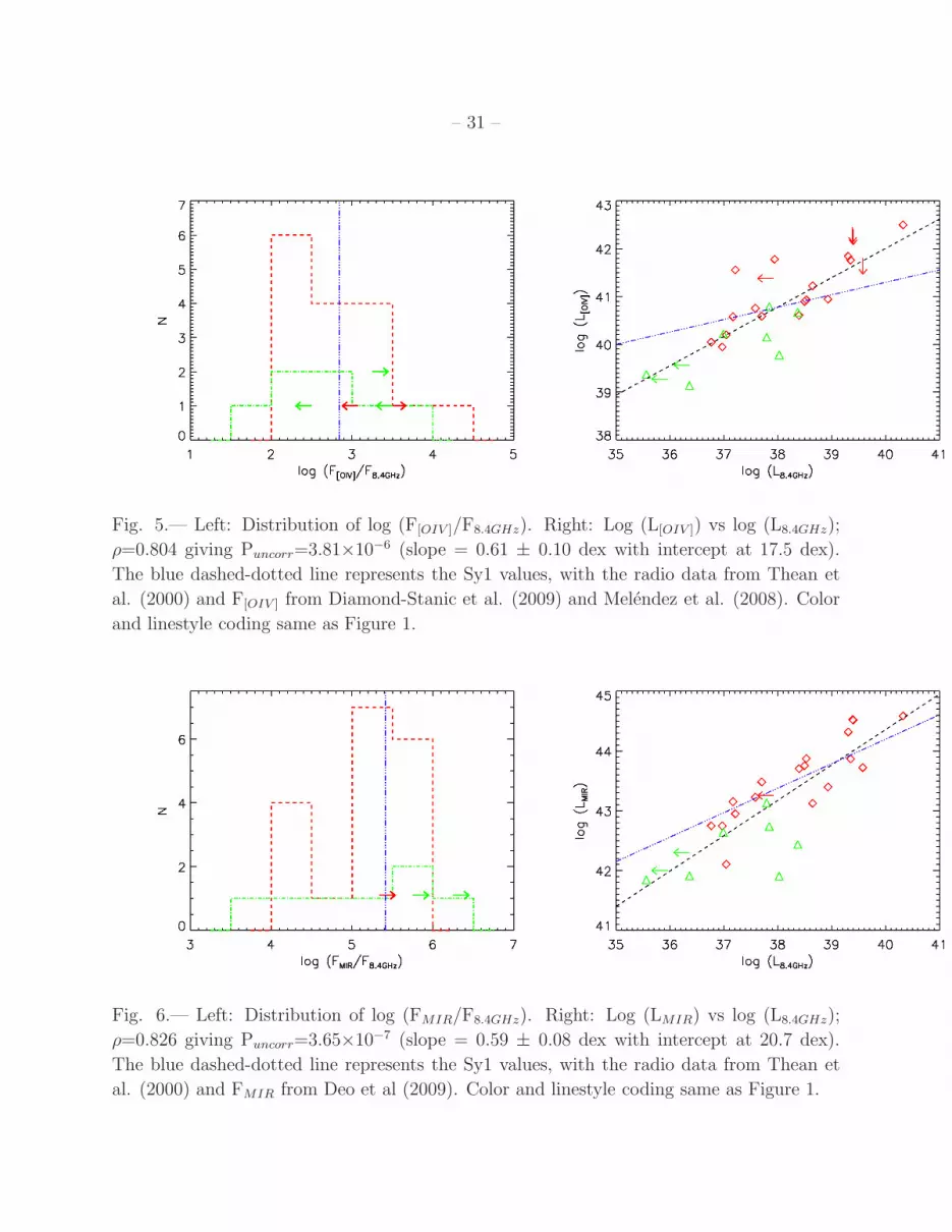
Fig. 5.— Left: Distribution of log (F[OIV ]/F8.4GHz). Right: Log (L[OIV ]) vs log (L8.4GHz);

ρ=0.804 giving Puncorr=3.81×10−6 (slope = 0.61 ± 0.10 dex with intercept at 17.5 dex).

The blue dashed-dotted line represents the Sy1 values, with the radio data from Thean et

al. (2000) and F[OIV ] from Diamond-Stanic et al. (2009) and Melendez et al. (2008). Color

and linestyle coding same as Figure 1.

Fig. 6.— Left: Distribution of log (FMIR/F8.4GHz). Right: Log (LMIR) vs log (L8.4GHz);

ρ=0.826 giving Puncorr=3.65×10−7 (slope = 0.59 ± 0.08 dex with intercept at 20.7 dex).

The blue dashed-dotted line represents the Sy1 values, with the radio data from Thean et

al. (2000) and FMIR from Deo et al (2009). Color and linestyle coding same as Figure 1.

– 32 –

(a) (b)

(c) (d)

Fig. 7.— a) Distribution of log (F14−195keV /F[OIII],corr). b) Log (L14−195keV ) vs log

(L[OIII],corr) with dashed line from survival analysis; Puncorr=0.0075 (slope = 0.50 ± 0.18 dex

with intercept at 21.5 dex). c) Distribution of log (F14−195keV /F[OIII],obs). d) Log (L14−195keV )

vs log (L[OIII],obs) with dashed line from survival analysis; Puncorr=0.0028 (slope = 0.53 ±

0.18 dex with intercept at 20.7 dex). In both luminosity vs. luminosity plots, the blue

dotted-dashed line represents the Sy1 values from the Winter et al. sample (2010). Color

and linestyle coding same as Figure 1.

– 33 –

Fig. 8.— Left: Distribution of log (F14−195keV /F[OIV ]). Right: Log (L14−195keV ) vs log (L[OIV ])

with dashed line from survival analysis; correlation probability ∼99.97% (slope = 0.78 ± 0.19

dex with intercept at 10.7 dex). The blue dotted-dashed and purple dashed lines represent

the Sy1 values from Weaver et al. (2010) and Rigby et al. (2009), respectively. Color and

linestyle coding same as Figure 1.

Fig. 9.— Left: Distribution of log (F14−195keV /FMIR). Right: Log (L14−195keV ) vs log (LMIR)

with dashed line from survival analysis; Puncorr=0.0064 (slope = 0.57 ± 0.19 dex with

intercept at 17.8 dex). Blue dotted-dashed line represents the Sy1 values, with F14−195keV

from Melendez et al. (2008) and Tueller et al. (2009) and FMIR from Deo et al. (2009).

Color and linestyle coding same as Figure 1.

– 34 –

Fig. 10.— Left: Distribution of log (F14−195keV /F8.4GHz). Right: Log (L14−195keV ) vs log

(L8.4GHz) with dashed line from survival analysis; correlation probability ∼99.4% (slope =

0.47 ± 0.16 dex with intercept at 24.6 dex). The blue dotted-dashed line represent the Sy1

values, with F14−195keV from Melendez et al. (2008) and Tueller et al. (2009) and F8.4GHz

from Thean et al. (2000). Color and linestyle coding same as Figure 1.

– 35 –

Fig. 11.— Log (F[OIV ]/F[OIII],obs vs Hα/Hβ. The green triangles are the 12µm sources with

D <1.2, the red diamonds are the 12µm sources with D ≥ 1.2 and the cyan asterisks represent

the [OIII] sample.

– 36 –

(a) (b)

(c)

Fig. 12.— In all 3 plots, the solid black line (arrows) represents the combined [OIII] and

12µm sample with detected (upper limits) 14-195 keV emission and the dotted-dashed blue

line represents the BAT selected Sy2s from Winter et al. (2010, panels a and b) and Weaver

et al. (2010, panel c). The vertical black line reflects the mean values for our combined [OIII]

and 12µm sample (from Survival Analysis) and the vertical dashed blue line delineates the

mean for the Sy2 samples from Winter et al. (2010, panels a and b) and Weaver et al. (2010,

panel c). In all cases, the BAT selected Sy2s have systematically higher hard X-ray emission

when normalized by other intrinsic AGN proxies as compared to the optical and IR selected

Sy2s, with the mean values differing by almost an order of magnitude or more.

– 37 –

(a) (b)

(c)

Fig. 13.— Flux ratios vs. LAGN/LEdd. The cyan asterisks represent the [OIII] sample, the

red diamonds the “PAH-weak” 12µm sub-sample and the green triangles the “PAH-strong”

12 µm sub-sample.

– 38 –

Fig. 14.— Left: Log (PAH EW 11.3µm) vs α20−30µm. Right: Log (PAH EW 17µm) vs

α20−30µm. The dashed line is the fit from linear regression, with ρ=0.609 and ρ=0.600,

giving probabilities of uncorrelation of Puncorr=1.47×10−5 and Puncorr=5.26×10−6 and slopes

of 0.52 ± 0.11 and 0.31 ± 0.06 with intercepts at -1.47 and -1.07, respectively. Color coding

same as Figure 13

Fig. 15.— Left: Log (PAH EW 11.3µm) vs log (F[OIV ]/F[NeII]). Right: Log (PAH EW 17µm)

vs log (F[OIV ]/F[NeII]). The dashed line is the fit from linear regression, with ρ=-0.677 and

ρ=-0.515, giving probabilities of uncorrelation of Puncorr=2.26×10−6 and Puncorr=4.89×10−4

and slopes of -1.08 ± 0.19 and -0.64 ± 0.17 with intercepts at -0.27 and -0.34, respectively.

The color coding is the same as in Figure 13.

– 39 –

(a) (b)

(c) (d)

Fig. 16.— a) Log (PAH EW 11.3µm) vs D. b) Log (PAH EW 17µm) vs D. c) Log

(F[OIV ]/F[NeII]) vs D. d) α20−30µm vs D. The color coding is the same as in Figure 13.

– 40 –

Fig. 17.— Left: Log (PAH EW 11.3µm) vs log (FIRAS/FIRS). Right: Log (F[OIV ]/F[NeII])

vs log (FIRAS/FIRS). The color coding is the same as in Figure 13.

– 41 –

(a) (b)

(c) (d)

Fig. 18.— a) Log (F[OIV ]/FMIR) vs log (PAH EW 11.3µm). b) Log (F[OIV ]/FMIR) vs log

(PAH EW 17µm). c) Log (F[OIV ]/FMIR) vs α20−30µm. d) Log (F[OIV ]/FMIR) vs. D. No

strong trends are apparent. The color coding is the same as in Figure 13.

– 42 –

(a) (b)

(c) (d)

Fig. 19.— a) Log (F[OIII,obs]/FMIR) vs log (PAH EW 11.3µm). b) Log (F[OIII,obs]/FMIR) vs

log (PAH EW 17µm). c) Log (F[OIII,obs]/FMIR) vs α20−30µm. d) Log (F[OIII,obs]/FMIR) vs.

D. No strong trends are apparent. The color coding is the same as in Figure 13.

– 43 –

Table 1: [OIII] Sample

Galaxy RA Dec z Distance MBH1

(J2000) (J2000) Mpc M⊙

NGC 0291 00 53 29.9 08 46 04 0.019 82.6 7.10

Mrk 0609 03 25 25.4 06 08 37 0.034 151.3 7.80

IC 0486 08 00 21.0 26 36 49 0.027 116.8 7.73

2MASX J08035923+2345201 08 03 59.2 23 45 20 0.029 128.8 7.25

2MASX J08244333+2959238 08 24 43.3 29 59 24 0.025 111.0 6.99

CGCG 064-017 09 59 14.8 12 59 16 0.034 150.9 6.77

2MASX J10181928+3722419 10 18 19.3 37 22 42 0.049 219.8 7.14

2MASX J11110693+0228477 11 11 06.9 02 28 48 0.035 154.9 7.33

CGCG 242-028 11 23 01.3 47 03 09 0.025 110.1 7.29

SBS 1133+572 11 35 49.1 56 57 08 0.051 229.0 7.99

Mrk 1457 11 47 21.6 52 26 58 0.049 216.6 7.85

2MASX J11570483+5249036 11 57 04.8 52 49 04 0.036 156.7 7.17

2MASX J12183945+4706275 12 18 39.4 47 06 28 0.094 431.4 8.17

2MASX J12384342+0927362 12 38 43.4 09 27 37 0.083 377.9 8.40

CGCG 218-007 13 23 48.5 43 18 04 0.027 119.4 7.65

2MASX J13463217+6423247 13 46 32.1 64 23 24 0.024 105.6 6.81

NGC 5695 14 37 22.1 36 34 04 0.014 61.1 7.44

2MASX J15522564+2753435 15 52 25.7 27 53 43 0.075 337.6 8.05

SBS 1609+490 16 10 51.8 48 54 39 0.045 200.0 6.87

2MASX J16164729+3716209 16 16 47.3 37 16 21 0.152 725.0 8.34

Distances based on redshift, assuming a cosmology of

H0 = 70 km s−1, ΩM = 0.27 and Ωvac = 0.73.1Masses based on velocity dispersion:

MBH = 108.13(σ/200 km s−1)4.02 M⊙ (Tremaine et al. 2002).

– 44 –

Table 2: 12µm Sample

Galaxy RA Dec z Distance MBH1 Ref2

(J2000) (J2000) Mpc M⊙

IRAS 00198-7926 00 21 53.6 -79 10 07 0.073 325.8 8.44 B07

NGC 0424 01 11 27.6 -38 05 00 0.012 51.2 7.78 B07

NGC 1068 02 42 40.7 -00 00 48 0.004 16.9 7.35 B07

NGC 1143/4 02 55 09.7 -00 10 40 0.028 120.8 8.29 B07

NGC 1320 03 24 48.7 -03 02 32 0.009 38.3 7.18 B07

NGC 1386 03 36 46.2 -35 59 57 0.003 12.7 7.24 B07

F04385-0828 04 40 54.9 -08 22 22 0.015 64.1 8.77 W07

NGC 1667 04 48 37.1 -06 19 12 0.015 64.1 7.88 B07

F05189-2524 05 21 01.5 -25 21 45 0.043 187.7 7.86 W07

F08572+3915 09 00 25.4 39 03 54 0.058 256.0 7.95 V09

NGC 3982 11 56 28.1 55 07 31 0.004 16.9 6.09 B07

NGC 4388 12 25 46.7 12 39 44 0.008 34.0 7.22 B07

NGC 4501 12 31 59.2 14 25 14 0.008 34.0 7.86 B07

TOLOLO 1238-364 12 40 52.8 -36 45 21 0.011 46.9 6.84 W07

NGC 4968 13 07 06.0 -23 40 37 0.010 42.6 7.27 P06

MCG-3-34-64 13 22 24.4 -16 43 43 0.017 72.7 7.70 P06

NGC 5135 13 25 44.0 -29 50 01 0.014 59.8 7.35 B07

NGC 5194 13 29 52.7 47 11 43 0.002 8.5 6.95 B07

NGC 5347 13 53 17.8 33 29 27 0.008 34.0 6.79 B07

Mrk 463 13 56 02.9 18 22 19 0.050 219.4 7.88 B07

NGC 5506 14 13 14.9 -03 12 27 0.006 25.5 6.65 B07

NGC 5929 15 26 06.1 41 40 14 0.008 34.0 7.25 B07

NGC 5953 15 34 32.4 15 11 38 0.007 29.7 9.80 P06

Arp 220 15 34 57.1 23 30 11 0.018 77.1 7.78 V09

NGC 6890 20 18 18.1 -44 48 25 0.008 34.0 6.48 B07

IC 5063 20 52 02.3 -57 04 08 0.011 46.9 7.74 B07

NCG 7130 21 48 19.5 -34 57 05 0.016 68.4 7.53 B07

NGC 7172 22 02 01.9 -31 52 11 0.009 38.3 7.67 B07

NGC 7582 23 18 23.5 -42 22 14 0.005 21.2 7.25 B07

NGC 7590 23 18 54.8 -42 14 21 0.005 21.2 6.79 B07

NGC 7674 23 27 56.7 08 46 45 0.029 125.3 7.56 B07

Distances based on redshift, assuming a cosmology of

H0 = 70 km s−1, ΩM = 0.27 and Ωvac = 0.73.

Coordinates and redshift values from NED.1Masses based on velocity dispersion: MBH = 108.13(σ/200 km s−1)4.02 M⊙ (Tremaine et al. 2002),

except for F08572+3915 which is based on photometry of the host galaxy (see V09 for details).

The FWHM of the [OIII] line was used as a proxy for σ for F04385-0828,

F05189-2524 and TOLOLO 1238-364 (Wang & Zhang 2007, Greene & Ho 2005).2References: B07 - Bian & Gu 2007; P06 - Peng et al. 2006;

V09 - Veilleux et al. 2009; W07 - Wang & Zhang 2007.

– 45 –

Table 3: Optical Emission Line Fluxes(10−14 erg s−1 cm−2) and Ratios for [OIII] Sample

Galaxy [OIII]obs [OIII]corr Hα/Hβ [NII]/Hα [OIII]/Hβ

NCG 0291 6.47 30.4 5.06 0.70 7.94

Mrk 0609 7.54 31.0 4.85 0.93 5.71

IC 0486 4.59 17.1 4.70 1.17 9.34

2MASX J08035923+2345201 5.22 6.45 3.32 1.02 10.1

2MASX J08244333+2959238 8.76 19.31 3.98 0.37 9.30

CGCG 064-017 8.46 12.33 3.49 0.24 6.63

2MASX J10181928+3722419 4.05 6.01 3.51 0.84 11.2

2MASX J11110693+0228477 4.04 5.45 3.41 0.91 9.31

CGCG 242-028 4.50 7.92 3.71 0.75 7.66

SBS 1133+572 4.71 27.3 5.41 0.90 6.28

Mrk 1457 4.27 16.2 4.72 0.78 4.63

2MASX J11570483+5249036 4.95 7.17 3.49 0.54 11.1

2MASX J12183945+4706275 4.94 10.4 3.93 0.21 10.6

2MASX J12384342+0927362 5.48 10.2 3.77 0.50 11.3

CGCG 218-007 4.12 21.3 5.22 0.96 6.24

2MASX J13463217+6423247 4.15 9.60 4.04 1.24 10.1

NGC 5695 5.93 9.30 3.57 1.36 9.56

2MASX J15522564+2753435 5.87 7.69 3.38 0.57 12.4

SBS 1609+490 4.68 8.22 3.71 0.86 10.6

2MASX J16164729+3716209 5.03 7.21 3.47 0.35 10.3

–46

–Table 4. Optical Emission Line Fluxes (10−14 erg s−1 cm−2) and Ratios for 12µm Sample

Object [OIII]obs [OIII]corr Hα/Hβ Ref1 [NII]/Hα Ref [OIII]/Hβ Ref

IRAS 00198-7926 3.88 38.5 6.41 D92 0.63 V93 11.5 V93

NGC 0424 70.0 121 3.69 V97 0.30 V97 4.55 V97

NGC 1068 1367 21280 7.39 S95 1.80 S95 13.0 S95

NGC 1144 4.30 28.7 5.65 D88 1.73 M06 7.10 D88

NGC 1320 14.0 58.0 4.86 T03 0.60 D92 8.98 D92

NGC 1386 79.2 1116 7.16 S89 1.28 S89 16.1 S89

F04385-0828 0.35 10.9 9.20 T03 >0.65 D92 >2.15 D92

NGC 1667 6.38 238 9.74 S95 0.69 S95 3.48 S95

F05189-2524 15.3 348 8.33 V99 0.46 V99 44.0 V99

F08572+3915 0.12 1.41 6.71 SDSS 0.40 SDSS 0.97 SDSS

NGC 3982 20.0 64.9 4.50 T03 ... ... 17.4 T03

NGC 4388 80.0 557 5.73 D92 2.47 D92 11.8 D92

NGC 4501 3.70 5.48 3.51 T03 1.86 S82 5.82 S82

TOLOLO 1238-364 45.7 289 5.56 S95 0.69 S95 5.31 S95

NGC 4968 17.7 1255 11.9 D92 1.01 D92 21.5 D92

M-3-34-64 151 3190 8.14 D92 0.99 D92 19.4 D92

NGC 5135 37.5 738 7.96 S95 0.87 S95 4.30 S95

NGC 5194 5.14 45.0 6.16 M06 2.40 M06 6.43 M06

NGC 5347 4.43 16.2 4.67 SDSS 0.66 SDSS 7.79 SDSS

Mrk 463 56.3 150.3 4.23 D92 0.40 D92 9.01 D92

NGC 5506 127 959 5.88 W10 0.70 W10 7.29 W10

NGC 5929 6.92 21.6 4.44 SDSS 0.59 SDSS 3.42 SDSS

NGC 5953 4.73 80.1 7.59 V95 0.78 V95 2.00 V95

Arp 220 0.18 33.7 16.2 SDSS 1.41 SDSS 2.33 SDSS

NGC 6890 23.3 86.1 4.69 S90 0.76 S90 10.2 S90

–47

–

Table 4—Continued

Object [OIII]obs [OIII]corr Hα/Hβ Ref1 [NII]/Hα Ref [OIII]/Hβ Ref

I5063 175 224 3.35 S90 0.54 S90 9.71 S90

NGC 7130 34.1 668 7.95 S95 0.75 S95 4.84 S95

NGC 7172 3.70 214 11.2 V97 0.30 V97 10.0 V97

NGC 7582 51.3 385 5.87 S95 0.78 S95 3.21 S95

NGC 7590 2.91 17.3 5.45 S95 0.65 S95 1.07 S95

NGC 7674 71.8 366 5.19 D92 0.64 D92 11.3 D92

1Optical References:

D88: Dahari & De Robertis, 1988; D92: de Grijp et al. 1992; M06: Moustakas & Kennicutt

2006; S89: Storchi-Bergmann et al. 1989; S90: Storchi-Bergman et al. 1990; S95: Storchi-

Bergmann et al. 1995; T03: Tran 2003; V97: Vaceli et al 1997, V95: Veilleux et al 1995;

V99: Veilleux et al. 1999; W10: Winter et al. 2010

– 48 –

Table 5. Spitzer Observation Summary1

Galaxy Program ID Mode Extraction Area2

” kpc

IRAS 00198-7926 30291b Staring ... ...

NGC 0424 30291b Staring ... ...

03269 Mapping 15.3×20.4 3.5×4.6

NGC 1068 00014 Staring ... ...

NGC 1144 00021b Staring ... ...

00021 Mapping 20.4×20.4 11.3×11.3

NGC 1320 30291 Staring ... ...

03269 Mapping 15.3×20.4 2.6×3.5

NGC 1386 00086 Staring ... ...

30572b Staring ... ...

F04385-0828 30291b Staring ... ...

03269 Mapping 15.3×20.4 4.7×6.2

NGC 1667 30291b Staring ... ...

03269 Mapping 15.3×20.4 4.7×6.3

F05189-2524 00105 Staring ... ..

F08572+3915 00105 Staring ... ...

NGC 3982 30291b Staring ... ...

03269 Mapping 15.3×20.4 1.3×1.8

NGC 4388 00086 Staring ... ...

30572b Staring ... ...

NGC 4501 30291b Staring ... ...

03269 Mapping 15.3×20.4 2.7×3.7

TOLOLO 1238-364 30291b Staring ... ...

03269 Mapping 15.3×20.4 3.9×5.2

NGC 4968 30291b Staring ... ...

03269 Mapping 15.3×20.4 3.4×4.6

M-3-34-64 30323 Staring ... ...

NGC 5135 00086 Staring ... ...

30572b Staring ... ...

NGC 5194 00159 Mapping 20.4×35.7 0.90×1.6

NGC 5347 00086 Staring ... ...

30572b Staring ... ...

– 49 –

Table 5—Continued

Galaxy Program ID Mode Extraction Area2

” kpc

Mrk 463 00105 Staring ... ...

NGC 5506 00086 Staring ... ...

30572b Staring ... ...

NGC 5929 20140b Staring ... ...

03269 Mapping 15.3×20.4 2.7×3.6

NGC 5953 00059 Staring ... ...

03269 Mapping 15.3×20.4 2.2×2.9

Arp 220 00105 Staring ... ...

NGC 6890 30291b Staring ... ...

03269 Mapping 15.3×20.4 2.4×3.2

IC 5063 00086 Staring ... ...

30572b Staring ... ...

NGC 7130 00086 Staring ... ...

30572b Staring ... ...

NGC 7172 00086 Staring ... ...

30572b Staring ... ...

NGC 7582 00024 Staring ... ...

40936b Staring ... ...

NGC 7590 30291b Staring ... ...

03269 Mapping 15.3×20.4 1.4×1.9

NGC 7674 03605 Staring ... ...

03269 Mapping 15.3×20.4 8.5×11.4

1The Program ID for the Sy2s in the [OIII] sample is 30773.

2For low resolution spectral mapping observations.

bGalaxies that had dedicated off-source high-resolution ob-

servations and were therefore background subtracted. See Sec-

tion 3.2 for details.

– 50 –

Table 6: MIR Flux and PAH EW values for [OIII] Sample

Galaxy [NeII]12.81µm [OIV]25.89µm FMIR EW α20−30µm

11.3µm 17µm

10−14 erg s−1 cm−2 10−11 erg s−1 cm−2 µm µm

NCG 0291 20.6±1.2 26.9±0.7 4.87 0.823 0.471 2.76

Mrk 0609 19.9±3.5 7.82±1.20 5.64 1.021 0.831 2.22

IC 0486 4.20±0.83 11.6±0.7 4.59 0.139 0.147 1.51

2MASX J08035923+2345201 0.96±0.71 3.18±0.51 0.63 0.232 0.552 0.44

2MASX J08244333+2959238 3.07±1.08 9.87±1.08 8.36 0.044 0.094 0.74

CGCG 064-017 2.52±0.27 4.44±2.59 0.73 0.458 0.373 1.56

2MASX J10181928+3722419 0.71±0.69 2.82±1.4 1.10 0.163 0.107 1.22

2MASX J11110693+0228477 1.15±0.68 2.83±1.11 1.56 0.100 0.272 0.14

CGCG 242-028 1.59±0.77 2.14±0.37 0.39 0.110 0.675 0.26

SBS 1133+572 13.0±0.9 16.1±3.8 9.63 0.135 0.131 1.57

Mrk 1457 9.87±0.89 3.22±0.78 2.93 0.631 0.421 1.92

2MASX J11570483+5249036 0.91±0.67 5.53±0.93 2.33 0.054 0.115 1.52

2MASX J12183945+4706275 <1.23 4.31±0.18 1.32 0.048 0.018 0.76

2MASX J12384342+0927362 <2.25 6.46±1.13 3.02 0.007 0.090 0.34

CGCG 218-007 10.7±0.7 17.0±0.8 2.95 0.887 0.435 2.66

2MASX J13463217+6423247 2.10±1.19 2.02±0.47 0.86 0.266 0.183 1.50

NGC 5695 2.94±0.58 7.64±0.20 0.87 0.459 0.666 1.83

2MASX J15522564+2753435 - 8.04±1.21 1.44 0.019 0.059 0.86

SBS 1609+490 <1.53 8.45±0.84 2.35 0.037 0.098 0.60

2MASX J16164729+3716209 1.78±0.79 5.11±0.54 1.73 0.051 0.066 1.38

– 51 –

Table 7: MIR Flux and PAH EW values for 12µm Sample

Galaxy [NeII]12.81µm [OIV]25.89µm FMIR EW α20−30µm

11.3µm 17µm

10−14 erg s−1 cm−2 10−11 erg s−1 cm−2 µm µm

IRAS 00198-7926 2.57+0.19−0.18 25.7+2.7

−2.4 - - - -

NGC 0424 9.23+0.70−0.66 25.2+3.3

−3.0 18.2 0.058 0.130 -0.08

NGC 1068 149+19−17 1763+221

−170 - - - -

NGC 1144 6.00+0.61−0.59 4.91+0.98

−0.70 4.28 0 0.347 1.92

NGC 1320 2.51+0.26−0.20 21.6+1.0

−0.9 8.09 0.135 0.117 0.51

NGC 13861 4.74+0.66−0.59 82.0+7.0

−6.6 6.59 0.131 0.239 1.57

F04385-0828 4.28+0.42−0.40 8.24+1.95

−1.50 10.3 0 0.131 1.00

NGC 1667 3.30+0.30−0.30 2.87+0.36

−0.35 2.76 0.578 1.35 1.45

F05189-2524 7.89+0.65−0.60 <69 7.98 0 0.129 2.74

F08572+3915 2.45+0.44−0.37 <33 4.19 0 1.85 4.13

NGC 3982 3.10+0.17−0.17 4.02+0.52

−0.53 2.39 1.63 0.933 1.53

NGC 43881 24.6+1.4−1.4 262+6

−6 6.44 0.083 0.187 1.79

NGC 4501 1.63+0.13−0.12 2.71+0.23

−0.21 1.41 0.947 1.86 1.35

TOLOLO 1238-364 13.9+0.4−0.4 14.9+4.2

−2.7 11.7 0.253 0.065 0.82

NGC 4968 8.08+0.46−0.46 26.3+2.0

−1.9 7.78 0.174 0.105 0.12

M-3-34-64 16.9+0.80−0.75 91.1+11.9

−9.9 11.7 0.010 0.035 0.85

NGC 51352 32.6+3.7−3.6 56.7+10.4

−11.0 4.16 0.387 0.322 2.46

NGC 5194 22.9+0.8−0.8 27.2+2.4

−1.9 8.07 1.71 1.63 2.06

NGC 53473 1.60+0.24−0.17 6.39+1.53

−1.08 4.04 0.086 0.060 0.54

Mrk 463 2.99+0.24−0.23 54.9+3.3

−3.1 6.72 0 0.016 0.58

NGC 55061 21.0+1.4−1.3 216+16

−16 17.1 0.048 0.257 1.37

NGC 5929 3.08+0.09−0.12 4.38+0.25

−0.24 0.58 1.15 0.792 1.61

NGC 5953 17.8+0.8−0.9 15.8+1.2

−1.1 4.17 2.28 1.82 2.55

Arp 220 21.8+1.0−1.0 <88 7.45 0 5.512 6.27

NGC 6890 3.48+0.20−0.20 8.07+0.59

−0.56 4.05 0.380 0.357 0.91

IC 5063 7.81+0.84−0.80 97.0+8.1

−7.2 14.2 0.009 0.063 0.97

NGC 71301 22.3+1.2−1.3 15.8+2.0

−1.8 4.46 0.138 0.113 2.51

NGC 7172 11.2+1.6−1.3 34.9+1.7

−1.6 3.13 0.170 2.31 2.53

NGC 7582 77.9+4.6−4.7 87.1+4.5

−4.4 5.06 1.51 0.275 2.70

NGC 7590 2.42+0.14−0.16 3.61+0.43

−0.43 1.79 1.95 1.95 1.80

NGC 7674 6.94+0.49−0.45 37.2+4.0

−3.5 11.1 0.012 0.103 0.641Program ID 30572 only for FMIR.2Program ID 00086 only for FMIR.3Program IDs 30572 and 00086 averaged together for FMIR.

– 52 –

Table 8: Diagnostic Ratios: Optical & Infrared

Diagnostic Ratio Sample Mean σ

dex dex

F[OIII],corr/F[OIII],obs Both (51 Sy2s) 0.73 0.52

[OIII]-only (20 Sy2s) 0.34 0.22

12µm-only (31 Sy2s) 0.97 0.51

Sy2s (Winter et al. 2010, 24) 0.43 0.49

Sy1s (Winter et al. 2010, 29) 0.28 0.48

F[OIV ]/F[OIII],corr Both (48 Sy2s) -0.59 0.48

[OIII]-only (20 Sy2s) -0.28 0.22

12µm-only (28 Sy2s) -0.82 0.49

Sy2s1 (8) -0.38 0.56

Sy1s1 (10) -0.90 0.58

F[OIV ]/F[OIII],obs Both (48 Sy2s) 0.08 0.41

[OIII]-only (20 Sy2s) 0.06 0.29

12µm-only (28 Sy2s) 0.09 0.48

Sy2s (Melendez et al. 2008, 12) 0.60 0.74

Sy2s (Diamond-Stanic et al. 2009, 56) 0.57 0.67

Sy1s (Melendez et al. 2008, 18) -0.21 0.42

Sy1s (Diamond-Stanic et al. 2009, 16) -0.07 0.53

FMIR/F[OIII],corr Both (49 Sy2s) 1.89 0.63

[OIII]-only (20 Sy2s) 2.24 0.26

12µm-only (29 Sy2s) 1.66 0.70

FMIR/F[OIII],obs Both (49 Sy2s) 2.61 0.63

[OIII]-only (20 Sy2s) 2.58 0.37

12µm-only (29 Sy2s) 2.62 0.77

Sy1s2 (12) 2.56 0.50

FMIR/F[OIV ] Both (46 Sy2s) 2.46 0.38

[OIII]-only (20 Sy2s) 2.52 0.26

12µm-only (26 Sy2s) 2.41 0.44

Sy1s3 (24) 2.59 0.38

Ratios in log space1Sy1 and Sy2 [OIII] values from Winter et al. (2010) and [OIV] values from Weaver et al. (2010)2Sy1 MIR values from Deo et al. (2009) and [OIII] values from Melendez et al. (2008)3Sy1 MIR values from Deo et al. (2009) and [OIV] values from Tommasin et al. (2010) &

Melendez et al. (2008)

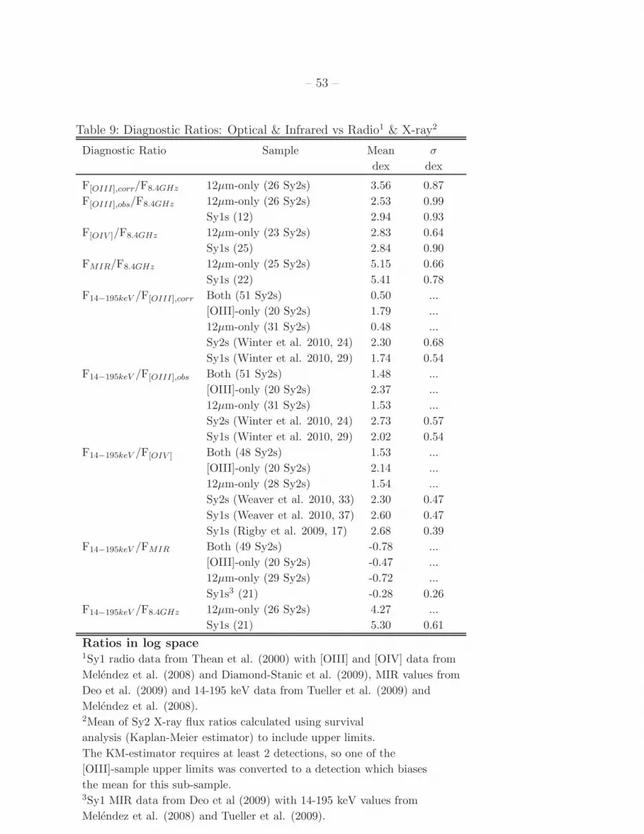
– 53 –

Table 9: Diagnostic Ratios: Optical & Infrared vs Radio1 & X-ray2

Diagnostic Ratio Sample Mean σ

dex dex

F[OIII],corr/F8.4GHz 12µm-only (26 Sy2s) 3.56 0.87

F[OIII],obs/F8.4GHz 12µm-only (26 Sy2s) 2.53 0.99

Sy1s (12) 2.94 0.93

F[OIV ]/F8.4GHz 12µm-only (23 Sy2s) 2.83 0.64

Sy1s (25) 2.84 0.90

FMIR/F8.4GHz 12µm-only (25 Sy2s) 5.15 0.66

Sy1s (22) 5.41 0.78

F14−195keV /F[OIII],corr Both (51 Sy2s) 0.50 ...

[OIII]-only (20 Sy2s) 1.79 ...

12µm-only (31 Sy2s) 0.48 ...

Sy2s (Winter et al. 2010, 24) 2.30 0.68

Sy1s (Winter et al. 2010, 29) 1.74 0.54

F14−195keV /F[OIII],obs Both (51 Sy2s) 1.48 ...

[OIII]-only (20 Sy2s) 2.37 ...

12µm-only (31 Sy2s) 1.53 ...

Sy2s (Winter et al. 2010, 24) 2.73 0.57

Sy1s (Winter et al. 2010, 29) 2.02 0.54

F14−195keV /F[OIV ] Both (48 Sy2s) 1.53 ...

[OIII]-only (20 Sy2s) 2.14 ...

12µm-only (28 Sy2s) 1.54 ...

Sy2s (Weaver et al. 2010, 33) 2.30 0.47

Sy1s (Weaver et al. 2010, 37) 2.60 0.47

Sy1s (Rigby et al. 2009, 17) 2.68 0.39

F14−195keV /FMIR Both (49 Sy2s) -0.78 ...

[OIII]-only (20 Sy2s) -0.47 ...

12µm-only (29 Sy2s) -0.72 ...

Sy1s3 (21) -0.28 0.26

F14−195keV /F8.4GHz 12µm-only (26 Sy2s) 4.27 ...

Sy1s (21) 5.30 0.61

Ratios in log space1Sy1 radio data from Thean et al. (2000) with [OIII] and [OIV] data from

Melendez et al. (2008) and Diamond-Stanic et al. (2009), MIR values from

Deo et al. (2009) and 14-195 keV data from Tueller et al. (2009) and

Melendez et al. (2008).2Mean of Sy2 X-ray flux ratios calculated using survival

analysis (Kaplan-Meier estimator) to include upper limits.

The KM-estimator requires at least 2 detections, so one of the

[OIII]-sample upper limits was converted to a detection which biases

the mean for this sub-sample.3Sy1 MIR data from Deo et al (2009) with 14-195 keV values from

Melendez et al. (2008) and Tueller et al. (2009).

– 54 –

Table 10: Results of Two Sample Tests between Sy1s and Sy2s

Kuiper Test KS Test

Diagnostic Ratio Neff D Probability D Probability

F[OIV ]/F[OIII],obs 19.9 0.310 0.223 0.301 0.042

FMIR/F[OIII],obs 8.49 0.274 0.912 0.160 0.949

FMIR/F[OIV ] 15.8 0.264 0.674 0.203 0.487

F[OIII],obs/F8.4GHz 8.21 0.385 0.544 0.340 0.242

F[OIV ]/F8.4GHz 12.0 0.318 0.576 0.200 0.684

FMIR/F8.4GHz 11.7 0.344 0.457 0.253 0.389

Neff = n1 × n2/(n1 + n2) where n1 and n2

are the number of data points in each sample.

Table 11: Correlation of Diagnostic Ratios with Eddington Parameters

Diagnostic Ratio ρ Puncorr

Optical & Infrared

F[OIII],corr/F[OIII],obs -0.224 0.115

F[OIV ]/F[OIII],corr -0.131 0.375

F[OIV ]/F[OIII],obs -0.351 0.015

FMIR/F[OIII],corr -0.164 0.259

FMIR/F[OIII],obs -0.376 0.008

FMIR/F[OIV ] -0.074 0.625

Radio and X-ray

F[OIII],corr/F8.4GHz 0.008 0.967

F[OIII],obs/F8.4GHz 0.142 0.491

F[OIV ]/F8.4GHz -0.220 0.314

FMIR/F8.4GHz -0.415 0.039

F14−195keV /F[OIII],corr ... 0.329

F14−195keV /F[OIII],obs ... 0.194

F14−195keV /F[OIV ] ... 0.914

F14−195keV /FMIR ... 0.449

F14−195keV /F8.4GHz ... 0.283

X-ray correlations computed using Cox Hazard Model

in ASURV software package.

– 55 –

A. Aperture Bias

As the optical data for the 12µm sample were culled from the literature, we examined

the data to see if an aperture bias was evident. The aperture sizes used for the optical data

(θOIII) ranged from 3 to 14” for the 12µm sources and was 3” for all the SDSS Sy2s. For

several of our sources, we found the size of the NLR (θNLR) from Schmitt et al (2003a) and

estimated the NLR for the remainder using log Rmaj = (0.31 ± 0.04) × log L[OIII] - 10.08

± 1.80 (Schmitt et al 2003b). As shown in Figure A.1 (same color coding as Figure 1 in the

main text), the aperture was large enough to encompass the full NLR for all sources. Hence,

we are not “missing” any of the NLR optical flux.

But are we observing too much [OIII] flux, perhaps from starburst contamination in the

host galaxy which would affect [OIII] emission more than [OIV]? If this is the case, we would

expect the F[OIV ]/F[OIII],obs ratio to decrease as the projected size of the aperture increases

and the “PAH-strong” sources to lie at systematically higher aperture sizes. However, neither

of these trends are apparent (Figure A.2), reaffirming the results in the main text where we

find no evidence for starburst bias on [OIII] emission. We also note that the opposite effect

is also absent, namely increase of F[OIV ]/F[OIII],obs with aperture size. This indicates that

though the [OIV] flux is collected from the Long-High module which has a larger aperture

than the [OIII] data, the [OIV] flux is not produced in regions outside of the NLR. Hence

the dispersion present in the flux ratios is not due to sampling the galaxies at different scales

between the separate IR and optical observations.

B. Starburst Contribution to the MIR

As discussed in the main text, in many cases the Spitzer IRS data show evidence for the

presence of both an AGN and active star formation. This implies that the MIR continuum

will include emission from warm dust heated by both the AGN and massive stars. Since we

are interested in using the MIR luminosity as an indicator of the intrinsic luminosity of the

AGN, we would need a way to subtract off the contribution from the dust heated by stars.

We attempted to make this correction by using a simple dilution model based on the

EW of the PAH features bracketing the continuum around 15.5µm (the PAH EW complexes

at 11.3µm and 17µm, c.f. Genzel et al. 1998, Wu et al. 2009). This approach assumes that

for starbursts there is a simple linear relationship between the PAH luminosity and that of

the MIR continuum, and that the only effect of the AGN is to produce an additional source

of MIR continuum emission, while not affecting the PAH luminosity.

As we have shown, the PAH EWs are indeed correlated with other indicators of star

– 56 –

formation activity. We therefore compared the average PAH EWs for starburst galax-

ies (< EW11.3µm,SB >=2.87 and < EW17µm,SB >=1.74, O’Dowd et al. 2009; Treyer

private communication) to the measured EWs for our Sy2s and used this to derive the

fraction of the MIR emission that is attributed to the AGN heating of the torus (i.e.

fAGN = 1 − EWSy2/ < EWSB >). In most cases, this correction was negligible. How-

ever, in the composite (strong PAH) AGN, this procedure seemed to subtract too much

MIR flux, leading to poorer agreement with the other proxies and strong systematic trends

with AGN luminosity (e.g. Figure A.3 as compared with Figure 3).

Such results indicate that accurately isolating the amount of MIR flux due to the AGN

in strongly composite systems requires more detailed modeling that takes account of the

possible influence of the AGN on the PAHs themselves. In the tight linear correlation we see

between the uncorrected MIR and [OIV] luminosities (Figure 3) there is no evidence that

the strong-PAH sources have systematically higher MIR luminosities. Taken at face value

this would imply that in these sources the starburst does not dominate the MIR continuum.

This would in turn imply that the EW of these long-wavelength PAHs with respect to the

pure starburst MIR continuum is unusually high. This can not be understood as resulting

from the destruction of PAHs by the AGN (e.g. Treyer et al. 2010), as the effect is in the

opposite direction.

– 57 –

Fig. A.1.— Ratio of the NLR size to the optical aperture size used for the [OIII] flux and

Hα and Hβ values. In all cases, the optical aperture encompasses the full NLR.

– 58 –

Fig. A.2.— Left: Log (F[OIV ]/F[OIII],obs) vs log (θOIII). Right: Log (F[OIV ]/F[OIII],obs) vs

log (θNLR/θOIII). The lack of significant trends suggest that the [OIV] flux originates in the

NLR, consistent with the [OIII] flux, and that star formation processes in the host galaxy

are not enhancing [OIII] emission.

Fig. A.3.— Left: Distribution of FMIR,AGN/F[OIV ], where FMIR,AGN subtractions out the

starburst contribution using the simple dilution model in the text. Right: Log (FMIR,AGN)

vs log (F[OIV ]). Compared with the raw MIR flux, this corrected flux leads to a poorer

agreement with the [OIV] flux and seems to over-substract the AGN contribution to the

MIR flux for the “PAH-strong” sources.