1

Deep Reinforcement Learning with Spatio-temporalTraffic Forecasting for Data-Driven Base Station

Sleep ControlQiong Wu, Xu Chen, Senior Member, IEEE, Zhi Zhou, Member, IEEE, Liang Chen, Junshan Zhang, Fellow, IEEE

Abstract—To meet the ever increasing mobile traffic demandin 5G era, base stations (BSs) have been densely deployed inradio access networks (RANs) to increase the network coverageand capacity. However, as the high density of BSs is designedto accommodate peak traffic, it would consume an unnecessarilylarge amount of energy if BSs are on during off-peak time. Tosave the energy consumption of cellular networks, an effectiveway is to deactivate some idle base stations that do not serveany traffic demand. In this paper, we develop a traffic-awaredynamic BS sleep control framework, named DeepBSC, whichpresents a novel data-driven learning approach to determine theBS active/sleep modes while meeting lower energy consump-tion and satisfactory Quality of Service (QoS) requirements.Specifically, the traffic demands are predicted by the proposedGS-STN model, which leverages the geographical and semanticspatial-temporal correlations of mobile traffic. With accuratemobile traffic forecasting, the BS sleep control problem is castas a Markov Decision Process that is solved by Actor-Criticreinforcement learning methods. To reduce the variance of costestimation in the dynamic environment, we propose a bench-mark transformation method that provides robust performanceindicator for policy update. To expedite the training process, weadopt a Deep Deterministic Policy Gradient (DDPG) approach,together with an explorer network, which can strengthen theexploration further. Extensive experiments with a real-worlddataset corroborate that our proposed framework significantlyoutperforms the existing methods.

Index Terms—Base station sleep control, spatio-temporal traf-fic forecasting, deep reinforcement learning.

I. INTRODUCTION

The past decade has witnessed an explosive growth ofmobile data traffic, which has triggered an accelerating de-ployment of base stations (BSs) to improve the cellular systemcapacity and enhance the network coverage. The deploymentof numerous BSs incurs dramatic energy consumption. It hasbeen reported that Information and Communication Tech-nology (ICT) is becoming a significant part of the worldenergy consumption and expected to grow even further inthe future [1]. For example, Telecom Italia, the incumbenttelecommunications operator in Italy, consumes about 1% ofthe total national energy demand, second only to the Italianrailway system. In short, cellular networks are among the mainenergy consumers in the ICT field and BSs are responsiblefor over 80% of the cellular network energy consumption [2].

Q. Wu, X. Chen and Z. Zhou are with School of Computer Science andEngineering, Sun Yat-sen University, Guangzhou 510006, China. L. Chen iswith the Department of Financial Technology, Tencent, Shenzhen 518054,China. J. Zhang is with the School of Electrical, Computer and EnergyEngineering, Arizona State University, Tempe, AZ 85287 USA.

Therefore, both researchers and operators are paying muchattention to improving energy efficiency of BSs for sustainabledevelopment.

In cellular networks, the traffic load could have both tem-poral and spatial fluctuations which are dependent on time,location, and population distributions. Besides, in dense urbanareas, base stations are deployed close to each other and thereexist coverage overlappings among these BSs. Based on thefacts above, dynamically switching the operation modes ofBSs between active and sleep modes based on the traffic loadfluctuation is a promising way to reduce energy consumption[3]. However, when some of the BSs are switched off to saveenergy, the user-perceived delay may then deteriorate due totraffic redirection. Therefore, one should carefully balance thetradeoff between energy saving and degradation in Qualityof Service (QoS) when making BS active/sleep decisions [4],[5]. Moreover, BS sleep control suffers from several practicalconstraints such as setup time and BS mode-changing cost(e.g., service migration cost, service delay, hardware wear-and-tear), indicating that the BS mode operation should bedone in a time scale much slower than user association inpractice.

Existing works on BS sleep operation rely heavily onidealistic assumptions such as Possion traffic demand models[6] and threshold-based sleep control [7], [8], which prevent itfrom being applied to complex realistic environments. Observ-ing that real-world mobile traffic demands exhibit remarkablespatial-temporal correlations, many existing studies proposeto utilize machine learning based methods (e.g., ARIMA [9])and deep learning approaches (e.g., STN [10]) for mobiletraffic forecasting. Nevertheless, these approaches only focuson the temporal and geospatial correlations of mobile trafficdemands without considering the fact that two areas withsimilar traffic patterns are not necessary to be geographicallyclose. Thus, in this paper we construct a semantic spatialcorrelation graph and devise an efficient geographical andsemantic spatial-temporal network (GS-STN) for timely andexact mobile traffic forecasting.

As for dynamic BS sleep control, it manifests a sequentialdecision-making process in nature [11]. Any two consecutiveBS switching operations are correlated with each other andthe current BS switching operation will also further influencethe overall energy consumption in the long run. However,many proposed analysis based approaches [6] and greedyalgorithms [12] ignore the sequential dependencies among theconsecutive BS sleep control decisions. Moreover, they usually

arX

iv:2

101.

0839

1v1

[cs

.NI]

21

Jan

2021

2

need repetitive and intensive computation at each time slotand thus are not suitable for practical BS sleep control inlarge-scale cellular networks. Recently, reinforcement learning(RL) has been proved to be a powerful tool to address thiskind of complex sequential decision-making problems [13].Nevertheless, we caution that traditional tabular-based RLmethods would fail in large-scale systems as it would facethe curse of dimensionality and the lack of exploration due tothe large state-action space.

To tackle this challenge, we formulate BS sleep controlas a Markov Decision Process (MDP) and then combinethe recent advances in deep learning and Actor-Critic (AC)architecture to solve the MDP. Specifically, we take advantageof Deep Deterministic Policy Gradient (DDPG) algorithm inthe training process. Note that the dynamic nature of theunderlying network brings direct challenge to precise costestimation in RL. For example, as the mobile traffic demandfluctuates dramatically with time, the cost estimation in RL canhave a large variance. When the agent receives a decrease ofcost, it is hard to distinguish if the decrease is the consequenceof previous actions or environment changes. To address thisissue, it is desirable to use the gap of the expected cost betweenthe current policy and the optimal policy when evaluatingthe learning performance. Since the optimal policy is hardto obtain, we propose the benchmark transformation methodwhich takes the cost estimated by some baseline policies (e.g.,greedy algorithm) as benchmark and uses the cost gap asthe criterion indicator. Furthermore, to assist exploration, wepropose to add an explorer network, which can overcome theinefficiency of the conventional randomness-based explorationmethods and significantly enhance the learning performance.

We summarize the main contributions of this paper asfollows:• We advocate a novel DeepBSC framework, which con-

ducts traffic-aware dynamic sleep control, based on deeplearning. The DeepBSC framework is data-driven andmodel-free, and is able to be applied to large-scalecellular networks with complex system dynamics.

• We devise the GS-STN model which harnesses the powerof Convolutional Neural Network (CNN) and Long Short-Term Memory (LSTM) in a joint model, to capture thecomplex spatial-temporal correlations of mobile trafficdemands. It should be noted that, for spatial correlations,we consider not only the correlations in geographicalspace, but also the correlations in semantic space byconstructing a traffic similarity graph.

• We propose a deep reinforcement learning (DRL) ap-proach to solve the dynamic BS sleep control prob-lem. To reduce the variance of cost estimation causedby the varying traffic demands, we propose a novelbenchmark transformation strategy. Moreover, we alsodevise an explorer network to strengthen the explorationduring the model training process further. Through theseenhancements, we can achieve significant performanceimprovement and outstanding learning acceleration.

• Extensive experiments are conducted using a realisticdataset of Milan city, which demonstrates the efficiencyof our proposed DeepBSC framework. Specifically, with

our precise mobile traffic demands predicted by GS-STN,we can obtain 20.5% cost reduction comparing with thewidely-used ARIMA traffic forecasting model. Moreover,our DRL based BS sleep control method can achieve12.8% cost saving when adopting benchmark transforma-tion and explorer network than the popular DQN method,which shows the effectiveness of our proposed DeepBSCframework.

The rest of this paper is organized as follows: In Section II,we review the related work of mobile traffic forecasting anddynamic BS sleep control. In Section III, we introduce thesystem model and describe the problem formulation. And wealso give the framework overview. The details of the GS-STNapproach to predict mobile traffic demands are described inSection IV. Our traffic-aware dynamic BS sleep control modelis elaborated in Section V. We conduct extensive experimentsin Section VI and conclude our paper in Section VII.

II. RELATED WORK

A. Mobile Traffic Forecasting

The recent works [14] and [15] present dynamic BS switch-ing algorithms with the traffic loads as a prior and preliminar-ily demonstrate the effectiveness of energy saving. Wu et al.assume that the traffic demands follow Poisson process andthen provide systematic insights [6]. However, these idealisticassumptions make these works suffer in practical applicationsas the real-world traffic loads are often much more complexdue to the phenomenons such as self-similarity and non-stationarity [11]. To dynamically and timely adjust the workingstatus of BSs, many studies begin to conduct mobile trafficforecasting. For example, ARIMA is employed to predict datatraffic across 9,000 base stations in Shanghai [9]. Tikunov andNishumura introduce a Holt-Winters exponential smoothingscheme for mobile traffic forecasting [16]. Nevertheless, theseexisting mobile traffic prediction mechanisms only considerprior temporal information in individual region, while ignor-ing the important spatial correlations of the traffic demandsin adjacent regions. Accordingly, spatio-temporal patterns ofmobile traffic have been recently considered [17]. However,these methods are only limited to geospatial correlationsbased on physical proximity. Different from these works, wepropose to leverage the spatial correlations in both dimensionsof geography and semantics, which demonstrates excellentperformance in our mobile traffic forecasting problem.

B. Base Station Sleep Control

The problem of energy saving with dynamic BS switch-ing is a well-known combinatorial problem, which has beenproven to be NP-hard [18]. Solving such problem generallyrequires global information (e.g., mobile traffic demand in-formation), which makes it more challenging. To address thisproblem, some greedy and heuristic algorithms are proposed.For example, Son et al. develop greedy-on and greedy-offalgorithms for BS energy saving [12]. Furthermore, thereare also some methods that tackle the BS operation problemwith optimization approaches [19], [20]. These methods canfind the optimal or sub-optimal configuration of BS modes

3

based on the assumption that the network environment remainsunchanged in the considered period. For the simplistic settingof Poisson traffic demand and exponential service time, thedouble-threshold hysteretic policy has been proven to beoptimal [7], [8]. While for more general traffic and servicepatterns, the double-threshold policy is not guaranteed tobe optimal. Moreover, it is computationally-challenging todetermine the proper threshold values [21]. Li et al. formulatethe traffic variations as a Markov decision process and design areinforcement learning framework based BS mode switchingscheme [22]. Liu et al. consider a single BS sleep controlproblem with varying traffic patterns using Deep Q-Network(DQN) [11]. Nevertheless, these approaches can only handlelow-dimensional action spaces and are likely intractable forhigh-dimensional action spaces which are difficult to exploreefficiently. In this paper, we hence propose a traffic-awareDRL-based BS sleep control approach for large-scale net-works. We introduce the ideas of benchmark transformationand explorer network to significantly enhance the learningperformance.

III. TRAFFIC-AWARE SLEEP CONTROL FOR BASESTATIONS

A. Network Model

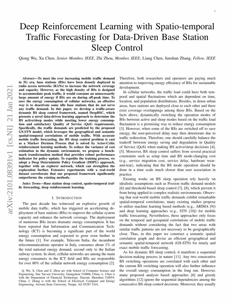
A cellular network usually consists of multiple base stations(BSs) to handle the mobile traffic loads. In this paper, weconsider a cellular network served by a set of BSs, denotedB = {1, 2, · · · , 𝐵}. As depicted in Fig. 1, the geographicalregion can be divided into non-overlapping grids, each basestation is deployed to handle traffic loads in its coverageregion (e.g., 3 × 3 grids) and different base stations mayhave coverage overlaps. As mobile traffic fluctuates overtime, many base stations are under-utilized most time, whichwould result in significant energy wastage and heavy energyinefficiency. Thus, it is necessary to change the operationmodes of BSs dynamically according to the varying trafficdemands. We assume that each base station is equippedwith a traffic monitor that can sense the traffic load in itscoverage area and correspondingly determine the operationmode (e.g., active/sleep mode) of the base station accordingto the traffic volume. However, frequent changes of the BSmodes will bring high cost of service migration, service delayand hardware wear-and-tear, thus we tend to perform BSactive/sleep mode operation in a large time scale. Specifically,we discretize the time into time slots, and each time slot hasa span of half an hour during which the mode of base stationremains unchanged.

B. Base Station Cost Model

Energy Consumption: In cellular network, the energyconsumption of a base station is not simply proportionalto the traffic loads within its coverage [23]. In fact, theenergy consumption of BS consists of two categories: fixedenergy consumption that is irrelevant to BS’s traffic loads andload-related energy cost. The fixed cost comes from circuitconsumption and cooling consumption, while the load-relatedenergy cost comes from the power amplifier. Hence, we adopt

Fig. 1. Network scenario. Each base station is deployed to handle the trafficdemand in its coverage region and different base stations may have coverageoverlaps.

the generalized energy model to represent the cost of a BS 𝑖

at time slot 𝑡, which can be summarized as

𝑝𝑡𝑖 = 𝑃𝑓

𝑖+ 𝑃𝑙𝑖 (𝜌𝑡𝑖 ), (1)

where 𝑃𝑓

𝑖is the fixed energy consumption and 𝑃𝑙

𝑖is load-

dependent energy cost which is relevant to 𝜌𝑡𝑖, the traffic load

of BS 𝑖 at time slot 𝑡.QoS degradation cost: Deactivating BSs will cause the

degradation of user’s Quality of Service (QoS). Specifically,user may suffer longer transmission delay and service delay.The transmission delay can be denoted as

𝑐𝑡𝑡𝑟𝑎𝑛 (𝐷𝑡 , 𝑎𝑡 ) = 𝑓𝑡𝑟𝑎𝑛 (𝐷𝑡 , 𝑎𝑡 ), (2)

where 𝐷𝑡 is the mobile traffic volume in all regions and 𝑎𝑡

indicates the active/sleep modes of base stations at time slot𝑡. 𝑓𝑡𝑟𝑎𝑛 (·) is the traffic dispatching function defined by thenetwork operator to reallocate the mobile traffic demands indifferent regions to the active base stations. Here our modelallows the flexibility that different network operators canimplement different traffic management schemes tailored totheir own operation demands and requirements (e.g., the trade-off between QoS and energy consumption). In our experiment,we use the widely adopted minimum cost network flow basedtraffic routing [24] as our traffic dispatching scheme. The totalservice delay of all base stations can be represented as:

𝑐𝑡𝑠𝑒𝑟 (𝜌𝑡 , 𝐶𝑡 ) =∑︁𝑖∈B

𝑓𝑠𝑒𝑟 (𝜌𝑡𝑖 , 𝐶𝑡𝑖 ), (3)

where the service latency of a base station 𝑖 is a function thatdepends on its traffic load 𝜌𝑡

𝑖and its current service capacity

𝐶𝑡𝑖. For ease of implementation, we use the average queueing

delay [25] to determine the function as 𝑓𝑠𝑒𝑟 (𝜌𝑡𝑖 , 𝐶𝑡𝑖 ) =1

𝐶𝑡𝑖−𝜌𝑡

𝑖

.And thus the QoS degradation cost can be summarized as

𝑐𝑡𝑑 (𝐷𝑡 , 𝑎𝑡 , 𝜌𝑡 , 𝐶𝑡 ) = 𝛽𝑑 · (𝑐𝑡𝑡𝑟𝑎𝑛 (𝐷𝑡 , 𝑎𝑡 ) + 𝑐𝑡𝑠𝑒𝑟 (𝜌𝑡 , 𝐶𝑡 )), (4)

where 𝛽𝑑 is a penalty factor.Base station switching cost: The base station switching

cost is incurred by toggling base stations into or out ofa power-saving mode between two adjacent time slots andincludes the service migration, service delay and hardwarewear-and-tear costs. Let 𝛽𝑖𝑠 be the cost to toggle the basestation 𝑖 from sleep mode to the active mode and we assumethe cost of transiting from the active to the sleep mode is 0.If this is not the case, we can simply fold the correspondingcost into the cost 𝛽𝑖𝑠 incurred in the next power-up operation.

4

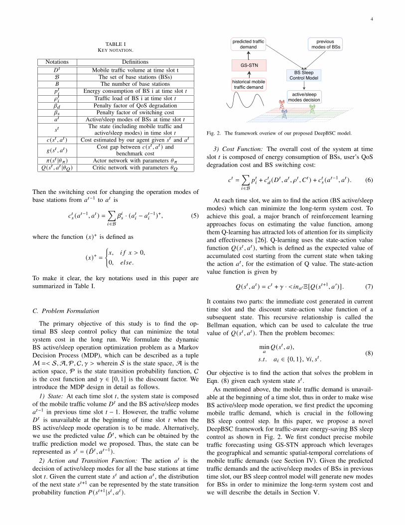
TABLE IKEY NOTATION.

Notations Definitions𝐷𝑡 Mobile traffic volume at time slot tB The set of base stations (BSs)𝐵 The number of base stations𝑝𝑡𝑖

Energy consumption of BS i at time slot 𝑡𝜌𝑡𝑖

Traffic load of BS i at time slot 𝑡𝛽𝑑 Penalty factor of QoS degradation𝛽𝑠 Penalty factor of switching cost𝑎𝑡 Active/sleep modes of BSs at time slot 𝑡

𝑠𝑡The state (including mobile traffic and

active/sleep modes) in time slot 𝑡𝑐(𝑠𝑡 , 𝑎𝑡 ) Cost estimated by our agent given 𝑠𝑡 and 𝑎𝑡

𝑔(𝑠𝑡 , 𝑎𝑡 ) Cost gap between 𝑐(𝑠𝑡 , 𝑎𝑡 ) andbenchmark cost

𝜋(𝑠𝑡 |\𝜋 ) Actor network with parameters \𝜋𝑄(𝑠𝑡 , 𝑎𝑡 |\𝑄) Critic network with parameters \𝑄

Then the switching cost for changing the operation modes ofbase stations from 𝑎𝑡−1 to 𝑎𝑡 is

𝑐𝑡𝑠 (𝑎𝑡−1, 𝑎𝑡 ) =∑︁𝑖∈B

𝛽𝑖𝑠 · (𝑎𝑡𝑖 − 𝑎𝑡−1𝑖 )+, (5)

where the function (𝑥)+ is defined as

(𝑥)+ ={𝑥, 𝑖 𝑓 𝑥 > 0,0, 𝑒𝑙𝑠𝑒.

To make it clear, the key notations used in this paper aresummarized in Table I.

C. Problem Formulation

The primary objective of this study is to find the op-timal BS sleep control policy that can minimize the totalsystem cost in the long run. We formulate the dynamicBS active/sleep operation optimization problem as a MarkovDecision Process (MDP), which can be described as a tupleM =< S,A,P, C, 𝛾 > wherein S is the state space, A is theaction space, P is the state transition probability function, Cis the cost function and 𝛾 ∈ [0, 1] is the discount factor. Weintroduce the MDP design in detail as follows.

1) State: At each time slot 𝑡, the system state is composedof the mobile traffic volume 𝐷𝑡 and the BS active/sleep modes𝑎𝑡−1 in previous time slot 𝑡 − 1. However, the traffic volume𝐷𝑡 is unavailable at the beginning of time slot 𝑡 when theBS active/sleep mode operation is to be made. Alternatively,we use the predicted value �̃�𝑡 , which can be obtained by thetraffic prediction model we proposed. Thus, the state can berepresented as 𝑠𝑡 = (�̃�𝑡 , 𝑎𝑡−1).

2) Action and Transition Function: The action 𝑎𝑡 is thedecision of active/sleep modes for all the base stations at timeslot 𝑡. Given the current state 𝑠𝑡 and action 𝑎𝑡 , the distributionof the next state 𝑠𝑡+1 can be represented by the state transitionprobability function 𝑃(𝑠𝑡+1 |𝑠𝑡 , 𝑎𝑡 ).

GS-STN

predicted trafficdemand

historical mobiletraffic demand

previousmodes of BSs

BS Sleep Control Model

active/sleep modes decision

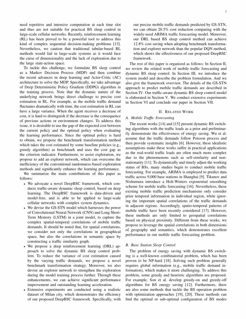
Fig. 2. The framework overiew of our proposed DeepBSC model.

3) Cost Function: The overall cost of the system at timeslot 𝑡 is composed of energy consumption of BSs, user’s QoSdegradation cost and BS switching cost:

𝑐𝑡 =∑︁𝑖∈B

𝑝𝑡𝑖 + 𝑐𝑡𝑑 (𝐷𝑡 , 𝑎𝑡 , 𝜌𝑡 , 𝐶𝑡 ) + 𝑐𝑡𝑠 (𝑎𝑡−1, 𝑎𝑡 ). (6)

At each time slot, we aim to find the action (BS active/sleepmodes) which can minimize the long-term system cost. Toachieve this goal, a major branch of reinforcement learningapproaches focus on estimating the value function, amongthem Q-learning has attracted lots of attention for its simplicityand effectiveness [26]. Q-learning uses the state-action valuefunction 𝑄(𝑠𝑡 , 𝑎𝑡 ), which is defined as the expected value ofaccumulated cost starting from the current state when takingthe action 𝑎𝑡 , for the estimation of Q value. The state-actionvalue function is given by

𝑄(𝑠𝑡 , 𝑎𝑡 ) = 𝑐𝑡 + 𝛾 · 𝑚𝑖𝑛𝑎′E[𝑄(𝑠𝑡+1, 𝑎′)] . (7)

It contains two parts: the immediate cost generated in currenttime slot and the discount state-action value function of asubsequent state. This recursive relationship is called theBellman equation, which can be used to calculate the truevalue of 𝑄(𝑠𝑡 , 𝑎𝑡 ). Then the problem becomes:

min𝑎𝑄(𝑠𝑡 , 𝑎),

𝑠.𝑡. 𝑎𝑖 ∈ {0, 1}, ∀𝑖, 𝑠𝑡 .(8)

Our objective is to find the action that solves the problem inEqn. (8) given each system state 𝑠𝑡 .

As mentioned above, the mobile traffic demand is unavail-able at the beginning of a time slot, thus in order to make wiseBS active/sleep mode operation, we first predict the upcomingmobile traffic demand, which is crucial in the followingBS sleep control step. In this paper, we propose a novelDeepBSC framework for traffic-aware energy-saving BS sleepcontrol as shown in Fig. 2. We first conduct precise mobiletraffic forecasting using GS-STN approach which leveragesthe geographical and semantic spatial-temporal correlations ofmobile traffic demands (see Section IV). Given the predictedtraffic demands and the active/sleep modes of BSs in previoustime slot, our BS sleep control model will generate new modesfor BSs in order to minimize the long-term system cost andwe will describe the details in Section V.

5

IV. GEOGRAPHICAL AND SEMANTIC SPATIAL-TEMPORALNETWORK FOR MOBILE TRAFFIC FORECASTING

A. Mobile Traffic Forecasting

The geographical area of a city can be divided into 𝑋 × 𝑌non-overlapping grids, then the mobile traffic volume in thisarea at time slot 𝑡 is

𝐷𝑡 =

𝑑𝑡(1,1) · · · 𝑑𝑡(1,𝑌 )...

......

𝑑𝑡(𝑋,1) · · · 𝑑𝑡(𝑋,𝑌 )

, (9)

where 𝑑𝑡(𝑥,𝑦) measures the data traffic volume in a grid withcoordinates (𝑥, 𝑦). To make accurate mobile traffic forecasting,we aim to find the most likely traffic demand at time slot 𝑡given truncated historical demand data

�̃�𝑡 = arg max𝐷𝑡

𝑝(𝐷𝑡 |𝐷𝑡−𝐾 , ..., 𝐷𝑡−1), (10)

where 𝐷𝑡−𝐾 , ..., 𝐷𝑡−1 are the observations of mobile trafficdemand at the previous 𝐾 time slots. As the traffic patterns arecomplex non-linear in nature, we propose to use deep learningtools to model the marginal distribution above. That is, we aimto find the function F (·) which can output the accurate mobiletraffic demand

�̃�𝑡 = F (𝐷𝑡−𝐾 , ..., 𝐷𝑡−1). (11)

B. Geographical and Semantic Spatial-Temporal Network

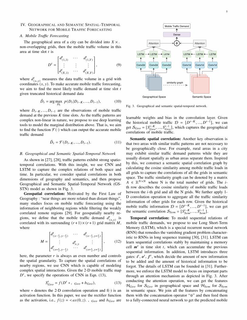
As shown in [27], [28], traffic patterns exhibit strong spatio-temporal correlations. With this insight, we use CNN andLSTM to capture the complex relations of both space andtime. In particular, we consider spatial correlations in bothdimensions of geography and semantics, and then proposeGeographical and Semantic Spatial-Temporal Network (GS-STN) model as shown in Fig. 3.

Geospatial correlation: Motivated by the First Law ofGeography : “near things are more related than distant things”,many studies focus on mobile traffic forecasting using theinformation of neighboring regions while filtering the weaklycorrelated remote regions [29]. For geospatially nearby re-gions, we define that the mobile traffic demand 𝑑𝑡(𝑥,𝑦) iscorrelated with its surrounding (𝑟 +1) × (𝑟 +1) grid matrix 𝑀 ,where

𝑀 =

𝑑𝑡(𝑥− 𝑟

2 ,𝑦−𝑟2 )· · · 𝑑𝑡(𝑥− 𝑟

2 ,𝑦+𝑟2 )

... 𝑑𝑡𝑥,𝑦...

𝑑𝑡(𝑥+ 𝑟2 ,𝑦−𝑟2 )· · · 𝑑𝑡(𝑥+ 𝑟2 ,𝑦+

𝑟2 )

, (12)

here, the parameter 𝑟 is always an even number and controlsthe spatial granularity. To capture the spatial correlations ofnearby regions, we use CNN which is capable of modelingcomplex spatial interactions. Given the 2-D mobile traffic map𝐷𝑡 , we specify the operations of CNN in Eqn. (13),

𝑆𝑡𝐺𝑒𝑜 = 𝑓 (𝐷𝑡 ∗𝑊𝐺𝑒𝑜 + 𝑏𝐺𝑒𝑜), (13)

where ∗ denotes the 2-D convolution operation and f(·) is anactivation function. In this paper, we use the rectifier functionas the activation, i.e., 𝑓 (𝑧) = 𝑚𝑎𝑥(0, 𝑧). 𝑊𝐺𝑒𝑜 and 𝑏𝐺𝑒𝑜 are

Conv2d Conv2d Conv2d Conv1d Conv1d Conv1d

LSTM LSTM LSTM LSTM LSTM LSTM

Dense

Mobile Traffic Demand

Geographical Space Semantic Space

similarity graph

Attention Attention

Fig. 3. Geographical and semantic spatial-temporal network.

learnable weights and bias in the convolution layer. Giventhe historical mobile traffic D = [𝐷𝑡−𝐾 , ..., 𝐷𝑡−1], we canget S𝐺𝑒𝑜 = [𝑆𝑡−𝐾

𝐺𝑒𝑜, ..., 𝑆𝑡−1

𝐺𝑒𝑜], which captures the geographical

correlations of mobile traffic.

Semantic spatial correlation: Another key observation isthat two areas with similar traffic patterns are not necessary tobe geographically close. For example, rural areas in a citymay exhibit similar traffic demand patterns while they areusually distant spatially as urban areas separate them. Inspiredby this, we construct a semantic spatial correlation graph bycalculating the cosine similarity among mobile traffic loads inall grids to capture the correlations of all the grids in semanticspace. The traffic similarity graph can be denoted by a matrix𝐴 ∈ R𝑁×𝑁 where N is the total number of grids. The 𝑖-th row describes the cosine similarity of mobile traffic loadsbetween the 𝑖-th grid and all the N grids. We further apply 1-D convolution operation to aggregate all the traffic similarityinformation of other grids for each row. Given the historicalmobile traffic information D = [𝐷𝑡−𝐾 , ..., 𝐷𝑡−1], we can getthe semantic correlation S𝑆𝑒𝑚 = [𝑆𝑡−𝐾

𝑆𝑒𝑚, ..., 𝑆𝑡−1

𝑆𝑒𝑚].

Temporal correlation: To model sequential relations ofmobile traffic demands, we propose to use Long Short-TermMemory (LSTM), which is a special recurrent neural network(RNN) that remedies the vanishing gradient problem character-istic to RNNs in long sequence training [30], [31]. LSTM canlearn sequential correlations stably by maintaining a memorycell 𝒎𝑡 in time slot 𝑡, which can accumulate the previoussequential information. In addition, LSTM introduces threegates: 𝒊𝑡 , 𝒐𝑡 , 𝒇 𝑡 , which decide the amount of new informationto be added and the amount of historical information to beforgot. The details of LSTM can be founded in [31]. Further-more, we enforce the LSTM model to focus on important partsthrough an attention mechanism as depicted in Fig. 3. Afterconducting the attention operation, we can get the featuresH𝐺𝑒𝑜 for S𝐺𝑒𝑜 in geographical space and H𝑆𝑒𝑚 for S𝑆𝑒𝑚in semantic space. We join all the features by concatenatingthem with the concatenation operator “⊕” and then feed themto a fully-connected neural network to get the predicted mobile

6

Policy

ValueFunction

Environment

Critic

Actor

ActionState

TDerror

Cost

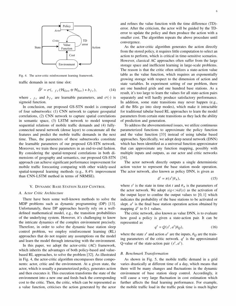
Fig. 4. The actor-critic reinforcement learning framework.

traffic demands in next time slot:

�̃�𝑡 = 𝜎(𝑊 𝑓 𝑐 (H𝐺𝑒𝑜 ⊕ H𝑆𝑒𝑐) + 𝑏 𝑓 𝑐), (14)

where 𝑊 𝑓 𝑐 and 𝑏 𝑓 𝑐 are learnable parameters, and 𝜎(·) issigmoid function.

In conclusion, our proposed GS-STN model is composedof four subnetworks: (1) CNN network to capture geospatialcorrelations, (2) CNN network to capture spatial correlationsin semantic space, (3) LSTM network to model temporalsequential relations of mobile traffic demands and (4) fully-connected neural network (dense layer) to concatenate all thefeatures and predict the mobile traffic demands in the nexttime. Thus, the parameters of these subnetworks constitutethe learnable parameters of our proposed GS-STN network.Moreover, we train these parameters in an end-to-end fashion.By considering the spatial-temporal correlations in both di-mensions of geography and semantics, our proposed GS-STNapproach can achieve significant performance improvement formobile traffic forecasting comparing with other widely-usedspatial-temporal learning methods (e.g., 8.4% improvementthan CNN-LSTM method in terms of NRMSE).

V. DYNAMIC BASE STATION SLEEP CONTROL

A. Actor Critic Architecture

There have been some well-known methods to solve theMDP problems such as dynamic programming (DP) [13].Unfortunately, these DP approaches heavily rely on a well-defined mathematical model, e.g., the transition probabilitiesof the underlying system. However, it’s challenging to knowthe intricate dynamics of the complex environment precisely.Therefore, in order to solve the dynamic base station sleepcontrol problem, we employ reinforcement learning (RL)approaches that do not require any assumptions on the modeland learn the model through interacting with the environment.

In this paper, we adopt the actor-critic (AC) framework,which inherits the advantages of both policy-based and value-based RL approaches, to solve the problem [32]. As illustratedin Fig. 4, the actor-critic algorithm encompasses three compo-nents: actor, critic and the environment. At a given state, theactor, which is usually a parameterized policy, generates actionand then executes it. This execution transforms the state of theenvironment into a new one and feeds back the correspondingcost to the critic. Then, the critic, which can be represented asa value function, criticises the action generated by the actor

and refines the value function with the time difference (TD)-error. After the criticism, the actor will be guided by the TD-error to update the policy and then produce the action with asmaller cost. The algorithm repeats the above procedure untilconvergence.

As the actor-critic algorithm generates the action directlyfrom the stored policy, it requires little computation to select anaction to perform, which is critical in time-sensitive scenarios.However, classical AC approaches often suffer from the largestorage space and inefficient learning in large-scale problems.The reason is that the critic often utilizes a state-action valuetable as the value function, which requires an exponentiallygrowing storage with respect to the dimension of action andstate variables. In experiment setting of our problem, thereare one hundred grids and one hundred base stations. As aresult, it’s too large to learn the values for all state-action pairsseparately and will hardly produce satisfactory performance.In addition, some state transitions may never happen (e.g.,all the BSs go into sleep modes), which make it intractablefor traditional tabular based RL approaches to learn the modelparameters from certain state transitions as they lack the abilityof prediction and generation.

To address the abovementioned issues, we utilize continuousparameterized functions to approximate the policy functionand the value function [33] instead of using tabular basedapproaches. Specifically, we adopt deep neural network (DNN)which has been identified as a universal function approximatorthat can approximate any function mapping, possibly withmultiple inputs and outputs, as our actor and critic networks[34].

The actor network directly outputs a single deterministicaction vector to represent the base station mode operation.The actor network, also known as policy DNN, is given as

�̃�𝑡 = 𝜋(𝑠𝑡 |\𝜋), (15)

where 𝑠𝑡 is the state in time slot 𝑡 and \𝜋 is the parameters ofthe actor network. We adopt 𝑠𝑖𝑔𝑚𝑜𝑖𝑑 (𝑥) as the activation ofthe output layer to confine the output values to [0, 1] whichindicates the probability of the base stations to be activated orslept. 𝑎𝑡 is the final base station operation action obtained bymapping �̃�𝑡 to 0-1 values.

The critic network, also known as value DNN, is to evaluatehow good a policy is given a state-action pair. It can berepresented as

𝑞𝑡 = 𝑄(𝑠𝑡 , 𝑎𝑡 |\𝑄), (16)

where the state 𝑠𝑡 and action 𝑎𝑡 are the inputs, \𝑄 are the train-ing parameters of the critic network. 𝑞𝑡 is the approximatedQ-value of the state-action pair (𝑠𝑡 , 𝑎𝑡 ).

B. Benchmark Transformation

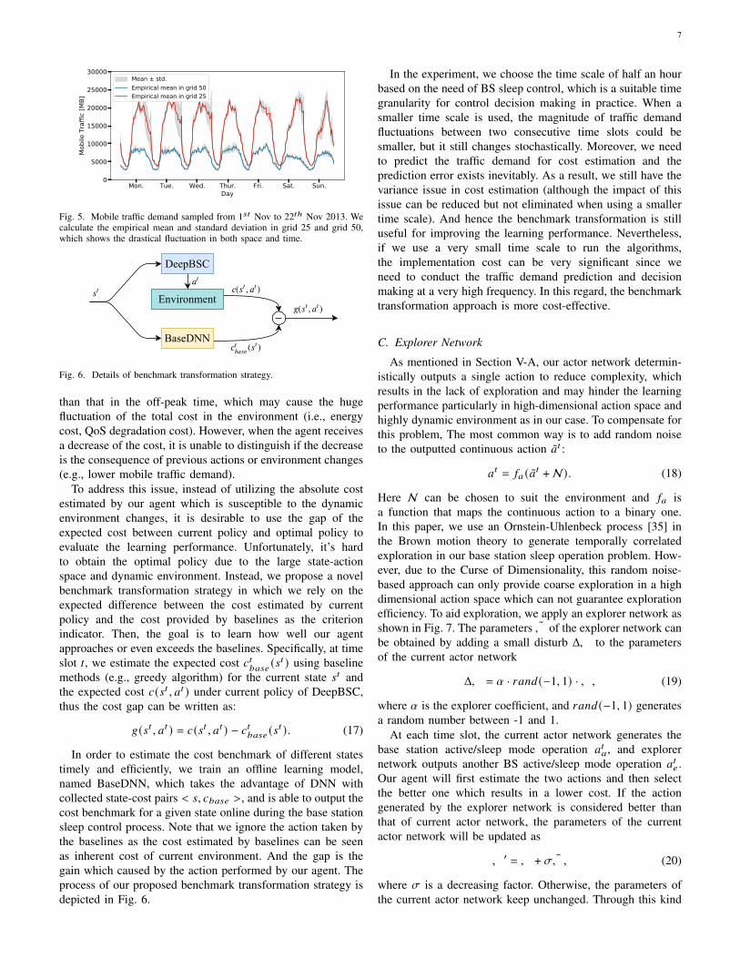
As shown in Fig. 5, the mobile traffic demand in a gridvaries drastically at different time of a day, which means thatthere will be many changes and fluctuations in the dynamicenvironment of base station sleep control. Accordingly, itwill cause a very large fluctuation in cost estimation whichfurther affects the final learning performance. For example,the mobile traffic load in the traffic peak time is much higher

7

Fig. 5. Mobile traffic demand sampled from 1𝑠𝑡 Nov to 22𝑡ℎ Nov 2013. Wecalculate the empirical mean and standard deviation in grid 25 and grid 50,which shows the drastical fluctuation in both space and time.

DeepBSC

Environment

BaseDNN

Fig. 6. Details of benchmark transformation strategy.

than that in the off-peak time, which may cause the hugefluctuation of the total cost in the environment (i.e., energycost, QoS degradation cost). However, when the agent receivesa decrease of the cost, it is unable to distinguish if the decreaseis the consequence of previous actions or environment changes(e.g., lower mobile traffic demand).

To address this issue, instead of utilizing the absolute costestimated by our agent which is susceptible to the dynamicenvironment changes, it is desirable to use the gap of theexpected cost between current policy and optimal policy toevaluate the learning performance. Unfortunately, it’s hardto obtain the optimal policy due to the large state-actionspace and dynamic environment. Instead, we propose a novelbenchmark transformation strategy in which we rely on theexpected difference between the cost estimated by currentpolicy and the cost provided by baselines as the criterionindicator. Then, the goal is to learn how well our agentapproaches or even exceeds the baselines. Specifically, at timeslot 𝑡, we estimate the expected cost 𝑐𝑡

𝑏𝑎𝑠𝑒(𝑠𝑡 ) using baseline

methods (e.g., greedy algorithm) for the current state 𝑠𝑡 andthe expected cost 𝑐(𝑠𝑡 , 𝑎𝑡 ) under current policy of DeepBSC,thus the cost gap can be written as:

𝑔(𝑠𝑡 , 𝑎𝑡 ) = 𝑐(𝑠𝑡 , 𝑎𝑡 ) − 𝑐𝑡𝑏𝑎𝑠𝑒 (𝑠𝑡 ). (17)

In order to estimate the cost benchmark of different statestimely and efficiently, we train an offline learning model,named BaseDNN, which takes the advantage of DNN withcollected state-cost pairs < 𝑠, 𝑐𝑏𝑎𝑠𝑒 >, and is able to output thecost benchmark for a given state online during the base stationsleep control process. Note that we ignore the action taken bythe baselines as the cost estimated by baselines can be seenas inherent cost of current environment. And the gap is thegain which caused by the action performed by our agent. Theprocess of our proposed benchmark transformation strategy isdepicted in Fig. 6.

In the experiment, we choose the time scale of half an hourbased on the need of BS sleep control, which is a suitable timegranularity for control decision making in practice. When asmaller time scale is used, the magnitude of traffic demandfluctuations between two consecutive time slots could besmaller, but it still changes stochastically. Moreover, we needto predict the traffic demand for cost estimation and theprediction error exists inevitably. As a result, we still have thevariance issue in cost estimation (although the impact of thisissue can be reduced but not eliminated when using a smallertime scale). And hence the benchmark transformation is stilluseful for improving the learning performance. Nevertheless,if we use a very small time scale to run the algorithms,the implementation cost can be very significant since weneed to conduct the traffic demand prediction and decisionmaking at a very high frequency. In this regard, the benchmarktransformation approach is more cost-effective.

C. Explorer Network

As mentioned in Section V-A, our actor network determin-istically outputs a single action to reduce complexity, whichresults in the lack of exploration and may hinder the learningperformance particularly in high-dimensional action space andhighly dynamic environment as in our case. To compensate forthis problem, The most common way is to add random noiseto the outputted continuous action �̃�𝑡 :

𝑎𝑡 = 𝑓𝑎 (�̃�𝑡 + N). (18)

Here N can be chosen to suit the environment and 𝑓𝑎 isa function that maps the continuous action to a binary one.In this paper, we use an Ornstein-Uhlenbeck process [35] inthe Brown motion theory to generate temporally correlatedexploration in our base station sleep operation problem. How-ever, due to the Curse of Dimensionality, this random noise-based approach can only provide coarse exploration in a highdimensional action space which can not guarantee explorationefficiency. To aid exploration, we apply an explorer network asshown in Fig. 7. The parameters �̃� of the explorer network canbe obtained by adding a small disturb Δ𝑊 to the parametersof the current actor network

Δ𝑊 = 𝛼 · 𝑟𝑎𝑛𝑑 (−1, 1) ·𝑊, (19)

where 𝛼 is the explorer coefficient, and 𝑟𝑎𝑛𝑑 (−1, 1) generatesa random number between -1 and 1.

At each time slot, the current actor network generates thebase station active/sleep mode operation 𝑎𝑡𝑎, and explorernetwork outputs another BS active/sleep mode operation 𝑎𝑡𝑒.Our agent will first estimate the two actions and then selectthe better one which results in a lower cost. If the actiongenerated by the explorer network is considered better thanthat of current actor network, the parameters of the currentactor network will be updated as

𝑊 ′ = 𝑊 + 𝜎�̃�, (20)

where 𝜎 is a decreasing factor. Otherwise, the parameters ofthe current actor network keep unchanged. Through this kind

8

DeepTes

Environment

BaseDNN

Actor Network   Explore Network  

Dense3

Dense2

Dense1

Dense3

Dense2

Dense1

Agent

state

actionaction trigger

Fig. 7. The explorer network. When the agent selects the action made byexplorer network, then it will trigger the update of parameters in actor networktowards explorer network.

of exploration, our agent is able to do more effective explo-ration in action generation process and will further acceleratethe convergence in training process.

D. DDPG Training Module

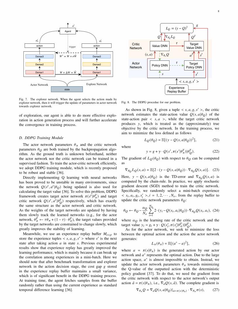
The actor network parameters \𝜋 and the critic networkparameters \𝑄 are both trained by the backpropagation algo-rithm. As the ground truth is unknown beforehand, neitherthe actor network nor the critic network can be trained in asupervised fashion. To train the actor-critic network efficiently,we adopt DDPG training module, which is recently proposedto be robust and stable [36].

Directly implementing Q learning with neural networkshas been proved to be unstable in many environments, sincethe network 𝑄(𝑠𝑡 , 𝑎𝑡 |\𝑄) being updated is also used forcalculating the target value [36]. To solve this problem, DDPGframework creates target actor network 𝜋(𝑠𝑡 |\𝑇𝜋 ) and targetcritic network 𝑄(𝑠𝑡 , 𝑎𝑡 |\𝑇

𝑄) respectively, which has exactly

the same structure as the actor network and critic network.As the weights of the target networks are updated by havingthem slowly track the learned networks (e.g., for the actornetwork, \𝑇𝜋 ← 𝜏\𝜋 + (1 − 𝜏) · \𝑇𝜋 ), the target values providedby the target networks are constrained to change slowly, whichgreatly improves the stability of learning.

Meanwhile, we use an experience replay buffer 𝑀𝑒𝑥𝑝 tostore the experience tuples < 𝑠, 𝑎, 𝑔, 𝑠′ > where 𝑠′ is the nextstate after taking action 𝑎 in state 𝑠. Previous experimentalresults show that experience replay has greatly improved thelearning performance, which is mainly because it can break upthe correlation among experiences in a mini-batch. Here weshould note that after benchmark transformation and explorernetwork in the action decision stage, the cost gap 𝑔 storedin the experience replay buffer maintains a small variance,which is of significant benefit in the DDPG training process.At training time, the agent fetches samples from the bufferrandomly rather than using the current experience as standardtemporal difference learning [36].

ExperienceReplay Buffer

Policy DNN Target Policy DNN

Value DNN Target Value DNN

ActorNetwork

CriticNetwork

Fig. 8. The DDPG procedue for our problem.

As shown in Fig. 8, given a tuple < 𝑠, 𝑎, 𝑔, 𝑠′ >, the criticnetwork estimates the state-action value 𝑄(𝑠, 𝑎 |\𝑄) of thestate-action pair < 𝑠, 𝑎 >, while the target critic networkproduces 𝑦, which is treated as the (approximately) trueobjective by the critic network. In the training process, weaim to minimize the loss defined as follows

𝐿𝑄 (\𝑄) = E[(𝑦 −𝑄(𝑠, 𝑎 |\𝑄))2], (21)

where𝑦 = 𝑔 + 𝛾 · 𝑄(𝑠′, 𝜋(𝑠′ |\𝑇𝜋 ) |\𝑇𝑄). (22)

The gradient of 𝐿𝑄 (\𝑄) with respect to \𝑄 can be computedas

∇\𝑄𝐿𝑄 (𝑠, 𝑎) = E[2 · (𝑦 −𝑄(𝑠, 𝑎 |\𝑄)) · ∇\𝑄𝑄(𝑠, 𝑎)] . (23)

Here, 𝑦 − 𝑄(𝑠, 𝑎 |\𝑄) is the TD-error and ∇\𝑄𝑄(𝑠, 𝑎) iscomputed by the chain-rule. In practice, we apply stochasticgradient descent (SGD) method to train the critic network.Specifically, we randomly select a mini-batch experience< 𝑠𝑖 , 𝑎𝑖 , 𝑔𝑖 , 𝑠

′𝑖>, 𝑖 = 1, 2, · · · , 𝑁𝑒, from the replay buffer to

update the critic network parameters \𝑄:

\𝑄 ← \𝑄−𝛼𝑄

𝑁𝑒

𝑁𝑒∑︁𝑖=1

2 · (𝑦𝑖−𝑄(𝑠𝑖 , 𝑎𝑖 |\𝑄)) ·∇\𝑄𝑄(𝑠𝑖 , 𝑎𝑖), (24)

where 𝛼𝑄 is the learning rate of the critic network and thetarget value 𝑦𝑖 = 𝑔𝑖 + 𝛾 · 𝑄(𝑠′𝑖 , 𝜋(𝑠′𝑖 |\𝑇𝜋 ) |\𝑇𝑄).

As for the actor network, we seek to minimize the lossbetween the optimal action and the action the actor networkgenerates:

𝐿 𝜋 (\𝜋) = E[(𝑎∗ − 𝑎)2], (26)

where 𝑎 = 𝜋(𝑠 |\𝜋) is the generated action by our actornetwork and 𝑎∗ represents the optimal action. Due to the largeaction space, 𝑎∗ is almost impossible to obtain. Instead, weupdate the actor network parameters \𝜋 towards minimizingthe Q-value of the outputted action with the deterministicpolicy gradient [37]. To do that, we need the gradient fromthe critic network with respect to the actor network’s outputaction �̃� = 𝜋(𝑠 |\𝜋), i.e., ∇�̃�𝑄(𝑠, �̃�). The complete gradient is

∇\𝜋𝑄 = ∇𝑎𝑄(𝑠, 𝑎 |\𝑄) |𝑎=𝜋 (𝑠 |\𝜋 ) · ∇\𝜋𝜋(𝑠), (27)

9

Algorithm 1 DRL based Base Station Sleep ControlInput: 𝑁𝑒𝑥𝑝: experience replay buffer maximum size; 𝑁𝑒:

Training batch size;1: Randomly initialize the network parameters \𝜋 , \𝑄, and

set \𝑇𝜋 = \𝜋 , \𝑇𝑄= \𝑄.

2: 𝑀𝑒𝑥𝑝 ← ∅3: for each episode 𝑒 ∈ {1, 2, 3, ...} do4: for t = 1, 2, ..., T do5: /*At the begining of the time slot t*/6: Predict the mobile traffic demand �̃�𝑡 by GS-STN7: Estimate real-time benchmark cost 𝑐𝑡

𝑏𝑎𝑠𝑒

8: Set current state 𝑠𝑡 = (�̃�𝑡 , 𝑎𝑡−1)9: /*At the end of time slot t*/

10: Generate the action 𝑎𝑡 and execute it11: Observe actual traffic 𝐷𝑡 , cost 𝑐𝑡 and new state 𝑠′

12: get the cost gap 𝑔𝑡 = 𝑐𝑡 − 𝑐𝑡𝑏𝑎𝑠𝑒

13: 𝑀𝑒𝑥𝑝 ← 𝑀𝑒𝑥𝑝 ∪ {(𝑠𝑡 , 𝑎𝑡 , 𝑔𝑡 , 𝑠′)}14: if |𝑀𝑒𝑥𝑝 | > 𝑁𝑒𝑥𝑝 then15: Remove the oldest tuple16: end if17: Sample a minibatch of 𝑁 tuples (𝑠, 𝑎, 𝑔, 𝑠′) from

𝑀𝑒𝑥𝑝18: Update critic network parameters with Eqn. (24)19: Update actor network parameters with Eqn. (28)20: Update target networks:

\𝑇𝜋 ← 𝜏\𝜋 + (1 − 𝜏) · \𝑇𝜋 ,\𝑇𝑄 ← 𝜏\𝑄 + (1 − 𝜏) · \𝑇𝑄 .

(25)

21: end for22: end for

where ∇\𝜋𝜋(𝑠) is computed by the chain-rule. It has beenproved that the stochastic policy gradient, which is the gradientof the policy’s performance, is equivalent to the empiricaldeterministic policy gradient [37]. Thus, in the model trainingprocess, we update the actor network parameters \𝜋 with amini-batch experience just as we do in critic network,

\𝜋 ← \𝜋 −𝛼𝜋

𝑁𝑒

𝑁𝑒∑︁𝑖=1∇𝑎𝑄(𝑠𝑖 , 𝑎 |\𝑄) |𝑎=𝜋 (𝑠𝑖 |\𝜋 ) · ∇\𝜋𝜋(𝑠𝑖), (28)

where 𝛼𝜋 is the learning rate of actor network.

E. The Holistic Algorithm

To sum up, the holistic mechanism of our DRL based BSsleep control process is presented in Algorithm 1. At thebegining of each time slot 𝑡, the agent first uses the historicalmobile traffic data to predict the traffic demand �̃�𝑡 for thecurrent time by our proposed GS-STN. Given the current state𝑠𝑡 = (�̃�𝑡 , 𝑎𝑡−1) in our environment, the agent will generate theactive/sleep mode decisions 𝑎𝑡 and estimate the benchmarkcost 𝑐𝑡

𝑏𝑎𝑠𝑒of current state. At the end of time slot 𝑡, the

actual traffic demand and system cost are known, the agent willstore the experiences in its replay buffer for future use. Andthe agent will randomly sample a minibatch of experiences toupdate the parameters of its networks in order to learn a betterpolicy.

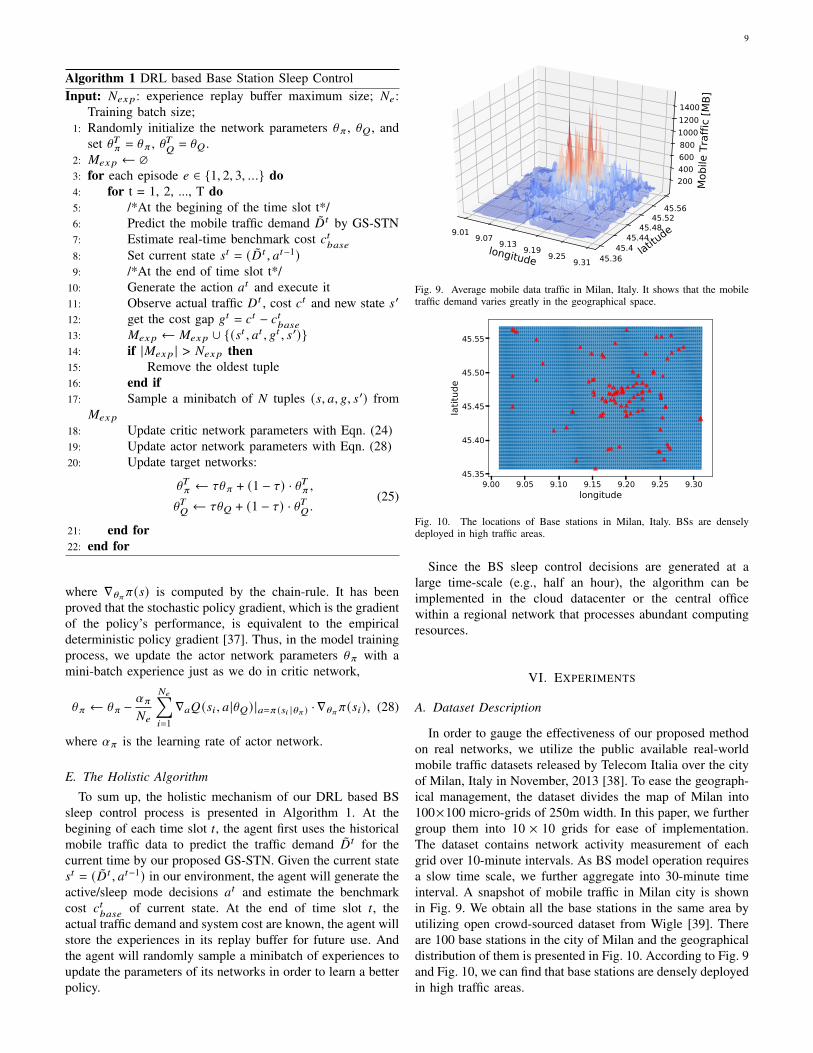
Fig. 9. Average mobile data traffic in Milan, Italy. It shows that the mobiletraffic demand varies greatly in the geographical space.

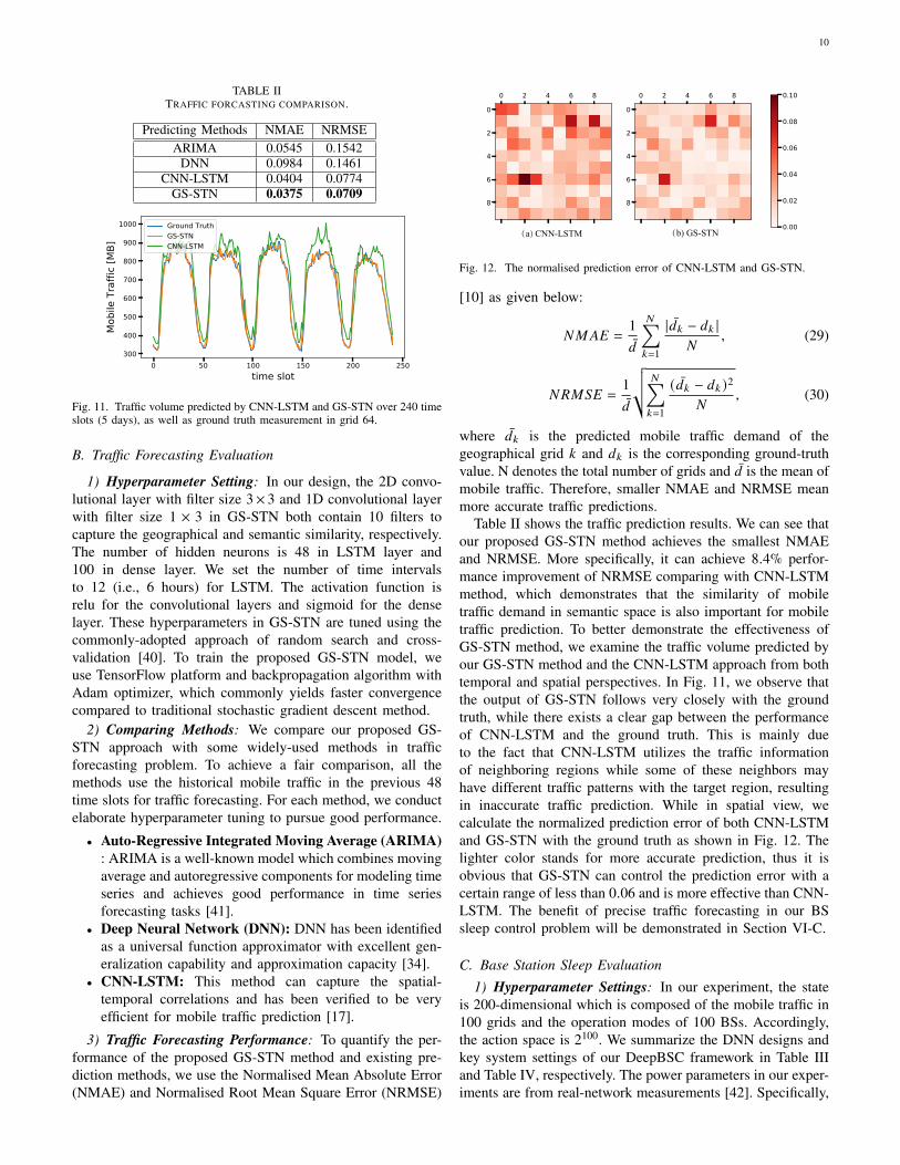
Fig. 10. The locations of Base stations in Milan, Italy. BSs are denselydeployed in high traffic areas.

Since the BS sleep control decisions are generated at alarge time-scale (e.g., half an hour), the algorithm can beimplemented in the cloud datacenter or the central officewithin a regional network that processes abundant computingresources.

VI. EXPERIMENTS

A. Dataset Description

In order to gauge the effectiveness of our proposed methodon real networks, we utilize the public available real-worldmobile traffic datasets released by Telecom Italia over the cityof Milan, Italy in November, 2013 [38]. To ease the geograph-ical management, the dataset divides the map of Milan into100×100 micro-grids of 250m width. In this paper, we furthergroup them into 10 × 10 grids for ease of implementation.The dataset contains network activity measurement of eachgrid over 10-minute intervals. As BS model operation requiresa slow time scale, we further aggregate into 30-minute timeinterval. A snapshot of mobile traffic in Milan city is shownin Fig. 9. We obtain all the base stations in the same area byutilizing open crowd-sourced dataset from Wigle [39]. Thereare 100 base stations in the city of Milan and the geographicaldistribution of them is presented in Fig. 10. According to Fig. 9and Fig. 10, we can find that base stations are densely deployedin high traffic areas.

10

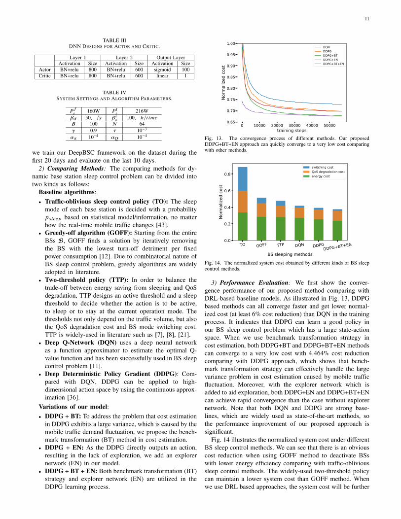
TABLE IITRAFFIC FORCASTING COMPARISON.

Predicting Methods NMAE NRMSEARIMA 0.0545 0.1542

DNN 0.0984 0.1461CNN-LSTM 0.0404 0.0774

GS-STN 0.0375 0.0709

Fig. 11. Traffic volume predicted by CNN-LSTM and GS-STN over 240 timeslots (5 days), as well as ground truth measurement in grid 64.

B. Traffic Forecasting Evaluation

1) Hyperparameter Setting: In our design, the 2D convo-lutional layer with filter size 3× 3 and 1D convolutional layerwith filter size 1 × 3 in GS-STN both contain 10 filters tocapture the geographical and semantic similarity, respectively.The number of hidden neurons is 48 in LSTM layer and100 in dense layer. We set the number of time intervalsto 12 (i.e., 6 hours) for LSTM. The activation function isrelu for the convolutional layers and sigmoid for the denselayer. These hyperparameters in GS-STN are tuned using thecommonly-adopted approach of random search and cross-validation [40]. To train the proposed GS-STN model, weuse TensorFlow platform and backpropagation algorithm withAdam optimizer, which commonly yields faster convergencecompared to traditional stochastic gradient descent method.

2) Comparing Methods: We compare our proposed GS-STN approach with some widely-used methods in trafficforecasting problem. To achieve a fair comparison, all themethods use the historical mobile traffic in the previous 48time slots for traffic forecasting. For each method, we conductelaborate hyperparameter tuning to pursue good performance.

• Auto-Regressive Integrated Moving Average (ARIMA): ARIMA is a well-known model which combines movingaverage and autoregressive components for modeling timeseries and achieves good performance in time seriesforecasting tasks [41].

• Deep Neural Network (DNN): DNN has been identifiedas a universal function approximator with excellent gen-eralization capability and approximation capacity [34].

• CNN-LSTM: This method can capture the spatial-temporal correlations and has been verified to be veryefficient for mobile traffic prediction [17].

3) Traffic Forecasting Performance: To quantify the per-formance of the proposed GS-STN method and existing pre-diction methods, we use the Normalised Mean Absolute Error(NMAE) and Normalised Root Mean Square Error (NRMSE)

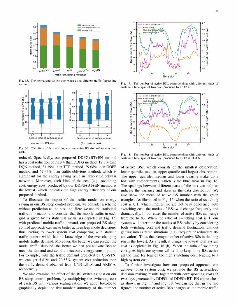
（a) CNN-LSTM （b) GS-STN

Fig. 12. The normalised prediction error of CNN-LSTM and GS-STN.

[10] as given below:

𝑁𝑀𝐴𝐸 =1𝑑

𝑁∑︁𝑘=1

|𝑑𝑘 − 𝑑𝑘 |𝑁

, (29)

𝑁𝑅𝑀𝑆𝐸 =1𝑑

√√√𝑁∑︁𝑘=1

(𝑑𝑘 − 𝑑𝑘 )2𝑁

, (30)

where 𝑑𝑘 is the predicted mobile traffic demand of thegeographical grid 𝑘 and 𝑑𝑘 is the corresponding ground-truthvalue. N denotes the total number of grids and 𝑑 is the mean ofmobile traffic. Therefore, smaller NMAE and NRMSE meanmore accurate traffic predictions.

Table II shows the traffic prediction results. We can see thatour proposed GS-STN method achieves the smallest NMAEand NRMSE. More specifically, it can achieve 8.4% perfor-mance improvement of NRMSE comparing with CNN-LSTMmethod, which demonstrates that the similarity of mobiletraffic demand in semantic space is also important for mobiletraffic prediction. To better demonstrate the effectiveness ofGS-STN method, we examine the traffic volume predicted byour GS-STN method and the CNN-LSTM approach from bothtemporal and spatial perspectives. In Fig. 11, we observe thatthe output of GS-STN follows very closely with the groundtruth, while there exists a clear gap between the performanceof CNN-LSTM and the ground truth. This is mainly dueto the fact that CNN-LSTM utilizes the traffic informationof neighboring regions while some of these neighbors mayhave different traffic patterns with the target region, resultingin inaccurate traffic prediction. While in spatial view, wecalculate the normalized prediction error of both CNN-LSTMand GS-STN with the ground truth as shown in Fig. 12. Thelighter color stands for more accurate prediction, thus it isobvious that GS-STN can control the prediction error with acertain range of less than 0.06 and is more effective than CNN-LSTM. The benefit of precise traffic forecasting in our BSsleep control problem will be demonstrated in Section VI-C.

C. Base Station Sleep Evaluation

1) Hyperparameter Settings: In our experiment, the stateis 200-dimensional which is composed of the mobile traffic in100 grids and the operation modes of 100 BSs. Accordingly,the action space is 2100. We summarize the DNN designs andkey system settings of our DeepBSC framework in Table IIIand Table IV, respectively. The power parameters in our exper-iments are from real-network measurements [42]. Specifically,

11

TABLE IIIDNN DESIGNS FOR ACTOR AND CRITIC.

Layer 1 Layer 2 Output LayerActivation Size Activation Size Activation Size

Actor BN+relu 800 BN+relu 600 sigmoid 100Critic BN+relu 800 BN+relu 600 linear 1

TABLE IVSYSTEM SETTINGS AND ALGORITHM PARAMETERS.

𝑃𝑓

𝑖160W 𝑃𝑙

𝑖216W

𝛽𝑑 50𝑊 /𝑠 𝛽𝑖𝑠 100𝑊ℎ/𝑡𝑖𝑚𝑒𝐵 100 𝑁 64𝛾 0.9 𝜏 10−3

𝛼𝜋 10−4 𝛼𝑄 10−4

we train our DeepBSC framework on the dataset during thefirst 20 days and evaluate on the last 10 days.

2) Comparing Methods: The comparing methods for dy-namic base station sleep control problem can be divided intotwo kinds as follows:

Baseline algorithms:• Traffic-oblivious sleep control policy (TO): The sleep

mode of each base station is decided with a probability𝑝𝑠𝑙𝑒𝑒𝑝 based on statistical model/information, no matterhow the real-time mobile traffic changes [43].

• Greedy-off algorithm (GOFF): Starting from the entireBSs B, GOFF finds a solution by iteratively removingthe BS with the lowest turn-off detriment per fixedpower consumption [12]. Due to combinatorial nature ofBS sleep control problem, greedy algorithms are widelyadopted in literature.

• Two-threshold policy (TTP): In order to balance thetrade-off between energy saving from sleeping and QoSdegradation, TTP designs an active threshold and a sleepthreshold to decide whether the action is to be active,to sleep or to stay at the current operation mode. Thethresholds not only depend on the traffic volume, but alsothe QoS degradation cost and BS mode switching cost.TTP is widely-used in literature such as [7], [8], [21].

• Deep Q-Network (DQN) uses a deep neural networkas a function approximator to estimate the optimal Q-value function and has been successfully used in BS sleepcontrol problem [11].

• Deep Deterministic Policy Gradient (DDPG): Com-pared with DQN, DDPG can be applied to high-dimensional action space by using the continuous approx-imation [36].

Variations of our model:• DDPG + BT: To address the problem that cost estimation

in DDPG exhibits a large variance, which is caused by themobile traffic demand fluctuation, we propose the bench-mark transformation (BT) method in cost estimation.

• DDPG + EN: As the DDPG directly outputs an action,resulting in the lack of exploration, we add an explorernetwork (EN) in our model.

• DDPG + BT + EN: Both benchmark transformation (BT)strategy and explorer network (EN) are utilized in theDDPG learning process.

0 10000 20000 30000 40000 50000training steps

0.65

0.70

0.75

0.80

0.85

0.90

0.95

1.00

Norm

alize

d co

st

DQNDDPGDDPG+BTDDPG+ENDDPG+BT+EN

Fig. 13. The convergence process of different methods. Our proposedDDPG+BT+EN approach can quickly converge to a very low cost comparingwith other methods.

TO GOFF TTP DQN DDPGDDPG+BT+EN

BS sleeping methods

0.0

0.2

0.4

0.6

0.8

Norm

alize

d co

st

switching costQoS degradation costenergy cost

Fig. 14. The normalized system cost obtained by different kinds of BS sleepcontrol methods.

3) Performance Evaluation: We first show the conver-gence performance of our proposed method comparing withDRL-based baseline models. As illustrated in Fig. 13, DDPGbased methods can all converge faster and get lower normal-ized cost (at least 6% cost reduction) than DQN in the trainingprocess. It indicates that DDPG can learn a good policy inour BS sleep control problem which has a large state-actionspace. When we use benchmark transformation strategy incost estimation, both DDPG+BT and DDPG+BT+EN methodscan converge to a very low cost with 4.464% cost reductioncomparing with DDPG approach, which shows that bench-mark transformation strategy can effectively handle the largevariance problem in cost estimation caused by mobile trafficfluctuation. Moreover, with the explorer network which isadded to aid exploration, both DDPG+EN and DDPG+BT+ENcan achieve rapid convergence than the case without explorernetwork. Note that both DQN and DDPG are strong base-lines, which are widely used as state-of-the-art methods, sothe performance improvement of our proposed approach issignificant.

Fig. 14 illustrates the normalized system cost under differentBS sleep control methods. We can see that there is an obviouscost reduction when using GOFF method to deactivate BSswith lower energy efficiency comparing with traffic-oblivioussleep control methods. The widely-used two-threshold policycan maintain a lower system cost than GOFF method. Whenwe use DRL based approaches, the system cost will be further

12

Fig. 15. The normalized system cost when using different traffic forecastingmethods.

(a) Active BS size (b) System cost

Fig. 16. The effect of the switching cost on active BS size and total systemcost.

reduced. Specifically, our proposed DDPG+BT+EN methodhas a cost reduction of 7.18% than DDPG method, 12.8% thanDQN method, 21.19% than TTP method, 29.08% than GOFFmethod and 57.33% than traffic-oblivious method, which issignificant for the energy saving issue in large-scale cellularnetworks. Moreover, each kind of the cost (e.g., switchingcost, energy cost) produced by our DDPG+BT+EN method isthe lowest, which indicates the high energy efficiency of ourproposed method.

To illustrate the impact of the traffic model on energysaving in our BS sleep control problem, we consider a schemewithout prediction as the baseline. Here we use the statisticaltraffic information and consider that the mobile traffic in eachgrid is given by its statistical mean. As depicted in Fig. 15,with predicted mobile traffic demand, our proposed BS sleepcontrol approach can make better active/sleep mode decisions,thus leading to lower system cost comparing with statistictraffic pattern which has no knowledge of the ever-changingmobile traffic demand. Moreover, the better we can predict themodel traffic demand, the better we can pre-activate BSs tomeet the demand and avoid unnecessary energy consumption.For example, with the traffic demand predicted by GS-STN,we can get 5.81% and 20.53% system cost reduction thanthe traffic demand obtained from CNN-LSTM and ARIMA,respectively.

We also examine the effect of the BS switching cost on ourBS sleep control problem, by multiplying the switching costof each BS with various scaling ratios. We adopt boxplot tographically depict the five-number summary of the number

0 20 40 60 80Time slot

40

45

50

55

60

65

70

75

The

num

ber o

f act

ive

BSs

number of active BSsenergy costQoS degradation costtraffic demand

0.2

0.3

0.4

0.5

0.6

0.7

0.8

0.9

1.0

Norm

alize

d co

st/tr

affic

vol

ume

Fig. 17. The number of active BSs, corresponding with different kinds ofcosts in a time span of two days produced by DDPG.

0 20 40 60 80Time slot

40

45

50

55

60

65

70

75

The

num

ber o

f act

ive

BSs

number of active BSsenergy costQoS degradation costtraffic demand

0.2

0.4

0.6

0.8

1.0

Norm

alize

d co

st/tr

affic

vol

ume

Fig. 18. The number of active BSs, corresponding with different kinds ofcosts in a time span of two days produced by DDPG+BT+EN.

of active BSs, which consists of the smallest observation,lower quartile, median, upper quartile and largest observation.The upper quartile, median and lower quartile make up abox with compartments, which is the blue areas in Fig. 16.The spacings between different parts of the box can help usindicate the variance and skew in the data distribution. Wealso show the mean of active BS number with the greentriangles. As illustrated in Fig. 16, when the ratio of switchingcost is 0.1, which implies we are not very concerned withswitching cost, the modes of BSs will change frequently anddramatically. In our case, the number of active BSs can rangefrom 26 to 83. When the ratio of switching cost is 1, oursystem will determine the modes of BSs wisely by consideringboth switching cost and traffic demand fluctuation, withoutgetting into extreme situations (e.g., frequent or redundant BSactivation). Thus, the average number of active BSs in the longrun is the lowest. As a result, it brings the lowest total systemcost as depicted in Fig. 16 (b). When the ratio of switchingcost goes high, our system will tend to keep more BSs activeall the time for fear of the high switching cost, leading to ahigh system cost.

To further investigate how our proposed approach canachieve lower system cost, we provide the BS active/sleepdecision making results together with corresponding costs intwo days generated by DDPG and DDPG+BT+EN approaches,as shown in Fig. 17 and Fig. 18. We can see that in the twofigures, the number of active BSs changes as the mobile traffic

13

fluctuates, which in turn causes the changes of different kindsof system costs (e.g., energy cost, QoS degradation cost).However, in the environment with the same mobile trafficdemand fluctuation, the two approaches make significantlydifferent sequential decisions. In Fig. 17, the number of activeBSs changes dramatically, and thus there may exist the casethat user’s QoS declines rapidly according to terrible BS modecontrol. For example, at time slot 45, user’s QoS degradationcost has a sharp rise as the DDPG agent deactivates someBSs unwisely. This is because that the large variance incost estimation caused by the environment changes degradesthe performance of DDPG in the training process. On thecontrary, DDPG+BT+EN approach eliminates the impact ofvarying traffic demand on cost estimation and strengthensthe exploration in the training process, leading to a wisersequential decision making strategy. As depicted in Fig. 18,the BS active/sleep decision made by DDPG+BT+EN rangesslightly, which can thus maintain a stable QoS as well as lowersystem cost.

VII. CONCLUSION

In this paper we design a traffic-aware DRL-based dynamicBS sleep control framework, named DeepBSC, for energysaving in large-scale cellular network. We first develop a GS-STN network for precise mobile traffic forecasting, which iscrucial for BS sleep control. Then we formulate the BS sleepcontrol problem as an MDP to minimize the long-term energyconsumption with the users’ QoS and switching cost consid-ered. To solve the MDP, we adopt Actor-Critic reinforcementlearning architecture and both actor and critic network areapproximated by DNN. We propose benchmark transformationstrategy to alleviate the large fluctuation in cost estimationcaused by the highly fluctuating traffic loads and devise anexplorer network to aid exploration to significantly enhancethe learning performance. By extensive experiments with real-world large-scale cellular network dataset, we demonstrate theeffectiveness of our proposed DeepBSC framework. We hopethat this work can help to elicit escalating attention on large-scale data-driven approach for future green cellular networkdesign by leveraging the power of AI.

REFERENCES

[1] M. A. Marsan, L. Chiaraviglio, D. Ciullo, and M. Meo, “Optimalenergy savings in cellular access networks,” in 2009 IEEE InternationalConference on Communications Workshops, 2009, pp. 1–5.

[2] F. Richter, A. J. Fehske, and G. P. Fettweis, “Energy efficiency aspectsof base station deployment strategies for cellular networks,” in IEEE70th Vehicular Technology Conference Fall, 2009, pp. 1–5.

[3] J. Zheng, Y. Cai, X. Chen, R. Li, and H. Zhang, “Optimal base stationsleeping in green cellular networks: A distributed cooperative frameworkbased on game theory,” IEEE Transactions on Wireless Communications,vol. 14, no. 8, pp. 4391–4406, 2015.

[4] E. Li, L. Zeng, Z. Zhou, and X. Chen, “Edge ai: On-demand acceleratingdeep neural network inference via edge computing,” IEEE Transactionson Wireless Communications, vol. 19, no. 1, pp. 447–457, 2020.

[5] T. Ouyang, Z. Zhou, and X. Chen, “Follow me at the edge: Mobility-aware dynamic service placement for mobile edge computing,” IEEEJournal on Selected Areas in Communications, vol. 36, no. 10, pp. 2333–2345, 2018.

[6] J. Wu, S. Zhou, and Z. Niu, “Traffic-aware base station sleepingcontrol and power matching for energy-delay tradeoffs in green cellularnetworks,” IEEE Transactions on Wireless Communications, vol. 12,no. 8, pp. 4196–4209, 2013.

[7] I. Kamitsos, L. Andrew, H. Kim, and M. Chiang, “Optimal sleep patternsfor serving delay-tolerant jobs,” in Proceedings of the 1st InternationalConference on Energy-Efficient Computing and Networking. ACM,2010, pp. 31–40.

[8] D. P. Heyman, “Optimal operating policies for m/g/1 queuing systems,”Operations Research, vol. 16, no. 2, pp. 362–382, 1968.

[9] H.-W. Kim, J.-H. Lee, Y.-H. Choi, Y.-U. Chung, and H. Lee, “Dynamicbandwidth provisioning using arima-based traffic forecasting for mobilewimax,” Computer Communications, vol. 34, no. 1, pp. 99–106, 2011.

[10] C. Zhang and P. Patras, “Long-term mobile traffic forecasting using deepspatio-temporal neural networks,” in Proceedings of the Eighteenth ACMInternational Symposium on Mobile Ad Hoc Networking and Computing.ACM, 2018, pp. 231–240.

[11] J. Liu, B. Krishnamachari, S. Zhou, and Z. Niu, “Deepnap: Data-drivenbase station sleeping operations through deep reinforcement learning,”IEEE Internet of Things Journal, vol. 5, no. 6, pp. 4273–4282, 2018.

[12] K. Son, H. Kim, Y. Yi, and B. Krishnamachari, “Base station operationand user association mechanisms for energy-delay tradeoffs in greencellular networks,” IEEE journal on selected areas in communications,vol. 29, no. 8, pp. 1525–1536, 2011.

[13] R. S. Sutton and A. G. Barto, “Reinforcement learning: An introduction,”IEEE Trans. Neural Networks, vol. 9, no. 5, pp. 1054–1054, 1998.

[14] E. Oh and B. Krishnamachari, “Energy savings through dynamic basestation switching in cellular wireless access networks,” in IEEE GlobalTelecommunications Conference GLOBECOM, 2010, pp. 1–5.

[15] S. Zhou, J. Gong, Z. Yang, Z. Niu, and P. Yang, “Green mobile accessnetwork with dynamic base station energy saving,” in ACM MobiCom,vol. 9, no. 262, 2009, pp. 10–12.

[16] D. Tikunov and T. Nishimura, “Traffic prediction for mobile net-work using holt-winter’s exponential smoothing,” in 15th InternationalConference on Software, Telecommunications and Computer Networks.IEEE, 2007, pp. 1–5.

[17] C. Huang, C. Chiang, and Q. Li, “A study of deep learning networkson mobile traffic forecasting,” in 28th IEEE Annual InternationalSymposium on Personal, Indoor, and Mobile Radio Communications,PIMRC, 2017, pp. 1–6.

[18] W.-T. Wong, Y.-J. Yu, and A.-C. Pang, “Decentralized energy-efficientbase station operation for green cellular networks,” in IEEE GlobalCommunications Conference (GLOBECOM), 2012, pp. 5194–5200.

[19] W.-C. Liao, M. Hong, Y.-F. Liu, and Z.-Q. Luo, “Base station activationand linear transceiver design for optimal resource management in het-erogeneous networks,” IEEE Transactions on Signal Processing, vol. 62,no. 15, pp. 3939–3952, 2014.

[20] B. Zhuang, D. Guo, and M. L. Honig, “Energy-efficient cell activation,user association, and spectrum allocation in heterogeneous networks,”IEEE Journal on Selected Areas in Communications, vol. 34, no. 4, pp.823–831, 2016.

[21] B. Leng, X. Guo, X. Zheng, B. Krishnamachari, and Z. Niu, “Await-and-see two-threshold optimal sleeping policy for a single serverwith bursty traffic,” IEEE Transactions on Green Communications andNetworking, vol. 1, no. 4, pp. 528–540, 2017.

[22] R. Li, Z. Zhao, X. Chen, J. Palicot, and H. Zhang, “Tact: A transferactor-critic learning framework for energy saving in cellular radio accessnetworks,” IEEE transactions on wireless communications, vol. 13,no. 4, pp. 2000–2011, 2014.

[23] R. Li, Z. Zhao, Y. Wei, X. Zhou, and H. Zhang, “Gm-pab: a grid-basedenergy saving scheme with predicted traffic load guidance for cellularnetworks,” in IEEE International Conference on Communications (ICC),2012, pp. 1160–1164.

[24] T. Kang, X. Sun, and T. Zhang, “Base station switching based dynamicenergy saving algorithm for cellular networks,” in 3rd IEEE Interna-tional Conference on Network Infrastructure and Digital Content, IC-NIDC, 2012, pp. 66–70.

[25] C. Newell, Applications of queueing theory. Springer Science &Business Media, 2013, vol. 4.

[26] B. J. A. Kröse, “Learning from delayed rewards,” Robotics and Au-tonomous Systems, vol. 15, no. 4, pp. 233–235, 1995.

[27] H. Wang, F. Xu, Y. Li, P. Zhang, and D. Jin, “Understanding mobiletraffic patterns of large scale cellular towers in urban environment,” inProceedings of the 2015 Internet Measurement Conference, 2015, pp.225–238.

[28] A. Furno, M. Fiore, and R. Stanica, “Joint spatial and temporal clas-sification of mobile traffic demands,” in IEEE INFOCOM 2017-IEEEConference on Computer Communications, 2017, pp. 1–9.

[29] H. Yao, F. Wu, J. Ke, X. Tang, Y. Jia, S. Lu, P. Gong, J. Ye, and Z. Li,“Deep multi-view spatial-temporal network for taxi demand prediction,”

14

in Proceedings of the Thirty-Second AAAI Conference on ArtificialIntelligence, (AAAI-18), 2018, pp. 2588–2595.

[30] S. Hochreiter and J. Schmidhuber, “Long short-term memory,” Neuralcomputation, vol. 9, no. 8, pp. 1735–1780, 1997.

[31] S. Hochreiter, Y. Bengio, P. Frasconi, J. Schmidhuber et al., Gradientflow in recurrent nets: the difficulty of learning long-term dependencies.A field guide to dynamical recurrent neural networks. IEEE Press, 2001.

[32] J. Ye and Y.-J. A. Zhang, “Drag: Deep reinforcement learning basedbase station activation in heterogeneous networks,” arXiv preprintarXiv:1809.02159, 2018.

[33] Y. Wei, F. R. Yu, M. Song, and Z. Han, “User scheduling andresource allocation in hetnets with hybrid energy supply: An actor-critic reinforcement learning approach,” IEEE Transactions on WirelessCommunications, vol. 17, no. 1, pp. 680–692, 2017.

[34] K. Hornik, M. Stinchcombe, and H. White, “Multilayer feedforwardnetworks are universal approximators,” Neural networks, vol. 2, no. 5,pp. 359–366, 1989.

[35] G. E. Uhlenbeck and L. S. Ornstein, “On the theory of the brownianmotion,” Physical review, vol. 36, no. 5, p. 823, 1930.

[36] T. P. Lillicrap, J. J. Hunt, A. Pritzel, N. Heess, T. Erez, Y. Tassa,D. Silver, and D. Wierstra, “Continuous control with deep reinforcementlearning,” arXiv preprint arXiv:1509.02971, 2015.

[37] D. Silver, G. Lever, N. Heess, T. Degris, D. Wierstra, and M. A.Riedmiller, “Deterministic policy gradient algorithms,” in Proceedingsof the 31th International Conference on Machine Learning, ICML 2014,pp. 387–395.

[38] G. Barlacchi, M. De Nadai, R. Larcher, A. Casella, C. Chitic, G. Torrisi,F. Antonelli, A. Vespignani, A. Pentland, and B. Lepri, “A multi-sourcedataset of urban life in the city of milan and the province of trentino,”Scientific data, vol. 2, no. 1, pp. 1–15, 2015.

[39] wigle.[n.d.], “Wireless basestation dataset.” [Online]. Available: https://wigle.net/.

[40] J. Bergstra and Y. Bengio, “Random search for hyper-parameter opti-mization,” J. Mach. Learn. Res., vol. 13, pp. 281–305, 2012.

[41] H.-W. Kim, J.-H. Lee, Y.-H. Choi, Y.-U. Chung, and H. Lee, “Dynamicbandwidth provisioning using arima-based traffic forecasting or mobilewimax,” Computer Communications, vol. 34, no. 1, pp. 99–106, 2011.

[42] M. Deruyck, W. Joseph, and L. Martens, “Power consumption modelfor macrocell and microcell base stations,” Transactions on EmergingTelecommunications Technologies, vol. 25, no. 3, pp. 320–333, 2014.

[43] C. Liu, B. Natarajan, and H. Xia, “Small cell base station sleep strategiesfor energy efficiency,” IEEE Transactions on Vehicular Technology,vol. 65, no. 3, pp. 1652–1661, 2015.