DEMAND AND SUPPLY CONCEPTS

1.0 THEORIES OF DEMAND AND SUPPLY 1.1.1: The concept of demandDemand can be defined as the amount of goods and/or services that consumers are able and willing to purchase at a given price in a specified period of time. Demand can either be Demand for “individual” or/and “Market”.Individual demand can be defined as the quantity of a commodity that an individual is willing and able to buy during a given time period (Hardwick, 1996).

Mr Sam Lesson Notes Form six (6) EGM,ECA & HGE

Market demand is nothing else than the sum of demands of individual consumers in a relevant market (Hardwick, 1996). The elementary theory of Demand states that, “the higher the market price the lower the quantity demanded”, all other things being held constant.Table 1.1 : Individual and Market Demand


Price of meat per kg

Juma Anna Market Demand (kg)

1,500 2 4 6

1,400 3 8 11

1,300 5 2 7

1.1.2: Movement along the Demand curve versus shift in Demand curve versus shift in Demand curveThe demand of a product may be influenced/affecting by the following ;The price of a good The price of a good or service is nearly always an instrumental factor in the demand picture. Other things being equal, the quantity demanded varies inversely in the price i.e. buyers are willing and able to purchase more of a good at a lower price than at higher price as mentioned in the discussion of the law of demand.


Consumers’ income:The average income of the consumers determines the ability to purchase goods and services. Where the income is high, the consumers’ demand for all their purchases will be high. An increase in the income of an individual tends to increase the demand for goods and services.When the market size is measured in terms of the purchasing power of the consumers, the higher the purchasing power, the higher will be the demand for all goods. In such a market the average consumption of all types of goods is higher for all consumers. Therefore the demand for any good will be significantly higher than in a market where the purchasing power is high.


The size of the market:The size of the market is measured in terms of the size of the population or by the affluence of the consumers ( the average purchasing power the consumers). Since the market size is measured in terms of the population, a high population size means a large market size and vice versa. In such a situation, the demand for all goods will be significantly higher than in a case where the population is low.


The prices of related goodsThis is particularly important for a single commodity Where there are many other similar goods, all compete for the consumers’ attention. This means that less of every one of these similar goods will be bought. If there were no similar goods, then more of the only available good would be purchased. When it comes to the prices of every one of these similar goods, the lowest priced of them all will have a higher chance of being bought than the ones that are costly. This argument particularly applies to the case of substitute goods.


Consumers’ tastes and preferences:Tastes represent a variety of social and historical influences. For example traditional beliefs, fashion etc. At one time miniskirts were very popular and their demand was very high. Future expectations:If a price rise is expected in the near future, people will tend to buy more now to avoid paying a higher price in the future. In the same light when the price is expected to fall in the near future, people will wait to buy at the future low price.


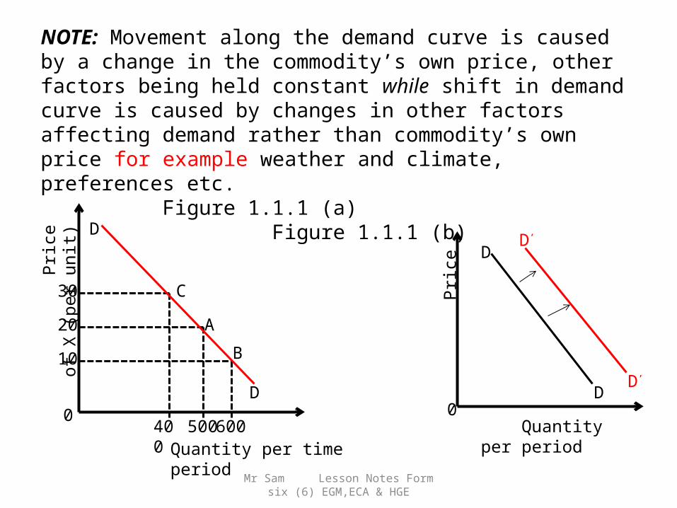
NOTE: Movement along the demand curve is caused by a change in the commodity’s own price, other factors being held constant while shift in demand curve is caused by changes in other factors affecting demand rather than commodity’s own price for example weather and climate, preferences etc. Figure 1.1.1 (a) Figure 1.1.1 (b)

Mr Sam Lesson Notes Form

six (6) EGM,ECA & HGE

CA

B

D

D

0 400

500600

102030

Pr

ice

of X

(pe

r un

it)

Quantity per time period

D

D

D’

D’

Quantity per period

Pr

ice

0

In figures above, figure 1.1.1 (a) show movements along a demand curve. Other things being equal, the effect of a change in the price of good X can be seen by moving along the

demand curve. Figure 1.1.1 (b) show a shift in the demand curve. For a normal good, arise in income causes the demand curve to shift to right while fall in income causes the demand curve to shift to left.


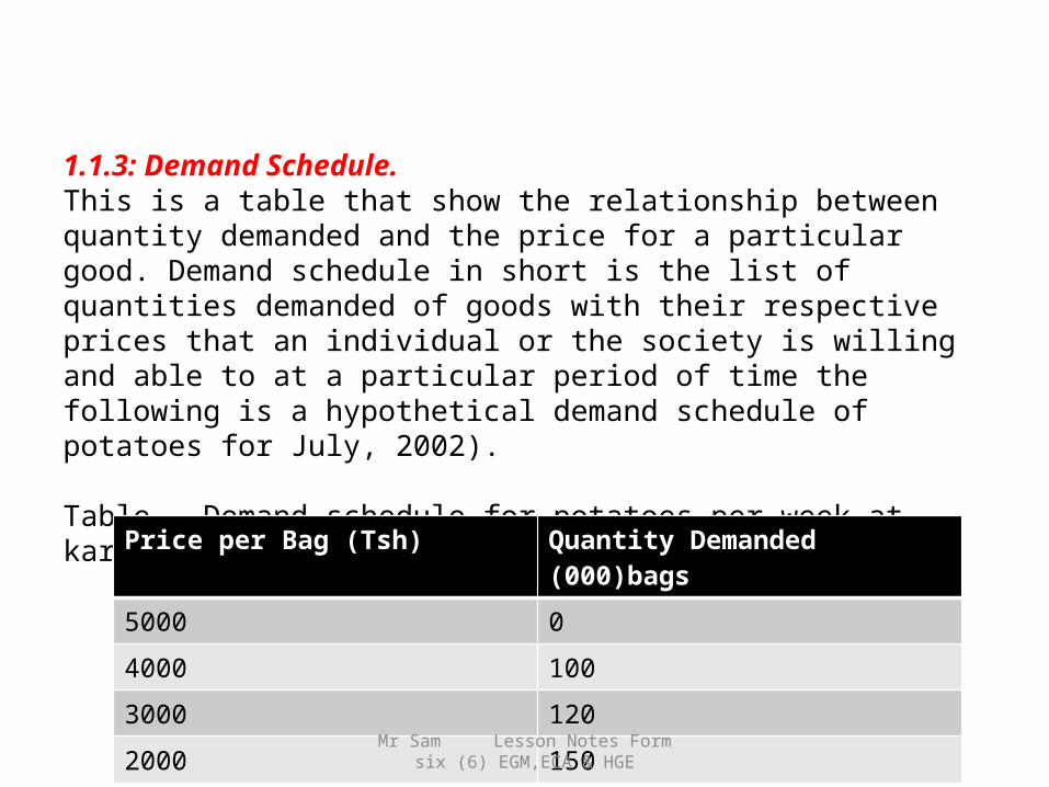
1.1.3: Demand Schedule.This is a table that show the relationship between quantity demanded and the price for a particular good. Demand schedule in short is the list of quantities demanded of goods with their respective prices that an individual or the society is willing and able to at a particular period of time the following is a hypothetical demand schedule of potatoes for July, 2002).

Table Demand schedule for potatoes per week at kariakoo marketPrice per Bag (Tsh) Quantity Demanded

(000)bags5000 04000 1003000 1202000 150


1.1.4: The demand Curve:This is the graphical representation of the quantity demanded with their respective prices curve. It graphs the quantity demanded on the horizontal axis and the price per unit on the vertical axis. The demand curve shows that the price and quantity demanded are inversely related, that is quantity demanded goes up as the price per unit goes down and vice versa. The curve slopes downwards from left to right. Figure () is the demand curve derived from the DD schedule above

figure 1.4: The demand curve for commodity x (bags)


D

D

Pric

e (0

00

Sh)

Quantity (000) bags

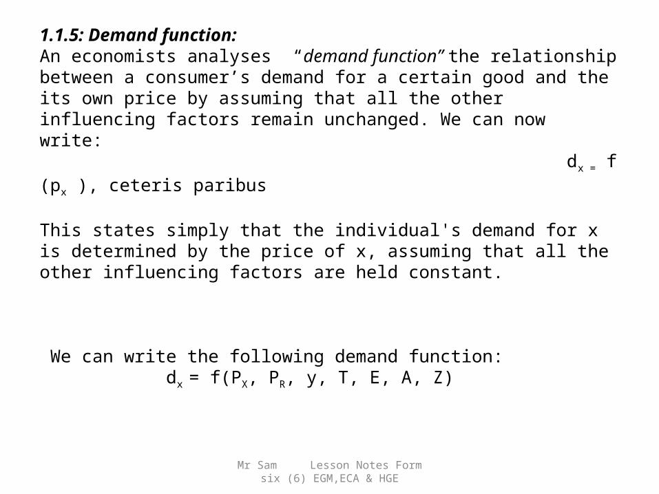
1.1.5: Demand function:An economists analyses “demand function” the relationship between a consumer’s demand for a certain good and the its own price by assuming that all the other influencing factors remain unchanged. We can now write: dx = f (px ), ceteris paribus This states simply that the individual's demand for x is determined by the price of x, assuming that all the other influencing factors are held constant.

We can write the following demand function: dx = f(PX, PR, y, T, E, A, Z)


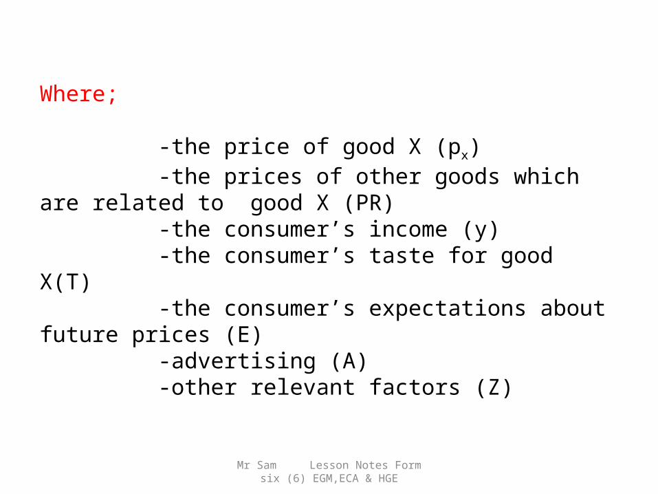
Where; -the price of good X (px) -the prices of other goods which are related to good X (PR) -the consumer’s income (y) -the consumer’s taste for good X(T) -the consumer’s expectations about future prices (E) -advertising (A) -other relevant factors (Z)


1.2.1: The law of DemandThis is the inverse relationship between the price of a commodity and the quantity demanded in the market. Law of demand states as “ A rise in the price of a good leads to a fall in the total quantity demanded. A fall in the price of a good leads to a rise in the total quantity demanded other things held constant”. From the demand curve it can be deduced that under normal circumstances, more of commodity will be purchased when the price is low while less of the commodity will be purchased at a higher price. 1.2.2: The law explains why demand for a good is inversely proportional to the price per unit of the good. The explanation for this lies in the following arguments;-

1. The law of diminishing marginal utilityAccording to this law, as one consumes more units of a good, the satisfaction obtained from the consumption of more units decreases with the increase in the number of units consumed. The satisfaction obtained from the consumption of last unit ( Marginal unit) is therefore lower than that of the preceding units. After a number of units have been consumed, the consumer would only be compelled to consume more if the price decreased.


2. Income and Substitution Effects:Income may affect the purchasing power of any individual and may result to the change in quantity demanded of that consumers’ as follow: A decrease in income decreases the purchasing power hence lead to decrease in quantity demanded and vice versa. In other words, a price decrease means that the existing purchasers can afford more units of the good than before. At the same time others will tend to abandon the more expensive substitutes and go for the cheaper good ( if has close substitute ) and this will increase the demand for that good. This is referred to as the substitution effect.

1.2.3: Exceptions of the law of demand/ abnormal demand curves:There are other goods whose demand does not obey the law of demand. These goods display what is called a regressive demand curve. That is the demand increases with an increase in price. The demand curve therefore slopes upwards from left to right. Which are these goods and why are behave in this manner?

i. Articles of Ostentation or Veblen goodsThese goods are prescribed as luxuries. Veblen goods are an extremely luxurious class of goods. In many cases, these goods are consumed to signify a certain class and not because of their intrinsic value. They are required to show a certain status or prestige. Examples of such goods are jewelry, luxury yatchts, luxury vehicles etc.


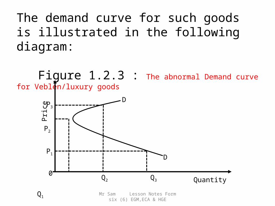
The demand curve for such goods is illustrated in the following diagram:

Figure 1.2.3 : The abnormal Demand curve for Veblen/luxury goods


D

D

Q3

Q2

Q1

0

P1

P2

P3

Pric

e

Quantity

In above diagram, at very low prices (P1 to P2 ), the demand curve behaves normally. However at prices beyond P2, the demand for these goods increases as price rises such that at a high price of P3 the quantity demanded is Q3. The reason is because the consumption of the good is giving those who can afford it more class. Note that the abnormality is noticed at the upper end of the demand curve.

( ii ) Inferior Goods and Giffen GoodsThese are the goods that are consumed by the lowest income earners whereby their demand tend to decrease when the income of the consumer increase and vice versa. The difference between inferior and Giffen is that giffen goods are special class of inferior goods. For example Maize and Rice respectively.


(iii) Fear of more drastic price change in the future. This will cause consumers to increase their quantity demanded to avoid paying an even higher price in future. This situation is often found in the stock of exchange where there is often an increase in the demand for the shares of a company if its share price is expected to increase.


1.2.4: Interrelated Demand Joint Demand refers to the demand for goods that must be consumed together in order to obtain any satisfaction from either. In such cases, the consumer purchases those goods together. The demand for one of the goods ultimately affects the demand for the other(s). Such goods are referred to as Complementary goods. A good example is the demand for shoes- the right shoe must be bought together with the left shoe. Other examples are demand for car and petrol, pillows and pillow cases, computer hardware and software, etc

Derived Demand This is the demand for those goods that are not used directly but are needed in order to get or in the production of other goods that can be used directly. Steel for example is needed because it is used in the production of cars and other steel products. The demand for steel, therefore, is derived from the demand for steel products. Goods that are not demanded for their own sake but because they are used to produce other goods are said to have a derived demand. Examples include MONEY, TIMBER, FUEL, COTTON, MINERALS, etc and Demand for capitals goods.


Competitive DemandIn some situations, consumers’ satisfaction can e obtained from several different goods. Each of these goods has the ability to satisfy the consumer. For that reason each of these goods is competing with every other good for the consumers’ attention. Such goods are said to be substitutes. Any of these goods can replace any other good without any great loss of satisfaction to the consumer. Substitutes goods are said to have a competitive demand. Changes in the price of one substitute will have an effect on the demand for the other substitute(s). A relative price increase for one good will certainly mean that more of its substitute will be purchased. This is because consumers will shift from consuming the costly good to the consumption of its relatively cheaper substitute. For examples Coffee and tea, Rice and maize meal, the different brands of soap, beer, cooking oil, Pepsi and Coca-Cola products etc.


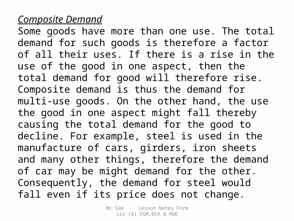
Composite DemandSome goods have more than one use. The total demand for such goods is therefore a factor of all their uses. If there is a rise in the use of the good in one aspect, then the total demand for good will therefore rise. Composite demand is thus the demand for multi-use goods. On the other hand, the use the good in one aspect might fall thereby causing the total demand for the good to decline. For example, steel is used in the manufacture of cars, girders, iron sheets and many other things, therefore the demand of car may be might demand for the other. Consequently, the demand for steel would fall even if its price does not change.


1.3.1: Elasticity of DemandintroductionThe quantity demanded is influenced by many factors such as the price of the good, the average income of the consumers, the prices of substitutes and many others. A change in any one of factors will definitely change the quantity demanded of that commodity. The degree of change as a result of a price change referred to as the Price elasticity of demand.


(i) Price Elasticity of Demand.This is the degree of responsiveness of quantity demand to changes in the price of the good. It is the proportionate change in the quantity demanded as a result of a change in the price of the good. Price elasticity is expressed in figures, these figures express the relationship between price changes and the change in quantity demanded. The following expression is commonly employed in the measurement of price elasticity of Demand. Price elasticity of demand = %change in quantity demanded %change in the price


P.e.d =QN – QO x 100 QO PN – PO x 100 P0

P.e.d = ∆Q x P0 ∆P x Q0


Where: P.e.d = P rice elasticity of Demand QO = the quantity demanded before the change in price QN = the quantity demanded after change in price ∆Q = (QN - QO ) is the change In quantity demanded PO = Original Price PN = New Price ∆P = ( PN – PO ) is the change in priceMr Sam Lesson Notes Form


Interpretation of Elasticity Figures:Demand can be price elastic, price inelastic or/and unitary elastic. Demand is elastic if a given proportionate change in price results to bigger proportionate change in the quantity demanded. For instance, if a 5% change in price results to a 10% change in the quantity demanded for a given commodity, then the demand for that commodity is price elastic.

Price Elastic Demand:This is a situation where the value of elasticity is greater than one (1). That is ( e ›1)

Exercise 01:The quantity demanded of a good X is 1000 units at a price of sh 500 per unit. After the price increase to sh 600 per, unit, the quantity demanded decreased to 600 units. (i) Calculate the P.e.d for good X (ii) Comment on whether the demand for good X is price elastic or not (iii) Is good X normal good or inferior?


Figure 1.3.1 (a): Elastic demand curve

A change in price from PO to P1 produces a larger proportionate change in demand from Q1 to Q0 and vice versaMr Sam Lesson Notes Form


D

D

Q1 Q0

P1 P0

0Quantity Demanded

Pric

e

Price inelastic Demand.This is a situation whereby a proportionately large change in the price of a good produces a smaller proportionate change in the quantity demanded of that good. For instance, a 10% change in the price results to a 3% change in the quantity demanded of that good. Price elasticity for the good which has inelastic demand is always less than one (1) i.e. ( e ‹ 1).


Figure 1.3.1 (b): Inelastic demand curve

At price P0, the quantity that is demanded for good Y is Q1. A price change from P0 to price P1 produces a smaller proportionate decrease in the quantity demanded from Q1 to Q0. Mr Sam Lesson Notes Form


D

D

P1 P0

0 Q0

Q1 Quantity Demanded

Price

Perfectly Inelastic Demand:This is a situation whereby a price change does not affect whatsoever the quantity demanded for a given commodity. A price change of whatever magnitude leaves quantity demanded unchanged. Goods with price inelastic display demand curves with an infinite slope. That is the demand curve is vertical. Such a demand curve is displayed in figure.


Figure 1.3.1 (c): Perfectly inelastic demand examples of those goods Water -- it's essential for survival ,Bread - same as above, Prescription drugs needed to save someone's life - most people will pay any amount to save their life Heating oil in a cold climate -- necessary in order not to freeze The most basic clothing imaginable -- culturally mandated, and, in most climates, essential

At any price, the demand is constant at Q0 . A price increase from P0 to P1 does not cause any change in the quantity demanded.


D

0

P0

P1

Q0 Quantity Demanded

Pric

e

Completely/Infinitely/Perfect elastic demandHere a small change in the price of a good would result to an infinite change in the quantity demanded for that good. For instance, a 1% increase in price would result to the quantity demanded falling to zero. Goods that are completely price elastic display horizontal demand curves where the slope is zero. Such a demand curve is displayed in the figure below.


Figure 1.3.1 (d): Infinitely/perfect elastic demand ;Examples of Perfectly Elastic Demand is Foreign currency exchange. If you are buying foreign currency, it is likely to exhibit the features of perfect competition. A buyer could choose from many different sellers. The product (e.g. dollars) is identical.

Perfect information about cheapest would be easy to find.Therefore, if one firm increased the price of dollars, above market equilibrium – no one

would buy from that firm. They would buy from cheaper alternatives

At a price P0, the quantity demanded is infinite. A price increase for example would not have an effect on the quantity

demanded, that can be determined.


DP0

0

Pric

e

Quantity Demanded

Unitary Elastic Demand:In such a case, a proportionate change in the price of the good will cause an equal proportionate change in the quantity demanded of that commodity. By calculation, the elasticity of demand equal to unity one. A good with a unitary elastic demand would display a demand curve such as the one shown below.


Figure 1.3.1 (e): Unitary elastic demand Example of Unit elastic, it would be useful to discuss a few examples of unit elastic demand and supply, such is not really possible. This is not due to any moral, religious, or philosophical objection to doing so. It is because that, unlike other elasticity alternatives, there is nothing particularly notable about goods that are unit elastic. Rather than a distinctive category, unit elastic is primarily a dividing line, a boundary, between elastic and inelastic. If the coefficient of elasticity is greater than one, then a good is elastic. If the coefficient of elasticity is less than one, then a good is inelastic. If the coefficient just happens to be exactly equal to one, then it is unit elastic. There is nothing intrinsic about a good in terms of either production or consumption that give rise to unit elastic.

A change in price from P0 to P1 will produce an equal percentage change in the quantity demanded from Q1 to Q0 .


D

D

P1 P0

0 Q0 Q1

Price

Quantity Demanded

Price elasticity of demand : summary

Where: “e” = coefficient of Elasticity

Term Value DescriptionPerfect inelastic demand

e = 0

Quantity demanded does not change with change in price

Inelastic demand

0 ‹ e ‹ 1

Quantity demanded changes by a smaller percentage than the change in price of the good

Unitary elastic demand

e = 1

Percentage change in quantity demanded is equal to percentage change in price.

Elastic demand

1 ‹ e ‹ ∞

Quantity demanded changes by a larger percentage than the change in the price.


Income Elasticity of Demand:The responsiveness of demand to changes in the average income(s) of consumers is referred to as income elasticity of demand . For most products, an increase in income will lead to an increase in the quantity demanded; hence income elasticity is therefore positive. An increase in income will therefore result to a positive shift in the demand curve other things being equal. Such goods are termed as normal goods because their demand increase with increase in income. However, for inferior goods, an increase in the income decrease the demand for these goods. They will therefore have negative income elasticity ( i.e. e is negative). Where the resulting elasticity is greater than one, then the demand for the good in question is income elastic. If the resulting elasticity is less than one, the good has an income inelastic demand. The good has a unitary income elastic demand if the resulting elasticity is equal to one.


Income elasticity of demand = %change in quantity demanded %change in price

Mathematical expression of I.e.d I.e.d = ∆Q x Y ∆Y Q


Where: I.e.d = Income elasticity of Demand QO = the quantity demanded before the change in income QN = the quantity demanded after change in income ∆Q = (QN - QO ) is the change In quantity demanded YO = Original income YN = New income ∆Y = ( YN – YO ) is the change in income


Summary: Income Elasticity of Demand

Term Value DescriptionInferior good

Elasticity has a negative figure ( e is negative)

Quantity demanded decrease with increase in income

Normal good

e is Positive Quantity demanded increase as income increase

Income inelastic

e ‹ 1 but is greater than zero

Quantity demanded changes by a smaller proportion than the change in income.

Income elastic

e › 1 Change in quantity demanded is proportionately larger than the change in income


Cross Elasticity of Demand: This is the responsiveness of demand for one good to changes in the price of another related good. The cross elasticity of demand for good ‘X’ is the responsiveness of the quantity demanded of good X to the changes in the price of good ‘Y’.NOTE; When ‘X’ and ‘Y’ are substitutes, the cross elasticity of demand for either product will take a positive sign (+). This is because the change in the price of one will have an opposite effect in the quantity demand for the other. For instance, an increase in the price of jam will cause the demand for margarine to increase. Therefore for substitutes, “e” is positive.


NOTE; When “x” and “y” are complements, the cross elasticity for either good will take a negative sign (-). This is because the change in price affects both goods in the same way. For example, an increase in the price of cars for one reduces the demand for both cars and petrol.Mr Sam Lesson Notes Form


Summary: Cross elasticity of Demand

Term Value DescriptionSubstitutes “e” is

positiveThe quantity of the good demanded and the price of the substitute are positively (directly) related

Complements “e” is negative

The quantity demanded and the price of a complement are negatively (inversely) related


THE THEORY OF SUPPLY1.1.1: The concept of SupplySupply refers to the quantity of a given commodity that a producer willing and able to sell at a given price over a specific time period. The supply schedule and supply curve demonstrate the relationship between Market prices and the quantities that suppliers are prepared to offer for sale. Supply differ from “existing stock” or the “amount available” in that it is concerned with amounts actually brought to the market. The basic law of supply states that “A greater quantity will be supplied at a higher price than at a lower price, and vice versa other things held constant”.


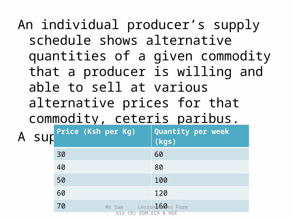
An individual producer’s supply schedule shows alternative quantities of a given commodity that a producer is willing and able to sell at various alternative prices for that commodity, ceteris paribus.

A supply schedule for OrangesPrice (Ksh per Kg) Quantity per week (kgs)

30 6040 8050 10060 12070 160Mr Sam Lesson Notes Form


The supply curve for Oranges

Note: The supply curve slopes upwards from left to right. It normally ‘never’ crosses the axis because at zero prices, nothing can be supplied i.e. there must be a price for supply of a commodity to occur.


S

40

30

60 800

Price

Quantity Supplied for Oranges

50

100

The supply FunctionFrom the law of supply, “other things” are assumed as fixed/held constant. However, in normal circumstances, its not only prices that influence the quantity supplied for a commodity. The supply function is therefore defined as “an algebraic expression that relates the quantity supplied with all the possible influencing factors”. There are four main factors that influence the supply in any particular market.


Which are• The price of the product• The prices of the factors of

production• The goals of the producing

firm• The state of technology

The effects of these factors on supply can be summarized as follows;

QS = f (Pn, F1,…….Fm )Mr Sam Lesson Notes Form


Where;QS = Quantity supplied of goodPn, F1,…….Fm = Respectively the prices of the factors of production, the goals of the firm and the state of technology which determine supply function “f”.


Factors affecting/determining/influencing supply.

Apart from the four(4) basic factors of supply, there are other important determinants of supply. A change in of these factors causes the supply to change. They include the following;-

• Price of the Good:From the law of supply, an increase in the price of good causes its supply to increase and vice versa. If the good is highly priced then we can expect more of it to be supplied. On the same token, a decrease in price will cause the supply of a good to decline.


• Price of other related Goods: Suppliers have the option of producing several goods that they can supply in the market. It is those commodities that can command a higher price that get to be produced because they can be more profitable. If a good has a higher price that its substitutes, then we can expect more of it to be hence its supply will be higher.Mr Sam Lesson Notes Form


• Goals of the firm: Apart from making profits, there are many other goals a firm can choose to pursue. For example, a firm may wish to gain more market share by supplying more of a commodity, at the minimum price. The firm will maximize sales by producing very large quantities hence the supply is high in this regard. A firm may also wish to maximize profits by selling at the highest price possible. To achieve this, the firm has to restrict the supply of the good in the question so as to drive up the price. In this regard, the quantity supplied will be lower.


• The state of technology Technological improvements or progress such as improvements in machine performance, management and organization or an improvement in the quality of raw materials leads to a lowering of costs through increased productivity and increases the profit margin on every unit sold. This should lead to an increase in supply.


• Indirect taxes and subsidies A tax on a commodity can be regarded as an increase in the costs of supplying that commodity and the supply curve will shift to the left as the result. Subsidies usually take the form of payments by governments to producers and will have the effect of lowering the costs of production and hence increasing the supply.


• Weather and ClimateThe supply of some goods is highly dependent on weather and climate. Some goods are only produced during certain seasons only. When the weather is conducive, then most agricultural commodities will be highly supplied and vice versa.

• Government Policy The government has a very great influence in what can be supplied in the market and how much of it is made available (supplied) through the various laws and regulations it sets. The government can restrict the supply of a commodity or promote its production for some reasons, by using taxes and subsidies respectively.


• Degree of freedom of EntryWhen entry into a certain industry is free and relatively ease, there is likely to be a large number of producers other things held constant. This will mean a large supply of the good in question. In industries where the entry is restricted, there will be very few firms, thus the output is likely to be low. In such industries, the producer(s) can restrict the supply in order to increase the price In former industry, the many producers have a less chance to restricting output in order to bid up raise prices.


• Prices of factors of productionAs the prices of factors of production used intensively by the producers of a certain commodity rise, so do the firm’s costs. This will cause the supply to fall since some firms will reduce output while other less efficient firms will make losses and eventually leave the industry. Similarly, I the price of one factor of production, say “land”, should increase some firms may move out of the production of land-intensive products into the production of goods that are intensive in some other factor of production which is relatively cheaper.


Interrelated Supply:Joint SupplySome products are jointly supplied; that is, one product cannot be supplied without the other being supplied as well. For example, the supply of hides cannot supplied cannot be supplied without accompanying beef. Likewise, the supply of any petroleum product must be accompanied by the supply of the other petroleum products. The production of one such good affects the supply of the other related good(s). A rise in the price of one will call for its supply to rise, but will also increase the supply of other jointly supplied good. If the supply increases without an accompanying increase in demand, the price is likely to fall.


• Competitive Supply: The supply of certain goods follows naturally from circumstances beyond mans control. A Canadian fur trapper, for example, cannot suddenly decide to start growing bananas. In most cases, however, firms can choose on what to produce. In this regard the alternatives are in competition with each other. This is referred to as competitive supply. For example, if we increase the land and labour to grow wheat, the supply for maize will be reduced because there will be less land and labour to use in growing maize. Therefore maize and wheat are competitive supply.


• Composite Supply This is totally supply for substitute goods. For instance the supply of all detergents is composite supply.


• Elasticity of SupplyElasticity of supply measure the extent to which quantity supplied responds changes in the factors affecting the supply.

Price elasticity of supply is the responsiveness of the quantity supplied to a change in the price of the good all other held constant. Elasticity of supply can be measured using he following expression;-


Price elasticity of supply = %change in quantity supplied %change in the price

P.e.s = QN – QO x 100 QO

PN – PO x 100 PO P.e.s = ∆Q x P0 ∆P x Q0


Where: P.e.s = Price elasticity of Supply QO = the quantity supplied before the change in price QN = the quantity supplied after change in price ∆Q = (QN - QO ) is the change In quantity supplied PO = Original Price PN = New Price ∆P = ( PN – PO ) is the change in price


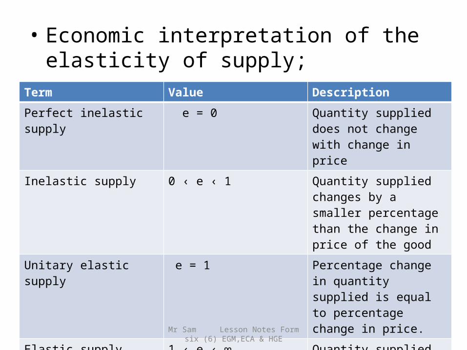
• Economic interpretation of the elasticity of supply;

Term Value DescriptionPerfect inelastic supply

e = 0 Quantity supplied does not change with change in price

Inelastic supply 0 ‹ e ‹ 1 Quantity supplied changes by a smaller percentage than the change in price of the good

Unitary elastic supply

e = 1 Percentage change in quantity supplied is equal to percentage change in price.

Elastic supply 1 ‹ e ‹ ∞ Quantity supplied changes by a larger percentage than the change in the price.


NOTE; (i) Equilibrium price and quantity obtained when Quantity Supplied is equal to quantity demanded i.e QS = Q D

(ii) Example of exceptions of law of supply is the Supply of labour; Where at a very high wages people are willing to supply less labour than at lower wages. This also known as Regressive supply curve


Exercise

The demand function for Book in Galanos stationary is given by:

Q = 205Y2.3 P-2.6 R1.7 where Q is quantity demanded, Y is income, P is mean retail price

Of Book and R is Mean retail price of all other commodities. Calculate

(a) Price elasticity of demand

(b) Income elasticity of demand

(c) Cross-price elasticity of demand


Documents

DEMAND AND SUPPLY CONCEPTS