Derivation of qualitative information in motion analysis

Derivation of qualitative i information n motion

analysis

Edouard FranE;ois and Patrick Bouthemy

A qualitative approach to ge t information about 3D kinematic behaviour of objects in a scene f rom apparent motion in the image sequence is presented. The process is in fact two-fold: first partition o f the image into areas comprising a unique motion; and second, symbolic description of the motion of each area. Here the second part is discussed. Kinematic description involves motion and trajectory type. It relies on geometrical cues tied to the velocity field such as divergence or rotational terms. First, it is shown how a comptete set o f such cues can be derived through a first order development of the 2D velocity field. Second, the relation between these cues and the 3D ,,notion parameters is established; which allows the determination o f a set o f labels associated with different kinematic configurations; Third, the label validation step is solved using a statistical approach (in fact, two methods have been studied). This approach avoids determining explicit 3D parameters such as a depth map or 3D motion measurements. Several experiments on different sequences are reportedl

Keywords: image sequence, velocity field, symbolic description, statistical criteria, qualitative motion interpretation

A very challenging task in dynamic scene analysis is t h e recovery of information about 3D motion and structure in a scene 1"2. One solution which has been widely investigated is to quantitatively e s t i m a t e the 3D motion parameter s using dense optical flow measurements 3=s. On the other hand, a minimal number of features like specific points or contour lines and correspondence methods 6-s can be used. Because of noisy measurements, problems of numerical instability and estimation errors of the 3D parameters often occur. In case of th e use of a noisy optical flow field, resulting ambiguities are thoroughly analyzed by Adiv 9. Quantitative bounds

IRISA/INRIA, Campus Universitaire de Beaulieu, 35042 Rennes Cedex, France

0262-8856/90/040279-10 vol 8 no 4 november 1990

are also derived by Young and Chellappa H) from a s ta t i s t i ca l point of view.

To obtain more stable and robust descriptions, it b e c o m e s a t t rac t ive to follow a qualitative approach which still provides relevant information in many situations. Indeed. theoretical studies have pointed o u t that the geometry of the apparent velocity field by itself contains significant and useful in fo rmat ion ' l 12 A qualitative way of reasoning and modelling was primarily introduced by Thompson et al. 13 for dynamic s c e n e analysis. It is emphasized that characterizing motion in terms of broad classes is quite relevant. As a matter of fact. an explicit 3D quantitative reconstruc- tion of the environment is not always necessary to achieve dynamic scene analysis tasks. Indeed. this classification relies only on intrinsic global cues. viz differential invariants of the velocity field, More recently, the obstacle avoidance problem has been solved by Nelson and Aloimonos 14 using a qualitative analysis based on an appropriate computation of t h e optic flow divergence cue. A qualitative motion understanding issue is also addressed by Burger and Bhanu ,5 by making use of the focus of expansion (FOE). A s e t of rules expressing typical dynamic behaviour is derived which enables us to construct a 3D qualitative model of th e environment.These aspects can also be considered as intermediate layers towards a comprehensive high level interpretation of a scene. Nagel I6 presents several approaches which provide conceptual descriptions of the scene, based on different typical situations.

Among the above mentioned qualitative approaches. t h o s e relying on the differential geometrical invariants of the optical flow s e e m to be promising when used to cope with dynamic scene analysis tasks Our purpose is to generalize them to provide a complete and general qualitative modelling of the 2D motion information extracted from the image sequence acquired by a camera. This camera can be stationary or mobile. The estimation and decision step (i.e. deriving kinematic symbols from 2D motion measurements') is a central problem which must not be neglected, since we are dealing with noisy data and non-perfectly exact models (first order models). To this end. we propose a new

© 1990 Butterworth-Heinemann Ltd 279

implementation of this derivation based on a statistical approach.

Once a symbolic description of the 2D motion information is derived, one can deliver in a robust and simple manner an interpretation of the observed scene by qualitatively reasoning on this set of symbols. This interpretation is expressed in terms of classes which essentially correspond to relevant combinations of these elementary symbols according to the application at hand. Indeed° we do not need to explicitly compute any 3D measurements such as depth maps, for instance, nor to extract the FOE. Moreover, as we aim to obtain a qualitative description, and not the precise quantitative estimation of 3D parameters, a camera calibration is not required.

The process is in fact two-fold:

• the partition of the image in areas comprising only one apparent coherent motion;

• the kinematic description of the motion of each area.

To cope with the first problem, we use the method described by Bouthemy and Santillana Rivero 17. We deal here with the latter method. Kinematic description involves motion type (e.g. rotation or translation) and trajectory type (e.g. perpendicular or parallel to the optical axis).

This problem has to be investigated according to different aspects, which can be described as follows (the two first aspects concern the theoretical analysis of the 'physical' problem, the third one is the explicit way of solving it):

t first, cues on the 2D velocity field are explicitly derived through a first order development, each of them representing a particular component of this field;

• second, we establish the relation between these cues and the 3D motion parameters, which enable to determine a set of labels (combinations of symbols) associated with different kinematic configurations;

• third, the labelling problem (numerical to symbolic step) is solved using a statistical approach.

2D V E C T O R FIELD D E S C R I P T I O N

As previously outlined, the starting idea of a qualitative motion understanding approach is that the geometry of th 2D velocity vector field in the image contains information about the 3D motion, which can be significant and sufficient to the interpretation. Studies on the human visual system ~s also give support to this assumption. The first step is then to introduce relevant terms, describing specific forms of the field, and which could be easily and naturally interpreted. It appears that a description of the velocity field up to the first order is sufficient to supply an efficient qualitative interpretation of the scene (a similar derivation is described in Reference 19). We consider the first order development of the velocity vector c~ around a point g(xg, yg) in the image:

(x-x=) ;),,_,=,

with:

Ou Ov Ou Ov (1) Ox - Ox' ' Oy

We can use the following decomposition of any matrix M 2o:

M = Vz(trace M ) I + V z ( M - M ~) +

Vz[M + M m - (trace M) I] (2)

t o ;) Considering M = /~ '

this allows the following formulation:

M = V2div [D] + V2rot[R] + V~_hyp 1 [H~] + 'Mhyp2 [H:]

where:

('7) (o_1) [D]= 0 ,[R]= x o '

[H,]= (10 _01), [H=]= (0 ;)

Hence:

~)(x, y) = bg + V 2 d y . d i v + V ; d x . r o t -

V2dy. hyp l + V~dx. h y p 2

with dx = x - Xg, dy = y - yg. The four terms whose coefficients are:

"-""~'~\\\ \ / / / / / / / - I ~#%7,~/~.._ ~ , ,(,II . . . . . -,x,\\,~

(s)

(4)

a b

'/, . . \ \ .~ ~. > -_ ~ J . / / U / / / / / ~ . . ' ~ . ~ _ ~ 2 ~ - - ~ / ~ ~ / / / /

/ J y / / / / / / I~ \',\'..~'-.~.~- X~'L\X',N%.~."~'C~EJ~z//{¢,~I/

[ ~ f / ] . 1 I / ' ' - ~ \ \ \ \ , \ ~ \ \ \ \ \

. .'->..~'-2.'~i ~ X X ! X X/Zi~ e d

Figure 1. (a) Divergent field, (b) rotational field, (c) and (d) hyperbolic fields

280 image and vision comput ing

• div - o~ + 8 (for divergence)

• r o t = Y - [3 (for rotational)

• h y p l = 8 - o ~

• h y p 2 = y+/3 (for hyperbolic terms)

(5)

correspond to fields which belong to four orthogonal supplementary subspaces. Four different fields of these four independent subspaces are represented in Figure 1. Any vector field can be approximated by a linear combination of a divergent field, a rotational field, and two hyperbolic fields. The interest of these terms in comparison with c~, /3, y and 8, is that the interpretation of any vector field, even non-linear, can be made more easily based on them. When the field is the projection of 3D velocity vectors in the image plane, a particular kind of motion in the scene will imply a particular combination of these basic fields. Indeed, a divergent velocity vector field is the result of an axial motion, i.e. along the optical axis of the sensor. A rotational field appears as the result of a rotation around this axis. We establish below the link between 3D motion parameters and each of the four terms introduced above.

LABEL SET DEFINITION

Relations 2D-3D

We consider the relative motion of an object, with respect to the camera, consisting of translational velocity T = ( U , V, W) T, and rotational velocity f I = ( A , /3, C) T, in coordinate system shown in Figure 2.

We define as the point p ( x , y) the perspective projection in the image plane of a point P = (X, Y, Z) T. We get (assuming focal length f i s equal to 1):

x = X / Z , y = Y / Z (6)

The instantaneous veloc+ity of P is given by the formula P = (X, F, Z ) r = ~ + ~ A ( )P. Deriving equation (6) with respect to time and after some developments, we obtain the following relations between the apparent 2D motion (u, v) at point p and the 3D motion parameters21:

f u = - - + B - C y - x - - - A x y + B x 2 Z Z

V W (7) v = - - - A + Cx - y --~ + Bxy - A y 2

Z Y

B

- - ' - U P ---Y

Z

W

Figure 2. Coordinate system

Given the above remark upon the relevance of first order terms for the interpretation, we only consider the first order terms of the depth function Z.

By combining with equation (6), this implies:

1 1 Z - Zo (1 - ylx - T 2 Y )

Let us point out that this relation is strictly verified if we consider planar patches. In this last case, Yl and y2 represent the orientation parameters of the plane.

We substitute in (7) the above expression for 1/Z. Then we derive relations (7) considering point P and reference point G. Subtracting corresponding equation members of the two derived systems, we get the following expressions:

b l = a g q - ( 31---~1 U - E I d x - ~ - ( - ' ) I 2 U - C t d y - } - 0 2 Zo Z o / \ Zo / (8)

where g = (xg, yg) is the projection of G, (ag, bg) r is the velocity vector of point g, and again dx = x - xg, dy = y - y g . By identifying in equation (8) the linear terms of equation (1), and using equation (5), we obtain:

W U div = - 2 - - - y~ - - - Y2 - -

Zo Zo

V U rot = 2 C - Yl -~o + Y2 Z-~o

U V : -- - - + T 2 - - hyp 1 Yl Zo Zo

V U h y p 2 = - y l Z - y 2 Z---~o

V

Z0

(9)

Since we only take into account a linearized version of the velocity field, the two rotation components, A around the X axis and B around the Y axis, do not appear in the expressions of the kinematical description parameters derived in (9). As A and B do not appear in the linear part of functions u(x , y) and v(x , y) (8), this leads to neglect their contribution to the parameters div, rot, h y p l , hyp2. In the estimation step the statistical test decides whether values of cues div, rot, h y p l , hyp2 are really significant or not, which is slightly different than merely deciding whether they are equal to zero or not. Therefore, it makes sense that the kinematical description relies on a linearized version of the velocity field, and makes use of relations (9).

As a matter of fact, quantities div, rot, h y p l , h y p 2 will be implicitly or explicitly computed from the optic flow field, as explained hereafter, whereas relatfons (9) imply that the true 2D motion field, projection on the image plane of the 3D velocity field, is considered. It is

2 2 known that discrepancies exist between these two 2D fields. However, they share common qualitative properties, leading to useful information about the 3D velocity field. This tells again in favour of a qualitative approach.

vol 8 no 4 november 1990 281

Qualitative interpretation overview

Briefly, the way of solving the interpretation problem is as follows:

• segmentation of the velocity field;

• estimation of kinematical parameters (or cues);

• selection of the significant labels and interpretation.

Since we are concerned with qualitative interpretation, what is important is the comparison of the parameters div, rot, hypl and hyp2 to zero, and not the estimation of each parameter of the 3D motion. Accordingly, we associate to each quantitative term div, rot, hypl, hyp2 a qualitative (Boolean) variable Vdiv, Vrot, Vhypl , Vhyp2 , equal to 0 if its associated quantitative variable is non- significant, and symbols D, R, HI, //2, respectively, otherwise.

Once the different variables and their possible states have been defined, it is important to take into account the right labels in the context of dynamic scene analysis. Given four independent parameters taking two possible states, there are 2 4 = 16 possible combinations (labels) in the (Vaiv, Vrot, Vhypl, Vhyp2) base.

The actual qualitative description corresponds to a subset of all these combinations. It takes into account the physical reality of the motion, explicitly contained in relations (9). Indeed, from these relations, it can be inferred that the only symbol associations which are really likely to exist in an image sequence depicting a usual indoor or outdoor scene are the following: (0, 0, 0, 0), (D, 0, 0, 0), (0, R, 0, 0), (D, R, 0, 0 )and (D, R, H i , / / 2 ) . For instance, if hypl and hyp2 are non-zero, then U or V are non-zero, and consequently div and rot are non-zero (unless in very particular cases). We can assume that the eleven other labels (such as (0, 0, HI, H2) label or (D, R, 0, H2) label . . . . ) can be disregarded. This can be related to the choice of only three parameters, div, rot, shear, in Reference t9 to characterize motion, since the shear magnitude is given by "V/hyp12+hyp22. The subset of these five labels is denoted by St~bet. From the relations (9), it is clear that several typical dynamic situations can be expressed. For instance, in the (Vdiv, Vrot, Vhypl , Vhyp2) basis, the (D, 0, 0, 0) association or label is the qualitative description of a motion along the optical axis (besides, it is usual to base the obstacle detection on a divergence cue). (0, R, 0, 0) describes a rotation around this axis, etc. • The higher level of interpretation depends on the considered application. Let us consider the example of a car driving situiation. As far as obstacle detection is concerned, the qualitative evaluation of the kinematic behaviour of the others objects in the scene relative to the vehicle of interest is crucial. Three main kinematic classes are introduced:

• object getting closer to the vehicle;

• object moving away from it;

• object moving cross in front of it.

These classes are directly tied to the labels described above. The first class corresponds to the (D, 0, 0, 0) label if the div sign is positive, the second to the same label but if the div sign is negative, and the last one to

(0, 0, 0, 0) if the own car is static, (D, R, Hi, /42) otherwise.

Let us give another remark. If we add to the four kinematical cues the two constant terms a~ and bg, pan and tiR motions, corresponding to rotation parameters B and A, could be also explicitly recognized. They would correspond to the extended labels (Ta, 0, 0, 0, 0, 0), (0, Tb, 0, 0, 0, 0) where Ta, resp. Tb, is the qualitative symbol corresponding to a significant value for quantitative variable ag, respectively bg.

LABELLING PROCESS

Before the labelling step, as already outlined, it is necessary to perform a spatio-temporal segmentation which gives an image partition in motion coherent regions, i.e. in which only one given linear 2D motion model is assumed to be present. To this end, we use the method described by Bouthemy and Santillana Rivero 17. It takes into account linear motion models and a partial motion information (the same as the one in relation (12)); it relies on the computation of likelihood ratio tests embedded in a region-growing procedure. Let us recall that motion segmentation is essential in most of the 2D motion analysis issues, motion estimation 23, motion characterization 24, and that it must be properly handled. Once the image is segmented, the motion of each region will be qualitatively interpreted. Let us note that motion segmentation and motion interpretation stages are consistent since both use linear models.

Observation and optimal estimation of parameters

Now, the key point is to properly achieve the numerical-to-symbolic step; i.e. deriving symbols from numerical data. Given an area in the image, we must determine the most convenient label, i.e. the one which is the best fit to the 3D motion of the object. The simple comparison of the magnitudes (or function of the magnitudes) of the quantitative terms div, rot, hypI, hyp2 to a threshold (initially described by Thompson et al. 13) remains very difficult and tricky. On the one hand, the threshold choice would be very dependent on the context and goals of the analysis. On the other hand, we cannot introduce a proper noise modelling with this approach, whereas the considered observations (optical flow) are actually noisy. More- over, we only consider a first order development of the velocity field (i.e. linear models) to characterize motion. That is the reason why we resort to a statistical approach to cope with these problems 25. The first point is to define what we take as observation.

Let us denote 2o the true velocity field, ~o,,, the velocity field generated by the linear model m para- metrized by Ore. For instance, for the (D, 0, 0, 0) label, Om= (div, 0, 0, 0) and:

~Jo,,,= ( ap + l/z'div'x ) \bp+ lM.div, y

I(x, y) is the image intensity function, V1 and It its spatial and temporal derivatives. ~ and I are linked by the well-known image flow constraint equation1:

~ . 51+ I, = 0 (10)

282 image and vision computing

If the true field has been estimated, we consider as observations the vectorial random variables:

7o,,,(x, y) = y) - o(x, y) (11)

If the tree velocity vector field is not available, we consider the following scalar random variables:

eo,,,(x, y) = ((~o,,,(x, y ) - N(.v, y)). VI(x, y)

i.e. using relation (10):

eo,,,(x, y) = U%,,,(x, y) . {I(x, y) + I,(x, y) (12)

In both cases, the considered variables are supposed to be independent Gaussian zero-mean variables. The likelihood function f(Om) of a model m can therefore be easily written. It is the product of the densities of each e~,,,,(x, y) within the given area Ak:

n 1 ( f(Om) = , ~ exp i=1

eo,,,(xi, yi) 2 ) 2o -2

e<,(xi, yi) 2 _ ( 1 ~ i=l

@ ) exp - 2o-2

where n is the number of points of A k. The optimal estimator Om of the parameter vector

@m for a given model, i.e. maximizing f, is in fact derived according to:

Om= arg min ~ eo,,,(Xi, yi) 2 (13) O,,, i= j

The unknown variance o-2 is supposed to depend on the given model and is a posteriori estimated by:

gr2 = 1 ~ e6,,,(xi, Yi) 2 n i = l

Finally, the likelihood function f(Om) can be expressed as:

1 '],, n

Likelihood tests

The problem now is to select the most convenient label. We must determine what the right state of each qualitative variable Vdi~, Vrot, Vhyel, Vhyp2 is. To this end we have designed a method based on statistical tests, viz likelihood test, which is known to be very powerful. We proceed as follows, knowing that only five combinations of these variable states are allowed. Vdi~ will be set by testing hypothesis Ho: (D, R, H1,//2) against hypothesis//_1: (0, R, H1, [12). This formalizes that the state of Vdi~ is determined while letting the three other variables free. Practically, we first estimate the optimal parameter vector Oo = (d[v, rot , h~pl, h~p2) for the (D, R, H1, [12) hypothesis, i.e. which maximizes the likelihood function f(O0) as expressed in equations (13) and 04).

In the same way, we determine O~ = (0, r6t, h~pl, h~p2) for the (0, R, H1, Ha) hypothesis. Then we

compare f (60/ f (Oo) (in fact the logarithm of this ratio: L(Vai~)=log[f(OOIf(Oo)] to a threshold a. If the ratio is lower than this preset threshold, the Vai~ symbol is equal to D, 0 otherwise:

(o)

HI >

L(Vd v) < a (15)

Ho (D)

The same holds for Vrot. If Vaiv or Vrot is equal to zero, then Vhypl and Vhyp2 a r e enforced to zero, following above mentioned remarks. Otherwise, the state of Vhypl and Vhyp2 is evaluated in a coupled way i.e, by testing (D, R, HI, / /2) hypothesis against (D, R, 0, 0) hypothesis. Once each symbol state is determined, the optimal label is defined as their association.

Let us pay some attention to the determination of the threshold value in the likelihood test. For the while we set it in a trial-and-error way. Nevertheless, it is not a critical matter, as shown below, where results are presented. However, it would be preferable to get it from a theoretical derivation. An attempt of this kind is described below,

Statistical information criterion

Statistical information criteria provide attractive means to cope with model-fitting problems. As far as our motion labelling problem is concerned, they could be seen as an answer to the automatic thresholding problem aforementioned. As a matter of fact, they present larger advantages. They allow to test together all the labels, contrary to the sequential decision tree- like procedure associated with the likelihood test method. The optimal model rh (and consequently the optimal label)will be given by26:

rh = arg min [ - log[f(Om)] + ~(n) . dim(Ore)] (16) m

wherefis again the likelihood function of the model m, Om denotes the optimal parameter vector of the model m, dim (Om) is the model dimension (for instance, the dimension of the (D, R, 0, 0) label is 2); and xF a given function. The different statistical criteria correspond to different functions xp issued from different assumptions and ways of tackling this problem 26. For instance, the Akaike information criterion (AIC) corresponds to • (n) = 1. It is used by Zhang and Modestino 27 for model-based image segmentation.

Before comparing the models, the optimal parameter vector Om has to be found for each model. The second term of the criterion acts as a penalization term on the model complexity. Hence, if the likelihood of a given model is not really better than a simpler one, the more complete model will be eliminated because of the penalization term. This means that, in fact, it does not bring any significant additional information. After preliminary tests, it appeared that the most interesting criterion for this application is the Rissanen criterion (RIC). In this case, ~(n) = 1/210g(n). (This version of xI* can also be derived from a Bayesian approach25.)


(o,o,o,o) (o,R,o,o) (D,o,o,o) (D,R,O,O) (D; R, ~1, g2)

a b

|

e d

!

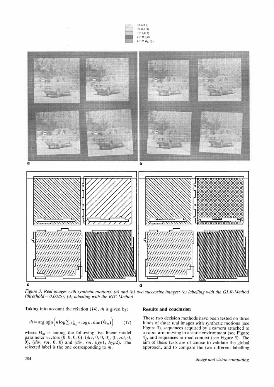
Figure 3. Real images with synthetic motions. (a) and (b) two successive images; (c) labelling with the GLR-Method (threshold = O. 0025); (d) labelling with the RIC-Method

Taking into account the relation (14), rh is given by:

rh = arg m in (n log ~ e 2 + log n. dim (Ore)) (17)

where 0 m is among the following five linear model parameter vectors (0, 0, 0, 0), (div, O, O, 0), (0, rot, O, 0), (div, rot, 0, 0) and (div, rot, hypl, hyp2). The selected label is the one corresponding to rh.

Resul t s and c o n c l u s i o n

These two decision methods have been tested on three kinds of data: real images with synthetic motions (see Figure 3), sequences acquired by a camera attached to a robot arm moving in a static environment (see Figure 4), and sequences in road context (see Figure 5). The aim of these tests are of course to validate the global approach, and to compare the two different labelling


a b

..~.....~~ ~~...~.......~. ~...;̀ ?........~.̀ ~....~̀ ~.............:.̀ ?..).~...?~.̀ ~.......~.. ?.....:.:......?.......?..~.........:.. y:.......~.. ̀ ~̀.~̀?..~ ~..?......~:.....~..~....7...̀ ~......)̀ .?. y......:...~...?.., v..̀?..?.~..~]..~.........~........~..~̀ .......v.......: ~..~..£.v..)............v..̀ £̀.?..?.......~

e 6

Figure 4. Static scene and moving camera rotation around the optical axis (0, R, O, O) - observations: 0 a. (a) and (b) Two successive images; (c) labelling with the GLR-Method (threshold = 0.01); (d) labelling with the RIC-Method

techniques (criteria (15) and (17)). All the experi- mental results reported hereafter are obtained using the scalar observation given in equation (12).

For convenience we denote the gradient based observation (12) Oc, the likelihood test method GLR - Method, and the Rissanen criterion method R I C - Method.

To validate the method principle, we first consider real data with simulated motions (Example 1 - Figure 3). Two successive images composed of four real subimages undergoing specific synthetic motions (scaling, translation, rotation, and a combination of scaling and rotation) we generated. These motions should be

labelled respectively (D, 0, 0, 0), (0, 0, 0, 0), (0, R, 0, 0) and (D, R, 0, 0). The images and the different results are presented in Figure 3. The motion segmentation step is first performed and only the largest regions are further considered for labelling.

The GLR - Method gives quite satisfactory results for the four different motions in the image, since it chooses for each one of the four regions the right label. The threshold value is always the same whatever the size of the analyzed region and the kind of motion.

The RIC - Method gives the right label for the three motions (D, 0, 0, 0), (0, R, 0, 0) and (D, R, 0, 0). For the motion (0, 0, 0, 0), this method selects the complete

vo! 8 no 4 november 1990 285

b

[]

¢

[]

N,

e d

[]

[]

N,

[]

e2

d

I - ' - l t

Figure 5. Road context sequence - labelling on Oc. (a) and (b) Two successive images," (c) labelling with the GLR- Method (threshold = 0.01); (d) labelling with the RIC-Method

label (D, R, H1, H2). The second set of experiments deals with sequences

acquired in the laboratory. The scene is static, and the camera is moving (Example 2 - Figure 4). In this example, the scene is composed of a scale model representing an abbaye, and the camera is attached to the end effector of a robot arm. Several kinds of motion have been considered. Here, we only report results corresponding to a camera rotation around its optical axis (that should be labelled (0, R, 0, 0)).

The results obtained with the GLR-Method (see Figure 4c and other complementary results not reported in this paper) induce the following remarks. First, the threshold can be set to the same predeter- mined value whatever the kind of motion and the size

of the analyzed region and along the entire sequence (25 images). We have observed excellent results (no labelling errors occurred).

Results obtained with the RIC-Method are less satisfactory than with the GLR-Method. Nearly half the images within the sequence of 25 images are well labelled. The rest is ill-labelled, but nevertheless, the selected labels always include the R symbol (i.e. (D, R, 0, 0) or (D, R, HI, H2) is chosen).

Finally, we have considered a real sequence depicting outdoor scenes in a road context (Example 3 - Figure 5). The vehicles in the scene are moving toward the camera, which is itself mounted on a moving car. All the movements in the scene are parallel to its optical axis. The corresponding regions in the image


should be labelled as (D, 0, 0, 0). We focus on the nearest vehicle in the scene. The considered observations are still the Oc observations.

Results obtained with the GLR-Method are again very good. The nearest car is labelled (D, 0, 0, 0). The threshold is equal to 0.01; it is interesting to notice that this is the same value as in the previous example. This threshold is the same on the whole sequence, and at each time of the sequence, the right label is chosen.

The RIC-Method gives the following results: in the sequence of eight images, the right label is chosen five times, the complete label twice, and a totally wrong label ((0, R, 0, 0)) one time.

The global behaviour of the two methods, with a rather complete set of data, can be summarized in several points:

• the GLR-Method yields excellent and stable results whatever the size of the analyzed area and the kind of motion.

• the RIC - Mehod is not as robust as the first one; the complete label (D, R, H1, //2) may be wrongly selected instead of a simpler one.

The tendency of the RIC-Method to validate the complete label can be explained: as soon as the estimation of a pure motion (e.g. (D, 0, 0, 0)) is too noisy, the resulting motion field can be seen as a complete motion one ((D, R, H1, H2)). Indeed, in the motion space, pure motions could be represented as 'Dirac distributions', all the remaining being the complete motion one. Thus, the distance between any pure motion class (e.g. (D, 0, 0, 0)) and the (D, R, H1, H2) class is very narrow. As we do not directly deal with an acquired digital signal but with the derived estimates, it may occur that the parameter estimation may be inaccurate. In such a case, the criterion is relatively flat, i.e. the criterion value for several models among the set are not greatly different because the first term increases and the penalty term becomes negligible. The the criterion may validate another model. Neverthe- less, the interest of such criterion lies in the fact that it does not require any threshold definition and does not compare models in pairs but together.

We have also carried out experiments on the same image data using the observations given by relation (11) involving the estimation of the velocity field. We have observed no improvement in the performances of the RIC-Method. As far as the GLR-Method is concerned, of course results are still excellent since the labelling process then relies on more accurate 2D motion information. Besides, it is still easier to set the threshold value: the interval of possible values is larger. However, the estimation of the velocitY field requires a substantial amount of supplementary computations.

This paper has dealt with the derivation of a qualitative description of the kinematic behaviour of the objects in the scene. It represents a real alternative to quantitative estimation of 3D motion and structure parameters. The interests of this study are threefold: first, we have in an explicit, analytical and simple manner linked the description cues to the 2D apparent motion and the 3D motion; second, we have described two model-based statistical decision methods to achieve the numerical-to-symbolic step - they enable us to address any determination of qualitative motion infor-

mation in a unified and non-heuristic manner; and third, motion interpretation is reachable even if the velocity field is not beforehand estimated.

On one hand the RIC-Method allows us to test together the defined labels without involving any threshold, but results are not yet completely satisfying. On the other hand, the GLR-Method yields excellent results, but requires the determination of a threshold value. Even if this is not a critical matter, it would be worth an explicit mathematical derivation being available. We are currently studying this subproblem in a different context than statistical information criteria.

Another extension should be the following. Up to now, labelling is achieved instantaneously (i.e. considering motion information between only two successive images). As in Subbarao 28, we are now integrating the temporal axis in the labelling process, which should enlarge the range of the qualitative description.

A C K N O W L E D G M E N T S

This work is supported by MRT (French Ministry of Research and Technology) in the context of the E U R E K A european project PROMETHEUS, under PSA-contract VY/85241753/14/Z10. We thank Dr Enkelman for providing the image sequence of Figure 5a-b. We would also like to thank C Geny for his contribution at an early stage of this study, and B Delyon for useful discussions on statistical topics.

REFERENCES

1 Aggarwal, J K and Nandhakumar, N 'On the computation of motion from sequences of images - a review' Proc. I E E E Vol 76 No 8 (August 1988) 917-935

2 Barron, J 'A survey of approaches for determining optical flow, environmental layout and egomotion' Tech. Rep. Univ. of Toronto, Dept of Computer Science, RBCV-TR-84-5 (November 1984)

3 Adiv, G 'Determining three-dimensional motion and structure from optical flow generated by several moving objects' I E E E Trans. on P A M I Vol 7 (July 1985) pp 384-401

4 Bruss, A R and Horn, B K P 'Passive navigation' Comput. Vision, Graph. Image Process. Vol 21 (1983) pp 3-20

5 Waxman, A M and Ullman, S 'Surface structure and three-dimensional motion from image flow kinematics' Int. J. Robot. Res. Vol 4 No 3 (1985) pp 72-94

6 Faugeras, O D, Lustman, F and Toseani, G 'Motion and structure from motion from point and line matching' Proc. 1st Int. Conf. Comput. Vision London, UK (1987)

7 Mitiehe, A 'On kineopsis and computation of structure and motion' I E E E Trans. P A M I Vol 8 No 1 (January 1986) pp 109-112

8 Tsai, R Y and Huang, T S 'Uniqueness and estimation of three-dimensional motion parameters of rigid objects with curved surface' I E E E Trans. P A M I Vol 6 No 1 (January 1984) pp 13-26

9 Adiv, G 'Inherent ambiguities in recovering 3d motion and structures from a noisy flow field' I E E E Trans. P A M I Vol 11 (1989) pp 477-489


10 Young, G S and Chellappa, R 'Statistical analysis of inherent ambiguities in recovering 3d motion from a noisy field' Proc. 10th Int. Conf. Patt. Recogn. Atlantic City, USA (1990)

11 Carlsson, S 'Information in the geometric structure of retinal flow field' Proc. 2nd Int. Conf. Comput. Vision (December 1988)

12 Koenderink, J J and Van Doorn, J J 'Invariant properties of the motion parallax field due to the movement of rigid bodies relative to an observer' Optica Acta Vol 22 No 9 (1975) pp 773-791

13 Thompson, W B, Berzins, V A and Mutch, K M 'Analyzing object motion based on optical flow' Proc. 7th Int. Conf. Patt. Recogn. Montreal, Canada (1984)

14 Nelson, R C and Aloimonos, J 'Obstacle avoidance using flow field divergence' IEEE Trans. PAMI Vol 11 No 10 (October 1989) pp 1102-1106

15 Burger, W and Bhanu, B 'Qualitative motion understanding' Proc. Int. Joint Conf. Artif. Intell. (1987) pp 819-821

16 Nagel, H H 'From image sequences towards conceptual descriptions' Image & Vision Comput. Vol 6 No 2 (May 1988) pp 59-74

17 Bouthemy, P and Santillana Rivero, J 'A hierarchi- cal likelihood approach for region segmentation according to motion-based criteria' Proc. 1st Int. Conf. Comput. Vision London, UK (1987)

18 Koenderink, J J 'Optic flow' Vision Res. Vol 26 No 1 (1986) pp 161-180

19 Subbarao, M 'Bounds on time-to-collision and rotational component from first-order derivatives of image flow' Comput. Vision, Graph. Image

Process. Vol 50 (1990) pp 329-341 20 Simard, P Y and Mailloux, G E 'A projection

operator for the restoration on divergence-free vector-fields' IEEE Trans. PAMI Vol 10 No 2 (1988) pp 248-256

21 Longuet-Higgins, H C and Prazduy, K 'The interpretation of a moving retinal image' Proc. Roy. Soc. Lond. Vol 208 (April 1980)

22 Verri, A and Poggio, T. 'Motion field and optical flow: qualitative properties' IEEE Trans. PAMI Vol 11 No 5 (May 1989) pp 490-498

23 Heitz, F and Bouthemy, P 'Multimodal motion estimation and segmentation using markov random fields' Proc. Int. Conf. Part. Recogn. Atlantic City, USA (1990)

24 Wohn, K and Waxman, A M 'The analytic structure of image flows' Comput. Vision, Graph. & Image Process Vol 49 (1990) pp 127-151

25 Francois~ E and Bouthemy, P 'Vers une iterpr6ta- tion qualitative de comportements cin6matiques dans la sc6ne h partir du mouvement apparent' Research Report INRIA-Rennes No 1081 (August 1989)

26 Shibata, R 'Criteria of statistical model selection' Research Report Depart. of Maths, Keio Univer- sity, Japan (August 1986)

27 Zhang, J and Modestino, J W 'A model-fitting approach to cluster validation with application to stochastic model-based image segmentation' Proc. Int. Conf. Acoust., Speech & Signal Proces..(1988)

28 Suhbarao, M 'Interpretation of image flow: a spatio-temporal approach' IEEE Trans. PAMI Vol 11 No 3 (1989) pp 266-278


Documents

Derivation of qualitative information in motion analysis