Embed Size (px)
Citation preview
HAL Id: tel-00674271https://tel.archives-ouvertes.fr/tel-00674271
Submitted on 27 Feb 2012
HAL is a multi-disciplinary open accessarchive for the deposit and dissemination of sci-entific research documents, whether they are pub-lished or not. The documents may come fromteaching and research institutions in France orabroad, or from public or private research centers.
L’archive ouverte pluridisciplinaire HAL, estdestinée au dépôt et à la diffusion de documentsscientifiques de niveau recherche, publiés ou non,émanant des établissements d’enseignement et derecherche français ou étrangers, des laboratoirespublics ou privés.
Hunting colored (quantum) butterflies A geometricderivation of the TKNN-equations
Giuseppe de Nittis
To cite this version:Giuseppe de Nittis. Hunting colored (quantum) butterflies A geometric derivation of the TKNN-equations. Mathematical Physics [math-ph]. SISSA, Trieste, Italie, 2010. English. tel-00674271
SCUOLA INTERNAZIONALE SUPERIORE DI STUDI AVANZATI
INTERNATIONAL SCHOOL FOR ADVANCED STUDIES
Hunting colored (quantum) butterfliesA geometric derivation of the TKNN-equations
Thesis submitted for the degree of Doctor Philosophiæ
Candidate:Giuseppe DE NITTIS
Advisors:Prof. Gianfausto DELL’ANTONIODr. Gianluca PANATI
TRIESTE, 29 OCTOBER 2010

To my grandfathers Giuseppe and Giovanni,who watch me from the sky;to my grandmothers Maria and Anna,who support me on earth.

Acknowledgments
Many people deserve my acknowledgments for the help and encouragement that theygave me along the way.
First and foremost, I would like to thank my advisor, Prof. Gianfausto Dell’Anto-nio, for his careful guidance during these years, for illuminating discussions, and forhis constant support. I am very grateful to my co-advisor, Gianluca Panati, for havingintroduced me to the topic of this thesis and for three years of fruitful and inspiringcollaboration. I am also indebted with Frédéric Faure, who shared with me his initialideas which have been a stimulating starting point for this dissertation.
I would like to thank SISSA, and especially the members of the Mathematical PhysicsSector, for giving me the opportunity to increase my (not only scientifically) knowledgeand for the friendly and stimulating atmosphere that I found here. In particular, I amgrateful to Prof. Giovanni Landi and Prof. Ludwik Dabrowski for introducing me to thefascinating world of Non-Commutative Geometry. Indeed, many ideas in this work arethe result of the interaction with the “non-commutative community”.
I am very grateful to Prof. Stefan Teufel for his interest in this work and his ad-vices and for inviting me to give a series of lectures on the subject of this thesis at theTübingen Universität. I am also indebted with Prof. Johannes Kellendonk, AnnalisaPanati and Max Lein for their hospitality and the chance to present my results at theiruniversities.
I thank Prof. Jean Bellissard who invited me to spend a beautiful month at GeorgiaTech. He taught me a lot in Mathematics and how important is looking at (not onlymathematical) problems from different perspectives.
I would like to thank Prof. Yosi Avron for many stimulating discussions and com-ments and for allowing me to use the pictures of colored quantum butterflies.
I am grateful to my friends and colleagues at SISSA for sharing many moments offun and work; in particular Emanuele, Davide, Antonio, Andrea, Gherardo, Francesco,Giacomo, Fabio.
Last but not least, I would like to thank my parents for encouraging my studies andmy wonderful wife Raffaella for the big help in creating the images of this thesis andmainly for her endless emotional support.
iii
It is a truth universally acknowledged, that a (almost!) young man can not achieve aPh.D. without a Good Fortune. The name that I give to my fortune is God!
This work was partially supported by the INdAM-GNFM projects Giovane ricercatore2009 and 2010.
Trieste, Giuseppe De NittisOctober 2010
Preface
This Ph.D. thesis concludes a research accomplished within the Mathematical PhysicsSector of SISSA, International School for Advanced Studies of Trieste, from November2007 to September 2010. The work has been carried out under the constant supervisionof Prof. Gianfausto Dell’Antonio and in collaboration with Gianluca Panati.
This dissertation is structured according to a fictitious tripartition.
• The first part (Chapters 1 and 2) aims at introducing the reader into the subjectand presenting in a concise but exhaustive way main results achieved and tech-niques employed. Chapter 1 starts with Avron’s tale about the story of the quan-tum Hall effect (QHE). These introductory pages, aimed to fix the basic physicalnotions and the nomenclature of the QHE, can be skipped by the reader expert inthe field. The rest of Chapter 1 is devoted to a general and non technical expositionof the initial motivations (open problems) that inspired this work and of the mainresults achieved (solution of the problems). Therefore, Chapter 1 fixes preciselythe scope of this thesis. In Chapter 2, the “Ariadne’s thread” of our research projectis unrolled. This chapter contains the rigorous statements of our main results, aswell a consistent presentation of needful mathematical tools. Reading these firsttwo chapters should be enough to have a detailed knowledge about scopes and re-sults of the thesis.
• The second part (Chapters 3, 4 and 5) contains the technical aspects, that is theproofs of the main theorems, as well the “paraphernalia” of lemmas, proposition,notions, needful to build the proofs. Chapter 3 and 4 are largely based on twopapers:
- (De Nittis and Panati 2010): “Effective models for conductance in magneticfields: derivation of Harper and Hofstadter models”. Available as preprint athttp://arxiv.org/abs/1007.4786.
- (De Nittis and Panati 2009): “The geometry emerging from the symmetries of aquantum system”. Available as preprint at http://arxiv.org/abs/0911.5270.
A third paper, containing a compendium of Chapter 2 and Chapter 5, is in prepa-ration with Gianluca Panati and Frédéric Faure.
• The third part (Appendices A, B and C), containing auxiliary material, aims tomake this dissertation as much self-consistent as possible.
v

In order to help the reader to “navigate” the text, each chapter has been equippedwith a small abstract which describes the content of the sections.
Trieste, Giuseppe De NittisOctober 2010

HUNTING COLORED (QUANTUM) BUTTERFLIES
Contents
Acknowledgements iii
Preface v
Prologue 5
1 Introduction 7
1.1 Ante factum: phenomenology of the QHE and topological quantum numbers 71.2 Factum: topological interpretation of the QHE by Thouless et al. . . . . . 141.3 Overview of the results . . . . . . . . . . . . . . . . . . . . . . . . . . . . . . 191.4 Why quantum butterflies? . . . . . . . . . . . . . . . . . . . . . . . . . . . . 22
2 Results and techniques 27
2.1 Physical background and relevant regimes for the QHE . . . . . . . . . . . 272.2 Why is space-adiabatic perturbation theory required? . . . . . . . . . . . . 322.3 Algebraic duality and isospectrality . . . . . . . . . . . . . . . . . . . . . . 342.4 Band spectrum, gap projections and gap labeling . . . . . . . . . . . . . . . 382.5 Colored butterflies as a gap labeling . . . . . . . . . . . . . . . . . . . . . . 422.6 Absence of unitary equivalence . . . . . . . . . . . . . . . . . . . . . . . . . 442.7 From projections to vector bundles: the “two-fold way” . . . . . . . . . . . 462.8 From geometric duality to TKNN-equations . . . . . . . . . . . . . . . . . . 512.9 A “non-commutative look” to TKNN-equations . . . . . . . . . . . . . . . . 522.10 Prospectives and open problems . . . . . . . . . . . . . . . . . . . . . . . . . 54
3 Derivation of Harper and Hofstadter models 57
3.1 An insight to space-adiabatic perturbation theory . . . . . . . . . . . . . . 573.2 Description of the model . . . . . . . . . . . . . . . . . . . . . . . . . . . . . 583.3 Space-adiabatic theory for the Hofstadter regime . . . . . . . . . . . . . . . 60
3.3.1 Adiabatic parameter for weak magnetic fields . . . . . . . . . . . . 603.3.2 Separation of scales: the Bloch-Floquet transform . . . . . . . . . . 613.3.3 The periodic Hamiltonian and the gap condition . . . . . . . . . . . 63
1
3.3.4 τ -equivariant and special τ -equivariant symbol classes . . . . . . . 653.3.5 Semiclassics: quantization of equivariant symbols . . . . . . . . . . 683.3.6 Main result: effective dynamics for weak magnetic fields . . . . . . 703.3.7 Hofstadter-like Hamiltonians . . . . . . . . . . . . . . . . . . . . . . 75
3.4 Space-adiabatic theory for the Harper regime . . . . . . . . . . . . . . . . . 773.4.1 Adiabatic parameter for strong magnetic fields . . . . . . . . . . . . 773.4.2 Separation of scales: the von Neumann unitary . . . . . . . . . . . 793.4.3 Relevant part of the spectrum: the Landau bands . . . . . . . . . . 803.4.4 Symbol class and asymptotic expansion . . . . . . . . . . . . . . . . 823.4.5 Semiclassics: the O(δ4)-approximated symbol . . . . . . . . . . . . . 843.4.6 Main result: effective dynamics for strong magnetic fields . . . . . 883.4.7 Harper-like Hamiltonians . . . . . . . . . . . . . . . . . . . . . . . . 953.4.8 Coupling of Landau bands in a periodic magnetic potential . . . . . 96
4 Bloch-Floquet transform and emerging geometry 99
4.1 Motivation for a “topological” decomposition . . . . . . . . . . . . . . . . . . 994.2 Some guiding examples . . . . . . . . . . . . . . . . . . . . . . . . . . . . . . 1024.3 The complete spectral theorem by von Neumann . . . . . . . . . . . . . . . 1044.4 The nuclear spectral theorem by Maurin . . . . . . . . . . . . . . . . . . . . 1074.5 The wandering property . . . . . . . . . . . . . . . . . . . . . . . . . . . . . 1094.6 The generalized Bloch-Floquet transform . . . . . . . . . . . . . . . . . . . 1144.7 Emergent geometry . . . . . . . . . . . . . . . . . . . . . . . . . . . . . . . . 123
5 The geometry of Hofstadter and Harper models 135
5.1 Standard physical frames . . . . . . . . . . . . . . . . . . . . . . . . . . . . 1355.1.1 Representation theory of the NCT-algebra . . . . . . . . . . . . . . . 1355.1.2 Standard physical frame for the Hofstadter representation . . . . . 1375.1.3 Standard physical frame for the Harper representation . . . . . . . 141
5.2 Bundle decomposition of representations . . . . . . . . . . . . . . . . . . . 1435.2.1 Bundle decomposition of the Hofstadter representation . . . . . . . 1435.2.2 Bundle decomposition of the Harper representation . . . . . . . . . 148
5.3 Geometric duality between Hofstadter and Harper representations . . . . 155
A Technicalities concerning adiabatic results 159
A.1 Self-adjointness and domains . . . . . . . . . . . . . . . . . . . . . . . . . . 159A.1.1 Self-adjointness of HBL and Hper . . . . . . . . . . . . . . . . . . . . 159A.1.2 Band spectrum of Hper . . . . . . . . . . . . . . . . . . . . . . . . . . 160A.1.3 The Landau Hamiltonian HL . . . . . . . . . . . . . . . . . . . . . . 161
A.2 Canonical transform for fast and slow variables . . . . . . . . . . . . . . . 163A.2.1 The transform W built “by hand” . . . . . . . . . . . . . . . . . . . . 163A.2.2 The integral kernel of W . . . . . . . . . . . . . . . . . . . . . . . . . 165
B Basic notions on operator algebras theory 167
B.1 C∗-algebras, von Neumann algebras, states . . . . . . . . . . . . . . . . . . 167B.2 Gel’fand theory, joint spectrum and basic measures . . . . . . . . . . . . . 168B.3 Direct integral of Hilbert spaces . . . . . . . . . . . . . . . . . . . . . . . . . 170B.4 Periodic cyclic cohomology for the NCT-algebra . . . . . . . . . . . . . . . . 171
C Basic notions on vector bundles theory 173
Bibliography 181
Index 187

Prologue
Despite of its title, this dissertation is not supposed to be a compendium of a youngentomologist’s research on new exotic species of colorful butterflies. The following
pages will not either tell the story of a hunter determined to catch unknown specimenof enigmatic multicolored insects living in the forest in the heart of Africa or SouthAmerica.
The unwary reader, possibly intrigued by the title, would be somehow surprised torealized that this work is actually a Ph.D. thesis in Mathematical Physics.
Nevertheless, this ambiguity hides some truths. Mathematical ideas fly light with“butterfly wings” in mathematician’s mind. They are painted with the “gaudy colors”of intuition and imagination. The mathematician spends his time “hunting for newproblems” just like the entomologist does for his preys. Tools he uses to get his “huntingtrophy” are theories, theorems, proofs and so on.
Keeping in mind this analogy, the reader may consider this thesis as the story of mypersonal hunt to unveil the secrets of quantum butterflies.
Well, It is time to cry aloud: - the hunt begins! -.
5

Chapter 1
Introduction
On ne connaît pas complètement une science tant qu’onn’en sait pas l’histoire.
(One does not know completely a science as long as onedoes not know its history.)
Auguste ComteCours de philosophie positive, 1830-1842
Abstract
The aim of this introductory chapter is to present the scope of this thesis fixing basicnotions and terminology, as well to provide a complete, but non technical, exposition ofthe main results. Section 1.1 is devoted to a historical review of the quantum Hall ef-fect (QHE), trough main steps that lead to its “topological interpretation”. The notionsof topological quantization and topological quantum numbers are expounded usingthe Dirac’s monopole as a paradigm. This first section is “borrowed” from (Avronet al. 2003, Avron et al. 2001). Thouless et al. showed in the seminal paper (Thoulesset al. 1982) that the quantized values of the Hall conductance are topological quan-tum numbers. The content of the paper by Thouless et al. is discussed in Section 1.2.A special attention is paid to the TKNN-equations which are Diophantine equationsfor the values of the quantized conductance. TKNN-equations play a crucial rôle inthis thesis. Some assertions in (Thouless et al. 1982) are lacking of rigorous justi-fications. These “gaps” in the mathematical structure of the work of Thouless et al.are listed in Section 1.3. One of the goal of this thesis is to fill such mathematicalgaps and so Section 1.3 can be considered as our “operation plan”. In this sectionwe present (quite informally) the main results of this thesis. Quantum butterflies arediagrammatic representations of the TKNN-equations. Section 1.4 contains a descrip-tion of the main features of these charming pictures. A geometric justification of theTKNN-equations is needed to provide quantum butterflies with a rigorous geometricmeaning. This is the main goal of this thesis.
1.1 Ante factum: phenomenology of the QHE and topologi-
cal quantum numbers
The quantum Hall effect (QHE) is the central argument of this thesis. Therefore,it could be appropriate to start with a brief review of the phenomenology and the
theory of QHE, in order to provide the inexpert reader with basic notions and needed
8 1. Introduction
terminology. The long story of the QHE, from the first experiments up to the brilliant in-tuition of its “topological interpretation”, has been excellently narrated by J. E. Avron inthe beautiful introductions of (Avron et al. 2003, Avron et al. 2001). Due to the complete-ness, the synthesis and the charm of Avron’s presentations, I realized that it was quiteimpossible (at least for me!) to expose in a better way the story of the QHE. Therefore, Iconsidered more “honest” to borrow the Avron’s tale, offering to the reader a moment ofquality literature. The reader expert in QHE is advised to skip directly to Sections 1.2and 1.3.
The beginning of the story
The story of Hall effect begins with a blunder made by J. C. Maxwell. In the first editionof his book, A treatise on Electricity and Magnetism, discussing about the deflection ofa current by a magnetic field, Maxwell wrote: “It must be carefully remembered, thatthe mechanical force1 which urges a conductor carrying a current across the lines ofmagnetic force, acts, not on the electric current, but on the conductor which carries it.[...] The only force which acts on the electric currents is the electromotive force, whichmust be distinguished from mechanical force [...].” (Maxwell 1873, pp. 144-145). Suchan assertion should sound odd to a modern reader, but at that time it was not so obviousto doubt the Maxwell’s words.
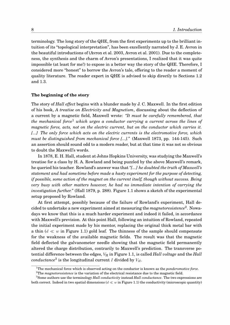
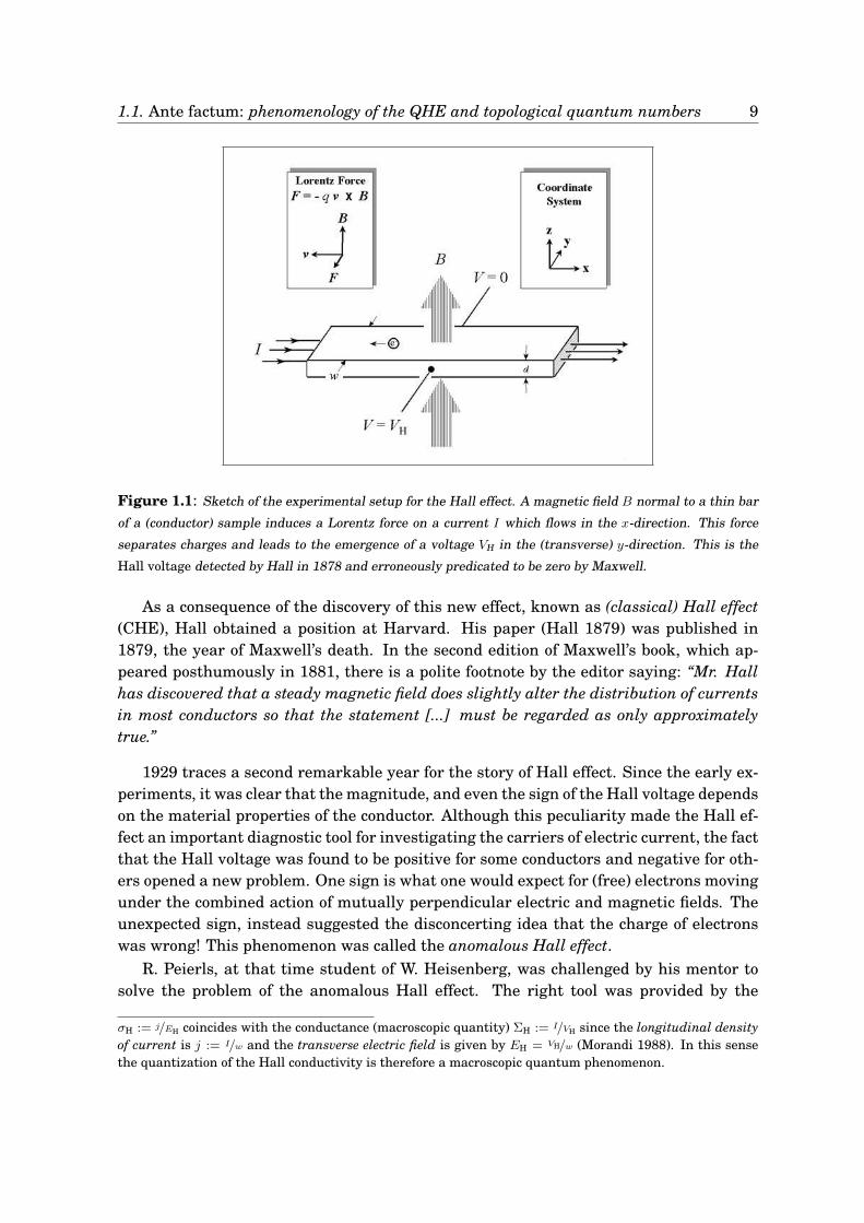
In 1878, E. H. Hall, student at Johns Hopkins University, was studying the Maxwell’streatise for a class by H. A. Rowland and being puzzled by the above Maxwell’s remark,he queried his teacher. Rowland’s answer was that “[...] he doubted the truth of Maxwell’sstatement and had sometime before made a hasty experiment for the purpose of detecting,if possible, some action of the magnet on the current itself, though without success. Beingvery busy with other matters however, he had no immediate intention of carrying theinvestigation further.” (Hall 1879, p. 288). Figure 1.1 shows a sketch of the experimentalsetup proposed by Rowland.
At first attempt, possibly because of the failure of Rowland’s experiment, Hall de-cided to undertake a new experiment aimed at measuring the magnetoresistence2. Nowa-days we know that this is a much harder experiment and indeed it failed, in accordancewith Maxwell’s prevision. At this point Hall, following an intuition of Rowland, repeatedthe initial experiment made by his mentor, replacing the original thick metal bar witha thin (d ≪ w in Figure 1.1) gold leaf. The thinness of the sample should compensatefor the weakness of the available magnetic fields. The result was that the magneticfield deflected the galvanometer needle showing that the magnetic field permanentlyaltered the charge distribution, contrarily to Maxwell’s prediction. The transverse po-tential difference between the edges, VH in Figure 1.1, is called Hall voltage and the Hallconductance3 is the longitudinal current I divided by VH .
1The mechanical force which is observed acting on the conductor is known as the ponderomotive force.2The magnetoresistence is the variation of the electrical resistance due to the magnetic field.3Some authors use the terminology Hall conductivity instead Hall conductance. The two expressions are
both correct. Indeed in two spatial dimensions (d ≪ w in Figure 1.1) the conductivity (microscopic quantity)
1.1. Ante factum: phenomenology of the QHE and topological quantum numbers 9
Figure 1.1: Sketch of the experimental setup for the Hall effect. A magnetic field B normal to a thin bar
of a (conductor) sample induces a Lorentz force on a current I which flows in the x-direction. This force
separates charges and leads to the emergence of a voltage VH in the (transverse) y-direction. This is the
Hall voltage detected by Hall in 1878 and erroneously predicated to be zero by Maxwell.
As a consequence of the discovery of this new effect, known as (classical) Hall effect(CHE), Hall obtained a position at Harvard. His paper (Hall 1879) was published in1879, the year of Maxwell’s death. In the second edition of Maxwell’s book, which ap-peared posthumously in 1881, there is a polite footnote by the editor saying: “Mr. Hallhas discovered that a steady magnetic field does slightly alter the distribution of currentsin most conductors so that the statement [...] must be regarded as only approximatelytrue.”
1929 traces a second remarkable year for the story of Hall effect. Since the early ex-periments, it was clear that the magnitude, and even the sign of the Hall voltage dependson the material properties of the conductor. Although this peculiarity made the Hall ef-fect an important diagnostic tool for investigating the carriers of electric current, the factthat the Hall voltage was found to be positive for some conductors and negative for oth-ers opened a new problem. One sign is what one would expect for (free) electrons movingunder the combined action of mutually perpendicular electric and magnetic fields. Theunexpected sign, instead suggested the disconcerting idea that the charge of electronswas wrong! This phenomenon was called the anomalous Hall effect.
R. Peierls, at that time student of W. Heisenberg, was challenged by his mentor tosolve the problem of the anomalous Hall effect. The right tool was provided by the
σH := j/EH coincides with the conductance (macroscopic quantity) ΣH := I/VH since the longitudinal densityof current is j := I/w and the transverse electric field is given by EH = VH/w (Morandi 1988). In this sensethe quantization of the Hall conductivity is therefore a macroscopic quantum phenomenon.
10 1. Introduction
new (quantum) mechanics of which Heisenberg was one of the founding father. In fact,Peierls was enlightened by the results of F. Bloch (also Heisenberg’s student) concerningthe quantum mechanical behavior of electrons in a periodic crystalline field. Peierlsrealized that when the conduction band is only partially full, the electrons behaves asfree particles, and the Hall response is consequently normal (right). However, whenthe conduction band is completely full the electrons move in the wrong way becauseof diffraction through the lattice. The conductance turns out to be determined by themissing electrons, i.e. the holes, and the anomaly is solved since the charge of a hole isopposite (wrong) to the charge of an electron (Peierls 1985, pp. 36-38).
The third step in the story of the Hall effect begins a century after Hall’s discovery. In1980, performing experiments at the Grenoble High Magnetic Field Laboratory (France)on the Hall conductance of a two-dimensional gas at very low temperature, K. von Kl-itzing discovered that the Hall conductance, as a function of the strength of the externalmagnetic field, exhibited a staircase sequence of wide plateaus. Moreover the values ofthe Hall resistance4 turn out to be integer multiples of a basic constant (the von Klitzingconstant)
RK :=h
e2≃ 25812.807557 Ω, (1.1)
where h ≃ 6.62606896 × 10⁻³⁴ J · s is the Planck constant and e ≃ 1.602176487 × 10⁻¹⁹ Cthe elementary electron charge. Von Klitzing was awarded the Nobel prize in 1985 forthe discovery of this new effect (von Klitzing et al. 1980), today named quantum Halleffect (QHE). The surprising precision in the (measured) quantization of the values of theresistance during experiments of QHE has provided metrologiste a superior standard ofelectrical resistance.
The most remarkable features of the QHE is that the quantization takes place withextraordinary precision in systems that are imprecisely characterized on the microscopicscale. Different samples have different distributions of impurities, different geometryand different concentrations of electrons. Nevertheless, whenever their Hall conduc-tance is quantized, the quantized values mutually agree with an astonishing precision.How to explain the robustness of this phenomenon of quantization?
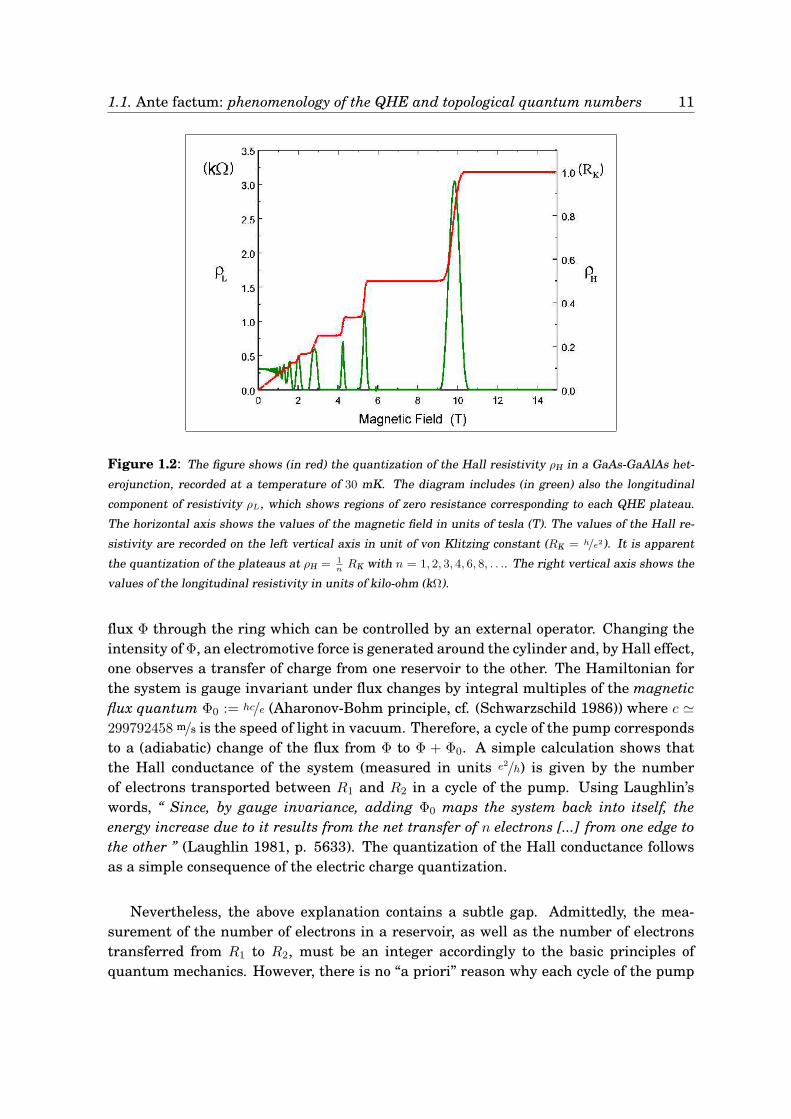
The first attempt in this direction was made in 1981 by R. Laughlin. In his paper(Laughlin 1981), the author considered a cold two-dimensional electron gas such thatthe thermal agitation can be neglected (the free particle approximation). In this regimethe time evolution of the system is recovered by the knowledge of the wavefunction ofa single electron. Laughlin suggested to interpret the QHE as the effect of a quantumpump. He assumed that the electron gas was confined on a cylindrical surface witha strong magnetic field applied in the normal direction as shown in Figure 1.3. Thetwo opposite edges of the surface are connected to distinct electron reservoirs R1 andR2. The pump effect, which transfers charges from R1 to R2, is driven by a magnetic
4The Hall resistance is defined as RH := VH/I. According to Footnote 3, RH is the inverse of the Hallconductance ΣH and, due to the two-dimensional geometry, it coincides also with the inverse of the Hallconductivity. The latter is by definition the Hall resistivity ρH := EH/j.
1.1. Ante factum: phenomenology of the QHE and topological quantum numbers 11
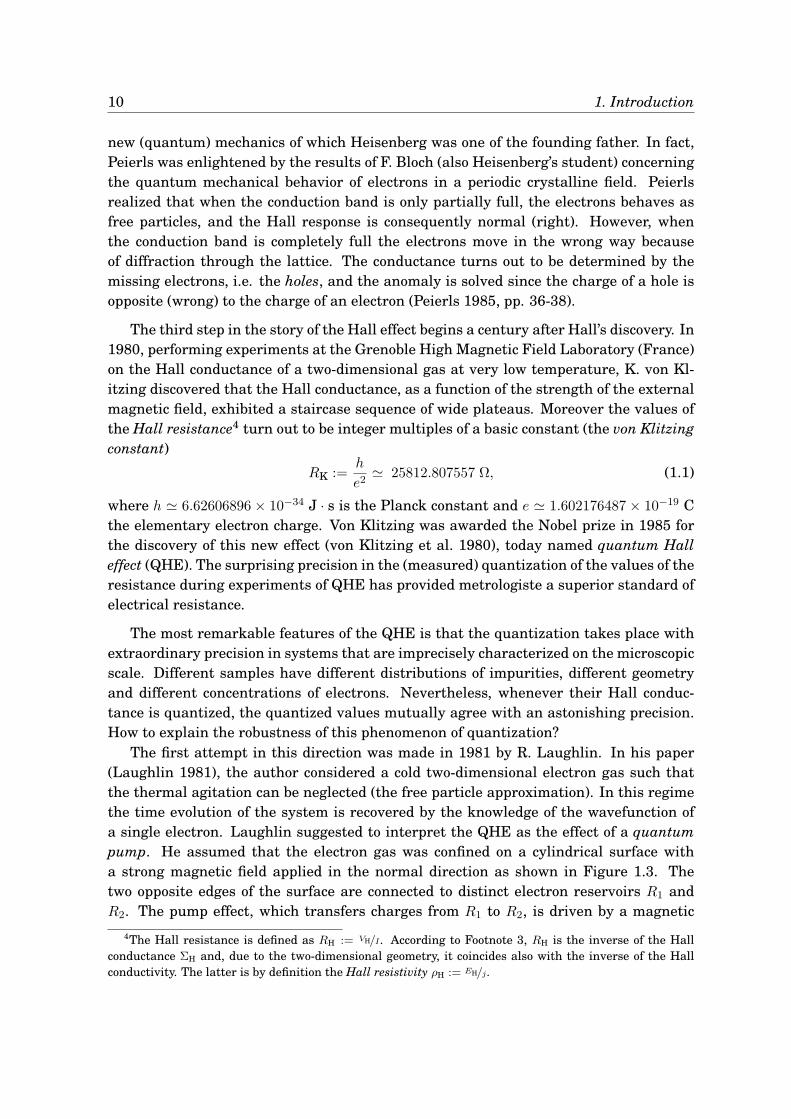
Figure 1.2: The figure shows (in red) the quantization of the Hall resistivity ρH in a GaAs-GaAlAs het-
erojunction, recorded at a temperature of 30 mK. The diagram includes (in green) also the longitudinal
component of resistivity ρL, which shows regions of zero resistance corresponding to each QHE plateau.
The horizontal axis shows the values of the magnetic field in units of tesla (T). The values of the Hall re-
sistivity are recorded on the left vertical axis in unit of von Klitzing constant (RK = h/e2). It is apparent
the quantization of the plateaus at ρH = 1n
RK with n = 1, 2, 3, 4, 6, 8, . . .. The right vertical axis shows the
values of the longitudinal resistivity in units of kilo-ohm (kΩ).
flux Φ through the ring which can be controlled by an external operator. Changing theintensity of Φ, an electromotive force is generated around the cylinder and, by Hall effect,one observes a transfer of charge from one reservoir to the other. The Hamiltonian forthe system is gauge invariant under flux changes by integral multiples of the magneticflux quantum Φ0 := hc/e (Aharonov-Bohm principle, cf. (Schwarzschild 1986)) where c ≃299792458 m/s is the speed of light in vacuum. Therefore, a cycle of the pump correspondsto a (adiabatic) change of the flux from Φ to Φ + Φ0. A simple calculation shows thatthe Hall conductance of the system (measured in units e2/h) is given by the numberof electrons transported between R1 and R2 in a cycle of the pump. Using Laughlin’swords, “ Since, by gauge invariance, adding Φ0 maps the system back into itself, theenergy increase due to it results from the net transfer of n electrons [...] from one edge tothe other ” (Laughlin 1981, p. 5633). The quantization of the Hall conductance followsas a simple consequence of the electric charge quantization.
Nevertheless, the above explanation contains a subtle gap. Admittedly, the mea-surement of the number of electrons in a reservoir, as well as the number of electronstransferred from R1 to R2, must be an integer accordingly to the basic principles ofquantum mechanics. However, there is no “a priori” reason why each cycle of the pump
12 1. Introduction
Figure 1.3: Schematic representation of the Laughlin’s gedanken experiment. A two dimensional surface
with a cylindrical geometry contains a cold gas of electrons. The two opposite edges of the surface are
connected to distinct electron reservoirs R1 and R2. A strong magnetic field B acts orthogonally to the
surface. Φ denotes a time-dependent magnetic flux through the loop formed by the surface.
should transfer the same number of particles5. In a quantum theory the measured Hallconductance is the average number of particles transferred in a cycle of the pump. Sincein general this number is a fluctuating integer, then its average does not need to bequantized.
Laughlin’s work played a fundamental rôle in the development of the theory of QHE.However, to fill the gap in his explanation, one has to explain why averages are alsoquantized. The “magic tools” which quantize averages are topological quantum numbers(Thouless 1998).
However, we are now far from the beginning of the story ... and it is time to gobeyond.
Topological quantization: the missing tool
There are two distinct mechanisms that force physical quantities to assume quantizedvalues. The first mechanism is the orthodox quantization, namely the quantizationemerging from the basic principles of quantum mechanics, according to the original for-
5 Gauge invariance requires that, after a cycle, the pump (i.e. the electron gas without the reservoirs)is back in its original state. Nevertheless, in a quantum theory, this does not imply that the transportedcharge in different cycles must be the same. While in classical mechanics reproducing the state of a systemnecessarily implies reproduction of the outcomes of a measure, the same is no longer true in the quantumworld. So the gauge invariance is not sufficient to state that the number of electrons transferred in everycycle of the pump is constant.
1.1. Ante factum: phenomenology of the QHE and topological quantum numbers 13
mulation given by W. Heisenberg, E. Schrödinger, M. Born, etc. Essentially, the orthodoxquantization is a consequence of the fact that observables are represented by matrices,and a measurement always yields an eigenvalue of the matrix as outcome. For instance,the number of charged particles that one finds in an electrometer is a quantized quan-tity since the operator “number of particles” (which can be thought as an infinite matrix)associated to this observable possesses a spectrum (set of eigenvalues) given by the setof integers 0, 1, 2, . . ..
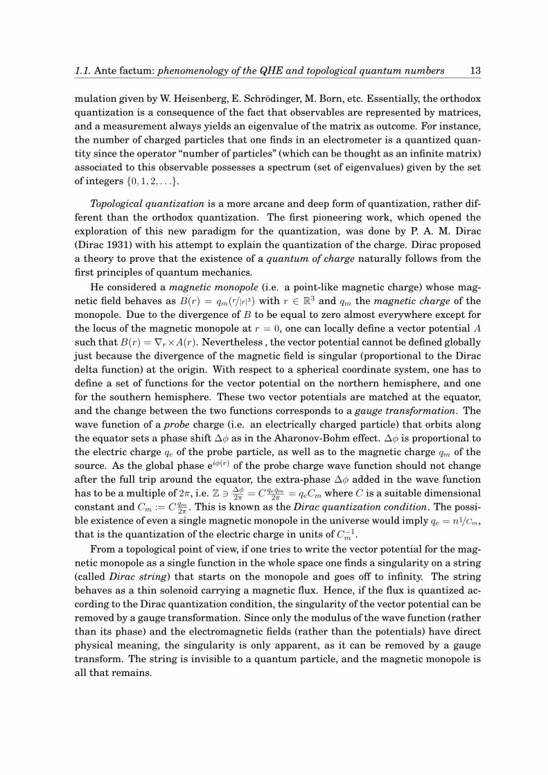
Topological quantization is a more arcane and deep form of quantization, rather dif-ferent than the orthodox quantization. The first pioneering work, which opened theexploration of this new paradigm for the quantization, was done by P. A. M. Dirac(Dirac 1931) with his attempt to explain the quantization of the charge. Dirac proposeda theory to prove that the existence of a quantum of charge naturally follows from thefirst principles of quantum mechanics.
He considered a magnetic monopole (i.e. a point-like magnetic charge) whose mag-netic field behaves as B(r) = qm(r/|r|3) with r ∈ R3 and qm the magnetic charge of themonopole. Due to the divergence of B to be equal to zero almost everywhere except forthe locus of the magnetic monopole at r = 0, one can locally define a vector potential Asuch thatB(r) = ∇r×A(r). Nevertheless , the vector potential cannot be defined globallyjust because the divergence of the magnetic field is singular (proportional to the Diracdelta function) at the origin. With respect to a spherical coordinate system, one has todefine a set of functions for the vector potential on the northern hemisphere, and onefor the southern hemisphere. These two vector potentials are matched at the equator,and the change between the two functions corresponds to a gauge transformation. Thewave function of a probe charge (i.e. an electrically charged particle) that orbits alongthe equator sets a phase shift ∆φ as in the Aharonov-Bohm effect. ∆φ is proportional tothe electric charge qe of the probe particle, as well as to the magnetic charge qm of thesource. As the global phase eiφ(r) of the probe charge wave function should not changeafter the full trip around the equator, the extra-phase ∆φ added in the wave functionhas to be a multiple of 2π, i.e. Z ∋ ∆φ
2π = C qeqm2π = qeCm where C is a suitable dimensional
constant and Cm := C qm2π . This is known as the Dirac quantization condition. The possi-
ble existence of even a single magnetic monopole in the universe would imply qe = n1/Cm,that is the quantization of the electric charge in units of C−1
m .
From a topological point of view, if one tries to write the vector potential for the mag-netic monopole as a single function in the whole space one finds a singularity on a string(called Dirac string) that starts on the monopole and goes off to infinity. The stringbehaves as a thin solenoid carrying a magnetic flux. Hence, if the flux is quantized ac-cording to the Dirac quantization condition, the singularity of the vector potential can beremoved by a gauge transformation. Since only the modulus of the wave function (ratherthan its phase) and the electromagnetic fields (rather than the potentials) have directphysical meaning, the singularity is only apparent, as it can be removed by a gaugetransform. The string is invisible to a quantum particle, and the magnetic monopole isall that remains.
14 1. Introduction
For various theoretical and experimental reasons, Dirac’s theory is not a completelysatisfactory solution of the charge quantization problem. However, it is a paradigm of aninteresting mechanism of quantization that has a topological origin. In Dirac’s scenariothe quantization of the charge qm is not a consequence of the fact that the extra-phase∆φ is associated to an operator with a discrete set of eigenvalues. In fact, qe and qm playthe rôle of ordinary numerical parameters in the theory. Since the quantization of qmhas a topological origin, one refers to it as a topological quantum number (TQN).
A consequence of the Dirac’s theory is that every measurement of the charge qe yieldsthe same value n (in units of C−1
m ), and not different multiples of a basic unit. Thus, boththe single measurement and the average are quantized with same value n. This is whytopological quantum numbers are responsible for the quantization of expectation values.
The arcane has been revealed ... and now we know the way to go beyond.
1.2 Factum: topological interpretation of the QHE by Thou-
less et al.
Nowadays, topological quantum numbers play a prominent rôle in many problemsarising in solid-state physics (Thouless 1998). Just to mention few examples, they
appear in the contexts of adiabatic evolutions (Berry 1984, Simon 1983), macroscopicpolarization (Thouless 1983, King-Smith and Vanderbilt 1993, Resta 1992, Panati et al.2009) and quantum pumps (Avron et al. 2004, Graf and Ortelli 2008). However, for thepurposes of this thesis we are mainly interested in the application of the topologicalquantization in the context of QHE (cf. (Graf 2007) for a recent review).
B. A. Dubrovin and S. P. Novikov discovered that a two dimensional system of non-interacting electrons in a periodic potential exhibits an interesting topology (Dubrovinand Novikov 1980). Novikov refers he queried his colleagues at the Landau Instituteabout the physical interpretation of the topological invariants he discovered, but nobodyprovided him with a useful insight6.
Only later in 1982 D. J. Thouless, M. Kohmoto, M. P. Nightingale and M. den Nijs(TKNN), studying independently the same model considered by Dubrovin and Novikov,realized that the emerging topological quantum numbers are related with the Hall con-ductance (Thouless et al. 1982).
As the work of Thouless et al. is the “starting point” for this thesis, it is worth togo through the major ideas contained in the “TKNN-paper” (Thouless et al. 1982). Thestrategy of their proof can be divided into four fundamental steps.
6The reader has to note that the paper of Dubrovin and Novikov was submitted on February 1980, twomonths before the submission of the seminal paper of von Klitzing et al. (May 1980). It is not surprisingthat nobody in Landau Institute was able, at that time, to recognize the link between the Novikov’s workand the QHE.
1.2. Factum: topological interpretation of the QHE by Thouless et al. 15
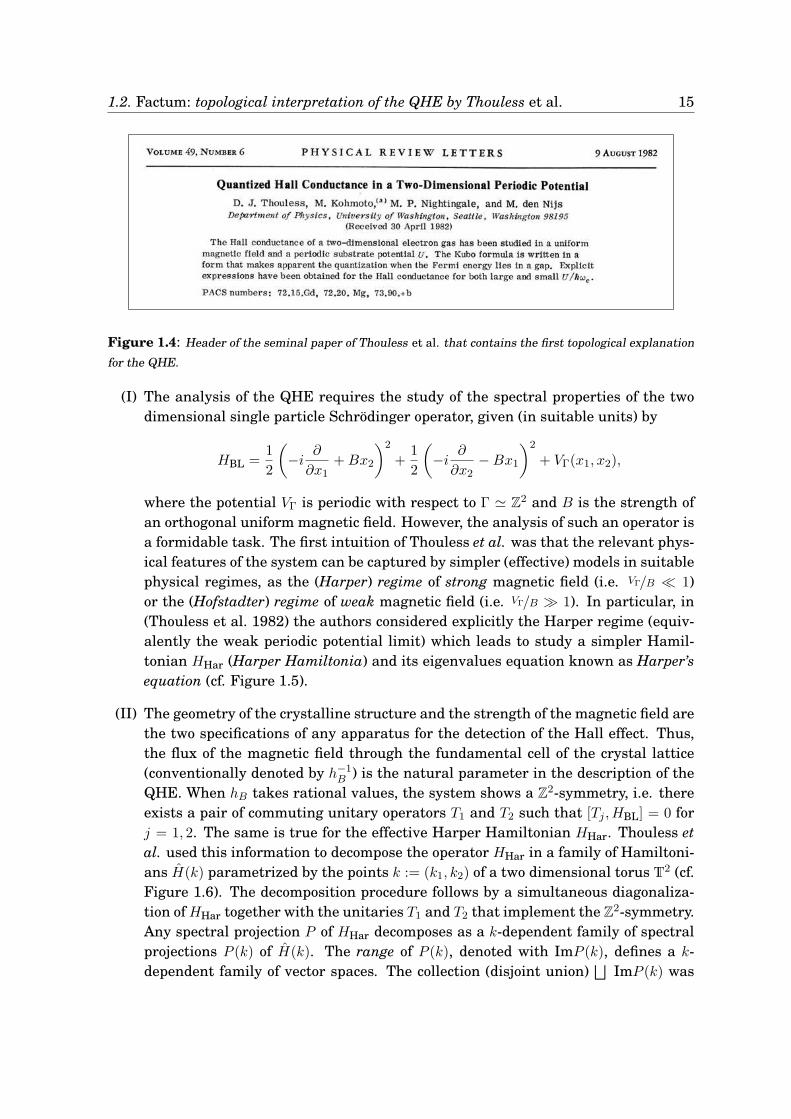
Figure 1.4: Header of the seminal paper of Thouless et al. that contains the first topological explanation
for the QHE.
(I) The analysis of the QHE requires the study of the spectral properties of the twodimensional single particle Schrödinger operator, given (in suitable units) by
HBL =1
2
(−i ∂∂x1
+Bx2
)2
+1
2
(−i ∂∂x2
−Bx1
)2
+ VΓ(x1, x2),
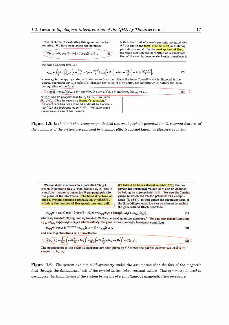
where the potential VΓ is periodic with respect to Γ ≃ Z2 and B is the strength ofan orthogonal uniform magnetic field. However, the analysis of such an operator isa formidable task. The first intuition of Thouless et al. was that the relevant phys-ical features of the system can be captured by simpler (effective) models in suitablephysical regimes, as the (Harper) regime of strong magnetic field (i.e. VΓ/B ≪ 1)or the (Hofstadter) regime of weak magnetic field (i.e. VΓ/B ≫ 1). In particular, in(Thouless et al. 1982) the authors considered explicitly the Harper regime (equiv-alently the weak periodic potential limit) which leads to study a simpler Hamil-tonian HHar (Harper Hamiltonia) and its eigenvalues equation known as Harper’sequation (cf. Figure 1.5).
(II) The geometry of the crystalline structure and the strength of the magnetic field arethe two specifications of any apparatus for the detection of the Hall effect. Thus,the flux of the magnetic field through the fundamental cell of the crystal lattice(conventionally denoted by h−1
B ) is the natural parameter in the description of theQHE. When hB takes rational values, the system shows a Z2-symmetry, i.e. thereexists a pair of commuting unitary operators T1 and T2 such that [Tj ,HBL] = 0 forj = 1, 2. The same is true for the effective Harper Hamiltonian HHar. Thouless etal. used this information to decompose the operator HHar in a family of Hamiltoni-ans H(k) parametrized by the points k := (k1, k2) of a two dimensional torus T2 (cf.Figure 1.6). The decomposition procedure follows by a simultaneous diagonaliza-tion ofHHar together with the unitaries T1 and T2 that implement the Z2-symmetry.Any spectral projection P of HHar decomposes as a k-dependent family of spectralprojections P (k) of H(k). The range of P (k), denoted with ImP (k), defines a k-dependent family of vector spaces. The collection (disjoint union)
⊔ImP (k) was
16 1. Introduction
interpreted by Thouless et al. as the total space of an “emerging” vector bundleover the base space T2.
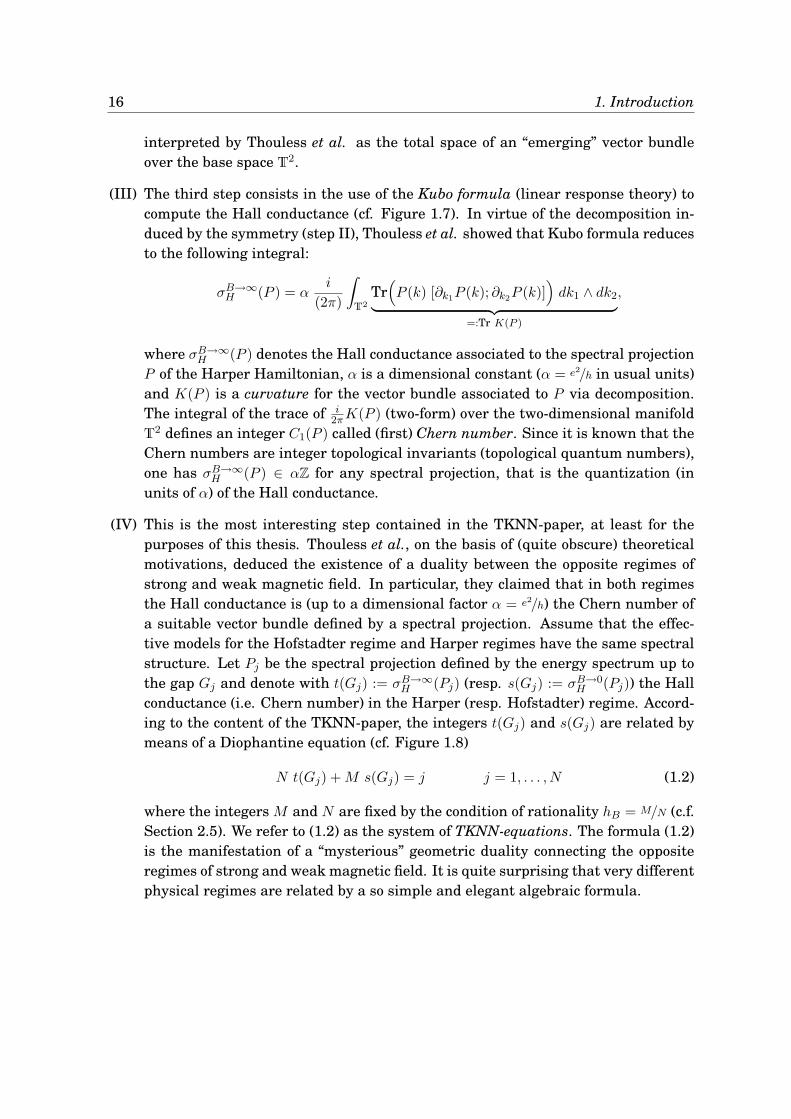
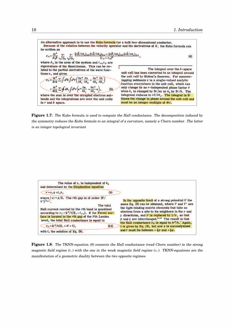
(III) The third step consists in the use of the Kubo formula (linear response theory) tocompute the Hall conductance (cf. Figure 1.7). In virtue of the decomposition in-duced by the symmetry (step II), Thouless et al. showed that Kubo formula reducesto the following integral:
σB→∞H (P ) = α
i
(2π)
∫
T2
Tr(P (k) [∂k1P (k); ∂k2P (k)]
)dk1 ∧ dk2
︸ ︷︷ ︸=:Tr K(P )
,
where σB→∞H (P ) denotes the Hall conductance associated to the spectral projection
P of the Harper Hamiltonian, α is a dimensional constant (α = e2/h in usual units)and K(P ) is a curvature for the vector bundle associated to P via decomposition.The integral of the trace of i
2πK(P ) (two-form) over the two-dimensional manifoldT2 defines an integer C1(P ) called (first) Chern number. Since it is known that theChern numbers are integer topological invariants (topological quantum numbers),one has σB→∞
H (P ) ∈ αZ for any spectral projection, that is the quantization (inunits of α) of the Hall conductance.
(IV) This is the most interesting step contained in the TKNN-paper, at least for thepurposes of this thesis. Thouless et al., on the basis of (quite obscure) theoreticalmotivations, deduced the existence of a duality between the opposite regimes ofstrong and weak magnetic field. In particular, they claimed that in both regimesthe Hall conductance is (up to a dimensional factor α = e2/h) the Chern number ofa suitable vector bundle defined by a spectral projection. Assume that the effec-tive models for the Hofstadter regime and Harper regimes have the same spectralstructure. Let Pj be the spectral projection defined by the energy spectrum up tothe gap Gj and denote with t(Gj) := σB→∞
H (Pj) (resp. s(Gj) := σB→0H (Pj)) the Hall
conductance (i.e. Chern number) in the Harper (resp. Hofstadter) regime. Accord-ing to the content of the TKNN-paper, the integers t(Gj) and s(Gj) are related bymeans of a Diophantine equation (cf. Figure 1.8)
N t(Gj) +M s(Gj) = j j = 1, . . . , N (1.2)
where the integers M and N are fixed by the condition of rationality hB = M/N (c.f.Section 2.5). We refer to (1.2) as the system of TKNN-equations. The formula (1.2)is the manifestation of a “mysterious” geometric duality connecting the oppositeregimes of strong and weak magnetic field. It is quite surprising that very differentphysical regimes are related by a so simple and elegant algebraic formula.
1.2. Factum: topological interpretation of the QHE by Thouless et al. 17
Figure 1.5: In the limit of a strong magnetic field (i.e. weak periodic potential limit), relevant features of
the dynamics of the system are captured by a simple effective model known as Harper’s equation.
Figure 1.6: The system exhibits a Z2-symmetry under the assumption that the flux of the magnetic
field through the fundamental cell of the crystal lattice takes rational values. This symmetry is used to
decompose the Hamiltonian of the system by means of a simultaneous diagonalization procedure.
18 1. Introduction
Figure 1.7: The Kubo formula is used to compute the Hall conductance. The decomposition induced by
the symmetry reduces the Kubo formula to an integral of a curvature, namely a Chern number. The latter
is an integer topological invariant
Figure 1.8: The TKNN-equation (9) connects the Hall conductance (read Chern number) in the strong
magnetic field regime (tr) with the one in the weak magnetic field regime (sr). TKNN-equations are the
manifestation of a geometric duality between the two opposite regimes.
1.3. Overview of the results 19
The strategy used in (Thouless et al. 1982) can be followed for a wide class of pe-riodic potentials. This explains why the QHE is insensitive to the fine details of themicroscopic structure of the sample used in the experiment. However, the theory ofThouless et al. does not explain the quantization of the Hall conductance either in thecase electron-electron interaction is taken into account, or in the case of presence of dis-order. Both factors play a rôle in the real Hall effect. Much progresses have been madein understanding this issue, (Laughlin 1983, Kunz 1987, Bellissard 1988b, Bellissardet al. 1994, Kellendonk and Schulz-Baldes 2004, Combes et al. 2006) but this is out fromthe scope of this thesis.
Finally, it is interesting to see how the theory of Thouless et al. has been experimen-tally verified (Albrecht et al. 2001). The experimental confirmation testifies once againthe relevance of the TKNN-paper.
1.3 Overview of the results
Although the TKNN-paper is a milestone in the way towards a theoretical explana-tion of the QHE, the structure of the proof contains many mathematical “gaps”. In
order to make the theory of Thouless et al. rigorous, one needs to complete some missing“mid-steps” between each of the four steps described in Section 1.2.
In this thesis we propose a rigorous “reinterpretation” of the work of Thouless et al.Using various mathematical tools (adiabatic theory, differential geometry, non-commuta-tive geometry, etc.), we derive a series of new and rigorous results which improve andgeneralize the theory sketched in (Thouless et al. 1982). For convenience we follow theabove steps subdivision to list the main results of this thesis.
(I) SAPT-type and algebraic-type results
During the last decades, there were many works aiming to a rigorous derivation of theeffective models for the Hamiltonian HBL in the limits of strong and weak magneticfields (Bellissard 1988a, Helffer and Sjöstrand 1989b). However, all the previous deriva-tions are based on a notion of “approximate model” which turns out to be too weak forour purpose. As discussed in Section 2.2, a rigorous procedure is needed to obtain effec-tive models that are unitarily equivalent (in a suitable asymptotic sense) to the originalmodel. This is a relevant property which assures that the content of physical informationof the original Hamiltonian HBL is fully preserved by the effective Hamiltonians. Space-adiabatic perturbation theory (SAPT) provides the appropriate mathematical machineryfor a unitarily equivalent derivation of the effective models.
A self-consistent presentation of the results concerning the adiabatic derivation ofthe effective Hamiltonians (“SAPT-type” results) is postponed to Section 2.1. Chapter 3contains the technicality concerning the derivation of the effective models by means ofthe mathematical apparatus of SAPT. In particular Theorem 3.3.14 concerns the rig-orous derivation of the Hofstadter Hamiltonian (effective model for the weak magnetic
20 1. Introduction
field limit), while the Harper Hamiltonian (effective model for the strong magnetic fieldlimit) is derived in Theorem 3.4.8. The content of our SAPT-type results is summarizedin the following diagram
HHof := ℘(U0,V0)OO
isospectrality
L2(T2) =: H0
Hphy := L2(R2) HBL
B→∞ ''PPPPPPPPPPPPP
B→077nnnnnnnnnnnnn
HHar := ℘(U∞,V∞) L2(R) =: H∞.
In Hofstadter regime (B → 0), the original Hamiltonian HBL, defined on the physicalHilbert space Hphy := L2(R2), is asymptotically unitarily equivalent to an effective op-erator HHof := ℘(U0,U0) (Hofstadter-like Hamiltonian) defined on the reference Hilbertspace H0 := L2(T2). The unitary operators U0 and V0 act on H0 according to equation(2.7), while ℘ denotes a formal polynomial in two variables containing also negativepowers; for instance ℘(x, y) = x + x−1 + y + y−1. Similarly, the asymptotically unitarilyequivalent effective model HHar := ℘(U∞,V∞) (Harper-like Hamiltonian) for the Harperregime (B → ∞), acts on the reference Hilbert space H∞ := L2(R) and it is given in termsof a polynomial combination of the unitaries U∞ and V∞ defined by equation (2.15).
From the above diagram some relevant consequences emerge (“algebraic-type” re-sults). Up to a special condition on the values of the magnetic fields in the strongand weak regimes (Assumption 2.3.6), Hofstadter-like Hamiltonians and Harper-likeHamiltonians share the same algebraic structure, which is the structure of the Non-Commutative Torus (NCT). This algebraic duality is analyzed in Section 2.3 (Theo-
rem 2.3.7) and its main consequence is the isospectrality between HHof and HHar (arrowoo //___ in the diagram).
(II) Spectral decomposition and emerging geometry
It is well known that, if a Hamiltonian operator commutes with a family of operators(symmetries) then their simultaneous diagonalization leads to a decomposition of theoriginal Hamiltonian into a family of (generally simpler) operators parametrized by aspectral parameter (e.g. the eigenvalues of the operators that implement the symme-tries). From a mathematical point of view, this is a sophisticated version of the spec-tral decomposition theory by von Neumann (Maurin 1968, Dixmier 1981). The so-calledBloch-Floquet theory (Wilcox 1978, Kuchment 1993) is one of the more fruitful applica-tion of the above idea. In the TKNN-paper the authors used a similar “decompositionstrategy”, provided that the magnetic flux per unit cell of the lattice takes a rationalvalue. However, the subtle point which needs more care is the association of the spectral-type decomposition coming from the von Neumann theory with a vector bundle structure.Indeed, it is no obvious that a spectral-type decomposition which is based on a measure-theoretic structure, can be related in a natural and unique way with a topological object
1.3. Overview of the results 21
like a vector bundle. Thus, the following questions arise: how does the topology (and thegeometry) of the decomposition emerge? To which extent is this topological informationindependent by the specific decomposition procedure?
In Chapter 4 we provide a complete answer to these questions in a quite generalframework. We introduce the notion of physical frame (Definition 4.1.2), i.e. a tripleH,A,S with H a separable Hilbert space which corresponds to the set of physicalstates, A ⊂ B(H) a C∗-algebra of bounded operators on H which contains the relevantphysical models, ; S ⊂ A′ (A′ is the commutant A) a commutative unital C∗-algebrawhich describes a set of simultaneously implementable physical symmetries. Assumingthat S is a Zd-algebra (i.e. it is generated by d unitaries U1, . . . , Ud according to Definition4.1.3) with the wandering property (Definition 4.5.1), we provide a “recipe” (generalizedBloch-Floquet transform) to realize “by hand” the von Neumann spectral decomposition(Theorem 4.6.4). The underlying vector bundle structure is recovered at an algebraiclevel and it is uniquely specified by the triple H,A,S (Theorem 4.7.9). The elementof the C∗-algebra A (up to some extra conditions) are mapped in continuous sectionsof the endomorphism bundle (Theorem 4.7.15) providing a unitarily equivalent bun-dle representation for A (Definition 2.7.2). In Sections 5.2 we apply the general theoryof Chapter 4 to Hofstadter-like and Harper-like models. The bundle decomposition ofthe Hofstadter-like Hamiltonians, as well as that of the Harper-like Hamiltonians, isestablished in Theorem 2.7.4.
(III) Kubo-Chern equivalence
The rigorous justification of the Kubo formula is generally a hard problem. Some rigor-ous results have been obtained in the context of QHE models (Bellissard et al. 1994, El-gart and Schlein 2004, Bouclet et al. 2005). However, for a rigorous justification of re-sults in the TKNN-paper, one has to derive the Kubo formula and prove the equivalencebetween transverse conductance and Chern numbers in the Hofstadter regime, as wellas in the Harper regime. This is still an open problem, out of the scope of this thesis. Inthe following part of this thesis we assume the pragmatic position that: Chern numbersassociated to spectral projections of a Hamiltonian are, by definition, the values of thetransverse conductance (Kubo-Chern equivalence).
(IV) Geometric duality and generalized TKNN-equations
The TKNN-paper contains no prove of the remarkable TKNN-equations. Nevertheless,according to the interpretation of the authors, the TKNN-equations establish a (alge-braic) duality between Chern numbers of different vector bundles. Although in thelast decades many works have been aimed to a rigorous derivation of TKNN-equations(Streda 1982, MacDonald 1984, Dana et al. 1985, Avron and Yaffe 1986), none of theseresults consider to look at the integers sr and tr (cf. Figure 1.8) as Chern numbers ofsuitable vector bundles. One of the main result of this thesis is the realization of apurely geometric proof of the TKNN-equations.
22 1. Introduction
If a Hamiltonians admits a bundle decomposition, then its spectral projections (intothe gaps) define vector subbundles (Lemma 2.7.3). The isospectrality between Hofstadter-like and Harper-like Hamiltonians implies a one-to-one correspondence between thespectral projections of HHof and HHar. Let L0(P ) (resp. L∞(P )) be the vector bundleassociated with the spectral (gap) projection P of the Hofstadter-like (resp. Harper-like)Hamiltonian HHof (resp. HHof). We prove (Theorem 2.8.1) that there exists an isomor-phism of vector bundles between L0(P ) and L∞(P ) established by the formula
f∗1 L∞(P ) ≃ f∗2 L0(P ) ⊗ I
where fj : T2 → T2, j = 1, 2, are suitable continuous maps, f∗j L♯(P ) denotes the pull-back vector bundle of L♯(P ) (♯ = 0,∞) via fj and I is a suitable line bundle whichintroduces an extra-twist. The above formula is a manifestation of a deep geometric du-ality which relates the opposite regimes of strong and weak magnetic field. The TKNN-equations are a straightforward consequence of such a geometric duality (Corollary
2.8.2). Non-ommutative geometry provide the appropriate “language” to explain the ge-ometric meaning of TKNN-equations and to generalize them to the case of an irrationalmagnetic flux (Section 2.9).
In particular, the set of results presented above fills the mathematical gaps containedin TKNN-paper. From this point of view, one of the merits of this thesis is that it endowsthe powerful theory of Thouless et al. with the mathematical exactness it deserves.
1.4 Why quantum butterflies?
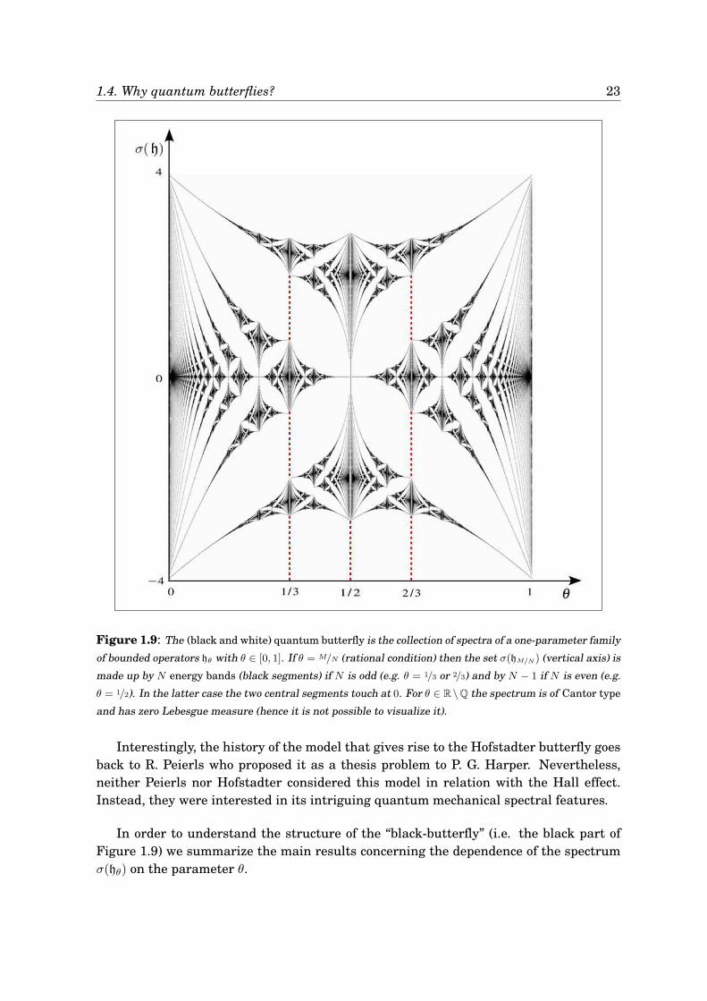
The Hofstadter butterfly or (black and white) quantum butterfly (Figure 1.9) is afractal-type diagram showing the collection of the energy spectra of a family of
bounded operators hθ, parametrized by θ ∈ R (universal Hofstadter operators, equation(2.29)).
Figure 1.9 was firstly described by D. Hofstadter in 1976, in his Ph.D. thesis underthe supervision of G. Wannier (Hofstadter 1976). Hofstadter was fascinated by M. Az-bel’s suggestion that under certain circumstances the energy spectrum of such quantumsystems can be a fractal set. Indeed, the self-similar character of the Hofstadter butter-fly turned out to be closely related to the fractal nature of its spectrum (for irrationalvalues of the parameter θ).
The importance of the Figure 1.9 for this thesis is due to the fact that the spectrumof hθ describes the spectrum of both the Hofstadter Hamiltonian and the Harper Hamil-tonian. In the first case the parameter θ is proportional to B, while in the latter to 1/B.Therefore in both limits θ plays the rôle of a small (adiabatic) parameter. The exactrelation between hθ, the Hofstadter Hamiltonian and the Harper Hamiltonian, as wellthe the meaning of θ, are clarified in Chapter 2 (in particular in Sections 2.1 and 2.3).
1.4. Why quantum butterflies? 23
Figure 1.9: The (black and white) quantum butterfly is the collection of spectra of a one-parameter family
of bounded operators hθ with θ ∈ [0, 1]. If θ = M/N (rational condition) then the set σ(hM/N) (vertical axis) is
made up by N energy bands (black segments) if N is odd (e.g. θ = 1/3 or 2/3) and by N − 1 if N is even (e.g.
θ = 1/2). In the latter case the two central segments touch at 0. For θ ∈ R\Q the spectrum is of Cantor type
and has zero Lebesgue measure (hence it is not possible to visualize it).
Interestingly, the history of the model that gives rise to the Hofstadter butterfly goesback to R. Peierls who proposed it as a thesis problem to P. G. Harper. Nevertheless,neither Peierls nor Hofstadter considered this model in relation with the Hall effect.Instead, they were interested in its intriguing quantum mechanical spectral features.
In order to understand the structure of the “black-butterfly” (i.e. the black part ofFigure 1.9) we summarize the main results concerning the dependence of the spectrumσ(hθ) on the parameter θ.
24 1. Introduction
(BH-1) For any θ ∈ R, ‖hθ‖ 6 4 which implies σ(hθ) ⊆ [−4, 4].
(BH-2) For any θ ∈ R the spectrum is symmetric with respect to the zero energy, i.e.σ(hθ) = σ(−hθ).
(BH-3) Since σ(hθ+n) = σ(hθ) for any integer n ∈ Z, one has that it is sufficient to studythe spectrum for θ ∈ [0, 1]. Furthermore, the equality σ(h−θ) = σ(hθ) also impliesisospectrality between hθ and h1−θ and then the symmetry of Figure 1.9 with re-spect to θ = 1/2.
(BH-4) Assume θ ∈ Q with θ = M/N, M ∈ Z, N ∈ N \ 0 and M and N coprime. Thespectrum σ(hM/N) is made up by N (resp. N − 1) energy bands if N is odd (resp.even). Note that in the case of a even N the central gap is “closed” (that is empty).The “open” (that is non-empty) gaps between two consecutive energy bands havewidth larger than 8−N (von Mouche 1989, Choi et al. 1990).
(BH-5) If θ ∈ R\Q then σ(hθ) is of Cantor-type (c.f. Definition 2.4.1) and has zero Lebesguemeasure.
(BH-6) Let θ and θ′ be such that |θ − θ′| < C. For any ǫ ∈ σ(hθ) there exists a ǫ′ ∈ σ(hθ′)
such that |ǫ− ǫ′| < 6√
2|θ − θ′| (Avron et al. 1990).
We provide a justification of (BH-1), (BH-2) and (BH-3) at the end of Section 2.3.Property (BH-5) has been, for a long time, a conjecture known as Ten Martini Prob-
lem7 (TMP). The proof was established only recently by A. Avila and S. Jitomirskaya(Avila and Jitomirskaya 2009). For a review on the history of the “long way” to thesolution of TMP we refer to (Last 2005, Section 3).
From (BH-4) and (BH-5), it follows that the butterfly (i.e. the black part) in Figure1.9 has zero Lebesgue measure as subset of the rectangle [0, 1] × [−4, 4]. This suggeststhat all the information is encoded in the gap structure (i.e. the white part).
Point (BH-6) states that the spectrum has a Hölder continuous dependence of order1/2 on the parameter θ. In particular, this implies that for every gap in the spectrumof hθ of length ℓ and for any θ′ such that 12
√2|θ − θ′| < ℓ, there is a corresponding gap
in the spectrum of hθ′ of length bigger than ℓ − 12√
2|θ − θ′|. In other words, the gapstructure of the Hofstadter’s butterfly is locally continuous, i.e. any point in the plane(θ, σ) of Figure 1.9 which is in a gap has an open neighborhood entirely contained in agap zone. This means that the gap structure of Figure 1.9 is made up by “open islands”containing no spectral points.
7 The proof of the Ten Martini Problem (TMP) establishes the topological structure of the spectrum of hθ
when θ ∈ R \ Q. However, a stronger version of this conjecture, the Strong Ten Martini Problem (STMP),is still open. The question is to prove that all the gaps prescribed by the Gap Labelling Theory (GLT) are“open” (i.e. non-empty). The interested reader can find in (Shubin 1994, Section 5) a complete explanationof the relations between GLT, TMP and STMP (and also Super-Strong Ten Martini Problem (SSTMP), avery strong version of the problem still unsolved). For GLT the reader can refer to the review (Simon 1982,and references therein).
1.4. Why quantum butterflies? 25
Finally, when hθ is rational, it follows from the theory of periodic Schrödinger op-erators that σ(hθ) is purely absolutely-continuous. Otherwise, when θ ∈ R \ Q, σ(hθ) issupported on an uncountable set of zero Lebesgue measure, i.e. it is singular-continuous.
Figure 1.9 gives a complete description of the structure of the energy spectrum of hθ
but it does not provide more detailed spectral information such as the degree of degen-eracy of the eigenspaces (i.e. the density of the states). Such information turns out to benecessary in the analysis of the QHE.
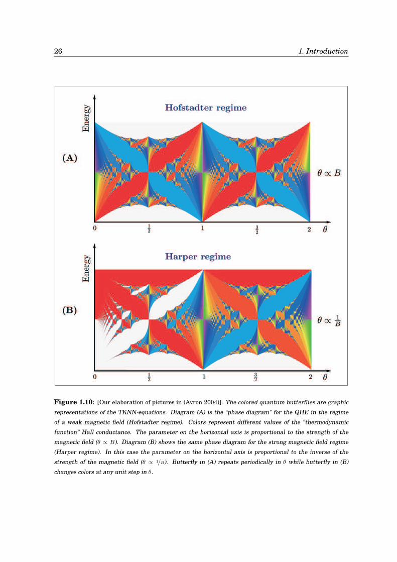
The colored quantum butterflies (Figure 1.10), are due to J. E. Avron and D. Osadchy(Avron 2004, Osadchy and Avron 2001) and interpreted by the authors as “thermody-namic” phase diagram for the Hall conductance (c.f. Section 2.5). Colors represent thequantized values of the Hall conductance. Warm colors (like red) correspond to posi-tive values for the Hall conductance, while cold colors (like blue) correspond to negativevalues. White means zero Hall conductance.
Diagram (A) in Figure 1.10 describes the situation in the regime of weak magneticfield (Hofstadter regime). In this case, the external magnetic field acts as a perturbationof the band spectrum structure of the periodic Bloch Hamiltonian which describes theinteraction with the crystal. The effect of this perturbation is the creation of new gaps.When the Fermi energy is placed in one of these gaps the Hall conductance is an integerwhich can be coded by a color. In this way any gap is associated to a color as showedin diagram (A). In this regime the colored butterfly repeats periodically on the θ-axis,with unit period. The white horizontal margins which flank the colored butterflies in (A)mean that the Hall conductance vanishes if the energy band associated to the crystallinestructure is either empty or completely full. This is what Peierls expected, that is -insulators should have vanishing Hall conductance! -
Diagram (B) in Figure 1.10 describes the situation in the regime of strong magneticfield (Harper regime). In this case, the periodic potential due to the crystalline structureacts as a perturbation of the Landau Hamiltonian. It is well known that the spectrumof the Landau Hamiltonian is a collection of equally spaced infinitely degenerate points,known as Landau levels. The weak periodic potential splits each of the Landau levelscreating new gaps. Diagram (B) describes the Hall conductance when the Fermi energysits within the gaps. Note that, contrary to the weak field regime, the color coding ofdiagram (B) is not periodic with respect to θ. Moreover each butterfly in (A) exhibitsinversion symmetry, while butterflies in (B) do not have such a symmetry.
Apparent differences between diagrams (A) and (B) in Figure 1.10 suggest that theregimes of weak and strong magnetic field give rise to very different physical scenarios.
Colored quantum butterflies play a relevant rôle for this thesis. The reason is thatthe color-coding of the butterflies has been computed by Avron using the DiophantineTKNN-equations. In other words Figure 1.10 is simply a graphic representation of theduality which relates the opposite regimes of weak and strong magnetic field.
The TKNN-equations are the foundation of the arcane beauty of the colored quantumbutterflies. A purely geometric derivation of the TKNN-equations is needed to “capture”these “flashy exotic mathematical insects”.
26 1. Introduction
Figure 1.10: [Our elaboration of pictures in (Avron 2004)]. The colored quantum butterflies are graphic
representations of the TKNN-equations. Diagram (A) is the “phase diagram” for the QHE in the regime
of a weak magnetic field (Hofstadter regime). Colors represent different values of the “thermodynamic
function” Hall conductance. The parameter on the horizontal axis is proportional to the strength of the
magnetic field (θ ∝ B). Diagram (B) shows the same phase diagram for the strong magnetic field regime
(Harper regime). In this case the parameter on the horizontal axis is proportional to the inverse of the
strength of the magnetic field (θ ∝ 1/B). Butterfly in (A) repeats periodically in θ while butterfly in (B)
changes colors at any unit step in θ.
Chapter 2
Results and techniques
Pour connaître la rose, quelqu’un emploie la géométrie etun autre emploie le papillon.
(To know the rose, someone uses the geometry and anotheruses the butterfly.)
Paul ClaudelL’Oiseau noir dans le soleil levant, 1927
Abstract
The present chapter aims to expose the main results of this thesis in a rigorous way.We introduce the principal notions and techniques which are indispensable for a self-consistent technical presentation of the arguments developed in this work. The firstpart of this thesis (adiabatic-part) concerns a series of results coming from the ap-plication of the space-adiabatic perturbation theory (SAPT) (c.f. Chapter 3). Theseresults are presented in the first two sections of this chapter. Section 2.1 is devotedto introduce the Hofstadter-like and Harper-like Hamiltonians which are the effectivemodels for the QHE in the limit of weak magnetic field (Hofstadter regime) or strongmagnetic field (Harper regime), respectively. Section 2.2 aims to explain the relevanceof SAPT for the purposes of this work. In Sections 2.3 and 2.4 we present the algebraicresults of this thesis (algebraic-part). The notion of Non-Commutative Torus (NCT)is used to prove the isospectrality between Hofstadter-like and Harper-like Hamiltoni-ans (algebraic duality), as well as to provide a description of the structure of the spec-trum of such models in terms of “abstract” spectral projections. Section 2.5 containsa description of the relation between the TKNN-equations and the colored quantumbutterflies. In Section 2.6 we justify the difference in the coloring of the two butter-flies as a consequence of the absence of a unitary equivalence between Hofstadter andHarper Hamiltonians. The last three sections of this chapter aim to describe the ge-ometric results of this thesis (geometric-part). In Section 2.7 we discuss the relationbetween “abstract” spectral projections and vector bundles. Section 2.8 is devoted toderive TKNN-equations from a geometric duality between the vector bundles associ-ated to spectral projections of the Hofstadter and Harper Hamiltonians. In Section2.9 we present a “non-commutative” generalized version of the TKNN-equations. Openproblems and possible generalizations are listed in Section 2.10.
2.1 Physical background and relevant regimes for the QHE
Schrödinger operators with periodic potential and magnetic field have been fascinatingphysicists and mathematicians for the last decades. Due to the competition between

28 2. Results and techniques
the crystal length scale and the magnetic length scale, these operators reveal strikingfeatures as fractal spectra (Geyler et al. 2000) or quantization of the Hall conductance(Thouless et al. 1982, Avron et al. 1983, Bellissard et al. 1994, Kellendonk et al. 2002).The colored quantum butterflies (c.f. Figure 1.10) summarize these features in pictorialdiagrams.
The mathematical model commonly used for the quantum Hall effect (QHE) (Morandi1988, Graf 2007) is the two-dimensional Bloch-Landau Hamiltonian
HBL :=1
2m
(−iℏ∇r − ιq
|q|B2c
e⊥ ∧ r)2
+ VΓ (r) , (2.1)
acting in the Hilbert space Hphy = L2(R2, d2r), r = (r1, r2) ∈ R2. Here c is the speed oflight, h := 2πℏ is the Planck constant, m is the mass and q the charge (positive if ιq = 1
or negative if ιq = −1) of the charge carrier, B is the strength of the external uniformtime-independent magnetic field, e⊥ = (0, 0, 1) is a unit vector orthogonal to the sample,and VΓ is a periodic potential which describes the interaction of the carrier with the ioniccores of the crystal. For the sake of a simpler notation, in this introduction we assumethat the periodicity lattice Γ is simply Z2.
While extremely interesting, a direct analysis of the fine properties of the operatorHBL is a formidable task. Thus the need to study simpler effective models which capturethe main features of (2.1) in suitable physical regimes, as for example in the limit of weak(resp. strong) magnetic field. The relevant dimensionless parameter appearing in theproblem is hB := Φ0/ZΦB ∝ 1/B, where Φ0 = hc/e is the magnetic flux quantum, ΦB = ΩΓB
is the flux of the external magnetic field through the unit cell of the periodicity lattice Γ
(whose area is ΩΓ) and Z = |q|/e is the magnitude of the charge q of the carrier in units ofe (the positron charge). It is also useful to introduce the reduced constant ℏB := hB/2π.
Hofstadter regime, Hofstadter-like Hamiltonians, Hofstadter unitaries
We refer to the limit of weak magnetic field as Hofstadter regime. In this limit, corre-sponding to ℏB → ∞, one expects that the relevant features are captured by the well-known Peierls’ substitution (Peierls 1933, Harper 1955, Hofstadter 1976), thus yieldingto consider, for each Bloch band E∗ = E∗(k1, k2) of interest, the following effective model:in the Hilbert space1 H0 := L2(T2, d2k), k being the Bloch momentum and T2 the two-dimensional torus (c.f. Convention 2.7.1), one considers the Hamiltonian operator
HB→0eff ϕ = E∗
(k −
(ιqℏB
)1
2e⊥ ∧ i∇k
)ϕ, ϕ ∈ H0. (2.2)
In physicists’ words, the above Hamiltonian corresponds to replace the variables k1 andk2 in E∗ with the symmetric operators (kinetic momenta)
K1 := k1 +i
2
(ιqℏB
)∂
∂k2, K2 := k2 −
i
2
(ιqℏB
)∂
∂k1. (2.3)
1We use the special symbol H0 to point out that this is the appropriate Hilbert space to describe thephysics of the QHE in the Hofstadter regime B → 0.
2.1. Physical background and relevant regimes for the QHE 29
Since (formally) [K1,K2] = i(ιq/ℏ) 6= 0, the latter prescription is formal and (2.2) must bedefined by an appropriate variant of the Weyl quantization.
The rigorous justification of the Peierls’ substitution and the definition and the deriva-tion of the Hamiltonian (2.2) are the content of Section 3.3.
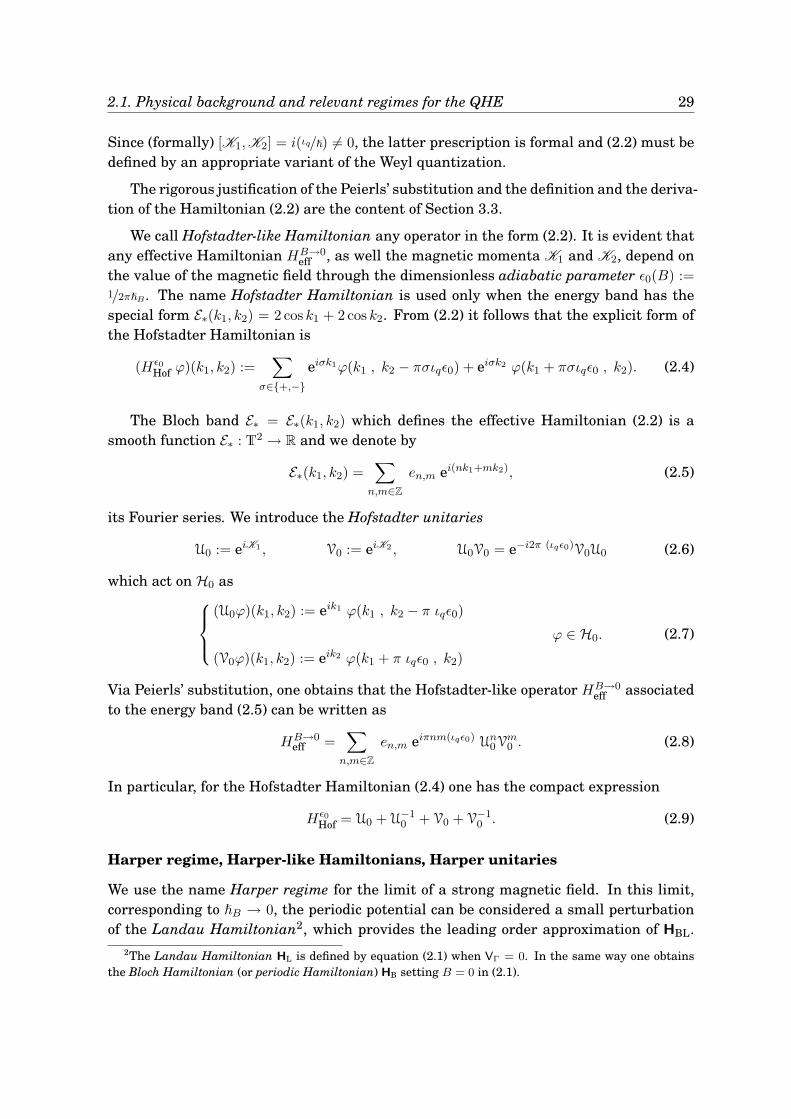
We call Hofstadter-like Hamiltonian any operator in the form (2.2). It is evident thatany effective Hamiltonian HB→0
eff , as well the magnetic momenta K1 and K2, depend onthe value of the magnetic field through the dimensionless adiabatic parameter ǫ0(B) :=1/2πℏB. The name Hofstadter Hamiltonian is used only when the energy band has thespecial form E∗(k1, k2) = 2 cos k1 + 2 cos k2. From (2.2) it follows that the explicit form ofthe Hofstadter Hamiltonian is
(Hǫ0Hof ϕ)(k1, k2) :=
∑
σ∈+,−eiσk1ϕ(k1 , k2 − πσιqǫ0) + eiσk2 ϕ(k1 + πσιqǫ0 , k2). (2.4)
The Bloch band E∗ = E∗(k1, k2) which defines the effective Hamiltonian (2.2) is asmooth function E∗ : T2 → R and we denote by
E∗(k1, k2) =∑
n,m∈Z
en,m ei(nk1+mk2), (2.5)
its Fourier series. We introduce the Hofstadter unitaries
U0 := eiK1 , V0 := eiK2 , U0V0 = e−i2π (ιqǫ0)V0U0 (2.6)
which act on H0 as
(U0ϕ)(k1, k2) := eik1 ϕ(k1 , k2 − π ιqǫ0)
ϕ ∈ H0.
(V0ϕ)(k1, k2) := eik2 ϕ(k1 + π ιqǫ0 , k2)
(2.7)
Via Peierls’ substitution, one obtains that the Hofstadter-like operator HB→0eff associated
to the energy band (2.5) can be written as
HB→0eff =
∑
n,m∈Z
en,m eiπnm(ιqǫ0) Un0Vm0 . (2.8)
In particular, for the Hofstadter Hamiltonian (2.4) one has the compact expression
Hǫ0Hof = U0 + U−1
0 + V0 + V−10 . (2.9)
Harper regime, Harper-like Hamiltonians, Harper unitaries
We use the name Harper regime for the limit of a strong magnetic field. In this limit,corresponding to ℏB → 0, the periodic potential can be considered a small perturbationof the Landau Hamiltonian2, which provides the leading order approximation of HBL.
2The Landau Hamiltonian HL is defined by equation (2.1) when VΓ = 0. In the same way one obtainsthe Bloch Hamiltonian (or periodic Hamiltonian) HB setting B = 0 in (2.1).
30 2. Results and techniques
To the next order of accuracy in ℏB, to each Landau level there corresponds an effec-tive Hamiltonian, acting on the Hilbert space3 H∞ := L2(R, dx), given (up to a suitablerescaling of the energy) by
HB→∞eff ψ = VΓ
(−i(ιqℏB)
∂
∂x, x
)ψ, ψ ∈ H∞, (2.10)
where the right-hand side refers to the ordinary (ιqℏB)-Weyl quantization of the Z2-periodic function VΓ : R2 → R. We refer to Section 3.4 for a rigorous derivation ofthe effective Hamiltonian (2.10).
Each effective HamiltonianHB→∞eff depends on the value of the magnetic field through
the dimensionless adiabatic parameter ǫ∞(B) := 2πℏB. We call Harper-like Hamiltonianany operator of the form (2.10), using the name Harper Hamiltonian for the specialcase VΓ(p, x) = 2 cos(2πp) + 2 cos(2πx). From equation (2.10), it follows that the HarperHamiltonian acts as
(Hǫ∞Har ψ)(x) := ψ(x− ǫ∞) + ψ(x+ ǫ∞) + 2 cos(2πx) ψ(x). (2.11)
The function VΓ : R2 → R which defines the effective Hamiltonian (2.10) is a smoothfunction VΓ : R2 → R which is Z2-periodic with Fourier series denoted by
VΓ(p, q) =∑
n,m∈Z
vn,m ei2π(np+mq). (2.12)
The effective Hamiltonian HB→∞eff is obtained from VΓ via the usual Weyl quantization
which agrees with the formal rule (p, q) 7→ (P,Q) where
Q := multiplication by x, P := − i
2π(ιqǫ∞)
∂
∂x, [Q;P ] =
i
2π(ιqǫ∞). (2.13)
We introduce the Harper unitaries
U∞ := ei2πQ, V∞ := ei2πP , U∞V∞ = e−i2π (ιqǫ∞)V∞U∞, (2.14)
explicitly defined by
(U∞ψ)(x) := ei2πx ψ(x)
ψ ∈ H∞.
(V∞ψ)(x) := ψ(x+ ιqǫ∞)
(2.15)
The Harper-like operator HB→∞eff associated to the periodic function (2.12) can be written
in terms of the Harper unitaries as
HB→∞eff =
∑
n,m∈Z
vn,m eiπnm(ιǫ∞) Vn∞Um∞. (2.16)
In particular, the Harper Hamiltonian (2.11) reads
Hǫ∞Har = U∞ + U−1
∞ + V∞ + V−1∞ . (2.17)
3As in Note 1, we use the special symbol H∞ to point out that this is the appropriate Hilbert space inthe Harper regime B → ∞.
2.1. Physical background and relevant regimes for the QHE 31
The choice of the nomenclature: an historical review
The use of operators of the form (2.2) as tight binding models for electrons in a crystaltraces back to the pioneering works of R. Peierls (Peierls 1933) and P. G. Harper (Harper1955). However, the study of the spectral properties of such operators began with theseminal paper (Hofstadter 1976) in which D. Hofstadter described the spectrum of theHamiltonian (2.4) producing the beautiful picture known as Hofstadter butterfly (Figure1.9). In view of that, we call Hofstadter Hamiltonian4 the operator (2.4) and, moregenerally, Hofstadter-like Hamiltonian any operator in the form (2.2). Hofstadter-likeoperators are the effective models for the regime of weak magnetic field. This justifiesthe name Hofstadter regime for the limit of zero magnetic field.
The regime of strong magnetic field was originally investigated by A. Rauh (Rauh1974, Rauh 1975). However the correct effective model, the operator (2.10), was derivedfirstly (but not rigorously) by M. Wilkinson in (Wilkinson 1987). In a remarkable seriesof papers (Helffer and Sjöstrand 1988, Helffer and Sjöstrand 1990, Helffer and Sjöstrand1989a) B. Helffer and J. Sjöstrand studied the spectrum of the operator (2.10) and itsrelation with the spectra of a one-parameter family of one-dimensional operators onℓ2(Z) defined by
(hθβu)n := un−1 + un+1 + 2 cos(2πθn+ β)un, unn ∈ ℓ2(Z), (2.18)
where θ ∈ R is a fixed number (deformation parameter) and β ∈ [0, 2π) is the param-eter of the family. In the work of the French authors, operator (2.18) is called Harperoperator (and indeed it was introduced by Harper in (Harper 1955)). However, in thelast three decades, operator (2.18) has been extensively studied by many authors (see(Last 2005, Last 1994) for an updated review) with the name of almost-Mathieu oper-ator. To avoid confusion and make the nomenclature clear, we chose to adhere to themost recent convention, using the name almost-Mathieu operator for (2.18). We thus de-cided to give credits to Harper’s work by associating his name to operators of type (2.10).Consequently we refer to the limit of strong magnetic field as Harper regime.
The first rigorous derivation of the effective models (2.2) and (2.10) was obtainedby J. Bellissard in an algebraic context in (Bellissard 1988a) and subsequently by B.Helffer and J. Sjöstrand in (Helffer and Sjöstrand 1989b), inspired by the latter paper.In particular, in (Helffer and Sjöstrand 1989b) it is proven that HB→∞
eff (resp. HB→0eff ) has,
locally on the energy axis, the same spectrum and the same density of states of HBL,in the appropriate limit. However, although relevant, this property of isospectrality isweaker than the notion of unitary equivalence.
4We insist on the fact that this nomenclature is far to be unique. For instance, the operator (2.4) (up toa Fourier transform) is called discrete magnetic Laplacian by M. A. Shubin in (Shubin 1994)
32 2. Results and techniques
2.2 Why is space-adiabatic perturbation theory required?
Beyond the spectrum and the density of states, there are other mathematical prop-erties of HBL which reveal interesting physical features, as for example the orbital
magnetization (Gat and Avron 2003, Thonhauser et al. 2005, Ceresoli et al. 2006) or theHall conductance. These properties are not invariant under a loose equivalence relationas isospectrality, then it is important to show that HB→∞
eff and HB→0eff are approximately
unitarily equivalent to HBL in the appropriate limits. This is one of the main goals ofthis thesis. The problem is not purely academic, since it is not hard to produce examplesof isospectral operators which are however not unitarily equivalent and which exhibitdifferences in the values of the physical observables. In particular, in Sections 2.3 and2.6, we show that Hǫ0
Hof and Hǫ∞Har are isospectral but not unitarily equivalent. Moreover
the TKNN-equations are a fingerprint of this lack of unitary equivalence. One concludesthat, in the study of phenomena like the conductance, it is not enough to prove that theeffective models are isospectral to the original Hamiltonians.
We thus introduce the stronger notion of unitarily effective model, referring to theconcept of almost-invariant subspace introduced by G. Nenciu (Nenciu 2002) and to therelated notion of effective Hamiltonian, which we shortly review. The common mathe-matical background for the aforementioned notions is the space-adiabatic perturbationtheory (SAPT) developed by G. Panati, H. Spohn and S. Teufel in (Panati et al. 2003b, Pa-nati et al. 2003a, Teufel 2003).
Let us focus on the regime of weak (resp. strong) magnetic field and define ε :=
2πǫ0 = 1/ℏB (resp. ǫ∞/2π = ℏB) so that ε→ 0 in the relevant limit. Let Πε be an orthogonalprojection in Hphy such that, for any N ∈ N, N ≤ N0 there exist a constant CN such that
‖[HBL; Πε]‖ ≤ CN εN (2.19)
for ε sufficiently small. Then ImΠε is called an almost-invariant subspace (Nenciu 2002,Teufel 2003) at accuracy N0, since it follows by a Duhammel’s argument that
‖(1 − Πε) e−isHBL Πε‖ ≤ CN εN |s|
for every s ∈ R, N ≤ N0. Granted the existence of such a subspace, we call (unitarily)effective Hamiltonian a self-adjoint operator Hε
eff acting on a Hilbert space Href, suchthat there exists a unitary Uε : ImΠε → Href such that for any N ∈ N, N ≤ N0, one has
‖(ΠεHBL − U−1
ε Hεeff Uε
)Πε‖ ≤ CN
′ εN . (2.20)
The estimates (2.19) and (2.20) imply that
‖(
e−isHBL − U−1ε e−isH
εeff Uε
)Πε‖ ≤ CN
′′ εN |s|. (2.21)
When the macroscopic time-scale t = εs is physically relevant, the estimate above issimply rescaled. The triple (Href, Uε,Heff) is, by definition, a unitarily effective model forHBL. To our purposes, it is important to notice that the asymptotic unitary equivalence
2.2. Why is space-adiabatic perturbation theory required? 33
in (2.20) assures that the topological quantities related with the spectral projections ofΠεH
εBL Πε (K-theory, Chern numbers, . . . ) are equal to those of Hε
eff, for ε sufficientlysmall. This claim follows by observing that the topological content of a system is pre-served by (symmetry preserving) unitary equivalences (cf. Chapter 4) and small pertur-bation (robustness of the topological invariants).
In Chapter 3 we prove that in the limit ℏB → ∞ the Hofstadter-like Hamiltonian(2.2) provides a unitarily effective model for HBL with accuracy N0 = 1, and we exhibitan iterative algorithm to construct an effective model at any order of accuracy N0 ∈ N
(Theorem 3.3.14). As for the limit ℏB → 0, up to a rescaling of the energy, the non-trivialleading order (accuracy N0 = 1) for the effective Hamiltonian is given by the Haper-likeHamiltonian (2.10). We also exhibit the effective Hamiltonian with accuracy N0 = 2,i.e. up to errors of order O(ε2) (Theorem 3.4.8). Moreover, due to the robustness of theadiabatic techniques, we can generalize the simple model described by (2.1) to includeother potentials, like a periodic vector potential AΓ, as in (3.1). This terms producesinteresting consequences especially in the Harper regime (c.f. Section 3.4.8) and it couldplay a relevant rôle in the theory of orbital magnetization. This kind of generalizationis new with respect to both (Bellissard 1988a) and (Helffer and Sjöstrand 1989b).
A numerical simulation of the spectrum of the Hofstadter operatorHǫ0Hof (resp. Harper
operator Hǫ∞Har), as a function of the adiabatic parameter ǫ0 = 1/hB (resp. ǫ∞ = hB), leads
to a fascinating Hofstadter butterfly (Figure 1.9). This claim will be clarified at the endof Section 2.3. As discussed in Section 1.4, the spectral structure of the butterfly (i.e.the black part) has zero measure as a subset of the square and so the physically rele-vant object is its complement, namely the gap structure (i.e. the white part). As pointedout by J. Avron and D. Osadchy (Avron 2004, Osadchy and Avron 2001), to each openconnected white region (island) can be associated a color which codes the value of thetransverse conductance and which can be considered as a label for a thermodynamicphase of the system. The correspondence color-gap depends on the particular regime,therefore one has a colored quantum butterfly for the Hofstadter Hamiltonian (diagram(A) of Figure 1.9) and similarly, a colored quantum butterfly for the Harper Hamiltonian(diagram (B) of Figure 1.9). With this language in mind and assuming the interpreta-tion of the colors as topological quantum numbers in the spirit of (Thouless et al. 1982),the main result of Chapter 3 can be reformulated by saying that the Hofstadter-likeand Harper-like Hamiltonians are “colour-preserving effective models” for the originalBloch-Landau Hamiltonian HBL. Thus they describe, though in a distorted and approx-imated way, some aspects of the thermodynamics of the original system. SAPT is a“colour-preserving” perturbation theory and for this reason a SAPT-type derivation ofthe effective models is need to provide a mathematical foundation for colored quantumbutterflies.
34 2. Results and techniques
2.3 Algebraic duality and isospectrality
The family of the Hofstadter-like Hamiltonians and that of the Harper-like Hamil-tonians have a common algebraic structure. To explore this algebraic analogy we
need to introduce a C∗-algebraic concept, that is the Non-Commutative Torus (NCT).
Basic notions about Non-Commutative Torus
The NCT (also called rotation C∗-algebra) was introduced by Connes in (Connes 1980)as a simple example of a non-commutative manifold and in the last decades it has beenextensively studied by many authors. We refer to the comprehensive monographes (Boca2001) and (Gracia-Bondía et al. 2001).
Due to the relevant rôle that the NCT plays in this thesis, we consider appropriate tointroduce this object rigorously. Following (Boca 2001, pp. 1-2), we define the C∗-algebraof the NCT in a formal (and universal) way starting from two “abstract” elements u andv which are unitary with respect to a formal involution ∗,
u = u∗, v = v∗, uv = ei2πθ vu, θ ∈ R. (2.22)
Last equation in (2.22) says that u and v commute up to a phase and θ is called deforma-tion parameter. The set Lθ of the finite complex linear combinations of the monomialsunvm, n,m ∈ Z, has the structure of a unital ∗-algebra with unit u0 = 1 = v0. The NCT-algebra with deformation parameter θ, denoted by Aθ, is the C∗-algebra generated bythe closure of Lθ with respect the universal norm
‖a‖ := supπ‖π(a)‖B(H) : π : Lθ → B(H) is a ∗ -representation.
When θ ∈ Q then Aθ is called rational NCT-algebra.
The NCT has a “universal behavior” as far as the representation theory is concerned.Two properties are of particular relevance for our aims (Boca 2001, Remark 1.2):
- Surjective representation property: Let U and V be two unitary operators act-ing on the Hilbert space H such that UV = ei2πθVU and denote by C∗(U,V) the C∗-algebra generated by them in B(H) (the algebra of bounded operators). The map-ping π(u) = U, π(v) = V extends algebraically to a representation (i.e. ∗-morphism)π : Aθ → C∗(U,V) ⊂ B(H) which is surjective.
- Universal property: If Bθ is a C∗-algebra generated by two unitaries u′ and v′
such that u′v′ = ei2πθv′u′, and if Bθ has the surjective representation property, thenthe mapping u 7→ u′ and v 7→ v′ extends to a ∗-isomorphism between Aθ and Bθ.
2.3. Algebraic duality and isospectrality 35
REMARK 2.3.1 (Frame and isomorphisms of NCT-algebra). Even though the definitionof the algebra Aθ is subordinate to a choice of a pair of generators (u, v), the algebraicstructure of Aθ is independent of such a choice. Let (u′, v′) be a frame, namely any pairof unitaries in Aθ such that u′v′ = ei2πθ v′u′. Each frame defines an equivalent system ofgenerators for Aθ and the universal property assures that there exists an automorphismα ∈ Aut(Aθ) such that α(u′) = u and α(v′) = v. This means that there is no canonicalchoice for the system of generators of the NCT-algebra. Having this in mind, we willrefer to the algebra Aθ assuming a “a priori” privileged choice for the generators (u, v).
Another consequence of the universal property is that the C∗-algebras Aθ and An+θ
are mutually ∗-isomorphic for any n ∈ Z. Moreover, the map c(u) = v and c(v) = u
defines a relevant ∗-ismorphism, called charge-conjugation, between Aθ and A−θ. Onecan prove that these two mappings are the only isomorphisms between NCT-algebraswith different deformation parameters. In other words, if θ, θ′ ∈ [0, 1/2] with θ 6= θ′, thenAθ and Aθ′ are not ∗-isomorphic (Gracia-Bondía et al. 2001, Corollary 12.7 and followingcomments).
When the deformation parameter is an integer N ∈ Z then AN is ∗-isomorphic tothe commutative C∗-algebra C(T2) of the continuous function on the two dimensionaltorus. In this sense Aθ, for θ /∈ Z, is the natural non commutative generalization of thealgebra C(T2). To prove the latter claim let i(z) := zi, i = 1, 2 for any z := (z1, z2) ∈ S1 ×S1 = T2 (coordinate functions). The Stone-Weierstrass Theorem (Reed and Simon 1973,Theorem IV.10) implies C∗(1, 2) = C(T2). If θ = N ∈ Z then u and v commute andπ(u) = 1, π(v) = 2 defines a surjective representation π : AN → C(T2) (surjectiverepresentation property). On the other hand the Gel’fand-Naımark Theorem (Bratteliand Robinson 1987, Theorem 2.1.11A) states that AN is ∗-isomorphic to C(X) → C(T2)
where X denotes the Gel’fand spectrum of AN and the injection follows observing thatX ⊆ σ(u) × σ(v) ⊆ S1 × S1. ♦
The smooth NCT-algebra A∞θ is defined by
A∞θ :=
a =
∑
n,m∈Z
an,munvm : an,m ∈ S(Z2)
(2.23)
where S(Z2) is the space of rapidly decreasing double sequences. This means that a ∈ A∞θ
if for any k ∈ N \ 0 one has bounded semi-norms
‖a‖k = supm,n∈Z
|an,m|(1 + |n| + |m|
)k<∞. (2.24)
A∞θ is a dense unital ∗-algebra in Aθ, stable under the holomorphic functional calcu-
lus, i.e. it is a Fréchet unital pre-C∗-algebra (Gracia-Bondía et al. 2001, Definition 12.6).Obviously A∞
θ ≃ C∞(T2) if θ ∈ Z.
Hofstadter representation
The universal property of the NCT-algebra and equation (2.6) imply that the mapping
π0(u) := U0, π0(v) := V0, (2.25)
36 2. Results and techniques
defines a representation, named Hofstadter representation, of Aθ on the Hilbert spaceH0. The representation
π0 : Aθ → C∗(U0,V0) ⊂ B(H0), θ(B) := −ιqǫ0(B) = − ιqhB
is surjective and sometime we use (with a little abuse of nomenclature) the name Hofs-tadter C∗-algebra to denote π0(Aθ) = C∗(U0,V0). The representation π0 encodes the fullalgebraic structure of the universal NCT-algebra, indeed
LEMMA 2.3.2. For any value of the deformation parameter θ, the Hofstadter representa-tion is faithful, i.e. π0 is a ∗-isomorphism between Aθ and C∗(U0,V0).
The proof of Lemma 2.3.2 is based on the GNS construction and it is postponed toSection 5.1.2. The above lemma, together with smoothness of the Bloch band E∗ whichenters into the definition of the Hofstadter-like operators imply
COROLLARY 2.3.3. Any Hofstadter-like operator (2.2) is realized as π0(d) with d a self-adjoint element (i.e. d = d∗) in the smooth algebra A∞
θ .
Harper representation
From (2.14) and the universal property of the NCT-algebra it follows that the mapping
π∞(u) := U∞, π∞(v) := V∞, (2.26)
defines a representation, named Harper representation, of the NCT-algebra on the Hilbertspace H∞. The representation
π∞ : Aθ → C∗(U∞,V∞) ⊂ B(H∞), θ(B) := −ιqǫ∞(B) = −ιqhB
is surjective and sometime we use (with a little abuse of nomenclature) the name HarperC∗-algebra to denote π∞(Aθ) = C∗(U∞,V∞). Similarly to the Hofstadter case, the repre-sentation π∞ encodes the full algebraic structure of the universal NCT-algebra, indeed
LEMMA 2.3.4. For any value of the deformation parameter θ, the Harper representationis faithful, i.e. π∞ is a ∗-isomorphism between Aθ and C∗(U∞,V∞).
The proof of Lemma 2.3.4 is postponed to Section 5.1.3. The assumption on the regu-larity of the periodic function VΓ (c.f. Assumption 3.2.1) together with the above lemmaimply
COROLLARY 2.3.5. Any Harper-like operator (2.10) is realized as π∞(d) with d a self-adjoint element (i.e. d = d∗) in the smooth algebra A∞
θ .
2.3. Algebraic duality and isospectrality 37
Algebraic duality and isospectrality
The algebraic structure of the NCT-algebra is common both to the Hofstadter and theHarper regimes. Indeed, Corollary 2.3.3 states that any Hofstadter-like Hamiltonian isan element of π0(Aθ) and similarly Corollary 2.3.5 states that any Harper-like Hamilto-nian is an element of π∞(Aθ′), where the deformation parameters θ and θ′ are relatedto the adiabatic parameters ǫ0 and ǫ∞, respectively. To compare the Hofstadter andHarper representations, looking for similarities and differences, one needs to assumeθ = θ′. This condition can be established in terms of the strength of the magnetic fieldswhich characterize the Hofstadter and Harper regimes.
ASSUMPTION 2.3.6 (Algebraic duality condition). Let B1 (resp. B2) be the strength ofa weak (resp. strong) magnetic field, i.e. 0 < B1 ≪ 1 ≪ B2. Let ǫ0(B1) = 1/hB1
be theadiabatic parameter for the Hofstadter regime and ǫ∞(B2) = hB2 the adiabatic parameterfor the Harper regime. The condition ǫ0(B1) = ǫ∞(B2) = −ιq θ, for some θ ∈ R, is calledalgebraic duality condition. In terms of the strength of the magnetic fields it is equivalentto set B1B2 = (Φ0/ZSΓ)
2, with |θ| =√B1/B2.
Observe that the sign of θ depends on the sign of the charge of the carriers. Inparticular, one has θ > 0 for electrons (ιq = −1) and θ < 0 for holes (ιq = +1). In viewof that, one calls charge-conjugation transform any operation which induces the changeθ 7→ −θ (cf. Remark 2.3.1).
If Assumption 2.3.6 holds true, then the mutual relations between the universalC∗-algebra Aθ, its Hofstadter realization π0(Aθ) ⊂ B(H0) and its Harper realizationπ∞(Aθ) ⊂ B(H∞) are summarized in the diagram below:
Aθ;;A
xxxx
xxxx
x ddB
$$HHHHHHHHH
π0(Aθ) ooC
// π∞(Aθ).
(2.27)
Here, the double arrow “ oo // ” denotes an isomorphism of C∗-algebras. Arrows A andB express the content of Lemmas 2.3.2 and 2.3.4, respectively. The existence of arrow C
follows by composition of A and B. In summary, the previous lemmas imply the following:
THEOREM 2.3.7 (Algebraic duality). If Assumption 2.3.6 holds true, the Hofstadter C∗-algebra C∗(U0,V0) and the Harper C∗-algebra C∗(U∞,V∞) are isomorphic.
The first consequence of the above result concerns the relations between the spectraof elements of Aθ and the spectra of the related representatives via π0 and π∞. Givena a ∈ Aθ, its algebraic spectrum is defined as σ(a) := C \ ρ(a) where ρ(a) := λ ∈ C :
(a − λ1)−1 ∈ Aθ denotes the resolvent set. Similarly, if A is a linear (not necessarilybounded) operator on the Hilbert space H, then the Hilbertian spectrum is defined asσH(A) := C \ ρH(A) where ρH(A) := λ ∈ C : (A− λ1H)−1 ∈ B(H).
38 2. Results and techniques
COROLLARY 2.3.8 (Isospectrality). Let Assumption 2.3.6 hold true. Then for any a ∈ Aθ
σH0(π0(a)) = σ(a) = σH∞(π∞(a)). (2.28)
Proof. The claim follows from two simple observations: 1) in the definition of ρ(a) (resp.ρH(A)) one can change Aθ with C∗(a) which is the commutative C∗-subalgebra generatedin Aθ by a (resp. B(H) with C∗(A)) (Bratteli and Robinson 1987, Proposition 2.2.7); 2)if π : Aθ → B(H) is a faithful representation then C∗(a) ≃ C∗(π(a)), which impliesρ(a) = ρH(π(a)).
Universal Hofstadter operator and Hofstadter butterfly
The universal Hofstadter operator is the element of the universal algebra Aθ defined by
hθ := u + u∗ + v + v∗. (2.29)
A comparison between equations (2.9), (2.17) and (2.29) shows that Hǫ0Hof = π0(hθ) and
Hǫ∞Har = π∞(hθ), provided that the algebraic duality condition −ιq ǫ0 = θ = −ιq ǫ∞ holds
true. Corollary 2.3.8 states the isospectrality of these operators, namely
σH0(Hǫ0Hof) = σ(hθ) = σH∞(Hǫ∞
Har) if ǫ0 = ǫ∞ = −ιq θ. (2.30)
The spectrum5 of hθ (when θ takes values in [0, 1]) is described by the Hofstadter but-terfly showed in Figure 1.9, and equation (2.30) proves the claim stated in Section 1.4concerning the isospectrality between the Hofstadter and the Harper Hmiltonians.
We are now in position to justify properties (HB-1), (HB-2) and (HB-3) listed in Sec-tion 1.4. The first follows from (2.29), indeed
‖hθ‖ 6 ‖u‖ + ‖u∗‖ + ‖v‖ + ‖v∗‖ = 4.
Property (HB-2) follows from the fact that (−u,−v) is a frame for Aθ and the mapping(u, v) 7→ (−u,−v) extends to an automorphism of Aθ. Property (HB-3) is a consequenceof the isomorphism between Aθ and Aθ+n and the fact that the mapping (u, v) 7→ (v, u)
extends to an isomorphism between Aθ and A−θ (cf. Remark 2.3.1).
2.4 Band spectrum, gap projections and gap labeling
The main consequence of Corollaries 2.3.3 and 2.3.5 is that one can investigate thespectral structure of Hofstadter-like and Harper-like Hamiltonians by looking at
the universal representatives in the algebra Aθ. In particular, we are interested in self-adjoint smooth elements, namely in operators d ∈ A∞
θ such that d = d∗. Two types ofspectral structures are important for the aims of this thesis.
5In order to fully appreciate the rich and elegant structure of the spectrum of hθ, we suggest to look atsome of its numerical drawings like Figure 1.9. A nice selection of numerically computed illustrations hasbeen provided in (Guillement et al. 1989).
2.4. Band spectrum, gap projections and gap labeling 39
DEFINITION 2.4.1 (Band spectrum vs. Cantor spectrum). Let d ∈ Aθ be a self-adjointelement and denote with σ(d) its spectrum. A closed interval I ⊂ R is an energy band ford if I ⊆ σ(d) and I ′ ∩ (R \ σ(d)) 6= ∅ for any open interval I ′ ⊃ I. An open (non-empty)interval G ⊂ R \ σ(d), delimited by two spectral points is called an (“open”=non-empty)gap for d. We will say that d has a band spectrum if σ(d) is a locally finite union of energybands6, while d has a Cantor spectrum if σ(d) is a closed, nowhere dense set, which hasno isolated points (Cantor structure).
An element p ∈ Aθ which is a self-adjoint idempotent, i.e. p∗ = p = p2, is called anorthogonal projection. We will denote by Proj(Aθ) the set of the orthogonal projections inAθ and with Proj(A∞
θ ) = Proj(Aθ)∩A∞θ the set of smooth projections. Obviously Proj(Aθ)
is non-empty since the trivial projections 0 and 1 are always elements of A∞θ . Generally,
Aθ has also non-trivial projections7. There exists a deep relation between the structureof the spectrum of self-adjoint elements of Aθ and the existence of non-trivial projections.
LEMMA 2.4.2 (Spectral projection). Let d ∈ Aθ (resp. d ∈ A∞θ ) be a self-adjoint element
and σ(d) ⊂ R its spectrum. For any λ1, λ2 ∈ R \ σ(d) (with λ1 < λ2) there exists a spectralprojection p[λ1,λ2] ∈ Proj(Aθ) (resp. p[λ1,λ2] ∈ Proj(A∞
θ )). Moreover p[λ1,λ2] = 0 (resp. = 1) ifand only if [λ1, λ2] ∩ σ(d) = ∅ (resp. σ(d) ⊂ [λ1, λ2]).
Proof. let Λ be a closed rectifiable path in C which intersects the real axis in λ1 andλ2 (see Figure 2.1). The projection p[λ1,λ2] is defined via holomorphic functional calculususing the Riesz formula
p[λ1,λ2] :=1
i2π
∮
Λ(λ1− d)−1 dλ.
Obviously p[λ1,λ2] ∈ Aθ since Aθ is closed under holomorphic calculus and p[λ1,λ2] = 0
(resp. 1) if and only if [λ1, λ2] ∩ σ(d) 6= ∅ (resp. σ(d) ⊂ [λ1, λ2]) since it depends only onthe germ of the constant function 1 on σ(d). Finally, d ∈ A∞
θ implies p[λ1,λ2] ∈ A∞θ since
the smooth algebra is stable under holomorphic calculus (Gracia-Bondía et al. 2001,Definitions 3.25 and 3.26, Proposition 3.45).
For the purposes of this thesis we are mainly interested in the spectral structure ofself-adjoint elements in the rational NCT-algebra. We fix the following:
CONVENTION 2.4.3 (rationality condition). When θ ∈ Q, its representative is uniquelyfixed as θ = M/N with M ∈ Z, N ∈ N \ 0 and M,N coprime, namely g.c.d(N,M) = 1.According to this convention sign(θ) := M/|M |.
In order to proceed with the analysis of the spectral structure of elements in Aθ, weneed an additional structure on the NCT. Let (u, v) be a (fixed) system of generators forAθ. The linear map
∫−−−: Aθ → C defined on the monomials by
∫−−− (unvm) := δn,0 δn,0 (2.31)
6Since a single point is a (trivial) closed interval, the pure point spectrum fits in the definition of bandspectrum.
7This claim is no longer true if θ ∈ Z. In fact, the integrality of θ implies Aθ ≃ C(T2) and the latterC∗-algebra has only trivial projections since T
2 is connected.
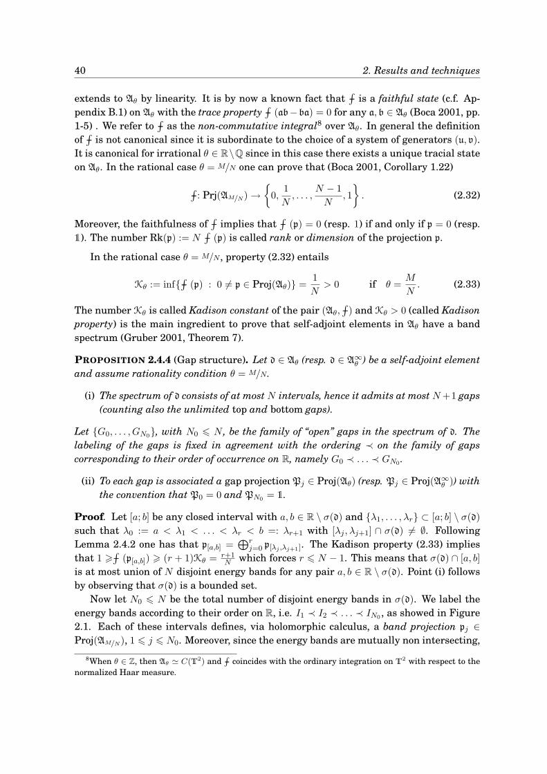
40 2. Results and techniques
extends to Aθ by linearity. It is by now a known fact that∫−−− is a faithful state (c.f. Ap-
pendix B.1) on Aθ with the trace property∫−−− (ab−ba) = 0 for any a, b ∈ Aθ (Boca 2001, pp.
1-5) . We refer to∫−−− as the non-commutative integral8 over Aθ. In general the definition
of∫−−− is not canonical since it is subordinate to the choice of a system of generators (u, v).
It is canonical for irrational θ ∈ R\Q since in this case there exists a unique tracial stateon Aθ. In the rational case θ = M/N one can prove that (Boca 2001, Corollary 1.22)
∫−−−: Prj(AM/N) →
0,
1
N, . . . ,
N − 1
N, 1
. (2.32)
Moreover, the faithfulness of∫−−− implies that
∫−−− (p) = 0 (resp. 1) if and only if p = 0 (resp.
1). The number Rk(p) := N∫−−− (p) is called rank or dimension of the projection p.
In the rational case θ = M/N, property (2.32) entails
Kθ := inf∫−−− (p) : 0 6= p ∈ Proj(Aθ) =
1
N> 0 if θ =
M
N. (2.33)
The number Kθ is called Kadison constant of the pair (Aθ,∫−−−) and Kθ > 0 (called Kadison
property) is the main ingredient to prove that self-adjoint elements in Aθ have a bandspectrum (Gruber 2001, Theorem 7).
PROPOSITION 2.4.4 (Gap structure). Let d ∈ Aθ (resp. d ∈ A∞θ ) be a self-adjoint element
and assume rationality condition θ = M/N.
(i) The spectrum of d consists of at most N intervals, hence it admits at most N+1 gaps(counting also the unlimited top and bottom gaps).
Let G0, . . . , GN0, with N0 6 N , be the family of “open” gaps in the spectrum of d. Thelabeling of the gaps is fixed in agreement with the ordering ≺ on the family of gapscorresponding to their order of occurrence on R, namely G0 ≺ . . . ≺ GN0 .
(ii) To each gap is associated a gap projection Pj ∈ Proj(Aθ) (resp. Pj ∈ Proj(A∞θ )) with
the convention that P0 = 0 and PN0 = 1.
Proof. Let [a; b] be any closed interval with a, b ∈ R \ σ(d) and λ1, . . . , λr ⊂ [a; b] \ σ(d)
such that λ0 := a < λ1 < . . . < λr < b =: λr+1 with [λj , λj+1] ∩ σ(d) 6= ∅. FollowingLemma 2.4.2 one has that p[a,b] =
⊕rj=0 p[λj ,λj+1]. The Kadison property (2.33) implies
that 1 >∫−−− (p[a,b]) > (r + 1)Kθ = r+1
N which forces r 6 N − 1. This means that σ(d) ∩ [a, b]
is at most union of N disjoint energy bands for any pair a, b ∈ R \ σ(d). Point (i) followsby observing that σ(d) is a bounded set.
Now let N0 6 N be the total number of disjoint energy bands in σ(d). We label theenergy bands according to their order on R, i.e. I1 ≺ I2 ≺ . . . ≺ IN0 , as showed in Figure2.1. Each of these intervals defines, via holomorphic calculus, a band projection pj ∈Proj(AM/N), 1 6 j 6 N0. Moreover, since the energy bands are mutually non intersecting,
8When θ ∈ Z, then Aθ ≃ C(T2) andR
−−− coincides with the ordinary integration on T2 with respect to the
normalized Haar measure.
2.4. Band spectrum, gap projections and gap labeling 41
pjpk = 0 whenever j 6= k. The gap structure of σ(d) consists ofN0+1 “open” gaps countingalso the (unlimited) bottom gap which is the open interval from −∞ to the minimum ofσ(d) and the (unlimited) top gap which is the open interval from the maximum of σ(d) to+∞. We can label the gaps by their order of occurrence on the real line, G0 ≺ G1 ≺ G2 ≺. . . ≺ GN0 with G0 the bottom gap and GN0 the top gap. To any gap it is associated thegap projection Pj :=
⊕ji=0 pi. The trivial projection 0(=: P0) is associated to the bottom
gap and the trivial projection 1(=: PN0) is associated to the top gap.
Figure 2.1: Band structure of the spectrum of a self-adjoint element d ∈ Aθ for a rational value θ = M/N
of the deformation parameter.
The number
N (Gj) := Rk(Pj) = N∫−−− (Pj), (2.34)
which coincides with the dimension of Pj , provide an alternative increasing labelingfor the gaps of the spectrum of d in the spirit of the celebrated gap labelling Theorem(Simon 1982, Bellissard 1993).
REMARK 2.4.5. (Gap structure for irrational deformation parameter) If the spectrumof d ∈ Aθ is Cantor (which may happen only if θ ∈ R \ Q) then any point in σ(d) is anaccumulation point and it is not possible to define the band projections via holomorphiccalculus. Nevertheless, we can yet define the gap projections. Since σ(d) is boundedwe can fix −∞ < λ0 < minσ(d) and for any λ ∈ R \ σ(d), λ > λ0 we can define thegap projection Pλ ∈ Aθ by means of the holomorphic functional calculus. The numberN (G) :=
∫−−− (Pλ) defines a label for the gap G ∋ λ which is independent on λ. A general
result shows that that for any non-trivial projection p ∈ Proj(Aθ) there exists a n ∈ Z\0such that
∫−−− (p) = nθ mod Z (Boca 2001, Corollary 11.8). If θ ∈ R\Q, then n is determined
uniquely and∫−−− maps the set Proj(Aθ) onto the countable dense set Gθ := (Z + θZ) ∩ [0, 1]
(Gracia-Bondía et al. 2001, Theorem 12.6). Thus n defines uniquely a canonical labelfor the element of Proj(Aθ) and Gθ coincides with the maximal set of possible gap-labelswhich, however, can be larger than the set of the actual “open” (i.e. non-empty) gapsin σ(d). The strong ten Martini problem consists in proving the existence of a bijectionbetween Gθ and the set of the “open” gaps in the (Cantor) spectrum of a self-adjointelement of Aθ when θ is irrational. ♦
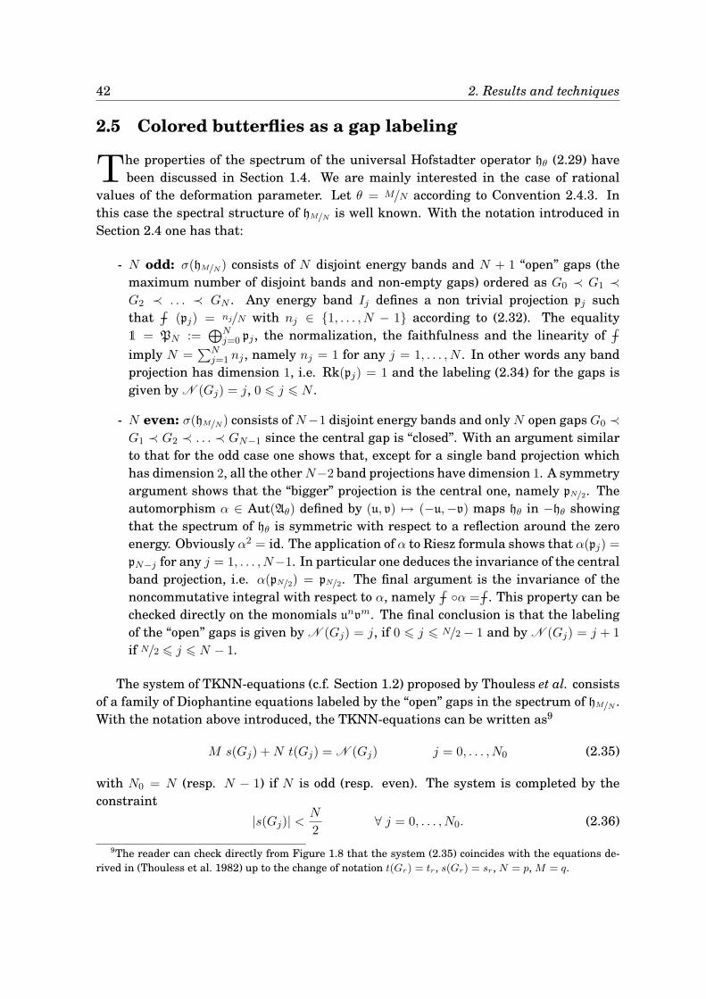
42 2. Results and techniques
2.5 Colored butterflies as a gap labeling
The properties of the spectrum of the universal Hofstadter operator hθ (2.29) havebeen discussed in Section 1.4. We are mainly interested in the case of rational
values of the deformation parameter. Let θ = M/N according to Convention 2.4.3. Inthis case the spectral structure of hM/N is well known. With the notation introduced inSection 2.4 one has that:
- N odd: σ(hM/N) consists of N disjoint energy bands and N + 1 “open” gaps (themaximum number of disjoint bands and non-empty gaps) ordered as G0 ≺ G1 ≺G2 ≺ . . . ≺ GN . Any energy band Ij defines a non trivial projection pj suchthat
∫−−− (pj) = nj/N with nj ∈ 1, . . . , N − 1 according to (2.32). The equality
1 = PN :=⊕N
j=0 pj , the normalization, the faithfulness and the linearity of∫−−−
imply N =∑N
j=1 nj , namely nj = 1 for any j = 1, . . . , N . In other words any bandprojection has dimension 1, i.e. Rk(pj) = 1 and the labeling (2.34) for the gaps isgiven by N (Gj) = j, 0 6 j 6 N .
- N even: σ(hM/N) consists of N−1 disjoint energy bands and only N open gaps G0 ≺G1 ≺ G2 ≺ . . . ≺ GN−1 since the central gap is “closed”. With an argument similarto that for the odd case one shows that, except for a single band projection whichhas dimension 2, all the otherN−2 band projections have dimension 1. A symmetryargument shows that the “bigger” projection is the central one, namely pN/2. Theautomorphism α ∈ Aut(Aθ) defined by (u, v) 7→ (−u,−v) maps hθ in −hθ showingthat the spectrum of hθ is symmetric with respect to a reflection around the zeroenergy. Obviously α2 = id. The application of α to Riesz formula shows that α(pj) =
pN−j for any j = 1, . . . , N−1. In particular one deduces the invariance of the centralband projection, i.e. α(pN/2) = pN/2. The final argument is the invariance of thenoncommutative integral with respect to α, namely
∫−−− α =
∫−−−. This property can be
checked directly on the monomials unvm. The final conclusion is that the labelingof the “open” gaps is given by N (Gj) = j, if 0 6 j 6 N/2 − 1 and by N (Gj) = j + 1
if N/2 6 j 6 N − 1.
The system of TKNN-equations (c.f. Section 1.2) proposed by Thouless et al. consistsof a family of Diophantine equations labeled by the “open” gaps in the spectrum of hM/N .With the notation above introduced, the TKNN-equations can be written as9
M s(Gj) +N t(Gj) = N (Gj) j = 0, . . . , N0 (2.35)
with N0 = N (resp. N − 1) if N is odd (resp. even). The system is completed by theconstraint
|s(Gj)| <N
2∀ j = 0, . . . , N0. (2.36)
9The reader can check directly from Figure 1.8 that the system (2.35) coincides with the equations de-rived in (Thouless et al. 1982) up to the change of notation t(Gr) = tr, s(Gr) = sr, N = p, M = q.
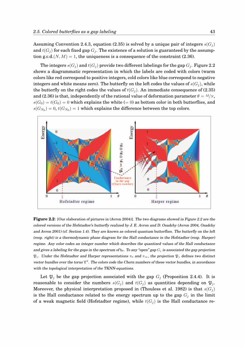
2.5. Colored butterflies as a gap labeling 43
Assuming Convention 2.4.3, equation (2.35) is solved by a unique pair of integers s(Gj)and t(Gj) for each fixed gap Gj . The existence of a solution is guaranteed by the assump-tion g.c.d.(N,M) = 1, the uniqueness is a consequence of the constraint (2.36).
The integers s(Gj) and t(Gj) provide two different labelings for the gapGj . Figure 2.2shows a diagrammatic representation in which the labels are coded with colors (warmcolors like red correspond to positive integers, cold colors like blue correspond to negativeintegers and white means zero). The butterfly on the left codes the values of s(Gj), whilethe butterfly on the right codes the values of t(Gj). An immediate consequence of (2.35)and (2.36) is that, independently of the rational value of deformation parameter θ = M/N,s(G0) = t(G0) = 0 which explains the white (= 0) as bottom color in both butterflies, ands(GN0) = 0, t(GN0) = 1 which explains the difference between the top colors.
Figure 2.2: [Our elaboration of pictures in (Avron 2004)]. The two diagrams showed in Figure 2.2 are the
colored versions of the Hofstadter’s butterfly realized by J. E. Avron and D. Osadchy (Avron 2004, Osadchy
and Avron 2001) (cf. Section 1.4). They are known as colored quantum butterflies. The butterfly on the left
(resp. right) is a thermodynamic phase diagram for the Hall conductance in the Hofstadter (resp. Harper)
regime. Any color codes an integer number which describes the quantized values of the Hall conductance
and gives a labeling for the gaps in the spectrum of hθ. To any “open” gap Gj is associated the gap projection
Pj . Under the Hofstadter and Harper representations π0 and π∞, the projection Pj defines two distinct
vector bundles over the torus T2. The colors code the Chern numbers of these vector bundles, in accordance
with the topological interpretation of the TKNN-equations.
Let Pj be the gap projection associated with the gap Gj (Proposition 2.4.4). It isreasonable to consider the numbers s(Gj) and t(Gj) as quantities depending on Pj .Moreover, the physical interpretation proposed in (Thouless et al. 1982) is that s(Gj)is the Hall conductance related to the energy spectrum up to the gap Gj in the limitof a weak magnetic field (Hofstadter regime), while t(Gj) is the Hall conductance re-
44 2. Results and techniques
lated to the same energy spectrum but in the opposite limit of a strong magnetic field(Harper regime). Thus, one can infer that the relation between s(Gj) and Pj dependson the Hofstadter representation π0, namely s(Gj) := C(π0(Pj)). Similarly, one can in-fer that t(Gj) := C(π∞(Pj)). The physical interpretation of the integers s(·) and t(·)leads to consider the colored butterflies in Figure 2.2 (c.f. Section 1.4) as thermodynamicphase diagrams (Avron 2004, Osadchy and Avron 2001). In particular, the butterfly onthe left shows the various thermodynamic phases for the Hall conductance (assumedas thermodynamic function) in the Hofstadter regime. In this case the thermodynamiccoordinates are the energy (proportional to the chemical potential) on the vertical axisand the magnetic field (θ ∝ B) on the horizontal axis. For a fixed value of the magneticfield, the color associated to the gap Gj codes (in unit of e2/h) the value of the Hall con-ductance when the chemical potential lies in the gap Gj . Similarly, the butterfly on theright shows the various phases for the Hall conductance in the Harper regime. In thiscase the thermodynamic coordinates are the energy and the inverse of the magnetic field(θ ∝ 1/B).
However, there is an open question from a mathematical point of view: what is themeaning of the function C which relates the integers s(·) and t(·) with the gap projec-tions via the representations π0 and π∞? One of the main results of this thesis is to provethat the “function” C denotes the (first) Chern number of a suitable vector bundle asso-ciated to the gap projection Pj and depending on the particular (Hofstadter or Harper)representation (cf. Section 2.7). This result leads to a rigorous proof of the topologicalinterpretation of the TKNN-equations.
2.6 Absence of unitary equivalence
Corollary 2.3.8 states that the Hofstadter-like Hamiltonian π0(a) and the Harper-likeHamiltonian π∞(a) associated to the same universal element a ∈ Aθ are isospec-
tral with spectrum given by σ(a), provided that the duality condition (Assumption 2.3.6)holds true. However, the relation of isospectrality between two operators is quite weaksince it concerns only the equality of the spectra as subsets of C; this property is re-lated only to the algebraic structure of the operator algebras and does not depend onthe representations. However, for a linear operator acting on a Hilbert space, the notionof algebraic spectrum can be enriched by means of the underlying Hilbert space struc-ture. As a matter of fact , the little amount of information in the algebraic spectrumis improved by the determination of the spectral measure or by analyzing the Lebesguedecomposition of the spectrum or computing the density of the states, etc. This informa-tion defines the spectral type of an operator. Obviously, two operators which are merelyisospectral, can have different spectral types, while two operators which are unitarilyequivalent have the same algebraic spectrum and the same spectral type. These con-siderations suggest the following question: under Assumption 2.3.6, do the isospectraloperators π0(a) and π∞(a) have the same spectral type?
2.6. Absence of unitary equivalence 45
A hint to answer the above question comes from the analysis of the colored butterfliesin Section 2.5. The isospectrality between the effective models Hθ
Hof and HθHar (with
θ = −ιqǫ0 = −ιqǫ∞ according to Assumption 2.3.6) leads to the same spectral diagram,the black and white quantum butterfly showed in Figure 1.9. However, if one looks tofiner properties like the Hall conductance, then the HamiltoniansHθ
Hof andHθHar produce
different colored butterflies (cf. Figure 1.10 or 2.2). Since the Hall conductance is a“spectral quantity” (it depends on the spectral projection associated to the gap), one cansuspect that Hθ
Hof and HθHar have different spectral type. This is not so surprising, in fact
HθHof and Hθ
Har are effective Hamiltonians which describe opposite and very differentphysical regimes. It is plausible that there exist physical quantities able to discriminatebetween the two regimes.
The above considerations suggest that the operators HθHof and Hθ
Har are not unitaryequivalent. A first, but partial, indication is given by the following result:
THEOREM 2.6.1 (Weak “no go”). Let Assumption 2.3.6 hold true. Then there exists nounitary map W : H0 → H∞ such that W U0 W
−1 = U∞ and W V0 W−1 = V∞.
Proof. We sketch an argument proposed by G. Emch in (Emch 1996). Suppose that sucha W exists. Then W implements unitarily the ∗-isomorphism defined by the arrow C ofdiagram (2.27), i.e. W π0(Aθ) W
−1 = π∞(Aθ). Such a unitary equivalence extends to aunitary equivalence of the related von Neumann algebras (c.f. Section B.1) M0(Aθ) :=
π0(Aθ)′′ and M∞(Aθ) := π∞(Aθ)
′′ . However, this is impossible since M0(Aθ) is a standardvon Neumann algebra (c.f. Section 5.1.2) while M∞(Aθ) is not standard (c.f. Section5.1.3) and the property to be standard (or not) is preserved by unitary equivalences.
The above “no go” result allows the Hofstadter-like Hamiltonian π0(a) and the Harper-like Hamiltonian π∞(a), related to the same element a ∈ Aθ, to have different spectraltypes, but it does not exclude the existence of a special unitary W which intertwinesonly π0(a) and π∞(a) and not the full C∗-algebras. To exclude the unitary equivalencebetween each pair of operators we need a stronger version of the above “no go” theorem.
The main result of this thesis is to provide a geometric and generalized version ofTKNN-equations which relate some “spectral fingerprints” of π0(a) and π∞(a) for any(self-adjoint) a ∈ Aθ. These spectral quantities can be defined in terms of topologicalinvariants (TQN) of suitable geometric structures emerging from the spectral decompo-sition of the algebras π0(Aθ) and π∞(Aθ) (see Section 2.7). The difference between thetopological invariants associated to π0(a) and π∞(a) it is enough to exclude the existenceof a special intertwiner W (strong “no go” result). The existence of a formula whichrelates these invariants is a consequence of a deep duality between π0(Aθ) and π∞(Aθ)
which is of geometric type. The proof of this geometric duality is the principal aim of thisthesis.
46 2. Results and techniques
2.7 From projections to vector bundles: the “two-fold way”
Section 2.5 ended with the assertion that there exists a relation between gap projec-tions of the Hofstadter (resp. Harper) Hamiltonian and vector bundles. The present
section aims to explain the nature of such a relation.
Firstly, we need to introduce some notations concerning the theory of vector bundles.For a detailed and complete exposition about this subject, we refer to (Lang 1985, Chap-ter III) or (Gracia-Bondía et al. 2001, Chapter 2). Fundamental notions useful for thepurpose of this thesis are sketched in Appendix C.
We use the symbol ι : E → T2 to denote a Hermitian vector bundle with two-dimensional torus as base space. To simplify notation we will occasionally use only thesymbol E . The vector bundle has rank N if ι−1(z) ≃ CN for any z ∈ T2. The symbol Γ(E )
denotes the (finitely generated and projective) C(T2)-module of continuous sections ofthe vector bundle. The endomorphism bundle (c.f. Proposition 4.7.13) associated to therank N vector bundle E → T2 is the rank N2-vector bundle End(E ) → T2 with typicalfiber End(CN ) ≃ MatN (C) and transition functions induced by the adjoint action of thoseof E . The symbol Γ(End(E )) denotes the corresponding C(T2)-module of sections.
CONVENTION 2.7.1 (n-dimesional torus). The manifold Tn := S1 × . . . × S1 (n times) isparametrized by the points (denoted with k) of the square [0, 2π]n up to the identification ofthe opposite edges. Such an identification is made explicit by the map k := (k1, . . . , kn) 7→z(k) := (eik1 , . . . , eikn). We consider Tn to be endowed with the flat metric (the productmetric of the canonical Riemannian metric on S1) in such a way that the related volumeform agrees with the normalized Haar measure dz(k) := dnk
(2π)n with dnk := dk1 ∧ . . .∧ dkn.Sometimes we use the short notation Lp(Tn) instead Lp(Tn, dz) to denote the space of thep-summable functions with respect to dz.
The Hermitian structure on the bundle E and the existence of a volume form on T2
allows us to define a scalar product on the space of sections Γ(E ) as
〈s; r〉 :=
∫
T2
(s(z); r(z))z dz, s, r ∈ Γ(E),
where (· ; ·)z denotes the scalar product in the fiber space ι−1(z) ≃ CN . The completionof Γ(E ) with respect to the norm ‖s‖L2 :=
√〈s; s〉 leads to the Hilbert space L2(E ) of the
L2-sections of the vector bundle E . Obviously, Γ(E ) ⊂ L2(E ) due to the compactness ofthe base manifold. We denote with B(L2(E )) the C∗-algebra of the bounded operatorson the Hilbert space L2(E ). The fiber metric (· ; ·)z defines a C(T2)-valued Hermitianstructure on Γ(E ) through s; r(z) := (s(z); r(z))z for s, r ∈ Γ(E). This endows Γ(E ) withthe structure of a Hilbert module over C(T2). Let EndC(T2)(Γ(E )) be the C∗-algebraof the adjontable operators on the C(T2)-module Γ(E ) (Boca 2001, Proposition 3.1 andTheorem 3.8). Any element in EndC(T2)(Γ(E )) extends uniquely to a bounded operator onL2(E ) hence, with a slight abuse of notation, we can write EndC(T2)(Γ(E )) ⊂ B(L2(E )).The (localization) isomorphism Γ(End(E )) ≃ EndC(T2)(Γ(E )) shows that Γ(End(E )) is aunital C∗-algebra and justifies the (abuse of) notation Γ(End(E )) ⊂ B(L2(E )).
2.7. From projections to vector bundles: the “two-fold way” 47
DEFINITION 2.7.2 (Bundle decomposition10 ). Let A ⊂ B(H) be a C∗-algebra of boundedoperators on the Hilbert space H. We say that A admits a bundle decomposition over Xif there exist a vector bundle E → X (with X a finite dimensional compact manifold) anda unitary map F : H → L2(E ) such that F A F−1 ⊂ Γ(End(E )).
The mere request of a unitary map between H and L2(E ) is trivial since all separa-ble Hilbert spaces are unitarily equivalent. Nevertheless, such a map transforms A ina subalgebra of B(L2(E )). The non-trivial part of the above definition consists in the(rather strong) request that F A F−1 ⊂ Γ(End(E )). The unitarity of the map F assuresthat spectral properties of operators in A are preserved after the decomposition. On theother hand, Γ(End(E )) is a geometric object and its geometry encodes features of theoriginal algebra A. In other words, an algebra of operators admits a bundle decompo-sition if it has a hidden geometric structure which emerges up to a unitary transform.A general scenario for the appearance of an emerging geometric structure is the exis-tence of a family of symmetries S for the algebra A. This point of view is developed inChapter 4. A triple H,A,S is called a physical frame (Definition 4.1.2). The contentof Theorems 4.7.9 and 4.7.15 is that (under some technical assumptions) any physicalframe with wandering property (Definition 4.5.1) induces a bundle decomposition F . Inthis case we say that the bundle decomposition F is subordinate to the physical frameH,A,S. If S is maximal commutative inside the commutant A′, then the physicalframe H,A,S is called irreducible and we refer to the induced F as an irreducible(subordinate) bundle decomposition.
The interpretation of the spectral properties of A in terms of emerging geometricquantities is supported by the following general result.
LEMMA 2.7.3. Let A ⊂ B(H) be a C∗-algebra admitting a bundle decomposition overX with (rank N ) vector bundle ι : E → X. Then, any projection P ∈ A defines a vectorsubbundle L (P ) ⊂ E .
Proof. If P ∈ A is a projection, then F P F−1 =: P (·) ∈ Γ(End(E )) is an projection-valued section, namely P (x) is a projection in End(ι−1(x)) ≃ MatN (C) for any x ∈ X.Since any element of Γ(End(E )) defines a bundle map (Gracia-Bondía et al. 2001, Corol-lary 2.7), we can build the image vector bundle associated to P (·). Let Im(P )x :=
P (x)v ; v ∈ ι−1(x) ⊂ ι−1(x) and consider the total space
L (P ) :=⊔
x∈XIm(P )x ≃ (x, v) ∈ X × E : ι(v) = x, P (x)v = v (2.37)
10The space L2(E ) agrees with the direct integral (c.f. Appendix B.3) of the Hilbert spaces H(z) := ι−1(z),i.e. L2(E ) =
R ⊕
T2 H(z) dz. The unitary map F : H → L2(E ) induces a direct integral decomposition ormore simply a fiber decomposition of the Hilbert space H. Let D ⊂ FB(H)F−1 be the set of decomposableoperators (or operator fields c.f. Appendix B.3). If FAF−1 ⊂ D , then the C∗-algebra A admits a fiberdecomposition, namely FAF−1 =
R ⊕
T2 πz(A) dz with πz : A → B(H(z)) is a representation of A for any z ∈
T2. However, the fiber decomposition of a C∗-algebra is a purely measure-theoretic notion which contains no
topological information. On the contrary, the notion of of bundle decomposition is purely topological and isrelated with the definition of continuous field of C∗-algebras (Dixmier 1982). Observing that Γ(E ) is densein L2(E ), it follows that the notion of bundle decomposition is stronger than that of fiber decomposition.Loosely speaking, a bundle decomposition is a continuous fiber decomposition.
48 2. Results and techniques
where the symbol⊔x∈X denotes the disjoint union of sets labeled by X. Equation (2.37)
implies that L (P ) ⊂ E and L (P ) ∩ ι−1(x) = Im(P )x and so defines the total space of avector subbundle ι : L (P ) → X provided that the function x 7→ dim(Im(P )x) = Rk(P (x))
is constant. The latter claim follows by standard arguments showing that the map x 7→Rk(P (x)) is both lower and upper semicontinuous, hence locally constant (Dixmier andDouady 1963, Section 1). If X is connected, then x 7→ Rk(P (x)) is constant and thecommon value, denoted with Rk(P ), fixes the rank of the vector subbundle E (P ). Theisomorphism which appears in the right-hand side of (2.37) is justified by the fact thatthe map (x, v) 7→ v defines a linear isomorphism between the fiber spaces x × Im(P )xand Im(P )x.
The relevance of the Definition 2.7.2 for a geometric derivation of the TKNN-equations(2.35) is related to the following fundamental result:
THEOREM 2.7.4 (Bundle decomposition in Hofstadter and Harper representations). LetAM/N be the the rational NCT-algebra (according to Convention 2.4.3), π0 : AM/N → H0
the Hofstadter representation and π∞ : AM/N → H∞ the Harper representation.
(i) The operator algebra π0(AM/N) ⊂ B(H0) admits an irreducible bundle decomposi-tion over T2 with (rank N ) Hermitian vector bundle E0 → T2 (called Hofstadter vec-tor bundle) and a unitary transform F0 : H0 → L2(E0). The decomposition is unique(up to equivalences). The vector bundle E0 is trivial, hence its (first) Chern number iszero, C1(E0) = 0. Finally, the bundle representation F0 π0(AM/N) F0
−1 is generatedby the endomorphism sections U0(·) := F0 π0(u) F0
−1 and V0(·) := F0 π0(v) F0−1
explicitly defined (in local coordinates according to Convention 2.7.1 ) by
U0(k) ≡ U(e−ik1), V0(k) ≡ V(eik2), k = (k1, k2) ∈ R2 (2.38)
where U and V are defined by (2.40).
(ii) The operator algebra π∞(AM/N) ⊂ B(H∞) admits an irreducible bundle decomposi-tion over T2 with (rank N ) Hermitian vector bundle E∞ → T2 (called Harper vectorbundle) and unitary transform F∞ : H∞ → L2(E∞). The decomposition is unique(up to equivalences). The vector bundle E∞ is non trivial with (first) Chern numberC1(E∞) = 1. Finally, the bundle representation F∞ π∞(AM/N) F∞−1 is generated bythe endomorphism sections U∞(·) := F∞ π∞(u) F∞−1 and V∞(·) := F∞ π∞(v) F∞−1
explicitly defined by
U∞(k) ≡ U(eiMNk1), V∞(k) ≡ V(eik2), k = (k1, k2) ∈ R2. (2.39)
To complete definitions (2.38) and (2.39) we need to introduce the N × N complex
2.7. From projections to vector bundles: the “two-fold way” 49
matrices
U(λ) := λ
1 0 0 . . . 0
0 ei2πMN 0 . . . 0
0 0 ei4πMN
......
......
. . . 0
0 0 0 . . . 0
0 0 0 . . . ei2π(N−1)MN
, V(λ) :=
0 0 0 . . . 0 λ
1 0 0 . . . 0 0
0 1 0...
......
.... . . . . . 0 0
0 0 0 0 0
0 0 0 . . . 1 0
(2.40)with λ ∈ C. Obviously, U(λ) and V(λ) are unitary if and only if |λ| = 1 (i.e. λ ∈ S1) and
U(λ)V(λ′) = ei2πMN V(λ′)U(λ), ∀ λ, λ′ ∈ C.
The proof of claim (i) is postponed in Section 5.2.1 where the Hofstadter vector bun-dles is built “by hand”. Similarly, claim (ii) is proved in Section 5.2.2. More generally,the proof of Theorem 2.7.4 is based on a general technique developed in Chapter 4. Theunitary maps F0 and F∞ are called generalized Bloch-Floquet transforms.
The uniqueness claimed in (i) of Theorem 2.7.4 means that any other bundle repre-sentation F0 subordinate to an irreducible physical frame with wandering property isunitarily equivalent to F0 and selects a vector bundle E ′
0 which is isomorphic to E0. Inother words, for the Hofstadter representation there exists a unique bundle decomposi-tion (up to equivalences) subordinate to an irreducible physical frame with wanderingproperty. The same holds true for the Harper representation. This form of uniquenessfor the bundle decomposition F0 (resp. F∞) implies that the geometry of the Hofstadter(resp. Harper) vector bundle is a fingerprint for the physics (observables + symmetries)of the Hofstadter (resp. Harper) regime.
In the Hofstadter case (c.f. Section 5.2.1) the structure of ι : E0 → T2 is defined bymeans of a system of N orthonormal sections ζ0 := ζ0
0 , . . . , ζN−10 , with ζj0 : R2 → Φ∗
0 (asuitable “ambient” vector space), subjected to periodic conditions
ζ0(k1 + 2π, k2) = ζ0(k1, k2 + 2π) = ζ0(k1, k2). (2.41)
Equations (2.41) allows ζ0 to be a global frame of sections over the base manifold T2,hence the resulting vector bundle is trivial, i.e. E0 ≃ T2 × CN . The triviality of thevector bundle implies automatically the vanishing of all the Chern classes and relatedChern numbers (Husemoller 1994, Proposition 4.1). The triviality of the vector bundleE0 implies also the triviality of endomorphism bundle End(E0) and in fact the sectionsU0(·) and V0(·) are globally defined, as showed by equation (2.38).
The structure of the Harper vector bundle ι : E∞ → T2 is defined by a system of Northonormal sections ζ∞ := ζ0
∞, . . . , ζN−1∞ , with ζj∞ : R2 → Φ∗
∞ (a suitable “ambient”vector space), subjected to covariance conditions
ζ∞(k1 + 2π, k2) = G(k2) · ζ∞(k1, k2), ζ∞(k1, k2 + 2π) = ζ∞(k1, k2) (2.42)
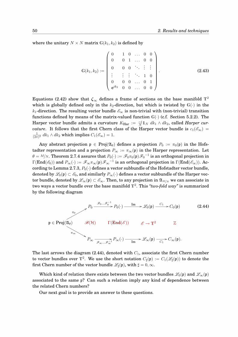
50 2. Results and techniques
where the unitary N ×N matrix G(k1, k2) is defined by
G(k1, k2) :=
0 1 0 . . . 0 0
0 0 1 . . . 0 0
0 0 0. . .
......
......
.... . . 1 0
0 0 0 . . . 0 1
eik2 0 0 . . . 0 0
. (2.43)
Equations (2.42) show that ζ∞ defines a frame of sections on the base manifold T2
which is globally defined only in the k2-direction, but which is twisted by G(·) in thek1-direction. The resulting vector bundle E∞ is non-trivial with (non-trivial) transitionfunctions defined by means of the matrix-valued function G(·) (c.f. Section 5.2.2). TheHarper vector bundle admits a curvature KHar := −i
N 1N dk1 ∧ dk2, called Harper cur-vature. It follows that the first Chern class of the Harper vector bundle is c1(E∞) =
1(2π)2
dk1 ∧ dk2 which implies C1(E∞) = 1.
Any abstract projection p ∈ Proj(Aθ) defines a projection P0 := π0(p) in the Hofs-tadter representation and a projection P∞ := π∞(p) in the Harper representation. Letθ = M/N. Theorem 2.7.4 assures that P0(·) := F0π0(p)F0
−1 is an orthogonal projection inΓ(End(E0)) and P∞(·) := F∞π∞(p)F∞
−1 is an orthogonal projection in Γ(End(E∞)). Ac-cording to Lemma 2.7.3, P0(·) defines a vector subbundle of the Hofstadter vector bundle,denoted by L0(p) ⊂ E0, and similarly P∞(·) defines a vector subbundle of the Harper vec-tor bundle, denoted by L∞(p) ⊂ E∞. Then, to any projection in AM/N we can associate intwo ways a vector bundle over the base manifold T2. This “two-fold way” is summarizedby the following diagram
P0
F0...F−10 // P0(·) Im // L0(p)
C1 // C0(p)
p ∈ Proj(Aθ)
π∞&&MMMMMMMMMMMM
π0
88qqqqqqqqqqqq
B(H) Γ(End(E )) E → T2 Z
P∞F∞...F−1
∞
// P∞(·)Im
// L∞(p)C1
// C∞(p).
(2.44)
The last arrows the diagram (2.44), denoted with C1, associate the first Chern numberto vector bundles over T2. We use the short notation C♯(p) := C1(L♯(p)) to denote thefirst Chern number of the vector bundle L♯(p), with ♯ = 0,∞.
Which kind of relation there exists between the two vector bundles L0(p) and L∞(p)
associated to the same p? Can such a relation imply any kind of dependence betweenthe related Chern numbers?
Our next goal is to provide an answer to these questions.
2.8. From geometric duality to TKNN-equations 51
2.8 From geometric duality to TKNN-equations
In this section we present one of the main results of this thesis which address thequestion stated at the end of Section 2.7.
We denote by ι : I → T2 the determinant line bundle associated to the Harper vectorbundle ι : E∞ → T2, namely I is the rank 1 Hermitian vector bundle with transitionfunctions given by the determinant of the transition functions of E∞. One has thatC1(I ) = C1(E∞) = 1 (c.f. Appendix C and equation (C.9)).
THEOREM 2.8.1 (Geometric duality). Let AM/N be the rational NCT-algebra (as in Con-vention 2.4.3) and p ∈ Proj(AM/N).
(i) The vector bundles L0(p) and L∞(p) have the same rank given by the number Rk(p)
which is the dimension of p (c.f. equation (2.34)).
(ii) Let f(n,m) : T2 → T2, with n,m ∈ Z, be the continuous map defined by
f(n,m)(eik1 , eik1) = (eink1 , eimk2). (2.45)
Thenf∗(N,1)L∞(p) ≃ f∗(−M,1)L0(p) ⊗ I (2.46)
where f∗(n,m)L♯(p), ♯ = 0,∞, denotes the pullback of the vector bundle L♯(p) inducedby the map f(n,m), and I is the determinant bundle of E∞ (c.f. Appendix C).
The proof of the duality relation (2.46) is postponed to Section 5.3. Claim (i) followsfrom (ii) and Proposition 5.2.2.
The geometric duality between the vector bundles L0(p) and L∞(p) is the core of ageometric derivation of the TKNN-equations.
COROLLARY 2.8.2 (Generalized TKNN-equations). Let AM/N be the rational NCT-algebra(according to Convention 2.4.3). Any p ∈ Proj(AM/N) defines a TKNN-equation
N C∞(p) +M C0(p) = Rk(p) (2.47)
which relates the Chern numbers C∞(p) and C0(p).
Proof. The derivation of equation (2.47) from the duality formula (2.46) is straightfor-ward. Observing that isomorphic vector bundles have same characteristic classes, onehas
c1(f∗(N,1)L∞(p)) = c1(f
∗(−M,1)L0(p) ⊗ I ).
Applying formula (C.10) to the right-hand side, one has
c1(f∗(N,1)L∞(p)) = c1(f
∗(−M,1)L0(p)) + Rk(p) c1(I ), (2.48)
since the rank of I is 1 and the rank of f∗(−M,1)L0(p) coincides with the rank of L0(p)
which is Rk(p).
52 2. Results and techniques
To complete the proof we need to integrate over T2 both sides of (2.48). From theleft-hand side one obtains
C1(f∗(N,1)L∞(p)) =
∫
T2
c1(f∗(N,1)L∞(p))
I=
∫
T2
f∗(N,1)c1(L∞(p))II= NC∞(p)
where equality I follows from the functoriality of the Chern class (i.e. c1(f∗E ) = f∗c1(E ))and equality II follows from Lemma C.0.2. The same computation for the right-handside shows that C1(f
∗(−M,1)L∞(p)) = −MC0(p). Finally, C1(I ) = C1(E∞) = 1.
If p = 1, then L0(1) = E0, L∞(1) = E∞, Rk(p) = N and equation (2.47) is compatiblewith the results obtained in Theorem 2.7.4 , namely C0(1) := C1(E0) = 0 and C∞(1) :=
C1(E∞) = 1.
Equation (2.47) defines a geometric generalized version of the TKNN-system (2.35).With the notation introduced in Section 2.5, let Pj ∈ Proj(A∞
M/N) the gap projectioncorresponding to the j-th gapGj (0 6 j 6 N0) in the spectrum of the universal Hofstadteroperator hM/N ∈ A∞
M/N . With the identification t(Gj) := C∞(Pj) and s(Gj) := C0(Pj) andusing the labeling N (Gj) := Rk(Pj) defined by (2.34), then equations (2.47) reduceexactly to the system of Diophantine equations (2.35) proposed by Thouless et al. in(Thouless et al. 1982).
2.9 A “non-commutative look” to TKNN-equations
The geometric generalization of the TKNN-equations (2.47) has been derived underthe assumption of rationality for the deformation parameter θ = M/N. A natural
question is whether it is possible to give any meaning to (2.47) also in the irrational caseθ ∈ R\Q. To provide an answer we need to introduce new structures on the NCT-algebra.
Canonical derivations and universal Chern number
In view of Remark 2.3.1, the map ρz(u) = z1u, ρz(v) = z2v extends to an automorphismfor any z = (z1, z2) ∈ T2. The map T2 ∋ z 7→ ρz ∈ Aut(Aθ) defines a strongly continuousaction of the commutative group T2 on Aθ. Let z(k) = (eik1 , eik2) ∈ T2. For any a in thedense set Lθ one defines ∂−−−j (a) ∈ Lθ, j = 1, 2, as
∂−−−j (a) := 2πd
dkjρz(k)(a)
∣∣∣∣k=0
. (2.49)
It follows that ∂−−−1 and ∂−−−2: (i) are C-linear Aθ-valued maps; (ii) satisfy the Leibniz’slaw ∂−−−j (ab) =∂−−−j (a) b + a ∂−−−j (b); (iii) are symmetric, ∂−−−j (a∗) =∂−−−j (a)∗; (iv) commute,∂−−−1 ∂−−−2=∂
−−−2 ∂−−−1. We refer to ∂−−−1 and ∂−−−2 as canonical derivations. Let (u, v) be a frame
for Aθ. A simple computation shows that
∂−−−1 (unvm) := i2πn unvm, ∂−−−2 (unvm) := i2πm unvm (2.50)
which proves that ∂−−−1 and ∂−−−2 are unbounded. The maximal invariant domain of defini-tion for ∂−−−1 and ∂−−−2 coincides with the smooth algebra A∞
θ
2.9. A “non-commutative look” to TKNN-equations 53
The universal Chern number is the map
C1 : Proj(A∞θ ) → Z
defined by
C1(p) :=1
i2π
∫−−− (p[∂−−−1 (p); ∂−−−2 (p)]) (2.51)
where [∂−−−1 (p); ∂−−−2 (p)] :=∂−−−1 (p) ∂−−−2 (p)− ∂−−−2 (p) ∂−−−1 (p). Equation (2.51) is called Connesformula. The integrality of C1 is proved in (Connes 1980), but more details can be foundin (Connes 1994, Chapter III).
The relevance of the map C1 for our purposes is related to the following result (c.f.Proposition 5.2.2):
PROPOSITION 2.9.1. For any p ∈ Proj(A∞M/N) one has C0(p) = C1(p).
Constraint for the TKNN-equations of the Hofstadter operator
The first interesting consequence of Proposition 2.9.1 concerns the bound (2.36) whichcompletes the TKNN-system proposed in (Thouless et al. 1982). Let Pj ∈ Proj(A∞
M/N)
the gap projection corresponding to the j-th gap Gj (0 6 j 6 N0) in the spectrum ofthe universal Hofstadter operator hM/N ∈ A∞
M/N . With the identification s(Gj) = C0(Pj),Proposition 2.9.1 leads to rewrite (2.36) as |C1(Pj)| < N/2. The latter bound has beenproved in (Choi et al. 1990, Corollary 3.4). Then, Proposition 2.9.1 provides a purelygeometric justification for the bound (2.36) and, together with Corollary 2.8.2, completesour purpose to find a rigorous geometric derivation of the result claimed in (Thoulesset al. 1982). However, the bound |C1(Pj)| < N/2 holds true only for the spectral projec-tions of the universal Hofstadter operator. In principle, the choice of a different operatorleads to a different bound and each bound depends on the form of the related operator.
Generalization to irrational values of the deformation parameter
By means of the equality C0 = C1, the definition Rk(p) := N∫−−− (p) and θ = M/N, one can
rewrite the TKNN-equation (2.47) in the following form
C∞(p) =∫−−− (p) − θ C1(p). (2.52)
Formally, equation (2.52) contains only quantity defined in terms of the abstract algebraAθ, hence it has a perfect meaning for any θ ∈ R.
The above formula has an interesting application. Let dθ ∈ A∞θ be a self-adjoint
element (not necessarily the universal Hofstadter operator hθ) and PG the gap projectionassociated to the gap G ⊂ R \ σ(dθ) and defined via Riesz formula according to Lemma2.4.2. If θ = M/N, then the integers C∞(PG) and C0(PG) defines two distinct numericallabels for the gap G. An interesting question is whether these labels, initially definedfor rational values of θ, are stable for small perturbations of the deformation parameter
54 2. Results and techniques
θ. A good criterion of stability is given in the following terms. Consider a family of self-adjoint elements dθ := f(u, v) with (u, v) a frame for Aθ, f ∈ C∞(T2) a fixed real smoothfunctions and θ ∈ I, where I is an interval of R. The functional expression of dθ is fixedand it depends on θ only through the fundamental commutation relation between thegenerators of Aθ. Moreover dθ ∈ A∞
θ for any θ ∈ I. Suppose that λG ∈ R \ σ(dθ) forany θ ∈ I and denote by Pθ
G ∈ Proj(A∞θ ) the related gap projection corresponding to
(−∞, λG]. The functions θ 7→ C1(PθG) is constant in I (Boca 2001, Proposition 11.11).
Moreover, as a consequence of the description of the group K0(Aθ) given in (Pimsner andVoiculescu 1980), one deduces that
∫−−− (Pθ
G) = m(PθG) + θC1(P
θG) (2.53)
(Boca 2001, p. 145), where the integer m(·) ∈ Z is uniquely determined by the condition0 6∫−−− (·) 6 1. Since C1(P
θG) is constant in I, one infers that also m(Pθ
G) is constant undersmall perturbations of θ. Since C0 = C1 in view of Proposition 2.9.1 and C∞ =
∫−−− −θC1 = m
(comparison between (2.52) and (2.53)), it follows that the integers C0 and C∞ are “stablelabels” for “stable gaps”. In other words equation (2.52) is meaningful also for irrationalvalues of the deformation parameter provided that there exists a stable “open” gap undersmall perturbation of θ.
Cohomological interpretation
A final remark concerns the link between the “non-commutative version” of the TKNN-equation (2.52) and the geometry of the NCT-algebra. Indeed equation (2.52) is re-lated to the periodic cyclic cohomology of the algebra A∞
θ which is the Z2-graded groupPH•(A∞
θ ) := PHev(A∞θ ) ⊕ PHod(A∞
θ ) with PH♯(A∞θ ) ≃ C2, ♯ = ev, od (Connes 1994)
(c.f. Appendix B.4 for the basic definitions). Since the two independent generators ofPHev(A∞
θ ) are exactly the noncommutative trace∫−−− and the universal Chern number
C1, it follows that the integer valued function C∞ is an element of the even part of theperiodic cyclic cohomology group of A∞
θ .
2.10 Prospectives and open problems
As usual, the solution of a problem opens the way to new speculations and stimulatingchallenges. This is true also for this thesis. During our investigation, we collected
interesting problems closely related with the arguments of this thesis, that we havenot had the time to examine. At the same time, we realized that some of our resultscould have relevant generalizations by means of interactions with other mathematicalfields. We sketch below a short list containing the main open problems and the morestimulating prospectives of further generalizations.
• Proof of the Kubo-Chern equivalence for the Harper and Hofstadter regimes (c.f.Section 1.3), supposedly by means of SAPT techniques.
2.10. Prospectives and open problems 55
• Derivation of the effective model for the Bloch-Landau Hamiltonian HBL (2.1) witha perturbed magnetic field B+δB in the limit δB → 0. This problem is related withthe non-triviality of the Bloch vector bundle in view of the absence of time-reversalsymmetry.
• Derivation of the effective models for the Harper and Hofstadter regimes takinginto account also of the effects due to disorder (random or aperiodic potential). Thefirst step should be the generalization of SAPT to the cases of aperiodic or randompotentials using non-commutative tools à la Bellissard (Bellissard et al. 1994).
• Generalization of the TKNN-equations to higher dimensional Harper representa-tions (work in progress with Giovanni Landi) and possible applications to the cou-pling of Landau bands in presence of a periodic vector potential (c.f. Section 3.4.8)and to the study of hexagonal lattices (graphene) (Bellissard et al. 1991).

Chapter 3
Derivation of Harper and Hofstadter models
Pour bien savoir les choses, il en faut savoir le détail; etcomme il est presque infini, nos connaissances sonttoujours superficielles et imparfaites.
(To understand matters rightly we should understandtheir details; and as that knowledge is almost infinite, ourknowledge is always superficial and imperfect. )
François de La Rochefoucauld,Réflexions ou sentences et maximes morales, 1665-1678
Abstract
Some relevant transport properties of solids do not depend only on the spectrum ofthe electronic Hamiltonian, but on finer properties preserved only by unitary equiv-alence, the most striking example being the conductance. When interested in suchproperties, and aiming to a simpler model, it is mandatory to check that the simplereffective Hamiltonian is approximately unitarily equivalent to the original one, in theappropriate asymptotic regime. In this chapter, we prove that the Hamiltonian forthe QHE is approximately unitarily equivalent to a Hofstadter-like (resp. Harper-like)Hamiltonian, in the limit of weak (resp. strong) magnetic field. Section 3.1 providesa brief compendium of the SAPT “philosophy” while Section 3.2 aims to fix the math-ematical description of the model. Section 3.3 is devoted to the adiabatic theory in theHofstadter regime while the Harper regime is expounded in Section 3.4. Finally, inSection 3.4.8 we show that an additional periodic magnetic potential induces in theHarper regime a non-trivial coupling of the Landau bands.
3.1 An insight to space-adiabatic perturbation theory
The results obtained in this chapter are based on the observation that both the Hofs-tadter and the Harper regime are space-adiabatic limits, and can be treated in the
framework of space-adiabatic perturbation theory, (SAPT) (Panati et al. 2003b, Panatiet al. 2003a), see also (Teufel 2003). As for the Hofstadter regime, the proof follows ideassimilar to the ones in (Panati et al. 2003a). Our generalization allows however to con-sider a constant magnetic field (while in (Panati et al. 2003a) the vector potential is as-sumed in C∞
b (Rd)) and to include a periodic vector potential. Moreover the proof extendsthe one in (Panati et al. 2003a), in view of the use of the special symbol classes definedin Section 3.3.4. On the contrary, from the discussion of the Harper regime ℏB → 0
some new mathematical problems emerge. Then, although the “philosophy” of the proof
58 3. Derivation of Harper and Hofstadter models
of Theorem 3.4.8 is of SAPT-type, the technical part is new as it will be explained inSection 3.4. Notice that the regime of weak magnetic field can also be conveniently ap-proached by using the magnetic Weyl quantization (Mantoiu and Purice 2004, Mantoiuet al. 2005, Iftimie et al. 2007, Iftimie et al. 2009), a viewpoint which is investigated in(De Nittis and Lein 2010).
For the sake of completeness, we summarize some salient aspects of the SAPT. Werefer to (Teufel 2003) for a complete exposition. Let H be the Hamiltonian of a genericphysical system which acts on the total (or physical) Hilbert space Hphy. For the SAPTto be applicable, three important ingredients needs:
(i) a distinction between fast and slow degrees of freedom which is mathematicallyexpressed by a unitary decomposition of the physical space Hphy into a productspace Hs ⊗Hf (or, more generally, a direct integral), the first factor being the spaceof slow degrees of freedom and the second the space of fast degrees of freedom;Hs ∼= L2(M) for suitable measure space M is also required;
(ii) a dimensionless adiabatic parameter ε≪ 1 that quantifies the separation of scalesbetween the fast and slow degrees of freedom and which measures how far are theslow degrees of freedom to be “classical” in terms of some process of quantization;
(ii) a relevant part of the spectrum for the fast dynamics which remains separatedfrom the rest of the spectrum under the perturbation caused by the slow degreesof freedom.
3.2 Description of the model
The Hamiltonian (2.1) describes the dynamics of particle with mass m and charge qwhich interacts with the ionic structure of a two dimensional crystal and with an
external orthogonal uniform magnetic field. A more general model is provided by theoperator
HBL :=1
2m
[−iℏ∇r −
q
cAΓ (r) − q
cA (r)
]2+ VΓ (r) + q Φ (r) (3.1)
still called Bloch-Landau Hamiltonian and, with an abuse of notation, still denotedwith the same symbol used in (2.1). The vector-valued function A := (A1,A2) is a vec-tor potential corresponding to an (orthogonal) external magnetic field B = ∇r ∧ A =
(∂1A2 − ∂2A1) e⊥, Φ is a scalar potential corresponding to a (parallel) external electricfield E = −∇rΦ and AΓ and VΓ are internal periodic potentials which describe the elec-tromagnetic interaction with the ionic cores of the crystal lattice. The external vectorpotential is assumed to have the following structure
A (r) = A0 (r) + AB (r) , (3.2)
where A0 is a bounded function and AB describes a uniform orthogonal magnetic field ofstrenght B, i.e. in the symmetric gauge
AB (r) =B
2e⊥ ∧ r =
(−B
2r2,
B
2r1
), ∇r ∧ AB = B e⊥, ∇r · AB = 0. (3.3)
3.2. Description of the model 59
The evolution of the system is prescribed by the Schrödinger equation
iℏd
dsψ(r, s) = HBL ψ(r, s), (3.4)
where s corresponds to a microscopic time-scale.
Mathematical description of the crystal structure
The periodicity of the crystal is described by a two dimensional lattice Γ ⊂ R2 (i.e. adiscrete subgroup of maximal dimension of the addictive group R2), thus Γ ≃ Z2. Leta, b ⊂ R2 be two generators of Γ, i.e.
Γ = γ ∈ R2 : γ = n1a+ n2b, n1, n2 ∈ Z.
The fundamental or Voronoi cell of Γ is MΓ := r ∈ R2 | r = l1 a+ l2 b, l1, l2 ∈ [0, 1] andits area is given by ΩΓ = |a ∧ b|. We fix the orientation of the lattice in such a way thatΩΓ = (a1b2−a2b1) > 0. We say that a function fΓ : R2 → C is Γ-periodic if fΓ(r+γ) = fΓ(r)
for all γ ∈ Γ and all r ∈ R2. The electrostatic and magnetostatic crystal potentials VΓ
and AΓ are assumed to be Γ-periodic according to the previous definition.An important notion is that of dual lattice Γ∗ which is the set of the vectors γ∗ ∈ R2
such that γ∗ · γ ∈ 2πZ for any γ ∈ Γ. Let a∗, b∗ ⊂ R2 be defined by the relationsa∗ · a = b∗ · b = 1 and a∗ · b = b∗ · a = 0; these vectors are the generators of the lattice Γ∗,i.e.
Γ∗ = γ∗ ∈ R2 : γ∗ = m1 2πa∗ +m2 2πb∗, m1,m2 ∈ Z.
The Brillouin zone
MΓ∗ := k ∈ R2 | k = k1 a∗ + k2 b
∗, k1, k2 ∈ [0, 2π]
is the fundamental cell of the dual lattice Γ∗. The explicit expressions for the dual gen-erators a∗, b∗ in terms of the basis a, b is
a∗ =e⊥ ∧ b|a ∧ b| =
1
ΩΓ(b2,−b1), b∗ = −e⊥ ∧ a
|a ∧ b| =1
ΩΓ(−a2, a1). (3.5)
It follows from (3.5) that the surface of the Brillouin zone is ΩΓ∗ = (2π)2|a∗∧b∗| = (2π)2/ΩΓ.Given a Γ-periodic function fΓ, we denote its Fourier decomposition as
fΓ(r) =∑
γ∗∈Γ∗
f(γ∗) eiγ∗·r =
∑
m1,m2∈Z
fm1,m2 ei2π(m1 a∗+m2 b∗)·r. (3.6)
A Z2-periodic function f : R2 → C is a function periodic with respect to an orthonormallattice, namely such that f(x1 +1, x2) = f(x1, x2 +1) = f(x1, x2) for any x1, x2 ∈ R. If onechanges the variables as x1 := a∗ · r and x2 := b∗ · r one has that fΓ(r) := f(a∗ · r, b∗ · r) isΓ-periodic in r. Every Γ-periodic function can be obtained in this way.
60 3. Derivation of Harper and Hofstadter models
Assumptions on the regularity of the potentials and self-adjointness
We denote by Cnb (R2,R) the space of real-valued n-times differentiable functions (smoothfunctions if n = ∞) with continuous and bounded derivatives up to order n. Concerningthe internal potentials AΓ and VΓ we need to assume that:
ASSUMPTION 3.2.1 (Internal potentials, strong form). The Γ-periodic potential VΓ andthe two components of the Γ-periodic vector potential AΓ are functions of class C∞
b (R2,R).
Sometime we can relax the above assumption and we can consider the weaker ver-sion:
ASSUMPTION 3.2.2 (Internal potentials, weak form). The two components of the Γ-periodic vector potential AΓ are in C1
b(R2,R). The Γ-periodic potential VΓ verifies thecondition
∫MΓ
|VΓ(r)|2 d2r < +∞.
Assumption 3.2.2 implies that VΓ is uniformly locally L2 and this implies also that VΓ
is infinitesimally bounded with respect to −∆r (Reed and Simon 1978, Theorem XIII.96).Concerning the external potentials A and Φ, we need to assume that:
ASSUMPTION 3.2.3 (External potentials). The scalar potential Φ is of class C∞b (R2,R).
The vector potential A consists of a linear term AB of the form (3.3) plus a bounded termA0 which is of class C∞
b (R2,R).
When the external potentials A and Φ vanish, the Bloch-Landau Hamiltonian (3.1)reduces to the periodic Hamiltonian (or Bloch Hamiltonian)
Hper :=1
2m
[−iℏ∇r −
q
cAΓ(r)
]2+ VΓ(r). (3.7)
The domains of self-adjointness of HBL and Hper are described in the following proposi-tion. Its proof, together with some basic notion about the Sobolev space H2(R2) and themagnetic-Sobolev space H2
M(R2), is postponed to Section A.1.1.
PROPOSITION 3.2.4. Let Assumptions 3.2.2 and 3.2.3 hold true. Then both HBL andHper are essentially self-adjoint operators on L2(R2, d2r) with common domain of essentialself-adjointness the space of smooth functions with compact support C∞
c (R2,C). Moreoverthe domain of self-adjointness of Hper is H2(R2) while the domain of self-adjointness ofHBL is H2
M(R2).
3.3 Space-adiabatic theory for the Hofstadter regime
3.3.1 Adiabatic parameter for weak magnetic fields
The SAPT for a Bloch electron developed in (Panati et al. 2003a) is based on theexistence of a separation between the microscopic space scale fixed by the lattice
spacing ℓ :=√
ΩΓ, and a macroscopic space scale fixed by the scale of variation of the“slowly varying” external potentials. The existence of such a separation of scales is
3.3. Space-adiabatic theory for the Hofstadter regime 61
expressed by introducing a dimensionless parameter ε ≪ 1 (adiabatic parameter) tocontrol the scale of variation of the vector potential and the scalar potential Φ appearingin (3.1), namely by setting A = A(εr) and Φ = Φ(εr). In particular the external magneticand electric fields are weak compared to the fields generated by the ionic cores.
It is useful to rewrite the (ε-dependent) Hamiltonian (3.1) in a dimensionless form.The microscopic unit of length being ℓ, we introduce the dimensionless position vectorx := r/ℓ and the dimensionless gradient ∇x = ℓ∇r. Moreover, since the vector poten-tial has the dimension of a length times a magnetic field, then A(εx) := ε/ℓB A(εℓx) isa dimensionless function, with B a dimensional constant which fixes the order of mag-nitude of the magnetic field due to A. Similarly for AΓ (with ε = 1). Factoring out thedimensional constants one finds
HBL :=1
E0HBL =
1
2
−i∇x −
qΩΓBΓ
cℏ︸ ︷︷ ︸=:ℏ−1
Γ
AΓ (x) − ιq|q|ΩΓB
cℏ︸ ︷︷ ︸=ℏ
−1B
1
εA (εx)
2
+VΓ (x) +φ (εx) , (3.8)
where E0 := ℏ2/mΩΓ is the natural unit of the energy fixed by the problem, VΓ(x) :=1/E0 VΓ(ℓx) and φ(εx) := q/E0 Φ(εℓx) are both dimensionless quantities. The constant ℏΓ
will play no particular rôle in the rest of this paper, so it is reabsorbed into the definitionof the dimensionless vector potential AΓ, i.e. formally ℏΓ = 1.
Comparing the dimensional Hamiltonian (3.8) with the original Hamiltonian (3.1),or observing that the strenght of the magnetic field goes to zero (at least linearly) withε, it is physically reasonable to estimate εℏB ∝ 1. This is rigorously true in the case of auniform external magnetic field.
The external force due to A and φ are of order of ε and therefore have to act over atime of order ε−1 to produce a finite change, which defines the macroscopic time-scale.The macroscopic (slow) dimensionless time-scale is fixed by t := εE0
ℏs where s is the
dimensional microscopic (fast) time-scale. With this change of scale the Schrödingerequation (3.4) reads
iεd
dtψ = HBL ψ (3.9)
with HBL given by equation (3.8).
REMARK 3.3.1. Observe that from the definition of the dimensionless periodic potentialAΓ and VΓ it follows that they are periodic with respect to the transform x 7→ x + γ/ℓ.This means that AΓ and VΓ are periodic with respect to a “normalized” lattice whosefundamental cell has surface 1. ♦
3.3.2 Separation of scales: the Bloch-Floquet transform
To make explicit the presence of the linear term of the external vector potential, wecan rewrite the (3.8) as follows
HBL =1
2
[−i∇−AΓ (x) −A0 (εx) − ιq
1
2e⊥ ∧ εx
]2
+ VΓ (x) + φ (εx) , (3.10)
62 3. Derivation of Harper and Hofstadter models
where the adiabatic parameter ε expresses the separation between the macroscopiclength-scale, defined by the external potentials, and the microscopic length-scale, de-fined by the internal Γ-periodic potentials. The separation between slow and fast degreesof freedom can be expressed decomposing the physical Hilbert space Hphy = L2(R2, d2x)
into a product of two Hilbert spaces or, more generally, into a direct integral. To thisend, we use the Bloch-Floquet transform (Kuchment 1993). As in (Panati et al. 2003a)we define the (modified) Bloch-Floquet transform Z of a function ψ ∈ S(R2) to be
(Zψ)(k, θ) :=∑
γ∈Γ
e−i(θ+γ)·kψ(θ + γ), (k, θ) ∈ R2 × R2. (3.11)
Directly from the definition one can check the following periodicity properties:
(Zψ)(k, θ + γ) = (Zψ)(k, θ) ∀ γ ∈ Γ, (3.12)
and(Zψ)(k + γ∗, θ) = e−iθ·γ
∗(Zψ)(k, θ) ∀ γ∗ ∈ Γ∗. (3.13)
Equation (3.12) shows that for any fixed k ∈ R2, (Zψ)(k, ·) is a Γ-periodic function andcan be seen as an element of Hf := L2(V, d2θ) with V := R2/Γ a two-dimensional slanttorus (Voronoi torus). The torus V coincides with the the fundamental cell MΓ endowedwith the identification of the opposite edges and d2θ denotes the (normalized) measureinduced on V by the identification with MΓ. The Hilbert space Hf is the space of fastdegrees of freedom, corresponding to the microscopic scale. Equation (3.13) involves aunitary representation of the group of the (dual) lattice translations Γ∗ on the Hilbertspace Hf, namely
Γ∗ ∋ γ∗τ−→ τ(γ∗) ∈ U (Hf)
where τ(γ∗) is the multiplication with eiθ·γ∗. It will be convenient to introduce the Hilbert
spaceHτ :=
ψ ∈ L2
loc
(R2, d2k,Hf
): ψ(k − γ∗, ·) = τ(γ∗) ψ(k, ·)
(3.14)
equipped with the inner product
〈ψ;ϕ〉Hτ :=
∫
MΓ∗
(ψ(k);ϕ(k))Hf d2k
where d2k := d2k(2π)2
is the normalized measure. There is a natural isomorphism fromHτ to L2
(MΓ∗ , d2k, Hf
)given by restriction from R2 to MΓ∗ , and with inverse given by
τ -covariant continuation, as suggested by (3.13). The Bloch-Floquet transform (3.11)extends to a unitary map
Z : Hphy −→ Hτ ≃ L2(MΓ∗ , d2k,Hf
)≃ L2(MΓ∗ , d2k) ⊗Hf. (3.15)
The Hilbert space L2(MΓ∗ , d2k) can be seen as the space of slow degrees of freedom andin this sense the transform Z produces a decomposition of the physical Hilbert spaceaccording to the existence of fast and slow degrees of freedom.
We need to discuss how differential and multiplication operators behave under Z.Let Q = (Q1, Q2) be the multiplication by x = (x1, x2) defined on its maximal domain
3.3. Space-adiabatic theory for the Hofstadter regime 63
and P = (P1, P2) = −i∇x with domain the Sobolev space H1(R2), then from (3.11) itfollows:
Z P Z−1 = k ⊗ 1Hf + 1L2(MΓ∗ ) ⊗−i∇θ, Z Q Z−1 = i∇τk (3.16)
where −i∇θ acts on the domain H1(V) while the domain of the differential operator i∇τk
is the space Hτ∩H1loc
(R2,Hf
), namely it consists of vector-valued distributions which are
in H1 (MΓ∗ ,Hf) and satisfy the θ-dependent boundary condition associated with (3.13).The central feature of the Bloch-Floquet transform is, however, that multiplication oper-ators corresponding to Γ-periodic functions like AΓ or VΓ are mapped into multiplicationoperators corresponding to the same function, i.e.
Z AΓ(x) Z−1 = 1L2(MΓ∗ ) ⊗AΓ(θ) Z VΓ(x) Z−1 = 1L2(MΓ∗ ) ⊗ VΓ(θ). (3.17)
Let HZ := Z HBL Z−1 be the Bloch-Floquet transform of the Bloch-Landau Hamilto-nian (3.10). According to relations (3.16) and (3.17) one obtains from (3.10) that
HZ =1
2
[−i∇θ + k −AΓ (θ) −A0 (iε∇τ
k) − ιq1
2e⊥ ∧ (iε∇τ
k)
]2
+ VΓ (θ) + φ (iε∇τk) . (3.18)
The domain of self-adjointness of HZ is ZH2M(R2) ⊂ Hτ , i.e. the image under Z of the
second magnetic-Sobolev space.
3.3.3 The periodic Hamiltonian and the gap condition
When ε = 0 the Bloch-Landau Hamiltonian (3.10) reduces to the periodic Hamilto-nian
Hper =1
2[−i∇x −AΓ (x)]2 + VΓ (x) . (3.19)
According to (3.18) the Bloch-Floquet transform maps Hper into a fibered operator. Inother words, denoting HZ
per := Z Hper Z−1, one has HZper =
∫ ⊕MΓ∗
Hper(k) d2k where, for
each k ∈MΓ∗
Hper(k) =1
2[−i∇θ + k −AΓ(θ)]2 + VΓ(θ). (3.20)
The operator Hper(k) acts on Hf = L2(V, d2θ) with self-adjointness domain D := H2(V)
(the second Sobolev space) independent of k ∈MΓ∗ . Moreover it is easy to check that theBloch-Floquet transform induces the following property of periodicity, called τ -equivariance:
Hper([k] − γ∗) = τ(γ∗) Hper([k]) τ(γ∗)−1 ∈ Γ∗ ∀γ∗ ∈ Γ∗. (3.21)
where the notation k := [k] − γ∗ denotes the a.e.-unique decomposition of k ∈ R2 as asum of [k] ∈MΓ∗ and γ∗ ∈ Γ∗.
REMARK 3.3.2 (Analiticity). For any k ∈ R2, let I(k) be the unitary operator acting onHf as the multiplication by e−iθ·k. Obviously I(k) = I([k] − γ∗) = I([k])τ(γ∗)−1. A simplecomputation shows that
Hper(k) = I(k) Hper(0) I(k)−1 (3.22)
64 3. Derivation of Harper and Hofstadter models
where the equality holds on the fixed domain of self-adjointness D = H2(V). The τ -equivariance property (3.21) follows immediately from (3.22). Moreover from (3.22) isevident that Hper(k) defines an analytic family (of type A) in the sense of Kato (Reed andSimon 1978, Chapter XII). Finally a short computation shows
(∂kjHper)(k) = −iI(k) [θj ;Hper(0)] I(k)−1 = I(k) (−i∇θ −AΓ (θ))j I(k)
−1
and (∂2kjHper)(k) = 1D, (∂2
k1,k2Hper)(k) = 0 on the domain D. ♦
The spectrum of Hper, which coincides with the spectrum of HZper, is given by the
union of all the spectra of Hper(k). The following classical results hold true:
PROPOSITION 3.3.3. Let VΓ and AΓ satisfy Assumption 3.2.2, then:
(i) for any k ∈ R2 the operator Hper(k) defined by (3.19) is self-adjoint with domainD = H2(V) and is bounded below;
(ii) Hper(k) has compact resolvent and its spectrum is purely discrete with eigenvaluesEn(k) → +∞ as n→ +∞;
(iii) let the eigenvalues be arranged in increasing order and repeated according to theirmultiplicity for any k ∈ MΓ∗ , i.e. E1(k) 6 E2(k) 6 E3(k) 6 . . . then En(k) is acontinuous Γ∗-periodic function of k.
The above result differs from the standard theory of periodic Schrödinger operatorsjust for the presence of a periodic vector potential AΓ. Since we were no able to find asuitable reference in the literature, we sketch its proof in Appendix A.1.1.
We call En(·) the n-th Bloch band or energy band. The corresponding normalizedeigenstates ϕn(k)n∈N ⊂ D are called Bloch functions and form, for any k ∈ MΓ∗ , anorthonormal basis of Hf. Notice that, with this choice of the labelling, En(·) and ϕn(·) arecontinuous in k, but generally they are not smooth functions if eigenvalue crossings arepresent.
We say that a family of Bloch bands En(·)n∈I , with I := [I+, I−] ∩ N, is isolated if
infk∈MΓ∗
dist
⋃
n∈IEn(k),
⋃
j /∈IEj(k)
= Cg > 0. (3.23)
The existence of an isolated part of the spectrum is a necessary ingredient for an adia-batic theory. We introduce the following:
ASSUMPTION 3.3.4 (Constant gap condition). The spectrum of Hper admits a family ofBloch bands En(·)n∈I which is isolated in the sense of (3.23).
Let PI(k) be the spectral projector of Hper(k) corresponding to the family of eigenval-ues En(k)n∈I , then PZ
I :=∫ ⊕MΓ∗
PI(k) d2k is the projector on the isolated family of Blochbands labeled by I. In terms of Bloch functions (using the Dirac notation), one has that
3.3. Space-adiabatic theory for the Hofstadter regime 65
PI(·) =∑
n∈I |ϕn(·)〉〈ϕn(·)|. However, in general, ϕn(·) are not smooth functions of k ateigenvalue crossing, while PI(·) is a smooth function of k because of the gap condition.Moreover, from the periodicity of Hper(·), one argues PI([k] − γ∗) = τ(γ∗) PI([k]) τ(γ∗)−1.In general the smoothness of PI(·) is not enough to assure the existence of family of or-thonormal basis for the subspaces ImPI(·) which varies smoothly (or only continuously)with respect to k ∈MΓ∗ . Then we need the following assumption.
ASSUMPTION 3.3.5 (Continuous frame). Let En(·)n∈I be a family of Bloch bands (|I| =
m > 1). We assume that there exists an orthonormal basis ψn(·)mj=1 of ImPI(·) whoseelements are smooth and (left) τ -covariant with respect to k, i.e. ψj(·−γ∗) = τ(γ∗)ψj(·) forall j = 1, . . . ,m and γ∗ ∈ Γ∗.
Note that it is not required that ψj(k) is an eigenfunction of Hper(k). However, in thespecial but important case in which the family of bands consist of a single isolated m-folddegenerate eigenvalue, i.e. En(k) = E∗(k) for every n = 1, . . . ,m, then the Assumption3.3.5 is equivalent to the existence of an orthonormal basis consisting of smooth andτ -covariant Bloch functions.
REMARK 3.3.6 (Time-reversal symmetry breaking). As far as low dimensional modelsare concerned (d ≤ 3), Theorem 1 in (Panati 2007) assures that Assumption 3.3.5 is truewhenever the Hamiltonian Hper is invariant with respect to the time-reversal symmetry,which is implemented in the Schrödinger representation by the complex conjugation op-erator. However, the term AΓ 6= 0 in Hper generically breaks the time reversal symmetry.Therefore, to consider also the effects due to a periodic vector potential, we need to as-sume the existence of a smooth family of frames. Anyway is opinion of the authors thatthe result in (Panati 2007) can be extended to the case of a periodic vector potential, atleast assuming that AΓ is small in a suitable sense. ♦
Let k0 be a fixed point in MΓ∗ and define the projection πr := PI(k0). If the Assump-tion 3.3.4 holds true then the dimension of πr agrees with the dimension of PI(k) for allk ∈ R2. Let χnmj=1 be an orthonormal basis for Im πr and define a unitary map
u0(k) := u0(k) + u⊥0 (k), with u0(k) :=∑
1≤j≤ℓ|χj〉〈ψj(k)|, (3.24)
which maps Im PI(k) in Im πr. The definition of this unitary is not unique becausethe freedom in the choice of the frame and of the orthogonal complement u⊥0 (k). Fromthe definition and the τ -covariance of ψj(·) one has that u0(k) PI(k) u0(k)
−1 = πr andu0([k] − γ∗) = u0([k]) τ(γ
∗)−1 (right τ -covariance).
3.3.4 τ -equivariant and special τ -equivariant symbol classes
Proposition 3.3.3 shows that for any k ∈ R2, the operator Hper(k) defines an un-bounded self-adjoint operator on the Hilbert space Hf with dense domain D :=
H2(V). However the domain D can be considered itself as a Hilbert space with respectto the Sobolev norm ‖ · ‖D := ‖(1Hf − ∆θ) · ‖Hf and so Hper(k) can be seen as a bounded
66 3. Derivation of Harper and Hofstadter models
linear operator from D to Hf, i.e. as an element of the Banach space B(D,Hf). Themap R2 ∋ k 7→ Hper(k) ∈ B(D,Hf) is a special example of a operator-valued symbol.For a summary about the theory of the Weyl quantization of vector-valued symbols, werefer to Appendices A and B in (Teufel 2003). In what follows we will need the followingdefinition.
DEFINITION 3.3.7 (Hörmander symbol classes). A symbol is any map F from the (cotan-gent) space R2 × R2 to the Banach space B(D,Hf), i.e. R2 × R2 ∋ (k, η) 7→ F (k, η) ∈B(D,Hf). A function w : R2 × R2 → [0,+∞) is said to be an order function if there existsconstants C0 > 0 and N0 > 0 such that
w(k, η) 6 C0
(1 + |k − k′|2 + |η − η′|2
)N02 w(k′, η′) (3.25)
for every (k, η), (k′, η′) ∈ R2 × R2. A symbol F ∈ C∞(R2 × R2,B(D,Hf)) is an element ofthe (Hörmander) symbol class Sw(B(D,Hf)) with order function w, if for every α, β ∈ N2
there exists a constant Cα,β > 0 such that ‖(∂αk ∂βηF )(k, η)‖B(D,Hf) 6 Cα,β w(k, η) for every
(k, η) ∈ R2 × R2.
According to the previous definition, the vector-valued mapHper(·) defines a Hörman-der symbol constant in the η-variables and with order function v(k, η) := 1 + |k|2 (see theproof of Proposition 3.3.12 below). However, as showed by equation (3.21), the symbolHper(·) satisfies an extra condition of periodicity.
DEFINITION 3.3.8 (τ -equivariant symbols). Let Γ∗ be a two dimensional lattice (the duallattice defined in Section 3.2 for our aims) and τ : Γ∗ → U (Hf) the unitary representationdefined in Section 3.3.2. Denote by τ := τ |D the bounded-operator 1 representation of Γ∗
in D. A symbol F ∈ Sw(B(D,Hf)) is said to be τ -equivariant if
F (k − γ∗, η) = τ(γ∗) F (k, η) τ(γ∗)−1 ∀ γ∗ ∈ Γ∗, k ∈ R2.
The space of τ -equivariant symbols is denoted as Swτ (B(D,Hf)).
For the purposes of this work, it is convenient to focus on special classes of symbols.By considering the kinetic momentum functionR2 × R2 ∋ (k, η)
κ7−→ κ(k, η) := k − A(η) ∈R2, with A fulfilling Assumption (B), one defines the minimal coupling map by
(k, η)κ7−→ κ(k, η) := (κ(k, η), η) ∈ R2 × R2. (3.26)
DEFINITION 3.3.9 (Special τ -equivariant symbols). Let w be an order function, in thesense of (3.25). We define
Swκ;τ (B(D,Hf)) := F = F κ : F ∈ Swτ (B(D,Hf)).1Clearly, τ(γ∗) acts as an invertible bounded operator on the space D, but it is no longer unitary with
respect to the Sobolev-norm defined on D.
3.3. Space-adiabatic theory for the Hofstadter regime 67
We refer to Swκ;τ (B(D,Hf)) as the class of special τ -equivariant symbols. The followingresult shows that special symbols can be considered as genuine τ -equivariant symbolswith respect to a modified order function. The key ingredient is the linear growth of thekinetic momentum.
LEMMA 3.3.10. With the above notations Swκ;τ (B(D,Hf)) ⊂ Sw′
τ (B(D,Hf)) where w′ :=
w κ.
Proof. If F ∈ Swτ (B(D,Hf)) then also F κ is τ -equivariant, indeed κ(k − γ∗, η) =
κ(k, η)−γ∗ and (Fκ)(k−γ∗, η) = τ(γ∗) (Fκ)(k, η) τ(γ∗)−1. Since κ is a smooth function,then also the composition F κ is a smooth function. Observing that (F κ)(k, η) =
F (k −A(η), η) it follows that
(∂kj(F κ))(k, η) = ((∂kj
F ) κ)(k, η)
(∂ηj (F κ))(k, η) = ((∂ηjF ) κ)(k, η) +
2∑
i=1
(∂ηjκi)(k, η) ((∂kiF ) κ)(k, η)
where ∂ηjκi are bounded functions in view of Assumption 3.2.3. From the first equationit follows that
‖∂kj(F κ)(k, η)‖B(D,Hf) 6 Cj,0 (w κ)(k, η) j = 1, 2
for suitable positive constants Cj,0. Similarly the second equation implies
‖∂ηj (F κ)(k, η)‖B(D,Hf) 6 [C0,j +K(C1,0 + C2,0)](w κ)(k, η).
where K > 0 is a bound for the functions ∂ηjκi. By an inductive argument on the numberof the derivatives one can proof that the derivatives of F κ are bounded by the functionw′ := w κ. To complete the proof we need to show that w′ is an order function accordingto Definition 3.3.7. This follows by a simple computation using the fact that κ has alinear growth in k and η.
In view of Lemma 3.3.10, all the results of Appendix B of (Teufel 2003) hold true forsymbols in Swκ;τ (B(D,Hf)) and in particular the quantization of a symbol in Swκ;τ (B(D,Hf))
preserves the τ -equivariance. Moreover, the pointwise product or the Moyal product oftwo symbols of order w1 and w2 produce a symbol of order w1w2 (Teufel 2003, Proposi-tions B.3 and B.4).
REMARK 3.3.11 (Notation). In what follows we use the short notation F (κ; η) := (F κ)(k, η) to denote the special symbol F κ ∈ Swκ;τ (B(D,Hf)) related to the τ -equivariantsymbols F ∈ Swτ (B(D,Hf)). We emphasize on the use of the semicolon “;” instead thecomma “,” and of the symbol of the kinetic momentum κ instead the Bloch-momentumk.
♦
68 3. Derivation of Harper and Hofstadter models
3.3.5 Semiclassics: quantization of equivariant symbols
As explained in Section 3.3.2, the Bloch-Floquet transform Z provides the separationbetween the fast degrees of freedom, associated to the Hilbert space Hf = L2(V, d2θ),
and the slow degrees of freedom, associated to the Hilbert L2(MΓ∗ , d2k). A fruitful pointof view is to consider the slow degrees of freedom “classical” with respect to the “quan-tum” fast degrees of freedom. Mathematically, this is achived by recognizing that theHamiltonian HZ defined in (3.18) is the Weyl quantization of an operator-valued “semi-classical” symbol over the classical phase space R2 × R2. As explained rigorously inthe Appendices A and B of (Teufel 2003), the quantization procedure maps an operator-valued symbol F : R2 × R2 → B(D,Hf) into a linear operator Opε(F ) : S(R2,D) →S(R2,Hf), where S(R2,H) denotes the space of H-valued Schwartz functions. The quan-tization procedure concerns only the slow degrees of freedom and at a formal level canbe identified with the prescription
k 7−→ Opε(k) := multiplication by k ⊗ 1D; η 7−→ Opε(η) := iε∇k ⊗ 1D. (3.27)
Let us consider the operator-valued symbol H0 : R2 × R2 → B(D,Hf) defined by
H0(k, η) :=1
2
[−i∇θ + k −AΓ (θ) −A0(η) − ιq
1
2e⊥ ∧ η
]2
+ VΓ (θ) + φ(η). (3.28)
The symbol H0 does not depend on ε and in view of Proposition 3.3.3 it defines an un-bounded operator on Hf with domain of self-adjointness D = H2(V) for any choice of(k, η) ∈ R2 × R2. According to the notation of Section 3.3.4, and comparing (3.28) with(3.20) we can write
H0(k, η) = Hper (κ(k, η)) + φ(η) = (Hφ κ)(k, η). (3.29)
where Hφ(k, η) := Hper(k) + φ(η). As suggested by equation (3.21), Hφ is a τ -equivariantsymbol. Thus the symbol H0 is τ -equivariant with respect to the kinetic momentum κ.The following result establishes the exact symbol class for H0.
PROPOSITION 3.3.12. If Assumption 3.2.2 and 3.2.3 hold true then H0 ∈ Svκ;τ (B(D;Hf))
with order function v(k, η) := 1 + |k|2.
Proof. Using the result of Lemma 3.3.10, we only need to show that Hφ ∈ Sv(B(D,Hf)).The later claim is easy to verify, indeed the derivative in η are bounded functions, thesecond derivative in k is a constant and the derivatives of higher order in k are zero.Then, we have to check only the growth of the first derivative in k. A simple computationshows that
‖(∂kjHφ)(k, η)‖B(D,Hf) = ‖(∂kj
Hper)(k) (1Hf − ∆θ)−1‖B(Hf)
and since ∂kjHper is τ -equivariant (see Remark 3.3.2), then
‖(∂kjHφ)(k, η)‖B(D,Hf) = ‖(∂kj
Hper)([k])τ(γ∗)−1(1Hf − ∆θ)
−1‖B(Hf).
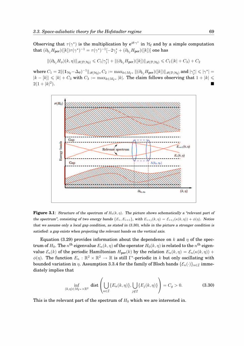
3.3. Space-adiabatic theory for the Hofstadter regime 69
Observing that τ(γ∗) is the multiplication by eiθ·γ∗
in Hf and by a simple computationthat (∂kj
Hper)([k])τ(γ∗)−1 = τ(γ∗)−1[−2γ∗j + (∂kj
Hper)([k])] one has
‖(∂kjHφ)(k, η)‖B(D,Hf) 6 C1|γ∗j | + ‖(∂kj
Hper)([k])‖B(D,Hf) 6 C1(|k| + C3) + C2
where C1 = 2‖(1Hf−∆θ)−1‖B(Hf), C2 := maxk∈MΓ∗ ‖(∂kj
Hper)([k])‖B(D,Hf) and |γ∗j | 6 |γ∗| =
|k − [k]| 6 |k| + C3 with C3 := maxk∈MΓ∗ |k|. The claim follows observing that 1 + |k| 6
2(1 + |k|2).
Figure 3.1: Structure of the spectrum of H0(k, η). The picture shows schematically a “relevant part of
the spectrum”, consisting of two energy bands E∗, E∗+1, with E∗+j(k, η) = E∗+j(κ(k, η)) + φ(η). Notice
that we assume only a local gap condition, as stated in (3.30), while in the picture a stronger condition is
satisfied: a gap exists when projecting the relevant bands on the vertical axis.
Equation (3.29) provides information about the dependence on k and η of the spec-trum ofH0. The nth eigenvalueEn(k, η) of the operatorH0(k, η) is related to the nth eigen-value En(k) of the periodic Hamiltonian Hper(k) by the relation En(k, η) = En(κ(k, η)) +
φ(η). The function En : R2 × R2 → R is still Γ∗-periodic in k but only oscillating withbounded variation in η. Assumption 3.3.4 for the family of Bloch bands En(·)n∈I imme-diately implies that
inf(k,η)∈MΓ∗×R2
dist
⋃
n∈IEn(k, η),
⋃
j /∈IEj(k, η)
= Cg > 0. (3.30)
This is the relevant part of the spectrum of H0 which we are interested in.
70 3. Derivation of Harper and Hofstadter models
According to the general theory (Teufel 2003, Appendices A and B), one has that
Opε(H0) =1
2
[−i∇θ + k −AΓ(θ) −A0 (iε∇k) − ιq
1
2e⊥ ∧ (iε∇k)
]2
+VΓ(θ)+φ (iε∇k) (3.31)
defines a linear operator from S(R2,D) in S(R2,Hf) and by duality it extends to a con-tinuous mapping Opε(H0) : S ′(R2,D) → S ′(R2,Hf) (with an abuse of notation we use thesame symbol for the extended operator). The τ -equivariance assures that Opε(H0)ϕ([k]−γ∗) = τ(γ∗)Opε(H0)ϕ([k]) (Teufel 2003, Proposition B.3). Since Opε(H0) preserves τ -equivariance, then it can be restricted to an operator on the domain ZH2
M(R2) ⊂ S ′(R2,D)
which is the domain of self-adjointness of HZ , according to (3.18). To conclude thatOpε(H0), restricted to ZH2
M(R2), agrees with HZ it is enough to recall that i∇τk is de-
fined as i∇k restricted to its natural domain H1(R2,D
)∩ Hτ and to use the spectral
calculus. These arguments justify the following:
PROPOSITION 3.3.13. The Hamiltonian HZ , defined by (3.18), agrees on its domain ofdefinition with the Weyl quantization of the operator-valued symbol H0 defined by (3.28).
With a little abuse of notation, we refer to this result by writing HZ = Opε(H0).
3.3.6 Main result: effective dynamics for weak magnetic fields
Let Aε and Bε be ε-dependent (possibly unbounded) linear operators in H. We writeAε = Bε + O0(ε
∞) if: for any N ∈ N there exist a positive constant CN such that
‖Aε −Bε‖B(H) ≤ CN εN (3.32)
for every ε ∈ [0, ε0). Notice that, though the operators are unbounded, the difference isrequired to be a bounded operator.
We refer to Appendices A and B of (Teufel 2003) for the basic terminology concerningpseudodifferential operators, and in particular as for the notions of principal symbol,asymptotic expansion, resummation, Moyal product.
THEOREM 3.3.14. Let Assumptions 3.2.2, 3.2.3, 3.3.4 and 3.3.5 be satisfied and letEn(·)n∈I (with |I| = m) be an isolated family of energy bands for H0 satisfying con-dition (3.30). Then:
1. Almost-invariant subspace: there exist an orthogonal projection Πε ∈ B(Hτ ), withΠε = Opε(π) + O0(ε
∞) and the symbol π(k, η) ≍ ∑∞j=0 ε
j πj(k, η) having principal partπ0(k, η) = PI(k −A(η)), so that
[HZ ; Πε] = O0(ε∞).
In particular for any N ∈ N there exist a CN such that
‖(1 − Πε) e−itεHZ
Πε‖ ≤ CN εN |t| (3.33)
3.3. Space-adiabatic theory for the Hofstadter regime 71
for ε sufficiently small, t ∈ R.
2. Effective dynamics: let Href = L2(MΓ∗ , d2k) ⊗ Hf, πr as defined above (3.24) andΠr = 1L2(MΓ∗ ) ⊗ πr ∈ B(Href). Then there exist a unitary operator
Uε : Hτ → Href
such that
(i) Uε = Opε(u) + O0(ε∞), where the symbol u ≍∑∞
j=0 εjuj has principal part u0 given
by (3.24) with k replaced by κ(k, η);
(ii) Πr = Uε Πε Uε−1;
(iii) posing K := ΠrHref, one has
Uε ΠεHZ Πε U
−1ε = Hε
eff + O0(ε∞) ∈ B(K)
withHεeff = Opε(h) and h a resummation of the formal symbol u ♯ π ♯H0 ♯ π♯u
−1 (thusalgorithmically computable at any finite order). Moreover,
‖(e−i tεHZ − U−1
ε e−itεHε
eff Uε) Πε‖ ≤ CN′ εN (ε+ |t|). (3.34)
REMARK 3.3.15. The previous theorem and the following proof generalize straightfor-wardly to any dimension d ∈ N. We prefer to state it only in the case d = 2 in view of theapplication to the QHE and of the comparison with the results in Section 3, the latterbeing valid only for d = 2. ♦
Proof of Theorem 3.3.14
Step 1. Almost-invariant subspace
The proof of the existence of the super-adiabatic projection is very close to the proof ofProposition 1 of (Panati et al. 2003a), so we only sketch the strategy and emphasize themain differences with respect to that proof.
First of all, one constructs a formal symbol π ≍ ∑∞j=0 ε
j πj (the Moyal projection)such that: (i) π♯π ≍ π; (ii) π† = π; (iii) H0♯π ≍ π♯H0 where ≍ denotes the asymptoticequivalence of formal series.
The symbol π is constructed recursively at any order j ∈ N starting from π0 and H0. Onefirstly show the uniqueness of π (Panati et al. 2003b, Lemma 2.3). The uniqueness allowsus to construct π locally, i.e. in a neighborhood of some point z0 := (k0, η0) ∈ R2 × R2.From the continuity of the map k 7→ Hper(k) and the condition (3.23) it follows thatthere exists a neighborhood Uk0 of k0 such that for every k ∈ Uk0 the set En(k)n∈I canbe enclosed by a positively-oriented circle Σ(k0) ⊂ C independent of k. Moreover it ispossible to choose Σ(k0) in such a way that: it is symmetric with respect to the real axis;
72 3. Derivation of Harper and Hofstadter models
dist(Σ(k0), σ(Hper(k))) > 14Cg for all k ∈ Uk0 ; Radius(Σ(k0)) 6 Cr with Cr independent of
k0; Σ(k0 − γ∗) = Σ(k0) for any γ∗ ∈ Γ∗.With the notation of Section 3.3.4 we have H0 = Hφ κ with Hφ(k, η) := Hper(k) + φ(η).Let Λ(k0, η0) := Σ(k0) + φ(η0) denote the translation of the circle Σ(k0) by φ(η0) ∈ R andpose Λ := Λ κ. From the smoothness of φ it follows that there exists a neighborhoodUz0 ⊂ R2 × R2 of z0 such that dist(Λ(z0), σ(H0(z))) > 1
4Cg for all z ∈ Uz0 . Moreover Λ(z0)
is symmetric with respect to the real axis, has radius bounded by Cr and is Γ∗-periodicin the variable κ = k −A(η) (see Figure 3.1).
We proceed by using the Riesz formula, namely by posing
πj(z) :=i
2π
∮
Λ(z0)dλ Rj(λ, z) on Uz0
where Rj(λ, ·) denotes the j-th term in the Moyal resolvent R(λ, ·) =∑∞
j=0 εjRj(λ, ·) (also
known as the parametrix), defined by the request that
(H0(·) − λ1D)♯R(λ, ·) = 1Hf , R(λ, ·)♯(H0(·) − λ1D) = 1D on Uz0 .
Each term Rj is computed by a recursive procedure starting from R0(λ, ·) := (H0(·) −λ1D)−1, as illustrated in (Gérard et al. 1991). Following (Panati et al. 2003a, equations(30) and (31)) one obtains that
Rj(λ, z) = −R0(λ, z) Lj(λ, z) (3.35)
where Lj is the (j − 1)-th order obstruction for R0 to be the Moyal resolvent, i.e.
(H0(·) − λ1D)♯
(j−1∑
n=0
εn Rj(λ, ·))
= 1Hf + εj Lj(·) + O(εj+1). (3.36)
At the first order L1 = − i2 H0, R0k,η, with ·, ·k,η the Poisson brackets.
The technical (and crucial) part of the proof is to show that
πj ∈ Svκ;τ (B(Hf,D)) ∩ S1κ;τ (B(Hf))
for all j ∈ N, with v(k, η) := (1+|k|2). By means of the recursive construction eachRj(λ, ·)inherits the special τ -equivariance from the principal symbol R0(λ, ·) = ((Hφ κ)(·) −λ1D)−1. The special periodicity in κ of the domain of integration Λ(·) which appears inthe Riesz formula assures also the special τ -equivariance of each πj(·).Since ‖(∂αz πj)(z)‖ 6 2πCr supλ∈Λ(z0) ‖∂αz (Rj)(λ, z)‖ ( means either B(Hf) or B(Hf;D),α ∈ N4 is a multiindex and ∂αz := ∂α1
k1∂α2k2∂α3η1 ∂
α4η2 ), we need only to prove that Rj(λ, ·) ∈
Svκ;τ (B(Hf,D)) ∩ S1κ;τ (B(Hf)) uniformly in λ. This is the delicate point of the proof.
First of all, from the definition of Λ(z0) it follows that
‖R0(λ, z)‖B(Hf) = [dist(λ, σ(H0(z)))]−1 6 4/Cg
3.3. Space-adiabatic theory for the Hofstadter regime 73
uniformly in λ. Let σ ∈ N4, with |σ| = 1. One observes that ∂σzR0(λ, z) = −R0(λ, z)Nσz (λ, z)
with Nαz (λ, z) := ∂αzH0(z) R0(λ, z). From the relation
∂σzNαz = Nα+σ
z −Nαz N
σz
and an inductive argument, it follows the chain rule
∂αz R0 = R0
∑ωβ1...β|α|
Nβ1z . . . N
β|α|z
where β1, . . . , β|α| ∈ N4, |α| := α1 + . . .+ α4, ωβ1...β|α|= ±1 is a suitable sign function and
the sum runs over all the combinations of multiindices such that β1 + . . .+ β|α| = α withthe convention N0
z = 1. The chain rule implies that R0 ∈ S1κ;τ (B(Hf)) provided that
‖Nαz ‖B(Hf) = ‖∂αzH0 R0‖B(Hf) 6 Cα uniformly in λ.
The latter condition is true since ‖(∂αzH0)(k, η) R0(λ, k, η)‖B(Hf) 6 (g κ)(k, η), for asuitable g(k, η), Γ∗-periodic in k and bounded in η; the latter claim can be checked as inProposition 3.3.12.
Similarly, to prove that R0 ∈ Svκ;τ (B(Hf,D)) we need to show that
‖R0 Nαz ‖B(Hf,D) = ‖(1Hf − ∆θ) R0 N
αz ‖B(Hf) 6 Cα v
′(·)
uniformly in λ. SinceNαz is bounded on Hf it is sufficient to show that ‖(1Hf−∆θ)R0(λ; z)‖B(Hf) 6
C ′α v
′(z). Observe that ‖(1Hf−∆θ)R0(λ, [κ]−γ∗; η)‖B(Hf) = ‖(1Hf−∆θ)τ(γ∗)−1R0(λ, [κ]; η)‖B(Hf).
The commutation relation
−∆θτ(γ∗)−1 = τ(γ∗)−1
(|γ∗|2 + i2γ∗ · ∇θ − ∆θ
)
and the straightforward bound
‖(|γ∗|2 + i2γ∗ · ∇θ − ∆θ
)(1Hf − ∆θ)
−1‖B(Hf) 6 C(1 + |γ∗|2) 6 C ′(1 + |κ(k, η)|2)
imply‖(1Hf − ∆θ)R0(λ, z)‖B(Hf) 6 C ′
α v′(z)‖(1Hf − ∆θ)R0(λ, [κ]; η)‖B(Hf)
with v′ := v κ. Finally observe that
‖(1Hf − ∆θ)R0(λ, [κ]; η)‖B(Hf) 6 C([κ]; η) 6 C ′′. (3.37)
The first inequality above follows by an expansion on the Fourier basis, for fixed [κ]
and η; the second follows from the fact that [κ] takes values on a compact set and theexplicit dependence on η is through the bounded function φ. The bound (3.37) impliesthat R0 ∈ Svκ;τ (B(Hf,D)) ∩ S1
κ;τ (B(Hf)) uniformly in λ.To prove that Rj ∈ S1
κ;τ (B(Hf)), we observe that for any α ∈ Nd one has
∂αz Rj(λ, z) = R0(λ, z) Mαz;j(λ, z)
where Mαz;j is a linear combination of terms which are product of Nβ
z and ∂δzLj with|β|, |δ| 6 |α|. Thus, it is sufficient to prove that Lj ∈ S1
κ;τ (B(Hf)) for every j ∈ N. The
74 3. Derivation of Harper and Hofstadter models
latter claim is proved by induction on j ∈ N. Referring to (3.35), one has trivially thatL1 ∈ S1
κ;τ (B(Hf)). Lj+1 is a linear combination of products of Nαz (with 0 6 |α| 6 j + 1)
and Mβz,i (with |β| + i = j + 1 and 0 6 i 6 j). Then the induction hypothesis on Li for all
i = 1, . . . , j implies that Lj+1 is in S1κ;τ (B(Hf)).
Finally observing that ‖∂αz Rj‖B(Hf,D) 6 ‖Mαz;j‖B(Hf) ‖R0‖B(Hf,D) and using the fact
that R0 ∈ Svκ;τ (B(Hf,D)) it follows that Rj ∈ Svκ;τ (B(Hf,D)) ∩ S1κ;τ (B(Hf)) uniformly in
λ, for all j ∈ N.As explained in Section 3.3.4, we can apply the result of Proposition B.4 in (Teufel
2003) to special τ -equivariant symbols obtaining H0♯π ∈ Sv2
κ;τ (B(Hf)). However the τ -equivariance of H0♯π and its derivatives implies that the norms are bounded in z, henceH0♯π ∈ S1
κ;τ (B(Hf)) which implies by adjointness also π♯H0 ∈ S1κ;τ (B(Hf)). By construc-
tion [HZ ; Opε(π)] = Opε(H0♯π − π♯H0) = O0(ε∞) where the remainder is bounded in the
norm of B(Hτ ).The operator Opε(π) is only approximately a projection, since Opε(π)2 = Opε(π♯π) =
Opε(π) + O0(ε∞). We obtain the super-adiabatic projection Πε by using the trick in
(Nenciu and Sordoni 2004). Indeed, one notices that, for ε sufficiently small, the spec-trum of Opε(π) does not contain e.g. the points 1/2 and 3/2. Thus, the formula
Πε =i
2π
∮
|z−1|=1/2(Opε(π) − z)−1. (3.38)
yields an orthogonal projector such that Πε = Opε(π) + O0(ε∞).
Finally, equation (3.33) follows by observing that [HZ ; Πε] = O0(ε∞) implies
[e−itεHZ
; Πε] = O0(ε∞|t|)
as proved in (Teufel 2003, Corollary 3.3).
Step 2. Construction of the intertwining unitary
The construction of the intertwining unitary follows as in the proof of Proposition 2 of(Panati et al. 2003a). Firstly one constructs a formal symbol u ≍∑∞
j=0 εjuj such that: (i)
u†♯u = u♯u† = 1Hf ; (ii) u♯π♯u† = πr.The existence of such a symbol follows from a recursive procedure starting from u0
and using the expansion of π ≍∑∞j=0 ε
jπj obtained above. However, the symbol u whichcomes out of this procedure is not unique.
Since u0 is right τ -covariant (c.f. end of Section 3.3.3) in κ, then one can prove byinduction that the same is also true for all the symbols uj and hence for the full symbol u.Finally, since u0 ∈ S1(B(Hf)) one deduces by induction also uj ∈ S1(B(Hf)) for all j ∈ N.The quantization of this symbol is an element of B(Hτ ,Href) satisfying the followingproperties:
(i) Opε(u)Opε(u)† = 1Href + O0(ε
∞),
(ii) Opε(u)†Opε(u) = 1Hτ + O0(ε
∞),
3.3. Space-adiabatic theory for the Hofstadter regime 75
(iii) Opε(u)ΠεOpε(u)† = Πr + O0(ε
∞).
Nevertheless Opε(u) can be modified by an O0(ε∞) term using the same technique of
Lemma 3.3 (Step II) in (Panati et al. 2003b) to obtain the true unitary Uε.
Step 3. Effective dynamics
The last step of the proof is identical to the corresponding part of (Panati et al. 2003a,Proposition 3).
3.3.7 Hofstadter-like Hamiltonians
We now focus on the special case of a single isolated energy band E∗, i.e. m = 1, andwe comment on the relation between the effective Hamiltonian, the celebrated
Peierls’ substitution and Hofstadter-like Hamiltonians (c.f. Sections 2.1 and 2.3).
In this special case, π0(κ) = |ψ∗(κ)〉〈ψ∗(κ)| and u0(κ) = |χ〉〈ψ∗(κ)| + u⊥0 where ψ∗(k) isthe eigenvector of Hper(k) corresponding to the eigenvalue E∗(k). Let h ∈ S1(B(Hf)) be aresummation of the formal symbol u♯π♯H0♯π♯u
−1. A straightforward computation yields
h0 = u0 π0H0 π0 u†0 = |χ〉〈ψ∗| |ψ∗〉〈ψ∗| H0 |ψ∗〉〈ψ∗| |ψ∗〉〈χ| = E∗ πr.
Since πr is one-dimensional, h0 can be regarded as a scalar-valued symbol with explicitexpression
h0(k, η) = E∗(k, η) = E∗ (k −A(η)) + φ(η).
By considering the quantization of the latter, the effective one-band Hamiltonian reads
Opε(h0) = E∗(k, iε∇k) = E∗ (k −A(iε∇k)) + φ(iε∇k). (3.39)
The latter formula corresponds to the momentum-space reformulation of the well-knownPeierls’ substitution (Peierls 1933, Ashcroft and Mermin 1976).
To illustrate this point, we specialize to the case of a uniform external magnetic fieldand zero external electric field, setting φ = 0 and A0 = 0 in (3.28). The leading ordercontribution to the dynamics in the almost invariant subspace is therefore given by abounded operator, acting on the reference Hilbert space L2(MΓ∗ , d2k), defined as thequantization (in the sense of Section 3.3.5) of the function E∗ κ : (k, η) 7→ E∗(k − A(η)),defined on Td × Rd.
Loosely speaking, the above procedure corresponds to the following “substitutionrule”: one may think to quantize the smooth function E∗ : Td → R by formally replacingthe variables (k1, k2) with the operators (K ′
1 ,K′
2 ) defined by
K′
1 := k1 +i
2(ιqε)
∂
∂k2, K
′2 := k2 −
i
2(ιqε)
∂
∂k1, (3.40)
regarded as unbounded operators acting on L2(MΓ∗ , d2k). To make this procedure rig-orous, one can expand E∗ in its Fourier series, i.e. E∗(k) =
∑n,m∈Z
cn,m ei2π(na+mb)·k and
76 3. Derivation of Harper and Hofstadter models
define the Peierls quantization of E∗ as the operator obtained by the same series expan-sion with the phases ei2π(na+mb)·k replaced by the unitary operators ei2π(na+mb)·K ′
(theseries is norm-convergent, in view of the regularity of E∗). This fixes uniquely the pre-scription for the quantization.
To streamline the notation, one introduces new coordinates ξ1 := 2π(a · k) and ξ2 :=
2π(b · k) such that the function E ′∗, E ′
∗(ξ1, ξ2) := E∗(k(ξ)) becomes (2πZ)2-periodic. Thechange of variables induces a unitary map from L2(MΓ∗
2, d2k) to L2(T2, d2ξ) which inter-twines the operators (3.40) with the operators (recall ε = 2π/hB)
K1 := ξ1 + iπ
(ιqhB
)∂
∂ξ2, K2 := ξ2 − iπ
(ιqhB
)∂
∂ξ1, (3.41)
so that 2π(a · K ′) 7→ K1 and 2π(b · K ′) 7→ K2.Let F : T2 → C be sufficiently regular that its Fourier series
F (ξ1, ξ2) =∑
n,m∈Z
fn,mei(nξ1+mξ2)
is uniformly-convergent. We define the Peierls quantization of F as
F :=∑
n,m∈Z
fn,mei(nK1+mK2).
Let U0 = eiK1 and V0 = eiK2 (Hofstadter unitaries), acting on H0 := L2(T2, d2ξ) as
(U0ψ)(ξ1, ξ2) = eiξ1ψ (ξ1, ξ2 − πιqǫ0) , (V0ψ)(ξ1, ξ2) = eiξ2ψ (ξ1 + πιqǫ0, ξ2) . (3.42)
where ǫ0(B) := 1/hB We regard (3.42) as the definition of the two unitaries, so there isno need to specify the domain of definition of the generators (3.41). Thus the Peierlsquantization of the function F defines a bounded operator on H0 given, in terms of theHofstadter unitaries, by
F =
+∞∑
n,m=−∞fn,m eiπnm(ιqǫ0) Un0 Vm0 , (3.43)
where the fundamental commutation relation U0V0 = e−i2π(ιqǫ0) V0U0 has been used.Formula (3.43) defines a Hofstadter-like Hamiltonian with deformation parameter −ιqǫ0(c.f. Section 2.1). Summarizing, we draw the following
CONCLUSION 3.3.16. Under the assumption of Theorem 3.3.14, for every VΓ ∈ L2loc(R
2, d2r),in the Hofstadter regime (hB → ∞), the dynamics generated by the Hamiltonian HBL (2.1)in the subspace related to a single isolated Bloch band, is approximated up to an errorof order ǫ0 = 1/hB (and up to a unitary transform) by the dynamics generated on the ref-erence Hilbert space H0 := L2(T2, d2ξ) by a Hofstadter-like Hamiltonian, i.e. by a powerseries in the Hofstadter unitaries U0 and V0 defined by (3.42).
3.4. Space-adiabatic theory for the Harper regime 77
3.4 Space-adiabatic theory for the Harper regime
3.4.1 Adiabatic parameter for strong magnetic fields
We now consider the case of a strong external magnetic field. Since we are interestedin the limit B → +∞ we set A0 = 0 and Φ = 0 in the Hamiltonian (3.1). By
exploiting the gauge freedom, we choose
∇r · AΓ = 0,
∫
MΓ
AΓ(r) d2r = 0, (3.44)
this choice being always possible (Sobolev 1997). Let us denote by Qr = (Qr1 , Qr2) themultiplication operators by r1 and r2 and with Pr = (Pr1 , Pr2) = −iℏ∇r. Taking intoaccount conditions (3.44) and A0 = 0, φ = 0, the Hamiltonian (3.1) is rewritten as
HBL =1
2m
[(Pr1 +
qB
2cQr2
)2
+
(Pr2 −
qB
2cQr1
)2]
+ VΓ(Qr) + W(Qr) (3.45)
where
VΓ(Qr) = VΓ(Qr) +q2
2mc2|AΓ(Qr)|2 (3.46)
and
W(Qr, Pr) = − q
mc(AΓ)1(Qr)
[Pr1 +
qB
2cQr2
]− q
mc(AΓ)2(Qr)
[Pr2 −
qB
2cQr1
](3.47)
with (AΓ)1 and (AΓ)2 the Γ-periodic components of the vector potential AΓ. The first of(3.44) assures that W is a symmetric operator.
REMARK 3.4.1. Observe that H0BL := HBL − W corresponds to a Bloch-Landau Hamilto-
nian without Γ-periodic vector potential and with a “modified” Γ-periodic scalar potentialVΓ. Then, the presence of a Γ-periodic vector potential AΓ can be described through anon-periodic “perturbation” W of the Bloch-Landau Hamiltonian H0
BL. Obviously AΓ = 0
implies VΓ = VΓ and W = 0. ♦
It is useful to define two new pairs of canonical dimensionless operators:
(fast)
K1 := − 1
2δb∗ ·Qr − ιq
δ
ℏa · Pr
K2 :=1
2δa∗ ·Qr − ιq
δ
ℏb · Pr
(slow)
G1 :=1
2b∗ ·Qr − ιq
δ2
ℏa · Pr
G2 :=1
2a∗ ·Qr + ιq
δ2
ℏb · Pr
(3.48)
where δ :=√
ℏB =√
Φ0/2πZΦB according to the notation introduced in Section 3.1. Sinceδ2 ∝ 1/B, the limit of strong magnetic field corresponds to δ → 0. We consider δ as theadiabatic parameter in the Harper regime. A direct computation shows that
[K1;K2] = iιq 1Hphy , [G1;G2] = iιq δ21Hphy , [Kj ;Gk] = 0, j, k = 1, 2. (3.49)
78 3. Derivation of Harper and Hofstadter models
These new variables are important for three reasons:
(a) they make evident a separation of scales between the slow degrees of freedomrelated to the the dynamics induced by the periodic potential and the fast degreesof freedom related to the cyclotron motion induced by the external magnetic field.Indeed, for VΓ = 0, the fast variables (K1,K2) (the kinetic momenta) describe thekinetic energy of the cyclotron motion, while the slow variables (G1, G2) correspondsemiclassically to the center of the cyclotron orbit and are conserved quantities.
(b) The new variables are dimensionless. According to the notation used in Section3.3.1 let HBL := 1/E0HBL be the dimensionless Bloch-Landau Hamiltonian withE0 := ℏ2/mΩΓ the natural unit of energy.
(c) The use of the new variables simplifies the expression of the Γ-periodic functionsappearing in HBL. Indeed, a∗ ·Qr = G2 + δ K2 and b∗ ·Qr = G1 − δ K1, hence if fΓ
is any Γ-periodic function one has
fΓ(Qr) = f(G2 + δ K2, G1 − δ K1) (3.50)
where f is the Z2-periodic function related to fΓ.
In terms of the new variables (3.48), the Hamiltonian HBL reads
HBL =1
δ2Ξ(K1,K2) + V (G2 + δ K2, G1 − δ K1) +
1
δW (K1, G1,K2, G2) (3.51)
whereΞ(K1,K2) :=
1
2ΩΓ
[|a|2K2
2 + |b|2K12 − a · b K1;K2
](3.52)
is a quadratic function of the operators K1 and K2 (·; · denotes the anticommutator),V is the Z2-periodic function related to the Γ-periodic function 1/E0VΓ and W denotes thefunction 1/E0W with respect the new canonical pairs, namely
W (K1, G1,K2, G2) = f1 (G2 + δ K2, G1 − δ K1)K1 − f2 (G2 + δ K2, G1 − δ K1)K2 (3.53)
where f1 and f2 are the Z2-periodic dimensionless functions
f1(a∗ · r, b∗ · r) := 2π
ZΩΓ
Φ0(a∗ · AΓ)(r) and f2(a
∗ · r, b∗ · r) := 2πZΩΓ
Φ0(b∗ · AΓ)(r).
An easy computation shows that the first gauge condition of (3.44) is equivalent to
∂f1
∂x1(x1, x2) +
∂f2
∂x2(x1, x2) = 0. (3.54)
Obviously W is a symmetric operator, since W is symmetric.The problem has a natural time-scale which is fixed by the cyclotron frequency ωc =
|q|Bmc . With respect to the (fast) ultramicroscopic time-scale τ := ωcs, equation (3.4) be-
comes
i1
δ2∂
∂τψ = HBLψ, δ2 =
E0
ℏωc. (3.55)
Thus the physically relevant Hamiltonian is
HδBL := δ2 HBL = Ξ(K1,K2) + δ W (K1, G1,K2, G2) + δ2 V (G2 + δ K2, G1 − δ K1) . (3.56)
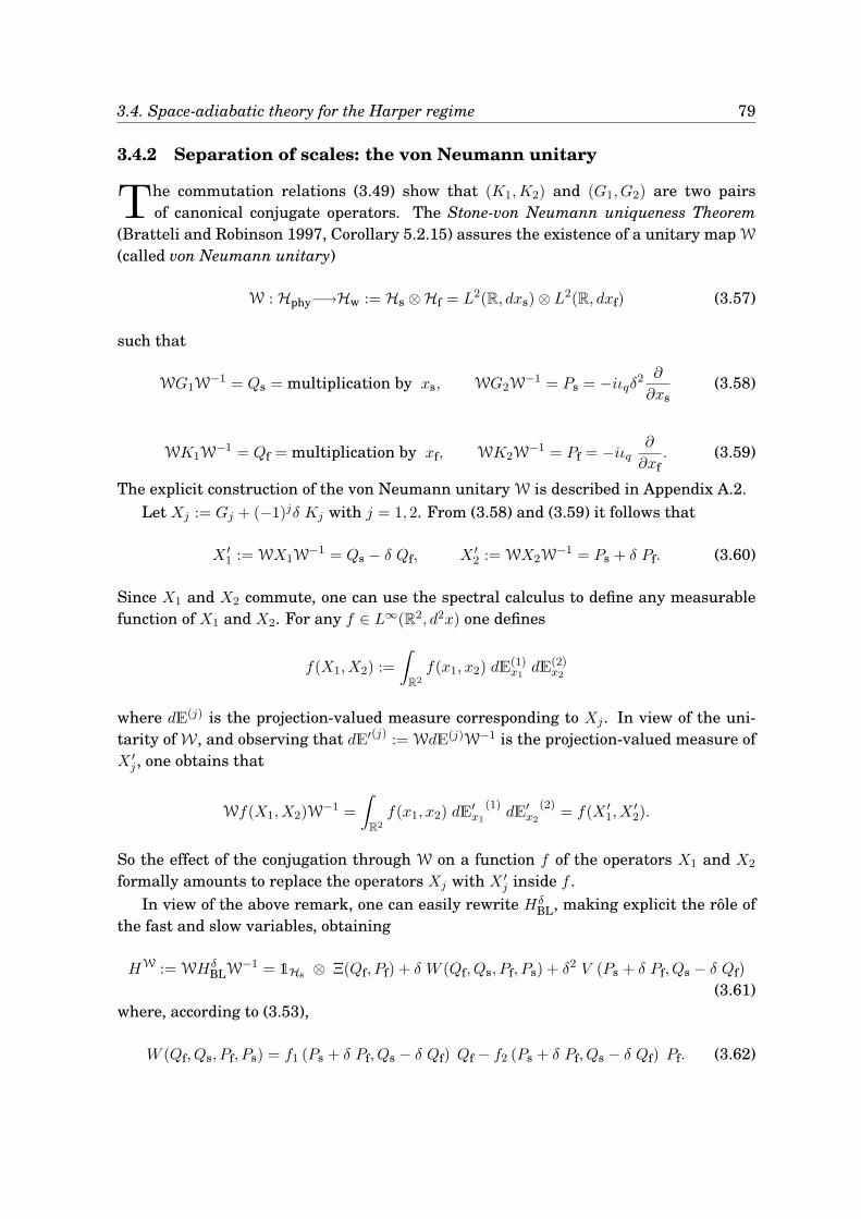
3.4. Space-adiabatic theory for the Harper regime 79
3.4.2 Separation of scales: the von Neumann unitary
The commutation relations (3.49) show that (K1,K2) and (G1, G2) are two pairsof canonical conjugate operators. The Stone-von Neumann uniqueness Theorem
(Bratteli and Robinson 1997, Corollary 5.2.15) assures the existence of a unitary map W
(called von Neumann unitary)
W : Hphy−→Hw := Hs ⊗Hf = L2(R, dxs) ⊗ L2(R, dxf) (3.57)
such that
WG1W−1 = Qs = multiplication by xs, WG2W
−1 = Ps = −iιqδ2∂
∂xs(3.58)
WK1W−1 = Qf = multiplication by xf, WK2W
−1 = Pf = −iιq∂
∂xf. (3.59)
The explicit construction of the von Neumann unitary W is described in Appendix A.2.
Let Xj := Gj + (−1)jδ Kj with j = 1, 2. From (3.58) and (3.59) it follows that
X ′1 := WX1W
−1 = Qs − δ Qf, X ′2 := WX2W
−1 = Ps + δ Pf. (3.60)
Since X1 and X2 commute, one can use the spectral calculus to define any measurablefunction of X1 and X2. For any f ∈ L∞(R2, d2x) one defines
f(X1, X2) :=
∫
R2
f(x1, x2) dE(1)x1
dE(2)x2
where dE(j) is the projection-valued measure corresponding to Xj . In view of the uni-tarity of W, and observing that dE′(j) := WdE(j)W−1 is the projection-valued measure ofX ′j , one obtains that
Wf(X1, X2)W−1 =
∫
R2
f(x1, x2) dE′x1
(1)dE′
x2
(2)= f(X ′
1, X′2).
So the effect of the conjugation through W on a function f of the operators X1 and X2
formally amounts to replace the operators Xj with X ′j inside f .
In view of the above remark, one can easily rewrite HδBL, making explicit the rôle of
the fast and slow variables, obtaining
HW := WHδBLW−1 = 1Hs ⊗ Ξ(Qf, Pf) + δ W (Qf, Qs, Pf, Ps) + δ2 V (Ps + δ Pf, Qs − δ Qf)
(3.61)where, according to (3.53),
W (Qf, Qs, Pf, Ps) = f1 (Ps + δ Pf, Qs − δ Qf) Qf − f2 (Ps + δ Pf, Qs − δ Qf) Pf. (3.62)
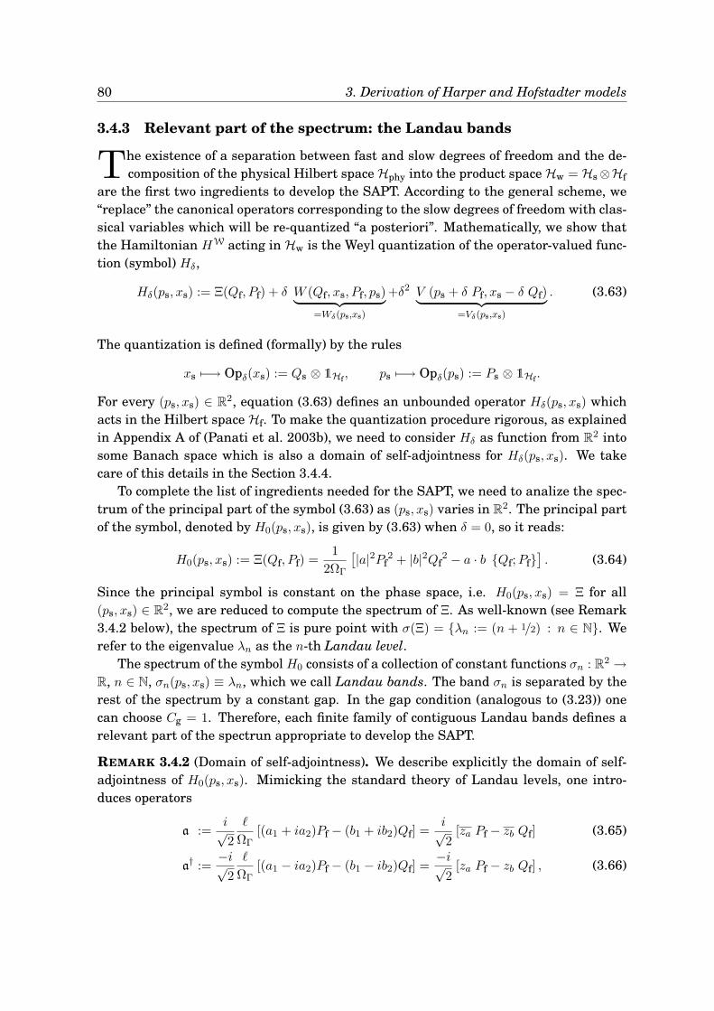
80 3. Derivation of Harper and Hofstadter models
3.4.3 Relevant part of the spectrum: the Landau bands
The existence of a separation between fast and slow degrees of freedom and the de-composition of the physical Hilbert space Hphy into the product space Hw = Hs ⊗Hf
are the first two ingredients to develop the SAPT. According to the general scheme, we“replace” the canonical operators corresponding to the slow degrees of freedom with clas-sical variables which will be re-quantized “a posteriori”. Mathematically, we show thatthe Hamiltonian HW acting in Hw is the Weyl quantization of the operator-valued func-tion (symbol) Hδ,
Hδ(ps, xs) := Ξ(Qf, Pf) + δ W (Qf, xs, Pf, ps)︸ ︷︷ ︸=Wδ(ps,xs)
+δ2 V (ps + δ Pf, xs − δ Qf)︸ ︷︷ ︸=Vδ(ps,xs)
. (3.63)
The quantization is defined (formally) by the rules
xs 7−→ Opδ(xs) := Qs ⊗ 1Hf , ps 7−→ Opδ(ps) := Ps ⊗ 1Hf .
For every (ps, xs) ∈ R2, equation (3.63) defines an unbounded operator Hδ(ps, xs) whichacts in the Hilbert space Hf. To make the quantization procedure rigorous, as explainedin Appendix A of (Panati et al. 2003b), we need to consider Hδ as function from R2 intosome Banach space which is also a domain of self-adjointness for Hδ(ps, xs). We takecare of this details in the Section 3.4.4.
To complete the list of ingredients needed for the SAPT, we need to analize the spec-trum of the principal part of the symbol (3.63) as (ps, xs) varies in R2. The principal partof the symbol, denoted by H0(ps, xs), is given by (3.63) when δ = 0, so it reads:
H0(ps, xs) := Ξ(Qf, Pf) =1
2ΩΓ
[|a|2Pf
2 + |b|2Qf2 − a · b Qf;Pf
]. (3.64)
Since the principal symbol is constant on the phase space, i.e. H0(ps, xs) = Ξ for all(ps, xs) ∈ R2, we are reduced to compute the spectrum of Ξ. As well-known (see Remark3.4.2 below), the spectrum of Ξ is pure point with σ(Ξ) = λn := (n + 1/2) : n ∈ N. Werefer to the eigenvalue λn as the n-th Landau level.
The spectrum of the symbol H0 consists of a collection of constant functions σn : R2 →R, n ∈ N, σn(ps, xs) ≡ λn, which we call Landau bands. The band σn is separated by therest of the spectrum by a constant gap. In the gap condition (analogous to (3.23)) onecan choose Cg = 1. Therefore, each finite family of contiguous Landau bands defines arelevant part of the spectrun appropriate to develop the SAPT.
REMARK 3.4.2 (Domain of self-adjointness). We describe explicitly the domain of self-adjointness of H0(ps, xs). Mimicking the standard theory of Landau levels, one intro-duces operators
a :=i√2
ℓ
ΩΓ[(a1 + ia2)Pf − (b1 + ib2)Qf] =
i√2
[za Pf − zb Qf] (3.65)
a† :=−i√
2
ℓ
ΩΓ[(a1 − ia2)Pf − (b1 − ib2)Qf] =
−i√2
[za Pf − zb Qf] , (3.66)
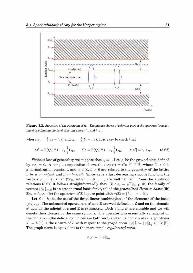
3.4. Space-adiabatic theory for the Harper regime 81
Figure 3.2: Structure of the spectrum of H0. The picture shows a “relevant part of the spectrum” consist-
ing of two Landau bands of constant energy λ∗ and λ∗+1.
where za := 1ℓ (a1 − ia2) and zb := 1
ℓ (b1 − ib2). It is easy to check that
aa† = Ξ(Qf, Pf) + ιq1
21Hf , a†a = Ξ(Qf, Pf) − ιq
1
21Hf , [a; a†] = ιq 1Hf . (3.67)
Without loss of generality, we suppose that ιq = 1. Let ψ0 be the ground state definedby aψ0 = 0. A simple computation shows that ψ0(xf) = Ce−(β−iα)x2
f , where C > 0 isa normalization constant, and α ∈ R, β > 0 are related to the geometry of the latticeΓ by α := a·b/2|a|2 and β := ΩΓ/2|a|2. Since ψ0 is a fast decreasing smooth function, thevectors ψn := (n!)−
12 (a†)nψ0, with n = 0, 1, . . ., are well defined. From the algebraic
relations (3.67) it follows straightforwardly that: (i) aψn =√nψn−1; (ii) the family of
vectors ψnn∈N is an orthonormal basis for Hf called the generalized Hermite basis; (iii)Ξψn = λnψn; (iv) the spectrum of Ξ is pure point with σ(Ξ) = λn : n ∈ N.
Let L ⊂ Hf be the set of the finite linear combinations of the elements of the basisψnn∈N. The unbounded operators a, a† and Ξ are well defined on L and on this domaina† acts as the adjoint of a and Ξ is symmetric. Both a and a† are closable and we willdenote their closure by the same symbols. The operator Ξ is essentially selfadjoint onthe domain L (the deficiency indices are both zero) and so its domain of selfadjointnessF := D(Ξ) is the closure of L with respect to the graph norm ‖ψ‖2
Ξ := ‖ψ‖2Hf
+ ‖Ξψ‖2Hf
.The graph norm is equivalent to the more simple regularized norm
‖ψ‖F := ‖Ξψ‖Hf .
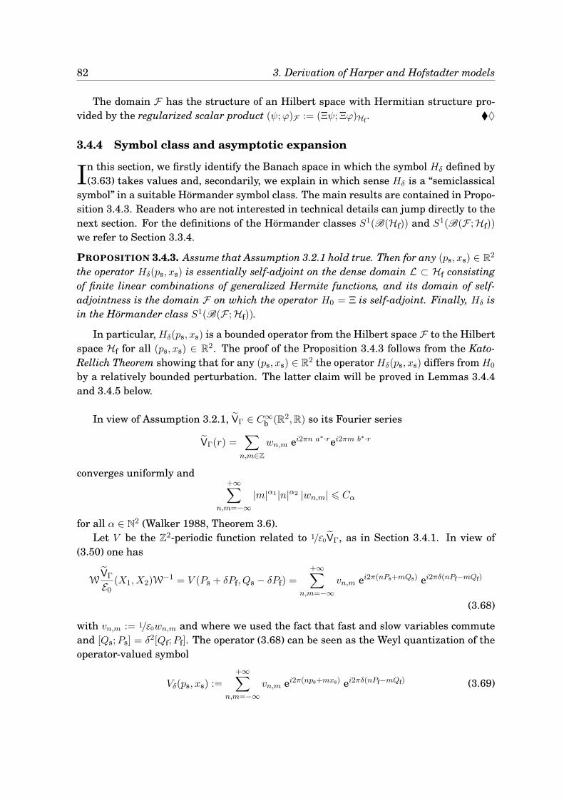
82 3. Derivation of Harper and Hofstadter models
The domain F has the structure of an Hilbert space with Hermitian structure pro-vided by the regularized scalar product (ψ;ϕ)F := (Ξψ; Ξϕ)Hf . ♦
3.4.4 Symbol class and asymptotic expansion
In this section, we firstly identify the Banach space in which the symbol Hδ defined by(3.63) takes values and, secondarily, we explain in which sense Hδ is a “semiclassical
symbol” in a suitable Hörmander symbol class. The main results are contained in Propo-sition 3.4.3. Readers who are not interested in technical details can jump directly to thenext section. For the definitions of the Hörmander classes S1(B(Hf)) and S1(B(F ;Hf))
we refer to Section 3.3.4.
PROPOSITION 3.4.3. Assume that Assumption 3.2.1 hold true. Then for any (ps, xs) ∈ R2
the operator Hδ(ps, xs) is essentially self-adjoint on the dense domain L ⊂ Hf consistingof finite linear combinations of generalized Hermite functions, and its domain of self-adjointness is the domain F on which the operator H0 = Ξ is self-adjoint. Finally, Hδ isin the Hörmander class S1(B(F ;Hf)).
In particular, Hδ(ps, xs) is a bounded operator from the Hilbert space F to the Hilbertspace Hf for all (ps, xs) ∈ R2. The proof of the Proposition 3.4.3 follows from the Kato-Rellich Theorem showing that for any (ps, xs) ∈ R2 the operator Hδ(ps, xs) differs from H0
by a relatively bounded perturbation. The latter claim will be proved in Lemmas 3.4.4and 3.4.5 below.
In view of Assumption 3.2.1, VΓ ∈ C∞b (R2,R) so its Fourier series
VΓ(r) =∑
n,m∈Z
wn,m ei2πn a∗·rei2πm b∗·r
converges uniformly and+∞∑
n,m=−∞|m|α1 |n|α2 |wn,m| 6 Cα
for all α ∈ N2 (Walker 1988, Theorem 3.6).Let V be the Z2-periodic function related to 1/E0VΓ, as in Section 3.4.1. In view of
(3.50) one has
WVΓ
E0(X1, X2)W
−1 = V (Ps + δPf, Qs − δPf) =+∞∑
n,m=−∞vn,m ei2π(nPs+mQs) ei2πδ(nPf−mQf)
(3.68)
with vn,m := 1/E0wn,m and where we used the fact that fast and slow variables commuteand [Qs;Ps] = δ2[Qf;Pf]. The operator (3.68) can be seen as the Weyl quantization of theoperator-valued symbol
Vδ(ps, xs) :=+∞∑
n,m=−∞vn,m ei2π(nps+mxs) ei2πδ(nPf−mQf) (3.69)
3.4. Space-adiabatic theory for the Harper regime 83
with quantization rule
Opδ(
ei2π(nps+mxs))
= ei2π(nPs+mQs) ⊗ 1Hf . (3.70)
LEMMA 3.4.4. Let Assumption 3.2.1 hold true. Then Vδ ∈ S1(B(Hf)) ∩ S1(B(F ;Hf)). Inparticular Vδ(ps, xs) is a bounded self-adjoint operator on Hf for all (ps, xs) ∈ R2.
Proof. It is sufficient to show that Vδ ∈ S1(B(Hf)) since
‖∂αVδ‖B(F ;Hf) = ‖(∂αVδ) Ξ−1‖B(Hf) 6 2‖∂αVδ‖B(Hf)
in view of ‖Ξ−1‖B(Hf) = 2. Let α := (α1, α2) ∈ N2, then
∥∥∂α1ps∂α2xsVδ(ps, xs)
∥∥B(Hf)
6 (2π)|α|+∞∑
n,m+−∞|n|α1 |m|α2 |vn,m| 6
(2π)|α|
E0Cα
for all (ps, xs) ∈ R2, as a consequence of the unitarity of ei2πδ(nPf−mQf). The self-adjointnessfollows by observing that vn,m are the Fourier coefficients of a real function.
Assumption 3.2.1 implies that the Γ-periodic functions a∗ ·AΓ and b∗ ·AΓ are elementsof C∞
b (R2,R). By the same arguments above, one proves that the operators fj(Ps +
δPf, Qs − δPf), j = 1, 2, appearing in (3.62), are the Weyl quantization of the operator-valued functions
f(j)δ (ps, xs) :=
+∞∑
n,m=−∞f (j)n,m ei2π(nps+mxs) ei2πδ(nPf−mQf) j = 1, 2 (3.71)
according to (3.70). The coefficients 12π
Φ0ZΩΓ
f(j)n,m are the Fourier coefficients of a∗ · AΓ if
j = 1 and of b∗·AΓ if j = 2. Thus, equation (3.62) shows that the operatorW (Qf, Qs, Pf, Ps)
coincides with the Weyl quantization of the operator-valued symbol
Wδ(ps, xs) := f(1)δ (ps, xs) Qf + f
(2)δ (ps, xs) Pf, (3.72)
defined, initially, on the dense domain L.
LEMMA 3.4.5. Let Assumption 3.2.1 hold true. Then f(j)δ ∈ S1(B(Hf)) ∩ S1(B(F ;Hf)),
for j = 1, 2. For any (ps, xs) ∈ R2, the bounded operators f (j)δ (ps, xs) are self-adjoint while
Wδ(ps, xs) is symmetric on the dense domain L and infinitesimally bounded with respectto Ξ. Finally Wδ ∈ S1(B(F ;Hf)).
Proof. As in the first part of the proof of Lemma 3.4.4, one proves that f (j)δ ∈ S1(B(Hf))∩
S1(B(F;Hf)) and its self-adjointness. The operator Wδ(ps, xs) is a linear combination ofQf and Pf, which are densely defined on L, multiplied by bounded operators. Using (3.54)one checks by a direct computation that Wδ(ps, xs) acts as a symmetric operator on L.Since Qf and Pf are infinitesimally bounded with respect to Ξ, then the same holds truefor Wδ(ps, xs), (ps, xs) ∈ R2. The last claim follows by observing that
‖∂α(f(j)δ Xf)‖B(F ;Hf) = ‖(∂αf (j)
δ ) Xf Ξ−1‖B(Hf) 6 ‖Xf Ξ
−1‖B(Hf) ‖∂αf(j)δ ‖B(Hf),
with j = 1, 2 and Xf = Qf or Pf. Since ‖Xf Ξ−1‖B(Hf) 6 C and f (j)
δ ∈ S1(B(Hf)), the claimis proved.
84 3. Derivation of Harper and Hofstadter models
Lemmas 3.4.4 and 3.4.5, together with the fact that H0 ≡ Ξ is clearly in S1(B(F ;Hf))
imply the last part of Proposition 3.4.3.
3.4.5 Semiclassics: the O(δ4)-approximated symbol
In this section we consider the asymptotic expansion for the symbol Hδ in the param-eter δ. The Fourier expansion (3.69) for Vδ and the similar expression for Wδ, namely
Wδ(ps, xs) =
+∞∑
n,m=−∞ei2π(nps+mxs) ei2πδ(nPf−mQf)
[f (1)n,m Qf + f (2)
n,m Pf
], (3.73)
suggest a way to expand the symbol Hδ in powers of δ. By inserting the expansionei2πδIn,m =
∑+∞j=0
(i2πδ)j
j! In,mj , with In,m := nPf −mQf, in (3.69) and (3.73) and by exchang-
ing the order of the series one obtains the formal expansions
Vδ(ps, xs) ≃+∞∑
j=0
δj Vj+2(ps, xs) Wδ(ps, xs) ≃+∞∑
j=0
δj Wj+1(ps, xs) (3.74)
where
Vj+2(ps, xs) :=(i2π)j
j!
+∞∑
n,m=−∞ei2π(nps+mxs) In,m
j vn,m (3.75)
and
Wj+1(ps, xs) :=(i2π)j
j!
+∞∑
n,m=−∞ei2π(nps+mxs) In,m
j[f (1)n,m Qf + f (2)
n,m Pf
]. (3.76)
In view of (3.54), one easily shows that the operators Wj are (formally) symmetric.The justification of the formal expansions above requires some cautions: (i) we need
to specify the domains of definitions of the unbounded operators In,mj and consequentlythe domains of definitions of Vj and Wj ; (ii) we need to justify the exchange of the orderof the series in the equations (3.69) and (3.73).
As for (i), one notices that
In,m = αn,m a + αn,m a†, αn,m :=nzb −mza√
2. (3.77)
For all (n,m) ∈ Z2 the operators In,m are essentially self-adjoint on the invariant densedomain L (their deficiency indices are both zero). The powers In,mj are also well definedand essentially self-adjoint on L, as consequence of the Nelson Theorem (Reed and Simon1975, Theorem X.39) since the set ψnn∈N of the generalized Hermite functions is a totalset of analytic vectors for every In,m (Reed and Simon 1975, Example 2, Section X.6). Thedomain of self-adjointness for In,mj is the closure of L with respect the correspondinggraph norm.
The operator Vj(ps, xs) defined by equation (3.75) is an homogeneous polynomial ofdegree j − 2 in a and a†. It is symmetric (hence closable) and essentially self-adjoint on
3.4. Space-adiabatic theory for the Harper regime 85
the invariant dense domain L. Analogously, the operators
M jn,m := In,m
j[f (1)n,m Qf + f (2)
n,m Pf
]= In,m
j[gn,m a + gn,m a†
], gn,m :=
zaf(1)n,m + zbf
(2)n,m√
2(3.78)
which appear in the right-hand side of equation (3.76), are essentially self-adjoint on Lsince the set of the generalized Hermite functions provides a total set of analytic vectors.Thus we answered to point (i).
Since the generalized Hermite functions are a total set of analytic vectors for anyIn,m, then the series
∑+∞j=0
(i2πδ)j
j! In,mjψ converges in norm for every ψ ∈ L. From this
observation, the fact that the series of coefficients vn,m, f (1)n,m and f
(2)n,m are absolutely
convergent and thatQf end Pf leave invariant the domain L, one argues that for all ψ ∈ Lthe double series which defines Vδ(ps, xs)ψ and Wδ(ps, xs)ψ are absolutely convergent,hence the order of the sums can be exchanged. Thus the series appearing on the right-hand side of (3.74) agrees with Vδ and Wδ respectively on the dense domain L. By adensity argument, the equality in (3.74) holds true on the full domain of definition of Vδ(which is Hf) and Wδ respectively.
In view of the above, we write the “semiclassical expansion” of the symbol Hδ as:
Hδ(ps, xs) = Ξ +
+∞∑
j=1
δj Hj(ps, xs), Hj(ps, xs) := Wj(ps, xs) + Vj(ps, xs) (3.79)
with V1 = 0.Proposition 3.4.3 shows that the natural domain for the full symbol Hδ(ps, xs) is the
domain F of self-adjointness of Ξ. However, if we want to truncate the series (3.79) atthe j-th order, we must be careful in the determination of the domain of definition of thesingle terms and to control the remainder. Every term in the expansion (3.79) is essen-tially self-adjoint on L. However, the j-th order term Hj is the sum of two homogeneouspolynomials in Qf and Pf (or equivalently in a and a†), Wj of degree j and Vj of degreej − 2. Since Wj = 0 if AΓ = 0, one obtains
deg Hj =
j, if AΓ 6= 0
j − 2, if AΓ = 0
where deg Hj means the degree of Hj as a polynomial in Qf and Pf. If deg Hj > 2 thenthe operator Hj is not bounded by the principal symbol Ξ, and in this sense it cannotbe considered as a “small perturbation” in the sense of Kato. Moreover, some otherproblems appear (see Remark 3.4.9). In order to avoid these problems, we truncate theexpansion (3.79) up to the polynomial term of degree 2, i.e. up to order δ2 if AΓ = 0 andup to order δ4 if AΓ 6= 0.
Hereafter let be the indicator function of the periodic vector potential, defined as
=
0, if AΓ 6= 0
1, if AΓ = 0.
86 3. Derivation of Harper and Hofstadter models
Let Hδ(ps, xs) := Ξ +
∑2(1+)j=1 δjHj(ps, xs), namely
H1δ (ps, xs) = Ξ + δ2
+∞∑
n,m=−∞vn,m ei2π(nps+mxs)
(1Hf + i2πδIn,m +
1
2(i2π)2δ2In,m
2
)(3.80)
H0δ (ps, xs) = Ξ + δ
+∞∑
n,m=−∞ei2π(nps+mxs)
[M0n,m + δ(i2πM1
n,m + vn,m1Hf)]. (3.81)
We call Hδ the approximated symbol up to order δ2(1+). As a consequence of the Kato-
Rellich theorem we have the following result:
PROPOSITION 3.4.6. Under Assumption 3.2.1 there exists a constant δ0 such that forevery δ < δ0 and for every (ps, xs) ∈ R2 the operator H
δ(ps, xs) (both for = 0 or 1) isself-adjoint on the domain F and bounded from below. Moreover H
δ ∈ S1(B(F ;Hf)).
Proof. As proved in Lemma A.1.2, a and a† are infinitesimally bounded with respect toΞ. This fact and Assumption 3.2.1, which assures the fast decay of the coefficients vn,mand gn,m (see (3.78)), imply that the operators
+∞∑
n,m=−∞vn,m ei2π(nps+mxs) (1Hf + i2πδIn,m) ,
+∞∑
n,m=−∞ei2π(nps+mxs)
[M0n,m + δvn,m1Hf
]
are infinitesimally bounded with respect to Ξ and are elements of S1(B(F ;Hf)).The operators In,m2 and M1
n,m are only bounded (and not infinitesimally bounded)
with respect to Ξ. First of all it is easy to check that ‖a♯2ψ‖Hf 6 3‖Ξψ‖Hf for every ψ ∈ F ,where a♯ means a or a†. Then, for every ψ ∈ F ,
‖In,m2ψ‖2Hf
6 |αn,m|4(‖a2ψ‖Hf + ‖a; a†2ψ‖Hf + ‖a†2ψ‖Hf
)26 27
d4
Ω2(n2 +m2)2 ‖Ξψ‖2
Hf
(3.82)where we used the inequality (α+β+γ)2 6 3(α2 +β2 +γ2), the identity a; a† = 2Ξ andthe bound |αn,m|2 6 d2/Ω(n2 −m2) with d2 := max|a|, |b|. Assumption 3.2.1 assures thatthe operator δ42π2
∑+∞n,m=−∞ vn,m ei2π(nps+mxs)In,m
2, which appears in (3.80), is boundedby Ξ by a constant δ4C, with C ∝ ∑+∞
n,m=−∞ vn,m(n2 + m2), and is in S1(B(F ;Hf)). The
claim for H1δ follows from the Kato-Rellich theorem fixing δ0 := C− 1
4 .The claim for H0
δ follows in the same way proving an inequality of the type (3.82)for M1
n,m = cn,ma2 + cn,ma†2
+ 2ℜ(dn,m)Ξ + ιqℑ(dn,m) where cn,m := αn,mgn,m and dn,m :=
αn,mgn,m. Observe that the series of coefficients gn,m decays rapidly, then also the seriecn,m and dn,m have a fast decay and in particular are bounded. This implies that in theinequality of type (3.82) we can find a global constant which does not depend on n andm.
It is useful to have explicit expressions of the first terms Hj , in terms of a and a†.From equations (3.79), (3.80) and (3.81), using the Fourier expansion of the derivativesof V and g := 1/
√2 (zaf1 + zbf2), it is easy to check the following:
3.4. Space-adiabatic theory for the Harper regime 87
- Case 1: AΓ = 0 - In this situation
H1δ = Ξ + δ2H2 + δ3H3 + δ4H4
with
H2(ps, xs) = V (ps, xs) 1Hf (3.83)
H3(ps, xs) = − 1√2
[Dz(V ) a +Dz(V ) a†
](3.84)
H4(ps, xs) =1
4
[|Dz|2(V ) 2Ξ +D2
z(V ) a2 +D2z(V ) a†
2]
(3.85)
where Dz is the differential operator defined by Dz :=(za
∂∂xs
− zb∂∂ps
)and Dz is obtained
by replacing za and zb with za and zb. Since V is real, Dz(V ) = Dz(V ), which showsthat H3 is symmetric. The explicit expression of the second order differential operator|Dz|2 := Dz Dz is
|Dz|2 =1
ΩΓ
(|a|2 ∂2
∂x2s− 2a · b ∂2
∂xs∂ps+ |b|2 ∂2
∂p2s
). (3.86)
For a square lattice |Dz|2 coincides with the Laplacian ∂2ps
+ ∂2xs
.
- Case 2: AΓ 6= 0 - In this situation
H0δ = Ξ + δH1 + δ2H2
with
H1(ps, xs) = g(ps, xs) a + g(ps, xs) a† (3.87)
H2(ps, xs) = V 1Hf −√
2Dz(g) Ξ − 1√2
[Dz(g) a2 +Dz(g) a†
2]. (3.88)
In the computation of (3.88) we used the first of the gauge conditions (3.44) which assuresthat
Dz(g) =1√2ΩΓ
[|a|2 ∂f1
∂xs+ a · b
(∂f2
∂xs− ∂f1
∂ps
)− |b|2 ∂f2
∂ps
]
is a real function. From the definition of g, f1 and f2 it follows that
g(a∗ · r, b∗ · r) = π√
2Zℓ
Φ0[(AΓ)1 − i(AΓ)2] (r), (3.89)
namely g is the dimensionless Z2-periodic function related to the Γ-periodic function(AΓ)1 − i(AΓ)2, up to a multiplicative constant.
88 3. Derivation of Harper and Hofstadter models
3.4.6 Main result: effective dynamics for strong magnetic fields
We need a preliminary estimates on the remainder. The difference R
δ := Hδ − H
δ
is a self-adjoint element of S1(B(F ;Hf)), which we call the remainder symbol. Todevelop the SAPT for the Harper regime we need to estimate the order of the remaindersymbol. The next result shows essentially that
Hδ(ps, xs) = Hδ(ps, xs) + O(δ2(+1)), πr Hδ(ps, xs) πr = πr H
δ(ps, xs) πr + O(δ2(+1)+1),
(3.90)where
πr :=m∑
i=1
|ψki〉〈ψki
| (3.91)
is the projection on the subspace spanned by the finite family of generalized Hermitefunctions ψki
mi=1. In other words, the error done by replacing the true symbol Hδ withthe approximated symbol H
δ (which has order 2( + 1) in δ) is of the same order of theapproximated symbol, so in this sense H
δ is not a good approximation for Hδ. On theother side, what we need to develop the SAPT is to control the operator πr Hδ πr, whichis well approximated by πr H
δ πr up to an error of order 2(+ 1) + 1 in δ.
PROPOSITION 3.4.7. Let Assumption 3.2.1 hold true. Then Rδ has order O(δ2(+1)),
i. e. there exist a constant C such that ‖Rδ(ps, xs)‖B(D,Hf) 6 Cδ2(+1) for all (ps, xs) ∈ R2.
Moreover ‖Rδ πr‖B(Hf) = ‖πr R
δ‖B(Hf) 6 Cδ2(+1)+1, for all (ps, xs) ∈ R2, i.e. R
δ πr, πr R
δ
and [Rδ;πr] are B(Hf)-valued symbols of order O(δ2(+1)+1).
Proof. (Case = 1) The explicit expression of the remainder symbol is
R1δ(ps, xs) = δ2
+∞∑
n,m=−∞vn,m ei2π(nps+mxs)
[ei2πδIn,m −
(1Hf + i2πδIn,m +
1
2(i2π)2δ2In,m
2
)].
(3.92)and from (3.92) it follows that ‖R1
δ(ps, xs)‖B(D,Hf) 6 δ2∑+∞
n,m=−∞ |vn,m|Λn,m with
Λn,m := supψ∈Hf\0
∥∥∥∥[ei2πδIn,m −
(1Hf + i2πδIn,m +
1
2(i2π)2δ2In,m
2
)]Ξ−1ψ
∥∥∥∥Hf
‖ψ‖Hf
(3.93)
since ‖ψ‖F := ‖Ξψ‖Hf and F = Ξ−1Hf. The operators In,m are essentially self-adjointon L and we denote their closure with the same symbol. Since the operators In,m2 arepositive, we can consider the resolvent operators Rn,m := (In,m
2 + 1Hf)−1. Let suppose
that
ζn,m(δ) :=
∥∥∥∥[ei2πδIn,m −
(1Hf + i2πδIn,m +
1
2(i2π)2δ2In,m
2
)]Rn,m
∥∥∥∥B(Hf)
6 ζ(δ), (3.94)
for all n,m ∈ Z, with supδ ζ(δ) < +∞. Then equation (3.93) would imply
Λn,m 6 ζ(δ)∥∥(In,m2 + 1Hf) Ξ−1
∥∥B(Hf)
.
3.4. Space-adiabatic theory for the Harper regime 89
Noticing that In,m2 = αn,m2 a2 +αn,m
2 a†2+2|αn,m|2 Ξ and observing that ‖Ξ−1‖B(Hf) = 2,
‖a2Ξ−1‖B(Hf) = 1 and ‖a†2Ξ−1‖B(Hf) = 2√
2, one deduces from inequality (3.94) that
‖R1δ(ps, xs)‖B(D,Hf) 6 C1
(+∞∑
n,m=−∞|vn,m|(|n| + |m|)2
)δ2ζ(δ) 6 C2δ
2ζ(δ)
for suitable positive constants C1 and C2.It remains to prove the inequality (3.94) and the estimate on ζ(δ). By spectral calcu-
lus one has that ζn,m(δ) = supt∈σ(In,m) |Zδ(t)| 6 supt∈R |Zδ(t)| =: ζ(δ) where
Zδ(t) := 4π2δ2ei2πδt −
(1 + i2πδt− 1
2(2πδt)2
)
(2πδt)2 + 4π2δ2.
After some manipulations and the change of variable τ := 2πδt one has that
Gδ(τ) :=1
4π4δ4
∣∣∣Zδ( τ
2πδ
)∣∣∣2
6τ4 + 4τ2 cos(τ) − 8τ sin(τ) − 8 cos(τ) + 8
τ4< C3.
Thus ζ(δ)2 = 4π4δ4 supτ∈RGδ(τ) 6 4π4C3δ4, hence ‖R1
δ(ps, xs)‖B(D,Hf) 6 Cδ4. This con-cludes the first part of the proof.
Since ‖R1δπr‖B(Hf) 6
∑mi=1 ‖R1
δ |ψki〉〈ψki
|‖B(Hf), then it is enough to show that for anyHermite vector ψk the inequality ‖R1
δ |ψk〉〈ψk|‖B(Hf) 6 Ckδ5 holds true. Observing that
‖R1δ |ψk〉〈ψk|‖B(Hf) = ‖R1
δψk‖Hf , one deduces
limδ→0
δ−5‖R1δ |ψk〉〈ψk|‖B(Hf) = lim
δ→0
∥∥∥∥∥∥
+∞∑
n,m=−∞vn,mei2π(nps+mxs)
+∞∑
j=3
(i2π)jδj−3
j!In,m
j
ψk
∥∥∥∥∥∥Hf
64
3π3
+∞∑
n,m=−∞|vn,m| ‖In,m3ψk‖Hf 6
32
3π3C ′‖a†3ψk‖Hf =
32
3
√(k + 3)! π3C ′ =: Ck
where C ′ :=∑+∞
n,m=−∞ |vn,m| |αn,m|3 is finite in view of Assumption 3.2.1.This shows that for all δ ∈ [0, δ0) (for a suitable δ0 > 0) the norm ‖R1
δ |ψk〉〈ψk|‖B(Hf)
is bounded by Ckδ5 and so it follows that ‖R1δπr‖B(Hf) 6 mCδ5 with C := max1,...,mCki
.Finally ‖πrR
1δ‖B(Hf) = ‖(R1
δπr)†‖B(Hf) = ‖R1
δπr‖B(Hf).(Case = 0) The proof proceeds as in the previous case. Divide the remainder symbol
in two terms R0δ = R0
0 + R01 where:
R00(ps, xs) := δ
+∞∑
n,m=−∞ei2π(nps+mxs)
(ei2πδIn,m − 1Hf − i2πδIn,m
)M0n,m
R01(ps, xs) := δ2
+∞∑
n,m=−∞vn,m ei2π(nps+mxs)
(ei2πδIn,m − 1Hf
).
The control of R01 is easy, indeed ‖R0
1‖B(D,Hf) 6 2‖R01‖B(Hf) 6 4Cδ2 whereC :=
∑+∞n,m=−∞ |vn,m|.
Moreover (with the same technique used for the case = 1), one can check that for any
90 3. Derivation of Harper and Hofstadter models
Hermite vector ψk the function t1(δ) := 1δ3‖R0
1(ps, xs)ψk‖Hf is bounded by a constantCk > 0 in a suitable interval [0, δ0). This assures that ‖R0
1 πr‖B(Hf) is of order O(δ3).To control R0
0 we need to estimate Σn,m := ‖(ei2πδIn,m − 1Hf − i2πδIn,m
)M0n,mΞ−1‖B(Hf).
LetR′n,m be the resolvent (In,m+i1Hf)
−1. It is easy to check that ‖(In,m+i1Hf)M0n,mΞ−1‖B(Hf)
is bounded by a linear expression in |n| and |m|. Indeed, as proved in Proposition3.4.6, both M0
n,m and M1n,m are bounded by Ξ. Finally, by means of spectral calculus
‖(ei2πδIn,m − 1Hf − i2πδIn,m
)R′n,m‖2
B(Hf)is bounded by the maximum in τ of the function
Fδ(τ) := 4π2δ2 τ2−2τ sin τ−2 cos τ+2τ2 .
The last part follows observing that M0n,m is a linear combinations of a and a† and
so they act splitting a Hermite vector ψk as ckn,mψk−1 + dkn,mψk+1 where, for a fixed
k, the coefficients depend on f(j)n,m. To conclude the proof it is sufficient to notice that
t0(δ) := 1δ2‖(ei2πδIn,m − 1Hf − i2πδIn,m
)ψk‖Hf is bounded by a constant Ck > 0 in a suit-
able interval [0, δ0).
We are now in position to derive the adiabatically decoupled effective dynamics Werecall that the Weyl quantization of the symbol Hδ is the Hamiltonian (3.61), namelyOpδ(Hδ) = HW. As for the approximated symbol H
δ , we pose H := Opδ(Hδ). Both HW
and H are bounded operators from L2(R, dxs) ⊗F to Hw := L2(R, dxs) ⊗Hf.
THEOREM 3.4.8. Let Assumption 3.2.1 be satisfied. Let σn(·)n∈I , with I = n, . . . , n+
m − 1, be a family of Landau bands for Ξ and let πr :=∑
n∈I |ψn〉〈ψn| be the spectralprojector of H0 = Ξ corresponding to the set σn(ps, xs)n∈I . Then:
1. Almost-invariant subspace: there exists an orthogonal projection Πδ ∈ B(Hw), with
Πδ = Opδ(π) + O0(δ
∞), π(ps, xs) ≍∑∞
j=0 δj πj(ps, xs), and π0(ps, xs) ≡ πr , such that
[H; Πδ] = O0(δ
∞), [HW; Πδ] = O0(δ
2(+1)+1). (3.95)
2. Effective dynamics: let Πr := 1Hs ⊗ πr ∈ B(Hw) and K := Im Πr ≃ L2(R, dxs) ⊗ Cm.Then there exists a unitary operator U δ ∈ B(Hw) such that
(i) U δ = Opδ(u)+O0(δ∞), where the symbol u ≍∑∞
j=0 δjuj has principal part u0 ≡ 1Hf ;
(ii) Πr = U δ Πδ U
δ
−1;
(iii) Let h in S1(B(Hf)) be a resummation of the formal symbol u♯π♯Hδ♯π♯u
† and definethe effective Hamiltonian by Hδ
eff := Opδ(h). Since [Hδ
eff; Πr] = 0, Hδeff is a bounded
operator on K. Then
U δ ΠδH
W Πδ U
δ
−1= Hδ
eff + O0(δ2(+1)+1) ∈ B(K). (3.96)
2’. Effective dynamics for a single Landau band when AΓ = 0: Consider a singleLandau band σ∗(·) = λ∗, so that πr = |ψ∗〉〈ψ∗|. Then, up to the order δ4, one has that
Hδeff = λ∗1Hs + δ2 V (Ps, Qs) + δ4
λ∗2Y (Ps, Qs) + O0
(δ5)
(3.97)
3.4. Space-adiabatic theory for the Harper regime 91
where V (Ps, Qs) := Opδ(V ) is the Weyl quantization of the Z2-periodic function V (ps, xs)
related to the Γ-periodic potential VΓ, while Y (Ps, Qs) := Opδ(|Dz|2(V )) is the Weyl quan-tization of the function |Dz|2(V )(ps, xs) defined through the differential operator (3.86).
The derivation of the effective dynamics when AΓ 6= 0 will be considered in Section3.4.8.
Proof of Theorem 3.4.8
Step 1. Almost-invariant subspace
As explained in the first part of proof of the Theorem 3.3.14 one constructs a formalsymbol π (the Moyal projection) such that: (i) π♯π ≍ π; (ii) π† = π; (iii) H
δ♯π ≍ π♯Hδ . Such
a symbol π ≍ ∑∞j=0 δ
jπj is constructed recursively order by order starting from π0 = πr
and Hδ and it is unique (Panati et al. 2003b, Lemma 2.3). The recursive relations are
πn := πDn + πOD
n (3.98)
where the diagonal part is πDn := πrGnπr + (1Hf − πr)Gn(1Hf − πr) with
Gn :=
n−1∑
j=0
δjπj
♯
n−1∑
j=0
δjπj
−
n−1∑
j=0
δjπj
n
. (3.99)
The off-diagonal part is defined by the implicit relation [H0;πODn ] = −Fn where
Fn :=
H
δ ♯
n−1∑
j=0
δjπj + δnπDn
−
n−1∑
j=0
δjπj + δnπDn
♯ H
δ
n
. (3.100)
The uniqueness allows us to construct π only locally and this local construction isexplained in the second part of Lemma 2.3 in (Panati et al. 2003b). In our case wecan choose a (ps, xs)-independent positively oriented complex circle Λ ⊂ C, symmetricwith respect to the real axis, which encloses the family of (constant) spectral bandsσn(·) = λnn∈I and such that dist(Λ, σ(H0)) > 1
2 (see Figure 3.2). For all λ ∈ Λ weconstruct recursively the Moyal resolvent (or parametrix) R(λ; ·) :=
∑∞j=0 δ
jRj(λ; ·) of
Hδ , following the same technique explained during the proof of Theorem 3.3.14. The
approximants of the symbol π are related to the approximants of the Moyal resolvent by
the usual Riesz formula πj(z) :=i
2π
∮Λ dλ R
j(λ; z) where z := (ps, xs) ∈ R2. Some care
is required to show (iii) since, by construction, Hδ♯π takes values in B(Hf) while π♯H
δ
takes values in B(F). To solve this problem one can use the same argument proposed inLemma 7 of (Panati et al. 2003a).
The technical and new part of the proof consist in showing that π ∈ S1(B(Hf)) ∩S1(B(Hf,F)). The Riesz formula implies ‖(∂αz πj)(z)‖ 6 2π supλ∈Λ ‖∂αz Rj(λ; z)‖ for allα ∈ N2 ( means either B(Hf) or B(Hf;F) and ∂αz := ∂α1
ps∂α2xs
) since Λ does not depend
on z. Then we need only to show that Rj(λ; ·) ∈ S1(B(Hf)) ∩ S1(B(Hf,F)). The choice
92 3. Derivation of Harper and Hofstadter models
of Λ assures ‖R0(λ; z)‖B(Hf) = ‖(Ξ − λ1Hf)−1‖B(Hf) 6 2. Moreover ∂αz R
0(λ; z) = 0 for all
α 6= 0 and this implies that R0 ∈ S1(B(Hf)) uniformly in λ. Since ‖R0(λ; z)‖B(Hf,F) =
‖Ξ(Ξ − λ1Hf)−1‖B(Hf) 6 ∞ one concludes that R0 ∈ S1(B(Hf,F)) uniformly in λ.
By means of equation (3.35), one has Rj = −R0Lj where Lj is the j-th order obstruc-
tion for R0 to be the Moyal resolvent. In view of this recursive relation, the proof ofRj ∈ S1(B(Hf)) for all j ∈ N is reduced to show that Lj ∈ S1(B(Hf)) for all j ∈ N.
The first order obstruction, computed by means of (3.36), is
L1(λ; z) = δ−1[(Hδ(z) − λ1Hf)♯R
0(λ; z) − 1Hf ]1 = H1(z) R
0(λ; z) − i
2Ξ;R0(λ; z)ps,xs .
Since Ξ and R0 do not depend on z ∈ R2 it follows that L1 = H1R0. The operator H1 is
linear in a and a† (with all its derivative) if = 0 or H1 = 0 if = 1. In both cases H1
(with its derivatives) is infinitesimally bounded with respect to Ξ (Lemma A.1.2). Thisshows that L1 ∈ S1(B(Hf)) (but not in S1(B(Hf,F)) if = 0).
We proceed by induction assuming that Lj ∈ S1(B(Hf)) for all j 6 m ∈ N. The (m+1)-
th order obstruction Lm+1 can be computed by means of equation (3.36) and the Moyalformula for the expansion of ♯ (Teufel 2003, equation (A.9)). After some manipulations,one gets
Lm+1(λ; z) =1
(2i)m+1
∑
α1+α2+r+l=m+1
06l6m, 06r62(+1)
(−1)|α|+1
α1!α2!
(∂α1xs∂α2psHrR
0
)(λ; z)
(∂α1ps∂α2xsLl
)(λ; z).
Since HrR0 ∈ S1(B(Hf)) uniformly in λ (c.f. Remark 3.4.9) then Lm+1 ∈ S1(B(Hf)), and
this concludes the inductive argument.Finally to proveRj ∈ S1(B(Hf,F)), observe that ‖∂αz Rj‖B(Hf,F) = ‖ΞR0 (∂αz L
j)‖B(Hf) 6
Cα‖ΞR0‖B(Hf) 6 +∞ for all j, α ∈ N.
REMARK 3.4.9. It clearly emerges from the proof that the order δ2(+1) is the best ap-proximation which can be obtained with this technique. The obstruction is the conditionHrR
0 ∈ S1(B(Hf)), which can be satisfied by the resolvent R0 := (Ξ − ζ1f)
−1 only for0 6 r 6 2(+ 1). ♦
Proposition A.9 of (Teufel 2003) assures that Hδ♯π ∈ S1(B(Hf)) and, by adjoint-
ness, also π♯Hδ ∈ S1(B(Hf)). By construction [H; Opδ(π)] = Opδ([H
δ ;π]♯) = O0(δ
∞)
where [Hδ ;π]♯ := H
δ♯π − π♯Hδ = O(δ∞) denotes the Moyal commutator. Observing
that [Hδ;π]♯ = [Hδ + R
δ;π]♯ = [R
δ;π]♯ + O(δ∞) and since Proposition 3.4.7 implies[R
δ;π]♯ = [Rδ;πr] + O(δ2(+1)+1) = O(δ2(+1)+1), it follows [Hδ;π]♯ = O(δ2(+1)+1) which
implies after the quantization [HW; Opδ(π)] = O0(δ2(+1)+1).
The last step is to obtain the true projection Πδ (the super-adiabatic projection) from
Opδ(π) by means of the formula (3.38). Since Πδ − Opδ(π) = O0(δ
∞), one recovers theestimates (3.95).
3.4. Space-adiabatic theory for the Harper regime 93
Step 2. Construction of the intertwining unitary
The construction of the intertwining unitary follows as in the proof of Theorem 3.1 of(Panati et al. 2003b). Firstly one constructs a formal symbol u ≍∑∞
j=0 δjuj such that: (i)
u†♯u = u♯u† = 1Hf ; (ii) u♯π♯u† = πr.The existence of such a symbol follows from a recursive procedure starting from
u0 (which can be fixed to be 1Hf in our specific case) and using the expansion of π ≍∑∞j=0 δ
jπj obtained above. However, the symbol u which comes out of this procedure isnot unique. The recursive relations are
un := an + bn with an := −1
2An, bn := [πr;Bn] (3.101)
where
An :=
n−1∑
j=0
δjuj
♯
n−1∑
j=0
δjuj
†
− 1Hf
n
(3.102)
and
Bn :=
n−1∑
j=0
δjuj + δnan
♯π♯
n−1∑
j=0
δjuj + δnan
†
− πr
n
(3.103)
Since u0 = 1Hf ∈ S1(B(Hf)), then it follows by induction that uj ∈ S1(B(Hf)) for allj ∈ N.
The quantization of u is an element of B(Hw) but it is not a true unitary. Neverthe-less Opδ(u) can be modified by an O0(δ
∞) term using the same technique of Lemma 3.3(Step II) in (Panati et al. 2003b) to obtain the true unitary U δ .
Step 3. Effective dynamics
By construction [Hδeff; Πr] = Opδ([h
;πr]♯) = [U δ Πδ H
δ Π
δ Uδ
−1; Πr] = 0 since Πr = U δ Π
δ Uδ
−1.
Moreover equation (3.96) follows observing that U δ ΠδH
W Πδ U
δ
−1 −Hδeff coincides with
the quantization of u♯π♯Rδ♯π♯u
† which is a symbol of order O(δ2(+1)+1).
Step 4. The case of a single Landau band when AΓ = 0
We need to expand the Moyal product h=1 = u♯π♯H1δ ♯π♯u
† = πr♯u♯H1δ ♯u
†♯πr + O(δ∞) upto the order δ4. To compute the various terms of the expansion h=1 ≍ ∑∞
j=0 δjhj it is
useful to define χj := [u♯H1δ ♯u
†]j , so that hj = πrχjπr. Observing that
u♯H1δ −
m−1∑
j=0
δj χj
♯u =
u♯H1
δ ♯u† −
m−1∑
j=0
δjχj
♯u+ O(δ∞) = δmχm + O(δm+1)
one obtains the useful formula
χm =
u♯H1
δ −
m−1∑
j=0
δj χj
♯u
m
. (3.104)
94 3. Derivation of Harper and Hofstadter models
At the zeroth order one finds h0 = π0 u0H0 u†0 π0 = πr Ξπr = λ∗ πr since u0 = 1Hf and
π0 = πr. Its quantization is the operator Opδ(h0) = λ∗1Hs acting on K = L2(R, dxs).As for the first order (m = 1), χ1 = u1H0 + u0H1 − χ0u1 + [u0♯H0]1 − [χ0♯u0]1 = [u1; Ξ]
since χ0 = u0H0u−10 = Ξ and H1 = 0. Then h1 = πr[u1; Ξ]πr = λ∗(πru1πr − πru1πr) = 0,
hence Opδ(h1) = 0.At the second order (m = 2), one obtains after some manipulations χ2 = H2 + u2 Ξ −
Ξu2 − χ1 u1 which implies h2 = πrH2πr − πrχ1u1πr. We need to compute u1. Usingequations (3.101), (3.102) and (3.103) one obtains that −2a1 :=
[u0♯u0
† − 1Hf
]1
= 0 andb1 := [πr;B1] with B1 = [u0♯π♯u0
∗−πr]1 = π1 since a1 = 0. To compute π1 we use equations(3.98), (3.99) and (3.100). Since G1 = [πr♯πr − πr]1 = 0 it follows that πD
1 = 0. In the caseof a single energy band in the relevant part of the spectrum, the implicit relation whichdefines πOD
n can be solved, obtaining the useful equation
πODn = πrFn(Ξ − λ∗1Hf)
−1(1Hf − πr) − (1Hf − πr)(Ξ − λ∗1Hf)−1Fnπr. (3.105)
Since F1 = [H1δ ♯πr−πr♯H
1δ ]1 = H1πr−πrH1 = 0, beingH1 = 0, it followsB1 = π1 = πOD
1 = 0
and consecutively u1 = b1 = 0. Then h2 = πrH2 πr = V πr, according to (3.83), and itsquantization defines on K the operator Opδ(h2) = V (Ps, Xs).
Considering (3.104) at the third order (m = 3) and using u1 = 0, one obtains aftersome computations χ3 = H3 +u3 Ξ−Ξu3 −χ1 u2 which implies h3 = πrH3 πr −πr χ1 u2 πr.Thus we need to compute u2. Since u1 = 0, it follows −2a2 = [u0♯u0
† − 1Hf ]2 = 0,B2 = [u0♯π♯u0
† − πr]2 = π2 and b2 = [πr;π2]. Since π1 = 0, one has that G2 = [πr♯πr −πr]2 = 0 which implies πD
2 = 0. To compute πOD2 we need F2 = [H1
δ ♯πr − πr♯H1δ ]2 =
[H2;πr] = [1Hf ;πr] = 0, where H2 = V 1Hf has been used. Then B2 = π2 = πOD2 = 0
and consequently u2 = b2 = 0. Therefore h3 = πrH3πr, and equation (3.84) implies thatπrH3πr = 0 in view of πraπr = 〈ψ∗|a|ψ∗〉πr = 0 and similarly for a†. Then Opδ(h3) = 0.
To compute the fourth order, we do not need to compute u3 and π3. Indeed, by com-puting (3.104) at the fourth order (m = 4) one finds χ4 = H4 +u4 Ξ−Ξu4 +u3H1−χ3 u1 =
H4 + u4 Ξ − Ξu4 since H1 = u1 = u2 = 0. Then h4 = πrH4πr = λ∗2 |Dz(V )|2 πr, according to
equation (3.85), and its quantization yields Opδ(h4) = λ∗2 Y (Ps, Qs).
REMARK 3.4.10. In the derivation of the effective dynamics, one realizes that π = πr +
O(δ3) and u = 1Hf + O(δ3). To find a non trivial correction we need to compute the thirdorder. Let u3 = a3 + b3 and π3 = πD
3 + πOD3 . Since u1 = u2 = 0 then −2a3 = 0. Moreover
b3 = [πr;B3] with B3 = π3 since a3 = 0. Since π1 = π2 = 0 one has that G3 = 0 whichimplies πD
3 = 0. To compute πOD3 we need F3 = [H1
δ ♯πr − πr♯H1δ ]3 = [H3;πr] since H2 and
its derivatives commute with πr. Now πrπ3(1Hf − πr) = πrF3(Ξ − λ∗1Hf)−1(1Hf − πr) =
−πrH3(Ξ − λ∗1Hf)−1(1Hf − πr) which implies
π3 = πOD3 = −(1Hf − πr)(Ξ − λ∗1Hf)
−1H3πr − πrH3(Ξ − λ∗1Hf)−1(1Hf − πr)
u3 = b3 = (1Hf − πr)(Ξ − λ∗1Hf)−1H3πr − πrH3(Ξ − λ∗1Hf)
−1(1Hf − πr).
To give an explicit representation of π = πr + δ3π3 + O(δ4) and u = 1Hf + δ3u3 + O(δ4)
we denote with H(3)∗ ⊂ Hf the three-dimensional vector space spanned by the three
3.4. Space-adiabatic theory for the Harper regime 95
Hermite vectors ψ∗+1, ψ∗ and ψ∗−1. Using the decomposition Hf = H(3)∗ ⊕ H(3)
∗⊥
andsetting ψ∗+1, ψ∗, ψ∗−1 as canonical basis of H(3)
∗ ≃ C3 one has that
π3 =
0 ω∗ 0
ω∗ 0 −µ∗0 −µ∗ 0
⊕ 0, u3 =
0 −ω∗ 0
ω∗ 0 −µ∗0 µ∗ 0
⊕ 0, (3.106)
where ω∗(ps, xs) :=
√2(n∗+1)
3 Dz(V )(ps, xs) and µ∗(ps, xs) :=√
2n∗Dz(V )(ps, xs) accordingto the notation of (3.84). ♦
3.4.7 Harper-like Hamiltonians
The first term in (3.97) is a multiple of the identity, and therefore does not contributeto the dynamics as far as the expectation values of the observables are concerned.
The leading term, providing a non-trivial contribution to the dynamics at the originalmicroscopic time scale s ∝ δ2τ , is the bounded operator V (Ps, Qs) acting on the refer-ence Hilbert space L2(R, dxs). This operator is the Weyl quantization of the Z2-periodicsmooth function V defined on the classical phase space R2. Hereafter we write xs ≡ x tosimplify the notation.
The quantization procedure can be reformulated by introducing the unitary opera-tors U∞ := e−i2πQ and V∞ := e−i2πP (Harper unitaries), acting on H∞ := L2(R, dx) as
(U∞ψ)(x) = e−i2πxψ(x), (V∞ψ)(x) = ψ(x− ιqǫ∞) (3.107)
where ǫ∞B := hB = 2πδ2.
For any Z2-periodic function
F (p, x) =+∞∑
n,m=−∞fn,me−i2π(np+mx)
whose Fourier series is uniformly convergent, the hB-Weyl quantization of F is given bythe formula
F (U∞,V∞) =
+∞∑
n,m=−∞fn,me−iπnm(ιqǫ∞) Vn∞Um∞. (3.108)
where the fundamental commutation relation U∞V∞ = e−i2π(ιqǫ∞) V∞U∞ has been used.Formula (3.108) defines a Harper-like Hamiltonian with deformation parameter −ιq ǫ∞(c.f. Sections 2.1 and 2.3).
In analogy with Section 3.3.7, we summarize the discussion in the following conclu-sion.
CONCLUSION 3.4.11. Under the assumptions of Theorem 3.4.8, for every VΓ ∈ C∞b (R2,R),
in the Harper regime (hB → 0), the dynamics generated by the Hamiltonian HBL (2.1) re-stricted to the spectral subspace corresponding to a Landau level λ∗ is approximated up
96 3. Derivation of Harper and Hofstadter models
to an error of order ǫ∞ := hB (and up to a unitary transform and an energy rescaling)by the dynamics generated on the reference Hilbert space H∞ := L2(R, dx) by a Harper-like Hamiltonian, i.e. by a power series in the Harper unitaries U∞ and V∞, defined by(3.107).
3.4.8 Coupling of Landau bands in a periodic magnetic potential
According to Theorem 3.4.8, the first non-trivial term which describes the effectivedynamics in the almost invariant subspace related to a single Landau band λ∗ is
of order δ2 ∝ hB. An important ingredient in the proof is that AΓ = 0 implies H1 = 0.Moreover, the second non-trivial correction appears at order δ4 ∝ hB
2 although H3 6= 0.Indeed, the correction at order δ3 vanishes since H3, defined by (3.84), is linear in a anda†, hence 〈ψ∗|H3|ψ∗〉 = 0. This observation suggests that for a family of Landau bandswhich contains two contiguous bands λ∗, λ∗+1 one has, in general, a second non-trivialcorrection of order δ3 ∝ hB
32 for the effective dynamics. Indeed, in this case one has
πrH3πr 6= 0 since 〈ψ∗|H3|ψ∗+1〉 is generally non zero. Nevertheless, also in this case, thefirst non-trivial correction is of order δ2.
Is there any mechanism to produce a non-trivial correction in the effective dynamicswith leading order δ ∝ hB
12 ? An affirmative answer requires H1 6= 0, and the latter
condition is satisfied if we include in the Hamiltonian HBL the effect of a Γ-periodicvector potential AΓ (i.e. = 0). Since in this situation H1 is linear in a and a†, to obtaina non-trivial effect we need to consider a spectral subspace which contains at least twocontiguous Landau bands.
Our goal is to derive the (non-trivial) leading order for the effective Hamiltonian inthis framework. According to the notation of Theorem 3.4.8, we need to expand theMoyal product h=0 = u♯π♯H0
δ ♯π♯u† = πr♯u♯H
0δ ♯u
†♯πr + O(δ∞) up to the first order δ. Thesymbols π = πr + O(δ) and u = 1Hf + O(δ) are derived as in the general constructionshowed in the proof of Theorem 3.4.8. Now K := Im Πr ≃ L2(R, dxs) ⊗ C2.
Expanding at zero order one finds h0 = π0 u0H0u−10 π0 = πr Ξπr = πr Ξ = Ξπr and its
quantization is the operator on K defined by
Opδ(h0) =
( (n∗ + 3
2
)1Hs 0
0(n∗ + 1
2
)1Hs
)= (n∗ + 1)1K +
(121Hs 0
0 −121Hs
)(3.109)
As for the next order, from equation (3.104) it follows χ1 = H1 + u1H0 −H0u1 (we useχ0 = H0) which implies h1 = πrχ1πr = πrH1 πr+πr [u1; Ξ]πr. To conclude the computationwe need u1 and π1. Using the recursive formulas (3.98), (3.99), (3.100), (3.101), (3.102)and (3.103), one obtains −2a1 :=
[u0♯u0
† − 1Hf
]1
= 0, b1 := [πr;B1] and B1 = [u0♯π♯u0∗ −
πr]1 = π1 since a1 = 0. Observing that G1 = [πr♯πr−πr]1 = 0, it follows that πD1 = 0 and so
u1 = [πr;π1] = [πr;πOD1 ] which implies πru1πr = 0. Finally πr[u1; Ξ]πr = πr[u1;πrΞπr]πr = 0
and so h1 = πrH1πr. According to (3.87) the quantization of h1 is an operator which acts
3.4. Space-adiabatic theory for the Harper regime 97
on K as
Opδ(h1) =√n∗ + 1
0 G(Ps, Qs)
G(Ps, Qs)† 0
(3.110)
where the operator G(Ps, Qs) is defined on L2(R, dxs) as the Weyl quantization of the Z2-periodic function g defined by equation (3.89). Summarizing, we obtained the followingresult:
THEOREM 3.4.12 (Effective Hamiltonian with a periodic magnetic potential). Underthe assumptions of Theorem 3.4.8, in the case AΓ 6= 0 the dynamics in the spectral sub-space related to a family of two contiguous Landau bands σ∗+j(·) = λ∗+j | j = 0, 1is approximated by the effective Hamiltonian Hδ
eff := Opδ(h(=0)) on the reference space
K = L2(R, dxs) ⊗ C2 which is given, up to errors of order δ2, by
Hδeff = (n∗ + 1)1K +
√n∗ + 1
12√n∗+1
1Hs δ G(Ps, Qs)
δ G(Ps, Qs)† − 1
2√n∗+1
1Hs
+ O0
(δ2), (3.111)
according to the notation introduced in (3.109) and (3.110).
Equation (3.89) shows that g(ps, xs) = g1(ps, xs)− ig2(ps, xs) where the function g1 andg2 are related to the component (AΓ)1 and (AΓ)2 of the Γ-periodic vector potential by therelation gj(a∗ · r, b∗ · r) = π
√2ZℓΦ0
(AΓ)j(r), j = 1, 2. Let Gj(Ps, Qs) be the Weyl quantizationof gj . By introducing the Pauli matrices
σ1 =
(0 1
1 0
), σ2 =
(0 −ii 0
), σ⊥ =
(1 0
0 −1
)(3.112)
one can rewrite the effective Hamiltonian (3.111) in the form
Hδeff =
((n∗ + 1)1C2 +
1
2σ⊥
)⊗ 1Hs + δ
√n∗ + 1
2∑
j=1
σj ⊗ Gj(Ps, Qs) + O0
(δ2). (3.113)
Clearly, the operator Gj(Ps, Qs) are Harper-like Hamiltonians and can be representedas a power series of the Harper unitaries U∞ and V∞ of type (3.108). In this case thecoefficients in the expansion are (up to a multiplicative constant) the Fourier coefficientsof the components (AΓ)j of the Γ-periodic vector potential.
The determination of the spectrum of Hδeff can be reduced to the (generally simpler)
problem of the computation of the spectrum of GG†.
PROPOSITION 3.4.13. Let Hδ=1eff be the first order approximation of the effective Hamil-
tonian (3.111) (or (3.113)). Then
σ(Hδ=1eff ) = (n∗ + 1) + S+ ∪ S−, S± := ±
√1/4 + δ2(n∗ + 1) λ : λ ∈ σ(GG†)
where σ(GG†) = σ(GG†) ∪ 0 if 0 ∈ σ(G†G) \ σ(GG†) and σ(GG†) = σ(GG†) otherwise.
98 3. Derivation of Harper and Hofstadter models
Proof. We give only a sketch of the proof. The term (n∗ + 1)1K shifts the spectrum by aconstant value (n∗+1), then we can consider only the spectrum of B := Hδ=1
eff −(n∗+1)1K.A simple computation shows that
B2 =
(121Hs δ
√n∗ + 1 G
δ√n∗ + 1 G† −1
21Hs
)2
=1
41K + δ2(n∗ + 1)
(GG† 0
0 G†G
)
which implies that σ(B2) = 1/4 + δ2(n∗ + 1)λ : λ ∈ σ(GG†) ∪ σ(G†G). The operatorsGG†, G†G and B are bounded and self-adjoint. To show that σ(GG†) \ 0 = σ(G†G) \ 0,let λ ∈ σ(GG†) with λ 6= 0 and ψnn∈N ⊂ Hs \ Ker(G†) be a sequence of non zerovectors such that ‖(GG† − λ)ψn‖Hs → 0 (Weyl’s criterion), then ‖(G†G − λ)G†ψn‖Hs 6
‖G†‖B(Hs)‖(GG† − λ)ψn‖Hs → 0. This implies that σ(GG†) ∪ σ(G†G) = σ(GG†). Now letε±(λ) := ±
√1/4 + δ2(n∗ + 1) λ with λ ∈ σ(GG†) and ψnn∈N a sequence of generalized
eigenvectors for GG† relative to λ. Then Ψ(±)n := ((1/2 + ε±)ψn, δ
√n∗ + 1G†ψn) ∈ Hs ⊗C2 is
a sequence of generalized eigenvectors for B relative to ε±.
Chapter 4
Bloch-Floquet transform and emerging geometry
Diviser chacune des difficultés que j’examinerais, enautant de parcelles qu’il se pourrait, et qu’il serait requispour les mieux résoudre.
(Divide each difficulty into as many parts as is feasibleand necessary to resolve it.)
René DescartesDiscours de la méthode, 1637
Abstract
We investigate the relation between the symmetries of a quantum system and its topo-logical quantum numbers, in a general C∗-algebraic framework. We prove that, un-der suitable assumptions on the symmetry algebra, there exists a generalization of theBloch-Floquet transform which induces a direct-integral decomposition of the alge-bra of observables. Such generalized transform selects uniquely the set of “continuoussections” in the direct integral, thus yielding a Hilbert bundle. The proof is construc-tive and yields an explicit description of the fibers. The emerging geometric structureprovides some topological invariants of the quantum system. In greater detail, thecontent of the paper is the following: Section 4.1 provides the the basic notions ofphysical frame and G-algebra; Section 4.2 contains some simple guiding examples;Section 4.3 and 4.4 are devoted to review the von Neumann’s complete spectral the-orem and the Maurin’s nuclear spectral theorem; Section 4.5 concerns the notion ofwandering property for a commutative C∗-algebra generated by a finite family of op-erators; Section 4.6 provides a formula which generalizes Bloch-Floquet transform tothe case of a ZN -algebra which satisfies the wandering property; Section 4.7 is devotedto show how a non trivial topology (and geometry) emerges in a canonical and essen-tially unique way from the decomposition induced by the generalized Bloch-Floquettransform.
4.1 Motivation for a “topological” decomposition
Topological quantum numbers play a prominent rôle in solid-state physics (Thouless1998) A typical way to compute a topological quantum number in presence of sym-
metries is to fibrate the C∗-algebra of physical observables, and the Hilbert space whereit is represented, with respect to the action of an abelian symmetry group. The proto-typical example is provided by periodic systems and the usual Bloch-Floquet transform.
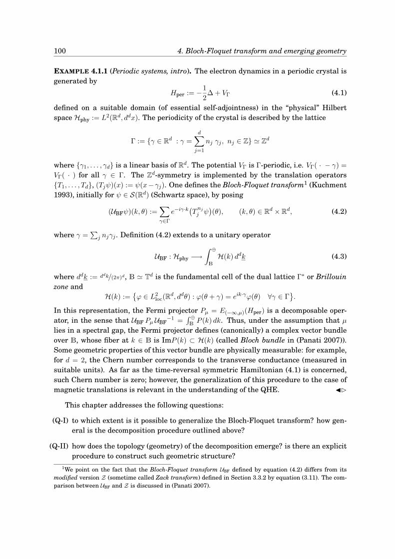
100 4. Bloch-Floquet transform and emerging geometry
EXAMPLE 4.1.1 (Periodic systems, intro). The electron dynamics in a periodic crystal isgenerated by
Hper := −1
2∆ + VΓ (4.1)
defined on a suitable domain (of essential self-adjointness) in the “physical” Hilbertspace Hphy := L2(Rd, ddx). The periodicity of the crystal is described by the lattice
Γ := γ ∈ Rd : γ =d∑
j=1
nj γj , nj ∈ Z ≃ Zd
where γ1, . . . , γd is a linear basis of Rd. The potential VΓ is Γ-periodic, i.e. VΓ( · − γ) =
VΓ( · ) for all γ ∈ Γ. The Zd-symmetry is implemented by the translation operatorsT1, . . . , Td, (Tjψ)(x) := ψ(x− γj). One defines the Bloch-Floquet transform1 (Kuchment1993), initially for ψ ∈ S(Rd) (Schwartz space), by posing
(UBFψ)(k, θ) :=∑
γ∈Γ
e−iγ·k(Tnj
j ψ)(θ), (k, θ) ∈ Rd × Rd, (4.2)
where γ =∑
j njγj . Definition (4.2) extends to a unitary operator
UBF : Hphy −→∫ ⊕
B
H(k) ddk (4.3)
where ddk := ddk/(2π)d, B ≃ Td is the fundamental cell of the dual lattice Γ∗ or Brillouinzone and
H(k) :=ϕ ∈ L2
loc(Rd, ddθ) : ϕ(θ + γ) = eik·γϕ(θ) ∀γ ∈ Γ
.
In this representation, the Fermi projector Pµ = E(−∞,µ)(Hper) is a decomposable oper-ator, in the sense that UBF Pµ UBF
−1 =∫ ⊕BP (k) dk. Thus, under the assumption that µ
lies in a spectral gap, the Fermi projector defines (canonically) a complex vector bundleover B, whose fiber at k ∈ B is ImP (k) ⊂ H(k) (called Bloch bundle in (Panati 2007)).Some geometric properties of this vector bundle are physically measurable: for example,for d = 2, the Chern number corresponds to the transverse conductance (measured insuitable units). As far as the time-reversal symmetric Hamiltonian (4.1) is concerned,such Chern number is zero; however, the generalization of this procedure to the case ofmagnetic translations is relevant in the understanding of the QHE. ⊲
This chapter addresses the following questions:
(Q-I) to which extent is it possible to generalize the Bloch-Floquet transform? how gen-eral is the decomposition procedure outlined above?
(Q-II) how does the topology (geometry) of the decomposition emerge? is there an explicitprocedure to construct such geometric structure?
1We point on the fact that the Bloch-Floquet transform UBF defined by equation (4.2) differs from itsmodified version Z (sometime called Zack transform) defined in Section 3.3.2 by equation (3.11). The com-parison between UBF and Z is discussed in (Panati 2007).
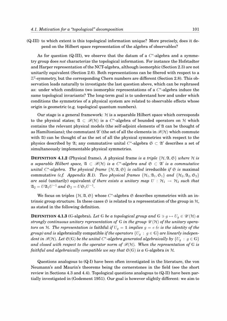
4.1. Motivation for a “topological” decomposition 101
(Q-III) to which extent is this topological information unique? More precisely, does it de-pend on the Hilbert space representation of the algebra of observables?
As for question (Q-III), we observe that the datum of a C∗-algebra and a symme-try group does not characterize the topological information. For instance the Hofstadterand Harper representation of the NCT-algebra, although isomorphic (Section 2.3) are notunitarily equivalent (Section 2.6). Both representations can be fibered with respect to aZ2-symmetry, but the corresponding Chern numbers are different (Section 2.8). This ob-servation leads naturally to investigate the last question above, which can be rephrasedas: under which conditions two isomorphic representations of a C∗-algebra induce thesame topological invariants? The long-term goal is to understand how and under whichconditions the symmetries of a physical system are related to observable effects whoseorigin is geometric (e.g. topological quantum numbers).
Our stage is a general framework: H is a separable Hilbert space which correspondsto the physical states; A ⊂ B(H) is a C∗-algebra of bounded operators on H whichcontains the relevant physical models (the self-adjoint elements of A can be thought ofas Hamiltonians); the commutant A′ (the set of all the elements in B(H) which commutewith A) can be thought of as the set of all the physical symmetries with respect to thephysics described by A; any commutative unital C∗-algebra S ⊂ A′ describes a set ofsimultaneously implementable physical symmetries.
DEFINITION 4.1.2 (Physical frame). A physical frame is a triple H,A,S where H isa separable Hilbert space, A ⊂ B(H) is a C∗-algebra and S ⊂ A′ is a commutativeunital C∗-algebra. The physical frame H,A,S is called irreducible if S is maximalcommutative (c.f. Appendix B.1). Two physical frames H1,A1,S1 and H2,A2,S2are said (unitarily) equivalent if there exists a unitary map U : H1 → H2 such thatA2 = UA1U
−1 and S2 = US1U−1.
We focus on triples H,A,S whose C∗-algebra S describes symmetries with an in-trinsic group structure. In these cases S is related to a representation of the group in H,as stated in the following definition.
DEFINITION 4.1.3 (G-algebra). Let G be a topological group and G ∋ g 7→ Ug ∈ U (H) astrongly continuous unitary representation of G in the group U (H) of the unitary opera-tors on H. The representation is faithful if Ug = 1 implies g = e (e is the identity of thegroup) and is algebraically compatible if the operators Ug : g ∈ G are linearly indepen-dent in B(H). Let S(G) be the unital C∗-algebra generated algebraically by Ug : g ∈ Gand closed with respect to the operator norm of B(H). When the representation of G isfaithful and algebraically compatible we say that S(G) is a G-algebra in H.
Questions analogous to (Q-I) have been often investigated in the literature, the vonNeumann’s and Maurin’s theorems being the cornerstones in the field (see the shortreview in Sections 4.3 and 4.4). Topological questions analogous to (Q-II) have been par-tially investigated in (Godement 1951). Our goal is however slightly different: we aim to
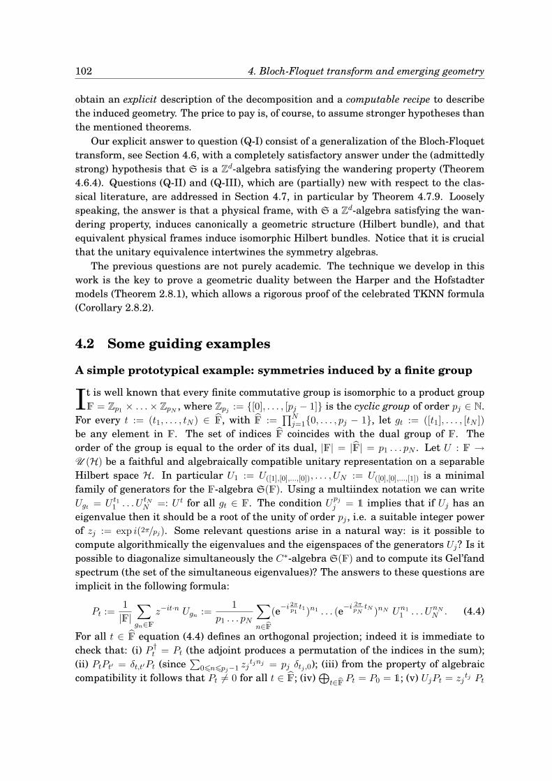
102 4. Bloch-Floquet transform and emerging geometry
obtain an explicit description of the decomposition and a computable recipe to describethe induced geometry. The price to pay is, of course, to assume stronger hypotheses thanthe mentioned theorems.
Our explicit answer to question (Q-I) consist of a generalization of the Bloch-Floquettransform, see Section 4.6, with a completely satisfactory answer under the (admittedlystrong) hypothesis that S is a Zd-algebra satisfying the wandering property (Theorem4.6.4). Questions (Q-II) and (Q-III), which are (partially) new with respect to the clas-sical literature, are addressed in Section 4.7, in particular by Theorem 4.7.9. Looselyspeaking, the answer is that a physical frame, with S a Zd-algebra satisfying the wan-dering property, induces canonically a geometric structure (Hilbert bundle), and thatequivalent physical frames induce isomorphic Hilbert bundles. Notice that it is crucialthat the unitary equivalence intertwines the symmetry algebras.
The previous questions are not purely academic. The technique we develop in thiswork is the key to prove a geometric duality between the Harper and the Hofstadtermodels (Theorem 2.8.1), which allows a rigorous proof of the celebrated TKNN formula(Corollary 2.8.2).
4.2 Some guiding examples
A simple prototypical example: symmetries induced by a finite group
It is well known that every finite commutative group is isomorphic to a product groupF = Zp1 × . . .× ZpN , where Zpj := [0], . . . , [pj − 1] is the cyclic group of order pj ∈ N.
For every t := (t1, . . . , tN ) ∈ F, with F :=∏Nj=10, . . . , pj − 1, let gt := ([t1], . . . , [tN ])
be any element in F. The set of indices F coincides with the dual group of F. Theorder of the group is equal to the order of its dual, |F| = |F| = p1 . . . pN . Let U : F →U (H) be a faithful and algebraically compatible unitary representation on a separableHilbert space H. In particular U1 := U([1],[0],...,[0]), . . . , UN := U([0],[0],...,[1]) is a minimalfamily of generators for the F-algebra S(F). Using a multiindex notation we can writeUgt = U t11 . . . U tNN =: U t for all gt ∈ F. The condition U
pj
j = 1 implies that if Uj has aneigenvalue then it should be a root of the unity of order pj , i.e. a suitable integer powerof zj := exp i(2π/pj). Some relevant questions arise in a natural way: is it possible tocompute algorithmically the eigenvalues and the eigenspaces of the generators Uj? Is itpossible to diagonalize simultaneously the C∗-algebra S(F) and to compute its Gel’fandspectrum (the set of the simultaneous eigenvalues)? The answers to these questions areimplicit in the following formula:
Pt :=1
|F|∑
gn∈Fz−it·n Ugn :=
1
p1 . . . pN
∑
n∈bF
(e−i2πp1t1)n1 . . . (e−i
2πpN
tN )nN Un11 . . . UnN
N . (4.4)
For all t ∈ F equation (4.4) defines an orthogonal projection; indeed it is immediate tocheck that: (i) P †
t = Pt (the adjoint produces a permutation of the indices in the sum);(ii) PtPt′ = δt,t′Pt (since
∑06n6pj−1 zj
tjnj = pj δtj ,0); (iii) from the property of algebraiccompatibility it follows that Pt 6= 0 for all t ∈ F; (iv)
⊕t∈bF
Pt = P0 = 1; (v) UjPt = zjtj Pt
4.2. Some guiding examples 103
for all j = 1, . . . , N . We will refer to Pt as the t-th Bloch-Floquet projection. The familyof the projections Ptt∈bF
induces an orthogonal decomposition of the Hilbert space Hlabeled by the set F. Let H(t) := Im(Pt), then the map
HUS(F)−→
⊕
t∈bF
H(t) (4.5)
defined by (US(F)ϕ)(t) := Ptϕ =: ϕ(t) is called (discrete) Bloch-Floquet transform. The
transform US(F) is unitary since ‖ϕ‖2H =
∑t∈bF
‖Ptϕ‖2H. Every Hilbert space H(t) is
a space of simultaneous eigenvectors for the C∗-algebra S(F), and the correspondingeigenvalues are generated as functions of zt11 , . . . , z
tNN . In particular the Gel’fand spec-
trum of S(F) (which coincides with the joint spectrum of the generating family U1, . . . , UN )is (homeomorphic to) the dual group F. Finally the transform US(F) maps the Hilbertspace H into a “fibered” space over the discrete set F. The Hilbert structure is obtained“gluing” the fiber spaces H(t) by the counting measure defined on F (direct integral, Ap-pendix B.3). The canonical projection
⊕t∈bF
H(t)π→ F endows the fibered space with the
structure of vector bundle (with 0-dimensional base). ⊲
Two examples of physical frame
In the rest of this work we will generalize the previous decomposition to cases in whichthe C∗-algebra of the symmetries is more complicated than the one generated by a fi-
nite group. However, this simple example encodes already many relevant aspects whichappear in the general cases.
EXAMPLE 4.2.1 (Periodic systems, part one). Let Hper be the operator defined by (4.1).The Gel’fand-Naımark Theorem (c.f. Appendix B.2) shows that there exists a isomor-phism between the commutative C∗-algebra C0(σ(Hper)) and a commutative non-unitalC∗-algebra A0(Hper) of bounded operators in H. The elements of A0(Hper) are the opera-tors f(Hper) ∈ B(H), for f ∈ C0(σ(Hper)), obtained via the spectral theorem. Let A(Hper)
be the multiplier algebra of A0(Hper) in B(H). This is a unital commutative C∗-algebrawhich contains A0(Hper) (as an essential ideal), its Gel’fand spectrum is the (Stone-Cech)compactification of σ(Hper) and the Gel’fand isomorphism maps A(Hper) into the unitalC∗-algebra of the continuous and bounded functions on σ(Hper) denoted by Cb(σ(Hper))
(c.f. Section B.2 for details). We assume that A(Hper) is the C∗-algebra of physical mod-els.
Let T1, . . . , Td be the translation operators corresponding to γ1, . . . , γd, defined inExample 4.1.1. Since [Ti; Tj ] = 0 for any i, j, it follows that the unital C∗-algebra ST
generated by the translations, their adjoints and the identity operator is commutative.Moreover, since [Hper; Tj ] = 0 it follows that ST ⊂ A(Hper)
′. Then the translations ST
are simultaneously implementable physical symmetries for the physics described by theHamiltonian (4.1). Thus Hphy,A(Hper),ST is a physical frame. It is a convenient modelto study the properties of an electron in a periodic medium. ⊲
104 4. Bloch-Floquet transform and emerging geometry
EXAMPLE 4.2.2 (Mathieu-like Hamiltonians, part one). Let T := R/(2πZ) be the one-dimensional torus. In the Hilbert space HM := L2(T, ds) consider the Fourier orthonor-mal basis enn∈Z defined by en(s) := (2π)−
12 eins. Let u and v be the unitary operators
defined, for any g ∈ HM, by
(ug)(s) := g(s+ 2πθ), (vg)(s) := eis g(s), uv = ei2πθ vu (4.6)
with θ ∈ R the deformation parameter. The commutation relation in (4.6) shows thatthe unitaries u and v define a representation (called Mathieu representation) of the theNCT-algebra Aθ on the Hilbert space HM (c.f. Section 2.3). We denote with Aθ
M := πM(Aθ)
the unital C∗-subalgebra of B(HM) generated by u := πM(u) and v := πM(v). With aninnocent abuse of nomenclature, we refer to Aθ
M as the Mathieu C∗-algebra and we callMathieu-like operator any element in Aθ
M. This name is due to the fact that the universalHofstadter operator hθ ∈ Aθ defined by equation (2.29) is mapped by πM in the almost-Mathieu operator
(hθ0g)(s) := g(s− 2πθ) + g(s+ 2πθ) + 2 cos(s)g(s). (4.7)
The action of u and v on the elements of the Fourier basis is given explicitly by uen =
ei2πθnen and ven = en+1 for all n ∈ Z and a simple computation shows that equation(4.7) coincides with equation (2.18) (with β = 0) up to a Fourier transform. The Mathieurepresentation πM is faithful only when θ /∈ Q.
We focus now on the commutant AθM
′ . Let h ∈ B(HM) be a bounded operator suchthat [h;u] = 0 = [h; v] and let hen =
∑m∈Z
hn,m em, hn,m ∈ C, be the action of h on thebasis vectors. The relation [h; v] = 0 implies hn+1,m+1 = hn,m and the relation [h;u] = 0
implies ei2π(n−m)θhn,m = hn,m for all n,m ∈ Z. If θ /∈ Q then ei2π(n−m)β 6= 1 unless n = m,hence hn,m = 0 if n 6= m and the condition hn+1,n+1 = hn,n implies that h = αh1 withαh ∈ C. This shows that in the irrational case θ /∈ Q the commutant of the MathieuC∗-algebra is trivial.
To have a non trivial commutant we need to assume that θ := p/q with p, q non zero
integers such that gcd(q, p) = 1. In this case the condition h ∈ Ap/qM
′implies that hn,m 6= 0
if and only ifm−n = kq for some k ∈ Z, moreover hn,n+kq = h0,kq =: h′k for all n ∈ Z. Let wbe the unitary operator defined on the orthonormal basis by wen := en+q, namely w = vq.
The relations for the commutant imply that h ∈ Ap/qM
′if and only if h =
∑k∈Z
h′k wk.
Then in the rational case the commutant of the Mathieu C∗-algebra is the von Neumannalgebra generated in B(HM) as the strong closure of the family of finite polynomials in w.We denote by S
qM := C∗(w) the unital commutative C∗-algebra generated by w. Observe
that it does not depend on p. The triple HM,Aq/pM ,Sq
M is an example of physical frame.⊲
4.3 The complete spectral theorem by von Neumann
The complete spectral theorem is a useful generalization of the usual spectral decom-position of a normal operator on a Hilbert space. It shows that symmetries reduce
4.3. The complete spectral theorem by von Neumann 105
the description of the full algebra A to a family of simpler representations. The main toolused in the theorem is the notion of the direct integral of Hilbert spaces (c.f. AppendixB.3). The “spectral” content of the theorem amounts to the characterization of the basespace for the decomposition (the “set of labels”) and of the measure which glues togetherthe spaces so that the Hilbert space structure is preserved. These information emergesessentially from the Gel’fand theory (c.f. Appendix B.2). The definitions of decomposableand continuously diagonal operator are reviewed in Appendix B.3.
THEOREM 4.3.1 (von Neumann’s complete spectral theorem). Let H,A,S be a phys-ical frame and µ the basic measure carried by the spectrum X of S (c.f. Appendix B.2).Then there exist
a) a direct integral H :=∫ ⊕X H(x) dµ(x) with H(x) 6= 0 for all x ∈ X,
b) a unitary map FS : H → H, called S-Fourier transform2,
such that:
(i) the unitary map FS intertwines the Gel’fand isomorphism C(X) ∋ fG7−→ Af ∈ S
and the canonical isomorphism of C(X) onto the continuously diagonal operatorsC(H), i.e. the following diagram commutes
f ∈ C(X)
G
xxqqqqqqqqqq
''PPPPPPPPPPPP
S ∋ Af FS ...FS−1
// Mf (·) ∈ C(H)
(ii) the unitary conjugation FS . . .F−1S maps the elements of A in decomposable opera-
tors on H; more precisely there is a measurable family x 7→ πx of representations ofA on H(x) such that FS A FS
−1 =∫ ⊕X πx(A) dµ(x);
(iii) the representations πx are irreducible if and only if the physical frame H,A,S isirreducible.
REMARK 4.3.2. For a complete proof of the above theorem one can see (Maurin 1968,Theorem 25, Chapter I and Theorem 2, Chapter V) or (Dixmier 1981, Theorem 1, PartII Chapter 6). For our purposes it is interesting to recall how the fiber Hilbert spacesH(x) are constructed. For ψ,ϕ ∈ H let µψ,ϕ = hψ,ϕ µ the relation which links the spectralmeasure µψ,ϕ with the basic measure µ. For µ-almost every x ∈ X the value of theRadon-Nikodym derivative hψ,ϕ in x defines a semi-definite sesquilinear form on H, i.e.(ψ;ϕ)x := hψ,ϕ(x). Let Ix := ψ ∈ H : hψ,ψ(x) = 0. Then the quotient space H/Ixis a pre-Hilbert space and H′(x) is defined to be the its completion. By constructionH′(x) 6= 0 for µ-almost every x ∈ X. Let N ⊂ X be the µ- negligible set on which H′(x)is trivial or not well defined. Then H :=
∫ ⊕X H(x) dµ(x) with H(x) := H′(x) if x ∈ X \ N
and H(x) := H if x ∈ N where H is an arbitrary non trivial Hilbert space. ♦
2 According to the terminology used in (Maurin 1968).
106 4. Bloch-Floquet transform and emerging geometry
The previous theorem provides only a partial answer to our motivating questions.Firstly, it provides only a partial answer to question (Q-I), since no explicit and com-putable “recipe” to construct the fiber Hilbert spaces is given. More importantly, Theo-rem 4.3.1 concerns a measure-theoretic decomposition of the Hilbert space, but it doesnot select a topological structure, yielding no answer to question (Q-II). In more geomet-ric terms, the elements of
∫ ⊕X H(x) dµ(x) can be regarded as L2-sections of a fibration
over X, while the topological structure is encoded by the (still not defined) space of con-tinuous sections. We will show in Section 4.7 that the Bloch-Floquet transform providesa natural choice of a subspace of
∫ ⊕X H(x) dµ(x) which can be interpreted as the subspace
of continuous sections, thus yielding a topological structure.
Given the triple H,A,S, the direct integral decomposition invoked in the state-ment of Theorem 4.3.1 is essentially unique in measure-theoretic sense. The space Xis unique up to homeomorphism: it agrees with the spectrum of C(H) in such a waythat the canonical isomorphism of C(X) onto C(H) may be identified with the Gel’fandisomorphism. As for the uniqueness of the direct integral decomposition, the followingresult holds true (Dixmier 1981, Theorem 3, Part II Chapter 6).
THEOREM 4.3.3 (Uniqueness). With the notation of Theorem 4.3.1, let ν be a positivemeasure with support X,
∏x∈X K(x) a field of non-zero Hilbert spaces over X endowed
with a measurable structure, K :=∫ ⊕X K(x) dν(x), C(K) the commutative unital C∗-
algebra of continuously diagonal operators on K and C(X) → C(K) the canonical isomor-phism. Let W be a unitary map from H onto K transforming Af ∈ S into M ′
f (·) ∈ C(K)
for all f ∈ C(X), i.e. such that the first diagram commutes.
Mf (·) ∈ C(H)77
FS ...FS−1
ooooooooooo gg
PPPPPPPPPPPP
S ∋ Af
W...W−1 ''NNNNNNNNNNNoo G
f ∈ C(X)
wwoooooooooooo
M ′f (·) ∈ C(K)
H??FS
~~~~
~~~
W (·)
H
W @@@
@@@@
K
Then, µ and ν are equivalent measures (so one can assume that µ = ν up to a rescalingisomorphism). Moreover there exists a decomposable unitary W (·) from H onto K, suchthat W (x) : H(x) → K(x) is a unitary operator µ-almost everywhere and W = W (·) FS,i.e. the second diagram commutes.
COROLLARY 4.3.4 (Unitary equivalent triples). Let H1,A1,S1 and H2,A2,S2 be twoequivalent physical frames and U the unitary map which intertwines between them. LetH1 and H2 denote the direct integral decomposition of the two triples and let FS1 and FS2
be the two S-Fourier transforms. Then W (·) := FS2 U FS1−1 is a decomposable unitary
operator from H1 to H2, so that W (x) : H1(x) → H2(x) is a unitary map for µ-almost everyx ∈ X.
4.4. The nuclear spectral theorem by Maurin 107
4.4 The nuclear spectral theorem by Maurin
The complete spectral theorem by von Neumann shows that any physical frameH,A,S admits a representation in which the Hilbert space is decomposed (in
a measure-theoretically unique way) in a direct integral FS : H →∫ ⊕X H(x) dµ(x), the
elements of S are simultaneously diagonalized and the C∗-algebra A is decomposed onthe fibers. In this sense the map FS|x restricted to the point x ∈ X generalizes therôle of the projection (4.4). The contribution of Maurin is a characterization of the fiberspaces H(x) as common generalized eigenspaces for S.
A key ingredient of the Maurin’s theorem is the notion of (nuclear) Gel’fand triple.The latter is a triple Φ,H,Φ∗ with H a separable Hilbert space, Φ ⊂ H a norm-densesubspace such that Φ has a topology for which it is a nuclear space and the inclusion mapı : Φ→H is continuous, and Φ∗ is the topological dual of Φ. Identifying H with its dualspace H∗, one gets an antilinear injection ı∗ : H→Φ∗. The duality pairing between Φ andΦ∗ is compatible with the scalar product on H, namely 〈ı∗(ψ1), ψ2〉 = (ψ1, ψ2)H wheneverψ1 ∈ H and ψ2 ∈ Φ. Hereafter we write 〈ψ1, ψ2〉 for 〈ı∗(ψ1), ψ2〉. If A is a bounded operatoron H such that A† leaves invariant Φ and A† : Φ → Φ is continuous with respect to thenuclear topology of Φ, one defines A : Φ∗ → Φ∗ by posing 〈A η;ϕ〉 := 〈η;A† ϕ〉 for allη ∈ Φ∗ and ϕ ∈ Φ. Then A is continuous and is an extension of A, defined on H, to Φ∗.References about the theory of Gel’fand triples can be found in (de la Madrid 2005).
Assume the notation of Theorem 4.3.1. Let ξk(·) : k ∈ N be a fundamental family oforthonormal measurable vector fields (see Appendix B.3) for the direct integral H definedby the S-Fourier transform FS. Any square integrable vector field ϕ(·) can be writtenin a unique way as ϕ(·) =
∑k∈N
ϕk(·) ξk(·) where ϕk ∈ L2(X, dµ) for all k ∈ N. Equippedwith this notation, the scalar product in H reads
〈ϕ(·);ψ(·)〉H =
∫
X
dim H(x)∑
k=1
ϕk(x) ψk(x) dµ(x).
For any ϕ ∈ H let ϕ(·) := FSϕ be the square integrable vector field obtained from ϕ bythe S-Fourier transform. Denote with Af ∈ S the operator associated with f ∈ C(X)
through the Gel’fand isomorphism. One checks that
(FSAfϕ)k(x) = (ξk(x); f(x)ϕ(x))x = f(x) ϕk(x) k = 1, 2, . . . ,dim H(x). (4.8)
Suppose that Φ,H,Φ∗ is a Gel’fand triple for the space H. If ϕ ∈ Φ then the mapΦ ∋ ϕ 7→ ϕk(x) := (ξk(x);ϕ(x))x ∈ C is linear; moreover it is possible to show that it iscontinuous with respect to the nuclear topology of Φ, for an appropriate choice of Φ. Thismeans that there exists ηk(x) ∈ Φ∗ such that
〈ηk(x);ϕ〉 := ϕk(x) = (ξk(x);ϕ(x))x k = 1, 2, . . . ,dim H(x). (4.9)
Suppose that Af : Φ → Φ is continuous with respect to the nuclear topology for everyf ∈ C(X). Then from equations (4.8) and (4.9) one has that the extended operator
108 4. Bloch-Floquet transform and emerging geometry
Af : Φ∗ → Φ∗, namely 〈Af η;ϕ〉 := 〈η;Af ϕ〉 for all η ∈ Φ∗ and ϕ ∈ Φ, satisfies
〈Af ηk(x);ϕ〉 = 〈ηk(x);Af ϕ〉 = f(x) ϕk(x) = 〈f(x)ηk(x);ϕ〉 k = 1, 2, . . . ,dim H(x)
(4.10)for all ϕ ∈ Φ. Hence,
Af ηk(x) = f(x) ηk(x) in Φ∗.
In this sense ηk(x) is a generalized eigenvector for Af . These claims are made precise inthe following statement.
THEOREM 4.4.1 (Maurin’s nuclear spectral theorem). With the notation and the as-sumptions of Theorem 4.3.1, let Φ,H,Φ∗ be a nuclear Gel’fand triple for the space Hsuch that Φ is S-invariant, i.e. each A ∈ S is a continuous linear map A : Φ → Φ. Then:
(i) for all x ∈ X the S-Fourier transform FS|x : Φ → H(x) such that Φ ∋ ϕ 7→ ϕ(x) ∈H(x) is continuous with respect to the nuclear topology for µ-almost every x ∈ X;
(ii) there is a family of linear functionals ηk(x) : k = 1, 2, . . . ,dim H(x) ⊂ Φ∗ suchthat equations (4.9) and (4.10) hold true for µ-almost all x ∈ X;
(iii) with the identification ηk(x) ↔ ξk(x) the Hilbert space H(x) is (isomorphic to) avector subspace of Φ∗; with this identification the FS-Fourier transform is definedon the dense set Φ by
Φ ∋ ϕFS |x7−→
dim H(x)∑
k=1
〈ηk(x);ϕ〉 ηk(x) ∈ Φ∗ (4.11)
and the scalar product in H(x) is formally defined by posing (ηk(x); ηj(x))x := δk,j ;
(iv) under the identification in (iii) the spaces H(x) become the generalized commoneigenspaces of the operators in S in the sense that if Af ∈ S then Af ηk(x) =
f(x) ηk(x) for µ-almost every x ∈ X and all k = 1, 2, . . . ,dim H(x).
For a proof we refer to (Maurin 1968, Chapter II). The identification at point (iii) ofthe Theorem 4.4.1 depends on the choice of a fundamental family of orthonormal mea-surable vector fields ξk(·) : k ∈ N for the direct integral H, which is clearly not unique.If ζk(·) : k ∈ N is a second fundamental family of orthonormal measurable vector fieldsfor H, then there exists a decomposable unitary map W (·) such that W (x)ξk(x) = ζk(x)
for µ-almost every x ∈ X and every k ∈ N. The composition U := FS−1 W (·) FS is
a unitary isomorphism of the Hilbert space H which induces a linear isomorphism be-tween the Gel’fand triples Φ,H,Φ∗ and Ψ,H,Ψ∗ where Ψ := UΦ. One checks that Ψ
is a nuclear space in H with respect to the topology induced from Φ by the map U (i.e.defined by the family of seminorms p′α := pα U−1). Ψ∗, the topological dual of Ψ, is UΦ∗,in view of the continuity of U−1 : Ψ → Φ. The isomorphism of the Gel’fand triples iscompatible with the direct integral decomposition. Indeed if ϑk(x) ↔ ζk(x) is the identi-fication between the new orthonormal basis ζk(x) : k = 1, 2, . . . ,dim H(x) of H(x) and
4.5. The wandering property 109
a family of linear functionals ϑk(x) : k = 1, 2, . . . ,dim H(x) ⊂ Ψ∗ then equation (4.9)implies that for any ϕ ∈ Ψ
〈ϑk(x);ϕ〉 := (ζk(x);ϕ(x))x =(ξk(x);W (x)−1ϕ(x)
)x
= 〈ηk(x);U−1ϕ〉 = 〈U ηk(x);ϕ〉.(4.12)
PROPOSITION 4.4.2. Up to a canonical identification of isomorphic Gel’fand triples therealization (4.11) of the fiber spaces H(x) as generalized common eigenspaces is canonicalin the sense that it does not depend on the choice of a fundamental family of orthonormalmeasurable fields.
From Proposition 4.4.2 and Corollary 4.3.4 and it follows that:
COROLLARY 4.4.3. Up to a canonical identification of isomorphic Gel’fand triples therealization (4.11) of the fiber spaces H(x) as generalized common eigenspaces is preservedby a unitary transform of the triple H,A,S.
Theorem 4.4.1 assumes the existence of a S-invariant nuclear space and the relatedGel’fand triple. If S is generated by a countable family, such nuclear space does existand there is an algorithmic procedure to construct it (Maurin 1968, Chapter II, Theorem6).
THEOREM 4.4.4 (Existence of the nuclear space). Let A1, A2, . . . a countable family ofcommuting bounded normal operators on the separable Hilbert space H which generate(together with their adjoints and the identity) the commutative C∗-algebra S. Then thereexists a countable S-cyclic system ψ1, ψ2, . . . which generates a nuclear space Φ ⊂ Hsuch that: a) Φ is dense in H; b) the embedding ı : Φ → H is continuous; c) the mapsAmj : Φ → Φ are continuous for all j,m ∈ N.
REMARK 4.4.5. We recall that a countable (or finite) family ψ1, ψ2, . . . of orthonormalvectors in H is a S-cyclic system for S if the set A†bAaψk : k ∈ N, a, b ∈ N∞
fin is densein H, where N∞
fin is the space of N−valued sequences which are definitely zero (i.e. an = 0
for any n ∈ N \ I with |I| < +∞) and Aa := Aa11 A
a22 . . . AaN
N for some integer N .Any C∗-algebra S (not necessarily commutative) has many S-cyclic systems. Indeed
one can start from any normalized vector ψ1 ∈ H to build the closed subspace H1 spannedby the action of S on ψ1. If H1 6= H one can choose a second normalized vector ψ2 in theorthogonal complement of H1 to build the closed subspace H2. Since H is separable, thisprocedure produces a countable (or finite) family ψ1, ψ2, . . . such that H = H1⊕H2⊕. . ..Obviously this construction is not unique. The nuclear space Φ claimed in Theorem 4.4.4depends on the choice of a S-cyclic system and generically many inequivalent choices arepossible. ♦
4.5 The wandering property
An interesting and generally unsolved problem is the construction of the invariantsubspaces of an operator or of a family of operators. Let S be a C∗-algebra contained
110 4. Bloch-Floquet transform and emerging geometry
in B(H). If ψ ∈ H then the subspace S[ψ] generated by the action of S on the vector ψ isan invariant subspace for the C∗-algebra. The existence of a particular decomposition ofthe Hilbert space in invariant subspaces depends on the nature of the C∗-algebra. Theproblem is reasonably simple to solve for the C∗-algebras which satisfy the wanderingproperty.
DEFINITION 4.5.1 (wandering property). Let S be a commutative unital C∗-algebragenerated by the countable family A1, A2, . . . of commuting bounded normal operatorsand their adjoints (with the convention A0
j := 1) in a separable Hilbert space H. Wewill say that S has the wandering property if there exists a (at most) countable familyψ1, ψ2, . . . ⊂ H of orthonormal vectors which is S-cyclic (according to Remark 4.4.5)and such that
(ψk;A†bAaψh)H = ‖Aaψk‖2
H δk,h δa,b ∀ h, k ∈ N, ∀ a, b ∈ N∞fin, (4.13)
where Aa := Aa11 A
a22 . . . AaN
N , δk,h is the usual Kronecker delta and δa,b is the Kroneckerdelta for the multiindices a and b.
Let Hk := S[ψk] be the Hilbert subspace generated by the action of S on the vectorψk. If S has the wandering property then the Hilbert space decomposes as H =
⊕k∈N
Hk
and each Hk is a S-invariant subspace. We will refer to Hk as a wandering subspaceand to ψ1, ψ2, . . . as the wandering system. In these subspaces each operator Aj acts asa unilateral weighted shift and this justifies the use of the adjective “wandering” (Nagyand Foias 1970, Chapter 1, Sections 1 and 2). The wandering property implies manyinteresting consequences.
PROPOSITION 4.5.2. Let S be a commutative unital C∗-algebra generated by the (atmost) countable family A1, A2, . . . of commuting bounded normal operators and theiradjoints in a separable Hilbert space H. Suppose that S has the wandering property withrespect to the family of vectors ψ1, ψ2, . . ., then:
(i) the generators can not be selfadjoint, and Anj 6= 1 for every n ∈ N \ 0;
(ii) every generator which is unitary has no eigenvectors;
(iii) if S is generated by N unitary operators then S is a ZN -algebra.
Proof. To prove (i) observe that the condition Aj = A†j implies that Ajψk = 0 for all ψk
in the system and the S-cyclicity imposes Aj = 0. As for the second claim, by settingb = 0 and h = k in equation (4.13) one sees that Aa = 1 implies a = 0.
To prove (ii) observe that if U,A1, A2, . . . is a set of commuting generators for S
with U unitary, then each vector ϕ ∈ H can be written as ϕ =∑
n∈ZUnχn where
χn =∑
k∈N, a∈ZN αk,aAaψk. Clearly Uϕ =
∑n∈Z
Unχn−1 and equation (4.13) impliesthat ‖ϕ‖2
H =∑
n∈Z‖χn‖2
H. If Uϕ = λϕ, with λ ∈ S1, then a comparison between thecomponents provides χn−1 = λχn, i.e. χn = λ−nχ0 for all n ∈ Z. This contradicts theconvergence of the series expressing the norm of ϕ.
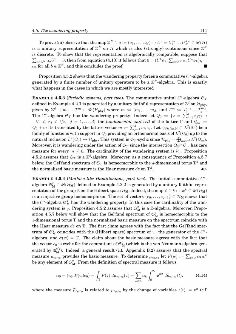
4.5. The wandering property 111
To prove (iii) observe that the map ZN ∋ a := (a1, . . . , aN ) 7→ Ua = Ua11 . . . UaN
N ∈ U (H)
is a unitary representation of ZN on H which is also (strongly) continuous since ZN
is discrete. To show that the representation is algebraically compatible, suppose that∑a∈ZN αaU
a = 0; then from equation (4.13) it follows that 0 = (U bψk;∑
a∈ZN αaUaψk)H =
αb for all b ∈ ZN , and this concludes the proof.
Proposition 4.5.2 shows that the wandering property forces a commutativeC∗-algebragenerated by a finite number of unitary operators to be a ZN -algebra. This is exactlywhat happens in the cases in which we are mostly interested
EXAMPLE 4.5.3 (Periodic systems, part two). The commutative unital C∗-algebra ST
defined in Example 4.2.1 is generated by a unitary faithful representation of Zd on Hphy,given by Zd ∋ m 7→ Tm ∈ U (Hphy) where m := (m1, . . . ,md) and Tm := Tm1
1 . . . Tmdd .
The C∗-algebra ST has the wandering property. Indeed let Q0 := x =∑d
j=1 xjγj :
−1/2 6 xj 6 1/2, j = 1, . . . , d the fundamental unit cell of the lattice Γ and Qm :=
Q0 + m its translated by the lattice vector m :=∑d
j=1mjγj . Let ψkk∈N ⊂ L2(Rd) be afamily of functions with support in Q0 providing an orthonormal basis of L2(Q0) up to thenatural inclusion L2(Q0) → Hphy. This system is ST -cyclic since Hphy =
⊕m∈Zd L2(Qm).
Moreover, it is wandering under the action of ST since the intersection Q0∩Qm has zeromeasure for every m 6= 0. The cardinality of the wandering system is ℵ0. Proposition4.5.2 assures that ST is a Zd-algebra. Moreover, as a consequence of Proposition 4.5.7below, the Gel’fand spectrum of ST is homeomorphic to the d-dimensional torus Td andthe normalized basic measure is the Haar measure dz on Td. ⊲
EXAMPLE 4.5.4 (Mathieu-like Hamiltonians, part two). The unital commutative C∗-algebra S
qM ⊂ B(HM) defined in Example 4.2.2 is generated by a unitary faithful repre-
sentation of the group Z on the Hilbert space HM. Indeed, the map Z ∋ k 7→ wk ∈ U (HM)
is an injective group homomorphism. The set of vectors e0, . . . , eq−1 ⊂ HM shows thatthe C∗-algebra S
qM has the wandering property. In this case the cardinality of the wan-
dering system is q. Proposition 4.5.2 assures that SqM is a Z-algebra. Moreover, Propo-
sition 4.5.7 below will show that the Gel’fand spectrum of SqM is homeomorphic to the
1-dimensional torus T and the normalized basic measure on the spectrum coincide withthe Haar measure dz on T. The first claim agrees with the fact that the Gel’fand spec-trum of S
qM coincides with the (Hilbert space) spectrum of w, the generator of the C∗-
algebra, and σ(w) = T. The claim about the basic measure agrees with the fact thatthe vector e0 is cyclic for the commutant of S
qM (which is the von Neumann algebra gen-
erated by Ap/qM ). Indeed, a general result (c.f. Appendix B.2) assures that the spectral
measure µe0,e0 provides the basic measure. To determine µe0,e0 let F (w) :=∑
k∈Zαkw
k
be any element of SqM. From the definition of spectral measure it follows
α0 = (e0;F (w)e0) =
∫
T
F (z) dµe0,e0(z) =∑
k∈Z
αk
∫ 2π
0eikt dµe0,e0(t). (4.14)
where the measure µe0,e0 is related to µe0,e0 by the change of variables z(t) := eit (c.f.
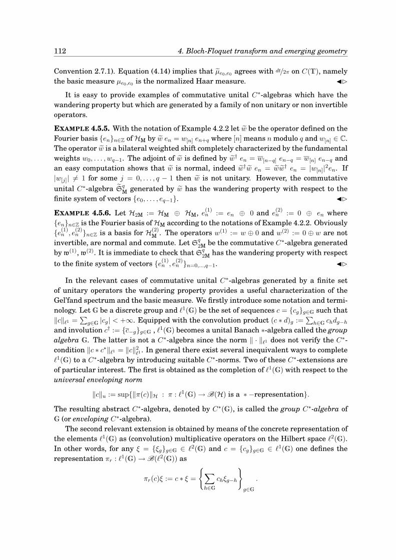
112 4. Bloch-Floquet transform and emerging geometry
Convention 2.7.1). Equation (4.14) implies that µe0,e0 agrees with dt/2π on C(T), namelythe basic measure µe0,e0 is the normalized Haar measure. ⊲
It is easy to provide examples of commutative unital C∗-algebras which have thewandering property but which are generated by a family of non unitary or non invertibleoperators.
EXAMPLE 4.5.5. With the notation of Example 4.2.2 let w be the operator defined on theFourier basis enn∈Z of HM by w en = w[n] en+q where [n] means n modulo q and w[n] ∈ C.The operator w is a bilateral weighted shift completely characterized by the fundamentalweights w0, . . . , wq−1. The adjoint of w is defined by w† en = w[n−q] en−q = w[n] en−q andan easy computation shows that w is normal, indeed w†w en = ww† en = |w[n]|2en. If|w[j]| 6= 1 for some j = 0, . . . , q − 1 then w is not unitary. However, the commutative
unital C∗-algebra SqM generated by w has the wandering property with respect to the
finite system of vectors e0, . . . , eq−1. ⊲
EXAMPLE 4.5.6. Let H2M := HM ⊕ HM, e(1)n := en ⊕ 0 and e(2)n := 0 ⊕ en where
enn∈Z is the Fourier basis of HM according to the notations of Example 4.2.2. Obviouslye(1)n , e
(2)n n∈Z is a basis for H(2)
M . The operators w(1) := w ⊕ 0 and w(2) := 0 ⊕ w are notinvertible, are normal and commute. Let S
q2M be the commutative C∗-algebra generated
by w(1), w(2). It is immediate to check that Sq2M has the wandering property with respect
to the finite system of vectors e(1)n , e(2)n n=0,...,q−1. ⊲
In the relevant cases of commutative unital C∗-algebras generated by a finite setof unitary operators the wandering property provides a useful characterization of theGel’fand spectrum and the basic measure. We firstly introduce some notation and termi-nology. Let G be a discrete group and ℓ1(G) be the set of sequences c = cgg∈G such that‖c‖ℓ1 =
∑g∈G |cg| < +∞. Equipped with the convolution product (c ∗ d)g :=
∑h∈G chdg−h
and involution c† := c−gg∈G , ℓ1(G) becomes a unital Banach ∗-algebra called the groupalgebra G. The latter is not a C∗-algebra since the norm ‖ · ‖ℓ1 does not verify the C∗-condition ‖c ∗ c∗‖ℓ1 = ‖c‖2
ℓ1 . In general there exist several inequivalent ways to completeℓ1(G) to a C∗-algebra by introducing suitable C∗-norms. Two of these C∗-extensions areof particular interest. The first is obtained as the completion of ℓ1(G) with respect to theuniversal enveloping norm
‖c‖u := sup‖π(c)‖H : π : ℓ1(G) → B(H) is a ∗ −representation.
The resulting abstract C∗-algebra, denoted by C∗(G), is called the group C∗-algebra ofG (or enveloping C∗-algebra).
The second relevant extension is obtained by means of the concrete representation ofthe elements ℓ1(G) as (convolution) multiplicative operators on the Hilbert space ℓ2(G).In other words, for any ξ = ξgg∈G ∈ ℓ2(G) and c = cgg∈G ∈ ℓ1(G) one defines therepresentation πr : ℓ1(G) → B(ℓ2(G)) as
πr(c)ξ := c ∗ ξ =
∑
h∈Gchξg−h
g∈G
.
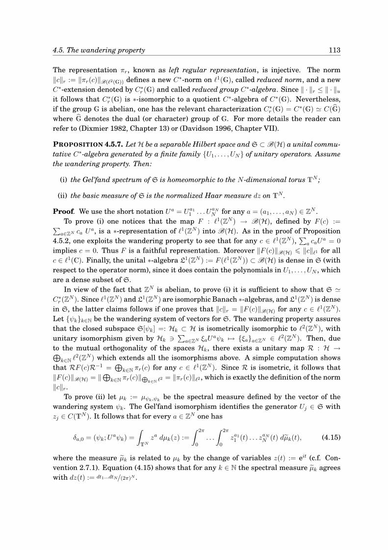
4.5. The wandering property 113
The representation πr, known as left regular representation, is injective. The norm‖c‖r := ‖πr(c)‖B(ℓ2(G)) defines a new C∗-norm on ℓ1(G), called reduced norm, and a newC∗-extension denoted by C∗
r (G) and called reduced group C∗-algebra. Since ‖ · ‖r ≤ ‖ · ‖uit follows that C∗
r (G) is ∗-isomorphic to a quotient C∗-algebra of C∗(G). Nevertheless,if the group G is abelian, one has the relevant characterization C∗
r (G) = C∗(G) ≃ C(G)
where G denotes the dual (or character) group of G. For more details the reader canrefer to (Dixmier 1982, Chapter 13) or (Davidson 1996, Chapter VII).
PROPOSITION 4.5.7. Let H be a separable Hilbert space and S ⊂ B(H) a unital commu-tative C∗-algebra generated by a finite family U1, . . . , UN of unitary operators. Assumethe wandering property. Then:
(i) the Gel’fand spectrum of S is homeomorphic to the N -dimensional torus TN ;
(ii) the basic measure of S is the normalized Haar measure dz on TN .
Proof. We use the short notation Ua = Ua11 . . . UaN
N for any a = (a1, . . . , aN ) ∈ ZN .To prove (i) one notices that the map F : ℓ1(ZN ) → B(H), defined by F (c) :=∑a∈ZN ca U
a, is a ∗-representation of ℓ1(ZN ) into B(H). As in the proof of Proposition4.5.2, one exploits the wandering property to see that for any c ∈ ℓ1(ZN ),
∑a caU
a = 0
implies c = 0. Thus F is a faithful representation. Moreover ‖F (c)‖B(H) 6 ‖c‖ℓ1 for allc ∈ ℓ1(C). Finally, the unital ∗-algebra L1(ZN ) := F (ℓ1(ZN )) ⊂ B(H) is dense in S (withrespect to the operator norm), since it does contain the polynomials in U1, . . . , UN , whichare a dense subset of S.
In view of the fact that ZN is abelian, to prove (i) it is sufficient to show that S ≃C∗r (Z
N ). Since ℓ1(ZN ) and L1(ZN ) are isomorphic Banach ∗-algebras, and L1(ZN ) is densein S, the latter claims follows if one proves that ‖c‖r = ‖F (c)‖B(H) for any c ∈ ℓ1(ZN ).Let ψkk∈N be the wandering system of vectors for S. The wandering property assuresthat the closed subspace S[ψk] =: Hk ⊂ H is isometrically isomorphic to ℓ2(ZN ), withunitary isomorphism given by Hk ∋ ∑
a∈ZN ξaUaψk 7→ ξaa∈ZN ∈ ℓ2(ZN ). Then, due
to the mutual orthogonality of the spaces Hk, there exists a unitary map R : H →⊕k∈N
ℓ2(ZN ) which extends all the isomorphisms above. A simple computation showsthat RF (c)R−1 =
⊕k∈N
πr(c) for any c ∈ ℓ1(ZN ). Since R is isometric, it follows that‖F (c)‖B(H) = ‖⊕k∈N
πr(c)‖L
k∈Nℓ2 = ‖πr(c)‖ℓ2 , which is exactly the definition of the norm
‖c‖r.To prove (ii) let µk := µψk,ψk
be the spectral measure defined by the vector of thewandering system ψk. The Gel’fand isomorphism identifies the generator Uj ∈ S withzj ∈ C(TN ). It follows that for every a ∈ ZN one has
δa,0 = (ψk;Uaψk) =
∫
TN
za dµk(z) :=
∫ 2π
0. . .
∫ 2π
0za11 (t) . . . zaN
N (t) dµk(t), (4.15)
where the measure µk is related to µk by the change of variables z(t) := eit (c.f. Con-vention 2.7.1). Equation (4.15) shows that for any k ∈ N the spectral measure µk agreeswith dz(t) := dt1...dtN/(2π)N .
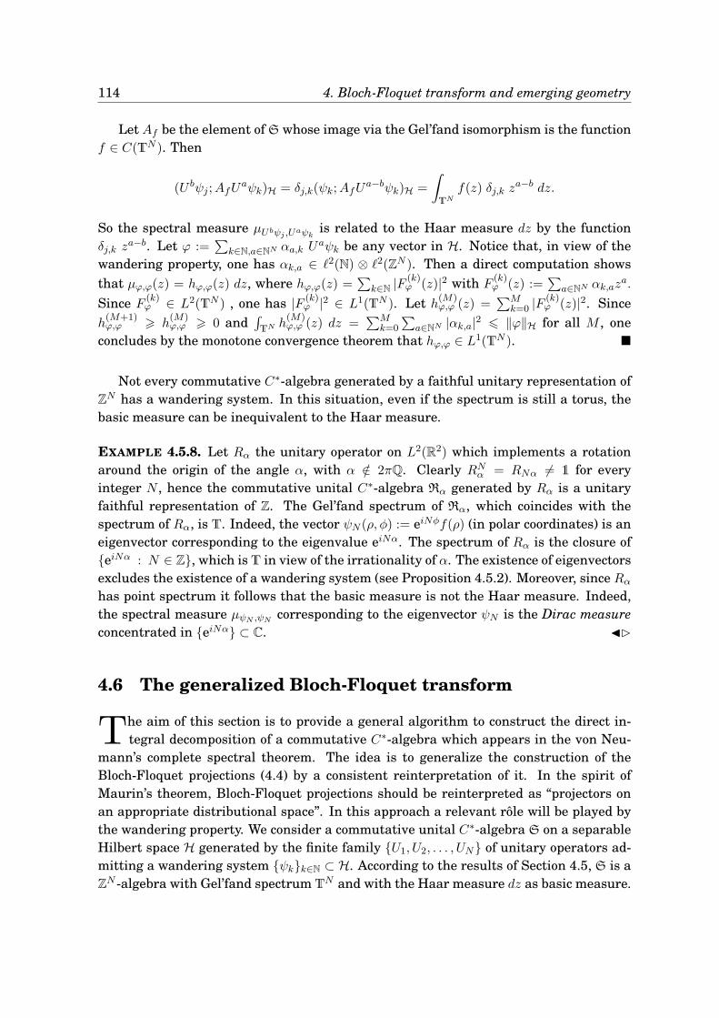
114 4. Bloch-Floquet transform and emerging geometry
Let Af be the element of S whose image via the Gel’fand isomorphism is the functionf ∈ C(TN ). Then
(U bψj ;AfUaψk)H = δj,k(ψk;AfU
a−bψk)H =
∫
TN
f(z) δj,k za−b dz.
So the spectral measure µUbψj ,Uaψkis related to the Haar measure dz by the function
δj,k za−b. Let ϕ :=
∑k∈N,a∈NN αa,k U
aψk be any vector in H. Notice that, in view of thewandering property, one has αk,a ∈ ℓ2(N) ⊗ ℓ2(ZN ). Then a direct computation shows
that µϕ,ϕ(z) = hϕ,ϕ(z) dz, where hϕ,ϕ(z) =∑
k∈N|F (k)ϕ (z)|2 with F
(k)ϕ (z) :=
∑a∈NN αk,az
a.
Since F (k)ϕ ∈ L2(TN ) , one has |F (k)
ϕ |2 ∈ L1(TN ). Let h(M)ϕ,ϕ (z) =
∑Mk=0 |F
(k)ϕ (z)|2. Since
h(M+1)ϕ,ϕ > h
(M)ϕ,ϕ > 0 and
∫TN h
(M)ϕ,ϕ (z) dz =
∑Mk=0
∑a∈NN |αk,a|2 6 ‖ϕ‖H for all M , one
concludes by the monotone convergence theorem that hϕ,ϕ ∈ L1(TN ).
Not every commutative C∗-algebra generated by a faithful unitary representation ofZN has a wandering system. In this situation, even if the spectrum is still a torus, thebasic measure can be inequivalent to the Haar measure.
EXAMPLE 4.5.8. Let Rα the unitary operator on L2(R2) which implements a rotationaround the origin of the angle α, with α /∈ 2πQ. Clearly RNα = RNα 6= 1 for everyinteger N , hence the commutative unital C∗-algebra Rα generated by Rα is a unitaryfaithful representation of Z. The Gel’fand spectrum of Rα, which coincides with thespectrum of Rα, is T. Indeed, the vector ψN (ρ, φ) := eiNφf(ρ) (in polar coordinates) is aneigenvector corresponding to the eigenvalue eiNα. The spectrum of Rα is the closure ofeiNα : N ∈ Z, which is T in view of the irrationality of α. The existence of eigenvectorsexcludes the existence of a wandering system (see Proposition 4.5.2). Moreover, since Rαhas point spectrum it follows that the basic measure is not the Haar measure. Indeed,the spectral measure µψN ,ψN
corresponding to the eigenvector ψN is the Dirac measureconcentrated in eiNα ⊂ C. ⊲
4.6 The generalized Bloch-Floquet transform
The aim of this section is to provide a general algorithm to construct the direct in-tegral decomposition of a commutative C∗-algebra which appears in the von Neu-
mann’s complete spectral theorem. The idea is to generalize the construction of theBloch-Floquet projections (4.4) by a consistent reinterpretation of it. In the spirit ofMaurin’s theorem, Bloch-Floquet projections should be reinterpreted as “projectors onan appropriate distributional space”. In this approach a relevant rôle will be played bythe wandering property. We consider a commutative unital C∗-algebra S on a separableHilbert space H generated by the finite family U1, U2, . . . , UN of unitary operators ad-mitting a wandering system ψkk∈N ⊂ H. According to the results of Section 4.5, S is aZN -algebra with Gel’fand spectrum TN and with the Haar measure dz as basic measure.
4.6. The generalized Bloch-Floquet transform 115
Construction of the nuclear space
Consider the orthonormal basis Uaψkk∈N,a∈ZN , where ψkk∈N is the wandering sys-tem, and denote by L ⊂ H the family of all finite linear combinations of the vectorsof such basis. For every integer m > 0 denote by Hm the finite dimensional Hilbertspace generated by the finite set of vectors Uaψk : 0 6 k 6 m, 0 6 |a| 6 m, where|a| := |a1| + . . .+ |aN |. Obviously Hm ⊂ L. Let denote by Dm the dimension of the spaceHm. If ϕ =
∑k∈N,a∈ZN αk,aU
aψk is any element of H then the formula
p2m(ϕ) := Dm
∑
0 6 k 6m
0 6 |a| 6m
|(Uaψk;ϕ)H|2 = Dm
∑
0 6 k 6m
0 6 |a| 6m
|αk,a|2, (4.16)
defines a seminorm for every m > 0. From (4.16) it follows that pm 6 pm+1 for all m. Thecountable family of seminorms pmm∈N provides a locally convex topology for the vectorspace L. Let denote by Σ the pair L, pmm∈N, i.e. the vector space L endowed with thelocally convex topology induced by the seminorms (4.16). Σ is a complete and metrizable(i.e. Fréchet) space. However, for our purposes, we need a topology on L which is strictlystronger than the metrizable topology induced by the seminorms (4.16).
The quotient space Φm := L/Nm, with Nm := ϕ ∈ L : pm(ϕ) = 0, is isomorphicto the finite dimensional vector space Hm, hence it is nuclear and Fréchet. This followsimmediately observing that the norm pm on Φm coincides, up to the positive constant√Dm, with the usual Hilbert norm. Obviously Φm ⊂ Φm+1 for all m > 0 and the topology
of Φm agrees with the topology inherited from Φm+1, indeed pm+1|Φm=√
Dm+1
Dmpm. We
define Φ to be⋃m∈N
Φm (which is L as a set) endowed with the strict inductive limittopology which is the stronger topology which makes continuous all the injections ım :
Φm → Φ. The space Φ is called a LF-space according to the definition in (Treves 1967,Chapter 13) and it is a nuclear space since it is the strict inductive limit of nuclearspaces (Treves 1967, Proposition 50.1). We will say that Φ is the wandering nuclearspace defined by the ZN -algebra S on the wandering system ψkk∈N.
PROPOSITION 4.6.1. The wandering nuclear space Φ defined by the ZN -algebra S onthe wandering system ψkk∈N verifies all the properties stated in Theorem 4.4.4.
Proof. A linear map : Φ → Ψ, with Ψ an arbitrary locally convex topological vec-tor space, is continuous if and only if the restriction |Φm
of to Φm is continuous foreach m > 0 (Treves 1967, Proposition 13.1). This implies that the canonical embeddingı : Φ → H is continuous, since its restrictions are linear operators defined on finite di-mensional spaces. The linear maps Ua : Φ → Φ for all a ∈ NN are also continuous for thesame reason. Finally Φ is norm-dense in H since as a set it is the dense domain L.
The strict inductive limit topology which defines Φ is stronger than the topology in-duced by the seminorms (4.16) which defines the Fréchet space Σ. The space Φ is com-plete but not metrizable since every Φm is closed in the topology of Φm+1 (Treves 1967,Theorem 13.1).
116 4. Bloch-Floquet transform and emerging geometry
The transform
We are now in position to define the generalized Bloch-Floquet transform US for the C∗-algebra S. The Gel’fand spectrum of S is TN and the Gel’fand isomorphism associatesto the generator Uj the function zj ∈ C(TN ). For any t ∈ [0, 2π)N and for any ϕ ∈ Φ wedefine (formally for the moment) the Bloch-Floquet transform of ϕ at point t as
Φ ∋ ϕUS |t7−→ (USϕ)(t) :=
a∈ZN∑
a∈ZN
z−a(t) Uaϕ (4.17)
where za(t) := eia1t1 . . . eiaN tN and Ua := Ua11 . . . UaN
N . The structure of equation (4.17)suggests that (USϕ)(t) is a common generalized eigenvector for the elements of S, indeeda formal computation shows that
Uj(USϕ)(t) = zj(t)∑
a∈ZN
z−1j (t)z−a(t)Uj U
aϕ = eitj (USϕ)(t). (4.18)
This guess is clarified by the following result.
THEOREM 4.6.2 (Generalized Bloch-Floquet transform). Let S be a ZN -algebra in theseparable Hilbert space H with generators U1, . . . , UN and wandering system ψkk∈N,and let Φ be the corresponding nuclear space. Under these assumptions the generalizedBloch-Floquet transform (4.17) defines an injective linear map from the nuclear spaceΦ into its topological dual Φ∗ for every t ∈ [0, 2π)N . More precisely, the transform US|tmaps Φ onto a subspace Φ∗(t) ⊂ Φ∗ which is a common generalized eigenspace for thecommutative C∗-algebra S, i. e. Uj (USϕ)(t) = eitj (USϕ)(t) in Φ∗. The map US|t : Φ →Φ∗(t) ⊂ Φ∗ is a continuous linear isomorphism, provided Φ∗ is endowed with the ∗-weaktopology.
Proof. We need to verify that the right-hand side of (4.17) is well defined as a linearfunctional on Φ. Any vector ϕ ∈ Φ is a finite linear combination ϕ =
∑fink∈N
∑finb∈ZN αk,b U
bψk(the complex numbers αk,b are different from zero only for a finite set of the values of theindex k and the multiindex b). Let φ =
∑finh∈N
∑finc∈NN βh,c U
cψh be another element in Φ.The linearity of the dual pairing between Φ∗ and Φ and the compatibility of the pairingwith the Hermitian structure of H imply
〈(USϕ)(t);φ〉 :=fin∑
k∈N
fin∑
b,c∈ZN
αk,bβk,c
∑
a∈ZN
za(t) (Ua+bψk;Ucψk)H
(4.19)
where in the right-hand side we used the orthogonality between the spaces generatedby ψk and ψh if k 6= h. Without further conditions equation (4.19) is a finite sum in k, b, c
(this is simply a consequence of the fact that ϕ and φ are “test functions”) but it is aninfinite sum in a which generally does not converge. However, in view of the wanderingproperty one has that (Ua+bψk;U
cψk)H = δa+b,c, so that (4.19) reads
〈(USϕ)(t);φ〉 =fin∑
k∈N
fin∑
b,c∈ZN
αk,bβk,c zc(t)z−b(t). (4.20)
4.6. The generalized Bloch-Floquet transform 117
Let Cϕ;k :=∑fin
b∈ZN |αk,b| and Cϕ := maxk∈NCϕ;k (which is well defined since the setcontains only a finite numbers of non-zero elements). An easy computation shows that
|〈(USϕ)(t);φ〉| 6
fin∑
k∈N
Cϕ,k
fin∑
c∈ZN
|βk,c|
6 Cϕ
fin∑
k∈N
fin∑
c∈ZN
|βk,c| .
Let m > 0 be the smallest integer such that φ ∈ Φm. The number of the coefficients βk,cdifferent from zero is smaller than the dimension Dm of Φm. Using the Cauchy-Schwarzinequality one has
|〈(USϕ)(t);φ〉| 6 Cϕ√Dm
fin∑
k∈N
fin∑
c∈NN
|βk,c|2
12
= Cϕ pm(φ). (4.21)
The inequality (4.21) shows that the linear map (USϕ)(t) : Φ → C is continuous whenit is restricted to each finite dimensional space Φm. Since Φ is endowed with the strictinductive limit topology, this is enough to assure that (USϕ)(t) is a continuous linearfunctional on Φ. So, in view of (4.21), (USϕ)(t) ∈ Φ∗ for all t ∈ [0, 2π)N and for all ϕ ∈ Φ.
The linearity of the map US|t : Φ → Φ∗ is immediate and from equation (4.20) itfollows that (USϕ)(t) = 0 (as functional) implies that αk,b = 0 for all k and b, henceϕ = 0. This prove the injectivity. To prove the continuity of the map US|t : Φ → Φ∗, inview of the strict inductive topology on Φ, we need only to check the continuity of themaps US|t : Φm → Φ∗ for all m > 0. Since Φm is a finite dimensional vector space withnorm pm, it is sufficient to prove that the norm-convergence of the sequence ϕn → 0 inΦm implies the ∗-weak convergence (USϕn)(t) → 0 in Φ∗, i.e. |〈(USϕn)(t);φ〉| → 0 for allφ ∈ Φ. As inequality (4.21) suggests, it is enough to show that Cϕn → 0. This is truesince ϕn :=
∑0<k,|b|6m α
(n)k,b U
bψk → 0 in Φm implies α(n)k,b → 0.
Finally, since the map U−a = (Ua)† is continuous on Φ for all a ∈ ZN then ˆ(Ua) : Φ∗ →Φ∗ defines a continuous map which extends the operator Ua originally defined on H. Inthis context the equation (4.18) is meaningful and shows that Φ∗(t) := US|t (Φ) ⊂ Φ∗ is aspace of common generalized eigenvectors for the elements of S.
The decomposition
The wandering system ψkk∈N generates under the Bloch-Floquet transform a specialfamily of elements of Φ∗, denoted as
ζk(t) := (USψk)(t) =
a∈ZN∑
a∈ZN
z−a(t) Uaψk ∀ k ∈ N. (4.22)
The injectivity of the map US implies that the functionals ζk(t)k∈N are linearlyindependent for every t. If ϕ =
∑fink∈N
∑finb∈ZN αk,b U
bψk is any element in Φ then a simplecomputation shows that
(USϕ)(t) =fin∑
k∈N
fin∑
b∈ZN
αk,b∑
a∈NN
z−a(t) Ua+bψk =fin∑
k∈N
fϕ;k(t) ζk(t) (4.23)
118 4. Bloch-Floquet transform and emerging geometry
where fϕ;k(t) :=∑fin
b∈ZN αk,b zb(t). The equalities in (4.23) should be interpreted in the
sense of “distributions”, i. e. elements of Φ∗. The functions fϕ;k : TN → C, for all k ∈N, are finite linear combination of continuous functions, hence continuous. Equation(4.23) shows that any subspace Φ∗(t) is generated by finite linear combinations of thefunctionals (4.22). For every t ∈ [0, 2π)N we denote by K(t) the space of the elementsof the form
∑k∈N
αk ζk(t) with αkk∈N ∈ ℓ2(N). This is a Hilbert space with the inner
product induced by the isomorphism with ℓ2(N). In other words the inner product isinduced by the “formal” conditions (ζk(t); ζh(t))t := δk,h. All the Hilbert spaces K(t) havethe same dimension which is the cardinality of the system ψkk∈N.
PROPOSITION 4.6.3. For all t ∈ [0, 2π)N the inclusions Φ∗(t) ⊂ K(t) ⊂ Φ∗ holds true.Moreover the generalized Bloch-Floquet transform US|t extends to a unitary isomorphismbetween the Hilbert space H ⊂ H spanned by the orthonormal system ψkk∈N and theHilbert space K(t) ⊂ Φ∗ spanned by the orthonormal frame ζ(t) := ζk(t)k∈N.
Proof. The first inclusion Φ∗(t) ⊂ K(t) follows from the definition. For the secondinclusion we need to prove that ω(t) :=
∑k∈N
αk ζk(t) is a continuous functional if
αkk∈N ∈ ℓ2(N). Let φ =∑
06h,|c|6m βh,c Ucψh be an element of Φm ⊂ Φ then, from the
sesquilinearity of the dual pairing and the Cauchy-Schwarz inequality it follows that
|〈ω(t);φ〉|2 6
(∑
k∈N
|αk| |〈(USψk)(t);φ〉|)2
6 ‖α‖2ℓ2
∑
k∈N
|〈(USψk)(t);φ〉|2 (4.24)
where ‖α‖2ℓ2 =
∑k∈N
|αk|2 < ∞. From equation (4.19) it is clear that 〈(USψk)(t);φ〉 =
0 if ψk /∈ Φm, then equation (4.21) and Cψk= 1 imply |〈ω(t);φ〉| 6 ‖α‖ℓ2
√m pm(φ).
This inequality shows that ω(t) is a continuous functional when it is restricted to eachsubspace Φm and, because the strict inductive limit topology, this proves that ω(t) lies inΦ∗.
As for the second claim, consider ωn(t) :=∑
06k6n αk ζk(t). Obviously one has that
ωn(t) = (USϕn)(t) ∈ Φ∗(t) since ϕn :=∑
06k6n αk ψk ∈ Φ. Moreover the inequality (4.24)can be used to show that (USϕn)(t) → ω(t) when n → ∞ with respect to the ∗-weaktopology of Φ∗. This enables us to define ω(t) := (USϕ)(t) for all ϕ :=
∑k∈N
αk ψk ∈H. The generalized Bloch-Floquet transform acts as a unitary isomorphism between H
and K(t) with respect to the Hilbert structure induced in K(t) by the orthonormal basisζk(t)k∈N.
THEOREM 4.6.4 (Bloch-Floquet spectral decomposition). Let S be a ZN -algebra in theseparable Hilbert space H with generators U1, . . . , UN, wandering system ψkk∈N andwandering nuclear space Φ. The generalized Bloch-Floquet transform US, defined on Φ
by equation (4.17), induces a direct integral decomposition of the Hilbert space H whichis equivalent (in the sense of Theorem 4.3.3) to the decomposition of the von Neumann’stheorem 4.3.1. Moreover, the spaces K(t) spanned in Φ∗ by the functionals (4.22) providean explicit realization for the family of common eigenspaces of S appearing in Maurin’stheorem 4.4.1.
4.6. The generalized Bloch-Floquet transform 119
Proof. Proposition 4.5.7 assures that the Gel’fand spectrum of S is the N -dimensionaltorus TN and the basic measure agrees with the normalized Haar measure dz. On thefield of Hilbert spaces
∏t∈TN K(t) we can introduce a measurable structure by the fun-
damental family of orthonormal vector fields ζ(·) := ζk(·)k∈N defined by (4.22). For allϕ ∈ Φ the generalized Bloch-Floquet transform defines a square integrable vector field(USϕ)(·) ∈ K :=
∫ ⊕TN K(t) dz(t). Indeed equation (4.23) shows that (USϕ)(t) ∈ K(t) for any
t and ‖(USϕ)(t)‖2t =
∑fink∈N
|fϕ;k(t)|2 is a continuous function (finite sum of continuousfunctions) hence integrable on TN . In particular
‖(USϕ)(·)‖2K =
∫
TN
‖(USϕ)(t)‖2t dz(t) =
∑
k∈N
∫
TN
fin∑
b,c∈ZN
αk,bαk,c zc−b(t)
︸ ︷︷ ︸=|fϕ;k(x)|2
dz(t) = ‖ϕ‖2H.
In view of the density of Φ, US can be extended to an isometry from H to K.It remains to show that US is surjective. Any square integrable vector field ϕ(·) ∈ K
is uniquely characterized by its expansion on the frame ζ(·), i.e. ϕ(·) =∑
k∈N ϕk(·) ζk(·)where ϕk(t)k∈N ∈ ℓ2(N) for all t ∈ [0, 2π)N . The condition
‖ϕ(·)‖2K =
∫
TN
∑
k∈N
|ϕk(t)|2 dz(t) < +∞
shows that ϕk ∈ L2(TN ) for all k ∈ N. Let ϕk(t) =∑
b∈ZN αk,bzb(t) be the Fourier expan-
sion of ϕk. Since
∑
k∈N
∑
b∈ZN
|αk,b|2 =∑
k∈N
‖ϕk‖2L2(TN ) = ‖ϕ(·)‖2
K < +∞
it follows that αk,bk∈N,b∈ZN is an ℓ2-sequences and the mapping
ϕ(·) =∑
k∈N
∑
b∈ZN
αk,b zb(·) ζk(·) US
−1
7−→ ϕ :=∑
k∈N
∑
b∈ZN
αk,b Ubψk (4.25)
defines an element ϕ ∈ H starting from the vector field ϕ(·) ∈ K. It is immediate to checkthat US maps ϕ in ϕ(·), hence US is surjective.
If Af ∈ S is an operator associated with the continuous function f ∈ C(TN ) via theGel’fand isomorphism, then USAfUS
−1ϕ(·) = f(·)ϕ(·), i.e. US maps Af ∈ S in Mf (·) ∈C(K). This allows us to apply the Theorem 4.3.3 which assures that the direct integralK coincides, up to a decomposable unitary transform, with the spectral decomposition ofS established in Theorem 4.3.1.
REMARK 4.6.5 (Generalized Bloch-Floquet transform and S-Fourier transform). Thegeneralized Bloch-Floquet transform US can be seen as a “computable” realization of theabstract S-Fourier transform FS in the von Neumann’s theorem 4.3.1. This allows us tointerchange the symbols US and FS, when necessary. From Proposition 4.6.3 and from
120 4. Bloch-Floquet transform and emerging geometry
general results about direct integrals (Dixmier 1981, Part II, Chapter 1, Section 8) oneobtains the following identifications:
H US ...US−1
//∫ ⊕
TN
K(t) dz(t) ≃∫ ⊕
TN
H dz(t) ≃ L2(TN ,H). (4.26)
♦
EXAMPLE 4.6.6 (Periodic systems, part three). In the case of Example 4.2.1 the general-ized Bloch-Floquet transform reduces to the usual one given by (4.2)
(USTϕ)(t, θ) :=
∑
γ∈Γ
z−γ(t)T γϕ(θ) =∑
γ∈Γ
e−im1t1 . . . e−imdtdϕ(θ − γ),
where γ :=∑d
j=1mjγj , for all ϕ in the wandering nuclear space Φ ⊂ Hphy, built accordingto Proposition 4.6.1 from any orthonormal basis of L2(Q0). The fiber spaces in the directintegral decomposition are all unitarily equivalent to L2(Q0) hence the Hilbert spacedecomposition is
HphyUST
...UST−1
//∫ ⊕
Td
L2(Q0) dz(t)
and the dimension of any fiber is ℵ0. The above equation agrees with the decomposition(4.3). ⊲
EXAMPLE 4.6.7 (Mathieu-like Hamiltonians, part three). In this case the wanderingnuclear space ΦM is the set of the finite linear combinations of the Fourier basis enn∈Z
and for all g(s) =∑fin
n∈Zαneins in ΦM the Bloch-Floquet transform is
(USqMg)(t, ϑ) :=
∑
m∈Z
e−imt wmg(ϑ) =
fin∑
n∈Z
αn
(∑
m∈Z
ei[nϑ+m(qϑ−t)]).
The collection ζM(t) := ζ0M(t, ·), . . . , ζq−1
M (t, ·) ⊂ Φ∗M, with
ζkM(t, ϑ) := (USqMek)(t, ϑ) = eikϑ
∑
m∈Z
eim(qϑ−t),
defines a fundamental family of orthonormal fields (or frames). The fiber spaces in thedirect integral decomposition are all unitarily equivalent to Cq hence the Hilbert spacedecomposition is
HM
US
qM...U
SqM
−1
//∫ ⊕
T
Cq dz(t).
The images of the generators u and v under the map USqM. . .US
qM
−1 are the two t depen-dent q × q matrices
u(t) :=
1
ei2πpq
. . .
ei2πpq(q−1)
v(t) :=
0 eit
1. . .. . . . . .
0 1 0
.
For every t ∈ R the matrices u(t) and v(t) generate an irreducible representation of theNCT-algebra Ap/q on the Hilbert space Cq (c.f. Section 5.1.1). ⊲

4.6. The generalized Bloch-Floquet transform 121
Equivalence of physical frames
The dimension of the vector space H in the decomposition (4.26) is fixed by the cardinal-ity of the wandering system chosen to define the Bloch-Floquet transform. Observingthat Theorem 4.3.3 assures that the direct integral decomposition is essentially unique(in measure theoretic sense), one has the following corollary of Theorem 4.6.4.
COROLLARY 4.6.8. Any two wandering systems associated with a given ZN -algebra S
have the same cardinality. Any two wandering systems for S are intertwined by a unitaryoperator which commutes with S.
The above result shows that the choice of a wandering system for a ZN -algebra isessentially unique (i.e. up to unitary equivalence).
The uniqueness of the spectral decomposition (Theorem 4.3.3) together with the iden-tification between Generalized Bloch-Floquet transform and S-Fourier transform (Re-mark 4.6.5) imply that the generalized Bloch-Floquet transform (Theorem 4.6.2) andthe related direct integral decomposition (Theorem 4.6.4) depend (up to a decomposableunitary) only on the equivalence class of physical frames. We can use this fact to provethe following result.
PROPOSITION 4.6.9. Let H,A,S1 and H,A,S2 be two physical frames where S1
and S2 are two Zd-algebras having wandering systems of the same cardinality N . Thenthe two physical frames are in the same equivalence class.
Proof. We need to prove that there exists a unitary map W : H → H such that A =
WAW−1 and S2 = WS1W−1. Let U1, . . . , Ud and ψ1, . . . , ψN be the generating sys-
tem and the wandering system for S1 and let V1, . . . , Vd and ψ1, . . . , ψN be the samefor S2. Since the two wandering systems have the same cardinality N , one can definea one-to one correspondence between the two systems by posing ψj ↔ ψσ(j), with σ anypermutation of the indexes 1, . . . , N. Fixed one of this N ! possible correspondences,we define a unitary map Wσ on the space H which intertwines the two orthonormal ba-sis generated by the wandering systems, namely Wσ(U
aψj) := V aψσ(j) for all a ∈ Nd andj ∈ 1, . . . , N. A simple computation shows that (Ui−W−1
σ Vi Wσ)Uaψj = 0 for all a ∈ Nd
and j ∈ 1, . . . , N which implies, in view of the completeness of the system Uaψj , thatUi = W−1
σ Vi Wσ for all i = 1, . . . , d, thus S2 = Wσ S1 W−1σ .
Let USi : H → HSi :=∫ ⊕Td H(t) dz(t), i = 1, 2 be the generalized Bloch-Floquet trans-
form related to the physical frame H,A,Si. In view of Remark 4.6.5, Theorem 4.3.3assures that US2 Wσ U−1
S1=∫ ⊕Td Wσ(t) dz(t) : HS1 → HS2 . Finally, the equality
Wσ A W−1σ = (WσU−1
S1)
(∫ ⊕
Td
π(1)t (A) dz(t)
)(WσU−1
S1)−1
= U−1S2
∫ ⊕
Td
Wσ(t) π(1)t (A) Wσ(t)
−1
︸ ︷︷ ︸=π
(2)k (A)
dz(t)
US2 = A
follows from point (ii) of Theorem 4.3.1.
122 4. Bloch-Floquet transform and emerging geometry
There exists a particular class of C∗-algebras which plays a relevant rôle for thepurpose of this thesis.
DEFINITION 4.6.10 (N -homogeneous C∗-algebra (Dixmier 1982)). A C∗-algebra A issaidN -homogeneous if all its irreducible representations are of the same finite dimensionN .
The importance of the above definition lies in the following uniqueness result
PROPOSITION 4.6.11. Let A be a N -homogeneous C∗-algebra, π : A → B(H) a faith-ful representation and H, π(A),Sj, j = 1, 2 two irreducible physical frames (Definition4.1.2) with Sj maximal commutative Zd-algebras in the commutant π(A). If Sj has awandering system then its cardinality is N . Assuming that both S1 and S2 have wan-dering system, one has that H, π(A),S1 and H, π(A),S2 are in the same equivalenceclass.
Proof. If Sj admits a wandering system then one can define the generalized Bloch-Floquet transform USj : H → HSj according to Theorem 4.6.4. Since R is maximalcommutative, USj decomposes π(A) in a direct integral of irreducible representations(Theorem 4.3.1). Observing that A and π(A) have the same representation theory, sinceπ is faithful and observing that the irreducible representations of A are N -dimensionalit follows that the fiber Hilbert spaces in the direct integral HSj are N -dimensional. Thefirst part of the claim follows by noticing that the dimension of the fiber Hilbert spacesis equal to the cardinality of the wandering system. The second part of the claim followsfrom Proposition 4.6.9.
The above result shows that it is possible to introduce a notion of standard physicalframe (in any faithful representation) for N -homogeneous C∗-algebras.
Wannier vectors from an algebraic point of view
Equation (4.25) in the proof of Theorem 4.6.4 provides a recipe to invert the unitarymap US : H → K :=
∫ ⊕T2 K(t) dz(t). According to (4.25) US
−1 maps the fundamentalvector fields ζk(·) into the wandering vectors ψk, and it intertwines multiplication bythe exponentials za(·) with the unitary operators Ua. We will say that US
−1(ϕ(·)) is theWannier vector (WV) associated to the vector field ϕ(·).
We denote by F :=∏t∈TN K(t) the set of all the vector fields. Let F∞ be the set of
square integrable vector fields ϕ(·) ∈ K whose component functions ϕk(·) are of classC∞(TN ). Similarly let Fω be the set of square integrable vector fields which componentfunctions are analytic, i.e. of class Cω(TN ). Obviously
US(Φ) ⊂ Fω ⊂ F∞ ⊂ K ⊂ F.
By ordinary Fourier theory, one observes that if ϕ(·) ∈ F∞ then the sequence of co-efficients αk,ak∈N,a∈ZN which defines the component functions ϕk(·) decays faster than
4.7. Emergent geometry 123
any polynomial. Similarly if ϕ(·) ∈ Fω, then the sequence αk,ak∈N,a∈ZN has an exponen-tial decay. In analogy with the ordinary Bloch-Floquet theory (Kuchment 1993), theseconsiderations suggest the name of super-polynomially localized Wannier vectors for theelements of Ω∞
S := US−1(F∞) and exponentially localized Wannier vectors for the ele-
ments of ΩωS := US
−1(Fω). The above definitions are summarized by the following table.
Symbol decay of αk,a NameΦ finite compact supported WV
ΩωS exponential exponentially localized WV
Ω∞S super-polynomial super-polynomial localized WV
ΩS ? continuous WVH ℓ2 generic
(4.27)
4.7 Emergent geometry
From a geometric viewpoint, the field of Hilbert spaces F :=
∏x∈X H(x) can be re-
garded as a pseudo vector-bundle ι : E−→X, where
E :=⊔
x∈XH(x) (4.28)
is the disjoint union of the Hilbert spaces H(x). The use of the prefix “pseudo” refers tothe fact that more ingredients are needed to turn ι : E−→X into a vector bundle. Firstof all, the map ι must be continuous, which requires a topology on E . As a first attempt,assuming that H(x) ⊂ Φ∗ for every x ∈ X, one might consider ι : E−→X as a sub-bundleof the trivial vector bundle ι : X × Φ∗−→X, equipped with the topology induced by theinclusion, so that ι : E−→X becomes a topological bundle whose fibers are Hilbert spaces.However, nothing ensures that the Hilbert space topology defined fiberwise is compatiblewith the topology of E , a necessary condition to have a meaningful topological theory.
Geometric vs. analytic viewpoint
We begin our analysis with the definition of topological fibration of Hilbert spaces. Fol-lowing (Fell and Doran 1988, Chapter II, Section 13) we have
DEFINITION 4.7.1 (Geometric viewpoint: Hilbert bundle). A Hilbert bundle is the da-tum of a topological Hausdorff spaces E (the total space) a compact Hausdorff space X(the base space) and a map ι : E−→X (the canonical projection) which is a continuousopen surjection such that:
a) for all x ∈ X the fiber ι−1(x) ⊂ E is a Hilbert space;
b) the application E ∋ p 7−→ ‖p‖ ∈ C is continuous;
124 4. Bloch-Floquet transform and emerging geometry
c) the operation + is continuous as a function on S := (p, s) ∈ E × E : ι(p) = ι(s) toE ;
d) for each λ ∈ C the map E ∋ p 7−→ λ p ∈ E is continuous;
e) let 0x be the null vector in the Hilbert space ι−1(x); for each x ∈ X, the collection ofall subsets of E of the form U (O, x, ε) := p ∈ E : ι(p) ∈ O, ‖p‖ < ε, where O is aneighborhood of x and ε > 0, is a basis of neighborhoods of 0x ∈ ι−1(x) in E .
We will denote by the short symbol E the Hilbert bundle ι : E−→X, when the basespace X and the projection ι are clarified by the context. A section of E is a functionψ : X → E such that ι ψ = idX . We denote by Γ(E ) the set of all continuous sectionsof E . As showed in (Fell and Doran 1988), from Definition 4.7.1 it follows that: (i) thescalar multiplication C × E ∋ (λ, p) 7→ λ p ∈ E is continuous; (ii) the open sets of E ,restricted to a fiber ι−1(x), generate the Hilbert space topology of ι−1(x); (iii) the setΓ(E ) has the structure of a (left) C(X)-module. The definition of Hilbert bundle includesall the requests which a “formal” fibration as (4.28) needs to fulfill to be a topologicalfibration with a topology compatible with the Hilbert structure of the fibers. In thissense the Hilbert bundle is the “geometric object” of our interest.
However, the structure that emerges in a natural way from the Bloch-Floquet decom-position (Theorem 4.6.4) is more easily understood from the analytic viewpoint. Switch-ing the focus from the total space E to the space of sections F, the relevant notion isthat of continuous field of Hilbert spaces, according to (Dixmier 1982, Section 10.1) or(Dixmier and Douady 1963, Section 1).
DEFINITION 4.7.2 (Analytic viewpoint: continuous field of Hilbert spaces). Let X be acompact Hausdorff space and F :=
∏x∈X H(x) a field of Hilbert spaces. A continuous
structure on F is the datum of a linear subspace Γ ⊂ F such that:
a) for each x ∈ X the set σ(x) : σ(·) ∈ Γ is dense in H(x);
b) for any σ(·) ∈ Γ the map X ∋ x 7→ ‖σ(x)‖x ∈ R is continuous;
c) if ψ(·) ∈ F and if for each ε > 0 and each x0 ∈ X, there is some σ(·) ∈ Γ such that‖σ(x) − ψ(x)‖x < ε on a neighborhood of x0, then ψ(·) ∈ Γ.
We will denote by the short symbol FΓ,X the field of Hilbert spaces F endowed withthe continuous structure Γ. The elements of Γ are called continuous vector fields. Thecondition b) may be replaced by the requirement that for any σ(·), (·) ∈ Γ, the functionX ∋ x 7→ (σ(x); (x))x ∈ C is continuous. Condition c) is called locally uniform clo-sure. Locally uniform closure is needed in order that the linear space Γ is stable undermultiplication by continuous functions on X. This condition implies that Γ is a (left)C(X)-module. A total set of continuous vector fields for FΓ,X is a subset Λ ⊂ Γ such thatΛ(x) := σ(x) : σ(·) ∈ Λ is dense in H(x) for all x ∈ X. The continuous field of Hilbertspaces is said to be separable if it has a countable total set of continuous vector fields.
4.7. Emergent geometry 125
The link between the notion of continuous field of Hilbert spaces and that of Hilbertbundle is clarified by the following result.
PROPOSITION 4.7.3 (Equivalence between geometric and analytic viewpoint). Let FΓ,X
be a continuous field of Hilbert spaces over the compact Hausdorff spaceX. Let E (FΓ,X) :=⊔x∈X H(x) be the disjoint union of the Hilbert spaces H(x) and ι the canonical sur-
jection of E (FΓ,X) onto X. Then, there exists a unique topology T on E (FΓ,X) makingι : E (FΓ,X)−→X a Hilbert bundle over X such that all the continuous vector fields inFΓ,X are continuous sections of E (FΓ,X). Moreover, every Hilbert bundle comes from acontinuous field of Hilbert spaces.
Proof. For the details of the proof we refer to (Dixmier and Douady 1963, Section 2) or(Fell and Doran 1988, Chapter II, Theorem 13.18). Here, we only sketch the main ideas.
We use the shorter notation FΓ,X ≡ F. One has to equip the set E (F) :=⊔x∈X H(x)
with a topology which satisfies the axioms of Definition 4.7.1. Such a topology T isgenerated by the basis of open sets whose elements are the tubular neighborhoodsU (O, σ, ε) := p ∈ E (F) : ι(p) ∈ O, ‖p − σ(ι(p))‖ < ε for all open sets O ⊆ X, allcontinuous vector fields σ(·) ∈ Γ and all positive numbers ε > 0. Since ι(U (O, σ, ε)) = O
it is clear that with respect to the topology T the map ι : E (F) → X is a continuousopen surjection. The topology induced by T on H(x) is equivalent to the norm-topology ofH(x). Any vector field σ(·) ∈ F can be seen as a map σ : X → E (F) such that ι σ = idX ,i.e. it is a section of E (F). It follows that σ(·) ∈ Γ if and only if σ is a continuous section.
Conversely, let ι : E → X be a Hilbert bundle over the compact Hausdorff spaceX and let Γ(E ) be the set of its continuous section. Let F(E ) :=
∏x∈X ι
−1(x) be thefield of Hilbert spaces associated to the bundle E . The compactness of X assures thatE has enough continuous sections, i.e. σ(x) : σ ∈ Γ(E ) = ι−1(x) =: H(x) (Fell andDoran 1988, Douady-Dal Soglio-Hérault theorem, Appendix C). For all σ ∈ Γ(E ) themap X ∋ x 7→ ‖σ(x)‖x is continuous since it is composition of continuous functions.Finally the family Γ(E ) fulfills the locally uniform closure property (Fell and Doran 1988,Corollary 13.13, Chapter II). This proves that the set of continuous sections Γ(E ) definesa continuous structure on the field of Hilbert spaces F(E ).
We will say that the set E (FΓ,X) endowed with the topology T and the canonicalsurjection ι defines the Hilbert bundle associated with the continuous structure Γ of F.
Triviality, local triviality and vector bundle structure
A Hilbert bundle is a generalization of a (infinite dimensional) vector bundle, in thesense that some other extra conditions are needed in order to turn it into a genuine vec-tor bundle. For the axioms of vector bundle we refer to (Lang 1985). The most relevantmissing condition, is the local triviality property (c.f. Section C).
Two Hilbert bundles ι1 : E1 :→ X and ι2 : E2 :→ X over the same base space X aresaid to be (isometrically) isomorphic if there exists a homeomorphism Θ : E1 → E2 suchthat a) ι2 Θ = ι1, b) Θx := Θ|ι−1
1 (x) is a unitary map from the Hilbert space ι−11 (x) to the
126 4. Bloch-Floquet transform and emerging geometry
Hilbert space ι2−1(x). From the definition it follows that if the Hilbert bundles E1 and E2
are isomorphic then the map Γ(E1) ∋ σ 7→ Θ σ ∈ Γ(E2) is one to one. A Hilbert bundle issaid to be trivial if it is isomorphic to the constant Hilbert bundle X×H → X where H isa fixed Hilbert space. It is called locally trivial if for every x ∈ X there is a neighborhoodO of x such that the reduced Hilbert bundle E |O := p ∈ E : ι(p) ∈ O = ι−1(O) isisomorphic to the constant Hilbert bundle O ×H → O. Two continuous fields of Hilbertspaces FΓ,X and F′
Γ′,X over the same space X are said to be (isometrically) isomorphic ifthe associated Hilbert bundles E (FΓ,X) and E (F′
Γ′,X) are isomorphic. A continuous fieldof Hilbert spaces FΓ,X is said to be trivial (resp. locally trivial) if E (FΓ,X) is trivial (resp.locally trivial).
PROPOSITION 4.7.4. Let FΓ,X be a continuous field of Hilbert spaces over the compactHausdorff space X and E (FΓ,X) the associated Hilbert bundle. Then:
(i) if FΓ,X is separable and X is second-countable (or equivalently metrizable) then thetopology defined on the total space E (FΓ,X) is second-countable;
(ii) if dim H(x) = ℵ0 for all x ∈ X and if X is a finite dimensional manifold then theHilbert bundle E (FΓ,X) is trivial;
(iii) if dim H(x) = q < +∞ for all x ∈ X then the Hilbert bundle E (FΓ,X) is a Hermitianvector bundle with typical fiber Cq.
Proof. For the proof of (i) we refer to (Fell and Doran 1988, Proposition 13.21, ChapterII). The claim (ii) is proved in (Dixmier and Douady 1963, Theorem 5). We only sketchthe proof of (iii).
First of all, we recall that to prove that a Hilbert bundle is a vector bundle we needto prove the local triviality and the continuity of the transition functions (Lang 1985,Chapter III). However, if the fibers are finite dimensional then the continuity of thetransition functions follows from the existence of the local trivializations (Lang 1985,Proposition 1, Chapter III).
Let F :=∏x∈X H(x) with dim H(x) = q for all x ∈ X and σ1(·), . . . , σq(·) ⊂ Γ such
that for a fixed x0 ∈ X the collection σ1(x0), . . . , σq(x0) is a basis for H(x0). Follow-ing (Dixmier and Douady 1963, Section 1), we show that σ1(x), . . . , σq(x) is a basisfor H(x) for all x in a suitable neighborhood of x0. The function ℘ : X × Cq → [0,+∞)
defined by ℘(x, α1, . . . , αq) := |α| ‖∑qj=1
αj
|α|σj(x)‖x, with |α|2 :=∑q
j=1 |αj |2, is continuous(composition of continuous function). Then the function κ : X → [0,+∞) defined byκ(x) := inf |α|=1 ℘(x, α) is also continuous since the unit sphere in Cq is compact. More-over κ(x0) > 0. Since σ1(x), . . . , σq(x) are linearly independent if and only if κ(x) > 0
it follows that the vectors are linearly independent in a suitable neighborhood Ox0 ofx0. In Ox0 we can use the Gram-Schmidt formula to obtain a local set of orthonor-mal continuous vector field σ1(·), . . . , σq(·). This local frame enables us to define amap hx0 : ι−1(Ox0) → Ox0 × Cq by hx0(p) := (ι(p), α1, . . . , αq) with ι(p) = x ∈ Ox0 andp =
∑qj=1 αj σj(x). The map hx0 is an homeomorphism and for each x ∈ Ox0 is a lin-
ear isomorphism between H(x) and Cq. The collection Ox0x0∈X is a open covering,
4.7. Emergent geometry 127
so we can select by the compactness of X a finite covering O1, . . . , Oℓ. The family(Oj , hj)j=1,...,ℓ is a finite trivializing atlas for the vector bundle.
Algebraic viewpoint
Roughly speaking a continuous field of Hilbert spaces is an “analytic object” while aHilbert bundle is a “geometric object”. There is also a third point of view which is ofalgebraic nature. We introduce an “algebraic object” which encodes all the relevantproperties of the set of continuous vector fields (or continuous sections).
DEFINITION 4.7.5 (Algebraic viewpoint: Hilbert module). A (left) pre-C∗-module overa commutative unital C∗-algebra A is a complex vector space Ω0 that is also a (left) A-module with a pairing ·; · : Ω0 × Ω0 → A satisfying, for σ, , ς ∈ Ω0 and for a ∈ A thefollowing requirements:
a) σ; + ς = σ; + σ; ς;
b) σ; a = aσ; ;
c) σ; ∗ = ;σ;
d) σ;σ > 0 if σ 6= 0.
The map ||| · ||| : Ω0 → [0,+∞) defined by |||σ||| :=√
‖σ;σ‖A is a norm in Ω0. Thecompletion Ω of Ω0 with respect to the norm ||| · ||| is called (left) C∗-module or Hilbertmodule over A.
PROPOSITION 4.7.6 (Equivalence between algebraic and analytic viewpoint). Let FΓ,X
be a continuous field of Hilbert spaces over the compact Hausdorff space X. The set ofcontinuous vector fields Γ has the structure of a Hilbert module over C(X). Converselyany Hilbert module over C(X) defines a continuous field of Hilbert spaces. This corre-spondence is one-to-one.
Proof. We shortly sketch the proof, see (Dixmier and Douady 1963, Section 3) for de-tails.
To prove the first part of the statement one observes that for all pairs of continuousvector fields σ(·), (·) ∈ Γ the pairing ·; · : Γ × Γ → C(X) defined fiberwise by the innerproduct, i.e. by posing σ; (x) := (σ(x); (x))x, satisfies Definition 4.7.5. The norm isdefined by |||σ||| := supx∈X ‖σ(x)‖x and Γ is closed with respect to this norm in view ofthe property of locally uniform closure.
Conversely let Ω be a C∗-module over C(X). For all x ∈ X define a pre-Hilbertstructure on Ω by (σ; )x := σ; (x). The set Ix := σ ∈ Ω : σ;σ(x) = 0 is alinear subspace of Ω. On the quotient space Ω/Ix the inner product ( ; )x is a positivedefinite sesqulinear form and we denote by H(x) the related Hilbert space. The collectionH(x) : x ∈ X defines a field of Hilbert spaces F(Ω) =
∏x∈X H(x). For all σ ∈ Ω the
canonical projection Ω ∋ σx7−→ σ(x) ∋ Ω/Ix defines a vector field σ(·) ∈ F(Ω). It is
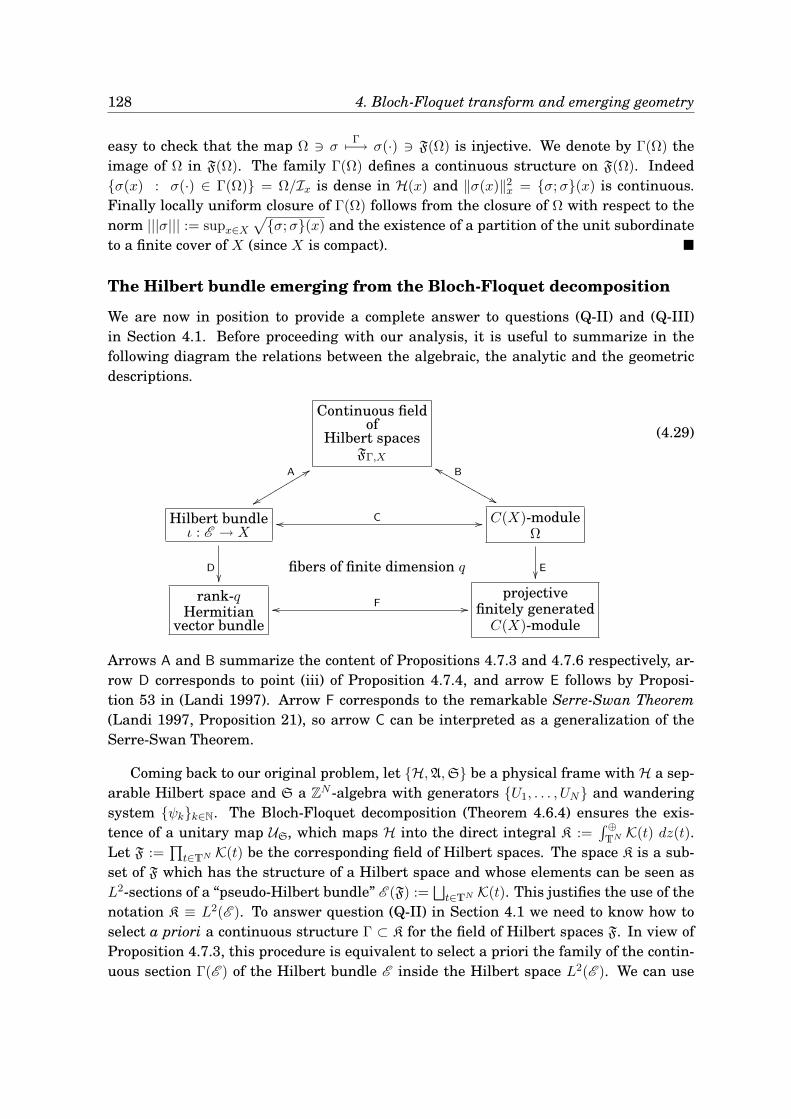
128 4. Bloch-Floquet transform and emerging geometry
easy to check that the map Ω ∋ σΓ7−→ σ(·) ∋ F(Ω) is injective. We denote by Γ(Ω) the
image of Ω in F(Ω). The family Γ(Ω) defines a continuous structure on F(Ω). Indeedσ(x) : σ(·) ∈ Γ(Ω) = Ω/Ix is dense in H(x) and ‖σ(x)‖2
x = σ;σ(x) is continuous.Finally locally uniform closure of Γ(Ω) follows from the closure of Ω with respect to thenorm |||σ||| := supx∈X
√σ;σ(x) and the existence of a partition of the unit subordinate
to a finite cover of X (since X is compact).
The Hilbert bundle emerging from the Bloch-Floquet decomposition
We are now in position to provide a complete answer to questions (Q-II) and (Q-III)in Section 4.1. Before proceeding with our analysis, it is useful to summarize in thefollowing diagram the relations between the algebraic, the analytic and the geometricdescriptions.
Continuous fieldof
Hilbert spacesFΓ,X
99A
yyrrrrrrrrrrff
B
&&MMMMMMMMMMM
Hilbert bundleι : E → X
fibers of finite dimension qD
oo C // C(X)-moduleΩ
E
rank-qHermitian
vector bundleoo F //
projectivefinitely generatedC(X)-module
(4.29)
Arrows A and B summarize the content of Propositions 4.7.3 and 4.7.6 respectively, ar-row D corresponds to point (iii) of Proposition 4.7.4, and arrow E follows by Proposi-tion 53 in (Landi 1997). Arrow F corresponds to the remarkable Serre-Swan Theorem(Landi 1997, Proposition 21), so arrow C can be interpreted as a generalization of theSerre-Swan Theorem.
Coming back to our original problem, let H,A,S be a physical frame with H a sep-arable Hilbert space and S a ZN -algebra with generators U1, . . . , UN and wanderingsystem ψkk∈N. The Bloch-Floquet decomposition (Theorem 4.6.4) ensures the exis-tence of a unitary map US, which maps H into the direct integral K :=
∫ ⊕TN K(t) dz(t).
Let F :=∏t∈TN K(t) be the corresponding field of Hilbert spaces. The space K is a sub-
set of F which has the structure of a Hilbert space and whose elements can be seen asL2-sections of a “pseudo-Hilbert bundle” E (F) :=
⊔t∈TN K(t). This justifies the use of the
notation K ≡ L2(E ). To answer question (Q-II) in Section 4.1 we need to know how toselect a priori a continuous structure Γ ⊂ K for the field of Hilbert spaces F. In view ofProposition 4.7.3, this procedure is equivalent to select a priori the family of the contin-uous section Γ(E ) of the Hilbert bundle E inside the Hilbert space L2(E ). We can use
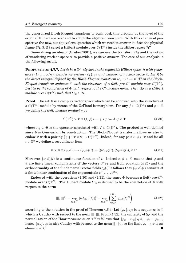
4.7. Emergent geometry 129
the generalized Bloch-Floquet transform to push back this problem at the level of theoriginal Hilbert space H and to adopt the algebraic viewpoint. With this change of per-spective the new, but equivalent, question which we need to answer is: does the physicalframe H,A,S select a Hilbert module over C(TN ) inside the Hilbert space H?
Generalizing an idea of (Gruber 2001), we can use the transform US and the notionof wandering nuclear space Φ to provide a positive answer. The core of our analysis isthe following result.
PROPOSITION 4.7.7. Let S be a ZN -algebra in the separable Hilbert space H with gener-ators U1, . . . , UN, wandering system ψkk∈N and wandering nuclear space Φ. Let K bethe direct integral defined by the Bloch-Floquet transform US : H → K. Then the Bloch-Floquet transform endowes Φ with the structure of a (left) pre-C∗-module over C(TN ).Let ΩS be the completion of Φ with respect to the C∗-module norm. Then ΩS is a Hilbertmodule over C(TN ) such that ΩS ⊂ H.
Proof. The set Φ is a complex vector space which can be endowed with the structure ofa C(TN )-module by means of the Gel’fand isomorphism. For any f ∈ C(TN ) and ϕ ∈ Φ
we define the (left) module product ⋆ by
C(TN ) × Φ ∋ (f, ϕ) 7−→ f ⋆ ϕ := Afϕ ∈ Φ (4.30)
where Af ∈ S is the operator associated with f ∈ C(TN ). The product is well definedsince Φ is S-invariant by construction. The Bloch-Floquet transform allows us also toendow Φ with a pairing ·; · : Φ × Φ → C(TN ). Indeed, for any pair ϕ, φ ∈ Φ and for allt ∈ Tn we define a sesquilinear form
Φ × Φ ∋ (ϕ, φ) 7−→ ϕ, φ(t) := ((USϕ)(t); (USφ)(t))t ∈ C. (4.31)
Moreover ϕ, φ(t) is a continuous function of t. Indeed ϕ, φ ∈ Φ means that ϕ andφ are finite linear combinations of the vectors Uaψk and from equation (4.25) and theorthonormality of the fundamental vector fields ζk(·) it follows that ϕ, φ(t) consists ofa finite linear combination of the exponentials eit1 , . . . , eitN .
Endowed with the operations (4.30) and (4.31), the space Φ becomes a (left) pre-C∗-module over C(TN ). The Hilbert module ΩS is defined to be the completion of Φ withrespect to the norm
|||ϕ|||2 := supt∈TN
‖(USϕ)(t)‖2t = sup
t∈TN
(fin∑
k∈N
|fϕ;k(t)|2)
(4.32)
according to the notation in the proof of Theorem 4.6.4. Let ϕnn∈N be a sequence in Φ
which is Cauchy with respect to the norm ||| · |||. From (4.32), the unitarity of US and thenormalization of the Haar measure dz on TN it follows that ‖ϕn − ϕm‖H 6 |||ϕn − ϕm|||,hence ϕnn∈N is also Cauchy with respect to the norm ‖ · ‖H, so the limit ϕn → ϕ is anelement of H.
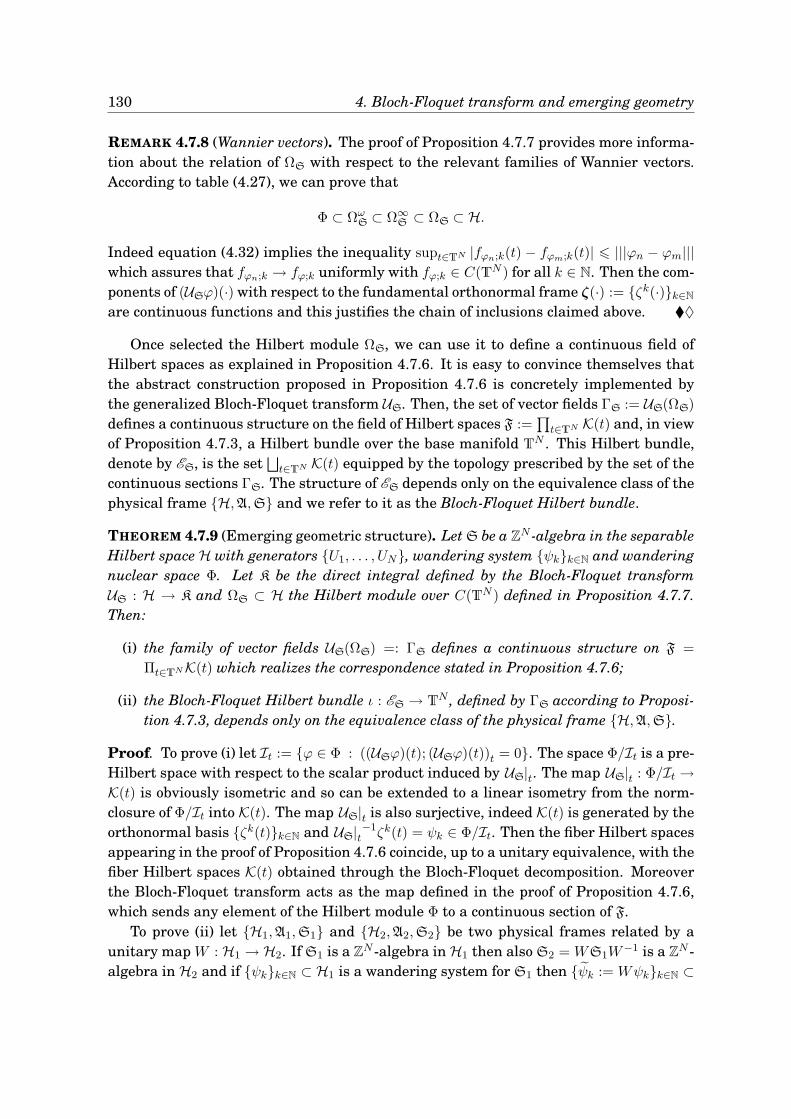
130 4. Bloch-Floquet transform and emerging geometry
REMARK 4.7.8 (Wannier vectors). The proof of Proposition 4.7.7 provides more informa-tion about the relation of ΩS with respect to the relevant families of Wannier vectors.According to table (4.27), we can prove that
Φ ⊂ ΩωS ⊂ Ω∞
S ⊂ ΩS ⊂ H.
Indeed equation (4.32) implies the inequality supt∈TN |fϕn;k(t) − fϕm;k(t)| 6 |||ϕn − ϕm|||which assures that fϕn;k → fϕ;k uniformly with fϕ;k ∈ C(TN ) for all k ∈ N. Then the com-ponents of (USϕ)(·) with respect to the fundamental orthonormal frame ζ(·) := ζk(·)k∈N
are continuous functions and this justifies the chain of inclusions claimed above. ♦
Once selected the Hilbert module ΩS, we can use it to define a continuous field ofHilbert spaces as explained in Proposition 4.7.6. It is easy to convince themselves thatthe abstract construction proposed in Proposition 4.7.6 is concretely implemented bythe generalized Bloch-Floquet transform US. Then, the set of vector fields ΓS := US(ΩS)
defines a continuous structure on the field of Hilbert spaces F :=∏t∈TN K(t) and, in view
of Proposition 4.7.3, a Hilbert bundle over the base manifold TN . This Hilbert bundle,denote by ES, is the set
⊔t∈TN K(t) equipped by the topology prescribed by the set of the
continuous sections ΓS. The structure of ES depends only on the equivalence class of thephysical frame H,A,S and we refer to it as the Bloch-Floquet Hilbert bundle.
THEOREM 4.7.9 (Emerging geometric structure). Let S be a ZN -algebra in the separableHilbert space H with generators U1, . . . , UN, wandering system ψkk∈N and wanderingnuclear space Φ. Let K be the direct integral defined by the Bloch-Floquet transformUS : H → K and ΩS ⊂ H the Hilbert module over C(TN ) defined in Proposition 4.7.7.Then:
(i) the family of vector fields US(ΩS) =: ΓS defines a continuous structure on F =
Πt∈TNK(t) which realizes the correspondence stated in Proposition 4.7.6;
(ii) the Bloch-Floquet Hilbert bundle ι : ES → TN , defined by ΓS according to Proposi-tion 4.7.3, depends only on the equivalence class of the physical frame H,A,S.
Proof. To prove (i) let It := ϕ ∈ Φ : ((USϕ)(t); (USϕ)(t))t = 0. The space Φ/It is a pre-Hilbert space with respect to the scalar product induced by US|t. The map US|t : Φ/It →K(t) is obviously isometric and so can be extended to a linear isometry from the norm-closure of Φ/It into K(t). The map US|t is also surjective, indeed K(t) is generated by theorthonormal basis ζk(t)k∈N and US|t−1ζk(t) = ψk ∈ Φ/It. Then the fiber Hilbert spacesappearing in the proof of Proposition 4.7.6 coincide, up to a unitary equivalence, with thefiber Hilbert spaces K(t) obtained through the Bloch-Floquet decomposition. Moreoverthe Bloch-Floquet transform acts as the map defined in the proof of Proposition 4.7.6,which sends any element of the Hilbert module Φ to a continuous section of F.
To prove (ii) let H1,A1,S1 and H2,A2,S2 be two physical frames related by aunitary map W : H1 → H2. If S1 is a ZN -algebra in H1 then also S2 = WS1W
−1 is a ZN -algebra in H2 and if ψkk∈N ⊂ H1 is a wandering system for S1 then ψk := Wψkk∈N ⊂
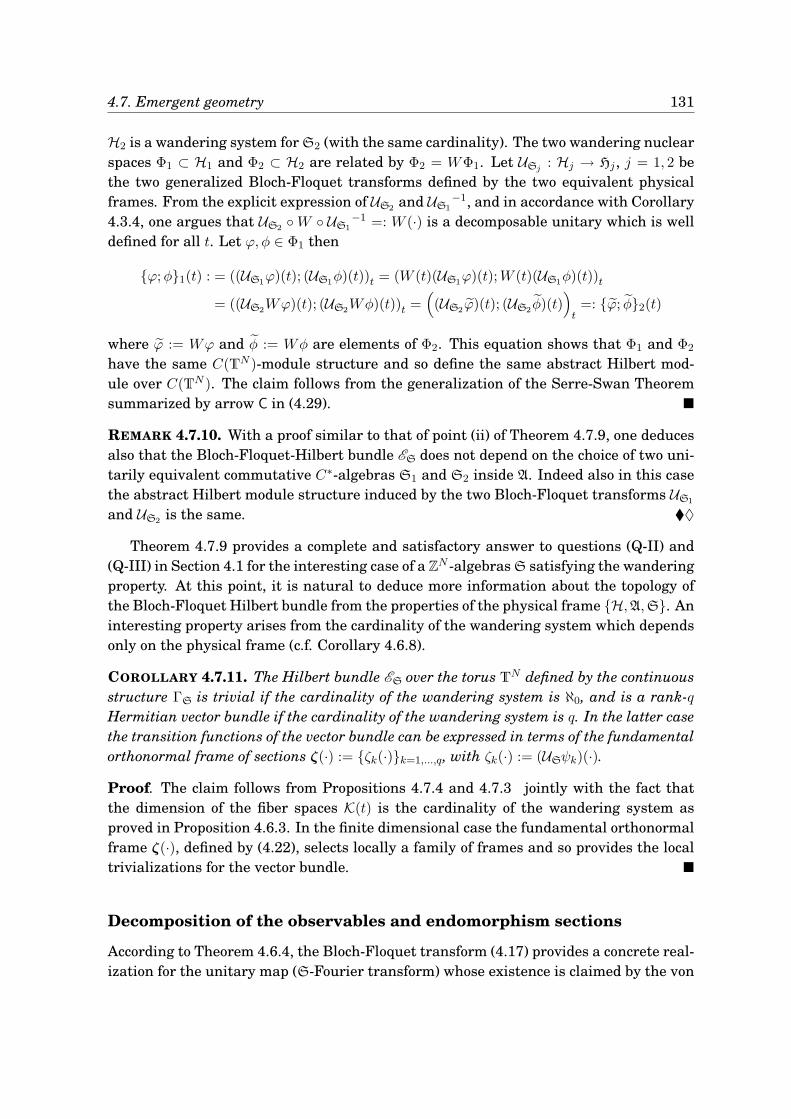
4.7. Emergent geometry 131
H2 is a wandering system for S2 (with the same cardinality). The two wandering nuclearspaces Φ1 ⊂ H1 and Φ2 ⊂ H2 are related by Φ2 = WΦ1. Let USj : Hj → Hj , j = 1, 2 bethe two generalized Bloch-Floquet transforms defined by the two equivalent physicalframes. From the explicit expression of US2 and US1
−1, and in accordance with Corollary4.3.4, one argues that US2 W US1
−1 =: W (·) is a decomposable unitary which is welldefined for all t. Let ϕ, φ ∈ Φ1 then
ϕ;φ1(t) : = ((US1ϕ)(t); (US1φ)(t))t = (W (t)(US1ϕ)(t);W (t)(US1φ)(t))t
= ((US2Wϕ)(t); (US2Wφ)(t))t =((US2ϕ)(t); (US2 φ)(t)
)
t=: ϕ; φ2(t)
where ϕ := Wϕ and φ := Wφ are elements of Φ2. This equation shows that Φ1 and Φ2
have the same C(TN )-module structure and so define the same abstract Hilbert mod-ule over C(TN ). The claim follows from the generalization of the Serre-Swan Theoremsummarized by arrow C in (4.29).
REMARK 4.7.10. With a proof similar to that of point (ii) of Theorem 4.7.9, one deducesalso that the Bloch-Floquet-Hilbert bundle ES does not depend on the choice of two uni-tarily equivalent commutative C∗-algebras S1 and S2 inside A. Indeed also in this casethe abstract Hilbert module structure induced by the two Bloch-Floquet transforms US1
and US2 is the same. ♦
Theorem 4.7.9 provides a complete and satisfactory answer to questions (Q-II) and(Q-III) in Section 4.1 for the interesting case of a ZN -algebras S satisfying the wanderingproperty. At this point, it is natural to deduce more information about the topology ofthe Bloch-Floquet Hilbert bundle from the properties of the physical frame H,A,S. Aninteresting property arises from the cardinality of the wandering system which dependsonly on the physical frame (c.f. Corollary 4.6.8).
COROLLARY 4.7.11. The Hilbert bundle ES over the torus TN defined by the continuousstructure ΓS is trivial if the cardinality of the wandering system is ℵ0, and is a rank-qHermitian vector bundle if the cardinality of the wandering system is q. In the latter casethe transition functions of the vector bundle can be expressed in terms of the fundamentalorthonormal frame of sections ζ(·) := ζk(·)k=1,...,q, with ζk(·) := (USψk)(·).
Proof. The claim follows from Propositions 4.7.4 and 4.7.3 jointly with the fact thatthe dimension of the fiber spaces K(t) is the cardinality of the wandering system asproved in Proposition 4.6.3. In the finite dimensional case the fundamental orthonormalframe ζ(·), defined by (4.22), selects locally a family of frames and so provides the localtrivializations for the vector bundle.
Decomposition of the observables and endomorphism sections
According to Theorem 4.6.4, the Bloch-Floquet transform (4.17) provides a concrete real-ization for the unitary map (S-Fourier transform) whose existence is claimed by the von
132 4. Bloch-Floquet transform and emerging geometry
Neumann’s complete spectral theorem. Let hereafter H,A,S be a physical frame withS a ZN -algebra admitting a wandering system. Point (ii) of Theorem 4.3.1 implies thatunder the Bloch-Floquet transform any O ∈ A is mapped into a decomposable operatoron the direct integral
∫ ⊕TN K(t) dz(t) , i.e. USO US
−1 =: O(·) : t 7→ O(t) ∈ B(K(t)) withO(·) weakly mesurable.
The natural question which arises is the following: there exists any topological struc-ture in theC∗-algebra A compatible with the Bloch-Floquet Hilbert bundle which emergesfrom the Bloch-Floquet transform? To answer to this question we firstly analyze the na-ture of the linear maps which preserve the (Hilbert module) structure of the set of thecontinuous sections.
DEFINITION 4.7.12 (Hilbert module endomorphism). Let Ω be a (left) Hilbert moduleover the commutative unital C∗-algebra A. An endomorphism of Ω is a A-linear mapO : Ω → Ω which is adjointable, i.e. there exists a map O† : Ω → Ω such that σ;Oρ =
O†σ; ρ for all σ, ρ ∈ Ω. We denote by EndA(Ω) the set of all the endomorphisms of Ω.
As proved in (Gracia-Bondía et al. 2001, Section 2.5) or (Landi 1997, Appendix A), ifO ∈ EndA(Ω), then also its adjoint O† ∈ EndA(Ω) and † is an involution over EndA(Ω).Moreover, EndA(Ω) endowed with the endomorphism norm
‖O‖End(Ω) := sup|||O(σ)||| : |||σ||| 6 1 (4.33)
becomes a C∗-algebra (of bounded operators). For any σ, ρ ∈ Ω one defines the rank-1endomorphism |σρ| ∈ EndA(Ω) by |σρ|(ς) := ρ; ς σ for all ς ∈ Ω. The adjoint of|σρ| is given by |ρσ|. The linear span of the rank-1 endomorphisms is a selfadjointtwo-sided ideal of EndA(Ω) (finite rank endomorphisms) and its (operator) norm closureis denoted by End0
A(Ω). The elements of the latter are called compact endomorphisms ofΩ. Since End0
A(Ω) is an essential ideal of EndA(Ω), it follows that End0A(Ω) = EndA(Ω)
if and only if 1Ω ∈ End0A(Ω).
A remarkable result which emerges from the above theory is the characterization ofthe compact endomorphisms of the C(X) Hilbert module Γ(E ) of the continuous sectionsof a rank-q Hermitian vector bundle ι : E → X.
PROPOSITION 4.7.13. Let ι : E → X be a rank-q Hermitian vector bundle over the com-pact Hausdorff space X and let Γ(E ) be the Hilbert module over C(X) of its continuoussections. Then
End0C(X)(Γ(E )) = EndC(X)(Γ(E )) ≃ Γ(End(E )) (4.34)
where Γ(End(E )) denotes the continuous sections of the endomorphism vector bundleι′ : End(E ) → X. The localization isomorphism appearing in right-hand side of (4.34)preserves the composition and the structure of C(X)-module.
Proof. The localization (right-hand) isomorphism in (4.34) is a consequence of the Serre-Swan Theorem (Gracia-Bondía et al. 2001, Theorems 2.10 and 3.8). Such a theoremstates that there exists an equivalence of categories between finite rank Hermitian vec-tor bundles over a compact space X and Hilbert modules over C(X) which are pro-jective and finitely generated. The latter are modules of the form pC(X)⊕M , where
4.7. Emergent geometry 133
C(X)⊕M := C(X) × . . . × C(X) (M -times), p ∈ MatM (C(X)) (M × M matrices withentries in C(X)) is an orthogonal projection (p2 = p = p†) and M is some positive integer(M > q).
The Γ-functor sends any (rank q) Hermitian vector bundle ι : E → X in the Hilbertmodule of its continuous sections Γ(E ) ≃ pC(X)⊕M (isomorphism of Hilbert modules)and any strong bundle map (i.e. a map which induces the identity in the base space) f :
E → E in a Hilbert module endomorphism Γ(f) ∈ EndC(X)(Γ(E )) ≃ EndC(X)(pC(X)⊕M ).Any strong bundle map f can be seen as a section of the endomorphism bundle ι′ :
End(E ) → X. This identification defines an isomorphism (of C(X)-modules preservingthe composition) between the set of the strong bundle maps and Γ(End(E )). The equiv-alence of categories induced by Γ implies the localization isomorphism EndC(X)(Γ(E )) ≃Γ(End(E )). The isomorphism of C(X)-modules (preserving the composition) (Gracia-Bondía et al. 2001, Lemma 2.18)
End0C(X)(pC(X)⊕M ) ≃ pMatM (C(X))p
shows that the identity endomorphism is in End0C(X)(pC(X)⊕M ) since the C∗-algebra
C(X) is unital. This implies that
End0C(X)(pC(X)⊕M ) = EndC(X)(pC(X)⊕M )
since the compact endomorphisms form an essential ideal (Gracia-Bondía et al. 2001,Proposition 3.2).
In Proposition 4.7.7 we proved that the Gel’fand isomorphism and the Bloch-Floquettransform equip the wandering nuclear space Φ with the structure of a (left) pre-C∗-module over C(TN ) by means of the (left) product ⋆ defined by (4.30) and the pairing ; defined by (4.31). The closure of Φ with respect to the module norm defines aHilbert module over C(TN ) denoted by ΩS ⊂ H. In this description what is the rôleplayed by A? Is it possible, at least under some condition, to interpret the elementsof A as endomorphism of the Hilbert module ΩS? One could try to answer to thesequestions by observing that for any O ∈ A, any Af ∈ S and any ϕ ∈ ΩS one has thatO(f ⋆ ϕ) := OAfϕ = AfOϕ. The latter might be interpreted as f ⋆ O(ϕ), implyingthe C(TN )-linearity of O ∈ A as operator on ΩS. However it may happen that Oϕ /∈ ΩS
which implies that O can not define an endomorphism of ΩS. Everything works properlyif one consider only elements in the subalgebra A0 ⊂ A defined by
A0 := O ∈ A : O : ΩS → ΩS. (4.35)
PROPOSITION 4.7.14. Let ΩS be the Hilbert module over C(TN ) defined by means of theBloch-Floquet transform according to Proposition 4.7.7. Let A0
s.a. be the C∗-subalgebraof A defined by A0
s.a. := O ∈ A : O,O† ∈ A0 (self-adjoint part of A0). Then A0s.a. ⊂
EndC(TN )(ΩS).
134 4. Bloch-Floquet transform and emerging geometry
Proof. Let O ∈ A0s.a.. By definition O is a linear map from ΩS to itself; it is also C(TN )-
linear since O(f ⋆ϕ) = OAfϕ = AfOϕ as mentioned. We need to prove that O is boundedwith respect to the endomorphism norm (4.33). From the definition (4.32) of the modulenorm ||| · ||| it follows that
|||Oϕ||| = supt∈TN ‖(USOϕ)(t)‖t = supt∈TN ‖πt(O)(USϕ)(t)‖t 6 ‖O‖B(H) |||ϕ||| (4.36)
where πt(O) := US|t O US|t−1 defines a representation of the C∗-algebra A on the fiberHilbert space K(t) and ‖πt(O)‖B(K(t)) 6 ‖O‖B(H) since any C∗ representation decreasesthe norm. Thus ‖O‖End(ΩS) 6 ‖O‖B(H), therefore O defines a continuous C(TN )-linearmap from ΩS to itself. To prove that O ∈ EndC(TN )(ΩS) we must show that O is ad-jointable, which follows from the definition of A0
s.a..
It is of particular interest to specialize the previous result to the case of a finitewandering system.
THEOREM 4.7.15 (Bloch-Floquet endomorphism bundle). Let H,A,S be a physicalframe where S is a ZN -algebra with generators U1, . . . , UN and wandering systemψ1, . . . , ψq of finite cardinality. Then:
(i) A0s.a. = A0;
(ii) US A0 US−1 ⊆ Γ(End(ES)) where ι : ES → TN is the rank q Bloch-Floquet vector
bundle defined in Corollary 4.7.11.
Proof. To prove (i) let O ∈ A0 and observe that if Oψk =∑q
h=1
∑b∈ZN α
(k)h,b U
bψh then
O†ψk =∑q
h=1
∑b∈ZN α
(h)k,b U
−bψh. Since Oψk ∈ ΩS, then f(k)h (t) :=
∑b∈ZN α
(k)h,b z
b(t) is acontinuous function on TN and
|||O†ψk|||2 = supt∈TN
(q∑
h=1
|f (h)k (t)|2
)< +∞.
Then O†ψk ∈ ΩS for all k = 1, . . . , q. Since O†(U bψk) = U b(O†ψk) ∈ ΩS for all b ∈ ZN itfollows that also O† ∈ A0. Point (ii) is an immediate consequence of Proposition 4.7.14,Corollary 4.7.11 and Proposition 4.7.13.
EXAMPLE 4.7.16 (Mathieu-like Hamiltonians, part four). It is immediate to check thatboth u and v preserve the wandering nuclear space ΦM, so that the full C∗-algebraA
p/qM consists of endomorphisms for the Hilbert module realized by means of the Bloch-
Floquet transform USqM
. Theorem 4.7.15 claims that USqM
maps Ap/qM in a subalgebra of
the endomorphism bundle associated to the trivial bundle T×Cq → T. The matrices u(t)and v(t) in Example 4.6.7 are a representation of the generators u and v as elements ofΓ(End(T× Cq)) ≃ C(T) ⊗ Matq(C). ⊲
Chapter 5
The geometry of Hofstadter and Harper models
On se persuade mieux, pour l’ordinaire, par les raisonsqu’on a soi-même trouvées, que par celles qui sont venuesdans l’esprit des autres.
(People are generally better persuaded by the reasonswhich they have themselves discovered than by thosewhich have come into the mind of others.)
Blaise PascalPensées, 1670
Abstract
This final chapter aims to present the proofs of the “geometric” results of this thesis,that is Theorem 2.7.4 and Theorem 2.8.1. In Section 5.1 we derive the (standard)physical frames for the Hofstadter and Harper representations. This first step showsthat the theory of the (generalized) Bloch-Floquet decomposition, developed in Chapter4, can be applied successfully to systems in Hofstadter or Harper regime. Employingthe machinery of the Bloch-Floquet decomposition, we derive in Section 5.2 the bundledecomposition of the Hofstadter (resp. Harper) representation, as well the geometricstructure of the Hofstadter (resp. Harper) vector bundle. The content of these firsttwo sections provides the proof of Theorem 2.7.4. Finally, the proof of Theorem 2.8.1is achieved is Section 5.3. In this last section, we derive the geometric duality be-tween vector subbundles of the Hofstadter or Harper vector bundles related to a given“abstract” projection, according to the “two-fold way” (2.44).
5.1 Standard physical frames
5.1.1 Representation theory of the NCT-algebra
The representation theory of the NCT-algebra depends heavily on the fact that thedeformation parameter is rational or irrational.
Irrational case
The representation theory of the NCT-algebra is particularly simple when the deforma-tion parameter is irrational (Boca 2001, Theorem 1.10):
- Simplicity and faithfulness: If θ ∈ R \ Q then the NCT-algebra Aθ is simple,i.e. it has no non-trivial closed two-sided ideals. This implies that any (non-trivial)
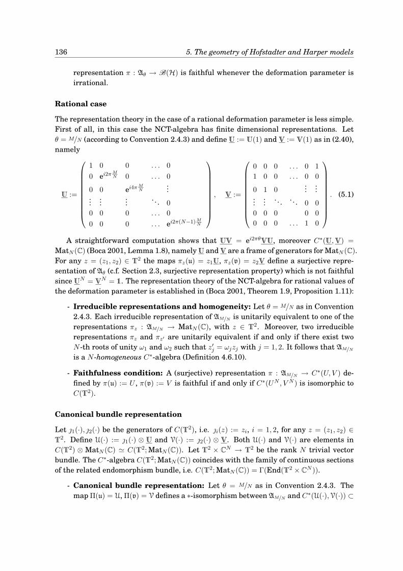
136 5. The geometry of Hofstadter and Harper models
representation π : Aθ → B(H) is faithful whenever the deformation parameter isirrational.
Rational case
The representation theory in the case of a rational deformation parameter is less simple.First of all, in this case the NCT-algebra has finite dimensional representations. Letθ = M/N (according to Convention 2.4.3) and define U := U(1) and V := V(1) as in (2.40),namely
U :=
1 0 0 . . . 0
0 ei2πMN 0 . . . 0
0 0 ei4πMN
......
......
. . . 0
0 0 0 . . . 0
0 0 0 . . . ei2π(N−1)MN
, V :=
0 0 0 . . . 0 1
1 0 0 . . . 0 0
0 1 0...
......
.... . . . . . 0 0
0 0 0 0 0
0 0 0 . . . 1 0
. (5.1)
A straightforward computation shows that UV = ei2πθVU, moreover C∗(U,V) =
MatN (C) (Boca 2001, Lemma 1.8), namely U and V are a frame of generators for MatN (C).For any z = (z1, z2) ∈ T2 the maps πz(u) = z1U, πz(v) = z2V define a surjective repre-sentation of Aθ (c.f. Section 2.3, surjective representation property) which is not faithfulsince U
N = VN = 1. The representation theory of the NCT-algebra for rational values of
the deformation parameter is established in (Boca 2001, Theorem 1.9, Proposition 1.11):
- Irreducible representations and homogeneity: Let θ = M/N as in Convention2.4.3. Each irreducible representation of AM/N is unitarily equivalent to one of therepresentations πz : AM/N → MatN (C), with z ∈ T2. Moreover, two irreduciblerepresentations πz and πz′ are unitarily equivalent if and only if there exist twoN -th roots of unity ω1 and ω2 such that z′j = ωjzj with j = 1, 2. It follows that AM/N
is a N -homogeneous C∗-algebra (Definition 4.6.10).
- Faithfulness condition: A (surjective) representation π : AM/N → C∗(U, V ) de-fined by π(u) := U , π(v) := V is faithful if and only if C∗(UN , V N ) is isomorphic toC(T2).
Canonical bundle representation
Let 1(·), 2(·) be the generators of C(T2), i.e. i(z) := zi, i = 1, 2, for any z = (z1, z2) ∈T2. Define U(·) := 1(·) ⊗ U and V(·) := 2(·) ⊗ V. Both U(·) and V(·) are elements inC(T2) ⊗ MatN (C) ≃ C(T2; MatN (C)). Let T2 × CN → T2 be the rank N trivial vectorbundle. The C∗-algebra C(T2; MatN (C)) coincides with the family of continuous sectionsof the related endomorphism bundle, i.e. C(T2; MatN (C)) = Γ(End(T2 × CN )).
- Canonical bundle representation: Let θ = M/N as in Convention 2.4.3. Themap Π(u) = U, Π(v) = V defines a ∗-isomorphism between AM/N and C∗(U(·),V(·)) ⊂
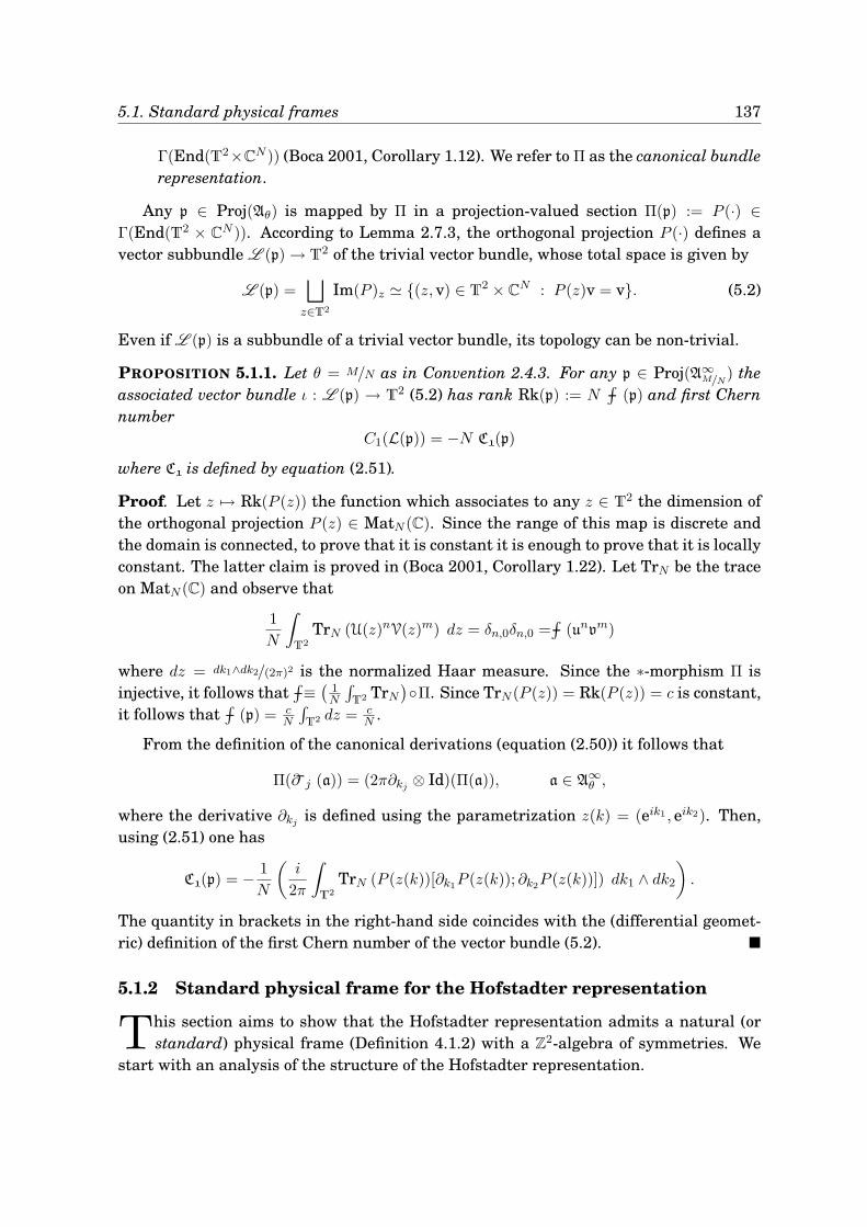
5.1. Standard physical frames 137
Γ(End(T2×CN )) (Boca 2001, Corollary 1.12). We refer to Π as the canonical bundlerepresentation.
Any p ∈ Proj(Aθ) is mapped by Π in a projection-valued section Π(p) := P (·) ∈Γ(End(T2 × CN )). According to Lemma 2.7.3, the orthogonal projection P (·) defines avector subbundle L (p) → T2 of the trivial vector bundle, whose total space is given by
L (p) =⊔
z∈T2
Im(P )z ≃ (z, v) ∈ T2 × CN : P (z)v = v. (5.2)
Even if L (p) is a subbundle of a trivial vector bundle, its topology can be non-trivial.
PROPOSITION 5.1.1. Let θ = M/N as in Convention 2.4.3. For any p ∈ Proj(A∞M/N) the
associated vector bundle ι : L (p) → T2 (5.2) has rank Rk(p) := N∫−−− (p) and first Chern
numberC1(L(p)) = −N C1(p)
where C1 is defined by equation (2.51).
Proof. Let z 7→ Rk(P (z)) the function which associates to any z ∈ T2 the dimension ofthe orthogonal projection P (z) ∈ MatN (C). Since the range of this map is discrete andthe domain is connected, to prove that it is constant it is enough to prove that it is locallyconstant. The latter claim is proved in (Boca 2001, Corollary 1.22). Let TrN be the traceon MatN (C) and observe that
1
N
∫
T2
TrN (U(z)nV(z)m) dz = δn,0δn,0 =∫−−− (unvm)
where dz = dk1∧dk2/(2π)2 is the normalized Haar measure. Since the ∗-morphism Π isinjective, it follows that
∫−−−≡
(1N
∫T2 TrN
)Π. Since TrN (P (z)) = Rk(P (z)) = c is constant,
it follows that∫−−− (p) = c
N
∫T2 dz = c
N .
From the definition of the canonical derivations (equation (2.50)) it follows that
Π(∂−−−j (a)) = (2π∂kj⊗ Id)(Π(a)), a ∈ A∞
θ ,
where the derivative ∂kjis defined using the parametrization z(k) = (eik1 , eik2). Then,
using (2.51) one has
C1(p) = − 1
N
(i
2π
∫
T2
TrN (P (z(k))[∂k1P (z(k)); ∂k2P (z(k))]) dk1 ∧ dk2
).
The quantity in brackets in the right-hand side coincides with the (differential geomet-ric) definition of the first Chern number of the vector bundle (5.2).
5.1.2 Standard physical frame for the Hofstadter representation
This section aims to show that the Hofstadter representation admits a natural (orstandard) physical frame (Definition 4.1.2) with a Z2-algebra of symmetries. We
start with an analysis of the structure of the Hofstadter representation.
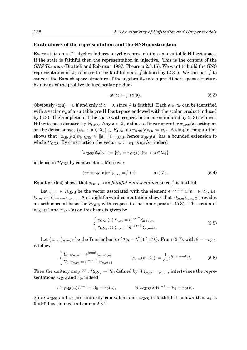
138 5. The geometry of Hofstadter and Harper models
Faithfulness of the representation and the GNS construction
Every state on a C∗-algebra induces a cyclic representation on a suitable Hilbert space.If the state is faithful then the representation in injective. This is the content of theGNS Theorem (Bratteli and Robinson 1987, Theorem 2.3.16). We want to build the GNSrepresentation of Aθ relative to the faithful state
∫−−− defined by (2.31). We can use
∫−−− to
convert the Banach space structure of the algebra Aθ into a pre-Hilbert space structureby means of the positive defined scalar product
〈a; b〉 :=∫−−− (a∗b). (5.3)
Obviously 〈a; a〉 = 0 if and only if a = 0, since∫−−− is faithful. Each a ∈ Aθ can be identified
with a vector ψa of a suitable pre-Hilbert space endowed with the scalar product inducedby (5.3). The completion of the space with respect to the norm induced by (5.3) defines aHilbert space denoted by HGNS. Any a ∈ Aθ defines a linear operator πGNS(a) acting onon the dense subset ψb : b ∈ Aθ ⊂ HGNS as πGNS(a)ψb := ψab. A simple computationshows that ‖πGNS(a)ψb‖GNS 6 ‖a‖ ‖ψb‖GNS, hence πGNS(a) has a bounded extension towhole HGNS. By construction the vector := ψ1 is cyclic, indeed
[πGNS(Aθ)] := ψa = πGNS(a) : a ∈ Aθ
is dense in HGNS by construction. Moreover
(;πGNS(a))HGNS =∫−−− (a) a ∈ Aθ. (5.4)
Equation (5.4) shows that πGNS is an faithful representation since∫−−− is faithful.
Let ξn,m ∈ HGNS be the vector associated with the element e−iπnmθ unvm ∈ Aθ, i.e.ξn,m := ψe−iπnmθ unvm . A straightforward computation shows that ξn,mn,m∈Z providesan orthonormal basis for HGNS with respect to the inner product (5.3). The action ofπGNS(u) and πGNS(v) on this basis is given by
πGNS(u) ξn,m = eiπmθ ξn+1,m
πGNS(v) ξn,m = e−iπnθ ξn,m+1.(5.5)
Let ϕn,mn,m∈Z be the Fourier basis of H0 = L2(T2, d2k). From (2.7), with θ = −ιqε0,it follows
U0 ϕn,m = eiπmθ ϕn+1,m
V0 ϕn,m = e−iπnθ ϕn,m+1
ϕn,m(k1, k2) :=1
2πei(nk1+mk2). (5.6)
Then the unitary map W : HGNS → H0 defined by Wξn,m = ϕn,m, intertwines the repre-sentations πGNS and π0, indeed
WπGNS(u)W−1 = U0 = π0(u), WπGNS(v)W−1 = V0 = π0(v).
Since πGNS and π0 are unitarily equivalent and πGNS is faithful it follows that π0 isfaithful as claimed in Lemma 2.3.2.
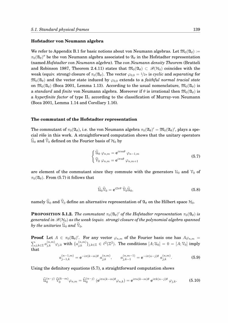
5.1. Standard physical frames 139
Hofstadter von Neumann algebra
We refer to Appendix B.1 for basic notions about von Neumann algebras. Let M0(Aθ) :=
π0(Aθ)′′ be the von Neumann algebra associated to Aθ in the Hofstadter representation
(named Hofstadter von Neumann algebra). The von Neumann density Theorem (Bratteliand Robinson 1987, Theorem 2.4.11) states that M0(Aθ) ⊂ B(H0) coincides with theweak (equiv. strong) closure of π0(Aθ). The vector ϕ0,0 = 1/2π is cyclic and separating forM0(Aθ) and the vector state induced by ϕ0,0 extends to a faithful normal tracial stateon M0(Aθ) (Boca 2001, Lemma 1.13). According to the usual nomenclature, M0(Aθ) isa standard and finite von Neumann algebra. Moreover if θ is irrational then M0(Aθ) isa hyperfinite factor of type II1 according to the classification of Murray-von Neumann(Boca 2001, Lemma 1.14 and Corollary 1.16).
The commutant of the Hofstadter representation
The commutant of π0(Aθ), i.e. the von Neumann algebra π0(Aθ)′ = M0(Aθ)
′, plays a spe-cial rôle in this work. A straightforward computation shows that the unitary operatorsU0 and V0 defined on the Fourier basis of H0 by
U0 ϕn,m = eiπmθ ϕn−1,m
V0 ϕn,m = eiπnθ ϕn,m+1
(5.7)
are element of the commutant since they commute with the generators U0 and V0 ofπ0(Aθ). From (5.7) it follows that
U0V0 = ei2πθ V0U0, (5.8)
namely U0 and V0 define an alternative representation of Aθ on the Hilbert space H0.
PROPOSITION 5.1.2. The commutant π0(Aθ)′ of the Hofstadter representation π0(Aθ) is
generated in B(H0) as the weak (equiv. strong) closure of the polynomial algebra spannedby the unitaries U0 and V0.
Proof. Let A ∈ π0(Aθ)′. For any vector ϕn,m of the Fourier basis one has Aϕn,m =∑
j,k∈Za
(n,m)j,k ϕj,k with a(n,m)
j,k j,k∈Z ∈ ℓ2(Z2). The conditions [A;U0] = 0 = [A;V0] implythat
a(n−1,m)j−1,k = e−iπ(k−m)θ a
(n,m)j,k , a
(n,m−1)j,k−1 = e−iπ(n−j)θ a(n,m)
j,k . (5.9)
Using the definitory equations (5.7), a straightforward computation shows
U(n−j)0 V
(k−m)0 ϕn,m = U
(n−j)0 (eiπn(k−m)θϕn,k) = eiπn(k−m)θ eiπk(n−j)θ ϕj,k. (5.10)
140 5. The geometry of Hofstadter and Harper models
Solving (5.10) with respect ϕj,k and using (5.9), one has
Aψn,m =∑
j,k∈Z
a(n,m)j,k
(e−iπn(k−m)θ e−iπk(n−j)θ U
(n−j)0 V
(k−m)0 ϕn,m
)
=
∑
j,k∈Z
a(n,m)j,k
(e−iπ(k−m)θ
)n (e−iπ(n−j)θ
)kU
(n−j)0 V
(k−m)0
ϕn,m
=
∑
j,k∈Z
a(0,m−k)j−n,0 U
(n−j)0 V
(k−m)0
ϕn,m =
∑
j,k∈Z
a(0,−k)−j,0 U
j0 Vk0
ϕn,m.
Since the previous equation holds true for any vector ϕn,m of the Fourier basis, it followsthat A =
∑j,k∈Z
αj,k Uj0 Vk0 where αj,k := a
(0,−k)−j,0 = (ϕ−j,0;Aϕ0,−k)H0 .
The Hofstadter physical frame
The separable Hilbert space H0 and the C∗-algebra π0(Aθ) ⊂ B(H0) are two ingredientsfor a physical frame (Definition 4.1.2). To complete the physical frame structure we needto select a maximal commutative subalgebra inside the commutant π0(Aθ)
′. Let θ = M/N
(as in Convention 2.4.3). In view of the commutation relation (5.8) it is easy to checkthat S0 := C∗(U0, V
N0 ) defines a commutative C∗-subalgebra of π0(AM/N)′.
LEMMA 5.1.3. TheC∗-algebra S0 is maximal commutative inside the commutant π0(AM/N)′.
Proof. Let A =∑
j,k∈Zαj,kU
j0 Vk0 be an element in π0(Aθ)
′ such that [U0;A] = 0 = [VN0 ;A].A direct computation shows that αj,k 6= 0 only if k ∈ NZ, which means A ∈ S0.
The triple H0, π0(AM/N),S0 is a physical frame. We refer to it as the standardphysical frame of the Hofstadter representation (or simply Hofstadter physical frame).It is immediate to recognize that the set ϕ0,jj=0,...,N−1 ⊂ H0, where ϕn,m is defined by(5.6), is a wandering system of cardinality N for S0. It follows that S0 is Z2-algebra(claim (iii) in Proposition 4.5.2). We refer to ϕ0,jj=0,...,N−1 as the standard wanderingsystem for the Hofstadter representation.
Obviously S0 is not the only maximal commutative C∗-subalgebra of π0(AM/N)′. In-
deed let p, q be two integers such that pq = N , then C∗(Up0, Vq0) is another maximal
commutative C∗-subalgebra of π0(AM/N)′ different from S0, with a wandering systemof cardinality N given by ϕi,ji=0,...,p−1,j=0,...,q−1. The ambiguity in the choice of thealgebra of symmetry is solved by Proposition 4.6.11. Since AM/N is a N -homogeneousC∗-algebra and π0 is a faithful representation it follows that there exists a unique equiv-alence class of irreducible physical frames with wandering property for the Hofstadterrepresentation. Therefore there is no loss of generality fixing the Hofstadter physicalframe H0, π0(AM/N),S0 as the standard representative of this class.
5.1. Standard physical frames 141
5.1.3 Standard physical frame for the Harper representation
In this section we derive the (standard) physical frame for the Harper representation.As in the previous section, we start with an analysis of the structure of the Harper
representation.
Faithfulness of the representation and generalized eigenvectors
We start this section giving the proof of Lemma 2.3.4 which states that the Harperrepresentation π∞ : Aθ → C∗(U∞,V∞) ⊂ B(H∞) is faithful.
The claim is certainly true when θ ∈ R \ Q since in this case any representation ofAθ is faithful, as explained at the beginning of Section 5.1.1. Then, we can assume thatθ = M/N (as in Convention 2.4.3). Under this hypothesis the faithfulness of π∞ follows ifone proves that C∗(UN∞,V
N∞) ≃ C(T2) (c.f. Section 5.1.1).
The Gel’fand-Naımark Theorem states that C∗(UN∞,VN∞) ≃ C(X) where the Gel’fand
spectrum X is (homeomorphic to) the joint spectrum of UN∞ and VN∞ (Hörmander 1990,Theorem 3.1.15), the latter being the set of the common generalized eigenvalues of UN∞and VN∞ (Samoilenko 1991, Proposition 2). In view of that, we have to prove that forany k = (k1, k2) ∈ [0, 2π) × [0, 2π) there exists a sequence ψ(k)
j j∈N ⊂ H∞ of normalizedvectors such that
‖(UN∞ − eik11)ψ(k)j ‖H∞ → 0, ‖(VN∞ − eik21)ψ
(k)j ‖H∞ → 0, if j → +∞.
This would mean that the joint spectrum of UN∞ and VN∞ is the full torus T2, thus it yieldsC∗(UN∞,V
N∞) ≃ C(T2). To complete the proof we exhibit the generalized eigenvectors,
namely
ψ(k)j (x) :=
√M
N
j∑
n=−jeink2 j
(x+ nM − 1
N
k1
2π
)
where j(x) :=√
Nj2
M(2j+1)(xj2) and is any smooth positive function supported in (−1, 1)
which satisfies the normalization condition ‖‖2H∞
=∫
R(x)2 dx = 1. The function j
is supported in (−1/j2, 1/j2) with square-norm NM(2j+1) and this is enough to show that
‖ψ(k)j ‖2
H∞= M
N
∑jn=−j ‖j‖2
H∞= 1.
Harper von Neumann algebra
Let M∞(Aθ) := π∞(Aθ)′′ be the von Neumann algebra associated to Aθ in the Harper
representation (called Harper von Neumann algebra). As usual M∞(Aθ) coincides withthe the weak (equiv. strong) closure of π∞(Aθ) in B(H∞). Contrary to the Hofstadtercase, the von Neumann algebra M∞(Aθ) is not standard (whenever θ 6= ±1), indeed if|θ| < 1 then M∞(Aθ) has a cyclic but not separating vector, while if |θ| > 1 then M∞(Aθ)
has a separating but not cyclic vector. The obstruction for M∞(Aθ) to be a standard vonNeumann algebra is discussed by G. G. Emch in (Emch 1996) and follows as a corollaryof two general results, one by M. A. Rieffel (Rieffel 1981, Theorem 3.2) and the secondby M. Takesaki (Takesaki 1969, Theorem 3).
142 5. The geometry of Hofstadter and Harper models
The commutant of the Harper representation
The latter paper by Takesaki is of particular interest in this work since it provides anexplicit description for the commutant π∞(Aθ)
′ = M∞(Aθ)′. A simple computation shows
that the unitaries
U∞ ψ(x) = ei2πθx ψ(x)
ψ ∈ H∞
V∞ ψ(x) = ψ(x− 1)
(5.11)
are elements of the commutant π∞(Aθ)′ since they commute with the generators U∞ and
V∞ of the algebra π∞(Aθ). Moreover,
U∞V∞ = ei2πθ V∞U∞, (5.12)
namely the unitaries U∞ and V∞ define a representation of A1/θ on the Hilbert spaceH∞. Since Takesaki proves that M∞(Aθ)
′ = M∞(A1/θ) (Takesaki 1969, Theorem 3), onehas
PROPOSITION 5.1.4. The commutant π∞(Aθ)′ of the Harper representation of Aθ is gen-
erated in B(H∞) as the weak (equiv. strong) closure of the polynomial algebra spannedby the unitaries U∞ and V∞.
The Harper physical frame
Similarly to the Hofstadter case, the separable Hilbert space H∞ and the C∗-algebraπ∞(Aθ) ⊂ B(H∞) are two ingredients for a physical frame. To complete the structure, weneed to select a maximal commutative subalgebra inside the commutant π∞(Aθ)
′ whichis generated by the unitaries U∞ and V∞. Let θ = M/N (according to Convention 2.4.3).In view of the commutation relation (5.12), it is easy to check that S∞ := C∗(U∞, VM∞)
defines a commutative C∗-subalgebra of π∞(AM/N)′. With the same proof of Lemma 5.1.3we have
LEMMA 5.1.5. TheC∗-algebra S∞ is maximal commutative inside the commutant π∞(AM/N)′.
The triple H∞, π∞(AM/N),S∞ is a physical frame and we refer to it as the standardphysical frame of the Harper representation (or simply Harper physical frame). In orderto select a wandering system for S∞, we introduce the following family of vectors
χj,n(x) :=
√N
|M | if x ∈ Ij,0
0 otherwise,
(5.13)
5.2. Bundle decomposition of representations 143
where, for any j, n ∈ Z, the intervals Ij,n are defined by
Ij,n :=
[jM
N+ nM ; (j + 1)
M
N+ nM
)if M > 0
((j + 1)
M
N+ nM ; j
M
N+ nM
]if M < 0.
(5.14)
The family χjj=0,...,N−1 ⊂ H∞, with χj ≡ χj,0, is a wandering system of cardinality Nfor S∞. Indeed, a simple check shows that
R =
N−1⋃
j=0
⋃
n∈Z
Ij,n, ⇒ H∞ ≃N−1⊕
j=0
⊕
n∈Z
L2(Ij,n). (5.15)
The characteristic function of each interval Ij,n is obtained as χj,n = VnM∞ χj and thefamily of vectors ei2π
NMmxχj,n = Un∞χj,n, with m ∈ Z, provides an orthonormal basis
for L2(Ij,n). We refer to χjj=0,...,N−1 ⊂ H∞ as the standard wandering system for theHarper representation. It follows that S∞ is a Z2-algebra (claim (iii) in Proposition4.5.2).
Obviously, as in the case of the Hofstadter representation, S∞ is not the only commu-tative C∗-subalgebra of π∞(AM/N)′. However, as in the previous case, Proposition 4.6.11,the N -homogeneity of AM/N and the faithfulness of π∞ assure that there is no loss ofgenerality fixing the standard physical frame H∞, π∞(Aθ),S∞ as the representativeof the equivalence class of the irreducible physical frames with wandering property.
5.2 Bundle decomposition of representations
5.2.1 Bundle decomposition of the Hofstadter representation
In this section we derive the bundle decomposition of the Hofstadter representationaccording to Definition 2.7.2. We use the technology developped in Chapter 4 to define
a generalized Bloch-Floquet transform F0 which provides a direct integral decomposi-tion of the algebra π0(AM/N). A relevant and essentially unique vector bundle structureemerges from such a decomposition in virtue of properties of F0. The content of thissection provides the proof of claim (i) in Theorem 2.7.4.
The Bloch-Floquet decomposition in the Hofstadter representation
The standard physical frame of the Hofstadter representation H0, π0(AM/N),S0, en-dowed with the standard wandering system ϕ0,jj=0,...,N−1 (c.f. Section 5.1.2) deter-mines the Hofstadter nuclear space Φ0 ⊂ H0, as explained at the beginning of Section4.6. Explicitly, the space Φ0 consists of finite linear combinations of vectors ϕn,m (definedby (5.6)) of the Fourier basis of H0.
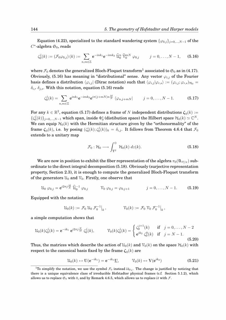
144 5. The geometry of Hofstadter and Harper models
Equation (4.22), specialized to the standard wandering system ϕ0,jj=0,...,N−1 of theC∗-algebra S0, reads
ζj0(k) := (F0ϕ0,j) (k) :=∑
n,m∈Z
e−ink1e−imk2 Un0 VmN0 ϕ0,j j = 0, . . . , N − 1, (5.16)
where F0 denotes the generalized Bloch-Floquet transform1 associated to S0 as in (4.17).Obviously, (5.16) has meaning in “distributional” sense. Any vector ϕi,j of the Fourierbasis defines a distribution 〈ϕi,j | (Dirac notation) such that 〈ϕi,j |ϕr,s〉 := (ϕi,j ;ϕr,s)H0 =
δi,r δj,s. With this notation, equation (5.16) reads
ζj0(k) =∑
n,m∈Z
eink1e−imk2eiπ(j+mN)nMN 〈ϕn,j+mN | j = 0, . . . , N − 1. (5.17)
For any k ∈ R2, equation (5.17) defines a frame of N independent distributions ζ0(k) :=
ζj0(k)j=0,...,N−1 which span, inside Φ∗0 (distibution space) the Hilbert space H0(k) ≃ CN .
We can equip H0(k) with the Hermitian structure given by the “orthonormality” of theframe ζ0(k), i.e. by posing (ζi0(k); ζ
j0(k))k = δi,j . It follows from Theorem 4.6.4 that F0
extends to a unitary map
F0 : H0 −→∫ ⊕
T2
H0(k) dz(k). (5.18)
We are now in position to exhibit the fiber representation of the algebra π0(AM/N) sub-ordinate to the direct integral decomposition (5.18). Obviously (surjective representationproperty, Section 2.3), it is enough to compute the generalized Bloch-Floquet transformof the generators U0 and V0. Firstly, one observe that
U0 ϕ0,j = ei2πjMN U−1
0 ϕ0,j V0 ϕ0,j = ϕ0,j+1 j = 0, . . . , N − 1. (5.19)
Equipped with the notation
U0(k) := F0 U0 F−10
∣∣k, V0(k) := F0 V0 F−1
0
∣∣k,
a simple computation shows that
U0(k)ζj0(k) = e−ik1 ei2πj
NM ζj0(k), V0(k)ζ
j0(k) =
ζj+10 (k) if j = 0, . . . , N − 2
eik2 ζ00 (k) if j = N − 1.
(5.20)Thus, the matrices which describe the action of U0(k) and V0(k) on the space H0(k) withrespect to the canonical basis fixed by the frame ζ0(k) are
U0(k) ↔ U(e−ik1) = e−ik1U, V0(k) ↔ V(eik2) (5.21)
1To simplify the notation, we use the symbol F0 instead US0. The change is justified by noticing that
there is a unique equivalence class of irreducible Hofstadter physical frames (c.f. Section 5.1.2), whichallows us to replace S0 with 0, and by Remark 4.6.5, which allows us to replace U with F .
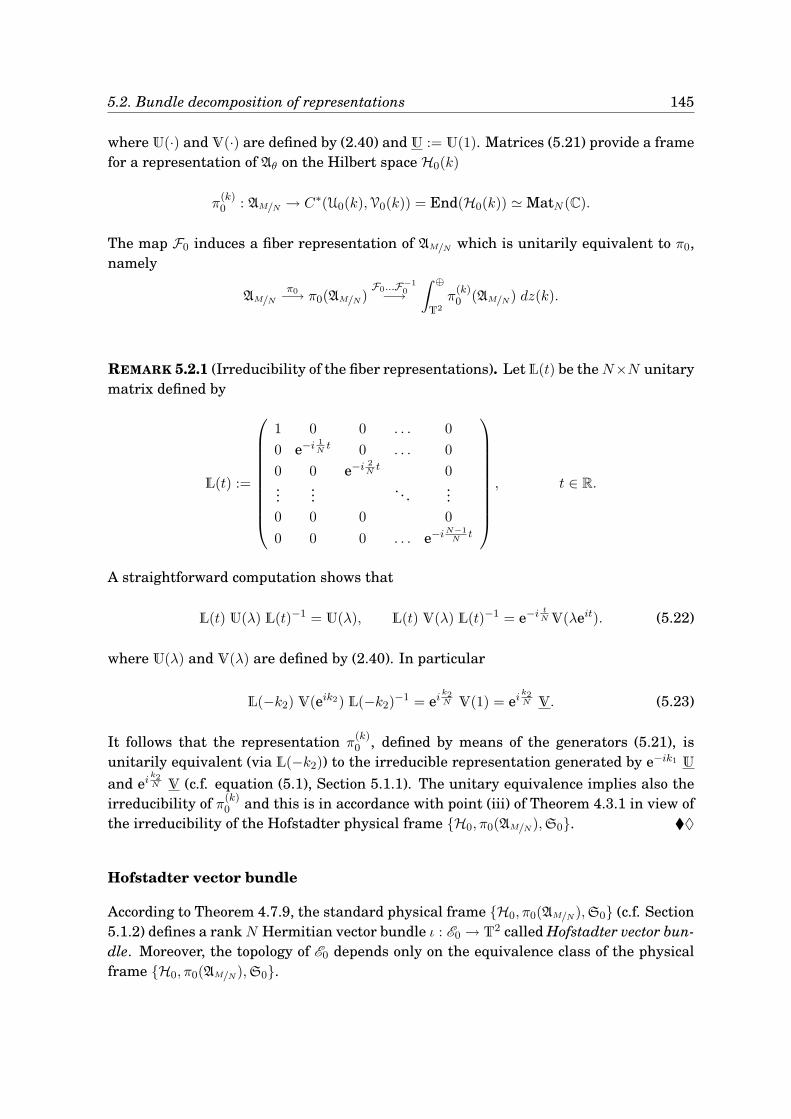
5.2. Bundle decomposition of representations 145
where U(·) and V(·) are defined by (2.40) and U := U(1). Matrices (5.21) provide a framefor a representation of Aθ on the Hilbert space H0(k)
π(k)0 : AM/N → C∗(U0(k),V0(k)) = End(H0(k)) ≃ MatN (C).
The map F0 induces a fiber representation of AM/N which is unitarily equivalent to π0,namely
AM/Nπ0−→ π0(AM/N)
F0...F−10−→∫ ⊕
T2
π(k)0 (AM/N) dz(k).
REMARK 5.2.1 (Irreducibility of the fiber representations). Let L(t) be theN×N unitarymatrix defined by
L(t) :=
1 0 0 . . . 0
0 e−i1Nt 0 . . . 0
0 0 e−i2Nt 0
......
. . ....
0 0 0 0
0 0 0 . . . e−iN−1
Nt
, t ∈ R.
A straightforward computation shows that
L(t) U(λ) L(t)−1 = U(λ), L(t) V(λ) L(t)−1 = e−itN V(λeit). (5.22)
where U(λ) and V(λ) are defined by (2.40). In particular
L(−k2) V(eik2) L(−k2)−1 = ei
k2N V(1) = ei
k2N V. (5.23)
It follows that the representation π(k)0 , defined by means of the generators (5.21), is
unitarily equivalent (via L(−k2)) to the irreducible representation generated by e−ik1 U
and eik2N V (c.f. equation (5.1), Section 5.1.1). The unitary equivalence implies also the
irreducibility of π(k)0 and this is in accordance with point (iii) of Theorem 4.3.1 in view of
the irreducibility of the Hofstadter physical frame H0, π0(AM/N),S0. ♦
Hofstadter vector bundle
According to Theorem 4.7.9, the standard physical frame H0, π0(AM/N),S0 (c.f. Section5.1.2) defines a rankN Hermitian vector bundle ι : E0 → T2 called Hofstadter vector bun-dle. Moreover, the topology of E0 depends only on the equivalence class of the physicalframe H0, π0(AM/N),S0.
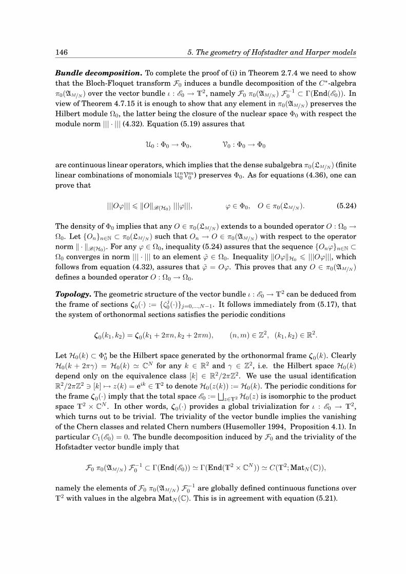
146 5. The geometry of Hofstadter and Harper models
Bundle decomposition. To complete the proof of (i) in Theorem 2.7.4 we need to showthat the Bloch-Floquet transform F0 induces a bundle decomposition of the C∗-algebraπ0(AM/N) over the vector bundle ι : E0 → T2, namely F0 π0(AM/N) F−1
0 ⊂ Γ(End(E0)). Inview of Theorem 4.7.15 it is enough to show that any element in π0(AM/N) preserves theHilbert module Ω0, the latter being the closure of the nuclear space Φ0 with respect themodule norm ||| · ||| (4.32). Equation (5.19) assures that
U0 : Φ0 → Φ0, V0 : Φ0 → Φ0
are continuous linear operators, which implies that the dense subalgebra π0(LM/N) (finitelinear combinations of monomials Un0Vm0 ) preserves Φ0. As for equations (4.36), one canprove that
|||Oϕ||| 6 ‖O‖B(H0) |||ϕ|||, ϕ ∈ Φ0, O ∈ π0(LM/N). (5.24)
The density of Φ0 implies that any O ∈ π0(LM/N) extends to a bounded operator O : Ω0 →Ω0. Let Onn∈N ⊂ π0(LM/N) such that On → O ∈ π0(AM/N) with respect to the operatornorm ‖ · ‖B(H0). For any ϕ ∈ Ω0, inequality (5.24) assures that the sequence Onϕn∈N ⊂Ω0 converges in norm ||| · ||| to an element ϕ ∈ Ω0. Inequality ‖Oϕ‖H0 6 |||Oϕ|||, whichfollows from equation (4.32), assures that ϕ = Oϕ. This proves that any O ∈ π0(AM/N)
defines a bounded operator O : Ω0 → Ω0.
Topology. The geometric structure of the vector bundle ι : E0 → T2 can be deduced fromthe frame of sections ζ0(·) := ζj0(·)j=0,...,N−1. It follows immediately from (5.17), thatthe system of orthonormal sections satisfies the periodic conditions
ζ0(k1, k2) = ζ0(k1 + 2πn, k2 + 2πm), (n,m) ∈ Z2, (k1, k2) ∈ R2.
Let H0(k) ⊂ Φ∗0 be the Hilbert space generated by the orthonormal frame ζ0(k). Clearly
H0(k + 2πγ) = H0(k) ≃ CN for any k ∈ R2 and γ ∈ Z2, i.e. the Hilbert space H0(k)
depend only on the equivalence class [k] ∈ R2/2πZ2. We use the usual identificationR2/2πZ2 ∋ [k] 7→ z(k) = eik ∈ T2 to denote H0(z(k)) := H0(k). The periodic conditions forthe frame ζ0(·) imply that the total space E0 :=
⊔z∈T2 H0(z) is isomorphic to the product
space T2 × CN . In other words, ζ0(·) provides a global trivialization for ι : E0 → T2,which turns out to be trivial. The triviality of the vector bundle implies the vanishingof the Chern classes and related Chern numbers (Husemoller 1994, Proposition 4.1). Inparticular C1(E0) = 0. The bundle decomposition induced by F0 and the triviality of theHofstadter vector bundle imply that
F0 π0(AM/N) F−10 ⊂ Γ(End(E0)) ≃ Γ(End(T2 × CN )) ≃ C(T2; MatN (C)),
namely the elements of F0 π0(AM/N) F−10 are globally defined continuous functions over
T2 with values in the algebra MatN (C). This is in agreement with equation (5.21).
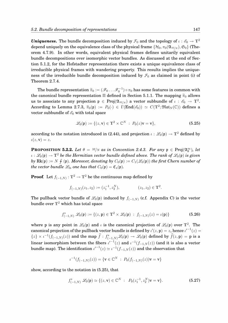
5.2. Bundle decomposition of representations 147
Uniqueness. The bundle decomposition induced by F0 and the topology of ι : E0 → T2
depend uniquely on the equivalence class of the physical frame H0, π0(AM/N),S0 (The-orem 4.7.9). In other words, equivalent physical frames defines unitarily equivalentbundle decompositions over isomorphic vector bundles. As discussed at the end of Sec-tion 5.1.2, for the Hofstadter representation there exists a unique equivalence class ofirreducible physical frames with wandering property. This results implies the unique-ness of the irreducible bundle decomposition induced by F0 as claimed in point (i) ofTheorem 2.7.4.
The bundle representation π0 := (F0 . . .F−10 ) π0 has some features in common with
the canonical bundle representation Π defined in Section 5.1.1. The mapping π0 allowsus to associate to any projection p ∈ Proj(AM/N) a vector subbundle of ι : E0 → T2.According to Lemma 2.7.3, π0(p) := P0(·) ∈ Γ(End(E0)) ≃ C(T2;MatN (C)) defines avector subbundle of E0 with total space
L0(p) := (z, v) ∈ T2 × CN : P0(z)v = v, (5.25)
according to the notation introduced in (2.44), and projection ι : L0(p) → T2 defined byι(z, v) = z.
PROPOSITION 5.2.2. Let θ = M/N as in Convention 2.4.3. For any p ∈ Proj(A∞θ ), let
ι : L0(p) → T2 be the Hermitian vector bundle defined above. The rank of L0(p) is givenby Rk(p) := N
∫−−− (p). Moreover, denoting by C0(p) := C1(L0(p)) the first Chern number of
the vector bundle L0, one has that C0(p) = C1(p).
Proof. Let f(−1,N) : T2 → T2 be the continuous map defined by
f(−1,N)(z1, z2) := (z−11 , zN2 ), (z1, z2) ∈ T
2.
The pullback vector bundle of L0(p) induced by f(−1,N) (c.f. Appendix C) is the vectorbundle over T2 which has total space
f∗(−1,N) L0(p) := (z,p) ∈ T2 × L0(p) : f(−1,N)(z) = ι(p) (5.26)
where p is any point in L0(p) and ι is the canonical projection of L0(p) over T2. Thecanonical projection of the pullback vector bundle is defined by ι′(z,p) = z, hence ι′−1(z) =
z × ι−1(f(−1,N)(z)) and the map f : f∗(−1,N)L0(p) → L0(p) defined by f(z,p) = p is a
linear isomorphism between the fibers ι′−1(z) and ι−1(f−1,N (z)) (and it is also a vectorbundle map). The identification ι′−1(z) ≃ ι−1(f−1,N (z)) and the observation that
ι−1(f(−1,N)(z)) = v ∈ CN : P0(f(−1,N)(z))v = v
show, according to the notation in (5.25), that
f∗(−1,N) L0(p) ≃ (z, v) ∈ CN : P0(z−11 , zN2 )v = v. (5.27)
148 5. The geometry of Hofstadter and Harper models
Let p = Fp(u, v) be the expression of the abstract projection in terms of the abstractgenerators of Aθ. Using equation (5.21), one has that
P0(z−11 (k), zN2 (k)) = Fp(U(eik1),V(eiNk2)).
By using the results of Remark 5.2.1, we can write
P0(z−11 (k), zN2 (k)) = L(−Nk2) Fp(z1(k)U, z2(k)V) L(−Nk2)
−1
= L(−Nk2) P (z1(k), z2(k)) L(−Nk2)−1
where P (·) := Π(p) is the projection-valued section in C(T2)⊗MatN (C) associated to theabstract projection p by means of the mapping Π. Since the unitary matrix L(−Nk2) isglobally defined, and so define a global change of the orthonormal frame in the fibers, itfollows that
f∗(−1,N) L0(p) ≃ L (p) (5.28)
where the vector bundle L (p) is defined by equation (5.2).The first consequence of the identification (5.28) is that the rank of the vector bun-
dle f∗(−1,N) L0(p) coincides with the rank of the vector bundle L (p) which is Rk(p) byProposition 5.1.1. The first part of the claim follows by observing that the operation ofpullback does not change the dimension of the fibers.
The second part follows from C1(L (p)) = −NC1(p) proved in Proposition 5.1.1 andC1(L (p)) = C1(f
∗(−1,N) L0(p)) = −NC1(L0(p)) as a consequence of Lemma C.0.2.
5.2.2 Bundle decomposition of the Harper representation
We derive in the present section the bundle decomposition of the Harper representa-tion using the technology developed in Chapter 4. We define a generalized Bloch-
Floquet transform F∞ which provides a direct integral decomposition of the algebraπ∞(AM/N) and selects a unique vector bundle structure emerging from such a decompo-sition. The content of this section provides the proof of claim (ii) in Theorem 2.7.4.
The Bloch-Floquet decomposition in the Harper representation
As explained at the beginning of Section 4.6, we can use the standard physical frameof the Harper representation H∞, π∞(AM/N),S∞ and the standard wandering systemχjj=0,...,N−1 (see Section 5.1.3) to build the Harper nuclear space Φ∞ ⊂ H∞. Explicitlythe space Φ∞ consists of functions supported on a finite number of intervals In,j , see(5.14), such that inside each In,j ⊂ R they are polynomials in ei2π
NMx. Therefore, the ele-
ments in Φ∞ are well defined compactly supported functions on R, which are everywheresmooth except at the points xj,n := jM/N + nM , j = 0, . . . , N − 1, n ∈ Z.
Equation (4.22), specialized to the standard wandering system χjj=0,...,N−1 of theC∗-algebra S∞, gives
ζj∞(k) := (F∞χj) (k) =∑
n,m∈Z
e−ink1e−imk2 Un∞ VmM∞ χj j = 1, . . . , N, (5.29)
5.2. Bundle decomposition of representations 149
where F∞ denotes the generalized Bloch-Floquet transform associated to S∞ as in (4.17)(for the notation c.f. Note 1 in Section 5.2.1). The distributions (5.29) can be rewrittenin a more convenient form.
PROPOSITION 5.2.3. For any (k1, k2) ∈ [0, 2π)2 the distributions ζj∞(k) ∈ Φ∗∞ act on Φ∞
as
ζj∞(k; ·) =
√|M |N
∑
m∈Z
e−imk2 δ[· − M
N
(k1
2π+ j
)−mM
]j = 1, . . . , N (5.30)
where δ(· − x0) acts on ψ ∈ Φ∞ as the evaluation in x0 (Dirac’s delta), i.e. 〈δ(· − x0);ψ〉 =
ψ(x0).
Proof. For any ψ ∈ Φ∞ one has
〈Un∞ VmM∞ χj ;ψ〉 : =(χj ; U
−n∞ V−mM
∞ ψ)
H∞
= (signθ)
√N
|M |
∫ MN
0e−i2π
NMnxψ
(x+ j
M
N+mM
)dx. (5.31)
Let φ : I0,0 → C be the function defined by
φ(x) := ψ
(x+ j
M
N+mM
),
with I0,0 defined by (5.14). The definition of Φ∞ implies that ψ, when restricted to any
interval Ij,n, is a finite linear combination of the exponentials ei2πN|M|
x. Then, one has
φ(x) :=
fin∑
n∈Z
φn ei2πN|M|
nx, φn := (signθ)
N
|M |
∫ MN
0e−i2π
N|M|
nxφ (x) dx (5.32)
for any x ∈ I0,0. A comparison between (5.31) and (5.32) shows that√
N
|M | 〈Un∞ VmM∞ χj ;ψ〉 = (signθ)
N
|M |
∫ MN
0e−i2π
N|M|
(signθ)nxφ (x) dx = φ(signθ)n.
The above equation implies
〈∑
n∈Z
e−ink1Un∞ VmM∞ χj ;ψ〉 =
√|M |N
∑
n∈Z
φ(signθ)n eink1 =
√|M |N
fin∑
n∈Z
φ(signθ)n ei2πN|M|
n“
|M|N
k12π
”
=
√|M |N
fin∑
n∈Z
φn ei2πN|M|
n“
MN
k12π
”
= φ
(M
N
k1
2π
)
where we used (5.32) whenever MN
k12π ∈ I0,0, i.e. k1 ∈ [0, 2π). In view of the definition of φ,
one has
〈∑
n∈Z
e−ink1Un∞ VmM∞ χj ;ψ〉 =
√|M |N
ψ
(M
N
k1
2π+ j
M
N+mM
).
150 5. The geometry of Hofstadter and Harper models
Finally, for any ψ ∈ Φ∞ one has
〈ζj∞(k);ψ〉 =
√|M |N
∑
m∈Z
eimk2ψ[M
N
(k1
2π+ j
)+mM
],
which implies (5.30).
For any k ∈ [0, 2π)2, equation (5.30) defines a frame of N independent distributionsζ∞(k) := ζj∞(k)j=0,...,N−1 which span, inside Φ∗
∞ (distibution space) the Hilbert spaceH∞(k) ≃ CN . We can equip H∞(k) with the Hermitian structure given by (ζi∞(k); ζj∞(k))k =
δi,j . It follows from Theorem 4.6.4 that F∞ extends to a unitary map
F∞ : H∞ −→∫ ⊕
T2
H∞(k) dz(k). (5.33)
Analogously to the case of the Hofstadter representation, we can exhibit the fiberrepresentation of the algebra π∞(AM/N) subordinate to the direct integral decomposition(5.33) by computing the generalized Bloch-Floquet transform of the generators U∞ andV∞. Let
ei2πx ≡∑
n∈Z
an ei2πN|M|
nx, an =
iN(1 − ei2π|M|N )
2π(|M | − nN)(5.34)
be the Fourier expansion of ei2πx restricted to the interval x ∈ I0,0. The symbol ≡ meansthat the series converges in L2-norm. Moreover, the series converges pointwise in theinterior of I0,0. Observing that
U∞ χj(x) = ei2πxχj(x) = ei2πMNjei2π(x−j
MN )χj(x) 6= 0 if x− j
M
N∈ I0,0
and using the L2-expansion (5.34), one has
U∞ χj(x) ≡ ei2πMNj∑
n∈Z
an ei2πN|M|
n(x−jMN )χj(x) = ei2π
MNj∑
n∈Z
an U(signθ)n∞ χj(x). (5.35)
It follows that
〈∑
n,m∈Z
e−ink1e−imk2Un∞ VmM∞ U∞χj ;ψ〉
= e−i2πMNj∑
ℓ∈Z
aℓ〈∑
n,m∈Z
e−ink1e−imk2Un+(signθ)ℓ∞ VmM∞ χj ;ψ〉 (5.36)
= e−i2πMNj
(∑
ℓ∈Z
aℓ ei(signθ)k1ℓ
)〈∑
n,m∈Z
e−ink1e−imk2Un∞ VmM∞ χj ;ψ〉.
In view of (5.34), one has(∑
ℓ∈Z
aℓ ei(signθ)k1ℓ
)ψ ≡ e−i
MNk1ψ, in Φ∞ ⊂ H∞.
5.2. Bundle decomposition of representations 151
The arbitrariness in the choice of the test function ψ ∈ Φ∞ in (5.36) implies∑
n,m∈Z
e−ink1e−imk2Un∞ VmM∞ U∞χj = eiMNk1 ei2π
MNj∑
n,m∈Z
e−ink1e−imk2Un∞ VmM∞ χj
where the equality is in distributional sense, i.e. as element of Φ∗∞. Equipped with the
notationU∞(k) := F∞ U∞ F−1
∞∣∣k, V∞(k) := F∞ V∞ F−1
∞∣∣k,
the above equation reads
U∞(k)ζj∞(k) = eiMNk1 ei2π
MNj ζj∞(k), j = 0, . . . , N − 1. (5.37)
The second generator V∞ acts on the vectors of the wandering system as
(V∞ χj)(x) = χj
(x− M
N
)= χj+1(x) j = 0, . . . , N − 2
(V∞ χN−1)(x) = χ0(x−M) = (VM∞χ0)(x)
(5.38)
then
V∞(k)ζj∞(k) =
ζj+1∞ (k) if j = 0, . . . , N − 2
eik2 ζ0∞(k) if j = N − 1.
(5.39)
From equations (5.37) and (5.39) one deduces the matrices which describes the actionof U∞(k) and V∞(k) on the space H∞(k) with respect to the canonical basis fixd by theframe ζ∞(k); explicitly
U∞(k) ↔ U(eiMNk1) = ei
MNk1U, V∞(k) ↔ V(eik2) (5.40)
where U(·) and V(·) are defined by (2.40) and U := U(1).
The matrices (5.40) are the frame for a representation of AM/N on the Hilbert spaceH∞(k)
π(k)∞ : AM/N → C∗(U∞(k),V∞(k)) = End(H∞(k)) ≃ MatN (C).
The map F∞ induces a fiber representation of AM/N which is unitarily equivalent to π∞,namely
AM/Nπ∞−→ π∞(AM/N)
F∞...F−1∞−→∫ ⊕
T2
π(k)∞ (AM/N) dz(k).
Analogously to the Hofstadter case, one can prove that the representations π(k)∞ are
irreducible (c.f. Remark 5.2.1). This is in agreement with point (iii) of Theorem 4.3.1 inview of the irreducibility of the Harper physical frame H∞, π∞(AM/N),S∞.
Harper vector bundle
According to Theorem 4.7.9, the standard physical frame H∞, π∞(AM/N),S∞ (c.f. Sec-tion 5.1.3) defines a rank N Hermitian vector bundle ι : E∞ → T2 called Harper vectorbundle. Moreover, the topology of E∞ depends only on the equivalence class of the phys-ical frame H∞, π∞(AM/N),S∞.
152 5. The geometry of Hofstadter and Harper models
Bundle decomposition. To complete the proof of (ii) in Theorem 2.7.4 we need to showthat the Bloch-Floquet transform F∞ induces a bundle decomposition of the C∗-algebraπ∞(AM/N) over the vector bundle ι : E∞ → T2, namely F∞ π∞(AM/N) F−1
∞ ⊂ Γ(End(E∞)).In view of Theorem 4.7.15 it is enough to show that the any element in π∞(AM/N) pre-serves the Hilbert module Ω∞ which is the closure of the nuclear space Φ∞ with respectto the module norm ||| · ||| (4.32). Analogously to the Hofstadter case, the claim followsfrom a density argument provided that
U∞ : Ω∞ → Ω∞, V∞ : Ω∞ → Ω∞. (5.41)
The analysis of the generator V∞ is simple. Indeed, equations (5.38) imply V∞ : Φ∞ →Φ∞ which by density proves the second of (5.41).
The analysis of U∞ requires more care. Firstly we need to show that U∞χj ∈ Ω∞for any vector χj of the wandering system. This means that we have to prove that|||U∞ χj ||| < +∞. In view of equation (5.35), one has
|||U∞ χj |||2 = |||fin∑
n∈Z
an(U(signθ)n∞ χj)|||2
definition (4.32) of ||| · |||= supk∈[0,2π)2‖
∑
n∈Z
an ei(signθ)nk1ζj∞(k)‖2k
= supk1∈[0,2π)
∑
n,n′∈Z
an an′ ei(signθ)(n′−n)k1
= supk1∈[0,2π)
fin∑
n,n′∈Z
an an′ei(signθ)2π N|M|
(n′−n)“
k12π
|M|N
”
< +∞
since the series∑
n∈Zane±i2π
N|M|
nx (5.34) converges pointwise in I0,0 and in particular toe±i2πx in the interior of I0,0. Since U∞χj ∈ Ω∞ for any χj , it follows that U∞Φ∞ → Ω∞.The density of Φ∞ and the inequality (5.24) imply the first of (5.41).
Topology. The geometric structure of the vector bundle ι : E∞ → T2 can be deducedfrom the frame of sections ζ∞(·) := ζj0(·)j=0,...,N−1. It follows from (5.30) that the mapζ∞(·), which associates to any k ∈ [0, 2π)2 a frame of N independent elements in Φ∗
∞, canbe extended to the whole plane R2 by means of the following covariance condition
ζj∞(k1 + 2π, k2) =
N−1∑
l=0
Gj,l(k1, k2) ζl∞(k1, k2)
j = 0, . . . , N − 1
ζj∞(k1, k2 + 2π) = ζj∞(k1, k2);
(5.42)
here theN×N unitary matrix G(k) := Gj,l(k)j,l=0,...,N−1 is defined for any k = (k1, k2) ∈
5.2. Bundle decomposition of representations 153
R2 by:
G(k1, k2) :=
0 1 0 . . . 0 0
0 0 1 . . . 0 0
0 0 0. . .
......
......
.... . . 1 0
0 0 0 . . . 0 1
eik2 0 0 . . . 0 0
. (5.43)
Equations (5.42) can be rewritten in the synthetic form
ζ0(k1 + 2πn, k2 + 2πm) = G(k)n · ζ0(k1, k2), (n,m) ∈ Z2, (k1, k2) ∈ R2. (5.44)
Moreover, a straightforward computation shows that
G(k)N = eik2 1N = (−1)N−1 (detG(k)) 1N . (5.45)
Let H∞(k) ∈ Φ∗∞ be the Hilbert space generated by the orthonormal frame ζ∞(k).
Clearly H∞(k + 2πγ) = H∞(k) ≃ CN for any k ∈ R2 and γ ∈ Z2, i.e. the Hilbert spaceH∞(k) depends only on the equivalence class [k] ∈ R2/2πZ2. We use the usual identifica-tion R2/2πZ2 ∋ [k] 7→ z(k) = eik ∈ T2 to denote H∞(z(k)) := H∞(k).
The covariance condition (5.44) for the frame ζ∞(·) do not provide a global trivializa-tion for
⊔z∈T2 H∞(z) as in the case of the Hofstadter representation. To build the non
trivial Harper vector bundle associated to ζ∞(·) we identify the space⊔k∈R2 H∞(k) with
a subset of R2 × Φ∗∞ and we introduce the equivalence relation ∼G , where
(k, v) ∼G (k′, v′) ⇔
k′ = k + 2πγ
for some γ := (n,m) ∈ Z2.
v′ = G(k)n · v
The equivalence relation is well posed, indeed k′ = k + 2πγ implies that v and v′ are inthe same space since H∞(k + 2πγ) = H∞(k). This assures that the matrix G(k) = G([k])
acts as an isomorphism of the space H∞([k]). The equivalence class with representative(k, v) ∈ ⊔k∈R2 H∞(k) is denoted as [k, v]. Then, the total space E∞ of the Harper vectorbundle is defined as
E∞ :=
⊔
k∈R2
H∞(k)
/ ∼G .
The base space is the flat torus T2 = R2/2πZ2 and the projection to the base spaceι : E∞ → T2 is ι([k, v]) = z(k), where z provides the projection z : R2 → T2. One checksthat ι : E∞ → T2 is a smooth complex vector bundle with typical fiber CN .
154 5. The geometry of Hofstadter and Harper models
A system of transition functions for ι : E∞ → T2 can be described by means of thestandard atlas of T2 (c.f. Example C.0.1 and Figure C.1, Appendix C). Let Oaa=1,...,4
the open cover given by (C.2) and g := ga,ba,b=1,...,4, with ga,b : Oa,b → U (CN ), therelated system of transition functions. Equation (5.44) show that the frame ζ∞(·) ispurely periodic in k2, then it defines a frame of sections for E∞ which is globally definedin the k2-direction. This implies
g1,3(z) = 1N = g3,1(z) if z ∈ O1,3, g2,4(z) = 1N = g4,2(z) if z ∈ O2,4, (5.46)
which means that on the overlaps O1 ∩ O3 and O2 ∩ O4 the gluing between the sectionsis trivial. The other transition functions are non trivial and take into account for thequotient induced by ∼G. The reader can check that (c.f. Appendix C)
ga,b(z) =
1N if z ∈ Oa,b(k1 ∼ π)tG(z) if z ∈ Oa,b(k1 ∼ 2π)
with (a, b) = (1, 2), (1, 4), (3, 2), (3, 4) (5.47)
where tG denotes the transpose of G. For instance, equation (5.47) specialized to (a, b) =
(1, 2) assures that the identification between the local frame ζ(1)∞ (k1, ·) = ζ∞(k1, ·) in O1
and the local frame ζ(2)∞ (k1, ·) = ζ∞(k1 + 2π, ·) in O2 (−ǫ < k1 < ǫ) is given by means of
the matrix G, according to (5.44) (c.f. Appendix C). The set of the transition functions iscompleted by the relations ga,b = gb,a
−1 and ga,a = 1N .
The computation of the first Chern number of the Harper vector bundle needs thechoice of a connection ω = ωaa=1,...,4 compatible with the system of transition functions(5.46), (5.47), i.e.
ωa = dga,b ga,b−1 + ga,b ωb ga,b
−1, a, b = 1, . . . , 4,
(c.f. Appendix C). We can rewrite the above consistency equation in terms of the covari-ance condition (5.42), namely
ω(k1, k2) = dtG(k1, k2)tG(k1, k2)
−1 + tG(k1, k2) ω(k1 + 2π, k2 + 2π) tG(k1, k2)
−1. (5.48)
A simple computation shows that the matrix valued 1-form
ωHar(k1, k2) :=−iN
k12π 0 . . . 0
0(k12π + 1
). . . 0
......
. . ....
0 0 . . .(k12π + (N − 1)
)
dk2 + 1Ndk1 (5.49)
verifies (5.48). The connection ωHar, defined by (5.49), is called Harper connection. SinceωHar is diagonal one has that ωHar∧ωHar = 0. The Harper curvature 2-form KHar, definedaccording to (C.6), is
KHar(k1, k2) = dωHar(k1, k2) =
( −i2πN
1N
)dk1 ∧ dk2. (5.50)
5.3. Geometric duality between Hofstadter and Harper representations 155
Notice that KHar is defined globally, as a consequence of the particular choice of theHarper connection. From (C.8), using the curvature KHar, one obtains the (differential)Chern class for the Harper vector bundle
c1(E∞) =i
2πTrN (KHar) =
1
(2π)2dk1 ∧ dk2. (5.51)
The integral of (5.51) over T2, provides the first Chern number for the Harper vectorbundle, namely
C1(E∞) :=
∫
T2
c1(E∞) =1
(2π)2
∫ 2π
0dk1
∫ 2π
0dk2 = 1.
Uniqueness. The discussion about the uniqueness of the Harper vector bundle followsas in the case the Hofstadter representation (c.f. Section 5.2).
5.3 Geometric duality between Hofstadter and Harper rep-
resentations
In this section we provide the proof of Theorem 2.8.1. Firstly, we need to introduce thecontinuous maps f(n,m) : T2 → T2, with n,m ∈ Z, defined by
f(n,m)(eik1 , eik1) := (eink1 , eimk1), (k1, k2) ∈ R2. (5.52)
Let ι : E∞ → T2 be the rank N Harper vector bundle relative to deformation param-eter θ = M/N. We can use the untwisting function f(N,1) to (partially) untwist the vectorbundle E∞ via pullback. The structure of
ι′ : f∗(N,1)E∞ → T2 (5.53)
can be determined by means of the frame of sections (5.42). By definition of pull-back (c.f. Appendix C), the fiber space (f∗(N,1)E∞)z := ι′−1(z) coincides with the fiberspace (E∞)f(N,1)(z) := ι−1(f(N,1)(z)) which is spanned by the family of sections ζ∞ :=
ζ0∞, . . . , ζ
N−1∞ evaluated at the point f(N,1)(z). In other words, the structure of f∗(N,1)E∞
can be derived from the pullback of the frame ζ∞, namely from f∗(N,1)ζ∞ := ζ∞ f(N,1).From (5.42) it follows that
f∗(N,1)ζ∞(k1 + 2π, k2) = ζ∞(Nk1 + 2πN, k2) = G(k1, k2)N · f∗(N,1)ζ∞(k1, k2)
f∗(N,1)ζ∞(k1, k2 + 2π) = ζ∞(Nk1, k2 + 2π) = f∗(N,1)ζ∞(k1, k2).
(5.54)
The structure of the vector bundle (5.53) is obtained from (5.54) by means a quotientwith respect to the equivalence relation ∼GN . The procedure is similar to that used toderive the Harper vector bundle E∞ from the frame of sections (5.42) and produces asystem of transition functions g := ga,ba,b=1,...,4 defined by
g1,3(z) = 1N = g3,1(z) if z ∈ O1,3, g2,4(z) = 1N = g4,2(z) if z ∈ O2,4, (5.55)
156 5. The geometry of Hofstadter and Harper models
and, in view of equation (5.45),
ga,b(z) =
1N if z ∈ Oa,b(k1 ∼ π)tG(z)N = (−1)N−1detga,b(z) 1N if z ∈ Oa,b(k1 ∼ 2π)
(5.56)
whenever (a, b) = (1, 2), (1, 4), (3, 2), (3, 4), where ga,ba,b=1,...,4 denotes the set of tran-sition functions for the Harper vector bundle E∞.
From (5.55) and (5.56), it follows that the vector bundle f∗(N,1)E∞ is (isomorphic to)the sum of N copies of a line bundle ι : I → T2 with system of transition functionsℓ := ℓa,ba,b=1,...,4 given by
ℓ1,3(z) = 1 = ℓ3,1(z) if z ∈ O1,3, ℓ2,4(z) = 1 = ℓ4,2(z) if z ∈ O2,4, (5.57)
and
ℓa,b(z) =
1 if z ∈ Oa,b(k1 ∼ π)
(−1)N−1detga,b(z) if z ∈ Oa,b(k1 ∼ 2π)(5.58)
when (a, b) = (1, 2), (1, 4), (3, 2), (3, 4). The transition functions (5.57) and (5.58) definethe determinant line bundle of E∞ (c.f. Appendix C), that is I ≃ det(E∞) where ≃denotes the isomorphism of vector bundles over T2. The latter claim is “tautological”when N is odd. It holds true also for even values of N since any line bundle is uniquelyclassified by its first Chern class and the transition functions (5.57) and (5.58) determinea unique curvature K = − i
2πdk1 ∧ dk2, independently of the value of N . Summarizing,one has the following isomorphisms of vector bundles
f∗(N,1)E∞ ≃ I ⊕ . . .⊕ I︸ ︷︷ ︸N−times
≃ (T2 × CN ) ⊗ I , with I ≃ det(E∞). (5.59)
Since the pullback of a trivial vector bundle is again (equivalent to) a trivial vectorbundle, one has f∗(−M,1)E0 ≃ T2 × CN , where E0 denotes the Hofstadter vector bundle.Including the latter equivalence in (5.59), one obtains the following isomorphism
f∗(N,1)E∞ ≃ f∗(−M,1)E0 ⊗ I , with I ≃ det(E∞). (5.60)
In order to complete the proof of Theorem 2.8.1, we have to extend the duality (5.60)to the vector subbundles of E∞ and E0, associated to a given projection p ∈ AM/N , accord-ing to the “two-fold way” (2.44). The Serre-Swan Theorem (Gracia-Bondía et al. 2001,Theorem 2.10 and 3.8) provides an usefull tool to achieve our goal.
Let ι : E → X be a rank N Hermitian vector bundle on the compact and connectedbase manifold X. The content of the Serre-Swan Theorem is that the vector bundle E
can be obtained as vector subbundle of the trivial vector bundle X × CN′ → X (for a
suitable N ′ > N ) by means of a projection-valued section
PE (·) ∈ Γ(End(X × CN ′
)) ≃ C(N ′) ⊗ MatN ′(C)
5.3. Geometric duality between Hofstadter and Harper representations 157
as in the proof of Lemma 2.7.3. In other words, the Serre-Swan Theorem claims thatE ≃ L (PE ) ⊂ X × CN
′where the total space is defined by
E ≃⊔
x∈XIm(PE )x ≃ (x, v) ∈ X × CN ′
: PE (x)v = v.
The Serre-Swan Theorem implies also Γ(End(E )) = PE (·) Γ(End(X×CM )) PE (·) (Gracia-Bondía et al. 2001, Lemma 2.18). In particular, any projection-valued section P (·) ∈Γ(End(E )) can be written as PE (·) P (·) PE (·) with Im(P )x ⊂ Im(PE )x for any x ∈ X. Thelatter condition is enough to prove that PE (·) P (·) = P (·) PE (·). As usual, the vectorsubbundle L (P ) ⊂ E , associated to the projection-valued section P (·), is described by
L (P ) ≃⊔
x∈XIm(P )x ≃ (x, v) ∈ X × CN ′
: P (x)PE (x)v = v. (5.61)
Equation (5.61) emphasizes the fact that the twisting of the vector subbundle L (P ) isdue to the twisting of the “environment” vector bundle E , coded by PE (·), plus an extratwisting coming from P (·).
Let p be an orthogonal projection in the NCT-algebra AM/N . We can associate to p twoprojection-valued sections
P0(·) := F0 π0(p)F−10 ∈ Γ(End(E0))
P∞(·) := F∞ π∞(p)F−1∞ ∈ Γ(End(E∞))
(5.62)
where π0 (resp. π∞) is the Hofstadter (resp. Harper) representation and F0 (resp. F∞)is the generalized Bloch-Floquet transform which induces the bundle decomposition (c.f.Sections 5.1.2 and 5.1.3). In view of Lemma 2.7.3, one can associate to projections (5.62)two vector subbundles L0(p) ⊂ E0 and L∞(p) ⊂ E∞, with total space defined by
L0(p) =⊔
z∈T2
Im(P0)z ≃ (z, v) ∈ T2 × CN : P0(z)v = v
L∞(p) =⊔
z∈T2
Im(P∞)z ≃ (z, v) ∈ T2 × CN ′
: P∞(z)PE∞(z)v = v(5.63)
where N ′ > N and PE∞(·) is the rank N projection in Γ(End(T2 × CN′)) which defines
the non trivial Harper vector bundle according to the Serre-Swan Theorem. Applyingthe definition of pullback bundle, one has
f∗(−M,1)L0(p) ≃ (z, v) ∈ T2 × CN : P0(f(−M,1)(z))v = v
f∗(N,1)L∞(p) ≃ (z, v) ∈ T2 × CN ′
: P∞(f(N,1)(z))PE∞(f(N,1)(z))v = v.(5.64)
Any abstract projection p ∈ AM/N is realized as a suitable function of the unitariesu and v, namely p = Fp(u, v) where the meaning of Fp is in the sense of a norm limit ofa sequence of polynomials. Using the fact that the bundle representations induced byπ♯ := (F♯ . . .F
−1♯ ) π♯ (♯ = 0,∞) are faithful, one has
P0(·) = F0 π0(Fp(u, v))F−10 = Fp(U0(·),V0(·))
P∞(·) = F∞ π∞(Fp(u, v))F−1∞ = Fp(U∞(·),V∞(·))
(5.65)
158 5. The geometry of Hofstadter and Harper models
where the unitary operators U♯(·) and V♯(·) are defined by (5.21) and (5.40). From (5.21),one deduces
U0(−Mk1, k2) ↔ U(eiMk1), U0(−Mk1, k2) ↔ V(eik2). (5.66)
Similarly, from (5.40) it follows that
U∞(Nk1, k2) ↔ U(eiMk1), V∞(Nk1, k2) ↔ V(eik2) (5.67)
and a comparison between (5.66) and (5.67) shows that U∞(f(N,1)(z)) = U0(f(−M,1)(z))
and V∞(f(N,1)(z)) = V0(f(−M,1)(z)). In view of (5.65), it follows that
P∞(f(N,1)(z)) = P0(f(−M,1)(z)) ∀ z ∈ T2. (5.68)
The first consequence of equation (5.68) is that the projections P∞(·) and P0(·) havethe same rank, which implies that the subbundles L∞(p) and L0(p) have the same ranktoo. Point (i) of Theorem 2.8.1 follows observing that Rank(P0(z)) = Rk(p) for any z ∈ T2
(Proposition 5.2.2).The second consequence of (5.68) comes from a comparison of the fiber spaces of
the subbundles f∗(N,1)L∞(p) and f∗(−M,1)L0(p). From (5.64) it follows that, for any fixedz ∈ T2, the two fiber spaces over z of f∗(−M,1)L0(p) and f∗(N,1)L∞(p) are deremined by thesame projection (5.68) acting on a N -dimensional complex vector space. Neverthelessin the Hofstadter case this vector space does not depend on z and coincides with CN asa consequence of the triviality of the Hofstadter vector bundle E0. Conversely, in theHarper case the vector space in which the projection acts depends on z as a consequenceof the non triviality of the Harper vector bundle E∞ and it is defined by PE∞(f(N,1)(z))C
N ′.
Then f∗(N,1)L∞(p) and f∗(−M,1)L0(p) coincide locally but f∗(N,1)L∞(p) has an extra twistinduced by the rank N projection (PE∞ f(N,1))(·). The latter is the projection associated(via Serre-Swan Theorem) to the vector bundle f∗(N,1)E∞ ≃ (T2 × CN ) ⊗ I (c.f. equation5.59). This isomorphism suggests that the non triviality due to (PE∞ f(N,1))(·) can befactorized out by means of the tensor product with the line bundle I . Let PI (·) ∈Γ(End(T2 ×CN ′′
)), with N ′′ > 1, be the rank one projection-valued section which definesthe line bundle I . The equivalence between f∗(N,1)EHar and (T2 × CN ) ⊗ I allows us towrite (PE∞ f(N,1))(·) = 1N ⊗ PI (·) where 1N denotes the rank N constant projection. Itfollows that
(P∞ f(N,1))(·) (PE∞ f(N,1))(·) = [(P∞ f(N,1))(·) ⊗ 1N ′′ ] [1N ⊗ PI (·)]= (P∞ f(N,1))(·) ⊗ PI (·)= (P0 f(−M,1))(·) ⊗ PI (·).
The above equation implies the the geometric duality
f∗(N,1)L∞(p) ≃ f∗(−M,1)L0(p) ⊗ I .
Appendix A
Technicalities concerning adiabatic results
Since in the analysis of Chapter 3 we include a periodic vector potential AΓ (as a newingredient with respect to the standard literature) we include a short discussion of
the self-adjointness and the spectral properties of the operators HBL and Hper.
A.1 Self-adjointness and domains
A.1.1 Self-adjointness of HBL and Hper
The second Sobolev space H2(R2) is defined to be the set of all ψ ∈ L2(R2) such that∂n1x1∂n2x2ψ ∈ L2(R2) in the sense of distributions for all n := (n1, n2) ∈ N2 with |n| :=
n1 + n2 6 2. One can proves that H2(R2) is the closure of C∞c (R2,C) with respect to the
Sobolev norm ‖ · ‖H2 := ‖(1 − ∆x) · ‖L2 and has a Hilbert space structure. Similarly thesecond magnetic-Sobolev space H2
M(R2) is defined to be the set of all ψ ∈ L2(R2) suchthat Dn1
1 Dn22 ψ ∈ L2(R2) in the sense of distributions for all n ∈ N2 with |α| 6 2, where
D1 := (∂x1 + i2x2) and D2 := (∂x2 − i
2x1). One can prove that H2M(R2) is the closure of
C∞c (R2,C) with respect to the magnetic-Sobolev norm ‖ · ‖H2
M:= ‖(1 − ∆M ) · ‖L2 , where
∆M := D12 + D2
2 is the magnetic-Laplacian. Moreover, H2M(R2) has a natural Hilbert
space structure. For further details see (Reed and Simon 1975, Section IX.6 and IX.7) or(Lieb and Loss 2001, Chapter 7).
Proof of Proposition 3.2.4.
We prove the claim for the dimensionless operators, namely we fix all the physical con-stants equal to 1 in (3.1) and (3.7).- Step 1. First of all we prove that Hper is essentially self-adjoint on C∞
c (R2,C) andself-adjoint on H2(R2). Notice that
Hper =1
2[−i∇x −AΓ(x)]2 + VΓ(x) = −1
2∆x + T1 +
1
2T2 (A.1)
with T1 := iAΓ · ∇x and T2 := i(∇x ·AΓ) + |AΓ|2 + 2VΓ. The free Hamiltonian −1/2∆x is aself-adjoint operator with domain H2(R2), essentially self-adjoint on C∞
c (R2,C) and fromAssumption 3.2.2 it follows that T2 is infinitesimally bounded with respect to −1/2∆x
(notice that T2 − 2VΓ is bounded). The symmetric operator T1 is unbounded with domainD(T1) ⊃ H2(R2). Let ψ ∈ H2(R2), then
∥∥(AΓ)j∂xjψ∥∥2
L2 6 ‖(AΓ)j‖2∞
∫
R2
λ2j |ψ(λ)|2 d2λ
160 A. Technicalities concerning adiabatic results
with ψ(λ) the Fourier transform of ψ(x). For every a > 0, if b = 12a then λ2
j 6 (a|λ|2 + b)2.
It follows that∥∥(AΓ)j∂xjψ
∥∥2
L2 6 C‖(a|λ|2 + b) ψ‖2L2 which implies that for all a′ > 0
(arbitrary small) there exists a b′ (depending on a′) such that
∥∥(AΓ)j∂xjψ∥∥2
L2 6 a′ ‖|λ|2 ψ‖2L2 + b′ ‖ψ‖2
L2 = a′ ‖∆xψ‖2L2 + b′ ‖ψ‖2
L2 .
This inequality implies that T1 is infinitesimally bounded with respect to −1/2∆x and thethesis follows form the Kato-Rellich Theorem (Reed and Simon 1975, Theorem X.12).- Step 2. The Bloch-Landau Hamiltonian is
HBL :=1
2[−i∇x −AΓ (x) −A (x)]2 + VΓ (x) + φ (x) . (A.2)
Assumptions 3.2.2 and 3.2.3 imply that (AΓ + A)j ∈ C1(R2,R), j = 1, 2, and VΓ + φ ∈L2
loc(R2) and this assures that HBL is essentially self-adjoint on C∞
c (R2,C) (Reed andSimon 1975, Theorem X.34). Let A = A0+AB be the decomposition of the external vectorpotential with A0 smooth and bounded and AB = 1
2(−x2, x1). By posing D := ∇x − iAB,∆M := |D|2 and Ab := AΓ +A0, the Hamiltonian HBL reads
HBL = −1
2∆M −Ab ·D +
1
2T.
where T := i(∇x · Ab) + |Ab|2 + 2(VΓ + φ). The operator T − 2VΓ is bounded and the ob-servation that Ab ·D is infinitesimally bounded with respect to −1/2∆M is an immediateconsequence of Lemma A.1.2. The assumption
∫MΓ
|VΓ(x)|2 d2x < +∞ implies that VΓ isuniformly locally L2 and hence, infinitesimally bounded with respect to −∆x (Reed andSimon 1978, Theorem XIII.96). As proved in (Avron et al. 1978, Theorem 2.4) this isenough to claim that VΓ is aslo infinitesimally bounded with respect to −∆M . Therefore,by the Kato-Rellich Theorem it follows that the domain of self-adjointness of HBL coin-cides with the domain of self-adjointness of the magnetic-Laplacian, which is H2
M(R2).
A.1.2 Band spectrum of Hper
We describe the spectral properties of the periodic Hamiltonian. The Bloch-Floquettransform maps unitarily Hper in HZ
per :=∫ ⊕M∗
ΓHper(k) d
2k. Then to have informationabout the spectrum of Hper we need to study the spectra of the family of Hamiltonians
Hper(k) =1
2[−i∇θ + k −AΓ(θ)]2 + VΓ(θ) = −1
2∆θ + T1(k) +
1
2T2(k)
where T1(k) := i(AΓ − k2 ) · ∇θ and T2(k) := i(∇θ · AΓ) + |k|2 + |AΓ|2 + 2VΓ are operators
acting on the Hilbert space Hf := L2(V, d2θ) with V := R2/Γ (Voronoi torus).
Proof of Proposition 3.3.3.
- (i) The operator −1/2∆θ on the Hilbert space Hf, is essentially selfadjoint on C∞(V), hasdomain of self-adjointness D := H2(V) and its spectrum is pure point with eiθ·γ
∗γ∗∈Γ∗
A.1. Self-adjointness and domains 161
a complete orthogonal system of eigenvectors. If Assumption 3.2.2 holds true, then T2(k)
infinitesimally bounded with respect to −1/2∆θ, indeed T − 2VΓ is bounded and VΓ isinfinitesimally bounded (Reed and Simon 1978, Theorem XIII.97). With a Fourier es-timate similar to those in the proof of Proposition 3.2.4 one can also show that T1(k)
is infinitesimally bounded with respect to −1/2∆θ, hence the Kato-Rellich Theorem im-plies that Hper(k) is essentially self-adjoint on C∞(T2) and self-adjoint on the domain D.Moreover since −1/2∆θ is bounded below then also Hper(k) is bounded below.- (ii) For all ζ in the resolvent set of −1/2∆θ the resolvent operator r0(ζ) := (−1/2∆θ −ζ1Hf)
−1 is compact. Since T1(k) + 12T2(k) is a bounded perturbation of −1/2∆θ it follows
that Hper(k) has compact resolvent (Reed and Simon 1978, Theorem XIII.68) and more-over it has a purely discrete spectrum with eigenvalues En(k) → +∞ as n → +∞ (Reedand Simon 1978, Theorem XIII.64).- (iii) The continuity of the function En(·) follows from the perturbation theory of dis-crete spectrum (Reed and Simon 1978, Theorem XII.13). Indeed, as discussed in Re-mark 3.3.2, Hper(·) is an analytic family (of type A) in the sense of Kato. Finally, sinceHper(k − γ∗) = τ(γ∗)Hper(k)τ(γ
∗)−1, with τ(γ∗) a unitary operator, then En(·) are Γ∗-periodic.
A.1.3 The Landau Hamiltonian HL
The Landau Hamiltonian is the operator
HL := −1
2∆M =
1
2
(K2
1 +K22
)=
1
2
[(−i ∂∂x1
+1
2x2
)2
+
(−i ∂∂x2
− 1
2x1
)2]
(A.3)
where Kj := −iDj , with j = 1, 2, are the kinetic momenta. The Landau HamiltonianHL is essentially self-adjoint on on C∞
c (R2; C) ⊂ L2(R2) (Reed and Simon 1975, TheoremX.34) and its domain of self-adjointness is exactly the second magnetic-Sobolev spaceH2
M(R2) defined in Section A.1.1. To describe the spectrum of HL is helpful to introduceanother pair of operators: G1 := −i∂x1 − 1
2x2 and G2 := i∂x2 − 12x1. The operators
K1,K2, G1, G2 are all essentially self-adjoint on C∞c (R2; C) (they have deficiency indices
equal to zero) and on this domain the following commutation relations hold true
[K1;K2] = [G1;G2] = i1, [Gj ;Ki] = 0. (A.4)
The last of (A.3) implies [Gj ;HL] = 0, hence the operators G1 and G2 are responsiblefor the degeneration of the spectral eigenspaces of HL. It is a common lore to introducethe annihilation operator a := i/
√2(K2 − iK1) (its adjoint a† is called creation operator)
and the degeneration operator g := i/√
2(G2 − iG1). They fulfill the following (bosonic)commutation relation
[a; a†] = [g; g†] = 1, [g;HL] = [g†;HL] = 0, [a;HL] = a, [a†;HL] = −a†. (A.5)
The last two relations follow from the equality HL = aa† − 1/21 = a†a + 1/21. De-fine the ground state ψ0 ∈ L2(R2) as the normalized solution of gψ0 = 0 = aψ0, i.e.
162 A. Technicalities concerning adiabatic results
ψ0(x) = Ce−14|x|2 . The generalized Hermite function of order (n,m) is defined to be
ψn,m := 1√n!m!
(g†)m (
a†)nψ0. We denote by L ⊂ L2(R2) the set of the finite linear combi-
nations of the vectors ψn,m and we will call it the Hermite domain. Clearly L ⊂ S(R2)
(the Schwartz space).
LEMMA A.1.1. With the notation above:
(i) the set ψn,m : n,m = 0, 1, 2, . . . is a complete orthonormal basis for L2(R2) and so Lis a dense domain;
(ii) the spectrum of HL is pure point and is given by λn := (n + 1/2) : n = 0, 1, 2, . . .,moreover HL ψn,m = λn ψn,m for every m = 0, 1, 2, . . . (degeneration index);
(iii) HL is essentially self-adjoint on L and the closure of L with respect to the magnetic-Sobolev norm coincides with the magnetic-Sobolev space H2
M(R2).
Proof. - (i) Let W : L2(R2, d2x) → L2(R, du)⊗ L2(R, dv) be the unitary map which trans-forms the conjugate pairs (K1,K2) and (G1, G2) into the canonical pairs (u,−i∂u) and(v,−i∂v). The existence of such a unitary W is discussed in Appendix A.2. Obviouslya 7→ a = 1/
√2(u + ∂u), g 7→ g = 1/
√2(v + ∂v). Moreover, ψ0 := Wψ0 is the solution of
gψ0 = aψ0 = 0, namely ψ0(u, v) = h0(u) ⊗ h0(v) where h0(t) := π−14 e−
12t2 is the 0-th Her-
mite function. Then ψn,m(u, v) := (Wψn,m)(u, v) = hn(u) ⊗ hm(v) which shows that thefunctions ψn,m define an orthonormal basis for L2(R, du) ⊗ L2(R, dv) since the Hermitefunctions hn are an orthonormal system for L2(R). The claim follows since W is a unitarymap.- (ii) Clearly HLψ0 = (a†a + 1/21)ψ0 = 1/2ψ0 and from relations (A.5) it follows thatHLψn,m = 1√
n!m!
(g†)m
HL(a†)nψ0 = 1/2ψn,m + 1√
n!m!
(g†)m
(a†a)(a†)nψ0 = λn ψn,m. Then
the generalized Hermite functions ψn,m are a complete set of orthonormal eigenvectorsfor HL. This proves that the spectrum of HL is pure point.- (iii) The operator HL is essentially self-adjoint on L since the deficiency indices are bothzero. This implies the last part of the claim.
LEMMA A.1.2. The operators K1, K2, a and a† are infinitesimally bounded with respectto HL.
Proof. Since K1 = 1/√
2(a + a†) and K2 = 1/i√
2(a − a†) it is enough to prove the claim fora and a†. Let ψ :=
∑+∞n,m=0 cn,m ψn,m ∈ H2
M(R2). An easy computation shows that
‖aψ‖2L2 =
+∞∑
n,m=0
|cn,m|2 n, ‖a†ψ‖2L2 =
+∞∑
n,m=0
|cn,m|2 (n+ 1) .
Since n 6 n+ 1 6 2(n+ 1
2
)6 a
(n+ 1
2
)2+ 1
a holds true for any a > 0 (arbitrarily small),then
‖a♯ψ‖2L2 6 a
+∞∑
n,m=0
|cn,m|2(n+
1
2
)2
+ b
+∞∑
n,m=0
|cn,m|2 = a‖HLψ‖2L2 + b‖ψ‖2
L2
with b := 1a + 1
2 where a♯ denotes either a or a†.
A.2. Canonical transform for fast and slow variables 163
A.2 Canonical transform for fast and slow variables
This section is devoted to the concrete realization of the von Neumann unitary W intro-duced (in abstract way) in Section 3.4.2. The unitary W maps the fast and slow variables,which satisfy canonical commutation relation, into a set of canonical Schrödinger oper-ators. In Section A.2.1 we derive a general version of the transform W “by hand”, as acomposition of three sequential transforms. In Section A.2.2 we compute the integralkernel of W.
A.2.1 The transform W built “by hand”
Let Hphy := L2(R2, d2r) be the initial Hilbert space, with r := (r1, r2). Let Qr := (Qr1 , Qr2)
where Qrj is the multiplication operator by rj and Pr := (Pr1 , Pr2) where Pr1 := −iℏ∂rj ,with j = 1, 2. Consider the fast and slow operators
(fast)
K1 := − α
2βv ·Qr −
αβ
ℏw∗ · Pr
K2 :=α
2βw ·Qr −
αβ
ℏv∗ · Pr
(slow)
G1 :=1
2v ·Qr −
β2
ℏw∗ · Pr
G2 :=1
2w ·Qr +
β2
ℏv∗ · Pr
(A.6)
with α, β ∈ C and v, w, v∗, w∗ ∈ R2 such that v · v∗ = w · w∗ = 1, v∗ · w = v · w∗ = 0 and|v ∧ w| = ℓ2 > 0.
REMARK A.2.1. The choice v = b∗, w = a∗, α =√ιq and β =
√ιq δ defines the operators
(3.48), while the choice v = v∗ = (0,−1), w = w∗ = (−1, 0), α = β = 1 defines the kineticmomenta and the related conjugate operators introduced in Section A.1.3. ♦
Observing that [a · Qr + b · Pr; c · Qr + d · Pr] = iℏ(a · d − b · c)1H one deduce that theoperators (A.6) verify the following canonical commutation relations (CCR)
[K1,K2] = iα21H, [G1, G2] = iβ2
1H, [Ki, Gj ] = 0, i, j = 1, 2. (A.7)
The Stone-von Neumann uniqueness theorem (Bratteli and Robinson 1997, Corollary5.2.15) assures the existence of a unitary map W (von Neumann unitary)
W : Hphy−→Hw := Hs ⊗Hf := L2(R, dxs) ⊗ L2(R, dxf) (A.8)
such that
WG1W−1 := Qs = multiplication by xs, WG2W
−1 := Ps = −iβ2 ∂
∂xs(A.9)
WK1W−1 := Qf = multiplication by xf, WK2W
−1 := Pf = −iα2 ∂
∂xf. (A.10)
In other words, (Qs, Ps) is a pair of operators which defines a Schrödinger represen-tation on the Hilbert space Hs := L2(R, dxs) while the pair (Qf, Pf) defines a Schrödinger
164 A. Technicalities concerning adiabatic results
representation on the Hilbert space Hf := L2(R, dxf). Our purpose is to give an ex-plicit construction for W. Firstly one considers the change of coordinates (r1, r2) 7→(k1 := v·r
ℓ , k2 := w·rℓ ). The inverse transforms are defined by r1(k) = 1
ℓ (w2k1 − v2k2)
and r2(k) = 1ℓ (v1k2 − w1k1). The map J : Hphy → L2(R2, d2k) defined by (Jψ)(k) :=
ψ(r(k)) for any ψ ∈ Hphy is unitary since the change of coordinates is invertible andisometric. Moreover JQrjJ −1 acts on L2(R2, d2k) as the multiplication by rj(k), whileJPrjJ −1 =
vj
ℓ Pk1 +wj
ℓ Pk2 where Pkj:= −iℏ∂kj
, with j = 1, 2. Then
JG1J −1 :=ℓ
2Qk1 −
β2
ℏ
1
ℓPk2 , JG2J −1 :=
ℓ
2Qk2 +
β2
ℏ
1
ℓPk1 (A.11)
JK1J −1 := −αβ
ℓ
2Qk1 −
αβ
ℏ
1
ℓPk2 , JK2J −1 :=
α
β
ℓ
2Qk2 −
αβ
ℏ
1
ℓPk1 . (A.12)
Let F2,µ : L2(R, dk2) → L2(R, dζ2) be the k2-Fourier transfor of weight µ, defined by
(F2,µψ)(ζ2) :=
√|µ|2π
∫R
e−iµζ2k2ψ(k2) dk2 and let Π1 : L2(R, dk1) → L2(R, dζ1) be the k1-parity operator defined by (Π2ψ)(ζ1) := ψ(−ζ1) (namely by the change of coordinatesk1 7→ ζ1). Let I the unitary map which identifies L2(R2, d2k) with L2(R, dk1)⊗L2(R, dk2).Let Qζ := (Qζ1 , Qζ2) whit Qζj the multiplication operator by ζj and Pζ := (Pζ1 , Pζ2) wherePζ1 := −iℏ∂ζj , with j = 1, 2. One can check that
F2,µQk2F−12,µ = − 1
µℏPζ2 , F2,µPk2F−1
2,µ = µℏQζ2 , Π1Qk1Π−11 = −Qζ1 , Π1Pk1Π
−11 = −Pζ1 .
(A.13)Fix µ := − ℓ2
2β2 , then the unitary map T := (Π1 ⊗F2,µ) I J : H → L2(R, dζ1)⊗L2(R, dζ2)
acts on the operators (A.6) in the following way
T G1T −1 := − ℓ2
(Qζ1 −Qζ2) , T G2T −1 := −1
ℓ
β2
ℏ(Pζ1 − Pζ2) (A.14)
TK1T −1 :=α
β
ℓ
2(Qζ1 +Qζ2) , TK2T −1 :=
1
ℓ
αβ
ℏ(Pζ1 + Pζ2) . (A.15)
Now we can consider the change of coordinates (ζ1, ζ2) 7→ (xs, xf) defined by
xs = − ℓ2(ζ1 − ζ2)
xf =α
β
ℓ
2(ζ1 + ζ2)
ζ1 = −1
ℓ
(xs −
β
αxf
)
ζ2 =1
ℓ
(xs +
β
αxf
)
The jacobian of this transformation is |∂(ζ1, ζ2)/∂(xs, xf)| = 2ℓ2
∣∣∣βα∣∣∣ =: C, then the map
(Rψ)(xs, xf) :=√C ψ(ζ(xs, xf)) defines a unitary map R : L2(R2, d2ζ) → L2(R2, dxs dxf).
With a direct computation one can check that RQζjR−1 acts on L2(R2, dxs dxf) as the
multiplication by ζj(xs, xf), while RPζjR−1 = ℓℏ2αβ
((−1)jαβ Ps + Pf
), with j = 1, 2. This
shows that the unitary map W := I R I−1 L := I R I−1 (Π1 ⊗ F2,µ) I J is thevon Neumann unitary that verifies the relations (A.9) and (A.10).
A.2. Canonical transform for fast and slow variables 165
A.2.2 The integral kernel of W
The unitary operators J : Hphy → L2(R2, d2k) and R : L2(R2, d2ζ) → L2(R2, dxs dxf) re-lated to the change of coordinates (r1, r2) 7→ (k1, k2) and (ζ1, ζ2) 7→ (xs, xf) can be writtenas an integral operators
(Jψ)(k) =
∫
R2
J(r; k) ψ(r) d2r, (Rψ)(xs, xf) =
∫
R2
R(ζ;xs, xf) ψ(ζ) d2ζ
with distributional integral kernels
J(r1, r2; k1, k2) := δ
(r1 −
1
ℓ(w2k1 − v2k2)
)δ
(r2 +
1
ℓ(w1k1 − v1k2)
)
R(ζ1, ζ2;xs, xf) :=√C δ
(ζ1 +
1
ℓ
(xs −
β
αxf
))δ
(ζ2 −
1
ℓ
(xs +
β
αxf
))
with C = 2ℓ2
∣∣∣βα∣∣∣. The k1-parity operator Π1 can be written as an integral operator with
the distributional kernel δ(r1 + k1) while the integral kernel of the k2-Fourier transform
F2,µ, with µ := − ℓ2
2β2 , is ℓ2|β|√πe
i ℓ2
2β2 ζ2k2 . Then the unitary map I−1 (Π1 ⊗ F2,µ) I :
L2(R2, d2k) → L2(R2, d2ζ) as the integral distributional kernel
L(k1, k2; ζ1, ζ2) := δ(ζ1 + k1)ℓ
2|β|√πei ℓ2
2β2 ζ2k2 .
Summarizing the total transform W : L2(R2, d2r) → L2(R2, dxs dxf) (up to the obviousidentification I) can be expressed as an integral operator
(Wψ)(xs, xf) =
∫
R2
W (r;xs, xf) ψ(r) d2r
with a (total) integral distributional kernel
W (r1, r2;xs, xf) :=ℓ√
2π|αβ|δ
(v · r −
(xs −
β
αxf
))ei w·r2β2 (xs+
βαxf).

Appendix B
Basic notions on operator algebras theory
For a comprehensive exposition of the theory of C∗-algebras, von Neumann algebrasand related topics, we refer to (Bratteli and Robinson 1987, Dixmier 1982, Dixmier
1981).
B.1 C∗-algebras, von Neumann algebras, states
A C∗-algebra A is a complex algebra, closed with respect to a norm ‖·‖ and endowed withan involution (or adjoint) ∗. The topological structure and the ∗-structure are related bythe C∗-property ‖AA∗‖ = ‖A‖2 for any A ∈ A. If A as a unit 1 (i.e. 1A = A = A1 for anyA ∈ A), then A is called unital. If AB = BA for any A,B ∈ A, then A is said commutative.
A representation π of the C∗-algebra A is a ∗-morphism π : A → B(H), with B(H)
the C∗-algebra of bounded operators on the Hilbert space H (endowed with the operatornorm and the adjoint operation). The representation is called faithful if the map π isinjective.
A state ω for a unital C∗-algebra A is a linear map ω : A → C which is normalizedω(1) = 1 and positive ω(AA∗) > 0 for any A ∈ A. The state ω is faithful if ω(AA∗) = 0 ifand only if A = 0. A trace is a state such that ω(AB) = ω(BA) for any A,B ∈ A.
Let A ⊂ B(H) be a C∗-algebra of bounded operators on the Hilbert space H. Thecommutant of A is defined by
A′ := T ∈ B(H) : [T ;A] = 0, ∀ A ∈ A.
The von Neuamma algebra M(A) associated to A is the double commutant (i.e. thecommutant of the commutant) of A, namely M(A) = A′′ where A′′ := (A′)′. The algebraM(A) coincides with the strong (equiv. weak) closure of A (Bratteli and Robinson 1987,Bicommutant Theorem 2.4.11). A vector ψ ∈ H is cyclic for M(A) if
[M(A)ψ] := φ ∈ H : φ = Aψ, A ∈ M(A)
is dense in H. A vector ψ ∈ H is separating for M(A) if Aψ = 0 with A ∈ M(A) impliesA = 0. A von Neumann algebra with a cyclic and separating vector is called standard.
A commutative C∗-algebra S ⊆ B(H) is said maximal commutative if there is noother commutative C∗-algebra in B(H) which contains properly S. Clearly the conditionof maximal commutativity implies the existence of a unit.
168 B. Basic notions on operator algebras theory
B.2 Gel’fand theory, joint spectrum and basic measures
Let A be a unital C∗-algebra and A× the group of the invertible elements of A. Thealgebraic spectrum of A ∈ A is defined to be σA(A) := λ ∈ C : (A− λ1) /∈ A×. If A0 isa non unital C∗-algebra and ı : A0 → A is the canonical embedding of A0 in the unitalC∗-algebra A (Bratteli and Robinson 1987, Proposition 2.1.5) then one defines σA0(A) :=
σA(ı(A)) for all A ∈ A0. This shows that the notion of spectrum is strongly linked tothe existence of the unit. If A is unital and C∗(A) ⊂ A is the unital C∗-subalgebragenerated algebraically by A, its adjoint A† and 1 (=: A0 for definition) then σA(A) =
σC∗(A)(A) (Bratteli and Robinson 1987, Proposition 2.2.7). As a consequence we havethat if A ⊂ B(H) is a concrete C∗-algebra of operators on the Hilbert space H and A ∈ A
then the algebraic spectrum σA(A) agrees with the Hilbertian spectrum σ(A) := λ ∈C : (A − λ1) /∈ GL(H) where GL(H) := B(H)× is the group of the invertible boundedlinear operators on the Hilbert space H.
Let S by a commutative C∗-algebra. A character of S is a nonzero homomorphismx : S → C (also called pure state). The Gel’fand spectrum of S, denoted by X(S) orsimply by X, is the set of all characters of S. The space X, endowed with the ∗-weaktopology (topology of the pointwise convergence on S) becomes a topological Hausdorffspace, which is compact if S is unital and only locally compact otherwise (Bratteli andRobinson 1987, Theorem 2.1.11A). If S is separable (namely it is generated algebraicallyby a countable family of commuting elements) then the ∗-weak topology in X is metriz-able (Brézis 1987, Theorem III.25) and if, in addition, S is also unital then X is com-pact and metrizable which implies (Choquet 1966, Proposition 18.3 and Theorem 20.9)that X is second-countable (has a countable basis of open sets), separable (has a count-able everywhere dense subset) and complete. Summarizing, the Gel’fand spectrum of acommutative separable unital C∗-algebra has the structure of a Polish space (separablecomplete metric space).
The Gel’fand-Naımark Theorem (Bratteli and Robinson 1987, Section 2.3.5), (Gracia-Bondía et al. 2001, Section 1.2) states that there is a canonical isomorphism betweenany commutative unital C∗-algebra S and the commutative C∗-algebra C(X) of the con-tinuous complex valued functions on its spectrum endowed with the norm of the uniform
convergence. The Gel’fand isomorphism C(X) ∋ fG7→ Af ∈ S maps any continuous f
in the unique element Af which satisfies the relation f(x) = x(Af ) for all x ∈ X. Thenwe can use the continuous functions on X to “label” the elements of S. If S0 is a non-unital commutative C∗-algebra then the Gel’fand-Naımark Theorem proves the isomor-phism between S0 and the commutative C∗-algebra C0(X0) of the continuous complexvalued functions vanishing at infinity on the locally compact space X0 which is the spec-trum of S0. If S0 ⊂ B(H) we define the multiplier algebra (or idealizer) of S0 to beS := B ∈ B(H) : BA,AB ∈ S0 ∀A ∈ S0 (Gracia-Bondía et al. 2001, Definition1.8 and Lemma 1.9). Obviously S is a unital C∗-algebra and the commutativity of S0
implies the commutativity of S. Moreover S contains S0 as an essential ideal. TheGel’fand spectrum X of S corresponds to the Stone-Cech compactification of the spec-
B.2. Gel’fand theory, joint spectrum and basic measures 169
trum X0. Since C(X) ≃ Cb(X0), the Gel’fand isomorphism asserts that the multiplieralgebra S can be described as the unital commutative C∗-algebra of bounded continuousfunctions on the locally compact space X0 (Gracia-Bondía et al. 2001, Proposition 1.10).For every Af ∈ S one has that σS(Af ) = f(x) : x ∈ X (Hörmander 1990, Theorem3.1.6) then Af is invertible if and only if 0 < |f(x)| 6 ‖Af‖S for all x ∈ X.
We often consider the relevant case of a finitely generated unital commutative C∗-algebra, i.e. of a S algebraically generated by a finite family A1, . . . , AN of commutingnormal elements, their adjoints and 1 (=: A0
j by definition).Let f1, . . . , fN be the continuous functions which label the elements of the generating
system. The map X ∋ x7→ (f1(x), . . . , fN (x)) ∈ CN is a homeomorphism of the Gel’fand
spectrumX on a compact subset of CN called the joint spectrum of the generating systemA1, . . . , AN (Hörmander 1990, Theorem 3.1.15). Then, when S is finitely generated,we can identify the Gel’fand spectrum X with its homeomorphic image (X) (the jointspectrum) which is a compact, generally proper, subset of σS(A1) × . . .× σS(AN ). WhenA1, . . . , AN ⊂ B(H) a necessary and sufficient condition for λ := (λ1, . . . , λN ) to be in(X) is that there exists a sequence of normalized vectors ψnn∈N such that ‖(Aj −λj)ψn‖ → 0 if n→ ∞ for all j = 1, . . . , N (Samoilenko 1991, Proposition 2).
REMARK B.2.1 (Dual group). The Gel’fand theory has an interesting application toabelian locally compact groups G. Usually the dual group (or character group) G isdefined to be the set of all continuous characters of G, namely the set of all the contin-uous homomorphism of G into the group S1 := z ∈ C : |z| = 1. However, to endow G
with a natural topology it is useful to give an equivalent definition of dual group. SinceG is locally compact and abelian there exists a unique (up to a multiplicative constant)invariant Haar measure on G denoted by dg. The space L1(G) becomes a commutativeBanach ∗-algebra, if multiplication is defined by convolution; it is called the group alge-bra of G. If G is discrete then L1(G) is unital otherwise L1(G) has always an approximateunit (Rudin 1962, Theorems 1.1.7 and 1.1.8). Every χ ∈ G defines a linear multiplica-tive functional χ on L1(G) by χ(f) :=
∫Gf(g)χ(−g) dµ(g) for all f ∈ L1(G) (the Fourier
transform). This map defines a one to one correspondence between G and the Gel’fandspectrum of the algebra L1(G) (Rudin 1962, Theorem 1.2.2). This enables us to considerG as the Gel’fand spectrum of L1(G). When G is endowed with the ∗-weak topologywith respect to L1(G) then it becomes a Hausdorff locally compact space. Moreover G iscompact (resp. discrete) if G is discrete (resp. compact) (Rudin 1962, Theorem 1.2.5).♦
Let X be a compact Polish space and B(X) the Borel σ-algebra generated by thetopology of X. The pair X,B(X) is called standard Borel space. A mapping µ : B(X) →[0,+∞] such that: µ(∅) = 0, µ(X) 6 ∞ which is additive with respect to the union ofcountable families of pairwise disjoint subsets of X is called a (finite) Borel measure. Ifµ(X) = 1 then we will said that µ is a probability Borel measure. Any Borel measureon a standard Borel space X,B(X) is regular, i.e. for all Y ∈ B(X) one has thatµ(Y ) = supµ(K) : K ⊂ Y, K compact = infµ(O) : Y ⊂ O, O open.
Let N be the union of all the open sets Oα ⊂ X such that µ(Oα) = 0. The closed setX \N is called the support of µ. If µ is a regular Borel measure then µ(N) = 0 and µ is
170 B. Basic notions on operator algebras theory
concentrated on its support.Let S be a unital commutative C∗-algebra acting on the separable Hilbert space H
with Gel’fand spectrum X. For all pairs ψ,ϕ ∈ H the mapping C(X) ∋ f 7→ (ψ;Afϕ)H ∈C is a continuous linear functional on C(X); hence the Riesz-Markov Theorem (Rudin1987, Theorem 2.14) implies the existence of a unique regular (complex) Borel measureµψ,ϕ, with finite total variation, such that (ψ;Afϕ)H =
∫X f(x) dµψ,ϕ(x) for all f ∈ C(X).
We will refer to µψ,ϕ as a spectral measure. The union of the supports of the (positive)spectral measures µψ,ψ is dense, namely for every open set O ⊂ X there exists a ψ ∈ Hsuch that µψ,ψ(O) > 0. A positive measure µ on X is said to be basic for the C∗-algebraS if: for every Y ⊂ X, Y is locally µ-negligible if and only if Y is locally µψ,ψ-negligiblefor any ψ ∈ H. From the definition it follows that: (i) if there exists a basic measure µon X, then every other basic measure is equivalent (has the same null sets) to µ; (ii) forall ψ,ϕ ∈ H the spectral measure µψ,ϕ is absolutely continuous with respect to µ, andthere exists a unique element hψ,ϕ ∈ L1(X) (the Radon-Nikodym derivative) such thatµψ,ϕ = hψ,ϕµ; (iii) since the union of the supports of the measures µψ,ψ is dense in X,then the support of a basic measure µ is the whole X (Dixmier 1981, Chapter 7, Part I).The existence of a basic measure for a commutative C∗-algebra S ⊂ B(H) is a generalfact. Indeed the existence of a basic measure is equivalent to the existence of a cyclicvector φ for the commutant S′ and the basic measure can be chosen to be the spectralmeasure µφ,φ (Dixmier 1981, Chapter 7, Proposition 3, Part I). Since a vector φ is cyclicfor S′ if and only if it is separating for the commutative von Neumann algebra S′′ ⊃ S,and since any commutative von Neumann algebra of operators on a separable Hilbertspace has a separating vector, it follows that any commutative unital C∗-algebra S ofoperators which acts on a separable Hilbert space has a basic measure carried on itsspectrum (Dixmier 1981, Chapter 7, Propositions 4, Part I).
B.3 Direct integral of Hilbert spaces
General references about the notion of a direct integral of Hilbert spaces can be found in(Dixmier 1981, Part II, Chapters 1-5) or in (Maurin 1968, Chapter I, Section 6). In thefollowing we assume that the pair X,B(X) is a standard Borel space and µ a (regular)Borel measure on X. For every x ∈ X let H(x) be a Hilbert space with scalar product( ; )x. The set F :=
∏x∈X H(x) (Cartesian product) is called a field of Hilbert spaces
over X. A vector field ϕ(·) is an element of F, namely a map X ∋ x 7→ ϕ(x) ∈ H(x).A countable family ξj(·) : j ∈ N of vector fields is called a fundamental family ofmeasurable vector fields if:
a) for all i, j ∈ N the functions X ∋ x 7→ (ξi(x); ξj(x))x ∈ C are measurable;
b) for each x ∈ X the set ξj(x) : j ∈ N spans the space H(x).
The field F has a measurable structure if it has a fundamental family of measurablevector fields. A vector field ϕ(·) ∈ F is said to be measurable if all the functions X ∋ x 7→
B.4. Periodic cyclic cohomology for the NCT-algebra 171
(ξj(x);ϕ(x))x ∈ C are measurable for all j ∈ N. The set of all measurable vector fields isa linear subspace of F. By the Gram-Schmidt orthonormalization we can always build afundamental family of orthonormal measurable fields (see (Dixmier 1981, Propositions1 and 4, Part II, Chapter 1). Such a family is called a measurable field of orthonormalframes. Two fields are said to be equivalent if they are equal µ-almost everywhere on X.The direct integral H of the Hilbert spaces H(x) (subordinate to the measurable structureof F), is the Hilbert space of the equivalence classes of measurable vector fields ϕ(·) ∈ F
satisfying
‖ϕ(·)‖2H :=
∫
X‖ϕ(x)‖2
x dµ(x) <∞. (B.1)
The scalar product on H is defined by
〈ϕ1(·);ϕ2(·)〉H :=
∫
X(ϕ1(x);ϕ2(x))x dµ(x) <∞. (B.2)
The Hilbert space H is often denoted by the symbol∫ ⊕X H(x) dµ(x). It is separable if X is
separable.Let ν be a positive measure equivalent to µ. The Radon-Nikodym theorem ensures
the existence of a positive ρ ∈ L1(X,µ) with 1ρ ∈ L1(X, ν) such that ν = ρµ. Let H be the
direct integral with respect to µ, K the direct integral with respect to ν and ϕ(·) ∈ H. Themapping H ∈ ϕ(·) 7→ ϕ′(·) ∈ K defined by ϕ′(x) = 1√
ρ(x)ϕ(x) for all x ∈ X is an unitary
map of H onto K and for fixed µ and ν. This isomorphism does not depend on the choiceof the representative for ρ and it is called the canonical rescaling isomorphism.
A (bounded) operator field A(·) is a map X ∋ x 7→ A(x) ∈ B(H(x)). It is called mea-surable if the function X ∋ x 7→ (ξi(x);A(x)ξj(x))x ∈ C is measurable for all i, j ∈ N. Ameasurable operator field is called a decomposable operator in the Hilbert space H. Letf ∈ L∞(X) (with respect to the measure µ); then the map X ∋ x 7→ Mf (x) := f(x)1x ∈B(H(x)) (with 1x the identity in H(x)) defines a simple example of decomposable op-erator called diagonal operator. When f ∈ C(X), the diagonal operator Mf (·) is calleda continuously diagonal operator. Denote by C(H) (resp. L∞(H)) the set of the con-tinuously diagonal operators (resp. the set of diagonal operators) on H. Suppose thatH(x) 6= 0 µ-almost everywhere on X, then the following facts hold true (Dixmier 1981,Part II, Chapter 2, Section 4): (i) L∞(H) is a commutative von Neumann algebra and themapping L∞(X) ∋ f 7→ Mf (·) ∈ L∞(H) is a (canonical) isomorphism of von Neumannalgebras; (ii) the commutant L∞(H)′ is the von Neumann algebra of decomposable oper-ators on H; (iii) the mapping C(X) ∋ f 7→ Mf (·) ∈ C(H) is a (canonical) homomorphismof C∗-algebras which becomes an isomorphism if the support of µ coincides with X; inthis case X is the Gel’fand spectrum of C(H) and µ is a basic measure.
B.4 Periodic cyclic cohomology for the NCT-algebra
Let (A∞θ )⊗k := A∞
θ ⊗ . . . ⊗ A∞θ (k-times) and denote by Ck(A∞
θ ) := Hom((A∞θ )⊗(k+1); C)
the space of (k + 1)-linear functionals on A∞θ with value in C. The elements of Ck(A∞
θ )
172 B. Basic notions on operator algebras theory
are called Hochschild k-cochains. The Hochschild differential b : Ck(A∞θ ) → Ck+1(A∞
θ ) isdefined by
(bϕ)(a0, . . . , ak, ak+1) :=k∑
j=0
(−1)jϕ(a0, . . . , ajaj+1, . . . ak+1) + (−1)k+1ϕ(ak+1a0, . . . ak).
One can check that b2 = 0. The cohomology of the complex (C•(A∞θ ), b) is called the
Hochschild cohomology of A∞θ and will be denoted by H•(A∞
θ ). A Hochschild k-cocyle isa k-cochain ϕ ∈ Ck(A∞
θ ) such that bϕ = 0. A Hochschild k-coboundary is a k-cochainϕ ∈ Ck(A∞
θ ) such that ϕ = bϕ′ for some ϕ′ ∈ Ck−1(A∞θ ).
A k-cochain ϕ ∈ Ck(A∞θ ) is called cyclic if ϕ(ak, a0, . . . , ak−1) = (−1)kϕ(a0, . . . , ak).
Cyclic cochain form a subcomplex (C•λ(A
∞θ ), b) ⊂ (C•(A∞
θ ), b) of the Hochschild compexcalled the Connes complex. Its cohomology is called cyclic cohomology of A∞
θ and will bedenoted by CH•(A∞
θ ). A cocycle for the cyclic cohomology is called a cyclic cocycle.An important tool in the cyclic cohomology is the periodic operator which is a map of
degree +2 between cyclic cocycles which is defined for all ϕ ∈ Ck(A∞θ ) by
(Sϕ)(a0, . . . , ak+2) := − 1
(k + 2)(k + 1)
k+1∑
j=1
ϕ(a0, . . . , aj−1ajaj+1, . . . ak+2)
− 1
(k + 2)(k + 1)
k+1∑
16i<j6n+1
ϕ(a0, . . . , ai−1ai, . . . , ajaj+1, . . . ak+2).
The map S defines the periodicity homomorphism S : CHk(A∞θ ) → CHk+2(A∞
θ ) (Gracia-Bondía et al. 2001, Lemma 10.4).
The periodicity map S defines two direct systems of abelian groups. Their inductivelimits
PHev(A∞θ ) := lim
→CH2k(A∞
θ ), PHod(A∞θ ) := lim
→CH2k+1(A∞
θ )
form a Z2 graded group PH•(A∞θ ) := PHev(A∞
θ ) ⊕ PHod(A∞θ ) called the periodic cyclic
cohomology of the algebra A∞θ . It turns out that PHev(A∞
θ ) ≃ PHod(A∞θ ) ≃ C2 indepen-
dently of θ.To describe the cohomology it is enough to exhibit a cyclic cocycle in each cohomology
class. Since a cyclic 0-cocycle is a trace, CH0(A∞θ ) is one-dimensional with generator the
canonical trace; i.e. CH0(A∞θ ) = C[
∫−−−]. With the two standard derivation ∂−−−1 and ∂−−−2 one
can define two cyclic 1-cocycles ψ1 and ψ2 by ψj(a0, a1) :=∫−−− (a0 ∂−−−j a1). It turns out that
CH1(A∞θ ) = C[ψ1] ⊕ C[ψ2]. Next there is a 2-cocycle obtained by promoting the trace
∫−−−
to a cyclic trilinear form (S∫−−−)(a0, a1, a2) :=
∫−−− (a0a1a2). However, there is another cyclic
2-cocycle that is not in the range of S and it is defined by
C1(a0, a1, a2) := − i
2π
∫−−− (a0(∂
−−−1 a1)(∂
−−−2 a2) − a0(∂
−−−2 a1)(∂
−−−1 a2)) .
It turns out that CH3(A∞θ ) = C[S
∫−−−]⊕C[C1]. For k > 3 the cohomology groups are stable
under repeated application of S, i.e. CHk(A∞θ ) = S(CHk−2(A∞
θ )) ≃ C⊕C. It follows thatPHev(A∞
θ ) is generated by [∫−−−] and [C1], while PHod(A∞
θ ) is generated by [ψ1] and [ψ2].

Appendix C
Basic notions on vector bundles theory
In this appendix we introduce some notations concerning the theory of vector bundles.For a detailed and complete exposition about this subject, we refer to (Lang 1985) or
(Gracia-Bondía et al. 2001) or (Greub et al. 1972). The reader expert in this field canskip this appendix.
Vector bundle and local frames
A rank N (complex) vector bundle ι : E → X is the datum of two topological spaces E (to-tal space) and X (base space, connected and compact for our purposes) and a continuousmap ι (canonical projection) such that for any x ∈ X, the set Ex := ι−1(x) is a complexvector space isomorphic to CN (fiber space) and there exists an open neighborhood Ox ofx and N continuous maps ζj : Ox → E such that ι ζj = id on Ox and such that the map
Ox × CN ∋ (y, v)ΦOx7−→ v0 ζ
0(y) + . . .+ vN−1 ζN−1(y) ∈ Ey, v := (v0, . . . , vN−1) (C.1)
is a homeomorphism of Ox × CN onto π−1(Ox). The maps ζj are called (canonical) localsections and the collection ζ := ζ0, . . . , ζN−1 is called a (canonical) local frame over Ox.
Local triviality and triviality
Let ιj : Ej → X, j = 1, 2, be two vector bundles over the same base space X. Morphismsin the category of vector bundles over a fixed X are continuous bundle maps Θ : E1 → E2
satisfying ι2 Θ = ι1 such that the associated fiber maps Θx : ι−11 (x) → ι−1
2 (x) are linearfor any x ∈ X. If the morphism Θ is an homeomorphism between E1 and E2 such thatΘx is a linear isomorphism for every x ∈ X, then the vector bundles E1 and E2 are saidto be isomorphic or equivalent. A rank N vector bundle is trivial if it is equivalent to theproduct bundle pr1 : X × CN → X. A vector bundle is trivial if and only if it admits aglobal frame ζ defined on the whole X.
Trivializing covering and transition functions
A trivializing covering (Oa, ζa)a∈I for the vector bundle ι : E → X is the datum of anopen covering Oaa∈I for X such that each Oa carries a local frame ζa := ζ0
a , . . . , ζNa .
If X is compact the trivializing covering can be chosen in such a way that I is finite.If Oa ∩ Ob 6= ∅, then the continuous (matrix-valued) function ga,b : Oa ∩ Ob → GL(CN )
defined by ga,b(x) := Φ−1Oa
ΦOb
∣∣x
according to (C.1), is called transition function between
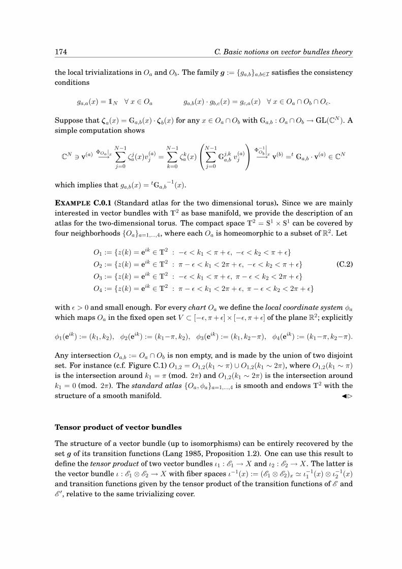
174 C. Basic notions on vector bundles theory
the local trivializations in Oa and Ob. The family g := ga,ba,b∈I satisfies the consistencyconditions
ga,a(x) = 1N ∀ x ∈ Oa ga,b(x) · gb,c(x) = gc,a(x) ∀ x ∈ Oa ∩Ob ∩Oc.
Suppose that ζa(x) = Ga,b(x) · ζb(x) for any x ∈ Oa ∩Ob with Ga,b : Oa ∩Ob → GL(CN ). Asimple computation shows
CN ∋ v(a) ΦOa |x−→N−1∑
j=0
ζja(x)v(a)j =
N−1∑
k=0
ζka (x)
N−1∑
j=0
Gj,ka,b v
(a)j
Φ−1Ob
˛
˛
˛
x−→ v(b) =tGa,b · v(a) ∈ CN
which implies that ga,b(x) = tGa,b−1
(x).
EXAMPLE C.0.1 (Standard atlas for the two dimensional torus). Since we are mainlyinterested in vector bundles with T2 as base manifold, we provide the description of anatlas for the two-dimensional torus. The compact space T2 = S1 × S1 can be covered byfour neighborhoods Oaa=1,...,4, where each Oa is homeomorphic to a subset of R2. Let
O1 := z(k) = eik ∈ T2 : −ǫ < k1 < π + ǫ, −ǫ < k2 < π + ǫ
O2 := z(k) = eik ∈ T2 : π − ǫ < k1 < 2π + ǫ, −ǫ < k2 < π + ǫ (C.2)
O3 := z(k) = eik ∈ T2 : −ǫ < k1 < π + ǫ, π − ǫ < k2 < 2π + ǫ
O4 := z(k) = eik ∈ T2 : π − ǫ < k1 < 2π + ǫ, π − ǫ < k2 < 2π + ǫ
with ǫ > 0 and small enough. For every chart Oa we define the local coordinate system φawhich maps Oa in the fixed open set V ⊂ [−ǫ, π+ ǫ]× [−ǫ, π+ ǫ] of the plane R2; explicitly
φ1(eik) := (k1, k2), φ2(eik) := (k1−π, k2), φ3(eik) := (k1, k2−π), φ4(eik) := (k1−π, k2−π).
Any intersection Oa,b := Oa ∩ Ob is non empty, and is made by the union of two disjointset. For instance (c.f. Figure C.1) O1,2 = O1,2(k1 ∼ π) ∪O1,2(k1 ∼ 2π), where O1,2(k1 ∼ π)
is the intersection around k1 = π (mod. 2π) and O1,2(k1 ∼ 2π) is the intersection aroundk1 = 0 (mod. 2π). The standard atlas Oa, φaa=1,...,4 is smooth and endows T2 with thestructure of a smooth manifold. ⊲
Tensor product of vector bundles
The structure of a vector bundle (up to isomorphisms) can be entirely recovered by theset g of its transition functions (Lang 1985, Proposition 1.2). One can use this result todefine the tensor product of two vector bundles ι1 : E1 → X and ι2 : E2 → X. The latter isthe vector bundle ι : E1 ⊗ E2 → X with fiber spaces ι−1(x) := (E1 ⊗ E2)x ≃ ι−1
1 (x) ⊗ ι−12 (x)
and transition functions given by the tensor product of the transition functions of E andE ′, relative to the same trivializing cover.
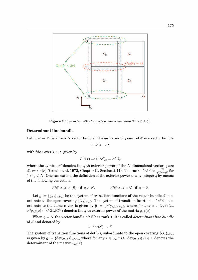
175
Figure C.1: Standard atlas for the two dimensional torus T2 ≃ [0, 2π)2.
Determinant line bundle
Let ι : E → X be a rank N vector bundle. The q-th exterior power of E is a vector bundle
ι : ∧qE → X
with fiber over x ∈ X given by
ι−1(x) =: (∧qE )x = ∧q Ex
where the symbol ∧q denotes the q-th exterior power of the N dimensional vector spaceEx := ι−1(x) (Greub et al. 1972, Chapter II, Section 2.11). The rank of ∧qE is N !
q!(N−q)! for1 6 q 6 N . One can extend the definition of the exterior power to any integer q by meansof the following convetions
∧qE ≃ X × 0 if q > N, ∧qE ≃ X × C if q = 0.
Let g := ga,ba,b∈I be the system of transition functions of the vector bundle E sub-ordinate to the open covering Oaa∈I . The system of transition functions of ∧qE , sub-ordinate to the same cover, is given by g := ∧qga,ba,b∈I , where for any x ∈ Oa ∩ Ob,∧qga,b(x) ∈ ∧qGL(CN ) denotes the q-th exterior power of the matrix ga,b(x).
When q = N the vector bundle ∧NE has rank 1; it is called determinant line bundleof E and denoted by
ι : det(E ) → X
The system of transition functions of det(E ), subordinate to the open covering Oaa∈I ,is given by g := det(ga,b)a,b∈I , where for any x ∈ Oa ∩ Ob, det(ga,b)(x) ∈ C denotes thedeterminant of the matrix ga,b(x).
176 C. Basic notions on vector bundles theory
Pullback vector bundle
Let ι : E → X be a Hermitian vector bundle and f : X → X a continuous function. Thepullback bundle ι′ : f∗E → X is the vector bundle with total space
f∗E := (x, v) ∈ X × E : ι(v) = f(x) (C.3)
and canonical projection ι′(x, v) = x. In other words we have the following isomorphismbetween the fiber spaces: (f∗E )x ≃ Ef(x) for all x ∈ X. Let (Oa, ζa)a∈I be a trivializingcovering for ι : E → X with transition functions g := ga,ba,b∈I . It follows from thedefinition that a trivializing covering for ι′ : f∗E → X is given by (f−1(Oa), f
∗ζa)a∈Iwhere f∗ζa := ζa f . In other words, the local frames of the pullback vector bundleare given by the pullback of the local frames of the original vector bundle. We remarkthat a (local) frame transforms by pullback and not by pushforward as for vector fields.The transition functions of a pullback vector bundle are given by f∗g := f∗ga,ba,b∈I ,where f∗ga,b : f−1(Oa) ∩ f−1(Ob) → GL(CN ) is defined by f∗ga,b := ga,b f . Namely,the transition functions of a pullback vector bundle are given by the pullback of thetransition functions of the original vector bundle. In particular the pullback of a trivialvector bundle is again a trivial vector bundle.
Module of continuous sections and endomorphism bundle
Let ι : E → X be a rank N vector bundle with trivializing covering (Oa, ζa)a∈I andtransition functions g := ga,ba,b∈I . The set of continuous sections is denoted by Γ(E ).Notice that Γ(E ) is a C(X)-module and the action of C(X) is just the (left) multiplicationin each fiber, i.e. (f · s)(x) := f(x)s(x) for any s ∈ Γ(E ) and f ∈ C(X).
The endomorphism bundle of the vector bundle ι : E → X is the rank N2 vectorbundle ι : End(E ) → X which has as typical fiber the vector space End(CN ) = MatN (C)
and transition functions Adga,ba,b∈I given by
Aa(x) = Adga,b(x) ·Ab(x) := ga,b(x) ·Ab(x) · g−1a,b(x), x ∈ Oa ∩Ob,
where Aa := A|Oa : Oa → MatN (C) and Ab := A|Ob: Ob → MatN (C) denote the local ex-
pressions of the continuous section A ∈ Γ(End(E )). The space Γ(End(E )) has the struc-ture of a unital C∗-algebra as showed by the (localization) isomorphism Γ(End(E )) ≃EndC(X)(Γ(E )), the latter being the C∗-algebra of the adjontable operators on the C(X)-module Γ(E ) (Proposition 4.7.13). In the case of a trivial vector bundle E = X×CN , thenΓ(End(E )) = C(X,MatN (C)) ≃ C(X) ⊗ MatN (C).
Hermitian structure and L2-sections
Each complex vector bundle ι : E → X can be endowed (in many ways) with a Hermitianstructure. For that, one can define a positive definite sesquilinear form (·; ·)x on eachι−1(Oa) ≃ Oa × CN , for Oa in a trivializing open cover of X, and then glue the metrictogether by using a partition of unity. Thereupon, we get a pairing ·; · : Γ(E )× Γ(E ) →
177
C(X), defined by s; r(x) := (s(x); r(x))x for any x ∈ X, s, r ∈ Γ(E ), which is C(X)-sesquilinear, conjugate -symmetric and positive definite.
Assume that the base space X is a finite dimensional oriented manifold (with realdimension n) with a Riemannian metric g. Denote with Ωr(X) the exterior form bundleof the r-forms over X. Let µg ∈ Ωn(X) be the Riemannian volume form associated to themetric g, i.e. (in local coordinates)
µg =√|g|dx1 ∧ · · · ∧ dxn
where dxi are the 1-forms providing an oriented basis for the cotangent bundle T ∗Xand |g| is the absolute value of the determinant of the metric tensor g. The Hermitianstructure of ι : E → X and the Riemannian strucure of the oriented manifold X allow todefine the notion of scalar product on the space of sections Γ(E ):
〈s; r〉 :=
∫
Xs; r(x) µg(x) s, r ∈ Γ(E ). (C.4)
The completion of Γ(E ) with respect to the norm ‖s‖L2 :=√
〈s; s〉 defines the Hilbertspace L2(E ) called the space of L2-sections of E .
Connections, curvatures, Chern classes
According to the general (axiomatic) definition (Husemoller 1994, definition 3.2, Chapter17), the Chern classes of a vector bundle ι : E → X are a sequence of elements of theinteger cohomology group H•(X; Z) :=
⊕j H
j(X; Z). The j-th Chern class of E , denotedby cj(E ), is an element of H2j(T2; Z). The total Chern class is defined as
c(E ) = c0(E ) + c1(E ) + c2(E ) + · · ·
with c0(E ) = 1. The definition of Chern class is functorial, namely
c(f∗E ) = f∗c(E )
for any continuous map f : X → X.
There are various equivalent ways to construct the Chern classes. Assuming thatX is a (Riemannian) manifold we can define the Chern classes by means of differentialgeometric tools. A connection ω for the Hermitian vector bundle ι : E → X, subordinateto the trivializing cover (Oa, ζa)a∈I , is a collection ωaa∈I ⊂ Ω1(Oa; u(CN )) of local dif-ferential 1-forms (called gauge potentials) with value in u(CN ) := iHerN (C) (the algebraof anti-Hermitian matrices) which satisfies the transformation rule
ωa = dga,b ga,b−1 + ga,b ωb ga,b
−1, (C.5)
where g := ga,ba,b∈I are the transition functions of E . u(CN ) is the Lie algebra of thegroup U (CN ) (unitary group on CN ), which is the group in which the transition functionsga,ba,b∈I take values. The curvature Kω associated to the connection ω = ωaa∈I is
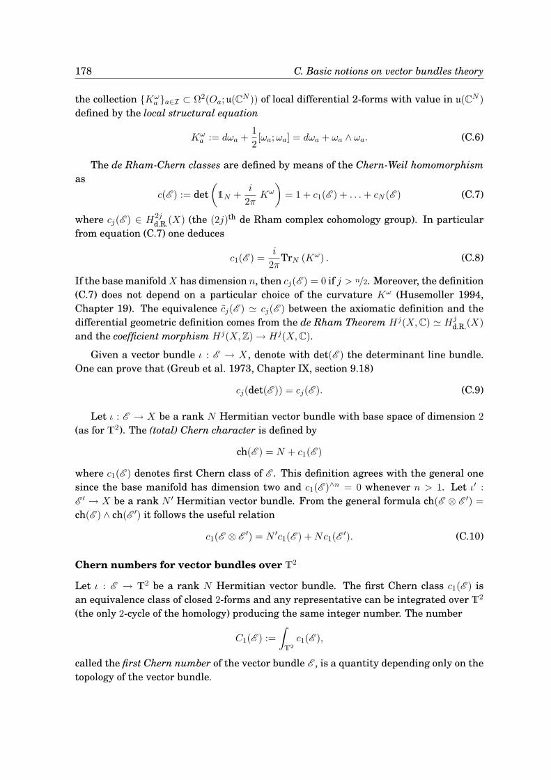
178 C. Basic notions on vector bundles theory
the collection Kωa a∈I ⊂ Ω2(Oa; u(CN )) of local differential 2-forms with value in u(CN )
defined by the local structural equation
Kωa := dωa +
1
2[ωa;ωa] = dωa + ωa ∧ ωa. (C.6)
The de Rham-Chern classes are defined by means of the Chern-Weil homomorphismas
c(E ) := det(1N +
i
2πKω
)= 1 + c1(E ) + . . .+ cN (E ) (C.7)
where cj(E ) ∈ H2jd.R.(X) (the (2j)th de Rham complex cohomology group). In particular
from equation (C.7) one deduces
c1(E ) =i
2πTrN (Kω) . (C.8)
If the base manifoldX has dimension n, then cj(E ) = 0 if j > n/2. Moreover, the definition(C.7) does not depend on a particular choice of the curvature Kω (Husemoller 1994,Chapter 19). The equivalence cj(E ) ≃ cj(E ) between the axiomatic definition and thedifferential geometric definition comes from the de Rham Theorem Hj(X,C) ≃ Hj
d.R.(X)
and the coefficient morphism Hj(X,Z) → Hj(X,C).
Given a vector bundle ι : E → X, denote with det(E ) the determinant line bundle.One can prove that (Greub et al. 1973, Chapter IX, section 9.18)
cj(det(E )) = cj(E ). (C.9)
Let ι : E → X be a rank N Hermitian vector bundle with base space of dimension 2
(as for T2). The (total) Chern character is defined by
ch(E ) = N + c1(E )
where c1(E ) denotes first Chern class of E . This definition agrees with the general onesince the base manifold has dimension two and c1(E )∧n = 0 whenever n > 1. Let ι′ :
E ′ → X be a rank N ′ Hermitian vector bundle. From the general formula ch(E ⊗ E ′) =
ch(E ) ∧ ch(E ′) it follows the useful relation
c1(E ⊗ E′) = N ′c1(E ) +Nc1(E
′). (C.10)
Chern numbers for vector bundles over T2
Let ι : E → T2 be a rank N Hermitian vector bundle. The first Chern class c1(E ) isan equivalence class of closed 2-forms and any representative can be integrated over T2
(the only 2-cycle of the homology) producing the same integer number. The number
C1(E ) :=
∫
T2
c1(E ),
called the first Chern number of the vector bundle E , is a quantity depending only on thetopology of the vector bundle.
179
The simple lemma below is useful to compute the first Chern numbers of pullbackvector bundles. Indeed the functoriality of the Chern classes implies
C1(f∗E ) :=
∫
T2
c1(f∗E ) =
∫
T2
f∗c1(E )
where f∗c1(E ) denotes the pullback of a 2-form over T2.
LEMMA C.0.2. Let ω ∈ Ω2(T2) be a 2-form and f : T2 → T2 the continuous functiondefined by f(z1, z2) = (zn1 , z
m2 ) with n,m ∈ Z. Then
∫
T2
f∗ω = nm
∫
T2
ω.
Proof. The local expression of the two form ω is ω(z(k)) = h(k) dk1 ∧ dk2. The pullbackf∗ω, defined by f∗ω|z (X1, X2) = ω|f(z) (f∗(X1), f∗(X2)) for any X2, X2 ∈ TzT
2 has localexpression (f∗ω)(z(k)) = nm h(nk1,mk2)dk1 ∧ dk2. An integration shows that
∫
T2
f∗ω = nm
∫ 2π
0dk1
∫ 2π
0dk2 h(nk1,mk2) = nm
∫
T2
ω
since h is a periodic function defined on T2.

Bibliography
Albrecht, C., Smet, J., von Klitzing, K., Weiss, D., Umansky, V. and Schweizer, H.: 2001, Evidenceof Hofstadter’s fractal energy spectrum in the quantized Hall conductance, Phys. Rev. Lett.86, 147–150.
Ashcroft, N. W. and Mermin, N. D.: 1976, Solid State Physics, Saunders.
Avila, A. and Jitomirskaya, S.: 2009, The ten Martini problem, Ann. Math. 170, 303–342.
Avron, J. E.: 2004, Colored Hofstadter butterflies, Multiscale Methods in Quantum Mechanics:Theory and Experiments, Birkhäuser.
Avron, J. E., Elgart, A., Graf, G. M. and Sadun, L.: 2004, Transport and dissipation in quantumpumps, J. Stat. Phys. 116, 425–473.
Avron, J. E., Herbst, I. and Simon, B.: 1978, Schrödinger Operators with Magnetic Fields I.General Interactions, Duke Math. J. 45 (4), 847–883.
Avron, J. E., Osadchy, D. and Seiler, R.: 2001, Butterflies and topological quantum numbers.Available as preprint at http://arxiv.org/abs/math-ph/0110026.
Avron, J. E., Osadchy, D. and Seiler, R.: 2003, A Topological Look at the Quantum Hall Effect,Physics Today 56 (8), 38–42.
Avron, J. E., Seiler, R. and Simon, B.: 1983, Homotopy and Quantization in Condensed MatterPhysics, Phys. Rev. Lett. 51, 51–53.
Avron, J. E., von Mouche, P. H. M. and Simon, B.: 1990, On the Measure of the Spectrum for thealmost Mathieu Operator, Commun. Math. Phys. 132, 103–118.
Avron, J. E. and Yaffe, L. G.: 1986, Diophantine Equation for the Hall Conductance of InteractingElectrons on a Torus, Phys. Rev. Let. 56, 2084–2087.
Bellissard, J.: 1988a, C∗-algebras in solid state physics. 2D electrons in a uniform magnetic field,Vol. II of Operator algebras and applications, University Press.
Bellissard, J.: 1988b, Ordinary quantum Hall effect and non-commutative cohomology, in Proc. ofthe Bad Schandau Conference on Localization, 1986, Eds. Ziesche & Weller, Teubner TextePhys.
Bellissard, J.: 1993, The Gap Labelling Theorems for Schrödinger’s Operators, From NumberTheory to Physics, Springer-Verlag, pp. 538–630.
Bellissard, J., Kreft, C. and Seiler, R.: 1991, Analysis of the spectrum of a particle on a triangularlattice with two magnetic fluxes by algebraic and numerical methods, J. Phys. A 24, 2329–2353.
182 BIBLIOGRAPHY
Bellissard, J., Schulz-Baldes, H. and Elst, A.: 1994, The Non Commutative Geometry of theQuantum Hall Effect, J. Math. Phys. 35, 5373–5471.
Berry, M. V.: 1984, Quantal phase factors accompanying adiabatic changes, Proc. R. Soc. A392, 45–57.
Boca, F. P.: 2001, Rotations C∗-algebras and almost Mathieu operators, Theta Foundation.
Bouclet, J.-M., Germinet, F., Klein, A. and Schenkerd, J. H.: 2005, Linear response theory formagnetic SchrŽdinger operators in disordered media, J. Funct. Anal. 226, 301–372.
Bratteli, O. and Robinson, D. W.: 1987, C∗- and W ∗-Algebras, Symmetry Groups, Decompositionof States, Vol. I of Operator Algebras and Quantum Statistical Mechanics, Springer-Verlag.
Bratteli, O. and Robinson, D. W.: 1997, Equilibrium States, Models in Quantum Statistical Me-chanics, Vol. II of Operator Algebras and Quantum Statistical Mechanics, Springer-Verlag.
Brézis, H.: 1987, Analyse fonctionnelle, Théorie et Application, Masson.
Ceresoli, D., Thonhauser, T., Vanderbilt, D. and Resta, R.: 2006, Orbital magnetization in crys-talline solids: multi-band insulators, Chern insulators, and metals, Phys. Rev. B 74, 024408.
Choi, M. D., Elliot, G. A. and Yui, N.: 1990, Gauss polynomials and the rotation algebra, Invent.Math. 99, 225–246.
Choquet, G.: 1966, Topology, Academic Press.
Combes, J.-M., Germinet, F. and Hislop, P.: 2006, On the quantization of Hall currents in pres-ence of disorder, Mathematical physics of quantum mechanics, Lecture Notes in Phys. 690,Springer-Verlag, pp. 307–323.
Connes, A.: 1980, C∗ algèbres et géométrie différentielle, C. R. Acad. Sci. Paris 290, 559–604.
Connes, A.: 1994, Noncommutative Geometry, Academic Press.
Dana, I., Avron, Y. and Zak, J.: 1985, Quantised Hall conductance in a perfect crystal, J. Phys. C18, L679–L6833.
Davidson, K. R.: 1996, C∗-Algebras by Example, American Mathematical Society.
de la Madrid, R.: 2005, The role of the rigged Hilbert space in Quantum Mechanics, Eur. J. Phys.26.
De Nittis, G. and Lein, M.: 2010, Applications of magnetic ΨDO techniques to Space-adiabaticPerturbation Theory. Available as preprint at http://arxiv.org/abs/1006.3103 .
De Nittis, G. and Panati, G.: 2009, The geometry emerging from the symmetries of a quantumsystem. Available as preprint at http://arxiv.org/abs/0911.5270 .
De Nittis, G. and Panati, G.: 2010, Effective models for conductance in magnetic fields: derivationof harper and hofstadter models. Available as preprint at http://arxiv.org/abs/1007.4786.
Dirac, P. A. M.: 1931, Quantised Singularities in the Electromagnetic Field, Proc. R. Soc. Lon-dony 133 , 60–72.
Dixmier, J.: 1981, von Neumann Algebras, North-Holland.
Dixmier, J.: 1982, C∗-Algebras, North-Holland.
Dixmier, J. and Douady, A.: 1963, Champs continus d’espaces hilbertiens et de C∗-algèbres, Bull.Soc. math. France 91, 227–284.
Dubrovin, B. A. and Novikov, S. P.: 1980, Ground states of a two-dimensional electron in aperiodic magnetic field, Sov. Phys. JETP 52 , 511.
BIBLIOGRAPHY 183
Elgart, A. and Schlein, B.: 2004, Adiabatic charge transport and the Kubo formula for Landau-type Hamiltonians, Comm. Pure Appl. Math. 57 , 590–615.
Emch, G. G.: 1996, Chaotic dynamics in noncommutative geometry, Quantization, CoherentStates, and Poisson Structures, Proceedings of the XV Workshop on Geometrical Methods inPhysics, Białowieea, Poland, S. T. Ali, A. Odzijewicz and A. Strasburger eds., pp. 193–205.
Fell, J. M. G. and Doran, R. S.: 1988, Basic Representation Theory of Groups and Algebras, Vol. 1of Representation of ∗-Algebras, Locally Compact Groups, and Banach ∗-Algebraic Bundles,Academic Press Inc.
Gat, O. and Avron, J. E.: 2003, Semiclassical analysis and the magnetization of the Hofstadtermodel, Phys. Rev. Lett. 91, 186801.
Gérard, C., Martinez, A. and Sjöstrand, J.: 1991, A mathematical approach to the effectiveHamiltonian in perturbed periodic problems, Commun. Math. Phys. 142, 217–244.
Geyler, V. A., Popov, I. Y., Popov, A. V. and Ovechkina, A. A.: 2000, Fractal spectrum of periodicquantum systems in a magnetic field, Chaos, solitons and fractals 11, 281–288.
Godement, R.: 1951, Sur la théorie des représentations unitaires, Ann. of Math. 53, 68–124.
Gracia-Bondía, J. M., Várilly, J. C. and Figueroa, H.: 2001, Elements of Noncommutative Geom-etry, Birkhäuser.
Graf, G. M.: 2007, Aspects of the Integer Quantum Hall Effect, Proceedings of Symposia in PureMathematics 76.1, 429–442.
Graf, G. M. and Ortelli, G.: 2008, Comparison of quantization of charge transport in periodic andopen pumps, Phys. Rev. B 77, 033304.
Greub, W., Halperin, S. and Vanstone, R.: 1972, Connections, Curvature, and Cohomology, Vol. I,Accademic Press.
Greub, W., Halperin, S. and Vanstone, R.: 1973, Connections, Curvature, and Cohomology, Vol. II,Accademic Press.
Gruber, M. J.: 2001, Non-commutative Bloch theory, J. Math. Phys. 42, 2438–2465.
Guillement, J. P., Helffer, B. and Treton, P.: 1989, Walk inside the Hofstadter’s butterfly, J. Phys.France 50, 2019–2058.
Hall, E. H.: 1879, On a New Action of the Magent on Electric Currents, American Journal ofMathematics, Vol. 2 2 (3), 287–292.
Harper, P. G.: 1955, Single band motion of conduction electrons in a uniform magnetic field, Proc.Phys. Soc. A 68, 874–892.
Helffer, B. and Sjöstrand, J.: 1988, Analyse semi-classique pour l’équation de Harper (avec appli-cation à l’étude de Schrödinger avec champ magnétique), Mém. Soc. Math. France 34, 1761–1771.
Helffer, B. and Sjöstrand, J.: 1989a, Analyse semi-classique pour l’équation de Harper III, Mém.Soc. Math. France 39.
Helffer, B. and Sjöstrand, J.: 1989b, Équation de Schrödinger avec champ magnétique et équationde Harper, Vol. 345 of Lecture Notes in Physics, Springer-Verlag.
Helffer, B. and Sjöstrand, J.: 1990, Analyse semi-classique pour l’équation de Harper II (com-portement semi-classique près d’un rationnel), Mém. Soc. Math. France 40.
184 BIBLIOGRAPHY
Hofstadter, D. R.: 1976, Energy levels and wave functions of Bloch electrons in rational andirrational magnetic fields, Phys. Rev. B 14, 2239–2249.
Hörmander, L.: 1990, Complex Analysis in Several Variables, North-Holland.
Husemoller, D.: 1994, Fibre Bundles, Springer-Verlag.
Iftimie, V., Mantoiu, M. and Purice, R.: 2007, Magnetic Pseudodifferential Operators, Publ.RIMS. 43 no. 3, 585–623.
Iftimie, V., Mantoiu, M. and Purice, R.: 2009, The magnetic formalism; new results, Contempo-rary Mathematics 500, 123–138.
Kellendonk, J., Richter, T. and Schulz-Baldes, H.: 2002, Edge Current Channels and ChernNumbers in the Integer Quantum Hall Effect, Rev. Math. Phys. 14, 87–119.
Kellendonk, J. and Schulz-Baldes, H.: 2004, Quantization of edge currents for continuous mag-netic operators, J. Funct. Anal. 209, 388–413.
King-Smith, R. D. and Vanderbilt, D.: 1993, Theory of polarization of crystalline solids, Phys.Rev. B 47, 1651–1654.
Kuchment, P.: 1993, Floquet Theory for Partial Differential Equations, Operator Theory: Ad-vances and Applications, Birkhäuser.
Kunz, H.: 1987, The quantum Hall effect for electrons in a random potential, Commun. Math.Phys. 112, 121–145.
Landi, G.: 1997, An Introduction to Noncommutative Spaces and their Geometries, Lecture Notesin Physics, Springer.
Lang, S.: 1985, Differential Manifolds, Springer.
Last, Y.: 1994, Zero measure spectrum for the almost Mathieu operator, Commun. Math. Phys.164, 421–432.
Last, Y.: 2005, Spectral theory of Sturm-Liouville operators on infinite intervals: A review ofrecent developments, Sturm-Liouville Theory (W. O. Amrein, A. M. Hinz, and D. B. Pearson,eds.), Birkhäuser, pp. 99–120.
Laughlin, R. B.: 1981, Quantized Hall conductivity in two dimensions, Phys. Rev. B 23 , 5632–5633.
Laughlin, R. B.: 1983, Anomalous Quantum Hall Effect: An Incompressible Quantum Fluid withFractionally Charged Excitations, Phys. Rev. Lett. 50 , 1395–1398.
Lieb, E. H. and Loss, M.: 2001, Analysis, American Mathematical Society.
MacDonald, A. H.: 1984, Quantized Hall effect in a hexagonal periodic potential, Phys. Rev. B29, 3057–3065.
Mantoiu, M. and Purice, R.: 2004, The Magnetic Weyl calculus, J. Math. Phys. 45, 1394.
Mantoiu, M., Purice, R. and Richard, S.: 2005, Twisted Crossed Products and Magnetic Pseudod-ifferential Operators, in Advances in Operator Algebras and Mathematical Physics pp. 137–172.
Maurin, K.: 1968, General Eigenfunction Expansions and Unitary Representations of TopologicalGroups, PWN.
Maxwell, J. C.: 1873, A treatise on Electricity and Magnetism, vol. II, Claredon Press, Oxford.Available on http://www.archive.org/details/electricandmag02maxwrich.
BIBLIOGRAPHY 185
Morandi, G.: 1988, Quantum Hall Effect, Bibliopolis.
Nagy, B. S. and Foias, C.: 1970, Harmonic Analysis of Operators on Hilbert Space, AmericanElsevier, North-Holland.
Nenciu, G.: 2002, On asymptotic perturbation theory for Quantum Mechanics: Almost invariantsubspaces and gauge invariant magnetic perturbation theory, J. Math. Phys. 43, 1273–1298.
Nenciu, G. and Sordoni, V.: 2004, Semiclassic limit for multistate Klein-Gordon systems: almostinvariant subspaces, and scattering theory, J. Math. Phys. 45, 3676.
Osadchy, D. and Avron, J. E.: 2001, Hofstadter butterfly as quantum phase diagram, J. Math.Phys. 42, 5665–5671.
Panati, G.: 2007, Triviality of Bloch and Bloch-Dirac bundles, Ann. Henri Poincaré 8, 995–1011.
Panati, G., Sparber, C. and Teufel, S.: 2009, Geometric currents in piezoelectricity, Arch. Rat.Mech. Anal. 91, 387–422.
Panati, G., Spohn, H. and Teufel, S.: 2003a, Effective dynamics for Bloch electrons: Peierlssubstitution and beyond, Commun. Math. Phys. 242, 547–578.
Panati, G., Spohn, H. and Teufel, S.: 2003b, Space-Adiabatic Perturbation Theory, Adv. Theor.Math. Phys. 7, 145–204.
Peierls, R.: 1933, Zur Theorie des Diamagnetismus von Leitungselektronen, Z. Phys. 80, 763–791.
Peierls, R.: 1985, Bird of Passage, Princeton University Press Press, Oxford.
Pimsner, M. and Voiculescu, D.: 1980, Exact sequences for K-groups and Ext-groups of certeincross-product C∗-algebras, J. Oper. Theory. 4, 93–118.
Rauh, A.: 1974, Degeneracy of Landau levels in crystals, Phys. Status Solidi B 65, K131–K135.
Rauh, A.: 1975, On the broadening of Landau levels in crystals, Phys. Status Solidi B 69, K9–K13.
Reed, M. and Simon, B.: 1973, Functional Analysis, Vol. I of Methods of Modern MathematicalPhysics, Academic Press.
Reed, M. and Simon, B.: 1975, Fourier Analysis, Self-Adjointness, Vol. II of Methods of ModernMathematical Phisics, Academic Press.
Reed, M. and Simon, B.: 1978, Analysis of Operators, Vol. IV of Methods of Modern MathematicalPhisics, Academic Press.
Resta, R.: 1992, Theory of the electric polarization in crystals, Ferroelectrics 136, 51–75.
Rieffel, M. A.: 1981, von Neumann Algebras Associated with Pairs of Lattices in Lie Groups,Math. Ann. 257, 403–418.
Rudin, W.: 1962, Fourier Analysis on Groups, Number 12 in Interscience Tracts in Pure andApplied Mathematics, Interscience.
Rudin, W.: 1987, Real and Complex Analysis, McGraw-Hill.
Samoilenko, Y. S.: 1991, Spectral Theory of Families of Self-Adjoint Operators, Mathematics andIts Applications, Kluwer.
Schwarzschild, B.: 1986, Currents in Normal-Metal Rings Exhibit Aharonov-Bohm Effect,Physics Today 39 (1), 17–20.
186 BIBLIOGRAPHY
Shubin, M. A.: 1994, Discrete Magnetic Laplacian, Commun. Math. Phys. 164, 259–275.
Simon, B.: 1982, Almost periodic Schrödinger operators: A review, Adv. Appl. Math. 3, 463–490.
Simon, B.: 1983, Holonomy, the Quantum Adiabatic Theorem, and Berry’s Phase, Phys. Rev. Lett.51, 2167–2170.
Sobolev, A. V.: 1997, Absolute continuity of the periodic magnetic Schrödinger operator, Invent.Math. 137, 85–112.
Streda, P.: 1982, Quantised Hall effect in a two-dimensional periodic potential, J. Phys. C15, L1299–L1303.
Takesaki, M.: 1969, A generalized commutation theorem for the regular representation, Bull.Soc. Math. France 97, 289–297.
Teufel, S.: 2003, Adiabatic Perturbation Theory in Quantum Dynamics, Vol. 1821 of Lecture Notesin Mathematics, Springer-Verlag.
Thonhauser, T., Ceresoli, D., Vanderbilt, D. and Resta, R.: 2005, Orbital magnetization in peri-odic insulators, Phys. Rev. Lett. 95, 137205.
Thouless, D. J.: 1983, Quantization of particle transport, Phys. Rev. B 27, 6083–6087.
Thouless, D. J.: 1998, Topological Quantum Numbers in Nonrelativistic Physics, World Scientific.
Thouless, D. J., Kohmoto, M., Nightingale, M. P. and Nijs, M.: 1982, Quantized Hall conductancein a two-dimensional periodic potential, Phys. Rev. Lett. 49, 405–408.
Treves, F.: 1967, Topological vector spaces, distributions and kernels, Academic Press.
von Klitzing, K., Dorda, G. and Pepper, M.: 1980, New Method for High-Accuracy Determina-tion of the Fine-Structure Constant Based on Quantized Hall Resistance, Phys. Rev. Lett.45, 494–497.
von Mouche, P. H. M.: 1989, The coexistence problem for the discrete Mathieu operator, Com-mun. Math. Phys. 122, 23–34.
Walker, J. S.: 1988, Fourier Analysis, Oxford University Press.
Wilcox, C. H.: 1978, Theory of Bloch waves, Journal d’Analyse Mathématique 33 , 146–167.
Wilkinson, M.: 1987, An exact effective Hamiltonian for a perturbed Landau level, J. Phys. A20, 1761–1771.
Index
τ -covarianceleft, 65right, 65
τ -equivariance, 63
algebraC∗, 167
commutative, 167group, 112Harper, 36Hofstadter, 36homogeneous, 122, 136maximal commutative, 167rotation, see Non-Commutative Torusseparable, 168simple, 135unital, 167
Zd, 21NCT, see Non-Commutative Torus, see Non-
Commutative Torusrational, 34, 48smooth, 35
von Neumann, 167Harper, 141Hofstadter, 139standard, 45, 139, 167
almost-invariant subspace, 70, 90analytic vectors (total set), 84atlas (standard), 154
bandBloch (energy), 28, 64energy, 24, 39, 42Landau, 80
Brillouin zone, 59bundle
decomposition, 46, 146
irreducible, 47endomorphism, 46enomorphism, 176Hilbert, 123
Bloch-Floquet, 130line, 22
determinant, 51, 156, 175map, 173product, 173vector, 16, 46, 173
Harper, 48, 50, 151Hermitian, 46Hofstadter, 48, 50, 145image, 47pullback, 22, 176tensor product, 174
butterfly(black and white) quantum, see Hofstadtercolored quantum, 25, 33, 44Hofstadter, 22, 33, 38
canonical derivations, 52CHE, see Hall, effect, classicalChern
character, 178class, 49, 155, 177
total, 177number, 16, 18, 49, 137, 155, 178
universal, 52commutant, 21, 167connection, 177
Harper, 154constant
Kadison, 40von Klitzing, 10
continuous field of Hilbert spaces, 124curvature, 16, 177
188 INDEX
Harper, 50, 154cyclotron frequency, 78
decompositionbundle, 152fiber, see direct integral decompositionspectral, see direct integral decomposition
Bloch-Floquet, 118degrees of freedom
fast, 58, 62, 78, 163slow, 58, 78, 163
direct integral, 47, 170direct integral decomposition, 47duality
algebraic, 37geometric, 22, 45, 51, 158
effective dynamics, 71, 75, 90, 93effective model (unitarily), 32electron, 37
formulaKubo, 16, 18Riesz, 39, 72, 91
frame, 35global, 173local, 173physical, 21, 47, 101
Harper (standard), 142Hofstadter (standard), 140irreducible, 47, 101standard, 122
sections, 50, 131global, 49
functiontransition, 173
gap“closed”, 24“open”, 24, 39, 42bottom, 40, 41structure, 41top, 40, 41
Gel’fand triple (nuclear), 107GNS construction, 36
Hallconductance, 26conductance, 8, 43
conductivity, 8effect
anomalous, 9classical, 9quantum, 10, 28
resistance, 10resistivity, 10
HamiltonianBloch, 25, 29, 60Bloch-Landau, 15, 28, 58, 78effective, 90effective (unitarily), 32Harper, 15, 30Harper-like, 20, 30, 95Hofstadter, 22, 29, 31Hofstadter-like, 20, 29, 31, 75, 76Landau, 25, 29, 161Mathieu-like, 103periodic, 29, 60, 63, 160
Harperequation, 15, 17Hofstadter, 22
Hermite basis (generalized), 81, 162Hilbert module, 127hole, 10, 37
indicator function, 85isomorphism
Gel’fand, 105, 168isospectrality, 20, 37, 38, 44
lattice, 59dual, 59
magneticflux quantum, 11, 28
measurebasic, 113Haar (normalized), 46spectral, 170
basic, 170minimal coupling, 66momentum
Bloch, 67kinetic, 28, 66, 78, 161
Moyalcommutator, 92product, 70resolvent, 72, 91
INDEX 189
NCT, see Non-Commutative Torusnon-commutative integral, 40Non-Commutative Torus, 20, 34nuclear space, 115
Harper, 148Hofstadter, 143wandering, 115
operator(continuously) diagonal, 171(universal) Hofstadter , 38almost-Mathieu, 31annihilation, 161creation, 161decomposable, 105, 171
order function, 66
parameteradiabatic, 58, 61ǫ0, 29, 76ǫ∞, 30, 95
deformation, 31, 34Pauli matrices, 97Peierls’ substitution, 28, 75periodic cyclic cohomology, 54, 171projection
band, 40gap, 40, 41Moyal, 71, 91orthogonal, 39smooth, 39super-adiabatic, 71, 74, 92trivial, 39valued section, 47
propertyC∗, 167Kadison, 40surjective representation, 34universal, 34wandering, 21, 47, 110
QHE, see Hall, effect, quantumquantization
Dirac condition, 13orthodox, 12Peierls, 76topological, 12Weyl, 30, 68, 80, 82, 95
magnetic, 58
quantum pump, 10
rank (of a projection), 40regime
Harper, 15, 25, 29, 31, 44Hofstadter, 15, 20, 25, 28, 31, 43
representation, 167bundle, 21
canonical, 137faithful, 136, 138, 141, 167fiber, 145, 151GNS, 138Harper, 36Hofstadter, 35irreducible, 105, 122, 136, 145, 151left regular, 112
SAPT, see space-adiabatic perturbation theorysection
L2, 46, 176local, 173
Sobolev space, 60, 159magnetic, 60, 159
space-adiabatic perturbation theory, 19, 32, 57spectral type, 44spectrum
algebraic, 37, 44, 168band, 39Cantor-type, 24, 39Gel’fand, 35, 113, 141Gel’fand , 168Hilbertian, 37, 168joint, 141, 169pure point, 39
standard atlas, 174state, 167
faithful, 167symbol
τ -equivariant, 66special, 66
approximated, 86Hörmander class, 66, 82operator-valued, 66, 82principal, 70remainder, 88
symmetric gauge, 58
theorem“no go” (weak), 45
190 INDEX
Gel’fand-Naımark, 168Maurin’s nuclear spectral, 108Serre-Swan, 156von Neumann’s complete spectral, 105
time-scalemacroscopic, 61microscopic, 59ultramicroscopic, 78
TKNN, 14equations, 16, 18, 21
generalized, 51paper, 14
topological quantum number, 12TQN, see topological quantum numbertransform
S-Fourier, 105Bloch-Floquet, 62, 100
discrete, 102generalized, 21, 49, 116, 144
charge-conjugation, 35, 37trivializing covering, 173
unit of energy, 78unit of the energy, 61unitary
Harper, 30, 95Hofstadter, 29, 76intertwining, 74, 93von Neumann, 79, 163
universal Hofstadter operators, 22
vectorcyclic, 138, 139, 167separating, 139, 167Wannier, 122, 130
exponentially localized, 123super-polynomial localized, 123
Voronoi cell, 59
wandering system, 110Harper (standard), 143Hofstadter (standard), 140


