Dirty surplus accounting flows and valuation errors

ABACUS, Vol. 42, Nos 3/4, 2006

doi: 10.1111/j.1467-6281.2006.00203.x

302

© 2006 Accounting Foundation, The University of Sydney

Blackwell Publishing AsiaMelbourne, AustraliaABACAbacus0001-3072© 2006 Accounting Foundation, Unviersity of Sydney423

ORIGINAL ARTICLE

DIRTY SURPLUS ACCOUNTING AND VALUATIONABACUS

HELENA ISIDRO, JOHN O’HANLON AND STEVEN YOUNG

Dirty Surplus Accounting Flows and Valuation Errors

For France, Germany, the U.K. and the U.S. for the period from 1994 to2001, this study explores empirically the association between valuationerrors from a standard empirical application of the residual incomevaluation model and violations of the clean surplus relationship (dirtysurplus accounting flows). Motivated by concern that the effect of dirtysurplus accounting on the applicability of accounting-based valuationmodels might vary across accounting regimes, the study also documentsdifferences across pairs of countries in the relationship between valu-ation errors and dirty surplus flows. The study finds some weak evidenceof predicted relationships between valuation errors and dirty surplusflows in the U.S., but finds little evidence of such relationships else-where. There is some limited evidence of cross-country difference in therelationship between valuation errors and dirty surplus flows, mostlyinvolving the U.S.

Key words:

Accounting; Clean surplus relationship; Dirty surplus account-ing; Valuation.

For France, Germany, the U.K. and the U.S. for the period from 1994 to 2001,this study explores empirically the association between valuation errors from astandard empirical application of the residual income valuation model (RIVM)and violations of the clean surplus relationship (CSR), which we term dirty surplusaccounting flows. Motivated by concern that the effect of dirty surplus accountingon the applicability of accounting-based valuation models might vary acrossaccounting regimes, we also document differences across pairs of countries in therelationship between valuation errors and dirty surplus flows.

CSR holds from an equity perspective if all accounting gains and losses of aperiod are included in that period’s net income. Violations of CSR (dirty surplusaccounting flows) arise when some recognized gains or losses are excluded from

Helena Isidro

([email protected]) is an Assistant Professor of Accounting at Instituto Superior deCiências do Trabalho e da Empresa (ISCTE), Lisbon,

John O

’

hanlon

([email protected]) aProfessor of Accounting at Lancaster University, and

Steven Young

([email protected]) aSenior Lecturer in Accounting at Lancaster University.The authors thank participants at the December 2005 Abacus Accounting Forum at the University ofSydney, and in particular the discussant Ann Tarca, Stuart McLeay and Holger Daske, for their help-ful comments. Financial support was provided by the European Commission Human Potential Pro-gramme (Contract #HPRN-CT-2000-00062) and Fundação para a Ciência e Tecnologia (ref. SFRH/BD/6021/2001). This study uses data from the Institutional Brokers Estimate System (I/B/E/S). This isa service of Thomson Financial, and the data have been provided as part of a broad academic programto encourage earnings expectations research.

DIRTY SURPLUS ACCOUNTING AND VALUATION

303


net income. There is a long history of concern that the relative lack of transpar-ency of dirty surplus accounting might limit the usefulness of accounting numbersin performance measurement (Paton, 1934; May, 1937; Littleton, 1940; Johnson

et al.

, 1995; Financial Accounting Standards Board, 1997; Linsmeier

et al.

, 1997).There has also been some concern that dirty surplus accounting may be a sourceof error in accounting-based valuation models (Linsmeier

et al

., 1997), and thatcross-regime differences in dirty surplus accounting may cause cross-country dif-ferences in the applicability of such models (Frankel and Lee, 1999). Such con-cerns have been reflected in moves by accounting regulators to eliminate dirtysurplus flows, or to require that they be reported more transparently in statementsof comprehensive income, which include all recognized gains and losses.

1

We implement a standard constant-growth continuing-value empirical formula-tion of RIVM, where inputs are constructed under the assumption that CSRholds. We note that this formulation gives the same value estimates as a corres-ponding formulation of the abnormal earnings growth model, provided thatgrowth assumptions are consistent across both models. We treat realized dirtysurplus flows as proxies for expected future dirty surplus flows, and investigateempirically the relationship between our valuation errors and those dirty surplusflows. We do so for France, Germany, the U.K. and the U.S. for the period from1994 to 2001, and document differences in the relationship across pairs of coun-tries. We use two separate samples of data: a large sample of U.K. and U.S. firms,and a small sample of French, German, U.K. and U.S. firms. This allows us to pro-vide evidence from available large samples of reliable machine-readable data ondirty surplus flows for the U.K. and the U.S., as well as comparative evidence forother countries where such flows are significant but can only be measured reliablythrough time-consuming hand collection of data from financial statements.

We find some weak evidence of predicted relationships between dirty surplusflows and valuation errors in the U.S., but find little evidence of predicted rela-tionships elsewhere. There is some limited evidence of cross-country difference inthe relationship between valuation errors and dirty surplus flows, mostly involvingthe U.S. Overall, our results do not suggest that dirty surplus flows are a consist-ent source of error in applications of accounting-based valuation models.

DIRTY SURPLUS ACCOUNTING PRACTICES AND SOME PRIOR EVIDENCE ON THEIR ROLE IN VALUATION

In the four countries considered in this study, dirty surplus accounting practiceshave been commonplace over our sample period of 1994 to 2001, and there has beensubstantial variation across these four countries with regard to the nature and scale

1

Examples include FRS 3,

Reporting Financial Performance

(Accounting Standards Board, 1992)and FRS 10,

Goodwill and Intangible Assets

(Accounting Standards Board, 1997) in the U.K. andSFAS 130,

Reporting Comprehensive Income

(Financial Accounting Standards Board, 1997) in theU.S. Also, a joint project on the reporting of financial performance being conducted by theInternational Accounting Standards Board and the Financial Accounting Standards Board includesconsideration of comprehensive income statements.

ABACUS

304


of those practices (Isidro

et al.

, 2004). In France, dirty surplus flows have includedgoodwill write-offs, asset revaluations, currency translation differences, prior-yearadjustments, subsidies, regulated provisions, consolidation scope adjustmentsand changes in accounting policy resulting from new accounting regulations. InGermany, they have included goodwill write-offs, currency translation differences,prior-year adjustments, certain consolidation adjustments and unrealized appre-ciation in investments. In the U.K., they have included goodwill write-offs (nowabolished), asset revaluations, currency translation differences and prior-year adjust-ments. In the U.S., they have included unrealized gains and losses on marketablesecurities, currency translation differences, minimum pension liability adjustments,prior-year adjustments and, towards the end of our sample period, unrealized gainsand losses on derivative instruments. Also, merger accounting, which can be viewedas giving rise to a dirty surplus flow similar to a goodwill write-off, was common inthe U.S. in our sample period and was also observed to a lesser extent in the U.K.

Although theory suggests that disregard for dirty surplus flows in the applica-tion of accounting-based valuation models could give rise to valuation errors, theevidence to date on the importance of such flows in valuation is mixed. Dhaliwal

et al.

(1999) measure the association between share returns and contemporaneousdirty surplus flows in the U.S. They find some association between returns andunrealized gains on marketable securities, but that the overall association betweenreturns and dirty surplus flows is weak. Kanagaretnam

et al.

(2005), using a laterdata set including a period subsequent to the implementation of SFAS 130,

Reporting Comprehensive Income

(Financial Accounting Standards Board, 1997),find a stronger association between dirty surplus flows and share returns thanwas reported by Dhaliwal

et al

. (1999). Biddle and Choi (2006) report that U.S.comprehensive income is more strongly associated with share returns than is netincome. Cahan

et al.

(2000) report evidence of association between share pricesand dirty surplus flows in New Zealand. Pinto (2005) reports that the currencytranslation component of comprehensive income can be value-relevant when con-sidered in conjunction with proxies for sources of currency exposure. O’Hanlonand Pope (1999) find only a weak association between long-interval share returnsand corresponding long-interval accumulations of dirty surplus flows in the U.K.Isidro

et al

. (2004) explore the association between market-to-book ratios andperfect-foresight forecasts of dirty surplus flows in France, Germany, the U.K.and the U.S., and find only weak association. To date there is no direct evidenceon the relationship between dirty surplus flows and valuation errors from stand-ard applications of accounting-based valuation models. In this paper, we providesuch evidence, using data from France, Germany, the U.K. and the U.S.

VALUE ESTIMATES AND VALUATION ERRORS IN RIVM

In this section, we show how RIVM is derived from the present value of expecteddividends (PVED), describe a standard empirical constant-growth continuing-value formulation of RIVM, and state predictions for the association betweenvaluation errors from this formulation of RIVM and dirty surplus flows.


305


RIVM is derived from PVED, which is as follows:

(PVED)

where

V

t

denotes the intrinsic value of equity at time

t

(the valuation date),

d

t

+

s

denotes dividend net of equity issues at time

t

+

s

,

r

denotes the cost of equity and

E

t

[.] is a time-

t

expectations operator. RIVM can be derived by adding to PVEDthe following zero-sum expression:

(1)

where

E

t

[

y

t

+

s

](1

+

r

)

−

s

→

0 as

s

→

∞

. Alternatively,

y

could be a finite series that isexpected to end at time

t

+

T

, where

E

t

[

y

t

+

T

] = 0. Addition of (1) to PVED gives

(2)

Defining

y

to be book value of equity, denoted

b

, gives

(3)

Under CSR, net income, denoted

x

, is equal to the change in the book value ofequity plus dividends net of equity issues:

(CSR)

Residual income for time

t

+

s

, denoted , is equal to

x

t

+

s

−

r

.

b

t

+

s

−

1

. Under CSR,this can be written as

(4)

Substitution of (4) into (3) gives RIVM:

(RIVM)

RIVM expresses the intrinsic value of equity as book value plus the present valueof forecast residual incomes (Ohlson, 1995).

Standard empirical per-share formulations of RIVM comprise book value pershare at time

t

, individually discounted residual incomes expected to arise from time

t

+

1 up to time

t

+

T

and a continuing-value term representing the present value ofall residual incomes expected to arise after time

t

+

T

, and use book value per shareforecasts derived under the assumption that CSR holds on a per-share basis (Frankeland Lee, 1998; Lee

et al.

, 1999; Gebhardt

et al.

, 2001). Such a formulation is as follows:

(5)

VE d

rt

t t s

ss

[ ]

( ),=

++

=

∞

∑ 11

01

11

1

[ ( ) ]

( ),= +

− ++

+ + −

=

∞

∑yE y r y

rt

t t s t s

ss

V yE y d r y

rt t

t t s t s t s

ss

[ ( ) ]

( ).= +

+ − ++

+ + + −

=

∞

∑ 11

1

1

V bE b d r b

rt t

t t s t s t s

ss

[ ( ) ]

( ).= +

+ − ++

+ + + −

=

∞

∑ 11

1

1

x b d bt s t s t s t s+ + + + −= + − .1

x t sa+

x b d b r bb d r b

t sa

t s t s t s t s

t s t s t s

+ + + + − + −

+ + + −

= + − −= + − +

. ( ) .

1 1

11

V bE x

rt t

t t sa

ss

[ ]

( ).= +

++

=

∞

∑ 11

VPS bpsxps

r

xps

r r gt t

t sa

s

t Ta

Ts

T

( )

( ) ( )

,= ++

++ −

+ + +

=∑ 1 1

1

1

ABACUS

306


where

VPS

t is the estimate of intrinsic value per share at time t, bpst is book value pershare at time t, is the time-t forecast of residual income per share for time t + s,r is the cost of equity as previously defined and g is the constant rate of expectedgrowth in residual income per share after time t + T + 1. is equal to xpst+s

− r.bpst+s−1, where xpst+s is the time-t forecast of earnings per share for time t + s andbpst+s for s > 0 is the time-t forecast of book value per share at time t + s. bpst+s isderived under the CSR assumption that bpst+s = bpst+s−1 + xpst+s − dpst+s, where dpst+s

is the time-t forecast of dividend per share for time t + s, calculated by applying apayout ratio to earnings per share. Our empirical analysis uses such a formulation.

Following Penman (2005), we note that this empirical formulation gives thesame value estimates as a corresponding empirical constant-growth continuing-value formulation of the abnormal earnings growth model (AEGM), providedthat growth assumptions are consistent across both models.2 This equivalence isshown in the Appendix to this paper.

In the empirical implementation of RIVM described above, forecast earnings isthe driver of forecast dividends. This is consistent with the notion that, over thewhole life of the firm, aggregate dividends net of equity issues must equal aggre-gate net accounting gains and that, holding book value constant, disregard for anexpected future accounting flow implies disregard for a dividend effect of thesame magnitude at some time in the future.3 We draw upon this notion in gener-ating our prediction with regard to the association between valuation errors fromaccounting-based valuation models and dirty surplus flows. If the valuation erroris defined as the intrinsic value estimate given by the flows used within the valu-ation model less the market price, which is assumed to reflect all forecast flowsincluding those that are excluded from the valuation model, then a negative asso-ciation is predicted between valuation errors and expected future dirty surplusflows. The omission of a positive (negative) expected future dirty surplus flowfrom an accounting-based valuation model will imply an underestimate (over-estimate) of expected future dividends, an underestimate (overestimate) of intrinsicvalue and, other things being equal, a negative (positive) valuation error and anegative relationship between valuation errors and expected future dirty surplusflows. However, we recognize that any such relationship could be weak if omittedexpected flows are distant or if a large proportion of the dividend impact of flowsis expected to arise long after the flow itself, for example, as part of a liquidatingdividend. In subsequent sections, we explore empirically whether expectations aboutdirty surplus flows, as proxied by realizations of such flows, are negatively associ-ated with valuation errors for our forecast-based implementation of RIVM. We alsocarry out a related test of the weaker prediction that the magnitude of valuation erroris positively associated with the magnitude of expected future dirty surplus flows.For this, we use absolute values of valuation errors and dirty surplus flows.

2 See Ohlson (2005) for the development of the AEGM, and Chen et al. (2004) for an empiricalapplication of the model.

3 Note that book value of equity at a point in time is equal to the sum of the aggregate net accountinggains less dividends net of equity issues from incorporation up to that point in time.

xps t sa+

xps t sa+


307© 2006 Accounting Foundation, The University of Sydney

EMPIRICAL METHODS

Empirical analysis is performed separately on two samples for the period 1994 to2001: a large sample of U.K. and U.S. firms, for which dirty surplus flows are col-lected from the Extel database supplied by Thomson Financial for the U.K. andfrom Compustat for the U.S.; and a small sample of French, German, U.K. andU.S. firms, for which dirty surplus flows are hand collected from published finan-cial statements. This approach enables us to provide evidence based on availablelarge samples of reliable machine-readable data on dirty surplus flows for theU.K. and the U.S., while also including comparative evidence for a wider set ofcountries for which dirty surplus flows are important but can only reliably bemeasured by time-consuming hand collection of data.4 In this section we describethe methods used to explore the empirical relationship between RIVM valuationerrors and dirty surplus flows for these two samples. First, we describe the proced-ure used to construct value estimates; second, we describe our procedures formeasuring dirty surplus flows; third, we describe the methods used to measure therelationship between the items.

RIVM Value EstimatesValue estimates are constructed in the same way for both the two-country largesample and the four-country small sample. Valuation dates are set by reference tofirms’ balance sheet dates. On the basis of inspection of the normal lag betweenthe balance sheet date and the reporting date in each country, the valuation dateis set at three months after the balance sheet date for France, the U.K. and theU.S., and five months after the balance sheet date for Germany. RIVM value pershare estimates are constructed as follows, consistent with the proceduredescribed in (5) (firm subscripts are suppressed)5:

(6)

where is forecast residual income per share for s years after the valuationdate t, as previously defined, equal to xpst+s − r.bpst+s−1. Book value per share atthe valuation date (bpst) is book value for common shareholders from the most

4 Although a comparison of hand-collected dirty surplus flows from U.K and U.S. firms’ financialstatements with corresponding data supplied by machine-readable financial databases revealedsome discrepancies, these did not lead us to conclude that the inferences from a large-sample studybased on these databases would be unreliable. A similar comparison of information on dirty sur-plus flows from French and German financial statements with corresponding machine-readabledata led us to conclude that the machine-readable data were insufficiently complete to supportinferences about the relationship between valuation errors and dirty surplus flows, or to supportcross-country comparisons between the relationships.

5 Following Lee et al. (1999), we also implement the models using additional periodic flows generatedunder the assumption that return on equity is expected to fade to the industry mean over a numberof years. This does not materially change our results. (See sensitivity tests.) We also implementAEGM using the same data used in implementing RIVM and using consistent growth assumptions,and confirm that both models give identical value estimates.

VPS bpsxps

r

xps

r r gt t

t sa

s

ta

s

( )

( ) ( )

,= ++

++ −

+ +

=∑ 1 1

3

21

2

xps t sa+

ABACUS


recent published financial statements, as given by Thomson Financial’s World-scope item Ws.03501 for French, German and U.K. firms and Compustat item 60for U.S. firms, divided by the number of common shares outstanding at the valu-ation date. Forecast earnings per share (xpst+s) is estimated as follows: for one andtwo years ahead it is estimated as the I/B/E/S mean consensus forecast of earningsper share6; for three years ahead, it is estimated as the product of (a) an expectedcountry-industry return on equity and (b) the forecast of opening book value pershare for that year. An expected country-industry return on equity for three yearsahead and thereafter, used in forecasting three-year-ahead earnings and in con-structing the continuing-value term, is set equal to the mean for industry j incountry k, calculated by dividing the aggregate of income before extraordinaryitems by the aggregate of the corresponding lagged book value for commonshareholders for the seven years up to the valuation date. Here, we use all avail-able accounting data for industry j in country k. The income item is Worldscopeitem Ws.01551 for French, German and U.K. firms and Compustat item 18 forU.S. firms.7 Here, and for other purposes for which industry-level estimates arerequired, we use the following four broad industry groups: (a) resources, basicand general industries and utilities; (b) consumer goods; (c) services, information,and technology; and (d) financial. As is standard in empirical applications ofRIVM, such as Lee et al. (1999), forecasts of book value per share for one and twoyears after the valuation date are obtained, as outlined in the previous section,under the assumption that CSR holds:

where dpst+s is set equal to π.xpst+s, where π is the constant expected dividend pay-out ratio for industry j in country k for t + 1 and thereafter. The expected payoutratio is computed for each country-industry by dividing aggregate common divi-dends (Worldscope item Ws.05376 for French, German and U.K. firms and Com-pustat item 21 for U.S. firms) by aggregate income for the seven years up to thevaluation date. Firms experiencing negative earnings are included in the calcula-tions to avoid bias towards profitable firms. Consistent with other studies (e.g.,Lee et al., 1999; Gode and Mohanram, 2003), we winsorize estimated payoutratios to lie between 0 and 1. Also, in order to avoid distortion due to firmsmaking distributions to shareholders through share repurchases, we eliminatenon-dividend-paying firms as in Lee et al. (1999). The estimated cost of equitycapital, r, at the valuation date t for a firm in industry j in country k, is set equalto the Treasury Bond rate for country k for the year ended at the valuation date,

6 The earnings per share forecasts and prices obtained from I/B/E/S are share-split adjusted. We con-vert the reported earnings per share forecasts to actual using I/B/E/S adjustment factors. We alsoconvert any earnings forecasts reported on a diluted basis to basic using I/B/E/S dilution factors.

7 We impose a lower bound equal to the cost of equity on the estimated return on equity used in thecontinuing-value-term. Negative-book-value observations are not considered in the estimation ofthe country-industry return on equity.

bps bps xps dpsbps bps xps dps xps dps

t t t t

t t t t t t

+ + +

+ + + + +

= + −= + − + −

1 1 1

2 1 1 2 2

,



plus the product of (a) an assumed risk premium of 5 per cent and (b) the meanequity beta for firms in industry j in country k, constructed from Datastream betaestimates. We assume that the cost of equity is expected to remain constant afterthe valuation date. The constant growth term in (6), g, is assumed equal to theproduct of (a) the expected country-industry return on equity for t + 3 and there-after and (b) the expected country-industry retention ratio (1 − π). This can beinterpreted as the expected constant rate of book value growth after t + 2 and,since the cost of equity and the return on equity are assumed constant for t + 3and thereafter, as the assumed constant rate of growth in residual income aftert + 3. Consistent with previous valuation studies, negative value estimates are set tozero (e.g., Francis et al., 2000).

The valuation error at valuation date t is measured as the intrinsic value pershare estimate less the observed share price at the valuation date, scaled by theobserved price. Share prices are obtained from I/B/E/S.8

Dirty Surplus Flow MeasuresOur predictions relate to the relationship between valuation errors and expectedfuture dirty surplus flows. Our empirical analysis uses realized dirty surplus flowsas proxies for expected future dirty surplus flows as at the valuation date.

For the large sample, we categorize dirty surplus flows in accordance with thecategories used by the databases, which differ between the two countries becauseof the different types of dirty surplus flows in those countries. For the U.K., fourcategories of dirty surplus flows reported by Extel are collected: prior-yearadjustments (Extel item ir_rsm), goodwill write-offs net of write-backs (Extelitem ir_gw), asset revaluations (Extel item ir_rvl) and currency translation differ-ences (Extel item ir_fx).9 For the U.S., we follow the procedure used by Dhaliwalet al. (1999) to collect the following three categories of dirty surplus flows fromCompustat: adjustments for marketable securities (change in Compustat item238), adjustments related to minimum pension liabilities (Compustat item 297 lessCompustat item 298, if negative) and currency translation differences (change inCompustat item 230).10

For the four-country small sample of French, German, U.K. and U.S. firms,total dirty surplus flows are obtained from the hand-collected database used in

8 As with our I/B/E/S earnings per share forecasts, we convert the I/B/E/S-reported prices to actualby reversing the share-split adjustments applied by I/B/E/S.

9 We use the Extel database supplied by Thomson Financial rather than its Worldscope database,because Worldscope does not report dirty surplus flows directly.

10 SFAS 133, Accounting for Derivative Instruments and Hedging Activities (Financial AccountingStandards Board, 1998) came into effect for fiscal years beginning after 15 June 1999, towards theend of our sample period. Some cases of unrealized gains and losses on derivative instrumentswere identified in the latter years of our small-sample data (see below). In the absence of an estab-lished method of identifying these items from Compustat, we did not deal with them in our largesample data.

ABACUS


Isidro et al. (2004).11 In constructing this database, all quoted firms identified byDatastream in respect of each of the four countries are assigned to one of the fourbroad industry categories referred to earlier (resources, basic and general indus-tries and utilities; consumer goods; services, information and technology;financial) and to one of four size categories within the assigned industry category.For each country, five firms from each of the resulting sixteen industry-size cat-egories are then randomly selected to produce a final sample of eighty firms percountry.12 For each firm-year, all movements in equity, comprising net income,transactions with shareholders and dirty surplus flows, are accounted for. Alldirty surplus flows are assigned to one of four broad categories common to allfour countries: (a) prior-year adjustments; (b) goodwill-related items, comprisinggoodwill write-offs net of write-backs (France, Germany and U.K. only) andissues of equity unrecorded due to merger accounting which are treated similarlyto a goodwill write-off (U.K. and U.S. only)13; (c) asset revaluations; and (d) otheritems, comprising currency translation differences, unrealized gains and losses onmarketable securities (U.S. only), adjustments related to minimum pension liabil-ities (U.S. only), and sundry gains and losses not included in any of the foregoingcategories, which include unrealized gains and losses on derivative instruments(for the U.S. in the last two years of our sample period), certain consolidationadjustments and subsidies.

For both samples, all dirty surplus flows are scaled by beginning-of-yearmarket value. For French, German and U.K. firms, market value is obtainedfrom Worldscope (item Ws.08001); for U.S. firms, it is obtained from Compustatby multiplying price per share (item 199) by the number of shares outstanding(item 25).

For our U.K. large-sample data, total dirty surplus flows are

TDSFt = PYAt + GWt + ARt + CURt,

for our U.S. large-sample data they are

TDSFt = MSECt + PENt + CURt,

11 See Isidro et al. (2004) for full details.

12 In the cases of France and Germany, a number of chosen firms switched from domestic GAAP toInternational Accounting Standards or U.S. GAAP during the period, and were replaced by otherfirms from the appropriate industry-size portfolio that used domestic GAAP throughout. Firms inexistence for only part of the period covered by the database were retained to avoid biasing thecountry samples towards established and surviving firms.

13 In the Isidro et al. (2004) database, issues of equity not recorded due to merger accountingappear as two compensating entries: once as a credit to shareholders’ funds (the issue of equity)and once as a debit to shareholders’ funds (similar to a goodwill write-off). The item is measuredas the excess of the market value of equity issued in respect of transactions accounted for asmergers over the increase in equity recognized in the financial statements in respect of themergers.



and for our four-country small-sample data they are

TDSFt = PYAt + GWGMt + ARt + OTHt.

Here, notation relates to market-value-scaled dirty surplus flows, and is as follows:TDSF denotes total dirty surplus flows, PYA denotes prior-year adjustments, GWdenotes goodwill write-offs net of write-backs, AR denotes asset revaluations,CUR denotes currency translation differences, MSEC denotes unrealized gainsand losses on marketable securities, PEN denotes adjustments related to min-imum pension liabilities, GWGM denotes the goodwill-related items, comprisinggoodwill write-offs (net of write-backs) and issues of equity unrecognized due tomerger accounting, and OTH denotes other items as described above. Goodwilland the goodwill-related items are normally of negative sign.

Tests of the Relationship Between Valuation Error and Dirty Surplus FlowsWe treat realized dirty surplus flows as proxies for expected future dirty surplusflows as at the valuation date. We carry out an initial exploration of the relation-ship between valuation errors and dirty surplus flows through inspection of thecross-country patterns in the overall valuation errors and the overall dirty surplusflows, for both the two-country large sample and the four-country small sample.We then explore the relationship through the use of regression models. For eachcountry and for all countries taken together, we test the relationship betweenfirm-mean valuation errors and firm-mean dirty surplus flows, where firm meansare calculated from available data over our entire sample period. For this, we usethe following regression model:

(7)

where AVEi is the mean scaled valuation error for firm i and ATDSFi is the meanscaled total dirty surplus flow for firm i, both based on all available data for thesample period, α1 and β1 are regression coefficients, and ε1,i is an error term. Wepredict a negative sign for β1: Positive (negative) disregarded expected futuredirty surplus flows would be expected to induce a negative (positive) valuationerror. We also carry out a test of the weaker prediction that the magnitude ofvaluation error is associated with the magnitude of dirty surplus flows. For this, weuse the following regression model:

(8)

where |AVEi | is the mean absolute scaled valuation error, |ATDSFi | is the meanabsolute scaled total dirty surplus flow, α2 and β2 are regression coefficients, andε2,i is an error term. If the magnitude of valuation error is associated with the mag-nitude of dirty surplus flows, β2 will be positive. Because goodwill is a major itemfor which the association with the value of the firm may reflect the positive signalthat profitable growth opportunities are available as well as the negative signalthat a cost is incurred, each of the regression models (7) and (8) is estimated

AVE ATDSFi i i ,,= + +α β ε1 1 1

| | | |AVE ATDSFi i i ,,= + +α β ε2 2 2

ABACUS


twice, inclusive and exclusive of goodwill.14 Motivated by concern that dirty sur-plus accounting might vary across countries with respect to its effect on the appli-cability of accounting-based valuation models, we test for differences across pairsof countries in the relationship between valuation errors and dirty surplus flows.Here, we use regression models containing dummy variables to test for cross-country differences in the regression slope coefficients.

For each of a number of years, we also run regression models in which thedependent variable is the scaled valuation error for firm i at valuation date t andthe explanatory variables are proxies for expected dirty surplus flows comprisingthe mean scaled flow for firm i for the three years up to the valuation date t. Weconsider both aggregate flows and components of flows, and both signed andabsolute values of the variables. The use of yearly valuation errors and corres-ponding recent dirty surplus flows provides evidence as to whether relationshipsare consistent across time periods. The disaggregation across components allowsus to observe whether effects with respect to total dirty surplus flows are due toparticular classes of flow.

For the U.K. large sample, our regression models are as follows:

(9)

(10)

(11)

(12)

where VEi,t(|VEi,t |) denotes the signed (absolute) price-scaled valuation error forfirm i at valuation date t, TDSF3i,t (|TDSF3i,t |) denotes the mean of the signed(absolute) scaled total dirty surplus flows for firm i for the three years up to thevaluation date t, PYA3, GW3, AR3 and CUR3 denote the corresponding three-year measures for prior-year adjustments, goodwill write-offs net of write-backs,asset revaluations, and currency translation differences, respectively, the α and βterms are regression coefficients and the ε terms are error terms.

For the U.S. large sample, the regression models are as follows:

(13)

(14)

(15)

14 Note also that the option to account for goodwill as a dirty surplus flow was removed in the U.K.in 1998 (FRS 10, Goodwill and Intangible Assets, Accounting Standards Board, 1997), and that theuse of merger accounting was abolished in the U.S. from 2001 (SFAS 141, Business Combinations,Financial Accounting Standards Board, 2001). In the periods prior to the implementation of thesestandards, it may therefore be inappropriate to view realizations of these items as proxies forexpectations of future dirty surplus flows. Nevertheless, to the extent that analyst forecasts failedto reflect the expected future costs associated with this class of item, it would act as a proxy forexpected accounting flows disregarded within the valuation models.

VE TDSFi t i t i t, , , , = + +α β ε31 31 313

VE PYA GW AR CURi t i t i t i t i t i t, , , , , , , = + + + + +α β β β β ε32 32 33 34 35 323 3 3 3

| | | |VE TDSFi t i t i t, , , , = + +α β ε41 41 413

| | | | | | | || |

VE PYA GW ARCUR

i t i t i t i t

i t i t

, , , ,

, , ,

,

= + + ++ +α β β β

β ε42 42 43 44

45 42

3 3 33


VE MSEC PEN CURi t i t i t i t i t, , , , , , = + + + +α β β β ε52 52 53 54 523 3 3




(16)

where MSEC3 and PEN3 denote the three-year measures for unrealized gainsand losses on marketable securities and minimum pension liability adjustments,respectively, and other notation is as in (9) to (12). As for models (7) and (8),we use regression models containing dummy variables to test for differencesbetween the U.K. and U.S. coefficients on total dirty surplus flows in models (9)and (13) and in models (11) and (15) but, because the individual flow categoriesdiffer across the two countries, we do not do so for the individual flow categoriesin this case.

For the four-country small sample, the regression models are as follows for allcountries, although the asset revaluation terms are not applicable for Germanyand U.S. and prior-year adjustments do not arise in our French sample:

(17)

(18)

(19)

(20)

where GWGM3 denotes the three-year measure for goodwill-related items (good-will write-offs net of write-backs plus issues of equity unrecognized due to mergeraccounting), and OTH3 denotes the three-year measure for other items (whichinclude currency translation differences, unrealized gains and losses on market-able securities, minimum pension liability adjustments, unrealized gains and losseson derivative instruments, certain consolidation adjustments and subsidies), andother notation is as in (9) to (12). Since the categories of dirty surplus flow usedin (17) to (20) are common across countries, we test for cross-country differencesin the regression slope coefficients for each category.

In the signed-value regression models (9), (10), (13), (14), (17) and (18),we predict a negative sign for the β coefficients; in the absolute-value regressionmodels (11), (12), (15), (16), (19) and (20), we predict a positive sign for the βcoefficients.

SAMPLE AND DATA

Our sample selection is summarized in Table 1. This provides details both for ourtwo-country large sample of U.K. and U.S. firms, and for our four-country smallsample of French, German, U.K. and U.S. firms. For our two-country large sam-ple, after eliminating as outliers the 2 per cent most extreme observations at eitherend of the distribution for both valuation errors and dirty surplus flows, there are3,780 U.K. firm-years and 23,648 U.S. firm-years for which we have both valuationerrors and dirty surplus flow data. For our four-country small sample, again after

| | | | | | | |VE MSEC PEN CURi t i t i t i t i t, , , , , , ,= + + + +α β β β ε62 62 63 64 623 3 3


VE PYA GWGM AROTH

i t i t i t i t

i t i t

, , , ,

, , ,

= + + ++ +α β β β

β ε72 72 73 74

75 72

3 3 33


| | | | | | | || |

VE PYA GWGM AROTH

i t i t i t i t

i t i t

, , , ,

, , ,

,

= + + ++ +α β β β

β ε82 82 83 84

85 82

3 3 33

AB

AC

US

314©

2006 Accounting F

oundation, The U

niversity of Sydney

Table 1

DETAILS OF SAMPLE

France Germany U.K. U.S. All

Panel A: Sample selection process

Firm-years for which prices, one-year-ahead earnings forecasts and two-year-ahead earnings forecasts are available from I/B/E/S for 1994 to 2001 1,622 1,777 4,656 26,040 34,095

Two-country large sampleFirm-years for 1994 to 2001 with data from Thomson Financial or Compustat for measurement of dirty surplus flows and of book valuea 14,914 171,264 186,178

Firm-years for 1994 to 2001 for which prices, value estimates and dirty surplus flows can be derived from data from I/B/E/S and Thomson Financial/Compustatb (per Table 2) 3,780 23,648 27,428

Four-country small sampleFirm-years for 1994 to 2001 with data from the Isidro, et al. (2004) database for measurement of dirty surplus flows, and from Thomson Financial or Compustat for measurement of book valuea 598 603 612 597 2,410

Firm-years for 1994 to 2001 for which prices, value estimates and dirty surplus flows can be derived from data from I/B/E/S, the Isidro et al. (2004) database and Thomson Financial/Compustatb (per Table 2) 167 141 171 235 714

DIR

TY

SU

RP

LU

S A

CC

OU

NT

ING

AN

D V

AL

UA

TIO

N

315© 2006 A

ccounting Foundation, T

he University of Sydney

Panel B: Numbers of yearly observations used to construct firm-means in tests reported in Tables 3 and 4

Large sample for U.K. and U.S.

Total number of firm-means 1,124 6,654 7,778

8 years of data 43 639 682





3 years of data 194 1,082 1,276

2 years of data 223 1,285 1,508

1 year of data 249 1,531 1,780

Small sample for France, Germany, U.K. and U.S.

Total number of firm-means: 51 46 43 50 190

8 years of data 2 0 2 8 12





3 years of data 10 11 8 4 33


1 year of data 15 9 5 9 38

a For France, Germany and the U.K., book value data are obtained from Thomson Financial’s Worldscope database; for the U.S., the book value dataare obtained from Compustat. These sources also provide the earnings and dividend data required to estimate country/industry estimates of return onequity and dividend payout. For the small sample, dirty surplus flow data are obtained from the Isidro et al. (2004) database; for the large sample, theyare obtained from the Extel database supplied by Thomson Financial in the case of the U.K. and from Compustat in the case of U.S.b These numbers are stated after eliminating 2% of extreme observations at both ends of the distributions for valuation errors and dirty surplus flows.

ABACUS


eliminating as outliers the 2 per cent most extreme observations at either end ofthe distribution for both valuation errors and dirty surplus flows, we have bothvaluation errors and dirty surplus flows for the following numbers of firm-years:France, 167; Germany, 141; the U.K., 171; the U.S., 235.15 Panel B gives details ofthe numbers of yearly observations used to construct the firm-means for whichcross-country comparisons are reported in Table 3, and for which results fromregression models (7) and (8) are reported in Table 4.

Table 2 presents descriptive statistics for firm-year observations for the samplessummarized in Panel A of Table 1. Panels A and B give statistics for return onequity, dividend payout, cost of equity, the book-to-price ratio, forecasts of earn-ings per share from I/B/E/S (scaled by price) for t + 1 and t + 2 (EPS1 and EPS2),yearly valuation errors as a proportion of price, and total dirty surplus flows as aproportion of price (signed and absolute, and inclusive and exclusive of goodwill).Panel A gives statistics for the two-country large sample, and Panel B gives statis-tics for the four-country small sample. Panel C gives a breakdown of the mean oftotal dirty surplus flows by category. In order to facilitate comparisons across thedata used in the large- and small-sample studies, categories included within otheritems in the four-country small sample are broken down where applicable into thecategories used in the two-country large-sample study. Panels A and B show that,across both samples and all countries, there is a consistent pattern of mediansigned valuation errors in the range −20% to −40%, with mean valuation errorsbeing higher. This is similar to the U.S. RIVM valuation errors reported by Franciset al. (2000). Medians of absolute valuation errors are in the range 40% to 60%.For all countries with the exception of France in the small-sample data, the meanof signed total dirty surplus flows is negative, both inclusive and exclusiveof goodwill-related items.16 Apart from the U.S. large-sample data, the medianvalue of absolute dirty surplus flows is greater than zero in all countries, whichindicates that dirty surplus flows arise in the majority of firm-years in thosecases. Comparison of mean absolute values confirms that dirty surplus flows havebeen larger in France, Germany and the U.K. than in the U.S. Panel C showsthat, where applicable, goodwill-related items tend to be a large component of dirtysurplus flows.

RESULTS

Table 3 presents cross-country comparisons of firm-mean valuation errors andfirm-mean total dirty surplus flows. These are based on both signed and absolutevalues, for both the two-country large sample and the four-country small sample.The firm-means used in these comparisons are constructed from the data

15 For both samples, we repeat our tests deleting as outliers only 1 per cent of items at each end of thedistribution. This has no material effect on our results. (See sensitivity tests.)

16 Note that goodwill-related items do not appear in the U.S. large-sample data but, because of theinclusion of the merger-accounting item in the small sample, they are included in the U.S. small-sample data.

DIR

TY

SU

RP

LU

S A

CC

OU

NT

ING

AN

D V

AL

UA

TIO

N

317© 2006 A



Table 2

SUMMARY STATISTICS: FIRM-YEAR OBSERVATIONS

Panel A: Large sample of U.K. and U.S. firmsa

Country N Input variables Valuation errors (as a proportion of price)

Total dirty surplus flows (as a proportion of beginning-

of-period market value)

Returnon

equity

Dividend payout

Cost of

equity

Book- to-price

ratio

Forecast EPS1

(scaled by price)

ForecastEPS2

(scaled by price)

Signed Absolute Signed including goodwill

Absolute including goodwill

Signed excluding goodwill

Absolute excludinggoodwill

All 27,428 Mean 0.134 0.531 0.110 0.554 0.055 0.076 0.147 0.798 −0.001 0.005 −0.001 0.005Median 0.133 0.548 0.110 0.444 0.063 0.077 −0.287 0.542 0.000 0.000 0.000 0.000SD 0.008 0.106 0.010 0.478 0.087 0.075 1.311 1.050 0.013 0.012 0.021 0.021Q1 0.129 0.428 0.101 0.259 0.038 0.052 −0.594 0.304 −0.001 0.000 −0.001 0.000Q3 0.140 0.629 0.115 0.707 0.088 0.104 0.348 0.794 0.000 0.004 0.000 0.003P1 0.117 0.315 0.089 0.014 −0.231 −0.143 −0.962 0.036 −0.058 0.000 −0.049 0.000P99 0.152 0.669 0.133 2.466 0.200 0.237 6.002 6.002 0.040 0.062 0.037 0.058

U.K. 3,780 Mean 0.134 0.529 0.111 0.569 0.077 0.092 0.020 0.729 −0.004 0.012 −0.001 0.008Median 0.133 0.527 0.105 0.423 0.076 0.087 −0.344 0.568 0.000 0.002 0.000 0.001SD 0.011 0.056 0.015 0.538 0.077 0.083 1.081 0.799 0.021 0.018 0.051 0.050Q1 0.128 0.491 0.096 0.225 0.054 0.065 −0.628 0.325 −0.006 0.000 −0.002 0.000Q3 0.138 0.581 0.127 0.756 0.102 0.115 0.260 0.802 0.000 0.015 0.000 0.007P1 0.105 0.402 0.092 −0.022 −0.131 −0.083 −0.958 0.036 −0.077 0.000 −0.060 0.000P99 0.160 0.654 0.137 2.619 0.236 0.265 4.679 4.679 0.054 0.077 0.051 0.065

U.S. 23,648 Mean 0.134 0.532 0.110 0.552 0.052 0.074 0.167 0.809 −0.001 0.004 −0.001 0.004Median 0.133 0.548 0.110 0.447 0.061 0.075 −0.277 0.538 0.000 0.000 0.000 0.000SD 0.007 0.112 0.009 0.468 0.088 0.073 1.343 1.085 0.011 0.010 0.011 0.010Q1 0.129 0.410 0.102 0.264 0.036 0.051 −0.587 0.301 0.000 0.000 0.000 0.000Q3 0.141 0.640 0.115 0.702 0.085 0.102 0.359 0.793 0.000 0.003 0.000 0.003P1 0.123 0.315 0.089 0.019 −0.242 −0.151 −0.963 0.036 −0.048 0.000 −0.048 0.000P99 0.149 0.669 0.131 2.433 0.191 0.230 6.235 6.235 0.035 0.055 0.035 0.055

AB

AC

US

318©

2006 Accounting F

oundation, The U

niversity of Sydney

Panel B: Small sample of French, German, U.K. and U.S. firmsa

Country N Input variables Valuation errors (as a proportion

of price)

Total dirty surplus flows (as a proportion of beginning-of-period

market value)

Return on

equity

Dividend payout

Cost of

equity

Book-to-price

ratio

Forecast EPS1

(scaled by price)

Forecast EPS2

(scaled by price)




Absolute excluding goodwill

All 714 Mean 0.115 0.538 0.085 0.608 0.069 0.086 0.001 0.660 −0.008 0.017 −0.001 0.008

Median 0.125 0.516 0.083 0.471 0.067 0.078 −0.315 0.497 0.000 0.003 0.000 0.002

SD 0.025 0.138 0.015 0.535 0.044 0.081 0.998 0.749 0.041 0.038 0.019 0.017

Q1 0.092 0.450 0.073 0.276 0.048 0.058 −0.564 0.275 −0.006 0.000 −0.003 0.000

Q3 0.133 0.590 0.094 0.769 0.090 0.104 0.151 0.730 0.002 0.014 0.001 0.009

P1 0.067 0.335 0.061 0.033 −0.066 0.000 −0.920 0.035 −0.204 0.000 −0.082 0.000

P99 0.160 1.000 0.121 2.532 0.213 0.251 4.354 4.354 0.074 0.204 0.059 0.082

France 167 Mean 0.085 0.461 0.078 0.594 0.067 0.081 −0.284 0.488 0.000 0.011 0.002 0.010

Median 0.081 0.450 0.075 0.534 0.068 0.077 −0.382 0.463 0.000 0.003 0.000 0.003

SD 0.015 0.117 0.010 0.379 0.041 0.036 0.605 0.455 0.028 0.026 0.019 0.017

Q1 0.075 0.412 0.073 0.308 0.048 0.061 −0.591 0.244 −0.001 0.001 −0.001 0.001

Q3 0.094 0.471 0.083 0.771 0.088 0.099 −0.156 0.651 0.006 0.012 0.006 0.012

P1 0.065 0.326 0.065 0.062 −0.012 −0.047 −0.923 0.029 −0.120 0.000 −0.060 0.000

P99 0.137 1.000 0.101 1.835 0.159 0.190 2.010 2.010 0.078 0.120 0.078 0.088

Table 2

(continued)

DIR

TY

SU

RP

LU

S A

CC

OU

NT

ING

AN

D V

AL

UA

TIO

N

319© 2006 A



Germany 141 Mean 0.101 0.596 0.071 0.674 0.063 0.087 −0.095 0.548 −0.011 0.018 −0.003 0.008

Median 0.097 0.554 0.070 0.491 0.060 0.068 −0.315 0.454 −0.001 0.005 0.000 0.002

SD 0.023 0.173 0.010 0.686 0.035 0.159 0.777 0.557 0.039 0.036 0.019 0.017

Q1 0.087 0.494 0.065 0.332 0.043 0.051 −0.533 0.249 −0.014 0.001 −0.005 0.000

Q3 0.109 0.616 0.075 0.810 0.084 0.094 0.151 0.689 0.001 0.017 0.001 0.008

P1 0.076 0.360 0.055 0.071 −0.066 0.004 −0.919 0.029 −0.193 0.000 −0.070 0.000

P99 0.190 1.000 0.092 4.852 0.158 0.230 3.137 3.137 0.081 0.193 0.043 0.070

U.K. 171 Mean 0.131 0.512 0.098 0.616 0.079 0.090 0.058 0.736 −0.014 0.030 −0.001 0.010

Median 0.130 0.510 0.090 0.445 0.069 0.083 −0.304 0.563 0.000 0.006 0.000 0.001

SD 0.012 0.063 0.015 0.522 0.057 0.058 1.024 0.711 0.060 0.054 0.023 0.021

Q1 0.123 0.466 0.083 0.212 0.046 0.055 −0.615 0.304 −0.009 0.001 −0.004 0.000

Q3 0.136 0.561 0.114 0.971 0.104 0.112 0.406 0.834 0.002 0.031 0.000 0.009

P1 0.101 0.383 0.079 −0.020 −0.095 −0.055 −0.930 0.035 −0.257 0.000 −0.111 0.000

P99 0.160 0.654 0.124 2.470 0.286 0.322 3.910 3.910 0.081 0.257 0.071 0.111

U.S. 235 Mean 0.134 0.577 0.089 0.572 0.067 0.086 0.221 0.794 −0.006 0.010 −0.002 0.006

Median 0.133 0.561 0.090 0.442 0.065 0.079 −0.239 0.504 0.000 0.001 0.000 0.001

SD 0.007 0.137 0.010 0.536 0.040 0.040 1.242 0.978 0.030 0.029 0.015 0.014

Q1 0.129 0.492 0.081 0.262 0.049 0.061 −0.535 0.310 −0.003 0.000 −0.003 0.000

Q3 0.141 0.651 0.095 0.665 0.090 0.106 0.472 0.748 0.000 0.008 0.000 0.007

P1 0.123 0.330 0.067 0.046 −0.091 0.000 −0.857 0.040 −0.186 0.000 −0.046 0.000

P99 0.149 1.000 0.112 2.956 0.186 0.223 4.867 4.867 0.028 0.186 0.034 0.079

p ) g g pmarket value)

Return on

equity

Dividend payout

Cost of

equity

Book-to-price

ratio

Forecast EPS1

(scaled by price)

Forecast EPS2

(scaled by price)




Absolute excluding goodwill

AB

AC

US

320©

2006 Accounting F

oundation, The U

niversity of Sydney

Panel C: Means of signed and absolute values of dirty surplus flow by class of flowb

Large sample Small sample

U.K. U.S. France Germany U.K. U.S.

Signed values

Prior-year adjustments 0.000 NC 0.000 0.000 0.000 0.000

Asset revaluations 0.001 NA 0.000 NA 0.000 NA

Currency translation differences −0.002 −0.001 0.003 −0.001 −0.002 −0.001

Gains/ losses on marketable securities NA 0.000 NA NA NA 0.000

Pension adjustments NA 0.000 NA NA NA 0.000

Sundry gains and losses NC NC −0.001 −0.002 0.001 −0.001

Total exclusive of goodwill-related items (per Panels A and B)c −0.001 −0.001 0.002 −0.003 −0.001 −0.002

Goodwill −0.003 NA −0.002 −0.008 −0.013 NA

Merger accounting NC NC NA NA 0.000 −0.004

Total of goodwill-related items −0.003 NC −0.002 −0.008 −0.013 −0.004

Total inclusive of goodwill-related items (per Panels A and B)c −0.004 −0.001 0.000 −0.011 −0.014 −0.006

Absolute values

Prior-year adjustments 0.003 NC 0.000 0.000 0.001 0.000

Asset revaluations 0.002 NA 0.000 NA 0.004 NA

Currency translation differences 0.003 0.002 0.008 0.003 0.005 0.002

Gains/losses on marketable securities NA 0.002 NA NA NA 0.004

Pension adjustments NA 0.000 NA NA NA 0.000

Sundry gains and losses NC NC 0.003 0.007 0.002 0.000

Total exclusive of goodwill-related items (per Panels A and B)c 0.008 0.004 0.010 0.008 0.010 0.006

Goodwill 0.007 NA 0.002 0.011 0.022 NA

Merger accounting NC NC NA NA 0.000 0.004

Total of goodwill-related items 0.007 NC 0.002 0.011 0.022 0.004

Total inclusive of goodwill-related items (per Panels A and B)c 0.012 0.004 0.011 0.018 0.030 0.010

Table 2

(continued)

DIR

TY

SU

RP

LU

S A

CC

OU

NT

ING

AN

D V

AL

UA

TIO

N

321© 2006 A



a Panels A and B report mean, median, standard deviation (SD), first quartile (Q1), third quartile (Q3), 1st percentile (P1) and 99th percentile (P99) ofthe variables. Panel A reports statistics for the large sample of U.K. and U.S. firms for which dirty surplus flows are collected from machine-readabledata sources; Panel B reports statistics for the small sample of French, German, U.K. and U.S. firms for which dirty surplus flows are obtained from theIsidro et al. (2004) hand-collected database. The variables described are as follows. Return on equity, used to obtain earnings forecasts for the third yearafter the valuation date and in constructing the continuing-value growth term, is the country-industry mean return on equity of the seven years prior tothe valuation date. The dividend payout ratio, used to obtain forecasts of dividends necessary to compute forecasts of book values for use in RIVM andin constructing the continuing-value growth term, is the country-industry mean payout of the same seven-year period. Cost of equity is the meanTreasury Bond rate for the year of the valuation date plus the product of the mean country-industry beta and an assumed 5% risk premium. The book-to-price ratio is common book value per share at the balance sheet date prior to the valuation date divided by price at the valuation date. EPS1 (EPS2)scaled by price is forecast earnings per share for one year (two years) after the valuation date, measured as the mean consensus analyst forecast ofearnings per share, divided by price at the valuation date. Valuation error as a proportion of price is the difference between the value estimate obtainedfrom the valuation models and the observed price per share at the valuation date, divided by the latter. Negative value estimates are set to zero. Totaldirty surplus flows are constructed as described in the text, and are expressed as a proportion of market value at the beginning of the year to which theyrelate. Observations that fall in the most extreme 2% at both ends of the distribution of valuation errors or of total dirty surplus flows are eliminated.b Panel C reports the mean of the signed and absolute values of components of dirty surplus flows. ‘NA’ indicates that the item is not applicable. ‘NC’indicates that the item is not calculated as part of the algorithm used in constructing the large-sample data.c The sum of the means of the signed values of the individual dirty surplus flow components is equal to the mean of the signed values of the total dirtysurplus flows. The sum of the means of the absolute values of the individual dirty surplus flow components is not equal to the mean of the absolutevalues of the total dirty surplus flows.

Panel C: Means of signed and absolute values of dirty surplus flow by class of flowb

AB

AC

US

322©

2006 Accounting F

oundation, The U

niversity of Sydney

Table 3

CROSS-COUNTRY COMPARISONS OF FIRM-MEAN VALUATION ERRORS AND TOTAL DIRTY SURPLUS FLOWSa

Panel A: Large sample of U.K. and U.S. firms

Country N Firm-mean valuation

errors (AVE)b

Firm-mean dirty surplus

flows (ATDSF)b

Signed Absolute Signed Absolute

All 7,778 Mean 0.221* 0.861 −0.001* 0.005Median −0.186* 0.584 0.000* 0.001

U.K. 1,124 Mean 0.045 0.730 −0.003* 0.011Median −0.198* 0.598 0.000* 0.006

U.S. 6,654 Mean 0.251* 0.884 −0.001* 0.004Median −0.183* 0.582 0.000* 0.000

Prob-values for differences Meanc <0.001 <0.001 <0.001 <0.001across countries Mediand 0.041 0.889 <0.001 <0.001

Panel B: Small sample of French, German, U.K. and U.S. firms

Country N Firm-mean valuation errors

(AVE)b

Firm-mean dirty surplus flows

(ATDSF)b


All 190 Mean 0.028 0.696 −0.009* 0.018Median −0.245* 0.551 0.000* 0.007

France 51 Mean −0.302* 0.515 0.001 0.010Median −0.420* 0.465 0.001* 0.004

Germany 46 Mean −0.168* 0.568 −0.011* 0.018Median −0.354* 0.517 −0.003* 0.009

U.K. 43 Mean 0.243 0.830 −0.021* 0.038Median −0.021 0.690 −0.004* 0.021

U.S. 50 Mean 0.360* 0.884 −0.007* 0.010Median 0.099 0.604 0.000* 0.003

DIR

TY

SU

RP

LU

S A

CC

OU

NT

ING

AN

D V

AL

UA

TIO

N

323© 2006 A



Prob-values for differences across countries

Firm-mean valuation errors (AVE) Firm-mean dirty surplus flows (ATDSF)


France Germany U.K. France Germany U.K. France Germany U.K. France Germany U.K.

Meanc

Germany 0.226 0.421 0.017 0.091

U.K. 0.001 0.018 0.004 0.021 0.007 0.263 <0.001 0.019

U.S. <0.001 0.004 0.586 0.001 0.008 0.712 0.053 0.381 0.080 0.894 0.082 <0.001

Mediand

Germany 0.263 0.402 <0.001 0.031

U.K. 0.003 0.041 0.005 0.043 0.001 0.780 <0.001 0.006

U.S. 0.001 0.013 0.616 0.002 0.020 0.926 <0.001 0.051 0.138 0.413 0.007 <0.001

a The table reports cross-country comparisons of firm-mean scaled valuation errors (AVE), based on both signed and absolute valuation errors, andcross-country comparisons of firm-mean scaled total dirty surplus flows (ATDSF), based on both signed and absolute dirty surplus flows. Panel A reportsresults for the large sample of U.K. and U.S. firms; Panel B reports results for the small sample of French, German, U.K. and U.S. firms. Means arecomputed using available data for 1994 to 2001. Valuation error is measured as the intrinsic value per share estimate less the observed share price,divided by the observed share price. Negative value estimates are set to zero.b An asterisk next to an item indicates that it is significantly different from zero at the 5% level.c Probability values based on a t-test of the null hypothesis of equality across pairs of countries of the mean of the firm-mean valuation errors or of themean of the firm-mean total dirty surplus flows.d Probability values based on a non-parametric Kruskal-Wallis test of the null hypothesis of equality across pairs of countries of the mean rank of thefirm-mean valuation errors or of the firm-mean total dirty surplus flows.

ABACUS


described in Tables 1 and 2 and are used in regression models (7) and (8).17

Results for the two-country large sample are given in Panel A, and results forthe four-country small sample are given in Panel B. Each panel reports the meansand medians of the firm-means of signed and absolute valuation errors and totaldirty surplus flows, probability values from t-tests of the null hypothesis of equalityof firm-mean valuation errors across pairs of countries, probability values fromt-tests of the null hypothesis of equality of firm-mean total dirty surplus flowsacross pairs of countries, and corresponding non-parametric Kruskal-Wallis tests ofthe null hypothesis of equality of mean rank of the items across pairs of countries.Table 3 provides some evidence as to whether predicted relationships betweenvaluation errors and total dirty surplus flows can be observed across countries. Recallthat the earlier analysis predicts a negative relationship between signed valuationerrors and signed dirty surplus flows, and a positive relationship between absolutevaluation errors and absolute dirty surplus flows. We might therefore predict thatcountries with a relatively high (low) mean or median signed dirty surplus flowwould have a relatively low (high) mean or median signed valuation error, and thatcountries with a relatively high (low) mean or median absolute dirty surplus flowwould have a relatively high (low) mean or median absolute valuation error.

The large-sample results reported in Panel A are not consistent with these pre-dictions. The mean of signed valuation errors is higher for the U.S. than for theU.K. but, inconsistent with our prediction, the mean of signed dirty surplus flowsis also higher for the U.S. than for the U.K., with cross-country differences forboth items being significant at the 5 per cent level. (Hereinafter, all references tostatistical significance are to the 5 per cent level. Because of the possible existencein some cases of factors that counteract the predicted relationships, tests are two-sided.) Also, again inconsistent with our prediction, the mean of absolute valuationerrors is higher for the U.S. than for the U.K. but the mean of absolute dirty sur-plus flows is higher for the U.K. than for the U.S., with cross-country differencesfor both items again being significant. Furthermore, the median valuation errorsand dirty surplus flows reported in Panel A do not support our predictions:Although the median of absolute valuation errors and the median of absolutedirty surplus flows are both higher for the U.K. than for the U.S., the differencebetween the valuation errors is not significant. As with the large sample results,the small-sample results reported in Panel B reveal little evidence of the predictedrelationships. Consistent with our predictions, the mean and median signed valuationerrors for France are lower than those for all other countries, and are usuallysignificantly different from these, and the mean and median signed dirty surplusflows for France are higher than the corresponding measures for all other countries,and are usually significantly different from these. However, there is no furtherevidence in the means and medians of the signed and absolute valuation errorsand dirty surplus flows that is consistent with our predictions at the cross-country level.

17 The mean valuation errors and dirty surplus flows given in Table 3 are means of firm means,whereas the means given in Table 2 are means of firm-year observations. Since the number offirm-year observations used in calculating firm means differs across firms, the means reported inTables 2 and 3 can differ from each other.



Overall, the results reported in Table 3 do not suggest that cross-country dif-ferences in valuation errors are associated with cross-country differences in dirtysurplus flows in the manner predicted.

Table 4 reports the results of regression models (7) (for signed values) and (8)(for absolute values), where valuation errors and total dirty surplus flows aremeasured as firm-means over the entire sample period. It reports results for allcountries taken together, and for each country separately. It also reports t-statisticsfrom dummy-variable regression models in respect of tests of equality of the coeffi-cient on total dirty surplus flows for pairs of countries. Panels A and B (Panels Cand D) report results for the large and small samples, respectively, where totaldirty surplus flows are measured inclusive (exclusive) of goodwill items.

Of the eight regression models labelled ‘All’, which are for pooled data fromdifferent countries, only the model using absolute dirty surplus flows inclusiveof goodwill-related items for the two-country large sample (Panel A) has asignificant β coefficient of the predicted sign (positive, in this case). Of the fourcountries, only the U.S. exhibits a pattern that is generally consistent with ourpredictions. For the large sample, where the U.S. data with and without goodwillare identical (Panels A and C), the coefficient β1 on signed dirty surplus flows inregression model (7) is negative, although it is not significantly different fromzero, and the coefficient β2 on absolute dirty surplus flows in regression model (8)is positive and significantly different from zero. For the small sample for whichresults are reported in Panels B and D, where the U.S. data with and withoutgoodwill-related items are different because of the merger-related item, the U.S.coefficient β1 on signed dirty surplus flows in regression model (7) is negative andsignificant and the U.S. coefficient β2 on absolute dirty surplus flows in regres-sion model (8) is positive and significant, whether dirty surplus flows are statedinclusive or exclusive of goodwill-related items. From Panel D for the goodwill-exclusive sample, the French β1 coefficient is significant and of the predictednegative sign, but other coefficients for France are not significant. Other results re-ported in Table 4 are generally inconsistent with our predictions, and some U.K.coefficients are significant but of the opposite sign to that predicted. From PanelsA and C for the U.K. large sample when signed dirty surplus flows are measuredboth inclusive and exclusive of goodwill, β1 is significant and opposite to the pre-dicted negative sign; from Panel B for the U.K. small sample when absolute dirtysurplus flows are measured inclusive of goodwill, β2 is significant and opposite tothe predicted positive sign.

We now consider the tests for equality across countries in the regressioncoefficients on total dirty surplus flows reported in Table 4. For the large sampleof U.K. and U.S. firms where dirty surplus flows are stated inclusive of goodwill-related items (see Panel A), the U.K. and U.S. coefficients for signed data, β1, aresignificantly different from each other, as are the corresponding coefficients forabsolute data, β2; where dirty surplus flows are stated exclusive of goodwill-related items (see Panel C), the U.K. and U.S. coefficients for signed data, β1, arenot significantly different from each other, but the corresponding coefficients forabsolute data, β2, are. For the four-country small sample where dirty surplus flows

AB

AC

US

326©

2006 Accounting F

oundation, The U

niversity of Sydney

Table 4

REGRESSION TESTS OF THE RELATIONSHIP BETWEEN FIRM-MEAN VALUATION ERRORS AND FIRM-MEAN TOTAL DIRTY SURPLUS FLOWSa

Panel A: Large sample of U.K. and U.S. firms—dirty surplus flows inclusive of goodwill

Country N Signed valuation errors Absolute valuation errors

Intercept ATDSF R2 Intercept |ATDSF | R2

All 7,778 0.221 3.187 0.001 0.809 9.297 0.009(15.552*) (1.548) (68.136*) (6.485*)

U.K. 1,124 0.065 7.443 0.017 0.718 0.900 0.000(2.346*) (4.196*) (29.217*) (0.663)

U.S. 6,654 0.246 −1.217 0.000 0.813 16.036 0.019(15.463*) (−0.370) (62.012*) (7.665*)

t-statistics for differenceacross countriesb (2.319*) (6.068*)

Panel B: Small sample of French, German, U.K. and U.S. firms—dirty surplus flows inclusive of goodwill



All 190 0.030 −0.085 0.000 0.695 0.133 0.000(0.452) (−0.042) (15.489*) (0.085)

France 51 −0.301 −0.853 0.001 0.522 −0.612 0.001(−4.455*) (−0.305) (10.186*) (−0.360)

Germany 46 −0.155 1.216 0.004 0.583 −0.843 0.005(−1.609) (0.575) (10.370*) (−0.707)

U.K. 43 0.328 3.971 0.050 0.946 −3.072 0.050(1.927) (1.817) (8.196*) (−2.217*)

U.S. 50 0.262 −17.392 0.104 0.764 13.288 0.139(1.689) (−3.570*) (7.090*) (3.240*)

DIR

TY

SU

RP

LU

S A

CC

OU

NT

ING

AN

D V

AL

UA

TIO

N

327© 2006 A



t-statistics for difference across pairs of countriesb

Country Signed valuation errors Absolute valuation errors

France Germany U.K. France Germany U.K.

Germany 0.590 0.111

U.K. 1.358 0.906 1.122 1.220

U.S. 2.943* 3.504* 4.001* 3.131* 3.308* 3.779*

Panel C: Large sample of U.K. and U.S. firms—dirty surplus flows exclusive of goodwill



All 7,778 0.218 0.148 0.000 0.853 0.806 0.001(15.600*) (1.068) (75.479*) (1.002)

U.K. 1,124 0.040 0.261 0.001 0.727 0.050 0.000(1.513) (4.670*) (39.354*) (0.800)

U.S. 6,654 0.246 −1.217 0.000 0.813 16.036 0.019(15.463*) (−0.370) (62.012*) (7.665*)

t-statistics for difference across countriesb 0.449 7.638*

AB

AC

US

328©

2006 Accounting F

oundation, The U

niversity of Sydney

Panel D: Small sample of French, German, U.K. and U.S. firms—dirty surplus flows exclusive of goodwill



All 190 0.024 −4.849 0.007 0.630 7.771 0.045(0.385) (−0.580) (13.267*) (1.660)

France 51 −0.281 −6.649 0.030 0.536 −2.474 0.012(−4.036*) (−2.441*) (9.901*) (−0.829)

Germany 46 −0.183 −3.845 0.007 0.570 −0.219 0.000(−1.836) (−0.586) (10.610*) (−0.055)

U.K. 43 0.259 9.708 0.037 0.722 8.806 0.063(1.771) (0.901) (7.141*) (1.150)

U.S. 50 0.323 −17.594 0.066 0.759 19.913 0.176(2.145*) (−2.628*) (7.481*) (8.199*)

t-statistics for difference across pairs of countriesb

Country Signed valuation errors Absolute valuation errors

France Germany U.K. France Germany U.K.

Germany 0.395 0.455U.K. 1.472 1.075 1.372 1.047U.S. 1.514 1.467 2.153* 5.820* 4.337* 1.382

a This table reports, for the two-country large sample and the four-country small sample, the regression coefficients, t-statistics (in parentheses) and R2

statistics for the following regression models:

AVEi = α1 + β1ATDSFi + ε1,i (7)

|AVEi | = α2 + β2 |ATDSFi | + ε2,i. (8)

AVEi (|AVEi |) is the mean of the signed (absolute) valuation errors for firm i for the available years in the period 1994 to 2001. Valuation error ismeasured as the intrinsic value per share estimate less the observed share price, scaled by the observed share price. Negative value estimates are set tozero. ATDSFi (|ATDSFi |) is the mean of the market-value-scaled signed (absolute) annual total dirty surplus flows for firm i over the available years inthe same period. The α and β terms are regression coefficients and the ε terms are error terms. t-statistics are calculated using the heteroskedasticity-consistent covariance matrix estimator (White, 1980). An asterisk next to a t-statistic indicates that the regression coefficient is significantly differentfrom zero at the 5% level. Panels A and B report results where dirty surplus flows are stated inclusive of goodwill and goodwill-related items,respectively; Panels C and D report results where dirty surplus flows are stated exclusive of goodwill and goodwill-related items, respectively. Goodwill-related items comprise both goodwill and issues of equity unrecorded due to merger accounting.b t-statistics, based on dummy-variable regression models, from tests of the null hypothesis that the regression slope coefficient (β1 or β2) is equal across pairs of countries. An asterisk indicates that the coefficients are significantly different from each other at the 5% level.

Table 4

(continued)



are stated inclusive of goodwill-related items (see Panel B), the U.S. coefficientfor signed data, β1, is significantly different from the corresponding coefficients forFrance, Germany and the U.K., and this is also true of the U.S. coefficient forabsolute data, β2; where dirty surplus flows are stated exclusive of goodwill-related items (Panel D), the U.S. coefficient for signed data, β1, is significantlydifferent from the corresponding coefficient for the U.K. but is not significantly dif-ferent from those for France and Germany; for absolute data, the U.S. coefficient,β2, is significantly different from the corresponding coefficient for France andGermany. Throughout Table 4, wherever a U.S. coefficient is significantly differ-ent from that for another country, the U.S. coefficient is always more consistentwith our prediction than the non-U.S. coefficient: For signed (absolute) data theU.S. coefficient is lower (higher) than the non-U.S. coefficient.

Overall, Table 4 does not provide strong evidence that dirty surplus flows are aconsistent source of error in valuation models in the manner predicted. There issome indication that relationships between valuation error and dirty surplus flowsfor the U.S. are more in line with our predictions than those for other countries.

Table 5 reports the results of applying regression models (9) to (12) to the largeU.K. sample and of applying regression models (13) to (16) to the large U.S. sample,where firms’ yearly valuation errors are regressed on the firm-mean dirty surplusflows for the three years up to the valuation date. In each case, we report resultsfor a univariate regression model in which the explanatory variable is total dirtysurplus flows and for a multivariate regression model in which the explanatoryvariables are categories of dirty surplus flow. Because dirty surplus flows are categor-ized differently across the two countries in this large sample, we do not report theresults of pooled regression models for the two countries taken together. Panel Areports results for signed values for the U.K. and the U.S., and Panel B reportsresults for absolute values for the U.K. and the U.S. In each case, we report in sum-mary form the results of running the regression models individually for the sixyears from 1996 to 2001.18 Beneath the results for each of the pooled regressionmodels, we report the number of years out of six for which regression coefficientsare (a) positive and significantly different from zero, and (b) negative and signific-antly different from zero. For signed values and absolute values, we also report thet-statistic from a test of equality of the coefficient on total dirty surplus flows forthe U.K. and the U.S., and report the number of years out of six for which eachcountry’s coefficient is higher than and significantly different from the other’s.

We first consider the results for the U.K. Panel A reports that the pooledcoefficient on signed total dirty surplus flows (1.632) is positive and significant, asis the corresponding coefficient for each of the six individual years. This is consist-ent with results reported in Table 4, which suggest that the relationship betweenvaluation errors and dirty surplus flows for the U.K. is not of the predicted nega-tive sign. The coefficients from the U.K. multivariate regression models suggestthat this is partly due to the effect of goodwill write-offs and asset revaluations,

18 For the tests reported in Tables 5 and 6, data for 1994 and 1995 are used only to measure three-year-mean dirty surplus flows prior to a valuation date.

AB

AC

US

330©

2006 Accounting F

oundation, The U

niversity of Sydney

Table 5

REGRESSION TESTS INCLUDING YEARLY VALUATION ERRORS AND MEAN DIRTY SURPLUS FLOWS OF LATEST THREE YEARS FOR THE LARGE SAMPLE OF U.K. AND U.S. FIRMSa

Panel A: Signed values—pooled for six years from 1996 to 2001

N Intercept TDSF3 PYA3 GW3 AR3 CUR3 R2

U.K.

Univariate regression model coefficients 3,335 0.096 1.632 0.033

t-statistics (5.647*) (3.436*)Multivariate regression model coefficients 3,335 0.039 0.733 0.965 5.696 −3.030 0.068t-statistics (2.183*) (1.509) (3.068*) (10.327*) (−1.878)Number of years for which coefficient is positive and significantly different from zero 6 2 5 5 0Number of years for which coefficient is negative and significantly different from zero 0 1 0 0 3

N Intercept TDSF3 CUR3 MSEC3 PEN3 R2

U.S.

Univariate regression model coefficients 17,541 0.348 −6.086 0.001

t-statistics (27.288*) (−3.244*)Multivariate regression model coefficients 17,541 0.355 3.192 −13.457 −8.310 0.002t-statistics (27.544*) (1.698) (−3.723*) (−1.569)Number of years for which coefficient is positive and significantly different from zero 2 1 2 0

Number of years for which coefficient is negative and significantly different from zero 3 1 3 1t-statistic from test of equality of coefficient on TDSF3 for U.K. and U.S.b 3.988*Number of years for which U.K. coefficient on TDSF3 is higher than and significantly

3different from U.S. coefficient

Number of years for which U.S. coefficient on TDSF3 is higher than and significantlydifferent from U.K. coefficient 2

DIR

TY

SU

RP

LU

S A

CC

OU

NT

ING

AN

D V

AL

UA

TIO

N

331© 2006 A



Panel B: Absolute values—pooled for six years from 1996 to 2001

N Intercept TDSF3 PYA3 GW3 AR3 CUR3 R2

U.K.


t-statistics (58.820*) (2.265*)

Multivariate regression model coefficients 3,335 0.685 0.205 −0.148 2.687 2.437 0.032t-statistics (56.897*) (1.630) (−1.552) (6.225*) (2.054*)

Number of years for which coefficient is positive and significantly different from zero 3 0 2 3 3

Number of years for which coefficient is negative and significantly different from zero 0 0 1 2 1

N Intercept TDSF3 CUR3 MSEC3 PEN3 R2

U.S.


t-statistics (79.737*) (7.171*)

Multivariate regression model coefficients 17,541 0.936 −13.888 19.833 −9.453 0.019t-statistics (76.351*) (−6.872*) (6.831*) (−2.534*)

Number of years for which coefficient is positive and significantly different from zero

5 0 5 0

Number of years for which coefficient is negative and significantly different from zero

0 5 0 1

t-statistic from test of equality of coefficient on TDSF3 for U.K. and U.S.b 6.951*

Number of years for which U.K. coefficient on TDSF3 is higher than and significantly

2different from U.S. coefficient

Number of years for which U.S. coefficient on TDSF3 is higher than and significantlydifferent from U.K. coefficient 4

AB

AC

US

332©

2006 Accounting F

oundation, The U

niversity of Sydney

a This table reports results for the two-country large sample for which dirty surplus flow data are obtained from financial databases. It reports for eachyear the results of regression models that include the valuation error for the year (dependent variable) and the mean of market-value-scaled dirtysurplus flows for the three years up to the valuation date (explanatory variables). t-statistics are reported in parentheses beneath the regressioncoefficients. These are calculated using the heteroskedasticity-consistent covariance matrix estimator (White, 1980). An asterisk next to a t-statisticindicates that the regression coefficient is significantly different from zero at the 5% level.Regression models are as follows for the U.K.:

VEi,t = α31 + β31TDSF3i,t + ε31,i,t (9)

VEi,t = α32 + β32PYA3i,t + β33GW3i,t + β34AR3i,t + β35CUR3i,t + ε32,i,t (10)

|VEi,t | = α41 + β41|TDSF3i,t | + ε41,i,t (11)

|VEi, t | = α42 + β42|PYA3i, t | + β43|GW3i, t | + β44|AR3i,t | + β45 |CUR3i,t | + ε42,i,t. (12)

Regression models are as follows for the U.S.:


VEi,t = α52 + β52MSEC3i,t + β53PEN3i,t + β54CUR3i,t + ε52,i,t (14)

|VEi,t | = α61 + β61|TDSF3i,t | + ε61,i,t (15)

|VEi,t | = α62 + β62 |MSEC3i,t | + β63 |PEN3i,t | + β64 |CUR3i,t | + ε62,i,t. (16)

VEi,t(|VEi,t |) is the signed (absolute) valuation error for firm i at valuation date t. Valuation error is measured as the intrinsic value per share estimateless the observed share price, scaled by the observed share price. Negative value estimates are set to zero. TDSF3i,t (|TDSF3i,t|) is the mean of the annualmarket-value-scaled signed (absolute) total dirty surplus flows for firm i for the three years up to the valuation date t, and PYA3, GW3, AR3, CUR3,MSEC3 and PEN3 denote the corresponding measures for the following individual classes of dirty surplus flow: prior-year adjustments, goodwill write-offs, asset revaluations, currency translation differences, unrealized gains and losses on marketable securities, and minimum pension liability adjust-ments. The α and β terms are regression coefficients and the ε terms are error terms. Beneath each set of regression results, we report the number of yearsout of six for which the corresponding coefficient is positive and significantly different from zero at the 5% level, and the number of years out of six forwhich the corresponding coefficient is negative and significantly different from zero at the 5% level.b t-statistics, based on dummy-variable regression models, from tests of the null hypothesis that pairs of regression slope coefficients (β31 and β51 or β41

and β61) are equal across the two countries. An asterisk indicates that the coefficients are significantly different from each other at the 5% level.


Table 5

(continued)



each of which has a significant positive coefficient in the pooled model (0.965 and5.696, respectively) and significant positive coefficients for five of the six years. Itis possible that the positive relationship between valuation errors and goodwillwrite-offs is driven by the relationship between goodwill write-offs and value-relevant growth opportunities, and that this effect swamps the ‘omitted expense’property of the omitted goodwill write-off, but it is not clear why signed valuationerrors should be positively associated with asset revaluations. Panel B reportsthat, although there is some evidence of the predicted positive relationshipbetween absolute valuation errors and absolute dirty surplus flows for the U.K.,the evidence is weak. The pooled coefficient on absolute total dirty surplus flows(0.313) is positive and significant, but significant positive coefficients are reportedfor only three of the six years. The coefficients from the multivariate regressionmodels suggest that the positive relationship between absolute valuation errorsand absolute total dirty surplus flows is partly due to the effect of asset revalu-ations and currency translation differences. Each of these items has a significantpositive coefficient in the pooled model, although in each case significant positivecoefficients are only found in three of the six years.

For the U.S., we note that the predicted negative relationship between signedvaluation errors and signed total dirty surplus flows reported in Table 4 is alsoobserved in the pooled univariate regression model results in Panel A of Table 5.The pooled coefficient for signed total dirty surplus flows (−6.086) is negative andsignificant. However, a significant negative coefficient is reported for only three ofthe six years, and in two of the remaining years a significant positive coefficientis reported. The results of the multivariate regression models suggest that thenegative relationship is partly due to the effect of unrealized gains and losses onmarketable securities, for which the regression coefficient in the pooled regression(−13.457) is negative and significant, although a significant negative coefficient isonly reported in three of the six years. It is notable that, for both total dirtysurplus flows and unrealized gains and losses on marketable securities, the threeyears for which the coefficients are of the predicted negative sign and significantare 1999, 2000 and 2001. These years post-date SFAS 130, which is effective for fiscalyears beginning after 15 December 1997. This result is consistent with the findingof Kanagaretnam et al. (2005) that the association between dirty surplus flows andshare returns is stronger in periods that post-dated the implementation of SFAS130 than in periods that pre-dated its implementation.19 The predicted positive rela-tionship between absolute valuation errors and absolute total dirty surplus flows forthe U.S. reported in Table 4 is also observed in the U.S. results in Panel B ofTable 5. The pooled coefficient on total absolute dirty surplus flows (11.581) is positiveand significant, and significant positive coefficients are also reported in five of the sixyears. Again, the results of the multivariate regression models suggest that the relation-ship observed in the univariate regression model is partly due to the effect of unrealizedgains and losses on marketable securities. The coefficient (19.833) is positive andsignificant, and there is a positive significant coefficient in five of the six years.

19 There were no other notable patterns across time in the yearly regression coefficients.

ABACUS


With regard to the tests for equality of regression slope coefficients acrosscountries, the results reported in Table 5 are not very conclusive. For signedvalues the pooled coefficient on total dirty surplus flows for the U.S. is significantlylower than that for the U.K. (t-statistic: 3.988), but the U.S. coefficient issignificantly lower than the U.K. coefficient in only three of the six years and issignificantly higher in two years. For absolute values the pooled coefficient for theU.S. is significantly higher than that for the U.K. (t-statistic: 6.951), but the U.S.coefficient is significantly higher than the U.K. coefficient in only four of the sixyears and is significantly lower in two years. Similar to the results reported inTable 5, the U.S. coefficients on total dirty surplus flows are more in line with ourpredictions than the corresponding non-U.S. coefficients. However, there is noconsistent pattern in the yearly regression results.

Overall, Table 5 reveals some evidence of predicted relationships between valu-ation errors and dirty surplus flows, particularly in the case of the U.S. However,the direction of the relationships is not consistent across time. In cross-countrycomparisons, there is some evidence that relationships between valuation errorsand dirty surplus flows in the U.S. are closer to those predicted than are thoseobserved in the U.K., but the pattern of these differences is not consistentacross time.

Table 6 reports the results of applying regression models (17) to (20) to thefour-country small sample. As with the large sample, firms’ yearly valuation errorsare regressed on the firm-mean dirty surplus flows for the three years up to thevaluation date, and we report results for univariate regression models with totaldirty surplus flows and for multivariate regression models with categories of dirtysurplus flow. In the small sample, common categories of dirty surplus flows areused for all four countries, and we therefore report results for all four countriestaken together, as well as results for single-countries. Panel A reports results forsigned values and Panel B reports results for absolute values. As in Table 5, wereport in summary form the results of running the regression models individuallyfor the six years from 1996 to 2001 inclusive: For each of the pooled regressionmodels, we report the number of years out of six for which regression coefficientsare (a) positive and significantly different from zero, and (b) negative and signi-ficantly different from zero. For signed values and absolute values, we also report t-statistics from tests of equality across pairs of countries in the regression coefficients.

Panel A of Table 6 reports that the coefficient on signed total dirty surplusflows for all four countries taken together for the six years (1.843) is positive andsignificant, contrary to our prediction, with significant positive coefficients beingreported in three of the six years. The four-country multivariate regression resultssuggest that this is partly due to the effect of goodwill-related items and assetrevaluations, both of which have significant positive coefficients (1.391 and 9.144,respectively). None of the coefficients on absolute total dirty surplus flows aresignificant. In the regression models for individual countries, the only countrywith the predicted negative coefficient on total signed dirty surplus flows is theU.S. (−1.883), although this is not significantly different from zero and a significantnegative coefficient is only reported in one of the six years. France, Germany and

DIR

TY

SU

RP

LU

S A

CC

OU

NT

ING

AN

D V

AL

UA

TIO

N

335© 2006 A



Table 6

REGRESSION TESTS INCLUDING YEARLY VALUATION ERRORS AND MEAN DIRTY SURPLUS FLOWS OF LATEST THREE YEARS FOR THE FOUR-COUNTRY SMALL SAMPLEa


N Intercept TDSF3 PYA3 GWGM3 AR3 OTH3 R2

All 581 0.118 1.843 0.010(2.416*) (3.815*)

581 0.112 −26.574 1.391 9.144 5.742 0.020(2.287*) (−1.816) (3.168*) (2.920*) (1.348)

Years +ve and significant 3 0 1 2 1

Years −ve and significant 0 4 0 0 0

France 135 −0.320 1.404 0.018(−8.472*) (3.002*)

135 −0.317 NA 1.610 28.613 0.709 0.018(−8.136*) (2.496*) (0.257) (0.616)

Years +ve and significant 3 2 0 0

Years −ve and significant 1 0 2 2

Germany 118 −0.124 0.651 0.003(−2.121*) (0.955)

118 −0.151 −11.641 1.409 NA −10.483 0.055(−2.415*) (−4.914*) (3.629*) (−1.747)



U.K. 152 0.270 3.591 0.111(3.103*) (4.992*)

152 0.161 −24.667 2.094 11.531 0.676 0.197(1.726) (−1.698) (3.911*) (7.288*) (0.100)



AB

AC

US

336©

2006 Accounting F

oundation, The U

niversity of Sydney

U.S. 181 0.602 −1.883 0.002(4.301*) (−0.390)

181 0.587 −3.483 −3.615 NA 50.728 0.066(4.394*) (−0.013) (−0.714) (4.386*)



t-statistics for differences across countriesb:

France vs Germany 0.651 NA 1.586 NA 0.366

France vs U.K. 2.093* NA 0.443 0.990 0.504

France vs U.S. 0.201 NA 1.614 NA 7.729*

Germany vs U.K. 2.726* 0.306 0.453 NA 0.612

Germany vs U.S. 0.512 1.186 0.985 NA 6.068*

U.K. vs U.S. 0.969 1.030 1.087 NA 3.690*



All 581 0.715 0.357 0.001(18.921*) (0.826)

581 0.673 12.073 −0.252 2.899 5.903 0.016(15.980*) (0.898) (−0.812) (1.091) (1.837)





Table 6

(continued)

(continued)

DIR

TY

SU

RP

LU

S A

CC

OU

NT

ING

AN

D V

AL

UA

TIO

N

337© 2006 A



France 135 0.463 0.231 0.001(17.420*) (0.458)

135 0.487 NA 1.008 −189.284 −2.413 0.036(16.032*) (1.640) (−2.049*) (−1.684)



Germany 118 0.503 0.253 0.001(15.005*) (0.609)

118 0.477 3.180 0.039 NA 4.045 0.016(11.456*) (2.562*) (0.083) (0.774)



U.K. 152 0.805 −0.113 0.000(12.625*) (−0.223)

152 0.774 −19.251 −1.097 5.919 1.404 0.123(11.193*) (−2.597*) (−2.153*) (3.597*) (0.364)



U.S. 181 1.035 5.794 0.033(8.730*) (1.363)

181 0.927 347.605 4.105 NA 18.227 0.087(8.299*) (2.160*) (0.911) (4.105*)



t-statistics for differences across countriesb:

France vs Germany 0.583 NA 1.756 NA 0.033

France vs. U.K. 0.070 NA 2.920* 3.356* 0.631

France vs. U.S. 1.387 NA 0.547 NA 6.378*

Germany vs. U.K. 0.935 1.749 2.273* NA 0.582

Germany vs U.S. 1.211 4.827* 0.222 NA 5.117*

U.K. vs U.S. 1.491 4.581* 1.928 NA 2.240*



AB

AC

US

338©

2006 Accounting F

oundation, The U

niversity of Sydney

a This table reports results for the four-country small sample, for which dirty surplus flow data are obtained from the Isidro et al. (2004) hand-collecteddatabase. It reports for each year the results of regression models that include the valuation error for the year (dependent variable) and the mean ofmarket-value-scaled dirty surplus flows for the three years up to the valuation date (explanatory variables). t-statistics are reported in parenthesesbeneath the regression coefficients. These are calculated using the heteroskedasticity-consistent covariance matrix estimator (White, 1980). An asterisknext to a t-statistic indicates that the regression coefficient is significantly different from zero at the 5% level.Regression models are as follows:


VEi,t = α72 + β72PYA3i,t + β73GWGM3i,t + β74AR3i,t + β75OTH3i,t + ε72,i,t (18)

|VEi,t | = α81 + β81 |TDSF3i,t | + ε81,i,t (19)

|VEi,t | = α82 + β82 |PYA3i,t | + β83 |GWGM3i,t | + β84 |AR3i,t | + β85 |OTH3i,t | + ε82,i,t. (20)

VEi,t (|VEi, t|) is the signed (absolute) valuation error for firm i at valuation date t. Valuation error is measured as the intrinsic value per share estimateless the observed share price, scaled by the observed share price. Negative value estimates are set to zero. TDSF3i,t (|TDSF3i,t|) is the mean of the annualmarket-value-scaled signed (absolute) total dirty surplus flows for firm i for the three years up to the valuation date t, and PYA3, GWGM3, AR3 andOTH3 denote the corresponding measures for the following individual classes of dirty surplus flow: prior-year adjustments, goodwill write-offs includingissues of equity unrecognized due to merger accounting, asset revaluations and other flows. ‘Other flows’ comprise among other things currencytranslation differences, unrealized gains and losses on marketable securities, minimum pension liability adjustments, unrealized gains and losses onderivative instruments, certain consolidation adjustments and subsidies. Asset revaluations are not applicable in Germany and the U.S., and prior-yearadjustments did not arise in the French sample. NA denotes ‘not applicable’. The α and β terms are regression coefficients and the ε terms are errorterms. Beneath each set of regression results, we report the number of years out of six for which the corresponding coefficient is positive andsignificantly different from zero (years +ve and significant) and the number of years out of six for which the corresponding coefficient is negative andsignificantly different from zero (years −ve and significant). The number of cases used in the four-country pooled regression models differs slightly fromthe sum of the numbers of cases used in the individual-country regression models, due to the outlier deletion procedure.b t-statistics, based on dummy-variable regression models, from tests of the null hypothesis that the regression slope coefficient (β coefficient) is equalacross pairs of countries. An asterisk indicates that the coefficients are significantly different from each other at the 5% level. NA denotes ‘not applicable’.



TABLE 6

(CONTINUED)



the U.K. each have positive coefficients (1.404, 0.651 and 3.591, respectively), withthe coefficients for France and the U.K. being significantly different from zero andsignificant positive coefficients being reported in three of the six years for each ofthese three countries. On the evidence of the multivariate regression models, thepositive coefficients for France, Germany and the U.K. are partly due to the effect ofthe goodwill-related item, which has a significant positive coefficient for each ofthese three countries (1.610, 1.409 and 2.094, respectively). Panel B reports thatFrance, Germany and the U.S. each have positive coefficients on absolute totaldirty surplus flows in the pooled regression (0.231, 0.253 and 5.794, respectively)and that the U.K. has a negative coefficient (−0.113). However, none of thesecoefficients are significant, nor are all but one of the corresponding yearly coefficients.

In the tests of equality across pairs of countries in the regression coefficients ontotal dirty surplus flows, there are few cases of significant cross-country differ-ences. Coefficients on signed total dirty surplus flows reported in Table 6, PanelA, are significantly different from each other for France/U.K. and for Germany/U.K.; from Table 6, Panel B, there are no significant cross-country differences incoefficients on absolute total dirty surplus flows. Consistent with Tables 4 and 5,the U.S. coefficient on signed total dirty surplus flows is lower than those for theother countries and the U.S. coefficient on absolute total dirty surplus flows ishigher than those for the other countries, but none of the differences between theU.S. coefficient and the coefficient for the other country are significant. For indi-vidual categories of flow, significant differences are reported for the followingitems and pairs of countries: for the signed data, other items for France/U.S.,Germany/U.S. and U.K./U.S.; for the absolute data, prior-year adjustments forGermany/U.S. and U.K./U.S., goodwill-related items for France/U.K. and Germany/U.K., asset revaluations for France/U.K., and other items for France/U.S., Germany/U.S. and U.K./U.S. Although many of the significant differences at the individual-flow level involve the U.S., there is no consistent pattern whereby the U.S. coefficientsare more in line with our predictions than the coefficients of other countries.

Overall, the results for the four-country small sample reported in Table 6 reveallittle evidence of predicted relationships between valuation errors and dirty sur-plus flows. For the U.S., there is some relatively weak evidence that is consistentwith predictions. For other countries, due partly to the effect of goodwill-relateditems, the results conflict with predictions. Tests for cross-country differences in therelationship between valuation errors and dirty surplus flows reveal no clear pattern.

Sensitivity TestsWe test the sensitivity of our results to a number of alternative approaches. First,following Lee et al. (1999), we implement the valuation models by using addi-tional periodic flows generated under the assumption that return on equity isexpected to fade to the industry mean over a number of years, rather than byassuming a constant rate of growth in residual income after year 3. Second, weeliminate as outliers the 1 per cent most extreme observations at either end of thedistribution for both valuation errors and dirty surplus flows, instead of the 2 percent most extreme observations eliminated in the tests for which results are

ABACUS


reported above. Third, we repeat all of our regressions using the ranks of the vari-ables rather than the variables themselves. None of these alternative approachesmaterially alters the pattern of results reported above.

Summary of ResultsOur empirical work provides some weak evidence of the predicted relationshipsbetween valuation errors and dirty surplus flows for the U.S., but provides littlesuch evidence for other countries. For countries other than the U.S., some rela-tionships between valuation errors and dirty surplus flows are contrary to ourpredictions, due in part to the effect of goodwill-related items. The overallimpression conveyed by our results is that omission of forecast dirty surplusaccounting flows is not a consistent source of valuation error in empirical applica-tions of RIVM. This suggests either that investors believe that realized flows arenot related to expected future flows or that any flows that are predictable fromcurrent flows are only likely to impact dividends in the distant future, with theresult that they are insignificant in present value terms. With regard to cross-country differences in respect of the relationship between valuation errors anddirty surplus flows, there is some limited evidence of cross-country difference inthe relationship between valuation errors and dirty surplus flows, mostly involvingthe U.S. Where differences arise, the U.S. relationship between valuation errorsand dirty surplus flows is usually more in line with our prediction than the corres-ponding relationship for the other country.

CONCLUSION

This paper explores the relationship between violations of the clean surplus rela-tionship and valuation errors from a standard constant-growth continuing-valueimplementation of the residual income valuation model, where inputs are con-structed under the assumption that the clean surplus relationship holds. Thesevaluation errors are equivalent to those from a corresponding and consistentimplementation of the abnormal earnings growth model. We treat realizations ofdirty surplus flows as proxies for expected future dirty surplus flows, and investig-ate empirically the relationship between our valuation errors and those dirty sur-plus flows. We use both a large sample of data for the U.K. and the U.S., wheredirty surplus flows can be measured relatively reliably using machine-readabledata, and a small sample for France, Germany, the U.K. and the U.S., whichallows us to report comparative evidence for countries where such flows areimportant but can only reliably be measured by direct reference to financial state-ments. Our analysis predicts that signed (absolute) valuation errors will be nega-tively (positively) associated with signed (absolute) dirty surplus flows. We findweak evidence of predicted relationships in the U.S. but not elsewhere. The lackof the predicted relationship elsewhere appears to be due in part to the effect ofgoodwill write-offs, which may proxy for the existence of growth opportunities.Motivated by concern that the effect of dirty surplus accounting on the applicabil-ity of accounting-based valuation models might vary across countries, we also



document differences across pairs of countries in the relationship between valu-ation error and dirty surplus flows. There is some limited evidence of cross-countrydifference in the relationship between these items, mostly involving the U.S.Where differences arise, the U.S. relationship between valuation errors and dirtysurplus flows is usually more in line with our prediction than the correspondingrelationship for the other country. Overall, our results do not suggest that dirtysurplus flows are a consistent source of error in applications of accounting-basedvaluation models, or that cross-country differences in dirty surplus accountingintroduce significant problems in international application of those models.

references

Accounting Standards Board, Financial Reporting Standard (FRS) 3, Reporting Financial Perform-ance, ASB, 1992.

——, Financial Reporting Standard (FRS) 10, Goodwill and Intangible Assets, ASB, 1997.

Biddle, G., and J. Choi, ‘Is Comprehensive Income Irrelevant?’, Journal of Contemporary Accountingand Economics, June 2006.

Cahan, S., S. Courtenay, P. Gronewoller and D. Upton, ‘Value Relevance of Mandated ComprehensiveIncome Disclosures’, Journal of Business Finance and Accounting, November/December 2000.

Chen, F., B. Jorgensen and Y. Yoo, ‘Implied Cost of Equity Capital in Earnings-Based Valuation:International Evidence’, Accounting and Business Research, Vol. 34, No. 4, 2004.

Dhaliwal, D., K. Subramanyam and R. Trezevant, ‘Is Comprehensive Income Superior to Net Incomeas a Measure of Firm Performance?’, Journal of Accounting and Economics, January 1999.

Financial Accounting Standards Board, Statement of Financial Accounting Standards No. 130, Report-ing Comprehensive Income, FASB, 1997.

——, Statement of Financial Accounting Standards No. 133, Accounting for Derivative Instrumentsand Hedging Activities, FASB, 1998.

——, Statement of Financial Accounting Standards No. 141, Business Combinations, FASB, 2001.

Francis, J., P. Olsson and D. Oswald, ‘Comparing the Accuracy and Explainability of Dividend, FreeCash Flow, and Abnormal Earnings Equity Value Estimates’, Journal of Accounting Research,Spring 2000.

Frankel, R., and C. Lee, ‘Accounting Valuation, Market Expectation, and Cross-Sectional StockReturns’, Journal of Accounting and Economics, June 1998.

——, ‘Accounting Diversity and International Valuation’, Working Paper, University of Michigan andCornell University, 1999.

Gebhardt, W., C. Lee and B. Swaminathan, ‘Toward an Implied Cost of Capital’, Journal of Account-ing Research, June 2001.

Gode, D., and P. Mohanram, ‘Inferring the Cost of Capital Using the Ohlson–Juettner Model’, Reviewof Accounting Studies, December 2003.

Isidro, H., J. O’Hanlon and S. Young, ‘Dirty Surplus Accounting Flows: International Evidence’,Accounting and Business Research, Vol. 34, No. 4, 2004.

Johnson, T., C. Reither and R. Swieringa, ‘Toward Reporting Comprehensive Income’, AccountingHorizons, December 1995.

Kanagaretnam, K., R. Mathieu and M. Shehata, ‘Usefulness of Comprehensive Income Reporting inCanada: Evidence from Adoption of SFAS 130’, Working Paper, McMaster University andWilfrid Laurier University, 2005.

Lee, C., J. Myers and B. Swaminathan, ‘What is the Intrinsic Value of the Dow?’, Journal of Finance,October 1999.

Linsmeier, T., J. Gribble, R. Jennings, M. Lang, S. Penman, K. Petroni, D. Shores, J. Smith and T.Warfield, ‘An Issues Paper on Comprehensive Income’, Accounting Horizons, June 1997.

ABACUS


Littleton, A., ‘The Integration of Income and Surplus Statements’, Journal of Accountancy, January1940.

May, G., ‘Eating Peas With Your Knife’, Journal of Accountancy, January 1937.

O’Hanlon, J., and P. Pope, ‘The Value-Relevance of UK Dirty Surplus Accounting Flows’, BritishAccounting Review, December 1999.

Ohlson, J., ‘Earnings, Book Values, and Dividends in Equity Valuation’, Contemporary AccountingResearch, Spring 1995.

——, ‘On Accounting-Based Valuation Formulae’, Review of Accounting Studies, June/September2005.

Paton, W., ‘Shortcomings of Present-Day Financial Statements’, Journal of Accountancy, February1934.

Penman, S., ‘Discussion of “On Accounting-Based Valuation Formulae” and “Expected EPS andEPS Growth as Determinants of Value”’, Review of Accounting Studies, June/September2005.

Pinto, J., ‘How Comprehensive is Comprehensive Income? The Value Relevance of Foreign CurrencyTranslation Adjustments’, Journal of International Financial Management and Accounting,Summer 2005.

White, H., ‘A Heteroskedasticity-Consistent Covariance Matrix Estimator and a Direct Test ofHeteroskedasticity’, Econometrica, May 1980.

APPENDIX

EQUIVALENCE OF RIVM AND AEGM WHEN CSR IS ASSUMED AND CONSISTENT GROWTH ASSUMPTIONS ARE USED

Following Penman (2005, p. 369), we explain in this Appendix why the empiricalformulation of RIVM used in this paper, where inputs are constructed under theassumption that CSR holds, is equivalent to a corresponding empirical formula-tion of AEGM, provided that consistent growth assumptions are used in bothmodels. We first describe AEGM in general terms, and then show the equivalencebetween the empirical formulation of RIVM used in this paper and a correspond-ing formulation of AEGM.

AEGM can be derived by defining yt+s in (2) as the expectation at time t ofearnings at time t + s + 1, capitalized as a perpetuity as at time t + s (Ohlson,2005):

Substitution of this into (2) gives

yE x

rt s

t t s+

+ += [ ]

.1

VE x

r

E xr d r

E xr

r

E x

r

E x x r x d

r

tt t

t t st s

t t s

ss

t t t t s t s t s t s

[ ]

[ ] ( )[ ]

( )

[ ]

[ ( ) ( )]

= ++ − +

+

= +− − −

+

+ ++

+

=

∞

+ + + + + +

∑1

1

1

1 1

1

1

(( ).

11 +=

∞

∑ r ss



Defining abnormal earnings growth for time t + s + 1, denoted aegt+s+1, as

aegt+s+1 = (xt+s+1 − xt+s) − r(xt+s − dt+s),

gives AEGM:

(AEGM)

AEGM expresses the intrinsic value of equity as the capitalized next-periodexpected earnings plus the present value of the capitalized forecast abnormalearnings growth of subsequent periods, where abnormal earnings growth is thedifference between periodic earnings change and a normal return on previous-period retained earnings.

An infinite-horizon version of the empirical formulation of RIVM given in (5)can be seen to be equivalent to a corresponding infinite-horizon formulation ofAEGM by recognizing the following three relationships. First,

Second,

Third, because the empirical formulation of RIVM described in (5) sets xpst+s −dpst+s equal to bpst+s − bpst+s−1 in accordance with the CSR assumption, abnormalearnings growth per share, denoted aegps and defined as change in earnings pershare less the product of the cost of equity and prior-period retained earnings pershare, is equal to the change in residual income per share:

where ∆ denotes the first difference. These three relationships give rise to the fol-lowing equivalence between an infinite-horizon formulation of RIVM and a cor-responding infinite-horizon formulation of AEGM:

VE x

r

E aeg

r rt

t t t t s

ss

[ ]

[ ]( )

.= ++

+ + +

=

∞

∑1 1

1 1

xps r bps xpst t ta

+ += +1 1 . .

11

11

111( )

( )

( )

.+

=+

−+−r r r r rs s s

aegps xps xps r xps dpsxps r bps xps r dps

xps xpsxps

t s t s t s t s t s

t s t s t s t s

t sa

t sa

t sa

+ + + + + + +

+ + + + + −

+ + +

+ +

= − − −= − − −= −=

1 1

1 1

1

1

( ) ( ) ( . ) ( . ) ,∆

VPS bpsxps

r

xps

r

xps

rxps

r r r r

xps

r

xps

r r

t tt sa

ss

t ta

t sa

ss s

t t sa

( )

( )

( )

(

= ++

= − ++

−+

= ++

+

=

∞

+ ++

=

∞

−

+ + +

∑

∑1

11

11

1

1

1 1

11

1 1∆))

( )

.

ss

t t sa

ss

xps

r

aegps

r r

=

∞

+ + +

=

∞

∑

∑= ++

1

1 1

1 1

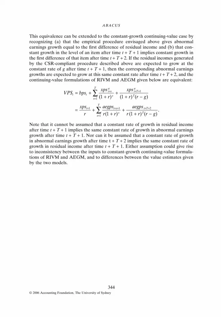
ABACUS


This equivalence can be extended to the constant-growth continuing-value case byrecognizing (a) that the empirical procedure envisaged above gives abnormalearnings growth equal to the first difference of residual income and (b) that con-stant growth in the level of an item after time t + T + 1 implies constant growth inthe first difference of that item after time t + T + 2. If the residual incomes generatedby the CSR-compliant procedure described above are expected to grow at theconstant rate of g after time t + T + 1, then the corresponding abnormal earningsgrowths are expected to grow at this same constant rate after time t + T + 2, and thecontinuing-value formulations of RIVM and AEGM given below are equivalent:

Note that it cannot be assumed that a constant rate of growth in residual incomeafter time t + T + 1 implies the same constant rate of growth in abnormal earningsgrowth after time t + T + 1. Nor can it be assumed that a constant rate of growthin abnormal earnings growth after time t + T + 2 implies the same constant rate ofgrowth in residual income after time t + T + 1. Either assumption could give riseto inconsistency between the inputs to constant-growth continuing-value formula-tions of RIVM and AEGM, and to differences between the value estimates givenby the two models.

VPS bpsxps

r

xps

r r g

xps

r

aegps

r r

aegps

r r r g

t tt sa

ss

Tt Ta

T

t t s

ss

Tt T

T

( )

( ) ( )

( )

( ) ( )

.

= ++

++ −

= ++

++ −

+

=

+ +

+ + +

=

+ +

∑

∑

1 1

1 1

1

1

1 1

1

2

Documents

Dirty surplus accounting flows and valuation errors