wPs1q ID

POLICY RESEARCH WORKING PAPER 1908

How Dirty Are "Quick Routine quick-and-clrtymethods of project appraisal

and Dirty" M ethods can be so dirty in guiding

of Project Appraisal? project selection as to wipeof Project Appraisal? uteescilanfol

out the net social gains fromipublic investment.

Dominique van de Walle

Dileni Gunewardena

The World BankDevelopment Research GroupApril 1998

Pub

lic D

iscl

osur

e A

utho

rized

Pub

lic D

iscl

osur

e A

utho

rized

Pub

lic D

iscl

osur

e A

utho

rized

Pub

lic D

iscl

osur

e A

utho

rized

Poi,icy RESEARCIH WORKING PAPER 1908

Summary findings

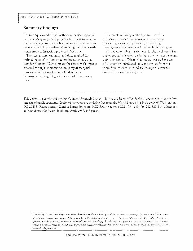
Routine "quick-and-dirty" methods of project appraisal The quick-and-dirte method performs lcl iHncan be sc dirty in guiding project selection as to wipe out esinmatm- average becnefits rnationally but can bethe net social gains from public investment, contend van misleading for some regions a;nd, by ignni- ing

de Walle and Gunewardena, illustrating their point with heterogeneity, overestimates now muc¢h the p ;iro i

a case study of irrigation projects in Vietnam. At moderate to high project cost lev¢ls, quick-i K d-cirry

They test a common quick-and-dirty method for makes enoc¢gh mistakes to e iinate the llct benetits fromti

estimating benefits from irrigation investmnents, using public investmrent. WhIen- irrigaltng as littie as 3 pircent

data for Vietnam. They compare the results with impacts of Vietnam s nonirrigated land:1, the sax igs -omn .heassessed through econometric modeling of marginal more data-intensive method are enough to cover -he

returns, which allows for household and area costs or the extra data required.

heterogeneity using integrated household-level survey

data.

This paper -a product of the Development Research Group -is part of a larger effort in the group to assess the welfare

impacts of public spending. Copies of the paper are available free from the World Bank, i 8 18 H Street NW. Washington,

DC 20433. Please contact Cynthia Bernardo, room MC2-501, telephone 202-473-114', fax 2)2-22-1 iS4. Internet

address cbernardoCc@worldbank.org. April 1998. (38 pages)

The Policy Research WYorking Paper Scries disseminates the ,indings of wvork in progress /0 ess ;ape thse exchange ofc u ii' a

de¢elozp;nent issues. An objective of the series is to get the fizdings out quickly, even n ithe hruesetat ins are iess than o-,nlc- ucpapers carr the names of the authors and should be cited accordingly. The findings. nuterOretaOnnt sio lO 'Mc;OnCillSio(ns e -cfprssi 'a lUi (J';<

paper are entirely those of the authors. They do not necessarily represenlt the lzen' of the 'rVnld Bsok, its lstxlccie uZiue >

countries they represent.

Produced by the Policy Research Dissemirna-ion Ceinter

How Dirty are "Quick and Dirty" Methods of Project Appraisal?

Dominique van de Walle and Dileni Gunewardena'

Key, words: Poverty; Welfare; Project evaluation; Irrigation; Viet NamJEL classi ication: H43; 022; 139

Dominique van de Walle is with the Development Research Group of the World Bank. DileniGunewardena is with the Department of Economics at the University of Peradeniya, Sri Lanka.Correspondence to van de Walle, MC2-507, 1818H St., NW, Washington, DC, 20433; (tel) 202-473-7935;(fax) 202-522-1154; (email) dvandewalle@worldbank.org

1 Introduction

An essential input to any project appraisal is an estimate of the quantity changes induced by the

project. Ideally, these estimates will allow for heterogeneity across projects and beneficiaries.

Ignoring such heterogeneity-by looking only at aggregates-can bias estimates of both average

benefits and their distribution. Typically, however, rapid assessments must be resorted to, and the

analysis conducted for a representative project and/or beneficiary. It is recognized that the methods used

in practice for assessing quantity changes in project appraisal simplify reality in this respect; they often

ignore household and area heterogeneity, behavioral responses and general equilibrium impacts. It is

implicitly assumed that economic losses due to these deficiencies are of second order importance. Is

that right? Would collecting better data, or using better methods, make an appreciable difference to the

social welfare outcomes from public investments? Would it be worth investing the extra resources

needed to make a more thorough assessment? Indeed, could the deficiencies of commonly used methods

be so great as to eliminate the entire social gains from the investments?

This paper addresses these questions for a commonly used "quick-and-dirty" (QD) method for

assessing rural infrastructure investments. The QD method we study is a stylized version of the method

that is normally used in practice to assess both the average gains and the distributional impacts of an

irrigation project. The method is implemented and the implied average benefit from irrigation in Viet

Nam is compared to the marginal benefit estimated by an alternative, more sophisticated econometric

method for estimating impacts on farm profits at the farm-household level. We call this the "slow-and-

clean" (SC) method. This is closer to a well-defined theoretical ideal, and is about as sophisticated a

method as one would expect to find in a small research project set up for the evaluation task. While it is

1

not perfect, we believe it represents a distinct improvement, and hence a reasonable test of the

conventional QD approach.

The comparison of our stylized QD and SC methods allows uIs to estimate the potential gains

from using more theoretically sound but costly behavioral methods, where those gains are assessed by

the same criteria used to assess the projects themselves. Here we will be concerned with both the

impacts on average incomes and the distribution of income. QD methods found in practice often appeal

to both efficiency and equity criteria for project selection. For example, appraisals of rural

infrastructuLral projects in developing countries often argue that since the project is to be located in a

poor area, it will help reduce poverty. However, this may be quite deceptive. The benefits from

physical infrastructure investments will be influenced by a number of factors which will typically be

hidden by quick- and dirty methods. Behavioral responses on the part of households may alter expected

outcomes. There mav be complementarities between physical and human infrastructure such that the

returnis to individual households depend in part on the household's level of human capital (van de Walle

1997). f wealthier households have higher human capital, they may also have higher gains. Retums to

irriation on the family farm may further depend on household size and composition in settings with

underdeveloped labor markets. The size of landholdings may also matter, again with obvious potential

skewness of benetits. A project analysis which ignores these factors may seriously misinform policy

conclusions about the impacts on poverty of public investments.

The next section outlines the theoretical ideal and the principles underlying the SC and QD

methods. It also briefly discusses the setting and the data which are used to implement the methods.

Section 3 then conmpares and contrasts results obtained by the alternative approaches including

2

implications for distributional assessments, for project selection and for the net social gains from public

investments. Section 4 concludes with a few comments.

2 Methods

In this section we start with a description of the theoretical ideal and then describe two

approximations-the SC and QD methods.

2.1 Tlte ideal

An important input to the appraisal of irrigation projects is assumed to be an estimate of the gain

in farm profit from irrigating given amounts of previously unirrigated land.2 The ideal method would

start with a general specification of the profit function for a farm household. We measure fann

household profit from crop production by total revenue minus total production costs, which we term net

crop income. This is assumed to be a function of output and input prices (p), non-irrigated (LN) and

irrigated (LI) annual crop land amounts, and other relevant variables (z). The generic profit function is:

(1) ,T, = ;r(pj, Lv, L'.zj)

which is the maximum profit received by the j'th household, G =1,...,n). The vector z will include other

fixed factors and parameters of the production function used by the j'th household.

In the case where a complete set of perfect markets exists for all farm outputs and inputs,

variables influencing consumption decisions, such as the prices of consumer goods and the size and

demographic composition of the household, would not alter the maximum profit from farming.

However, when markets are incomplete-so that the conditions required for separability between

3

production and consumption decisions do not hold-such variables will spillover into production

decisions (Strauss 1986). For example, in Viet Nam, rural labor markets are thin, or non-existent,

reflecting the dual effects of the past socialist organization of rural production and reliance on self-

subsistence farming as well as possibly high supervision costs and limited mobility in the early stages of

transition. Variables such as family size and composition will then influence the amount of labor

available for farming and hence, maximum profits. Then z may include factors besides the parameters

of the farm household's production function. The specification in (I) can thus be made general enough

to encompass market effects of credit or labor market failure.

Now consider a project which involves irrigating amounts A Lj1 of previously unirrigated land

for each of n households (possibly zero for some). The benefit to the j'th farm-household is given by the

increment to its profits from farming, i.e., the benefit is

(2) B, = ;r(P,,L,'-AL'.L +ALj,zj) - fr(P,.LA,L1.z,-

One would then calculate average benefit ( JBj / n) or some distribution-weighted average benefit. In

the special case in which one unit of land is irrigated it is useful to define the marginal benefit finction

as

(3) MB =1 - r(p, L,, L',,)

If we knew the profit function then the task would be complete. In the rest of this section we describe

two approximations to this ideal, one of which-the SC method-is undoubtedly more accurate than the

other. but is still an approximation. But first we need to describe some key features of our data.

4

2.2 Settinog and data

We test irrigation project appraisal methods using data from the Viet Nam Living Standards

Survey (VNLSS) of 1992-93. This is a nationally representative, high quality household consumption

survey covering a sample of 4800 households.3 The data include detailed coverage of agricultural

production and incomes which allows us to construct a comprehensive measure of annual crop incomes

net of all production costs. The survey also collects detailed information on land assets, including

quality of plots, and other inputs to crop production, including family labor inputs. We use total

household per capita expenditures (including the imputed value of consumption from own production),

appropriately deflated to allow for spatial cost of living differences, as our welfare measure.

Viet Nam is a largely agricultural economy where in 1992/93 84 percent of the rural labor force

aged 6 years or older claimed agriculture as their primary occupation. A majority of households are

engaged in small-scale self-subsistence farming relying almost exclusively on household labor and

traditional inputs. About half of the country's arable crop land is under irrigation. It is generally agreed

that there is great potential for an expansion of the area served by new irrigation infrastructure as well as

by the rehabilitation of long non-functioning irrgation networks (Barker 1994). Such investments have

not been undertaken due to the combination of historical factors such as war, highly constrained public

budgets. and lack of access to credit.

The current distribution of access to crop land and irrigation varies across regions but much less

so witlhin regions due to past land refonn. In general, land endowments are relatively equitably

distributed in the North but less so in the South where on average the poor have access to less than half

the amount of land the non-poor have (van de Walle 1996). The existing distribution of irrigation is

5

somewhat more equitable than that of land, though similar. Given its current distribution, it cannot be

argued that irrigation investments will necessarily benefit the poor more than the rich.

Although Viet Nam has been undergoing reform since 1986, markets were still relatively

underdeveloped in 1992-93. Field work suggested that, in some parts of the country, labor and land

markets did not exist at all. Using the same data, van de Walle (1997) finds evidence that household

demographics and human capital exert considerable influence on farm household crop incomes. As

already discussed, this would not be the case if markets performed well such that households could buy

and sell labor time and skills.

2.3 A slow amd clean approach

The SC method works by assuming a functional form for the profit function which is then

estimated by regression methods using suitable micro data-in this case the 1992/3 VNLSS. The

chosen specification allows a number of variables-including land itself, demographics, education

variables and regional dummny variables for Viet Nam's 7 regions-to have direct effects on the marginal

returns from irrigated and non-irrigated crop land. For the SC method used here, the profit function is

assumled to have the following parameterization:

(4) X, = a+±IvLv+>j/L+rzj+1 5d,+-,

where

(5) A, =b, + bPY dj + b2 z+ b3Y L

and

6

(6) b o+bjdy + bdbzj+b'L1

and where d is a vector of regional dummy variables which are assumed to fully capture the variation in

prices faced.4 The error term e is assumed to be independently and identically normally distributed.

The country's regions are made up of provinces, districts and, at the lowest level, communes.

Dummny variables for 119 out of the 200 sampled conimunes are included in the intercept of the profit

function (d in equation 4) to capture variations in prices and any other spatial, cross-commune variations

in omitted or fixed factors such as land and soil quality. Thus, prices of outputs and variable inputs are

assumed to vary between but not within communes. The conmmune dummies will also pick up the

influences of geographical and social and physical infrastructure variations at the commune level. We

also collapse the commune dummies into 7 regional dummy variables and interact them with irrigated

and non-irrigated land (d in equations 5 and 6) and other land types, thus permitting regional effects on

the marginal returns to land.

Of course. this specification is only one of a number that might be proposed. However, by

allowing nonlinearitv in land and interaction effects with other variables, it is a reasonably flexible

functional form for the present purposes.5

The vector: includes other land in agricultural production, land tenure variables, education,

health and demographic variables, and location specific agro-ecological variables. As discussed, a range

of variables are included in z in order to capture characteristics specific to a transition economy in which

markets are still underdeveloped.

OLS is used on a sample consisting of the 3049 farm households in the data set (including some

urban farming households). Table 1 describes the variables. Regression results are given in Table 2.6

7

Irrigated and non-irrigated crop land are both found to have high but diminishing impacts on crop

income. Household size has a positive effect as does its interaction with many land variables. One

notable exception is size interacted with irrigated land with a pronounced negative effect on crop

income. Further investigation finds that when the model is run separately for the North and South of the

country, the negative impact is only upheld for the South where labor markets are somewhat more

developed and where farms are often larger and either fully irrigated or completely without irrigation.

We interpret the results as showing that family labor is more of a constraining factor in farm household

production in the North than in the South and even less so for large irrigated farms in the South

(particularly the Mekong Delta).

The effects of education are also strong. The primary education of the household head is convex

in its impact suggesting increasing returns to schooling. Interaction effects between primary education

variables and irrigated land are generally large and positive. There are also significant commune fixed

effects and significant spatial differences in the effects of both irrigated and non-irrigated land, and other

land types.'

From the regression model, a marginal benefit function for irrigation is derived which allows for

the heterogeneity across households. The marginal benefit from irrigating one unit of previously

unirrigated land is given by the difference in the derivatives of the regression function with respect to

irrigated land and non-irrigated land:

MB, =

(7)

=b' -b,N) + (bl -bi ) 8dj + (b' b2 zj + b3 L' -b3 Lh

8

The estimates of equation 7 are given in Table 3. As expected, marginal benefits from irrigation

fall as irrigated area increases, and increase with the amount of unirrigated land. The results also show

the strong influence of the household's demographic and education endowments on the gains from

moving one unit of non-irrigated land into irrigation. In order to calculate the mean marginal benefit we

evaluate this function at the sample variable means.

2.4 A quick and dirty approach

The "slow-and-clean" method described above is demanding in a number of respects. Special

microdata are required-namely an integrated household survey ("integrated" in that the survey

collected all the relevant variables for the same sampled households). And the method requires

econometric modeling. Without such data and methods (or the resources to obtain them) one has little

option but to do a rapid assessment of the impacts of an irrigation infrastructure expansion on less than

ideal data. The essence of the QD method is to estimate the marginal benefit finction using simple

averag,es that can be readily calculated in the field or using simple pre-existing (non-integrated) surveys.

To guide our characterization of the QD approach it is useful to look first at what is currently

done in practice. In general the aim is to assess the income gain over pre-project rainfed crop incomes

for the average farmer with the average amount of land (for example see Londero 1987; Carruthers and

Clark 1983; OECD 1985). Project appraisal staff typically go to a target area, observe the amount of

land that can be irrigated in the catchment area, and make an estimate of incomes on non-itrigated farms.

Predictions of the gain in farm output from the irrigation project are made on the basis of these field

observations, sometimes also drawing on an assumed "modelr of a representative farm household.

90

Sometimes province level statistics on cropping patterns, intensities and yields are employed; sometimes

estimates are based solely on the field visit. It is rarely clear how the estimate of the gain in farm output

is obtained and what confidence one might have in it.

Such methods are the norm in the World Bank's practice.8 However, there is heterogeneity in the

quality of the inputs. In reviewing the institution's irrigation project appraisals, we found that some

project analyses used more finely disaggregated assessments of the ouput gains by geographical area, by

type of crop or by allowing for some farm heterogeneity through using representative farm models for

more than one farm size. But we also found that in most cases the methods do not allow for within-area

heterogeneity and tend to assume that all farmers will have equal access and benefits.

The method proposed here is a characterization of the methods found in practice. We do,

howvever, take advantage of the availability of farm level data on crop incomes from the VNLSS

consumption survev. Although wve use household survey data to carry out this exercise that is solely a

matter of convenience-there is nothing inherent in our procedure which requires such data. We do not

use the inte(rated nature of the survey (whereby a wide range of different types of data are obtained for

the same sample). Rather wve use the survey to estimate simple means as one might obtain from special

purpose surveys or field trips. The same approach could be enacted through a rapid assessment survey

of a project area or drawing on information collected through a small agricultural survey.

There is an advantage to using the same survey for calibrating both methods since it allows us to

control for differences due to sampling. We may otherwise find differences in the results which are due

to nothing more than sampling errors. By the same token, it could be argued that basing the QD

estimates on a statistically-sound household survey renders them less "dirty" than the typical rapid

10

appraisal estimates using less rigorous sarnpling methods.

Our aim is to calculate the difference in the value of crop incomes net of costs per area of

irrigated versus the same area of non-irrigated land. This difference is then a measure of the average

benefit from irrigation allowing for any difference in production costs associated with a change in

irrigation.

We use the survey data to approximate what the project appraisal would do in the field. Clearly,

the appraiser would not pay attention to non-farmers, or farmers producing crops which do not require

irrigation. This leads us to estimate the mean over a restricted sample of the survey households.

Specifically, we exclude households who are not primarily engaged in the production of rice, other food

crops or annual industrial food crops-typically the major users of irrigation. We restrict the sample to

households whose income from these sources comprise 90 or more percent of their total crop income.

The excluded households have a greater dependence on income from perennial industrial crops, fruit and

forest tree crops.

It is unlikely that a rapid field appraisal would be able to exactly identify households that have

only irrigated (or non-irrigated) land. We therefore allow for some probable margin of error and further

limit the samples to households that have 90 percent or more irrigated or non-irrigated land (as opposed

to 100%) and calculate mean net crop incomes for these groups. The difference between these amounts

expressed per unit of irrigated and non-irrigated land gives us our measure of the average benefit. We

calculate average benefits for the national level as well as for regional subsamples. The latter is done for

six of Viet Nam's seven regions-excluding the Central Highlands where there is very little irrigation

and no households with 90 or more percent of their land under irrigation.9

11

In trying to emulate the approach that a rapid appraisal might adopt, we have made a number of

choices and assumptions in calculating the average benefits from irrigation as described above. To

check the sensitivity of the estimates to our choices we also calculate the means under alternative

assumptions. We experiment by increasing (decreasing) the sample to include households with a

smaller (larger) share of crop incomes from rice, other food and annual industrial food crops, and more

or less precision in defining the sample of only irrigated and non-irrigated land. The results indicate

reasonably similar magnitudes (details below).

The QD method just described has a number of obvious limitations. These include the neglect of

heterogeneity across households and regions and of behavioral effects. For example, the household's

level of human capital and demographic size and composition may influence the returns to irrigation

infrastructure. Impacts will then vary according to how such characteristics vary across households.

Furthermore, these characteristics will not be changed by the irrigation project, so they should be

controlled for when assessing project benefits.

Our QD method appears to be representative of common practice. However, as discussed above,

there is some diversity in the amount of effort put into estimating quantity changes in practice. Some

project appraisals may well do better than our QD method, such as by allowing for some heterogeneity.

Equally well some are likely to do worse, since simple models are used and estimated benefit streams

driven by assumptions. The comparison of our SC and QD methods does allow us to judge how much

extra effort is warranted.

12

2.5 Can we predict what difference the choice of method makes?

Before we compare empirical results from the two methods, we may well ask whether something

can be said a priori about the comparison. Can we expect the QD method to over- or underestimate the

marginal benefits? Consideration of two stylized cases is sufficient to establish that there can be no

theoretical presumption as to which method will indicate higher benefits.

Consider the relationship between profits and land holding, both irrigated and non-irrigated,

under the following assumptions: Case 1: The function relating profits to the amount of irrigated land is

strictly concave (marginal profit declines as land increases throughout) while that of the function relating

profit to non-irrigated land is linear. Case 2: The reverse holds; profit is linear in irrigated land, but

concave in non-irrigated land. Let us also assume that profits are zero when there is no land. In case 1,

both the QD and SC methods will give exactly the same estimate of the lost profit from having one unit

less unirrigated land. while the QD method will overestimate the marginal gain from an extra unit of

irrigated land (because the concavity implies that the average profit per unit of land will be higher than

the marginal profit). Thus, in case 1, the QD method will overestimate the gain as assessed by the SC

method. The ordering reverses in case 2, since the QD method will then overestimate the loss from one

less unit of non-irrigated land, while the two methods will agree on the gain from extra irrigated land.

It is possible to construct a number of other examples which relax these assumptions and exhibit

similar ambiguity. The above argument is sufficient, however, to illustrate that there can be no general

supposition as to wvhich of the two methods will give the higher estimate of the gains from irrigation.

That is an empirical question to which we now turn.

13

3 Quick-and-Dirty versus Slow-and-Clean

This section turns to the empirical implementation of the two methods described above and

attempts to assess what the gains are from the SC method relative to QD and how those gains are

distributed.

3.1 Comparing mean and marginal benefits

For the national sample, the QD method gives a mean benefit of 316 Dongs per year per meter

square of irrigated land. The mean marginal benefit calculated by the SC method is not far off at 304

Dongs.'0 Given the same data base, the means are probably biased to being close. However, upon

disagaregating to the regional level, we find both larger variation between the two methods' estimates for

a particular region and a striking variation in the mean regional gains whatever the method employed.

Table 4 presents the regional benefit estimates.

There is clearly a regional dimension which is quite diverse. As one would expect, it is clearly

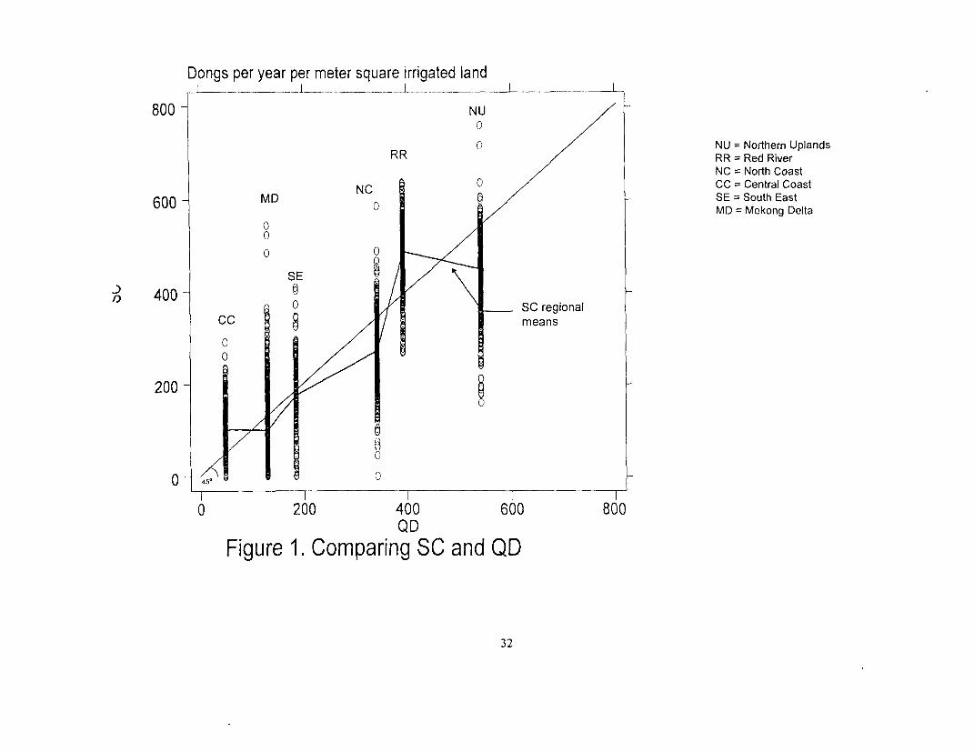
more accurate to use the QD regional estimates than the QD national mean. Figure I plots the SC

marginal benefits (on the vertical axis) against the QD mean benefits at the household level. This

provides an overall summary of our results. (Recall that the SC estimates are household specific while

the QD estimates are the same for all households within a specific region. The figure also identifies the

regional means.) The 45 degree line indicates the line of equality between the estimates. The horizontal

distance between the line of equality and the SC regional means indicates the amount by which the QD

mean over-or underestimates the SC mean. This distance is greater for regions in the North (especially

in the Northern Uplands and in the Red River region) than in the South (South East and Mekong Delta).

14

In no case is the SC only over-or underestimated by the QD method. The scatterplot of SC estimates

indicates a rather wide distribution of household level marginal benefits within each region that is not

captured by the QD. We now take a closer look at the distributions.

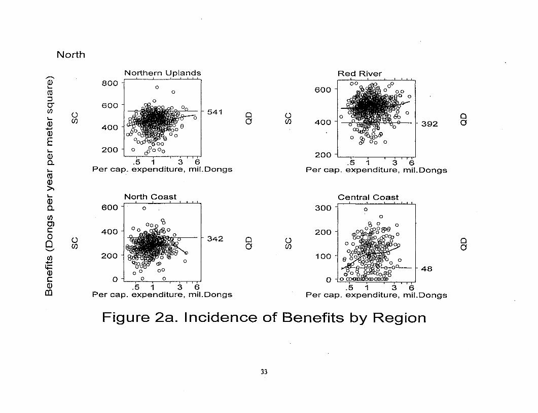
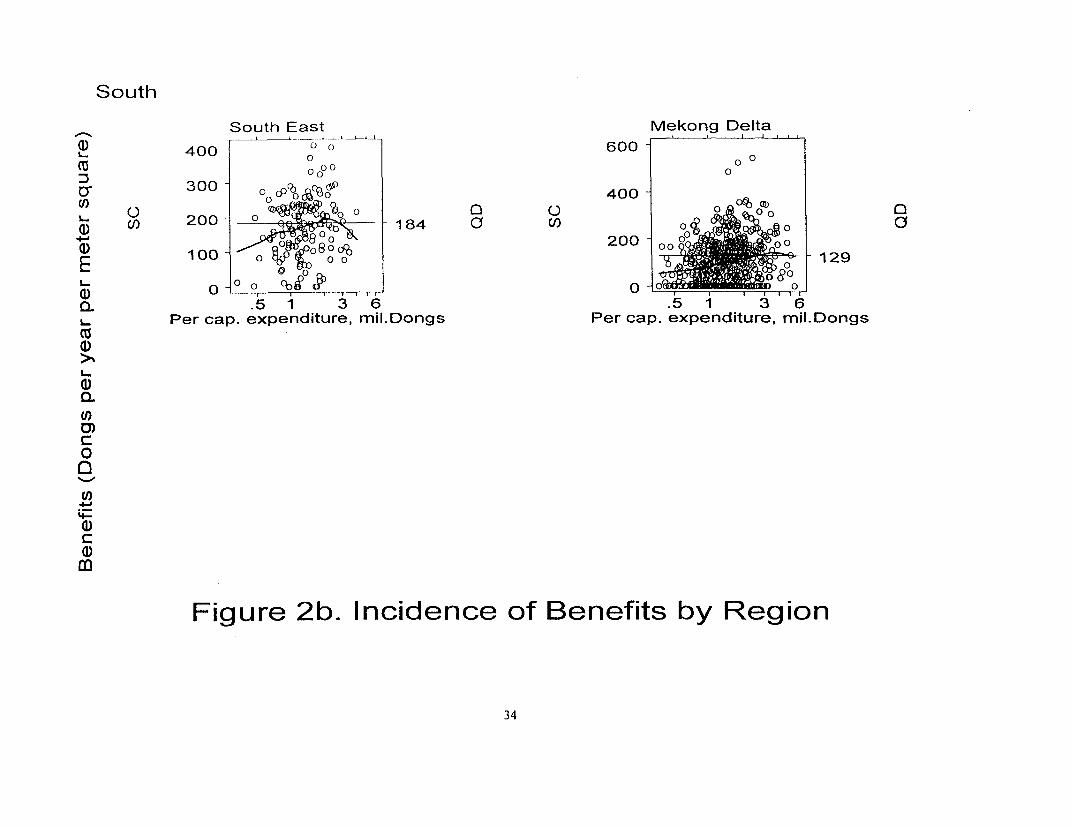
3.2 Distributional implications

We have seen that there is much variation in mean and marginal benefits across regions. Our

next question concerns how much the SC estimates vary with per capita expenditures and what that

means for the QD approximation. We first look at the distribution across per capita expenditures for

each region individually in Figures 2a and 2b. We have plotted the QD measure (a constant in each

region and hence a horizontal straight line), and the household level measures estimated by the SC

method. The figures also show the line of best fit estimated using non-parametric methods for the

distribution of marginal benefits across per capita expenditure."'

The figures display a positive association of benefits with per capita expenditure, although this is

stronger in some regions than others. The Red River region has the least variation in benefits across

expenditure while the other regions have slightly higher variation. In general, there is a tendency for the

QD method to overestimate (underestimate) benefits to households with low (high) per capita

expenditure.

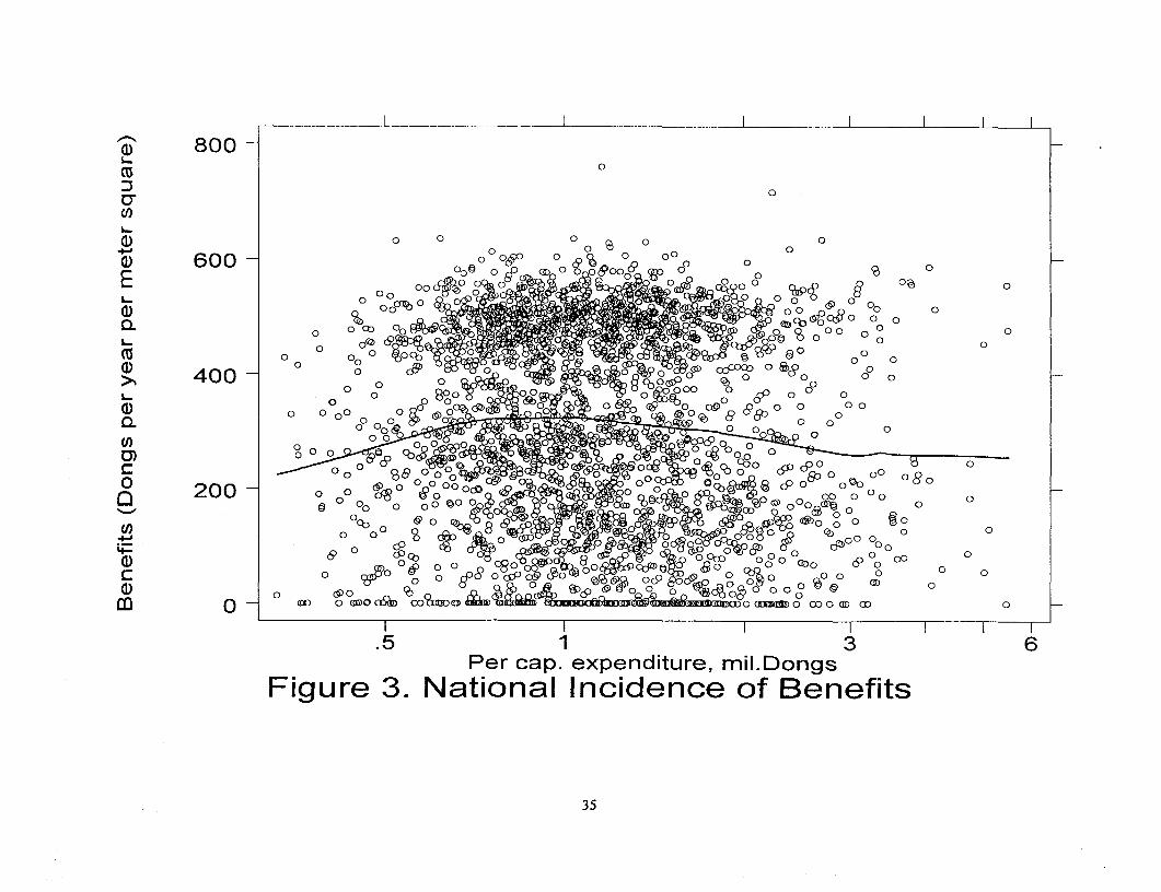
Figure 3 puts together these household level SC estimates to provide a national picture. One can

observe concentration of both high and low marginal benefits. This is partly due to the regional

composition. The line of best fit takes on a slight inverted U shape reflecting regional and household

specific variation in the level and distribution of benefits.

15

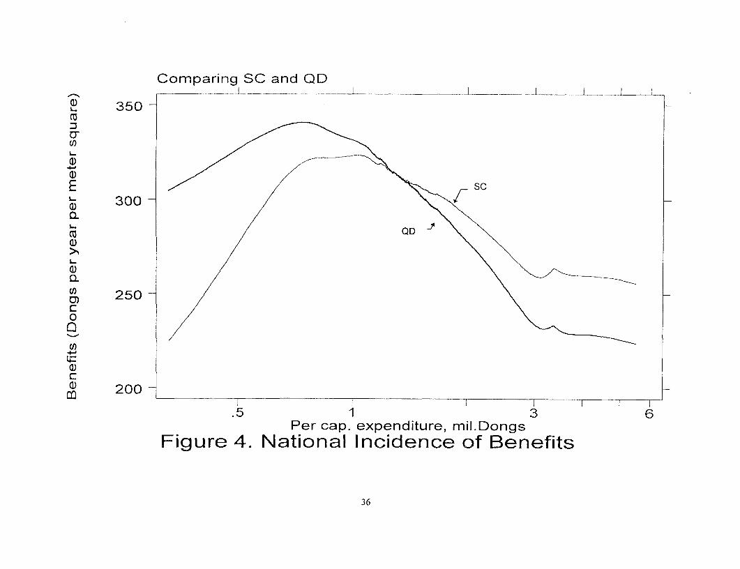
In figure 4, we plot the line of best fit for the QD measures overlaid with the line of best fit

obtained in figure 3 for the SC measures. This emphasizes the main distributional implication: the

regional QD tends to overestimate benefits for the poor and underestimate them for the better off.

The distributional results partly reflect the influence of household specific characteristics as

shown by the marginal benefit function (table 3). In addition to an important regional dimension, the

marginal benefits from irrigated land are significantly affected by the household's size and its level of

primary education. Household size-which has a negative effect on the marginal benefit-tends to be

larger for poorer rural Vietnamese households and to decline with per capita expenditures. Primary

education has a positive influence on marginal returns, and tends to be positively associated with the

level of consumption. In the aggregate, both variables will tend to lower marginal benefits for less-well

off households and to raise them for households at higher per capita expenditure levels. Thus, even

allowing for regional differences, there are household specific characteristics which drive the potential

benefits from irrigation down for the poor and by the same token, enhance the returns to the better off.

These factors are missed by QD.

3.3 Distributional impacts of an irrigation e-xpansion

So far we have explored the marginal and mean benefits associated with a small change. We

have show n that these vary regionally and with household expenditures. Together these factors have

distributional implications. However, in determining the distributional impact of a policy of irrigation

infrastructure investment, the existing distribution of land and access to irrigation will influence the

outcomes. Farms with larger amounts of non-irrigated land are those best positioned to gain from such a

16

policy but we have seen that the level of their gains will depend on a number of factors not connected to

their land assets.

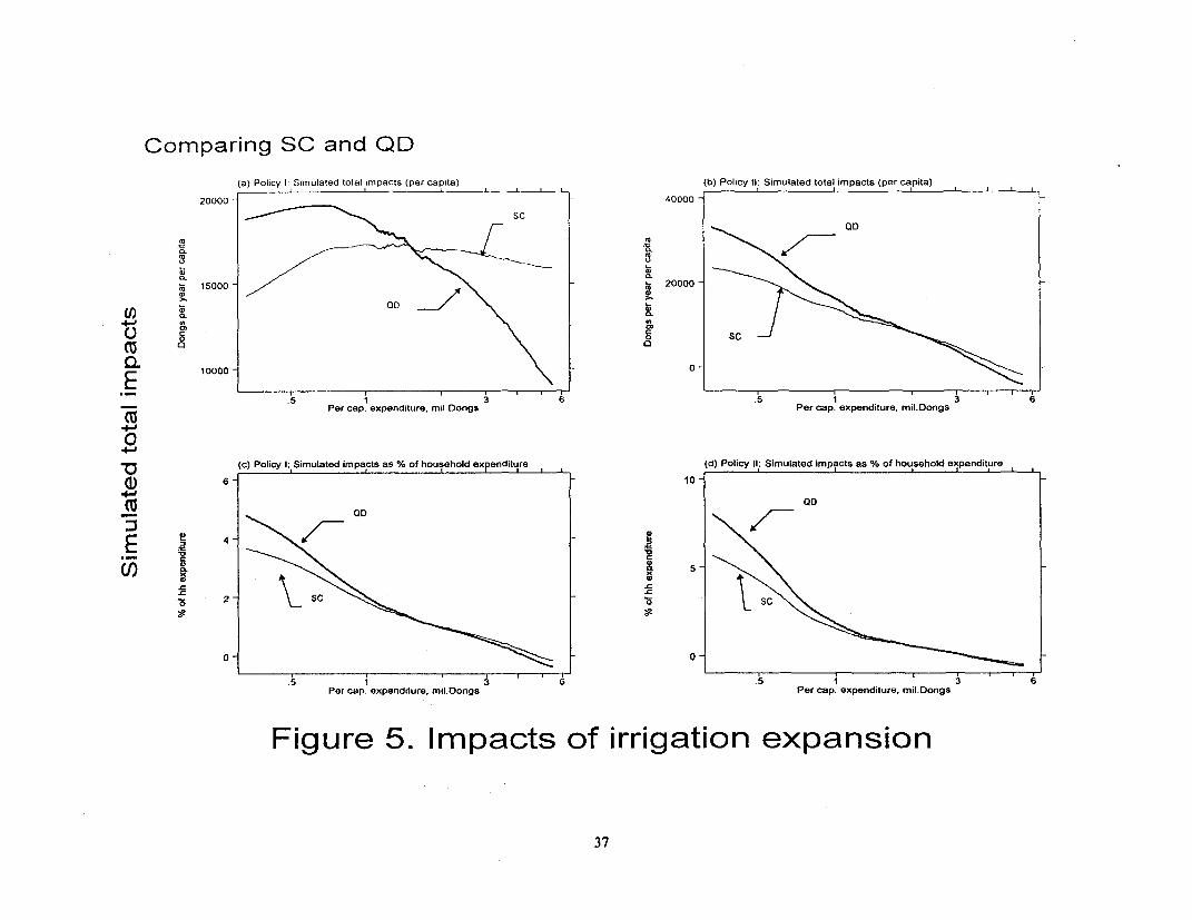
To examine the distributional implications of irrigation infrastructure investments, we simulate a

policy of a 10 percent expansion in the area of currently non-irrigated land into irrigation. The

distribution across households of that expansion is enacted under two scenarios. Policy I simply

increases the amount of land covered by irrigation similarly for each household subject only to

feasibility as determined by current land and irrigation holdings and the expansion being considered.

Policy II is explicitly pro-poor in that it distributes the 10 percent irigation expansion to households

with low per capita land holdings only.'"

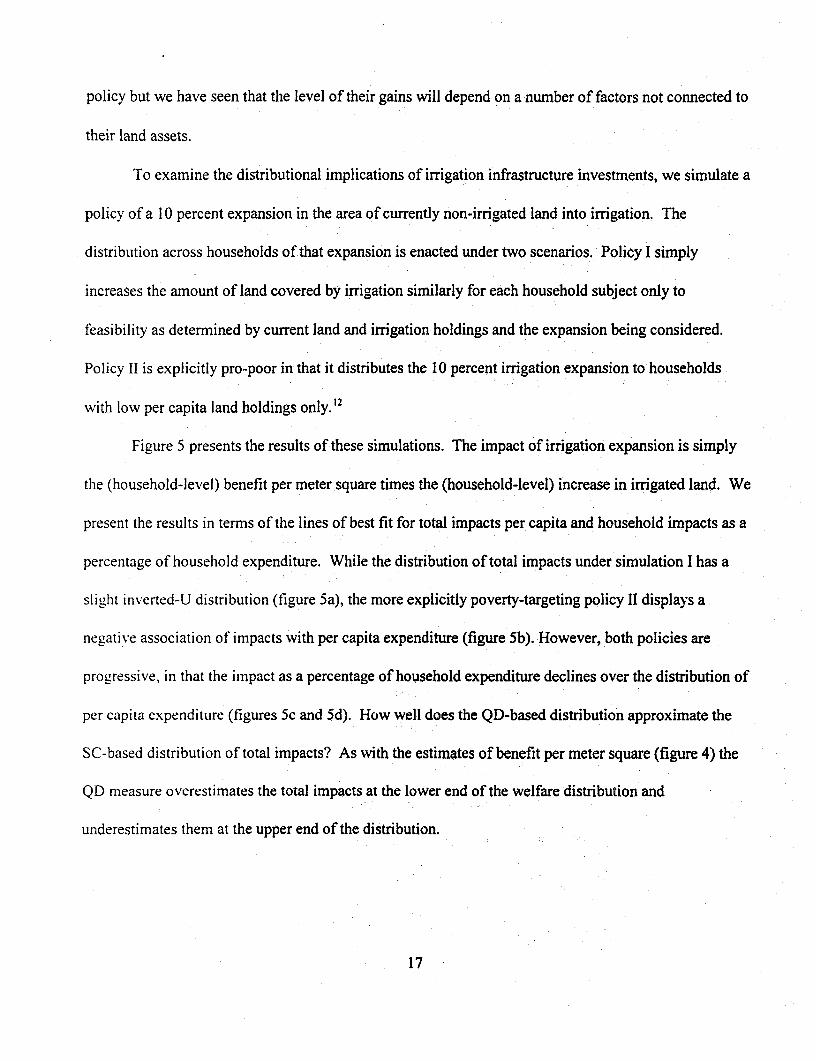
Figure 5 presents the results of these simulations. The impact of irrigation expansion is simply

the (household-level) benefit per meter square times the (household-level) increase in irrigated land. We

present the results in terms of the lines of best fit for total impacts per capita and household impacts as a

percentage of household expenditure. While the distribution of total impacts under simulation I has a

sligzht inverted-U distribution (figure 5a), the more explicitly poverty-targeting policy II displays a

negative association of impacts with per capita expenditure (figure 5b). However, both policies are

progressive, in that the impact as a percentage of household expenditure declines over the distribution of

per capita expenditure (figures 5c and Sd). How well does the QD-based distribution approximate the

SC-based distribution of total impacts? As with the estimates of benefit per meter square (figure 4) the

QD measure overestimates the total impacts at the lower end of the welfare distribution and

underestimates them at the upper end of the distribution.

17

3.4 Impact on project selection

Irrigation investment projects should ideally be approved where benefits exceed costs. It is

interesting to ask how the two methods we have reviewed would differ in determining where and which

projects to undertake. Table 5 conducts such an exercise using hypothetical costs. At each unit cost

level. we ask how many projects would be accepted by the two methods of calculating household level

benefits, where each sampled farm-household is counted as one potential project. The overall results

indicate that the SC and QD estimates tend to be in agreement at both ends of the cost spectrum, but

there is a greater margin of error when the cost is around 400 per m2 (Dongs per year). There is also

some regional variation.

Table 6 gives an overall assessment of the outcomes under the QD approach. The table gives

sumnmary data on the acceptance rates for projects under both the QD and SC acceptance rules for

various cost levels. The QD and SC rules agree in the selection of projects most of the time up to project

costs nearing 400. However, there is greater disagreement at 400 Dongs per meter square and higher.

\We also presenit the net benefits which wvould be realized were project selection to be decided

according to each method. Benefits for both sets of projects are evaluated using the SC estimates to

work OlIt actual benefit levels. These are then expressed per meter square. The difference between the

net benefits realized under each rule then gives us some idea of the potential losses due to use of the QD

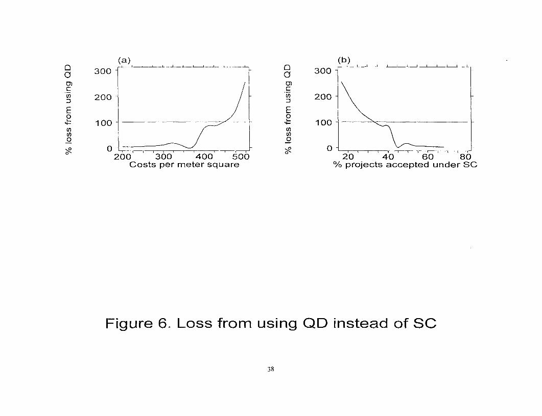
method: in particular, the final column of Table 6 gives the percentage of the benefits realized under the

SC method which is lost under the QD rule for accepting projects.'3 This is small for low cost projects,

which is unsurprising since one is unlikely to make serious errors in this case, as most potential projects

w6ill be accepted. However, the loss from the QD method rises rapidly above costs of about 375 Dongs

18

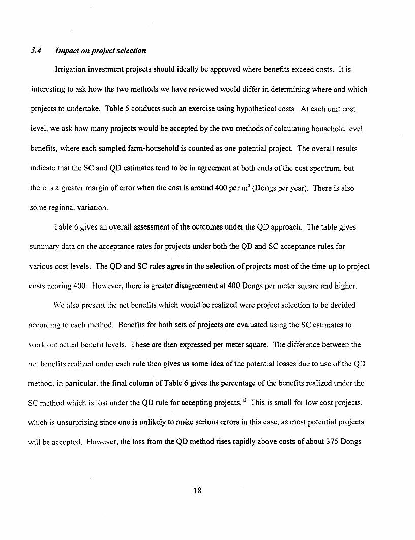
per square meter; at a unit cost of about 450, the entire project benefit is lost when project selection is

based on the QD method. This can be seen clearly in Figure 6a which plots the loss under QD against

the unit cost. Figure 6b plots the loss under QD against the proportion of projects accepted under the SC

rule which is a decreasing function of the unit cost. The sharp increase in the loss from the QD method

starts to set in at a point when less than half of all projects should be accepted under the SC rule. The

realized net benefits under QD fall to zero when about one third of the projects should be accepted.

We have said much about the potential benefits of adopting the SC method but little about its

costs. Integrated household surveys such as the VNLSS can seem expensive propositions. For example,

depending on how one accounts for various inputs (such as jeeps and computers which will continue to

be used after data collection) the 1992-93 VNLSS cost between one-half to one million US dollars.

However, our results suggest that this outlay is dwarfed by the potential benefits from using the SC

method for project selection. 14 Figure 7 graphs the benefits in millions of dollars from using the SC

instead of the QD method against irrigation project sizes expressed as percentages of currently non-

irrigated arable land in Viet Nam. We plot this relationship for both low and high project unit costs. We

also indicate the approximate cost of the VNLSS survey. Even at relatively low unit costs of irrigation

projects. the realized benefit from extra data when irrigating only 3 percent of unirrigated land would be

sufficient to cover the cost of that data. Of course, that data would also have other benefits.

4 Conclusions

Ex-post, irrigation evaluations often find that measured project benefits are less than had been

predicted at appraisal stage (Carruthers and Clark 1983). Problems in project implementation are often

19

blamed. But errors in appraisal and project selection may also explain the gap between ex-ante and ex-

post evaluation results. Extensions of the type of analysis in this paper to other settings would be needed

to properly test that hypothesis. Although it would in many respects be harder than our stylized case

study, it would also be desirable to apply similar methods to the evaluation of appraisals for specific

projects subsequently implemented.

We have provided a case-study of how well commonly used "quick and dirty" methods for

project appraisal approximate mean benefits and their distribution, whether such methods would result in

fundamentally different project recommendations from those emerging from a more arduous "slow and

clean" approach, and what benefits can be expected from the extra effort needed to implement the latter

approach. As in all empirical research, our results are to some extent data specific. However, there has

been so little research into the benefits of doing more thorough ex-ante project evaluations that even one

case study can be instructive. And there do appear to be some potential lessons for other settings.

We find that at the national level in Viet Namn, QD mean benefits are similar to SC mean

benefits. At the regional level, there is greater variation. One cannot determine a priori whether the QD

method would over- or underestimate SC mean benefits, and our empirical results show that there is no

tendency for QD to only over- or underestimate the SC benefits.

Our results indicate that the QD method overestimates the progressivity of a policy of irrigation

expansion in Viet Nam. The QD results suggest a more pro-poor distribution of gains than the SC

method. This is true when we define gains as the benefit per square meter, as well as when we take into

account the existing distribution of land and access to irrigation. This is explained by the QD method's

neglect of household and regional heterogeneity. The poor have characteristics that reduce the gains

20

relative to the mean. This cannot be revealed by the QD method.

We find that the QD method rejects some projects that should have been accepted, and accepts

some that should have been rejected. We used the SC method to evaluate the realized benefits when

project selection is based on the QD method, and compared this to the benefits realized when the SC

method is used for project selection. The comparison suggests that the QD method entails only small

losses when project unit cost is low, and (hence) most potential projects are easily accepted. However,

the loss from the QD method rises sharply at medium to high project cost levels. Indeed, at unit costs at

which about one third of the potential projects should be accepted (and would yield large net benefits),

the QD method will incorrectly choose enough projects to wipe out the realized benefits.

Although a potentially profitable set of projects exists according to the SC method, selection

based on the QD method will realize a net loss. The savings from the more data intensive SC method

are sufficient to cover the costs of its extra data requirements (even ignoring other benefits from the

data) if irrigating more than 3 percent of unirrigated land. This case study suggests that unless project

size and cost are small or distributional impacts are irrelevant, there can be large social benefits to

investing in more thorough evaluations.

21

Notes

For comments and suggestions, the authors would like to thank Lionel Demery, Gaurav Datt, Shanta Devarajan,Gunnar Eskeland, Jeff Hammer, David Hughart, Peter Lanjouw, Jennie Litvack, Howard Pack, VijayaRamachandran, Martin Ravallion and seminar participants at IFPRI and the World Bank. The findings,interpretations, and conclusions expressed in this paper are entirely those of the authors. They do not necessarilyrepresent the views of the World Bank, its Executive Directors, or the countries they represent.

1. For an overview of these and other issues in project evaluation see Dreze and Stern (1990).

2. We can abstract from whether the investments are public or private since either way, an estimate of the gainsin farm yields are needed.

3. A detailed description of the data set is given in Glewwe (1994).

4. Because the paper's focus is with irrigated and non-irrigated annual crop land we show the marginal retums onlyfor these land types. Note however that the specification allows for the same variables to also interact with otherland types which are contained in the z vector.

5. As is common in the literature and indeed is true of most rapid assessment methods of project appraisal, ourSC method ignores general equilibrium and dynamic welfare effects. Moreover, a large number of econometricspecifications might be used instead of the one we choose. There is clearly a continuum of quick and dirty aswell as slow and clean methods for estimating benefits. Our purpose here is not to challenge the conventionalmethod with the best possible test. Rather, we aim to improve on the method typically used in ways that aremethodologically and technically feasible and to then see whether policy conclusions and choices aresignificantly altered.

6. A number of functionial form specifications were tried (for further discussion see van de Walle 1997). Thepresented linear model with quadratics in land and education variables was found to perform best. Full regressiondetails are available from the authors.

7. Biases due to endogenous explanatory or omitted variables which are correlated with included variables is apotential issue here. However, as a result of past land reform and distribution processes, land and irrigation inputscan reasonably be treated as exogenous at the household level. Possible omitted variable bias is more worrying.The regressions control for omitted between-commune variance through the commune dummies. But, there mayalso be latent heterogetneity in (say) land or soil quality within communes. Still, including land quality in theregression did not reveal any sign of such bias (van de Walle 1997). This could be more of an issue in the SouthWhere salinity and acidity are common problems in the Mekong Delta, though unobserved in the VNLSS data.

8. We reviewed all 19 irrigation project appraisal reports prepared in the World Bank since 1992.

9. Viet Nani's other six regions include the Northern Uplands (NU), Red River (RR), North Coast (NC), andCentral Coast (CC) in the North, and the South East (SE), Mekong Delta (MD) and the excluded CentralHighlands (ClI) in the South.

22

10. To check for sensitivity of the QD measure to our assumptions, we increased (decreased) the sample toinclude households with a smaller (larger) share of crop incomes from rice, other food and annual industrial foodcrops, and more or less precision in defining the sample of only irrigated and non-irrigated land. Keeping theassumptions about crop income shares, but (a) assuming 100% (instead of 90%) precision in defining the sampleof households with only irrigated or non-irrigated land, yielded a national mean of 306 Dongs per m2. (b)Assuming less precision (75%) in defining households with only irrigated or non-irrigated land gave an averagebenefit per m2 of 320 Dongs. Keeping the assumption of 90% precision in defining households with onlyirrigated or non-irrigated land but changing the sample to include households with a larger (smaller) share ofincome from rice, other food and annual industrial crops also yielded results of similar magnitude: (c) forhouseholds wlhere 100% of crop income is from these crops, the mean benefit per m2 was 345 Dongs, and for (d)households where 75% or more of crop income is from these crops, mean benefit per mi2 was 310 Dongs. Thus,under all assumptions, the QD estimates at the national level slightly overestimate the gains from irrigation.

11. The estimates are obtained using Cleveland's (1979) locally weighted smoothed scatterplots (LOWESS)-amethod of nonparametric estimation which is of the nearest neighborhood type.

12. Given the existing distribution of land, this policy extends irrigation to the non-irrigated land of allhouseholds with landholdings less than 610 m2 per person.

13. Note that columns (3) and (5) give average net benefits, averaged over all accepted projects. To obtain totalbenefits it is therefore necessary to multiply these columns by columns (2) and (4) respectively. The percentage ofbenefits lost from using the QD method given in column (6) thus reflects accepted projects which should have beenrejected and rejected projects which should have been accepted.

14. The total benefit from using the SC method is simply the loss per square meter from using QD, given in Table6 bv [Col(4) x Col(5)] minus [Col(3) x Col(2)] for a given project unit cost times the project size.

23

References

Barker, Randolph, 1994. Agricultuiral Policy Analysis for transition to a Market-Oriented Economy in Viet Nam:Selected Issues, FAO Economic and Social Development Paper 123, FAO, Rome.

Carritlers, lan and Colin Clark. 1983. The Economics of Irrigation, Liverpool University Press, Liverpool.

Cleveland, W.S. 1979. "Robust Locally Weighted Regression and Smoothing Scatter Plots", Journal of theAmerican Statistical Association, 74:829-836.

Dreze, Jean and Nicholas Stern. 1990. "Policy Reform, Shadow Prices, and Market Prices" Journal of PublicEcon1om07ics, 42: 1-45.

Glewwe, Paul. 1994. "Viet Nam Living Standards Survey (VNLSS), 1992-93: Basic Information". mimeo,Poverty and Human Resources Division, Policy Research Department, The World Bank, Washington, D.C.

Kumar, Krishna. 1993. Rapid Appraisal Methods. World Bank Regional and Sectoral Studies, Washington, D.C.

Londero, Elio. 1987. Benefits and Beneficiaries: An Introduction to Estimating Distributional Effects in Cost-Beniefit Analysis, Inter-American Development Bank, Washington, D.C.

OECD. 1985. Mtfaniagemiient of Water Projects: Decision-making and Investment Appraisal, Paris: Organisationfor Economic Cooperation and Development.

Strauss, John. 1986. "The Theory and Comparative Statics of Agricultural Household Models: A GeneralApproach (Appendix)." In Singh, Inderjit, Lyn Squire, and John Strauss, eds.,Agricultural Household Models:Extensions, Applications anld Policy, Baltimore: Johns Hopkins Universitv Press.

Suiltania. Parvin. Paul NI. Thompson and Mike G. Daplyn. 1995. "Impact of Surface Water Management Projectson Agriculture in Bangladesh." Project Appraisal, 10:243-259.

van de Walle. Dominique. 1996. "Infrastructure and Poverty in Viet Nam", Living Standards MeasurementStudy Working Paper No. 121, The World Bank, Washington, D.C.

van de Walle, Dominique. 1997. "Human Capital and Labor Market Constraints in Developing Countries: ACase Study of Irrigation in Viet Nam" mimeo, Policy Research Department, The World Bank, Washington, D.C.

24

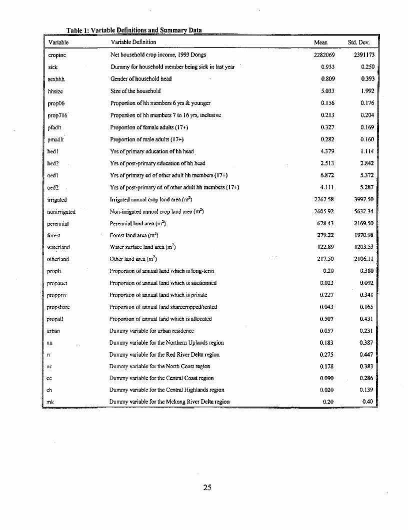
Table 1: Variable Definitions and Summary Data

Variable Variable Definition Mean Std. Dev.

cropinc Net household crop income, 1993 Dongs 2282069 2391173

sick Dummy for household member being sick in last year 0.933 0.250

sexhhh Gender of household head 0.809 0.393

hhsize Size of the household 5.033 1.992

propO6 Proportion of hh members 6 yrs & younger 0.156 0.176

prop716 Proportion of hh members 7 to 16 yrs, inclusive 0.213 0.204

pfadlt Proportion of female adults (17+) 0.327 0.169

pmadit Proportion of male adults (17+) 0.282 0.160

hedl Yrs of primary education of hh head 4.379 1.114

hed2 Yrs of post-primary education of hh head 2.513 2.842

oedl Yrs of primary ed of other adult hh members (17+) 6.872 5.372

oed2 Yrs of post-primary ed of other adult hh members (17+) 4.111 5.287

irrigated Irrigated annual crop land area (mi2) 2267.58 3997.50

nonirrigated Non-irrigated annual crop land area (mi2) 2605.92 5632.34

perennial Perennial land area (mi2) 678.43 2169.50

forest Forest land area (mi2) 279.22 1970.98

waterland Water surface land area (M2) 122.89 1203.53

otherland Other land area (m) 217.50 2106.11

propit Proportion of annual land which is long-term 0.20 0.380

propauct Proportion of annual land which is auctionned 0.023 0.092

proppriv lProportion of annual land which is private 0.227 0.341

propshare lProportion of annual land sharecropped/rented 0.043 0.165

propall Proportion of annual land which is allocated 0.507 0.431

urban Dummy variable for urban residence 0.057 0.231

nu Dummy variable for the Northemr Uplands region 0.183 0.387

rr Dummy variable for the Red River Delta region 0.275 0.447

nc Dummy variable for the North Coast region 0.178 0.383

cc Dummy variable for the Central Coast region 0.090 0.286

ch Dummy variable for the Central Highlands region 0.020 0.139

ink Dummy variable for the Mekong River Delta region 0.20 0.40

25

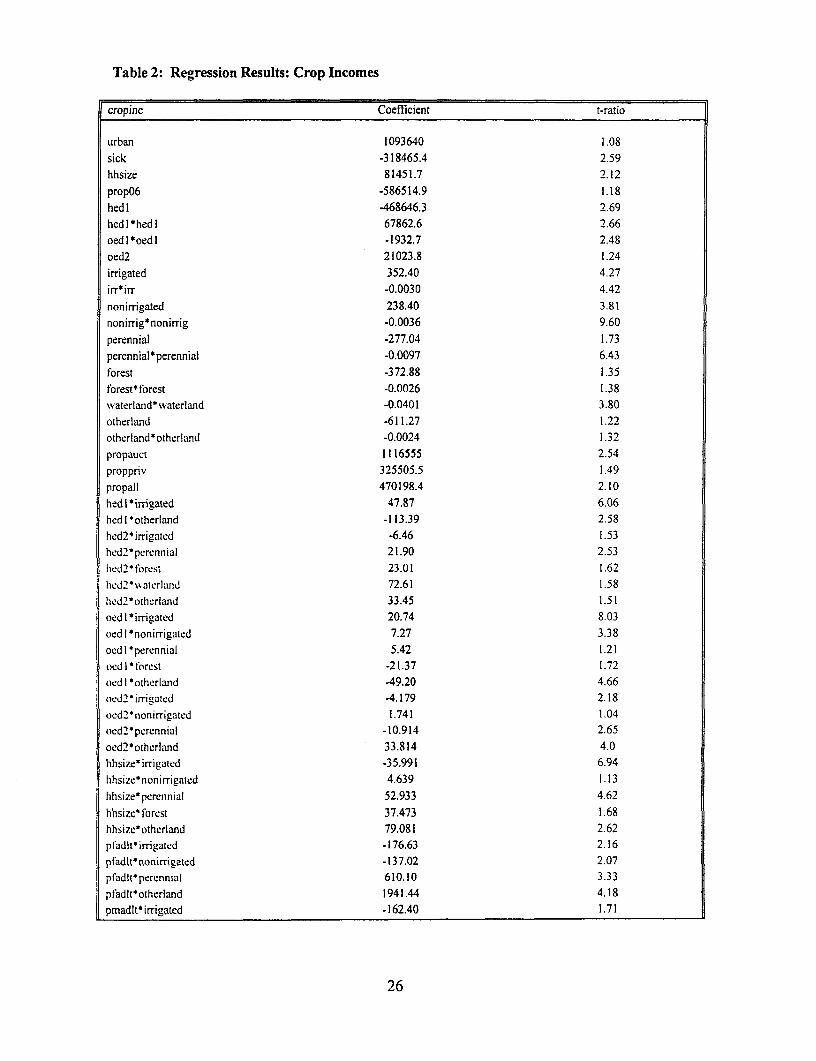
Table 2: Regression Results: Crop Incomes

cropinc Coefficient t-ratio

urban 1093640 1.08sick -318465.4 2.59hhsize 81451.7 2.12

propO6 -586514.9 1.18hed 1 -468646.3 2.69hedIThedi 67862.6 2.66oed I *oed I -1932.7 2.48oed2 21023.8 1.24irrigated 352.40 4.27irr*irr -0.0030 4.42nonirrigated 238.40 3.81nonirrig*nonirrig -0.0036 9.60

perennial -277.04 1.73

perennialperennial -0.0097 6.43forest -372.88 1.35forest*forest -0.0026 1.38waterland* waterland -0.0401 3.80

otherland -611.27 1.22otherland*otherland -0.0024 1.32propauct 1116555 2.54proppriv 325505.5 1.49propall 470198.4 2.10hed I * irrigated 47.87 6.06hed I *otherland -113.39 2.58hed2* irrigated -6.46 1.53hed2*perennial 21.90 2.53hed2*forest 23.01 1.62hed2* % aterlaid 72.61 1.58hed2 otherland 33.45 1.51

oed I irrigated 20.74 8.03oed I nonirrigated 7.27 3.38oed I perennial 5.42 1.21ocd I * torest -21.37 1.72oed I otherland 49.20 4.66oed2 irrigated 4.179 2.18oed2*nonirrigated 1.741 1.04oed2* perennial -10.914 2.65oed2*otherland 33.814 4.0hhsize*irrigated -35.991 6.94bhsize*nonirrigated 4.639 1.13hhsize*perennial 52.933 4.62

hhsize t forest 37.473 1.68hhsize*otherland 79.081 2.62pfadlt irrigated -176.63 2.16praditnonirrigated -137.02 2.07pfaditperennial 610.10 3.33pfadVt*otherland 1941.44 4.18pmadVt irrigated -162.40 1.71

26

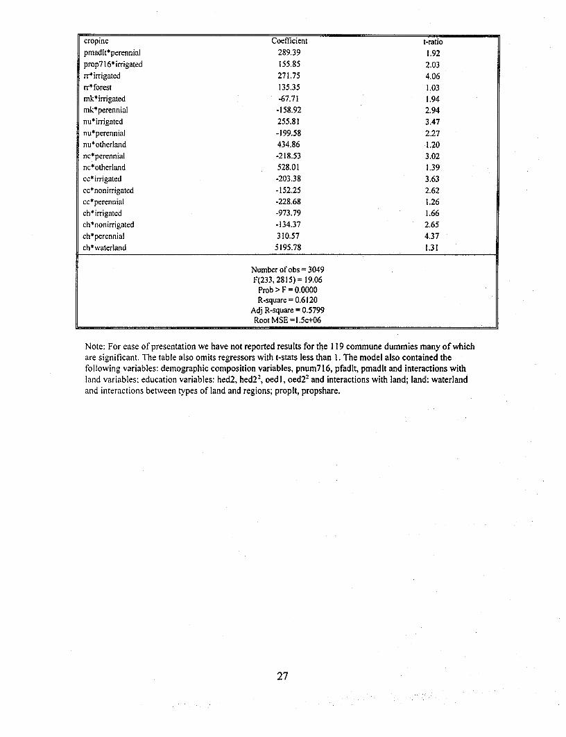
cropinc Coefficient t-ratiopmadlt*perennial 289.39 1.92prop716*irrigated 155.85 2.03rr*irrigated 271.75 4.06rr* forest 135.35 1.03mk*irrigated -67.71 1.94mk*perennial -158.92 2.94nu*irrigated 255.81 3.47nu*perennial -199.58 2.27nu*otherland 434.86 1.20nc*perennial -218.53 3.02nc*otherland 528.01 1.39cc* irrigated -203.38 3.63cc*nonirrigated -152.25 2.62cc*perennial -228.68 1.26ch*irrigated -973.79 1.66ch*nonirrigated -134.37 2.65ch*perennial 310.57 4.37ch*waterland 5195.78 1.31

Number of obs = 3049F(233, 2815) = 19.06Prob > F = 0.0000R-square = 0.6120

Adj R-square = 0.5799Root MSE=1.5e+06

Note: For ease of presentation we have not reported results for the 119 commune dummies many of whichare significant. The table also omits regressors with t-stats less than 1. The model also contained thefollowing variables: demographic composition variables, pnum7 16, pfadlt, pmadlt and interactions withland variables; education variables: hed2, hed22, oedl, oed22 and interactions with land; land: waterlandand interactions between types of land and regions; propit, propshare.

27

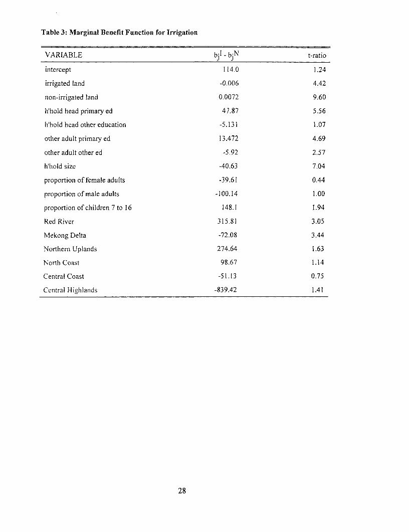
Table 3: Marginal Benefit Function for Irrigation

VARIABLE bil- bhN t-ratio

intercept 114.0 1.24

irrigated land -0.006 4.42

non-irrigated land 0.0072 9.60

h'hold head primary ed 4 7.87 5.56

hWhold head other education -5.131 1.07

other adult primary ed 13.472 4.69

other adult other ed -5.92 2.57

h'liold size -40.63 7.04

proportion of female adults -39.61 0.44

proportion of male adults -100.14 1.00

proportion of children 7 to 16 148.1 1.94

Red River 315.81 3.05

Mekong Delta -72.08 3.44

Northern Uplands 274.64 1.63

North Coast 98.67 1.14

Central Coast -51.13 0.75

Central Highlands -839.42 1.41

28

Table 4: Benefits by Region

Benefits North Red North Central South Mekong(Dongs/year/m2) Uplands River Coast Coast East Delta

(I) Slow and Clean 449 488 272 102 175 100

(2) Quick and Dirty 541 392 342 48 184 129

(2) - (1) 92 -96 70 -54 9 29

29

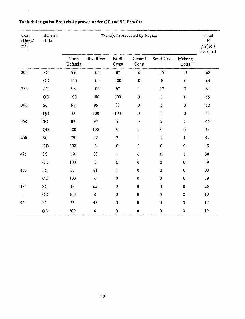
Table 5: Irrigation Projects Approved under QD and SC Benefits

Cost Benefit % Projects Accepted by Region Total(Dong/ Rule %m2) projects

accepted

North Red River North Central South East MekongUplands Coast Coast Delta

200 SC 99 100 87 6 45 13 68

QD 100 100 100 0 0 0 65

250 SC 98 100 67 1 17 7 61

QD 100 100 100 0 0 0 65

300 SC 95 99 32 0 5 3 52

QD 100 100 100 0 0 0 65

350 SC 89 97 9 0 2 1 46

QD 100 100 0 0 0 0 47

400 SC 79 92 3 0 1 1 41

QD 100 0 0 0 0 0 19

425 SC 69. 88 1 0 0 1 38

QD 100 0 0 0 0 0 19

450 SC 53 81 1 0 0 0 33

QD 100 0 0 0 0 0 19

475 SC 38 65 0 0 0 0 26

QD 100 0 0 0 0 0 19

500 SC 26 45 0 0 0 0 17

QD 100 0 0 0 0 0 19

30

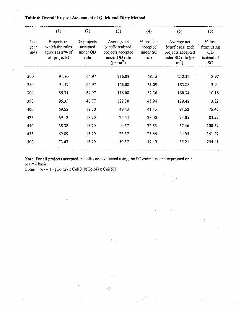
Table 6: Overall Ex-post Assessment of Quick-and-Dirty Method

(1) (2) (3) (4) (5) (6)

Cost Projects on % projects Average net % projects Average net % loss(per which the rules accepted benefit realized: accepted benefit realized: from usingm2) agree (as a-% of under QD projects accepted under SC projects accepted QD

all projects) rule under QD rule rule under SC rule (per instead of(per m2) m2) SC

200 91.80 64.97 216.08 68.15 212.32 2.97

250 91.17 64.97 166.08 61.09 183.88 3.94

300 85.71 64.97 116.08 52.36 160.34 10.16

350 95.35 46.77 122.30 45.94 129.48 3.82

400 69.52 18.70 49.43 41.15 91.52 75.46

425 69.12 18.70 24.43 38.00 73.05 83.55

450 68.38 18.70 -0.57 32.85 57.46 100.57

475 69.89 18.70 -25.57 25.66 44.95 141.47

500 73.47 18.70 -50.57 17.40 35.21 254.41

Note: For all projects accepted, benefits are evaluated using the SC estimates and expressed on aper mn2 basis.Column (6) = I - [Col(2) x Col(3)]/[Col(4) x Col(5)]

31

Dongs per year per meter square irrigated land

800 NU

O NU = Northern UplandsRR / RR = Red River

NC = North CoastNC 0 CC = Central Coast

600 MD O SE = South EastMD Mekong Delta00

SE

400SE 74 0 SC regionalCC means

00

200

0 45' C)

0 200 400 600 800QD

Figure 1. Comparing SC and QD

32

North

Northern Uplands Red River(D 800- ,o

U o O 600 - ,o °0

@ 400 t; a 09 4 00 - 39 a

0

600 200, .5541 1 3

U) 0 0 0 ~~~~~~~~ ~~~400 - 0S 'O 392 0)I ~~400-

E 0~~~~~~0 0 ! 0a

L. ~~200 0 c 00o 200 _ _ _ _ _ _ _

CL ~.5 1 36 3 6i Per cap. expenditure, mil.Dongs Per cap. expenditure, mil.Dongs

>)North Coast Central Coast

QL 600 o 300- 00 o 342

0) 0 0 0

4200 - 0 200 -48U) U

U) .5 1.5 1 3 6Per cap. expenditure, mil.Dongs Per cap. expenditure, mil.Dongs

Figure 2a. Incidence of Benefits by Region

33

South

South East Mekong Delta0) ~~~~~~~~~;0~ 0400 - 0 600

:J 3 0^ @t 0 0300 4000U) 0 0%~~~~~~~0 .L- 184 0 0) 0 )

E 184 (100 200 - 129

QL .5 1 3 6 6.51 36Per cap. expenditure, mil.Dongs Per cap. expenditure, mil.Dongs

0)

c

a-

Figure 2b. Incidence of Benefits by Region

34

a) 800 0

0

a) 0 .I0.0 0 0 0 0

U) 600 ~ ~ ~~0~0 D O 6 1E 0~ o ~P00 expnd t 0 ongs

400 ~ ~ 0 0&

Figure L o I o

0)~~~~~~~~~~~~~~~~3

a)0. U)00Q o &00

0) ~ ~ ~ 00

0) ooc~~~0 oo

0 0 0 C 00) 0 &)~00 RD 0 6P O0 0

M o0) ~ ~ ~ .

c 0 00 00 erca. xpndtue,mi.Dng0 20 Figur 3. National inie ce of Benefit

0 QO C2) ON 0 0~~~3

Comparing SC and QD.1_ __ ,_____- I __ ___ _I_ __ _1_ II

350

(I)

E S300

U)~~~~~~~~~~~~Q

(7> 250 -

0~

L.

4)

a)C /

a) 200

.5 1 3 6Per cap. expenditure, mil.Dongs

Figure 4. National Incidence of Benefits

36

Comparing SC and QD(a) Policy I: Simulated total impacts (per capita) (b) Policy II: Simulated total impacts (per capita)

20000 - 40000 -SC

F5 5. I of i

37

0 ~~~~~~~~~~~~~~~~~~~~~~~~~~~~~~~~~0~a, a,

C C

.5 1 3 6. Pe a. expenditure, mil.Dongs Per cap. expenditure, mil.Dongs

(c) Policy 1:, Siuae mat s%oousehold expenditure (d) Policy IIt: Simulated impacts as % of household expenditure

(D 10.4-I

OD ~~~~~~~~~~~~~~~~~QD

E4c~~~~~~~~~~~~~~~~~~~~~~~~~~~~~~

Cax, FL

0 0

Per cap. expenditure. mit tDongs Per cap, expenditure, mil.Dongs

Figure 5. Impacts of irrigation expansion

37

(a) (b)a) 300 - 300

0)~~~~~~~~~~~~~~~~~~~~~~~~~C

200 200

4 J0 E Eo 0

4- 1 00 4- 100(I) (I)C/) Cl)o 0

0 _ _ _ _ _ _ _ _ _0 0 -

200 300 400 500 20 40 60 80Costs per meter square % projects accepted under SC

Figure 6. Loss from using QD instead of SC

38

Policy Research Working Paper Series

ContactTitle Author Date for paper

WPS1883 intersectoral Resource Allocation and FumihideTakeuchi February 1998 K. Labrieits Impact on Economic Development Takehiko Hagino 31001in the Philippines

WVPS1884 Fiscal Aspects of Evolving David E. Wildasin February 1998 C. BernardoFederations: Issues for Policy and 31148Research

WPS1885 Aid. Taxation, and Development: Christopher S. Adam February 1998 K. LabrieAnalytical Perspectives on Aid Stephen A. O'Connell 31001Effectiveness in Sub-Saharan Africa

WPS1886 Country Funds and Asymmetric Jeffrey A. Frankel February 1998 R. MartinInformation Sergio L. Schmukler 39065

WPS1887 The Structure of Derivatives George Tsetsekos February 1998 P. KokilaExchanges: Lessons from Developed Panos Varangis 33716and Emerging Markets

VVPS1888 What Do Doctors Want? Developing Kenneth M. Chomitz March 1998 T. Charvetincentives for Doctors to Serve in Gunawan Setiadi 87431Indonesia's Rural and Remote Areas Azrul Azwar

Nusye ismailWidivarti

WPS1889 Development Strategy Reconsidered: Toru Yanagihara March 1998 K. LabrieMexico, 1960-94 Yoshiaki Hisamatsu 31001

WPS1 890 Market Development in the United Andrej Juris March 1998 S. VivasKingdom's Natural Gas Industry 82809

WPS1891 The Housing Market in the Russian Alla K. Guzanova March 1998 S. GraigFederation: Privatization and Its 33160Implications for Market Development

WPS1892 The FRole of Non-Bank Financial Dimitri Vittas March 1998 P. Sintim-AboagyeIntermediaries (with Particular 38526Reference to Egypt)

WPS1 893 Regulatory Controversies of Private Dimitri Vittas March 1998 P. Sintim-AboagyePension Funds 38526

VVPS1894 Applying a Simple Measure of Good Jeff Huther March 1998 S. ValleGovernance to the Debate on Fiscal 84493Decentralization

'WPS1895 The Emergence of Markets in the Andrej Juris March 1998 S. VivasNatural Gas Industry 82809

WPS1896 Congestion Pricing and Network Thomas-Olivier Nasser March 1998 S. VivasExpansion 82809

Policy Research Working Paper Series

ContactTitle Author Date for paper

WPS1897 Development of Natural Gas and Andrej Juris March 1998 S. Viv8sPipeline Capacity Markets in the 82809United States

WPS1898 Does Membership in a Regional Faezeh Foroutan March 1998 L. TabadaPreferential Trade Arrangement Make 36896a Country More or Less Protectionist?

WPS1899 Determinants of Emerging Market Hong G. Min March 1998 Er OhBond Spread: Do Economic 33410Fundamentals Matter?

WPSI900 Determinants of Commercial Asli Demirg0g-Kunt March 1998 P. Sintim-AboagyeBank Interest Margins and Harry Huizinga 37656Profitability: Some InternationalEvidence

WPS1901 Reaching Poor Areas in a Federal Martin Ravallion March 1998 P. SaderSystem 33902

WPS1902 When Economic Reform is Faster Martin Ravallion March 1998 P. Saderthan Statistical Reform: Measuring Shaohua Chen 33902and Explaining Inequality in RuralChina

WPS1903 Taxing Capital Income in Hungary Jean-Jacques Dethier March 1998 J. Smithand the European Union Christoph John 87215

WPS1904 Ecuador's Rural Nonfarm Sector Peter Lanjouw March 1998 P. Lanjouwas a Route Out of Poverty 34529

WPS1905 Child Labor in C6te d'lvoire Christiaan Grootaert March 1998 G. OchiengIncidence and Determinants 31123

WPS1906 Developing Countries' Participation Constantine Michalopoulos March 1998 L. Tabadain the World Trade Organization 36896

WPS1907 Development Expenditures and the Albert D K. Agbonyltor Apri! 1998 L. JamesLocal Financing Constraint 35621