Distribution system feeder reconfiguration considering different model of DG sources

Electrical Power and Energy Systems 68 (2015) 210–221

Contents lists available at ScienceDirect

Electrical Power and Energy Systems

journal homepage: www.elsevier .com/locate / i jepes

Distribution system feeder reconfiguration considering different modelof DG sources

http://dx.doi.org/10.1016/j.ijepes.2014.12.0230142-0615/� 2014 Elsevier Ltd. All rights reserved.

⇑ Corresponding author. Tel.: +86 18745168368.E-mail address: [email protected] (W. Guan).

Wanlin Guan a,b,⇑, Yanghong Tan b, Haixia Zhang b, Jianli Song b

a Heilongjiang Electric Power Research Institute, Harbin, Heilongjiang, 150030, Chinab College of Electrical and Information Engineering, Hunan University, Changsha, Hunan 410082, China

a r t i c l e i n f o a b s t r a c t

Article history:Received 16 December 2013Accepted 5 December 2014Available online 9 January 2015

Keywords:Distribution feeder reconfigurationDistributed generation (DG)Decimal encodingQuantum particle swarm optimization(QPSO)Reactive power output

This work presents a methodology for distribution system feeder reconfiguration considering differentmodel of DGs with an objective of minimizing real power loss. The distributed generation availabilityof wind turbines, solar photovoltaic panels and fuel cell etc., are classified into different models accordingto their operation modes and control characteristics. Decimal coded quantum particle swarm optimiza-tion (DQPSO) has been applied to solve feeder reconfiguration of DGs. The method applies decimal encod-ing to quantum particle swarm optimization (QPSO), which can decrease the particle length, generate fewinfeasible solutions and have better search efficiency. Aiming to the problem that the reactive poweroutput of PV model sometimes exceeds the limit, this paper researches the impact factors of the outputreactive power during reconfigurations, such as rated active power and rated voltage magnitude. Themethod has been tested on IEEE 33-bus and PG&E 69-bus radial distribution systems to demonstratethe performance and effectiveness of the proposed method.

� 2014 Elsevier Ltd. All rights reserved.

Introduction

Electrical distributed systems usually operate in radial configu-ration. Two types of switches are often used in typical distributionsystems: normally closed switches (sectionalizing switches) andnormally open switches (tie switches). Feeder reconfigurationentails altering the topological structure of distribution feedersby changing the open/close status of the switches under both nor-mal and abnormal operating conditions [1]. Our expectation is toreduce power losses, maintain load balance, and enhance servicereliability through it. Since many candidate-switching combina-tions are possible in distribution system, so feeder reconfigurationis a complicated combinatorial, non-differentiable constrainedoptimization problem.

In recent years, many researchers have investigated distributionfeeder reconfiguration. Genetic algorithm (GA) is commonly dis-crete coded, and can handle multi-dimensional optimization prob-lem well. For these reasons, it was earlier applied to distributionnetwork reconfiguration as artificial intelligence algorithm [2].But traditional GA is CPU cost and encoding complex. In order toachieve better optimization, improved genetic algorithms wereused in the distribution network reconfiguration [3–5].

Particle swarm optimization (PSO), however, as an optimizationtechnique has been paid attention by many researchers because itis easy to set parameters and cost less time than GA [6]. The PSOalgorithm is a method for optimizing complex numerical functionsbased on simulating the social behavior of bees PSO has no over-lapping and mutation calculation. Only the most optimist particlecan transmit information onto the other particles, and the speedof the researching is fast [7]. PSO is applied to the distribution fee-der reconfiguration [8]. Traditional particle swarm algorithmadopts continuous encoding, but distribution feeder reconfigura-tion is a discrete problem, so binary particle swarm encodingwas used in Refs. [9,10], but with the network extending and thedimension number of particles increasing, the rate of convergencewill slow down and even cannot get optimal convergence results.Ref. [11] used decimal coding and applied genetic algorithm to dis-tribution feeder reconfiguration, decreasing particle dimensionand avoiding a large number of infeasible solutions.

Distributed generators (DGs) are grid-connected or stand-aloneelectric generation units located within the distribution system ator near the end user. With the challenges DGs are acting an impor-tant role in electrical systems. The accepted connection of highnumber of DG units to electrical power systems may cause someproblems in power system operation and planning. With theadvent of DGs, however, locally looped networks would appearin power distribution systems and bidirectional power flows is

W. Guan et al. / Electrical Power and Energy Systems 68 (2015) 210–221 211

inevitable. The problems of power system operations and planningschemes will be arising due to the increase of distribution genera-tion units to the distribution power systems. Moreover, the prob-lem of DG allocation and sizing is of great important. InstallingDG units at optimal placement and sizing will decrease the systemlosses and improve the voltage level of system [12]. An analyticalmethod is proposed in Ref. [13] to determine the optimal locationof DGs. In Ref. [14] the sitting and sizing of renewable DGs isaddressed with the objectives of minimization of cost, emission,and losses by an improved Honey Bee Mating optimization. InRef. [15] authors presented a multi-objective expansion planningin presence of DGs. In Ref. [7], PSO techniques has been used tosolve the optimal placement of different types of DGs. As the pen-etration of distributed generation is expected to increase signifi-cantly in the near future, the control, operation and planning ofdistributed networks need to shift if this generation is to be inte-grated in a cost-effective manner. So it is necessary to researchthe distribution feeder reconfiguration considering distributedgenerators [16]. In recent years, new methodologies of reconfigura-tion with distributed generations have been presented. Most ofrecent researches [17–23], however, assume that the output ofDG units is dispatchable and controllable. Authors of Ref. [17]adopted Genetic algorithm to the problem of network reconfigura-tion with dispersed generations. In Ref. [18] the authors appliedparticle swarm optimization for distribution feeder reconfigurationconsidering DGs. In Ref. [19] a tabu search algorithm has been usedto the feeder reconfiguration problem with dispatchable distrib-uted generators. Authors in Ref. [20] propose a reconfigurationmethodology based on an Ant Colony Algorithm (ACA) that aimsat achieving the minimum power loss and increment load balancefactor of radial distribution networks with distributed generators.An ant colony algorithm has been adopted in Ref. [21] to achievethe minimum power loss and increment load balance of distribu-tion system feeder reconfiguration with DGs. Ref. [22] presents anew method HAS and different scenarios of DG placement andreconfiguration of network are considered. In most of them, DGsare treated as PQ only, In actually, different models of DGs havetheir operation modes and control characteristics, so handle DGas PQ model in power flow is not accurate. The work of Taher Nik-nam et al. [23] presents a modified evolutionary algorithm basedon HBMO to solve the distribution feeder reconfiguration problem.Fuel cells, wind energy, and photo-voltage cells were consideredand modeled as PQ or PV node simply. the wind turbines con-trolled by Fixed speed and slip asynchronous need absorb reactivepower from power system to build the magnetic field, this type ofDG have not capability of output reactive power, so we cannotmodel this type of DG as PQ or PV.

In this paper, a DQPSO methodology is proposed to solve thefeeder reconfiguration problem with different model of DGs. DGsare classified into four models (PQ, PV, PQ (V) and PI) accordingto their operation modes and control characteristics. When the sys-tem is placed with PV model DGs, the output reactive power some-times exceeds the limit, this paper researches the relation of ratedactive power, rated voltage magnitude and output reactive powerof PV model DGs in the reconfiguration problem. The main disad-vantage of PSO is that global convergence cannot be guaranteed[24]. Quantum-behaved particle swarm optimization (QPSO) algo-rithm is a global convergence guaranteed algorithms, which out-performs original PSO in search ability but has fewer parametersto control. So QPSO has been used to feeder reconfiguration consid-ering different model of DGs in this paper. Decimal encoding isapplied to QPSO and make QPSO adjust to the feeder reconfigura-tion problem. The layout of this paper is as follows: the nextsection presents the formulation for distributed feeder reconfigu-ration considering DGs. Models of various DGs are stated in Section‘Models of various DGs’. Basic mechanism of (DQPSO) is presented

in Section ‘Proposed method’. Finally, in Section ‘Experimentresults’, the method this paper put forward is tested in IEEE33-bus and PG&E69-bus distribution systems and other referencesare compared.

Problem formulation

Distribution feeder reconfiguration problem is to find a bestconfiguration of radial network that gives minimum power losseswhile the imposed operating constraints are satisfied. ConsideringN bus distribution system, the objective function for the minimiza-tion of real power loss is described as

f ploss ¼XN�1

i¼1

kiriP2

i þ Q 2i

U2i

ð1Þ

where ri is the resistance of the ith branch; Ui is the voltage magni-tude at bus i; Pi, Qi are the active and reactive power inject bus i; ki

is a binary variable, the state of, ki = 0 or 1 indicates the switch i isopen or close.

Subject to

(i) System power flow equations must be satisfied.

Pi þ PDGi � PLi � Ui

XN�1

i¼1

UjðGij cos hij þ Bij sin hijÞ ¼ 0

Q i þ Q DGi � Q Li � Ui

XN�1

i¼1

UjðGij sin hij þ Bij cos hijÞ ¼ 0

8>>>><>>>>:

ð2Þ

where Gij and Bij are the conductance and susceptance of the linebetween bus i and bus j. PDGi and QDGi are power generations of gen-erators at bus i. PLi and QLi are the loads at bus i; hij is the d-value ofthe voltage angle at bus i and j

(ii) Branch capacity and node voltage constraints:

Ui min 6 Ui 6 Ui max

Sij 6 Sij max

�ð3Þ

Define Sijmax as the maximum allowable capacity of the branchbetween bus i and j; Voltage magnitude Ui at each node must liewithin their permissible ranges to maintain power quality. Trans-mission power capacity in each branch must lie within their per-missible ranges to maintain safety of network.

(iii) DG capacity constraint

PDGi min 6 PDGi 6 PDGi maxð1 6 i 6 N � 1Þ ð4Þ

where PDGimin and PDGimax are the upper and lower bounds of DGcapacity connected to node i.

(iv) Radial network constraint

Distribution system in normal operation should be radial struc-ture and have not islets and loops.

Models of various DGs

DGs combine with distribution system through three interfaces:synchronous generator, induction generator and power electronicdevices (DC/AC or AC/AC). DGs such as geothermal power, tidalpower and internal-combustion engine merge into distributionsystem using synchronous generator. Photovoltaic system, fuelcells and storage battery merge into distribution system with DC/AC convertor, and micro-turbines use AC/AC convertor. Therefore,

Fig. 1. The approximate model of asynchronous generator.

212 W. Guan et al. / Electrical Power and Energy Systems 68 (2015) 210–221

this paper divides DGs into four models, (PQ, PV, PQ (V) and PI) anddiscusses respectively.

PQ model

Direct driven synchronous wind turbines are usually connectedto grid by transducer which can control generator’s active poweroutput and reactive power respectively. So the direct driven syn-chronous and doubly fed wind turbines may be described as PQmodel in flow calculations as well as power factor controlled com-bined heat and power generators. The type of DG is capable ofinjecting both real and reactive power.

PV mode

Generally photovoltaic system is connected to power system bycurrent controlled or voltage controlled inverter. If photovoltaicsystem equipped with voltage controlled inverter, its voltage maybe constant. The active power of fuel cell output is constant. Andthe voltage of fuel cell can be controlled by converter’s parameter.So voltage controlled photovoltaic system, fuel cell and voltage con-trolled combined heat and power generator may be described as PVmodel. Usually, for keep the voltage constant, PV node needamounts of reactive power reserve. But output reactive power forphotovoltaic system is limited. Therefore, we should set upper limit(Qmax) and lower limit (Qmin) for reactive power for PV node duringsimulations. If the output of reactive power of the converter exceedsits limit (Qmax or Qmin), PV model can be converted into PQ modelwhere the output reactive power Qout is restricted to the limit. Thispaper adopts Zbus method and a sensitive matrix to solve Qout. It fol-lows that

MQout ¼ DV ð5Þ

Q out ¼ DVM�1 ð6Þ

where Qout and DV are the output reactive power mismatch vectorand the voltage mismatch vector of PV model DGs respectively. M isthe sensitivity matrix. Detailed derivations of the sensitivity matrixcan be found in Ref. [25] .

PQ (V) mode

Fixed speed and slip controlled asynchronous wind turbineswhich absorb reactive power from power system to build the mag-netic field, do not have the ability of voltage regulation and thiswill lend to the increasing of network real power losses. Generally,compensative capacities are used to supply the reactive powerwhich asynchronous generator need. Through this, asynchronouswind turbines need not absorb reactive power from power system,network real power losses will decrease. Actually, the reactivepower capacities supplied also depend on the voltage of asynchro-nous generator. So fixed speed and slip controlled asynchronouswind turbines may be described as PQ (V) model. And the reactivepower should be modified according to the node voltage calculatedin each iteration step. The approximate model of asynchronousgenerator is depicted in Fig. 1.

Assume that U is the voltage of asynchronous generator s isslip; R is rotor resistance; xr is the sum of stator reactance androtor reactance; xm is excitation reactance; P and Q are the asyn-chronous wind turbines active power output and reactive powerabsorbed; s and Q can be calculated by the following Eqs. (7)and (8):

s ¼RðU2 �

ffiffiffiffiffiffiffiffiffiffiffiffiffiffiffiffiffiffiffiffiffiffiU4 � 4x2

rPq

Þ2x2

rPð7Þ

Q ¼ R2 þ xrðxr þ xmÞs2

RxmsP ð8Þ

Parallel capacities need output compensative reactive power QC

to increase the power factor of wind turbines from cos u1 tocos u2.

It follows that

QC ¼ P

ffiffiffiffiffiffiffiffiffiffiffiffiffiffiffiffiffiffiffiffiffiffiffiffiffiffiffiffiffi1

cos u1ð Þ2� 1

s�

ffiffiffiffiffiffiffiffiffiffiffiffiffiffiffiffiffiffiffiffiffiffiffiffiffiffiffiffiffi1

ðcos u2Þ2 � 1

s !ð9Þ

Define UN as rated voltage; U as the actual voltage of wind tur-bines; QN-Unit as the unit capacity of parallel capacitors. In actualoperation, the number of capacitors paralleled must be integer.So assume n as Parallel capacitors number, n is calculated as

n ¼ intðQ C=QN�UnitÞ ð10Þ

where int() is the function for integer arithmetic. Under Rated volt-age UN, Parallel capacitors output compensative reactive power isQCN.

QCN ¼ n � Q N�Unit � U2=U2N ð11Þ

Through compensative reactive power, the power factor of windturbines will improve to cos u. It follows that

cos u ¼ P=ffiffiffiffiffiffiffiffiffiffiffiffiffiffiffiffiffiffiffiffiffiffiffiffiffiffiffiffiffiffiffiffiffiffiffiP2 þ Q CN � Qð Þ2

qð12Þ

If cos u is in the permissible range, e.g. 0.9 to 1.0, the compen-sation process stop; if not, the number of parallel capacities willincrease or decrease until cos u is accepted.

PI model

Photovoltaic system only supplies active power to power sys-tem. If photovoltaic system equipped with current inverter, thecurrent output is constant. The corresponding compensative reac-tive power can be gotten by Eq. (13).

Qkþ1 ¼ffiffiffiffiffiffiffiffiffiffiffiffiffiffiffiffiffiffiffiffiffiffiffiffiffiffiffiffiffiffiffiffiffiffiffiffiffiffiffijImj2ðe2

k þ f 2kÞ � P2

qð13Þ

where Qk+1 is the reactive power of DG in the (k + 1) iteration; ek

and fk are the real part and imaginary part of voltage in the k iter-ation respectively; Im is the current magnitude of DG; P is the activepower of DG.

Proposed method

DQPSO is proposed in this paper. The proposed method is basedon the original QPSO, by adopting decimal encoded to dealdistribution system feeder reconfiguration problem. For adaptingto feeder reconfiguration better, this paper also proposes multi-dimension initialization strategy and boundary variation dealingstrategy to update DQPSO.

2 3 4 5 6 7 8 9 10 11 12 13 14 15 16 17

25

26 27 28 29 30 31 32

23 24

19 20 21

22

1

18

35

34

36

37

33LOOP 1 LOOP 3

LOOP 5

LOOP 2LOOP 4

Fig. 2. IEEE 33-bus distribution network system.

Table 1Decimal encoding of 33-bus system.

Loopnumber

Tieswitchin loop

Switch number in loop Decimal encodingof switches inloop

1 33 7,6,5,4,3,2,20,19,18,33 1–102 34 14,13,12,11,10,9,34 1–73 35 11,10,9,8,7,6,5,4,3,2,21,20,19,18,35 1–154 36 17,16,15,14,13,12,11,10,9,8,7,6,32 1–215 37 24,23,22,28,27,26,25,5,4,3,37 1–11


Overview of QPSO

Particle Swarm Optimization (PSO) was developed by JamesKennedy and Russell Eberhart in 1995, inspired by social behaviorof birds flocking and develops from Frank Heppner’s biologicalgroup model [26]. Compared with genetic algorithms (GA), PSOadapts strategy of biological groups sharing information, so PSOconverges fast, especially in the early evolution and need lessadjustable parameters. But in the later stage of evolution, the algo-rithm is easy to fall into local optimal solution or stagnant state.

Aiming at this shortcoming of PSO, Sun et al. proposed quantumparticle swarm algorithm (QPSO) in 2004 [27], QPSO improves theclassic particle swarm optimization (PSO), combing the idea ofquantum physics and key consideration of each particle’s currentlocal optimum information and global optimum location informa-tion. QPSO bases on DELTA, considering that the particles havequantum behavior. In quantum space, the particles make stochas-tic optimization search in the whole feasible solution space, soQPSO has stronger global optimization capability than standardPSO [28]. QPSO algorithm makes use of the wave function w(x, t)to describe the state of the particles, obtains probability densityfunction particles appear in a certain point by solving the Schrö-dinger Equation and gets particles position Eq. (14) as followsthrough Monte Carlo random simulation:

XðtÞ ¼ p� L2

ln1u

� �ð14Þ

where

Lðt þ 1Þ ¼ 2 � bjmbest � xðtÞj ð15Þ

QPSO algorithm evolutions are as follows:

mbestðtÞ ¼ 1M

XM

i¼1

PiðtÞ ¼1M

XM

i¼1

Pi1ðtÞ;1M

XM

i¼1

Pi2ðtÞ; . . .1M

XM

i¼1

PiDðtÞ" #

ð16Þ

PidðtÞ ¼ u � PidðtÞ þ ð1�uÞ � PgdðtÞ ð17Þ

Xidðt þ 1Þ ¼ PidðtÞ � b � jmbestðtÞ � XidðtÞj � ln1u

� �ð18Þ

where M is the number of particles in the population; D is the par-ticle dimension; u and u are the uniformly distributed randomnumber in [0,1] respectively; Pid (t) is the current optimum positionof particle i in the iteration t; Pgd (t) is the globally optimum positionof particle i in the iteration mbest(t) is population average optimumposition of all particles in the iteration i; Pid (t)is a random pointbetween Pid (t) and Pgd (t). b is the contraction and expansion coef-ficient, it is an important parameter of QPSO. For better optimiza-tion effect, b dynamic changes with the number of iterations asfollow:

b ¼ m� ðm� nÞ � tMaxlters

ð19Þ

where MaxIters is the maximum number of iterations. b increasesfrom n to m with the iterations linearly, usually m = 1, n = 0.5.

DQPSO algorithm

Because the distributed network is radial topology structure,the opening and closing of the switches in the network is not inany combination. Through analysis network topology, we can find:closing a tie switch will constitute a small loop, for keeping theradial topology, we must open a sectionalizing switch in each loop.Therefore, one tie switch decides a loop, the opening and closing ofall switches constitutes a distribution network reconfigurationscheme. Decimal loop coding rules are depicted as follows: Num-ber all tie switches in natural numbers, then number the switchesin each loop separately from 1 to total number of each loop.Dimension of PSO particle is equal to the number of tie switchesin the network. Serial number of switches in each loop indicateseach dimension element of the particle. Detailed process will beexplained through 33-bus distribution system as follows. Fig. 2contains five tie switches, the solid line represents a sectionalizingswitch, dotted line indicates the tie switch. Decimal encoding of33-bus system is shown in Table 1. From Table 1, we can find, Par-ticle [10 7 15 21 11] indicates open switch 33 in loop 1, switch 34in loop 2, switch 35 in loop 3, switch 36 in loop 4, switch 37 in loop5 in 33-bus system. So Particle [10 7 15 21 11] is equal to open alltie switches. Moreover, Particle [2 3 14 2 1] indicates openswitches 6, 12, 18, 16, 24.

Switch 1 does not in any loop, so switch 1 need not be codedand considered in reconfiguration. For 33-bus system, if we adoptbinary encoding, we will get 232 = 4.2950e + 009 solutions, andinfeasible solution ratio reaches 98.54% [17]. This will cost muchComputer resources and amount of calculation is useless. However,DQPSO adopts decimal encoding, only have 10 � 7 � 15 �21 � 11 = 242,550 solutions and infeasible solution ratio reducesto 74.38%. So decimal encoding can produce fewer infeasible solu-tions and time saving than binary encoding.

Distribution feeder reconfiguration is a type of discrete optimi-zation problem. Because of the original QPSO is not suitable for dis-crete optimization problem, it need to be modified so it can beapplied to the feeder reconfiguration. All solutions are all integerswhen decimal encoding is used. A solution obtained from PSO canbe rounded to the nearest integer value. This paper adopt this idea


to QPSO and round the particle position to the nearest discretevalue. Thus, position update Eq. (18) can be modified as Eq. (20).Numbers in the particle’s position based on the modified Equationare all integers. Hence this paper named this method decimalcoded quantum particle swarm optimization.

Xidðt þ 1Þ ¼ round PidðtÞ � b � jmbestðtÞ � XidðtÞj � ln1u

� �� ð20Þ

Multi-dimension initialization strategy

In the original QPSO, all particles search in same space, eachdimension has the same initial upper and lower range. But forthe decimal encoded distribution feeder reconfiguration, eachdimension of particle represents a switch to open in each loop.Because the number of switches in the loop is different, eachdimension’s initial upper and lower range is also different. So it’snecessary to initialize upper and lower range for each dimensionseparately. This paper adopts multi-dimension initialization strat-egy, and initializes upper and lower range for each dimension sep-arately according to the following Eqs. (21) and (22).

Ub ¼ ½Ub1;Ub2; � � � ;Ubn� ð21Þ

Lb ¼ ½Lb1; Lb2; � � � ; Lbn� ð22Þ

where Ub and Lb are the upper and lower initialization limit matrixof all dimension of particles; Ubi is upper initialization of dimensioni; Lbi is lower initialization of dimension i; i = 1, 2, . . ., Dim, and Dimis the number of dimensions.

Start

Initialize ParametersOf Distribution Network

Initialize Parameters of DGsModel of DGs Placement and Sizing

Decimal Encoding

Initialize Parameters of DQPSO

Generate Initialize Population under Restraint of Search Space

Model for Judging Feasibility of Swarm

Evaluate the Fitness Values of Population

Terminated Condition?

UpdatePopulation

N

Output Reconfiguration Result

End

Y

Fig. 3. Flow chart of distribution feeder reconfiguration considering DGs based onDQPSO.

Boundary variation dealing strategy

The particles tend to appear out of bounds when random searchin the solution space. If ith dimension of particle is greater than theupper limit Ubi, then generates a random integer between Lbi andUbi through function rand int(). Conversely, if i dimension of parti-cle is smaller than the upper limit Lbi, generates a random integerbetween Lbi and Ubi through function rand int(). By this, Algorithmcan ensure the particles still meet decimal requirements aftermutation. Where, the function rand int() is used to generate amatrix of uniformly distributed random integer in MATLAB. Aboveprocedure is shown in the following Eqs. (23) and (24):

If Xidi > Ubi

Xidi ¼ rand intð1;1; ½Lbi;Ubi�Þð23Þ

else

If Xidi < Lbi

Xidi ¼ rand intð1;1; ½Lbi;Ubi�Þð24Þ

The computational procedure for reconfiguration

� Step 1: Initialization distribution network parameters: initializedistribution network parameters, including branch parametersand node parameters.� Step 2: Initialization DGs parameters, including model type,

location and capacity.� Step 3: Decimal encoding: Initialize the number of loops, and

encode the particles according to the Section ‘DQPSO algorithm’.� Step 4: Initialization parameters of DQPSO: according to the

decimal encoding, set matrix Ub, Lb and b, c, Swarmsize andMaxIter. Initialize iteration t = 0. Random generate Swarm-size � Dim matrix under limit of matrix Ub and Lb as initial pop-ulation of particles.� Step 5: Model for judging feasibility of solutions: judging feasi-

bility of solutions for each particle, if feasible, then go to step 6;if not, then set the particle’s pbest as C (C takes a large positivenumber).� Step 6: Evaluate the fitness values of population: initialize local

optimum position of each particle (pbest) as their initial posi-tions, and initialize global optimal position as the optimal posi-tion of entire population (gbest).� Step 7: Optimization strategy: update particles’ new position

according to Eqs. (14)–(18) and Eq. (20), go to step 5. t = t + 1.� Step 8: Algorithm stopping criteria: when t reaches to MaxIters

or particles have not get better value in maximum number ofiterations (determined by the minimum error value Errgoal),the algorithm stops, and output optimization results.

Experiment results

The proposed method is tested on IEEE33-bus and PG&E69-busradial distribution systems, and results are obtained to evaluate itseffectiveness. For these two systems, the substation voltage is con-sidered as 1 p.u., and all tie and sectionalizing switches are consid-ered as candidate switches for reconfiguration. Assume Ploss is theactive loss of network; Vmin is lowest voltage of all nodes.

Test case 1

To verify the performance of DQPSO and compare with GA,BPSO [29] and DPSO [30] for feeder reconfiguration, a 33-bus12.66 kV, radial distribution system as shown in Fig. 2 is used. Itconsists of 5 tie switches and 32 sectionalize switches. The nor-mally open switches are 33 to 37, and normally closed switches

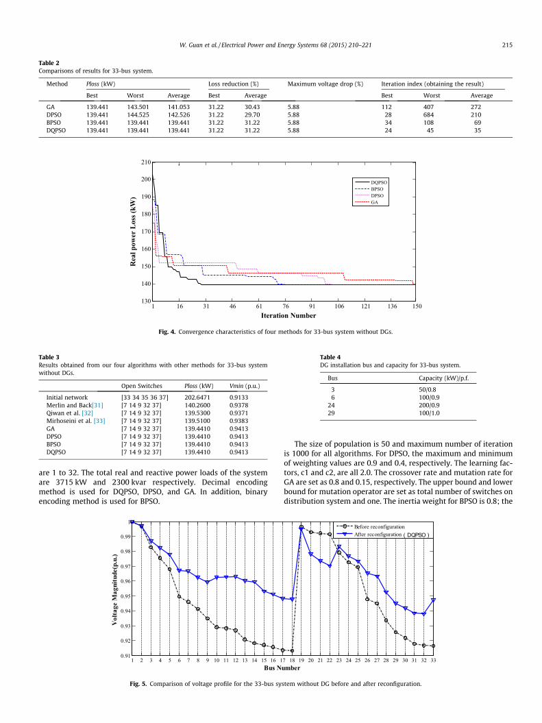
Table 2Comparisons of results for 33-bus system.

Method Ploss (kW) Loss reduction (%) Maximum voltage drop (%) Iteration index (obtaining the result)

Best Worst Average Best Average Best Worst Average

GA 139.441 143.501 141.053 31.22 30.43 5.88 112 407 272DPSO 139.441 144.525 142.526 31.22 29.70 5.88 28 684 210BPSO 139.441 139.441 139.441 31.22 31.22 5.88 34 108 69DQPSO 139.441 139.441 139.441 31.22 31.22 5.88 24 45 35

1 16 31 46 61 76 91 106 121 136 150130

140

150

160

170

180

190

200

210

Iteration Number

Rea

l pow

er L

oss (

kW)

DQPSOBPSODPSOGA

Fig. 4. Convergence characteristics of four methods for 33-bus system without DGs.

Table 3Results obtained from our four algorithms with other methods for 33-bus systemwithout DGs.

Open Switches Ploss (kW) Vmin (p.u.)

Initial network [33 34 35 36 37] 202.6471 0.9133Merlin and Back[31] [7 14 9 32 37] 140.2600 0.9378Qiwan et al. [32] [7 14 9 32 37] 139.5300 0.9371Mirhoseini et al. [33] [7 14 9 32 37] 139.5100 0.9383GA [7 14 9 32 37] 139.4410 0.9413DPSO [7 14 9 32 37] 139.4410 0.9413BPSO [7 14 9 32 37] 139.4410 0.9413DQPSO [7 14 9 32 37] 139.4410 0.9413

Table 4DG installation bus and capacity for 33-bus system.

Bus Capacity (kW)/p.f.

3 50/0.86 100/0.9

24 200/0.929 100/1.0


are 1 to 32. The total real and reactive power loads of the systemare 3715 kW and 2300 kvar respectively. Decimal encodingmethod is used for DQPSO, DPSO, and GA. In addition, binaryencoding method is used for BPSO.

1 2 3 4 5 6 7 8 9 10 11 12 13 14 15 16 10.91

0.92

0.93

0.94

0.95

0.96

0.97

0.98

0.99

1

Bus Nu

Vol

tage

Mag

nitu

de(p

.u.)

Fig. 5. Comparison of voltage profile for the 33-bus sys

The size of population is 50 and maximum number of iterationis 1000 for all algorithms. For DPSO, the maximum and minimumof weighting values are 0.9 and 0.4, respectively. The learning fac-tors, c1 and c2, are all 2.0. The crossover rate and mutation rate forGA are set as 0.8 and 0.15, respectively. The upper bound and lowerbound for mutation operator are set as total number of switches ondistribution system and one. The inertia weight for BPSO is 0.8; the

7 18 19 20 21 22 23 24 25 26 27 28 29 30 31 32 33mber

Before reconfigurationAfter reconfiguration

tem without DG before and after reconfiguration.

Table 5Results obtained from DQPSO with other methods for 33-bus system with DGs.

Open switches Ploss (kW) Vmin (p.u.)

Initial network [33 34 35 36 37] 169.7386 0.9183Mirhoseini et al. [33] [7 14 9 32 28] 115.7200 –Choi and Kim [17] [7 14 9 32 28] 115.0000 –DQPSO [7 14 9 32 28] 114.6500 0.9478


learning factors, c1 and c2, are both equal to 2.0. The particles’dimension of DQPSO is 5, equal to number the tie switches. 10 runsfor each algorithm were performed in order to calculate the aver-age performance Fig. 3.

The results of all algorithms for 33-bus system are shown inTable 2. The iteration index indicates the lowest number of itera-tion when the optimal result is obtained. The maximum voltage

Table 6Comparisons of the reconfiguration with same modes of DGs in buses 21 and 50.

Scheme number Model of DGs Output reactive power (kvar)

DG1 DG2

1 – – –2 PQ (V) �64.00 �59.003 PQ 72.60 72.604 PI 110.00 100.005 PV 535.10 783.80

Because of no load in node 45, 46 and 47, so open switch 44, 45, 46 or 47 will get samnetwork. Output reactive power of PQ (V) model is a negative number and it represents

Table 7Comparisons of the reconfiguration with different modes of DGs in buses 21 and 50.

Scheme number Model of DGs Output reactive power (k

DG1 DG2 DG1 DG

6 PQ PQ (V) 72.60 �6PQ (V) PQ �63.00 72

7 PI PQ (V) 100.00 �6PQ (V) PI �64.00 10

8 PI PQ 83.90 72PQ PI 72.60 10

9 PV PQ 286.00 72PQ PV 72.60 14

10 PV PI 410.00 10PI PV 109.00 14

11 PV PQ (V) 431.00 �6PQ (V) PV �62.00 27

1 2 3 4 5 6 7 8 9 10 11 12 13 14 15 16 10.91

0.92

0.93

0.94

0.95

0.96

0.97

0.98

0.99

1

Bus Nu

Vol

tage

Mag

nitu

de(p

.u.)

Fig. 6. Comparison of voltage magnitude for the 33-bus

drop shows the percentage of voltage drop of the best solutionsin 10 runs. The illegal chromosome number shows the percentageof illegal solutions in 10 runs. Although the percentage of illegalchromosomes of DQPSO is higher than DPSO and GA, the best solu-tion can be identified in less iteration. The convergence character-istics of the best results for all methods tested on 33-bus systemare shown in Fig. 4. DQPSO can find best solution in fewer iterationand more efficient than other methods.

The open switches for the optimal solution found by all meth-ods are show in Table 3. DQPSO got same result with Refs. [31–33], GA, DPSO and BPSO, opened switches [7 14 9 32 37], So DQPSOcould be applied to the distributed reconfiguration well. Afterreconfiguration, the real power losses reduced from 202.7467 kWto 139.4731 kW with improvement of 31.17%, minimum voltageof nodes also increased from 0.9133 p.u. to 0.9378 p.u. Voltage pro-file of 33-bus (before and after reconfiguration) is shown in Fig. 5.

Open switches Ploss (kW) Vmin (p.u.)

[69 70 14 50 44] 100.9661 0.9425[69 70 14 50 44] 91.0703 0.9447[69 70 14 50 47] 81.2675 0.9479[69 70 12 50 45] 79.3819 0.9485[68 16 10 50 46] 66.3405 0.9690

e result. Symbol ‘‘–’’ in Scheme 1 represents the DG absorbs reactive power fromthat the DG need absorb reactive power from network.

var) Open switches Ploss (kW) Vmin (p.u.)

2

0.00 [69 70 14 52 45] 89.2077 0.9433.60 [69 70 12 50 45] 84.6175 0.94783.00 [69 70 13 50 44] 87.2911 0.94460.80 [69 70 14 50 44] 83.2299 0.9485.60 [69 70 14 50 45] 80.5568 0.94780.00 [69 70 14 50 44] 80.0149 0.9485.60 [69 18 12 50 44] 79.2420 0.947887.00 [69 13 12 50 46] 63.5634 0.96750.00 [7010 12 50 47] 78.7483 0.948587.00 [69 14 12 50 44] 62.9221 0.96820.00 [70 10 12 50 46] 86.5122 0.944693.00 [68 7317 9 50] 210.5755 0.9515

7 18 19 20 21 22 23 24 25 26 27 28 29 30 31 32 33mber

Before reconfigurationAfter reconfiguration

system with DGs before and after reconfiguration.

LOOP 1

1 2 3 4 5 6 7 8 9 10 11 12 13 14 15 16 17 18 19 20 21 22 23 24 25 26

60 62 6361 64 65 66 686759

28

2931 32 33 3430

40 57

42

5541

36 383743 44 45 46 47 48 49 50 51 52 53

54

5639

35

69 71

70

73

72

27

58 DG1

DG2

LOOP 2

LOOP 3

LOOP 4LOOP 5

Fig. 7. PG&E 69-bus distribution network system.

1 6 11 16 21 26 31 36 41 46 51 56 61 66 690.94

0.95

0.96

0.97

0.98

0.99

1

Bus Number

Vol

tage

Mag

nitu

de(p

.u.)

Scheme1 Without DGsScheme2 PQ(V)/PQ(V)Scheme3 PQ/PQScheme4 PI/PIScheme5 PV/PV

Fig. 8. Comparison of voltage magnitude for Schemes 1–5.


Through reconfiguration, voltage profile of 33-bus had been greatlyimproved than initial network, so applied DQPSO to distributedsystem feeder reconfiguration, we can not only decrease the realpower losses, but also improve voltage profile of the network(see Tables 4 and 5).

Because most recent Refs for network reconfiguration treat DGas PQ model which is described in Section ‘PQ model’, so we installPQ model DG in 33-bus system, and compare with other Refs.Table 6 shows the DG installation nodes with associated capacityfor 33-bus system.

The open switches for the optimal solution found by all meth-ods are show in Table 7. DQPSO acquired same result with Refs.[17,33], So DQPSO could be applied to the distributed reconfigura-tion with DGs well. Voltage profile of 33-bus (before and afterreconfiguration) is shown in Fig. 6. Through reconfiguration withDGs, voltage magnitude of 33-bus had been greatly improved thaninitial network with DGs. Compare with Figs. 5 and 6, we can findthe buses which inject DGs have the improvement in voltage mag-nitude, for example, the voltage of 26 bus improves from0.9650 p.u. in Fig. 5 to 0.9830 p.u. in Fig. 6.

Test case 2

To demonstrate the applicability of the proposed method inother distribution systems, it was applied to a PG&E 69-bus,12.66 kV system as shown in Fig. 7. It consists of 5 tie switchesand 68 sectionalizing switches. The numbers in the figure indicatethe switch number. Because switches 1, 2, 39, 40, 54–57, 27–34don not in any loop, so these switches closed throughout, and need

not be considered in the reconfiguration. This is also an advantageof decimal encoding. The total power loads are 3802.19 kW and2694.60 kvar. For initial network without DGs, normally openswitches [69 70 71 72 73], and real power losses (Ploss) is226.4735 kW, Vmin is 0.9089 p.u. Particle dimension is 5, popula-tion size is 50, the number of iteration is 100, and convergence pre-cision is set to 1e-6.

Suppose place DG1 in bus 21, DG2 in bus 50. This test adoptsseveral schemes (As shown in Tables 6 and 7) to analysis influenceof different models of DG on the distribution network reconfigura-tion. Assume Qmax and Qmin as the upper and lower limit of the out-put reactive power respectively; Vm and Qout are the rated voltagemagnitude and output reactive power of PV model DG respec-tively; Im is the rated current magnitude of PI model DG;P is theactive power of DGs. In order to analysis and calculate Qout of PVunder the given Vm, this paper ignores the PV/PQ transform pro-gress in the reconfigurations.

Parameters of DGs with different models are set as follows:Active power of all model DGs are set as 150 kW. Power factor ofPQ model is 0.9; Vm = 0.9800 p.u., Qmax = 800 kvar and Qmin =�300 kvar; Im is 0.10 kA; xm is 2.205952 X, xr is 0.20933 X, R is0.00486 X.

Scheme 1 has no DGs in the system, Ploss is 100.9661 kW,greater than other schemes. Vmin is 0.9425 p.u., also lower thanother schemes. So reconfigurations with DGs decrease more Plossand increase more Vmin than reconfiguration with no DGs. Differ-ent models of DGs will affect the distribution network reconfigura-tion result. Comparing Scheme 2–5, we can find reconfigurationwith different models of DGs acquired different reconfiguration

Table 8Comparisons of the reconfiguration with PQ/PV mode DGs.

P (kW) Vm (p.u.) Output reactive power (kvar) Open switches Ploss (kW) Vmin (p.u.) (Bus No.)

PQ PV

150 0.98 72.60 1487 [69 13 12 50 46] 63.5634 0.9675(51)0.96 72.60 653 [10 70 12 51 44] 66.8854 0.9600(50)0.94 72.60 �140 [69 14 12 51 41] 96.4073 0.9400(50)0.92 72.60 1113 [8 17 68 50 73] 149.9553 0.9200(50)

200 0.98 72.60 1465 [10 16 71 51 46] 68.9915 0.9584(52)0.96 72.60 578 [10 70 13 51 44] 65.3036 0.9597(51)0.94 72.60 �231 [10 14 71 51 45] 106.0761 0.9400(50)0.92 72.60 1018 [8 14 68 50 73] 143.5054 0.9200(50)

250 0.98 72.60 1359 [69 13 12 50 44] 55.8507 0.9675(51)0.96 72.60 499 [69 13 12 50 46] 60.3960 0.9600(50)0.94 72.60 �280 [69 18 12 51 46] 97.8422 0.9400(50)0.92 72.60 916 [8 70 12 52 73] 127.2876 0.9200(50)

300 0.98 72.60 1361 [10 16 68 51 46] 63.3259 0.9576(52)0.96 72.60 504 [10 16 71 51 46] 67.2527 0.9584(52)0.94 72.60 �255 [69 16 12 51 41] 99.5173 0.9400(50)0.92 72.60 767 [8 18 12 51 73] 124.8779 0.9200(50)

Table 9Comparison of the reconfigurations with PI/PV mode DGs in buses 21 and 50.


PI PV

150 0.98 109 1487 [69 14 12 50 44] 62.9221 0.9682(51)0.96 109 653 [69 14 12 51 47] 62.4904 0.9600(50)0.94 109 �112 [69 13 12 51 41] 95.6511 0.9400(50)0.92 100 1099 [8 17 68 50 73] 149.0875 0.9200(50)

200 0.98 106 1465 [10 18 68 51 46] 69.5734 0.9590(52)0.96 106 578 [10 17 71 51 44] 69.9092 0.9595(52)0.94 105 �231 [10 16 68 51 47] 102.1248 0.9400(50)0.92 102 895 [8 70 14 50 73] 131.2302 0.9200(50)

250 0.98 105 1439 [10 16 68 51 44] 66.1735 0.9584(52)0.96 109 531 [69 14 12 51 44] 59.2004 0.9597(51)0.94 107 �205 [10 70 13 51 41] 98.9516 0.9400(50)0.92 103 850 [8 70 13 51 73] 126.7738 0.9200(50)

300 0.98 107 1361 [9 70 13 51 44] 56.1592 0.9646(52)0.96 109 448 [69 13 12 50 44] 58.3160 0.9600(50)0.94 109 �255 [69 13 12 51 41] 95.1467 0.9400(50)0.92 101 758 [8 70 12 52 73] 122.8650 0.9200(50)

Table 10Comparison of the reconfigurations with PQ (V)/PV mode DGs in buses 21 and 50.


PQ (V) PV

150 0.98 �62 2793 [9 17 68 50 73] 210.5755 0.9515(51)0.96 �63 1365 [10 70 14 52 73] 92.0024 0.9600(50)0.94 �63 930 [9 17 71 72 73] 111.9230 0.9369(54)0.92 �61 947 [69 70 12 48 45] 154.6134 0.9200(50)

200 0.98 �62 2657 [10 16 68 50 73] 188.6327 0.9518(51)0.96 �63 1233 [10 18 13 51 73] 86.2606 0.9594(52)0.94 �64 842 [9 15 67 20 73] 105.5773 0.9380(53)0.92 �62 1057 [8 14 12 52 73] 135.7590 0.9200(50)

250 0.98 �52 2505 [10 16 12 50 73] 164.3494 0.9505(51)0.96 �62 998 [10 70 14 50 73] 78.1955 0.9587(51)0.94 �60 948 [10 19 12 20 73] 103.9257 0.9334(21)0.92 �61 983 [7 13 12 50 73] 137.1950 0.9200(50)

300 0.98 �52 2356 [10 18 14 50 73] 141.3911 0.9507(51)0.96 �62 871 [10 19 14 50 73] 76.6656 0.9565(51)0.94 �66 752 [69 14 12 72 73] 102.6675 0.9350(24)0.92 �61 965 [8 16 67 52 73] 137.5935 0.9200(50)



schemes, Ploss and Vmin. Scheme 5 achieved lowest Ploss(66.3405 kW), also acquired highest Vmin (0.9690 p.u.). The reasonis that reactive power output decreases Ploss and improves Vmin.PV model DGs output reactive power 535.10 kvar and 783.80 kvarrespectively to keep their voltage constant. But in Scheme 2,though parallel capacities group compensate reactive power tothe PQ (V) model DG, DG1 and DG2 also need absorb reactivepower 64 kvar and 59 kvar respectively from network, so compar-ing with Scheme 5, Ploss of Scheme 2 increased from 66.3405 kWto 91.0703 kW, Vmin also decreased from 0.9690 p.u. to 0.9447 p.u.The comparison of voltage profile for Scheme 1–5 is shown inFig. 8. It is inferred that Scheme 2–5 have the better voltage profilethan Scheme 1. Under the same active power, network injectedwith PV model DGs have best voltage profile, however, otherSchemes decrease according the sequence 4, 3, 2, 1 approximately.

To analyze the impact of different models of DGs on the recon-figuration, different models of DGs were placed on bus21 and 50.Comparisons of the reconfiguration with different modes of DGsin two buses is described in Table 7. In Scheme 9, PV and PQ modelof DGs were placed in bus21 and bus 50 respectively. Results show

150 200 250 300-400

-200

0

200

400

600

800

1000

1200

1400

1600

Active Power of PV Model DG (kW)

Qou

t of P

V M

odel

DG

(kva

r)

Fig. 9. Comparison of Qout of PV and real power loss for reco

150 200 250 300-400

-200

0

200

400

600

800

1000

1200

1400

1600


Qou

t of P

V M

odel

DG

(kva

r)

Fig. 10. Comparison of Qout of PV and real power loss for rec

that their output reactive power are between Scheme 5 and 3, Plossand Vmin also obey this law. Therefore, accurately determiningmodel of DGs is very important to the feeder reconfiguration con-sidering DGs.

The voltage of bus 50 is the lowest in 69-bus system beforereconfiguration. If PV model DG (Vm = 0.9800 p.u.) is placed inbus 50. PV need output much reactive power to improve the volt-age of bus 50 from 0.9089 p.u. to 0.9800 p.u. It can be seen inTable 7 that in Schemes 9, 10, 11, when DG2 is PV mode, the outputreactive powers (Qout) of PV mode DG exceed the Qmax. Especially inScheme 11, Qout up to 2793 kvar and Ploss is greater than otherSchemes. The reason for this is that much reactive power transferin the system causes the increase of the active power loss (Ploss).However, if injecting appropriate excessive reactive power, thePloss in network will decrease. Qout of Schemes 9, 10 is all1487 kvar, but their Ploss are less than other Schemes. This kindof situation is not allowed in practice. To achieve larger reductionin Ploss in the condition that Qout within its limit, it is necessary toresearch the impact factors of Qout and Ploss. Three model combina-tions of DGs (PQ/PV, PI/PV, PQ (V)/PV) have been adopted. Tables

150 200 250 30050

60

70

80

90

100

110

120

130

140

150

160


Rea

l Pow

er L

oss (

kW)

Vm=0.98Vm=0.96Vm=0.94Vm=0.92

nfigurations with PQ/PV model DGs in buses 21 and 50.

150 200 250 30050

60

70

80

90

100

110

120

130

140

150

160


Rea

l pow

er lo

ss (k

W)

Vm=0.98

Vm=0.96

Vm=0.94

onfigurations with PI/PV model DGs in buses 21 and 50.

150 200 250 300500

1000

1500

2000

2500

3000


Qou

t of P

V M

odel

DG

(kva

r)

150 200 250 300

60

80

100

120

140

160

180

200

220


Rea

l Pow

er L

oss (

kW)

Vm=0.98Vm=0.96Vm=0.94Vm=0.92

Fig. 11. Comparison of Qout of PV and real power loss for reconfigurations with PQV/PV model DGs in buses 21 and 50.


8–10 are the comparisons of the reconfiguration model combina-tions of DGs. Figs. 8–10 are the comparison of Qout for PV and realpower loss for network with model combinations of DGs. Two DGsare also placed in bus 21 and 50.

It is inferred in Figs. 9, 10 that when Vm is 0.96 p.u., Qout iswithin the limit. Ploss of it reduces to a lower level. If Vm is0.94 p.u., Qout is below zero, also within the limit, PV need absorbreactive power from system to keep the lower voltage magnitudein this condition. However, when Vm decreases to 0.92 p.u., Qout

increases to a high level and exceeding the limit. For achievingreduction in real power loss, PV need output much reactive powerto improve the voltage level of the system. Ploss of it is also greatestin all conditions. Moreover, when Vm is set to 0.98 p.u., though Qout

is greatest in all situations, Ploss decreases a lot for the high voltagelevel of the system. In Fig. 11, however, the results are differentwith Figs. 9 and 10. For PQ (V) model, though compensative capac-ities are used to supply the reactive power, it also need absorbreactive power from power system. As shown in Table 10, the out-put reactive powers of PQ (V) model are all below zero. So PV needoutput more reactive power to compensate the lack in system.Because of this reason, Qout is improved to a high level and Plossfor this combination model also greater than others. The conditionthat Vm is 0.94 can receive best result in combination model ofPQV/PV. Compare with Figs. 9–11, it can be found that Qout of PVmodel is related to Vm and Vm decides the Qout in a certain extent.However, the active power of PV model have a little impact on Qout.Ploss of the system also obey this rule in some degree. Moreover,the combination models also affect the Qout and Ploss, PQ/PV andPI/PV models have the same rule, as depicted in Figs. 9 and 10,but PQV/PV model presents different rules.

Conclusions

This paper has presented feeder reconfiguration consideringdifferent models of DG using DQPSO technique to minimize thereal power losses in the distributed networks. The proposedmethod is based on the original QPSO, by adopting decimal encod-ing. The combination of all the open switches defined as a particleand the number of tie switches decides dimensions of particles, soparticle dimensions of QPSO with decimal encoding is much smal-ler than PSO with binary encoding. And switches which are not inloops need not be considered during reconfiguration, this can alsohelp produce fewer infeasible solutions and time saving. Moreover,

the proposed and other methods are tested on 33-bus system. Theresults show that compared to GA, DPSO and BPSO, the searchingof DQPSO convergent to its balance points more quickly and canacquire right results in all ten experiments. Therefore, the pro-posed DQPSO has the properties of effective, high efficiency. DGsare divided into PQ, PV, PQ (V) and PI models according to theiroperation modes and control characteristics. Several Schemes withdifferent models of DG have been experimented on PG&E 69-bussystem, the result show that feeder reconfiguration consideringDGs with different models can acquire different reconfigurationresult and be much closer to the actual situation. The output reac-tive power of PV model DG sometimes exceed the limit, especiallythe PV model DG is place in bus with low voltage magnitude.Experiment results shows that Qout of PV model is related to Vm.However, the active power of PV model has a little impact on Qout.If we set the Vm appropriately in reconfiguration progress, theactive power loss of system will reduce a lot and best combinationof Open Switches will be acquired.

Acknowledgements

This work was partially supported by National Natural ScienceFoundation of China (No. 61102039), Science and Technology Plan-ning Project of Hunan Province (No. 2011FJ3080), and the Funda-mental Research Funds for the Central Universities. The authorsalso appreciate the insightful comments and suggestions fromanonymous reviewers.

References

[1] Civanlar S, Grainger J, Yin H. Distribution feeder reconfiguration for lossreduction. IEEE Trans Power Del 1988;3(3):1217–23.

[2] Nara K, Shiose A, Kitagawa M. Implementation of genetic algorithm fordistribution systems loss minimum reconfiguration. IEEE Trans Power Syst1992;7(3):1044–51.

[3] Zhu JZ. Optimal reconfiguration of distribution network using the refinedgenetic algorithm. Electr Power Syst Res 2002;62:37–42.

[4] Enacheanu B, Raison B, Caire R, Devaux O, Bienia W, Hadjsaid N. Radialnetwork reconfiguration using genetic algorithm based on the matroid theory.IEEE Trans Power Syst 2008;23(1):186–95.

[5] Macedo Braz de HD, Souza de BA. Distribution network reconfiguration usinggenetic algorithms with sequential encoding: subtractive and additiveapproaches. IEEE Trans Power Syst 2011;26(2):582–93.

[6] Gaing ZL. Particle swarm optimization to solving the economic dispatchconsidering the generator constraints. IEEE Trans Power Syst2003;18(3):1187–95.


[7] Kansal S, Kumar V, Tyagi B. Optimal placement of different type of DG sourcesin distribution networks. Int J Electr Power Energy Syst 2013;53:752–60.

[8] Esmin AAA, Lambert Torres G, De Souza ACZ. A hybrid particle swarmoptimization applied to loss power minimization. IEEE Trans Power Syst2005;20(2):855–66.

[9] Wu WC, Tsai MS. Feeder reconfiguration using binary coding particle swarmoptimization. Int J Control Automat Syst 2008;6(4):488–94.

[10] Yin SA, Lu CN. Distribution feeder scheduling considering variable load profileand outage costs. IEEE Trans Power Syst 2009;24(2):652–60.

[11] Ma XF, Zhang LZ. Distribution networkreconfigurationbased ongenetic algorithmusing decimal encoding. Trans China Electrotech Soc 2004;19(10):65–9.

[12] Al Abri RS, El-Saadany EF, Atwa YM. Optimal placement and sizing method toimprove the voltage stability margin in a distribution system using distributedgeneration. IEEE Trans Power Syst 2013;28(1):326–34.

[13] Caisheng W, Nehrir MH. Analytical approaches for optimal placement ofdistributed generation sources in power systems. IEEE Trans Power Syst2004;19:2068–76.

[14] Niknam T, Taheri SI, Aghaei J, Tabatabaei S, Nayeripour M. A modified honeybee mating optimization algorithm for multiobjective placement of renewableenergy resources. Appl Energy 2011;88:4817–30.

[15] Gitizadeh M, Vahed AA, Aghaei J. Multistage distribution system expansionplanning considering distributed generation using hybrid evolutionaryalgorithms. Appl Energy 2013;101:655–66.

[16] Wu WC, Tsai MS. Application of enhanced integer coded particle swarmoptimization for distribution system feeder reconfiguration. IEEE Trans PowerSyst 2011;26(3):291–3.

[17] Choi JH, Kim JC. Network reconfiguration at the power distribution systemwith dispersed generations for loss reduction. Power Eng Soc Winter Meet,IEEE 2000;4:2363–7.

[18] Olamaei J, Niknam T, Gharehpetian G. Application of particle swarmoptimization for distribution feeder reconfiguration considering distributedgenerators. Appl Math Comput 2008;201(1–2):575–86.

[19] Rugthaicharoencheep N, Sirisumrannukul S. Feeder reconfiguration withdispatchable distributed generators in distribution system by Tabu Search.Universities Power Engineering Conference (UPEC), In: Proceedings of the 44thInternational, vol. 1; 2009. p. 1–5.

[20] Wu Y, Lee C, Liu L, Tsai S. Study of reconfiguration for the distribution systemwith distributed generators. IEEE Trans Power Del 2010;25(3):1678–85.

[21] Wu YK, LEE CY, LIU LC. Study of reconfiguration for the distribution systemwith distributed generators. IEEE Trans Power Del 2010;25(3):1678–85.

[22] Rao RS, Ravindra K, Satish K. Power loss minimization in distribution systemusing network reconfiguration in the presence of distributed generation. IEEETrans Power Syst 2013;28(1):317–25.

[23] Niknam T, Fard AK, Seifi A. Distribution feeder reconfiguration considering fuelcell/wind/photovoltaic power plants. Renewable Energy 2012;37:213–25.

[24] Omkar SN, Khandelwal R, Ananth TVS. Quantum behaved particle swarmoptimization (QPSO) for multi-objective design optimization of compositestructures. Expert Syst Appl 2009;36(8):11312–22.

[25] Chen HY, Chen JF, Shi DY, Duan XZ. IEEE Power Engineering Society GeneralMeeting 2006;8:18–22.

[26] Kennedy J, Eberhart R. Particle swarm optimization. In: Proceedings of the IEEEInternational Conference on Neural Networks; 1995. p. 1942–8.

[27] Sun J, Feng B, Xu WB. Particle swarm optimization with particles havingquantum behavior. In: Proceedings of Congress on Evolutionary Computation.Portland: IEEE; 2004. p. 325–3l.

[28] Jamalipour M, Gharib M, Sayareh R, Khoshahval F. PWR power distributionflattening using quantum particle swarm intelligence. Ann Nucl Energy2013;56:143–50.

[29] Yin SA, Lu CN. Distribution feeder scheduling considering variable load profileand outage costs. IEEE Trans Power Syst 2009;24(2):652–60.

[30] Sivanagaraju S, Rao JV, Raju PS. Discrete particle swarm optimization tonetwork reconfiguration for loss reduction and load balancing. Electric PowerCompon Syst 2008;36(5):513–24.

[31] Merlin A, Back G. Search for minimum-loss operational spanning treeconfiguration for an urban power distribution system. In: Proceedings of 5thpower system conference, Cambridge; 1975. p. 1–18.

[32] Qiwan L, Wei D, Jianquan Z, Anhui L. A new reconfiguration approach fordistribution system with distributed generation. ICEET, IEEE; 2009. p. 23–6.

[33] Mirhoseini SH, Hosseini SM, Ghanbari M, Ahmadi M. A new improved adaptiveimperialist competitive algorithm to solve the reconfiguration problem ofdistribution systems for loss reduction and voltage profile improvement. Int JElectr Power Energy Syst 2014;55:128–43.

Documents

Distribution system feeder reconfiguration considering different model of DG sources