Embed Size (px)
Citation preview
Contact:
Aga Khan Agency for Habitat405A/407, Jolly Bhavan No. 1, 10, New Marine Lines-400020, Mumbai, Maharashtra, India.
Copyright © 2021 by AKAHI
No part of this publication may be reproduced, distributed or transmitted in any form, or by any means, including photocopying, recording, image-capture, or other electronic or mechanical methods, without the prior written permission of the publisher, except in the case of brief quotations embodied in reviews and certain other non-commercial uses permitted by copyright law.
Digital Edition, September 2021
Toolkit for Urban Ecosystem Management
Published by:
Aga Khan Agency for Habitat
Project Team:
Sucharita RoyHead - Planning & BuildingUrban and Regional Planner- Architect
Damodar PujariProgram ManagerMSc Environmental Science
Malvika SaraswatProject CoordinatorEnvironmental Planner
Anusha KantProject CoordinatorUrban Designer
Subhadeep KarmakarProject CoordinatorEnvironmental Planner
Toolkit Design:
Damodar PujariProgram Manager- Climate Change
Malvika SaraswatConsultant - Aga Khan Agency for Habitat, India
Ankush Chandran
AcknowledgmentsThis project was funded by Prince Sadruddin Aga Khan Fund for Environment which promotes the management and development of sustainable natural resources through education, area development and related research.
This interactive toolkit for assessment and finding solutions for effective Urban Ecosystem Management has been developed by a dedicated team of planners and environmentalists in Aga Khan Agency for Habitat, India. The study was conceptualised and led by Sucharita Roy, the head of the Planning and Building department in the agency. The project team consisted of Damodar Pujari, Project Manager, and project coordinators Malvika Saraswat, Anusha Kant, Subhadeep Karmakar, who led the work on data collection, preparation of all the analytics, spatial and non-spatial evaluation of the cases studies. Ankush Chandran provided editorial and creative design and layout support for the development of this handy toolkit. The project team would like to convey their special appreciation to Tameeza Alibhai the Chief Executive officer and Rahim Dobariya, Program Manager-Geospatial Information, for their support throughout the entire project period.
This tool kit was prepared in partnership with the Environmental Management Centre (EMC) LLP, Mumbai led by Dr. Prasad Modak, Executive President, and the team including Krupa Desai, Jay Mehta and Richa Thakur. EMC has guided the project team with the analytics and developed the ecosystem health assessment framework, a comprehensive assessment tool which can help with agile and evidence-based planning and management of any urban system. A collection of tested nature-based solutions which are a part of the toolkit have been curated by the Environment Management Centre.

ForewordTime is running out in our battle to control global warming. As we see more frequent and extreme natural disasters, new vulnerabilities exposed in the wake of COVID-19 and unrelenting pressure on our towns, cities, and natural habitats, without urgent action to reset how we impact and interact with our natural and built environment, we will lose our last chance to protect humanity’s future on our planet.
Housing more than half of humanity and responsible for over 70% of carbon dioxide emissions, cities are on the frontline of this effort. Our cities are increasingly exposed to the effects of climate change including extreme weather, water stress, air pollution, urban heat island effect and sea level rise. Lower-income urban residents feel these effects the most as they often live in poorly constructed structures in more marginal or exposed areas with weaker services and infrastructure. We must adapt the way our urban areas are planned and managed and look at how cities can be drivers of innovation for climate-proof development through efficient planning and green infrastructure.
An ecosystems-based approach that looks at managing the built environment as part of the natural and socio-economic environments as an integrated urban ecosystem offers a framework for long-term sustainable development, in balance with nature. The Aga Khan Agency for Habitat is committed to helping communities undertake inclusive, evidence-based, resilient urban planning and climate action. We have developed this Urban Ecosystems Management Toolkit as a holistic framework to assess, monitor, and develop plans to restore urban ecosystems. This framework provides tools and solutions to rebalance the natural urban ecosystem as a pathway for long-term sustainability. The Toolkit guides practitioners through an evidence-based approach to assess hotspots in different urban contexts and develop nature-based solutions to protect and restore urban ecosystems. It is our hope that this toolkit will be used widely to experiment with and scale innovations for a greener urban way of life.
Onnol RühlGeneral Manager
Aga Khan Agency for Habitat
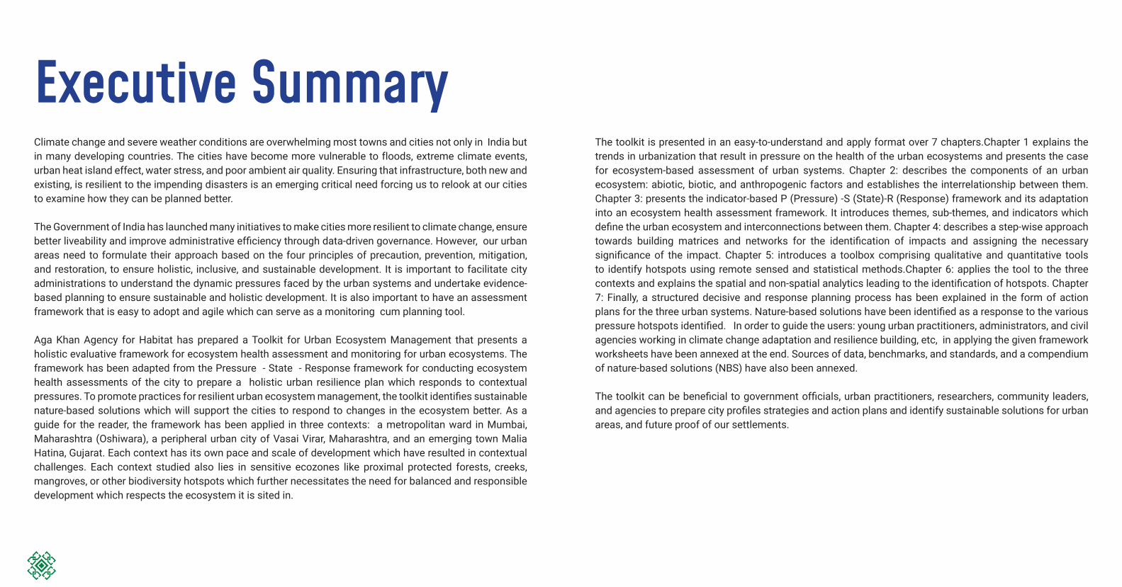
Executive SummaryClimate change and severe weather conditions are overwhelming most towns and cities not only in India but in many developing countries. The cities have become more vulnerable to floods, extreme climate events, urban heat island effect, water stress, and poor ambient air quality. Ensuring that infrastructure, both new and existing, is resilient to the impending disasters is an emerging critical need forcing us to relook at our cities to examine how they can be planned better.
The Government of India has launched many initiatives to make cities more resilient to climate change, ensure better liveability and improve administrative efficiency through data-driven governance. However, our urban areas need to formulate their approach based on the four principles of precaution, prevention, mitigation, and restoration, to ensure holistic, inclusive, and sustainable development. It is important to facilitate city administrations to understand the dynamic pressures faced by the urban systems and undertake evidence-based planning to ensure sustainable and holistic development. It is also important to have an assessment framework that is easy to adopt and agile which can serve as a monitoring cum planning tool.
Aga Khan Agency for Habitat has prepared a Toolkit for Urban Ecosystem Management that presents a holistic evaluative framework for ecosystem health assessment and monitoring for urban ecosystems. The framework has been adapted from the Pressure - State - Response framework for conducting ecosystem health assessments of the city to prepare a holistic urban resilience plan which responds to contextual pressures. To promote practices for resilient urban ecosystem management, the toolkit identifies sustainable nature-based solutions which will support the cities to respond to changes in the ecosystem better. As a guide for the reader, the framework has been applied in three contexts: a metropolitan ward in Mumbai, Maharashtra (Oshiwara), a peripheral urban city of Vasai Virar, Maharashtra, and an emerging town Malia Hatina, Gujarat. Each context has its own pace and scale of development which have resulted in contextual challenges. Each context studied also lies in sensitive ecozones like proximal protected forests, creeks, mangroves, or other biodiversity hotspots which further necessitates the need for balanced and responsible development which respects the ecosystem it is sited in.
The toolkit is presented in an easy-to-understand and apply format over 7 chapters.Chapter 1 explains the trends in urbanization that result in pressure on the health of the urban ecosystems and presents the case for ecosystem-based assessment of urban systems. Chapter 2: describes the components of an urban ecosystem: abiotic, biotic, and anthropogenic factors and establishes the interrelationship between them. Chapter 3: presents the indicator-based P (Pressure) -S (State)-R (Response) framework and its adaptation into an ecosystem health assessment framework. It introduces themes, sub-themes, and indicators which define the urban ecosystem and interconnections between them. Chapter 4: describes a step-wise approach towards building matrices and networks for the identification of impacts and assigning the necessary significance of the impact. Chapter 5: introduces a toolbox comprising qualitative and quantitative tools to identify hotspots using remote sensed and statistical methods.Chapter 6: applies the tool to the three contexts and explains the spatial and non-spatial analytics leading to the identification of hotspots. Chapter 7: Finally, a structured decisive and response planning process has been explained in the form of action plans for the three urban systems. Nature-based solutions have been identified as a response to the various pressure hotspots identified. In order to guide the users: young urban practitioners, administrators, and civil agencies working in climate change adaptation and resilience building, etc, in applying the given framework worksheets have been annexed at the end. Sources of data, benchmarks, and standards, and a compendium of nature-based solutions (NBS) have also been annexed. The toolkit can be beneficial to government officials, urban practitioners, researchers, community leaders, and agencies to prepare city profiles strategies and action plans and identify sustainable solutions for urban areas, and future proof of our settlements.
Back to Contents
List of AnnexuresToolbox Nature Based
Solutions
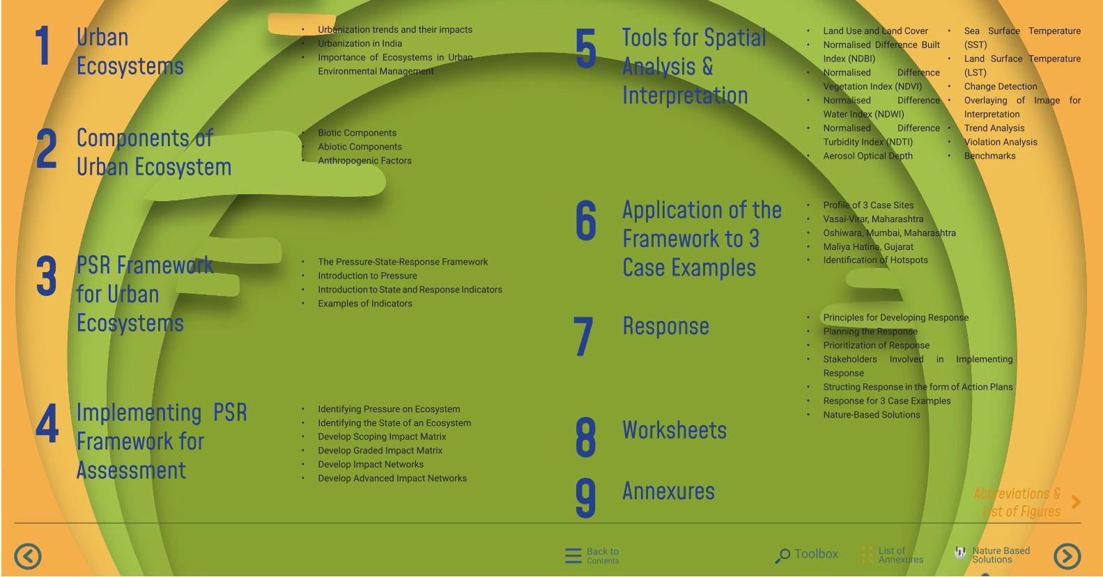
Urban Ecosystems1
2 Components of Urban Ecosystem
• Urbanization trends and their impacts• Urbanization in India• Importance of Ecosystems in Urban
Environmental Management
• Biotic Components• Abiotic Components• Anthropogenic Factors
• The Pressure-State-Response Framework• Introduction to Pressure• Introduction to State and Response Indicators• Examples of Indicators
• Identifying Pressure on Ecosystem• Identifying the State of an Ecosystem• Develop Scoping Impact Matrix• Develop Graded Impact Matrix• Develop Impact Networks • Develop Advanced Impact Networks
3 PSR Frameworkfor Urban Ecosystems
4 Implementing PSR Framework for Assessment
Response7
Tools for Spatial Analysis & Interpretation
5
Application of the Framework to 3 Case Examples
6
Worksheets8Annexures9
• Profile of 3 Case Sites• Vasai-Virar, Maharashtra• Oshiwara, Mumbai, Maharashtra• Maliya Hatina, Gujarat• Identification of Hotspots
• Principles for Developing Response• Planning the Response• Prioritization of Response • Stakeholders Involved in Implementing
Response• Structing Response in the form of Action Plans• Response for 3 Case Examples• Nature-Based Solutions
• Land Use and Land Cover• Normalised Difference Built
Index (NDBI)• Normalised Difference
Vegetation Index (NDVI)• Normalised Difference
Water Index (NDWI)• Normalised Difference
Turbidity Index (NDTI)• Aerosol Optical Depth
• Sea Surface Temperature (SST)
• Land Surface Temperature (LST)
• Change Detection• Overlaying of Image for
Interpretation• Trend Analysis• Violation Analysis• Benchmarks
Abbreviations & List of Figures
Back to Contents
List of Annexures
Back to SectionUrban Ecosystems Nature Based
SolutionsToolbox
Abbreviations List of FiguresClick on Figure Name to go to Page
4P Policy, Plan, Program and Project
AKAH Aga Khan Agency for Habitat
AKDN Aga Khan Development Network
AOD Aerosol Optical Depth
BOD Biochemical Oxygen Demand
CGWB Central Ground Water Board
COD Chemical Oxygen Demand
CPCB Central Pollution Control Board
DPSIR Driving Force - Pressure - State - Impact - Response
GIS Geographic Information System
GW Ground Water
HIGs High Income Groups
IUCN International Union for Conservation of Nature
LIGs Low Income Groups
LST Land Surface Temperature
LULC Land Use and Land Cover
MLD Million Litres per Day
MMR Mumbai Metropolitan Region
MODIS Moderate Resolution Imaging Spectroradiometer
MPN Most Probable Number
NDBI Normalized Difference Built-Up Index
NDTI Normalized Difference Turbidity Index
NDVI Normalized Difference Vegetation Index
NDWI Normalized Difference Water Index
OECD Organisation for Economic Co-operation and Development
PSR Pressure-State-Response Framework
SGNP Sanjay Gandhi National Park
SST Sea Surface Temperature
UHI Urban Heat Island
VVCMC Vasai Virar City Municipal Corporation
WRI World Resources Institute
Fig. 1 Urban population growth in India (red dots ) and the surrounding region (orange dots) 1950–2025 Source: Femke Reitsma, 2012
Fig. 2 Spatial growth of Bangalore from 1537 (red) to 2007 (light yellow)
Fig. 3 Causal loop diagram for urban sprawl and resulting water dynamics
Fig. 4 Ecosystem Services, Threats and Remediation through Stakeholder engagement
Fig. 5 Urban Ecosystem and Interactions within the components
Fig. 6 Pressure-State-Response Framework for Ecosystem Health Assessment
Fig. 7 The DPSIR Framework
Fig. 8 Maps showing Maryland’s Coastal Bays
Fig. 9 A bio indicator, in this case macro algae, used to trace nitrogen sources in Maryland’s Coastal Bays.
Fig. 10 Themes under Pressure on Ecosystem
Fig. 11 Themes under State of Ecosystem
Fig. 12 Example of Scoping Impact Matrix
Fig. 13 Example of Rule base for assigning significance to the interaction between State and Pressure Indicators
Fig. 14 Example of assigning significance to the interaction between State and Pressure Indicators
Fig. 15 Impact Network with Stakeholders
Fig. 16 Illustration of Change Detection in Oshiwara
Fig. 17 Illustration depicting the overlay of layers for Oshiwara in GIS.
Fig. 18 Illustration of the components of a Box-Whisker plot
Fig. 19 Illustration of difference in medians of a data distribution
Fig. 20 A daily time series plot of NO2 highlighting violations of 24-hr average standards
Fig. 21 Location of Vasai Virar
Fig. 22 Location of Oshiwara
Fig. 23 Location of Maliya Hatina
Fig. 24 Growth of Population in Vasai Virar City
Fig. 25 Population Density in Vasai Virar City
Fig. 26 Land Use in Vasai Virar
Fig. 27 Land Use Land Cover Map of Vasai Virar(2020)
Fig. 28 Road Network and Industries in Vasai Virar
Fig. 29 Tributaries of Oshiwara River
Fig. 30 Land use Land cover distribution in Oshiwara
Fig. 31 Land use Land Cover Map of Oshiwara 2019
Fig. 32 Built Use in Oshiwara Region in 2014
Fig. 33 Land Use Distribution in Maliya Hatina (2020)
Fig. 34 Road Network and Industries in Maliya Hatina
Fig. 35 Land Use of Maliya Hatina (2020)
Fig. 36 Map of Oshiwara Study Area
Fig. 37 NDVI (Vegetation Cover) in Oshiwara in 2015 and 2020
Fig. 38
Fig.39
Reduction in NDVI from 2015 to 2020 due to human encroachment in Sanjay Gandhi National ParkNDTI of water bodies in Oshiwara - 2015 and 2020
Fig. 40 Water Quality deterioration in Oshiwara River
Fig. 41 Environmental Crisis in Oshiwara & Excerpts from print media
Fig. 42 Oshiwara - ConnectivityFig. 43 Biodiversity in Oshiwara
Fig. 44 Changes in Mangrove abundance (1996 & 2016) in Oshiwara river system (left) and Thane Creek (right)
Fig. 45 Change in Land use Land Cover between 2015-20
Fig. 46 Land Use Change in Vasai VirarFig. 47 Major Land Use Change Detection Between
2015-20Fig. 48 Location of Pelhar Dam
Fig. 49 Location of Pelhar River
Fig. 50 Pelhar River - A view
Fig. 51 Sanctioned DP showing development around Pelhar Dam
Fig. 52 Change in Built Index around Pelhar Dam between 2015 -2020
Fig. 53 Change in Vegetation Index around Pelhar Dam between 2015-20
Fig. 54 Flora Fauna around Pelhar dam
Fig. 55 Location of Vasai Creek
Fig. 56 Map showing LULC Change around Vasai Creek
Fig. 57 Map Showing NDBI Change around Vasai Creek
Fig. 58 Map showing NDVI Change around Vasai Creek
Fig. 59 Loss of Mangrove Cover around Vasai Creek
Fig. 60 Construction along Vasai Creek
Fig. 61 Presence of Threatened Flora and Fauna around the Vasai Creek
Fig. 62 Loss of Mangrove cover around Ulhas River
see more figures & tables..
Back to Contents
List of Annexures
Back to SectionUrban Ecosystems Nature Based
SolutionsToolbox
List of FiguresFig. 63 Map of Maliya-Hatina
Fig. 64 Map showing status of wells near Maliya-Hatina in terms of Hardness of water
Fig. 65 Map showing status of wells near Maliya-Hatina in terms of depth of water level in the Post Monsoon Season
Fig. 66 Map of City X showing the six monitoring stations and metro route
Fig. 67 Action points for the six localities on the basis of ambient air data analysis
Fig. 68 Change in Turbidity Index of Meghal River from 2016 to 2020
Fig. 69 Principles for Developing Response
Fig. 70 Hypothetical scenario of Nature-based Solutions being used in conjunction with infrastructure
Fig. 71 Picture Showing Gorla Maggiore Water Park
Fig. 72 Image showing Mangroves in Vietnam
Fig. 73 Image showing Godrej Mangroves in Mumbai
Fig. 74 Image showing bioswales in Museum of Science Portland
Fig. 75 Image showing bioswale in Jellicoe Street, Auckland, New Zealand
Fig. 76 Image showing Bioretention in Derbyshire Street, London
Fig. 77 Image showing blue roofs in Walter Bos Complex, Apeldoorn
Fig. 78 Image showing blue roofs in Walter Bos Complex, Apeldoorn
Fig. 79 Image showing Edible forest in Alcalá de Henares, Spain
Fig. 80 Image showing Alpilles Regional Natural Park
Fig. 81 Image showing Rainfall runoff response of the green roof and conventional roof
Fig. 82 Image showing Fukuoka Prefectural International Hall, Tokyo
Fig. 83 Image showing Vertical Gardens in Bengaluru
Fig. 84 Image showing Vertical gardens in Caixa Forum plaza, Madrid
Fig. 85 Image showing Urban Green in New Orleans City, USA
Fig. 86 Image showing Railway Platforms on Parkland Walk, North London, England
Fig. 87 Image showing Community garden in Bogotá and urban garden in London
Fig. 88 Image showing activities of Sustainable Land Management in Augustenborg, Denmark
Fig. 89 Image showing Constructed Wetland in city of Tianjin, China
Fig. 90 Image showing Kanjli Wetland, Punjab
Fig. 91 Image showing Raingarden in Middlebury Vermount.
Fig. 92 Image showing Permeable Pavements along Jackshon stree, St. Paul
Fig. 93 Image showing Miyawaki Forests in Delhi
Fig. 94 Image showing Miyawaki Forests in Delhi
Fig. 95 Poster for Rainwater Harvesting
Fig. 96 Image showing Stormwater Tree Pits in Minnesota, USA
Fig. 97 Image showing Traffic Island in Pennsylvania, USA
Fig. 98 Image showing slope stabilization in French Broad river bank in Tennessee, USA
Fig. 99 Image showing Before and after state of river Re-meandering
Fig. 100 Image showing Mahadevapura Lake in Bangalore, India
Fig. 101 Image showing Neknampur Lake in Hyderabad
Fig. 102 Image showing Port of Antwerp, Belgium
Fig. 103 Image showing Taj Hotel at Madurai, India
Fig. 104 Image showing Powai Lake in Mumbai City
Fig. 105 Image showing Bioremediation of River Ganga
Fig. 106 Image showing Loktak Lake in Manipur, India
Fig. 107 Image showing Garden Festival in Geneva
Fig. 108 Sources and Scoping of Community Scale GHG emissions
Fig. 109 Biogas Digester
List of TablesTable 1 Illustrative Indicators under Industry Theme
Table 2 Illustrative Indicators under Water Theme
Table 3 Classification of Roads in Oshiwara
Table 4 Summary of Hotspots in Oshiwara
Table 5 Summary of Hotspots in Vasai-Virar
Table 6 Trends in Total Hardness of Ground Water in wells near Maliya- Hatina
Table 7 Trends in Ground Water depth in wells near Maliya-Hatina
Table 8 Analysis and Averaging Used for CAAQMS data in CIty X
Table 9 Results of data analytics applied to the CAAQMS data
Table 10 Decision Matrix applied to data analysis performed on CAAQMS data for City X
Table 11 Illustration of Response Identification in 4P Perspective
Table 12 Criteria for assessing effectiveness of the Response
Table 13 Suggested Nature-based Solutions and their expected impact on Themes
Click on Figure Name to go to Page Click on Table Name to go to Page
see list of annexures..

Back to Contents
List of Annexures
Back to SectionUrban Ecosystems Nature Based
SolutionsToolbox
List of AnnexuresAnnexure 1 State and Pressure Indicators
Annexure 2 Pressure Indicators
Annexure 3 Benchmarks and Standards for Environmental Indicators
Annexure 4 Detailed Actions: Policy, Plan, Program and Project
Annexure 5 Methodology for Toolbox
Click on Annexures to go to Page
Back to Contents
List of Annexures
Back to Section
Nature Based SolutionsToolbox
Urban Ecosystems
Urbanisation Trends and their ImpactsOver the last five decades rapid increase in urbanisation has led to deterioration of ecosystem health. Impacts include loss of biodiversity, threat to the security of resources (especially water) and public health. In-migration, expansion of built-up areas and urban infrastructure is leading to high consumption of natural resources, in particular water, timber, and energy. The physical extents of urban areas are rapidly expanding demanding augmentation of the transport infrastructure and increasing economic activities. Continued outward growth of cities often consume prime agricultural land, with long term impacts on habitats, biodiversity and ecosystem services. Thus, the impacts do not limit only to the administrative boundaries of urban areas, but also impact the peripheral towns and regions due to the intense patterns of consumption of the urban population. The urban economies across the world are also primary sources of waste generation that include sewage, industrial effluents, air emissions and solid wastes that include construction and demolition waste and hazardous waste streams such as biomedical and electronic wastes. In recent decades, management of plastic waste has become a daunting challenge. Sound management of such waste streams is therefore needed to protect the urban ecosystems. Finally, in addition to climate change at regional and global levels, urban activities modify the local and regional climate through the urban heat island (UHI) effect. These changes together cause significant impacts on net primary production, functions of ecosystems, and biodiversity.
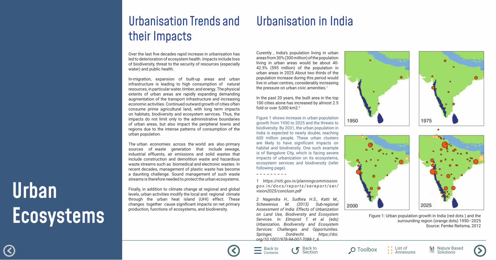
Curently , India’s population living in urban areas from 30% (300 million) of the population living in urban areas would be about 40-42.5% (595 million) of the population in urban areas in 2025 About two thirds of the population increase during this period would live in urban centres, considerably increasing the pressure on urban civic amenities.1
In the past 20 years, the built area in the top 100 cities alone has increased by almost 2.5 fold or over 5,000 km2.2
Figure 1 shows increase in urban population growth from 1950 to 2025 and the threats to biodiversity. By 2031, the urban population in India is expected to nearly double, reaching 600 million people. These urban clusters are likely to have significant impacts on habitat and biodiversity. One such example is of Bangalore City, which is facing severe impacts of urbanization on its ecosystems, ecosystem services and biodiversity (refer following page).
1 https://niti.gov.in/planningcommission.g o v. i n / d o c s / r e p o r t s / s e r e p o r t / s e r /vision2025/conclusn.pdf
2 Nagendra H., Sudhira H.S., Katti M., Schewenius M. (2013) Sub-regional Assessment of India: Effects of Urbanization on Land Use, Biodiversity and Ecosystem Services. In: Elmqvist T. et al. (eds) Urbanization, Biodiversity and Ecosystem Services: Challenges and Opportunities. Springer, Dordrecht. https://doi.org/10.1007/978-94-007-7088-1_6
Figure 1: Urban population growth in India (red dots ) and the surrounding region (orange dots) 1950–2025
Source: Femke Reitsma, 2012
Urbanisation in India
Back to Contents
List of Annexures
Back to SectionUrban Ecosystems Nature Based
SolutionsToolbox
Impacts of Urbanization on Ecosystems, Ecosystem Services and Biodiversity in Bangalore3
3 Local Assessment of Bangalore: Graying and Greening in Bangalore – Impacts of Urbanization on Ecosystems, Ecosystem Services and Biodiversity, H. S. Sudhira and Harini Nagendra, 2013
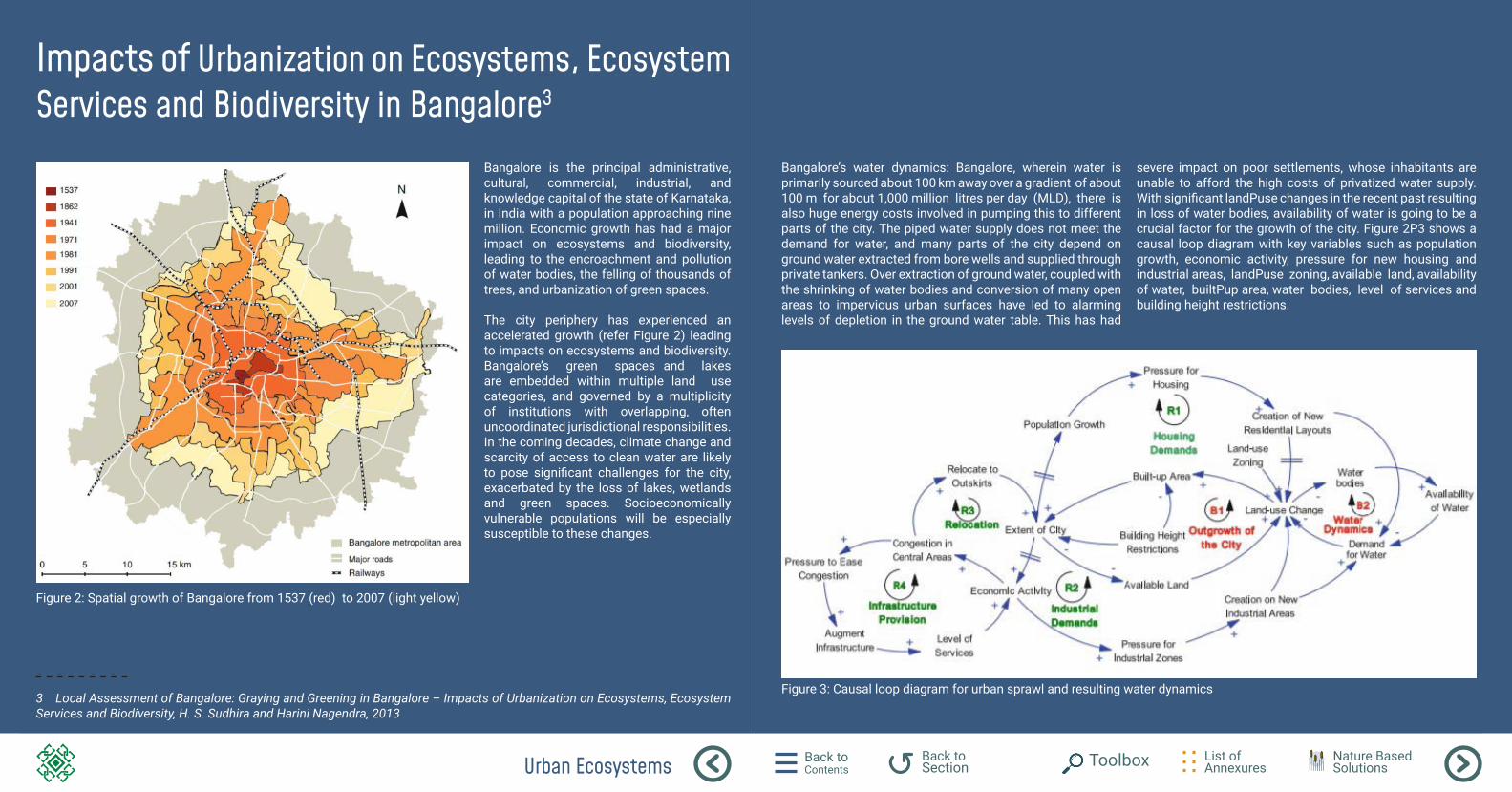
Bangalore is the principal administrative, cultural, commercial, industrial, and knowledge capital of the state of Karnataka, in India with a population approaching nine million. Economic growth has had a major impact on ecosystems and biodiversity, leading to the encroachment and pollution of water bodies, the felling of thousands of trees, and urbanization of green spaces. The city periphery has experienced an accelerated growth (refer Figure 2) leading to impacts on ecosystems and biodiversity. Bangalore’s green spaces and lakes are embedded within multiple land use categories, and governed by a multiplicity of institutions with overlapping, often uncoordinated jurisdictional responsibilities. In the coming decades, climate change and scarcity of access to clean water are likely to pose significant challenges for the city, exacerbated by the loss of lakes, wetlands and green spaces. Socioeconomically vulnerable populations will be especially susceptible to these changes.
Figure 2: Spatial growth of Bangalore from 1537 (red) to 2007 (light yellow)
Bangalore’s water dynamics: Bangalore, wherein water is primarily sourced about 100 km away over a gradient of about 100 m for about 1,000 million litres per day (MLD), there is also huge energy costs involved in pumping this to different parts of the city. The piped water supply does not meet the demand for water, and many parts of the city depend on ground water extracted from bore wells and supplied through private tankers. Over extraction of ground water, coupled with the shrinking of water bodies and conversion of many open areas to impervious urban surfaces have led to alarming levels of depletion in the ground water table. This has had
severe impact on poor settlements, whose inhabitants are unable to afford the high costs of privatized water supply. With significant landPuse changes in the recent past resulting in loss of water bodies, availability of water is going to be a crucial factor for the growth of the city. Figure 2P3 shows a causal loop diagram with key variables such as population growth, economic activity, pressure for new housing and industrial areas, landPuse zoning, available land, availability of water, builtPup area, water bodies, level of services and building height restrictions.
Figure 3: Causal loop diagram for urban sprawl and resulting water dynamics
Back to Contents
List of Annexures
Back to SectionUrban Ecosystems Nature Based
SolutionsToolbox
Importance of Ecosystems in Urban Environmental ManagementNatural ecosystems such as forests, grasslands, mangroves and wetlands as well as other managed ecosystems provide a range of ‘services’ to sustain human welfare. These include:
• ‘Provisioning’ services such as food, water, timber, fibre and genetic resources • ‘Regulating’ services such as regulation of climate, floods, drought, land degradation, water quality and disease prevention • ‘Supporting’ services such as soil formation, pollination and nutrient cycling • ‘Cultural’ services such as recreational, spiritual, religious and other non-material benefits 4 Ecosystems and their services are critical to human health and well-being and provide society with products that support biodiversity and economic development (e.g., food, clean water, flood mitigation and disease control). A diverse group of urban ecosystems provides ecosystem goods and services including: green spaces such as parks and urban forests, cemeteries, gardens and yards, and campus areas; blue spaces including streams, lakes, ponds, artificial swales and storm water retention ponds. Healthy and functional urban ecosystems provides multiple environmental, social and economic benefits (refer below).
Environmental, Social and Economic Benefits of Ecosystem5
Environmental benefits: Natural spaces such as urban parks, green walls, green roofs and street trees provide a number environmental benefits. They offset the UHI effect, improve air quality and reduce air temperatures through shade, thereby reducing energy use for cooling. Ecosystem services within and around cities provide buffer against many extreme events such as flooding and storms. Urban wetland ecosystems acts as filtration systems treating storm water to reduce pollution. Natural spaces and green infrastructure can reduce soil erosion and protect river banks as well as help manage water quality and quantity by reducing total runoff, including untreated runoff, before it enters water bodies. Moreover, ecosystems play a vital role in cycling and storing carbon for climate regulation. Soils store carbon while vegetation, particularly trees and forests, store carbon in biomass.
Social benefits: Urban natural spaces provide mental and physical health benefits. Access to green space has been linked to reduced mortality and improved, perceived and actual general and mental health benefits. In urban areas, vegetation helps to significantly reduce air and noise pollution, positively affecting health. In addition, natural spaces provide an excellent opportunity for education and citizen’s involvement in their communities, which in turn can promote development of a stewardship culture and create opportunities for residents to be meaningfully engaged in planning processes.
4 https://millenniumassessment.org/documents/document.300.aspx.pdf
5 https://www.iisd.org/system/files/publications/pcc-brief-climate-resilient-city-urban-ecosystems.pdf
Economic benefits: Urban ecosystems and green infrastructure combined with engineered infrastructure are often more cost-effective than grey infrastructure alone. Elmqvist et. al. (2015)6 analysed 25 studies done in urban regions that estimated the monetary value of benefits of ecosystem services based on quantification in biophysical units (e.g., carbon storage, storm water reduction, pollution removal). The data from the studied cities estimated that the ecosystems analysed provided between USD 3,212 and USD 17,772 benefits per hectare of urban green areas per year. These calculations provide a useful economic rationale for investments in protection of urban ecosystems. Green infrastructure can also simultaneously provide both climate change mitigating and adaptation benefits, which are particularly beneficial in the context of urban areas working within limited budgets.
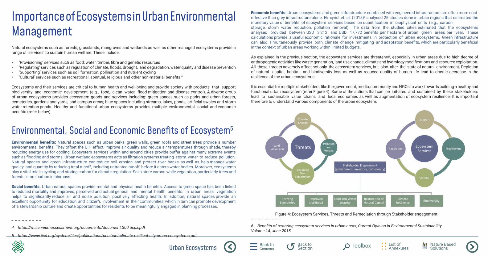
As explained in the previous section, the ecosystem services are threatened, especially in urban areas due to high degree of anthropogenic activities like waste generation, land use change, climate and hydrology modifications and resource exploitation. All these threats adversely affect not only the ecosystem services, but also alter the state of natural environment. Depletion of natural capital, habitat and biodiversity loss as well as reduced quality of human life lead to drastic decrease in the resilience of the urban ecosystems. It is essential for multiple stakeholders, like the government, media, community and NGOs to work towards building a healthy and functional urban ecosystem (refer Figure 4). Some of the actions that can be initiated and sustained by these stakeholders lead to sustainable value chains and local economies as well as augmentation of ecosystem resilience. It is important therefore to understand various components of the urban ecosystem.
6 Benefits of restoring ecosystem services in urban areas, Current Opinion in Environmental Sustainability Volume 14, June 2015
Figure 4: Ecosystem Services, Threats and Remediation through Stakeholder engagement
Back to Contents
List of Annexures
Back to Section Toolbox Nature Based
Solutions
Components of Urban Ecosystem
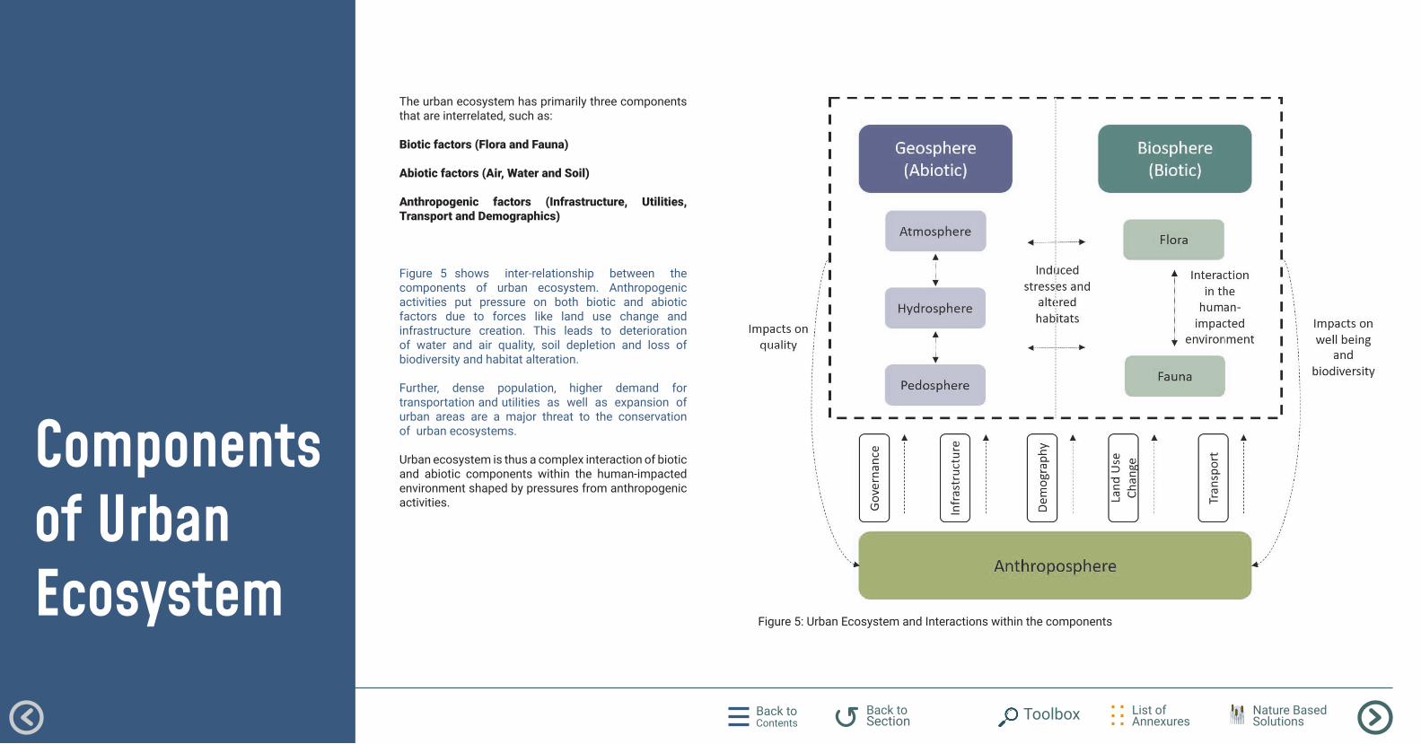
The urban ecosystem has primarily three components that are interrelated, such as: Biotic factors (Flora and Fauna)
Abiotic factors (Air, Water and Soil)
Anthropogenic factors (Infrastructure, Utilities, Transport and Demographics)
Figure 5 shows inter-relationship between the components of urban ecosystem. Anthropogenic activities put pressure on both biotic and abiotic factors due to forces like land use change and infrastructure creation. This leads to deterioration of water and air quality, soil depletion and loss of biodiversity and habitat alteration.
Further, dense population, higher demand for transportation and utilities as well as expansion of urban areas are a major threat to the conservation of urban ecosystems.
Urban ecosystem is thus a complex interaction of biotic and abiotic components within the human-impacted environment shaped by pressures from anthropogenic activities.
Figure 5: Urban Ecosystem and Interactions within the components
Components of Urban Ecosystems Back to Contents
List of Annexures
Back to Section Toolbox Nature Based
Solutions
Biotic Components
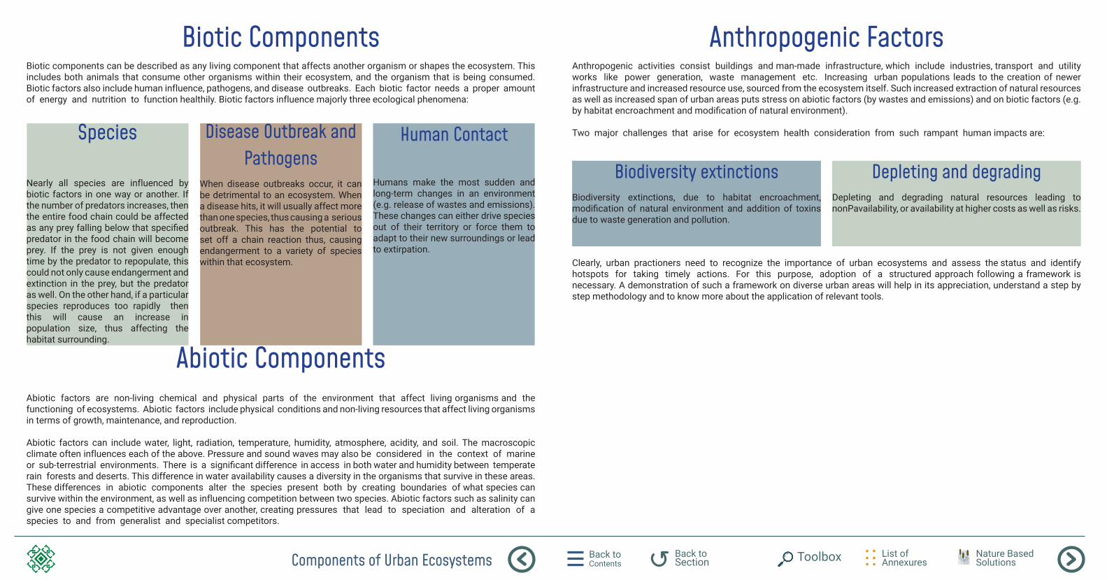
Biotic components can be described as any living component that affects another organism or shapes the ecosystem. This includes both animals that consume other organisms within their ecosystem, and the organism that is being consumed. Biotic factors also include human influence, pathogens, and disease outbreaks. Each biotic factor needs a proper amount of energy and nutrition to function healthily. Biotic factors influence majorly three ecological phenomena:
Abiotic Components
Abiotic factors are non-living chemical and physical parts of the environment that affect living organisms and the functioning of ecosystems. Abiotic factors include physical conditions and non-living resources that affect living organisms in terms of growth, maintenance, and reproduction. Abiotic factors can include water, light, radiation, temperature, humidity, atmosphere, acidity, and soil. The macroscopic climate often influences each of the above. Pressure and sound waves may also be considered in the context of marine or sub-terrestrial environments. There is a significant difference in access in both water and humidity between temperate rain forests and deserts. This difference in water availability causes a diversity in the organisms that survive in these areas. These differences in abiotic components alter the species present both by creating boundaries of what species can survive within the environment, as well as influencing competition between two species. Abiotic factors such as salinity can give one species a competitive advantage over another, creating pressures that lead to speciation and alteration of a species to and from generalist and specialist competitors.
Species
Nearly all species are influenced by biotic factors in one way or another. If the number of predators increases, then the entire food chain could be affected as any prey falling below that specified predator in the food chain will become prey. If the prey is not given enough time by the predator to repopulate, this could not only cause endangerment and extinction in the prey, but the predator as well. On the other hand, if a particular species reproduces too rapidly then this will cause an increase in population size, thus affecting the habitat surrounding.
Disease Outbreak and Pathogens
When disease outbreaks occur, it can be detrimental to an ecosystem. When a disease hits, it will usually affect more than one species, thus causing a serious outbreak. This has the potential to set off a chain reaction thus, causing endangerment to a variety of species within that ecosystem.
Human Contact
Humans make the most sudden and long-term changes in an environment (e.g. release of wastes and emissions). These changes can either drive species out of their territory or force them to adapt to their new surroundings or lead to extirpation.
Anthropogenic Factors
Anthropogenic activities consist buildings and man-made infrastructure, which include industries, transport and utility works like power generation, waste management etc. Increasing urban populations leads to the creation of newer infrastructure and increased resource use, sourced from the ecosystem itself. Such increased extraction of natural resources as well as increased span of urban areas puts stress on abiotic factors (by wastes and emissions) and on biotic factors (e.g. by habitat encroachment and modification of natural environment).
Two major challenges that arise for ecosystem health consideration from such rampant human impacts are:
Clearly, urban practioners need to recognize the importance of urban ecosystems and assess the status and identify hotspots for taking timely actions. For this purpose, adoption of a structured approach following a framework is necessary. A demonstration of such a framework on diverse urban areas will help in its appreciation, understand a step by step methodology and to know more about the application of relevant tools.
Biodiversity extinctionsBiodiversity extinctions, due to habitat encroachment, modification of natural environment and addition of toxins due to waste generation and pollution.
Depleting and degradingDepleting and degrading natural resources leading to nonPavailability, or availability at higher costs as well as risks.
PSR Framework for Urban Ecosystems Back to Contents
List of Annexures
Back to Section Toolbox Nature Based
Solutions
PSR Framework for Urban Ecosystems
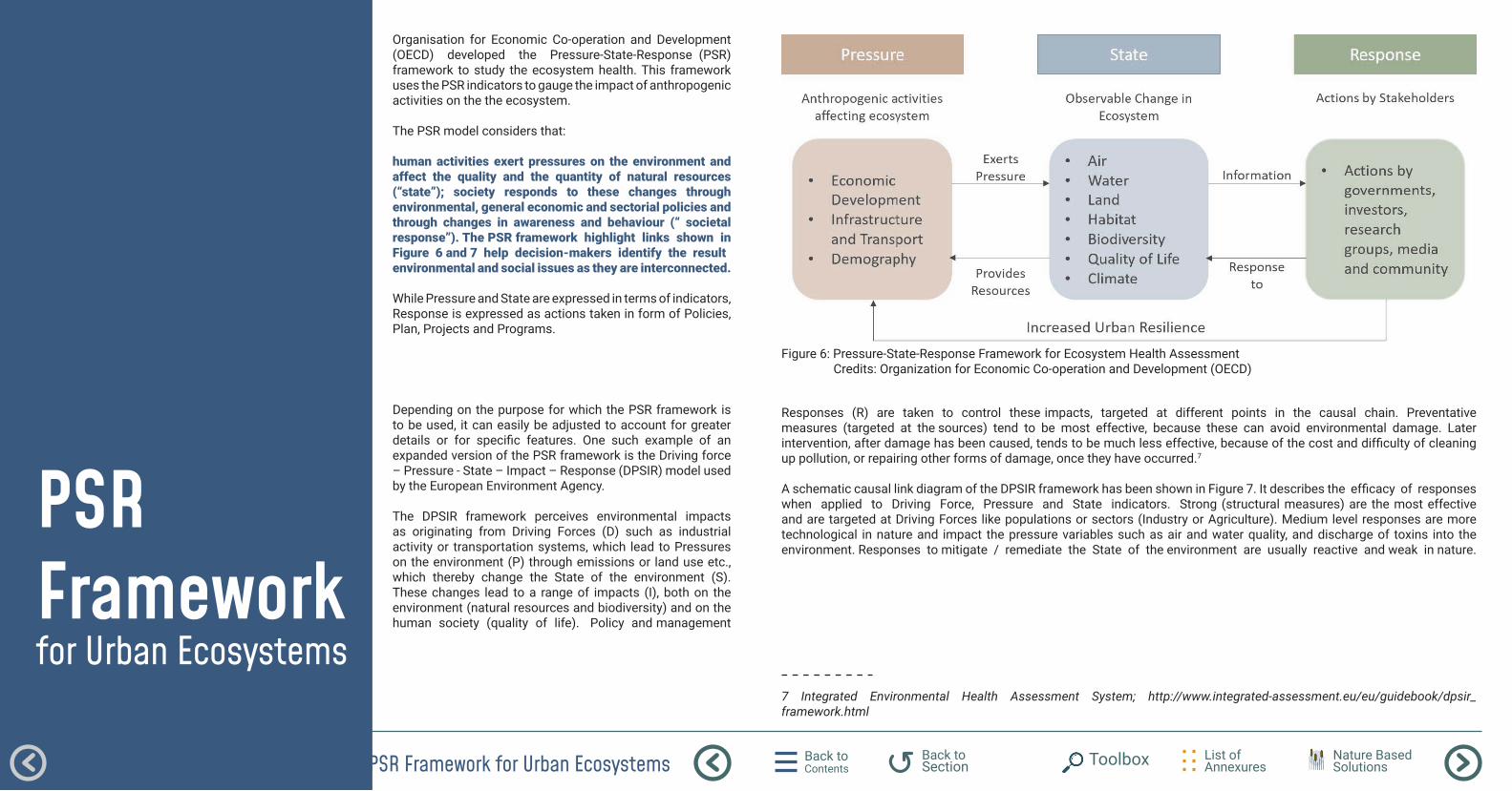
Organisation for Economic Co-operation and Development (OECD) developed the Pressure-State-Response (PSR) framework to study the ecosystem health. This framework uses the PSR indicators to gauge the impact of anthropogenic activities on the the ecosystem.
The PSR model considers that:
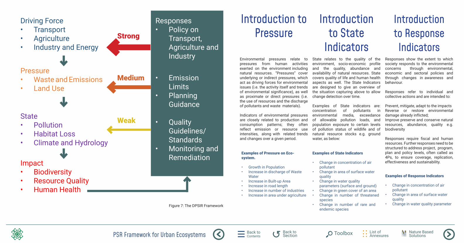
human activities exert pressures on the environment and affect the quality and the quantity of natural resources (“state”); society responds to these changes through environmental, general economic and sectorial policies and through changes in awareness and behaviour (“ societal response”). The PSR framework highlight links shown in Figure 6 and 7 help decision-makers identify the result environmental and social issues as they are interconnected. While Pressure and State are expressed in terms of indicators, Response is expressed as actions taken in form of Policies, Plan, Projects and Programs.
Depending on the purpose for which the PSR framework is to be used, it can easily be adjusted to account for greater details or for specific features. One such example of an expanded version of the PSR framework is the Driving force – Pressure - State – Impact – Response (DPSIR) model used by the European Environment Agency. The DPSIR framework perceives environmental impacts as originating from Driving Forces (D) such as industrial activity or transportation systems, which lead to Pressures on the environment (P) through emissions or land use etc., which thereby change the State of the environment (S). These changes lead to a range of impacts (I), both on the environment (natural resources and biodiversity) and on the human society (quality of life). Policy and management
Figure 6: Pressure-State-Response Framework for Ecosystem Health Assessment Credits: Organization for Economic Co-operation and Development (OECD)
Responses (R) are taken to control these impacts, targeted at different points in the causal chain. Preventative measures (targeted at the sources) tend to be most effective, because these can avoid environmental damage. Later intervention, after damage has been caused, tends to be much less effective, because of the cost and difficulty of cleaning up pollution, or repairing other forms of damage, once they have occurred.7 A schematic causal link diagram of the DPSIR framework has been shown in Figure 7. It describes the efficacy of responses when applied to Driving Force, Pressure and State indicators. Strong (structural measures) are the most effective and are targeted at Driving Forces like populations or sectors (Industry or Agriculture). Medium level responses are more technological in nature and impact the pressure variables such as air and water quality, and discharge of toxins into the environment. Responses to mitigate / remediate the State of the environment are usually reactive and weak in nature.
7 Integrated Environmental Health Assessment System; http://www.integrated-assessment.eu/eu/guidebook/dpsir_framework.html
PSR Framework for Urban Ecosystems Back to Contents
List of Annexures
Back to Section Toolbox Nature Based
Solutions
Introduction to Pressure
Environmental pressures relate to pressures from human activities exerted on the environment including natural resources. “Pressures” cover underlying or indirect pressures, which act as driving forces for environmental issues (i.e. the activity itself and trends of environmental significance), as well as proximate or direct pressures (i.e. the use of resources and the discharge of pollutants and waste materials).
Indicators of environmental pressures are closely related to production and consumption patterns; they often reflect emission or resource use intensities, along with related trends and changes over a given period.
Introduction to State
Indicators
State relates to the quality of the environment, socio-economic profile and the quality, abundance and availability of natural resources. State covers quality of life and human health aspects as well. The State Indicators are designed to give an overview of the situation capturing above to allow change detection over time.
Examples of State indicators are: concentration of pollutants in environmental media, exceedance of allowable pollution loads, and population exposure to certain levels of pollution status of wildlife and of natural resource stocks e.g. ground water, as below:
Introduction to Response Indicators
Responses show the extent to which society responds to the environmental concerns through environmental, economic and sectoral policies and through changes in awareness and behaviour.
Responses refer to individual and collective actions and are intended to: Prevent, mitigate, adapt to the impacts Reverse or restore environmental damage already inflicted; Improve preserve and conserve natural resources, abundance, quality e.g. biodiversity Responses require fiscal and human resources. Further responses need to be structured to address project, program, plan and policy levels, often called as 4Ps, to ensure coverage, replication, effectiveness and sustainability.
Examples of Pressure on Eco-system.
• Growth in Population • Increase in discharge of Waste
Water • Increase in Built-up Area • Increase in road length • Increase in number of industries • Increase in area under agriculture
Examples of State Indicators
• Change in concentration of air pollutant
• Change in area of surface water quality
• Change in water quality parameters (surface and ground)
• Change in green cover of an area • Change in number of threatened
species • Change in number of rare and
endemic species
Examples of Response Indicators
• Change in concentration of air pollutant
• Change in area of surface water quality
• Change in water quality parameterFigure 7: The DPSIR Framework
Driving Force• Transport• Agriculture• Industry and Energy
Strong
Medium
Weak
Responses• Policy on
Transport, Agriculture and Industry
• Emission Limits
• Planning Guidance
• Quality Guidelines/ Standards
• Monitoring and Remediation
Pressure• Waste and Emissions• Land Use
State• Pollution• Habitat Loss• Climate and Hydrology
Impact• Biodiversity• Resource Quality• Human Health
PSR Framework for Urban Ecosystems Back to Contents
List of Annexures
Back to Section Toolbox Nature Based
Solutions
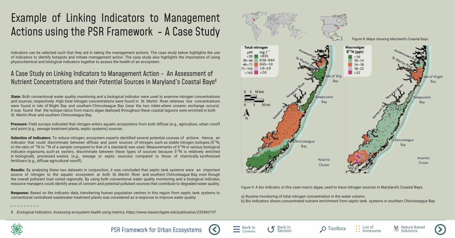
Example of Linking Indicators to Management Actions using the PSR Framework - A Case Study Indicators can be selected such that they aid in taking the management actions. The case study below highlights the use of indicators to identify hotspots and initiate management action. The case study also highlights the importance of using physiochemical and biological indicators together to assess the health of an ecosystem.
A Case Study on Linking Indicators to Management Action - An Assessment of Nutrient Concentrations and their Potential Sources in Maryland’s Coastal Bays8
State: Both conventional water quality monitoring and a biological indicator were used to examine nitrogen concentrations and sources, respectively. High total nitrogen concentrations were found in St. Martin River, whereas low concentrations were found in Isle of Wight Bay and southern Chincoteague Bay (near the two inlets where oceanic exchange occurs). It was found that the isotope ratios from macro algae deployed throughout these coastal lagoons were enriched in both St. Martin River and southern Chincoteague Bay. Pressure: Field surveys indicated that nitrogen enters aquatic ecosystems from both diffuse (e.g., agriculture, urban runoff and point (e.g., sewage treatment plants, septic systems) sources. Selection of Indicators: To reduce nitrogen, ecosystem experts identified several potential courses of actions. Hence, an indicator that could discriminate between diffuse and point sources of nitrogen, such as stable nitrogen isotopes (δ15N, or the ratio of 15N to 14N of a sample compared to that of a standard) was used. Measurements of δ15N in various biological indicator organisms, such as oysters, discriminate between these types of sources because δ15N is relatively enriched in biologically processed wastes (e.g., sewage or septic sources) compared to those of chemically synthesized fertilizers (e.g., diffuse agricultural runoff). Results: By analysing these two datasets in conjunction, it was concluded that septic tank systems were an important source of nitrogen to the aquatic ecosystem at both St. Martin River and southern Chincoteague Bay, even though the overall pollutant load varied regionally. By using both conventional water quality monitoring and a biological indicator, resource managers could identify areas of concern and potential pollutant sources that contribute to degraded water quality. Response: Based on the indicator data, transferring human population centres in this region from septic tank systems to conventional centralized wastewater treatment plants was considered as a response to improve water quality.
8 Ecological Indicators: Assessing ecosystem health using metrics; https://www.researchgate.net/publication/235960197
Figure 9: A bio indicator, in this case macro algae, used to trace nitrogen sources in Maryland’s Coastal Bays.
a) Routine monitoring of total nitrogen concentration in the water column. b) Bio indicators shows concentrated nutrient enrichment from septic tank systems in southern Chinctoeague Bay.
Figure 8: Maps showing Maryland’s Coastal Bays
Back to Contents
List of Annexures
Back to Section Toolbox Nature Based
Solutions
Implementing PSR Framework for Assessment
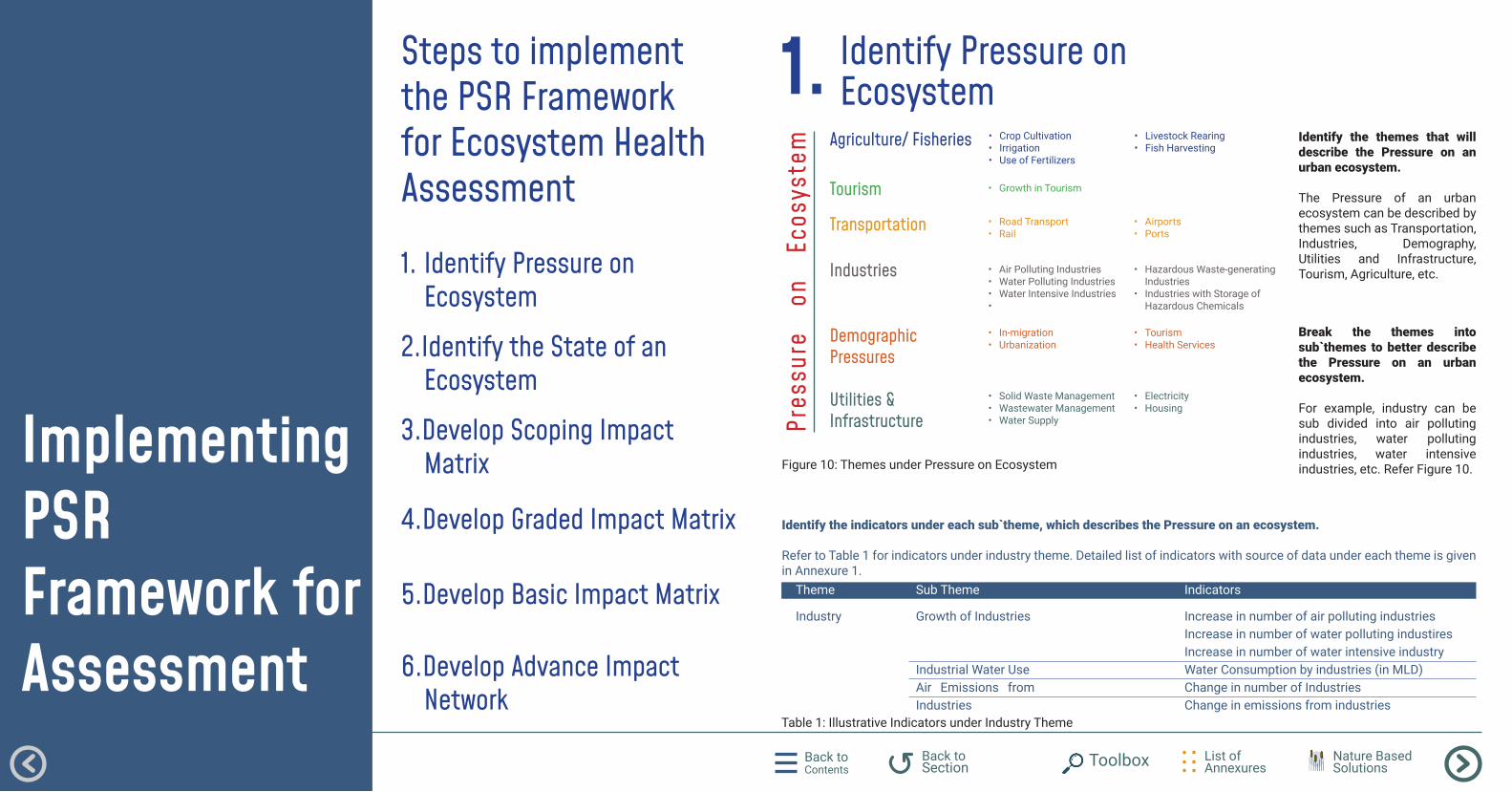
Steps to implement the PSR Framework for Ecosystem Health Assessment
1. Identify Pressure on Ecosystem
2.Identify the State of an Ecosystem
3.Develop Scoping Impact Matrix
4.Develop Graded Impact Matrix
5.Develop Basic Impact Matrix
6.Develop Advance Impact Network
Identify Pressure on Ecosystem1.
Figure 10: Themes under Pressure on Ecosystem
Table 1: Illustrative Indicators under Industry Theme
Identify the themes that will describe the Pressure on an urban ecosystem.
The Pressure of an urban ecosystem can be described by themes such as Transportation, Industries, Demography, Utilities and Infrastructure, Tourism, Agriculture, etc.
Break the themes into sub`themes to better describe the Pressure on an urban ecosystem.
For example, industry can be sub divided into air polluting industries, water polluting industries, water intensive industries, etc. Refer Figure 10.
Identify the indicators under each sub`theme, which describes the Pressure on an ecosystem.
Refer to Table 1 for indicators under industry theme. Detailed list of indicators with source of data under each theme is given in Annexure 1.
Theme Sub Theme Indicators
Industry Growth of Industries
Industrial Water UseAir Emissions from Industries
Increase in number of air polluting industries Increase in number of water polluting industires Increase in number of water intensive industry Water Consumption by industries (in MLD) Change in number of Industries Change in emissions from industries
Pres
sure
on
Ec
osys
tem Agriculture/ Fisheries
Tourism
Transportation
Industries
Demographic Pressures
Utilities & Infrastructure
• Crop Cultivation• Irrigation• Use of Fertilizers
• Livestock Rearing• Fish Harvesting
• Road Transport• Rail
• Airports• Ports
• Air Polluting Industries• Water Polluting Industries• Water Intensive Industries•
• Hazardous Waste-generating Industries
• Industries with Storage of Hazardous Chemicals
• In-migration• Urbanization
• Tourism• Health Services
• Solid Waste Management• Wastewater Management• Water Supply
• Electricity• Housing
• Growth in Tourism
Implementing PSR Framework for Assessment Back to Contents
List of Annexures
Back to Section Toolbox Nature Based
Solutions
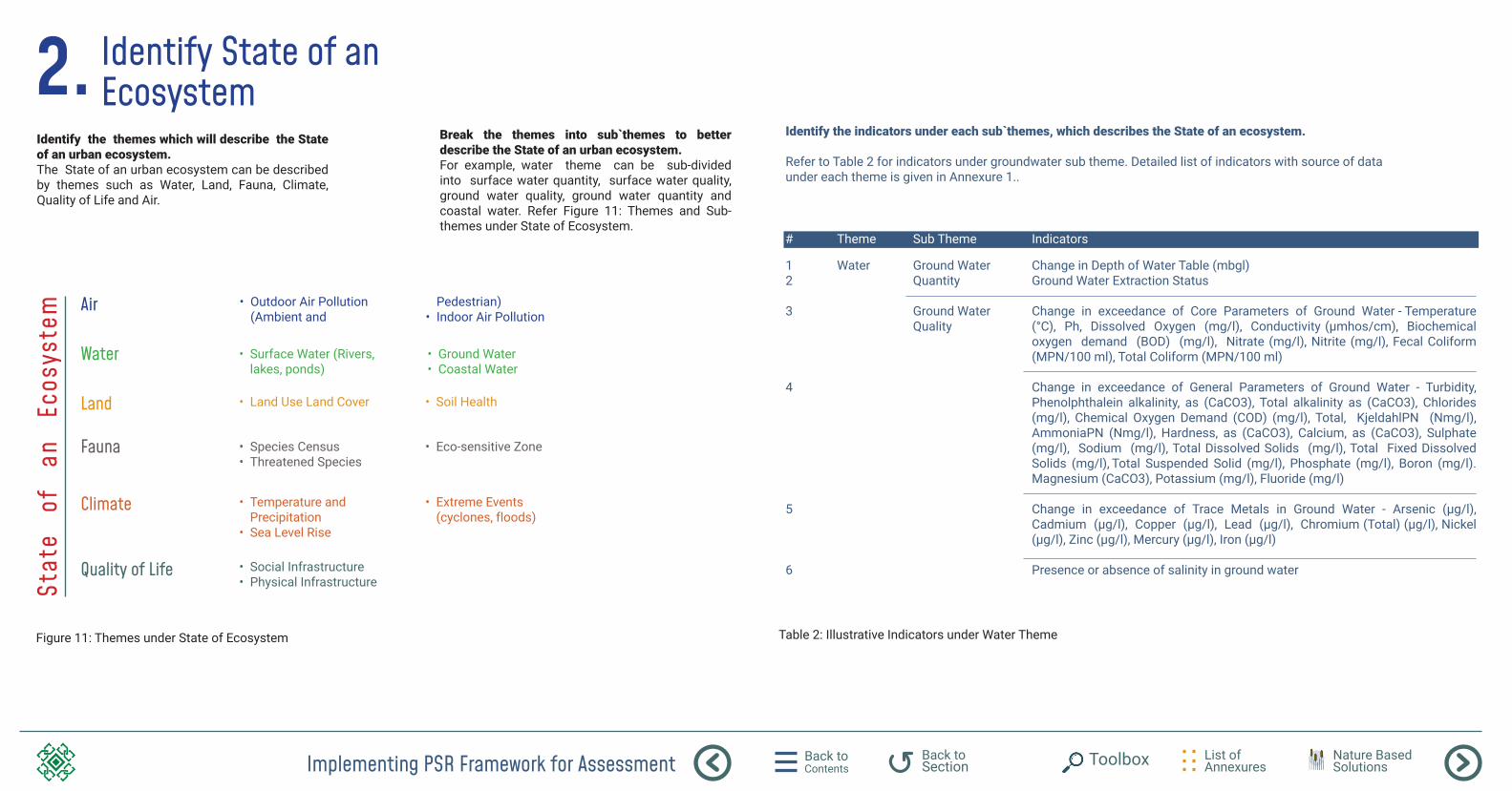
Identify State of an Ecosystem2.
Identify the themes which will describe the State of an urban ecosystem.The State of an urban ecosystem can be described by themes such as Water, Land, Fauna, Climate, Quality of Life and Air.
Break the themes into sub`themes to better describe the State of an urban ecosystem. For example, water theme can be sub-divided into surface water quantity, surface water quality, ground water quality, ground water quantity and coastal water. Refer Figure 11: Themes and Sub-themes under State of Ecosystem.
Figure 11: Themes under State of Ecosystem Table 2: Illustrative Indicators under Water Theme
Identify the indicators under each sub`themes, which describes the State of an ecosystem.
Refer to Table 2 for indicators under groundwater sub theme. Detailed list of indicators with source of data under each theme is given in Annexure 1..
# Theme Sub Theme Indicators
12
3
4
5
6
Water Ground Water Quantity
Ground Water Quality
Change in Depth of Water Table (mbgl) Ground Water Extraction Status
Change in exceedance of Core Parameters of Ground Water - Temperature (°C), Ph, Dissolved Oxygen (mg/l), Conductivity (μmhos/cm), Biochemical oxygen demand (BOD) (mg/l), Nitrate (mg/l), Nitrite (mg/l), Fecal Coliform (MPN/100 ml), Total Coliform (MPN/100 ml)
Change in exceedance of General Parameters of Ground Water - Turbidity, Phenolphthalein alkalinity, as (CaCO3), Total alkalinity as (CaCO3), Chlorides (mg/l), Chemical Oxygen Demand (COD) (mg/l), Total, KjeldahlPN (Nmg/l), AmmoniaPN (Nmg/l), Hardness, as (CaCO3), Calcium, as (CaCO3), Sulphate (mg/l), Sodium (mg/l), Total Dissolved Solids (mg/l), Total Fixed Dissolved Solids (mg/l), Total Suspended Solid (mg/l), Phosphate (mg/l), Boron (mg/l). Magnesium (CaCO3), Potassium (mg/l), Fluoride (mg/l)
Change in exceedance of Trace Metals in Ground Water - Arsenic (μg/l), Cadmium (μg/l), Copper (μg/l), Lead (μg/l), Chromium (Total) (μg/l), Nickel (μg/l), Zinc (μg/l), Mercury (μg/l), Iron (μg/l)
Presence or absence of salinity in ground water
Stat
e of
an
Ec
osys
tem Air
Water
Land
Fauna
Climate
Quality of Life
• Outdoor Air Pollution (Ambient and
Pedestrian)• Indoor Air Pollution
• Land Use Land Cover • Soil Health
• Species Census• Threatened Species
• Eco-sensitive Zone
• Temperature and Precipitation
• Sea Level Rise
• Extreme Events (cyclones, floods)
• Social Infrastructure• Physical Infrastructure
• Surface Water (Rivers, lakes, ponds)
• Ground Water• Coastal Water
Implementing PSR Framework for Assessment Back to Contents
List of Annexures
Back to Section Toolbox Nature Based
Solutions
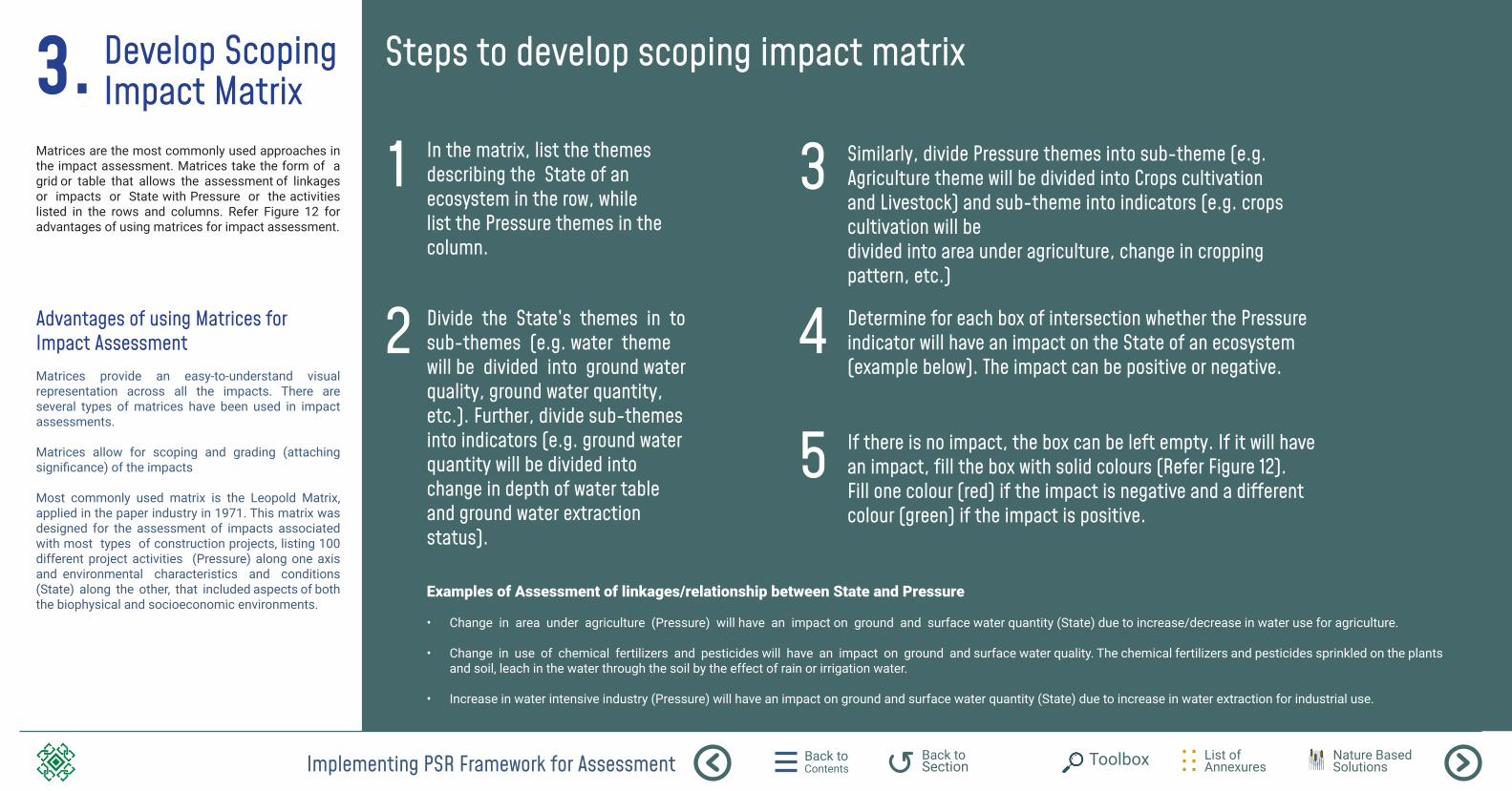
3.Matrices are the most commonly used approaches in the impact assessment. Matrices take the form of a grid or table that allows the assessment of linkages or impacts or State with Pressure or the activities listed in the rows and columns. Refer Figure 12 for advantages of using matrices for impact assessment.
Advantages of using Matrices for Impact AssessmentMatrices provide an easy-to-understand visual representation across all the impacts. There are several types of matrices have been used in impact assessments. Matrices allow for scoping and grading (attaching significance) of the impacts Most commonly used matrix is the Leopold Matrix, applied in the paper industry in 1971. This matrix was designed for the assessment of impacts associated with most types of construction projects, listing 100 different project activities (Pressure) along one axis and environmental characteristics and conditions (State) along the other, that included aspects of both the biophysical and socioeconomic environments.
Develop Scoping Impact Matrix
In the matrix, list the themes describing the State of an ecosystem in the row, while list the Pressure themes in the column.
Divide the State’s themes in to sub-themes (e.g. water theme will be divided into ground water quality, ground water quantity, etc.). Further, divide sub-themes into indicators (e.g. ground water quantity will be divided into change in depth of water table and ground water extraction status).
1
2
Steps to develop scoping impact matrix
Similarly, divide Pressure themes into sub-theme (e.g. Agriculture theme will be divided into Crops cultivation and Livestock) and sub-theme into indicators (e.g. crops cultivation will be divided into area under agriculture, change in cropping pattern, etc.)
Determine for each box of intersection whether the Pressure indicator will have an impact on the State of an ecosystem (example below). The impact can be positive or negative.
If there is no impact, the box can be left empty. If it will have an impact, fill the box with solid colours (Refer Figure 12). Fill one colour (red) if the impact is negative and a different colour (green) if the impact is positive.
Examples of Assessment of linkages/relationship between State and Pressure
• Change in area under agriculture (Pressure) will have an impact on ground and surface water quantity (State) due to increase/decrease in water use for agriculture. • Change in use of chemical fertilizers and pesticides will have an impact on ground and surface water quality. The chemical fertilizers and pesticides sprinkled on the plants
and soil, leach in the water through the soil by the effect of rain or irrigation water. • Increase in water intensive industry (Pressure) will have an impact on ground and surface water quantity (State) due to increase in water extraction for industrial use.
3
4
5
Implementing PSR Framework for Assessment Back to Contents
List of Annexures
Back to Section Toolbox Nature Based
Solutions
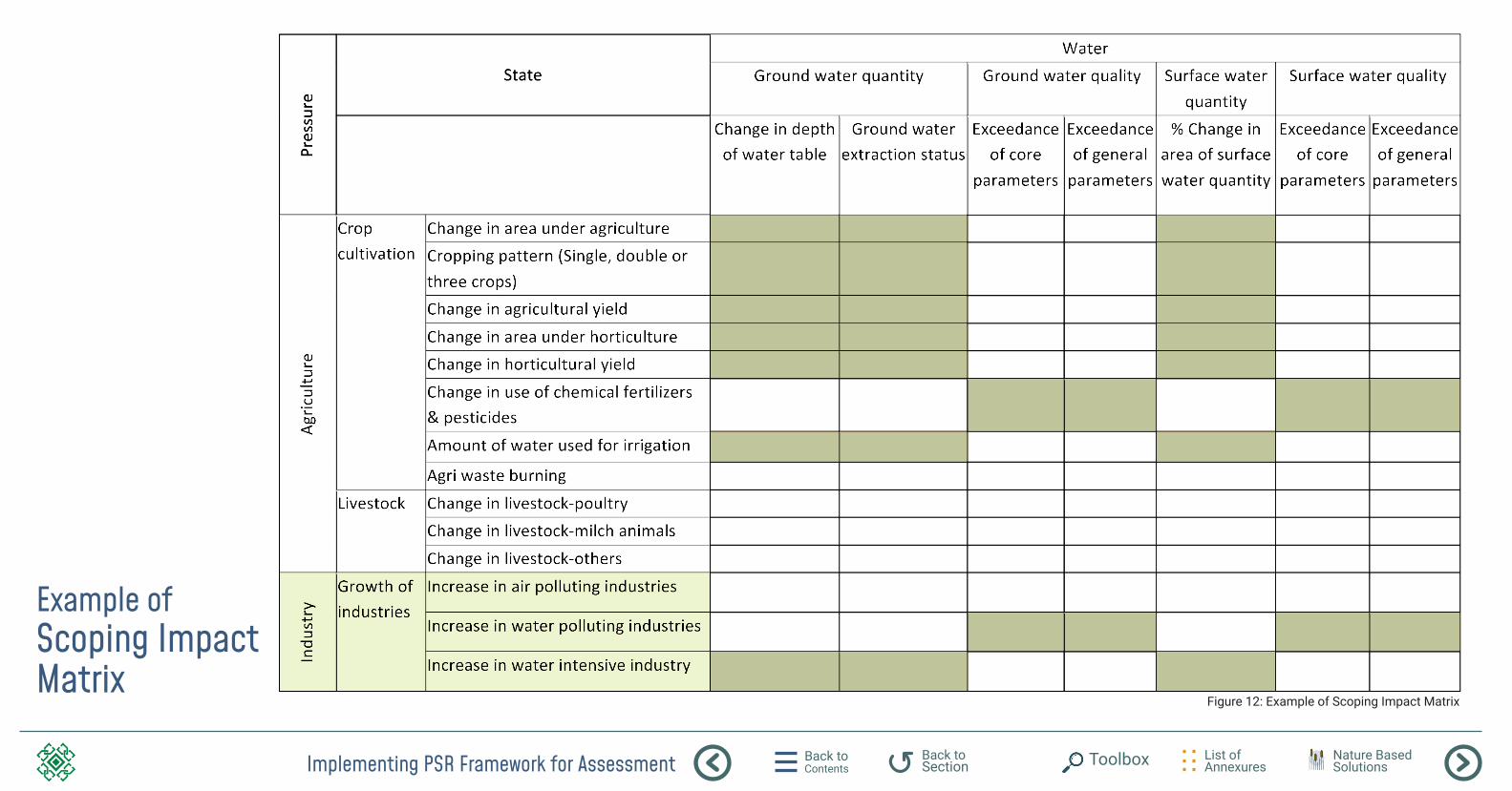
Example of Scoping Impact Matrix
Figure 12: Example of Scoping Impact Matrix
Implementing PSR Framework for Assessment Back to Contents
List of Annexures
Back to Section Toolbox Nature Based
Solutions
Develop Graded Impact Matrix from Scoping Impact Matrix4.
Steps to develop graded impact matrix
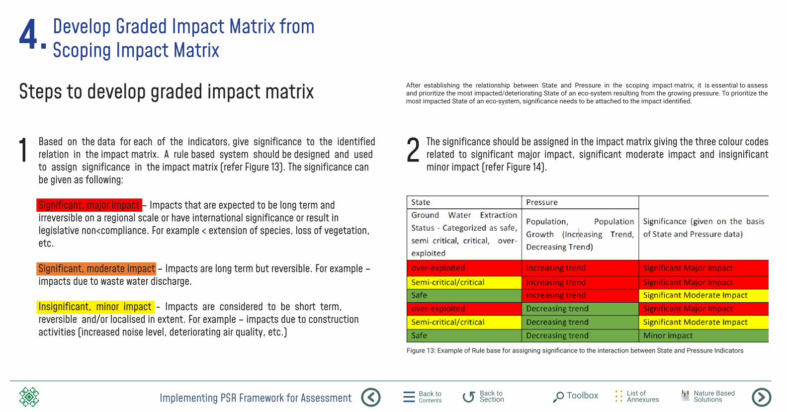
Based on the data for each of the indicators, give significance to the identified relation in the impact matrix. A rule based system should be designed and used to assign significance in the impact matrix (refer Figure 13). The significance can be given as following: Significant, major impact – Impacts that are expected to be long term and irreversible on a regional scale or have international significance or result in legislative non<compliance. For example < extension of species, loss of vegetation, etc. Significant, moderate impact – Impacts are long term but reversible. For example – impacts due to waste water discharge. Insignificant, minor impact - Impacts are considered to be short term, reversible and/or localised in extent. For example – impacts due to construction activities (increased noise level, deteriorating air quality, etc.)
1
After establishing the relationship between State and Pressure in the scoping impact matrix, it is essential to assess and prioritize the most impacted/deteriorating State of an eco-system resulting from the growing pressure. To prioritize the most impacted State of an eco-system, significance needs to be attached to the impact identified.
The significance should be assigned in the impact matrix giving the three colour codes related to significant major impact, significant moderate impact and insignificant minor impact (refer Figure 14).
2
Figure 13: Example of Rule base for assigning significance to the interaction between State and Pressure Indicators
Implementing PSR Framework for Assessment Back to Contents
List of Annexures
Back to Section Toolbox Nature Based
Solutions
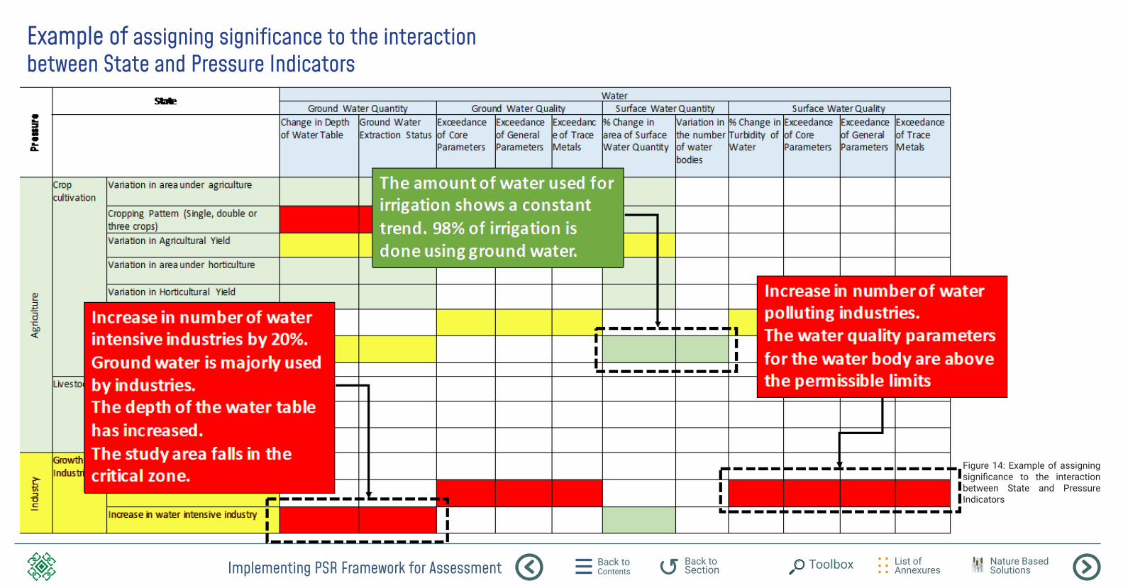
Example of assigning significance to the interaction between State and Pressure Indicators
Figure 14: Example of assigning significance to the interaction between State and Pressure Indicators
Implementing PSR Framework for Assessment Back to Contents
List of Annexures
Back to Section Toolbox Nature Based
Solutions
Develop Impact Networks5.
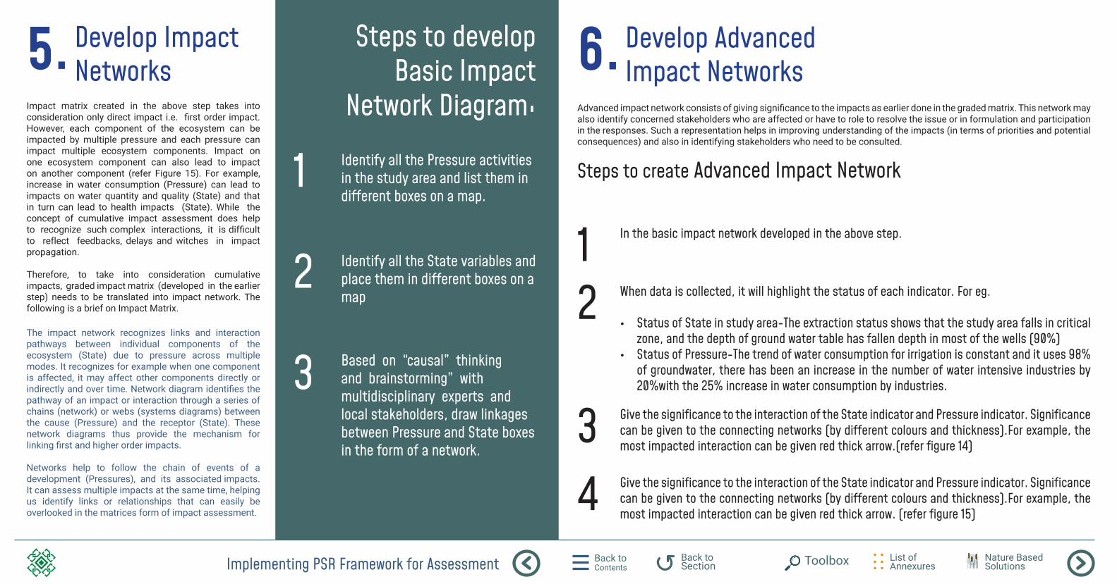
Impact matrix created in the above step takes into consideration only direct impact i.e. first order impact. However, each component of the ecosystem can be impacted by multiple pressure and each pressure can impact multiple ecosystem components. Impact on one ecosystem component can also lead to impact on another component (refer Figure 15). For example, increase in water consumption (Pressure) can lead to impacts on water quantity and quality (State) and that in turn can lead to health impacts (State). While the concept of cumulative impact assessment does help to recognize such complex interactions, it is difficult to reflect feedbacks, delays and witches in impact propagation.
Therefore, to take into consideration cumulative impacts, graded impact matrix (developed in the earlier step) needs to be translated into impact network. The following is a brief on Impact Matrix.
The impact network recognizes links and interaction pathways between individual components of the ecosystem (State) due to pressure across multiple modes. It recognizes for example when one component is affected, it may affect other components directly or indirectly and over time. Network diagram identifies the pathway of an impact or interaction through a series of chains (network) or webs (systems diagrams) between the cause (Pressure) and the receptor (State). These network diagrams thus provide the mechanism for linking first and higher order impacts. Networks help to follow the chain of events of a development (Pressures), and its associated impacts. It can assess multiple impacts at the same time, helping us identify links or relationships that can easily be overlooked in the matrices form of impact assessment.
Steps to develop Basic Impact
Network Diagram: Identify all the Pressure activities in the study area and list them in different boxes on a map.
Identify all the State variables and place them in different boxes on a map
Based on “causal” thinking and brainstorming” with multidisciplinary experts and local stakeholders, draw linkages between Pressure and State boxes in the form of a network.
1
2
3
Develop Advanced Impact Networks6.
Advanced impact network consists of giving significance to the impacts as earlier done in the graded matrix. This network may also identify concerned stakeholders who are affected or have to role to resolve the issue or in formulation and participation in the responses. Such a representation helps in improving understanding of the impacts (in terms of priorities and potential consequences) and also in identifying stakeholders who need to be consulted.
Steps to create Advanced Impact Network
In the basic impact network developed in the above step.
When data is collected, it will highlight the status of each indicator. For eg.
• Status of State in study area-The extraction status shows that the study area falls in critical zone, and the depth of ground water table has fallen depth in most of the wells (90%)
• Status of Pressure-The trend of water consumption for irrigation is constant and it uses 98% of groundwater, there has been an increase in the number of water intensive industries by 20%with the 25% increase in water consumption by industries.
12
Give the significance to the interaction of the State indicator and Pressure indicator. Significance can be given to the connecting networks (by different colours and thickness).For example, the most impacted interaction can be given red thick arrow.(refer figure 14)
Give the significance to the interaction of the State indicator and Pressure indicator. Significance can be given to the connecting networks (by different colours and thickness).For example, the most impacted interaction can be given red thick arrow. (refer figure 15)
34
Implementing PSR Framework for Assessment Back to Contents
List of Annexures
Back to Section Toolbox Nature Based
Solutions
GW Quantity
GW Quality
Water use for
Agriculture
Water use by Industries
Amount of water used for irrigation
Area under agriculture
Cropping pattern
Depth of Water Table
GW extraction status
Amount of water used by industries
Effluent generation
Core Parameters of GW Quality
General Parameters of GW Quality
Water use for Domestic
Purpose
Amount of water used for domestic
Sewage generation
Use of Chemical Pesticides/ Fertilizers
Water
Water Scarcity
Mitigation
Water Pollution
Mitigation
Decentralized WastewaterTreatment
Stringent pollution Standards
Use of Organic Fertilizers
Water Pricing
Industrial Rain water harvesting
Construction of Water Harvesting
Structures( RWH, Recharge Pits,Check dams)
Gaps in Treatment Capacity
Gaps in Wastewater Treatment
SW Quantity
SW Quality
No. of water bodies
Water withdrawn
Surface area of water bodies
Core Parameters of SW Quality
General Parameters of SW Quality
Trace Metals
Pressure ResponseState
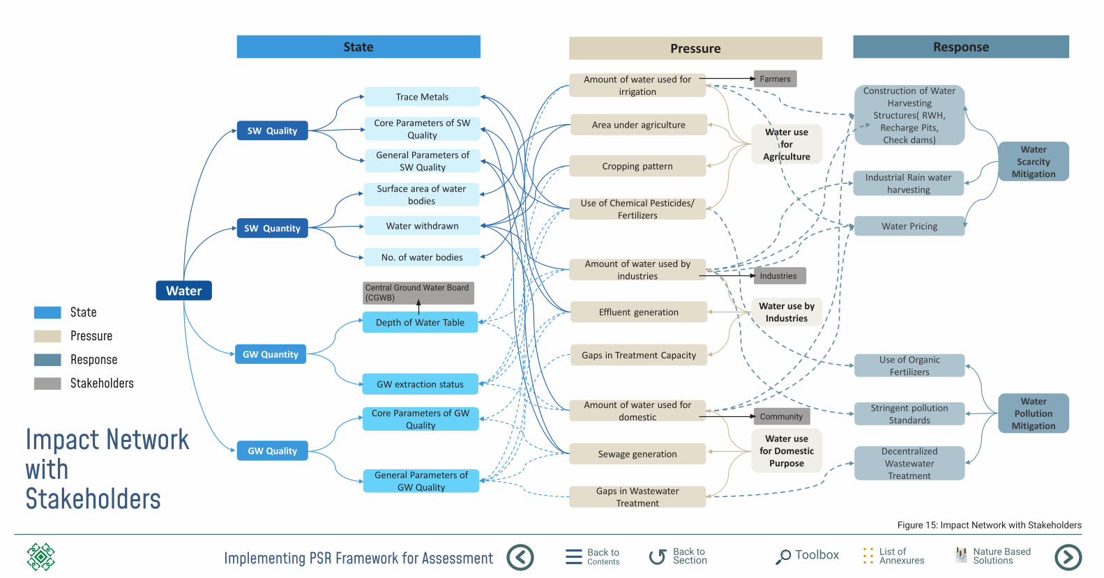
Impact Network with Stakeholders
Figure 15: Impact Network with Stakeholders
State
Pressure
Response
Stakeholders
Central Ground Water Board (CGWB)
Farmers
Industries
Community
Back to Contents
List of Annexures
Back to Section Toolbox Nature Based
Solutions
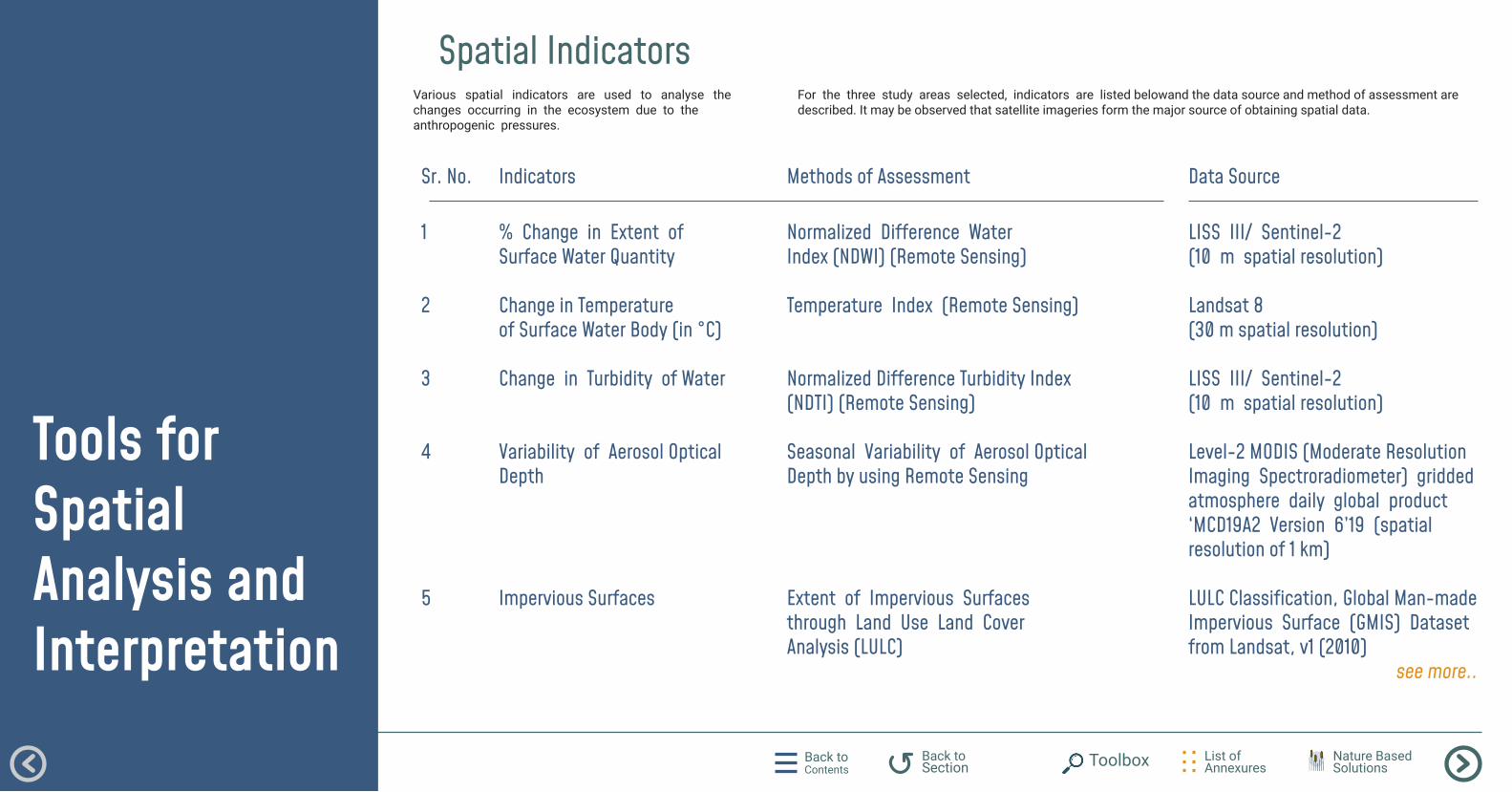
Spatial IndicatorsVarious spatial indicators are used to analyse the changes occurring in the ecosystem due to the anthropogenic pressures.
Tools for Spatial Analysis and Interpretation
1
2
3
4
5
% Change in Extent of Surface Water Quantity
Change in Temperature of Surface Water Body (in °C)
Change in Turbidity of Water
Variability of Aerosol Optical Depth
Impervious Surfaces
Sr. No. Indicators
For the three study areas selected, indicators are listed belowand the data source and method of assessment are described. It may be observed that satellite imageries form the major source of obtaining spatial data.
Normalized Difference Water Index (NDWI) (Remote Sensing)
Temperature Index (Remote Sensing)
Normalized Difference Turbidity Index (NDTI) (Remote Sensing)
Seasonal Variability of Aerosol Optical Depth by using Remote Sensing
Extent of Impervious Surfaces through Land Use Land Cover Analysis (LULC)
LISS III/ Sentinel-2 (10 m spatial resolution)
Landsat 8 (30 m spatial resolution)
LISS III/ Sentinel-2 (10 m spatial resolution)
Level-2 MODIS (Moderate Resolution Imaging Spectroradiometer) gridded atmosphere daily global product ‘MCD19A2 Version 6’19 (spatial resolution of 1 km)
LULC Classification, Global Man-made Impervious Surface (GMIS) Dataset from Landsat, v1 (2010)
Methods of Assessment Data Source
see more..
Back to Contents
List of Annexures
Back to Section Toolbox Nature Based
Solutions
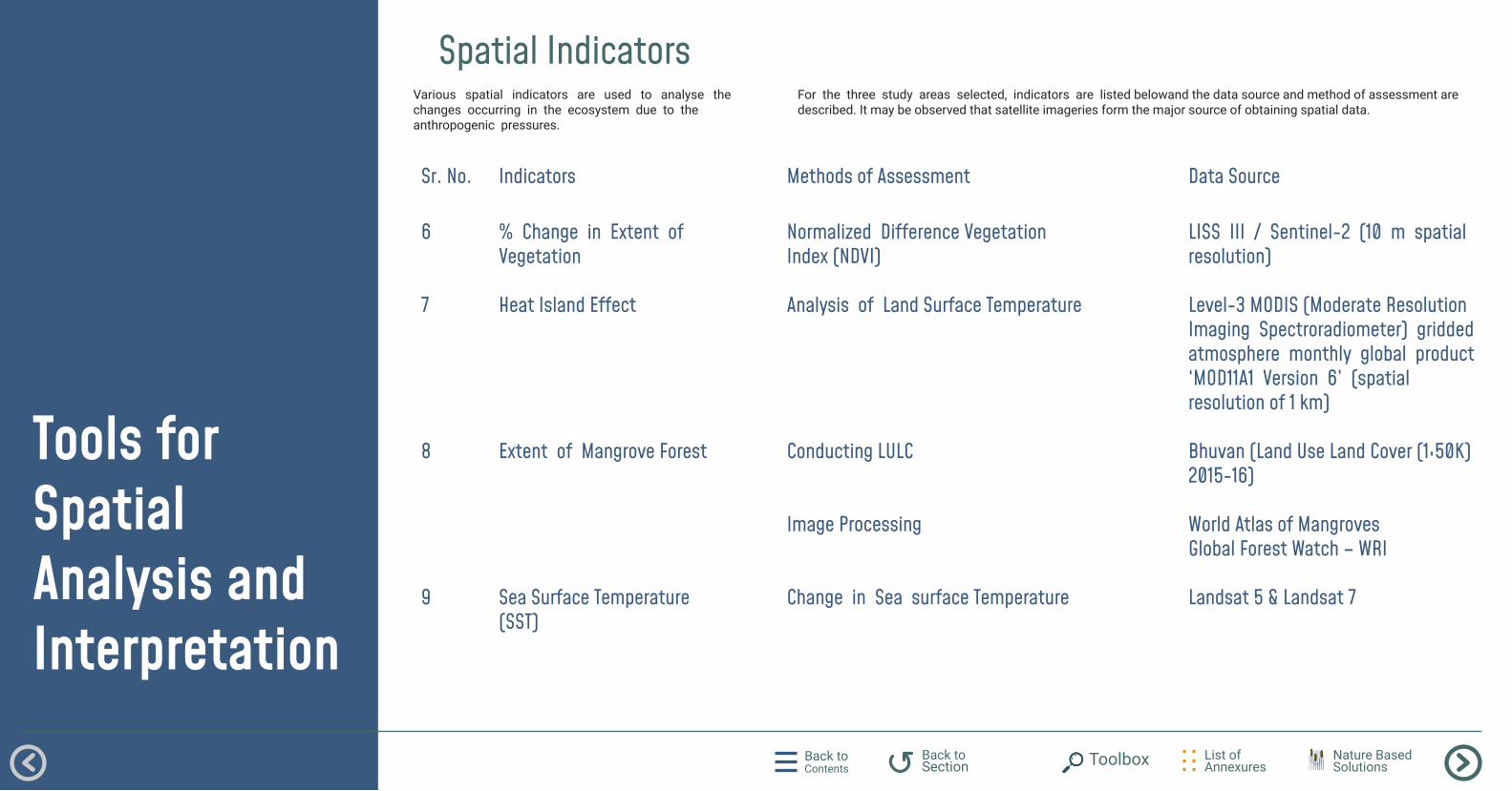
Spatial IndicatorsVarious spatial indicators are used to analyse the changes occurring in the ecosystem due to the anthropogenic pressures.
Tools for Spatial Analysis and Interpretation
6
7
8
9
% Change in Extent of Vegetation
Heat Island Effect
Extent of Mangrove Forest
Sea Surface Temperature (SST)
Sr. No. Indicators
Normalized Difference Vegetation Index (NDVI)
Analysis of Land Surface Temperature
Conducting LULC
Image Processing
Change in Sea surface Temperature
LISS III / Sentinel-2 (10 m spatial resolution)
Level-3 MODIS (Moderate Resolution Imaging Spectroradiometer) gridded atmosphere monthly global product ‘MOD11A1 Version 6’ (spatial resolution of 1 km)
Bhuvan (Land Use Land Cover (1:50K) 2015-16)
World Atlas of Mangroves Global Forest Watch – WRI
Landsat 5 & Landsat 7
Methods of Assessment Data Source
For the three study areas selected, indicators are listed belowand the data source and method of assessment are described. It may be observed that satellite imageries form the major source of obtaining spatial data.
Tools for Spatial Analysis and Interpretation Back to Contents
List of Annexures
Back to Section Toolbox Nature Based
Solutions
Land Use and Land Cover
Objective
Approach
• To identify land cover like vegetation, urban infrastructure, water, bare soil , etc. • To establish the baseline information for activities like thematic mapping and change detection
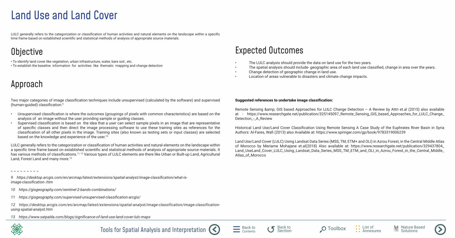
LULC generally refers to the categorization or classification of human activities and natural elements on the landscape within a specific time frame based on established scientific and statistical methods of analysis of appropriate source materials.
Two major categories of image classification techniques include unsupervised (calculated by the software) and supervised (human-guided) classification.9
• Unsupervised classification is where the outcomes (groupings of pixels with common characteristics) are based on the analysis of an image without the user providing sample or guiding classes.
• Supervised classification is based on the idea that a user can select sample pixels in an image that are representative of specific classes and then direct the image processing software to use these training sites as references for the classification of all other pixels in the image. Training sites (also known as testing sets or input classes) are selected based on the knowledge and experience of the user.10
LULC generally refers to the categorization or classification of human activities and natural elements on the landscape within a specific time frame based on established scientific and statistical methods of analysis of appropriate source materials. It has various methods of classifications.11, 12 Various types of LULC elements are there like Urban or Built-up Land, Agricultural Land, Forest Land and many more.13
9 https://desktop.arcgis.com/en/arcmap/latest/extensions/spatial-analyst/image-classification/what-is-image-classification-.htm
10 https://gisgeography.com/sentinel-2-bands-combinations/
11 https://gisgeography.com/supervised-unsupervised-classification-arcgis/
12 https://desktop.arcgis.com/en/arcmap/latest/extensions/spatial-analyst/image-classification/image-classification-using-spatial-analyst.htm
13 https://www.satpalda.com/blogs/significance-of-land-use-land-cover-lulc-maps
Expected Outcomes• The LULC analysis should provide the data on land use for the two years.• The spatial analysis should include- geographic area of each land use classified, change in area over the years.• Change detection of geographic change in land use.• Location of areas vulnerable to disasters and climate change impacts.
Suggested references to undertake image classification:
Remote Sensing & GIS based Approaches for LULC Change Detection – A Review by Attri et.al (2015) also available at : https://www.researchgate.net/publication/325145097_Remote_Sensing_GIS_based_Approaches_for_LULC_Change_Detection_-_A_Review
Historical Land Use/Land Cover Classification Using Remote Sensing A Case Study of the Euphrates River Basin in Syria Authors: Al-Fares, Wafi (2013) also Available at: https://www.springer.com/gp/book/9783319006239
Land Use/Land Cover (LULC) Using Landsat Data Series (MSS, TM, ETM+ and OLI) in Azrou Forest, in the Central Middle Atlas of Morocco by Meriame Mohajane et.al(2018) Also available at: https://www.researchgate.net/publication/329437804_Land_UseLand_Cover_LULC_Using_Landsat_Data_Series_MSS_TM_ETM_and_OLI_in_Azrou_Forest_in_the_Central_Middle_Atlas_of_Morocco
Tools for Spatial Analysis and Interpretation Back to Contents
List of Annexures
Back to Section Toolbox Nature Based
Solutions
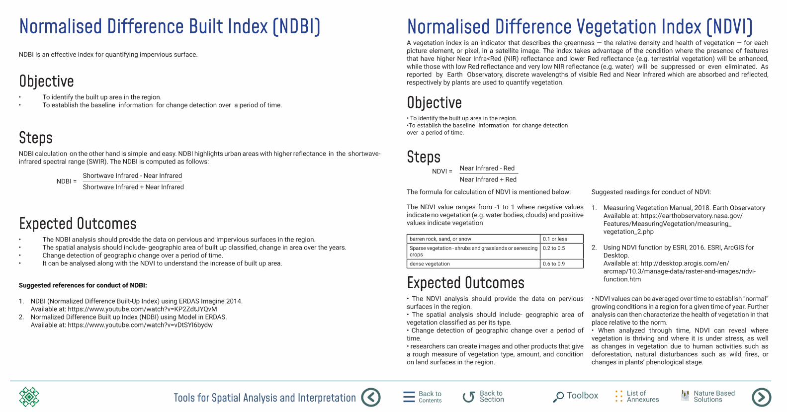
Normalised Difference Built Index (NDBI)NDBI is an effective index for quantifying impervious surface.
StepsNDBI calculation on the other hand is simple and easy. NDBI highlights urban areas with higher reflectance in the shortwave-infrared spectral range (SWIR). The NDBI is computed as follows:
Shortwave Infrared - Near InfraredNDBI =
Shortwave Infrared + Near Infrared
Expected Outcomes• The NDBI analysis should provide the data on pervious and impervious surfaces in the region.• The spatial analysis should include- geographic area of built up classified, change in area over the years.• Change detection of geographic change over a period of time.• It can be analysed along with the NDVI to understand the increase of built up area.
Objective• To identify the built up area in the region. • To establish the baseline information for change detection over a period of time.
Suggested references for conduct of NDBI:
1. NDBI (Normalized Difference Built-Up Index) using ERDAS Imagine 2014. Available at: https://www.youtube.com/watch?v=KP2ZdtJYQvM
2. Normalized Difference Built up Index (NDBI) using Model in ERDAS. Available at: https://www.youtube.com/watch?v=vDtSYI6bydw
The formula for calculation of NDVI is mentioned below:
The NDVI value ranges from -1 to 1 where negative values indicate no vegetation (e.g. water bodies, clouds) and positive values indicate vegetation
Suggested readings for conduct of NDVI:
1. Measuring Vegetation Manual, 2018. Earth Observatory Available at: https://earthobservatory.nasa.gov/Features/MeasuringVegetation/measuring_vegetation_2.php
2. Using NDVI function by ESRI, 2016. ESRI, ArcGIS for Desktop. Available at: http://desktop.arcgis.com/en/arcmap/10.3/manage-data/raster-and-images/ndvi-function.htm
A vegetation index is an indicator that describes the greenness — the relative density and health of vegetation — for each picture element, or pixel, in a satellite image. The index takes advantage of the condition where the presence of features that have higher Near Infra<Red (NIR) reflectance and lower Red reflectance (e.g. terrestrial vegetation) will be enhanced, while those with low Red reflectance and very low NIR reflectance (e.g. water) will be suppressed or even eliminated. As reported by Earth Observatory, discrete wavelengths of visible Red and Near Infrared which are absorbed and reflected, respectively by plants are used to quantify vegetation.
Expected Outcomes• The NDVI analysis should provide the data on pervious surfaces in the region.• The spatial analysis should include- geographic area of vegetation classified as per its type.• Change detection of geographic change over a period of time.• researchers can create images and other products that give a rough measure of vegetation type, amount, and condition on land surfaces in the region.
Objective• To identify the built up area in the region. •To establish the baseline information for change detection over a period of time.
Normalised Difference Vegetation Index (NDVI)
StepsNear Infrared - RedNDVI = Near Infrared + Red
barren rock, sand, or snow 0.1 or less
Sparse vegetation - shrubs and grasslands or senescing crops
0.2 to 0.5
dense vegetation 0.6 to 0.9
• NDVI values can be averaged over time to establish “normal” growing conditions in a region for a given time of year. Further analysis can then characterize the health of vegetation in that place relative to the norm. • When analyzed through time, NDVI can reveal where vegetation is thriving and where it is under stress, as well as changes in vegetation due to human activities such as deforestation, natural disturbances such as wild fires, or changes in plants’ phenological stage.
Tools for Spatial Analysis and Interpretation Back to Contents
List of Annexures
Back to Section Toolbox Nature Based
Solutions
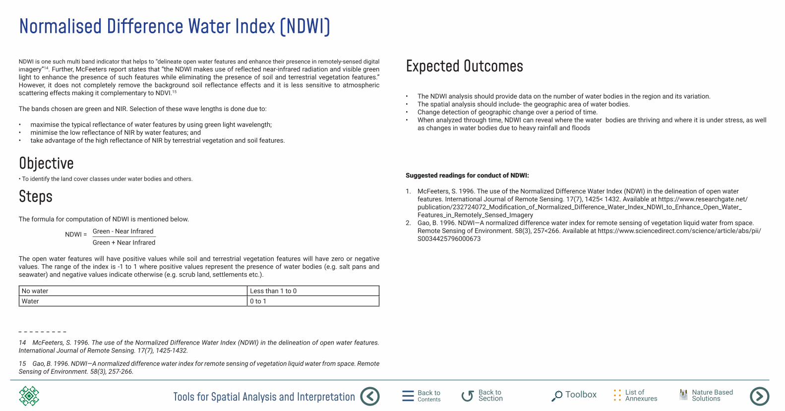
Normalised Difference Water Index (NDWI)NDWI is one such multi band indicator that helps to “delineate open water features and enhance their presence in remotely-sensed digital imagery”14. Further, McFeeters report states that “the NDWI makes use of reflected near-infrared radiation and visible green light to enhance the presence of such features while eliminating the presence of soil and terrestrial vegetation features.” However, it does not completely remove the background soil reflectance effects and it is less sensitive to atmospheric scattering effects making it complementary to NDVI.15
The bands chosen are green and NIR. Selection of these wave lengths is done due to:
• maximise the typical reflectance of water features by using green light wavelength; • minimise the low reflectance of NIR by water features; and • take advantage of the high reflectance of NIR by terrestrial vegetation and soil features.
14 McFeeters, S. 1996. The use of the Normalized Difference Water Index (NDWI) in the delineation of open water features. International Journal of Remote Sensing. 17(7), 1425-1432.
15 Gao, B. 1996. NDWI—A normalized difference water index for remote sensing of vegetation liquid water from space. Remote Sensing of Environment. 58(3), 257-266.
Steps
Objective• To identify the land cover classes under water bodies and others.
The formula for computation of NDWI is mentioned below.
The open water features will have positive values while soil and terrestrial vegetation features will have zero or negative values. The range of the index is -1 to 1 where positive values represent the presence of water bodies (e.g. salt pans and seawater) and negative values indicate otherwise (e.g. scrub land, settlements etc.).
Green - Near InfraredNDWI = Green + Near Infrared
No water Less than 1 to 0Water 0 to 1
• The NDWI analysis should provide data on the number of water bodies in the region and its variation.• The spatial analysis should include- the geographic area of water bodies.• Change detection of geographic change over a period of time.• When analyzed through time, NDWI can reveal where the water bodies are thriving and where it is under stress, as well
as changes in water bodies due to heavy rainfall and floods
Suggested readings for conduct of NDWI:
1. McFeeters, S. 1996. The use of the Normalized Difference Water Index (NDWI) in the delineation of open water features. International Journal of Remote Sensing. 17(7), 1425< 1432. Available at https://www.researchgate.net/publication/232724072_Modification_of_Normalized_Difference_Water_Index_NDWI_to_Enhance_Open_Water_Features_in_Remotely_Sensed_Imagery
2. Gao, B. 1996. NDWI—A normalized difference water index for remote sensing of vegetation liquid water from space. Remote Sensing of Environment. 58(3), 257<266. Available at https://www.sciencedirect.com/science/article/abs/pii/S0034425796000673
Expected Outcomes
Tools for Spatial Analysis and Interpretation Back to Contents
List of Annexures
Back to Section Toolbox Nature Based
Solutions
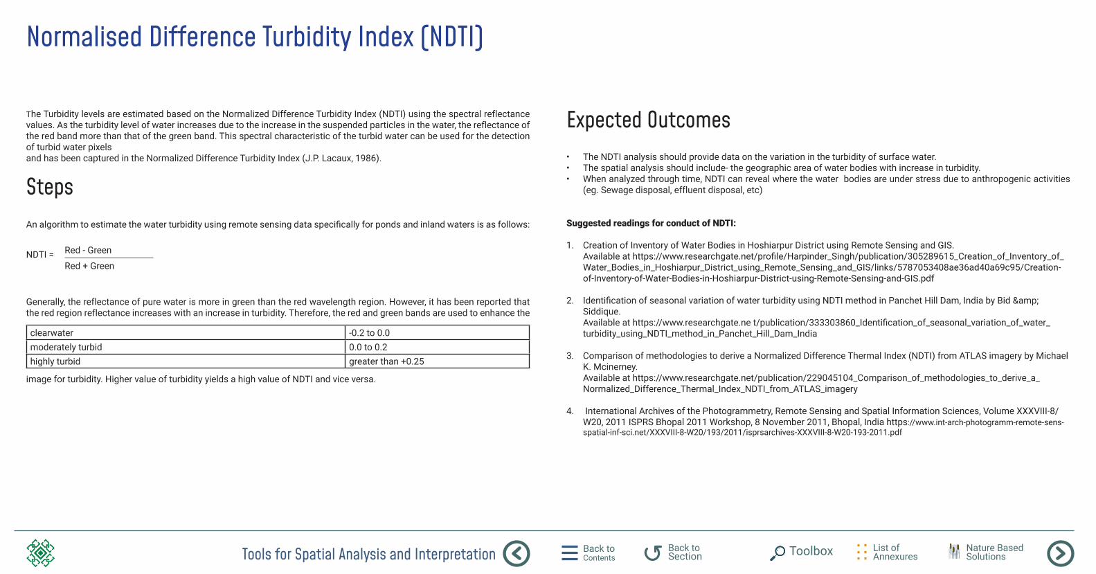
Normalised Difference Turbidity Index (NDTI)
The Turbidity levels are estimated based on the Normalized Difference Turbidity Index (NDTI) using the spectral reflectance values. As the turbidity level of water increases due to the increase in the suspended particles in the water, the reflectance of the red band more than that of the green band. This spectral characteristic of the turbid water can be used for the detection of turbid water pixelsand has been captured in the Normalized Difference Turbidity Index (J.P. Lacaux, 1986).
An algorithm to estimate the water turbidity using remote sensing data specifically for ponds and inland waters is as follows:
Generally, the reflectance of pure water is more in green than the red wavelength region. However, it has been reported that the red region reflectance increases with an increase in turbidity. Therefore, the red and green bands are used to enhance the
image for turbidity. Higher value of turbidity yields a high value of NDTI and vice versa.
Steps
Red - GreenNDTI = Red + Green
clearwater -0.2 to 0.0moderately turbid 0.0 to 0.2highly turbid greater than +0.25
• The NDTI analysis should provide data on the variation in the turbidity of surface water. • The spatial analysis should include- the geographic area of water bodies with increase in turbidity.• When analyzed through time, NDTI can reveal where the water bodies are under stress due to anthropogenic activities
(eg. Sewage disposal, effluent disposal, etc)
Suggested readings for conduct of NDTI:
1. Creation of Inventory of Water Bodies in Hoshiarpur District using Remote Sensing and GIS. Available at https://www.researchgate.net/profile/Harpinder_Singh/publication/305289615_Creation_of_Inventory_of_Water_Bodies_in_Hoshiarpur_District_using_Remote_Sensing_and_GIS/links/5787053408ae36ad40a69c95/Creation-of-Inventory-of-Water-Bodies-in-Hoshiarpur-District-using-Remote-Sensing-and-GIS.pdf
2. Identification of seasonal variation of water turbidity using NDTI method in Panchet Hill Dam, India by Bid & Siddique. Available at https://www.researchgate.ne t/publication/333303860_Identification_of_seasonal_variation_of_water_turbidity_using_NDTI_method_in_Panchet_Hill_Dam_India
3. Comparison of methodologies to derive a Normalized Difference Thermal Index (NDTI) from ATLAS imagery by Michael K. Mcinerney. Available at https://www.researchgate.net/publication/229045104_Comparison_of_methodologies_to_derive_a_Normalized_Difference_Thermal_Index_NDTI_from_ATLAS_imagery
4. International Archives of the Photogrammetry, Remote Sensing and Spatial Information Sciences, Volume XXXVIII-8/W20, 2011 ISPRS Bhopal 2011 Workshop, 8 November 2011, Bhopal, India https://www.int-arch-photogramm-remote-sens-spatial-inf-sci.net/XXXVIII-8-W20/193/2011/isprsarchives-XXXVIII-8-W20-193-2011.pdf
Expected Outcomes
Tools for Spatial Analysis and Interpretation Back to Contents
List of Annexures
Back to Section Toolbox Nature Based
Solutions
Aerosol Optical Depth
To estimate particulates in the atmospheric column using Moderate- Resolution Imaging Spectroradiometer (MODIS) Terra Aerosol Optical Depth (AOD) datasets accessible at NASA’s EARTHDATA web portal.
Data quality (QA/QC) matrices are available in MODIS datasets with uncertainty surrounding the values of each pixel, along with supporting metadata. MODIS Terra product for AOD at 1 km spatial resolution and daily averaging periods can be used to estimate aerosols in urban ecosystems and track changes over time. The product code is MOD04.
The data product derived from MODIS has to undergo processing in a GIS tool. Data distribution and basic statistics can be calculated using Raster Calculator Toolbox in ArcGIS. Advanced ground truthing studies have also established relationship between AOD and ground-level particulate matter (PM).
Objective
Approach
AOD in many ways serves as a proxy for particulates in the atmospheric column. In the absence of ground- based monitoring data, AOD values can be used to understand the intensity of particulate pollution in the study area. AOD values from past years can be derived to observe changes in atmospheric aerosols. AOD values range from 0 (low) to 5 (polluted) and might be prone to interference from cloud covers. Due to cloud cover, it is important to check the data quality flags before using the data.
• When analyzed through time, AOD can reveal the land use which is experiencing increase in the AOD levels due to activities like ( vehicle pollution, construction activities, etc).
• The seasonal values depict how the levels depend on the air density.
Suggested readings for air quality analysis and particulate matter estimation using AOD:
1. MODIS aerosol optical depth observations over urban areas in Pakistan: quantity and quality of the data for air quality monitoring. Available at https://www.sciencedirect.com/science/article/pii/S1309104215303998
2. Estimating Air Particulate Matter Using MODIS Data and Analyzing Its Spatial and Temporal Pattern over the Yangtze Delta Region. Available at https://www.sciencedirect.com/science/article/pii/S1309104215303998
3. An empirical relationship between PM 2.5 and aerosol optical depth in Delhi Metropolitan. Available at https://www.ncbi.nlm.nih.gov/pmc/articles/PMC3237057/
Expected Outcomes
Tools for Spatial Analysis and Interpretation Back to Contents
List of Annexures
Back to Section Toolbox Nature Based
Solutions
To derive the temperature of the sea from the satellite imageries , the methodology given in Landsat 716 and Landsat 817 can be followed.The analysis is not limited to the detection of only the sea surface temperature. The same method could be deployed to analyse the surface temperature of land locked water bodies as well.
The first step is to convert the image digital number (DN) values into radiance.
For Landsat 5, the following formula can be used to convert the DN values to radiance:Lλ = ((LMAXλ - LMINλ)/(QCALMAX-QCALMIN)) * (QCAL-QCALMIN) + LMINλ
Where,Lλ = Spectral Radiance at the sensor’s aperture in watts/(meter squared * ster * µm); LMINλ = the spectral radiance that is scaled to QCALMIN in watts/(meter squared * ster * µm); LMAXλ = the spectral radiance that is scaled to QCALMAX in watts/(meter squared * ster * µm); QCALMIN = the minimum quantized calibrated pixel value (corresponding to LMINλ) in DN = 1; QCALMAX = the maximum quantized calibrated pixel value (corresponding to LMAXλ) in DN = 255; QCAL = the quantized calibrated pixel value in DN
For Landsat 8, the following formula can be used to convert the DN values to radiance :Lλ = ML*Qcal + AL
Where,Lλ = Spectral radiance (W/(m2 * sr * μm)); ML = Radiance multiplicative scaling factor for the band (RADIANCE_MULT_BAND_n from the metadata); AL = Radiance additive scaling factor for the band (RADIANCE_ADD_BAND_n from the metadata); Qcal = L1 pixel value in DN
16 Landsat 7 Data Users Handbook. Available at https://landsat.gsfc.nasa.gov/wp-content/uploads/2016/08/Landsat7_Handbook.pdf
17 Landsat 8 Data Users Handbook. Available at https://landsat.usgs.gov/sites/default/files/documents/Landsat8DataUsersHandbook.pdf
Steps
Sea Surface Temperature (SST)
Objective
The second step is to convert the radiance into temperature value in Kelvin using following formula:
Where,T = Effective at-satellite temperature in Kelvin;K2 = Thermal conversion constant for the bandK1 = Thermal conversion constant for the band; L = Spectral radiance in watts/(meter squared * ster * µm)
• The SST analysis should provide data on the variation in the temperature of the sea in the region. • The spatial analysis should include- the geographic area of water bodies with increase in temperature.• When analyzed through time, SST can reveal where the temperature of the water bodies has increased majorly due to
anthropogenic activities (eg. Loss of vegetation along the water bodies, effluent disposal, etc)
Suggested readings for conduct of SST:
1. Landsat 7 Data Users Handbook. Available at https://landsat.gsfc.nasa.gov/wp-content/uploads/2016/08/Landsat7_Handbook.pdf
2. Landsat 8 Data Users Handbook. Available at https://landsat.usgs.gov/sites/default/files/documents/Landsat8DataUsersHandbook.pdf
Expected Outcomes
Tools for Spatial Analysis and Interpretation Back to Contents
List of Annexures
Back to Section Toolbox Nature Based
Solutions
Moderate-Resolution Imaging Spectroradiometer (MODIS) Terra night time and daytime Land Surface Temperature (LST) datasets accessible at NASA’s EARTHDATA web portal are used to estimate Land Surface Temperature. LST values are also used as proxies for understanding the impact of land use change in urban areas.
To identify changes in built-up area and other land-use changes, Night time LST values from past years can be accessed and processed to observe changes in night time emissivity from land surface and attribute it to changing energy demand and land use change.
The data product derived from MODIS has to undergo processing in a GIS tool. Data distribution and basic statistics can be calculated using Raster Calculator Toolbox in ArcGIS. Land Surface Temperature data can be processed in GIS in order to estimate the temperature differences between city centres and peripheral areas; and also study the change in night time temperatures in highly built up areas. The study of temperature gradients in urban areas using night time LST data lead to identification of heat stress areas or UHIs. LST can also be used as a proxy indicator in cases where air temperature data is not available. MODIS Terra product for LST at 1 km spatial resolution and 8-day averaging periods can be used to estimate night time surface temperatures in urban ecosystems and track changes over time. The product code is MOD11A2.
Land Surface Temperature (LST)
Objective• To identify changes in land temperature due to change in built-up area and other landuse. • Nighttime LST values from past years can be accessed and processed to observe changes in night time emissivity from
land surface and attribute it to changing energy demand and land use change. • To estimate the temperature differences between city centres and peripheral areas; and also study the change in night
time temperatures in highly built up areas. • To study the temperature gradients in urban areas using night time LST data to identify heat stress areas or UHIs.
• The LST analysis should provide data on the variation in the temperature of the land in the region. • The spatial analysis should include- the geographic area of land cover with an increase in temperature.• When analyzed through time, LST can reveal where the temperature of the area has increased majorly due to anthropogenic
activities (eg. Loss of vegetation, increase in built up area, etc)
Suggested readings for UHI analysis using remote sensing:
1. Assessment with satellite data of the urban heat island effects in Asian mega cities. Available at https://www.sciencedirect.com/science/article/abs/pii/S0303243405000565
2. Derivation of Birmingham’s summer surface urban heat island from MODIS satellite images. Available at https://rmets.onlinelibrary.wiley.com/doi/abs/10.1002/joc.2261
3. A new method to quantify surface urban heat island intensity. Available at https://www.sciencedirect.com/science/article/pii/S0048969717334186
Expected Outcomes
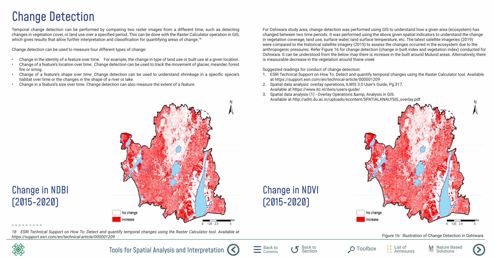
Tools for Spatial Analysis and Interpretation Back to Contents
List of Annexures
Back to Section Toolbox Nature Based
Solutions
Temporal change detection can be performed by comparing two raster images from a different time, such as detecting changes in vegetation cover, or land use over a specified period. This can be done with the Raster Calculator operation in GIS, which gives results that allow further interpretation and classification for quantifying areas of change.18
Change detection can be used to measure four different types of change:
• Change in the identity of a feature over time. For example, the change in type of land use or built use at a given location. • Change of a feature’s location over time. Change detection can be used to track the movement of glacier, meander, forest
fire or smog.• Change of a feature’s shape over time. Change detection can be used to understand shrinkage in a specific specie’s
habitat over time or the changes in the shape of a river or lake.• Change in a feature’s size over time. Change detection can also measure the extent of a feature.
18 ESRI Technical Support on How To: Detect and quantify temporal changes using the Raster Calculator tool. Available at https://support.esri.com/en/technical-article/000001209
Change Detection
Change in NDBI (2015-2020)
Change in NDVI (2015-2020)
For Oshiwara study area, change detection was performed using GIS to understand how a given area (ecosystem) has changed between two time periods. It was performed using the above given spatial indicators to understand the change in vegetation coverage, land use, surface water, land surface temperature, etc. The latest satellite imageries (2019) were compared to the historical satellite imagery (2015) to assess the changes occurred in the ecosystem due to the anthropogenic pressures. Refer Figure 16 for change detection (change in built index and vegetation index) conducted for Oshiwara. It can be understood from the below map there is increase in the built around Mulund areas. Alternatively, there is measurable decrease in the vegetation around thane creek
Suggested readings for conduct of change detection:1. ESRI Technical Support on How To: Detect and quantify temporal changes using the Raster Calculator tool. Available
at https://support.esri.com/en/technical-article/000001209 2. Spatial data analysis: overlay operations, ILWIS 3.0 User’s Guide, Pg.317.
Available at https://www.itc.nl/ilwis/users-guide/ 3. Spatial data analysis (1) - Overlay Operations & Analysis in GIS.
Available at http://aditi.du.ac.in/uploads/econtent/SPATIALANALYSIS_overlay.pdf
Figure 16: Illustration of Change Detection in Oshiwara
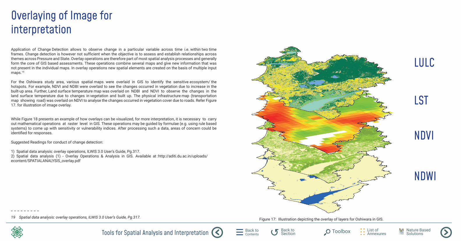
Tools for Spatial Analysis and Interpretation Back to Contents
List of Annexures
Back to Section Toolbox Nature Based
Solutions
Overlaying of Image for interpretationApplication of Change Detection allows to observe change in a particular variable across time i.e. within two time frames. Change detection is however not sufficient when the objective is to assess and establish relationships across themes across Pressure and State. Overlay operations are therefore part of most spatial analysis processes and generally form the core of GIS based assessments. These operations combine several maps and give new information that was not present in the individual maps. In overlay operations new spatial elements are created on the basis of multiple input maps.19
For the Oshiwara study area, various spatial maps were overlaid in GIS to identify the sensitive ecosystem/ the hotspots. For example, NDVI and NDBI were overlaid to see the changes occurred in vegetation due to increase in the built-up area. Further, Land surface temperature map was overlaid on NDBI and NDVI to observe the changes in the land surface temperature due to changes in vegetation and built up. The physical infrastructure map (transportation map showing road) was overlaid on NDVI to analyse the changes occurred in vegetation cover due to roads. Refer Figure 17. for illustration of image overlay.
While Figure 18 presents an example of how overlays can be visualized, for more interpretation, it is necessary to carry out mathematical operations at raster level in GIS. These operations may be guided by formulae (e.g. using rule based systems) to come up with sensitivity or vulnerability indices. After processing such a data, areas of concern could be identified for responses. Suggested Readings for conduct of change detection:
1) Spatial data analysis: overlay operations, ILWIS 3.0 User’s Guide, Pg.317.2) Spatial data analysis (1) - Overlay Operations & Analysis in GIS. Available at :http://aditi.du.ac.in/uploads/econtent/SPATIALANALYSIS_overlay.pdf
19 Spatial data analysis: overlay operations, ILWIS 3.0 User’s Guide, Pg.317. Figure 17: Illustration depicting the overlay of layers for Oshiwara in GIS.
LULC
LST
NDVI
NDWI
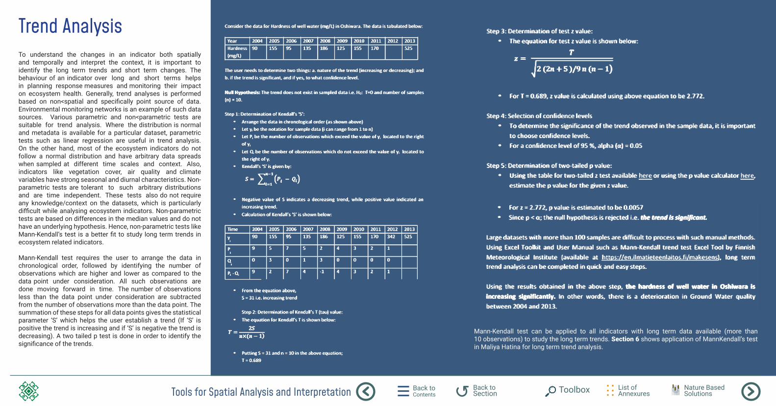
Tools for Spatial Analysis and Interpretation Back to Contents
List of Annexures
Back to Section Toolbox Nature Based
Solutions
Trend AnalysisTo understand the changes in an indicator both spatially and temporally and interpret the context, it is important to identify the long term trends and short term changes. The behaviour of an indicator over long and short terms helps in planning response measures and monitoring their impact on ecosystem health. Generally, trend analyses is performed based on non<spatial and specifically point source of data. Environmental monitoring networks is an example of such data sources. Various parametric and non<parametric tests are suitable for trend analysis. Where the distribution is normal and metadata is available for a particular dataset, parametric tests such as linear regression are useful in trend analysis. On the other hand, most of the ecosystem indicators do not follow a normal distribution and have arbitrary data spreads when sampled at different time scales and context. Also, indicators like vegetation cover, air quality and climate variables have strong seasonal and diurnal characteristics. Non-parametric tests are tolerant to such arbitrary distributions and are time independent. These tests also do not require any knowledge/context on the datasets, which is particularly difficult while analysing ecosystem indicators. Non-parametric tests are based on differences in the median values and do not have an underlying hypothesis. Hence, non-parametric tests like Mann-Kendall’s test is a better fit to study long term trends in ecosystem related indicators.
Mann-Kendall test requires the user to arrange the data in chronological order, followed by identifying the number of observations which are higher and lower as compared to the data point under consideration. All such observations are done moving forward in time. The number of observations less than the data point under consideration are subtracted from the number of observations more than the data point. The summation of these steps for all data points gives the statistical parameter ‘S’ which helps the user establish a trend (If ‘S’ is positive the trend is increasing and if ‘S’ is negative the trend is decreasing). A two tailed p test is done in order to identify the significance of the trends.
Mann-Kendall test can be applied to all indicators with long term data available (more than 10 observations) to study the long term trends. Section 6 shows application of MannKendall’s test in Maliya Hatina for long term trend analysis.
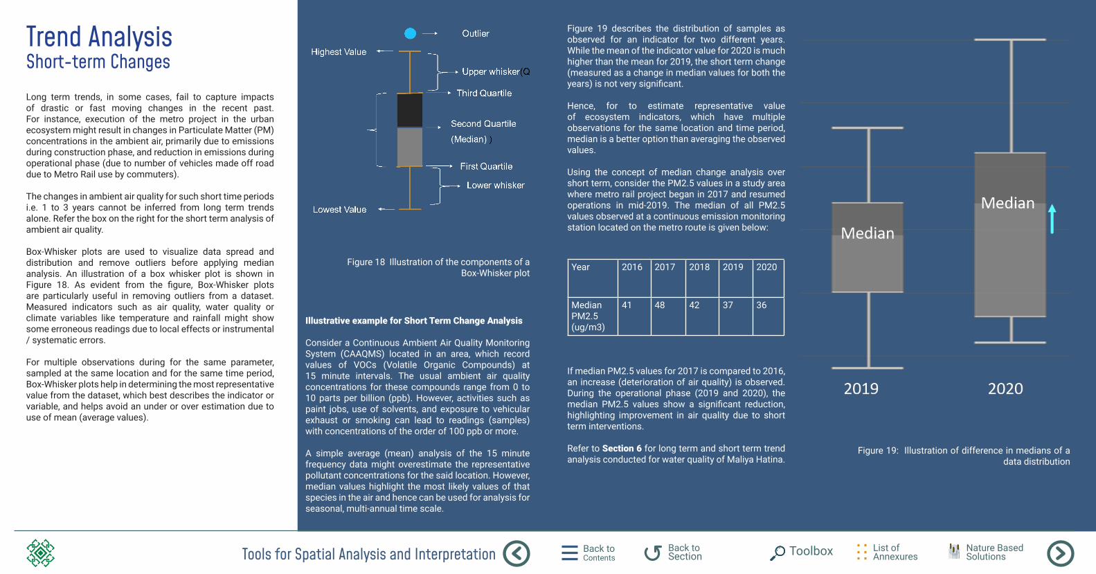
Tools for Spatial Analysis and Interpretation Back to Contents
List of Annexures
Back to Section Toolbox Nature Based
Solutions
Trend AnalysisShort-term ChangesLong term trends, in some cases, fail to capture impacts of drastic or fast moving changes in the recent past. For instance, execution of the metro project in the urban ecosystem might result in changes in Particulate Matter (PM) concentrations in the ambient air, primarily due to emissions during construction phase, and reduction in emissions during operational phase (due to number of vehicles made off road due to Metro Rail use by commuters).
The changes in ambient air quality for such short time periods i.e. 1 to 3 years cannot be inferred from long term trends alone. Refer the box on the right for the short term analysis of ambient air quality.
Box-Whisker plots are used to visualize data spread and distribution and remove outliers before applying median analysis. An illustration of a box whisker plot is shown in Figure 18. As evident from the figure, Box-Whisker plots are particularly useful in removing outliers from a dataset. Measured indicators such as air quality, water quality or climate variables like temperature and rainfall might show some erroneous readings due to local effects or instrumental / systematic errors.
For multiple observations during for the same parameter, sampled at the same location and for the same time period, Box-Whisker plots help in determining the most representative value from the dataset, which best describes the indicator or variable, and helps avoid an under or over estimation due to use of mean (average values).
Illustrative example for Short Term Change Analysis
Consider a Continuous Ambient Air Quality Monitoring System (CAAQMS) located in an area, which record values of VOCs (Volatile Organic Compounds) at 15 minute intervals. The usual ambient air quality concentrations for these compounds range from 0 to 10 parts per billion (ppb). However, activities such as paint jobs, use of solvents, and exposure to vehicular exhaust or smoking can lead to readings (samples) with concentrations of the order of 100 ppb or more.
A simple average (mean) analysis of the 15 minute frequency data might overestimate the representative pollutant concentrations for the said location. However, median values highlight the most likely values of that species in the air and hence can be used for analysis for seasonal, multi-annual time scale.
Figure 19: Illustration of difference in medians of a data distribution
Figure 19 describes the distribution of samples as observed for an indicator for two different years. While the mean of the indicator value for 2020 is much higher than the mean for 2019, the short term change (measured as a change in median values for both the years) is not very significant.
Hence, for to estimate representative value of ecosystem indicators, which have multiple observations for the same location and time period, median is a better option than averaging the observed values.
Using the concept of median change analysis over short term, consider the PM2.5 values in a study area where metro rail project began in 2017 and resumed operations in mid-2019. The median of all PM2.5 values observed at a continuous emission monitoring station located on the metro route is given below:
If median PM2.5 values for 2017 is compared to 2016, an increase (deterioration of air quality) is observed. During the operational phase (2019 and 2020), the median PM2.5 values show a significant reduction, highlighting improvement in air quality due to short term interventions.
Refer to Section 6 for long term and short term trend analysis conducted for water quality of Maliya Hatina.
Year 2016 2017 2018 2019 2020
Median PM2.5 (ug/m3)
41 48 42 37 36
Figure 18 Illustration of the components of a Box-Whisker plot
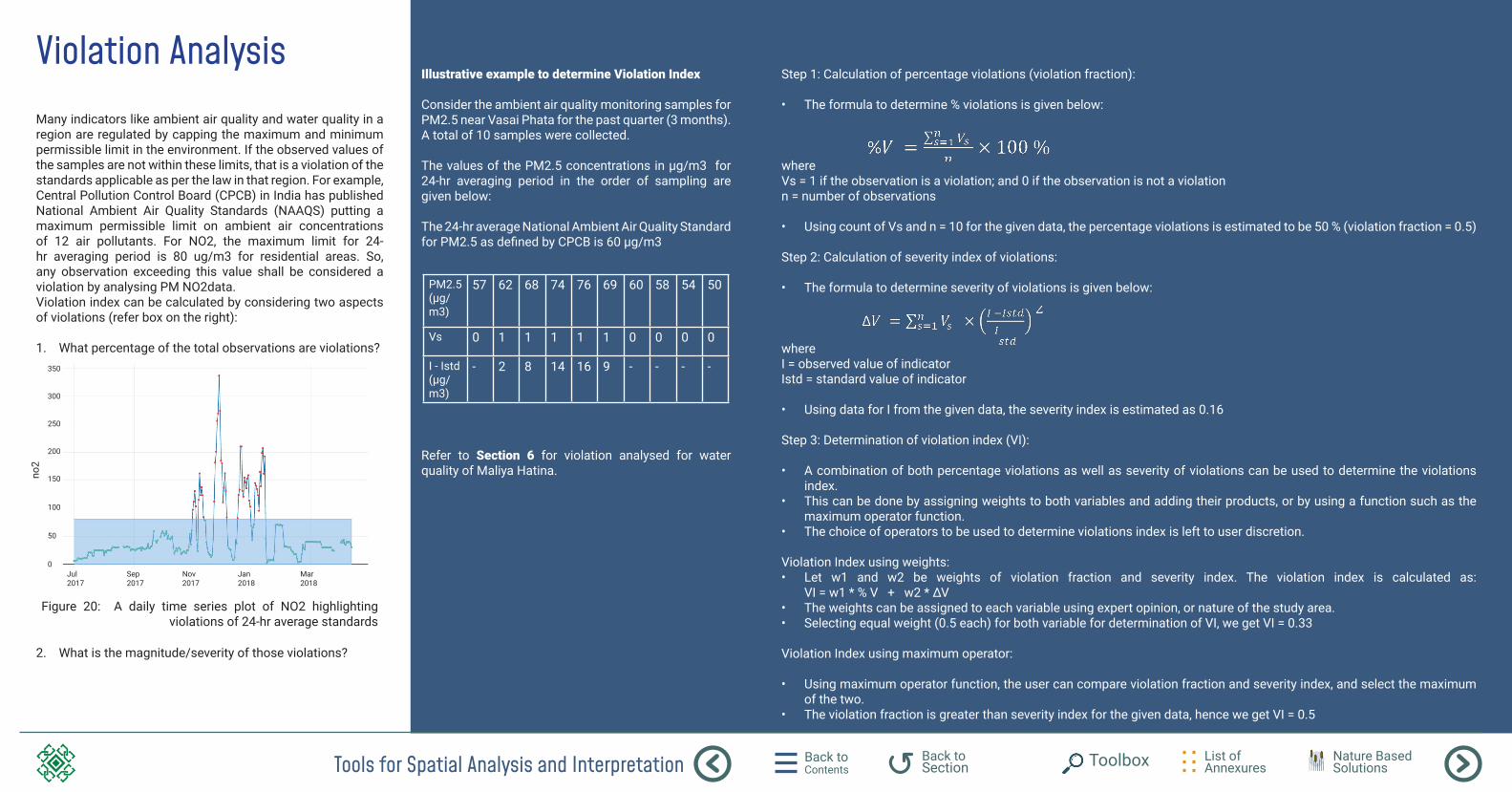
Tools for Spatial Analysis and Interpretation Back to Contents
List of Annexures
Back to Section Toolbox Nature Based
Solutions
Violation AnalysisMany indicators like ambient air quality and water quality in a region are regulated by capping the maximum and minimum permissible limit in the environment. If the observed values of the samples are not within these limits, that is a violation of the standards applicable as per the law in that region. For example, Central Pollution Control Board (CPCB) in India has published National Ambient Air Quality Standards (NAAQS) putting a maximum permissible limit on ambient air concentrations of 12 air pollutants. For NO2, the maximum limit for 24-hr averaging period is 80 ug/m3 for residential areas. So, any observation exceeding this value shall be considered a violation by analysing PM NO2data. Violation index can be calculated by considering two aspects of violations (refer box on the right):
1. What percentage of the total observations are violations?
2. What is the magnitude/severity of those violations?
Illustrative example to determine Violation Index
Consider the ambient air quality monitoring samples for PM2.5 near Vasai Phata for the past quarter (3 months). A total of 10 samples were collected.
The values of the PM2.5 concentrations in µg/m3 for 24-hr averaging period in the order of sampling are given below:
The 24-hr average National Ambient Air Quality Standard for PM2.5 as defined by CPCB is 60 µg/m3
Refer to Section 6 for violation analysed for water quality of Maliya Hatina.
PM2.5 (µg/m3)
57 62 68 74 76 69 60 58 54 50
Vs 0 1 1 1 1 1 0 0 0 0
I - Istd (µg/m3)
- 2 8 14 16 9 - - - -
Figure 20: A daily time series plot of NO2 highlighting violations of 24-hr average standards
Step 1: Calculation of percentage violations (violation fraction):
• The formula to determine % violations is given below:
where Vs = 1 if the observation is a violation; and 0 if the observation is not a violationn = number of observations
• Using count of Vs and n = 10 for the given data, the percentage violations is estimated to be 50 % (violation fraction = 0.5)
Step 2: Calculation of severity index of violations:
• The formula to determine severity of violations is given below:
where I = observed value of indicatorIstd = standard value of indicator
• Using data for I from the given data, the severity index is estimated as 0.16
Step 3: Determination of violation index (VI):
• A combination of both percentage violations as well as severity of violations can be used to determine the violations index.
• This can be done by assigning weights to both variables and adding their products, or by using a function such as the maximum operator function.
• The choice of operators to be used to determine violations index is left to user discretion.
Violation Index using weights:• Let w1 and w2 be weights of violation fraction and severity index. The violation index is calculated as:
VI = w1 * % V + w2 * ∆V• The weights can be assigned to each variable using expert opinion, or nature of the study area. • Selecting equal weight (0.5 each) for both variable for determination of VI, we get VI = 0.33
Violation Index using maximum operator:
• Using maximum operator function, the user can compare violation fraction and severity index, and select the maximum of the two.
• The violation fraction is greater than severity index for the given data, hence we get VI = 0.5
350
300
250
200
150no2
100
Jul 2017
Sep 2017
Nov 2017
Jan 2018
Mar 2018
50
0
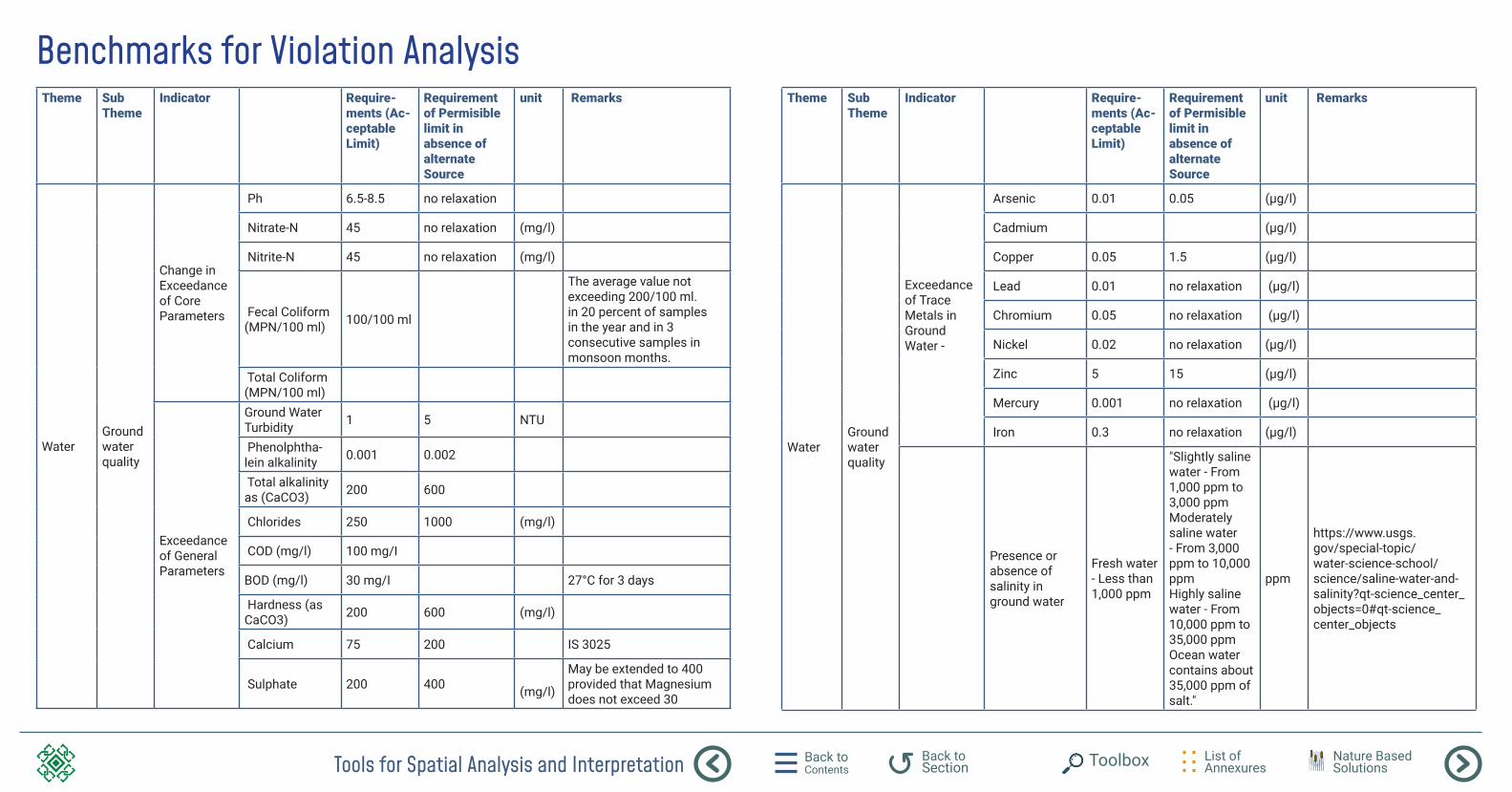
Tools for Spatial Analysis and Interpretation Back to Contents
List of Annexures
Back to Section Toolbox Nature Based
Solutions
Benchmarks for Violation AnalysisTheme Sub
ThemeIndicator Require-
ments (Ac-ceptable Limit)
Requirement of Permisible limit in absence of alternate Source
unit Remarks
WaterGround water quality
Change in Exceedance of Core Parameters
Ph 6.5-8.5 no relaxation
Nitrate-N 45 no relaxation (mg/l)
Nitrite-N 45 no relaxation (mg/l)
Fecal Coliform (MPN/100 ml) 100/100 ml
The average value not exceeding 200/100 ml. in 20 percent of samples in the year and in 3 consecutive samples in monsoon months.
Total Coliform (MPN/100 ml)
Exceedance of General Parameters
Ground Water Turbidity 1 5 NTU
Phenolphtha-lein alkalinity 0.001 0.002
Total alkalinity as (CaCO3) 200 600
Chlorides 250 1000 (mg/l)
COD (mg/l) 100 mg/I
BOD (mg/l) 30 mg/I 27°C for 3 days
Hardness (as CaCO3) 200 600 (mg/l)
Calcium 75 200 IS 3025
Sulphate 200 400 (mg/l)
May be extended to 400 provided that Magnesium does not exceed 30
Theme Sub Theme
Indicator Require-ments (Ac-ceptable Limit)
Requirement of Permisible limit in absence of alternate Source
unit Remarks
WaterGround water quality
Exceedance of Trace Metals in Ground Water -
Arsenic 0.01 0.05 (μg/l)
Cadmium (μg/l)
Copper 0.05 1.5 (μg/l)
Lead 0.01 no relaxation (μg/l)
Chromium 0.05 no relaxation (μg/l)
Nickel 0.02 no relaxation (μg/l)
Zinc 5 15 (μg/l)
Mercury 0.001 no relaxation (μg/l)
Iron 0.3 no relaxation (μg/l)
Presence or absence of salinity in ground water
Fresh water - Less than 1,000 ppm
"Slightly saline water - From 1,000 ppm to 3,000 ppm Moderately saline water - From 3,000 ppm to 10,000 ppm Highly saline water - From 10,000 ppm to 35,000 ppm Ocean water contains about 35,000 ppm of salt."
ppm
https://www.usgs.gov/special-topic/water-science-school/science/saline-water-and-salinity?qt-science_center_objects=0#qt-science_center_objects
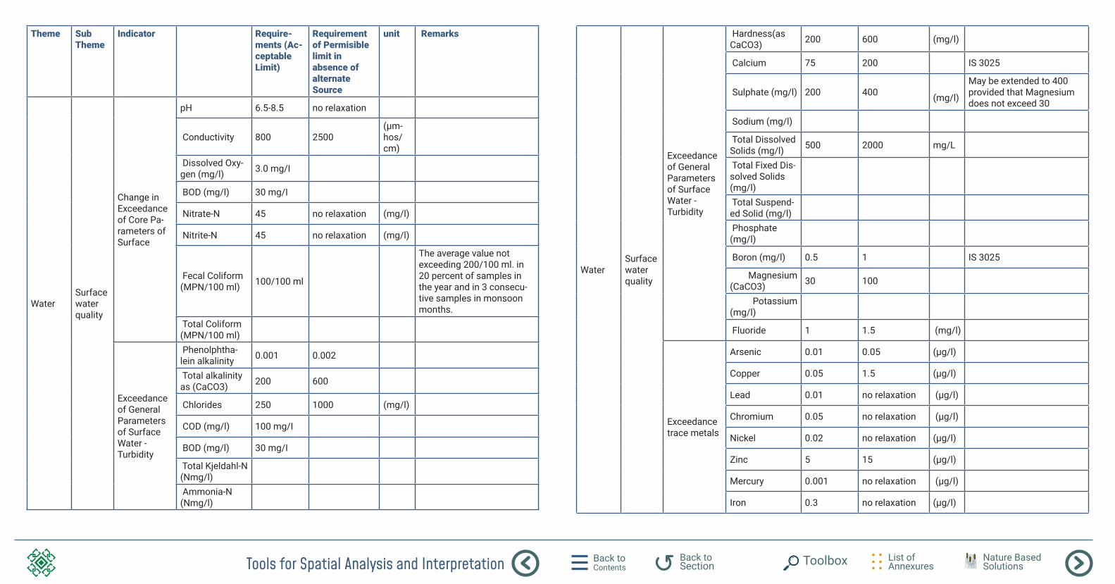
Tools for Spatial Analysis and Interpretation Back to Contents
List of Annexures
Back to Section Toolbox Nature Based
Solutions
Theme Sub Theme
Indicator Require-ments (Ac-ceptable Limit)
Requirement of Permisible limit in absence of alternate Source
unit Remarks
WaterSurface water quality
Change in Exceedance of Core Pa-rameters of Surface
pH 6.5-8.5 no relaxation
Conductivity 800 2500(μm-hos/cm)
Dissolved Oxy-gen (mg/l) 3.0 mg/I
BOD (mg/l) 30 mg/I
Nitrate-N 45 no relaxation (mg/l)
Nitrite-N 45 no relaxation (mg/l)
Fecal Coliform (MPN/100 ml) 100/100 ml
The average value not exceeding 200/100 ml. in 20 percent of samples in the year and in 3 consecu-tive samples in monsoon months.
Total Coliform (MPN/100 ml)
Exceedance of General Parameters of Surface Water - Turbidity
Phenolphtha-lein alkalinity 0.001 0.002
Total alkalinity as (CaCO3) 200 600
Chlorides 250 1000 (mg/l)
COD (mg/l) 100 mg/I
BOD (mg/l) 30 mg/I
Total Kjeldahl-N (Nmg/l) Ammonia-N (Nmg/l)
WaterSurface water quality
Exceedance of General Parameters of Surface Water - Turbidity
Hardness(as CaCO3) 200 600 (mg/l)
Calcium 75 200 IS 3025
Sulphate (mg/l) 200 400 (mg/l)
May be extended to 400 provided that Magnesium does not exceed 30
Sodium (mg/l)
Total Dissolved Solids (mg/l) 500 2000 mg/L
Total Fixed Dis-solved Solids (mg/l) Total Suspend-ed Solid (mg/l) Phosphate (mg/l)
Boron (mg/l) 0.5 1 IS 3025
Magnesium (CaCO3) 30 100
Potassium (mg/l)
Fluoride 1 1.5 (mg/l)
Exceedance trace metals
Arsenic 0.01 0.05 (μg/l)
Copper 0.05 1.5 (μg/l)
Lead 0.01 no relaxation (μg/l)
Chromium 0.05 no relaxation (μg/l)
Nickel 0.02 no relaxation (μg/l)
Zinc 5 15 (μg/l)
Mercury 0.001 no relaxation (μg/l)
Iron 0.3 no relaxation (μg/l)
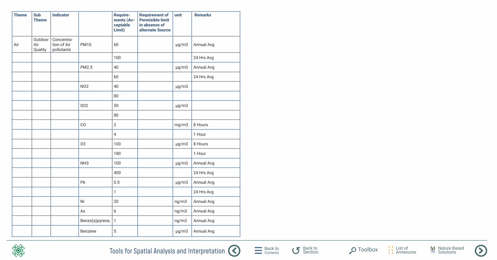
Tools for Spatial Analysis and Interpretation Back to Contents
List of Annexures
Back to Section Toolbox Nature Based
Solutions
Theme Sub Theme
Indicator Require-ments (Ac-ceptable Limit)
Requirement of Permisible limit in absence of alternate Source
unit Remarks
AirOutdoor Air Quality
Concentra-tion of Air pollutants
PM10 60 µg/m3 Annual Avg
100 24 Hrs Avg
PM2.5 40 µg/m3 Annual Avg
60 24 Hrs Avg
NO2 40 µg/m3
80
SO2 50 µg/m3
80
CO 2 mg/m3 8 Hours
4 1 Hour
O3 100 µg/m3 8 Hours
180 1 Hour
NH3 100 µg/m3 Annual Avg
400 24 Hrs Avg
Pb 0.5 µg/m3 Annual Avg
1 24 Hrs Avg
Ni 20 ng/m3 Annual Avg
As 6 ng/m3 Annual Avg
Benzo(a)pyrene, 1 ng/m3 Annual Avg
Benzene 5 µg/m3 Annual Avg
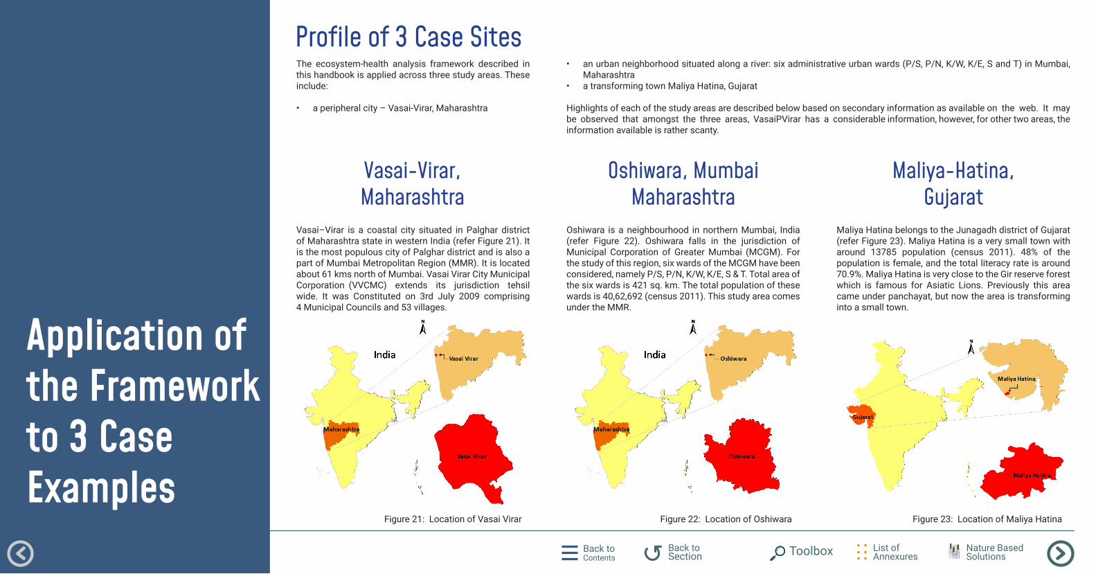
Back to Contents
List of Annexures
Back to Section Toolbox Nature Based
Solutions
Application of the Framework to 3 Case Examples
Profile of 3 Case Sites
Vasai-Virar,Maharashtra
The ecosystem-health analysis framework described in this handbook is applied across three study areas. These include: • a peripheral city – Vasai-Virar, Maharashtra
Vasai–Virar is a coastal city situated in Palghar district of Maharashtra state in western India (refer Figure 21). It is the most populous city of Palghar district and is also a part of Mumbai Metropolitan Region (MMR). It is located about 61 kms north of Mumbai. Vasai Virar City Municipal Corporation (VVCMC) extends its jurisdiction tehsil wide. It was Constituted on 3rd July 2009 comprising 4 Municipal Councils and 53 villages.
Figure 21: Location of Vasai Virar
Oshiwara, MumbaiMaharashtra
Maliya-Hatina,Gujarat
Oshiwara is a neighbourhood in northern Mumbai, India (refer Figure 22). Oshiwara falls in the jurisdiction of Municipal Corporation of Greater Mumbai (MCGM). For the study of this region, six wards of the MCGM have been considered, namely P/S, P/N, K/W, K/E, S & T. Total area of the six wards is 421 sq. km. The total population of these wards is 40,62,692 (census 2011). This study area comes under the MMR.
Maliya Hatina belongs to the Junagadh district of Gujarat (refer Figure 23). Maliya Hatina is a very small town with around 13785 population (census 2011). 48% of the population is female, and the total literacy rate is around 70.9%. Maliya Hatina is very close to the Gir reserve forest which is famous for Asiatic Lions. Previously this area came under panchayat, but now the area is transforming into a small town.
• an urban neighborhood situated along a river: six administrative urban wards (P/S, P/N, K/W, K/E, S and T) in Mumbai, Maharashtra
• a transforming town Maliya Hatina, Gujarat
Highlights of each of the study areas are described below based on secondary information as available on the web. It may be observed that amongst the three areas, VasaiPVirar has a considerable information, however, for other two areas, the information available is rather scanty.
Figure 22: Location of Oshiwara Figure 23: Location of Maliya Hatina
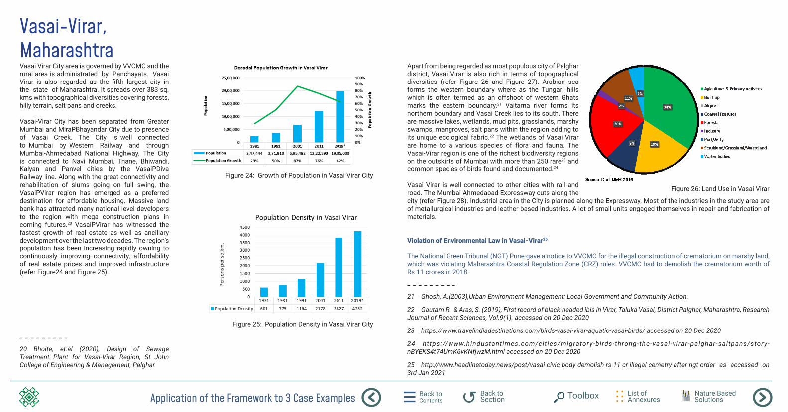
Application of the Framework to 3 Case Examples Back to Contents
List of Annexures
Back to Section Toolbox Nature Based
Solutions
Vasai Virar City area is governed by VVCMC and the rural area is administrated by Panchayats. Vasai Virar is also regarded as the fifth largest city in the state of Maharashtra. It spreads over 383 sq. kms with topographical diversities covering forests, hilly terrain, salt pans and creeks.
Vasai-Virar City has been separated from Greater Mumbai and MiraPBhayandar City due to presence of Vasai Creek. The City is well connected to Mumbai by Western Railway and through Mumbai-Ahmedabad National Highway. The City is connected to Navi Mumbai, Thane, Bhiwandi, Kalyan and Panvel cities by the VasaiPDiva Railway line. Along with the great connectivity and rehabilitation of slums going on full swing, the VasaiPVirar region has emerged as a preferred destination for affordable housing. Massive land bank has attracted many national level developers to the region with mega construction plans in coming futures.20 VasaiPVirar has witnessed the fastest growth of real estate as well as ancillary development over the last two decades. The region’s population has been increasing rapidly owning to continuously improving connectivity, affordability of real estate prices and improved infrastructure (refer Figure24 and Figure 25).
20 Bhoite, et.al (2020), Design of Sewage Treatment Plant for Vasai-Virar Region, St John College of Engineering & Management, Palghar.
Vasai-Virar,Maharashtra
Figure 24: Growth of Population in Vasai Virar City
Figure 25: Population Density in Vasai Virar City
Apart from being regarded as most populous city of Palghar district, Vasai Virar is also rich in terms of topographical diversities (refer Figure 26 and Figure 27). Arabian sea forms the western boundary where as the Tungari hills which is often termed as an offshoot of western Ghats marks the eastern boundary.21 Vaitarna river forms its northern boundary and Vasai Creek lies to its south. There are massive lakes, wetlands, mud pits, grasslands, marshy swamps, mangroves, salt pans within the region adding to its unique ecological fabric.22 The wetlands of Vasai Virar are home to a various species of flora and fauna. The Vasai-Virar region is one of the richest biodiversity regions on the outskirts of Mumbai with more than 250 rare23 and common species of birds found and documented.24
Vasai Virar is well connected to other cities with rail and road. The Mumbai-Ahmedabad Expressway cuts along the city (refer Figure 28). Industrial area in the City is planned along the Expressway. Most of the industries in the study area are of metallurgical industries and leather-based industries. A lot of small units engaged themselves in repair and fabrication of materials.
Violation of Environmental Law in Vasai-Virar25
The National Green Tribunal (NGT) Pune gave a notice to VVCMC for the illegal construction of crematorium on marshy land, which was violating Maharashtra Coastal Regulation Zone (CRZ) rules. VVCMC had to demolish the crematorium worth of Rs 11 crores in 2018.
21 Ghosh, A.(2003),Urban Environment Management: Local Government and Community Action.
22 Gautam R. & Aras, S. (2019), First record of black-headed ibis in Virar, Taluka Vasai, District Palghar, Maharashtra, Research Journal of Recent Sciences, Vol.9(1). accessed on 20 Dec 2020
23 https://www.travelindiadestinations.com/birds-vasai-virar-aquatic-vasai-birds/ accessed on 20 Dec 2020
24 https://www.hindustantimes.com/cities/migratory-birds-throng-the-vasai-virar-palghar-saltpans/story-nBYEKS4t74UmK6vKNfjwzM.html accessed on 20 Dec 2020
25 http://www.headlinetoday.news/post/vasai-civic-body-demolish-rs-11-cr-illegal-cemetry-after-ngt-order as accessed on 3rd Jan 2021
Figure 26: Land Use in Vasai Virar
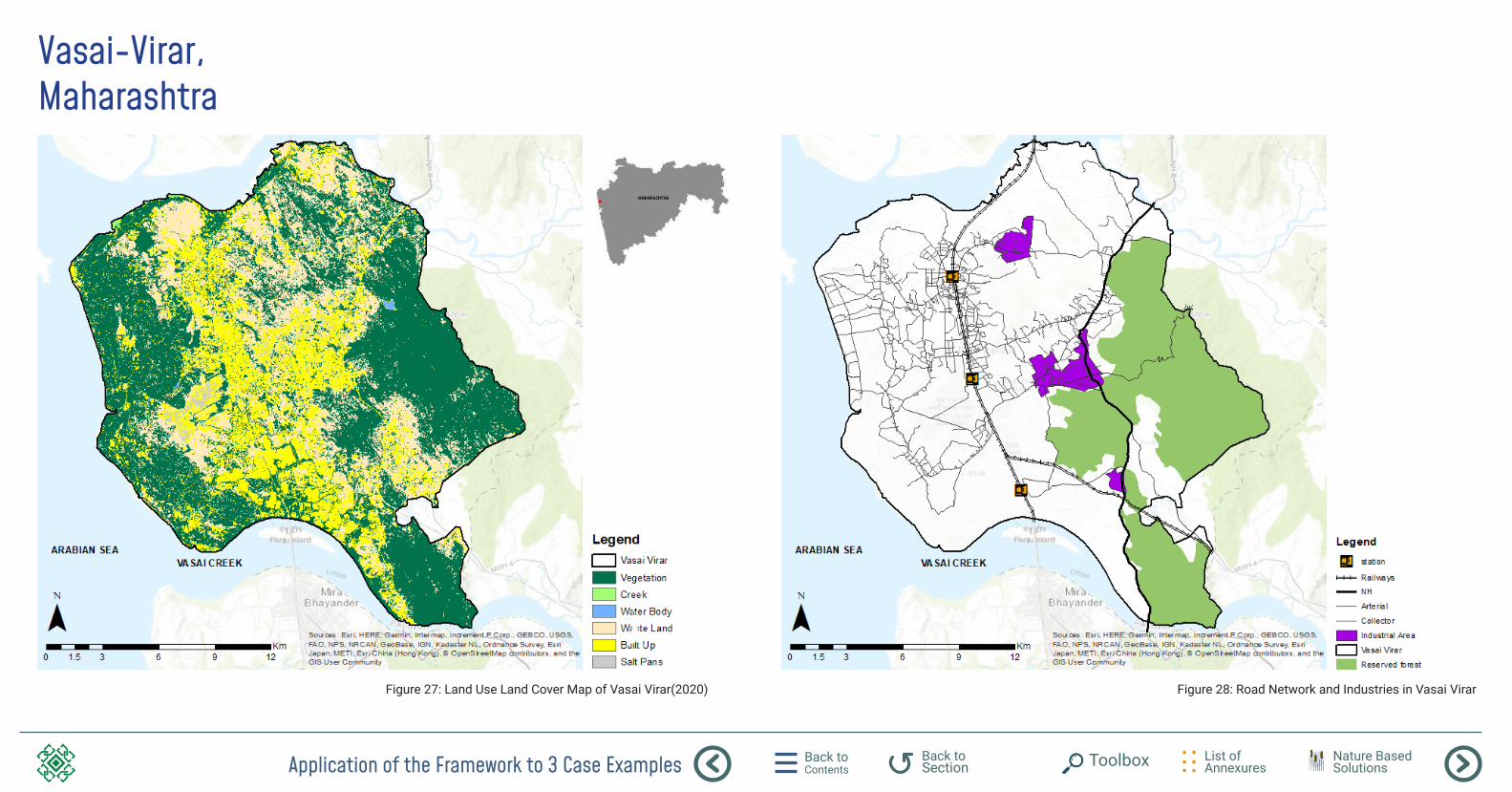
Application of the Framework to 3 Case Examples Back to Contents
List of Annexures
Back to Section Toolbox Nature Based
Solutions
Figure 27: Land Use Land Cover Map of Vasai Virar(2020)
Vasai-Virar,Maharashtra
Figure 28: Road Network and Industries in Vasai Virar
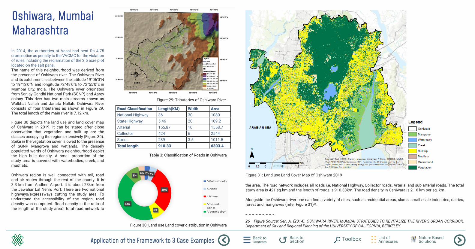
Application of the Framework to 3 Case Examples Back to Contents
List of Annexures
Back to Section Toolbox Nature Based
Solutions
In 2014, the authorities at Vasai had sent Rs 4.75 crore notice as penalty to the VVCMC for the violation of rules including the reclamation of the 2.5 acre plot located on the salt pans.The name of this neighbourhood was derived from the presence of Oshiwara river. The Oshiwara River and its catchment lies between the latitude 19°06′0″N to 19°12′0″N and longitude 72°48′0″E to 72°55′0″E in Mumbai City, India. The Oshiwara River originates from Sanjay Gandhi National Park (SGNP) and Aarey colony. This river has two main streams known as Walbhat Nallah and Janata Nallah. Oshiwara River consists of four tributaries as shown in Figure 29. The total length of the main river is 7.12 km.
Figure 30 depicts the land use and land cover map of Oshiwara in 2019. It can be stated after close observation that vegetation and built up are the classes occupying the region extensively (Figure 30). Spike in the vegetation cover is owed to the presence of SGNP, Mangrove and wetlands. The densely populated wards of Oshiwara neighbourhood depict the high built density. A small proportion of the study area is covered with waterbodies, creek, and mudflats.
Oshiwara region is well connected with rail, road and air routes through the rest of the county. It is 3.3 km from Andheri Airport. It is about 23km from the Jawahar Lal Nehru Port. There are two national highways/expressways cutting the study area. To understand the accessibility of the region, road density was computed. Road density is the ratio of the length of the study area’s total road network to
Oshiwara, MumbaiMaharashtra
Figure 29: Tributaries of Oshiwara River
Figure 30: Land use Land cover distribution in Oshiwara
Table 3: Classification of Roads in Oshiwara
Road Classification Length(KM) Width AreaNational Highway 36 30 1080State Highway 5.46 20 109.2Arterial 155.87 10 1558.7Collector 424 6 2544Street 289 3.5 1011.5Total length 910.33 6303.4
Figure 31: Land use Land Cover Map of Oshiwara 2019
the area. The road network includes all roads i.e. National Highway, Collector roads, Arterial and sub arterial roads. The total study area is 421 sq.km and the length of roads is 910.33km. The road density in Oshiwara is 2.16 km per sq. km.
Alongside the Oshiwara river one can find a variety of sites, such as residential areas, slums, small scale industries, dairies, forest and mangroves (refer Figure 31)26.
26 Figure Source: Sen, A. (2014). OSHIWARA RIVER, MUMBAI STRATEGIES TO REVITALIZE THE RIVER’S URBAN CORRIDOR, Department of City and Regional Planning of the UNIVERSITY OF CALIFORNIA, BERKELEY
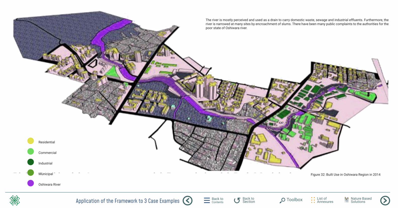
Application of the Framework to 3 Case Examples Back to Contents
List of Annexures
Back to Section Toolbox Nature Based
Solutions
The river is mostly perceived and used as a drain to carry domestic waste, sewage and industrial effluents. Furthermore, the river is narrowed at many sites by encroachment of slums. There have been many public complaints to the authorities for the poor state of Oshiwara river.
Residential
Commercial
Industrial
Municipal
Oshiwara River
Figure 32: Built Use in Oshiwara Region in 2014
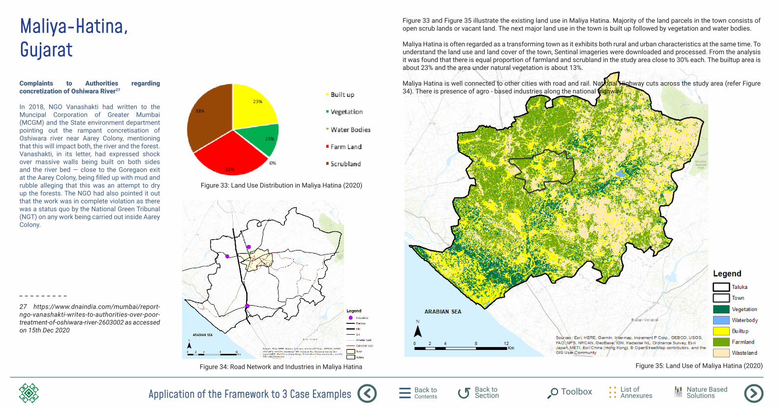
Application of the Framework to 3 Case Examples Back to Contents
List of Annexures
Back to Section Toolbox Nature Based
Solutions
Complaints to Authorities regarding concretization of Oshiwara River27
In 2018, NGO Vanashakti had written to the Muncipal Corporation of Greater Mumbai (MCGM) and the State environment department pointing out the rampant concretisation of Oshiwara river near Aarey Colony, mentioning that this will impact both, the river and the forest. Vanashakti, in its letter, had expressed shock over massive walls being built on both sides and the river bed — close to the Goregaon exit at the Aarey Colony, being filled up with mud and rubble alleging that this was an attempt to dry up the forests. The NGO had also pointed it out that the work was in complete violation as there was a status quo by the National Green Tribunal (NGT) on any work being carried out inside Aarey Colony.
27 https://www.dnaindia.com/mumbai/report-ngo-vanashakti-writes-to-authorities-over-poor-treatment-of-oshiwara-river-2603002 as accessed on 15th Dec 2020
Maliya-Hatina,Gujarat
Figure 33: Land Use Distribution in Maliya Hatina (2020)
Figure 34: Road Network and Industries in Maliya Hatina Figure 35: Land Use of Maliya Hatina (2020)
Figure 33 and Figure 35 illustrate the existing land use in Maliya Hatina. Majority of the land parcels in the town consists of open scrub lands or vacant land. The next major land use in the town is built up followed by vegetation and water bodies.
Maliya Hatina is often regarded as a transforming town as it exhibits both rural and urban characteristics at the same time. To understand the land use and land cover of the town, Sentinal imageries were downloaded and processed. From the analysis it was found that there is equal proportion of farmland and scrubland in the study area close to 30% each. The builtup area is about 23% and the area under natural vegetation is about 13%.
Maliya Hatina is well connected to other cities with road and rail. National Highway cuts across the study area (refer Figure 34). There is presence of agro - based industries along the national highway.
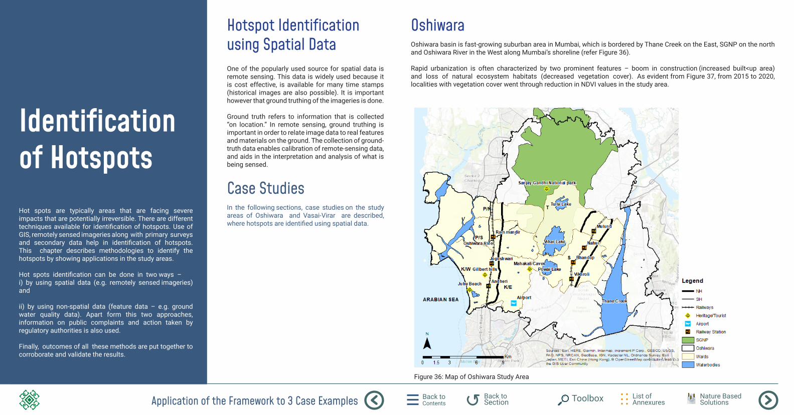
Application of the Framework to 3 Case Examples Back to Contents
List of Annexures
Back to Section Toolbox Nature Based
Solutions
Identification of HotspotsHot spots are typically areas that are facing severe impacts that are potentially irreversible. There are different techniques available for identification of hotspots. Use of GIS, remotely sensed imageries along with primary surveys and secondary data help in identification of hotspots. This chapter describes methodologies to identify the hotspots by showing applications in the study areas. Hot spots identification can be done in two ways – i) by using spatial data (e.g. remotely sensed imageries) and
ii) by using non-spatial data (feature data – e.g. ground water quality data). Apart form this two approaches, information on public complaints and action taken by regulatory authorities is also used.
Finally, outcomes of all these methods are put together to corroborate and validate the results.
Case StudiesIn the following sections, case studies on the study areas of Oshiwara and Vasai-Virar are described, where hotspots are identified using spatial data.
Figure 36: Map of Oshiwara Study Area
OshiwaraOshiwara basin is fast-growing suburban area in Mumbai, which is bordered by Thane Creek on the East, SGNP on the north and Oshiwara River in the West along Mumbai’s shoreline (refer Figure 36).
Rapid urbanization is often characterized by two prominent features – boom in construction (increased built<up area) and loss of natural ecosystem habitats (decreased vegetation cover). As evident from Figure 37, from 2015 to 2020, localities with vegetation cover went through reduction in NDVI values in the study area.
Hotspot Identification using Spatial DataOne of the popularly used source for spatial data is remote sensing. This data is widely used because it is cost effective, is available for many time stamps (historical images are also possible). It is important however that ground truthing of the imageries is done. Ground truth refers to information that is collected “on location.” In remote sensing, ground truthing is important in order to relate image data to real features and materials on the ground. The collection of ground-truth data enables calibration of remote-sensing data, and aids in the interpretation and analysis of what is being sensed.
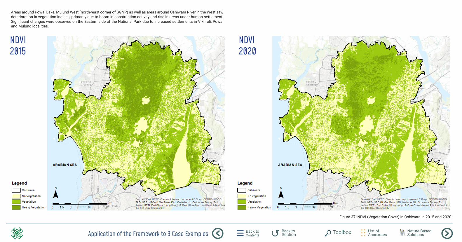
Application of the Framework to 3 Case Examples Back to Contents
List of Annexures
Back to Section Toolbox Nature Based
Solutions
NDVI 2015
NDVI 2020
Figure 37: NDVI (Vegetation Cover) in Oshiwara in 2015 and 2020
Areas around Powai Lake, Mulund West (north<east corner of SGNP) as well as areas around Oshiwara River in the West saw deterioration in vegetation indices, primarily due to boom in construction activity and rise in areas under human settlement. Significant changes were observed on the Eastern side of the National Park due to increased settlements in Vikhroli, Powai and Mulund localities.
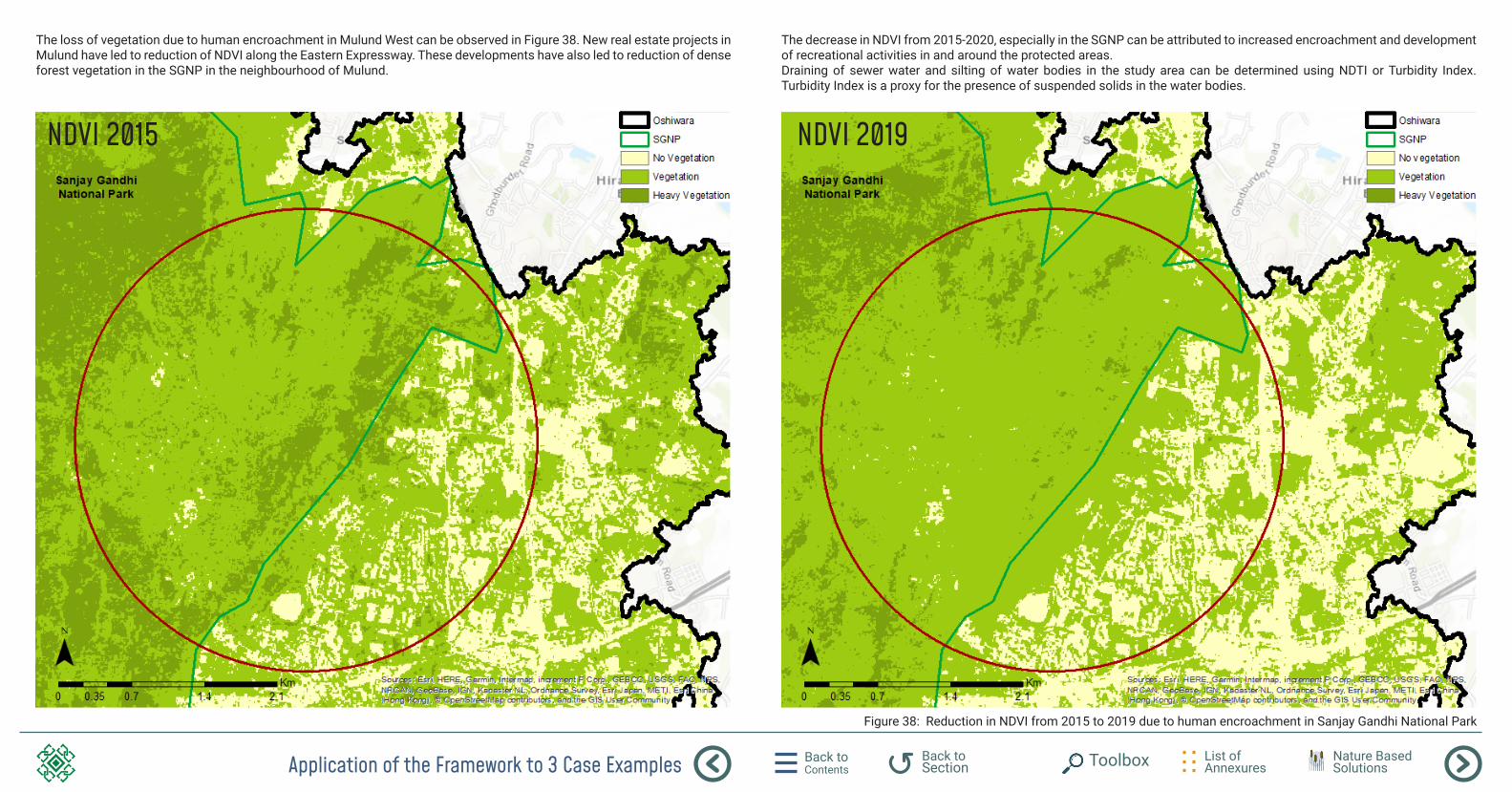
Application of the Framework to 3 Case Examples Back to Contents
List of Annexures
Back to Section Toolbox Nature Based
Solutions
NDVI 2015 NDVI 2019
Figure 38: Reduction in NDVI from 2015 to 2019 due to human encroachment in Sanjay Gandhi National Park
The loss of vegetation due to human encroachment in Mulund West can be observed in Figure 38. New real estate projects in Mulund have led to reduction of NDVI along the Eastern Expressway. These developments have also led to reduction of dense forest vegetation in the SGNP in the neighbourhood of Mulund.
The decrease in NDVI from 2015-2020, especially in the SGNP can be attributed to increased encroachment and development of recreational activities in and around the protected areas. Draining of sewer water and silting of water bodies in the study area can be determined using NDTI or Turbidity Index. Turbidity Index is a proxy for the presence of suspended solids in the water bodies.
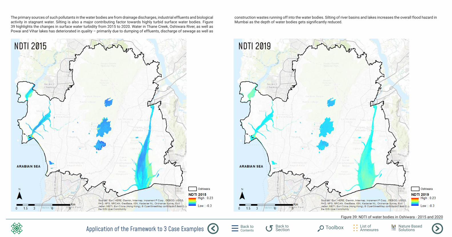
Application of the Framework to 3 Case Examples Back to Contents
List of Annexures
Back to Section Toolbox Nature Based
Solutions
The primary sources of such pollutants in the water bodies are from drainage discharges, industrial effluents and biological activity in stagnant water. Silting is also a major contributing factor towards highly turbid surface water bodies. Figure 39 highlights the changes in surface water turbidity from 2015 to 2020. Water in Thane Creek, Oshiwara River, as well as Powai and Vihar lakes has deteriorated in quality – primarily due to dumping of effluents, discharge of sewage as well as
construction wastes running off into the water bodies. Silting of river basins and lakes increases the overall flood hazard in Mumbai as the depth of water bodies gets significantly reduced.
Figure 39: NDTI of water bodies in Oshiwara - 2015 and 2020
NDTI 2015 NDTI 2019
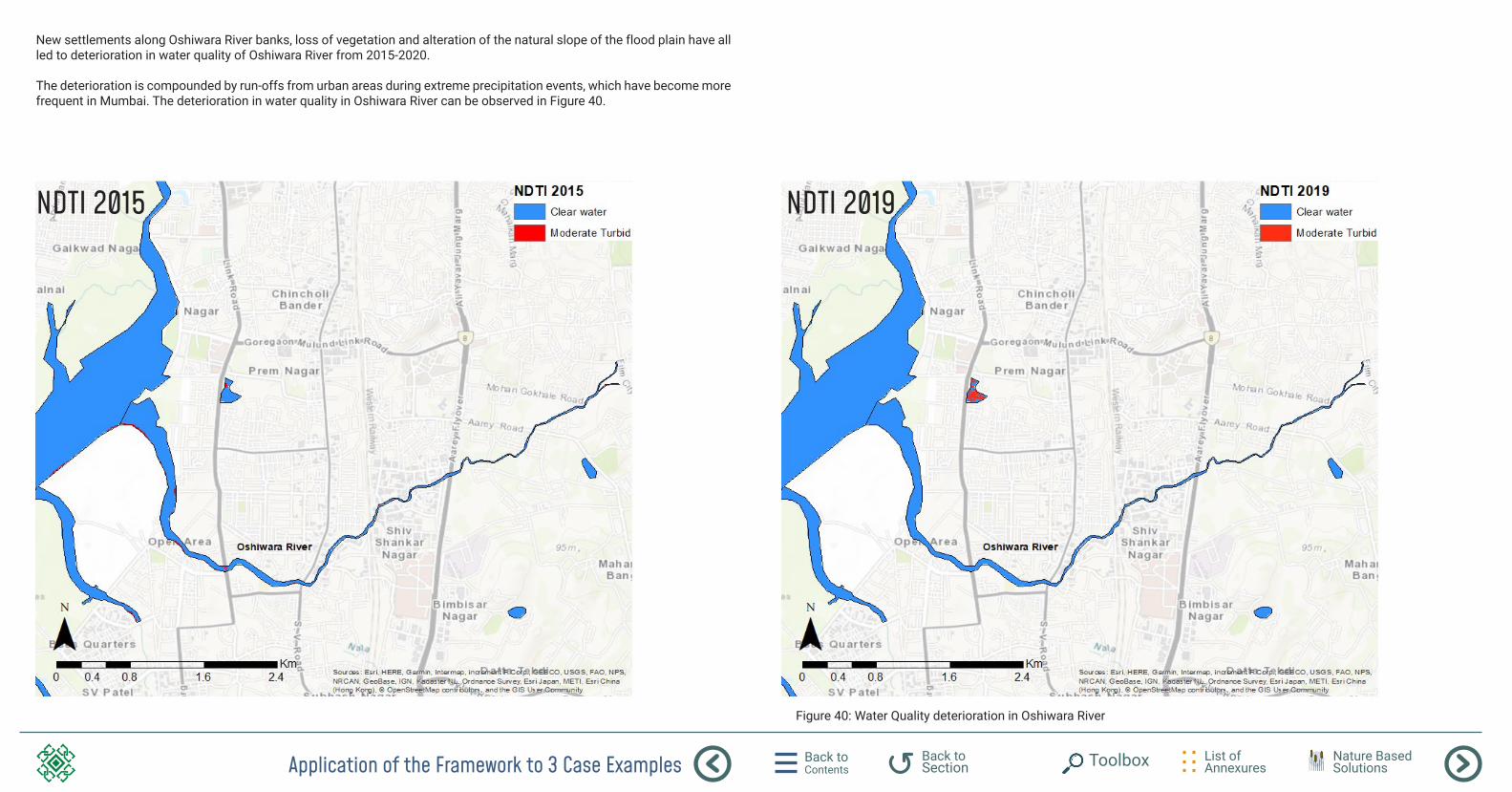
Application of the Framework to 3 Case Examples Back to Contents
List of Annexures
Back to Section Toolbox Nature Based
Solutions
New settlements along Oshiwara River banks, loss of vegetation and alteration of the natural slope of the flood plain have all led to deterioration in water quality of Oshiwara River from 2015-2020.
The deterioration is compounded by run-offs from urban areas during extreme precipitation events, which have become more frequent in Mumbai. The deterioration in water quality in Oshiwara River can be observed in Figure 40.
Figure 40: Water Quality deterioration in Oshiwara River
NDTI 2015 NDTI 2019
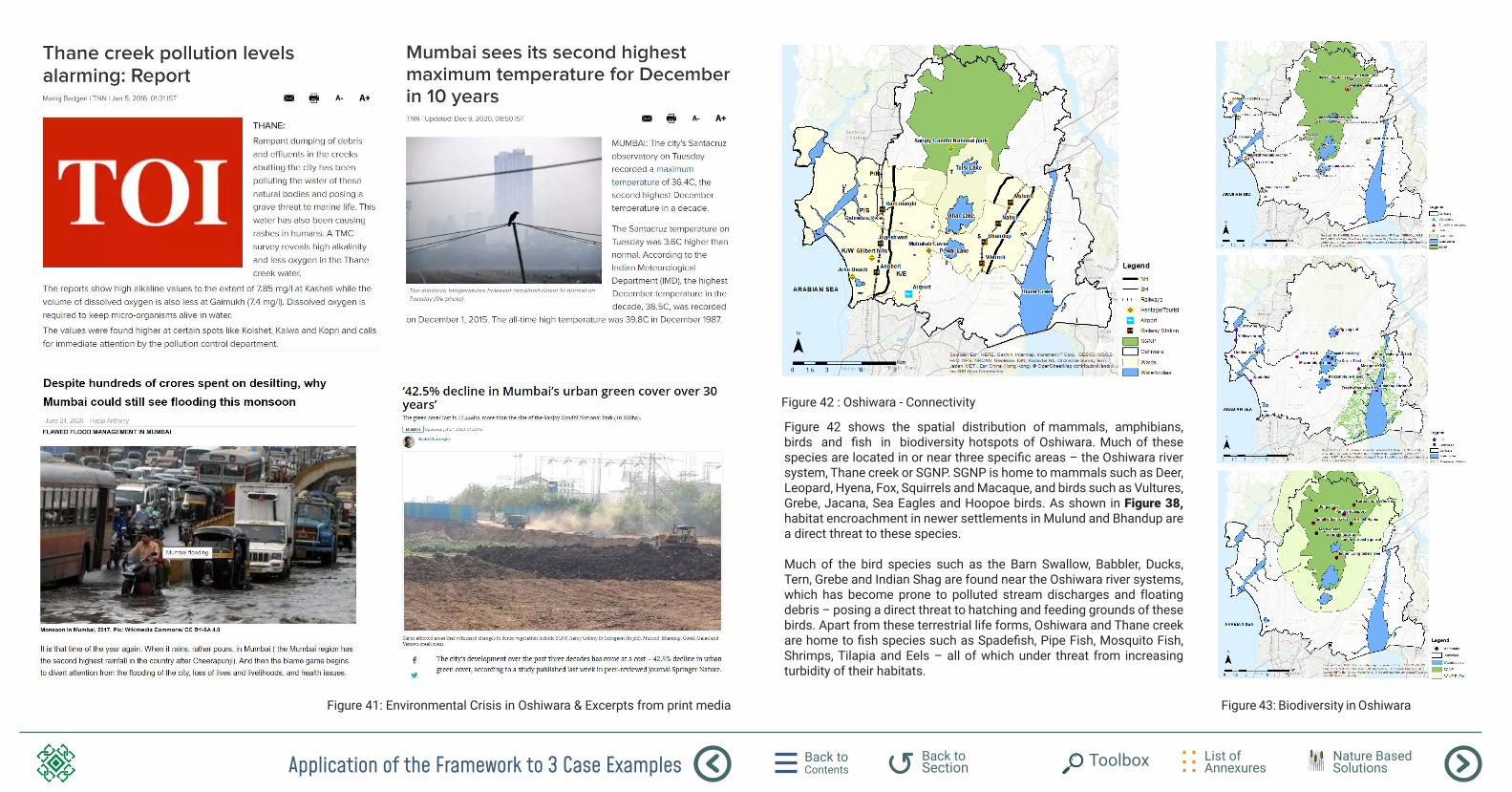
Application of the Framework to 3 Case Examples Back to Contents
List of Annexures
Back to Section Toolbox Nature Based
Solutions
Figure 41: Environmental Crisis in Oshiwara & Excerpts from print media Figure 43: Biodiversity in Oshiwara
Figure 42 : Oshiwara - Connectivity
Figure 42 shows the spatial distribution of mammals, amphibians, birds and fish in biodiversity hotspots of Oshiwara. Much of these species are located in or near three specific areas – the Oshiwara river system, Thane creek or SGNP. SGNP is home to mammals such as Deer, Leopard, Hyena, Fox, Squirrels and Macaque, and birds such as Vultures, Grebe, Jacana, Sea Eagles and Hoopoe birds. As shown in Figure 38, habitat encroachment in newer settlements in Mulund and Bhandup are a direct threat to these species. Much of the bird species such as the Barn Swallow, Babbler, Ducks, Tern, Grebe and Indian Shag are found near the Oshiwara river systems, which has become prone to polluted stream discharges and floating debris – posing a direct threat to hatching and feeding grounds of these birds. Apart from these terrestrial life forms, Oshiwara and Thane creek are home to fish species such as Spadefish, Pipe Fish, Mosquito Fish, Shrimps, Tilapia and Eels – all of which under threat from increasing turbidity of their habitats.
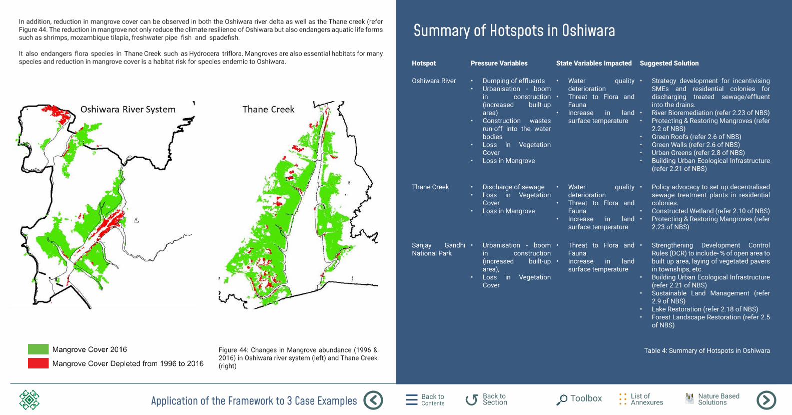
Application of the Framework to 3 Case Examples Back to Contents
List of Annexures
Back to Section Toolbox Nature Based
Solutions
Figure 44: Changes in Mangrove abundance (1996 & 2016) in Oshiwara river system (left) and Thane Creek (right)
Summary of Hotspots in Oshiwara
Hotspot Pressure Variables State Variables Impacted Suggested Solution
Oshiwara River • Dumping of effluents• Urbanisation - boom
in construction (increased built-up area)
• Construction wastes run-off into the water bodies
• Loss in Vegetation Cover
• Loss in Mangrove
• Water quality deterioration
• Threat to Flora and Fauna
• Increase in land surface temperature
• Strategy development for incentivising SMEs and residential colonies for discharging treated sewage/effluent into the drains.
• River Bioremediation (refer 2.23 of NBS)• Protecting & Restoring Mangroves (refer
2.2 of NBS)• Green Roofs (refer 2.6 of NBS)• Green Walls (refer 2.6 of NBS)• Urban Greens (refer 2.8 of NBS)• Building Urban Ecological Infrastructure
(refer 2.21 of NBS)
Thane Creek • Discharge of sewage• Loss in Vegetation
Cover• Loss in Mangrove
• Water quality deterioration
• Threat to Flora and Fauna
• Increase in land surface temperature
• Policy advocacy to set up decentralised sewage treatment plants in residential colonies.
• Constructed Wetland (refer 2.10 of NBS)• Protecting & Restoring Mangroves (refer
2.23 of NBS)
Sanjay Gandhi National Park
• Urbanisation - boom in construction (increased built-up area),
• Loss in Vegetation Cover
• Threat to Flora and Fauna
• Increase in land surface temperature
• Strengthening Development Control Rules (DCR) to include- % of open area to built up area, laying of vegetated pavers in townships, etc.
• Building Urban Ecological Infrastructure (refer 2.21 of NBS)
• Sustainable Land Management (refer 2.9 of NBS)
• Lake Restoration (refer 2.18 of NBS)• Forest Landscape Restoration (refer 2.5
of NBS)
Table 4: Summary of Hotspots in Oshiwara
In addition, reduction in mangrove cover can be observed in both the Oshiwara river delta as well as the Thane creek (refer Figure 44. The reduction in mangrove not only reduce the climate resilience of Oshiwara but also endangers aquatic life forms such as shrimps, mozambique tilapia, freshwater pipe fish and spadefish.
It also endangers flora species in Thane Creek such as Hydrocera triflora. Mangroves are also essential habitats for many species and reduction in mangrove cover is a habitat risk for species endemic to Oshiwara.
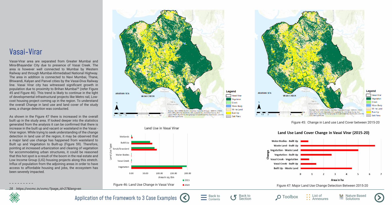
Application of the Framework to 3 Case Examples Back to Contents
List of Annexures
Back to Section Toolbox Nature Based
Solutions
Figure 46: Land Use Change in Vasai Virar
Figure 45: Change in Land use Land Cover between 2015-20
Figure 47: Major Land Use Change Detection Between 2015-20
Vasai-VirarVasai-Virar area are separated from Greater Mumbai and Mira-Bhayandar City due to presence of Vasai Creek. The area is however well connected to Mumbai by Western Railway and through Mumbai-Ahmedabad National Highway. The area in addition is connected to Navi Mumbai, Thane, Bhiwandi, Kalyan and Panvel cities by the Vasai-Diva Railway line. Vasai Virar city has witnessed significant growth in population due to proximity to Brihan Mumbai28 (refer Figure 45 and Figure 46). This trend is likely to continue in the light of developmental infrastructural projects like Metro rail, Low-cost housing project coming up in the region. To understand the overall Change in land use and land cover of the study area, a change detection was conducted. As shown in the Figure 47 there is increased in the overall built up in the study area. If looked deeper into the statistics generated from the analysis it can be confirmed that there is increase in the built up and vacant or wasteland in the Vasai - Virar region. While trying to seek understanding of the change detection in land use of the region, it may be observed that a major land use change has happened from wasteland to Built up and Vegetation to Built-up (Figure 59). Therefore, pointing at increased urbanization and clearing of vegetation for accommodating urban structures, it could be reasoned that this hot spot is a result of the boom in the real estate and Low Income Group (LIG) housing projects along this stretch. Influx of population from the adjoining areas in order to have access to affordable housing and jobs, the ecosystem has been severely impacted.
28 https://vvcmc.in/vvmc/?page_id=27&lang=en
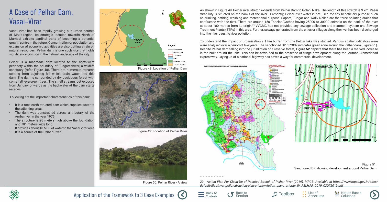
Application of the Framework to 3 Case Examples Back to Contents
List of Annexures
Back to Section Toolbox Nature Based
Solutions
Figure 50: Pelhar River - A view
Figure 49: Location of Pelhar River
Figure 48: Location of Pelhar Dam
Figure 51: Sanctioned DP showing development around Pelhar Dam
A Case of Pelhar Dam, Vasai-VirarVasai Virar has been rapidly growing sub urban centres of MMR region. Its strategic location towards North of Mumbai exhibits cardinal traits of becoming a potential growth centre in the future. Concentration of population and expansion of economic activities are also putting strain on natural resources. Pelhar dam is one such site that holds significance position in the natural landscape of the city.
Pelhar is a manmade dam located to the north-west periphery within the boundary of Tungareshwar, a wildlife sanctuary (refer Figure 48). There are numerous streams coming from adjoining hill which drain water into this dam. The dam is surrounded by dry deciduous forest with some tall, evergreen trees. The small streams get exposed from January onwards as the backwater of the dam starts recedes.
Following are the important characteristics of this dam:
• It is a rock earth structed dam which supplies water to the adjoining areas.
• The dam was constructed across a tributary of the Amba river in the year 1975.
• The structure is 26 meters high above the foundation and 701 meters wide long.
• It provides about 10 MLD of water to the Vasai Virar area• It is a source of the Pelhar River.
As shown in Figure 49, Pelhar river stretch extends from Pelhar Dam to Golani Naka. The length of this stretch is 9 km. Vasai Virar City is situated on the banks of the river. Presently, Pelhar river water is not used for any beneficiary purpose such as drinking, bathing, washing and recreational purpose. Sapora, Tungar and Waliv Nallah are the three polluting drains that confluence with the river. There are around 150 Tabelas/Gothas having 25000 to 30000 animals on the bank of the river at about 100 metres from its origin.29 VVCMC has not provided any sewage collection and treatment system and Sewage Treatment Plants (STPs) in this area. Further, sewage generated from the cities or villages along the river has been discharged into the river causing river pollution.
To understand the impact of urbanization a 1 km buffer from the Pelhar lake was studied. Various spatial indicators were were analysed over a period of five years. The sanctioned DP of 2009 indicates green zone around the Pelhar dam (Figure 51). Despite Pelhar dam falling into the jurisdiction of a reserve forest, Figure 52 depicts that there has been a marked increase in the built around the lake. This can be attributed to the presence of fringe development along the Mumbai Ahmedabad expressway. Laying up of a national highway has paved a way for commercial development.
29 Action Plan For Clean-Up of Polluted Stretch of Pelhar River (2019), MPCB. Available at https://www.mpcb.gov.in/sites/default/files/river-polluted/action-plan-priority/Action_plans_priority_IV_PELHAR_2019_03072019.pdf
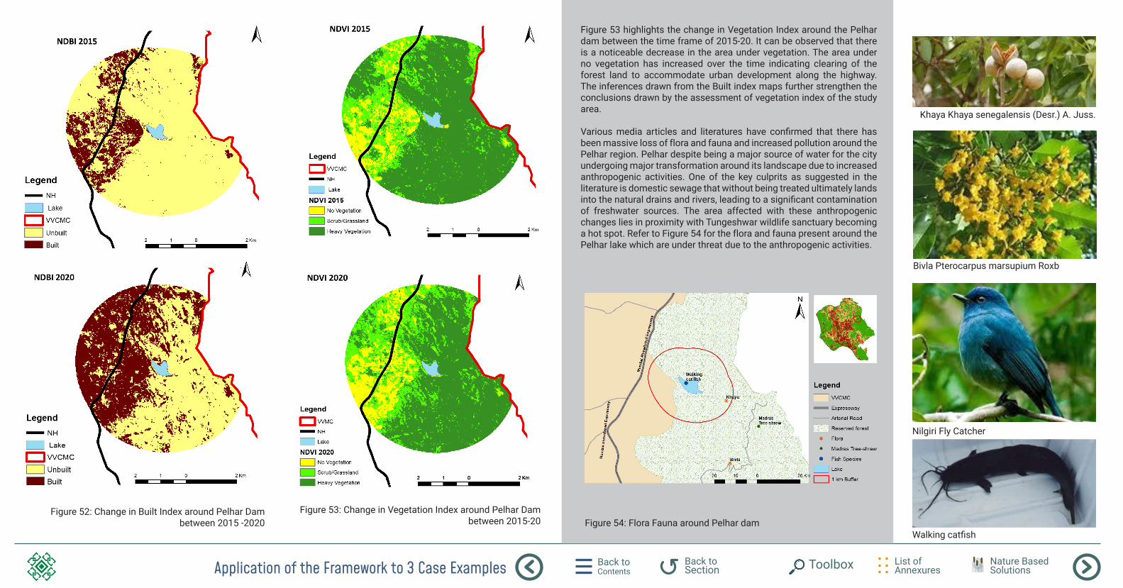
Application of the Framework to 3 Case Examples Back to Contents
List of Annexures
Back to Section Toolbox Nature Based
Solutions
Figure 52: Change in Built Index around Pelhar Dam between 2015 -2020
Figure 53: Change in Vegetation Index around Pelhar Dam between 2015-20
Khaya Khaya senegalensis (Desr.) A. Juss.
Bivla Pterocarpus marsupium Roxb
Nilgiri Fly Catcher
Walking catfishFigure 54: Flora Fauna around Pelhar dam
Figure 53 highlights the change in Vegetation Index around the Pelhar dam between the time frame of 2015-20. It can be observed that there is a noticeable decrease in the area under vegetation. The area under no vegetation has increased over the time indicating clearing of the forest land to accommodate urban development along the highway. The inferences drawn from the Built index maps further strengthen the conclusions drawn by the assessment of vegetation index of the study area.
Various media articles and literatures have confirmed that there has been massive loss of flora and fauna and increased pollution around the Pelhar region. Pelhar despite being a major source of water for the city undergoing major transformation around its landscape due to increased anthropogenic activities. One of the key culprits as suggested in the literature is domestic sewage that without being treated ultimately lands into the natural drains and rivers, leading to a significant contamination of freshwater sources. The area affected with these anthropogenic changes lies in proximity with Tungeshwar wildlife sanctuary becoming a hot spot. Refer to Figure 54 for the flora and fauna present around the Pelhar lake which are under threat due to the anthropogenic activities.
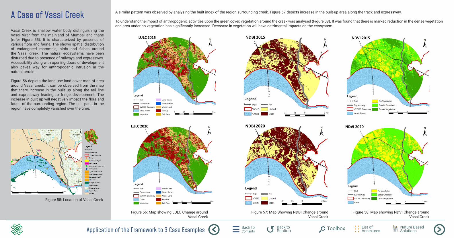
Application of the Framework to 3 Case Examples Back to Contents
List of Annexures
Back to Section Toolbox Nature Based
Solutions
Figure 55: Location of Vasai Creek
Figure 56: Map showing LULC Change around Vasai Creek
Figure 57: Map Showing NDBI Change around Vasai Creek
Figure 58: Map showing NDVI Change around Vasai Creek
A Case of Vasai CreekVasai Creek is shallow water body distinguishing the Vasai Virar from the mainland of Mumbai and thane (refer Figure 55). It is characterized by presence of various flora and fauna. The shows spatial distribution of endangered mammals, birds and fishes around the Vasai creek. The natural ecosystems have been disturbed due to presence of railways and expressway. Accessibility along with opening doors of development also paves way for anthropogenic intrusion in the natural terrain.
Figure 56 depicts the land use land cover map of area around Vasai creek. It can be observed from the map that there increase in the built up along the rail line and expressway leading to fringe development. The increase in built up will negatively impact the flora and fauna of the surrounding region. The salt pans in the region have completely vanished over the time.
A similar pattern was observed by analysing the built index of the region surrounding creek. Figure 57 depicts increase in the built-up area along the track and expressway.
To understand the impact of anthropogenic activities upon the green cover, vegetation around the creek was analysed (Figure 58). It was found that there is marked reduction in the dense vegetation and area under no vegetation has significantly increased. Decrease in vegetation will have detrimental impacts on the ecosystem.
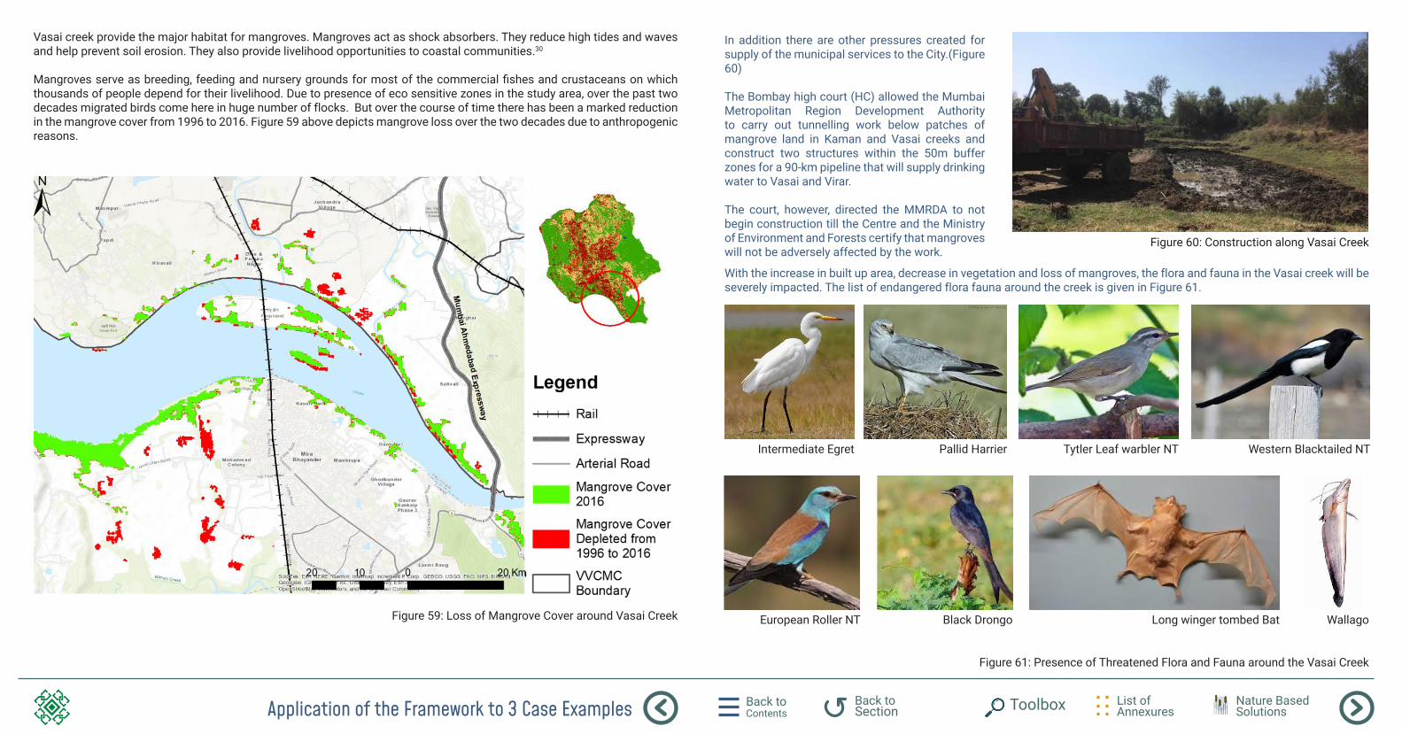
Application of the Framework to 3 Case Examples Back to Contents
List of Annexures
Back to Section Toolbox Nature Based
Solutions
Figure 59: Loss of Mangrove Cover around Vasai Creek
Western Blacktailed NTTytler Leaf warbler NTPallid HarrierIntermediate Egret
WallagoBlack Drongo Long winger tombed BatEuropean Roller NT
Figure 61: Presence of Threatened Flora and Fauna around the Vasai Creek
Figure 60: Construction along Vasai Creek
Vasai creek provide the major habitat for mangroves. Mangroves act as shock absorbers. They reduce high tides and waves and help prevent soil erosion. They also provide livelihood opportunities to coastal communities.30
Mangroves serve as breeding, feeding and nursery grounds for most of the commercial fishes and crustaceans on which thousands of people depend for their livelihood. Due to presence of eco sensitive zones in the study area, over the past two decades migrated birds come here in huge number of flocks. But over the course of time there has been a marked reduction in the mangrove cover from 1996 to 2016. Figure 59 above depicts mangrove loss over the two decades due to anthropogenic reasons.
In addition there are other pressures created for supply of the municipal services to the City.(Figure 60)
The Bombay high court (HC) allowed the Mumbai Metropolitan Region Development Authority to carry out tunnelling work below patches of mangrove land in Kaman and Vasai creeks and construct two structures within the 50m buffer zones for a 90-km pipeline that will supply drinking water to Vasai and Virar.
The court, however, directed the MMRDA to not begin construction till the Centre and the Ministry of Environment and Forests certify that mangroves will not be adversely affected by the work.
With the increase in built up area, decrease in vegetation and loss of mangroves, the flora and fauna in the Vasai creek will be severely impacted. The list of endangered flora fauna around the creek is given in Figure 61.
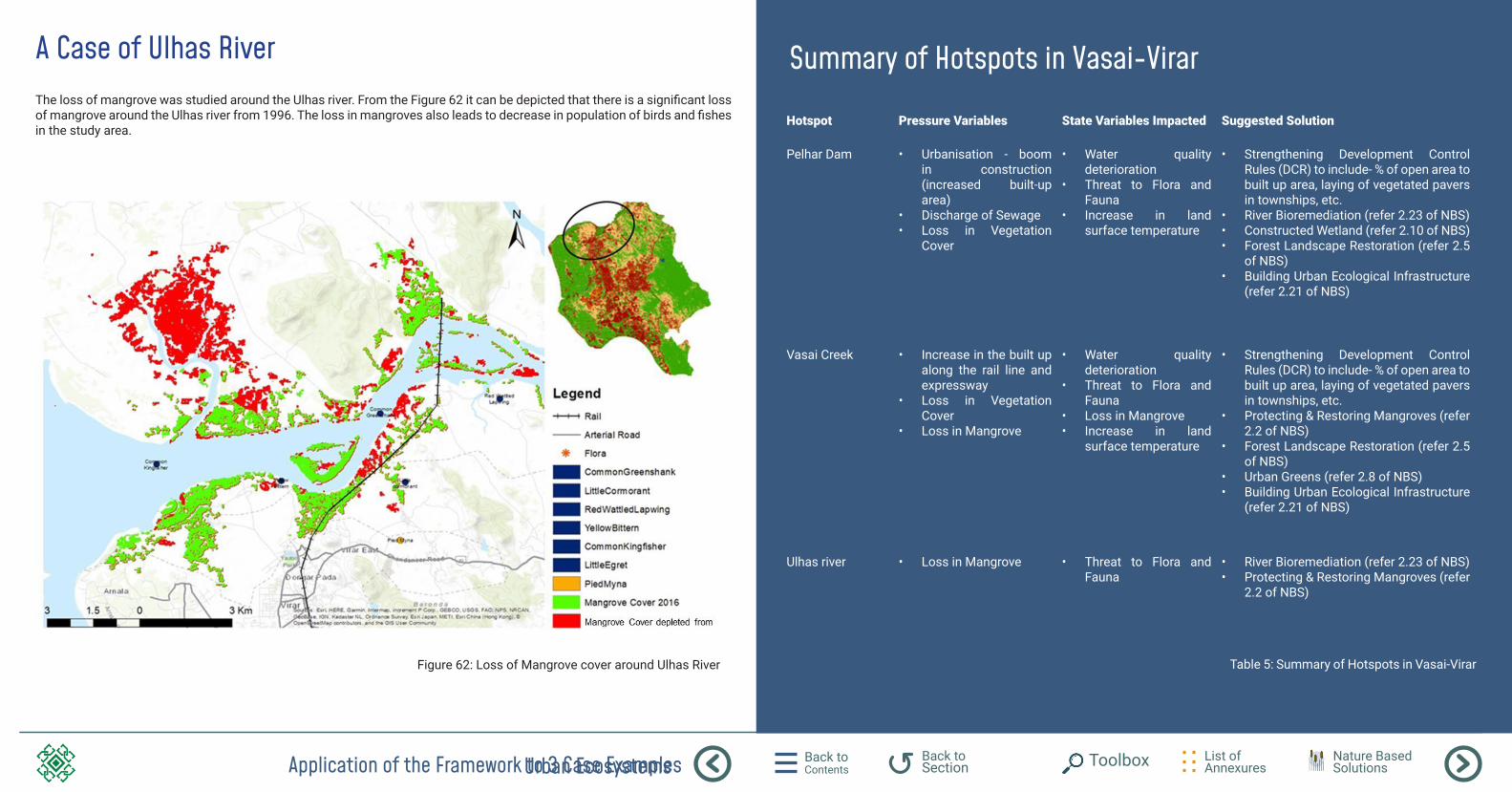
Back to Contents
List of Annexures
Back to SectionUrban Ecosystems Nature Based
SolutionsToolboxApplication of the Framework to 3 Case Examples
Figure 62: Loss of Mangrove cover around Ulhas River
Summary of Hotspots in Vasai-Virar
Hotspot Pressure Variables State Variables Impacted Suggested Solution
Pelhar Dam • Urbanisation - boom in construction (increased built-up area)
• Discharge of Sewage• Loss in Vegetation
Cover
• Water quality deterioration
• Threat to Flora and Fauna
• Increase in land surface temperature
• Strengthening Development Control Rules (DCR) to include- % of open area to built up area, laying of vegetated pavers in townships, etc.
• River Bioremediation (refer 2.23 of NBS)• Constructed Wetland (refer 2.10 of NBS)• Forest Landscape Restoration (refer 2.5
of NBS)• Building Urban Ecological Infrastructure
(refer 2.21 of NBS)
Vasai Creek • Increase in the built up along the rail line and expressway
• Loss in Vegetation Cover
• Loss in Mangrove
• Water quality deterioration
• Threat to Flora and Fauna
• Loss in Mangrove• Increase in land
surface temperature
• Strengthening Development Control Rules (DCR) to include- % of open area to built up area, laying of vegetated pavers in townships, etc.
• Protecting & Restoring Mangroves (refer 2.2 of NBS)
• Forest Landscape Restoration (refer 2.5 of NBS)
• Urban Greens (refer 2.8 of NBS)• Building Urban Ecological Infrastructure
(refer 2.21 of NBS)
Ulhas river • Loss in Mangrove • Threat to Flora and Fauna
• River Bioremediation (refer 2.23 of NBS)• Protecting & Restoring Mangroves (refer
2.2 of NBS)
Table 5: Summary of Hotspots in Vasai-Virar
A Case of Ulhas RiverThe loss of mangrove was studied around the Ulhas river. From the Figure 62 it can be depicted that there is a significant loss of mangrove around the Ulhas river from 1996. The loss in mangroves also leads to decrease in population of birds and fishes in the study area.
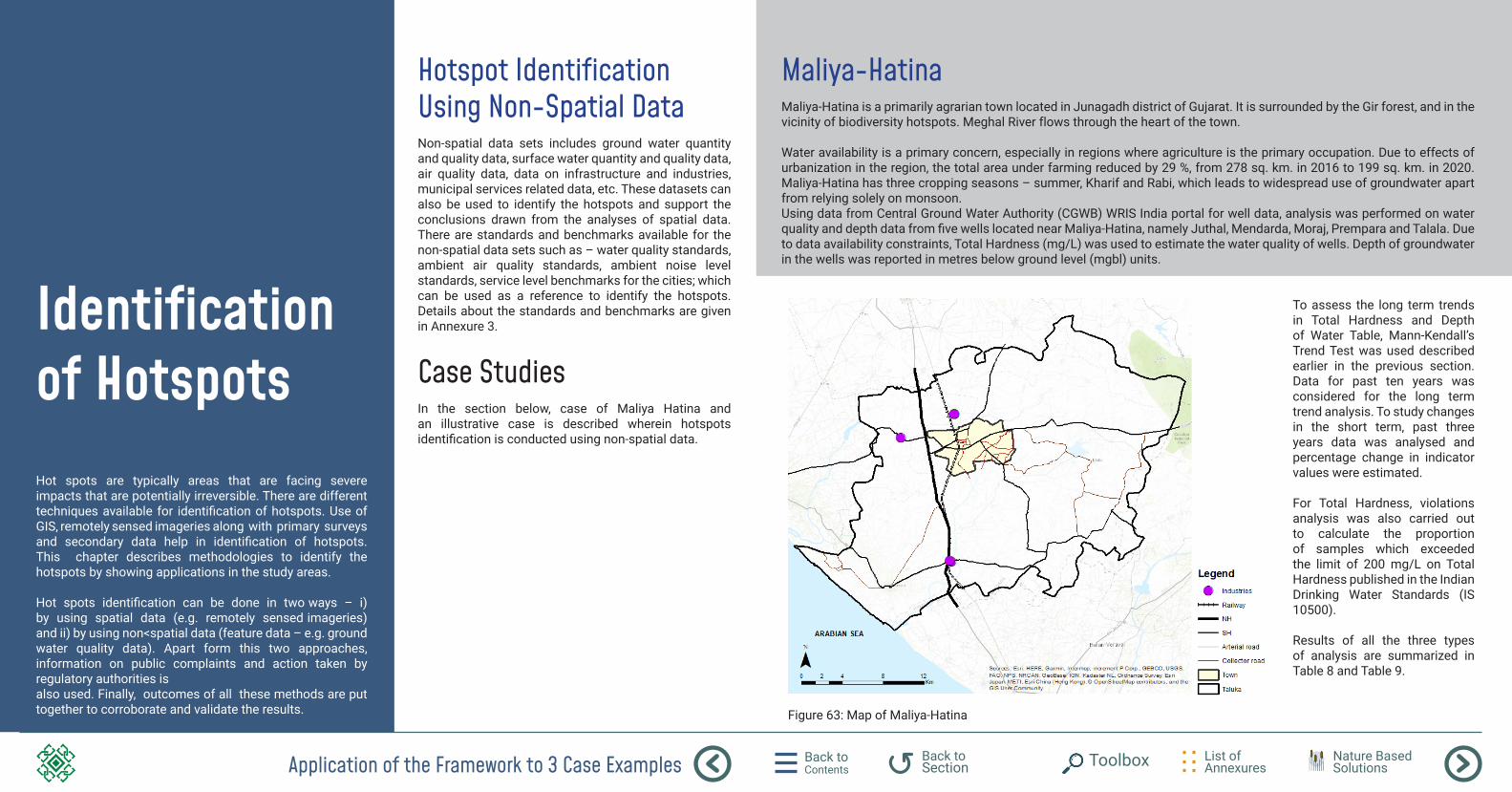
Application of the Framework to 3 Case Examples Back to Contents
List of Annexures
Back to Section Toolbox Nature Based
Solutions
Identification of HotspotsHot spots are typically areas that are facing severe impacts that are potentially irreversible. There are different techniques available for identification of hotspots. Use of GIS, remotely sensed imageries along with primary surveys and secondary data help in identification of hotspots. This chapter describes methodologies to identify the hotspots by showing applications in the study areas. Hot spots identification can be done in two ways – i) by using spatial data (e.g. remotely sensed imageries) and ii) by using non<spatial data (feature data – e.g. ground water quality data). Apart form this two approaches, information on public complaints and action taken by regulatory authorities is also used. Finally, outcomes of all these methods are put together to corroborate and validate the results.
Hotspot Identification Using Non-Spatial DataNon-spatial data sets includes ground water quantity and quality data, surface water quantity and quality data, air quality data, data on infrastructure and industries, municipal services related data, etc. These datasets can also be used to identify the hotspots and support the conclusions drawn from the analyses of spatial data. There are standards and benchmarks available for the non-spatial data sets such as – water quality standards, ambient air quality standards, ambient noise level standards, service level benchmarks for the cities; which can be used as a reference to identify the hotspots. Details about the standards and benchmarks are given in Annexure 3.
Case StudiesIn the section below, case of Maliya Hatina and an illustrative case is described wherein hotspots identification is conducted using non-spatial data.
Maliya-HatinaMaliya-Hatina is a primarily agrarian town located in Junagadh district of Gujarat. It is surrounded by the Gir forest, and in the vicinity of biodiversity hotspots. Meghal River flows through the heart of the town.
Water availability is a primary concern, especially in regions where agriculture is the primary occupation. Due to effects of urbanization in the region, the total area under farming reduced by 29 %, from 278 sq. km. in 2016 to 199 sq. km. in 2020. Maliya-Hatina has three cropping seasons – summer, Kharif and Rabi, which leads to widespread use of groundwater apart from relying solely on monsoon. Using data from Central Ground Water Authority (CGWB) WRIS India portal for well data, analysis was performed on water quality and depth data from five wells located near Maliya-Hatina, namely Juthal, Mendarda, Moraj, Prempara and Talala. Due to data availability constraints, Total Hardness (mg/L) was used to estimate the water quality of wells. Depth of groundwater in the wells was reported in metres below ground level (mgbl) units.
To assess the long term trends in Total Hardness and Depth of Water Table, Mann-Kendall’s Trend Test was used described earlier in the previous section. Data for past ten years was considered for the long term trend analysis. To study changes in the short term, past three years data was analysed and percentage change in indicator values were estimated.
For Total Hardness, violations analysis was also carried out to calculate the proportion of samples which exceeded the limit of 200 mg/L on Total Hardness published in the Indian Drinking Water Standards (IS 10500).
Results of all the three types of analysis are summarized in Table 8 and Table 9.
Figure 63: Map of Maliya-Hatina
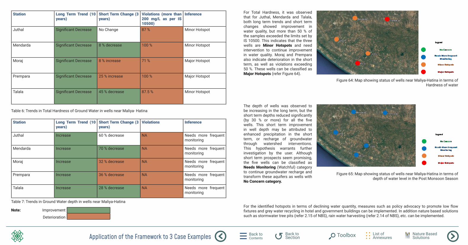
Application of the Framework to 3 Case Examples Back to Contents
List of Annexures
Back to Section Toolbox Nature Based
Solutions
Station Long Term Trend (10 years)
Short Term Change (3 years)
Violations (more than 200 mg/L as per IS 10500)
Inference
Juthal Significant Decrease No Change 87 % Minor Hotspot
Mendarda Significant Decrease 8 % decrease 100 % Minor Hotspot
Moraj Significant Decrease 8 % increase 71 % Major Hotspot
Prempara Significant Decrease 25 % increase 100 % Major Hotspot
Talala Significant Decrease 45 % decrease 87.5 % Minor Hotspot
Station Long Term Trend (10 years)
Short Term Change (3 years)
Violations Inference
Juthal Increase 60 % decrease NA Needs more frequent monitoring
Mendarda Increase 70 % decrease NA Needs more frequent monitoring
Moraj Increase 32 % decrease NA Needs more frequent monitoring
Prempara Increase 36 % decrease NA Needs more frequent monitoring
Talala Increase 28 % decrease NA Needs more frequent monitoring
Table 6: Trends in Total Hardness of Ground Water in wells near Maliya- Hatina
Table 7: Trends in Ground Water depth in wells near Maliya-Hatina
ImprovementNote:
Deterioration
For Total Hardness, it was observed that for Juthal, Mendarda and Talala, both long term trends and short term changes showed improvement in water quality, but more than 50 % of the samples exceeded the limits set by IS 10500. This indicates that the three wells are Minor Hotspots and need intervention to continue improvement in water quality. Moraj and Prempara also indicate deterioration in the short term, as well as violations exceeding 50 %. These wells can be classified as Major Hotspots (refer Figure 64).
The depth of wells was observed to be increasing in the long term, but the short term depths reduced significantly (by 30 % or more) for all the five wells. This short term improvement in well depth may be attributed to enhanced precipitation in the short term, or recharge of groundwater through watershed interventions. This hypothesis warrants further investigation by the user. Although short term prospects seem promising, the five wells can be classified as Needs Monitoring (Watchful) category to continue groundwater recharge and transform these aquifers as wells with No Concern category.
For the identified hotspots in terms of declining water quantity, measures such as policy advocacy to promote low flow fixtures and grey water recycling in hotel and government buildings can be implemented. In addition nature based solutions such as stormwater tree pits (refer 2.15 of NBS), rain water harvesting (refer 2.14 of NBS), etc. can be implemented.
Figure 64: Map showing status of wells near Maliya-Hatina in terms of Hardness of water
Figure 65: Map showing status of wells near Maliya-Hatina in terms of depth of water level in the Post Monsoon Season

Application of the Framework to 3 Case Examples Back to Contents
List of Annexures
Back to Section Toolbox Nature Based
Solutions
An Example of Identification of Hotspots due to Air PollutionAmbient air quality data for the three study areas was not available while conceiving this handbook. Hence, it becomes imperative to understand how to make sense of air quality data for a study area when it is available to the user. The section below describes analysis and interpretation of air quality data.
As shown in above section for Ground Water data in Maliya-Hatina, a three-pronged approach may be used to interpret trends in ambient air quality and design engineering and administrative interventions. The three methods, as described in Section 6.4 and 6.5, are Long Term Trend Analysis (using Mann-Kendall’s trend test), Short Term Change Analysis (using Median Comparison for recent years) and Violations Analysis (by comparing the measures values with Ambient Air Quality Standards and computing the percentage and severity of those violations).
Consider a City X located within a wider Metropolitan Region (see Figure 66 below) with typically urban growth characteristics. City X has 06 (six) Continuous Ambient Air Quality Monitoring Stations (CAAQMS) located in different areas as shown in the map. The six stations register ambient air and meteorological data at one hour frequency. Historical data is available for a period of 12 years (2009 to 2020) for the City X. PM2.5 is the pre-dominant pollutant in the City, and has been considered in this illustration for analysis of the overall air quality of the City X.
Figure 66: Map of City X showing the six monitoring stations and metro route
The following analysis was carried out on the ambient air quality data (also refer to Section 5.11 and Section 5.12 for each type of analysis) for each of the six stations:
Additional contextual data about the City X was also obtained through secondary research and primary surveys. A metro construction project was initiated in the beginning of 2018 and was completed by the end of 2019. The route for metro construction has been shown in the map as a red line. The metro project was deemed to replace several on-road vehicles between the stations from 2020 onwards. The results for air quality data analysis for the six stations has been summarized in the shown below
Analysis Type Data Used Averaging Time
Long Term Analysis (Mann-Kendall’s Trend Test)
PM2.5 data for the past 12 years Annual averages for each year.
Short Term Change (Median Analysis PM2.5 data of the last quarter of 2018, 2019 and 2020
Median of daily averaged data for each quarter of each year.
Violations Index PM 2.5 data for the last year (2020) Daily Average values for each day of the last year.
Station Number Long-term trend Short-term change Violation Index
1 Deterioration Improvement 0.38
2 Deterioration Improvement 0.11
3 Deterioration Improvement 0.48
4 Improvement Deterioration 1.35
5 Improvement Deterioration 0.13
6 Deterioration Deterioration 0.86
Table 8: Analysis and Averaging Used for CAAQMS data in CIty X
Table 9: Results of data analytics applied to the CAAQMS data
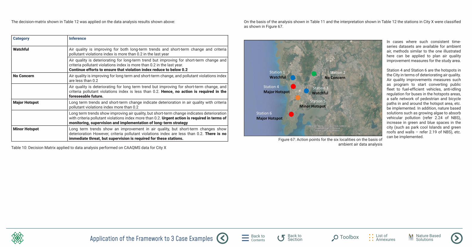
Application of the Framework to 3 Case Examples Back to Contents
List of Annexures
Back to Section Toolbox Nature Based
Solutions
The decision-matrix shown in Table 12 was applied on the data analysis results shown above: On the basis of the analysis shown in Table 11 and the interpretation shown in Table 12 the stations in City X were classified as shown in Figure 67.
In cases where such consistent time-series datasets are available for ambient air, methods similar to the one illustrated here can be applied to plan air quality improvement measures for the study area.
Station 4 and Station 6 are the hotspots in the City in terms of deteriorating air quality. Air quality improvements measures such as program to start converting public fleet to fuel-efficient vehicles, anti-idling regulation for buses in the hotspots areas, a safe network of pedestrian and bicycle paths in and around the hotspot area, etc. be implemented. In addition, nature based solutions such as growing algae to absorb vehicular pollution (refer 2.24 of NBS), increase in green and blue spaces in the city (such as park cool Islands and green roofs and walls – refer 2.19 of NBS), etc. can be implemented.
Category Inference
Watchful Air quality is improving for both long-term trends and short-term change and criteria pollutant violations index is more than 0.2 in the last year Air quality is deteriorating for long-term trend but improving for short-term change and criteria pollutant violations index is more than 0.2 in the last year.Continue efforts to ensure that violation index reduce to below 0.2
No Concern Air quality is improving for long term and short-term change, and pollutant violations index are less than 0.2Air quality is deteriorating for long term trend but improving for short-term change, and criteria pollutant violations index is less than 0.2. Hence, no action is required in the foreseeable future.
Major Hotspot Long term trends and short-term change indicate deterioration in air quality with criteria pollutant violations index more than 0.2Long term trends show improving air quality, but short-term change indicates deterioration with criteria pollutant violations index more than 0.2. Urgent action is required in terms of monitoring, supervision and implementation of long-term strategy
Minor Hotspot Long term trends show an improvement in air quality, but short-term changes show deterioration However, criteria pollutant violations index are less than 0.2. There is no immediate threat, but supervision is required for these stations. Figure 67: Action points for the six localities on the basis of
ambient air data analysisTable 10: Decision Matrix applied to data analysis performed on CAAQMS data for City X
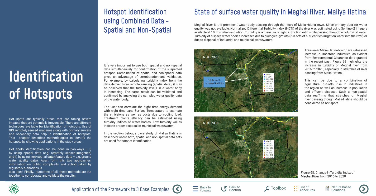
Application of the Framework to 3 Case Examples Back to Contents
List of Annexures
Back to Section Toolbox Nature Based
Solutions
Identification of HotspotsHot spots are typically areas that are facing severe impacts that are potentially irreversible. There are different techniques available for identification of hotspots. Use of GIS, remotely sensed imageries along with primary surveys and secondary data help in identification of hotspots. This chapter describes methodologies to identify the hotspots by showing applications in the study areas. Hot spots identification can be done in two ways – i) by using spatial data (e.g. remotely sensed imageries) and ii) by using non<spatial data (feature data – e.g. ground water quality data). Apart form this two approaches, information on public complaints and action taken by regulatory authorities is also used. Finally, outcomes of all these methods are put together to corroborate and validate the results.
Hotspot Identification using Combined Data - Spatial and Non-Spatial
It is very important to use both spatial and non-spatial data simultaneously for confirmation of the suspected hotspot. Combination of spatial and non-spatial data gives an advantage of corroboration and validation. For example, by calculating turbidity index from the data derived from remote sensing (spatial data), it may be observed that the turbidity levels in a water body is increasing. The same result can be validated and confirmed by analysing the sampled water quality data of the water body.
The user can correlate the night time energy demand with night time Land Surface Temperature to estimate the emissions as well as costs due to cooling load. Treatment plants efficacy can be estimated using turbidity indices of water bodies. Low turbidity values indicate proper disposal of municipal wastewater.
In the section below, a case study of Maliya Hatina is described where both, spatial and non-spatial data sets are used for hotspot identification
State of surface water quality in Meghal River, Maliya HatinaMeghal River is the prominent water body passing through the heart of Malia-Hatina town. Since primary data for water quality was not available, Normalized Differential Turbidity Index (NDTI) of the river was estimated using Sentinel-2 imagery available at 10 m spatial resolution. Turbidity is a measure of light extinction ratio while passing through a column of water. Turbidity of surface water bodies increases due to biological growth (run-offs of nutrient rich irrigation water into the river) or due to disposal of industrial and municipal wastewaters.
Figure 68: Change in Turbidity Index of Meghal River from 2016 to 2020
Areas near Malia-Hatina town have witnessed increase in limestone industries, as evident from Environmental Clearance data granted in the recent past. Figure 68 highlights the increase in turbidity of Meghal river from 2016 to 2020, especially in stretches of river passing from Malia-Hatina.
This can be due to a combination of agricultural run-offs, rise in industries in the region as well as increase in population and effluent disposal. Such a non-spatial data reaffirms that stretches of Meghal river passing though Malia-Hatina should be considered as hot spots.
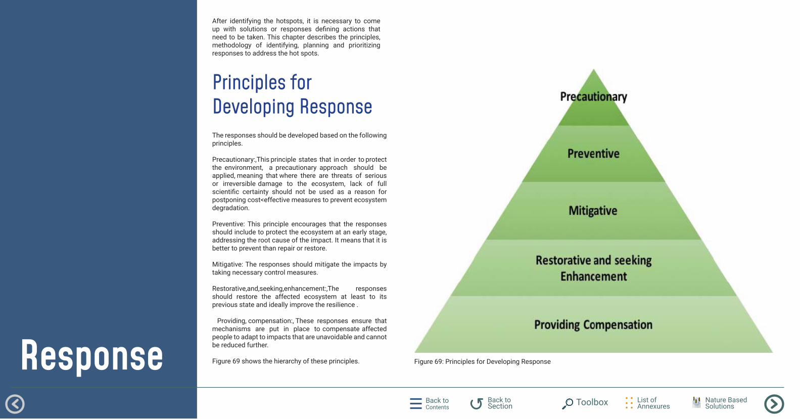
Back to Contents
List of Annexures
Back to Section Toolbox Nature Based
Solutions
Response
After identifying the hotspots, it is necessary to come up with solutions or responses defining actions that need to be taken. This chapter describes the principles, methodology of identifying, planning and prioritizing responses to address the hot spots.
The responses should be developed based on the following principles. Precautionary:,This principle states that in order to protect the environment, a precautionary approach should be applied, meaning that where there are threats of serious or irreversible damage to the ecosystem, lack of full scientific certainty should not be used as a reason for postponing cost<effective measures to prevent ecosystem degradation. Preventive: This principle encourages that the responses should include to protect the ecosystem at an early stage, addressing the root cause of the impact. It means that it is better to prevent than repair or restore. Mitigative: The responses should mitigate the impacts by taking necessary control measures. Restorative,and,seeking,enhancement:,The responses should restore the affected ecosystem at least to its previous state and ideally improve the resilience . Providing, compensation:, These responses ensure that mechanisms are put in place to compensate affected people to adapt to impacts that are unavoidable and cannot be reduced further. Figure 69 shows the hierarchy of these principles.
Principles for Developing Response
Figure 69: Principles for Developing Response
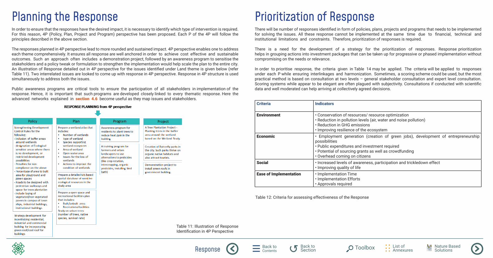
Response Back to Contents
List of Annexures
Back to Section Toolbox Nature Based
Solutions
Planning the ResponseIn order to ensure that the responses have the desired impact, it is necessary to identify which type of intervention is required. For this reason, 4P (Policy, Plan, Project and Program) perspective has been proposed. Each P of the 4P will follow the principles described in the above section. The responses planned in 4P perspective lead to more rounded and sustained impact. 4P perspective enables one to address each theme comprehensively. It ensures all response are well anchored in order to achieve cost effective and sustainable outcomes. Such an approach often includes a demonstration project, followed by an awareness program to sensitise the stakeholders and a policy tweak or formulation to strengthen the implementation would help scale the plan to the entire city. An illustration of Response detailed out in 4P perspective for the issues identified under Land theme is given below (refer Table 11). Two interrelated issues are looked to come up with response in 4P perspective. Response in 4P structure is used simultaneously to address both the issues. Public awareness programs are critical tools to ensure the participation of all stakeholders in implementation of the response. Hence, it is important that such programs are developed closely linked to every thematic response. Here the advanced networks explained in section 4.6 become useful as they map issues and stakeholders.
Table 11: Illustration of Response Identification in 4P Perspective
Prioritization of ResponseThere will be number of responses identified in form of policies, plans, projects and programs that needs to be implemented for solving the issues. All these response cannot be implemented at the same time due to financial, technical and institutional limitations and constraints. Therefore, prioritization of responses is required. There is a need for the development of a strategy for the prioritization of responses. Response prioritization helps in grouping actions into investment packages that can be taken up for progressive or phased implementation without compromising on the needs or relevance. In order to prioritise response, the criteria given in Table 14 may be applied. The criteria will be applied to responses under each P while ensuring interlinkages and harmonization. Sometimes, a scoring scheme could be used, but the most practical method is based on consultation at two levels – general stakeholder consultation and expert level consultation. Scoring systems while appear to be elegant are often plagued with subjectivity. Consultations if conducted with scientific data and well moderated can help arriving at collectively agreed decisions.
Table 12: Criteria for assessing effectiveness of the Response
Criteria Indicators
Environment • Conservation of resources/ resource optimization• Reduction in pollution levels (air, water and noise pollution)• Reduction in GHG emissions• Improving resilience of the ecosystem
Economic • Employment generation (creation of green jobs), development of entrepreneurship possibilities• Public expenditures and investment required• Potential of sourcing grants as well as crowdfunding • Overhead coming on citizens
Social • Increased levels of awareness, participation and trickledown effect• Improving quality of life
Ease of Implementation • Implementation Time• Implementation Efforts• Approvals required
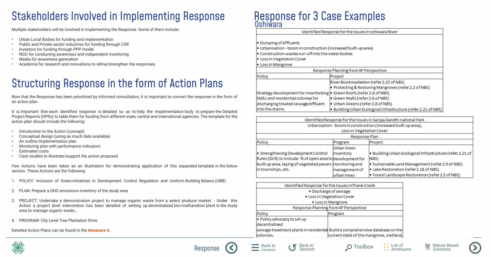
Response Back to Contents
List of Annexures
Back to Section Toolbox Nature Based
Solutions
Stakeholders Involved in Implementing Response
Structuring Response in the form of Action Plans
Response for 3 Case ExamplesOshiwara
Multiple stakeholders will be involved in implementing the Response. Some of them include: • Urban Local Bodies for funding and implementation • Public and Private sector industries for funding through CSR • Investors for funding through PPP model • NGO for conducting awareness and independent monitoring • Media for awareness generation• Academia for research and innovations to refine/strengthen the responses
Now that the Response has been prioritized by informed consultation, it is important to convert the response in the form of an action plan. It is important that each identified response is detailed so as to help the implementation body to prepare the Detailed Project Reports (DPRs) to table them for funding from different state, central and international agencies. The template for the action plan should include the following: • Introduction to the Action (concept) • Conceptual design (using as much data available) • An outline Implementation plan • Monitoring plan with performance indicators • Estimated costs • Case studies to illustrate/support the action proposed Few Actions have been taken as an illustration for demonstrating application of this expanded template in the below section. These Actions are the following: 1. POLICY: Inclusion of Green-Initiatives in Development Control Regulation and Uniform Building Bylaws (UBB)
2. PLAN: Prepare a GHG emissions inventory of the study area
3. PROJECT: Undertake a demonstration project to manage organic waste from a select produce market - Under this Action a project level intervention has been detailed of setting up decentralized bio<methanation plant in the study area to manage organic waste.,
4. PROGRAM: City Level Tree Plantation Drive
Detailed Action Plans can be found in the Annexure 4.
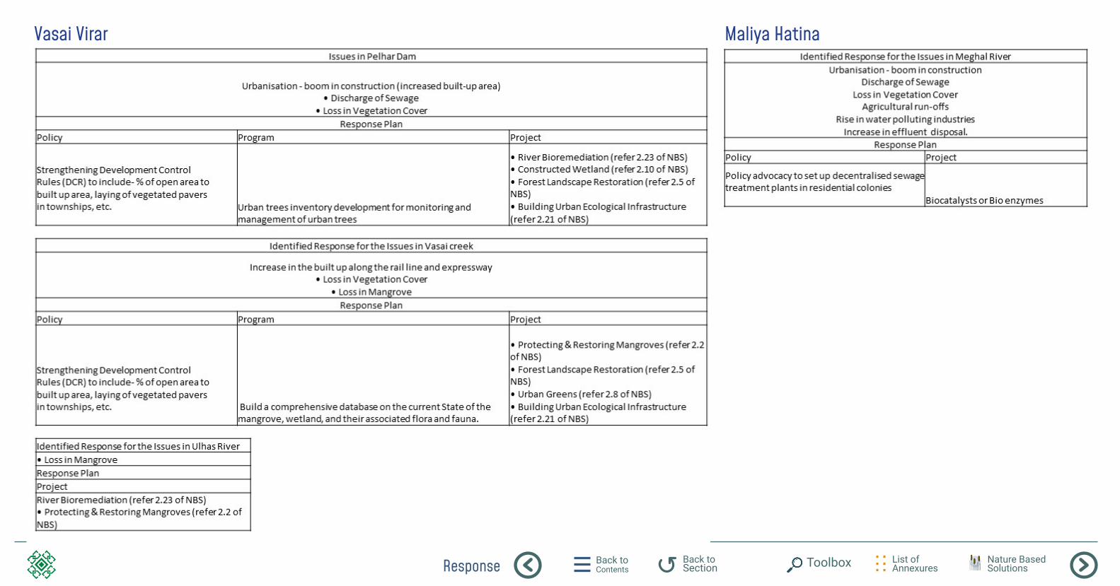
Response Back to Contents
List of Annexures
Back to Section Toolbox Nature Based
Solutions
Vasai Virar Maliya Hatina
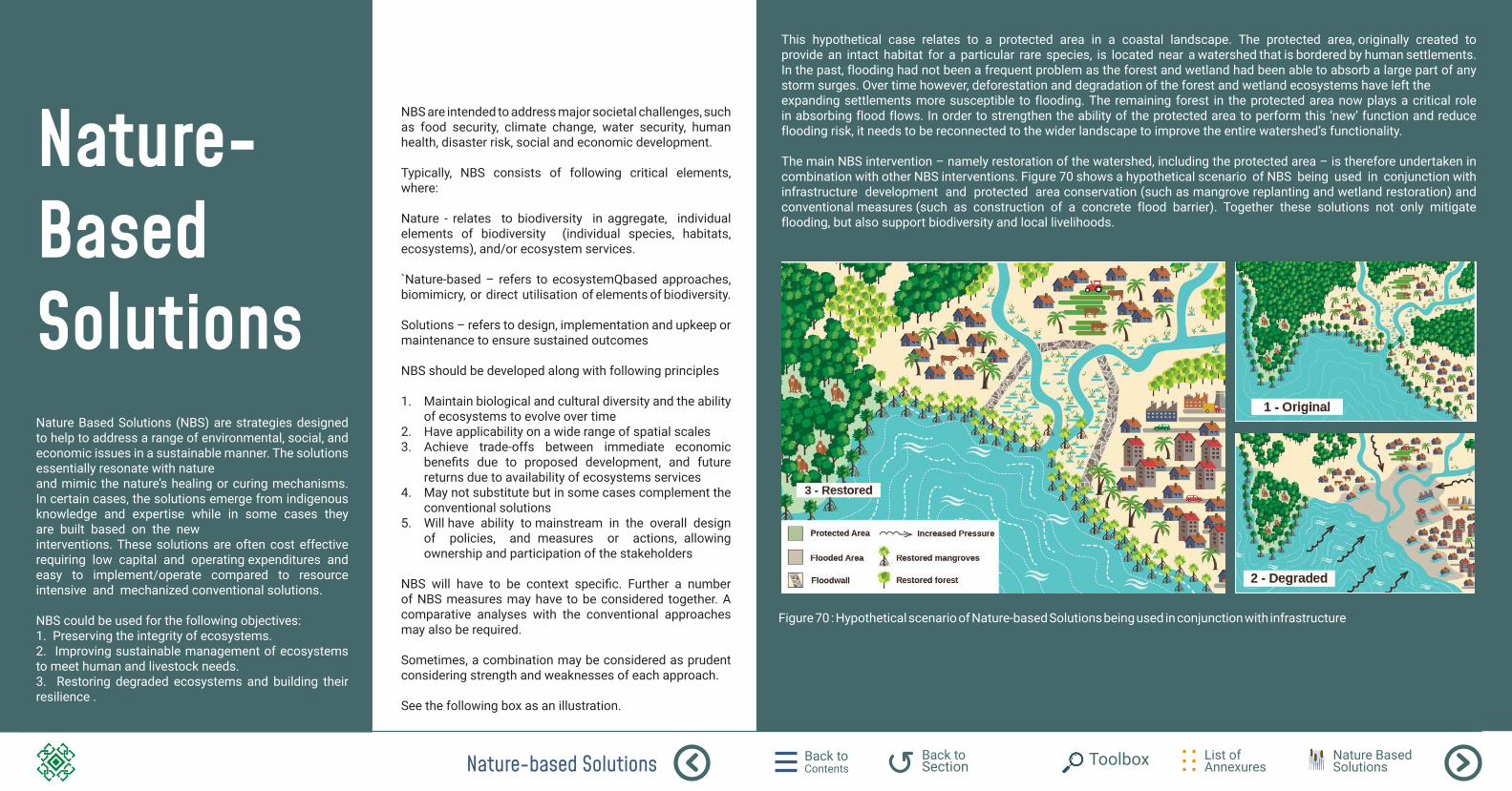
Nature-based Solutions Back to Contents
List of Annexures
Back to Section Toolbox Nature Based
Solutions
Nature-Based Solutions
NBS are intended to address major societal challenges, such as food security, climate change, water security, human health, disaster risk, social and economic development. Typically, NBS consists of following critical elements, where: Nature - relates to biodiversity in aggregate, individual elements of biodiversity (individual species, habitats, ecosystems), and/or ecosystem services.
`Nature-based – refers to ecosystemQbased approaches, biomimicry, or direct utilisation of elements of biodiversity.
Solutions – refers to design, implementation and upkeep or maintenance to ensure sustained outcomes NBS should be developed along with following principles 1. Maintain biological and cultural diversity and the ability
of ecosystems to evolve over time 2. Have applicability on a wide range of spatial scales 3. Achieve trade-offs between immediate economic
benefits due to proposed development, and future returns due to availability of ecosystems services
4. May not substitute but in some cases complement the conventional solutions
5. Will have ability to mainstream in the overall design of policies, and measures or actions, allowing ownership and participation of the stakeholders
NBS will have to be context specific. Further a number of NBS measures may have to be considered together. A comparative analyses with the conventional approaches may also be required.
Sometimes, a combination may be considered as prudent considering strength and weaknesses of each approach.
See the following box as an illustration.
Nature Based Solutions (NBS) are strategies designed to help to address a range of environmental, social, and economic issues in a sustainable manner. The solutions essentially resonate with nature and mimic the nature’s healing or curing mechanisms. In certain cases, the solutions emerge from indigenous knowledge and expertise while in some cases they are built based on the new interventions. These solutions are often cost effective requiring low capital and operating expenditures and easy to implement/operate compared to resource intensive and mechanized conventional solutions. NBS could be used for the following objectives: 1. Preserving the integrity of ecosystems. 2. Improving sustainable management of ecosystems to meet human and livestock needs. 3. Restoring degraded ecosystems and building their resilience .
This hypothetical case relates to a protected area in a coastal landscape. The protected area, originally created to provide an intact habitat for a particular rare species, is located near a watershed that is bordered by human settlements. In the past, flooding had not been a frequent problem as the forest and wetland had been able to absorb a large part of any storm surges. Over time however, deforestation and degradation of the forest and wetland ecosystems have left the expanding settlements more susceptible to flooding. The remaining forest in the protected area now plays a critical role in absorbing flood flows. In order to strengthen the ability of the protected area to perform this ‘new’ function and reduce flooding risk, it needs to be reconnected to the wider landscape to improve the entire watershed’s functionality. The main NBS intervention – namely restoration of the watershed, including the protected area – is therefore undertaken in combination with other NBS interventions. Figure 70 shows a hypothetical scenario of NBS being used in conjunction with infrastructure development and protected area conservation (such as mangrove replanting and wetland restoration) and conventional measures (such as construction of a concrete flood barrier). Together these solutions not only mitigate flooding, but also support biodiversity and local livelihoods.
Figure 70 : Hypothetical scenario of Nature-based Solutions being used in conjunction with infrastructure
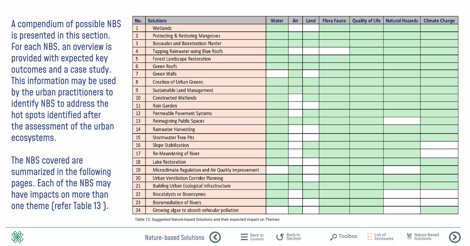
Nature-based Solutions Back to Contents
List of Annexures
Back to Section Toolbox Nature Based
Solutions
A compendium of possible NBS is presented in this section. For each NBS, an overview is provided with expected key outcomes and a case study. This information may be used by the urban practitioners to identify NBS to address the hot spots identified after the assessment of the urban ecosystems. The NBS covered are summarized in the following pages. Each of the NBS may have impacts on more than one theme (refer Table 13 ).
Table 13: Suggested Nature-based Solutions and their expected impact on Themes
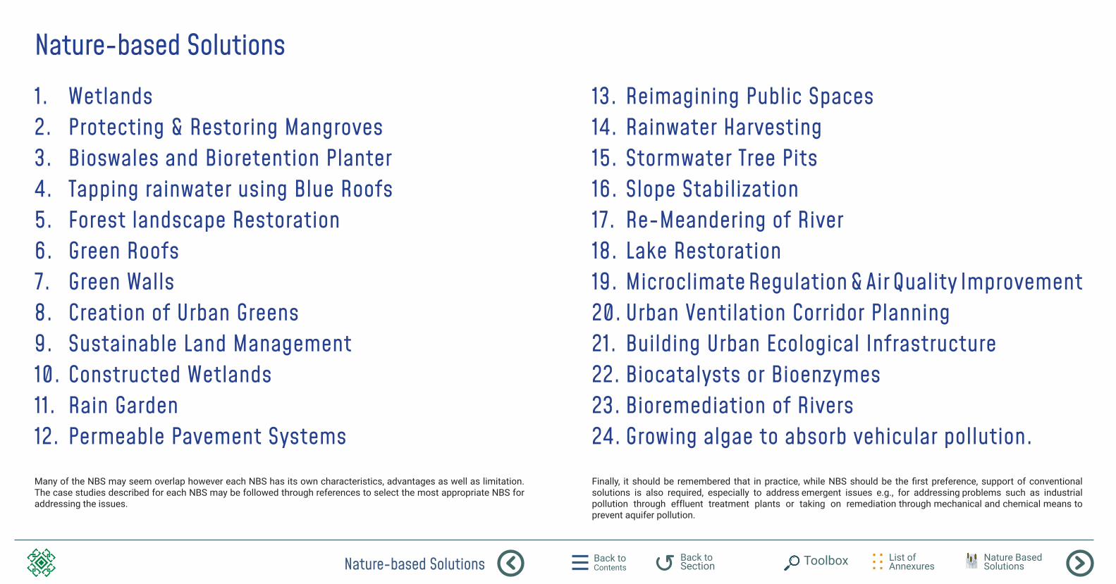
Nature-based Solutions Back to Contents
List of Annexures
Back to Section Toolbox Nature Based
Solutions
1. Wetlands 2. Protecting & Restoring Mangroves 3. Bioswales and Bioretention Planter 4. Tapping rainwater using Blue Roofs 5. Forest landscape Restoration 6. Green Roofs 7. Green Walls 8. Creation of Urban Greens 9. Sustainable Land Management 10. Constructed Wetlands 11. Rain Garden 12. Permeable Pavement Systems
Many of the NBS may seem overlap however each NBS has its own characteristics, advantages as well as limitation. The case studies described for each NBS may be followed through references to select the most appropriate NBS for addressing the issues.
Nature-based Solutions
13. Reimagining Public Spaces14. Rainwater Harvesting 15. Stormwater Tree Pits 16. Slope Stabilization 17. Re-Meandering of River 18. Lake Restoration 19. Microclimate Regulation & Air Quality Improvement 20. Urban Ventilation Corridor Planning 21. Building Urban Ecological Infrastructure 22. Biocatalysts or Bioenzymes 23. Bioremediation of Rivers 24. Growing algae to absorb vehicular pollution.
Finally, it should be remembered that in practice, while NBS should be the first preference, support of conventional solutions is also required, especially to address emergent issues e.g., for addressing problems such as industrial pollution through effluent treatment plants or taking on remediation through mechanical and chemical means to prevent aquifer pollution.
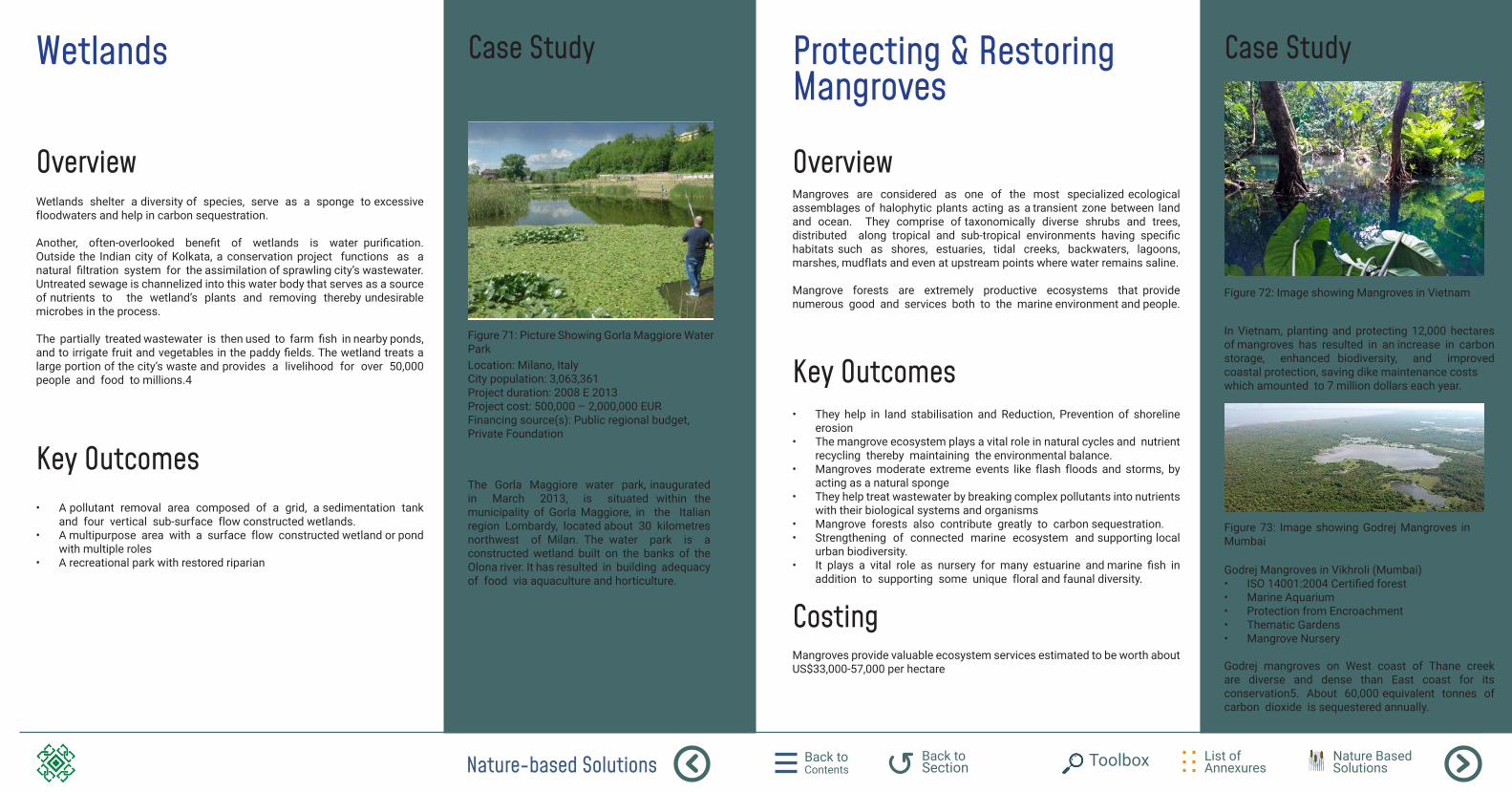
Nature-based Solutions Back to Contents
List of Annexures
Back to Section Toolbox Nature Based
Solutions
Wetlands
Overview
Case Study
Wetlands shelter a diversity of species, serve as a sponge to excessive floodwaters and help in carbon sequestration. Another, often-overlooked benefit of wetlands is water purification. Outside the Indian city of Kolkata, a conservation project functions as a natural filtration system for the assimilation of sprawling city’s wastewater. Untreated sewage is channelized into this water body that serves as a source of nutrients to the wetland’s plants and removing thereby undesirable microbes in the process. The partially treated wastewater is then used to farm fish in nearby ponds, and to irrigate fruit and vegetables in the paddy fields. The wetland treats a large portion of the city’s waste and provides a livelihood for over 50,000 people and food to millions.4
Location: Milano, ItalyCity population: 3,063,361 Project duration: 2008 E 2013 Project cost: 500,000 – 2,000,000 EUR Financing source(s): Public regional budget, Private Foundation
The Gorla Maggiore water park, inaugurated in March 2013, is situated within the municipality of Gorla Maggiore, in the Italian region Lombardy, located about 30 kilometres northwest of Milan. The water park is a constructed wetland built on the banks of the Olona river. It has resulted in building adequacy of food via aquaculture and horticulture.
• A pollutant removal area composed of a grid, a sedimentation tank and four vertical sub-surface flow constructed wetlands.
• A multipurpose area with a surface flow constructed wetland or pond with multiple roles
• A recreational park with restored riparian
Key Outcomes
Figure 71: Picture Showing Gorla Maggiore Water Park
Protecting & Restoring Mangroves
Overview
Case Study
Mangroves are considered as one of the most specialized ecological assemblages of halophytic plants acting as a transient zone between land and ocean. They comprise of taxonomically diverse shrubs and trees, distributed along tropical and sub-tropical environments having specific habitats such as shores, estuaries, tidal creeks, backwaters, lagoons, marshes, mudflats and even at upstream points where water remains saline. Mangrove forests are extremely productive ecosystems that provide numerous good and services both to the marine environment and people.
Mangroves provide valuable ecosystem services estimated to be worth about US$33,000-57,000 per hectare
In Vietnam, planting and protecting 12,000 hectares of mangroves has resulted in an increase in carbon storage, enhanced biodiversity, and improved coastal protection, saving dike maintenance costs which amounted to 7 million dollars each year.
Godrej Mangroves in Vikhroli (Mumbai) • ISO 14001:2004 Certified forest • Marine Aquarium • Protection from Encroachment • Thematic Gardens • Mangrove Nursery Godrej mangroves on West coast of Thane creek are diverse and dense than East coast for its conservation5. About 60,000 equivalent tonnes of carbon dioxide is sequestered annually.
• They help in land stabilisation and Reduction, Prevention of shoreline erosion
• The mangrove ecosystem plays a vital role in natural cycles and nutrient recycling thereby maintaining the environmental balance.
• Mangroves moderate extreme events like flash floods and storms, by acting as a natural sponge
• They help treat wastewater by breaking complex pollutants into nutrients with their biological systems and organisms
• Mangrove forests also contribute greatly to carbon sequestration. • Strengthening of connected marine ecosystem and supporting local
urban biodiversity. • It plays a vital role as nursery for many estuarine and marine fish in
addition to supporting some unique floral and faunal diversity.
Key Outcomes
Costing
Figure 72: Image showing Mangroves in Vietnam
Figure 73: Image showing Godrej Mangroves in Mumbai

Nature-based Solutions Back to Contents
List of Annexures
Back to Section Toolbox Nature Based
Solutions
Bioswales and Bioretention Planter
Overview
Case Study
Bioswales are planned green spaces that collect runoff and remove harmful pollutants from the stormwater before it is discharged into surface water sources. They are shallow drainage courses that are filled with vegetation, compost, and/or riprap. As a part of the surface runoff flow path, they are designed to maximize the time water spends in the swale, that aids in the trapping and breakdown of certain pollutants. A bioretention planter is an impervious ponding reservoir containing a minimum of 45 cm of bioretention soil, a layer of uniformly graded washed gravel, an underdrain, and an overflow.
The average cost of installation of Bioswale is about USD 10-20 per sq. m.
It promotes infiltration and filtration through the largely sand media and underdrain while maintaining stormwater conveyance on the surface during large rainfall events.
• Reduced runoff: In a typical road, a 4Hmeter swale can reduce approximately 25 percent of total rainfall runoff.
• Instead of releasing stormwater into the drainage system, stormwater can be filtered and may provide some groundwater recharge.
• Sustainable, decentralized stormwater management systems may be more cost effective than centralized stormwater systems. At the minimum, these nature based technologies reduce pressure on existing systems and the maintenance costs associated with centralized stormwater management systems.
• Bioswales are more suitable for storm-water control on a large scale. They can be made along the roadsides so that rainwater from the road flows towards them and percolates into the ground.
Key Outcomes
Costing
Figure 74: Image showing bioswales in Museum of Science Portland
Figure 75: Image showing bioswale in Jellicoe Street, Auckland, New Zealand
Figure 76: Image showing Bioretention in Derbyshire Street, London
Tapping Rainwater using Blue Roofs
Overview
Case Study
Blue roof are non-vegetated roofs that use to detain and retain the stormwater. Dikes used at drain inlets allow temporary water storage and gradual release of rainwater. The potential of blue roofs is mostly untapped in india owing to various reasons such as erratic rainfall patterns and extreme temperatures.
The average cost of Blue Roofs (50 years of life cycle) is about USD 10-25 per sq. m.
• The pivotal focus of blue roofs is to harvest rainwater in a catchment • Light coloured roofing material is used to maintain low temperature
on rooftop • They are cost effective as compared with green roofs and can
substantially reduce the runoff in an area. • It reduces the chances of flash floods in urban areas.
Key Outcomes
Costing
Figure 77: Image showing blue roofs in Walter Bos Complex, Apeldoorn
Figure 78: Image showing blue roofs in Walter Bos Complex, Apeldoorn
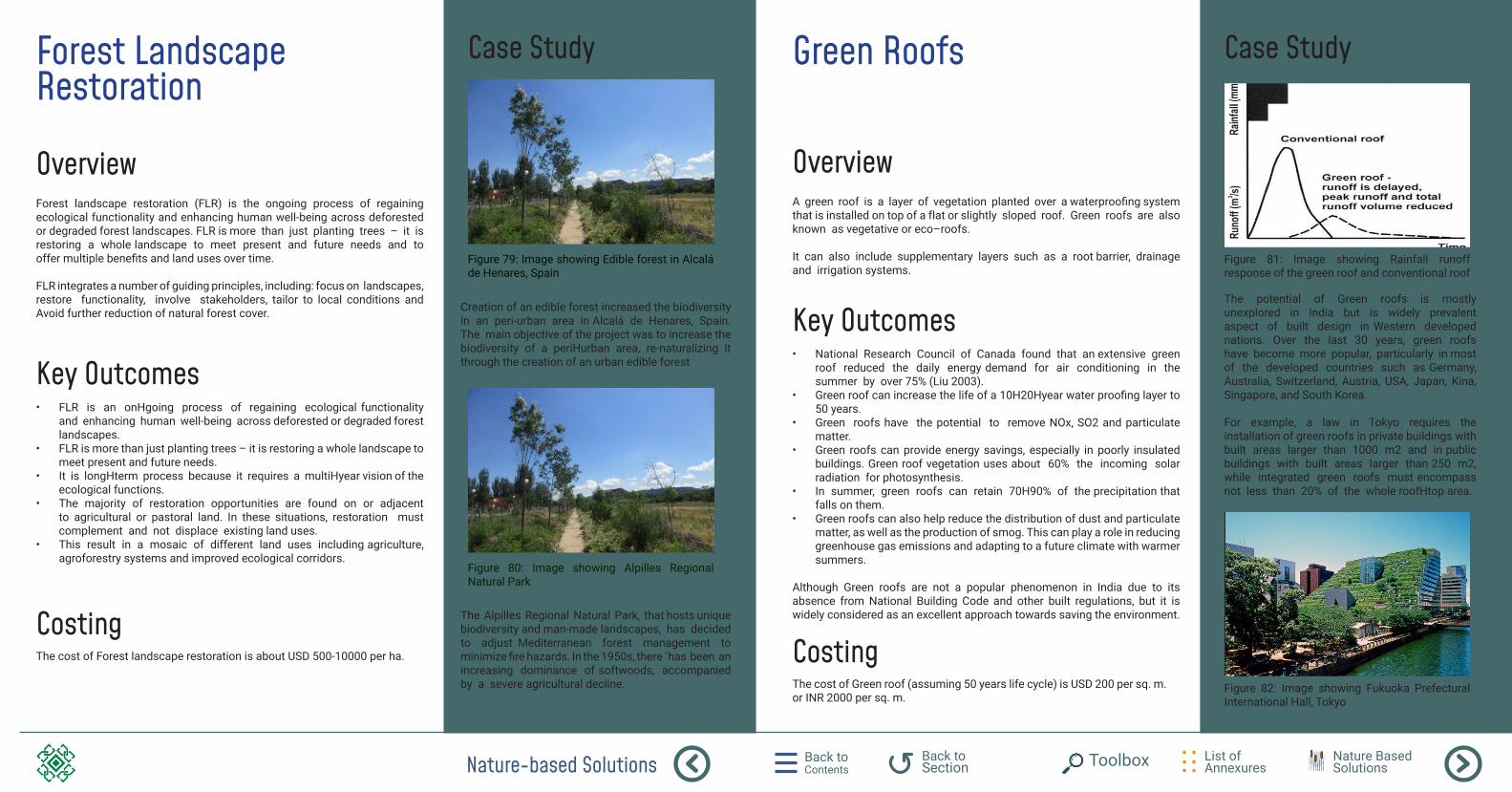
Nature-based Solutions Back to Contents
List of Annexures
Back to Section Toolbox Nature Based
Solutions
Forest Landscape Restoration
Overview
Case Study
Forest landscape restoration (FLR) is the ongoing process of regaining ecological functionality and enhancing human well-being across deforested or degraded forest landscapes. FLR is more than just planting trees – it is restoring a whole landscape to meet present and future needs and to offer multiple benefits and land uses over time. FLR integrates a number of guiding principles, including: focus on landscapes, restore functionality, involve stakeholders, tailor to local conditions and Avoid further reduction of natural forest cover.
The cost of Forest landscape restoration is about USD 500-10000 per ha.
• FLR is an onHgoing process of regaining ecological functionality and enhancing human well-being across deforested or degraded forest landscapes.
• FLR is more than just planting trees – it is restoring a whole landscape to meet present and future needs.
• It is longHterm process because it requires a multiHyear vision of the ecological functions.
• The majority of restoration opportunities are found on or adjacent to agricultural or pastoral land. In these situations, restoration must complement and not displace existing land uses.
• This result in a mosaic of different land uses including agriculture, agroforestry systems and improved ecological corridors.
Key Outcomes
Costing
Figure 79: Image showing Edible forest in Alcalá de Henares, Spain
Figure 80: Image showing Alpilles Regional Natural Park
Creation of an edible forest increased the biodiversity in an peri-urban area in Alcalá de Henares, Spain. The main objective of the project was to increase the biodiversity of a periHurban area, re-naturalizing it through the creation of an urban edible forest
The Alpilles Regional Natural Park, that hosts unique biodiversity and man-made landscapes, has decided to adjust Mediterranean forest management to minimize fire hazards. In the 1950s, there ̀ has been an increasing dominance of softwoods, accompanied by a severe agricultural decline.
Green Roofs
Overview
Case Study
A green roof is a layer of vegetation planted over a waterproofing system that is installed on top of a flat or slightly sloped roof. Green roofs are also known as vegetative or eco–roofs. It can also include supplementary layers such as a root barrier, drainage and irrigation systems.
The cost of Green roof (assuming 50 years life cycle) is USD 200 per sq. m. or INR 2000 per sq. m.
• National Research Council of Canada found that an extensive green roof reduced the daily energy demand for air conditioning in the summer by over 75% (Liu 2003).
• Green roof can increase the life of a 10H20Hyear water proofing layer to 50 years.
• Green roofs have the potential to remove NOx, SO2 and particulate matter.
• Green roofs can provide energy savings, especially in poorly insulated buildings. Green roof vegetation uses about 60% the incoming solar radiation for photosynthesis.
• In summer, green roofs can retain 70H90% of the precipitation that falls on them.
• Green roofs can also help reduce the distribution of dust and particulate matter, as well as the production of smog. This can play a role in reducing greenhouse gas emissions and adapting to a future climate with warmer summers.
Although Green roofs are not a popular phenomenon in India due to its absence from National Building Code and other built regulations, but it is widely considered as an excellent approach towards saving the environment.
Key Outcomes
Costing
Figure 81: Image showing Rainfall runoff response of the green roof and conventional roof
Figure 82: Image showing Fukuoka Prefectural International Hall, Tokyo
The potential of Green roofs is mostly unexplored in India but is widely prevalent aspect of built design in Western developed nations. Over the last 30 years, green roofs have become more popular, particularly in most of the developed countries such as Germany, Australia, Switzerland, Austria, USA, Japan, Kina, Singapore, and South Korea. For example, a law in Tokyo requires the installation of green roofs in private buildings with built areas larger than 1000 m2 and in public buildings with built areas larger than 250 m2, while integrated green roofs must encompass not less than 20% of the whole roofHtop area.
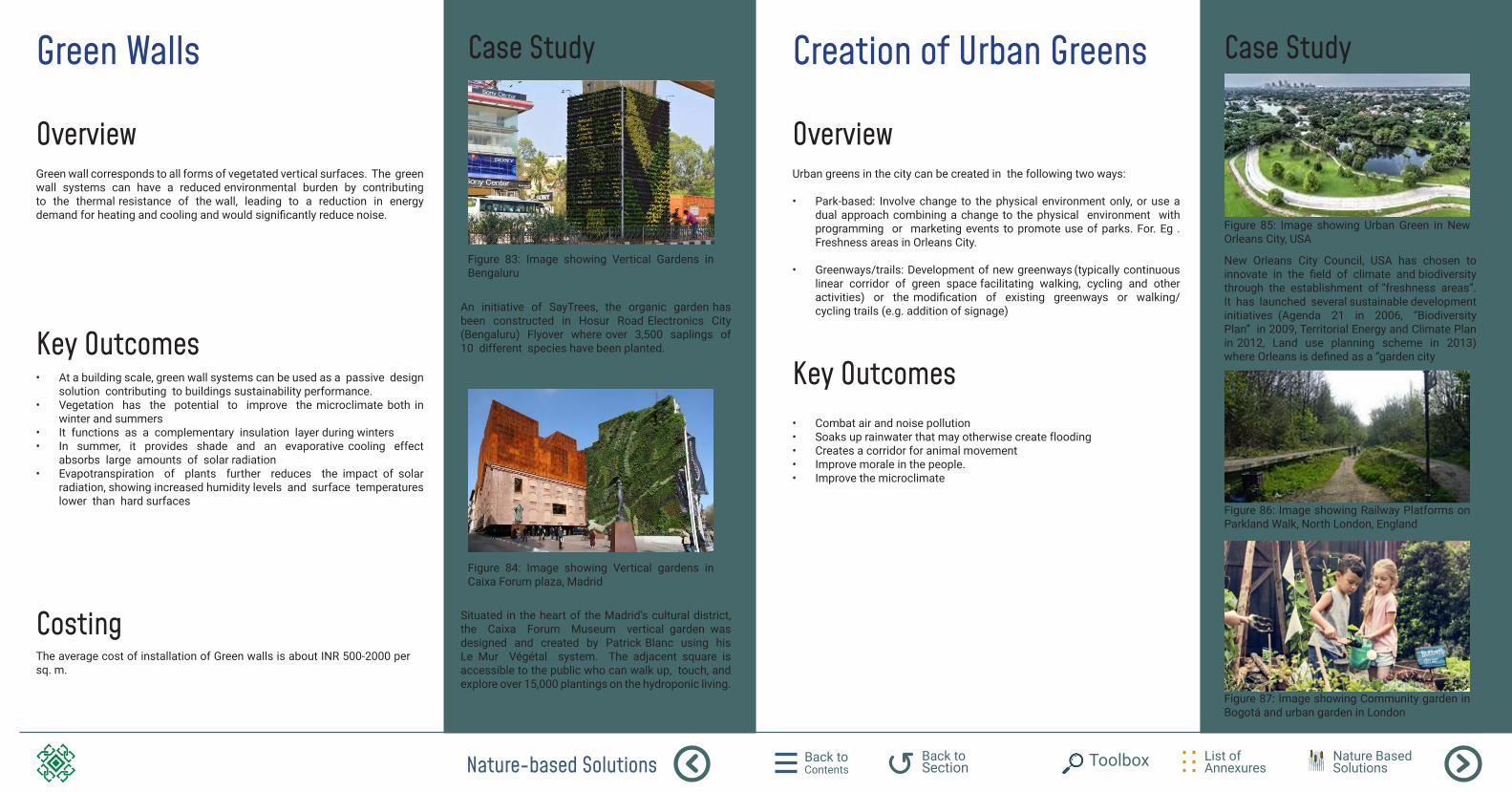
Nature-based Solutions Back to Contents
List of Annexures
Back to Section Toolbox Nature Based
Solutions
Green Walls
Overview
Case Study
Green wall corresponds to all forms of vegetated vertical surfaces. The green wall systems can have a reduced environmental burden by contributing to the thermal resistance of the wall, leading to a reduction in energy demand for heating and cooling and would significantly reduce noise.
The average cost of installation of Green walls is about INR 500-2000 per sq. m.
• At a building scale, green wall systems can be used as a passive design solution contributing to buildings sustainability performance.
• Vegetation has the potential to improve the microclimate both in winter and summers
• It functions as a complementary insulation layer during winters • In summer, it provides shade and an evaporative cooling effect
absorbs large amounts of solar radiation • Evapotranspiration of plants further reduces the impact of solar
radiation, showing increased humidity levels and surface temperatures lower than hard surfaces
Key Outcomes
Costing
Figure 83: Image showing Vertical Gardens in Bengaluru
Figure 84: Image showing Vertical gardens in Caixa Forum plaza, Madrid
An initiative of SayTrees, the organic garden has been constructed in Hosur Road Electronics City (Bengaluru) Flyover where over 3,500 saplings of 10 different species have been planted.
Situated in the heart of the Madrid’s cultural district, the Caixa Forum Museum vertical garden was designed and created by Patrick Blanc using his Le Mur Végétal system. The adjacent square is accessible to the public who can walk up, touch, and explore over 15,000 plantings on the hydroponic living.
Creation of Urban Greens
Overview
Case Study
Urban greens in the city can be created in the following two ways: • Park-based: Involve change to the physical environment only, or use a
dual approach combining a change to the physical environment with programming or marketing events to promote use of parks. For. Eg . Freshness areas in Orleans City.
• Greenways/trails: Development of new greenways (typically continuous
linear corridor of green space facilitating walking, cycling and other activities) or the modification of existing greenways or walking/cycling trails (e.g. addition of signage)
• Combat air and noise pollution • Soaks up rainwater that may otherwise create flooding • Creates a corridor for animal movement • Improve morale in the people. • Improve the microclimate
Key Outcomes
Figure 85: Image showing Urban Green in New Orleans City, USA
Figure 86: Image showing Railway Platforms on Parkland Walk, North London, England
Figure 87: Image showing Community garden in Bogotá and urban garden in London
New Orleans City Council, USA has chosen to innovate in the field of climate and biodiversity through the establishment of “freshness areas”. It has launched several sustainable development initiatives (Agenda 21 in 2006, “Biodiversity Plan” in 2009, Territorial Energy and Climate Plan in 2012, Land use planning scheme in 2013) where Orleans is defined as a “garden city
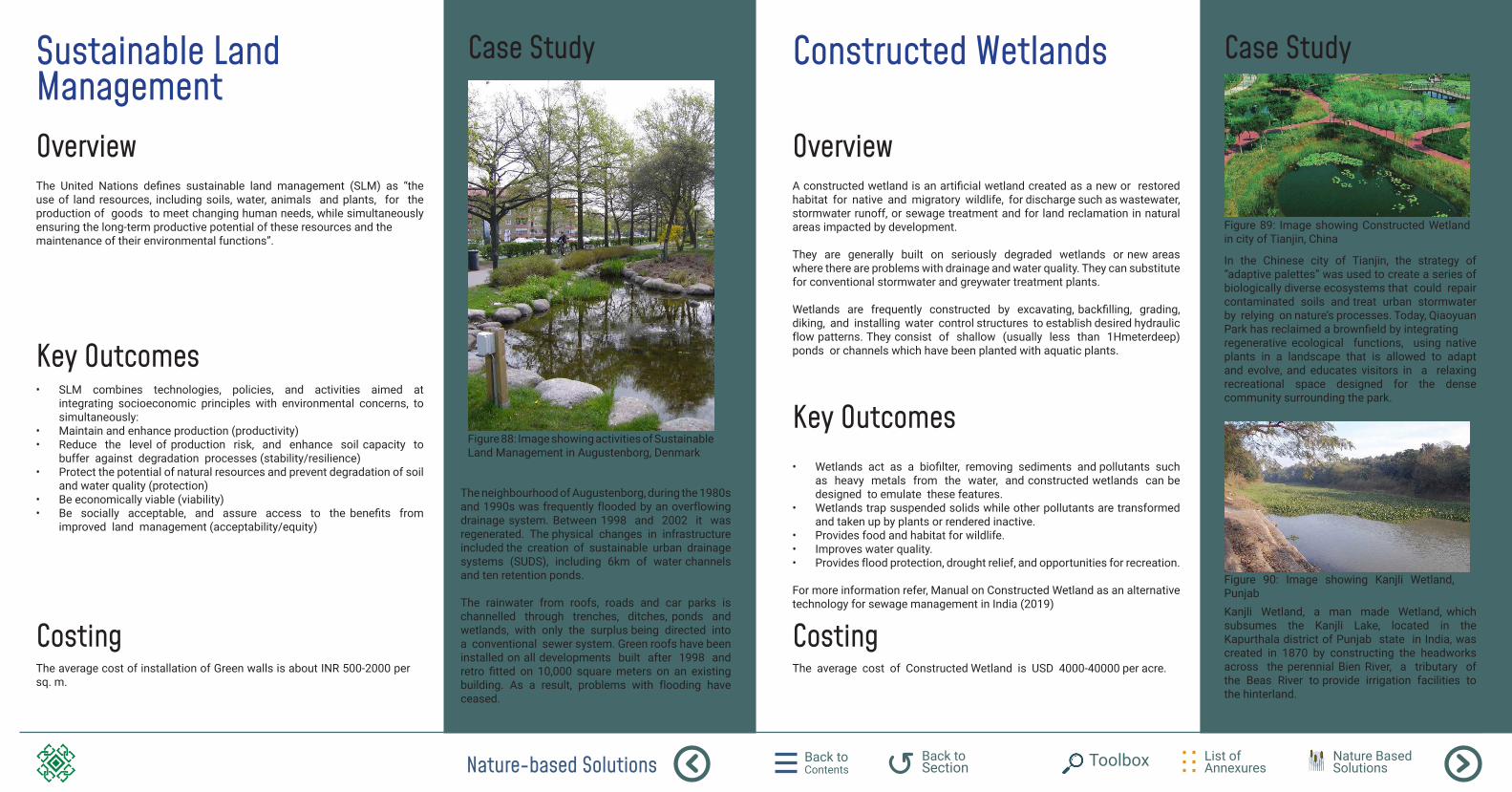
Nature-based Solutions Back to Contents
List of Annexures
Back to Section Toolbox Nature Based
Solutions
Sustainable Land ManagementOverview
Case Study
The United Nations defines sustainable land management (SLM) as “the use of land resources, including soils, water, animals and plants, for the production of goods to meet changing human needs, while simultaneously ensuring the long-term productive potential of these resources and the maintenance of their environmental functions”.
The average cost of installation of Green walls is about INR 500-2000 per sq. m.
• SLM combines technologies, policies, and activities aimed at integrating socioeconomic principles with environmental concerns, to simultaneously:
• Maintain and enhance production (productivity) • Reduce the level of production risk, and enhance soil capacity to
buffer against degradation processes (stability/resilience) • Protect the potential of natural resources and prevent degradation of soil
and water quality (protection) • Be economically viable (viability) • Be socially acceptable, and assure access to the benefits from
improved land management (acceptability/equity)
Key Outcomes
Costing
Figure 88: Image showing activities of Sustainable Land Management in Augustenborg, Denmark
The neighbourhood of Augustenborg, during the 1980s and 1990s was frequently flooded by an overflowing drainage system. Between 1998 and 2002 it was regenerated. The physical changes in infrastructure included the creation of sustainable urban drainage systems (SUDS), including 6km of water channels and ten retention ponds. The rainwater from roofs, roads and car parks is channelled through trenches, ditches, ponds and wetlands, with only the surplus being directed into a conventional sewer system. Green roofs have been installed on all developments built after 1998 and retro fitted on 10,000 square meters on an existing building. As a result, problems with flooding have ceased.
Constructed Wetlands
Overview
Case Study
A constructed wetland is an artificial wetland created as a new or restored habitat for native and migratory wildlife, for discharge such as wastewater, stormwater runoff, or sewage treatment and for land reclamation in natural areas impacted by development. They are generally built on seriously degraded wetlands or new areas where there are problems with drainage and water quality. They can substitute for conventional stormwater and greywater treatment plants. Wetlands are frequently constructed by excavating, backfilling, grading, diking, and installing water control structures to establish desired hydraulic flow patterns. They consist of shallow (usually less than 1Hmeterdeep) ponds or channels which have been planted with aquatic plants.
• Wetlands act as a biofilter, removing sediments and pollutants such as heavy metals from the water, and constructed wetlands can be designed to emulate these features.
• Wetlands trap suspended solids while other pollutants are transformed and taken up by plants or rendered inactive.
• Provides food and habitat for wildlife. • Improves water quality. • Provides flood protection, drought relief, and opportunities for recreation.
For more information refer, Manual on Constructed Wetland as an alternative technology for sewage management in India (2019)
Key Outcomes
Figure 89: Image showing Constructed Wetland in city of Tianjin, China
Figure 90: Image showing Kanjli Wetland, Punjab
In the Chinese city of Tianjin, the strategy of “adaptive palettes” was used to create a series of biologically diverse ecosystems that could repair contaminated soils and treat urban stormwater by relying on nature’s processes. Today, Qiaoyuan Park has reclaimed a brownfield by integrating regenerative ecological functions, using native plants in a landscape that is allowed to adapt and evolve, and educates visitors in a relaxing recreational space designed for the dense community surrounding the park.
Kanjli Wetland, a man made Wetland, which subsumes the Kanjli Lake, located in the Kapurthala district of Punjab state in India, was created in 1870 by constructing the headworks across the perennial Bien River, a tributary of the Beas River to provide irrigation facilities to the hinterland.
The average cost of Constructed Wetland is USD 4000-40000 per acre.
Costing
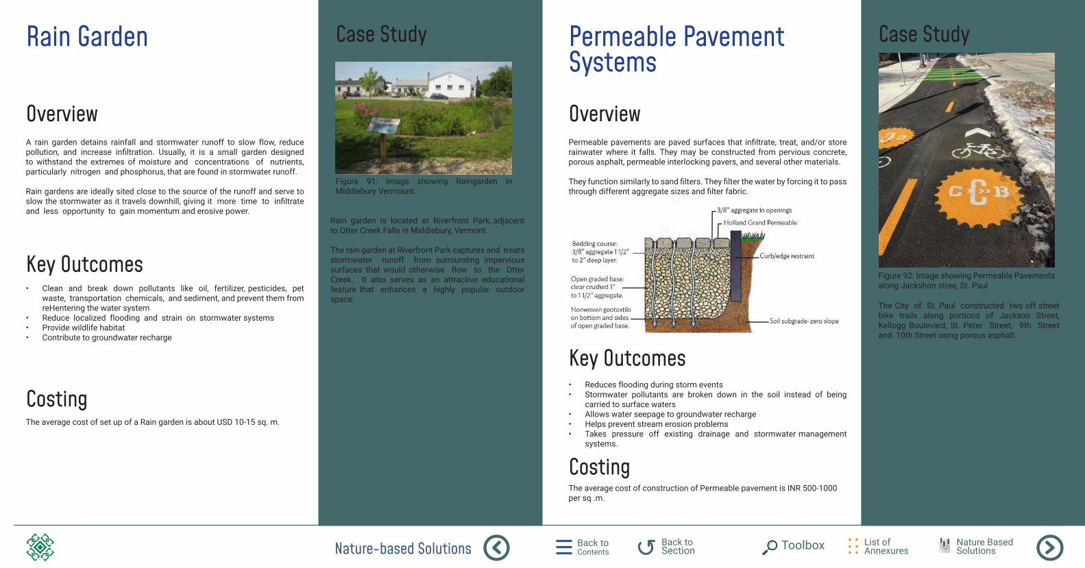
Nature-based Solutions Back to Contents
List of Annexures
Back to Section Toolbox Nature Based
Solutions
Rain Garden
Overview
Case Study
A rain garden detains rainfall and stormwater runoff to slow flow, reduce pollution, and increase infiltration. Usually, it is a small garden designed to withstand the extremes of moisture and concentrations of nutrients, particularly nitrogen and phosphorus, that are found in stormwater runoff. Rain gardens are ideally sited close to the source of the runoff and serve to slow the stormwater as it travels downhill, giving it more time to infiltrate and less opportunity to gain momentum and erosive power.
The average cost of set up of a Rain garden is about USD 10-15 sq. m.
• Clean and break down pollutants like oil, fertilizer, pesticides, pet waste, transportation chemicals, and sediment, and prevent them from reHentering the water system
• Reduce localized flooding and strain on stormwater systems • Provide wildlife habitat • Contribute to groundwater recharge
Key Outcomes
Costing
Figure 91: Image showing Raingarden in Middlebury Vermount.
Rain garden is located at Riverfront Park, adjacent to Otter Creek Falls in Middlebury, Vermont. The rain garden at Riverfront Park captures and treats stormwater runoff from surrounding impervious surfaces that would otherwise flow to the Otter Creek. It also serves as an attractive educational feature that enhances a highly popular outdoor space.
Permeable Pavement Systems
Overview
Case Study
Permeable pavements are paved surfaces that infiltrate, treat, and/or store rainwater where it falls. They may be constructed from pervious concrete, porous asphalt, permeable interlocking pavers, and several other materials. They function similarly to sand filters. They filter the water by forcing it to pass through different aggregate sizes and filter fabric.
• Reduces flooding during storm events • Stormwater pollutants are broken down in the soil instead of being
carried to surface waters • Allows water seepage to groundwater recharge • Helps prevent stream erosion problems • Takes pressure off existing drainage and stormwater management
systems.
Key Outcomes
Figure 92: Image showing Permeable Pavements along Jackshon stree, St. Paul
The average cost of construction of Permeable pavement is INR 500-1000 per sq .m.
Costing
The City of St. Paul constructed two off street bike trails along portions of Jackson Street, Kellogg Boulevard, St. Peter Street, 9th Street and 10th Street using porous asphalt.
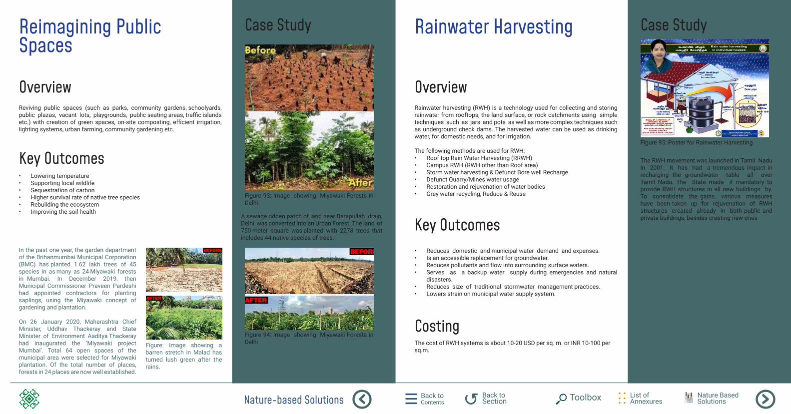
Nature-based Solutions Back to Contents
List of Annexures
Back to Section Toolbox Nature Based
Solutions
Reimagining Public Spaces
Overview
Case Study
Reviving public spaces (such as parks, community gardens, schoolyards, public plazas, vacant lots, playgrounds, public seating areas, traffic islands etc.) with creation of green spaces, on-site composting, efficient irrigation, lighting systems, urban farming, community gardening etc.
• Lowering temperature • Supporting local wildlife • Sequestration of carbon • Higher survival rate of native tree species • Rebuilding the ecosystem • Improving the soil health
Key Outcomes
Figure 93: Image showing Miyawaki Forests in Delhi
Figure 94: Image showing Miyawaki Forests in Delhi
A sewage ridden patch of land near Barapullah drain, Delhi was converted into an Urban Forest. The land of 750 meter square was planted with 2278 trees that includes 44 native species of trees.
In the past one year, the garden department of the Brihanmumbai Municipal Corporation (BMC) has planted 1.62 lakh trees of 45 species in as many as 24 Miyawaki forests in Mumbai. In December 2019, then Municipal Commissioner Praveen Pardeshi had appointed contractors for planting saplings, using the Miyawaki concept of gardening and plantation.
On 26 January 2020, Maharashtra Chief Minister, Uddhav Thackeray and State Minister of Environment Aaditya Thackeray had inaugurated the ‘Miyawaki project Mumbai’. Total 64 open spaces of the municipal area were selected for Miyawaki plantation. Of the total number of places, forests in 24 places are now well established.
Figure: Image showing a barren stretch in Malad has turned lush green after the rains.
Rainwater Harvesting
Overview
Case Study
Rainwater harvesting (RWH) is a technology used for collecting and storing rainwater from rooftops, the land surface, or rock catchments using simple techniques such as jars and pots as well as more complex techniques such as underground check dams. The harvested water can be used as drinking water, for domestic needs, and for irrigation. The following methods are used for RWH: • Roof top Rain Water Harvesting (RRWH) • Campus RWH (RWH other than Roof area) • Storm water harvesting & Defunct Bore well Recharge • Defunct Quarry/Mines water usage • Restoration and rejuvenation of water bodies • Grey water recycling, Reduce & Reuse
• Reduces domestic and municipal water demand and expenses. • Is an accessible replacement for groundwater. • Reduces pollutants and flow into surrounding surface waters. • Serves as a backup water supply during emergencies and natural
disasters. • Reduces size of traditional stormwater management practices. • Lowers strain on municipal water supply system.
Key Outcomes
Figure 95: Poster for Rainwater Harvesting
The RWH movement was launched in Tamil Nadu in 2001. It has had a tremendous impact in recharging the groundwater table all over Tamil Nadu. The State made it mandatory to provide RWH structures in all new buildings by. To consolidate the gains, various measures have been taken up for rejuvenation of RWH structures created already in both public and private buildings, besides creating new ones
The cost of RWH systems is about 10-20 USD per sq. m. or INR 10-100 per sq.m.
Costing
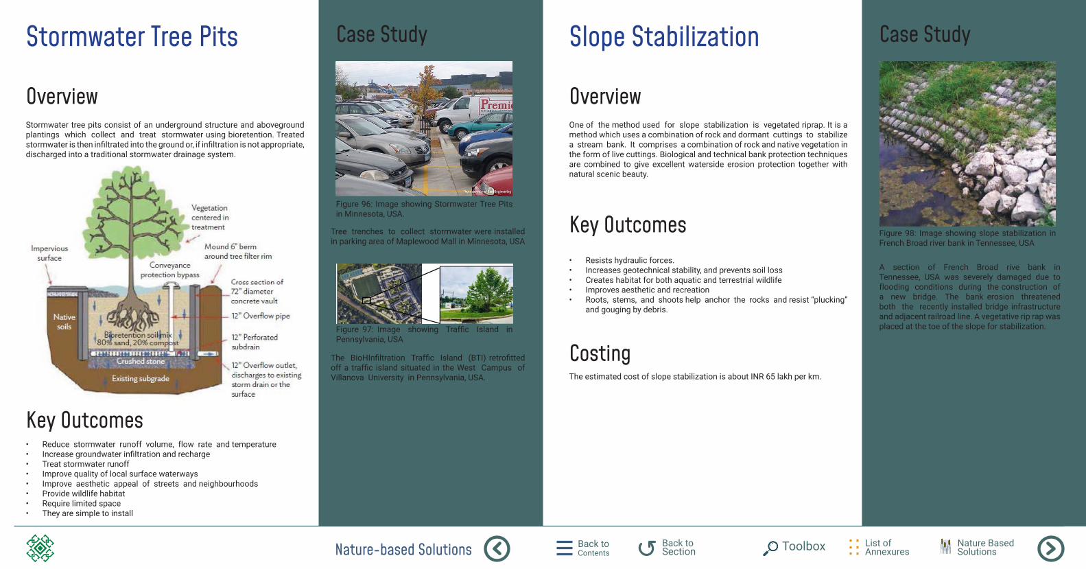
Nature-based Solutions Back to Contents
List of Annexures
Back to Section Toolbox Nature Based
Solutions
Stormwater Tree Pits
Overview
Case Study
Stormwater tree pits consist of an underground structure and aboveground plantings which collect and treat stormwater using bioretention. Treated stormwater is then infiltrated into the ground or, if infiltration is not appropriate, discharged into a traditional stormwater drainage system.
• Reduce stormwater runoff volume, flow rate and temperature • Increase groundwater infiltration and recharge • Treat stormwater runoff • Improve quality of local surface waterways • Improve aesthetic appeal of streets and neighbourhoods • Provide wildlife habitat • Require limited space • They are simple to install
Key Outcomes
Figure 96: Image showing Stormwater Tree Pits in Minnesota, USA.
Figure 97: Image showing Traffic Island in Pennsylvania, USA
Tree trenches to collect stormwater were installed in parking area of Maplewood Mall in Minnesota, USA
The BioHInfiltration Traffic Island (BTI) retrofitted off a traffic island situated in the West Campus of Villanova University in Pennsylvania, USA.
Slope Stabilization
Overview
Case Study
One of the method used for slope stabilization is vegetated riprap. It is a method which uses a combination of rock and dormant cuttings to stabilize a stream bank. It comprises a combination of rock and native vegetation in the form of live cuttings. Biological and technical bank protection techniques are combined to give excellent waterside erosion protection together with natural scenic beauty.
• Resists hydraulic forces. • Increases geotechnical stability, and prevents soil loss • Creates habitat for both aquatic and terrestrial wildlife • Improves aesthetic and recreation • Roots, stems, and shoots help anchor the rocks and resist “plucking”
and gouging by debris.
Key Outcomes Figure 98: Image showing slope stabilization in French Broad river bank in Tennessee, USA
A section of French Broad rive bank in Tennessee, USA was severely damaged due to flooding conditions during the construction of a new bridge. The bank erosion threatened both the recently installed bridge infrastructure and adjacent railroad line. A vegetative rip rap was placed at the toe of the slope for stabilization.
The estimated cost of slope stabilization is about INR 65 lakh per km.
Costing
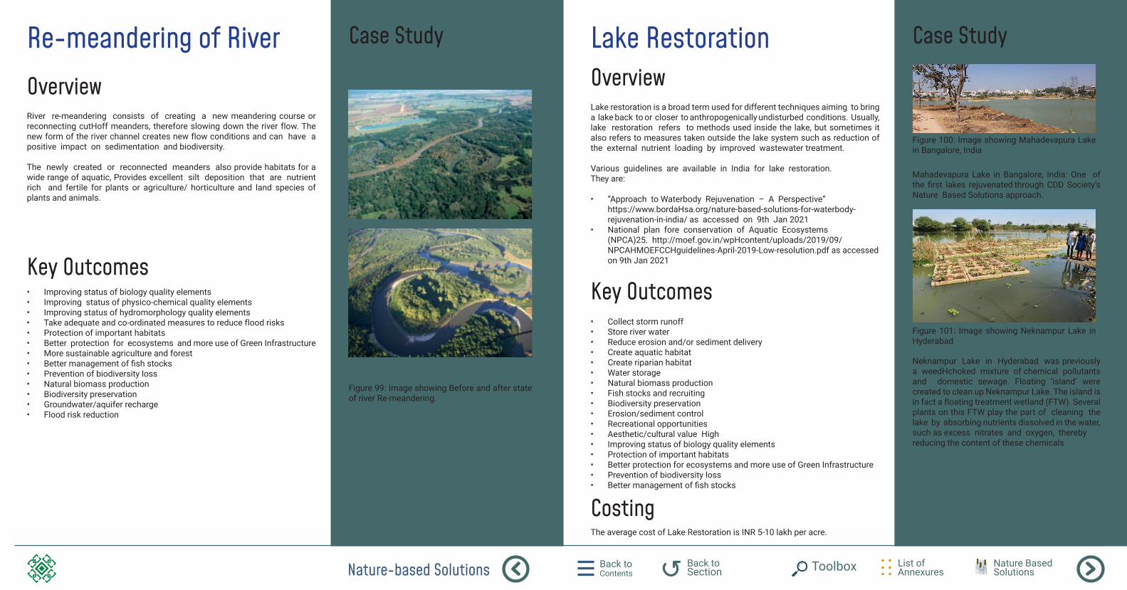
Nature-based Solutions Back to Contents
List of Annexures
Back to Section Toolbox Nature Based
Solutions
Re-meandering of RiverOverview
Case Study
River re-meandering consists of creating a new meandering course or reconnecting cutHoff meanders, therefore slowing down the river flow. The new form of the river channel creates new flow conditions and can have a positive impact on sedimentation and biodiversity. The newly created or reconnected meanders also provide habitats for a wide range of aquatic, Provides excellent silt deposition that are nutrient rich and fertile for plants or agriculture/ horticulture and land species of plants and animals.
• Improving status of biology quality elements • Improving status of physico-chemical quality elements • Improving status of hydromorphology quality elements • Take adequate and co-ordinated measures to reduce flood risks • Protection of important habitats • Better protection for ecosystems and more use of Green Infrastructure • More sustainable agriculture and forest • Better management of fish stocks • Prevention of biodiversity loss • Natural biomass production • Biodiversity preservation • Groundwater/aquifer recharge • Flood risk reduction
Key Outcomes
Figure 99: Image showing Before and after state of river Re-meandering.
Lake RestorationOverview
Case Study
Lake restoration is a broad term used for different techniques aiming to bring a lake back to or closer to anthropogenically undisturbed conditions. Usually, lake restoration refers to methods used inside the lake, but sometimes it also refers to measures taken outside the lake system such as reduction of the external nutrient loading by improved wastewater treatment. Various guidelines are available in India for lake restoration. They are:
• “Approach to Waterbody Rejuvenation – A Perspective” https://www.bordaHsa.org/nature-based-solutions-for-waterbody-rejuvenation-in-india/ as accessed on 9th Jan 2021
• National plan fore conservation of Aquatic Ecosystems (NPCA)25. http://moef.gov.in/wpHcontent/uploads/2019/09/NPCAHMOEFCCHguidelines-April-2019-Low-resolution.pdf as accessed on 9th Jan 2021
• Collect storm runoff • Store river water • Reduce erosion and/or sediment delivery • Create aquatic habitat • Create riparian habitat • Water storage • Natural biomass production • Fish stocks and recruiting • Biodiversity preservation • Erosion/sediment control • Recreational opportunities • Aesthetic/cultural value High • Improving status of biology quality elements • Protection of important habitats • Better protection for ecosystems and more use of Green Infrastructure • Prevention of biodiversity loss • Better management of fish stocks
Key Outcomes
Figure 100: Image showing Mahadevapura Lake in Bangalore, India
Figure 101: Image showing Neknampur Lake in Hyderabad
Mahadevapura Lake in Bangalore, India: One of the first lakes rejuvenated through CDD Society’s Nature Based Solutions approach.
Neknampur Lake in Hyderabad was previously a weedHchoked mixture of chemical pollutants and domestic sewage. Floating ‘island’ were created to clean up Neknampur Lake. The island is in fact a floating treatment wetland (FTW). Several plants on this FTW play the part of cleaning the lake by absorbing nutrients dissolved in the water, such as excess nitrates and oxygen, thereby reducing the content of these chemicals
The average cost of Lake Restoration is INR 5-10 lakh per acre.
Costing
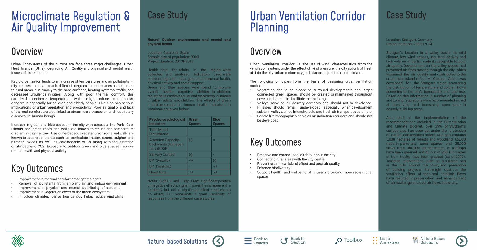
Nature-based Solutions Back to Contents
List of Annexures
Back to Section Toolbox Nature Based
Solutions
Microclimate Regulation & Air Quality Improvement
Overview
Case Study
Urban Ecosystems of the current era face three major challenges: Urban Heat Islands (UHIs), degrading Air Quality and physical and mental health issues of its residents. Rapid urbanization leads to an increase of temperatures and air pollutants in city centres that can reach different degrees in some cases as compared to rural areas, due mainly to the hard surfaces, heating systems, traffic, and decreased turbulence in cities. Along with poor thermal comfort, this can lead to extreme temperatures which might induce heat shocks, dangerous especially for children and elderly people. This also has serious implications or urban vegetation and productivity. Poor air quality and lack of thermal comfort are also linked to stress, cardiovascular and respiratory diseases in human beings. Increase in green and blue spaces in the city with concepts like Park Cool Islands and green roofs and walls are known to reduce the temperature gradient in city centres. Use of herbaceous vegetation on roofs and walls are known to absorb pollutants such as particulate matter, ozone, sulphur and nitrogen oxides as well as carcinogenic VOCs along with sequestration of atmospheric CO2. Exposure to outdoor green and blue spaces improve mental health and physical activity
• Improvement in thermal comfort amongst residents • Removal of pollutants from ambient air and indoor environment • Improvement in physical and mental wellHbeing of residents • Improvement in vegetation cover of the urban ecosystem • In colder climates, dense tree canopy helps reduce wind chills
Key Outcomes
Natural Outdoor environments and mental and physical health
Location: Catalonia, Spain Sample size of population: 9000 Project duration: 2010H2012 Health data for adults in the region were collected and analysed. Indicators used were sociodemographic data, general and mental health, physical activity and social support. Green and Blue spaces were found to improve overall health, cognitive abilities in children, reduction in cardiovascular and respiratory diseases in urban adults and children. The effects of green and blue spaces on human health indicators in Catalonia are given below:
Psycho-psychological Indicators
Green Spaces
Blue Spaces
Total Mood Disturbance
- -
Attention Capacity- backwards digit-span task (BDSP)
(-) =
Salivary Cortisol (-) -BP (Systolic) -/+ (-)BP (Diastolic) + -/+Heart Rate -/+ -/+
Notes: Signs + and – represent significant positive or negative effects, signs in parenthesis represent a tendency but not a significant effect, = represents no effect, E/+ represents a great variability of responses from the different case studies.
Location: Stuttgart, Germany Project duration: 2008H2014
Stuttgart’s location in a valley basin, its mild climate, low wind speeds, industrial activity and high volume of traffic made it susceptible to poor air quality. Development on the valley slopes had prevented air from moving through the city, which worsened the air quality and contributed to the urban heat island effect. A Climate Atlas was developed for the Stuttgart region, presenting the distribution of temperature and cold air flows according to the city’s topography and land use. Based on this information, a number of planning and zoning regulations were recommended aimed at preserving and increasing open space in densely builtHup areas.
As a result of the implementation of the recommendations included in the Climate Atlas and Climate Booklet, over 39% of Stuttgart’s surface area has been put under the protection of nature conservation orders. Stuttgart contains 5,000 hectares of forests and woodland, 65,000 trees in parks and open spaces and 35,000 street trees. 300,000 square meters of rooftops have been greened and 40 out of 250 kilometres of tram tracks have been grassed (as of 2007). Targeted interventions such as a building ban in the hills around the town, and prevention of building projects that might obstruct the ventilation effect of nocturnal coldHair flows have resulted in preservation and enhancement of air exchange and cool air flows in the city.
Urban Ventilation Corridor Planning
Overview
Case Study
Urban ventilation corridor is the use of wind characteristics, from the ventilation system, under the effect of wind pressure, the city suburb of fresh air into the city, urban carbon oxygen balance, adjust the microclimate. The following principles form the basis of designing urban ventilation corridors:• Vegetation should be placed to surround developments and larger,
connected green spaces should be created or maintained throughout developed areas to facilitate air exchange
• Valleys serve as air delivery corridors and should not be developed • Hillsides should remain undeveloped, especially when development
exists in valleys, since intensive cold and fresh air transport occurs here • Saddle-like topographies serve as air induction corridors and should not
be developed
• Preserve and channel cool air throughout the city • Connecting rural areas with the city centre • Prevent urban heat island effect and poor air quality • Enhance biodiversity • Support health and wellbeing of citizens providing more recreational
spaces
Key Outcomes
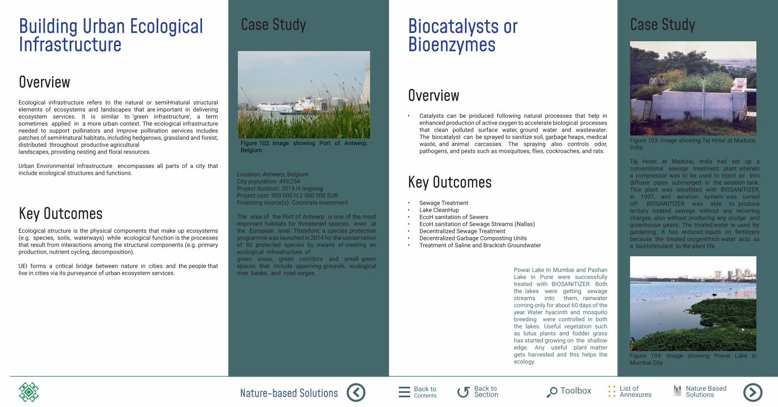
Nature-based Solutions Back to Contents
List of Annexures
Back to Section Toolbox Nature Based
Solutions
Building Urban Ecological Infrastructure
Overview
Case Study
Ecological infrastructure refers to the natural or semiHnatural structural elements of ecosystems and landscapes that are important in delivering ecosystem services. It is similar to ‘green infrastructure’, a term sometimes applied in a more urban context. The ecological infrastructure needed to support pollinators and improve pollination services includes patches of semiHnatural habitats, including hedgerows, grassland and forest, distributed throughout productive agricultural landscapes, providing nesting and floral resources. Urban Environmental Infrastructure encompasses all parts of a city that include ecological structures and functions.
Ecological structure is the physical components that make up ecosystems (e.g. species, soils, waterways) while ecological function is the processes that result from interactions among the structural components (e.g. primary production, nutrient cycling, decomposition). UEI forms a critical bridge between nature in cities and the people that live in cities via its purveyance of urban ecosystem services.
Key Outcomes
Figure 102: Image showing Port of Antwerp, Belgium
Location: Antwerp, Belgium City population: 499,254 Project duration: 2015 H ongoing Project cost: 500 000 H 2 000 000 EUR Financing source(s): Corporate investment The area of the Port of Antwerp is one of the most important habitats for threatened species, even at the European level. Therefore, a species protection programme was launched in 2014 for the conservation of 90 protected species by means of creating an ecological infrastructure of green areas, green corridors and small green spaces that include spawning grounds, ecological river banks, and road verges.
Biocatalysts or Bioenzymes
Overview
Case Study
• Catalysts can be produced following natural processes that help in enhanced production of active oxygen to accelerate biological processes that clean polluted surface water, ground water and wastewater. The biocatalyst can be sprayed to sanitize soil, garbage heaps, medical waste, and animal carcasses. The spraying also controls odor, pathogens, and pests such as mosquitoes, flies, cockroaches, and rats.
• Sewage Treatment • Lake CleanHup • EcoH sanitation of Sewers • EcoH sanitation of Sewage Streams (Nallas) • Decentralized Sewage Treatment • Decentralized Garbage Composting Units • Treatment of Saline and Brackish Groundwater
Key Outcomes
Figure 103: Image showing Taj Hotel at Madurai, India
Figure 104: Image showing Powai Lake in Mumbai City
Taj Hotel at Madurai, India had set up a conventional sewage treatment plant wherein a compressor was to be used to inject air into diffuser pipes submerged in the aeration tank. This plant was retrofitted with BIOSANITIZER, in 1997, and aeration system was turned off. BIOSANITIZER was able to produce tertiary treated sewage without any recurring charges, also without producing any sludge and greenhouse gases. The treated water is used for gardening. It has reduced inputs on fertilizers because the treated oxygenHrich water acts as a bioHstimulant to the plant life.
Powai Lake In Mumbai and Pashan Lake in Pune were successfully treated with BIOSANITIZER. Both the lakes were getting sewage streams into them, rainwater coming only for about 60 days of the year. Water hyacinth and mosquito breeding were controlled in both the lakes. Useful vegetation such as lotus plants and fodder grass has started growing on the shallow edge. Any useful plant matter gets harvested and this helps the ecology.
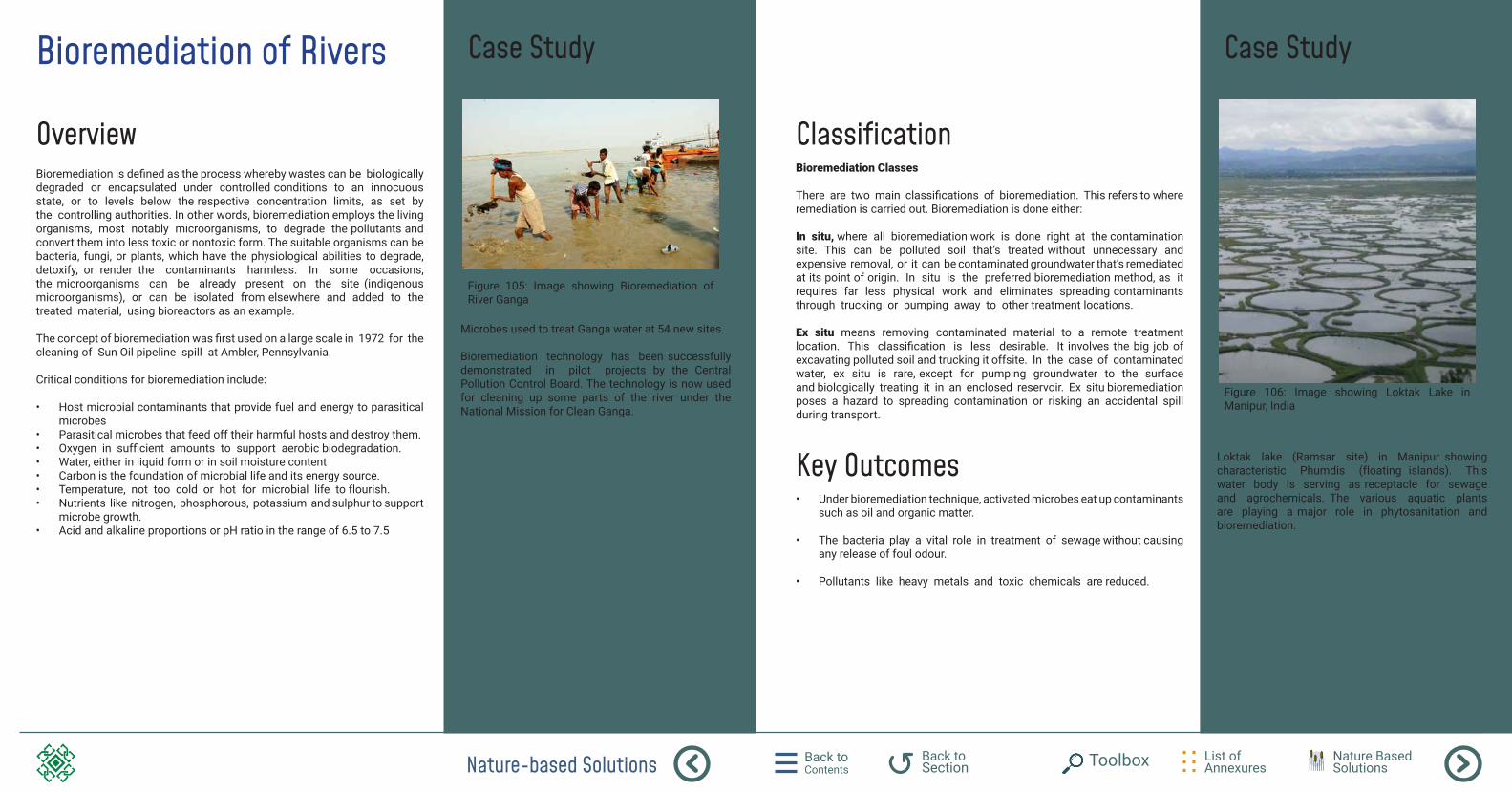
Nature-based Solutions Back to Contents
List of Annexures
Back to Section Toolbox Nature Based
Solutions
Bioremediation of Rivers
Overview
Case Study
Bioremediation is defined as the process whereby wastes can be biologically degraded or encapsulated under controlled conditions to an innocuous state, or to levels below the respective concentration limits, as set by the controlling authorities. In other words, bioremediation employs the living organisms, most notably microorganisms, to degrade the pollutants and convert them into less toxic or nontoxic form. The suitable organisms can be bacteria, fungi, or plants, which have the physiological abilities to degrade, detoxify, or render the contaminants harmless. In some occasions, the microorganisms can be already present on the site (indigenous microorganisms), or can be isolated from elsewhere and added to the treated material, using bioreactors as an example. The concept of bioremediation was first used on a large scale in 1972 for the cleaning of Sun Oil pipeline spill at Ambler, Pennsylvania. Critical conditions for bioremediation include: • Host microbial contaminants that provide fuel and energy to parasitical
microbes • Parasitical microbes that feed off their harmful hosts and destroy them. • Oxygen in sufficient amounts to support aerobic biodegradation. • Water, either in liquid form or in soil moisture content • Carbon is the foundation of microbial life and its energy source. • Temperature, not too cold or hot for microbial life to flourish. • Nutrients like nitrogen, phosphorous, potassium and sulphur to support
microbe growth. • Acid and alkaline proportions or pH ratio in the range of 6.5 to 7.5
Figure 105: Image showing Bioremediation of River Ganga
Microbes used to treat Ganga water at 54 new sites. Bioremediation technology has been successfully demonstrated in pilot projects by the Central Pollution Control Board. The technology is now used for cleaning up some parts of the river under the National Mission for Clean Ganga.
Case Study
Bioremediation Classes
There are two main classifications of bioremediation. This refers to where remediation is carried out. Bioremediation is done either:
In situ, where all bioremediation work is done right at the contamination site. This can be polluted soil that’s treated without unnecessary and expensive removal, or it can be contaminated groundwater that’s remediated at its point of origin. In situ is the preferred bioremediation method, as it requires far less physical work and eliminates spreading contaminants through trucking or pumping away to other treatment locations. Ex situ means removing contaminated material to a remote treatment location. This classification is less desirable. It involves the big job of excavating polluted soil and trucking it offsite. In the case of contaminated water, ex situ is rare, except for pumping groundwater to the surface and biologically treating it in an enclosed reservoir. Ex situ bioremediation poses a hazard to spreading contamination or risking an accidental spill during transport.
• Under bioremediation technique, activated microbes eat up contaminants such as oil and organic matter.
• The bacteria play a vital role in treatment of sewage without causing
any release of foul odour. • Pollutants like heavy metals and toxic chemicals are reduced.
Classification
Key Outcomes
Figure 106: Image showing Loktak Lake in Manipur, India
Loktak lake (Ramsar site) in Manipur showing characteristic Phumdis (floating islands). This water body is serving as receptacle for sewage and agrochemicals. The various aquatic plants are playing a major role in phytosanitation and bioremediation.

Back to Contents
List of Annexures
Back to SectionUrban Ecosystems Nature Based
SolutionsToolbox
Growing algae to absorb vehicular pollution
Overview
Case Study
Road transportation is the greatest contributor of global warming according to NASA, accounting for more than half of the carbon monoxide and nitrogen oxide levels emitted into the air. To reduce the pollution from road transportation, an algae farm is set on an overpass over the highway and consists of a closed system of transparent, algaeHfilled tubes. The tubes are hooked up to secondary equipment such as filters, pumps and solar panels. Careful species selection for landscaping and road side vegetation to retain the aim or beautification, barrier, sound control but increase the ability to absorb pollutants.
Figure 107: Image showing Garden Festival in Geneva
As part of a recent garden festival in Geneva, the team at Cloud Collective aimed to create an algae garden that uses the highway’s excess of carbon dioxide coupled with sunlight to transform the polluted landscape into a smart space for urban farming. The system is quite simple, the algae are cultivated inside tubes, and a series of pumps, filters and solar panels aid the process. Once the algae mature, they can be used into a number of different products, including biodiesel, nutrients, medication and cosmetics.
Algae is ten times more efficient in producing oxygen than that of trees and grass and can cut CO2 emissions by up to 68 % when converted into biofuel.
Key Outcomes
Worksheets Back to Contents
List of Annexures
Back to Section Toolbox Nature Based
Solutions
Worksheets
The worksheets are given in the following section for urban practioners to use them in ecosystem health assessment.
The following worksheets are developed:
Worksheet 1
Worksheet 2
Worksheet 3
Worksheet 4
Worksheet 5
Worksheet 6
Worksheet 7
Identify Pressure indicators (mapping to section 5.1)
Identify State indicators (mapping to section 5.2)
Prepare scoping impact matrix (mapping to section 5.3)
Prepare graded impact matrix (mapping to section 5.4)
Create basic impact network (mapping to section 5.5)
Create advance impact network (mapping to section 5.6)
Identify Responses (mapping to section 8)
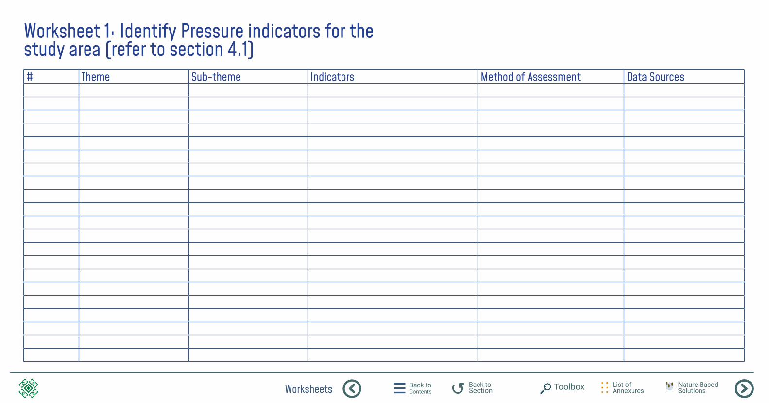
Worksheets Back to Contents
List of Annexures
Back to Section Toolbox Nature Based
Solutions
Worksheet 1: Identify Pressure indicators for the study area (refer to section 4.1)# Theme Sub-theme Indicators Method of Assessment Data Sources
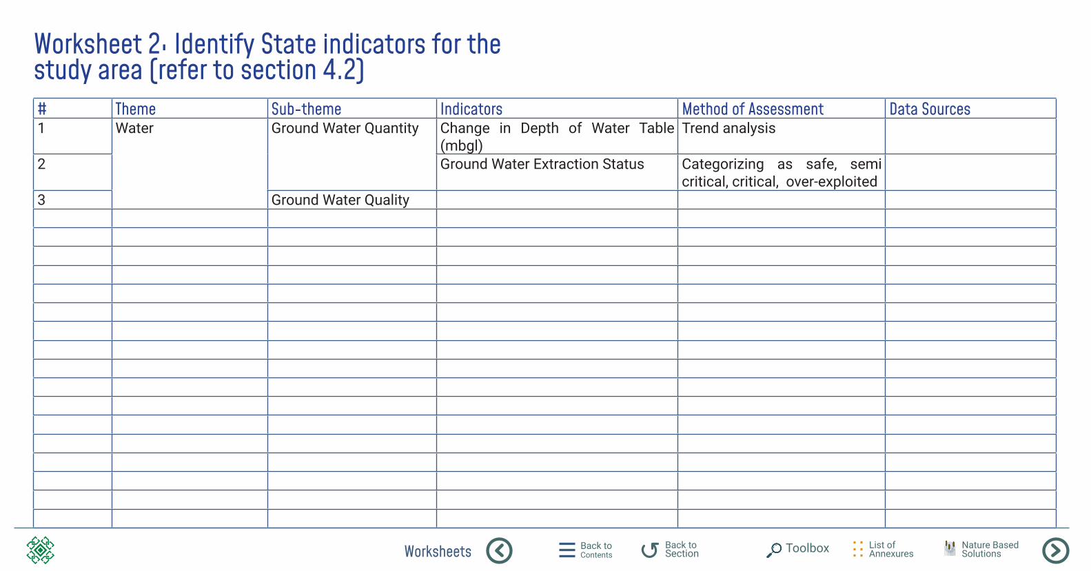
Worksheets Back to Contents
List of Annexures
Back to Section Toolbox Nature Based
Solutions
Worksheet 2: Identify State indicators for the study area (refer to section 4.2)# Theme Sub-theme Indicators Method of Assessment Data Sources1 Water Ground Water Quantity Change in Depth of Water Table
(mbgl)Trend analysis
2 Ground Water Extraction Status Categorizing as safe, semi critical, critical, over-exploited
3 Ground Water Quality
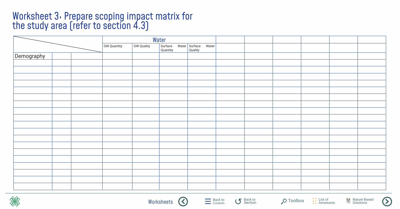
Worksheets Back to Contents
List of Annexures
Back to Section Toolbox Nature Based
Solutions
Worksheet 3: Prepare scoping impact matrix for the study area (refer to section 4.3)
WaterGW Quantity GW Quality Surface Water
QuantitySurface Water Quality
Demography
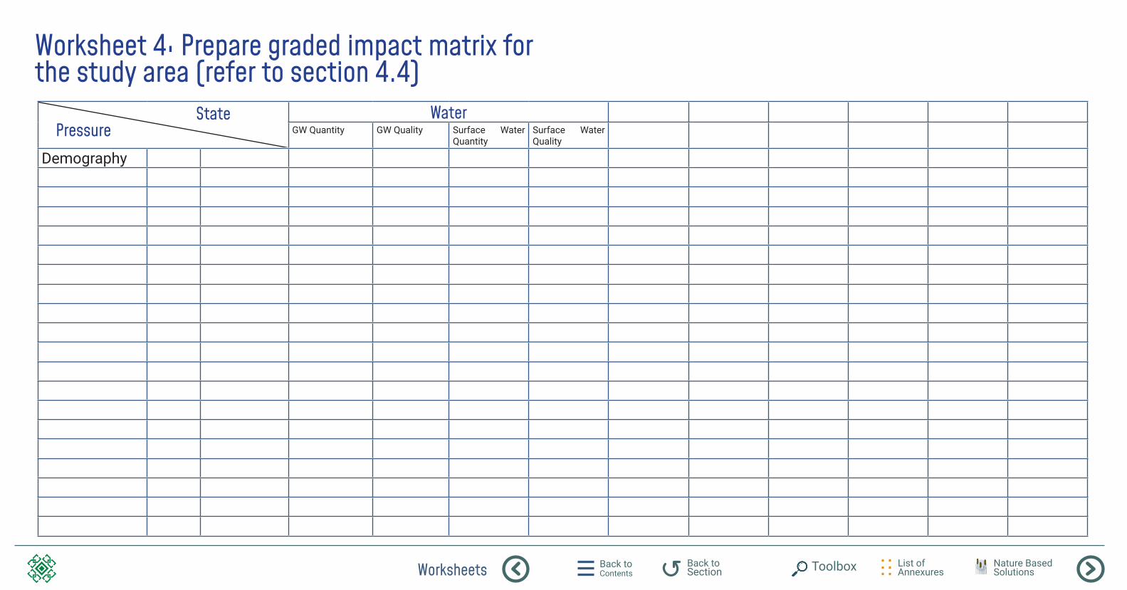
Worksheets Back to Contents
List of Annexures
Back to Section Toolbox Nature Based
Solutions
Worksheet 4: Prepare graded impact matrix for the study area (refer to section 4.4)
WaterGW Quantity GW Quality Surface Water
QuantitySurface Water Quality
Demography
PressureState

Worksheets Back to Contents
List of Annexures
Back to Section Toolbox Nature Based
Solutions
Worksheet 5: Create basic impact network for the study area (refer to section 4.5)

Worksheets Back to Contents
List of Annexures
Back to Section Toolbox Nature Based
Solutions
Worksheet 7: Identify Response for the Issues (refer to section 7)Issues
Policy Plan Program ProjectResponse Planning from 4P Perspective
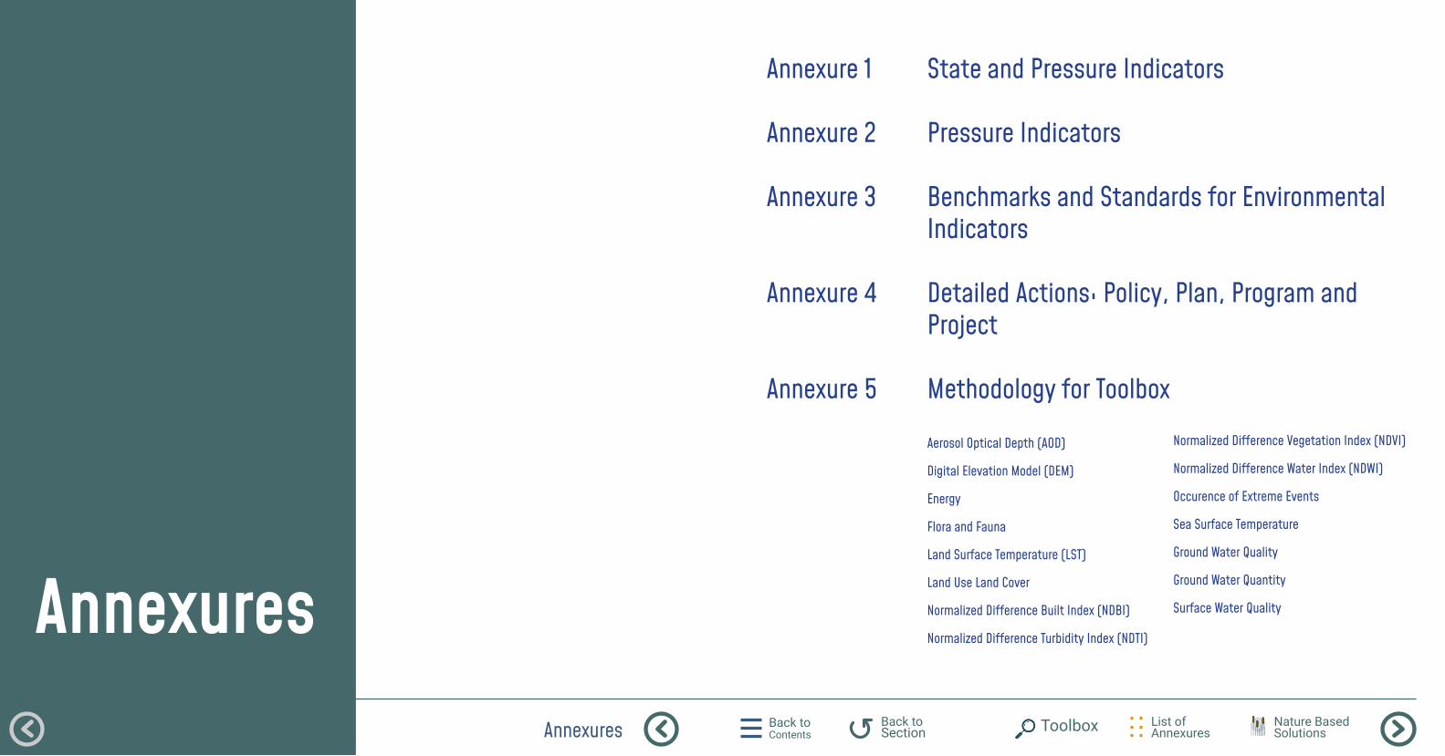
Annexures Back to Contents
List of Annexures
Back to Section Toolbox Nature Based
Solutions
Annexures
Annexure 1
Annexure 2
Annexure 3
Annexure 4
Annexure 5
State and Pressure Indicators
Pressure Indicators
Benchmarks and Standards for Environmental Indicators
Detailed Actions: Policy, Plan, Program and Project
Methodology for Toolbox
Aerosol Optical Depth (AOD)
Digital Elevation Model (DEM)
Energy
Flora and Fauna
Land Surface Temperature (LST)
Land Use Land Cover
Normalized Difference Built Index (NDBI)
Normalized Difference Turbidity Index (NDTI)
Normalized Difference Vegetation Index (NDVI)
Normalized Difference Water Index (NDWI)
Occurence of Extreme Events
Sea Surface Temperature
Ground Water Quality
Ground Water Quantity
Surface Water Quality
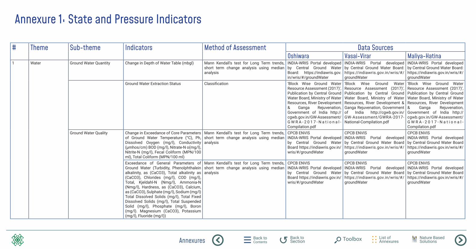
Annexures Back to Contents
List of Annexures
Back to Section Toolbox Nature Based
Solutions
Annexure 1: State and Pressure Indicators
# Theme Sub-theme Indicators Method of Assessment Data SourcesOshiwara Vasai-Virar Maliya-Hatina
1 Water Ground Water Quantity Change in Depth of Water Table (mbgl) Mann Kendall's test for Long Term trends, short term change analysis using median analysis
INDIA-WRIS Portal developed by Central Ground Water Board: https://indiawris.gov.in/wris/#/groundWater
INDIA-WRIS Portal developed by Central Ground Water Board: https://indiawris.gov.in/wris/#/groundWater
INDIA-WRIS Portal developed by Central Ground Water Board: https://indiawris.gov.in/wris/#/groundWater
Ground Water Extraction Status Classification ‘Block Wise Ground Water Resource Assessment (2017)’, Publication by Central Ground Water Board, Ministry of Water Resources, River Development & Ganga Rejuvenation, Government of India http://cgwb.gov.in/GW-Assessment/G W R A - 2 0 1 7 - N a t i o n a l -Compilation.pdf
‘Block Wise Ground Water Resource Assessment (2017)’, Publication by Central Ground Water Board, Ministry of Water Resources, River Development & Ganga Rejuvenation, Government of India http://cgwb.gov.in/GW-Assessment/GWRA-2017-National-Compilation.pdf
‘Block Wise Ground Water Resource Assessment (2017)’, Publication by Central Ground Water Board, Ministry of Water Resources, River Development & Ganga Rejuvenation, Government of India http://cgwb.gov.in/GW-Assessment/G W R A - 2 0 1 7 - N a t i o n a l -Compilation.pdf
Ground Water Quality Change in Exceedance of Core Parameters of Ground Water Temperature (°C), Ph, Dissolved Oxygen (mg/l), Conductivity (μmhos/cm) BOD (mg/l), Nitrate-N o(mg/l), Nitrite-N (mg/l), Fecal Coliform (MPN/100 ml), Total Coliform (MPN/100 ml)
Mann Kendall’s test for Long Term trends, short term change analysis using median analysis
CPCB ENVISINDIA-WRIS Portal developed by Central Ground Water Board https://indiawris.gov.in/wris/#/groundWater
CPCB ENVISINDIA-WRIS Portal developed by Central Ground Water Board https://indiawris.gov.in/wris/#/groundWater
CPCB ENVISINDIA-WRIS Portal developed by Central Ground Water Board https://indiawris.gov.in/wris/#/groundWater
Exceedance of General Parameters of Ground Water (Turbidity, Phenolphthalein alkalinity, as (CaCO3), Total alkalinity as (CaCO3), Chlorides (mg/l), COD (mg/l), Total, Kjeldahl-N (Nmg/l), Ammonia-N (Nmg/l), Hardness, as (CaCO3), Calcium, as (CaCO3), Sulphate (mg/l), Sodium (mg/l)Total Dissolved Solids (mg/l), Total Fixed Dissolved Solids (mg/l), Total Suspended Solid (mg/l), Phosphate (mg/l), Boron (mg/l). Magnesium (CaCO3), Potassium (mg/l), Fluoride (mg/l))
Mann Kendall’s test for Long Term trends, short term change analysis using median analysis
CPCB ENVISINDIA-WRIS Portal developed by Central Ground Water Board https://indiawris.gov.in/wris/#/groundWater
CPCB ENVISINDIA-WRIS Portal developed by Central Ground Water Board https://indiawris.gov.in/wris/#/groundWater
CPCB ENVISINDIA-WRIS Portal developed by Central Ground Water Board https://indiawris.gov.in/wris/#/groundWater
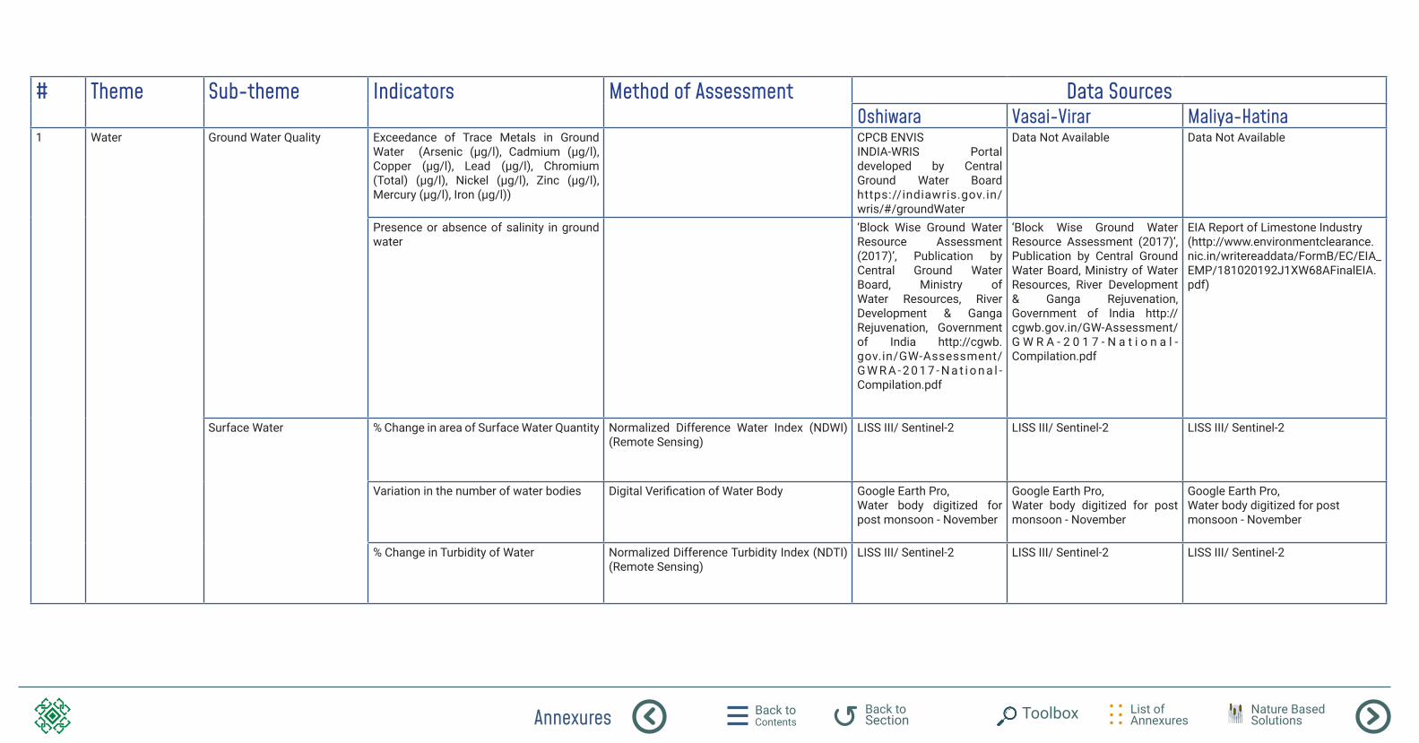
Annexures Back to Contents
List of Annexures
Back to Section Toolbox Nature Based
Solutions
# Theme Sub-theme Indicators Method of Assessment Data SourcesOshiwara Vasai-Virar Maliya-Hatina
1 Water Ground Water Quality Exceedance of Trace Metals in Ground Water (Arsenic (μg/l), Cadmium (μg/l), Copper (μg/l), Lead (μg/l), Chromium (Total) (μg/l), Nickel (μg/l), Zinc (μg/l), Mercury (μg/l), Iron (μg/l))
CPCB ENVISINDIA-WRIS Portal developed by Central Ground Water Board https://indiawris.gov.in/wris/#/groundWater
Data Not Available Data Not Available
Presence or absence of salinity in ground water
‘Block Wise Ground Water Resource Assessment (2017)’, Publication by Central Ground Water Board, Ministry of Water Resources, River Development & Ganga Rejuvenation, Government of India http://cgwb.gov.in/GW-Assessment/G W R A - 2 0 1 7 - N a t i o n a l -Compilation.pdf
‘Block Wise Ground Water Resource Assessment (2017)’, Publication by Central Ground Water Board, Ministry of Water Resources, River Development & Ganga Rejuvenation, Government of India http://cgwb.gov.in/GW-Assessment/G W R A - 2 0 1 7 - N a t i o n a l -Compilation.pdf
EIA Report of Limestone Industry (http://www.environmentclearance.nic.in/writereaddata/FormB/EC/EIA_EMP/181020192J1XW68AFinalEIA.pdf)
Surface Water % Change in area of Surface Water Quantity Normalized Difference Water Index (NDWI) (Remote Sensing)
LISS III/ Sentinel-2 LISS III/ Sentinel-2 LISS III/ Sentinel-2
Variation in the number of water bodies Digital Verification of Water Body Google Earth Pro,Water body digitized for post monsoon - November
Google Earth Pro,Water body digitized for post monsoon - November
Google Earth Pro,Water body digitized for post monsoon - November
% Change in Turbidity of Water Normalized Difference Turbidity Index (NDTI) (Remote Sensing)
LISS III/ Sentinel-2 LISS III/ Sentinel-2 LISS III/ Sentinel-2
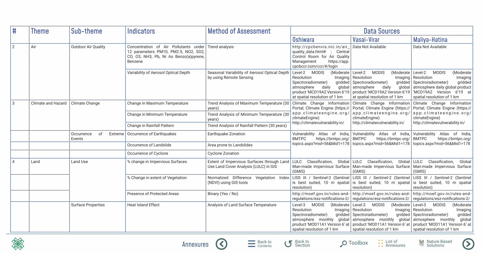
Annexures Back to Contents
List of Annexures
Back to Section Toolbox Nature Based
Solutions
# Theme Sub-theme Indicators Method of Assessment Data SourcesOshiwara Vasai-Virar Maliya-Hatina
2 Air Outdoor Air Quality Concentration of Air Pollutants under 12 parameters PM10, PM2.5, NO2, SO2, CO, O3, NH3, Pb, Ni As Benzo(a)pyrene, Benzene
Trend analysis http://cpcbenvis.nic.in/air_quality_data.html# ; Central Control Room for Air Quality Management https://app.cpcbccr.com/ccr/#/login
Data Not Available Data Not Available
Variability of Aerosol Optical Depth Seasonal Variability of Aerosol Optical Depth by using Remote Sensing
Level-2 MODIS (Moderate Resolution Imaging Spectroradiometer) gridded atmosphere daily global product ‘MCD19A2 Version 6’19 at spatial resolution of 1 km
Level-2 MODIS (Moderate Resolution Imaging Spectroradiometer) gridded atmosphere daily global product ‘MCD19A2 Version 6’19 at spatial resolution of 1 km
Level-2 MODIS (Moderate Resolution Imaging Spectroradiometer) gridded atmosphere daily global product ‘MCD19A2 Version 6’19 at spatial resolution of 1 km
3 Climate and Hazard Climate Change Change in Maximum Temperature Trend Analysis of Maximum Temperature (30 years)
Climate Change Information Portal; Climate Engine (https://a p p . c l i m a t e e n g i n e . o r g /climateEngine)http://climatevulnerability.in/
Climate Change Information Portal; Climate Engine (https://a p p . c l i m a t e e n g i n e . o r g /climateEngine)http://climatevulnerability.in/
Climate Change Information Portal; Climate Engine (https://a p p . c l i m a t e e n g i n e . o r g /climateEngine)http://climatevulnerability.in/
Change in Minimum Temperature Trend Analysis of Minimum Temperature (30 years)
Change in Rainfall Pattern Trend Analysis of Rainfall Pattern (30 years)
Occurrence of Extreme Events
Occurrence of Earthquakes Earthquake Zonation Vulnerability Atlas of India, BMTPC https://bmtpc.org/topics.aspx?mid=56&Mid1=178
Vulnerability Atlas of India, BMTPC https://bmtpc.org/topics.aspx?mid=56&Mid1=178
Vulnerability Atlas of India, BMTPC https://bmtpc.org/topics.aspx?mid=56&Mid1=178Occurrence of Landslide Area prone to Landslides
Occurrence of Cyclone Cyclone Zonation
4 Land Land Use % change in Impervious Surfaces Extent of Impervious Surfaces through Land Use Land Cover Analysis (LULC) in GIS
LULC Classification, Global Man-made Impervious Surface (GMIS)
LULC Classification, Global Man-made Impervious Surface (GMIS)
LULC Classification, Global Man-made Impervious Surface (GMIS)
% Change in extent of Vegetation Normalized Difference Vegetation Index (NDVI) using GIS tools
LISS III / Sentinel-2 (Sentinel is best suited, 10 m spatial resolution)
LISS III / Sentinel-2 (Sentinel is best suited, 10 m spatial resolution)
LISS III / Sentinel-2 (Sentinel is best suited, 10 m spatial resolution)
Presence of Protected Areas Binary (Yes / No) http://moef.gov.in/rules-and-regulations/esz-notifications-2/
http://moef.gov.in/rules-and-regulations/esz-notifications-2/
http://moef.gov.in/rules-and-regulations/esz-notifications-2/
Surface Properties Heat Island Effect Analysis of Land Surface Temperature Level-3 MODIS (Moderate Resolution Imaging Spectroradiometer) gridded atmosphere monthly global product ‘MOD11A1 Version 6’ at spatial resolution of 1 km
Level-3 MODIS (Moderate Resolution Imaging Spectroradiometer) gridded atmosphere monthly global product ‘MOD11A1 Version 6’ at spatial resolution of 1 km
Level-3 MODIS (Moderate Resolution Imaging Spectroradiometer) gridded atmosphere monthly global product ‘MOD11A1 Version 6’ at spatial resolution of 1 km
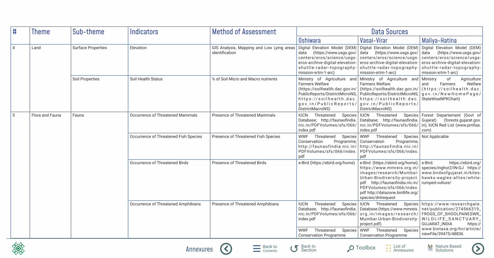
Annexures Back to Contents
List of Annexures
Back to Section Toolbox Nature Based
Solutions
# Theme Sub-theme Indicators Method of Assessment Data SourcesOshiwara Vasai-Virar Maliya-Hatina
4 Land Surface Properties Elevation GIS Analysis, Mapping and Low Lying areas identification
Digital Elevation Model (DEM) data (https://www.usgs.gov/centers/eros/science/usgs-eros-archive-digital-elevation-shut t le - radar - topography-mission-srtm-1-arc)
Digital Elevation Model (DEM) data (https://www.usgs.gov/centers/eros/science/usgs-eros-archive-digital-elevation-shut t le - radar - topography -mission-srtm-1-arc)
Digital Elevation Model (DEM) data (https://www.usgs.gov/centers/eros/science/usgs-eros-archive-digital-elevation-s h u t t l e - ra d a r - to p o g ra p h y -mission-srtm-1-arc)
Soil Properties Soil Health Status % of Soil Micro and Macro nutrients Ministry of Agriculture and Farmers Welfare(https://soilhealth.dac.gov.in/PublicReports/DistrictMicroNS, h t t p s : // s o i l h e a l t h . d a c .g o v . i n / P u b l i c R e p o r t s /DistrictMacroNS)
Ministry of Agriculture and Farmers Welfare(https://soilhealth.dac.gov.in/PublicReports/DistrictMicroNS, h t t p s : // s o i l h e a l t h . d a c .g o v . i n / P u b l i c R e p o r t s /DistrictMacroNS)
Ministry of Agriculture and Farmers Welfare ( h t t p s : // s o i l h e a l t h . d a c .g o v . i n / N e w H o m e P a g e /StateWiseNPKChart)
5 Flora and Fauna Fauna Occurrence of Threatened Mammals Presence of Threatened Mammals IUCN Threatened Species Database; http://faunaofindia.nic.in/PDFVolumes/sfs/066/index.pdf
IUCN Threatened Species Database; http://faunaofindia.nic.in/PDFVolumes/sfs/066/index.pdf
Forest Departement (Govt of Gujarat) (forests.gujarat.gov.in), IUCN Red List (www.pmfias.com)
Occurrence of Threatened Fish Species Presence of Threatened Fish Species WWF Threatened Species Conservation Programme; http://faunaofindia.nic. in/PDFVolumes/sfs/066/index.pdf
WWF Threatened Species Conservation Programme, http://faunaof india.nic. in/PDFVolumes/sfs/066/index.pdf
Not Applicable
Occurrence of Threatened Birds Presence of Threatened Birds e-Bird (https://ebird.org/home) e-Bird (https://ebird.org/home); https://www.mmreis.org.in/images/research/Mumbai-Urban-Biodiversity-project.pdf http://faunaofindia.nic.in/PDFVolumes/sfs/066/index.pdf http://datazone.birdlife.org/species/dnlrequest
e-Bird: https://ebird.org/species/inghor2/IN-GJ https://www.birdsofgujarat.in/kites-hawks-eagles-al l ies/white-rumped-vulture/
Occurrence of Threatened Amphibians Presence of Threatened Amphibians IUCN Threatened Species Database; http://faunaofindia.nic.in/PDFVolumes/sfs/066/index.pdf
IUCN Threatened Species Database (https://www.mmreis.o r g . i n / i m a g e s / r e s e a r c h /Mumbai-Urban-Biodiversity-project.pdf)
https://www.researchgate.net/publication/274566319_FROGS_OF_SHOOLPANESWR_W I L D L I F E _ S A N C T U A R Y _GUJARAT_INDIA https://www.biotaxa.org/hn/article/viewFile/39475/48836
WWF Threatened Species Conservation Programme
WWF Threatened Species Conservation Programme
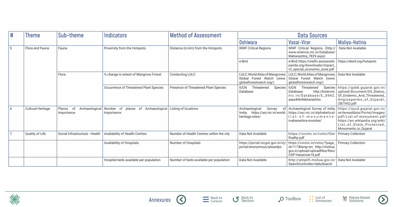
Annexures Back to Contents
List of Annexures
Back to Section Toolbox Nature Based
Solutions
# Theme Sub-theme Indicators Method of Assessment Data SourcesOshiwara Vasai-Virar Maliya-Hatina
5 Flora and Fauna Fauna Proximity from the Hotspots Distance (in km) from the Hotspots WWF Critical Regions WWF Critical Regions, (http://www.wiienvis.nic.in/Database/Maharashtra_7829.aspx)
Data Not Available
e-Bird e-Bird; https://wwfin.awsassets.panda.org/downloads/impact_of_special_economic_zone.pdf
https://ebird.org/hotspots
Flora % change in extent of Mangrove Forest Conducting LULC LULC; World Atlas of Mangroves; Global Forest Watch (www.globalforestwatch.org/)
LULC; World Atlas of Mangroves; Global Forest Watch (www.globalforestwatch.org/)
Data Not Available
Occurrence of Threatened Plant Species Presence of Threatened Plant Species IUCN Threatened Species Database
IUCN Threatened Species Database; http://bsienvis.n i c . i n / D a t a b a s e / E _ 3 9 4 2 .aspx#divMaharashtra
https://gsbb.gujarat.gov.in/upload/document/03_Status_Of_Endemic_And_Threatened_A n g i o s p e r m s _ o f _ G u j a ra t _(SETAG).pdf
6 Cultural Heritage Places of Archaeological Importance
Number of places of Archaeological Importance
Listing of locations Archaeological Survey of India; https://asi.nic.in/world-heritage-sites/
Archaeological Survey of India; https://asi.nic.in/alphabetical-l i s t - o f - m o n u m e n t s -maharashtra-mumbai/
https://sycd.gujarat.gov.in/writereaddata/Portal/Images/pdf/L is t -of -monument .pdf https://en.wikipedia.org/wiki/L i s t _ o f _ S t a t e _ P r o t e c t e d _Monuments_in_Gujarat
7 Quality of Life Social Infrastructure - Health Availability of Health Centres Number of Health Centres within the city Data Not Available https://vvcmc.in/vvmc/file/finalhp.pdf
Primary Collection
Availability of Hospitals Number of Hospitals https://portal.mcgm.gov.in/irj/portal/anonymous/qlwardps
https://vvcmc.in/vvmc/?page_id=117&lang=en; http://mohua.gov.in/upload/uploadfiles/files/CDP-Vasaivirar18.pdf
Primary Collection
Hospital beds available per population Number of beds available per population Data Not Available http://amplifi.mohua.gov.in/SearchController/tabluSearch
Data Not Available
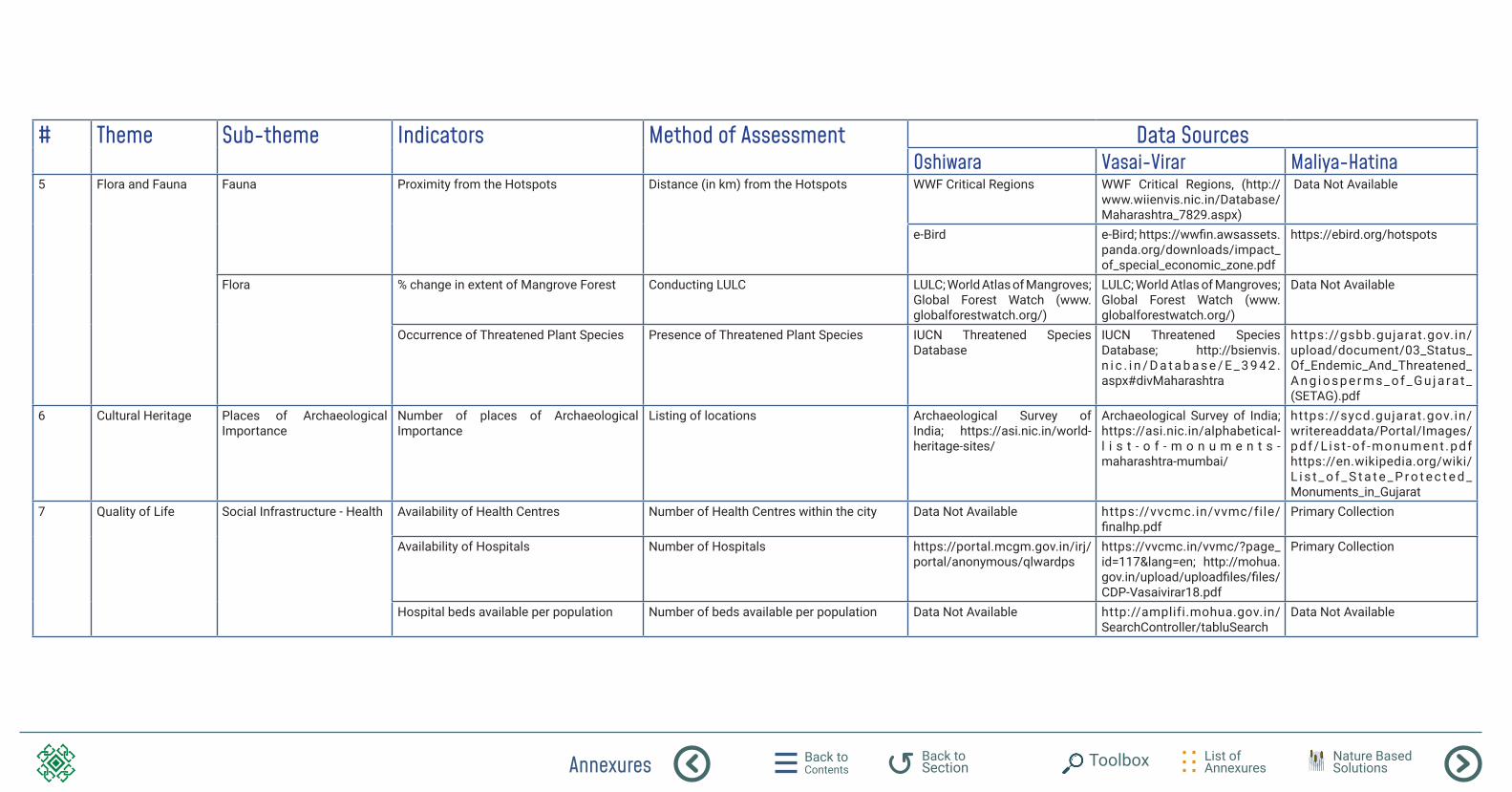
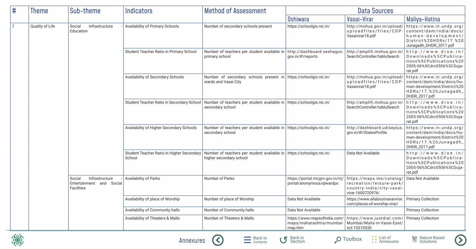
Annexures Back to Contents
List of Annexures
Back to Section Toolbox Nature Based
Solutions
# Theme Sub-theme Indicators Method of Assessment Data SourcesOshiwara Vasai-Virar Maliya-Hatina
7 Quality of Life Social Infrastructure - Education
Availability of Primary Schools Number of secondary schools present https://schoolgis.nic.in/ http://mohua.gov.in/upload/u p l o a d f i l e s / f i l e s / C D P -Vasaivirar18.pdf
h t t p s : // w w w. i n . u n d p . o r g /c o n t e n t / d a m / i n d i a / d o c s /h u m a n - d e v e l o p m e n t /D i s t r i c t % 2 0 H D R s / 1 7 . % 2 0Junagadh_DHDR_2017.pdf
Student Teacher Ratio in Primary School Number of teachers per student available in primary school
http://dashboard.seshagun.gov.in/#!/reports
http://amplifi.mohua.gov.in/SearchController/tabluSearch
h t t p : / / w w w . d i s e . i n /D o w n l o a d s % 5 C P u b l i c a -t i o n s % 5 C P u b l i c a t i o n s % 2 02005-06%5Cdrc0506%5CGuja-rat.pdf
Availability of Secondary Schools Number of secondary schools present in wards and Vasai City
https://schoolgis.nic.in/ http://mohua.gov.in/upload/u p l o a d f i l e s / f i l e s / C D P -Vasaivirar18.pdf
h t t p s : // w w w. i n . u n d p . o r g /content/dam/india/docs/hu-man-development/District%20H D R s / 1 7 . % 2 0 J u n a g a d h _DHDR_2017.pdf
Student Teacher Ratio in Secondary School Number of teachers per student available in secondary school
https://schoolgis.nic.in/ http://amplifi.mohua.gov.in/SearchController/tabluSearch
h t t p : / / w w w . d i s e . i n /D o w n l o a d s % 5 C P u b l i c a -t i o n s % 5 C P u b l i c a t i o n s % 2 02005-06%5Cdrc0506%5CGuja-rat.pdf
Availability of Higher Secondary Schools Number of teachers per student available in secondary school
https://schoolgis.nic.in/ http://dashboard.udiseplus.gov.in/#!/StatesProfile
h t t p s : // w w w. i n . u n d p . o r g /content/dam/india/docs/hu-man-development/District%20H D R s / 1 7 . % 2 0 J u n a g a d h _DHDR_2017.pdf
Student Teacher Ratio in Higher Secondary School
Number of teachers per student available in higher secondary school
https://schoolgis.nic.in/ Data Not Available h t t p : / / w w w . d i s e . i n /D o w n l o a d s % 5 C P u b l i c a -t i o n s % 5 C P u b l i c a t i o n s % 2 02005-06%5Cdrc0506%5CGuja-rat.pdf
Social Infrastructure - Entertainment and Social Facilities
Availability of Parks Number of Parks https://portal.mcgm.gov.in/irj/portal/anonymous/qlwardps
https://maps.me/cata log/r e c r e a t i o n / l e i s u r e - p a r k /c o u n t r y - i n d i a / c i t y - v a s a i -virar-1600720976/
Data Not Available
Availability of place of Worship Number of place of Worship Data Not Available https://www.allaboutvasaivirar.com/places-of-worship-virar/
Primary Collection
Availability of Community halls Number of Community halls Data Not Available Primary Collection
Availability of Theaters & Malls Number of Theaters & Malls https://www.mapsofindia.com/maps/maharashtra/mumbai-map.htm
https://www.justdia l .com/Mumbai/Malls-in-Vasai-East/nct-10310530
Primary Collection
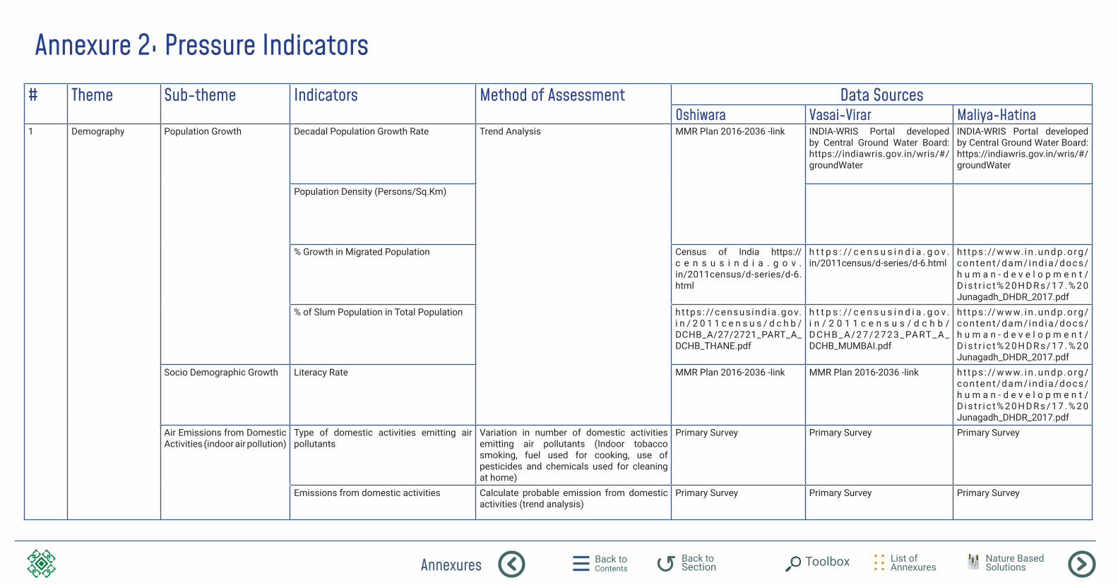
Annexures Back to Contents
List of Annexures
Back to Section Toolbox Nature Based
Solutions
Annexure 2: Pressure Indicators# Theme Sub-theme Indicators Method of Assessment Data Sources
Oshiwara Vasai-Virar Maliya-Hatina1 Demography Population Growth Decadal Population Growth Rate Trend Analysis MMR Plan 2016-2036 -link INDIA-WRIS Portal developed
by Central Ground Water Board: https://indiawris.gov.in/wris/#/groundWater
INDIA-WRIS Portal developed by Central Ground Water Board: https://indiawris.gov.in/wris/#/groundWater
Population Density (Persons/Sq.Km)
% Growth in Migrated Population Census of India https://c e n s u s i n d i a . g o v .in/2011census/d-series/d-6.html
h t t p s : // c e n s u s i n d i a . g o v .in/2011census/d-series/d-6.html
h t t p s : // w w w. i n . u n d p . o rg /content/dam/ ind ia/docs/h u m a n - d e v e l o p m e n t /D i s t r i c t % 2 0 H D R s / 1 7 . % 2 0Junagadh_DHDR_2017.pdf
% of Slum Population in Total Population ht tps : //census ind ia .gov.i n / 2 0 1 1 c e n s u s / d c h b /DCHB_A/27/2721_PART_A_DCHB_THANE.pdf
h t t p s : // c e n s u s i n d i a . g o v .i n / 2 0 1 1 c e n s u s / d c h b /DCHB_A/27/2723_PART_A_DCHB_MUMBAI.pdf
h t t p s : // w w w. i n . u n d p . o rg /content/dam/ ind ia/docs/h u m a n - d e v e l o p m e n t /D i s t r i c t % 2 0 H D R s / 1 7 . % 2 0Junagadh_DHDR_2017.pdf
Socio Demographic Growth Literacy Rate MMR Plan 2016-2036 -link MMR Plan 2016-2036 -link h t t p s : // w w w. i n . u n d p . o rg /content/dam/ ind ia/docs/h u m a n - d e v e l o p m e n t /D i s t r i c t % 2 0 H D R s / 1 7 . % 2 0Junagadh_DHDR_2017.pdf
Air Emissions from Domestic Activities (indoor air pollution)
Type of domestic activities emitting air pollutants
Variation in number of domestic activities emitting air pollutants (Indoor tobacco smoking, fuel used for cooking, use of pesticides and chemicals used for cleaning at home)
Primary Survey Primary Survey Primary Survey
Emissions from domestic activities Calculate probable emission from domestic activities (trend analysis)
Primary Survey Primary Survey Primary Survey
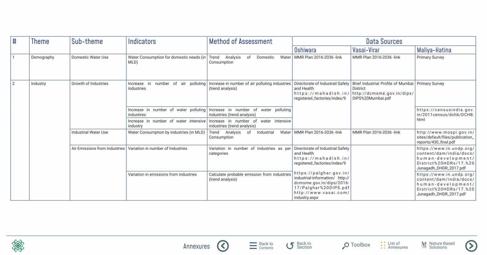
Annexures Back to Contents
List of Annexures
Back to Section Toolbox Nature Based
Solutions
# Theme Sub-theme Indicators Method of Assessment Data SourcesOshiwara Vasai-Virar Maliya-Hatina
1 Demography Domestic Water Use Water Consumption for domestic needs (in MLD)
Trend Analysis of Domestic Water Consumption
MMR Plan 2016-2036 -link MMR Plan 2016-2036 -link Primary Survey
2 Industry Growth of Industries Increase in number of air polluting industries
Increase in number of air polluting industries (trend analysis)
Directorate of Industrail Safety and Health h t t p s : // m a h a d i s h . i n /registered_factories/index/9
Brief Industrial Profile of Mumbai District ht tp ://dcmsme.gov. in/dips/DIPS%20Mumbai.pdf
Primary Survey
Increase in number of water polluting industires
Increase in number of water polluting industries (trend analysis)
h t t p s : // c e n s u s i n d i a . g o v.in/2011census/dchb/DCHB.htmlIncrease in number of water intensive
industryIncrease in number of water intensive industries (trend analysis)
Industrial Water Use Water Consumption by industries (in MLD) Trend Analysis of Industrial Water Consumption
MMR Plan 2016-2036 -link MMR Plan 2016-2036 -link ht tp : //www.mospi .gov. in/sites/default/files/publication_reports/430_final.pdf
Air Emissions from Industries Variation in number of Industries Variation in number of industries as per categories
Directorate of Industrial Safety and Health h t t p s : // m a h a d i s h . i n /registered_factories/index/9
h t t p s : // p a l g h a r . g o v. i n /industrial-information/ http://dcmsme.gov.in/dips/2016-1 7 / P a l g h a r % 2 0 D I P S . p d f h t t p : // w w w. v a s a i . c o m /industry.aspx
h t t p s : // w w w. i n . u n d p . o rg /content/dam/ ind ia/docs/h u m a n - d e v e l o p m e n t /D i s t r i c t % 2 0 H D R s / 1 7 . % 2 0Junagadh_DHDR_2017.pdf
Variation in emissions from industries Calculate probable emission from industries (trend analysis)
h t t p s : // w w w. i n . u n d p . o rg /content/dam/ ind ia/docs/h u m a n - d e v e l o p m e n t /D i s t r i c t % 2 0 H D R s / 1 7 . % 2 0Junagadh_DHDR_2017.pdf
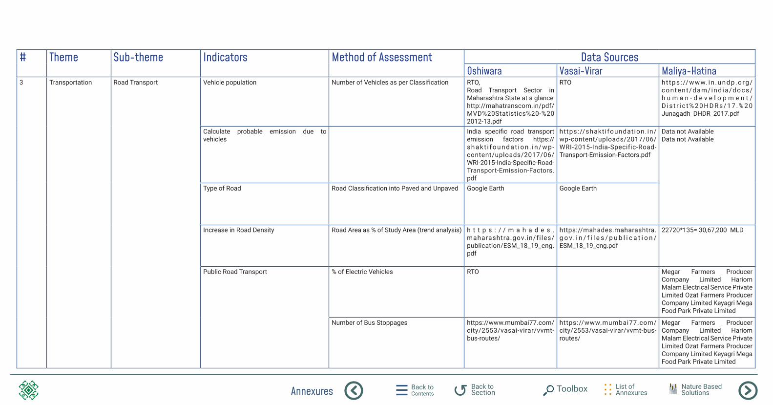
Annexures Back to Contents
List of Annexures
Back to Section Toolbox Nature Based
Solutions
# Theme Sub-theme Indicators Method of Assessment Data SourcesOshiwara Vasai-Virar Maliya-Hatina
3 Transportation Road Transport Vehicle population Number of Vehicles as per Classification RTO, Road Transport Sector in Maharashtra State at a glancehttp://mahatranscom.in/pdf/MVD%20Statistics%20-%202012-13.pdf
RTO h t t p s : // w w w. i n . u n d p . o rg /content/dam/ ind ia/docs/h u m a n - d e v e l o p m e n t /D i s t r i c t % 2 0 H D R s / 1 7 . % 2 0Junagadh_DHDR_2017.pdf
Calculate probable emission due to vehicles
India specific road transport emission factors https://s h a k t i f o u n d a t i o n . i n / w p -content/uploads/2017/06/WRI-2015-India-Specific-Road-Transport-Emission-Factors.pdf
https://shakt ifoundation. in/wp-content/uploads/2017/06/WRI-2015-India-Specific-Road-Transport-Emission-Factors.pdf
Data not AvailableData not Available
Type of Road Road Classification into Paved and Unpaved Google Earth Google Earth
Increase in Road Density Road Area as % of Study Area (trend analysis) h t t p s : / / m a h a d e s .maharashtra.gov.in/fi les/publication/ESM_18_19_eng.pdf
https://mahades.maharashtra.g o v . i n / f i l e s / p u b l i c a t i o n /ESM_18_19_eng.pdf
22720*135= 30,67,200 MLD
Public Road Transport % of Electric Vehicles RTO Megar Farmers Producer Company Limited Hariom Malam Electrical Service Private Limited Ozat Farmers Producer Company Limited Keyagri Mega Food Park Private Limited
Number of Bus Stoppages https://www.mumbai77.com/city/2553/vasai-virar/vvmt-bus-routes/
https://www.mumbai77.com/city/2553/vasai-virar/vvmt-bus-routes/
Megar Farmers Producer Company Limited Hariom Malam Electrical Service Private Limited Ozat Farmers Producer Company Limited Keyagri Mega Food Park Private Limited
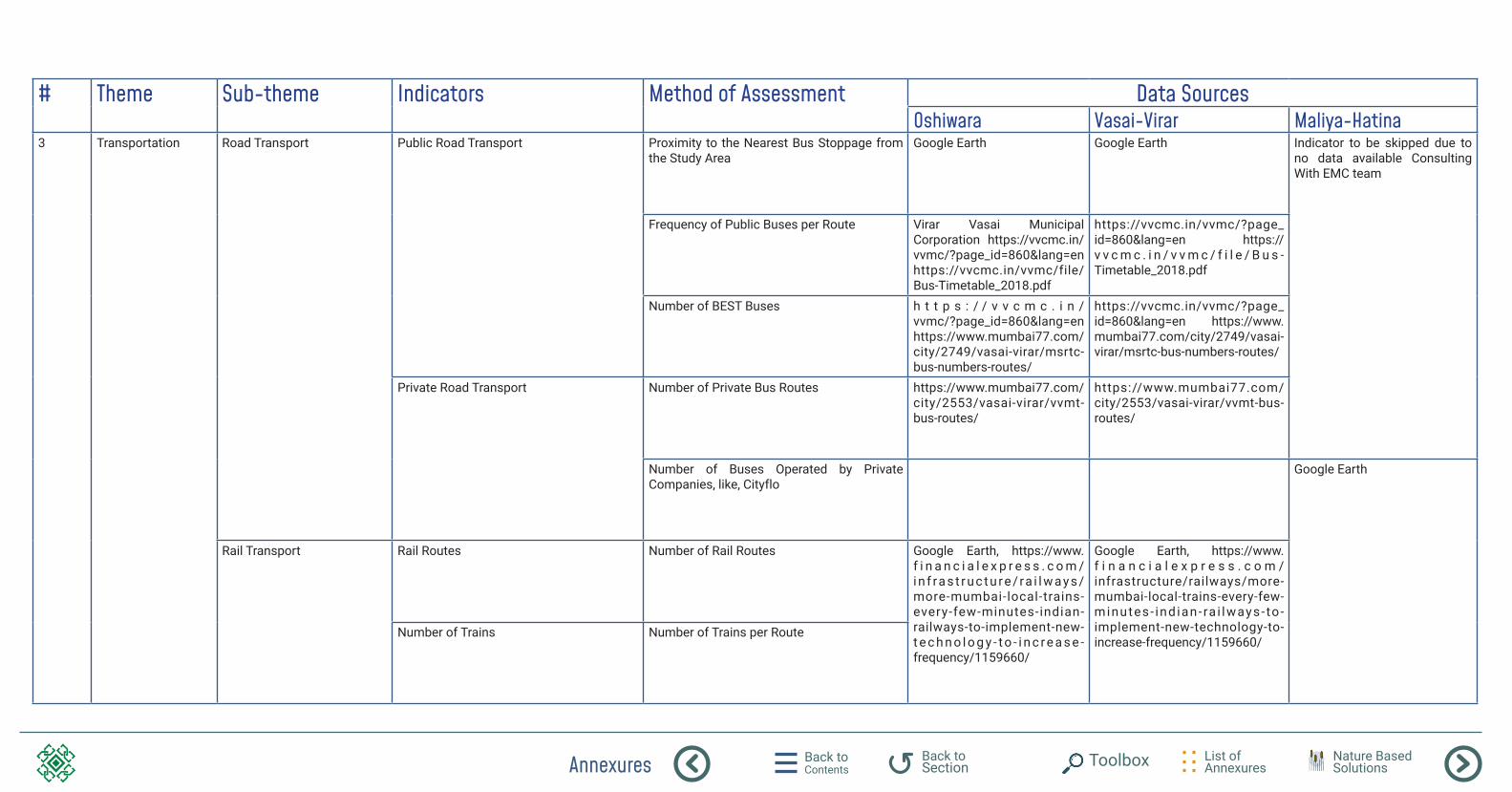
Annexures Back to Contents
List of Annexures
Back to Section Toolbox Nature Based
Solutions
# Theme Sub-theme Indicators Method of Assessment Data SourcesOshiwara Vasai-Virar Maliya-Hatina
3 Transportation Road Transport Public Road Transport Proximity to the Nearest Bus Stoppage from the Study Area
Google Earth Google Earth Indicator to be skipped due to no data available Consulting With EMC team
Frequency of Public Buses per Route Virar Vasai Municipal Corporation https://vvcmc.in/vvmc/?page_id=860&lang=en https://vvcmc.in/vvmc/file/Bus-Timetable_2018.pdf
https://vvcmc.in/vvmc/?page_id=860&lang=en https://v v c m c . i n / v v m c / f i l e / B u s -Timetable_2018.pdf
Number of BEST Buses h t t p s : / / v v c m c . i n /vvmc/?page_id=860&lang=en https://www.mumbai77.com/city/2749/vasai-virar/msrtc-bus-numbers-routes/
https://vvcmc.in/vvmc/?page_id=860&lang=en https://www.mumbai77.com/city/2749/vasai-virar/msrtc-bus-numbers-routes/
Private Road Transport Number of Private Bus Routes https://www.mumbai77.com/city/2553/vasai-virar/vvmt-bus-routes/
https://www.mumbai77.com/city/2553/vasai-virar/vvmt-bus-routes/
Number of Buses Operated by Private Companies, like, Cityflo
Google Earth
Rail Transport Rail Routes Number of Rail Routes Google Earth, https://www.f i n a n c i a l e x p r e s s . c o m /i n f ra s t r u c t u re / ra i l w ay s /more-mumbai-local-trains-every-few-minutes-indian-railways-to-implement-new-t e c h n o l o g y - t o - i n c r e a s e -frequency/1159660/
Google Earth, https://www.f i n a n c i a l e x p r e s s . c o m /infrastructure/railways/more-mumbai-local-trains-every-few-minutes - ind ian- ra i lways- to -implement-new-technology-to-increase-frequency/1159660/
Number of Trains Number of Trains per Route
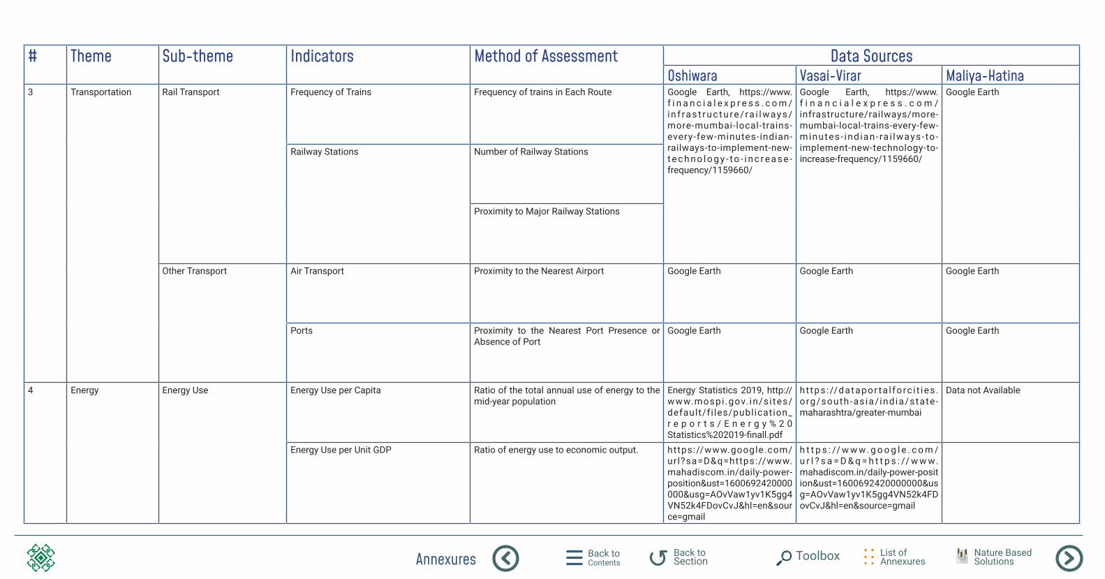
Annexures Back to Contents
List of Annexures
Back to Section Toolbox Nature Based
Solutions
# Theme Sub-theme Indicators Method of Assessment Data SourcesOshiwara Vasai-Virar Maliya-Hatina
3 Transportation Rail Transport Frequency of Trains Frequency of trains in Each Route Google Earth, https://www.f i n a n c i a l e x p r e s s . c o m /i n f ra s t r u c t u re / ra i l w ay s /more-mumbai-local-trains-every-few-minutes-indian-railways-to-implement-new-t e c h n o l o g y - t o - i n c r e a s e -frequency/1159660/
Google Earth, https://www.f i n a n c i a l e x p r e s s . c o m /infrastructure/railways/more-mumbai-local-trains-every-few-minutes - ind ian- ra i lways- to -implement-new-technology-to-increase-frequency/1159660/
Google Earth
Railway Stations Number of Railway Stations
Proximity to Major Railway Stations
Other Transport Air Transport Proximity to the Nearest Airport Google Earth Google Earth Google Earth
Ports Proximity to the Nearest Port Presence or Absence of Port
Google Earth Google Earth Google Earth
4 Energy Energy Use Energy Use per Capita Ratio of the total annual use of energy to the mid-year population
Energy Statistics 2019, http://www.mospi .gov. in/s i tes/default/fi les/publication_r e p o r t s / E n e r g y % 2 0Statistics%202019-finall.pdf
ht tps : //datapor ta l forc i t ies .org/south-as ia/ ind ia/state -maharashtra/greater-mumbai
Data not Available
Energy Use per Unit GDP Ratio of energy use to economic output. https://www.google.com/url?sa=D&q=https://www.mahadiscom.in/daily-power-position&ust=1600692420000000&usg=AOvVaw1yv1K5gg4VN52k4FDovCvJ&hl=en&source=gmail
h t t p s : // w w w. g o o g l e . c o m /u r l ? s a = D & q = h t t p s : // w w w.mahadiscom.in/daily-power-position&ust=1600692420000000&usg=AOvVaw1yv1K5gg4VN52k4FDovCvJ&hl=en&source=gmail
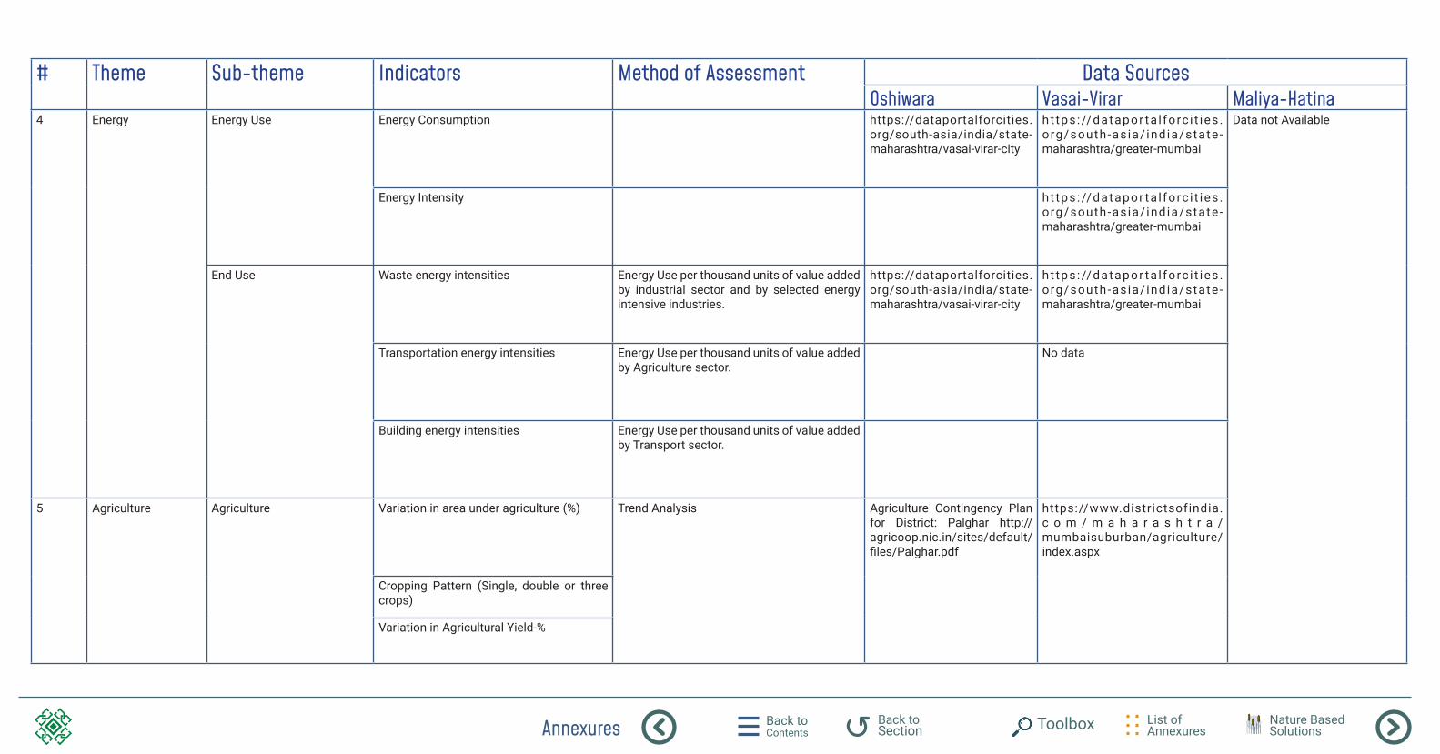
Annexures Back to Contents
List of Annexures
Back to Section Toolbox Nature Based
Solutions
# Theme Sub-theme Indicators Method of Assessment Data SourcesOshiwara Vasai-Virar Maliya-Hatina
4 Energy Energy Use Energy Consumption https://dataportalforcities.org/south-asia/india/state-maharashtra/vasai-virar-city
ht tps : //datapor ta l forc i t ies .org/south-as ia/ ind ia/state -maharashtra/greater-mumbai
Data not Available
Energy Intensity ht tps : //datapor ta l forc i t ies .org/south-as ia/ ind ia/state -maharashtra/greater-mumbai
End Use Waste energy intensities Energy Use per thousand units of value added by industrial sector and by selected energy intensive industries.
https://dataportalforcities.org/south-asia/india/state-maharashtra/vasai-virar-city
ht tps : //datapor ta l forc i t ies .org/south-as ia/ ind ia/state -maharashtra/greater-mumbai
Transportation energy intensities Energy Use per thousand units of value added by Agriculture sector.
No data
Building energy intensities Energy Use per thousand units of value added by Transport sector.
5 Agriculture Agriculture Variation in area under agriculture (%) Trend Analysis Agriculture Contingency Plan for District: Palghar http://agricoop.nic.in/sites/default/files/Palghar.pdf
https://www.districtsofindia.c o m / m a h a r a s h t r a /mumbaisuburban/agriculture/index.aspx
Cropping Pattern (Single, double or three crops)
Variation in Agricultural Yield-%
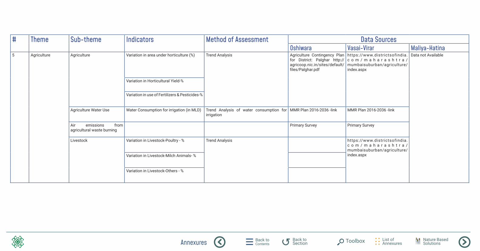
Annexures Back to Contents
List of Annexures
Back to Section Toolbox Nature Based
Solutions
# Theme Sub-theme Indicators Method of Assessment Data SourcesOshiwara Vasai-Virar Maliya-Hatina
5 Agriculture Agriculture Variation in area under horticulture (%) Trend Analysis Agriculture Contingency Plan for District: Palghar http://agricoop.nic.in/sites/default/files/Palghar.pdf
https://www.districtsofindia.c o m / m a h a r a s h t r a /mumbaisuburban/agriculture/index.aspx
Data not Available
Variation in Horticultural Yield-%
Variation in use of Fertilizers & Pesticides-%
Agriculture Water Use Water Consumption for irrigation (in MLD) Trend Analysis of water consumption for irrigation
MMR Plan 2016-2036 -link MMR Plan 2016-2036 -link
Air emissions from agricultural waste burning
Primary Survey Primary Survey
Livestock Variation in Livestock-Poultry - % Trend Analysis https://www.districtsofindia.c o m / m a h a r a s h t r a /mumbaisuburban/agriculture/index.aspxVariation in Livestock-Milch Animals- %
Variation in Livestock-Others - %
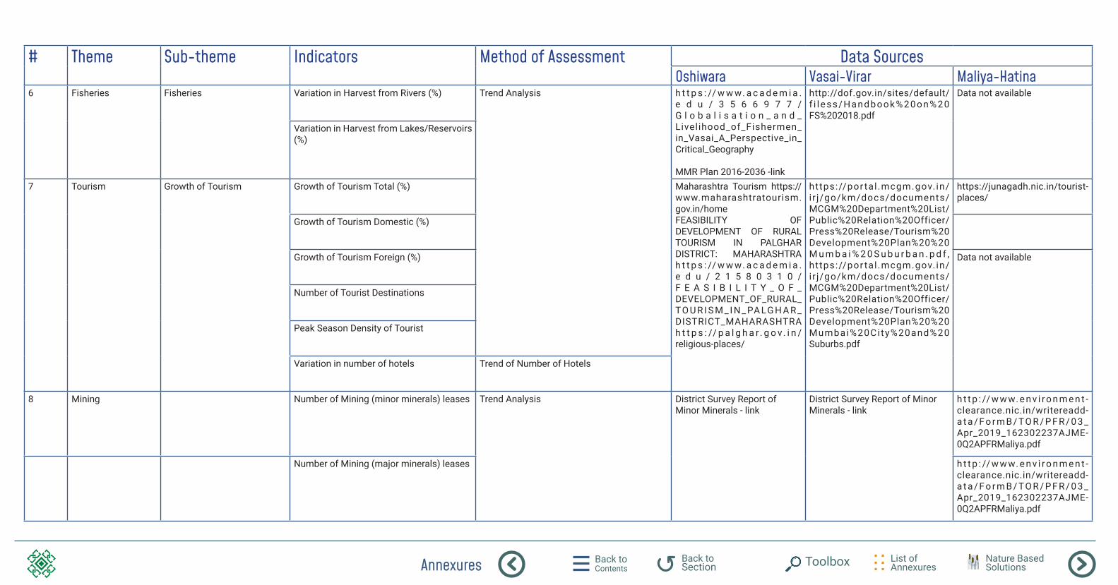
Annexures Back to Contents
List of Annexures
Back to Section Toolbox Nature Based
Solutions
# Theme Sub-theme Indicators Method of Assessment Data SourcesOshiwara Vasai-Virar Maliya-Hatina
6 Fisheries Fisheries Variation in Harvest from Rivers (%) Trend Analysis h t t p s : // w w w. a c a d e m i a .e d u / 3 5 6 6 9 7 7 /G l o b a l i s a t i o n _ a n d _Livelihood_of_Fishermen_in_Vasai_A_Perspective_in_Critical_Geography
MMR Plan 2016-2036 -link
http://dof.gov.in/sites/default/f i l ess/Handbook%20on%20FS%202018.pdf
Data not available
Variation in Harvest from Lakes/Reservoirs (%)
7 Tourism Growth of Tourism Growth of Tourism Total (%) Maharashtra Tourism https://www.maharashtratourism.gov.in/home FEASIBILITY OF DEVELOPMENT OF RURAL TOURISM IN PALGHAR DISTRICT: MAHARASHTRA h t t p s : // w w w. a c a d e m i a .e d u / 2 1 5 8 0 3 1 0 / F E A S I B I L I T Y _ O F _DEVELOPMENT_OF_RURAL_TO U R I S M _ I N _ PA LG H A R _DISTRICT_MAHARASHTRA h t t p s : // p a l g h a r . g o v. i n /religious-places/
https://por tal .mcgm.gov. in/ir j/go/km/docs/documents/MCGM%20Department%20List/Public%20Relation%20Officer/Press%20Release/Tourism%20Development%20Plan%20%20M u m b a i % 2 0 S u b u r b a n . p d f , https://por tal .mcgm.gov. in/ir j/go/km/docs/documents/MCGM%20Department%20List/Public%20Relation%20Officer/Press%20Release/Tourism%20Development%20Plan%20%20Mumbai%20City%20and%20Suburbs.pdf
https://junagadh.nic.in/tourist-places/
Growth of Tourism Domestic (%)
Growth of Tourism Foreign (%) Data not available
Number of Tourist Destinations
Peak Season Density of Tourist
Variation in number of hotels Trend of Number of Hotels
8 Mining Number of Mining (minor minerals) leases Trend Analysis District Survey Report of Minor Minerals - link
District Survey Report of Minor Minerals - link
h t t p : // w w w. e n v i r o n m e n t -clearance.nic.in/writereadd-a t a / F o r m B / TO R / P F R / 0 3 _Apr_2019_162302237AJME-0Q2APFRMaliya.pdf
Number of Mining (major minerals) leases h t t p : // w w w. e n v i r o n m e n t -clearance.nic.in/writereadd-a t a / F o r m B / TO R / P F R / 0 3 _Apr_2019_162302237AJME-0Q2APFRMaliya.pdf
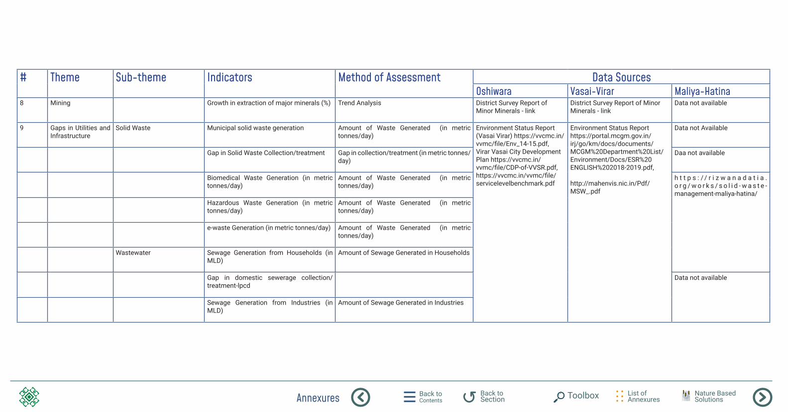
Annexures Back to Contents
List of Annexures
Back to Section Toolbox Nature Based
Solutions
# Theme Sub-theme Indicators Method of Assessment Data SourcesOshiwara Vasai-Virar Maliya-Hatina
8 Mining Growth in extraction of major minerals (%) Trend Analysis District Survey Report of Minor Minerals - link
District Survey Report of Minor Minerals - link
Data not available
9 Gaps in Utilities and Infrastructure
Solid Waste Municipal solid waste generation Amount of Waste Generated (in metric tonnes/day)
Environment Status Report (Vasai Virar) https://vvcmc.in/vvmc/file/Env_14-15.pdf, Virar Vasai City Development Plan https://vvcmc.in/vvmc/file/CDP-of-VVSR.pdf, https://vvcmc.in/vvmc/file/servicelevelbenchmark.pdf
Environment Status Report https://portal.mcgm.gov.in/irj/go/km/docs/documents/MCGM%20Department%20List/Environment/Docs/ESR%20ENGLISH%202018-2019.pdf,
http://mahenvis.nic.in/Pdf/MSW_.pdf
Data not Available
Gap in Solid Waste Collection/treatment Gap in collection/treatment (in metric tonnes/day)
Daa not available
Biomedical Waste Generation (in metric tonnes/day)
Amount of Waste Generated (in metric tonnes/day)
h t t p s : / / r i z w a n a d a t i a .o r g / w o r k s / s o l i d - w a s t e -management-maliya-hatina/
Hazardous Waste Generation (in metric tonnes/day)
Amount of Waste Generated (in metric tonnes/day)
e-waste Generation (in metric tonnes/day) Amount of Waste Generated (in metric tonnes/day)
Wastewater Sewage Generation from Households (in MLD)
Amount of Sewage Generated in Households
Gap in domestic sewerage collection/treatment-lpcd
Data not available
Sewage Generation from Industries (in MLD)
Amount of Sewage Generated in Industries
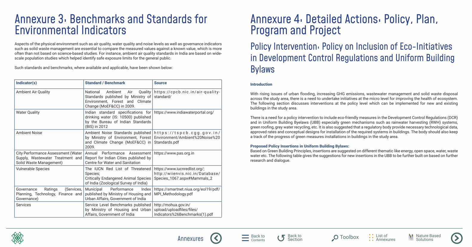
Annexures Back to Contents
List of Annexures
Back to Section Toolbox Nature Based
Solutions
Annexure 3: Benchmarks and Standards for Environmental IndicatorsAspects of the physical environment such as air quality, water quality and noise levels as well as governance indicators such as solid waste management are essential to compare the measured values against a known value, which is more often than not based on science-based studies. For instance, ambient air quality standards in India are based on wide-scale population studies which helped identify safe exposure limits for the general public.
Such standards and benchmarks, where available and applicable, have been shown below:
Indicator(s) Standard / Benchmark Source
Ambient Air Quality National Ambient Air Quality Standards published by Ministry of Environment, Forest and Climate Change (MoEF&CC) in 2009.
ht tps ://cpcb.n ic . in/a i r -qual i ty -standard/
Water Quality Indian standard specifications for drinking water (IS: 10500) published by the Bureau of Indian Standards (BIS) in 2012
https://www.indiawaterportal.org/
Ambient Noise Ambient Noise Standards published by Ministry of Environment, Forest and Climate Change (MoEF&CC) in 2009.
h t t p s : / / t s p c b . c g g . g o v . i n /Environment/Ambient%20Noise%20Standards.pdf
City Performance Assessment (Water Supply, Wastewater Treatment and Solid Waste Management)
Annual Performance Assessment Report for Indian Cities published by Centre for Water and Sanitation
https://www.pas.org.in
Vulnerable Species The IUCN Red List of Threatened Species;Critically Endangered Animal Species of India (Zoological Survey of India)
https://www.iucnredlist.org/;http://wiienvis.nic.in/Database/Species_1067.aspx#Mammals_2
Governance Ratings (Services, Planning, Technology, Finance and Governance)
Municipal Performance Index published by Ministry of Housing and Urban Affairs, Government of India
https://smartnet.niua.org/eol19/pdf/MPI_Methodology.pdf
Services Service Level Benchmarks published by Ministry of Housing and Urban Affairs, Government of India
http://mohua.gov.in/upload/uploadfiles/files/Indicators%26Benchmarks(1).pdf
Annexure 4: Detailed Actions: Policy, Plan, Program and Project Policy Intervention: Policy on Inclusion of Eco-Initiatives in Development Control Regulations and Uniform Building BylawsIntroduction
With rising issues of urban flooding, increasing GHG emissions, wastewater management and solid waste disposal across the study area, there is a need to undertake initiatives at the micro level for improving the health of ecosystem. The following section discusses interventions at the policy level which can be implemented for new and existing buildings in the study area.
There is a need for a policy intervention to include eco-friendly measures in the Development Control Regulations (DCR) and in Uniform Building Byelaws (UBB) especially green mechanisms such as rainwater harvesting (RWH) systems, green roofing, grey water recycling, etc. It is also suggested that a regulatory body provide necessary technological data, approved rates and conceptual designs for installation of the required systems in buildings. The body should also keep a track of the progress of green measures installations in buildings in the study area.
Proposed Policy Insertions in Uniform Building Bylaws:Based on Green Building Principles, insertions are suggested on different thematic like energy, open space, water, waste water etc. The following table gives the suggestions for new insertions in the UBB to be further built on based on further research and dialogue.
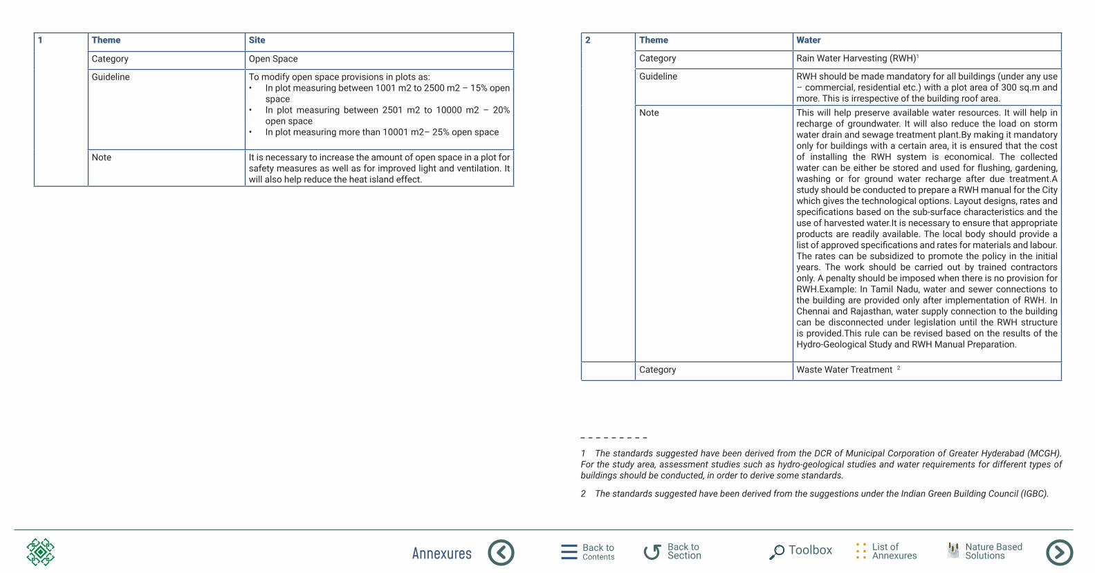
Annexures Back to Contents
List of Annexures
Back to Section Toolbox Nature Based
Solutions
1 Theme Site
Category Open Space
Guideline To modify open space provisions in plots as:• In plot measuring between 1001 m2 to 2500 m2 – 15% open
space• In plot measuring between 2501 m2 to 10000 m2 – 20%
open space• In plot measuring more than 10001 m2– 25% open space
Note It is necessary to increase the amount of open space in a plot for safety measures as well as for improved light and ventilation. It will also help reduce the heat island effect.
2 Theme Water
Category Rain Water Harvesting (RWH)1
Guideline RWH should be made mandatory for all buildings (under any use – commercial, residential etc.) with a plot area of 300 sq.m and more. This is irrespective of the building roof area.
Note This will help preserve available water resources. It will help in recharge of groundwater. It will also reduce the load on storm water drain and sewage treatment plant.By making it mandatory only for buildings with a certain area, it is ensured that the cost of installing the RWH system is economical. The collected water can be either be stored and used for flushing, gardening, washing or for ground water recharge after due treatment.A study should be conducted to prepare a RWH manual for the City which gives the technological options. Layout designs, rates and specifications based on the sub-surface characteristics and the use of harvested water.It is necessary to ensure that appropriate products are readily available. The local body should provide a list of approved specifications and rates for materials and labour. The rates can be subsidized to promote the policy in the initial years. The work should be carried out by trained contractors only. A penalty should be imposed when there is no provision for RWH.Example: In Tamil Nadu, water and sewer connections to the building are provided only after implementation of RWH. In Chennai and Rajasthan, water supply connection to the building can be disconnected under legislation until the RWH structure is provided.This rule can be revised based on the results of the Hydro-Geological Study and RWH Manual Preparation.
Category Waste Water Treatment 2
1 The standards suggested have been derived from the DCR of Municipal Corporation of Greater Hyderabad (MCGH). For the study area, assessment studies such as hydro-geological studies and water requirements for different types of buildings should be conducted, in order to derive some standards.
2 The standards suggested have been derived from the suggestions under the Indian Green Building Council (IGBC).
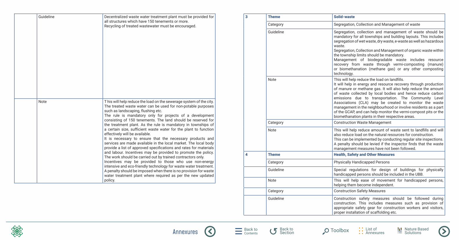
Annexures Back to Contents
List of Annexures
Back to Section Toolbox Nature Based
Solutions
Guideline Decentralized waste water treatment plant must be provided for all structures which have 150 tenements or more. Recycling of treated wastewater must be encouraged.
Note T his will help reduce the load on the sewerage system of the city. The treated waste water can be used for non-potable purposes such as landscaping, flushing etc.The rule is mandatory only for projects of a development consisting of 150 tenements. The land should be reserved for the treatment plant. As the rule is mandatory in townships of a certain size, sufficient waste water for the plant to function effectively will be available.It is necessary to ensure that the necessary products and services are made available in the local market. The local body provide a list of approved specifications and rates for materials and labour. Incentives may be provided to promote the policy. The work should be carried out by trained contractors only.Incentives may be provided to those who use non-energy intensive and eco-friendly technology for waste water treatment.A penalty should be imposed when there is no provision for waste water treatment plant where required as per the new updated policy.
3 Theme Solid-waste
Category Segregation, Collection and Management of waste
Guideline Segregation, collection and management of waste should be mandatory for all townships and building layouts. This includes segregation of wet waste, dry waste, e-waste as well as hazardous waste. Segregation, Collection and Management of organic waste within the township limits should be mandatory. Management of biodegradable waste includes resource recovery from waste through vermi-composting (manure) or biomethanation (methane gas) or any other composting technology.
Note This will help reduce the load on landfills. It will help in energy and resource recovery through production of manure or methane gas. It will also help reduce the amount of waste collected by local bodies and hence reduce carbon emissions due to transportation. The Community Level Associations (CLA) may be created to monitor the waste management in the neighbourhood or involve residents as a part of the GCAP, and can help monitor the vermi-compost pits or the biomethanation plants in their respective areas.
Category Construction Waste Management
Note This will help reduce amount of waste sent to landfills and will also reduce load on the natural resources for construction.This can be implemented by conducting regular site inspections. A penalty should be levied if the inspector finds that the waste management measures have not been followed.
4 Theme Health, Safety and Other Measures
Category Physically Handicapped Persons
Guideline Special regulations for design of buildings for physically handicapped persons should be included in the UBB.
Note This will help ease of movement for handicapped persons, helping them become independent.
Category Construction Safety Measures
Guideline Construction safety measures should be followed during construction. This includes measures such as provision of appropriate safety gear for construction workers and visitors, proper installation of scaffolding etc.
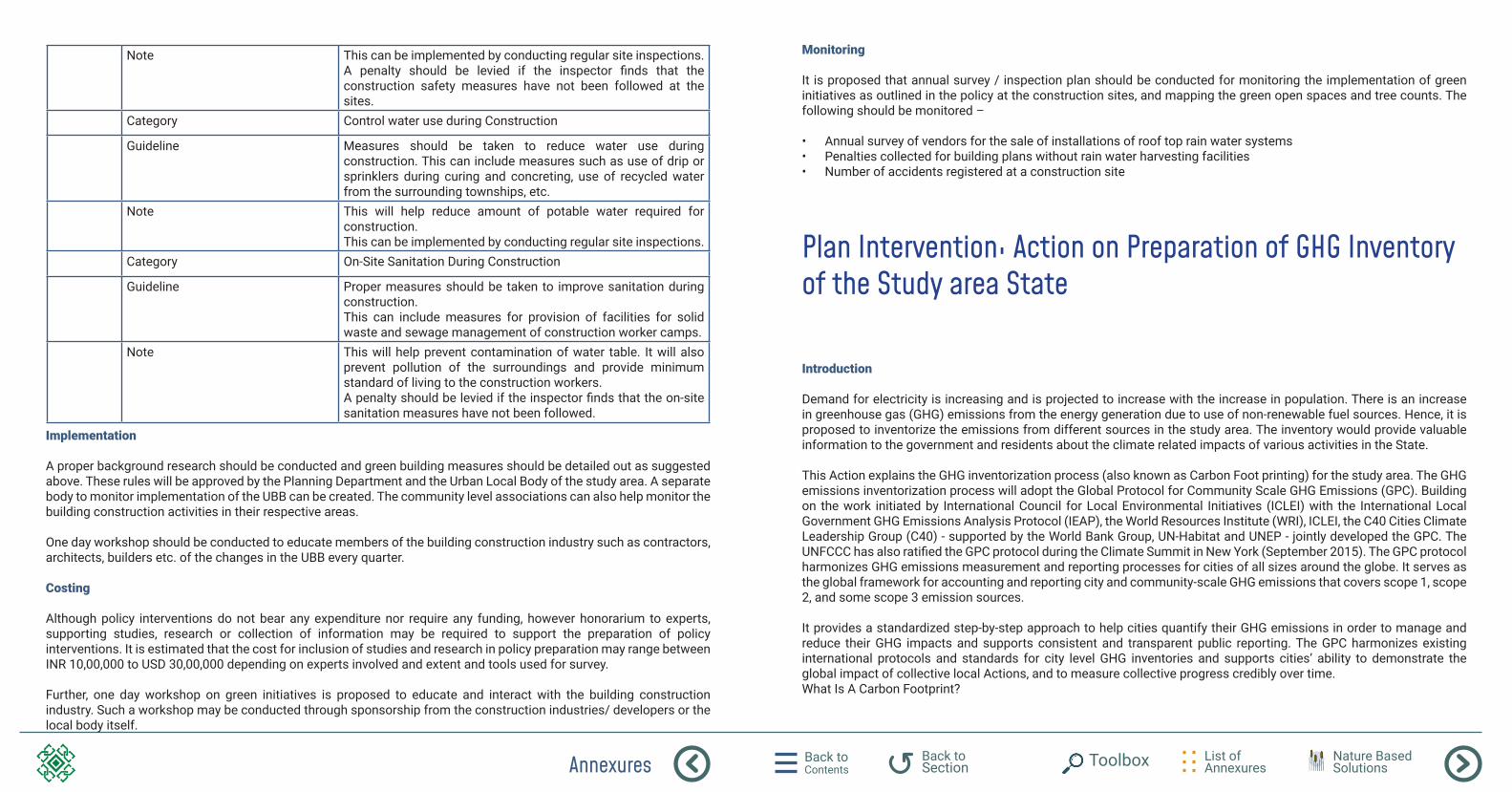
Annexures Back to Contents
List of Annexures
Back to Section Toolbox Nature Based
Solutions
Note This can be implemented by conducting regular site inspections. A penalty should be levied if the inspector finds that the construction safety measures have not been followed at the sites.
Category Control water use during Construction
Guideline Measures should be taken to reduce water use during construction. This can include measures such as use of drip or sprinklers during curing and concreting, use of recycled water from the surrounding townships, etc.
Note This will help reduce amount of potable water required for construction.This can be implemented by conducting regular site inspections.
Category On-Site Sanitation During Construction
Guideline Proper measures should be taken to improve sanitation during construction. This can include measures for provision of facilities for solid waste and sewage management of construction worker camps.
Note This will help prevent contamination of water table. It will also prevent pollution of the surroundings and provide minimum standard of living to the construction workers.A penalty should be levied if the inspector finds that the on-site sanitation measures have not been followed.
Implementation
A proper background research should be conducted and green building measures should be detailed out as suggested above. These rules will be approved by the Planning Department and the Urban Local Body of the study area. A separate body to monitor implementation of the UBB can be created. The community level associations can also help monitor the building construction activities in their respective areas.
One day workshop should be conducted to educate members of the building construction industry such as contractors, architects, builders etc. of the changes in the UBB every quarter.
Costing
Although policy interventions do not bear any expenditure nor require any funding, however honorarium to experts, supporting studies, research or collection of information may be required to support the preparation of policy interventions. It is estimated that the cost for inclusion of studies and research in policy preparation may range between INR 10,00,000 to USD 30,00,000 depending on experts involved and extent and tools used for survey.
Further, one day workshop on green initiatives is proposed to educate and interact with the building construction industry. Such a workshop may be conducted through sponsorship from the construction industries/ developers or the local body itself.
Monitoring
It is proposed that annual survey / inspection plan should be conducted for monitoring the implementation of green initiatives as outlined in the policy at the construction sites, and mapping the green open spaces and tree counts. The following should be monitored –
• Annual survey of vendors for the sale of installations of roof top rain water systems• Penalties collected for building plans without rain water harvesting facilities • Number of accidents registered at a construction site
Plan Intervention: Action on Preparation of GHG Inventory of the Study area State
Introduction
Demand for electricity is increasing and is projected to increase with the increase in population. There is an increase in greenhouse gas (GHG) emissions from the energy generation due to use of non-renewable fuel sources. Hence, it is proposed to inventorize the emissions from different sources in the study area. The inventory would provide valuable information to the government and residents about the climate related impacts of various activities in the State.
This Action explains the GHG inventorization process (also known as Carbon Foot printing) for the study area. The GHG emissions inventorization process will adopt the Global Protocol for Community Scale GHG Emissions (GPC). Building on the work initiated by International Council for Local Environmental Initiatives (ICLEI) with the International Local Government GHG Emissions Analysis Protocol (IEAP), the World Resources Institute (WRI), ICLEI, the C40 Cities Climate Leadership Group (C40) - supported by the World Bank Group, UN-Habitat and UNEP - jointly developed the GPC. The UNFCCC has also ratified the GPC protocol during the Climate Summit in New York (September 2015). The GPC protocol harmonizes GHG emissions measurement and reporting processes for cities of all sizes around the globe. It serves as the global framework for accounting and reporting city and community-scale GHG emissions that covers scope 1, scope 2, and some scope 3 emission sources.
It provides a standardized step-by-step approach to help cities quantify their GHG emissions in order to manage and reduce their GHG impacts and supports consistent and transparent public reporting. The GPC harmonizes existing international protocols and standards for city level GHG inventories and supports cities’ ability to demonstrate the global impact of collective local Actions, and to measure collective progress credibly over time. What Is A Carbon Footprint?
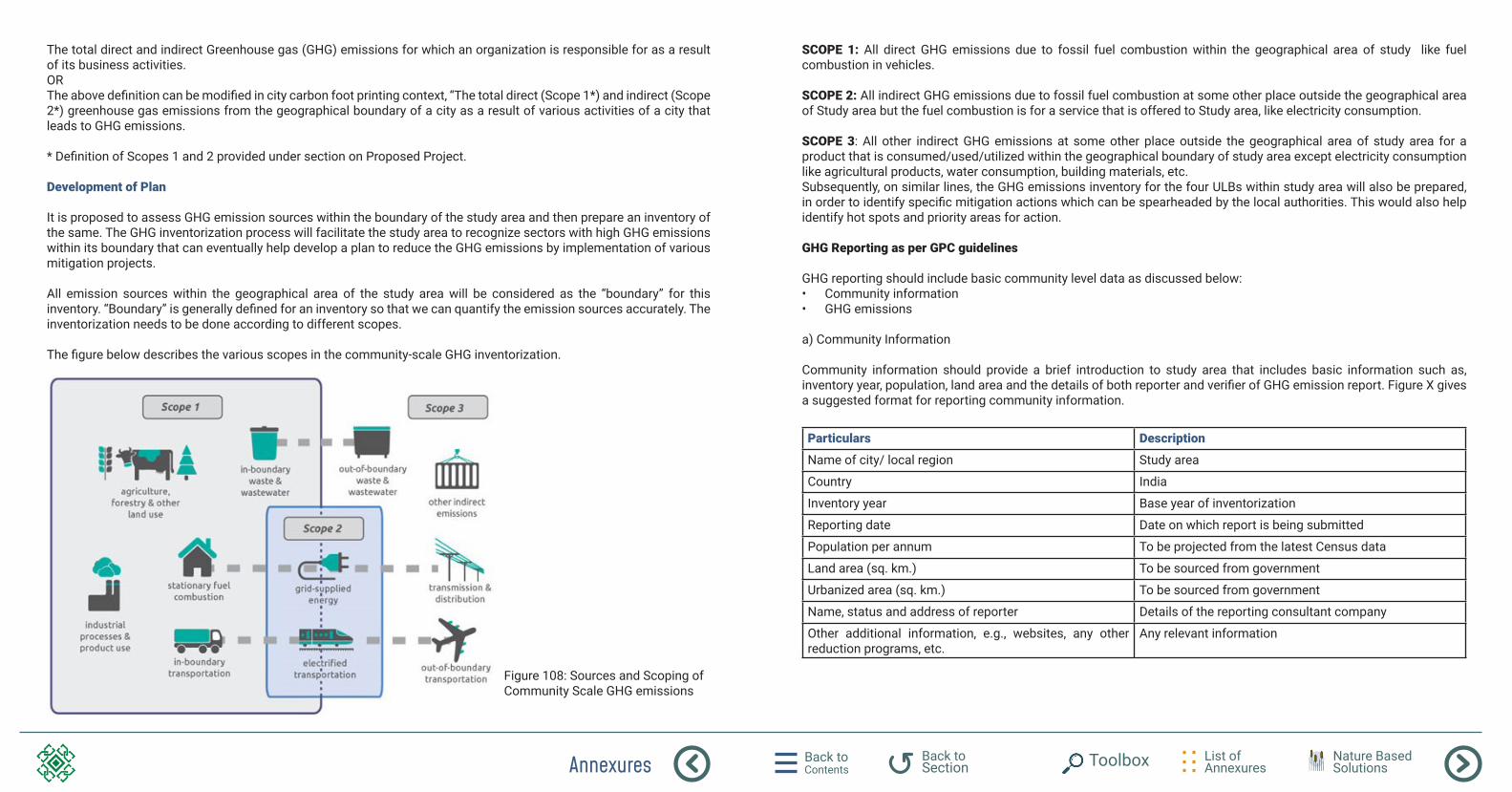
Annexures Back to Contents
List of Annexures
Back to Section Toolbox Nature Based
Solutions
The total direct and indirect Greenhouse gas (GHG) emissions for which an organization is responsible for as a result of its business activities.ORThe above definition can be modified in city carbon foot printing context, “The total direct (Scope 1*) and indirect (Scope 2*) greenhouse gas emissions from the geographical boundary of a city as a result of various activities of a city that leads to GHG emissions.
* Definition of Scopes 1 and 2 provided under section on Proposed Project.
Development of Plan
It is proposed to assess GHG emission sources within the boundary of the study area and then prepare an inventory of the same. The GHG inventorization process will facilitate the study area to recognize sectors with high GHG emissions within its boundary that can eventually help develop a plan to reduce the GHG emissions by implementation of various mitigation projects.
All emission sources within the geographical area of the study area will be considered as the “boundary” for this inventory. “Boundary” is generally defined for an inventory so that we can quantify the emission sources accurately. The inventorization needs to be done according to different scopes.
The figure below describes the various scopes in the community-scale GHG inventorization.
Figure 108: Sources and Scoping of Community Scale GHG emissions
SCOPE 1: All direct GHG emissions due to fossil fuel combustion within the geographical area of study like fuel combustion in vehicles.
SCOPE 2: All indirect GHG emissions due to fossil fuel combustion at some other place outside the geographical area of Study area but the fuel combustion is for a service that is offered to Study area, like electricity consumption.
SCOPE 3: All other indirect GHG emissions at some other place outside the geographical area of study area for a product that is consumed/used/utilized within the geographical boundary of study area except electricity consumption like agricultural products, water consumption, building materials, etc.Subsequently, on similar lines, the GHG emissions inventory for the four ULBs within study area will also be prepared, in order to identify specific mitigation actions which can be spearheaded by the local authorities. This would also help identify hot spots and priority areas for action.
GHG Reporting as per GPC guidelines
GHG reporting should include basic community level data as discussed below: • Community information• GHG emissions
a) Community Information
Community information should provide a brief introduction to study area that includes basic information such as, inventory year, population, land area and the details of both reporter and verifier of GHG emission report. Figure X gives a suggested format for reporting community information.
Particulars Description
Name of city/ local region Study area
Country India
Inventory year Base year of inventorization
Reporting date Date on which report is being submitted
Population per annum To be projected from the latest Census data
Land area (sq. km.) To be sourced from government
Urbanized area (sq. km.) To be sourced from government
Name, status and address of reporter Details of the reporting consultant company
Other additional information, e.g., websites, any other reduction programs, etc.
Any relevant information
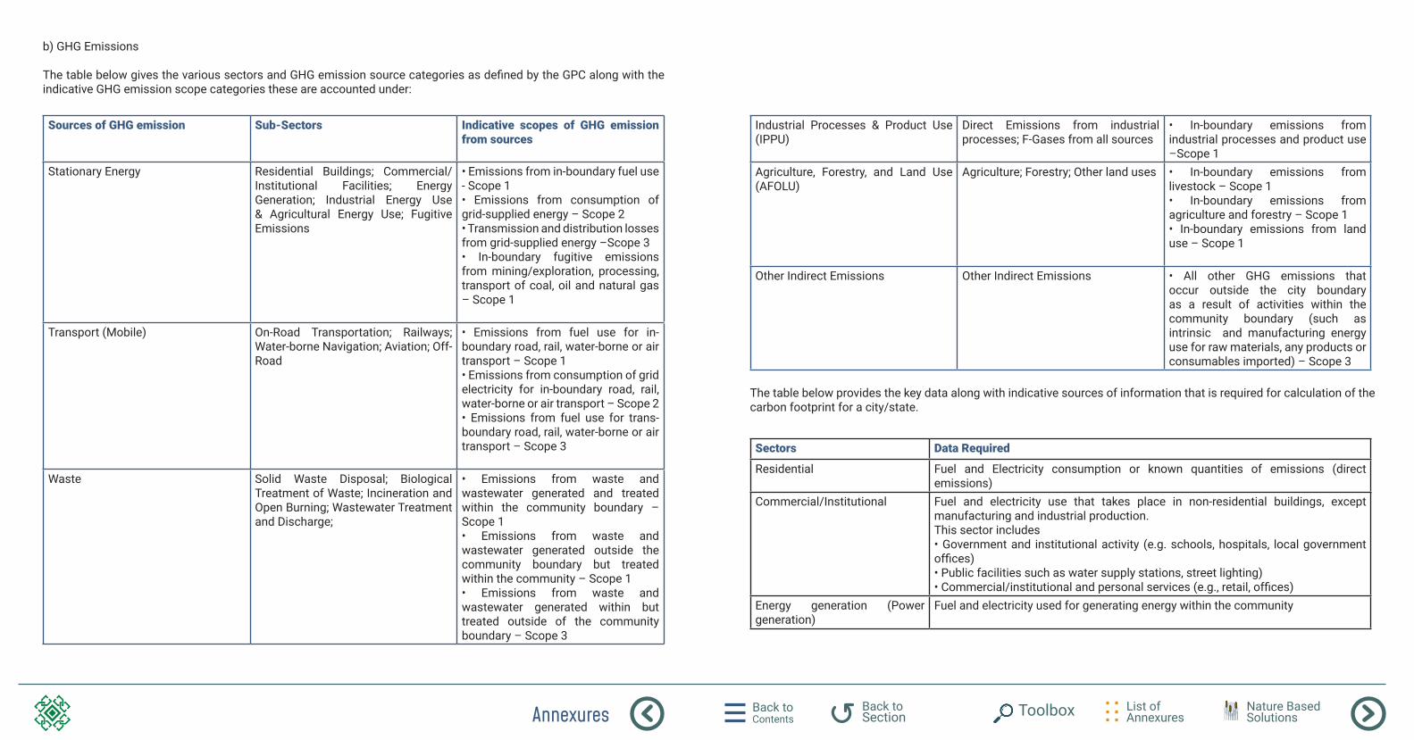
Annexures Back to Contents
List of Annexures
Back to Section Toolbox Nature Based
Solutions
b) GHG Emissions
The table below gives the various sectors and GHG emission source categories as defined by the GPC along with the indicative GHG emission scope categories these are accounted under:
Sources of GHG emission Sub-Sectors Indicative scopes of GHG emission from sources
Stationary Energy Residential Buildings; Commercial/Institutional Facilities; Energy Generation; Industrial Energy Use & Agricultural Energy Use; Fugitive Emissions
• Emissions from in-boundary fuel use - Scope 1• Emissions from consumption of grid-supplied energy – Scope 2• Transmission and distribution losses from grid-supplied energy –Scope 3• In-boundary fugitive emissions from mining/exploration, processing, transport of coal, oil and natural gas – Scope 1
Transport (Mobile) On-Road Transportation; Railways; Water-borne Navigation; Aviation; Off-Road
• Emissions from fuel use for in-boundary road, rail, water-borne or air transport – Scope 1• Emissions from consumption of grid electricity for in-boundary road, rail, water-borne or air transport – Scope 2• Emissions from fuel use for trans-boundary road, rail, water-borne or air transport – Scope 3
Waste Solid Waste Disposal; Biological Treatment of Waste; Incineration and Open Burning; Wastewater Treatment and Discharge;
• Emissions from waste and wastewater generated and treated within the community boundary – Scope 1• Emissions from waste and wastewater generated outside the community boundary but treated within the community – Scope 1• Emissions from waste and wastewater generated within but treated outside of the community boundary – Scope 3
Industrial Processes & Product Use (IPPU)
Direct Emissions from industrial processes; F-Gases from all sources
• In-boundary emissions from industrial processes and product use –Scope 1
Agriculture, Forestry, and Land Use (AFOLU)
Agriculture; Forestry; Other land uses • In-boundary emissions from livestock – Scope 1• In-boundary emissions from agriculture and forestry – Scope 1• In-boundary emissions from land use – Scope 1
Other Indirect Emissions Other Indirect Emissions • All other GHG emissions that occur outside the city boundary as a result of activities within the community boundary (such as intrinsic and manufacturing energy use for raw materials, any products or consumables imported) – Scope 3
The table below provides the key data along with indicative sources of information that is required for calculation of the carbon footprint for a city/state.
Sectors Data Required
Residential Fuel and Electricity consumption or known quantities of emissions (direct emissions)
Commercial/Institutional Fuel and electricity use that takes place in non-residential buildings, except manufacturing and industrial production. This sector includes • Government and institutional activity (e.g. schools, hospitals, local government offices)• Public facilities such as water supply stations, street lighting) • Commercial/institutional and personal services (e.g., retail, offices)
Energy generation (Power generation)
Fuel and electricity used for generating energy within the community
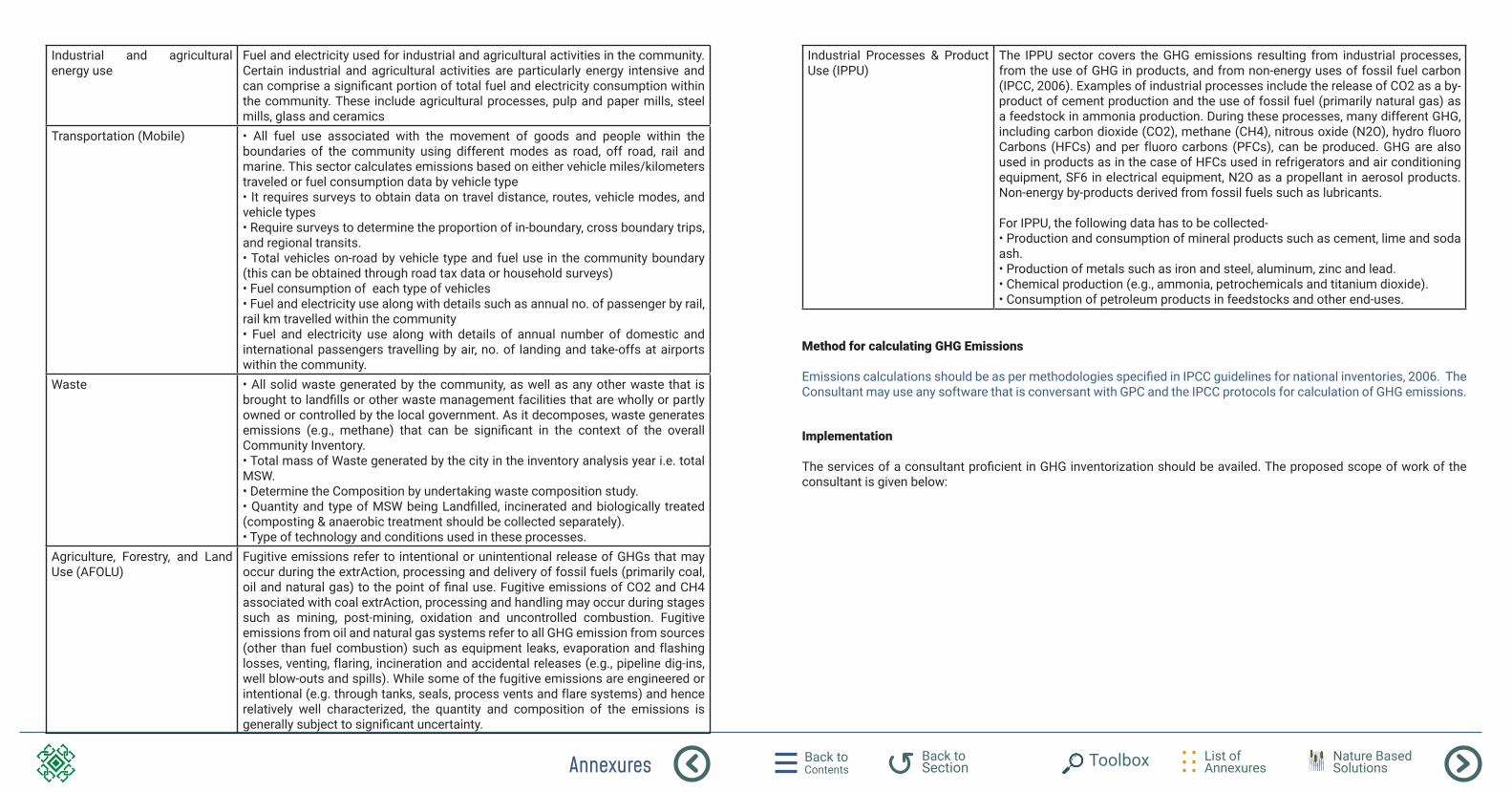
Annexures Back to Contents
List of Annexures
Back to Section Toolbox Nature Based
Solutions
Industrial and agricultural energy use
Fuel and electricity used for industrial and agricultural activities in the community. Certain industrial and agricultural activities are particularly energy intensive and can comprise a significant portion of total fuel and electricity consumption within the community. These include agricultural processes, pulp and paper mills, steel mills, glass and ceramics
Transportation (Mobile) • All fuel use associated with the movement of goods and people within the boundaries of the community using different modes as road, off road, rail and marine. This sector calculates emissions based on either vehicle miles/kilometers traveled or fuel consumption data by vehicle type• It requires surveys to obtain data on travel distance, routes, vehicle modes, and vehicle types • Require surveys to determine the proportion of in-boundary, cross boundary trips, and regional transits. • Total vehicles on-road by vehicle type and fuel use in the community boundary (this can be obtained through road tax data or household surveys) • Fuel consumption of each type of vehicles • Fuel and electricity use along with details such as annual no. of passenger by rail, rail km travelled within the community• Fuel and electricity use along with details of annual number of domestic and international passengers travelling by air, no. of landing and take-offs at airports within the community.
Waste • All solid waste generated by the community, as well as any other waste that is brought to landfills or other waste management facilities that are wholly or partly owned or controlled by the local government. As it decomposes, waste generates emissions (e.g., methane) that can be significant in the context of the overall Community Inventory. • Total mass of Waste generated by the city in the inventory analysis year i.e. total MSW. • Determine the Composition by undertaking waste composition study. • Quantity and type of MSW being Landfilled, incinerated and biologically treated (composting & anaerobic treatment should be collected separately). • Type of technology and conditions used in these processes.
Agriculture, Forestry, and Land Use (AFOLU)
Fugitive emissions refer to intentional or unintentional release of GHGs that may occur during the extrAction, processing and delivery of fossil fuels (primarily coal, oil and natural gas) to the point of final use. Fugitive emissions of CO2 and CH4 associated with coal extrAction, processing and handling may occur during stages such as mining, post-mining, oxidation and uncontrolled combustion. Fugitive emissions from oil and natural gas systems refer to all GHG emission from sources (other than fuel combustion) such as equipment leaks, evaporation and flashing losses, venting, flaring, incineration and accidental releases (e.g., pipeline dig-ins, well blow-outs and spills). While some of the fugitive emissions are engineered or intentional (e.g. through tanks, seals, process vents and flare systems) and hence relatively well characterized, the quantity and composition of the emissions is generally subject to significant uncertainty.
Industrial Processes & Product Use (IPPU)
The IPPU sector covers the GHG emissions resulting from industrial processes, from the use of GHG in products, and from non-energy uses of fossil fuel carbon (IPCC, 2006). Examples of industrial processes include the release of CO2 as a by-product of cement production and the use of fossil fuel (primarily natural gas) as a feedstock in ammonia production. During these processes, many different GHG, including carbon dioxide (CO2), methane (CH4), nitrous oxide (N2O), hydro fluoro Carbons (HFCs) and per fluoro carbons (PFCs), can be produced. GHG are also used in products as in the case of HFCs used in refrigerators and air conditioning equipment, SF6 in electrical equipment, N2O as a propellant in aerosol products. Non-energy by-products derived from fossil fuels such as lubricants.
For IPPU, the following data has to be collected-• Production and consumption of mineral products such as cement, lime and soda ash.• Production of metals such as iron and steel, aluminum, zinc and lead.• Chemical production (e.g., ammonia, petrochemicals and titanium dioxide).• Consumption of petroleum products in feedstocks and other end-uses.
Method for calculating GHG Emissions
Emissions calculations should be as per methodologies specified in IPCC guidelines for national inventories, 2006. The Consultant may use any software that is conversant with GPC and the IPCC protocols for calculation of GHG emissions.
Implementation
The services of a consultant proficient in GHG inventorization should be availed. The proposed scope of work of the consultant is given below:

Annexures Back to Contents
List of Annexures
Back to Section Toolbox Nature Based
Solutions
Implementation
The services of a consultant proficient in GHG inventorization should be availed. The proposed scope of work of the consultant is given below:
1. Initial meetings with the consultant: Consultant should meet with the local body to finalize the proposed work plan/methodology. Details of support required by the corporation to prepare the GHG emissions inventory and assess their climate Action plans will also be discussed.
2. Preparation of GHG emissions inventory software tool: Upon confirmation of the assignment, the consultant shall complete the development of a study area specific GHG emissions inventory software tool.
3. Providing initial training to corporation, city officials and other stakeholders on the use of the GHG emissions software: The consultant will organize an introductory training on an appropriate software tool for officials of the cities. All sources of data shall be discussed and finalized with the consultant.
4. Providing technical support to corporation to assess their GHG baseline inventories: Further support shall be extended to the staff of Corporation and other core team members for the preparation of the GHG emissions inventory. It is envisaged that the core team in shall be able to aggregate the requisite data for the GHG emissions inventory within 3 months after the training.
5. Preparation of GHG Emissions Inventory for the Study area The preparation of the GHG emissions inventory for the study area using the GHG emissions software will be initiated by the city staff and supported by the staff from the consultant.
6. Preparation of Mitigation Action Plan for the cityBased on the GHG inventory, mitigation actions should be developed by the consultant to reduce the GHG emissions from the study area. The mitigation actions should be developed in consultation with the multiple stakeholders.
Estimated Project Duration
8-10 months
Case Study
Vancouver City Carbon Footprint
• City: Vancouver
• Country: Canada
• Metro Area: 2,878.52 sq. km.
• Metro Population: 2,116,581 (as per 2006 census)
• Inventory Year: 2008
• Community: 2,740,000 tC02e per annum (sectors included in the study are: buildings, light duty vehicles, heavy duty
vehicles and solid waste)
• Municipality: 335,500 tCO2e per annum (sectors included in the study are: buildings, street and traffic lighting,
Vancouver landfill and vehicle fleet)
• Protocol: ICLEI’s International Local Government GHG Emissions Analysis Protocol
• Emission factors: BC Government draft 2007 Community Energy and Greenhouse Gas Emissions Inventory (CEEI)
for Vancouver (for natural gas) , BC Hydro GRI (for electricity), Canada’s Greenhouse Gas Inventory Report 1990-
2005 (for vehicle fuel)
• Boundary: Geographical and Organizational
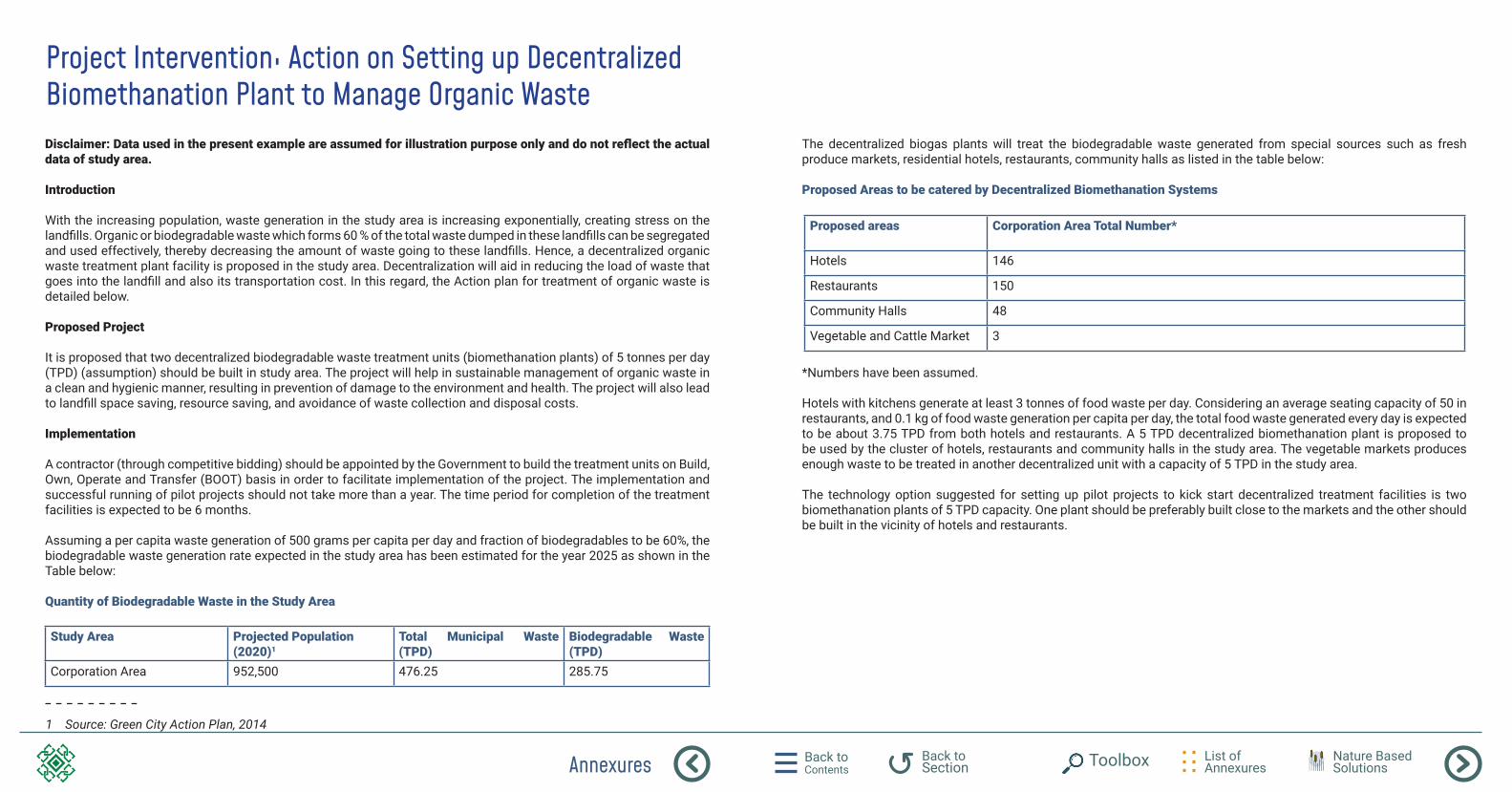
Annexures Back to Contents
List of Annexures
Back to Section Toolbox Nature Based
Solutions
Project Intervention: Action on Setting up Decentralized Biomethanation Plant to Manage Organic WasteDisclaimer: Data used in the present example are assumed for illustration purpose only and do not reflect the actual data of study area.
Introduction
With the increasing population, waste generation in the study area is increasing exponentially, creating stress on the landfills. Organic or biodegradable waste which forms 60 % of the total waste dumped in these landfills can be segregated and used effectively, thereby decreasing the amount of waste going to these landfills. Hence, a decentralized organic waste treatment plant facility is proposed in the study area. Decentralization will aid in reducing the load of waste that goes into the landfill and also its transportation cost. In this regard, the Action plan for treatment of organic waste is detailed below.
Proposed Project
It is proposed that two decentralized biodegradable waste treatment units (biomethanation plants) of 5 tonnes per day (TPD) (assumption) should be built in study area. The project will help in sustainable management of organic waste in a clean and hygienic manner, resulting in prevention of damage to the environment and health. The project will also lead to landfill space saving, resource saving, and avoidance of waste collection and disposal costs.
Implementation
A contractor (through competitive bidding) should be appointed by the Government to build the treatment units on Build, Own, Operate and Transfer (BOOT) basis in order to facilitate implementation of the project. The implementation and successful running of pilot projects should not take more than a year. The time period for completion of the treatment facilities is expected to be 6 months.
Assuming a per capita waste generation of 500 grams per capita per day and fraction of biodegradables to be 60%, the biodegradable waste generation rate expected in the study area has been estimated for the year 2025 as shown in the Table below:
Quantity of Biodegradable Waste in the Study Area
Study Area Projected Population (2020)1
Total Municipal Waste (TPD)
Biodegradable Waste (TPD)
Corporation Area 952,500 476.25 285.75
1 Source: Green City Action Plan, 2014
The decentralized biogas plants will treat the biodegradable waste generated from special sources such as fresh produce markets, residential hotels, restaurants, community halls as listed in the table below:
Proposed Areas to be catered by Decentralized Biomethanation Systems
*Numbers have been assumed.
Hotels with kitchens generate at least 3 tonnes of food waste per day. Considering an average seating capacity of 50 in restaurants, and 0.1 kg of food waste generation per capita per day, the total food waste generated every day is expected to be about 3.75 TPD from both hotels and restaurants. A 5 TPD decentralized biomethanation plant is proposed to be used by the cluster of hotels, restaurants and community halls in the study area. The vegetable markets produces enough waste to be treated in another decentralized unit with a capacity of 5 TPD in the study area.
The technology option suggested for setting up pilot projects to kick start decentralized treatment facilities is two biomethanation plants of 5 TPD capacity. One plant should be preferably built close to the markets and the other should be built in the vicinity of hotels and restaurants.
Proposed areas Corporation Area Total Number*
Hotels 146
Restaurants 150
Community Halls 48
Vegetable and Cattle Market 3
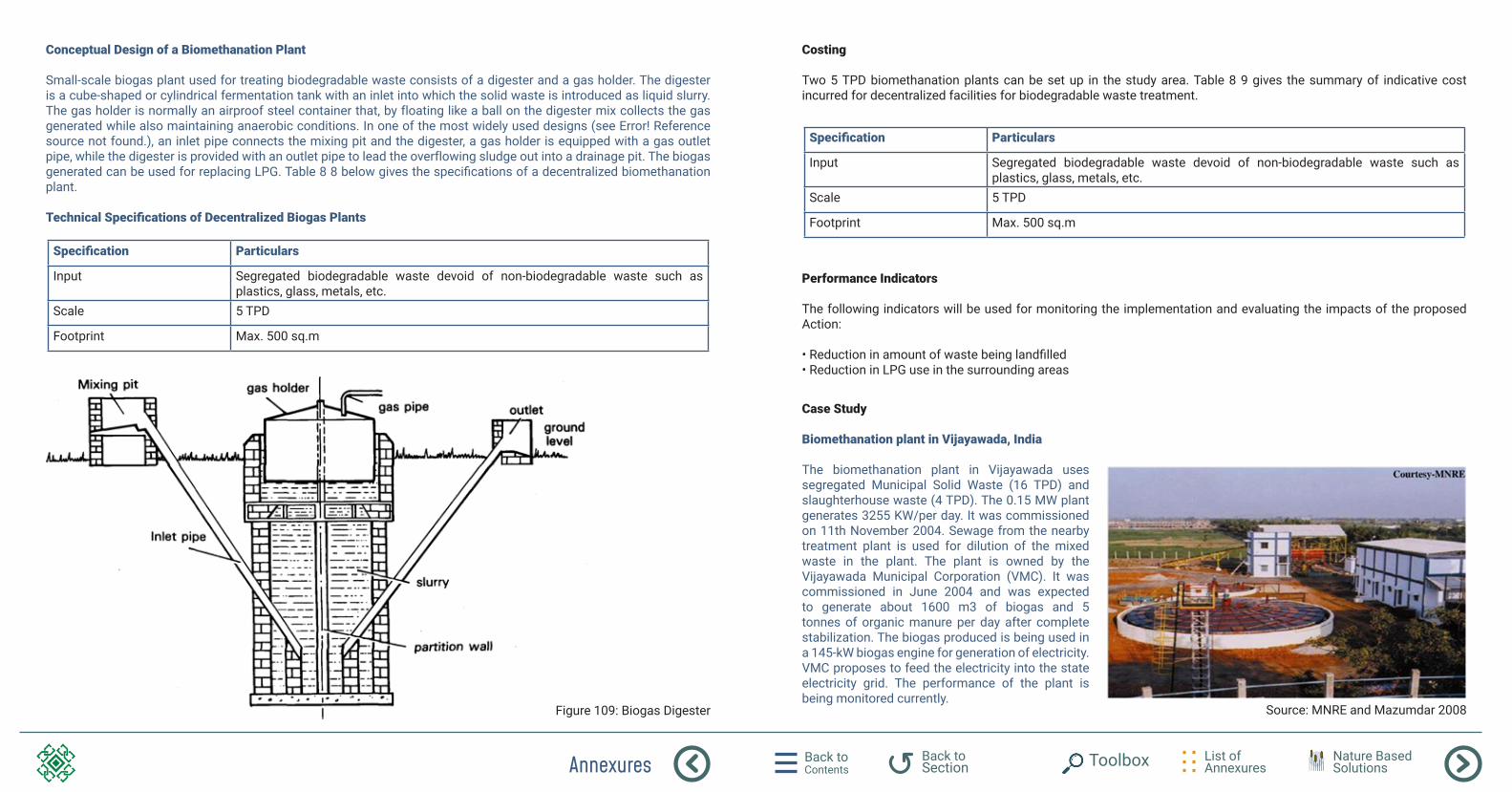
Annexures Back to Contents
List of Annexures
Back to Section Toolbox Nature Based
Solutions
Conceptual Design of a Biomethanation Plant
Small-scale biogas plant used for treating biodegradable waste consists of a digester and a gas holder. The digester is a cube-shaped or cylindrical fermentation tank with an inlet into which the solid waste is introduced as liquid slurry. The gas holder is normally an airproof steel container that, by floating like a ball on the digester mix collects the gas generated while also maintaining anaerobic conditions. In one of the most widely used designs (see Error! Reference source not found.), an inlet pipe connects the mixing pit and the digester, a gas holder is equipped with a gas outlet pipe, while the digester is provided with an outlet pipe to lead the overflowing sludge out into a drainage pit. The biogas generated can be used for replacing LPG. Table 8 8 below gives the specifications of a decentralized biomethanation plant.
Technical Specifications of Decentralized Biogas Plants
Specification Particulars
Input Segregated biodegradable waste devoid of non-biodegradable waste such as plastics, glass, metals, etc.
Scale 5 TPD
Footprint Max. 500 sq.m
Figure 109: Biogas Digester
Costing
Two 5 TPD biomethanation plants can be set up in the study area. Table 8 9 gives the summary of indicative cost incurred for decentralized facilities for biodegradable waste treatment.
Performance Indicators
The following indicators will be used for monitoring the implementation and evaluating the impacts of the proposed Action:
• Reduction in amount of waste being landfilled • Reduction in LPG use in the surrounding areas
Specification Particulars
Input Segregated biodegradable waste devoid of non-biodegradable waste such as plastics, glass, metals, etc.
Scale 5 TPD
Footprint Max. 500 sq.m
Case Study
Biomethanation plant in Vijayawada, India
The biomethanation plant in Vijayawada uses segregated Municipal Solid Waste (16 TPD) and slaughterhouse waste (4 TPD). The 0.15 MW plant generates 3255 KW/per day. It was commissioned on 11th November 2004. Sewage from the nearby treatment plant is used for dilution of the mixed waste in the plant. The plant is owned by the Vijayawada Municipal Corporation (VMC). It was commissioned in June 2004 and was expected to generate about 1600 m3 of biogas and 5 tonnes of organic manure per day after complete stabilization. The biogas produced is being used in a 145-kW biogas engine for generation of electricity. VMC proposes to feed the electricity into the state electricity grid. The performance of the plant is being monitored currently.
Source: MNRE and Mazumdar 2008
Annexures Back to Contents
List of Annexures
Back to Section Toolbox Nature Based
Solutions
Project Intervention: Action on Setting up Decentralized Biomethanation Plant to Manage Organic WasteDisclaimer: Data used in the present example are assumed for illustration purpose only and do not reflect the actual data of study area.
Introduction
With the increasing population, waste generation in the study area is increasing exponentially, creating stress on the landfills. Organic or biodegradable waste which forms 60 % of the total waste dumped in these landfills can be segregated and used effectively, thereby decreasing the amount of waste going to these landfills. Hence, a decentralized organic waste treatment plant facility is proposed in the study area. Decentralization will aid in reducing the load of waste that goes into the landfill and also its transportation cost. In this regard, the Action plan for treatment of organic waste is detailed below.
Proposed Project
It is proposed that two decentralized biodegradable waste treatment units (biomethanation plants) of 5 tonnes per day (TPD) (assumption) should be built in study area. The project will help in sustainable management of organic waste in a clean and hygienic manner, resulting in prevention of damage to the environment and health. The project will also lead to landfill space saving, resource saving, and avoidance of waste collection and disposal costs.
Implementation
A contractor (through competitive bidding) should be appointed by the Government to build the treatment units on Build, Own, Operate and Transfer (BOOT) basis in order to facilitate implementation of the project. The implementation and successful running of pilot projects should not take more than a year. The time period for completion of the treatment facilities is expected to be 6 months.
Assuming a per capita waste generation of 500 grams per capita per day and fraction of biodegradables to be 60%, the biodegradable waste generation rate expected in the study area has been estimated for the year 2025 as shown in the Table below:
Quantity of Biodegradable Waste in the Study Area
Program Intervention: Action on City Level Tree Plantation DriveIntroduction
This activity promotes the plantation of saplings with intent to increase tree cover and its related myriad health and environmental benefits as well as increasing awareness of the ill effects of depleting forest cover and the importance of growing trees in the cities. The drive would emphasize on the effect of increasing tree cover on reduction of heat island effect and prevention of runoff.
The main objectives of the tree plantation drive are as follows:
- To raise awareness of the importance of trees and create an awareness among people about the benefits of tree plantation- To plant indigenous trees / saplings in the areas around the study area- To encourage the general public to participate in tree planting driveThe drive should be implemented during the rainy season (July- August).
Program Details
Selection of areas and planting of saplings
1. The Forestry Department would be involved in the selection of the area for plantation2. The forestry department will organize for saplings to be distributed to the general public free of charge.3. Native tree species can be planted along the roads. Mumbai native tree species are Peepal (sacred fig/Ficus religiosa), vad (banyan/Ficus benghalensis), amla (Indian gooseberry/ Phyllanthus emblica), bael (Aegle marmelos) and ashoka (Saraca asoca).
Promotion of the Plantation Drive
1. The drive will be promoted through the advertisements in the local newspapers, radio and cable TV channels inviting the public to take the saplings and plant them in their surrounding areas.2. On the day of the drive, the local NGO may consider inviting a well-known personality to inaugurate the drive and plant a symbolic sapling.3. Distribution of saplings to attending members for plantation.
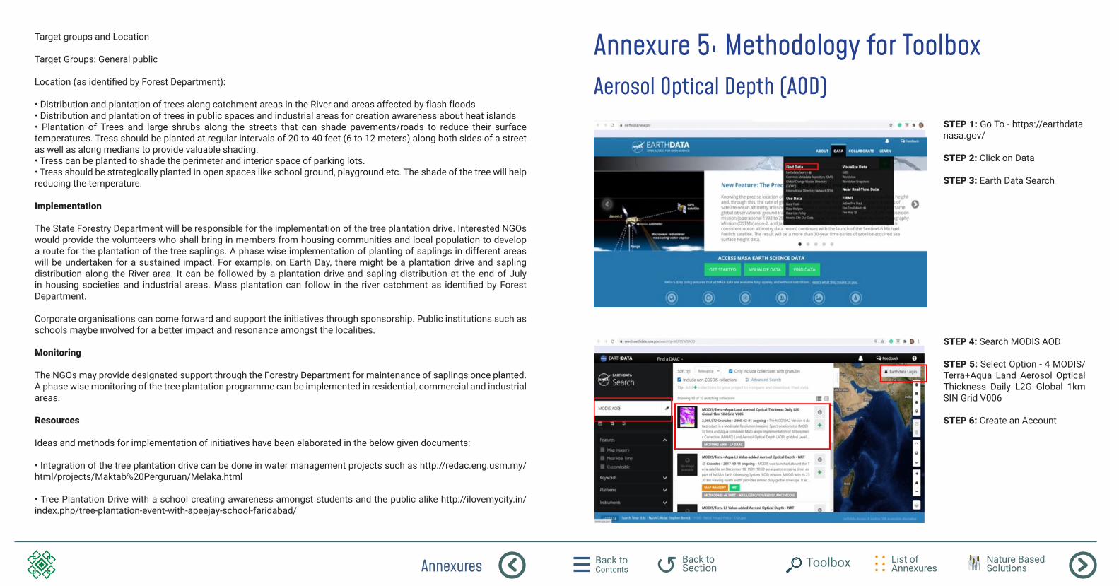
Annexures Back to Contents
List of Annexures
Back to Section Toolbox Nature Based
Solutions
Target groups and Location
Target Groups: General public
Location (as identified by Forest Department):
• Distribution and plantation of trees along catchment areas in the River and areas affected by flash floods• Distribution and plantation of trees in public spaces and industrial areas for creation awareness about heat islands• Plantation of Trees and large shrubs along the streets that can shade pavements/roads to reduce their surface temperatures. Tress should be planted at regular intervals of 20 to 40 feet (6 to 12 meters) along both sides of a street as well as along medians to provide valuable shading.• Tress can be planted to shade the perimeter and interior space of parking lots.• Tress should be strategically planted in open spaces like school ground, playground etc. The shade of the tree will help reducing the temperature.
Implementation
The State Forestry Department will be responsible for the implementation of the tree plantation drive. Interested NGOs would provide the volunteers who shall bring in members from housing communities and local population to develop a route for the plantation of the tree saplings. A phase wise implementation of planting of saplings in different areas will be undertaken for a sustained impact. For example, on Earth Day, there might be a plantation drive and sapling distribution along the River area. It can be followed by a plantation drive and sapling distribution at the end of July in housing societies and industrial areas. Mass plantation can follow in the river catchment as identified by Forest Department.
Corporate organisations can come forward and support the initiatives through sponsorship. Public institutions such as schools maybe involved for a better impact and resonance amongst the localities.
Monitoring
The NGOs may provide designated support through the Forestry Department for maintenance of saplings once planted. A phase wise monitoring of the tree plantation programme can be implemented in residential, commercial and industrial areas.
Resources
Ideas and methods for implementation of initiatives have been elaborated in the below given documents: • Integration of the tree plantation drive can be done in water management projects such as http://redac.eng.usm.my/html/projects/Maktab%20Perguruan/Melaka.html
• Tree Plantation Drive with a school creating awareness amongst students and the public alike http://ilovemycity.in/index.php/tree-plantation-event-with-apeejay-school-faridabad/
Annexure 5: Methodology for ToolboxAerosol Optical Depth (AOD)
STEP 1: Go To - https://earthdata.nasa.gov/ STEP 2: Click on Data STEP 3: Earth Data Search
STEP 4: Search MODIS AOD
STEP 5: Select Option - 4 MODIS/Terra+Aqua Land Aerosol Optical Thickness Daily L2G Global 1km SIN Grid V006
STEP 6: Create an Account
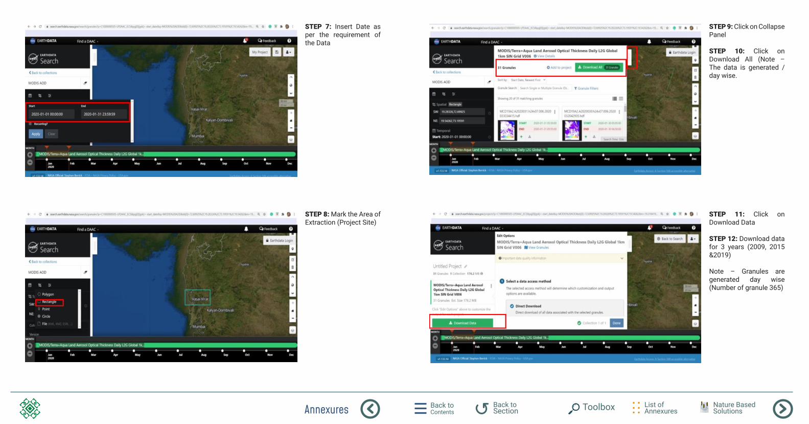
Annexures Back to Contents
List of Annexures
Back to Section Toolbox Nature Based
Solutions
STEP 7: Insert Date as per the requirement of the Data
STEP 9: Click on Collapse Panel
STEP 10: Click on Download All (Note – The data is generated / day wise.
STEP 8: Mark the Area of Extraction (Project Site)
STEP 11: Click on Download Data
STEP 12: Download data for 3 years (2009, 2015 &2019)
Note – Granules are generated day wise (Number of granule 365)
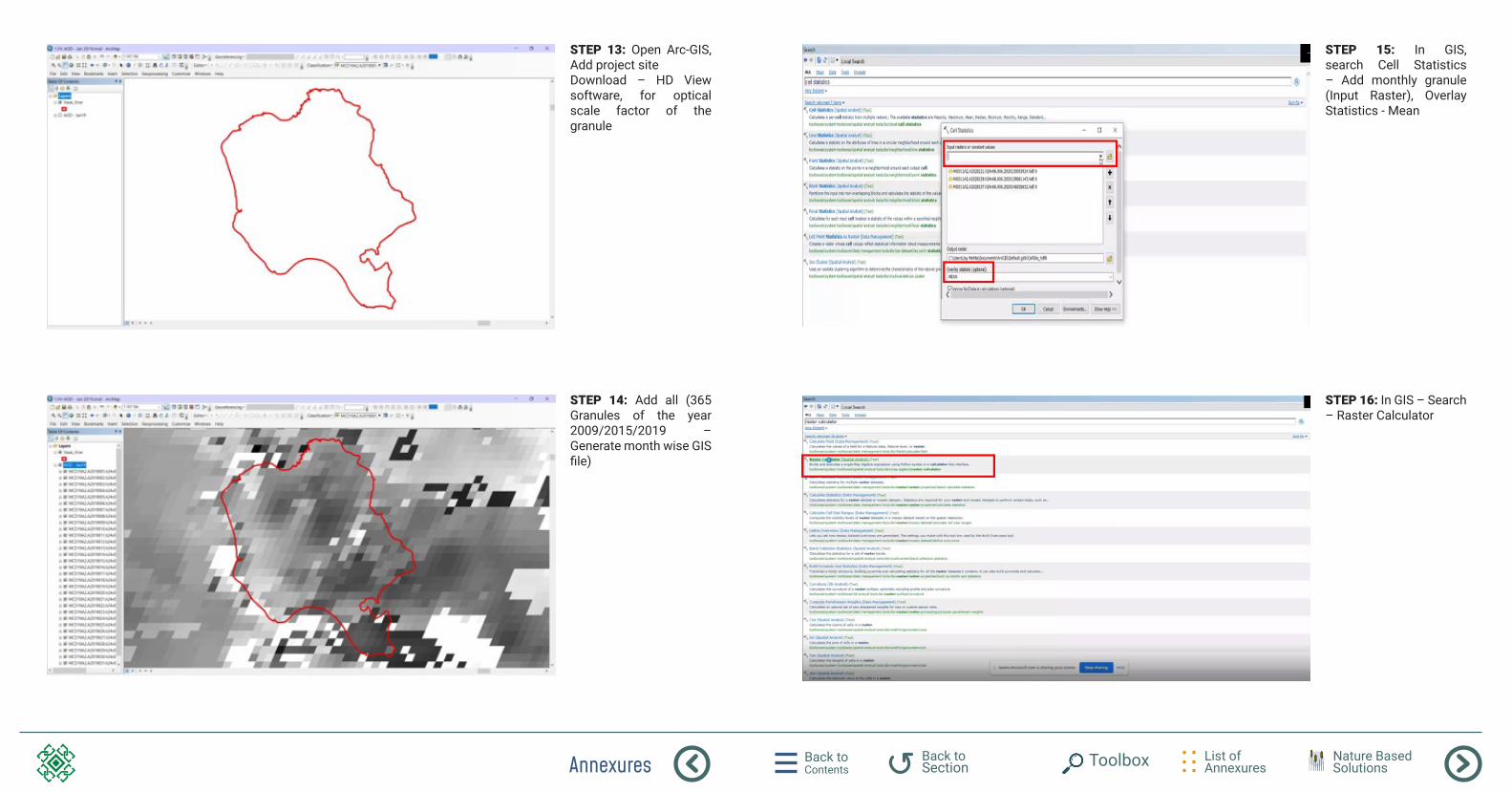
Annexures Back to Contents
List of Annexures
Back to Section Toolbox Nature Based
Solutions
STEP 13: Open Arc-GIS, Add project siteDownload – HD View software, for optical scale factor of the granule
STEP 15: In GIS, search Cell Statistics – Add monthly granule (Input Raster), Overlay Statistics - Mean
STEP 14: Add all (365 Granules of the year 2009/2015/2019 – Generate month wise GIS file)
STEP 16: In GIS – Search – Raster Calculator
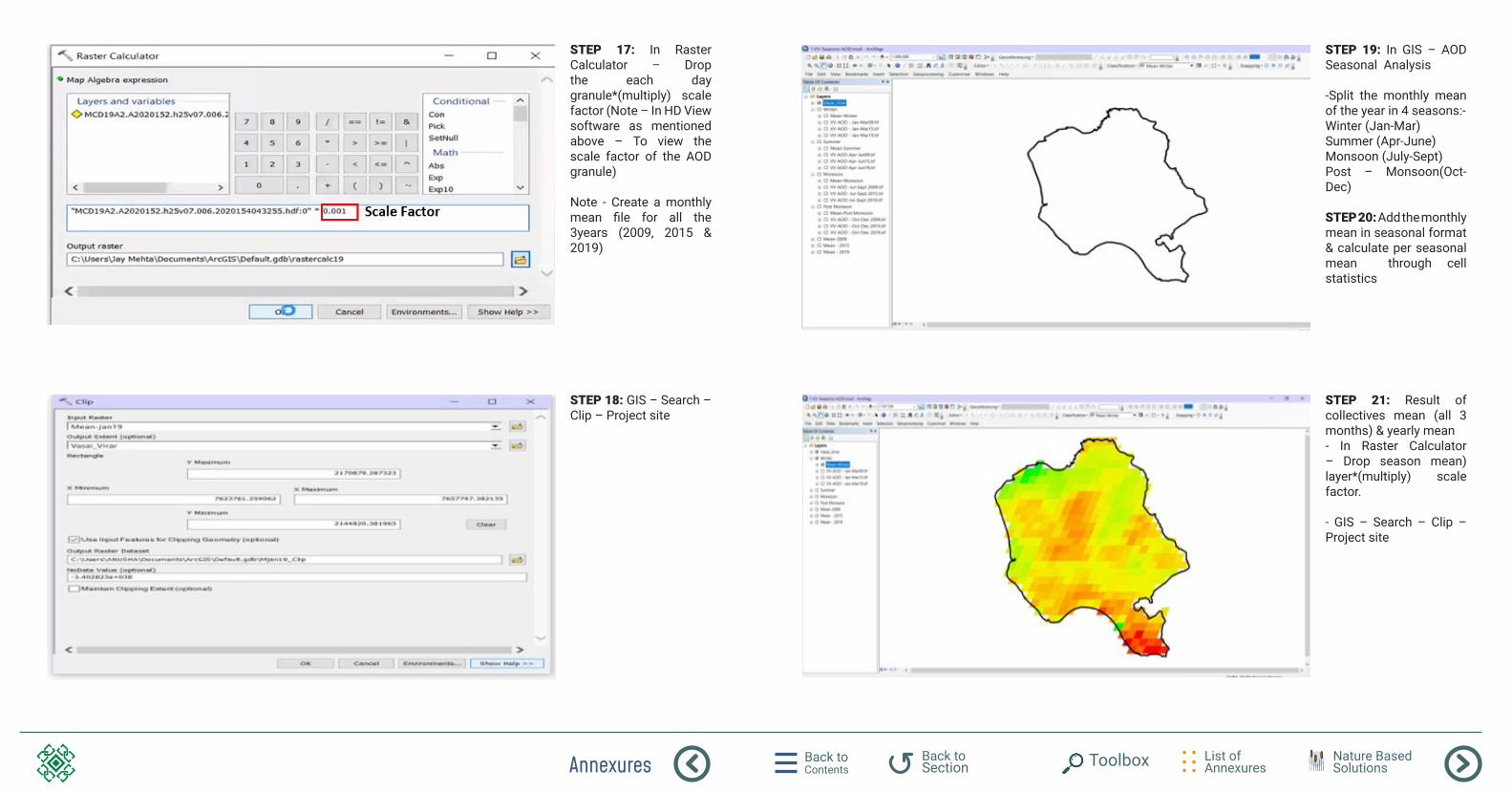
Annexures Back to Contents
List of Annexures
Back to Section Toolbox Nature Based
Solutions
STEP 17: In Raster Calculator – Drop the each day granule*(multiply) scale factor (Note – In HD View software as mentioned above – To view the scale factor of the AOD granule)
Note - Create a monthly mean file for all the 3years (2009, 2015 & 2019)
STEP 19: In GIS – AOD Seasonal Analysis
-Split the monthly mean of the year in 4 seasons:-Winter (Jan-Mar)Summer (Apr-June)Monsoon (July-Sept)Post – Monsoon(Oct-Dec)
STEP 20: Add the monthly mean in seasonal format & calculate per seasonal mean through cell statistics
STEP 18: GIS – Search – Clip – Project site
STEP 21: Result of collectives mean (all 3 months) & yearly mean- In Raster Calculator – Drop season mean) layer*(multiply) scale factor.
- GIS – Search – Clip – Project site
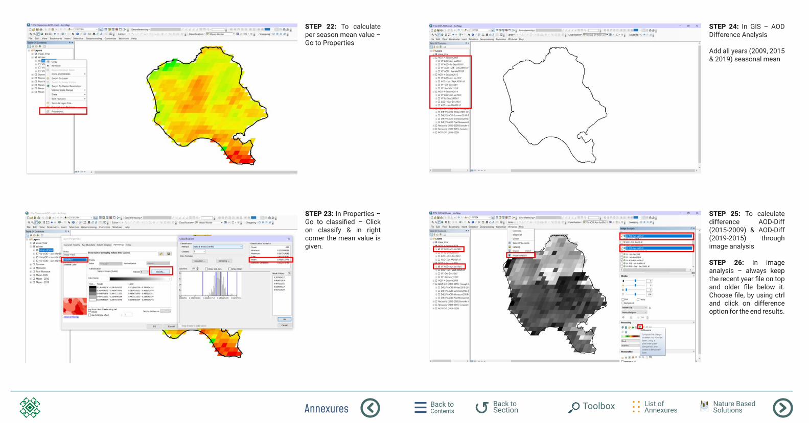
Annexures Back to Contents
List of Annexures
Back to Section Toolbox Nature Based
Solutions
STEP 22: To calculate per season mean value – Go to Properties
STEP 24: In GIS – AOD Difference Analysis
Add all years (2009, 2015 & 2019) seasonal mean
STEP 23: In Properties – Go to classified – Click on classify & in right corner the mean value is given.
STEP 25: To calculate difference AOD-Diff (2015-2009) & AOD-Diff (2019-2015) through image analysis
STEP 26: In image analysis – always keep the recent year file on top and older file below it. Choose file, by using ctrl and click on difference option for the end results.
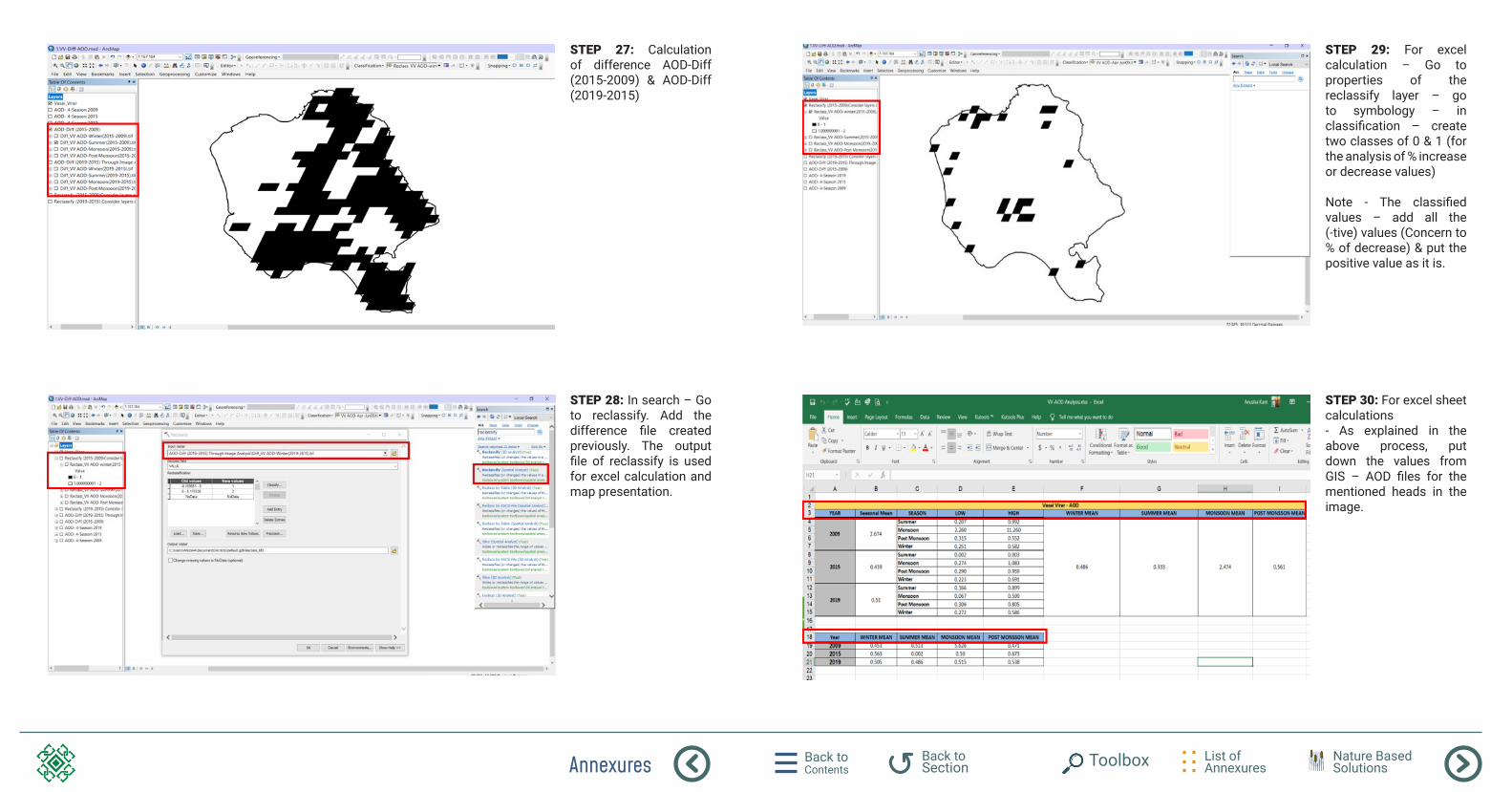
Annexures Back to Contents
List of Annexures
Back to Section Toolbox Nature Based
Solutions
STEP 27: Calculation of difference AOD-Diff (2015-2009) & AOD-Diff (2019-2015)
STEP 29: For excel calculation – Go to properties of the reclassify layer – go to symbology – in classification – create two classes of 0 & 1 (for the analysis of % increase or decrease values)
Note - The classified values – add all the (-tive) values (Concern to % of decrease) & put the positive value as it is.
STEP 28: In search – Go to reclassify. Add the difference file created previously. The output file of reclassify is used for excel calculation and map presentation.
STEP 30: For excel sheet calculations- As explained in the above process, put down the values from GIS – AOD files for the mentioned heads in the image.
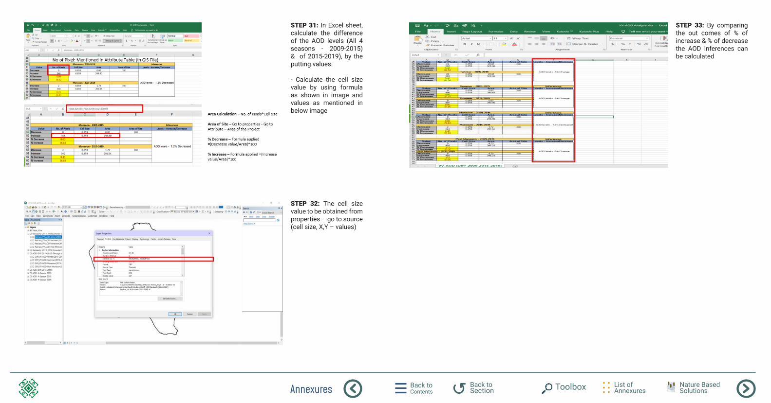
Annexures Back to Contents
List of Annexures
Back to Section Toolbox Nature Based
Solutions
STEP 31: In Excel sheet, calculate the difference of the AOD levels (All 4 seasons - 2009-2015) & of 2015-2019), by the putting values.
- Calculate the cell size value by using formula as shown in image and values as mentioned in below image
STEP 33: By comparing the out comes of % of increase & % of decrease the AOD inferences can be calculated
STEP 32: The cell size value to be obtained from properties – go to source (cell size, X,Y – values)
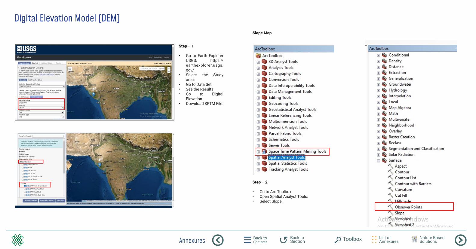
Annexures Back to Contents
List of Annexures
Back to Section Toolbox Nature Based
Solutions
Digital Elevation Model (DEM)
Step – 1
• Go to Earth Explorer USGS. https://earthexplorer.usgs.gov/
• Select the Study area.
• Go to Data Set.• See the Results • Go to Digital
Elevation.• Download SRTM File.
Step – 2
• Go to Arc Toolbox• Open Spatial Analyst Tools.• Select Slope.
Slope Map
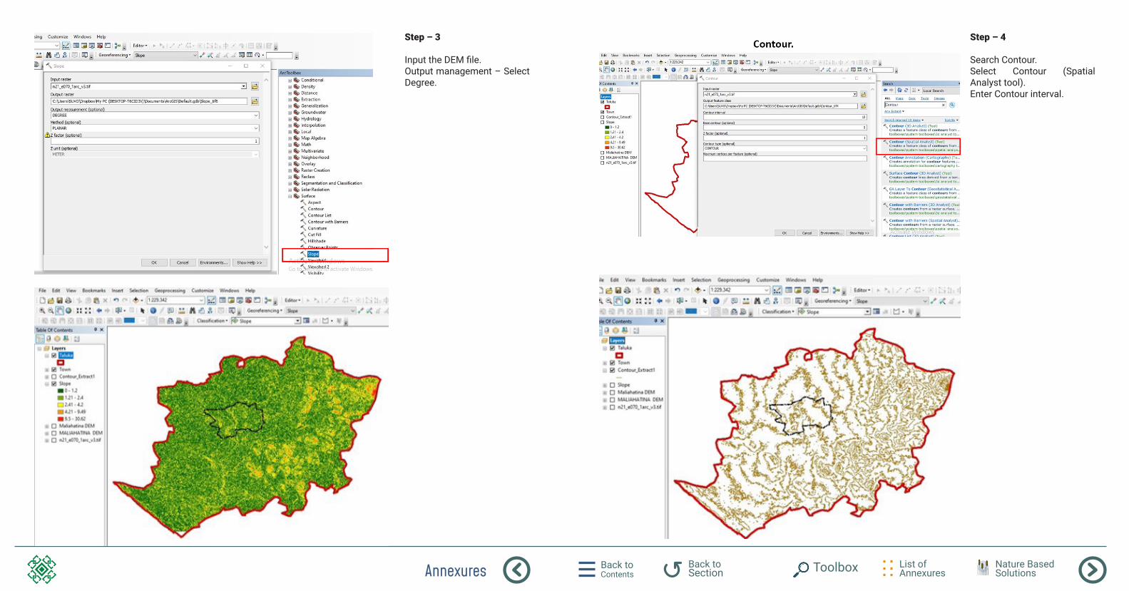
Annexures Back to Contents
List of Annexures
Back to Section Toolbox Nature Based
Solutions
Step – 3
Input the DEM file.Output management – Select Degree.
Step – 4
Search Contour.Select Contour (Spatial Analyst tool).Enter Contour interval.
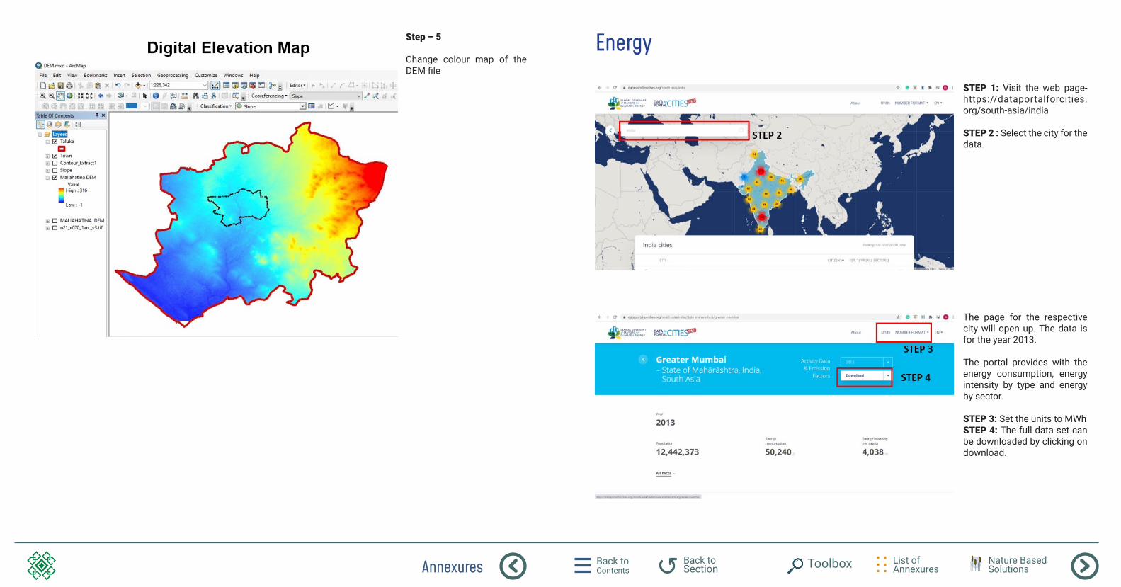
Annexures Back to Contents
List of Annexures
Back to Section Toolbox Nature Based
Solutions
Step – 5
Change colour map of the DEM file
Energy
STEP 1: Visit the web page- https://dataportalforcities.org/south-asia/india
STEP 2 : Select the city for the data.
The page for the respective city will open up. The data is for the year 2013.
The portal provides with the energy consumption, energy intensity by type and energy by sector.
STEP 3: Set the units to MWhSTEP 4: The full data set can be downloaded by clicking on download.
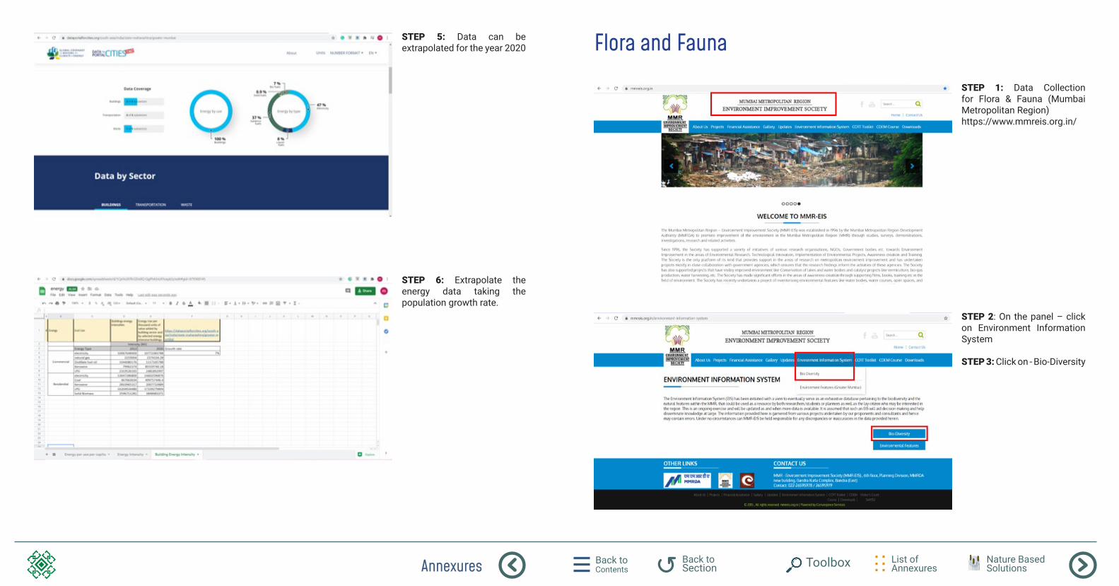
Annexures Back to Contents
List of Annexures
Back to Section Toolbox Nature Based
Solutions
STEP 5: Data can be extrapolated for the year 2020
STEP 6: Extrapolate the energy data taking the population growth rate.
Flora and Fauna
STEP 1: Data Collection for Flora & Fauna (Mumbai Metropolitan Region)https://www.mmreis.org.in/
STEP 2: On the panel – click on Environment Information System
STEP 3: Click on - Bio-Diversity
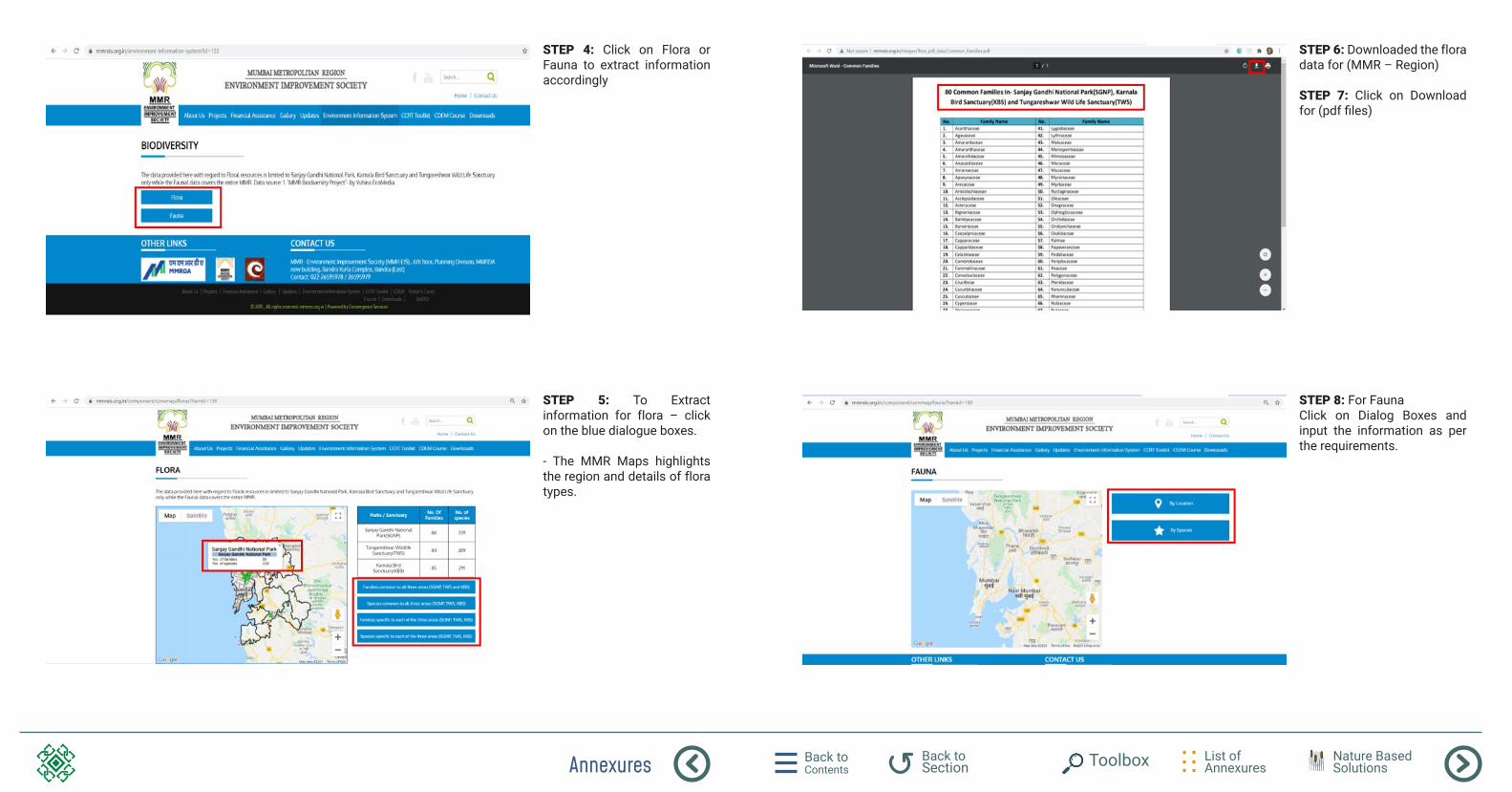
Annexures Back to Contents
List of Annexures
Back to Section Toolbox Nature Based
Solutions
STEP 4: Click on Flora or Fauna to extract information accordingly
STEP 6: Downloaded the flora data for (MMR – Region)
STEP 7: Click on Download for (pdf files)
STEP 8: For FaunaClick on Dialog Boxes and input the information as per the requirements.
STEP 5: To Extract information for flora – click on the blue dialogue boxes.
- The MMR Maps highlights the region and details of flora types.
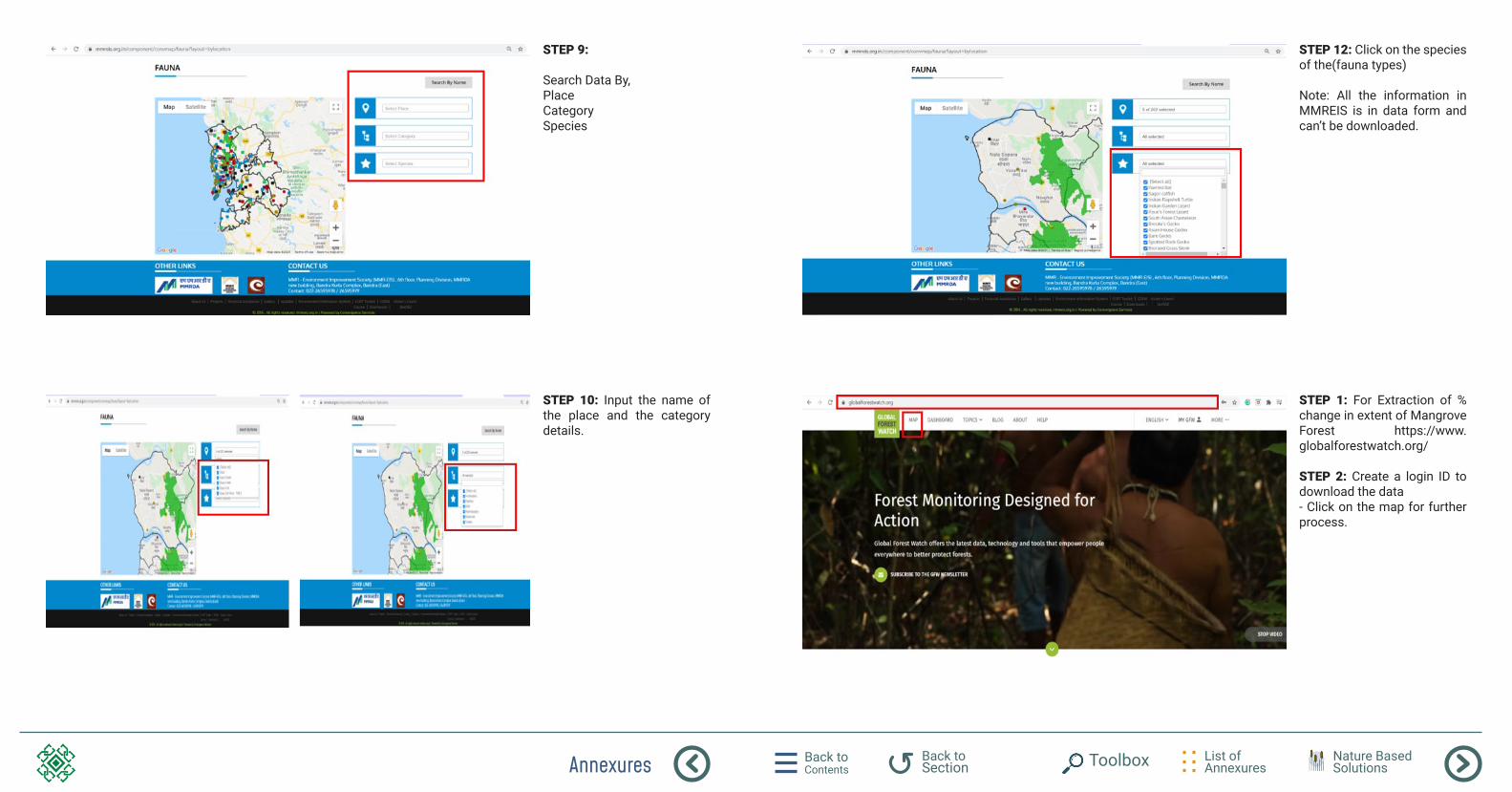
Annexures Back to Contents
List of Annexures
Back to Section Toolbox Nature Based
Solutions
STEP 9:
Search Data By, PlaceCategorySpecies
STEP 12: Click on the species of the(fauna types)
Note: All the information in MMREIS is in data form and can’t be downloaded.
STEP 10: Input the name of the place and the category details.
STEP 1: For Extraction of % change in extent of Mangrove Forest https://www.globalforestwatch.org/
STEP 2: Create a login ID to download the data- Click on the map for further process.
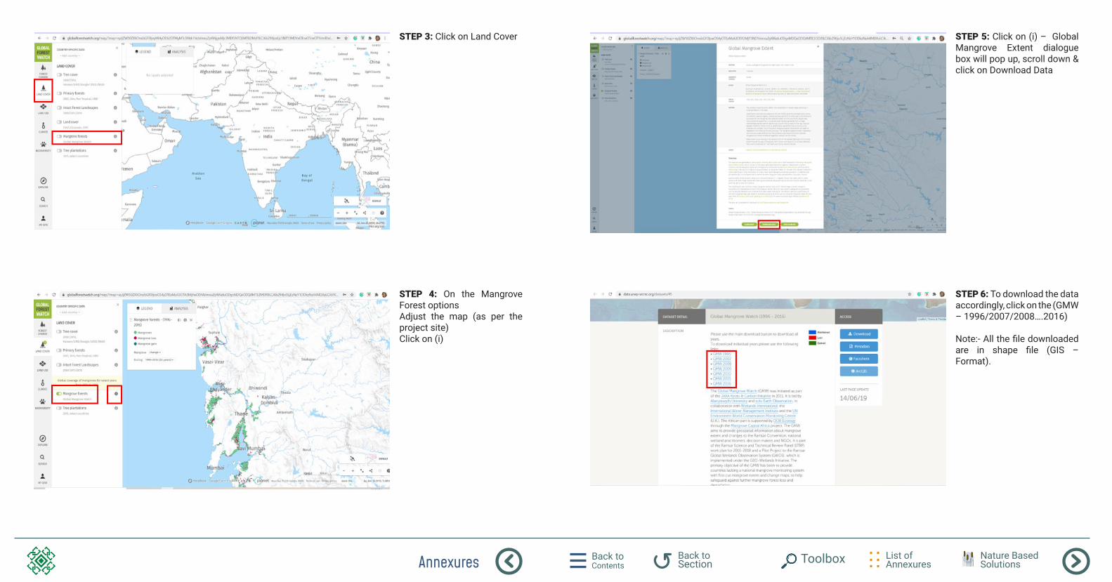
Annexures Back to Contents
List of Annexures
Back to Section Toolbox Nature Based
Solutions
STEP 3: Click on Land Cover STEP 5: Click on (i) – Global Mangrove Extent dialogue box will pop up, scroll down & click on Download Data
STEP 4: On the Mangrove Forest optionsAdjust the map (as per the project site)Click on (i)
STEP 6: To download the data accordingly, click on the (GMW – 1996/2007/2008….2016)
Note:- All the file downloaded are in shape file (GIS – Format).
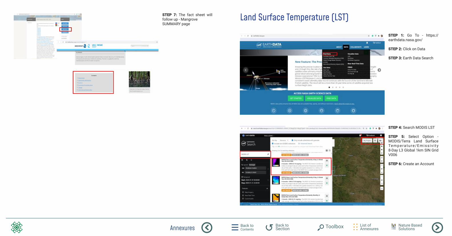
Annexures Back to Contents
List of Annexures
Back to Section Toolbox Nature Based
Solutions
STEP 7: The fact sheet will follow up - MangroveSUMMARY page
Land Surface Temperature (LST)
STEP 1: Go To - https://earthdata.nasa.gov/ STEP 2: Click on Data STEP 3: Earth Data Search
STEP 4: Search MODIS LST
STEP 5: Select Option - MODIS/Terra Land Surface Te m p e ra t u re / E m i s s i v i t y 8-Day L3 Global 1km SIN Grid V006
STEP 6: Create an Account
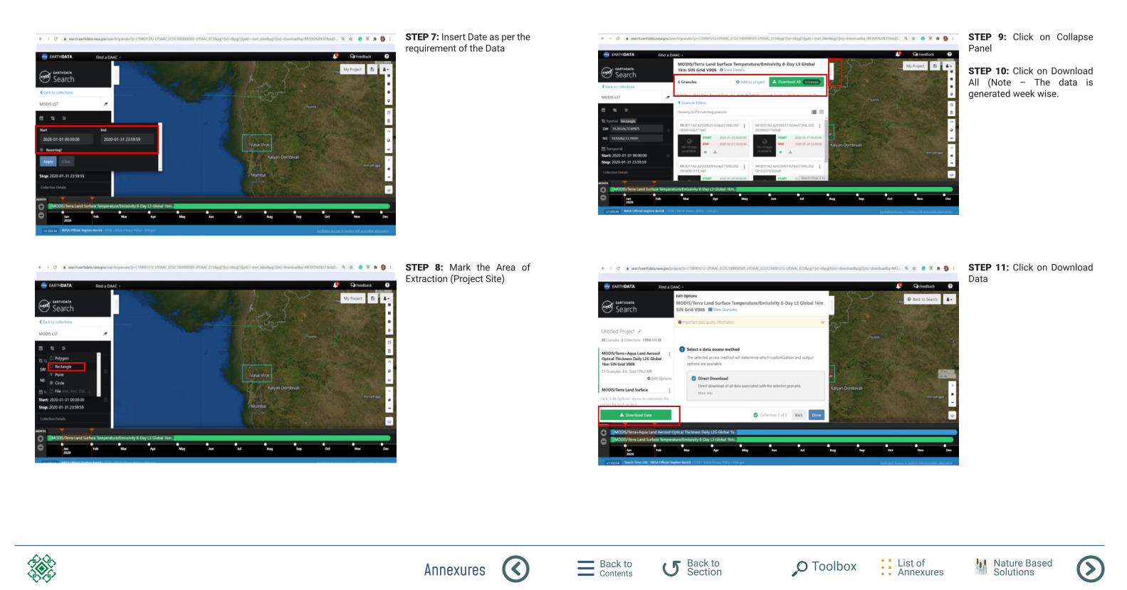
Annexures Back to Contents
List of Annexures
Back to Section Toolbox Nature Based
Solutions
STEP 7: Insert Date as per the requirement of the Data
STEP 9: Click on Collapse Panel
STEP 10: Click on Download All (Note – The data is generated week wise.
STEP 8: Mark the Area of Extraction (Project Site)
STEP 11: Click on Download Data
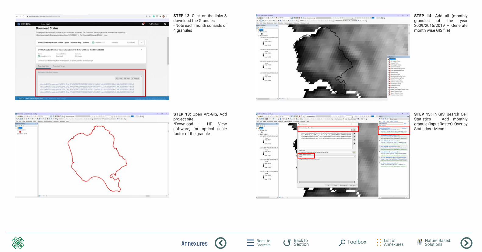
Annexures Back to Contents
List of Annexures
Back to Section Toolbox Nature Based
Solutions
STEP 12: Click on the links & download the Granules - Note each month consists of 4 granules
STEP 14: Add all (monthly granules of the year 2009/2015/2019 – Generate month wise GIS file)
STEP 13: Open Arc-GIS, Add project site*Download – HD View software, for optical scale factor of the granule
STEP 15: In GIS, search Cell Statistics – Add monthly granule (Input Raster), Overlay Statistics - Mean
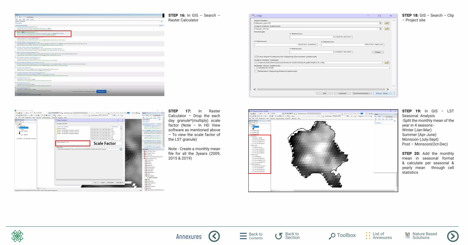
Annexures Back to Contents
List of Annexures
Back to Section Toolbox Nature Based
Solutions
STEP 16: In GIS – Search – Raster Calculator
STEP 18: GIS – Search – Clip – Project site
STEP 17: In Raster Calculator – Drop the each day granule*(multiply) scale factor (Note – In HD View software as mentioned above – To view the scale factor of the LST granule)
Note - Create a monthly mean file for all the 3years (2009, 2015 & 2019)
STEP 19: In GIS – LST Seasonal Analysis-Split the monthly mean of the year in 4 seasons:-Winter (Jan-Mar)Summer (Apr-June)Monsoon (July-Sept)Post – Monsoon(Oct-Dec)
STEP 20: Add the monthly mean in seasonal format & calculate per seasonal & yearly mean through cell statistics
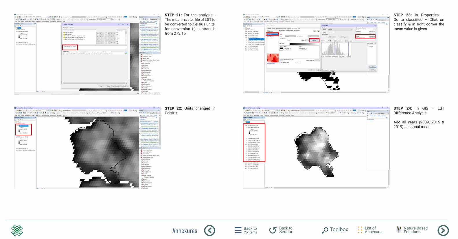
Annexures Back to Contents
List of Annexures
Back to Section Toolbox Nature Based
Solutions
STEP 21: For the analysis - The mean - raster file of LST to be converted to Celsius units, for conversion (-) subtract it from 273.15
STEP 23: In Properties – Go to classified – Click on classify & in right corner the mean value is given
STEP 22: Units changed in Celsius
STEP 24: In GIS – LST Difference Analysis
Add all years (2009, 2015 & 2019) seasonal mean
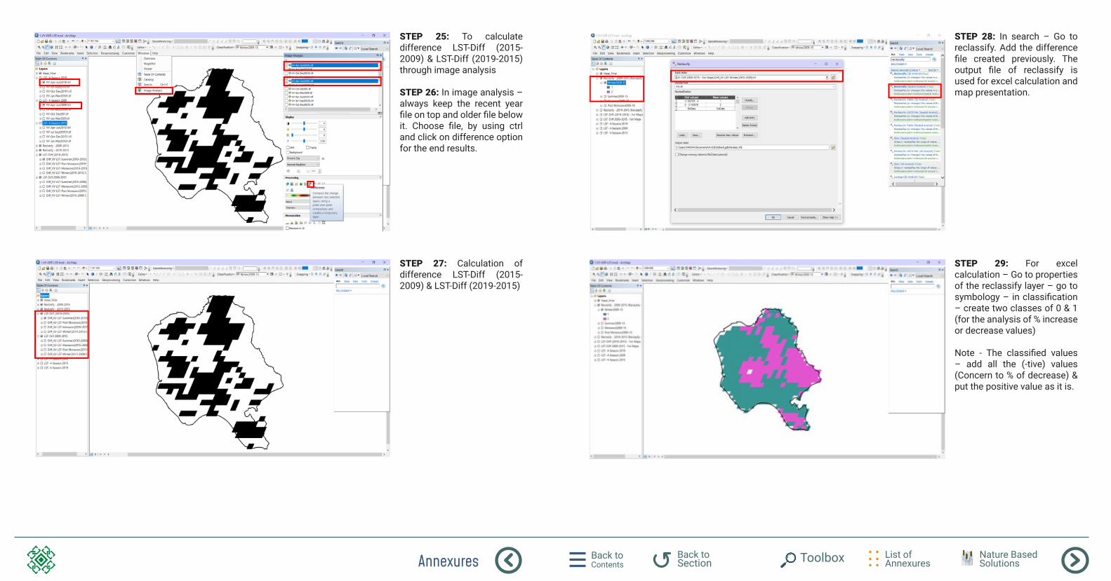
Annexures Back to Contents
List of Annexures
Back to Section Toolbox Nature Based
Solutions
STEP 25: To calculate difference LST-Diff (2015-2009) & LST-Diff (2019-2015) through image analysis
STEP 26: In image analysis – always keep the recent year file on top and older file below it. Choose file, by using ctrl and click on difference option for the end results.
STEP 28: In search – Go to reclassify. Add the difference file created previously. The output file of reclassify is used for excel calculation and map presentation.
STEP 27: Calculation of difference LST-Diff (2015-2009) & LST-Diff (2019-2015)
STEP 29: For excel calculation – Go to properties of the reclassify layer – go to symbology – in classification – create two classes of 0 & 1 (for the analysis of % increase or decrease values)
Note - The classified values – add all the (-tive) values (Concern to % of decrease) & put the positive value as it is.
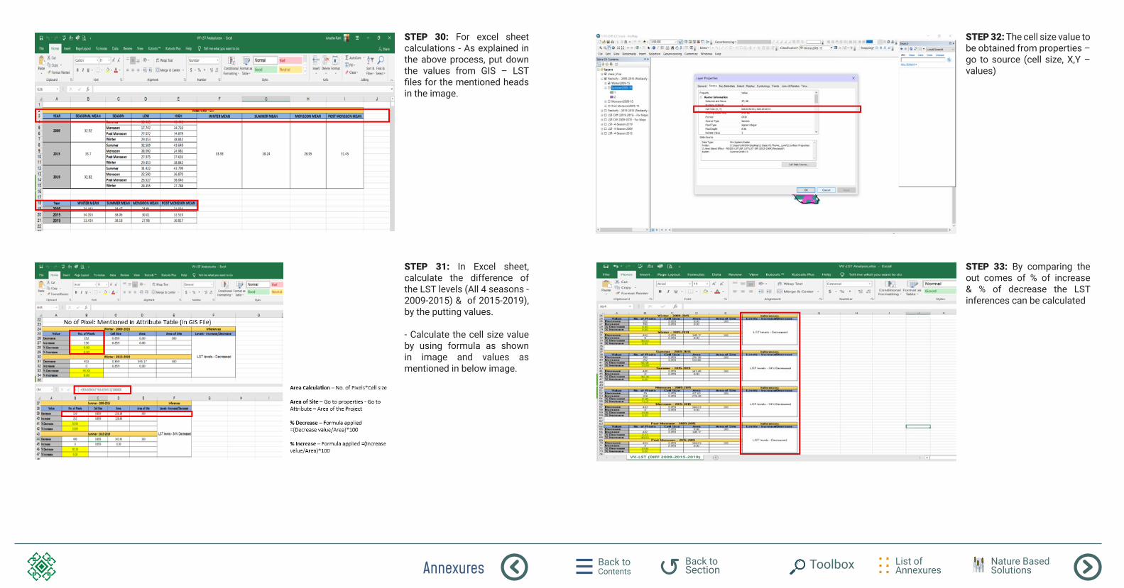
Annexures Back to Contents
List of Annexures
Back to Section Toolbox Nature Based
Solutions
STEP 30: For excel sheet calculations - As explained in the above process, put down the values from GIS – LST files for the mentioned heads in the image.
STEP 32: The cell size value to be obtained from properties – go to source (cell size, X,Y – values)
STEP 31: In Excel sheet, calculate the difference of the LST levels (All 4 seasons - 2009-2015) & of 2015-2019), by the putting values.
- Calculate the cell size value by using formula as shown in image and values as mentioned in below image.
STEP 33: By comparing the out comes of % of increase & % of decrease the LST inferences can be calculated
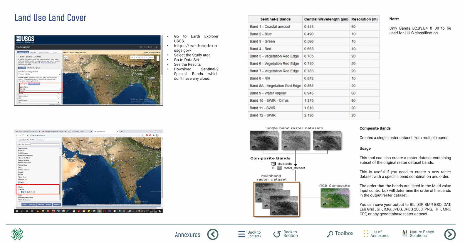
Annexures Back to Contents
List of Annexures
Back to Section Toolbox Nature Based
Solutions
Land Use Land Cover
• Go to Earth Explorer USGS.
• https://ear thexplorer.usgs.gov/
• Select the Study area.• Go to Data Set.• See the Results • Download Sentinal-2
Special Bands which don’t have any cloud.
Note:
Only Bands B2,B3,B4 & B8 to be used for LULC classification
Composite Bands
Creates a single raster dataset from multiple bands
Usage
This tool can also create a raster dataset containing subset of the original raster dataset bands.
This is useful if you need to create a new raster dataset with a specific band combination and order.
The order that the bands are listed in the Multi-value Input control box will determine the order of the bands in the output raster dataset.
You can save your output to BIL, BIP, BMP, BSQ, DAT, Esri Grid , GIF, IMG, JPEG, JPEG 2000, PNG, TIFF, MRF, CRF, or any geodatabase raster dataset.
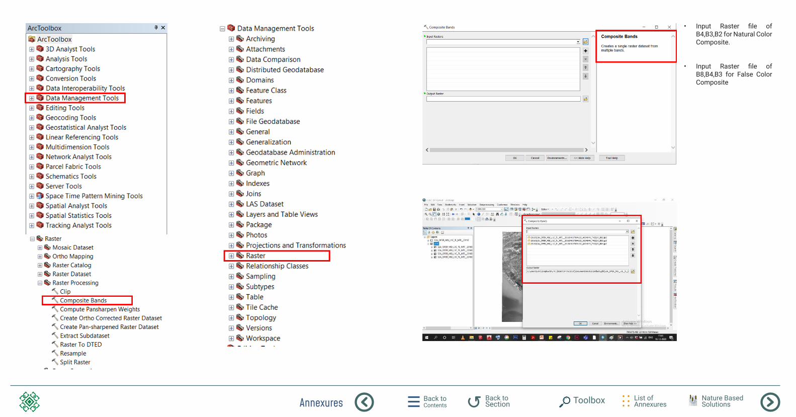
Annexures Back to Contents
List of Annexures
Back to Section Toolbox Nature Based
Solutions
• Input Raster file of B4,B3,B2 for Natural Color Composite.
• Input Raster file of B8,B4,B3 for False Color Composite
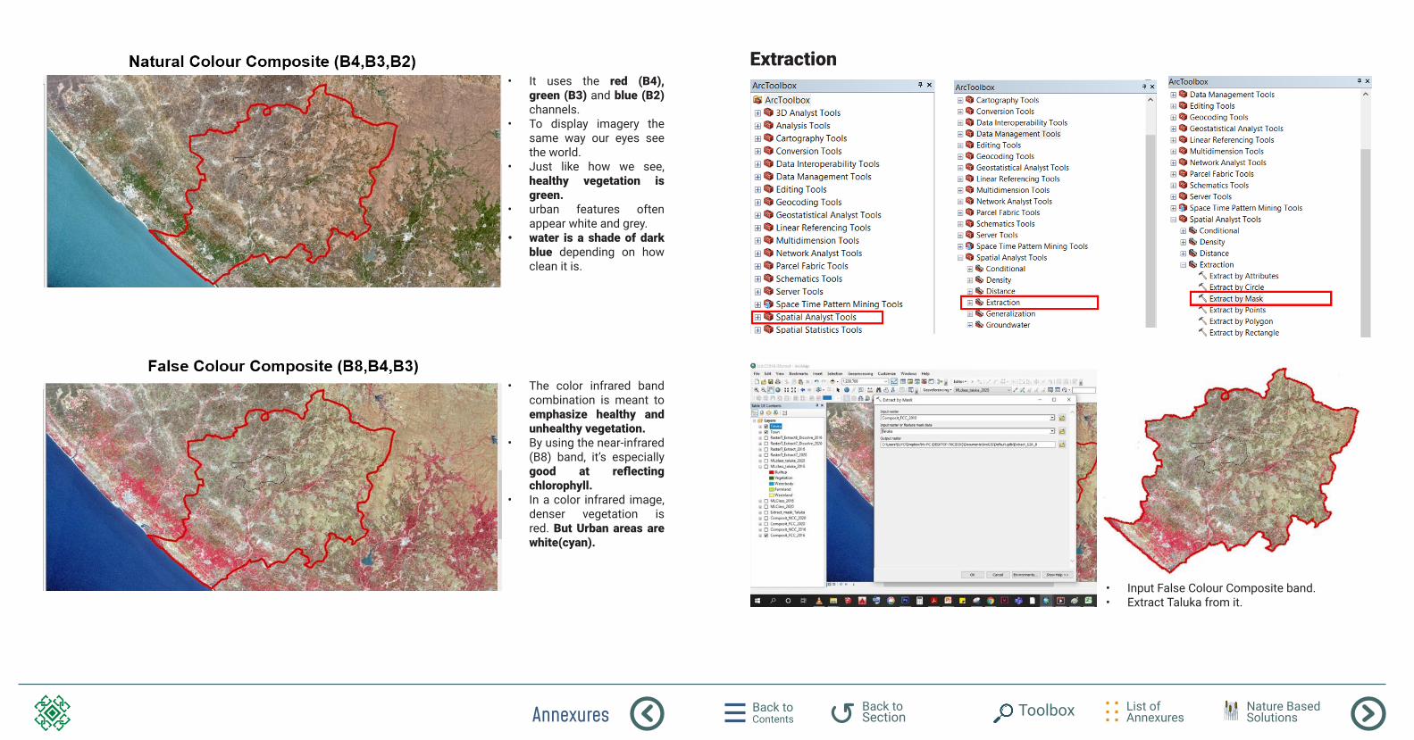
Annexures Back to Contents
List of Annexures
Back to Section Toolbox Nature Based
Solutions
• It uses the red (B4), green (B3) and blue (B2) channels.
• To display imagery the same way our eyes see the world.
• Just like how we see, healthy vegetation is green.
• urban features often appear white and grey.
• water is a shade of dark blue depending on how clean it is.
• The color infrared band combination is meant to emphasize healthy and unhealthy vegetation.
• By using the near-infrared (B8) band, it’s especially good at reflecting chlorophyll.
• In a color infrared image, denser vegetation is red. But Urban areas are white(cyan).
Extraction
• Input False Colour Composite band.• Extract Taluka from it.
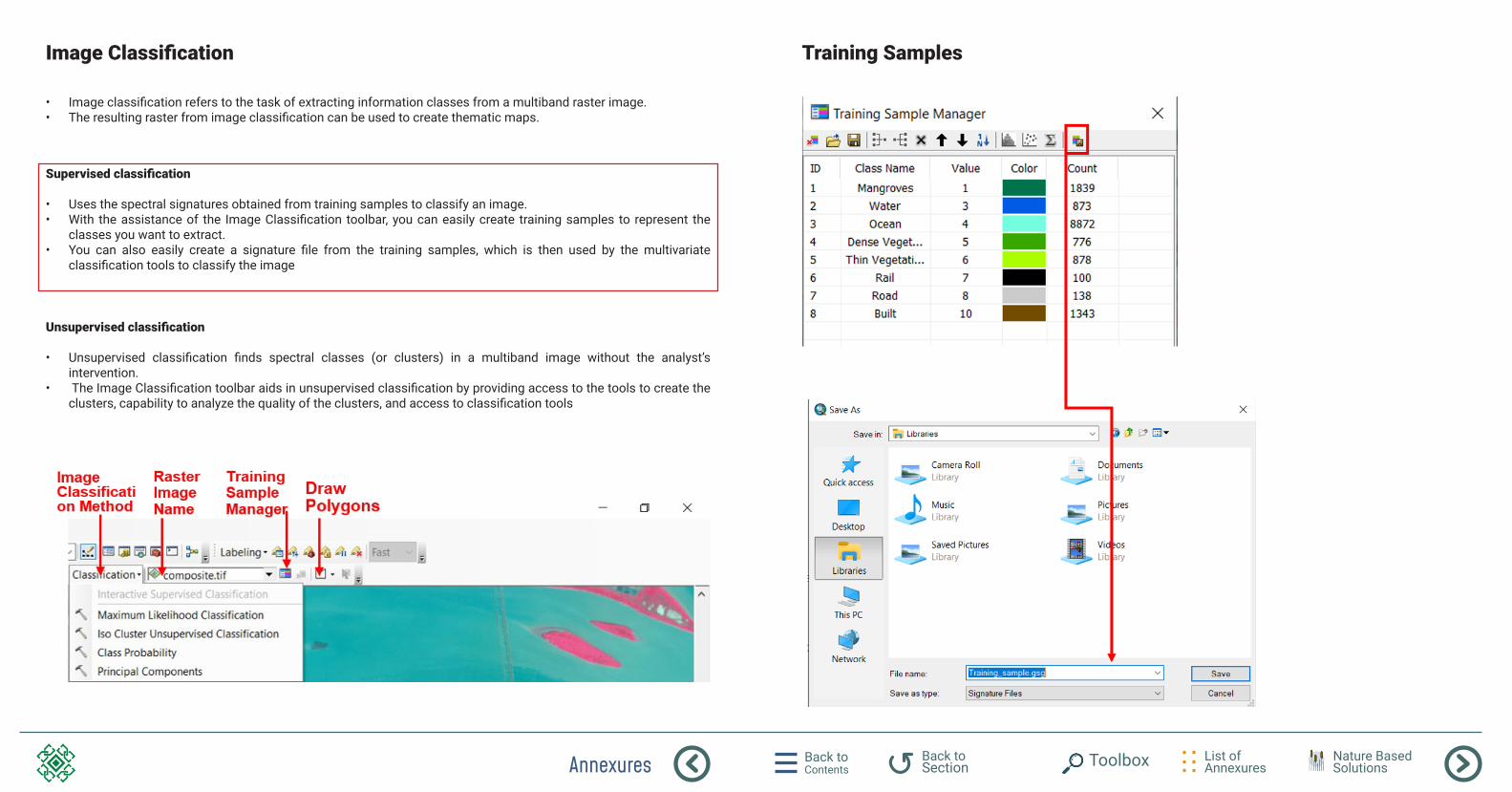
Annexures Back to Contents
List of Annexures
Back to Section Toolbox Nature Based
Solutions
Image Classification Training Samples
• Image classification refers to the task of extracting information classes from a multiband raster image. • The resulting raster from image classification can be used to create thematic maps.
Supervised classification
• Uses the spectral signatures obtained from training samples to classify an image. • With the assistance of the Image Classification toolbar, you can easily create training samples to represent the
classes you want to extract. • You can also easily create a signature file from the training samples, which is then used by the multivariate
classification tools to classify the image
Unsupervised classification
• Unsupervised classification finds spectral classes (or clusters) in a multiband image without the analyst’s intervention.
• The Image Classification toolbar aids in unsupervised classification by providing access to the tools to create the clusters, capability to analyze the quality of the clusters, and access to classification tools
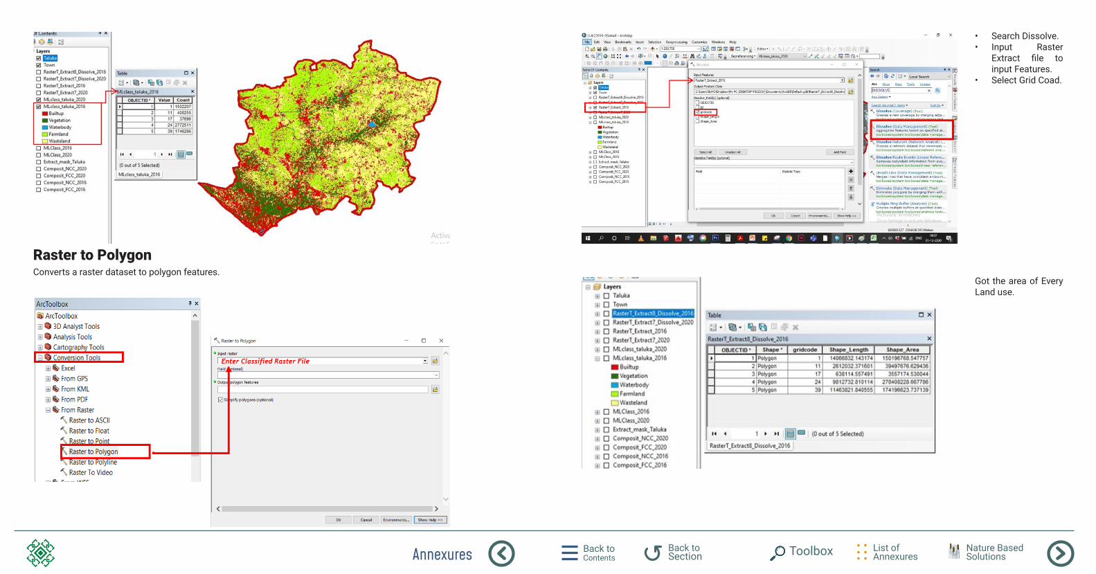
Annexures Back to Contents
List of Annexures
Back to Section Toolbox Nature Based
Solutions
Raster to Polygon Converts a raster dataset to polygon features.
• Search Dissolve.• Input Raster
Extract file to input Features.
• Select Grid Coad.
Got the area of Every Land use.
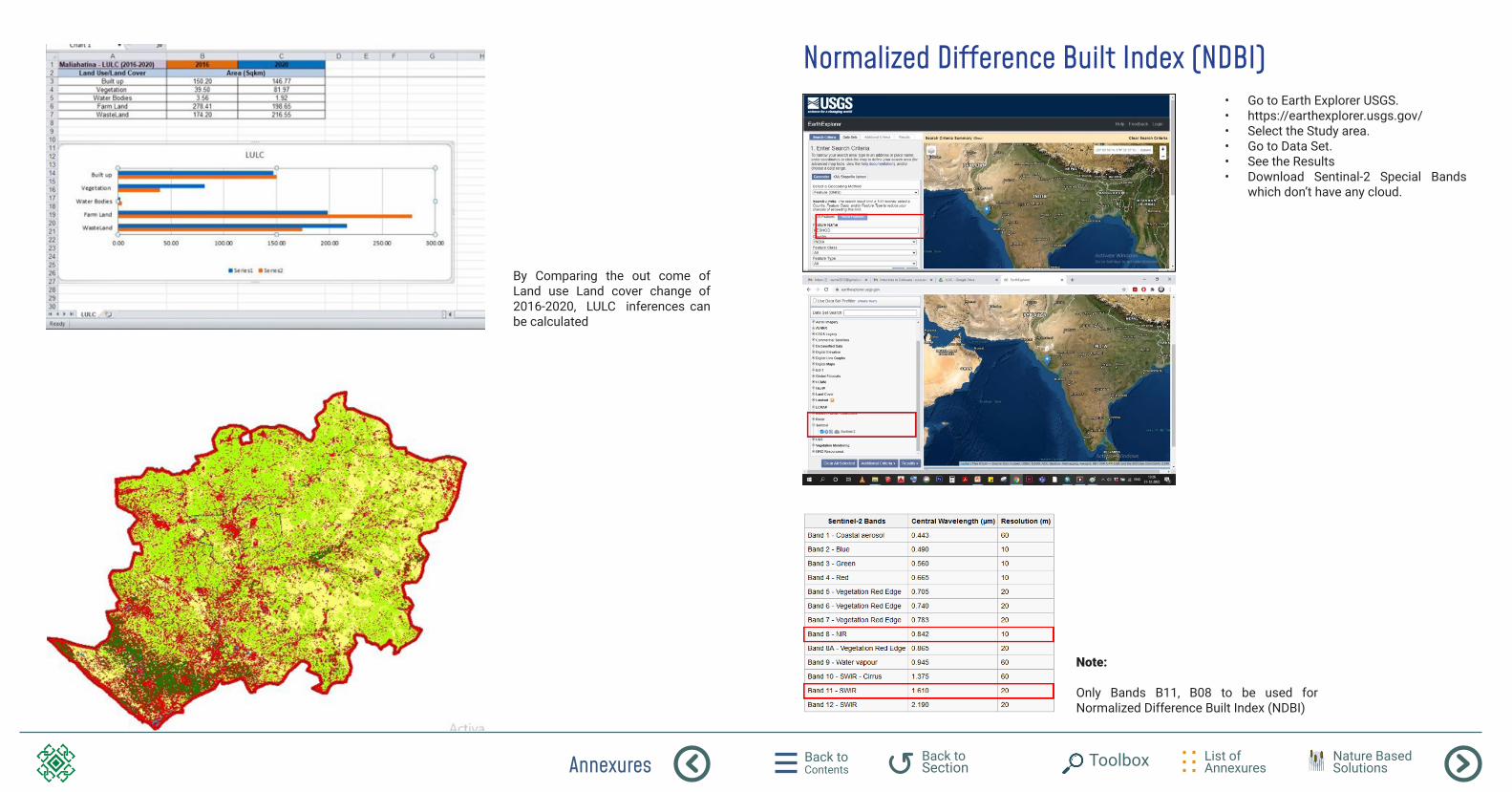
Annexures Back to Contents
List of Annexures
Back to Section Toolbox Nature Based
Solutions
By Comparing the out come of Land use Land cover change of 2016-2020, LULC inferences can be calculated
Normalized Difference Built Index (NDBI)• Go to Earth Explorer USGS.• https://earthexplorer.usgs.gov/• Select the Study area.• Go to Data Set.• See the Results • Download Sentinal-2 Special Bands
which don’t have any cloud.
Note:
Only Bands B11, B08 to be used for Normalized Difference Built Index (NDBI)
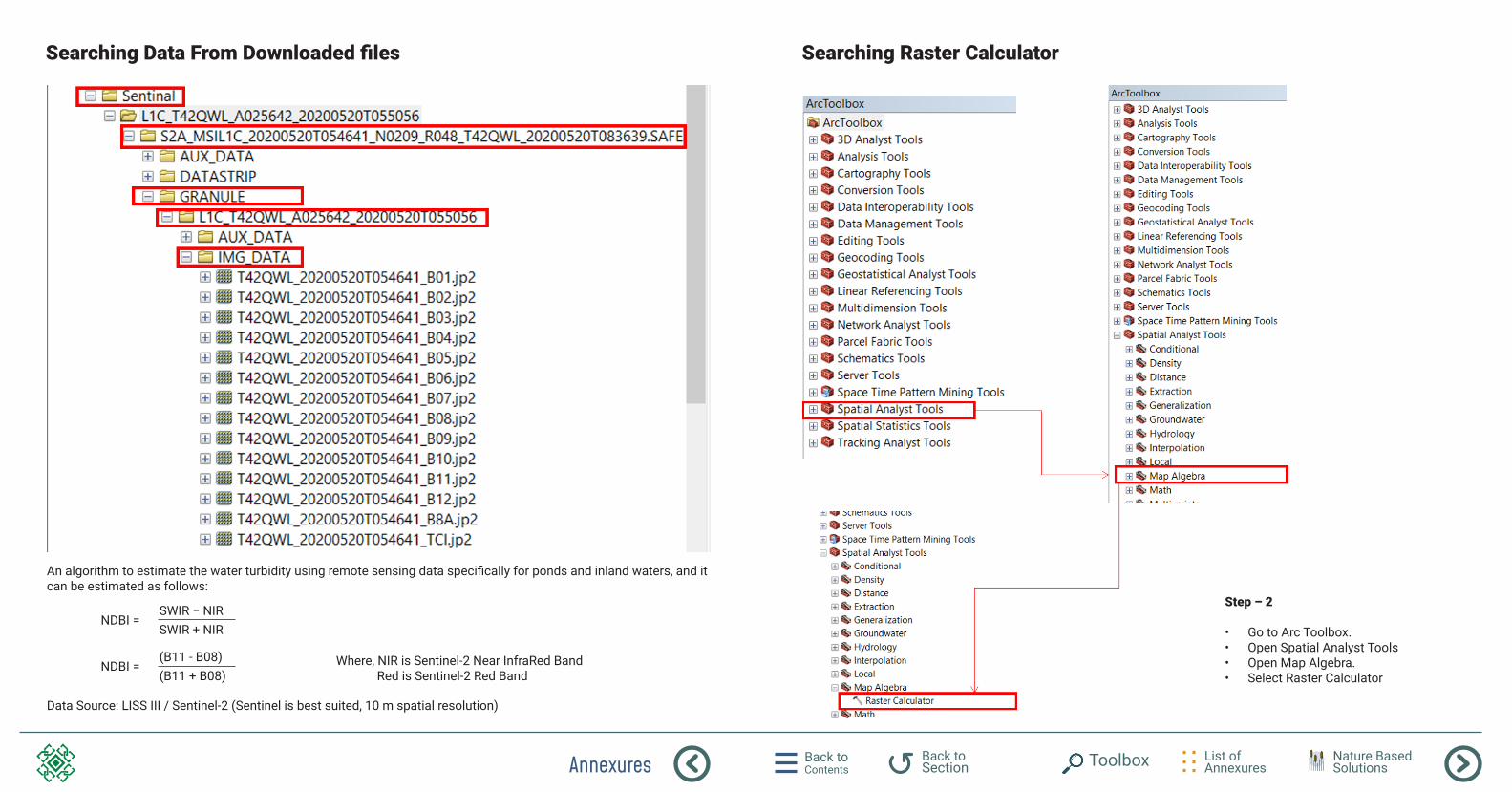
Annexures Back to Contents
List of Annexures
Back to Section Toolbox Nature Based
Solutions
Searching Data From Downloaded files Searching Raster Calculator
An algorithm to estimate the water turbidity using remote sensing data specifically for ponds and inland waters, and it can be estimated as follows:
Where, NIR is Sentinel-2 Near InfraRed Band Red is Sentinel-2 Red Band
Data Source: LISS III / Sentinel-2 (Sentinel is best suited, 10 m spatial resolution)
NDBI =
NDBI =
SWIR − NIR
(B11 - B08)
SWIR + NIR
(B11 + B08)
Step – 2
• Go to Arc Toolbox.• Open Spatial Analyst Tools• Open Map Algebra.• Select Raster Calculator

Annexures Back to Contents
List of Annexures
Back to Section Toolbox Nature Based
Solutions
Raster Calculator ExtractionBuilds and executes a single Map Algebra expression using Python syntax in a calculator-like interface.
float(“T42QXJ_B11.jp2” - “T42QXJ_B08.jp2”) / float(“ T42QXJ_B11.jp2” + “T42QXJ_B08.jp2 “)
Step – 3
• Open Raster Calculator and put the respected file with Commend “float”.
• Extracted the file based on the Study area.
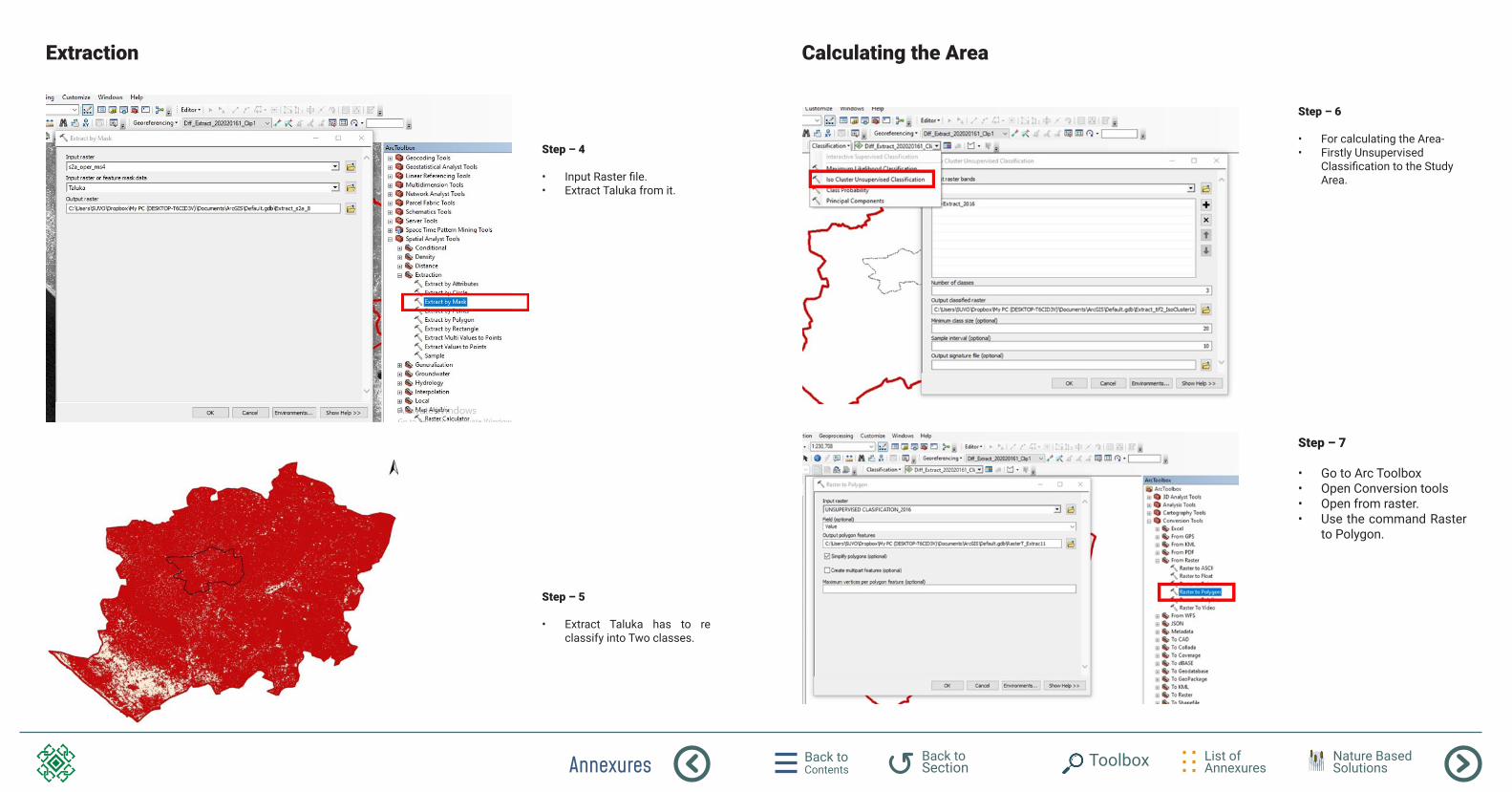
Annexures Back to Contents
List of Annexures
Back to Section Toolbox Nature Based
Solutions
Extraction Calculating the Area
Step – 4
• Input Raster file. • Extract Taluka from it.
Step – 6
• For calculating the Area- • Firstly Unsupervised
Classification to the Study Area.
Step – 7
• Go to Arc Toolbox• Open Conversion tools• Open from raster.• Use the command Raster
to Polygon.
Step – 5
• Extract Taluka has to re classify into Two classes.
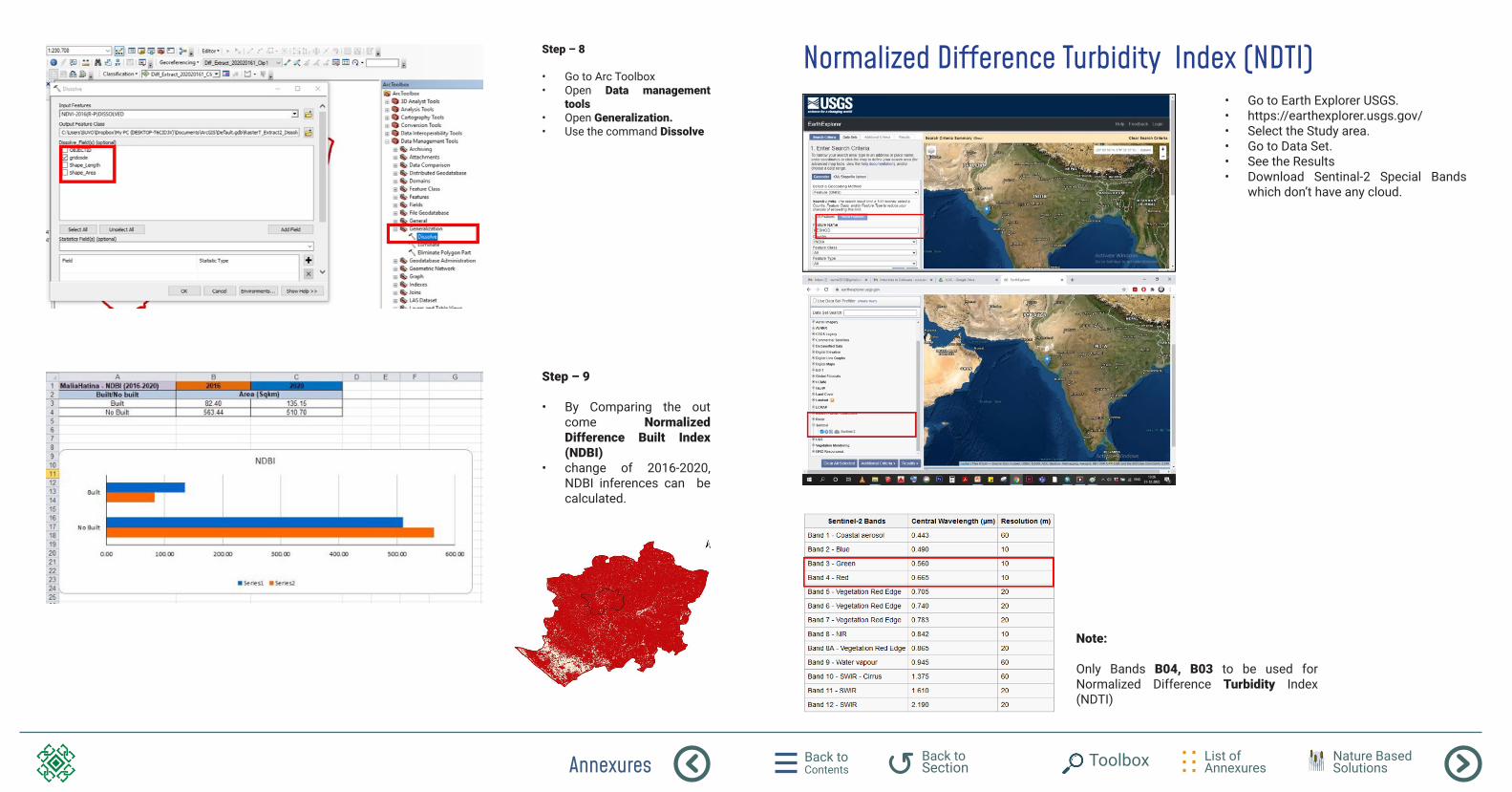
Annexures Back to Contents
List of Annexures
Back to Section Toolbox Nature Based
Solutions
Step – 8
• Go to Arc Toolbox• Open Data management
tools• Open Generalization. • Use the command Dissolve
Step – 9
• By Comparing the out come Normalized Difference Built Index (NDBI)
• change of 2016-2020, NDBI inferences can be calculated.
Normalized Difference Turbidity Index (NDTI)• Go to Earth Explorer USGS.• https://earthexplorer.usgs.gov/• Select the Study area.• Go to Data Set.• See the Results • Download Sentinal-2 Special Bands
which don’t have any cloud.
Note:
Only Bands B04, B03 to be used for Normalized Difference Turbidity Index (NDTI)

Annexures Back to Contents
List of Annexures
Back to Section Toolbox Nature Based
Solutions
Searching Data From Downloaded files Searching Raster Calculator
An algorithm to estimate the water turbidity using remote sensing data specifically for ponds and inland waters, and it can be estimated as follows:
Data Source: LISS III / Sentinel-2 (Sentinel is best suited, 10 m spatial resolution)
Red - GreenRed + Green
Step – 2
• Go to Arc Toolbox.• Open Spatial Analyst Tools• Open Map Algebra.• Select Raster Calculator
NDTI =
Where, NIR is Sentinel-2 Near InfraRed Band Red is Sentinel-2 Red Band
NDTI = (B04 - B03)(B04 + B03)
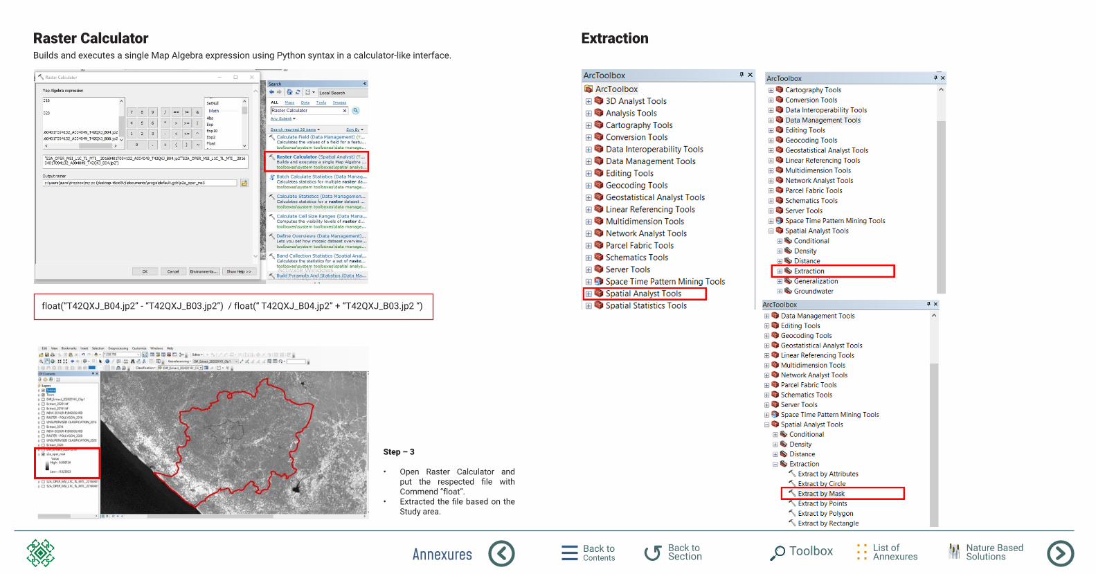
Annexures Back to Contents
List of Annexures
Back to Section Toolbox Nature Based
Solutions
Raster Calculator ExtractionBuilds and executes a single Map Algebra expression using Python syntax in a calculator-like interface.
float(“T42QXJ_B04.jp2” - “T42QXJ_B03.jp2”) / float(“ T42QXJ_B04.jp2” + “T42QXJ_B03.jp2 “)
Step – 3
• Open Raster Calculator and put the respected file with Commend “float”.
• Extracted the file based on the Study area.
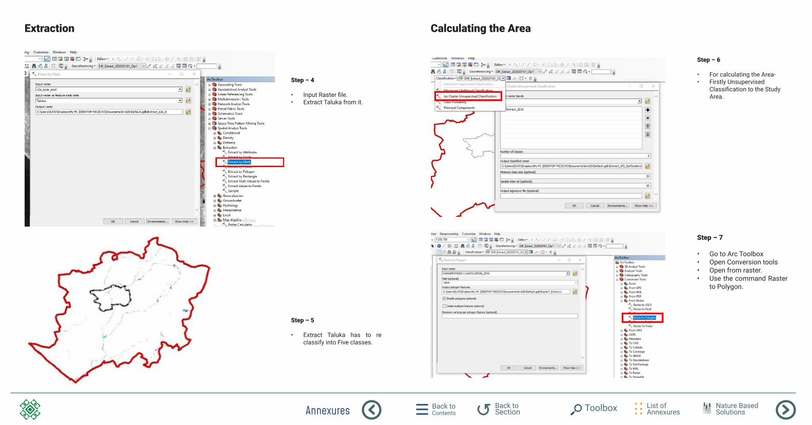
Annexures Back to Contents
List of Annexures
Back to Section Toolbox Nature Based
Solutions
Extraction Calculating the Area
Step – 4
• Input Raster file. • Extract Taluka from it.
Step – 6
• For calculating the Area- • Firstly Unsupervised
Classification to the Study Area.
Step – 7
• Go to Arc Toolbox• Open Conversion tools• Open from raster.• Use the command Raster
to Polygon.
Step – 5
• Extract Taluka has to re classify into Five classes.
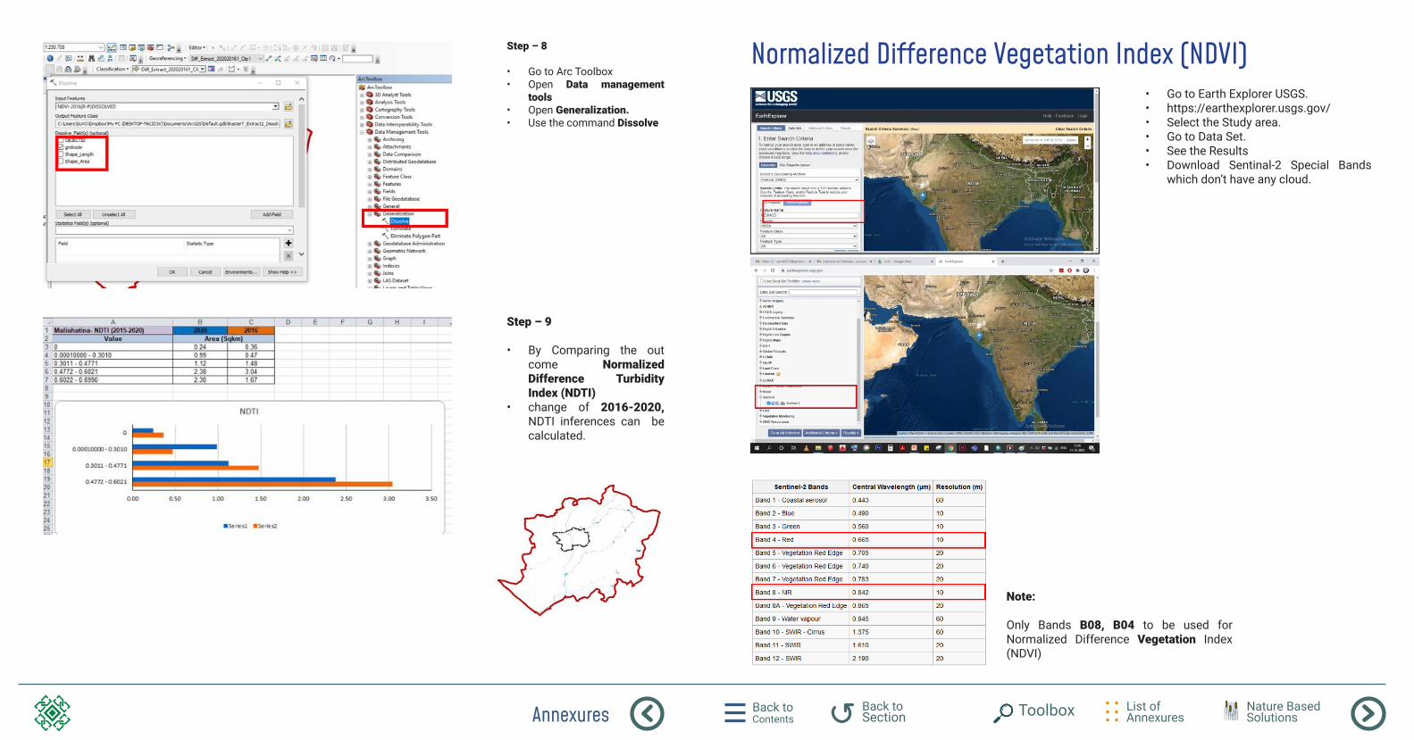
Annexures Back to Contents
List of Annexures
Back to Section Toolbox Nature Based
Solutions
Step – 8
• Go to Arc Toolbox• Open Data management
tools• Open Generalization. • Use the command Dissolve
Step – 9
• By Comparing the out come Normalized Difference Turbidity Index (NDTI)
• change of 2016-2020, NDTI inferences can be calculated.
Normalized Difference Vegetation Index (NDVI)• Go to Earth Explorer USGS.• https://earthexplorer.usgs.gov/• Select the Study area.• Go to Data Set.• See the Results • Download Sentinal-2 Special Bands
which don’t have any cloud.
Note:
Only Bands B08, B04 to be used for Normalized Difference Vegetation Index (NDVI)
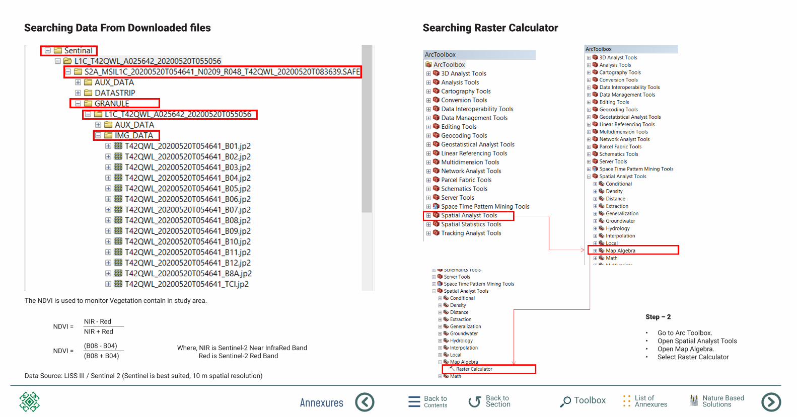
Annexures Back to Contents
List of Annexures
Back to Section Toolbox Nature Based
Solutions
Searching Data From Downloaded files Searching Raster Calculator
The NDVI is used to monitor Vegetation contain in study area.
Data Source: LISS III / Sentinel-2 (Sentinel is best suited, 10 m spatial resolution)
NIR - Red NIR + Red
Step – 2
• Go to Arc Toolbox.• Open Spatial Analyst Tools• Open Map Algebra.• Select Raster Calculator
NDVI =
Where, NIR is Sentinel-2 Near InfraRed Band Red is Sentinel-2 Red Band
NDVI = (B08 - B04)(B08 + B04)

Annexures Back to Contents
List of Annexures
Back to Section Toolbox Nature Based
Solutions
Raster Calculator ExtractionBuilds and executes a single Map Algebra expression using Python syntax in a calculator-like interface.
float(“T42QXJ_B08.jp2” - “T42QXJ_B04.jp2”) / float(“ T42QXJ_B08.jp2” + “T42QXJ_B04.jp2 “)
Step – 3
• Open Raster Calculator and put the respected file with Commend “float”.
• Extracted the file based on the Study area.
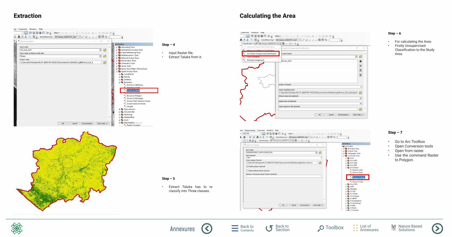
Annexures Back to Contents
List of Annexures
Back to Section Toolbox Nature Based
Solutions
Extraction Calculating the Area
Step – 4
• Input Raster file. • Extract Taluka from it.
Step – 6
• For calculating the Area- • Firstly Unsupervised
Classification to the Study Area.
Step – 7
• Go to Arc Toolbox• Open Conversion tools• Open from raster.• Use the command Raster
to Polygon.
Step – 5
• Extract Taluka has to re classify into Three classes.
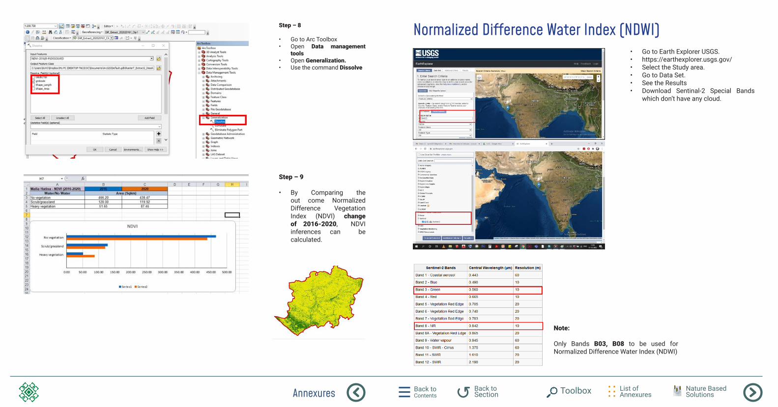
Annexures Back to Contents
List of Annexures
Back to Section Toolbox Nature Based
Solutions
Step – 8
• Go to Arc Toolbox• Open Data management
tools• Open Generalization. • Use the command Dissolve
Step – 9
• By Comparing the out come Normalized Difference Vegetation Index (NDVI) change of 2016-2020, NDVI inferences can be calculated.
Normalized Difference Water Index (NDWI)• Go to Earth Explorer USGS.• https://earthexplorer.usgs.gov/• Select the Study area.• Go to Data Set.• See the Results • Download Sentinal-2 Special Bands
which don’t have any cloud.
Note:
Only Bands B03, B08 to be used for Normalized Difference Water Index (NDWI)

Annexures Back to Contents
List of Annexures
Back to Section Toolbox Nature Based
Solutions
Searching Data From Downloaded files Searching Raster Calculator
An algorithm to estimate the water turbidity using remote sensing data specifically for ponds and inland waters, and it can be estimated as follows:
Data Source: LISS III / Sentinel-2 (Sentinel is best suited, 10 m spatial resolution)
Green − NIR Green + NIR
Step – 2
• Go to Arc Toolbox.• Open Spatial Analyst Tools• Open Map Algebra.• Select Raster Calculator
NDWI =
Where, NIR is Sentinel-2 Near InfraRed Band Red is Sentinel-2 Red Band
NDWI = (B03 - B08)(B03 + B08)

Annexures Back to Contents
List of Annexures
Back to Section Toolbox Nature Based
Solutions
Raster Calculator ExtractionBuilds and executes a single Map Algebra expression using Python syntax in a calculator-like interface.
float(“T42QXJ_B03jp3” - “T42QXJ_B08.jp2”) / float(“ T42QXJ_B03.jp2” + “T42QXJ_B08.jp2 “)
Step – 3
• Open Raster Calculator and put the respected file with Commend “float”.
• Extracted the file based on the Study area.
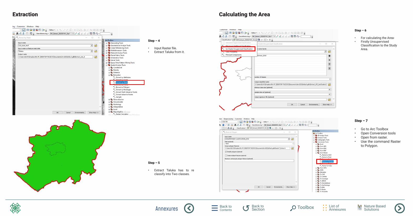
Annexures Back to Contents
List of Annexures
Back to Section Toolbox Nature Based
Solutions
Extraction Calculating the Area
Step – 4
• Input Raster file. • Extract Taluka from it.
Step – 6
• For calculating the Area- • Firstly Unsupervised
Classification to the Study Area.
Step – 7
• Go to Arc Toolbox• Open Conversion tools• Open from raster.• Use the command Raster
to Polygon.
Step – 5
• Extract Taluka has to re classify into Two classes.
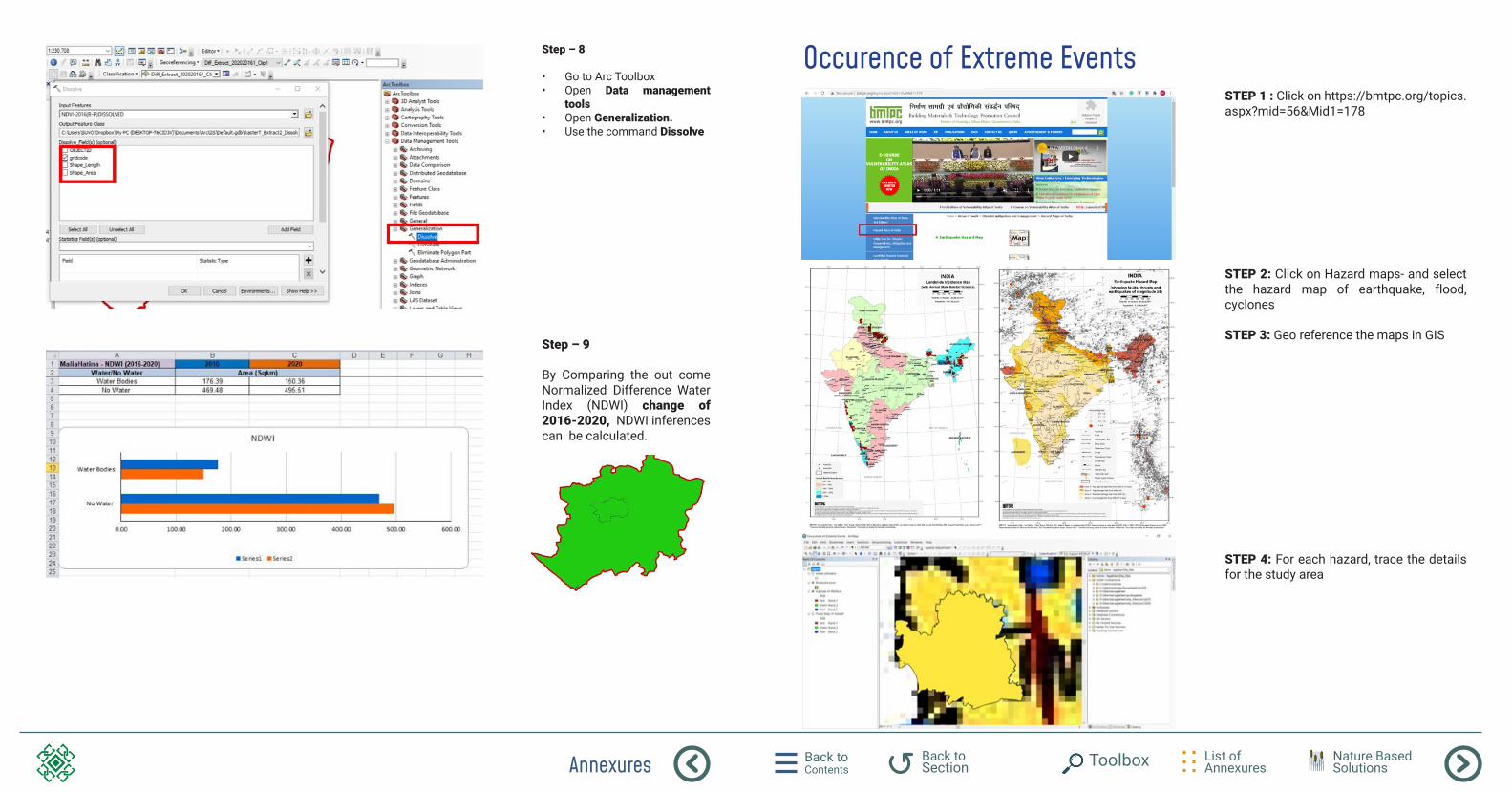
Annexures Back to Contents
List of Annexures
Back to Section Toolbox Nature Based
Solutions
Step – 8
• Go to Arc Toolbox• Open Data management
tools• Open Generalization. • Use the command Dissolve
Step – 9
By Comparing the out come Normalized Difference Water Index (NDWI) change of 2016-2020, NDWI inferences can be calculated.
Occurence of Extreme EventsSTEP 1 : Click on https://bmtpc.org/topics.aspx?mid=56&Mid1=178
STEP 2: Click on Hazard maps- and select the hazard map of earthquake, flood, cyclones
STEP 3: Geo reference the maps in GIS
STEP 4: For each hazard, trace the details for the study area
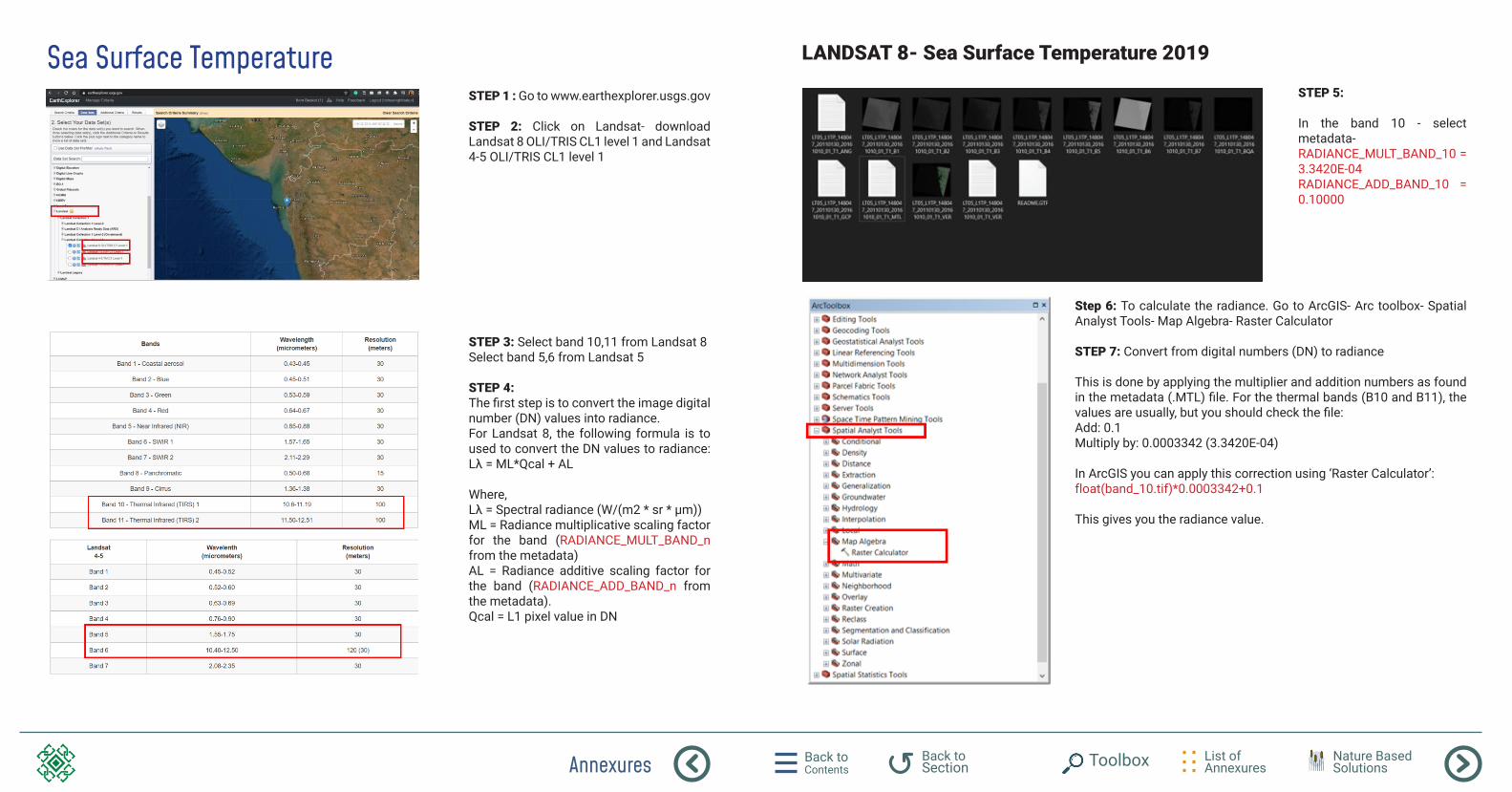
Annexures Back to Contents
List of Annexures
Back to Section Toolbox Nature Based
Solutions
Sea Surface TemperatureSTEP 1 : Go to www.earthexplorer.usgs.gov
STEP 2: Click on Landsat- download Landsat 8 OLI/TRIS CL1 level 1 and Landsat 4-5 OLI/TRIS CL1 level 1
STEP 3: Select band 10,11 from Landsat 8Select band 5,6 from Landsat 5
STEP 4: The first step is to convert the image digital number (DN) values into radiance.For Landsat 8, the following formula is to used to convert the DN values to radiance: Lλ = ML*Qcal + AL
Where,Lλ = Spectral radiance (W/(m2 * sr * μm))ML = Radiance multiplicative scaling factor for the band (RADIANCE_MULT_BAND_n from the metadata) AL = Radiance additive scaling factor for the band (RADIANCE_ADD_BAND_n from the metadata). Qcal = L1 pixel value in DN
LANDSAT 8- Sea Surface Temperature 2019
STEP 5:
In the band 10 - select metadata- RADIANCE_MULT_BAND_10 = 3.3420E-04RADIANCE_ADD_BAND_10 = 0.10000
Step 6: To calculate the radiance. Go to ArcGIS- Arc toolbox- Spatial Analyst Tools- Map Algebra- Raster Calculator
STEP 7: Convert from digital numbers (DN) to radiance
This is done by applying the multiplier and addition numbers as found in the metadata (.MTL) file. For the thermal bands (B10 and B11), the values are usually, but you should check the file:Add: 0.1Multiply by: 0.0003342 (3.3420E-04)
In ArcGIS you can apply this correction using ‘Raster Calculator’:float(band_10.tif)*0.0003342+0.1
This gives you the radiance value.
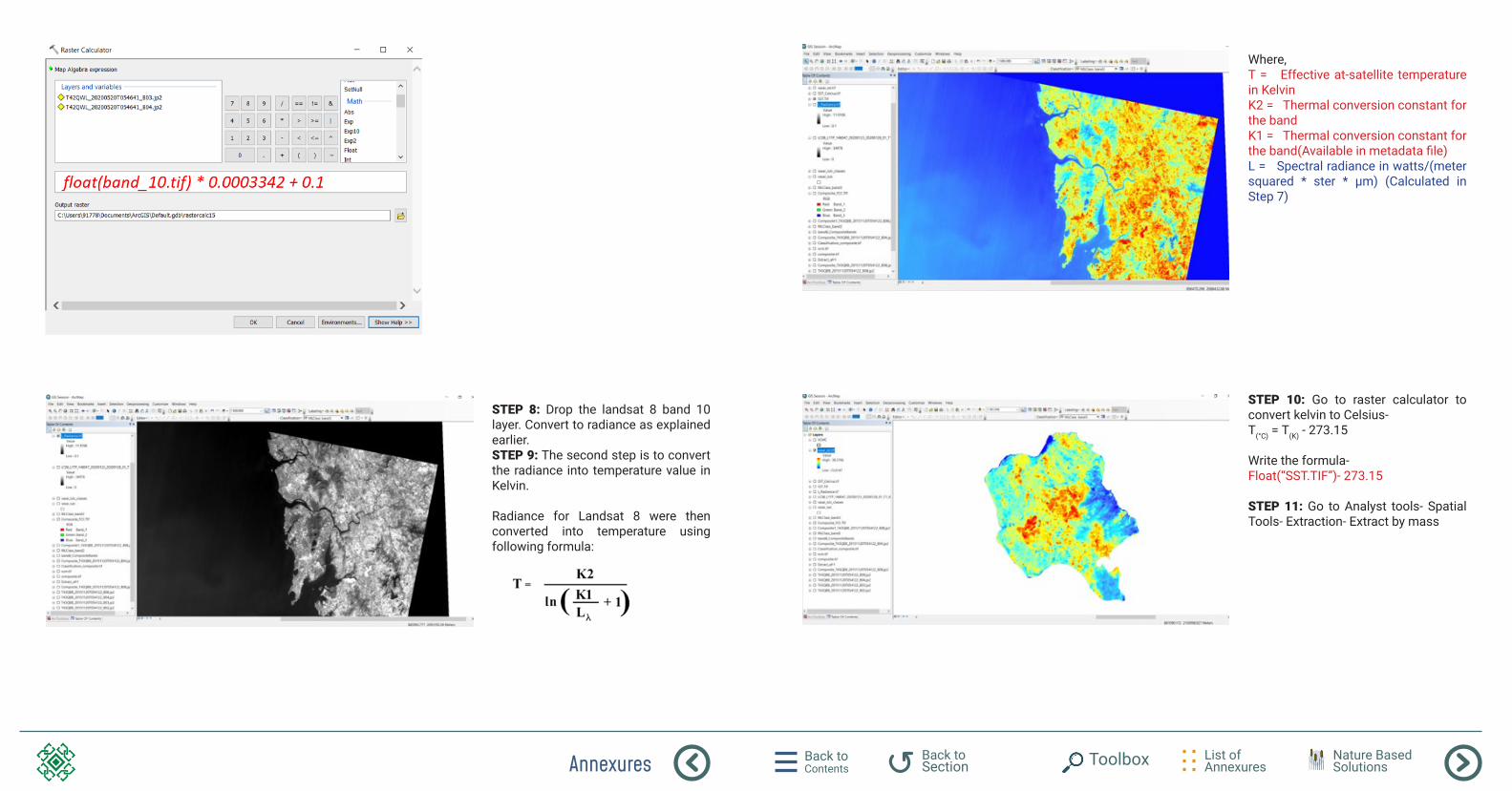
Annexures Back to Contents
List of Annexures
Back to Section Toolbox Nature Based
Solutions
STEP 8: Drop the landsat 8 band 10 layer. Convert to radiance as explained earlier.STEP 9: The second step is to convert the radiance into temperature value in Kelvin.
Radiance for Landsat 8 were then converted into temperature using following formula:
Where,T = Effective at-satellite temperature in Kelvin K2 = Thermal conversion constant for the bandK1 = Thermal conversion constant for the band(Available in metadata file)L = Spectral radiance in watts/(meter squared * ster * µm) (Calculated in Step 7)
STEP 10: Go to raster calculator to convert kelvin to Celsius-T(°C) = T(K) - 273.15 Write the formula- Float(“SST.TIF”)- 273.15
STEP 11: Go to Analyst tools- Spatial Tools- Extraction- Extract by mass
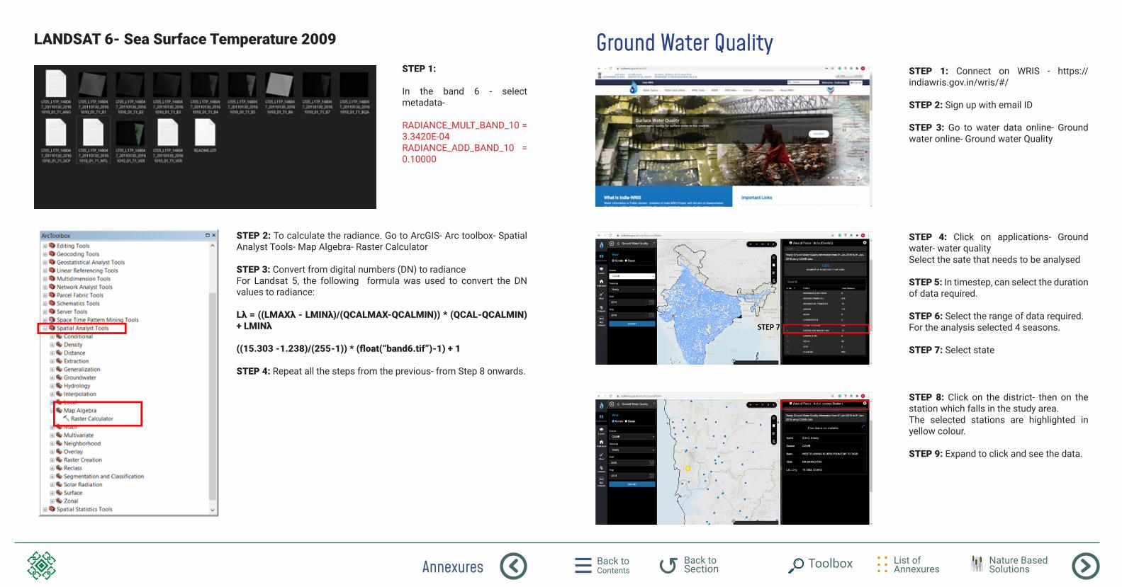
Annexures Back to Contents
List of Annexures
Back to Section Toolbox Nature Based
Solutions
LANDSAT 6- Sea Surface Temperature 2009
STEP 1:
In the band 6 - select metadata-
RADIANCE_MULT_BAND_10 = 3.3420E-04RADIANCE_ADD_BAND_10 = 0.10000
STEP 2: To calculate the radiance. Go to ArcGIS- Arc toolbox- Spatial Analyst Tools- Map Algebra- Raster Calculator
STEP 3: Convert from digital numbers (DN) to radianceFor Landsat 5, the following formula was used to convert the DN values to radiance:
Lλ = ((LMAXλ - LMINλ)/(QCALMAX-QCALMIN)) * (QCAL-QCALMIN) + LMINλ
((15.303 -1.238)/(255-1)) * (float(“band6.tif”)-1) + 1
STEP 4: Repeat all the steps from the previous- from Step 8 onwards.
Ground Water QualitySTEP 1: Connect on WRIS - https://indiawris.gov.in/wris/#/
STEP 2: Sign up with email ID
STEP 3: Go to water data online- Ground water online- Ground water Quality
STEP 4: Click on applications- Ground water- water qualitySelect the sate that needs to be analysed
STEP 5: In timestep, can select the duration of data required.
STEP 6: Select the range of data required.For the analysis selected 4 seasons.
STEP 7: Select state
STEP 8: Click on the district- then on the station which falls in the study area. The selected stations are highlighted in yellow colour.
STEP 9: Expand to click and see the data.
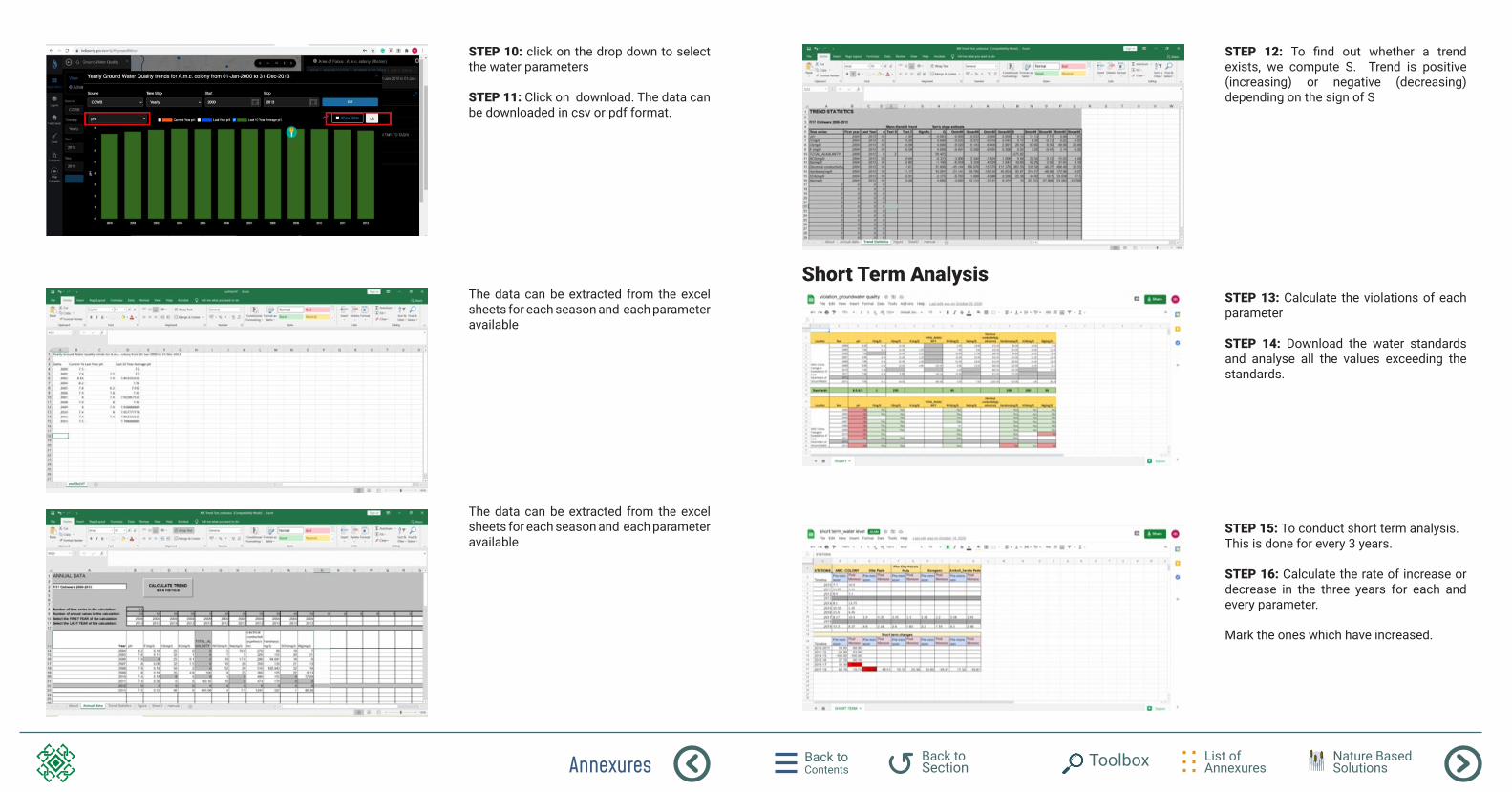
Annexures Back to Contents
List of Annexures
Back to Section Toolbox Nature Based
Solutions
STEP 10: click on the drop down to select the water parameters
STEP 11: Click on download. The data can be downloaded in csv or pdf format.
STEP 12: To find out whether a trend exists, we compute S. Trend is positive (increasing) or negative (decreasing) depending on the sign of S
The data can be extracted from the excel sheets for each season and each parameter available
STEP 13: Calculate the violations of each parameter
STEP 14: Download the water standards and analyse all the values exceeding the standards.
The data can be extracted from the excel sheets for each season and each parameter available
STEP 15: To conduct short term analysis.This is done for every 3 years.
STEP 16: Calculate the rate of increase or decrease in the three years for each and every parameter.
Mark the ones which have increased.
Short Term Analysis
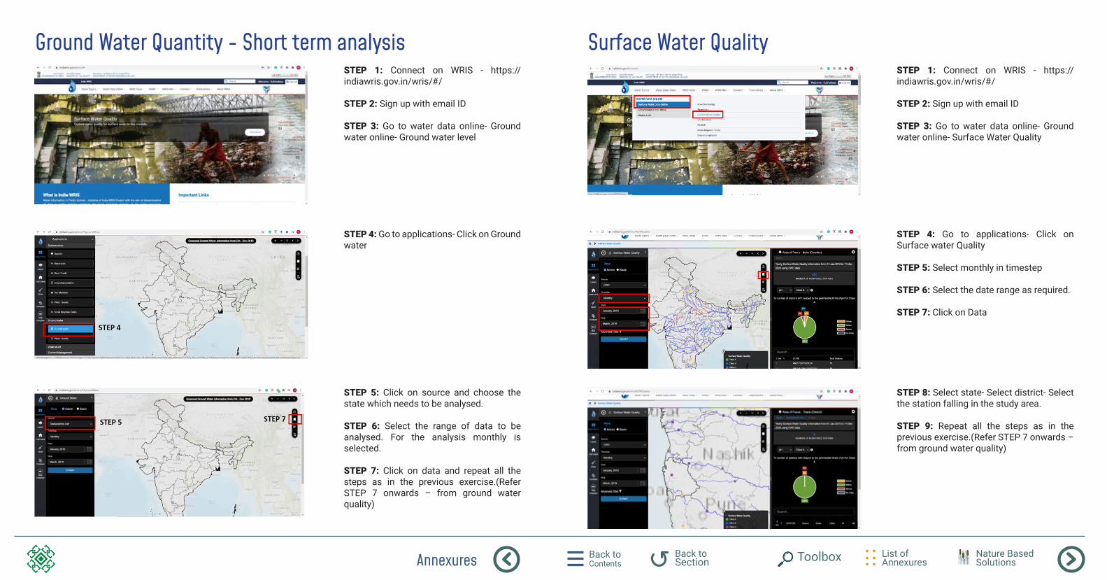
Annexures Back to Contents
List of Annexures
Back to Section Toolbox Nature Based
Solutions
Ground Water Quantity - Short term analysis Surface Water QualitySTEP 1: Connect on WRIS - https://indiawris.gov.in/wris/#/
STEP 2: Sign up with email ID
STEP 3: Go to water data online- Ground water online- Ground water level
STEP 1: Connect on WRIS - https://indiawris.gov.in/wris/#/
STEP 2: Sign up with email ID
STEP 3: Go to water data online- Ground water online- Surface Water Quality
STEP 4: Go to applications- Click on Ground water
STEP 4: Go to applications- Click on Surface water Quality
STEP 5: Select monthly in timestep
STEP 6: Select the date range as required.
STEP 7: Click on Data
STEP 5: Click on source and choose the state which needs to be analysed.
STEP 6: Select the range of data to be analysed. For the analysis monthly is selected.
STEP 7: Click on data and repeat all the steps as in the previous exercise.(Refer STEP 7 onwards – from ground water quality)
STEP 8: Select state- Select district- Select the station falling in the study area.
STEP 9: Repeat all the steps as in the previous exercise.(Refer STEP 7 onwards – from ground water quality)