arX

iv:a

stro

-ph/

0506

736v

1 2

9 Ju

n 20

05Mon. Not. R. Astron. Soc. 000, 1–12 (2005) Printed 5 February 2008 (MN LATEX style file v2.2)

Effects of clumping on temperature I: externally heated

clouds

S. D. Doty1, R. A. Metzler1,2, M. L. Palotti1,21Department of Physics and Astronomy, Denison University, Granville, OH 43023, USA2Department of Physics, University of Wisconsin-Madison, Madison, WI 53706-1390, USA

Accepted ; Received in original form

ABSTRACT

We present a study of radiative transfer in dusty, clumpy star-forming regions. Aseries of self-consistent, three-dimensional, continuum radiative transfer models areconstructed for a grid of models parameterized by central luminosity, filling factor,clump radius, and face-averaged optical depth. The temperature distribution withinthe clouds is studied as a function of this parameterization. Among our results, wefind that: (a) the effective optical depth in clumpy regions is less than in equivalenthomogeneous regions of the same average optical depth, leading to a deeper pene-tration of heating radiation in clumpy clouds, and temperatures higher by over 60per cent; (b)penetration of radiation is driven by the fraction of open sky (FOS) –which is a measure of the fraction of solid angle along which no clumps exist; (c) FOSincreases as clump radius increases and as filling factor decreases; (d) for values ofFOS > 0.6 − 0.8 the sky is sufficiently “open” that the temperature distribution isrelatively insensitive to FOS; (e) the physical process by which radiation penetrates ispreferentially through streaming of radiation between clumps as opposed to diffusionthrough clumps; (f) filling factor always dominates the determination of the tempera-ture distribution for large optical depths, and for small clump radii at smaller opticaldepths; (g) at lower face-averaged optical depths, the temperature distribution is mostsensitive to filling factors of 1 - 10 per cent, in accordance with many observations; (h)direct shadowing by clumps can be important for distances approximately one clumpradius behind a clump.

Key words: stars: formation – infrared: stars – ISM: clouds.

1 INTRODUCTION

An understanding of the star formation process requires anunderstanding of the underlying density distribution in starforming regions. In a direct sense, knowledge of the densitydistribution can help distinguish between different potentialdynamical scenarios for energy injection, collapse, fragmen-tation, and outflow. In a more indirect sense, the densitydistribution significantly affects our ability to infer sourceproperties through its influence on thermal balance, chem-istry, local emission, and the processing of radiation (radia-tive transfer) between the emitting region and the observer.

The density distribution is important for the dust aswell as the gas. In particular, the dust forms the domi-nant source of opacity to visible and infrared (IR) radia-tion, and is the dominant source of IR continuum radiation.Perhaps more importantly, the dust dominates thermal bal-ance by direct interaction with the radiation field (van deHulst 1949), and through collisions with the gas (Greenberg1971; Goldreich & Kwan 1974). As the problems of ther-

mal balance and radiative transfer are non-local, non-linearfeedback problems, comparison of detailed models with ob-servations remain the best choice of reliably inferring thesource properties.

Source geometry is a significant problem in modelingstar-forming regions. While it is normal to assume some ge-ometric symmetry, such restrictions are generally not realis-tic. In particular, a wealth of observations (e.g. Migenes etal. 1989; Dickman et al. 1990; Falgarone et al. 1991; Cesaroniet al. 1991; Marscher et al. 1993; Zhou et al. 1994; Plumeet al. 1997; Shepherd et al. 1997) show that and fragmenta-tion (see also Goldsmith 1996; Tauber 1996 and referencestherein). This is supported by dynamical models (e.g. Tru-elove et al. 1998; Marinho & Lepine 2000; Klapp & Sigalotti1998; Klessen 1997) which naturally produce clumpy andfragmented structures.

Previous work on radiative transfer in dusty, clumpyenvironments has been undertaken (e.g. Hegmann & Kegel2003; Witt & Gordon 1996; Varosi & Dwek 1999; Boisse1990). However, much of the previous work has concentrated

c© 2005 RAS

2 S. D. Doty et al.

on scattering (e.g. with application to reflection nebulae),the detailed methods of solution, and/or some of the fun-damental results such as ability of radiation to penetrate toapparently high optical depths. In this paper we use a 3-Dmonte carlo radiative transfer model to extend the previouswork to a wider and different range of physical conditions.In particular, we construct a large grid of models in an ef-fort to better delineate and understand the effects of clumpymedia on radiative transfer. By controlling and varying theparameterization of the source, we attempt to disentanglesome of the underlying physical causes of these effects.

In section two we describe the model. We discuss thegeneral effects of clumping in section three. In section four,we introduce the “fraction of open sky” (FOS), and discussthe effects of number density, FOS, optical depth, filling fac-tor, and clump size on the dust temperature distribution. Wediscuss the effects of shadowing in section five. Finally, wedraw conclusions in section six.

2 MODEL

2.1 Monte carlo model and invariant parameters

We have constructed detailed, self-consistent, three-dimensional radiative transfer models through dust. Themodel utilizes a monte-carlo approach, combined with anapproximate lambda iteration to ensure true convergenceeven at high optical depths. The model has been testedagainst existing 1-D (Egan, Leung, & Spagna 1988) and 2-D (Spagna, Leung, & Egan 1991) codes, and in modeling a3-D source (Doty et al. 2005) with good success. Since thepresent study concentrates upon opaque molecular cloudswhere far-infrared radiaton should dominate both for exter-nal heating and emission, we ignore the effects of scattering.Test cases in both one- and multiple-dimensions show thatscattering plays only a very small role on the temperaturedistribution within the majority of the sources.

Based upon the input parameters discussed below, wesolve for the dust temperature and radiation field at eachpoint in the model cloud. The computational volume istaken to be cubical of size 1 pc. Each model utilized an81×81×81 cell grid, yielding a typical resolution of ∼ 3×1016

cm. The region is taken to be a two-phase medium consist-ing of high density clumps, and a low density inter-clumpmedium. The clump/inter-clump density ratio is taken to benclump/ninter−clump = 100 from observations (e.g. Bergin etal. 1996). The external radiation field is taken from inter-stellar radiation field (ISRF) compiled by Mathis, Mezger,& Panagia (1983). Finally, we adopt the dust opacities incolumn 5 of Table 1 of Ossenkopf & Henning (1994), whichhave been successful at fitting observations of both high-mass (e.g., van der Tak et al. 1999, 2000) and low-mass(e.g., Evans et al. 2001) regions of star formation.

2.2 Model parameters

We adopt a uniformly distributed interclump mediuminterspersed with higher density clumps havingnclump/ninter−clump = 100. The clumps are randomlydistributed within the computational volume. The numberof clumps, and the densities of the clumps and interclump

Table 1. Model input parameters

Number L∗ f rc τ(L⊙) (pc)

1 0 0.01 0.025 102 3 0.1 0.05 1003 300 0.3 0.1 n/a

medium depend upon the filling factor (f), the clumpradius (rc), and the face-averaged optical depth (τ).

The filling factor specifies the fraction of the volume athigh density. It is given by f ≡ Vclumps/Vtotal. We adoptfilling factors of f = 0.01, 0.1, and 0.3 in accord with obser-vations (e.g. Snell et al. 1984; Bergin et al. 1996; Carr 1987).When all other parameters are kept fixed, a higher f cor-responds to a larger number of clumps, and a more nearlycontinuous dust distribution. Furthermore, due to opticaldepth constraint (see τ below), a larger f also correspondsto clumps and interclump medium of lower density.

We make the simplifying assumption that all non-overlapping clumps are spheres of radius rc. We chooserc = 0.025 pc, 0.05 pc, and 0.1 pc in accord with obser-vations (e.g. Carr 1987; Howe et al. 1993). Again, the con-straint on the optical depth implies that larger clump radiiyield smaller densities within the clumps.

The dust number densities are normalized by averagingthe optical depth over one entire (81×81) face of the compu-tational cube. We call this the face-averaged optical depth,and denote it by τ . This was done to simulate the opticaldepth / column density that might be inferred by a verylarge beam, although it has the same effect as normalizingto the total cloud mass. The face-averaged optical depth istaken to be τ = 10, and 100, in keeping with observationsfrom extinction studies (Lada, Alves, & Lada 1999).

Finally, the models are specified by the strength ofthe internal radiation field, specified by the luminosity ofthe central source, L∗. We have constructed a grid havingL∗ = 0L⊙, 3L⊙, and 300L⊙ to represent a starless core, alow-luminosity central object, and a high-luminosity centralobject, respectively. However, in this paper, we restrict ourreport to the starless cores only (L∗ = 0). The others willbe presented in a forthcoming paper.

The ranges of parameters specified above led to a gridof 54 models. Each model is numbered by a four-digit integerILIfIrcIτ . The integers, and their corresponding values aregiven in Table 1 for reference. As an example, model 1221has L∗ = 0, f = 0.01, rc = 0.025 pc, and τ = 10.

2.3 Invariance with clump and photon

randomization

One concern with “random” clump distribution and monte-carlo simulation is the reproducibility of results with differ-ent realizations of the clump distribution (i.e. different ini-tial seeds in the clump generation), and different photon raypaths. As a test, we have considered 9 different initial seedsfor the clump distributions and photon paths respectively.

To quantify the temperature distribution, we calculatea spherical average temperature, given by

c© 2005 RAS, MNRAS 000, 1–12

Clumping in star-forming regions 3

-0.1 0 0.1 0.2 0.3 0.4 0.5 0.6 0.7 0.8 0.9 1 1.15

6

7

8

9

10

11

12

1K

8 photon

20 photon

50 photon

100 photon

200 photon

Figure 1. Spherical average temperature as a function of radialposition for varying number of initial photons (ray pays) per cellface for the same random clumpy model.

〈T (r)〉 =

N∑i

Tini/

N∑i

ni. (1)

Here N is the number of cells a distance between r andr + ∆r from the center, where ∆r is the size of a single cell,and Ti and ni are the temperature and density of the cellsrespectively. In keeping with the viewpoint that the highdensity clumps mostly affect the local radiation field, whilethe the low density medium best probes the radiation field,the average temperature is taken only over the low-densitycells.

The differences in 〈T (r)〉 between different clump dis-tribution realizations are always much less than 1K, andare on average less than 0.1K. Based upon this (and directcomparison of later analyses) the specific realization of thedensity distribution does not affect our conclusions.

Likewise, we have modified the number and distributionof incident photons to test for sufficient monte carlo cover-age. The effect of number of photons on for 〈T (r)〉 is shownin Fig. 1. To be conservative, we adopt 100 photons per cellface, at which point differences are less than 0.05K (1 percent).

Similarly, varying the random distribution of photonpaths causes deviations of < 0.1K, confirming that the cov-erage of the cells by ray-paths is sufficient to concentrate onthe consequences of clumping.

3 CLUMPING: GENERAL

In this section we briefly discuss the general effects of clump-ing on the dust temperature distribution. For clarity, wedirectly compare a clumpy, externally heated (L∗ = 0), low-density (f = 0.1), opaque (τ = 10), model having smallclumps (rc = 0.05 pc) to one with a uniform density distri-

-1 -0.5 0 0.5 14

6

8

10

12

14

16 x-axis4

6

8

10

12

14

16 y-axis4

6

8

10

12

14

16 z-axis clumpsno clumps

Figure 2. The temperature as a function of position withina clumpy (solid line) and non-clumpy (dotted line) low opticaldepth (τ = 10) model, along the three principal axes.

0 0.1 0.2 0.3 0.4 0.5 0.6 0.7 0.8 0.9 1 1.1

0.5

0.55

0.6

0.65

0.7

0.75

Figure 3. The fractional difference in 〈T (r)〉 between a clumpyand non-clumpy externally heated (L∗ = 0), low optical depth(τ = 10) model.

bution and the same optical depth and external heat source,so we can directly measure the effects of clumping. We havedone similar comparisons for all other models, with similarresults.

The temperature distributions along the principal axesfor a representative clumpy and equivalent homogeneousmodel are shown in Fig. 2. To quantify the differences be-tween the temperature distributions, in Fig. 3 we plot the

c© 2005 RAS, MNRAS 000, 1–12

4 S. D. Doty et al.

-1 -0.5 0 0.5 14

6

8

10

12

14

16 x-axis4

6

8

10

12

14

16 y-axis4

6

8

10

12

14

16 z-axis Tlog(n)

-1 -0.5 0 0.5 1

-9

-8

-7

-6

-5

-9

-8

-7

-6

-5

-9

-8

-7

-6

-5

Figure 4. Distribution of temperature (solid lines, left-handscale) and density (dotted lines, right-hand scale) for cuts alongthe x-, y-, and z-axes of model 1221. Other models yield qualita-tively identical results.

fractional difference in 〈T (r)〉 between these two represen-tative models. From these two figures, it is immediately ob-vious that the inclusion of clumps – even for the same τ –changes the temperature structure significantly. In particu-lar, the clumpy model experiences higher temperatures byup to 50 per cent toward the center, and up to ∼ 65 per centat intermediate radii. As a result, we conclude that clump-ing itself affects the temperature distribution, even when theaverage source mass or column density is held constant.

This result confirms the previous finding of others (e.g.Hegmann & Kegel 2003; Witt & Gordon 1996; Varosi &Dwek 1999) that the effective optical depth in a clumpymedium is less than the homogeneous value. It also suggeststhat it is important to understand the way in which the pa-rameterization of the clumpy density distribution can affectthe dust temperature. We address these individually below.

4 CLUMPING: EFFECTS OF PARAMETERS

4.1 Number density

In Fig. 4 we plot the temperature (solid lines, left hand scale)and dust number density (dotted lines, right hand scale) forcuts along the x-, y-, and z-axes. The clumps are signifiedby the higher density regions. As can be seen, the clumpsare resolved, and appear to be of different sizes as the axesdo not penetrate all clumps along a diameter. The “wiggles”and ∼ 0.1−0.2 K deviations in the temperature distributionare not simply indicative of the uncertainties in the montecarlo calculation (see previous results, and Fig. 2). Instead,the majority are dominated by local differences in radiationfield due to different amounts of blocking of radiation by thesurrounding clumps (see Sect. 5 for more discussion).

As can be seen in Fig. 4, the dust temperature is lower

Figure 5. Temperature as a function of angle-averaged atten-uation (〈e−τ 〉) for three distances from source center (Rout/3,Rout/2, and 2Rout/3). The solid symbols correspond to the tem-perature in the low density interclump medium, while the opensymbols correspond to the high density clumps. This result is formodel 1221. Other models are qualitatively identical.

within the high density clumps than it is within the lower-density interclump medium. Since the total emission bygrains of absorption efficiency 〈Qabsπa2〉 ∝ νβ goes as T 4+β,one might expect a factor of 100 increase in density to leadto a decrease in temperature by a factor 1001/(4+β). Giventhat β ∼ 1.8 in the FIR for the adopted dust model, this isa decrease by a factor of ∼ 2.2. For comparison, the averagedecrease within the clumps is a factor of 1.5 with a great-est decrease a factor of 1.6. This is due to the fact that theclump centers can be warmed by absorbing the radiationemitted from the clump edges, in effect trapping radiationwithin the clumps (similar to the opaque centers of centrallyheated envelopes, Doty & Leung 1994).

Of even further interest is the fact that while the tem-perature decreases coincide with the locations of the clumps,the shape of the temperature profiles do not match the steep-ness of the clump/interclump interfaces. This further sug-gests that radiative transfer effects play a role.

4.2 Effective optical depth

Previous authors (e.g., Hegmann & Kegel 2003; Witt & Gor-don 1996; Varosi & Dwek 1999) identified the effective opti-cal depth (− ln[LAT/L∗]), where LAT is the attenuated fluxintegrated over all solid angles and L∗ is the unattenuatedflux integrated over all solid angles or equivalently the aver-age attenuation (〈e−τ 〉 ≡

∫e−τdΩ/

∫dΩ) as a key measure

of the ability of radiation to penetrate. This is reasonable,as the fewer photons penetrating leads to cooler dust, whichis confirmed in Fig. 5, where we plot the dust temperatureat three different positions along the x-axis as a function of〈e−τ 〉 for model 1221.

One question is left unanswered – the physical process

c© 2005 RAS, MNRAS 000, 1–12

Clumping in star-forming regions 5

driving the angle-averaged attenuation must be identified.There are two possibilities: (1) the ability of radiation topenetrate is dominated by general attenuation by multipleclumps along a given line of sight and attenuation by thelow-density interclump medium; or (2) the radiation streamsprimarily through the “holes” between clumps. We considerthese two possibilities in the following subsection.

4.3 Optical depth and fraction of open sky

4.3.1 Motivation and definition of 〈τ 〉 and FOS

In order to answer the question of whether and howmuch geometry matters in determining the local temper-ature/radiation field, we consider two limiting cases. Theseare a measure with limited geometry information, the angle-averaged optical depth (〈τ 〉), and a measure which is dom-inated by geometry information, the fraction of open sky(FOS). We consider these seperately below.

If the radiation generally diffuses and is attenuated bymultiple clumps or the low-density interclump medium, wemight expect to find a dependence of source properties onthe optical depth averaged over all directions. As a result,we define the angle-averaged optical depth to be

〈τ 〉 ≡

∫τ (Ω)dΩ/

∫dΩ. (2)

On the other hand, if the radiation penetrates mainlyby streaming through holes between clumps, then the sourceproperties should depend more significantly on the fractionof the sky that is uncovered by the clumps. Consequently,we also define the fraction of open sky, FOS, to be

FOS ≡

∫qdΩ/

∫dΩ. (3)

Here q = 1 if there is no clump along the given line of sight(i.e. if the sky is “open” in that direction), while q = 0 ifthere is a clump along the given line of sight (i.e. if the skyis “closed” in that direction). Consequently, FOS=1 impliesan open sky with no clumps, while FOS=0 corresponds toa closed sky where all lines of sight are blocked by clumps.

As a first test of the effect of FOS on temperature, inFig. 6 we plot the temperature (solid lines, left-hand scale)and FOS (dotted lines, right-hand scale) for cuts along thex-, y-, and z-axes, similar to Fig. 4. There is a strong cor-relation of dust temperature with FOS. Interestingly, theshape of the temperature distribution correlates with FOSto a much higher degree than it anti-correlates with the dustnumber density. This strongly suggests that FOS plays a keyrole, which we test in the following discussion.

4.3.2 Effect of 〈τ 〉 on temperature

To test the role of angle-averaged optical depth, we considerthe dependence of temperature on 〈τ 〉 for a fixed FOS. Inthis way, we can isolate the effects of 〈τ 〉 from FOS. TheFOS value here was chosen to maximize the number of datapoints to provide for the best possible statistics. The re-sulting dependence of temperature on 〈τ 〉 for three differentradial positions is shown in Fig. 7. We note that the cho-sen FOS range is small to make the result independent of

-1 -0.5 0 0.5 14

6

8

10

12

14

16 x-axis4

6

8

10

12

14

16 y-axis4

6

8

10

12

14

16 z-axis TFOS

-1 -0.5 0 0.5 1

0

0.2

0.4

0.6

0.8

0

0.2

0.4

0.6

0.8

0

0.2

0.4

0.6

0.8

Figure 6. Distribution of temperature (solid lines, left-handscale) and FOS (dotted lines, right-hand scale) for cuts along thex-, y-, and z-axes of model 1221. Other models yield qualitativelyidentical results.

9.5

10

10.5

11

11.5

12

0.432pc

8.5

9

9.5 0.309pc

0.1 0.2 0.3 0.46.5

7

7.5

8

8.5 0.185pc

Figure 7. Temperature as a function of angle-averaged opti-cal depth (〈τ〉) for three distances from source center (Rout/3,Rout/2, and 2Rout/3), for a fixed FOS. This result is for model1221. Other models are qualitatively identical.

FOS, though moderate increases in the range lead to similarresults.

There appears to be little correlation of temperaturewith 〈τ 〉 at a given position. We quantify this by fittingthe data distribution at each radial distance with a best-fit

c© 2005 RAS, MNRAS 000, 1–12

6 S. D. Doty et al.

0 0.1 0.2 0.3 0.4 0.5 0.6 0.7 0.8 0.9 1 1.1-5

0

5

10

Figure 8. Slope of the best fit temperature - 〈τ〉 relationshipdivided by the uncertainty in the slope as a function of positionin the source. Notice the small correlation that exists, suggestingthat 〈τ〉 is of only minimal importance in determining the tem-perature distribution. The dotted lines denote θ(〈τ〉) = ±3 (i.e.a 3σ deviation from zero). This result is for model 1221. Othermodels are qualitatively identical.

straight line. To understand the significance of the slope /correlation, we define a correlation parameter,

θ(〈τ 〉) ≡ m(〈τ 〉)/σm(〈τ〉). (4)

Here, m(〈τ 〉) is the slope of the best-fit line relating thetemperature and 〈τ 〉, and σm(〈τ〉) is the uncertainty in thatslope. The results are shown in Fig. 8. We have also includeddashed lines at m = ±3σm(〈τ〉) as a guide.

To best understand the utility of this comparison, con-sider a case for which the temperature and 〈τ 〉 are uncorre-lated. In this case, the fit between them should yield a zeroslope, and thus θ(〈τ 〉) = 0. Likewise, a significant correlationshould yield θ > 3 (i.e., a 3σ result). The results in Fig. 8are much more consistent with θ(〈τ 〉) = 0 throughout muchof the cloud, and only reach θ(〈τ 〉) = 3 for r > 0.7Rout.Consequently, we conclude that there may exist only a weakcorrelation between the dust temperature and 〈τ 〉.

4.3.3 Effect of FOS on temperature

In a similar manner to 〈τ 〉, we consider the effect of FOSon temperature. In this case, we keep 〈τ 〉 fixed. In analogywith before, 〈τ 〉 was chosen to maximize the number of datapoints to ensure the best possible statistics. The resultingdependence of temperature on FOS for three different radialpositions is shown in Fig. 9.

Inspection of Fig. 9 suggests that there exists some cor-relation of temperature with FOS. In a similar manner to〈τ 〉, we quantify this by fitting the data distribution at eachradial distance with a best-fit straight line. We again definea correlation parameter,

8.59

9.510

10.511

11.512

12.50.432pc

8

8.5

9

9.5

100.309pc

0.3 0.4 0.5 0.6 0.76

6.5

7

7.5

8

8.5

9

0.185pc

Figure 9. Temperature as a function of fraction of open sky(FOS) for three distances from source center (Rout/3, Rout/2,and 2Rout/3), for a fixed 〈τ〉. This result is for model 1221. Othermodels are qualitatively identical.

0 0.1 0.2 0.3 0.4 0.5 0.6 0.7 0.8 0.9 1 1.1-5

0

5

10

15

20

Figure 10. Slope of the best fit temperature - FOS relationshipdivided by the uncertainty in the slope as a function of positionin the source. Notice the large correlation that exists, suggestingthat FOS has significance in determining the temperature distri-bution. This result is for model 1221. Other models are qualita-tively identical.

c© 2005 RAS, MNRAS 000, 1–12

Clumping in star-forming regions 7

Table 2. Temperature dependence on FOS and 〈τ〉. See text fordiscussion.

Model xmax xcut(〈τ〉) xcut(FOS) θ(FOS)/θ(〈τ〉)

1111 0.00 0.64 0.77 n/a1121 0.00 0.47 0.84 n/a1131 0.00 0.84 0.64 n/a1211 0.94 0.64 0.30 2.11221 0.55 0.69 0.27 ∞1231 0.00 0.74 0.99 n/a1311 0.99 0.10 0.30 1.41321 0.97 0.97 0.22 4.11331 0.86 0.94 0.92 n/a

1112 0.00 0.64 0.94 n/a1122 0.00 0.49 0.94 n/a1132 0.00 0.82 0.84 n/a1212 0.94 0.74 0.64 1.01222 0.55 n/a 0.99 n/a1232 0.00 0.79 n/a n/a1312 0.99 0.07 0.59 0.81322 0.97 0.97 0.30 1.81332 0.86 0.94 n/a n/a

θ(FOS) ≡ m(FOS)/σm(FOS). (5)

Here, m(FOS) is the slope of the best-fit line relating thetemperature and FOS, and σm(FOS) is the uncertainty inthat slope. The results are show in Fig. 10. We have alsoincluded dashed lines at ±3σm(FOS) as a guide.

The results in Fig. 10 are generally not consistent withθ(FOS) = 0, and lie at or above θ(FOS) = 3 for a gooddeal of the cloud (r > 0.25Rout). Consequently, we can saythat there exists a significant correlation between the dusttemperature and FOS.

Finally, it is encouraging to note that the correlationbetween temperature and FOS is positive. This is expected,since a higher FOS leads to more direct heating by the ex-ternal radiation field, and is evidenced by m(FOS) > 0.

4.3.4 Extension and interpretation of 〈τ 〉, FOS results

We can extend the discussion of FOS and 〈τ 〉 to the remain-der of our family of models. The results are summarized inTable 2. In this table, we specify the fractional radial posi-tion from cloud center as x ≡ r/Rout.

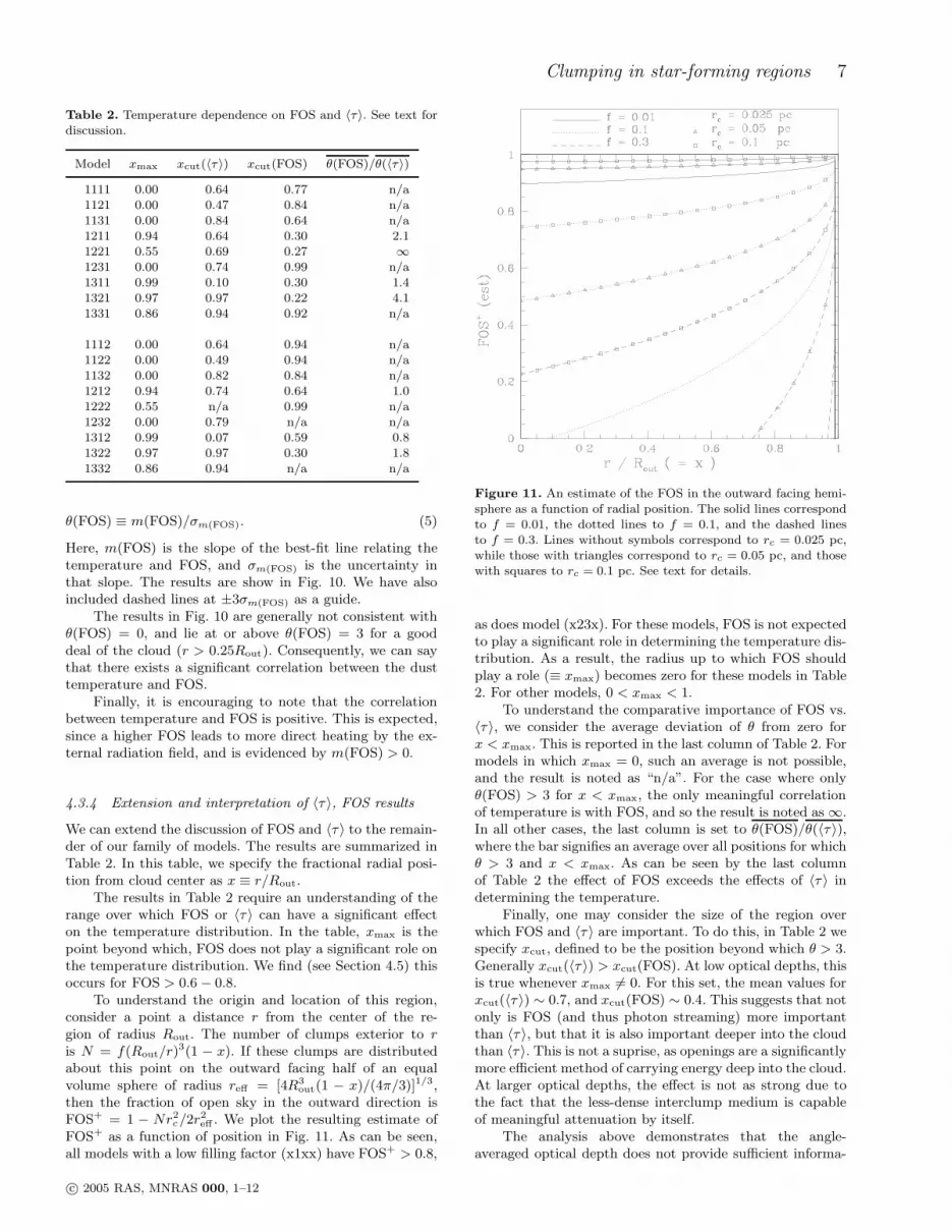
The results in Table 2 require an understanding of therange over which FOS or 〈τ 〉 can have a significant effecton the temperature distribution. In the table, xmax is thepoint beyond which, FOS does not play a significant role onthe temperature distribution. We find (see Section 4.5) thisoccurs for FOS > 0.6 − 0.8.

To understand the origin and location of this region,consider a point a distance r from the center of the re-gion of radius Rout. The number of clumps exterior to ris N = f(Rout/r)3(1 − x). If these clumps are distributedabout this point on the outward facing half of an equalvolume sphere of radius reff = [4R3

out(1 − x)/(4π/3)]1/3,then the fraction of open sky in the outward direction isFOS+ = 1 − Nr2

c/2r2eff . We plot the resulting estimate of

FOS+ as a function of position in Fig. 11. As can be seen,all models with a low filling factor (x1xx) have FOS+ > 0.8,

Figure 11. An estimate of the FOS in the outward facing hemi-sphere as a function of radial position. The solid lines correspondto f = 0.01, the dotted lines to f = 0.1, and the dashed linesto f = 0.3. Lines without symbols correspond to rc = 0.025 pc,while those with triangles correspond to rc = 0.05 pc, and thosewith squares to rc = 0.1 pc. See text for details.

as does model (x23x). For these models, FOS is not expectedto play a significant role in determining the temperature dis-tribution. As a result, the radius up to which FOS shouldplay a role (≡ xmax) becomes zero for these models in Table2. For other models, 0 < xmax < 1.

To understand the comparative importance of FOS vs.〈τ 〉, we consider the average deviation of θ from zero forx < xmax. This is reported in the last column of Table 2. Formodels in which xmax = 0, such an average is not possible,and the result is noted as “n/a”. For the case where onlyθ(FOS) > 3 for x < xmax, the only meaningful correlationof temperature is with FOS, and so the result is noted as ∞.In all other cases, the last column is set to θ(FOS)/θ(〈τ 〉),where the bar signifies an average over all positions for whichθ > 3 and x < xmax. As can be seen by the last columnof Table 2 the effect of FOS exceeds the effects of 〈τ 〉 indetermining the temperature.

Finally, one may consider the size of the region overwhich FOS and 〈τ 〉 are important. To do this, in Table 2 wespecify xcut, defined to be the position beyond which θ > 3.Generally xcut(〈τ 〉) > xcut(FOS). At low optical depths, thisis true whenever xmax 6= 0. For this set, the mean values forxcut(〈τ 〉) ∼ 0.7, and xcut(FOS) ∼ 0.4. This suggests that notonly is FOS (and thus photon streaming) more importantthan 〈τ 〉, but that it is also important deeper into the cloudthan 〈τ 〉. This is not a suprise, as openings are a significantlymore efficient method of carrying energy deep into the cloud.At larger optical depths, the effect is not as strong due tothe fact that the less-dense interclump medium is capableof meaningful attenuation by itself.

The analysis above demonstrates that the angle-averaged optical depth does not provide sufficient informa-

c© 2005 RAS, MNRAS 000, 1–12

8 S. D. Doty et al.

16.5 17 17.5 180.5

0.55

0.6

0.65

0.7

0.75

0.8

0.85

0.9

0.95

1

f=0.01f=0.1f=0.3

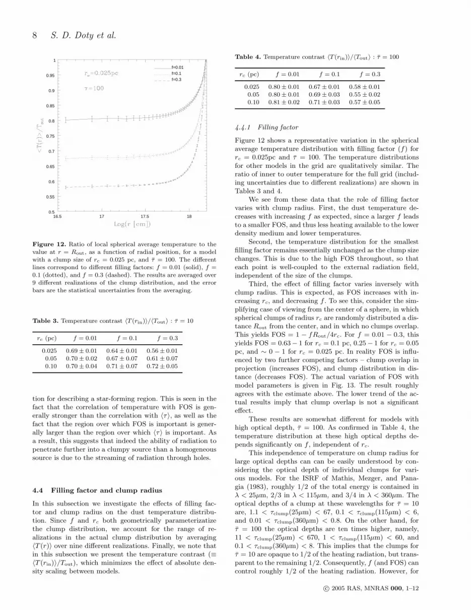
Figure 12. Ratio of local spherical average temperature to thevalue at r = Rout, as a function of radial position, for a modelwith a clump size of rc = 0.025 pc, and τ = 100. The differentlines correspond to different filling factors: f = 0.01 (solid), f =0.1 (dotted), and f = 0.3 (dashed). The results are averaged over9 different realizations of the clump distribution, and the errorbars are the statistical uncertainties from the averaging.

Table 3. Temperature contrast 〈T (rin)〉/〈Tout〉 : τ = 10

rc (pc) f = 0.01 f = 0.1 f = 0.3

0.025 0.69 ± 0.01 0.64 ± 0.01 0.56 ± 0.010.05 0.70 ± 0.02 0.67 ± 0.07 0.61 ± 0.070.10 0.70 ± 0.04 0.71 ± 0.07 0.72 ± 0.05

tion for describing a star-forming region. This is seen in thefact that the correlation of temperature with FOS is gen-erally stronger than the correlation with 〈τ 〉, as well as thefact that the region over which FOS is important is gener-ally larger than the region over which 〈τ 〉 is important. Asa result, this suggests that indeed the ability of radiation topenetrate further into a clumpy source than a homogeneoussource is due to the streaming of radiation through holes.

4.4 Filling factor and clump radius

In this subsection we investigate the effects of filling fac-tor and clump radius on the dust temperature distribu-tion. Since f and rc both geometrically parameterizatizethe clump distribution, we account for the range of re-alizations in the actual clump distribution by averaging〈T (r)〉 over nine different realizations. Finally, we note thatin this subsection we present the temperature contrast (≡〈T (rin)〉/Tout), which minimizes the effect of absolute den-sity scaling between models.

Table 4. Temperature contrast 〈T (rin)〉/〈Tout〉 : τ = 100

rc (pc) f = 0.01 f = 0.1 f = 0.3

0.025 0.80 ± 0.01 0.67 ± 0.01 0.58 ± 0.010.05 0.80 ± 0.01 0.69 ± 0.03 0.55 ± 0.020.10 0.81 ± 0.02 0.71 ± 0.03 0.57 ± 0.05

4.4.1 Filling factor

Figure 12 shows a representative variation in the sphericalaverage temperature distribution with filling factor (f) forrc = 0.025pc and τ = 100. The temperature distributionsfor other models in the grid are qualitatively similar. Theratio of inner to outer temperature for the full grid (includ-ing uncertainties due to different realizations) are shown inTables 3 and 4.

We see from these data that the role of filling factorvaries with clump radius. First, the dust temperature de-creases with increasing f as expected, since a larger f leadsto a smaller FOS, and thus less heating available to the lowerdensity medium and lower temperatures.

Second, the temperature distribution for the smallestfilling factor remains essentially unchanged as the clump sizechanges. This is due to the high FOS throughout, so thateach point is well-coupled to the external radiation field,independent of the size of the clumps.

Third, the effect of filling factor varies inversely withclump radius. This is expected, as FOS increases with in-creasing rc, and decreasing f . To see this, consider the sim-plifying case of viewing from the center of a sphere, in whichspherical clumps of radius rc are randomly distributed a dis-tance Rout from the center, and in which no clumps overlap.This yields FOS = 1 − fRout/4rc. For f = 0.01 − 0.3, thisyields FOS = 0.63− 1 for rc = 0.1 pc, 0.25− 1 for rc = 0.05pc, and ∼ 0 − 1 for rc = 0.025 pc. In reality FOS is influ-enced by two further competing factors – clump overlap inprojection (increases FOS), and clump distribution in dis-tance (decreases FOS). The actual variation of FOS withmodel parameters is given in Fig. 13. The result roughlyagrees with the estimate above. The lower trend of the ac-tual results imply that clump overlap is not a significanteffect.

These results are somewhat different for models withhigh optical depth, τ = 100. As confirmed in Table 4, thetemperature distribution at these high optical depths de-pends significantly on f , independent of rc.

This independence of temperature on clump radius forlarge optical depths can can be easily understood by con-sidering the optical depth of individual clumps for vari-ous models. For the ISRF of Mathis, Mezger, and Pana-gia (1983), roughly 1/2 of the total energy is contained inλ < 25µm, 2/3 in λ < 115µm, and 3/4 in λ < 360µm. Theoptical depths of a clump at these wavelengths for τ = 10are, 1.1 < τclump(25µm) < 67, 0.1 < τclump(115µm) < 6,and 0.01 < τclump(360µm) < 0.8. On the other hand, forτ = 100 the optical depths are ten times higher, namely,11 < τclump(25µm) < 670, 1 < τclump(115µm) < 60, and0.1 < τclump(360µm) < 8. This implies that the clumps forτ = 10 are opaque to 1/2 of the heating radiation, but trans-parent to the remaining 1/2. Consequently, f (and FOS) cancontrol roughly 1/2 of the heating radiation. However, for

c© 2005 RAS, MNRAS 000, 1–12

Clumping in star-forming regions 9

Figure 13. Fraction of open sky at the central point in themodel cloud (FOSc) as a function of filling factor for models1xxx (L∗ = 0). The lines correspond to different clump radii:rc = 0.025 pc (solid), rc = 0.05 pc (dotted), and rc = 0.1 pc(dashed). Note that the results are the same for all optical depths,for a given clump distribution. Results for different realizationsof clump distributions are similar.

τ = 100, the clumps are opaque to 2/3 - 3/4 of the heatingradiation, meaning that f (and FOS) can control a greateramount of the energy that penetrates to a given depth. Asa result, it is not suprising to realize that as the clumps be-come more opaque, filling factor and the ability of radiationto stream between the clumps becomes more important.

4.4.2 Clump radius

Figure 14 shows a representative variation in the sphericalaverage temperature distribution with clump radius (rc) forf = 0.1 and τ = 100. Again, the temperature distributionsin the other models are qualitatively similar, and the tem-perature contrast results are shown in Tables 3 & 4.

We see from these data that the role of clump radiusvaries with filling factor. In comparison to the case of fillingfactor, the smallest clumps yield the lowest temperatures,and the largest clumps the highest temperatures, consistentwith the FOS findings in Fig. 13.

The independence of temperature with rc for f = 0.01 isdue to the large FOS. In particular, there exists a large num-ber of open lines of sight to any point, making clump vari-ation unimportant. Conversely, as f increases, clump sizebecomes more important. This is due to the fact that highfilling factor models have a commensurately greater num-ber of small clumps. As discussed previously, many smallclumps are more effective at covering the sky than fewerlarge clumps – see Fig. 13. Consequently, clump radius is animportant factor in determining the temperature profile forhigh filling factors.

As before, the results differ for regions of higher opti-

16.5 17 17.5 180.6

0.65

0.7

0.75

0.8

0.85

0.9

0.95

1

Figure 14. Ratio of local spherical average temperature to thevalue at r = Rout as a function of radial position, for a modelwith a filling factor of f = 0.1 pc, and τ = 100. The different linescorrespond to different clump radii: rc = 0.025 (solid), rc = 0.05(dotted), and rc = 0.1 (dashed). The results are averaged over 9different realizations of the clump distribution, and the error barsare the statistical uncertainties from the averaging.

cal depth, τ = 100. In Table 4 we can see the variation inthe temperature contrast. As discussed previously, the in-creasing opacity of the clumps further amplifies the effectof filling factor and FOS on the temperature distribution,leaving the effect of clump radius as unimportant.

4.4.3 Relative regions of importance

By combining the results of the two previous subsections(e.g. Fig. 13 and Tables 3 & 4), we can infer the regions of im-portance for filling factor and clump radius. We first considerthe case of τ = 10. At these moderate optical depths, we seethat clump radius only becomes important for f > 0.1. Inthe case of f < 0.1, clump radius essentially plays no roleand is dominated by the fact that the FOS is always highfor such small filling factors.

On the other hand, we see that filling factor only be-comes important for rc < 0.05 pc. For rc > 0.05 pc, thetemperature is dominated by the fact that the FOS is rela-tively insensitive to f , due to the large number of holes leftby scenarios with small numbers of large clumps.

It is interesting that the inferred values of f from ob-servations routinely fall in the range of a few per cent (e.g.Hogerheijde, Jansen, van Dishoeck 1995; Snell et al. 1984;Mundy et al. 1986; Bergin 1996). In light of the resultsabove, this may not be a suprise. For smaller filling factors,f and rc do not play a significant role in the temperaturedistribution. On the other hand, for larger filling factors,the cloud is closer to homogeneous, and more sensitive toclump radius than f . As a result, the temperature distri-bution is most sensitive to changes in f for f ∼ 0.1. While

c© 2005 RAS, MNRAS 000, 1–12

10 S. D. Doty et al.

0 0.05 0.1 0.15 0.2 0.25 0.3 0.350

0.1

0.2

0.3

0.4

0.5

0.6

0.7

0.8

0.9

1

1.1

Figure 15. The deviation of the temperature distribution froman equivalent homogeneous model, as specified by φ(f)2/φmax

(see text) as a function of the filling factor, for models with rc =0.5 pc, and τ = 10.

many interpretations of filling factor are not driven by con-tinuum observations, these results are relevant since one ofthe dominant thermal regulators for the gas is collisions withthe dust – meaning that sensitivity to Tdust near f ∼ 0.1 canlead to sensitivity in line processes near f ∼ 0.1.

As a test, we have run additional models f = 0.03, andf = 0.2 for the model numbers 1x21. In order to quantify thedeviation from the homogenous model, we have calculated aparameter, φ2 ≡ 1

N

∑(〈T (ri)〉−〈Thom(ri)〉)

2/σ(r)2hom. Herethe sum is over radial positions, 〈Thom(ri)〉 is the spher-ical average temperature for the homogenous model, andσ(r)hom is the uncertainty in the temperature distributionin the homogenous model. In Fig. 15 we plot the ratio ofthe φ(f)2 to the maximum value, φ2

max as a function of fill-ing factor. Notice that, indeed, the deviation from the ho-mogeneous models peaks for intermediate values of f . Inparticular, the greatest sensitivity to f occurs in the rangef = 0.01 − 0.1 – a resultin accord with the ranges of fillingfactors commonly reported.

When the optical depth increases to τ = 100, we findthat filling factor plays the dominant role over a much widerrange. As a result, the sensitivity to filling factor near f ∼0.01 − 0.1 for τ = 10 is not an effect here. At high opticaldepth, we also find that the clump radius is not important.This is due to the fact that f has a larger effect on FOSthan rc does, and that as optical depth increases, the clumpsbecome more opaque, thereby blocking a higher fraction ofthe impinging radiation.

4.5 Range of importance of FOS

From the previous discussion, FOS is necessary to de-scribe the local radiation field and heating within a clumpymedium. Here we attempt to infer the strength of the effect

Figure 16. Deviation of temperature for a given point from thespherical average, as a function of the FOS for that point. Eachtenth point is plotted. The grid of models having τ=10 (i.e. mod-els 1xx1) are all plotted. Notice the increased spread for FOS> 0.6 − 0.8, and the correlation for FOS < 0.6 or so.

of FOS on temperature. While this has been addressed inpassing, here we collect and further distill that informationto help draw more general conclusions.

As seen in Section 4.3.4 and Fig. 8, the greatest effect ofθ(FOS) is at large radii. We find that this is generally trueacross our grid of models. As expected, these points tend tohave the highest FOS. Interestingly, however, the effect ofFOS is on the situations where the FOS is relatively small.This can be inferred in three ways.

First, we note that the largest values of θ(FOS) occur forthe models that have the lowest FOS. This can be indirectlyseen in that the models with the largest θ(FOS)/θ(〈τ 〉) inTable 2 tend to have the larger filling factors. As seen inFigs. 11 & 13, higher f corresponds to lower values of FOS.

We can roughly quantify this by saying that FOS is im-portant for those regions where FOS ∼ 0.5 or so. To begin toquantify this we can consider the temperature distributionsand deviations in Tables 3 & 4, together with the FOS valuesin Fig. 13. In particular, we note that meaningful differencesin spherical average temperature occur between all modelsat the smallest clump radius, that essentially no variationoccurs with filling factor for the largest clump radius, andthat meaningful variation may occur as one changes fillingfactor at the intermediate clump radius. From Fig. 13 wesee that the largest clump radius has values of FOS > 0.5.On the other hand, for the smallest clump radius models,FOS varies from ∼ 0.86 to ∼ 0.25 as one changes f . Finally,for the intermediate clump radius models, as one changesfrom f = 0.01 to f = 0.1 FOS varies from ∼ 0.95 to ∼ 0.5,with uncertain corresponding change in the temperature dis-tribution. But, when the difference between f = 0.01 andf = 0.3 is considered, there is a meaningful temperaturechange. Taken together, this suggests that variation in FOSfor FOS > 0.5 may not be as important as variations in FOSwhen FOS < 0.5 or so.

A more direct comparison suggests that FOS always

c© 2005 RAS, MNRAS 000, 1–12

Clumping in star-forming regions 11

Figure 17. Deviation of temperature for a given point from thespherical average, as a function of the FOS for that point. Eachtenth point is plotted. The grid of models having τ=100 (i.e.models 1xx2) are all plotted. Notice the increased spread for FOS> 0.6 − 0.8, and the correlation for FOS < 0.6 or so.

plays some role, but that a change in FOS becomes increas-ingly important in determining the temperature for FOS< 0.6. For FOS > 0.6 − 0.8, the spread in temperatures in-creases. To see this in Figs. 16 & 17 we have plotted thefractional deviation of the temperature of a point from thespherical average as a function of the FOS at that pointfor all models in our grid. The points plotted cover all radiiin the models. It is clear by inspection that FOS directlycorrelates with the temperature deviation. Interestingly, thecorrelation is strongest for FOS less than ∼ 0.6. On theother hand, for FOS > 0.6 − 0.8, there does not appear tobe a direct relationship between FOS and temperature de-viation. However, for the larger values of FOS the spread intemperatures is indeed greater.

Taken together, this agrees well with the idea of stream-ing of photons through holes in a clumpy medium. For mod-els with a small average FOS, a position with a few extralines of sight can receive significant additional heating. Onthe other hand, when the FOS for a point is high, it is well-heated by the external radiation field. However, direct shad-owing of a point by a nearby clump, and attenuation bythe (assumed) tenuous interclump medium can play roles.In fact, for the high optical depth models (τ = 100), theranges of temperture deviations are smaller than for low op-tical depth models, due to the greater attenuation by theinterclump medium.

5 SHADOWING

One further impact of clumps is to directly shadow pointsbehind them, leading to lower temperatures. This effect canbe seen directly in Fig. 4. In this externally heated model,points just interior to clumps are decreased in temperaturerelative to equivalent points not directly behind clumps.Two important questions arise: (1) over what length scale

does this effect hold?, and (2) is the cause a decrease in FOSfor these points?

To answer the first question, we have considered thetemperature distribution as a function of distance behindclumps. The temperature at these points is consistentlylower than the spherical average by 5−25 per cent. To iden-tify the shadowinglengthscale, we determine the distance, d,behind the clump at which the deviation is 1/2 the maxi-mum. A fit of d of the form d = δ × rc yields δ = 1.2 ± 0.4.As a result, we infer shadowing is important for lengthscaleof ∼ 1.2 clump radii behind a clump.

To answer the second question – the role of FOS – wecan reconsider Fig. 6, which plots the FOS and temperatureas functions of position along three axes for a representativemodel. Notice how well FOS correlates with temperature,especially in the shadowed regions behind clumps. This ishighly suggestive that FOS is the determining factor in shad-owing. More quantitatively, we can consider the fraction ofsky closed (FCS) by the clump. Using the previous nota-tion, the fraction of closed sky is FCS = r2

c/(4d2) = 1/4δ2.For δ = 1.2, this yields FCSclump = 0.17, and a correspond-ing FOS of 0.83. This is near the limit of FOS= 0.8 weinferred previously above which the sky is sufficiently openfor the temperature to be insensitive to FOS. As a result,we conclude that FOS (and thus actual shadowing) is theimportant mechanism directly behind a clump.

6 CONCLUSIONS

We have constructed a grid of three-dimensional continuumradiative transfer models for clumpy star-forming regions,in order to better delineate and understand the effects ofclumping on radiative transfer. Based upon this work, wefind that:

1. The inclusion of clumps – even for a constant totalmass / average optical depth – can significantly change thetemperature distribution within the cloud. These differencesin temperature can be in excess of 60 per cent, and are dueto the lower effective optical depth for clumpy media relativeto equivalent homogeneous media (Sect. 3).

2. The centers of clumps are warmer than would be ex-pected on energy density grounds due to radiation trapping(Sect. 4.1).

3. The temperature distribution is driven by the abilityof radiation to penetrate, and is thus strongly correlatedwith the angle-averaged attenuation 〈e−τ 〉 (Sect. 4.2).

4. While there exists an anti-correlation of temperaturewith density (Sect. 4.1), the correlation with fraction of opensky (FOS) is stronger (Sect. 4.2).

5. We find only a weak correlation of dust temperaturewith angle-averaged optical depth, 〈τ 〉 (Sect. 4.3.2). On theother hand, there exists a significant correlation betweendust temperature and FOS (Sect. 4.3.3). This is interpretedas the dominance of streaming of radiation between clumpsover diffusion through them in determining the radiationfield (Sect. 4.3.4).

6. The dependence of radiation penetration on FOS ver-sus 〈τ 〉 is robust. The stronger correlation with FOS versus〈τ 〉 extends throughout the grid of models and for differentrealizations of clump distribution (Sect. 4.3.4).

c© 2005 RAS, MNRAS 000, 1–12

12 S. D. Doty et al.

7. While 〈τ 〉 may be an effect near the cloud edges, FOSis more important deeper into the cloud (Sect. 4.3.4).

8. At low face-averaged optical depths, τ = 10, fillingfactor is more important for small clump radii than largeclump radii. At large optical depths τ = 100, filling factoris the dominant effect for all situations (Sect. 4.4.1).

9. The effects of clump size are only important for thelargest filling factors (f = 0.3) and lower optical depthsτ = 10. It is unimportant for lower filling factors or largeroptical depths, τ = 100 (Sect. 4.4.2).

10. For lower face-average optical depths, τ = 10, fillingfactor is most important in determining the temperaturedistribution for f = 0.01 − 0.1, in accordance with mostobservations. For very opaque clouds with τ = 100, fillingfactor is important over a larger range (Sect. 4.4.3).

11. FOS increases as clump radius increases and as fill-ing factor decreases (Sect. 4.4).

12. The variation of temperature with FOS is more sig-nificant in cases of small FOS (high filling factor or smallclump radii), while 〈τ 〉 is relatively unimportant (Sect. 4.5).

13. For FOS > 0.6−0.8 the sky is sufficiently open thatthere is little dependence of temperature on FOS (Sect. 4.5).

14. Clumps can directly shadow the regions behindthem. On average, this regime extends to distance ∼ 1.2times the clump radius behind the clump, where the clumponly subtends a small fraction of the sky (Sect. 5).

ACKNOWLEDGEMENTS

We are grateful to Sheila Everett, Lee Mundy, and DanHoman for thoughtful comments and interesting discussions,and the referee whose comments significantly improved thepresentation. This work was partially supported under agrant from The Research Corporation (SDD), and Battelle.

REFERENCES

Bergin, E. A., Snell, R. L., & Goldsmith, P. F. 1996, ApJ, 460,343

Boisse, P. 1990, A&A, 228, 483Carr, J. S. 1987, ApJ, 323, 170Cesaroni, R., Walmsley, C. M., Koempe, C., & Churchwell, E.

1991, A&A, 252, 278Dickman, R. L., Horvath, M. A., & Margulis, M. 1990, ApJ, 365,

586Doty, S. D., Everett, S. E., Shirley, Y. L., Evans, N. J., & Palotti,

M. L. 2005, MNRAS, 359, 228Doty, S. D., & Leung, C. M. 1994, ApJ, 424, 729Egan, M. P., Leung, C. M., & Spagna, G. F., Jr. 1988, Comput.

Phys. Comm., 48, 271Evans II, N. J., Rawlings, J. M. C., Shirley, Y. L., & Mundy, L.

G. 2001, ApJ, 557, 193Falgarone, E., Phillips, T. G., & Walker, C. K. 1991, ApJ, 378,

186

Goldreich, P., & Kwan, J. 1974, ApJ, 189, 441Goldsmith, P. F. 1996, in Amazing Light, R. Y. Chiao, ed.,

Springer Verlag, New York, p. 285Greenberg, J. M. 1971, A&A, 12, 240Hegmann, M., & Kegel, W. H. 2003, MNRAS, 342, 453Hogerheijde, M. R., Jansen, D. J., & van Dishoeck, E. F. 1995,

A&A, 294, 792Howe, J. E., Jaffe, D. T., Grossman, E. N., Wall, W. F., Mangum,

J. G., & Stacey, G. J. 1993, ApJ, 410, 179

Klapp, J., & Sigalotti, L. D. G. 1998, ApJ, 504, 158

Klessen, R. 1997, MNRAS, 292, 11Lada, C. J., Alves, J., & Lada, E. A. 1999, ApJ, 512, 250Marinho, E. P., & Lepine, J. R. D. 2000, A&AS, 142, 165Marscher, A. P., Moore, E. M., & Bania, T. M. 1993, ApJ, 419,

101LMathis, J. S., Mezger, P. G., & Panagia, N. 1983, A&A, 128, 212Migenes, V., Johnston, K. J., Pauls, T. A., & Wilson, T. L. 1989,

ApJ, 347, 294Mundy, L. G., Evans, N. J. II, Snell, R. L., Goldsmith, P. F., &

Bally, J. 1986, ApJ, 306, 670Ossenkopf, V., & Henning, Th. 1994, A&A, 291, 943Plume, R., Jaffe, D. T., Evans, N. J. II, Martin-Pintado, J., &

Gomez-Gonzalez, J. 1997, ApJ, 476, 730Shepherd, D. S., Churchwell, E., & Wilner, D. J. 1997, ApJ, 482,

355Snell, R. L., Goldsmith, P. F., Erickson, N. R., Mundy, L. G., &

Evans, N. J. II 1984, ApJ, 276, 625Spagna, G. F. Jr., Leung, C. M., & Egan, M. P. 1991, ApJ, 379,

232Tauber, J. A. 1996, A&A, 315, 591Truelove, J. K., Klein, R. I., McKee, C. F., et al. 1998, ApJ, 495,

821van de Hulst, H. C. 1949, Rech. astr. Obs., Utrecht, 11, Part 2van der Tak, F. F. S., et al. 1999, ApJ, 522, 991van der Tak, F. F. S., et al. 2000, ApJ, 537, 283Varosi, F., & Dwek, E. 1999, ApJ, 523, 265Witt, A. N., & Gordon, K. D. 1996, ApJ, 463, 681Zhou, S., Evans, N. J. II, Wang, Y., Peng, R., & Lo, K. Y. 1994,

ApJ, 433, 131

c© 2005 RAS, MNRAS 000, 1–12