Under consideration for publication in J. Fluid Mech. 1

Heated falling films

By P. M. J. TREVELYAN1†, B. SCHEID2‡,C. RUYER-QUIL3

AND S. KALLIADASIS1

1Department of Chemical Engineering, Imperial College London, London, SW7 2AZ, UnitedKingdom

2Service de Chimie-Physique E.P., Universite Libre de Bruxelles, C.P. 165/62, 1050 Brussels,Belgium

3Laboratoire FAST, UMR 7608, CNRS, Universites P. et M. Curie et Paris Sud, Bat. 502,Campus Universitaire, 91405 Orsay Cedex, France

ptrevely@ulb.ac.be; bscheid@ulb.ac.be, ruyer@fast.u-psud.fr; s.kalliadasis@imperial.ac.uk

(Received 1 August 2007)

We present new insights and results for the problem of a film falling down a heatedwall: (i) treatment of a mixed heat flux boundary condition on the substrate; (ii) de-velopment of a long-wave theory for large Peclet numbers; (iii) refined treatment of theenergy equation based on a high-order Galerkin projection in terms of polynomial testfunctions which satisfy all boundary conditions; (iv) time-dependent computations forthe free-surface height and interfacial temperature; (v) numerical solution of the full en-ergy equation; (vi) demonstrate the existence of a thermal boundary layer at the frontstagnation point of a solitary pulse; (vii) development of models that prevent negativetemperatures and are in good agreement with the numerical solution of the full energyequation.

Keywords: falling films; thermocapillary Marangoni effect; solitary waves.

1. Introduction

1.1. Isothermal films

The dynamics of an isothermal film falling down a planar substrate is driven by the clas-sical long-wave instability mode first observed in the pioneering experiments by Kapitza& Kapitza (1949). Benney (1966) was the first to apply to this problem an expansion withrespect to the long-wave parameter ǫ. This expansion, frequently referred to as ‘long-waveexpansion’ (LWE), leads to a single equation of the evolution type for the free surface.Later on, Pumir et al. (1983) and Nakaya (1989) constructed numerically solitary wavesof the first-order LWE and demonstrated that the solitary wave solution branches forthe speed of the waves as a function of the Reynolds number show branch multiplicityand turning points above which solitary waves do not exist. Further, time-dependentcomputations by Pumir et al. (1983) showed that LWE exhibits finite-time blow-up be-havior when this equation is integrated in regions of the parameter space where solitarywaves do not exist. The connection between the absence of solitary wave solutions and

† Present address: Centre for Nonlinear Phenomena and Complex Systems, CP 231, UniversiteLibre de Bruxelles, 1050 Brussels, Belgium

‡ Present address: Division of Engineering and Applied Sciences, Harvard University, Cam-bridge MA 02138, USA

2 P.M.J. Trevelyan, B. Scheid, C. Ruyer-Quil, S. Kalliadasis

finite-time blow up was recently investigated by Scheid et al. (2004). Clearly, this behav-ior is unrealistic and marks the failure of LWE to correctly describe nonlinear waves farfrom criticality – close to criticality LWE is exact as far as critical/neutral conditionsare concerned; this is not surprising as LWE is a regular perturbation expansion of thefull Navier-Stokes. A review of the developments in isothermal falling films is given byChang & Demekhin (2002).

Following the pioneering theoretical work by Kapitza (1948), an ad-hoc but conve-nient simplification was employed by Shkadov (1967, 1968) who developed the integral-boundary-layer (IBL) approximation which combines the boundary-layer approximationof the Navier-Stokes equation assuming a self-similar parabolic velocity profile and longwaves on the interface with the Karman-Pohlhausen averaging method in boundary-layertheory. This procedure results in a two-equation model for the free surface and flow rateand unlike LWE, IBL has no turning points and predicts the existence of solitary wavesfor all Reynolds numbers. However, despite its success to describe nonlinear waves farfrom criticality, Shkadov’s IBL approach does have some shortcomings with the princi-pal one being an erroneous prediction of the critical Reynolds number. By combining agradient expansion with a weighted residual technique using polynomial test functions,Ruyer-Quil & Manneville (2000, 2002) obtained a two-equation model having the samestructural form as Shkadov’s but recovering correctly the instability threshold.

1.2. Heated films

The dynamics of a film falling down a heated wall is driven by both the Kapitza modeand the long-wave Marangoni mode obtained by Smith in his study of horizontal layersheated uniformly from below (Smith 1966). The nonlinear stage of the instability for theuniformly heated falling film was investigated by Joo et al. (1991) who utilized the LWEto obtain an evolution equation for the film thickness. In addition to the Marangoni effect,these authors also included evaporation effects and long-range attractive intermolecularinteractions. A review of a wide variety of fluid flow problems using LWE includingproblems with Marangoni effects is given by Oron et al. (1997).

The first study to investigate the dynamics of a film falling down a uniformly heatedwall far from criticality was that of Kalliadasis et al. (2003a). Their analysis was based onthe model equations derived by Kalliadasis et al. (2003b) for a falling film heated frombelow by a local heat source. These authors formulated an IBL approximation of theequations of motion by adopting a linear test function for the temperature field to obtaina weighted residuals approach for the energy equation yielding a three-equation modelfor the free surface, flow rate and interfacial temperature. However, despite the fact thatthis IBL model behaves well in the nonlinear regime, it does not predict very accuratelyneutral and critical conditions and hence it suffers from the same limitations with theShkadov model for the isothermal film. The limitations of the model equations derivedby Kalliadasis et al. (2003a,b) were recently overcome by Ruyer-Quil et al. (2005) andScheid et al. (2005). In addition, these authors also took into account the second-orderdissipative effects both in the momentum and energy equations. These second-order termswere neglected in the formulation by Kalliadasis et al. (2003a,b) while they indeed playan important role in the dispersion of waves for larger Reynolds numbers. The procedurefollowed is effectively an extension of the methodology applied in the case of isothermalflows by Ruyer-Quil & Manneville (2000, 2002) and is based on a high-order weightedresiduals approach with polynomial expansions for both velocity and temperature fields.Details of the theoretical developments are also given in the thesis by Scheid (2004)which contains an extensive study of the heated falling film problem including the caseof non-uniform heating (see also Kabov (1998) and Scheid et al. (2002)).

Heated falling films 3

1.3. Outline

Here we revisit the heated falling film problem. We impose two types of wall boundaryconditions: a heat flux (HF) and a specified temperature (ST) condition. Note thatall previous studies on the heated falling film problem imposed the ST condition only.Scheid’s thesis is the first study that introduced HF. This condition involves the heat fluxfrom the wall to the substrate and the heat losses from the wall to the ambient gas phase.Hence it is a more realistic condition than the ST one. The two cases are contrasted andwe demonstrate that they are similar only when heat transport convective effects canbe neglected and for certain values of the Marangoni and Biot numbers. Further, weemploy the same first order in ǫ single-mode Galerkin representation for the transportof momentum given by equations (5.17a) and (5.17b) in Scheid (2004) (and equations(4.18a) and (4.18b) in Ruyer-Quil et al. (2005)). However, for the transport of heatwe develop a refined treatment of the energy equation for both HF and ST problems.This results in an alternative system of first order in ǫ amplitude equations obtained byintroducing a new set of test functions which satisfy all boundary conditions so that ourGalerkin approach incorporates the boundary conditions within its projection. On theother hand, the models derived in Scheid (2004) and Ruyer-Quil et al. (2005) adoptedtest functions which do not satisfy all boundary conditions. The Galerkin projectionthen incorporated the boundary conditions in the boundary terms resulting throughintegrations by parts following the averaging of the energy equation. Moreover, unlikethe studies by Scheid (2004) and Ruyer-Quil et al. (2005) where the amplitudes in theexpansion for the temperature field are assigned certain orders with respect to ǫ, in theprojection for the temperature field presented here the order of the amplitudes is notspecified.

We demonstrate that the linear stability properties of a three-equation model (for thefree surface, flow rate and interfacial temperature) obtained by a single-mode Galerkinprojection is in good agreement with an Orr-Sommerfeld analysis of the linearized Navier-Stokes and energy equations. We also develop an LWE approximation which is used toensure that the models obtained from our refined weighted residuals approach based on ahigh-order Galerkin projection yield LWE with an appropriate gradient expansion, thusconfirming the validity of the models close to criticality. The LWE expansion is also usedto contrast the HF and ST problems. Note that unlike all previous LWE theories in thearea of heated thin films, e.g. Joo et al. (1991), which typically assume the Peclet numberto be O(1), our LWE equation is obtained by assuming a large Peclet number. Indeed,the Peclet number can be much larger than the Reynolds number due to the ratio of themomentum to the thermal diffusivity being usually much larger than unity.

We construct bifurcation diagrams for traveling solitary waves and we demonstratethat LWE exhibits turning points and branch multiplicity or points where the solutionbranches terminate [this last feature has not been observed before in isothermal fallingfilm problems where the solution branches always exhibit turning points]. On the otherhand, the new three-equation model based on the single-mode Galerkin projection pre-dicts the continuing existence of solitary waves for all Reynolds numbers. Further, theHF case shows the existence of negative-hump solitary waves in certain regions of theparameter space, unlike ST which only yields positive-hump waves (here we are referringto single-hump waves only). The predictions of the bifurcation diagrams are confirmedby time-dependent computations of the single-mode Galerkin projection model for bothHF and ST [the previous studies by Kalliadasis et al. (2003a) and Scheid et al. (2005) onheated falling films focused on the construction of stationary solitary waves only withoutany time-dependent computations]. Interestingly, for the HF case the system can evolve

4 P.M.J. Trevelyan, B. Scheid, C. Ruyer-Quil, S. Kalliadasis

0

loss

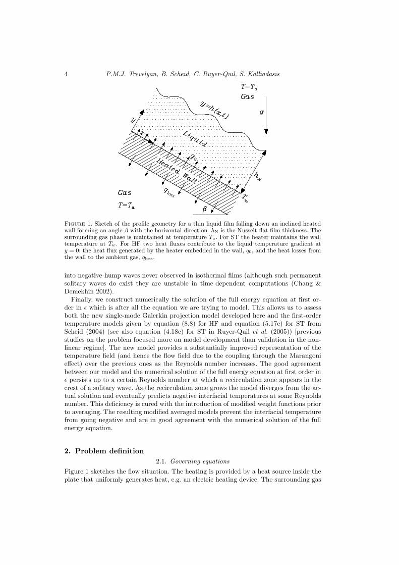
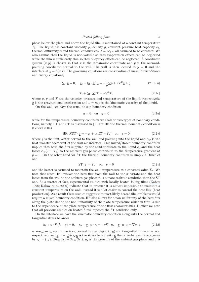
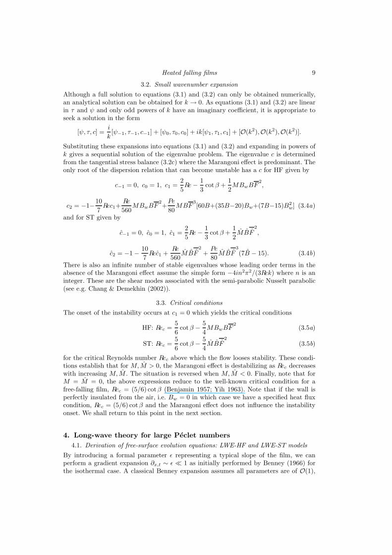
Figure 1. Sketch of the profile geometry for a thin liquid film falling down an inclined heatedwall forming an angle β with the horizontal direction. hN is the Nusselt flat film thickness. Thesurrounding gas phase is maintained at temperature Ta. For ST the heater maintains the walltemperature at Tw. For HF two heat fluxes contribute to the liquid temperature gradient aty = 0: the heat flux generated by the heater embedded in the wall, q0, and the heat losses fromthe wall to the ambient gas, qloss.

into negative-hump waves never observed in isothermal films (although such permanentsolitary waves do exist they are unstable in time-dependent computations (Chang &Demekhin 2002).

Finally, we construct numerically the solution of the full energy equation at first or-der in ǫ which is after all the equation we are trying to model. This allows us to assessboth the new single-mode Galerkin projection model developed here and the first-ordertemperature models given by equation (8.8) for HF and equation (5.17c) for ST fromScheid (2004) (see also equation (4.18c) for ST in Ruyer-Quil et al. (2005)) [previousstudies on the problem focused more on model development than validation in the non-linear regime]. The new model provides a substantially improved representation of thetemperature field (and hence the flow field due to the coupling through the Marangonieffect) over the previous ones as the Reynolds number increases. The good agreementbetween our model and the numerical solution of the full energy equation at first order inǫ persists up to a certain Reynolds number at which a recirculation zone appears in thecrest of a solitary wave. As the recirculation zone grows the model diverges from the ac-tual solution and eventually predicts negative interfacial temperatures at some Reynoldsnumber. This deficiency is cured with the introduction of modified weight functions priorto averaging. The resulting modified averaged models prevent the interfacial temperaturefrom going negative and are in good agreement with the numerical solution of the fullenergy equation.

2. Problem definition

2.1. Governing equations

Figure 1 sketches the flow situation. The heating is provided by a heat source inside theplate that uniformly generates heat, e.g. an electric heating device. The surrounding gas

Heated falling films 5

phase below the plate and above the liquid film is maintained at a constant temperatureTa. The liquid has constant viscosity µ, density ρ, constant pressure heat capacity cp,thermal diffusivity κ and thermal conductivity λ = ρcpκ, all assumed to be constant. Wealso assume that the liquid is non-volatile so that evaporation effects can be neglectedwhile the film is sufficiently thin so that buoyancy effects can be neglected. A coordinatesystem (x, y) is chosen so that x is the streamwise coordinate and y is the outward-pointing coordinate normal to the wall. The wall is then located at y = 0 and theinterface at y = h(x, t). The governing equations are conservation of mass, Navier-Stokesand energy equations,

∇ · u = 0, ut + (u · ∇)u = −1

ρ∇p+ ν∇2u+ g (2.1a, b)

Tt + (u · ∇)T = κ∇2T, (2.1c)

where u, p and T are the velocity, pressure and temperature of the liquid, respectively.g is the gravitational acceleration and ν = µ/ρ is the kinematic viscosity of the liquid.

On the wall, we have the usual no-slip boundary condition

u = 0 on y = 0 (2.2a)

while for the temperature boundary condition we shall on two types of boundary condi-tions, namely, HF and ST as discussed in § 1. For HF the thermal boundary condition is(Scheid 2004)

HF: λ∇T · j = −q0 + αw(T − Ta) on y = 0 (2.2b)

where j is the unit vector normal to the wall and pointing into the liquid and αw is theheat transfer coefficient of the wall-air interface. This mixed/Robin boundary conditionimplies that both the flux supplied by the solid substrate to the liquid q0 and the heatlosses αw(T − Ta) to the ambient gas phase contribute to the temperature gradient aty = 0. On the other hand for ST the thermal boundary condition is simply a Dirichletone

ST: T = Tw on y = 0 (2.2c)

and the heater is assumed to maintain the wall temperature at a constant value Tw. Wenote that since HF involves the heat flux from the wall to the substrate and the heatlosses from the wall to the ambient gas phase it is a more realistic condition than the STone. As a matter of fact, experimental studies with locally heated falling films (Kabov1998; Kabov et al. 2000) indicate that in practice it is almost impossible to maintain aconstant temperature on the wall, instead it is a lot easier to control the heat flux (heatproduction). As a result these studies suggest that most likely heated film problems wouldrequire a mixed boundary condition. HF also allows for a non-uniformity of the heat fluxalong the plate due to the non-uniformity of the plate temperature which in turn is dueto the dependence of the plate temperature on the flow characteristics. Further we notethat all previous studies on heated films imposed the ST condition only.

On the interface we have the kinematic boundary condition along with the normal andtangential stress balances

ht + u · ∇(h− y) = 0, pa + τ · n · n = −σ∇ · n, τ · n · t = ∇σ · t (2.2d)

where n and t are unit vectors, normal (outward-pointing) and tangential to the interface,respectively and τ = −pI + 2µe is the stress tensor with e the rate-of-strain tensor givenby eij = (1/2)(∂ui/∂xj + ∂uj/∂xi). pa is the pressure of the ambient gas phase and σ is

6 P.M.J. Trevelyan, B. Scheid, C. Ruyer-Quil, S. Kalliadasis

the surface tension. The thermal boundary condition on the free surface is:

λ∇T · n = −αg(T − Ta) on y = h (2.2e)

where αg is the heat transfer coefficient between the liquid and air. Finally, the thermo-capillary effect is modeled using a linear approximation for the surface tension

σ = σa − γ(T − Ta) (2.3)

where σa is the surface tension at the temperature Ta and γ > 0 for typical liquids.

2.2. Scalings and non-dimensionalization

System (2.1)-(2.3) has a trivial solution corresponding to the plane-parallel base state,the Nusselt flat film solution:

h = hN, p = pa + ρ(hN − y)g cosβ, u =g sinβ

2ν(2hNy − y2), v = 0 , (2.4a)

HF: T = Ta + βT [λ+ αg(hN − y)] , ST: T = Ta + βT [λ+ αg(hN − y)] (2.4b)

where βT = q0/[λ(αw +αg) +αwαghN] and βT = (Tw −Ta)/(λ+αghN). Using both thedimensional Nusselt film thickness, hN , and the viscous-gravity length and time scales,

l0 =ν2/3

(g sinβ)1/3, t0 =

ν1/3

(g sinβ)2/3

we employ the non-dimensionalization

(x, y, h) =(x, y, h)

hN, t =

tt0l0hN

, (u, v) =(u, v)

h2

N

t0l0

, p =p− pa

ρ l0hN

t20

HF: T =T − Ta

q0hN

λ

, ST: T =T − Ta

Tw − Ta.

The temperature scales for HF and ST, q0hN/λ and Tw − Ta, respectively, are naturalcontrol parameters in experiments.

In terms of these non-dimensional variables, the equations of motion and energy become

ux + vy = 0 (2.5a)

3Re(ut + uux + vuy) = −px + uxx + uyy + 1 (2.5b)

3Re(vt + uvx + vvy) = −py + vxx + vyy − cotβ (2.5c)

3Pe(Tt + uTx + vTy) = Txx + Tyy (2.5d)

where bars have been dropped for convenience. The wall boundary conditions become

u = v = 0, HF: Ty = −1 +BwT, ST: T = 1 (2.6a)

and the free-surface boundary conditions are written as

ht + uhx − v = 0 (2.6b)

p+ (We−MT )N−3

2hxx = 2N−1(vy − hx(uy + vx) + h2xux) (2.6c)

uy +M(Tx + hxTy)N1

2 = −vx − 2hx(vy − ux) + h2x(uy + vx) (2.6d)

Ty +BTN1

2 = hxTx (2.6e)

where N = 1 + h2x. We now introduce the Kapitza, Marangoni, wall Biot and surface

Heated falling films 7

Biot numbers for HF, respectively,

Ka =σa

ρgl20 sinβ, Ma =

γq0λρgl0 sinβ

, Biw =αwl0λ

, Bi =αgl0λ

,

and the Marangoni and surface Biot numbers for ST, respectively,

Ma =γ(Tw − Ta)

ρgl20 sinβ, Bi = Bi

where hats throughout this study are used to denote parameters associated with the STproblem. Further, we introduce the dimensionless Nusselt flat film thickness, hN = hN/l0.The dimensionless groups in (2.5-2.6) can then be written as

Re =h3

N

3, P e = RePr , We =

Ka

h2N

, M =Ma

hN, Bw = BiwhN , B = BihN (2.7)

corresponding to the Reynolds, Peclet, Weber and the modified groups, Marangoni, wallBiot and surface Biot numbers for HF, respectively, and

M =Ma

h2N

, B = BihN

corresponding to the modified groups, Marangoni and surface Biot numbers for ST,respectively. Pr = ν/κ is the Prandtl number.

The set of dimensionless groups in (2.7) isolates the dependence on the dimensionlessNusselt flat film thickness hN and the physical properties of the problem. Hence, thesystem of equations (2.5-2.6) is governed by the inclination angle β, hN or equivalentlythe Reynolds number and the five dimensionless parameters, Ka, Ma, Pr, Biw and Bifor HF and the four dimensionless groups, Ka, Ma, Pr and Bi for ST. As a consequence,a complete investigation over the entire parameter space would be impractical. How-ever, for a given liquid-gas system, heating conditions and geometry, the parameters β,Ka,Ma, Pr,Biw, Bi, Ma and Bi are fixed and the only free parameter is the Reynoldsnumber which is a flow control parameter so that the heated falling film problem is aone-parameter system only. On the other hand, if we only fix the liquid and inclinationangle β, the Prandtl and Kapitza numbers are fixed, thus reducing the number of relevantparameters by three, which is a substantial simplification. As an example assuming theliquid phase to be water at 25◦C and the plane to be vertical, β = π/2, Ka ≃ 2850 andPr ≃ 7. The HF problem then has four free parameters, Re, Ma, Biw and Bi while theST problem has three free parameters, Re, Ma and Bi. The values for the parameters,Biw, Bi,Ma, Bi and Ma will be discussed in § 4.

2.3. On the two wall thermal conditions: retrieving ST from HF

We close this section with a comment on the wall thermal boundary condition for HF in(2.6a). The temperature field has been non-dimensionalized with q0hN/λ. An alternativescaling could have been T ∗ = (T − Ta)/(q0/αw) that would convert (2.2b) to

T ∗

y = Bw(T ∗ − 1). (2.8)

In the limit Bw → ∞, (2.8) yields T ∗ → 1 thus retrieving the boundary condition for ST(2.6a). But (2.6a) is obtained by scaling the temperature field with Tw −Ta. This scalingmust be related to that used to obtain (2.8) as in the limit Bw → ∞, ST and HF areone and the same problem. Converting now T ∗ = 1 to dimensional variables and settingT = Tw yields q0 = αw(Tw − Ta): q0 is now the heat transported between the liquid andthe gas. This is to be expected as in the limit Bw → ∞ the wall is effectively decoupled

8 P.M.J. Trevelyan, B. Scheid, C. Ruyer-Quil, S. Kalliadasis

from the problem and we are concerned with the heat transfer between the liquid andthe gas only.

Taking the limit Bw → ∞ in (2.6a) yields T → 0. It would then appear that wecannot retrieve the ST problem from (2.6a) in this limit. Note, however, that (2.6a) canbe converted to (2.8) with the transformation

T =1

BwT ∗. (2.9)

Thus in the limit Bw → ∞, T ∗ → 1 becomes T → 0 and hence, the alternative form ofthe wall thermal boundary condition in (2.8) is equivalent to (2.6). The ‘advantage’ of(2.8) is that it makes the recovery of ST from HF in the limit Bw → ∞ transparent. Onthe other hand, the ‘advantage’ of (2.6a) is that it makes the limit Bw → 0 more obviousas in this limit we retrieve the case of a specified heat flux boundary condition.

3. Linear Stability Analysis

3.1. The Orr-Sommerfeld eigenvalue problem

We now examine the linear stability of the Nusselt flat film solution (2.4). For ST, thisproblem was first formulated and solved by Goussis & Kelly (1991) and more recentlywas reconsidered in detail by Scheid et al. (2005). The Nusselt solution can be writtenas

h = 1 , v = 0 , u = y −1

2y2 , p = (1 − y) cotβ , T = [1 +B(1 − y)]F

where for ST F → F with

HF: F = (Bw +B +BwB)−1 , ST: F = (1 + B)−1.

Normal form disturbances are introduced as

[h, u, v, p, T ] = [h, u(y), v(y), p(y), T (y)] + χeik(x−ct)[H,ψy(y),−ikψ(y), π(y), τ(y)]

where k and c are the wavenumber and complex phase velocity of the infinitesimal pertur-bations, respectively. The disturbances are substituted into (2.5) and (2.6) which are thenlinearised in χ. The pressure field is eliminated from the problem via the two momen-tum equations and the normal stress condition to yield the Orr-Sommerfeld eigenvalueproblem

(D2 − k2)2ψ = 3ikRe[

ψ + (u− c) (D2 − k2)ψ]

(3.1a)

(D2 − k2)τ = 3ikPe[

BFψ + (u− c) τ]

, (3.1b)

subject to the wall boundary conditions

ψ(0) = Dψ(0) = 0, HF: Dτ(0) = Bwτ(0), ST: τ(0) = 0 (3.2a)

and the interfacial boundary conditions[

D2 − 3k2 + 3ikRe

(

c−1

2

)]

Dψ(1) = ik[cotβ + k2(We−MF )]H (3.2b)

(D2 + k2)ψ(1) = H + ikM

BDτ(1) (3.2c)

Dτ(1) = B[BFH − τ(1)] with H =ψ(1)

c− 1/2, (3.2d)

where D ≡ d/dy. For ST (M,F ,B) → (M, F , B).

Heated falling films 9

3.2. Small wavenumber expansion

Although a full solution to equations (3.1) and (3.2) can only be obtained numerically,an analytical solution can be obtained for k → 0. As equations (3.1) and (3.2) are linearin τ and ψ and only odd powers of k have an imaginary coefficient, it is appropriate toseek a solution in the form

[ψ, τ, c] =i

k[ψ−1, τ−1, c−1] + [ψ0, τ0, c0] + ik[ψ1, τ1, c1] + [O(k2),O(k2),O(k2)].

Substituting these expansions into equations (3.1) and (3.2) and expanding in powers ofk gives a sequential solution of the eigenvalue problem. The eigenvalue c is determinedfrom the tangential stress balance (3.2c) where the Marangoni effect is predominant. Theonly root of the dispersion relation that can become unstable has a c for HF given by

c−1 = 0, c0 = 1, c1 =2

5Re−

1

3cotβ +

1

2MBwBF

2,

c2 = −1−10

7Rec1+

Re

560MBwBF

2+Pe

80MBF

3[60B+(35B−20)Bw+(7B−15)B2

w] (3.4a)

and for ST given by

c−1 = 0, c0 = 1, c1 =2

5Re−

1

3cotβ +

1

2MBF

2

,

c2 = −1 −10

7Rec1 +

Re

560MBF

2

+Pe

80MBF

3

(7B − 15). (3.4b)

There is also an infinite number of stable eigenvalues whose leading order terms in theabsence of the Marangoni effect assume the simple form −4in2π2/(3Rek) where n is aninteger. These are the shear modes associated with the semi-parabolic Nusselt parabolic(see e.g. Chang & Demekhin (2002)).

3.3. Critical conditions

The onset of the instability occurs at c1 = 0 which yields the critical conditions

HF: Rec =5

6cotβ −

5

4MBwBF

2(3.5a)

ST: Rec =5

6cotβ −

5

4MBF

2

(3.5b)

for the critical Reynolds number Rec above which the flow looses stability. These condi-tions establish that for M, M > 0, the Marangoni effect is destabilizing as Rec decreaseswith increasing M, M . The situation is reversed when M, M < 0. Finally, note that forM = M = 0, the above expressions reduce to the well-known critical condition for afree-falling film, Rec = (5/6) cotβ (Benjamin 1957; Yih 1963). Note that if the wall isperfectly insulated from the air, i.e. Bw = 0 in which case we have a specified heat fluxcondition, Rec = (5/6) cotβ and the Marangoni effect does not influence the instabilityonset. We shall return to this point in the next section.

4. Long-wave theory for large Peclet numbers

4.1. Derivation of free-surface evolution equations: LWE-HF and LWE-ST models

By introducing a formal parameter ǫ representing a typical slope of the film, we canperform a gradient expansion ∂x,t ∼ ǫ ≪ 1 as initially performed by Benney (1966) forthe isothermal case. A classical Benney expansion assumes all parameters are of O(1),

10 P.M.J. Trevelyan, B. Scheid, C. Ruyer-Quil, S. Kalliadasis

with the exception of the Weber number which is taken to be much larger. The Reynoldsnumber, Marangoni number and wall/free-surface Biot numbers are then assumed ofO(1). The Weber number is assumed to be O(ǫ−2), to bring the dominant surface tensioneffects in at O(ǫ). These stabilizing terms prevent the waves from forming shocks andfrom breaking thus satisfying the long-wave approximation. With regards to the Pecletnumber, all previous LWE theories in the area of heated thin films, e.g. Joo et al. (1991)and Oron et al. (1997), have assumed the Peclet number to be O(1). As a consequence, theconvective heat transport effects only enter the velocity field at O(ǫ2) and temperaturefield at O(ǫ), but these higher order corrections are rather lengthy leading in turn tolengthy evolution equations for the free surface.

In practice, however, the Peclet number can be much larger than the Reynolds numberdue to the ratio of the momentum and thermal diffusivities being much larger than unity– note that for water Pr = 7. We then expect that convection at large Peclet numbers canlead to a downstream convective distortion of the free-surface temperature distributionobtained by assuming an O(1) Peclet number. As a result the transport of heat by theflow becomes important and can significantly modify the interfacial temperature andconsequently the Marangoni effect on the fluid flow. Hence we assume Pe ∼ O(ǫ−n) with0 < n < 1 so that the convective heat transport effects are included at a low relevantorder. If Pe = O(1) then for the level of truncation employed here the convective heattransport effects would be neglected and as noted earlier one would have to go up toO(ǫ2) and O(ǫ) for the velocity and temperature fields, respectively.

We then carry out an expansion for the velocity up to O(ǫ2−n) and we neglect termsof O(ǫ2) and higher. This level of truncation allows the derivation of a relatively simpleevolution equation for the local film thickness. The pressure and temperature are bothexpanded up to O(ǫ1−n) and hence terms of O(ǫ) and higher are omitted from theseexpansions. At this level of truncation, the solutions for the temperature field are givenby equation (A 1) in Appendix A. The velocity components can be conveniently expressedin the form u = ψy and v = −ψx where the streamfunction ψ is given by equation (A 2)in Appendix A. The free-surface evolution equation can then be easily obtained from thekinematic boundary condition in (2.6b):

HF: ht + h2hx +

(

2

5Reh6hx −

1

3h3hx cotβ +

1

2MBwBF

2h2hx +1

3Weh3hxxx

)

x

−Pe

80MB

[

h2(

Gh3hx

)

x

]

x= 0. (4.1)

with the functions F andG being given in Appendix A. The equivalent evolution equationfor the ST problem is obtained with (G,MBwBF

2,MB) → (G, MBF 2, MB).A linear stability analysis of the trivial solution h = 1 of (4.1) and the equivalent

evolution equation for ST gives the same critical conditions as (3.5) obtained from theOrr-Sommerfeld eigenvalue problem of the full Navier-Stokes and energy equation. Thisis to be expected as LWE is exact regarding critical/neutral conditions as pointed outin § 1.1. However, LWE being a single equation predicts only the mode that becomesunstable and fails to recover the stable modes obtained with Orr-Sommerfeld, a conse-quence of the fact that in LWE these modes are slaved to h (these modes have their ownintrinsic dynamics and can be destabilized for very large Re).

4.1.1. Physical consequences of vanishing wall/free-surface Biot numbers

When Bw = 0 the fifth term in (4.1) vanishes and the Marangoni effect no longer influ-ences the instability onset. This means that for a specified heat flux boundary conditionor equivalently a plate that is perfectly insulated from the gas phase below, the long-

Heated falling films 11

wave thermocapillary instability is suppressed. In this case, the interfacial temperaturedistribution is T |y=h = B−1 +(3/2)PeB−1h3hx which has two contributions: B−1 due toheat conduction across the film and (3/2)PeB−1h3hx due to convective heat transport.The first term is independent of h and as a result thermocapillarity does not affect theinstability as variations of h do not induce perturbations on the interfacial temperaturedistribution through heat conduction. The second term of Ty=h due to heat convectiondoes depend on h and controls the dispersion of the waves through the last term in (4.1)(via the functionals G, G). Hence, enabling heat losses at the wall through the mixedboundary condition (2.6a) is the only way to enable the Marangoni instability (unlessthe wall supplies a non-uniform heat flux, e.g. Scheid et al. (2002)).

On the other hand, for the ST problem the interfacial temperature distribution isT |y=h = (1 + Bh)−1 + (1/40)PeBGh3hx. The first term arises from heat conduction anddepends on h so that the Marangoni forces in this case always influence the instabilityonset, as long as B 6= 0. However, if B = 0, i.e. the interface is a poor heat conductorperfectly insulated from the surrounding gas, the Marangoni effect does not influence thesystem. In this case T = 1 from (A 1b) and the temperature is everywhere uniform andequal to the wall temperature so that there is no instability due to the thermal effectsor influence on the dispersion of the waves; the momentum and heat transport problemsare decoupled in this limit.

4.2. Rescaling the LWE equations

For convenience let us now rescale the evolution equations using the scalings introducedby Shkadov (1977). This author introduced a length scale in the streamwise directioncorresponding to the balance of the pressure gradient σahxxx due to surface tension andthe gravitational acceleration ρg sinβ. This length scale, say lS , corresponds effectivelyto the characteristic length of the steep front of the waves. Note that lS should be muchlarger than the film thickness hN in order to sustain the long-wave assumption. Simplealgebra then shows that lS/hN = We1/3 which is a large ratio as long as the Webernumber is sufficiently large. The rescaled space and time coordinates are then defined asx = We1/3X and t = We1/3Θ to yield

HF: hΘ + h2hX +

(

A(h)hX + B(h)h2X + C(h)hXX +

1

3h3hXXX

)

X

= 0 (4.2)

where

A(h) =2δ

15h6 −

ζ

3h3 +

M

2BwBF

2h2, B(h) = h2 ∂

∂h

(

C(h)

h2

)

, C(h) = −Prδ

240MBGh5.

For ST, A is obtained from A with MBwBF2 → MBF 2 and C is obtained from C with

MBG→ MBG. The parameters

δ = 3Re/We1/3, ζ = cotβ/We1/3, M = M/We1/3 and M = M/We1/3

are reduced Reynolds number, reduced slope and reduced Marangoni numbers.

In what follows, the evolution equation (4.2) will be referred to as LWE-HF and thecorresponding equation for ST as LWE-ST. The LWE models are developed to verifythe behavior of the weighted residuals models obtained in the following sections in theregion where LWE is valid, i.e. close to criticality. It is exactly because of the presence ofconvective heat transport terms in the weighted residuals models to be developed, thatwe have developed a long-wave theory to include these terms.

12 P.M.J. Trevelyan, B. Scheid, C. Ruyer-Quil, S. Kalliadasis

4.3. Comparing HF and ST

4.3.1. Conditions under which HF and ST are identical

Despite the different wall boundary conditions, the HF and ST problems yield similarMarangoni terms in their respective long-wave evolution equations. As discussed ear-lier, the leading-order Marangoni effects arise via heat conduction and the higher-orderMarangoni effects via heat convection. By comparing equation (4.1) for the HF problemto its counterpart for the ST problem, it is clear that the leading-order Marangoni termsin these two equations, also responsible for the thermocapillary instability, are identicalwhen MBwBF

2 = MBF 2. This relationship can be made independent of h when thefollowing two conditions are satisfied:

B =BwB

Bw +B, M =

M

Bw +B.

By eliminating the film parameter hN, the above conditions can be written as

Bi =BiwBi

Biw +Bi, Ma =

Ma

Biw +Bi. (4.3)

In this case, the critical Reynolds numbers given in (3.5a) and (3.5b) become identical.This shows that the Marangoni effects associated with the HF and ST problems areidentical at least in the long-wave limit and provided that the convective effects can beneglected, i.e. small Pe. Away from the small Pe limit, the criticality conditions are thesame but the phase velocities of the infinitesimal disturbances are different – recall thatthe convective heat transport effects influence the dispersion of the waves. The two caseswill also be different in the nonlinear stage of the instability.

4.3.2. On the type of small amplitude waves

The LWE equation obtained by Trevelyan & Kalliadasis (2004a) in their study of thedynamics of a reactive falling film is the same to that in (4.2) but with A, B and Cdifferent polynomial functions of h. Hence, the results of the Trevelyan & Kalliadasis(2004a) study can be easily extended to (4.2), and for that matter to any evolutionequation of the type given in (4.2) where A, B and C some polynomial functions of h.In particular, as these authors demonstrated, for evolution equations of the type givenin (4.2) we can have both positive and negative stationary solitary wave solutions at theweakly nonlinear stage, but one of them is unstable in time-dependent computations.More specifically, when C is sufficiently large and positive (the bar denotes evaluation ofthe function C at h = 1), time-dependent computations show that the system evolvesinto a train of positive-hump solitary waves. Such waves travel with a speed faster thanthe linear wavespeed and their largest free-surface deformation is away from the wall.On the other hand, when C is sufficiently large and negative, the system evolves into atrain of negative-hump waves which travel with speed smaller to the linear wavespeedand with the largest free-surface deformation towards the wall. We note that althoughC determines the type of the waves (positive or negative) it is the full term Chxxx thatgoverns the dispersion of small amplitude waves.

The sign of C is opposite to that of the convective functions G and G. In the limitof very thin films, i.e. hN → 0, the signs of the convective functions G in Appendix A

determine that for ST C > 0, whilst for HF C is only positive when Biw/Bi > 3. Thus,in the ST case we always have positive-hump solitary waves, whilst in the HF case wecan have either positive- or negative-hump solitary waves. We note that in the limit ofzero hN the Reynolds number tends to zero and the critical Reynolds number tends to

Heated falling films 13

minus infinity which is of course unphysical and implies a zero critical Reynolds number.Nevertheless, we refrain from using the expression ‘close to criticality’ in this limit as ingeneral it implies small amplitude waves. Obviously, close to criticality, i.e. for a finitevalue of Rec, the dispersive effects of the (small amplitude) waves in LWE are controlledby Chxxx.

4.3.3. Choosing parameter values to contrast HF and ST

In order to contrast now the ST and HF problems we shall apply both conditions in(4.3). The first condition in equation (4.3) requires that both Bi and Biw are greater thanBi. It is realistic to expect poor heat transfer characteristics at the liquid-gas interfaceand so physically the parameters Bi and Bi should be small. For the surface Biot numberwe take Bi = 1

10 for ST throughout this study. By rearranging now the conditions in

(4.3) we obtain Bi = BiwBi/(Biw − Bi) and Ma = MaBiw2/(Biw − Bi). We then consider

two sets of parameter values for HF, namely,

[Biw, Bi,Ma] =

[

1

5,1

5,2

5Ma

]

and [Biw, Bi,Ma] =

[

3

5,

3

25,18

25Ma

]

.

For the first set of parameters Biw/Bi = 1 whilst for the second set Biw/Bi = 5, the tworatios being equidistant from 3. The first set yields C < 0 for small hN whilst the secondset yields C > 0 for small hN and we expect that the second set will yield qualitativeagreement (at least for small Re) to the ST problem which always has C > 0 for smallhN.

The only free parameters then are Ma and Re – see also our discussion in § 2.2.

5. Weighted residuals approach

5.1. The momentum equation

The starting point of the weighted residuals approach is to assume long waves in thestreamwise direction. For consistency with LWE, we shall also neglect the second orderdiffusive terms uxx and Txx of the Navier-Stokes and energy equations. Part of theanalysis presented in this section parallels the works by Kalliadasis et al. (2003a,b) andthe reader is referred to these studies for further details. The second order terms can beincluded with the methodology developed by Ruyer-Quil et al. (2005).

To leading order, the y-component of the equation of motion (2.5c) and normal stressbalance (2.6c) are py = − cotβ and p|y=h = −Wehxx. Hence, the pressure distributionis given by p = (h − y) cotβ −Wehxx which when substituted into the x-component ofthe momentum equation (2.5b) and neglecting terms of O(ǫ2) and higher yields

uyy + 1 = hx cotβ −Wehxxx + 3Re(ut + uux + vuy). (5.1a)

The y-component of the velocity can be eliminated by using the continuity equation (2.5a)along with the no slip boundary condition to obtain v = −

∫ y

0uxdy

′. The u velocity mustsatisfy the no-slip boundary condition and the leading-order tangential stress balance onthe interface from (2.6d),

u = 0 on y = 0 and uy = −Mθx on y = h (5.1b)

where terms of O(ǫ2) and higher have been neglected from the tangential stress balanceand θ(x, t) is the interfacial temperature, i.e. θ ≡ T |y=h and θx ≡ (Tx + hxTy)|y=h. Theabove system is coupled with the energy equation and thermal boundary conditions,however, we can examine the flow field by assuming that the function θ is known. The

14 P.M.J. Trevelyan, B. Scheid, C. Ruyer-Quil, S. Kalliadasis

system is then closed via the kinematic boundary condition in (2.6), which by integratingthe continuity equation in (2.5) across the film can be written as

ht + qx = 0 (5.1c)

where q =∫ h

0u dy is the flow rate. In the absence of the Marangoni term Mθx appearing

in the stress balance at the free surface, equations (5.1) are the so-called ‘boundary-layerequations’.

Following Kalliadasis et al. (2003a,b) we assume the following velocity profile,

u = 3q

h

(

η −1

2η2

)

+Mθxh

(

1

2η −

3

4η2

)

≡ u(0) +Mθxh

(

1

2η −

3

4η2

)

, (5.2)

where η = y/h(x, t) is a reduced normal coordinate. u(0) is the test function that containsq for which an equation is sought that would provide a closure for the weighted resid-uals approach (it is identical to the test function introduced by Shkadov (1967, 1968)for isothermal flows). The second function is chosen so that the profile in (5.2) satis-fies all boundary conditions (in fact its the simplest possible profile that does so). Theintroduction of this profile into (5.1a) yields the following residual at O(ǫ):

Ru = 3Re(u(0)t + u(0)u(0)

x + v(0)u(0)y ) − uyy − 1 + hx cotβ −Wehxxx (5.3)

where v(0) = −∫ y

0u

(0)x dy′. Indeed, the Marangoni terms in (5.2) are of O(ǫM) so that

they only contribute to the viscous diffusion term ∂2/∂y2 and are neglected from theinertial terms which are of O(ǫRe).

For the isothermal falling film problem, Ruyer-Quil & Manneville (2000, 2002) showedthat a Galerkin projection for the velocity field with just one test function, the profileassumed by Shkadov (1967, 1968), and with a weight function equal to the test functionitself fully corrects the critical Reynolds number obtained from the Shkadov IBL approx-imation. We shall demonstrate that this is also the case in the presence of Marangonieffects when the weight function is taken as the test function for the velocity, namelyη − 1

2η2. The momentum residual is then minimized from 〈η − 1

2η2, Ru〉 = 0 – the inner

product is defined as 〈f, g〉 =∫ 1

0fgdη for any two functions f and g with appropriate

boundary conditions – which yields the averaged momentum equation

18

5Re

(

qt +17

7

q

hqx −

9

7

q2

h2hx

)

+3q

h2= h+Wehhxxx − hhx cotβ −

3

2Mθx, (5.4)

used in the remainder of the study. Note that equations (5.1c) and (5.4) correspond toequations (5.17a) and (5.17b) in Scheid (2004) (and equations (4.18a) and (4.18b) inRuyer-Quil et al. (2005)).

Ruyer-Quil & Manneville (2000, 2002) also developed high-order IBL models usingrefined polynomial expansions for the velocity field (corresponding to corrections of theShkadov parabolic self-similar profile) and high-order weighted residuals techniques. Herewe leave the momentum equation as simple as possible and we aim to improve thetreatment of the energy equation.

5.2. Simple weighted residuals for the energy equation: the SHF and SST models

5.2.1. Derivation of the models

The boundary conditions for the temperature field are the wall conditions in (2.6a)and the leading-order interfacial condition from (2.6e)

Ty = −BT on y = h, (5.5)

Heated falling films 15

where terms of O(ǫ2) and higher have been neglected. Like with the averaging of themomentum equation, the first step in modeling the energy equation is the introductionof a test function for the temperature field. As a first approximation we choose a linearprofile which satisfies the wall boundary condition in (2.6a) along with T |η=1 = θ:

HF: T = θ +1 −Bwθ

1 +Bwhh(1 − η) , ST: T = 1 + (θ − 1)η. (5.6)

Hence, the assumption here is that the linear temperature profile obtained for a flatfilm persists even when the interface is no longer flat. Note that θx occurs explicitlyin the momentum equation (5.4) and so it is convenient to explicitly include θ in thetemperature fields.

By analogy now with our analysis for the momentum equation, the introduction of theabove test functions for the temperature fields into (2.5d) yields the following residualat O(ǫ):

RT = 3Pe(Tt + u(0)Tx + v(0)Ty) − Tyy (5.7)

where the terms of O(ǫM) of u and v are neglected from the heat transport convectiveterms which are of O(ǫPe). The energy residual can then be minimized from 〈wT , RT 〉 = 0where wT is an appropriately chosen weight function.

We note that although the temperature distributions in (5.6) satisfy their respectivewall boundary conditions in (2.6a), they do not satisfy the leading-order interfacial condi-tion in (5.5), unlike the velocity profile in (5.2) which satisfies all boundary conditions. Itis in fact impossible for a linear profile to satisfy (5.5) and 〈wT , RT 〉 = 0, however, as waspointed out by Kalliadasis et al. (2003a) by choosing the weight function appropriately,the boundary terms resulting from integrations by parts involve either Tη on η = 1 or Ton η = 0 and thus the interfacial boundary condition can be included in the boundaryterms resulting from the integrations by parts. Hence, although the test function doesnot satisfy all boundary conditions, the averaged energy equation does and the flat filmsolution can still be retained in our averaging formulation.

For HF we take wT ≡ 1 which gives

0 =2 +Bwh

2θt +

8 + 5Bwh

8hqθx −

(1 −Bwθ)

8(1 +Bwh)

[

(5 +Bwh)qx − 3qhx

h

]

+θF−1 − 1

3Peh. (5.8a)

Equations (5.4) and (5.8a) along with the kinematic boundary condition in (5.1c) willbe referred to hereafter as the SHF model – a simple heat flux model. For ST we takewT ≡ y which gives

0 = θt +27q

20hθx +

7qx(θ − 1)

40h+

1

Peh2(θF−1 − 1) (5.8b)

Equations (5.4) and (5.8b) along with the kinematic boundary condition in (5.1c) will bereferred to hereafter as the SST model – a simple specified temperature model. Equations(5.8a) and (5.8b) correspond to equations (8.8) and (5.17c) in Scheid (2004). Equation(5.8b) also corresponds to equation (4.18c) in Ruyer-Quil et al. (2005).

For consistency the SHF and SST models are both rescaled in the same way as theLWE-HF and LWE-ST, i.e. x = We1/3X and t = We1/3Θ. Finally, we note that althoughthe SST model essentially uses the test function as the weight function, we refrain fromcalling this model a ‘Galerkin approach’. Indeed with a linear test function Tyy ≡ 0

16 P.M.J. Trevelyan, B. Scheid, C. Ruyer-Quil, S. Kalliadasis

and as pointed out earlier SST satisfies the boundary conditions through integrations byparts.

5.2.2. Linear stability of flat film solution for the SHF and SST models

By construction, the SHF and SST models satisfy their appropriate flat film solutions,namely

h = 1, q =1

3, HF: θ = F , ST: θ = F .

We consider the stability of these solutions with respect to infinitesimal perturbationsin the form of normal modes ∼ eik(X−cΘ) where k and c are the wavenumber and com-plex phase velocity of the perturbations, respectively. Substituting these modes into theSHF/SST models linearized about their flat film solutions gives the dispersion relationfor ω as a function of k with three roots for c.

To obtain the critical condition for the onset of instability we consider k ≪ 1 andexpand the phase velocity as c ∼ (i/k)c-1 + c0 + ikc1 + k2c2 +O(k3) (see also § 3.2). Twoof the roots have c-1 < 0 and the corresponding modes are stable (note ωR = ℜ(−ikc) =c-1 + k2c1 + O(k4) for small k). The third root can have a positive growth rate. For theSHF model the first few orders of the wavespeed for this mode are given by,

c-1 = 0, c0 = 1, c1 =2δ

15−ζ

3+

1

2MBwBF

2

c2 =

(

B

4−Bw

12+BwB

16

)

(1 +Bw)PrδMBF3−

10

21δc1. (5.9a)

For the SST model we also have two roots with c-1 < 0. The first few orders of thewavespeed of the third mode that can become unstable are given by

c-1 = 0 , c0 = 1 , c1 =2δ

15−ζ

3+

1

2MBF

2

c2 = (7B − 15)Prδ

240MBF

3

−10

21δc1. (5.9b)

The onset of the instability occurs at c1 = 0 for SHF and c1 = 0 for SST which yieldsthe same critical Reynods number with LHE-HF and LWE-ST which in turn is the sameto that predicted from the Orr-Sommerfeld analysis – see (3.5). Regarding the linearwavespeed, the Orr-Sommerfeld analysis in § 3.2 (with the wavenumber k scaled with1/We1/3), LWE and SHF/SST all give the same values for c0, c1, c0 and c1 but not forc2 and c2; agreement for c2 and c2 would require taking into account for both LWE andSHF/SST the second order dissipative terms which have been neglected here. Note thatunlike Orr-Sommerfeld, for the weighted residuals models we have a finite number ofmodes due to their polynomial dispersion relation as a result of projection of the originalequations onto a finite number of test functions (clearly, increasing the number of testfunctions would increase the number of modes).

Finally, the neutral stability curve is obtained from cI = 0. In general this has to besolved numerically, however, by taking the limit of small hN an analytical solution ispossible. This gives cR = 1 where

HF: k =h−1/6N

B +Bw

√

3MBBw

2Ka1/3

[

1 − hN

(

BBw

B +Bw+

(B + Bw)2 cotβ

3MBBw

)]

+ O(h11/6N )

ST: k = h−1/6N

√

3MB

2Ka1/3

[

1 − hN

(

B +cotβ

3MB

)]

+ O(h11/6N ).

Heated falling films 17

Hence, the neutral wavenumber k for both HF and ST tends to infinity as hN tendsto zero. Recall from § 4.3.2 that in this limit the Reynolds number tends to zero andthe critical Reynolds number tends to minus infinity which is of course unphysical andimplies a zero critical Reynolds number. Notice that by using condition (4.3) the aboveexpressions for the HF and ST neutral wavenumbers are identical. This is to be expectedsince convection does not enter the above expansions in hN at the level of truncation forthese expansions. Notice also that these expansions are not valid for M = 0. In this casean expansion for small hN is not necessary since we have the exact solution,

cR = 1 , k = We−1/6

√

6

5Re − cotβ ≡We−1/6

√

6

5(Re−Rec),

which is identical to the LWE neutral stability curve in the absence of the Marangonieffect as can be easily shown from (4.1).

5.3. Galerkin residuals of the energy equation: the GHF[m] and GST[m] models

5.3.1. Derivation of the models

The simple weighted residuals models SHF and SST are useful prototypes for thestudy of the dynamics of a heated film. Also, the linear stability analysis of these modelsin § 5.2.2 showed that they do predict the correct critical Reynolds number. However, wealso wish to recover close to criticality the LWE models obtained in § 4.

A more refined treatment of the temperature field will enable a weighted residualsapproach to yield LWE via an appropriate gradient expansion. We consider a generalpolynomial expansion for the temperature field in powers of η and with amplitudes thatare only functions of x and t:

HF: T =

m∑

i=−1

A(i)(x, t)ηi+1 , ST: T =

m∑

i=−2

A(i)(x, t)ηi+2.

We note that unlike the studies by Scheid (2004) and Ruyer-Quil et al. (2005) where theamplitudes in the expansion for the temperature field are assigned certain orders withrespect to ǫ, in our projection for the temperature field the order of the amplitudes is notspecified. We also note that the test functions utilized by Scheid (2004) and Ruyer-Quilet al. (2005) did not satisfy all boundary conditions; instead the weight functions werechosen so that the boundary conditions can be included in the boundary terms resultingfrom the integrations by parts as was done in § 5.2.1.

Here we require that the temperature field satisfies all of its boundary conditions alongwith T |η=1 = θ, a total of three conditions that need to be satisfied. For the HF problemthen we eliminate a total of three amplitudes, A(−1), A(0) and A(1). For the ST problemwe also utilize the condition Tyy = 0 on the wall which originates from a Taylor seriesexpansion of the energy equation (2.5d) at y = 0 (this is also consistent with LWE-ST – T in (A 1b) has no quadratic term in y) and hence we eliminate four amplitudes,A(−2), A(−1), A(0)(≡ 0) and A(1). In weighted residuals terminology, the elimination ofthese amplitudes for the HF and ST problems is effectively equivalent to a ‘tau’ method(Gottlieb & Orszag 1977).

We then project the temperature field onto the new set of test functions φ,

HF: T = φ0 + θφ1 +

m∑

i=2

A(i)(x, t)φi, ST: T = φ0 + θφ1 +

m∑

i=2

A(i)(x, t)φi (5.10)

where we now have m amplitude functions, θ, A(2)...A(m) and the test functions are

18 P.M.J. Trevelyan, B. Scheid, C. Ruyer-Quil, S. Kalliadasis

defined by

φ0 =h(1 − η)2

2 +Bwh, φ1 = 1 + (1 − η)ηBh+ φ0(B −Bw) ,

φi = ηi+1 − (i+ 1)η2

2+

(i− 1)(2 + (2 − η)ηBwh)

2(2 +Bwh)for 2 6 i 6 m

and

φ0 = 1 −3η

2+η3

2, φ1 = 1 − φ0 + Bh(1 − η2)

η

2,

φi = (i− 1)η

2− (i+ 1)

η3

2+ ηi+2 for 2 6 i 6 m.

All the φi’s and φi’s are non-negative in the open interval (0, 1). Also, by construction

the φi’s and φi’s satisfy the same conditions on the surface, namely, φ0 = φ0 = φ1 − 1 =φ1−1 = φi = φi = 0 and φ0η

= φ0η= φ1η

+Bh = φ1η+Bh = φiη

= φiη= 0. On the wall

the φi’s satisfy φ0η+h−Bwhφ0 = φ1η

−Bwhφ1 = φiη−Bwhφi = 0, while the φi’s satisfy

φ0−1 = φ1 = φi = 0, thus ‘homogenizing’ the inhomogeneous wall boundary conditions.These new sets of test functions allow the temperature fields in (5.10) to satisfy all theirboundary conditions for each problem.

We now let wj denote the weight functions for the energy equation. In the Galerkinweighted residuals approach, wj ≡ φj . The residuals 〈wj , RT 〉 = 0, 1 6 j 6 m, for HFcan then be written in matrix form as

3Pe(

Mα At +Mβ Ax +Mγ A+ δ)

= ∆ +MΓ A (5.11)

whereA = [θ,A(2)...A(m)]t, the matrices [Mα]ij = 〈φj , φi〉, [Mβ]ij = 〈φj , u(0)φi〉, [Mγ ]ij =

〈φj , φit+u(0)φix+v(0)φiy〉 and [MΓ]ij = 〈φj , φiyy〉 are of dimensionm×m and the vectors

[δ]j = 〈φj , φ0t +u(0)φ0x + v(0)φ0y〉 and [∆]j = 〈φj , φ0yy〉 are of dimension m×1. The setof equations (5.1c), (5.4) and (5.11) will be referred to hereafter as the GHF[m] model.

The corresponding set of equations for ST can be obtained from (5.11) with φj → φj .The resulting set of equations will be referred to hereafter as the GST[m] model.

5.3.2. Obtaining LWE-HF/LWE-ST from the GHF[m]/GST[m] models

We now demonstrate that LWE-HF and LWE-ST in § 4 can be obtained from an ap-propriate expansion of GHF and GST. For this purpose we assign the same orders ofmagnitude for the parameters Re, Pe, We, M , B and Bw as in the LWE. It is importantto point out here that our averaged model in (5.11) has been derived without overlyrestrictive stipulations on the order of the dimensionless groups (see Kalliadasis et al.(2003a,b) for a discussion of lower/upper bounds on the order of magnitude of the di-mensionless parameters). For example, changing the order of Pe in (5.11) would lead toa different long-wave expansion to that obtained in § 4.

Let us now expand q and the amplitudes θ and A(i) as q = q0 + ǫq1 + O(ǫ2), θ =θ0 + ǫ1−nθ1, A

(i) = A0i + ǫ1−nA1i where Pe = O(ǫ−n) with 0 < n < 1 and we truncateour expansions so that terms of O(ǫ2) and higher in (5.4) are neglected while terms ofO(ǫ) and higher in (5.11) are neglected. Equation (5.4) then yields

q =1

3h3 +

2

5Reh6hx −

1

3h3hx cotβ −

1

2Mh2θx +

1

3Weh3hxxx (5.12)

We note that at this point θx from the averaged system in (5.11) remains undetermined,however, we shall demonstrate that it is identical to the one obtained from LWE.

Heated falling films 19

LWE-HF LWE-ST SHF SST GHF[1] GST[1]

(5.1c) (5.1c) (5.1c) (5.1c)

(4.1a) (4.1b) (5.4) (5.4) (5.4) (5.4)

(5.8a) (5.8b) (B 1a) (B 1b)

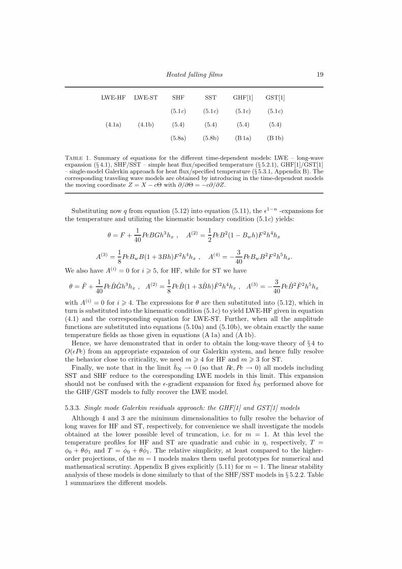
Table 1. Summary of equations for the different time-dependent models: LWE – long-waveexpansion (§ 4.1), SHF/SST – simple heat flux/specified temperature (§ 5.2.1), GHF[1]/GST[1]– single-model Galerkin approach for heat flux/specified temperature (§ 5.3.1, Appendix B). Thecorresponding traveling wave models are obtained by introducing in the time-dependent modelsthe moving coordinate Z = X − cΘ with ∂/∂Θ = −c∂/∂Z.

Substituting now q from equation (5.12) into equation (5.11), the ǫ1−n -expansions forthe temperature and utilizing the kinematic boundary condition (5.1c) yields:

θ = F +1

40PeBGh3hx , A(2) =

1

2PeB2(1 −Bwh)F

2h4hx

A(3) =1

8PeBwB(1 + 3Bh)F 2h4hx , A(4) = −

3

40PeBwB

2F 2h5hx.

We also have A(i) = 0 for i > 5, for HF, while for ST we have

θ = F +1

40PeBGh3hx , A(2) =

1

8PeB(1 + 3Bh)F 2h4hx , A(3) = −

3

40PeB2F 2h5hx

with A(i) = 0 for i > 4. The expressions for θ are then substituted into (5.12), which inturn is substituted into the kinematic condition (5.1c) to yield LWE-HF given in equation(4.1) and the corresponding equation for LWE-ST. Further, when all the amplitudefunctions are substituted into equations (5.10a) and (5.10b), we obtain exactly the sametemperature fields as those given in equations (A 1a) and (A 1b).

Hence, we have demonstrated that in order to obtain the long-wave theory of § 4 toO(ǫPe) from an appropriate expansion of our Galerkin system, and hence fully resolvethe behavior close to criticality, we need m > 4 for HF and m > 3 for ST.

Finally, we note that in the limit hN → 0 (so that Re, Pe → 0) all models includingSST and SHF reduce to the corresponding LWE models in this limit. This expansionshould not be confused with the ǫ-gradient expansion for fixed hN performed above forthe GHF/GST models to fully recover the LWE model.

5.3.3. Single mode Galerkin residuals approach: the GHF[1] and GST[1] models

Although 4 and 3 are the minimum dimensionalities to fully resolve the behavior oflong waves for HF and ST, respectively, for convenience we shall investigate the modelsobtained at the lower possible level of truncation, i.e. for m = 1. At this level thetemperature profiles for HF and ST are quadratic and cubic in η, respectively, T =φ0 + θφ1 and T = φ0 + θφ1. The relative simplicity, at least compared to the higher-order projections, of the m = 1 models makes them useful prototypes for numerical andmathematical scrutiny. Appendix B gives explicitly (5.11) for m = 1. The linear stabilityanalysis of these models is done similarly to that of the SHF/SST models in § 5.2.2. Table1 summarizes the different models.

20 P.M.J. Trevelyan, B. Scheid, C. Ruyer-Quil, S. Kalliadasis

(a) (b)

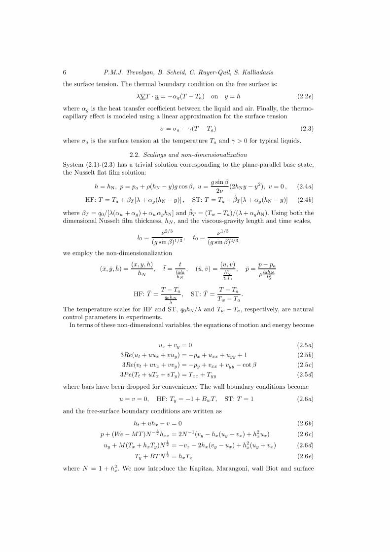
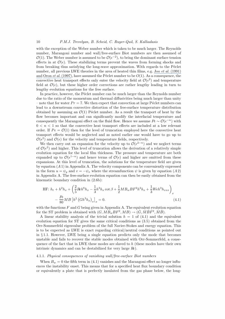
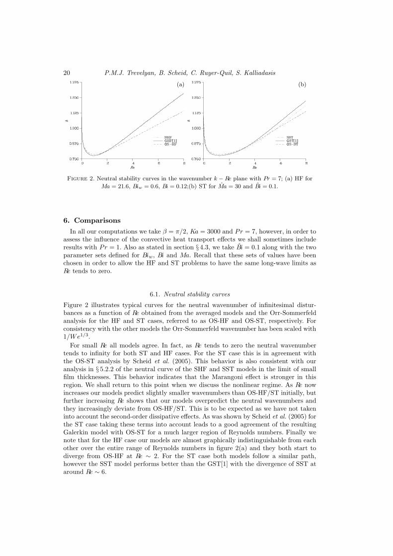
Figure 2. Neutral stability curves in the wavenumber k −Re plane with Pr = 7; (a) HF for

Ma = 21.6, Biw = 0.6, Bi = 0.12;(b) ST for Ma = 30 and Bi = 0.1.

6. Comparisons

In all our computations we take β = π/2, Ka = 3000 and Pr = 7, however, in order toassess the influence of the convective heat transport effects we shall sometimes includeresults with Pr = 1. Also as stated in section § 4.3, we take Bi = 0.1 along with the twoparameter sets defined for Biw, Bi and Ma. Recall that these sets of values have beenchosen in order to allow the HF and ST problems to have the same long-wave limits asRe tends to zero.

6.1. Neutral stability curves

Figure 2 illustrates typical curves for the neutral wavenumber of infinitesimal distur-bances as a function of Re obtained from the averaged models and the Orr-Sommerfeldanalysis for the HF and ST cases, referred to as OS-HF and OS-ST, respectively. Forconsistency with the other models the Orr-Sommerfeld wavenumber has been scaled with1/We1/3.

For small Re all models agree. In fact, as Re tends to zero the neutral wavenumbertends to infinity for both ST and HF cases. For the ST case this is in agreement withthe OS-ST analysis by Scheid et al. (2005). This behavior is also consistent with ouranalysis in § 5.2.2 of the neutral curve of the SHF and SST models in the limit of smallfilm thicknesses. This behavior indicates that the Marangoni effect is stronger in thisregion. We shall return to this point when we discuss the nonlinear regime. As Re nowincreases our models predict slightly smaller wavenumbers than OS-HF/ST initially, butfurther increasing Re shows that our models overpredict the neutral wavenumbers andthey increasingly deviate from OS-HF/ST. This is to be expected as we have not takeninto account the second-order dissipative effects. As was shown by Scheid et al. (2005) forthe ST case taking these terms into account leads to a good agreement of the resultingGalerkin model with OS-ST for a much larger region of Reynolds numbers. Finally wenote that for the HF case our models are almost graphically indistinguishable from eachother over the entire range of Reynolds numbers in figure 2(a) and they both start todiverge from OS-HF at Re ∼ 2. For the ST case both models follow a similar path,however the SST model performs better than the GST[1] with the divergence of SST ataround Re ∼ 6.

Heated falling films 21

6.2. Solitary waves

We now seek travelling wave solutions propagating at a constant speed c. We introducethe moving coordinate transformation Z = X−cΘ in the time-dependent models of table1 with ∂/∂Θ = −c∂/∂Z for the waves to be stationary in the moving frame.

The equation obtained from the LWE model in (4.2) in the moving frame can thenbe integrated once with the integration constant determined from the far field conditionh → 1 as Z → ±∞ which leads to a nonlinear eigenvalue problem for the speed of thetraveling waves c. For the weighted residuals models we use the kinematic condition (5.1c)which in the moving frame yields −ch′+q′ = 0. This can be integrated once and we fix theintegration constant by demanding h, q → 1, 1

3 as Z → ±∞. This gives a relation betweenthe flow rate and the film thickness, q = (1/3)+c(h−1). The SHF/GHF[1] traveling wavemodels consist of (5.4) and (5.8a)/(B1a) in the moving frame and with q eliminated fromthe above expression. These equations along with the boundary conditions h(±∞) = 1and θ(±∞) = F define the SHF/GHF[1] nonlinear eigenvalue problems for the speed cof the solitary waves. Finally, the SST/GST[1] traveling wave models consist of (5.4) and(5.8b)/(B1b,) in the moving frame and with q eliminated from the above expression.

These equations along with the boundary conditions h(±∞) = 1 and θ(±∞) = F definethe SHF/GHF[1] nonlinear eigenvalue problems for the speed c of the solitary waves.

Here we restrict our attention to single-hump solitary waves. They correspond to theprincipal homoclinic orbits of the dynamical systems corresponding to the traveling wavemodels. We compute them using the continuation software AUTO97 (Doedel et al. 1997).Appendix C analyzes the linearized traveling wave equations for the different models andprovides necessary conditions for the existence of solitary waves and sufficient conditionsfor the non-existence of such waves.

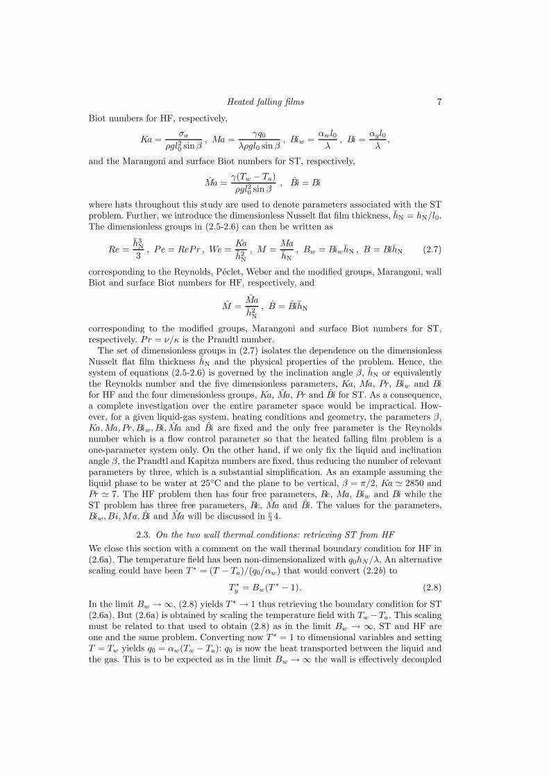
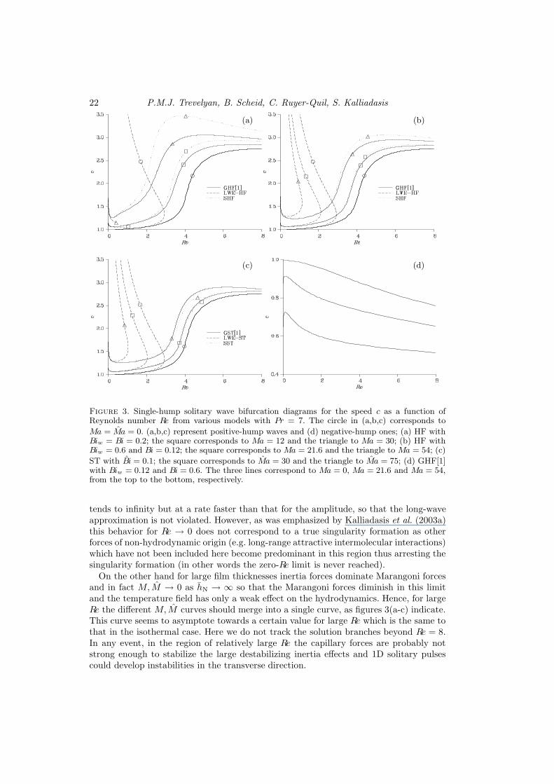
Figure 3 shows typical bifurcation diagrams for the speed c of the solitary waves asa function of Re. Figures 3(a-c) depict bifurcation diagrams for positive-hump waves(characterized by c > 1) and figure 3(d) negative-hump waves (characterized by c < 1).The ST problem has positive-hump waves only while the HF problem has negative-humpwaves co-existing with positive-hump ones. The ST problem admits negative multi-humpwaves but as we pointed out earlier here we focus on single-hump waves only.

We first discuss figures 3(a-c). Following our discussion in § 4.3 we take in these figurestwo sets of parameter values with Biw = Bi = 0.2 and Biw = 0.6, Bi = 0.12 (ourdiscussion in § 4.3 was based on LWE but for comparisons purposes we choose the samevalues for the other models). For the ST models we take Ma = 0, 30 and 75. Hence, thefirst set of values for the HF models is Ma = 0, 12 and 30 and the second set is Ma = 0,21.6 and 54.

Interestingly as Re tends to zero the speed (and amplitude) of the solitary pulsestends to infinity. This is consistent with the linear stability analysis in figure 2 whichindicates that the influence of the Marangoni effect is larger for small Re. This unusualbehavior was first pointed out for the ST case by Kalliadasis et al. (2003a) and wasfurther discussed by Scheid et al. (2005). In the limit of vanishing Reynolds number,inertia effects are negligible and the Marangoni effect is very strong. This is also evidentfrom our scalings in § 2.2, M = Ma/hN and M = Ma/h2

N, which show that M, M → ∞as hN → 0. In this region of small film thicknesses, the destabilizing forces are interfacialforces due to the Marangoni effect (capillary forces are always stabilizing). Contrast withthe isothermal falling film where the only destabilizing forces are inertia forces which arevanishing as Re tends to zero so that c in this region should approach the infinitesimalwave speed 1, as the Ma = Ma = 0 curves in figure 3 do. In the presence of the Marangonieffect our computations indicate that for Re → 0 the width of the solitary pulses also

22 P.M.J. Trevelyan, B. Scheid, C. Ruyer-Quil, S. Kalliadasis

(a) (b)

(c) (d)

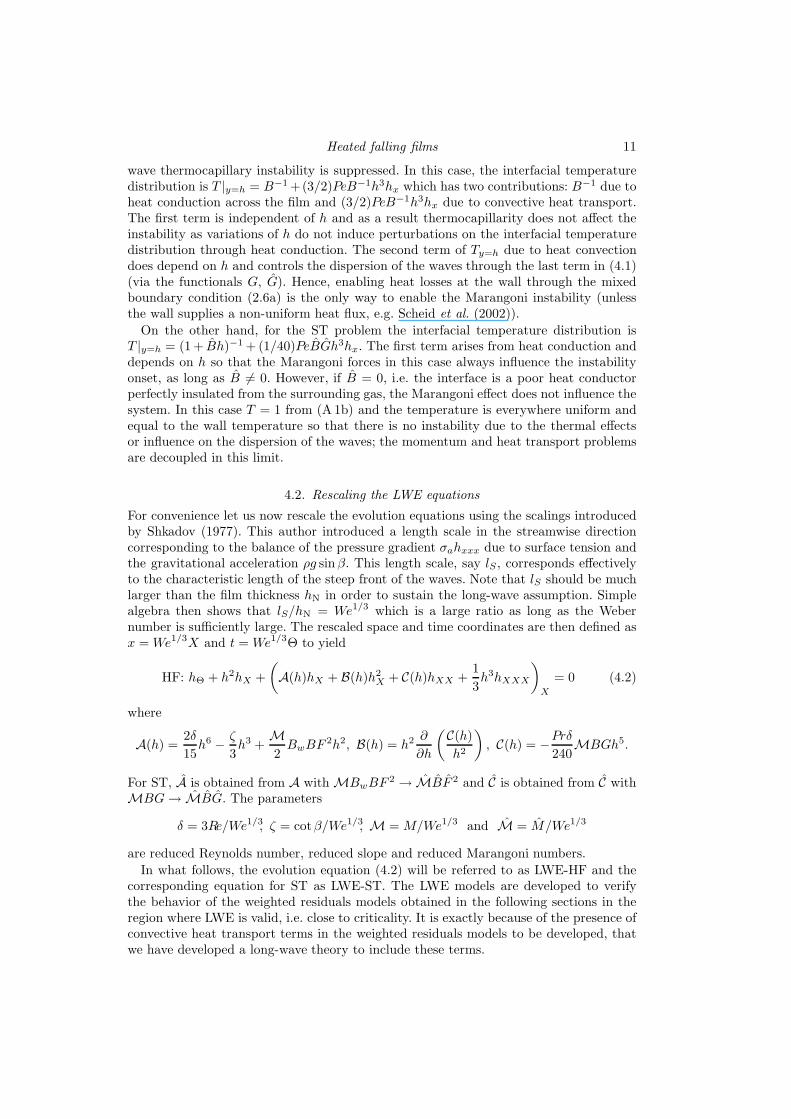
Figure 3. Single-hump solitary wave bifurcation diagrams for the speed c as a function ofReynolds number Re from various models with Pr = 7. The circle in (a,b,c) corresponds to

Ma = Ma = 0. (a,b,c) represent positive-hump waves and (d) negative-hump ones; (a) HF withBiw = Bi = 0.2; the square corresponds to Ma = 12 and the triangle to Ma = 30; (b) HF withBiw = 0.6 and Bi = 0.12; the square corresponds to Ma = 21.6 and the triangle to Ma = 54; (c)

ST with Bi = 0.1; the square corresponds to Ma = 30 and the triangle to Ma = 75; (d) GHF[1]with Biw = 0.12 and Bi = 0.6. The three lines correspond to Ma = 0, Ma = 21.6 and Ma = 54,from the top to the bottom, respectively.

tends to infinity but at a rate faster than that for the amplitude, so that the long-waveapproximation is not violated. However, as was emphasized by Kalliadasis et al. (2003a)this behavior for Re → 0 does not correspond to a true singularity formation as otherforces of non-hydrodynamic origin (e.g. long-range attractive intermolecular interactions)which have not been included here become predominant in this region thus arresting thesingularity formation (in other words the zero-Re limit is never reached).

On the other hand for large film thicknesses inertia forces dominate Marangoni forcesand in fact M, M → 0 as hN → ∞ so that the Marangoni forces diminish in this limitand the temperature field has only a weak effect on the hydrodynamics. Hence, for largeRe the different M, M curves should merge into a single curve, as figures 3(a-c) indicate.This curve seems to asymptote towards a certain value for large Re which is the same tothat in the isothermal case. Here we do not track the solution branches beyond Re = 8.In any event, in the region of relatively large Re the capillary forces are probably notstrong enough to stabilize the large destabilizing inertia effects and 1D solitary pulsescould develop instabilities in the transverse direction.

Heated falling films 23

Figures 3(a-c) indicate that both LWE models exhibit an unrealistic behavior withbranch multiplicity and turning points at particular values of Re. By analogy now withthe isothermal case and as we discussed in § 1 we expect that LWE exhibits a finite-time blow-up behavior for Re larger than the values corresponding to the turning points(this has been confirmed by time-dependent computations). Obviously this catastrophicbehavior is related to the non-existence of solitary waves and indicates the inability ofLWE to correctly describe nonlinear waves far from criticality. Moreover figure 3(a) showsthe existence of limit points where LWE simply terminates, not observed before in studiesof the isothermal falling film. In Appendix C1 we show that this corresponds to all ofthe spatial eigenvalues of the linearized system at h = 1 having real parts with the samesign so that homoclinic orbits do not exist.

Figures 3(a-c) also indicate that all models collapse into a single line in the regionRe → 0. This is consistent with our observation at the end of § 5.3.2. Also for Ma =Ma = 0 (curves marked with a circle) the figures 3(a), (b) and (c) give the same solutionbranches for each of the LWE, simple weighted residuals and Galerkin approximations,as expected. We note that figures 3(b) and 3(c) (with the exception of the Ma = Ma = 0curves) are almost identical for LWE. This is consistent with our discussion in § 4.3:indeed C > 0 in figure 3(b) while for LWE-ST C is always > 0. The Galerkin models infigures 3(b,c) are qualitatively similar, note, however, the relatively flat region aroundRe ∼ 2 for GST[1] with Ma = 75. The simple weighted residuals models in figures 3(b,c)are also qualitatively similar, notice however, that SHF is slightly above GHF[1] in figure3(b) and slightly below GHF[1] in figure 3(c). Note that in figure 3(c) we were not ableto continue the numerical solution to Re above ∼ 5 due to the fact that the coefficientof θZ is close to zero in this region (see § 8.3). This is purely a numerical difficulty anddoes not imply that the solution ceases to exist after this point.

Further, we note that figures 3(a) and 3(b) (again with the exception of the Ma =Ma = 0 curves) are different for all LWE models. Now C < 0 in figure 3(a) while forLWE-ST C is always > 0. Following then from our discussion in § 4.3 the LWE-HF andLWE-ST models show different behaviors. The simple weighted residuals and Galerkinmodels in figures 3(a) are qualitatively similar to those in figure 3(b), however, a markeddifference between the two is observed as the Marangoni number increases. Note alsothat in figure 3(a) the SHF model predicts faster waves than the GHF[1] model whilstin figure 3(c) we see that the SST model predicts slower waves than the GST[1] model.

We now turn to the negative-hump waves in figure 3(d). With the exception of theMa = 0 curve that approaches the speed of 1 as Re tends to zero, for the remainingcurves the speed approaches minus infinity, consistent with our earlier observation thatthe Marangoni effect is very strong in this region. Again forces of non-hydrodynamicorigin such as intermolecular interactions would introduce a lower bound here especiallyas for negative-hump waves the largest free-surface deformation is towards the wall. Onthe other hand, for large Re all curves merge into a single one like with the positive-humpwaves but one needs to go to sufficiently large Re, e.g. for Re > 60 the three differentcurves have speeds in the interval [0.4, 0.5]. The final asymptotic value for the threecurves is c ∼ 0.4.

7. Spatio-temporal dynamics

We now illustrate the spatio-temporal dynamics of the heated falling film by usingthe GST[1] and GHF[1] models. The previous studies by Kalliadasis et al. (2003a) andScheid et al. (2005) on heated falling films focused on the construction of stationarysolitary waves only (using ST) without any time-dependent computations. For our com-

24 P.M.J. Trevelyan, B. Scheid, C. Ruyer-Quil, S. Kalliadasis(a) (b)

(c) (d)

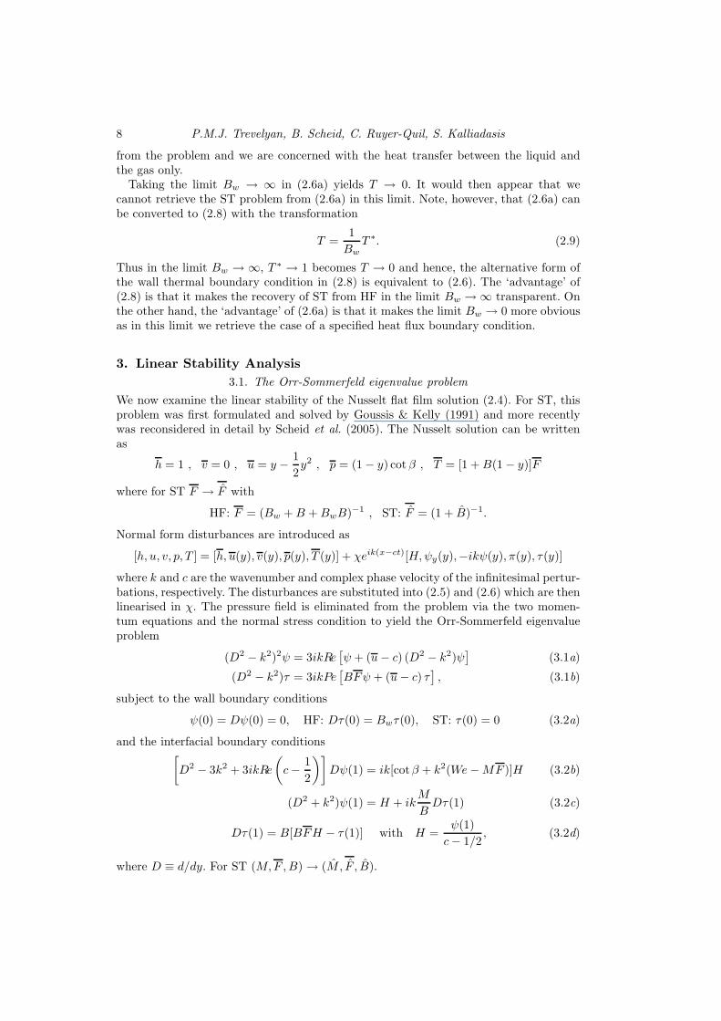
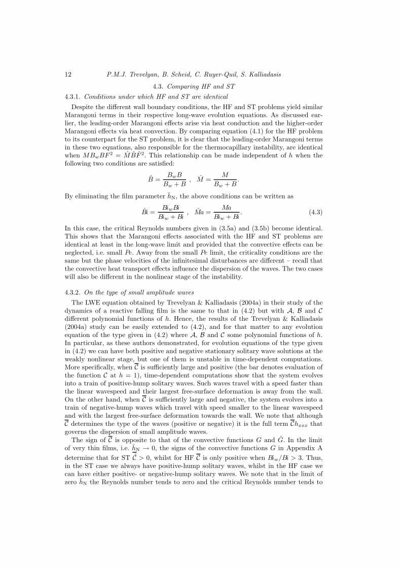
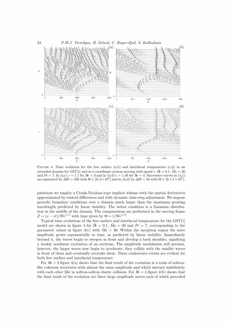
Figure 4. Time evolution for the free surface (a,b) and interfacial temperature (c,d) in an

extended domain for GST[1] and in a coordinate system moving with speed c. Bi = 0.1, Ma = 30and Pr = 7. In (a,c) c = 1.1 for Re = 3 and in (b,d) c = 1.46 for Re = 4. Successive curves in (a,c)are separated by ∆Θ = 100 with Θ ∈ [0, 3×103] and in (b,d) by ∆Θ = 50 with Θ ∈ [0, 1.5×103 ].

putations we employ a Crank-Nicolson-type implicit scheme with the spatial derivativesapproximated by central differences and with dynamic time-step adjustment. We imposeperiodic boundary conditions over a domain much larger than the maximum growingwavelength predicted by linear stability. The initial condition is a Gaussian distribu-tion in the middle of the domain. The computations are performed in the moving frameZ = (x− ct)/We1/3 with time given by Θ = t/We1/3.

Typical time evolutions of the free surface and interfacial temperature for the GST[1]model are shown in figure 4 for Bi = 0.1, Ma = 30 and Pr = 7, corresponding to theparameter values in figure 3(c) with Ma = 30. Within the inception region the waveamplitude grows exponentially in time, as predicted by linear stability. Immediatelybeyond it, the waves begin to steepen in front and develop a back shoulder, signifyinga weakly nonlinear excitation of an overtone. The amplitude modulation still persists,however, the larger waves now begin to accelerate, they collide with the smaller wavesin front of them and eventually overtake them. These coalescence events are evident forboth free surface and interfacial temperature.

For Re = 3 figure 4(a) shows that the final result of the evolution is a train of soliton-like coherent structures with almost the same amplitude and which interact indefinitelywith each other like in soliton-soliton elastic collision. For Re = 4 figure 4(b) shows thatthe final result of the evolution are three large amplitude waves each of which preceded

Heated falling films 25(a) (b)

(c) (d)

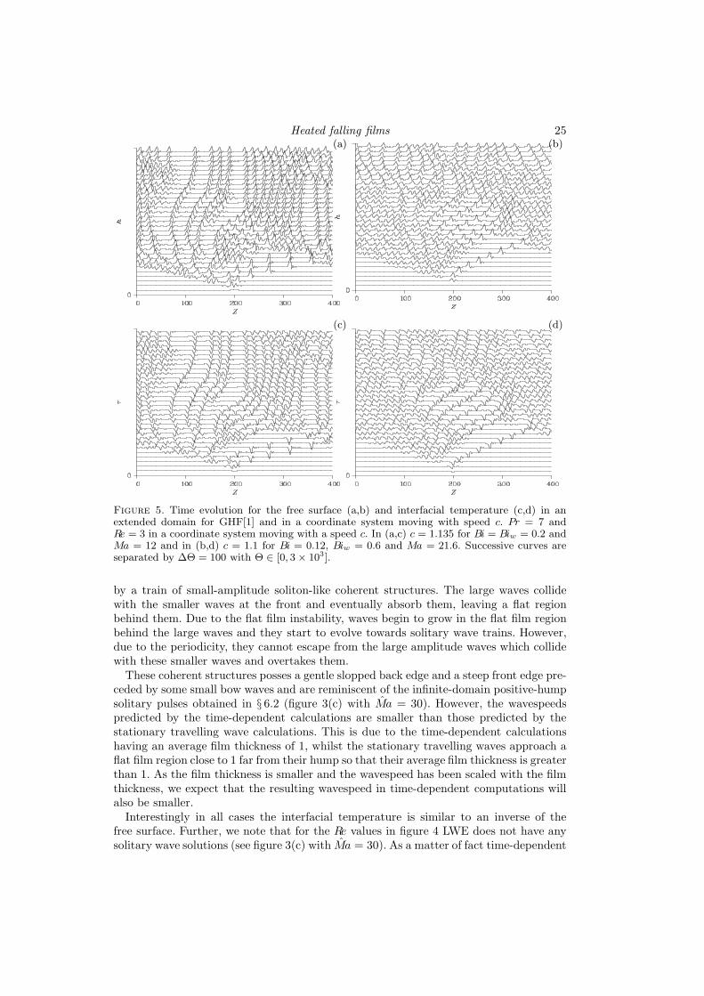
Figure 5. Time evolution for the free surface (a,b) and interfacial temperature (c,d) in anextended domain for GHF[1] and in a coordinate system moving with speed c. Pr = 7 andRe = 3 in a coordinate system moving with a speed c. In (a,c) c = 1.135 for Bi = Biw = 0.2 andMa = 12 and in (b,d) c = 1.1 for Bi = 0.12, Biw = 0.6 and Ma = 21.6. Successive curves areseparated by ∆Θ = 100 with Θ ∈ [0, 3 × 103].

by a train of small-amplitude soliton-like coherent structures. The large waves collidewith the smaller waves at the front and eventually absorb them, leaving a flat regionbehind them. Due to the flat film instability, waves begin to grow in the flat film regionbehind the large waves and they start to evolve towards solitary wave trains. However,due to the periodicity, they cannot escape from the large amplitude waves which collidewith these smaller waves and overtakes them.

These coherent structures posses a gentle slopped back edge and a steep front edge pre-ceded by some small bow waves and are reminiscent of the infinite-domain positive-humpsolitary pulses obtained in § 6.2 (figure 3(c) with Ma = 30). However, the wavespeedspredicted by the time-dependent calculations are smaller than those predicted by thestationary travelling wave calculations. This is due to the time-dependent calculationshaving an average film thickness of 1, whilst the stationary travelling waves approach aflat film region close to 1 far from their hump so that their average film thickness is greaterthan 1. As the film thickness is smaller and the wavespeed has been scaled with the filmthickness, we expect that the resulting wavespeed in time-dependent computations willalso be smaller.

Interestingly in all cases the interfacial temperature is similar to an inverse of thefree surface. Further, we note that for the Re values in figure 4 LWE does not have anysolitary wave solutions (see figure 3(c) with Ma = 30). As a matter of fact time-dependent

26 P.M.J. Trevelyan, B. Scheid, C. Ruyer-Quil, S. Kalliadasis(a) (b)

(c) (d)

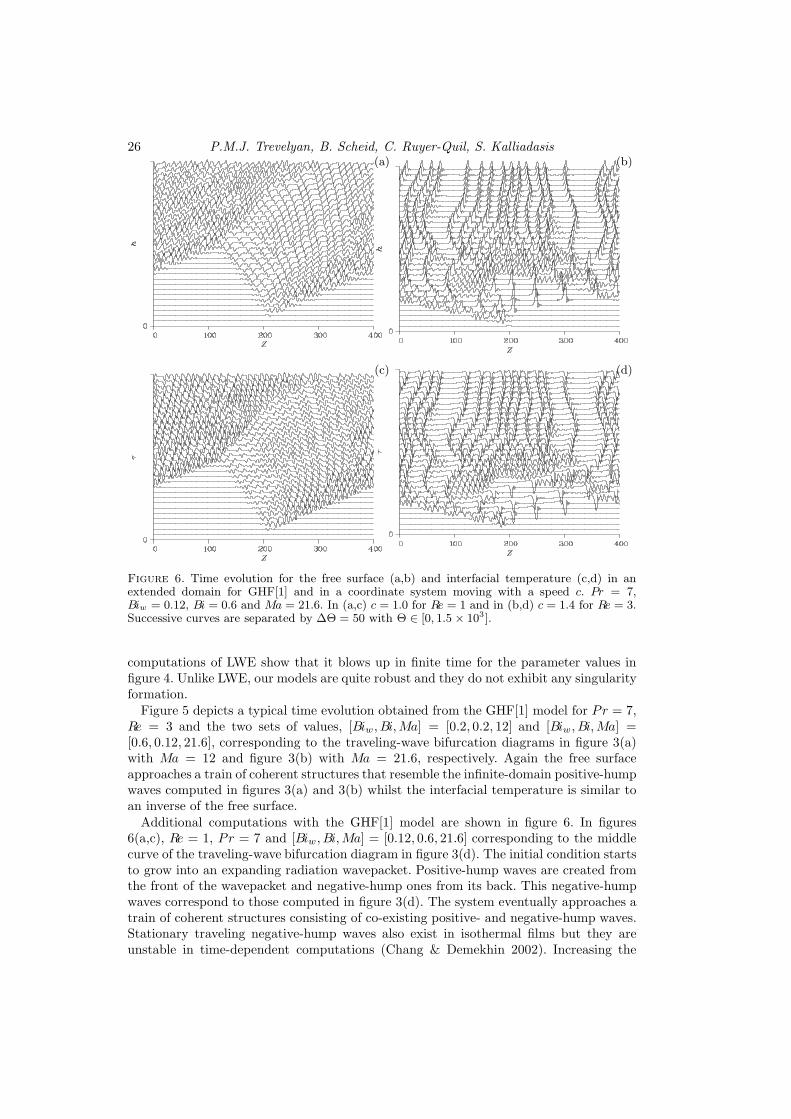
Figure 6. Time evolution for the free surface (a,b) and interfacial temperature (c,d) in anextended domain for GHF[1] and in a coordinate system moving with a speed c. Pr = 7,Biw = 0.12, Bi = 0.6 and Ma = 21.6. In (a,c) c = 1.0 for Re = 1 and in (b,d) c = 1.4 for Re = 3.Successive curves are separated by ∆Θ = 50 with Θ ∈ [0, 1.5 × 103].

computations of LWE show that it blows up in finite time for the parameter values infigure 4. Unlike LWE, our models are quite robust and they do not exhibit any singularityformation.

Figure 5 depicts a typical time evolution obtained from the GHF[1] model for Pr = 7,Re = 3 and the two sets of values, [Biw, Bi,Ma] = [0.2, 0.2, 12] and [Biw, Bi,Ma] =[0.6, 0.12, 21.6], corresponding to the traveling-wave bifurcation diagrams in figure 3(a)with Ma = 12 and figure 3(b) with Ma = 21.6, respectively. Again the free surfaceapproaches a train of coherent structures that resemble the infinite-domain positive-humpwaves computed in figures 3(a) and 3(b) whilst the interfacial temperature is similar toan inverse of the free surface.

Additional computations with the GHF[1] model are shown in figure 6. In figures6(a,c), Re = 1, Pr = 7 and [Biw, Bi,Ma] = [0.12, 0.6, 21.6] corresponding to the middlecurve of the traveling-wave bifurcation diagram in figure 3(d). The initial condition startsto grow into an expanding radiation wavepacket. Positive-hump waves are created fromthe front of the wavepacket and negative-hump ones from its back. This negative-humpwaves correspond to those computed in figure 3(d). The system eventually approaches atrain of coherent structures consisting of co-existing positive- and negative-hump waves.Stationary traveling negative-hump waves also exist in isothermal films but they areunstable in time-dependent computations (Chang & Demekhin 2002). Increasing the

Heated falling films 27

Reynolds number to Re = 3 in figures 6(b,d) suppresses the negative-hump waves andleads to a train of positive-hump ones. Note that the large-time behavior of the freesurface in figure 6(a) is reminiscent of the Kuramoto-Sivashinsky (KS) spatio-temporalchaos/turbulent-like dynamics. On the other hand, in figure 6(b) the surface approaches aseries of ‘bounded states’ like in Kawahara equation (KS with dispersion) for sufficientlylarge dispersion (Kawahara 1983). This highlights the significance of the dispersive effectassociated with the Peclet number: increasing the Pclet number ‘regularizes’ the systemand selects a regular train of large amplitude solitary pulses.

8. Finite differences solutions of the energy equation for HF and ST:FDHF and FDST

We now contrast the interfacial temperature distribution obtained from our (one-dimensional) one-mode averaged models with the solution of the two-dimensional (2D)energy equation in (5.7), which is after all the equation we trying to model. We setMa = Ma = 0. The reason for this is two-fold: (i) the hydrodynamic and thermal prob-lems are decoupled so that the temperature field does not have any influence on thefilm thickness. However, the evolution of the film thickness does affect the temperaturefield. We emphasize that Shkadov’s IBL solitary wave solution branches are in quantita-tive agreement with the boundary-layer (Demekhin et al. 1987) and full Navier-Stokesequations (Salamon et al. 1994; Ramaswamy et al. 1996) while the single-mode correctedShkadov model in (5.4) (with M = 0) is in quantitative agreement with full Navier-Stokes(Ruyer-Quil & Manneville 2000, 2002). Hence we do have a proper description of the hy-drodynamics; (ii) the decoupling of hydrodynamics from energy significantly simplifiesthe computations of the 2D temperature field.

Substituting the flow field from (5.2) and (2.5a) into (5.7), we obtain

Tηη =Prδ

2

[(

3qh(2η − η2) − 2ch2)

TZ + chhZη(η − 1)(η − 2)Tη

]

(8.1a)

subject to the boundary conditions

Tη = −BhT on η = 1 (8.1b)

Tη = −h+BwhT on η = 0 for HF (8.1c)

T = 1 on η = 0 for ST (8.1d)

which is solved in 2D along with periodic boundary conditions in the Z-direction whereh is obtained from the isothermal momentum equation (5.4) in the moving frame Z withq = 1

3 + c(h − 1). The above system was solved numerically using a finite-differencingscheme. We shall refer to the numerical solution of equations (8.1a), (8.1b) and (8.1c) as‘finite differences for HF’ or FDHF and the numerical solution of equations (8.1a), (8.1b)and (8.1d) as ‘finite differences for ST’ or FDST. Note that although the computationswere performed over an extended domain here we only illustrate the solutions near thewave maximum.

Figure 7 compares the temperature distributions obtained for the different models forPr = 7, Ma = Ma = 0 and in the region of moderate Re. LWE is not included as inthis region it does not predict the existence of solitary waves. All models use the sameisothermal fluid flow and free surface. Clearly, for small values of Re all models are ingood agreement, as expected. For larger Re we observe a difference between our modelsand FD. This difference increases as Re increases. More specifically, figures 7(a,c,e) forRe = 10/3 show that the interfacial temperature distributions obtained from our averaged

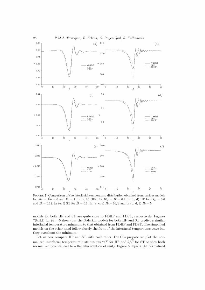
28 P.M.J. Trevelyan, B. Scheid, C. Ruyer-Quil, S. Kalliadasis

(a) (b)

(c) (d)

(e) (f)

Figure 7. Comparison of the interfacial temperature distribution obtained from various modelsfor Ma = Ma = 0 and Pr = 7. In (a, b) (HF) for Biw = Bi = 0.2. In (c, d) HF for Biw = 0.6

and Bi = 0.12. In (e, f) ST for Bi = 0.1. In (a, c, e) Re = 10/3 and in (b, d, f) Re = 5.

models for both HF and ST are quite close to FDHF and FDST, respectively. Figures7(b,d,f) for Re = 5 show that the Galerkin models for both HF and ST predict a similarinterfacial temperature minimum to that obtained from FDHF and FDST. The simplifiedmodels on the other hand follow closely the front of the interfacial temperature wave butthey overshoot the minimum.

Let us now compare HF and ST with each other. For this purpose we plot the nor-

malized interfacial temperature distributions θ/F for HF and θ/F for ST so that bothnormalized profiles lead to a flat film solution of unity. Figure 8 depicts the normalized

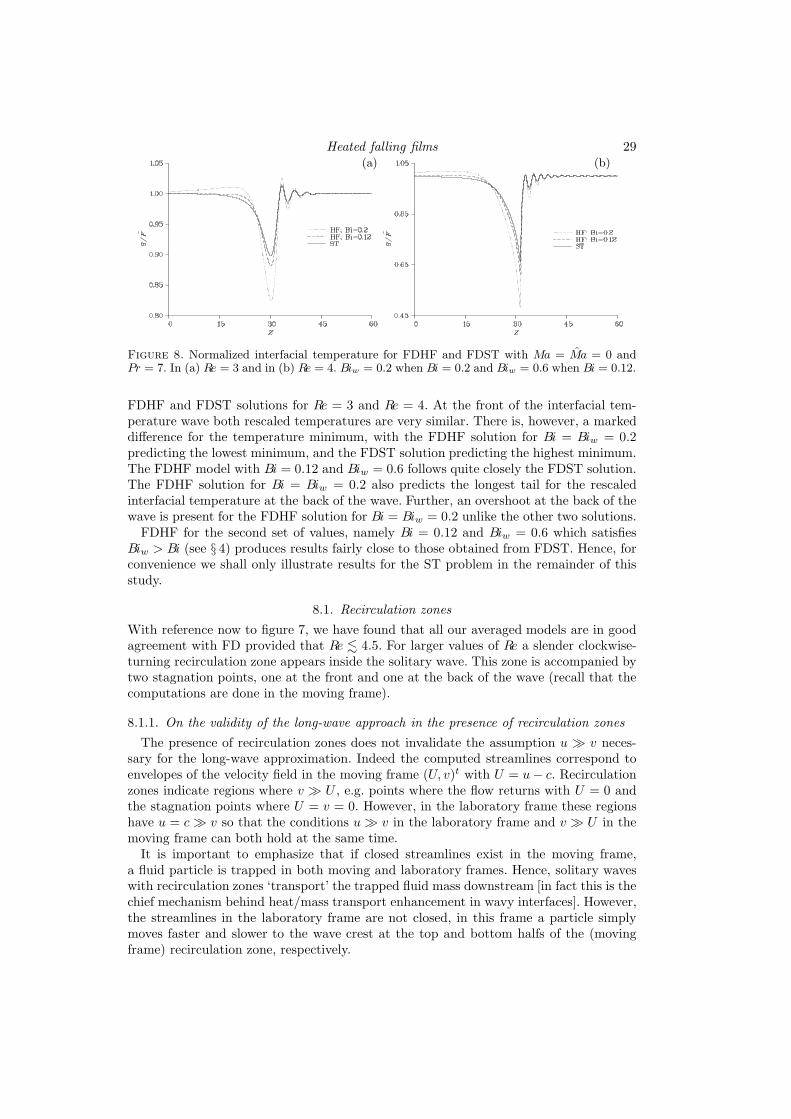
Heated falling films 29(a) (b)

Figure 8. Normalized interfacial temperature for FDHF and FDST with Ma = Ma = 0 andPr = 7. In (a) Re = 3 and in (b) Re = 4. Biw = 0.2 when Bi = 0.2 and Biw = 0.6 when Bi = 0.12.

FDHF and FDST solutions for Re = 3 and Re = 4. At the front of the interfacial tem-perature wave both rescaled temperatures are very similar. There is, however, a markeddifference for the temperature minimum, with the FDHF solution for Bi = Biw = 0.2predicting the lowest minimum, and the FDST solution predicting the highest minimum.The FDHF model with Bi = 0.12 and Biw = 0.6 follows quite closely the FDST solution.The FDHF solution for Bi = Biw = 0.2 also predicts the longest tail for the rescaledinterfacial temperature at the back of the wave. Further, an overshoot at the back of thewave is present for the FDHF solution for Bi = Biw = 0.2 unlike the other two solutions.

FDHF for the second set of values, namely Bi = 0.12 and Biw = 0.6 which satisfiesBiw > Bi (see § 4) produces results fairly close to those obtained from FDST. Hence, forconvenience we shall only illustrate results for the ST problem in the remainder of thisstudy.

8.1. Recirculation zones

With reference now to figure 7, we have found that all our averaged models are in goodagreement with FD provided that Re . 4.5. For larger values of Re a slender clockwise-turning recirculation zone appears inside the solitary wave. This zone is accompanied bytwo stagnation points, one at the front and one at the back of the wave (recall that thecomputations are done in the moving frame).

8.1.1. On the validity of the long-wave approach in the presence of recirculation zones

The presence of recirculation zones does not invalidate the assumption u ≫ v neces-sary for the long-wave approximation. Indeed the computed streamlines correspond toenvelopes of the velocity field in the moving frame (U, v)t with U = u− c. Recirculationzones indicate regions where v ≫ U , e.g. points where the flow returns with U = 0 andthe stagnation points where U = v = 0. However, in the laboratory frame these regionshave u = c ≫ v so that the conditions u ≫ v in the laboratory frame and v ≫ U in themoving frame can both hold at the same time.

It is important to emphasize that if closed streamlines exist in the moving frame,a fluid particle is trapped in both moving and laboratory frames. Hence, solitary waveswith recirculation zones ‘transport’ the trapped fluid mass downstream [in fact this is thechief mechanism behind heat/mass transport enhancement in wavy interfaces]. However,the streamlines in the laboratory frame are not closed, in this frame a particle simplymoves faster and slower to the wave crest at the top and bottom halfs of the (movingframe) recirculation zone, respectively.

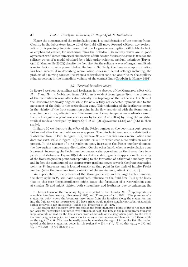
30 P.M.J. Trevelyan, B. Scheid, C. Ruyer-Quil, S. Kalliadasis

Hence the appearance of the recirculation zone is a manifestation of the moving frame.Clearly, in the laboratory frame all of the fluid will move forward without any recircu-lation. It is precisely for this reason that the long-wave assumption still holds. In fact,as emphasized earlier, for isothermal films the Shkadov IBL solitary waves are in goodagreement with direct numerical simulations of full Navier-Stokes (the same is true for thesolitary waves of a model obtained by a high-order weighted residual technique (Ruyer-Quil & Manneville 2002)) despite the fact that for the solitary waves of largest amplitudea recirculation zone is present below the hump. Similarly, the long-wave approximationhas been successful in describing recirculation zones in different settings including, theproblem of a moving contact line where a recirculation zone can occur below the capillaryridge appearing in the immediate vicinity of the contact line (Goodwin & Homsy 1991).

8.2. Thermal boundary layers

In figure 9 we show streamlines and isotherms in the absence of the Marangoni effect withPr = 7 and Re = 4, 5 obtained from FDST. As is evident from figures 9(c,d) the presenceof the recirculation zone alters dramatically the topology of the isotherms. For Re = 4the isotherms are nearly aligned while for Re = 5 they are deflected upwards due to themovement of the fluid in the recirculation zone. This tightening of the isotherms occursin the vicinity of the front stagnation point in the flow associated with the formation ofsteep temperature gradients there. The formation of steep temperature gradients close tothe front stagnation point was also shown by Scheid et al. (2005) by using the weightedresidual models developed by Ruyer-Quil et al. (2005)(systems (4.18) and (6.6) in theirstudy).

In figure 10 we illustrate the effect of the Peclet number on the heat transport processbefore and after the recirculation zone appears. The interfacial temperature distributionis obtained from FDST. In figure 10(a) we take Re = 4 in which case a recirculation zonedoes not exist while in figure 10(b) we take Re = 5 in which case a recirculation zone ispresent. In the absence of a recirculation zone, increasing the Peclet number dampensthe free-surface temperature distribution. On the other hand, when a recirculation zoneis present, increasing the Peclet number causes a sharp gradient on the free-surface tem-perature distribution. Figure 10(c) shows that the sharp gradient appears in the vicinityof the front stagnation point corresponding to the formation of a thermal boundary layerand in fact the maximum of the temperature gradient moves towards the front stagnationpoint as Pr increases and is located exactly at that point in the limit of infinite Pecletnumber (note the non-monotonic variation of the maximum gradient with h) †‡.

We expect that in the presence of the Marangoni effect and for large Peclet numbers,the sharp spike in θZ will have a significant influence on the fluid flow. It is quite likelythat in this case thermocapillarity might cause the formation of a recirculation zoneat smaller Re and might tighten both streamlines and isotherms due to enhancing the

† The thickness of the boundary layer is expected to be of order Pe−1/2 appropriate fora mobile interface, see e.g. Shraiman (1987) and Trevelyan et al. (2002). The presence of astagnation point where the boundary layer turns from the interface along the stagnation lineinto the fluid as well as the presence of a free surface would make a singular perturbation analysisrather involved if not impossible (unlike e.g. Trevelyan et al. (2002)).

‡ The reason the boundary layer appears at the front stagnation point is due to the fact thatfor large Pe (convection dominates over diffusion of heat) the flow in the moving frame transferslarge amounts of heat on the free surface from either side of the stagnation point: to the left ofthe front stagnation point we have a clockwise recirculation zone and hence U > 0 there whileto the right U < 0. This can be easily seen by checking the sign of U on the flat film regionahead of the front stagnation point: in this region ψ = (3h− y)(y2/6) so that u|y=1 = 1/2 andU|y=1 = (1/2) − c < 0 since c > 1.

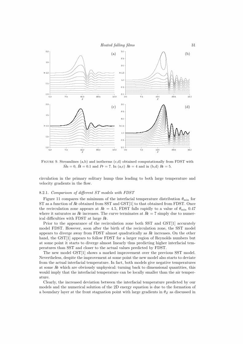
Heated falling films 31

(a) (b)

(c) (d)

Figure 9. Streamlines (a,b) and isotherms (c,d) obtained computationally from FDST with

Ma = 0, Bi = 0.1 and Pr = 7. In (a,c) Re = 4 and in (b,d) Re = 5.

circulation in the primary solitary hump thus leading to both large temperature andvelocity gradients in the flow.

8.2.1. Comparison of different ST models with FDST

Figure 11 compares the minimum of the interfacial temperature distribution θmin forST as a function of Re obtained from SST and GST[1] to that obtained from FDST. Oncethe recirculation zone appears at Re = 4.5, FDST falls rapidly to a value of θmin 0.47where it saturates as Re increases. The curve terminates at Re = 7 simply due to numer-ical difficulties with FDST at large Re.

Prior to the appearance of the recirculation zone both SST and GST[1] accuratelymodel FDST. However, soon after the birth of the recirculation zone, the SST modelappears to diverge away from FDST almost quadratically as Re increases. On the otherhand, the GST[1] appears to follow FDST for a larger region of Reynolds numbers butat some point it starts to diverge almost linearly thus predicting higher interfacial tem-peratures than SST and closer to the actual values predicted by FDST.

The new model GST[1] shows a marked improvement over the previous SST model.Nevertheless, despite the improvement at some point the new model also starts to deviatefrom the actual interfacial temperature. In fact, both models give negative temperaturesat some Re which are obviously unphysical: turning back to dimensional quantities, thiswould imply that the interfacial temperature can be locally smaller than the air temper-ature.

Clearly, the increased deviation between the interfacial temperature predicted by ourmodels and the numerical solution of the 2D energy equation is due to the formation ofa boundary layer at the front stagnation point with large gradients in θZ as discussed in

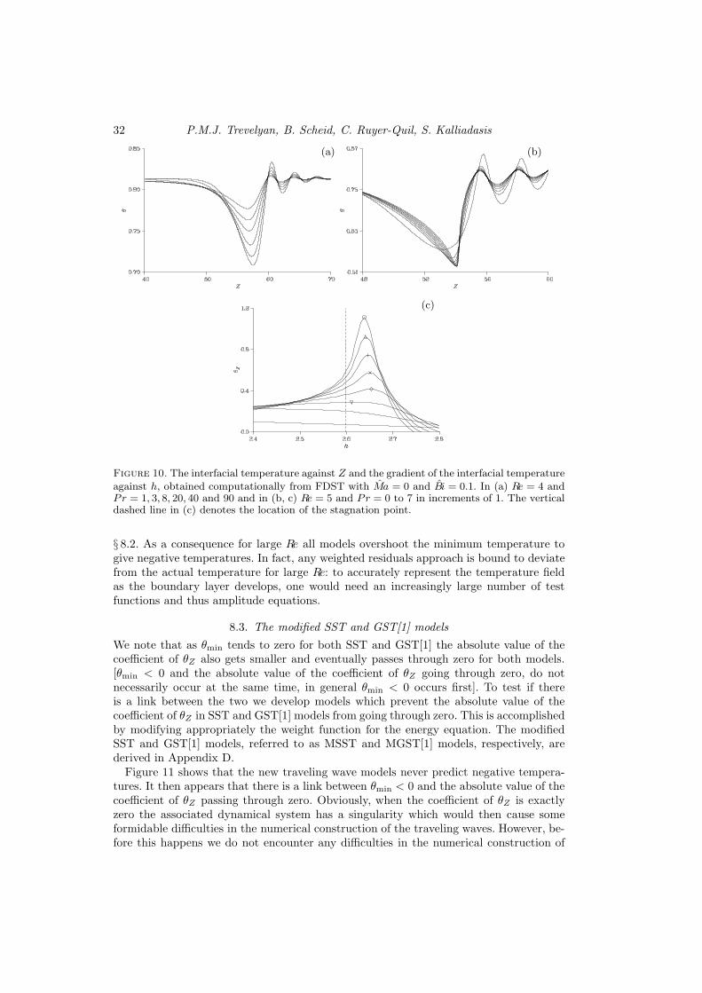
32 P.M.J. Trevelyan, B. Scheid, C. Ruyer-Quil, S. Kalliadasis

(a) (b)

(c)

Figure 10. The interfacial temperature against Z and the gradient of the interfacial temperatureagainst h, obtained computationally from FDST with Ma = 0 and Bi = 0.1. In (a) Re = 4 andPr = 1, 3, 8, 20, 40 and 90 and in (b, c) Re = 5 and Pr = 0 to 7 in increments of 1. The verticaldashed line in (c) denotes the location of the stagnation point.

§ 8.2. As a consequence for large Re all models overshoot the minimum temperature togive negative temperatures. In fact, any weighted residuals approach is bound to deviatefrom the actual temperature for large Re: to accurately represent the temperature fieldas the boundary layer develops, one would need an increasingly large number of testfunctions and thus amplitude equations.

8.3. The modified SST and GST[1] models

We note that as θmin tends to zero for both SST and GST[1] the absolute value of thecoefficient of θZ also gets smaller and eventually passes through zero for both models.[θmin < 0 and the absolute value of the coefficient of θZ going through zero, do notnecessarily occur at the same time, in general θmin < 0 occurs first]. To test if thereis a link between the two we develop models which prevent the absolute value of thecoefficient of θZ in SST and GST[1] models from going through zero. This is accomplishedby modifying appropriately the weight function for the energy equation. The modifiedSST and GST[1] models, referred to as MSST and MGST[1] models, respectively, arederived in Appendix D.

Figure 11 shows that the new traveling wave models never predict negative tempera-tures. It then appears that there is a link between θmin < 0 and the absolute value of thecoefficient of θZ passing through zero. Obviously, when the coefficient of θZ is exactlyzero the associated dynamical system has a singularity which would then cause someformidable difficulties in the numerical construction of the traveling waves. However, be-fore this happens we do not encounter any difficulties in the numerical construction of

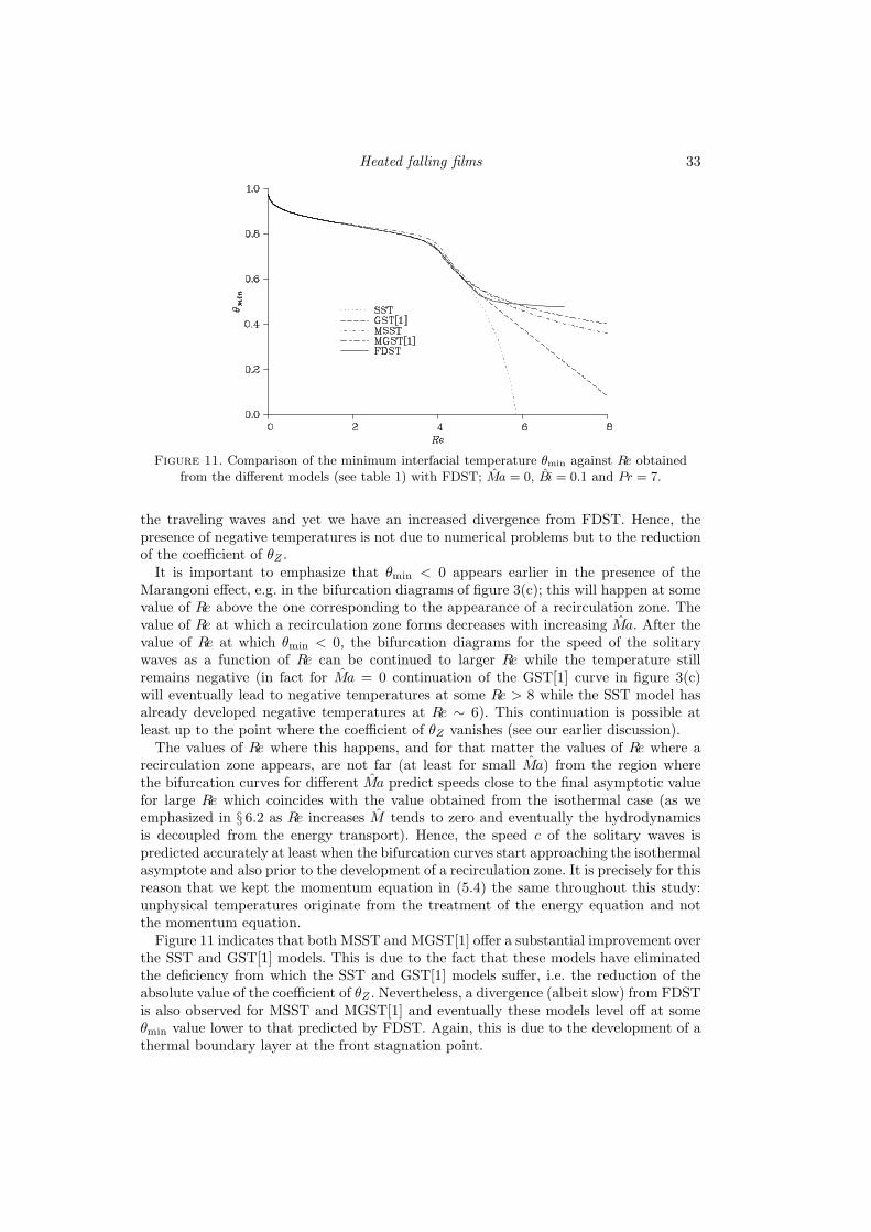
Heated falling films 33

Figure 11. Comparison of the minimum interfacial temperature θmin against Re obtainedfrom the different models (see table 1) with FDST; Ma = 0, Bi = 0.1 and Pr = 7.

the traveling waves and yet we have an increased divergence from FDST. Hence, thepresence of negative temperatures is not due to numerical problems but to the reductionof the coefficient of θZ .

It is important to emphasize that θmin < 0 appears earlier in the presence of theMarangoni effect, e.g. in the bifurcation diagrams of figure 3(c); this will happen at somevalue of Re above the one corresponding to the appearance of a recirculation zone. Thevalue of Re at which a recirculation zone forms decreases with increasing Ma. After thevalue of Re at which θmin < 0, the bifurcation diagrams for the speed of the solitarywaves as a function of Re can be continued to larger Re while the temperature stillremains negative (in fact for Ma = 0 continuation of the GST[1] curve in figure 3(c)will eventually lead to negative temperatures at some Re > 8 while the SST model hasalready developed negative temperatures at Re ∼ 6). This continuation is possible atleast up to the point where the coefficient of θZ vanishes (see our earlier discussion).

The values of Re where this happens, and for that matter the values of Re where arecirculation zone appears, are not far (at least for small Ma) from the region wherethe bifurcation curves for different Ma predict speeds close to the final asymptotic valuefor large Re which coincides with the value obtained from the isothermal case (as weemphasized in § 6.2 as Re increases M tends to zero and eventually the hydrodynamicsis decoupled from the energy transport). Hence, the speed c of the solitary waves ispredicted accurately at least when the bifurcation curves start approaching the isothermalasymptote and also prior to the development of a recirculation zone. It is precisely for thisreason that we kept the momentum equation in (5.4) the same throughout this study:unphysical temperatures originate from the treatment of the energy equation and notthe momentum equation.

Figure 11 indicates that both MSST and MGST[1] offer a substantial improvement overthe SST and GST[1] models. This is due to the fact that these models have eliminatedthe deficiency from which the SST and GST[1] models suffer, i.e. the reduction of theabsolute value of the coefficient of θZ . Nevertheless, a divergence (albeit slow) from FDSTis also observed for MSST and MGST[1] and eventually these models level off at someθmin value lower to that predicted by FDST. Again, this is due to the development of athermal boundary layer at the front stagnation point.

34 P.M.J. Trevelyan, B. Scheid, C. Ruyer-Quil, S. Kalliadasis

9. Conclusion

We have analyzed the dynamics of a film falling down a heated wall. We consideredtwo types of wall boundary conditions: heat flux (HF) and specified temperature (ST).The flow and heat transport were first modeled with a long-wave theory for large Pecletnumbers. We subsequently developed averaged models using a weighted residuals ap-proach. In these models the flow was modeled via a first order in ǫ single mode Galerkinapproximation of the momentum equation. The transport of heat was modeled in twoways: (i) a simple first order in ǫ weighted residuals approximation with a single testfunction which does not satisfy all boundary conditions; (ii) a refined treatment of theenergy equation by using a first order in ǫ Galerkin approximation based on a set of testfunctions that satisfy all boundary conditions.

We examined the solitary wave solutions of the long-wave theory and the modelsobtained from the simple weighted residuals and single-mode Galerkin projections forboth HF and ST cases. The bifurcation diagrams for the speed of the solitary waves asa function of Reynolds number obtained from the long-wave theory is unrealistic withturning points and branch multiplicity (a lower branch and upper branch) or pointswhere the solution branches terminate. On the other hand our averaged models showthe continuing existence of solitary waves for all Reynolds numbers. The HF averagedmodels in particular show the existence of both positive- and negative-hump solitarywaves unlike the ST ones which only yield positive-hump waves. The averaged models arealso robust in time-dependent computations. These computations reveal that sufficientlylarge Peclet numbers bring about an organization of the free surface which otherwiseexhibits a complex spatio-temporal dynamics reminiscent of the KS chaos.

Subsequently we compared the interfacial temperature distribution obtained from ouraveraged models to that obtained from the full (first order in ǫ) energy equation. Thesingle-mode Galerkin projections are in good agreement with the actual solution and pro-vide a substantial improvement for the interfacial temperature over the simple weightedresiduals models as the Reynolds number increases. The agreement persists up to a cer-tain Reynolds number at which point a recirculation zone appears in the primary solitaryhump. Further increase of the Reynolds number leads to the development of a thermalboundary layer at the front stagnation point that results in an increased deviation fromthe actual interfacial temperature but at a rate slower to that observed for the simpleweighted residuals models which diverge first.

Eventually all models predict negative interfacial temperatures at some Reynolds num-ber. This deficiency was attributed to the coefficient of interfacial temperature derivativewith respect to the moving coordinate going through zero and was cured with the intro-duction of modified weight functions prior to averaging. The resulting modified averagedmodels prevent the interfacial temperature from going negative and showed a markedimprovement over the previous averaged models. Nevertheless, the modified models alsodeviate from the full energy equation again due to the presence of the boundary layer.

The recirculation zone below a primary solitary hump is physical and does not inval-idate the long-wave assumption which forms the basis of any boundary-layer approxi-mation. It is the thermal boundary layer at the front stagnation point connected withlarge gradients of the interfacial temperature which is not allowed within the long-waveframework. Therefore, thermal boundary layers are signs of the breakdown of the theorypresented here. However, it is quite likely that the 2D flow cannot sustain a sharp bound-ary layer and will attempt to diffuse it in the transverse direction with a developmentof a 3D instability. The system then naturally relaxes the strong gradients of interfacialtemperature.

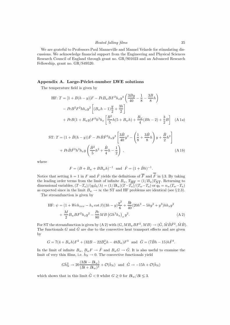
Heated falling films 35

We are grateful to Professors Paul Manneville and Manuel Velarde for stimulating dis-cussions. We acknowledge financial support from the Engineering and Physical SciencesResearch Council of England through grant no. GR/S01023 and an Advanced ResearchFellowship, grant no. GR/S49520.

Appendix A. Large-Peclet-number LWE solutions

The temperature field is given by

HF: T = [1 +B(h− y)]F − PeBwBF2hxy

4

(

3By

40−

1

8−

3B

8h

)

− PeB2F 2hhxy2

[

(Bwh− 1)y

2+

3h

2

]

+ PeB(1 +Bwy)F3h3hx

[

B2

5h(5 +Bwh) +

Bw

4(Bh− 2) +

3

2B

]

(A 1a)

ST: T = (1 + B(h− y))F − PeBF 2hxy3

[

3B

40y2 −

(

1

8+

3B

8h

)

y +B

2h2

]

+ PeBF 3h3hxy

(

B2

5h2 +

B

4h−

1

2

)

, (A 1b)

where

F = (B +Bw +BBwh)−1 and F = (1 + Bh)−1.

Notice that setting h = 1 in F and F yields the definitions of F and F in § 3. By takingthe leading order terms from the limit of infinite Bw, THF = (1/Bw)TST. Returning todimensional variables, (T−Ta)/(q0l0/λ) = (1/Biw)(T−Ta)/(Tw−Ta) or q0 = αw(Tw−Ta)as expected since in the limit Bw → ∞ the ST and HF problems are identical (see § 2.3).

The streamfunction is given by

HF: ψ = (1 +Wehxxx − hx cotβ)(3h− y)y2

6+Re

40(20h3 − 5hy2 + y3)hhxy

2

+M

2BwBF

2hxy2 −

Pe

80MB

(

Gh3hx

)

xy2. (A 2)

For ST the streamfunction is given by (A 2) with (G,MBwBF2,MB) → (G, MBF 2, MB).

The functionals G and G are due to the convective heat transport effects and are givenby

G = 7(4 +Bwh)F2 + (32B − 22B2

wh− 48Bw)F 3 and G = (7Bh− 15)hF 3.

In the limit of infinite Bw, BwF → F and BwG → G. It is also useful to examine thelimit of very thin films, i.e. hN → 0. The convective functionals yield

Gh2N → 20

(3Bi−Biw)

(Bi+Biw)3+ O(hN) and G→ −15h+ O(hN)

which shows that in this limit G < 0 whilst G ≷ 0 for Biw/Bi ≶ 3.

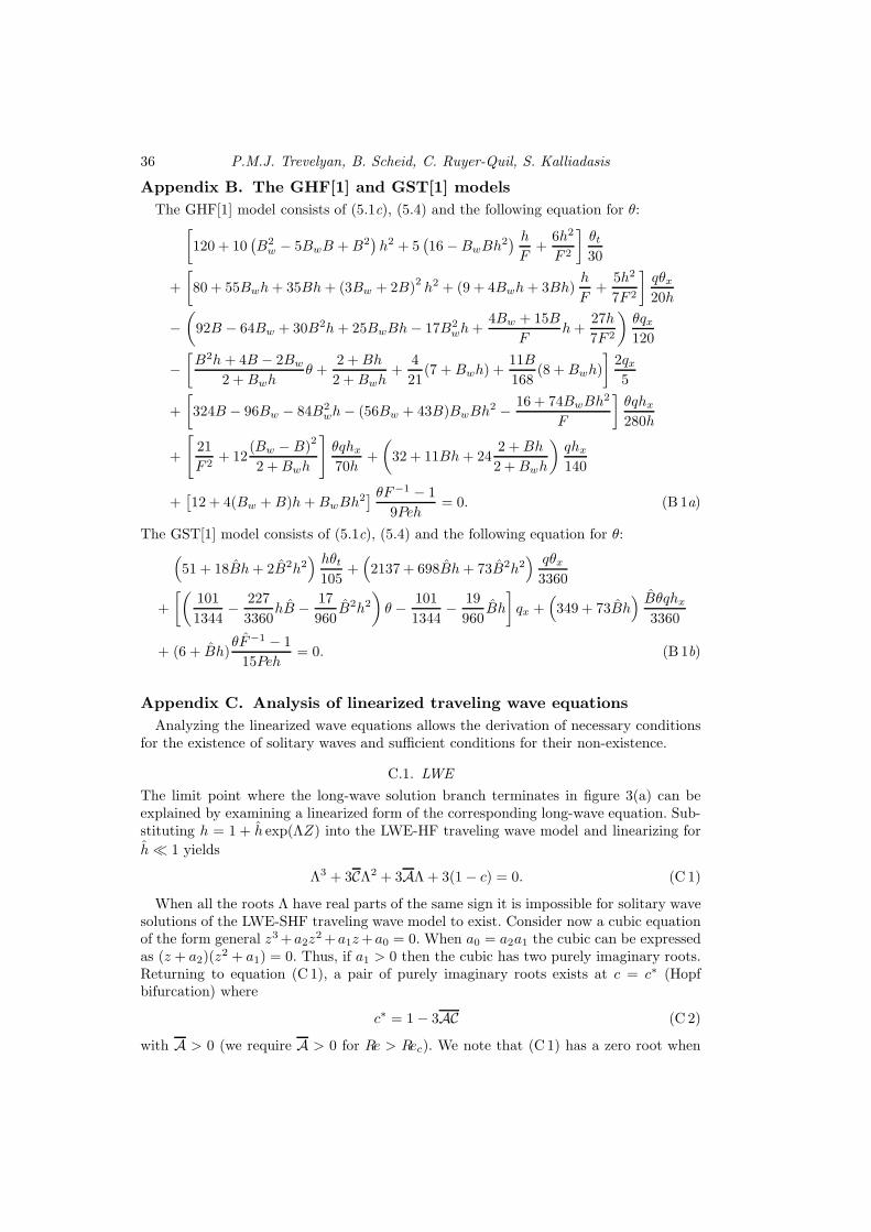
36 P.M.J. Trevelyan, B. Scheid, C. Ruyer-Quil, S. Kalliadasis

Appendix B. The GHF[1] and GST[1] models

The GHF[1] model consists of (5.1c), (5.4) and the following equation for θ:[

120 + 10(

B2w − 5BwB +B2

)

h2 + 5(

16 −BwBh2) h

F+

6h2

F 2

]

θt

30

+

[

80 + 55Bwh+ 35Bh+ (3Bw + 2B)2h2 + (9 + 4Bwh+ 3Bh)

h

F+

5h2

7F 2

]

qθx

20h

−

(

92B − 64Bw + 30B2h+ 25BwBh− 17B2wh+

4Bw + 15B

Fh+

27h

7F 2

)

θqx120

−

[

B2h+ 4B − 2Bw

2 +Bwhθ +

2 +Bh

2 +Bwh+

4

21(7 +Bwh) +

11B

168(8 +Bwh)

]

2qx5

+

[

324B − 96Bw − 84B2wh− (56Bw + 43B)BwBh

2 −16 + 74BwBh

2

F

]

θqhx

280h

+

[

21

F 2+ 12

(Bw − B)2

2 +Bwh

]

θqhx

70h+

(

32 + 11Bh+ 242 +Bh

2 +Bwh

)

qhx

140

+[

12 + 4(Bw +B)h+BwBh2] θF−1 − 1

9Peh= 0. (B 1a)

The GST[1] model consists of (5.1c), (5.4) and the following equation for θ:

(

51 + 18Bh+ 2B2h2) hθt

105+(

2137 + 698Bh+ 73B2h2) qθx

3360

+

[(

101

1344−

227

3360hB −

17

960B2h2

)

θ −101

1344−

19

960Bh

]

qx +(

349 + 73Bh) Bθqhx

3360

+ (6 + Bh)θF−1 − 1

15Peh= 0. (B 1b)

Appendix C. Analysis of linearized traveling wave equations

Analyzing the linearized wave equations allows the derivation of necessary conditionsfor the existence of solitary waves and sufficient conditions for their non-existence.

C.1. LWE

The limit point where the long-wave solution branch terminates in figure 3(a) can beexplained by examining a linearized form of the corresponding long-wave equation. Sub-stituting h = 1 + h exp(ΛZ) into the LWE-HF traveling wave model and linearizing for

h≪ 1 yields

Λ3 + 3CΛ2 + 3AΛ + 3(1 − c) = 0. (C 1)

When all the roots Λ have real parts of the same sign it is impossible for solitary wavesolutions of the LWE-SHF traveling wave model to exist. Consider now a cubic equationof the form general z3 +a2z

2 +a1z+a0 = 0. When a0 = a2a1 the cubic can be expressedas (z + a2)(z

2 + a1) = 0. Thus, if a1 > 0 then the cubic has two purely imaginary roots.Returning to equation (C 1), a pair of purely imaginary roots exists at c = c∗ (Hopfbifurcation) where

c∗ = 1 − 3AC (C 2)

with A > 0 (we require A > 0 for Re > Rec). We note that (C 1) has a zero root when

Heated falling films 37

c = 1 which is the kinematic wave velocity. A sufficient and necessary condition nowfor positive solitary waves not to exist is c 6 c∗. At the point where the solitary wavesolution branch in figure 3(a) terminates we have c = c∗.

When C > 0 a pair of purely imaginary roots only exists when c = c∗ < 1, i.e. fornegative solitary waves. Similarly, when C < 0 then a pair of purely imaginary roots onlyexists when c = c∗ > 1, i.e. for positive solitary waves. Two necessary conditions forpositive solitary waves to exist are c > 1 and c > c∗.

C.2. SHF and SST

Substitution of h = 1 + h exp(ΛZ) and θ = F + θ exp(ΛZ) into the SHF traveling wave

model and linearizing for h, θ ≪ 1 yields[

Λ3 + Λ

(

2δ

35(21c2 − 17c+ 3) − ζ

)

+ 3(1 − c)

]

h−3

2MΛθ = 0. (C 3)

(

Bw −c(5 +Bw) − 1

8PrδΛ

)

Bh+

[

1

F+

(

1

3− c+

5

24Bw −

1

2Bwc

)

PrδΛ

]

θ

F= 0. (C 4)

For SST, (C 4) is replaced by(

1 −7cPrδΛ

120

)

Bh+

[

1

F+

(

3

20−c

3

)

PrδΛ

]

θ

F= 0. (C 5)

By eliminating h and θ, we obtain a quartic dispersion relation for both SHF and SST,of the form z4 + a3z

3 + a2z2 + a1z + a0 = 0. Sufficient and necessary conditions for all

roots of this polynomial to have negative real parts can be obtained with an extensionof the Routh-Hurwitz theorem (Strelitz 1977). For a quartic the result is a3 > 0, a2 > 0,0 < a1 < a2a3 and 0 < a0 < (a1a2a3 − a2

1)/a23. With z → −z, we can then obtain the

sufficient and necessary conditions for all roots to have positive real parts. By simplychanging the sign of a1 and a3 in the previous conditions, the new conditions are a3 < 0,a2 > 0, a2a3 < a1 < 0 and 0 < a0 < (a1a2a3 − a2

1)/a23. These two sets of inequalities

define two regions, say R1 and R2 in the fourth-dimensional space {a0, a1, a2, a3}. InR1

⋃

R2 all roots have real parts of the same sign and hence it is impossible for solitarywaves to exist there. Hence, a necessary condition for solitary waves to exist is that theroots lie outside R1

⋃

R2.

Appendix D. Modified traveling wave models

The coefficient of the interfacial temperature derivative with respect to the traveling

wave coordinate z = x− ct in the single-mode Galerkin projection is given by∫ 1

0(u(0) −

c)φ21dη. As the interfacial waves become larger, the flow becomes faster so that the term

u(0) − c which is strictly negative for small amplitude waves, passes through zero andbecomes positive. Note that in the absence of Marangoni effects u(0) = c on the interfacewhen h = 3 − (2/c) which marks the location of the stagnation points for the largest

solitary waves; see also § 8.1. Hence, as the height of the waves increases,∫ 1

0(u(0)−c)φ2

1dηcan in fact change sign and become positive. Note that as we pointed out in § 8.1 thecondition u(0) = c does not violate the long-wave approximation.

To alleviate the difficulties associated with a zero coefficient we appropriately modifyour projection approach. More specifically, we introduce the weight function

w1 = (u(0) − c)φ1

38 P.M.J. Trevelyan, B. Scheid, C. Ruyer-Quil, S. Kalliadasis

so that the coefficient of θZ becomes∫ 1

0(u(0) − c)2φ2

1dη which is non-negative. Hence, bymultiplying the weight function in GST[1] by (u − c) we obtain the ‘modified GST[1]’model which we denote by MGST[1]:

0 =

(

5287

144+

45

4Bh+

161

144B2h2

)

(3c− 1)2θ′−

(

8215

144+

1021

72Bh+

163

144B2h2

)

(3c− 1)chθ′

+

(

665

24+

175

24Bh+

2

3B2h2

)

c2h2θ′+

(

301

192ch−

61

6(3c− 1)

)

(θ − 1)ch′+101θ− 2

96c2h2Bh′

+

[(

45

8+

161

144Bh

)

(3c− 1)2 +

(

11

64ch−

41

36(3c− 1)

)

Bch2

]

Bθh′

+11

8Prδh(θF−1 − 1)[(149 + 23Bh)(1 − 3c) + (111 + 13Bh)ch]. (D 1)

Similarly, by multiplying the weight function in SST by (u − c) and using integrationby parts in a similar way to the derivation of SST, we obtain the ‘modified SST’ modelwhich we denote by MSST:

0 =

(

29

20(3c− 1)2 +

12

5(1 − 3c)ch+

27

20c2h2

)

θ′ +

(

19(1 − 3c) +2231

40ch

)

(θ − 1)ch′

+7

6Prδh(θF−1 − 1)(1 − 3c+ ch). (D 2)

The time-dependent analogues of these models can be obtained by multiplying theenergy equation with θt + u(0)θx prior to averaging. The resulting averaged equationsinvolve θ2t , θ2x and θtθx. For example, the ST model is of the form

a1θ2t + a2

q

hθtθx + a3

q2

h2θ2x +

q

h2θx (qx [a4 + a5θ] + a6qhxθ)

+θt

h(qx [a7 + a8θ] + a9qhxθ) +

θF−1 − 1

Peh2

(

a10θt + a11q

hθx

)

= 0,

with ai = ai(h; B).

REFERENCES

Benjamin, T. B. 1957 Wave formation in laminar flow down an inclined plane. J. Fluid Mech.2, 554–574.

Benney, D. J. 1966 Long waves on liquid films J. Math. Phy. 45, 150–155.Chang, H.-C. & Demekhin, E.A. 2002 Complex Wave Dynamics on Thin Films. Elsevier,

New York.Demekhin, E.A., Kaplan, M.A. & Shkadov, V.Ya 1987 Mathematical models of the theory

of viscous liquid films. Izv. Akad. Nauk SSSR, Mekh. Zhidk i Gaza 6, 9–16.Doedel, E., Champneys, A., Fairfrieve, T., Kuznetsov Y., Sandstede, B. & Wang X.

1997 Auto 97 Continuation and Bifurcation Software for Ordinary Differential Equations.Montreal Concordia University

Goodwin, R. & Homsy, G.M. 1991 Viscous flow down a slope in the vicinity of a contact line.Phys. Fluids 3, 515–528.

Gottlieb, D. & Orszag, S. A. 1977 Numerical Analysis of Spectral Methods: Theory andApplications. SIAM

Goussis, D. A. & Kelly, R. E. 1991 Surface waves and thermocapillary instabilities in a liquidfilm flow. J. Fluid Mech. 223, 24–45.

Joo, S. W., Davis, S. H. & Bankoff S. G. 1991 Long-wave instabilities of heated fallingfilms: two-dimensional theory of uniform layers. J. Fluid Mech. 230, 117–146.

Kabov, O. A. 1998 Formation of regular structures in a falling liquid film upon local heating.Thermophysics and Aeromechanics 5, 547–551.

Heated falling films 39

Kabov, O.A., Legros, J.K., Marchuk, I.V. & Scheid, B. 2000 Deformation of the freesurface in a moving locally-heated thin liquid layer. Izv. Akad. Nauk SSSR, Mekh. ZhidkGaza 3, 200–208.

Kalliadasis, S., Demekhin, E. A., Ruyer-Quil, C. & Velarde M. G. 2003a Thermocap-illary instability and wave formation on a film falling down a uniformly heated plane. J.Fluid Mech. 492, 303–338.

Kalliadasis, S., Kiyashko, A. & Demekhin, E. A. 2003b Marangoni instability of a thinliquid film heated from below by a local heat source. J. Fluid Mech. 475, 377–408.

Kapitza, P. L. 1948 Wave flow of thin layers of a viscous fluid. Zh. Eksp. Teor. Fiz. 18, 3–28.Kapitza, P. L. & Kapitza, S. P. 1949 Wave flow of thin layers of a viscous fluid: III. Exper-

imental study of undulatory flow conditions. Zh. Eksp. Teor. Fiz. 19, 105–120.Kawahara, T. 1983 Formation of saturated solitons in a nonlinear dispersive system with

instability and dissipation. Phys. Rev. Lett. 51, 381–383.Nakaya, C. 1989 Waves on a viscous fluid film down a vertical wall. Phys. Fluids A 1 (7),

1143–1154.Oron, A., Davis, S. H. & Bankoff S. G. 1997 Long-scale evolution of thin liquid films. Rev.

Mod. Phys. 69, 931–980.Pumir, A., Manneville, P. & Pomeau Y. 1983 On solitary waves running down an inclined

plane. J. Fluid Mech. 135, 27–50.Ramaswamy, B., Chippada, S. & Joo, S.W. 1996 A full-scale numerical study of interfacial

instabilities in thin film flows. J. Fluid Mech. 325, 163–194.Ruyer-Quil, C. & Manneville, P. 2000 Improved modeling of flows down inclined planes.

Eur. Phys. J. B. 15, 357–369.Ruyer-Quil, C. & Manneville, P. 2002 Further accuracy and convergence results of the

modeling of flows down inclined planes by weighted residual approximations. Phys. Fluids14, 170–183.

Ruyer-Quil, C., Scheid, B., Kalliadasis, S., Velarde, M.G. & Zeytonian, R.Kh. 2005Thermocapillary long waves in a liquid film flow. Part 1. Low-dimensional formulation. J.Fluid Mech. 538, 199–222.

Salamon, T. R., Armstrong, R. C. & Brown, R. A. 1994 Travelling waves on vertical films:Numerical analysis using the finite element method. Phys. Fluids 6 (6), 2202–2220.

Scheid, B., Oron, A., Colinet, P., Thiele, U. & Legros, J. C. 2002 Nonlinear evolutionof nonuniformly heated falling liquid films. Phys. Fluids 14 (12), 4130–4151.

Scheid, B. 2004 Evolution and stability of falling liquid films with thermocapillary effects. PhDthesis, Universite Libre de Bruxelles.

Scheid, B., Ruyer-Quil, C., Thiele U., Kabov, O.A., Legros, J.C & Colinet, P. 2004Validity domain of the Benney equation including Marangoni effect for closed and openflows. J. Fluid Mech. 527, 303–335.

Scheid, B., Ruyer-Quil, C., Kalliadasis, S., Velarde, M.G. & Zeytounian, R.Kh. 2005Thermocapillary long waves in a liquid film flow. Part 2. Linear stability and nonlinearwaves. J. Fluid Mech. 538, 223–244.

Shkadov, V. Ya 1967 Wave models in the flow of a thin layer of a viscous liquid under theaction of gravity. Izv. Akad. Nauk SSSR, Mekh. Zhidk Gaza 1, 43–50.

Shkadov, V. Ya 1968 Theory of wave flow of a thin layer of a viscous liquid. Izv. Akad. NaukSSSR, Mekh. Zhidk Gaza 2, 20–25.

Shkadov, V. Ya 1977 Solitary waves in a layer of viscous liquid. Izv. Akad. Nauk SSSR, Mekh.Zhidk Gaza 12, 63–66.

Shraiman, B. 1987 Diffusive transport in a Rayleigh-Benard convection cell. Phys. Rev. A 36,261–267.

Smith, K. A. 1966 On convective instability induced by surface-tension gradients. J. FluidMech. 14, 401–414.

Strelitz, S. 1977 On the Routh-Hurwitz problem. Amer. Math. Monthly 84, 542–544.Trevelyan, P.M.J., Kalliadasis, S., Merkin, J.H. & Scott, S.K. 2002a Mass transport

enhancement in regions bounded by rigid walls. J. Eng. Math. 42, 45–64.Trevelyan, P. M. J. & Kalliadasis, S. 2004 Dynamics of a reactive falling film at large

Peclet numbers. I. Long-wave approximation. Phys. Fluids 16 (8), 3191–3208.Yih, C.-S. 1963 Stability of liquid flow down an inclined plane. Phys. Fluids 6 (3), 321–334.