econstor www.econstor.eu

Der Open-Access-Publikationsserver der ZBW – Leibniz-Informationszentrum WirtschaftThe Open Access Publication Server of the ZBW – Leibniz Information Centre for Economics

Nutzungsbedingungen:Die ZBW räumt Ihnen als Nutzerin/Nutzer das unentgeltliche,räumlich unbeschränkte und zeitlich auf die Dauer des Schutzrechtsbeschränkte einfache Recht ein, das ausgewählte Werk im Rahmender unter→ http://www.econstor.eu/dspace/Nutzungsbedingungennachzulesenden vollständigen Nutzungsbedingungen zuvervielfältigen, mit denen die Nutzerin/der Nutzer sich durch dieerste Nutzung einverstanden erklärt.

Terms of use:The ZBW grants you, the user, the non-exclusive right to usethe selected work free of charge, territorially unrestricted andwithin the time limit of the term of the property rights accordingto the terms specified at→ http://www.econstor.eu/dspace/NutzungsbedingungenBy the first use of the selected work the user agrees anddeclares to comply with these terms of use.

zbw Leibniz-Informationszentrum WirtschaftLeibniz Information Centre for Economics

DeJong, David Neil; Dharmarajan, Hariharan; Liesenfeld, Roman; Moura,Guilherme V.; Richard, Jean-François

Working Paper

Efficient likelihood evaluation of state-spacerepresentations

Economics working paper / Christian-Albrechts-Universität Kiel, Department of Economics,No. 2009,02

Provided in Cooperation with:Christian-Albrechts-University of Kiel, Department of Economics

Suggested Citation: DeJong, David Neil; Dharmarajan, Hariharan; Liesenfeld, Roman; Moura,Guilherme V.; Richard, Jean-François (2009) : Efficient likelihood evaluation of state-spacerepresentations, Economics working paper / Christian-Albrechts-Universität Kiel, Department ofEconomics, No. 2009,02

This Version is available at:http://hdl.handle.net/10419/27737

D

efficient likelihood evalution of state-space representations

a revised version of ewp 2007-25

by David N. DeJong, Hariharan Dharmarajan, Roman Liesenfeld, Guilherme V. Moura and Jean-François Richard

No 2009-02

E¢ cient Likelihood Evaluation of State-Space Representations

David N. DeJong �

Department of EconomicsUniversity of PittsburghPittsburgh, PA 15260, USA

Hariharan DharmarajanDepartment of EconomicsUniversity of PittsburghPittsburgh, PA 15260, USA

Roman LiesenfeldDepartment of Economics

Universität Kiel24118 Kiel, Germany

Guilherme V. MouraDepartment of Economics

Universität Kiel24118 Kiel, Germany

Jean-François RichardDepartment of EconomicsUniversity of PittsburghPittsburgh, PA 15260, USA

First Version: April 2007 This Revision: March 2009

Abstract

We develop a numerical procedure that facilitates e¢ cient likelihood evaluation in applica-tions involving non-linear and non-Gaussian state-space models. The procedure approximatesnecessary integrals using continuous approximations of target densities. Construction is achievedvia e¢ cient importance sampling, and approximating densities are adapted to fully incorporatecurrent information. We illustrate our procedure in applications to dynamic stochastic generalequilibrium models.

Keywords: particle �lter; adaption, e¢ cient importance sampling; kernel density approxima-tion; dynamic stochastic general equilibrium model.

�Contact Author: D.N. DeJong, Department of Economics, University of Pittsburgh, Pittsburgh, PA 15260, USA;Telephone: 412-648-2242; Fax: 412-648-1793; E-mail: dejong@pitt.edu. Richard gratefully acknowledges researchsupport provided by the National Science Foundation under grant SES-0516642. For helpful comments, we thankChetan Dave, Jesus Fernandez-Villaverde, Hiroyuki Kasahara, Juan Rubio-Ramirez, Enrique Sentana, and seminarand conference participants at the Universitites of Comenius, Di Tella, Texas (Dallas), Pennsylvania, the 2008 Econo-metric Society Summer Meetings (CMU), the 2008 Conference on Computations in Economics (Paris), and the 2008Vienna Macroecnomics Workshop. We also thank Chetan Dave for assistance with compiling the Canadian data setwe analyzed. Pseudo-code, GAUSS and MATLAB code, and data sets used to demonstrate implementation of theEIS �lter are available at www.pitt.edu/�dejong/wp.htm

1 Introduction

Likelihood evaluation and �ltering in applications involving state-space models requires the

calculation of integrals over unobservable state variables. When models are linear and stochastic

processes are Gaussian, required integrals can be calculated analytically via the Kalman �lter.

Departures entail integrals that must be approximated numerically. Here we introduce an e¢ cient

procedure for calculating such integrals: the EIS �lter.

The procedure takes as a building block the pioneering approach to likelihood evaluation and

�ltering developed by Gordon, Salmond and Smith (1993) and Kitagawa (1996). Their approach

employs discrete �xed-support approximations to unknown densities that appear in the predictive

and updating stages of the �ltering process. The discrete points that collectively provide density

approximations are known as particles; the approach is known as the particle �lter. Examples of

its use are becoming widespread; in economics, e.g., see Kim, Shephard and Chib (1998) for an

application involving stochastic volatility models; and Fernandez-Villaverde and Rubio-Ramirez

(2005, 2009) for applications involving dynamic stochastic general equilibrium (DSGE) models.

While conceptually simple and easy to program, the particle �lter su¤ers two shortcomings.

First, because the density approximations it provides are discrete, associated likelihood approxi-

mations can feature spurious discontinuities, rendering as problematic the application of likelihood

maximization procedures (e.g., see Pitt, 2002). Second, the supports upon which approximations

are based are not adapted: period-t approximations are based on supports that incorporate infor-

mation conveyed by values of the observable variables available in period t � 1, but not period t

(e.g., see Pitt and Shephard, 1999). This gives rise to numerical ine¢ ciencies that can be acute

when observable variables are highly informative with regard to state variables, particularly given

the presence of outliers.

Numerous extensions of the particle �lter have been proposed in attempts to address these

problems. For examples, see Pitt and Shephard (1999); the collection of papers in Doucet, de Freitas

and Gordon (2001); Pitt (2002); Ristic et al. (2004), and the collection housed at http://www-

sigproc.eng.cam.ac.uk/smc/papers.html. Typically, e¢ ciency gains are sought through attempts

at adapting period-t densities via the use of information available through period t. However, with

the exception of the extension proposed by Pitt (2002), once period-t supports are established they

1

remain �xed over a discrete collection of points as the �lter advances forward through the sample,

thus failing to address the problem of spurious likelihood discontinuity. (Pitt employs a bootstrap-

smoothing approximation designed to address this problem for the specialized case in which the

state space is unidimensional.) Moreover, as far as we are aware, no existing extension pursues

adaption in a manner that is designed to achieve optimal e¢ ciency.

Here we propose an extension that constructs adapted period-t approximations, but that fea-

tures a unique combination of two characteristics. The approximations are continuous; and period-t

supports are adjusted using a method designed to produce approximations that achieve near-optimal

e¢ ciency at the adaption stage. The approximations are constructed using the e¢ cient importance

sampling (EIS) methodology developed by Richard and Zhang (RZ, 2007). Construction is facili-

tated using an optimization procedure designed to minimize numerical standard errors associated

with the approximated integral.

Here, our focus is on the achievement of near-optimal e¢ ciency for likelihood evaluation. Ex-

ample applications involve the analysis of DSGE models, and are used to illustrate the relative

performance of the particle and EIS �lters. In a companion paper (DeJong et al., 2008) we focus

on �ltering, and present an application to the bearings-only tracking problem featured prominently,

e.g., in the engineering literature.

As motivation for our focus on the analysis of DSGE models, a brief literature review is help-

ful. The pioneering work of Sargent (1989) demonstrated the mapping of DSGE models into

linear/Gaussian state-space representations amenable to likelihood-based analysis achievable via

the Kalman �lter. DeJong, Ingram and Whiteman (2000) developed a Bayesian approach to ana-

lyzing these models. Subsequent work has involved the implementation of DSGE models towards a

broad range of empirical objectives, including forecasting and guidance of the conduct of aggregate

�scal and monetary policy (following Smets and Wouters, 2003).

Prior to the work of Fernandez-Villaverde and Rubio-Ramirez (2005, 2009), likelihood-based

implementation of DSGE models was conducted using linear/Gaussian representations. But their

�ndings revealed an important caveat: approximation errors associated with linear representations

of DSGE models can impart signi�cant errors in corresponding likelihood representations. As a

remedy, they demonstrated use of the particle �lter for achieving likelihood evaluation for non-

linear model representations. But as our examples illustrate, the numerical ine¢ ciencies noted

2

above su¤ered by the particle �lter can be acute in applications involving DSGE models. By

eliminating these ine¢ ciencies, the EIS �lter o¤ers a signi�cant advance in the empirical analysis

of DSGE models.

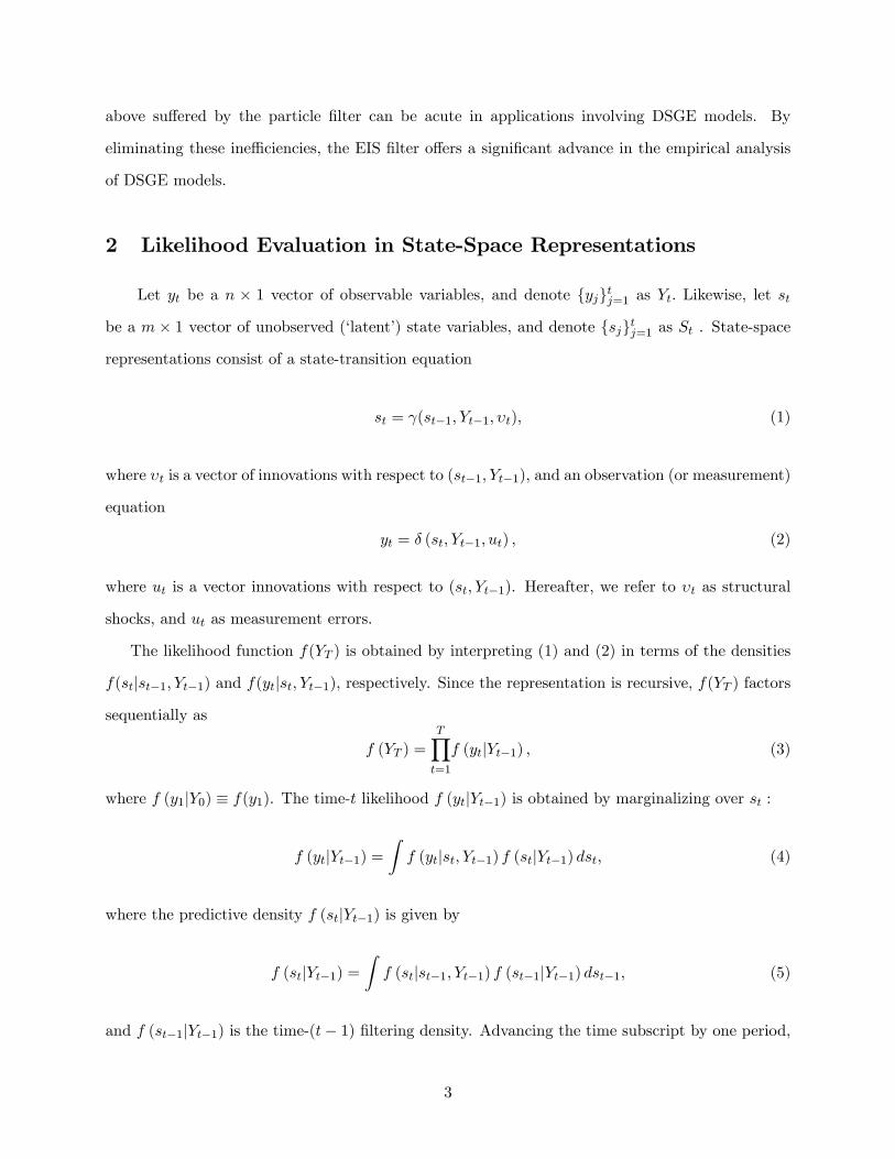
2 Likelihood Evaluation in State-Space Representations

Let yt be a n � 1 vector of observable variables, and denote fyjgtj=1 as Yt: Likewise, let st

be a m � 1 vector of unobserved (�latent�) state variables, and denote fsjgtj=1 as St . State-space

representations consist of a state-transition equation

st = (st�1; Yt�1; �t); (1)

where �t is a vector of innovations with respect to (st�1; Yt�1), and an observation (or measurement)

equation

yt = � (st; Yt�1; ut) ; (2)

where ut is a vector innovations with respect to (st; Yt�1). Hereafter, we refer to �t as structural

shocks, and ut as measurement errors.

The likelihood function f(YT ) is obtained by interpreting (1) and (2) in terms of the densities

f(stjst�1; Yt�1) and f(ytjst; Yt�1), respectively. Since the representation is recursive, f(YT ) factors

sequentially as

f (YT ) =TYt=1

f (ytjYt�1) ; (3)

where f (y1jY0) � f(y1). The time-t likelihood f (ytjYt�1) is obtained by marginalizing over st :

f (ytjYt�1) =Zf (ytjst; Yt�1) f (stjYt�1) dst; (4)

where the predictive density f (stjYt�1) is given by

f (stjYt�1) =Zf (stjst�1; Yt�1) f (st�1jYt�1) dst�1; (5)

and f (st�1jYt�1) is the time-(t� 1) �ltering density. Advancing the time subscript by one period,

3

from Bayes�theorem, f (stjYt) is given by

f (stjYt) =f (yt; stjYt�1)f (ytjYt�1)

=f (ytjst; Yt�1) f (stjYt�1)

f (ytjYt�1): (6)

Likelihood construction is achieved by calculating (4) and (5) sequentially from periods 1 to T ,

taking as an input in period t the �ltering density constructed in period (t� 1). In period 1 the

�ltering density is the known marginal density f(s0), which can be degenerate as a special case;

i.e., f (s0jY0) � f(s0).

In turn, �ltering entails the approximation of the conditional (upon Yt) expectation of some

function h(st) (including st itself). In light of (6) and (4), this can be written as

Et (h(st)jYt) =

Zh(st)f (ytjst; Yt�1) f (stjYt�1) dstZf (ytjst; Yt�1) f (stjYt�1) dst

: (7)

3 The Particle Filter and Leading Extensions

Since our procedure is an extension of the particle �lter developed by Gordon, Salmond and

Smith (1993) and Kitagawa (1996), we provide a brief overview here. The particle �lter is an

algorithm that recursively generates random numbers approximately distributed as f (stjYt). To

characterize its implementation, let sr;it denote the ith draw of st obtained from the conditional

density f (stjYt�r) for r = 0; 1. A single draw sr;it is a particle, and a set of draws fsr;it gNi=1 is a

swarm of particles. The object of �ltration is that of transforming a swarm fs0;it�1gNi=1 to fs0;it gNi=1.

The �lter is initialized by a swarm fs0;i0 gNi=1 drawn from f(s0jY0) � f(s0).

Period-t �ltration takes as input a swarm fs0;it�1gNi=1. The predictive step consists of transforming

this swarm into a second swarm fs1;it gNi=1 according to (5). This is done by drawing s1;it from the

conditional density f�stjs0;it�1; Yt�1

�, i = 1; :::; N . Note that fs1;it gNi=1 can be used to produce an

MC estimate of f (ytjYt�1), which according to (4) is given by

bfN (ytjYt�1) = 1

N

NXi=1

f(ytjs1;it ; Yt�1): (8)

Next, f (stjYt) is approximated by re-weighting fs1;it gNi=1 in accordance with (6) (the updating

4

step): a particle s1;it with prior weight 1N is assigned the posterior weight

w0;it =f(ytjs1;it ; Yt�1)NXj=1

f(ytjs1;jt ; Yt�1)

: (9)

The �ltered swarm fs0;it gNi=1 is then obtained by drawing with replacement from the swarm fs1;it gNi=1

with probabilities fw0;it gNi=1 (i.e., bootstrapping).

Having characterized the particle �lter, its strengths and weaknesses (well documented in pre-

vious studies) can be pinpointed. Its strength lies in its simplicity: the algorithm described above

is straightforward and universally applicable.

Its weaknesses are twofold. First, it provides discrete approximations of f(stjYt�1) and f(stjYt),

which moreover are discontinuous functions of the model parameters. The associated likelihood

approximation is therefore also discontinuous, rendering the application of maximization routines

problematic (a point raised previously, e.g., by Pitt, 2002).

Second, as the �lter enters period t, the discrete approximation of f(st�1jYt�1) is set. Hence

the swarm fs1;it gNi=1 produced in the augmentation stage ignores information provided by yt. (Pitt

and Shephard, 1999, refer to these augmenting draws as �blind�.) It follows that if f (ytjst; Yt�1)

- treated as a function of st given Yt - is sharply peaked in the tails of f(stjYt�1), fs1;it gNi=1 will

contain few elements in the relevant range of f (ytjst; Yt�1). Thus fs1;it gNi=1 represents draws from

an ine¢ cient sampler: relatively few of its elements will be assigned appreciable weight in the

updating stage in the following period. This is known as �sample impoverishment�: it entails a

reduction in the e¤ective size of the particle swarm.

Extensions of the particle �lter employ adaption techniques to generate gains in e¢ ciency.

An extension proposed by Gordon et al. (1993) and Kitagawa (1996) consists simply of making

N 0 >> N blind proposals fs1;jt gN0

j=1 as with the particle �lter, and then obtaining the swarmns0;it

oNi=1

by sampling with replacement, using weights computed from the N 0 blind proposals.

This is the sampling-importance resampling �lter; it seeks to overcome the problem of sample

impoverishment by brute force, and can be computationally expensive.

Carpenter, Cli¤ord and Fearnhead (1999) sought to overcome sample impoverishment using

a strati�ed sampling approach to approximate the prediction density. This is accomplished by

5

de�ning a partition consisting of K subintervals in the state space, and constructing the prediction

density approximation by sampling (with replacement) Nk particles from among the particles in

each subinterval. Here Nk is proportional to a weight de�ned for the entire kth interval; also,PKk=1Nk = N . This produces wider variation in re-sampled particles, but if the swarm of proposals

fs1;it gNi=1 are tightly clustered in the tails of f(stjYt�1), so too will be the re-sampled particles.

Pitt and Shephard (1999) developed an extension that ours perhaps most closely resembles.

They tackle adaption using an Importance Sampling (IS) procedure. Consider as an example the

marginalization step. Faced with the problem of calculating f (ytjYt�1) in (4), but with f (stjYt�1)

unknown, importance sampling achieves approximation via the introduction into the integral of an

importance density g(stjYt):

f (ytjYt�1) =Zf (ytjst; Yt�1) f (stjYt�1)

g(stjYt)g(stjYt)dst: (10)

Obtaining drawings s0;it from g(stjYt); this integral is approximated as

bf (ytjYt�1) � 1

N

NXi=1

f�ytjs0;it ; Yt�1

�f�s0;it jYt�1

�g(s0;it jYt)

: (11)

Pitt and Shephard referred to the introduction of g(stjYt) as adaption. Full adaption is achieved

when g(stjYt) is constructed as being proportional to f (ytjst; Yt�1) f (stjYt�1) ; rendering the ratios

in (11) as constants. Pitt and Shephard viewed adaption as computationally infeasible, due to the

requirement of computing f�s0;it jYt�1

�for every value of s0;it produced by the sampler. Instead

they developed samplers designed to yield partial adaption.

The samplers result from Taylor series approximations of f (ytjst; Yt�1) around st = �kt =

E�stjs0;kt�1; Yt�1

�:A zero-order expansion yields their auxiliary particle �lter; a �rst-order expansion

yields their adapted particle �lter. (Smith and Santos, 2006, study examples under which it is

possible to construct samplers using second-order expansions.)

These samplers help alleviate blind sampling by reweightingns0;it�1

oto account for information

conveyed by yt: However, sample impoverishment can remain an issue, since the algorithm does

not allow adjustment of the support ofns0;it�1

o. Moreover, the samplers are suboptimal, since �kt

is incapable of fully capturing the characteristics of f (ytjst; Yt�1). Finally, these samplers remain

6

prone to the discontinuity problem.

Pitt (2002) addressed the discontinuity problem for the special case in which the state space

is unidimensional by replacing the weights in (9) associated with the particle �lter (or comparable

weights associated with the auxiliary particle �lter) with smoothed versions constructed via a

piecewise linear approximation of the empirical c.d.f. associated with the swarmns0;it

oNi=1

: This

enables the use of common random numbers (CRNs) to produce likelihood estimates that are

continuous functions of model parameters (Hendry, 1994).

4 The EIS Filter

EIS is an automated procedure for constructing continuous importance samplers fully adapted

as global approximations to targeted integrands. Section 4.1 outlines the general principle behind

EIS, in the context of evaluating (4). Section 4.2 then discusses a key contribution of this paper: the

computation of f(stjYt�1) in (4) at auxiliary values of st generated under period-t EIS optimization.

Section 4.3 discusses two special cases that often characterize state-space representations: partial

measurement of the state space; and degenerate transition densities. Elaboration on the pseudo-

code presented below is available at www.pitt.edu/�dejong/wp.htm.

4.1 EIS integration

Let 't(st) = f(ytjst; Yt�1) � f(stjYt�1) in (4), where the subscript t in 't replaces (yt; Yt�1).

Implementation of EIS begins with the preselection of a parametric class K = fk(st; at); at 2 Ag

of auxiliary density kernels. Corresponding density functions g are

g(st; at) =k(st; at)

�(at); �(at) =

Zk(st; at)dst: (12)

The selection of K is problem-speci�c; here we discuss Gaussian speci�cations; DeJong et al. (2008)

discusses an extension to piecewise-continuous speci�cations. The objective of EIS is to select the

parameter value bat 2 A that minimizes the variance of the ratio 't(st)g(stjat) over the range of integration.

7

Following RZ, a (near) optimal value bat is obtained as the solution to(bat;bct) = argmin

at;ct

Z[ln't(st)� ct � ln k(st; at)]2 g(st; at)dst; (13)

where ct is an intercept meant to calibrate ln('t=k). Equation (13) is a standard least squares

problem, except that the auxiliary sampling density itself depends upon at. This is resolved by

reinterpreting (13) as the search for a �xed-point solution. An operational MC version implemented

(typically) using R << N draws, is as follows:

Step l + 1: Given balt, draw intermediate values fsit;lgRi=1 from the step-l EIS sampler g(st;balt),and solve

(bal+1t ;bcl+1t ) = argminat;ct

RXi=1

�ln't(s

it;l)� ct � ln k(sit;l; at)

�2: (14)

If K belongs to the exponential family of distributions, there exists a parameterization at such that

the auxiliary problems in (14) are linear.

Three points bear mentioning here. First, the evaluation of 't(st) entails the evaluation of

f(stjYt�1), which is unavailable analytically and must be approximated; this is discussed below in

Section 4.2. Second, the selection of the initial value ba1t is important for achieving rapid convergence;Section 5 presents an e¤ective algorithm for specifying ba1t in applications involving DSGE models(one step in each of the examples we consider). Third, to achieve rapid convergence, and to ensure

continuity of corresponding likelihood estimates, fsit;jg must be obtained by a transformation of a

set of common random numbers (CRNs) fuitg drawn from a canonical distribution (i.e., one that

does not depend on at; e.g., standardized Normal draws when g is Gaussian).

At convergence to bat, the EIS �lter approximation of f(ytjYt�1) in (4) is given bybfN (ytjYt�1) =

1

N

NXi=1

!�sit; bat� ; (15)

!�sit; bat� =

f�ytjsit; Yt�1

�f�sitjYt�1

�g(sit; bat) ; (16)

where�sitNi=1

are drawn from the (�nal) EIS sampler g(st; bat). This estimate converges almostsurely towards f(ytjYt�1) under weak regularity conditions (outlined, e.g., by Geweke, 1989). Vio-

lations of these conditions typically result from the use of samplers with thinner tails than those of

8

't. RZ o¤er a diagnostic measure that is adept at detecting this problem. The measure compares

the MC sampling variances of the ratio 'tg under two values of at: the optimal bat, and one that

in�ates the variance of the st draws by a factor of 3 to 5.

Pseudo-code for implementing the EIS �lter is as follows:

� At period t; we inherit the sampler g(st�1;dat�1); and corresponding draws and weights�sit�1; !

�sit�1;dat�1�Ni=1 from period t� 1; where in period 0 g(s0; ba0) � f (s0) :

� Using an initial value ba1t ; obtain R draws nsi;lt oRi=1

from g(st;ba1t ); and solve (14) to obtain ba2t :Repeat until convergence, yielding bat:

� Obtain N values�sitNi=1

from the optimized sampling density g (st;bat) ; and calculate (15)and (16).

� Pass g (st;bat) and �sit; ! �sit; bat�Ni=1 to period t+ 1: Repeat until period T is reached.As we shall now explain,

�sit; !

�sit; bat�Ni=1 are passed from period t to t + 1 to facilitate the

approximation of the unknown f(stjYt�1) appearing in (14) and (16).

4.2 Continuous approximations of f(stjYt�1)

As noted, the EIS �lter requires the evaluation of f(stjYt�1) at any value of st needed for

EIS iterations. Here we discuss three operational alternatives for overcoming this hurdle (a fourth,

involving non-parametric approximations, is also possible but omitted here). Below, S denotes the

number of points used for each individual evaluation of f(stjYt�1).

Weighted-sum approximations

Combining (5) and (6), we can rewrite f(stjYt�1) as a ratio of integrals:

f(stjYt�1) =Rf(stjst�1; Yt�1)f(yt�1jst�1; Yt�2)f(st�1jYt�2)dst�1R

f(yt�1jst�1; Yt�2)f(st�1jYt�2)dst�1; (17)

where the denominator represents the likelihood integral for which an EIS sampler has been con-

9

structed in period t� 1. A direct MC estimate of f(stjYt�1) is given by

bfS(stjYt�1) =SXi=1

f(stjsit�1; Yt�1) � !(sit�1;bat�1)SXi=1

!(sit�1;bat�1); (18)

where fsit�1gSi=1 denotes EIS draws from g(st�1jbat�1), and �!(sit�1;bat�1)Si=1 denotes associatedweights (both of which are carried over from period-t� 1).

Obviously g(st�1jbat�1) is not an EIS sampler for the numerator in (17). This can impart apotential loss of numerical accuracy if the MC variance of f(stjst�1; Yt�1) is large over the support

of g(st�1jbat�1). This would be the case if the conditional variance of stjst�1; Yt�1 were signi�cantlysmaller than that of st�1jYt�1. But the fact that we are using the same set of draws for the

numerator and the denominator typically creates positive correlation between their respective MC

estimators, thus reducing the variance of their ratio.

A constant weight approximation

When EIS delivers a close global approximation to f(st�1jYt�1), the weights !(st�1;bat�1) willbe near constants over the range of integration. Replacing these weights by their arithmetic means

! (bat�1) in (17) and (18), we obtain the following simpli�cation:f(stjYt�1) '

Zf(stjst�1; Yt�1) � g(st�1;bat�1)dst�1: (19)

This substitution yields rapid implementation if additionally the integral in (19) has an analytical

solution. This will be the case if, e.g., f(stjst�1; Yt�1) is a conditional normal density for stjst�1,

and g is also normal. In cases for which we lack an analytical solution, we can use the standard

MC approximation

bfS(stjYt�1) ' 1

S

SXi=1

f(stjs0;it�1; Yt�1): (20)

EIS evaluation

Evaluation of f(stjYt�1) can sometimes be delicate, including situations prone to sample im-

poverishment (such as when working with degenerate transitions, discussed below). Under such

circumstances, one might consider applying EIS not only to the likelihood integral (�outer EIS�),

10

but also to the evaluation of f(stjYt�1) itself (�inner EIS�).

While outer EIS is applied only once per period, inner EIS must be applied for every value of st

generated by the former. Also, application of EIS to (5) requires the construction of a continuous

approximation to f(st�1jYt�1): Two obvious candidates are as follows. The �rst is a non-parametric

approximation based upon a swarm fsit�1gSi=1:

bfS(st�1jYt�1) = 1

Sh

SXi=1

�

�st�1 � sit�1

h

�:

The second is the period-(t� 1) EIS sampler g(st�1;bat�1); under the implicit assumption that thecorresponding weights !(st�1;bat�1) are near-constant, at least over the range of integration. It isexpected that in pathological cases, signi�cant gains in accuracy resulting from inner EIS will far

outweigh approximation errors in f(st�1jYt�1):

4.3 Special cases

Partial measurement

Partial measurement refers to cases in which st can be partitioned (possibly after transforma-

tion) into st = (pt; qt), so that

f (ytjst; Yt�1) � f (ytjpt; Yt�1) : (21)

In this case, likelihood evaluation requires integration only with respect to pt:

f (ytjYt�1) =Zf (ytjpt; Yt�1) f (ptjYt�1) dpt; (22)

and the updating equation (6) factorizes into the product of the following two densities:

f (ptjYt) =f (ytjpt; Yt�1) f (ptjYt�1)

f (ytjYt�1); (23)

f (qtjpt; Yt) = f (qtjpt; Yt�1) : (24)

Stronger conditional independence assumptions are required in order to produce factorizations

11

in (5). In particular, if pt is independent of qt given (pt�1; Yt�1), so that

f (ptjst�1; Yt�1) � f (ptjpt�1; Yt�1) ; (25)

then

f (ptjYt�1) =Zf (ptjpt�1; Yt�1) f (pt�1jYt�1) dpt�1: (26)

Note that under conditions (21) and (25), likelihood evaluation does not require processing sample

information on fqtg : The latter is required only if inference on fqtg is itself of interest.

Degenerate transitions

When state transition equations include identities, corresponding transition densities are de-

generate (or Dirac) in some of their components. This situation requires an adjustment to EIS

implementation. Again, let st partition into st = (pt; qt) ; and assume that the transition equations

consist of two parts: a proper transition density f (ptjst�1; Yt�1) for pt; and an identity for qtjpt; st�1

(which could also depend on Yt�1, omitted here for ease of notation):

qt � � (pt; pt�1; qt�1) = � (pt; st�1) : (27)

The evaluation of f (stjYt�1) in (5) now requires special attention, since its evaluation at a

given st (as selected by the EIS algorithm) requires integration in the strict subspace associated

with identity (27). Note in particular that the presence of identities raises a conditioning issue

known as the Borel-Kolmogorov paradox (e.g., see DeGroot, 1975, Section 3.10). We resolve this

issue here by reinterpreting (27) as the limit of a uniform density for qtjpt; st�1 on the interval

[� (pt; st�1)� "; � (pt; st�1) + "] :

Assuming that � (pt; st�1) is di¤erentiable and strictly monotone in qt�1; with inverse

qt�1 = (pt; qt; pt�1) = (st; pt�1) (28)

we can take the limit of the integral in (5) as " tends to zero, producing

f (stjYt�1) =ZJ (st; pt�1) f (ptjst�1; Yt�1) f (pt�1; qt�1jYt�1) jqt�1= (st;pt�1)dpt�1; (29)

12

where with k � k denoting the absolute value of a determinant,

J (st; pt�1) = k@

@q0t (st; pt�1) k: (30)

Note that (29) requires that for any st; f (st�1jYt�1) must be evaluated along the zero-measure

subspace qt�1 = (st; pt�1). This rules out use of the weighted-sum approximation introduced

above, since the probability that any of the particles s0;it�1 lies in that subspace is zero. Instead, we

can approximate (29) by replacing f (st�1jYt�1) by ! (bat�1) g (st�1jbat�1):bf (stjYt�1) = Z J (st; pt�1) f (ptjqt�1; Yt�1) g (pt�1; qt�1jbat�1) jqt�1= (st;pt�1)dpt�1: (31)

In this case, since g (pt�1; (st; pt�1) jbat�1) is not a sampler for pt�1jst, we must evaluate (31) eitherby quadrature or its own EIS sampler.

One might infer from this discussion that the EIS �lter is tedious to implement under degenerate

transitions, while the particle �lter handles such degeneracy trivially in the transition fromns0;it�1

otons1;it

o. While this is true, it is also true that these situations are prone to signi�cant sample

impoverishment problems, as illustrated in the examples below.

5 Application to DSGE Models

As noted, the work of Fernandez-Villaverde and Rubio-Ramirez (2005, 2009) revealed that

approximation errors associated with linear representations of DSGE models can impart signi�cant

errors in corresponding likelihood representations. As a remedy, they demonstrated use of the

particle �lter for achieving likelihood evaluation for non-linear model representations. Here we

demonstrate the implementation of the EIS �lter using two workhorse models. The �rst is the

standard two-state real business cycle (RBC) model; the second is a small-open-economy (SOE)

model patterned after those considered, e.g., by Mendoza (1991) and Schmitt-Grohe and Uribe

(2003), but extended to include six state variables.

We analyze two data sets for both models: an arti�cial data set generated from a known model

parameterization; and a corresponding real data set. Thus in total we consider four applications,

each of which poses a signi�cant challenge to the successful implementation of a numerical �ltering

13

algorithm. Details follow.

5.1 Example 1: Two-State RBC Model

The �rst application is to the simple DSGE model used by Fernandez-Villaverde and Rubio-

Ramirez (2005) to demonstrate implementation of the particle �lter. The model consists of a

representative household that seeks to maximize the expected discounted stream of utility derived

from consumption c and leisure l:

maxct;lt

U = E0

1Xt=0

�t

�c't l

1�'t

�1� �

1��

;

where (�; �; ') represent the household�s subjective discount factor, degree of relative risk aversion,

and the relative importance assigned to ct and lt in determining period-t utility.

The household divides its available time per period (normalized to unity) between labor nt and

leisure. Labor combines with physical capital kt and a stochastic productivity term zt to produce

a single good �t, which may be consumed or invested (we use � in place of the usual representation

for output �y �to avoid confusion with our use of y as representing the observable variables of a

generic state-space model). Investment it combines with undepreciated capital to yield kt+1; thus

the opportunity cost of period-t consumption is period-(t+ 1) capital. Collectively, the constraints

faced by the household are given by

�t = ztk�t n

1��t ;

1 = nt + lt;

�t = ct + it;

kt+1 = it + (1� �)kt;

zt = z0egte!t ; !t = �!t�1 + "t;

where (�; �; g; �) represent capital�s share of output, the depreciation rate of capital, the growth

rate of total factor productivity (TFP), and the persistence of innovations to TFP.

Optimal household behavior is represented in terms of policy functions for (�t; ct; nt; lt; it) in

14

terms of the state (kt; zt): Given the policy function i(kt; zt), the state-transitions equations reduce

to

�1 +

g

1� �

�kt = i(kt�1; zt�1) + (1� �)kt�1 (32)

ln zt = (1� �) ln(z0) + � ln zt�1 + "t; "t � N(0; �2"); (33)

and the observation equations are

xt = x(kt; zt) + ux;t; x = �; i; n; (34)

ux;t � N(0; �2x): (35)

Policy functions are expressed as Chebyshev polynomials in the state variables (kt; zt) ; constructed

using the projection method described in DeJong and Dave (2007, Ch. 10.5.2).

Given the form of (33), it will be useful represent state variables as logged deviations from

steady state: st = [ln(kt=k�) ln(zt=z�)]0 : For ease of notation, hereafter we will denote ln(kt=k�)

as kt; and ln(zt=z�) as zt: In addition, given the form of (34), yt is de�ned as yt = [�t it nt]0 : All

subsequent formulas should be read in accordance with these representations.

To obtain the predictive density associated with (32) and (33), note that since (32) is an identity,

the transition density of the system is degenerate in kt: Thus we invert (32) to obtain

kt�1 = (kt; zt�1) ; (36)

J (kt; zt�1) = j @@kt

(kt; zt�1) j; (37)

and express the predictive density as

f (stjYt�1) =ZJ (kt; zt�1) f (ztjst�1) f (st�1jYt�1) jkt�1= (kt;zt�1)dzt�1: (38)

From (33), note that

f (ztjst�1) � N1

��0 �

�st�1; �2"

�;

with Nr () denoting an r�dimensional normal distribution. Finally, as the inversion of Chebyshev

15

polynomials is awkward, we approximate (36) and (37) using third-order polynomials in (kt; zt�1) :

With the predictive density established, the time-t likelihood is standard:

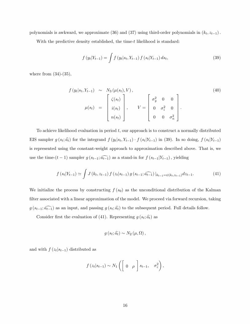
f (ytjYt�1) =Zf (ytjst; Yt�1) f (stjYt�1) dst; (39)

where from (34)-(35),

f (ytjst; Yt�1) � N3 (�(st); V ) ; (40)

�(st) =

266664�(st)

i(st)

n(st)

377775 ; V =

266664�2y 0 0

0 �2i 0

0 0 �2n

377775 :

To achieve likelihood evaluation in period t, our approach is to construct a normally distributed

EIS sampler g (st; bat) for the integrand f (ytjst; Yt�1) � f (stjYt�1) in (39). In so doing, f (stjYt�1)is represented using the constant-weight approach to approximation described above. That is, we

use the time-(t� 1) sampler g (st�1;dat�1) as a stand-in for f (st�1jYt�1) ; yieldingf (stjYt�1) '

ZJ (kt; zt�1) f (ztjst�1) g (st�1;dat�1) jkt�1= (kt;zt�1)dzt�1: (41)

We initialize the process by constructing f (s0) as the unconditional distribution of the Kalman

�lter associated with a linear approximation of the model. We proceed via forward recursion, taking

g (st�1;dat�1) as an input, and passing g (st; bat) to the subsequent period. Full details follow.Consider �rst the evaluation of (41). Representing g (st; bat) as

g (st; bat) � N2 (�;) ;

and with f (ztjst�1) distributed as

f (ztjst�1) � N1

��0 �

�st�1; �2"

�;

16

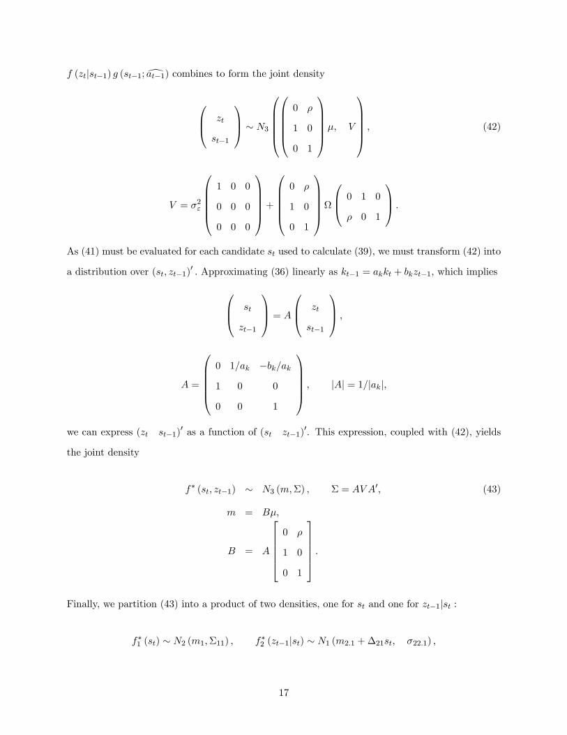
f (ztjst�1) g (st�1;dat�1) combines to form the joint density

0B@ zt

st�1

1CA � N3

0BBBB@0BBBB@0 �

1 0

0 1

1CCCCA�; V

1CCCCA ; (42)

V = �2"

0BBBB@1 0 0

0 0 0

0 0 0

1CCCCA+0BBBB@0 �

1 0

0 1

1CCCCA0B@ 0 1 0

� 0 1

1CA :

As (41) must be evaluated for each candidate st used to calculate (39), we must transform (42) into

a distribution over (st; zt�1)0 : Approximating (36) linearly as kt�1 = akkt + bkzt�1; which implies0B@ st

zt�1

1CA = A

0B@ zt

st�1

1CA ;

A =

0BBBB@0 1=ak �bk=ak

1 0 0

0 0 1

1CCCCA ; jAj = 1=jakj;

we can express (zt st�1)0 as a function of (st zt�1)

0. This expression, coupled with (42), yields

the joint density

f� (st; zt�1) � N3 (m;�) ; � = AV A0; (43)

m = B�;

B = A

2666640 �

1 0

0 1

377775 :

Finally, we partition (43) into a product of two densities, one for st and one for zt�1jst :

f�1 (st) � N2 (m1;�11) ; f�2 (zt�1jst) � N1 (m2:1 +�21st; �22:1) ;

17

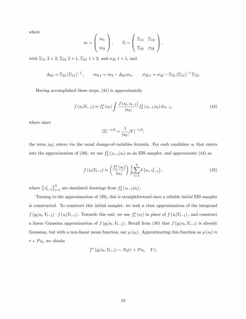
where

m =

0B@ m1

m2

1CA ; � =

0B@ �11 �12

�21 �22

1CA ;

with �11 2� 2; �12 2� 1; �21 1� 2; and �22 1� 1; and

�21 = �21 (�11)�1 ; m2:1 = m2 ��21m1; �22:1 = �22 � �21 (�11)�1�12:

Having accomplished these steps, (41) is approximately

f (stjYt�1) � f�1 (st)

ZJ (st; zt�1)

jakjf�2 (zt�1jst) dzt�1; (44)

where since

j�j�1=2 = 1

jakjjV j�1=2;

the term jakj enters via the usual change-of-variables formula. For each candidate st that enters

into the approximation of (39), we use f�2 (zt�1jst) as an EIS sampler, and approximate (44) as

f (stjYt�1) ��f�1 (st)

jakj

�1

S

SXi=1

J�st; z

it�1�; (45)

where�zit�1

Si=1

are simulated drawings from f�2 (zt�1jst) :

Turning to the approximation of (39), this is straightforward once a reliable initial EIS sampler

is constructed. To construct this initial sampler, we seek a close approximation of the integrand

f (ytjst; Yt�1) � f (stjYt�1) : Towards this end, we use f�1 (st) in place of f (stjYt�1) ; and construct

a linear Gaussian approximation of f (ytjst; Yt�1) : Recall from (40) that f (ytjst; Yt�1) is already

Gaussian, but with a non-linear mean function, say � (st) : Approximating this function as � (st) �

r + Pst; we obtain

f� (ytjst; Yt�1) � N3(r + Pst; V ):

18

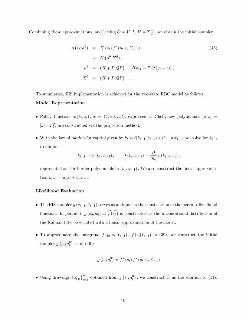
Combining these approximations, and letting Q = V �1; H = ��111 ; we obtain the initial sampler

g�st; a

0t

�= f�1 (st) f

� (ytjst; Yt�1) (46)

� N��0;�0

�;

�0 =�H + P 0QP

��1 �Hm1 + P

0Q (yt � r)�;

�0 =�H + P 0QP

��1:

To summarize, EIS implementation is achieved for the two-state RBC model as follows.

Model Representation

� Policy functions x (kt; zt) ; x = (�; c; i; n; l), expressed as Chebyshev polynomials in st =

[kt zt]0, are constructed via the projection method.

� With the law of motion for capital given by kt = i(kt�1; zt�1) + (1� �)kt�1; we solve for kt�1

to obtain

kt�1 = (kt; zt�1) ; J (kt; zt�1) =@

@kt (kt; zt�1) ;

represented as third-order polynomials in (kt; zt�1) : We also construct the linear approxima-

tion kt�1 = akkt + bkzt�1:

Likelihood Evaluation

� The EIS sampler g (st�1;dat�1) serves as an input in the construction of the period-t likelihoodfunction. In period 1, g (s0; ba0) � \f (s0) is constructed as the unconditional distribution of

the Kalman �lter associated with a linear approximation of the model.

� To approximate the integrand f (ytjst; Yt�1) � f (stjYt�1) in (39), we construct the initial

sampler g�st; a

0t

�as in (46):

g�st; a

0t

�= f�1 (st) f

� (ytjst; Yt�1)

� Using drawings�sit;0Ri=1

obtained from g�st; a

0t

�; we construct bat as the solution to (14).

19

This entails the computation of

't(sit;l) = f

�ytjsit;l; Yt�1

�f�sit;ljYt�1

�;

where f (ytjst; Yt�1) is given in (40), and f (stjYt�1) is approximated as indicated in (45).

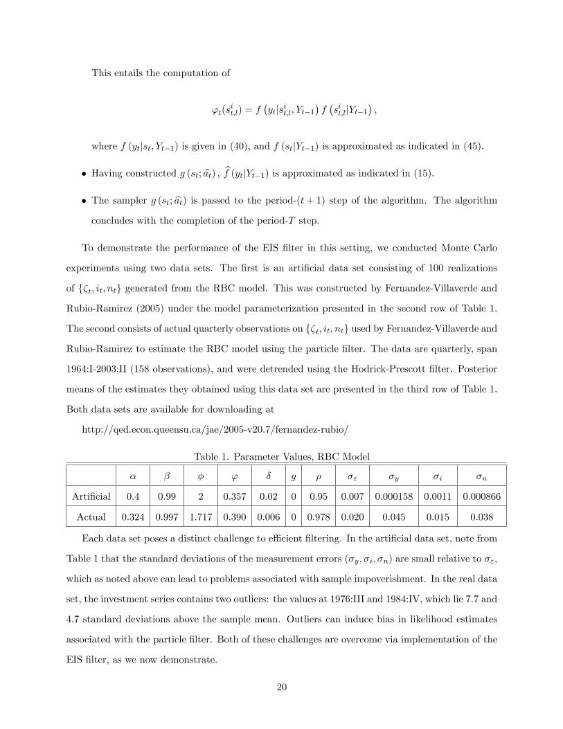
� Having constructed g (st; bat) ; bf (ytjYt�1) is approximated as indicated in (15).� The sampler g (st; bat) is passed to the period-(t+ 1) step of the algorithm. The algorithmconcludes with the completion of the period-T step.

To demonstrate the performance of the EIS �lter in this setting, we conducted Monte Carlo

experiments using two data sets. The �rst is an arti�cial data set consisting of 100 realizations

of f�t; it; ntg generated from the RBC model. This was constructed by Fernandez-Villaverde and

Rubio-Ramirez (2005) under the model parameterization presented in the second row of Table 1.

The second consists of actual quarterly observations on f�t; it; ntg used by Fernandez-Villaverde and

Rubio-Ramirez to estimate the RBC model using the particle �lter. The data are quarterly, span

1964:I-2003:II (158 observations), and were detrended using the Hodrick-Prescott �lter. Posterior

means of the estimates they obtained using this data set are presented in the third row of Table 1.

Both data sets are available for downloading at

http://qed.econ.queensu.ca/jae/2005-v20.7/fernandez-rubio/

Table 1. Parameter Values, RBC Model

� � � ' � g � �" �y �i �n

Arti�cial 0.4 0.99 2 0.357 0.02 0 0.95 0.007 0.000158 0.0011 0.000866

Actual 0.324 0.997 1.717 0.390 0.006 0 0.978 0.020 0.045 0.015 0.038

Each data set poses a distinct challenge to e¢ cient �ltering. In the arti�cial data set, note from

Table 1 that the standard deviations of the measurement errors (�y; �i; �n) are small relative to �";

which as noted above can lead to problems associated with sample impoverishment. In the real data

set, the investment series contains two outliers: the values at 1976:III and 1984:IV, which lie 7.7 and

4.7 standard deviations above the sample mean. Outliers can induce bias in likelihood estimates

associated with the particle �lter. Both of these challenges are overcome via implementation of the

EIS �lter, as we now demonstrate.

20

Using both data sets, we conducted a Monte Carlo experiment under which we produced 1,000

approximations of the likelihood function (evaluated at Table-1 parameter values) for both the

particle and EIS �lters using 1,000 di¤erent sets of random numbers. Di¤erences in likelihood ap-

proximations across sets of random numbers are due to numerical approximation errors. Following

Fernandez-Villaverde and Rubio-Ramirez, the particle �lter was implemented using N = 60; 000;

requiring 40.6 seconds of CPU time per likelihood evaluation on a 1.8 GHz desktop computer using

GAUSS for the arti�cial data set, and 63 seconds for the real data set. The EIS �lter was imple-

mented using N = 20; S = R = 10; with one iteration used to construct bat; this required 0.22seconds per likelihood evaluation for the arti�cial data set, and 0.328 seconds for the real data set.

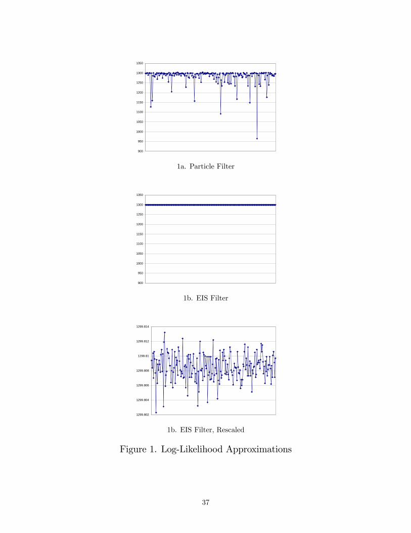
Considering �rst the arti�cial data set, the mean and standard deviation of the 1,000 log-

likelihood approximations obtained using the particle �lter are (1; 285:51; 33:48), and (1; 299:81; 0:00177)

using the EIS �lter (the likelihood value obtained using the Kalman �lter is 1; 300:045). Thus the

EIS �lter reduces numerical approximation errors by four orders of magnitude in this applica-

tion. Figure 1 plots the �rst 200 likelihood approximations obtained using both �lters (in order

to enhance visibility). Note that the particle-�lter approximations (top panel) often fall far below

the EIS sample mean of 1; 299:81 (by more than 50 on the log scale in twenty instances, and by

more than 100 in eight instances); this largely accounts for the distinct di¤erence in sample means

obtained across methods. But as the �gure indicates, even abstracting from the occasional large

likelihood crashes su¤ered by the particle �lter, the EIS �lter is extremely precise: the maximum

di¤erence in log-likelihood values it generates is less than 0.012 (bottom panel), while di¤erences

of 10 are routinely observed for the particle �lter.

Hereafter, we shall refer to di¤erences observed between sample means of log-likelihood values

obtained using the particle and EIS �lters as re�ecting bias associated with the particle �lter. This

presumes that the values associated with the EIS �lter closely represent �truth�. This presumption

is justi�ed in a number of ways, in this experiment and each of those that follow. First, the small

numerical approximation errors associated with the EIS �lter indicate virtual replication across

sets of random numbers. Second, as we increase the values of (N;R) used to implement the EIS

�lter, resulting mean log-likelihood approximations remain virtually unchanged, while numerical

errors are inversely proportional to N�1=2; as expected. Finally, when we implement the EIS �lter

using linear model approximations, the log-likelihood values we obtain match those produced by

21

the Kalman �lter almost exactly (virtually to the limits of numerical precision).

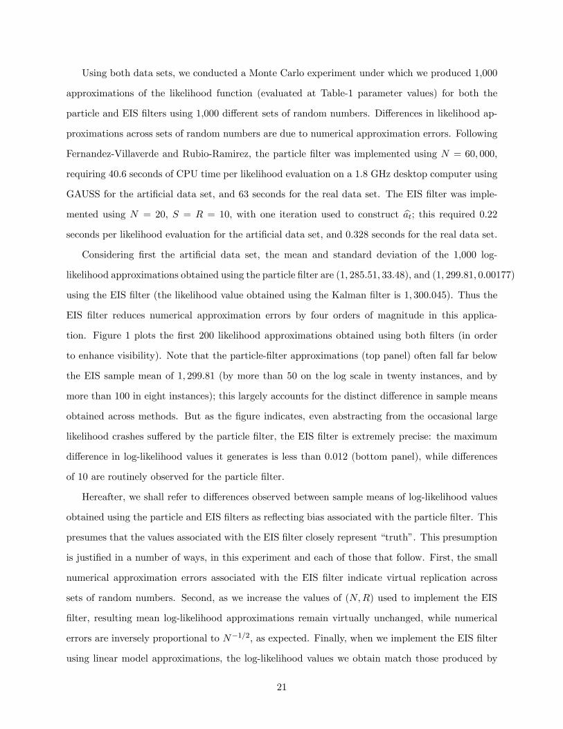
Figure 2 provides an illustration and diagnosis of the problems faced by the particle �lter

in this application. The focus here is on a representative Monte Carlo replication generated as

described above. The �gure contains two panels, each of which represents a distinct scenario

observed routinely across time periods within this replication. The top panel corresponds with

t = 53; the bottom with t = 18:

Each panel contains two graphs, both of which depict zt on the vertical axis and kt on the

horizontal axis. The measurement density f (ytjst; Yt�1) is the large thin ellipse depicted in both

graphs (di¤erences in vertical scales across graphs account for di¤erences in its appearance). In the

bottom graph, the swarm of dots comprises the particle-�lter representation of f (stjYt�1) ; and the

wide ellipse comprises the EIS representation of f (stjYt�1) : In the upper graph, the swarm of dots

comprises the particle-�lter representation of f (stjYt) ; particles in the upper swarm were obtained

by sampling repeatedly from the bottom swarm, with probabilities assigned by the measurement

density. The upper graph also depicts the EIS representation of f (stjYt) (small ellipse).

Beginning with period 53, note that the vast majority of particles in the bottom graph are

assigned negligible weight by the measurement density, and are thus discarded in the resampling

step. Speci�cally, only 407 particles, or 0.68% of the total candidates, were re-sampled at least

once in this instance. The average (across time periods) number of re-sampled particles is 350, or

0.58% of the total. This phenomenon re�ects the sample impoverishment problem noted above. It

results from the �blindness�of proposals generated under the particle �lter algorithm, and accounts

for its numerical inaccuracy.

As noted, the small ellipse depicted in the upper graph is the EIS representation of f (stjYt) : The

di¤erence between this and the corresponding particle-�lter representation re�ects a second problem

su¤ered by the particle �lter in this application: there is non-trivial bias in the �ltered values of the

state it produces. This also re�ects the �blindness�problem, coupled with the fact that alternative

proposals for st cannot be re-generated in light of information embodied in yt: (Note from the �gure

that this bias is not easily eliminated through an increase in the number of particles included in

the proposal swarm, since the probability that the proposal density will generate particles centered

on the EIS representation of f(stjYt) is clearly miniscule.) As described above, under suitable

initialization the EIS �lter avoids these issues by generating proposals from an importance density

22

tailored as the optimal global approximation of the targeted integrand f (ytjst; Yt�1) � f (stjYt�1) :

Regarding period 18, note that the representations of both f (stjYt�1) and f (stjYt) generated

using the particle �lter are discontinuous in kt; a spurious phenomenon that occurs frequently

through the sample. This exacerbates the bias associated with �ltered values of the state, and

contributes to a �nal problem associated with the particle �lter illustrated in Figure 3.

Like its predecessor, Figure 3 was produced using a representative Monte Carlo replication. It

depicts an approximation of the log-likelihood surface over � obtained by holding the remaining

parameters �xed at their true values, and varying � above and below its true value. Three surfaces

are depicted: those associated with the particle, EIS, and Kalman �lters (the latter obtained using

a linear model representation). The particle and EIS surfaces were produced with common random

numbers, so that changes in � serve as the lone source of variation in log-likelihoods.

Note that while the surfaces associated with the EIS and Kalman �lters are continuous and

peak at the true value of 0.4, the surface associated with the particle �lter is discontinuous and

has a slightly rightshifted peak. Thus in addition to being numerically ine¢ cient and producing

biased �ltered values of the state, the particle �lter generates likelihood surfaces that are spuriously

discontinuous in the underlying parameters of the model, rendering as problematic the attainment

of likelihood-based model estimates.

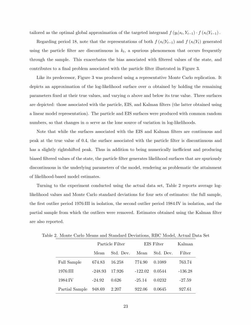
Turning to the experiment conducted using the actual data set, Table 2 reports average log-

likelihood values and Monte Carlo standard deviations for four sets of estimates: the full sample,

the �rst outlier period 1976:III in isolation, the second outlier period 1984:IV in isolation, and the

partial sample from which the outliers were removed. Estimates obtained using the Kalman �lter

are also reported.

Table 2. Monte Carlo Means and Standard Deviations, RBC Model, Actual Data Set

Particle Filter EIS Filter Kalman

Mean Std. Dev. Mean Std. Dev. Filter

Full Sample 674.83 16.258 774.90 0.1089 763.74

1976:III -248.93 17.926 -122.02 0.0544 -136.28

1984:IV -24.92 0.626 -25.14 0.0232 -27.59

Partial Sample 948.69 2.207 922.06 0.0645 927.61

23

Note �rst that unlike in the experiment conducted using the arti�cial data set, there are non-

trivial di¤erences between the log-likelihood values associated with the Kalman and EIS �lters. The

explanation for this is as follows. Since there are no outliers in the arti�cial data set, deviations from

steady state are relatively small, thus the linear model approximations employed in implementing

the Kalman �lter are relatively accurate. However, accuracy breaks down when deviations from

steady state are large (i.e., in the presence of outliers). Indeed, when the EIS �lter is implemented

using linear model approximations, di¤erences in likelihoods produced by the EIS and Kalman

�lters virtually disappear (becoming at most 1.58e-9 in 1976:IV).

Here, the EIS �lter yields MC standard deviations two orders of magnitude below those associ-

ated with the particle �lter in the full sample (increasing (N;R) from (20; 10) to (200; 100) increases

the order-of-magnitude reduction from two to four, at the cost of increasing computation time from

0.328 to 3.28 seconds per function evaluation). But the striking aspect of this experiment is the

large di¤erence in log-likelihood means obtained using the two �lters: 100, almost exactly. As the

breakdown by dates indicates, the large outlier, 1976:III, accounts for the bulk of this di¤erence.

As Figure 4 illustrates, the 1976:III outlier (time period 51) imparts signi�cant bias in the

approximations of the likelihood function f (ytjYt�1) and �ltering density f (stjYt) produced by the

particle �lter; this accounts for the di¤erences in log-likelihood means just noted. The construction

of the �gure mimics that of Figure 2. The top panel, constructed using time period 148, depicts a

typical period in the sample for which the particle �lter is relatively accurate and precise. In this

case, there is considerable overlap between the representations of f (stjYt�1) and f (stjYt) associated

with both �lters (although the particle-�lter representations are slightly leftshifted). The bottom

panel conveys an entirely di¤erent story.

Note from the lower graph in the bottom panel that the EIS and particle �lter representations

of f (stjYt�1) are centered at roughly the same location in the sample space, far away from the

location of f (ytjst; Yt�1) due to the outlier. However, it is important to recognize a key di¤erence

in their supports. That of the particle �lter representation is con�ned to the discrete support

highlighted by the blue dots, and allows for no adjustments beyond this range. That of the EIS

�lter representation spans the entire plane, and thus allows for whatever adjustment is required

given the location of f (ytjst; Yt�1) :

Casual inspection of this diagram suggests that the �ltering density f (stjYt), which is the

24

product of f (stjYt�1) and f (ytjst; Yt�1) ; normalized by f (ytjYt�1), ought to lie considerably above

f (stjYt�1) ; as indeed is the case with the EIS representation of f (stjYt) in the top graph. However,

since the representation of f (stjYt) produced by the particle �lter is obtained by resampling with

replacement from f (stjYt�1) ; it is not possible to achieve the dramatic relocation in the sample

space required to successfully construct f (stjYt) in this case. Again, under the particle �lter the

support of f (stjYt) is �xed prior to the observation of yt, thus the representation it produces in the

presence of an outlier is badly biased. As the �gure makes clear, even a dramatic increase in the

size of the particle swarms it employs cannot remedy the situation e¤ectively.

Consider now the biased estimate of the likelihood function produced by the particle �lter.

Returning to the lower graph, recall that the likelihood function f (ytjYt�1) is the integral of the

product of f (stjYt�1) and f (ytjst; Yt�1) : Once again, casual inspection suggests that this prod-

uct lies considerably above f (stjYt�1). Thus, the optimal importance sampler for approximating

f (ytjYt�1) lies considerably above f (stjYt�1), and is not con�ned to the outer reaches of the state

space as is the importance sampler associated with the particle �lter (i.e., its discrete approximation

of f (stjYt�1)). Indeed, since the EIS importance sampler g (st; bat) is constructed as the normallydistributed approximation of the �ltering density f (stjYt) ; it is centered and shaped as the optimal

normal distribution available for approximating f (ytjYt�1). Thus to understand the source of bias

in approximating f (ytjYt�1) produced by the particle �lter given this outlier, one merely needs to

observe the di¤erence between the particle-�lter importance sampler (the discrete representation of

f (stjYt�1) in the lower-right corner of the lower graph) and the EIS importance sampler (a normal

approximation of f (stjYt) in the upper-right portion of the upper graph).

Returning to the biased approximation of f (stjYt) produced by the particle �lter in this case

(the small cluster of dots in the upper graph), in the following period this will impart bias in its

approximations of f (st+1jYt) and f (yt+1jYt) as well. This is due to the fact that the particle �lter

employs f (stjYt) as an importance sampler for computing the integral of f (st+1jst; Yt) � f (stjYt) in

constructing f (st+1jYt) ; the bias in f (stjYt) thus imparts bias in f (st+1jYt) : In turn, as f (st+1jYt)

serves as the importance sampler in computing f (yt+1jYt) ; it too will be biased. (Indeed the

di¤erence between log-likelihood means produced by the EIS and particle �lters is 5.15 in period

1976:IV.)

As emphasized by RZ, it is important to distinguish between the numerical error associated with

25

a given approximation technique (quanti�ed using the MC standard errors described above), and

the sampling error associated with the statistic being approximated (in this case, the log-likelihood

function). To characterize sampling error, we conducted two additional experiments. In both, we

constructed a data generation process (DGP) using a parameterization of the RBC model, and

generated 100 arti�cial data sets consisting of time-series observations of (�; i; n) of length T . For

each arti�cial data set, we used the EIS �lter implemented using (N;R) = (200; 100) to obtain

100 approximations of the log-likelihood function. The standard deviation of the log-likelihoods

calculated in this manner serves as an estimate of the statistical sampling error associated with

this summary statistic.

The DGPs employed in the two experiments were tailored to the empirical applications described

above. The �rst was constructed using the parameters reported in the second row of Table 1, with

T = 100; the second using the parameters reported in the third row of Table 1, with T = 158:

The �rst yielded an estimated sampling error of 16.48; the second 20.45. For comparison, recall

that the corresponding MC standard errors associated with the particle �lter are 33.48 and 16.26,

while those associated with the EIS �lter are 0.00177 and 0.109. This comparison indicates that

the particle �lter is an unreliable tool for assessing statistical uncertainty in this context, since its

associated numerical errors are �rst-order comparable to the associated statistical errors targeted

for approximation.

To conclude, tightly-distributed measurement distributions and sample outliers are troublesome

sources of numerical error and bias that can plague applications of the particle �lter, but that can

be overcome via application of the EIS �lter. We now demonstrate application of the EIS �lter in

a second example model featuring an expanded state space.

5.2 Example 2: Six-State Small Open Economy Model

This application is to a small-open-economy (SOE) model patterned after those considered,

e.g., by Mendoza (1991) and Schmitt-Grohe and Uribe (2003). The model consists of a represen-

tative household that seeks to maximize

U = E0

1Xt=0

�t

�ct � 't!�1n!t

�1� � 11� ; ! > 0; > 0;

26

where 't is a preference shock that a¤ects the disutility generated by labor e¤ort (introduced, e.g.,

following Smets and Wouters, 2002). Following Uzawa (1968), the discount factor �t is endogenous

and obeys

�t+1 = � (ect; ent) �t; �0 = 1;

� (ect; ent) =�1 + ect � !�1 ent!�� ; > 0;

where (ect; ent) denote average per captia consumption and hours worked. The household takes theseas given; they equal (ct; nt) in equilibrium. The household�s constraints are collectively

dt+1 = (1 + rt) dt � �t + ct + it +�

2(kt+1 � kt)2

�t = Atk�t n

1��t

kt+1 = ��1t it + (1� �) kt

lnAt+1 = �A lnAt + "At+1

ln rt+1 = (1� �r) ln r + �r ln rt + "rt+1

ln �t+1 = �v ln vt + "vt+1

ln't+1 = �' ln't + "'t+1;

where relative to the RBC model, the new variables are dt; the stock of foreign debt, rt; the

exogenous interest rate at which domestic residents can borrow in international markets, �t; an

investment-speci�c productivity shock, and the preference shock 't.

The state variables of the model are (dt; kt; At; rt; �t; 't) ; the controls are (�t; ct;it; nt) : In this

application we obtain non-linear policy functions

xt = x (st) ; xt = (�t; ct;it; nt) ; st = (dt; kt; At; rt; �t; 't)

using a second-order Taylor Series approximation of the system of expectational di¤erence equations

associated with the model, following Schmitt-Grohe and Uribe (2004). Given these policy functions,

27

the state-transitions equations reduce to

dt+1 = (1 + rt) dt � � (st) + c (st) + i (st) +�

2(kt+1 � kt)2 (47)

kt+1 = ��1t i (st) + (1� �) kt (48)

lnAt+1 = �A lnAt + "At+1 (49)

ln rt+1 = (1� �r) ln r + �r ln rt + "rt+1 (50)

ln �t+1 = �v ln vt + "vt+1 (51)

ln't+1 = �' ln't + "'t+1; (52)

and the observation equations are

ln (xt=x(st)) = ux;t; x = �; c; i; n; (53)

ux;t � N(0; �2x): (54)

As with the RBC model, hereafter we represent state variables as logged deviations from steady

state: In addition, given the form of (53), yt is de�ned as yt = [ln �t ln ct ln it lnnt]0 : All

subsequent formulas should be read in accordance with these representations.

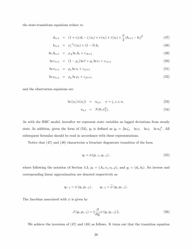
Notice that (47) and (48) characterize a bivariate degenerate transition of the form

qt = � (pt�1; qt�1) ; (55)

where following the notation of Section 4.3, pt = (At; rt; vt; '), and qt = (dt; kt) : Its inverse and

corresponding linear approximation are denoted respectively as

qt�1 = (qt; pt�1) ; qt�1 = e (qt; pt�1) :The Jacobian associated with is given by

J (qt; pt�1) = k@

@q0t (qt; pt�1) k: (56)

We achieve the inversion of (47) and (48) as follows. It turns out that the transition equation

28

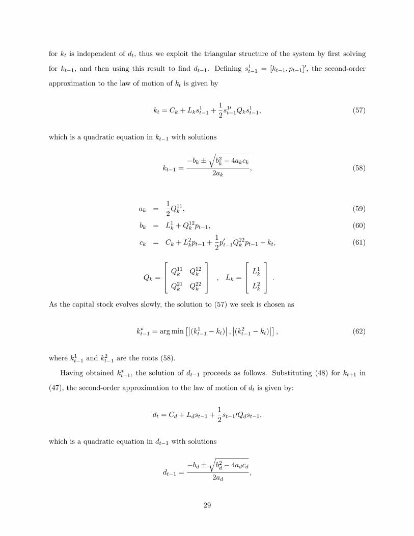
for kt is independent of dt, thus we exploit the triangular structure of the system by �rst solving

for kt�1, and then using this result to �nd dt�1. De�ning s1t�1 = [kt�1; pt�1]0, the second-order

approximation to the law of motion of kt is given by

kt = Ck + Lks1t�1 +

1

2s10t�1Qks

1t�1; (57)

which is a quadratic equation in kt�1 with solutions

kt�1 =�bk �

qb2k � 4akck2ak

; (58)

ak =1

2Q11k ; (59)

bk = L1k +Q12k pt�1; (60)

ck = Ck + L2kpt�1 +

1

2p0t�1Q

22k pt�1 � kt; (61)

Qk =

264 Q11k Q12k

Q21k Q22k

375 ; Lk =

264 L1k

L2k

375 :

As the capital stock evolves slowly, the solution to (57) we seek is chosen as

k�t�1 = argmin���(k1t�1 � kt)�� ; ��(k2t�1 � kt)��� ; (62)

where k1t�1 and k2t�1 are the roots (58).

Having obtained k�t�1, the solution of dt�1 proceeds as follows. Substituting (48) for kt+1 in

(47), the second-order approximation to the law of motion of dt is given by:

dt = Cd + Ldst�1 +1

2st�10Qdst�1;

which is a quadratic equation in dt�1 with solutions

dt�1 =�bd �

qb2d � 4adcd2ad

;

29

ad =1

2Q11d ; (63)

bd = L2d +Q12d s

1t�1; (64)

cd = Cd + L2ds1t�1 +

1

2s10t�1Q

22k s

1t�1 � dt; (65)

Qd =

264 Q11d Q12d

Q21d Q22d

375 ; Ld =

264 L1d

L2d

375 :

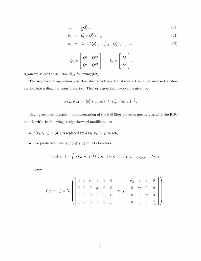
Again we select the solution d�t�1 following (62).

The sequence of operations just described e¤ectively transforms a triangular inverse transfor-

mation into a diagonal transformation. The corresponding Jacobian is given by

J (qt; pt�1) =�b2k + 4akck

�� 12 ��b2d + 4adcd

�� 12 :

Having achieved inversion, implementation of the EIS �lter proceeds precisely as with the RBC

model, with the following straightforward modi�cations:

� J (kt; zt�1) in (37) is replaced by J (dt; kt; pt�1) in (56).

� The predictive density f (stjYt�1) in (41) becomes

f (stjYt�1) 'ZJ (qt; pt�1) f (ptjst�1) g (st�1;dat�1) jqt�1= (qt;pt�1)dpt�1;

where

f (ptjst�1) = N4

0BBBBBBB@

266666664

0 0 �A 0 0 0

0 0 0 �r 0 0

0 0 0 0 �v 0

0 0 0 0 0 �'

377777775pt�1;

266666664

�2A 0 0 0

0 �2r 0 0

0 0 �2v 0

0 0 0 �2'

377777775

1CCCCCCCA:

30

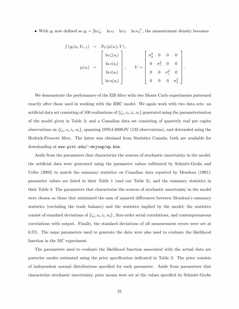
� With yt now de�ned as yt = [ln �t ln ct ln it lnnt]0 ; the measurement density becomes

f (ytjst; Yt�1) � N3 (�(st); V ) ;

�(st) =

266666664

ln �(st)

ln c(st)

ln i(st)

lnn(st)

377777775; V =

266666664

�2y 0 0 0

0 �2c 0 0

0 0 �2i 0

0 0 0 �2n

377777775:

We demonstrate the performance of the EIS �lter with two Monte Carlo experiments patterned

exactly after those used in working with the RBC model. We again work with two data sets: an

arti�cial data set consisting of 100 realizations of f�t; ct; it; ntg generated using the parameterization

of the model given in Table 3; and a Canadian data set consisting of quarterly real per capita

observations on f�t; ct; it; ntg, spanning 1976:I-2008:IV (132 observations), and detrended using the

Hodrick-Prescott �lter. The latter was obtained from Statistics Canada; both are available for

downloading at www.pitt.edu/�dejong/wp.htm.

Aside from the parameters that characterize the sources of stochastic uncertainty in the model,

the arti�cial data were generated using the parameter values calibrated by Schmitt-Grohe and

Uribe (2003) to match the summary statistics on Canadian data reported by Mendoza (1991):

parameter values are listed in their Table 1 (and our Table 3), and the summary statistics in

their Table 3. The parameters that characterize the sources of stochastic uncertainty in the model

were chosen as those that minimized the sum of squared di¤erences between Mendoza�s summary

statistics (excluding the trade balance) and the statistics implied by the model; the statistics

consist of standard deviations of f�t; ct; it; ntg ; �rst-order serial correlations, and contemporaneous

correlations with output. Finally, the standard deviations of all measurement errors were set at

0.5%. The same parameters used to generate the data were also used to evaluate the likelihood

function in the MC experiment.

The parameters used to evaluate the likelihood function associated with the actual data are

posterior modes estimated using the prior speci�cation indicated in Table 3. The prior consists

of independent normal distributions speci�ed for each parameter. Aside from parameters that

characterize stochastic uncertainty, prior means were set at the values speci�ed by Schmitt-Grohe

31

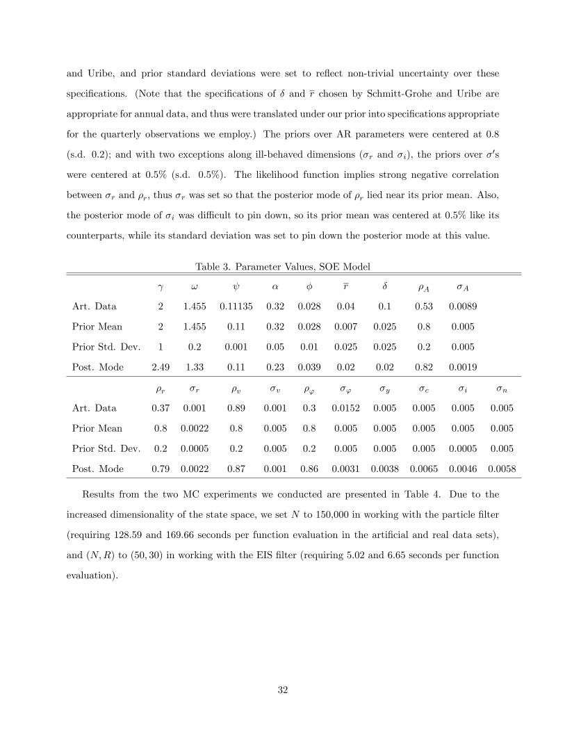
and Uribe, and prior standard deviations were set to re�ect non-trivial uncertainty over these

speci�cations. (Note that the speci�cations of � and r chosen by Schmitt-Grohe and Uribe are

appropriate for annual data, and thus were translated under our prior into speci�cations appropriate

for the quarterly observations we employ.) The priors over AR parameters were centered at 0.8

(s.d. 0.2); and with two exceptions along ill-behaved dimensions (�r and �i), the priors over �0s

were centered at 0.5% (s.d. 0.5%). The likelihood function implies strong negative correlation

between �r and �r; thus �r was set so that the posterior mode of �r lied near its prior mean. Also,

the posterior mode of �i was di¢ cult to pin down, so its prior mean was centered at 0.5% like its

counterparts, while its standard deviation was set to pin down the posterior mode at this value.

Table 3. Parameter Values, SOE Model

! � � r � �A �A

Art. Data 2 1.455 0.11135 0.32 0.028 0.04 0.1 0.53 0.0089

Prior Mean 2 1.455 0.11 0.32 0.028 0.007 0.025 0.8 0.005

Prior Std. Dev. 1 0.2 0.001 0.05 0.01 0.025 0.025 0.2 0.005

Post. Mode 2.49 1.33 0.11 0.23 0.039 0.02 0.02 0.82 0.0019

�r �r �v �v �' �' �y �c �i �n

Art. Data 0.37 0.001 0.89 0.001 0.3 0.0152 0.005 0.005 0.005 0.005

Prior Mean 0.8 0.0022 0.8 0.005 0.8 0.005 0.005 0.005 0.005 0.005

Prior Std. Dev. 0.2 0.0005 0.2 0.005 0.2 0.005 0.005 0.005 0.0005 0.005

Post. Mode 0.79 0.0022 0.87 0.001 0.86 0.0031 0.0038 0.0065 0.0046 0.0058

Results from the two MC experiments we conducted are presented in Table 4. Due to the

increased dimensionality of the state space, we set N to 150,000 in working with the particle �lter

(requiring 128.59 and 169.66 seconds per function evaluation in the arti�cial and real data sets),

and (N;R) to (50; 30) in working with the EIS �lter (requiring 5.02 and 6.65 seconds per function

evaluation).

32

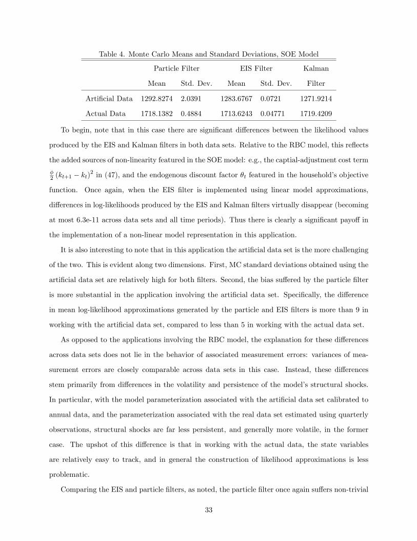
Table 4. Monte Carlo Means and Standard Deviations, SOE Model

Particle Filter EIS Filter Kalman

Mean Std. Dev. Mean Std. Dev. Filter

Arti�cial Data 1292.8274 2.0391 1283.6767 0.0721 1271.9214

Actual Data 1718.1382 0.4884 1713.6243 0.04771 1719.4209

To begin, note that in this case there are signi�cant di¤erences between the likelihood values

produced by the EIS and Kalman �lters in both data sets. Relative to the RBC model, this re�ects

the added sources of non-linearity featured in the SOE model: e.g., the captial-adjustment cost term

�2 (kt+1 � kt)

2 in (47), and the endogenous discount factor �t featured in the household�s objective

function. Once again, when the EIS �lter is implemented using linear model approximations,

di¤erences in log-likelihoods produced by the EIS and Kalman �lters virtually disappear (becoming

at most 6.3e-11 across data sets and all time periods). Thus there is clearly a signi�cant payo¤ in

the implementation of a non-linear model representation in this application.

It is also interesting to note that in this application the arti�cial data set is the more challenging

of the two. This is evident along two dimensions. First, MC standard deviations obtained using the

arti�cial data set are relatively high for both �lters. Second, the bias su¤ered by the particle �lter

is more substantial in the application involving the arti�cial data set. Speci�cally, the di¤erence

in mean log-likelihood approximations generated by the particle and EIS �lters is more than 9 in

working with the arti�cial data set, compared to less than 5 in working with the actual data set.

As opposed to the applications involving the RBC model, the explanation for these di¤erences

across data sets does not lie in the behavior of associated measurement errors: variances of mea-

surement errors are closely comparable across data sets in this case. Instead, these di¤erences

stem primarily from di¤erences in the volatility and persistence of the model�s structural shocks.

In particular, with the model parameterization associated with the arti�cial data set calibrated to

annual data, and the parameterization associated with the real data set estimated using quarterly

observations, structural shocks are far less persistent, and generally more volatile, in the former

case. The upshot of this di¤erence is that in working with the actual data, the state variables

are relatively easy to track, and in general the construction of likelihood approximations is less

problematic.

Comparing the EIS and particle �lters, as noted, the particle �lter once again su¤ers non-trivial

33

bias, on scales similar to those observed in working with the RBC model. Regarding MC standard

errors, these di¤er by two orders of magnitude in the arti�cial data set, but by only one order of

magnitude in the actual data set. These results indicate that increases in the dimensionality of

the state space do not necessarily amplify the numerical problems su¤ered by the particle �lter:

outliers and narrow measurement densities are far more important sources of di¢ culty.

We conclude our analysis of the SOE model by reporting sampling errors associated with the

log-likelihood estimates reported in Table 4. Following the procedure described above in working

with the RBC model, we estimate these errors to be 25.55 using the parameterization associated

with the arti�cial data set, and 17.92 using the parameterization associated with the actual data

set. Comparing these estimates with the MC standard errors reported in Table 4, we see that the

particle �lter serves as a better potential gauge of statistical uncertainty than was the case in the

applications involving the RBC model. In particular, its MC standard errors are only 1/13th and

1/36th the size of their associated sampling errors in this case, while recall that in working with

the RBC model, these ratios were roughly 2 and 4/5ths. The ratios associated with the EIS �lter

are 1/354th and 1/376th in this case, compared with roughly 1/10,000 and 1/200 in working with

the RBC model.

6 Conclusion

We have proposed an e¢ cient means of facilitating likelihood evaluation in applications involv-

ing non-linear and/or non-Gaussian state space representations: the EIS �lter. The �lter is adapted

using an optimization procedure designed to minimize numerical standard errors associated with

targeted integrals. Resulting likelihood approximations are continuous in underlying likelihood pa-

rameters, greatly facilitating the implementation of ML estimation procedures. Implementation of

the �lter is straightforward, and the payo¤ of adoption can be substantial.

34

References

[1] Carpenter, J.R., P. Cli¤ord and P. Fernhead, 1999, �An Improved Particle Filter for Non-

Linear Problems�, IEE Proceedings-Radar, Sonar and Navigation, 146, 1, 2-7.

[2] DeJong, D.N. with C. Dave, 2007, Structural Macroeconometrics. Princeton: Princeton Uni-

versity Press.

[3] DeJong, D.N., H. Dharmarajan, R. Liesenfeld, and J.-F. Richard, 2008, �E¢ cient Filtering in

State-Space Representations�, University of Pittsburgh Working Paper.

[4] DeJong, D.N., B.F. Ingram, and C.H. Whiteman, 2000, �A Bayesian Approach to Dynamic

Macroeconomics�, Journal of Econometrics. 98, 203-233.

[5] Devroye, L., 1986, Non-Uniform Random Variate Generation. New York: Springer.

[6] Doucet, A., N. de Freitas and N. Gordon, 2001, Sequential Monte Carlo Methods in Practice.

New York: Springer.

[7] Fernandez-Villaverde, J. and J.F. Rubio-Ramirez, 2005, �Estimating Dynamic Equilibrium

Economies: Linear versus Nonlinear Likelihood�, Journal of Applied Econometrics 20, 891-

910.

[8] Fernandez-Villaverde, J. and J.F. Rubio-Ramirez, 2009, �Estimating Macroeconomic Models:

A Likelihood Approach�, Review of Economic Studies. Forthcoming.

[9] Geweke, J., 1989, �Bayesian Inference in Econometric Models Using Monte Carlo Integration�,

Econometrica. 57, 1317-1339.

[10] Gordon, N.J., D.J. Salmond and A.F.M. Smith, 1993, �A Novel Approach to Non-Linear and

Non-Gaussian Bayesian State Estimation�, IEEE Proceedings F. 140, 107-113.

[11] Hendry, D.F., 1994, �Monte Carlo Experimentation in Econometrics�, in R.F. Engle and D.L.

McFadden, Eds. The Handbook of Econometrics, Vol. IV. New York: North Holland.

[12] Kim, S., N. Shephard, and S. Chib, 1998, �Stochastic Volatility: Likelihood Inference and

Comparison with ARCH Models�, Review of Economic Studies. 65, 361-393.

[13] Kitagawa, G., 1996, �Monte Carlo Filter and Smoother for Non-Gaussian Non-Linear State-

Space Models�, Journal of Computational and Graphical Statistics. 5, 1-25.

[14] Mendoza, E., 1991, �Real Business Cycles in a Small-Open Economy�, American Economic

Review. 81, 797-818.

[15] Pitt, M.K., 2002, �Smooth Particle Filters for Likelihood Evaluation and Maximisation�, Uni-

versity of Warwick Working Paper.

35

[16] Pitt, M.K. and N. Shephard, 1999, �Filtering via Simulation: Auxiliary Particle Filters�,

Journal of the American Statistical Association. 94, 590-599.

[17] Richard, J.-F. and W. Zhang, 2007, �E¢ cient High-Dimensional Monte Carlo Importance

Sampling�, Journal of Econometrics. 141, 1385-1411.

[18] Ristic, B., S. Arulampalam, and N. Gordon, 1984, Beyond the Kalman Filter: Particle Filters

for Tracking Applications. Boston: Artech Hous Publishers.

[19] Sargent, T.J., 1989, �Two Models of Measurements and the Investment Accelerator�, Journal

of Political Economy. 97, 251-287.

[20] Schmitt-Grohe, S. and M. Uribe, 2003, �Closing Small Open Economy Models�, Journal of

International Economics. 61, 163-185.

[21] Schmitt-Grohe, S. and M. Uribe, 2004, �Solving Dynamic General Equilibrium Models Using

a Second-Order Approximation to the Policy Function�, Journal of Economic Dynamics and

Control. 28, 755-775.

[22] Smets, F. and R. Wouters, 2003, �An Estimated Dynamic Stochastic General Equilibrium

Model of the Euro Area�, Journal of the European Economic Association. 1, 1123-1175.

[23] Smith, J.Q. and A.A.F. Santos, 2006, �Second-Order Filter Distribution Approximations for

Financial Time Series with Extreme Outliers�, Journal of Business and Economic Statistics.

24, 329-337.

[24] Uzawa, H., 1968, �Time Preference, the Consumption FUnction adn Optimum Asset Hold-

ings�, In Wolfe, J.N. (Ed.), Value, Capital and Growth: Papers in Honor of Sir John Hicks.

Edinburgh: The University of Edinburgh Press, 485-504.

36

900

950

1000

1050

1100

1150

1200

1250

1300

1350

1a. Particle Filter

900

950

1000

1050

1100

1150

1200

1250

1300

1350

1b. EIS Filter

1299.802

1299.804

1299.806

1299.808

1299.81

1299.812

1299.814

1b. EIS Filter, Rescaled

Figure 1. Log-Likelihood Approximations

37

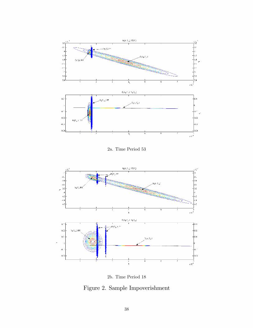
2a. Time Period 53

2b. Time Period 18

Figure 2. Sample Impoverishment

38

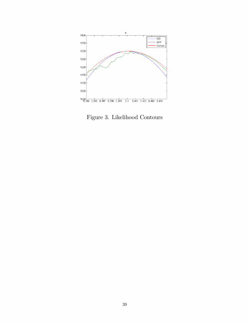
Figure 3. Likelihood Contours

39

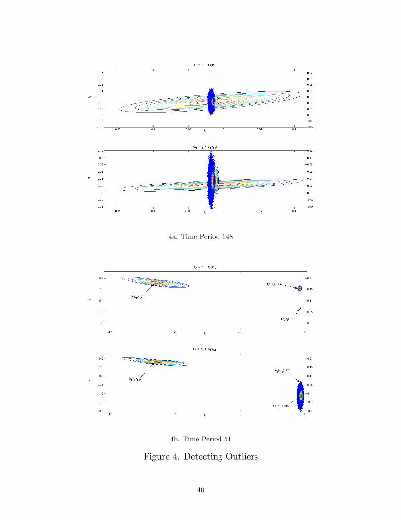
4a. Time Period 148

4b. Time Period 51

Figure 4. Detecting Outliers

40