Ellipsoidal Bounds for Uncertain Linear Equations

and Dynamical Systems∗

Giuseppe Calafiore† and Laurent El Ghaoui‡

†Dipartimento di Automatica e Informatica

Politecnico di Torino

Corso Duca degli Abruzzi, 24 – 10129 Torino, Italy

‡Dept. of Electrical Engineering and Computer Science

University of California at Berkeley, USA

July 24, 2003

Abstract

In this paper, we discuss semidefinite relaxation techniques for computing minimal sizeellipsoids that bound the solution set of a system of uncertain linear equations. The proposedtechnique is based on the combination of a quadratic embedding of the uncertainty, and theS-procedure. This formulation leads to convex optimization problems that can be essentiallysolved in O(n3) — n being the size of unknown vector — by means of suitable interior pointbarrier methods, as well as to closed form results in some particular cases. We further showthat the uncertain linear equations paradigm can be directly applied to various state-boundingproblems for dynamical systems subject to set-valued noise and model uncertainty.

Keywords: Uncertain linear equations, set-valued filtering, interior-point methods.

1 Introduction

This paper discusses a technique for computing deterministic confidence bounds on the solutions ofsystems of linear equations whose coefficients are imprecisely known, and presents an application ofthis technique to the problem of set-valued prediction and filtering for uncertain dynamical systems.

Uncertain linear equations (ULE) arise in many engineering endeavors, when the actual dataare imprecisely known and reliable bounds on the possible solutions need to be determined. Forinstance, in many problems of system identification one must solve a linear system of normal equa-tions arising from minimization of a least-squares criterion. When the regression data are subject tobounded uncertainty, this gives rise to a system of uncertain linear equations of the type examinedin this paper. Similarly, ULEs arise in Vandermonde systems for polynomial interpolation, whenthe abscissae of the interpolation points are assumed uncertain, as well as in Toeplitz systems forfinite impulse response estimation (see an example in Section 2.4.2). Also, in solid and structural

∗This work has been supported in part by FIRB funds of Italian Ministry of University and Research.

mechanics, uncertain linear equations are used to determine bounds on the system dynamic re-sponse for many scenarios of load and stiffness terms, [19, 23]. Specific applications in the contextof set-valued prediction and filtering for uncertain dynamical systems are discussed in Section 3 ofthis paper.

A basic version of the problem we deal with is well-known in the context of interval linear algebra,where one is given matrices A ∈ R

n,n and y ∈ Rn, the elements of which are only known within

intervals, and seeks to compute intervals of confidence for the set of solutions, if any, to the equationAx = y, see e.g. [15, 27]. Obtaining exact estimates on the confidence intervals for the elements ofx in the above context is known to be an NP-hard problem, [33, 34].

Here, we consider a more general situation in which the data matrix [A y] belongs to an uncer-tainty set U described by means of a linear fractional representation (LFR), and use semidefiniterelaxation techniques [13] to determine efficiently computable minimal ellipsoidal bounds for theset of solutions. In particular, we develop a special decoupled formulation of the problem whichleads to very efficient interior-point algorithms that scale with problem size essentially as O(n3), seeSection 2.1 and Section 2.2. Besides, we discuss special situations in which semidefinite relaxationsare lossless, and show how we can recover explicit closed-form solutions in these cases. Semidefiniterelaxation techniques for uncertain linear equations have been originally introduced by the authorsin [7].

In a subsequent part of the paper, we show the versatility of the ULE model by applying itto the solution of set-valued prediction and filtering problems relative to uncertain, discrete-timedynamical systems. The problem of determining a set that is guaranteed to contain the state of thesystem, despite the action of unknown-but-bounded additive noise, has a long history in the controlliterature. Early references on this topic include [3, 10, 35, 36], while more recent contributions arefound in [6, 20, 28, 37], to mention but a few. A fundamental point to remark is that in all theabove mentioned references the system description is assumed to be exactly known, while the maincontribution of this paper is to derive efficiently computable bounds on the system states when,in addition to unknown-but-bounded additive noise, structured deterministic uncertainty affectsthe system description in a possibly non-linear fashion. Semidefinite relaxation techniques in thiscontext have been first introduced by the authors in [8] for set-valued simulation, and in [12] forset-valued filtering. In the present paper, we derive similar results for predictor/corrector filterrecursions, using the unifying theoretical framework provided by the ULE paradigm.

This paper is organized as follows. Section 2 introduces the ULE model, and contains all therelative fundamental results. Section 2.2 provides a detailed discussion on the numerical complexityof computing bounds on ULEs, while Section 2.3 presents closed form results in the special caseof unstructured uncertainty. Numerical examples are discussed in Section 2.4. Finally, Section 3discusses the application of the ULE model in set-valued prediction and filtering for uncertaindynamical systems. A numerical example related to set-valued filtering is presented in Section 3.3,while conclusions are drawn in Section 4. To improve readability, several useful technical resultshave been collected in the appendices.

2

1.1 Notation and preliminaries

For a square matrix X, X 0 (resp. X 0) means X is symmetric, and positive-definite (resp.semidefinite). For a matrix X ∈ R

n,m, R(X) denotes the space generated by the columns of X,and N (X) denotes the kernel of X. An orthogonal complement of X is denoted by X⊥, which is amatrix containing by columns a basis for N (X), i.e. a matrix of maximal rank such that XX⊥ = 0.X† denotes the (Moore-Penrose) pseudo-inverse of X. ‖X‖ denotes the spectral (maximum singularvalue) norm of X, or the standard Euclidean norm, in case of vectors. In, 0n,m, and 1n,m denoterespectively the identity matrix of dimension n × n, the zero matrix, and the matrix of ones ofdimension n×m; dimensions are sometimes omitted when they can be easily inferred from context.

Ellipsoids. Ellipsoids will be described as

E = x : x = x + Ez, ‖z‖ ≤ 1,where x ∈ R

n is the center, and E ∈ Rn,m, Rank(E) = m ≤ n is the shape matrix of the ellipsoid.

This representation can handle all bounded ellipsoids, including ‘flat’ ellipsoids, such as points orintervals. An alternative description involves the squared shape matrix P = EET

E(P, x) =

x :

[P (x − x)

(x − x)T 1

] 0

.

When P 0, the previous expression is also equivalent to

E(P, x) =x : (x − x)T P−1(x − x) ≤ 1

.

The ‘size’ of an ellipsoid is a function of the squared shape matrix P , and will be denoted f(P ).Throughout this paper, f(P ) will be either trace (P ), which corresponds to the sum of squares ofthe semi-axes lengths, or log det(P ), which is related to the volume of the ellipsoid.

Uncertainty description. Structured uncertainty is described as follows: ∆ is a subspace ofR

np,nq , called the structure subspace (for instance, the space of matrices with certain block-diagonalstructure). Then, the uncertain matrix ∆ is restricted to

∆ ∈ ∆1.= ∆ ∈ ∆ : ‖∆‖ ≤ 1 .

Associated to the structure subspace, we introduce the scaling subspace B(∆)

B(∆) =(S, T, G) : ∀∆ ∈ ∆, S∆ = ∆T, G∆ = −∆T GT

. (1.1)

A structure that frequently arises in practice is the independent block-diagonal structure

∆ = ∆ : ∆ = diag (∆1, . . . ,∆), ∆i ∈ Rnpi,nqi . (1.2)

For this structure, the scaling subspace is constituted of all triples S, T, G with S = diag (λ1Inp1 ,

. . . , λInp), T = diag (λ1Inq1 , . . . , λInq

), G = 0. A particular case of this situation arises for = 1,and it is denoted as the unstructured uncertainty case.

Independent scalar uncertain parameters δ1, . . . , δ with bounded magnitude |δi| ≤ 1 are repre-sented in our framework via the structure subspace

∆ =∆ : ∆ = diag (δ1Inp1 , . . . , δInp

), δi ∈ R

, (1.3)

3

and the corresponding scaling subspace, constituted of all triples S, T, G with S = T = diag (S1 . . . , S),Si = ST

i ∈ Rnpi,npi , G = diag (G1, . . . , G), Gi = −GT

i ∈ Rnpi,npi .

More general uncertainty structures, together with their corresponding scaling spaces, are detailedfor instance in [11, 13].

2 Uncertain Linear Equations

Let the uncertain data be described as

[A(∆) y(∆)] = [A y] + L∆(I − H∆)−1[RA Ry], (2.4)

where A ∈ Rm,n, y ∈ R

m, L ∈ Rm,np , RA ∈ R

nq ,n, Ry ∈ Rnq , H ∈ R

nq ,np , and ∆ ∈ ∆1 ⊂ Rnp,nq ,

and let this linear fractional representation (LFR) be well-posed over ∆1, meaning that det(I −H∆) = 0, ∀∆ ∈ ∆1. Lemma A.2 reported in the Appendix provides a well-known and readilycheckable sufficient condition for the well-posedness of the above linear fractional representation.

The representation (2.4) includes as special cases, for instance, interval matrices discussed in manyreferences [15, 27, 33, 34], as well as additive uncertainty of the form [A + ∆A y + ∆y]. In thislatter case, the linear fractional representation is simply given by L = [Im Im], [RA Ry] = In+1,H = 0n+1,2m, and ∆ = diag (∆A, ∆y). The description (2.4) also allows for representation ofgeneral rational matrix functions of a vector of uncertain parameters δ1, . . . , δ, see [11, 13] forfurther details and constructive procedure for building the LFR in this general case.

Define now the set X of all the possible solutions to the linear equations A(∆)x = y(∆), i.e.

X .= x : A(∆)x = y(∆), for some ∆ ∈ ∆1.

In the sequel, we provide conditions under which the set X is contained in a bounded ellipsoid E ,and we exploit these conditions to determine a minimal (in the sense of the selected size measuref(·)) ellipsoid containing the solution set X .

We first state a key lemma.

Lemma 2.1. Let

Ψ .= [A L y], (2.5)

Υ .=

[RA H Ry

0np,n Inp 0np,1

], (2.6)

Ω(S, T, G) .= ΥT

[T G

GT −S

]Υ. (2.7)

Let further the orthogonal complement Ψ⊥ be chosen as

Ψ⊥.=

[Ψ⊥1 ψ⊥2

0 · · · 0 −1

], (2.8)

where Ψ⊥1 is an orthogonal complement of [A L], and ψ⊥2 is any vector such that [A L]ψ⊥2 = y.(If no such ψ⊥2 exists, then the solution set X is empty).

4

Then, for any triple (S, T, G) ∈ B(∆), with S 0 and T 0, the set

X S,T,G.=

x = [In 0 0]Ψ⊥

[ν

1

], ν : [νT 1]ΨT

⊥Ω(S, T, G)Ψ⊥[νT 1]T ≥ 0

, (2.9)

is an outer approximation for the solution set X , i.e. X ⊆ X S,T,G.Furthermore, when ∆ is a full block (unstructured uncertainty) the approximation is exact, i.e.

X S,T,G ≡ X . In this latter case, the solution set is the quadratic set

X =

x = [In 0 0]Ψ⊥

[ν

1

], ν : [νT 1]ΨT

⊥Ω(I, I, 0)Ψ⊥[νT 1]T ≥ 0

. (2.10)

Proof. Consider the linear fractional description (2.4), and rewrite equation A(∆)x = y(∆) as

Ax − y + L∆(I − H∆)−1(RAx − Ry) = 0,

which in turn can be expressed using a slack vector p in the form

Ax − y + Lp = 0 (2.11)

RAx + Hp − Ry = q (2.12)

p = ∆q. (2.13)

Let Ψ be as defined in (2.5), and let

ξ.= [xT pT − 1]T , (2.14)

then all vectors ξ compatible with (2.11) must be orthogonal to Ψ, and can be expressed as

ξ = Ψ⊥η, with η.=

[ν

1

], Ψ⊥

.=

[Ψ⊥1 ψ⊥2

0 · · · 0 −1

], (2.15)

where Ψ⊥1 is an orthogonal complement of [A L], and ψ⊥2 is any vector such that [A L]ψ⊥2 = y.Notice that if no such ψ⊥2 exists, then (2.11) is not solvable, and hence the solution set X is clearlyempty. All feasible ξ must therefore lie on the flat

F .=

ξ : ξ = Ψ⊥η, with η =[

νT 1]T

,

and the corresponding feasible x on the projection Fx.= x = [In 0n,np 0n,1]ξ : ξ ∈ F. The

feasible ξ are further constrained by (2.12)–(2.13): By the Quadratic Embedding Lemma A.5 (inthe Appendix), for any triple (S, T, G) ∈ B(∆), S 0, T 0, the set of all pairs (q, p) such thatp = ∆q for some ∆ ∈ ∆1, is bounded by the set

QS,T,G.=

[

q

p

]:

[q

p

]T [T G

GT −S

][q

p

]≥ 0

. (2.16)

5

Therefore, the set of ξ compatible with (2.12)–(2.13) is bounded by the set

HS,T,G.= ξ : ξT Ω(S, T, G)ξ ≥ 0, (2.17)

where Ω(S, T, G) is defined in (2.7). To conclude, the set of ξ compatible with all conditions (2.11)–(2.13) is bounded by the intersection F ∩ HS,T,G, and therefore X ⊆ X S,T,G, where X S,T,G is theprojection

X S,T,G =x = [In 0 0]Ψ⊥η : ηT ΨT

⊥Ω(S, T, G)Ψ⊥η ≥ 0

, (2.18)

with η and Ψ⊥ defined in (2.15).When ∆ is unstructured, the embedding in Lemma A.5 is tight, and the approximation is exact,

i.e. X S,T,G = X . Moreover, in this case the scalings are S = λI, T = λI, G = 0, and hence (2.10)follows.

The next theorem provides a characterization of a bounding ellipsoid for the solution set X .

Theorem 2.1. Let all symbols be defined as in Lemma 2.1. If there exist (S, T, G) ∈ B(∆), S 0,T 0 such that [

P [I 0 x]Ψ⊥ΨT

⊥[I 0 x]T ΨT⊥ (diag (0, 0, 1) − Ω(S, T, G)) Ψ⊥

] 0 (2.19)

is feasible, then the ellipsoid E(P, x) contains the solution set X .

Proof. From Lemma 2.1, we have that for any triple (S, T, G) ∈ B(∆), S 0, T 0, the conditionE(P, x) ⊇ X S,T,G implies E(P, x) ⊇ X . Consider then the following points.

1. The family of ellipsoids E(P, x) that lie in Fx satisfy the flatness condition (I − P †P )(x −x) = 0, ∀x ∈ Fx, which can be expressed using the notation introduced previously, as(I − P †P )[In 0 x]Ψ⊥η = 0, ∀η, i.e.

(I − P †P )[In 0 x]Ψ⊥ = 0. (2.20)

2. An ellipsoid E(P, x) ⊂ Fx contains the point x = [In 0 0]Ψ⊥η ∈ Fx if and only if (notice thatx − x = [In 0 x]Ψ⊥η) [

P [In 0 x]Ψ⊥η

∗ 1

] 0. (2.21)

Using Schur complements (Lemma A.6 in the Appendix), this is rewritten as

1 − ηT ΨT⊥[In 0 x]T P †[In 0 x]Ψ⊥η ≥ 0 (2.22)

(I − P †P )[In 0 x]Ψ⊥η = 0. (2.23)

Since (2.20) holds for all ellipsoids that lie entirely in Fx, condition (2.23) is always satisfied,therefore the ellipsoid E(P, x) ⊂ Fx contains the point x = [In 0 0]Ψ⊥η ∈ Fx if and only if(2.22) is satisfied.

6

3. The ellipsoid E(P, x) lies in Fx and contains X S,T,G if and only if (2.20) holds, and (2.22) issatisfied for all η such that ηT ΨT

⊥Ω(S, T, G)Ψ⊥η ≥ 0. By the S-procedure and homogenization(see Lemma A.3 and Lemma A.4), the above happens if (2.20) holds, and there exist τ ≥ 0such that

ΨT⊥(diag (0, 0, 1) − [I 0 x]T P †[I 0 x]

)Ψ⊥ τΨT

⊥Ω(S, T, G)Ψ⊥.

Using the Schur complement rule, the two previous conditions are written in the equivalentmatrix inequality form as[

P [I 0 x]Ψ⊥ΨT

⊥[I 0 x]T ΨT⊥ (diag (0, 0, 1) − τΩ(S, T, G)) Ψ⊥

] 0. (2.24)

Further, from Lemma A.4, we have that (2.24) is also a necessary condition for the inclusion,provided that there exist η0: ηT

0 ΨT⊥Ω(S, T, G)Ψ⊥η0 > 0.

In synthesis, if there exist (S, T, G) ∈ B(∆), S 0, T 0, such that (2.24) is satisfied (noticethat τ can be absorbed in the S, T, G variables and then eliminated from the condition), then theellipsoid E(P, x) lies in Fx and contains X . Moreover, if there exist η0: ηT

0 ΨT⊥Ω(S, T, G)Ψ⊥η0 > 0,

(2.24) is also necessary for an ellipsoid E(P, x) ⊂ Fx to include X S,T,G.

Remark 2.1. Based on the condition (2.19), we can subsequently minimize a (convex) size measuref(P ) of the bounding ellipsoid, subject to this inclusion constraint. Solving the convex optimizationproblem in the variables P, x, S, T, G

minimize f(P ) subject to (2.25)

(S, T, G) ∈ B(∆), S 0, T 0, (2.19) (2.26)

hence yields an outer ellipsoidal approximation of X , that is optimal in the sense of the sufficientcondition (2.19). Notice that this optimization problem is a semidefinite program (SDP), if f(P ) =trace (P ), and a MAXDET problem, if f(P ) = log det(P ). In both cases the problem can beefficiently solved in polynomial-time by interior point methods for convex programming, [39, 40].

We also remark that Lemma 2.1 can be used for directly determining optimized bounds onindividual elements of the solution vector x. In this case, one is not interested in determining abounding ellipsoid for the entire solution vector, but rather a minimal width interval containing aspecific entry of x. This is basically a special case of the problem considered in Theorem 2.1, andwe leave this easy modification to the reader.

In the particular case of unstructured uncertainty, the condition expressed in the Theorem 2.1becomes necessary and sufficient, as detailed in the following corollary.

Corollary 2.1. Let ∆ = Rnp,nq , and assume there exists η0 such that

ηT0 ΨT

⊥ΥT

[I 00 −I

]ΥΨ⊥η0 > 0. (2.27)

7

Then the ellipsoid E(P, x) lies in Fx and contains the solution set X if and only if there existsτ ≥ 0 such that

P [I 0 x]Ψ⊥

ΨT⊥[I 0 x]T ΨT

⊥

(diag (0, 0, 1) − τΥT

[I 00 −I

]Υ

)Ψ⊥

0. (2.28)

The proof of this corollary follows immediately from the tightness of the embedding in Lemma A.5in the unstructured case, and from the losslessness of the S-procedure, under the assumption(2.27); see discussions following formulas (2.18) and (2.24). Minimizing the ellipsoid size f(P )under constraint (2.28) then yields the globally optimal ellipsoid containing X . We also noticethat condition (2.27) is satisfied if and only if the kernel matrix has at least one (strictly) positiveeigenvalue, and it is therefore easy to check.

2.1 Decoupled ellipsoid equations

We now build upon the LMI condition given in Theorem 2.1, in order to derive decoupled con-ditions for the optimal ellipsoid in terms of its shape matrix P and center x separately. Thesedecoupled conditions are based on a variable elimination technique and permit to obtain explicitclosed form results in the case of unstructured uncertainty. More fundamentally, they lead to aconvex optimization problem of reduced numerical complexity with respect to the one given inTheorem 2.1, as it is discussed in detail in Section 2.2.

A first result is stated in the following corollary.

Corollary 2.2. Let all symbols be defined as in Lemma 2.1, and define the partition

Q(S, T, G) =

[Q11 q12

qT12 1 − q22

].= ΨT

⊥ (diag (0, 0, 1) − Ω(S, T, G)) Ψ⊥, (2.29)

B.= [In 0]Ψ⊥1. (2.30)

Consider the optimization problem in the variables (S, T, G) ∈ B(∆)

minimize f(BQ†11B

T ) subject to: (2.31)

S 0, T 0, (2.32)

Q(S, T, G) 0, (2.33)

(I − Q†11Q11)BT = 0. (2.34)

If the above problem is feasible, then there exist a bounded ellipsoid that contains X . In this case,calling Sopt, Topt, Gopt the optimal values of the problem variables, the ellipsoid E(Popt, xopt) with

Popt = BQ†11(Sopt, Topt, Gopt)BT (2.35)

xopt = [In 0]ψ⊥2 − BQ†11(Sopt, Topt, Gopt)Q12 (2.36)

is an outer ellipsoidal approximation of X , that is optimal in the sense of the sufficient condition(2.19). This solution is equivalent to the one obtained minimizing f(P ) subject to the conditionsin Theorem 2.1.

8

Proof. See Appendix B.

Remark 2.2 (Boundedness). From Corollary 2.2 we immediately obtain a readily checkablesufficient condition for the solution set of uncertain linear equations to be bounded: If there exist(S, T, G) ∈ B(∆) such that (2.32)–(2.34) are satisfied, then the solution set X is bounded. Theseconditions become also necessary, under the hypotheses of Corollary 2.1.

Remark 2.3 (Emptiness and uniqueness). A preliminary analysis of (2.11) through (2.15)shows that a necessary condition in order to have (at least) one solution is that y ∈ R([A L]).Notice also that if N ([A L]) is empty, then the uncertain linear equations may have at most onesolution. In this case, the solution of the optimization problems in Theorem 2.1 and Corollary 2.2would yield an ellipsoid reduced to a point, i.e. Popt = 0.

Without need to solve any optimization problem, we may therefore conclude that:

if y ∈ R([A L]) ⇒ X is empty;

if N ([A L]) = 0 ⇒ X is either empty or reduced to a point.

In the latter case, if y ∈ R([A L] then X is certainly empty, otherwise the only candidate solutionis of the form x = [In 0]ψ⊥2, with ψ⊥2

.= [xT pT ]T . To check if this is actually a solution, we canin some cases proceed by direct inspection. For instance, let q = RAx + Hp−Ry, then in the caseof unstructured uncertainty x is the unique solution if and only if pT p ≤ qT q.

2.2 Analysis of numerical complexity

We next provide estimates of the numerical complexity of solving the ULE bounding problem, inboth the coupled form of Theorem 2.1 and the decoupled form of Corollary 2.2. This analysis showsin particular that the formulation in Corollary 2.2 provides a drastic improvement in numericalefficiency with respect to the one in Theorem 2.1.

For the sake of clarity in the presentation, we here limit ourselves to the case of structuredblock-diagonal uncertainties of the type

∆ =

∆ : ∆ = diag (∆1, . . . ,∆), ∆i ∈ Rd,d

(all blocks of the same size), for which the scaling subspace is constituted of all triples S, T, G withS = T = diag (λ1Id, . . . , λId), G = 0. Besides, within this section we shall assume the trace as theellipsoid optimality criterion. Results similar to the ones reported below can also be determined ifthe log-determinant criterion is used instead of the trace.

Under the above hypotheses, the optimization problem (2.25), (2.19) derived from Theorem 2.1is a convex semidefinite programming problem (SDP) involving a constraint matrix of dimensionM = n + (n − m + d + 1) + ,1 and N = n(n + 1)/2 + n + decision variables (the elements ofP, x and λ1, . . . , λ). Therefore, using a general-purpose primal-dual interior-point SDP solver (i.e.we are in a sense considering a worst-case situation of a solver that does not exploit any possiblestructure in the problem) the complexity grows with problem size as

O(√

M)O(M2N2),1We assumed Ψ full-rank, in order to fix the dimension of the orthogonal complement Ψ⊥.

9

where the first factor denotes the number of outer iterations of the algorithm, and the second factordenotes the cost per iteration, see [39]. It is also observed in [39], Section 5.7 that in practice thesealgorithms behave much better that predicted by the above bound and that, in particular, thefirst factor can be assumed almost constant, so that the practical complexity is O(M2N2). Noticehowever that in our context this gives O(n6 +n5d+d2(4 +n42 +n23)), i.e. an O(n6) dependenceon the dimension of x, and O(d24) dependence on the size and number of uncertainty blocks.

Consider now the decoupled problem in Corollary 2.2, which is here rewritten in the equivalentform (all the previous hypotheses still holding)

inf α subject to: (2.37)

α − trace (BQ−111 (λ1, . . . , λ)BT ) ≥ 0

λi ≥ 0, i = 1, . . . ,

Q(λ1, . . . , λ) 0,

where Q(λ1, . . . , λ) is affine in λ1, . . . , λ, see (2.29).A basic idea for solving (2.37) is to associate a barrier for the feasible set, and solve a sequence

of unconstrained minimization problems, involving a weighted combination of the barrier and the(linear) objective. The complexity of a path-following interior-point method as described in [25,p.93] depends on our ability of finding a ‘self-concordant barrier’ associated with the constraints.When such a barrier is known, the number of outer iterations grows as O(

√θ), where θ is the

‘parameter of the barrier’. The cost of each iteration is proportional to that of computing thegradient g and Hessian H of the barrier, and solving the linear system Hv = g, where the unknownv is the search direction. We note again that in practice, the number of outer iterations is almostindependent of problem size.

We can indeed find a self-concordant for problem (2.37), and find its parameter. To do this, weapply the addition rule [25, Prop. 5.1.3], which says that to find the barrier for multiple constraints,we simply add barriers and their respective parameters. The following is a direct consequence ofthe result [25, Prop. 5.1.8]: The function

F (α, λ1, . . . , λ) = − log(α − trace (BQ−1

11 (λ1, . . . , λ)BT ))− log detQ(λ1, . . . , λ) −

∑i=1

log λi

(2.38)is a self-concordant barrier for problem (2.37), with parameter θ = 1+(ω+1)+ = ω++2, whereω

.= n−m+d (note that B has size n×ω, and Q11 has size ω×ω). A tedious but straightforwardcalculation shows that the cost of computing the gradient and Hessian of the barrier and solvingfor direction v is O(ω3 + 2ω2), hence the total complexity estimate is

O(√

θ)O(ω3 + 2ω2).

As noted above, the number of outer iterations is almost constant in practice, so the practicalcomplexity can be assumed to be O(ω3 + 2ω2). From this, it results that the complexity of thedecoupled problem is O(n3 + n2d2 + nd23 + d34), which implies an O(n3) dependence on thedimension of x, and O(d34) dependence on the size and number of uncertainty blocks. Hence,for fixed number and size of the uncertainty blocks, the decoupled problems improves upon thecoupled one by a factor of O(n3).

10

2.3 Special case: unstructured uncertainty

In this section, we analyze in further detail the case when the uncertainty affecting the system oflinear equations is unstructured, i.e. when ∆ is a full matrix block.

For unstructured uncertainty the multipliers S, T, G simplify to S = λI, T = λI, G = 0. Thematrices Q11(λ), q12(λ), q22(λ) defined in Corollary 2.2 are linear in λ, and it is convenient to expressthem as Q11(λ) = λQ11, q12(λ) = λq12, q22(λ) = λq22, with

Q11.= ΨT

⊥1([0 I]T [0 I] − [RA H]T [RA H])Ψ⊥1, (2.39)

q12.= ΨT

⊥1[RA H]T Ry + ΨT⊥1([0 I]T [0 I] − [RA H]T [RA H])ψ⊥2, (2.40)

q22.= RT

y Ry − 2ψT⊥2[RA H]T Ry − ψT

⊥2([0 I]T [0 I] − [RA H]T [RA H])ψ⊥2. (2.41)

The optimal ellipsoid containing the solution set is in this case computable in closed form, asdetailed in the following corollary.

Corollary 2.3. Let ∆ = Rnp,nq , B

.= [In 0]Ψ⊥1, and assume that y ∈ R([A L]), (if this conditionis not satisfied, the solution set is empty).

Then, the solution set X is bounded if

Q11 0, (2.42)

(I − Q†11Q11)B = 0, (2.43)

(I − Q†11Q11)q12 = 0. (2.44)

The above conditions are also necessary, if there exists η0 such that

ηT0

[−Q11 q12

qT12 q22

]η0 > 0. (2.45)

When (2.42)–(2.44) are satisfied, the optimal ellipsoid containing X is given by

Popt =1

λoptBQ†

11BT (2.46)

xopt = [In 0]ψ⊥2 − BQ†11q12, (2.47)

with1

λopt= maxq22 + qT

12Q†11q12, 0.

When Popt = 0 then the solution set contains at most one point. In particular, if q22 ≥ 0, thenX = [In 0]ψ⊥2, otherwise X is empty.

Proof. With the current scalings S = λI, T = λI, G = 0, problem (2.31)–(2.34) is easily restatedas

minimize f(BQ†11(λ)BT ) s.t.:

λ ≥ 0, Q11(λ) 0,

1 − q22(λ) − qT12(λ)Q†

11(λ)q12(λ) ≥ 0,

(I − Q†11(λ)Q11(λ))q12(λ) = 0,

(I − Q†11(λ)Q11(λ))B = 0.

11

Since all dependencies are linear in λ (and since λ = 0 cannot be optimal), the problem is equivalentto

minimize f( 1λBQ†

11BT ) s.t.:

λ > 0, Q11 0,

1 − λq22 − λqT12Q

†11q12 ≥ 0,

(I − Q†11Q11)q12 = 0,

(I − Q†11Q11)B = 0.

Since f(·) is non-increasing in λ, if the problem is feasible the optimum is attained by the largestpossible value of λ, i.e. for

1λopt

= maxq22 + qT12Q

†11q12, 0.

The statements of the corollary then follow easily from the above considerations.The necessity of conditions for boundedness of the solution set follows from the S-procedure, see

Lemma A.4. The last statement of the corollary follows from the discussion in Remark 2.3, noticingthat pT p ≤ qT q if and only if q22 ≥ 0.

Remark 2.4. Notice that, according to Lemma 2.1, in the unstructured case the actual solutionset is the quadratic set

X =

x = Bν + [In 0]ψ⊥2, ν :

[ν

1

]T [Q11 q12

qT12 −q22

][ν

1

]≤ 0

.

This set is indeed an ellipsoid, whenever Q11 0 and q22 + qT12Q

−111 q12 > 0, and hence Corollary 2.3

returns the exact solution set in this case.

2.3.1 Additive unstructured uncertainty

An even more specialized case of the unstructured uncertainty situation above arises when the dataA, y are affected by additive uncertainty, i.e.

[A(∆) y(∆)] = [A y] + L∆[RA Ry],

with L = ρIm, ρ > 0, [RA Ry] = In+1, H = 0, ∆ ∈ Rm,n+1, and ‖∆‖ ≤ 1.

In this case, we may choose the orthogonal complements as

Ψ⊥1 =

[ρIn

−A

]; ψ⊥2 =

[0

y/ρ

],

and therefore Q11 = AT A − ρ2I, q12 = −AT y/ρ, q22 = 1 − yT y/ρ2. The solution set is hence thequadratic set

X =

x :

[x

1

]T [ 1ρ2 AT A − I − 1

ρ2 AT y

− 1ρ2 yT A 1

ρ2 yT y − 1

][x

1

]≤ 0

. (2.48)

In this simple situation, the set X could be analyzed directly, but we check what it is predictedby Corollary 2.3: Condition (2.45) is satisfied if and only if ρ2 > λmin[A y]T [A y]. In this case,

12

the solution set is bounded if and only if Q11 0, i.e. for ρ2 < λminAT A. On the other hand,if ρ2 < λmin[A y]T [A y] then ρ2 < λminAT A and q22 < 0,2 therefore the solution set is empty.Lastly, we consider the situation when ρ2 = λmin[A y]T [A y] and ρ2 < λminAT A. In this casewe have that the kernel matrix in (2.48) is positive semi-definite, hence the only points in X arethose who annihilate the quadric

g(x) .= xT (AT A − ρ2I)x − 2yT Ax + (yT y − ρ2).

Since g(x) is strictly convex, it has the unique minimizer x = (AT A − ρ2I)−1AT y. Substituting x

back into g(x), we have that x is in the solution set if and only if ρ2(yT (ρ2I − AAT )−1y − 1) = 0;notice however that in the current situation, this latter condition is always satisfied.3

We may resume these results as follows.

• If λmin[A y]T [A y] < ρ2 < λminAT A, then X is an ellipsoid with

Popt = α(AT A − ρ2I)−1

xopt = (AT A − ρ2I)−1AT y,

where α.= ρ2(1 − yT (ρ2I − AAT )−1y).

• If ρ2 < λmin[A y]T [A y], then the solution set is empty.

• If ρ2 > λminAT A, then the solution set is unbounded.

• If ρ2 = λmin[A y]T [A y] < λminAT A, then the solution set is the singleton X = xopt.

It is worth to remark that ρ2 = λmin[A y]T [A y] is the minimal perturbation size for which X isnon-empty and that, in this case, the central solution xopt coincides with the Total Least Squares

solution (see for instance [18]) of the system of equations ([A y] + ∆)

[x

−1

]= 0.

The case when only the matrix A is uncertain (i.e. y is given and fixed) can be analyzed similarly,setting the LFR

[(A + ρ∆) y] = [A y] + L∆[RA 0n],

with L = ρIm, RA = In. In this case we have Q11, q12 as before, and q22 = − 1ρ2 yT y. The solution

set is therefore the quadratic set

X =

x :

[x

1

]T [ 1ρ2 AT A − I − 1

ρ2 AT y

− 1ρ2 yT A 1

ρ2 yT y

][x

1

]≤ 0

. (2.49)

2This is since λmin[A y]T [A y] ≤ λminAT A, and

[−Q11 q12

qT12 q22

] 0 if and only if ρ2 ≤ λmin[A y]T [A y].

3This fact can be proved as follows: ρ2 = λmin[A y]T [A y] implies that det(ρ2I − [A y]T [A y]) = 0, but since

ρ2 < λminAT A, this is equivalent (by the Schur determinant rule) to yT (I −A(AT A− ρ2I)−1AT )y− ρ2 = 0, which

in turn, by application of matrix inversion lemma is equivalent to ρ2(yT (ρ2I − AAT )−1y − 1) = 0.

13

2.4 Numerical examples

2.4.1 Example 1

Consider the data

A(∆) = I2 + 0.2δ1

[1 00 −1

]+ 0.5δ2

[0 1−1 0

]; y =

[11

],

with |δ1| ≤ 1, |δ2| ≤ 1. Here, the matrix A(∆) is the identity, plus two additive perturbations. Theuncertain data can be expressed in LFR format as

[A(∆) | y(∆)] =

[1 0 10 1 1

]+ L∆[RA | Ry], (2.50)

L =

[0.2 0 0 0.50 −0.2 −0.5 0

], RA = [I2 I2]T , Ry = 0, (2.51)

∆ = diag (δ1I2, δ2I2), with |δ1| ≤ 1, |δ2| ≤ 1. The scaling subspace is in this case given by the setof triples (S, T, G) with S = T = diag (S1, S2), S1, S2 ∈ R

2,2 symmetric, and G = diag (G1, G2),with G1, G2 ∈ R

2,2 skew-symmetric.To have an approximate idea of the shape of the solution set X , we randomly generated a number

of samples of δ1, δ2, and solved the corresponding linear equations. The points obtained are shownin Figure 1 (notice that the solution set of this ULE is not convex), together with the optimalbounding ellipsoid, determined by the solution of the convex problem in Theorem 2.1, havingparameters

x =

[0.8590.859

]; P =

[0.462 −0.246−0.246 0.462

].

We next considered a modification of the previous example, in which H = 0. In particular, theULE is now described by the LFR

[A(∆) | y(∆)] =

[1 0 10 1 1

]+ L∆(I − H∆)−1[RA | Ry], (2.52)

with

L =

[0.2 0 0 0.50 −0.2 −0.5 0

], RA = [I2 I2]T , Ry = 0, H = 0.5I4 (2.53)

and ∆ = diag (δ1I2, δ2I2), |δ1| ≤ 1, |δ2| ≤ 1. The scaling subspace is the same as in the previousversion of the example, and the application of Theorem 2.1 yields an optimal bounding ellipsoidwith parameters

x =

[0.56871.0549

]; P =

[0.8092 −0.1759−0.1759 0.6578

].

This optimal ellipsoid is depicted in Figure 2, together with randomly generated points in theinterior of the solution set.

14

0 0.2 0.4 0.6 0.8 1 1.2 1.4 1.60

0.2

0.4

0.6

0.8

1

1.2

1.4

1.6

Figure 1: Solution set and bounding ellipsoid for the ULE resulting from the data in (2.50), (2.51)and structured uncertainty ∆ = diag (δ1I2, δ2I2).

−0.4 −0.2 0 0.2 0.4 0.6 0.8 1 1.2 1.4 1.60.2

0.4

0.6

0.8

1

1.2

1.4

1.6

1.8

2

Figure 2: Solution set and bounding ellipsoid for the ULE resulting from the data in (2.52), (2.53)and structured uncertainty ∆ = diag (δ1I2, δ2I2).

2.4.2 Example 2: FIR estimation

We next address the problem of estimating intervals of confidence for the coefficients of a discrete-time impulse response vector x, from uncertain input and output measurement. Specifically, theuncertain linear equation we consider has the form A(∆)x = y(∆), where A is a lower-triangularToeplitz matrix whose first column is the input vector u, and y is the system output. Both the

15

input u and output y are unknown-but-bounded componentwise, that is

|ui − unomi | ≤ ρ, i = 1, . . . , n,

|yi − ynomi | ≤ ρ, i = 1, . . . , n,

where unom is the nominal input vector, ynom is the measured output vector, and ρ ≥ 0 is a givenscalar. It is easy to derive a linear fractional representation for the uncertain system in this case.The uncertainty matrix has the following structure:

∆ = diag (δu1In, δu2In−1, . . . , δun, δy1, δy2, . . . , δyn),

where δui (resp. δyi) are the componentwise absolute errors in u (resp. y), normalized so that theuncertainty matrix is bounded in maximum singular value norm by one. The parameters of thelinear fractional representation of the system are in this case

L = ρ

[In

[01,n−1

In−1

] [02,n−2

In−2

]· · ·

[0n−1,1

1

]In

]∈ R

n,n(n+1)/2+n,

RA =

In[In−1 0n−1,1

][

In−2 0n−2,2

]...[

1 01,n−1

]0n,n

∈ R

n(n+1)/2+n,n, Ry =

0n(n+1)/2,1

11...1

∈ R

1,n(n+1)/2+n,

and H = 0n(n+1)/2+n,n(n+1)/2+n. Taking ρ = 0.1, and unom = sin(i), vector y is generated byfeeding this input to an FIR filter with coefficients hnom = cos(i). For n = 5, the optimal result is

P =

0.1879 −0.2669 0.1369 −0.0700 0.1400−0.2669 0.6201 −0.5059 0.2987 −0.29610.1369 −0.5059 1.0446 −0.8017 0.6084−0.0700 0.2987 −0.8017 1.4154 −1.27400.1400 −0.2961 0.6084 −1.2740 2.4356

, x =

0.6270−0.5851−0.8145−0.83950.5467

.

This results in intervals of confidence for the coefficients of the FIR filter, obtained by projectingthe ellipsoid of confidence on the coordinate axes:

0.1935−1.3726−1.8365−2.0292−1.0140

≤ x ≤

1.06060.20240.20760.35022.1073

.

16

3 Set-valued prediction and filtering for uncertain systems

In this section, we study the problem of recursive ellipsoidal state bounding for uncertain discrete-time linear dynamical systems. First, we consider the set-valued prediction problem, i.e. given anellipsoid Ek containing the state of the system at time k, we wish to determine an ellipsoid thatcontains the set of states that the system can achieve at time k + 1, under a norm-bounded inputand model uncertainty. Then, we discuss how this information can be recursively updated usinguncertain measurement information. The objective of this section is to show that robust ellipsoidalprediction and filtering problems are just particular instances of the ULE problem discussed in theprevious section and, as such, they are amenable to efficient numerical solution.

The approach taken here is derived from the deterministic interpretation of the discrete-timeKalman filter given in [3]. The deterministic filter in [3] was shown to give a state estimate inthe form of an ellipsoidal set of all possible states consistent with the given measurements and adeterministic additive description of the noise. The idea of propagating ellipsoids of confidence forsystems with ellipsoidal noise has been studied by several authors. Early contributions in this fieldare due to Schweppe [36], whose ideas were later developed by [5, 6, 20, 22, 29, 37], among manyothers. However, these authors consider the case with additive noise, assuming that the state-spaceprocess matrices are exactly known, in parallel to standard Kalman filtering.

The main contribution of this section is to extend the above mentioned set-valued approach to themodel uncertainty case, i.e. when structured uncertainty affects every system matrix. Semidefiniterelaxation techniques for this purpose have been first introduced by the authors in [8] for set-valued simulation, and in [12] for set-valued filtering. A particular case in which the system matrixuncertainty is jointly ellipsoidal-constrained with the process noises is also discussed in [32].

In the sequel, we derive general results for predictor/corrector filter recursions, using a unifyingtheoretical framework based on the uncertain linear equations paradigm discussed in the previoussection. The proposed recursive filter has the classical predictor/corrector structure, therefore wefirst discuss ellipsoidal prediction, and then show how to update the predicted information with anupcoming measurement.

3.1 Prediction step

Consider the uncertain discrete-time linear system

xk+1 = Ak(∆k)xk + Bk(∆k)uk, k = 0, 1, . . . (3.54)

At a given time instant k, denote for ease of notation xk = x, uk = u, Ak = A, Bk = B, ∆k = ∆,and xk+1 = x+. Assume that x ∈ E = E(P, x), P = EET , and ‖u‖ ≤ 1, and let the systemuncertainty be described in LFR form as

[A(∆) B(∆)] = [A B] + L∆(I − H∆)−1[RA RB], (3.55)

where A ∈ Rn,n, B ∈ R

n,nu , L ∈ Rn,np , RA ∈ R

nq ,n, RB ∈ Rnq ,nu , H ∈ R

nq ,np , and ∆ ∈ ∆1 ⊂R

np,nq , and let this LFR be well-posed over ∆1. Let X+ denote the set of all one-step reachablestates x+, for x ∈ E , u : ‖u‖ ≤ 1, and ∆ ∈ ∆1. Our objective is to determine a minimal ellipsoidE+(P+, x+) that is guaranteed to contain X+. To this end, a key observation is given in the followingproposition.

17

Proposition 3.1. The set X+ of states reachable (in one step) by system (3.54), for x ∈ E(P, x),P = EET , u : ‖u‖ ≤ 1, and ∆ ∈ ∆1, coincides with the solution set of the ULEs

A(∆)x = y(∆),

with[A(∆) y(∆)] .= [In Ax] + L∆(I − H∆)−1[0nq+2,n Ry], (3.56)

where

L =[

L AE B]

H =

[H RAE RB

02,np 02,n 02,nu

]

Ry =

RAx

11

,

and ∆ = diag (∆, δx, δu), δx ∈ Rn, δu ∈ R

nu, and ‖∆‖ ≤ 1.

Proof. Observe first that the set of x ∈ E and u : ‖u‖ ≤ 1 can be described in LFR format as[x(δx)u(δu)

]=

[x

0

]+ diag (E, Inu)diag (δx, δu)

[11

],

where δx ∈ Rn, δu ∈ R

nu , and ‖δx‖, ‖δu‖ ≤ 1. Hence, it is clear from (3.54) that the reachablestates coincide with the solution set of the uncertain linear equations Inx+ = y(∆), where y(∆) isthe product of LFRs

y(∆) .= [Ak(∆k) Bk(∆k)]

[x(δx)u(δu)

],

∆ = diag (∆, δx, δu). The LFR representation of y(∆) is constructed by using a standard rule formultiplication of LFRs (see for instance [41]), from which the proposition statement immediatelyfollows.

An immediate consequence of the above proposition is that a sub-optimal bounding ellipsoid forthe reachable set X+ can be obtained applying Theorem 2.1 or Corollary 2.2 to the ULEs in (3.56).

Remark 3.1. If we specialize the ULEs above to the case when no model uncertainty is present,but only additive noise is acting on the system, then straightforward (but tedious) manipulationsshow that, if the trace criterion is chosen, this specific instance of the optimization problem inCorollary 2.2 can be solved in closed form and yields an optimal ellipsoid with center in x+ = Ax

and shape matrix

P+ =1τx

APAT +1τu

BBT ,

with

τx =

√traceAPAT

√traceAPAT +

√traceBBT

, τu =

√traceBBT

√traceAPAT +

√traceBBT

.

18

It can also be observed that in this case the semidefinite relaxation scheme searches the optimumover a parameterized family of ellipsoids that coincides with the classical Schweppe ellipsoidalfamily, [35]. The same parameterized family is used in [6] (Theorem 4.2) for approximating thesum of k given ellipsoids.

We also remark that, in the considered particular case, a recent result of Ben-Tal and Nemirovski[1] provides an assessment on the tightness of the approximation. In particular, they proved thatthe ratio between the volume of the volume-optimal ellipsoid obtained by the semidefinite relaxationmethod and the volume of the best possible bounding ellipsoid is less than (π/2)n/2, where n is thedimension of the state vector x. Using a technique similar to that of [1, 26], it can be proved thatif E∗ is the minimum trace ellipsoid obtained via the semidefinite relaxation method and E∗ is theminimum trace ellipsoid among all possible ellipsoids, then√

trace P ∗+√

trace P+∗≤√

π

2 1.253.

Notice further that the above bound states that the size of the sub-optimal bounding ellipsoid isat most 25.3% larger that the actual optimal size, and that this figure holds independently of thestate dimension. The interested reader is also addressed to [16, 21, 24] for further discussion ofsemidefinite relaxations of non-convex quadratic problems.

3.2 Measurement update step

Suppose that at time instant k + 1 we are given the information coming from the prediction step:

x+ ∈ E+(P+, x+). (3.57)

Now, an observation (measurement) z+ of the state x+ becomes available, where

z+ = C(∆)x+ + D(∆)v, (3.58)

with[C(∆) D(∆)] = [C D] + L∆(I − H∆)−1[RC RD],

where C ∈ Rnz ,n, D ∈ R

nz ,nv , L ∈ Rnz ,np , RC ∈ R

nq ,n, RD ∈ Rnq ,nv , H ∈ R

nq ,np , ∆ ∈ ∆1 ⊂ Rnp,nq ,

v ∈ Rnv , ‖v‖ ≤ 1 is a measurement noise term, and we assume that the above LFR is well-posed

over ∆1.As in a standard filtering problem, we want to update the predicted state estimate E+ with the

information carried by the measurement, and determine a minimal filtered ellipsoid E+|+(P+|+, x+|+)which contains the states that are consistent with both the prediction and the measurement.

The reasoning is similar to the previous one: Let P+ = E+ET+, then it is known from the

prediction step that x+ = x+ + E+δx, for some ‖δx‖ ≤ 1. Considering also the measurementequation (3.58), we see that the admissible states x+ (i.e. those which are consistent with both theprediction and measurement) are the solutions of the uncertain linear equations

Inx+ = x+ + E+δx

C(∆)x+ = z+ −D(∆)v.

19

Applying standard rules of LFR algebra, we can construct an explicit linear fractional representationfor these equations, and hence apply the results in Theorem 2.1 or Corollary 2.2 to numericallycompute the filtered ellipsoid. The following proposition explicitly reports the representation forthe ULEs to be used in the measurement update step.

Proposition 3.2. The set X+|+ of states consistent with set-valued prediction (3.57) and measure-ment model (3.58), coincides with the solution set of the ULEs

A(∆)x = y(∆),

with

[A(∆) y(∆)] .=

[C z+

In x+

]+ L∆(I − H∆)−1[RA Ry], (3.59)

where

L =

[L −D 0nz ,n

0n,np 0n,nv E+

]

H =

[H −RD 0nq ,n

02,np 02,nv 02,n

]

RA =

[RC02,n

]; Ry =

[0nq ,1

12,1

],

∆ = diag (∆, δv, δx), δx ∈ Rn, δv ∈ R

nv , and ‖∆‖ ≤ 1.

Remark 3.2. In the case when there is no model uncertainty, but only additive noise v is presentin the measurement equation, then the update problem reduces to the classical one of boundingthe intersection of two ellipsoids, see for instance [6], Section 5. Observe that in this case ∆ =diag (δv, δx), and the scalings are S = diag (λvInu , λxIn), T = diag (λv, λx), G = 0. Therefore, theconvex optimization problem in Corollary 2.2 involves only the two scalar variables λv, λx.

3.3 Numerical example

In the following example, we illustrate the mechanism of the robust ellipsoidal bounding algorithmsfor one-step-ahead prediction, and the successive measurement update.

Consider first the setup of Section 3.1, with

[A(∆) B(∆)] =[0.2 1 0−0.5 0.3 0.01

]+ L∆[RA | RB] =

[0.2 1 0

−0.5 + 0.4δ1 0.3 0.03

],

L =

[0

0.5

], RA = [1 0], RB = 0,

∆ = δ1, and |δ1| ≤ 1. Let xk belong to the ellipsoid E having center x = [0 0]T and shape

matrix P =

[0.01 00 0

]. Applying Proposition 3.1 and successively Corollary 2.2 (using the trace

20

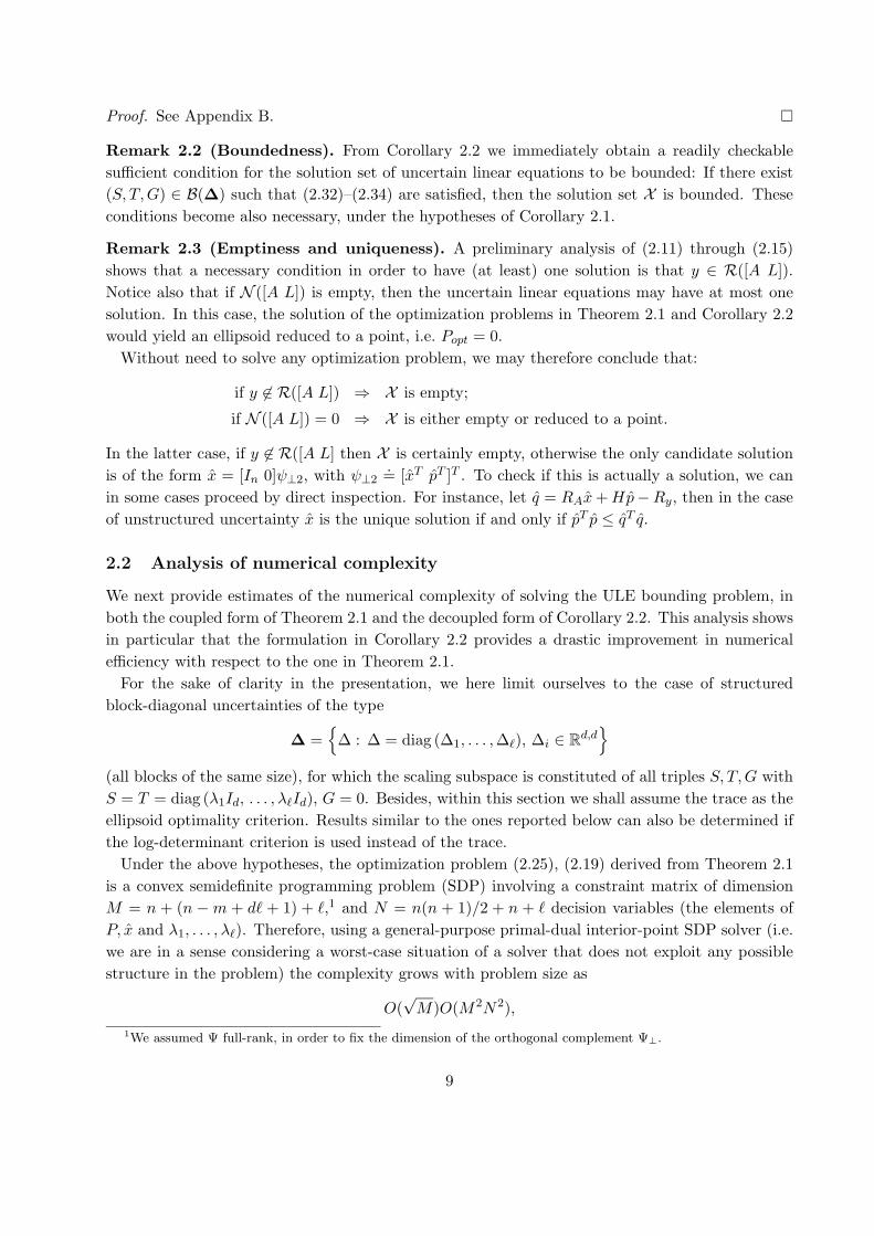
criterion) on the resulting ULEs, we determined the optimal bounding ellipsoid E+ for the states

at time k + 1, having center x+ = [0 0]T and P+ =

[0.0008 −0.0021−0.0021 0.0121

]. In order to give a

pictorial idea of the reachable set at time k +1, Figure 3 shows the predicted ellipsoid E+, togetherwith random points in X+.

−0.03 −0.02 −0.01 0 0.01 0.02 0.03−0.2

−0.15

−0.1

−0.05

0

0.05

0.1

0.15

x1(k+1)

x 2(k+

1)

Figure 3: Optimal predicted ellipsoid E+ and random points in X+.

Consider now the setup of Section 3.2, and assume that the measurement z+ = 0.018 becomesavailable, according to the model (3.58), with

[C(∆) D(∆)] =[

1 0 0.005]

+ L∆[RC | RD] =[

1 + 0.01δ2 0 0.005],

∆ = δ2, |δ2| ≤ 1, and L = 0.01, RC = [1 0], RD = 0. Then, we update the prediction informationwith this new measurement, constructing the ULEs according to Proposition 3.2 and solving therelative optimization problem in Corollary 2.2 (using the trace criterion). The updated ellipsoid

E+|+ has center in x+|+ = [0.0149 − 0.0373]T and shape matrix P+|+ =

[0.0001 −0.0003−0.0003 0.0064

].

Figure 4 shows the shrunk updated ellipsoid in comparison with the predicted one. In a dynamicsetting, the process is then iteratively repeated predicting forward in time E+|+ through the uncer-tain dynamic equations (3.54), etc...

21

−0.03 −0.02 −0.01 0 0.01 0.02 0.03−0.2

−0.15

−0.1

−0.05

0

0.05

0.1

0.15

x1(k+1)

x 2(k+

1)

Figure 4: Predicted ellipsoid E+ (light line) and updated ellipsoid E+|+ (bold line).

4 Conclusions

In this paper, we presented a comprehensive discussion of semidefinite relaxation methods forapproximation problems that arise in the context of systems affected by unknown-but-boundeduncertainties. A main points of the paper is to introduce the uncertain linear equations paradigmand to show that bounds on the solution set can be obtained efficiently via convex optimization.Besides being of interest in its own right from a theoretical point of view, the ULE model hasdirect application in many engineering problems, and in particular in system identification andset-membership prediction and filtering.

In this latter respect, the results in Section 3 extend the existing literature on set-membershipfiltering to the case when uncertainty is present in the system description. When there is nouncertainty in the system description, but only unknown-but-bounded additive noise is present, werecover classical ellipsoidal filtering results.

Some comments are in order regarding the employed methodology. We remark that all thediscussed problems are numerically hard to solve exactly. From a practical point of view, thestandard semidefinite relaxation that we use provides a viable methodology for computing a sub-optimal solution, at a provably low computational cost (basically O(n3), see Section 2.2). In somespecial cases, we pointed out that the approximation is actually exact (Corollary 2.1), or a precisebound on the conservatism can be assessed, see Remark 3.1. However, no result on the sharpness ofthe approximation is to date available for the general case, and this issue is currently a hot researchtopic, see e.g. [2, 14, 21, 26]. In principle, the sharpness of the approximation can be improvedusing higher order semidefinite relaxations, at the expense of increased computational burden, see

22

[30], Chapter 6, and [21] for further results along this line.

Acknowledgments

We gratefully acknowledge Arkadi Nemirovski for a precious suggestion regarding the barrier func-tion used in Section 2.2.

Appendix

A LMI technical lemmas

For easier reference of the reader, this section gathers several technical results on LMI manipulation.Most of these results can be found in standard texts such as [4, 38].

Lemma A.1 (Projection). Let F = F T . The inequality ξT Fξ ≤ 0 holds for all ξ: Qξ = 0, ifand only if QT

⊥FQ⊥ 0.

Lemma A.2 (Well-posedness). The LFR M(∆) = M +L∆(I −H∆)−1R is well-posed over ∆1

if and only if det(I − H∆) = 0 for all ∆ ∈ ∆1. A sufficient condition for well-posedness is: thereexist a triple (S, T, G) ∈ B(∆), S 0, T 0 such that[

H

I

]T [T G

GT −S

][H

I

] 0.

The above condition is also necessary in the unstructured case, i.e. when ∆ = Rnp,nq .

This lemma was first derived in the context of µ-analysis in [9]. A proof of the results in theform given here may be found in [13].

Lemma A.3 (Homogenization). Let T = T T . The following two conditions are equivalent.

(a)

[ξ

1

]T [T u

uT v

][ξ

1

]≥ 0 for all ξ;

(b)

[T u

uT v

] 0.

Proof. The implication from (b) to (a) is trivial. We show that (a) implies (b) by contradiction.

Suppose ∃ ξ, α such that[

ξT α] [ T u

uT v

] [ξT α

]T< 0. Then, if α = 0, dividing both sides

by α2, we get[

1α ξT 1

] [ T u

uT v

] [1α ξT 1

]T< 0, which clearly contradicts the hypothesis (a).

On the other hand, α = 0 would imply that ξT T ξ < 0. Choosing then ξ = βξ and substituting in(a) we have

β2(ξT T ξ) + 2βuT ξ + v, (A.60)

which is a concave parabola in β, since ξT T ξ < 0. Therefore, there will exist a value of β such that(A.60) is negative, which contradicts the hypothesis.

23

Lemma A.4 (S-procedure). Let F0(ξ), F1(ξ), . . . , Fp(ξ) be quadratic functions in the variableξ ∈ R

n

Fi(ξ) = ξT Tiξ + 2uTi ξ + vi, i = 0, . . . , p,

with Ti = T Ti . Then, the implication

F1(ξ) ≥ 0, . . . , Fp(ξ) ≥ 0 ⇒ F0(ξ) ≥ 0 (A.61)

holds if there exist τ1, . . . , τp ≥ 0 such that

F0(ξ) −p∑

i=1

τiFi(ξ) ≥ 0, ∀ξ. (A.62)

When p = 1, condition (A.62) is also necessary for (A.61), provided there exist some ξ0 such thatF1(ξ0) > 0. An extension of this result to the case of p = 2 can be found in [31]. Notice also that,by homogenization, condition (A.62) is equivalent to

∃τ1, . . . , τp ≥ 0 such that

[T0 u0

uT0 v0

]−

p∑i=1

τi

[Ti ui

uTi vi

] 0. (A.63)

Lemma A.5 (Quadratic embedding). Let Q .=[

qT pT]T

: p = ∆q for some ∆ ∈ ∆1

,

and B(∆) =(S, T, G) : ∀∆ ∈ ∆, S∆ = ∆T, G∆ = −∆T GT

. For any triple (S, T, G) ∈ B(∆),

S 0, T 0, define the set

QS,T,G.=

[

q

p

]:

[q

p

]T [T G

GT −S

][q

p

]≥ 0

. (A.64)

Then Q ⊆ QS,T,G.In the case of unstructured uncertainty ∆ ≡ R

np,nq we have in particular that Q ≡ QS,T,G, forS = λInp, T = λInq , λ ∈ R, and G = 0, λ > 0.

Proof. Let [qT pT ]T ∈ Q, then for any (S, T, G) ∈ B(∆), S 0, T 0 we have that qT Gp =qT G∆q = 0, by the skew-symmetry of G∆. In addition, we have

qT Tq − pT Sp = qT (T − ∆T S∆)q= qT (T − ∆T ∆T )q 0.

In the above, we have used the fact that, since S∆ = ∆T , the matrix ∆T ∆T is symmetric,then T commutes in the product with ∆T ∆, and therefore these two matrices are simultaneouslydiagonalizable ([17], Corollary 4.5.18), i.e. we may write the factorizations T = V JT V T , ∆T ∆ =V J∆V T , where JT , J∆ are diagonal, and V is orthogonal. It then follows that the eigenvalues ofT − ∆T ∆T are the diagonal terms of (I − J∆)JT , which are non-negative, if T 0. The previousconditions are written compactly as[

q

p

]T [T G

GT −S

][q

p

]≥ 0, (A.65)

24

which proves the first part of the lemma.To prove the second part of the lemma, we consider the case of unstructured uncertainty, i.e.

∆ = Rnp,nq (only one full block). In this case the set B(∆) reduces to the set of triples (S, T, G),

with S = λInp , T = λInq , λ ∈ R, and G = 0. Clearly, p = ∆q for some ∆ : ‖∆‖ ≤ 1 if and only ifpT p ≤ qT q, which is equivalent to (A.65), for any λ > 0.

Lemma A.6 (Schur complements). The condition[A B

BT D

] 0

is equivalent toD 0, A − BD†BT 0, (I − D†D)BT = 0

and also toA 0, D − BT A†B 0, (I − A†A)B = 0,

where A†, D† denote the Moore-Penrose pseudoinverse of A and D, respectively. Notice that thecondition (I − A†A)B = 0 means that R(B) ⊆ R(A). Similarly, the condition (I − D†D)BT = 0means that N (D) ⊆ N (B) or, equivalently, that R(BT ) ⊆ R(D).

Lemma A.7 (Block elimination). Let Q11 = QT11, Q22 = QT

22. There exist matrices X = XT

and Z such that X Z B

ZT Q11 Q12

BT QT12 Q22

0 (A.66)

if and only if [Q11 Q12

QT12 Q22

] 0, and (A.67)

∃X = XT :

[X B

BT Q22

] 0. (A.68)

Proof. This result is closely related to the variable elimination lemma well-known in LMIliterature (see for instance [38], Theorem 2.3.12). We next report a proof for our specific formulationof the lemma.

The implication from (A.66) to (A.67)–(A.68) is straightforward, since if a matrix is positivesemi-definite, so are all principal sub-matrices. For the converse, notice that, by Lemma A.6,condition (A.66) is equivalent to

Q22 0 (A.69)[X Z

ZT Q11

]−[

B

Q12

]Q†

22

[B

Q12

]T

0 (A.70)

(I − Q†22Q22)

[B

Q12

]T

= 0. (A.71)

25

Clearly, (A.67) implies (I − Q†22Q22)QT

12 = 0, and (A.68) implies (I − Q†22Q22)BT = 0, therefore

(A.67)–(A.68) imply (A.71). Define now

X.= BQ†

22BT (A.72)

Z.= BQ†

22QT12 (A.73)

Q11.= Q11 − Q12Q

†22Q

T12, (A.74)

then (A.70) writes [X − X (Z − Z)

(Z − Z)T Q11

] 0. (A.75)

From (A.67) it follows that Q11 0, therefore (A.75) is feasible for X = X, Z = Z, which concludesthe proof.

Corollary A.1 (Decoupling). Let all symbols be defined as in Lemma A.7, and let

[Q11 Q12

QT12 Q22

] 0.

Then the problem

minX,Z

f(X) subject to (A.66) (A.76)

is equivalent to

minX

f(X) subject to (A.68). (A.77)

Moreover, if problem (A.77) is feasible and f(·) is either the trace function f(X) = trace (X), orthe log-det function f(X) = log det(X), then problem (A.76) has a unique optimal solution givenby

X.= BQ†

22BT (A.78)

Z.= BQ†

22QT12 (A.79)

Proof. When (A.67) holds, we know from Lemma A.7 that (A.66) is feasible if and only if (A.68)is feasible, which immediately proves the equivalence between problems (A.76) and (A.77).

If the latter is feasible, then (A.66) is also feasible, and therefore (A.75) holds (with the symbolsdefined in (A.72)–(A.74)), which means that

X X + (Z − Z)Q†11(Z − Z)T

(I − Q†11Q11)(Z − Z)T = 0.

Now, since f(X1) ≥ f(X2) whenever X1 X2 (both in the case of trace and log-determinant) theminimum of f(X) is achieved for X = X, Z = Z.

26

B Proof of Corollary 2.2

With the position (2.15), let us define the following partitions[[In 0] x

]Ψ⊥

.=[

B z]

ΨT⊥ (diag (0, 0, 1) − Ω(S, T, G)) Ψ⊥

.= Q =

[Q11 q12

qT12 1 − q22

],

where B = [In 0]Ψ⊥1, z = [In 0]ψ⊥2 − x. Notice that ΨT⊥diag (0, 0, 1)Ψ⊥ = diag (0, 0, 1). Then,

condition (2.19) is equivalent to the following condition, obtained by simple reordering of the blocks(dependence on S, T, G is sometimes omitted to avoid clutter)

P z B

zT 1 − q22 qT12

BT q12 Q11

0.

Now, by Lemma A.7, the above matrix inequality is feasible for some P, z if and only if

Q(S, T, G) 0,

[P B

BT Q11

] 0 (B.80)

is feasible for some P . Therefore problem (2.25) is equivalent to

minS,T,G

minP

f(P ) subject to (B.80),

(S, T, G) ∈ B(∆), S 0, T 0,

which, by Corollary A.1, is equivalent to

minS,T,G

f(X(S, T, G)) subject to

(S, T, G) ∈ B(∆), S 0, T 0,

Q(S, T, G) 0,

(I − Q†11Q11)BT = 0,

where X(S, T, G) = BQ†11(S, T, G)BT .

If Sopt, Topt, Gopt are the optimal values of the above optimization problem, then (again by Corol-lary A.1) the optimal ellipsoid is given by

Popt = BQ†11(Sopt, Topt, Gopt)BT

zopt = BQ†11(Sopt, Topt, Gopt)Q12.

From the latter we then retrieve the ellipsoid center as

xopt = [In 0]ψ⊥2 − zopt.

27

References

[1] A. Ben-Tal and A. Nemirovski. Lectures on modern convex optimization. SIAM, 2001.

[2] A. Ben-Tal and A. Nemirovski. On tractable approximations of uncertain linear matrix in-equalities affected by interval uncertainty. SIAM Journal on Optimization, 12(3):811–833,2002.

[3] D.P. Bertsekas and I.B. Rhodes. Recursive state estimation with a set-membership descriptionof the uncertainty. IEEE Trans. Aut. Control, 16:117–128, 1971.

[4] S. Boyd, L. El Ghaoui, E. Feron, and V. Balakrishnan. Linear Matrix Inequalities in Systemand Control Theory, volume 15 of Studies in Applied Mathematics. SIAM, Philadelphia, PA,June 1994.

[5] F.L. Chernousko. State Estimation of Dynamic Systems. CRC Press, Boca Raton, FL, 1993.

[6] C. Durieu, E. Walter, and B. Polyak. Multi-input multi-output ellipsoidal state bounding. InJournal of Optimization Theory and Applications, volume 111, 2001.

[7] L. El Ghaoui and G. Calafiore. Confidence ellipsoids for uncertain linear equations withstructure. In Proc. IEEE Conf. on Decision and Control, volume 2, pages 1922–1927, Phoenix,AZ, December 1999.

[8] L. El Ghaoui and G. Calafiore. Worst-case simulation of uncertain systems, volume 245 ofLecture Notes in Control and Information Sciences, pages 134–146. Springer-Verlag, London,1999.

[9] M.K.H. Fan, A.L. Tits, and J.C. Doyle. Robustness in the presence of mixed parametricuncertainty and unmodeled dynamics. IEEE Trans. Aut. Control, 36:25–38, 1991.

[10] E. Fogel and Y.F. Huang. On the value of information in system identification - bounded noisecase. Automatica, 18(2):229–238, 1982.

[11] L. El Ghaoui. Inversion error, condition number, and approximate inverses of uncertain ma-trices. Linear Algebra and its Applications, 342(1-3), February 2002.

[12] L. El Ghaoui and G. Calafiore. Robust filtering for discrete-time systems with bounded noiseand parametric uncertainty. IEEE Trans. Aut. Control, 46(7):1084–1089, July 2001.

[13] L. El Ghaoui and H. Lebret. Robust solutions to uncertain semidefinite programs. SIAM J.Optim., 9(1):33–52, 1998.

[14] M.X. Goemans and D.P. Williamson. .878-approximation for MAX CUT and MAX 2SAT.Proc. 26th ACM Sym. Theor. Computing, pages 422–431, 1994.

[15] E.R. Hansen. Bounding the solution of interval linear equations. SIAM J. on NumericalAnalysis, 29:1493–1503, 1992.

28

[16] D. Henrion, S. Tarbouriech, and D. Arzelier. LMI approximations for the radius of the inter-section of ellipsoids. J. of Optimization Theory and Applications, 108(1):1–28, 2001.

[17] R.A. Horn and C.R. Johnson. Matrix Analysis. Cambridge University Press, Cambridge, U.K.,1985.

[18] S. Van Huffel and J. Vandewalle. The Total Least Squares Problem: Computational Aspectsand Analysis. SIAM, Philadelphia, 1991.

[19] U. Koyluoglu, A.S.Cakmak, and S.R.K. Nielsen. Interval algebra to deal with pattern loadingand structural uncertainty. Journal of Engineering Mechanics, pages 1149–1157, 1995.

[20] A.B. Kurzhanski and I. Valyi. Ellipsoidal Calculus for Estimation and Control. Birkhauser,Boston, 1996.

[21] J.B. Lasserre. Global optimization with polynomials and the problem of moments. SIAMJournal on Optimization, 11(3):796–817, 2001.

[22] D.G. Maskarov and J.P. Norton. State bounding with ellipsoidal set description of the uncer-tainty. Int. J. Control, 65(5):847–866, 1996.

[23] R.L. Muhanna and R.L. Mullen. Uncertainty in mechanics problems - interval-based approach.ASCE Journal of Engineering Mechanics, 127(6):557–566, 2001.

[24] A. Nemirovski, C. Roos, and T. Terlaky. On maximization of quadratic form over intersectionof ellipsoids with common center. Math. Program., 86(3):463–473, 1999.

[25] Y. Nesterov and A. Nemirovski. Interior point polynomial methods in convex programming:theory and applications. SIAM, Philadelphia, 1994.

[26] Yu. Nesterov. Semidefinite relaxation and non-convex quadratic optimization. OptimizationMethods and Software, 12:1–20, 1997.

[27] A. Neumaier. Interval Methods for Systems of Equations. Cambridge University Press, Cam-bridge, UK, 1990.

[28] J.P. Norton and S.M. Veres. Developments in parameter bounding. In L. Gerencser and P. E.Caines, editors, Topics in Stochastic Systems: Modelling, Estimation and Adaptive Control,pages 1137–1158. Springer-Verlag, Berlin, 1991.

[29] A.I. Ovseevich. On equations of ellipsoids approximating attainable sets. Journal of Opti-mization Theory and Applications, 95(3):659–676, 1997.

[30] P.A. Parrilo. Structured Semidefinite Programs and Semialgebraic Geometry Methods in Ro-bustness and Optimization. Ph.D. Thesis, California Institute of Technology, 2000.

[31] B.T. Polyak. Convexity of quadratic transformations and its use in control and optimization.Journal of Optimization Theory and Applications, 99(3):553–583, 1998.

29

[32] B.T. Polyak, S.A. Nazin, C. Durieu, and E. Walter. Ellipsoidal estimation under model un-certainty. In Proceedings of IFAC 2002 World Congress, Barcelona, Spain, 2002.

[33] J. Rohn. Systems of linear interval equations. Linear Algebra and its Applications, 126:39–78,1989.

[34] J. Rohn. Overestimations in bounding solutions of perturbed linear equations. Linear Algebraand its Applications, 262:55–66, 1997.

[35] F.C. Schweppe. Recursive state estimation: unknown but bounded errors and system inputs.IEEE Trans. Aut. Control, 13(1):22–28, 1968.

[36] F.C. Schweppe. Uncertain Dynamic Systems. Prentice-Hall, New York, 1973.

[37] J.S. Shamma and K.-Y. Tu. Set-valued observers and optimal disturbance rejection. IEEETrans. Aut. Control, 44(2):253–264, 1999.

[38] R.E. Skelton, T. Iwasaki, and K. Grigoriadis. A unified algebraic approach to linear controldesign. Taylor & Francis, London, 1998.

[39] L. Vandenberghe and S. Boyd. Semidefinite programming. SIAM Review, 38(1):49–95, March1996.

[40] L. Vandenberghe, S. Boyd, and S.-P. Wu. Determinant maximization with linear matrixinequality constraints. SIAM J. on Matrix Analysis and Applications, 19(2):499–533, April1998.

[41] K. Zhou, J.C. Doyle, and K. Glover. Robust and Optimal Control. Prentice-Hall, Upper SaddleRiver, 1996.

30