Embed Size (px)
Citation preview
Ninth Edition

o.
Single Payment Compound Amount:
F To FindFGiven P (FIP,i,n) F = P(1 + iy
Present Worth:
To Find PGiven F (P IF,i,n) P = F(1 + i)-np
Arithmetic Gradient Arithmetic Gradient Uniform Series:
(n - l)G3G
To Find AGiven G (AIG,i,n) A = G
[(1 .+ i)n - in - 1
Jl (1 + i)n - i2G
o or[
1 n '
JA = G i - (1 + i)n - 1G
Arithmetic Gradient Present Worth:
To Find PGiven G (P IG,i,n)
p.......
--
UniformSeries Series Compound Amount:
To FindF(FIA,i,n)
F = A [(1 + ir - 1JA A A A A Given A
Sinking Fund:
To Find A(AI F,i,n)
[ l JGiven FA-F
F (1 + i)n - 1
A A A A A Capital Recovery:I . . . .
To FindA(AI P,i,n)
A = P [ i (1 + i)n JGiven P (1 + i)n - 1
Series Present Worth:p
To Find P(P IA,i,n)
P = A [(1 + i)n - 1JGiven A i(1 + i)n
A A A A A
(n - l)G.3G
2G
G t0

L;;
To Find PGiven AI, g
(P j A,g,i,n)When i = g P = Al [n(1+ i)~IJ"
Geometric Gradient
Geometric Series Present Worth:
To Find P
Given AI, g(P j A,g,i,n)When i # g
P = Al[
1 - (1 +.g)n(1 + i)-n]l-g
p
Continuous Compounding at Nominal Rate r
SinglePayment: F = p[ern] P = F[e-rn]
Uniform Series: A=F[
er-l
]ern - 1
F = A[
ern - 1
]er - 1
Continuous, Uniform Cash flow (One Period)With Continuous Compo.unding at Nominal Rate r
Present Worth:
ToFind PGivenF [PjF,r,n]
F
UCompound Amount:
To Find FGiven P [Fj p,r,n]
P = F[~
]rern
1
P
~",'
/'
"
."
",
LJ p
r'mpound Interesti = Interestrate per interestperiod*.n = Number of interest periods.
P = A present sum of money.
F = A futuresum of money.The future sum F is an amount,n interestperiodsfromthe present,that is equivalent to P with interest rate i. '
A = An end-of-period cash receipt or disbursement in a uniform series continuing for n periods, theentire series equivalent to P or F at interest rate i.
G = Uniform p~riod-by-period increase or decrease in cash receipts or disbursements; the arithmeticgradient.
g = Uniform rate of cash flow increase or decrease from period to period; the geometric gradient.
r = Nominal interest rate per interest period*.
m = Number of compounding subperiods per period*.
P,F = Amount of money flowing continuously and uniformly during one given period.
n
F
*Nonnally the interest period is one year, but it could be something else. .
[' I
'," 1
~:~... L:7~' .~_c:.::,.:;.~..jg{~j~..;~c.-::,.~':.: .~-~;~~::-':-:1":~-~'~.-~~:.-;';f~~:,. ._:-:..:'-:;~~,,-.:.-~ ".:. _. .;.._'-. ::.; _i._,"_ __-: .'. -:~ ~::__-~ .~:;,~~:..::.
-- -
- - - - -- -

-
ENGINEERING
ECONOMIC
ANALYSIS
IIII
/,
-- -- - -- ---

ENGINEERINGECONOMICANALYSISNINTH EDITION
Donald G. NewnanProfessor Emeritus of Industrial and Systems Engineering
Ted G. EschenbachUniversity of Alaska Anchorage
Jerome P. LavelleNorth Carolina State University
New York OxfordOXFORD UNIVERSITY PRESS2004
Oxford University Press
Oxford New YorkAuckland Bangkok BuenosAires CapeTown ChennaiDar es Salaam Delhi Hong Kong Istanbul Karachi KolkataKualaLumpur Madrid Melbourne MexicoCity Mumbai NairobiSiloPaulo Shanghai Taipei Tokyo Toronto
Copyright @ 2004 by Oxford University Pr(:ss, Inc.
Published by Oxford University Press, Inc.198 Madison Avenue, New York, New York 10016WWW.oup.com
Oxford is a registered trademark of Oxford University Press
All rights reserved. No part of this publication may be reproduced,stored in a retrieval system, or transmitted, in any form or by any means,electronic, mechanical, photocopying, recording, or otherwise,without the prior permission of Oxford University Press.
Library of Congress Cataloging-in-Publication Data
Newnan, Donald G.Engineering economic analysis / Donald G. Newnan, Ted G. Eschenbach, JeromeP. Lavelle. - 9th ed.
p.cm.Includes bibliographical references and index.ISBN 0-19-516807-0 (acid-free paper)1. Engineering economy. 1.Eschenbach, Ted. n. Lavelle, Jerome P. m. TItle.
TA177.4N482004658.15-dc22
2003064973
Photos: Chapter 1 @ Getty Images; Chapter 2 @ SAN FRANCISCO CHRONICLE/CORBIS SABA; Chapter 3@ Olivia Baumgartner/CORBIS SYGMA; Chapter 4 @ Pete Pacifica/Getty Images; Chapter 5 @ Boeing Man-agement Company; Ch.apter 7 @ Getty Images; Chapter 8 @ Michael Nelson/Getty Images; Chapter 9 @ GuidoAlberto Rossi/Getty Images; Chapter 10 @ Terry Donnelly/Getty Images; Chapter 11 @ Michael Kim/CORBIS;Chapter 12 @ Getty Images; Chapter 13 @ Richard T Nowitz/CORBIS; Chapter 14 @ CORBIS SYGMA; Chap-ter 15 @ Shephard Sherbell/CORBIS SABA; Chapter 16 @ Macduff Everton/CORBIS; Chapter 17 @ UnitedDefense, L.P.; Chapter 18 @. Steve Cole/Getty Images.
Printingnumber: 9 8 7 6 5 4 3
Printed in the United States of America
on acid-free paper

Eugene Grant and Dick Bernhardfor leadingthe field of engineering economic analysis
from Don
Richard Corey Eschenbach for his lifelong exampleof engineering leadership and working well with others
from Ted
My lovely wife and sweet daughters,who always support all that I do
from Jerome
I
I ",,~.,,,,..:.;~.:~,~,,;~.#;;., ,j~- --

--------
PREFACE XVII
1 'AAKING ECONOMICDECISIONS
A Sea of Problems 4
Simple Problems 4Intennediate Problems 4
Complex Problems 4
The Role of Engineering Economic Analysis 5Examples of Engineering Economic Analysis 5
The Decision-Making Process 6Rational Decision Making 6
Engineering Decision Making for Current Costs 15Summary 18Problems 19
2 ENGINEERINGCOSTSAND COST ESTIMATING
Engineering Costs 28Fixed, Variable, Marginal, and Average Costs 28Sunk Costs 32
Opportunity Costs 32Recurring and Nonrecurring Costs 34Incremental Costs 34Cash Costs Versus Book Costs 35
Life-Cycle Costs 36
vii
viii CONTENTS
Cost Estimating 38Types of Estimate 38Difficulties in Estimation 39
Estimating Models 41Per-Unit Model 41
Segmenting Model 43Cost Indexes 44
Power-Sizing Model 45Triangulation 47Improvement and the Learning Curve 47
Estimating Benefits 50Cash Flow Diagrams 50
Categories of Cash Flows 51Drawing a Cash Flow Diagram 51Drawing Cash Flow Diagrams witha Spreadsheet 52
Summary 52Problems 54
3 INTERESTAND EQUIVALENCE
Computing Eash Flows 62Time Value of Money 64
Simple Interest 64Compound Interest 65Repaying a Debt 66
Equivalence 68Differencein RepaymentPlans 69 .
Equivalence Is Dependent on Interest Rate 71Application of Equivalence Calculations 72
Single Payment Compound Interest Formulas 73Summary 81Problems 82
4 MORE INTERESTFORMULAS
Uniform Series Compound Interest Formulas 86
Relationships Between Compound Interest Factors 97

-~-~ ~----
CONTENTS ix
Single Payment 97Uniform Series 97
ArithmeticGradient 98 .
Derivation of Arithmetic Gradient Factors 99
Geometric Gradient 105Nominal and Effective Interest 109
Continuous Compounding 115Single Payment Interest Factors: Continuous Compounding 116Uniform Payment Series: Continuous Compounding at Nominal Rate rper Period 118Continuous, Uniform Cash Flow (One Period) with Continuous Compoundingat Nominal Interest Rate r 120
Spreadsheets for Economic Analysis 122Spreadsheet Annuity Functions 122Spreadsheet Block Functions 123Using Spreadsheets for Basic Graphing 124
Summary 126Problems 129
5 PRESENTWORTH ANALYSIS
Assumptions in Solving Economic Analysis Problems 144End-of-Year Convention 144
Viewpoint of Economic Analysis Studies 145Sunk Costs 145
Borrowed Money Viewpoint 145Effect of Inflation and Deflation 145Income Taxes 146
Economic Criteria 146
Applying Present Worth Techniques 147
Useful Lives Equal the Analysis Period 147Useful Lives Different from the Analysis Period 151Infinite Analysis Period: Capitalized Cost 154Multiple Alternatives 158
Spreadsheetsand PresentWorth 162Summary 164Problems 165
',/k
~. ._~~~(~

x CONTENTS
6 ANNUAL CASH FLOWANALYSIS
Annual Cash Flow Calculations 178
Resolving a Present Cost to an Annual Cost 178Treatment of Salvage Value .. 178 .
Annual Cash Flow Analysis 182Analysis Period 184
Analysis Period Equal to Alternative Lives 186Analysis Period a Common Multipleof Alternative Lives 186
Analysis Period for a Continuing Requirement 186Infinite Analysis Period 187Some Other Analysis Period 188
Using Spreadsheets to Analyze Loans 190Building an Amortization Schedule 190How Much to Interest? How Much to Principal? 191Finding the Balance Due on a Loan 191Pay Off Debt Sooner by Increasing Payments 192
Summary 193Problems 194
7 RATE OF RETURN ANALYSIS
Internal Rate of Return 204
Calculating Rate of Return 205Plot ofNPW versus Interest Rate i 209
Rate of ReturnAnalysis 212Present Worth Analysis 216Analysis Period 219
Spreadsheets and Rate of ReturnAnalysis 220Summary 221Problems 222
Appendix 7A Difficulties in Solving for an Interest Rate 229
8 INCREMENTALANALYSIS
Graphical Solutions 246
IncrementalRateof ReturnAnalysis 252

CONTENTS xi
Elements in Incremental Rate of Return Analysis 257Incremental Analysis with Unlimited Alternatives 258
Present Worth Analysis with Benefit cost .Graphs 260Choosing an Analysis Method 261Spreadsheets and Incremental Analysis 262
Summary 263Problems 264
9 OTHER ANALYSISTECHNIOUES
Future Worth Analysis 272Benefit-Cost Ratio Analysis 274
Continuous Alternatives 279
Payback Period 280Sensitivity and Breakeven Analysis 285
Graphing with Spreadsheets for Sensitivity and Breakeven Analysis 289
Summary 293Problems 293
10 UNCERTAINTYIN FUTURE EVENTS
Estimates and Their Use in Economic Analysis 304
A Range of Estimates 306Probability 308
Joint Probability Distributions 311Expected Value 313Economic Decision Trees 316Risk 322Risk Versus Return 324Simulation 326
Summary 330Problems 330
11 DEPRECIATION
BasicAspectsof Depreciation 338Deterioration and Obsolescence 338
Depreciation and Expenses 339

xii CONTENTS
Types of Property 340Depreciation Calculation Fundamentals 341
Historical Depreciation Methods 342Straight-Line Depreciation 342Sum-of-Years'-Digits Depreciation 344Declining Balance Depreciation 346
Modified Accelerated Cost Recovery System (MACRS) 347Cost Basis and Placed-in-Service Date 348
Property Class and Recovery,Period 348Percentage Tables 349Where MACRS Percentage Rates Crt)Come From 351MACRS Method Examples 353Comparing MACRS and Historical Methods 355
Depreciation and Asset Disposal 356Unit-of-Production Depreciation 359Depletion 360
Cost Depletion 360Percentage Depletion 361
Spreadsheets and Depreciation 362Using VDB for MACRS 363
Summary 364Problems 365
12 INCOME TAXES
A Partner in the Business 372Calculation of Taxable Income 372
Taxable Income of Individuals 372
Classificatio~ of Business Expenditures 373Taxable Income of Business Firms 374
Income Tax Rates 375Individual Tax Rates 375
Corporate Tax Rates 377Combined Federal and State Income Taxes 379
Selecting an Income Tax Rate for Economy Studies 380
Economic AnalysisTakingIncome Taxes into Account 380

CONTENTS xiii
Capital Gains and Losses for Nondepreciated Assets 384Investment Tax Credit 384
Estimating the After-Tax Rate of Return- -385After-Tax Cash Flows and Spreadsheets 385Summary 386Problems 387
13 REPLACEMENTANALYSIS
The Replacement Problem 400Replacement Analysis Decision Maps 401What Is the Basic Comparison? 401
Minimum Cost Life of the Challenger 402Use of Marginal Cost Data 404Lowest EUAC of the Defender 411
No Defender Marginal Cost Data Available 415Repeatability Assumptions Not Acceptable 418A Closer Look at Future Challengers 419
After-Tax Replacement Analysis 420Marginal Costs on an After-Tax Basis 420 .After-Tax Cash Flows for the Challenger 422Mter- Tax Cash Flows for the Defender 422Minimum Cost Life Problems 427
Spreadsheets and Replacement Analysis 429Summary 429Problems 431
14 INFLATIONAND PRICECHANGE
Meaning and Effect of Inflation 440HowDoesInflationHappen? 440 .
Definitions for Considering Inflation in Engineering Economy 441
Analysis in Constant Dollars Versus Then-Current Dollars 448Price Change with Indexes 450 .
\--
What Is a Price Index? 450
Composite Versus Commodity Indexes 453How to Use Price Indexes in Engineering Economic Analysis 456

xiv CONTENTS
Cash Flows That Inflate at Different Rates 456
Different Inflation Rates per Period 458Inflation Effect on After-TaxCf!'.c~l(lti9.ns 460
Using Spreadsheets for Inflation Calculations 462Summary 464Problems 465
15 SELECTIONOF A MINIMUM ATTRACTIVERATEOF RETURN
Sources of Capital 474Money Generated from the Operation of the Firm 474External Sources of Money 474Choice of Source of Funds 474
Cost of Funds 475
Cost of Borrowed Money 475Cost of Capital 475
Investment Opportunities 476Opportunity Cost 476
Selecting a Minimum Attractive Rate of Return 479
Adjusting MARRto Account for Riskand UncertaintyInflation and the Cost of Borrowed Money 481
Representative Values of MARRUsed in Industry 482Spreadsheets, Cumulative Investments, and the OpportunityCost of Capital 483
Summary 485Problems 485
479
16 ECONOMIC ANALYSIS IN THE PUBLIC SECTOR
Investment Objective 490
Viewpoint for Analysis 492Selecting an Interest Rate 493
No Time-Value-of-Money Concept 494Cost of Capital Concept 494Opportunity Cost Concept 494Recommended Concept 495
The Benefit-Cost Ratio 496

CONTENTS xv
Incremental Benefit-Cost Analysis 498Elements of the Incremental Benefit-Cost Ratio Method 499
Other Effects of Public Projects . -505
Project Financing 505Project Duration 506Project Politics 507
Summary 509Problems 510
17 RATIONINGCAPITALAMONG COMPETINGPROJECTS
Capital Expenditure Project Proposals 518Mutually Exclusive Alternatives and Single Project Proposals 519Identifying and Rejecting Unattractive Alternatives 520Selecting the Best Alternative from Each Project Proposal 521
Rationing Capital by Rate of Return 521Significance of the Cutoff Rate of Return 523
Rationing Capital by Present Worth Methods 524Ranking Project Proposals 530Summary 532Problems 533
18 ACCOUNTINGAND ENGINEERINGECONOMY
The Role of Accounting 540Accounting for Business Transactions 540
The Balance Sheet 541Assets 541Liabilities 542
Equity 543Financial Ratios Derived from Balance Sheet Data 543
The Income Statement 544Financial Ratios Derived from Income Statement Data 546
Linking the Balance Sheet, Income Statement, and Capital Transactions 546
Traditional Cost Accounting 547Direct and Indirect Costs 548Indirect Cost Allocation 548

xvi CONTENTS
Problems with Traditional Cost Accounting 549Other Problems to Watch For 550
Problems 551
ApPENDIXA INTRODUCTION TO SPREADSHEETS 554
The Elements of a Spreadsheet 554
Defining Variables in a Data Block 555Copy Command 555
ApPENDIXB COMPOUND INTERESTTABLES 559
REFERENCE 591
INDEX 593
.

In the first edition of this book we said:
This book is designed to teach the fundamental concepts of engineering economy toengineers. By limiting the intended audience to engineers it is possible to provide anexpanded presentation of engineering economic analysis and do it more concisely thanif the book were written for a wider audience.
Our goal was, and still is, to provide an easy to understand and up-to-date presentationof engineering economic analysis. That means the book's writing style must promote thereader's understanding. We most humbly find that our approach has been well receivedby engineering professors-and more importantly-by engineering students through eightprevious editions.
This edition has significant improvements in coverage:
·Appendix7A (Difficultiesin Solving for anInterestRate) hasbeen thoroughlyrevisedto use the power of spreadsheets to identify and resolve multiple root problems.
· Chapter 10 (Probability and Uncertainty) has been completely rewritten to empha-size how to make good choices by considering the uncertainty that is part of everyengineering economy application.
· Chapter 12(Income Taxes)has been updated to reflect 2003 tax legislation and rates.· Chapter 13 (Replacement Analysis) has been rewritten to clarify the comparison of
existing assets with newer alternatives.·Chapter 18 (Accounting and Engineering Economy) has been added in response toadopter requests.
In this edition, we have also made substantial changes to increase student interest andunderstanding. Thes~ include:
·Chapter-opening vignettes have been added to illustrate real-world applications ofthe questions being studied.· Chapter learning objectives are included to help students check their comprehensionof the chapter material.·The end-of-chapter problems have been reorganized and updated thro~ghout.
· The interior design is completely reworked, including the use of color, to improvereadability and facilitate comprehension of the material.
xvii

In the first edition of this book we said:
This book is designed to teach the fundamental concepts of engineering economy toengineers. By limiting the intended audience to engineers it is possible to provide anexpanded presentation of engineering economic analysis and do it more concisely thanif the book were written for a wider audience.
Our goal was, and still is, to provide an easy to understand and up-to-date presentationof engineering economic analysis. That means the book's writing style must promote thereader's understanding. We most humbly find that our approach has been well receivedby engineering professors-and more importantly-by engineering students through eightprevious editions.
This edition has significant improvements in coverage:
.Appendix7A (Difficultiesin Solvingfor anInterest Rate)hasbeen thoroughlyrevisedto use the power of spreadsheets to identify and resolve multiple root problems..Chapter 10 (Probability and Uncertainty) has been completely rewritten to empha-size how to make good choices by considering the uncertainty that is part of everyengineering economy application..Chapter 12(Income Taxes)has been updated to reflect 2003 tax legislation and rates.
. Chapter 13 (Replacement Analysis) has been rewritten to clarify the comparison ofexisting assets with newer alternatives..Chapter 18 (Accounting and Engineering Economy) has been added in response toadopter requests.
In this edition, we have also made substantial changes to increase student interest andunderstanding. These include:
.Chapter-opening vignettes have been added to illustrate real-world applications ofthe questions being studied.. Chapter learning objectives are included to help students check their comprehensionof the chapter material..The end-of-chapter problems have been reorganized and updated thr0tlghout.
. The interior design is completely reworked, including the use of color, to improvereadability and facilitate comprehension of the material.
xvii

xviii PREFACE
The supplement package for this text has been updated and expanded for this edition. Forstudents:
·A completely rewritten Study Guide by Ed Wheeler of the University of Tennessee,Martin. . ,.' . -
· Spreadsheet problem modules on CD by Thomas Lacksonen of the University ofWisconsin-Stout.
· Interactive multiple-choice problems on CD by William Smyer of Mississippi StateUniversity.
For instructors:
·A substantially enlarged exam file edited by Meenakshi Sundaram of TennesseeTechnologicalUniversity.· PowerPoiIltlecture notes for key chapters by David Mandeville of Oklahoma StateUniversity.
· Instructor's Manual by the authors with complete solutions to all end-of-chapterproblems.· The compoundinterest tables from the textbook are available in print or Excel formatfor adopting professors who prefer to give closed book exams.
For students and instructors:
· A companionwebsite is availablewith updates to these supplementsatwww.oup.comJus/engineeringeconomy
This ~ditionmaintains the approach to spreadsheets that was established in thepreviousedition. Rather than relying on spreadsheet templates, the emphasis is on helping studentslearn to use the eOormouscapabilities of software that is available on every computer.Thisapproach reinforces the traditional engineering economy factor approach, as the equivalentspreadsheet functions (PMT,PV,RATE, etc.) are used frequently.
For those studentswho would benefit from a refresher or introduction on how to write
good spreadsheets,there is an appendixto introduce spreadsheets.In Chapter2, spreadsheetsare used to draw cash flow diagrams. Then, from Chapter 4 to Chapter 15, every chapterhas a concluding section on spreadsheet use. Each section is designed to support the othermaterial in the chapterand to add to the student's knowledge of spreadsheets.If spreadsheetsare used, the student will be very well prepared to apply this tool to real-world problemsafter graduation.
This approachis designed to support a range of approaches to spreadsheets.Professorsand students can rely on the traditional tools of engineering economy and, without loss ofcontinuity, completelyignore the material on spreadsheets. Or at the other extreme,profes-sors can introducethe concepts and require all computations to be done with spreadsheets.Or a mix of approaches depending on the professor, students, and particular chapter maybe taken.
Acknowledgments
Many people havedirectly or indirectly contributed to the content of the book in its ninthedition. We have been influenced by our Stanford and North Carolina State Universityeducations, our universitycolleagues, and students who have provided invaluablefeedbackon content and form.We are particularly grateful to the following professors for their work
I
_' ". """"~'-....
."
i.. ,... ~_ .. ~.~..,"'.-: ,~'"' " '-
' .
. I
'-. I .~~ I~;;;)~.:'

- .-. - - -
PREFACE xix
on previous editions:
Dick Bernhard, North Carolina State UniversityCharles Burford, Texas Tech UniversityJeff Douthwaite, UniversitYofWilsbingtonUtpal Dutta, University of Detroit, MercyLou Freund, San Jose State UniversityVernonHillsman, Purdue UniversityOscar Lopez, Florida International UniversityNic Nigro, Cogswell College NorthBen Nwokolo, Grambling State UniversityCecil Peterson, GMI Engineering & Management InstituteMalgorzata Rys, Kansas State UniversityRobert Seaman, New England CollegeR. Meenakshi Sundaram, Tennessee Technological UniversityRoscoe Ward, Miami UniversityJan Wolski, New Mexico Institute of Mining and Technologyand particularly Bruce Johnson, U.S. Naval Academy
We would also like to thank the following professors for their contributions to this edition:
Mohamed Aboul-Seoud, Rensselaer Polytechnic InstituteV. Dean Adams, University of Nevada RenoRonald Terry Cutwright, Florida State UniversitySandra Duni Eksioglu, University of FloridaJohn Erjavec, University of North DakotaAshok Kumar Ghosh, University of New MexicoScott E. Grasman, University of Missouri-RollaTed Huddleston, University of South AlabamaRJ. Kim, Louisiana Tech UniversityC. Patrick Koelling, Virginia Polytechnic Institute and State UniversityHampton Liggett, University of TennesseeHeather Nachtmann, University of ArkansasT. Papagiannakis, Washington State UniversityJohn A. Roth, VanderbiltUniversityWilliam N. Smyer, Mississippi State UniversityR. Meenakshi Sundaram, Tennessee Technological UniversityArnold L. Sweet, Purdue UniversityKevin Taaffe, University of FloridaRobert E. Taylor,VIrginiaPolytechnic Institute and State UniversityJohn Whittaker, University of Alberta
Our largest thanks must go to the professors (and their students) who have developedthe supplements for this text. These include:
Thomas Lacksonen, University of Wisconsin-StoutDavid Mandeville, Oklahoma State UniversityWilliam Peterson, Old Dominion University

xx PREFACE
William Smyer, Mississippi State UniversityR. Meenakshi Sundaram, Tennessee TechnologicalUniversityEd Wheeler, University of Tennessee, Martin
Textbooks are produced through the 'efforts of many people. We would like to thank BrianNewnan for bringing us together and for his support. We would like to thank our previous
. editors,PeterGordonandAndrewGyory,for theirguidance.We wouldalsolike to thankPeter for suggesting the additionof chapter-openingvignettes and Ginger Griffinfor draftingthem. Our editor Danielle Christensen has pulled everything together so that this could beproduced on schedule. Karen Shapiro effectivelymanaged the text's design and production.
We would appreciate being informed of errors or receiving other comments about the book.Please write us c/o Oxford University Press, 198 Madison Avenue, New York, NY 10016or through the book's website at www.oup.comlus/engineeringeconomy.
," I ,',
~ I / .I
Ii~;;Jl.#;~i:.z;;,~~~,:::t;#ii~~~.i~L..' ~f~~-",";'~.;;1;,.;,~~;,;.~'.i>;i,::;;';~£'-c t:i£i;;.'.:':',.e'~iO"~"'i>h'''';<,~,~,,,,=~,:~~~!~.

ENGINEERING
ECONOMIC
ANALYSIS

..
After Completing This Chapter...The student should be able to:
· Distinguish between simple and complex problems.· Discuss the role and purpose of engineering economic analysis.· Describe and give examples of the nine steps in the economic decision making process.· Select appropriate economic criteria for use with different type of problems.· Solvesimpleproblemsassociatedwithengineeringdecisionmaking.
QUESTIONS TO CONSIDER
1. How did the cost and weight of fireproofing material affect the engineers' decisionmaking when the Twin Towerswere being constructed?
2. How much should a builder be expected to spend on improved fireproofing, given theunlikelihood of an attack on the scale of 9/11?
3. How have perceptions of risk changed since the 9/11 attacks, and how might this affectfuture building design decisions?

--.---------
'"
, ~~-' .,..~.~'-1.\:~~c-.-~---r--;\.
~~lA\1J?1f~~-u
Making EconomicDecisions
Could the World Trade Center Have Withstoodthe 9/11 Attacks?In the immediate aftermath of the terrorist attacks of September II, 200I, most commen-tators assumed that no structure, however well built, could have withstood the damageinflicted by fully fueled passenger jets traveling at top speed.
But questions soon began to be raised. Investigators scrutinizingthe towers' collapse noted that they had withstood the initial impactwith amazing resiliency. What brought them down was the fires thatfollowed. Knowledgeable investigators noted that the rapid progress ofthe Twin Towers' fires showed similarities with earlier high-rise blazesthat had resulted from more mundane causes, suggesting that better fireprevention measures could have saved the ,buildingsfrom crumbling.
In spring 2002, a report drafted by the Federal Emergency Manage-ment Agency and the American Society of Civil Engineers suggestedthat the light, fluffy spray-applied fireproofingused throughout the tow-ers might have been particularly vulnerable to damage from an impactor bomb blast. Sturdier material had been available, but it would haveadded significant weight to the building.
- -

4 MAKING ECONOMIC DECISIONS
This book is about making decisions. Decision making is a broad topic, for it is a majoraspect of everyday human existence. This book develops the tools to properly analyze andsolve the economic problems that are commorny faced by engineers. Even very complexsituations can be broken do~. into .c0l!lponents from which sensible solutions are pro-duced. If one understands the decision-making process and has tools for obtaining realisticcomparisons between alternatives, one can expect to make better decisions.
Although we will focus on solving problems that confront firms in the marketplace,we will also use examples of how these techniques may be applied to the problems faced indaily life. Since decision making or problem solving is our objective, let us start by lookingat some problems.
A SEA OF PROBLEMS
A careful look at the world around us clearly demonstrates that we are surrounded by a seaof problems. There does not seem to be any exact way of classifying them, simply becausethey are so diverse in complexity and "personality." One approach would be to arrangeproblems by their difficulty.
Simple ProblemsOnthe lowerendof our classificationof problemsaresimplesituations.
·Should I pay cash or use my credit card?· Do I buy a semester parking pass or use the parking meters?·Shall we replace a burned-out motor?· If we use three crates of an item a week, how many crates should we buy at a time?
These are pretty simple problems, and good solutions do not require much time or effort.
Intermediate Problems
At the middle level of complexity we find problems that are primarily economic.
·Shall I buy or lease my next car?·Which equipment should be selected for a new assembly line?·Which materials should be used as roofing, siding, and structural support for a newbuilding?· Shall I buy a 1- or 2-semester parking pass?
· Which printing press should be purchased? A low-cost press requiring three opera-tors, or a m9re expensive one needing only two operators?
Complex ProblemsAttheupperendofourclassificationsystemwediscoverproblemsthatareindeedcomplex.Theyrepresenta mixtureof economic,political,anqhumanisticelements.
·The decision of Mercedes-Benz to build an automobile assemblyplant in Thscaloosa,Alabama, illustrates a complex problem. Beside the economic aspects, Mercedes-Benz had to consider possible reactions in the American auto industry. Would the

_.+--- --------
The Role of Engineering Economic Analysis 5
Germangovernment pass legislationto prevent the overseasplant? What aboutGerman labor unions?· The selection of a girlfriend or a boyfriend (who may later become a spouse) isobviously complex. Economic ~alysis can be of little or no help.· The annual budget ofa corPoration-isan allocation of resources, but the budget pro-cess is heavily influencedby noneconomic forces such as power struggles, geograph-ical balancing, and impact on individuals, programs, and profits. For multinationalcorporations there are even national interests to be considered.
THE ROLE OF ENGINEERING ECONOMIC ANALYSIS
Engineering economic analysis is most suitablefor intermediateproblems and the economicaspects of complex problems. They have these qualities:
1. The problem is important enough to justify our giving it serious thought and effort.2. The problem can't be worked in one's head-that is, a careful analysis requires that
we organize the problem and all the various consequences, and this is just too muchto be done all at once.
3. The problem has economic aspects important in reaching a decision.
When problems meet these three criteria, engineering economic analysis is an appropri-ate technique for seeking a solution. Since vastnumbers of problems that one will encounterin the business world (and in one's personal life) meet these criteria, engineering economicanalysis is often required.
Examples of Engineering Economic AnalysisEngineering economic analysis focuses on costs, revenues, and benefits that occur at dif-ferent times. For example, when a civil engineer"designs a road, a dam, or a building, theconstruction costs occur in the near future; thebenefits to usersbegin onlywhen constructionis finished, but then the benefits continue for a long time.
In fact nearly everything that engineers design calls for spending money in the designand building stages, and after completion revenues or benefits occur-usually for years.Thus the economic analysis of costs, benefits, and revenues occurring over time is calledengineering economic analysis.
Engineering economic analysis is used to answer many different questions.
· Which engineeringprojects are worthwhile? Has the mining or petroleum engineershown that the mineral or oil deposit is worth developing?
· Which engineering projects should have a higher priority? Has the industrial engi-neershownwhichfactoryimprovementprojectsshouldbe fundedwiththeavailable-dollars?
· How should the engineering project be designed? Has the mechanical or electricalengineer chosen the most economical motor size? Has the civil or mechanical engi-neer chosen the best thickness for insulation? Has the aeronautical engineer madethe best trade-offs between 1) lighter materials that are expensive to buy but cheaperto fly and 2) heavier materials that are cheap to buy and more expensive to fly?

6 MAKINGECONOMIC DECISIONS
Engineering economic analysis can also be used to answer questions that are personallyimportant.
·How to achieve long-termfinancial goals: How much should you save each monthto buy a house, retir~,offund a trip around the world? Is going to graduate schoola good investment-Will your additional earnings in later years balance your lostincome while in graduate school?
· How to compare different ways to finance purchases: Is it better to finance yourcar purchase by using the dealer's low interest rate loan or by taking the rebate andborrowing money from your bank or credit union?
· How to make short and long-term investment decisions: Is a higher salary better thanstock options? Should you buy a 1- or 2-semester parking pass?
TH,E DECISION-MAKING PROCESS
Decision making may take place by default; that is, a person may not consciously recognizethat an opportunity for decision making exists. This fact leads us to a first element in adefinition of decision making. To have a decision-making situation, there must be at leasttwo alternatives available. If only one course of action is available, there can be no decisionmaking, for there is nothing to decide. There is no alternative but to proceed with the singleavailable course of action. (It is rather unusual to find that there are no alternative coursesof action. More frequently, alternatives simply are not recognized.)
At this point we might conclude that the decision-making process consists of choosingfrom among alternativecourses of action. But this is an inadequate definition. Consider thefollowing:
At a race track, a bettor was uncertain about which of the five horses to bet on in the
next race. He closed his eyes and pointed his finger at the list of horses printed in theracing program. Upon opening his eyes, he saw that he was pointing to horse number 4.He hurried off to place his bet on that horse. .
Does the racehorse selection represent the process of decision making? Yes, it clearlywas a process of choosing among alternatives (assuming the bettor had already ruled outthe "do-nothing" alternative of placing no bet). But the particular method of deciding seemsinadequate and irrational. We want to deal with rational decision making.
Rational Decision MakingRational decision making is a complex process that contains nine essential elements, whichare shown sequentially in Figure 1-1. Although these nine steps are shown sequentially,it is common for decision making to repeat steps, take them out of order, and do stepssimultaneously. For example, when a new alternative is identified, then more data will berequired. Or when the outcomes are summarized, it may become clear that the problemneeds to be redefined or new goals established.
The value of this sequential diagram is to show all the steps that are usually required,. and to show them in a logical order. Occasionally we will skip a step entirely. For example,
a new alternative may be so clearly superior that it is immediately adopted at Step 4 withoutfurther analysis. The following sections describe the elements listed in Figure 1-1.

The Decision-Making Process 7
FIGURE I-lOne possible flowchartof thedecision process.
.. ~.'i ~ 'W
1. Recognize problel!l
2. Define the goal or objective
3. Assemble relevant data
...' ~-.. - ~
4. Identify feasible alternatives
." - L ~
5. Select the criterion to determine the best alternative
6. Constructa model
".., ~ , ~ ~-'''''''''''.- , "--- ~-- ~,.." ,- ~",-"->.-~
7. Predict each alternative's outcomes or consequences
0;;< . _ __
8. Choose the best alternative
-, ..--9. Audit the result
1. Recognize the ProblemThe starting point in rational decision making is recognizing that a problem exists.
Some years ago, for example, it was discovered that several species of ocean fishcontained substantial concentrations of mercury. The decision-making process began withthis recognition of a problem, and the rush was on to determine what should be done.Research revealedthat fishtakenfrom the ocean decadesbefore andpreserved in laboratoriesalso contained similar concentrations of mercury. Thus, the problem had existed for a longtime but had not been recognized.
In typical situations, recognition is obvious and immediate. An auto accident, an over-drawn check, a burned-out motor, an exhausted supply of parts all produce the recognitionof a problem. Once we are aware of the problem, we can solve it as best we can. Many firmsestablish programs for total quality management (TQM) or continuous improvement (CI)that are designed to identify problems, so that they can be solved.
2. Define the Goal or ObjectiveThe goal or objective can be a grand, overall goal of a person or a firm. For example, apersonal goal could be to lead a pleasant and meaningful life, and a firm's goal is usuallyto operate profitably. The presence of multiple, conflicting goals is often the foundation ofcomplex problems.
But an objective need not be a grand, overall goal of a business or an individual. Itmay be quite narrow and specific: "I want to payoff the loan on my car by May," or "The
r'
~ i!<. I .~.'~ .~"".; -_,.. .c-_- --

8 MAKING ECONOMIC DECISIONS
plant must produce 300 golf carts in the next 2 weeks," are more limited objectives. Thus,defining the objective is the act of exactly describing the task or goal.
3. Assemble Relevant Data'
To make a good decision, one must first assemble good information. In addition to all the. publishedinformation,thereis a vastquantityof informationthatis not writtendownany-
where but is stored as individuals' knowledge and experience. There is also information thatremains ungathered. A question like "How many people in your town would be interestedin buying a pair of left-handed scissors?" cannot be answered by examining published dataor by asking anyone person. Market research or other data gathering would be required toobtain the desired information.
From all this information, what is relevant in a specific decision-making process?Deciding which data are important andwhich are notmaybe acomplex task. The availabilityof data further complicates this task. Some data are available immediately at little or nocost in published form; other data are available by consulting with specific knowledgeablepeople; still other data require surveys or research to assemble the information. Some datawill be of high quality-that is, precise and accurate, while other data may rely on individualjudgment for an estimate.
If there is a published price or a contract, the data may be known exactly. In mostcases, the data is uncertain. What will it cost to build the dam? How many vehicles willuse the bridge next year and in year 20? How fast will a competing firm introduce acompeting product? How will demand depend on growth in the economy? Future costs andrevenues are uncertain, and the range of likely values should be part of assembling relevantdata.
The problem's time horizon is part of the data that must be assembled. How long willthe building or equipment last? How long will it be needed? Will it be scrapped, sold,or shifted to another use? In some cases, such as for a road or a tunnel, the life may becenturies with regular maintenance and occasional re-building. A shorter time period, suchas 50 years, may be chosen as the problem's time horizon, so that decisions can be basedon more reliable data.
In engineering decision making, an important source of data is a firm's own account-ing system. These data must be examined quite carefully. Accounting data focuses onpast information, and engineering judgment must often be applied to estimate currentand future values. For example, accounting records can show the past cost of buyingcomputers, but engineering judgment is required to estimate the future cost of buyingcomputers.
Financial and cost accounting are designed to show accounting values and the flowof money-specifically costs and benefits-in a company's operations. Where costs.aredirectlyrelatedto specificoperations,thereis nodifficulty;butthereareothercoststhatare .
not related to specific operations. These indirect costs, or overhead, are usually allocatedto a company's operations and products by some arbitrary method. The results are gener-ally satisfactory for cost-accounting purposes but may be unreliable for use in economicanalysis.
To create a meaningful economic analysis, we must determine the true differencesbetween alternatives, which might require some adjustment of cost-accounting data. Thefollowing example illustrates this situation.

The Decision-Making Process 9
The cost-accounting records of a large company show the average monthly costs for the three-person printing department. The wages of the three--departmentmembers and benefits, such asvacation and sick leave, make up the first category of direct labor. The company's indirect oroverhead costs-such as heat, electricity, and employee insurance-must be distributed to itsvarious departments in some manner and, like many other firms, this one usesfloor space as thebasis for its allocations.
5,000
$18,000
The printing department charges the other departments for its services to recover its $18,000monthly cost. For example, the charge to run 1000copies of an announcement is:
Direct labor $ 7.60Materials and supplies 9.80Overhead costs 9.05
Cost to other departments $26.45
Direct labor (including employee benefits)Materials and supplies consumedAllocated overhead costs:
200 m2 of floor area at $25/m2
$ 6,0007,000
The shipping department checks with a commercial printer which would print the same 1000copies for $22.95. Although the shipping department needs only about 30,000 copies printed amonth, its foreman decides to stop using the printing department and have the work done by theoutside printer. The in-house printing department objects to this. As a result, the general managerhas asked you to study the situation and recommend what should be done.
Much of the printing department's output reveals the company's costs, prices, and other finan-cial information. The company president considers the printing department necessary to preventdisclosing such information to people outside the company. ~
A review of the cost-accounting charges reveals nothing unusual. The charges made by theprinting department cover direct labor, materials and supplies, and overhead. The allocation ofindirect costs is a customaryprocedure in cost-accounting systems, but it is potentially misleading
c: ~ for pe£isio!:lIllaIQng,~asthe.:followingdiscussion indicates~ =';;; ~ ~ = = =::;::Ii:c;r; ~ r:;; ... I
Printing Department Outside Printer
1000
Copies
30,000
Copies
. .1
Direct labor
Materials and suppliesOverhead costs
$ 7.609.809.05
$26.45
$228.00294.00271.50
$793.50 $22.95 $688.50
,.. _ _ --- - . - --- .-----
Ii
1
\-- " ~.' --,~~'.'''' ..-,'';' ,...",., . ,.-. . -' "'.:,.-./£'~----
1000 30,000Copies Copies
$22.95 $688.50

The Decision-Making Process 13
· One might wish to invest in the stock market, but the total cost of the investment isnot fixed, and neither are the benefits.· An automobile battery is needed. Batteries are available at different prices, andalthough each will provide the energy to start the vehicle, the useful lives of thevariousproductsaredifferent. '
What should be the criterion in this category? Obviously, to be as economically efficientaspossible, wemust maximize the differencebetween the return from the investment (benefits)and the cost of the investment. Since the difference between the benefits and the costs is
simply profit, a businessperson would define this criterion as maximizing profit.For the three categories, the proper economic criteria are:
CategoryFixed inputFixed outputNeither input nor
output fixed
Economic Criterion
Maximize the benefits or other outputs.Minimize the costs or other inputs.Maximize (benefits or other outputs minus costs
or other inp:uts)or, stated another way,maximizeprofit.
6. Constructing the ModelAt some point in the decision-making process, the various elements must be broughttogether. The objective, relevant data, feasible alternatives, and selection criterion mustbe merged. For example, if one were considering borrowing money to pay for an auto-mobile, there is a mathematical relationship between the following variables for the loan:amount, interest rate, duration, and monthly payment.
Constructing the interrelationships between the decision-making elements is frequentlycalled model building or constructing the model. Toan engineer,modelingmaybe a scaledphysical representation of the real thing or system or a mathematical equation, or set ofequations, describing the desired interrelationships. In a laboratory there may be a physicalmodel, but in economic decision making, the model is usually mathematical.
In modeling, it is helpful to represent only that part of the real system that is importantto the problem at hand. Thus, the mathematical model of the student capacity of a classroommight be,
lwCapacity= k
where 1=length of classroom, in metersw =widthof classroom,in metersk =classroom arrangement factor
The equation for student capacity of a classroom is a very simple model; yet it may beadequate for the problem being solved.
7. Predicting the Outcomes for Each AlternativeA model and the data are used to predict the outcomes for each feasible alternative. Aswas suggested earlier, each alternative might produce a variety of outcomes. Selecting amotorcycle, rather than a bicycle, for example, may make the fuel supplier happy, the
ro.' i~ ' I" I
;I
'
"~ ~
~ ~
E'"" ." ">-,.I~-::--S;.~,~~~~~,;~",""".;,~;,,,,~:;,';;,,,i;;;,~'~-"';'~~';'~;"'::"':""_~'h£'- c.,-~.,;;~

10 MAKING ECONOMIC DECISIONS
The shipping department would reduce its cost from $793.50 to $688.50 by using the outsideprinter. In that case, how much would the printing department's costs decline? We will examineeach of the cost components: __ '.' _ " _.. \
1. Direct Labor. If the printing department had been working overtime, then.the overtimecould be reduced or eliminated. But, assuming no overtime, how much would the savingbe? It seems unlikely .thata printer could be fired or evenput on less.than'a 40~hourworkweek. Thus, although there might be a $228 saving, it is I11uchmoreJjkelythat.therewillbe no reduction in direct labor.
2. Materials and Supplif?s. There would be a $294 saving ill materials aIldsupplies. ~ ~
3. Allocated Overhead Costs: TherewiU be no reduction"inthe prirlting.dePartm~nt's monthly$5000 overhead, for there will be 110reduction in departmentf:lOOl:space. (Actually, ofcourse, there may be a slight reductionin the AfII1:SpO~er~,g§ls!fth~l?ri1l,Wt~d~l?artInentdoes less work.)
The firm will save $294 in materials and.supplies ancll)1ayorillay not save $228 ill ciiI:ectlabor if the printing department no longer does the sl:1ippingdepartInellt work. }'lJ.el))'axl.mUW
saving would be $294 + 228... $A2&:.~u!i~Jl!e$lril?Bing d~(>'lftIDeIJfis~pe~tt€d ~9 obtain .."its printing from the outside printer, the fifJ;llmust pay $688.50 alnonth. 17b.esavillgf,1:'omn9t -doing the shipping departInent work in the printing departInerit wouldllot.exceed .$5:42,arid it.probably would be only $294, The result would bea net increase in CQstto ~heAI1).1..Forthisreason, the shipping department should be discouraged from sending itsprintirig to the outsideprinter.
j.
Gathering cost data presents other difficulties. One way to look at the financialconsequences--costs and benefits-of various alternatives is as follows.
. Market Consequences. These consequences have an established price in the market-place. We can quickly determine raw material prices, machinery costs, labor costs,and so forth.
. Extra-Market Consequences. There are other items that are not directly priced inthe marketplace. But by indirect means, a price may be assigned to these items.(Economists call these prices shadow prices.) Examples might be the cost of anemployee injury or the value to employees of going from a 5-day to a 4-day,40-hourweek.
. Intangible Consequences. Numerical economic analysis probably never fully de-scribes the real differences between alternatives. The tendency to leave out con-
sequences that do not have a significant impact on the analysis itself, or on theconversion of the finaldecision into actual money, is difficult to resolve or eliminate.How does one evaluate the potential loss of workers' jobs due to automation? Whatis the value of landscaping around a factory? These and a variety of other conse-quences may be left out of the numerical calculations, but they should be consideredin conjunction with the numerical results in reaching a decision.
~< :>--:..'-~~£~~ . '\~.~,;::--J:~tj~~,f/!~~Y~7_~~~~~~~"~~!'~~~'T-.: ~~'"-"t~~\ 't.~1~~~~:+:?:~_'-lt';:f~~P-1':(-:1~~~#)sJr\'?;;'--'- / _ 1
I
_. .
-: .0-
~. :.!. - .
--, . . . .....
I~;.;.'&\>..:~-~j).f.~:~>_,-:,!~';';;;i\ C!~;~<~:-:'"'""3i,~",-j,];.,". .:S c._i,~_>,:.,:~...~--,i;';'- ~,;,...,";::J:,A'"+'.-- -

The Decision-Making Process 11
4. Identify Feasible AlternativesOne must keep in mind that unless the best alternative is considered, the result will alwaysbe suboptimal.1Two types of alternatives are sometimes ignored. First, in many situationsa do-nothing alternative is fe3,$ible.This may be the "Let's keep doing what we are nowdoing," or the "Let's not spend any money on that problem" alternative. Second, there areoften feasible (but unglamorous) alternatives, such as "Patch it up and keep it running foranother year before replacing it."
There is no way to ensure that the best alternative is among the alternatives beingconsidered. One should try to be certain that all conventional alternatives have been listedand then make a serious effort to suggest innovative solutions. Sometimesa group of peopleconsidering alternatives in an innovative atmosphere-brainstorming--can be helpful.Even impractical alternatives may lead to a better possibility. The payoff from a new,innovative alternative can far exceed the value of carefully selecting between the existingalternatives.
Any good listing of alternativeswill produce both practical and impractical alternatives.It would be of little use, however,to seriously consider an alternativethat cannot be adopted.An alternative may be infeasible for a variety of reasons. For example, it might violatefundamental laws of science, require resources or materials that cannot be obtained, or itmight not be available in time. Only the feasible alternativesare retained for further analysis.
5. Select the Criterion to Determine the Best Alternative
The central task of decision making is choosing from among alternatives.How is the choicemade? Logically, to choose the best alternative, we must define what we mean by best.There must be a criterion, or set of criteria, to judge which alternative is best. Now, werecognize that best is a relative adjective on one end of the following relative subjectivejudgment:
Worst Good Better
relative subjective judgment spectrum
Since we are dealing in relative terms, rather than absolute values, the selection willbe the alternative that is relatively the most desirable. Consider a driver found guilty ofspeeding and given the alternativesof a $175 fineor 3 days injail. In absolute terms, neitheralternative is good. But on a relative basis, one simply makes the best of a bad situation.
There maybe an~nlimitednumberof ways that onemightjudge the various alternatives.Several possible criteria are:
. Create the least disturbance to the environment.. Improve the distribution of wealth among people.
1A group of techniques called value analysis is sometimes used to examine past decisions. With thegoal of identifying a better solution and, hence, improving decision making, value analysis reexaminesthe entire process that led to a decision viewed as somehow inadequate.
12 MAKING ECONOMIC DECISIONS
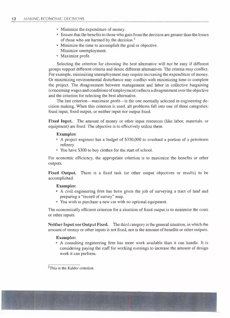
· Minimize the expenditure of money.· Ensure that the benefits to those who gain from the decision are greater than the lossesof those who are harmed by the decision.2
· Minimize the time to accomplish the goal or objective.· Minimize unemployment. .. .· Maximize profit.
Selecting the criterion for choosing the best alternative will not be easy if differentgroups support different criteria and desire different alternatives. The criteria may conflict.For example, minimizing unemployment may require increasing the expenditure of money.Or minimizing environmental disturbance may conflict with minimizing time to completethe project. The disagreement between management and labor in collective bargaining(concerning wages andconditions of employment) reflectsa disagreement over the objectiveand the criterion for selecting the best alternative.
The last criterion-maximize profit-is the one normally selected in engineering de-cision making. When this criterion is used, all problems fall into one of three categories:fixed input, fixed output, or neither input nor output fixed.
Fixed Input. The amount of money or other input resources (like labor, materials, orequipment) are fixed. The objective is to effectively utilize them.
Examples:· A project engineer has a budget of $350,000 to overhaul a portion of a petroleum
refinery.· Youhave $300 to buy clothes for the start of school.
For economic efficiency, the appropriate criterion is to maximize the benefits or otheroutputs.
Fixed Output. There is a fixed task (or other output objectives or results) to beaccomplished.
Examples:· A civil engineering firm has been given the job of surveying a tract of land and
preparing a "record of survey" map.· Youwish to purchase a new car with no optional equipment.
The economically efficient criterion for a situation of fixed output is to minimize the costsor other inputs.
Neither Input nor Output Fixed. The third category is the general situation, in which theamount of money or other inputs is not fixed, nor is the amount of benefits or other outputs.
Examples:· A consulting engineering firm has more work available than it can handle. It is
considering paying the staff for working evenings to increase the amount of designwork it can perform.
2This is the Kaldor criterion.
r:
l'~'.'
~ .r~'
Lc~",",..~...~,;;::,,,-",~, :,~~~- _.:'~:i~':",..::';:~c. ";::';~::'~';':~,:::.,,,:.':';<-",,,.,,i;.,._,,,,-.,.._,...,;;~ ..~:.;;".~_>", '_'Ec~"'__"..c -.,-.~~>J----

14 MAKING ECONOMIC DECISIONS
neighbors unhappy, the environmentmore polluted, and one's savings account smaller. But,to avoid unnecessary complications, we assume that decision making is based on a singlecriterion for measuring the relative attractiveness of the various alternatives. If necessary,one could devise a single composite criterion that is the weighted average of severaldifferentchoice criteria. . ." .. . .
To choose the best alternative, the outcomes for each alternative must be stated in acomparable way.Usually the consequences of each alternativeare stated in terms of money,that is, in the form of costs and benefits. This resolution of consequences is done with allmonetary and nonmonetary consequences. The consequences can also be categorized asfollows:
Market consequences-where there are established market prices available
Extra-market consequences-no direct market prices, so priced indirectly
Intangible consequences-valued by judgment not monetary prices.
In the initial problems we will examine, the costs and benefits occur over a short timeperiod and can be considered as occurring at the same time. In other situations the variouscosts and benefits take place in a longer time period. The result may be costs at one pointin time followed by periodic benefits. We will resolve these in the next chapter into a cashflow diagram to show the timing of the various costs and benefits.
For these longer-term problems, the most common error is to assume that the currentsituation will be unchanged for the do-nothing alternative. For example, current profitswill shrink or vanish as a result of the actions of competitors and the expectations ofcustomers; and trafficcongestionnormally increases overthe years as the number of vehiclesincreases-doing nothing does not imply that the situation will not change.
8. Choosing the Best Alternative .
Earlier we indicated that choosing the best alternative may be simply a matter of determin-ing which alternative best meets the selection criterion. But the solutions to most problemsin economics have market consequences, extra-market consequences, and intangible con-sequences. Since the intangible consequences of possible alternatives are left out of thenumerical calculations, they should be introduced into the decision-making process at thispoint. The alternative to be chosen is the one that best meets the choice criterion afterconsidering both the numerical consequences and the consequences not included in themonetary analysis.
During the decision-makingprocess certain feasible alternativesare eliminated becausethey are dominated by other, better alternatives. For example, shopping for a computeron-line may allow you to buy a custom-configured computer for less money than a stockcomputer in a local store. Buying at the local store is feasible, but dominated. While elimi- .
nating dominated alternatives makes the decision-making process more efficient, there aredangers.
Having examined the structure of the decision-making process, it is appropriate toask, When is a decision made, and who makes it? If one person performs all the steps indecision making, then he is the decision maker. When he makes the decision is less clear.
I j
I
1~~;.~:J<.~#"~{~;iit~",-!!:,~i~..::~~.-:;.."",.-i~'~.'.:~-~";'2.:i;;~.;;;i,,~~~":;',~,4:~~J.f.{t~~~~

" . .--'-- ----.-.......-
Engineering Decision Making for Current Costs 15
The selection of the feasible alternatives may be the key item, with the rest of the analysisa methodical process leading to the inevitable decision. We can see that the decision maybe drastically affected, or even predetermined, by the way in which the decision-makingprocess is carried out. This is illustrated by the following example.
Liz, a young engineer, was assigned to make an analysis of additional equipment neededfor the machine shop. The single criterion for selection was that the equipment shouldbe the most economical, considering both initial costs and future operating costs. Alittle investigation by Liz revealed three practical alternatives:
1. A new specialized lathe2. A new general-purpose lathe3. A rebuilt lathe available from a used-equipment dealer
A preliminary analysis indicated that the rebuilt lathe would be the most economical.Liz did not like the idea of buying a rebuilt lathe, so she decided to discard that alter-native. She prepared a two-alternative analysis that showed that the general-purposelathe was more economical than the specialized lathe. She presented this completedanalysis to her manager. The manager assumed that the two alternatives presented werethe best of all feasible alternatives, and he approved Liz's recommendation.
At this point we should ask: Who was the decision maker, Liz or her n'Ianager? Although themanager signed his name at the bottom of the economic analysis worksheets to authorizepurchasing the general-purpose lathe, he was merely authorizing what already had beenmade inevitable, and thus he was not the decision maker. Rather Liz had made the keydecision when she decided to discard the most economical alternative from further consid-
eration. The result was a decision to buy the better of the two less economically desirablealternatives.
9. Audit the ResultsAn audit of the results is a comparison of what happened against the predictions. Do theresults of a decision analysis reasonably agree with its projections? If a new machine toolwas purchased to save labor and improve quality,did it? If so, the economic analysis seemsto be accurate. If the savings are not being obtained, what was overlooked? The audit mayhelp ensure that projected operating advantages are ultimately obtained. On the other hand,the economic analysis projections may have been unduly optimistic. We want to know this,too, so that the mistakes that led to the inaccurate projection are not repeated. Finally, aneffective way to promote realistic economic analysis calculations is for all people involvedto know that there will be an audit of the results!
ENGINEERING DECISION MAKING FOR CURRENT COSTS
Some of the easiest forms of engineering decision making deal with problems of alternatedesigns, methods, or materials. If results of the decision occur in a very short period oftime, one can quickly add up the costs and benefits for each alternative. Then, using thesuitable economic criterion, the best alternative can be identified. Three example problemsillustrate these situations.

16 MAKING ECONOMIC DECISIONS
A concrete aggregate mix is required to contain at least 31% sand by volume for proper batching.One source of material, which has 25% ~_a.ndan.~_75% coarse aggregate, sells for $3 per cubicmeter (m3). Another source, which has 40% sand and 60% coarse aggregate, sells for $4AO/m3.Determine the least cost per cubic meter of blended aggregates.
The least cost of blended aggregates will result from maximum us~ of the lower-cost material.The higher-cost material will be used to increase the proportion of sand up to the minimumlevel(31%) specified. ..
Let x = Portion of blended aggregates from $3.DO/Ill3.source
1 - x =Portion of blended aggregates froIll $4AO/m3source.'"
Sand Balance
x(0.25) + (1 = x) (0040)=0.31
0.25x + 0040- OAOx - 0.31
0.31- 0040 -0.09x- · .--.
- 0.25- 0040- -0.15
=Q.60Thus the blended aggregates will contain
60% of $3.00/Ill3Illaterial
40% of $4.40/m3material
The least cost per cubic meter of blended.aggregates.is;;
0.60($3.00) -I-0040($4.40) -1.~O-l-l.76
.'. ...$3.S6/m3
.II
iI
.0.,
A machine part is manufactured at a unit cost of 40,i for material and 15,i for direct labor. .Aninvestment of $500,000 in tooling is required. The order calls for 3 million pieces. Halfwaythroughthe order,a new1.11ethodof manufacturecan.be put into.effectthatwi11~reducefue UIiit 1
costs to~4,i for materi('ilandlO,i forcdifect labor-=-but"'it::wiJl"require,:$~OQ;00Q'for~ddiijopa.I=-->1,tooling. This tooling will not be usefUlfor future orders.Oth~r costs are allocated at 2.5 tiIDesthe ·
direcflabor cost. What, if'<'lPything,should be done?_ __ _oIao ",,,,, ____
Jt....~,..'r
~'"--~~~ .~,:.;.;~~~k~i~~~~iL.:..;':':':-.~~;~j:_~'_,L.._~~k~~"'_d'!::~K<~~~{'...:..;:'.=1:~~i:~

Engineering Decision Making for Current Costs 17
Since there is only one way to handle first 1.5 million pieces, our problem concerns only thesecond half of the order. ..0 '" '... ,
Alternative A: Continue with Present Method
Material costDirect labor costOther costs
1,500,000 pieces x 0040 =1,500,000pieces x 0.15=2.50 x direct labor cost =
$600,000225,000562,500
$1,387,500
-,
Cost for remaining 1,500,000pieces
Alternative B: Change the Manufacturing Method
Additional tooling cost $100,000Material cost 1,500,000pieces x 0.34 = 510,000Directlaborcost 1,500,000pieces x 0.10__ 150,000Other costs 2.50 x direct labor cost - 375,000
Cost forremaining 1,500,000pieces $1,135,000
Before making a final decision, one should closely examine the Other costs to see that theydo, in fact, vary as the Direct labor cost varies.Assuming they do, the decision would be to changethe manufacturing method.
......
In the design of a cold-storage warehouse, the specifications call for a maximum heat transferthrough the warehouse walls of 30,000 joules per hour per square meter of wall when there is a30°C temperature difference between the inside surface and the outside surface of the insulation.The two insulation materials being considered are as follows:
Insulation MaterialRock woolFoamed insulation
Cost per Cubic Meter$12.50
14.00
Conductivity(J-m/m2-oC-hr)
140110
The basic equation for heat conduction through a wall is:
Q = K(b.T)L
where Q = heat transfer, in J/hr/m2 of wallK = cpnduc,tiyityin J-mlm2_oC.,hr
b.T ~ clj.fferencein temperature between the two surfaces, in ~CL = thickness of insulating material, in meters
Which insulation material should be selected?_ _ __ IiIII - ... -- - .. - .. - -- -
, I
L~~-~- -:ce._,""_. ,.:-",~,Lc.d~i.- ",<,.:--~~~l;;;~;,:;:d:f.i~~k:- ".f...';Si~~~::"">._i,:-,..i .'--,_"_''.';-~,~." .-,' _:.'_:"~;"h.~. .:"-i:--.~" ~

18 MAKING ECONOMIC DECISIONS
There are two steps required to solve th~_pr.()ble~:First, the required thickness of each of thealternate materials must be calculated. Then, since the problem is one of providing a fixed.output(heat transfer through the wall limited to a fixed maximum amount), the criterion is to minimizethe input (cost).
Required Insulation Thickness
30000 _ 140(30), . L
110(30)Foamed insulation 30,000 = ~
L
Cost of Insulation per Square Meter of Wall
Unit cost~ COSt/Ill3x IlJ,sulati()lJ,thickness, in..il1e.t~J:SUnit cost. $12.50 x 0.14Ill~ $1.75/il12Unit cost .. $14.00 X 0.11IIi-$154/IIl2
Rock wool L O.14m
L-O.llm
Rock woolFoamedinsulation
- =~ - ......... !The foamed insulation is the lesser cost alternative.However, tl1ete.lsalvilJ,talJ,giblecOn.sttailJ,ttl1atmust be considered. How thick is the available wall space? EngineeplJ,geconomy and.tljet.iil1evalUeof money are neededto decide what the maX1.mUmheattransfershould be. Whatis the costof more insulation versus the cost of cooling the warehouse oVerits life?
SUMMARY
Classifying ProblemsMany problems are simple and thus easy to solve. Others are of intermediate difficultyand need considerable thought and/or calculation to properly evaluate. These intermediateproblems tend to have a substantial economic component, hence are good candidates foreconomic analysis. Complex problems, on the other hand, often contain people elements,along with political and economic components. Economic analysis is still very important,but the best alternative must be selected considering all criteria-not just economics.
The Decision-Making ProcessRational decision.making usesa logical method of analysis to select the best alternativefromamong the feasible alternatives.The following nine steps can be followed sequentially,butdecision makers often repeat some steps, undertake some simultaneously, and skip othersaltogether. .
1. Recognize the problem.2. Define the goal or objective: What is the task?3. Assemble relevant data: What are the facts? Are more data needed, and is it worth
more than the cost to obtain it?
4. Identify feasible alternatives.

_..-..-
Problems 19
5. Select the criterion for choosing the best alternative: possible criteria includepolitical, economic, environmental, and humanitarian. The single criterion maybe a composite of several different criteria.
6. Mathematically model the various interrelationships.7. Predict the outcomes for each ilIiemative.8. Choose the best alternative.9. Audit the results.
Engineering decision making refers to solving substantial engineering problems inwhich economic aspects dominate and economic efficiency is the criterion for choosingfrom among possible alternatives. It is a particular case of the general decision-makingprocess. Some of the unusual aspects of engineering decision making are as follows:
1. Cost-accounting systems, while an important source of cost data, contain allocationsof indirect costs that may be inappropriate for use in economic analysis.
2. The various consequences--costs and benefits---of an alternative may be of threetypes:(a) Market consequences-there are established market prices(b) Extra-market consequences-there are no dii-ectmarket prices, but prices can
be assigned by indirect means(c) Intangible consequences-valued by judgment, not by monetary prices
3. The economic criteria for judging alternatives can be reduced to three cases:(a) For fixed input: maximize benefits or other outputs.(b) For fixed output: minimize costs or other inputs.(c) When neither input nor output is fixed:maximizethe differencebetween benefits
and costs or, more simply stated, maximize profit.The third case states the general rule from which both the first and second casesmay be derived.
4. To choose among the alternatives, the market consequences and extra-market con-sequences are organized into a cash flow diagram. We will see in Chapter 3 thatengineering economic calculations can be used to compare differing cash flows.These outcomes are compared against the selection criterion.From this comparisonplus the consequences not included in the monetary analysis, the best alternative isselected.
5. An essential part of engineering decision making is the postaudit of results. Thisstep helps to ensure that projected benefits are obtained and to encourage realisticestimates in analyses.
PROBLEMS
1-1 Think back to your first hour after awakening thismorning. List 15 decision-making opportunities thatexisted during that hour. After you have done that,mark the decision-making opportunities that youactuallyrecognizedthis morningand upon which youmade a conscious decision.
1-2 Someof the followingproblemswouldbe suitableforsolution by engineering economic analysis. Whichones are they?(a) Would it be better to buy an automobile with a
diesel engine or a gasolineengine?

20 MAKING ECONOMIC DECISIONS
(b) Should an automatic machine be purchased toreplace three workers now doing a task by hand?
(c) Would it be wise to enroll for an early morn-ing class so you could avoid traveling during themorningtrafficrushhours? . ....
(d) Would you be better off if you changed yourmajor?
(e) One of the people you might marry has a job thatpays very little money, while another one has aprofessionaljob with an excellent salary.Whichone should you marry?
1-3 Which one of the followingproblems is most suitablefor analysis by engineeringeconomic analysis?(a) Some 45jt candy bars are on sale for 12 bars for
$3. Sandy, who eats a couple of candy bars aweek, must decide whether to buy a dozen at thelower price.
(b) A woman has $150,000 in a bank checkingaccount that pays no interest. She can either investit immediately at a desirable interest rate or waita week and know that she will be able to obtain
an interest rate that is 0.15% higher.(c) Joe backed his car into a tree, damaging the
fender. He has automobile insurance that will payfor the fender repair. But if he files a claim forpayment, they may change his "good driver"rating downward and charge him more for carinsurance in the future.
1-4 If you have $300 and could make the right decisions,how long would it take you to become a millionaire?Explain briefly what you would do.
1-5 Many people write books explaining how to makemoney in the stock market. Apparently the authorsplan to make their money selling books telling otherpeople how to profit from the stock market. Why don'tthese authors forget about the books and make theirmoney in the stock market?
1-6 The owner of a small machine shop has just lost one ofhis larger customers. The solution to his problem, hesays, is to fire three machinists to balance his work-force with his current level of business. The owner
says it is a simple problem with a simple solution.The three machinists disagree. Why?
1-7 Every college student had the problem of selectingthe college or university to attend. Was this a simple,intermediate, or complex problem for you? Explain.
1-8 Toward the end of the twentieth century, the U.S.government wanted to save money by closing a small
portion of all its military installations throughout theUnited States. While many people agreed that sav-ing money was a desirable goal, areas potentially af-fected by selection to close soon reacted negatively.Congress finally selected a panel of people whose taskwas to develop a list of installations to close, with thelegislation specifying that Congress could not alterthe list. Since the goal was to save money, why wasthis problem so hard to solve?
1-9 The college bookstore has put pads of engineeringcomputation paper on sale at half price. What is theminimum and maximum number of pads you mightbuy during the sale? Explain.
1-10 Consider the seven situations described. Which onesituation seems most suitable for solution by engi-
neering economic analysis?(a) Jane has met two college students that interest
her. Bill is a music major who is lots of fun tobe with. Alex, on the other hand, is a fellow en-gineering student, but he does not like to dance.Jane wonders what to do.
(b) You drive periodically to the post office to pickup your mail. The parking meters require 10jt for6 minutes-about twice the time required to getfrom your car to the post office and back. If park-ing fines cost $8, do you put money in the meteror not?
(c) At the local market, candy bars are 45 jt each orthree for $1. Should you buy them three at a time?
(d) The cost of automobile insurance varies widelyfrom insurance company to insurance company.Should you check with several companies whenyour insurance comes up for renewal?
(e) There is a special local sales tax ("sin tax") on avariety of things that the town council would liketo remove from local distribution. As a result a
store has opened up just outside the town and of-fers an abundance of these specific items at pricesabout 30% less than is charged in town. Shouldyou shop there?
(f) Your mother reminds you that she wants you to at-tend the annual family picnic. That same Saturdayyou already have a date with a person you have.been trying to date for months.
(g) One of your professors mentioned that you havea poor attendance record in her class. You wonderwhether to drop the course now or wait to see howyou do on the first midterm exam. Unfortunately,the course is required for graduation.

... -------..
Problems 21
1-11 An automobile manufacturer is considering locatingan automobile assembly plant in your region. List twosimple, two intermediate, and two complex problemsassociated with this proposal.
1-12 Consider the following situations. Which ones appearto represent rational decision making? Explain.(a) Joe's best friend has decided to become a civil
engineer, so Joe has decided that he, too, willbecome a civil engineer.
(b) Jill needs to get to the university from her home.She bought a car and now drives to the universityeach day. When Jim asks her why she didn't buy abicycle instead, she replies, "Gee, I never thoughtof that."
(c) Don needed a wrench to replace the spark plugsin his car. He went to the local automobile sup-ply store and bought the cheapest one they had.It broke before he had finished replacing all thespark plugs in his car.
1-13 Identify possible objectives for NASA. For yourfavorite of these, how should alternative plans toachieve the objective be evaluated?
1-14 Suppose you have just 2 hours to answer the question,How many people in your home town would be inter-ested in buying a pair of left-handed scissors? Give astep-by-step outline of how you would seek to answerthis question within two hours.
1-15 A college student determines that he will have only$50 per month available for his housing for the com-ing year. He is determined to continue in the univer-sity, so he has decided to list all feasible alternativesfor his housing. To help him, list five feasible alter-natives.
1-10 Describe a situation where a poor alternative wasselected, because there was a poor search for betteralternatives.
1-17 If there are only two alternatives available and bothare unpleasant and undesirable, what should yo~ do?
The three economic criteria for choosing the bestalternative are minimize input, maximize output, andmaximize the difference between output and input.For each of the following situations, what is theappropriate economic criterion?(a) A manufacturer of plastic drafting triangles can
sell all the triangles he can produce at a fixedprice. As he increases production, his unit costsincrease as a result of overtime pay and so forth.The manufacturer's criterion should be _'
1-18
(b) An architectural and engineering firm has beenawarded the contract to design a wharf for apetroleumcompanyfor a fixedsumof money.Theengineering firm's criterion should be_.
'(c) A book publisher is about to set the list price(retail price) on a textbook. The choice of a lowlist price wouldmean less advertisingthan wouldbe used for a higher list price. The amount ofadvertising will affect the number of copies sold.The publisher's criterion should be _'
(d) At an auctionof antiques,a bidderfor aparticularporcelain statue would be trying to _'
1-19 As in Problem 1-18, state the appropriate economiccriterion for each of the following situations.(a) The engineering school held a raffle of an auto-
mobile with tickets selling for'50~each or threefor $1. When the students were selling tickets,they notedthat manypeople had troubledecidingwhetherto buyone or three tickets.Thisindicatesthe buyers' criterion was _'
(b) A student organization bought a soft-drinkmachine for use in a student area. There wasconsiderablediscussionoverwhethertheyshouldset the machine to charge SOt, 75~, or $1 perdrink. The organizationrecognized that the num-ber of soft drinks sold would depend on the pricecharged. Eventually the decision was made tocharge 75~. Their criterion was_.
(c) In many cities, grocery stores find that their salesare much greater on days when they have adver-tised their special bargains. However,the adver-tised specialprices do not appear to increase thetotal physicalvolumeof groceries soldby a store.This leads us to conclude that many shoppers'criterion is _'
(d) A recently graduated engineer has decided to re-turn to school in the evenings to obtain a master'sdegree. He feels it should be accomplished in amanner that will allow him the maximum amount
of time for his regular day job plus time for recre-ation. In working for the degree, he will _'
1-20 Seven criteria are given in the chapter for judging'which is the best alternative. After reviewing thelist, devise three additional criteria that might beused.
1-21 Suppose you are assigned the task of determiningthe route of a new highway through an older sectionof town. The highway will require that many olderhomes must be either relocated or torn down. Two

22 MAKINGECONOMIC DECISIONS
possible criteria that might be used in deciding ex-actly where to locate the highway are:(a) Ensure that there are benefits to those who gain
from the decision and that no one is harmed bythe decision. . .-
(b) Ensure that the benefits to those who gain fromthe decision are greater than the losses of thosewho are harmed by the decision.
Which criterion will you select to use in determiningthe route of the highway? Explain.
1-22 Identify benefits and costs for Problem 1-21.
1-23 In the fall, Jay Thompson decided to live in a uni-versity dormitory. He signed a dorm contract underwhich he was obligated to pay the room rent for thefull college year. One clause stated that if he movedout during the year, he could sell his dorm contract toanother student who would move into the dormitoryas his replacement. The dorm cost was $2000 for thetwo semesters, which Jay had already paid.
A month after he moved into the dorm, he
decided he would prefer to live in an apartment. Thatweek, after some searching for a replacement to fulfillhis dorm contract, Jay had two offers. One student of-fered to move in immediately and to pay Jay $100 permonth for the eight remaining months of the schoolyear. A second student offered to move in the second'semester and pay $700 to Jay.
Jay estimates his food cost per month is $300if he lives in the dorm and $250 if he lives in an
apartment with three other students. His share of theapartment rent and utilities will be $200 per month.Assume each semester is 41/2months long. Disregardthe small differences in the timing of the disburse-ments or receipts.(a) What are the three alternatives available to Jay?(b) Evaluate the cost for each of the alternatives.(c) What do you recommend that Jay do?
1-24 In decision making we talk about the construction ofa model. What kind of model is meant?
1-25 An electric motor on a conveyor burned out. The fore-man told the plant manager that the motor had to bereplaced. The foreman indicated that there were noalternatives and asked for authorization to order the
replacement. In this situation, is any decision makingtaking place? If so, who is making the decision(s)?
1-26 Bill Jones's parents insisted that Bill buy himself anew sport shirt. Bill's father gave specific instruc-tions, saying the shirt must be in "good taste,"that is,
neither too wildly colored nor too extreme in tailor-ing. Bill found three types of sport shirts in the localdepartment store:
·Rather somber shirts that Bill's father would want
him to buy· Good-looking shirts that appealed to Bill· Weirdshirts that were even too much for Bill
He wanted a good-looking shirt but wondered howto convince his father to let him keep it. The clerksuggestedthat Bill takehome tWoshirts for his fatherto see and return the one he did not like. Bill.selected
a good-lookingblue shirt he liked, and also a weirdlavender shirt. His father took one look and insisted
that Bill keep the blue shirt and return the lavenderone. Billdid as hisfather instructed.Whatwasthe keydecision in this decision process, and who made it?
1-27 A farmer must decide what combination of seed,water, fertilizer, and pest control will be most prof-itable for the coming year. The local agriculturalcollege did a study of this farmer's situation andprepared the following table.
PlanABCD
Cost/acre$ 600
150018002100
Income/acre$ 800
190022502500
The last page of the college's study was torn off, andhence the farmer is not sure. which plan the agricul-tural college recommends. Which plan should thefarmer adopt? Explain.
1-28 Identify the alternatives, outcomes, criteria, and pro-cess for the selection of your college major? Did youmake the best choice for you?
1-29 Describe a major problem you must address in thenext two years. Use the techniques of this chapter to
. structure the problem and recommend a decision.
1-30 One strategy for solving a complex problem is tobreak the problem into a group of less complex prob-lems and then find solutions to the smaller problems.The result is the solutionof the complexproblem..Give an example in which this strategy will work.Then giveanotherexamplein which this strategywillnot work.
1-31 On her firstengineeringjob, Joy Hayes was giventheresponsibility of determining the productionrate fora new product. She has assembled data as indicated
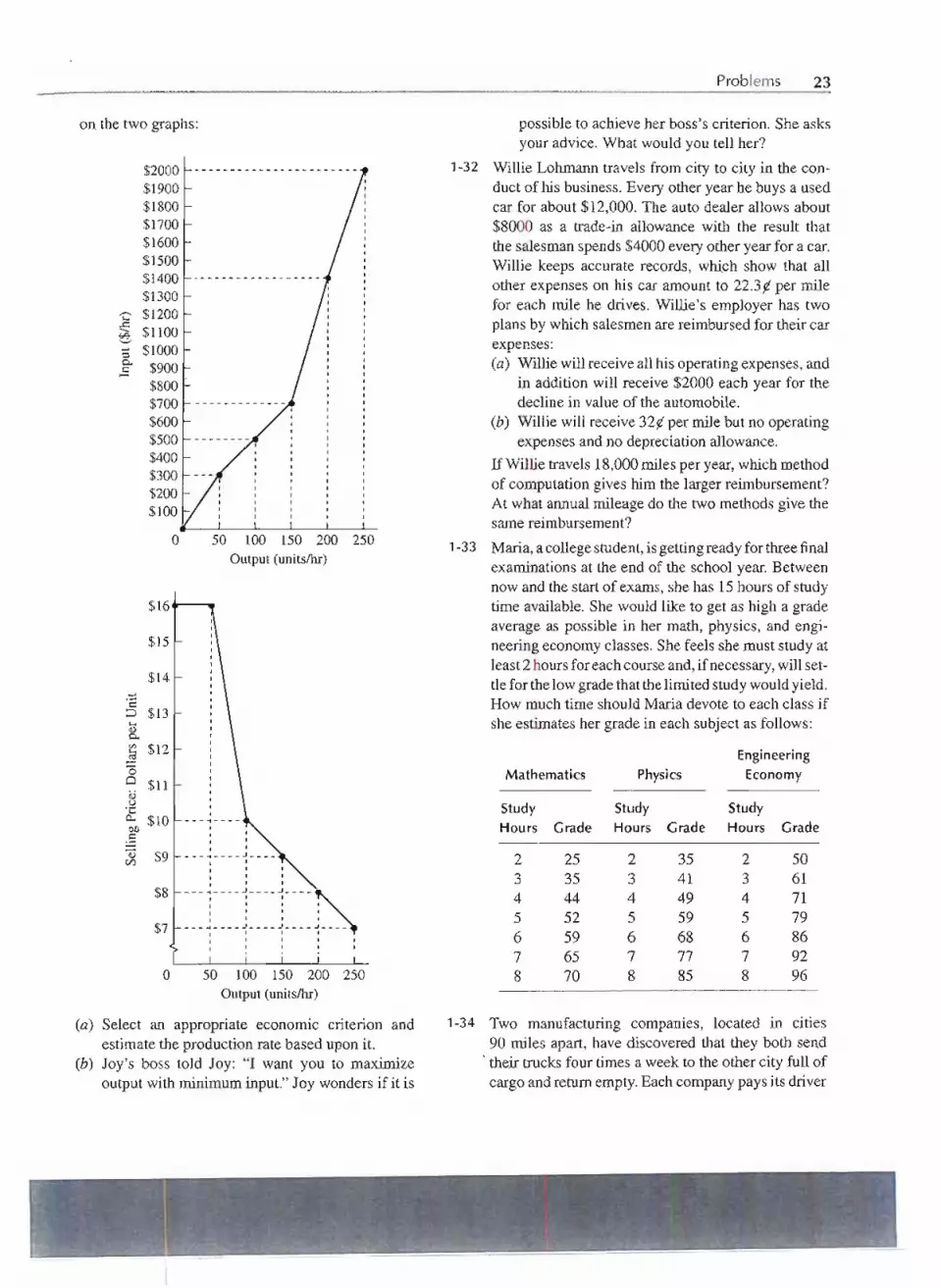
Problems 23
----------------------- 1-32
possible to achieve her boss's criterion. She asksyour advice. What would you tell her?
Willie Lohmann travels from city to city in the con-duct of his business. Every other year he buys a used
. car for about $12,000. The auto dealer allows about$8000 as a trade-in allowance with the result that
the salesman spends $4000 every other year for a car.Willie keeps accurate records, whi.ch show that allother expenses on his car amount to 22.3 ~per milefor each mile he drives. Willie's employer has twoplans by which salesmen are reimbursed for their carexpenses:(a) Willie will receive all his operating expenses, and
in addition will receive $2000 each year for thedecline in value of the automobile.
(b) Willie will receive 32~ per mile but no operatingexpenses and no depreciation allowance.
If Willie travels 18,000 miles per year, which methodof computation gives him the larger reimbursement?At what annual mileage do the two methods give thesame reimbursement?
Maria, a college student, is getting ready for three finalexaminations at the end of the school year. Betweennow and the start of exams, she has 15 hours of studytime available. She would like to get as high a gradeaverage as possible in her math, physics, and engi-neering economy classes. She feels she must study atleast 2 hours for each course and, if necessary, will set-tie for the low grade that the limited study would yield.How much time should Maria devote to each class if
she estimates her grade in each subject as follows:
on the two graphs:
$2000$1900$1800$1700$1600$1500$1400$1300
~ $1200G't $1100~ $1000§' $900 ,.
$800$700$600$500$400$300$200$100
,o
------------------
50 100 150 200 250
Output (unitslhr)1-33
~c..'" $12lS'0Q $11asu
if $10bI).S~ $9tI)
Mathematics Physics
EngineeringEconomy
I---;----II II II It J____I II I II I I
$8 I- -- - ~-- -- ~-- -- ~-- --I I I II I I II I I I
$71 ~ ~ ~ ~----I I I II I I I
StudyHours Grade
StudyHours Grade
StudyHours Grade
o 50 100 150 200 250
Output (unitslhr)
(a) Select an appropriate economic criterion andestimate.the production rate based upon it.
(b) Joy's boss told Joy: "I want you to maximizeoutput with minimum input." Joy wonders if it is
1-34 Two manufacturing companies, located in cities90 miles apart, have discovered that they both send
, their trucks four times a week to the other city full ofcargo and return empty. Each company pays its driver
rI
~.
i;, c.. ~,._~_ . <>;,~,;~;.;:" '¥"~~~;';' ;, "d;.7Ji;~._'i.:.;h,,"~;:.: ~''''~,~...''''''.J-i-i.:,., h~ ";0 ~ --;,,:,'-."-~ ; - ~;>~ --:',.";~- _~';'~.c =,.:c"ii:~~
$16
$15
$14.....
'8$13
2 25 2 35 2 503 35 3 41 3 614 44 4 49 4 715 52 5 59 5 796 59 6 68 6 867 65 7 77 7 928 70 8 85 8 96

24 MAKING ECONOMIC DECISIONS
$185 a day (the round trip takes all day) and havetruckoperatingcosts (excludingthe driver)of 60fCa mile. How much could each company save eachweek if they shared the task, with eachs-ending itstruck twice a week and hauling the other comparifscargo on the return trip?
1-35 A city is in need of increasing its rubbish disposalfacilities. There is a choice of two rubbish disposalareas, as follows.
Area A: A gravel pit with a capacity of 16 mil-lion cubic meters. Owing to the possibility ofhigh ground water, however, the Regional WaterPollution-Control Board has restricted the lower2 million cubic meters of fill to inert material
only (earth, concrete, asphalt, paving, brick,etc.). The inert material, principally clean earth,must be purchased and hauled to this area forthe bottom fill.
Area B: Capacity is 14 million cubic meters.The entire capacity may be used for general rub-bish disposal. This area will require an averageincrease in a round-trip haul of 5 miles for 60%of the city, a decreased haul of 2 miles for 20%of the city. For the remaining 20% of the city,the haul is the same distance as for Area A. .
Assume the followingconditions:
· Cost of inert material placed in Area A will be. $2.35 1m3.·Average speed of trucks from last pickup to dis-
posal site is 15 miles per hour.· The rubbish truck and a two-man crew will cost
$35 per hour.·Truck capacity of 41/2tons per load or 20 m3.· Sufficient cover material is available at all areas;
however, inert material for the bottom fill in AreaA must be hauled in.
Which of the sites do you recommend? (Answer:Area B)
1-36 An oil company is considering adding an additionalgrade of fuel at its service stations. To do this, an addi-tional3000-gallon tank must be buried at each station.Discussions with tank fabricators indicate that the
least expensive tank would be cylindrical with mini-mum surface area. What size tank should be ordered?
(Answer: 8 it diameter by 8 ft length)
1-37 The vegetable buyer for a group of grocery storeshas decided to sell packages of sprouted grain in the
vegetable section of the stores. The product is per-ishable and any remaining unsold after one week inthe store is discarded. The supplier will deliver thepackages to the stores, arrange them in the displayspace, and remove and dispose of any old packages.The price the supplierwill charge the stores dependson the size of the total weekly order for all the stores.
Weekly OrderLess than 1000packages1000-14991500-19992000 or more
Price per Package35fC282520
The vegetable buyer estimates the quantity that canbe soldperweek, atvariousselling prices,as follows:
Selling Price Packages Sold per Week60fC 30045 60040 120033 170026 2300
The sprouted grain will be sold at the same price inall the grocery stores. How many packages should bepurchased per week, and at which of the five priceslisted above should they be sold?
Cathy Gwynn, a recently graduated engineer, de-cided to invest some of her money in a "Quick Shop"grocery store. The store emphasizes quick service, alimited assortment of grocery items, and rather highprices. Cathy wants to study the business to see if thestore hours (currently 0600 to 0100) can be changedto make the store more profitable. Cathy assembledthe following information.
1-38
Time Period0600-07000700-08000800-09000900-12001200-15001500-18001800-21002100-22002200-23002300-24002400-0100
Daily Sales inthe Time Period
$ 204060
200180300400100306020
The cost of the groceries sold averages 70% of sales.The incremental cost to keep the store open, including
I
I~~~..~ c~~.c:;x.~,,, ~'''''''~'_': 'c :."'~-j~ .",:" ..< .,.,"'..;, :.~., -4~
I

...-
Problems 25
the clerk's wage and other incremental operatingcosts, is $10 per hour. To maximize profit, whenshould the store be opened, and when should it beclosed?
Jim Jones, a motel owner, noticed that just down thestreet the "Motel 36" advertises a $36-per-night roomrental rate on its sign. As a result, this competitor rentsall 80 rooms every day by late afternoon. Jim, on theother hand, does not advertise his rate, which is $54per night, and he averages only a 68% occupancy ofhis 50 rooms.
There are a lot of other motels nearby, but onlyMotel 36 advertises its rate on its sign. (Rates at theother motels vary from $48 to $80 per night.) Jimestimates that his actual incremental cost per nightfor each room rented, rather than remaining vacant,is $12. This $12 pays for all the cleaning, launder-ing, maintenance, utilities, and so on. Jim believeshis eight alternatives are:
1-39
AlternativeResulting
Occupancy Rate
1234
Advertise
and Charge
$35 per night42 per night48 per night54 per night
Do Not Advertise
and Charge
$48 per night54 per night62 per night68 per night
100%948066
70%686656
5678
What should Jim do? Show how you reached yourconclusion.
A firm is planning to manufacture a new product.The sales department estimates that the quantity thatcan be sold depends on the sellingprice. As the sell-ing price is increased, the quantity that can be sold
1-40
decreases. Numerically they estimate:
P = $35.00 - 0.02Q
where P =selling price per unitQ = quantity sold per year
On the other hand, the management estimates thatthe average cost of manufacturing and selling theproduct will decrease as the quantity sold increases.They estimate
C = $4.00Q + $8000
1-41
where C = cost to produce and sell Q per year
The firm's management wishes to produce and sellthe product at the rate that will maximize profit, thatis, where income minus cost will be a maximum.What quantity should the decision makers plan toproduce and sell each year? (Answer: 775 units)
A manufacturing firm has received a contract to as-semble 1000units of test equipment in the next year.The firm must decide how to organize its assemblyoperation. Skilled workers, at $22 per hour each,could be assigned to individually assemble the testequipment. Each worker would do all the assemblysteps, and it would take 2.6 hours to complete oneunit. An alternate approach would be to set up teamsof four less skilledworkers (at$13 perhour each)andorganize the assembly tasks so that each workerdoespart of the assembly. The four-man team would beable to assemble a unit in one hour. Which approachwould result in more economically assembly?
A grower estimates that if he picks his apple cropnow, he will obtain 1000 boxes of apples, which hecan sell at $3 per box. However, he thinks his cropwill increase by 120 boxes of apples for each weekhe delayspicking,but that theprice will drop at a rateof l5~ per box per week; in addition, he estimatesapproximately20 boxes per week will spoil for eachweekhe delayspicking.Whenshould hepick hiscropto obtain the largest total cash return? How much willhe receive for his crop at that time?
1-42
f" I;. I~ Ii-. 1 --
~i:.~,~ ~ -"~~'O"'c:;~ l.>:~s;t~~ ,~J<~.",z"..~-,.";'.~"'~.';;.~:~:d~ .;.."";... :.,;,.:: "/ci._~..;' ;,'-'. ~:. :~."">, <>','-.c,.~"-'. , ,.. ". i~...:.: {;,j
--1-

After Completing This Chapter...The student should be able to:
· Define various cost concepts. .
· Provide specificexamplesof howand whythese engineering costconcepts areimportant.· Define engineering cost estimating.· Explain the three types of engineering estimate, as well as common difficultiesencoun-
tered in making engineering cost estimates.· Use several common mathematical estimating models in cost estimating.· Discuss the impact of the learning curve on cost estimates.· State the relationship between cost estimating and estimating project benefits.· Draw cashflow diagrams to show project costs and benefits.
QUESTIONS TO CONSIDER;;.
1. By investing heavily in warehouses and other infrastructure, Webvan incurred large"fixed costs" that it would have to pay regardless of whether it attracted customers. Bycontrast, Tesco invested a more modest sum up front and hired employees only whencustomer orders increased enough to warrant it. How might these choices have affectedthe financial fates of the two companies?
2. In most cases, businesses that are seeking 'financing for start-up or expansion must de-velop detailed estimates of their likely costs and future earnings. But Webvanconvincedinvestors that it was operating in a "new world" of Internet COlTIlTIerce,to which theold rules did not apply. How did this affect investors' willingness to accept Webvan'sestima.tesof its financial prospects?
3. Generally, businesses view cost considerations as a constraint. Inthis case, however,Jhedotcom boom of the 1990s stood that rule on its head: the more Webvan spent, the more '
money investors seemed willing to give the company-at least until the boom ran itscourse. Would Webvan have been better off with investors who asked more questionsand imposed more limits? Why or why not?
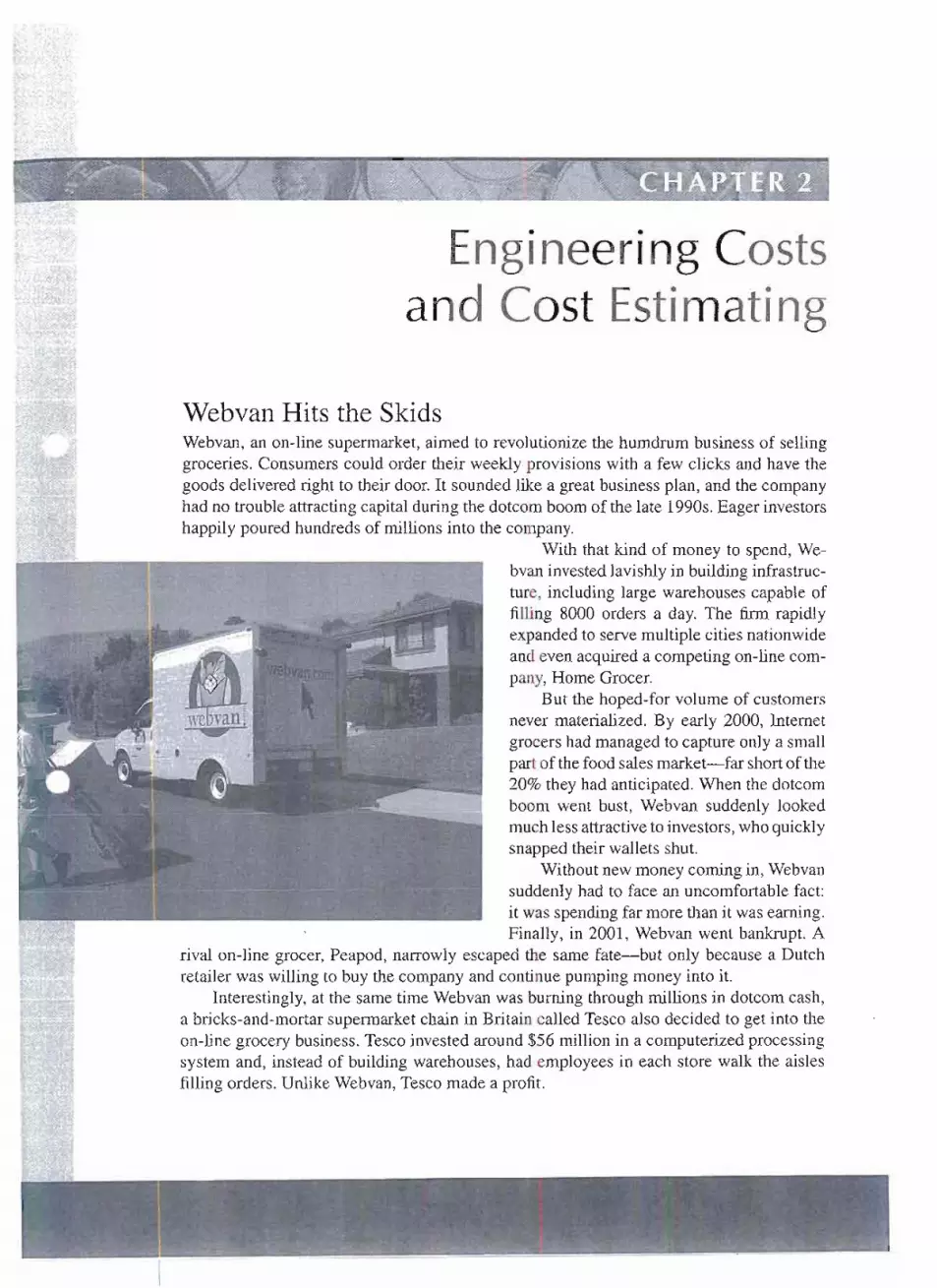
'. ..,- .",.~ c_-.:__-,-.-.-~-,,,, _
4"'@OO~lifIt~
Engineeri ng Costsand Cost Estimating-
Webvan Hits the SkidsWebvan, an on-line supermarket, aimed to revolutionize the humdrum business of sellinggroceries. Consumers could order their weekly provisions with a few clicks and have thegoods delivered right to their door. It sounded like a great business plan, and the companyhad no trouble attracting capital during the dotcom boom of the late 1990s.Eager investorshappily poured hundreds of millions into the company.
With that kind of money to spend, We-bvan investedlavishly in building infrastruc-ture, including large warehouses capable offilling 8000 orders a day. The firm rapidlyexpanded to serve multiple cities nationwideand even acquired a competing on-line com-pany, Home Grocer.
But the hoped-for volume of customersnever materialized. By early 2000, Internetgrocers had managed to capture only a smallpart of the food sales market-far short of the20% they had anticipated. When the dotcomboom went bust, Webvan suddenly lookedmuch less attractiveto investors,who quicklysnapped their wallets shut.
Without new money coming in, Webvansuddenly had to face an uncomfortable fact:it was spending far more than it was earning.Finally, in 2001, Webvan went bankrupt. A
rival on-line grocer, Peapod, narrowly escaped the same fate-but only because a Dutchretailer was willing to buy the company and continue pumping money into it.
Interestingly, at the same time Webvan was burning through millions in dotcom cash,a bricks-and-mortar supermarket chain in Britain called Tesco also decided to get into theon-line grocery business. Tesco invested around $56 million in a computerized processingsystem and, instead of building warehouses, had employees in each store walk the aislesfilling orders. Unlike Webvan,Tesco made a profit.
II
I
\
.t~i' ;~~.JiL~~;,,~ ,.;;;~~.~.. .'--;-~i~,,_;,~~~~~~~~,:.~." . ~.:"~::'.~~~,"';~-F...);.> ~~ ;.,~~ ;""..;" ,,~.-- .-: .>,,' -. ~.~ - : -~: ."~~ ':', " ~.-"~.;'-:~j

28 ENGINEERINGCOSTSAND COST ESTIMATING
This chapter defines fundamental cost concepts. These include fixed and variable costs,marginal and average costs, sunk and opportunity costs, recurring and nonrecurring costs,incremental cash costs, book costs, and life-cycle costs. We then describe the various typesof estimates and difficultiessometimes encountered. The models that are described includeunit factor, segmenting, cost indexes";power sizing, triangulation, and learning curves. Thechapter discusses estimating benefits, developing cash flow diagrams, and drawing thesediagrams with spreadsheets.
Understanding engineering costs is fundamental to the engineering economic analysisprocess, and therefore this chapter addresses an important question: Where do the numberscome from?
ENGINEERING COSTS
Evaluating a set of feasible alternatives requires that many costs be analyzed. Examplesinclude costs for initial investment, new construction, facility modification, general labor,parts and materials, inspection and quality, contractor and subcontractor labor, training,computer hardware and software,material handling, fixturesand tooling, data management,and technicalsupport, as well as general support costs (overhead). In this section wedescribeseveral concepts for classifying and understanding these costs.
Fixed, Variable, Marginal, and Average CostsFixed costs are constant or unchanging regardless of the level of output or activity. Incontrast, variable costs depend on the level of output or activity. A marginal cost is thevariable cost for one more unit, while the average cost is the total cost divided by thenumber of units.
For example, in a production environment fixed costs, such as those for factory floorspace and equipment, remain the same even though production quantity, number of em-ployees, and level of work-in-process may vary.Labor costs are classified as a variable costbecause they depend on the number of employees in the factory. Thusfixed costs are levelor constant re~ardless of output or activity, and variable costs are changing and related tothe level of output or activity.
As another example, many universities charge full-time students a fixed cost for 12 to18hours and a cost per credit hour for each credit hour over 18.Thus for full-time studentswho are taking an overload (> 18 hours), there is a variable cost that depends on the levelof activity.
This example can also be used to distinguish between marginal and average costs. Amarginal cost is the cost of one more unit. This will depend on how many credit hours thestudent is taking. If currently enrolled for 12 to 17 hours, adding one more is free. Themarginal cost of an a~ditionalcredit hour is $0. However,if the student is taking 18or more .
hours, then the marginal cost equals the variable cost of one more hour.To illustrate average costs, the fixed and variable costs need to be specified. Suppose
the cost of 12 to 18hours is $1800 per term and overload credits are $120/hour.If a studenttakes 12 hours, the average cost is $1800/12 = $150 per credit hour. If the student wereto take 18 hours, the average cost decreases to $1800/18 = $100 per credit hour. If thestudent takes 21 hours, the average cost is $102.86 per credit hour [$1800 + (3 x $120) /21].
r- I
~ ~-. ..
~...~
~ . - ':- '. ,. -. '-. . -,
. ~¥~f~~~~~.~~~:,-;)";!-.~j1J;:Ji2~~~~;~~~.~{;;;.l~~,~£.~~.~:.::{~j~'r)~~~'~>".i;-~--- -~-
r

Engineering Costs 29
Average cost is thus calculated by dividing the total cost for all units by the total number ofunits. Decision makers use average cost to attain an overall cost picture of the investmenton a per unit basis.
Marginal cost is used to decide w~~therthe additional unit should be made, purchased,or enrolled in. For the full-time'studentatourexampleuniversity,the marginalcost of anothercredit is $0 or $120 depending on how many credits the student has already signed up for.
An entrepreneur named DK was considering the money-making potential of chartering a bus totake people from his hometown to an event in a larger city. DK planned to provide transportation,tickets to the event,andrefreshmentson the bus forhis customers.He gathereddata andcategorizedthe predicted expenses as either fixed or variable.
DK's Fixed CostsBus rental
Gas expenseOther fuelsBus driver
$80752050
DK's Variable CostsEvent ticketRefreshments
$12.50 per person7.50 per person
Develop an expression of DK's total fixed and total variable costs for chartering this trip.,
SOlUT.ION
DK's fixed costs will be incurred regardless of how many people sign up for the trip (even if onlyone person signs up!). These costs include bus rental, gas and fuel expense, apd the cost to hire adriver:
Total fixed costs = 80 + 75 + 20 + 50 = $225
DK's variable costs depend on how many people sign up for the charter, which is the level ofactivity. Thus for event tickets and refreshments, we would write
= - -
From Example 2-1 we see how it is possible to calculate total fixed and total variablecosts. Furthennore, these valuescan be combined into a single total cost equation as follows:
Total cost =Total fixed cost + Total variable cost (2-1)
The relationship between total cost and fixedand variable costSare shownin Figure 2-1.The fixed-costportion of $3000 is the same across the entire range of the output variable x.Often, the variable costs are linear (y equals a constant times x); however, the variablecosts can be nonlinear. For example, employees are often paid at 150% of their hourly ratefor overtime hours, so that production levels requiring overtime have higher variable costs.
.~ ,II
I{ \.~~~~ _: I. ...:.~:<,,:.<..-~~...:~:-:~~ -'L '~~ :.,.. ~_i£~. ...z~-:: ", ,.~-~.:.;~,::;~:; .~_co, j-~~~ ~.:-. - ,;~...~..~,~.;. : ~:.-~...,~;'.::..-~ _..:."- . '~, ~-, :;,;,~.:..~;..-}~.; ~~~:.Jj

30 ENGINEERING COSTSAND COST ESTIMATING
FIGURE 2-1 Fixed, variable,and total costs.
$8000TotalCost
$6000
Variable Cost...en
8 $4000
$2000FixedCost
5 10 15
Volume
Totalcost in Figure2-1 is a fixedcostof $3000plus a variablecost of $200per unit forstraight-time production of up to 10 units and $300 per unit for overtime production of upto 5 moreunits. .
Figure 2-1 can also be used to illustrate marginal and average costs. At a volume of5 units the marginal cost is $200 per unit, while at a volume of 12units the marginal cost is$300 per unit. The respective average costs are $800 per unit, or (3000 + 200 x 5)/5, and$467 per unit, or (3000 + 200 x 10 + 300 x 2)/12.
In Example 2-1, DK develop~dap overall total cost equation for his business expenses. Now hewants to evaluate the potential to make money from this chartered bus trip.
SOLlJTION! ' ~.
We use Equation 2-1 to find DK's total cost equation:
Total cost"_. total fixed'cost +~otal'variable'cost - ;;;
= $225 + ($20)(number of people on the trip)
where number of people on the trip ='X. Thus, :::
Total cost = 225 + 20x
Using this relationship, DK can calculate the total cost for any number of people-:-up to thefcapacity of the bus. What he lacks is a revenue equatiQnto offset his costs. DK's total revenue
:; from this trip can.b~expressed as: i'! = ;;;;:: = ~
Total revenue:::: (Charter ticketprice)(Number of people on the trip) = (Ticket price) (x)-- ~- - - -- -- - - -... -
11';'
~: /
\i.. 1.~~._;'$~~k~~~~"~~,_~;;jl.,=:,.~~~:.,,.~.,,:;'.~~_.,.;:,_':~~2.iiL'f~~:~

Engineering Costs 31
DK believes that he could attract 30 people at a charter ticket price of $35. Thus
Total profit = (Total revenue) - (Tot~ costs) - (35x) - (225 + 20x)- 15x - 225.. ',,;;~'" .':"- :-:.
Atx - 30,
Total profit = 35 x 30 '"- (225 + 20 x 30) = $225I'!
So, if3P people take the charter,DKwill net acprofit of $225. Th§ ,§ojIle}Vh~tsimpA$tic.analysisignores the value of DK's time-he would have to "pay himself" out of his $?25 profit.
In Examples 2-1 and2-2 DKdeveloped totalcost and total revenueequations to describethe charter bus proposal. These equations can be used to create what is called aprofit-lossbreakeven chart (see Figure 2-2). Both the costs and revenuesassociated with various levelsof output (activity) are placed on the same set of x-y axes. This allows one to illustrate.a breakevenpoint (in terms of costs and revenue) and regions of profit and loss for somebusiness activity. These terms can be defined as follows.
Breakeven point: The level of business activity at which the total costs to providethe product, good, or service are equal to the revenue (or savings) generated byproviding the service. This is the level at which one "just breaks even."
Profit region: The output levelof the variablex greater than the breakevenpoint, wheretotal revenue is greater than total costs.
Loss region: The output level of the variable x less than the breakeven point, wheretotal costs are greater than total revenue. .
Notice in Figure 2-2 that the breakeven point for the number of persons on the chartertrip is 15 people. For more than 15people, DK will make a profit. If fewer than 15 sign up
FIGURE 2-2 Profit-lossbreakevenchart for
Examples 2-1 and 2-2.Totalrevenue ..
y = 35x....................
~
Breakeven point
5 10 15Customers
20
$1200
$1000
$800
....
8 $600
$400
$200
$00

32 ENGINEERING COSTSAND COST ESTIMATING
there will be a net loss. At the breakeven level the total cost to provide the charter equals therevenuereceived from the 15passengers. Wecan solve for the breakevenpoint by settingthetotal costs and total revenue expressions equal to each other and solving for the unknownvalue of x. From Examples 2-1 and 2-2:
Total cost = Total revenue
$225 + 20x = 35x
x = 15 people
Su n k Costs
A sunk cost is money already spent as a result of a past decision. Sunk costs should bedisregarded in our engineering economic analysis because current decisions cannot changethe past. For example, dollars spent last year to purchase new production machinery ismoney that is sunk: the money allocated to purchase the production machinery has alreadybeen spent-there is nothing that can be done now to change that action. As engineeringeconomists we deal with present and future opportunities.
Many times it is difficult not to be influenced by sunk costs. Consider 100 shares ofstock in XYZ, Inc., purchased for $15 per share last year. The share price has steadilydeclined over the past 12months to a price of $10 per share today. Current decisions mustfocus on the $10 per share that could be attained today (as well as future price potential),not the $15 per share that was paid last year. The $15 per share paid last year is a sunk costand has no influence on present opportunities.
As anotherexample,whenRegina was a sophomore,shepurchased a newest-generationlaptop from the college bookstore for $2000. By the time she graduated, the most anyonewould pay her for the computer was $400 because the newest models were faster, cheaperand had more capabilities. For Regina the original purchase price was a sunk cost that hasno influence on her present opportunity to sell the laptop at its current market value ($400).
Opportu n ity Costs
An opportunity cost is associated with using a resource in one activity instead of another.Every time we use a business resource (equipment, dollars, manpower, etc.) in one activity,we give up the opportunity to use the same resources at that time in some other activity.
Every day businesses use resources to accomplish various tasks-forklifts are used totransport materials, engineers are used to design products and processes, assembly linesare used to make a product, and parking lots are used to provide parking for employees'vehicles. Each of these resources costs the company money to maintain for those intendedpurposes. However, that cost is not just made up of the dollar cost, it also includes theopportunity cost. Each resource that a firm owns can feasibly be used in several alternativeways. For instance, the assembly line could produce a different product, and the parking lotcould be rented out, used as a building site, or converted into a small airstrip. Each of thesealternative uses would provide some benefit to the company.
A firm that chooses to use the resource in one way is giving up the benefits that wouldbe derived from using it in those other ways. The benefit that would be derived by usingthe resource in this "other activity" is the opportunity cost for using it in the chosenactivity. Opportunity cost may also be considered a forgone opportunity cost because weare forgoing the benefit that could have been realized. A formal definition of opportunity
~'
b '
.';'~. ;c~::'"' ., ",'.-.'">"'~";~"",~,,,, ~J''''''i';'''.''~'~",;~;"",~~","",;,;,,"-~

- ---- ---.------
Engineering Costs 33
cost might be:
An opportunity cost is the benefit that is forgone by engaging a business resource in achosen activity instead of engaging that same resource in the forgone activity.
As an example, suppose that friends invite a college student to travel through Europeover the summer break. In considering the offer, the student might calculate all the out-of-pocket cash costs that would be incurred. Cost estimates might be made for items such asair travel, lodging, meals, entertainment, and train passes. Suppose this amounts to $3000for a to-week period. After checking his bank account, the student reports that indeed hecan afford the $3000 trip. However, the true cost to the student includes not only his out-of-pocket cash costs but also his opportunity cost. By taking the trip, the student is givingup the opportunity to earn $5000 as a summer intern at a local business. The student'stotal cost will comprise the $3000 cash cost as well as the $5000 opportunity cost (wagesforgone)-the total cost to our traveler is thus $8000.
A distributor of electricpumps must decide what to do with a "lot" of old electric pumps purchased3 years ago. Soon after the distributorpurchased the lot, technology advances made the old pumpsless desirable to customers. The pumps are becoming more obsolescent as they sit in inventory.The pricing manager has the following information.
Distributor's purchase price 3 years ago $ 7,000Distributor's storage costs to date 1,000Distributor's list price 3 years ago 9,500Current list price of the same number of new pumps 12,000Amount offered for the old pumps from a buyer 2 years ago 5,000Current price the lot of old plimps would bring 3,000
Looking at the data, the pricing manager has concluded that the price should be set at $8000.This is the money that the firm has "tied up" in the lot of old pumps ($7000 purchase and $tOOO
stor~$e), and it ~as re~soned th~t the c..oml?~.yshould at least recqy~r pup f;os}.Fu_rthermo.r~,the pricing manager has argtied that an $8000 price would be $1500 less than the list price from3 years ago, and it would be $4000 less than what a lot of new pumps would cost ($12,000 -$8000). What would be your advice on price?
SOlUTlpN~ - = " =
Let's look'more closely at each of the data items.
DistrIbutor's purchase price 3 years ago: This is a sunk cost that should not be consideredin setting the price today. 1:1
Distributor's storage costs to date: The storage costs for keeping the pumps in inventorya],:esunk costs; that is, they have been paid. Hence they should not influence the pricingdecision.
------------- --- I- - - __I

34 ENGINEERING COSTSAND COST ESTIMATING
Distributor's listprice 3 years ago: If there have been no willing buyers in the past 3 years atthis price, it is unlikely that a buyer will emerge in the future. This past list price shouldhave no influence on the current pricing decision. ~
Current listprice of newerpumps: Newer pumps now include technology and features thathave made the older pumps less valuable. Directly comparing the older pumps to thosewith new technology is misleading. However, the price of the new pumps and the valueof the new features help determine the market value of the old pumps.
Amount offeredfrom a buyer 2 years ago: This is a forgone opportunity. At the time ofthe offer, the company chose to keep the lot and thus the $5000 offered became anopportunity cost for keeping the pumps. This amount should not influence the currentpricing decision.
Current price the lot could bring: The price a willing buyer in the marketplace offers iscalled the asset's market value. The lot of old pumps in question is believed to have acurrent market value of $3000.
From this analysis, it. is easy to see the flaw in the' pricing manager's reasoning. In anengineering economist analysis we deal only with today's and prospective future opportunities.It is impossible to go back in time and change decisions that have been made. Thus, the pricingmanager should recommend to the distributor that the price be set at the current value that a buyerassigns to the item: $3000. .
Recurring and Nonrecurring CostsRecurring costs refer to any expense that is known, anticipated, and occurs at regularintervals. Nonrecurring costs are one-of-a-kind expenses that occur at irregular intervalsand thus are sometimes difficult to plan for or anticipate from a budgeting perspective.
Examples of recurring costs include those for resurfacing a highway and reshingling aroof. Annualexpensesfor maintenance and operation are also recurring expenses.Examplesof nonrecurring costs include the cost of installing a new machine (including any facilitymodifications required), the cost of augmenting equipment based on older technology torestore its usefulness, emergency maintenance expenses, and the disposal or close-downcosts associated with ending operations.
In engineering economic analyses recurring costs are modeled as cash flowsthat occurat regular intervals.(such as every year or every 5 years.) Their magnitude can be estimated,and they can be included in the overall analysis. Nonrecurring costs can be handled easilyin our analysis if we are able to anticipate their timing and size. However,this is not alwaysso easy to do.
Incremental Costs
One of the fundamental principles in engineering economic analysis is that in making achoice among a set of competing alternatives, focus should be placed on the differencesbetween those alternatives. This is the concept of incremental costs. For instance, one

~~-
Engineering Costs 35
may be interested in comparing two options to lease a vehicle for personal use. The twolease options may have several specifics for which costs are the same. However, there maybe incremental costs associated with one option not required or stipulated by the other. Incomparing the two leases, the focus should be on the differences between the alternatives,not on the costs that are the same.
Philipis choosingbetweenmodelA (a budgetmodel)and modelB (withmore featuresand a .
higher purchase price). What incremental costs would Philip incur if he chose model B insteadof the less expensive model A?
Cost Items
Purchase priceInstallation costsAnnual maintenance costsAnnual utility expensesDisposal costs after useful life
Model A
$10,0003,5002,5001,200
700
Model B
$17,5005,000
7502,000
500
. . - j
SOLUTION. i. -.
We are interested in the incremental or extra costs that are associated with choosing model Binstead of model A. To obtain these we subtract model A costs from model B costs for eachcategory (cost item) with the following results.
IncrementalCost Items (Model B Cost - A Cost) Cost of B
Purchase price 17,500 - 10,000 $7500Installation costs 5,000 - 3,500 1500Annual maintenance costs 750 -2,500 -1750/yrAnnual utility expenses 2,000 - 1,200 800/yrDisposalcostsafterusefullife 500 ~ 700 -200
= ~otice that for thecost categooesgiven,.the~incremel1talcostso(model B arebothpositive'I:;
and negative. Positive incremental costs mean that model B costs more than model A, and nega-tive incremental costs indicate that there would be a savings (reduction in cost) if model B wherechosen instead.
;; Because model Bhas more featiife"S',a~d~'tisif)n=wou1~ctlsohTlvelo reflecTconsid~raT1onthe :t:;
incremental benefits offered by that model.
Cash Costs Versus Book Costs
A cash cost requires the cash transaction of dollars "out of one person's pocket" into "thepocket of someone else." When you buy dinner for your friends or make your monthlyautomobile payment you are incurring a cash cost or cash flow.Cash costs and cash flowsare the basis for engineering economic analysis.
.I
!
. .'
.. , -. .'. ~:i..~s<::.:,..:~::::.:~-~_'E:~~!.-b.~, .>;>.~~~~~~..- ~.,~;:..t.:~~,.~:,.-'~-~-~: : ~.~0~~-'J..~~~ . r ' -__~ . -::'..'L- - ~'. - ..". ~-~~-~~~"";.~.~ -~
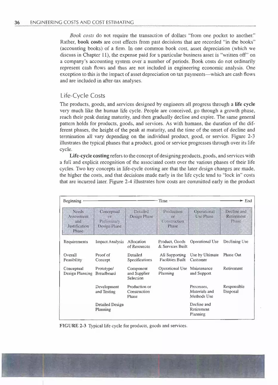
36 ENGINEERING COSTS AND COST ESTIMATING
Book costs do not require the transaction of dollars "from one pocket to another."Rather, book costs are cost effects from past decisions that are recorded "in the books"(accounting books) of a firm. In one common book cost, asset depreciation (which wediscuss in Chapter 11), the expense paid for a particular business asset is "written off" ona company's accounting sy'stemover a number of periods. Book costs do not ordinarilyrepresent cash flows and thus are not included in engineering economic analysis. Oneexception to this is the impact of asset depreciation on tax payments-which are cash flowsand are included in after-tax analyses.
Life-Cycle Costs .
The products, goods, and services designed by engineers all progress through a life cyclevery much like the human life cycle. People are conceived, go through a growth phase,reach their peak during maturity, and then gradually decline and expire. The same generalpattern holds for products, goods, and services. As with humans, the duration of the dif-ferent phases, the height of the peak at maturity, and the time of the onset of decline andtermination all vary depending on the individual product, good, or service. Figure 2-3illustrates the typical phases that a product, good or service progresses through over its lifecycle.
Life-cycle costing refers to the concept of designingproducts, goods, and services witha full and explicit recognition of the associated costs over the various phases of their lifecycles. Two key concepts in life-cycle costing are that the later design changes are made,the higher the costs, and that decisions made early in the life cycle tend to "lock in" coststhat are incurred later. Figure 2-4 illustrates how costs are committed early in the product
FIGURE 2-3 Typical life cycle for products, goods and services.
~~ I
~. 1~:~~~~~.',~~.~.;~~~~~~~.~;~~~~ c;-=-..:+",~~",,~.,.1""<'~~;~&'~.ii~ -;:-j~~.;~~;':.i._"~y;:g,;,j;'~~"'"-!Jj"~:"L~::;;'-'
Beginning Time ) End
."'. ."'-
Needs COJ;lceptual Detailed QperalioniJ,l Decline andAS$eSsment or r>e$igJ:lEhase or U§eEhase Retirement
and PreXimjI)ary Constnicti!:m PhaseJustification DeSign Ehase Phase
Phe..,,-
Requirements Impact Analysis Allocation Product, Goods Operational Use Declining Useof Resources & Services Built
Overall Proof of Detailed All Supporting Use by Ultimate Phase OutFeasibility Concept Specifications Facilities Built Customer
Conceptual Prototype/ Component Operational Use Maintenance RetirementDesign Planning Breadboard and Supplier 'Planning and Support
Selection
Development Production or Processes, Responsibleand Testing Construction Materials and Disposal
Phase Methods Use
Detailed Design Decline andPlanning Retirement
Planning
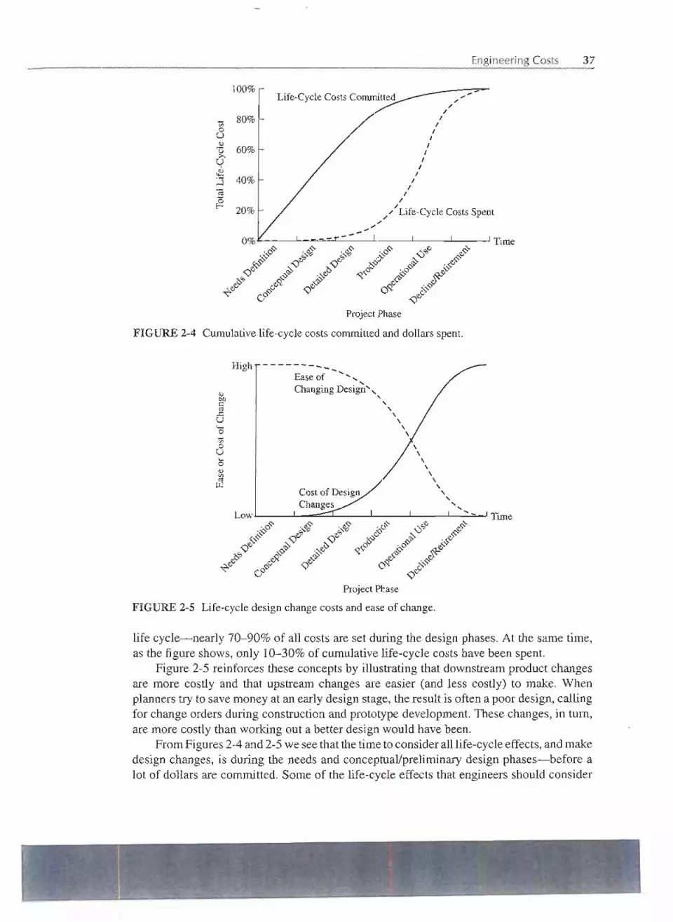
Engineering Costs 37
100%
... 80%CI)oUII)
"0>.U
I
~;.::s
'5~
60%
40%
20%
JTime
Project Phase
FIGURE 2-4 Cumulativelife-cycle costs committedand dollars spent.
High --------... ......Ease of .........Changing Design', , ,,,,,,
II)b/)!::o:s
..r::U'+-<o
Time
...CI)o
U...oII)CI)o:s
~
Project Phase
FIGURE 2-5 Life-cycle design change costs and ease of change.
life cycle-nearly 70-90% of all costs are set during the design phases. At the same time,as the figure shows, only 10-30% of cumulative life-cycle costs have been spent.
Figure 2-5 reinforces these concepts by illustrating that downstream product changes'are more costly and that upstream changes are easier (and less costly) to make. Whenplanners try to save money at an early design stage, the result is often a poor design, callingfor change orders during construction and prototype development. These changes, in turn,are more costly than working out a better design would have been.
From Figures2-4 and 2-5 we seethat the time to consider all life-cycleeffects, and makedesign changes, is during the needs and conceptual/preliminary design phases-before alot of dollars are committed. Some of the life-cycle effects that engineers should consider
t '~ I,Ir.., ..J~~~;1;.~~:;;.~ti_-.,~~.-/,,,i,.;i'h.,;; :;~:£~Ji ,",,.;L: _}.i,,,,..~~,::ji,,,,.c_-,;i;,.;.,,,.-;::;;,:;,.::;...< ."I;j:""3,~.,;,;i~

38 ENGINEERINGCOSTSAND COST ESTIMATING
at design time include product costs for liability, production, material, testing and qualityassurance, and maintenance and warranty. Other life-cycle effects include product featuresbased on customer input and product disposal effects on the environment. The key point isthat engineers who design products and the systems that produce them should consider alllife-cycle costs. . ..
COST ESTIMATING
Engineering economic analysis focuses on the future consequences of current decisions.Because these consequences are in the future, usually they must be estimated and cannotbe known with certainty. Examples of the estimates that may be needed in engineeringeconomic analysis includepurchase costs, annualreven.ue,yearly maintenance, interestratesfor investments, annual labor and insurance costs, equipment salvage values, and tax rates.
Estimating is the foundation of economic analysis. As is the case in any analysisprocedure, the outcome is only as good as the quality of the numbers used to reach thedecision. For example, a person who wants to estimate her federal income taxes for a givenyear could do a very detailed analysis, including social security deductions, retirementsavings deductions, itemized personal deductions, exemption calculations, and estimatesoflikely changes to the tax code. However, this very technical and detailed analysis will begrossly inaccurate if poor data are used to predict the next year's income. Thus, to ensure thatan analysis is a reasonable evaluation of future events, it is very important to make carefulestimates.
Types of EstimateThe American poet and novelist Gertrude Stein wrote in The Making of Americans in 1925that "a rose is a rose is a rose is a rose." However,what holds for roses does not necessarilyhold for estimates because "an estimate is not an estimate." Ms. Stein was not suggestingthat all roses are the same, but it is true that all estimates are not the same. Rather, we candefine three general types of estimate whose purposes, accuracies, and underlying methodsare quite different.
Rough estimates: Order-of-magnitude estimates used for high-level planning, fordetermining macrofeasibility, and in a project's initial planning and evaluationphases. Rough estimates tend to involve back-of-the-envelope numbers with littledetail or accuracy. The intent is to quantify and consider the order of magnitudeof the numbers involved. These estimates require minimum resources to develop,and their accuracy is generally -30% to +60%.
Notice the nonsymmetry in the estimating error. This is because decision makerstend to underestimate the magnitude of costs (negative economic effects). Also asMurphy's law predicts, there seem to be more ways for results to be worse thanexpected than there are for the results to be better than expected.
Semidetailed estimates: Used for budgeting purposes at a project's conceptual or pre-liminary design stages. These estimates are more detailed, and they require addi-tional time and resources to develop. Greater sophistication is used in developing
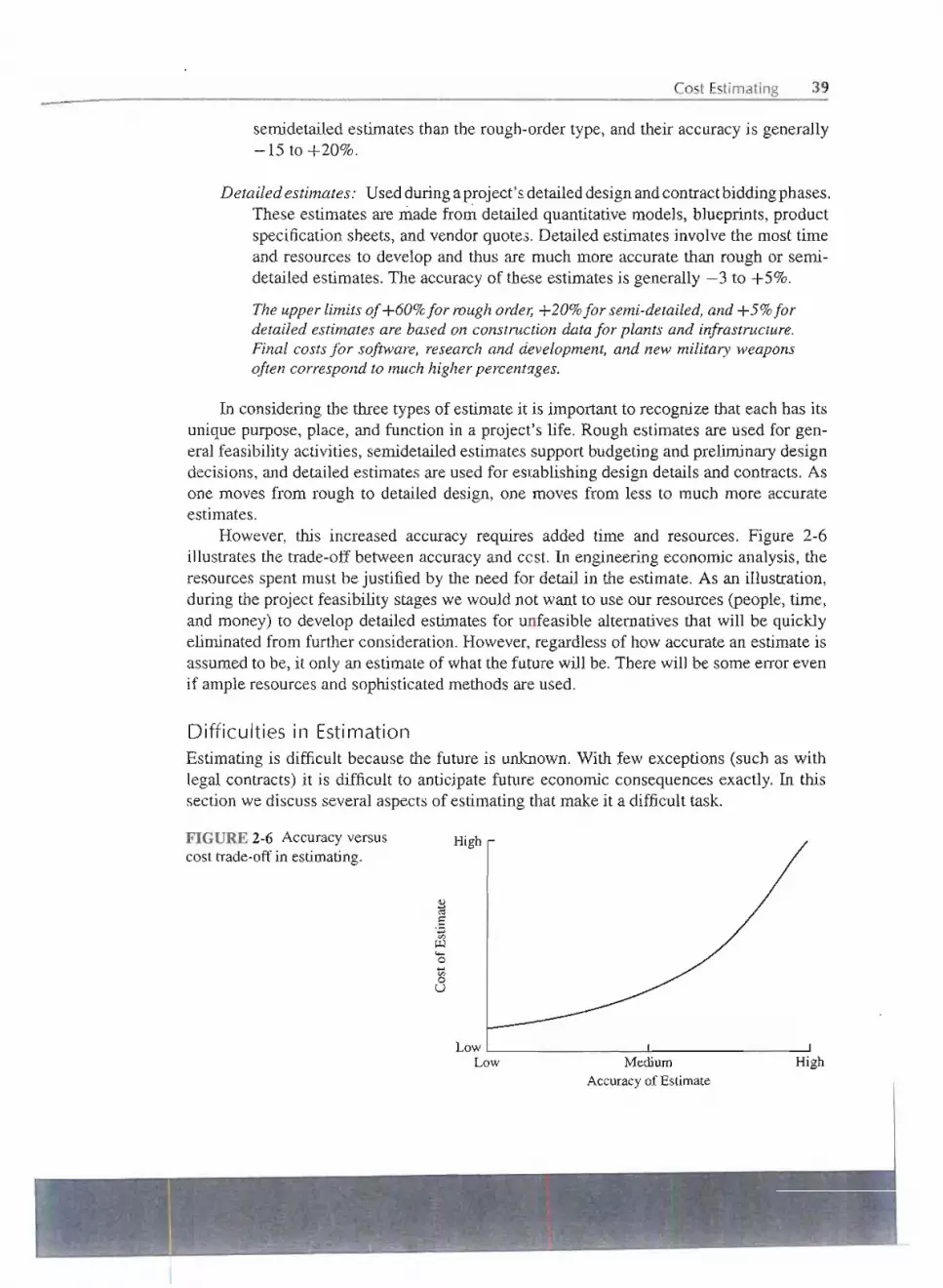
Cost Estimating 39
semidetailed estimates than the rough-order type, and their accuracy is generally-15 to +20%.
Detailed estimates: Usedduringap!oject' sdetailed designandcontractbiddingphases.These estimates are made from detailed quantitative models, blueprints, productspecification sheets, and vendor quotes. Detailed estimates involve the most timeand resources to develop and thus are much more accurate than rough or semi-detailed estimates. The accuracy of these estimates is generally -3 to +5%.
The upper limits of +60%for rough order, +20%for semi-detailed, and +5%fordetailed estimates are based on construction data for plants and infrastructure.Final costs for software, research and development, and new military weaponsoften correspond to much higher percentages.
In considering the three types of estimate it is important to recognize that each has itsunique purpose, place, and function in a project's life. Rough estimates are used for gen-eral feasibility activities, semidetailed estimates support budgeting and preliminary designdecisions, and detailed estimates are used for establishing design details and contracts. Asone moves from rough to detailed design, one moves from less to much more accurateestimates.
However, this increased accuracy requires added time and resources. Figure 2-6illustrates the trade-off between accuracy and cost. In engineering economic analysis, theresources spent must be justified by the need for detail in the estimate. As an illustration,during the project feasibility stages we would not want to use our resources (people, time,and money) to develop detailed estimates for unfeasible alternatives that will be quicklyeliminated from further consideration. However, regardless of how accurate an estimate isassumed to be, it only an estimate of what the future will be. There will be some error evenif ample resources and sophisticated methods are used.
Difficulties in Estimation
Estimating is difficult because the future is unknown. With few exceptions (such as withlegal contracts) it is difficult to anticipate future economic consequences exactly. In thissection we discuss several aspects of estimating that make it a difficult task.
FIGURE 2-6 Accuracy versus Highcost trade-off in estimating.
~e.,::1'"~....o....'"oU
LowLow Medium
Accuracy of Estimate
High
~. I
i(.
\~.
.'.
"
~-
~:_};,_ ':'_~~' ~-;*.;k~~~~,~~i,-.-,,~, ".:;.;.__ ..~ --."_..'.. .ijj

40 ENGINEERING COSTSAND COST ESTIMATING
One-of-a-Kind Estimates
Estimated parameters can be for one-of-a-kind or first-runprojects. The first time somethingis done, it is difficult to estimate costs required to design, produce, and maintain a productover its life cycle. Conside~the. prqjec.tedcost estimates that were developed for the firstNASA missions. The U.S. space program initially had no experience with human flight inouter space; thus the development of the cost estimates for design, production, launch, andrecovery of the astronauts, flight hardware, and payloads was a "first-time experience."Thesame is true for any endeavor lacking local or global historical cost data. New products orprocesses that are unique and fundamentally different make estimating costs difficult.
The good news is that there are very few one-of-a-kind estimates to be made in en-gineering design and analysis. Nearly all new technologies, products, and processes have"close cousins" that have led to their development. The concept of estimation by analogyallows one to use knowledge about well-understood activities to anticipate costs for newactivities. In the 1950s, at the start of the military missile program, aircraft companies drewon their in-depth knowledge of designing and producing aircraft when they bid on missilecontracts. As another example, consider the problem of estimating the production laborrequirements for a brand new product, X. A company may use its labor knowledge aboutProduct Y, a similar type product, to build up the estimate for X. Thus, although "first-run"estimates are difficult to make, estimation by analogy can be an effective tool.
Time and Effort Available
Our ability to develop engineering estimates is constrained by time and person-poweravailability. In an ideal world, it would cost nothing to use unlimited resources over anextended period of time. However, reality requires the use of limited resources in fixedintervals of time. Thus for a rough estimate only limited effort is used.
Constraints on time and person-power can make the overall estimating task moredifficult. If the estimate does not require as much detail (such as when a rough estimate isthe goal), then time and personnel constraints may not be a factor.When detail is necessaryand critical (such as in legal contracts), however, requirements must be anticipated andresource use planned.
Estimator ExpertiseConsider two common phrases: The past is our greatest teacher and knowledge is power.These simple axioms hold true for much of what we encounter during life, and they are truein engineeringestimating as well. The more experiencedandknowledgeable the engineeringestimator is, the less difficult the estimating process will be, the more accurate the estimatewill be, the less likely it is that a major error will occur, and the more likely it is th~t theestimate will be of high quality.
How is experience acquired in industry? One approach is to assign inexperiencedengineers relatively smallerjobs, to create expertise and build familiarity with products andprocesses. Another strategy used is to pair inexperienced engineers with mentors who havevast technical experience. Technical boards and review meetings conducted to ''justify thenumbers" also are used to build knowledge and experience. Finally, many firms maintaindatabases of their past estimates and the costs that were actually incurred.

Estimating Models 41
ESTIMATING MODELS
This section develops several estimating models that can be used at the rough, semidetailed,or detailed design levels. For rough estimates the models are used with rough data, likewisefor detaileddesign estimates they-areused-withdetailed data. The level of detail will dependupon the accuracy of the model's data.
Per-Unit Model
The per-unit model uses a "per unit" factor, such as cost per square foot, to develop theestimate desired. This is a very simplistic yet useful technique, especially for developingestimates of the rough or order-of-magnitude type. The per unit model is commonly usedin the construction industry. As an example, you may be interested in a new home that isconstructed with a certain type of material andhas a specificconstruction style.Based on thisinformation a contractor may quote a cost of $65 per square foot for your home. If you areinterested in a 2000 square foot floorplan, your cost would thus be: 2000 x 65 = $130,000.Other examples where per unit factors are utilized include
· Service cost per customer· Safety cost per employee· Gasoline cost per mile· Cost of defects per batch· Maintenance cost per window· Mileage cost per vehicle· Utility cost per square foot of floor space· Housing cost per student
It is important to note that the per-unit model does not make allowances for economiesof scale (the fact that higher quantities usually cost less on a per-unit basis). In most cases,however, the model can be effective at getting the decision maker "in the ballpark" of likelycosts, and it can be very accurate if accurate data are used.
Use the per-unit model to estimate the cost per student that you will incur for hosting 24 foreignexchange students at a local island campground for 10 days. During camp you are planning thefollowing activities:
· 2 days of canoeing· 3 campsite-sponsored day hikes· 3 days at the lake beach (swimming, volleyball, etc.)· Nightly entertainment
After calling the campground and collecting other information, you have accumulated the follow-ing data:
· Vanrental from your city to the camp (one way) is $50 per 15 person van plus gas.· Camp is 50 miles away, the van gets 10 miles per gallon, and gas is $1 per gallon.- - -.... -
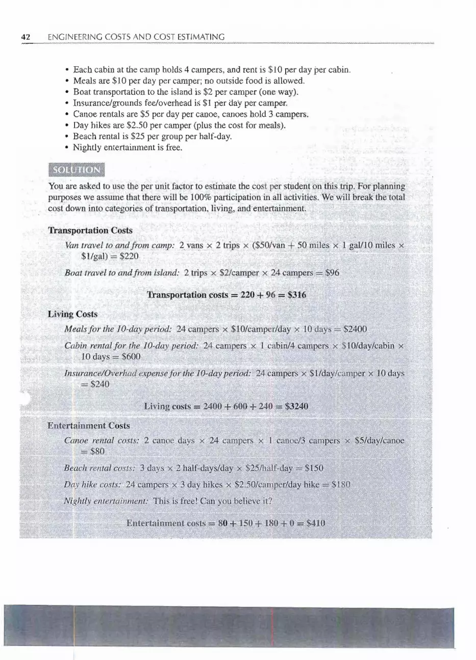
42 ENGINEERING COSTSAND COST ESTIMATING
· Each cabin at the camp holds 4 campers, and rent is $10 per day per cabin.·Meals are $10 per day per camper; no outside food is allowed.· Boat transportation to the island is $2 per camper (one way).· Insurance/grounds fee/overhead is $fpetday.per camper.· Canoe rentals are $5 per day per canoe, canoes hold 3 campers.· Day hikes are $2.50 per camper (plus the cost for meals).· Beach rental is $25 per group per half-day.· Nightly entertainment is free.
You are asked to use the per unit factpr to estimate the cosfperstudent ontJ:1istrip. Forplanningpurppses we assume that there will be 100% participation in all actiyities.We will break the totalcost down into categories of transportation, living, and entertainment.
ill'
Transportation Costs
Vantravel to andfrom,camp: 2 vans x :2trips x ($50/van + 50 ]:Iplesx 1 gal/lOmiles x ~ ",".
$lIgal) =$220 .; ~.~,~ ;; ~~ :::;' ::;: ;; :;=
Boat travelto andfrom island: 2 trips...x$2lcamperx 24 c~pers .$96
Transportation costs =~20+ 96 =-$316
Living Costs
Mealsfor the lO-dayperiod: 24 campers x $10/cainper/day x 10 days $2400
Cabin rentalfor the lO-day period.~24 campers x 1. capinl4 carIlperSx$10/day/cabin. x10 days-.$600
lnsurance/Overhad expensefor the lO-dtiyperiod: 24 campers x $1/day/ca1DJ>erx 10 days= $240
Living costs =2400 +.600+ 240 =.$.~Z40-Entertfiinment Costs
Canoe rental costs:' 2 canoe days x 24calllpeJ,"s xf canoe/3 c~per$ x$5/day/canoe_ __ ~_=j8Q_ ~ _ + _ _ _ _ ""- _-- ." .., - "'" ... "'" r:C- __ _,_i:~:;:': _;; r~"-- v ,;-,:~=- =~::J ~~
Beach rental costs: 3 days)( 2 ha.lf-days/dayx$25!b;iU'.,day..l$150
Day hike costs: .24campers x3 dayl1jJ.(e$x$2.50/C;iIp.per/dayhilte ...$18Q
Nightly entertainment: This is free! Can you believe it?
'"_.~_.- --
F -~...
.. ..
h;,..~;_:. ii~~~_-:~.i{~=~J;;;~~':"~-;:;i::~;~;{jL_'''''-''''''''''''''~~_~£+~~;~4i~,.~~~~

--..--.--
Estimating Models 43
Total cost
Total cost for 10-day period = Transportation co,s!s+ Living costs + Entertainment costs
= 316 + 3240 + 410 __ $3966
Thus, the cost per student would be $3966/24 = $165.25.Thus, it would cost you $165.25 per student to host the students at theisland campground for
the lO-dayperiod. In this case the per-urtitmodel gives you a very detailed cost estimate (althoughits accuracy depends on the accuracy of your data and assumptions you've made).
Segmenti ng ModelThe segmenting model can be described as "divide and conquer." An estimate is decom-posed into its individual components, estimates are made at those lower levels, and then theestimates are aggregated (added) back together. It is much easier to estimate at the lowerlevels because they are more readily understood. This approach is common in engineer-ing estimating in many applications and for any level of accuracy needed. In planning thecamp trip of Example 2-5, the overall estimate was segmented into the costs for travel,living, and entertainment. The example illustrated the segmenting model (division of theoverall estimate into the various categories) together with the unit factor model to make thesubestimates for each category. Example 2-6 provides another example of the segmentingapproach.
Clean Lawn Corp. a manufacturer of yard equipment is planning to introduce a new high-endindustrial-use lawn mower called the Grass Grabber. The Grass Grabber is designed as a walk-behind self-propelled mower. Clean Lawn engineers have been asked by the accounting depart'-ment to estimate the material costs that will make up the new mower. The material cost estimatewill be used, along with estimates for labor and overhead to evaluate the potential of this newmodel.
:-..;..~ '--t~--t-:'SOLUTIO~~
. " . . ~-- '-.-'-.--:, -.' .., .' .;,-I' '.-'; ;:. .'.'~
:
The engineers decide to decompose the design specifications for the GraSs Grabber into itssubcomponents, estimate the material costs for each of the subcomponents, and then sum thesecosts up tQobtain their overall estimate. The engineers are using a segmenting approach to buildup their estimate. Mter careful consideration; the engineers have divided the mower into the"following$ajoHmbsystems: chassis, drive tram~'controls,'andcutting/coUectionsystem. Each ofthese isfqrther divided as appropriate, and unjt material costs were estimated at this lowest of
- ~ - .. - - .--- -- -- - - - --.
, 1
\"
11;:.; -. ; : ~~ ~._;,...).s_~.~_~_.-~~~)-- ~ -":" ~ - --=-,~ .::;;
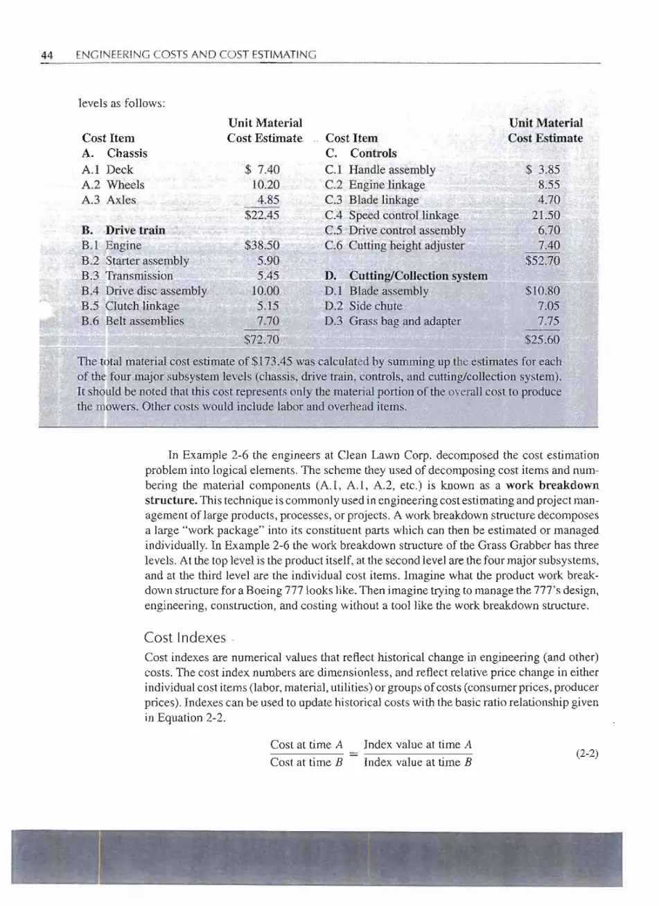
44 ENGINEERINGCOSTSAND COST ESTIMATING
levels as follows:
Cost ItemA. ChassisA.I DeckA.2 WheelsA.3 Axles
Unit MaterialCost Estimate
$ 7.40.10.20.4.85
$22.45B. Drive train
B.I EngineB.2 Starter assemblyB.3 TransmissionB.4 ;Drivedisc assemblyB.5 Clutch linkageB.6 ;Beltassemblies
$38.50.5.90.5.45
10.0.0.5.157.70.
$72:70.
Cost ItemC. Controls
C.1 Handle assemblyC.2 Engine linkageC.3 Blade linkageC.4 Speed control linkageC05 Drive control assemblyC.6 Cutting height adjuster
Unit MaterialCost Estimate
$ 3.858.554.70.
21.50.6.70..7.40.
$52.70.D. Cutti!lglCollection systemD.1 Blade assemblyD.2 Side chute
D.3 Grass bag and adapter
$10.80.7.0.57.75
$25.60.
The tOtalmaterial cost estimate of $173.45 was calculated by summing up theestimates for eachof the four major subsystem levels (chassis, drive train, controls, and cuttinglcollection system).It should be noted that this cost represents only the material portion of the overall cost to producethe mowers. Other costs would include labor and overhead items.
~. - '-~--'~-'~..~ --.
In Example 2-6 the engineers at Clean Lawn Corp. decomposed the cost estimationproblem into logical elements. The scheme they used of decomposing cost items and num-bering the material components (A.I, A.I, A.2, etc.) is known as a work breakdownstructure. This technique is commonlyused in engineeringcostesti(llatingandproject man-agement of largeproducts, processes, or projects. A work breakdownstructure decomposesa large "work package" into its constituent parts which can then be estimated or managedindividually. In Example 2-6 the work breakdown structure of the Grass Grabber has threelevels. At the top level is the product itself, at the second level are the four major subsystems,and at the third level are the individual cost items. Imagine what the product work break-down structure for a Boeing 777 looks like. Then imagine trying to manage the 777's design,engineering, construction, and costing without a tool like the work breakdown structure.
Cost Indexes .
Cost indexes are numerical values that reflect historical change in engineering (and other)costs. The cost index numbers are dimensionless, and reflect relativeprice change in either.individualcost items (labor,material, utilities) or groupsof costs (consumerprices,producerprices). Indexes can be used to update historical costs with the basic ratio relationship givenin Equation 2-2.
Cost at time A Index value at time A
Cost at time B Index value at time B(2-2)
,.
)
~.,1.-~
~> . + .."K:' - . . ~. . .'. ~'. - -. ..' .."
~..: .~'. '".',~~~.it~.iC..,,~~.~~;.~t~.~." ~.~~~~~c~._.4~.j,;~"",~ d~ :...:;;;:.:~'" . ,;c..;.:i~&;.:Ji.~:(<!f~:;"~

Estimating Models 45
Equation 2-2 states that the ratio of the cost index numbers at two points in time (Aand B) is equivalent to the dollar cost ratio of the item at the same times (see Example 2-7).
Miriam isinterested in estimating the annuallabQrandmaterialcosts for a new production facility.She was able to obtain the following labor and material cost data:
Labor costs
· Lapor cost index value was at 124 ten years ago and is 188 today.·Annual labor costs for a similarfacility were $575,500 ten years ago.
Material Costs
·Material cost index value was at 544 three years ago and is 715 today.·AJ;:inualmaterialcosts for a similar facility were $2,455,OPQthJ;eeyears ago.
-- ~ ,'J!i!- .... .. _. .. : h ,-,..
Miriam will use Equation 2,.2to develop her cost estimat~s for;annual.labor and material costs.
Labor
"Annual cost today _ Index value today
Annual cost 10 years ago Index value 10 years ago
188 .
Annual cost today 124 x $575,500 $871,800II
lv.{aterial~
..
Annual cost today Index value today
Annual cost 3 years ago - Index value 3 years ago
715 . J=:;;;; ;; ..~11lWJll C.Qst..!op~y';_521-~~J,#~.,2,PQO.-:=...$3,221,-..OOO :;;~ 4 ='=... =;:;:;;;:= - - :;;:: ..:::!:!J:
"
Cost index data are collected and published by several private and public sources inthe United States (and world). The U.S. government publishes data through the Bureau ofLabor Statistics of the Department of Commerce. The Statistical Abstract of the United-States publishes cost indexes for labor, construction, and materials. Another useful sourcefor engineering cost index data is the Engineering News Record.
Power-Sizing ModelThe power-sizingmodel is usedto estimatethe costsof industrialplantsand equipment.Themodel"scalesup"or "scalesdown"knowncosts,therebyaccountingforeconomiesof

- - ---- -_.- - .- - - ---
46 ENGINEERING COSTS AND COST ESTIMATING
scale that are common in industrial plant and equipment costs. Consider the cost to build arefinery.Would it cost twice as much to build the samefacility with double the capacity? It isunlikely. The power-sizing model uses the exponent (x), called the power-sizing exponent,to reflect economies of scale in the size or capacity:
Cost of equipment A (Size(capacity) of equipment A)x
= (2-3)Cost of equipment B Size(capacity) of B
where x is the power-sizing exponent, costs of A and B are at the same point in time (samedollar basis), and size or capacity is in the same physical units for both A and B.'
The power-sizing exponent (x) can be 1.0(indicating a linear cost-versus-size/capacityrelationship) or greater than 1.0 (indicating diseconomies of scale), but it is usually lessthan 1.0 (indicating economies of scale). Generally the ratio should be less than 2, and itshould never exceed 5.This model works best in a "middle" range-not very small or verylarge size.
Exponent values for plants and equipment of many types may be found in severalsources, including industry reference books, research reports, and technical journals. Suchexponent values may be found in Perry's Chemical Engineers' Handbook, Plant Designand Economics for Chemical Engineers, and Preliminary Plant Design in ChemicalEngineering. Table 2-1 gives power sizing exponent values for several types of industrialfacilities and equipment. The exponent given applies only to equipment within the sizerange specified.
In Equation 2-3 equipment costs for both A and B occur at the same point in time. Thisequation is useful for scaling equipment costs but not for updating those costs. When thetime of the desired cost estimate is different from the time in which the scaling occurs (perEquation 2-3) cost indexes accomplish the time updating. Thus, in cases like Example 2-8involving both scaling and updating, we use the power sizing model together with.costindexes.
TABLE2-1 Example Power-Sizing Exponent Values
Equipment/Facility
Blower, centrifugalCompressorCrystallizer, vacuum batchDryer, drum, single atmosphericFan, centrifugalFilter, vacuum rotary drumLagoon, aeratedMotor
Reactor, 300 psiTank, atmospheric, horizontal
Size RangePower-Sizing
Exponent
10,000-100,000 ft3fmin
200-2100 hp500-7000 ft210-100 ft220,000-70,000 ft2fmin10-1500 ft2
0.05-20 million gal/day5-20 hp100-1000 gal100-40,000 gal
0.590.320.370.401.170.481.130.690.560.57

Estimating Models 47
Based on her work in Example 2-7, Miriam has been asked to estimate the cost today of a 25.0.0ft2heat exchange system for the new plant being-analyzed.'She has the following data.
· Her company paid $5.0,.0.0.0for a 10.0.0ft2 heat exchanger 5 years ago.· Heat exchangers within this range of capacity have a power sizing exponent (x) of .0.55.· Five years ago the Heat Exchanger Cost Index (HECI) was 13.06;it is 1487 today.
mmJ:imIMiriam will first use Equation 2-3 to scale up the cost of the 10.0.0ft2 exchanger to one that is25.0.0ft2using the .0.55power-sizing exponent.
Cost of 25.0.0ft2 equipment (25.0.0ft2 equipment )0.55
Cost of 10.0.0ft2 equipment - 1.0.0.0ft2 equipIIlent
(25.0.0
)0.55
Cost of 25.0.0ft2 equipment - ~ x 5.0,.0.0.0= $82,8.0.010.0.0
Miriam knows that the $82,8.0.0reflects only the scaling up of the cost of the 10.0.0ft2 modelto a 25.0.0ft2 model. Now she will use Equation 2-2 and the HECI data to estimate the cost of a25.0.0ft2 exchanger today. Miriam's cost esti)]late would be:
Equipment cost today _Index value todayEquipment cost 5 years ago - Index Value5 years ago
1487
Equipment cost today = 13.06 x $82,8.0.0 '-0..$94,3.0.0
Triangulation
Triangulationis used in engineering surveying. A geographicalarea is divided into trianglesfrom which the surveyor is able to map points within that region by using three fixedpoints and horizontal angular distances to locate fixed points of interest (e.g., property linereferencepoints). Since any point can be located with two lines, the third line represents anextra perspective and check. We will not use trigonometry to arrive at our cost estimates,but we can utilize the concept of triangulation. We should approach our economic estimatefrom differentperspectives because such varied perspectives add richness, confidence, andquality to the estimate. Triangulation in cost estimating might involve using differentsourcesof data or using different quantitative models to arrive at the value being estimated.As decisionmakers we should always seek out varied perspectives.
Improvement and the Learning CurveOne commonphenomenon observed, regardless of the task being performed, is that as thenumberof repetitions increases, performance becomes faster andmore accurate. This is the
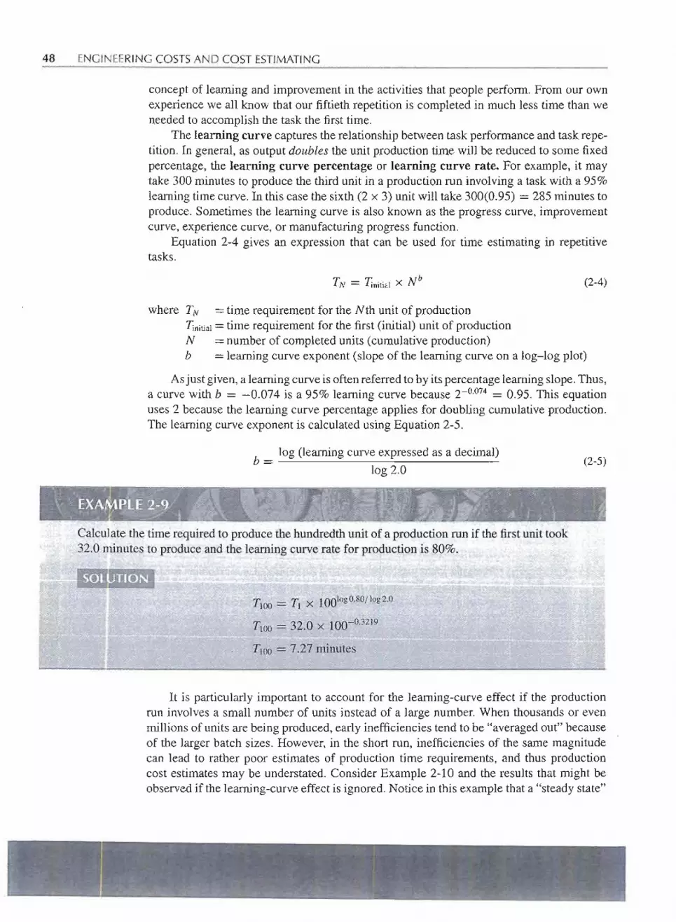
..- - .- --. -.. - -- .-
48 ENGINEERING COSTSAND COST ESTIMATING
conceptof learningandimprovementin theactivitiesthatpeopleperfonn.Fromour ownexperienceweall knowthatour fiftiethrepetitionis completedin muchlesstimethan weneededto accomplishthe taskthe firsttime.
The learning curve captures the relationship between task perfonnance and task repe-tition. In general. as output doubles the-unit production time will be reduced to some fixedpercentage. the learning curve percentage or learning curve rate. For example. it maytake 300 minutes to produce the third unit in a production run involving a task with a 95%learning time curve. In this case the sixth (2 x 3) unit will take 300(0.95) = 285 minutes toproduce. Sometimes the learning curve is also known as the progress curve. improvementcurve. experience curve. or manufacturing progress function.
Equation2-4 givesan expressionthat can be used for time estimatingin repetitivetasks.
(2-4)
where TN =time requirement for the Nth unit of productionTinitial= time requirement for the first (initial) unit of productionN =number of completed units (cumulative production)b = learning curve exponent (slope of the learning curve on a log-log plot)
Asjust given.a learning curve is oftenreferred to by itspercentage.learningslope.Thus.a curve with b = -0.074 is a 95% learning curve because 2-0.074 = 0.95. This equationuses 2 because the learning curve percentage applies for doubling cumulative production.The learning curve exponent is calculated using Equation 2-5.
b = log (learning curve expressed as a decimal)log 2.0
(2-5)
Calculate the time required to produce the hundredth unit of a production run if the first unit took32.0 minutes to produce and the learning curve rate for production is 80%.
!"" "' -,.,," "-,:,,,,",'-'
-SOL UTlp~+
Two = T1 X 100Iog0.80/log2.0
Two = 32.0 X 100-0.3219..
Two = 7.27 minutes'"
It is particularly important to account for the learning-curve effect if the productionrun involves a small number of units instead of a large number. When thousands or evenmillions of units are being produced. early inefficiencies tend to be "averaged out" becauseof the larger batch sizes. However. in the short run. inefficiencies of the same magnitudecan lead to rather poor estimates of production time requirements. and thus productioncost estimatesmay be understated.ConsiderExample2-10 and the resultsthat mightbeobservedif thelearning-curveeffectis ignored.Noticein thisexamplethata "steadystate"
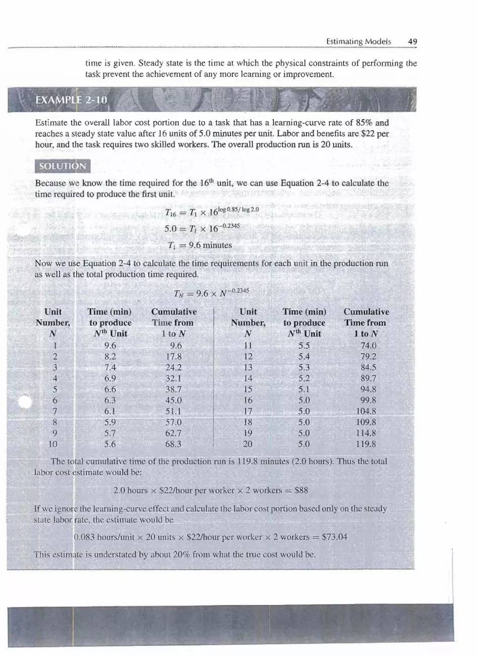
Estimating Models 49
time is given. Steady state is the time at which the physical constraints of performing thetask prevent the achievement of any more learning or improvement.
Estimate the overall labor cost portion due to a task that has a learning-curve rate of 85% andreaches a steady state value after 16units of 5.0 minutes per unit. Labor and benefits are $22 perhour, and the task requires two skilled workers. The overall production run is 20 units.
SOlUTlQN
Because we know the time required for the 16thunit, we can use Equation 2-4 to calculate thetime required to produce the first unit.
Tl6 = Tl X 16Iog0.85/log2.0
5.0 = TI X 16-0.2345
TI - 9.6 minutes;;
Now we use Equation 2-4 to calculate the time requirements for each unit in the production runas well as the total production time required.
=The foral ctTmulativetime oftKe proctuctioniim is~119.8minutes (2.01ours). Thus the totallabor cost'~stimate would be:,<
2.0 hours x $22/hour per worker x 2 workers = $88
If we ignot~ the learning-cu~v~effect and c~cul'!t~the lilQprcost portion based only,on tbe steadystatelabotH:ate,tbe estip.1atewould be
0.083 hours/unit x 20 units x $22/hour per worker x 2 workers = $73.04
. This estiIIl'£lteis understated by about 20% from what the true cost would be.IL
I
I
, . -. -~ ,s:~~~~Jjc"",~~~~-~ ~?..J:~~~i-i:~~':';:_~~;"'-"'~-:"'~£;~i..i'i:';~~~j.~.'~;.,.~-. ~.'- ::-.~- __000._- .~~~
TN = 9.6 X N-0.2345,
Unit Time (min) Cumulative Unit Time (min) CumulativeNumber, to produce Time from Number, to produce Time from
N Nth Unit ltoN N Nth Unit ltoN1 9.6 9.6 11 5.5 74.02 8.2 17.8 12 5.4 79.23 7.4 24.2 13 5.3 84.54 6.9 32.1 14 5.2 89.75 6.6 38.7 15 5.1 94.86 6.3 45.0 16 5.0 99.87 6.1 51.1 17 50 lQ1.8" ;:= ;;
'8':;
5'.9 57.0:;;;:
18 5.0 109.89 5.7 62.7 19 5.0 114.8
10 5.6 68.3 20 5.0 119.8
-.- - -_.__A._.-_.
50 ENGINEERING COSTSAND COST ESTIMATING
ESTIMATING BENEFITS
This chapter has focused on cost tenns and cost estimating. However, engineeringeconomists must often also estimate benefits. Example benefits include sales of products,revenues from bridge tolls--and-electricpower sales, cost reductions from reduced mate-rial or labor costs, reduced time spent in trafficjams, and reduced risk of flooding. Manyengineering projects are undertaken precisely to secure these benefits.
The cost concepts and cost estimating models can also be applied to economic benefits.Fixed and variable benefits, recurring and nonrecurring benefits, incremental benefits, andlife-cycle benefits all have meaning. Also, issues regarding the type of estimate (rough,semidetailed, and detailed) as well as difficulties in estimation (one of a kind, time andeffort, and estimator expertise) all apply directly to estimating benefits. Last, per unit,segmented, and indexed models are used to estimate benefits. The concept of triangulationis particularly important for estimating benefits.
The uncertainty in benefit estimates is also typically asymmetric, with a broader limitfor negative outcomes. Benefits are more likely to be overestimated than underestimated,so an example set of limits might be (-50%, +20%). One difference between cost andbenefit estimation is that many costs of engineering projects occur in the near future (fordesign and construction),but the benefitsare further in the future.Because benefitsare oftenfurther in the future, they are more difficult to estimate accurately, and more uncertainty istypical.
The estimation of economic benefits for inclusion in our analysis is an important stepthat should not be overlooked. Many of the models, concepts, and issues that apply in theestimation of costs also apply in the estimation of economic benefits.
CASH FLOW DIAGRAMS
The costs andbenefitsof engineeringprojects occur over time and are summarized on a cashflow diagram (CFD). Specifically,a CFD illustrates the size, sign, and timing of individualcash flows. In this way the CFD is the basis for engineering economic analysis.
A cash flow diagram is created by first drawing a segmented time-based horizontalline, divided into appropriate time units. The time units on the CFD can be years, months,quarters, or any other consistent time unit. Then at each time at which a cash flow willoccur, a vertical arrow is added-pointing down for costs and up for revenues or benefits.These cash flows are drawn to relative scale.
The cash flows are assumed to occur at time 0 or at the end of each period. ConsiderFigure 2-7, the ~FD for a specific investment opportunity whose cash flows are describedas follows:
Timing of Cash FlowAt time zero (now or today)1 time period from today2 time periods from today3 time periods from today4 time periods from today5 time periods from today
Size of Cash Flow
A positive cash flow of $100A negative cash flow of $100A positive cash flow of $100A negative cash flow of $150A negative cash flow of $150A positive cash flow of $50
r.~':.
t". ~~2i~~~j~;;t~i;-i.¥b~~...~.c.~-;,;'::~~-;;-';'.L:_,-i'."';~":::~~",;,~~i;.,.iJ--,-i~,;,:~. ."-,-.-_..~;:c'_,.;;-;;;s;c~

FIGURE 2-7 An example cash flowdiagram (CFD).
(+)
+(-)
$100 $100 ~nd of Period 2
tD~":~~ 1
i
IS also Beginning
~ of Period 3. $50
/0-1-2-3-4-JTime0 !
j j("today") $100$150 $150
Categories of Cash FlowsThe expenses and receipts due to engineering projects usually fall into one of the followingcategories.
First cost = expense to build or to buy and install
Operations and maintenance (O&M) = annual expense, such as electricity, labor, andminor repairs
Salvage value = receipt at project termination for saleor transfer of the equipment (canbe a salvage cost)
Revenues = annual receipts due to sale of products or services
Overhaul = major capital expenditure that occurs during the asset's life
Individual projects will often have specific costs, revenues, or user benefits. For ex-ample, annual operations and maintenance (O&M) expenses on an assembly line might bedivided into direct labor, power, and other. Similarly, a public-sector dam project mighthave its annual benefits divided into flood control, agricultural irrigation, and recreation.
Drawing a Cash Flow DiagramThe cash flow diagram shows when all cash flows occur. Look at Figure 2-7 and the $100positive cash flow at the end of period 2. From the time line one can see that this cash flowcan also be described as occurring at the beginning of period 3. Thus, in a CFD the endof period t is the saI}letime as the beginning of period t + 1. Beginning-of-period cashflows (such as rent, lease, and insurance payments) are thus easy to handle: just draw yourCFD and put them in where they occur. Thus O&M, salvages, revenues, and overhauls areassumed to be end-of-period cash flows.
The choice of time 0 is arbitrary. For example, it can be when a project is analyzed,when funding is approved, or when construction begins. When construction periods areassumed to be short; first costs are assumed to occur at time 0, and the first annual revenuesand costs start at the end of the first period. When construction periods are long, time 0 isusually the date of commissioning-when the facility comes on stream.
Perspective is also important when one is drawing a CFD. Consider the simple trans- -
action of paying $5000 for some equipment. To the firm buying the equipment, the cashfJ,owis a cost and hence negative in sign. To the firm selling the equipment, the cash flowis a revenue and positive in sign. This simple example shows that a consistent perspectiveis required when one is using a CFD to model the cash flows of a problem. One person'scash outflow is another person's inflow.
Often two or more cash flows occur in the same year, such as an overhaul and an O&Mexpense or the salvage value and the last year's O&M expense. Combining these into one

- . .-------- -.---....
52 ENGINEERING COSTSAND COST ESTIMATING
total cash flowper year would simplify the cash flowdiagram. However, it is better to showeach individually, to ensure a clear connection from the problem statement to each cashflow in the diagram.
Drawing Cash Flow 'Diagrams with a SpreadsheetOne simple way to draw cash flow diagrams with "arrows" proportional to the size of thecash flows is to use a spreadsheet to draw a stacked bar chart. The data for the cash flows isentered, as shown in the table part of Figure 2-8. To make a quick graph, select cells B1 toD8, which are the three columns of the cash flow.Then select the graph menu and choosecolumn chart and select the stack option. Except for labeling axes (using the cells for yearo to year 6), choosing the scale for the y axis, and adding titles, the cash flow diagram isdone. Refer to the appendix for a review of basic spreadsheet use. (Note: a bar chart labelsperiods rather than using an x axis with arrows at times 0, 1,2 )
1
2:3
4
5
6
7
, 8
9
:~io
11
''''1''i' .
13
"14
15
16
'11='
18
19
"'20I 21~; 22
E F
$10
$0
~ -$10§gj -$20o.s -$30'-'~ -$40o
Ii:: -$50..c::
~ -$60U-$70
-$802 5 6o 3
Year41
FIGURE 2-8 Example of cash flow diagram in spreadsheets.
SUMMARY
This chapter has introduced the following cost concepts: fixed and variable, marginal andaverage, sunk, opportunity, recurring and nonrecurring, incremental, cash and book, andlife-cycle. Fixed costs are constant and unchanging as volumes change, while variable
'''''':'_''''",'i:."c-::;,'-;z;: ,>.----'..7'""''':''-.''.''''::-'5' "'"".'":'"'7:''-', . .--------,---,
A B C D
Year Capital Costs O&M Overhaul
0 - 80000
1 -12000
2 -12000
3 -12000 I -25000
4 -12000
5 -12000
6 10000 -12000
Summary 53
costs change as output changes. Fixed and variable costs are used to find a breakeven valuebetween costs and revenues, as well as the regions of net profit and loss. A marginal costis for one more unit, while the average cost is the total cost divided by the number of units.
. Sunk costs result from past decis.io~sand shouldnot influenceour attitudetowardcurrent and future opportunities. Remember, "sunk costs are sunk." Opportunity costsinvolve the benefit that is forgone when we choose to use a resource in one activity insteadof another. Recurring costs can be planned and anticipated expenses; nonrecurring costsare one-of-a-kind costs that are often more difficult to anticipate.
Incremental costs areeconomic consequences associatedwith the differencesbetweentwo choices of action. Cash costs are also knownas out-of-pocket costs that represent actualcash flows. Book costs do not result in the exchange of money, but rather are costs listedin a firm's accounting books. Life-cycle costs are all costs that are incurred over the lifeof a product, process, or service. Thus engineering designers must consider life-cycle costswhen choosing materials and components, tolerances, processes, testing, safety,service andwarranty, and disposal.
Cost estimating is the process of "developing the numbers" for engineering economicanalysis. Unlike a textbook, the real world does not present its challenges with neat problemstatements that provide all the data. Rough estimates give us order-of-magnitude numbersand are useful for high-level and initial planning as well asjudging the feasibility of alterna-tives. Semidetailed estimates are more accurate than rough-order estimates, thus requiringmore resources (people, time, and money) to develop. These estimates are used in prelim-inary design and budgeting activities. Detailed estimates generally have an accuracy of::1::3-5%.They are used during the detailed design and contract bidding phases of a project.
Difficulties are common in developing estimates. One-of-a-kind estimates will haveno basis in earlier work, but this disadvantage can be addressed through estimation byanalogy. Lack of time availableis best addressedbyplanning andby matching the estimate'sdetail to the purpose-one should not spend money developing a detailed estimate whenonly a rough estimate is needed. Estimator expertise must be developed through workexperiences and mentors.
Several general models and techniques for developing cost estimates were discussed.The per-unit and segmenting models use different levelsof detail and costs per squarefootor other unit. Cost index data are useful for updating historical costs to formulate currentestimates. The power-sizing model is useful for scalingup or down aknown cost quantitytoaccount for economies of scale, with different power-sizing exponents for industrial plantsand equipment of different types. Triangulation suggests that one should seek varyingperspectives when developing cost estimates. Different information sources, databases,and analytical models can all be used to create unique perspectives. As the number oftask repetitions increases, efficiencyimproves because of learning or improvement. This issummarizedin thelearning-curvepercentage, wheredoublingthecumulativeproduction-
reduces the time to complete the task, which equals the learning-curvepercentage timesthecurrent production time.
Cash flow estimation must include project benefits. These include labor cost savings,avoidedquality costs, direct revenuefrom sales, reduced catastrophic risks, improvedtrafficflow, and cheaper power supplies. Cash flow diagrams are used to model the positiveand negative cash flows of potential investment opportunities. These diagrams provide aconsistent view of the problem (and the alternatives)to support economic analysis.
... .-.-..-
54 ENGINEERINGCOSTSAND COST ESTIMATING
PROBLEMS
2-1 Bob Johnson decided to purchase a new home. Afterlooking at tracts of new homes, he decided .that acustom-built home was preferable. He hired an archi-tect to prepare the drawings. In due time, the archi-tect completed the drawings and submitted them. Bobliked the plans; he was less pleased that he had to paythe architect a fee of $4000 to design the house. Bobasked a building contractor to provide a bid to con-struct the home on a lot Bob already owned. Whilethe contractor was working to assemble the bid, Bobcame across a book of standard house plans. In thebook was a home that he and his wife liked better than
the one designed for them by the architect. Bob paid$75 and obtained a complete set of plans for this otherhouse. Bob then asked the contractor to provide a bidto construct this "stock plan" home. In this way Bobfelt he could compare the costs and make a decision.The building contractor submitted the following bids:
Custom-designed homeStock-plan home
$128,000128,500
~-2
Bob w~s willing to pay the extra $500 for it. Bob'swife, however, felt they should go ahead with thecustom-designed home, for, as she put it, "We can'tafford to throwaway a set of plans that cost $4000."Bob agreed, but he disliked the thought of building ahome that is less desirable than the stock plan home.Then he asked your advice. Which house would youadvise him to build?Explain.
Venus Computer can produce 23,000 personal com-puters a year on its daytime shift. The fixed manu-facturing costs per year are $2 million and the totallabor cost is $9,109,000. To increase its productionto 46,000 computers per year, Venus is consideringadding a second shift.The unit labor cost for the sec-ond shift would be 25% higher than the day shift, butthe total fixed manufacturing costs would increaseonly to $2.4 million from $2 million.(a) Compute the unit manufacturing cost for the
daytime shift.(b) Wouldadding a second shift increase or decrease
the unit manufacturingcost at the plant?
A small machine shop, with 30 hp of connected load,purchases electricity under the following monthlyrates (assume any demand charge is included in thisschedule):
2-3
First 50 kw-hr per hp of connected load at 8.6~per kw-hr
Next 50 kw-hr per hp of connected load at 6.6~per kw-hr
Next 150 kw-hr per hp of connected load at 4.0~per kw-hr
All electricity over 250 kw-hr per hp of con-nected load at 3.7~per kw-hr
The shop uses 2800 kw-hr per month.(a) Calculate the monthly bill for this shop. What are
the marginal and average costs per kilowatt-hour?(b) Suppose Jennifer, the proprietor of the shop,
has the chance to secure additional business that
will require her to operate her existing equip-ment more hours per day. This will use an extra1200 kw-hr per month. What is the lowest fig-ure that she might reasonably consider to be the"cost" of this additional energy? What is this perkilowatt-hour?
(c) She contemplates installing certain new machinesthat will reduce the labor time required on cer-tain operations. These will increase the connectedload by 10 hp, but since they will operate only oncertain special jobs, will add only 100 kw-hr permonth. In a study to determine the economy ofinstalling these new machines, what should beconsidered as the "cost" of this energy? What isthis per kilowatt-hour?
2-4 1\vo automatic systems for dispensing maps are beingcompared by the state highway department. Theaccompanying breakeven chart of the comparisonof these systems (System I vs System II) showstotal yearly costs for the number of maps dispensedper year for both alternatives. Answer the followingquestions.(a) What is the fixed cost for System I?(b) What is the fixed cost for System II?(c) What is the variable cost per map dispensed for
System I? ,
(d) What is the variable cost per map dispensed forSystem II?
(e) What is the breakeven point in terms of mapsdispensed at which the two systems have equalannual costs?
(f) For what range of annual number of maps dis-pensed is System I recommended?
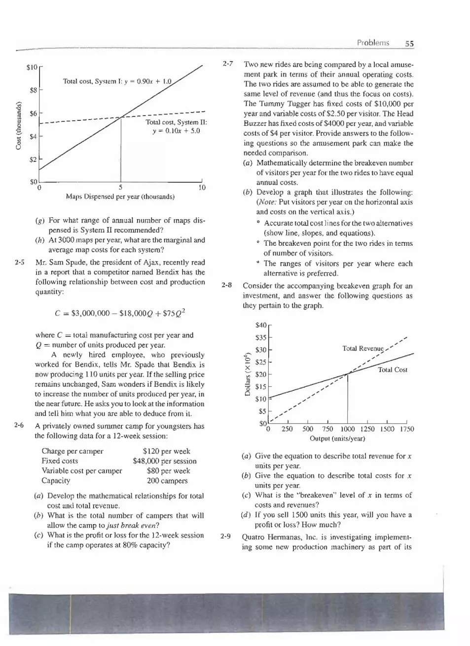
.. ----
Problems 55
Totalcost, System I: y = 0.9Ox+ 1.0
Total cost, System II:y = O.lOx + 5.0
5 10Maps Dispensedper year (thousands)
2-5
(g) For what range of annual number of maps dis-pensed is System ITrecommended?
(h) At 3000mapsper year,what arethe marginalandaveragemap costs for each system?
Mr. Sam Spade, the president of Ajax, recently readin a report that a competitor named Bendix has thefollowing relationship between cost and productionquantity:
c = $3,000,000 - $18,000Q + $75Q2
where C = total manufacturing cost per year andQ = number of units produced per year.
A newly hired employee, who previouslyworked for Bendix, tells Mr. Spade that Bendix isnowproducing 110units per year. If the selling priceremains unchanged, Sam wonders if Bendix is likelyto increase the number of units produced per year, inthe near future.He asks youto look at the informationand tell him what you are able to deduce from it.
2-6 A privately owned summer camp for youngstershasthe followingdata for a 12-weeksession:
Charge per camperFixed costs
Variable cost per camperCapacity
$120 per week$48,000 per session
$80 per week200 campers
(a) Develop the !Ilathematical relationships for totalcost and total revenue.
(b) What is the total number of campers that willallow the camp to just break even?
(c) What is the profit or loss for the 12-week sessionif the camp operates at 80% capacity?
2-7 Two new rides are being compared by a local amuse-ment park in terms of their annual operating costs.The two rides are assumed to be able to generate thesame level of revenue (and thus the focus on costs).The Thmmy Thgger has fixed costs of $10,000 peryear and variable costs of $2.50 per visitor. The HeadBuzzer has fixed costs of $4000 per year, and variablecosts of $4 per visitor. Provide answers to the follow-ing questions so the amusement park can make theneeded comparison.(a) Mathematically determine the breakeven number
of visitors per year for the two rides to have equalannual costs.
(b) Develop a graph that illustrates the following:(Note: Put visitors per year on the horizontal axisand costs on the vertical axis.)· Accurate total cost lines for the two alternatives
(show line, slopes, and equations).· The breakeven point for the two rides in termsof number of visitors.·The ranges of visitors per year where eachalternativeis preferred.
2-8 Consider the accompanying breakeven graph for aninvestment, and answer the following questions asthey pertain to the graph.
$40
$35
$30" ,.....
~ $25x'-' $20E'0Q
,.,.,.Total Revenue,.",.,.,.,.,.,.....
.,,.$15 ,.,.",.$10 - ",,.",.,.$5 ,.,.,.,.$0 ,.
o 250 500 750 1000 1250Output (units/year)
(a) Give the equation to describe total revenue for xunits per year.
(b) Give the equation to describe total costs for xunits per year.
(c) What is the "breakeven" level of x in terms ofcosts and revenues?
(d) If you sell 1500 units this year, will you have aprofit or loss? How much?
2-9 Quatro Hermanas, Inc. is investigating implement-ing some new production machinery as part of its
fy,~t. , - .
O' ,~!} '6"" -';/<;i;';":-'"''':4':;J:~:~_''''''' .> ;':';""" ,._;~,~
$10
$8
-;;;-"0
$6!arI.I
6@,
$4rI.I0
()
$2
$00

56 ENGINEERING COSTSAND COST ESTIMATING
operations. Three alternatives have been identified,and they have the following fixed and variablecosts:
AnnualVariable Costs
per Unit$20.00
5.007.50
AlternativeABC
AnnualFixed Costs
$100,000200,000150,000
2-10
Determine the ranges of production (units pro-duced per year) over which each alternative wouldbe recommended for implementation by QuatroHermanas. Be exact. (Note: Consider the range ofproduction to be from 0-30,000 units per year.)
Three alternative designs have been created bySnakisco engineers for a new machine that spreadscheese between the crackers in a Snakisco snack.Each machine design has unique total costs (fixedand variable) based on the annual production rateof boxes of these crackers. The costs for the threedesigns are given (where x is the annual productionrate of boxes of cheese crackers).
DesignABC
Fixed Cost
$100,000350,000600,000
Variable Cost ($Ix)20.5x1O.5x8.0x
2-11
You are asked to do the following.(a) Mathematically determine which of the machine
designs would be recommended for differentlevels of annual production of boxes of snackcrackers. Management is interested in the produc-tion interval of 0-150,000 boxes of crackers peryear. Over what production volume would eachdesign (A or B or C) be chosen?
(b) Depict your solution from part (a) graphically,putting x per year on the horizontal axis and $on the vertical axis, so that management can seemore easily the following:
i. Accurate total cost lines for each alternative
(show line, slopes, and line equations).ii. Any relevant breakeven, or crossover points
in terms of costs between the alternatives.
iii. Ranges of annual production where eachalternative is preferred.
iv. Clearly label your axes and include a title forthe graph.
A small company manufactures a certain product.Variable costs are $20 per unit and fixed costs
are $10,875. The price-demand relationship for thisproduct is P = -0.25D + 250, where P is the unitsales price of the product and D is the annual demand.Use the data (and helpful hints) that follow to workout answers to parts (a)-(e).
· Total cost = Fixed cost + Variable cost·Revenue= Demand x Price· Profit = Revenue - Total cost
2-12
Set up your graph with dollars on the y axis, (betweeno and $70,000) and, on the x axis, demand D: (unitsproduced or sold), between 0 and 1000 units.(a) Develop the equations for total cost and total
revenue.
(b) Find the breakeven quantity (in terms of profitand loss) for the product.
(c) What profit would the company obtain by maxi-mizing its total revenue?
(d) What is the company's maximum possible profit?(e) Neatly graph the solutions from parts (a), (b),
(c), and (d).
A painting operation is performed by a productionworker at a labor cost of $1.40 per unit. A robot spray-painting machine, costing $15,000, would reducethe labor cost to $0.20 per unit. If the device wouldbe valueless at the end of 3 years, what is the mini-mum number of units that would have to be paintedeach year tojustify the purchase of the robot machine?
Company A has fixed expenses of $15,000 per yearand each unit of product has a $0.002 variable cost.Company B has fixed expenses of $5000 per yearand can produce the same product at a $0.05 vari-able cost. At what number of units of annual produc-tion will Company A have the same overall cost asCompany B?
A firm believes the sales volume (S) of its productdepends on its unit selling price (P) and can be deter-mined from the equation P = $100 - S. The cost (C)
of producing the product is $1000 + lOS.(a) Draw a graph with the sales volume(S) from 0 to
100on the x axis, and total cost and total incomefrom 0 to 2500 on the y axis. On the graph -drawthe line C = $1000 + lOS. Then plot the curveof total income [which is sales volume (S) x unitselling price ($100 - S)]. Mark the breakevenpoints on the graph.
(b) Determine the breakeven point (lowest salesvolume where total sales income just equals totalproduction cost). (Hint: This may be done by trial
2-13
2-14

Problems 57
and error or by using the quadratic equation tolocate the point at which profit is zero.)
(c) Determine the sales volume (8) at which thefirm's profit is a maximum. (Hint: Write an equa-tion for profit and solve it by trial and error, or asa minima-maxima calculus problem.)
2-15 Consider the situation of owning rental propertiesthat local university students rent from you on an aca-demic year basis. Develop a set of costs that you couldclassify as recurring and others that could be classi-fied as nonrecurring.
2-16 Define the difference between a "cash cost" and a"book cost." Is engineering economic analysis con-cerned with both types of cost? Give an example ofeach, and provide the context in which it is important.
2--- In your own words, develop a statement of what theauthors mean by "life-cycle costs." Is it important fora firm to be aware of life-cycle costs? Explain why.
2-18 In lookiiig at Figures 2-4 and 2-5, restate in your ownwords what the authors are trying to get across withthese figures. Do you agree that this is an importanteffect for companies? Explain.
2-19 In the text the authors describe three effects that com-
plicate the process of making estimates to be usedin engineering economy analyses. List these threeeffects and comment on which of these might be mostinfluential.
2-20 Northern Tundra Telephone (NIT) has received acontract to install emergency phones along a new100-mile section of the Snow-Moose Thrnpike. Fiftyemergency phone systems will be installed about2 miles apart. The material cost of a unit is $125.NTT will need to run underground communica-tion lines that cost NTT $7500 per mile (includinglabor) to install. There will also be a one-time cost of$10,000 to network these phones into NTT's currentcommunication system. You are asked to developa cost estimate of the project from NIT's perspec-tive. If NTT adds a profit margin of .35% to itscosts, how much will it cost the state to fund theproject?
2-21 You and your spouse are planning a second honey-moon to the Cayman Islands this summer and wouldlike to have your house painted while you are away.Estimate the total cost of the paint job from the infor-mation given below, where:
Costtotal = Costpaint+ Costlabor + Costfixed
Paint information: Your house has a surface areaof 6000 ft2. One can of paint can cover 300 ft2.You are estimating the cost to put on two coats ofpaint for the entire house, using the cost per cangiven. Note the incremental decrease in unit costper can as you purchase more and more cans.
Number of Cans Purchased
First 10 cans purchasedSecond 15 cans purchasedUp to next 50 cans purchased
Cost per Can$15.00$10.00$7.50
Labor information: You plan to hire fivepainters who will paint for 10hours per day each.You estimate that the job will require 4.5 daysof their painting time. The painter's labor rate is$8.75 per hour.
Fixed cost information: There is a fixed cost of$200 per job that the painting company chargesto cover travel expenses, clothing, cloths, thin-ner, administration, and so on.
You are interested in having a mountain cabin builtfor weekend trips, vacations, to host family, andperhaps eventually to retire in. After discussing theproject with a local contractor, you receive an esti-mate that the total construction cost of your 2000 ft2lodge will be $150,000. Costs within each categoryinclude labor, material, and overheaditems. The per-centage of costs for each of severalitems (categories)is broken down as follows:
2-22
Cost Items
Constructionpermits, legal andtitle fees
Roadway, site clearing,preparationFoundation, concrete, masonryWallboard, flooring,carpentryHeating, ventilation,air
conditioningElectric, plumbing,communicationsRoofing, flooringPainting, finishing
Percentage ofTotal Costs
8%
15131213
101217
100
(a) What is the cost per square foot of the 2000 ft2lodge?
(b) If you are also considering a 4000 ft2 layoutoption, estimate your construction costs if:
i. All cost items (in the table) change propor-tionately to the size increase.
~
I. . .
." .°0'-- -'. . - _. ' . - . .-. - '.. - ~-~ -. . . - .,
j;!I¥;,;\.~w~.,-),;:~~~i,i$~~~~~~'; ,_._~,,~ '~..":' a..:.~l..

- ~ - ----.---------
58 ENGINEERING COSTSAND COST ESTIMATING
n. The first two cost items do not change at all;all others are proportionate.
2-23 SungSam, Inc. is currently designing a new digitalcamcorder that is projected to have the following perunit costs to manufacture: . . - . . .
Cost CategoriesMaterials costsLabor costsOverhead costs
Total Unit Cost
Unit Costs$112
85213
$410
SungSam adds 30% to its manufacturing cost forcorporate profit. Answer the following questions:(a) What unit profit would SungSam realize on each
camcorder?
(b) What is the overall cost to produce a batch of10,000 camcorders?
(c) What would SungSam's profit be on the batch of10,000 if historical data shows that 1% of productwill be scrapped in manufacturing, and 3% of fin-ished product will go unsold, 2% of sold productwill be returned for refund?
(d) How much can SungSam afford to pay for a con-tract that would lock in a 50% reduction in the
unit material cost previously given? ITSungSamdoes sign the contract, the sales price will remainthe same as before.
2-24 Fifty years ago, Grandma Bell purchased a set of gold-plated dinnerware for $55, and last year you inheritedit. Unfortunately a house fire at your home destroyedthe set. Your insurance company is at a loss to definethe replacement cost and has asked your help. You dosome research and find that the Aurum Flatware Cost
Index (AFCI) for gold-plated dinnerware, which was112 when Grandma Bell bought her set, is at 2050today. Use the AFCI to update the cost of Bell's setto today's cost to show to the insurance company.
2-25 Your boss is the director of reporting for the AthensCounty Construction Agency (ACCA). It has been hisjob to track the cost of construction in Athens County.1\venty-five years ago he created the ACCA CostIndex to track these costs. Costs during the first yearof the index were $12 per square foot of constructedspace (the index value was set at 100 for that firstyear). This past year a survey of contractors revealedthat costs were $72 per square foot. What index num-ber will your boss publish in his report for this year?ITthe index value was 525 last year, what was the costper square foot last year?
2-26 An refinisher of antiques named Constance has beenso successful with her small business that she is plan-ning to expand her shop with all new equipment. Sheis going to start enlarging her shop by purchasing thefollowing equipment.
2-27
What would be the net cost to Constance to obtain this
equipment-assume that she can trade the old equip-ment in for 15% of its original cost. Assume also thatthe relative price to purchase the equipment has notchanged over time (that is, there has been no inflationin equipment prices).
Refer to Problem 2-26 and now assume the pricesfor the equipment that Constance wants to replacehave not been constant. Use the cost index data for
each piece of equipment to update the costs to theprice that would be paid today. Develop the overallcost for Constance, again assuming the 15% trade-inallowance for the old equipment. Use any necessarydata from Problem 2-26.
Cost Index
When OriginallyPurchased
1.54780
49
OriginalEquipmentVarnishbath
Power scraperPaint booth
Cost Index
Today17190076
2-28 Five years ago, when the relevant cost index was120, a nuclear centrifuge cost $40,000. The centrifugehad a capacity of separating 1500 gallons of ionizedsolution per hour. Today, it is desired to build a cen-trifuge with capacity of 4500 gallons per hour, butthe cost index now is 300. Assuming a power-sizingexponent to reflect economies of scale, x, of 0.75, usethe power-sizing model to determine the approximatecost (expressed in today's dollars) of the new re~ctor.
Padre works for a trade magazine that publishes.lists of Power-Sizing Exponents (PSE) that reflecteconomies of scale for developing engineering es-timates of various types of equipment. Padre hasbeen unable to find any published data on the VMICmachine and wants to list its PSE value in his next
issue. Given the following data (your staff was ableto find data regarding costs and sizes of the VMIC
2-29
Cost of Power- NewOriginal Original Sizing Equipment
Equipment Size Equipment Exponent SizeVarnishbath 50 gal $3500 0.80 75 galPowerscraper 3/4 hp $250 0.22 1.5hpPaint booth 3ft3 $3000 0.6 12ft3

Problems 59
machine) calculate the PSE value that Padre shouldpublish. (Note: The VMIC-I00 can handle twice thevolume of a VMIC-50.)
Cost of VMIC-100 today $100,000Cost of VMIC-50 5 years ago $45,000VMIC equipment index today = 214VMIC equipment index 5 years ago = 151
2-30 Develop an estimate for each of the followingsituations.
(a) The cost of a 500-mile automobile trip, if gasolineis $1 per gallon, vehicle wear and tear is $0.08 permile, and our vehicle gets 20 miles per gallon.
(b) The total number of hours in the average humanlife, if the average life is 75 years.
(c) The number of days it takes to travel around theequator using a hot air balloon, if the balloonaverages 100 miles per day, the diameter of theearth is ""4000 miles. (Note: Circumference = 7r
times diameter.)(d) The total area in square miles of the United States
of America, if Kansas is an average-sized state.Kansas has an area of 390 miles x 200 miles.
2-31 If 200 labor hours were required to produce the 15tunitin a production run and 60 labor hours were requiredto produce the 7th unit, what was the learning-curverate during production?
2-32 Rose is a project manager at the civil engineering con-sulting firm of Sands, Gravel, Concrete, and Waters,Inc. She has been collecting data on a project in whichconcrete pillars were being constructed, however notall the data are available. She has been able to find
out that the 10th pillar required 260 person-hours toconstruct, and that a 75% learning curve applied. Sheis interested in calculating the time required to con-struct the 15tand 20th pillars. Compute the values forher.
2-33 Sally Statistics is implementing a system of statisti-cal process control (SPC) charts in her factory in aneffort to reduce the overall cost of scrapped product.The current cost of scrap is $X per month. If an 80%learning curve is expected in the use of the SPC chartsto reduce the cost of scrap, what would the percent-age reduction in monthly scrap cost be after the chartshave been implemented for 12 months? (Hint: Modeleach month as a unit of production.)
2-34 Randy Duckout has been asked to develop an esti-mate of the per-unit selling price (the price that eachunit will be sold for) of a new line of hand-crafted
booklets that offer excuses for missed appointments.His assistant Doc Duckout has collected information
that Randy will need in developing his estimate:
Cost of direct labor $20 per hourCost of materials $43.75 per batch
of 25 bookletsCost of overhead items 50% of direct labor
cost
Desired profit 20% of totalmanufacturing cost
Doc also finds out that (1) they should use a 75%learning curve for estimating the cost of direct labor,(2) the time to complete the 15tbooklet is estimatedat 0.60 hour, and (3) the estimated time to completethe 25th booklet should be used as their standard time
for the purpose of determining the unit selling price.What would Randy and Doc's estimate be for the unitselling price?
2-35 Develop a statement that expresses the extent to whichcost estimating topics also apply to estimating bene-fits. Provide examples to illustrate.
2-36 On December 1, AI Smith purchased a car for$18,500. He paid $5000 immediately and agreed topay three additional payments of $6000 each (whichincludes principal and interest) at the end of 1, 2, and3 years. Maintenance for the car is projected at $1000at the end of the first year and $2000 at the end of eachsubsequent year. AI expects to sell the car at the endof the fourth year (after paying for the maintenancework) for $7000. Using these facts, prepare a table ofcash flows.
2-37 Bonka Toys is considering a robot that will cost$20,000 to buy. After 7 years its salvage value will be$2000. An overhaul costing $5000 will be needed inyear 4. O&M costs will be $2500 per year. Draw thecash flow diagram.
2-38 Pine Village needs some additional recreation fields.Construction will cost $225,000 and annual O&Mexpenses are $85,000. The city council estimates thatthe value of added youth leagues is about $190,000.annually. In year 6 another $75,000 will be neededto refurbish the fields. The salvage value is estimatedto be $100,000 after 10 years. Draw the cash flowdiagram.
2-39 Identify your major cash flows for the current schoolterm as first costs, O&M expenses, salvage values,revenues, overhauls, and so on. Using a week as thetime period, draw the cash flow diagram.

<'",.;;,,,~,ji;~!!!-olio- _ ..-
After Completing This Chapter...Thestudent should be able to:· Define and provide examples of the time value of money.· Distinguish between simple and compoundinterest,and use compound interest in engi-
neering economic analysis.· Explain equivalenceof cash flows.· Solve problems using the single payment compound interest formulas.
QUESTIONS TO CONSIDER ;:;.
1. Tobaccobonds oftenpay interest of as much as 7%, whileconventionalstate governmentbonds may pay only 5%. On a $1 million bond with a term of 25 years, how much doesthis interest differential amount to, in total?
2. Assuming a 2% interest differential, over a 25-year period, how much are states losingby opting to take the settlement money "up front" instead of collecting the long-termpayout?
3. When themoney theyget from sellingbonds runsout, state governmentswillhave to finda new way of closing their budget gaps. Already, some commentators are suggestingthat states may soon look to other business sectors as "deep pockets." The tobaccoindustry was particularly vulnerable because it sold a product that came to be seen asdangerous and socially undesirable. What other industries might face the same fate inyears to come? How about fast-food restaurant chains, or sellers of alcohol products?Should a company like Anheuser-Buschbe worried? Should companies in potentially"problematic" industries consider setting aside money for future settlement costs?

r -
f
- - - - - - - -- - - - ---
Interest and Equivalence
Going Up in SmokeStategovernmentsthroughoutthe United States agreed to a largefinancialwindfall in 1998.Tobaccocompaniesagreedtopay inperpetuityto settleclaimsarisingfromthe healtheffectsof smoking. Payments over the first 25 years are estimated to be nearly $250 billion.
State officials announced they would earmark these funds for goals such as healthcare, education and, of course, antismoking campaigns. But several states involved in thesettlement were chronically short of money and were desperate to plug budget deficits. Ifonly they could get their hands on the full value of that tobacco settlementnow, instead ofwaiting for the payments to dribble in year by year.
That's when someonehit on the idea ofrais-
ing instant money by issuing "tobacco bonds":the states would sell bonds to investors and paythem interest out of the tobacco settlement pay-ments the states were receiving. State govern-ments could get the whole sale price of the bondup front; investors would get ongoing incomefromthe bond. .
A growing number of states are now sell-ing these bonds, andpocketingquickbillions. Toattract buyers, however, the states have to paya high rate of interest on their tobacco bonds,since investors view them as riskier than othergovernment-backed securities. Investors reasonthat tobacco companies could go broke, afterall--especially if the no-smoking laws beingpassed allover the countrycause enough peopleto snuff out their cigarettehabit for good.
tI
f
r

62 INTERESTAND EQUIVALENCE
In the first chapter, we discussed the engineeringeconomic decision process. In Chapter 2we described models used to estimate the costs and benefits that are summarized in cashflow diagrams.For many of the situations we examined, the economic consequencesof analternativewere immediate or took place in a very short period of time, as in Example 1-2,- ~ .' . -- .
(the decision on the design of a concrete aggregate mix) or Example 1-3 (the change ofmanufacturing method). In such relatively simple situations, we total the various positiveand negativeaspects, compare our results, and quickly reach a decision. But can we do thesame if the economic consequencesoccur over a considerableperiod of time?
No we cannot, because money has value over time. Would you rather: (1) receive$1000 today or (2) receive $1000 ten years from today? Obviously, the $1000 today hasmore value. Money's value over time is expressed by an interest rate. In this chapter, wedescribe two introductory concepts involving the time value of money: interest and cashflow equivalence.
COMPUTING CASH FLOWS
Installing an expensivepiece of machineryin aplant obviouslyhas economicconsequencesthat occuroveranextendedperiodof time.If the machinerywereboughtoncredit,the simpleprocess of payingfor it maytake severalyears.What abouttheusefulnessof the machinery?Certainly it was purchased because it would be a beneficial addition to the plant. Thesefavorable consequences may last as long as the equipment performs its useful function.In these circumstances,we do not add up the various consequences; instead, we describeeach alternativeas cash receipts or disbursements at differentpoints in time. In this way,each alternativeis resolved into a set of cash flows. This is illustrated by Examples 3-1and 3-2.
The manager has decidedto purchase a new $30,000mixing machine. The machine may be paidfor in one of two ways:
1. Pay the full price nowminus a 3% discount.2. Pay $5000 now; at the end of one year, pay $8000; at the end of each of the next four
years, pay $6000.
List the alternatives in theform of a table of cash flows.
In this problem the two alternativesrepresent different ways to pay for the mixing machine.While the first plan represents a~lumpsum of $29,100 now, the second one calls for paymentscOhtinuinguntilthe end of the fifthyear.Theproblemis to convertan alternativefnto cashreceiptsor disbursementsandshow the tirn,ingof each.receipt or disbursement.The result is called a cashflQwtable or, more simply,a set of cashflows.I.. III_ - - - -- - -- - - - .. - - - ...-.. - -.. ..

-_. -
Computing Cash Flows 63
The cash flowsfor both the alternativesin this problem are very simple.The cash flowtable,with disbursementsgiven negative signs, is as follows:
End of Year
o (now)12345
Pay in FuUNow--$29,100
ooooo
Pay Over 5 Years---$5000-8000-6000-6000-6000-6000
=.-
~..~. _..~. .~ .
A manborrowed $1000from a bank at 8% interest.He agreedto repay the loan in twoend-of-yearpayments. At the end of the first year, he will repay half of the $1000 principal amount plus theinterest that is due. At the end of the second year,he will repay the remaining half of the principalamountplus the interest for the second year. Compute the borrower's cash flow.
. SOL '.TI()N
In engineeringeconomicanalysis, we normallyrefer to the beginningof the firstyear as "time 0."At this point the manreceives$1000 from the bank. (A positivesignrepresents a receipt of moneyand a negative sign, a disbursement.)Thus, at time 0, the cash flow is +$1000.
At the end of the first year, the man pays 8% interest for the use of $1000 for one year. Theinterest is 0.08 x $1000 = $80. In addition, he repays half the $1000 loan, or $500. Therefore,the end-of-year-I cash flow is -$580.
At the end of the second year, the payment is 8% for the use of the balance of the principal($500) for the one-year period, or 0.08 x 500 = $40. The $500principal is also repaid for a totalend-of.;.year-2cash flow at -$540. The cash flow is:
End of Year
o (now)12
Cash Flow+$1000
-580-540
l
In this chapter, we will demonstrate techniques for comparing the value of money atdifferentdates, an ability that is essential to engineeringeconomicanalysis.Wemust be ableto compare, for example, a low-costmotor with a higher-costmotor. If there were no otherconsequences, we would obviously prefer the low-cost one. But if the higher-cost motorwere more efficient and thereby reduced the annual electric power cost, we would wantto consider whether to spend more money now on the motor to reduce power costs in the

64 INTERESTAND EQUIVALENCE
future. This chapter will provide the methods for comparing the alternatives to determinewhich motor is preferred.
TIME VALUE OF MONEY
We often find that the monetary consequences of any alternative occur over a substantialperiod of time-say, a year or more. When monetary consequencesoccur in a short periodof time, we simply add up the various sums of money and obtain a net result. But can wetreat money this way when the time span is greater?
Which would you prefer, $100 cash today or the assurance of receiving $100 a yearfrom now? Youmight decide you wouldprefer the $100now because that is one way to becertain of receiving it. But suppose you were convinced that you would receive the $100one yearhence. Now what wouldbe your answer?A little thoughtshould convinceyou thatit still would be more desirable to receive the $100 now.If you had the money now,ratherthan a year hence, you wouldhave the use of it for an extra year.And if you had no currentuse for $100, you could let someoneelse use it.
Money is quite a valuable asset-so valuable that people are willing to pay to havemoney availablefor their use. Money can be rented in roughly the same way one rents anapartment, only with money,the charge is called interest instead of rent. The importanceof interest is demonstratedby banks and savings institutions continuously offering to payfor the use of people's money,to pay interest.
If the current interest rate is 9% per year, and you put $100 into the bank for one year,how much will you receive back at the end of the year? You will receive your original$100 together with $9 interest, for a total of $109. This example demonstrates the timepreference for money: we would rather have $100 today than the assured promise of $100one year hence; but we might well considerleaving the $100 in a bank if we knew it wouldbe worth $109 one year hence. This is because there is a time value of money in the formof the willingness of banks, businesses, and people to pay interest for the use of varioussums.
Simple InterestSimple interest is interest that is computed only on the original sum and not on accruedinterest. Thus if you were to loan a present sum of moneyP to someone at a simple annualinterest rate i (stated as a decimal)for a period of n years, the amount of interest you wouldreceive from the loan wouldbe:
Totalinterest earned = P x i x n = Pin (3-1)
At the end of n years the amountof moneydue you, F, would equal the amount of the loan .
P plus the total interest earned. That is, the amount of money due at the end of the loanwould be
F = P + Pin (3-2)
or F = PO + in).

r- -
Time Value of Money 65
You have agreed to loan a friend $5000 for 5 years at a simple interest rate of 8% per year. Howmuch interest will you receive from the loan'? How much will your friend pay you at the end of5 years?
Total interestearned= Pin = ($5000)(0.08)(5 yr) - $2000
Amount due at end'of loan = P + Pin = 5000 + 2000 = $7000I;;..,
In Example 3-3 the interest earned at the end of the first year is (5000)(0.08)(1) = $400, butthis money is not paid to the lender until the end of the fifth year. As a result, the borrowerhas the use of the $400 for four years without paying any interest on it. This is how simpleinterest works, and it is easy to seewhy lenders seldom agree to make simple interest loans.
Compound InterestWith simple interest, the amount earned (for investedmoney) or due (for borrowedmoney)in oneperiod doesnot affectthe principalfor interest calculationsin laterperiods.However,this is not how interest is normally calculated. In practice, interest is computed usingthe compound interest method. For a loan, any interest owed but not paid at the endof the year is added to the balance due. Thus, the next year's interest is calculatedbased onthe unpaidbalancedue, which includes the unpaid interestfromthe precedingperiod. In thisway, compound interest can be thought of as interest on top of interest. This distinguishescompound interest from simple interest. In this section, the remainder of the book, and inpractice you should assume that the rate is a compound interest rate. The few exceptionswill clearly state use "simple interest."
Tohighlight the differencebetween simple and compoundinterest, rework Example 3-3 using aninterest rate of 8% per year compound interest. How will this change affect the amount that yourfriend pays you at the end of 5 years?
~.
.
.
..-:
.~Original loan amount (originalprincipal) = $5000Loan term = 5 years
Int~rest rate charged 8%per year cOlnpound interest1.________ - ..- - - - - - - --- - - - - - ..- - - -- -- - -- - ---

-- -- ------...-
66 INTERESTAND EQUIVALENCE
In the following table we calculate on a year-to-yearbasis the total dollar amount due at the endof each year. Notice that this amount becomes the principal upon which interest is calculated inthe next year (this is the compoundingeff~?t). ._ . ___
The total amount due at the end of the fifthyear, $7347, is the amount that your friend will giveyou to repay the original loan. Notice that this amount is $347 more than the amountyoureceivedfor loaning the same amount, for the same period, at simple interest. This, of course, is becauseof the effect of interest being earned (by you) on top of interest.
Repaying a DebtTo better understand the mechanics of interest, let us say that $5000 is owed and is tobe repaid in 5 years, together with 8% annual interest. There are a great many ways inwhich debts are repaid; for simplicity,we have selected four specificways for our example.Table 3-1 tabulates the four plans.
In Plan 1, $1000 will be paid at the end of each year plus the interest due at the end ofthe year for the use of moneyto that point. Thus, at the end of the firstyear,we will havehadthe use of $5000. The interest owed is 8% x $5000 = $400. The end-of-year payment is,
therefore, $1000principalplus $400 interest, for a total paymentof $1400.At the end of thesecond year, another$1000 principalplus interest will be repaid on the money owed duringthe year.This time the amountowedhas declinedfrom $5000 to $4000becauseof the $1000principal payment at the end of the first year. The interest payment is 8% x $4000=$320,making the end-of-year payment a total of $1320. As indicated in Table 3-1, the se-ries of payments' continues each year until the loan is fully repaid at the end of thefifth year.
Plan 2 is another way to repay $5000 in 5 years with interest at 8%. This time the .
end-of-year payment is limited to the interest due, with no principal payment. Instead, the$5000 owed is repaid in a lump sum at the end of the fifth year. The end-of-year paymentin each of the first four years of Plan 2 is 8% x $5000 = $400. The fifth year, the paymentis $400 interestplus the $5000 principal, for a total of $5400.
Plan 3 calls for five equal end-of-yearpayments of $1252 each. At this point, we havenot shown how the figure of $1252 was computed (see later: Example 4-3). However, it is
Total Principal (P) Interest (I) Owed at the End Total Amount Due at theon Which Interest is of Year n from Year n's End of Year n, New Total
Year Calculated in Year n Unpaid Total Principal Principal for Year n + 1
1 $5000 , $5000 x 0.08 = 400 $5000+ 400 = 5400
2 5400 5400 x 0.08 = 432 5400 + 432 = 5832
3 5832 5832 x 0.08 = 467 5832 + 467 = 6299
4 6299 6299 x 0.08 = 504 6299 + 504 = 6803
5 6803 6803 x 0.08 = 544 6803 + 544 = 7347

Time Value of Money 67
(a)
TABLE 3-1 Four Plans for Repayment of $5000 in 5 Yearswith Interest at 8%
(e) (f)Total
End-of-Year
Payment
(b)Amount Owed
at Beginning ofYear
(c)Interest Owed for
That-Year,8% x (b)
(d)Total Owed at
End of Year,(b) + (c)Year
PrincipalPayment
Plan 1: At end of each year pay $1000principalplus interestdue.1 $5000 $ 400 $54002 4000 320 43203 3000 240 32404 2000 160 21605 1000 80 1080
$1200
$10001000100010001000
$5000
$14001320124011601080
$6200
Plan 2: Pay interestdue at end of each year and principalat end of 5 years.1 $5000 $ 400 $5400 $2 5000 400 54003 5000 400 54004 5000 400 54005 5000 400 5400
$2000
oooo
5000$5000
$ 400400400400
5400
$7000
Plan 3: Pay in fiveequal end-of-yearpayments.1 $5000 $ 4002 4148 3313 3227 2584 2233 1785 1159 93
$1260
$54004479348524111252
$ 852921994
10741159
$5000
$1252*1252125212521252
$6260
Plan 4: Pay principaland interest in one payment at end of 5 years.1 $5000 $ 400 $54002 5400 432 58323 5832 467 62994 6299 504 68035 6803 544 7347
$2347
$ 0ooo
5000$5000
$ 0ooo
7347$7347
*The exact value is $1252.28, which has been rounded to an even dollar amount.
clear that there is some equal end-of-year amount that would repay the loan. By followingthe computations in Table 3-1, we see that this series of five payments of $1252 repays a$5000 debt in 5 years with interest at 8%.
Plan 4 is still another method of repaying the $5000 debt. In this plan, no payment ismade until the end of the fifthyear when the loan is completely repaid. Note what happensat the end of the first year: the interest due for the first year-8% x $5000=$400-is notpaid; instead, it is added to the debt. At the second year, then, the debt has increased to$5400. The second year interest is thus 8% x $5400= $432. This amount, again unpaid, is

---- -- - . - -- ._---
-- - ---
68 INTERESTAND EQUIVALENCE
added to the debt, increasing it further to $5832. At the end of the fifth year, the total sumdue has grown to $7347 and is paid at that time (see Example 3-4).
Note that when the $400 interest was not paid at the end of the first year, it was addedto the debt and, in the second ye~, tilere was interest chargedon this unpaid interest. Thatis, the $400 of unpaid interest resulted in 8% x $400= $32 of additional interest charge inthe secondyear.That $32, togetherwith 8% x $5000=$400 interest on the $5000 originaldebt,broughtthe total interestchargeat the end of the secondyear to$432.Chargingintereston unpaid interest is called compound interest. We will deal extensivelywith compoundinterestcalculationslaterin thischapter. .
With Table 3-1 we have illustrated four different ways of accomplishing the sametask, that is, to repay a debt of $5000 in 5 years with interest at 8%. Having described thealternatives,we will now use them to present the important concept of equivalence.
EQUIVALENCE
When we are indifferent as to whether we have a quantity of money now or the assuranceof some other sum of money in the future, or series of future sums of money, we say thatthe present sum of money is equivalent to the future sum or series of future sums.
If an industrial firm believed 8% was an appropriate interest rate, it would have noparticular preference about whether it received $5000 now or was repaid by Plan 1 ofTable 3-1. Thus $5000 today is equivalent to the series of five end-of-year payments. Inthe same fashion, the industrial firmwould accept repayment Plan 2 as equivalentto $5000now.Logic tells us that if Plan 1 is equivalent to $5000 now and Plan 2 is also equivalentto $5000 now, it must follow that Plan 1is equivalent to Plan 2. In fact, allfour repaymentplans must be equivalent to each other and to $5000 now.
Equivalenceis an essential factor in engineering economic analysis. In Chapter 2, wesawhowan alternativecouldbe representedby acash flowtable.Howmight two alternativeswith different cash flows be compared? For example, consider the cash flows for Plans 1and 2:
Year12345
Plan 1-$1400-1320-1240-1160-1080
-$6200
Plan 2-$400-400-400-400
-5400
-$7000
If you were given your choice between the two alternatives,which one would you choose?Obviously the two plans have cash flows that are different. Plan 1 requires that there be .
larger payments in the first 4 years, but the total payments are smaller than the sum ofPlan 2's payments. To make a decision, the cash flows must be altered so that they can becompared. The technique of equivalence is the way we accomplish this.
Using mathematicalmanipulation,we can determinean equivalentvalueat some pointin time for Plan 1 and a comparable equivalent value for Plan 2, based on a selected

Equivalence 69
interest rate. Then we canjudge the relative attractivenessof the two alternatives,not fromtheir cash flows,but from comparable equivalentvalues. Since Plan 1, like Plan 2, repays apresent sum of $5000 with interest at 8%, the plans are equivalentto $5000 now; therefore,the alternatives are equally attractive. This cannot be deduced from the given cash flowsalone. It is necessary to learn this by deieimining the equivalentvalues for each alternativeat some point in time, which in this case is "the present."
Difference in Repayment PlansThe four plans computed in Table 3-1 are equivalent in nature but different in structure.Table 3-2 repeats the end-of-year payment schedules from Table 3-1 and also graphs eachplan to show the debt still owed at any point in time. Since $5000 was borrowed at thebeginning of the firstyear, all the graphs begin at that point. We see,however, that the fourplans result in quite different situations on the amount of money owed at any other pointin time. In Plans 1 and 3, the money owed declines as time passes. With Plan 2 the debtremains constant,whilePlan 4 increases the debtuntil the end of the fifthyear.These graphsshow an importantdifferenceamongthe repaymentplans-the areasunder the curvesdiffergreatly. Sincethe axes are Money Owed and Time,the area is their product: Money owed xTime, in years.
In the discussion of the time value of money, we saw that the use of money over atime period was valuable, that people are willing to pay interest to have the use of moneyfor periods of time. When people borrow money, they are acquiring the use of money asrepresentedby the area under the curve for Money owed vs Time-.It follows that, at a giveninterest rate, the amount of interest to be paid will be proportional to the area under thecurve. Since in each case the $5000 loan is repaid, the interest for each plan is the totalminus the $5000 principal:
Plan Total Interest Paid1 $12002 20003 12604 2347
We can use Table3-2 and the data from Table 3-1, to compute the area under each ofthe four curves, that is, the area bounded by the abscissa, the ordinate, and the curve itself.We multiply the ordinate (Money owed) by the abscissa (1 year) for each of the fiveyears,then add:
Shaded area = (Money owed in Year 1)(1year)
+ (Moneyowedin Year2)(1year)
+...
+ (Moneyowedin Year5)(1year)
or
Shaded area [(Money owed)(Time)] = Dollar-Years

.. . _. ---
70 INTERESTAND EQUIVALENCE
TABLE 3-2 End-of-Year PaymentSchedules and Their Graphs
Plan 1: At end of each year pay $1000 principalplus interest due. $6000
End-of- Year$5000
] $4000Year Payment 01 $1400 .... $3000u2 1320
s::o $2000
3 12404 1160
$1000
5 1080 $02- 1 3 4 5
$6200 Time (years)
Plan 2: Pay interest due at end of each year andprincipal at end of 5 years.
$6000
End-of- Year$5000
"'c:I
Year Payment$4000
01 $ 400 $3000
2 400s::o $2000
3 400 $10004 4005 5400 $0
1 2 3 4 5-$7000 Time (years)
Plan 3: Pay in five equal end-of-year payments. $6000
End-of- Year$5000
"'c:I
Year Payment$4000
01 $1252 $3000'
2 1252s::
$20003 1252 $10004 12525 1252 $0
4 5- 1 2 3
$6260 Time (years)
Plan 4: Pay principal and interest in one payment $7000at end of 5 years. $6000
End-of- Year$5000
Year Payment$4000
....1 $ 0 $3000
0
2 0 $20003 0 $10004 05 7347 $0 h_. ...-....".,
1 2 3 4 5-$7347 TIme(years)
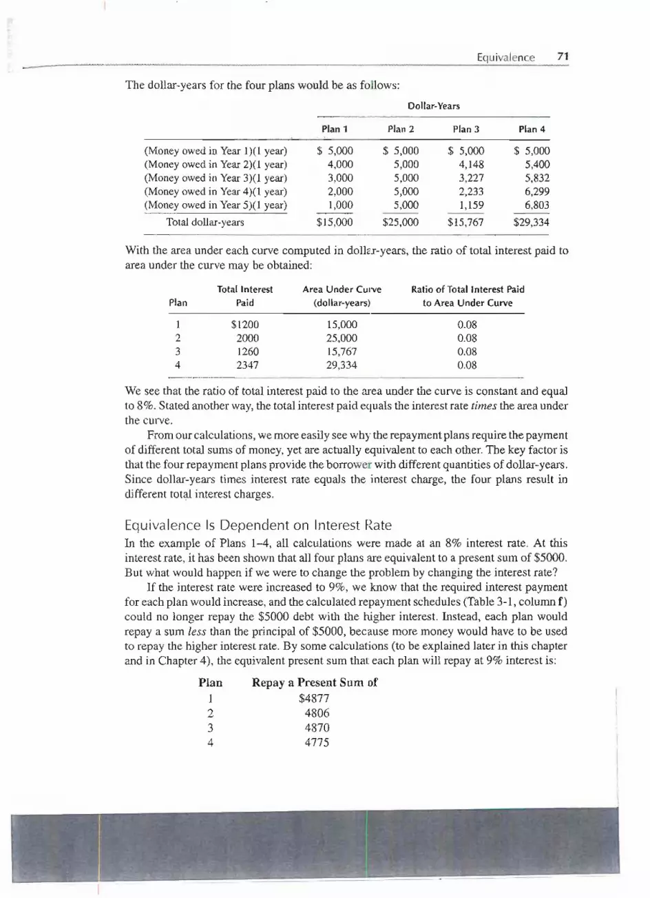
Equivalence 71
The dollar-yearsfor the four plans would be as follows:Dollar-Years
Plan 1 Plan 2 Plan 3 Plan 4
(Money owed in Year 1)(1 year)(Money owed in Year 2)(1 year)(Money owed in Year 3)(1 year)(Money owed in Year 4)(1 year)(Money owed in Year 5)(1 year)
Total dollar-years
$ 5,0004,0003,0002,0001,000
$15,000
$ 5,0005,0005,0005,0005,000
$25,000
$ 5,0004,1483,2272,2331,159
$15,767
$ 5,0005,4005,8326,2996,803
$29,334
With the area under each curve computed in dollar-years, the ratio of total interest paid toarea under the curve may be obtained:
We see that the ratio of total interest paid to the area under the curve is constant and equalto 8%.Stated anotherway,the total interestpaid equals the interestrate times the area underthe curve.
Fromour calculations,wemore easilyseewhytherepaymentplansrequire thepaymentof different total sums of money,yet are actually equivalentto each other.The key factor isthat the four repaymentplans provide the borrower with differentquantitiesof dollar-years.Since dollar-years times interest rate equals the interest charge, the four plans result indifferent to~ interest charges.
Equivalence Is Dependent on Interest RateIn the example of Plans 1-4, all calculations were made at an 8% interest rate. At thisinterest rate, it has been shownthat all four plans are equivalentto a present sum of $5000.But what would happen if we were to change the problem by changing the interest rate?
If the interest rate were increased to 9%, we know that the required interest paymentfor each plan would increase,and the calculatedrepaymentschedules (Table3-1, columnf)could no longer repay the $5000 debt with the higher interest. Instead, each plan wouldrepay a sum less than the principal of $5000, because more money would have to be usedto repay the higher interest rate. By some calculations (to be explained later in this chapter -
and in Chapter4), the equivalentpresent sum that each plan will repay at 9% interest is:
Plan1234
Repay a Present Sum of$4877480648704775
Total Interest Area Under Curve Ratio of Total Interest PaidPlan Paid (dollar-years) to Area Under Curve
1 $1200 15,000 0.082 2000 25,000 0.083 1260 15,767 0.084 2347 29,334 0.08

n .....
72 INTERESTAND EQUIVALENCE
As predicted,at the higher9%interesteachof therepaymentplansof Table3-1repaysapresent sum less than $5000. But they do not repay the same present sum. Plan 1 wouldrepay $4877 with 9% interest, while Plan 2 would repay $4806. Thus, with interest at 9%,Plans 1 and 2 are no longer equivalent, for they will not repay the same present sum. Thetwo series of payments (Plan 1 and Plan 2) were equivalent at 8%, but not at 9%. Thisleads to the conclusion that equivalence is dependent on the interest rate. Changing theinterest rate destroys the equivalencebetween two series of payments.
Could we create revised repayment schemes that would be equivalent to $5000 nowwith interest at 9%? Yes, of course we could: to revise Plan I of Table 3-1, we need toincrease the total end-of-year payment in order to pay 9% interest on the outstanding debt.
Year12345
Amount Owed at
Beginning of Year$50004000300020001000
9% Interestfor Year
$45036027018090
Total End-of-Year Payment($1000 plus interest)
$14501360127011801090
Plan 2 of Table 3-1 is revised for 9% interest by increasing the first four payments to9% x $5000 = $450 and the finalpayment to $5450.Twoplans that repay $5000in 5 yearswith interest at 9% are:
Revised End-of-Year PaymentsYear Plan 1 Plan 2
1 $1450 $ 4502 1360 4503 lTIO ~O4 1180 4505 1090 5450
Wehavedeterminedthat RevisedPlan 1is equivalentto apresent sumof $5000andRevisedPlan 2 is equivalentto $5000 now;it followsthat at 9% interest, RevisedPlan 1is equivalentto Revised Plan 2.
Application of Equivalence CalculationsTo understand the usefulness of equivalencecalculations,consider the following:
Alternative A: Alternative B:Lower Initial Cost, Higher Initial Cost,
Higher Operating Cost Lower Operating Cost-$600 -$850
-115 -80-115 -80-115 -80
. Year
o (now)123
10 -115 -80
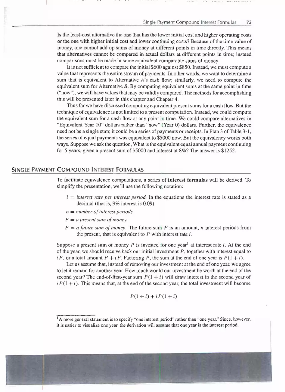
-- -- ._--- - -. - --- _.- --- .--- - - -- - -- --.-. " --- ---------
Single PaymentCompound Interest Formulas 73
Is the least-costalternativethe onethat hasthe lower initial costandhigher operatingcostsor the onewith higher initial cost and lowercontinuing costs? Because of the time value ofmoney, one cannot add up sums of money at different points in time directly. This meansthat alternatives cannot be compared in actual dollars at different points in time; insteadcomparisons must be made in some equivalent comparable sums of money.
It is not sufficientto comparethe initial$600 against $850. Inste~d,we must compute avalue that represents the entire stream of payments. In other words, we want to determine asum that is equivalent to Alternative A's cash flow; similarly, we need to compute theequivalent sum for Alternative B. By computing equivalent sums at the same point in time("now"), we will havevalues thatmaybe validlycompared.Themethods for accomplishingthis will be presented later in this chapter and Chapter 4. .
Thus far we have discussed computingequivalentpresent sums for a cash flow.But thetechniqueof equivalenceis not limitedto a presentcomputation.Instead,we could computethe equivalent sum for a cash flow at any point in time. We could compare alternatives in"Equivalent Year 10" dollars rather than "now" (Year0) dollars. Further, the equivalenceneed not be a single sum; it couldbe a seriesof payments or receipts. In Plan 3 of Table3-1,the series of equal payments was equivalentto $5000 now.But the equivalencyworks bothways. Supposewe ask the question,What is the equivalentequal annualpaymentcontinuingfor 5 years,givena presentsumof $5000andinterest at 8%?The answeris $1252.
SINGLE PAYMENT COMPOUND INTEREST FORMULAS
To facilitate equivalence computations, a series of interest formulas will be derived. Tosimplify the presentation, we'll use the following notation:
i = interest rate per interestperiod. In the equations the interest rate is stated as adecimal(thatis, 9%interestis 0.09).
n = number of interest periods.
P = a present sum of money.
F = a future sum of money. The future sum F is an amount, n interest periods fromthe present, that is equivalentto P with interest rate i.
Suppose a present sum of money P is investedfor one yearl at interest rate i. At the endof theyear,we shouldreceivebackourinitialinvestmentP, togetherwithinterestequaltoiP, or a total amount P + iP. Factoring P, the sum at the end of one year is P (1 + i).
Let us assumethat, instead of removingour investmentat the end of one year,we agreeto let it remain for anotheryear.How much wouldour investmentbe worth at the end of thesecond year? The end-of-first-yearsum P(1 + i) will draw interest in the second year of.i P(1 + i). This means that, at the end of the second year, the total investmentwill become
P(1+i)+iP(1+i)
IA more general statement is to specify "one interest period" rather than "one year." Since, however,it is easier to visualize one year, the derivation will assume that one year is the interest period.

74 INTERESTAND EQUIVALENCE
This may be rearranged by factoring P(1 + i), which gives us
P(1 + i)(l + i)
or
If the process is continued for a third year, the end-of-the-third-yeartotal amount will beP(1 + i)3; at the end of n years, we will have P(l + i)n. The progression looks like this:
Year123
Amount at Beginning ofInterest Period
PP(1 + i)P(1 + i)2P(l + i)n-l
+ Interest forPeriod
+iP+iP(l+i)+iP(1+i)2+ iP(1 + i)n-l
= Amount at End ofInterest Period
=P(1+i)= P(1 +i)2= P(1 + i)3= P (1 + i)nn
In other words, a present sum P increases in n periods to P (1 + i)n. We therefore have arelationship between a present sum P and its equivalentfuture sum, F.
Future sum = (Present sum) (1 + i)n
F = P(1 + i)n (3-3)
This is the single payment compound amount formula and is written in functional nota-tion as
F=P(FjP,i,n) (3-4)
The notation in parentheses (F j P, i, n) can be read as follows:
To find a future sum F, given a present sum, P, at an interest rate i per interest period,and n interest periods hence. .
Functional notation is designed so that the compound interest factors may be written inan equation in an algebraically correct form. In Equation 3-4, for example, the functionalnotation is interpreted as
which is dimensionallycorrect.Withoutproceedingfurther,we can see that whenwe derive.a compound interest factor to find a present sum P, given a future sum F, the factor willbe (P j F, i, n); so, the resulting equation would be
P=F(PjF,i,n)
which is dimensionally correct.

Single Payment Compound Interest Formulas 75
If $500 were depositedin a bank savingsaccount,how much would be in the account three yearshence if the bank paid 6% interest [email protected]~Jy?
We can draw a diagram of the problem. [Note:To have a consistent notation, we will repre-sent receipts by upward arrows (and positive signs), and disbursements (or payments) will havedownward arrows (and negative signs).]
.SQlUl1I0N
Fromthe viewpointof theperson depositingthe $500, the diagramfor "today" (Time=0) throughYear3 is as follows:
Receipts (+$)
F=?
r
Disbursements (-$)
0-1-2-3
t n=3i = 0.06P = 500
Weneed to identify the various elementsof the equation.The presentsum P is $500. The interestrate per interest period is 6%, and in 3 years there are three interest periods. The future sum F isto be computed from the formula
F = P(1 + it = 500(1 + 0.06)3 = $595.50
where P = $500,i = 0.06,n = 3, and F is unknown.
Thus if we deposit $500 in the bank now at 6% interest, there will be $595.50 in the accountin three years.
The equation F = P (I + i)n neednot be solvedwith ahand calculator.Instead, thesinglepaymentcompound amount factor, (1 + i)n, is readily determined from computed~tables~The factor iswritten in convenientnotation as
=
(1 + i)n = (F j P, i, n)= ;;:= =
and in functional notation as
(Fj P, 6%, 3) r,Knowing n = 3, locate the proper row in the 6% table.2 To find F given P, look in the ~stcolumn,which is headed "SinglePayment, Compound1\.mountFactor": forn = 3,we find 1.191.
IN ~_ -- - ...--
2The appendix contains compound interest tables for rates between 1/4 and 60%.

76 INTERESTAND EQUIVALENCE
Thus,
F = 500(F j P, 6%, 3) = 500(1.191) = $595.50
Before leaving this problem, let's draw another-diagramof it, this time from the bank's point ofVIew.
Receipts(+)
P = 500
t0-1-2-3
1n=3i ==0.06 F=?
Disbursements (,--)
This indicates the bank receives $500 now and must make a disbursement of F at the end of
3 years. The computation, from the bank's point of view, isII
F = 500(Fj P, 6%,3) =500(1.191) =$595.50
This is exactly the Sameas what was computed from the depositor's viewpoint, since this is justthe other side of the same transaction. The bank's future disbursement equals the depositor'sfuture receipt.
If we take F = P(l + i)n and solve for P, then
1P = F = F (1 + i)-n
(1 + i)n
This is the single payment present worth formula. The equation
P = F (1 + i)-n (3-5)
in our notation becomes
P = F(PjF,i,n) (3-6)
If you wish to have $800 iri a savings account at the end of 4 years, and 5% interest was paidannually,how much should you put into the savings account now?
, C~LUTION
F =$800 i - 0.05 n = 4 P =unJpIown
P = F(1 + i)~n= 800(1 + 0.05)-4 = 800(0.8227) - $658.16
Thus to have $800 in the savings account at the end of 4 years, we must deposit $658.16 now.
I'I
,...

Single PaymentCompound Interest Formulas 77
Receipts (+)
Fo;:; 800
r
..
Disbursements (...c.) n=4
i = 0.05p=?
EtOhl thGcornpoundinterest tables, ~ ~
10;'" - .. J
P f (P I }!i',i,n) ... $800(t'IF, 5%,4)
iO'I II"
(PI F,5%, 4) 0.8227
~ P '~"$800(0.8227)~ $658.1'6 ~
Here the problem has an exact answer. In many situations, however, the answer is roundedoff, recognizing that it can be only as acc,urate as the input information on which it isbased.
Suppose the bank changed their interest policy in Example 3-5 to "6% interest, compoundedquarterly." For this situation, how much money would be in the account at the end of 3 years,assuming a $500 depositnow?
First, we must be certain to understand the meaningo( 6% interest, compoUnded quarterly.' 'I'h~t;eare two elements:
6% [pterest: Unless otherwise described,itis customary-to as~umc;that the sta.tc;dP1teresti~.for a one-year period.ljthe stated interest is for othetthgn a one-yeatperiod, the fimgframe must be clgarly statgd.
Compounded quarterlY:Tl1isil1dicat~~ th~reare fgl1rint~rest periods pet y-ear; that is, an"' rillt~restperiodis.31TIonths IOllg.
il
We kno~ that the 6% interest is an annual rate because ifit were for a different period, it would
have be9P stated. Since we are dealing with four interest periods per 'year, if foijows that the '"_~ !..I - - - - - - ...-

I
78 INTERESTAND EQUIVALENCE
interest rate per interest period is 111z%.For the total3-year duration, there are 12interestperiods.Thus
P = $500 i = 0.015'''' n''''::'(4 x 3) = 12 F = unknown
F = P (1 + it= P (F / P, i, n)
= $500(1 + 0.015)12= $500(F / P, Jlh%, 12)
= $500(1.196) = $598
A $500 deposit now would yield $598 in 3 years.
Consider the following situation:
Year CashFlowo +P1 02 03 -4004 05 -600
Solve for P assuming a 12% interest rate and using the compound interest tables. Recall thatreceipts have a plus sign and disbursements or payments have a negative sign. Thus, the diagram is:
p
R,oeip"(+) t0-1-2-3-4-5
Disbursements ( ) ~!400
600
f = ,I
P = 400(P / F, 12%,3) + 600(P / F, 12%,5)
= 400(0.7118) + 600(0.5674)
- $625.16J
It i$ important to understandjust what the solution, $625.16,represents. We can say that $625.16is tbe amount of moneythat would need to be invested at 12% annual interest to allow for thewithdraWalof $400 at the end of 3 years and $600 at the 'endof 5 years.
...

u. .. _ _ _..u_
Single Payment Compound Interest Formulas 79
Let's examine the computationsfurther.If $625.16 is invested for one year at 12% interest, it will increase to [625.16+
0.12(625.16)] = $700.18. If for the second year the $700.18 is invested at 12%, it willincrease to [700.18+0.12(700.18)] = $784.20. And if this is repeated for another year,[784.20+ 0.12(784.20)]=$878.30. .
We are now at the end of Year 3. The original $625.16 has increased through theaddition of interest to $878.30. It is at this point that the $400 is paid out. Deducting $400from $878.30 leaves $478.30.
The $478.30 can be invested at 12%for the fourth year and will increase to [478.30+0.12(478.30)] = $535.70.Andifleft at interestforanotheryear,itwill increaseto [535.70+0.12(535.70)] = $600. We are now at the end of Year 5; with a $600 payout; there 1snomoney remaining in the account.
In other words, the $625.16 wasjust enough money,at a 12% interest rate, to exactlyprovidefor a $400disbursementat the end of Year3 and alsoa $600disbursementat the endof Year5. Weend up neither short of moneynor with money left over: this is an illustrationof equivalence.The initial $625.16is equivalent to the combinationof a $400disbursementat the end of Year 3 and a $600 disbursementat the end of Year 5.
There is another way to see what the $625.16 value of P represents.Suppose at Year0 you were offereda piece of paper that guaranteedyou would be paid $400
at the end of 3 years and $600 at the end of 5 years. How much would you be willing to pay forthis piece of paper if you wanted your money to produce a 12% interestrate?
This.altemate statement of the problem changes the signs in the cash flow and the diagram:
Receipts (+)
400
t0-1-2 ,3-4 5
1
600
1
Disbursements (- )
!I
= . .. - - :;,
I
II
I
SiIl
..
ce t
.
be~.
:O
.
a
.
lis to recov
.
er our in
.
it!
.
.aliTI.
. vestmen.
tP togeth.
enY.
ith
..
.
.
12%inte.
re.
sq~er year, weca.
n see
that P mu~~be less than the total amountto be received in the future (that is, $400 + 600 =$1000).
I i~~ ~'
.
W.
e...
mus.
t ~fl.
.. 1culateth.
e presellt.
stun P thatis equivalent, at 12%interest, to an aggregate of $400
~ears;~Ild $600 in 5 years.
Yearo12345
Cash Flow-P
oo
+400o
+600

80 INTERESTAND EQUIVALENCE
Since we have already derived the relationship
p = (1 + i) -n F~-- - -- ~. --".-.
we write
p :- 400(1 + 0.12)-3 + 600(1 + 0.12r5
$625.17
This is virtuallythe same amount computed from the first statement of this example. [The slightdiffe;rence is due to the rounding in the compound interest tables. For example, (1 + 0.12)-5 =0.56'742I!bu~!hecompound in,teresJtable for J2%~hows 0.5674.] !!: ,. ~ ~
-
Both problems in Example 3-8 have been solved by computing the value of P that isequivalent to $400 at the end of Year3 and $600 at the end of Year 5. In the first problem,we received + P at Year0 and were obligated to payout the $400 and $600 in later years.In the second (alternate formation) problem, the reverse was true. We paid -P at Year 0and would receive the $400 and $600 sums in later years. In fact, the two problems couldrepresent the buyer and seller of the same piece of paper. The seller would receive + P atYear 0 while the buyer would pay - P. Thus, while the problems looked different, theycould have been one situationexaminedfirst from the viewpointof the seller and then fromthat of the buyer.Either way, the solution is based on an equivalencecomputation.
The second set of cash flowsin Example 3-8 was:
Yearo12345
Cash Flow-P
oo
+400o
+600
Ata 12% interest rate, P was computed to be $625.17. Suppose the interest rate is increasedto 15%. Will the value of P be larger or smaller?---On~can consider P as a sum of moneyinvested at 15% from which one is to obtain $400 at theendlof 3 years and $600 at the end of 5 years. At 12%, the required P is $625.17. AtJ5%, P will
-.. - -..- ---~

Summary 81
earn more interest each year, indicating that we can begin with a smaller P and still accumulateenough moneyfor the subsequentcash flows.The computationis:
P 400(P / F, i5'%,3) + 600(P/ F, 15%,5)
= 400(0.6575) +600(0.4972)
= $561.32
The value of P is smaller at 15% than at 12% interest.
.-.
SUMMARY
This chapter describes cash flow tables, the time value of money, and equivalence. Thesingle payment compoundinterest formulaswere derived. It is essential that these conceptsand the use of the interest formulas be carefully understood, since the remainder of thisbook and the practice of engineering economy are based on them.
Timevalue of money: The continuingoffer of banks to pay interest for the temporaryuse of other people's money is ample proof that there is a time value of money.Thus, we would always choose to receive $100 today rather than the promise of$100 to be paid at a future date.
Equivalence: What sum would a person be willing to accept a year hence insteadof $100 today? If a 9% interest rate is considered to be appropriate, he wouldrequire $109 a year hence. If $100 today and $109 a year hence are consideredequally desirable, we say the two sumsof money are equivalent.But, if on furtherconsideration, we decided that a 12%interest rate is applicable, then $109 a yearhencewouldno longerbe equivalentto$100 today.This illustratesthatequivalenceis dependent on the interest rate.
Single Payment FormulasTheseformulasarefor compoundinterest,whichis usedin engineeringeconomy.
Compound amount
Present worth
F = P(l + i)n = P(F / P, i, n)
P = F(1+ i) -n = F (P/ F, i, n)
where i =interest rate per interest period (stated as a decimal)n = number of interest periodsP =a present sum of moneyF =a future sum of money; the future sum F is an amount, n interest periods from
the present, that is equivalentto P with interest rate i
This chapteralsodefinedsimpleinterest,whereinterestdoes notcarryoverandbecomepart of the principal in subsequentperiods. Unless otherwise specified,all interest rates inthis text are compound rates.

82 INTERESTAND EQUIVALENCE
PROBLEMS
3-1 In your own words explain the time value of money.From your own life (either now or in a situation -thatmight occur in your future), provide an example inwhich the time value of money would be important.
Magdalen, Miriam, and Mary June were asked to con-sider two different cash flows: $500 that they couldreceive today and $1000 that would be received3 years from today. Magdalen wanted the $500 dollarstoday, Miriam chose to collect $1000 in 3 years, andMary June was indifferent between these two options.Can you offer an explanation of the choice made byeach woman?
A woman borrowed $2000 and agreed to repay it atthe end of 3 years, together with 10% simple interestper year. How much will she pay 3 years hence?
A $5000 loan was to be repaid with 8% simple annualinterest. A total of $5350 was paid. How long was theloan outstanding?
Solve the diagram below for the unknown Q assum-ing a 10% interest rate.
3-2
3-3
3-4
3-5
200
t0-1-2-3-4
t n = 4Q
3-6
(Answer: Q = $136.60)
The followingseriesof paymentswill repayapresentsum of $5000 at an 8% interest rate. Using singlepayment factors, what present sum is equivalent tothis seriesof payments at a 10%interest rate?
End-of-YearYear PaYIDent
1 $14002 13203 12404 11605 1080
3-7 A man wentto his bank and borrowed $750. He agreedto repay the sum at the end of 3 years, together withthe interest at 8% per year. How much will he owethe bank at the end of 3 years? (Answer: $945)
3-8 What sum of moneynow is equivalentto $8250 twoyears hence, if interest is 4% per 6-month period?(Answer: $7052)
3-9 The local bank offers to pay 5% interest on savingsdeposits. In a nearby town, the bank pays 1.25% per 3-month period (quarterly). A man who has $3000 to putin a savings account wonders whether the increasedinterest paid in the nearby town justifies driving hiscar there to make the deposit. Assuming he will leaveall money in the account for 2 years, how much addi-tional interest would he obtain from the out-of-townbank over the local bank?
3-10 A sum of money invested at 2% per 6-month period(semiannually), will double in amount in approxi-mately how many years? (Answer: 171/zyears)
3-11 The Apex Company sold a water softener to MartySmith. The price of the unit was $350. Marty askedfor a deferred payment plan, and a contract was writ-ten. Under the contract, the buyer could delay payingfor the water softener if he purchased the coarse saltfor recharging the softener from Apex. At the end of2 years, the buyer was to pay for the unit in a lumpsum, with interest at a rate of 1.5% per quarter-year.According to the contract, if the customer ceased buy-ing salt from Apex at any time prior to 2 years, thefull payment due at the end of 2 years would auto-matically become due.
Six months later, Marty decided to buy salt else-where and stopped buying from Apex, whereuponApex asked for the full payment that was to have beendue 18 months hence. Marty was unhappy about this,so Apex offered as an alternative to accept the $350with interest at 10% per semiannual period for the6 months that Marty had been buying salt from Apex.Which of these alternatives should Marty accept?Explain.
3-12 The United States recently purchased $1 billion of30-year zero-coupon bonds from a struggling foreignnation. The bonds yield 41/z% per year interest.The zero-coupon bonds pay no interest during their30-year life. Instead, at the end of 30 years, theU.S. government is to receive back its $1 billion.together with interest at 4112%per year. A U.S. senator'objected to the purchase, claiming that the correct in-terest rate for bonds like this is 5lf4%. The result,he said, was a multimillion dollar gift to the foreign

Problems 83
country without the approval of Congress. Assum-ing the senator's math is correct, how much will theforeign country have saved in interest when it repaysthe bonds at 41/z% instead of 51/4% at the end of
30 years?
3-13 One thousand dollars is borrowed for one year at an in-terest rate of 1% per month. If the same sum of moneycould be borrowed for the same period at an interestrate of 12% per year, how much could be saved ininterest charges?
3-14 A sum of money Q will be received 6 years from now.At 5% annual interest. the present worth now of Qis $60. At the same interest rate, what would be thevalue of Q in 10 years?
3-15 In 1995 an anonymous private collector purchased apainting by Picasso entitled Angel Fernandez de Sotofor $29,152,000. The picture depicts Picasso's frienddeSoto seated in a Barcelona cafe drinking absinthe.The painting was done in 1903 and valued then at$600. If the painting was owned by the same fam-ily until its sale in 1995, what rate of return did theyreceive on the $600 investment?
3-16 (a) If $100 at Time "0" will be worth $110 a yearhence and was $90 a year ago, compute the inter-est rate for the past year and the interest rate nextyear.
(b) Assume that $90 invested a year ago will return$110 a year from now. What is the annual interestrate in this situation?
3-17 How much must you invest now at 7.9% interest toaccumulate $175,000 in 63 years?
3-18 We know that a certain piece of equipment will cost$150,000 in 5 years. How much will it cost todayusing 10% interest?
3-19 The local garbage company charges $6 a month for- - ---- -garbage collection. It had been their practice to send
out bills to their 100,000 customers at the end ofeach 2-month period. Thus, at the end of February itwould send a bill to each customer for $12 for garbagecollection during January and February.
Recently the firm changed its billing date: it nowsends out the 2-month bills after one month's service
has been performed. Bills for January-February, forexample, are sent out at the end of January. The localnewspaper points out that the firm is receiving half itsmoney before the garbage collection. This unearnedmoney, the newspaper says, could be temporarily in-vested for one month at 1% per month interest by thegarbage company to earn extra income.
Compute how much extra income the garbagecompany could earn each year if it invests the moneyas described by the newspaper. (Answer: $36,000)
3-20 Sally Stanford is buying an automobile that costs$12,000. She will pay $2000 immediately and the re-maining $10,000 in four annual end-of-year principalpayments of $2500 each. In addition to the $2500, shemust pay 15% interest on the unpaid balance of theloan each year. Prepare a cash flow table to representthis situation.

After Completing This Chapter...The student should be able to:· Solve problems modeled by the uniform series compound interest formulas.· Use arithmeticand geometric gradients to solve appropriatelymodeled problems.· Apply nominal and effective interest rates.· Use discrete and continuous compoundingin appropriate contexts.· Use spreadsheets and financial functions to model and solve engineering economic
analysis problems. .
QUESTIONS TO CONSIDER.::;,
1. Set asideyour calculator and test your intuition for a minute. What annual rate of returndo you suppose it would take to turn $5000 into $20 million in 51 years? 100%?200%?
2. Now get out the calculator. What was Anne Scheiber's actual average annual rate ofreturn during the years she was investing?
3. How does that rate compare with the overallperformanceof the stock market duringtheperiod from 1944 to 1995?

-...
More Interest Formulas
Anne Scheiber's BonanzaWhen Anne Scheiber died in 1995,age 101,she left an estate worthmore than $20 million.It all went to YeshivaUniversityin New York.The university's officialswere grateful.Butwho, they asked, was Anne Scheiber?
She wasn't a mysterious heiress or a busi-ness tycoon, it turned out. She was a retiredIRS auditor who had started investing in 1944,putting $5000-her life savings up to thatpoint-into the stock market.
Scheiber's portfolio was not based on get-rich-quick companies. In fact, it containedmostly "garden variety" stocks like Coca Colaand Exxon. Scheiber typically researched stockpurchases carefully, and then held onto hershares for years, rather than trading them. Shealso continually reinvestedher dividends.
Despite her increasing wealth, Scheibernever indulged in a lavish lifestyle. Acquain-tances described her as extremely frugal andreported that she lived as a near recluse in hersmall apartment.
What motivated Scheiber to accumulate somuchmoney?In largepart, it seemstohavebeen
areactiontoher life experiences.Scheiberworkedforover20yearsas a tax auditorbut failedto receivepromotions.Sheattributedher lackof professionaladvancementto discriminationagainsther as aJewishwoman.At herrequest, the endowmentshe left to YeshivaUniversitywas used to fund scholarships and interest-free loans for women students.
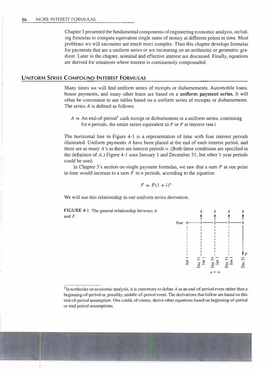
86 MORE INTERESTFORMULAS
Chapter3 presentedthe fundamentalcomponentsof engineeringeconomicanalysis,includ-ing formulas to compute equivalent single sums of money at different points in time. Mostproblems we will encounter are much more complex. Thus this chapter developsformulasfor payments that are a uniform series or are increasing on an arithmetic or geometric gra-dient. Later in the chapter;noilliriaIand effectiveinterest are discussed. Finally,equationsare derived for situations where interest is continuouslycompounded.
UNIFORM SERIES COMPOUND INTERESTFORMULAS
Many times we will find uniform series of receipts or disbursements. Automobile loans,house payments, and many other loans are based on a uniform payment series. It willoften be convenient to use tables based on a uniform series of receipts or disbursements.The series A is definedas follows:
A = An end-of-periodl cash receipt or disbursementin a uniform series, continuingfor n periods, the entire series equivalent to P or F at interest rate i
The horizontal line in Figure 4-1 is a representation of time with four interest periodsillustrated. Uniform payments A have been placed at the end of each interest period, andthere are as many A's as there are interest periods n. (Both these conditions are specifiedinthe definitionof A.) Figure 4-1 uses January 1 and December 31, but other I-year periodscould be used.
In Chapter 3's section on single payment formulas, we saw that a sum P at one pointin time would increase to a sum F in n periods, according to the equation
F = P(1+ it
We will use this relationship in our uniform series derivation.
FIGURE 4-1 The general relationship between AandF.
Year
A A A A
t t t t0-1-2-3-4I I I II I I II I I II I I II I I II I I II I I II I I II I I II I I I
= ~~ ~~ ~~~ 0 ~ 0 ~ 0 ~v v v....
~ ~ ~n=4
F
1In textbooks on economic analysis, it is customary to define A as an end-of-period event rather than a.beginning-of-period or, possibly, middle-of-period event. The derivations that follow are based on thisend-of-period assumption. One could, of course, derive other equations based on beginning-of-periodor mid period assumptions.

Uniform Series Compound Interest Formulas 87
Looking at Figure 4-1, we see that if an amount A is investedat the end of each year for4 years, the total amount F at the end of 4 years will be the sum of the compound amountsof the individual investments.
A A A A A A A A+ + + + + ..q'-- -+ + +
0-1-2-3-4=0-1-2-3-4+0-1-2-3-4+0-1-2-3-4+0-1-2-3-4
1 1 ~ t
F A(l + i)3 + A(l + i)2 + A(l + i) + A
In the general case for n years,
F = A(1 + i)n-l + ... + A(1 + i)3+ A(1 + i)2 + A(1 + i) + A (4-1)
Multiplying Equation (4-1) by (1 + i), we have .
(1 + i)F = A(1 + i)n+ . . . + A(1 + i)4
+ A(1 + i)3+ A(1 + i)2+ A(1 + i) (4-2)
Factoring out A and subtracting Equation 4-1 gives
(4-3)
(4-4)
Solving Equation 4-4 for F gives
[
(1 + i)n - 1
]
.F=A i =A(F/A,z%,n) (4-5)
Thus we have an equation for F when A is known. The term inside the brackets
is called the uniform series compound amount factor and has the notation (F/ A, i, n).
A man deposits $500 in a credit union at the end of each year fot 5 years. The credit union pays5% interest, compoundedannually.At the end of 5 years, immediatelyafter the fifthdeposit,howmuch does the man have in his account?
-- - ----------

88 MORE INTERESTFORMULAS
.....S...bU:JTlON1I c.".,," ...,>~
The diagram on the left shows the situation from the man's point of view; the one on the right,from the credit union's point of view.Either way,-thediagramof the fivedeposits and the desiredcomputationof the future sum F duplicates the situationfor the uniform seriescompound amountformula
F
rA A A A A+ + + + +
0 1--'--2 3--'--4---5
1
0-1-2-3-4-5t t t t tA A A A A
F ;:
[
(1 + on - 1.
]
. .F - A. · i... = A(FIA, z%,n)
where A = $500, n . ..5, i. ...0.05, Funknown. Filling i.11fi1eknownvariable$gives
F . .$500(F IA, 5%, 5) $500(5.526) . $2763
Th~re willbe $2763 in the account followingthefifthdeposih
If Equation4-5 is solvedfor A, we have
[
i
]A-F
- (1 + On- I
= F(AI F, i%, n) (4-6)
where
is called the uniform series sinking fund2 factor and is written as (AI F, i, n).
2A sinking fund is a separate fund into which one makes a unifonn series of money deposits (A) withthe goal of accumulating some desired future sum (F) at a given future point in time.

Uniform Series Compound Interest Formulas 89
Jim Hayes read that out west, a parcel of land could be purchased for $1000 cash. Jim decidedto save a uniform amount at the end of eacn month.sothat he would have the required $1000 atthe end of one year. The local credit union pays 6% interest, compoundedmonthly. How muchwould Jim have to deposit each month?
In this example,
F = $1000 n = 12 A = unknown
A = 1000(AjF, 1/2%,12)= 1000(0.0811) = $81.10=
Jim would have to deposit $81.10 each month.
If we use the sinking fund formula (Equation 4-6) and substitute for F the single paymentcompound amount formula (Equation 3-3), we obtain
[
i
]
n
[
i
]A-F -PI i
- (1 + i)n - 1 - (+) (1 + i)n - 1
[
i(I+i)n
]
.A = P . = P(AjP,I%,n)
(1 + l)n - 1(4-7)
Wenowhavean equationfor determiningthe valueof a seriesof end-of-periodpayments-or disbursements-A when the present sum P is known.
The portion inside the brackets
[
i (1 + i)n
](1 + i)n - 1
is called the uniform.series capital recovery factor and has the notation (Aj P, i, n).
Consider a situation in which you borrow $5000. You will repay the loan in five equal end-of-the-year payments. The first payment is due one year after you receive the loan. Interest on theloan is 8%. What is the size of each of the fivepayments?
- - ... -- .. - - -.. - _ _. J

90 MORE INTERESTFORMULAS
p
rO-1 2~3-4 5
t t t t tA A A A A
I =--
44
~-~~
P = $5000 n=5 i__8% A =unknown
=
Tb;eannualloan paymeQtis $1252.
In Example 4-3, with interest at 8%, a present sum of $5000 is equivalent to five equal.end-of-period disbursementsof $1252. This is another way of stating Plan 3 of Table 3-1.The method for determining the annual payment that would repay $5000 in 5 years with8% interest has now been explained.The calculation is simply
A = 5000(Aj P, 8%, 5) = 5000(0.2505) = $1252
If the capital recovery formula (Equation 4-7) is solved for the present sum P, weobtain the uniform seriespresent worth formula
[
(1 + i)n - 1
]= A(PjA, i%, n)
P = A i (1 + i)n(4-8)
and
[
(1 + i)n - 1
](PjA,i%,n)= i(1+i)n
which is the uniform series present worth factor.
An investor holds a time payment purchase contract on some machine tools. The contract callsfor.the payment of $140 at the end of eactlmonth for a5..yearperiod/I'hefirstpaYmetlt is duein one month..fle offers to sell you the cOlltractfor $6800 cash today.lf you otherwise can make1% per monThon yourmoQey,WqUId.you accept or reject tlJ,ewvestpr's.pffer?
-- - -- ~ -I'1

Uniform Series Compound Interest Formulas 91
n = 60i=1%
p=
'SOlUfflbN,)" ,I.. .,'
In this problem we are being offered a contract that will pay $140 per month for 60 months. Wemust determinewhetherthe contract is worth $6800, if we consider 1% per month to be a suitableinterestrate. Using the uniform series pt:esentworth formula, w~\yill <;;.omgutethepresent worthof the cOntract.
P - A(PjA,i,n) .140(PjA, 1%,60)
= 140(44.955)
= $6293.70
It is clear that if we pay the $6800 asking price for the contract, we wil).receive less than the 1%per month interest we desire. We wi11,therefore,reject the investor's offer.
- .- .~--.-
Suppose we decided to pay the $6800 for the time purchase contract in Example 4-4. Whatmonthly rate of return would we obtain on our investment?
In this situation, we know P,.A, and n, but we do not know i. The problem may be solved byusing either the uniform seriespresent worth formula
P=A(PjA,i,n)
or the uniform series capital recovery formulaI
rI
A=P(AjP,i,n)
Either way, we have one equation with one unknown.
P =$6800 A = $140 n- 60 i - unknown-.. - ..---- - -- --- --.....

92 MORE INTERESTFORMULAS
P = A(P/A,i,n)
$6800 = $140(P/A, i, 60). .~.;... .. ... . ._~ .-
6800(P /A, i, 60) = - = 48.571140
We know the value of the uniform series present worth factor, but we do not know the interestrate i. As a result, we need to look through several compound interest tables and then computethe rate of return i by interpolation. Entering values from the tables in the appendix, we find
(PIA, i, 60)
5L726:lJ48.571.-.J d48.174
The rate of return, which is between 1/2%and %%, may indeed be computedby a linear interpola-tiOh.The interestformulas are not linear, so a linear interpolation will not give an exact solution.To minimize the error, the interpolation should be computed usinginterest rates as close to thecorrect answer as possible. [Since a/b = e/d, a = bee/d)], we write
Rate ofreturn i = 0.5%+ a
= 0.5% + bee/d)
(51.726 - 48.571
)= 0.50%+ 0.25%. 6. 51.72 - 48.174
(3.155
)= 0.50% + 0.25% ~ = 0.50% + 0.22%3.552
= 0.72% per month
The)monthly rate of return on our investmentwould be 0.72% per month.
Using a 15% interest rate, compute the value of F in the followingcash flow:
Year Cash Flow1 + 1002 + 1003 +1004 05 -F
-.. -.... - '

r
Uniform Series Compound Interest Formulas 93
100 100 100
t t t0-1-2-3-4-5
. .. ... . 1F
We see that the cash flow diagram is not the same as the diagram shown in Example 4-1, whichis a sinking fund factor diagram.
A A A
t t t0-1-2---'---3
1F
Since the diagrams do not agree, the problem is more difficult than those We've discussed sofar. The general approach to use in this situation is to convert the cash flow fronl its presentform into standard forms, for which we have compoundinterest factors and compound interesttables.
On~way to solve this problem is to consider the cash flow as a series of single paYJ:l1entsPand thet}to compute their sum F. In other words, the cash flow is bJ;okeninto three parts, eachIJ, . ,
one of Whichwe can solve."
100 100 100
t t t0 1)-2---,3 4 5=
_w
100
t+ 0 1"--'2.=3~4--.,5
{
. - ,.. ....
F II1"IF W FI + F'z+ F3 .. JOO(FI P,15%, 4) +lQO(f IP, 15%, 3) + 100(F I P, 15%, 2)
= 100(1.749) -I- 100(1.521) + 100(1.322)
$459.20"II
"
The val~~of Fin theilfustrated cash flow is $459.20.- - - ""...- """'"'" -- - 11II...__ ___ _ ___

94 MORE INTERESTFORMULAS
IALTERNATESOLUTION.
100 100 100
t t t0-1-2-3-4-5 -
100 100 100
t t t0-1-2-3-4-5
1
F F
Looked at this way, we first solve for Fl'
FI = 100(F / A, 15%,3) = 100(3.472)= $347.20
Now FI can be considered a present sum P in the diagram
3-4-5
F
and so
F = FI(F/ P, 15%,2)
= 347.20(1.322)
$459.00~
:
]he slightly different value from the preceding computation is due to rounding in the compoundinterest tables.
This has been a two-step solution:
FI = 100(F/ A, 15%,3)
F-:- FI(F/P, 15%,2)I"
I- - .. ---'- -- - ...- - - --. -- ...- -.. -- - --

u + __ n
Uniform Series Compound Interest Formulas 95
One could substitute the value of FI frO!llthe first equation into the second equation and solvefor F, without computing Fl,
,~;;.~ ;;; = =t-~ ;!iI:Ci
F = 100(F lA, 15%,3)(P I P, 15%,2)
= 100(3.472)(1.322)
= $459.00
Consider the following situation:
30
t t t0~1-2-3-4
1
i = 15%
p
The diagramis not in a standardform, indicating that there will be a multiple-stepsolution.Thereare at least three differentways of computingthe answer.(It is important that you understandhowthe three computations are made, so please study all three solutions.)
,:- - -"-- j
SOLUfflON 1.
P = PI + P2 + P3
= 20(P I F, 15%,2) + 30(P I F, 15%,3) + 20(P I F, 15%,4)::; ~ ~:;:; :: ~
= 20(0.7561) + 30(0.6575) + 20(0.5718)
- $46.28
30
W t wP = 0-1-1-3'--4 + 0 ,--1-2'--3'--4 + 0-1-2-3-1
!; ! ~
- -- - ---- -- ----- - - - -..------

96 MORE INTERESTFORMULAS
!SOlUTION 230
t. t 2;0-1-2-3-4
1 1P F
The relationship between P and F in the diagram is
P = F(PjF, 15%,4)
Next we compute the future sums of the three payments, as follows:
30
t t tF = 0-1-2-3-4 + 0-1-2-3-4 + 0-1-2-3-4
t t 2t
F = FI + F2+ 20
- 20(Fj P, 15%,2)+ 30(Fj P, 15%,1) + 20
Combining the two equations, we have
P = [FI + F2+ 20](Pj F, 15%,4)
= [20(Fj P, 15%,2) + 30(Fj P, 15%, 1) + 20](P j F, 15%,4)
= [20(1.322) + 30(1.150) + 20](0.5718)
= $46.28
:..f ;..'~.'.'.._ ",."_",,,"~~"-'_"..',_H"'_' ,:, ,.- ~
...SOlUJ}Q~[3.='
30
Y t Y0-1-2-3-4
~ ~P PI
30
Y t Y Y Y Y ~1-2-3-4 = 1-2-3-4 + 1-2-3-4
tt ~ =
PI
P = PI (PjF, 15%, 1) PI = 20(P j A, 15%,3) + lO(Pj F, 15%,2)-- .. ..-

-- - --- --- ----
Relationships Between Compound Interest Factors 97
Combining, we have
P - [20(P I A, 15%,3) + 10(PIF, 15%,2)](P I F, 15%, 1). . -.. . '~- -
= [20(2.283) + 10(0.7561)](0.8696)
= $46.28=--
RELATIONSHIPS BETWEEN COMPOUND INTEREST FACTORS
From the derivations,we see there are several simple relationshipsbetween the compoundinterest factors. They are summarizedhere.
Single Payment1
Compoundamount factor = Present worth factor
1
(FIP,i,n) = (PIF,i,n)(4-9)
Uniform Series
. 1Capital recovery factor = Present worth factor
1
(AIP,i,n) = (PIA,i,n)
1
Compoundamount factor = Sinking fund factor1
(F I A, i, n) = (AI F, i, n)
(4-10)
(4-11)
The uniform series present worth factor is simply the sum of the n terms of the singlepayment present worth factor
n
(PIA,i,n) = L(PIF,i, J)1=1
(4-12)
For example:
(P IA, 5%, 4) = (PI F, 5%, 1) + (PI F, 5%, 2) + (PI F, 5%,3) + (PI F, 5%, 4)
3.546 = 0.9524 + 0.9070 + 0.8638 + 0.8227

98 MORE INTERESTFORMULAS
TJIeuniform series compound amount factor equals 1plus the sum of (n - 1) terms ofthe single payment compound amount factor
n-l
(FfA;i;n) = 1+ L (F I P, i, J)J=1
(4-13)
For example,
(FIA,5%,4) = 1+(FIP,5%,I)+(FIP,5%,2)+(FIP,5%,3)
4.310 = 1 + 1.050 + 1.102 + 1.158
The uniform seriescapital recoveryfactor equals the uniform series sinkingfund factorplus i:
(AIP,i,n) = (AIF,i,n)+i (4-14)
For example,
(AI P, 5%, 4) = (AI F, 5%, 4) + 0.05
0.2820 = 0.2320 + 0.05
This may be proved as follows:
(AIP,i,n) = (AIF,i,n)+i
[
i (1 + i)n
] [
1
]
.
(1 + i)n - 1 = (1 + i)n - 1 + l
Multiply by (1 + i)n - 1 to get
ARITHMETIC GRADIENT
It frequently happens that the cash flowseries is not of constant amount A. Instead, there isa uniformly increasing series as shown:
t0-1-2-3-4-5
t
1 r r

r
Arithmetic Gradient 99
Cash flows of this form may be resolved into two components:
A+4G
A + 2GA+
r
3G 4
r
G_.- . -". 3GA+G
A A A A A 2Gi t 1 . t t t t t 0 ~ t ,
r-l-Z-3-4-S =r-l-Z-3-4-S + 1-I-Z-3-4-Sp
Note that by resolving the problem in this manner, the first cash flow in the arithmeticgradient series becomeszero. This is done so that G is the change from period to period,and because the gradient (G) series normally is used along with a uniform series (A). Wealready have an equationfor P', and we need to derive an equation for P". In this way,wewill be able to write
P = P' + p" = A(P/A, i, n) + G(PfG, i, n)
Derivation of Arithmetic Gradient Factors
The arithmeticgradientis a series of increasing cash flowsas follows:
(n- })G
(n - 2)G
2G
ro X tO-}-2-3~n -}-n
NOdune~O~ !The arithmeticgradientseriesmay be thought of as a series of individualcash flows:
(n- })G
2G
X t
0-I-Z-3-+-n-l-t + 0-I-z-3-+-n-1-1 + +Fn
(n - 2)G
iO-}-2-3-+-n-}-n + O-}-2-3-+-n-}-n
1Fill
The value of F for the sum of the cash flows= FI + Fn + . . . + Fill+ FlY, or
F =G(1+ i)n-2+ 2G(1+ i)n-3+... + (n - 2)(G)(1+ i) 1+ (n - l)G (4-15)

100 MORE INTERESTFORMULAS
Multiply Equation 4-15 by (1 + i) andfactor out G, or
(1+ i)F = G[(1+ i)n-l + 2(1+ i)n-2 +.". + (n - 2)(1+ i)2 + (n -1)(1 + i)l] (4-16)
Rewrite Equation 4-15 to'show other-terms in the series,
F = G[(1+ i)n-2+ ". " + (n - 3)(1 + i)2 + (n - 2)(1 + i)1 + n - 1] (4-17)
SubtractingEquation 4-17 from Equation 4-16, we obtain
F + iF - F = G[(1 + it-1 + (1+ i)n-2 + ." .+ (1+ i)2 + (1+ i)1 + 1]- nG (4-18)
In the derivation of Equation 4-5, the terms inside the brackets of Equation 4-18 were shownto equal the series compoundamount factor:
(1 + ")n 1[(1 + i)n-l + (1 + i)n-2 + .". + (1+ i)2+ (1+ i)1+ 1]= 1.-
I
Thus, Equation4-18 becomes
.
[
(1 +i)n -1
]IF = G - nG
i
Rearranging and solving for F, we write
F = ~ [(1+ir - 1 - n](4-19)
Multiplying Equation 4-19 by the single payment present worth factor gives
P = G[(1 + i)n - 1 _n
] [
1
]i i (1 + i)n
= G[
(1 + i)n - in - 1
]i2(1 + i)n
[
(1+i)n-in-1
](PjG,i,n)= i2(1+i)n(4-20)
Equation4-20 is the arithmetic gradient present worth factor. MultiplyingEquation4-19by the sinking fund factor, we have
A = G[(1+ i)n - 1 _ n
] [
i
]= G [
(1 + i)n - in - 1]i i (1 + i)n - 1 i (1 + i)n - i
.[
(1+ i)n - in - 1] [
In
](AjG,I,n) = i(l +i)n -i = i - (1 +i)n -1(4-21) .
Equation 4-21 is the arithmetic gradient uniform series factor.

Arithmetic Gradient 101
A man has purchased a new automobile. He wishes to set aside enough money in a bank accountto pay the maintenanceon the car for the firstS years-.-Ithas been estimated that the maintenancecost of an automobile is as follows:
Year12345
Maintenance Cost$120
150180210240
Assume the maintenance costs occur at the end of each year and that the bank pays 5% interest.How much should the car owner deposit in the bank now?
SOLU)"ION
210240
0-1-2-3-4-5
tp
The cash flowmay be broken into its two components:240
210180
6030 to !
0-1-2-3-4-5 = 0-1-2~3 4-5 + 0-1-2 ,;:;-3~4-5
1 t A~120 1
150
If"1
120 120 120 120 120
r r r r r
G::; 30
p
Both components represent cash flows for which compound interest factors have been derived. Thefirst is a uniform series present worth, and the second is an arithmetic gradient seriespresent worth:
P = A(P j A, 5%, 5) + G(I' jG, 5%,5)--- - .

102 MORE INTERESTFORMULAS
Note that the value of n in the gradient factor is 5, not 4. In deriving the gradient factor, we had(n - 1) terms containing G. Here there are four terms containing G.
Thus,(n - 1) =4, son = 5.
P = 120(P j A, 5%, 5) + 30(P jG, 5%" 5)
= 120(4.329) + 30(8.237)
= 519+247
= $766
He ~houlddeposit $766 in the bank now.,."'-.."" =..-.~
On a certain piece of machinery, it is estimated that the maintenance expense will be as follows:
Year1234
Maintenance$100
200300400
What is the equivalent uniform annual maintenance cost for the machinery if 6% interest isused?
SOLUTION
400
It T r [0-1-2-3-4
! ! ! !Ao AA A,=
" IThe first cash flow in the arithmetic gradient series is zero, hence the diagram is not in properfOffilJorthe arithmeticgradientequation.Asin.Example4-8, the cash flpwmust beresolved into
-- ------- -- -- -- -- - ---

Arithmetic Gradient 103
two components:
,100
t0~1--'-'---'-2---'---3~4
200
t
400
TI200
t
300
J
A = 100 + 100(Aj G, 6%, 4)= 100+ 100(1.427) . .'$242.70
:: .;;;, :iiiiii ~ -",.,,-~ J, iII!! ...~:;;~
The equiyalentunifonn annualmafntenan,ceCosti$$242.70.:.0-_ -.-- .-
A textile mill in India installed a number of new looms. It is expected that initial maintenancecosts and expenses for repairs will be high but will then decline for several years. The projectedcost is:
Maintenance and
Year Repair Costs (rupees)1 24,0002 18,0003 12,0004 6,000
What is the projected equivalent annual maintenance and ,repair cost if interest is 1O%?
=
The projecte~fcashflowis not in the fonn of the arithmeticgradientfactors.Both factorswerederived for an increasing gradient overtime. The factors cannot be uSeddirectlyfor a decpning
;II..I

104 MORE INTERESTFORMULAS
gradient. Instead, we will subtract an increasing gradient from an assumed uniform series ofpayments.
6000
o t0-1-2-3-4 - 0-1-2-3-4
24'
[
000 18,000
i
12,000
t 60;0= 0-1-2-3-4
1 1 1 1A' A' A' A'
A' = 24,000- 6000(AjG, 10%,4)
=,24,000 -- 6000(1.38t)
= 15,714 rupees
The projected equivalentuniform maintenanceand repair cost is 15,714rupees per year.oS
Compute the value of P in the diagram. Use a 10% interest rate.
150
50
o t0-1-2-3-4-5~6
100
r
p
~.,,_. "'.-; ",
SptlJ11()~' ,.IWith the arithmeticgradient series present worth factor, we can compute a present sum J.
'- -- --------- - - -- - - - -- --

Geometric Gradient 105
150
50
o t0 -l-- --- -2-3-4 5 6
1 !p J
100
r
It is important that you closely examine the location of J .Based on the way the factor wasderived,therewillbe onezerovalu~in thegradientserjesto therightof J " (If this seems strangeor incorr~ct,review the beginning of this section on arithmetic gradients.)
J - G(PIG, i, n)
= 50(PI G, 10%,4) (Note: 3 would be incorrect.)
== 50(4.378) . · 218.90
Then
P .. J(P IF, 10%,2)
To o1;>tainthe present worth of theft.1turesum J, use tbe (PIF,'i, n) factor. Combining, wehave
[I
P = 50(P IG, 10%, 4)(P I}?, 10%,2)
.. 50(4.378)(0.8264)' $180.90"
The value of Pis $1.80.90.
GEOMETRIC GRADIENT
In the precedingsection, we sawthat the arithmeticgradientis applicablewhere the period-by-periodchangein acashreceiptor paymentis auniformamount.There areother situationswhere the period-by-period change is a uniform rate, g. For example, if the maintenancecosts for an automobileare $100 the firstyear and they increaseat a uniformrate, g, of 10%per year, the cash flow for the first 5 years would be as follows:
Year Cash Flow1 100.00 - $100.002 100.00 + 10%(100.00) = 100(1 + 0.10)1 - 110.00 . I3 110.00+ 10%(110.00)= 100(1+ 0.10)2 - 121.004 121.00 + 10%(121.00) = 100(1 + 0.10)3 - 133.105 133.10 + 10%(133.10) = 100(1+ 0.10)4 - 146.41

106 MORE INTERESTFORMULAS
0-1-2-3-4-5
:..00 ----1.00 - _
110.00---_121.00-----....133.10-.......
146.41'
From the table, we can see that the maintenancecost in any year is
$100(1 + gt-1
Stated in a more general form,
(4-22) .
where g =uniform rate of cash flowincrease/decreasefrom periodto period, that is, the geometricgradient
Al =value of cash flow at Year 1 ($100 in the example)An =value of cash flow at any Year n
Since the present worth Pnof any cash flow An at interest rate i is
(4-23)
we can ~ubstituteEquation 4-22 into Equation 4-23 to get
This may be rewritten as
P =A1(1 +0-1 t (1 +~ )X-l
x=1 1+ l
(4-24)
The present worth of the entiregradient seriesof cash flowsmay be obtainedby expanding .
Equation 4-24:
P = A1(1 +0-1 t (1 +~ )X-l
x=1 1+ l
(4-25)

,.
Geometric Gradient 107
:
A A3A 2 __ --;---r--- f
O-1-2-3-..t---n-l-n
Ip
In the general case, where i =fg, Equation 4-24 may be written out as follows:
P = Al (1 + i)n-I + Al (1 + i)-I (~::) + Al (1 + i)-I (~::) 2
(1+
)n-I
+ . . . + Al(1+ i)-I 1+ : ,
Let a = Al (1 + i)-I and b = (1 + g)/(1 + i). Equation 4-26 becomes
P = a + ab + ab2 + . . . + abn-I
Multiply Equation 4-27 by b:
bP = ab + ab2 + ab3 + . . . + abn-I + abn
Subtract Equation 4-28 from Equation 4-27:
P - bP = a - abn
P(1 - b) = a(1 - bn)
a(1 - bn)P=I-b
Replacing the original values for a and b, we obtain:
where i =f g.
(4-26)
(4-27)
(4-28)
(4-29)

108 MORE INTERESTFORMULAS
The expressionin the bracketsof Equation4-29 is the geometric series present worthfactor where i =J g.
(PIA, g, i,-it) ...
[1 ~-(1 +.g)n(1 + i)-n
]z-gwhere i =Jg (4-30)
In the special case of i = g, Equation4-29 becomes
(PIA,g,i,n) = [n(1+ i)-I] where i = g (4-31)
The first-yearmaintenancecost for a new automobileis estimated to be $100, and it increases ata uniform rate of 10% per year. Using an 8% interest rate, calculate the present worth of cost ofthe first 5 years of maintenance.
STEP-BY-STEPSOLUTION,
PWofMaintenance
$ 92.5994.3096.0597.8399.65
$480.42
III iiiI ::=;'
P = Al[1 - (1 +. g)n(1 + i)-n
]. Z - gwhere i =Jg
= 100.00[
1 - (1.10)5(1.08)-5
]= $480.42
-0.02
IIIII.The present worth of cost of maintenancefor the first 5 years is $480.42.
MaintenanceYear n Cost (P / F, 8%, n)
1 100.00 = 100.00 x 0.9259 =2 100.00+ 10%(100.00) = 110.00 x 0.8573 =3 110.00+ 10%(110.00) = 121.00 x 0.7938 =4 121.00+ 10%(121.00) = 133.10 x 0.7350 =5 133.10+ 10%(133.10) = 146.41 x 0.6806 =

Nominal and Effective Interest 109
NOMINAL AND EFFECTIVE INTEREST
Consider the situationof a person depositing $100 into a bank that pays 5%interest, compoundedsemiannually.How much would be in the savings account at the end of one year?
. SOlU~tO~n
Fivepercent interest, compoundedsemiannually,means that the bank pays 21/2%every6 months.Thus, the initial amount P =$100 wouldbe creditedwith 0.025(100) =$2.50interest at the endof 6 months, or
P --* P + Pi = 100+ 100(0.025) = 100 + 2.50 = $102.50
The $102.50 is left in the savings account; at the end of the second 6-month period, the interestearned is 0.025(102.50) = $2.56, for a total in the account at the end of one year of 102.50 +2.56 = $105.06, or
(P + Pi) --* (P + Pi) + i(P + Pi) = P(1 + i)2 = 100(1+ 0.025)2
= $105.06
Nominal interest rate per year, r, is the annual interest rate without considering theeffect of any compounding.
In the example, the bank pays 21/2%interest every 6 months.The nominal interest rate peryear, r, therefore, is 2 x 21h%= 5%.
Effective interest rate per year, ia, is the annual interest rate taking into account theeffect of any compoundingduring the year.
In Example 4-13 we saw that $100 left in the savings account for one year increased to$105.06, so the interest paid was $5.06. The effective interest rate per year, ia, is $5.06/$100.00 = 0.0506 = 5.06%.
r = Nominal in~erestrate per interest period (usually one year)
i = Effective interest rate per interest period
ia = Effectiveinterest rate per year
m = Number of compounding subperiods per time period
Using the method presented in Example 4-13, we can derivethe equation for the effectiveinterest rate. If a $1 deposit were made to an account that compounded interest m times

110 MORE INTERESTFORMULAS
per year and paid a nominal interest rate per year, r, the interest rate per compoundingsubperiodwould be r/ m, and the total in the account at the end of one year would be
. $t(1 +:)m orsimply (1 + :)m
If we deduct the $1 principal sum, the expressionwould be
Therefore,
Effective interest rate per year (4-32)
where r = nominal interest rate per yearm =numberof compoundingsubperiodsperyear
Or, substitutingthe effectiveinterest rate per compounding subperiod, i = (r/m),
Effective interest rate per year (4-33)
where i = effectiveinterest rate per compoundingsubperiodm =number of compoundingsubperiodsper year
Either Equation4-32 or 4-33 may be used to compute an effectiveinterest rate per year.Oneshouldnote that i was describedin Chapter3 simplyas the interestrate per interest
period. We were describing the effective interest rate without maldng any fuss about it.A more precise definition,we now know, is that i is the effective interest rate per interestperiod. Although it seems more complicated, we are describing the same exact situation,but with more care.
Thenominalinterestrate r is often givenfor a one-yearperiod (but it couldbe givenforeither a shorter or a longer time period). In the specialcase of a nominal interest rate that isgiven per compoundingsubperiod, the effectiveinterest rate per compounding subperiod,i, equalsthe nominal interest rate per subperiod,r.
In thetypicaleffectiveinterestcomputation,therearemultiplecompoundingsubperiods(m> 1). The resulting effective interest rate is either the solution to the problem .or anintermediatesolution,whichallowsus to use standardcompoundinterestfactors to proceedto solvethe problem.
For continuous compounding (which is described in the next section),
Effective interest rate per year (4-34)

- - '-,- -_. .. --'..
Nominal and EffectiveInterest 111
If a savingsbank pays 11/2%interest every 3 months, what are the nominal and effectiveinterestrates per year?
Nominal interest rate per year r = 4 x 11/2%= 6%
Effective interest rate per year ia = (1+:) m - 1
(0.06
)4
= 1 + "4 - 1 = 0.061
=6.1%
Alternately,
Effective interest rate per year ia = (1 + i)m - 1
= (1 + 0.015)4 - 1 = 0.061
=6.1%
Table4-1 tabulates the effective interest rate for a range of compoundingfrequenciesandnominalinterestrates. It shouldbe notedthatwhenanominalinterestrate iscompoundedI
TABLE 4-1 Nominal and Effective Interest
Nominal Interest EffectiveInterest Rate per Year,i/l WhenRate per Year Nominal Rate Is Compounded
r (%) Yearly Semiannually Monthly Daily Continuously
1 1.0000% 1.0025% 1.0046% 1.0050% 1.0050%2 2.0000 2.0100 2.0184 2.0201 2.02013 3.0000 3.0225 3.0416 3.0453 3.04554 4.0000 4.0400 4.0742 4.0809 4.08115 5.0000 5.0625 5.1162 5.1268 5.12716 6.0000 6.0900 6.1678 6.1831 6.18378 8.0000 8.1600 8.3000 8.3278 8.3287
10 10.0000 10.2500 10.4713 10.5156 10.517115 15.0000 15.5625 16.0755 16.1798 16.183425 25.0000 26.5625 28.0732 28.3916 28.4025

-~ ----------------- -------------
112 MORE INTERESTFORMULAS
annually, the nominal interest rate equals the effective interest rate. Also, it will be notedthatincreasingthe frequencyof compounding(for example,from monthly to continuously)hasonly a small impact on the effective interest rate.But if the amountof money is large,evensmall differencesin the effective interest rate canbe significant.
A loan sharklendsmoney on the following terms: "If I give you $50 on Monday, you owe me$60 on the following Monday."
(a) What nominal interest rateper year (r) is the loan sharkcharging?(b) What effectiveinterest rateper year (ia)is he charging?(c) If the loan shark started with $50 and was able to keep it, as well as all the money he
received,out in loans at all times, how much money would he have at the end of oneyear?
F = P(FjP, i, n)
60 = 50(F j P, i, 1)
(FjP, i, 1) = 1.2
Therefore, i = 20% per week.
Nominal interest rate per year = 52 weeks x 0.20 = 10.40 = 1040%
Effective interest rate per year ia = (1 + ~) m - 1
(10.40
)52
= 1+ 52 - 1 = 13,105- 1
= 13,104- 1,310,400%
Or
Effectiveinterest rate per year ia = (1 + i)m ~ 1
I
- (1 + 0.20)52- 1 = 13,104
- 1,310,400%
I-II'
-- - - - -- .. - ...--- - --- - ..---II
__ _ ~...J
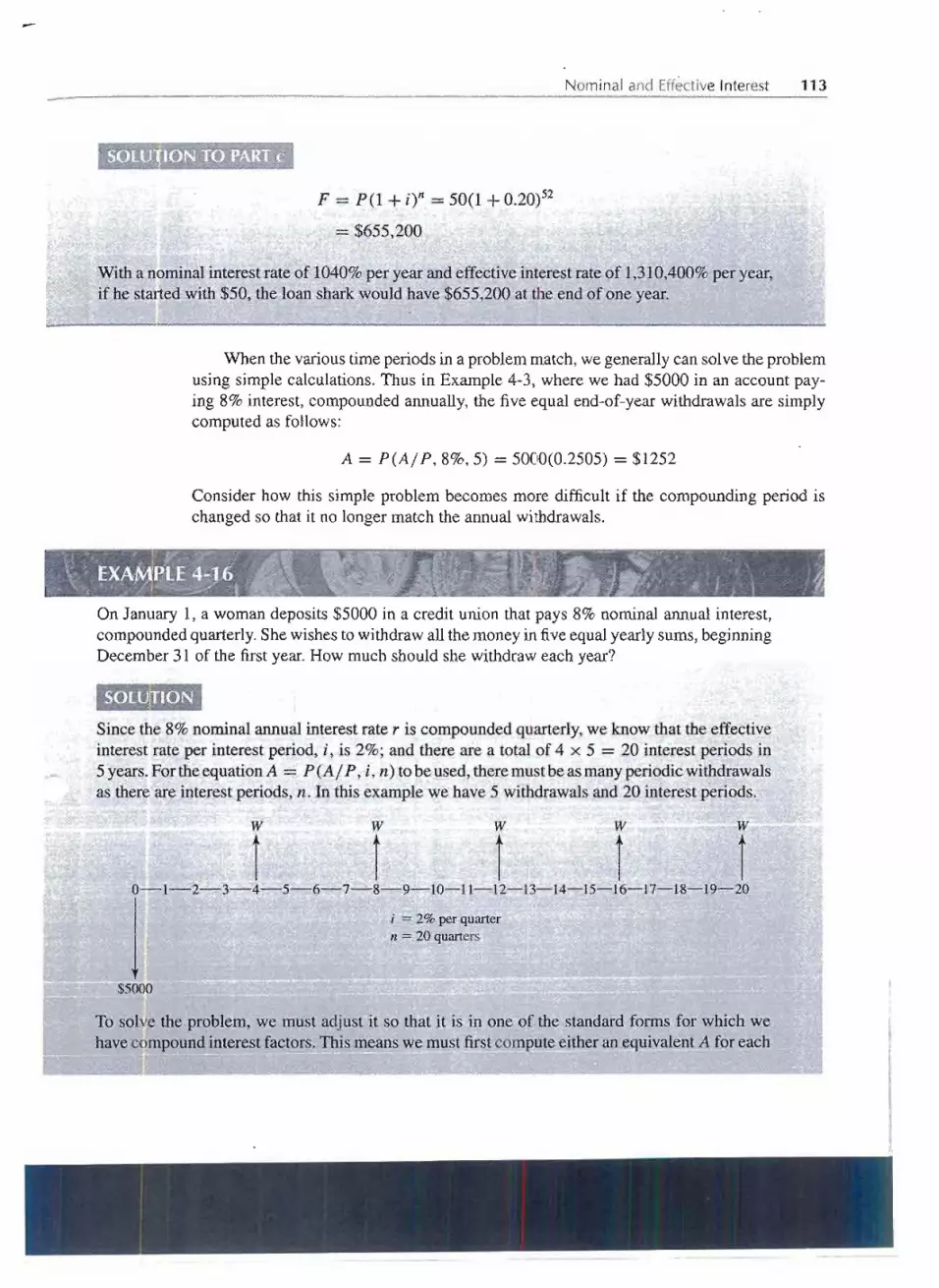
Nominal and Effective Interest 113
F = P (1 + i)n = 50(1 + 0.20)52
= $655,200
Witha nominal interest rate of 1040%per year and effectiveinterest rate of 1,310,400%per year,ifhe started with $50, the loan shark would have $655,200 at the end of one year.
When the varioustime periods in a problem match,we generallycan solve the problemusing simple calculations. Thus in Example 4-3, where we had $5000 in an account pay-ing 8% interest, compounded annually, the five equal end-of-year withdrawals are simplycomputed as follows:
A = P(Aj P, 8%, 5) = 5000(0.2505) = $1252
Consider how this simple problem becomes more difficult if the compounding period ischanged so that it no longer match the annual withdrawals.
T::::f-~It....'
.. ..' ...'ff"'H. ..
..1.
....
.
.
'.0 ,.0,. .' ." .
:l"""" J; "'. . " vi,
II. ~ ,,-": " I; .J\'. ' ~~..
On January 1, a woman deposits $5000 in a'credit union that pays 8% nominal annual interest,compoundedquarterly.She wishesto withdrawall the moneyin fiveequalyearly sums,beginningDecember 31 of the firstyear. How much should she withdraw each year?
SOlUjTlON
Since the 8% nominal annual interest rate r is compoundedquarterly,we know that the effectiveinterest rate per interest period, i, is 2%; and there are a total of 4 x 5 = 20 interest periods in5 years. For the equation A = P (A j P, i, n) to be used, there must be as many periodic withdrawalsas there'are interest periods, n. In this example we have 5 withdrawalsand 20 interest periods.
w
f
w
f
w
f
w
f
w
f0---1---2---3---4---5---6---7---8---9--10--11--12--13--14--15--16--17--18--19--20
1
j = 2% per quartern = 20 quarters
$5000
To solve the problem, we must adjust it so that it is in one of the standard forms for which wehavecompoundinterest factors.This meanswe must firstcomp;pt~either an equivalentA.{oreach _== = ~;;:. - :;: ~ C! ~ ~ ;; = = a~ -. - - ..
~---- - -- -- -.. - --

- - -- - -- ------ - -- - -- ----
114 MORE INTEREST FORMULAS
3-month interest period or an effective i for each time period between withdrawals.Let's solvethe problem both ways.
Compute an equivalent A for each 3-month time period.If we had been required to compute the amount that could be withdrawn quarterly, the diagramwould be as follows:"
AAAAAAAAA A A A A A A A A A A A
iiiiii i i i i i i i i i i i i i i0-1-2-3-4-5-6-7-8-9-10-11-12-13-14-15-16-17-18-19-20
1
i = 2% per quartern = 20 quarters
$5000
A = P(AI P, i, n) = 5000(AI P, 2%, 20) = 5000(0.0612) = $306
Now, since we know A, we can construct the diagram that relates it to our desired equivalentannualwithdrawal,W:
1111111111111111111r$3~0-1-2-3-4-5-6-7-8-9-10-11-12-13-14-15-16-17-18-19-20
1 1 1 1 1w w w w w
Looking at a one-year period,
A = $306
i i t i0-1~2~3-4
1- w-
i ==2% per quartern=4 quarters
----- --
W = A(FIA,i,n) .306(FIA,2%,4) 306(4.122)
=,,= 'II ..
.._ ___ iii _ .__

----.------ __ _ _d_ ~ontinuous Gompound~ng 115
~TjF~~Compute an effective i for the time period between withdrawals.Between withdrawals, W, there are four interest periods, hence m =4 compoundingsubperiodsper year.Since the nominal interestrate per year,r, is 8%, we canproceed to compute the effectiveinterest rate per year.
ffi. .
(r
)m
(0.08
)4'
E ectivemterestrateper year ia.= 1+ m - 1 = 1+ 4 - 1
= 0.0824 =8.24% per year
Now the problem may be redrawn as follows:
w w w w w
t t t t t0-1-2-3-4-5
1
i = 8.24% per yearn = 5years
$5000
This diagram may be directly solved to determine the annual withdrawal W using tl),ecapitalrecovery factor:
W = P(AI P, i, n) = 5000(AI P, 8.24%,5) .
=P[
i (1 + i)n
]= 5000
[
0.0824(1 + 0.0824)5
](1 + i)n - 1 (1 + 0...0824)5- 1
= 5000(0.2520) = $1260
The depositor should withdraw $1260 per year.
CONTINUOUS COMPOUNDING
Two variables we have introduced are:
r = Nominal interest rate per interest period
m = Number of compounding subperiodsper time period
Since the interest period is normally one year, the definitionsbecome:
r = Nominal interest rate per year
m = Number of compounding subperiodsper year

116 MORE INTERESTFORMULAS - ! - -- ....-
r- = Interest rate per interest periodm
mn = Number of compounding subperiods in n years
Single Payment Interest Factors: Continuous CompoundingThe single payment compound amount formula (Equation 3-3)
may be rewritten as
If weincreasem, the number of compoundingsubperiodsperyear,withoutlimit,m becomesvery large and approaches infinity,and r/ m becomes very small and approaches zero.
This is the condition of continuous compounding, that is, where the duration of theinterest period decreases from some finite duration D.t to an infinitely small duration dt,and the number of interest periods per year becomesinfinite. In this situationof continuous _
compounding:
F=P lim (1+..c. )mn
m~oo m. (4-35)
An important limit in calculus is:
lim(1 + X)l/x = 2.71828 = ex~o
(4-36)
If wesetx = r / m, then mn may be written as (1/x)(rn). Asm becomesinfinite,x becomesO.Equation 4-35 becomes
F = P[lim(1 + x)l/xynx-+o
Equation4-36 tellsus the quantity insidethe bracketsequalse. So returningto Equation3-3,we find that
F = P(l + it becomes F = Pern (4-37)
and
P = F(1 + i)-n becomes P = Fe-rn (4-38)
We see that for continuous compounding,
or, as shown earlier,
Effective interest rate per year (4.,34)

Continu_ous C~mpounding 117
To find compound amount and present worth for continuous compounding and a singlepayment, we write:
Compoundamount
Presentworth
F = P(ern) = P[F / P, r, n]
P = F(e-rn) = F[P/ F, r, n]
(4-39)
(4-40)
Square brackets around the factors distinguish continuous compounding. If your hand cal-culator does not have eX, use the table of ern and e-rn, provided at the end of the appendixcontaining the compound inter~st tables.
~_$~;~~~~r'~"
If you were to deposit$2000in a bank that pays 5% nominal interest, compoundedcontinuously,how much wouldbe in the account at the end of 2 years?
The single paymentcompoundamountequationfor continuous compounding is
where r = nominalinterest rate = 0.05n =number of years = 2
F = 2000e(O.05)(2) = 2000(1.1052) = $2210.40
There wouldbe $2210.40in the account at the end of 2 years........
---A bank offers to sell savingscertificatesthat will pay the purchaser $5000 at the end of 10yearsbut will pay nothingto the purchaserin the meantime.If interest is computed at 6%, compoundedcontinuously,at what price is the bank sellingthe certificates?
F = $5000 r = 0.06 1'J= 10 years
P= 5000e-O.06xlO= 5000(0.5488) = $2744
TherefQre,the bank is selling the $5000 certificatesfor $2744.
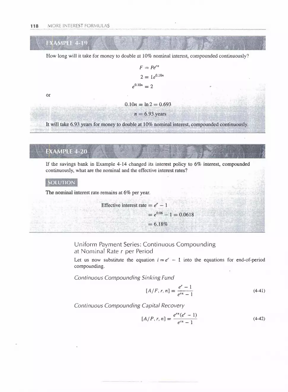
118 MORE INTERESTFORMULAS
I....
9V!)..-~- .:~ <-. .~
How long will it take for money to double at 10% nominal interest, compounded continuously?
F = Pern
2 = 1 eO.IOn
eO.IOn = 2
or
O.lOn = 102 = 0.693
n = 6.93 years
It will take 6.93 years for money to double at 10% noniinal interest, compounded continuously.
If the savings bank in Example 4-14 changed its interest policy to 6% interest, compoundedcontinuously,what are the nominal and the effectiveinterest rates?
- SOLUTION
The nominal interest rate remains at 6% per year.
Effectiveinterest rate = er- 1
= eO.06 - 1 = 0.0618
= 6.18%..:.
Uniform Payment Series: Continuous Compoundingat Nominal Rate r per PeriodLet us now substitute the equation i = er - 1 into the equations for end-of-periodcompounding.
Continuous Compounding Sinking Funder -1
[AI F, r, n] = ern _1 (4-41)
Continuous Compounding Capital Recovery
ern(er - 1)[AlP, r,n]= ern - 1
(4-42)
-- -

Continuous Cpmpounding 119
Continuous Compounding Series Compound Amount
ern - 1[F/A,r,n] = er-l (4-43)
Continuous Compounding Series Present Worth
ern - 1
[P / A, r, n] = ern(er _ 1)(4-44)
In Example 4-1, a II.1andeposited $500 per year into a credit union that paid 5% interest, com-pounded annually. At the end of 5 years, he had $2763 in the credit union. How much would hehave if the institution paid 5% nominal interest, compounded continuously?
SOLUTION. ,., . -. " ' ! ...~..'- '-", .-~;""~~
A = $500 r = 0.05 n = 5 years
(ern _1
) (eOo05(5) - 1
)F=A[F/A,r,n]=A =500 005er - 1 e 0 - 1
= $2769.84
He would have $2769.84.
In Example4-2, Jim Hayes wished to save a uniform amounteach month so he wouldhave $1000at the end of a year. .Based on 6% nominal interest, compounded monthly, he had to deposit$81.10 per month. How much would he have to deposit if his credit union paid 6%.nominalinterest, compounded continuously?'. .. ,.. .,.,....
SOLUTlO~;;
The deposits are made monthly; hence, there are 12 compounding subperiods in the one-year time
period. : =;;;; ~
.. .'. 0.065r= nommal mterest rate/mterest penod = ~ - 0.0012
n = 12 compounding subperiods iQ the one-year geri9PQfJhe PJohl~,n:1.
F =$1000
= ~ ::- - __ _ r........_ ----
-- - -- ----

- -- - - --- - --
120 MORE INTERESTFORMULAS
(er - 1
) (eO.OO5- 1
)A = F[AI F, r, n] = F ern _1 = 1000 eO.OO5(l2)_ 1
= 1000(°.005013
) = $81.070.061837
He would have to deposit $81.07 per month. Note that the differencebetween monthly and con-tinuous compounding is just 3 cents per month.
Continuous, Uniform Cash Flow (One Period) with ContinuousCompounding at Nominal Interest Rate rEquations for a continuous, uniform cash flow during one period only, with contin~ouscompounding, can be derivedas follows. Let the continuous,uniform cash flowtotaling Pbe distributed over m subperiods within one period (n = 1). Thus PI m is the cash flQw atthe
end of each subperiod. Since the nominal interest rate per period is r, the effectiveinterestrate per subperiod is rim. Substituting these values into the uniform series compoundamount equation (Equation 4-5) gives
F = p[
[1 + (rlm)]m - 1
]m rim(4-45)
Setting x = rim, we obtain
F = P[
[1 +xY/x - 1
]= P
[
[(1 +X)l/xy -1
]m rim r(4-46)
As m increases, x approaches zero. Equation 4-36 says
lim(1 + X)l/x = eX °
hence Equation 4-46 for one period becomes
p
LJ' ,. ... .. ,
9F .-
(4-47)
--- - - - - r --

Continuous Compounding 121
MultiplyingEquation4-43 by the singlepayment,continuouscompoundingfactors,we canfind F for any future time and P for any present time.
For Any Future Time
F = 15(er ; 1) (er(n-l» = 15 [.(er -r~;(ern)]
n
F
Compound amount [Fj15, r, n] =[
(er -IHern)
]rer(4-48)
ForAny Present Time
P = F(er - 1.)(e-rn)= F[
er - 1
]r rern
1
p
[
er - 1
]Presentworth [PjF,r,n] = -
rern(4-49) .
A self-service gasoline station has been equipped with an automatic teller machine (ATM).Cus-tomers may obtain gasoline sin!ply byins~rting tpeir ATM bank card into tJ:J.emachine and filling ;::
their tank with gasoline. When they have finished, theATM unit automatically deducts the gasolinepurchaSe from the customer's bank account and credits it to the gas station's bank account. Thega§§Ultionres;ejx~~,,"$40,qOO~etmonth.;inthisJIlanner,,,,,with,thecash flowing"uniformly throughout-- ---' -..-----..-
I"
I1
--- - - --
--- -"1------- --- - -

. ..- -. -....... ...-.
122 MORE INTERESTFORMULAS
th~ month. If the bank pays 9% nominal interest, compounded continuously, how much will bein the gasoline station bank account at the end of the month?
The exampleproblem may be solvedby either Equation4-47 or 4-48. Here the latter, thegeneralequation,is used. "
.."
N.
al.
th0.09
r = omm mterest rate per mon = - = 0.007512
_[
(er _1)(ern) ] [(eO.OO75_ l)(eo.oo 75(1))]F = P =40,000rer 0.0075eo.OO75
= 40000 [(0.0075282)(1.0075282)]= $40 150, 0.00755646 '
p
LJ9
FThere will be $40,150 in the station's bank account.
SPREADSHEETS FOR ECONOMIC ANALYSIS
Spreadsheets are used in most real world applications of engineering economy.Commontasks include the following:
1. Constructing tables of cash flows.2. Using annuity functions to calculate a P, F, A, N, or i.3. Using a block function to find the present worth or internal rate of return for a table
of cash flows.4. Making graphs for analysis and convincingpresentations.5. Calculating "what-if' for differentassumed values of problem variables.
Constructing tables of cash flowsrelies mainly on the spreadsheetbasics that are coveredinAppendix A. These basics include using and naming spreadsheet variabl~s,understandingthe difference between absolute and relative addresses when copying a formula, and for-matting a cell. Appendix A uses the example of the amortization schedule shown in Table3-1, Plan 3. This amortizationscheduledivideseach scheduledloan payment into principaland interest and includes the outstandingbalance for each period. .
Becausespreadsheetfunctionscan be foundthroughpointingandclickingonmenus,those steps are not detailed. In Excel the startingpoint is the Ix button. Excel functionsareused here, but there are only minor syntaxdifferencesfor most other spreadsheetprograms.
Spreadsheet Annuity FunctionsIn tables of engineeringeconomyfactors, i is the table, n is the row,and two of P, F, A, andG definea column.The spreadsheetannuityfunctions list four argumentschosenfrom n, A,P, F, and i, and solve for the fifthargument.The Typeargument is optional. If it is omittedor 0, then the A value is assumed to be the end-of-periodcash flow.If the A valuerepresentsthe beginning-of-periodcash flow,then a value of 1 can be entered for the Type variable.
- - - - - - - --- - - - --- -

. . -- - --._._-- ---
Spreadsheets for Economic Analysis 123
To find the equivalent PTo find the equivalent ATo find the equivalent FTo find nTo find i
-PV(i,n,A,F,Type)-PMT(i,n,P,F,Type)- FV(i ,n,A,P ,Type)NPER(i ,A,P ,F,Type)RATE(n,A,P ,F,Type,guess)
The sign conventionfor the first three functions seems odd to some students. The PVof $200 per period for 10periods is negative and the PV of -$200 p.erperiod is positive.So a minus sign is inserted to find the equivalent P, A, or F. Without this minus sign, thecalculated value is not equivalent to the four given values.
A new engineer wants to save money for down payment on a house. The initial deposit is $685,and $375 is deposited at the end of each month. The savings account earns interest at an annualnominal rate of 6% with monthly compounding.How much is on deposit after 48 months?
Because deposits are made monthly, the nominal annual interest rate of 6% must be converteqto1/2%per month for the 48 months. Thus we must find F if i = 0.5% = 0.005, n = 48, A = 375,and P . .. 685. Note both the initial and periodic deposits are positive cash flows for the savingsaccount. The Excel function is multiplied by-lor -FV(0.005,48,375,685,0), and the result is$21,156.97.
A new engineer buys a car with 0% down financing from the dealer. The cost with all taxes,registration,and license fees is $15,732. If each of the 48 monthly paymentsis $398, what is themonthly interest rate? What is the effective annual interest rate?- . . -'. ." . -- .~ - ". ".-
SOlUTION~:;.. -.' '-..~ ' ::. I . -~ :.:.","--. .., - ..-, '
The RATE function can be used to find the monthly interest rate.. given that n = 48, A =-398,P=15,732, and F=O. The Excel function is RATE(48,-398,15732,0) and the resultis 0.822%. The effective annual interest rate is 1.0082212- 1 = 10.33%.
Spreadsheet Block FunctionsCash flows can be specified period-by-period as a block of values. These cash flows areanalyzed by block functions that identify the row or column entries for which a presentworth or an internal rate of return should be calculated. In Excel the two functions areNPV(i,values) and IRR(values,guess).
----- -
T - -- --- -

124 MORE INTERESTFORMULAS
Excel FunctionNPV(i,values)IRR(values,guess);guess argument is optional
Excel's IRR function can be used to findthe interest rate for a loan with irregularpayments(other applications are covered in Chapter 7).
These block functions make different assumptions about the range of years included.For example,NPV(i,values)assumesthat Year0 is NOTincluded,while IRR(values,guess)assumes that Year 0 is included. These functions require that a cash flow be identifiedforeachperiod. Youcannotleavecells blankevenif the cash flowis $0.The cashflowsfor 1tonare assumed to be end-of-period flows. All periods are assumed to be the same length of time. .
Also the NPV functions returns the present worth equivalent to the cash flows,unlikethe PV annuity function, which returns the negative of the equivalentvalue.
For cash flowsinvolvingonlyconstantvaluesof P, F, and A thisblock approachseemsto be inferior to the annuity functions. However,this is a conceptually easy approach formore complicated cash flows,such as arithmetic gradients. Suppose the years {row 1) andthe cash flows (row 2) are specifiedin columns B through E.
Economic Criteria
Net present valueInternal rate of return
Values for Periods1to nOto n
A B C D E F
1
2
If an interest rate of 8% is assumed, then the present worth of the cas~ .flowscan becalculated as =B2+NPV(.08,C2:F2), which equals $4172.95. This is the present worth
equivalent to the five cash flows, rather than the negative of the.present worth equivalentreturnedby the PV annuityfunction.The internal rate of return calculatedusing IRR(B2:F2)is 14.5%.Notice how the NPV function does not include the Year0 cash flow in B2, whilethe IRR function does.
· PW = B2+NPV(.08,C2:F2)· IRR = IRR(B2:F2)
NPV range without Year qIRR range with Year0 .
-Using Spreadsheets for Basic GraphingOften we are interested in the relationship between two variables. Examples include thenumber and size of payments to repay a loan, the present worth of an M.S. degree and howlong until we retire, and the interest rate and present worth for a new machine.This kind oftwo-variablerelationship is best shown with a graph.
As we will show in Example4-26, the goal is to place one variable on each axis of thegraph and then plot the relationship. Modem spreadsheets automate most steps <;>fdrawinga graph, so that it is quite easy. However, there are two very similar types of chart, andwe must be careful to choose the xy chart and not the line chart. Both charts measure they variable, but they treat the x variable differently. The xy chart measures the x variable;thus its x value is measured along the x axis. For the line chart, each x value is placed anequal distance along the x axis. Thus x values of 1, 2,4,8 would be spaced evenly,rather
- -
Year 0 1 2 3 4
Cash flow -25,000 6000 8000 10,000 12,000

.Spreadsheets for EconolT,licAnalysis 125
than doubling each distance. The line chart is really designed to plot y values for different, categories,suchaspricesfor modelsof carsor enrollmentsfor differentuniversities.
Drawing an xy plot with Excel is easiest if the table of data lists the x valuesbefore they values.This conventionmakes it easy for Excel to specifyone set of x valuesand severalsets of y values. The block ofxy values is selected,and then the chart tool is selected. Thenthe spreadsheet guides the user through the rest of the steps.
Graph the loan payment as a function of the number of payments for a possible auto loan. Let thenumber of monthly payments vary between 36 and 60. The nominal annual interest rate is 12%,andtheamountborrowedis $18,000..
The spreadsheet table shown in Figure 4-2 is constructed first. Cells AS:B 10 are selected, andthen the Chartwizard icon is selected.The first step is to select anxy (scatter)plot with smoothed
== == = ==- = 'II' = ;
-..- - .. - ---.-'"II I
-- - - - - - --
A B C D E F
1 12% nominal annual interest rate
2 1% monthly interest r-ate3 $18,000 amount borrowed
4 i# Monthly
5 Payments Payment
6 36 $597.86 = PMT($A$2,A6,-$A$3)
7 42 $526.96
8 48 $474.01
9 54 $433.02 ..
10 60 $400.40 I11
12 $600.00
1314 =
CI)
S15
j:I.16 >. $500.00 ---------------- ----------------------------
:217 =
0
18 ::E
19 I ,20 $400.0036 42 48 54 60
. 21 Number.of Payments
22

126 MORE INTERESTFORMULAS
lines, and without markers as the chart type. (The other choices are no lines, straight lines, andadding markers for the data points.) The second step shows us the graph and allows the optionof changing the data cells selected. The third step is for chart options.Here we add titles for thetwo axes and turn off showing the legend. (Since we have only one line in our graph, the legendis not needed. Deleting it leaves more room for the graph.) In the fourth step we choose wherethe chart is placed.
Because xy plots are normally graphed with the origin set to (0, 0), an a~active plot is bestobtained if the minimum and maximum values are changed for each axis. This is done by placingthe mouse cursor over the axis and left-clicking. Handles or small black boxes should appear onthe axis to show that it has been selected. Right-clicking brings up a menu to select format axis.The scale tab allows us to change the minimum and maximum values.
SUMMARY
The.compoundinterest formulasdescribedinthis chapter,along withthose in Chapter3~willbe referred to throughout the rest of the book. It is very important that the reader understandthe concepts presented and how these formulas are used. The following notation i.susedconsistently.
i = effectiveinterest rate per interest period3(stated as a decimal)n = number of interest periodsP = a present sum of moneyF = a future sum of money: the future sum F is an amount, n interest periods
from the present, that is equivalentto P with interest rate iA = an end-of-period cash receipt or disbursementin a uniform series
continuing for n periods; the entire series equivalent to P or F at interest rate iG = uniform period-by-period increase or decrease in cash receipts or
disbursements; the arithmetic gradientg = uniform rate of cash flow increase or decrease from period to period; the
geometric gradient. .r = nominal interest rate per interest period (see footnote 3)ia = effectiveinterestrate per year(annum)m = number of compounding subperiodsper period (see footnote 3)
P, F = amount of money flowing continuouslyand uniformly during a given period
Single Payment Formulas (derived in Chapter 3)Compoundamount:
F = P(1 +i)n = P(FjP,i,n)
3Normally the interest period is one year, but it could be some other period (e.g., quarter, month,semiannual).
._-
- - --- T - - ----

-Summary 127
Present worth:
P = F (1 + i) -n = F (P I F, i, n)
Uniform Series Formulas
Compoundamount:
[
(1 + i)n -1
]= A(FIA, i, n)F=A i
Sinking fund:
Capital recovery:
A = P[
i(1 + i)n
](1 + i)n _1 = P(AI P, i, n)
Present worth:
[
(1 + i)n - 1
]= A (P IA, i, n)
P = A i (1 + i)n
Arithmetic Gradient Formulas
Arithmetic gradient present worth:
.
[
(1 +i)n -in -1
]= G(PIG,i,n)P = G i2(1+ i)n
Arithmetic gradient uniform series:
[
(I+i)n-in-1
] G[
1 n
]G(AIG
.)A-G - -- - l n
- i (1 + i)n - i - i (1 + i)n - 1 - , ,
Geometric Gradient Formulas
Geometric series present worth, where i =I- g:
[
1-(I+g)n(1+i)-n
]=AI(PIA,g,i,n)
P = Al i _ g
Geometric series present worth, where i = g:
P = AI[n(1 + i)-I] = AI(PIA, g, i, n) = AI(PIA, i, i, n)
- - - - ------

128 MORE INTERESTFORMULAS
Single Payment Formulas: Continuous Compoundingat Nominal Rate r per PeriodCompound amount:
F = P(ern) = P[F I P, r, n]
Present worth:
P = F(e-rn) = F[P I F, r, n]
Note that square brackets around the factors are used to distinguish continuous.compounding.
Uniform Payment Series: Continuous Compoundingat Nominal Rate r per PeriodContinuouscompoundingsinkingfund:
[
er-1
]A = F = F[AjF,r,n]ern - 1
COJ,ltinuouscompounding capital recovery:
[
ern(er - 1)
]A = P = P[AIP,r,n]
ern - 1
Continuous compoundingseries compound amount:
[
ern - 1
]F=A =A[FIA,r,n]
. er - 1 .
Continuous compounding series present worth:
[
ern - 1
]P=A =A[PIA,r,n]
ern (er - 1)
Continuous, Uniform Cash Flow (One Period) with ContinuousCompounding at Nominal Interest Rate rCompoundamount
-[
(er - 1Hern)
]= F[F IF, r, n]
F = P rer .
- - - - - --- -----

--- -- --- ---... - _._.. h __..__
Present worth
Problems 129
_
[
er - 1
]
_ _P=F - =F[P/F,r,n]rern
Nominal Interest Rate per Year,rThe annual interest rate without considering the effect of any compoun<:fu.1g.
Effective Interest Rate per Year, iaTheannualinterestrate takingintoaccounttheeffectof anycompoundingduringtheyear.
Effectiveinterestrateper year(periodiccompounding):
or
Effective interest rate per year (continuouscompounding):
PROBLEMS
4-1 Solve diagrams (a)-(c) for the unknowns R, S, andT, assuming a 10% interest rate.
R s(a) (b)
120
90 t3. Y t I
0-1-2-3-4-5
~ ~ ~ ~ ~T T T T T
(c)
(Answers: R = $464.10;S = $218.90;T = $54.30)
ia. er - 1
4-2 For diagrams (a)-(d), compute the unknown values:B, C, V, x, respectively, using the minimum numberof compound interest factors.
100 100 100
f f f0-1-2-3-4-5
!
i=10%n=5
200 200 200 200
r r r r0-1-2-3-4
1
i= 10%
B c(a) (b)
4x
r r
2x10 10 10 10 x
tt t t t +0-1-2-3-4-5 0-1-2-3-4
i=1O%!
I i=1O%t x=?
V 500(c) (d)
,
- -- --- -- ---

130 MORE INTERESTFORMULAS
(Answers: B = $228.13; C = $634; V = $51.05;x = $66.24)
For diagrams (a)-(d), compute the unknown valuesC, A, F, A, respectively.
4-3
75
1
50
2+ t0-1-2-3-4
tC
i = 10%
(a)
A A A A A A
t t t t t t0-1-2-3-4-5-6
t500
(c)F
i = 10%
(b)
120
80 t+0 I I
0-1-2-3-4
i = 10% ~ ~ ~ ~A A A A
(d)
(Answers: C = $109.45; A = $115;F = $276.37;A = $60.78)
4-4 For diagrams (a)-(d), compute the unknown valuesW, X, Y, Z, respectively.
100
7f i50
21 t0-1-2-3-4
1
i = 10%
w(a)
'Ii'.~i!
L....__
200
if 10-1-2-3-4-5
1
i = 10%
x(b)
100 100
1 t 10-1-2-3
1 i ~ 10%y z
(c) (d)
4-5 Compute the value of P in the diagram.
250200
IT T 10-1-2-3
1 i ~ 10%p
(Answer: P = $589.50)
4-6 Use a 10% interest rate to compute the value of X iJthe diagram.
500
TTiT3r0-1-2-3-4-5
1X
4-7 Use a 15% interest rate to compute the value of P iJthe diagram.
300
r 5f r r r0-1-2---=-3-4-5-
1p
.,
---,----
- --

Problems 131
4-8 If i = 12%,what is the value of B in the diagram?
800 800 800
f r r r0-1-2-3-4
1 1 !1.5B
4-9 Compute the value of n for the diagram, assuminga10% interest rate.
A=1
t t t t t.t
0-1-2-'-."-' -2-. -1-1n=?
F = 35.95
4-10 What is the value of n, for this diagram, based on a31/2%interestrate?
A= 50
t t t t t t t t t t0-1-2-3-4-5-6-7-8-9-'" - n
1
n=?
1000
4-11 Compute the value of J for the diagram, assuming a10% interest rate.
100 100 100
r r r0-1-2-3-4-5-6-7-8
! ! !J J J
4-12 Compute the value of C for the diagram, assuming a10% interest rate.
300
If T r0-1-2-3-4-5-6-7-8
~ ~ ~C C C
4-13 If i = 12%,compute G in the diagram.
60
50
40
'f r
20
X t0-1-2-3-4-5-6
~ ~500 500
4-14 Compute the value of D in the diagram.
300
T r100
t0-1-2-3-4-5-6-7-8
~ ~ ~ ~D D D D
i = 10%
4-15 Compute E for the diagram.
300
r T
300
r
200 200
If r If r0-1-2-3-4-5-6-7-8
t tE E
i = 10%
4-16 Using a 10% interest rate, compute B in the diagram.
400
3B
4B
-- - -
--------

132 MORE INTERESTFORMULAS
4-17 Find the value of P for the following cash flowdiagram.
3000
1250
rTT
p=?
4-18 The following cash flow transactions are said to beequivalent in terms of economic desirability at an in-terest rate of 12% compounded annually. Determinethe unknown value A.
750
600
TTIA A A A 150
+ + + + +0-1-2-3-4 = 0-1-2-3-4-5
Cash Flow 1 Cash Flow 2
4-19 Upon the birth of his first child, Dick Jones decided to. establish a savings account to partly pay for his son's
education. He plans to deposit $20 per month in theaccount, beginning when the boy is 13 months old.The savings and loan association has a current inter-est policy of 6% per annum, compounded monthly,paid quarterly. Assuming no change in the interestrate, how much will be in the savings account whenDick's son becomes 16 years old?
4-20 Mary Lavor plans to save money at her bank for usein December. She will deposit $30 a month, begin-ning on March 1and continuing through November 1.She will withdraw all the money on December 1. Ifthe bank pays 1/2% interest each month, how muchmoney will she receive on December 1?
-----..
4-21 Derive an equation to find the end of year future sumF that is equivalent to a series of n beginning-of-yearpayments B at interest rate i. Then use the equationto determine the future sum F equivalent to six Bpayments of $100 at 8% interest.(Answer: F = $792.28)
4-22 If $200 is deposited in a savings account at thebeginning of each of 15 years, and the account drawsinterest at 7% per year, how much will be in the ac-count at the end of 15 years?
4-23 A company deposits $2000 in a bank at the end ofevery year for 10 years. The company makes no de-posits during the subsequent 5 years. If ~e bank pays8% interest, how much would be in the account at endof 15 years?
4-24 How much must be deposited now at 5.25%interest to produce $300 at the end of ~very year for10 years?
4-25 A student wants to have $30,000 at graduation 4 yearsfrom now to buy a new car. His grandfather gave him$10,000 as a high school graduation present. Howmuch must the student sa,\,eeach year if he depositsthe $10,000 today and can earn 12% on both the$10,000 and his earnings in a mutual fund his grand-father recommends?
4-26 A city engineer knows that she will need $25 millionin 3 years to' replace toll booths on a toll road in thecity. Traffic on the road is estimated to be 20 millionvehicles per year. How much per vehicle should thetoll be to cover the cost of the toll booth replacementproject? Interest is 10%. (Simplify your analysis byassuming that the toll receipts are received at the endof each year in a lump sum.)
4-27 Using linear interpolation, determine the value of(P / A, 61/2%,10)from the compoundinteresttables.Compute this same value using the equation. Why dothe values differ?
4-28 A man wants to help provide a college education forhis young daughter. He can afford to invest $600/yrfor the next 4 years, beginning on the girl's fourthbirthday. He wishes to give his daughter $4000 onher 18th, 19th, 20th, and 2Pt birthdays, for a totalof $16,000. Assuming 5% interest, \yhat uniformannual investment will he have to make on the girl's8th through 17th birthdays? (Answer: $792.73)
4-29 How many months will it take to payoff a $525debt, with monthly payments of $15 at the end of
- - -- -- --- ---

Problems 133
each month, if the interest rate is 18%, compounded
monthly? (~nswer: 50 months)
4-30 For how many months, at an interest rate of 1% permonth, does money have to be invested before it willdouble in value?
4-31 A bank recently announced an "instant cash" plan forholders of its bank credit cards. A cardholder mayreceive cash from the bank up to a preset limit (about$500). There is a special charge of 4% made at thetime the "instant cash" is sent to the cardholders. The
debt may be repaid in monthly installments. Eachmonth the bank charges 11/2%on the unpaid balance.The monthly payment, including interest, may be aslittle as $10. Thus, for $150 of "instant cash," an ini-tial charge of $6 is made and added to the balance due.Assume the cardholder makes a monthly payment of$10 (this includes both principal and interest). Howmany months are required to repay the debt? If youranswer includes a fraction of a month, round up tothe next month.
4-32 A man borrowed $500 from a bank on October 15th.
He must repay the loan in 16 equal monthly payments,due on the 15th of each month, beginning November15th. If interest is computed at 1% per month, howmuch must he pay each month? (Answer: $33.95)
4-33 In Table 3-1 in the text, four plans were presentedfor the repayment of $5000 in 5 years with inter-est at 8%. Still another way to repay the $5000would be to make four annual end-of-year paymentsof $1000 each, followed by a final payment at theend of the fifth year. How much would the finalpayment be?
4-34 An engineer borrowed $3000 from the bank, payablein six equal end-of-year payments at 8%. The bankagreed to reduce the interest on the loan if interestrates declined in the United States before the loan
was fully repaid. At the end of 3 years, at the timeof the third payment, the bank agreed to reduce theinterest rate from 8% to 7% on the remaining debt.What was the amount of the equal annual end-of-yearpayments for each of the first 3 years? What was theamount of the equal annual end-of-year payments foreach of the last 3 years?
4-35 A $150bicyclewaspurchasedon December 1with a$15 down payment. The balance is to be paid at therate of $10 at the end of each month, with the firstpayment due on December 31. The last payment maybe some amount less than $10. If interest on the un-
paid balance is computed at 11/2%per month, howmany payments will there be, and what is the amountof the final payment? (Answers: 16 payments; finalpayment: $1.99)
4-36 A companybuysa machinefor $12,000,whichitagrees to pay for in fiveequal annual payments, begin-ning one year after the date of purchase, at an interestrate of 4% per annum. Immediately after the secondpayment, the terms of the agreement are changed toallow the balance due to be paid off in a single pay-ment the next year. What is the final single payment?(Answer: $7778)
4-37 Anengineeringstudentboughtacar at a localusedcarlot. Including tax and insurance, the total price was$3000. He is to pay for the car in 12 equal monthlypayments, beginning with the first payment immedi-ately (in other words, the first payment was the downpayment). Nominal interest on the loan is 12%, com-pounded monthly. After six payments (the down pay-ment plus five additional payments), he decides tosell the car. A buyer agrees to pay a cash amount topayoff the loan in full at the time the next payment isdue and also to pay the engineering student $1000. Ifthere are no penalty charges for thiSearly payment ofthe loan, how much will the car cost the new buyer?
4-38 A realtor sold a house on August 31, 1997, for$150,000 to a buyer in which a 20% down paymentwas made. The buyer took a 15-year mortgage onthe property with an effective interest rate of 8% perannum. The buyer intends to payoff the mortgageowed in yearly payments starting on August 31, 1998.(a) How much of the mortgage will still be owed after
the payment due on August 31,2004, has beenmade?
(b) Solve the same problem by separating the interestand the principal amounts.
4-39 To provide for a college education for his daugh-ter, a man opened an escrow account in which equaldeposits were made. The first deposit was made onJanuary 1, 1981, and the last deposit was made onJanuary 1, 1998. The yearly college expenses includ-ing tuition were estimated to be $8000, for each ofthe 4 years. Assuming the interest rate to be 5.75%,how much did the father have to deposit each year inthe escrow account for the daughter to draw $8000per year for 4 years beginning January 1, 1998?
4-40 Develop a complete amortization table for a loanof $4500, to be paid back in 24 uniform monthly

134 MORE INTERESTFORMULAS
installments, based on an interest rate of 6%.The amortization table must include the followingcolqmn headings:
Payment Number, Principal Owed (begin-ning of period), Interest Owed in EachPeriod, Total Owed (end of each period),Principal Paid in Each Payment, UniformMonthly Payment Amount
You must also show the equations used to calculateeach column of the table. You are encouraged to usespreadsheets. The entire table must be shown.
4-41 Using the loan and payment plan developed in Prob-lem 4-40, determine the month that the final paymentis due, and the amount of the final payment, if $500is paid for payment 8 and $280 is paid for payment10. This problem requires a separate amortizationtable giving the balance due, principal payment, andinterest payment for each period of the loan.
4-42 A couple borrowed $80,000 at 7% to purchase ahouse. The loan is to be repaid in equal monthlypayments over a 30-year period. The first paymentis paid exactly at the end of the first month. Calculatethe interest and principal in the second payment, ifthe second payment is made 33 days after the firstpayment.
4-43 Jim Duggan made an investment of $10,000 in a sav-ings account 10 years ago. This account paid inter-est of 51/2% for the first 4 years and 61/2% interestfor the remaining 6 years. The interest charges werecompounded quarterly. How much is this investmentworth now?
4-44 Consider the cash flow:
Yearo12345
Cash Flow-$100
+50+60+70+80
+140
Which one of the following is correct for this cashflow?
(a) 100 = 50 + lO(AjG, i, 5) + 50(P j F, i, 5)
b 50(PjA, i, 5) + lO(PjG, i, 5) + 50(PjF, i, 5)() 100
= 1(c) 100(Aj P, i, 5) = 50 + lO(AjG, i, 5)(d) None of the equationsare correct.
4-45 Considerthe followingcash flow:
Year Cash Flowo -$P1 + 10002 +8503 +7004 +5505 +4006 . +4007 +4008 +400
Alice was asked to compute the value of P for thecash flowat 8% interest. She wrote three equations:(a) P = 1000(PjA, 8%, 8) -150(PjG, 8%, 8) +
150(P jG, 8%, 4)(P j F, 8%,4)(b) P = 400(P j A, 8%, 8) + 6oo(p j A, 8%, 5)'-
150(P jG, 8%,4)(c) P = 150(P jG, 8%,4) + 850(P j A, 8%,4) +
400(P j A, 8%, 4)(P j F, 8%,4)Which of the equations is correct?
4-46 It is estimated that the maintenance cost on a new car
will be $40 the first year. Each subsequent year, thiscost is expected to increase by $10. How much wouldyou need to set aside when you bought a new car topay all future maintenance costs if you planned tokeep the vehicle for 7 years? Assume interest is 5%per annum. (Answer: $393.76)
4-47 A young engineer wishes to become a millionaire bythe time he is 60 years old. He believes that by care-ful investment he can obtain a 15% rate of return.
He plans to add a uniform sum of money to his in-vestment program each year, beginning on his 20thbirthday and continuing through his 59th birthday.How much money must the engineer set aside in thisproject each year?
4-48 The council members of a small town have decidedthat the earth levee that protects .the town from anearby river should be rebuilt and strengthened. Thetown engineer estimates that the cost of the work atthe end of the first year will be $85,000. He esti-mates that in subsequent years the annual repair costswill decline by $10,000, making the second-year cost$75,000; the third-year $65,000, and s~ forth. Thecouncil members want to know what the equivalentpresent cost is for the first 5 years of repair work ifinterest is 4%. (Answer: $292,870)
4-49 A company expects to install smog control equip-ment on the exhaust of a gasoline engine. The local
T

- -----.-- .... . ...-..---.--
Problems 135
smog control district has agreed to pay to the firm alump sum of money to provide for the first cost of theequipment and maintenance during its lO-year use-fullife. At the end of 10 years the equipment, whichinitially cost $10,000, is valueless. The company andsmog control district have agreed that the followingare reasonable estimates of the end-of-year mainte-nance costs:
Year 12345
$500100125150175
Year6789
10
$200225250275300
4-50
Assuming interest at 6% per year~how much shouldthe smog control district pay to the company nowto provide for the first cost of the equipment and itsmaintenance for 10 years? (Answer: $11,693)
A debt of $5000 can be repaid, with interest at 8%,by the following payments.
Year Payment1 $ 5002 10003 15004 20005 X
The payment at the end of the fifth year is shown asX. How much is X?
A man is purchasing a small garden tractor. Therewill be no maintenance cost during the first 2 yearsbecause the tractor is sold with 2 years free main-tenance. For the third year, the maintenance is esti-mated at $20. In subsequent years the maintenancecost will increase by $20 per year (i.e., fourth-yearmaintenance will be $40, fifth-year $60, etc.). Howmuch would need to be set aside now at 8% interest to
pay the maintenance costs on the tractor for the first6 years of ownership?
Mark Johnson saves a fixed percentage of his salaryat the end of each year. This year he saved $1500. Forthe next 5 years, he expects his salary to increase at an8% annual rate, and he plans to increase his savingsat the same 8% annual rate. He invests his money inthe stock market. Thus there will be six end-of-yearinvestments (the initial $1500 plus five more). Solvethe problem using the geometric gradient factor.(a) How much will the investments be worth at the
end of 6 years if they increase in the stock marketat a 10% annual rate?
4-51
4-52
4-53
(b) How much will Mark have at the end of 6 yearsif his stock market investments increase only at8% annually?
The Macintosh Company has an employee savingsplan that allows every employee to invest up to 5%of his or her annual salary. The money is invested incompany common stock with the company guaran-teeing that the annual return 'rill never be less than8%. Jill was hired at an annual salary of $52,000. Sheimmediately joined the savings plan investing the full5% of her salary each year. If Jill's salary increases atan 8% uniform rate, and she continues to invest 5% ofit each year, what amount of money is she guaranteed.to have at the end of 20 years?
The football coach at a midwestem universitywas given a 5-year employment contract that paid$225,000 the first year, and increased at an 8% tmi-form rate in each subsequent year. At the end of thefirst year's football season, the alumni demanded thatthe coach be fired. The alumni agreed to buy hisremaining years on the contract by paying him the.equivalent present sum, computed using a 12% inter-est rate. How much will the coach receive?
Traffic at a certain intersection is currently 2000 carsper day. A consultant has told the city that trafficis ex-pected to grow at a continuous rate of 5% per year forthe next 4 years. How much traffic will be expectedat the end of 2 years?
A local bank will lend a customer $1000 on a 2-yearcar loan as follows:
4-54
4-55
4-56
Money to pay for carTwo years' interest at 7%: 2 x 0.07 x 1000
$1000140
$1140
114024 monthlypayments= - = $47.5024
4-57
The first payment must be made in 30 days. What isthe nominal annual interest rate the bank is receiving?
A local lending institution advertises the "51-50Club." A person may borrow $2000 and repay $51 forthe next 50 months, beginning 30 days after receivingthe money. Compute the nominal annual interest ratefor this loan. What is the effective interest rate?
A loan company has been advertising on television aplan that allows people to borrow $1000 and makea payment of $10.87 per month. This payment isfor interest only and includes no payment on
4-58
- - ----

-------
136 MORE INTERESTFORMULAS
the principal. What is the nominal annual interest rate 4-68 A student bought a $75 used guitar and agreed to pa:that, they are charging? for it with a single $85 payment at the end of 6 months
4-59 What effective interest rate per annum corresponds Assuming semiannual (every 6 months) compound
to a nominal rate of 12% compounded monthly? ing, what is the nominal annual interest rate? What i:
(Answer: 12.7%) the effective interest rate?
4-60 A woman opened an account in a local store. In 4-69 A firm charges its credit customers 13/4%interest pe
the charge account agreement, the store indicated it month. What is the effective interest rate?
charges 11/2% each month on the unpaid balance. 4-70 A thousand dollars is invested for 7 months at atWhat nominal annual interest rate is being charged? interest rate of 1%. per month. What is the nomiWhat is the effective interest rate? nal interest rate? What is the effective interest rate'
4-61 The Bawl Street Journal costs $206, payable now, (Answers: 12%; 12.7%)
for a 2-year subscription. The newspaper is published 4-71 What interest rate, compounded quarterly, is equiva.252 days per year (5 days per week, except holidays). lent to a 9.31% effective interest rate?
If a 10% nominal annual interest rate, compounded 4-72 If the nominal annual interest rate is 12% com.quarterly,is used: pounded quarterly, what is the effective annual in.(a) What is the effective annual interest rate in this terest rate?
problem? 4-73 A contractor wishes to set up a special fund by male.(b) Compute the equivalent interest rate per 1/252of
'ing uniform semiannual end-of-period deposits fo]a year.20 years. The fund is to provide $10,000 at the enc(c) What is a subscriber's cost per copy of the news-
paper, taking interest into account? of each of the last 5 years of the 20-year period. 1.1.interest is 8%, compounded semiannually, what is the
4-62 Pete Sampras borrows $10,000 to purchase a car. He required semiannual deposit?must repay the loan in 48 equal end-of-period monthly 4-74 What amount will be reqUired to pur<?hase,on a man'payments. Interest is calculated at 1.25% per month.Determine the following: 40th birthday, an annuity to provide him with 30 equaJ
(a) The nominal annual interest rate semiannual payments of $1000 each, the first to be
(b) The effective annual interest rate received on his 50th birthday, if nominal hiterest i
(c) The amount of the monthly payment 4% compounded semiannually?
4-63 Picabo Street borrows $1000. Torepay the amount she4-75 A man decides to deposit $50 in the bank today and
makes 12 equal monthly payments of $90.30. Deter- to make 10 additional deposits every 6 months begin-
mine the following:ning 6 months from now, the first of which will be
(a) The effective monthly interest rate $50 and increasing $10 per deposit after that. A few
(b) The nominal annual interest rate minutes after making the last deposit, he decides to
(c) The effective annual interest rate withdraw all the money deposited. If the bank pays. 6% nominal interest compoUnded semiannually, how
4-64 At the Central Furniture Company, customers who much money will he receive?purchase on credit pay an effective annual interest rate 4-76 A man makes an investment every 3 months at aof 16.1%, based on monthly compounding. What isthe nominal annual interest rate that they pay? nominal annual interest rate of 28%, compounded
quarterly. His first investment was $100, followed4-65 What monthly interest rate is equivalent to an effec- by investments increasing $20 each 3 months. Thus,
tive annual interest rate of 18%? the second investment was $120, the third investment4-66 A bank advertises it pays 7% annual interest, com- $140, and so on. If he continues to make this series of
pounded daily, on savings accounts, provided the investments for a total of 20 years, what will be themoney is left in the account for 4 years. What value of the investments at the end of that time?
effective annual interest rate do they pay? 4-77 A 25-year old engineer is opening an individual retire-4-67 To repay a $1000 loan, a man paid $91.70 at the end ment account (IRA) at a bank. Her goal is to accwnu-
of each month for 12 months. Compute the nominal late $1 million in the account by the time she retiresinterest rate he paid. from work in 40 years. The bank manager estimates

~------
-l-------
Problems 137
she may expect to receive 8% nominal annual inter- was paid on money not in the account for the fullest, compounded quarterly, throughout the 40 years. 3-month period. How much was in Ann's account atThe engineer believes her income will increase at a the end of 3 years? (Answer: $3912.30)
7% annual rate during her career. She wishes to start 4-83 What is the present worth of a series of equal quar-with as Iowa deposit as possible to her IRA now and terly payments of $3000 that extends over a periodincrease it at a 7% rate each year. Assuming end-of- of 8 years if the interest rate is 10% compoundedyear deposits, how much should she deposit the first monthly?year? 4-84 The first of a series of equal seII}iannualcash flows oc-
4-78 What single amount on April 1, 1998, is equivalent to curs on July 1, 1997, and the last occurs on January 1,a series of equal, semiannual cash flows of $1000 that 2010. Each cash flow is equal to $128,000. The nom-starts with a cash flow on January 1, 1996, and ends inal interest rate is 12% compounded semiannually.with a cash flow on January 1, 2005? The interest rate What single amount on July 1,2001 is equivalent tois 14% and compounding is quarterly. this cash flow system?
4-79 Paco's saving account earns 13% compounded 4-85 A man buys a car for $3000 with no money down. Heweekly and receives quarterly deposits of $38,000. pays for the car in 30 equal monthly payments withHis first deposit occurred on October 1, 1996, and the interest at 12% per annum, compounded monthly.last deposit is scheduled for April 1, 2012. Tisha's What is his monthly loan payment?account earns 13% compounded weekly. Semiannual (Answer: $116.10)deposits of $18,000 are made into her account, with 4-86 On January 1, Frank Jenson bought a used car forthe first one occurring on July 1, 2006, and the last one
$4200 and agreed to pay for it as follows: 1/3downoccurring on January 1, 2015. What single amount on
payment; the balance to be paid in 36 equal monthlyJanuary 1,2007, is equivalent to the sum of both cash
payments; the first payment due February 1;an annual.flow series?interest rate of 9%, compounded monthly.
4-80 The first of a series of equal, monthly cash flows of (a) What is the amount of Frank's monthly payment?$2000 occurred on April 1, 1998, and the last of the (b) During the summer, Frank made enough moneymonthly cash flows occurred on February 1, 2000. to cause him to decide to payoff the entire bal-This series of monthly cash flows is equivalent to a ance due on the car as of October 1. How muchseries of semiannual cash flows. The first semiannual did Frank owe on October 1?cash flow occurred on July 1,2001, and the last semi-
On January 1,Laura Brown borrowed $1000 from theI
annual cash flow will occur on January 1,2010. What4-87 ,II
Friendly Finance Company. The loan is to be repaidis the amount of each semiannual cash flow? Useby four equal payments, which are due at the end of
a nominal interest rate of 12% with monthly com-March, June, September, and December. If the finance
pounding on all accounts.company charges 18% interest, compounded quar-
4 1 A series of monthly cash flows is deposited into an terly, what is the amount of each payment? What is the"
account that earns 12% nominal interest compounded effective annual interest rate? (Answers: $278.70;II
monthly. Each monthly deposit is equal to $2100. The 19.3%);Ifirst monthly deposit occurred on June 1, 1998 and the 4-88 The Rule of 78's is a commoDly used method of com- uI
last monthly deposit will be on January 1,2005. Theputing the amount of interest when the balance of a ;i
account (the series of monthly deposits, 12% nominal IIi:
interest, and monthly compounding) also has equiva-loan is repaid in advance.
!Irlent quarterly withdrawals from it. The first quarterly Adding the numbers representing ,illl
!imwithdrawal is equal to $5000 and occurred on Octo- 12 months gives
I!ber 1,1998. The last $5000withdrawalwill occur on 1+ 2 + 3 + 4 + 5 + .. . + 11+ 12= 78 JJanuary 1, 2005. How much remains in the account
If a 12-month loan is repaid at'the ecfoflafter the last withdrawal?
4-82 Ann deposits $100 at the end of each month into her one month, for example, the interest the
bank savings account. The bank paid 6% nominal borrower would be charged is 12/78 of the
interest, compounded and paid quarterly. No interest year's interest. If the loan is repaid at the

u_......_ .. ... ... ..- -...-.- - -- --
- .- -_. --- ---
r- - - ---
138 MORE INTERESTFORMULAS
end of 2 months,the total interestcharged (a) What washis monthly loan payment?ould be (12+ 11)/78, or 23/78 of the (b) What must he have paid (in addition to his regu-
year's interest. After 11 months the inter- lar 120thmonthly payment) to pay the remainingest charge would therefore be 77/78 of the balance of his loan?
total year's interest. (c) Recomputepart (a) using 6% compoundedcontinuously.
Helen.Reddy borrowed $10,000 on January 1 at 9%annual interest, compounded monthly. The loan was 4-93 An automobile may be purchased with a $3000 down
to be repaid in 12 equal end-of-period payments. payment now and 60 ,monthly payments of $280. IfHelen made the first two payments and then decided the interest rate is 12% compounded monthly, what
to repay the balance of the loan when she pays the is the price of the automobile?
third payment. Thus she will pay the third payment 4-94 A man has $5000 on deposit in a bank that pays 5%plus an additional sum. interest compounded annually. He wonders how
You are to calculate the amount of this additional much more advantageous it would be to transfer hissum funds to another bank whose dividend policy is 5%(a) Based on the rule of 78s. interest, compounded continuously. Compute how(b) Based on exact economicanalysis methods. much he would have in his savings account at the
4-89 A bank is offeringa loan of $25,000 with a nominal end of 3 years under each of these situations.
interest rate of 18% compounded monthly, payable 4-95 A friend was left $50,000 by his uncle. He has de-in 60 months. (Hint: The loan origination fee of 2% cided to put it into a savings account for the nextwill be taken out from the loan amount.) year or so. He finds there are varying interest rates(a) What is the monthlypayment? at savings institutions: 43/8% compounded annually,(b) If a loan origination fee of 2% is charged at the 41/4%compounded quarterly, and 41/8%compounded
time of the loan, what is the effective interest rate? continuously. He wishes to select the savings institu-
4-90 Our cat, Fred, wants to purchase a new litter box. The tion that will give him the highest return on his money.
cost is $100 and he'll finance it over 2 years at an What interest rate should he select?
annual rate of 18% compounded monthly and to be 4-96 One of the local banks indicates that it computes therepaid in 24 monthly payments. interest it pays on savings accounts by the continuous(a) What is his monthlypayment? compounding method. Suppose you deposited $100(b) At the time of the thirteenth payment, Fred in the bank and they pay 4% per annum, compounded
decides to payoff the remainder of the loan. continuously. After 5 years, how much money willUsing regular compound interest factors, determine there be in the account?
the amount of this last payment. 4-97 A college professor won $85,000 in the state lot-4-91 Our cat, Fred, has convinced me that I should set up tery; income taxes will take about half the amount.
an account that will assure him of his Meow Mix for She plans to spend her sabbatical year on leave fromthe next 4 years. I will deposit an amount P today the university on an around-the-world trip with herthat will permit Fred to make end-of-the-month with- husband, but she must continue to teach 3 more yearsdrawals of $10 for the next 48. months. Consider an first. She estimates the trip will cost $40,000 and theyinterest rate of 6% compounded monthly and that the will spend the money as a continuous flow of fundsaccount will be emptied with the last withdrawal. during their year of travel. She will put nough of her(a) What is the value of P that I must deposit today? lottery winnings in a bank account now to pay for(b) What is the account balance immediately after the trip. The bank pays 7% nominal interest, com-
the 24th withdrawal has been made? pounded continuously. She asks you to compute how
4-92 When Jerry Garcia was alive he bought a house formuch she should set aside in the account for the
$500,000 and made a $100,000 down payment. He trip.
obtained a 30-year loan for the remaining amount. 4-98 Michael Jacks deposited $500,000 into a bank forPayments were made monthly. The nominal annual 6 months. At the end of that time, he withdrew the
interest rate was 9%. After 10 years (120 payments) money and received $520,000. If the bank paid inter-he decided to pay the remaining balance on the loan. est based on continuous compounding:

Problems 139
(a) What was the effective annual interest rate?(b) What was,the nominal annual interest rate?
4-99 How long will it take for $10,000, invested at 5% peryear, compounded continuously, to triple in value?
4-100 A bank pays 10% nominal annual interest on specialthree-year certificates. What is the effective annualinterest rate if interest is compounded:(a) Every three months?(b) Daily?(c) Continuously?
4-101 Bart Simpson wishes to tour the country with hisfriends. To do this, he is saving money for a bus.(a) How much money must Bart deposit in a savings
account paying 8% nominal annual interest, com-pounded continuously, in order to have $8000 in41/2years?
(b) A friend offers to repay Bart $8000 in 41/2yearsif Bart gives him $5000 now. Assuming contin-uous compounding, what is the nominal annualinterest rate of this offer?
4-102 Select the best alternative among the following fivealternatives. Assume the investment is for a period of4 years and P = $10,000.(a) 11.98% interest rate compounded continuously(b) 12.00% interest rate compounded daily(c) 12.01% interest rate compounded monthly(d) 12.02% interest rate compounded quarterly(e) 12.03% interest rate compounded yearly
4-103 What single amount on October 1, 1997, is equalto a series of $1000 quarterly deposits made into anaccount? The first deposit occurs on October 1, 1997and the last deposit occurs on January 1, 2011. Theaccount earns 13% compounded continuously.
4 4 You are taking a $2000 loan. You will pay it backin four equal amounts, paid every 6 months starting3 years from now. The interest rate is 6% compoundedsemiannually. Calculate:(a) The effective interest rate, based on both semi-
annual and continuous compounding(b) The amount of each semiannual payment(c) The total interest paid
4-105 If you want a 12% rate ofreturn, continuously com-pounded, on a project that will yield $6000 at the endof 21/2years, how much must you be willing to investnow? (Answer: $4444.80)
4-106 A department store charges 13/4%interest per month,compounded continuously, on its customer's charge
accounts. What is the nominal annual interest rate?What is the effective interest rate? (Answers: 21%;-23.4%)
4-107 A bank is offering to sell 6-month certificates ofdeposit for $9500. At the end of 6 months, the b~will pay $10,000 to the certificate owner. Based on a6-month interest period, compute the nominal annualinterest rate and the effective annual interest rate.
4-108 Two savings banks are located across the street fromeach other. The West Bank put a sign in the windowsaying, "We pay 6.50%, compounded daily." The EastBank put up a sign saying, "We pay 6.50%, com-pounded continuously."
Jean Silva has $10,000 which she will put in abank for one year. How much additional interest willJean receive by placing her money in the East Bankrather than the West Bank?
4-109 Sally Struthers wants to have $10,000 in a savingsaccount at the end of 6 months. The bank pays 8%, -compounded continuously. How much should Sallydeposit now? (Answer: $9608)
4-110 The I've Been Moved Corporation receives a con-stant flow of funds from its worldwide operations.This money (in the form of checks) is continuouslydeposited in many banks with the goal of earningas much interest as possible for "IBM." One billiondollars is deposited each month, and the money earnsan average of 1/2%interest per month, compoundedcontinuously. Assume all the money remains in theaccounts until the end of the month.
(a) How much interest does IBM earn each month?(b) How much interest would IBM earn each 1I).0nth
if it held the checks and made deposits to its bankaccounts just four times a month?
4-111 A group of 10 public-spirited citizens has agreed thatthey will support the local school hot lunch program.Each year one of the group is to pay the $15,000cost that occurs continuously and uniformly duringthe year. Each member of the group is to underwritethe cost for one year. Slips of paper numbered year 1through year 10 are put in a hat. As one of the group,you draw the slip marked year 6. Assuming an 8%nominal interest rate per year, how much do you needto set aside now to meet your obligation in year 6?
4-112 A forklift truck costs $29,000. A company agrees topurchase such a truck with the understanding that itwill make a single payment for the balance due in3 years. The vendor agrees to the deal and offers two
- - - -
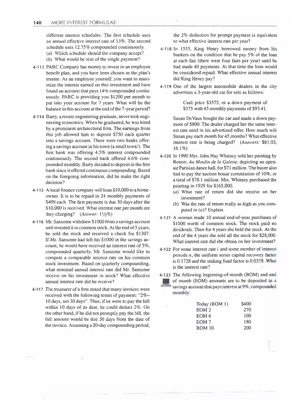
140 MORE INTERESTFORMULAS
different interest schedules. The first schedule usesan annual effective interest rate of 13%. The second
schedule uses 12.75% compounded continuously.(a) Which schedule should the company accept?(b) What would be size of the single payment?
4-113 PARC Company has money to invest in an employeebenefit plan, and you have been chosen as the plan'strustee. As an employee yourself, you want to maxi-mize the interest earned on this investment and have
found an account that pays 14% compounded contin-uously. PARC is providing you $1200 per month toput into your account for 7 years. What will be thebalance in-this account at the end of the 7-year period?
4-114 Barry, a recent engineering graduate, never took engi-neering economics. When he graduated, he was hiredby a prominent architectural firm. The earnings fromthis job allowed him to deposit $750 each quarterinto a savings account. There were two banks offer-ing a savings account in his town (a small town!). Thefirst bank was offering 4.5% interest compoundedcontinuously. The second bank offered 4.6% com-pounded monthly. Barry decided to deposit in the firstbank since it offered continuous compounding. Basedon the foregoing information, did he make the rightdecision?
4-115 A local finance company will loan $10,000 to a home-owner. It is to be repaid in 24 monthly payments of$499 each. The first payment is due 30 days after the$10,000 is received. What interest rate per month arethey charging? (Answer: 11/2%)
4-116 Mr. Sansome withdrew $1000 from a savings accountand invested it in common stock. At the end of 5 years,he sold the stock and received a check for $1307.
If Mr. Sansome had left his $1000 in the savings ac-count, he would have received an interest rate of 5%,compounded quarterly. Mr. Sansome would like tocompute a comparable interest rate on his commonstock investment. Based on quarterly compounding,what nominal annual interest rate did Mr. Sansomereceive on his investment in stock? What effectiveannual interest rate did he receive?
4-117 The treasurer of a firm noted that many invoices werereceived with the following terms of payment: "20/0-10 days, net 30 days". Thus, if he were to pay the billwithin 10 days of its date, he could deduct 2%. Onthe other hand, if he did not promptly pay the bill, thefull amount would be due 30 days from the date ofthe invoice. Assuming a 20-day compounding period,
the 2% deduction for prompt payment is equivalentto what effective interest rate per year?
4-118 In 1555, King Henry borrowed money from hisbankers on the condition that he pay 5% of the loanat each fair (there were four fairs per year) until hehad made 40 payments. At that time the loan wouldbe considered repaid. What effective annual interestdid King Henry pay?
4-119 One of the largest automobile dealers in the cityadvertises a 3-year-old car for sale as follows:
Cash price $3575, or a down payment of$375 with 45 monthly payments of $93.41.
Susan DeVaux bought the car and made a down pay-ment of $800. The dealer charged her the same inter-est rate used in his advertised offer. How much will
Susan pay each month for 45 months? What effectiveinterest rate is being charged? (Answers: $81.03;16.1%)
4-120 In 1990 Mrs. John Hay Whitney sold her painting byRenoir, Au Moulin de ZaGaZette, depicting ari open-air Parisian dance hall, for $71 million. The buyer alsohad to pay the auction house commission of 10%, ora total of $78.1 million. Mrs. Whitney purchased thepainting in 1929 for $165,000.(a) What rate of return did she receive on her
investment?
(b) Was the rate ofreturn really as high as you com-puted in (a)? Explain.
4-121 A woman made 10 annual end-of-year purchases of$1000 worth of common stock. The stock paid nodividends. Then for 4 years she held the stock. At theend of the 4 years she sold all the stock for $28,000.What interest rate did she obtain on her investment?
4-122 For some interest rate i and some number of interest
periods n, the uniform series capital recovery factoris 0.1728 and the sinking fund factor is 0.0378. Whatis the interest rate? .
4-123 The following beginning-of-month (BOM) and end.of month (EOM) amounts are to be deposited in a- savings account that pays interest at 9%, compounded .
monthly:
Today (BOM 1)EOM2EOM6EOM7BOM 10
$400270100180200
-- -

ur
Problems 141
Set up a spreadsheet to calculate the account balanceat the end of~e first year (EOM12). The spreadsheetmust include the following column headings: MonthNumber, Deposit BOM, Account Balance at BOM,Interest Earned in Each Month, Deposit EOM, Ac-count Balance at EOM. Also, use the compound inter-est tables to draw a cash flow diagram of this problemand solve for the account balance at the EOM 12.
4-124 Net revenues at an older manufacturing plant will be
.II. $2 million for this year. The net revenue will decrease15% per year for 5 years, when the assembly plantwill be closed (at the end of Year 6). If the firm's in-terest rate is 10%, calculate the PW of the revenuestream.
4-125 What is the present worth of cash flows that begin at_ $10,000 and increase at 8% per year for 4 years? The. interest rate is 6%.
4-126 What is the present worth of cash flows that begin at. $30,000 and decrease at 15% per year for 6 years?The interest rate is 10%.
4-127 Calculate and print out the balance due, principal.payment, and interest payment for each period of a~ used-car loan. The nominal interest is 12% per year,
compounded monthly. Payments are made monthlyfor 3 years. The original loan is for $11,000.
4-128 Calculate and print out the balance due, principal pay-.ment, and interestpayment for each period of a newcar loan. The nominal interest is 9% per year, com-pounded monthly. Payments are made monthly for5 years. The original loan is for $17,000.
4-129 For the used car loan of Problem 4-127, graph the
JIlmonthlypayment.. (a) As a function of the interest rate (5-15%).
(b) As a function of the number of payments (24-48).
4-130 For the new car loan of Problem 4-128, graph the
JI.monthly payment.(a) As a function of the interest rate (4-14%).(b) As a function of the number of payments (36-84).
4-131 Your beginning salary is $50,000. You deposit 10%. at the end of each year in a savings account that. earns 6% interest. Your salary increases by 5% per
year. What value does your savings book show after40 years?
4-132 The market volume for widgets is increasing by 15%
.IL per year from current profits of $200,000. Investingin a design change will allo~ the profit per widgetto stay steady; otherwise they will drop 3% per year.What is the present worth of the savings over the next5 years? Ten years? The interest rate is 10%.
4-133 A 30-year mortgage for $120,000 has been issued._ The interest rate is 10% and payments are made. monthly. Print out the balance due, principal payment.
and interest payment for each period.
4-134 A homeowner may upgrade a furnace that runs on
JIlLfuel oil to a natural gas unit. The investment win be.. $2500 installed. The cost of the natural gas will aver-
age $60 per month over the year, instead of the $145per month that the fuel oil costs. If the interest rateis 9% per year, how long will it take to recover theinitial investment?
4-135 Develop a general-purpose spreadsheet to calculate
A out the balance due, principal payment, ~d interestpayment for each period of a loan. The user inputs tothe spreadsheet will be the loan amount, the number ofpayments per year, the number of years payments aremade, and the nominal interest rate. Submit printoutsof your analysis ofa loan in the amount of $15,000 at8.9% nominal rate for 36 months and for 60 months .of payments.
4-136 Use the spreadsheet developed for Problem 4-135 to
JI.analyze 180-month and 360-month house loan pay-. ments. Analyzea $100,000mortgageloan at a nom-
inal interest rate of 7.5% and submit a graph of the.interest and principal paid over time. You need notsubmit the printout of the 360 payments because itwill not fit on one page.
II'!
---
1

After Completing This Chapter...The student should be able to:· Define and apply the present worth criteria.· Compare two competing alternative choices using present worth (PW).· Apply the PW model in cases with equal, unequal, and infinite project lives,. Compare multiple alternatives using the PW criteria.. Develop and use spreadsheets to make present worth calculations.
QUESTIONS TO CONSIDER.. )
1. Sofar,Boeinghas notbeen ableto sell the SonicCruiseridea to airlines.Fastis good, theysay,but cheap is better. Why isn't increased speed more attractive to airlines, especiallyoverlong-haulflights?Can't airlineschargemoreforfasterflights? .
2. In many cases, air travelers actually spend as much time on the group.das in the air.Going through security,changing planes, clearing customs, and picking up baggage cancollectively add hours to their travel time. How might this affect a traveler's decisionabout whether to pay more to fly on a faster plane like the Sonic Cruiser?
3. Airlines seemto be moreinterested in the new Airbusmodel. Canyou state somereasonsfor this apparent preference?
~ ,~ ----
- - - ---------

Present Worth Analysis
Boeing Versus AirbusFor several years, Boeing has been working on developmentof the Sonic Cruiser, an inno-vative lightweightplane that can fly near the speed of sound.This is about 15%faster thana conventionaljet, so flying the Sonic Crqiser would allow airlines to cut long-haul flighttimes.
I~_. J
..
~
'.
'
.
.
.
'.'
..
..,.,!,," "...
1
----
Meanwhile, Airbus, Boeing's rival in thepassenger aircraftbusiness,has also been work-ing on its versionof a lighterplane. ButAirbusisbetting on size rather than speed. Its new model,the A380, is knownas the super-jumboand willbe the largest passengerplane in the world.
Airbus is hoping to use several recently'developed composite materials, with the aim ofreducing by 20% both the weight and the man-ufacturing cost. Airbusestimates that flying thecomposite plane will allow airlines to cut theiroperating costs by about 8%.
-- - --
J:--1=
;01

. . - .. ...-
144 PRESENTWORTH ANALYSIS
In Chapters 3 and 4 we accomplished two important tasks. First, we presented the conceptof equivalence. We are powerless to compare series of cash flows unless we can resolvethem into some equivalent arrangement. Second, equivalence, with alteration of cash flowsfrom one series to an equivalent sum or series of cash flows, created the need for compoundinterest factors. So, we derived a whole series of compound interest factors-some forperiodic compounding and some for continuous compounding. This background sets thestage for the chapters that follow.
ASSUMPTIONS IN SOLVING ECONOMIC ANALYSIS PROBLEMS
One of the difficulties of problem solving is that most problems tend to be very compli-cated. It becomes apparent that some simplifying assumptions are needed to make suchproblems mana,geable. The trick, of course, is to solve the simplified problem and still besatisfied that the solution is applicable to the real problem! In the subsections that fol-low, we will consider six different items and explain the customary assumptions that aremade. These assumptions apply to all problems and examples, unless other assumptions aregiven.
End-of- Year Convention
As we indicated in Chapter 4, economic analysis textbooks and practice follow the end-of-period convention.This makes"A" a seriesof end-of-period receiptsor disbursements.(We generally assumein problems that all seriesof receiptsor disbursementsoccur at theend of the interest period. This allows us to usevaluesfromourcompoundinteresttableswithout any adjustments.)
A cash flow diagram of P, A, and F for the end-of-period conventionis as follows:
Year0Jan 1
End of Year 1Dee 31 Jan 1
.End of Year 2Dee 31
A,A
tFp
If one were to adopt a middle-of-period convention, the diagram would be:
Year0Jan 1
MiddleofYear1Jun 30 Dee 31 Jan 1
Middle ofYear 2Jun 30
End of Year 2Dee 31
A A
p F
As the diagrams illustrate, only A shifts; P remains at the beginning-of-period and F at theend-of-period, regardless of the convention.The compound interest tables in the Appendixare based on the end-of-period convention.
-- - .-
-- -- - -

-.- ----- -------.
Assumptions in Solving Economic Analysis Problems 145
Viewpoint of Economic Analysis StudiesWhen we makeeconomic analysis calculations,we must proceed from a point of reference.Generally, we will want to take the point of view of a total firm when doing industrialeconomic analyses. Example 1-1vividly illustrated the problem: a firm's shipping depart-ment decided it could save money having its printing work done outside rather than bythe in-house printing department. An analysis from the viewpoint of the shipping depar:t-ment supported this, as it could get for $688.50 the same printing it was paying $793.50for in house. Further analysis showed, however, that its printing department costs woulddecline less than using the commercialprinter would save. From the viewpointof the firm,the net result would be an increase in total cost.
From Example 1-1 we see it is important that the viewpoint of the study be carefullyconsidered. Selecting a narrow viewpoint,like that of the shipping department, may resultin a suboptimal decision from the viewpointof the firm. For this reason, the viewpoint ofthe total firm is used in industrial economic analyses.
Sunk CostsWe know that it is the differences between alternatives that are relevant in econonllcanalysis. Events that have occurred in the past really have no bearing.on what we shoulddo in the future.Whenthejudge says,"$200fineor 3 daysinjail,'~the eventsthat led to .
these ~nhappy alternatives really are unimportant. It is the current and future differencesbetween the alternatives that are important.Past costs, like past events;have no beari.Iigondeciding between alternatives unless the past costs somehow affect the present or futurecosts. In general, past costs do not affect the present or the future, so we refer to them as .
sunk costs and disregard them.
Borrowed Money ViewpointIn most economic analyses, the proposed alternativesinevitably require money to be spent,and so it is natural to ask the source of that money.The source will vary from situation tosituation. In fact, there are two aspects of money to determine: one is the financing-theobtaining of money-problem; the other is .the investment-the spending of money-problem. Experience has shown that these two concerns should be distinguished. Whenseparated,the problems of obtainingmoneyand of spendingit are both logical and straight-forward. Failure to separate them sometimesproduces confusing results and poor decisionmaking.
The conventionalassumptionin economicanalysisis that themoneyrequiredto financealternatives/solutionsin problem solving is considered to be borrowed at interest rate i.
Effect of Inflation and Deflation
For the present we will assume that prices are stable. This means that a machine that costs$5000 today can be expected to cost the same amount several years hence. Inflation anddeflation can be serious problems for after-tax analysis and for cost and revenues whoseinflation rates differ from the economy's inflation rates, but we assume stable prices fornow.
T - --

146 PRESENTWORTH ANALYSIS
Income Taxes
This aspect of economicanalyses, likeinflationand deflation,mustbe consideredto findthereal payoff of a project. However,taxeswill often affectalternativessimilarly,allowingus tocompare our choices without considering income taxes. So, we will defer our introductionof income taxes into economic analyses until later.
ECONOMIC CRITERIA
We have shown how to manipulate cash flows in a variety of ways, and in so doing wecan now solve many kinds of compound interest problems. But engineering economicanalysis is morethan simplysolvinginterestproblems.Thedecisionprocess (seeFigure 1-1)requires that the outcomes of feasible alternativesbe arranged so that they may be judgedfor economic efficiency in terms of the selectioncriterion. The economic criterion will beone of the following, depending on the situation1:
Situation
For fixed inputFor fixed outputNeither input nor output fixed
Criterion
Maximize outputMinimize inputMaximize (output - input)
We will now examine ways to resolve engineeringproblems, so that criteria for economicefficiencycan be applied.
Equivalenceprovides the logic by whichwe may adjust the cash flowfor a given alter-'native into someequivalent sum or series.Toapplythe selectioncriterionto the outcomesofthe feasible alternatives,we must first resolve them into comparable units. The question is,How should theybe compared? In this chapter we'll learnhow analysiscan resolve alterna-tives into equivalentpresent consequences,referred to simply as present worth analysis.Chapter 6 will showhow given alternativesare convertedinto an equivalentuniformannualcashflow, and Chapter 7 solves for the interest rate at which favorableconsequences-thatis, benefits-are equivalent to unfavorableconsequences--or costs.
As a general rule, any economic analysis problem may be solved by the methodspresented in this and in the two following chapters. This is true because present worth,annual cash flow, and rate of return are exact methods that will always yield the samesolutionin selectingthebest alternativefromamonga setof mutuallyexclusivealternatives.2Some problems, however,may be more easily solved by one method than by another.For"this reason, we now focus on the kinds of problems that are most readily solved by preseJ?-tworth analysis.
IThe short table summarizes the discussion on selection of criteria in Chapter 1 (see item 5, selectthe criterion to determine the best alternative, page 9).
2"Mutually exclusive" means that selecting one alternative precludes selecting any other alternative.For example, constructing a gas station and constructing a drive-in restaurant on a particular piece ofvacant land are mutually exclusive alternatives.
..1
-----
T

Applying Present Worth Techniques 147
ApPLYING PRESENT WORTH TECHNIQUES
One of the easiest ways to compare mutually exclusive alternatives is to resolve theirconsequences to the present time. The three criteria for economic efficiencyare restated interms of present worth analysis in Table 5-1.
TABLE5-1 Present Worth Analysis
Situation Criterion
Fixed input Amount of money or other inputresources are fixed
There is a fixed task, benefit, orother output to be accomplished
Neither amount of money, orother inputs, nor amount ofbenefits, or other output, is fixed
Maximize present worth of benefitsor other outputs
Minimize present worth of costsor other inputs
Maximize (present worth of benefitsminus present worth of costs), that is,maximize net present worth
Fixed output
Neither inputnor output isfixed
Present worth analysis is most frequently used to determine the present value of futuremoney receipts and disbursements. It would help us, for example, to determine a presentworth of income-producing property, like an oil well or an apartment house. If the futureincome and costs are known, then we can use a suitable interest rate to calculate the presentworth of the property.This shouldprovide a goodestimate of the price at which the propertycould be bought or sold. Another application might be determining the valuationof stocksor bonds based on the anticipated future benefits from owning them.
In presentworthanalysis,carefulconsiderationmust be givento the timeperiodcoveredby the analysis. Usually the task to be accomplishedhas a time period associated with it. Inthat case, the consequences of each alternative must be considered for this period of timewhich is usually called the analysis period, or sometimes the planning horizon.
The analysis period for an economy study should be determined from the situation. Insome industries with rapidly changing technologies, a rather short analysis period or plan-ning horizon might be in order. Industries with more stable technologies(like steelmaking)might use a longer period (say, 10-20 years), while government agencies frequently useanalysis periods extending to 50 years or more.
Three different analysis-period situations are encountered in economic analysisproblems:
1. The useful life of each alternativeequals the analysis period.2. The alternativeshave useful lives different from the analysis period.3. There is an infinite analysis period, n = 00.
1. Useful Lives Equal the Analysis PeriodSince different lives and an infinite analysis period present some complications, we willbegin with four examples in which the useful life of each alternative equals the analysisperiod.
....--...-
- - - ---

.. ~~... - +.. h._..+ +
148 PRESENTWORTH ANALYSIS
,#";ci~~;'~i31~~'~~~It;
A firm is considering which of two mechanical devices to install to reduce costs in a particularsituation. Both devicescost $1000 and have useful lives of 5 years and no salvage value. DeviceA can be expected to result in $300 savingsannually.Device B willprovide cost savingsof $400the firstyear but will decline $50 annually,making the second-year savings $350, the third-y~arsavings $300, and so forth. With interest at 7%, which device should the firmpurchase?
SOLUTION
The analysisperiod can convenientlybe selectedas the useful life of the devices, or 5 years.Sinceboth devices cost $1000, there is a fixed input (cost) of $1000 regardless of whether A or B ischosen. The appropriatedecision criterion is to choose the alternativethat maximizes the presentworth of benefits.
PW of Benefits PW of Benefits
PW of benefitsA = 300(PjA, 7%,5) = 300(4.100)= $1230
PW of benefits B = 400(PjA, 7%, 5) - 50(PjG, 7%, 5)
= 400(4.100) - 50(7.647) = $1257.65
Device B has the larger present worth of benefitsand is, therefore, the preferred alternative.It isworth noting that, if we ignore the time value of money,both alternativesprovide $1500 worthofbenefitsover the 5-year period. Device B provides greater benefits in the first2 years and smallerbenefits in the last 2 years. This more rapid flowof benefits from B, although the total magnitudeequals that of A, results in a greater present worth of benefits.
Wayne County will build an aqueduct to bring water in from the upper part of the state. I~canbe built at a reduced size now for $300 million and be enlarged 25 years hence for an additional$350 million. An alternativeis to construct the full-sized aqueduct now for $400 million.
Both alternativeswouldprovide the needed capacity for the 50-year analysis period.Mainte-nanCecosts are small and~may.beignored. At 6% interest, which alternatiye should be selected?
- --- - --- -- -- ----
DeviceA DeviceB
A = 300 400 350
i300
r t t t t r t250 200
t t0-1-2-3-4-5 01-2-3-4-5
! n = 5years ! n = 5 years

Applying PresentWorth Techniques 149
SOL~TION
This problem illustrates staged construction. The aqueduct may be built in a single stage, or in asmaller first stage followedmany years later by a second stage to provide the additional capacitywhen needed.
For the Two-Stage Construction
PW of cost = $300 million + 350 million(P / F, 6%, 25)
= $300 million + 81.6 million
= $381.6 million
For the Single-Stage Construction
PW of cost = $400 million
The two-stage constructionhas a smaller present worth of cost and is the preferred construc-tion plan.
A purchasing agent is considering the purchase of some new equipment for the mailroom. Twodifferent manufacturers have provided quotations. An analysis of the quotations indicates thefollowing:
Manufacturer
SpeedyAllied
Cost$1500
1600
Useful Life(years)
55
End-of-Useful..LifeSalvage Value
$200325
The equipmentof both manufacturersis expected to perform at the desired levelof (fixed)output.For a 5-year analysis period, which manufacturer's equipment should be selected? Assume 7%interest and equal maintenance costs.
I"
, SOLUTION'I ",
For fixed output, the criterion is to minimize the present worth of cost.
Speedy
PW of cost ..:..1500 - 200(Pj F, 7%!,5)
= 1500- 200(0.7130)
=:J?Op - J~3=-$l357... - -... ---
~
-- ----- - - - -- -- - - -- -

150 PRESENTWORTH ANALYSIS
Allied
PW of cost = 1600 - 325(P / F, 7%,5) = 1600- 325(0.7130)
= 1600 - 232 = $1368
Since it is only the differences between alternatives that are relevant, maintenance co~tsmay be left out of.the economic analysis. Although the PWs of cost for all the alternatives arenearly identical, we would, nevertheless, choose the one with minimum present worth of costunless there were other tangible or intangibledifferences that would change the decision.Buy theSpeedy equipment.
A finn is trying to decide which of two weighing scales it should install to check a package-fillingoperation in the plant. The ideal scale would allow better control of the filling operation and resultin less overfilling. If both scales have lives equal to the 6-year analysis period, which on~ shouldbe selected? Assume an 8% interest rate.
AlternativesAtlas scaleTom Thumb scale
Cost$2000
3000
UniformAnnual Benefit
$450600
End-of-Useful-LifeSalvage Value
$100700
~OlUTION .'.
Atlas Scale
PW of benefits - PW of cost = 450(P / A, 8%, 6) + 100(P/ F, 8%, 6) - 2000
= 450(4.623) + 100(0.6302) - 2000
= 2080+ 63 --'-'2000= $143
Tom Thumb Scale
PW of benefits - PW'of cost = 600(P / A, 8%, 6) + 700(P /F, 8%"p) ~ 3000
= 600(4.623) + 700(0.6302) - 3000
= 2774 + 441 - 3000. $215
I
I
II
The salvage value of th~ scale, it .shol}ld be noted,!s ;sjmpLytre<l,tedas..oanotherbenefit of.::the alternative. Since the criterion is to maximize tbe"present worth of' benefits minus the presentworth of cost, the preferred alternative is the Tom Thumb scale.
"
" ~'~""..,. -J
;...
- -- ----- --

.Applying Present Worth Techniques 151
In Example 5-4, we compared two alternativesand selectedthe one in whichpresent worthof benefits minus present worth of cost was a maximum. The criterion is called the netpresent worth criterion and written simply as NPW:
Net present worth =Present worth of benefits - Present worth of cost
NPW = PW of benefits - PW of cost
2. Useful Lives Different from the Analysis PeriodIn present worth analysis, there always must be an identified analysis period. It follows,then, that each alternativemust be considered for the entire period. In Examples 5-1 to 5-4,the useful life of each alternative was equal to the analysis period. Often we can arrangeit this way,but in many situations the alternativeswill have useful lives different from theanalysis period. This section describes one way to evaluatealternativeswith livesdifferentfrom the study period. .
In Example 5-3, suppose that the Allied equipment was expected to have a 1O-yearuseful life, or twice that of the Speedyequipment.Assumingthe Allied salvagevaluewouldstill be $325 in 10 years, which equipment should now be purchased? We can recomputethe present worth of cost of the Allied equipment, starting as follows:
PW of cost = 1600- 325(P / F,.7%, 10)
= 1600- 325(0.5083)
= 1600- 165= $1435
Thepresentworthof costhas increased.This is due,of course,to the moredistantrecoveryofthe salvagevalue.More importantly,we now findourselves attempting to compare Speedyequipment, with its 5-year life, against the Alliedequipment with a 1O-yearlife. Becauseof the variation in the useful life of the equipment, we no longer have a situation of fixedoutput. Speedy equipment in the mailroomfor 5 years is certainly not the same as 10yearsof service with Allied equipment. .
For present worth calculations, it is important that we select an analysis period andjudge the consequences of each of the alternativesduring the selected analysis period. Assuch, it is not a fair comparison to compare the NPW of the Allied equipment over its1O-yearlife against the NPW of the Speedy equipment over its 5-year life.
Not only is the firm and its economic environment important in selecting an analysisperiod, but also the specific situation being analyzed is important. If the Allied equipment(Example5-3) has a useful life of 10years, and the Speedy equipment will last 5 years, onemethodis to select an analysisperiod that is the least common multiple of their useful lives.Thus we would compare the 1O-yearlife of Allied equipment against an initial purchase ofSpeedy equipmentplus its replacement with new Speedy equipment in 5 years. The resultis to judge the alternativeson the basis of a 1O-yearrequirement in the mailroom. On thisbasis the economic analysis is as follows.
1
-- --- ---
r- - -

152 PRESENTWORTH ANALYSIS
Assuming the replacement Speedy equipment 5 years hence will also cost $1500,
rOriginal Speedy Investment ---1200 200
t t0-1-2-3-4-5-6-7-8-9-10
1 1 . J1500 1500I--- ReplacementSpeedyInvestment
PW of cost = 1500+ (1500- 200)(P / F, 7%, 5) - 200(P / F, 7%, 10)
= 1500+ 1300(0.7130) - 200(0.5083)
= 1500 + 927 - 102 = $2325
For the Allied equipment,on the other hand, we have the following results:.
325
t0-1-2-3-4-5-6~7-8-9-10
...
1600
PW of cost = 1600- 325(P / F, 7%, 10) = 1600 - 325(0.5083) = $1435
For the fixed output of 10years of service in the mailroom, the Allied equipment, with it:smaller present worth of cost, is preferred. .
We have seen that setting the analysis period equal to the least common multiple 0the lives of the two alternativesseems reasonable in the revised Example 5-3. What woul<one do, however, if the alternativeshad useful lives of 7 and 13 years, respectively?Herethe least common multipleof lives is 91 years. An analysisperiod of 91 years hardly seem:realistic. Instead, a suitable analysis period should be based on how long the equipment i:likely to be needed. This may require that terminal valuesbe estimated for the alternative:at some point prior to the end of their useful lives.
Figure 5-1 graphicallyrepresents this concept.As Figure 5-1 indicates, it is not neces.sary for the analysis period to equal the useful life of an alternativeor some multiple of thtuseful life. To properly reflect the situation at the end of the analysis period, an estimate i1required of the market valueof the equipment at that time. The calculationsmight be easie]if everything came out even, but it is not essential.
T-----------

Applying Present Worth Techniques 153
Alternative 1Salvage TerminalValueatValue End of 10thYear
t t0-1-2-3-4-5-6-7-8-9-10-11-12-13-14
1Initial Replacement
1!
Cost Cost II
I. 7-yearLife I 7-yearLifeI
Alternative 2Terminal Value atEnd of 10th Year
. t0-1-2-3-4-5-6-7-8-9-10-11-12-13
1
1'
. Initial i
Cost II
13-year Life
lO-year Analysis Period
FIGURE 5.1 Superimposing a lO-year analysis period on 7- and 13-year alternatives.
A diesel manufacturer is considering the two alternative production machines graphically depictedin Figure 5-1. Specific data are as follows.
Initial costEstimated salvage value at end of useful lifeUseful life of equipment, in years
Alt. 1
$50,000$10,000
7
Alt. 2$75,000$12,000
13
The manufacturer uses an interest rate of 8% and wants to use the PW method to compare thesealternatives over an analysis period of 10yeats.
Estimated market value, end of lO-year.analysis period
Alt. 1
$20;000
Alt. 2
$15,000
SOLUTION
In this case, the decision maker is setting the analysis period at 10 years rather than acceptiug acommon multiple of the lives of the alternatives, or assuming that the period of needed serviceis infinite (to be discussed in the next section). This is a legitimate approach-perhaps the dieselmanuf~cturer will be phasing out this model at the end of the 10-year period. In.any event, we
~ n~cl t<)!fOffiRNyt,e a\!emaJiyesOY,yI;tbe 1O~y.ear.period. ;;;; ~1iII ~
'II'il
II"
I
'll1
,1'
1,Iu- -----..
=~--
-- - -- -- - ---r

-.. ... u .._.-.
154 PRESENTWORTH ANALYSIS
As.illustrated in Figure 5-1, we may assumethatAlternative 1will bereplacedby anidenticalmachineafter its 7-yearuseful life. Alternative 2 hasa 13-yearuseful life. The dieselmanufacturerhasprovided an estimatedmarket value of the equipmentat the time of the analysisperiod. Assuchwe cannow comparethe two choicesover 10 yearsas follows:
PW (Alt. 1) = -50,000 + (10,000--50,000)(P /F, 8%,7)+ 20,000(P/ F, 8%,10)
= -50,000 - 40,000(0.5835)+ 20,000(0.4632)
= -$64,076
PW (Alt. 2,)= -75,000 + 15,000(P/ F, 8%, 10)
- -75,000 +. 15,000(0.4632)
= -$69,442I.
To minimize PW of coststhe dieselmanufacturershould selectAlt 1.
3. Infinite Analysis Period: Capitalized CostAnother difficulty in presentworth analysis arises when we encounter an infinite analysisperiod (n =00). In governmentalanalyses, a service or condition sometimesmust be main-tained for an infinite period. The need for roads, dams, pipelines, and other componentsof national, state, or local infrastructure is sometimesconsidered to be permanent. In thesesituations a present worth of cost analysis would have an infinite analysis period. We callthis particular analysis capitalized cost.
Capitalizedcost is thepresentsum of moneythatwouldneedtobe set asidenow,at someinterest rate, to yield the funds required to provide the service (or whatever)indefinitely.Toaccomplish this, the money set aside for future expenditures must not decline. The interestreceived on the money set aside can be spent, but not the principal. When one stops tothink about an infinite analysis period (as opposed to something relatively short, like ahundred years), we see that an undiminishedprincipal sum is essential; otherwise one willof necessity run out of money prior to infinity.
In Chapter 4 we saw that
principal sum + interest for the period = amount at end of J?~!i0d,or
P + iP = P + iP
If we spend iP, then in the next interest period the principal sum P will again increase toP + i P. Thus, we can again spend i P. -
This concept may be illustratedby a numerical example. Suppose you deposited $200in a bankthatpaid4% interestannually.Howmuchmoneycouldbe withdrawneachyearwithout reducing the balance in the account below the initial $200? At the end of the firstyear, the $200 would have earned 4%($200) = $8 interest. If this interest were withdrawn,
---
T

Applying Present Worth Techniques 155.the $200 would remain in the account. At the end of the second year, the $200 balancewould again earn 4%($200) = $8. This $8 could also be withdrawn and the account wouldstill have$200. This procedure could be continued indefinitelyand the bank account wouldalways contain $200.
The year-by-year situation would be depicted like this:
Year1: $200 initial P ~ 200 + 8 = 208Withdrawal i P = - 8
Year 2: $200 ~ 200 + 8 = 208Withdrawal iP = - 8
$200andsoon
Thus, for any initial present sum P, there can be an end-of-period withdrawal of Aequal to iP each period, and these withdrawalsmay continue forever without diminishingthe initial sum P. This gives us the basic relationship:
For n = 00, A = Pi
This relationship is the key to capitalized cost calculations. Earlier we defined capitalizedcost as the present sum of money that would need to be set aside at some interest rate toyield the funds to provide the desired task or service forever.Capitalized cost is thereforethe P in the equation A = i P. It follows that:
CapitalizedcostA
P=-i (5-2)
If we can resolve the desired task or service into an equivalentA, the capitalized cost maybe computed. The following examples illustrate such computations.
How much should one set aside to pay $50 per year for maintenance on a gravesite if interest isassumedto be 4%? For perpetual maintenance, the principal sum must remain undiminishedaftermaking the annual disbursement.
'SOLUTION. ,
Capitalized cost P = Annual disbursement AInterest rate i .
~ 50'P= .'. 0.04= $1250
One ~hould$et aside. $1250.== = .~ _ !!IC:'''=== =====-_ = IiiII:I='==;;:::::1:::11<= 111I ~
---
-- --- -- -
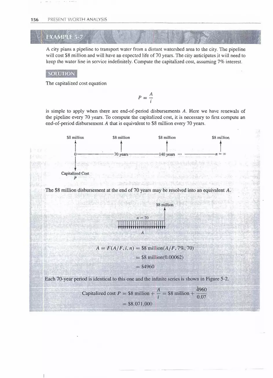
156 PRESENT WORTH ANALYSIS
A city plans a pipeline to transport water from a distant watershed area to the city. The pipelinewill cost $8 million and will have an expected life of 70 years. The city anticipates it will need tokeep the water line in service indefinitely.Compute the capitalized cost, assuming 7% interest.
-SOLUTION
The capitalized cost equation
Ap=-
i
is simple to apply when there are end-of-period disbursements A. Here we have renewals ofthe pipeline every 70 years. To compute the capitalized cost, it is necessary to first compute anend-of-period disbursement A that is equivalent to $8 million every 70 years.
$8 million
to
1
$8 million
t70 years
$8 million
t140 years
$8 million
tn=oo
Capitalized Costp
The $8 million disbursement at the end of 70 years may be resolved into an equivalentA.
$8 million
n ;:: 70
A
A = F(Aj F, i, n) = $8 rnillion(A/ F, 7%, 70)
= $8 million(0.0Q()62)
.= $4960I '
Each 70-year period is identical to this one and the infinite series is shown in Figure 5-2.
. .d $ mil
. A$"8
.lli
4960CapItalIze cost P = 8 lIon+ -:-= ID1 on + _0 0l . 7
= $8,071,000........ -- -- ----
'"I
- --- --- ---
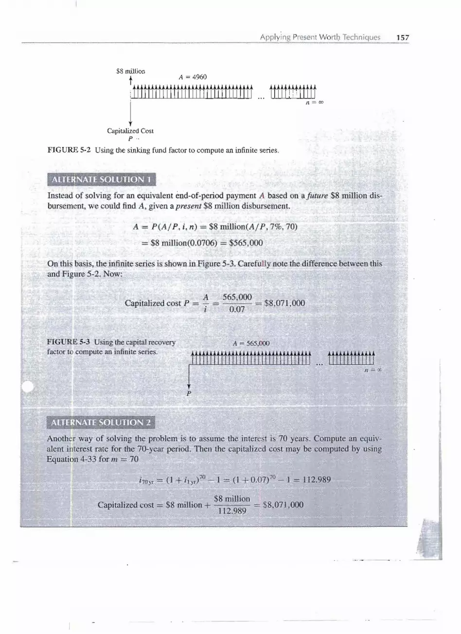
I
I
I
~
Applying Present Wortb Techniques 157
$8 millionA = 4960
n=oo
Capitalized Costp --.
FIGURE 5-2 Using the sinking fund factor to compute an infinite series.
AlTE~NATESOLUTION~1J
Instead of solving for an equivalent end-of-period payment A based on afuture $8 million dis-bursement, we could find A, given a present $8 million disbursement.
A = P(Aj P, i, n) = $8 million(Aj P, 7%, 70)
= $8 milIion(0.0706) = $565,000
On this basis, the infiniteseries is shownin Figure 5-3. Carefullynote the differencebetween thisandFigure5-2.Now: .
. . A 565,000CapItalizedcost P = - = - $8,071,000i 0.07
FIGURE5-3 Using the capitalrecoveryfactor to compute an infiniteseries.
A = 565,000
n=oo
p
Another way of solving the problem is to assume the interest is 70 years. Compute an equiv-alent interest rate for the 70-year period. Then the capitalized cost may be computed by using\.
Equation 4-33 for m = 70
=i70yr = (1 + i1yr)70- 1 = (1 + 0.07)70- J = 112.989
= ~ ~ ;.
$.Ii
$8 million$Capitalized cost = 8 mIl on +. = 8,071,000112.989 .
- -
- -- -
--
1....
-----

158 PRESENTWORTH ANALYSIS
Multiple Alternatives
So far the discussionhas been based on exampleswith only two alternatives.But multipllalternative problems may be solved by exactly the same methods employed for problenwith two alternatives. (The only reason for avoiding multiple alternativeswas to simpli1the examples.)Examples 5-8 and 5-9 have multiple alternatives.
A contractor has been awarded the contract to construct a 6-mile-Iong tunnel in the mountains.During the 5-year construction period, the contractor will need water from a nearby stream. Hewill construct a pipeline to conveythe water to the main construction yard. An analysis of costsfor various pipe sizes is as follows:
Pipe Sizes (in.)
2 3 4 6
Installed cost of pipeline and pumpCost per hour for pumping
$22,000$1.20
$23,000$0.65
$25,000$0.50
$30,000$0.40
The pipe and pump will have a salvage value at the end of 5 years, equal to the cost to removethem. The pump will operate 2000 hours per year.The lowest interestrate at which the contractoris willing to investmoney is 7%. (Theminimumrequired interestrate for investedmoney is calledthe minimum attractive rate of return, or MARR.) Select the alternativewith the least presentworth of cost.
SdllJTI ON ...-,. -.'.. .-.'.' .
We can comptite the present worth of cost for each alternative. For each pipe size, the presentworth of cost is equal to the installed cost of the pipeline and pump plus the present worth of5 years of pumping costs.
Pipe Size (in.)
2 6
II~I
Installed cost of pipeline and pump1.20 x 2000 hr x (P / A, 7%, 5)0.65 x 2000 hr x 4.1000.50 x 2000 hr x 4.1000.40 x 2000 hr x 4.100
Present worth of cost
$22,0009,840
$30,000
3,280;$33,280$31,840
Select the 3 in. pipe size. - .. :=; =.=~-
,IiIooL_ _____
-- r- - - - --- -

Applying Present Worth Techniques 159
An investor paid $8000 to a consulting firm to analyze what he might do with a small parcel ofland on the edge of town that can be bought for $30,000.In their report, the consultantssuggestedfour alternatives:
*Includes the land and structures but does not include the $8000 fee to the consulting .finn.
Assuming 10% is the minimum attractive rate pf retlirn, what should the investor. do?
Alternative A represents the "do-nothing" alternative. Generally, one feasible alternativein anysituation is to remain in the present status and do nothing. In this problem, the investor coulddecide that the most attractivealternative is notto purchase the property ~d develop it. Thisisclearly a do-nothing decision.
We note, however,that if he does nothing, the total venture wouldnot be a very satisfactoryone. Thisis because the investor spent $8000for professional advice"on the possible uses of theproperty. But because the $8000 is a past cost, it is a sunk cost. The only relevant costs in aneconomic analysis arepresent andfilJure costs; past events and past, or sunk, costs are gone andcannot be allowedto affectfuture planning. (Past costsmay be relevan.tincomputingdepreciationcharges and income taxes, but 110whereelse.) The past should not deter the investor from makingthe best decision now,regardless of the costs that brought him to this situatipn arid point oftime.
This problemis one of neitherfixedinputnor fixedoutput,soourcriterionwillbe tomaxiIni:z:ethe present worth of benefits minu~ the present worth of cost; Or,simply stated, maxirni:z:enetpresent Worth.
Alter!lative A, Do NothingI
I
r Alternative B, Vegetable Market
NPW= -50,000 +5100(Pj A, 1O%i4(»+ 30,000(P/F, 10%, 2Q)
= """"50,0~0--I-Q10Z~85~4)+ 30,000(<l1~86)j! :
= ~50,OOO+ 43,420 + 4460
;;; -~212Q "= = ;;:"" ~ !I'==:'=&_ <=: ==;t =: ~
1:1
'I'
li~
~
I
f
'f
I,
I
NPW- 0
- ..........-..... _ u..__...
- -
Total Investment Uniform Net Terminal ValueAlternatives Including Land* Annual Benefit at Endof 20 yr
A Do nothing $ 0 $ 0 $ 0B Vegetable market 50,000 5,100 30,000C Gas station 95,000 10,500 30,000D Small motel 350,000 36,000 150,000

160 PRESENTWORTH ANALYSIS
AI(ernative C, Gas Station
NPW = -95,000 + 1O,500(P/ A, 10%,20) + 30,000(P / F, 10%,20)
= -95,000 + 89,400 + 4460
= -$1140
Alternative D, Small Motel
NPW = -350,000 + 36,000(P/ A, 10%,20)+ 150,000(P/ F, 10%,20)
= -350,000 + 306,500+ 22,290
= -$21,210
The criterion is to maximize net present worth. In this situation, one alternative has NPW equalto zero, and three alternativeshave negative values for NPW. We will select the best of the.fouralternatives, namely, the do-nothing Alt. A, with NPW equal to zero.
A piece ofland may be purchased for $610,000 to be strip-minedfor the underlyingcoal. Annualnet income will be $200,000 per year for 10 years. At the end of the 10 years, the surface ofthe land will be restored as required by a federal law on strip mining. The reclamation will cost$1.5 million more than the resale value of the land after it is restored. Using a 10% interest rate,determine whether the project is desirable.
, . -.-"
;SQlUTION
The investment opportunity may be described by the followingcash flow:
Year Cash Flow (thousands)o -$610
1-10 +200 (per year)10 -1500
NPW = -610 + 200(P / A, 10%, 10) - 1500(P / F, 10%, 10)
= -610 + 200(6.145) - 1500(0.3855)
= -610 + 1229 - 578
= +$41
!
!
i,I
..L
Since NPW is positive, the project is desirable. (See Appendix 7A for a more complete analysisof this type of problem. At interest rates of 4.07% and i8.29~the NPW= 0.)< I!;!:I
,-I
--- - -

.Applying Present Wort~ Techniques 161
\:~1{~ ~~~~
Two pieces of construction equipment are being analyzed:
Yearo12345678
Alt. A-$2000+ 1000+850+700+550+400+400+400+400
Alt.B-$1500
+700+300+300+300+300+400+500+600
Based on an 8% interest rate, which alternativeshould be selected?
SOUUTION'J. . ".. '". '. -. I', ,,-. . _ ~ Joo;
Alternative A
l00
r
~ --850- - - -r - ----- __ 700 J
---1--==f===~--4r---i9---iF--~0-1-2-3-4-5-6-7-8
12000
PW of benefits = 400(PlA, 8%,8) + 600(PIA, 8%,4) - 150(PIG, 8%,4)
= 400(5.747) + 600(3.312) - 150(4.650) -' 3588.50
PW of cost = 2000
Net present worth = 3588.50 - 2000 = +$1588.50
Alternative B
II
IrL
.1
= = Ii::
- --
,I
1500
.~
I
I
I
:::: ~-.....

162 PRESENTWORTH ANALYSIS
PW of benefits = 300(P / A, 8%, 8) + (700 - 300)(P / F, 8%, 1)
+ 100(P/ G, 8%, 4)(P / F, 8%,4)
= 300(5.747) + 400(0.9259) + 100(4.650)(0.7350)
= 2436.24
PW of cost = 1500
Net present worth = 2436.24 - 1500
= +$936.24
To maximize NPW,choose Alt. A.
SPREADSHEETSAND PRESENTWORTH
Spreadsheetsmake it easy to build more accurate models with shorter time periods. Whenusing factors, it is common to assume that costs and revenues are uniform for n years.With spreadsheets it is easy to use 120 months instead of 10 years, and the cash flowscan be estimated for each month. For example, energy costs for air conditioning peak inthe summer, and in many areas there is little construction during the winter. Cash flowsthat depend on population often increase at x% per' year, such as for electric power andtransportationcosts. ,
In spreadsheets any interest rate is entered exactly-so no interpolation is needed.This makes it easy to calculate the monthly repayment schedule for a car loan or a housemortgage. Examples 5-12 and 5-13 illustrate using spreadsheets to calculate PWs.
NLE Construction is bidding on a project whose costs are divided into $30,000 for start-up and$240,000 for the first year. If the interest rate is 1% per month or 12.68%per year, what is thepresent worth with monthly compounding?
. SOlUTION~. - - --. -.. . -. ._-"~"." - , ~,
Figure 5-4 illustratesthe spread,sheetsolutionwiththe assumptionthat costs are distributedevenlythroughout the year (-20,000 = -240,000/12).
i!!! := ill;! ="__ 118888I__........_ - - -
--- - -1 - - - - - -- -

Spreadsheets and Present Worth 163
FIGURE 5-~ Spreadsheet with monthlycash flows.
Since the costs are uniform, th~factor ~olt1tioriis:
PWIjlon .=-"30,OQO+20,000(P lA, 1%,12) ==--,-$255,102
The value of monthly periods.can be'itl'l1strated..bycomputing thePW assuming an annualpeqoCt.Theresults differbY4'Il01:e!h.al1$,12,OOO,because$2Q,000 at the el1dofMonth~ 1 through12 is not the same ?s$240,OOO.at theynd QfMonth 12. The timing of tile ca~htlows makest:lJ,ediffere:flce,even thougb the effective.interesttate§'are tbesa,tIl.e.
PWannual= -30,000 240,QOO(P[F,12,68%,1» ,90,000 240,OQ0/1.:1268-$242,993'" "
II,
I
I
1
1
IJ
Regina Industries has a new product whose sales are expected to be 1.2,3.5, 7, 5, (llld 3 millionunits per year over the next 5 years; Prpductiol1, distrib4tipn, (llld..ov~rh~adicos~s are stable at $120
per unit The price will be $200 petunitfoI:tbefi,r~t~2 yearS,al1a.thbn$r80~$i6(), aIld~$f4Uforthe next 3 years. The remaining R&D (llldproduction costs are $300n:;riUion.Jfiis 15%, WJ;1atis
b:: thep!e$,eptwor;.t~2';~~~~w!,~~d~ctZ=*,,,,,,~== ~~=::;a ==~ ;;;;;~~:=11_ "".. _ _ ___ , J;I
-
1---
A B C D
1 1% i
2 -30,000 initial cash flow
3 -240,000 annual amount
4
5 Month Cash Flow
6 0 - 30000
7 1 -20000 I8 2 -200009 3 -"20000 ..
10 4 -20000
11 5 ...,,20000
12 6 -20000
13 7 -'-20000 I
14 8 -20000 ,
15 9 -20000 --16 10 ,.,....20000
17 11 ""-20000
18 12 ---20000
19 NPV -$255,102 =NPV(A1,B7:B18)+B6

164 PRESENTWORTH ANALYSIS
SOLUTION.
It is easiest to calculate the yearly net revenue per unit before building the spreadsheet showninFigure 5-5. Those values are the yearly price minus the $120 of costs, which equals $80, $80,$60, $40, and $20.
FIGURE 5-5 Present worth of a new product.
SUMMARY
Present worth analysis is suitable for almost any economic analysis problem. But it isparticularly desirable when we wish to know the present worth of future costs and benefits.And we frequentlywant to knowthe valuetoday of such things as income-producingassets,stocks, and bonds.
For present worth analysis, the proper economic criteria are:
Fixed inputFixed outputNeither input nor
output is fixed
Maximize the PW of benefitsMinimize the PW of costsMaximize (PW of benefits - PW of costs)
or, more simply stated:Maximize NPW
Tomake validcomparisons, we need to analyze each alternativein a problemover the sameanalysis period or planning horizon. If the alternatives do not have equal lives, sometechnique must be used to achieve a common analysis period. One method is to select ananalysis period equal to the least commonmultiple of the alternative lives.Anothermethodis to select an analysis period and then compute end-of-analysis-periodsalvage values forthe alternatives.
Capitalized cost is the present worth of cost for an infinite analysis period (n = 00).When n = 00, the fundamental relationship is A = i P. Some form of this equation is usedwhenever there is a problem with an infiniteanalysis period.
The numerous assumptions routinely made in solving economic analysis problemsinclude the following.
-- ----
A B C D E
1 12% i
2 Net Cash3 Year Sales (M) Revenue Flow($M)4 0 -300
5 1 1.2 80 96
6 2 3.5 80 280
7 3 7 60 420
8 4 5 40 200
9 5 3 20 60
10 D4+NPV(Al,D5:D9)= $469 Million

- --- -._---
Problems 165
1. Present sums P are beginning of period and all series receipts or disbursementsAand future sums F occur at the end of the interest period. The compound interesttables were derived on this basis.
2. In industrial economic analyses, the appropriate point of reference from which tocompute the consequences of alternatives is the total firm. Taking a narrower viewof the consequences can result in suboptimal solutions.
3. Only the differencesbetween the alternativesare relevant.Past costs are sunk costsand generally do not affectpresent or future costs. For this reason they are ignored.
4. The investment problem is isolated from the financing problem. We generallyassume that all required money is borrowed at interest rate i.
5. For now, stable prices are assumed. The inflation-deflation problem is deferred toChapter 14.Similarly, our discussion of income taxes is deferred to Chapter 12.
6. Oftenuniform cash flowsor arithmeticgradients arereasonable assumptions.How-ever, spreadsheets simplify the findingof PW in more complicated problems.
PROBLEMS
Jl Most problems could be solved with a spreadsheet, butcalculators and tabulated factors are often easier. The
icon indicates that a spreadsheet is recommended.
5-1 Compute P for the following diagram.
5-3 What is the valueof P for the situationdiagrammed?
200
r I
300
I
200
r
100
5; t0-1-2-3-4
1
i = 10%
100
t 00-1-2-3-4
1
i = 12%
p p
5-2 Compute the value of P that is equivalent to the fourcash flows in the following diagram. (Answer: P = $498.50)
Compute the value of Q in the following diagram.5-430
r t t0-1-2-3
1
30
r 50 50 50 50 50 50
t t t t t t0-1-2-3-4-5
1Q
i = 15%
i = 12%
p
----- - - - -
II~
.,
:IiII
rt,

166 PRESENTWORTH ANALYSIS
5-5 Computethe value of P for the followingdiagram. 5-8 If i = 10%, what is the value of P?
B B B B
120 120 120 t t t tt r 5; r t r o-[-2-3-4-5-6-7~~'oo
0-[-2-3-4-5-6-7-8-9 1
j
i=lO% P
5-9 A stonecutter, assigned to carve the headstone for awell-known engineering economist, began with the
p following design.
5-6 Compute the value of P for the following diagram.5G
4G
60 60 60 60 60
t t t t t0-1-2-3-4-5
1
120
rG
f0-1-2-3-4-5
2G
r
3G
r
i = 10%
p
p
(Answer: P = $324.71)
5-7 Use a geometric gradient factor to solve the followingdiagram for P.
He then started the equation as follows:
P = G(PjG,i,6)
266.20He realized he had made a mistake. The equationshould havebeen
P = G(PjG, i, 5) + G(PjA, i, 5)
i = 15%
The stonecutter does not want to discard the stone and
start over. He asks you to help him with his problem.The right-hand side must be for the first equation tobe correct for the carved figure, mul!iplied by onecompound interest factor, taking the form:
. ''Op= G(PjG, i, 6)( , i, )
p Write the complete equation.
- -
T-- -----

--- --- -- ----------
Problems 167
5-10 Using 5% nominal interest, compounded continu-ously, solvefor,P.
500 500
LJ.. .i1 2 3
P
5-11 Find P for the following cash flow diagram.
1000 1000 1000 1000
r T3t. r TT2+ r r0-1-2-3-4-5-6-7-8-9-1O-11-12-13~oo
1
i=8%
p
5-12 The annual income from a rented house is $12,000.The annual expenses are $3000. If the house can besold for $145,000 at the end of 10 years, how muchcould you afford to pay for it now, if you considered18% to be a suitable interest rate?
(Answer: $68,155)
5-13 Consider the following cash flow.At a 6% interestrate, what is the value of P, at the end of Year 1,that is equivalentto the benefitsat the end of Years2through 7? .
Year Cash Flow
1 -P2 +1003 +2004 +3005 +4006 +5007 +600
5-14 How much would the owner of a building be justifiedin paying for a sprinkler system that will save $750a year in insurance premiums if the system has to bereplacedevery20years and has a salvagevalueequalto 10%of its initialcost? Assumemoneyisworth7%.(Answer: $8156)
5-15 A manufacturer is considering purchasing equipmentwhich will have the following financial effects:
If money is worth 6%, should he invest in the equip-ment?
5-16 Jerry Stans, a young industrial engineer, preparedan economic analysis for some equipment to replaceone production worker. The analysis showed that thepresent worth of benefits (of employing one less pro-duction worker) just equaled the present worth of theequipment costs, based on a lO-year useful life forthe equipment. It was decided not to purchase theequipment.
A short time later, the production workers won anew 3-year union contract that granted them an imme-diate 40~-per-hour wage increase, plus an additional25~-per-hour wage increase in each of the two sub-sequent years. Assume that in each and every futureyear, a 25~-per-hour wage increase will be granted.
Jerry Stans has been asked to r~vise his earliereconomic analysis. The present worth of benefits ofreplacing one production employee will now increase.Assuming an interest rate of 8%, the justifiable costof the automation equipment (with a lO-year usefullife) will increase by how much? Assume the plantoperates a single 8-hour shift, 250 days per year.
5-17 In a present worth analysis of certain equipment, onealternative has a net present worth of +420, based on .
a 6-year analysis period that equals the useful life ofthe alternative. A 10% interest rate was used in the
computations.The alternative device is to be replaced at the
end of the 6 years by an identical item with thesame cost, benefits, and useful life. Based on a 10%interest rate, compute the net present worth of thealternative equipment for the 12-year analysis period.(Answer: NPW = +657.09)
5-18 A project has a net present worth of -140 as ofJanuary 1,2000. If a 10% interest rate is used, whatis the project NPW as of December 31, 1997?
5-19 On February 1, the Miro Company needs to purchasesome office equipment. The company is presentlyshort of cash and expects to be short for several
'I
11IJ
- -- ._- -.-'-"
Year Disbursements Receipts0 $4400 $ 01 660 8802 660 19803 440 24204 220 1760

168 PRESENTWORTH ANALYSIS
I
!LL
months. The company treasurer has indicated that hecould pay for the equipment as follows:
Date
April 1June 1Aug. 1Oct. 1Dec. 1
Payment$150300450600750
5-20
A local office supply firm will agree to sell the equip-ment to the firm now and accept payment accordingto the treasurer's schedule. If interest will be chargedat 3% every 2 months, with compounding once every2 months, how much office equipment can the MiroCompany buy now? (Answer: $2020)
By installing some elaborate inspection equipmenton its assembly line, the Robot Corp. can avoid hir-ing an extra worker who would have earned $26,000a year in wages and an additional $7500 a year inemployee benefits. The inspection equipment has a6-year useful life and no salvage value. Use a nomi-nall8% interest rate in your calculations. How muchcan Robot afford to pay for the equipment if the wagesand worker benefits would have been paid(a) At the end of each year(b) Monthly(c) Continuously(d) Explain why the answers in (b) and (c) are larger
than in (a).
Assume the compounding matches the way the wagesand benefits would have been paid (i.e., annually,monthly, and continuously, respectively).
Annual maintenance costs for a particular section ofhighway pavement are $2000. The placement of a newsurface would reduce the almual maintenance cost to
$500 per year for the first 5 years and to $1000 peryear for the next 5 years. After 10 years the annualmaintenance would again be $2000. If maintenancecosts are the only saving, what investment can bejustified for the new surface. Assume interest at 4%.
An investor is considering buying a 20-year corpo-rate bond. The bond has a face value of $1000 and
pays 6% interest per year in two semiannual pay-ments. Thus the purchaser of the bond will receive $30every 6 months in addition to $1000 at the end of20 years, along with the last $30 interest payment.If the investor wants to receive 8% interest, com-pounded semiannually, how much would he or shebe willing to pay for the bond?
5-21
5-22
5-23 A road building contractor has received a major high-way construction contract that will require 50,000 m3of crushed stone each year for 5 years. The neededstone can be obtained from a quarry for $5.80/m3.As an alternative, the contractor has decided to tryand purchase the quarry. He believes that if he ownedthe quarry, the stone would only cost him $4.301m3.He thinks he could resell the quarry at-the end of5 years for $40,000. If the contractor uses a 10% inter-est rate, how much would he be willing to pay for thequarry?
5-24 A new office building was constructed 5 years ago bya consulting engineering firm. At that time the firmobtained a bank loan for $100,000 with a 12% annualinterest rate, compounded quarterly. The terms of theloan call for equal quarterly payments to repay theloan in 10 years. The loan also allows for its prepay-ment at any time without penalty.
As a result of internal changes in the firm, it isnow proposed to refinance the loan through an insur-ance company. The new loan would be for a 20-yearterm with an interest rate of 8% per year, compoundedquarterly. The new equal quarterly payments wouldrepay the loan in the 20-year period~ The insurancecompany requires the payment of a 5% loan initia-tion charge (often described as a "5-point loan fee"),
- which will be added to the new loan. .
(a) What is the balance due on the original mortgageif 20 payments have been made in the last fiveyears?
(b) What is the difference between the equal quar-.terly payments on the present bank loan and theproposed insurance company loan?
5-25 ffiP Inc. is considering establishing a new machine toautomate a meat packing process. The machine willsave $50,000 in labor annually. The machine can bepurchased for $200,000 today and will be used for aperiod of 10 years. It is has a salvage value of $10,000at the end of its useful life. The new machine willrequire an annual maintenance cost of $9000. Thecorporationhas a minimumrate of returnof 10%.Doyou recommendautomatingthe process?
5-26 Argentinais consideringconstructinga bridgeacrossthe Rio de la Plata to connect its northern coastto the southern coast of Uruguay. If this bridgeis constructed, it will reduce the travel time fromBuenos Aires, Argentina, to Sao Paulo, Brazil, byover 10 hours and has the potential to significantlyimprovethe flowof manufacturedgoodsbetweenthe

.. - __h '--'-' --- ---
Problems 169
two countries. The cost of the new bridge, which willbe the longest bridge in the world, spanning over 50miles, will be $700 million. The bridge will require anannual maintenance of $10 million for repairs and up-grades and is estimated to last 80 years. It is estimatedthat 550,000 vehicles will use the bridge during thefirst year of operation, and an additional 50,000 vehi-cles per year until the tenth year. These data are basedon an a toll charge of $90 per vehicle. The annual traf-fic for the remainder of the life of the bridge life will be1,000,000 vehicles per year. The Argentine govern-ment requires a minimum rate of return of 9% to pro-ceed with the project.(a) Does this project provide sufficient revenues to
offset its costs? .
(b) What considerations are there besides economicfactors in deciding whether to construct thebridge?
5-27 A student has a job that leaves her with $250 permonth in disposable income. She decides that she willuse the money to buy a car. Before looking for a car,she arranges a 100% loan whose terms are $250 permonth for 36 months at 18% annual interest. What is
the maximum car purchase price that she can affordwith her loan?
5-28 The student in Problem 5-27 finds a car she likes and
the dealer offers to arrange financing. His terms are12% interest for 60 months and no down payment.The car's sticker price is $12,000. Can she afford topurchase this car with her $250 monthly disposableincome?
5-29 The student in Problem 5-28 really wants this par-ticular car. She decides to try and negotiate a differ-ent interest rate. What is the highest interest rate thatshe can accept, given a 60-month term and $250 permonth payments?
5-30 We know a car costs 60 monthly payments of $199.The car dealer has set us a nominal interest rate of
4.5% compounded daily. What is the purchase priceof the car?
5-31 A machine costs $980,000 to purchase and will pro-vide $200,000 a year in benefits. The company plansto use the machine for 13 years and then will sellthe machine for scrap, receiving $20,000. The com-pany interest rate is 12%. Should the machine bepurchased?
5-32 A corporate bond has aface value of$l 000 with matu-rity date 20 years from today. The bond pays interest
semiannually at a rate of 8% per year based on theface value. The interest rate paid on similar corporatebonds has decreased to a current rate of 6%. Deter-mine the market value of the bond.
5-33 Calculate the present worth of a 4.5%, $5000 bondwith interest paid semiannually. The bond matures in10 years, and the investor desires to make 8% per yearcompounded quarterly on the investment.
5-34 A rather wealthy man decided he would like to arrangefor his descendants to be well educated. He would likeeach child to have $60,000 for his or her education. Heplans to set up a perpetual trust fund so that six chil-dren will receive this assistance in each generation.He estimates that there will be four generations percentury, spaced 25 years apart. He expects the trustto be able to obtain a 4% rate of return, and the firstrecipients to receive the money 10 years hence. Howmuch money should he now set aside in the trust?(Answer: $389,150)
5-35 The president of the E. L. Echo Corporation thought itwould be appropriate for his firm to "endow a chair"in the Department of Industrial Engineering of thelocal university; that is, he was considering givingthe university enough money to pay the salary of oneprofessor forever. That professor, who would be des-ignated the E. L. Echo Professor of Industrial Engi-neering, would be paid from the fund established bythe Echo Corporation. If the professor holding thatchair will receive $67,000 per year, and the interestreceived on the endowment fund is expected to remainat 8%, what lump sum of money will the Echo Cor-poration need to provide to establish the endowmentfund? (Answer: $837,5(0)
5-36 A man who likes cherry blossoms very much wouldlike to have an urn full of them put on his grave onceeach year forever after he dies. In his will, he in-tends to leave a certain sum of money in the trust of alocal bank to pay the florist's annual bill. How muchmoney should be left for this purpose? Make what-ever assumptions you feel are justified by the factspresented. State your assumptions, and compute asolution.
5-37 A home builder must construct a sewage treatm~ntplant and deposit sufficient money in a perpetual trustfund to pay the $5000 per year operating cost and toreplace the treatment plant every 40 years. The plantwill cost $150,000, and future replacement plantswill also cost $150,000 each. If the trust fund earns
-- --- - ---

.....-
170 PRESENTWORTH ANALYSIS
8% interest, what is the builder's capitalized cost toconst:l1Jctthe plant and future replacements, and topay the operating costs?
5-38 The local botanical society wants to ensure that thegardens in the town park are properly cared for. Theyrecently spent $100,000 to plant the gardens. Theywould like to set up a perpetual fund to provide$100,000 for future replantings of the gardens every10 years. If interest is 5%, how much money wouldbe needed to forever pay the cost of replanting?
5-39 An elderly lady decided to distribute most of her con-siderable wealth to charity and to retain for herselfonly enough money to provide for her living. Shefeels that $1000 a month will amply provide for herneeds. She will establish a trust fund at a bank that
pays 6% interest, compounded monthly. At the endof each month she will withdraw $1000. She has ar-
ranged that, upon her death, the balance in the accountis to be paid to her niece, Susan. If she opens the trustfund and deposits enough money to pay herself $1000a month in interest as long as she lives, how much willSusan receive when her aunt dies?
5-40 What amount of money deposited 50 years ago at8% interest would provide a perpetual payment of$10,000 a year beginning this year?
5-41 A small dam was constructed for $2 million. Theannual maintenance cost is $15,000. If interest is 5%,compute the capitalized cost of the dam, includingmaintenance.
5-42 A depositor puts $25,000 in a savings account thatpays 5% interest, compounded semiannually. Equalannual withdrawals are to be made from the account,
beginning one year from now and continuing forever.What is the maximum annual withdrawal?
5-43 A trust fund is to be established for three purposes:(1) to provide $750,000 for the construction and$250,000 for the initial equipment of a small engi-neering laboratory; (2) to pay the $150,000 per yearlaboratory operating cost; and (3) to pay for $100,000of replacement equipment every 4 years, beginning4 years from now.
At 6% interest, how much money is requiredin the trust fund to provide for the laboratory andequipment and its perpetual operation and equipmentreplacement?
5-44 The local Audubon Society has just put a new birdfeeder in the park at a cost of $500. The feeder has auseful life of 5 years and an annual maintenance cost
of $50. Our cat, Fred, was very impressed with theproject. He wants to establish a fund that will main-tain the feeder in perpetuity (that's forever!). Replace-ment feeders cost $500 every 5 years. If the fund willearn 5% interest, what amount must he raise for itsestablishment? Note that both maintenance and re-
placement costs following the intial investment mustbe covered.
5-45 We want to donate a marble birdbath to the city parkas a memorial to our cat, Fred, while he can stillenjoy it. We also want to set up a perpetual care fundto cover future expenses "forever." The initial costof the bath is $5000. Routine annual operating costsare $200 per year, but every fifth year the cost .willbe $500 to cover major cleaning and maintenance aswell as operation.(a) What is the capitalized cost of this project if the
interest rate is 8%?
(b) How much is the present worth of this projectif it is to be demolished after 75 years? Thefinal $500 payment in the 75th year will cover theyear's operating cost and the site reclamation.
5-46 Dr. Fog E. Professor is retiring and wants to endow a .
chair of engineering economics at his university. It isexpected that he will need to cover an annual cost of$100,000 forever. What lump sum must.he donate tothe university today if the endowment will earn 10%interest? .
5-47 A man had to have the muffler replaced on his 2-year-old car. The repairman offered two alternatives. For$50 he would install a muffler guaranteed for 2 years.But for $65 he would install a muffler guaranteed "foras long as you own the car." Assuming the presentowner expects to keep the car for about 3 more years,which muffler would you advise him to have installedif you thought 20% were a suitable interest rate andthe less expensive muffler would only last 2 years?
5-48 A consulting engineer has been engaged to advisea town how best to proceed with the constructionof a 200,000 m3 water supply reservoir. Since only120,000 m3 of storage will be required for the next25 years, an alternative to building the full capac-.ity now is to build the reservoir in two stages. Ini-tially, the reservoir could be built with 120,000 m3of capacity and then, 25 years hence, the additional80,000 m3 of capacity could be added by increas-ing the height of the reservoir. Estimated costs are asfollows:

- --. "--. ---
Problems 171
ConstructionCost
AnnualMaintenance
Cost
operation for 30 years. The telephone company isevaluating two options to serve the demand.
Option 1 Provide one cable now with capacity toserve 4000 lines. The cable cost will be
$200,000, and annual maintenance costswill be $15,000.
Option 2 Provide a cable with capacity to serve2000 lines now and a second cable to
serve the other 2000 lines in 10 years.The cost of each cable will be $150,000,and each cable will have an annual main-tenance of $10,000.
The telephone cables will last at least 30 years, and thecost of removing the cables is offset by their salvagevalue.
(a) Which alternative should be selected based on a10% interest rate?
(b) Will your answer to (a) change if the demandfor additional lines occurs in 5 years instead of10 years?
5-53 Dick Dickerson Construction Inc. has asked to youhelp them select a new backhoe. Youhave a choice be-tween a wheel-mounted version, which costs $50,000and has an expected life of 5 years and asalvagevalue of $2000, and a track-mounted one, which costs$80,000, with a 5-year life and an expected salvagevalue of $10,000. Both machines will achieve the
same productivity. Interest is 8%. Which one will yourecommend? Use a present worth analysis.
5-54 Walt Wallace Construction Enterprises is investigat-ing the purchase of a new dump truck. Interest is 9%.The cash flows for two likely models are as follows:
in two stages:t stage: 120,000 m3~servoir
ond stage: Add 80,000 m3Ifcapacity, additionalonstruction andnaintenance costs
full capacity now),000 m3 reservoir
$14,200,000
$12,600,000
$22,400,000
$75,000
$25,000
$100,000
If interest is computed at 4%, which construction planis preferred? .
A ""'ekly businessmagazineoffersa I-year subscrip-til-_ for $58 and a 3-year subscription for $116. Ifyou thoughtyou wouldread the magazinefor at leastthe next 3 years, and consider 20% as a minimumrate of return, which way would you purchase themagazine:Withthree I-year subscriptionsor a single3-year subscription? (Answer: Choose the 3-yearsubscription. )
Use an 8-year analysis period and a 10% interest rateto determine which alternative should be selected:
First costUniform annual benefit
Useful life, in years
A
$5300$1800
4
B
$10,700$2,100
8
Two alternative courses of action have the followingschedules of disbursements:
Based on a 6% interest rate, which alternative shouldbe selected?
2 Telefono Mexico is expanding its facilities to serve anew manufacturing plant. The new plant will require2000 telephone lines this year, and another 2000 linesafter expansion in 10 years. The plant will be in
(a) Using present worth analysis, which truck shouldthe firm buy, and why?
(b) Before the construction company can close thedeal, the dealer sells out of Model B and cannotget any more. What should the firm do now andwhy? ..a..-
5-55 Two different companies are offering a punch pressfor sate. Company A charges $250,000 to deliver andinstall the device. Company A has estimated that the
J'
)I!l~'
r''I
Year A B0 -$13001 0 -$1002 0 -2003 0 -3004 0 -4005 0 -500-
-$1300 -1500
AnnualFirst Operating Annual' Salvage
Model Cost Cost Income Value LifeA $50,000 $2000 $9,000 $10,000 lOyrB $80,000 $1000 $12,000 $30,000 lOyr

I ---.----
172 PRESENTWORTH ANALYSIS
machine will have maintenance and operating costsof $4000 a year and will provide an annual benefit of$89,000. Company B charges $205,000 to deliver andinstall the device. Company B has estimated mainte-nance and operating costs of the press at $4300 ayear, with an annual benefit of $86,000. Both ma-chines will last 5 years and can be sold for $15,000for the scrap metal. Use an interest rate of 12%.Whichmachine should your company purchase, based on theforgoing data?
5-56 A battery manufacturing plant has been ordered tocease discharging acidic waste liquids containingmercury into the city sewer system. As a result, thefirm must now adjust the pH and remove the mer-cury from its waste liquids. Three "firmshave providedquotations on the necessary equipment. An analysisof the quotations provided the following table of costs.
If the installation can be expected to last 20 yearsand money is worth 7%, which equipment should bepurchased? (Answer: Almaden)
5-57 A firm is considering three mutually exclusive alter-natives as part of a production improvement program.The alternatives are:
The salvage value at the end of the useful life of eachalternative is zero. At the end of 10 years, AlternativeA could be replaced with another A with identical costand benefits. The maximum attractive rate of returnis 6%. Which alternative should be selected?
5-58 A steam boiler is needed as part of the design of anew plant. The boiler can be fired by natural gas, fueloil, or coal. A decision must be made on which fuel touse. An analysis of the costs shows that the installed
cost, with all controls, would be least for natural gas at$30,000; for fuel oil it would be $55,000; and for coalit would be $180,000. If natural gas is used rather thanfuel oil, the annual fuel cost will increase by $7500.If coal is used rather than fuel oil, the annual fuel costwill be $15,000 per year less. Assuming 8% interest, a20-year analysis period, and no salvage value, whichis the most economical installation?
5-59 Austin General Hospital is evaluating new officeequipment offered by three companies. In each casethe interest rate is 15% and the useful life of the
equipment is 4 years. Use NPW analysis to determinethe company from which you should purchase theequipment.
5-60 The following costs are associated" with threetomato-peeling machines being considered for use ina canning plant.
If the canning company uses an interest rate of 12%,which is the best alternative? Use NPW to make yomdecision. (Note: Consider the least common multipleas the study period.)
5-61 A railroad branch line to a missile site is to be con.
structed. It is expected that the railroad line will beused for 15 years, after which the missile site will beremoved and the land turned back to agricultural useThe railroad track and ties will be removed at tha'time.
In building the railroad line, either treated OJuntreated wood ties may be used. Treated ties have arinstalled cost of $6 and a 1O-year life; untreated tie!are $4.50 with a 6-year life. If at the end of 15 yean
- -
AnnualIncome
Annual fromInstalled Operating Mercury Salvage
Bidder Cost Cost Recovery ValueFoxhill $ 35,000 $8000 $2000 $20,000
InstrumentQuicksilver 40,000 7000 2200 0Almaden 100,000 2000 3500 0
A B CInstalled cost $10,000 $15,000 $20,000Uniform annual $1,625 $1,530 $1,890
benefit
Useful life, 10 20 20
in years
Company Company CompanyA B C
First cost $15,000 $25,000 $20,000Maintenanceand 1,600 400 900
operating costsAnnualbenefit 8,000 13,000 11,0Salvagevalue 3,000 6,000 4,500
Machine Machine MachineA B C'
First cost $52,000 " $63,000 $67,000Mainnance and $15,000 $9,000 $12,000
operating costsAnnual benefit $38,000 $31,000 . $37,000Salvage value $13,000 $19,000 $22,000Usefullife, 4 6 12
in years

Problems 173
the ties then in place have a remaining useful life of4 years or more, they will be used by the railroadelsewhere and have an estimated salvage value of $3each. Any ties that are removed at the end of theirservice life, or too close to the end of their service lifeto be used elsewhere, can be sold for $0.50 each.
Determine the most economical plan for theinitial railroad ties and their replacement for the 15-year period. Make a present worth analysis assuming8% interest.
5-62 Consider A-E, five mutually exclusive alternatives:
A$600
100
B$600
100
C$600
100
E$600
150
D$600
150Initial costUniform annual
benefits for first) years
F, .ist 5 years 50 100 110 0 50
The interest rate is 10%. If all the alternatives have
a lO-year useful life, and no salvage value, whichalternative should be selected?
5-63 An investor has carefully studied a number of com-panies and their common stock. From his analysis, hehas decided that the stocks of six firms are the best of
the many he has examined. They represent about thesame amount of risk and so he would like to determine
one single stock in which to invest. He plans to keepthe stock for 4 years and requires a 10% minimumattractive rate of return.
Which stock from Table P5-63, if any, shouldthe investor consider purchasing? (Answer: SpartanProducts)
5-64 Six mutually exclusive alternatives, A-F (seeTable P5-64), are being examined. For an 8% interest
rate, which alternative should be selected? Eachalternative has a six-year useful life.
The management of an electronics manufacturingfirm believes it is desirable to automate its produc-tion facility. The automated equipment would havea lO-year life with no salvage value at the end of10 years. The plant engineering department has sur-veyed the plant and suggested there are eight mutuallyexclusive alternatives available.
5-65
Plan12345678
Initial Cost(thousands)
$265220180100305130245165
Net Annual Benefit(thousands)
$5139261557234733
If the firm expects a 10% rate of return, which plan,if any, should it adopt? (Answer: Plan 1)
A local symphony association offers memberships asfollows:
5-66
Continuing membership, per yearPatron lifetime membership
$ 15375
The patron membership has been based on the sym-phony association's belief that it can obtain a 4% rateof return on its investment. If you believed 4% to bean appropriate rate of return, would you be willingto purchase the patron membership? Explain why orwhy not.
---
-- --- --- -' ---
--
TABLE P5-63Price Annual End-of- Year Estimated Price
Common Stock per Share Dividend per Share at End of 4 Years
Western House $233/4 $1.25 $32Fine Foods 45 4.50 45Mobile Motors 305/8 0 42
IISpartan Products 12 0 20 I .U.S. Tire 333/8 2.00 40 i
Wine Products 521/2 3.00 60 I
TABLEP5-64A B C D E F
Initial cost $20.00 $35.00 $55.00 $60.00 $80.00 $100.00Uniform annual benefit 6.00 9.25 13.38 13.78 24.32 24.32

174 PRESENTWORTH ANALYSIS
5-67 Using capitalized cost, detennine which type of roadsurface is preferred on a particular section of highway.Use 12% interest rate.
Initial costAnnual maintenance
Periodic resurfacingResurfacing interval
A
$500,00035,000
350,00010 years
B
$700,00025,000
450,00015 years
5-68 A city has developed a plan to provide for futuremunicipal water needs. The plan proposes an aque-duct that passes through 500 feet of tunnel in a nearbymountain. Two alternatives are being considered. Thefirst proposes to build a full-capacity tunnel nowfor $556,000. The second proposes to build a half-capacity tunnel now (cost = $402,000), which shouldbe adequate for 20 years, and then to build a secondparallel half-capacity tunnel. The maintenance costof the tunnel lining for the full-capacity tunnel is$40,000 every 10 years, and for each half-capacitytunnel it is $32,000 every 10 years.
The friction losses in the half-capacity tunnelwill be greater than if the full-capacity tunnel werebuilt. The estimated additional pumping costs in thesingle half-capacity tunnel will be $2000 per year, andfor the two half-capacity tunnels it will be $4000 peryear. Based on capitalized cost and a 7% interest rate,which alternative should be selected?
5-69 An engineer has received two bids for an elevatorto be installed in a new building. The bids, plus hisevaluation of the elevators, are shown in Table P5-69.
The engineer will make a present worth analysisusing a 10% interest rate. Prepare the analysis anddetennine which bid should be accepted.
5-70 A building contractor obtained bids for some as-phalt paving, based on a specification. Three paving
TABLEP5-69
subcontractors quoted the following prices and tenof payment:
Paving Co.Quick
Price
$85,000Payment Schedule
50% payable immediate25% payable in 6 month25% payable at the end
of one yearPayable immediately25% payable immediate]75% payable in 6 month.
TartanFaultless
$82,000$84,000
5-71
The building contractor uses a 12% nomineinterest rate, compounded monthly, in this type (bid analysis. Which paving subcontractor should bawarded the paving job?
Given the following data, use present worth analysito find the best alternative, A, B, or (.
5-72Use an analysis period of 12 years and 10% interest.
Consider the following four alternatives. Three are"do something" and one is "do nothing."
CostNet annual benefit
Usefullife, in years
ABC D$0 $50 $30 $40o 12 4.5 6
51010
At the end of the 5-year useful life of B, a replace-ment is not made. If a 1O-year analysis period and a10% interest rate are selected, which is the preferredalternative?
- --
<\I.\
--- ---
A B CInitial cost $10,000 15,000 $12,00(Annual benefit 6,000 10,000 5,00<Salvage value 1,000 - 2,000 3,00(Usefullife 2 years 3 years 4 years
Engineer's Estimates
Bids: Service Life Annual Operating Salvage Value at EndAlternatives Installed Cost (years) Cost, Including Repairs of Service Life
Westinghome $45,000 10 $2700/yr $3000Itis 54,000 15 2850/yr 4500

I
Problems 175
Use a 10-year analysis period for the four mutuallyexclusive alternatives. At the end of 5 years, Alterna-tives 1 and 2 may be replaced with identical alterna-tives (with the same cost, benefits, salvage value, anduseful life).(a) If an 8% interest rate is used, which alternative
should be selected?
(b) If a 12% interest rate is used, which alternativeshould be selected?
5-74 Assume monthly car payments of $500 per month for
A 4 years and an interest rate of 1/2% per month. What- initial principal or PW will this repay?
5-75 Assume annual car payments of $6000 for 4 years and
.- an interest rate of 6% per year. What initial principalor PW will this repay?
5-76 Assume annual car payments of $6000 for 4 years_ and an interest rate of 6.168% per year. What initialprincipal or PW will this repay?
5-77 Why do the values in Problems 5-74, 5-75, and_ 5-76 differ?5-78 Assume mortgage payments of $1000 per month for
L 30 years and an interest rate of 1/2% per month. Whatinitial principal or PW will this repay? .
5-79 Assume annual mortgage payments of $12,000 for
A 30 years and an interest rate of 6% per year. Whatinitial principalor PW will this repay?
TABLEP5-82Year 0 1 2 3 4 5 6 7Net cash ($) 0 -120,000 -60,000 20,000 40,000 80,000 100,000 60,000
5-73 A cost analysis is to be made to determine what, ifanything, shoqld be done in a situation offering three"do-something" and one "do-nothing" alternatives.Estimates of the cost and benefits are as follows.
5-80 Assume annual mortgage payments of $12,000 for
JIL 30 years and an interest rate of 6.168% per year. What- initialprincipalor PW will this repay?
5-81 Why do the values in Problems 5-78, 5-79, and. 5-80 differ?5-82 Ding Bell Imports requires a return of 15% on a,ll.projects. If Ding is planning an overseas development
project with the cash flows shown in Table P5-82,what is the project's net present value?
5-83 Maverick Enterprises is planning a new product..- Annual sales, unit costs, and unit revenues are as tab-ulated; the first cost of R&D and setting up the as-sembly line is $42,000. If i is 10%, what is the PW?
5-84 Northern Engineering is analyzing a mining project._Annual production, unit costs, and unit' revenuesare in the table. The first cost of the mine setup is$8 million. If i is 15%, what is the PW? .
Uniform End-of- UsefulAnnual Useful-Life Life
Alternatives Cost Benefit Salvage Value (years)1 $500 $135 $ 0 52 600 100 250 53 700 100 180 104 0 0 0 0
Year Annual Sales C.ost/unit Price/unit1 $ 5000 $3.50 $62 6000 3.25 5.753 9000 3.00 5.504 10,000 2.75 5.255 8000 2.5 4.56 4000 2.25 3
Annual Cost PriceYear Production (tons) per ton per ton
1 70,000 $25 $352 90,000 20 343 120,000 22 334 100,000 24 345 80,000 26 356 60,000 28 367 40,000 30 37

After Completing This Chapter...Thestudent should be able to:· Define equivalent uniform annual cost (EUAC) and equivalent uniform annual benefit~
(EUAB ).'· Resolve an engineeringeconomic analysis probleminto its annual cash flowequivalent· Conduct an annual worth analysis for a single investment.· Use EUACand EUABto compare alternativeswith equal, common multiple, or contin-uous lives, or over some fixed study period.· Develop and use spreadsheets to analyze loans for purposes of building an amortizationtable, calculating interest versus principal, finding the balance due, and determiningwhether to payoff a loan early.
QUESTIONS TO CONSIDER~
1. Retailers frequently attract buyer interest by advertising low sale prices for print~rs,butthey almost never mention the cost of the ink cartridges. In analyzing the likely cost ofoperating a printer over its useful lifetime, how much weight should the buyer give tothe price of the printer itself, and how much to the cost of the ink cartridges?
2. King Camp Gillette, inventor of the safety razor, designed his product to work with aspeciallycrafted blade that did not need sharpeningand could be disposed of after a fewuses. Gillette eventuallyannounced,to everyone's as~onishment,that he would be giving'his razors away for free. Many people couldn't imagine how he could possibly makemoney this way. In fact, Gillette revolutionized marketing, and his business revenuesoared. Can you explain why? .
3. WouldGillette's strategy work with a product such as, say, an automobile?Why or whynot?
--

...
Annual Cash Flow Analysis
Lowest Prices on the Net! Buy Now!Next time you review your e-mail and scroll through the spam, take a look at how manyunsolicited messages are offering cut-rate ink cartridges for your printer.
Strange, isn't it? Why would spam pestsimagine they can capture your attention withads for cheap printer ink, especiallywhen com-peting spammersgenerally are advertising farmore (shall we say) intriguing products?
The answer becomes clear when you lookat thepriceof an ink cartridgefor a typicalinkjerprinter. Cartridges often cost $30 or more, andtheyneedto be replacedfrequently.By contrast,a good quality inkjet printer can often be pur-chased for under $100. .
'.W
--"- -----
T
- - -

-- -- - - - __ - ___ - . h_ __ __ . ___
178 ANNUAL CASH FLOW ANALYSIS
This chapter is devotedto annual cash flowanalysis-the secondof the three major analysistechniques. As we've said, alternativesmust be resolved into a fonn that allows them to becompared. This means we must use the equivalence concept to convert from a cash flowrepresenting the alternativeinto some equivalent sum or equivalentcash flow.
With present worth analysis, we resolved an alternative into an equivalent cash sum.This might have been an equivalent present worth of cost, an equivalent present worth ofbenefit, or an equivalent net present worth. Here we compare alternatives based on theirequivalentannualcashflows.Dependingon theparticularsituation,wemaywish to computethe equivalentunifonn annual cost (EUAC),the equivalentunifonn annualbenefit (EUAB),or their difference (EUAB - EUAC).
To prepare for a discussion of annual cash flow analysis, we will review some annualcash flow calculations, then examine annual cash flow criteria. Following this, we willproceed with annual cash flow analysis.
ANNUAL CASH FLOW CALCULATIONS
Resolving a Present Cost to an Annual CostEquivalencetechniqueswere used in prior chaptersto convertmoney,at onepoint in time,tosome equivalent sum or series. In annual cash flowanalysis, the goal is to convertmoney toan equivalentunifonn annual cost or benefit.The simplestcase is to convertapresent sum Pto a seriesof equivalentunifonn end-of-periodcash flows.This is illustratedin Example6-1.
A student bought $1000 worth of home furniture. If it is expected to last 10 years, what will theequivalentunifonn annual cost be if interest is 7%?
0-1-2-3-4-5--6-7-8-9-10
1 ! ! ! ! ! ! ! ! ! !n == 10yearsi=7%
P = 1000
SOLUTION'
Equivalent unifonn annual cost = P (A j P, i, n)
- 1000(Aj P, 7%, 10)
= $142.40
Equivalentunifonn annual cost is $142.40.........
ii
LJ_
Treatment of Salvage ValueWhen there is a salvage value, or future value at the end of the usefu1life of an asset, theresult is to decrease the equivalentunifonn annual cost.
--
- - --- --- -

Annual Cash Flow Calculations 179
The student in Example 6-1 now believes the furniture can be sold at the end of 10 years for $200.Under these circumstances, what is the equivalent uniform annual cost?
Resale Value8=200
t0-1-2-3-4-5-6-7-8-9 ,10
1 i i i i i i i i i iP = 1000
For this situation, the problem may be solvedby means of three different calculations.
EUAC= P(AI P, i, n) - S(AIF, i, n)
= 1000(A I P, 7%, 1O).~200(AIF, 7%, 10)
- 1000(0.1424)- 200(0.0724)
= 142.40 - 14.48 = $127.92 (6-1)
This method reflects the annual cost of the cash disbursement minus the annual benefit of thefuture resale value.
EquatiOIl 6-1 describes a relationship that maybe modified by an identity presented ill Chaptet:,4:
(AI p, i, n). (AI F, i, n) + i
Substituting this into Equation 6-1 gives:iI
I
J
iI
~
.~ ~~s method c()mputes.'th.e"equiyalel).tarmui.lIc?s~~~et()the(utIrecQyete~US~O(}when~the"furnitty"e~=.JIS sold, and adds annual mtereston the $1000 mveStinent ]
'..:..: .: ,'-',, .. __ .. "~., I~iiA ~=-W:;;;::~J1'-4>.." ~...; 'UMtltJ r LV :;;;:-~~c.ooF -AI
EUAC = P(AI F, t, n) + 'Pi =- SCAlF, t, n)
= (P'-" S)(AIF, i.,it) -+ Pi.
= (1000 - 2(0) (AIF, 7%, 10) +1000(0.07)
,. .800(0.0724) +70 57.92+70= ~~ ~ ~ ;;;;:::: ~ ;;;;~ =;'1~~ ~ :-.:
. '. $127.92 (6-3)
- --

180 ANNUAL CASH FLOW ANALYSIS
SOlUTiQ~N:~{ ..
lithe value for (AI F, i, n) from Equation 6-2 is substituted into Equation 6-1, we obtain:
EUAC= P(AI P, i, n) - S(AI P, i, n) + Si
= (P - S)(AI P, i, n) + Si
= (1000 - 200)(AI P, 7%,10) + 200(0.07)
= 800(0.1424) + 14 = 113.92 + 14 = $127.92 (6-4)
This method computes the annual cost of the $800 decline in value during the 10 years, plusinterest on the $200 tied up in the furniture as the salvagevalue.
When there is an initial disbursementP followedby a salvagevalue S, the annu"alcost maybe computed in the three different ways introduced in Example 6-2.
EUAC = P(AI P, i, n) - S(AI F, i, n)
EUAC = (P - S)(Aj F, i, n) + Pi
EUAC= (P - S)(AI P, i, n) + Si
(6-1)
(6-3)
(6-4) .
Each of the three calculationsgives the same results. In practice, the first and third methodsare most commonlyused. TheEUACcalculatedin Equations6-1, 6-3,and 6-41salsoknownas the capital recoverycost of a project.
Bill owned a car for 5 years; One day he wondered what his uniform annual cost for maintenanceand repairs had been. He assembled the following data:
Maintenance and RepairCost for Year
$ 4590
180135225
Year12345
Compute the equivalent uniform annual cost (EUAC) assuming 7% interest and end-of-yeardisbursements. ~
--
LL

Annual Cash Flow Calculations 181
The EUACmay be computed for this irregular series of payments in two steps:
1. Use single payment present worth factors to compute the present worth of costJor the5 years.
2. With the PW of cost known, use the capital recovery factor to computeEUAC.
PW of cost - 45(P I F, 7%?1) + 90(P IF, 7%,2) + 180(PI F, 7%, 3)
+ 135(P I F, 7%, 4) + 225(P I F, 7%, 5)
.. 45(0.9346) + 90(0.8734) + 180(0.8163)+ 135(0.7629}+ 225(0.7130)-
. $531
EUAC = 53l(AIP, 7%,5)531(0.2439) -- $130
Bill reexamined his calculations and found that in his table he had reversed the maintenance andrepair costs for years 3 and 4. The correct table is:
Maintenance and RepairCost for Year
$ 4590
135180225
Year12345
Recompute the EUAC.
This time the schedule of disbursements is an arithmetic gradjent series plus a uniform annualcost, as follows:
225
180 180
135 135
..
"'10_ _=- ~ _ .....--...-!!II_ _ __ __.,....
~~-
- - --- -- - -
Ii,.

182 ANNUAL CASH FLOW ANALYSIS
EUAC = 45 + 45(A/G, 7%, 5)
= 45 + 45(1.865)
= $129
Since the timing of the expenditures is different in Examples 6-3 and 6-4, we would not expectto obtain the same EUAC.
The examples have shown four essential points concerning cash flow calculations:
1. There is a direct relationship between the present worth of cost and the equivalentunifonn annual cost. It is
EUAC = (PW of cost)(A/ P, i, n)
2. In a problem, an expenditure of money increases the EUAC, while a receipt ofmoney (obtained,for example,from selling an item for its salvagevalue) decreasesEUAC.
3. When there are irregular cash disbursementsover the analysis period, a convenientmethod of solution is to first determine the PW of cost; then, using the equation inItem 1 above, the EUACmay be calculated.
4. Where there is an arithmetic gradient, EUAC may be rapidly computed by usingthe arithmetic gradient unifonn series factor, (A/ G, i, n).
ANNUAL CASH FLOW ANALYSIS
Thecriteriafor economicefficiencyare presentedinTable6-1.One noticesimmediatelythatthe tableisquite similartoTable5-1.In thecase of fixedinput, forexample,thepresentworthcriterion is maximize PW of benefits, and the annual cost criterion is maximize equivalentuniform annual benefits. It is appar~nt that, if you are maximizing the present worth ofbenefits, simultaneously you must be maximizing the equivalentunifonn annual benefits.This is illustrated in Example 6-5.
TABLE6-1 Annual Cash Flow Analysis
Input/Output
Fixed input
Situation Criterion
Fixed output
Amount of money or otherinput resources is fixed
There is a fixed task, benefit,or other output to beaccomplished
Neither amount of money, orother inputs, nor amount ofbenefits, or other outputs, is fixed
~axUITrizeequivmentunUormbenefits (maxUITrizeEUAB)
Minimize equivment unUormannum cost (minimize EUAC)
Neither inputnor output is fixed
~aximize (EUAB - EUAC)
--
- - ---- -- --- -

Annual Cash Flow Analysis 183
A finn is considering which of two devices to install to reduce costs in a particular situation.Both devices cost $1000 and have useful lives of 5 years with no salvage value. DeviceA can beexpected to result in $300 savings annually.Device B will provide cost savings of $400 the firstyear but will decline $50 annually,making the second year savings $350, the third year savings$300, and so forth. With interest at 7%, which device should the finn purchase?
Device A
EUAB = $300
Device B
EUAB = 400 - 50(AjG, 7%, 5)
== 400 - 50(1.865)
= $306.75 ,. I
JTo maximize EUAB, selectDevice B.
Example 6-5 was presented earlier, as Example 5-1, where we found:
PW of benefits A = 300(PjA, 7%, 5)
= 300(4.100) = $1230
This is converted to EUAB by multiplying by the capital recovery factor:
EUABA = 1230(Aj P, 7%, 5) = 1230(0.2439) = $300
PW of benefits B = 400(P j A, 7%, 5) - 50(P jG, 7%, 5)
=400(4.100) - 50(7.647) = $1257.65
and, hence,
EUABB = 1257.65(Aj P, 7%, 5) = 1257.65(0.2439)
= $306.75
We see, therefore, that it is easy to convertthe present worth analysis results into the annualcash flow analysis results. We could go from annual cash flow to present worth just aseasily, by using the series present worth factor.And, of course, both methods indicate thatDevice B is the preferred alternative.
--

184 ANNUAL CASH FLOW ANALYSIS
Three alternatives are being considered for improving an operation on the assembly line alongwith the "do nothing" alternative. Equipment costs vary, as do the annual benefits of each incomparison to the present situation. Each of Plans A, B, and C has a lO-year life and a scrapvalue equal to 10% of its original cost.
Installed cost of equipmentMaterial and labor savingsper yearAnnual operating expensesEnd-of-usefullife scrap value
Plan A
$15,00014,0008,0001,500
Plan B$25,000
9,0006,0002,500
Plan C
$33,00014,0006,0003,300
If interest is 8%, which plan, if any,should be adopted?
Since neither installed cost nor output benefits are fixed, the economic criterion is to maximizeEUAB - EUAC.
Based on our criterion of maximizingEUAB -. EUAC, Plan A is the best of the four alternatives.We note, however, that. since the do-nothing alternative has EUAB - EUAC .,0, it isa D;).oredesirable alternative than Plan B.
ANALYSIS PERIOD
In Chapter 5, we saw that the analysis period is an important consideration in computingpresent worth comparisons. In such problems, a common analysis period must be usedfor each alternative. In annual cash flow comparisons, we again have the analysis periodquestion. Example 6-7 will help in examining the problem.
J
-- - - -
DoPlanA PlanB PlanC "Nothing
Equivalent uniform annual benefit (EUAB)Material and labor per year $14,000 $9,000 $14,000 $0Scrap value (AI F, 8%, 10) 104 172 228 0-
EUAB = $14,104 $9,172 $14,228 $0
Equivalent uniform annual cost (EUAC)Installed cost (AI P, 8%, 10) $ 2,235 $3,725 $ 4,917 $0Annual operating expenses 8,000 6,000 6,000 0-
....EUAC = $10,235 $9,725 $10,917 $0
(EUAB -,-EUAC) , $ 3,869 -$ .553 $ 3,311 '$0

Analysis Period 185
Two pumps are being considered for purchase. If interest is 7%, which pump should be bought?
Initial cost
End-of-useful-life salvage valueUseful life, in years
Pump A$7000
150012
Pump B$5000
10006
The annual cost for 12years of Pump A can beJound by using Equation 6-4:
EUAC = (P - S)(Aj P, i, n) + Si
= (7000 - 1500)(Aj P, 7%,12) + 1500(0.07)
= 5500(0.1259) + 105 = $797
Now compute the annual cost for 6 years of Pump B:
EUAC = (5000 - 1000)(Aj P, 7%, 6) + 1000(0.07)
= 4000(0.2098) + 70 = $909
For a common analysis period of 12 years, we need to replace Pump B at the end of its 6-yearuseful life. If we assume that another pump B' can be obtained, having the same $5000 initialcost, $1000 salvage value, and 6-year life, the cash flow wilt be as follows:
1000 1000
t .t0-1-2-3-4"---5-6~7-8--9 10 "11 "12
1 1 -J'
5000 5000
1 PumpB I, ReplacementPumpB'6 years 6 years
For the 12-yearanalysis period, the annual cost for Pump B is
EUAC = [5000- 1000(PIF, 7%, 6) + 5000(P j F, 7%, 6)
- 1000(P j F, 7%, 12)] x (AlP, 7%, 12)
[5000 - 1000(0.6663) + 5000(0.6663) - 1000(0.4449,11 x (0.125Q)
= (5000 - 666 + 3331 - 444)(0.1259)
= (7211)(Q.,!.459)= $9£)9 =\11.. __ _ 11IO_ ___...___
""'---
1
I
~,I'
J
1
'
..
1
.ii
II'
Ii
.. ,
II
II
t.
-II"
L--

186 ANNUAL CASH FLOW ANALYSIS
The annual cost of B for the 6-year analysis period is the same as the annual cost for the 12-yearanalysis period. This is not a surprising conclusion when one recognizes that the annual costof the first 6-year period is repeated in the second 6-year period. Thus the lengthy calculationof EUAC for 12 year~ of Pump B and B' was not needed. By assuming that the shorter-lifeequipment is replaced by equipment with identical economic consequences, we have avoided alot of calculations. SelectPump A.
Analysis Period Equal to Alternative LivesIn the ideal situation, the analysis period for an economy study coincides with the usefullife for each alternative.The economy study is based on this analysis period.
Analysis Period a Common Multipleof Alternative Lives
When the analysis period is a common multiple of the alternative lives (for example, inExample 6-7, the analysis period was 12 years with 6- and 12-year alternative lives),a "replacement with an identical item with the same costs, performance, and so forth"is frequently assumed. This means that when an alternative has reached the en~ of itsuseful life, it is assumed to be replaced with an identical item. As shown in E~am-pIe 6-7, the result is that the EUAC for Pump B with a 6-year useful life is equal tothe EUAC for the entire analysis period based on Pump B plus the replacement unit,Pump B'. .
Under these circumstances of identical replacement, it is appropriate to compare theannualcashflowscomputedforalternativesbasedon theirownservicelives.InExample6-7,the annual cost for Pump A, based on its 12-yearservicelife, wascompared with the annualcost for Pump B,.based on its 6-year service life.
Analysis Period for a Continuing RequirementMany timesaneconomicanalysisis undertakento determinehowto providefor a moreorless continuing requirement. One might need to pump water from a well as a continuingrequirement. There is no distinct analysis period. In this situation, the analysis period isassumed to be long but undefined. .
If, forexample,wehad acontinuingrequirementtopumpwaterandalternativePumpsAand B had useful lives of 7 and 11 years, respectively,what should we do? The customaryassumptionis that Pump A's annual cash flow (based on a 7-year life) may be comparedtoPump B's annual cash flow (based on an ll-year life). This is done without m':1chconcernthat the least common multiple of the 7- and ll-year lives is 77 years. This cOJIlparisonof "different-life" alternatives assumes identical replacement (with identical costs, perfor-mance, etc.) when an alternative reaches the end of its useful life. Example 6-8 illustratesthe situation.
~-
- -

Analysis Period 187
Pump B in Example 6-7 is now believed to have a 9-year useful life. Assuming the same initialcost and salvage value, compare it with Pump A using the same 7% interest rate.
If we assume that the need for A or B will exist for some continuingperiod?the comparison ofannual costs for the unequal lives is an acceptable technique. For 12 years of Pump A:
EUAC = (7000 - 1500)(AI P, 7%, 12) + 1500(0.07) $797
For 9 years of Pump B:
EUAC - (5000 -1000)(AI p, 7%, 9) + 1000(0.07). $684
For minimum EUAC, select Pump B.
Infinite Analysis PeriodAt times we havean alternativewith a limited (finite)useful life in an infiniteanalysisperiodsituation. The equivalent uniform annual cost may be computed for the limited life. Theassumption of identical replacement (replacementshave identical costs, performance, etc.)is often appropriate.Basedon this assumption,the sameEUACoccurs for each replacementof the limited-life alternative.The EUAC for the infinite analysis period is therefore equalto the EUACcomputed for the limited life. With identical replacement,
EUACinfinite analysisperiod= EUACfor limited life n
A somewhat different situation occurs when there is an alternative with an infinite life in a
problem with an infinite analysis period:
EUACnfinite analysisperiod= P(AI P, i, (0) + Any other annual costs
When n = 00, we have A = Pi and, hence, (AI P, i, (0) equals i.
EUACinfinite analysisperiod= Pi + Any other annual costs
In the construction of an aqueduct to expand the water supply of a city, ther~are t~o aJ-ternativesfor a particular portion of the aqueduct. Either a tunnel can be constructed tlu:ougha mountain,or a pipeline can be laid to go around themountain. If there is a permanentneed for the aqueduct, ,
J
.------
--- ---
1

188 ANNUAL CASH FLOW ANALYSIS
should the tunnel or the pipeline be selectedfor this particular portion of the aqueduct? Assumea 6% interest rate.
Initial costMaintenanceUsefullifeSalvage value
ThnnelThrough Mountain$5.5 million
oPermanent
o
Pipeline Around Mountain$5 million
o50 years
oThnnelFor the tunnel, with its permanent life, Wewant (AI P, 6%, 00). For an infinite life, the capitalrecovery is simply interest on the investedcapital. SO(AI P, 6%, 00) = i, andwe write
EUAC = Pi = $5.5 million(0.06)
= $330,000
Pipeline
EUAC = $5 million(AIP, 6%, 50)
= $5 million(0.0634) = $317,000
For fixedoutput, minimize EUAC. Select the pipeline.
The difference in annual cost between a long life and an infinite life is small unless anunusually low interest-rateis used. In Example 6-9 the tunnel is assumed to be permanent.For comparison, compute the annual cost if an 85-year life is assumed for the tunnel.
EUAC = $5.5 million(AI P, 6%, 85)
= $5.5 million(0.0604)
= $332,000
The difference in time between 85 years and infinity is great indeed, yet the difference inannual costs in Example 6-9 is very small.
Some Other Analysis PeriodThe analysis period in a particular problem maybe somethingother than one of the four wehave sofar described. It maybe equal to the life of the shorter-lifealternative,the longer-lifealternative, or something entirely different. One must carefully examine the consequences
l
- ---
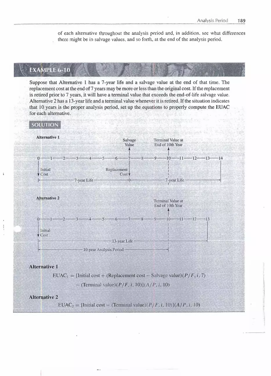
I
Analysis Period 189
of each alternative throughout the analysis period and, in addition, see what differencesthere might be in salvage values, and so forth, at the end of the analysis period.
Suppose that Alternative 1 has a 7-year life and a salvage value at the end of that time. Thereplacementcost at the end of 7 years maybe more or lessthan the originalcost. If the replacementis retired prior to 7 years, it will have a terminal value that exceeds the end-of-life salvage value.Alternative2 has a 13-year life and a terminalvaluewheneverit isretired. If the situationindicatesthat 10 years is the proper analysis period, set up the equations to properly compute the EUACfor each alternative.
Alternative 1Salvage TerminalValueatValue Endof 10thYear
f fO~1-2~3---:::-4~5~6~1---8---9-1O-11---12-13---14
l,jnitii1 R"Plae<menil
.. i
Cost Cost II
I 7~yearLife I 7-yearLifeI
Altemative2Terminal Value atEnd of 1OthYear
fO~1-2-3___4~5 6" 7~8 9~10 11---12-13
l 1'titii1Cost
, '
13-year Life II
--I
II
10-year Analysis Period
Altel'native.l
'.EUAC1 [Initial cost + (Replacetnentcost - Salvage value)(P j F, i, 7,)
- (Terminalvalue)(PjF, i, lO)](AjP, i, 10).I
r= Alterp.ative2
:,.=' I: ~~ f1J1C"2,,.DIJit!~co~t-~~Ji~l£k.!W.J~Ic.P ~JPl =
- -- - - --
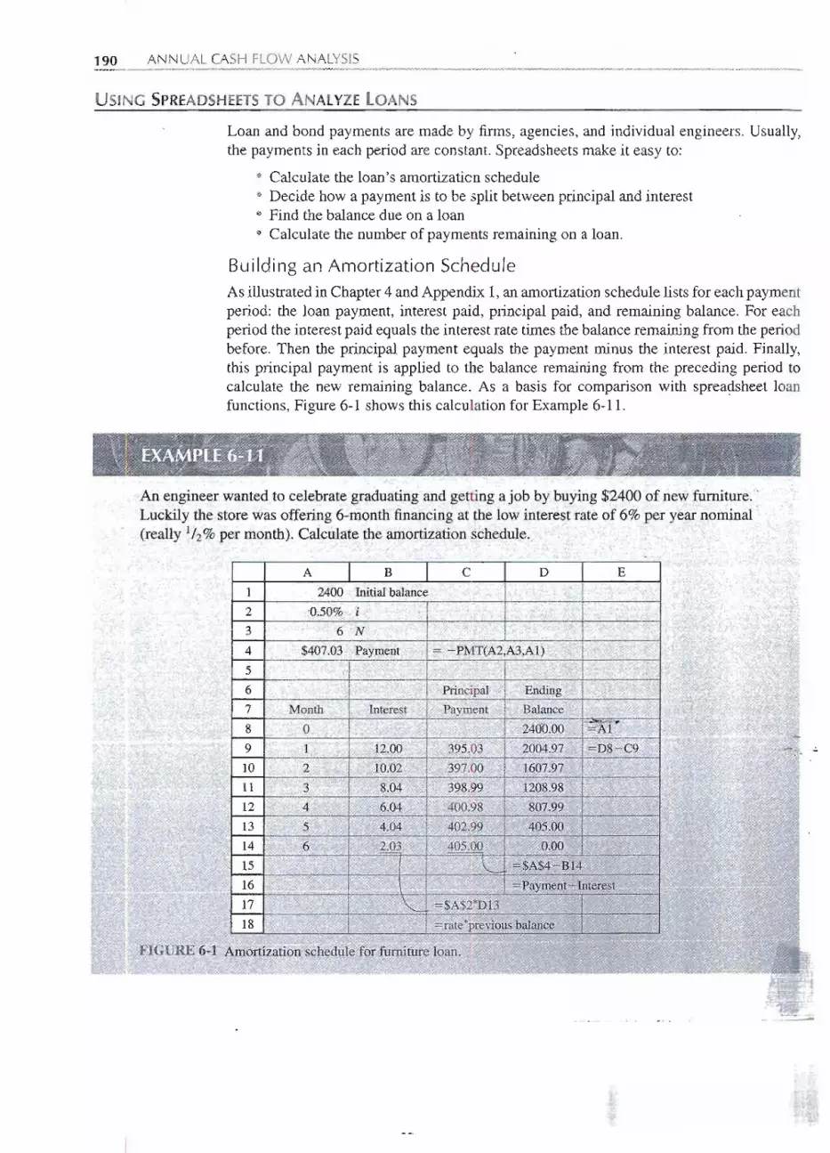
190 ANNUAL CASH FLOW ANALYSIS
USING SPREADSHEETS TO ANALYZE LOANS
Loan and bond payments are made by firms, agencies, and individual engineers. Usually,the payments in each period are constant. Spreadsheetsmake it easy to:
· Calculate the loan's amortization schedule· Decide how a payment is to be split between principal and interest· Find the balance due on a loan·Calculate the number of payments remaining on a loan.
Building an Amortization ScheduleAs illustrated in Chapter4 and Appendix 1,an amortizationschedulelists for each paymentperiod: the loan payment, interest paid, principal paid, and remaining balance. For eachperiod the interest paid equals the interest rate times the balance remaining from the period'before. Then the principal payment equals the payment minus the interest paid. Finally,this principal payment is applied to the balance remaining from the' preceding period tocalculate the new remaining balance. As a basis for comparison with sprea~sheet loanfunctions, Figure 6-1 shows this calculation for Example 6-11.
An engineer wanted to celebrate graduating and getting a job by buying $2400 of new furniture.Luckily the store was offering 6-month financing at thelow interest rate of 6% per year nominal'(really 1/2%per month). Calculate the amortization schedule.
~: ~:; ~ ~.pI.
t'" '1'1~'FIGURE'6:r AIDomzati6n schedrile:forfUnllture1oah.
..,.~. ..;.Ij
I
L ,'--"
,_ ~"1 _ _ _ __ - .. ---
- - --
A B C D E
1 2400 Initial balance
2 0.50% i
3 6 N
4 $407.03 Payment ""'.--PM)'(A2,A3,Al)
5
6 Principal El11:ling ,
7 Month Interest Payment Balance
8 0 , 240"0.00 #Al9 1 , 12.00 395.03 2004.97 ==D8--C9
10 2 10.02 397.00 1607.97
11 3 8;04 398.99 1208.98
12 4 I 6.04 400.98 807.99
13 5 4.04 402,99 I 405.00 ,
14 6 2.03 405.00 0.0015
,\. '",. ....
. "k'''' ,, ,
16.'
<;;J'!i;==.,"'" ,"" . . ....... '.0 .= ,",'
17 . ==$A$2*Dl3 .''.
18 * ,,> . . '. .. """'==,." ;;.. :;;;:11:1:

Using Spreadsheets to Analyze Loans 191
The first step is to calculate the monthly payment:
A -2400(AjP,lh%, 6) .2400 (0..J.696) ..$407.Q
With tlIi~iIlformation to p.al).dtQe engiIieer cap. us~. the $pJ;ea<l$he~tofEiguI:e 6-1 to obtafu theamowzatiQJ.).schedule. '1: =
How Much to Interest? How Much to Principal?
For a loan with constant payments, we can answer these questions for any period withoutthe full amortization schedule. For a loan with constant payments, the functions IPMTand PPMT directly answer these questions. For simple problems, both functions have fourarguments (i, t, n, -P), where t is the time period being calculated. Both functions haveoptional arguments that permit adding a balloon payment (an F) and changing from end-of-period payments to beginning-of-periodpayments.
For example, consider Period 4 of Example 6-11. The spreadsheet formulas give the .
same answer as shown in Figure 6-1.
Interes4 = IPMT(0.5%, 4, 6, -2400) = $6.04
Principalpayment4= PPMT(0.5%,4,6, -2400) =$400.98
Finding the Balance Due on a LoanAn amortizationschedulecan be used to calculatethe balance due on a loan. Or more easilythe balance due equals the present worth of the remaining payments. Interest is paid in fullafter each payment, so later payments are simply based on the balance due.
I
L
A.caris pUJ.'chasedWith a 48-month, 9% nominal loan with an initial balance of $15,000. Whatis the,balance dtl~ halfway through the 4 years?
'J!l
Th,.eW$t~Jep j~JQ;f81q1l1at~ !h.~1J1P!lfuJypay.w.el).t".3-ta mon(hlyinteJ;est;-ate,J>fJ /4%.Jbis ~quals ~W"
"II
,IPaYIIlel).f' '..15,QOO(AJP,'0.75%,48) or. ...PMT(0,75%, 48, -15,000)
: = d! R: . ~{/15',"6(0){6.iQ2];9) ~;$17330~'" bt~ J!.1373;28
-.-
- ----

192 ANNUAL CASH FLOW ANALYSIS
The next step will use ~e spreadsheet answer, because it is more accurate (there are only threesignificantdigits in the tabulated factor).
After 24 paymentsandwith24 left, theremainingbalance equals (P / A, i, Nremaining)payment
Balance = (P / A, 0.75%, 24)$373.28 or
= (21.889)(373.28) =$8170.73 or
= PV(0.75%, 24,373.28)
. $8170.78
Thus halfway through the repayment schedule, 54.5% of the original balance is still owed.
! . Pay Off Debt Sooner by Increasing PaymentsPaying off debt can be a good investment because the investmentearns the rate of intereston the loan. For example, this could be 8% for a mortgage, 10% for a car loan, or 19%for a credit card. When making extra payments on a loan, the common question is: Howmuch sooner will the debt be paid off? Until the debt is paid off, any early payments areessentially locked up, since the same payment amount is owed each month.
The firstreasonthatspreadsheetsare convenientis fractionalinterestrates.For example,an auto loan might be at a nominal rate of 13% with monthly compounding or 1.08333%per month. The second reason is that the function NPER calculates the number of periodsremaining on a loan.
NPER can be used to calculate how much difference one extra payment makes orhow much difference increasing all payments by x% makes. Extra payments are appliedentirely to principal, so the interest rate, remaining balance, and payment amounts are allknown. NremainingequalsNPER(i, payment, remainingbalance) with optional argumentsforbeginning-of-periodcash flows and balloon payments. The signs.of the payment and theremaining balance must be different.
Maria has a 7.5% mortgage with monthly payments for 30 years. Her original balance was$100,000, and she just made her twelfth payment. Each month she also pays into a reserveaccount, which the bank uses to pay her fire and liability insurance ($900 annually) and propertytaxes ($1500 annually). By how much does she shorten the loan if she makes an extra loanpayment today? If shemakes an extra total payment?If she increases each total payment to 110%of her current total payment?
SOLUTION
The first step is to calculate Maria's loan payment for the 360 months. Rather than calculating asix.-significantdigit monthly interest rate,it is easier to use 0.075/12 in the spreadsheetformulas.
Payment-CPMT(O.01s/12,360, -100000) = $699.21...- - - - ...- -- - --
---

Summary 193
The remainjngbalanceafter 12suchpayments is thepresent worthof theremaining348payments.
Balance12 = PV(0.075jI2,348,699.21) = $99,077.53(after 12 payments, she has paid off $922!)
If she pays an extra $699.21, then the number of periods remaining is
NPER(0.075jI2,-699.21, 99077.53 - 699.21) = 339.5
This is 8.5 payments less than the 348 periods left before the extra payment. If she makes anextratotal payment, then
Total payment = 699.21 +900j12 + 1500j12 - $899.21jmonth
NPER(0.075j12, -699.21,99244 -,,-.899.21) = 337.1
or2.4;more paYlllentssaved.If sqemakes an extra 10%paYlllentOnthetotalpaymenfof $899.21,th~ ~
NPER([0.075jI2, ---(1.1)(899.21-200)],99077.53) .246.5 payments
or IOl.5 payments saved.IIQ'btethat.$200 of the total paYlllentgoes to payfori:nsnf<Ulceand t~es.
SUMMARY
Annual cash flowanalysis is the secondof the threemajormethodsof resolvingalternativesinto comparablevalues.When an alternativehas an initial cost P and salvagevalue S, thereare three ways of computing the equivalentuniform annual cost:
· EUAC = P(Aj P, i, n) - S(Aj F, i, n)· EUAC= (P - S)(AjF, i, n) + Pi· EUAC= (P- S)(Aj P, i, n) + Si
(6-1)(6-3)(6-4) .
All threeequationsgivethe same answer.This quantityis alsoknownas the capital recovery.cost of the project.
The relationship between the present worth of cost and the equivalent uniform annualcost is:
· EUAC = (PW of cost)(Aj P, i, n)
The three annual cash flow criteria are:
For fixedinputFor fixed outputNeither input nor output fixed
Maximize EUABMinimize EUACMaximize EUAB - EUAC
In present worth analysis there must be a common analysis period. Annual cash flowanalysis, however,allows some flexibilityprovided the necessary assumptions are suitablein the situation being studied. The analysis period may be different from the lives of the
---

194 ANNUAL CASH FLOW ANALYSIS
alternatives, and provided the following criteria are met, a valid cash flow analysis may lmade.
1. When an alternativehas reached the endof its useful life, it is assumedto be replaceby an identical replacement (with the same costs, performance, etc.).
2. The analysis period is a common multiple of the useful lives of the alternatives, (there is a continuingor perpetual requirement for the selected alternative.
If neither condition applies, it is necessary to make a detailed study of the consequenceof the various alternatives over the entire analysis period with particular attention to thdifference between the alternativesat the end of the analysis period.
There is very little numericaldifferencebetween a long-life alternativeand a perpetuaalternative. As the value of n increases, the capital recovery factor approaches i. At tholimit, (AI P, i, (0) = i.
One of the most common uniform payment series is the repayment of loans. Spreadsheets are useful in analyzing loans (balance due, interest paid, etc.) for several reasons: they have specializedfunctions, many periods are easy, and any interest rate can btused.
PROBLEMS
6-1- Compute the value of C for the following diagram,based on "a10% interest rate.
6-3 Computethe value of E:
60
~ 'f r r0-1-2-3-4
~ ~ ~ ~
60
1
45
t 3f +0-1-2-3-4
! ! ! !E E E E
i = 12%c c c c
6-4 If i = 6%, compute the value of D that is equivalentto the two disbursementsshown.
6-2(Answer: C = $35.72)
Compute the value of B for the following diagram:
B B B B B
t t t t t0-1-2-3-4-5
~ i = 15% ~
100
t0-1-2-3-4-5-6
t t t t "t tD D D D D D
200
r-
100 100
~
.-'~Answer: D = $52.31)
,
1

6-5 For the diagram, compute the value of D:
Problems 195
6-9 On April 1 a man borrows $100. The loan is to berepaid in three equal semiannual (every 6 months)payments. If the annual interest rate is 7% com-pounded semiannually, how much is each payment?(Answer: $35.69)
An electronics firm invested $60,000 in a precisioninspection device. It cost $4000 to operate and main~tain in the first year and $3000 in each of the subse-quent years. At the end of 4 years, the firm changedtheir inspection procedure, eliminating the need forthe device. The purchasing agent was very fortunatein being able to sell the inspection device for $60,000,the original price. The plant manager asks you to com~ .
pute the equivalent uniform annual cost of the deviceduring the 4 years it was used. Assume interest at 10%per year. (Answer: $9287)
A firm is about to begin pilot plant operation on a pro-cess it has developed. One item of optional equipmentthat could be obtained is a heat exchanger unit. Thecompany finds that a unit now available for $30,000could be used in other company operations. It is es-timated that the heat exchanger unit will be worth$35,000 at the end of 8 years. This seemingly high sal-vage value is due primarily to the fact that the $30,000purchase price is really a rare bargain. If the firmbelieves 15% is an appropriate rate of return, whatannual benefit is needed to justify the purchase of theheat exchanger unit? (Answer: $4135)
6-12 The maintenance foreman of a plant in reviewing hisrecords found that a large press had the followingmaintenance cost record:
1.5D
t t r t t0-1-2-3-4-5
1
i = 12%
500
~ ~
i r t ~ t r i0-1-2-3-4-5-6-7
~ ~ ~ ~ ~ ~ ~A A A A A A A
6-8 As shown in the cash flow diagram, there is an annualdisbursement of money that varies from year to yearfrom $100 to $300 in a fixed pattern that repeatsforever. If interest is 10%, compute the value of A,also continuing forever, that is equivalent to the fluc-tuating disbursements.
-. -~
300 300 300
It T r T TT r T ItT r T0-1-2-3-4-5-6-7-g-9-1O-1l-12 n = co
! ! ! ! ! ! ! ! ! ! ! !A A A A A A A A A A A A
i = 10%
5 yearsago4 years ago3 years ago2 years agoLast year
$ 600700800900
1000
6-6 What is C in the accompanying figure?
6-10
40
i
30
r
20
t10 10! !
0-1-2-3-4-5
C C C Ci = 10%
6-11
6-7 If interest is 10%,what is A?

196 ANNUAL CASH FLOW ANALYSIS
After consulting with a lubrication specialist, hechanged the preventive maintenance schedule. He be-liev~s that this year maintenance will be $900 andwill decrease $100 a year in each of the following4 years. If his estimate of the future is correct, whatwill be the equivalent uniform annual maintenancecost for the 10-year period? Assume interest at 8%.(Answer: $756)
6-13 A firm purchased some equipment at a very favorableprice of $30,000. The equipment resulted in an an-nual net saving of $1000 per year during the 8 yearsit was used. At the end of 8 years, the equipment wassold for $40,000. Assuming interest at 8%, did theequipment purchase prove to be desirable?
6-14 When he started work on his twenty-second birthday,D. B. Cooper decided to invest money each monthwith the objective of becoming a millionaire by thetime he reaches age 65. If he expects his invesnnentsto yield 18% per annum, compounded monthly, howmuch should he invest each month? (Answer: $6.92a month.)
6-15 Linda 0' Shay deposited $30,000 in a savings accountas a perpetual trust. She believes the account will earn7% annual interest during the first 10 years and 5%interest thereafter. The trust is to provide a uniformend-of-year scholarship at the university. What uni-form amount could be used for the student scholarshipeach year, beginning at the end of the first year andcontinuing forever?
6-16 A machine costs $20,000 and has a 5-year useful life.At the end of the 5 years, it can be sold for $4000. Ifannual interest is 8%, compounded semiannually,what is the equivalent uniform annual cost of themachine? (An exact solution is expected.)
6-17 The average age of engineering students at gradu:'ation is a little over 23 years. This means that theworking career of most engineers is almost exactly500 months. How much would an engineer need tosave each month to become a millionaire by the endof his working career? Assume a 15% interest rate,compounded monthly.
6-18 The Johnson Company pays $200 a month to a truckerto haul wastepaper and cardboard to the city dump.The material could be recycled if the company were tobuy a $6000 hydraulic press bailer and spend $3000 ayear for labor to operate the bailer. The bailer has anestimated useful life of 30 years and no salvage value.Strapping material would cost $200 per year for the
- --
estimated 500 bales a year that would be producecA wastepaper company will pick up the bales at thplant and pay Johnson $2.30 per bale for them. USIan annual cash flow analysis in working this problem(a) If interest is 8%, is it economical to install ant
operate the bailer?(b) Would you recommend that the bailer be
installed?
6-19 An engineer has a fluctuating future budget for th~maintenance of a particular machine. During each 01the first 5 years, $1000 per year will be budgeted.During the second 5 years, the annual budget will be$1500 per year. In addition, $3500 will be budgetedfor an overhaul of the machine at the end of the fourth
year, and another $3500 for an overhaul at the end ofthe eighth year.
The engineer asks you to compute the uniformannual expenditure that would be equivalent to thesefluctuating amounts, assuming interest at 6% per year.
6-20 An engineer wishes to have $5 million by the time heretires in 40 years. Assuming 15% nominal interest,compounded continuously, what annual sum must heset aside? (Answer: $2011)
6-21 Art Arfons, a K-State-educated engineer, has madea considerable fortune. He wishes to start a per-
petual sch?larship for engineering students at K-State. The scholarship will provide a student with anannual stipend of $2500 for each of 4 years (fresh-men through senior), plus an additional $5000 duringthe senior year to cover entertainment expenses. As-sume that students graduate in 4 years, a new awardis given every 4 years, and the money is provided atthe beginning of each year with the first award at thebeginning of year one. The interest rate is 8%.(a) Determine the equivalent uniform annual cost
(EUAC) of providing the scholarship. .(b) How much money must Art donate to K-State?
6-22 Jenny McCarthy is an engineer for a municipal powerplant. The plant uses natural gas, which is currentlyprovided from an existing pipeline at an annual costof $10,000 per year. Jenny is considering a project toconstruct a new pipeline. The initial cost of the newpipeline would be $35,000, but it would reduce theannual cost to $5000 per year. Assume. an analysisperiod of 20 years and no salvage value for either theexisting or new pipeline. The interest rate is 6%.(a) Determine the equivalent uniform annual cost
(EUAC) for the new pipeline?(b) Should the new pipeline be constructed?
--:-'
- - - --------

Problems 197
6-23 A machine has a first cost of $150,000, an annualoperation and, maintenance cost of $2500, a life of10 years, and a salvage value of $30,000. At the endof years 4 and 8, it requires a major service, whichcosts $20,000 and $10,000, respectively. At the endof year 5, it will need to be overhauled at a cost of$45,000. What is the equivalent uniform annual costof owning and operating this particular machine?
6-24 Mr. Wiggley wants to buy a new house. It willcost $178,000. The bank will loan 90% of thepurchase price at a nominal interest rate of 10.75%compounded weekly, and Mr. Wiggley will makemonthly payments. What is the amount of the monthlypayments if he intends to pay the house off in25 years?
6-25 Steve Lowe must pay his property taxes in two equalinstallments on December 1 and April 1. The twopayments are for taxes for the fiscal year that be-gins on July I and ends the following June 30. Stevepurchased a home on September 1. He estimates theannual property taxes will be $850 per year. Assum-ing the annual property taxes remain at $850 per yearfor the next several years, Steve plans to open a sav-ings account and to make uniform monthly depositsthe first of each month. The account is to be used to
pay the taxes when they are due.To begin the account, Steve deposits a lump
sum equivalent to the monthly payments that will nothave been made for the first year's taxes. The savingsaccount pays 9% interest, compounded monthly andpayable quarterly (March 31, June 30, September 30,and December 31). How much money should Steveput into the account when he opens it on September 1?What uniform monthly deposit should he make fromthat time on? (A careful exact solution is expected.)(Answers: Initial deposit $350.28; monthly deposit$69.02)
6-26 Claude James, a salesman, needs a new car for use inhis business. He expects to be promoted to a supervi-sory job at the end of 3 years, and so his concern nowis to have a car for the 3 years he expects to be "on theroad." The company reimburses salesmen each monthat the rate of 251iper mile driven. Claude has decidedto drive a low-priced automobile. He finds, however,that there are three different ways of obtaining theautomobile:
(a) Purchase for cash; the price is $13,000.(b) Lease the car; the monthly charge is $350 on a 36-
month lease, payable at the end of each month;
at the end of the 3 year period, the car is returnedto the leasing company.
(c) Lease the car with an option to purchase it at theend of the lease; pay $360 a month for 36 months;at the end of that time, Claude could purchase thecar, if he chooses, for $3500.
Claude believes he should use a 12% interest rate
in determining which alternative to select. If the carcould be sold for $4000 at the end of 3 years, whichmethod should he use to obtain it?
6-27 A motorcycle is for sale for $2600. The motorcycledealer is willing to sell it on the following terms:
No down payment; pay $44 at the end ofeach of the first 4 months; pay $84 at theend of each month after that until the loan
has been paid in full.
Based on these terms and a 12% annual interest rate
compounded monthly, how many $84 payments willbe required?
6-28 When he purchased his home, AI Silva borrowed$80,000 at 10% interest to be repaid in 25 equalannual end-of-year payments. After making 10 pay-ments, AI found he could refinance the balancedue on his loan at 9% interest for the remaining15 years.
To refinance the loan, AI must pay the originallender the balance due on the loan, plus a penaltycharge of 2% of the balance due; to the new lenderhe also must pay a $1000 service charge to obtain theloan. The new loan would be made equal to the bal-ance due on the old loan, plus the 2% penalty charge,and the $1000 service charge. Should AI refinancethe loan, assuming that he will keep the house for thenext 15 years? Use an annual cash flow analysis inworking this problem.
6-29 A company must decide whether to provide theirsalesmen with company-owned automobiles or to paythe salesmen a mileage allowance and have them drivetheir own automobiles. New automobiles would cost
about $18,000 each and could be resold 4 years laterfor about $7000 each. Annual operating costs wouldbe $600 per year plus 12,t per mile. If the sales~endrove their own automobiles, the company probablywould pay them 30}!!per mile. Calculate the numberof miles each salesman would have to drive each yearfor it to be economically practical for the companyto provide the automobiles. Assume a 10% annualinterest rate. Use an annual cash flow analysis.
- -
-- ----
-------

!~t!i!III
i
II
jijII!
IIIiI!! it II ;
LL
198 ANNUALCASH FLOWANALYSIS
6-30 Your company must make a $500,000 balloon pay-ment on a lease 2 years and 9 months from today.You have been directed to deposit an amount ofmoney quarterly, beginning today, to provide for the$500,000 payment. The account pays 4% per year,compounded quarterly. What is the required quarterlydeposit? Note: Lease payments are due at beginningof the quarter.
A manufacturer is considering replacing a produc-tion machine tool. The new machine, costing $3700,would have a life of 4 years and no salvage value,but would save the firm $500 per year in direct la-bor costs and $200 per year indirect labor costs. Theexisting machine tool was purchased 4 years ago at acost of $4000. It will last 4 more years and will haveno salvage value at the end of that time. It could besold now for $1000 cash. Assume that money is worth8% and that the difference in taxes, insurance, and soforth, for the two alternatives is negligible. Use anannual cash flow analysis to determine whether thenew machine should be purchased.
1\vo possible routes for a power line are under study.Data on the routes are as follows:
6-31
6-32
LengthFirst costMaintenance
Useful life, in yearsSalvage valueYearly power lossAnnual property taxes
Aroundthe Lake
15km$5000/km
$200/km/yr15$3000/km$500/km2% of first cost
Underthe Lake
5km$25,OOO/km
$400/km/yr15$5000/km$500/km2% of first cost
6-33
If 7% interest is used, should the power line be routedaround the lake or under the lake? (Answer: Aroundthe lake.)
An oil refinery finds that it is now necessary to subjectits waste liquids to a costly treating process before dis-charging them into a nearby stream. The engineeringdepartment estimates that the waste liquid processingwill have cost $30,000 by the end of the first year. Bymaking process and plant alterations, it is estimatedthat the waste treatment cost will decline $3000 each
year. As an alternate, a specialized firm, Hydro-Clean,has offered a contract to process the waste liquids for10 years for a fixed price of$15,000 per year, payableat the end of each year. Either way, there should beno need for waste treatment after 10 years. The re-finery manager considers 8% to be a suitable interest
rate. Use an annual cash flow analysis to determinewhether he should accept the Hydro-Clean offer.
6-34 Bill Anderson buys an automobile every 2 years a!follows: initially he makes a down payment of $600Con a $15,000 car. The balance is paid in 24 equa:monthly payments with annual interest at 12%. Wherhe has made the last payment on the lo~n, he trade!in the 2-year-old car for $6000 on a new $15,000 carand the cycle begins over again.
Doug Jones decided on a different purchase planHe thought he would be better off if he paid $15,OOCcash for a new car. Then he would make a monthly de.posit in a savings account so that, at the end of2 yearshe would have $9000 in the account. The $9000 plmthe $6000 trade-in value of the car will allow Dou~to replace his 2-year-old car by paying $9000 for,new one. The bank pays 6% interest, compoundecquarterly. ' . .(a) What is Bill Anderson's monthly payment to pa)
off the loan on the car?
(b) After he purchased the new car for cash, ho"much per month should Doug Jones deposit iihis savings account to have sufficient money fo]the next car two years hence?
(c) Why is Doug's monthly savings account deposismaller than Bill's payment?
6-35 Alice White has arranged to buy some home record.ing equipment. She estimates that it will have a 5-ye3.Juseful life and no salvage value. The dealer, who is ,friend, has offered Alice two alternative ways to pa~for the equipment:(a) Pay $2000 immediately and $500 at the end 0:
one year.(b) Pay nothing until the end of 4 years, when a singh
payment of $3000 must be made.Alice believes 12% is a suitable interest rate
Use an annual cash flow analysis to determine whiclmethod of payment she should select.(Answer: Select (b»
6-36 Two mutually exclusive alternatives are being considered.
YearoI2345
A-$3000
+845+845+845+845+845
B-'$5000+1400+ 1400+ 1400+1400+1400 ;'
,,\.'l
:t

Problems 199
6-37
One of the alternatives must be selected. Using a 15%nominal inteJ:est rate, compounded continuously,determine which one. Solve by annual cash flowanalysis.
A certain industrial firm desires an economic analysisto determine which of two different machines should
be purchased. Each machine is capable of performingthe same task in a given amount of time. Assume theminimum attractive return is 8%. The following dataare to be used in this analysis:
First cost
Estimated life, in yearsSalvage valueAnnual maintenance cost
Machine X$5000
5oo
Machine Y$8000
12$2000
150
6-38
Which machine would you choose? Base your answeron annualcost. (Answers:X = $1252;Y = $1106)
A suburban taxi company is considering buying taxiswith diesel engines instead of gasoline engines. Thecars average 50,000 km a year, with a useful life of3 years for the taxi with the gas engine and 4 yearsfor the diesel taxi. Other comparative information isas follows:
Diesel
$13,00048~
35300500
2,000
Gasoline$12,000
51~28
$ 200500
3,000
Vehicle cost
Fuel cost per literMileage, in km/literAnnual repairs $Annual insurance premil1;In. . ..End-of-useful-life resai.; v~"""
Use an annual cash flow analysis to determine themore economical choice if interest is 6%.
6-39 A company must decide whether to buy Machine Aor Machine B:
Initial cost
Usefullife, in yearsEnd-of-useful-life
salvage valueAnnual maintenance
Machine A Machine B
$10,000 $20,0004 10
$10,0001,000
$10,000o
At a 10% interest rate, which machine should beinstalled?Use an annual cash flowanalysisin work-ing this problem. (Answer:MachineA)
6-40 Consider the following alternatives:
A B
Cost $50 $180Uniform annual benefit 15 60
Useful life, in years 10 5
The analysis period is 10 years, but there will be ~oreplacement for Alternative B at the end of 5 years.Based on a 15% interest rate, determine which alter-native should be selected. Use an annual cash flow
analysis in working this problem.
6-41 Consider the following two mutually exclusivealternatives:
A B
Cost $100 $150Uniform annual benefit 16 24
Useful life, in years 00 20
Alternative B may be replaced with an identical itemevery 20 years at the same $150 cost and will have thesame $24 uniform annual benefit. Using a 10% inter-est rate, and an annual cash flow analysis, determinewhich alternative should be selected.
6-42 Some equipment will be installed in a warehousethat a firm has leased for 7 years. There are twoalternatives:
A B
Cost $100 $150Uniform annual benefit 55 61
Useful life, in years 3 4
At any time after the equipment is installed, it hasno salvage value. Assume that Alternatives A and Bwill be replaced at the end of their useful lives byidentical equipment with the same costs and benefits.For a 7-year analysis period and a 10% interest rate,:use an annual cash flow analysis to determine whichalternative should be selected.
6-43 A pump is required for 10 years at a remote loca-tion. The pump can be driven by an electric motorif a power line is extended to the site. Otherwise, agasoline engine will be used. Use an annual cash flowanalysis to determine, based on the following data anda 10% interest rate, how the pump should be powered.
Gasoline Electric
First cost $2400 $6000
Annual operating cost 1200 750Annual maintenance 300 50
Salvage value 300 600Life, in years 5 10
- -- --

200 ANNUAL CASH FLOW ANALYSIS
6-44 The town of Dry Gulch needs an additional supplyof water from Pine Creek. The town engineer hasselected two plans for comparison: a gravity plan(divert water at a point 10 miles up Pine Creek andcarry it through a pipeline by gravity to the town) anda pumping plan (divert water at a point closer to thetown and pump it to the town). The pumping plantwould be built in two stages, with half-capacity in-stalled initially and the other half installed 10 yearslater.
An analysis will assume a 40-year life, 10%interest, and no salvage value. Costs are as follows:
. . Initial investmentAdditional investment in
10th yearOperation and maintenancePower cost
Average first 10 yearsAverage next 30 years
Gravity$2,800,000
None
Pumping$1,400,000
200,000
1O,OOO/yr 25,000/yr
NoneNone
50,000/yr100,000/yr
6-45
Use an annual cash flow analysis to determine themore economical plan.
Uncle Elmo needs to replace the family privy.The local sanitary engineering firm has submittedtwo alternative structural proposals with respectivecost estimates as shown. Which construction shouldUncle Elmo choose if his minimum attractive rate of
return is 6%. Use both a present worth and annualcost approach in your comparison.
First costAnnual maintenance
Salvage valueService life, in years
Masonite$250
20104
Brick$1000
1010020
6-46 The manager in a canned food processing plant is try-ing to decide between two labeling machines. Theirrespective costs and benefits are as follows:
First costMaintenance and
operating costsAnnual benefit
Salvage valueUseful life, in years
Machine A
$15,0001,600
Machine B
$25,000400
8,0003,000
7
13,0006,000
10
Assume an interest rate of 12%. Use annual cashflow analysisto determine which machine should beselected.
6-47 Carp, Inc. wants to evaluate two methods of shippinJtheir products. The following cash flows are associated with the alternatives:
First costMaintenance and
operating costs+ Cost gradient
(begin Year 1)Annual benefit
Salvage valueUseful life, in years
A
$700,00018,000
B
$1,700,00029,000
+900/yr +750/yr
154,000142,000
10
.303,000210,000
20
6-48
Use an interest rate of 15% and annual cash flow anal
ysis to decide which is the most desirable alternative
A college student has been looking for a new tire fohis car and has located the following alternatives:
Tire Warranty(months)
12243648
Price per Tire$39.9559.9569.9590.00
6-49
The student feels that the warranty period is a goocestimate of the tire life and that a 10% interest ran
is appropriat~. Use an annual cash flow analysis tcdeterminewhichtire he should buy. .
Consider the following three mutually exclusiv(alternatives:
CostUniform annual benefit
Useful life, in years
A
$10010
B
$150.0017.6220
C
$200.0055.48500
Assuming that Alternatives B and C are replaced wid:identical replacements at the end of their useful lives.and an 8% interest rate, which alternative should b(selected? Use an annual cash flow analysis in workin~this problem. (Answer: Select C)
6-50 A new car is purchased for $12,000 with a 0% down.
.IlL 9% loan. The loan's length is 4 years. After making30 payments, the owner desires to payoff the loan'~remaining balance. How much is owed?
6-51 A year after buying her car, Anita has been offered
JIL ajob in Europe. Her car loan is for $15,000 at a 9%nominal interest rate for 60 months. If she can sell the
car for $12,000, how much does she get to keep afterpaying off the loan?

...
- . - ........ __n.. ..
Problems 201
6-52 A $78,000 mortgage has a 30-year term and a 9%
A nominal interest rate.(a) What is the monthly payment?(b) After the first year of payments, what is the out-
standing balance?(c) How much interest is paid in month 13? How
much principal?
6-53 A $92,000 mortgage has a 30-year term and a 9%-. nominal interestrate.(a) What is the monthly payment?(b) After the first year of payments, what fraction of
the loan has been repaid?(c) After the first 10 years of payments, what is the
outstanding balance? .
(d) How much interest is paid in Month 25? Howmuch principal?
1 A 30-year mort~~~e for $95,000 is issued at a 9%
JI. nominal interest rate.. . (a) What is the monthly payment?
(b) How long does i!~e to pay off the mortgage, if$1000 per month is,paid?
(c) How long does it take to pay off the mortgage, ifdouble payments are made?
6-55 A 30-year mortgage for $145,000 is issued at a 6%
A nominal interest rate.-,.. (a) What is the monthly payment?(b) How long does it take to payoff the mortgage,if
$1000 per month is paid?(c) How long does it take to payoff the mortgage, if
20% extra is paid each month?
6-56 Solve Problem 6-32 for the breakeven first cost per
AIL kilometer of going under the lake.6-57 Redo Problem 6-38 to calculate the EUAW of the_ alternatives as a function of miles driven per year to- .. see if there is a crossover point in the decision process.
Graph your results.
6-58 Set up Problem 6-18 on a spreadsheet to make all the
A input data variable and determine various scenarioswhich would make the bailer economical.
6-59 Develop a spreadsheet to solve Problem 6-44. What
A is the breakeven cost of the additional primpinginvestment in year 10?
~"--- -"
II'
- 'IIl,..
----------- -- -

~
_/:>~~;J~~>
After Completing This Chapter...The student should be able to:. Evaluateproject cash flowsusing the internal rate of return (IRR) methodology.. Plot a project's present worth (PW) against the interest rate.. Use an incremental rate of return analysis to evaluatecompeting alternat:ives.. Develop and use spreadsheets to make IRR and incremental rate of ret~ calculatio~
.QUESTIONSTO CONSIDER
1. Imagine that you are a manufacturer who is consideringusing RFID chips to track Y01products.Whatcost andbenefit factorswouldyou considerin decidingw.hetherto embechips in your pr9ducts, and how much to invest in the necessary techD.ology?
2. Now assume that you are a retailer who is also considering the RFID technology.Ho'wouldyour cost and benefitconsiderationsdiffer from those of a product manufacture}What specificfactors would you consider? What if the manufacturersyou buy produclfrom have already adopted the technology? How would this affect your decision?
3. Since October 2000, the U.S. military has been using RFID technology in its Joint TouAssetVisibility(ITAV)program,whichtracksequipmentandsupplies.ITAVhasreduce.duplicate orders, helped speed up troop deployment, and allowed mi~tary planners toaccomplish missions with fewer ships, planes, and ground vehicles. How is the ITA'program likely to affect the pace ofRFID's adoptionby priva~ industry?
4. Some consumers have already expressed concern about RFID chips, calling them aJinvasion of privacy.What ethical and social concerns are raised by RFID chips?
5. In response to consumer worries, RFID chip manufacturersare developing"kill" technologiesthat can allowconsumersto disable RFIDchips after theyhavepurchasedgood:containing these miniature tracking devices. How might this affect consumer attitudes',
I _-.:0
- - - ------

- - -- - -
Rate of Return Analysis
II
Big Brother Is Tracking YouDo you everget the feeling that your closet is spying on you? Well, you may be right.
Manufacturers of products ranging from jeans to shampoo are trying out a new tech-nology called radio-frequencyidentification (RFID), which embeds tiny tracking chips inmerchandise. The chips can follow goods from the time they leave the plant until you buythem at your local shopping mall-and even after you take them home.
RFID chips offer a wealth of advantages toproduct makers and retailers. They can tell ship-pers when trucks are delayed, and they can alertstore security when products are being stolen.They can also tell managers when stocksof pop-ular products are running low.
The chips still suffer from some technicaldrawbacks, including vulnerability to interfer-ence from cell phones and other electronic de-vices. A bigger drawback,however,is their cost.As of early2003,RFID chips cost about30 centseach, which makes them too expensive to em-bed in low-cost products like soap and shavingcream. Moreover,the scanner~required to readthe chips currently cost about $1000 each. Andcompanies that want to use the technologymustalso investin the electronicequipmentnecessaryto keep track of the chips.
The cost hurdle may be falling soon, though. A major manufacturer of RFID chipssays it can produce them for 5 cents each if the customer orders a batch of at least a billion.Even more substantialcost reductions arelikely whenthe technologybecomes more widelyadopted.
I
--- --- - - --- -----
---- -- -----------
204 RATEOF RETURNANALYSIS
In this chapter we will examine three aspects of rate of return, the third of the three majoranalysis methods. First, we describe the meaning of "rate of return"; then, the calculationof rate of return is illustrated; finally,rate of return analysis problems are presented. In anappendix to this chapter, we describe difficulties sometimes encountered in attempting tocompute an interest rate for cash flows of certain kinds.
INTERNAL RATE OF RETURN
. i
In Chapter 3 we examined four plans to repay $5000 in 5 years with interest at 8%(Table 3-1). In each of the four plans the amount loaned ($5000) and the loan duration(5 years) were the same. Yet the total interest paid to the lender varied from $1200 to$2347, depending on the loan repayment plan. We saw,however, that the lender received8% interest each year on the amount of money actually owed. And, at the end of 5 years,the principal and interest payments exactly repaid the $5000 debt with interest at 8%. Wesay the lender received an "8% rate of return."
Internal rate of return is defined as the interest rate paid on the unpaid balance ofa loan such that the payment schedule makes the unpaid loan balance equal to zerowhen the final payment is made.
Instead of lending money, we might invest $5000 in a machine tool wi~ a 5-year use-fullife and an equivalent uniform annual benefit of $1252. An appr<?priatequestion is,What rat~ of return would we receive on this investment? The cash flow would be asfollows:
Yearo12345
Cash Flow-$5000+1252+1252+ 1252+1252+1252
We recognize the cash flow as Plan 3 of Table 3-1. We know that five payments of$1252 are equivalentto a present sum of $5000 when interest is 8%. Therefore, the rate ofreturn on this investment is 8%. Stated in terms of an investment,we may define internalrate of return as follows:
Internal rate of return is the interest rate earned on the unrecovered investment suchthat the payment schedule makes the unrecovered investment equal to zero at the endof the life of the investment.
It must be understoodthat the 8% rate of return does not mean an annual return of 8% onthe$5000 investment,or $400 in each of the 5 years with $5000 returned at the end of Year5.Instead, each $1252 payment represents an 8% return on the unrecovered investmentplus
- ---

This cash flow represents a $5000 investmentwith benefitsthat produce an 8% rate ofreturnontheunrecoveredinvestment. . .
Althoughthetwodefinitionsofinternalrateofreturnarestateddifferently,oneinterms .
of a loan and the other in terms of an investment, there is only one fundamental conceptbeing described. It is that the int~rnal rate of return is the interest rate at which thebenefits are equivalent to the costs or the present worth (PW)is O.Since we are describingsituations of funds that remain within the investment throughout its life, the resulting rateof return is described as the internal rate of return, i.
CALCULATING RATE OF RETURN
To calculate a rate of return on an investment,we must convert the various consequencesof the investment into a cash flow. Then we will solve the cash flow for the unknownvalue of the internal rate of return (IRR). Five forms of the cash flow equation are asfollows:
PW of benefits - PW of costs = 0
PW of costs = PW of benefits
PW of benefits = 1PW of costs
Net present worth = 0
EUAB - EUAC = 0
The fiveequations represent the same concept in different forms. They can relate costs andbenefits with the IRR as the only unknown. The calculation of rate of return is illustratedby the following examples.
- -- .-
- -- --
CalculatingRateof Return 205
the partial return of the investment.This may be tabulated as follows:
Unrecovered 8% Return on Investment UnrecoveredInvestment at Unrecovered Repayment at Investment at
Year Cash Flow Beginning of Year Investment End of Year End of Year0 -$50001 +1252 $5000 $ 400 $ 852 $41482 +1252 4148 331 921 32273 +1252 3227 258 994 22334 +1252 2233 178 1074 11595 +1252 1159 93 1159 0- -
$1260 $5000
(7-1)
(7-2)
(7-3)
(7-4)
(7-5)
t

206 RATEOF RETURNANALYSIS
An $8200 investment returned $2000 per year over a 5-year useful life. What was the rate ofreturn on the investment?
Using Equation 7-2, we write
PW of benefits=1
PW of costs2000(P I A, i, 5) =1
8200
Rewriting, we see that
8200 =4.1(PIA, i, 5) = 2000
Then look at the compound interest tables for the value of i where (PIA, i, 5) = 4.1; if notabulated value of i gives this value, we will then find values on either side of the desired value(4.1) and interpolate to find thelM.
From interest tables we find:
In this example, no interpolation is needed because the internal rate of return is exactly 7%.
. An investmentresulted in the following cash flow.Compute the rate,of return.
Year Cash Flow
o -$7001 + 1002 +1753 + 2504 +325
EUAB - EUAC = 0
100 + 75(AI G,i, 4) -- 700(AI P, i, 4) = 0
'""In this situation,we navetwo differentinterestfactors in the equation.We wilLnotbe able to solveit as easily as ExaIllple 7-1. Since there is no convenient direct method of so!ution, we will solve
!"! "'....a
.
i
i (P/A,i,S)6% 4.2127% 4.1008% 3.993

. -- --- --
Calculating Rate of Return 207
the equatiop by trial and error. Try i = 5% first:
EUAB - EUAC = 0
100+ 75(AjG, 5%, 4) -700(Aj P, 5%, 4) = 0
100 + 75(1.439) - 700(0.2820) =0
At i = 5%,
EUAB- EUAC = 208 -197 = +11
The EUAC is too low.If the interest rate is increased,EUAC will increase. Try i = 8%:
EUAB - EUAC = 0
100+ 75(AjG, 8%,4) -700(Aj P, 8%,4) = 0
100 + 75(1.404) - 700(0.3019) = 0
--I
Ati = 8%,
EUAB - EUAC = 205 - 211 =-6-I'
This time the EUACis too large. We see that the true rate of return is between 5% and 8%. Tryi =7%:
EUAB - EUAC = 0
100+ 75(AjG, 7%, 4) -700(Aj P, 7%, 4) = 0
100 + 75(1.416) - 700(0.2952) = 0
At i = 7%,
EUAB -EUAC -.:...206 - 206 = 0
The IRR is 7%.
Calculate the rate of return on the investment on the followingcash flow.
Yearo12345
Cash Flow-$100
+20+30+20+40+40
=
- - -- - -- -~- iiii..._ b
- ----
- - - --- - --

208 RATEOF RETURN ANALYSIS
Using a net present worth of 0, try i = 10%:
NPW = -100 + 20(P / F, 10%, 1) + 30(P / F, 10%,2) + 20(P / F, 10%,3)
+ 40(P / F, 10%,4) + 40(P / F, 10%,5)
= -100 + 20(0.9091) + 30(0.8264) + 20(0.7513) + 40(0.6830)
+ 40(0.6209)
= -100 + 18.18+ 24.79 + 15.03 + 27.32 + 24.84
= -100 + 110.16 = +10.16
The trial interest rate i is too low.Select a second trial, i = 15%:
NPW = -100 + 20(0.8696) + 30(0.7561) + 20(0.6575) + 40(0.5718)
+ 40(0.4972)
= -100 + 17.39 + 22.68 + 13.15 + 22.87 + 19.89
= -100 + 95.98
= -4.02
FIGURE 7-1 Plot of NPW versusinterest rate i.
15
5%
These 10 and 15% points areplotted in Figure 7-1. By linear interpolation we compute the rateof return as follows: .
(10.16
)IRR = 10% + (15% - 10%) .. - 13.5%10.16 + 4.02
We can prove that the rate of return is very close to 131/2%by showing that theunrecoveredinvestment is very close to zero at the end of the life of the investment. f'
- - - - - -- - - -

Problems 201
6-52 A $78,000 mortgage has a 30-year term and a 9%-. nominal intere.strate.(a) What is the monthly payment?(b) After the first year of payments, what is the out-
standing balance?(c) How much interest is paid in month 13? How
much principal?
6-53 A $92,000 mortgage has a 30-year term and a 9%
JI. nominal interest rate.(a) What is the monthly payment?(b) After the first year of payments, what fraction of
the loan has been repaid?(c) After the first 10 years of payments, what is the
outstandingbalance? .
(d) How much interest is paid in Month 25? Howmuch principal?
1 A 30-year mortgage for $95,000 is issued at a 9%
JII.. nominal interest rate.(a) What is the monthly payment?(b) How long does it take to pay off the mortgage, if
$1000 per month is paid?(c) How long does it take to payoff the mortgage, if
double payments are made?
6-55 A 30-year mortgage for $145,000 is issued at a 6%_nominal interest rate.. .. (a) What is the monthly payment?(b) How long does it take to payoff the mortgage, if
$1000 per month is paid?(c) How long does it take to payoff the mortgage, if
20% extra is paid each month?
6-56 Solve Problem 6-32 for the breakeven first cost per. kilometer of going under the lake.&:IiiiIiiii86-57 Redo Problem 6-38 to calculate the EUAW of the
all. alternativesas a function of miles drivenper year tosee if there is a crossover point in the decision process.Graph your results.
6-58 Set up Problem 6-18 on a spreadsheet to make all the
A input data variable and detennine various scenarioswhich would make the bailer economical.
6-59 Develop a spreadsheet to solve Problem 6-44. What. is the breakeven cost of the additional plimpinginvestment in year 10?
=
_.--- L
--- ---

'i~;'''' ,1; -", _.-
II .:W. ,.",,~~<,.-~-_.
::z.."~'"----
After Completing This Chapter...The student should be able to:· Evaluate project cash flowsusing the internal rate of return (IRR) methodology.. Plot a project's present worth (PW) against the interest rate.. Usean incrementalrateof returnanalysistoevaluatecompetingalternatives.. Develop and use spreadsheets to make IRR and incremental rate of ret~ calculatio~
QUESTIONS TO CONSIDER
1. Imagine that you are a manufacturer who is consideringusingRFID chips to trackYOIproducts.What cost andbenefitfactorswouldyouconsiderin decidingwhetherto embtchips in your products, and how much to invest in the necessary technology?
2. Now assume that you are a retailer who is also considering the RFID technology.Ho'would your cost and benefitconsiderations differfrom those of a product manufactureIWhat specific factors would you consider? What if the manufacturersyou buy product'from have already adopted the technology? How would this affect your decision?
3. Since October 2000, the U.S. military has been using RFID technology in its Joint TouAssetVisibility(ITAV)program,whichtracksequipmentandsupplies.ITAVhasreduceduplicate orders, helped speed up troop deployment, and allowed mi~tary planners t,accomplish missions with fewer ships, planes, and ground vehicles. How is the ITA'program likely to affect the pace qf RFID's adoptionby priva~ industry?
4. Some consumers have already expressed concern about RFID chips, calling them aJinvasion of privacy.What ethical and social concerns are raised by RFID chips?
5. In response to consumer worries, RFID chip manufacturersare developing "kill" technologiesthat can allowconsumersto disableRFIDchips aftertheyhavepurchasedgood:containing these miniature tracking devices. How might this affect consumer attitudes~
I~
""""" ~_ ,_ok-_-' - ._.,-
- --- --

Rate of Return Analysis
"
Big Brother Is Tracking YouDo you ever get the feeling that your closet is spying on you? Well, you may be right.
Manufacturers of products ranging from jeans to shampoo are trying out a new tech-nology called radio-frequency identification (RFID), which embeds tiny tracking chips inmerchandise. The chips can follow goods from the time they leave the plant until you buythem at your local shopping mall-and even after you take them home.
RFID chips offer a wealth of advantagestoproduct makers andretailers. They can tell ship-pers when trucks are delayed, and they can alertstore security when products are being stolen.They can also tell managers when stocksof pop-ular products are running low.
The chips still suffer from some technicaldrawbacks, including vulnerability to interfer-ence from cell phones and other electronic de-vices. A bigger drawback,however,is their cost.As of early2003,RFID chips cost about30 centseach, which makes them too expensive to em-bed in low-cost products like soap and shavingcream. Moreover,the scanner~required to read
"'1'. the chipscurrentlycost about$1000each.Andcompanies that want to use the technologymustalso investin the electronicequipmentnecessaryto keep track of the chips.
The cost hurdle may be falling soon, though. A major manufacturer of RFID chipssays it can produce them for 5 cents each if the customer orders a batch of at least a billion.Even more substantialcost reductions arelikely whenthe technologybecomes morewidelyadopted.
- ----- -- --
- -- - ---- -

204 RATEOF RETURNANALYSIS
In this chapter we will examine three aspects of rate of return, the third of the three majoranalysis methods. First, we describe the meaning of "rate of return"; then, the calculationof rate of return is illustrated; finally, rate of return analysis problems are presented. In anappendix to this chapter, we describe difficulties sometimes encountered in attempting tocompute an interest rate for cash flows of certain kinds.
INTERNAL RATEOF RETURN
In Chapter 3 we examined four plans to repay $5000 in 5 years with interest at 8%(Table 3-1). In each of the four plans the amount loaned ($5000) and the loan duration(5 years) were the same. Yet the total interest paid to the lender varied from $1200 to$2347, depending on the loan repayment plan. We saw,however, that the lender received8% interest each year on the amount of money actually owed. And, at the end of 5 years,the principal and interest payments exactly repaid the $5000 debt with interest at 8%. Wesay the lender received an "8% rate of return."
Internal rate of return is defined as the interest rate paid on the unpaid balance ofa loan such that the payment schedule makes the unpaid loan balance equal to zerowhen the final payment is made.
;
Insteadof lendingmoney,we might invest$5000in a machinetool wit;ha 5-yearuse-.
fullife and an equivalent uniform annual benefit of $1252. An apprqpriate question is,What rate of return would we receive on this investment? The cash flow would be asfollows:, ,
Yearo12345
Cash Flow-$5000+1252+1252+1252+1252+1252
We recognize the cash flow as Plan 3 of Table 3-1. We know that five payments of$1252 are equivalentto a present sum of $5000 when interest is 8%. Therefore, the rate ofreturn on this investment is 8%. Stated in terms of an investment,we may define internalrate of return as follows:
Internal rate of return is the interest rate eamed on the unrecovered investment suchthat the payment schedule makes the unrecovered investment equal to zero at the endof the life of the investment.
It must be understood that the 8%rate of return doesnot mean an annualreturn of 8%on the$5000 investment,or $400 in each of the 5 years with $5000 returned at the end of Year5.Instead, each $1252 payment represents an 8% return on the unrecovered investmentplus

This cash flow represents a $5000 investmentwith benefits that produce an 8% rate ofreturnontheunrecoveredinvestment. .
Althoughthetwodefinitionsofinternalrateofreturnarestateddifferently,oneinterms .
of a loan and the other in terms of an investment, there is only one fundamental conceptbeing described. It is that the int~rnal rate of return is the interest rate at which thebenefits are equivalent to the costs or the present worth (PW)is O.Sincewe are describingsituations of funds that remain within the investment throughout its life, the resulting rateof return is described as the internal rate of return, i.
CALCULATING RATE OF RETURN
To calculate a rate of return on an investment,we must convert the various consequencesof the investment into a cash flow. Then we will solve the cash flow for the unknownvalue of the internal rate of return (IRR). Five forms of the cash flow equation are asfollows:
PW of benefits - PW of costs = 0 (7-1)
PW of benefits=1
PWof costs (7-2)
Net present worth = 0 (7-3)
EUAB - EUAC = 0 (7-4)
PW of costs = PW of benefits (7-5)
The fiveequations represent the same concept in different forms.They can relate costs andbenefits with the IRR as the only unknown. The calculation of rate of return is illustratedby the following examples.
-
- ---- - - -- - -
CalculatingRateof Return 205
the partial return of the investment.This may be tabulated as follows:
Unrecovered 8% Return on Investment UnrecoveredInvestment at Unrecovered Repayment at Investment at
Year Cash Flow Beginning of Year Investment End of Year End of Year0 -$50001 +1252 $5000 $ 400 $ 852 $41482 + 1252 4148 331 921 32273 + 1252 3227 258 994 22334 +1252 2233 178 1074 11595 +1252 1159 93 1159 0- -
$1260 $5000

206 RATEOF RETURNANALYSIS jI
I
An $8200 investment returned $2000 per year over a 5-year useful life. What was the rate ofreturn on the investment?
J .. .
ScpLUTION
Using Equation 7-2, we write
PW of benefits=1
PW of costs2000(P I A, i, 5) = 1
8200
Rewriting,we see that
8200(PIA, i, 5) = - = 4.12000
Then look at the compound interest tables for the value of i where (PIA, i, 5) = 4.1; if notabulated value of i gives this value, we will then find values on either side of the desired value(4.1) and interpolate to findthe IRR.
From interest tables we find:
i (PIA, i, s)6% 4.2127% 4.1008% 3.993
In this example,no interpolation is needed because the internal rate of return is exactly 7%.
. An investmentresulted in the following cash flow.Compute the rate.of return.
Year Cash Flowo -$7001 + 1002 +1753 + 2504 +325
..~OLUTION
EUAB - EUAC = 0
100+ 75(AIG, i, 4) -700(AI P, i, 4) =0
In this situation,we have two different interestfactors in the equation.WewilLnotbe able to solveit as easily as Example 7-1. Since there is no convenientdirect method of solution, we will solve
--- - - - --

Calculating Rate of Return 207
the equatiotl by trial and error. Try i =5% first:
Ati = 5%,
EUAB - EUAC = 0
100 + 75(AfG, 5%, 4) -700(Af P, 5%, 4) = 0
100 + 75(1.439) -700(0.2820) = 0
EUAB - EUAC =208 -197 = +11
The EUACis too low.If the interest rate is increased, EUACwill increase. Try i = 8%:
Ati = 8%,
EUAB - EUAC = 0
100+ 75(AfG, 8%,4) -700(Af P, 8%,4) = 0
100 + 75(1.404) - 700(0.3019) = 0
EUAB - EUAC = 205 - 211 = -6
This time the EUAC is too large. We see that the true rate of return is between 5% and 8%. Tryi =7%:
At i = 7%,
The IRR is 7%.
~
EUAB - EUAC = 0
100 + 75(AfG, 7%, 4) -700(Af P, 7%, 4) = 0
100 + 75(1.416) - 700(0.2952)= 0
EUAB- EUAC- 206- 206 = 0
Calculate the rate of return on the investmenton the followingcash flow.
Yearo12345
Cash Flow-$100
+20+30+20+40+40
,.....- - - - . - -- -. - --
--

208 RATEOF RETURN ANALYSIS
Using a net present worth of 0, try i = 10%:
NPW = -100 + 20(P / F, 10%, 1) + 30(P / F, 10%,2) + 20(P / F, 10%,3)
+ 40(P / F, 10%,4) + 40(P / F, 10%,5)
= -100 + 20(0.9091) + 30(0.8264) + 20(0.7513) + 40(0.6830)
+ 40(0.6209)
= -100 + 18.18 + 24.79 + 15.03 + 27.32 + 24.84
= -100 + 110.16 = +10.16
The trial interest rate i is too low. Select a second trial, i = 15%:
NPW = -100 + 20(0.8696) + 30(0.7561) + 20(0.6575) + 40(0.5718)
+ 40(0.4972)
= -100 + 17.39 + 22.68 + 13.15 + 22.87 + 19.89
= -100 + 95.98
= -4.02
FIGURE 7-1 Plot of NPW versusinterest rate i.
IS
'€ 10~fi S'"~
Q. 0VZ
...:..S
S%
These 10 and 15% points are plotted in Figure 7-1. By linear interpolation we compute the rateof return as follows: .
, i (10.16
)IRR = 10% + (15% -10%) .. 6.. -13.5%10.1 + 4.02- ..
We can prove that the rate of return is very close to 131/2%by showing that theunrecoveredinvestment is very close to zero at the end of the life of the investment.
--

*This small unrecovered investment indicates that the rate ofreturn is slightly less than 131/2%.
If in Figure 7-1 net present worth (NPW) had been computed for a broader range ofvalues of i, Figure 7-2 would have been obtained. From this figure it is apparent that theerror resulting from linear interpolation increases as the interpolationwidth increases.
-50
FIGURE 7-2 Replot ofNPW versus interest rate i over a larger range of values.
Plot of NPW versus Interest Rate i
Figure 7-2-the second.plot of NPW versus interest rate i-is an important source ofinformation. For.a cash flow representing an investment followed by benefits from theinvestment, the plot ofNPW versus i (we will call it an NPW plot for convenience)wouldhave the form of Figure 7-3.
FIGURE 7-3 NPW plot for a typical investment... .~
- r,"'"
- - - -- - -- --
Calculating Rate of Return 209
Unrecovered 13% % Return on Investment UnrecoveredInvestment at Unrecovered Repayment at Investment at
Year Cash Flow Beginning of Year Investment End of Year End of Year
0 -$1001 +20 $100.0 $13.5 $ 6.5 $93.52 +30 93.5 12.6 17.4 76.13 +20 76.1 10.3 9.7 66.4 .
4 +40 66.4 8.9 31.1 35.35 +40 35.3 4.8 35.2 0.1*
+50
'€
cu'"
£ 0-
Year Cash Flow0 -p1 +Benefit A2 +A
+
3 +A i=:4 +A 0

210 RATEOF RETURNANALYSIS
If, on the other hand, borrowed money was involved,the NPW plot would appear asin Figure 7-4. This form of cash flowtypically results when one is a borrower of money. Insuch a case, the usual pattern is a receipt of borrowed money early in the time period witha later repayment of an equal sum,plus payment of interest on the borrowed money. In allcases in which interest is charged, the NPW at 0% will be negative.
FIGURE 7-4 TYPicalNPW plot for borrowed money.
How do we determine the interestrate paid by the borrower in this situation'l~ically .
we would write an equation, such as PW of income =PW of disbursements,aild solve forthe unknown IRR. Is the resulting IRR positive or negative from the borrower's point ofview? If the lender said he was receiving,say, + 11% on the debt, it might seem reasonableto state that the borrower is faced with -11 % interest. Yet this is not the way interest iscalculated. A banker says he pays 5% interest on savings accounts and charges 11% onpersonal loans. Both rates are positive.
Thus, we implicitly recognize interest as a charge for the use of someoneelse's moneyand a receipt for letting othersuse our money.In determining the interest rate in a particularsituation, we solve for a single unsigned value of it. We then view this value of i in thecustomary way, that is, as either a charge for borrowing money or a receipt for lendingmoney.
A new corporate bond was initially sold by a stockbroker to an investor for $1000. The issuingcorporation promised to pay the bopdholder $40 interest on the $1000 face value of the bondevery 6 months, and to repay the $1000 at the end of 10 years. After one year the bond was soldby the original buyer for $950.
(a) ~at.rate of.,J:etl1lJ1d,!dJ!1eor!ginaJ.buy~rreceiv~ on pisjnve§.tment?(b) What rate ofreturn can the newbuyer (paying$950) expect to receive if he keeps the bond
for its remaining 9-year life?a ii..E.__ - -- -- __ _ _ _ :1 a...~ .,.
-
- -- - - - - - - - -- -- - - --
Year Cash Flow0 +p +1 - Repayment A2 -A3 -A 0
4 -A

Calculating Rate of Return 211
950
40Jt t0-1-2
11000
Since $40 is received each 6 months, we will solve the problem using a 6-month interest period.LetPWof cost=PW of benefits, and.write
1000 = 40(P / A, i, 2) + 950(P / F, i, 2)
Try i = 11/2%:
1000 ~ 40(1.956) + 950(0.9707) = 78.24 + 922.17 ~ 1000.41
Theinterestrateper6 months,~ mon, is verycloseto I1h%.Thismeansthenominal(annual)interest rate is 2 x 1.5%= 3%. The effective (annual) interest rate =IRR= (1 + 0.015)2 -1 =3.02%.
SOUhION'TO b
1000
Jt t t t t t t t t t t t. t t t t t t
I-l-2-3-4-5 6--7-8--:-:::-IO~II-12-\3~14-15~16-17~18
A =40
950
Given the same $40 semiannual interest payments, for 6-month interest periods we write
950 = 40(P / A, i, 18) + IOOO(P/ F, i, 18)
Try i =5%:
950 ~ 40(11.690) + 1000(0.4155)=467.60+415.50 ~883.10
The PW of benefits is too low. Try a lower interest rate, say, i =4%:-.". '950 ~40(12.659) 4- 1000(0.4936)~'''506.3<1+~93.60~ == ~
~ 999.96- - - -- - --....
-
----------
212 RATEOF RETURNANALYSIS
The valUeof the IRR is between 4 and 5%. By interpolation,
(999.96 -950.00
).. . 4.43%IRR 4% t (1%) 999.96 -883.10
!he nominal interestrate is 2 x 4.43 % ' 8.86%. Tbe ef(ective interestra.te is (1+ 0.0443)L.,. 1 .9.05%.
RATE OF RETURN ANALYSIS
Rate of return analysis is probably the most frequently used exact analysis technique'in industry. Although problems in computing rate of return sometimes occur, its majoradvantageoutweighs the occasionaldifficulty.The major advantageis that we can computea single figure of merit that is readily understood.
Consider these statements:
·The net present worth on the project is $32,000.·The equivalent uniform annual net benefit is $2800.· The project will produce a 23% rate of return.
While none of these statements tells ~e complete story, the third one gives a measureof desirability of the project in terms that are wide.1yunderstood. It is this acceptance byengineers and business leaders alike of rate of return that has promoted its more frequentuse than present worth or annual cash flow methods.
There is another advantageto rate of return analysis. In both present worth and annualcash flow calculations, one must select an interest rate for use in the calculations-andthis may be a difficult and controversial item. In rate of return analysis, no interest rate isintroducedinto the calculations(exceptasdescribedin Appendix7A).Instead,wecomputearate of return (more accurately called internal rate of return)from the cash flow.To decidehow,to proceed, the calculated rate of return is compared with a preselected minimumattractive rate of return, or simply MARR. This is the same value of i used for presentworth and annual cash flow analysis.
When there are two alternatives, rate of return analysis is performed by computingthe incremental rate of return-~IRR-on the difference between the alternatives. Sincewe want to look at increments of investment,the cash flow for the differencebetween thealternativesis computed by taking the higher initial-cost alternativeminus the lower initial-cost alternative. If ~IRR is the same or greater than the MARR, choose the higher-costalternative.If .6.IRRis less than the MARR, choose the lower-costalternative.
Two-Alternative Situation.6.IRR~ MARR~IRR < MARR
Decision
Choose the higher-cost alternativeChoose the lower-costalternative
Rate of return and incremental rate of return analysis are illustrated by Examples 7-5through 7-8.'
------ --- - - -
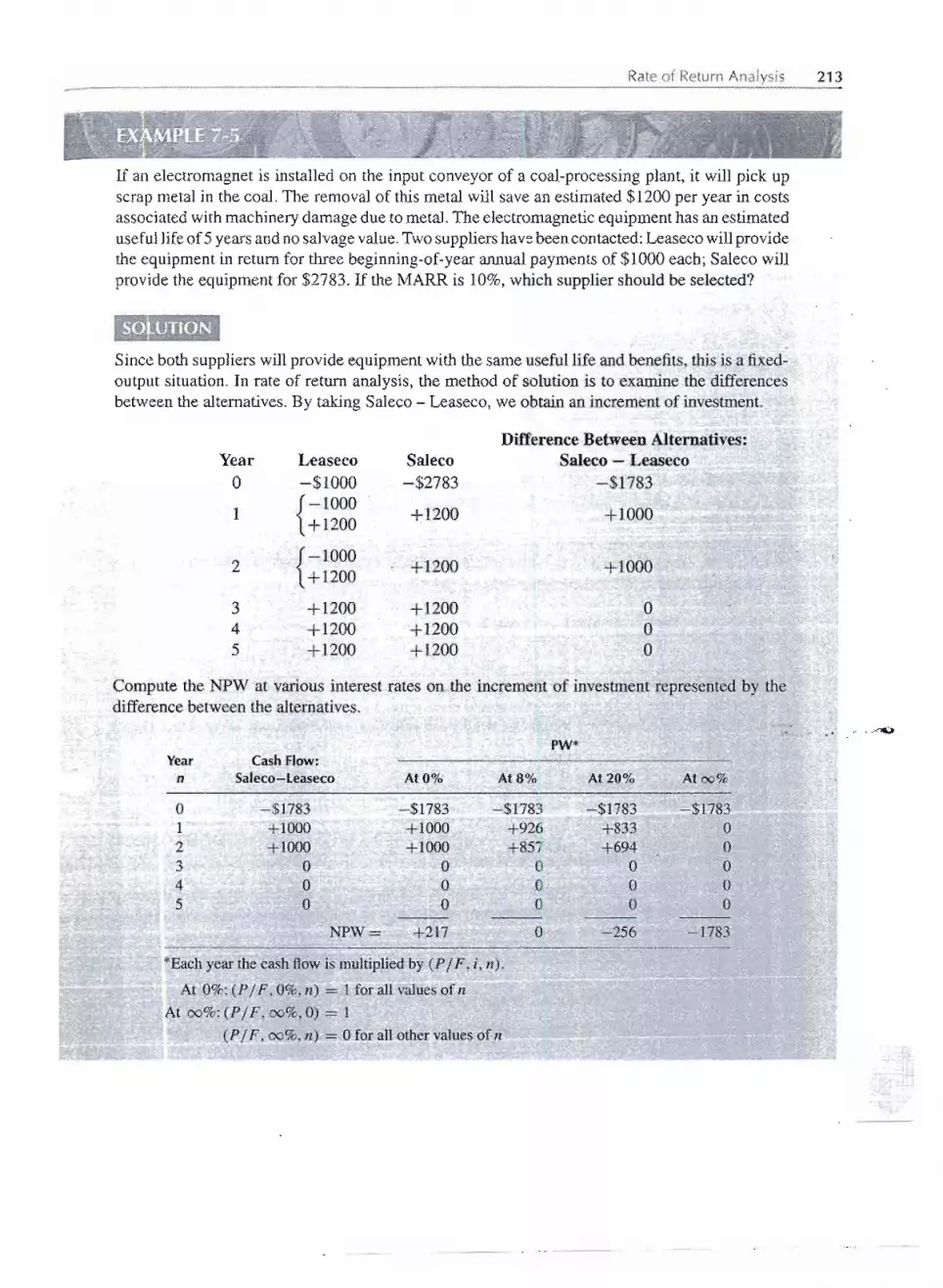
- -. -- ... - -. . - - _.. -- -
-- - - _._-
Rate of Return Analysis 213
If an electromagnet is installed on the input conveyor of a coal-processing plant, it will pick upscrap metal in the coal. The removal of this metal will save an estimated $1200 per year in costsassociated with machinery damage due to metal. The electromagnetic equipment has an estimateduseful life of 5 years and no salvage value. Two suppliers havebeen contacted: Leaseco will providethe equipment in return for three beginning-of-year annual payments of $1000 each; Saleco willprovide the equipment for $2783. If the MARR is 10%, which supplier should be selected?
SOLUTION
Sinceboth suppliers will provide equipment with the same useful life and benefits, this is a fixed-output situation. In rate of return analysis, the method of solution is to examine the differencesbetween the alternatives.By taking Saleco - Leaseco, we obtain an increment of inves-tment..
Compute the NPW at various interest rates on the increment of investment represented by thedifference between the alternatives.
*Each year the cash flow is multiplied by (P / F, i, n).
At O%:(P / F, 0%, n) = 1 for all values of n
At 00%: (P / F, 00%,0) = 1
(Pj F, 00%, n) = 0 for all other values of n
"
----.- - "
--- - - - - ---'- ----- - -----
Difference Between Alternatives:Year Leaseco Saleco Saleco - Leaseco
0 -$1000 -$2783 -$1783
1{ -1000
+ 1200 +1000+ 1200
2{ -1000
+ 1200 + 1000.+ 1200
3 + 1200 + 1200 04 +1200 + 1200 05 + 1200 +1200 0
,. ..' .,., -' .........,.gpw*
Year CashFlow:n Saleco-Leaseco At0%. At8% At 20% At 00%
0 -$1783 -$1783 -$173 -$1783 -$17831 + 1000 + 1000 +926 +833 02 + 1000 + 1000 +857 +694 03 0 0 0 0 04 0 0 0 0 05 0 0 0 0 0
NPW= +217 0 -256 -1783
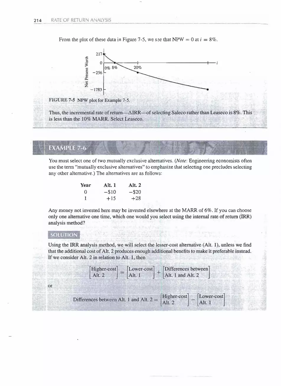
214 RATEOF RETURNANALYSIS
From the plot of these data in Figure 7-5, we see that NPW = 0 at i = 8%.
217'€~i:$G)'"~
Q..,...G)Z
-1783
FIGURE 7-5 NPW plot for Example 7-5.
Thus, the incrementalrate of return-b.IRR--of selectingSalecorather than Leaseco is 8%.Thisis less than the 10% MARR. Select Leaseco.
Youmust selectone of two mutually exclusivealternatives.(Note:Engineeringeconomists oftenuse the term "mutuallyexclusivealternatives"to emphasizethat selectingone precludes selectingany other alternative.)The alternativesare as follows:
Yearo1
Alt. 1-$10+15
Alt. 2-$20+28
Any money not investedhere may be invested elsewhereat the MARR of 6%. If you can chooseonly one alternativeone time, which one would you select using the internal rate of return (lRR)analysis method?
:.~9!-qTION
Using the IRR analysis method, we will select the lesser-cost alternative(Alt. 1), unless we findthat the additionalcost of Alt. 2 producesenough additionalbenefitsto make it preferable instead.If we consider Alt. 2 in relation to Alt. 1, then
[Higher-cost
]=
[
LOWer-cost
]+
[
Differencesbetween
]Alt. 2 Alt. 1 Alt. 1 and Alt. 2
or
Differe~cesbetwe;n ~t. 1 and Alt. 2 =[Higher-cost
]_
[
LOWer-cost
]Alt. 2 Alt. 1- - - ..--
-- - - -
Rate of Return Analysis 215
The choic~ between the two alternatives reduces to an examination of the differences betweenthem. We can compute the rate of return on the differencesbetween the alternatives.Writing thealternatives again,
Yearo1
Alt. 1-$10'+15
Alt. 2-$20+28
Alt. 2 - Alt. 1
-$20 - (-$10) = -$10+28 - (+15) = +13
PW of cost of differences (Alt. 2 - Alt. 1) = PW of benefit of differences (Alt. 2 - Alt. 1)
10 = 13(PjF, i, 1)
Thus,
10(PjF,i, 1) = - =0.769213
One can see that if $10 increases to $13 in one year, the interestrate must be 30%.The compoundinterest tables confirm this conclusion. The 30% rate of return on the difference between thealternatives is far higher than the 6% MARR. The additional $10 investment to obtain Alt. 2 issuperior to investingthe $10 elsewhere at 6%. To obtain this desirable increment of investment,with its 30% rate of return, Alt. 2 is selected.
Tounderstandmore about Example7-6, compute the rate of return for each alternative.
Alternative 7
PW of cost of Alt. 1 = PW of benefit of Alt. 1
$10 = $15(P j F, i, 1)
Thus,
10(PjF, i, 1) = - =0.666715
From the compound interest tables: rate of return = 50%.
Alternative 2
PW of cost of Alt. 2 = PW of benefit of Alt.2
$20 = $28(P j F, i, 1) I~
- _. ------
--- - - - - -- --

216 RATEOF RETURNANALYSIS
Thus,
. 20(PjF, 1,1) = - = 0.714328
From the compound interest tables: rate of return =40%.
One may be tempted to select Alt. 1, based on these rate of return computations.Wehave already seen, however, that this is not the correct solution. Solve the problem again,this time using present worth analysis.
Present Worth AnalysisAlternative 1
NPW= -10+ 15(PjF,6%, 1) = -10+ 15(0.9434)=+$4.15
Alternative 2
NPW = -20 + 28(P j F, 6%, 1) = -20 + 28(0.9434)= +$6.42
Alternative 1 has a 50% rate of return and an NPW (at the 6% MARR) of +$4.15. Alter-native 2 has a 40% rate of return on a larger investment,with the result that its NPW (at the6% MARR) is +$6.42. Our economic criterion is to maximize the return, rather than therate of return. To maximize NPW, select Alt. 2. This agrees with therate of return analysison the differencesbetween the alternatives.
i.
If the computations for Example 7-6 do not convinceyou, and you still think Alternative 1 wouldbe preferable, try this problem.
Youhave $20 in your wallet and two alternativeways of lendingBill some money.
(a) Lend Bill $10 with his promise of a 50% return. That is, he will pay you back $15 at theagreed time.
(b) Lend Bill $20 with his promise of a 40% return. He will pay you back $28 at the sameagreed time.
Youcan select whether to lend Bill $10 or $20. This is a one-time situation, and any money notlent to Bill will remain in your wallet. Which alternativedo you choose?
SOLUTION
So you see that a 50% return on the smaller sum is less rewardingfo you tnan 40% on th"elarger ;,
sum? Since you would prefer to have $28 than $25 ($15 from Bill plus $10 remaining in yourwallet) after the loan is paid, lend Bill $20.
- -

Rate of Return Analysis 217
:! ....
!1'~.~
Solve Example 7-6 again,but this time computethe interestrateon theincrement (Alt. 1 - Alt. 2).How do you interpret the results?
This time the problem is being viewed as follows:
Alt. 1 = A1t.2 + [Alt. 1 - Alt. 2]
Yearo1
Alt. 1-$10+15
Alt. 2-$20+28
[Alt. 1 - Alt. 2]-$10 - (-$20) = +$10
+15 - (+28) = -13
We can write one equation in one unknown:
NPW = PW of benefit of differences - PW of cost of differences = 0
+lO-13(PIF,i, 1) =0
Thus,
10(PIF, i, 1) = - = 0.769213
Once again the interest rate is found to be 30%. The critical question is, what does the 30%represent? Looking at the increment again:
Year Alt. 1 - Alt. 2o +$101 -13
1..,..-r ."-
The cash flowdoes not representan investment;instead, it representsa loan. It is as if we borrowed$10 in Year 0 (+$10 represents a receipt of money) and repaid it in Year 1 (-$13 represents adisbursement).The 30% interest rate means this is the amount we would pay for the use of the$10 borrowed in Year0 and repaid inYear 1. .
Is this a desirable borrowing? Since the MARR on investments is 6%, it is reasonable toassume our maximum interest rate on borrowing would also be 6%. Here the interest rate is30%, which means the borrowing is undesirable. Since Alt. 1=Alt. 2 + (Alt. 1 -- Alt. 2), andwe do not like the (Alt. 1 - Alt. 2) increment, we should reject Alternative 1, which contains theundesirable increment.This means we should selectAlternative2-the same conclusionreachedin EXan1ple7-6.
Example 7-8 illustrated that one can analyze either increments of investment orincrements of borrowing. When looking at increments of investment, we accept the in-crement when the incremental rate of return equals or exceeds the minimum attractive rate
''''~ a..II- --- ,.,.,
--- - - - --- - -- ----
-----------
218 RATEOF RETURN ANALYSIS
of return (~IRR ~ MARR). When looking at increments of borrowing, we accept the in-crement when the incremental interest rate is less than or equal to the minimum attractiverate of return (~IRR ~ MARR). One way to avoid much of the possible confusion is toorganize the solution to any problem so that one is examining increments of investment.This is illustrated in the next example.
A firmis considering whichof two devicesto install to reduce costs in a particular situation.Bothdevices cost $1000, and both have useful lives of 5 years and no salvage value. Device A can beexpected to result in $300 savings annually.Device B will provide cost savings of $400 the firstyear but will decline $50 annually,making the second-year savings $350, the third-year savings$300, and so forth. For a 7% MARR, which device should the firmpurchase?
This problem has been solved by present worth analysis (Example5-1) and annual cost analysis(Example6-5). This time we will use rate of return analysis.The examplehas fixedinput ($1000)and differing outputs (savings).
In determiningwhether to use an (A - B) or (B - A) differencebetween the alternatives,weseek an increment of investment.By looking at both (A - B) and (B - A), we find that (A - B)is the one that represents an increment of investment.
Yearo12345
Device A-$1000
+300+300+300+300+300
Device B-$1000
+400+350+300+250+200
Difference Between Alternatives:Device A - Device B
$0-100-50
o+50
+100
For the difference between the alternatives,write a single equation with i as the only unknown.
EUAC = EUAB
[100(Pj F, i, 1) + 50(P j F, i, 2)](Aj P, i, 5) [50(Fj P, i, 1) + 100](Aj F, i, 5)
The equation is cumbersome, but need not be solved. Instead, we observe that the sum of thecosts (-100 and -50) equals the sum of the benefits (+50 and + 100).This indicates that 0% isili~ IRRA-B on the A - B increment of investment. This is less than the 7% MARR; therefore,the increment is undesirable. Reject Device A and choose Device B.
As describedin Example7-8,if theincrel11enteXal1:).inedis (B ~ A),'the interestratewouldagain be 0%, indicating a desirableborrowing situation. Wewould choose Device B.
, :; =::z' ==;; :::I...

.-- --.--------
Rate of Return Analysis 219
Analysis Period, In discussing present worth analysis and annual cash flow analysis, an important consid-eration is the analysis period. This is also true in rate of return analysis. The method ofsolution for two alternativesis to examine the differencesbetween the alternatives.Clearly,the examination must cover the selected analysisperiod. For now,we can only suggest thatthe assumptionsmade shouldreflectone's perceptionof the future as accuratelyas possible,
In Example 7-10 the analysis period is a common multiple of the alternative servicelives and identical replacement is assumed. This problem illustrates an analysis of thedifferencesbetween the alternativesover the analysis period.
Two machines are being considered for purchase. If the MARR is 10%,which machine shouldbe bought? Use an IRR analysis comparison.
Initial costUniform annual benefitEnd-of-useful-lifesalvage valueUsefullife, in years
Machine X$200
9550
6
Machine Y$700
12015012
SOU!JTION
The solution is based on a 12-yearanalysisperiod and a replacement machine X that is identicalto the presentmachineX. The cash flowfor the differencesbetween the alternatives,is as follows:
Machine Y - Machine XMachine Y
-$700+120+120+120+120+120
+120
-$500+25+25+25+25+25
+25
+150
+120+120+IW+120
: +120
+120+150
+25+25+25+25
=-+25
+25+100
--- ..-
---
- - - -- - ---------- - - ---
Year MachineX
0 -$2001 +952 +953 +954 +955 +95-
{ +95'
6 +50-200
7 +958 +95
I 9 +95l 10 +95
ii:I;=:; '='= ;;: ::,;; 1:; == 11 +95
I 12{+95+50
1:1 ....-. ...---
-,.II; II!
I
I!II!
0; I

220 RATEOF RETURNANALYSIS
PW of cost of differences = PW of benefits of differences
500 = 25(P / A, i, 12) + 150(P/ F, i, 6) + 100(P/ F, i, 12)
The sum of the benefits over the 12 years is $550, which is only a little greater than the $500additional cost. This indicates that the rate of return is quite low. Try i = 1%.
500 ~ 25(11.255) + 150(0.942) + 100(0.887)
~ 281 + 141 + 89 =511
The interest rate is too low.Try i = 11/2%:
500 '!/::25(10.908) + 150(0.914) + 100(0.836)
'!/::273 + 137 + 84 = 494
The internal rate of return on the Y - X increment, IRRy-X, is about 1.3%, far below the 19%minimum attractive rate of return. The additional investment to obtain Machine Y yields an. . .
" unsatisfactoryrate of return, therefore X is the preferred alternative.
SPREADSHEETS AND RATE OF RETURN ANALYSIS
The spreadsheetfunctions covered in earlier chapters are particularly useful in caIculatiDginternal rates of returns (IRRs). If a cash flow diagram can be reduced to at most"one P,one A, and/or one F, then the RATE investmentfunction can be used. Otherwise the IRRblockfunction is used with a cash flow in each period. .
The Excel investmentfunctionis RATE(n,A,P ,F ,type,guess).The A, P, and F cannotall be the same sign. The F, type, and guess are optional arguments. The "type" is end orbeginning of period cash flows (for A, but not F), and the "guess" is the starting value inthe search for the IRR. .
ConsideringExample7-1,where P = -8200, A = 2000,and n = 5, the RATEfunctionwould be:
RATE(5,2000,-8200)
which gives an answer of 7.00%, which matches that found in Example 7-1.For Example 7-2, where P = -700, A = 100, G = 75, and n = 4, the RATE
function cannot be used, since it has no provisions for the arithmetic gradient, G. Supposethe years (row 1) and the cash flows (row 2) are specified in columns B through E. Theinternal rate of retum calculated using IRR(B2:F2) is 6.91%.
A B C D E F
1
2
Figure 7-6 illustrates using a spreadsheet to graph the present worth of a cash flow seriesversus the interest rate. The interest rate with present worth equal to 0 is the IRR. The
Year 0 1 2 3 4
Cash flow -700 100 175 250 325

Summary 221
SUMMARY
FIGURE 7-6 Graphing present worth versus i.
y axis on this graphhas been modifiedso that the x axis intersectsat a present worth of -50rather than at O.To do this click on the y axis, then right-click to bring up the "format axis"option. Selectthis and then selectthe tab for the scale of the axis.This has a selectionfor theintersection of the x axis. This process ensures that the x-axis labels are outside the graph.
Rate of return may be definedas the interest rate paid on the unpaidbalance of a loan suchthat the loan is exactlyrepaid if the scheduleof paymentsis followed.On an investment,rateof return is the interest rate earned on the unrecovered investment such that the paymentschedule makes the unrecovered investment equal to zero at the end of the life of theinvestment.Althoughthe two definitionsof rate of return are stated differently,there is onlyone fundamental concept being described.It is that the rate of return is the interest rate i atwhich the benefitsare equivalent to the costs.
There are a variety of ways of writing the cash flowequation in which the rate of returni may be the single unknown.Five of them are as follows:
PW of benefits - PW of costs = 0
PWof benefits=1
PWof costsNPW= 0
EUAB- EUAC = 0
PW of costs = PW of benefits
---
------------ --- -
;11. ,, II
,[1'1
-~
.-.Q'.....,. _.._C-. .'.'__._...r . . . ._.._---- ..
A B C D E F1 Year Cash flow i PW
2 0 -700 0% 150.0 =$B$2+NPV(D2,$B$3:$B$6)3 1 100 2% 102.14 2 175 4% 58.0
5 ; 3 250 6% 17.4
, 6 4 325 8% -20.0
7 10% -54.7
8
: 9 150.0
10
'11'€ 100.0
12 0
13 C 50.0QJ'"
14 £15 0.0
16-50.0 I
: 17 0% 2% 4% 6% 8% 10%18 Interest rate19 I I I I

),
i
j (
, !
, )
: !
)
L
222 RATEOF RETURNANALYSIS
Rate of return analysis: Rate of return analysis is the most frequently used method iJindustry, as the resulting rate of return is readily understood. Also, the difficultiein selecting a suitable interest rate to use in present worth and annual cash flovanalysis are avoided.
CriteriaTwo Alternatives
Computethe incrementalrateof return-~IRR-on theincrementof investmentbetweelthe alternatives.Then,
· if ~IRR 2:MARR,choosethehigher-costalternative,or,· if ~IRR < MARR, choose the lower-cost alternative
When an increment of borrowing is examined, where ~IRR is the incremental interes.rate,
· if ~IRR ::::MARR, the increment is acceptable, or· if ~IRR > MARR, the increment is not acceptable
Three or More Alternatives
Incremental analysis is needed, which is described in Chapter 8.
Looki ng Ahead
Rate of return is further described in Appendix 7A. This material.concentrates on thedifficulties that occur with some cash flows that yield more than one root for the rate ofreturn equation.
PROBLEMS
7-1 For the following diagram, compute the IRR towithin 112%. .
7-2 For the following diagram, compute the interest rateat which the costs are equivalent to the benefits.
80 80 80 80 80 80
t t t t t t0-1-2-3-4-5-6
11' 1200 200 200
5060 (Answer: 50%)
-- - - - --

7-3
Problems 223
For the following diagram, compute the rate of return.25
2f I
15
i10
l t0-1-2-3-4-5
142.55
7-4 For the following diagram, compute the rate of returnon the $3810 investment.
500 500 500 500
i 'to i 'to i 'to i0-1-2-3-4-5-6-7- ... n = 00
13810
7-5 For the following diagram, compute the rate of return.A = 1000
o I I I I I I I I 11Oli.ii.i.ii1... n = 00
.to 15000
7-6 Considerthe followingcash flow:Year Cash Flow
o -$5001 +2002 +1503 +1004 +50
Compute the rate of return represented by the cashflow.
7-7 Considerthe followingcash flow:Year Cash Flow
o -$10001 02 +3003 +3004 +3005 +300
Compute the rate of return on the $1000 investmentto within 0.1%. (Answer: 5.4%)
Consider the following cash flow:7-8
Yearo12345
Cash Flow-$400
o+200+150+100+50
Write one equation, with i as the only unknown, forthe cash flow. In the equation you are not to use morethan two single payment compound interest factors.(You may use as many other factors as you wish.)Then solve your equation for i.
Compute the rate of return for the following cash flowto within 112%.
7-9
Yearo
1-10
Cash Flow-$100
+27
(Answer: 23.9%)
7-10 Solve the following cash flow for the rate of return to
within an 112%.
Yearo12345
Cash Flow-$500-100+300+300+400+500
7-11 Compute the rate of return for the following cash flow.
Year1-5
6-10
Cash Flow
-$233+1000
7-12 Compute the rate of return for the following cash flowto within 0.5%.
Yearo12345
(Answer: 9.3%)
Cash Flow-$640
o100200300300
, ,
( ,
-- ---

224 RATEOF RETURNANALYSIS
7-13 Compute the rate of return for the following cash flow.
Year Cash Flow
o -$5001-3 04 +4500
7-14 A woman went to the Beneficial Loan Company andborrowed $3000. She must pay $119.67 at the end ofeach month for the next 30 months.
(a) Calculate the nominal annual interest rate she ispaying to within ::1::0.15%.
(b) What effective annual interest rate is she paying?
7-15 Helen is buying a $12,375 automobile with a $3000down payment, followed by 36 monthly paymentsof $325 each. The down payment is' paid immedi-ately, and the monthly payments are due at the endof each month. What nominal annual interest rate is
Helen paying? What effective interest rate?(Answers: 15%; 16.08%)
7-16 Peter Minuit bought an island from the ManhattoesIndians in 1626 for $24 worth of glass beads and trin-kets. The 1991 estimate of the value of land on thisisland was $12 billion. What rate of return would theIndians have received if they had retained title to theisland rather than selling it for $24?
7-17 A man buys a corporate bond from a bond brokeragehouse for $925. The bond has a face value of $1000and pays 4% of its face value each year. If the bondwill be paid off at the end of 10 years, what rate ofreturn will the man receive? (Answer: 4.97%)
7-18 A well-known industrial firm has issued $1000 bonds
that carry a 4% nominal annual interest, rate paidsemiannually. The bonds mature 20 years from now,at which time the industrial firm will redeem them
for $1000 plus the terminal semiannual interest pay-ment. From the financial pages of your newspaper youlearn that the bonds may be purchased for $715 each($710 for the bond plus a $5 sales commission). Whatnominal annual rate of return would you receive ifyou purchased the bond now and held it to maturity20 years hence? (Answer: 6.6%)
7-19 One aspect of obtaining a college education is theprospect of improved future earnings in comparisonto non-college graduates. Sharon Shay estimates thata college education has a $28,000 equivalent cost atgraduation. She believes the benefits of her educationwill occur throughout 40 years of employment. Shethinks that during the first 10 years out of college,her income will be high~r than that of a non-college
-. ~ , -
graduate by $3000 per year. During the subsequent10 years, she projects an annual income that is $6000per year higher. During the last 20 years of employ-ment, she estimates an annual salary that is $12,000above the level of the non-college graduate. If her es-timates are correct, what rate of return will she receiveas a result of her investment in a college education?
7-20 An investor purchased a one-acre lot on the outskirtsof a city for $9000 cash. Each year he paid $80 ofproperty taxes. At the end of 4 years, he sold thelot. After deducting his selling expenses, the investorreceived $15,000. What rate ofreturn did he receiveon his investment? (Answer: 12.92%)
7-21 A popular reader's digest offers a lifetime subscrip-'tion to the magazine for $200. Such a subscnptionmay be given as a gift to an infant at birth (the par-ents can read it in those early years), or taken butby an individual for himself. Normally, the magazine.costs $12.90 per year. Knowledgeable people say itprobably will continue indefinitely at this $12.90 rate. .What rate of return would be obtained if a life sub-
scription were purchased for an infant, rather thanpaying $12.90 per year beginning immediately? Youmay make any reasonable assumption!;, but the com-pound interest factors must be correctly used.
7-22 On Apri12, 1988, an engineer bought a $1000 bondof an American airline for $875. The bond paid 6%on its principal amount of $1000, half in each of itsApril 1and October 1 semiannual payments; it repaidthe $1000 principal sum on October 1, 2001. Whatnominal rate of return did the engineer receive fromthe bond if he held it to its maturity (on October 1,2001)? (Answer: 7.5%)
7-23 The cash price of a machine tool is $3500. Thedealer is willing to accept a $1200 down payment and24 end-of-month monthly payments of $110 each. Atwhat effective interest rate are these terms equivalent?(Answer: 14.4%)
7-24 A local bank makes automobile loans. It charges 4%per year in the following manner: if$3600 is borrowedto be repaid over a 3-year period, the bank interestcharge is $3600 x 0.04 x 3 years = $432. The bankdeducts the $432 of interest from the $3600 loan and
gives the customer $3168 in cash. The customer mustrepay the loan by paying 1136of $3600, or $100, atthe end of each month for 36 months. What nominalannual interest rate is the bank actually charging forthis loan?
--

Problems 225
7-25 Upon graduation, every engineer must decide whetherto go on to graduate school. Estimate the costs ofgoing full time to the university to obtain a masterof science degree. Then estimate the resulting costsand benefits. Combine the various consequences intoa cash flow table and compute the rate of return.Nonfinancial benefits are probably relevant here too.
7-26 A table saw costs $175 at a local store. You may eitherpay cash for it or pay $35 now and $12.64 a monthfor 12 months beginning 30 days hence. If you choosethe time payment plan, what nominal annual interestrate will you be charged? (Answer: 15%)
7-27 An investment of $5000 in Biotech common stockproved to be very profitable. At the end of 3 yearsthe stock was sold for $25,000. What was the rate ofreturn on the investment?
7 -, The Southern Guru Copper Company operates a large
J!!! mine in a South American country. A legislator in theNational Assembly said in a speech that most of thecapital for the mining operation was provided by loansfrom the Word Bank; in fact, Southern Guru has only$500,000 of its own money actually invested in theproperty. The cash flow for the mine is:
Yearo1234567
Cash Flow$0.5 million investment
3.5 millionprofit0.9 millionprofit3.9 millionprofit8.6 millionprofit4.3 millionprofit3.1 millionprofit6.1 millionprofit
The legislator divided the $30.4 million total profit bythe $0.5 million investment. This produced, he said,a 6080% rate of return on the investment. SouthernGuru claims the actual rate of return is much lower.
They ask you to compute their rate of return.
7-29 An insurance company is offering to sell an annuityfor $20,000 cash. In return the firm will guarantee topay the purchaser 20 annual end-of-year payments,with the first payment amounting to $1100. Subse-quent payments will increase at a uniform 10% rateeach year (second payment is $1210; third paymentis $1331, etc.). What rate of return will the purchaserreceive if he buys the annuity?
7-30 A bank proudly announces that it has changed its in-terest computation method to continuous compound-
ing. Now $2000 left in the bank for 9 years will doubleto $4000.
(a) What nominal interest rate, compounded contin-uously, is the bank paying?
(b) What effective interest rate is it paying?
7-31 Fifteen families live in Willow Canyon. Althoughseveral water wells have been drilled, none has pro-duced water. The residents take turns driving a watertruck to a fire hydrant in a nearby town. They fill thetruck with water and then haul it to a storage tank inWillow Canyon. Last year truck fuel and maintenancecost $3180. This year the residents are seriously con-sidering spending $100,000 to install a pipeline fromthe nearby town to their storage tank. What rate ofreturn would the Willow Canyon residents receive ontheir new water supply pipeline if the pipeline is con-sidered to last
(a) Forever?(b) 100 years?(c) 50 years?(d) Would you recommend that the pipeline be
installed? Explain.
7-32 Ian purchased 100 shares of Peach Computer stockfor $18 per share, plus a $45 brokerage commission.Every 6 months she received a dividend from Peachof 50 cents per share. At the end of 2 years, just afterreceiving the fourth dividend, she sold the stock for$23 per share and paid a $58 brokerage commissionfrom the proceeds. What annual rate of return did shereceive on her investment?
7-33 The Diagonal Stamp Company, which sells usedpostage stamps to collectors, advertises that itsaverage price has increased from $1 to $5 in thelast 5 years. Thus, management states, investors whohad purchased stamps from. Diagonal 5 years agowould have received a 100% rate of return each
year.(a) To check their calculations, compute the annual
rate of return.
(b) Why is your computed rate of return less than100%?
7-34 An investor purchased 100 shares of Omega commonstock for $9000. He held the stock for 9 years. Forthe first 4 years he received annual end-of-year di-vi-dends of $800. For the next 4 years he received annualdividends of $400. He received no dividend for the
ninth year. At the end of the ninth year he sold hisstock for $6000. What rate of return did he receive onhis investment?
- --- - - -------

.....---------- .- ,.226 RATEOF RETURNANALYSIS
7-35 You spend $1000 and in return receive two payments be willing to lend AI on the proposed repaymentof $1094.60--:<>neat the end of 3 years and the other plan ?at the end of 6 years. Calculate the resulting rate of 7-41 The following advertisement appeared in the Wallreturn. Street Journal on Thursday, February 9, 1995.
7-36 A mine is for sale for $240,000. It is believed the minewill produce a profit of $65,000 the first year, but the ''There's nothing quite like the Sevilleprofit will decline $5000 a year after that, eventually SmartLease. Seville SLS $0 down, $599reaching zero, whereupon the mine will be worthless. a monthj36 months."What rate of return would this $240,000 investment
produce for the purchaser of the mine?First month's lease payment of $599 plus $625 re-
7-37 Fred, our cat, just won the local feline lottery to the fundable security deposit and a consumer down pay-tune of 3000 cans of "9-Lives" cat food (assorted ment of $0 for a total of $1224 due at lease signing.flavors). A local grocer offers to take the 3000 cans Monthly payment is based on a net capitalized cost ofand in return, supply Fred with 30 cans a month for $39,264 for total monthly payments of $21,564. Pay-the next 10 years. What rate of return, in terms of ment examples based on a 1995 Seville SLS: $43,658nominal annual rate, will Fred realize on this deal? MSRP including destination charge. Tax, license,'(Compute to nearest 0.01%.) title fees, and insurance extra. Option to purcha.se at
7-38 An apartment building in your neighborhood is for lease end for $27,854. Mileage charge of $0.15 persale for $140,000. The building has four units, which mile over 36,000 miles.are rented at $500 per month each. The tenants have (a) Set up the cash flows.long-term leases that expire in 5 years. Maintenance (b) Determine the interest rate (nominal and effec-and other expenses for care and upkeep are $8000 tive) for the lease.annually. A new university is being built in the vicin- 7-42 After 15years of working for one employer, you trans-ity and it is expected that the building could be sold fer to a new job. During these years your employerfor $160,000 after 5 years. contributed (that is, she diverted from your salary)(q) What is the internal rate of return for this $1500 each year to an account for your retirement
investment?(a fringe benefit), and you contributed a matching
(b) Should this investment be accepted if the your amount each year. The whole fund was invested atother options have a rate of return of 12%? 5% during that time and the valu of the account now
7-39 A new machine can be purchased today for $300,000. stands at $30,000. You are now faced with two alter-The annual revenue from the machine is calculated natives. (1) You may leave both contributions in theto be $67,000, and the equipment will last 10 years. fund until retirement in 35 years, during which youExpect the maintenance and operating costs to be will get the future value of this amount at 5% inter-$3000 a year and to increase $600 per. year. The est per year. (2) You may take out the total value ofsalvage value of the machine will be $20,000. What "your" contributions, which is $15,000 (one-half ofis the rate of return for this machine? the total $30,000). You can do as you wish with the
7-40 AI Larson asked a bank to lend him money on money you take out, but the other half will be lost
January 1,based on the following repayment plan: the as far as you are concerned. In other words, you can
first payment would be $2 on February 28, with sub- give up $15,000 today for the sake of getting now
sequent monthly payments increasing by $2 a month the other $15,000. Otherwise, you must wait 35 years iI
on an arithmetic gradient. (The March 31 payment more to get the accumulatedvalueof the entire fund.
wouldbe $4; the April30 paymentwouldbe $6, etc.) Which alternative is more attractive? Explain your IThe payments are to continue for 11 years, making a choice.
]total of 132 payments. 7-43 A finance company is using the following "Money(a) Compute the total amount of money AI will pay by Mail" offer. Calculate the yearly nominal IRR
the bank, based on the proposed repayment plan. received by the company if a customer chooses the
j
(b) If the bank charges interest at 12% nominal per loan of $2000 and accepts the credit insurance (Lifeyear, compounded monthly, how much would it and Dis.).
I
-

Problems 227
Non-Negotiable INE1/96
For theAmount of $3000 or $2000 or $1000
Pay to the Order of I Feel RichLimited Time Offer
Dollars
For the Amount of $3000 DollarsPay to theOrder of I Feel Rich
Total of Payments $4,280.40Number of Monthly Payments
36 Months
Amount Financed $3,246.25
APR 18.95%
Finance Charge $1034.29
Monthly Payment $118.90Credit Line Premium
$83.46*Credit Disabilit Premium $162.65*
For the Amount of $2000 Dollars
Pay to theOrder of I Feel Rich
Total of Payments $2,731.50Number of Monthly Payments
30 MonthsAmount Financed $2,137.25
APR 19.95%
Finance Charge $594.25
Monthly Payment $91.05Credit Line Premium
$44.38*Credit Disabilit Premium $92.87*
For the Amount of $1000 DollarsPay to theOrder of I Feel Rich
Total of Payments $1,300.80Number of Monthly Payments
24 MonthsAmount Financed $1055.26
APR 20.95%
Finance Charge $245.54
Monthly Payment $54.20Credit Line Premium
$16.91 *Credit Disabilit Premium $39.02*
*Credit insurance. If selected, premium will be paid from amount financed. If not selected,cash advance is total amount financed.
To borrow $3000,$2000, or $1000
$3000 loan terms
$2000 loan terms
$1000 loan terms
The owner of a comer lot wants to find a use that will
yield a desirable return on his investment. After muchstudy and calculation, the owner decides that the twobest alternatives are:
7-44 A finance company is using the "Money byMail" offer shown in Problem 7-43. Calculate the
yearly nominal IRR received by the company if acustomer chooses the $3000 loan but declines thecredit insurance.
7-45 In his will, Frank's uncle has given Frank the choicebetween two alternatives:
7-46
$2000 cash
$150 cash now plus $100 permonth for 20 months beginningthe first day of next month
(a) At what rate of return are the two alternativesequivalent?
(b) If Frank thinks the rate ofretum in (a) is too low,which alternative should he select?
First cost
Annual property taxesAnnual income
Life of building, in yearsSalvage value
Alternative 1Alternative 2
BuildGas Station
$80,0003,000
11,00020o
Build SoftIce Cream
Stand$120,000
5,00016,000
,20o
If the owner wants a minimum attractive rate of return
on his investment of 6%, which of the two alternativeswould you recommend?
---
--

228 RATEOF RETURN ANALYSIS
7-47 Two alternatives are as follows:
Yearo123
A-$2000
+800+800+800
B-$2800+1100+ 1100+1100
If 5% is considered the minimum attractive rate ofreturn, which alternative should be selected?
7-48 Consider two mutually exclusive alternatives:
Year
o1234
X-$100
35353535
y-$50.0
"16.516.516.516.5
If the minimum attractive rate of return is 10%, whichalternative should be selected?
Consider these two mutually exclusive alternatives:7-49
Yearo1234
A-$50
17171717
B-$53
17171717
At a MARR of 10%, which alternative should beselected? (Answer: A)
1\\'0 mutually exclusive alternatives are being consid-ered. Both have a 10-year useful life. If the MARR is8%, which alternative is preferred?
7-50
Initial costUniform annual benefit
A$100.00
19.93
B
$50.0011.93
7-51 Consider two mutually exclusive alternatives:
Yearo1234
X-$5000-3000+4000+4000+4000
y-$5000+2000+2000+2000+2000
If the MARR is 8%, which alternative should beselected?
7-53
If the minimum attractive rate of return is 8%, which
alternative should be selected? Solve the problem by(a) Present worth analysis "
(b) Annual cash flow analysis(c) Rate of return analysis
A contractor is considering whether to purchaseor lease a new machine for his layout site work.Purchasing a new machine will cost $12,000 witha salvage value of $1200 at the end of the machine'suseful life of 8 years. On the other hand, leasing re-quires an annual lease payment of $3000. Assumingthat the MARR is 15% and on the basis of an internal
rate of return analysis, which alternative should thecontractor be advised to accept. The cash flows are ~follows:
Year (n)o12345678
Alt. A (purchase)-$12,000
Alt. B (lease)o
-$3000-3000-3000- 3000-3000- 3000-3000-3000+1200
7-54 Two hazardous environment facilities are being eval-uated, with the projected life of each facility being10 years. The caSh flows are as follows:
- -- - - - ---
7-52 Two mutually exclusive alternatives are beingconsidered.
Year A B0 -$2500 -$60001 +746 + 16642 +746 +16643 +746 + 16644 +746 + 16645 +746 + 1664
Alt. A -Alt.BFirst cost $615,000 $300,000Maintenanceand 10,000 25,000
operatingcostAnnual benefitS 158,000 92,000Salvagevalue 65,000 -5,000

Difficulties in Solving for an Interest Rate 229
7-55
The company uses a MARR of 15%. Using rate ofreturn analysis, wpich alternative should be selected?
Two alternatives are being considered:
First costUniform annual benefit
Useful life, in years
A
$9200$1850
8
B
$5000$1750'
4
7-56
If the minimum attractive rate of return is 7%, whichalternative should be selected?
Jean has decided it is time to purchase a new batteryfor her car. Her choices are:
First cost
Guarantee period, in months
Zappo$56
12
Kicko$9024
Jean believes the batteries can be expected to lastonly for the guarantee period. She does not want toinvest extra money in a battery unless she can ex-pect a 50% rate of return. If she plans to keep herpresent car another 2 years, which battery should shebuy?
7-57 Two alternatives are being considered:
Initial costUniform annual benefit
Usefullife, in years
A
$92001850
8
B
$50001750
4
Base your computations on a MARR of 7% and an8-year analysis period. If identical replacement is as-sumed, which alternative should be selected?
7-58 Two investmentopportunitiesare as follows:
First costUniform annual benefit
End-of-useful-life salvage valueUsefullife, in years
A$150
252015
B$100
22.25o
10
At the end of 10 years, Alt. B is not replaced. 'Thus,the comparison is 15 years of A versus 10 years ofB. If the MARR is 10%, which alternative should beselected?
APPENDIX 7A Difficulties in Solvingfor an Interest Rate
Mter completing this chapter appendix, students should be able to:
.Describe why some project's cash flows cannot be solved for a single positive interestrate.· Identify when multiple roots can occur.
. Evaluate how many potential roots exist for a particular project..Use the modified internal rate of return (MIRR) methodology in multiple-rootcases.
Example 7A-I illustrates the situation.

1230 RATEOF RETURNANALYSIS
The Going Aircraft Company has an opportunity to supply a large airplane to Interair, a foreignairline. Interair will pay $19 million when the contract is signed and $10 million one year later.Going estimates its second- and third-year costs at $50 million each. Interair will take deliveryof the airplane during Year 4 and agrees to pay $20 million at the end of that year and the $60million balance at the end of Year 5. Compute the rate ofretum on this project.
SplUTION
The PW of each cash flowcan be computed at various interest rates. For example, for Year2 andi = 10%: PW = -50(P / F, 10%,2) = -50(0.826) = -41.3.
10.00
8.00
6.00
~ 4.00Q.,. 2.00
0.00
-2.00
-4.000% 10% 20% 30% 40% 50%
FIGURE 7A-l PW plot.
The PW plot-for this cash flow is represented in Figure 7A- LWe see theftthis cash flow producestwopointsat whichPW =0: oneat 10.24%andtheotherat 47.30%.
---------
Year Cash Flow 0% 10% 20% 40% 50%0 +$19 +$19 +$19 +$19 +$19 +$191 +10 +10 +9.1 +8.3 +7.1 +6.72 -50 -50 -41.3 -34.7 -25.5 -22.2
"3 -50 -50 -37.6 -28.9 -18.2 -14.84 +20 +20 +13.7 +9.6 +5.2 +3.95 +60 +60 +37.3 +24.1 +11.2 +7.9-
PW= +$9 +$0.1 -$2.6 -$1.2 +$0.5
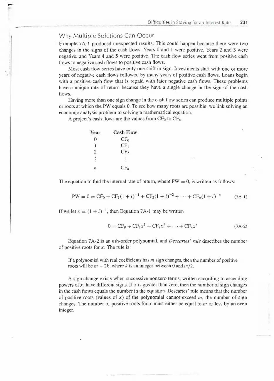
r
- Difficulties in Solvingfor an Interest Rate 231
Why Multiple Solutions Can Occur, Example7A-l producedunexpectedresults.This couldhappenbecausethere weretwo
changes in the signs of the cash flows. Years 0 and 1 were positive, Years 2 and 3 werenegative, and Years4 and 5 were positive. The cash flow series went from positive cashflowsto negative cash flowsto positivecash flows.
Most cash flow series have only one shift in sign. Investmentsstart with one or moreyears of negative cash flows followed by many years of positive cash flows. Loans beginwith a positive cash flow that is repaid with later negative cash flows. These problemshave a unique rate of return because they have a single change in the sign of the cashflows.
Havingmore than one sign change in the cash flowseries can produce multiple pointsor roots at which the PW equals O.To see how many roots are possible, we link solving aneconomicanalysis problem to solving a mathematical equation.
A project's cash flows are the values from CFoto CFn.
The equation to find the internal rate of return, where PW =0, is written as follows:
PW = 0 -:-CFo+ CFI(1 + i)-I + CFz(1 + i)-z +... + CFn(1+ i)-n (7A-l)
If we let x = (1 + i) -I, then Equation 7A-I may be written
(7A-2)
Equation 7A-2 is an nth-order polynomial, and Descartes' rule describes the numberof positive roots for x. The rule is:
If a polynomial with real coefficients has m sign changes, then the number of positiveroots will be m - 2k, where k is an integer between 0 and m12.
A sign change exists when successivenonzero terms, written according to ascendingpowers of x, have different signs. If x is greater than zero, then the number of sign changesin the cash flowsequals the number in the equation. Descartes' rule means that the numberof positive roots (values of x) of the polynomial cannot exceed m, the number of signchanges. The number of positive roots for x must either be equal to m or less by an eveninteger.
III
- - -- ------
Year Cash Flow0 CFo1 CFI2 CFz
n CFn

232 RATEOF RETURN ANALYSIS
Thus, Descartes' rule for polynomials gives the following:
Number of SignChanges, m
o1234
Number of PositiveValues of x
o1
20rO3 or 1
4, 2, or 0
N~ber of PositiveValues of i
o10rO
2, 1, or 03, 2, 1, or 0
4, 3, 2, 1, or 0
If x is greater than I, the correspondingvalue of i is negative. If there is only one rootand it is negative, then it is a valid IRR. One example of a valid negative IRR comes froma bad outcome, such as the IRR for a failed research and development project. Anotherexample would be a privately sponsored student loan set up so that if a student volunteersfor the Peace Corps, only half of the principal need be repaid. .
If a project has a negative and a positive root for i, then for most projects only thepositive root of i is used. .
Projects with Multiple Sign ChangesExample7A-I is representativeof projects for which there are initial payments (e.g., whenthe order for the ship, airplane, or building is signed), then the bulk of the costs occur, andthen there are more payments on completion. .
Projectsof other types oftenhave two or more sign changesin their cash flows.Projectswith a salvage cost typically have two sign changes. This salvage cost can be large forenvironmentalrestoration at termination. Examples include pipelines, open.pit mines, andnuclear power plants. The following cash flow diagramis representative.
$50K
t t t t t t0-1-2-3-4-5-6-7
j ~tK$180K
Many enhancement projects for existing mines and deposits have a pattern of twosign changes. Example 7A-2 describes an oil well in an existing field. The initial invest-ment recovers more of the resource and speeds recovery of resources that would havebeen recovered eventually.The resources shifted for earlier recovery can lead to :twosignchanges.
In Example 7A-3, we consider staged construction, where three sign changes arecommon.
---

Difficulties in Solving for an Interest Rate 233
Other examples can be found in incremental comparisons of alternatives with unequallives. In the next section we learn how to determine whether each of these examples hasmultiple roots.
Adding an oil well to an existing field costs $4 million (4M). It will increase recovered oil by$3.5M, and it shifts $4.5M worth of production from Years 5, 6, and 7 to earlier years. Thus,the cash flows for Years 1 through 4 total$8M and Years 5 through 7 total -$4.5M. If the well isjustified, one reason is that the oil is recovered sooner. How many roots for the PW equation arepossible? .
SOLUTION.
The first step is to draw the cash flow diagram and count the number of sign changes. The followingpattern is representative, although most wells have a longer life.
~$4M
There are two sign changes, thus there may be 0, 1, or 2 positive roots for the PW =0 equation.The additio}Jalrecovery corresponds to an investment, and the shifting of (ecovery to earlier yearscorresponds to a 10aJ;).(positive cash flow now and negative later). Thus, the oil wells are neitheranirlVe$hnent }JOtaloan; they are a combination of both.
A projecthas a first cost of $120,000. Net revenues begin at $30,000 in Year 1 and then increase* ~ by $2000 pefyear. In Year 5 the facility is expanded at a cost of $60,000 so that demand can
confiJrueto expandat $2000peryear.HowfilanYrootsfor thePWequationarepossible? _~
':'"I~-
- -- ~ - -~l - - - -
( .
;I
I
'11.,
.'!,
IIIII
. i"'

234 RATEOF RETURNANALYSIS"1
SOLUTION.
The first step is to draw the cash flow diagram. Then counting the three sign changes is easy.
$30K $32K $34K $36K $40K $42K $44K $46K $48K
t t t t t t t t t0-1-2-3-4-5-6-7-8-9-10
! -$221{~ JoK ~ $38K-$120K
With three sign changes, there may be 0, 1, 2, or 3 positive roots for the PW = 0 equation.
Evaluati ng How Many Roots There AreThe number of sign changes tells us how many roots are possible-not how many rootsthere are. Rather than covering the many mathematical approaches that may tell us if theroot will be unique, it is more useful to employ the powerof the spreadsheet.A spreadsheetcan show us if a root is unique and the value of each root that exists.
The approach is simple. For any set of cash flows,graph the PW as a function of theinterest rate. We are interested in positive interest rates, so the graph usually starts at i =O.
Since Descartes' rule is based on x > 0, and x = (1+ i)-1, sometimes the graph is startedclose to i = -1. This will identify any negative valuesof i that solve the equation.
If the root is unique, we're done. We've found the internal rate of return. If there aremultiple roots, then we know the project's PW at all interest rates-including the one ourorganizationuses. Wecan alsouse the approachof the next sectionto finda modifiedinternalrate of return.
The easiest way to build the spreadsheetis to use the NPV(i ,values) functionin Excel.Remember that this function applies to cash flowsin periods 1 to N, so that the cash flowat time 0 must be added in separately.The followingexamplesuse a spreadsheetto answerthe question of how many roots each cash flow diagram in the last section has.
This project is representativeof ones with a salvage cost. How many roots for the PW equationexist?
$50K
t t t t t t0-1~2-3-4-5-6-7
j '. .. $1_ .$180K-- - = -= - : .. :;::
- -- ----- --

Difficulties in Solving for an Interest Rate 235
Figure 7A-2 shows the spreadsheet calculations and the graph ofPW versus i.
FIGURE 7A-2 PW versus i for project with salvage cost.
In this case, there is I positive root of .10.45%.The value can be used as an IRR. There is alsoa negative root of i = -"38.29%. This root is not useful. With two sign changes, other similardiagrams may have 0, I, or 2 positive roots for tlie PW = 0 equation. The larger the value of thefinal salvage cost, the more likely 0 or 2 positive roots are to occur.
. -- _-~IIIIIIIII!!'!!I!!!!!I~
--- -------
A B C D E F G
1 Year Cash Flow i PW
2 0 -180 -40% -126.39 =$B$2 + NPV(D2,$B$3:$B$9)3 1 50 -30% 219.99
4 2 50 -20% 189.89
5 3 50 -10% ; 114.496 4 50 0% 50.007 5 50 10% 1.848 6 50 20% -33.26
9 7 -70 30% -59.02
10 40% -78.24
11 IRR 10.45% 50% -92.8812 root - 38.29%
13 250.0014 200,0015 150.0016 100.0017 50.00c..18 0.00
f19 -50.00
20 -100.00-150.00 I I I
21 -40% -20% 0% 20% 40%22 i

....I
236 RATEOF RETURNANALYSIS
$2.5M
t $1.5M
I t $01M0-1-2-3-4-5-6-7-8
j
-$J.5M ~
1-$I.5M
-$2.5M
$3.5M
1
-$4M
SOLUTION
Figure 7A-3.shows the spreadsheetcalculations and the graph of PW .versusi.
FIGURE7A-3PW versusi foroilwell.
41this case, there are 2 positiyerpots..at4.73and 37.20%.These roots ~ not "seful.1}ris proj7ct",is a combination of an investment and a loan, so we don't even know if we want a high rate ora low rate. If our interest rate is about 20%, then the project has a positive PW. However, smallchanges~inthe,datacan mak.efor~largechangesin.these,JesuJts. 11;':;;1;;:;;'1:10== 1:1I:I:;;== iii!'==-=
It is useful to apply the modified internal rate of return described in the next section.
=
-- .-~ - -
--- - ---
A B. C D E F G
1 Year CashFlow i PW2 0 -4.00 0% -0.50 =$B$2+NPV(D2,$B$3:$B$9)3 1 3.50 5% 0.024 2 2.50 10% 0.285 3 1.50 15% 0.376 4 0.50 20% 0.367 5 -0.50 25% 0.298 6 - 1.50 30% 0.199 7 -2.50 35% 0.06
10 40% -0.08
11 root 4.73% 45% -0.2212 root 37.20% 50% -0.3613 004014 /15 0.2016 0.0017
Ic..
18-0.20
19 -004020 I I I-0.6021 0% 10% 20% 30% 40% 50%22 i

Difficulties in Solving for an Interest Rate 237
A project has a firstcostof $120,000.Net revenuesbegin at $30,000in Year1,and then increaseby$2000 per year. In Year 5 the facility is expanded at a cost of $60,000 so that demand can continueto expand at $2000 per year. How many roots for the PW equation have a positive value for i?
$30K $32K $34K $36K $40K $42K $44K $46K $48K
t t t t t t t t t0-1-2-3-4-5-6-7-8-9 ,.10
! -$22K ~ $~K - $38K-$120K
Figure 7A-4 shows the spreadsheet calculations and the graph ofPW versus i.
I
F=I.
-
r ·iIGt1RW 7A4f!W ve"'"" i forp«>jec,WltJ, staged eOl)J;toJefjOo.L__,_ ____ .~==
Iti
""i1.
-- -- I
A B C D E F G1 Year CashFlow i pw2 0 -120.00 -80% 579646330 =$B$2 +NJ>V(D2,$B$3:$B$12)3 1 30.00 -60% 7357234 2 32.00 I -40% 17651
5 3 34.00 I .....30% 1460I6 4 I 36.00 . 0% 210 r
7 5 -22.00 10% 73 , !i I
8 6 40.00 20% 7I
9 7 42.00 I 30% -2810 8 44.00 i 40%
II48 I
11 9 46.00 50% 6212 10 48.00
I60% -71 ! !
{
13 i 70% -78 II14 IRR 21.69% > 80% ,83
15I
90% 87
16 ,,17 I
200 I18
150 I
19,
20 100 iI
21 50 -'p.,
22, I
0 ,<c
23" --,50
24 =,':::I :: ::II ....,._ ">I'" - --- =, "'''' ..-- .:.-100 I" I I I
25 0% 10% '20% 30% 40% 50%26 i 1-- . ," ;,::;........

~-. . -. -. - ....
.~.- ~._~.
238 RATEOF RETURNANALYSIS
In this case, there is 1positive root of 21.69%. The value can be used as an IRR, and the projecti~very attractive.
~ - .
When there are two or more sign changes in the cash flow, we know that there areseveral possibilities concerning the number of positive values of i. Probably the greatestdanger in this situation is to fail to recognize the multiple possibilities and to solve for avalue of i. The approach of constructing the PW plot both establishes whether there aremultipleroots and what their valuesare. This may be tedious to do by hand but is very easywith a spreadsheet (or a graphing calculator).
If there is a single positive value of i, we have no problem. On the other hand, ifthere is no positive value of i, or if there are multiple positivevalues, the situation may beattractive,unattractive,or confusing. Where there are multiple positivevalues of i, none ofthem should be considered a suitable measure of the rate of return or attractiveness of thecash flow.
Modified Internal Rate of Return (MIRR)Two external rates of return can be used to ensure that the resulting equation is solvablefor a unique rate of return-the MIRR. The MIRR is a measureof the attractivenessof thecash flows,but it is also a function of the two external rates of return.
The rates that are external to the project's cash flows are (1) the rate at which theorganization normally invests and (2) the rate at which it normally borrows. These areexternal rates for investing, einv,and for financing, efin.Because profitable firms invest athigher rates than they borrow at, the rate for investingis generally higher than the rate forfinancing.Sometimesa singleexternalrate is used forboth,but thisrequires thequestionableassumption that investing and financinghappen at the same rat~.
The approach is:
1. Combine cash flowsin each period into a single net receipt, R" or net expense, Et.2. Find the present worth of the expenses with the financingrate.3. Find the future worth of the receipts with the investingrate.4. Find the MIRR which makes the present and future worths equivalent.
The result is Equation7A-3. This equation will havea uniqueroot, since it has a singlenegativepresent worth and a single positive future worth. There is only one sign change inthe resulting series.
(F / P, MIRR, n) L Et(P / F, efin,t) = L RtCF/ P, einv,n - t)t t
(7A-3)
There are other external rates of return, but the MIRR has historically been the mostclearly defined.All of the external rates of return are affectedby the assumed values for theinvesting and financing rates, so none are a true rate of return on the project's cash flow.The MIRR also has an Excel function, so it now can very easily be used. Example 7A-7illustrates the calculation, which is also summarized in Figure 7A-5.
r
1
J

Difficulties in Solving for an Interest Rate 239
External Investing Rate
-$0.5M
-$1.5M
- $2.5M
-$4MExternal
FinancingRate
P(1 + MIRR)n = F
FIGURE 7A-5 MIRR for the oil well.
Adding an oil well to an existing field had the cash flows summarized in Figure 7A-5. If thefirmnormally bOlTowsmoney at 8% and invests at 15%,find the modifiedinternal rate of return(MIRR).
i~OlUTlO~
Figure 7A-6 shows the spreadsheet calculations.
FIGURE7A-6MIRR for oil well.
Itis alsopossible to calculate the MIRRby hand. While morework, the proceSsdoes clarify whatthe MIRRfunction.is doing.
1. Each period's cash flow is already a single net receipt or,y~Rendittlre.2. Find the present.worth of the expenseswith the financingrate.
1:1 :: IIIIi '...'"'"-. - -~ - -:::
RW ~ --4M -' O.5M(PIF, 8%, 5) -1.5M(P I F, 8%,6) -- 2.5M(P IF, 8%, 7)
II !II= = ~ == '.', ~iM. -- Qft~M,(Q~q~.Q§}--1~jO.63,02) -' 2.5M4o.5835)..;:;~.(j,,;z44M#k1'~
--
. 'I
"
A B C I D E F G H I1 8% externalfinancingrate I
2 15% externalinvestingrateI
3 Year . 0 1I
2 3 4 5 6 7
4 Cash Flow -4.00 3.50 I 2.50 I 1.50 0.50 -0.50 -1.50 -2.50
5 13.64% Cell A5 contains =MIRR(A4:14,AI,A2) ,
-.' ,...

I .-
240 RATEOF RETURNANALYSIS
3., Find the future worth of the receipts with the investingrate.
FW = 3.5M(FjP, 15%,6) +2.5M(FjP, 15%,5) + 1.5M(FjP, 15%,4) +O.5M(FjP, 15%,3)
= 3.5M(2.313) + 2.5M(2.011) + 1.5M(1.749) + O.5M(1.521)= 16.507M
4. Find the MIRR that makes the present and future worths equivalent.
0= (1 +MIRRt .PW +FW
0= (1 +MIRR)7(-6.744M) + 16.507M
(1 + MIRR)7 = 16.507Mj6.744M = 2.448
(1 + MIRR) = 2.4481/7 = 1.1364
MIRR = 13.64%
The MIRR does allow calculation of a rate of return for any set of cash flows.However,the result is only as realistic as the externalrates that are used. The MIRR valuecan dependas much on the external rates that are used, as it does on the cash flowsthat it is describing.
SUMMARY
In cash flows with more than one sign change, we find that solving the cash flow equationcan result in more than one positiverate of return. Typicalsituations include a new oil wellin an existing field, a project with a significantsalvagecost, and staged construction.
In a sign change, successivenonzero values in the cash flow have different signs (thatis, they change from + to -, or vice versa). Zero sign changes indicates there is no rate ofreturn, as the cash flow is either all disbursementsor all receipts.
One sign change is the usual situation, and a single positive rate of return generallyresults. There will be a negative rate of return whenever loan repayments are less than theloan or an investmentfails to return benefits at least equal to the investment.
Multiple sign changesmayresult in multiplepositiveroots for i. When theyoccur,noneof the positive multiple roots are a suitable measure of the project's economic desirability.If multiple roots are identified by graphing the present worth versus the interest rate, thenthe modified internal rate of return can be used to evaluate the project.
Graphing the present worth versus the interest rate ensures that the analyst recognizesthat the cash flowhas multiple sign changes. Otherwisea rate could be found and used thatis not in fact a meaningful descriptor of the project.
The modified internal rate of return (MIRR)relies on rates for investingand borrowingthat are external to the project. The number of sign changes are reduced to one, ensuringthat the MIRR can be found.
PROBLEMS
Unless the problem asks a different question or pro-vides different data: (1) determine how many rootsare possible, and (2) graph the PW versus the inter-
est rate to see whether multiple roots occur. If theroot is a unique IRR, it is the project's rate of re-turn. If there are multiple roots, then use an external
--------- -- - - --

Problems 241
7A-1
investing rate of 12% and an external borrowing rateof 6%. Compute and use the MIRR as the project'srate of return.
Find the rate of return for the following cash flow:
Year Cash Flow
o -$15,0001 10,0002 -8,0003 11,0004 13,000
(Answer: 21.2% IRR)
A group of businessmen formed a partnership tobuy and race an Indianapolis-type racing car. Theyagreed to pay an individual $50,000 for the car andassociated equipment. The payment was to be in alump sum at the end of the year. In what must havebeen "beginner's luck," the group won a major racethe first week and $80,000. The rest of the first year,however, was not as good: at the end of the first year,the group had to payout $35,000 for expenses plusthe $50,000 for the car and equipment. The secondyear was a poor one: the group had to pay $70,000just t()clear up the racing debts at the end of the year.During the third and fourth years, racing income justequaled costs. When the group was approached by aprospective buyer for the car, they readily accepted$80,000 cash, which was paid at the end of the fourthyear. What rate of return did the businessmen obtainfrom their racing venture? (Answer: 9.6% MIRR)
A student organization, at the beginning of the fallquarter, purchased and operated a soft-drink vendingmachine as a means of helping finance its activities.The vending machine cost $75 and was installed ata gasoline station near the university. The studentorganization pays $75 every 3 months to the stationowner for the right to keep the vending machine atthe station. During the year the student organiza-tion owned the machine, they received the follow-ing quarterly income from it, before making the $75quarterly payment to the station owner:
7A-2
7A-3
QuarterFallWinter
SpringSummer
Income$150
25125150
At the end of one year, the student group resold themachine for $50. Determine the quarterly cash flow.
7A-4
7A-5
7A-6
7A-7
7A-8
7A-9
Then determinea quarterlyrate of return, a nominalannual rate, and an effectiveannualrate.
Giventhe followingcash flow,determine the rate ofreturn on the project. (Answer: 11.3%MIRR)
Year Cash Flowo -$5001 +20002 -12003 - 300
Given the following cash flow, determine the rate ofreturn on the investment. (Answer: IRR = 21.1 %
IRR)Year Cash Flow
o -$5001 2002 -5003 1200
Giventhe followingcash flow,determinethe rate ofreturn on the investment.
Year Cash Flowo -$1001 3602 -5703 360
Compute the rate of return on the investmentchar-acterizedby the followingcash flow.
Year Cash Flowo -$1101 -5002 3003 -1004 4005 500
Compute the rate of return on the investmentchar~acterizedby the followingcash flow.
Year Cash Flowo -$50.01 +20.02 -403 +36.84 +36.85 +36.8
(Answer: IRR = 15.4%)
A firminvested$15,000in a projectthat appearedtohaveexcellentpotential.Unfortunately,a lengthyla-bor dispute in Year3 resultedin costs that exceeded
r- ---

242 RATEOF RETURNANALYSIS
benefits by $8000. The cash flow for the project isas follows:
Year Cash Flow
o -$15,0001 +10,0002 +6,0003 -8,0004 +4,0005 +4,0006 +4,000
Compute the rate of return for the project.
The followingcashflowhasnopositiveinterestrate.The project, which had a projected life of 5 years,was terminated early.
Yearo12
7A-10
Cash Flow
-$50+20+20
There is, however, a negative interest rate. Computeits value. (Answer: -13.7%)
For the following cash flow, compute the rate ofreturn.
7A-11
Yearo12345
Cash Flow-$20
o-10+20-10
+100
Given the following cash flow:
Year Cash Flow
o -$8001 +5002 +5003 -3004 +4005 +275
7A-12
What is the rate of return on the investment?(Answer: 26.55% IRR)
Consider the following cash flow.7A-13
Yearo12
Cash Flow-$100
240-143
If the minimum attractive rate of return is 12%,should the project be undertaken?
- - - ---
7A-14 Refer to the strip-mining project in Example 5-10.Compute the rate of return for the project.
7A-15 Consider the following cash flow.
Year Cash Flowo -$5001 8002 1703 -550
Compute the rate of return on the investment. .
7A-16 Determine the rate of return on the investment forthe following cash flow.
Yearo123
Cash Flow-$100+360-428
168
7A-17 Compute the rate of return on the investment on thefollowing cash flow.
Yearo123456
Cash Flow-$1200
+358+358+358+358+358-394
7A-18 Determine the rate of return on the investment on the
following cash flow.
Yearo
1-34
5-8
Cash Flow-$3570+ 1000-3170+1500
7A-19 Bill purchased a vacation lot he saw advertised ontelevision for an $800 down and monthly paymentsof $55. When he visited the lot he had purchased,he found it was not something he wanted to own.After 40 months he was finally able to sell the lot.The new purchaser assumed the balance of the loanon the lot and paid Bill $2500. What rate of returndid Bill receive on his investment?
- -- - --

Calculate the rate of return and state whether it has
been an acceptable rate of return.
7A-25 Consider the following situation.
Year Cash Flowo -$2001 +4002 -100
What is the rate of return?
7A-26 An investor is considering two mutually exclusiveprojects. He can obtain a 6% before-tax rate of returnon external investments, but he requires a minimumattractive rate of return of7% for these projects. Usea 10 year analysis period to compute the incrementalrate of return from investing in Project A rather thanProject B.
7A-27 In January, 2003, an investor purchased a convert-ible debenture bond issued by the XLA Corporation.The bond cost $1000 and paid $60 per year interest inannual payments on December 31. Under the con-vertible feature of the bond, it could be convertedinto 20 shares of common stock by tendering the.bond, together with $400 cash. The day after theinvestor received the December 31, 2005, interest
payment, he submitted the bond together with $4;00to the XLA Corporation. In return, he received the20 shares of common stock. The common stock paidno dividends. On December 31, 2007, the investor
. sold the stock for $1740, terminating his 5-yearinvestment in XLA Corporation. What rate of returndid he receive?
- - --1---
Problems 243
Year Cash Flow0 -$103,0001 102,7002 -87,0003 94,5004 -8,3005 38,500
7A-20 Computethe rate of return on an investmenthavingthe followingcash flow.
Year Cash Flow0 -$8500 +600
2-9 +20010 -1800
7A-21 Assumethat the followingcash flowsare associatedwith a project.
Year Cash Flow0 -$16,0001 -8,0002 11,0003 13,0004 -7,0005 8,950
Compute the rate of return for this project.
7A-22 Compute the rate of return for the following cashflow.
Year Cash Flow0 -$2001 +1002 +1003 +1004 -3005 +1006 +2007 +2008 -124.5
(Answer: 20%)
!3 Followingarethe annualcostdata fora tomatopress.
Year Cash Flow0 -$210,0001 88,0002 68,0003 62,0004 -31,0005 30,0006 55,0007 65,000
What is the rate of return associated with thisproject?
7A-24 A project has been in operationfor 5 years, yieldingthe followingannual cash flows:
Project A: Project B:Build Drive-Up Buy Land
Photo Shop in Hawaii
Initial capital $58,500 $ 48,500investment
Net uniform 6,648 0annual income
Salvagevalue 30,000 138,00010 years hence
Computedrate 8% 11%of return

..~ -----~~-' '~":'~-~$-.~1
~. .:.:..~
',.&~~-
. #_'_:~ 15
..,-po .
~~--:-:-~~~.
f~ ~~ ~. . .
~'~ ~k:t?~jt~-~___,;.,~-,~~~;~~~~~.'-~ ...---
After Completing This Chapter...The student should be able to:· Define incrementalanalysis and differentiate it from a standard present worth, annual
worth, and internal rate of return analyses.· Use a graphical incrementaltechnique to visualize and solve problems involvingmutu-ally exclusivechoices.· Use the generalized incremental approach with the internal rate of return method forcomparing alternatives.
· lliustrate how the present worth of costs versusbenefits can be used incrementally.· Use spreadsheets to solve incremental analysisproblems.
QUESTIONSTO CONSIDER ;.
1. In today's more environmentally aware decision-making climate, costly features suchas the proposed light-rail lanes may have to be included in any proposal for new bridgeconstruction just to get the project off the drawing board. How does this affect the"threshold" cost of public works projects?
2. Any bridge that is built would have to undergo extensive environmental impact reviewand a public comment period prior to approval. This is likely to result in pressure foradditional environmentally friendly components to be built into the project, includingmethods for limiting emissions from cars that are waiting to access the bridge. Howwould this affect the ultimate cost of the project?
r-._ ;,.
- - -- - --------

1-,.I
l
Incremental Analysis
Tapping into ControversyWhen New York's TappanZee Bridge openedin 1955,it seemed big enough to handle anyamount of traffic that was likely to come its way.The bridge spanned the Hudson River ata crossing in Westchester County, well north of New York City, near.towns seemingly soremoved from Manhattan that they were referred to as "satellite communities." Invokingvisions of westward expansion and unpopulated vistas, state government officialsproudJ.Ytold voters that the $81 million bridge project would open up "new frontiers."
During its first full year of operation, the bridge' carried only 18,000vehiclesper day, far below its design capacity of 100,000.By 2000, the satellitecommunities were called "suburbs,"and the TappanZee Bridge was being usedby 135,000vehicles every day.That number is expected to increase to 175,000over the next two decades.
Clearly, something must be done to ease the growing congestion on ~ebridge. But what? Thebridge's usable space has already been expandedonce byconvertinga large median stripinto a reversibletrafficlane. And the bridge itselfis nearing the end of its useful life, which originallywas intendedto be 50 years.
Upgrading the existing bridge would likely cost over $1 billion and wouldnot adequately alleviate trafficcongestion. Building a new bridge could cost asmuch as $4 billion dollars-quite a jump from the original price tag.
Why so costly? Inflationexplainspart of it, of course. The original TappanZee Bridge would cost almost $600 million in today's dollars. The new bridgewould also be bigger. It would have eight lanes instead of six, a 33% increase.
But much of the cost would come from additional expenses that could nothave been contemplated 50 years ago. Backers of the original bridge happilypredicted that it would increase property values and attract new homebuyersto "outlying areas." And so it did. But nowadays, this effect is called suburbansprawl, and most taxpayers want less of it, not more. Many local residentsfear that enlarging the bridge would simply encourage evenmore traffic-soonleading back to the same quandary they are now in.
To address these concerns, some government officials have suggested in-corporatinglight-rail tracks and bus lanes into the new structure, in an attempt to encouragegreater use of mass transit. Others have suggestedinstallation of a more sophisticatedtoll-collection system that would givediscounts to off-peaktravelers. Any such additionsto thebridge would considerably drive up the cost of construction:
I
I
I,I
II
Ii
II
l'!
II
II
II
----------------.----.
-- ----- - - -- - --

246 INCREMENTALANALYSIS
We now see how to solve problems by each of three major methods, with one exception:for three or more alternatives,no rate of return solutionwas given. The reason is that underthese circumstances, incremental analysis is required and it has not been djscussed. Thischapter will show how to solve that problem.
Incremental analysis can be defined as the examination of the differences betweenalternatives.By emphasizingalternatives,we are really decidingwhether or not differentialcosts arejustified by differentialbenefits.
In retrospect, we see that the simplest form of incremental analysis was presentedin Chapter 7. We did incremental analysis by the rate of return evaluation of the differ-ences between two alternatives.Werecognized that the two alternativescould be rela.tedasfollows:
[Higher-~ost
]=
[Lower-~ost
]+
[
Differences
]alternatIve alternatIve between them
Wewill see that incrementalanalysiscan be examinedeithergraphicallyor numerically.Wewill first look at graphicalrepresentationsof problems,proceed with numerical'solutionsofrate of return problems, and see that a graphical representationmay be useful in examiningproblemswhetherusingincrementalanalysisor not. "
GRAPHICAL SOLUTIONS
In the last chapter, we examined problems with two alternatives. O~ method of solutionrepresented a form of incremental analysis. A graphical review of that situation will helpto introduceincrementalanalysis. "
This is a review of Example 7-6, featuring two mutually exclusivealternatives:
Year AIt.1 Alt. 2o -$10 -$201 +15 +28
If 6% interest is assumed, which alternative should be selected?
For this problem, we will plot the two alternativeson a graph showingPW of benefits versusPWof cost.
Alternative 1
PW of cost = $10
PW of benefits = $15(P / F, 6%, 1) = 15(0.9434)
= $14.15:::I".. ~ = II' =11'I:II ill:a
---.. - - 11II.._ ___
T-- -
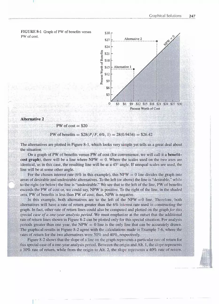
Graphical Solutions 247
FIGURE 8-t Graph ofPW of benefitsversusPW of cost.
$30
$27
$24
Alternative 2--------------------------
$6
$3
o $3 $6 $9 $12 $15 $18$21 $24 $27$30PresentWorthof Cost
Alternative 2
PW of cost - $20
PW of benefits = $28(PjF, 6%,1) = 28(0.9434) = $26.42
I.I,.
The alternatives are plotted in Figure 8-1, which looks very simple yet tells us a great deal aboutthe situation.' '
On a graph of PW of benefits versus PW of cost (for convenience,we willcall it a benefit...,cost graph), there will be a line where NPW O.Where the scales used on the two axes areidentical, as in this case, the resulting line will be at a 45° angle. If unequal scales are used~theline will be at some other angle.
For the chosen interest rate (6% in this example), thisNPW= 0 line divides the graph iIltoareas of desirable and undesirablealternatives.To the left (or above) the line is "de~irable,"whileto the right (or below) the line is "undesirable." Wesee that to the left of the liIle,PW of bynefitsexceeds thePW of cost or, we could say, NPW is positive. To the right of the lU1e,in the shadedarea,PW of benefits is less than PW of cost; thus, NPW is negative.
In this example,both alternativesare to the left of the NPW=0 line. Therefore, bothalternatives will have a rate of return greater than the 6% interest rate used in COIlstructingthegraph. In fact, other rate of return lines could also be computed and plotted on the graphfor thisspecial case ofa one-year analysisperiod: We must emphasize ai the outs~t that the additioIlalrate of return lines shownin Figure 8-2 can be plotted only for this special situation.For:analysisperiod~ greater than one y~ar,the NPW . . 0 line is the only line that caIl be accurately cir"aWn.The graphicalresultS in Figure 8-2 agree with the calculations.made in Example 7-6, Where the
=' ~rates,ofretQrnJor'the'two alternatives were"50%' tind 40%, respectively. :: ~
Figure 8..2showsthat1;beslope of a line on the graph represents ap~!cular rate ofrettirnfor
thisspecialcase?fa oIle-rearan~ysispe~od.Bet:veenthe2riginapdAlt.1,theslqp~!~We~~ ama'=5Q%~Tat~DfY'eti.Ibi':wIfile fr15m'the o~n.gihToKft~ 2: the sTope represeIlts a'"40% raie~fretlllJJ. ..
- -- - - - -
- - -
I'
l
'
..
il:1
Ii
.,"'"....
<.,

248 INCREMENTALANALYSIS
$30
$27
$24CI)
tE $21G.>c::
~ $18'5'€ $15o
~ $12c::G.>
~ $9p..,
Alternative 1
$6
$3
$3 $6 $9 $12. $15 $18 $21 .$24 $27 $30PresentWorth of Cost
FIGURE 8-2 Benefit-cost gra.ph for Example 8-1with a one-yearanalysisperiod. .
Since
$30
$27.
$24
Rate of Return
Alternative 2 ~o ~o /'8 ~~~o~o ~\:J
11)/\~~. ;v 4-Difference /./0 .b~o'.;;Betweenthe ~J'// / .h
Alternatives' I,i / /\:J~o
'"~ $21c::<UE $18o'E $15o~ $125~ $9
p..,
Alternative 1
$6
$3
$3 $6 $9 $12 $15 $18 $21 $24 $27 $30PresentWorth of Cost
FIGURE 8-3 Benefit-cost graph for Alternatives 1and 2 with a one-year analysis period.
[Higher-cost Alt. 2] = [Lower-costAlt. 1] + [Differencebetween them]
the differencebetween the alternativescan be represented by a line shown in Figure 8-3.Viewed in this manner, we clearly see that Alt. 2 may be considered to be two' separate
increments of investment. The first increment is Alt. 1 and the second one is the differencebetween the alternatives.Thus we will select Alt. 2 if the differencebetween the alternativesis adesirable increment of investment.
Since the slope of the line represents a rate of return, we see that the increment is desirable ifthe slope of the increment is greater than the slope of the 6% line that corresponds to NPW = O.We can see that the slope is greater; hence, the increment of investment is, attractive. In fact, acareful examination shows that the "Differencebetween the alternatives"line has the same slopeas.the 30% rate of .return line. We can say, therefore, that the incremental rate of return fromselectingAlt. 2 rather than Alt. 1 is 30%. This is the same as was computedin Example 7-6. Weconclude that Alt. 2 is the preferred alternative.
Solve Example 7-10 by means of a benefit-cost graph. Two machines are being considered forpurchase. If the minimum attractive rate of return (MARR) is 10%, which machine should be.pought?
- --
..
--

Graphical Solutions 249
Initial costUniform annual benefit
End-of-useful-life-salvage valueUsefullife, in years
Machine X$200
9550
6
Machine Y$700
12015012
,- . -. .'.
. SOLUTION
Noting that forboth Machine X andMachine Y, the PW of cost reflectsthe conventionof treatingsalvagevalue as a reduction in cost rather than a benefit, and using a 12-yearanalysis period, wehave
Machine X
PW of cost:;::: 200 + (200 -- 50)(P I F, 10%,6) - 50(P / F, 10%,12)
= 200+ 150(0.5645)- 50(0.3186) = 269
PW of benefit :;:::95(PIA,1O%,12) = 95(6.814):;::: 647
Machine Y
fW of cost:;::: 700 - 150(PIF, 10%,12) =700 - 150(0.3186)==652
PW of benefit = 120(P IA,10%,12)-120(6.814) :;:::818
Wben the two alternativesplotted (Figure 8-4), we see that the incrementY-X has a slope muchless than the 10%rate of return line. The rate of return on the incrementof investmentis less than10%;hence, the increment is undesirable. This means that Machine X should be selected ratherthan Machine Y.
EIGURE8-4 Benefit'-{;ostgraph. $900
$800
$700'"q::g $6000)
J:Q
'S" $500€~$400i:~ $300J:
$2QO
"' ,,$Joo
y
:=
=
$100 $200 $300 $400 $500 $600 $700 $800Present Worth o£?€ost==f==- 'III~ "" -"
II
I.
.t
'I
Ii
II
,\'II]Ii'I
-

250 INCREMENTALANALYSIS
FIGURE 8-5 Solvingmultiple-alternative problems bysuccessive two-alternative analyses.
Three Alternatives
A~Y'i'B ~1 Bestof3
C tLI Alternatives
Four Alternatives
1\vo-Alternative Analysis
J
K
LM
Best of 4Alternatives
Five Alternatives
1\vo-Alternative Analysis
p
Best of 5Altemlttives
Q
R
ST
The two example problems show us some aspects of incremental analysis. We now willexamine some multiple-alternativeproblems. We can solve multiple-alternativeproblemsby means of present worth and annual cash flow analysis without any difficulties.Rate ofreturn analysis requires that the differencesbetween two alternativesmust be examinedtosee whether either is desirable. Now, if we can choose between two alternatives,then by asuccessiveexamination we can choose from multiple alternatives.Figure 8-5 illustrates themethod.
Consider three mutually exclusive alternatives:
A
$2000~41O~
Initial costUnifofriiannual bem5fit
B$4000
639
C$5000
700"
Each alternative has a 20-year life and no salvage value. If the MARR is 6%, which alternativeII shouldhe,selected? = 1S; :
-- -----
-- - - - -

Graphical Solutions 251
At 6%, (PW of benefits) = (Uniform annual benefit) x (Series present worth factor).
PW of benefits = (Uniform annual benefit)(P / A, 6%,20)
PW of benefits for Alt. A = $410(11.470) = $4703
Alt. B = $639(11.470) = $7329
Alt. C = $700(11.470) - $8029
Figure 8-6 is a plot of the situation;we see that the slope of the line from the origin to A is greaterthan the 6%line (NPW =0). Thus therate ofretumfor A is greater than 6%. For the incrementofadditional cost of B over A, the slope of line B-A is greater than the 6% line. This indicates thatthe rate of return on theincrement of investmentalso exceeds6%.But J:4eslope of incrementC-Bindicates its rate of return is less than 6%, b,ence,undesirable. Weconclude that the Ainvestmentis satisfactory as well as the B-,-Aincrement; therefore, B is satisfactory.The C-B increment isunsatisfactory; so C is undesirable ip comparison to B. Our decision is to select Alternative B,
E'IGURE 8-6 Benefit--cost graph forExample 8-3.
$9000
$8000
$3000 $5000 $7000PresentWorthof Cost
Further study of the three alternativesof Ex:ample8-3reveals that Alt. A's uniform annualbenefitwas overstated.It is now projected to be $122 rather than $410. Replotthebep.efit-cost graph for
~ this cbanged,situ,<i.tiop. '" ~ '= ~ _ ; em' III~= ~ IB ~,; '" ~ i:i: ""'.>"iI
L_ -_,_ _ ,_____
I1
I
'"
ilii1'
1'Ii
.
.1
1'I',I
,ql'
I
I
;
\
1
I
.'I!:11If'
-- -

252 INCREMENTALANALYSIS
Alt. A': PW of benefits = 122(P / A, 6%, 20)
= 122(11.470) = 1399
The revised plot of the three alternatives (Figure 8-7) shows that the revised Alt. A' is no longerdesirable. We see that it has a rate of return less than 6%.
FIGURE 8-7 Benefit-cost graph forExample 8-4. $9000
$8000
$7000'"-f.,t:;g $6000(\)
~'"0 $5000..Q1::
~ $4000-=~ $3000(\)
~$2000
$1000
'"
o $1000 $3000 $5000 $7000PresentWorthof Cost
$9000
Now we wish to examineAlt. B. Shouldwe compareit with thedo-nothingalternative(wIiichis representedby the origin)or as a B-A' incrementover A'? Graphically;shouldwe examine lineO-B or B-A'? Since A' is an undesirable alternative, it should be discarded and not consideredfurther. Thus ignoring A', we should compare B with the do-nothing alternative, which is lineO-B. Alternative B is preferred over the do-nothing alternative because it has a rate of returngreater than 6%. Then increment C--B is examined and, as we saw,it is an undesirable incrementof investment.The decisionto selectB has not changed,whichshouldbe no surprise:if an inferiorA had become an even less attractiveA', we still would select the superior alternative, B.
The graphical solution of the four exampleproblemshas helped us visualize the mechanicsof incremental analysis. While problems could be solved this way, in practice they aresolved mathematically rather than graphically. We will now proceed to solve problemsmathematically by incremental rate of return analysis.
INCREMENTAL RATE OF RETURN ANALYSIS
To illustrate incremental rate of return analysis, we will solve three of the examples againby mathematical, rather than graphical, methods.
- - - - --- --

Incremental Rate of Return Analysis 253
Solve Example 8-1 mathematically.With two mutually exclusivealternativesand a 6% MARR,which alternative should be selected?
Yearo1
Alt. 1-$10+15
Alt. 2-$20+28
Examine the differencesbetween the alternatives.
Yearo1
Alt. 2 - Alt. 1-20 - (-10) = -10+28 - (+15) -+13
Ip.crementalinternal rate of return (~IRR),
10 = 13(PIF, i, 1)10
(P I F, i, 1) = --,.. = 0.769213
LlIRR. 30%
The Ll:IBRis greater than the MARR; hence, we will select the alteroative that gives this increment.
[Higher-cost All. 2] = [Lower-costAlt. 1] + [mcremel1tbetween theIll] .
Select Alternative 2.
Recompute Example 8-3 for MARR =6%. Each alternative has a 20-year life and no salvage value.
Initial costUniform annual benefit
A$2000
410
B$4000
639
C$5000
700
A practical first step is to compute the rate of return for each alt~rnative.
Alt~matiye A
2000 410(PIA, t, 20)2000 . , .
(p .I .A . ""'0). .-" - -"-"11878 - ''''~ '20nT/-- -
'. .l;1, l, ""L. = "'="'-="''-t. . - r-" " -/o'~ w410
=
..------
r----- - I

1
254 INCREMENTALANALYSIS
Alternative B
4000 = 639(P IA, i, 20)
4000(PIA, i, 20) = _6 = 6.259 i = 15%
39
Alternative C
5000 = 700(P I A, i, 20)
. 5000(PIA, i, 20) = - = 7.143700
The rate of return is between 12 and 15%:
(7.469 -7.143
)i = 12% + (3%) = 12.8%7.469 - 6.259
At this point, we would reject any alternative that fails to meet the MARR criterion of 6%. Allthree alternatives exceed the MARR in this example.
Next, we arrange the alternatives in order of increasing initial cost. Then we can examine theincrements between the alternatives.
Initial costUniform annual benefitRate of return
A$2000
41020%
B$4000
63915%
C$5000
70012.8%
Incremental costIncremental uniform annual benefit
IncrementB-A$2000
229
Incremental rate of return:
2000 = 229(P I A, i, 20)
2000 ~IRR(PIA,i,20) = 229 9.6%
The B-A increment is satisfactory; therefore, B is preferred over A. Because B is preferred toA, the next incremental comparison is of C with B. (If A was preferred to B, then the nextincremental comparison wouldhave been of C with A.)
Incremental costJncremenJal'l,.uMofIIJ,an,nualb~nefi!
Increment C-B$1000
pI- ..-- - ...-- - - ...--- -
--- - -----

_ ,_ _"_,, 'U' ,__
Incremental Rate of Return Analysis 255
1000 = 61(P IA, i, 20)1000 ~IRR
(PIA, i, 20) = 61 2.0%
The C- B increment has an unsatisfactory 2% rate of return; therefore, B is preferred over C.(Answer: Alt. B)
Solve Example 8.4 mathematically.Alternative A in Example 8-6 was believed to have an over-stated benefit. The new situation for A (we will again call it A') is a uniform annual benefit of122. Compute the rate of return for A'.
SOLUTION
2000 = 122(P IA, i, 20)2000
(PIA, i, 20) = - = 16.39 i -.2%122
This time Alt. A' has a rate of return less than the MARR of 6%. AlternativeA' is rejected, and theproblem now becomes selecting the better of B and C. In Example 8-6.we sawthat the incrementC-B had a ~IRR of 2% and it, too, was undesirable.
Thus, we again select Alternative B.
The following information is provided for fivemutually exclusivealternatives that have 20-yearuseful lives. If the minimum attractiverate of return is 6%, which alternativeshould be selected?
IIi !II
I*PW of benefit = (uniform annual benefit)(P IA, 6%,20)= 11.470 (uniform annual benefit). Theseval1,leswill be,used later to plot a curve'f()r,P~f c()stversus'PWofbenBftt,1I'
;;I
. - -- - ......
- ------
Alternatives
A B C D E
Cost $4000 $2000 $6000 $1000 $9000Uniform annual benefit 639 410 761 117 785PW of benefit* 7330 4700 8730 1340 9000- - < .
Rate of return 15% ; = 20q;h=w::I:
'ii% 10% 6%

256 INCREMENTAL ANALYSIS
SOLUTION
We see that the rate of return for each alternative equals or exceeds the MARR, therefore, noalternatives are rejected at this point. Next, we rearrange the alternativesto put them in order ofincreasing cost:
Beginning with the analysis of increment B-D, we compute..anIRRB-D of29%. Alternativ~Bis thus preferred to Alt. D, and D may be discarded at this point. The IRRA-B for A-B is alsosatisfactory,so A is retained and B is nowdiscarded:The C-A incrementhas a rate of return lessthan the MARR. Therefore, C is discarded and A continues to be retained. .
At this point, we have examined four alternatives-D; B, A, C-arid hav.eretained A afterdiscarding the other three. Now we must decide whether A or E is the superior alternative. Theincrement we will examine is E-A. (Note:Increment E-C would have no particular meaningforwe have already discarded C.)
~Cost~Annual benefit
Increment E-A$5000
146
Over the 20-year useful life, the total benefits (20 x 146 - 2920) are less than the cost. Thus, therate of return on this incrementis negative.This is an unsatisfactoryincrement, so E is discarded.Alternative A is the best of the five alternatives.
The benefit-cost graph (Figure 8-8) of this example illustrates an interesting situation.All five alternativeshave rates of return equal to or greater than the MARR of 6%. Yet,ondetailed examination, we see that Alternatives C and E contain increments of i~vestmentthat are unsatisfactory. Even though C has an 11% rate of return, it is unsatisfactory incomparison to Alt. A.
Also noteworthy, the project with the greatest rate of return-Alternative B-is notthe best alternative, since the proper economic criterion in this situation is to accept allseparable increments of investmentthat have a rate of return greater than the 6% MARR.
--- -
Alternatives
D B A C f
Cost $1000 $2000 $4000 $6000 $9000Unifonn annual benefit 117 410 639 761 785Rate of return 10% 20% 15% 11% 6%
Increments
B-D A-B C-A
L\Cost $1000 $2000 $2000L\Annual benefit 293 229 122L\Rate of return 29% 10% 2%

-Elements in Incremental Rateof Return Analysis 257
FIGURE 8-8 Benefit-cost .6%graph for Example 8-8 data.
o $1000 $3000 $5000 $7000 $9000Present Worth of Cost
We found a desirable A-B increment with a 10% IRRA-B. For the relationship betweenAlternatives A and B, and the computed rates of return, we write:
[
Higher-cost Alt. A:
]=
[
Alt. B: 20% rate
]+
[
Differencesbetween A and B:
]15% rate of return ofreturn 10% rate ofreturn
By selecting Alt. A we have, in effect, acquired a 20% rate of return on $2000'and a10% rate of return on an additional $2000, both desirable outcomes.Taken together as A,the result is a 15%rate of return on a $4000 investment.This is economically preferable toa 20% rate of return on a $2000 investment, assuming we seek to invest money wheneverwe can identify an investmentopportunitythat meets our 6% MARR criterion.This impliesthat we have sufficientmoney to accept all investmentopportunities for which the MARRis exceeded that come to our attention. This assumption of an abundaritsupply of moneyis considered appropriate in most industrial analyses, but it is not likely to be valid forindividuals. The selection of an appropriate MARR is discussed in Chapter 15.
ELEMENTS IN INCREMENTAL RATE OF RETURN ANALYSIS
1. Be sure all the alternatives are identified. In textbook problems the alternativeswill be well defined,but industrial problemsmay be less clear.Beforeproceeding, onemusthave all the mutually exclusive alternatives tabulated, including the "do-nothing" or "k~epdoing the same thing" alternative, if appropriate.
2. (Optional) Compute the rate of return for each alternative. If one or morealternatives has a rate of return equal to or greater than the minimum attractive rate ofreturn (IRR 2:MARR), then anyother alternativeswithan IRR less than the MARR maybeimmediatelyrejected.This optional step requirescalculationsthatmayor may not eliminate
I)
. - -----
- -- -r
$9000
$8000
J!J $7000
I A /'.
!.;:1$6000
j:Q
'c; $5000"€
$4000
-=$3000
$2000
$1000

258 INCREMENTALANALYSIS
alternatives.In an exam,this stepprobably shouldbe skipped,but in lesspressing situations,these are logical computations.
3. Arrange the remaining alternatives in ascending order of investment. The goalis to organizethe alternativesso that the incrementalanalysiswillbe of separableincrementsof investmentwhen we analyze the higher-costalternativeminus the lower-costalternative.In textbook problems, this is usually easy-but there are lots of potential difficulties infollowing this simple rule.
The ordering of alternatives is not a critical element in incremental analysis; in fact,the differences between any two alternatives, like X and Y, can be examined either as anX-Y increment or a Y-X increment. If this is done in a random fashion, however, wewill be looking sometimes at an increment of borrowing and sometimesat an incrementofinvestment.It can get a little difficultto keep all this straight;the basic goal is to restrict theincremental analysis, where possible, to increments of investment.
4. Make a two-alternative analysis of the first two alternatives. If the incrementexamined is Y - X, which represents an increment of investment.
[
Higher-cost
]Alt. Y_
[
LOWer-cost
] [
Differences between
]Alt. X + them (Y - X)
Compute the ~IRR on the increment of investment. The criterion is:
· If ~IRR ~ MARR, retain the higher-cost Alt. Y.· If ~IRR < MARR, retain the lower-costAlt. X.· Reject the other alternativeused in the analysis.
Sometimes the two alternativesbeing examined cannot be described as "higher cost" and"lowercost." In Example7-8, we encounteredtwo alternatives,A and B, with equal invest-ments. There we selected the A-B incrementbecause it was an increment of investment.
On the other hand, when we are examihingan incrementof borrowing, the criteria areas follows:
· If ~IRR ::::MARR, the increment is acceptable.· If ~IRR > MARR, the increment is not acceptable.
5. Take the preferred alternative from Step 4, and the next alternative from thelist created in Step 3. Proceed with another two-alternativecomparison.
6. Continue until all alternatives have been examined and the best of the multiplealternatives has been identified.
Incremental Analysis with Unlimited AlternativesAt times the possible alternativesare a more or less continuous function. For example, inan analysis to determine the economical height of a dam, the number of alternativescouldbe infinite. If the alternatives were limited, however, to heights in even feet, the numberof alternatives would still be large and would have many of the qualities of a continuousfunction, as in the following example.
- -- ---

Elements in Incremental Rate of Return Analysis 259
A careful analysis has been made of the consequences of constructinga dam in the Blue Canyon.It would be feasible to construct a dam at this site with a height anywherefrom 200 to 500 feet.Using a 4% MARR and a 75-year life, the various data have been used to construct Figure 8-9.Note particularly that the dam heights are plotted on the x axis along with the associated PWofcost. What height of dam should be constructed?
FIGURE 8-9 Benefit-costgraph forExample 8-9.
11
-c:4)CIJe 1
i:l.o
1 2 3 4 5 6 7 8 9 10 11
PresentWorth of Cost (millionsof dollars)I I I I I I
200 250300 400 500
PaIn Height (ft)
Five points have been labeled on Figure 8-9 to aid in the discussion. Damheignts below Point Ahave a PW of cost> PW of benefit; hence, the rate of return is le.ssthanMARR.. and wewoulqnot build a dam of these heights..In the region of Point B, an increment of additional PW ofcost-.6.C-produces a larger increment of PW ofbenefit-AB. These are,tI1erefore,desirableincrements of additional investment and, hence, dam height. At poirit D and also atPoint E, tI1ereverse is true. An increment of additionalJnvestment-.6.C-p],"oduces."a smalle.rincreIIientofPW of benefit-.6.B; this is undesirable.We do notwant theseincrements, so.tI1e~aIIlshould notbe bUiltto these heights.
At Point C, we see that fJ.B= .6.C.LoWer dam heights have desirable increments of.in.-vestmeIltand higher dam heights have unfavorable increments of investri;lent.1;'heoptimal damheight, th.erefore, is where.6.B = .6.C.In Figure 8..9,this corresponds to a heighto£app],"oximately250 feet. Anotherway of definingthe poin.tatwhich fJ.B= AC is to describe it as tI1epointwnerethe slope of the curve equals the slope of the NPW 0 line,
The techniquesfor solvingdiscrete alternativesor continuousfunctionalternativesarereallythe same. We proceed by adding increments whenever .6.IRR2:MARR and discardingincrements when, fJ.IRR< MARR.
,I,
:1
II1'1I
~1'1I"I
Ii
II!!Ii'II
Iij
II
I
il
ii,"~
",
--

260 INCREMENTALANALYSIS
PRESENT WORTH ANALYSIS WITH BENEFIT-COST GRAPHS
Any of the exampleproblems presented so far in this chaptercould be solvedby the preselworth method. The benefit-cost graphs we introduced earlier can be used to graphicallsolve problems by present worth analysis.
In presentworth analysis,whereneither inputnor outputis fixed,the economiccriteriois to maximize NPW. In Example 8-1, we had two alternatives and the MARR equcto 6%:
These points are plotted in Figure 8-10, which has the NPW = 0 line at 450,since identicalscales were used on both axes. The point for Alt. 2 is plotted at the coordinates (PW ofcost, PW of benefits). We drop a vertical line from Alt. 2 to the diagonal NPW = 0 line.The coordinates of any point on the graph are (PW of cost, PW of benefits), but along,theNPW = 0 line (450line), the x and y coordinatesare equal.Thus, the coordinates of Point4are also (pW of cost, PW of cost). Since
NPW = PW of benefits - PW of cost
the verticaldistance from Point 4 to Alt. 2 represents NPW.Similarly, the vertical distancebetweenPoint 3 andAlt. 1presentsNPW for Alt. 1.Sincethe criterionis to maximizeNPW,
FIGURE 8-10 Benefit-cost graph forPW analysis.
$27
$24
$21'"tE~ $18~r:Q
'C3 $15
'€~ $12C~ $9£
2
$6
$3 $6 $9 $12 $15 $18 $21PresentWorth of Cost
$3
.. --'--
-

Choosing an Analysis Method 261
c
A
$3000 $5000 $7000PresentWorthof Cost
FIGURE 8-11 Present worth analysis of Example 8-8 using a benefit-cost plot.
$1000 $9000
we select Alt. 2 with largerNPW. The same technique is used in situations where there are .
multiple alternatives or continuous alternatives. In Example 8-8 there were five alternatives;Figure 8-11 plots these five alternatives. We can see that A has the greatest NPW and,therefore, is the preferred alternative.
CHOOSING AN ANALYSIS METHOD
At this point, we have examined in detail the three major economic analysis techniques:present worth analysis, annual cash flow analysis, and rate of return analysis. A practicalquestion is, which method should be used for a particular problem?
While the obvious answer is to use the method requiring the least computations, anumber of factors may affect the decision. .
1. UnlesstheMARR-minimum attractiverateofreturn (orminimumrequiredinterestrate for investedmoney)-is known,neither present worth analysis nor annual cashflow analysis is possible.
2. Present worth analysis and annual cash flow analysis often require far less compu-tation than rate of return analysis.
3. In some situations,a rate of return analysis is easier to explain to people unfamiliarwith economic analysis. At other times, an annual cash flow analysis may be easierto explain.
4. Business enterprises generally adopt one, or at most two, analysis techniques forbroad categories of problems. If you work for a coq>orationand the policy manualspecifiesrate of return analysis, you would appear to have no choice in the matter.
Since one may not always be able to choose the analysis technique computationally bestsuited to the problem, this book illustrates how to use each of the three methods in all
--
$9000
$8000
$7000'".....I.t:
g $6000cuj:Q'C; $5000 I- B
€$4000
.....Q
$3000£
$2000
$1000

262 INCREMENTALANALYSIS
feasible situations. Ironically,the most difficultmethod-rate of return analysis-is the onemost frequently used by engineers in industry!
SPREADSHEETS AND INCREMENTAL ANALYSIS
An incremental analysis of two alternativesis easily done with the RATEor IRR functionswhen the lives of the alternatives are the same. The problem is more difficult, however,when the lives are different.As discussedin Chapters5 and 6, when comparing alternativeshaving lives of different lengths, the usual approach is to assume that the alternatives arerepeated until the least commonmultiple of their lives.This can be done with a spreadsheet,but Excel supports an easier approach.
Excel has a tool called GOAL SEEKthat identifiesa formula cell, a target value,and avariablecell. This tool causes the variablecell to be changedautomaticallyuntil the formulacell equals the target value. To find an IRR for an incremental analysis, the formula cellcan be the difference between two equivalentannual worths with a target value of O.Thenif the variable cell is the interest rate, GOAL SEEK will find the IRR.
In Excel this tool is accessed by selecting T(ools) on the main toolbar or menu andG(oal seek) on the submenu.As shownin Example 8-10, the variable cell (with the interestrate) must somehow affectthe formulacell (differencein equivalentuniform annual worthsor costs (EUAWsor EUACs», although it need not appear directly in the formula cell. IiIFigure 8-12a and 8-12b the interest rate (cell AI) appears in the EUACformulas (cells D3and D4), but not in the formula cell (cell D5).
Two different asphalt mixes can be used on a highway.The goodmix will last 6 years, and it willcost $600,000 to buy and lay down. The better mix will last 10years, and it will cost $800,000 tobuy and lay down. Find the incremental IRR for using the more expensivemix.
SOLUTION
This example would be difficult to solve without the GOAL SEEK tool. The least commonmultiple of 6 and 10 is 30 years, which is the comparison period. With the GOAL SEEK toola very simple spreadsheet does the job. In Figure 8-12a the spreadsheeUs shown before GOALSEEK. Figure 8-12b shows the result after the goal (D5) has been set .0 and A1selected as thevariable cell to change.
- --- ~ ~
FIGURE 8-12a Spreadsheetbefore,GOAI--SEp:rC..-.. -----
T--
. -. -. ..
A B C D E F;...---,.,'-...,.".,.-",.."..,.,-",-.
1 8.00% Interest rate
2 Alternative Cost Life EUAC ..3 Good 600000 6 129,789 ,:: -PMT($A$I,C3,B3)4 Better ! 800000 " 10 ..119,2 :I'::S'-PMT($A$1C4,B4)'
-.......5 difference= . to,5§ . ,0=;D3 -D4

Summary 263
FIGURE 8-12b Spreadsheet after GOAL SEEK.
The incremental IRR found by GOAL SEEK is 14.52%.....
SUMMARY
A graph of the PW of benefits versus PW of cost (called a benefit-cost graph) can be aneffective way to examine two alternatives by incremental analysis. And since multiple-alternative incremental analysis is done by the successive analysis of two alternatives,benefit-cost graphs can be used to solve multiple-alternative and continuous-functionalternativesas easily as two alternativeproblems.
The important steps in incremental rate of return analysis are as follows:
1. Check to see that all the alternatives in the problem are identified.2. (Optional)Computethe rate of return for each alternative.If oneor more alternatives
has IRR :::MARR, reject any alternativeswith IRR < MARR.,3. Arrange the remaining alternatives in ascendingorder of investment.4. Make a two-alternativeanalysis of the first two alternatives.5. Take the preferred alternative from Step 4, and the next alternativefrom the list in
Step 3. Proceed with another two-alternativecomparison.6. Continue until all alternatives have been examined and the best of the multiple
alternativeshas been identified.
Decision Criteria for Increments of Investment
· If LlIRR::: MARR, retain the higher-cost alternative.. If LlIRR < MARR, retain the lower-cost alternative.· Reject the other alternative used in the analysis.
Decision Criteria for Increments of Bo"owing
· If, LlIRR ~ MARR, the increment is acceptable.· If, LlIRR > MARR, the increment is not acceptable.
Benefit-cost graphs, which plot the PW of benefitsversus the PW of cost, can also be usedin present worth analysis to graphically show the NPW for each alternative.
-
J- ---
, A B C D E F
1 14.52% Interestrate2 Alternative Cost Life EUAC3 Good 600000 6 156,503 = -PMT($A$1,C3,B3)4 Better 800000 10 156,503 = -PMT($A$1,C4,B4)5 difference = 0 =,D3-D4

264 INCREMENTALANALYSIS
PROBLEMS
Unless otherwise noted, all problems for Chapter 8should be solved by rate of return analysis.
8-1 A firm is considering moving its manufacturing plantfrom Chicago to a new location. The industrial en-gineering department was asked to identify the var-ious alternatives together with the costs to relocatethe plant, and the benefits. The engineers examinedsix likely sites, together with the do-nothing alterna-tive of keeping the plant at its present location. Theirfindings are summarized as follows:
Plant LocationDenverDallasSan Antonio
Los AngelesClevelandAtlanta
Chicago
FirstCost ($OOOs)
$300550450750150200
o
Uniform AnnualBenefit ($OOOs)
$ 52137117167
1849o
The annual benefits are expected to be constant overthe 8-year analysis period. IT the firm uses 10%annual interest in its economic analysis, whereshould the manufacturing plant be located? (An-swer: Dallas)
8-2 In a particular situation, four mutually exclusivealternatives are being considered. Each of the al-ternatives costs $1300 and has no end-of-useful-life
salvage value.
AlternativeA
B
C
D
IT the MARR is 8%, which alternative should beselected? (Answer: Alt. C)
8-3 A more detailed examination of the situation in Prob-lem 8-2 reveals that there are two additional mutu-
ally exclusive alternatives to be considered. Both costmore than the $1300 for the four original alternatives.
8-4
IT the MARR remains at 8%, which one of the sixalternatives should be selected? Neither Alt. E nor F
has any end-of-useful-life salvage value.(Answer: Alt. F)
The owner of a downtown parking lot has employed acivil engineering consulting firm to advise him on theeconomic feasibility of constructing an office build-ing on the site. Bill Samuels, a newly hired civil engi-neer, has been assigned to make the analysis. He hasassembled the following data:
AlternativeTotal
Investment-
TotalNet Annual
Revenue fromProperty
Sell parking lotKeep parking lotBuild I-story buildingBuild 2-story buildingBuild 3-story buildingBuild 4-story buildingBuild 5-story building
$. 0200,000400,000555,000750,000875,000
1,000,000
$ 022,00060,00072,000
100,000105,000120,000
*Includes the value of the land.
The analysis period is to be 15 years. For all alterna-tives, the property has an estimated resale (salvage)value at the end of 15 years equal to the present totaJinvestment. If the MARR is 10%, whatrecommenda-tion should Bill make?
8-5 An oil company plans to purchase a piece of vacan1land on the comer of two busy streets for $70,000.On properties of this type, the company installs busi-nesses of four different types.
Useful CalculatedLife Rate
Annual Benefit (years) of Return
$100 at end of first 10 10.0%
year; increasing$30per year thereafter$10 at end of first 10 8.8%
year; increasing$50per year thereafterAnnual end-of-year 10 15.0%benefit= $260$450at end of first 10 18.1%
year; declining$50per year thereafter
AnnualEnd-of- Useful Calculated
Years Life RateAlternative Cost Benefit (years) of Return
E $3000 $ 488 10 10.0%F 5850 1000 10 11.2%

Problems 265
PlanCost of
Improyements. Type of Business
A $ 75,000 Conventional gas stationwith service facilities for
lubrication, oil changes,etc.Automatic carwash facil-
ity with gasoline pumpisland in front
Discount gas station (noservice bays)Gas station with low-cost,quick-carwash facility
B 230,000
c 30,000
D 130,000
*Cost of improvements does not include the $70,000cost of land.
In each case, the estimated useful life of the im-
provements is 15 years. The salvage value for each isestimated to be the $70,000 cost of the land. The netannuat income, after paying all operating expenses,is projected as follows:
Plan
ABCD
Net Annual Income
$23,30044,30010,00027,500
If the oil company expects a 10% rate of return on itsinvestments, which plan (if any) should be selected?
8-6 A firm is considering three mutually exclusive alter-natives as part of a production improvement program.The alternatives are as follows:
Installed costUniform annual benefit
Usefullife, in years
A
$10,0001,625
10
C
$20,0001,890
20
B
$15,0001,625
20
For each alternative, the salvage value at the end-of-useful-life is zero. At the end of 10 years, Alt. Acould be replaced by another A with identical costand benefits. The MARR is 6%. If the analysis periodis 20 years, which alternative should be selected?
8-7 Given the following four mutually exclusive alterna-tive,sand using 8% for the MARR, which alternativeshould be selected?
First costUniform annual benefit
Usefullife, in yearsEnd-of-useful-life
salvage valueComputed rate of return
A$75
1610o
D$85
1710o
B$50
1210o
C$50
1010o
16.8% 20.2% 15.1% 15.1%
(Answer: A)
8-8 Consider the following three mutually exclusivealternatives:
A
$20059.7
B
$30077.1
C
$600165.2
First cost.Uniform annual
benefit
Useful life,in years
End-of-useful-life
salvage valueComputed rate
of return
For what range of values of MARR is Alt. C thepreferred alternative? Put your answer in the follow-ing form: "Alternative C is preferred when _ % .:::
MARR.:::_%." .
5 5 5
o o o
15% 11.7%9%
8-9 Consider four mutually exclusive alternatives,eachhavingan 8-yearuseful life:
If the minimum attractive rate of return is 8%, whichalternative should be selected?
8-10 Three mutually exclusive projects are being consid-.ered:
When each project reaches the end of its useful life,it would be sold for its salvage value and there wouldbe no replacement. If 8% is the desired rate of return,which project should be selected?
--------. -- ..- --_.----
--- -- --
A B C DFirst cost $1000 $800 $600 $500Uniform annual 122 120 97 122
benefitSalvagevalue 750 500 500 0
A B CFirst cost $1000 $2000 $3000Uniform annual 150 150 0
benefit
Salvagevalue 1000 2700 5600Usefullife, 5 6 . 7
in years

266 INCREMENTALANALYSIS
8-11 Consider three mutually exclusive alternatives:
Yearo1234
Do Nothingooooo
Buy X-$100.0
+31.5+31.5+31.5+31.5
BuyY-$50.0+16.5+16.5+16.5+16.5
Which alternative should be selected:
(a) If the minimum attractive rate of return equals6%?
(b) If MARR = 9%?(c) If MARR = 10%?(d) IfMARR = 14%?(Answers: (a) X; (b) Y; (c) Y; (d) Do nothing)
8-12 Consider the three alternatives:
8-13
Which alternative should be selected:
(a) IfMARR = 6%?(b) IfMARR = 8%?(c) If MARR = 1O%?
A firm is considering two alternatives:
Initial costUniform annual benefits .
Salvage value at end of useful lifeUseful life, in years
A
$10,7002,100
o8
B$5500
1800o4
8-14
At the end of 4 years, another B may be purchasedwith the same cost, benefits, and so forth. If theMARR is 10%, which alternative should be selected?
Consider the following alternatives:
Initial costUniform annual benefits
A$300
41
C$200
35
B$600
98
Each alternative has a lO-year useful life and nosalvage value. If the MARR is 8%, which alternativeshould be selected?
8-15 Given the following:
Yearo1
X-$10+15
Y-$20+28
Over what range of values ofMARR is Y the preferredalternative?
8-16 Consider four mutually exclusive alternatives:
The analysis period is 8 years. At the end of 2, 4, and6 years, Alt. A will have an identical replacement.Alternative B will have a single identical replacementat the end of 4 years. Over what range of values ofMARR is Alt. B the preferred alternative?
8-17 Consider the three alternatives:
8-18
Each alternative has a lO-year useful life and liosalvage value. Based on a MARR of 15%, whichalternative should be selected? Where appropriate,use an external interest rate of 10% to transform a
cash flow to one sign change before proceeding withrate of return analysis.
A new 1O,000~square-meter warehouse next door tothe Tyre Corporation is for sale for $450,000. Theterms offered are $100,000 down with the balancebeing paid in 60 equal monthly payments based on15% interest. It is estimated that the warehouse would
have a resale value of $600,000 at the end of 5 years.Tyre has the needed cash available and could buy
the warehouse but does not need all the warehouse
space at this time. The Johnson Company has offeredto lease half the new warehouse for $2500 a month.
Tyre presently rents and utilizes 7000 square me-ters of warehouse space for $2700 a month. It has theoption of reducing the rented space to 2000 square
-- - --
Year A B Do Nothing0 -$100 -$150 01 +30 +43 02 +30 +43 03 +30 +43 04 +30 +43 05 +30 +43 0
A B C 'DInitial cost $770.00 $1406.30 $2563.30 0Uniform annual 420.00 420.00 420.00 0
benefit
Useful life, 2 4 8 0
in yearsComputed rate 6.0% 7.5% 6.4% 0
of return
A B CInitial cost $1500 $1000 $2035Annualbenefitin each 250 250 650
of first 5 yearsAnnualbenefit in each 450 250 145
of subsequent5years
;'
meters, in which case the monthly rent would be$1000 a mont;h. Further, Tyre could cease rentingwarehouse space entirely. Tom Clay, the Tyre Corp.plant engineer, is considering three alternatives:1. Buy the new warehouse and lease the Johnson
Company half the space. In turn, the Tyre-rentedspace would be reduced to 2000 square meters.
2. Buy the new warehouse and cease renting anywarehouse space.
3. Continue as is, with 7000 square meters of rentedwarehouse space.
Based on a 20% minimum attractive rate of return,which alternative should be selected?
8-19 Consider the following alternatives:
8-21 Three mutually exclusive alternatives are being stud-ied. If the MARR is 12%, which alternative shouldbe selected?
Year
o1234
A
-$20,000+10,000+5,000
+10,000+6,000
B
-$20,000+10,000+10,000+10,000
o
c- $20,000
+5,000+5,000+5,000
+15,000
Use present worth analysis, an 8% interest rate, andan infinite analysis period. Which alternative shouldbe selected in each of the two following situations?1. Alternatives B and C are replaced at the end of
their useful lives with identical replacements.2. Alternatives Band C are replaced at the end of
their useful lives with alternatives that provide an8% rate of return.
8-20 A problem often discussed in the engineering econ-omy literature is the "oil-well pump problem."}Pump 1 is a small pump; Pump 2 is a larger pump thatcosts more, will produce slightly more oil, and willproduce it more rapidly. If the MARR is 20%, whichpump should be selected? Assume that any temporaryexternal investment of money earns 10% per year andthat any temporary financing is done at 6%.
} One of the more interesting exchanges of opinionabout this problem is in Prof. Martin Wohl's "Com-mon Misunderstandings About the Internal Rate ofReturn and Net Present Value Economic AnalysisMethods;" and the associated discussion by Profes-sors Winfrey, Leavenworth, Steiner, and Bergmann,published in Evaluating Transportation Proposals,Transportation Research Record 731, Transporta-tion Research Board, Washington, D.C. See alsoAppendix 7A in Chapter 7.
The South End bookstore has an annual profit of$170,000. The owner is considering opening a sec-ond bookstore on the north side of the campus. Hecan lease an existing building for 5 years with anoption to continue the lease for a second 5-yearperiod. If he opens the second bookstore, he expectsthe existing store will lose some business that will hegained by "The North End," the new bookstore.. It willtake $500,000 of store fixtures and inventory to openThe North End. He believes that the two stores will
have a combined profit of $260,000 a year after all theexpenses of both stores have been paid.
The owner's economic analysis is based on a5-yearperiod. He will be able to recover this $500,000investment at the end of 5 years by selling the storefixtures and inventory. The owner will not open TheNorth End unless he can expect a 15% rate of return.What should he do? Show computations to justifyyour decision. .
8-23 A paper mill is considering two types of pollutioncontrol equipment.
Neutralization PrecipitationInitial cost $700,000 $500,000Annual chemical 40,000 110,000
cost
Salvage value 175,000 125,000Usefullife, 5 5
IIIyears
The firm wants a 12% rate ofreturn on any avoidableincrements of investment. Which equipment shouldbe purchased?
8-24 A stockbroker has proposed two investments in low-rated corporate bonds paying high interest rates and
..~ L
T
Problems 267
Pump 1 Pump 2Year ($OOOs) ($OOOs)
0 -$100 -$1101 +70 +1152 +70 +30
A B C 8-22Initial cost $100.00 $150.00 $200.00Uniform annual 10.00 17.62 55.48
benefitUseful life, Infinite 20 5
in years

268 INCREMENTALANALYSIS
selling below their stated value (in other words, junkbonds), Both bonds are rated as equally risky. Which,if any, of the bonds should you buy if your MARRis 25%?
Annual Current Market
Stated Interest Price, Including BondBond Value Payment BuyingCommission Maturity.
Gen Dev $1000RJR 1000
$ 94140
$480630
15 years15
*At maturity the bondholder receives the last interest pay-ment plus the bond stated value.
8-25 Three mutually exclusive alternatives are beingconsidered.
Initial investmentAnnual net income
Computed rateof return
A
$50,0005,093
8%
B
$22,0002,077
7%
C
$15,0001,643
9%
Each alternative has a 20-year useful life with nosalvage value. If the minimum attractive rate of re-turn is 7%, which alternative should be selected?
8-26 A firm is considering the following alternatives, aswell as a fifth choice: do nothing.
8-27
Each alternative has a 5-year useful life. The firm's
minimqm attractive rate of return is 8%. Whichalternative should be selected?
Alternatives
8-28 Our cat Fred's summer kitty-cottage needs a newroof. He's considering the following two proposalsand feels a 15-year analysis period is in line with hisremaining lives. Which roof should he choose if hisMARR is 12%? What is the actual value of the IRRon the incremental cost? (There is no salvage valuefor old roofs.)
First cost
Annual upkeepService life, in years
Thatch
$2053
Slate$40
25
8-29 Don Garlits is a landscaper. He is considering thepurchase of a new commercial lawn mower, either,the Atlas or the Zippy. The minimum attractive rateof return is 8%, and the table provides all the neces-sary information for the two machines.
(a) Determine the rate of return on the Atlas mower(to the nearest 1%).
(b) Does the rate ofreturn on the Zippy mower ex-ceed the MARR?
(c) Use incremental rate of return analysis to decidewhich machine to purchase.
8-30 QZY, Inc. is evaluating new widget machines offeredby three companies. The machines have the followingcharacteristics: .
MARR = 15%. Using rate of return analysis, fromwhich company, if any, should you purchase thewidget machine?
r
1 2 3 4
Initial cost $100,000 $130,000 $200,000 $330,000Uniform annual 26.38 38.78 47.48 91.55
net income ($1000s)Computed rate 10% 15% 6% 12%
of return
A B C D
Initial cost $2000 5000 4000 3000
Annual benefit 800 500 400 1300
Salvage value 2000 1500 1400 3000
Life, in years 5 6 7 4
MARR required 6% 6% 6% 6%
Find the best alternative using incremental IRRanalysis.
Atlas ZippyInitial cost $6700 $16,900
Annual operation and 1500 1,200maintenance cost
Annual benefit 4000 4,500
Salvage value 1000 . 3,500Usefullife, in years 3 6
Company Company CompanyA B C
First cost $15,000 $25,000 $20,000Maintenance 1,600 400 900
and operatingAnnual benefit 8,000 13,000 9,000
Salvage value 3,000 6,000 4,500
Usefullife, 4 4 4
in years

---TOO-- .-- --. - .-.
Problems 269
Using an MARR of 15% and a rate of return analysis,which alternative, if any, should be selected?
8-33 A firm must decide which of three alternatives to
adopt to expand its capacity. The firm wishes a mini-mum annual profit of 20% of the initial cost of eachseparable increment of investment.. Any money notinvested in capacity expansion can be invested else-where for an annual yield of 20% of initial cost.
--- --
Alt.ABC
Initial Cost$100,000300,000500,000
Annual Profit
$30,00066,00080,000
Profit Rate30%22%16%
Which alternative should be selected? Use a rate of
return analysis.
8-34 The New England Soap Company is consideringadding some processing equipment to the plant to aid-in the removal of impurities from some raw materials.By adding the processing equipment, the firm can pur-chase lower-grade raw material at reduced cost andupgrade it for use in its products.
Four different pieces of processing equipmentare being considered:
The company can obtain a 15% annual return on its'investment in other projects and is willing to investmoney on the processing equipment only as long as_it can obtain 15% annual return on each increment of
money invested. Which one, if any, of the alternativesshould be selected? Use a rate of return analysis.
8-35 Build a spreadsheet to find the EAC of each roof in
.II. Problem 8-28. Use the GOAL SEEK tool of Excel tofind the IRR of the incremental investment.
8-36 Build a spreadsheet to find the EAW of each lawn-
JI. mower in Problem 8-29. Use the GOAL SEEK tool of. Excel to find the IRR of the incrementalinvestment.
_.............-.--;0 - - -
-- -- --
8-31 The Croc Co. is considering a new milling machinefrom among three alternatives:
Alternative
Deluxe Regular Economy
First cost $220,000 $125,000 $75,000Annual benefit 79,000 43,000 28,000Maintenance and 38,000 13,000 8,000
L. operating costsSalvage value 16,000 6,900 3,000
All machines have a life of 10 years, and MARR =15%. Using incremental rate of return analysis, whichalternative, if any, should the company choose?
8-32 Wayward Airfreight, Inc. has asked you to rec-ommend a new automatic parcel sorter. You haveobtained the following bids:
SHIP-R SORT-Of U-SORT-M
First cost $184,000 $235,000 $180,000Salvage value 38,300 44,000 14,400Annual benefit 75,300 89,000 68,000Yearly maintenance 21,000 21,000 12,000
and operating costUseful life, in years 7 7 7
A B C D
Initial investment $10,000 $18,000 $25,000 $30,000Annual saving 4,000 6,000 7,500 9,000
in materialscosts
Annual operating 2,000 3,000 3,000 4,000cost

After Completing This Chapter...Thestudent should be able to: .. Use future worth, benefit-cost ratio, payback period, and sensitivity analysis methods.
to solve engineering economy problems. .. Link the use of thefuture worth analysis to the present worth and annual worth methodsdevelopedearlier. .. Mathematically develop the benefit-cost ratio, and use thistnodel to select alternativesand make economic choices.. Understandthe concept of thepaybackperiod of an investment,andbe able t~ calculatethis quantity for prospectiveprojects.. Demonstrate a basic level understanding of sensitivity and breakevenanalyses and theuse of these tools in an engineeringeconomic analysis.. Use a spreadsheet to perform sensitivity and breakeven analyses.
QUESTIONS TO CONSIDER )
1. Officeleases frequently require building owners, rather than tenants, to pay heating andcooling costs. What effect might this have on the decision making of potential tenantsfor green buildings?'
2. The green building movement has had more success among developers who hold ontotheir buildings for years and rent them out, rather than selling them as soon as they areconstructed. What factors might influence their views?
3. Manyenvironmentallyfriendlybuildingsare architecturallydistinctiveandfeaturebetterquality materials and workmanshipthan traditionalcommercialstructures.Environmen-tal advocateshopethesecharacteristicswillhelpgreenbuiJ,.dingsattracta rent "premium."How might these features make the buildings more attractive to tenants?

..
Other AnalysisTechniques
Clean, Green, and.Far BetweenDesigners and engineers have made great progress in developingenvironmentallyfriendlyconstruction materials and building techniques. And "green" office buildings offer numerous . i .
advantages. They use energy more efficiently, provide a more natural environment for.workers, and can even reduce indoor air pollution.
The only problem is, no one wants to build them. In the commercial sector,barely 1% of officeconstructionprojectshavebotheredto applyfor certificationas green buildings.
Commercial developershave found th~tenvironmentallyfriendly featuresaddto the expenseof construction.Eventhoughadditionalcostsmayincrease I..overall construction expenses by only 1 or 2%, they can make it harder for:thebuilder to recoup its investment and break even on the project.
Moreover, the extra expenditures apparently do little to attract potentialtenants. Renters may like the idea of being cleaner and greener-but they don'twant to pay extra for it.
= .....
=-- ----
.1'
d
i'jl
1
'1
. : ,j
~ . ,.

--. -. .. - . - . - ... ... .. .....
272 OTHER ANALYSISTECHNIQUES
Chapter 9 examines four topics:
· Future worth analysis· Benefit-cost ratio analysis· Payback period·Sensitivityand breakeven analysis
Future worth analysis is very much like present worth analysis, dealing with then (futureworth) rather than with now (present worth) situations.
Previously,we have written economic analysis relationships based on either:
PW of cost = PW of benefit or EUAC = EUAB
Instead of writing it in this form, we could define these relationships as
PW of benefit=1
PWof costor
EUAB=1
EUAC
When economic analysis is based on these ratios, the calculations are called benefit-costratio analysis.
Payback period is an approximate analysis technique, generally defined as the timerequired for cumulativebenefits to equalcumulativecosts. Sensitivitydescribes the relativemagnitude of a particular variation in one or more elements of a problem that is sufficientto change a particular decision. Closely related is breakeven analysis, which determinesthe conditionswhere two alternativesare equivalent.Thus, breakeven analysis is a form ofsensitivity analysis.
FUTUREWORTH ANALYSIS
Wehaveseenhoweconomicanalysistechniquesresolvedalternativesintocomparableunits.In present worth analysis, the comparison was made in terms of the present consequencesof taking the feasible courses of action. In annual cash flow analysis, the comparison wasin terms of equivalent uniform annual costs (or benefits). We saw that we could easilyconvertfrom present worth to annualcash flow,and vice versa.But the concept of resolvingalternatives into comparable units is not restricted to a present or annual comparison.Thecomparison may be made at any point in time. In many situations we would like to knowwhat thefuture situation will be, if we take some particular course of action now. This iscalled future worth analysis.
Ron Jamison, a 20-year-old college student, consumes about a carton of cigarettes a week. Hewonders how much money h~ could accumulate by age 65 if he quit smoking now and put hiscigarett~moneyinto~asavingsaccount. Cig"aretiescost $35 per carton. Ron expects:that a savingsaccount would earn 5% interest, compounded semiannually. Compute Ron's future worth atage 65.;,."..'::1: -.
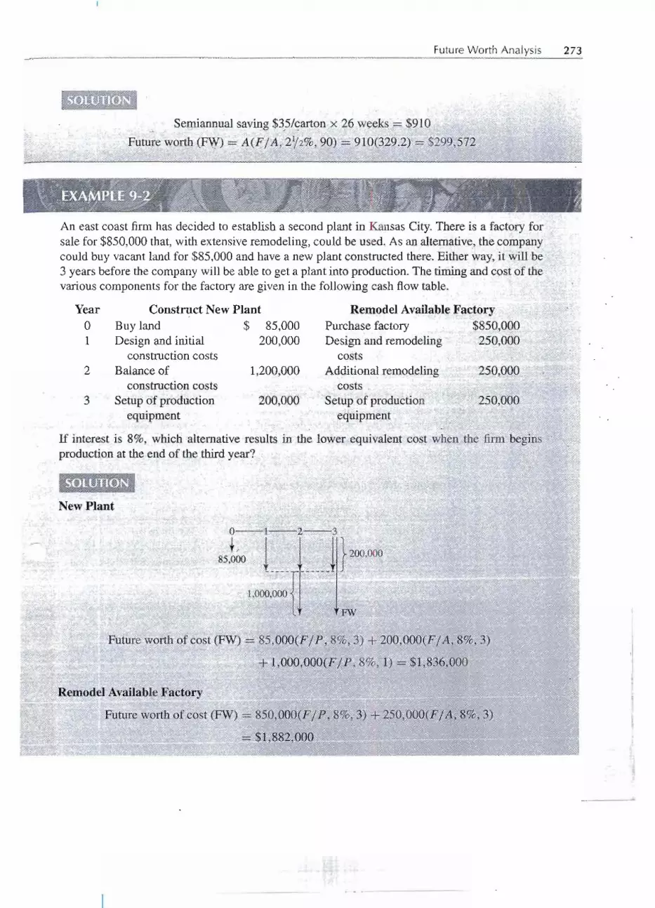
....
Future Worth Analysis 273
SOUJTIONi
Semiannual saving $35lcarton x 26 weeks . . $910
Future worth (FW)- A(FjA,,2'l2%, 90) = 910(329.2) . . $299,57f
An east coast firm has decided to establish a second plant in Kansas City.There is a factory forsale for $850,000 that, with extensiveremodeling,could be used. As an alternative,the companycould buy vacant land for $85,000 and have a new plant constructed there. Either way, it will be3 years before the company will be able to get a plant into production. The timing and cost of thevarious components for the factory are given in the following cash flowtable.
Yearo1
Construct New PlantBuy land $ 85,000Design and initial 200,000
construction costsBalanceof . 1,200,000
construction costsSetup of production 200,000
equipment
2
3
Remodel Available F~ctoryPurchase factory $850,000Design and remodeling 250,000
costs
Additional remodeling 250,000costs
Setup of production 250,000equipment
If interest is 8%, which alternative results in the lower equivalent cost when th~,fiim begins .production at the end of the third year?
New Plant
Future worth of cost (FW) - 85,000(Fj P,8%, 3) + 200,000(FjA, 8%,3)
+ 1,000,OOO(FjP, 8%,1)- $1,836,000
Remodel Available Factory
Future worth of cost (FW) . 850,OOO(Fj P, 8%, 3) + 250,000(FjA., 8%, 3)
iii

274 OTHER ANALYSISTECHNIQUES
The total cost of remodeling the available factory ($1,600,000) is smaller than the total cost of anew plant ($1,685,000). The timing of the expenditures, however, is less favorable than buildingthe new plant. The new plant is projected to have the smaller future worth of cost and thus is thepreferred altefl1ative..
BENEFIT-COST RATIO ANALYSIS
At a given minimum attractive rate of return (MARR), we would consider an alternativeacceptable, provided
PW of benefits - PW of costs ~ 0 or EUAB - EUAC 2: 0
These could also be stated as a ratio of benefits to costs, or
;
; ,
B PW of benefit _EUAB > 1Benefit-cost ratio C = PW of costs - EUAC -
, '
Rather than using present worth or annual cash flow analysis to solve problems, we canbase the calculations on the benefit-cost ratio, BIe. The criteria are presentedin Table9-1.We will illustrate "B/C analysis" by solving the same example problems worked by othereconomic analysis methods. ' ' ,
, , TABLE9-1 Benefit-Cost Ratio Analysis
Situation Criterion
Fixed input Amount of money or otherinput resources are fixed
Fixed task, benefit, orother output to beaccomplished
Neither amount of moneyor other inputs noramount of benefits or
other outputs are fixed
Fixed output
Neither inputnor outputfixed
Maximize BIC
Maximize B IC
Two alternatives: Computeincremental benefit-cost ratio
(~BI ilC) on the incrementof investment between thealternatives. If ilBI ilC ::::1,choose higher-cost alternative;otherwise, choose lower~costalternative. ,Three or more alternatives:
Solve by benefit-cost ratioincremental analysis

Benefit-Cost Ratio Analysis 275
A finn is trying to decide which of two devices to install to reduce costs in a particular situation.Both devices cost $1000 and have useful lives of 5 years and no salvage value. Device A canbe expected to result in $300 savings annually. Device B will provide cost savings of $400the first year, but savings will decline by $50 annually, making the second...yearsavings $350,the third-year savings $300, and so forth. With interest at 7%, which device should the firmpurchase?
jSOtuTION
Wehave used three types of analysis thus far to solve this problem: presentworthin Example 5-1,annual cash flowin Example 6-5, and rate of return in Example 7-9.
Device A
PW of cost = $1000
PW of benefits = 300(PjA, 7%,5)
- 300(4.100) = $J230
B PW of benefit 1230- · --;---= 1.23C PW of costs 1000
Device B
rI
PW of cost -- $1000
PW of benefit = 400(P j A, 7%, 5) - 50(P fG-, 7%, 5)
= 400(4.100).--' 50(7.647)= 1640 --'382= 1258
BPW of benefit 1258---= . . .' ... ., = --- --1.26CPWof costs 1000
To ma)!:imizethe benefit-cost ratio, select Device B,.
Twomachines are being considered for purchase.Assuming 10%interest, which machine shouldbe bought?
r
1:- --~
, - -..---
Initial costUnifonn, annual benefitEnd-of-useful-lifesalvage value
.,,, UsefuUife,.in years
Machine X$200
95506
::I;;;: ~ 1
·-- .d
Machine Y$700
120150
=~ :=.ef2'i1''I: ~=
..
-- - - -
( ,

276 OTHER ANALYSISTECHNIQUES
SOLUTION
Assuming a 12-yearanalysis period, the cash flowtable is:
Yearo
1-5
MachineX-$200
+95
{
+95-200+50+95
{+95+50
6
7-11
12
We will solve the problem using
Machine Y-$700+120
+120
+120
+120+150
B EUABC EUAC
and considering the salvage value of the machines to be reductions in cost, rather than increasesin benefits. This choice affects the ratio value, but not the decision.
Machine X
EUAC = 200(Aj P, 10%,6) - 50(Aj F, 10%,6)
= 200(0.2296) - 50(0.1296) = 46 - 6 = $40
EUAB = $95
Note that this assumes the replacement for the last 6 years has identical costs. Under thesecircumstances, the EUACfor the fi~st6 years equals the EUACfor all 12years.
Machine Y
EUAC = 700(Aj P, 10%, 12) - 150(Aj F, 10%, 12)
- 700(0.1468) - 150(0.0468) = 103 -7 = $96
EUAB = $120
Machine Y - Machine X
dB = 120- 95 _ 25 = 0.45= ;; LSC= 96 - 40 56 =
Since the incremental benefit-costratio isless than 1, it represents an undesirable increment ofinvestmenf! We-=thereforechoosethe lower-cost alternative-Machine Xi' If we had computed
-- -- -- ---
- -- - -- -
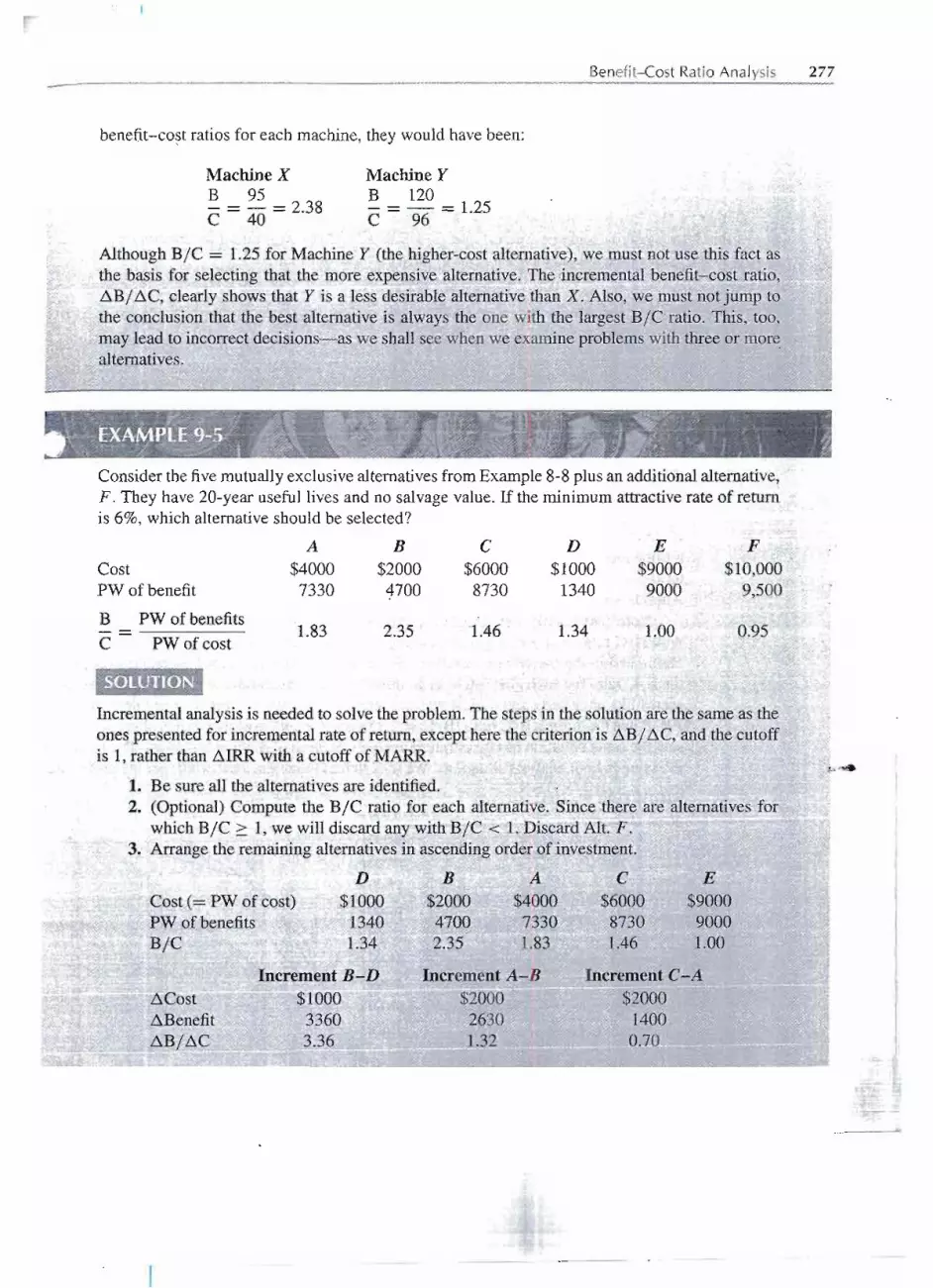
r
Benefit-Cost Ratio Analysis 277
benefit-co~t ratios for each machine, they would have been:
Machine XB 95- = - = 2.38C 40
Machine YB 120C =. 96 = 1.25
Although BIC = 1.25 for Machine Y (the higher-cost alternative), we must not use this fact asthe basis for selecting that the more expensive alternative. The incremental.benefibcost ratio,~B Ib.C, clearly shows that Y is a less desirable alternative than X. Also, we must not jump tothe conclusion that the best alternative is always the one with the largest B/Cratio. This, too,may lead to incorrect decisions-as we shall see when we examine problems with three orJIlor~alternatives.
I
I.
Consider the fivemutuallyexclusivealternativesfrom Example 8-8 plus an additionalalternative,F. They have 20-year useful lives and no salvagevalue. If the minimum attractiverate of returnis 6%, which alternative should be selected?
',-' -.".
SOLUTION.
Incremental analysis is needed to solve the problem.The steps in the solution are the same as theones presented for incremental rate of return, excepthere the criterion is b.B/ b.C, and the cutoffis 1,rather than b.IRR with a cutoff of MARR.
1. Be sure all the alternatives are identified.2. (Optional) Compute the BIC ratio for each alternative. Since there are alternatives for
which B/C ::::1, we will discard any withB/C < 1. Discard Alt. F.3. Arrange the remaining alternativesin ascendingorder of investment.
Cost (= PW of cost)PW of benefitsB/C
D$1000
13401.34
B$200047002.35
A
$400073301.83
C$600087301.46
E$900090001.00
~ b.Cost~Benefitb.BI b.C
Increment B-D$1060 ~
33603.36
Increment A-B$2006-2630
J..32 ;
Increment C-A: $2000 =~
1400Q.2J).c
"
il
"_II _ ...__
- --- -
A B C D E FCost $4000 $2000 $6000 $1000 $9000 $10,000PW of benefit 7330 4700 8730 1340 9000 9,500
B PW of benefits1.34- 1.83 2.35 1.46 1.00 0.95
C PW of cost

278 OTHER ANALYSISTECHNIQUES
4. Examine each separable increment of investment. If ~BI ~c < 1, the increment is notattractive. If D.BI~C 2: 1, the increment of investment is desirable. The increments B-Dand A-B are desirable. Thus, of the first three alternatives (D, B, and A), Alt. A is thepreferred alternative.Increment C-Ais not attractiveas ~BI ~C = 0.70,whichindicatesthat of the first four alternatives (D, B, A, and C), A continues as the best of the four.Now we want to decide between A andE, which we'll do by examining the incrementofinvestmentthat represents the differencebetween these alternatives.
Increment E-A$500b
16700.33
D.Cost~BenefitD.BI4C
The increment is undesirable. We choose Alt. A as the best of.the six alternatives. One shouldnote that the best alternativein this example does not have the highest B/C ratio.
I, '
Benefit-cost ratio analysis may be graphically represented. Figure 9.1 is a graph ofExample 9-5. We see that F has a B/C < 1 and can be discarded. Alternative D is thestarting point for examining the separable increments of investment. The slope of lineB-D indicates a ~BI D.Cratio of > 1. This is also true for line A-B. Increment C-A hasa slope much flatter than BIC = 1, indicating an undesirable increment of investment.Al-ternative C is therefore discarded and A retained. Increment E-A is similarlyunattractive.Alternative A is therefore the best of the six alternatives.
Note particularly two additional things about Figure 9-1: fin;t, even if alternativeswith B/C ratio < 1 had not been initially excluded, they would have been systematicallyeliminated in the incremental analysis. Since this is the case, it is not essential to computethe B/C ratio for each alternativeas an initial step in incremental analysis. Nevertheless,itseems like an orderly and logical way to approach a multiple-alternativeproblem. Second,Alt. B had the highestB/C ratio (B/C = 2.35), but Itis not thebest ofthe sixaltematives.Wesaw the same situation in rate of return analysis of three or more alternatives.The reason isthe same in both analysis situations.We seek to maximizethe total profit, not the profit rate.
FIGURE 9-1 Benefit-cost ratio
graph of Example9-5.$10,000
$9000
~ $8000I+::
~ $7000~
E $6000o'€ $5000o~ $4000-=~ $3000!!:!~ $2000
$1000
B/C=2.0 B/C=1.5 B/C=1.0
"
, .
a
, ,
" o 4000 6000 8000 10,600PresentWorthof Cost

Benefit-Cost Ratio Analysis 279
Continuous Alternatives
At times the feasiblealternativesare a continuous function.When we consideredthe heightof a dam in Chapter 8 (Example 8-9), we found that it was possible to build the damanywherefrom 200 to 500 feet high.
In many situations, the projected capacity of an industrial plant can be varied contin-uously over some feasible range. In these cases, we seek to add increments of investmel).twhere /1Bj /1C 2: 1 and avoid increments where /1Bj /1C < 1. The optimal size of such aproject is where /1Bj /1C = 1.Figure 9-2a shows the line of feasible alternativeswith their
Maximum Present Worth
",of Benefits Obtainable atEach Level of Cost
I.
rIC=O.5
o
I
'H'. '"_~+ . . _ _.' '-. ~." .~.n<_,,_._.I Present Worth of CostII (a)IIII-- OptimalValueforII PW of CostIIII
Present Worth of Cost
(b)
Present Worth of Cost
(c)
FIGURE 9-2 Selecting optimal size of project: (a) feasible alternatives, (b) changes in ~B / ~C, and(c) total NPW plotted versus size of the project.
---

- - . -- .. -- ... ..--
280 OTHER ANALYSISTECHNIQUES
costs and benefits. This may represent a lot of calculations to locate points through whichthe line passes.
Figure9-2bshowshowthe incrementalbenefit-costratio (L\.BjL\.C)changesas onemoves along the line of feasible alternatives.Figure 9-2b also plots the ratio of incrementalnetpresent worthto incrementalcost (L\.NPWj L\.C). As expected,weare addingincrementsof NPW as long as L\.BjL\.C> 1. Finally, in Figure 9-2c, we see the plot of (total) NPWversus the size of the project.
This three-part figure demonstrates that present worth analysis and benefit-cost ratioanalysis lead to the same optimal decision. We saw in Chapter 8 that rate of return andpresent worth analysis led to identical decisions. Any of the exact analysis methods-present worth, annual cash flow,rate of return, or benefit-cost ratio-will lead to the samedecision. Benefit-cost ratio analysis is extensivelyused in economic analysis at all levelsof government.
PAYBACK PERIOD
Payback period is the period of time required for the profit or other benefits from aninvestment to equal the cost of the investment.This is the general definitionfor paybackperiod, but there are other definitions. Others consider depreciation of the investment,interest, and income taxes; they, too, are simply called "payback period."For now,we willlimit our discussion to the simplest form.
Payback period is the period of time required for the profit or other benefits of aninvestment to equal the cost of the investment.
Thecriterionin all situationsis tominimizethepaybackperiod.Thecomputationofpaybackperiod is illustrated in Examples 9-6 and 9-7.
The cash flowsfor two alternativesare as follows:
Yearo12345
A-$1000
+200+200
+1200+1200+1200
B-$2783+1200+1200+ 1200+ 1200+1200
You may assume the benefits occur throughout the year rather than just at the end of the year.
Based ong~.!>a~kperiod, ,,;:hichaltern~tiveshould be selected?L ---- - - - ... ---
- - - - - - -- - - -

.r _.u.._ --. --.-.-...
rPayback Period 281
Alternative A
Payback period is theperiod of time required for the profit or other benefitsof an investmenttoequal thecostof the investment.In the first 2 years,only $400ofthe$1000costis recovered.Theremaining $600 cost is recovered in the firsthalf of Year3.Thus the payback period for Alt. A is2.5 years.
Alternative B
Since the annual benefits are uniform, the payback period is simply
$2783/$1200 per year - 2.3 years
To minimize the payback period, choose Alt. B.
A firm is trying to decide which of two weighingscalesit shouldinstall to check a package-fillingoperation in the plant. If both scales have a 6-year life, which one should be selected? Assume an8% interest rate. .
AlternativeAtlas scaleTom Thumb scale
Cost$20003000
Uniform AnnualBenefit$450600
End-of-Useful-LifeSalvage Value
$100700
..SQkl)T10~...
Atlas Scale
CostPayback period = Uniform annual benefit
2000 = 4.4 years= 450
Tom Thumb Scale
Cost
Payback period ~ Uniform annual benefir ::!
=
_3000-II 600 ... 5 years!I =-= 0; Ii:
..- - - ..- .._-
------ - -

282 OTHER ANALYSISTECHNIQUES
$3000 $3000Cost = $3000
$2000 $2000
$1000 $1000
o 12341 54.4
o 1 2 3 4 5
Year Year
(a) (b)
FIGURE 9-3 Payback period plots for Example 9-7: (a) Atlas scale and (b) Tom Thumb scale.
Figure 9-3 illustrates the situation. To minimize payback period, select the Atlas scale.
There are four important points to be understood about payback period calculations:
1. This is an approximate, rather than an exact, economic analysis calculation.2. All costs and all profits, or savingsof the investment,prior to payback are included
without considering differences in their timing. .
3. All the economic consequences beyond the payback period are completely ignored.4. Being an approximate calculation, payback period mayor may not select the cor-
rect alternative. This is, the payback period calculations may select an alternativedifferent from that found by exact economic analysis techniques. .
This last point-that payback period may select the wrong alternative-was illustratedbyExample9-7. When payback period is used, the Atlas scaleappears to be the more attractivealternative. Yet, when the same problem was solved earlier by the present worth method .
(Example 5-4), the TomThumb scale was the chosen alternative. A review of the problemreveals the reason for the differentconclusions.The $700 salvagevalue at the end of 6 yearsfor the TomThumb scale is a significantbenefit.The salvagevalueoccurs after the paybackperiod, so it was ignored in the payback calculation. It was considered in the present worthanalysis, with the result that the TomThumb scale was in fact more desirable.
But if payback period calculationsare approximateand may lead to the selectionof thewrong alternative, why is the method used at all? There are two primary answers: first, thecalculations can be readily made by people unfamiliar with economic analysis. One doesnot need to know how to use gradient factors, or even to have a set of compound interesttables. Second, payback period is a readily understoodconcept. Earlier we pointed out thatthis was also an advantage to rate of return.
Moreover,paybackperioddoes giveus a usefulmeasure,tellingus howlong itwill takefor the cost of the investmentto be recoveredfrom thebenefitsof the investment.Businessesand industrial firms are often very interested in this time period: a rapid return of invested
J.u~I
..:...
~
r

--- --+_. ... ......-.-.
Payback Period 283
capital means that it can be reused sooner for other purposes. But one must not confuse the, speedof thereturnof the investment,as measuredby thepaybackperiod,witheconomic
efficiency.They are two distinctly separateconcepts. The formeremphasizes the quicknesswith which invested funds return to a firm; the latter considers the overall profitability ofthe investment.
We can create another situation to illustrate how selectingbetween alternativesby thepayback period criterion may result in an unwise decision.
A :firmis purchasing production equipment for a new plant. Two alternativemachines are beingconsideredfor a particular operation. .
Installed costNet annual benefit after
all annual expenseshave been deducted
Useful life, in years
Tempo Machine$30,000$12,000 the first year,
declining $3000 per yearthereafter
4
Dura Machine
$35,000$1000 the first year,
increasing $3000per year thereafter
8
Neither machine has anysalvage value. Compute the payback period for each of the alternatives.
SOLUTION BASED ON PAYBACKPERIOD
Cost = $35,000
1 2 3 4 5Year
(a) (b)
FIGURE 9-4 Payback period plots for Example 9-7: (a) Tempo machine and (b) Dura machine.
= The Tempo machine has a declining annual benefit, while the Dura has an increasing annualbenefit. Figure 9-4 shows the Tempo has a 4-year payback period and the Dura has a 5-year.
II ~ == Ril~b<!p!5;p~lii>4.lJ> .Q1ir}jmize.thepayback period, theTempo is selected.' ~ ~ ==1-- -- .. i- - - .........
II
I'
:illII
--
- - - - --- -----
$35,000 $35,000Cost = $30,000
$30,000$30,000 ./T.eo
$25,000 I- ! / I $25,000.<q'lJ
$20,000I- S'lJY I $20,000
$15,000 I- PI I $15,0000
.... $10,000 $10,000
$5,000 $5,000
0 1 2 3 4 5 0Year

284 OTHER ANALYSISTECHNIQUES
Now, as a check on the payback period analysis, compute the rate of return for each alternative."Assume the minimum attractive rate of return is 10%.
The cash flowsfor the two alternativesare as follows:
Yearo12345678
TempoMachine-$30,000+ 12,000+9,000+6,000+3,000
ooooo
Dura Machine
-$35,000+1,000+4,000+7,000
+10,000+ 13,000+16,000+19,000+22,000
+57,000
Tempo Machine
Since the sum of the cash flows for the Tempo machine is zero, we see immediately that the$30,000 investment just equals the subsequent benefits. The resulting rate of return is 0%.
Dura Machine
35,000 = 1000(PjA, i, 8) +3000(PjG, i, 8)
Try i = 20%:
35,000 ~ 1000(3.837)+ 3000(9.883)
~3837 + 29,649 = 33,486
The 20% interest rate is too high. Try i = 15%:
35,000 ~ 1000(4.487)+ 3000(12.481)
~4487 + 37,443 = 41,930
This time, the interest rate is too low. Linear interpolation would show that the rate of return isapproximately 19%.
Using an exact calculation-rate of return--;-,-itis clear that the Tempo is not very attJ.'active
economiq.l}y. Y~t it ~s thi~ aJle!ll~t:tve,and nq.t."the.,QurawacJ:rine, that w,~ preferred based On ~
the payback period calculations. On the other hand, the shorter payback period for the Tempo doesgive a measure of the speed of the return of the investment not found in the Dura. The conclusion
I to be drawn~iSJhatJiqfiidity;ffild,profitability may be two quite different criteria. \1I.. . .,~- ..~
-- - -

Sensitivity and Breakeven Analysis 285
Fromthe discussionandthe examples,wesee thatpaybackperiodcanbe helpful inprovidinga measure of the speed of the return of the investment. This might be quite important,for example, for a company that is short of working capital or for a firm in an industryexperiencing rapid changes in technology.Calculation of payback period alone, however,must notbe confusedwith a carefuleconomic analysis.Wehaveshownthat a shortpaybackperiod does not always mean that the associated investment is desirable. Thus, paybackperiod should not be considered a suitable replacement for accurate economic analysiscalculations.
SENSITIVITY AND BREAKEVEN ANALYSIS
Sincemany datagathere~in solvingaproblemrepresentprojectionsof futureconsequences;there maybe considerableuncertaintyregardingthe data's accuracy.Sincethe desiredresultof the analysis is decision making, an appropriate question is, To what extent do variationsin the data affectmy decision?When smallvariationsin a particular estimate would changeselection of the alternative, the decision is said to be sensitive to the estimate. To betterevaluate the impact of any particular estimate, we compute "the variation to a particular .
estimate that would be necessary to change a particular decision."This is called sensitivityanalysis.
An analysisof the sensitivityof aproblem's decisiontoits variousparametershighlightsthe important and significantaspectsof that problem. For example,one might be concernedthat the estimates for annual maintenance and future salvagevalue in a particular problemmay vary substantially. Sensitivity analysis might indicate that the decision is insensitiveto the salvage-valueestimate over the full range of possible values. But, at the same time,we might find that the decision is sensitiveto changes in the annual maintenance estimate.Under these circumstances, one should place greater emphasis on improving the annualmaintenance estimate and less on the salvage-valueestimate.
As indicated at the beginning of this chapter, breakeven analysis is a form of sensi-tivity analysis. To illustrate the sensitivity of a decision between alternatives to particularestimates, breakeven analysis is often presented as a breakeven chart. .
Sensitivityandbreakevenanalysisfrequently areuseful in engineeringproblemscalledstage construction. .Should a facility be constructed now to meet its future full-scalerequirement, Or should it be constructed in stages as the need for the increased capac-ity arises? Three examples of this situation are:
· Should we install a cable with 400 circuits now or a 200-circuit cable now and another200-circuit cable later?· A 10 cm water main is needed to serve a new area of homes. Should it be installednow, or should a 15 cm main be installed to ensure an adequate water supply toadjoining areas later, when other homes have been built?· An industrial firm needs a new warehouse now and estimates that it will need todouble its size in 4 years. The firm could have a warehouse built now and laterenlarged, or have the warehouse with capacity for expanded operations built rightaway.
Examples 9-9 and 9-10 illustrate sensitivityand breakevenanalysis.--~
-- --
-- ---
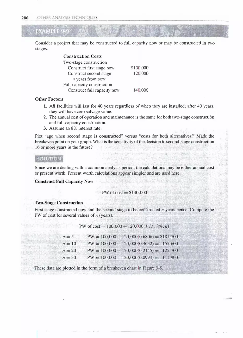
286 OTHER ANALYSISTECHNIQUES
Consider a project that may be constructed to full capacity now or may be constructed in twostages.
Construction Costs
Two-stageconstructionConstruct first stage nowConstruct second stage
n years from nowFull-capacity construction
Construct full capacity now
$100,000120,000
140,000
Other Factors
1. All facilities will last for 40 years regardless of when they are installed; after 40 years,they will have zero salvagevalue.
2. The annual cost of operation andmaintenanceis the same for both two-stageconstructionand full-capacity construction.
3. Assume an 8% interest rate.
Plot "age when second stage is constructed" versus "costs for both alternatives." Mark thebreakevenpoint on your graph.What is the sensitivityof the decisionto second-stageconstruction16 or more years in the future? '
[Sp'LOTION'~.. ~'-- ~".".",.~,,: '.. ...."..',.~""..- ~. "
Since we are dealing with a common analysis period, the calculationsJ;Ilaybe either annual costor present worth. Present worth calculations appear simpler and are used here.
Construct Full Capacity Now
PW of cost = $140,000
Two-Stage Construction
First stage constructed now and the second stage to be constructedn years hence...Compute thePW of cost for severalvalues of n (years).
PW of cost = 100,000 + 120,000(P IF, 8%, n)
n=5
n = 10
n -20
n=30
PW 100,000+ 120,000(0.6806) -- $181,700
PW = 100,000+ 120,000(0.4632)' J55,600
PW 100,900 + 120,000(0.+145) --: 125,700
pw" .100,00.0-h;120,.000(0..0994,)...J.ll.,2iliL _ u ~.____'."-"_.~. <po ,', "'-"-'-"-"~''''~~ .. '," '--r:,: - -""---',.: :..,.".,..."--~ -' - - '_. 'M1!l't._ C!IIIii
These data are plotted in the form of a breakevell chart in Figure 9..5.- -.. - ~ ~
r --
-- -

Sensitivity and Breakeven Analysis 287
FIGURE 9-5- Breakeven chart for
Example 9-9.$250,000
$200,000...'"ou'Ci$150,000-E
~i:: $100,000Q)'"£
$50,000
10 25 30o 15 20Year
AgeWhenSecondStage C0E-structed
5
Figure 9-5 portrays the PW of cost for the two alternatives. The x-axis variable is the timewhen the second stage is constructed. We see that the PW of cost for two-stage constructionnaturally decreases as the time for the second stage is deferred. The one-stage construction(full capacity now) is unaffected by the x-axis variable and, hence, is a horizontal line on thegraph.
The breakeven point on the graph is the point at which both alternatives have equivalent costs.We see that if, in two-stage construction, the second stage is deferred for 15 years, then the PWofcost of two-stage construction is equal to one-stage construction; Year 15 is the breakeven point.The graph also shows that if the second stage were to be needed prior to Year 15, then one-stageconstruction, with its smaller PW of cost, would be preferred. On the other hand, if the secondstage would not be required until after 15 years, two-stage construction is preferred.
The decision on how to construct the project is sensitive to the age at which the second stageis needed only if the range, of estimates includes 15 years. For example, if one estimated that thesecond stage capacity would be needed between 5 and 10 years hence, the decision is insensitive t9that estimate. For any value within that range, the decision does not change. The more eQollomicalthing to do is to build the full capacity now. But, if the second-stage capacity were to be neededsometime between, say, 12 and 18 years, the deciSion would be sensitive to the estimate of whenthe full capacity would be needed.
One question posed by Example 9-9 is how sensitive the decision is to the need forthe second stage at 16years or beyond. The graph shows that the decisionis insensitive. Inall cases for construction on or after 16 years, two-stage construction has a lower PW ofcost.
=! .~ :tu..
I
-- --- ----

288 OTHER ANALYSISTECHNIQUES
--.Example 8-3 posed the followingsituation. Three mutuallyexclusivealternativesare given,eachwith a 20-year life and no salvagevalue. The minimum attractive rate of return is 6%.
Initial costUniform annual benefit
A$2000
410
B$4000
639
C$5000
700
In Example 8-3 we found that Alt. B was the preferred alternative.Here we would like to knowhow sensitive the decisionis to our estimate of the initial cost of B. If B is preferred at an initialcost of $4000, it will continue to be preferred at any smaller initial cost. But how much higherthan $4000 can the initial cost be and still have B the preferred alternative? The computationsmay be done several differentways. With neither input nor output fixed,maximizing net presentworth is a suitable criterion.
Alternative A
NPW = PW of benefit - PW of cost
=41O(P j A, 6%, 20) - 2000
= 410(11.470) - 2000 = $2703
Alternative B
Let x = initial cost of B.
NPW = 639(P j A, 6%, 20) - x
= 639(11.470)- x
= 7329- x
Alternative C
NPW = 700(PjA, 6%,20) - 5000
= 700(11.470) - 5000 = $3029
For the three alternatives,we see that B will only maximize NPW as long as its NPW is greaterthan 3029.
3029 = 7329 - x
x = 7329 - 3029 = $4300
:: Therefore, B is tbe preferred alternativeif its initial cost does not exceed $4300.Figure 9-6 is a breakeven chart for the three alternatives.Here the criterion is to maximize
NPW; as a result, the graph shows that B is preferred if its initial cost is less than $4300. At an
- - -------
- - -- -
f

Graphing with Spreadsheetsfor Sensitivity and Breakeven Analysis 289
FIGURE 9~6 Breakeven chart forExample 9-10.
$6000Alternative IAlternative
B I CIPreferred I Preferred$5000
'€ $4000~5 $3000'"
£~ $2000
$1000
o $1000 $2000 $3000 $4000 $5000 $6000Initial Cost of Alternative B
initial cost above $4300, C is preferred. We have a breakeven point at $4300. When B has anipitial cost of $4300, B and C are equally desirable.
Sensitivityanalysis and breakeven point calculationscan be very useful in identifying howdifferent estimates affect the calculations. It must be recognized that these calculationsassume that all parameters except one are held constant, and the serisitivityof the decisionto that one variable is evaluated. Later we will look further at the impact of parameterestimates on decision making.
GRAPHING WITH SPREADSHEETS FOR SENSITIVITY
AND BREAKEVEN ANALYSIS
Chapter 4 introduced drawing xy plots with spreadsheets, and Chapter 7 reviewed thisprocedure for plotting present worth versus i. The Chapter 7 plot is an example of breakevenanalysis, as it is used to determine at what interest rate does the project break even or havea present worth of O.This section will present some of the spreadsheet tools and optionsthat can make the xy plots more effective and attractive.
The spreadsheet tools and options can be used to:
· Modify the x or y axes
Specify the minimum or maximum valueSpecify at what value the other axis intersects (default is 0)
· Match line types to data
Use line types to distinguish one curve from anotherUse markers to show real dataUse lines without markers to plot curves (straight segmentsor smooth curves)
- - -- - -- -- -

292 OTHER ANALYSISTECHNIQUES
"shoWlegend" off.Similarly,we can turn the x-axis gridlines on.The line style for these gridlinesshould be changed to match the y-axis gridlines. This allows us to see that the breakeventime isbetween 14and 15years.
To make the graph less busy, change the scale on the x axis so that the interval is 5 yearsrather than automatic.Also eliminate the gridlines for the y axis (by selecting the chart area, chartoptions, and gridlinestabs). The graph size can be increased for easier reading, as well. This mayrequire specifyingart interval of 10,000for the scale of the y axis.
Finally to addthe labels for thefull-capacitycurveand the two-stagecurve, findthe toolbarforgraphics, which is open when the chart is selected(probablyalongthe bottom of the spreadsheet).Select the text box icon, and click on a location close to the two-stage chart. Typein the label fortwo-stage construction.Notice how including a return and a few spaces can shape the label to fitthe slanted line. Add the label for full construction. Figure 9-8 is the result.
FIGURE 9-8 Spreadsheet of Figure 9-7 with improved graph.
-- -
A B C D
1 Time Full Capacity Two Stage2 0 140,000 100,0003 n 120,000
4
5 life 40
6 i 8%
7 Present worth of
8 n Full Capacity Two Stage9 0 140,000
10 5 140,000 181,670 =$C$2+PV($B$6,A1O,0, -$C$3)
11 10 140,000 155,58312 20 140,000 125,74613 30 140,000 111,925
14 I -15 tj 155,000 1"---... Two Stage
,I. -
160
... ...... Construction.
U I..... .........
, -0 ,
17"€ 145,000
...... , Full CapacityI- ... I -...... , Construction18 ...... I
.', .-
19135,000
' ...f- ' ...... -I ......
20 '" , ....... ...... -p.. . ......21 : '"
125,000 -22 10 15 20 -23 Years until Capacity Needed
24

Problems 293
SUMMARY
In this chapter, we have looked at four new analysis techniques.
PROBLEMS
Future worth: When the comparison between alternatives will be made in the future,the calculation is called future worth. This is very similar to present worth, whichis based on the present, rather than a future point in time.
Benefit-cost ratio analysis: This technique is based on the ratio of benefi,tsto costsusing either present worth or annual cash flow calculations.The method is graph-ically similar to present worth analysis. When neither input nor output is fixed,incremental benefit-cost ratios (~B/ ~C) are required. The method is similar inthis respect to rate of return analysis. Benefit-cost ratio analysis is often used atthe various levels of government.
Paybackperiod: Here we definepayback as the period of time required for the prQfitor other benefits of an investmentto equal the cost of the investment. Althoughsimple to use and simple to under~tand,payback is a poor analysis techniquefor ranking alternatives. While it provides a measure of the speed of the re-turn of the investment, it is not an accurate measure of the profitability of an.investment.
Sensitivity and breakeven analysis: These techniques are used to see how sensitivea decision is to estimates for the various parameters. Breakevenanalysis is dOJ?eto locate conditions under which the alternatives are equivalent. This is oftenpresented in the form of breakevencharts. Sensitivity analysis is an examinationof a range of values for some parameters to determine their effect on a particulardecision.
9-1 For a 12% interest rate, compute the value of F in thefollowing diagram.
9-2 Compute F for the followingdiagram.
200
f
r -2-3-t-'
1
0-1 t100
100 100 100
t t t0-1-2-3-4-5-6
i=lO% + + +100 100 F
F
- - --- -
I
--
- --
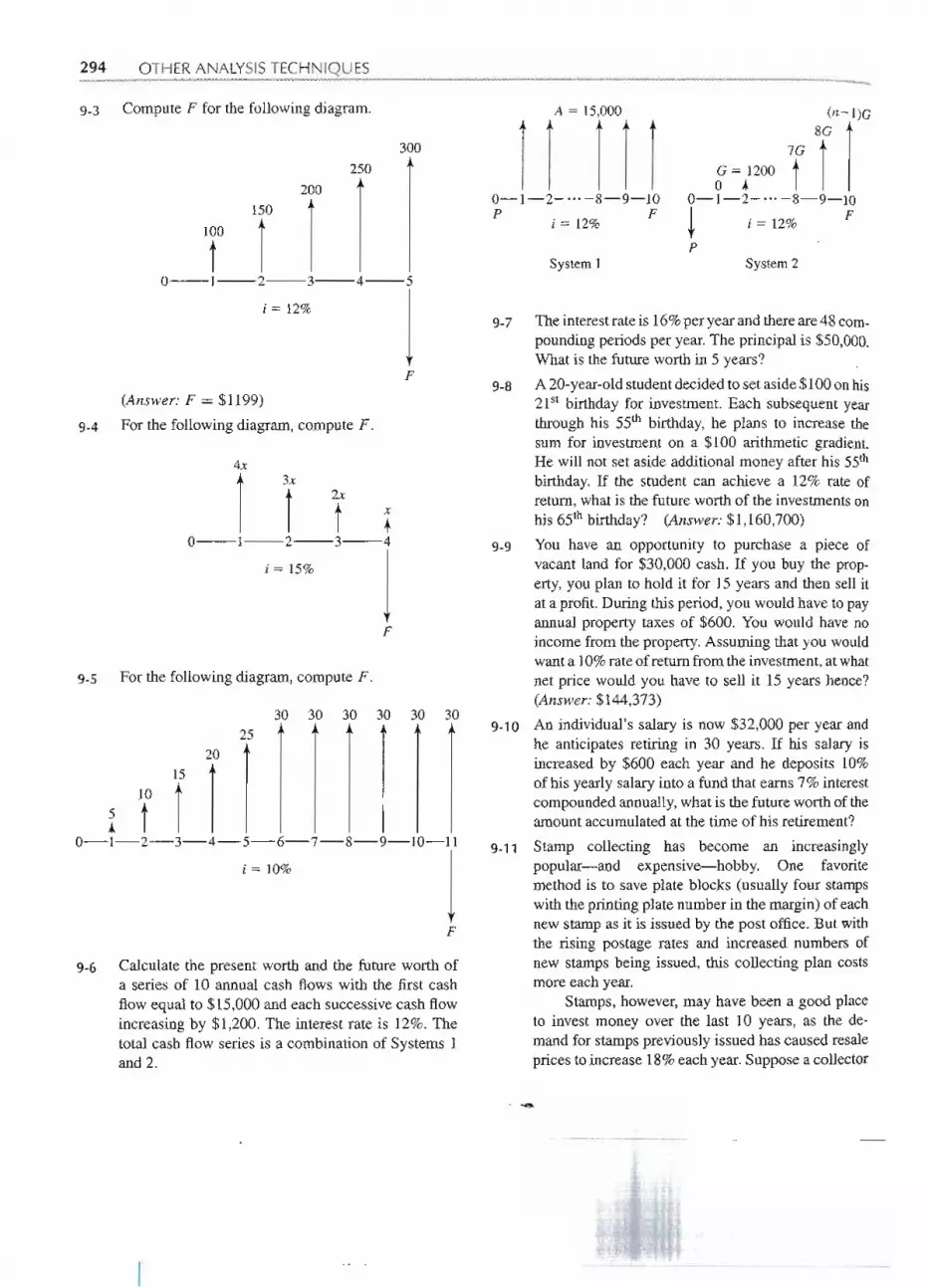
294 OTHER ANALYSISTECHNIQUES
9-3 Compute F for the followingdiagram.
300250
150
1
200
I
100
t0-1-2-3-4-5
1
i = 12%
8~nTG
~~FOO 7f i I
0-1-2-"'-8-9-10
~ i = 12% FP
0-1-2-"'-8-9-10P F
i = 12%
System 1 System 2
F
9-7 The interest rate is 16% per year and there are 48 com-pounding periods per year. The principal is $50,000.What is the future worth in 5 years?
A 20-year-old student decided to set aside $100 on his2pt birthday for investment. Each subsequent yearthrough his 55th birthday, he plans to increase thesum for investment on a $100 arithmetic gradient.He will not set aside additional money after his 55thbirthday. If the student can achieve a 12% rate ofreturn, what is the future worth of the investments onhis 65th birthday? (Answer: $1,160,700)
You have an opportunity to purchase a piece ofvacant land for $30,000 cash. If you buy the prop-erty, you plan to hold it for 15 years and then sell itat a profit. During this period, you would have to payannual property taxes of $600. You would have noincome from the property. Assuming that you wouldwant a 10% rate of return from the investment, at what
net price would you have to sell it 15 years hence?(Answer: $144,373)
An individual's salary is now $32,000 per year andhe anticipates retiring in 30 years. If his salary isincreased by $600 each year and he deposits 10%of his yearlysalaryinto a fund that earns7% interestcompoundedannually,what is the future worthof theamountaccumulatedat the time of his retirement?
9-11 Stamp collecting has become an increasinglypopular-and expensive-hobby. One favoritemethod is to save plate blocks (usually four stampswith the printingplate numberin the margin)of eachnew stamp as it is issuedby the post office.But withthe rising postage rates and increased numbers ofnew stamps being issued, this collecting plan costsmore each year.
Stamps, however, may have been a good placeto invest money over the last 10 years, as the de-mand for stamps previously issued has caused resaleprices to increase 18% each year. Suppose a collector
25
f r I
10
i t0-1-2-3-4-5-6-7-8-9-10-11
1
i = 10%
9-6 Calculate the present worth and the future worth ofa series of 10 annual cash flows with the first cash
flow equal to $15,000 and each successive cash flowincreasing by $1,200. The interest rate is 12%. Thetotal cash flow series is a combination of Systems 1and 2.
.-------------
F9.8
(Answer: F = $1199)
9.4 For the following diagram, compute F.
4x
1
3x
t
2x
t x.
0-1-2-3-4 9-9
i = 15%
1F
9.5 For the following diagram, compute F.
30 30 30 30 30 309.10

Problems 295
9-12
purchased $100 worth of stamps 10 years ago, andincreased his pqrchases by $50 per year in each sub-sequent year. After 10 years of stamp collecting, whatis the future worth of the stamp collection?
Sally deposited $100 a month in her savings accountfor 24 months. For the next 5 years she made nodeposits. What is the future worth in Sally's savingsaccount at the end of the 7 years, if the accountearned 6% annual interest, compounded monthly?(Answer: $3430.78)
In the early 1980s, planners were examining alter-nate sites for a new airport to serve London. In theireconomic analysis, they computed the value of thestructures that would need to be removed from various
airport sites. At one airport site, the twelfth-centuryNorman church of St. Michaels, in the village ofStewkley, would be demolished. The planners usedthe value of the fire insurance policy on the church-a few thousand pounds sterling-as the value of thestructure.
An outraged antiquarian wrote to the LondonTimes that an equally plausible computation wouldbe to assume that the original cost of the church(estimated at 100 pounds sterling) be increased at therate of 10% per year for 800 years. Based on his pro-posal, what would be the future worth ofSt. Michaels?(Note: There was great public objection to tearingdown the church, and it was spared.)
Bill made a budget and planned to deposit $150 amonth in a savings account, beginning September 1.He did this, but on the following January 1, he re-duced the monthly deposits to $100 a month. In allhe made 18 deposits, four at $150 and 14 at $100.If the savings account paid 6% interest, compoundedmonthly, what was the future worth of his savingsaccount immediately after he made the last deposit?(Answer: $2094.42)
A company deposits $1000 in a bank at the beginningof each year for 6 years. The account earns 8% inter-est, compounded every 6 months. What is the futureworth of the account at the end of 6 years? Make acareful, accurate computation.
Don Ball is a 55-year-old engineer. According to mor-tality tables, a male at age 55 has an average lifeexpectancy of 21 more years. In prior years, Donhas accumulated $48,500 including interest, towardhis retirement. He is now adding $5000 per year to hisretirement fund. The fund earns 12% interest. Don's
9-13
9-14
9-15
9-16
9-21
9-17
goal is to retire when he can obtain an annual incomefrom his retirement fund of $20,000 per year, assum-ing he lives to age 76. He will make no provision for aretirement income after age 76. What is the youngestage at which Don can retire, based on his criteria?
Jean invests $100 in Year 1 and doubles the amount
each year after that (so the investment is $100, 200,400,800, . . .). If shecontinuesto do this for 10years,and the investment pays 10% annual interest, whatis the future worth of her investment at the end of
10 years?
If you invested $2500 in a bank 24-month certificateof deposit paying 8.65%, compounded monthly, whatis the future worth of the certificate of deposit whenit matures in 2 years?
After receiving an inheritance of $25,000 on her21st birthday, Ayn Rand deposited the inheritance"ina savings account with an effective annual interestrate of 6%. She decided that she would make regu-lar deposits on each future birthday, beginning with$1000 on her 22nd birthday and then increasing theamount by $200 in each following year (i.e., $1200on her 23rd birthday, $1400 on her 24th birthday, etc.).What was the future worth of Ayn's deposits on her56th birthday?
The Association of General Contractors (AGe)wished to establish an endowment fund of $1 mil-lion in 10 years for the Construction EngineeringTechnology Program at Grambling State Universityin Grambling, Louisiana. In doing so, the AGC estab-lished an escrow account in which 10 equal end-of-year deposits that earn 7% compound interest weremade. After seven deposits, the Louisiana legisla-ture revised laws relating to the licensing fees AGecan charge its members, with the result that therewas no deposit at the end of Year 8. What must theamount of the remaining equal end-of-year depositsbe sure that the $1 million is available to GramblingState for its Construction Engineering TechnologyProgram?
On her birthday, a 25-year-old engineer is consideringinvesting in an individual retirement account (IRA).After some research, she finds a mutual fund wi~an average return of 10% per year. What is the futureworth of her IRA at age 65 if she makes annual invest-ments of $2000 into the fund beginning on her 25thbirthday? Assume that the fund continues to earn anannual return of 10%.
J1
9-18
9-19
9-20
J
1
--
---

-"" --- - ----
296 OTHER ANALYSISTECHNIQUES
9-22 IPS COrp. will upgrade its package-labeling
mac~nery. It costs $150,000 to buy the machineryand have it installed. Operation and maintenance costsare $1500 per year for the first 3 years and increase by$500 per year for the remaining years of the machine's1O-year life. The machinery has a salvage value of 5%of its initial cost. Interest is 10%. What is the future
worth of cost of the machinery?
9-23 A company is considering buying a new bottle-capping machine. The initial cost of the machine is$325,000 and it has a 1O-year life. Monthly mainte-nance costs are expected to be $1200 per month for thefirst 7 years and $2000 per month for the remainingyears. The machine requires a major overhaul costing$55,000 at the end of the fifth year'of service. Assumethat all these costs occur at the end of the appropriateperiod. What is the future value of all the costs asso-ciated with owning and operating this machine if thenominal interest rate is 7.2%?
9-24 A family starts an education fund for their son Patrickwhen he is 8 years old, investing $150 on his eighthbirthday increasing the yearly investment by $150 peryear until Patrick is 18 years old. The fund pays 9%annual interest. What is the future worth of the fundwhen Patrick is 18?
9-25 A bank account pays 19.2% interest with monthlycompounding. A series of deposits started with a de-posit of $5000 on January 1, 1997. Deposits in the se-ries were to occur each 6 months. Each deposit in theseries is for $150 less than the one before it. The last
deposit in the series will be due on January 1,2012.What is the future worth of the account on July 1,2014, if the balance was zero before the first depositand no withdrawals are made?
9-26 Let's assume that a late-twentieth century collegegraduate got a good job and began a savings account.He is paid monthly and authorized the bank to auto-matically withdraw $75 each month. The bank madethe first withdrawal on July 1, 1997 and is instructedto make the last withdrawal on January 1,2015. Thebank pays a nominal interest rate of 4.5% and com-pounds twice a month. What is the future worth of theaccount on January 1, 2015?
9-27 Bob, an engineer, decided to start a college fund forhis son. Bob will deposit a series of equal, semi-annual cash flows with each deposit equal to $1500.Bob made the first deposit on July 1, 1998 and willmake the last deposit on July 1,2018. Joe, a friend of
=
9-28
Bob's, received an inheritance on April 1, 2003, andhas decided to begin a college fund for his daughter.Joe wants to send his daughter to the same collegeas Bob's son. Therefore, Joe needs to accumulatethe same amount of money on July 1,2018, as Bobwill have accumulated from his semiannual deposits.Joe never took engineering economics ~d had noidea how to determine the amount that should bedeposited. He decided to deposit $40,000 on July 1,2003. Will Joe's deposit be sufficient? If not, howmuch should he have put in? Use a nominal interestof7% with semiannual compounding on all accounts.
A business executive is offered a management jobat Generous Electric Company, which offers him a5-year contract that calls for a salary of $62,000per year, plus 600 shares of GE stock at the end ofthe 5 years. This executive is currently employed byFearless Bus Company, which also has offered him a5-year contract. It calls for a salary of $65,000, plus100 shares of Fearless stock each year. The Fearlessstock is currently worth $60 per share and pays anannual dividend of $2 per share. Assume end-of-yearpayments of salary and stock. Stock dividends beginone year after the stock is received. The executivebelieves that the value of the stock and the dividendwill remain constant. If the executive c.onsiders 9% asuitable rate of return in this situation, what must theGenerous Electric stock be worth per share to makethe two offers equally attractive? Use the future worthanalysis method in your comparison.(Answer: $83.76)
A project will cost $50,000. The benefits at the end ofthe first year are estimated to be $10,000, increasingat a 10% uniform.rate in subsequent years. Using an8-year analysis period and a 10% interest rate, com-pute the benefit-cost ratio.
Each of the three alternatives shown has a 5-year use-fullife. If the MARR is 10%, which alternative shouldbe selected? Solve the problem by benefit-cost ratioanalysis.
9-29
9-30
CostUniform annual benefit
A
$600.0158.3
C
$200.058.3
B
$500.0138.7
9-31(Answer: B)
Consider three alternatives, each with a 10-year use-fullife. If the MARR is 10%, which alternative shouldbe selected? Solve the problem by benefit-cost ratioanalysis.
- --

Problems 297
Cost .
Uniform annual benefit
A$800
142
C$150
33.5
B$300
60
9-32 An investor is considering buying some land for$100,000 and constructing an office building on it.Three different buildings are being analyzed.
Building Height
2 Stories 5 Stories 10 Stories
Cost of building $400,000 $800,000(excluding costof land)
Resale value* of 200,000 300,000land andbuilding at end
20-yearanalysis period
Annual rental 70,000 105,000income after all
operatingexpenses havebeen deducted
$2,100,000
400,000
256,000
*Resale value to be considered a reduction in cost, ratherthan a benefit.
Using benefit-cost ratio analysis and an 8% MARR,determine which alternative, if any, should beselected.
9-33 Using benefit-cost ratio analysis, determine whichone of the three mutually exclusive alternatives shouldbe selected.
First costUniform annual benefitSalvagevalue
A$560
14040
C
$12040o
B$340
100o
Each alternative has a 6-year useful life. Assume a10% MARR.
9-34 Consider four alternatives, each of which has an8-year useful life;
CostUniform annual benefit
Salvage value
ABC D$100.0 $80.0 $60.0 $50.0
12.2 12.0 9.7 12.275.0 50.0 50.0 0
If the MARR is 8%, which alternative should beselected? Solve the problem by benefit-cost ratioanalysis.
9-35 Usingbenefit-cost ratio analysis,a 5-yearusefullife,and a 15%MARR,determinewhic~of the followingalternativesshouldbe selected.
9-36 Five mutually exclusive investment alternatives havebeen proposed. Based on benefit-cost ratio analysis,and a MARR of 15%, which alternative should beselected?
~M ABC D E Fo -$200 -$125 -$100 -$125 -$150 -$225
1-5 +68 +40 +25 +42 +52 +68
9-37 Able Plastics, an injection-molding firm, has negoti- .ated a contract with a national chain of department.stores. Plastic pencil boxes are to be produced for a2-year period. AJ:>lePlastics has never produced theitem before and, therefore, requires all new dies. Ifthe firm invests $67,000 for speciai removal equip-ment to unload the completed pencil boxes from' themolding machine, one machine operator can be elimi-nated. This would save $26,000 per year. The removalequipment has no salvage value and is not expected tobe used after the 2-y~ar production contract is com-pleted. The equipment, although useless, would beserviceable for about 15 years. You have been askedto do a payback period analysis on whether to pur-chase the special removal equipment. What is the pay-back period? Should Able Plastics buy the removalequipment?
9-38 A cannery is considering installing an automatic case-sealing machine to replace current hand methods.If they purchase the machine for $3800 in June, atthe beginning of the canning season, they will save$400 per month for the 4 months each year that theplant is in operation. Maintenance costs of the case-sealing machine are expected to be negligible. Thecase-sealing machine is expected to be useful for fiveannual canning seasons and will have no salvage valueat the end of that time. What is the payback period?Calculate the nominal annual rate of return based onthe estimates.
...
---
A B C D E-Cost $100 $200 $300 $400 $500Uniform 37 69 83 126 150
annualbenefit

298 OTHER ANALYSISTECHNIQUES -9-39 A project has the followingcosts and benefits.What
is the payba~kperiod?
Year Costso $14001 5002 300
3-10
Benefits
$400300 in each year
9-40 A car dealer presently leases a small computer withsoftware for $5000 per year. As an alternative he couldpurchase the computer for $7000 and lease the soft-ware for $3500 per year. Any time he would decide toswitch to some other computer system he could can-cel the software lease and sell the computer for $500.If he purchases the computer and leases the software,(a) What is the payback period?(b) If he kept the computer and software for 6 years,
what would be the benefit-cost ratio, based on a10% interest rate?
A large project requires an investment of $200 mil-lions. The construction will take 3 years: $30 millionwill be spent during the first year, $100 million dur-ing the second year and $70 million during the thirdyear of construction. Two project operation periodsare being considered: 10 years with the expected netprofit of $40 million per year and 20 years with theexpected net profit of $32.5 million per year. For sim-plicity of calculations it is assumed that all cash flowsoccur at end of year. The company minimum requiredreturn on investment is 10%.
Calculate for each alternative:
(a) The payback periods(b) The total equivalent investment cost at the end of
the construction period(c) The equivalent uniform annual worth of the
project (use the operation period of each alter-native)
Make your recommendations based on the foregoingeconomic parameters.
Two alternatives are being considered:
9-41
9-42
Initial costUniform annual cost
Useful life, in years
A$500200
8
B
$800150
8
Both alternatives provide an identical benefit.(a) Compute the payback period if Alt. B is pur-
chased rather than Alt. A.
9-44
l9-43
(b) Use a MARR of 12% and benefit-cost ratio anal-ysis to identify the alternative that should beselected.
Tom Sewel has gathered data on the relative costs ofa solar water heater system and a ~onventional elec-tric water heater. The data are based on statistics for
a mid-American city and assume that during cloudydays an electric heating element in the solar heatingsystem will provide the necessary heat.
The installed cost of a conventional electric wa-ter tank and heater is $200. A family of four uses anaverage of 300 liters of hot water a day, which takes$230of electricity per year. The glass-lined tank hasa 20-year guarantee. This is probably a reasonableestimate of its actual useful life.
The installed cost 'of two solar panels, a smallelectric pump, and a storage tank with auxiliary elec-tric heating element is $1400. It will cost $60-a yearfor electricity to run the pump and heat water oncloudy days. The solar system will require $180 ofmaintenance work every 4 years. Neither theconven-tional electric water heater nor the solar water heaterwill have any salvage value at the end of their usefullives.
(a) Using Tom's data. what is the payback period ifthe solar water heater system is installed, ratherthan the conventional electric water heater?
(b) Chris Cook studied the same situation and de~cided that the solar system will not require the$180 of maintenance every 4 years. Chris believesfuture replacements of either the conventionalelectric water heater, or the solar water heatersystem can be made at the same costs and usefullives as the initial installation. Based on a 10%interest rate, what must be the useful life of thesolar system to make it no more expensive thanthe electric water heater system?
Consider four mutually exclusive alternatives:
CostUniform annual benefit
ABC D$75.0 $50.0 $15.0 $90.0
18.8 13.9 4.5 23.8
Each alternativehas a 5-year useful life and .nosal-vage value. The MARR is 10%. Which alternativeshould be selected, based on(a) Future worth analysis(b) Benefit-cost ratio analysis(c) The payback period
IJ
--

JIll""""'""
.
Problems 299
9-48 Three mutually exclusive alternatives are beingconsidered:
At the end of its usefUl life, an alternative is not re-placed. If the MARR is 10%, which alternative shouldbe selected:
(a) Based on the payback period?(b) Based on benefit-cost ratio analysis?
Year E F G H
o -$90 -$110 -$100 -$1201 20 35 0 02 20 35 10 03 20 35 20 0-4 20 35 30 05 20 0 40 06 20 0 50 180
(a) Based on fUture worth analysis, which of the fouralternatives is preferred at 6% interest?
(b) Based on fUture worth analysis, which alt~rnativeis preferred at 15% interest?
(c) Based on the payback period, which alternativeis preferred? _
(d) At 7% interest, what is the benefit-cost ratio forAlt. G?
Tom Jackson is preparing to buy a new car. He knowsit represents a large expenditure of money, so he wantsto do an analysis to see which of two cars is moreeconomical. Alternative A is an American-built com-
pact car. It has an initial cost of $8900 and operatingcosts of 9,i1km, excluding depreciation. Tom checkedautomobile resale statistics. From them he estimatesthe American automobile can be resold at the end of
3 years for $1700. Alternative B is a foreign-builtFiasco. Its initial cost is $8000, the operating cost,also excluding depreciation, is 8,i1km.How low couldthe resale value of the Fiasco be to provide equallyeconomical transportation? Assume Tom will drive12,000 km/year and considers 8% as an appropriateinterest rate. (Answer: $175)
A newspaper is considering purchasing locked vend-ing machines to replace open newspaper racks forthe sale of its newspapers in the downtown area. The
T
- -- -
9-45 Consider three alternatives:
A 8 C
First cost $50 $150 $110Uniform annual benefit 28.8 39.6 39.6
UsefUl life, in years* 2 6 4
Computed rate of return 10% 15% 16.4%
*At the end of its usefUllife, an identical alternative(with the same cost, benefits,and usefUllife) may beinstalled.
All the alternatives have no salvage value. If theMARRis 12%,which alternativeshouldbe selected?(a) Solve the problemby future worth analysis.(b) Solve the problemby benefit-cost ratio analysis. 9-49(c) Solve the problemby paybackperiod.(d) If the answers in parts (a), (b), and (c) differ,
explain whythis is the case.
9-46 Consider three mutually exclusive alternatives.TheMARR is 10%.
Year X Y Z0 -$100 -$50 -$50I 25 16 212 25 16 213 25 16 214 25 16 21
(a) For Alt. X, computethe benefit-cost ratio.(b) Based on the payback period, which alternative
should be selected?(c) Determine the preferred alternativebased on an 9-50
exact economicanalysismethod.7 The cash flowsfor three alternativesare as follows:
Year A B C0 -$500 -$600 -$9001 -400 -300 02 200 350 2003 250 300 2004 300 250 2005 350 200 2006 400 150 200
(a) Based on payback period, which alternativeshould be selected?
(b) Using fUtureworth analysis, and a 12% inter- 9-51est rate, determine which alternative should beselected.
A B CInitial cost $500 $400 $300Benefit at end of the first 200 200 200
yearUniform benefit at end of 100 125 100
subsequent yearsUsefUl life, in years 6 5 4

300 OTHERANALYSISTECHNIQUES
newspaper vending machines cost $45 each. It is ex-pected that the annual revenue from selling the samequantity of newspapers will increase $12 per vendingmachine. The useful life of the vending machine isunknown.
(a) To determine the sensitivity of rate of return touseful life, prepare a graph for rate of returnversus useful life for lives up to 8 years.
(b) If the newspaper requires a 12% rate of return,what minimum useful life must it obtain from the
vending machines?(c) What would be the rate of return if the vending
machines were to last indefinitely?9-52 Data for two alternatives are as follows:
CostUniform annual benefit
Usefullife, in years
A
$800230
5
B
$1000230
X
If the MARR is 12%, compute the value of X thatmakes the two alternatives equally desirable.
9-53 What is the cost of Alt. B that will make it at the
breakeven point with Alt. A, assuming a 12% interestrate?
CostUniform annual benefit
Salvage valueUsefullife, in years
A
$15040
1006
B
$X65
2006
9-54 Consider two alternatives:
CostUniform annual benefit
~sefullife, in years
A
$50075
Infinity
B
$30075X
Assume that Alt. B is not replaced at the end of itsuseful life. If the MARR is 10%, what must be theuseful life of B to make Alternatives A and B equallydesirable?
9-55 Jane Chang is making plans for a summer vacation.She will take $1000 with her in the form of traveler's
checks. From the newspaper, she finds that if she pur-chases the checks by May 31, she will not have to paya servicecharge.That is, shewill obtain$1000worthof traveler's checks for $1000. But if she waits andbuys the checks until just before starting her summer
trip, she must pay a 1% service charge. (It will costher $1010 for $1000 of traveler's checks.)
Jane can obtain a 13% interest rate, compoundedweekly, on her money. To help with her planning, Janeneeds to know how many weeks after May 31 she canbegin her trip and still justify buying the traveler'schecks on May 31. She asks you to make the compu-tations for her. What is the answer?
9-56 Fence posts for a particular job cost $10.50 each to in-stall, including the labor cost. They will last 10 years.If the posts are treated with a wood preservative theycan be expected to have a 15-year life. Assuming a10% interest rate, how much could one afford to payfor the woodpreservativetreatment? .
9-57 A piece of property is purchased for $10,000 andyields a $1000 yearly net profit. The property is soldafter 5 years. What is its minimum price to breakevenwith interest at 1O%? .
9-58 Rental equipment is for sale for $110,000. A prospec-tive buyer estimates he would keep the equipment for12 years and spend $6000 a year on maintaining the .
equipment. Estimated annual net receipts from equip- .ment rentals would be $14,400. It is estimated rental .equipment could be sold for $80,000 at the end of12 years. If the buyer wants a 7% rate of return onhis investment, what is the maximum price he shouldpay for the equipment?
9-59 A motor with a.200-horsepower output is neededin the factory for intermittent use. A Graybar motorcosts $7000, and has an electrical efficiency of 89%.A B1ueball motor costs $6000 and has an 85% ~ffi-ciency. Neither motor would have any salvage value,as the cost to remove it would equal its scrap value.The annual maintenance cost for either motor is
estimated at. $300 per year. Electric power costs$O.072/kilowatt-hour (1 hp = 0.746 kW). If a 10%interest rate is used in the calculations, what is theminimum number of hours the higher initial costGraybar motor must be used each year to justify itspurchase?
9-60 Plan A requires a $100,000 investment now. Plan Brequires a~ $80,000 investment now and an additional$40,000 investment at a later time. At 8% interest,compute the breakeven point for the timing of the$40,000 investment.
9-61 A low-carbon-steel machine part, operating in a cor-rosive atmosphere, lasts 6 years, and costs $350 in-stalled. If the part is treated for corrosion resistance.
- - - - - ----

.-...-
Problems 301
it will cost $500 installed. How long must the treatedpart last to be the preferred alternative, assuming10% interest?
9-62 Neither of the following machines has any net salvagevalue.
At what useful life are the machines equivalent if(a) 10% interest is used in the computations?(b) 0% interest is used in the computations?
9-63 A machine costs $5240 and produces benefits of$1000 at the end of each year for eight years. Assumecontinuous compounding and a nominal annual inter-est rate of 10%.
(a) What is the payback period (in years)?(b) What is the breakeven point (in years)?(c) Since the answers in (a) and (b) are different,
which one is "correct"?
- - -- -
~'!
A B
Original cost $55,000 $75,000Annual expenses
Operation 9,500 7,200Maintenance 5,000 3,000Taxes and insurance 1,700 2,250

.~,,:<.;~;n _<. 4~i:-. <. i'ii/i'7'!#"'---
After Completing This Chapter...The student should be able to:· Use a range of estimated variables to evaluatea project.· Describe possible outcomes with probability distributions.· Combine probability distributions for individual variables into joint probability
distributions.· Use expected values for economic decision making.· Useeconomicdecisiontreesto describeandsolvemorecomplexproblems.· Measure and consider risk when making economic decisions.· Understandhow simulation can be used to evaluate economic decisions.
QUESTIONS TO CONSIDER ~
1. How can a company quantify the risk of an event such as discovery of TCE on itsproperty?
2. What are some ways a. company might estimate the cost of such an event,.should.itoccur?
3. Priorto the mid-1970s,it wascommon (andlegal)for manufacturerstolandfillchemicalsand other potentially hazardous materials. When Superfund was adopted in 1980, i~required companies that had disposed of these materials to clean up the landfill sites,evenif disposalhad takenplace years before, at a time when the practicewas not againstthe law. How can companies anticipate and prepare for future laws that might penalizeactivitieswhich arelegal today,butmaybecome illegal (orat least sociallyunacceptable)in the future?
-~ , -- ' - -
-- - --- -

r- -- - - - -- -
. U ncertai ntyFuture Events
They Only Thought They Were DoneSince the early 1980s, the federal law known as "Superfund" has required companies toclean up property sites that are contaminatedby hazardous waste. So far, hundreds of siteshave been cleaned up (or "remediated," in Superfund terminology), at a collective costthat runs to the billions of dollars; hundreds of other sites are still in the process of beingdecontaminated. Superfund cleanups usually take years to complete, and often involveexpensive legal wrangling among the parties involved.
A large number of Superfund sites-including some wherecleanup has been completed-have been found to containtrichloroethylene (TCE), a widely used solvent. To compli-cate mattersfurther, the United StatesEnvironmentalProtectionAgency (BPA)has now discovered that TCE may be far moretoxic than originally thought.
Moreover,the cleanuptechniquesused in the past to removethe substance from groundwater may actually have made theproblemworseby causingTCE to be emittedin vapor form.Thisvapor can concentrate in buildings and other enclosed spaces,increasingthepotentialtoxicityevenfurther. .
EPA is now studying whether previously cleaned Super-fund sites should be "reopened" for additional remediation ofTCE. The decision is made more difficultby the fact that somepreviouslycleaned sites have been sold since the Superfundre-mediationwas finished,andmay havehad buildingsconstructedon them. .
- - - --

304 UNCERTAINTY IN FUTURE EVENTS
An assembly line is built after the engineeringeconomicanalysishas shown that the antici-pated productdemandwill generateprofits.A new motor,heatexchanger,or filtrationunit isinstalled after analysis has shown that future cost savings will economicallyjustify currentcosts. A new road.,school, or other public facility is built after analysis has shown that thefuture demand and benefitsjustify the present cost to build. However,future performanceof the assembly line, motor, and so on is uncertain, and demand for the product or publicfacility is more uncertain.
Engineering economic analysis is used to evaluate projects with long-term conse-quences when the time value of money matters. Thus, it must concern itself with futureconsequences;butdescribing thefuture accuratelyisnot easy.In thischapterweconsidertheproblemof evaluatingthefuture.The easiestwayto beginis to makeacarefulestimate.Thenwe examine the possibility of predicting a range of possible outcomes.Finally,we considerwhathappenswhenthe probabilitiesofthe variousoutcomesareknownor maybe estimated.We will show that the tools of probability are quite useful for economic decision making.
ESTIMATES AND THEIR USE IN ECONOMIC ANALYSIS
Economic analysis requires evaluating the future consequences of an alternative. In prac-tically every chapter of this book, there are cash flow tables and diagrams that describeprecisely the costs and benefits for future years. We don't really believe that we can exactlyforetell a future cost or benefit. Instead, our goal is to select a single value representing thebest estimate that can be made.
We recognize that estimated future consequences are not precise and that the actualvalues will be somewhat different from our estimates. Even so, it is likely we have madethe tacit assumption that these estimates are correct. We know estimates will not alwaysturn out to be correct; yet we treat them like facts once they are in the economic analysis.We do the analysis as though the values are exact. This can lead to trouble. If actual costsand benefits are different from the estimates, an undesirable alternative may be selected.This is because the variability of future consequences is concealed .by assuming that thebest estimates will actually occur. The problem is illustrated by Example 10-1.
Two alternatives are being considered. The best estimates for the various consequences are asfollows:
A BCost $1000 $2000Net annual benefit $150 $250Usefullife, in years 10 10
= End-of-useful-life~salvage value $100 ..$400
If interest is 3Y2%,which alternative has the better net present worth (NI>W)?.. __ _.. _ _ ..Iii ......
IJ--
r-- - - --

Estimates and Their Use in Economic Analysis 305
SOLUTION
Alternative A
NPW = -1000+ 150(PjA, 3Y2%,10) + 100(PjF, 3Y2%,10)
= -1000 + 150(8.317) + 100(0.7089)
= -1000 + 1248+ 71
= +$319
Alternative B
NPW = -2000 + 250(P j A, 3Y2%, 10) + 400(P j F, 3Y2%, 10)
= -2000 + 250(8.317) + 400(0.7089)
= -2000 + 2079 + 284
= +$363
Alternative B, with its larger NPW, would be selected.
Alternate Formation of Example 10-1
Suppose that at the end of 10years, the actual salvage value for B were $300 instead of the $400best estimate. If all the other estimates were correct, is B still the preferred alternative?
Revised B
NPW = -2000 + 250(P j A, 3Y2%, 10) + 300(P j F, 3Y2%, 10)
= -2000 + 250(8.317) + 300(0.7089)
= -2000 + 2079 + 213
= +$292 -+ A is now the preferred alternative.
Example 10-1 shows that the change in the salvage value of Alternative B actuallyresults in a change of preferredalternative.Thus, a more thoroughanalysisof Example 10-1wouldconsider(1) whichvaluesare uncertain, (2)whethertheuncertaintyis :1:5%or ~50 to+80%, and(3) whichuncertainvaluesleadto differentdecisions.A morethoroughanalysis,which is done using the tools of this chapter, determines which decision is better over therange of possibilities.Explicitly considering uncertainty lets us make better decisions.Thetool of breakeven analysis is illustrated in Example 10-2.
iU~'Iii
I
- ---

306 UNCERTAINTY IN FUTURE EVENTS
Use the data of Example 10-1 to compute the sensitivity of the decision to the Alt. B salvagevalue by computing the breakevenvalue. For Alt. A, NPW =+319. For breakeven between thealternatives,
NPW A= NPW B
+319 = -2000 + 250(P / A, 312%, 10) + SalvagevalueB(P/ F, 312%, 10)
= -2000 + 250(8.317) + Salvage valueB(0.7089)
At the breakeven point
319+ 2000- 2079 = 240 = $339Salvage valueB= 0.7089 0.7089
When Alt. B salvagevalue >$339, B is preferred; when <$339, A is preferred.
Breakeven analysis, as shown in Example 10-2, provides one means of examininJthe impact of the variability of some estimate on the outcome. It helps by answering thlquestion, How much variability can a parameterhave before the decision will be affected'While the preferred decision depends on whether the salvage value is above or below thebreakevenvalue,the economicdifferencebetweenthe alternativesis smallwhenthe salvagevalue is "close" to breakeven. Breakeven analysis does not answer the basic problem 0how to take the inherent variability of parameters into account in an economic analysisThis will be considered next.
A RANGE OF ESTIMATES
It is usuallymorerealistic to describeparameterswith a range of possible values,rather thara single value.A range could include an optimistic estimate, the most likely estinlMe7-anta pessimistic estimate. Then, the economic analysis can determine whether the decisioni~sensitive to the range of projected values.
A firmis considering an investment.Themost likely data valueswere found during the feasjbilitystudy. Analyzing past data of similar projects shows that optimistic values for the first cost andthe annual benefit are 5% better than most likely values. Pessimistic values are 15% worse. Thefirm's most experienced project analyst has estimated the values for the useful life and salvagevalue.
IL
-
-----

A Range of Estimates 307
CostNet annual benefitUsefullife, in yearsSalvage value
Optimistic$950$210
12$100
Most Likely$1000$200
10$0
Pessimistic$1150$175
8$0
Compute the rate of return for each estimate. If a 10% before-tax minimum attractive rate ofreturn is required, is the investmentjustified under all three estimates? If it is onlyjustified undersome estimates, how can these results be used.
, SQLQjJQ~JOptimistic Estimate
PW of cost = PW of benefit
$950 = 21O(P / A, IRRopt>12) + 100(P / F, IRRopt, 12)
IRRopt = 19.8%
Most Likely Estimate
$1000 = 200(P / A, IRRmostlikely,10)
(P / A, IRRmostlikely,10) = 1000/200 = 5 ~ IRRmostlikely = 15.1%
Pessimistic Estimate
$1150 - 170(P/A, IRRpess,8)
(P / A, IRRpess,8) = 1150/170 . 6.76 ~ IRRpess= 3.9%
From the calculations we concludethat the rate of return for this investmentis most likely tobe 15.1%, but might range from 3.9%to 19.8%.The investmentmeets the 10%MARR criterionfor two of the estimates. These estimates can be considered to be scenariosof what may happenwith this project. Since one scenario indicates that the project is not attractive,we need t9 have amethod of weighting the scenarios or consideringhow likely each is.
Example 10-3 made separate calculations for the sets of optimistic, most likely, and ~il
pessimistic values. The range of scenarios is useful. However,if there are more than a fewuncertain variables it is unlikelythat all will prove to be optimistic (best case) or most likelyor pessimistic (worstcase).It is more likely that manyparameters are the most likelyvalues,while some are optimisticand some are pessimistic.
This can be addressed by using average or mean values for each parameter, basedon Equation 10-1. Equation 10-1 puts four times the weight on the most likely value
- --- -- -
308 UNCERTAINTY IN FUTURE EVENTS
than on the other two. This equation was developed as an approximation with the betadistribution.
Optimistic value + 4(Most likely value) + Pessimistic valueMean value = 6 (10-1)
This approach is illustrated in Example 10-4.
Solve Example 10-3by using Equation 10-1.Compute the resulting mean rate of return.
. SOLUTION
Compute the mean for each parameter:
Mean cost = [950 + 4 x 1000+ 1150]/6 = 1016.7
Mean net annual benefit - [210 + 4 x 200 + 170]/6 = 196.7
Mean useful life = [12 + 4 x 10+ 8]/6 = 10.0
Mean salvage life = 100/6 = 16.7
Compute the mean rate of return:
PW of cost = PW of benefit
$1016.7 = 196.7(j> / A, IRRbeta,10) + 16.7(j>I F,IRRbeta, 10)
IRRbeta= 14.2%Iioo
Example 10-3 gave a most likely rate of return (15.1%) that differed from the meanrate of return (14.2%) computed in Example 10-4.These values are different because theformer is based exclusivelyon the most likely values and the latter takes into account thevariability of the parameters.
In examiningthe data,we see that the pessimisticvaluesare furtherawayfrom the mostlikely values than are the optimisticvalues. This is a common occurrence.For example, asavingsof 10 to 20% may be the maximumpossible,but a cost overrun can be 50%, 100%,or even more. This causes the resulting weighted mean values to be less favorable than themost likely values. As a result, the mean rate of return, in this example, is less than the rateof return based on the most likely values. '
PROBABILITY
We all have used probabilities. For example, what is the probability of getting a "head"when flipping a coin? Using a model that assumes that the coin is fair, both the head andtail outcomes occur with a probability of 50%, or Y2'This probability is the likelihood {'
- --------
Probability 309
an event in a single trial. It also describes the long-run relative frequencyof occurrence ofgetting heads in many trials (out of 50 coin flips, we expect to average25 heads).
Probabilities can also be based on data, expert judgment, or a combination of both.Past data on weather and climate, on project completion times and costs, and on highwaytraffic is combined with expertjudgment to forecast future events. These examples can beimportant in engineering economy.
Another example based on long-run relative frequency is the PW of a flood-protectiondam that dependson the probabilitiesof different-sizedfloodsovermanyyears. This wouldbe based on data about past floods and would include many years of potential flooding.An example of a single event that may be estimated by expert judgment is the probabilityof a successful outcome for a research and development project, which will determineits PW.
All the data in an engineering economy problem may have some level of uncertainty.However,smalluncertaintiesmaybe ignored,so thatmoreanalysiscan be donewiththe .large uncertainties.For example, the price of an off-the-shelfpiece of equipmentmay varyby only ::1::5%.The price could be treated as a known or deterministic value. On the otherhand, demandover the next20yearswill havemore uncertainty.Demandshouldbe 3l\alyzedas a random or stochastic variable. We should establish probabilities for differentvalues ofdemand.
There are also logical or mathematicalrules for probabilities. If an outcome can neverhappen, then the probability is O.If an outcome will certainly happen, then the probabilityis 1, or 100%.This means that probabilities cannot be negative or greater than 1; in otherwords, they must be within the interval [0, 1], as indicated shortly in Equation 10-2.
Probabilities are defined so that the sum of probabilities for all possible outcomes is1 or 100% (Equation 10-3). Summing the probability of 0.5 for a head and 0.5 for a tailleads to a total of 1for the possible outcomes from the coin flip.An explorationwell drilledin a potential oil field will have three outcomes (dry hole, noncommercial quantities, orcommercial quantities) whose probabilities will sum to one.
Equations 10-2 and 10-3 can be used to check that probabilities are valid. If the prob-abilities for all but one outcome are known, the equations can be used to find the unknownprobability for that outcome (see Example 10-5).
o ~ Probability ~ 1 (10-2)
L P(outcomej) = 1, where there are Koutcomes (10-3)j=l to K
Lr
lL
In a probability course many probability distributions, such as the normal, uniform,and beta are presented. These continuous distributions describe a large population of data.However,for engineering economyit is more common to use 2 to 5 outcomes with discreteprobabilities--even though the 2 to 5 outcomes only represent or approximatethe range ofpossibilities.
This is done for two reasons. First, the data often are estimated by expert judgment, sothat using 7 to 10outcomes would be false accuracy.Second, each outcome requires moreanalysis.In most cases the2 to 5 outcomesrepresents thebest trade-offbetweenrepresentingthe range of possibilities and the amount of calculation required. Example 10-5 illustratesthese calculations.
- - - - - - - - -- --- --

I -- - -_.-- -.- - . " - -- --. - ---
310 UNCERTAINTY IN FUTURE EVENTS
What are the probability distributionsfor the annual benefit and life for the followingproject?The annual benefit's most likely value is $8000 with a probability of 60%. There is a 30%
probability that it will be $5000, and the highest value that is likely is $10,000. A life of 6 yearsis twice as likely as a life of 9 years.
sOluTION ..
Probabilities are given for only two of the possible outcomes for the annual benefit. The thirdvalue is found using the fact that the probabilities for the three outcomes must sum to 1, (Equa-tion 10-3).
1 = P(Benefit is $5000) + P(Benefit is $8000) + P(Benefit is $10,000)
P (Benefitis $10,000) = 1 - 0.6 - 0.3 = 0.1
Theprobabilitydistributioncan thenbe summarizedin a table.Thehistogramorrelativefrequencydiagram is Figure 10-1.
Annual benefitProbability
$50000.3
$80000.6
$10,0000.1
FIGURE 10-1 Probabilitydistribution 0.7for annual benefit.
0.6
0.5
.~:= 0.4~~£ 0.3
0.2
0.1
o$5,000 $8,000 $10,000
AnnualBenefit
The problem statement tells us:
P(life is 6 years) = 2P(life is 9 years)- -
Equation 10-3 can be applied to write a second equation for the two unknownprobabilities:
P(6) + P£9)= 1
- - - ---

....
Joint Probability Distributions 311
CombiningJhese, we write
2P(9) + P(9) __ t
P(9) 1/3
P(6) = 2/3
The probability distributionfor thelifejs P(6) ... 6,6.7%and P(9) - 33.3%.
JOINT PROBABILITY DISTRIBUTIONS
Example 10-5 constructed the probability distributions for a project's annual benefit andlife. These examples show how likely each value is for the input data of the problem. .Wewould like to construct a similar probability distribution for the project's present worth. Thisis the distribution that we can use to evaluate the project. That present worth depends onboth input probability distributions, so we need to construct the joint probability distributionfor the different combinations of their values.
For this introductory text, we assume that two random variables such as the an-nual benefit and life are unrelated or statistically independent. This means that the jointprobability of a combined event (Event A defined on the first variable and Event B onthe second variable) is the product of the probabilities for the two events. This isEquation 10-4:
If A and B are independent, then peA and B) = peA) x PCB) (10-4)
For example, flipping a coin and rolling a die are statisticallyindependent.Thus, the prob-abilityof {flippinga headandrollinga 4} equalstheprobabilityof a {heads}= Y2timesthe probability of a {4}= 1/6, for a joint probability = 1/12.
. The number of outconies in the joint distribution is the product of the number ofoutcomes in each variable's distribution. Thus, for the coin and the die, there are 2 times6 or 12combinations.Each of the 2 outcomes for the coin is combined with each of the 6outcomes for the die.
Somevariablesare not statisticallyindependent,and the calculationof theirjoint prob-ability distribution is more complex. For example, a project with low revenues may beterminated early and one with high revenues may be kept operating as long as possible.In these cases annual cash flow and project life are not independent. While this type ofrelationshipcan sometimesbe modeledwith economicdecisiontrees (coveredlater:inthis chapter),we will limit our coveragein this text to the simplercase of independentvariables.
Example 10-6uses the three valuesand probabilities for the annual benefitand the twovalues and probabilities for the life to construct the six possible combinations. Then thevalues and probabilities are constructed for the project's PW.
J
I
II
-- --

---
312 UNCERTAINTY IN FUTURE EVENTS
The project described in Example 10-5 has a first cost of $25,000. The finn uses an interest rateof 10%. Assume that the probability distributions for annual benefit and life are unrelated orstatistically independent. Calculate the probability distributionfor the PW.
5.QLUTION
Since there are three outcomes for the annual benefit and two outcomes for the life, there aresix combinations. The first four columns of the following table show the six combinations oflife and annual benefit. The probabilities in columns 2 and 4 are multiplied to calculate the jointprobabilities in column 5. For example, the probability of a low annual benefit and a short life is0.3 x 2/3, which equals 0.2 or 20%.
The PW values include the $25,000 first cost and the results of each pair of annual benefitand life. For example, the PW for the combination of high benefit and long life is:
PW$IO,OOO,9= -25,000 + 1O,000(P/ A, 10%,9) = -25,000 + 10,000(5.759) = $32,590
Figure 10-2 shows the probabilities for the PW. This is called the histogram, relative frequencydistribution, or probability distributionfunction.
40
o-$3,224 $3,795 $9,842 $18,553$21,072
PresentWorth$32,590
I
LaFIGURE 10-2 Probability distribution function for PW.::
- - - - - - -- - -
Annual JointBenefit Probability Life Probability Probability PW
$ 5,000 30% 6 66.7% 20.0% -$ 3,2248,000 60 6 66.7 40.0 9,842
10,000 10 6 66.7 6.7 18,5535,000 30 9 33.3 10.0 3,7958,000 60 9 33.3 20.0 2.1,072
10,000 10 9 33.3 3.3 32,590100.0%
30,.......
'-'
g 20:g.c8p.,
10

Expected Value 313
This prQbability distribution function shows that there is a 20% chance of having a negativePW. It also shows that there is a small 3.3% chance of the PW being $32,590. The three valuesused to describe possible annual benefits for the project and the two values for life have beencombined to describe the uncertainty in the project's PW.
Creating a distribution, as in Example 10-6, gives us a much better understanding ofthe possiblePW values along with their probabilities.The three possibilities for the annualbenefit and the two for the life are representative of the much broader set of possibilitiesthat really exist. Optimistic, most likely,andpessimistic valuesare a good way to representthe uncertainty about a variable.
Similarly the six val1.lesfor the PW represent the much broader set of possibilities. The20% probability of a negativePW is one measure of risk that we will talk about later in thechapter.
Some problems, such as Examples 10-3 and 10-4,have so many variables or differentoutcomes that constructing the joint probability distributionis arithmeticallyburdensome.If the valuesin Equation 10-1are treated as a discrete probability distributionfunction, theprobabilities are 1/6, 2/3, 1/6. With an optimistic, most likely, and pessimistic outcomefor each of 4 variables, there are 34 = 81 combinations.In Examples10-3and 10-4,the salvage value has only two distinct values, so there are still 3 x 3 x 3 x 2 = 54combinations.
When the problem is important enough, the effort to construct the joint probabil-ity distribution is worthwhile. It gives the analyst and the decision maker a better un- .derstanding of what may happen. It is also needed to calculate measures of a project'srisk. While spreadsheets can automate the arithmetic, simulation (described at the endof the chapter) can be a better choice when there are a large number of variables andcombinations.
EXPECTEDVALUE
For any probability distribution we can compute the expected value (EV) or arithmeticaverage (mean). To calculate the EV, each outcome is weighted by its probability, andthe results are summed. This is NOT the simple average or unweighted mean. When theclass average on a test is computed, this is an unweighted mean. Each student's test hasthe same weight. This simple "average" is the one that is shown by the button x on manycalculators.
The expected value is a weighted average,like a student's GPAor gradepoint average.For a GPAthe grade in each class is weighted by the number of credits. For the expectedvalue of a probability distribution, the weights are the probabilities. .
This is described in Equation 10-5.We sawin Example 10-4,that theseexpected valuescan be used to compute a rate of return. They can also be used to calculate a present worthas in Example 10-7.
Expected value =OutcomeA x peA) + OutcomeBx PCB)+... (10-5)
.-- -- ...

314 UNCERTAINTY IN FUTURE EVENTS
The first cost of the project in Example 10-5 is $25,000. Use the expected values for annualbenefits and life to estimate the present worth. Use an interest rate of 10%.
EVbenefit = 5000(0.3) + 8000(0.6) + 10,000(0.1) = $7300
EVlife = 6(2/3) + 9(1/3) = 7 years
The PW using these values is
PW(EV) = -25,000 + 7300(P / A, 10%,7) = -25,000 +6500(4.868) = $10,536
[Note: This is the present worth of the expected values, PW(EV), not the expected value of thepresent worth, EV(PW). It is an easy value to calculate that approximates the EV(PW), whichwill be computed using the joint probability distributioI).found in Example 10.6.]
Example 10-7 is a simple way to approximate the project's expected PW. But the trueexpected valueof the PW is somewhatdifferent.Tofindit, we must use thejoint probabilitydistribution for benefit and life, and the resulting probability distribution function for PWthat was derived in Example 10-6.Example 10-8 shows the expected value of the PW orthe EV(PW).
Use the probability distributionfunction of the PW that was derivedin Example 10-6to calculatethe EV(PW). Does this indicate an attractiveproject?
The table from Example 10-6can be reused with one additional column for the weighted valuesof the PW (= PW x probability). Then, the expected value of the PW is calculated by summingthe column of present worth values that have been weightedby their probabilities.
Annual Life Joint. ';" Benefit Probability (years) Probability Probability
$ 5,000 30% 6 66.7% 20.0%8,000 60 6 66.7 40.0
10,000 10 6 66.7 6.75,000 30 9 33.3 10.08,00000 9 33.3 20.0
10,000 10 9 33.3 3.3-100.0%,.
PW x JointPW Probability
-$ 3,224 -$ 6459,842 3,937
18,553 1,2373,795 380
21,072 4,21432,590 1,086
EV(PW) = $10,209
- --

Expected Value 315
With an expected PW of $10,209, this is an attractiveproject. While there is a 20% chanceof a negative PW, the possible positive outcomes are larger and more likely. Having analyzedthe project under uncertainty,we are much more knowledgeable about the potential result of thedecision to proceed.
The$~0,209 value is more aCClli"atethan the approximatevalue calculatedin Example10-7.The values differ.because PW is a nonlinear function of the life. The more accurate value of$~0,209is lowerbecause the annual benefit values for the longyrlife are discounted by 1/(1 + i)formOry ye~.
In Examples 10-7 and 10-8, the question was whether the project had a positivePW. With two or more alternatives, the criterion would have been to maximize the PW. .
With equivalentuniform annual costs (EUACs)the goal is to minimize the EUAC.Exam-ple 10-9 uses the criterion of minimizingthe EV of the EUACto choose the best height fora dam. .
A dam is being considered to reduce river flooding.But if a dam is built, what height should itbe? Increasing the dam's height will (1) reduce a flood's probability, (2) reduce the damage whenfloods OCClli",and (3) cost more. Which dam height minimizes the expected total annual cost?The state uses an interest rate of 5% for flood protection projects, and all the dams should last50 years.
DamHeight (ft)
No dam203040
First Cost$ 0700,000800,000900,000
AnnualP (flood) > Height
0.250.050.010.002
Damages IfFlood Occurs
$800,000500,000300,000200,000
The easiest way to solve this problemis to c400se the dam height with the lowest equivalent-unifonn annual cost (EUAC). Calcu.lating the EUAC of the first cost requires multiplying the firstcoStby (4jP, 5%, 50). For example, for the da:m20ft high. this is 700,000(Aj P,5%, 50) .. ..
$38,344.Calculating the annual expected.floodd.a:rp.ageco~tfo1"eachalternativeis simplifiedbecause
=- ~~~!~~ ~or~:."PJ~~ tt~~~tdr~! ~~t'?'2~~usethed.ama~eSi~no~ood,!!:~ ~~4Thus~e=ne~dto ~ ~~JGaJclllateonfy ffietermIorflo03111g.'I'lilSIS~~5YmartiPIymgIDeP(IIoOd)tU1lesthe damages 1
: if,a floodhappens. For example, the expected annual flood da:mageco~twith no leveeis 0.25 x It\ ~ $80'p,000, ~i $2g0!OQQ~; f.I~: ~= =n ~ =- ~;::; ~;r,; ~ ; '" I
~ y- - - -_ """"'- J

316 UNCERTAINTY IN FUTURE EVENTS
Then the EUACof the first cost and the expected annual flood damage are added together tofind the total EUACfor each height. The 30 ft dam is somewhatcheaper than the 40 ft dam.
ECONOMIC DECISION TREES
Some engineeringprojects are more complex, and evaluatingthem properly is correspond-ingly more complex. For example, consider a new product with potential sales.volumesranging from low to high. If the sales volumeis low, then the product may be discontinuedearly in its potential life. On the other hand, if sales volume is high, additional capacitymay be added to the assembly line and new product variations may be added. This can bemodeled with a decision tree.
The following symbols are used to model decisions with decision trees:
Dl
/Decision node D -- D2: Decision maker chooses 1 of the availablepaths.
'\Dx
;;;:C1
Chance node 0~C2: Represents a probabilistic (chance) event. Each possible
~.Cy
outcome (CI, Cz, ..., Cy) has a probability (PI, pz, ..., py) associated with it.
Outcome node --0: Shows result for a partic~lar path through the decision tree.
Pruned branch ---H--: The double hash mark indicates that a branch has been prunedbecause another branch has been chosen. This can happen only at decision nodes,not at chancenodes.The term "pruned" is chosento correspondwiththe gardener'spractice of trimming or pruning off branches to make a tree or bush healthier.
Figure 10-3 illustrates how decision nodes D, chance nodes 0, and outcome nodeso can be used to describe the problem's structure. Details such as the probabilitiesandcosts can be added on the branches that link the nodes. With the branches from decisionand chance nodes the model becomes a decision tree.
----- ---
Dam EUAC of Expected Annual TotalHeight (ft) First Cost Flood Damages Expected EUAC
No dam $ 0 $200,000 $200,00020 38,344 25,000 63,34430 43,821 3000 46,82140 49,299 400 49,699
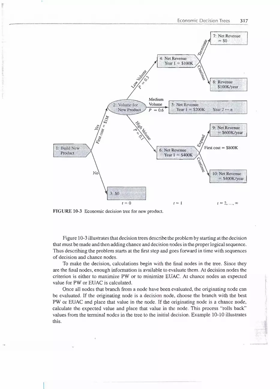
.
Economic Decision Trees 317
1: Build NewProduct
8: Revenue$100Klyear
7: Net Revenue="$0
4: Net RevenueYear!:;:: $100K
5: Net RevenlleYear 1 "".$200K Year 2 ... n
6: Net RevenueYear 1 == $400K
9: Net Revenue=. $600K/year
10: Net Revenue== $400K/year
t == 0
FIGURE 10-3 Economic decision tree for new product.
t == 1 t ==2, ..., ex>
Figure 10-3illustrates thatdecisiontrees describetheproblemby startingat the decisionthat mustbe made and thenaddingchance anddecisionnodesin theproper logical sequence.Thus describing the problem starts at the first step and goes forward in time with sequencesof decision and chance nodes.
To make the decision, calculations begin with the final nodes in the tree. Since theyare the final nodes, enough infonnation is availableto evaluate them. At decision nodes thecriterion is either to maximize PW or to minimize EUAC. At chance nodes an expectedvalue for PW or EUACis calculated.
Once all nodes that branch from a node have been evaluated,the originating node <;:anbe evaluated. If the originating node is a decision node, choose the branch with the bestPW or EUAC and place that value in the node. If the originating node is a chance node,calculate the expected value and place that value in the node. This process "rolls back'"values from the terminal nodes in the tree to the initial decision. Example 10-10illustratesthis.
If"IiI
".!_
.J;
--

318 UNCERTAINTY IN FUTURE EVENTS
What decision should be made on the new product summarized in Figure 1O-3?What is theexpected value of the product's PW? The firm uses an interest rate of 10% to evaluate projects.If the product is terminatedafter oneYear,the capital equipmenthas a salvagevalue of $550,000for use with other new products. If the equipment is used for 8 years, the salvage valut?is $0.
Evaluating decision trees is done by startingwith the end outcome nodes and the decisions thatlead to them. In this case the decisionsare whetherto terminateafter 1year if sales volumeis lowand whether to expand after 1 year if sales volumeis high.
The decision to terminate the product depends on which is more valuable, the equipment'ssalvagevalueof $550,000or the revenueof $100,000peryear for 7 more years.The worth (PW1)of the salvage value is $550,000. The worth (PW1)of the revenue stream at the end of Year 1shown in node 8 is:
PW1 for node 8 = 100,000(PjA, 10%,7)
- 100,000(4.868) = $486,800
Thus, terminatingthe product and using the equipmentfor other products is better. We enter thetwo "present worth" valuesat the end of Year1in nodes7 and 8. We make the arc-tonode 7 bold,and use a double hash mark to show that we're pruning the arc to node 8.
The decision to expand at node 6 could be based on whether the $800,000 first cost forexpansion can be justified based on increasingannualrevenues for 7 years by $200,000 per year.However,this is difficult to show on the tree. It is easier to calculate the "present worth" valuesat the end of Year 1 for each of the two choices.The worth (PW1)of node 9 (expand) is:
.~
PW1for node 9 - -800,000 + 600,000(P j A, 10%,7)
;::::; -800,000 + 600,000(4.868)
.$2,120,800
The value of node 10 (continuewithoutexpanding) is:
:PW1 for pode 10 . 400,000(Pj A, 10%,7)
.4OQ,0()O(4. 868)
--'=$1~947,200
This is $173,600less.thaI}tIleexpaJ1sioJ).node,sothee)(pansionshouldhappen if volumeis high,Figure 10=4suni1nanz~swjiat,w~iW.ff~~HiU"S~geofthepro~ess. '" ~ ~
__ - - ...". ~ II _.. .. ..
- - ----
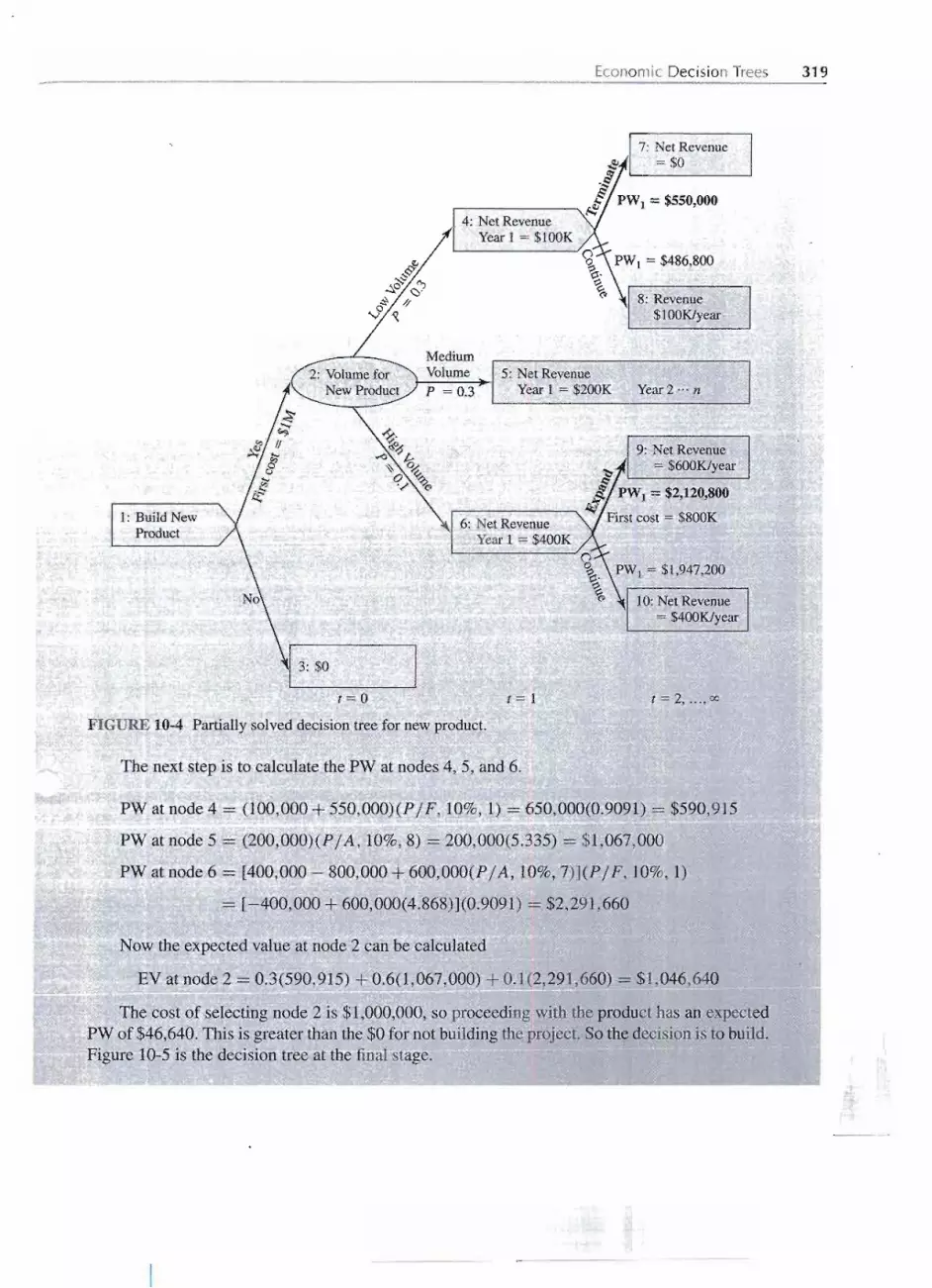
Economic Decision Trees 319
1: Build NewProduct
t= 0
FIGURE 10-4 Partially solved decision tree for new product.
The next step is to calculate the PW at nodes 4,5, and 6.
7: Net Revenue= $0
4: Net RevenueYear 1 = $looK
~\ PWI = $486,800~~ 8: Revenue
$ lOOK/year
5: Net RevenueYear 1 = $200K Year 2 ... n
9: Net Revenue
III =$600K/year~.PW 1 = $2,120,800~ First cost = $800K6: Net Revenue
Year1 = $400K
/g~~~ 10: Net Revenue
= $4ooK/year
t = 1 t = 2, ...,00
PW at node 4 = (100,000 + 550,000)(P / F, 10%,1) = 650,000(0.9091)- $590,915
PW at node 5 = (200,000)(P / A, 10%,8) - 20Q,000(5.335)= $1,067,000
PW at node 6 = [400,000 - 800,000 + 600,000(P / A, 10%,7)](P / F, 10%, 1)
= [-400,000 + 600,000(4.868)](0.9091) = $2,291,660
Now the expected value at node 2 can be calculated
EV at node 2 - 0.3(590,915) + p.6(1,067,002) + ~1(2,~~~l,~669~~$\,04~,640
The cost of selecting node 2 is $1,000,000, so proceeding witb.the prpduct.has an.expect~dPW of $46,640.This is greater than the $0 for not buildingthe project. So the decisionis to build.Figure 10-5 is the decision tree anhe finaJ.stage. ='
----
---

320 UNCERTAINTY IN FUTURE EVENTS
PW '"" $590,915
7: Net Revenue= $0
PW = $46,6401: Build New
Product
4: Net RevenueYear 1 '""$100K
8: Revenue$100Klyear
PW == $1,067,000
5: Net RevenueYear 1 ~ $200K Year 2 ...n
PW= $2,291,660
6: Net RevenueYear 1= $4QOK
9: Net Revenue
'1:17'11 ~ $600K/yearI::
#1 pW1 = $2,120,800fl:J First cost = $800K
(=0
FIGURE 10-5 Solved decision tree for new product.
(= 2, ...,00
I,:
I.II
J
II,
10: Net Revenue= $400K/year
Example 10-10 is representative of many problems in engineering economy. The maincriteria is maximizing PW or minimizing EUAC. However, as shown in Example 10-11,other criteria, such as risk, are used in addition to expected value.
i,
iIi .L
Consider the economic evaluationof collision and comprehensive(fire, theft, etc.) insurance fora car. This insurance is typically required by lenders, but once the car has been paid for, thisihsurance is not required. (Liabilityinsurance is'typically a legalrequirement.)
Figure 10-6 begins with a decision node with two alternativesfor the next year. Insurance
~il1 ~ost$800 per year with.a $500 d~~~ctibleif a loss occurs.The other option i&to self.-insure,whichmeans to go withoutbuying cQ;u.1s1onana comprebensivein&urance.Tl1enif alosroc~ut=r;= l' .
L - - ......- .. ...- - - _III!I _III__~~'
-----

Economic Decision Trees 321
$0
$300 «$500 deductible)
$500
$0
$300
$13,000
FIGURE 10-6 Decision tree for buying auto collision insurance.
the owner must replace the vehicle with money from savings or a loan, or do without a vehicleuntil the owner can afford to replace it.
Three accident severities are used to represent the range of possibilities: a 90% chance of noaccident, a 7% chance of a small accident (at$300, which is less than the deductible), and a 3%chance of totaling the $13,000 vehicle. Since our driving habits are likely to be the same with andwithout insurance, the accident probabilities are the Same for both chance nodes.
Even though this is a text on engineering economy, we have simplified the problem andignored the difference in timing of the cash flows. Insurance payments are made at the beginningof the covered period, and accident costs occur during the covered period. Since car insurance isusually paid semiannually, the results of the economic analysis are not changed significantly by thesimplification. We focus on the new concepts of expected value, economic decision trees, and risk.
What are the expected values for each alternative, and what decision is recommended?. . - - - '. '. - .
'SQhUI10N
The expected values are computed by using Equation 10-5.Ifinsured, the maximum cost equals~ thedeductible"'of $500.If selr-insure'O,thecostis thecosfof tileaccident.
EVaccident w/ins. = (0.9 X 0) + (0.07 X 300) + (0.03 X 500) = $36'="= ~ =: 1:1I=;; = =
EVaccident w/o ins. = (0.9 X 0) + (0.07X 300)+ (0.03X 13,000)= $411
. I
--
'.
- - -
322 UNCERTAINTY IN FUTURE EVENTS
Thus, buyinginsurance lowersthe expectedcost of an accidentby $375. Toevaluatewhetherwe should buy insurance,we must also accountfor the cost of the insurance.Thus, theseexpectedcosts are combined with the $0 for self-insuring (total $411) and the $800 for insuring (total')$836). Thus self-insuringhas an expefted value cos,tthat is $425 less per year;($836 - $411).This is not surprising, since the premiums collected must cover both.the costs of operating theinsurance company and the expected value of the payouts.
This is also an example ofexpectedv(llues alone not determining the decision. BuyingiIlsuranc,ehas an expectedcosttb,atis $425perye~ highet, but tb,atinsunll1ce}imitsthe maxiInutnloss to $500 rather thaI)$13,000.:rbe$425may be worth spendi,Ilgto avoidthatpsk.
RISK
Risk can be thought of as the chance of getting an outcomeother than the expectedvalue-with an emphasis on something negative. One common measure of risk is the probabilityof a loss (see Example 10-6).The other common measure is the standard deviation (a),which measures the dispersion of outcomes about the expected value. For example,manystudents have used the normal distribution in other classes. The normal distribution has68% of its probable outcomes within ::1:1stand~d deviationof the mean and 95% within::1:2standard deviations of the mean.
Mathematically, the standard deviation is defined as the square root of the variance.This term is definedas the weightedaverageof the squareddifferencebetweenthe outc.omesof the random variable X and its mean. Thus the larger the difference,between the meanand the values, the largerare the standard deviationand the variance.This is Equation 10-6:
Standard deviation (a) = V[EV(X - mean)2] (10-6)
Squaring the differences between individual outcomes roWthe EV ensures that positive. -.'
andnegativedeviationsreceivepositiveweights.Consequently,negativevaluesfor the stan-dard deviationare impossible,and they instantly indicatearithmeticmistakes.The standarddeviation equals.0 if only one outcome is possible. Otherwise, the standard deviation ispositive.
This is not the standard deviation formula built into most calculators, just as theweighted average is not the simple average built into most calculators. The calculatorformulas are for N equally likely data points from a randomlydrawn sample, so that eachprobability is 1/N. In economic analysis we will use a weighted average for the squareddeviations since the outcomes are not equally likely.
The second difference is that for calculations (by hand or the calculator), it is easierto use Equation 10-7, which is shown to be equivalent to Equation 10-6 in introductoryprobability and statistics texts.
Standard deviation (a) = V{EV(X2) - [EV(X)]2} (10-7)
- {Outcomei. x peA) + Outcome~ x PCB)+... - expected value2} (10-7')
---

.- .. - - - - - ---
Risk 323
This equation is the square root of the difference between the average of the squaresand the squareof the average.The standarddeviationis used insteadof the variancebecausethe standard deviation is measured in the same units as the expected value. The variance ismeasured in "squared dollars"-whatever they are.
The calculation of a standard deviationby itself is only a descriptivestatistic of limitedvalue. However,as shownin the next section on risk/return trade-offs,it is useful when thestandard deviation of each alternativeis calculated and these are compared. But first, someexamples of calculating the standard deviation.
Consider the economicevaluationof collision andcomprehensive(fire,theft, etc.) insurancefor anauto. One example wasdescribed in Figure 10-6.The probabilitiesand outcomes are summarizedin the calculation of the expected values, which was done using Equation 10-5.
EVaccidentw/ins.= (0.9 x 0) + (0.07 x 300) + (0.03 x 500) = $36
EVaccidentw/oins.= (0.9 x 0) + (0.07 x 300) + (0.03 x 13,000) = $411
Calculate the standard deviations for insuring and not insuring.
'SOLutiON:. - - -.. - --.
The first step is to calculate the EV(outcome2) for each.
EV~ident w/ins. = (0.9 X 02) + (0.07 x 3002)+ (0.03 x 5002) = $13,800
EV;ccident w/o ins. = (0.9 X 02) + (0.07 x 3002)+ (0.03 x 13,0002) = $5,076,300
Then the standard deviationscan be calculated.
O"w/ins."= -/(13,800 - 362) = JI2,504= $112
O"w/oins. = -/(5,076,300 -4112) = -/4,907,379 =$2215
As described in Example 10-11, the expected value cost of insuring is $836 (= $36 + $800)and the expected value cost of self-insuring is $411. Thus the expected cost of not insuring isabout half the cost of insuring.But the standard deviationof self-insuringis 20 times larger. It isclearlyr,iskier.
Which choice is preferred depends on how much risk yoti are comfortable with.As stated before, this is an example of expected values alone not determining the decision.
Buying insurance ,has an expected cost:::that ~is-$425=-peryear higher, but that "insurancelim-its the maximum loss to $500 rather than $13,000. The $425 may be wortb spendiJ:!gto avoidthat risk.
I:I
'"
:
f

324 UNCERTAINTY IN FUTURE EVENTS
Using the probability distribution for the PW from Example 10-6, calculate the PW's standarddeviation.
The following table adds a column for (PW) (probability) to calculate the EV(PW2).
Annual Life Joint PW xBenefit Probability (years) Probability Probability PW Probability$ 5,000 30% 6 66.7% 20.0% ~$ 3,224 -$ 645
8,000 60 666.7 40.0 9,842 3,93710,000 10 6 66.7 6.7 18,553 1,2375,000 30 9 33.3 10,0 3,795 380
8,000 60 9 33.3 20.0 21,072 4,2!410,000 10 9 33.3 3.3 32,590 1,086
EV $10,209
Standard deviation V{EV(X--:;;~ [EV(X)]2}
(J. '. J{l89,405,745~ [l0,209]2}'- y'85, 182,064 = $9229
PW2xProbability
$ 2,079,48038,j47,9~422,950,061
1,442,10088,797,40835,392,740
$189,409,745
For those with stronger backgrounds in probability than this chapter assumes, let usconsider how the standard deviation in Example 10-13depends on the assumptionof inde-pendence between the variables. While exceptions exist, a positive statistical dependencebetween variablesoften increases the PW's $tandarddeviation. Similarly,a negativestatis-tical dependencebetween variablesoften decreases the PW's standard deviation.
RISK VERSUS RETURN
A graph of risk versus return is one way to consider these items together. Figure 10-7 inExample 10-14illustrates the most common format. Risk measured by standard deviationis placed on the x axis, and return measuredby expected value is placed on the y axis. Thisis usually done with the internal rates of return of the alternativesor projects.
A large firmis discontinuingan older product, so some facilitiesare becoming availablefor otheruses. The followingtable sunmiarizeseighfnew projects that woulduse the facilities.Coriside~ngexpected return and risk, wbjch projects are good candidates? The .firmbelieves it can earn 4%on a risk-free investmentin govel11p1entsecurities (labeled as PJ;QjectF).: = ~ !!.~ ::: = == ::;=. == ~~, ~
t ~- - -- -- -
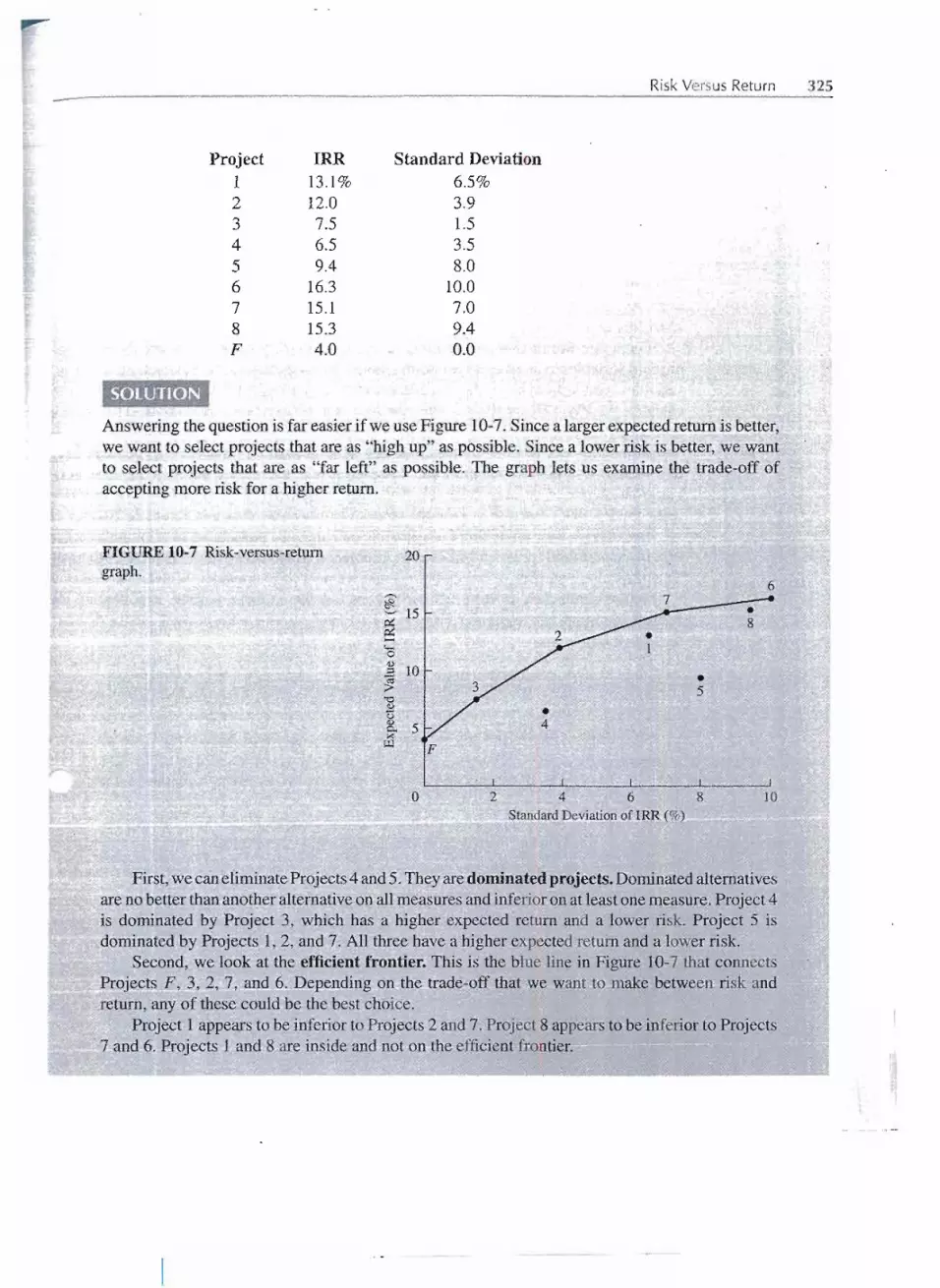
-
IRisk Versus Return 325
Project12345678F
SOLUTION
IRR13.1%12.07.56.59.4
16.315.115.34.0
Standard Deviation6.5%3.91.53.58.0
10.07.09.40.0
Answering the question is far easier if we use Figure 10-7.Since a largerexpectedreturn is better,we want to select projects that are as "high up" as possible. Since a lower risk is better, we.wantto select project~ that are as "far left" as possible. The graph lets us examine the trade-off ofaccepting more risk for a higher return.
FIGURE 10-7 Risk-versus-retumgraph.
20
6 .7 .
8
.5
5.,F
.4
o 246 8Standard Deviation of 1M (%)
10
First, we can eliminate Projects 4 and 5.They are dominated projects. Dominated alternativesare no better than another alternative on all measures and inferior on at least one measure. Project 4.is dominated by Project 3, which has a higher expected return and a lower risk. Project 5 isdominated by Projects 1, 2, and 7. All three have a higher expected return and a lower risk.
Second, we look at the efficient frontier. This is the blue line in Figure 10-7 that connectsProj~ctE,P' 3, 2~..7,and 6. I)epencijng, on the trade"of( that~we want to make betweell risk andreturn, any of these could be the best choice.
Project 1 appears to be inferior to Projects 2 and 7. Project 8 appears to be inferior to Projects::: 7"and6. Pmjects 1 and 8 are inside and not on the efficient frontier."== ;;:; ==z:=:= = ~
.,
- ... --
--~
-- -- - ------ ----

, -" -- - -. -
326 UNCERTAINTY IN FUTURE EVENTS
, There are models of risk and return that can allow us to choose between Projects F, 3, 2, 7,and 6; but thosemodels are beyond what.is coveredhere.
-
SIMULATION
Simulation is a more advancedapproach to consideringrisk in engineeringeconomy prob-lems. As such, the followingdiscussionfocusesonwhat it is. As the examplesshow,spread-sheet functions and add-in packages make simulation easier to use for economic analysis.
Economic simulation uses random samplingfrom the probability distributionsof oneor more variables to analyze an economicmodel for many iterations. For each iteration, allvariables with a probability distribution are randomly sampled. These values are used tocalculate the PW, IRR, or EUAC.Then the results of all iterations are combined to create aprobability distribution for the PW,IRR, or EUAC. .
Simulation can be done by hand, using a table of random numbers-if there are onlya few random variables and iterations. However,results are more reliable as the number ofiterations increases, so in practice this is usually computerized.This can be done in Excelusing the RANDO function to generate random numbers, as shownin Example 10-15.
Because we were analyzingeach possibleoutcome,the probabilitydistributionsearlierin this chapter (and in the end-of-chapterproblems) used two or three discrete outcomes.This limited the number of combinations that we needed to consider.Simulation makes iteasy to use continuous probability distributionslike the uniform, normal, exponential, lognormal,binomial, and triangular.Examples 10-15and 10-16use the normal and the discreteuniform distributions. .
ShipM4U is considering installing a new, more accurate scale, which will reduce the errorjncomputingpostagechargesandsave$250ayear.Thescale'susefullifeisbelievedtobeuniformlydistributedover 12, 13, 14,15,and 16years.The initialcostof the scale is estimatedtobe normallydistributed with a mean of $1500 and a standarddeviationof $150.
Use Excel to simulate 25 random samples of the problemand compute the rate of return foreach sample. Construct a graph of rate of return versus frequencyof occurrence.
SOLUTION
I.
t
This problem is simple enough to construct a table with each iteration's values of the life andthe first cost. From these values and the annual savings of $250, the IRR for eacb iteration canbe calculated using the RATE function. These are shown in Figure 10-8. The IRR values. aresummarized in a relative frequency diagram in Figure 10-9.
~.. ,'" - .--'. -«:;11 _ _. ""
(Note: Each time Excel recaJ,cul<Itesthe spreadsheet, different values for all tlie ranaoIIlnumbers are generated. Thus the results depend on the set of random numbers, and your resultswill be different if you create this spreadsheet.)
in ..c_ c: 'Ii = :r::::r:::I::~!: ~ I:!: == =
= .....
- -- - - --- --- ..---
-- -- -- ----

rSimulation 327
FIGURE 10-8 Excel spreadsheet forsimulation (N = 25).
Note for students who have had a course in probability and statistics: Creating the randomvalues for life and first cost is done as follows. Select a random number in [0, 1) using Excel'sRAND function:,This is tlteVal~eof the ~ug1Ulati,yedi~tributionfunctionfor .thevariable.Convertthis to the variable's value by using an inversefunction from Excel, or build the inversefunction.For the discreteuniform life the function is =.minlife +INT(tange* RANDO).For the normally
"distributed first C()st the,functions is<-NORMINY(RANDO, mean, standard deviation). ~
-- ------ - - -.. - - .. - . - - - -- ---
- ------
A B C D
1 250 Annual Savings2 Life First Cost
3 Min 12 1500 Mean
4 Max 16 150 Std dev
5
6 Iteration IRR
7 1 12 1277 16.4%
8 2 15 1546 13.9%
9 3 12 1523 12.4%
10 4 16 1628 13.3%
11 5 14 1401 15.5%
12 6I
12 1341 15.2%
13 7 12 1683 10.2%
14 8 14 1193 19.2%
15 9 15 1728 11.7%
16 10 12 1500 12.7%
17 11 16.
1415 16.0%
18 12 12 1610 11.2%
19 13 15 1434 15.4%
20 14 12 1335 15.4%
21 15 14 1468 14.5%
22 16 13 1469 13.9%
23 17 14 1409 15.3%
24 18 15 1484 14.7%
25 19 14 1594 12.8%
26 20 15 1342 16.8%
27 21 14 1309 17.0%
28 22 12 1541 12.1%
29 23 16 1564 14.0%
30 24 13 1590 12.2%
31 25 . 16 1311 17.7%
32
33 Mean 14 1468 14.4%
34 Std dev 2 135 2.2%

328 UNCERTAINTY IN FUTURE EVENTS
o8
FJGURE .10-9 Graph of 1M values.
Stand-alone simulation programs and commercialspreadsheet add-in packages suchas @Riskand Crystal Ball provide probabilitydistributionfunctions to use for each inputvariable. In Example 10-16 the functions RiskUniformand RiskNormal are used. Thepackages also collect values for the output variables,such as the IRR for Example 10-16.In other problems the PW or EUAC could be collected. These values form a probabilitydistribution for the PW, IRR, or EUAC.Fromthis distributionthe simulationpackage cancalculate the expected return, P(1oss),and thestandarddeviation of the return.
Example 10-16 uses @Risk to simulate 1000 iterations of PW for the data in Ex-ample 10-15. A simulation package makes it easy to do more iterations. More importantstill, since it is much easier to use differentprobabilitydistributions and parameters, moreaccurate models can be built. Because the modelsare easier to build, they are less likely tocontain errors.
Consider the scale described in Example 10-15. Generate 1000iterations and construct a frequencydistribution for the scale's rate of return.
The first IRR (cell A8) of 14.0t% tgat t~computed in Figure10-10is based on the average bYeand the average first cost. TheB~cop:d''1RR(cell 1\1.1)bfi.~.Ol%'is comptited by @Riskusing :;
the average of each distributjoJ).. Th.e cell content i§ the RATE fOfJ).1ulawith its l~is1<:UmfofJ).1and
."..f!I.
---
6
5
I
a
4;>.us:::Q)
6- 3
r.x..2

Simulation 329
FIGURE 10-10 Simulation spreadsheetfor Example 10-15 and 10-16.
RiskNonnal function, however spreadsheets with @Riskfunctionsdisplayby default the resultsof using average values.
The RATEfunction contains two @Riskfunctions: RiskUnifonn and RiskNonnal. The uni-fonn distributionhas the minimum and maximum valuesas parameters.The nonnal distributionhas the average and standard deviationas parameters.
The third IRR (cell A13) is the average for 1000 iterations. It will change each time the=simulationis done.=I'hegraph in Figure 10-10 withl 000'"iterations is much §mootIier""thanThegraph from Example 10-15,where 25 iterations were done.
"----
JI
I
. ~
~ I
I
I
I
i
="'iF
~
A B I c D E F1 -1500 averagefirst cost2 150 standarddeviationof first cost3 12 minimumvalueof life
4 16 maximumvalue of life5 250 annualbenefit
6 I7 IRR computedusing averages8 14.01% = RATE((A3+A4)j2,A5,Al)9 I10 IRR for each simulation iteration
11 14.01% = RA TE(RiskUniform(A3,A4),A5,RiskNorma1(Al,A2))
12 I
13 14.15% = average value of All (IRR) from 1000 iterations
14 2.17% = standard deviation of All (IRR) from 1000 iterations
15I
16 DistributionforIRR(cellAll)16
-17 -------18 14 -19 12 - -20 --- -
1O -21 a
8 -22
.0-
23 0 6 r- -------24 4 - -25 2
l,n,n.nIr-1I-
26 "n,0 -27 7 8.5 10 11.5 13 14.5 16 17.5 19 20.5 -28 IRR(%)

330 UNCERTAINTY IN FUTURE EVENTS
SUMMARY
Estimating the future is required for economic analysis, and there are several ways to dothis. Precise estimates will not ordinarily be exactly correct, but they are considered to bethe best single values to represent what we think will happen.
A simple way to representuncertaintyis through a range of estimates for each variable,such as optimistic,most likely,andpessimistic.The full range of prospectiveresults.maybeexaminedby using the optimisticvalues to solve the problem andthen using the pessimisticvalues. Solving the problem with the most likely values is a good single value estimate.However,the extremeswith all optimisticvalues or all pessimisticvaluesare less likely-itis more likely that a mix of optimistic, most likely,and pessimistic values will occur.
One approach uses weightedvalues instead of a range of estimates.One set of weightssuggestedis:
Estimate
OptimisticMost likelyPessimistic
Relative Weight141
The most commonly used approach for decision making relies on expected values.Here, known or estimated probabilities for future events are used as weights for the corre-sponding outcomes.
Expected value = OutcomeAx ProbabilityA+ OutcomeBx ProbabilityB+ .. .Expected value is the most useful and the most frequently used technique for estimatingaproject's attractiveness. .
However, risk as measured by standard deviation and the probability of a loss is alsQimportant in evaluating projects. Since projects with higher expected returns also frequentlyhave higher risk, evaluating the trade-off's between risk and return is useful in decisionmaking.
More complicatedproblems can be summarizedand analyzed by using decision trees, .which allow logical evaluationof problems with sequentialchance, decision, and outcomenodes.
Where the elements of an economic analysis are stated in terms of probability dis-tributions, a repetitive analysis of a random sample is often done. This simulation-basedapproachrelies on the premise that a random samplingof increasing size becomes a betterandbetter estimate of the possibleoutcomes.The largenumber of computationsmeans thatsimulationis usually computerized.
PROBLEMS
10-1 Telephone poles exemplify items that have varyinguseful lives. Telephone poles, once installed in alocation, remain in useful service until one of a varietyof events occur.
(a) Name three reasons why a telephone pole might
be removed from useful service at a particularlocation.
(b) You are to estimate the total useful life of tele-phone poles. If the pole is removedfrom an orig-inal location while it is still serviceable, it will

. ..rProblems 331
be installed elsewhere. Estimate the optimisticlife, most likely life, and pessimistic life for tele-phone poles. What percentage of all telephonepoles would you expect to have a total useful lifegreater than your estimated optimistic life?
10-2 The purchase of a used pickup for $9000 is being con-sidered. Records for other vehicles show that costs for
oil, tires, and repairs about equal the cost for fuel. Fuelcosts are $990 per year if the truck is driven 10,000miles. The salvage value after 5 years of use dropsabout $0.08 per mile. Find the equivalent uniformannual cost, if the interest rate is 8%. How muchdoes this change if the annual mileage is 15,000?5000?
10-3 A heat exchanger is being installed as part of a plantmodernization program. It costs $80,000, includinginstallation, and is expected to reduce the overall plantfuel cost by $20,000 per year. Estimates of the use-fullife of the heat exchanger range from an optimistic12years to a pessimistic 4 years. The most likely valueis 5 years. Using the range of estimates to computethe mean life, determine the estimated before-tax rateof return. Assume the heat exchanger has no salvagevalue at the end of its useful life.
10-4 For the data in Problem 10-2 assume that the 5000,10,000, and 15,000 mileage values are, respectively,pessimistic, most likely, and optimistic estimates. Usea weighted estimate to calculate the equivalent annualcost.
10-5 When a pair of dice are tossed, the results may beany whole number from 2 through 12. In the game ofcraps one can win by tossing either a 7 or an lion thefirst roll. What is the probability of doing this? (Hint:There are 36 ways that a pair of six-sided dice can betossed. What portion of them result in either a 7 or anII?) (Answer: 8/36)
10-6 Annual savings due to an energy efficiency projecthave a most likely value of $30,000. The high esti-mate of $40,000 has a probability of 0.2, and the lowestimate of $20,000 has a probability of 0.30. Whatis the expected value for the annual savings?(Answer: $29,000)
10-7 Over the last 10 years, the hurdle or discount rate forprojects from the firm's research and developmentdivision been 10% twice, 15% three times, and 20%the rest of the time. There is no recognizable pat-tern. Calculate the probability distribution and theexpected value for next year's discount rate.
10-8 The construction time for a bridge depends on weatherconditions. The project is expected to take 250 daysif the weather is dry and the temperature is hot. Ifthe weather is damp and cool, the project is expectedto take 350 days. Otherwise, it is expected to take300 days. Historical data suggest that the probabilityof cool, damp weather is 30% and that of dry, hotweather is 20%. Find the project's probability distri-bution and expected completion time.
10-9 You recently had an auto accident that was your fault.If you have another accident or receive a another mov-ing violation within the next 3 years, you will becomepart of the "assigned risk" pool, and you will pay anextra $600 per year for insurance. If the probabilityof an accident or moving violation is 20% per year,what is the probability distribution of your "extra"insurance payments over the next 4 years? Assumethat insurance is purchased annually and that viola-tions register at the end of the year-just in time toaffect next year's insurance premium.
10-10 Two instructors announced that they "grade on thecurve," that is, give a fixed percentage of each of thevarious letter grades to each of their classes. Theircurves are as follows:
GradeABCDF
Instructor A10%15451515
Instructor B15%15302020
If a random student came to you and said that hisobject was to enroll in the class in which he could ex-pect the higher grade point average, which instructorwould you recommend? (Answer: GPAB =. 1.95,Instructor A)
10-11 A man wants to determine whether or not to invest
$1000 in a friend's speculative venture. He will do soif he thinks he can get his money back in one year.He believes the probabilities of the various outcomesat the end of one year are as follows:
Result
$2000 (double his money)15001000500
o (lose everything)
Probability0.30.10.20.30.1
--.'
- - - --- --

332 .UNCERTAINTY IN FUTURE EVENTS -What would be his expected outcome if he invests the$1000? '
10-12 The MSU football team has 10 games scheduledfornext season. The business manager wishes to estimatehow much money the team can be expected to haveleft over after paying the season's expenses, includingany postseason "bowl game" expenses. From recordsfor the past season and estimates by informed people,the business manager has assembled the followingdata:
Based on the business manager's data, what is theexpected net income for the team next season?(Answer: $355,000)
10-13 In the New Jersey and Nevada gaming casinos, crapsis a popular gambling game. One of the many betsavailable is the "Hard-way 8." A $1 bet in this fash-ion will win the player $4 if in the game the pair ofdice come up 4 and 4 prior to one of the other ways oftotaling 8. For a $1 bet, what is the expected result?(Answer: 80jt)
10-14 If your interest rate is 8%, what is the expected valueof the present worth of the "extra" insurance paymentsin Problem 1O-9? (Answer: $528.7)
10-15 A decision has been made to perform certain re-pairs on the outlet works of a small dam. For a par-ticular 36-inch gate valve, there are three availablealternatives:
(a) Leave the valve as it is.(b) Repair the valve.(c) Replace the valve.
If the valve is left as it is, the probability of afailure of the valve seats, over the life of the project,is 60%; the probability of failure of the valve stem is50%; and of failure of the valve body is 40%.
If the valve is repaired, the probability of a fail-ure of the seats, over the life of the project, is 40%;of failure of the stem is 30%; and of failure of the
body is 20%. If the valve is replaced, the probabilityof a failure of the seats, over the life of the project, is30%; of failure of the stem is 20%; and offailure ofthe body is 10%.
The present worth of cost of future repairs andservice disruption of a failure of the seats is $10,000;the present worth of cost of a failure of the stem.is$20,000; the present worth of cost of a failure of thebody is $30,000. The cost of repairing the valve nowis $10,000; and of replacing it is $20,000. If the crite-rion is to minimize expected costs, which 'alternativeis best?
10-16 A man went to Atlantic City with $500 and placed100 bets of $5 each, one after another, on the samenumber on the roulette wheel. There are 38 numbers
on the wheel and the gaming casino pays 35 timesthe amount bet if the ball drops into the bettor's num-bered slot in the roulette wheel. In addition, the bettorreceives back the original $5 bet. Estimate how muchmoney the man is expected to win or lose in AtlanticCity.
10-17 A factory building is located in an area subject tooccasional flooding by a nearby river. You have beenbrought in as a consultant to determine whether flood-proofing of the building is economically justified. Thealternatives are as follows:
(a) Do nothing. Damage in a moderate flood is$10,000 and in a severe flood, $25,000.
(b) Alter the factory building at a cost of $15,000to withstand moderate flooding without damageand to withstand severe flooding with $10,000damages.
(c) Alter the factory building at a cost of $20,000 towithstand a severe flood without damage.
In any year the probability of flooding is as follows:0.70, no flooding of the river; 0.20, moderate flood-ing; and 0.10, severe flooding. If inter.est is 15%and a 15-year analysis period is used, what do yourecommend?
10-18 An industrial park is being planned for a tract of landnear the river. To prevent flood damage to the in-dustrial buildings that will be built on this low-lying
Prob-Situation ability Situation . Net Income
Regular season Regular seasonWin 3 games 0.10 Win 5 or $250,000
Win 4 games 0.15 fewer
Win 5 games 0.20 gamesWin 6 games 0.15 Win6to8 400,000
Win 7 games 0.15 gamesWin 8 games 0.10
Win 9 games 0.07 Win 9 or 10 600,000
Win 10 games 0.03 games
Postseason Postseason Additional
Bowl game 0.10 Bowl game income of$100,000

.- -- -, - - - - -_.-Problems 333
land, an earthen embankment can be constructed.
The height of tlIe embankment will be determined byan economic analysis of the costs and benefits. Thefollowing data have been gathered.
Embankment HeightAbove Roadway (m)
2.02.53.03.54.0
Initial Cost$100,000
165,000300,000400,000550,000
FloodLevel Above
Roadway (m)2.02.53.03.54.0
Average FrequencyThat Flood Level
Will Exceed
Height in Col. 1Once in 3 yearsOnce in 8 yearsOnce in 25 yearsOnce in 50 yearsOnce in 100 years
The embankment can be expected to last 50 yearsand will require no maintenance. Whenever the floodwater flows over the embankment, $300,000 of dam-age occurs. Should the embankment be built? ITso, towhich of the five heights above the roadway? A 12%rate of return is required.
10-19 Should the following project be undertaken if its lifeis 10 years and it has no salvage value? The firmuses an interest rate of 12% to evaluate engineeringprojects.
First Cost
$300,000400,000600,000
P
0.20.50.3
Net Revenue
$ 70,00090,000
100,000
P
0.30.50.2
(Answer: $45,900, yes)
10-20 A robot has just been installed at a cost of $81,000.It will have no salvage value at the end of its usefullife. Given the following estimates and probabilitiesfor the yearly savings and useful life, determine theexpected rate of return.
Savingsper year
$18,00020,00022,000
Useful
Life (years)1254
Probability0.20.70.1
Probability
1/62/31/6
10-21 Five years ago a dam was constructed to impoun~irrigation water and to provide flood protection forthe area below the dam. Last winter a 100-year floodcaused extensive damage both to the dam and to thesurrounding area. This was not surprising, since thedam was designed for a 50-year flood.
The cost to repair the dam now will be $250,000.Damage in the valley below amounts to $750,000. ITthe spillway is redesigned at a cost of $250,000 andthe dam is repaired for another $250,000, the dammay be expected to withstand a 100-year flood with-out sustaining damage. However, the storage capaCityof the dam will not be increased and the probabilityof damage to the surrounding area below the damwill be unchanged. A second dam can be constructedup the river from the existing dam for $1 million.The capacity of the second dam would be more thatadequate to provide the desired flood protection. Ifthe second dam is built, redesign of the existing damspillway will not be necessary, but the $250,000 ofrepairs must be done.
The development in the area below the dam isexpected to be complete in 10 years. A new 100-year flood in the meantime will cause a $1 millionloss. After 10 years the loss would be $2 million. Inaddition, there would be $250,000 of spillway dam-age if the spillway is not redesigned. A 50-yearflood is also likely to cause about $200,000 ofdamage, but the spillway would be adequate. Sim-ilarly, a 25-year flood would cause about $50,000 ofdamage.
There are three alternatives: (1) repair the exist-ing dam for $250,000 but make no other alterations,(2) repair the existing dam ($250,000) and redesignthe spillway to take a 100-year flood ($250,000), and(3) repair the existing dam ($250,000) and build thesecond dam ($1 million). Based on an expected an-nual cash flow analysis, and a 7% interest rate, whichalternative should be selected? Draw a decision tree
to clearly describe the problem.
10-22 A new product's chief uncertainty is its annual net
JI.. revenue. So far, $35,000 has been spent on devel-. opment, but an additional $30,000 is required finish
development. The firm's interest rate is10%.
- --

334 UNCERTAINTYIN FUTURE EVENTS -(a) What is the expected PW for deciding whether to
prQceed?(b) Find the P(loss) and the standard deviation for
proceeding.
10-23 (a) In Problem 10-22 how much is it worth to the. firm to terminate the product after 1 year if thenet revenues are negative?(b) How much does the ability to terminate early
change the P (loss) and the standard deviation?
10-24 Find the probability distribution and the expected PW
JI. to modify an assembly line. The first cost is $80,000,and its salvage value is $0. The firm's interest rateis 9%. The savings shown in the table depend onwhether the assembly line runs one, two, or threeshifts, and on whether the product is made for 3 or5 years.
10-25 In Problem 10-24, how much is it worth to the firm.- to be able to extend the product's life by 3 ye~~,.ata cost of $50,000, at the end of the product's Imtialuseful life?
10-26 Al took a midterm examination in physics and re-ceived a score of 65. The mean was 60 and the stan-dard deviation was 20. Bill received a score of 14in mathematics, where the exam mean was 12 andthe standard deviation was 4. Which student ranked
higher in his class? Explain.
10-27 The Graham Telephone Company may invest innew switching equipment. There are three possi-ble outcomes, having net present worth of $6570,$8590, and $9730. The probability of each outcomeis 0.3, 0.5, and 0.2, respectively. Calculate the ex-pected return and risk associated with this proposal.(Answer: Epw = $8212, Uf'W= $1158)
10-28 A new machine will cost $25,000. The machine isexpected to last 4 years and have no salvage value. Ifthe interest rate is 12%, determine the return and therisk associated with the purchase.
P
Annual savings
0.3$7000
0.4$8500
0.3$9500
10-29 What is your risk associated with Problem 10-14?
10-30 Measure the risk for Problem 10-19 using the P(loss),
JIL range of PW values, and standard deviation of thePWs. (Answer: Uf'W= $127,900)
10-31 (a) In Problem 10-24, describe the risk using theP(1oss) and standard deviation of the PWs. .
(b) How much do the answers change if the possiblelife extension in Problem 10-25 is allowed?
10-32 An engineer decided to make a careful analysis of thecost of fire insurance for his $200,000 home. From a
fire rating bureau he found the following risk of fireloss in any year.
OutcomeNo fire loss
$ 10,000 fire loss40,00Q fire loss
200,000 fire loss
Probability0.9860.0100.0030.001
(a) Compute his expected fire loss in any year.(b) He finds that the expected fire loss in any year is
less than the $550 annual cost of fire insurance.
In fact, an insurance agent "explains that this isalways true. Nevertheless, the engineer buys fireinsurance. Explain why this is or ISnot a logicaldecision.
10-33 A firm wants to select one new research and devel-
opment project. The following table summarizes sixpossibilities. Considering expected return and risk,which projects are good candidates? The firm believesit can earn 5% on a risk-free investment in govern-ment securities (labeled as Project F).
Project123456F
IRR15.8%12.010.412.114.218.55.0
Standard Deviation6.5%4.1,6.35.18.0
10.00.0
State
Bad OK Great
Probability 0.3 0.5 0.2Net revenue -$15,000 $15,000 $20,000Life, in years 5 5 10
Shifts! Savings! Useful Lifeday year Probability (years) Probability
1 $15,000 0.3 3 0.62 30,000 0.5 5 0.43 45,000 0.2

rI Problems
10-34 A firm is choosing a new product. The followingtable summaIjzes six new potential products. Con-sidering expected return and risk, which products aregood candidates? The firm believes it can earn 4%on a risk-free investment in government securities(labeled as Product F).
- - -
Product123456F
IRR10.4%9.86.0
12.112.213.84.0
StandardDeviation3.2%2.31.63.68.06.50.0
335
I
I.!
. Jl

.0_."'"
After Completing This Chapter...The student should be able to:· Describe depreciation, deterioration, and obsolescence.· Distinguishvarioustypes of depreciableproperty and differentiatebetweendepreciation
expensesand other business expenses. .· Use historical depreciation methods to calculate the annual depreciation charge and
book value over the asset's life.· Explain the differences between the historical depreciation methods and the modified .
accelerated cost recovery system (MACRS).· Use MACRS to calculate allowable annual depreciation charge and book value over theasset's life for various cost bases, placed in service combinations,property classes, andrecoveryperiods.· Fully account for capital gainsllosses, ordinary losses, and depreciation recapture dueto the disposal of a depreciated business asset.· Use the units of production and depletion depreciation methods as needed in engineeringeconomicanalysisproblems.· Use spreadsheetsto calculate depreciation.
QUESTIONS TO CONSIDER)
1. Whendeterminingtheir cashflow,ownersof baseballteams dedu~tstadiumdepreciation,which can amount to as much as $5 million per year. How would this affect theircalculations?
2. Even though Barry Bonds is in peak.health and hit a record 73 home runs in 2002,the IRS considers him a "wasting asset" and allows the owners of his baseball club todepreciate a large portion of his contract. Explain.
1
- - - -- - ---- - -

{ I
Depreciation
Is Baseball Going Broke?In 2001, major league baseball brought in record revenues totaling over $3.5 billion. Greatbusiness, you say? Not according to Bud Selig, baseball's commissioner.
In December of that year, Selig went before Congress to plead poverty,asserting that baseball had suffered a loss of over $200 million for the year.Many journalists (and even more fans) weren't buying it. A few months later,Forbes magazine published an article stating that baseball had in fact had anoperating profit (that is, earnings before interest, taxes, and depreciation) of$75 million for the year.
Selig angrily denounced the Forbes article as "pure fiction." In response,Forbes suggested that perhaps Selig was "afraid of being called before Congressand explaining his figures in more detail."
reL
I JJ'~.-o..:.:-"_
-"- --- --
- - --- --- --

338 DEPRECIATION
We have so far dealt with a variety of economic analysis problems and many techniquesfor their solution. In the process we have avoided income taxes, which are an imponantelement of many private-sectoreconomic analyses. Now,we can move to more realistic_and,unfonunately,morecomplex-situations. .
Ourgovernmenttaxes individualsandbusinessesto support its processes-lawmaking,domestic and foreign economic policymaking, even the making and issuing of money it-self. The omnipresenceof taxes requires that they be included in economicanalyses,whichmeans that we must understand something about the way taxes are imposed. For capitalequipment,depreciation is required to compute income taxes. Chapter 11examines depre-ciation, and Chapter 12 illustrates how depreciation is used in income tax computations.The goal is to support decision making on engineering projects, not to support final taxcalculations.
BASIC ASPECTS OF DEPRECIATION
Theworddepreciation is definedas a "decreasein value."This is notan entirelysatisfactorydefinition,for value has several meanings. In the context of economic analysis, value mayrefer either to market value-that is, the monetary valueothers place on property--or valueto the owner. For example, an assembly line is far more valuable to the manufacturingfirm that it was designed for, than it is to a used equipment market. Thus, we now havetwo definitions of depreciation: a decrease in value to the market or a decrease to theowner. .
Deterioration and ObsolescenceA machine may depreciate because it is deteriorating or wearing out and no longer per-formingits function as well as when it was new.Manykinds of machineryrequire increasedmaintenanceas they age, reflectinga slowbut continuingfailureof individualparts. In othertypes of equipment, the quality of output may decline owing to wear on components andresultingpoorer mating of parts. Anyonewho hasworked to maintain artauto has observeddeterioration due to failure of individual parts (such as fan belts, mufflers, and batteries)and the wear on components (such as bearings,piston rings, and alternatorbrushes).
Depreciationis also caused by obsolescence. A mach~neis described as obsoletewhenit is no longer needed or usefuLA machine that is in excellent working condition may stillbe obsolete.In the 1970s,mechanicalbusinesscalculatorswith hundredsof gears and leversbecame obsolete. The advanceof integrated circuits resulted in a completely differentandfar superior approach to calculator design. Thus, mechanical calculators rapidly declinedor depreciatedin value.
If your auto depreciated in the last year, that means it has declined in market value. Ithas less value to potential buyers. On the other hand, a manager who indicates {;hata pieceof machineryhas depreciatedmay be describinga machine that has deterioratedbecauseofuse and/orbecause it has become obsoletecomparedwith newermachinery.Both situationsindicate a decline in value to the owner.
The accountingprofession definesdepreciationin yet anotherway.Although in every-day conversationwe are likely to use "depreciation" to mean a decline in market value or
-

.....
Basic Aspects of Depreciation 339
value to the owner, accountants define depreciation as allocating an asset's cost over itsuseful or depreciable life. Thus, we now have three distinct definitionsof depreciation:
1. Decline in market value of an asset.2. Decline in value of an asset to its owner.3. Systematicallocation of an asset's cost over its depreciablelife.
Depreciation and ExpensesIt is this third (accountant's) definition that is used to compute depreciation for businessassets. Businesscosts are generallyeitherexpensed or depreciated. Expensed items, suchas labor, utilities, materials, and insurance, are part of regular business operations and are"consumed" overshortperiods of time (sometimesrecurring).These costs do not lose valuegraduallyover time. For tax purposes theyare subtractedfrom businessrevenueswhen theyoccur. Expensed costs reduce income taxes because businesses are able to write off ~eirfull amount when they occur.
In contrast, business costs due to depreciated assets are not fully written off whenthey occur. A depreciated asset does lose value gradually and must be written off overan extended period. For instance, consider a plastic injection-molding machine used toproduce the beverage cups found at sporting events. The plastic pellets melted into thecup shape lose their value as raw material directly after manufacturing.The raw materialcost for production material (plastic pellets) is written off, or expensed, immediately. Onthe other hand, the plastic injection mold machine itself will lose value over time, andthus its cost (purchase price and installation expenses) are written off (or depreciated)over a period of years. The number of years over which the machine is depreciated iscalled its depreciable life or recovery period, which is often different from the asset'suseful or most economic life. Depreciable life is determined by the depreciation methodused to spread out the cost-depreciated assets of many types operate well beyond theirdepreciable life.
Depreciation is a noncash cost that requires no exchange of dollars. Companies donotwritea checktosomeonetopay theirdepreciationexpenses.Rather,thesearebusiness.
expenses that are allowed by the government to offset the loss in value of business assets.Remember, the company has already paid for assets up front; depreciationis simply a wayto claim these "businessexpenses" over time. Depreciation is important to the engineeringeconomiston an after-taxbasisbecause, eventhoughit is a noncashcost, it does change thecash flows due to taxes. Depreciation deductions reduce the taxable income of husine"ssesand thus reduce the amount of taxes paid.
In general business assets can be depreciated only if they meet the following basicrequirements:
1. The property must be used for business purposes to produce income.2. The property must have a useful life that can be determined, and this life must be
longer than one year. II3. Thepropertymustbe an asset thatdecays,getsused up,wearsout,becomesobsolete,
or loses value to the owner from natural causes.
- -- -r -

'-'. ..........
340 DEPRECIATION
Consider the costs that areincurred by a local pizza business.Identifyeach cost as eitherexpensedor depreciated and describe why.
· Cost for pizza dough and toppings· Costtopaywagesforjanitor· Cost of a new baking oven· Cost of new deliveryvan· Cost of furnishings in dining room· Utilitycostsfor sodarefrigerator
..SOLUTION.
Cost Item
Pizza dough and toppingsNew delivery vanWages for janitorFurnishings in dining roomNew baking ovenUtilities for soda refrigerator
Type of CostExpensedDepreciatedExpensedDepreciatedDepreciatedExpensed
WhyLife < t year; lose value immediatelyMeets 3 requirements for depreciation .Life < 1 year; lose value immediatelyMeet 3 requirements for depreciationMeets 3 requirements for depreciationLife < 1 year; lose value immediately
_ ~.."~~.r.. - J
Types of PropertyThe rules for depreciation are linked to the classification of business property as eithertangible or intangible. Tangibleproperty is further classified as either real or personal.
Tangible property can be seen, touched, and felt.
Real property includes land, buildings, and all things growing on, built upon,constructed on, or attached to the land.Personal property includes equipment, furnishings, vehicles, office machinery,and anything that is tangible excluding assets definedas realproperty.
Intangible property is all property that has value to the owned but cannot be directlyseen or touched. Examples include patents, copyrights, trademarks, trade names, andfranchises.
Many different types of property that wear out, decay, or lose valuecan be depreciatedas business assets. This wide range includescopy machines, helicopters,buildings, interiorfurnishings, production equipment, and computer networks. Almost all tangible propertycan be depreciated.
One important and notable exception is land, which is never depreciated..Landdoesnot wear out, lose value, or have a determinable useful life and thus does not qualify as adepreciableproperty.Consider the aspect of loss in value. Rather than decreasing in value,most land becomes more valuable as time passes. In addition to the land itself, expensesfor clearing, grading, preparing, planting, and landscaping are not generally depreciatedbecause they have no fixed useful life. Other tangible property that cannot be depreciatetincludes factory inventory, containers considered as inventory, equipment used to bui!.:
-- - ---- - ---

--- ---
rBasic Aspects of Depreciation 341
capital improvements, and leased property. The leased property exception highlights thefact that only the owner of property may claim depreciation expenses.
Tangible properties used in both business and personal activities, such as a vehicleused in a consulting engineering firm that is also used to take one's kids to school, can bedepreciated.However,in suchcases onecan take depreciationdeductionsonlyin proportionto the use for businesspurposes. Accurate records indicating the portion of use for businessand personal activities are required.
Depreciation Calculation FundamentalsTounderstandthe complexitiesof depreciation,the first step is to examine the fundamentalsof depreciation calculations. Figure 11-1 illustrates the general depreciation problem ofallocating the total depreciation charges over the asset's life. The vertical axis is labeledbook value, and the curve of asset cost or basis minus depreciationcharges made starts atthe first cost and declines to the salvagevalue,
Book value = Asset cost - Depreciation charges made to date
Looked at another way,book value is the asset's remaining unallocated cost.In Figure 11-1,book valuegoes from a value of B at time zero in the recoveryperiod to
a value of S at the end of Year5. Thus, book value is a dynamic variable that changes overan asset's recoveryperiod. The equationused to calculate an asset's book valueovertime is:
t
BV, = Cost basis - L djj=l
(11-1)
where B \l, = book value of the depreciated asset at the end of time tCost basis = B = dollar amount that is being depreciated; this includes the asset's
purchase price as well as any other costs necessary to make the asset"ready for use"
t .
L dj = sum of depreciation deductions taken from time 0 to time t, where djj=l is the depreciation deduction in Year j
FIGURE 11-1 General
depreciation.Cost
B
~ T" TotalDepreciation,
" Charges, , , ," CurveValuesDependon
", DepreciationMethod, , , , , , ,'.........
S~
I
SalvageValue
o
I1 234
UsefulLife (years)
5
1
- - - - --

- --.. . -._-
342 DEPRECIATION
rEquation 11-1 shows that year-to-year depreciation charges reduce an asset's book
value over its life. The following section describes methods that are or have been allowedunder federal tax law for quantifying these yearly depreciation deductions.
HISTORICAL DEPRECIATION METHODS
Allowing businesses to deduct the cost for capital expenditures over time (that i$, to de-preciate business assets) has long been part of the tax code. However, over time severalversions of various depreciation methods have been used to calculate these deductions.Ingeneral, accounting depreciation methods can be categorizedas follows.
Pre-1981 historical methods: These methods include the straight-line, sum-oj-the-years' -digits, and declining balance methods. Each method required estimates.ofan asset's useful life and salvagevalue.Firms could elect to use anyof these meth-ods for assets, and thus there was little uniformity in how depreciation expenseswere reported.
1981-1986 method: With the EconomicRecoveryTaxAct (ERTA)of 1981,Congresscreated the accelerated cost recovery system (ACRS). The ACRS method hadthree key features: (1) property class lives were created and all depreciated assetsassigned to one particular category, (2) the need to estimate salvage values waseliminated because all assets were fully depreciated over their recovery period,and (3) shorterrecoveryperiods were used to calculate annual depreciation,whichaccelerated the write-off of capital costs more quickly than did the historicalmethods-thus the name.
1986 to present: The modified accelerated cost recovery system (MACRS)has beenin effect since the Tax Reform Act of 1986 (TRA-86). The MACRS method issimilar to the ACRS system except that (1) the number of property classes wasexpanded and (2) the annual depreciationpercentages were modified to include ahalf-year conventionfor the first and final years.
In this chapter, our primary focus is to describe the MACRS depreciation method.However,it is useful to first describe three historical depreciationmethods. These methodsare used in some countries, and MACRSis based on two of them.
Straight-Line DepreciationThe simplest and best known depreciationmethod is straight-line depreciation.To calcu-late the constant annual depreciationcharge, the total'amount to be depreciated, B - S,is divided by the depreciable life, in years, N:1
B-SAnnual depreciation charge = dt = - N
(11-2)
1N is used for the depreciation period because it may be shorter than n, the horizon.
-- - ----

Historical Depreciation Methods 343
I:"~.:~l.\~\
'~- ~.~
Consider the following:
Cost of the asset, BDepreciable life, in years, NSalvage value, S
$9005
$70
Compute the straight-line depreciation schedule.
B - S 900 - 70Annual depreciation charge = dt = - = _ = $166N
This situation is illustrated in Figure 11-2.Notice the constant $166 dt each year for 5 years,and that the asset has been depreciated down to a book value of $70, which was the estimatedsalvage value.
FIGURE 11-2 Straight-linedepreciation.
. 166
Straight-Line AnnualDepreciation Charge
J
166
..........
-
-~!1,..
'SI I I 1
1 2 3 4 5
Time,DepreciableLife = N (years)
Depreciation Sum of Depreciation Book Value atYear, for Year t, Charges Up to Year t, the End of Year t,
t t
t dt Ldj BVt=B- Ldjj=l j=l
1 $166 $166 900 - 166 = 7342 166 332 900 - 332 = 5683 166 498 900 - 498 = 4024 166 664 900 - 664 = 2365 166 830 900 - 830 = 70 = S
_R$900
734
u 568::s
40200j:CI
236
70
0

344 DEPRECIATION
The straight-line (SL) method is often used for intangible property. Veronica's finnbought a patent in April that was not acquired as part of acquiring a business. She paid$6800 for this patent and must use the straight-line method to depreciate it over 17 yearswith no salvagevalue. The annual depreciation is $400 (=$6800/17). Since the patent Waspurchased in April, the deduction must be prorated over the 9 months of ownership. Thisyear the deduction is $300 (=$400 x 9/12), and then next year she can begin taking thefull $400 per year.
Sum-of-Years'-Digits DepreciationAnother method for allocating an asset's cost minus salvagevalue over its depreciable lifeis called sum-of-years'-digits (SOYD) depreciation. This method results in larger-than-straight-line depreciation charges during an asset's early years and smaller charges as theasset nears the endof its depreciablelife. Eachyear, thedepreciationchargeequals a fractionof the total amount to be depreciated (B - S). The denominatorof the fraction is the sumofthe years' digits. For example, if the depreciable life is 5 years, 1+ 2 + 3 + 4 + 5 = 15=SOYD. Then 5/15,4/15,3/15,2/15, and 1/15 are the fractions from Year 1 to Year 5.Each year the depreciation charge shrinks by 1/15 of B - S. Because this change is thesame every year, SOYD depreciation can be modeled as an arithmetic gradient, G. Theequations can also be written as:
(
Sum-of-years' -digits
)depreciation charge for =any year
(Remaining depreciable life)at beginning of year (Totalamount depreciated)
(Sum of years' digits )for total depreciable life
_ N - t + 1(B _ S)dt - ~~~~ (11-3)
where dt = depreciationcharge in any year tN =number of years in depreciable life
SOYD =sum of years' digits, calculated as N(N + 1)/2 = SOYDB = cost of the asset made ready for useS =estimated salvage value after depreciable life
Compute the SOYDdepreciation schedulefor the situation in Example 11.2.
Cost of the asset, BDepreciable life, in years, NSalvage value, S
$9005
$70
SOlUTIQ,~;
..--- - - -- - -
's 5OYD _ ~ >&6~=15
- - - -

Historical Depreciation Methods 345
Thus,
dl = 5 - 1 + 1(900 _ 70) = 27715
5-2+1d2 = (900 - 70) = 22115
d3 = 5 - 3 + 1(900 _ 70) = 166. 15
5-4+1d4= (900-70) = 11115
5-5+1ds= . _ (900- 70) = 55
These data are plotted in Figure 11-3.
FIGURE 11-3 Sum~of-years' -digitsdepreciation.
$900 .B
SOYD DepreciationCharges
277
= = :=
- ~.,..,-""--- --- ~ '. -- ..,.~ .--~ -
.
I1t
IJ
SI I I I I
1 234 5
Time,DepreciableLife = N (years)
- -- --
Depreciation Sum of Depreciation Book ValueYear, for Year t, Charges Up to Year t, at End of Year t,
t t
t dt "Ldj BVt=B-"Ldjj=l j=l
1 $277 $277 900 - 277 - 6232 221 498 900 - 498 = 4023 166 664 900 - 664 = 2364 111 775 900 - 775 = 1255 55 830 900 - 830 = 70 = S
6230,)::I«i>
40200
j:Q
236
L12570
0

- - --~-- - -- ~.- '" - ~- -
346 DEPRECIATION
Declining Balance DepreciationDeclining balance depreciation applies a constantdepreciation rate to the property's de-clining book value.Tworates were commonlyusedbefore the 1981and 1986tax revisions,and they areused to computeMACRSdepreciationpercentages.These are 150and200%ofthe straight-linerate. Since200% is twice the straight-linerate, it is calleddouble decliningbalance, or DDB; the general equation is
2Double declining balance dt = -(Book valuet_I)N (11-4a)
Since book value equals cost minus depreciationcharges to date,
2 ..hDDB dt = -(Cost - DeprecIationc arges to date)N
or
(ll-4b)
Compute the DDB depreciation schedulefor the situationsin Examples 11-2 and 11-3.
Cost of the asset, BDepreciable life, in years, NSalvagevalue, S
$9005
$70
SOLUTION
Year,Depreciation for Year tUsing Equation 11-4a,
t dt
Sum of DepreciationCharges Up to Year t,
t
Ldjj=I
$360576706784830
=
Book Valueat End of Year t,
t
BVt=B- Ldjj=I
900 - 360 = 540900 - 576 - 324900- 706 - 194900 -784= 116
::i: Ii == 'iiiiiii'
900 - 830 - 70 - S
12345
(2/5)900= 360(2/5)540 = 216(2/5)324 = 130
~7/5l194= 78(2/5)116= 46
-
~Fjgure 11-;1,illl!strates tl;1p~itufltiO!h-....... - ---- ---
i '-
--- - - -- -- - -

Modified Accelerated Cost Recovery System (MACRS) 347
FIGURE 1\-4 Decliningbalancedepreciation.
$900 .B
Declining BalanceDepreciation Charges
The final salvagevalue of $70 for Examples 11-2, 11-3,and 11-4was chosento matchthe ending value for the double-decliningbalance method. This does not normallyhappen.If the final salvage value of Example 11-4 had not been $70, the double declining balancemethodwouldhavehad to be modified.One modificationstopsfurtherdepreciationonce thebook value comes to equal the salvage value-this prevents taking too much depreciation.The other modificationwould switch from decliningbalance depreciationto straightline-this ensures taking enough depreciation.
These modifications are not detailed here because (1) MACRS has been the legallyappropriate system since 1986 and (2) as will be shown, MACRS incorporates the shiftfrom declining balance to straight-line depreciation.
MODIFIED ACCELERATEDCOST RECOVERYSYSTEM (MACRS)
The modifiedacceleratedcost recovery system (MACRS)depreciation method, introducedby the TaxReform Act of 1986,has been continued with the TaxpayerRelief Act of 1997.Three major advantages of MACRS are that (1) the "property class lives" are less than the"actual useful lives," (2) salvage values are assumed to be zero, and (3) tables of annualpercentages simplify computations.
The definition of the MACRS classes of depreciable property is based on work bythe U.S. Treasury Department. In 1971 the Treasury published guidelines for about 100broad asset classes. For each class there was a lower limit, a midpoint, and an upper limitof useful life, called the asset depreciation range (ADR). The ADR midpoint lives weresomewhat shorter than the actual average useful lives.These guidelines have been incorpo-rated into MACRS so that the property class lives are again shorter than the ADR midpointlives.
Use of MACRS focuses on the general depreciation system (GDS), which is basedon declining balance with switch to straight-line depreciation. The alternative depre-ciation system (ADS) provides for a longer period of recovery and uses straight-line
360
I r540
Q)::sC;>
3340j:Q
194
116
70,S
I I I I I
0 1 2 3 4 5
Time, Depreciable Life = N (years)

- .- -- -."-"."...
348 DEPRECIATION -depreciation.Thusit is muchlesseconomicallyattractive.Underlaw,ADSmustbe usedfor (1) any tangible property used primarily outside the United States, (2) any propertythatis tax exempt or financed by tax-exempt bonds, and (3) farming property placed in ser-vice when uniform capitalization rules are not applied. The ADS may also be electedfor property that can be depreciated using the GDS system. However, once ADS hasbeen elected for an asset, it is not possible to switch back to the GDS system. Becausethe ADS makes the depreciation deductions less valuable, unless ADS is specificallymentioned, subsequent discussion assumes the GDS system when reference is made toMACRS.
Once a property has been determined to be eligible for depreciation,the next step is tocalculate its depreciation deductions over its life. The following information is requiredtocalculate these deductions:
·The cost basis of the property.·The property class and recoveryperiod of the asset.·The asset's placed-in-service date.
Cost Basis and Placed-in-Service Date
The cost basis, B, is the cost to obtain and place the asset in service fit for use. However,for real property the basis may also include certain fees and charges that the buyer pays aspart of the purchase. Examples of such fees include legal and recording fees, abstract fees,surveycharges, transfer taxes, title insurance, and amountsthat the sellerowes that youpay(back taxes, interest, sales commissions, etc.).
Depreciationforabusinessassetbeginswhenthe asset isplaced inservicefor abusinesspurpose. If an asset is purchased and used in a personal context, depreciation may not betaken. If that asset is later used in business for income-producingactivity,depreciationmaybegin with the change in usage.
Property Class and Recovery PeriodEach depreciated asset is placed in a MACRS property class, which defines the recoveryperiod and the depreciation percentage for each year. Historically the IRS.assigned eachtype of depreciable asset a class life or an asset depreciation range. With MACRS, assetclass liveshave been pooled together in theproperty classes.Table 11-1lists the class livesand GDS and ADS property classes for severalexample depreciable assets. Table 11-2liststhe MACRS GDS property classes.
The MACRS GDS property classes are described in more detail in Table 11-2.Theproper MACRS property class.can be found several different ways. In the list below, thefirst approach that works should be used.
1. Property class given in problem.2. Asset is named in Table 11-2.3. IRS tables or Table 11-1.4. Class life.5. Seven-yearproperty for "all other property not assigned to another class."
--- -

Once the MACRS property class is known, as well as the placed-in-service date andcost basis, the year-to-yeardepreciation deductions can be calculated for GDS assets overtheir depreciable life using
dt = B x rt (11-5)
where dt = depreciationdeduction in year tB = cost basis being depreciatedrt = appropriateMACRS percentage rate
Percentage Tables ~
The IRS has prepared tables to assist in calculating depreciation charges when MACRS I
~
i
GDS depreciation is used. Table 11-3 gives the yearly depreciation percentages (rt) that fife :
used for the sixpersonal property classes (3-, 5-, 7-, 10-, 15-,and 20-year property classes), :
and Table 11-4givesthe percentages for nonresidentialreal property.Notice that the values I~
are given in percentages-thus, for example, the value of 33.33% (given in Table 11-3for J
Year 1 for a 3-year MACRS GDS property) is 0.3333.
-- ~
r
Modified Accelerated Cost Recovery System (MACRS) 349
TABLE 11-1 Example Class Lives and MACRS Property Classes
MACRSProperty
IRSAsset Class Life(years)Class (years)
Class Asset Description ADR GDS ADS
00.11 Office furniture, fixtures, and equipment 10 7 1000.12 Information systems: computers/peripheral 6 5 600.22 Automobiles, taxis 3 5 600.241 Light general-purpose trucks 4 5 600.25 Railroad cars and locomotives 15 7 1500.40 Industrial steam and electric distribution 22 I 15 2201.11 Cotton gin assets 10 7 1001.21 Cattle, breeding or dairy 7 5 713.00 Offshore drilling assets 7.5 5 7.513.30 Petroleum refining assets 16 10 1615.00 Construction assets 6 5 620.10 Manufacture of grain and grain mill products 17 10 1720.20 Manufacture of yarn, thread, and woven fabric 11 7 1124.10 Cutting of timber 6 5 I 632.20 Manufacture of cement 20 15 2020.1 Manufacture of motor vehicles 12 7 1248.10 Telephone distribution plant 24 15 24
I I
48.2 Radio and television broadcasting equipment 6 5 649.12 Electric utility nuclear production plant 20 15 2049.13 Electric utility steam production plant 28 120 2849.23 Natural gas production plant 14 7 14I50.00 Municipal wastewater treatment plant 24 15 2480.00 Theme and amusement park assets 12.5 7 12.5

- -. -._-
350 DEPRECIATION -TABLE11-2 MACRSCDS Property Classes
Property Class Personal Property (all property except real estate)
3-year property Special handling devices for food and beverage manufactureSpecial tools for the manufacture of finished plastic products, fabricated metal
products, and motor vehiclesProperty with ADR class life of 4 years or less
5-year property Automobiles* and trucksAircraft (of non-air-transport companies)Equipment used in research and experimentationComputersPetroleum drilling equipmentProperty with ADR class life of more than 4 years and less than 10 years
7-year property All other property not assigned to another classOffice furniture, fixtures, and equipmentProperty with ADR class life of 10 years or more and less than 16 ye3!s
10-year property Assets used in petroleum refining and certain food productsVessels and water transportation equipmentProperty with ADR class life of 16 years or more and less than 20 years
IS-year property Telephone distribution plantsMunicipal sewage treatment plantsProperty with ADR class life of 20 years or more and less than 25 years
20-yearproperty Municipal sewersProperty with ADR class life of 25 years or more
Property Class Real Property (real estate)
27.5 years Residential rental property (does not include hotels and motels)
39 years Nonresidential real property
*The depreciation deduction for automobiles is limited to $7660 (maximum) the first tax year, $4900the second year, $2950 the third year, and $1775 per year in subsequent years.
Source: U.S. Department of the Treasury, Internal Revenue Service Publication 946, How to Depre-ciate Property. Washington, DC: U.S. Government Printing Office. .
Notice in Table 11-3 that the depreciation percentages continue for one year beyondthe property class life. For example, a MACRS lO-year property has an rt value of 3.28% inYear 11. This is due to the half-year convention that also halves the percentage for the firstyear. The half-year convention assumes that all assets are placed in service at the midpointof the first year. .
Another characteristic of the MACRS percentage tables is that the rt values in anycolumn sum to 100%. This means that assets depreciated using MACRS are fully depre-ciated at the end of the recovery period. This assumes a salvage value of zero. This is
--- --

Modified Accelerated Cost Recovery System (MACRS) 351
TABLE11-3 MACRS Depreciation for Personal Property: Half-Year Convention
Computation method· The 3-, 5-, 7-, and 1O-year classes use 200% and the 15- and 20-year classes use 150% decliningbalance depreciation.· All classes convert to straight-line depreciation in the optimal year, shown with asterisk (*).
· A half-year of depreciation is allowed in the first and last recovery years.· If more than 40% of the year's MACRS property is placed in service in the last 3 months, then amid quarter convention must be used with depreciation tables that are not shown here.
a departure from the pre-1981 historical methods, where an estimated salvage value wasconsidered.
Where MACRSPercentage Rates (rt) Come FromThis section describes the connection between historical depreciation methods and theMACRS percentages that are shown in Table 11-3. Before ACRS and MACRS, the mostcommon depreciation method was declining balance with a switch to straight line. Thatcombined method is used for MACRSwith three further assumptions.
--- --------- -- - - - --
ApplicablePercentagefor PropertyClass
Recovery 3-Year 5-Year 7-Year 10-Year 15-Year 20-YearYear Property Property Property Property Property Property
1 33.33 20.00 14.29 10.00 5.00 3.7502 44.45 32.00 24.49 18.00 9.50 7.2193 14.81* 19.20 17.49 14.40 8.55 6.677
4 7.41 11.52* 12.49 11.52 7.70 6.1775 11.52 8.93* 9.22 6.93 5.7136 5.76 8.92 7.37 6.23 5.285
7 8.93 6.55* 5.90* 4.8888 4.46 6.55 5.90 4.5229 6.56 5.91 4.462*
10 6.55 5.90 4.46111 3.28 5.91 4.46212 5.90 4.461
13 5.91 4.46214 5.90 4.46115 5.91 4.462
16 2.95 4.46117 4.46218 4.461
19 4.46220 4.46121 2.231
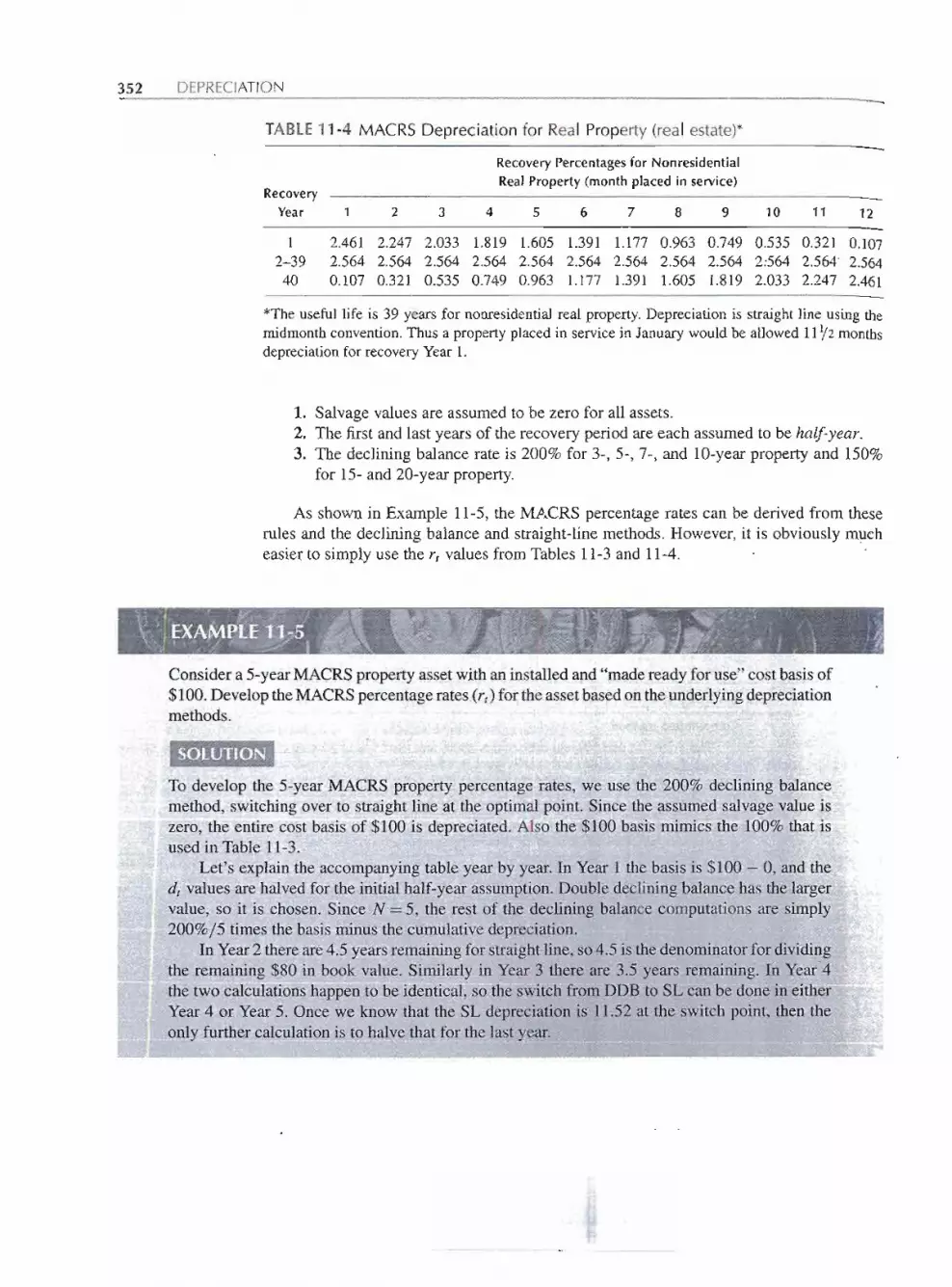
- - -
*The useful life is 39 years for nonresidential real property. Depreciation is straight line using themidmonth convention. Thus a property placed in service in January would be allowed 11'l2 monthsdepreciation for recovery Year 1.
1. Salvagevalues are assumed to be zero for all assets.2. The first and last years of the recovery period are each assumed to be half-year.3. The declining balance rate is 200% for 3-,5-, 7-, and 1O-yearproperty and 150%
for 15- and 20-year property.
As shown in Example 11-5, the MACRS percentage rates can be derived from theserules and the declining balance and straight-line methods. However,it is obviously mucheasier to simply use the rt values from Tables 11-3 and 11-4.
Consider a 5-year MACRSproperty asset with an installed and "madeready for use" cost basis of$100. Developthe MACRSpercentagerates (rt) for the asset basedon the underlyingdepreciationmethods.
SOLUTION
To develop the 5-year MACRS property percentage rates, we use the 200% declining balancemethod, switching over to straight line at the optimal point. Since the assumed salvage value iszero, the entire cost basis of $100 is depreciated. Also the $100 basis mimics the 100% that isused in Table 11-3.
Let's explain the accompanyingtable year by year. In Year 1 the basis is $100 - 0, aQdthedt values are halved for the initial half-year assumption.Double decliningbalance has the largervalue, so it is chosen. Since N = 5, the rest of the decliningbalancecomputationsare simply200%/5 times the basis minus the cumulativedepreciation.
In Year2 thereare 4.5 years remainingfor straightline, so 4.5 is the denominatorfor dividingthe remaining $80 in book value. Similarly in Year 3 there are 3.5 years remaining. In Year"4
,. -:' ~ ." _ _ ',- ,-.,.- - ~_. ,r;
the two calculationshappen to be identical, so the switc"hfrom DDB to SL can be dOllein eitherYear 4 or Year 5. Once we know that the SL depreciation is 11.52 at the switch point, then the
smly furt!ler cal,cuiatioll is to halve that for the lastJetg". liE'" "'''' ~-- - - - ..- -- ...-----
- -- - - -- - - ----------
352 DEPRECIATION -TABLE 11-4 MACRS Depreciation for Real Property (real estate)*
Recovery Percentages for Nonresidential
RecoveryReal Property (month placed in service)
Year 1 2 3 4 5 6 7 8 9 10 11 12
1 2.461 2.247 2.033 1.819 1.605 1.391 1.177 0.963 0.749 0.535 0.321 0.1072-39 2.564 2.564 2.564 2.564 2.564 2.564 2.564 2.564 2.564 2:564 2.564' 2.564
40 0.107 0.321 0.535 0.749 0.963 1.177 1.391 1.605 1.819 2.033 2.247 2.461

. .-- '..,-----
Modified Accelerated Cost Recovery System (MACRS) 353
Notice,that the DDB calculations get smaller every year, so that at some point the straight-linecalculations lead to faster depreciation. This point is the optimal switch point, and it is built intoTable 11-3 for MACRS.
Year123456
DDB Calculation
1/2(2/5)(100- 0) =20.00(2/5)(100 - 20.00) = 32.00(2/5)(100 - 52.00)= 19.20(2/5)(100 - 71.20) = 11.52
SL Calculation
1/2(100 - 0)/5 = 10.00(100 - 20)/4.5 = 17.78(100 - 52)/3.5 = 13.71
(100 - 71.20) /2.5 = 11.5211.52
(112)(11.52) = 5.76
MACRS Tt
(%) Rates
20.00 (DDB)32.00 (DDB)19.20 (DDB)11.52 (either)11.52 (SL)5.76 (SL)
CumulativeDepreciation (%) .
20.0052.0071.2082.7294.24
100.00
The values given in this example match the rt percentage rates given in Table 11-3 for a 5-yearMACRS property.
-'-"~-',---~-.~
MACRS Method ExamplesRemember the key questions in using MACRS: (1) What type of asset do you have, anddoes it qualify as depreciableproperty? (2)What amount are you depreciating [costbasis]?and (3) When are you placing the asset in service? Let's look at several examples of usingMACRS to calculate both depreciation deductions and book values.
Use the MACRS GDS method to calculate the yearly depreciation allowances and book valuesfor a firm that has purchased $150,000 worth of office equipment that qualifies as depreciableproperty. This office furiritureis estimated to have.a salvage (market) value of $30,000 (20% ofthe original cost) after the end of its depreciable life.
i .
SqLUTION
1. The assets qualify as depreciable property.2. The cost basis is given as $150,000.3. The assets are being placed in service in Year 1 of our analysis.4. MACRS GDS applies.5. The salvage value is not used with MACRS to calculate depreciation or book value.
. _ " .-;< _ _,_ ~ _ .JOffice equipmetItis listed in Table 11-2 as a 7-year property.We now use the MACRS <1bS- - ~-I
7-year property percentages from Tab.
le 11-3 and Eq. 11_5to calculate the year-to-year <!erred- Iation allowances.We use Equation 11-1 to calculate the book value of the asset. .- ..-- .. -. - .. ...- po --
J
- - - --- ----
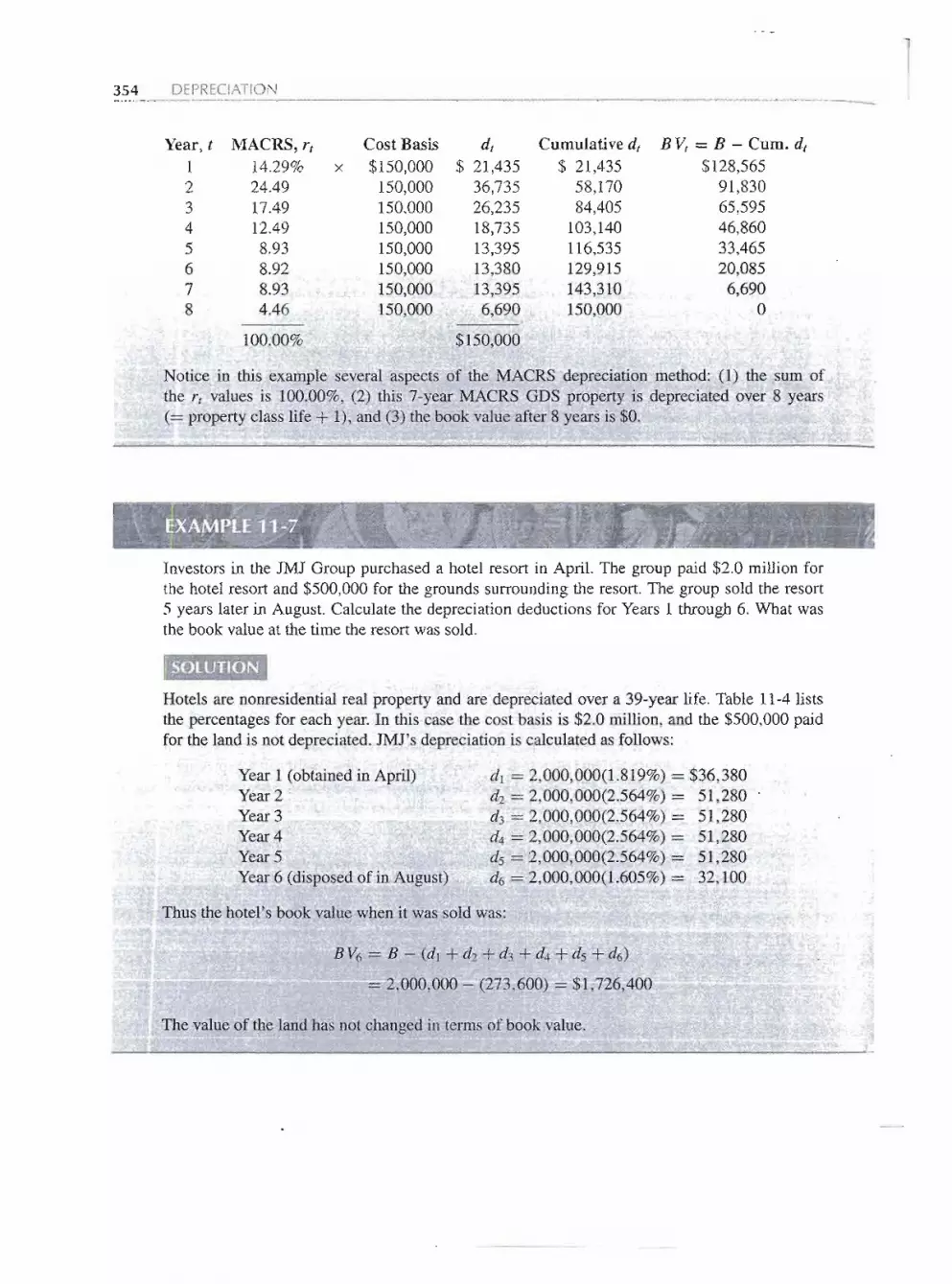
Notice in this example several aspects of the MACRS depreciation method: (1) the sum ofthe rt values is 100.00%, (2) this 7-year MACRS GDS property is depreciated over 8 years(-- property class life + 1), and (3) the book value after 8 years is $0.
Investors in the JMJ Group purchased a hotel resort in April. The group paid $2.0 million forthe hotel resort and $500,000 for the grounds surrounding the resort. The group sold the resort5 years later in August. Calculate the depreciation deductions for Years 1 through 6. What wasthe book value at the time the resort was sold.
Hotels are nonresidential real property and are depreciated over a 39-year life. Table 11-4 liststhe percentages for each year. In this case the cost basis is $2.0 million, and the $500,000 paidfor the land is not depreciated. JMJ's depreciation is calculated as fo!1ows:
Year 1 (obtained in April)Year 2Year 3Year4Year5Year 6 (disposed of in August)
d1 = 2,000,000(1.819%)= $36,380dz = 2,000,000(2.564%) = 51,280d3 = 2,000,000(2.564%) = 51,280d4 = 2,000,000(2.564%) = 51,280ds = 2,000,000(2.564%) = 51,280d6 = 2,000,000(1.605%) = 32,100
Thus the hotel's book value when it was sold was:
BV6 -- B - (d1 + dz + d3+ d4+ ds + d6)
.~2,OOO,000:£..::(273,600) ~ $1,'726,400
The value of the land has not challged in terms of book value.
--- - -- --
- _.... .......- - -
1I
354 DEPRECIATION
Year, t MACRS, Tt Cost Basis dt Cumulative dt B Vt = B - Cum. dt1 14.29% x $150,000 $ 21,435 $ 21,435 $128,5652 24.49 150,000 36,735 58,170 91,8303 17.49 150,000 26,235 84,405 65,5954 12.49 150,000 18,735 103,140 46,8605 8.93 150,000 13,395 116,535 33,4656 8.92 150,000 13,380 129,915 20,0857 8.93 150,000 13,395 143,310 6,6908 4.46 150,000 6,690 150,000 0
100.00% $150,000

,"I
Modified Accelerated Cost Recovery System (MACRS) 355
Comparing MACRSand Historical MethodsIn Examples 11-2 through 11-4 we used the straight-line, sum-of-the-years'-digits,anddeclining balance depreciation methods to illustrate how the book value of an asset thatcost $900 and had a salvage value of $70 changed over its 5-year depreciationlife.Fig-ures 11-2through 11-4provideda graphicalviewof bookvalueoverthe 5-yeardepreciationperiodusing thesemethods.Example 11-8comparestheMACRSODSdepreciationmethoddirectly against the historical methods.
Consider the furniture that was purchased in Example 11-6. Calculate the asset's depreciationdeductions and book values over its depreciable life for MACRS and the historical methods.
SOLUTION
Table11-5andFigure 11-5compareMACRSandhistoricaldepreciationmethods.MACRSdepre-ciation is the most acceleratedor fastestdepreciationmethod-remember its nameis the modifiedaccelerated cost recovery system. The book value drops fastest and furthest with MACRS,thusthe present worth is the largest for the MACRS depreciation deductions.
Depreciation deductions benefit a firm after taxes because they reduce taxable income andtaxes.The timevalueof moneyensures that it is better to takethese deductionsas soonaspossible.In general, MACRS, which allocates larger deductions earlier in the depreciation life, providesmore economic benefits than historical methods.
I
-- -- -- -- -------
TABLE 11-5 Comparison of MACRSand Historical Methods for Asset Iin Example "-6 I
Double Sum-of- Years' '"MACRS Straight line Declining Digits
Year,dt BYt dt BYt dt BVt dt BYt
1 21,435 128,565 12,000 138,000 30,000 120,000 21,818 128,1822 36,735 91,830 12,000 126,000 24,000 96,000 19,636 108,5453 26,235 65,595 12,000 114,000 19,200 76,800 17,455 91,091 I
4 18,735 46,860 12,000 102,000 15,360 61,440 15,273 75,818 I5 13,395 33,465 12,000 90,000 12,288 49,152 13,091 62,727 l6 13,380 20,085 12,000 78,000 9,830 39,322 10,909 51,818
III7 13,395 6,690 12,000 66,000 7,864 31,457 8,727 43,0918 6,690 0 12,000 54,000 1,457 30,000 6,545 36,5459 0 0 12,000 42,000 0 30,000 4,364 32,182
10 0 0 =1000 ",30p =: ;;;:;; <1= o:3q,gOp = ii:;;;'" 4" 182 30,OOO:ili
I
PW $108,217 $73,734 $89,918 $84,118(10% )
. .---..
........--- .-.....--..- - - .. - - . -- --

1
356 DEPRECIATION
$150,000
'..'.......
....
'."'" .., , ". .,." ,...
$125,000
«) $100,000:::I
~~ $75,000oo
I:Q $50,000
$25,000
o 2 4 6 8 10Year, t
FIGURE 11-5 Comparing MACRS ( ) and historical depreciation methods: double decliningbalance ( 4. ), sum of the years' digits (_ _ _ _ _), and straight line ( ; )
DEPRECIAliON AND ASSET DISPOSAL
When a depreciated asset is disposed of, the key question is, Which is larger, the asset'sbook value, BV (whatwe show in our accounting records after applying the rules set by thegovernment)or the asset's market value,MV (what a willing buyerpays)? If the bookvalueis lower than the market value, then too much depreciationhas been deducted from taxableincome. On the other hand, if the book value is higher than the market value, there is a losson the disposal. In either case, the current level of taxes owed changes.
Depreciationrecapture(ordinarygains): Depreciationrecapture, also called ordinarygains, is necessarywhenan asset is soldfor morethan anasset's currentbookvalue.If more than the original cost basis is received, only the amount up to the originalcost basis is recaptured depreciation. Ordinary gains are also called depreciationrecapturebecause the amount of gain represents the overexpense in depreciationthat has been claimed.In other words,we've taken toomuchexpensefor the asset's"loss in value."Since MACRSassumes S = 0 for its annual calculations,MACRSoften has recaptured depreciation at disposal.
Losses: A loss occurs when less than book value is received for a depreciated asset.In the accounting records we've disposed of an asset for a dollar amount less thanits book value, which is a loss. In this case a company has not claimed enoughdepreciation expense.
Capital gains: Capital gains occur when more than the asset's original cost basis isreceived for it. The excess over the original cost basis is the capital gain. Asdescribed in Chapter 12, the tax rate on such gains is sometimes lower than therate on ordinary income, but this depends on how long the investment has beenheld ("short," ::: 18months; "long," ~ 18months). In most engineering economic
- - - --- - - - - - -- - -

Depreciation and Asset Disposal 357
analyses capital gains are veryuncommonbecausebusiness andproduction equip-ment andfacilitiesalmost alwayslosevalueovertime.Capitalgains aremuch morelikely to occur for nondepreciated assets like stocks, bonds, real estate, jewelary,art, and collectibles.
The relationship between depreciation recapture, loss, and capital gain is illustrated inFigure 11-6.
$16,000
$14,000
$12,000
$10,000
$8,000
$6,000
$4,000
$2,000
$0
$14,000
$10,000 $4000 Capital Gain
$5000 Depreciation Recapture
$5000
CostBasis
Market BookValue Value
(c) Capital Gain and Depreciation Recapture
FIGURE 11-6 Recaptured depreciation, loss on sale, and capital gain.
Consider an asset with a cost basis of $10,000 that has been depreciated using the MACRS method~This asset is a 3-year MACRS property. What is the gain or loss if the asset is disposed of after5 years of operation for (a) $7000, (b) $0, and (c) a cost of $2000.
::;;
Tq find gain or loss at disposal we compare market and book value. Since MACRS depreciatestoa salvage value of 0, and 5 years is greater than the recovery period, the book value equals $0.
11:I
I!!I...~iICIi:I ---
L
- - -- - - -
$12,000 $12,000$10,000 I $10 000
$10,000 $10,000 '
$8,000 $7000 $8,000
$6,000 - - - - -$5000-1 :ciatiOn $6,000 $5000
$4,000 !; . - - Recapture $4,000I $3000 Loss
. .$2000
$2,000 $2,000 .$0
Cost Market Book$0
Cost Market BookBasis Value Value Basis Value Value
(a) Depreciation Recapture (ordinary gain) (b) Loss

~ ..--..----
358 DEPRECIATION -(a) Recaptured depreciation = $7000, since the book value is $7000 higher.(b) Since market value equals salvagevalue, there is no recaptured depreciation or loss.(c) Since the money is paid for disposal, this is less than the book value, and there is a loss.
This generalmethodforcalculatingrecaptureddepreciationor lossappliestoallofthedepreciationmethods described in this chapter.
If the asset is in the middle of its depreciable life, then recaptured depreciation andlosses are calculatedin a similarmanner--compare the market and book values at the timeof disposal.However,in computingthe book valuewith MACRSdepreciationa specialrulemust be applied for assets disposed of before the end of the recovery period. The rule is totake one half of the allowable depreciationdeductionfor that year. This rule assumesth&tdisposals take place on averagehalfway through the year. Thus for a 5-year asset disposedof in the middle of Year4, the rate allowed for MACRS depreciation is half of 11.52%or5.76%. If the asset is disposedof in Year6, it is alreadypast the recoveryperiod, and ahalf-year assumptionhas alreadybeenbuilt into the MACRSschedule.Thus, the full r6is taken.Example 11-10illustrates severalcases of disposal before the asset is fully depreciated.
Consider the $10,000 asset in Example 11-9.Do the following:
1. Calculate the effect of disposal if this asset is sold during Year2 for $2500.2. Calculate the effect of disposal if the asset is sold during Year3 for $2500.3. Calculate the effect of disposal if the asset is sold after Year 3 for $4000 if straight-line
depreciationis used over the asset's 5-year life, and a salvagevalue of $5000 is assumed.
SOLUTION
1. Marketvalu~ = $2500
Bookvaluez= 10,000- 1O,009[rl+ rzl2]= 10,000- 10,000[0.3333+ 0.4445/2]
= $4444.5
Loss = $1944.5 (= 4444.5 - 2500) (Loss, since BV greater than MV)
(Note: If the full rather than half deduction were taken in Year 2, then the book valuewould be $2222.50 less and the loss would become a gain of $278. Since depreciationwould increase by that $2222.50, the total of (depreciation) + (loss or gain) would be$4167 in either calculation.)
2. Market value3= $2500
BoolC'value~~, 10,000 10,000[rp.-/-:=rz *' r3/2]
= 10,000 -10,000[0.3333 + 0.4445 + 0.1481/2] = $1481.50
Recapturea[fepi'eaatimf 2500~ 1481.50;-1$1018.50 (Recaptured, since.MV> BY)--- - -- ...-
-- -- -

Unit-oF-Production Depreciation 359
3. Straight-linerate = (B - S)/ N = (10,000 - 5000)/5 =$1000
Market value4 = $4000
Book value4= 10,000 - (4)(1000) = $6000
Loss = 6000 - 4000 = $2000
If the asset were disposed of during the year rather than at year's end, then the straight-line depreciation deduction would have to be prorated for the number of months duringthe year that the asset was in service.There is no half-year conventionwith the historicaldepreciation methods. For example, if disposal occurred on September 30 of Year 4,d4 = (9/12)(1000) = $750.
(Note: In Case 1 it was shown that the required half-year convention did not affect the totaldeductions from taxable income. This is true for the other cases as well, since both recaptureddepreciation and losses are treated as ordinary income.)
UNIT-Of-PRODUCTION DEPRECIATION
At times the recovery of depreciation on a particular asset is more closely related to usethan to time. In these few situations (and they are rare), the unit-of-production (UOP)depreciation in any year is
.. . Production for yearUOP deprecIatIOn III any year = .. . (B - S) (11-6)
Total lIfetimeproduction for asset
This method might be useful for machinery that processes natural resources if theresources will be exhaustedbefore the machinery wears out. Historically,this method wassometimesused for constructionequipment that had veryheavy use in some years and verylight use in others. It is not consideredan acceptablemethodfor generaluse in depreciatingindustrial equipment.
For numerical sjrnilarity with previous examples, assume that equipment costing $900 has beenpurchased for use in a sand and gravel pit. The pit will operate for 5 years, while a nearby airportis being reconstructed and paved. Then the pit will be shut down, and the equipment removedand sold for $70. Compute the unit-of-production (UOP) depreciation schedule if the airportreconstruction schedule calls for 40,000 m3of sand and gravel as follows.:
Year Required Sand and Gravel (m3)1 4,0002 8,0003 16,0004 8,0005 4,000
:
::I =
- -- ....---
-------

.-. hh_ ___.
360 DEPRECIATION
SO~UTION
The cost basis, B, is $900.The salvagevalue, S, is $70. The total lifetimeproductionfor the assetis 40,000 m3 of sand and gravel. From the airport reconstruction schedule, the first-year UOPdepreciation would be:
. . 4000 m3$9 $ 0 $FIrst-yearUOP deprecIation= '> ( 00 - 7 ) = 83
40,000 m
Similar calculationsfor the subsequent4 years give the complete depreciation schedule:
Year12345
UOP Depreciation$ 83
16633216683
$830
It should be noted that the actual unit-of-production depreciation charge in any year is basedon the actual production for the year rather than the scheduled production.
DEPLETION
Depletion is the exhaustionof natural resources as a result of theirremoval.Since depletioncovers such things as mineral properties, oil and gas wells, and standing timber, removalmay take the form of digging up metallic or nonmetallic minerals, producing petroleum or .natural gas from wells, or cutting down trees. .
. Depletion is recognized for income taxes for the same reason depreciation is--capitalinvestment is being consumed or used up. Thus a portion of the gross income should beconsidered to be a return of the capital investment. The calculation of the depletion al-lowanceis differentfrom depreciationbecause there are two distinctmethods of calculatingdepletion: cost depletion and percentage depletion. Except for standing timber and mostoil and gas wells, depletion is calculated by both methods and the larger value is taken asdepletion for the year.For standing timber and most oil and gas wells, only cost depletionispermissible.
Cost DepletionDepreciation relied on an asset's cost, depreciable life, and salvagevalue to apportion thecost minus salvagevalue over the depreciable life. In some cases, where the asset is used atfluctuatingrates, we might use the unit-of-production (UOP) method of depreciation. Formines, oil wells, and standing timber, fluctuating production rates are the usual situation.
- ---- -- -- -

Depletion 361
Thus, cost depletion is computed like unit-of-productiondepreciation using:
1. Property cost, less cost for land.2. Estimated number of recoverableunits (tons of ore, cubic meters of gravel, barrels
of oil, million cubic feet of natural gas, thousand board-feet of timber, etc.).3. Salvage value, if any,of the property.
A small lumber company bought a tract of timber for $35,000, of which $5000 was the land'svalue and $30,000 was the value of the estimated 1Y2million board-feet of standing timber. Thefirst year, the company cut 100,000 board-feet of standing timber. What was the year's depletionallowance?
SOLUTION:I, c' ,r.,..
Depletion allowanceper 1000board-ft = $35,000- $50001500board-ft
= $20 per 1000 board-ft
The depletion allowance for the year would be
100,000 board-ft x $20 per 1000board-ft = $2000- ~. .
Percentage DepletionPercentage depletion is an alternatemethod for mineral property and some oil or gas wells.The allowance is a certain percentage of the property's gross income during the year.Thisis an entirely different concept from depreciation. Unlike depreciation, which allocatescost over useful life, the percentage depletion allowanceis based on the property's grossincome.
Since percentage depletion is computed on the income rather than the property's cost,the total depletion may exceed the cost of the property. In computing the allowable per-centage depletion on a property in any year, the percentage depletion allowance cannotexceed 50% of the property's taxable income computed without the depletion deduction.The percentage depletioncalculations are illustrated by Example 11-13.
TABLE11-6 PercentageDepletionAllowance for SelectedItems
Typeof Deposit
Lead, zinc, nickel, sulfur, uraniumOil and gas (small producers only)Gold, silver, copper, iron oreCoal and sodium chloride
Sand, gravel, stone, clam and oyster shells, brick, tile clayMost other minerals and metallic ores
Depletion Allowance
22%1515105
14
--- ---

-----------.------
362 DEPRECIATION -A coal mine has a gross income of $250,000 for the year. Mining expenses equal $210,000.Compute the allowablepercentage depletion deduction.
!.SOU..J.tION'
From Table 11-6, coal has a 10% depletion allowance. The percentage depletion deduction iscomputed from gross mining income. Then the taxable income must be computed.The allowablepercentagedepletiondeduction is limited to the computedpercentagedepletionor 50% of taxableincome, whichever is smaller.
Computed PercentageDepletionGross income from mineDepletion percentage
Computed percentage depletion
TaxableIncome LimitationGross income from mineLess: Expenses other than depletion
Taxable income from mineDeduction limitation
Taxableincome limitation
$250,000x 10%
$ 25,000
$250,000-210,000
40,000x 50%
$20,000
Since the taxable income limitation ($20,000) is less than the computed percentage depletion($25,000), the allowablepercentage depletiondeduction is $20,000.
As previously stated, on mineral property and some oil and gas wells (small producersonly), the depletion deduction can be based on either cost or percentage depletion. Eachyear, depletion is computed by both methods, and the allowabledepletion deduction is thelarger of the two amounts. ' .
SPREADSHEETS AND DEPRECIATION
The spreadsheet functions for straight-line, double declining balance, and sum-of-years'-digits depreciation are listed in Table 11-7. Because these techniques are simple and were
Depreciation Technique
TABLE 11-7 Spreadsheet Functions for Depreciation
Excel
Straight lineDeclining balanceSum of years' digitsMACRS
SLN(cost, salvage, life)DDB(cost, salvage, life, period, factor)SYD(cost, salvage, life, period)VDB(cost, salvage, life, start-period, end_period, factor, no-switch)

r
Spreadsheets and Depreciation 363
replacedby MACRSin 1986,they are not coveredin detail here. All three functions includeparameters for cost (initialbook value), salvage (final salvagevalue), and life (depreciationperiod). Both DDB and SYD change depreciation amounts every year, so they include aparameter to pick the period (year). Finally,DDB includes afactor. The default value is 2for 200% or double decliningbalance, but another commonly used value is 1.5 for 150%.
Using VDB for MACRS .
The Excel function VDB is a flexibleor variable declining balance method. It includes theability to specify the startingand ending periods, rather than simply a year. It also includesan optional nO-8witchfor problems where a switch from declining balance to straight-linedepreciation is NOT desired.
To use VDB to calculate MACRS depreciation, the following are true.
1. Salvage= 0, since MACRS assumes no salvage value.2. Life = recovery period of 3,5, 7, 10, 15, or 20 years.3. First period runs from 0 to 0.5, 2ndperiod from 0.5 to 1.5, 3rdfrom 1.5 to 2.5, tth
from t - 1.5 to t - 0.5, and last period from life -0.5 to life.4. Factor= 2 for recovery periods of 3,5, 7, or 10 years and = 1.5 forrecovery periods
of 15 or 20 years.5. Since MACRS includes a switch to straight line, no_switchcan be omitted.
The starLperiod andend_periodargumentsare from t - 1.5to t - 0.5, becauseMACRSuses a half-year convention for the first year. Thus the first year has 0 to 0.5 year ofdepreciation, and the second year starts where the first year stops. When one is writing theExcel function, either the first and last periods must be edited individually,or start_periodmust be definedwith a minimumof 0 and end_periodwith a maximumof life. This preventsthe calculation of depreciation from -0.5 to 0 and from life to life +0.5.
The results of using the VDB function match Table 11-4,except that the VDB func-tion has more significant digits rather than being rounded to 2 decimals. Example 11-14illustrates the use of the VDB function.
Return to the data of Example 11-5 which had $150,000 of office equipment, which is 7-yearMACRS property.Use VDB to compute the depreciation amounts.
SOLUTION.
The spreadsheetin Figure 11-7de:finest:!lestart...periodwith a minimum of Q¥1d tpe end_pefiog~lthfnfaximum of life.Thus thisformulacouldbe usedfor anyyearof anyrecoveryschedule.No-tice that the VDBformulauses the value0 for thesalvage value,rather thanreferringtothe data cellfor thes~v~g~ v'tlue.~A~RSoa§sumesca§ill,v~gy.valueot:zer~nomatter what the value truly is:-- ---- -- --- -.. .. -- -.. - ..-
-,- ........---

364 DEPRECIATION -
FIGURE 11-7 Using VDB to calculate MACRS depreciation.
SUMMARY
Depreciation is the foundationfor including income taxes in economic analysis. There arethree distinct definitionsof depreciation:
1. Decline in asset's market value.2. Decline in asset's value to its owner.3. Allocating the asset's cost less its salvagevalue over its recovery period or depre-
ciable life.
While the first two definitions are used in everyday discussions, it is the third, oraccountant's, definition that is used in tax computations and in this chapter. Book value isthe remaining unallocated cost of an asset, or
Book value = Asset cost - Depreciationcharges made to date
This chapter describeshow depreciable assets are written off (or claimed as a businessexpense) overa period of years instead of expensed in a single period (like wages,materialcosts, etc.). The depreciation methods described include the historical pre-1981 methods:straight line, sum of the years' digits, and declining balance. These methods requiredestimatingtheasset'ssalvagevalueanddepreciablelife. .
The current tax law specifiesuse of the modified accelerated capital recovery system(MACRS).This chapterhas focusedon the general depreciationsystem (GDS) withlimiteddiscussion of the less attractive alternative depreciation system (ADS). MACRS (GDS)specifiesfaster recoveryperiods and a salvagevalueof zero, so it is generallyeconomicallymore attractivethan the historical methods.
,A B C D E F G
1 150,000 First Cost
2 0 Salvage3 7 Life
4 200% Factor
56 Period Depreciation7 1 $21,428.57 = VDB($A$1,0,$A$3,MAX(0,A7-1.5),MIN($A$3,A7-O.5),$A$4)8 2 $36,734.69 or (cost, salvage,life, max(O,(-1.5), min (life, (- .5), factor)9 3 $26,239.07 j10 4 $18,742.19
II
11 5 $13,387.28
12 6 $13,387.28
13 7 $13,387.28
14 8 $6,693.64
15 $150,000 = Sum

..-- - .- - -- .- -- -. -- - --. -.. A _.___________
Problems 365
The MACRS systemis the current tax law,and it assumesa salvagevalueof zero. This, is in contrast with historical methods, which ensured the final book value would equal the
predicted salvage value. Thus, when one is using MACRSit is often necessary to considerrecaptured depreciation.This is the excess of salvagevalue overbook value, and it is taxedas ordinary income. Similarly, losses on sale or disposal are taxed as ordinary income.
Integrating depreciation schedules with cash flows often involves a lot of arithmetic.Thus, the tool of spreadsheetscan be quite helpful.The functionsfor the historicalmethods,straight line, sum of the years' digits, and declining balance, are straightforward. Ratherthan individuallyenteringMACRSpercentagesinto the spreadsheet,the functionVDB canbe used to calculate MACRS depreciation percentages.
Unit-of-production (UOP) depreciation relies on usage to quantify the loss in value.UOP is appropriate for assets that lose value based on the number of units produced, thetons of gravel moved, and so on (vs number of years in service). However,this method isnot considered to be acceptable for most business assets.
Depletion is the exhaustion of natural resources like minerals, oil and gas wells, andstanding timber.The ownersof the natural resourcesare consumingtheir investmentsas thenatural resources are removed and sold.Cost depletionis computedbased on the fraction ofthe resource that is removed or sold. For minerals and some oil and gas wells, an alternatecalculationcalled percentagedepletion is allowed.Percentagedepletionis basedon income,so the total allowabledepletion deductions may exceed the investedcost.
PROBLEMS
11-1 A depreciable asset costs $10,000 and has an esti-mated salvage value of $1600 at the end of its 6-yeardepreciable life. Compute the depreciation schedulefor this asset by both SOYD depreciation and DDBdepreciation.
11-2 A million-dollar oil drilling rig has a 6-year deprecia-ble life and a $75,000 salvage value at the end of thattime. Determine which one of the following methodsprovides the preferred depreciation schedule: DDBor SOYD. Show the depreciation schedule for thepreferred method.
11-3 A new machine tool is being purchased for $16,000and is expected to have a zero salvage value at theend of its 5-year useful life. Compute the DDBdepreciation schedule for this capital asset. Assumeany remaining depreciation is claimed in the last year.
11-4 Some special handling devices can be obtained for$12,000. At the end of 4 years, they can be soldfor $600. Compute the depreciation schedule for thedevices using the following methods:(a) Straight-line depreciation.(b) Sum-of-years' -digits depreciation.(c) Double declining balance depreciation.
(d) MACRS depreciation.
11-5 The company treasurer is uncertain which of four de-preciation methods the firm should use for office fur-niture that costs $50,000, and has a zero salvage valueat the end of a 1O-yeardepreciable life. Compute thedepreciation schedule for the office furniture usingthe methods listed:
(a) Straight line.(b) Double declining balance.(c) Sum-of-years' -digits.(d) Modified accelerated cost recovery system.
11-6 The RX Drug Company has just purchased a cap-sulating machine for $76,000. The plant engineerestimates the machine has a useful life of 5 years andlittle or no salvage value. He will use zero salvagevalue in the computations.
Compute the depreciation schedule for themachine using:(a) Straight-line depreciation.(b) Sum-of-years'-digits depreciation.(c) Double declining balance depreciation. Assume
any remaining depreciation is claimed in the lastyear.
HIII
-- - -- --

366 DEPRECIATION
11-7 The Acme Chemical Company purchased $45,000 ofresearch equipment, which it believes will have zerosalvage value at the end of its 5-year life. Computethe depreciation schedule for the equipment by eachof the following methods: .(a) Straight line.(b) Sum-of-years'-digits.(c) Double declining balance.(d) Modified accelerated cost recovery system.
11-8 Consider a $6500 piece of machinery, with a 5-yeardepreciable life and an estimated $1200 salvagevalue. The projected utilization of the machinerywhen it was purchased, and its actual production todate, are shown below.
Year12345
ProjectedProduction (tons)
35004000450050005500
ActualProduction (tons)
30005000[Notyet
known]
Compute the machinery depreciation schedule byeach of the following methods:(a) Straight line.(b) Sum-of-years' -digits.(c) Double declining balance.(d) Unit of production (for first 2 years only).(e) Modified accelerated cost recovery system.
11-9 A large profitable corporation purchased a small jetplane for use by the firm's executives in January.The plane cost $1.5 million and, for depreciationpur-poses, is assumed to have a zero salvage value at theend of 5 years. Compute the MACRS depreciationschedule.
11-10 For an asset that fits into the MACRS "All prop-erty not assigned to another class" designation, showin a table the depreciation and book value over theasset's lO-year life of use. The cost basis of the assetis $10,000.
11-11 A company that manufactures food and beveragesin the vending industry has purchased some han-dling equipment that cost $75,000 and will be depre-ciated using MACRS GDS. The class life of theasset is 4 years, show in a table the yearly depre-ciation amount and book value of the asset over its
depreciation life.
- - - - -- ----
They are based on the same initial cost, useful life,and salvage value. Identify each schedule as one ofthe following
. Straight-line depreciation.. Sum-of-years' -digits depreciation.. 150% declining balance depreciation..Double declining balance depreciation.
. Unit-of-production depreciation.. Modified accelerated cost recovery system. .
11-13 The depreciation schedule for an asset, with a sal-vage value of $90 at the end of the recoveryperiod,has been computedby severalmethods. Identifythedepreciationmethodused for each schedule.Year ABC D
1 $323.3 $212.0 $424.0 $194.02 258.7 339.2 254.4 194.03 194.0 203.5 152.6 194.04 129.3 122.1 91.6 194.05 64.7 122.1 47.4 194.0.6 61.1-----
970.0 lO60.0 970.0 970.0 970.0
jiI
IJI
E.$lO7.0216.0324.0216.0
. 107.0
11-14 The depreciatib.n schedule for a microcomputer hasbeen arrived at by several methods. The estimated sal-vage value of the equipment at the end of its 6-yearuseful life is $600. Identify the resulting depreciationschedules.
Year ABC D
1 $2114 $2000 $1600 $12332 1762 1500 2560 12333 14lO 1125 1536 12334 1057 844 922 12335 705 633 922 12336 352 475 460 1233
11-15 TELCO Corp has leased some industrial land nearits plant. It is building a small warehouse on the siteat a cost of $250,000. The building will be ready foruse January 1. The lease will expire 15 years afterthe building is occupied. The warehouse will belongat that time to the landowner, with the result thaI
J
1
11-12 Consider fivedepreciationschedules:
Year A B C D E1 $45.00 $35.00 $29.00 $58.00 $43.502 36.00 20.00 46.40 34.80 30.453 27.00 30.00 27.84 20.88 21.324 18.00 30.00 16.70 12.53 14.925 9.00 20.00 16.70 7.52 10.446 8.36

. ... .. - .
Problems 367
there will be no salvage value to TELCO. The ware-house is to be depreciated either by MACRS or SOYDdepreciation. If 10% interest is appropriate, whichdepreciation method should be selected?
11-16 A profitable company making earthmoving equip-ment is considering an investment of $100,000 onequipment that will have 5-year useful life and a$20,000 salvage value. If money is worth 10%, whichone of the following three methods of depreciationwould be preferable?(a) Straight-line method.(b) Double declining balance method.(c) MACRS method.
11-17 The White Swan Talc Company purchased $120,000of mining equipment for a small talc mine. The miningengineer's report indicates the mine contains 40,000cubic meters of commercial quality talc. The com-pany plans to mine all the talc in the next 5 years asfollows:
Year12345
Talc
Production (m3)15,00011,0004,0006,0004,000
At the end of 5 years, the mine will be exhausted andthe mining equipment will be worthless. The com-pany accountant must now decide whether to use sum-of-years' -digits depreciation or unit-of-productiondepreciation. The company considers 8% to be anappropriate time value of money. Compute the de-preciation schedule for each of the two methods.Which method would you reco~end that the com-pany adopt? Show the computations to justify yourdecision.
11-18 For its fabricated metal products, the Able Corp. isbuying $10,000 of special tools that have a 4-yearuseful life and no salvage value. Compute the de-preciation charge for the second year by each of thefollowing methods:(a) DDB.(b) Sum-of -years' -digits.(c) Modified accelerated cost recovery system.
11-19 The MACRS depreciation percentages for 7-yearpersonal property are given in Table 11-3. Make thenecessary computations to determine if the percent-ages shown are correct.
11-20 The MACRS depreciation percentages for lO-yearpersonal property are given in Table 11-3. Make thenecessary computations to determine if the percent-ages shown are correct.
11-21 Use MACRS GDS depreciation for each of the assets,1-3, to calculate the following items, (a)-(c).1. A light general-purpose truck used by a delivery
business, cost = $17,000.
2. Production equipment used by a Detroit auto-maker to produce vehicles, cost = $30,000.
3. Cement production facilities used by a construc-tion firm, cost $130,000.
(a) The MACRS GDS property class.(b) The depreciation deduction for Year 3.(c) The book value of the asset after 6 years.
11-22 On July 1,Nancy Regan paid $600,000 foracommer-cial building and an additional $150,000 for the landon which it stands. Four years later, also on July 1, sbesold the property for $850,000. Compute the modi-fied accelerated cost recovery system depreciation foreach of the five calendar years during which she hadthe property.
11-23 A group of investors has formed Trump Corpora-tion to purchase a small hotel. The asking price is$150,000 for the land and $850,000 for the hotelbuilding. If the purchase takes place in June, computethe MACRS depreciation for the first three calendaryears. Then assume the hotel is sold in June of thefourth year, and compute the MACRS depreciationin that year also.
11-24 Mr. Donald Spade purchased a computer in Januaryto keep records on all the property he owns. Thecomputer cost $70,000 and is to be depreciated usingMACRS. Donald's accountant pointed out that un-der a special tax rule (the rule applies when the valueof property placed in service in the last 3 months ofthe tax year exceeds 40% of all the property placedin service during the tax year), the computer and allproperty that year would be subject to the midquar-ter convention. The midquarter convention assumesthat all property placed in service in any quarter-yearis placed in service at the midpoint of the quarter.Use the mid-quarter convention to compute Donald'sMACRS depreciation for the first year.
11-25 A company is considering buying a new piece ofmachinery. A 10% interest rate will be used inthe computations. Two models of the machine areavailable.
- - - -

368 DEPRECIATION
lI
-Initial costEnd-of-useful-life
salvage value, SAnnual operating
cost
Usefullife, in years
MachineI Machinen$80,000 $100,00020,000 25,000
18,000 15,000 first 10 years20,000 thereafter
2520
(a) Determine which machine should be purchased,based on equivalent uniform annual cost.
(b) What is the capitalized cost of Machine I?(c) Machine I is purchased and a fund is set up to
replace Machine I at the end of 20 years. Computethe required uniform annual deposit.
(d) Machine I will produce an annual saving ofmaterial of $28,000. What is the rate of return ifMachine I is installed?
(e) What will be the book value of Machine I after 2years, based on sum-of- years' -digits depreciation?
if) What will be the book value of Machine nafter 3 years, based on double declining balancedepreciation?
(g) Assuming that Machine n is in the 7-year propertyclass, what would be the MACRS depreciation inthe third year?
11-26 Equipment costing $20,000 that is a MACRS 3-yearproperty is disposed of during the second year for$14,000. Calculate any depreciation recapture, ordi-nary losses, or capital gains associated with disposalof the equipment.
11-27 An asset with a 8-year ADR class life costs $50,000and was purchased on January I, 2001. Calcu-late any depreciation recapture, ordinary losses, orcapital gains associated with selling the equipmenton December 31, 2003, for $15,000, $25,000, and$60,000. Consider two cases of depreciation for theproblem: if MACRS GDS is used, and if straight-linedepreciation over the ADR class life is used with a$10,000 salvage value.
11-28 When a major highway was to be constructed nearby,a farmer realized that a dry streambed running throughhis property might a valuable source of sand andgravel. He shipped samples to a testing labora-tory and learned that the material met the require-ments for certain low-grade fill material. The farmercontacted the highway construction contractor, whooffered 65/ c per cubic meter for 45,000 cubicmeters of sand and gravel. The contractor wouldbuild a haul road and would use his own equip-
ment. All activity would take place during a singlesummer.
The farmer hired an engineering student for$2500 to count the truckloads of material hauledaway. The farmer estimated that 2 acres of streambedhad been stripped of the sand and gravel. The 640-acrefarm had cost him $300 per acre, and the farmer feltthe property had not changed in value. He knew thatthere had been no use for the sand and gravel prior tothe construction of the highway, and he could foreseeno future use for any of the remaining .50,000 cubicmeters of sand and gravel. Determine the fanner'sdepletion allowance. (Answer: $1462.50)
11-29 Mr. H. Salt purchased a ys interest in a producingoil well for $45,000. Recoverable oil reserves for thewell were estimated at that time at 15,000 barrelsys of which represented Mr. Salt's share of the re~serves. During the subsequent year, Mr. Smt received$12,000 as his ysshare of the gross income from thesale of 1000 barrels of oil. From this amount, he had
to pay $3000 as his share of the expense of producingthe oil. Compute Mr. Salt's depletion allowance forthe year. (Answer: $3000)
11-30 A heavy construction firm has been awarded a con-tract to build a large concrete dam. It is expected thata total of 8 years will be required to complete thework. The firm will buy $600,000 worth of specialequipment for the job. During the preparation of thejob cost estimate, the following utilization schedulewas computed for the special equipment:
At the end of the job, it is estimated that the equipment. can be sold at auction for $60,000.(a) Compute the sum-of-years-digits' depreciation
schedule.
(b) Compute the unit-of-prQduction depreciationschedule.
11-31 Some equipment costs $1000, has a 5-year deprecia-
.II. ble life, and an estimated $50 salvage value at the endof that time. You have been assigned the problem todetermine whether to use straight-line or SOYD de-preciation. If a 10% interest rate is appropriate, whichis the preferred depreciation method for this profit.!"""
Utilization UtilizationYear (hr/yr) Year (hr/yr)
1 6000 5 8002 4000 6 8003 4000 7 22004 1600 8 2200
Problems 369
corporation? Use a spreadsheet to show your compu-tations of the Qifference in present worths.
11-32 The FOURX Corp. has purchased $12,000 of exper-. imental equipment. The anticipated salvage value is~ $400 at the end of its 5-year depreciable life. This
profitable corporation is considering two methods ofdepreciation: sum of years' digits and double declin-ing balance. If it uses 7% interest in its comparison,which method do you recommend? Show computa-tions to support your recommendation. Use a spread-sheet to develop your solution.
11-33 Given the data in Problem 11-16, use a spreadsheet
ala function to compute the MACRS depreciation sch-edule. Show the total depreciation taken (=sum( » as
well as the PW of the depreciation charges discountedat the MARR %.
11-34 Office equipment whose initial cost is $100,000 has. an estimated actual life of 6 years, with an estimated~ salvage value of $10,000. Prepare tables listing the
annual costs of depreciation and the book value atthe end of each 6 years, based on the straight-line,sum-of-years' -digits, and MACRS depreciation. Usespreadsheet functions for the depreciation methods.
11-35 You are equipping an office. The total office equip-
Ala ment will have a first cost of $1,750,000 and a salvagevalue of $200,000. You expect the equipnient will last10 years. Use a spreadsheet function to compute theMACRS depreciation schedule.
---------

.-.-....-
After Completing This Chapter...The student should be able to:. Calculate taxes due or taxes owed for both individualsand corporations.. Understand the incremental nature of the individual and corporate tax rates used for
calculating taxes on income.. Calculate a combined income tax rate for state and federal income taxes and select anappropriate tax rate for engineering economic analyses.. Utilize an after-tax tax table to findthe after-taxcash flowsfor a prospective investmentproject.. Calculate after-tax measures of merit, such as present worth, annual worth, paybackperiod, internalrate of return, andbenefit-cost ratio,from developedafter-taxcash flows.. Evaluate investment alternativeson an after-tax basis including asset disposal.. Use spreadsheetsfor solving after-taxeconomic analysis problems.
QUESTIONS TO CONSIDER ;;.
1. The wind energy production tax credit has become controversial among some com-mentators, who see it as "corporate welfare." These critics contend that the govern-ment should not be in the business of encouraging wind energy-or any other type ofenergy source, for that matter.Instead, they argue, the market should determine whetheralternative energy sources such as wind power succeed or fail. Are these critics right?
2. Proponents of the wind production tax credit counter that the energy market has neverbeen genuinely "free." They point out that other types of energy production (notablycoal and oil) have obtained large government subsidies over the years in the form ofdepletion allowances and other tax provisions. In fact, these proponents argue, carbon-based sources enjoy a tremendous "hidden subsidy" because the environmental andhealth effects of these more-polluting energy sources are not paid for by coal and oilproducers, but are borne by society at large. Are these proponents right?
3. Developing a wind power project takes many years and requires the commitment oflarge sums of investmentcapital before the project begins to return a profit. What is theeffect on investmentwhen the windpower production tax credit is allowed to expire, oris extended for periods of only a few years?
4. The federal income tax was introduced in the United States in 1913.Using the Internet,can you determinehowtaxrates changedthroughoutthe course of the twentieth century?How has this affected the value of tax credits to industry?
------------

Income Taxes'
On with the WindFor at least three decades now, environmental activists and community leaders have be-moaned American dependenceon foreign oil. The war in Iraq againhighlighted the precar-iousness of relying on an unstable regionof the world to producea major part of our energyrequirements.
One solutionto this dilemmais to rely more on renewablesourcesofenergy,such as solarpower and wind.The technologyfor suchalternativeenergy sources has been around for many years, and most voters seemto favor more reliance on renewables. If good intentions were all it took,we'd be getting much of our electricity from windmills.
But, of course, making the transition to greater use of wind powerrequires a significantinvestmentin infrastructure,especiallycostly windturbines. And few investorsare willing to plunk downtheir money unlessthey have a solid expectation of earning a competitivereturn.
Until fairly recently, cost factors kept wind energy from becomingan attractive investment. As recently as the late 1980s, wind-generatedpowercost roughlytwice as muchto produceas energyfromconventionalsources.
In the past few years, however,wind energy has decreased dramatically in price. TheAmerican Wind Energy Association (AWEA) reports that many modem, state-of-the-artwindplantscan nowproducepowerfor less than5 centsper kilowatt~hour,makingthem .
competitivewith conventional sources. Unsurprisingly,investmentin wind power produc-tion has also increased substantially.
How did this happen? In part, it was driven by advances in wind turbine technology.But it was helped significantlyby a provision of the federal tax law contained in the EnergyPolicy Act of 1992.This statute allowedutilities and other electricity suppliers a "produc-tion tax credit" of 1.5 cents per kilowatt-hour (later adjustedto 1.7 cents to account for theeffects of inflation).
This was a key incentive to the wind power industry which, like all energy producers,must expend large sums on capital assets. The tax credit had a dramatic effect on the windenergy market. During 2001, for instance, energy producers added almost 1700megawattsof wind-generating capacity-enough to power nearly half a million homes.
But what the governmentgiveth, the government can take away.When the productiontax credit briefly expired at the end of 2001, an estimated $3 billion worth of wind projectswere suspended, and hundreds of workers were laid off.
-
-----
I
I. t
-~ t1f

~. ~... ~..- -..~-- ... .....-.
-,372 INCOME TAXES -
Fortunately for the industry, the credit was subsequently extended to the end of 2003,andis expectedto be extendedfurther. As a result, theAWEA anticipatesthat another1500to 1800megawattsof wind-:generatingcapacity will comeon line during 2003. -As Benjamin Franklin said, two things are inevitable: death andtaxes. In this chapterWewill examinethe structureof taxesin the United States.There is, of course,a wide :varietyof taxesranging from salestaxes,gasoline taxes,and property taxesto stateand federalincome taxes,andsoforth. Here we will concentrateour attentionon federal incometaxes.Income taxesarepart of most real problems and often havea substantialimpactthatmustbe considered.
First, we must understand the way in which taxes are imposed.Chapter 11concerningdepreciation is an integral part of this analysis, so the principles covered there must be wellunderstood. Then; having understood the mechanism, we will see how federal income taxesaffect our economic analysis. The various analysis techniques will be used in examples ofafter-tax calculations.
A PARTNER IN THE BUSINESS
Probably the most straightforward way to understand the role of federal income taxes isto considerthe U.S. governmentas a partner in everybusinessactivity.As a partner,thegovernment shares in the profits from every successful venture. And in a somewhatmorecomplex way, the government shares in the losses of unprofitableventures. The tax lawsare complex, and it is not our purpose to fully explain them. 1Instead, we will examine thefundamental concepts of the federal income tax laws-and we emphasize at the start thatthereareexceptionsandvariationsto almosteverystatementwe shallmake!
CALCULATION OF TAXABLEINCOME
At the mention of income taxes, one can visualize dozens of elaborate and complex calcu-lations. And there is some truth to that vision, for there can be complexities of all sorts inthe computationof income taxes. Yet some of the difficulty is removed when one definesincomes taxes as just another type of disbursement. Our economic analysis calculationsin prior chapters have dealt with all sorts of disbursements:operating costs, maintenance,labor and materials, and so forth. Now we simply add one more prospectivedisbursementto the list-income taxes.
Taxable Income of Individuals
The amountof federal income taxes to be paid depends on taxable income and the incometax rates. Therefore, our first concern is the definition of taxable income. To begin, onemust computehis or her gross income:
Gross income =Wages, salary, etc. + Interest income + Dividends+ Capi~ gains+ Unemploymentcompensation+ Other income
-1Manygovernmentandprivatesourcesexistthatdescribedetailedtaxationinformation.Theseincludethe Internal Revenue Service (www.irs.gov), U.S. Treasury (www.treasury.gov), Commerce Clean::,House (www.cch.com), and Research Institute of America (www.riahome.com).
----- - -
Calculation of Taxable Income 373
From gross income, we subtract any allowable retirement plan contributions and other,adjustments. The result is adjusted gross income (AGI). From adjusted gross income,individuals may deduct the following items:2
1. Personal Exemptions. One exemption ($3050 for 2003) is provided for each per-son who depends on the gross income for his or her living.3
2. Itemized Deductions. Some of these are:
(a) Excessive medical and dental expenses (exceeding 71/2%of adjusted grossincome)
(b) State and local income, property and personal property tax(c) Home mortgage interest(d) Charitable contributions(e) Casualty and theft losses (exceeding $100 + 10% of adjusted gross income)(I) Miscellaneous deductions (some categories must exceed 2% of adjusted gross
income)(g) Car and other business expenses(h) Taxbenefits for work-relatededucation
3. Standard Deduction. Each taxpayer may either itemize his or her deductions, orinstead take a standard deduction as follows: . .
(a) Single taxpayers, $4750 (for 2003)(b) Married taxpayers filing a joint return, $7950 (for 2003)
The result is taxable income.
For individuals, taxable income is computed as follows:
Adjusted gross income = Gross income - Adjustments
Taxable income =Adjusted gross income
- Personal exemption(s)
- Itemized deductionsor Standarddeduction (12-1)
Classification of Business ExpendituresWhen an individual or a firm operates a business, there are three distinct types of businessexpenditure:
1. For depreciable assets.2. For nondepreciable assets.3. All other business expenditures.
2The 2003 itemized deduction are limited if adjusted gross income is more than $139,500 ($69,750if married filing separately.)
3Personal exemptions for high-income taxpayers are being phased out. In 2003, for taxpayers whoare married, filing jointly, the personal exemption is phased out beginning at an AGI of $209,250.The phaseout is complete at an AGI of $331,750. For single taxpayers, the beginning and completephaseout numbers are $139,500 and $262,000, respectively. ..
-- ------

374 INCOME TAXES -Expendituresfor depreciable assets: When facilities or productive equipment with
useful lives in excess of one year are acquired, the taxpayer will recover his in-vestment through depreciation charges.4Chapter 11 examined in great detail theseveral ways in which the cost of the asset could be allocated over its useful life.
Expendituresfor nondepreciable assets: Land is considered to be a nondepreciableasset, for there is no finite life associated with it. Other nondepreciable ~setsare properties not used either in a trade, in a business, or for the production ofincome.An individual'shome andautomobileare generallynondepreciableassets.The final category of nondepreciable assets are those subject to depletion, ratherthan depreciation. Since business firms generally acquire assets for use in thebusiness, their only nondepreciableassets normally are land and assets subjecttodepletion.
All other business expenditures: This category is probably the largest of all, for it in-cludes all the ordinary and necessary expendituresof operating a business.Laborcosts, materials, all direct and indirect costs, and facilities and produ~tiveequip-ment with a useful life of one year or less are part of the routine expenditures.They are charged as a business expense-expensed-when they occur.
Business expenditures in the first two categories-that is, for either depreciable ornondepreciable assets-are called capital expenditures. In the accounting records of thefirm, they are capitalized; all ordinary and necessaryexpenditures in the third categoryareexpensed.
Taxable Income of Business Firms
The starting point in computing a firm's taxable income is gross income. All ordinary andnecessary expenses to conduct the business-except capital expenditures-are deductedfrom gross income. Capital expendituresmay not be deducted from gross income. Exceptfor land, business capita! expenditures are charged to expense period by period througb;depreciation or depletion charges.
For business firms, taxable income is computed as follows:
Taxable income = Gross income
- All expenditures except capital expenditures
- Depreciation and depletion charges (12-2)
Because of the treatment of capital expenditures for tax purposes, the taxable income of afirm may be quite different from the actual cash results.
4There is an exception. In 2003, businesses may immediately deduct (expense) up to $25,000 ofbusiness equipment (via the Section 179 Business Deduction) in a year, provided their total equipmentexpenditure for the year does not exceed $200,000. Between $200,000 and $224,000 in qualifying179 Property the dollar limit is reduced by the amount over $200,000. Above $224,000 a Section 179deduction cannot be taken.
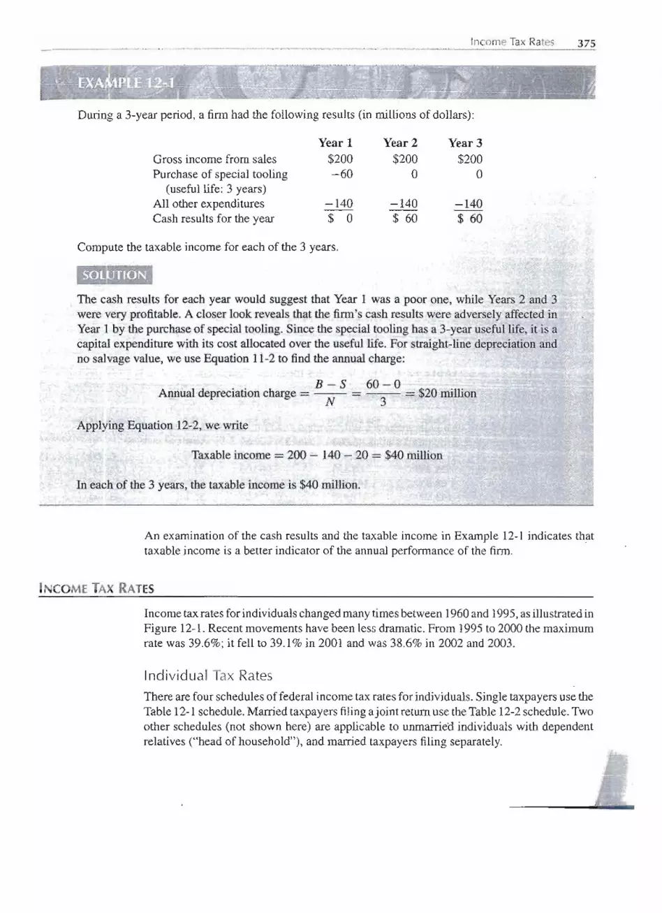
Income Tax Rates 375
_.During a 3-year period, a finn had the followingresults (in millions of dollars):
Gross income from salesPurchase of special tooling
(useful life: 3 years)All other expendituresCash results for the year
Year 1$200-60
Year 2$200
o
Year3$200
o
-140$ 0
-140$ 60
-140$ 60
Compute the taxable income for each of the 3 years.
.SOl~TlON'
The cash results for each year would suggest that Year 1 was a poor one, while Years 2 and 3were very profitable. A closer look reveals that the finn's cash results were adversely affectedinYear 1 by the purchase of special tooling. Since the special tooling has a 3-year useful life, it is acapital expenditure with its cost allocated over the useful life. For straight-line depreciation andno salvage value, we use Equation 11-2 to findthe annual charge:
B-S 60-0Annualdepreciationcharge= - = =$20millionN 3
Applying Equation 12-2,we write
Taxableincome =200 - 140 - 20 = $40 million
In each of the 3 years, the taxable income is $40 million.
An examination of the cash results and the taxable income in Example 12-1indicates th~ttaxable income is a better indicator of the annual perfonnance of the finn.
INCOME TAX RATES
Incometaxrates for individualschangedmanytimesbetween 1960and 1995,asillustratedinFigure 12-1.Recent movementshavebeen less dramatic.From 1995to 2000 the maximumrate was 39.6%; it fell to 39.1% in 2001 and was 38.6% in 2002 and 2003.
Individual Tax Rates
There arefour schedulesof federal incometax rates forindividuals. Singletaxpayersuse theTable 12-1schedule.Marriedtaxpayersfilingajointretum use the Table12-2schedule.1\voother schedules (not shown here) are applicable to unmarriea individualswith dependentrelatives ("head of household"), and married taxpayers filing separately.

--,
-
1975 1980 1985Year
1990
FIGURE 12-1 Maximum federal income tax rates for individuals.
TABLE12-1 2003 Tax Rates for Single Taxpayers
Taxable Income Tax
TABLE12-2 2003 Tax Rates for Married Individuals FilingJointly
------
376 INCOME TAXES
100
90
80
70'-"
£60
50eS 40
.>(30
20
10
01960 1965 1970
Over But Not Over BaseTax Plus On Income Over
$ 0 $ 6,000 $ 0.00 10% $ 06,000 28,400 600.00 15% 6,000
28,400 68,800 3,960.00 27% 28,40068,800 143,500 14,868.00 30% 68,800
143,500 311 ,950 37,278.00 35% 143,500Over 311,950 96,235.50 38.6% . 311,950
'.Taxable Income Tax
Over But Not Over BaseTax Plus On Income Over
$ 0 $ 17,000 $ 0.00 10% $ 012,000 47,450 1,200.00 15% 12,00047,450 114,650 6,517.50 27% 47,45
114,650 174,700 24,661.50 30% 114,650174,700 311,950 42,676.50 35% 174,700
Over 311,950 90,714.00 38.6% 311,950 . ..... ..> .
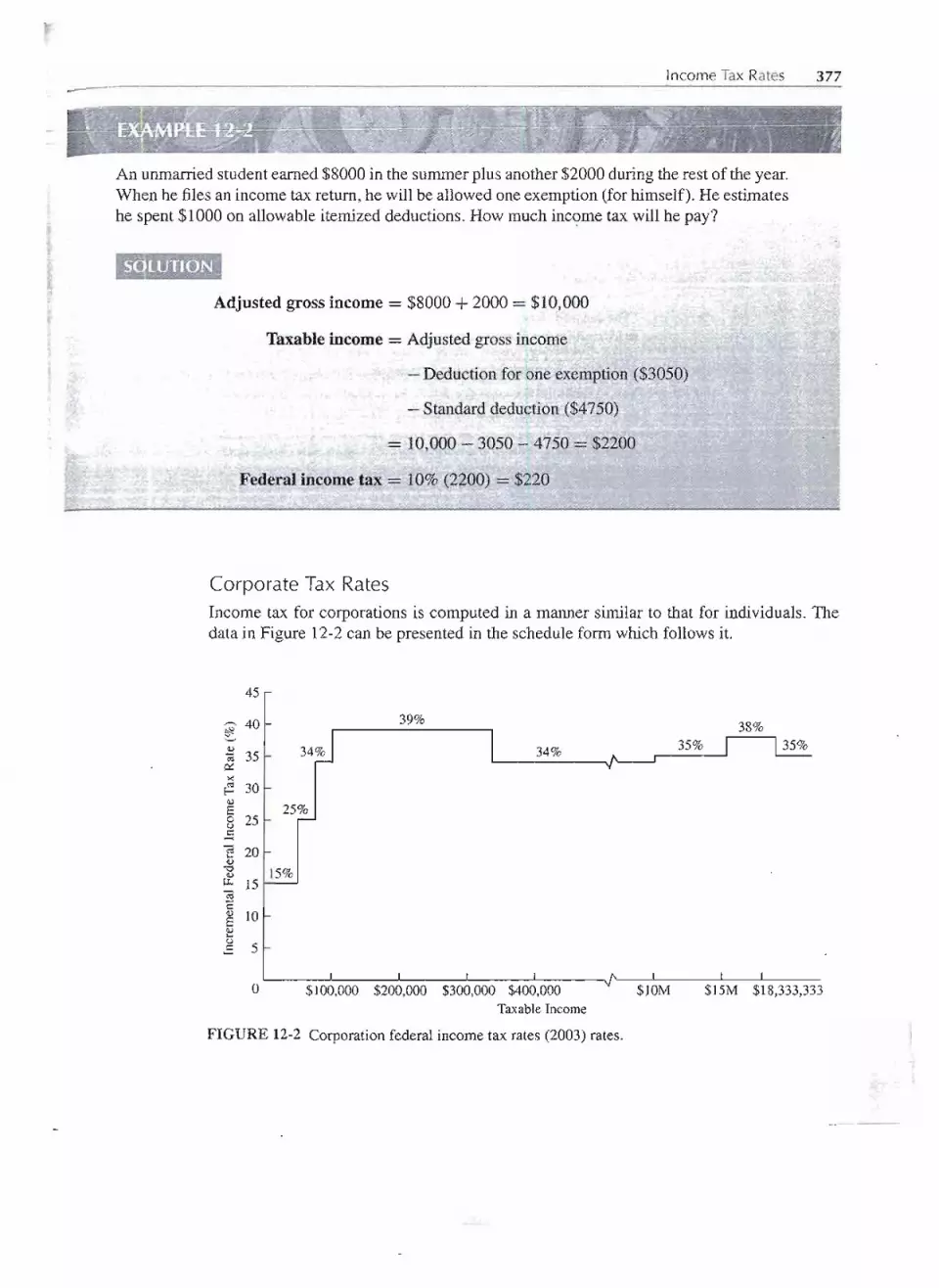
Income Tax Rates 377-
An unmarried studentearned $8000 in the summer plus another$2000 duringthe rest of the year.When he filesan income tax return,he will be allowedone exemption(forhimself). He estimateshe spent $1000 on allowable itemized deductions. How much income tax will he pay?
SqLUTION
Adjusted gross income = $8000 + 2000 = $10,000
Taxable income = Adjusted gross income
- Deduction for one exemption ($3050)
- Standard deduction ($4750)
= 10,000- 3050- 4750= $2200
Federal income tax = 10% (2200) - $220
Corporate Tax RatesIncome tax for corporations is computed in a manner similar to that for individuals. Thedata in Figure 12-2can be presented in the schedule form which follows it.
39% 38%
34% 34% 35%
25%
$100,000 $200,000 $300,000 $400,000TaxableIncome
$ 10M $15M $18,333,333:Ii
FIGURE 12-2 Corporation federal income tax rates (2003) rates.
- - - - ---- -- -- - -
45
40'-'Q)<;j 35a:::
30Q)e0 250s::-";j....g
'5s::Q)e0s::-
20
115%15
10
5
0

378 INCOME TAXES
Taxable Income Tax RateI
Corporate Income Tax
-Not over $50,000$50,000-75,000$75,000-100,000$100,000-335,000
$335,000-10 million$10 million-15 million$15 million-18,333,333
:::$18,333,333
15%25%34%39%*34%35%38%35%
15% over $0$7,500 + 25% over $50,000
$13,750 + 34% over $75,000$22,250 + 39% over $100,000$113,900 + 34% over $335,000
$3,400,000 + 35% over $10 million$5,159,000 + 38% over $15 million$6,425,667 + 35% over $18,333,333
*The extra 5% from $100,000 to $335,000 was chosen so that firms in the $335,000to $10 million bracket pay a flat 34% tax rate. [(0.39-0.34)](335,000-100,000) =(0.34 - 0.15)(50,000) + (0.34 - 0.25)(75,000 - 50,000)] so tax = 0.34 (taxincome) ~n$335,000 to $10 million bracket. Similarly, for corporate incomes over$18,333,333 the tax rate schedule is equivalent to a flat tax rate of 35%.
The French ChemicalCorporationwas fOnnedto producehousehold bleach.The firmbought land ,for $220,000,had a $900,000 factory building erected, and installed $650,000worth of chemicaland packaging equipment. The plant was completed and operations begun on April 1. The grossincome for the calendar year was $450,000. Supplies and all operating expenses, excluding thecapital expenditures,were $100,000.The firmwill use modifiedacceleratedcost recovery system(MACRS)depreciation.
(a) What is the first-year depreciationcharge?(b) Whatis the first-yeartaxableincome?(c) How much will the corporationpay in federal.income taxes for the year?
lSO'LUTION
(a) MACRS depreciation: Chemical eqt1ipm~ntigpersonal propeIty:I3romTable11-2, iUsprobably in the "7-year, all other property" class.
I3irst-yeardepreciation(equipment) .,,$650,000x 14.29%-<$92,885
Thebuilding is in the 39-yearreal propertyclass.Sm(;e itwas placedin serVjceon April 1,the.first-year depreciationis:
First-year depre(;iatioIl(buildiIlg)... ... $90Q,000x 1.819%' ..$16,37,1 (see Tablet 1-4)-- ---
I~
. - .,,~ .'
----
I
'~II i

Income Tax Rates 379
(b) Taxable income = Gross income
- All expenditures except capital expenditures
- Depreciation and depletion charges
= $450,000 - 100,000 - 109,256 = $240,744
(c) Federal income tax = $22,250 + 39%(240,744 - 100,000)
= $77,140
Combined Federal and State Income Taxes
In addition to federal income taxes, most individuals and corporations pay state incometaxes. Itwould be convenientif we could derive a single tax rate to represent both the stateand federal incremental tax rates. In the computation of taxable income for federal taxes,the amount of state taxes paid is one of the allowable itemized deductions. Federal incometaxes are not, however,generally deductible in the computation of state taxable income.Therefore, the state income tax is applied to a larger taxable income than is the federalincome tax rate. As a result, the combined incremental tax rate will not be the sum of twotax rates.
For an increment of income (Lllncome) and tax rate on incremental income (LlTaxrate):
"III
State income taxes = (LlState tax rate) (Lllncome)
Federal taxable income = (~lncome)(1 - ~State tax rate)
Federalincometaxes = (~Federaltaxrate)(Lllncome)x (1 - b.Statetaxrate)
The total of state and federal income taxes is
[LlStatetax rate + (LlFederaltax rate)(1 - ~State tax rate)](~Income)
The tenn in the brackets gives the combined incremental tax rate.
Combined incremental tax rate
= LlStatetax rate + (LlFederaltax rate)(1 - ~State tax rate) (12-3)
An engineer has an income that puts him in the 27% federal income tax bracket and at the 10%state incremental tax rate. He has an opportunityto earn an extra $500by doing a smallconsultingjob. What will be his combined state and federal income tax rate on the additional income?_._ ...;...;._.:--:.L...;._.__________
59~~IIOr~Jii
Use Equation 12-3 to find the combined incremental tax rate: 0.10 + 0.27(1"-'-'.0.10)= 34.3%.
:;
I
I; ;; =!

380 INCOME TAXES -Selecting an Income Tax Rate for Economy StudiesSince income tax rates vary with the level of taxable income for both individuals andcorporations, one must decide which tax rate to use in a particular situation. The simpleanswer is that the tax rate to use is the incremental tax rate that applies to the change intaxable income projected in the economic analysis. If a married couple filingjointly has ataxable income of $40,000 and can increase their incomeby $2000, what tax rate shouldbeused for the $2000 of incremental income? From Table 12-2,we see the $2000 falls withinthe 15% tax bracket.
Now suppose this couple could increase their $40,000 income by $10,000. In thissituation, Table 12-2 shows that the 15% incremental tax rate should be applied to thefirst $7,450 and a 27% incremental tax rate to the last $2,550 of extra income. The ap-propriate incremental tax rate for corporations is equally easy to determine. For largercorporations, the federal incremental tax rate is 35%. In addition, there may be up to a12-15% state tax.
ECONOMIC ANALYSIS TAKING INCOME TAXES INTO ACCOUNT
An importantstep in economicanalysis hasbeen to resolve the consequencesof alternativesinto a cash flow.Because income taxes have been ignored, the result has been a before-taxcashflow. This before-taxcash flowis an essentialcomponentin economicanalysisthatalsoconsiders the consequences of income tax. The principal elements in an after-tax analysisare as follows:
· Before-tax cash flow·Depreciation· Taxableincome(Before-taxcashflow- Depreciation)· Income taxes (Taxableincome x Incremental tax rate)·After-tax cash flow (Before-tax cash flow - Income taxes)
These elements are usually arranged to form a cash flow table. This is illustrated byExample 12-5.
Ip !'
L'
A IDedium-sizedprofitablecorporation is considering the purchase of a $3000 used pickup truckfor use by the shipping and .receiving department. puring the trucJ<:'s5-year useful life, it isestimated the .finn will save $800 per year after all the costs of oWniJ:J.gand operati.ngthe truckhave been paid. Truck salvage value is estimated at$750.
:I (a) Wbatistfie befo~e-ta:~;~te~lretOtn?~ = =:=: =- ~;; =~ ~=:= = =:e ;;;;;:;;; '=
(b) What is th~after-taxrate ofretutIl 911tb,is capit<l! expellaitur~? AssuIDe straight4ine_ depreciation.
::I Ii ~..,.. ,:.,... ..e>-' ,..,..,',',,';; =;11: t!tiI =tI!!I:.:=: =;;'~ == ;:; a::IICIi I:!i f!I i!i----
- - ---- -- -

Economic Analysis Taking Income Taxesinto Account 381
For a before-tax rate of return, we must first compute the before-tax cash flow.
Year Before- Tax Cash Flow
o -$30001 +8002 +WO3 +8004 +800
5{
+800+750
-Solve for the before-tax rate of return, IRRBT:
3000 = 800(P / A, i, 5) + 750(P / F, i, 5)
Try i = 15%:
3000 ~ 800(3.352) + 750(0.4972) ~ 2682 + 373 = 3055
Sincei is slightlylow,try i = 18%:
3000 ~ 800(3.127) + 750(0.4371) :fl=2502 + 328 = 2830
(3055 - 3000
)IRRBT = 15%+ 3% = 15%+ 3%(0.15)= 15.7%3055 - 2830
. .
SOUJTI()N,tOEXAM~lE12~5(b) ,; . -. . .' -, -. -,. ~.' , .-' "". > -,
For an after-tax rate of return, we must set up the cash flow table (Table 12-3). The starting pointis the before-tax cash flow. Then we will need the depreciation schedule for the truck:
.. .. B - S 3000 - 750Stnnght-ltne depreCIatIOn= ;;;- = ~ = $450 per year
Taxable income is the before-tax cash flow minus depreciation. For this medium-sizedpro:(itablecorporation, let's assume an incremental federal income tax rate of 34%. Therefore income taxesare 34% of taxable income. Finally, the after-tax cash flow equals the before-tax cash flow minusincome taxes. These data are used to compute Table 12-3.
The after-tax cash flow may be solved to find the after-tax rate of return, IRRAT.Try i = 10%:
3000 :fl=681(P / A, 10%,5) + 750(P/ F, 10%,5)
~ 681(3.791) + 750(0.6209) :- 3047
Since i is slightly low, try i= 12%:
3000 ~ 681(3:605)+150(0.5674)= 2881 .,
(3047 - 3000
)IRRAT= 10% + 2% .. .. .' ~1O.6%3047 - 2~81
11III _.__
- - -- -
--- ----
I
=1
I!I'i:I,iii
, ]1
~I.iI.

382 INCOMETAXES
*Sign convention for income taxes: a minus (-) represents a disbursement of money to payincome taxes; a plus (+) represents the receipt of money by a.decrease in the tax liability.tThe after-tax cash flow is the before-tax cash flow minus income taxes. Based on the income
tax sign convention, this is accomplished by adding columns (a) and (d).
The calculations required to compute the after-tax rate of return in Example 12-5 werecertainly more elaborate than those for the before-taxrate of return. It must be emphasized,however, that often the after-tax rate of return is the key value, since income taxes are amajor disbursement that cannot be ignored.
An analysis of a firm's sales activitiesindicates that a number of profitablesales are lost each yearbecause the firm cannot deliver some of its products quickly enough. By investing an additional$20,000 in inventoryit is believedthat the firmwill realize $1000 more in before-taxprofits in thefirst year. In the second year, before-tax extra profit will be $1500. Profits for subsequent yearsare expected to continue to increaseon a $500-per-yeargradient.The investmentin the additionalinventory may be recovered at the end of a 4-year analysis period simply by selling it and notreplenishing the inventory.Compute:
(a) The before-tax rate of return.(b) The after-tax rate of return assuming an incremental tax rate of 39%.
Inventory is not considered to be a depreciable asset. Therefore, the investment in additionalinventory is not depreciated.The cash flow table for the problem is presented in Table 12-4.Itl CI!~
---
JABLE 12-3 Cash Flow Table for Example 12-5
(c) (d) (e)(a) (b) A(Taxable 34% Income After-Tax
Before-Tax Straight-Line Income) Taxes Cash FlowYear Cash Flow Depreciation (a) - (b) -0.34 (c)* (a) + (d)t
0 -$3000 -$30001 800 $450 $350 -$119 6812 800 450 350 -119 6813 800 450 350 -119 6814 800 450 350 -119 681
5{800
450 350 -119{ 681750 750
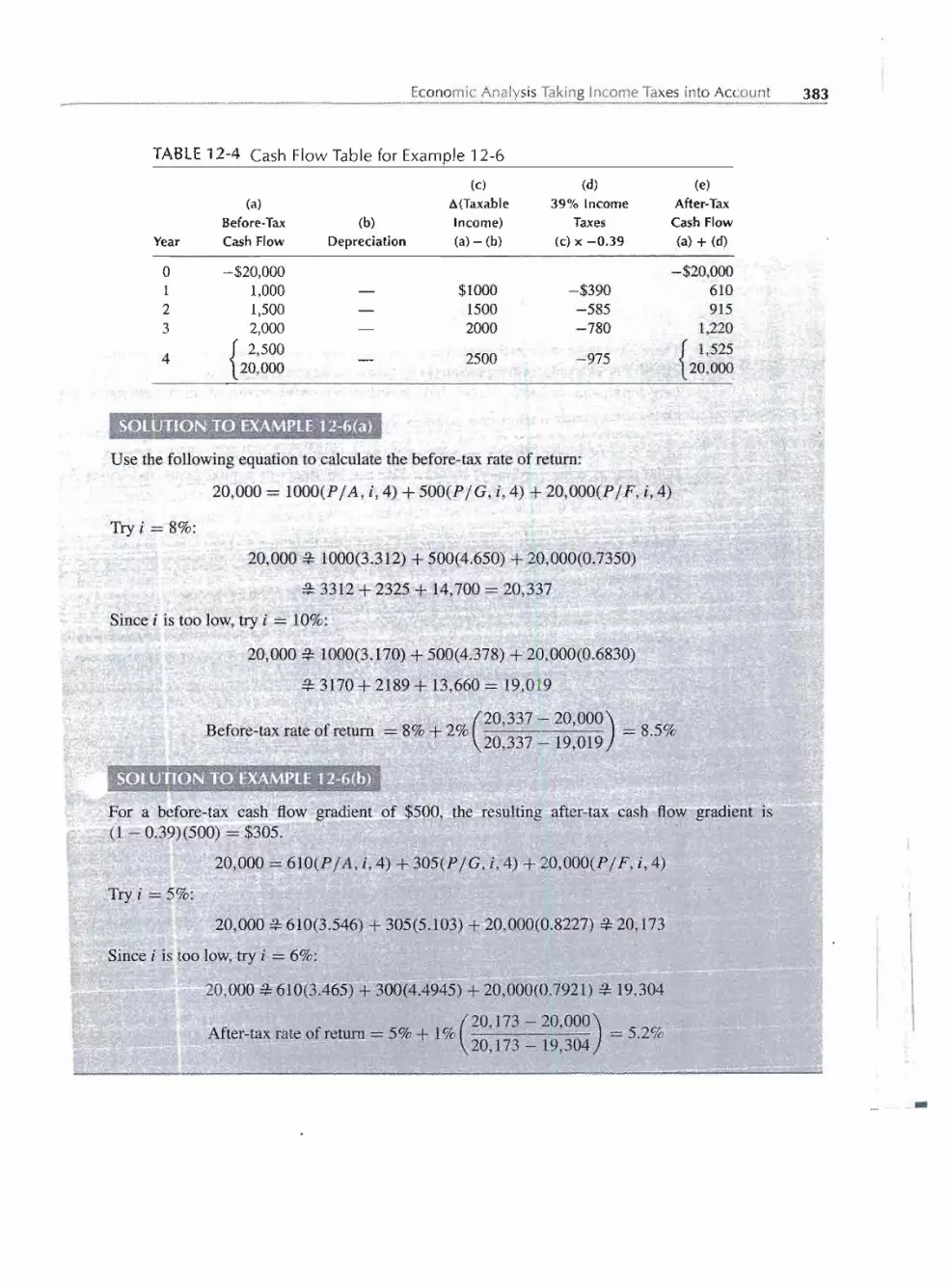
Economic Analysis Taking Income Taxesinto Account 383
SOlW. . :TlO....~(t.O ..EXAMPlE12=6(a).' ~. . ..,..' .
Use the following equation to calculate the before-tax rate of return:
20,000 = 1000(P / A, i, 4) + 500(P / G, i, 4) + 20,OOO(Pj F, i, 4)
Try i = 8%:
20,000 #=1000(3.312) + 500(4.650) + 20,000(0.7350)
#=3312+ 2325 + 14,700 = 20,337
Since i is too low, try i = 10%:
20,000 #=1000(3.170) + 500(4.378) + 20,000(0.6830)
#=3170 + 2189 + 13,660 = 19,019
(20,337 - 20,000
)Before-tax rate of return =8% + 2% .' = 8.5%20,337 - 19,019
For a before-tax cash flow gradie!lt of $500, the resulting after-tax cash flow gradient is(1 - 0.39)(500) = $305. .
20,000 = 61O(Pj A, i,4) + 305(P jG, i, 4) +.20,000(P / F, i, 4)
Try i =5%:
20,000 *610(3.546) + 305(5.103) + 20,000(0.8227) #=20, 173
Since i is too low,try i = 6%:
20;000 $olO(3~465r+ 3ot>(4:4945)+ 20,000(0.7921) i: 19,304
(20, 173 ~ 20,000
)After-tax. rate ofietnrn :::;.5%, +. J%'h " 04 ~ 5.2%-,~~ r:!t. ..' 20,173 _ 19,3
Id... iii II
\
TABLE 12-4 Cash Flow Table for Example 12-6
(c) (d) (e)(a) A(Taxable 39% Income After-Tax
Before-Tax (b) Income) Taxes CashFlowYear CashFlow Depreciation (a)- (b) (c) x -0.39 (a) +(d)
0 -$20,000 -$20,0001 1,000 - $1000 -$390 6102 1,500 - 1500 -585 9153 2,000 - 2000 -780 1,220
4{ 2,500
2500 -975{ 1,52520,000
-20,000

384 INCOME TAXES
CAPITAL GAINS AND LOSSES FOR NON DEPRECIATEDASSETS
When a nondepreciatedcapital asset is sold or exchanged,there must be entries in the firm'saccounting records to reflect the change. If the sellingprice of the capital asset exceeds theoriginal cost basis, the excess is called a capital gain. If the selling price is less thanthe original cost basis, the difference is a capital loss. Examples of nondepreciated assetsinclude stocks, land, art, and collectibles.
Capital [~~:] = Selling price - Original cost basis
There have been quite elaborate rules in the past for the tax treatment of capital gains andlosses. For example, nondepreciated capital assets held for more than 6 months produced.long-term gains or losses. Assets held less than 6 months produced short-ierm gains andlosses.
Current tax law sets the net capital gains tax at 20% for most assetsheld by individualsmore than one year. This is in 'contrast to recaptured depreciation, which is taxed at thesame rate as other (ordinary) income. The tax treatment of capital gains and losses fornondepreciatedassets is shownin Table 12-5.
TABLE12-5 Tax Treatment of Capital Gains and Losses
For Individuals
Capital gain
Capital loss
For assets held for less than I year, taxed as ordinary income.For assets held for more than 1 year, taxed at 20% tax rate.*
Subtract capital losses from any capital gains; balance may be deducted fromordinary income, but not more than $3000 per year. Excess capital losses maybe carried into future taxable years indefinitely.
For CorporationsCapital gain
Capital loss
Taxed as ordinary income.
Corporations may deduct capital losses only to the extent of capital gains.Any capital loss in the current year that exceeds capital gains can be carriedback 2 years, and, if not completely absorbed, is then carried forward forup to 20 years.
*Depending on tax bracket, type of asset, and duration of ownership the capital gain tax rate can rangefrom 8 to 28%. In addition, a special 0% capital gain tax rate applies to homeowners who treat theirhome as a primary residence for at least 2 years before selling. In such cases, single taxpayers areallowed $250,000 in tax-free gain ($500,000 for married couples).
Investment Tax Credit
When the economy slows down and unemploymentrises, the U.S. government frequentlyalters its tax laws to promote greater industrial activity.One technique used to stimulatecapital investments has been the investment tax credit. Businesses were able to deductfrom 4 to 8% of their new business equipmentpurchases as a tax credit.This meant that thefinn's net cost of the equipment was reduced by the amount of the investment tax credit.
I
J
I

-After-TaxCash Flows and Spreadsheets 385
Depending on the specific investment tax credit provisions, the credit might be subtracted,from the basis for depreciation, or the basis for computing depreciation might remain thefull cost of the equipment. The Tax Reform Act of 1986 eliminated the investment taxcredit. It is likely, however, that it will reappear at some future time.
ESTIMATING THE AFTER-TAX RATEOF RETURN
There is no shortcut method for computing the after-tax rate of return from the before-taxrate of return. One possible exception to this statement is in the situationof nondepreciableassets. In this special case, we have
After-tax rate of return= (1 - Incremental tax rate) x (Before-tax rate of return)
For Example 12-6,we could estimate the after-tax rate of return from the before-taxrate ofreturn as follows:
After-tax rate ofreturn = (1 - 0.39)(8.5%)= 5.2%
This value agrees with the value computed in Example 12-6(b).This relationship may be helpful for selecting a trial after-tax rate of return when the
before-tax rate of return is known. It must be emphasized, however, this relationship 'is onlya rough approximation in almost all situations.
AFTER-TAXCASH FLOWS AND SPREADSHEETS
The starting point for after-tax analysis is to calculate before-tax cash flows (BTCF) andtaxable income. Before-tax cash flows may include first costs and principal payments onloans, which are not tax deductible.Taxable income deducts depreciation-which is not acash flow.Once these principles are understood, spreadsheetscan help with the arithmetic.Taxes are computed based on taxable income, and after-tax cash flows are computed bysubtracting taxes from BTCF.
Realistic after-tax analysis requires spreadsheets. Even if costs and revenues are thesame every year, MACRS depreciation percentages are not. The steps for calculating'anafter-taxinternal rate of return are illustrated in Example 12-7.Becausesome cash flowsaretaxed and some are not, the spreadsheetis easier to build if these two classes are separated.Spreadsheet construction is easier, as well, if recaptured depreciationor other gainllossondisposal or sale is tabulated separately.
Taxes are considered even if only the costs of a project are known. The firm that d~esan engineering project must generate profits-or go out of business.Even if a firm has anunprofitable year, the tax law includes carry forward and backwardprovisions to transferdeductions to profitable years. The depreciation and revenues in Example 12-7 result in anegative taxable income for Year 2. Thus the positive cashflow due to taxes that is shownin Year 2 of Example 12-7 really represents tax savings for the firm.
---
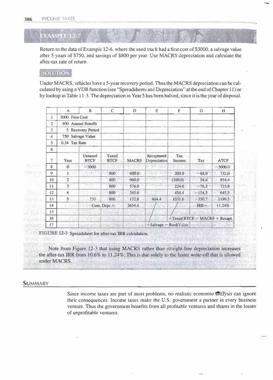
386 INCOME TAXES
Return to the data of Example 12-6,where the used truck had a firstcost of $3000, a salvagevalueafter 5 years of $750, and savings of $800 per year. Use MACRS depreciation and calculate theafter-tax rate of return.
Under MACRS, vehicles have a 5-year recovery period. Thus the MACRS depreciation can be cal-.culated by using a VDB function (see "Spreadsheets and Depreciation" at the end of Chapter 11) orby lookup in Table 11-3. The depreciation in Year 5 has been halved, since it is the year of disposal.
FIGURE 12-3 Spreadsheet for after-taxJRR calculation.
Note .from Figtire 12-3 that usingMACRS rather than straigl1Mine depreciation increasesthe after-tax 1RR from 10.6% fo 11..24%. This is due sQ!ely to the faster wriJe-offthat is allowedUl1derMACRS.
SUMMARY
Since income taxes are part of most problems, no realistic economie-~ysis can ignoretheir consequences. Income taxes make the U.S. government a partner in every businessventure. Thus the governmentbenefits from all profitable ventures and shares in the lossesof unprofitableventures.
--
A B C D E F G H1 3000 First Cost
2 800 Annual Benefit
3 5 Recovery Period4 750 Salvage Value5 0.34 Tax Rate
6
Untaxed Taxed Recaptured Tax7 Year BTCF BTCF I MACRS Depreciation Income Tax ATCF8 0 -3000 -3000.09 1 t 800 600.0 200.0 -68.0 732.010 2 800 960.0 (160.0) 54.4 854.4 .11 3 800 576.0 224.0 -76.2 723.812 4 800 345.6 454.4
I-154.5 645.5..
13 5 750 800 172.8 404.4 1031.6 .....,350.7 1199.314 Cum. Depr."'" 2654.4 i 7 7 IRR:::; 11.24%15 7 / .-16 / ""'.}'aJl:ed.BTCF - ;MACRS + Recapt.17
I=SaJvage - Boo.kValUe

Problems 387
The first step in computing individual income taxes is to tabulate gross income. Any~djustments-for example,allowabletaxpayer contributionsto a retirement fund-are sub-tracted to yield adjustedgross income. Personal exemptionsand either itemizeddeductionsor the standard deduction are subtracted to findtaxable income. This is used, togetherwitha tax rate table, to compute the income tax liability for the year.
For corporations,taxable income equalsgross income minus all ordinary andnecessaryexpenditures (except capital expenditures) and depreciation and depletion charges. The.income tax computation (whether for an individual or a corporation) is relatively simple,with rates ranging from 10to 39.6%. The proper rate to use in an economic analysis is theincremental tax rate applicable to the increment of taxable income being considered.
Most individuals and corporations pay state income taxes in addition to federal in-come taxes. Since state income taxes are an allowable deduction in computing federaltaxable income,it follows that the taxable income for the federal computation is lower thanthe state taxable income. .
Combined state and federal incremental tax rate
= L\Statetaxrate + (L\Federaltaxrate)(1- L\State tax rate)
Tointroducethe effectof income taxes intoan economicanalysis, the startingpoint is abefore-tax cash flow.Then the depreciation schedule is deducted from appropriateparts ofthe before-taxcash flowto obtain taxable income. Incometaxesare obtainedby multiplyingtaxable income by the proper tax rate. Before-tax cash flow less income taxes equals theafter-tax cash flow.
Current tax law has decreased long-term capital gains on most nondepreciated assetsfor individuals to 20% when held for more than 1 year and provided an exclusion on thegain of the principal residence held for more than 2 years.
When dealing with nondepreciable assets, there is a nominal relationship betweenbefore-tax and after-taxrate of return. It is
After-tax rate of return = (1 - L\Tax rate)(Before-tax rate of return)
There is no simple relationship between before-tax and after-tax rate of return in the moreusual case of investmentsinvolving depreciable assets.
PROBLEMS
_ These can be solved by hand, but most will be solved~ much more easily with a spreadsheet.
12-1 An unmarried taxpayer with no dependents expectsan adjusted gross income of $48,000 in a given year.His nonbusiness deductions are expected to be $3400.(a) What will his federal income tax be?(b) He is considering an additional activity expected
to increase his adjusted gross income. If this in-crease should be $16,000 and there should be nochange in nonbusiness deductions or exemptions,
what will be the increase in his federal incometax?
12-2 John Adams has a $50,000 adjusted gross incomefrom Apple Corp. and allowable itemized deductionsof $5000. Mary Eve has a $45,000 adjusted gross in~come and $2000 of allowable itemized deductions.
Compute the total tax they would pay as unmar-ried individuals. Then compute their tax as a marriedcouple filing a joint return. (Answers: $7618.50 +6336 = $13,954.50; $15,562.50)
~
-- -

388 INCOME TAXES
12-3 Bill Jackson worked during school and during the first2 months of pis summer vacation. After factoring inhis deductions and personal exemption as a singleman, Bill found that he had a total taxable incomeof $1800. Bill's employer wants him to work anothermonth during the summer, but Bill had planned tospend the month hiking. If an additional month's workwould increase Bill's taxable income by $1600, howmuch more money would he have after paying theincome tax? (Answer: $1440)
12-4 A married couple filing jointly have a combined totaladjusted gross income of $75,000. They have com-puted that their allowable itemized deductions are$4000. Compute their federal income tax.(Answer: $10,162.50) .
12-5 Jane Shay operates a management consulting busi-ness. The business has been successful and now pro-duces a taxable income of $65,000 per year after all"ordinary and necessary" expenses and depreciationhave been deducted. At present the business is oper-ated as a proprietorship; that is, Jane pays personalfederal income tax on the entire $65,000. For tax pur-poses, it is as if she had ajob that pays her a $65,000salary per year.
As an alternative, Jane is considering incorpo-rating the business. If she does, she will pay her-self a salary of $22,000 a year from the corporation.The corporation will then pay taxes on the remain-ing $43,000 and retain the balance of the money asa corporate asset. Thus Jane's two alternatives are tooperate the business as a proprietorship or as a cor-poration. Jane is single and has $2500 of itemizedpersonal deductions. Which alternative will result ina smaller total payment of taxes to the government?(Answer: Incorporation, $8280 versus $11,736)
12-6 Bill Alexander and his wife Valerie are both em-
ployed. Bill will have an adjusted gross income thisyear of $70,000. Valerie has an adjusted gross in-come of $2000 a month. Bill and Valerie have agreedthat Valerie should continue working only until thefederal income tax on their joint income tax returnbecomes $11,500. On what date should Valerie quither job?
12-7 A company wants to set up a new office in a countrywhere the corporate tax rate is asJollows: 15% of first$50,000 profits, 25% of next $25,000, 34% of next$25,000, and 39% of everything over $100,000. Ex-ecutives estimate that they will have gross revenues of$500,000, total costs of $300,000, $30,000 in allow-
---
able tax deductions, and a one time business start-upcredit of $8000. What is taxable income for the first
year and how much should the company expect to payin taxes?
12-8 ARKO oil company purchased two large compres-sors for $125,000 each. One compressor was installedin the firm's Texas refinery and is being depreciatedby MACRS depreciation. The other compressor wasplaced in the Oklahoma refinery, where it is being de- .
preciated by sum-of-years' -digits depreciation withzero salvage value. Assume the company pays fed-eral income taxes each year and the tax rate is Con-stant. The corporate accounting department noted thatthe two compressors are being depreciated differentlyand wonders whether the corporation will wind uppaying more income taxes over the life of the equip-ment as a result of this. What do you tell them?
12-9 Sole Brother Inc. is a shoe outlet to a major shoe man-ufacturing industry located in Chicago. Sole Brotheruses accounts payable as one of its financing sources.Shoes are delivered to Sole Brother with a 3% dis-
count if payment on the invoice is received within10 days of delivery. By paying after the lO-day pe-riod, Sole is borrowing money and paying (givingup) the 3% discount. Although Sole Brother is not re-quired to pay interest on delayed payments, the shoemanufacturers require that payments not be delayedbeyond 45 days after the invoice date. To be sure ofpaying within 10 days, Sole Brothers decides to payon the fifth day. Sole has a marginal corporate incometax of 40% (combined state and federal). By payingwithin the 10-day period, Sole is avoiding paying afairly high price to retain the money owed shoe manu-facturers. What would have been the effective annualafter-tax interest rate?
12-10 To increase its market share, Sole Brother Inc. decidedto borrow $5000 from its banker for the purchaseof newspaper advertising for its shoe retail line. Theloan is to be paid in four equal annual payments with15% interest. The loan is discounted 6 points. The6 "points" is an additional interest charge of 6% of theloan, deducted immediately. This additional interest6%(5000) = $300 means the actual amount receivedfrom the $5000 loan is $4700. The $300 additionalinterest may be deducted as four $75 additional an-nual interest payments. What is the after-tax interestrate on this loan?
12-11 A major industrialized state has a state corporate taxrate of 9.6% of taxable income. If a corporation has
----

Problems 389
a state taxable income of $150,000, what is the to-tal state and f~deral income tax it must pay? Also,compute its combined incremental state and federalincome tax rate. (Answers: $50,534; 43.93%)
12-12 An unmarried individual in California with a taxableincome of about $80,000 has a federal incrementaltax rate of 30% and a state incremental tax rate of9.3%. What is his combined incremental tax rate?
12-13 The Lynch Bull investment company suggests thatSteven Comstock, a wealthy New York City investor(his incremental income tax rate is 38.6%), considerthe following investment.
Buy corporate bonds on the New York Stock Ex-change with a face value (par value) of $100,000 anda 5% coupon rate (the bonds pay 5% of $100,000,which equals $5000 interest per year). These bondscan be purchased at their present market value of$75,000. At the end of each year, Steve will receivethe $5000 interest, and at the end of 5 years, when thebonds mature, he will receive $100,000 plus the last$5000 of interest.
Steve will pay for the bonds by borrowing$50,000 at 10% interest for 5 years. The $5000 inter-est paid on the loan each year will equal the $5000 ofinterest income from the bonds. As a result Steve will
have no net taxable income during the five years dueto this bond purchase and borrowing money scheme.
At the end of 5 years, Steve will receive $100,000plus $5000 interest from the bonds and will repay the$50,000 loan and pay the last $5000 interest. Thenet result is that he will have a $25,000 capital gain;that is, he will receive $100,000 from a $75,000 in-vestment. (Note: This situation represents an actualrecommendation of a brokerage firm.)(a) Compute Steve's after-tax rate of return on this
dual bond-plus-loan investment package.(b) What would be Steve's after-tax rate ofreturn if
he purchased the bonds for $75,000 cash and didnot borrow the $50,000?
12-14 Albert Chan decided to buy an old duplex as an in-vestment. After looking for several months, he founda desirable duplex that could be bought for $93,000cash. He decided that he would rent both sides of the
duplex, and determined that the total expected incomewould be $800 per month. The total annual expensesfor property taxes, repairs, gardening, and so forth areestimated at $600 per year. For tax purposes, Al plansto depreciate the building by the sum-of-years' -digitsmethod, assuming that the building has a 20-year
remaining life and no salvage value. Of the total$93,000 cost of the property, $84,000 represents thevalue of the building and $9000 is the value of the lot.Assume that Al is in the 38% incremental income tax
bracket (combined state and federal taxes) throughoutthe 20 years.
In this analysis Al estimates that the income an.dexpenses will remain constant at their present levels.If he buys and holds the property for 20 years, whatafter-tax rate of return can he expect to receive on hisinvestment, using the following assumptions?(a) Al believes the building and the lot can be sold at
the end of 20 years for the $9000 estimated valueof the lot.
(b) A more optimistic estimate of the future value ofthe building and the lot is that the property canbe sold for $100,000 at the end of 20 years.
12-15 Zeon, a large, profitable corporation, is consideringadding some automatic equipment to its productionfacilities. An investment of $120,000 will produce aninitial annual benefit of $29,000, but the benefits areexpected to decline $3000 per year, making second-year benefits $26,000, third-year benefits $23,000,and so forth. If the firm uses sum-of-years' -digits de-preciation, an 8-year useful life, and $12,000 salvagevalue, will it obtain the desired 6% after-tax rate ofreturn? Assume that the equipment can be sold for its$12,000 salvage value at the end of the 8 years. Alsoassume a 46% income tax rate for state and federaltaxes combined.
12-16 A group of businessmen formed a corporation to leasefor 5 years a piece of land at the intersection of twobusy streets. The corporation has invested $50,000in car-washing equipment. They will depreciate theequipment by suin-of-years'-digits depreciation, as-suming a $5000 salvage value at the end of the 5 yearuseful life. The corporation is expected to have abefore-tax cash flow, after meeting all expenses ofoperation (except depreciation), of $20,000 the firstyear, declining $3000 per year in future years (secondyear = $17,000, third year = $14,000, etc.). The cor-poration has other income, so it is taxed at a combinedcorporate tax rate of 20%. If the projected income iscorrect, and the equipment can be sold for $50oo.atthe end of 5 years, what after-tax rate of return wouldthe corporation receive from this venture?(Answer: 14%)
12-17 The effective combined tax rate in an owner-managedcorporation is 40%. An outlay of $20,000 for certain

390 INCOME TAXES
-,
new assets is under consideration. It is estimated that
for the next 8 years, these assets will be responsi-ble for annual receipts of $9000 and annual disburse-ments (other than for income taxes) of $4000. Mterthis time, they will be used only for stand-by purposes,and no future excess of receipts over disbursementsis estimated.
(a) What is the prospective rate ofretum before in-come taxes?
(b) What is the prospective rate of return after taxesif straight-line depreciation can be used to writeoff these assets for tax purposes in 8 years?
(c) What is the prospective rate of return after taxesif it is assumed that these assets must be written
off for tax purposes over the next 20 years, usingstraight-line depreciation?
12-18 A firm is considering the following investmentproject:
Yearo1234
5
Before-TaxCash Flow
(thousands)-$1000
+500+340+244+100
{
+100
}+ 125 Salvage value
The project has a 5-year useful life with a $125,000salvage value, as shown. Double declining balancedepreciation will be used, assuming the $125,000
, salvage value. The income, tax rate is 34%. If thefirm requires a 10% after-tax rate of return, shouldthe project be undertaken?
12-19 The Shellout Corp. owns a piece of petroleum drillingequipment that costs $100,000 and will be depreci-ated in 10 years by double declining balance depre-ciation, with conversion to straight-line depreciationat the optimal point. Assume no salvage value in thedepreciation computation and a 34% tax rate. Shell-out will lease the equipment to others and each yearreceive $30,000 in rent. At the end of 5 years, thefirm will sell the equipment for $35,000. (Note thatthis is different from the zero-salvage-value assump-tion used in computing the depreciation.) What is theafter-tax rate of return Shellout will receive from this
equipment investment?
-------
12-20 A mining corporation purchased $120,000 of produc-tion machinery and depreciated it using SOYD de-preciation, a 5-year depreciable life, and zero salvagevalue. The corporation is a profitable one that has a34% incremental tax rate.
At the end of 5 years the mining companychanged its method of operation and sold the pro-duction machinery for $40,000. During the 5' yearsthe machinery was used, it reduced mine operatingcosts by $32,000 a year, before taxes. If the companyMARR is 12% after taxes, was the investment in the
machinery a satisfactory one?
12-21 An automobile manufacturer is buying some specialtools for $100,000. The tools are being'depreciated'by double declining balance depreciation using a 4-year depreciable life and a $6250 salvage value. Itis expected the tools will actually be kept in servicefor 6 years and then sold for $6250. The before-taxbenefit of owning the tools is as follows:
Before-TaxCash Flow'$30,000
30,00035,00040,00010,00010,0006,250 Selling price
Compute the after-tax rate of return for this invest-ment situation, assuming a 46% incremental tax rate.(Answer: 11.6%)
12-22 This is the continuation of Problem 12-21. Insteadof paying $100,000 cash for the tools, the corpora-tion will pay $20,000 ~ow and borrow the remaining$80,000. The depreciation schedule will remain un-changed. The loan will be repaid by 4 equal end-of-year payments of $25,240.
Prepare an expanded cash flow table that takesinto account both the special tools and the loan.(a) Compute the after-tax rate of return for the tools,
taking into account the $80,000 loan.(b) Explain why the rate of return obtained in part
(a) is different from the rate of return obtained inProblem 12-21.
Hints: 1. Interest on the loan is 10%, $25,240 =80,000 (AlP, 10%,4). Each payment ismade up of part interest and part principal.Interest portion for any year is 10% of bal-ance due at the beginning of the year.
Year12345'6

Problems 391
2. Interest payments are tax deductible (i.e.,they re,duce taxable income and thus taxespaid). Principal payments are not. Sepa-rate each $25,240 payment into interest andprincipal portions.
3. The Year-Ocash flow is -$20,000 (100,000- 80,000).
4. After-tax cash flow will be before-tax
cash flow - interest payment - principalpayment - taxes.
12-23 A project will require the investment of $108,000 inequipment (sum-of-years' -digits depreciation with adepreciable life of 8 years and zero salvage value)and $25,000 in raw materials (not depreciable). Theannual project income after all expenses except de-preciation have been paid is projected to be $24,000.At the end of 8 years the project will be discontinuedand the $25,000 investment in raw materials will berecovered.
Assume a 34% income tax rate for this corpo-ration. The corporation wants a 15% after-tax rate ofreturn on its investments. Determine by present worthanalysis whether this project should be undertaken.
12-24 A profitable incorporated business is considering aninvestment in equipment having the following before-tax cash flow. The equipment will be depreciated bydouble declining balance depreciation with conver-sion, if appropriate, to straight-line depreciation atthe preferred time. For depreciation purposes a $700salvage value at the end of 6 years is assumed. Butthe actual value is thought to be $1000 and it is thissum that is shown in the before-tax cash flow.
Year
o123456
Before-Tax Cash Flow$12,000
1,7272,4142,8723,1773,3581,9971,000Salvagevalue
If the firm wants a 9% after-tax rate of return and
its incrementalincometax rate is 34%, determinebyannual cash flow analysis whether the investmentisdesirable.
12-25A salad oil bottlingplant can eitherpurchasecaps forthe glass bottles at 5 cents each or install $500,000worthof plastic moldingequipmentand manufacture
-----
the caps at the plant. The manufacturing engineer es-timates the material, labor, and other costs would be3 cents per cap.(a) If 12 million caps per year are needed and the
molding equipment is installed, what is the pay-back period?
(b) The plastic molding equipment would be depre-.ciated by straight-line depreciation using a 5-yearuseful life and no salvage value. Assuming a 40%income tax rate, what is the after-tax payback pe-riod, and what is the after-tax rate of return?
12-26 A firm has invested $14,000 in machinery with a 7-year useful life. The machinery will have no salvagevalue, as the cost to remove it will equal its scrapvalue. The uniform annual benefits from the machin-
ery are $3600. For a 47% income tax rate, and sum-of-years' -digits depreciation, compute the after-tax rat~of return.
12-27 A firm manufactures padded shipping bags. Onehundred bags are packed in a cardboard carton. Atpresent, machine operators fill the cardboard cartonsby eye: that is, when the cardboard carton looks full,it is assumed to contain 100 shipping bags. Actualinspection reveals that the cardboard carton may con-tain anywhere from 98 to 123 bags with an averagequantity of 105.5 bags.
The management has never received complaintsfrom its customers about cartons containing fewerthan 100 bags. Nevertheless, management realizesthat they are giving away 51/2% of their output byoverfilling the cartons. One solution would be to countthe shipping bags to ensure that 100 are packed in eachcarton. Another solution would be to weigh each filledshipping carton. Underweight cartons would have ad-ditional shipping bags added, and ov~ht cartonswould have some shipping bags removed. This wouldnot be a perfect solution because the actual weight ofthe shipping bags varies slightly. If the weighing isdone, it is believed that the average quantity of bagsper carton could be reduced to 102, with almost nocartons containing fewer than 100 bags.
The weighing equipment would cost $18,600.The equipment would be depreciated by straight-linedepreciation using a lO-year depreciable life and a$3600 salvage value at the end of 10 years. The$18,600 worth of equipment qualifies for a 10% in-vestment tax credit. One person, hired at a cost of$16,000 per year, would be required to operate theweighing equipment and to add or remove padded
, .
l-'~~h.

392 INCOME TAXES
bags from the cardboard cartons. 200,000 cartonswill be ,checked on the weighing equipment eachyear, with an average removal of 3.5 padded bags percarton with a manufacturing cost of 3 cents per bag.This large profitable corporation has a 50% combinedfederal-plus-state incremental tax rate. Assume alO-year study period for the analysis and an after-taxMARR of 20%.
Compute:(a) The after-tax present worth of this investment.(b) The after-tax internal rate of return of this
investment.
(c) The after-tax simple payback period of thisinvestment.
12-28 Mr. Sam K. Jones, a successful businessman, is con-sidering erecting a small building on a commerciallot he owns very close to the center of town. A localfurniture company is willing to lease the building for$9000 per year, paid at the end of each year. It is a netlease, which means the furniture company must alsopay the property taxes, fire insurance, and all otherannual costs. The furniture company will require a5-year lease with an option to buy the building andland on which it stands for $125,000 at the end ofthe 5 years. Mr. Jones could have the building con-structed for $82,000. He could sell the commercial
lot now for $30,000, the same price he paid for it. Mr.Jones files a joint return and has an annual taxableincome from other sources of $63,900. He would de-preciate the commercial building by modified accel-erated cost recovery system (MACRS) depreciation.Mr. Jones believes that at the end of the 5-year leasehe could easily sell the property for $125,000. Whatis the after-tax present worth of this 5-year venture ifMr. Jones uses a 10% after-taxMARR?
12-29 One January Gerald Adair bought a small house andlot for $99,700. He estimated that $9700 of thisamount represented the value of the land. He rentedthe house for $6500 a year during the 4 years he ownedthe house. Expenses for property taxes, maintenance,and so forth were $500 per year. For tax purposesthe house was depreciated by MACRS depreciation(27.5-year straight-line depreciation with a midmonthconvention is used for rental property). At the end of4 years the property was sold for $105,000. Gerald ismarried and works as an engineer. He estimates thathis incremental state and federal combined tax rate is24%. What after-tax rate of return did Gerald obtain
on his investment in the property?
-12-30 A corporation with a 34% income tax rate is consider_
ing the following investment in research equipmentand has projected the benefits as follows: '
Yearo123456
Before-TaxCash Flow-$50,000
+2,000+8,000
+17,600+ 13,760+5,760+2,880
Prepare a cash flow table to determine the year-by-year after-tax cash flow assuming MACRSdepreciation.(a) What is the after-tax rate.ofreturn? .(b) What is the before-tax rate of return?
12-31 An engineer is working on the layout of a new re-search and experimentation facility. Two plant op-erators will be required. If, however, an. additional$100,000 of instrumentation and remote controlswere added, the plant could be run by a single oper~-tor. The total before-tax cost of each plant operator isprojected to be $35,000 per year~The instrumentationand controls will be depreciated by means of the mod-ified accelerated cost recovery system (MACRS).
If this corporation (34% corporate tax rate) in-vests in the additional instrumentation and controls,how long will it take for the after-tax benefits to equalthe $100,000 cost? In other words, what is the after-tax payback period? (Answer: 3.24 years).
12-32 A special power tool for plastic products costs $400,has a 4-year useful life, no salvage value, and a 2-yearbefore-tax payback period. Assume uniform annualend-of-year benefits.(a) Compute the before-tax rate of return.(b) Compute the after-tax rate of return, based on
MACRS depreciation and a 34% corporate in-come tax rate.
12-33 The Ogi Corporation, a construction company, pur-chased a pickup truck for $14,000 and used MACRSdepreciation in the income tax return. During the timethe company had the truck, they estimated that it saved$5000 a year. At the end of 4 years, Ogi sold the truckfor $3000. The combined federal and state income
tax rate for Ogi is 45%. Compute the after-tax rate ofreturn for the truck. (Answer: 12.5%)
-- ---

Problems 393
12-34 A profitable wood products corporation is consid-ering buying a parcel of land for $50,000, buildinga small factory building at a cost of $200,000, andequipping it with $150,000 of MACRS 5-year classmachinery.
If the project is undertaken, MACRS deprecia-tion will be used. Assume the plant is put in serviceOctober 1.The before-tax net annual benefit from the
project is estimated at $70,000 per year. The analysisperiod is to be 5 years, and planners assume the saleof the total property (land, building, and machinery)at the end of 5 years, also on October 1, for $328,000.Compute the after-tax cash flow based on a 34% in-come tax rate. If the corporation's criterion is a 15%after-tax rate of return, should it proceed- with theproject?
12-35 A small vessel was purchased by a chemical companyfor $55,000 and is to be depreciated by MACRS de-preciation. When its requirements changed suddenly,the chemical company leased the vessel to an oil com-pany for 6 years at $10,000 per year. The lease alsoprovided that the vessel could be purchased at the endof 6 years by the oil company for $35,000. At the endof the 6 years, the oil company exercised its optionand bought the vessel. The chemical company has a34% incremental tax rate. Compute its after-tax rateof return on the vessel. (Answer: 9.86%)
12-36 Xon, a small oil company, purchased a new petroleumdrilling rig for $1,800,000. Xon will depreciate thedrilling rig using MACRS depreciation. The drillingrig has been leased to a drilling company, which willpay Xon $450,000 per year for 8 years. At the endof 8 years the drilling rig will belong to the drillingcompany. If Xon has a 34% incremental tax rate anda 10% after-tax MARR, does the investment appearto be satisfactory?
12-37 The profitable Palmer Golf Cart Corp. is consideringinvesting $300,000 in special tools for some of theplastic golf cart components. Executives of the com-pany believe the present golf cart model will continueto be manufactured and sold for 5 years, after whicha new cart design will be needed, together with a dif-ferent set of special tools.
The saving in manufacturing costs, owing to thespecial tools, is estimated to be $150,000 per year for5 years. Assume MACRS depreciation for the specialtools and a 39% income tax rate.
(a) What is the after-tax payback period for thisinvestment?
(b) If the company wants a 12% after-tax rate ofre-turn, is this a desirable investment?
12-38 Uncle Elmo is contemplating a $10,000 investmentin a methane gas generator. He estimates his grossincome would be $2000 the first year and increase by$200 each year over the next 10years. His expenses of$200 the first year would increase by $200 each yearover the next 10 years. He would depreciate the gen-erator by MACRS depreciation, assuming a 7-yearproperty class. A lO-year-old methane generator hasno market value. The income tax rate is 40%. (Re-member that recaptured depreciation is taxed at thesame 40% rate).(a) Construct the after-tax cash flow for the 10 year
project life.(b) Determine the after-tax rate ofreturn on this in-
vestment. Uncle Elmo thinks it should be at least8%.
(c) If Uncle Elmo could sell the generator for $7000at the end of the fifth year, would his rate of returnbe better than if he kept the generator for 10years?You don't have to actually find the rate of return,Just do enough calculations to see whether it ishigher than that of part (b).
12-39 Granny's Butter and Egg Business is such that shepays an effective tax rate of 40%. Granny is consider-ing the purchase of a new Thrbo Churn for $25,000.This churn is a special handling device for food man-ufacture and has an estimated life of 4 years and asalvage value of $5000. The new churn is expectedto increase net income by $8000 per year for eachof the 4 years of use. If Granny works with an after-tax MARR of 10% and uses MACRS depreciation,should she buy the churn? -
12-40 Eric Heiden has a house aDdlot for sale for $70,000.It is estimated that $10,000 is the value of the landand $60,000 is the value of the house. Bonnie Blair ispurchasing the house on January 1 to rent and plansto own the house for 5 years. After 5 years, it is ex-pected that the house and land can be sold on Decem-ber 31 for $80,000. Total annual expenses (mainte-nance, property taxes, insurance, etc.) are expected tobe $3000 per year. The house would be depreciatedby MACRS depreciation using a 27.5-year straight-line rate with midmonth convention for rental prop-erty. For depreciation, a salvage value of zero wasused. Bonnie wants a 15% after-tax rate of return Oijher investment. You may assume that Bonnie has anincremental income tax rate of 27% in each ofthe
"
- - --

394 INCOME TAXES
..,
5 years. Capital gains are taxed at 20%. Detenninethe following:(a) The annual depreciation.(b) The capital gain (loss) resulting from the sale of
the house.
(c) The annual rent Bonnie must charge to producean after-tax rate of return of 15%. (Hint: Write analgebraic equation to solve for rent.)
12-41 Bill Cavitt owns a data processing company. He plansto buy an additional computer for $20,000, use thecomputer for 3 years, and sell it for $10,000. He ex-pects that use of the computer will produce a net in-come of $8000 per year. The combined federal andstate incremental tax rate is 45%. Using MACRS de-preciation, complete Table P12-41 to detennine thenet present worth of the after tax cash flow using aninterest rate of 12%.
12-42 Refer to Problem 12-33. To help pay for the pickuptruck the Ogi Corp. obtained a $10,000 loan from thetruck dealer, payable in four end-of-year paymentsof $2500 plus 10% interest on the loan balance eachyear.(a) Compute the after-tax rate of return for the truck
together with the loan. Note that the interest onthe loan is tax deductible, but the $2500 principalpayments are not.
(b) Why is the after-tax rate of return computed inpart (a) so much different from the 12.5% ob-tained in Problem 12-33?
12-43 A store owner, Joe Lang, believes his business hassuffered from the lack of adequate customer park-ing space. Thus, when he was offered an opportu-nity to buy an old building and lot next to his store,he was interested. He would demolish the old build-
ing and make off-street parking for 20 customers'
cars. Joe estimates that the new parking would in-crease his business and produce an additional before-income-tax profit of $7000 per year. It would cost$2500 to demolish the old building. Mr. Lang's ac-countant advised that both costs (the property anddemolishing the old building) would be consideredto comprise the total value of the land for tax pur-poses, and it would not be depreciable. Mr. Langwould spend an additional $3000 right away to puta light gravel surface on the lot. This expenditure,he believes, may be charged as an operating expenseimmediately and need not be capitalized. To computethe tax consequences of adding the parking lot, Joeestimates that his combined state and federal incre.-mental income tax rate will average 40%. If Joe wantsa 15% after-tax rate of return from this project, howmuch could he pay to purchase the adjoining landwith the old building? Assume that the analysis pe-riod is 10 years and that the parking lot could alwaysbe sold to recover the costs of buying the property anddemolishing the old building. (Answer: $23,100)
12-44 The management of a private hospital is consider-ing the installation of an automatic telephone switch-board, which would replace a manual switchboardand eliminate the attendant operator's position. Theclass of service provided by the new equipment is es-timated to be at least equal to the present method ofoperation. To provide telephone service, five opera-tors will work three shifts per day, 365 days per year.Each operator earns $14,000 per year. Company-paidbenefits and overhead are 25% of wages. Money co'sts8% after income taxes. Combined federal and state in-
come taxes are 40%. Annual property taxes and main-tenance are 21;2 and 4% of investment, respectively.Depreciation is I5-year straight line. Disregarding
--
After-Tax PresentYear I Cash Flow Depreciation Tax (45%) Cash Flow Worth (12%)
0 -$20,000
1 +8,000
2 +8,000
3 +8,000-+10,000
I I
Net Present worth =

Problems 395
inflation, how large an investment in the new equip-ment can be eQonomically justified by savings ob-tained by eliminating the present equipment and laborcosts? The existing equipment has zero salvage value.
12-45 A contractor has to choose one of the following alter-natives in performing earth-moving contracts:(a) Purchase a heavy-duty truck for $13,000. Salvage
value is expected to be $3000 at the end of thevehicle's 7-year depreciable life. Maintenance is$1100 per year. Daily operating expenses are $35.
(b) Hire a similar unit for $83 per day.
Based on a 10% after-tax rate of return, how manydays per year must the truck be used to justify itspurchase? Base your calculations on straight-linedepreciation and a 50% income tax rate.(Answer: 91 Y2 days)
1" ") The Able Corporationis consideringthe installationof a small electronic testing device for use in con-junction with a government contract the firm has justwon. The testing device will cost $20,000, and havean estimated salvage value of $5000 in 5 years whenthe government contract is finished. The firm will de-preciate the instrument by the sum-of-years' -digitsmethod, using 5 years as the useful life and a $5000salvage value. Assume that Able pays 50% federaland state corporate income taxes and uses 8% after-tax in economic analysis. What minimum equal an-nual benefit must Able obtain before taxes in each ofthe 5 years to justify purchasing the electronic testingdevice? (Answer: $5150)
12-47 A house and lot are for sale for $155,000. It is es-timated that $45,000 is the value of the land and$110,000 is the value of the house. If purchased,the house can be rented to provide a net income of$12,000 per year after taking all expenses, except de-preciation, into account. The house would be depre-ciated by straight line depreciation using a 27.5-yeardepreciable life and zero salvage value.
Mary Silva. the prospective purchaser, wants a10% after-tax rate of return on her investment after
considering both annual income taxes and a capitalgain when she sells the house and lot. At what pricewould she have to sell the house at the end of 10 yearsto achieve her objective? You may assume that Maryhas an incremental income tax rate of 27% in each of
the 10 years.
12-48 A corporation is considering buying a medium-sizedcomputer that will eliminate a task that must be per-formed three shifts per day, 7 days per week, except
for one 8-hour shift per week when the operationis shut down for maintenance. At present four peo-ple are needed to perform the day and night tasks.Thus the computer will replace four employees. Eachemployee costs the company $32,000 per year($24,000 in direct wages plus $8000 per year in othercompany employee costs). It will cost $18,000 pe~year to maintain and operate the computer. The com-puter will be depreciated by sum-of-years' -digits de-preciation using a 6-year depreciable life, at whichtime it will be assumed to have zero salvage value.
The corporation has a combined federal and stateincremental tax rate of 50%. If the firm wants a 15%
rate of return, after considering both state and federalincome taxes, how much can it afford to pay for thecomputer?
12-49 A sales engineer has the following alternatives .toconsider in touring his sales territory.(a) Buy a new car for $14,500. Salvage value is ex-
pected to be about $5000 after 3 years. Main-tenance and insurance cost is $1000 in the first
year and increases at the rate of $500/year insubsequent years. Daily operating expenses are$50/day.
(b) Rent a similar car for $80/day.
Based on a 12% after-tax rate of return, how manydays per year must he use the car to justify its pur-chase? You may assume that this sales engineer isin the 30% incremental tax bracket. Use MACRS
depreciation.
12-50 A large profitable company, in the 40% federal/statetax bracket, is considering the purchase of a new pieceof equipment. The new equipment will yield benefitsof $10,000 in Year 1, $15,000 in Year 2, $20,000 in.Year 3, and $20,000 in Year4. The equipment is to bedepreciated using 5-year MACRS depreciation start-ing in the year of purchase (Year0). It is expected thatthe equipment will be sold at the end of fourth yearat 20% of its purchase price. What is the maximumequipment purchase price the company can pay if iisafter-tax MARR is 1O%?
12-51 A prosperous businessman is considering two alter-native investments in bonds. In both cases the first
interest payment would be received at the end ofthe first year. If his personal taxable income is fixedat $40,000 and he is single, which investment pro-duces the greater after-tax rate of return? Compute theafter-tax rate of return for each bond to within y4 of1 percent.
H_81'
1"_I:
- - - -

396 INCOME TAXES
'I
Ann Arbor Municipal Bonds: A bond with a facevalue of $1000 pays $60 per annum. At the endof 15 years, the bond becomes due ("matures"),at which time the owner of the bond will receive
$1000 plus the final $60 annual payment. Thebond may be purchased for $800. Since it is amunicipal bond, the annual interest is not subjectto federal income tax. The difference between
what the businessman would pay for the bond($800) and the $1000 face value he would re-ceive at the end of 15 years must be included intaxable income when the $1000 is received.
Southern Coal Corporation Bonds: A thousand-dollar bond yields $100 per year in annual inter-est payments. When the bonds mature at the endof 20 years, the bondholder will receive $1000plus the final $100 interest. The bonds may bepurchased now for $1000. The income from cor-poration bonds must be included in federal tax-able income.
12-52 A small-business corporation is considering whetherto replace some equipment in the plant. An analy-sis indicates there are five alternatives in addition to
the do-nothing option, Alt. A. The alternatives have a5-year useful life with no salvage value. Straight-linedepreciation would be used.
AlternativesABCDEF
Cost(thousands)
$ 025105
1530
Before-Tax UniformAnnual Benefits
(thousands)$0
7.531.758.7
The corporation has a combined federal and state in-come tax rate of 20%. If the corporation expects a10% after-tax rate of return for any new investments,which alternative should be selected?
12-53 A corporation with $7 million in annual taxableincome is considering two alternatives:
Before-TaxCash Flow
Year Alt. 1 Alt. 2
o1-1011-20
-$10,0004,500
o
-$20;0004,5004,500
Both alternatives will be depreciated by straight-linedepreciation assuming a lO-year depreciable life andno salvage value. Neither alternative is to be replacedat the end of its useful life. If the corporation has a
minimum attractive rate of return of 10% after taxes,which alternative should it choose? Solve the problemby:(a) Present worth analysis(b) Annual cash flow analysis(c) Rate of return analysis(d) Future worth analysis(e) Benefit-cost ratio analysis(f) Any other method you choose
12-54 Two mutually exclusive alternatives are being Con'-sidered by a profitable corporation with an annualtaxable income between $5 million and $10 million.
Both alternatives have a 5-yearuseful and depreciablelife and no salvage value. Alternative A would be de-preciated by sum-of-years' -digits depre,ciation, andAlt. B by straight-line depreciation. If the MARR is10% after taxes, 'Yhich alternative should"beselected?(Answer: Alt. B)
12-55 A large profitable corporation is considering twomutually exclusive capital investments:
Alt. A
$11,0003,0002,000
Alt. B
$33,0009,0003,000
Initial costUniform annual benefit
End-of-depreciable-lifesalvage value
Depreciation methodEnd-of -useful-life
salvage value obtainedDepreciable life, in years 3 4Useful life, in years 5 5
J
~
If the firm's after-tax minimum attractive rate of re-
turn is 12% and its incremental income tax rate is ....
34%, which project should be selected?~,
SL2,000
SOYD5,000
- --
Before-Tax Cash Flow
Year Alt. A Alt. B
0 -$3000 -$50001 1000 10002 1000 12003 1000 14004 1000 26005 1000 2800

Problems 397
12-56 Assume that you are debating whether to lease a caror buy one to U$e exclusively in business. The es-timated mileage in both cases will be 12,000/year.Insurance costs will be the same in either case at $600per year. You want to examine the tax impacts of thetwo options to see which is preferred. Use MACRSdepreciation.
Assume that you will have leased or purchasedthe car on June 30, 2003, and that your intend to keepthe car for 36 months. List any assumptions that youmake in your analysis. Use a 12% MARR, a 40% taxrate, and assume end of year payments.
Lease option: $2250 down and $369 a month for36 months.
Purchase option: The car that you are interestedin lists for $29,188 and the dealer finance plancalls for 30 monthly payments of $973 with nomoney down and 0% interest. Estimated valueafter 36 months $15,200. Remember that the taxlaw limits the depreciation on cars according tothe following rule:
Depreciation Limitation on AutomobilesPurchased During 2003TaxYear Amount
FirstSecondThirdFourth and later
$7660490029501775
12-57 A plant can be purchased for $1,000,000 or it can beleased for $200,000 per year. The annual income isexpected to be $800,000 with the annual operatingcost of $200,000. The resale value of the plant is es-timated to be $400,000 at the end of its lO-year life.The company's combined federal and state incometax rate is 40%. A straight-line depreciation can beused over the 10 years with the full first-year depr~-ciation rate.
(a) If the company uses ~e after-tax minimum at-tractive rate of return of 10%, should it lease orpurchase the plant?
(b) What is the breakeven rate of return of purchaseversus lease?
- -- - ----

1J
I
;,~~-~... ,, ;..-~': -.,=-~-. - J;.A- :~.
.~~ ...u...~
After Completing This Chapter...The student should be able to:· Recast an equipment reinvestment decision as a challenger versus defender analysis.· Use the replacementanalysis decision map to select the appropriate economic.analysis
technique to apply. .· Calculate the minimum cost life of economic challengers.· "Incorporate concepts such as repeatability assumption for replacement analysisand marginal cost datafor the defender to select the appropriate economic analysistechniques.· Perform replacement problems on an after-tax basis, utilizing the defender sign changeprocedure when appropriate.· Use spreadsheetsfor solving before-tax and after-taxreplacement analysis problems.
QUESTIONS TO CONSIDER ;:0,
1. Using the Internet, can you determine what it would cost Intel to build a new fab fromscratch?
2. Will Intel need to scrap all its current production assets when it does the upgrade?3. How might Intel determinewhat to keep in operation and what to purchase new?
,
I
j
, - :, -

...-- - -- -- --
I
lReplacement Analysis
The $2 Billion UpgradeIn February 2003, Intel.CorPoration announced it was planning to spend $2 billion tomodernize and update its silicon wafer manufacturing plant in Chandler, Arizona. Theupgradewill allowIntel to manufacture300-millimeterchips,rather than the 200-:millimeter.size it had been producing at the plant, known as "Fab 12."The project is also expectedtodouble manufacturing capacity at the facility,while loweringoverall operating costs.
Upgrade work will probably take over a year to be completed. It willinclude remodeling the interior of the plant, and will require Intel to buynew wafer fabrication tools.
Despite the seeminglyhuge price tag for the project,Intel statesthat itwill be savingmoneyby upgradingthe existingfabricationfacilityinsteadof buildinga newone. Thecompanyalso noted that, by deciding to remainin its currentlocation,it wouldbe abletoretainits currentworkforce,whichis highly skilled.
Moreover,the new,largerwaferwill accommodatemore chips,whichshould lower production costs at the plant. The upgraded plant will alsouse a newerprocess that allowschips to hold smaller and faster transistors.
- .
I.....
- --

,400 REPLACEMENTANALYSIS
Up to this point in our economic analysis we have considered the evaluationand selectionof new alternatives. Which new car or washing machine should we purchase? What newmaterial handling system or ceramic grinder should we install? However,a choice betweennew alternatives is not always what we must consider--economic analysis weighs morefrequently existing versusnew facilities. For most engineers the problem is less likely to beone of building a new plant; rather the goal is more often keeping a present plant operatingeconomically.We are not choosingbetween new ways to perform the desired task. Instead,we have equipmentperformingthe task, and the questionis, Should the existingequipmentbe retained or replaced? This adversarial situation has given rise to the terms defenderand challenger. The defender is the existing equipment; the challenger is the best availablereplacementequipment.An economicevaluationof the existingdefenderand the challengerreplacement is the domain of replacement analysis.
THE REPLACEMENT PROBLEM
The replacement of an existing asset may be appropriate in various situations includingobsolescence, depletion, and deterioration due to aging. In each of these cases, the abilityof a previously implemented business asset to produce a desired output is challenged.Forcases of obsolescence, depletion, and aging, it may be economical to replace the existingasset. We defineeach of these situations.
Obsolescence: Occurs when the technology of an asset is surpassed by newer and/ordifferent technologies. Changes in technology cause subsequent changes in themarket demand for older assets. As an example,today's personal computers(PCs)with moreRAM, faster clockspeeds, largerhard drives,and more powerfulcentralprocessorshavemadeolder, lesspowerfulPCs obsolete.Thus, obsoleteassetsmayneed to be replaced with newer,more technologicallyadvanced ones. .
Depletion: The gradual loss of market value of an asset as it is being consumed orexhausted. Oil wells and timber tracts are examples of such assets. In most casesthe asset will be used until it is depleted, at which time a replacement asset will beobtained. Depletion was treated in Chapter 11.. .
Deteriorationdue to aging: The general conditionofloss in valueof some asset due tothe aging process. Production machinery and other business assets that were oncenew eventuallybecome aged. To compensate for a loss in functionality due to theagingprocess, additionaloperatingand maintenanceexpensesare usually incurredto maintain the asset at its operating efficiency.
Aging equipment often has a greaterrisk of breakdowns.Planned replaceII}entscan bescheduled to minimize the time and cost of disruptions. Unplanned replacements can bevery costly or even, as with an airplane engine, potentially catastrophic.
In industry, as in government, expenditures are normally monitored by means ofannual budgets.One important facet of a budget is the allocation of money for new capitalexpenditures, either new facilitiesor replacement and upgrading of existing facilities.
- ---

.. ..- ....-.........
What Is the Basic Comparison? 401
Replacement analysis may, therefore, produce a recommendation that certain equip-ment be replaced and money for the rephicement be included in the capital expendituresbudget. Even if there is no recommendation to replace the equipment at the current time,such a recommendationmay be made the following year or subsequently.At some point,the existingequipmentwill bereplaced, either when it is no longernecessaryor whenbetterequipment is available.Thus, the question is not if the defender will be replaced, but whl!nit will be replaced.This leads us to the first aspect of the defender-challenger comparison:
Shall we replace the defender no}1l, or shall we keep it for one or more additional years?
REPLACEMENT ANALYSIS DECISION MAP
Figure 13-1 is a basic decision map for conducting a replacement analysis.
DefenderIdentify
Participantsof COI11parison
Best Challenger
Available Not Available
NoFind LowestEUAC forDefender
FindEUAC OverGiven Life
Analysis Technique. I
iCompare the next-yearI:marginal cost of the defender
with the EUAC of the
challenger.
Analysis Technique 2Compare the lowest EUACof the defender with theEUAC of the challenger atits minimum cosf'ijfe;
""-0.
Analysis Technique 3Lacking defender rnarg!palcost data.compare the EUAC of defender overits remaining useful life,with the EUACof challenger at its minimum cost life.
FIGURE 13-1 Replacement analysis decision map.
Looking at the map, we can see.there are three replacement analysis techniques that areappropriate under differentcircumstances.The appropriatereplacementanalysis techniqueto use in making a replacement comparisonof old versus new asset is a function of the dataavailable for the alternativesand how the data behave over time. .
WHAT Is THE BASICCOMPARISON?
By looking at the replacementanalysis map, we see that the first step is to identify the basicparticipants of the economic comparison.Again, in replacement analysis we are interested
- ._--
-- ---- ---

402 REPLACEMENTANALYSIS
Mutually Exclusive Set of Challengers
"Current Champion" Asset(previously implemented)
~'<cc,.
~"' ,.
.
...
.
...~~ ..~,vJJi."<,<:!t'<;.::)@;;,:;.,
c-",:-,~_:__,~,,_,_ "",,,,ctik:>;f}J~H
Challenger-l Challenger-2
~"' «.
.2ft"h~W'
~"',._O~"-:---,-;:;.?:/:;".",.:<;.
Challenger-3
vs "Wmner" of Challengers Comparison
FIGURE 13-2 Defender-challenger comparison.
in comparing our previously implemented asset (the defender) against the best currentavailablechallenger.
If the defender proves more economical, it will be retained. If the challenger provesmore economical, it will be installed.
In this comparisonthe challengerbeing evaluatedagainst a defenderhas been selectedfrom a mutuallyexclusiveset of competing challengers.Figure 13-2illustrates this concept
in the context of a drag race between the 4~X~der and the challenger. Notice that thechallenger that is competing against the defender has emerged from an earlier competitionamong a set of potential challengers. Any of the methods for evaluating sets of mutuallyexclusivealternatives,previouslydiscussed in this text, could be used to identifythe "best"challenger to race against the defender.However,it is important to note that the comparisonof these potential challenger alternatives should be made at each alternative's respectiveminimum cost life. This concept is discussed next.
Minimum Cost Life of the ChallengerThe minimum cost life of any new (or existing) asset is the number of years at which theequivalentuniform annual cost (EUAC)of ownershipis minimized.This minimumcost lifeis often shorter than either the physical or useful life of the asset due to increasing operatingand maintenance costs in the later years.of asset ownership. The challenger asset selected
.~--+._--
- -- --- ----

- - -.
What Is the Basic Comparison? 403
to "race" against the defender (in Figure 13-2) is the one having the lowest minimum cost, life of all the competing mutually exclusivechallengers.
To calculate the minimum cost life of an asset, determine the EUAC that results ifthe asset is kept for each possible life less than or equal to its useful life. As is illustratedin Example 13-1, the EUAC tends to be high if the asset is kept only a few years, thendecreases to some minimum EUAC and increases again as the asset ages. By identifyingthe number of years at which the EUACis a minimum and then keeping the asset for thatnumber of years, we are minimi7.ingthe yearly cost of ownership.Example 13-1 illustrateshow minimumcost life is calculated for a new asset.
A piece of machinerycosts $7500and has no salvagevalueafter it is installed.Themanufacturer'swarranty will pay the first year's maintenance and repair costs. In the second year, maintenancecosts will be $900, and this item will increase on a $900 arithmetic gradient in subsequent years,Also, operating expenses for the machinery will be $500 'the first year and will increase on a$400 arithmetic gradient in the following years. If interest is 8%, compute the useful life of th~machinery that results in a minimum EUAC. That is, findits minimum cost life.
SOLUTION
'- :=&i:-.~' ." " ._".. _ _ .' II; c: .~ ',' : :::11I ~ =II:I!C;;::I ;; ~1Iii,!! _ '==. ;II --:- .;!I;.. =:ii~, .','. = iiii- 11le tot.~lEUACdata are plottedin Figure 13-3.From either the tabulation gr tbefigure, we seethattb~lminimum cost life of the machinery is 4 yeaJ."S,with a II1it:).imUJ.nEUACof $4589£or each
==,.gtJ;hQ.~,!i1a¥e~ === -.- == ;;, ==11::II' "III= 1;;1=_ II '11''11'11~ i::IIi:II 11;11III:==:m:>"m===-
--- ---
I
t
If Retired at the Endof Yearn
EUACof Capital EUACof Maintenance EUACof
RecoveryCosts: and Repair Costs: Operating Costs:Year,n $7500(AjP, 8%, n) $900(A/G,8%, n) $500 + $400(A/G, 8%, n) EUACTotal
$8100 $ 0 $ 500 $86004206 433 692 5331
.2910 854 880 46442264 1264 1062 4589+-
5 1878 1661 1238 4779
g 1622 2048 1410 5081 ,- r 1440 2425 1578 5443
$ 1305 2789 1740 .5834
9, 1200 3142 1896 6239
10 1117 3484 2048 6650
11. 1050 3816 2196 7063
121 995 4136 2338 7470'"13. 948 4446 2476 7871
14 909 4746 2609 8265
1$1 87q 5035 2738 8648'...... .""
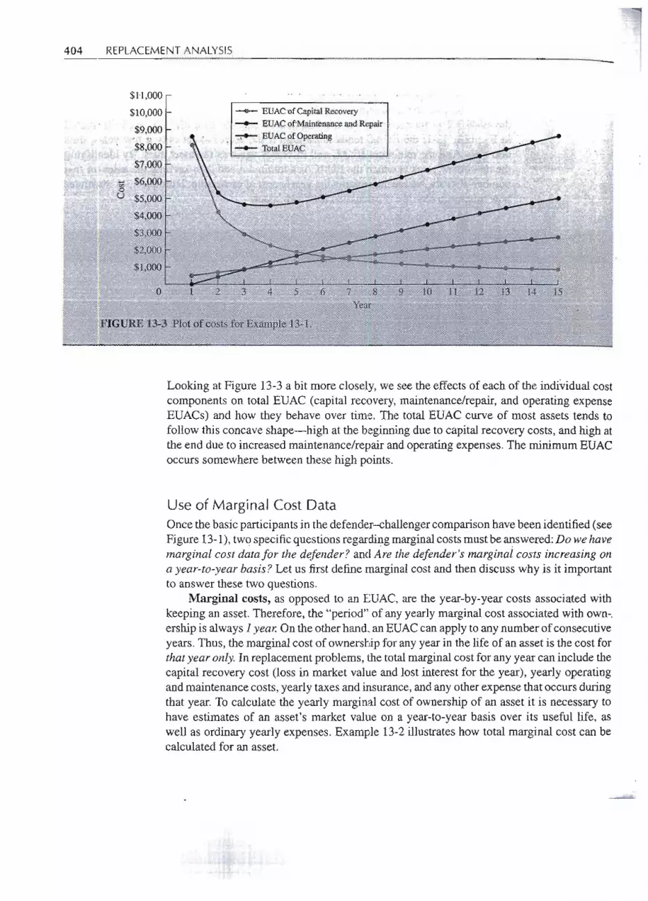
l404 REPLACEMENTANALYSIS
EUAC of Capital Recovery
EUAC 9fMllintenance and Repair
#EUAC ofpperating--t- Total EUAC
,,:
~
r'J!! I>, ~
15
"I~IGURE13-3 Plot ofcostS.fot Example 13.:1.If - .
a
Looking at Figure 13-3 a bit more closely,we see the effects of each of the individualcostcomponents on total EUAC (capital recovery,maintenance/repair,and operating expenseEUACs) and how they behave over time. The total EUAC curve of most assets tends tofollow this concaveshape-high at the beginningdue to capital recovery costs, and high atthe end due to increasedmaintenance/repairand operatingexpenses.The minimumEUACoccurs somewherebetween these high points.
Use of Marginal Cost DataOnce the basicparticipantsin the defender-challengercomparisonhavebeen identified(seeFigure 13-1),two specificquestionsregardingmarginalcostsmustbe answered:Do we havemarginal cost datafor the defender? and Are the defender's marginal costs increasingona year-to-year basis? Let us first define marginalcost and then discuss why is it importantto answer these two questions.
Marginal costs, as opposed to an EUAC,are the year-by-year costs associated withkeeping an asset. Therefore, the "period" of anyyearlymarginal cost associated with own-.ership is always1year.Onthe otherhand, anEUACcan applyto anynumber of consecutiveyears. Thus, the marginalcost of ownershipfor anyyear in the life of an asset is the cost forthatyear only. In replacementproblems, the totalmarginalcost for anyyear can include thecapital recovery cost (loss in market value and lost interest for the year), yearly operatingandmaintenancecosts, yearlytaxes and insurance,andanyotherexpensethat occursduringthat year. To calculate the yearly marginal cost of ownershipof an asset it is necessary tohave estimates of an asset's market value on a year-to-year basis over its useful life, aswell as ordinary yearly expenses. Example 13-2illustrateshow total marginal cost can becalculated for an asset.
$1'1,000
$10,000
$9,000
$8,000--
;;r $,7,000
$6,0000
U $5,000 I r".
$4,000
-$3,Q90r;
$4,OOOilfl
.. $1,000
',i
} 0"id

rWhat Is the Basic Comparison? 405
A new piece of production machinery has the followingcosts.
Investmentcost . =$25,000Annual operating and maintenance cost =$2000 the firstyear and increasing
at $500 per year thereafterAnnual cost for risk of breakdown = $5000per year for 3ye~s, then
increasing by $1500 per year thereafterUsefullife =7 yearsMARR = 15%per year
Calculate the marginal cost of keeping this ass~tover its useful life.
SOLUTION
From the problem data we call easily find tbe marginal costs for O&M and risk of breakdowns.However, to calculate the marginal capital recovery cost, we need estimates of the year-to-yearmarket value: the prices of the production machinery would bring over its 7-year useful life.Market value estimates were made as follows:
.
I
I
t
I
I
I
We can now calculate the marginal cost (year-to-year cost o,f ownership) of the productionmachinery over its 7-year useful life.
Cost of TotalO&M Breakdown Marginal
Loss in Market Forgone Interest Costin Risk CostValue in Year n in Y~ar n Year n in Year n in Yearn
2,5,000 - 18,000 = $7000 25,000(0.15) = $3750 $2000' $5,000 $1.7;75018,000 - 13,000= 5000 18,000(0.15) == 2700 2500 5,000 15,200d3,ooQ- 9,000 = 4000 13,000(0.15) = 1950 3000 5,000 13,950
9,000 - 6,000 = 3000 9,000(0.15) == 1350 3500 6,500 14,3506,000 -'- 4,000 = 2000 6,000(0.15) = 900 4000 8,000 14,'900-4,000- 3,000= 1000 4,000(0.15).~. 600 45QO 9,500 15,~OQ3,000- 2,500== 500 3,000(0,15)' 450 5000 11,odb 16,950
'NpticeC'thflfthefatalrn1irgiilafcosrJdfea~ Y'eaf'.j$mad~~~p=o!,fuss1'0.l11arketvalue, fot:golleintere~~,O&M cost, and cost for risk of breakdowns.AsaIIe~fu1J.ple,theYear-5.:marginalcostof$14,900 is calculated as 2,000+ 900 + 4,000 + 8,000._ '='== ' = =:!!I 101 "'= _:llt_ ~I!!I::Ii= -=. -= "= 'll'a=
~,.--
I Year,n1234567
Year .Market ValueI $18,0002 13,0003 9,000 I , it
4 6,0005 4,0006 3,000
II
7 2,500

406 lREPLACEMENT ANALYSIS -Do We Have Marginal Cost Data for the Defender?Our decision map indicates that it is necessary to know whether marginal cost data areavailable for the defender asset to detennine the appropriate replacement technique touse. Usually in engineering economic problems annual savings and expenses are givenfor all alternatives.However,as in Example 13-2, it is also necessary to have year-to-yearsalvage value estimates to calculate total marginal costs. If the total marginal costs for thedefender can be calculated, and if the data are increasing on a year-to-year basis, then itis appropriate to use replacement analysis technique 1 for comparing the defender to thechallenger.
Are These Marginal Costs Increasing?We have seen that it is important to know whether the marginal cost for the defender isincreasing on a year-to-yearbasis. This is detennined by inspecting the total marginalcostof ownershipof the defenderover its remaininglife. Example 13-3illustrates the calculationof the total marginal cost for the defender asset.
"An ~ssetpurchased 5 years agoror $75,000 Canbe sold today f9r$15,OOO.Operating expensesin the pastp.ave been $10,000 per year, but these are estimated to increase in the future by$1500 per year each year. lEis estiplated tbafthe marlcetvalue or the .olda$~etwi.1ldecreaseby $1000 per year over the next 5 years. If theMARR usedpyth~ company is 15%, calculate
lithetotal marginal cost of ownership of tbjs old asset (thatjs,~the defender) for eacQof the next5 years.
II
I SOLUTIONI,I, __;;Wecalculate the total marginal cost of majntaining the qld asset for the n~xt ?-::yearperioq as::tollows;
lear, n~! 1~I -
U 2II 3
II 45
Loss in Mar~etValue in Year-n
15,000 - 14,000$1000"14,OQO- 13,000 _ _ 100013,000 - 12,000 - 100012,000 ..,... 11,000 . tOQQ, "-C.--';' '.-.:.- .. ',:-- ..'
11,000 -- 10,000' . 1000_
.]j'orgoneInterestin:)~earn .'
15~000(0.q)C$~250J,A,900(Q.};DJ," 2.lPD13,OOO(o.l~Y - _-J9iSO
12,OOO(0~~t5');"'-N ~180t>n 'co"~, -:;~.. ,," ,'C'.".. ',:/!::-':"_:;:~ ',:2':: -:;,,,~:,-".~:-."It, 000(0. rs},. "'~,:1J~~Q'
Qpef~JingCost
i)) Yearn
$IQ,QOO1'1,500J3 000
"'i.;...l .:'I:!io
14~500- 16000
';"':';'-"~';;"i~ ',. .
M8t~atCost'inYear11
$13250~ " ..".,
i4,60015,,9SQ!T300,-",-"'-,.:; .'...,," .,~,"".
18656":-~." ".,t,, ' ,,:L...,
We can see that the marginal costs increase in each subsequent year of ownership. Whenthe conditionof increasingmarginal costs for the defenderhas been met, then the defender-challengercomparison is appropriatelymade by using replacementanalysis technique 1.
-- -~-
-- -

-.. .----.....-.. .. - ... .-. -. .- .---
What Is the Basic Comparison? 407
Replacement Analysis Technique 1:Defender Marginal Costs Can Be Computed and Are IncreasingWhen our firstmethodof analyzingthe defenderasset againstthebestavailablechallengerisused, the basic comparisoninvolvesthe marginalcost dataof thedefenderand the minimumcost life data of the challenger,
In the case of the marginal cost of the defender increasing on a year-to-yearbasis, wewill maintain that defender as long as the marginal cost of keeping it one more year is lessthan the minimum EUACof the challenger.Thus our decision rule is as follows:.-
.I~I
Maintain the defender as long as the marginal cost of ownership for one more year isless than the minimum EUAC of the challenger. When the marginal cost of the defenderbecomes greater than the minimum EUAC of the challenger, then replace the defenderwith the challenger.
One can see that this technique assumes that the current best challenger,with its mini-mum EUAC,will be availableand unchanged in the future. However,it is easy to update areplacementanalysiswhen marginalcosts for the defenderchange or when there is a changein the cost and/orperformance of availablechallengers.Example 13-4illustrates the use ofthis technique for comparing defender and challenger assets.
Takip.gthe machinery in Example 13-2 as the challenger and the m~chineryin Example 13-3 asthe liefender,use replacement analysis technique 1 to determine when, if at all, a replacementdecision should be made.
SOLUTION" -
Replacement analysis technique 1 is appropriate only in the condition of increasing marginal'1costs for the defender. Since these marginal costs are increasing for the defender (from,Example 13-3), we can proceed by comparing defender marginal costs against the minimumEUACof the challenger asset. In Example 13-2we calculatedonly the marginalcost&of the chal-leng~r;thus it is necessary to calculate the challenger's minimum EUAC.The EUACof keepingthis asset for each year of its useful life is worked out as follows. "
Year, 1I12345 !i:
67
c;hallengerTotal Marginal<;]08tip Year"
$17,75015,20013,95014,350
= 14,900" 15,600
16,950=
EUAC of Challenger OwnershipIf Kept 'l'hrough Year n a
[17,750(P/F, 15%, 1)](A/P, 15%, 1)=$17,750[17,750(P/ F, 15%,1) +15,200(P/ F, 15%, 2)](A/P, 15%,2)16,560[17,756(P/F,15%,1)+... + 13,95Q(P/F,J5%,3)](A/P,IJ%,3) ..' 15,81.0[17,750(P/P, 15%, 1) + ... + 14,350(P/F,15%,4)](A./J-\15%,4) 15,520'.
-=[17,;950(P7F,15%~1) f.. ::'¥'14;900(P7F;I3"%, 5)](~/J';"i'5%,"'5r ~. "15,43U
[17,750(P/F,15%, 1) +... + 15,60Q(P/F,15%, 6)](4/11,1~%,.~ == 15.450__[!2.,750Ct!! ~~ ~t . .~1~,2~Pi~J~, .wr0~7J~ ===~.5.8
----
-

408 REPLACEMENTANALYSIS
A minimum EUAGof $15,430is attainedfor thechallengerat Year5, whichis thechallenger'sminimum cost life.Weproceed by comparingthis value against the marginalcosts of the defenderfrom Example 13-3:
Defender TotalMarginal Cost.
in Year n~
~13?250
CbatIengerM1nmuInlEtJAC
$15,430
2 14,600 15,430
COlIlpariso~Result and Recolnnlcndanon
Since $13,250 is ressthqn $15,430,keep def~nder.
Since$t4,600is.less than $15,430,keep defender.
Since$J5,950 is greatel; t1Jqn$15,4~O,replace defender. .
Qi i"1
Year,n1
II
II 3 15,950. ;;;
II
a
One may ask, Why can't replacementanalysis technique 1 be used when the marginaicosts of the defender do not increase? To answer this question we must understand thatfor this technique to be valid, the following basic assumptions must be valid: the bestchallengerwill be available"with the same minimumEUAC" at any time in the future; andthe period of needed service in our business is indefinitelylong. In other words, we assumethat once the decision has been made to replace, there will be an indefiilite replacementof the defender, with continuing "cycles" of the current best challenger asset. These twoassumptionstogether are much like the repeatability assumptionsthat allowedus to use theannual cost method from earlier chapters to compare competing alternativeswith differentuseful lives. Taken together, we call these the replacement repeatability assumptions.They allow us to greatly simplify the comparison of the defender and the challenger. Westate these assumptions formally below.
Replacement Repeatability AssumptionsThe two assumptions are as follows:
1. The currently availablebest challenger will continue to be available in subsequentyears and will be unchangedin its economic costs. When the defender is ultimatelyreplaced, it will be replaced with this challenger. Any challengers put into servicewill also be replaced with the same currently availablechallenger.
2. The period of needed service of the asset is indefinitely long. Thus the challengerasset, once put into service,will continuouslyreplace itself in repeating,unchangedcycles.

.. . ... . .-. -.-.......-
What Is the Basic Comparison? 409
~I
Given that the defenderwill ultimatelybe replaced with the current best challenger,wewouldnotwant toeverincur a defendermarginalcostgreaterthan the challenger's minimumEUAC. And because the defender's marginal costs are increasing, we can be assured thatonce the marginal cost of the defender has become greater than the challenger's minimumEUAC,it will continue to be so in the future.However,if the marginalcosts do not increase,we haveno guaranteethat replacementanalysis technique1 will producethe alternativethatis of the greatest economicadvantage.One may ask,Are thereordinaryconditions in whiahthe marginalcosts are not increasing?The answer to this questionis yes. Consider the newasset in Example 13-2.Thisnew assethasmarginalcosts thatbeginatahigh of $17,750,thendecrease over the next years to a low of $13,950, and then increasethereafter to $16,950inYear7. If this asset were implemented and then evaluatedoneyear after implementationasa defender asset, it would not have increasing marginal costs. Thus, defenders in the early .
stages of their respective implementations would not fit the requirements of replacementanalysis technique1. In.the situationgraphedin Figure 13-3,such defender assets wouldbein the downward slope of a concavemarginal cost curve. Example 13-5illustrates the errorthat can be introduced when replacementanalysis technique 1 is applied when defen~ersdo not have consistently increasing marginal cost curves.
t..~. -- ..,~_.'. ,,_v ... - . . ,. .~, . -,
~ LetuslookagainatthedefenderandchallengerassetsinExample13-4.Thistimeletusarbitrarilychange the defender's marginal costs for its 5-year useful life. Now when, if at all, should thedefender be replaced with the challenger?
Defender Total MarginalCost in Year n
$16,00014,00013,50015,30017,500
II
Year, n12345
SOLUTION
=
IIIthi$case the totalmarginalcostsof the defenderarenotconsistentlyincreasingfromyear to year.:a()w~ver,ifwe ignore this fact and apply replacementanalysis technique1, the recoIIlI)1endati9nwoulg be to replace the defender now, because the marginal cost of the defender for the firstyear t$J6,OOO)is greater than.th,eminimUITlEUAC of the challenger ($15,430). Let usteviewthis d~ci$ion.One can see that' the first-year marginal cost of the defender is greater than.theminiJji1iID.aUA.C:of thec:hallenger,bittin the secondthroughfourthyearsthemarginalcoStsareless.Wus marginalcostsdecrease4e.refor3 yearstoa minimumapdthenincreasethefollowing~,
: 2ye~; .. ~ ~ .. ~ . =; ~ ~ = == == ;;. ;; -~~= . = a ~ ~:; = . -xitUscalculate the EUAC of k~epiIi15the defender asset each of its remaining 5 years, ati ...:.lft%.""
--- - --------- - ---

410 REPLACEMENTANALYSIS
-t.
iij Year, n
12345
-EUAC of Defender
Ownership HKept n Years
$16,00015,07014,61814,75415,162
Challenger Minimum EUAC ='$15,430= 16,000(PIF, 15%, I)(AI P, 15%, 1)= [16,000(P I F, 15%, 1) + 14,000(P I F, 15%, 2)](AI P, 15%,2)
= [16,000(PIF, 15%, 1) + ... + 13,500(PIF, 15%,3)](AI P, 15%,3)= [16,000(PI F, 15%,1)+... + 15,300(PI F, 15%,4)](AI P, 15%,4)= [16,000(PI F, 15%, 1) +... + 17,5OO(PI F, 15%,5)](AI P, 15%,5)
The minimum EUAC of the defender for 3 years is $14,618, which is less than that ofthe challenger. But this comparison alone is not sufficient to indicate that we should keep thedefender for 3 years and thenreplace it. In looking at a study period of 5 years, we really have sixoptions.
Option 1:
Option 2:
Option 3:
Option4:
Option 5:
Option 6:
:Implementthe challenger today (at $15,430/year).
Keep the defender for 1 year (at $16,000) and the challenger for 4 years(at $15,430/year).
Keep the defenderfor 2 years (at $15,070/year)and the challenger for 3 years(at $15,430/year).
Keep the defender for 3 more years (at $14,618/year)and the challenger for2 years (at $15,430/year).
Keep the defender for 4 years (at $14,754/year)and the challenger for 1 year(at $15,430).
Keep the defender for 5 years (at $15,162/year).
The EUAC of each of these options at 15% is:
One can see that 0I?tion5 produces the nrinimum.EUAC.Thus we should keep the defen~erfor 4 more years and then reevaluate the defender-'Challengerdecision. Notice that if we replace
;;; ~~the defenderno\V~witlf tfie"'C1ffi:neii@r'1>eFteplaZ'1fm~ni7lect~8n rutel:ll, w~ wlfrlid ifdr adYieft::a minimum EUAC over this 5-year period. Notice also that the lowest cost life of 3 years forthe defender is NOT how-long we sJiouldkeep the defender.In Year 5, the defender's marginal13 ~ - ='!II!CI! II:; =-- I: :c 11:I11 II =' ,.
Option 1:
Option 2:
. Option 3:
Option 4:
Option 5:
Option 6:
-- .. ----
--
EUAC is $15,430.
EUACis [16,000 + 15,430(PI A, 15%,4)](P I F, 15%, I)(AI P, 15%,5) = $15,578.
EUACis [15,070(PlA, 15%,2) + 15,430(PlA, 15%,3)(P I F, 15%, 2)] x(AI P, 15%,~) = $15,255.
EUACis [14,618(PlA, 15%,3) + 15,430(PI A, 15%,2)(P IF, 15%,3)] x(AI P, 15%,5)= $14,877.
EUAC is [14, 754(P IA, 15%,4) + 15,430(P I F, 15%, 5)](AI P, 15%, 5) = $14,855.
EUAC is $15,162.II'1
l
r 4
--

l'
What Is the Basic Comparison? 411
- .co~t again expeeds t}lechall~nger's minimum EUAC. We emphasize that this analysis is validonly 1?ecauseof thereplacement repeatabilityassumptions.These assumptionshold that after the5-yeat;pepod, all altemativ~shave the exact same yearly cash flowof $15,430(thuswe can ignoretheIil)~and theseidentical cash flowscontillue indefinitely.
Lr
Example 13-5demonstratesthat whenthe marginalcostsof the defenderarenot consistentlyincreasing from year to year, it is necessary to calculate the lowest EUACof the defender.In the next section we describe this calculation.
Lowest EUACof the Defender
How long can a defender asset be kept operating? Anyone who has seen or heard oldmachinery in operation, whether it is a 50-year-oldautomobileor 20-year-oldpiece of pro-duction equipment,has realized that almost any machine can be kept operatingindefinitely,provided it receives proper maintenance and repair. However, even though one might beable to keep a defender going indefinitely, the cost may prove excessive. So, rather thanasking what remaining operating life,the defender may have, we really want to ask whatis the minimum cost life of the asset. The minimum cost life of the defender is defined asthe number of years of ownership in the future that results in a minimum EUAC for thedefender and the challenger combined, as in Example 13-5.
However,for decision-making now, the answer to a simpler calculation is enough. Isthe defender's lowest or minimum EUACless than the challenger's minimum EUAC?
An l1-year-old piece of equipment is being considered for replacement. It can be sold for $2000now,and it is believedthat the same salvagevaluecan alsobe obtainedin futureyears.Thecurrentmaintenance cost is $500per year and is expected to increase $100per year in future years. If theequipment is retained in service, compute the minimum EUAC,based on 10% interest.
SOLUTION
Here the salvage value is not expecied to decline fromits present $2000. The annual cost of thisinvested capital is Si = 2000(0.10) =$200. The maintenance is represented by $500 + $100G.A year-by-year computation of EUACis as follows:
EUAC of Maintenance Total[= 500 + 100(AIG, 10%, n)] EUAC
$500 $700548 748--- ~- - - -=;::;I-- --.. --- :>~q- --- - ,9'4,-638 8~8
:;; z ~8111' = II au z=~Jl
--------
---- ---
il
IIijt'I
lIfill!
II'
I
III:!,
I'I II
"=
Age of EUAC of InvestedYear, n Equipment (years) Capital (= Si)
1 11 $2002 12 200
II 3 - . - -_. -- - - --..== ;;;;;:0.3= :: = :==;;:'1 ' ;:; ;;; : - - - -2()0 - - ---4 14 2005 " 15 200" II: II = ill.. = =' ;

p '.
,I;
,
. j1!iIj
j
!j!i
:!
iIIjI
!I
I,iIJ
'1
- -- --
412 REPLACEMENTANALYSIS
FIGURE 13-4 EUAGvalues for different
remaining lives.$900
$800
"
$600
"" $500""o~
u $400
$300
$200
$LOO ti
EIJACOf II).vested CapiW
11 . 1'512 13 14I!! "
Age QfEqUipment
3 4Yearn
5
"
Ii
I~1 2
II
\1 The lowest EUAC is $700. That nUJ;Ilbercan be compared with the challenger's best EUAC todeterminewhethertbeequipmentshouldbereplacednow. "-
These data are plotted "jp'Fig. 13-4. We see that the aIWualcost of continuing to u§e theequipment is jncreasing. Jt ISreasonable to assume tqat if the equipment is not replaf:ed110W,.it will be reviewed again next year. I:fthe def~llder'sand challeilgefs cost,data do not chapge,we can cOl1,1putethe'defender's marginal co~t toyxten.d seiYice~ach year to decide wheI1;.toreplace. ~ ~
Example 13-6 represents a common situation. The salvage value is stable, but themaintenancecost is increasing.The marginal cost to extendthe defender's life and its totalEUAC will continue to increase as time passes, which means that the defender's lowestEUACwill be based on retainingthe defender for 1 more year.This is not always the case,as is shown in Example 13-7.
! '3:year-okirpacliine, whose Currentrpatketvalue is $5000, is beIng analyzedlo deternlin~itsecoIioIQiclife il).a reI>!ac~mentatlalysis.Compute its lowest EUi\C using a 10% mter:estf(,ite.
i~.g~l\l$,-~aJWe~a~c~..£.s,Uteae..~i~Il!~~~q~:.ta~= ~;< ~ ..-L_1:-'=_ ". - - ,. ','__ 'II,' Ij.':.'
-- -

rWhat Is the Basic Comparison? 413
If Retired at Endof Yearn
Yearsof
RemainingLife, n
Estimated SalvageValue (5) at
End of Year n
EstimatedMaintenanceCost for Year
EUACof EUACof
Capital Recovery Maintenance(P S) x (AI P, 10%, n) + Si 100(AI G, 10%, n)Total "EUAC
$ 04894
138181222262300337372406
$l5,QQ12621198117711721111107810621058+-10601068
SOLUTION
A mWimumEUACof $1,058is computed at Year 9,forthe:existing machiI.le.
Looking againat Examples 13-6and 13-7,we findthat the twocasesrepresent the samemachine being examined at differentpoints in its life. (In Year6 and later in Example 13-7the costsmatch those of Example 13-6.)Example 13-7indicatesthat the 5-year-oldmachinehas a minimum EUACat a life of 9 years.
For older equipment with a negligible or stable salvage value, it is likely that theoperating and maintenance costs are increasing. Under these circumstances,the useful lifeat which EUACis a minimum is 1 year.
It is necessary to calculate the defender's minimum EUAC when marginal costs arenot consistently increasing. Having made this calculation, we can now use replacementanalysis technique2 to compare the defender against the challenger.
Replacement Analysis Technique 2:Defender Marginal Cost Can Be Computed and Is Not IncreasingUsing our second method of analyzing the defender asset against the best available chal-lenger the basic comparison involvesthe lowest EUACof the defenderand the EUACof thechallengerat its minimum cost life.
We calculate the minimum EUAC of the defender and compare this directly againstthe minimum EUAC of the challenger. Remember that the replacement repeatabilityas-sumptions allow us to do this. In this comparison we then choose the alternative with !helowest EUAC. In Example 13-5 the comparison involved the defender with the lowestEUAC = $14,618at a life of 3 years and the challenger with an economic life of 5 yearsand EUAC = $15,430. Here we would recommend that the defender be retained for 4 more
years, as its marginal costs for later years will be increasing above the challenger's EUAC.Then, replacementanalysis technique 1 would apply. Consider Example 13-8. ~
J
0 p = $50001 4000 .$ 0 $1100 + 4002 3500 100 864 + 3503 3000 200 804 + 3004 2500 300 789 + 2505 2000 400 791 + 2006 2000 500 689 + 2007.1 2000 600 616 +- 2008 2000 700 562 + 2009 2000 800 521 + 200
10 2000 900 488 + 20011 2000 1000 462 + 200

-I
. I
.-- -.. -- ..,. --..-------
414 REPLACEMENTANALYSIS
An economic analysis is to be made to detennine whether existing (defender) equipment in anindustrial plant shouldbe replaced.A $4000 overhaulmust be done now if the equipmentis to beretained in service.Maintenanceis estimatedat $1800 in each of the next 2 years, after which it isexpected to increaseby $1000each year.The defenderhas no present or future salvagevalue.Theequipment describedin Example 13-1is the challenger.Makea replacementanalysis to determiIiewhether to retain the defender or replace it by the challenger if 8% interest is used.
SOLUTION
The first step is to detennine the lowest EUAC of the defender. The pattern of overhaul andmaintenance costs (Figure 13-5) suggests that if the overhaul is done, the equipment should bekept for several years. The computation is as follows:
If Retired at End of Year n
Year,nEUAC of Overhaul
$4000(A/I', 8%, n) Total EUACEUACof Maintenance $1800 + $1000
Gradient from Year3 on
12345
$43202243155212081002
$612040433660+-36913881 .
$180018001800 + 308*1800 + 683t1800 + 1079
*For the first 3' years, the maintenance is $1800, $1800, and $2800. Thus, EUAC = 1800 +1000(Aj F, 8%, 3) = 1800 + 308.
tEUAC = 1800 + loo0(P j G, 8%, 3)(P j F, 8%, 1)(Aj P, 8%,4) = 1800 + 683.
FIGURE 13-5 Overhaul and maintenance costs for the
defender in Example 13-8.4800
4000
r
3800
r
2800
f
1800 1800
t t0~1~2~3~4~5
Year
The lowestEUACof thedefenderis $3660.In Example 13~1,wedeterminedthat theminimumcost life of the challenger is 4 years and that the resulting EUAC is $4589. If we assume theequipment is needed for at least 4 years, the EUACof the defender($3660) is less than the EtJACof the challenger ($4589). In this sifuation the defender should not be replaced yet.
If the defender's and challenger's cost data do not change, we can use replacementanalysistechnique 1 ,todetennine- when=the,defehder~hould b-M'epJ.a'COO.W~Kii5W; nom I"the.1hifi.ii'fihm :EUAC calculation that the defender should be kept at least 3 years. Is this the best life? Thefollowing table computes the marginal cost to answer this question.
.. " _ 1IftI:III!In:I= ~;;r:~ II 1111;~ '" 1:1" '.I; ~..-............. -- - ----------
I
I......,I
~

rnI
What Is the Basic Comparisori? 415
r
trI
-
Year,no1
:.2345
Overhaul Cost$4000
ooooo
Margin81 Cost to Extend ServiceMaintenance Cost$ 018001800280038004800
$6120 = 4000(1.08) + 18001800280038004800
Year 5 is the first year after the year with the lowest EUAC in which the $4800 marginalcost for the defender exceeds the $4589 minimum EUAC for the challenger.Thus, the defendershould be kept 4 more years if costs do not change. (Note that if the defender can be overhauled-' :::; "
again after 3 years, that might be an even better choice.)
No Defender Marginal Cost Data AvailableEarlier we described replacement analysis techniques for comparing the defender andchallenger if marginal cost data are available for the old asset. Youmay recall that yearlysalvage valueestimates were necessary to calculate these marginal costs. Sometimes,how-ever, it is difficultto obtain end-of-the-yearsalvage value estimates for the defender asset.A defender based on aging technology with a shrinking market might be such an asset.Or, from a student's problem-solvingperspective,perhaps salvagevalue data are not givenas part of the problem data. Without these data, it is impossible to calculate the marginalcost of the defender,and thus impossible to use marginal cost data to compare the defenderagainst the challenger.How should we proceed?
Given the replacement repeatability assumptions, it is possible for us to calculatethe EUAC of the defender over its remaining useful life. Then, knowing that both thedefender and challenger will be replaced with indefinite cycles of the challenger, we mayuse replacementanalysis technique3 to compare defender and challenger.
Replacement Analysis Technique 3: .
When Defender Marginal Cost Data Are Not AvailableWhen our third methodof analyzingthe defenderasset againstthe best availablechallengeris used, the basic comparison involvesthe EUACof the defender over its stated useful life,and the minimum EUACof the challenger.
We will calculate the EUAC of the defender asset over its remaining useful life andcompare this directly against the EUACof the challengerat its minimum cost life, and thenchoose the lesser of these two values. However,in making this basic comparison an oftencomplicating factor is deciding what first cost to assign to the challenger and the defenderassets.
Defining Defender and Challenger FirstCostsBecausethedefenderis alreadyin service,analystsoftenmisunderstandwhatfirstcosttoassignit. Example13-9demonstratesthisproblem. ..
-- ---
I--!/II
: "'.t.~.~ .
----

416 REPLACEMENTANALYSIS lI
A laptop word processor model SK-30 was purchased 2 years ago for $1600; it has been depre-ciated by straight-line depreciation using a 4-year life and zero salvage value. Because of recentinnovationsin wordprocessors,the currentpriceof t4e SK-30 laptophas beenreducedfrom $1600to $995. An officeequipment supply finn has offereda trade-in allowanceof $350 for the SK-30on anew $1200 model EL-40 laptop. Some discussionrevealed that without a trade-in, the EL-40can be purchased for $1050, indicating the originally quoted price of the EL-40 was overstatedto allow a larger trade-in allowance.The true current market value of the SK-30is probably only$200. In a replacement analysis, what value should be assigned to the SK-30 laptop?
SOLUTION I
"
In the example, fivedifferent dollar amounts relating to the SK-30 laptop have been outlined:
1. Original cost: The laptop cost.$1600 2 years ago.2. Present cost: The laptop noW'.sellsfor $995.3..Book value; The originalcost less2 yearsof depreciationis 1600-%(1600 ~O) = $800.4. Trade-invalue.~'The offer was $350.5. Market value: The estimate>was$200.
We know that an economic analy§i§is based on the CUrrentsituation, not 0)1the past. We,refertP past costs as sunk costs to emphasize tbat, since these costs caUJ10tbe a1tet;~d,they are notrill. ..'c... , ',' . . .,' . .:"',. . .',. ,'. . ..' ", ,_.-,,"
r.elevant.(There is one exception: past costs may affect present or futUreincome taxes.) In theanalysis we want to use actual,cashftows for each altemativ~.a~re the questioI;lis, What valueshould be used in an economic analysisfor ,theSK~30?Tbe relevant costis the present marketKaluefor the equipment.Neither the ori~inalcost, thepresent cost,the bookvalue,)lorthetrade..in)!'alueis relevant. >"
At first glance, the trade-in value of an asset would appear to be a suitable presentvaluefor the equipment. Often the trade-in price is inflatedalong with the price for the newitem. (This practice is so common in new-car showroomsthat the term overtrade is usedto describe the excessive portion of the trade-in allowance.The purchaser is also quoted ahigher price for the new car.)Distortion of the present valueof the defender, or a distortedprice for the challenger, can be serious because these distortions do not cancel out in aneconomic analysis.
Example 13-9illustrated that of the severaldifferentvaluesthat can be assigned to thedefender, the most appropriate is the present market value. If a trade-in value is obtained,care should be taken to ensure that it actually representsa fair market value.
Determining the value for the installed cost of the challenger asset should be lessdifficult. In such cases the first cost is usually made up of purchase price, sales tax,installation costs, and other items that occur initially on a one-time basis owing to theselection of the challenger. These values are usually rather straightforward to obtain if athorough analysis is conducted. One aspect to consider in assigninga firstcost to the chal-lenger is the potential disposition (ormarketor salvage)valueof the defender.One must not

--- ........-..-.
What Is the Basic Comparison? 417
arbitrarily subtract the disposition cost of the defender from the first cost of the challenger, asset,forthispracticecan leadto an incorrectanalysis.
As described in Example 13-9, the correct first cost to assign to the defender SK-30laptop is its $200 current market value. This value represents the present economicbenefitthat we would be forgoing to keep the defender. This can be called our opportunityfirstcost. If, instead of assuming that this is an opportunity cost to the defender, we assumeit is a cash benefit to the challenger, a potential error arises. Consider the following caseinvolving the SK-30 and EL-40 laptops. Assume the followingdata:
Market valueRemaining life
SK-30$2003 years
First costUseful life
EL-40$10503 years
In this case the remaining life of the defender (SK-30) is 3 years, and so is the usefullife of the challenger (EL-40). If we use an opportunitycost perspective,then the calculatedcapital recovery effect of first cost using an annual cost comparison is:
Annualized first coStSK-30= $200(Aj P, 10%,3) = $80
Annualized first costEL-40 = $1050(Aj P, 10%,3) = $422
The difference in annualized first cost between the SK-30 and EL-40 is:
AFCEL-40 - AFCSK-30 = $422 - $80 = $342
Now use a cashflow perspectiveto look at the firstcostsof the defenderand challenger.In this case we use the actual cash that changes hands when each alternative is selected.A first cost of zero ($0) cash would be assigned to the defender and a first cost of $850to the challenger(-$1 050 purchasepriceof the challengerand +$200 in salvagevaluefrom defender).We calculate the differencedue to first cost between the SK-30 and EL-40to be:
Annualized first coStSK-30= $O(AjP, 10%,3) = $0
Annualiied first costEL-40= ($1050 - 200)(Aj P, 10%,3) =$342
AFCEL-40- AFCSK-30= $342 - $0 = $342
I~l
~
When both the remaining life of the defender and the useful life of the challenger arethe same, 3 years in this case, the analysis of the first cost yields an identical (and correct)result. Both the opportunity cost and cashflow perspectivesfor considering first cost of thedefender and challenger result in a difference of $342 between the two alternativeson anannual cost basis.
Now see whathappens whenthe remaininglife of the defender is Q.otequal to the usefullife of the challenger.Consider the SK-30 and EL-40 word processors, but assume that thelives have been changed as follows: '
-"I
1'1
f1;1'
Remaining life
SK-30
3 years UsefullifeEL-40
5 years
L ~ -
---- ----

.. ... .h ___ _ U ,I
418 REPLACEMENTANALYSIS
Looking at this second case from an opportunity cost perspective, we use an annualcost comparison to calculate capital recovery effect of the first cost as follows:
Annualized first COStSK-30= $200(Aj P, 10%,3) = $80
Annualized firstcostEL-40= $1050(AjP, 10%,5)=$277
The difference in annualized first cost between the SK-30 and EL-40 is:
AFCEL-40 - AFCSK-30 = $277 - $80 = $197
Now using a cashjlow perspective to look at the first costs of the defender and challenger,we can calculate the difference due to first cost between the SK-30 and EL-40.
Annualized first costSK-30 = $O(Aj P, 10%, 3) = $0
Annualized first costEL-40= ($1050 - 200)(Aj P, 10%,5) = $224
AFCEL-40 - AFCSK-30 = $224 - $0 = $224
When the remaining life of the defender (3 years) differs from that of the useful life ofthe challenger (5 years), analyses of the annualized first costs yield different results. Thecorrectdifferenceof$197 is shownbyusing the opportunitycostapproach,.and aninaccuratedifference of $224 is obtained if the cashjlow perspectiveis used. In the opportunity costcase the $200 is spread out over 3 years as a cost to the defender, yet in the cash flow casethe opportunity cost is spread out over 5 years as a benefit to the challenger. Spreadingthe$200over3 years in one caseand 5 years in the othercasedoesnotproduceequivalentannualizedamounts.Becauseof the differencein the livesof the assets, the annualized$200opportunity cost for the defender cannot be called an equivalentbenefit to the challenger.
In the case of unequal lives, the correct method is to assign the current market valueofthe defender as its time zero opportunity costs, rather than subtractingthis amount from thefirst cost of the challenger.Because the cash flow approach yields an incorrect value whenchallenger and defender have unequal lives, the opportunity cost approach for assigning afirst cost to the challenger and defender assets should always be used.
Repeatability Assumptions Not AcceptableUnder certain circumstances,the repeatability assumptionsdescribed earlier may not applyfor a replacement analysis. In these cases replacement analysis techniques 1,2, and 3 maynotbe validmethodsfor comparison.For instance,adecisionmakermay set the studyperiodinstead of assuming that there is an indefinite need for the asset. For example, co~r thecase of phasing out production after a certain number of years-perhaps a person who isabout to retire is closing down a business and selling all the assets. Other examplesincludeproduction equipment such'as molds and dies that are no longer needed when a new modelwith new shapes is introduced.
The studyperiod could potentiallybe set at any number of years relative to the livesofthe defender and the challenger, such as equal to the life of the defender, equal to the lifeof the challenger, less than the life of the defender, greater than the life of the challenger,
-----. ---.----.--.--- - -

--. ---
What Is the Basic Comparison? 419
or somewhere between the lives of the defender and challenger.The essential principle inthis case is that in setting the study period, the decision maker must use an appropriatemethod as described in earlier chapters. The analyst must be explicit about the economiccosts and benefitsof the challenger that is assumed for replacement of the defender (whenreplacement is made), as well as residual or salvagevalues of the alternativesat the end ofthe study period. In this case the repeatabilityreplacement assumptions do not apply, andthus the replacementanalysis techniquesare not necessarilyvalid. The analysis techniquesin the decision map also may not apply when future challengers are not assumed to beidentical to the current best challenger.This concept is discussed in the next section.
A Closer Look at Future Challengers
We defined the challenger as the best available alternative to replace the defender. But intime, the best available.alternativecan change. And given the trend in our technologicalsociety, it seems likely that future challengerswill be better than the present challenger.Ifso, the prospect of improvedfuture challengersmay affectthe present decisionbetween thedefender and the challenger.
Figure 13-6 illustrates two possible estimates of future challengers. In many techno-logical areas it seems likely that the equivalentuniform annual costs associated with futurechallengers will decreaseby a constantamounteach year.In other fields,however,a rapidlychanging technology will produce a sudden and substantially improved challenger-withdecreased costs or increased benefits. The uniform decline curve of Figure 13-6 reflectsthe assumption that each future challenger has a minimum EUAC that is a fixed amountless than the previous year's challenger.This assumption, of course, is only one of manypossible assumptionsthat could be maderegarding future challengers.
If futurechallengerswillbe betterthan thepresentchallenger,whatimpactwill thishaveon an analysis now? The prospect of better future challengers may make it more desirableto retain the defender and to reject the present challenger. By keeping the defender fornow, we may be able to replace it later by a better future challenger.Or, to state it anotherway, the present challengermay be made less desirable by the prospect of improved futurechallengers.As engineeringeconomicanalysts,we mustfamiliarizeourselveswithpotential
FIGURE 13-6 Two possible ways theEUAC of future challengers may decline.
PresentChallenger
o 2Year
1 3
- -

l420 REPLACEMENT ANALYSIS
technological advancesin assets targeted for replacement.This part of the decisionprocessis much like the search for all available alternatives,from which we select the best. Uponfinding out more about what alternativesand technologies are emerging, we will be betterable to understand the repercussions of investing in the current best available challeng~r.Selecting the current best challenger asset can be particularly risky when (l) the costsare very high and/or (2) the useful minimum cost life of that challenger is relativelylong(5-10 years or more). When one or both of these conditions exist, it may be bette~to keepor even augment our defender asset until better future challengers emerge.
There are, of course, many assumptions that could be made regarding future chal-lengers. However, if the replacement repeatability assumptions do not hold, the analysistechniques described earlier may not be valid.
AFTER-TAX REPLACEMENT ANALYSIS
As describedin Chapter 12, an after-taxanalysis adds an expandedperspectiveto our prob-lems becausevarious very importanteffectscan be included.We sawearlier that eXamining'problems on an after-tax basis provides greater realism and insight. This advantage alsoexists when one is considering the replacement problems discussed in this chapter. Taxeffects have the potential to alter recommendations made in a before-tax-only analysis.After-tax effects may influence calculations in the remaining economic life of defender,in the economic life of challenger, and in the defender-challenger comparisons discussedearlier. Consequently, one should always perform these analyses on an after-tax basis. Inthis sectionwe illustrate the complicatingcircumstancesthat are introducedby an after-taxanalysis.
Marginal Costs on an After-Tax BasisAs in the before-tax case, the defender-challenger comparison is sometimesbased on themarginal costs of the defender on a year-to-yearbasis. Marginal costs on an after-taxbasisrepresent the cost that would be incurred through ownership of the asset in each year. Onan after-taxbasis we must consider the effects of ordinary taxes as well as gains and lossesdue to asset disposal in calculating the after-tax marginal costs. Consider Example 13-10.
Refer to Example 13-2, where we calculated the before-tax marginai costs for a new pieceII of production machinery. Before-:tax~ual ,cost infonp.ation was given, as well as year'"en.d" salvagevaluesfor theassetbverits usefullife.Calculatetheafter-taxD;1argimilcostsof thisasset a
consid~ringthe additionalinformationbelqw.
· D~p.rechltion.isby ~e stfatght-line'method, with S ,$0 imdn ,5ye¥8.,. Ordinary"incoine:1s ta:xe1i~at""aTate~Q~~40%.:= ::~ i:.o=:~~ -= r.;,;;: = r;;1:1:;;;':1 I!O:II::;;=."""· Assume that all gains andIQssesare t(lxedat a tate of 28%.
. ,.,. " 110"~ The after.,tax.~MARR is 10%~ ..'
- -< -- - &a= ... -. - -.- ===_ -: ~_~
II
III.II ==
-.

I,.tI
J
I
After-Tax Replacement Analysis 421
J - . ..' -.~-~-~
cS9~UTIQ~j
The after-taxmarginalcostof ownershipwill involvethe followingelements:forgone gainor los§,forgone interest, annual loss in after-taxvalue, and annual operatinglmaintenanceanctinsurance.We calculate the marginal cost of each of these in Table 13.;.1.
TABLE13-1 Marginal Costs of Ownership
Forgone Capital Gains/Losses
Lost After-Tax Value
Year,n
After-TaxValue at
Beginning Yearn
Loss in After-Tax
Value in Year nAfter~Tax Value at
End Year n
12345
$25?00018,56013,5609,2805720!!I~' _':---11;;= ==::=;2,8802,160
18,'000 + 560= $18,560'13;000+ 560== 13,560
9,OOQ+ 280..:... 9,28Q6,000.,.- 280 == 5,72,0
=:=:4.0Qil""i112~ =2~~~ _ =:= 1m~3,000 - 840= 2,1602.5Qp-" 700;:::: 1,800
$6440500042803560
!!::284Q ='720360
= ----.-7
~D! 11III II:IJ!i&:I~'1:z . ::t!llll1II1ZI !!QiIl:.lil:lliiI:=: iI!!Ib = II: II
- .- - -.- --
--- -
II
"I Ii,
II
I
1
i
J
,t
I
Ii
II
It
,
r
J
".
'!I!
I I
, .
~
Gainor Loss Forgone MarginalCostinMarketValue Book Value If Asset Sold Gainor Loss Yearn Dueto
Year,n in Yearn in Yearn in Yearn IfDecideto Keepin Yearn Forgone Gain/Los
1 $18,000 $20,000 -$2000 $ 0 02 13,000 15,000 -2000 -2000( -0.28)..:... 560 5603 9,000 10,000 -1000 - 2000(-0.28) = 560 5604 6,000 5,000 1000 -1000(-0.28) = 280 2805 4,000 0 4000 1000(-0.28) = -280 -2806 3,000 0 3000 40oo(-"0.28)== -1120 -11207 2,500 0 2500 30oo(-0.28) = -840 -840
Forgone Interest Marginal O&M, Insurance Costs
Market Value Forgone Total O&M Marginal CostBeginning of After-Tax Interest and Insurance in Yearn Due to
Year,n Year n in Yearn Cost in Yearn O&M and Insurance
1 $25,000 $25,000(0.10)(0.60) = $1500 "$7,000 7,000(0.60) = $42002 18,000 18,000(0.10)(0.60)= 1080 7,500 7,500(0.60):- 45003 II 13,000 13,000(0.lQ)(0.60) = 780 8,000 8,000(0.60)= 48004 9,000 9,000(0.10)(0.60) = 540 10,000 10,000(0.60) = 60005 6,000 6,000(0.10)(0.60) - 360 12,000 12,000(0.60) .. 72006 4,000 4,000(0.1O)(0.6(}) = 240 14,000 14,000(0.60) = 8400
.7 3,000 3,000(0.10)(0.60) == 180 16,000 16,000(0.60) - 9600

422 REPLACEMENTANALYSIS
Total Marginal Costs Due to Ownership
l'lotice that the total marginal cost for each year is thu,chdiffereIltfrom th~pJ.~ginalcost for the
~~eass~t on a before...t~basis. _ '~1:1
After-Tax Cash Flows for the ChallengerFinding the after-tax cash flowsfor the challenger asset is straightforward.Here we use thestandard after-tax cash flow table and method developedin Chapter 12 to incorporate allthe relevant tax effects,which include before-tax cash flows,depreciation, taxes, and gainsand losses at disposal. After obtaining the after-tax cash flowsfor challenger, it is a simpletaskto calculatetheEUACoverthechallenger'slife. .
After-Tax Cash Flows for the Defender
Finding the after-tax cash flows for the defender is not straightforward.The main compli-cating factor is that the defender is an asset that has been previously placed in service. Assuch, depreciation has been taken on the cost basis (amount being depreciated) up to thepresent, which changes the book value of the asset. Thus, when looking at the first cost ofthe defender on an after-taxbasis (value at time zero), we must consider the current market(salvage) value that can be obtained for the asset, as well as any depreciation recapture orlosses at disposal presently associated with the defender.
We have already suggested the use of the opportunity cost perspective for assigninga first cost to both the defender and challenger. For the challenger, this first cost will bethe after-tax cash flow at time zero. Assuming use of equity financing, the first cost ofthe challenger is the purchase price plus installation cost. However, for the defender theafter-tax first cost will be made up of the forgone market value of the asset at the presenttime plus any forgone gains or losses associated with keeping the asset. To develop theafter-tax cash flow of the defender at time zero, it is often convenient to use the d~fendersign change procedure, described next.
Defender Sign Change ProcedureThedefendersignchangeprocedureallowsustofindtheafter-taxcashflow(ATCF)forthedefenderassetin after-taxdefender~hallengercomparisons.Tofindthe time zeroATCF
- - - -- -- -----
Forgone Forgone Marginal Cost in Lossin After-Tax TotalGain/Loss After-TaxInterest Yearn Due to O&M Market Value Marginal Cost
Year,n in Yearn in Year n ..., and Insurance in Yearn in Yearn
1 $ 0 $1500 $4200 $6440 $12,1402 560 1080 4500 5000 11,1403 560 780 ". 4800 4280 10,4204 280 540 6000 3560 10,3805 280 360 7200 2840 10,1206 --1120 240 8400. 720 8,2407 .."..840 180 9600 360 9,300
f.ir

rI
I
r-
I
~
After-Tax Replacement Analysis 423
of the defender use the following steps:
1. Assume you are selling the defender now (time 0).2. Find the ATCFfor selling the defender at time O.3. Then, because you are actually keeping the defender, not selling it, change all the
signs (plus to minus, minus to plus) in the tax table used to develop the ATCF attime O.
4. Thus the ATCFfor selling now becomes the after-tax opportunity cost for keepingthe defender. Assign this cost to the defender at time O.
Find the after-tax first cost (today's cost) that should be assigned to a defender asset as describedby the following data:
First cost when implemented 5 years agoDepreciation method
= $12,500= Straight-linedepreciation
(with estimated S = $2500,n = 10 years)=$8000__ 10years- $3000= $4500= $1500=34%
Current market valueRemaining useful lifeAnn1ialcostsAnnual benefits" .
Market value after useful lifeCompined tax rate(for ordinary income and capital gainsllosses)
SOLUTION
The defender ~ign change procedure has four steps."
Steps 1 and 2
A$sm;P.ethat we will sell the defender ndw (Time zero), then:
Yearl~ depreciation - ($12,500 - $2500)/10 = $1000 year:aefore-tax cash flow= +8000Gainsl:1osses= Current market value - Current book value
:=
Current market value - $8000
Currentbookvalue__ Cost:basis=-Sumof depreciationcb.argesto date12,500 - 5(1000)12,500 - 5000 - $75QO
;;;;: 8000."", '7:S00'=$500:()rdin~gain'(deprecia.tion :'re-c8.ptlirer=
Tax.eson gain = 500(-0.34)= -$170
After-faxca§hflow = 8000 -- 170 __$7830
~I
---

-,424 REPLACEMENTANALYSIS
Thus if we sell at the outset (n =0) we have:
(Sell)Year, n
o
Before-TaxCash Flow
+8000"Depreciation
TaxableIncome+500
IncomeTaxes-170
After-TaxCash Flow
+$7830
Step 3 and 4
Change signs. The after-tax cash flow figure is the time zero opportunity cost for keeping thedefender.
(Keep)
Year, no
Before-TaXCash Flow
-8000Depreciation
TaxaJ)JeInco~e-500
IncomeTaxes+170.
After.;TaXCash Flow
-$7830
After-tax Time-O costfor the defender = --$7830
Determine whether the SK-3"0laptop of Example 13-9 should be replaced by the EL-40 model.In addition to the data given in Example 13-9, the followingestimateshave been made:
· The SK-30 maintenance and service contract costs $80 a year. :· The EL-40 will require no maintenance.· Either laptop is expected to be used for the next 5 years.·At the end of that time, the SK-30 will have no value, but the EL-40 probably could besold for $250.
..The EL-40 laptop is faster and easier to use than the SK-30 model.This benefit is ~xiJlll!tlto save about $120 a year by reducing the needfor part-time employees.
I
I
I
I
{jdfflatiVM ". = · =... ."" = · " " ..-=. ~0.
"
.
U
.
r first option.
is t
..
o kee.
p.
the
.
SK-30rat..
h
..
er th
..an sell it. Use the following data to compute the J
. after-tax cashfiow~.9ver the 5:'YGar studyperiod.~ lIP fII III tJ
Solve this problem with a MARR equal to 8% after taxes. Both laptop computers will be depre-ciated by straight-line depreciation using a 4-yeafclepreciablelife. The SK-30 is already 2 yearsold, so only 2 years of depreciationremain. The analysis period remains at 5 years. Assume a3.4%corporate income tax rate.

After-TaxReplacement Analysis 425
Straight-lineDepreciation
$400400
ooo
*If sold for $200, there would be a $600 loss on disposal. If $600 of gains were offset by the loss duringthe year, there would be no gain to tax, saving 34% x $600 ',= $204. If the SK-30 is not sold, this loss isnot realized, and the resulting income taxes will be a $204 higher than if it had been sold.
tThis .~sthe sum of the $200 selling"price forgone plus the $204 income tax saving forgone.
tGainILoss = Market value - Book value = 0 - [1600 - (4)400] = O.
EUAC = [404 - 83(P f A, 8%, 2) + 53(P fA, 8%, 3)(P f F, 8%, 2)](Af P, 8%,5)
= $93
Alternative B
Our second option is to purchase an EL-40. Use the following datato compute the after-taxcashflow.
-I
I
I
II
COqJ.put~.the EUAC:
gUAC '. [1050 -147(1:'/ A, 8%,4) .,.,.(79 + 250)(P f F, 8%, 5)](Af P, 8%, 5)... _ ""_ - - 08! =:; = '::;;- - !"'!'-- -. -.
.. .
'
..
'- ~ ... =;:;:;: == = - ~ - -- -.. -- - - -- -r- -=,$8.J
..Based~4~s~~~1~~i~~..EL4Qj$=tJJ~f~qP:9~lnnati~e,,=== ~ = ==:= O!!:
- - -- -- - - --- -- - - --
Before-TaxYear CashFlow
(Sell) 0 $200(Keep) 0 -200
1 -802 -803 804 -805 -805 o Salvage
Taxable 34% Income After-TaxIncome Taxes CashFlow
-$600* $204* $404 ='
+600 - 204* -404t-480 +163 +8}-480 +163 +83-80 +27 -53-80 +27 -'-53-80 +27 -53
ot 0 0
Before-Tax Straight-Line Taxable 34% Income After-Tax..Cash Flow Depreciation Income Taxes Cash FlowYear
0 -$1050 -'-$10501 +120 $200 ---$80 +$27 +1'4-7
I2 +120 200 -80 +27 +1473 +120 200 -80 +27 +147 I il
4 +120 200 -80 +27 +1475 +120 0 +120 ......41 -79,is +250 0* 0 +250
*ss = Market value - Book value = 250 - [1050 - (4)200] = O.

"I
426 REPLACEMENTANALYSIS
Solve Example 13-12 by computing the rate of return on the difference between alternatives. InExample 13-12,the two alternativeswere "keep the SK-30" and "buy an EL-40."The differencebetween the alternativeswould be:
Buy an EL-40Alternative B
Rather than
minusKeep the SK-30
Alternative A
SOLUTION;
The after-tax cash flow for the differencebetween the alternativesmay be computed as follows:
The rate of return on the differencebetween the alternativesis computed as follows:
PW of cost = PW of benefit
646 = 64(P / A, i, 2) + 200(P / A, i, 2)(P / F, i, 2) + 382(P / F, i, 5)
Try i = 9.%:
646 ~ 64(1.759) + 200(1.759)(0.8417) + 382(0.6499)
~ 656.9 ,f
Try i = 10%:
646 ~'64(1.736) + 200(1.736)(0.8264) + 382(0.6209)
~ 635.2
.
(656.9 - 646.0
)The rate of return IRR - 9%+ (0.10- 0.09) 656.9_ 635.2 = 9.5%
Therate ofreturn is greaterthan the 8%after-taxMARR.Theincrementof investmentis desirable.iBuythe EL-40 model.
Example 13-13illustratestheuse ofthe incrementalIRR methodindefender-ehallengercomparisonsonanafter-taxbasis.In theexamplethis analysismethodis appropriatebecausethe life of the SK-30(defender)is equivalentto the economic life of the EL-40 (challenger).
- -- - - --- - -
Year A" B B-A0 -$404 -$1050 -$6461 +83 +147 +642 +83 +147 +643 -53 +147 +2004 -53 +147 +2005 -53 +329 +382

. -....-.......... .- -. . . .. ... -.
TII
After-Tax Replacement Analysis 427
Since these livesare the same, a present or future worth analysis also could havebeen used., However,far more commonly the lives of the defender and the challengerare different. In
such cases, if we are willing to make the assumption of a continuing requirement for theasset, then the comparisonmethod to use is the annual cash flowmethod.As in our previousdiscussion, this method allowsa direct comparisonof the annual cash flowof the defenderasset over its life against the annual cash flowof the challenger over its minimumcost life.The annual cash flow method is also appropriate for comparison when the lives are equal(as in Example 13-12),but more importantly,it is appropriate for the case of lives that aredifferent, under the replacementrepeatabilityassumptions.
. Minimum Cost Life ProblemsIn this section we illustrate the effect that tax considerations can have on the calculationof the minimum cost life of the defender and the challenger. The c~culation of minimumEUAC on an after-tax basis can be affected by both the depreciation method used and bychanges in the asset's market value over time, for either defender or challenger.Using anaccelerated depreciation method (like MACRS) tends to reduce the after-tax costs earlyin the life of an asset. This effect alters the shape of the total EUAC curve-the concaveshape can be shifted and the minimum EUAC changed. Example 13-14 illustrates theeffect that taxes can have when either the straight-line or MACRS depreciation method isused.
Some.new production machinery has a first cost of $100,000 and a useful °lifeof 10 years. Itsestimated operatingand maintenance (O&M)costs are $10,000the firstyear, which will increaseannually by $4000. The asset's before-tax market value will be $50,000 at the end of the firstyear and then will-decreaseby $5000 annually.Calculate the after-tax cash flowsusing MACRSdepreciation.This propertyis a 7-yearMACRSproperty.Thecompanyuses a6% after tax MARRand is.;'subjectto a combined federal/state tax ~ateof 40%.
SOLUTION
::::
To fin~ the minimum cost life of this new production machinery we first.find the after-tax cashflow effect of the O&M costs and depreciation (Table 13-2). Then, we find the ATCFsof dis-posal if the equipment is sold in each of the 10 years (Table 13-3). Finally in the closing sec-tion od spreadsheets, we combine these two ATQFs(in FiguI"e1~-7) and choose.the minimumcost lif~.
. In,I'Ta1;l1~~3-2, th~ O&M expense simply starts at $10,00~ ~d increases .at $~OOOpet; year. IThed~preclatlOn entrIes equal the 7-year rt .MACRS depreclat.10n values gIVen ill Table 11-3 -
~lUl!i~ned b)' t.qe:$1OO,OPQfir~ ~q~.~~t~~gIJl~~phts.sim~~..&Mcostsminus: = ~ ==the depreciation values, is then multiplied 1;Iymn;lUsthe tax rate to detenn,iqe the impact ofthis taX,ableincome on taxes. The O&M expense plus taxes is the. Table 13-2 portion of t!Ie
'" tpta1,A'tCF. 'II ~F .. II '= = II'
I,
.- - -- " -. --- - --
-- ------- - --

Regarding the market value data in this problem, it should be pointed out that the initialdecrease of $50,000in Year1is not Uncommon.This is especiallytrue for custOJJ,1;.builtequipmentfor aparticular and uniqueapplicationat a specificplant. Suchequipmentwouldnotbe as valuableto others in the marketplace as to the company for which it was built. Also, the $100,000 firstcost (cost basis) could ha,ve-inclpde£lcosts dlle to iJ.1s1allatioJ.1,facility modifications,orreJIlovalof old equipment. The $50,000is realjstic for the market value of one-year-oldequipment.
The next step is to determine the ATCFsthat would occur in each possible year of disposal.(The ATCFfor year 0 is easy; it is -$100,000.) For example, as shown in Table 13-3, in Year 1there is a $35,710 loss as the book value exceeds the market value. The t:axsavings from tlri.sloss..areadded to the salvage (market) value to determine the ATCF (If the asset is disposed ditringYear1).
This table assumes that depreciationis taken during the year of disposal and then calculatesthe recaptured depreciation (gain) or loss on the book value at the end of the year.
iI
I ,TABLE13-3 ATCF in Yearof Disposal for Example 13-14Year,
tATCFIf
Disppsedof
Gain/Loss Tax
(at40%)
II
Market Value BooJ< Value. Gain or Loss
-$35,710-16,220-3,730
3,7607,690
11,61015~540
"5;00010,00Q5,000'
$85,71061,22043,73031,24022,31013,39Q
___4,~60u_ -=0 II;
oo
$50,00045,00040,00035,00030,00025,00020,000
~:= i5,oITo,=;:I
10,OQO
5,000
$14,2846,4881,4921,504
-3,076'..".4,644
6,216== ~ffooo'~;;;;
o ".' . ~
-4A')PQ
.o.,i,OOQ
$64,28451,48841,49233,49626,924
20;356.13,784
'101='9;'000-Q,ooO3,000
123
" 4II 5
67
-- - ----8 ~
--II910
""""-"--"'~''''''''''''.,,,,,,._._ _,.'" . '-- ~
- -
IIti
I
J
I
I
a
l
428 REPLACEMENTANALYSIS --TABLE'13-2 ATCF for' O&M and Depreciation for Example 13-14
Year, O&M MACRS Taxable Taxes O&Mt Expense Depreciation,dt Income (at40%) Depreciation ATCF
1 -$10,000 $14,290 -$24,290 $ 9,716 -$2842 -14,000 24,490 -38,490 15,396 1,3963 -18,000 17,490 -35,490 14,196 . -3,8044 -22,000 12,490 ....34,490 13,196 -8,2045 -26,000 8,930 -34,930 13,972 -12,0286 -30,000 8,920' -38,920 15,568 -14,4327 -34,000 8,930 -42,930 17,172 -16,8288 -38,000 4,460 ....42,460 16,984 -21,0169 -42,000 0 -42,000 16,800.- --25,200 .
10 -46,000 0 -46,000 18,400 -27,600

Summary 429
SPREADSHEETSAND REPLACEMENTANALYSIS
Spreadsheets are obviously useful in nearly all after-tax calculations.However, they areabsolutely required for optimal life calculations in after-tax situations.Because MACRSis the tax law, the after-tax cash flows are different in every year.Thus, the NPV functionand the PMT function are both needed to findthe minimumEUACaftertaxes. Figure 13-7illustrates the calculation of the minimum cost life for Example 13-14.
"' A--'~" <-~lr-'-"C '. ;E--- ::".'~.:\~.S;"'. ~ _ . . -<Jl J'i- . .<: JL "
. t. Table13-2 Table 13-3 6% InterestRate
.2. O&M & Depr. if disposed of
j Year ATCF ATCF NPV EAC<4 0 -$100,000
. 5 1 -$284 . $64,284 -39,623 $42,000 =PMT($D$I,A5,D5)
6 2 1,396 51,488 -53,201 29,018
'7.. 3 -3,804 41,492 -67,382 25,208
i..8. . 4 -8,204 33,496 -82,186 23,7189 5 -12,028 26,924 -97,587 23,167
.10 6 -14,432 20,356 -113,530 23,088 optimallife .
.11 7 -16,828 13,784 -129,904 23,270
,)2" 8 -21,016 9,000 -146,610 23,610
13 '9 -25,200 6,000 -163,621 24,056
~t1 10 -27,600 3,oo.g..~-180,909 24,580 =PMT($D$I,A14,D14)
15 ____16 =NPV($D$I,$B$5:BI4)+$I $4+PV($D$I,AI4,O,-C14)
17 =NPV(i, B column) + year( + presentvalueofa futuresalvage
FIGURE 13-7 Spreadsheet for life with minimum after-tax cost.
In Figure 13-7, the NPV finds the present worth of the irregular cash flows from Period 1through Period t for t = 1 to life. The PV function is used to find the PW of the salvage value.Then PMT can be used to find the EUACover each potential life. Before-taxreplacementanalysis can also be done this way.The spreadsheetblock functionNPVis used to find thePW of cash flows from Period 1 to Period t. Note that the cell for Period 1 is an absoluteaddress and the cell for period t is a relative address. This allows the fonnula to be copied.
UMMARY
In selecting equipment for a new plant the question is, which of the machines availableon the market will be more economical? But when a given piece of equipment is nowperforming the desired task, the analysis is more complicated. The existing equipment .(called the defender) is already in place, so the question is, shall we replace it now, orshall we keep it for one or more years? When a replacement is indicated, it will be bythe best available replacement equipment (called the challenger). When we already haveequipment, there may be a tendency to use past costs in the replacementanalysis. But onlypresent and future costs are relevant.
-- --- -
:~,~I
I I
if
,.
!II

This chapter has presented three distinctly different replacement analysis techniqueswhich are all relevant and appropriate depending upon the conditions of the cash flowsfor the defenderand the challenger.In all cases of analysisthe simplifyingreplace. .
ment repeatability assumptions are accepted. These state that the defender will ulti-matelybe replacedby the currentbest challenger(as will any challengersimplemented.in the future), and that we have an indefinite need for the service of the asset inquestion.
In the usual case, marginalcost data are both availableand increasingon a year-to-yearbasis, and thus replacement analysis technique 1 allows a comparison of the marginalcost data of the defender, against the minimum EUAC of the challenger.In this case weshould keep the defender as long as its marginal cost is less than the minimum EUACofthe challenger.
When marginal cost data are available for the defender but are not increasing on ayear-to-year basis, 'replacement analysis technique 2 calls for a comparison of the lowestEUAC of the defender against the minimum EUACof the challenger.
If the defender's lowest EUACis smaller,we do not replace it yet. If the challenger'sEUACis less, we would select this asset in place of the defender today. If the cost"dataforthe challenger and the defender do not change, we will replace the defender after the lifethat minimizes its EUACwhen its marginal cost data exceed the minimum EUACfor thechallenger.
In the case of no marginal cost data availablefor the defender, replacement analysistechnique 3 prescribesacomparisonof the EUACof thedefenderover itsstated life,againstthe minimum EUAC of the challenger.
As in the case of replacementanalysis technique2, we would select the alternativethathas the smallestEUAC.An importantconceptwhencalculatingthe EUACof both defenderand challenger is the first cost to be assigned to each alternative for calculation purposes.When the lives of the two alternativesare equivalent,either an opportunity cost or a cashflow approach may be used. However,in the more common case of different useful lives,only the opportunity cost approach accurately assigns an investment cost to the defenderand challenger assets.
It is important when performing engineeringeconomic analyses to include the effectsof taxes. In minimum economic life and marginal cost calculations, and in finding cashflows over the life of a defender or challenger, the effects of taxes can be significant. Thereplacement analysis techniquesdescribed on a before-taxbasis are also used for the after-tax case-the differencebeing that after-tax cash flowsare used in place of before-tax cash
.flows.Effects on an after-taxbasis include opportunitygains and losses at time zero, incometaxes and depreciationover the assets' lives, and gains and losses at disposition time. Thesign-changeprocedure can be used to determineopportunitygains and losses when one isassigning a firstcost to the defender in after-taxproblems.
Replacement analyses are vastly important, yet often ignored by companies as theyinvest in equipment and facilities. Investmentsin business and personal assets s~ould notbe forgotten once an initial economic evaluationhas produced a "buy" recommendation.It is important to continue to evaluate assets over their respective life cycles to ensure thatinvested monies are continuing to yield the greatest benefit for the investor. Replacementanalyses help us to ensure this.
II
JI,
430 REPLACEMENT ANALYSIS
---

-- --- ...-
TII
~
t
f PROBLEMSF '
Problems 431
,.-ili-
f
13-2It
13-1 Typically there are two alternatives in a replace-ment analysis. One alternative is to replace the de-fender now. The other alternative is which one of the
following?(a) Keep the defender for its remaining useful life.(b) Keep the defender for another year and then
reexamine the situation.
(c) Keep the defender until there is an improved chal-lenger that is better than the present challenger.
(d) The answer to this question depends on the dataavailable for the defender and challenger as wellas the assumptions made regarding the period ofneeded service and future challengers.
The economic life of the defender can be obtainedif certain estimates about the defender can be made.
Assuming those estimates prove to be exactly correct,one can accurately predict the year when the defendershould be replaced, even if nothing is known about thechallenger. Is this assumption true or false? Explain.
A proposal has been made to replace a large heat ex-changer (3 years ago, the initial cost was $85,000)with a new, more efficient unit at a cost of $120,000.The existing heat exchanger is being depreciatedby the MACRS method. Its present book value is$20,400, but it has no current value, since its scrapvalue just equals the cost to remove it from the plant.In preparing the before-tax economic analysis tosee whether the existing heat exchanger should bereplaced, the proper treatment of the $20,400 bookvalue becomes an issue. Three possibilities are thatthe $20,400 book value of the old heat exchanger is:(a) Added to the cost of the new exchanger in the
economic analysis.(b) Subtracted from the cost of the new exchanger in
the economic analysis.(c) Ignored in this before-tax economic analysis.Which of the three possibilities is correct?
A machine tool, which has been used in a plant for10 years, is being considered for replacement. It cost$9500 and was depreciated by MACRS depreciationusing a 5-year recovery period. An equipment dealerindicates that the machine has no resale value. Main-
tenance on the machin~ tool has been a problem, withan $800 cost this year. Future annual mamtenancecosts are expected to be higher. What is the economiclife of this machine tool if it is kept in service?
13-3
13-4
13-5 A new $40,000bottlingmachinehas just been in-stalled in a plant. It will have no salvage value whenit is removed. The plant manager has asked you toestimate the economic service life for the machine,ignoring income taxes. He estimates that the annuaimaintenance cost will be constant at $2500 per year.What service life will result in the lowest equivalentuniform annual cost?
13-6 Which one of the following is the proper dollarvalue of defender equipment to use in replacementanalysis?(a) Original cost.(b) Present market value.(c) Present trade-in value.(d) Present book value.(e) Present replacement cost, if different from origi-
nal cost.
13-7 You have the following options for a major equipmentunit:
(a) Buy new.(b) Trade in and buy a similar, rebuilt equipment from
the manufacturer.
(c) Have the manufacturer rebuild your equipmentwith all new available options.
(d) Have the manufacturer rebuild your equipment tothe original specifications.
(e) Buy used equipment.State advantages and disadvantages of each optionwith respect to after-tax benefits.
13-8 Considerfollowingdatafor a defenderasset.Whatis the appropriate replacement analysis technique to
-compare this asset against a:competing challenger?How is this method used? That is, what comparisonis made, and how do we choose?
BTCF in Year n
Year, n (marginal costs)1 -$20002 -17503 -15004 -12505 -10006 -10007 -10008 -15009 -2000
10 -3000
..
~I
...~ I...
------ - - - --

. ... ..- -- ... .---
432 REPLACEMENTANALYSISI
13-9 The Clap Chemical Company needs a large insulatedstainless s~eeltank.for the expansion of its plant. Claphas located such a tank. at a recently closed brewery.The brewery has offered to sell the tank. for $15,000delivered to the chemical plant. The price is so lowthat Clap believes it can sell the tank. at any futuretime and recover its $15,000 investment.
The outside of the tank.is covered with heavy in-sulation that requires considerable maintenance withestimated costs as follows:
Yearo12345'
InsulationMaintenance Cost
$2000500
1000150020002500
(a) Based on a 15% before-tax MARR, what life ofthe insulated tank.has the lowest EUAC?
(b) Is it likely that the insulated tank.will be replacedby another tank. at the end of the period with thelowest EUAC? Explain.
13-10 The plant manager has just purchased a piece of un-usual machinery for $10,000. Its resale value at theend of 1 year is estimated to be $3000, because thedevice is sought by antique collectors, resale value isrising at the rate of $500 per year.
The maintenance cost is expected to be $300 peryear for each of the first 3 years, and then it is expectedto double each year after that. Thus the fourth-yearmaintenance will be $600; the fifth-year maintenance,$1200, and so on. Based on a 15% before-tax MARR,what life of this machinery has the lowest EUAC?
13-11 In a replacement analysis problem, the following factsare known:
Initial costAnnualMaintenance
$12,000None for the first 3 years$2000 at the end of the
fourth year$2000 at the end of the
fifth yearIncreasing $2500 per year
after the fifth year($4500 at the end of thesixth year, $7000 at theend of the seventh year, etc.)
- - --
Actual salvage value in any year is zero. Assume a10% interest rate and ignore income taxes. Computethe life for this challenger having the lowest EUAC.(Answer: 5 years)
13-12 An injection molding machine has a first cost of
$1,050,000 and a salvage value of $225,000 in anyyear the machine is sold. The maintenance and op-erating cost is $235,000 with an annual gradientof $75,000. The MARR is 10%. What is the mosteconomic life?
13-13 Bill's father read that, at the end of each year, an aut~
mobile is worth 25% less than it was at the beginningof the year. After a car is three years old, the rate of
decline reduces to 15%. Maintenance and operating'costs, on the other hand, increase as the age of the carincreases. Because of the manufacturer's warranty,first-year maintenance is very low.
Age of Car(years)
1234567
MaintenanceExpense
$ 50150180200300390500
Bill decided this is a good economic analysis problem.Bill's dad wants to keep his annual cost of automo-bile ownership low. The car Bill's dad prefers costs$11,200 new. Should he buy a new or a used car and,if used, when would you suggest he buy it, and howlong should it be kept? Give a practical, rather thana theoretical, solution. (Answer: Buy a 3-year-oldcar and keep it 3 years.) .
13-14 A professor of engineering economics owns a 1996automobile. In the past 12 months, he has paid $2000to replace the transmission, bought two new tires for$160, and installed a new tape deck for $110. Hewants to keep the car for 2 more years because heinvested money 3 years ago in a 5-year certificate ofdeposit, which is earmarked to pay for his dream ma-chine, a red European sports car. Today the old car'sengine failed. The professor has two alternatives. Hecan have the engine overhauled at a cost of $1800 andthen most likely have to pay another $800 per year forthe next 2 years for maintenance. The car will have nosalvage value at that time. Alternatively, a colleagueoffered to make the professor a $5000 loan to buy
-------- -- --

- ... ... ... - - .. - ...-........-..
Problems 433
another used car. He must pay the loan back in twoequal installments of $2500 due at the end of Year1 and Year 2, and at the end of the second year hemust give the colleague the car. The "new" used carhas an expected annual maintenance cost of $300. Ifthe professor selects this alternative, he can sell hiscurrent vehicle to a junkyard for $1500. Interest is5%. Using present worth analysis, which alternativeshould he select and why?
~ 13-15 The Ajax Corporation purchased a railroad tank car8 years ago for $60,000. It is being depreciated bySOYD depreciation, assuming a 10-year depreciablelife and a $7000 salvage value. The tank car needsto be reconditioned now at a cost of $35,000. If thisis done, it is estimated the equipment will last for 1°more years and have a $10,000 salvage value at theend of the 1° years.
On the other hand, the existing tank car could besold now for $10,000 and a new tank car purchasedfor $85,000. The new tank car would be depreciatedby MACRS depreciation. Its estimated actual salvagevalue would be $15,000. In addition, the new tankcar would save $7000 per year in maintenance costs,compared to the reconditioned tank car.
Based on a 15% before-tax rate of return, deter-mine whether the existing tank car should be recon-ditioned or a new one purchased. (Note: The problemstatement provides more data than are needed, whichis typical of real situations.) (Answer: Reconditionthe old tank car.)
13-16 The Quick Manufacturing Company, a large prof-itable corporation, is considering the replacement ofa production machine tool. A new machine wouldcost $3700, have a 4-year useful and depreciable life,and have no salvage value. For tax. purposes, sum-of-years'-digits depreciation would be used. The ex-isting machine tool was purchased 4 years ago at acost of $4000 and has been depreciated by straight-line depreciation assuming an 8-year life and no sal-vage value. The tool could be sold now to a usedequipment dealer for $1000 or be kept in servicefor another 4 years. It would then have no salvagevalue. The new machine tool would save about $900
per year in operating costs compared to the existingmachine. Assume a 40% combined state and federaltax rate.
(a) Compute the before-tax rate of return on the re-placement proposal of installing the new machinerather than keeping the existing machine.
.i
t
(b) Compute the after-tax rate of return on this re-placement proposal. (Answer: (a) 12.6%)
13-17 The Plant Department of the local telephone com-pany purchased four special pole hole diggers 8 yearsago for $14,000 each. They have been in constantuse to the present. Owing to an increased workload,additional machines will soon be required. Recentlyit was announced that an improved model of thedigger has been put on the market. The new ma-chines have a higher production rate and lower main-tenance expense than the old machines, but will cost$32,000 each. The service life of the new machinesis estimated to be 8 years, with salvage value esti-mated at $750 each. The four original diggers havean immediate salvage of $2000 each and an esti-mated salvage value of $500 each 8 years hence.The estimated average annual maintenance expe~eassociated with the old machines is approximately$1500 each, compared with $600 each for the newmachines.
A field study and trial indicate that the work-load would require three additional new machines ifthe old machines are continued in service. However,if the old machines are all retired from service, thepresent workload plus the estimated increased loadcould be carried by six new machines with an annualsavings of $12,000 in operation costs. A personneltraining program to prepare employees to run the ma-chines will be necessary at an estimated cost of $700per new machine. If the MARR is 9% before taxes,what should the company do?
13-18 Five years ago, Thomas Martin purchased and imple-. mentedproductionmachinerythat had a first cost of
$25,000. At the time of the initial purchase it was esti-mated that yearly costs would be $1250, increasing by$500 in each year that followed. It was also estimatedthat the market value of this machinery would be only90% of the previous year's value. It is currently pro-jected that this machine will be useful in operationsfor 5 more years. There is a new machine availablenow that has a first cost of $27,900 and no yearlycosts over its 5 year-minimum cost life. If ThomasMartin uses an 8% before-tax MARR, when, if at all,should he replace the existing machinery with the n~wunit?
13-19 Consider Problem 13-18 involving Thomas Martin.Suggest when, if at all, the old should be replacedwith the new, if the values for the old machine are asfollows. The old machine retains only 70% of its value
-- -------

434 REPLACEMENTANALYSIS
in the market from year-to-year. The yearly costs ofthe old machine were $3000 in Year 1 and increase at10% thereafter.
13-20 Mary O'Leary's company ships fine wool garmentsfrom County Cork, Ireland. Five years ago she pur-chased some new automated packing equipment hav-ing a fir~t cost of $125,000 and a MACRS class lifeof 7 years. The annual costs for operating, mainte-nance, and insurance, as well as market value data foreach year of the equipment's lO-year useful life areas follows:
II
maintenance costs are as follows. Big-J CC Uses aMARR of 20%; the current market value of the paveris $120,000.
Estimates of Operating & MaintenanceCost and Market Value fof Next 7 Years(old paver)
Now Mary is looking at the remaining 5 years of herinvestment in this equipment, which she had initiallyevaluated on the basis of an after-tax MARR of 25%
and a tax rate of35% on ordinary equipment. Assum-ing that the replacement repeatability assumptions arevalid, answer the following questions.(a) What is the before-tax marginal cost for the
remaining 5 years?(b) When, if at all, should Mary replace this packing
equipm~tifa~wchall~~~withaminimumEUAC of $110,000, has been identified: Use thedata from the table and the decision map fromFigure 13-1.
13-21 Big-J Construction Company, Inc. (Big-J CC) isconducting routine periodic review of existing fieldequipment. The owner of Big-J CC has asked fora replacement evaluation of a paving machine nowin use. A newer, more efficient machine is be-ing considered. The old machine was purchased3 years ago for $200,000, and yearly operating and
(a) What is the lowest EUAC of the defender?(b) What is the minimum cost life of the challenger?(c) When, if at all, should we replace the defender
with the challenger?
13-23 SHOJ Enterprises has asked you to look at the follow-ing data. The interest rate is 10%. After consideringthe data, answer questions (a)-(c).
Operating Maintenance Market ValueYear, Cost in Cost in If Sold
n Yearn Yearn in Yearn
1 $15,000 $ 9,000 $85,0002 15,000 10,000 65,0003 17,000 12,000 50,0004 20,000 18,000 40,0005 25,000 20,000 35,0006 30,000 25,000 30,0007 35,000 30,000 25,000
AnnualCostsin Yearn for MarketYear, Valuein
n Operating Maintenance Insurance Yearn
1 $16,000 $ 5,000 $17,000 $80,0002 20,000 10,000 16,000 78,0003 24,000 15,000 15,000 76,0004 28,000 20,000 14,000 74,000 Data for the new paving machine have been ana-5 32,000 25,000 12,000 72,000 lyzed. Its most economic life is at 8 years with a6 36,000 30,000 11,000 70,000 minimum EUACof $62,000.Make a recommenda-7 40,000 35,000 10,000 68,000 tion to Big-J CC regding the paving machine in8 44,000 40,000 10,000 66,000 question.9 48,000 45,000 10,000 64,000
13-22 VMIC Corp. has asked you to look at the follow41g10 52,000 50,000 10,000 62,000data. The interest rate is 10%.After consideringthedata, answer questions (a)-(c).
Marginal EUACIfCost Data Kept n Years
Year,n Defender Challenger
1 $2500 $45002 2400 36003 2300 30004 2550 26005 2900 27006 3400 35007 4000 4000

Problems 435
(a) What is the lowest EUAC of the defender?(b) What is the economic life of the challenger?(c) When, if at all, should we replace the defender
with the challenger?
13-24 As proprietor of your own business, you are consid-ering the option of purchasing a new high-efficiencymachine to replace older machines currently in use.You believe that the new technology can be used toreplace four of the older machines, each with a cur-rent market value of $600. The new machine will cost
$5000 and will save the equivalent of 10,000 kW-hrof electricity per year over the older machines. Aftera period of 10 years neither option (new or old) willhave any market value. If you use a before tax MARRof 25% and pay $0.075 per kilowatt-hour, would youreplace the old machines today with the new one?
13-25 Fifteen years ago the Acme Manufacturing Companybought a propane-powered forklift truck for $4800.The company depreciated the forklift using straight-line depreciation, a 12-year life, and zero salvagevalue. Over the years, the forklift has been a goodpiece of equipment, but lately the maintenance costhas risen sharply. Estimated end-of-year maintenancecosts for the next 10 years are as follows:
Year1234
5-10
Maintenance Cost$400600800
10001400/year
The old forklift has no present or future net salvagevalue, as its scrap metal value just equals the cost tohaul it away. A replacement is now being consideredfor the old forklift. A modem unit can be purchasedfor $6500. It has an economic life equal to its 10-year depreciable life. Straight-line depreciation willbe employed, with zero salvage value at the end of the
10-year depreciable life. At any time the new fork-lift can be sold for its book value. Maintenance on
the new forklift is estimated to be a constant $50 peryear for the next 10 years, after which maintenanceis expected to increase sharply. Should Acme Manu_-facturing keep its old forklift truck for the present, orreplace it now with a new one? The firm expects an.8% after-tax rate of return on its investments. Assumea 40% combined state-and-federal tax rate.
(Answer: Keep the old forklift truck.)
13-26 A firm is concerned about the condition of some ofits plant machinery. Bill James, a newly hired engi-neer, was assigned the task of reviewing the situa-tion and determining what alternatives are available.After a careful analysis, Bill reports that there are fivefeasible, mutually exclusive alternatives.
Alternative A: Spend $44,000 now repairingvarious items. The $44,000 can be charged asa current operating expense (rather than cap-italized) and deducted from other taxable in-come immediately. These repairs are anticipatedto keep the plant functioning for the next 7years with operating costs remaining at presentlevels.
Alternative B: Spend $49,000 to buy general-purpose equipment. Depreciation would bestraight line, with the depreciable life equal tothe 7-year useful life of the equipment. Theequipment will have no end-of-useful-life sal-vage value. The new equipment will reduce op-erating costs $6000 per year below the presentlevel.
Alternative C: Spend $56,000 to buy new spe-cialized equipment. This equipment would bedepreciated by sum-of-years' -digits deprecia-tion over its 7-year useful life. This equipmentwould reduce operating costs $12,000 per yearbelow the present level. It will have no end-of-useful-life salvage value.
Alternative D: This alternative is the same as
Alternative B, except that this particular equip-ment would reduce operating costs $7000 peryear below the present level.
Alternative E: This is the "do-nothing" alterna-tive. If nothing is done, future annual operatingcosts are expected to be $8000 above the presentlevel.
- -.-
- - - - -- --
Dr.
ii'l
w-
Marginal EUACIfCostData Kept n Years
Year,n Defender Challenger
1 $3000 $45002 3150 40003 3400 33004 3800 41005 4250 44006 4950 6000

436 REPLACEMENTANALYSIS
This profitable firm pays 40% corporate incometaxes. InJheir economic analysis, they require a 10%after-tax rate of return. Which of the five alternatives
should the firm adopt?
13-27 Machine A has been completely overhauled f()r$9000and is expected to last another 12 years. The $9000was treated as an expense for tax purposes lastyear. Machine A can be sold now for $30,000 netafter selling expenses, but will have no salvage value12 years hence. It was bought new 9 years agofor $54,000 and has been depreciated since then bystraight-line depreciation using a 12-year depreciablelife.
Because less output is now required, MachineA can now be replaced with a smaller machine:Machine B costs $42,000, has an anticipated life of12 years, and would reduce operating costs $2500 peryear. It would be depreciated by straight-line depre-ciation with a 12-year depreciable life and no salvagevalue.
Both the income tax and capital gains tax ratesare 40%. Compare the after-tax annual cost of thetwo machines and decide whether Machine A should
be retained or replaced by Machine B. Use a 10%after-tax rate of return in the calculations.
13-28 Fred's Rodent Control Corporation has been us-ing a low-frequency sonar device to locate subter-ranean pests. This device was purchased 5 years agofor $18,000. The device has been depreciated usingSOYD depreciation with an 8-year depreciable lifeand a salvage value of $3600. Presently, it could besold to the cat next door for $7000. If it is kept for thenext 3 years, its market value is expected to drop to$1600.
A new lightweight subsurface heat-sensingsearcher (SHSS) is available for $10,000 that wouldimprove the annual net income by $500 for each ofthe next 3 years. The SHSS would be depreciated asa 5-year class property, using MACRS. At the endof 3 years, the SHSS should have a market value of$4000. Fred's Rodent Control is a profitable enter-prise subject to a 40% tax rate.(a) Construct the after-tax cash flow for the old sonar
unit for the next 3 years.(b) Construct the after-tax cash flow for the SHSS
unit for the next 3 years.(c) Construct the after-tax cash flow for the differ-
ence between the SHSS unit and the old sonar
unit for the next 3 years.
lI
(d) Should Fred buy the new SHSS unit if his MARRis 20%? You do not have to calculate the incre-mental rate of return; just show how you reachyour decision.
13-29 (a) A new employee at CLL Engineering ConSulting, , Inc., you are asked tojoin a team performingan
economic analysis for a client. Your te~ seeltlSstumped on how to assign an after-tax first costto the defender and challenger assets under con-sideration. Your task is to take the following dataand find the ATCF for each alternative. There isno need for a complete analysis-your colleaguescan handle that responsibility-they need helponly with the time 0 ATCFs. CLL Inc. has a com-
bined federal/state tax rate of 45% on ordinaryincome, depreciation recapture, and losses.
Defender: This asset was placed in service7 years ago. At that time the $50,000 cost ba-sis was set up on a straight-line depreciation '
schedule with an estimated salvage value of$15,000 over its lO-year ADR life. This assethas a present market value of $30,060.
Challenger: The new asset being consideredhas a first cost of $85,000 and will be depre-ciated by MACRS depreciation over its lO-yearclass life. This asset qualifies for'a 10% invest-ment tax credit.
(b) How would your calculations change if the' ,present market value of the defender is $25,5OO?
(c) How would your calculations change if thepresent market value of the defender is $18,0001
13-30 Foghorn Leghorn is considering the replacement ofan old egg-sorting machine used with his Foggy'sFarm Fresh Eggs business. The old ,egg machine isnot quite running eggs-actly the way it was originallydesigned and will require an additional investmentnow of $2500 (expensed at time 0) to get it backin working shape. This old machine was purchased6 years ago for $5000 and has been depreciated bythe straight-line method at $500 per year. Six yearsago the estimated salvage value for tax purposes was$1000. Operating expenses for the old machine areprojected at $600 this next year and are increasing by$150 per year each year thereafter. Foggy projects thatwith refurbishing, machine will last another 3 years.Foggy believes that he could sell the old machineas-is today for $1000 to his friend Fido to sort bones.
- - - --- - -- -

.. .. - _. . h_ __ -------
Problems 437
He also believes he could sell it 3 years from now atthe barnyard flea market for $500.
The new egg-sorting machine, a deluxe model,has a purchase price of $10,000 and will last 6 years,at which time it will have a salvage value of $1000.The new machine qualifies as a MACRS 7-year prop-erty and will have operating expenses of $100 the firstyear, increasing by $50 per year thereafter. Foghornuses an after-tax MARR of 18% and a tax rate of 35%
on original income.(a) What was the depreciation life used with the
defender asset (the old egg sorter)?(b) Calculate the after-tax cash flows for both the
defender and challenger assets.(c) Use the annual cash flow method to offer a recom-
mendation to Foggy. What assumptions did youmake in this analysis?
1. I BC Junction purchased some embroidering equip-
JIlLment for their Denver facility 3 years ago for$15,000. This equipment qualified as MACRS 5-year
!'"
property. Maintenance costs are estimated to be $1000
this next year and will increase by $1000 per yearthereafter. The market (salvage) value for the equip-ment is $10,000 at the end of this year and declinesby $1000 per year in the future. If BC Junction has anafter-tax MARR of 30%, a marginal tax rate of 45%on ordinary income, and depreciation recapture an4losses, what after-tax life of this previously purchasedequipment has the lowest EUAC? Use a spreadsheetto developyour solution. '
13-32 Reconsider the acquisition of packing equipment
JJL for Mary O'Leary's business, as described inProblem 13-20. Given the data tabulated there, andagain using an after-tax MARR of 25% and a taxrate of 35% on ordinary income to evaluate theinvestment,determinethe after-tax lowest EUACofthe equipment. Use a spreadsheet to develop y~ursolution.
-.-
- - ------ --------
,-I.
, ,
j'

';~~~~~;~-~
After Completing This Chapter...The student should be able to:· Describe inflation, explain how it happens, and list its effects on purchasingpower.· Define real and actual dollars and interest rates.· Conduct constant dollar and the current dollar analyses.· Define and utilize composite and commodity-specificprice indexes.· Develop and use cash flowsthat inflate at different interest rates and cash flowssubject
to different interest rates per period.· Incorporate the effects of inflation in before-tax and after-tax calculations..· Developspreadsheetsto solveengineeringeconomyproblemsthat incorporatethe effectsof inflation and price change.
QUESTIONS TO CONSIDER
1. Flared jeans are all the rage these days. The Gap currently sells them for about $49.50a pair. Flares were also in fashion back in the 1960s.Based on the BLS formula, whatwould a similar pair have sold for in 1967?
2. Somethingshave come down in price since the mid-1960s.Televisionsets, for instance.What are some others?
. 3. Many of the products we commonly use today, such as cell phones and personal com-puters, didn't even exist in the 1960sconsumer market. How can this be inc1!}dedwhencalculating inflation over time?
4 ; _'_. _ _.~ .....
- -- ---- ---

-- ---- - -- - - - - -- ------
Inflation and Price Change
Austin Powers Shops at Wal-MartEven an internationalman of mysteryhas to buy toothpasteonce in a while. And, of course,nobody could benefit from good dental hygiene more than Austin Powers.
But prices certainly have changed since he entered sus-pendedanimationinthe 1960s"In 1967(whenAustinPowerswasathis originalshagadelicbest) a first-classpostage stampcost 5 cents.
And according to the online inflation calculator of theBureau of Labor Statistics (BLS), a dollar bill that AustinPowers's nemesis,Dr.Evil, foldedin the pocket of his Nehrujacket that year would now be able to purchase only about18% of what it could buy back then.
I
.~.J
~ ----
- - - - - - -- - - - -
!"~.I

440 INFLATION AND PRICECHANGE lI
Thusfarwehaveassumedthat dollars in our analyseswereunaffectedbyinflationorpricechange. However,this assumption is not always valid or realistic. If inflation occurs in thegeneral economy,or if there are price changes in economic costs and benefits, the impactcan be substantialon both before- and after-taxanalyses. In this chapter we developseveralkey concepts and illustrate how inflation and price changes may be incorporated into ourproblems.
MEANING AND EFFECTOF INFLATION
Inflationis an importantconcept becausethe purchasingpowerof moneyusedin mostworldeconomiesrarely staysconstant.Rather,over timethe amountof goods andservicesthatcanbe purchased with a fixedamount of money tends to change.Inflationcauses U.S. dollarstolosepurchasingpower.Thatis,whenpricesinflatewecanbuylesswiththesameamount.of money.Inftation inakes future dollars less valuable than present dollars. Think aboutexamples in your own life, or for an even starker comparison, ask your grandparentshowmuch a loaf of bread or a new car cost 50 years ago. Then compare these prices with whatyou would pay today for the same items. This exercisewill reveal the effect of inflation:astime passes, goods and services cost more, andmore of the same monetaryunits are neededto purchase the same goods and services.
Because of inflation, dollars in one period of time are not equivalent to dollars inanother. We know from our previous study that engineering economic analysis requiresthat comparisons be made on an equivalent basis. So, it is important for us to be able toincorporate the effects of inflation in our analysis of alternatives.
When the purchasing power of a monetary unit increases rather than decreases astime passes, the result is deflation. Deflation, very rare in the modern world, nonethelesspotentially exists. Deflation has the opposite effect of inflation-one can purchase morewith money in future years than can be purchased today. As such, deflation makes futuredollars more valuable than current dollars.
How Does Inflation Happen?Economists do not agree on all the sources of inflation,but most believe that the followingeffects influenceinflation either in isolation or in combination.
Money supply: The amount of money in our national economy is thought to have aneffecton its purchasingpower.If thereis toomuchmoneyinthe system (theFederalReserve controls the flow of money) versus goods and services to purchase withthat money,the value of dollars tends to decrease. When there are fewer dollars inthe system,theybecome morevaluable.TheFederalReserve,through its influenceon the money supply, seeks to increase the volumeof money in the system at thesame rate that the economy is growing. .
Exchange rates: The strength of the U.S. dollar in world markets affects the prof-itability of international companies in those markets. Price rates may be adjustedto compensate for the relative strength or weakness of the dollar in the worldmarket. As corporations' profits are weakened or eliminated in some markets
------ .-------.
------- -- --

Meaning and Effectof Inflation 441
owing to fluctuations in exchange rates, prices may be raised in other markets tocompensate.
Cost-push inflation: This type of inflation develops as producers of goods and ser-vices "push" their increasing operatingcosts alongto the customerthrough higherprices. These operating costs include fabrication/manufacturing,marketing, andsales.
Demand-pull inflation: This effect is realized whenconsumersspendmoneyfreelyongoods and services. Often "free spending" is at the expense of consumer saving.As more and more people demand certain goods and services, the prices of thosegoods and services will rise (demand exceedingsupply).
A further considerationinanalyzinghowinflationworksistheusuallydifferentratesatwhich the prices of goods and servicesrise versusthe wagesof workers.Do workersbenefitif, as their wages increase, the prices of goods and servicesincrease, as well? To determine.the net effect of differing rates of inflation, we must be able to make comparisons andunderstand costs and benefits from an equivalent perspective.In this chapter's examples,we willlearnhowto makesuchcomparisons.
Definitions for Considering Inflation in Engineering EconomyThe following definitions are used throughout this chapter to illustrate how inflation andprice change affect two quantities: interest rates and cash flows.
Inflation rate (I): As suggestedearlier, the inflationrate captures the effect of goodsand services costing more-a decrease in the purchasingpower of dollars. Moremoney is required to buy a good or service whosepricehas inflated.The inflationrate is measured as the annual rate of increase in the number of dollars needed topay for the same amount of goods and services.
Real interest rate (if): This interest rate measures the "real" growth of our money ex-cluding the effect of inflation. Because it does not include inflation, it is sometimescalled the inflation-free interest rate.
Market interest rate (i): This is the rate of interest that one obtains in the generalmarketplace. For instance, the interest rates on passbook savings, checking plus,and certificates of deposit quoted at the bank are all market rates. The lendinginterest rate for autos and boats is also a market rate.This rate is sometimescalledthe combined interest rate because it incorporatesthe effect of both real moneygrowth and inflation.We can view i as follows:
Marketinterest
rate
Effectof
inflation
"Real"
growthof money
andhas in it
-- -- --
;'1 "'!
,I- I
rII
I,."',.
!
;j"

442 INFLATION AND PRICECHANGE
The mathematicalrelationship between the inflation,real and market interest rates is givenas:
i = i' + J + (i')(J) (14-1)
S1,1pposeTiger WqodSWaIltSltoinvest soWerecent golf winniIJ.gsin his hometown bank for oneyear. Currently, th.ebank is paying a rate of 55% compounded annually. Assume inflation isanticipateq to be 2% per year or 8%,per year for the year of Tiger's investment. In each caseidentify i, J, and i'.
SOLUTION,
If Inflation.Is 2% per Year
F:t;ptnthe precedingdefinitions the inteJ;'estratethat the bankis paying is the market rate (i). Theinflation rate (f) is given in the problem statement.What is left, then, is to find the real interesirate (i').
i=5.5% f 2% i'=?"
Sqlving for i' in Equation 14-1,weh.ave"
II ii' + J + (i')(J)
i ~ Ji + (l')(f)
i ,--,. J. , i'(1 + J)
i' (i ---/)/(1 + J)
-- (O.05~'-i0.02)/(1+ 0.02)
I-t
II
ia - ... , !!Ii- - ,.--
.II.1
'ffiismeans that Tiger Woods wi11Ji!lye3.4% lIlorepurchasingpowerwitb. tl,ledollaJ,"sinve$ted 1
iniltb.ataccQuntthan b,ehad ayear ago.At tl,leend of the year hy cWlPUfchas.e3.4%D:}oJ;'egoods ·aq,dservigesthan he could have atth.~beginmng oftheyear. A$~Il eXCll1lpleofthegroWth of his
ItnQney,assUmehe was purchasiIlg golf balls that cost .$5eachalld tU!wheh.adillve$1:ed$loQOi'Ph;sh.ometownbank accoUnt.
~'~Mthe beginningoftheyearh~could pUl"Ch~se: !~ -"- = 1;1-':;;a;-"~ -;0;:. -, !='iif.Dollars today;,availabJe t~b~ halls J
}(Umbe~o1~m.purqfi~t~y ::::5~~::::::j~~c~~~-- __m 1J:
.'Q.034or 3.4% per ye~
- ---~-- - -- -<-------..---.- ..--

Meaning and Effectof Inflation 443
At the end of the year he could purchase:
Number of balls purchased at end of year = Dollars available for purchase at end of yearCost per ball at end of year
In this case:
Dollars available at endof year = ($I000)(F /P, 5.5%, 1) = $1055
Ball cost at end of year (inflated at 2%) = ($5)(1 + 0.02)1 = $5.10
Thus:
Number of balls purchased at end of year =$1055/5.10 = 207 golf balls
Tiger Woodscan, after one year, purchase3.4%more golf balls than he could before. In this case207 balls is about 3.4% more than 200 balls.
If Inflation Is 8 %
As for the lower inflation rate, we would solve for i':
i' = (i - f)/O + f)
= (0.055- 0.08)/(1 + 0.08)
= -0.023 or -2.3% per year
In this case we can see that the real growth in money has decreased by 2.3%, so that Tiger cannow purchase 2.3% fewer balls with the moneyhe had investedin the bank. Even though he hasmore money at the end of the year, it is worth less, so he can purchase less. .
Regm:dlessof howinflationbehavesovertheyear,thebankwillpayTiger$1055at theendof theyear.However,as wehave seen,inflationcan greatlyaffectthe "real" growthof dollarsovertime. In que of his State of the Union.addresses, ]>residentGeorge H. W. Bush called inflation"that thie:fij'because .itstealsreal purchasing power frOIi1our dollars. Wehave seen this effect inthis examnte.
Let us continue the discussionof the effectsof inflationby focusingnow on cash flowsin our problems. We define dollars of two "types" in our analysis:
Actual dollars (A$): These are the dollars that we ordinarily think of when we thinkof money. These dollars circulate in our economy and are used for investmentsand payments. We can touch these dollars and often keep them in our purses andwallets-they are "actual" and existphysically.Sometimestheyare called inflateddollars because they carry any inflationthat has reduced their worth.
I.

Problems 465
purchasing power than those originallyborrowed.This conditionis advantageousto lendersat the expense of borrowers.Inflationand deflationhave opposite effects on the purchasingpower of a monetary unit over time.
To distinguish and account for the effect of inflation in our engineering economicanalysis, we define inflation,real, and market interest rates. These interest rates are relatedby the following expression: .
i = if + f + iff
Each rate applies in a differentcircumstance,and it is important to apply the correct rate tothe correct circumstance.Cash flowsare expressedin term.sof either actual or real dollars.The market interestrate should be used with actual dollars and the real interestrate shouldbe used with real dollars.
The different cash flows in our analysis may inflate or change at different interestrates when we look over the life cycle of the investment. Also, a single cash flow mayinflateor deflateat different rates over time. These two circumstancesare handledeasily byapplying the appropriate inflationrate to each cash flow over the study period to obtain theactual dollar amounts occurring in each year. After the actual dollar quantities have beencalculated, the analysis proceeds, as in earlier chapters, utilizing the market interest rate tocalculate the measure of merit of interest. .
Historical price change for single commoditiesand bundlesof commoditiesare trackedwith price indexes. The Consumer Price Index (CPI) is an example of a composite indexformed by a bundle of consumer goods. The CPI serves as a surrogate for general inflationin our economy. Indexes can be used to calculate the averageannual increase(ordecrease)of the costs and benefits in our analysis. The historical data provide valuable informationabout how economic quantities may behave in the future over the long run.
The effectof inflationon the computedrate of return for an investmentdependsonhowfuture benefits respond to the inflation. If benefits produce constant dollars, which are notincreased by inflation, the effect of inflationis to reduce the before-tax rate of return on theinvestment. If, on the other hand, the dollar benefits increase to keep up with the inflation,the before-tax rate of return will not be adversely affectedby the inflation.This outcome isnot found when an after-tax analysis is made. Even if the future benefits increase to matchthe inflation rate, the allowabledepreciation schedule does not increase. The result will beincreased taxable income and income tax payments, which reduce the available after-taxbenefitsand, therefore, the after-taxrate of return.The importantconclusionis thatestimatesof future inflationor deflationmaybe important in evaluatingcapital expenditureproposals.
BLEMS
fine inflation in tenns of the purchasing power oflars.
line and describe the relationships between theowing: actual and real dollars; and inflation, real!market (combined) interest rates.
14-3 How does inflationhappen-describe a few circum-stances that cause prices in an economyto increase.
14-4 Is it necessary for inflation to be accounted for inan engineering economy study? What are the twoapproachesfor handlinginflation.insuch analyses?
--- -
'11
II~.~',.,
.
J"
l.r

l444 INFLATION AND PRICECHANGE -
C base (t) $ at (t) ~fforOperiods
A$ at (t) ~It
i' ~ R base (t) $ at::Jn)f for the
n tpe'od~A$at(n) - n,
In
Time
FIGURE 14-1 Relationship between i, f, i', A$, and R$.
Real dollars (R$): These dollars are a bit harder to define.They are always expressed'in terms of some constantpurchasing power "base" year, for example,2002-baseddollars. Real dollars are sometimescalled cQnstantdollars or constantpurchasingpower dollars, and because they do not carry the effects of inflation,they are alsoknown as inflation-freedollars. .
Having defined market, inflation, and real interest rates as well as actual and realdollars, let us describe how these quantities relate. Figure 14-1 illustrates the relationshipbetween these quantities.
Figure 14-1illustrates the followingprinciples:
When dealingwith actual dollars(A$), use a market interestrate (i), and when dis-countingA$ overtime, alsouse i.
When dealing with real dollars (R$), use a real interest rate (i'), and when discountingR$ over time, also use i'.
Figure 14-1 shows the relationships between A$ and R$ that occur at the same period oftime. Actual and real dollars are related by the inflation rate, in this case, over the periodof years defined by n - t. To translate between dollars of one type to dollars of the other(A$ to R$ or R$ to A$) use the inflation rate for the appropriate number of periods. Thefollowing example illustrates many of these relationships.
'!J:!. ''51: - __-'
Aurrivers!tyis considering replacing its staqiUl]1with a new facjlity~,When the prese:ntbuil4ingw~s completed in 1950, the total co§t was $1.2 million. At that time a wealthy alumnus giftedthe u~iversity with $1.2 rhinion to beuse{l for a funire replacement.. University administrators are
ncr considering building the new facility in the year 2Q05. .AJ~sumethe following:
~I ·Inflation is 6:0% perye~ troIn.i;9~Pto 2005.II . In 19~0the universityiny~~l¥t4~gi{t ata:lp.ar,ketjritere~trateof 8.Q%per year.
=' ;:;;===II:=:<",.,..~=,~,~'~,:;"~'-"" ~ "'='~~;-=<i-:!J!:I--""",.q.- ~- - - - = - -c--n/()Dfi
,'. "
f$'
dfr~ '
ill'-bl
- -~ - - -- - -- '--II . a e ne l, l " , A ~an. I.J..,"..Qm,.e pr6 em, .
(b) How Inany flctual dolr~ji;vth~ye .'~.~OQ5 will tl.1egift be Worth?
(c) flow much would the~~~tYA~4!:iilai~il}2005 be in t~nns, <:>t.1950 purchasing power?i'~ " ","~)~e,:,¥&::~;'::?~y--'<",-~-- '. . _ _' __.""- ~~ -
...
-- -------
--- ---

Meaning and Effectof Inflation 445
Since 6.0% is the inflation rate (I) and 8.0%is the market interest rate (i), we can write
if = (0.08 - 0.06)/0 + 0.06)= 0.01887, or 1.887%
Therefore, $1,200,000 was the cost of the building in 1950. These were the actual. dollars (A.$)spent in 1950.
FromFigure14-1wearegoingfromactualclollarsat t, in )950, to actualdollarsat n, in2005.To do so, we use the market interest fate andcompQuridthis amountfo:rWardiIlnm~55years, asillustrated in Figure 14-2.
Actual dpllars in 2005 = Actual doUars.in.1950(FI P, i,55 years)
= $1,200,000(FIP~8%,55)
. $82,701,600
FIGtJ~14-2 DiscountingA$ in 1950to A$in 2005.
$82,701,600
III
I
$1,200,000
t195,9
8% .2005
Now we"want to detefITIinethe amount of realdollars'--.basedinl;95rJ.=that(Jccurin theyear2005, wnich are equivalent to the$82.7nll1li~n ft(jrn the solutiQp. to partb; tetl.ls'S()rV~ .tJjisproblern;hvo ways.
1.. trt this approachletusdirectly'tJ;anslatethe actualilollars in the yegr 2005 to re.al,)950"based dollars in the.year 2005..FrornJ3igutel4-1 w~can'hse.tlJ,~i1J,fl~ti()I11"9te to.sn-ip
55 years of inflation from the actual. d6I1ars.We .dotlJiS by usip.gtlJ,eP{f faC.!9t;fo(55.years at tlJ,einflation rat~.We arep.()tPbysic~llYI~lpvingtlJ,e.dQll(lf~i1J,tim~in tljiscase;rlther we are siInplyremovinginflatioufromthese dollars one' !~(lfata tft!Je"'tl},ecf1lf~1ctordoes thatfor us. Tltis.isillustratedip. tJ:iefOllowing eqpatiop,and,Ifigur~14-J;II
~ J~'..x~!<i.-5.P~1:t~~d:.4oUars~mc.2QQ.$-," ..~(~~tp.Al,,-dPU~~-'f~Q.Q.~}Q~Ul,ik~5~):;:;:: ~
. ($82, 701,600)(P iF, 6%, 5~).. .. ,. "
. $3,357,000
II
\I
---.--

446 INFLATION AND PRICECHANGE I-RB= 1950$ in 2005~ 3,357,000l Slrippmg
.
Out55 yearsof
A$ in 2005 = 82,701,600 6% Inflationt
2005Time
FIGURE 14-3 Translation of A$ in 20.0.5to R 195o.-baseddollars in 2005.
2. In this methodwe startby recognizingthat theactualdollars in 1950are exactlyequivalentto real 1950-hased dollars fhatexistin 1950.By definition,dollars thafhave today as thepurchasing power base are the same as actualdollars today. 'Thus,actual.flollm-~in 20.0.4are the same as real 2o.04.,-baseddollars that occur in 20.0.4.So in this example, the $1.2million can also be said to be reaLJ950-baseddollars that occur in 1950..As such, letustranslate thosereal'dollm-sfrom 1950to the year 20.0.5.'Since they are realdollar$,we usethe real interest rate.
Real 195Q-baseddollars in 20.05= (Real 1950-based dollm-s iIl195o.)(P 1P,i', 55)
! '
..
· ($1;20.0.,0.0.0)(FjP, 1.887%, 55)f
.~ $3,355,0.00.It
FIGUllE14.,4 Translation of R 1950-baseddollars in 1950.to R 195o.-based dollars in 20.0.5.
~ $3.355,qoo
$1,200,000
t1950
')
I
1:887% 2005" Time
(No~e:The differencebetween the answets to parts 1 and 2 is due t9 rounding themarkeOnterestrate"offto 1.887%versuscaI"fYingitoutto mote significant digits. The amount of difference dueto this rounding is less than 1%.'If vJewete to ca:Tythe caIcula.tlonof i' to a sufficientnumlJer6fdigffs, the answers to the twoparts would,be identical.)
From Example 14-2we can see therelationshipbetweendollars of differentpurchasingpower bases, the selectionof appropriateinterestrates to use for movingdollars in time, andstripping out or adding in inflation.In that example the $1.2 million initially investedgrewin the 55-yearperiod to over $82.7 million, whichbecomes the amount available to pay forconstruction of the new complex.Does this mean that the new stadium will be 82.~/1.2 orabout70.times "better" than the onebuilt in 195o.?The answerto that question is no, becausein the year 20.0.5the purchasingpowerof a dollar is less than it was in the year 1950..Assum-ing that construction costs increased at the rate of 6% per year given in the problem, thenthe amount available for the project in terms of 1950-based dollars is almost $3.4 million.This means that the new stadium will be about 3.4/1.2 or approximately2.8 times "better"than the original one using real dollars-not the 70.times ratio if actual dollars are used.

Meaning and Effectof Inflation 447
l_- ~-I
~~ -
In 1924Mr. O'Learyburied$1000worthof quartersin his backyard.Over the yearshe hadalways thought that the money would be a nice nest egg to give to his first grandchild.His firstgranddaughter, Gabrielle, arrived in 1994. At the time of her birth Mr. O'Leary was taking aneconomic analysis course in his spare time. He had learned that over the years 1924 to 1994,inflation averaged4.5%, the stock market increased an averageof 15%per year, and investmentsin guaranteed government obligations averaged 6.5% return per year. What was the relativepurchasing power of the jar of quarters that Mr. O'Leary gave to his granddaughterGabrielle atthe time of her birth? What might have been a better choice for his "backyard investment?"
SOLUTION!
Mr. O'Leary's $1000 dollars are actual dollars in both 1924and in 1994.To obtain the real 1924-baseddollar equivalentof the $1000 that Gabriellereceivedin 1994
wewouldstrip70yearsofinflationoutofthosedollars.Asit turnedout,Gabrielle'sgrandfathergave her $45.90 worth of 1924purchasing power at the time of her birth. Because inflation has"stolen" purchasing power from his stash of quarters duringthe 70-yearperiod, Mr.O'Leary gavehis grandaughtermuch less than the amounthe first spadedunderground.This loss of purchasingpower caused by inflationover time is calculated as follows:
Real 1924-based dollars in 1994 = (Actual dollars in 1994)(P 1F, t, 1994- 1924)
= $1000(P/ F, 4.5%,70) $45.90
On the other hand, if Mr. O'Leary had put his $1000 in the stock market in 1924,he would havemadebabyGabriellean instantmultimillionaireby givingher $17,735,000.We calculatethis asfollows:
Actual dollars in 1994 = (Actual dollars in 1924)(F 1P, i, 1994- 1924)
= $1000(FI P, -15%,70) = $17,735,000
At the tiple of Gabrielle's birth that $17.7 million translates to $814,069 in 1924 purchasingpower. This is quite a bit different from the $45.90 in 1924purchasing power calculated for theunearthedjar of quarters.
Real 1924-based dollars in 1994 = $17,735,OOO(P 1F, 4.5%, 70) = $814,069
Mr. O'Leary was nevera risk taker, so it is doubtfulhe would havechosen the stockIDarketforhisfuture gJ:IDIdchild'snest egg. If he had chosen guaranteed governmentobligations instead of hisbackyard,by 1994 the investmentwould have grown to $59,076 (actual dollars)-the equivalentof $271~ in 1924purchasing power.
I "
~= ~= Actuahiollars'in 1994~ ""(Acttial dollars in 1924)(F 1P/i, 1994~ 1924)
.. $1OO0(FIP, 6%, 70) = $59,076~I
~ 'Real1924-basetl'dollafsihr994'~~$59',076'(~:PllIp,4.5%,70) --- $2712'c 'III II1:1
---
I
I"
I
rj I
!""';J
1
....

448 INFLATION AND PRICECHANGE
Obviously,either option would have been better than the choice Mr. O'Leary made. Thisexample illustrates the effects of inflation and purchasing power, as well as the power ofcompounded interest over time. However, in Mr. O'Leary's defense, if the United Stateshad experienced 70 years of deflation instead of inflation, he might have had the lastlaugh!
There are in general two ways to approach an economic analysis problem after thepotential effects of inflation have been recognized. The first is to conduct the analysis bysystematicallyincludingthe effectsof inflation;the secondis toignore the effectsof inflationin conducting the analysis. Each case requires a different approach.
Incorporating inflation in the analysis: Use a market interest rate and actual dollarsthat include inflation.
Ignoring 'inflation in the analysis: Use real dollars and a real interest rate that doesnot reflect inflation.
ANALYSIS IN CONSTANT DOLLARS VERSUS THEN-CURRENT DOLLARS
Performing an analysis requires that we distinguish cash flows as being either constantdollars (real dollars, expressed in terms of some purchasing power base) or then-currentdollars (actualdollarsthat are then-currentwhenthey occur).As previouslystated,constant(real) dollars require the use of a real interest rate for discounting, then-current dollarsrequire a market (or combined) interest rate. It is not appropriate to mix these two dollartypes whenperformingan analysis.If both types are statedin the problem, one must converteither the constant dollars to then-current dollars or the then-current dollars to constantdollars, so that a consistentcomparisoncan be made.
'(heWayg!<1teCorporationis interestedin evaluatingamajor newvideod!splaytechnology(VDT).Two competing computer innovationc:o!llpanieshave approachedWaygate to develop the tech-nologyfor the new VDT.Waygate believesthatboth companieswill.be able to deliverequivalentproducts at the end of a 5,.yearpeli,od..Eromthe yearly developmentcosts of theVD'r foJ."eachofihe two companies as given, detenjUnewhichWaj'gate shotildcboose.if the c0IJ.?0rateM1\RR(in}{estmeJ1t.marketrate) .is25%apd geJ1era.lpqcejnfla.nolli.s~sumed tope 3.5% perj'ear overthe'mext5 years.
tl..:_" _ '''' ",'-', _ " __.,',." ',' _' .',_."'- _' ,,' __,,',' _ _ _.<'"
II CQmpany Alpha costs: DeveloP.lJleJ1t costs Will he $15Q;OOOtlIe'firstyeaJ.". ap.d W.mincrease~ ;!::.:~ at,arate ot.5% oYeJ;'tbe~Ye~I!eriog! ~.;;: ~~ ~ == ~ ~,= = ~ ' .;;:~ =:: = = ':I'\':
0_.:: CQmpany Be-faco~ts:DeveI9~J:l1ehtJcosts will bea COll$t!!Il.t'$1'5Q,OOO'petj'eMipte11Il$of." ',' loday's dollars over the5'C"Yea.r~, . , Ir=E==,rZ ~ ~~ ~== ~-, l1' " . -=,: == III ;:;f - ==-~-;:;;;;:; ~
- - - --

Analysis in Constant Dollars Versus Then-Current Dollars 449
SOLUTION. .
The costs for each of the two alternativesare as follows:
Year12345
Then-Current CostsStated by Alpha
$150,000 x (1.05)° = $150,000150,000 x (1.05)1 = 157,500150,000 x (1.05)2- 165,375150,000 x (1.05)3- 173,644150,000 x (1.05)4 = 182,326
Constant Dollar CostsStated by Beta
$150,000150,000150,000150,000150,000
We inflate (or escalate) the stated yearlYocost given by Company Alpha by 5% per year to obtain'the then-current (actual) dollars each year. Company Beta's costs are given in terms of today-basedconstant dollars.
:I
Using a Constant Dollar Analysis
Here we must convertthe then-currentcosts given by CompanyAlpha to constant today-baseddollars. We do this by stripping the appropriate number of years of general inflation from eachyear's cost using (P / F, f, n) or (l + f)-n.
- - - - ---.------
Constant Dollar CostsStated by Beta
$150,000150,000150,000150,000150,000
We use the real interestrate (i') calculated from Equation 14-1 tq calculate the presentwor$ ofcosts for each alternative:
i' = (i - f)/(1 + f) = (0.25- 0.035)/(1+ 0.035)=0.208tIIi
r
I
PW of cost (Alpha) = $144,928(P / F, 20.8%, 1) + $147,028(P I F, 20.8%, 2)
+ $149, 159(P / F, 20.8%, 3) + $151,321(P / F, 20.8%, 4)
+ $153,514(P /F, 20.8%,5) -- $436,000
I?Wof cost (Beta) = $150,000(P/ A,20.8%, 5) = $150,000(2.9387)-- $441,000
Using a'Then-Current Dollar Amilysis _ . ;II_. _ a ...
1fere w~ must convert the constant dollar costs of Company Beta to then-current dollars. Wedo this by using (FIP, f, n) or (1 + f)n to "add in" the appropriate number of years of gen,eral. fl<>1.'t h '. =' lll~tlOq\ 0 e~c _. y~ilt~sGP§t..: ~ ~I:' '=Ii;;;;;:=; e: == =='" ~ _ ==11I:II:= = ~== !II= 11_
Year12345
Constant Dollar CostsStated by 1\1pha
$150,000 x (1.035)-1 = $144,928
157,500 x (1.035)-2 = 147,02?165,375 x (1.035)-3 = 149,159173,644 x (1.035)-4 151,321182,326 x (1.035)-5= 153,514
t

- --.-.----
450 INFLATION AND PRICECHANGE
Year12345
Then-Current CostsStated by Alpha
$150,000 x (1.05)° = $150,000150,000 x (1.05)1 - 157,500150,000 x (1.05)2 165,375150,000 x (1.05)3 = 173,644150,000 x (1.05)4 = 182,326
Then-Current CostsStated by Beta
$150,000 x (1.035)1 = $155,250150,000 x (1.035)2= 160,684150,000 x (1.035)3= 166,308150,000 x (1.035)4= 172,128150,000 x (1.035)5= 178,153
Calculate the present worth of costs for each alternativeusing the market interest rate (i).
PW of cost (Alpha) = $150,000(P I F, 25%, 1) + $157,500(P I F, 25%, 2)
+ $165,375(P I F, 25%,03) +'$173,644(P j F, 25%, 4)
+ $182,326(P I F, 25%, 5) ". $436,000
PW of cost (Beta) = $155,250(P IF, 25%,1) + $160,684(P I F, 25%, 2)
+ $166,308(P I F, 25%, 3)+ $172, 128(P I F, 25%, 4)
+$178,153(PjF, 25%, 5) = $441,000
USingeither a constant dollar or then-current dollar analysis Waygate should chose CompanyAlpha's offer, which has the lower present worth of costs. There may, of course, be intangibleelements in the decision making that also should be considered.
PRICE CHANGE WITH INDEXES
We have already described the effects that inflation can have on money over time. Also,severaldefinitionsandrelationshipsregardingdollars and interestrateshavebeen given.Wehave seen that it is not appropriateto compare the benefitsof an investment in 2004-1;>aseddollars againstcosts in 2006-baseddollars.This is likecomparingapples and oranges.SuchcompariS'8f1g~fbenefits and costs can be meaningfulonly if a standard purchasing powerbase of money is used. An often askedquestion is, How do I know what inflationrate to usein my studies?This is avalidquestion.Whatcan we useto measurepricechangesovertime?
What Is a Price Index?
Price indexes are used as a means to describe the relative price fluctuation of goods andservices in our national economy. They provide a historical record of the behavior ofthese quantities over time. Price indexes are tracked for specific commodities as.well asfor bundles (composites) of commodities. As such, price indexes can b~ used to measurehistorical price changes for individual cost items (like labor and material costs) as wellas general costs (like consumerproducts). In understanding the past price fluctuationswehave more information for predicting the future behavior of those cash flows.
- - - - -- -----

I'
Table 14-1lists the historic prices of sending a first-classletter in the United States viathe Postal Service from 1970to 2003. The cost is givenboth in terms of dollars (cents) andas measured by a fictitiousprice index that we could call the letter cost index (LCI).
Notice two important aspects of the LCI. First, as with all cost or price indexes; thenumbers used to express the change in price over time are based on some base year. Withprice (or cost) indexes the base year is always assigned a valueof 100. Our LCI has a baseyear of 1970-thus for 1970,LCI = 100. The letter cost index value given in subsequentyears is stated in relation to 1970as the base year. A second aspect to notice is that the LCIchanges only when the cost of first-classpostage changes. In years when this quantity doesnot change (in other words, there was no price increase), the LCI is not affected. Thesegeneral observationsapply to all price indexes.
In general, engineering economists are the "users" of cost indexes such as our hy-pothetical LCI. That is, cost indexes are calculated or tabulated by some other party, andour interest is in assessing what the index tells us about the historical prices and howthese may affect our estimate of future costs. However, since we are "users" of indexes,"rather than "compilers," it may be of interest to illustrate how the LCI in Table 14-1 wascalculated.
In Table 14-1,the LCI is assigneda value of 100because 1970serves as our base year.In the following years the LCI is calculated on a year-to-yearbasis based on the annualpercentage increase in first-classmail. Equation 14-2illustrates the arithmeticused.
LCIyear,n = ([(cost(n) - cost 1970)/cost 1970] x 100%)+ 100 (14-2)
--___ _.__n ------
PriceChangewith Indexes 451
TABLE 14-1 Historic Prices of First-Class Mail, 1970-2003, and Letter Cost Index
Cost of First- Annual Cost of First- AnnualYear,n ClassMail LCI Increasefor n Year,n ClassMail LCI Increasefor n
1970 $0.06 100 .0.00% 1987 $0.22 367 0.00%1971 0.08 133 33.33 1988 0.25 417 13.641972 0.08 133 0.00 1989 0.25 417 0.001973 0.08 133 0.00 1990 0.25 417 0.001974 0.10 166 25.00 1991 0.29 483 16.001975 0.13 216 30.00 1992 0.29 483 0.001976 0.13 216 0.00 1993 0.29 483 0.001977 0.13 216 0.00 1994 0.29 483 0.001978 0.15 250 15.74 1995 0.32 533 10.341979 0.15 25Q 0.00 1996 0.32 533 0.001980 0.15 250 0.00 1997 0.32 533 0.001981 0.20 333 33.33 1998 0.33 550 3.131982 0.20 333 0.00 1999 0.33 550 0.00'1983 0.20 333 0.00 2000 0.33 550 0.001984 0.20 333 0.00 2001 0.34 567 3.031985 0.22 367 10.00 2002 0.37 617 8.821986 0.22 367 0.00 2003 0.37 617 0.00

-,
452 INFLATION AND PRICECHANGE
For example, consider the LCI for the year 1980.We calculate the LCI as follows.
LCI year 1980 = ([(0.15 - 0.06)/0.06] x 100) + 100= 250
As mentioned, engineering economists are often in the business of using cost indexes to ~project future cash flows. As such, our first job is to use a cost index to calculate annualcost increases for the items tracked by the index. To calculate the year-to-yearpercentageincrease (or inflation)of prices tracked by an index, one can use Equation 14-3.
Annual percentage increase, n = ([Index(n) - Index(n-1) ]/Index(n -1» x 100% (14-3)
To illustrate the use of this equation, let us look at the percent change from 1977 to1978for the LCI just given. .
Annual percentage increase (1978) = [250 - 216]/216 x 100%= 15.74%
For 1978the price of mailing a first-classletter increasedby 15.74%overthe previousyear.This is the value tabulated in Table 14-1.
An engineering economist often wants to know howa particular cost quantitychangesover time.Oftenwe areinterestedincalculatingthe averagerate of priceincreaseor inflationin some quantity,such as the cost of postage, over a period of time. For instance,one mightwant to know the average yearly increase in postal prices from 1970 to 2003. How do wecalculate this quantity? Can we use Equation 14-2? If we were to use Equation 14-2 tocalculate the percent change from 1970to 2003, we would obtain the following:
% Increase (1971 to 1991) = (617 - 100)/100 x 100% = 517% .
But how do we use this calculation to obtain the average rate of increase over thoseyears? Should we divide 517% by 33 years (517/33 = 15.67%)? Of course not! As wasestablishedin earlier chapters,theconceptof compoundingpreclud~ssucha simpledivision.To do so would be to treat the interestrate as simpleinterest-where compoundingis not ineffect. Sothe question remains:Howdo we calculate an equivalentaveragerateof increasein postage rates over a period of time? Let us start by thinking about the LCI. We havea number (index value) of 100 in year 1970 and another number, 617, in year 2003, andwe want to know the interest rate that relates these two numbers. If we think of the indexnumbersas cash flows,it is easyto seethat we havea simpleinternal rate of return problem.Given this approach, let us calculate the average rate of increase in postage rates for theyears under consideration.
P=100 F =617 n = 33 years i =?
UsingF = P(1 + i)n 617= 100(1+ i)33 i = (617/100)1/33- 1 i = 0.0567'= 5.7%
In the same way,we can use a cost index to calculate the averagerate of increase overany period of years. Understandingof how costs have behaved historically should provideinsight into how they may behave in the future.
--- -- --

Price Change with Indexes 453
Composite Versus Commodity ~ndexes
'Cost indexes, in general, come in two types: commodity-specificindexes and compositeindexes.Each type of index is useful to theengineeringeconomist.Commodity-specificin-dexesmeasure the historical changein priceforspecificitems-such as green beans or ironore. Common commodities that are trackedby price indexesand used in engineering eco-nomic analysis include utility commodities,laborcosts,andpurchaseprices. Commodity .
indexes, like our letter cost index, areusefulwhenaneconomicanalysis includes individualcost items that are tracked by such indexes.Forexample,if we need to estimate the direct-labor costportionof a constructionproject,wecouldusean indexthat tracks the inflation,orescalation,of thisparticular cost over time.TheU.S.Departmentsof Commerce and Labortrack many cost quantities through the Departmentof Economic Analysis and Bureau ofLabor Statistics.For our example constructionproject,we wouldreference the appropriatelabor index and investigatehow this cost itemhadbehavedin the past. This should give usvaluable information about how to estimatethiscost in the future.
Congratulations!Yoursisterjust had ababy girlnamedVeronica.Whenyouhear thishappynews,you fondly remember the finepony you had as a young child,andyou decide you would like togive your new niece a pony .forher fifth birthday.Youwouldlike to know how much you mustput into your passbook savings account (earning4% interestper year) today to purchase a ponyand saddlp for Veronica5 years from now. But you haveno idea howmuch a pony and saddlemight cost in 5 years.
SOlUTI9N
Divide the;problem into the following steps:
Step 1 trse commodity indexes to measure past pqce changesforboth ponies and saddles.Step 2 dan several dealers to get prices on the currentco~tsof poniesand saddles.Step 3 Use the averageprice increasevalues for eachcommodity(ponyandsaddle) to estimate
~ttat the cost of each will be in 5 yearS. . .
Step 4 C1uculatehow much you would have to put intoyourbankaccoUnttoday to cover thosecc>stsin 5 years. ..
II
I
Step 1A trip to tl)elibrary.reveals that, indeed, there are price indexesfor thetwo items that you wouldlike to buy,j.n5 years: a pony and a saddle. From the indexesyoufindthat in the last 10years thelittle pony;price index (LPP.I)has gone from 213 to 541, and the leathersaddleindex (LSI) from1046 to 1229. For each commodity you calculate the averagerateofprice increasefor the past10 yea:t;s <1$:.' =ii .;::: = ==:: ::;;!:i!!!:=-==iii= ~ ~ :; = = = ~ -== = ;;;;;jjjji iiI
= '== ::: -. - .. ---- .. - ---
II
A.veragepricechang~ (LPPI) is 541= 213(1+i)1O
solviyg tor i for ppQj.~s= 9.8% per year
I'
I~
I~
---

-- - - ---
454 INFLATION AND PRICECHANGE -Average price change (LSI) is 1229 = 1046(1+ i)10
solving for i for saddles = 1.6% per year
Step 2
Call a stable and a tack shop to obtain the current price of a registeredpony at $600 and leatherpony saddle at $350.
Step 3
Using the current prices for both the pony and saddle, inflate these costs at the respectivepricechange rates calculated in Step 1. The assumption you are making is that the prices for poniesand saddles will change in the next 5 years at the same rate as the average of the last 10 years.The cost for the two items, and the total, in 5 years will be:
Pony cost in 5 years = 600(1 + 0.098)5 = $958
Saddle cost in 5 years = 350(1 + 0.016)5 = $378
Total cost in 5 years = $958 + $378 = $1336
Step 4
Your final step is to calculate the amount that must be set aside today at 4% interest for 5 yearsto accumulate the future cost.
Amount invested noW = 1336(1 + 0.04)-5 = $1098
So it will require $1098 today to make Veronicaa very happy pony rider on her fifthbirthday!
Composite cost indexes do not track historical prices for individual items. Instead, theymeasure the historicalprices of groups or bundles of assets. Thus a composite index mea-sures the overallprice change that is a composite of severaleffects.Examples of compositeindexes include the ConsumerPrice Index (CPI) and the ProducerPrice Index (PPI). TheCPI measures the effect of prices as experienced by consumers in the U.S. marketplace,and the PPI measuresprices as felt by producers of goods in the U.S. economy.
The CPI, an index calculated by the Bureau of Labor Statistics, tracks the cost of astandardbundleof consumergoods from year to year.This "consumerbundle"or "basketofconsumer goods" is made up of common consum~rexpenses including housing, clothing,food, transportation, and entertainment. Because of its focus on consumer goods, peopleoften use the CPI as a substitute measure for general inflation in the economy. 'Dtere areseveral problems with the use of the CPI in this manner, one being the assumption thatall consumers purchase the same "basket of consumer goods" year after year. However,even with its deficiencies,the CPI enjoys popular identificationas an "inflation" indicator.Table 14-2givesthe yearly index values and annual percent increase in the CPI for the past30 years.
J

15
o1973 1994 1997 2000 20021976 1979 1982 1985 1988
Year1991
FIGURE 14-5 CPI Inflation Rate over 30 years (1973-2002).
Composite indexes can be used in much the same way as commodity-specificindexes,described earlier. That is, we can pick a single value from the table if we are interested inmeasuring the historic price for a single year, or we can calculate an average inflationrateor average rate of price increase as measured by the index over a time period extendingseveral years.
- - - - --- --
PriceChangewith Indexes 455
TABLE14-2 CPllndex Values and Yearly Percentage Increases,1973-2002
Year CPIValue* CPllncrease Year CPIValue. CPllncrease
1973 44.4 6.2% 1988 118.3 4.1%1974 49.3 11.0 1989 124.0 4.81975 53.8 9.1 1990 130.7 5.41976 56.9 5.8 1991 136.2 4.21977 60.6 6.5 1992 140.3 3.01978 65.2 7.6 1993 144.5 3.01979 72.6 11.3 1994 148.2 2.61980 82.4 13.5 1995 152.4 2.81981 90.9 10.3 1996 156.9 2.91982 96.5 6.2 1997 160.5 2.31983 99.6 3.2 1998 163.0 1.61984 103.9 4.3 1999 166.6 2.21985 107.6 3.6 2000 172.2 3.41986 109.6 1.9 2001 177.1 2.81987 113.6 3.6 2002 179.1 1.6
*Referencebase: 1982-1984 = 100.

456 INFLATION AND PRICECHANGE
How to Use Price Indexes in Engineering Economic Analysis
One may question the usefulness of historical data (as provided by price indexes) whenengineeringeconomic analysisdeals with economic effectsprojectedto occur in thefuture.However,both commodity-specificandcomposite indexesindeed are useful in manyanaly-ses. Engineeringeconomicanalysisis concernedwith makingestimatesof future events:theoutcomes of yearly costs and benefits,interest rates, salvagevalues;and tax rates are all ex-amplesof suchestimates.Associatedwith theseestimatesare varyingdegreesof uncertainty.
The challenge for the engineering economist is to reduce this uncertainty for eachestimate. Historical data provide a snapshot of how the quantitiesof interest have behavedin the past. Knowingthispast (historical)behaviorshouldprovideinsightonhowto estimate
. their behavior in the future, as well as to reduce the uncertainty of that estimate. This iswhere the data that price indexes provide come into play. Although it is very dangerousto extrapolate past d~ta into the future in the short run, price index data can be useful inmaking estimates (especially when considered from a long-term perspective). In this waythe engineering economist can use average historicalpercentage increases (or decreases)from commodity-specificandcompositeindexes,alongwith data from market analysesandother sources, to estimate how economic quantities may behave in the future.
One may wonder how both commodity-specificand composite price indexes may beused in engineering economic analyses.The answer to that question is reasonably straight-forward. As we have established, price indexes can be useful in making estimates of fu-ture outcomes.The followingprinciple applies to commodity-specificand composite priceindexes and such estimates:
When the estimated quantities are items that are tracked by commodity specific indexes,then those indexes should be used to calculate average historical percentage increases(or decreases).
If no commodity-specificindexes are kept, one shoulduse an appropriate composite indexto make this calculation.For example, to estimate electricusage costs for a turret lathe overa 5-year period, one would firstwant to refer to a commodity-specificindex that tracks thisquantity. If such an index does not exist, one might use a specificindex for a very closelyrelated commodity-perhaps, in this case, an index of electric usage costs of screw lathes.In the absence of such substitute or related commodity indexes, one could use appropriatecomposite indexes: there may be a composite index that tracks electric usage costs forindustrial metal-cutting machinery.Or, as before, a related composite index.couldbe used.The keypoint is that one shouldtry to identify and use aprice indexthat most closely relatesto the quantity being estimated in the analysis.
CASH FLOWS THAT INFLATEAT DIFFERENTRATES
Engineering economic analysis requires the estimation of various parameters. It is notuncommon that over time, these parameters will inflate or increase (or even decrease)at different rates. For instance, one parameter might increase 5% per year, another 15%per year, and a third decrease 3.5% per year. This phenomenon is important because ofthe various items of different types that are sometimes included in engineering economicanalyses. Since we are looking at the behavior of cash flowsover time, we must have a wayof handling this effect.
~
_l
I,.
I.
j
I
J
j.!!I
IIJ
.' iJ~

~ _.. ~.~. ~..~. ...~.._~ h..'~_~.'~.. ~~ ~._ .~~ ~.~_.~.~~..~.~~.._-._-----
Cash Flows That Inflate at Different Rates 457
On your first assignment as an engineer, your boss asks you to develop the utility cost portionof an estimate for the cost of a new manufacturing facility.After some research you define theproblem as finding the present worth of utility costs given the followingdata:
· Yourcompany uses a minimumattractive rate of return (MARR) = 35%as i.· The project has a useful life of 25 years.·Utilities to be estimated include electricity,water, and natural gas.· The 35-year historical data reveal:
Electricity costs increase at 8.5% per yearWater costs increase at 5.5%per yearNatural gas costs increase at 6.5% per year
· First-year estimates of the utility costs (in today's dollars) are as follows:Electricity cost will be $55,000Water cost will be $18,000Natural gas will be $38,000
SOLUTION
For this problem we will take each of the utilities used in our manufacturing facility and inflatethem independently at their respective historical annual rates. Once we have these actual dollaramounts (A$), we can total them and then discount each year's total at 35% for the appropriatenumber of periods back to the present.
II
IL..I
24 55,000(1.085)23= 359,12625 55,000(1.085)24= 389,652
38,000(1.065)23 = 161,74338,000(1.065)24 = 172,256
18,000(1.055)23= 61,67118,OOO(1.055}24= 65,063
582,539626,970
The present worth of the total yearly utility costs is:_ _ _ ~_ _ """"___: =-=::iiiii:i~~ = = ;:;:;:; = ~ '== = i:;;= .. I!: a
'PW = $Qf,OOO(P/F,35"%,1)+$119';135(P/F, 35%, 2) +... +$6+6,970(P/F, 35%, 25)
- $5,,540,000
- -- --- --
I
I
-I.~,I~',
J
Year Electricity Water Natural Gas Total
1 55,000(1.085)° = $ 55,000 18,000(1.055)°= $18,000 38,000(1.065)° =$ 38,000 $111,0002 55,000(1.085)1 = 59,675 18,000(1.055)1 = 18,990 38,000(1.065)1 = 40,470 119,1353 55,000a.085)2 = 64,747 18,000(1.055)2 = 20,034 38,000(1.065)2 = 43,101 127,8824 55,000(1.085)3 = 70,251 18,000(1.055)3= 21,136 38,000(1.065)3 = 45,902 137,2895 55,000(1.085)4 = 76,222 18,000(1.055)4 = 22,299 38,000(1.065)4 = 48,886 147,4076 55,000(1.085)5 = 82,701 18,000(1.055)5 = 23,525 38,000(1.065)5 = 52,063 158,2907 55,000(1.085)6 = 89,731 18,000(1.055)6 = 24,819 38,000(1.065)6 = 55,447 169,9978 55,000(1.085)7 = 97,358 18,000(1.055)7 = 26,184 38,000(1.065)7 = 59,051 182,594

In Example 14-6 several parameters changed at different rates over the period of theeconomicstudy.Byusing therespectiveindividualinflationrates, theactualdollaramountsfor each parameter were obtained in each year. Then, we used a market interest rate todiscount these actual dollar amounts. Problems of this type can be handled by inflatingthevarious parameters at their respective estimated inflationrates, combining these cash flowsif appropriate, and then treating them as actual dollars that occur in those years.
lI!,I
458 INFLATION AND PRICECHANGE
DIFFERENT INFLATION RATES PER PERIOD
In this section we address the situation of inflation rates for the various cash flows in ananalysis that are changing over the life of the study period. Rather than different inflationrates for different cash flows, in Example 14-7 the interest rate for the same cash flow ischanging over time. A method for handling this situation is much like that of the precedingsection. We can simply apply the inflation rates in the years in which they are projected tooccur. We would do this for each of the individual cash flows over the entirety of the studyperiod. Once we have all these actual dollar amounts, we can use the market interest rateand decision criteria to apply any of the measures of merit developedearlier.
While working as a clerk atPiggly Wiggly,Elvis has learned much about the cost of differentvegetables. Thekitchen manager atHeartbr.eakHotel called..receIit1y,reqllestingElvis to estimatethe rawmaterialcostover the next5 yearsto introducesuccotash(limabeans andcom) to thebuffetline. To develophis estimate, Elvis has used his advanced knowledgeof soil growingconditions,.,wor14demand, and govel1)IIlentsubsidyprograI11sfor these two crops. He has estimated the~ ....
follqwing data:
II
I
t
· Costs for lima beans willinfiate at3%per year for the next 3years and tl1~Iiat4% for thefollowing.2 years.
'., Co~tsfor com will inflate at8%per yearfor the next 2 years and then will decrease 2% in:: the (ollowing :3years.
The ''kitchenmanager.Wants to know the~ql!iva.lent~nual cost ofpr()vidiI1gsuccofushon thebuffet line over.the 5-yearperiod.Hisbefor:e-tilX .,1'v1A.R.Ris20%.Tb,efrn.lllager.estiIIJatesthat bewilfpeed an average of 50 pounds each()f be~s and (O()fIleach qay. Jiliebotel kitchen operates6 days perwee1c, 52 week~per year. GliITentcosts are $0.35111:>fPtIim& bean$ and$0.80Ilb for
~!1' -, '.~" ''''',-' ~. ';~~' .....
conn . ....-...-il
. I
SOLUTlON1;- .,. .~J..:i,._",~",,,,
II 1111II 1:1 II II! '" II
~~ ;rodf~'s;cosHor;;Qll~,,¥~at:§,.§1.i:QR.W ~Q~g~.w.fil~~s~:'"~ ~ ~ =--;;;p;;;;0:;~ = =;: = =
U Lima beans 0.3$$ti1?x..~pJ1Jlij~y")y6;day/Wkx$fl. ~¥Jyr $S4()Q/yr
= ~J~ ~~ ~ .,= :y~l}l~ f:., =., ;;=~Q,$lib~~~_xi6.qaJ/~~~,$2wP~~ j~~89~ _IIIi':
---

Different Inflation Ratesper Period 459
EUAC - [19, 102(PI F, 20%, 1) + 20,349(PI F, 20%, 2) + 20,238(P I F, 70%, 3)
+ 20, 197(P IF, 20%, 4) + 20,171(P IF, 20%, 5)](Alf,20%, 5)
-- 1$19,900 per year
In Example 14-7,both today's cost for each vegetable and the respectiveinflationrateswere used to calculate the yearly costsof purchasing the desired quantitiesover the 5-yearperiod. As in Example 14-6,we obtained a total marginal cost (in terms of actual dollars)by combining the two individual yearly costs. We then calculated the equivalentuniformannual cost (EUAC)using the given market interest rate.
Example 14-8providesanotherexample of how the effect of changesin inflationratesover time can affect an analysis.
r~"
If general price inflation is estimated to be 5% for the next 5 years, 7.5% for the 3 years afterthat, and 3% the following 5 years, at what market interest rate (i) would you have to investyourmoney to maintain a real purchasing power growthrate (i') of 10%during those years?
r1ImIIill Years1-5 Youmustinvestat 0.10+ 0.050+ (0.10)(0.050)= 0.1150= 11.50%per year.In Years6-8 you must invest at 0.10 + 0.075 + (9.10)(0.075) = 0.1825 = 18.25%per year.In Years9-13 yoUmust invest at 0.10 + 0.030 + (0.10)(0.030)- 0.1330 == 13.30%per year.
(Note: This,exarqple illustrates a common problemin timing: the market interest rate necessaryto maintain the real purchasing power of the investment must be calculated at a time when the
-inflation rate is Qnlyan estimate. Most interest-bearing investments have fixed, up-front rates
I that the investorwell understandsgoingjnto the investment.Variable.rateinvestmentsat"ethelexception. On the!other hand, inflation is not quantified, and its effect on our real return is n2t~mea'sured;ffiitil1hwe1fd1>fthefear5T~eI&e~10 acliiev~ilieconOitibns~reqiiire=a1nfue erampie, --l
one would either ijave to anticipate inflation and adjust one's investments accordingly, or accept
the !<;lct~hat theJe~ investment return (i') mar not tupI;;out to be wh~t w~ origjnalty r~9.uiredJ
I!'il
I,'j
I-
Ir <~ TI
~_tdJ
Year , Lima Beans Corn Total0 $5,460 $12,4801 5,460(1.03) =5,624 12,480(1.08) = 13,478 $19,1022 5,624(1.03) = 5,793 13,478(1.08) = J4,556- 20,349
:\:
3 5,793(1.03) = 5,967 14,556(1.02)-1 = 14,271 20,2384 5,967(1.04) = 6,206 14,271(1.02)'-1= 13,991 20,1975 6,206(1.04) = 6,454 13,991(1.02)-1 = 13,717 20,171

460 INFLATION AND PRICECHANGEI
I-INFLATION EFFECT ON AFTER-TAX CALCULATIONS -
Earlier we noted the impactof inflationonbefore-tax calculations.Wefound that if the sub-sequentbenefitsbrought constant quantities of dollars, then inflationwill diminish the truevalueof the future benefitsand, hence, the real rate of return. If, however,the future benefitskeep up with the rate of inflation, the rate of return will not be adversely affected by theinflation. Unfortunately, we are not so lucky when we consider a situation with incometaxes,as illustratedbyExample14-9. .
A $12,000 investment will refum'anI1ualbenefits for 6 years with np salvage value at the end ofth~period. Assume straight-linedepreciationand a46% incometaX t;ate.Th~probleJ1}islo solvefor both before- and after-taxrates of return, the latter fortwo sitUations:
1. No inflation: the annual b~nefitsare copstant at$:4918Reryear.2. Inflationequal to 5%:. the benefits from theinve$tin~nt;increa&eatthiss~e rate, so that
they continue to be the ~uivaIent of$2~:I8 in -y-ear,.O-})ase&'dbllars.
The benefit schedule for the two,situationsis asfollows:~ '
iI
II
Annual Benefit for
BotJt Situations(Year-O.based dollars),
No Inflation,Actuaf Dollars
Received5% Inflation
Factor*
5%loflatioJ1,Actual DoUars
ReceivedYearIt
!I
II
tI
\1
123456
$291~2918291829182918
?918
$291829{8.29182.9182918291.8
(t05)1(1.05)2(1.05)3(1.05)4(1.05)5(1.05),6
$30643217337835473724
39~0IIII
*May be read from the 5% compound interest tabfe as (F / P, 5%, n)."
,I~
II
\I
II
IL ~
iF ,.
PW of cost J:>Wof benefit, '. ' '.' " 12,000.,
12,OQO - 2918(P /...4,i, 6}1'! ~'" (f[Adr62 = -<:'''"".,, ~'4~\J- - -.;.' - :.:...A; ,.I!I:._~ ;.~ .: 2918,:",-.~;. .__ _ __~_~ ,- - __;iiO Blfti1M__!lb.' .' ___,___",_~"""~'C~..,,,,,,-<-,-:.~AtW-,__ 21' _ '"
.,.
~.... -II
Fr¥.m compound interest tables:
I
)
- --- --------

Inflation Effecton After-Tax Calculations 461
After-Tax R~te of Return, No Inflation
Yearo
1-6
Before-TaxCash Flow
-$12,000+2,918
Straight-LineDepreciation
TaxableIncome
46% IncomeTaxes
$2000 $918
Actual Dollars, andYear-O-BasedDollars,After-Tax CaSh Flow
-$12,000+2,496-$422
From compound interest tables: after-tax rate of return equals6.7%.
PW of cost =PW of benefit
12,000 = 2496(P / A, i, 6) (P / A, i, 6) = 12,0002496 = 4.81
Converting to Year-O-BasedDollars and Solving for Rate of Return
Actual Dollars, Year-O-BasedAfter-Tax Conversion Dollars, After-Tax,Cash Flow Factor Cash Flow-$12,000 -$12,000
+2,575 x(1.05)-1 = +2,452+2,657 x (1.05)-2 = +2,410+2,744 X (1.05)-3 = +2,370+2,835 X (1.05)-4 = +2,332+2,931 x(1.05)-5:;::: +2,297+3,031 X(1.05)-6 = +2,262
Yearo123456
Linear interpolation between 4 and 5%:
--
PresentWodhat5%
-$12,000+2,335+2,186+2,047+1,919+ 1.800+ 1,688
-25
PresentWodhat.4%
-$12,000+2,358+2,228+2,107+ 1,993+1,888+1,788
+362
--
From Example 14-9, we see that the before-tax rate of return for both situations (no infla-tion and 5% inflation) is the same. Equal before-tax rates of return are expected because the
- - - --- --
After- Tax Rate of Return, 5 % InflationII
Before- Tax Straight-Line Taxable 46% Income Actual Dollars,,II
Year Cash Flow Depreciation Income Taxes After-Tax Cash Flow0 -$12,000 -$12'000.'1 + 3,064 $2000 $1064 -$489 +2,5752 +3,217 2000 1217 -560 + 2,6573 +3,378 2000 1378 ,.-634 +2,7444 +3,547 2000 1547 -712 + 2,8355 +3,724 2000 1724 -793 +2,9316 +3,910 2000 1910 -879 +3,031 I II:,

462 INFLATION AND PRICECHANGE -benefitsin the inflationsituationincreasedin proportiontothe inflation.This exampleshowsthat whenfuture benefitsfluctuatewith changesin inflationordeflation,the effectsdonotal-ter the year-O-baseddollar estimates. Thus, no specialcalculationsare needed in before-taxcalculations when future benefits are expected to respond to inflation or deflationrates.
The after-tax calculations illustrate a different result. The two situations, with equalbefore-tax rates of return, do not produce equal after-taxrates of return:
SituationNo inflation5% inflation
Before-TaxRate of Return
12%12%
Mter- TaxRate of Return
6.7%4.9%
Thus, 5% inflation .results in a smaller after-tax rate of return, even though the benefitsincrease at the same rate as the inflation. A review of the cash flow table reveals that whilebenefits increase, the depreciation schedule does not. Thus, the inflation results in increasedtaxable income and, hence, larger income tax payments; but there are not sufficient increasesin benefits to offset these additional disbursements.
The result is that while the after-tax cash flow in actual dollars increases, the augmentedamount is not high enough to offset both inflation and increased income taxes. This effect isreadily apparent when the equivalent year-O-based-dollar after-tax cash flow is examined.With inflation, the year-O-based-dollar after-tax cash flow is smaller than the year-O-based-dollar after-tax cash flow without inflation. Of course, inflation might cause equipment tohave a salvage value that was not forecast, or a larger one than had been projected. This effectwould tend to reduce the unfavorable consequences of inflation on the after-tax rate of return.
USING SPREADSHEETSFOR INFLATION CALCULATIONS
Spreadsheets are the perfect tool for incorporating consideration of inflation into analysesof economic problems. For example, next year's labor costs are likely to be estimated asequal to this year's costs times (1 + f), where f is the inflation rate. Thus each year'svalue is different, so we can't use factors for uniform flows,A. Also the formulas that linkdifferent years are easy to write. The result is problems that are very tedious to do by hand,and easy by spreadsheet.
Example 14-10illustrates two different ways to write the equation for inflating costs~Example 14-11illustrates that inflationreduces the after-taxrate of return because inflationmakes the depreciation deduction less valuable.
I
i..I
illliI!'
III I"
G9stsf9r construction of a small, remotemi,ne are for labor apd tratispOJ.1ati9n.Jjabor costs
ar~ e5}pectedt~be $350,000 t4e first year,\Vit?inflatiop. of6%annuany.Up.it~~W0rta~onaCQsts.~e.' e~pected"19 ipJiate at5% annually,bJit th~ gqluII).yllqr1Jiatyrialbefug:n]J)Y~Cl~h;lJlgese~cJi)e.;lt.~ iiiiie:6 amriirs,:tke ffiin~<fuati($tl c~m~ ~tlIn1t1~:tO iJ~-:4b;<)QO~q~;000,~$R(),Q20,ap.d $30,000 in Yews J thro~gh .4.Theinflatiop~a~e f9rthe val~e 9f~~dol~~ is,Q~tie~ni. f' t4e JIDJl J!.§e§.l!!l i I .Qt. 7 %".»;.~all ~; .is th£ egu.ival~nt;lQJ:luaJc()~tfo:rthj$ 4-YeID"i?:roject?
~.;~ if - '''.. - M< .. .,;j,":: 111I 1;.; ~= ~i lEt' !;; ~~
If
i,I
J I~...
--

Using Spreadsheets for Inflation Calculations 463
SOlUT:ION'
The data for labor costs can be stated so that no inflationneeds to be applied in Year 1: the cost is$350,000. In contrast, the transportationcosts for Year 1 are determined by multiplying $40,000by 1.05 (= 1 + f).
Also in later years the labor costt = labor coStt-l (1 + f), while each transportation costmust be computed as the time-Ovalue times (1 + f)t. In Figure 14-6, the numbers in the Year0(or real) dollar column equal the values in the actual dollars column divided by (I,03.Y.
FIGURE 14-6 Spreadsheetforinflation.
The equivalentannual cost equals $168,791.
For the data of Example 14-9,calculate the IRR with and without inflation with MACRS depre-ciation. How are the results affectedby inflation by comparison with the earlier results.
SOlUTlQN
.=
Most of the formulas for this spreadsheet are given in rows 11and 12 for the data in Year6. Thebenefits received are computed from the base value in cell B5. The depreciation is the MACRSpercentage times the $120,000 spent in Year O.This value is not influenced by inflation, so thedepreciation deduction is less valuable as inflation increases. The tax paid equals the tax ratetimes the taxable income, which equals dollars received minus the depreciation charge. ThenATCF(after-taxcash flow)equals the before-tax cash flow.minusthe tax paid.
In~Fig~ 1<t.-7~ifbfi'Ce="thllfmYeaf2"thcde-prd!iatidniicharge is~nu.ge~nobgfito cause'-='thfsproject to pe.y"negative" tax. for a firm, this meaI)sthat the deductionon this project will be usedto offset inc.omefrom other projects.
L.... --
- - - - - -
t
I.1.
II!
~r
\
~:
.. .-..-...
A B C D E F G H
1- - - ., ,- .--.- -.
--7% InflationFreeInt&esr2 Inflation Rate 6% 5% 3%
3'. , . ., ."'--........-.-.... ..:.. "...;- _-;..,.'_. .-'J-' . - ,_. ", ''''.''
Total ...-
Transportation Costs Total
4 Year ..Labor Costs Year 0 $s Actual $8 Actual $8 Real $s
5 1. .
120',000 -40,000-. "42:000---162,000."'157,282--= Es/(l+$F$2)"A56 2 127,200 60,000 66,150 193,350 182,2517 3 134,832 50;000 57,881 192,713 176,3608 4 ,142,922 30,000 36,465 179,387 159,3839 / / I , $571,732= NPV(Fl,F5:F8)10 / / =B8+D8 $168,791 ==.",.PMT(Fl,4,F9)11 =B7*(1+$B$2) =C8*(1+$D$2)"A8

464 INFLATION AND PRICE CHANGE
I
,III ~I
j
:!;; FIct.URE=:14-7 e'After-taxJRR8::.with MAGRS:anddn:flation~;:;, ' - ..
JII
1/
;: The IRRs arethigher in this eXaJ1.lple(1~29%without' inflation yi';6.7% with straight':lfne,._ . _ .', : __ " '. . ,,' ", ,-'"' '", :_ ,_,.:: .', ,_ . " .,_ . - "'. .. ',', :,{i-~:'"":,, . ,.-~'ji:; --_,:co' ,..,' _ _ " . ...:. _','. '_ . ., , , ., :.' . ,". . .. _ _ ,', . _"..,'. ..., ,', __ "':'" . . . . _ '",' ,,' .i .. ... ,
deyreciationin Example 14-9,and5.<58%with irt'flationvs 4.9%) b~causeMACR,Ssupportsfasterdepreciation, so the depreciation deductioQsare II1orevalllable..Alsobecause the depreciationisfa~!er,the results are affected ~6mewhatlessby inf\a.qQn~Specifically;witb,'MACRS5% inflationlowers the IRR by 1.6%and Withstrai~ht-:lilledepredation, 5% infliltionlowersthe 1M by 1.8%.
SUMMARY
Inflation is characterizedby rising prices for goods and services,while deflationproducesafall in prices. An inflationarytrend makes future dollarshave less purchasing power thanpresent dollars. Inflationbenefits a long-term borrowerof money because paymeritof debtin the future is made with dollars that have reduced purchasing power. This advantage toborrowers is at the expense of lenders.
Deflationhas the opposite effect from inflation. If money is borrowed over a period oftime in which deflation is occurring, then debt will be repaid with dollars that have more
-- -- -----
A B C D E F G H1 0% == InflationRate 46% = Tax Rate
2 Actual$$ MACRS Actual$8 Actual$$ Actual$$ Real$$-3 Year Received Deprec.% peprec. Tax ATCF ATCF
4 0 -12000 -12000 -'-120005 1 2918 20.00% 2400 238 2680 2680=:;:.F5/(1+$B$l)AA56 2 2918 32.00% 840 -424 3342 33427 3 2918 19.20% 2304 282 2636 2636
8 4 2918 11.52% ta82 706 2212 ' 2212
9 5 2918 11.52% 1382 706 2212 2212
10 6 2918 5.76% ....6Ql. ,)024 ,)894 '1894I 11 Formulas / ==..;-"$B$4",CI0 . /'
./#BlO-E10
12 for Yr q ;:=$B$5*(1-j-$B$1)AA10 (BlO-IJtO)*$E$t 7.29% ;:;;;IRR
13"
= Inflationi4te.
14 5% 46% ;:;;;Tax Rate
15 ActuaUs>
,- Actual$$ MACRS .Actlla.l$s Actllal $8 Real$s16 Year Received Depree. % Pelmc. Tax A1'CF ATCF
.. ,.
I 17 0 -12000 -.-12000 '"'-12000 .
.... 18 1 3064 2().OR% 2400 ......305 2759 2627. " .
19 .... 3217 32.00% 3840 ..,287 > 3504 3178
20 3 3378 19.20% 2304 494 2884 .2,491
21 4 3547 11.52% ' 1382 996. 2551 ." .2099.22 5 I 3724 11.52% 1382 J()n 2647 '.' .2074
.
! 23 6 3910 5.76% .691 1481 243() 1813! 24 .' . ..., 5.68% '..I:@..
w
466 INFLATION AND PRICECHANGE
14-5 What is the Consumer Price Index (CPI)? What is the
difference between commodity specific and compo-site price indexes? Can each be used in engineeringeconomic analysis?
14-6 In Chapters 5 (Present Worth Analysis) and 6(Annual Cash Flow Analysis) it is assumed that pricesare stable and a machine purchased today for $5000can be replaced for the same amount many yearshence. In fact, prices have generally been rising, sothe stable price assumption tends to be incorrect.Under what circumstances is it appropriate to use the"stable price" assumption when prices actually arechanging?
14-7 An economist has predicted that there will be a 7%per year inflation of prices during the next 10 years.If this proves to be correct, how much will an itemthat presently sells for $10 bring a decade hence?(Answer: $19.67)
14-8 A man bought a 5% tax-free municipal bond. It cost$1000 and will pay $50 interest each year for 20 years.The bond will mature at the end of the 20 yearsand return the original $1000. If there is 2% annualinflation during this period, what rate of return willthe investor receive after the effect of inflation hasbeen accounted for?
14-9 A man wishes to set aside some money for his daugh-ter's college education. His goal is to have a banksavings account containing an amount equivalent to$20,000 with today's purchasing power of the dollar,at the girl's 18th birthday. The estimated inflation rateis 8%. If the bank pays 5% compounded annually,what lump sum of money should he deposit in thebank savings account on the child's 4th birthday?(Answer: $29,670)
. .
14-10 An economist has predicted that for the next 5 years,the United States will have an 8% annual inflation
rate, followed by 5 years at a 6% inflation rate. Thisis equivalent to what average price change per yearfor the entire 1O-year period?
14-11 A newspaper reports that in the last 5 years, priceshave increased a total of 50%. This is equivalentto what annual inflation rate, compounded annually?(Answer: 8.45%)
14-12 A South American country has had a high rate of in-flation. Recently, its exchange rate was 15 cruzadosper dollar; that is, one dollar will buy 15 cruzadosin the foreign exchange market. It is likely that thecountry will continue to experience a 25% inflation
rate and that the United States will continue at a 7%inflation rate. Assume that the exchange rate will varythe same as the inflation. In this situation, one dollarwill buy how many cruzados 5 years from now?(Answer: 32.6)
14-13 An automobile manufacturer has an automobile thatgets 10 kilometers per liter of gasoline. It is estimatedthat gasoline prices will increase at a 12% per yearrate, compounded annually, for the next 8 years. Thismanufacturer believes that the automobile fuel con-
sumption for its new automobiles should decline asfuel prices increase, so that the fuel cost will remainconstant. To achieve this~ what must be the fuel rat-ing, in kilometers per liter, of the automobiles 8 yearshence?
14-14 An economist has predicted that during the next6 years, prices in the United States will increase 55%.He expects a further increase of25% in the subsequent4 years, so that prices at the end of 10 years will haveincreased to 180% of the present level. Compute theinflation rate, f, for the entire 10-year period.
14-15 Sally Johnson loaned a friend $10,000 at 15% inter-est, compounded annually. She is to repay the loan.in five equal end-of-year payments. Sally estimatesthe inflation rate during this period is 12%. After tak-ing inflation into account, what rate of return is Sallyreceiving on the loan? Compute your answer to thenearest 0.1%. (Answer: 2.7%)
14-16 Dale saw that the campus bookstore is having a specialon pads of computation paper normally priced at $3 apad, now on sale for $2.50 a pad. This sale is unusualand Dale assumes the paper will not be put on saleagain. On the other hand, Dale expects that there willbe no increase in the $3 regular price, even though theinflation rate is 2% every 3 months. Dale believes thatcompetition in the paper industry will keep wholesaleand retail prices constant. He uses a pad of computa-tion paper every 3 months. Dale considers 19.25% asuitable minimum attractive rate of return. Dale will
buy one pad of paper for his immediate needs. Howmany extra pads of computation paper should he buy?(Answer: 4)
14-17 An investor wants a real rate of return if (rate ofreturn without inflation) of 10% per year on anyprojects in which he invests. If the expected annualinflation rate for the next several years is 6%, whatinterest rate i should be used in project analysiscalculations?

Problems 467
14-18 (a) Compute the equivalent annual inflation rate,based on the consumer price index, for the periodfrom 1981 to' 1986.
(b) Using the equivalent annual inflation rate com-puted in part (a), estimate the consumer priceindex in 1996, working from the 1987 ConsumerPrice Index.
14-19 How much will a $20,000 automobile cost 10 yearsfrom now if inflation continues at an annual rate of4% for the next decade?
14-20 You are considering the purchase, for $15,000, of anannuity that pays $2500 per year for the next 10 years.You want to have a real rate of return of 5%, and youestimate inflation will average 6% per year over thenext 10 years. Should you buy the annuity?
14-21 Inflation is a reality for the general economy of theUnited States for the foreseeable future. Given this
assumption, calculate the number of years it will takefor the purchasing power of today's dollars to equalone-fifth of their present value. Assume that inflationwill average 6% per year.
14-22 A homebuilder's advertising has the caption, "Infla-tion to Continue for Many Years." The advertisementcontinues with the explanation that if one buys a homenow for $97,000, and inflation continues at a 7%annual rate, the home will be worth $268,000 in15 years. According to the advertisement, by pur-chasing a new home now, the buyer will realize aprofit of $171,000 in 15 years. Do you find this logicpersuasive? Explain.
14-23 Sally Seashell bought a lot at the Salty Sea for $18,000cash. She does not plan to build on the lot, but insteadwill hold it as an investment for 10 years. She wants a10% after-tax rate of return after taking the 6% annualinflation rate into account. If income taxes amount to
15% of the capital gain, at what price must she sell thelot at the end of the 10 years? (Answer: $95,188)
14-24 A group of students decided to lease and run a gaso-line service station. The lease is for 10 years. Almostimmediately the students were ~onfronted with theneed to alter the gasoline pumps to read in liters. TheDayton Company has a conversion kit available for$900 that may be expected to last 10 years. The firmalso sells a $500 conversion kit that has a 5-year usefullife. The students believe that any money not investedin the conversion kits may be invested elsewhere at a10% interest rate. Income tax consequences are to beignored in this problem.
(a) Assuming that future replacement kits cost thesame as today, which alternative should beselected?
(b) If one assumes a 7% inflation rate, which alter-native should be selected?
14-25 Pollution control equipment must be purchased toremove the suspended organic material from liquid.being discharged from a vegetable packing plant.Two alternative pieces of equipment are available thatwould accomplish the task. A Filterco unit presentlycosts $7000 and has a 5-year useful life. A Duro unit,on the other hand, now costs $10,000 but will have alO-year useful life.
With inflation, equipment costs are rising at8% per year, compounded annually, so when theFilterco unit needed to be replaced, the cost would bemuch more than $7000. Based on a lO-year analysisperiod, and a 20% minimum attractive rate of retuni,before taxes, which piece of pollution control equip-ment should be purchased?
14-26 The City of Columbia is trying to attract a new manu-facturing business to the area. It has offered to installand operate a water pumping plant to provide serviceto the proposed plant site. This would cost $50,000now, plus $5000 per year in operating costs for thenext 10 years, all measured in year-O dollars.
To reimburse the city, the new business must paya fixed uniform annual fee, A, at the end of each yearfor 10 years. In addition, it is to pay the city $50,000at the end of 10 years. It has been agreed that thecity should receive a 3% rate of return, after takingan inflation rate, f, of 7% into account.
Determine the amount of the uniform annual fee.(Answer:$12,100) .
14-27 Sam purchased a home for $150,000 with some cre-ative financing. The bank, which agreed to lend Sam$120,000 for 6 years at 15% interest, took a first mort-gage on the house. The Joneses, who sold Sam thehouse, agreed to lend Sam the remaining $30,000for 6 years at 12% interest. They received a secondmortgage on the house. Thus Sam became the ownerwithout putting up any cash. Sam pays $1500 a monthon the first mortgage and $300 a month on the sec-
ond mortgage. In both cases these are "interes~only".loans, and the principal is due at the end of the loan.
Sam rented the house, but after paying the taxes,insurance, and so on, he had only $800 left. so he wasforced to put up $1000 a month of his own moneyto make the monthly payments on the mortgages. At

468 INFLATION AND PRICECHANGE
-I
the end of 3 years, Sam sold the house for $205,000.After paying off the two loans and the real estatebroker, he had $40,365 left. After taking an 8% in-flation rate into account, what was his before-tax rateof return?
14-28 General price inflation is estimated to be 3% forthe next 5 years, 5% the 5 years after that, and 8%the following 5 years. If you invest $10,000 at 10%for those 15 years, what is the future worth of yourinvestment in terms of actual dollars at that time andin terms of real base-zero dollars at that time?
14-29 Ima Luckygirl recently found out that her grand-father has passed away and left her his RockyMountain Gold savings account. The account wasoriginally opened 50 years ago when Ima's grand-father deposited $2500. He had not added to or sub-tracted from the account since then. If the account has
earned an average rate of 10% per year and inflationhas been 4% per year, answer the following:(a) How much money "iscurrently in the account in
actual dollars?
(b) Express the answer to part (a) in terms of thepurchasing power of dollars from 50 years ago.
14-30 Auntie Frannie wants to provide tuition for her twinnephews to attend a private school. She-anticipatessending a check for $2000 at the end of each of thenext 8 years to apply to the cost of schooling.(a) If general price inflation, as well as tuition price
inflation, is expected to average 5% per year forthose 8 years, calculate the present worth of thegifts. Assume that the real interest rate will be3% per year.
(b) If Auntie Frannie wants her gifts to keep pacewith inflation, what would be the present worthof her gifts? Again assume inflation is 5% andthe real interest rate is 3%.
14-31 As a recent graduate, you are considering employ-ment offers from three different companies. However,in an effort to confuse you and perhaps make theiroffers seem better, each company has used a differentpurchasing power base for expressing your annualsalary over the next 5 years. If you anticipate inflationto be 6% for the next 5 years and your personal (real)MARR is 8%, which plan would you choose?
Company A: A constant $50,000 per yefU"interms of today's purchasing power.
Company B: $45,000 the first year, withincreases of $2500 per year thereafter.
---
Company C: A constant $65,000 per year interms of Year-5-based purchasing power.
14-32 Calculate the future equivalent in Year 15 of:(a) Dollars having today's purchasing power.(b) Then-current purchasing power dollars, of
$10,000 today. Use a market interest rate of15% and an inflation rate of 8%.
14-33 A firm is having a large piece of equipment over-hauled. It anticipates that the machine will be neededfor the next 12 years. The firm has an 8% minimumattractive rate of return. The contractor has suggestedthree alternatives:
(a) A complete overhaul for $6000 that should permit12 years of operation.
(b) A major overhaul for $4500 that can be expectedto provide 8years of service. At the end of 8 years,a minor overhaul would be needed.
(c) A minor overhaul now. At the end of 4 arid8 years,additional minor overhauls would be needed.
If minor overhauls cost $2500, which alternativeshould the firm select? If minor overhauls, whichnow cost $2500, increase in cost at +5% per year,but other costs remain unchanged, which alte~ativeshould the firm select? (Answers: Alt. (c); Alt. (a»
14-34 A couple in Ruston, Louisiana, must decide whetherit is more economical to buy a home or to continueto rent during an inflationary period. Presently thecouple rents a one-bedroom duplex for $450 a monthplus $139 a month in basic utilities (heating andcooling). These costs tend to increase with inflation,and with the projected inflation rate of 5%, the cou-ple's monthly costs per year over a 1O-yearplanninghorizon are as follows.
n = 1. 2 3 4 5 6 7 8 9 10Rent 450 473 496 521 547 574.~603 633 665 698Utilities 139 146 153 161 169 177 186 196 205 216
The couple would like to live on the north side of thetown, where an average home of 150 m2 of heatingarea costs $75,000. A local mortgage company willprovide a loan for the property provided the couplemakes a down payment of 5% plus estimated closingcosts of 1% cash for the home. The couple prefersa 30-year fixed-rate mortgage with an 8% interestrate. Based on the couple's gross annual income, thecouple falls in the 30% marginal income tax rate(federal plus state), and as such, buying a home willprovide them some tax write-off. It is also estimatedthat the basic utilities for the home inflating at 5%
--- --

Problems 469
will cost $160 per month; insurance and maintenancealso inflating at 5% ,will cost $50 per month. Thehome will appreciate in value about 6% per year.Assuming a nominal interest rate of 15.5%, whichalternative will be more attractive to the couple on thebasis of the present worth analysis? (Note: Realtor'ssales commission here is 5%.)
35 Given the following data, calculate the present worthof the investment.
First cost = $60,000 Project life = 10 years
Salvagevalue = $15,000 MARR= 25%Generalprice inflation= 4% per year
Annualcost1=$4500inYear1and .
inflating at 2.5% per yearAnnual cost 2 = $7000 in Year 1 and
inflating at 10.0% per yearAnnual cost 3 = $10,000 in Year 1 and
inflating at 6.5% per yearAnnual cost 4 = $8500 in Year 1 and
inflating at -2.5% per year
J6 Here is some information about a professor salaryindex (PSI).
Year
19911992199319941995199619971998
PSI8289
100b
107116
Change in PSI3.22%8.50
a4.00
cd
5.177.58
e132
(a\ Calculate the unknown quantities a, b, c, d, e inme table. Review Equation 14..:3.
(b) What is the base year of the PSI? How did youdetermine it?
(c) Given the data for the PSI, calculate the averageannual price increase in salaries paid to profes-sors for between 1991 and 1995 and between1992 and 1998.
7 From the data in Table 14-1 in the text calculate the
average annual inflation rate of first class postage asmeasured by the LCI for the following years:(a) End of 1970 to end of 1979(b) End of 1980 to end of 1989(c) End of 1990 to end of 1999
8 From the data in Table 14-1 in the text, calculate theoverall rate change of first-class postage as measured
by the LCI for the following decades:(a) The 1970s (1970-1979)(b) The 1980s (1980-1989)(c) The 1990s (1990-1999)
14-39 From the data in Table 14-2 in the text calculate the
average annual inflation rate as measured by the CPIfor the following years:(a) End of 1973 to end of 1982(b) End of 1980 to end of 1989(c) End of 1985 to end of 2002
14-40 Homeowner Henry is building a fireplace for thehouse he is constructing. He estimates that his fire-place will require 800 bricks. Answer the following:(a) If the cost of a chimney brick in 1978 was $2.10,
calculate the material cost of Henry's project in1998. The chimney brick index (CBI) was 442 in1970 and is expected to be 618 in 1998.
(b) Estimate the material cost of a similar fireplaceto be built in the year 2008. What assumption didyou make?
14-41 If a composite price index for the cost of vegetarianfoods called eggs, artichokes and tofu (EAT) wasat a value of 330 ten years ago, and has averagedan increase of 12% per year after that, calculate thecurrent value of the index.
14-42 As the owner of Beanie Bob's Basement Brewery,you are interested in a construction project to increaseproduction to offset competition from your crosstownrival, Bad Brad's Brewery and Poolhall. Construc-tion cost percentage increases, as well as current costestimates, for required construction costs are givenin the table below over a three year period. Use amarket interest rate of 25%, and assume that generalprice inflation is 5% over the 3-year period.
--------
!
~ I
LJ..
i..
.
.
" -
fJ .,-
Cost IfCost Percentage Increase
IncurredItem Today Year 1 Year2 Year3
Structural $120,000 4.3% 3.2% 6.6%metal/concrete
Roofing materials 14,000 2.0 2.5 3.0
Heating/plumbing 35,000 1.6 2.1 3.6
equipment/fixturesInsulation material 9,000 5.8 6.0 7.5Labor 85,000 5.0 4.5 4.5
(a) What would the costs be for labor in Years 1,2,and 3?

470 INFLATION AND PRICECHANGE
---!
-(b) What is the average percentage increase of labor
cost .over the 3-year period? .(c) What is the present worth of the insulation cost
of this project?(d) Calculate the future worth of the labor and insu-
lation material cost portion of the project.(e) Calculate the present worth of the total construc-
tion project for Beanie Bob.
14-43 Philippe Marie wants to race in the Tour de France tena years from now. He wants to know what the cost of. a custom-builtracing bicycle will be ten years from
today. Calculate the cost given the following data.
the boat, and agreed to the terms of the following loan:all principal and interest is due in three years (balloon
loan), first year annual interest (on the purchase price)is set at 5%, this is to be adjusted up 1.5% per year foreach of the following years of the loan. How muchdoes Andrew owe to payoff the loan in three years?
14-47 Youwere recently looking at the historical pri~es paidfor homes in a neighborhood that you are interestedin. The data that you found, average price paid, isgiven below. Calculate on a year-to-year basis howhome prices in this neighborhood have inflated (a-ein the table below).
14-44 Due to cost structures, trade policies and corporatechanges the costs for three big automakers are esti-mated to vary over the next three-year period. Thesechanges will be reflected in the purchase prices oftheir vehicles. Mary Clare will graduate in three yearsand will be buying a new vehicle-she is consideringone model from each company. Which car shouldMary Clare purchase three years from now, assumingeverything but purchase price is equivalent?
Price Will Inflate
x% per Year4 %1.58
AutomakerXYZ
Current Price$27,50030,00025,000
14-45 Granny Viola has been saving money in the Bread &Butter mutual fund for 15 years. She has been asteady contributor to this fund over those years andhas a pattern of putting $100 into the account every3 months. If her original investment 15 years ago was$500 and interest in the account has varied as shown,what is the current value of her savings?
Years Interest Earned in the Account
1-5 12% compounded quarterly6-10 16 compounded quarterly
10-15 8 compounded quarterly
14-46 Andrew just purchased a new boat for $15,000 to useon the river near his home. He has received delivery of
(f) What is your estimate of the inflation rate forthis year?
14-48 The U.S. tax laws provide for the depreciation ofequipment based on original cost. Yet owing to sub-stantial inflation, the replacement cost of equipmentis often much greater than the original cost. Whateffect, if any, does this have on a firm's ability to buynew equipment to replace old equipment?
14-49 Sam Johnson inherited $85,000 from his father. Samis considering investing the money in a house, whichhe will then rent to tenants. The $85,000 cost of the
propertY,consists of $17,500 for the land, and $67,500for the house. Sam believes he can rent the house and
have $8000 a year net income left after paying theproperty taxes and other expenses. The house willbe depreciated by straight-line depreciation using a45-year depreciable life.(a) If the property is sold at the end of 5 years for
its book value at that time, what after-tax rateof return will Sam receive? Assume that his in-
cremental personal income tax rate is 34% forfederal and state taxes.
(b) Now assume there is 7% per year inflation, com-pounded annually. Sam will increase the rent 7%per year to match the inflation rate, so that afterconsidering increased taxes and other expenses,the annual net income will go up 7% per year.
--
Cost Will Inflate Average Inflation RateItem Current Cost x% per Year Year Home Price for That YearFrame $800 2 %
5 years ago $165,000 (a)Wheels 350 104 years ago 167,000 (b)
Gearing system 200 53 years ago 172,000 .(c)
Braking system 150 32 years ago 180,000 (d)"Saddle 70 2.5last year 183,000 (e)Finishes 125 8this year 190,000 (f, see below)

Problems 471
Assume Sam's incremental income tax rate re-
mains at 34:.%for all ordinary taxable incomerelated to the property. The value of the prop-erty is now projected to increase from its present$85,000 at a rate of 10% per year, compoundedannually.
If the property is sold at the end of 5 years,compute the rate of return on the after-tax cashflow in actual dollars. Also compute the rate ofreturn on the after-tax cash flow in year-O dollars.
14-50 Tom Ward put $10,000 in a 5-year certificate ofdeposit that pays 12% interest per year. At the endof the 5 years the certificate will mature and he willreceive his $10,000 back. Tom has substantial incomefrom other sources and estimates that his incremental
income tax rate is 42%. If the inflation rate is 7% peryear, find his(a) before-tax rate of return, ignoring inflation(b) after-tax rate of return, ignoring inflation(c) after-tax rate of return, after taking inflation into
account
14-51 Dick DeWolf and his wife have a total taxable income
of $60,000 this year and file a joint federal incometax return. If inflation continues for the next 20 yearsat a 7% rate, compounded annually, Dick wonderswhat their taxable income must be in the future to
provide them the same purchasing power, after taxes,as their present taxable income. Assuming the federalincome tax rate table is unchanged, what must theirtaxable income be 20 years from now?
14-52 A small research device is purchased for $10,000 anddepreciated by MACRS depreciation. The net bene-fits from the device, before deducting depreciation,a,re $2000 at the end of the first year and increasing$1000 per year after that (second year equals $3000,third year equals $4000, etc.), until the device ishauled to the junkyard at the end of 7 years. Duringthe 7-year period there is an inflation rate f of 7%.
This profitable corporation has a 50% combinedfederal and state income tax rate. If it requires a 12%after-tax rate of return on its investment, after takinginflation into account, should the device have beenpurchased?
14-53 When there is little or no inflation, a homeowner canexpect to rent an unfurnished home for 12% of themarket value of the property (home and land) per year.About 18 of the rental income is paid out for prop-erty taxes, insurance, and other operating expenses.Thus the net annual income to the owner is 10.5%
of the market value of the property. Since prices arerelatively stable, the future selling price of the prop-erty often equals the original price paid by the owner.
For a $150,000 property (where the land isestimated at $46,500 of the $150,000), compute theafter-tax rate of return, assuming the selling price
59 months later (in December) equals the original pur-,chase price. Use modified accelerated cost recoverysystem depreciation beginning January 1. Also,assume a 35% income tax rate. (Answer: 6.84%)
14-54 (This is a continuation of Problem 14-53.) As inflationhas increased throughout the world, the rental incomeof homes has decreased and a net annual rental income
of 8% of the market value of the property is common.On the other hand, the market value of homes tendsto rise about 2% per year more than the inflationrate. As a result, both annual net rental income, andthe resale value of the property rise faster than theinflation rate. Consider the following situation.
A $150,000 property (with the house valued at$103,500 and the land at $46,500) is purchased forcash in Year O. The market value of the propertyincreases at a 12% annual rate. The annual rental
income is 8% of the beginning-of-year market valueof the property. Thus the rental income also increaseseach year. The general inflation rate f is 10%.
The individual who purchased the property hasan average income tax rate of 35%.(a) Use MACRS depreciation, beginning January
1, to compute the actual dollar after-tax rate ofreturn for the owner, assuming he sells the prop-erty 59 months later (in December).
(b) Similarly, compute the after-tax rate of return forthe owner, after taking the general inflation rateinto account, assuming he sells the property 59months later.
14-55 Consider two mutually exclusive alternatives statedin year-O dollars. Both alternatives have a 3-year lifewith no salvage value. Assume the annual inflationrate is 5%, an income tax rate of 25%, and straightline depreciation. The minimum attractive rate ofreturn (MARR) is 7%. Use rate ofreturn analysis todetermine which alternative is preferable.
- -- - --
Year A B I0 -$420 -$3001 200 1502 200 1503 200 150

~;~~": -'-:-'_.~'>< ';--~ :::-:-g -~...~
<"". - - ~
t'~~Ji~~~~~~~f~~~~~~.
After Completing This Chapter...The student should be able to:· Definevarious sources of capital and the costs of those funds to the firm.· Selecta firm's MARRbased on the opportunitycostapproachfor analyzinginvestments.· Adjust the firm's MARR to account for risk and uncertainty.· Discuss the impact of inflation and the cost of borrowed money.· Use spreadsheetsto developcumulativeinvestmentsand the opportunitycost of capital.
QUESTIONS TO CONSIDER ~
1. Many of BP's older sources of oil are now reaching the end of their useful life. Howmight this have affected the firm's decisionto invest in TyumenOil?
2. Outside of Tyumen,there are few other oil companies left in Russia for competitors tobuy.How might this have affected BP's decision?
3. Where else are the world's largest availableoil reserves located? How does the businessclimate in these areas compare to Russia's?
4. Most of the largest oil-producing nations are members of OPEC (the Organization ofPetroleum Exporting Countries), but Russia is not. Is this good orbad forBP?
- --

Selection of a Minimum-Attractive Rate of Return
BP Goes to RussiaIn the early 1990s,western investors flockedto Russia, hoping to reap a fortune as market~openedupfollowingthefall of the SovietUnion.Manydidn't stay longonce theydiscoveredwhat it was like to do businessin a countrywherecontractswereoften impossibleto enforceand bribery was the norm. In 1998, when Russia devalued its currency and defaulted ondebt obligations,most of the remaining investors fled in panic.
Despite thisdismalbusinessoutlook,BritishPetroleum (BP) announced in early 2003 that itwas planning to pay $6.75 billion for a 50% in-terest in Tyumen Oil Company, Russia's fourthlargest producer of oil. BP's decision is particu-larly striking in view of the company's own pasthistory in Russia: in 1997 it bought a share in asmall Russian oil company,only to lose part ofits investmenta few years later after a bitter courtbattle. Moreover, Russia's state-owned pipelineinfrastructure is outdated and inadequate-and
. the government has been slow to allow pri-vate companies to build and operate their ownpipelines.
Given all these drawbacks,BP would seemto be taking abig gambleby investingin Tyumen.
- - - --- - - - - -
!~,~~~.
II
II
"
"
..,oJ

474 SELECTION OF A MINIMUM ATTRACTIVERATEOF RETURN
I!-
The preceding chapters have said very little about what interest rate or minimum attractiverate of return is suitablefor use in a particular situation.Since thisproblemis quitecomplex,there is no single answer that is always appropriate.A discussion of a suitable interestrateto use must inevitably begin with an examination of the sources of capital, followedby alook at the prospective investment opportunities and risk. Only in this way can an interestrate or minimum attractive rate of return be chosen intelligently.
SOURCES OF CAPITAL
In broad terms there are four sources of capital availableto a firm:money generated fromthe operation of the firm, borrowed money, sale of mortgage bonds, and sale of capitalstock.
Money Generated from the Operation of the Firm
A major source of capital investment money is through the retention of profits resul.tingfrom the operation of the firm. Since only about half of the profits of industrial firins arepaid out to stockholders, the half that is retained is an important source of funds for allpurposes, including capital investments. In addition to profit, there is money generated inthe business equal to the annual depreciation charges on existing capital assets if the firmis profitable. In other words, a profitable firmwill generate money equal to its deprecia~onchargesplus its retained profits. Even a firm that earns zero profit will still generate moneyfrom operations equal to its depreciation charges. (A firmwith a loss, of course, will havestill less funds.)
External Sources of MoneyWhen a firm requires money for a few weeks or months, it typically borrows from banks.Longer-term unsecured loans (of, say, 1-4 years) may also be arranged through banks.While banks undoubtedly finance a lot of capital expenditures,regular bank loans cannotbe considered a source of permanent financing.
Longer-termsecuredloans maybe obtainedfrom banks, insurance companies,pensionfunds, or even the public. The security for the loan is frequently a mortgage on specificproperty of the firm.When sold to the public, this financingis by mortgage bonds. The saleof stock in the firm is still another source of money.While bank loans and bonds representdebt that has a maturity date, stock is considered a permanent addition to the ownershipofthe firm.
Choice of Source of Funds
Choosing the source of funds for capital expenditures is a decision for the firm's topexecutives,and it may require approvalof the board of directors. When internal operationsgenerate adequate funds for the desired capital expenditures,external sourcesof moneyarenot likely to be used. But when the internal sources are inadequate, external sources mustbe employed or the capital expenditures will have to be deferred or canceled.
---- - --- -

. u . . - -
Cost of Funds 475
COST OF FUNDS
'Cost of Borrowed MoneyA first step in deciding on a minimum attractive rate of return might be to determine theinterest rate at which money can be borrowed.Longer-termsecured loans may be obtainedfrom banks, insurance companies,or the variety of places in which substantial amounts ofmoney accumulates (for example, the oil-producingnations).
A large, profitablecorporationmight be able to borrow money at the prime rate, thatis, the interest rate that banks charge their best and most sought-after customers. All otherfirms are charged an interest rate that is higher by one-half to several percentage points.In addition to the financial strength of the borrower and his ability to repay the loan, theinterest rate will vary depending on the duration of the loan.
Cost of Capital
Another relevant interest rate is the cost of capital. The general assumption concerningthe cost of capital is that all the money the firm uses for investmentsis drawn from all thecomponents of the overall capitalization of the firm. The mechanics of the computation isgiven in Example 15-1.
For a particular firm, the purchasers of common stock require an 11% rate of return, mortgagebonds are sold at a 7% interest rate, and bank loans are available at 9%. Compute the cost ofcapital for the following capital structure: .
$ 20 million2060
Bank loan
Mortgage bondsCommon stock and
retained earnings
Rate ofReturn
9%7
11
AnnualAmount
$1.8 million1.46.6
$100 million $9.8 million
,SOLUTIONr
Interest payments on debt, like bank loans and mortgage bonds, are tax deductible business.expenses. Thus:
After-tax interest cost = (Before-tax interest cost) x (1 - Tax rate)
If,weass4me thaMl).e..firm,pays40% income::taxes,,;thecomputat:j.onSbecome: ': .: - --
Bank loan After-tax interest cost .9%(1- 0.40) ~ 5.4%MOJ:tgageponds AfteJi:-taxinteJ;est cost ~~7~(1- 0.40) .. 4.2%
-------- - -- ----
--~
--- -- - -

--,476 SELECTIONOF A MINIMUMATTRACTIVERATEOF RETURN -
Dividends paid on the ownership in the finn (common stock + retained earnings) are not taXdeductiple. Combining the three components, the after-tax interest cost for the $\00 million ofcapital is:
$20 million (5.4%) + $20 millioll (4.2%) + $60p:)jllionOJ %) .. $8.52rp.illion
.. $8.52II1illionCost of.capItal ..>';';,.;..~ """ .. . 8.52%
iz:... ..
In an actual situation, the cost of capital is quite difficult to compute. The fluctuationin the price of common stock, for example,makes it difficultto pick a cost, and becauseof.the fluctuatingprospects of the finn, it is evenmore difficultto estimate the future benefitspurchasers of the stock might expect to receive. Given the fluctuatingcosts and prospectsof future benefits,what rate of return do stockholdersrequire? There is no precise answer,but we can obtain an approximate answer.Similar assumptionsmust be made for the other.components of a finn's capitalization. .
INVESTMENT OPPORTUNITIES
An industrial finn can invest its money in many more places than are available to anindividual. A finn has larger amounts of money, and this alone makes certain kinds ofinvestment possible that are unavailable to individual investors, with their more limitedinvestment funds. The U.S. government, for example, borrows money for short tenns of90 or 180 days by issuing certificates called Treasury bills that frequently yield a .greaterinterest rate than savings accounts. The customary minimum purchase is $25,000. .
More important,however,is the fact that a finn conducts a business,which itself offersmanyinvestmentopportunities.Whileexceptionscan be found,a goodgeneraliza~onis .
that the opportunities for investment of money within the finn are superior to the invest-ment opportunities outside the finn. Consider the available investment opportunities for aparticular finn as outlined in Table 15-1.Figure 15-1 plots these projects by rate ofretumversus investment.The cumulative investmentrequired for all projects at or above a givenrate of return is given in Figure 15-2.
Figures 15-1 and 15-2 illustrate that a finn may have a broad range of investmentopportunitiesavailableat varyingrates of return and with varyinglivesand uncertainties.Itmay take some study and searching to identify the better investmentprojects available to afinn. If this is done, the availableprojects will almost certainly exceed the money the firmbudgets for capital investmentprojects.
Opportunity Cost
We see that there are two aspects of investing that are basically independent. One factor isthe source andquantityof money availablefor capital investmentprojects. The other aspectis the investmentopportunities themselves that are available to the firm.
These two situations are typically out of balance, with investment opportunities ex-ceeding the availablemoney supply.Thus some investment opportunities can be selected
- - - -- -

. ___... . __.... _. ... ..d.
Investment Opportunities 477
TABLE15-1 A Firm1sAvailable Investment Opportunities
, ProjectNumber Project Cost (x103)
EstimatedRate of Return
123
InvestmentRelated to Current OperationsNew equipmentto reduce labor costs $150Other newequipmentto reduce labor costs 50Overhaulparticular machineto reduce 50
material costsNew test equipmentto reduce defective 100
products produced
30%4538
4 40
40 38 35 30 28 25 20 18 15
Rate of Return(%)
FIGURE 15-1 Rate of return versus project investment.
o 45 10 8
iir"
....
New Operations5 Manufacture parts that previously had 200 35
been purchased6 Further processing of products 100 28
previously sold in semifinished form7 Further processing of other products 200 18
New Production Facilities
8 Relocate production to new plant 250 25
External Investments
9 Investment in a different industry 300 2010 Other investment in a different industry 300 1011 Overseas investment 400 1512 Purchase of Treasury bills Unlimited 8
Unlimited
$500
,........,0X $400'-'....c:Q)
$300Q);>c:
........0.21 $2000
$100

]478 SELECTION OF A MINIMUM ATTRACTIVERATEOF RETURN
10 I 12
o 200 400 600 800 1000 1200 1400 1600 1800 2000 2200 2400
CumulativeInvestment($ X 103)
FIGURE 15-2 Cumulative investment required for all projects at or above a given rate of return.
and many must be rejected. Obviously, we want to ensure that all the selected projects arebetter than the best rejected project. To do this, we must know something about the rate ofreturn on the best rejected project. The best rejected project is the best opportunity forgone,and this in turn is called the opportunity cost.
Opportunity cost = Cost of the best opportunity forgone
= Rate of return on the best rejected project
If one could predict the opportunity cost for some future period (like the next 12months),this rate of return could be one way tojudge whetherto accept or rejectanyproposed capitalexpenditure.
Consider the situation represented by Figures 15-1 and 15-2.For a capital expenditurebudget of$1.2 million ($1.2 x 10⁶),what is the opportunity cost?
.SOLUTION\.1-' '. ' =
FroqlFigtiry 15-2 we see tbat the eight projects with a rate of return of 20% Orqlore require acUqlp.lativewvestqlent6f$1.2 (x 106).We would ta,keOPtheseprojects andreject the other four
C""~'~":_;:;;:,'..": ,_,,.,,,,:,,:",,,._:,4>:,,:,,, , "'." _' '/~:;.-;"-_.~ "'_'_ =." _.~:.' -i:i..::. ,," _,,;',cM' _,__
(7, 'trI, 10, and 12)witli rates Qfr;etuI'J:lof 18%~o{less.]he bestreject~d projectis 7, and irhas-ah18%rate ofTettitn.1'huStheopPorWnity co,stis 18%,I
l ...
-- --,,-------.-
---
45
40
35
30
e 25B<U
'S 20<U
15
1: t 5 [ 6
Project Number
8 I 9 I 7 I 11

Adjusting MARR to Account for Risk and Uncertainty 479
SELECTING A MINIMUM ATTRACTIVE RATE OF RETURN
Focusing on the three concepts on the cost of money (the cost of borrowed money, thecost of capital, and opportunity cost), which, if any, of these values should be used as theminimum attractive rate of return (MARR)in economic analyses?
Fundamentally,weknow that unless the benefitsof a project exceedits cost, we cannotadd to the profitability of the firm. A lower boundary for the minimum attractive rate of.return mustbe the costof the moneyinvestedin the project.It wouldbe unwise, for example,to borrow money at 8% and invest it in a project yielding a 6% rate of return.
Further, we know that no firm has an unlimited ability to borrow money. Bankers-and others who evaluate the limits of a firm's ability to borrow money-look at both theprofitability of the firm and the relationship between the components in the firm's capitalstructure. This means that continuedborrowing of money will require that additional stockmust be sold to maintain an acceptableratio between ownership and debt. In other words,borrowing for a particular investment project is only a block of money from the overallcapital structure of the firm. This suggests that the MARR should not be less than the costof capital. Finally,we know that the MARR should not be less than the rate of return on thebest opportunity forgone. Stated simply,
Minimum attractive rate of return should be equal to the largest one of the following:cost of borrowed money, cost of capital, or opportunity cost.
ADJUSTING MARR TO ACCOUNT FOR RISK AND UNCERTAINTY
We know from our study of estimatingthe future that what actuallyoccurs is often differentfrom the estimate. When we arefortunateenough to be able to assignprobabilitiesto a set ofpossible future outcomes,we call this a risk situation.Wesawin Chapter 10that techniqueslike expected value and simulation may be used when the probabilities are known.
Uncertainty is the term used to describe the condition when the probabilities are notknown. Thus, if the probabilities of future outcomes are known we have risk, and if theyare unknown we have uncertainty.
One way to reduce the likelihood of undertaking projects that do not produce satis-. . .
factory results is to pass up marginal projects. In other words, no matter what projectsare undertaken, some will turn out better than anticipated and some worse. Some undesir-able results can be preventedby selecting only the best projects and avoiding those whoseexpected results are closer to a minimum standard: then (in theory, at least) the selectedprojects will provide results above the minimum standard even if they do considerablyworse than anticipated.
In projects accompanied by normal business risk and uncertainty, the MARR is usedwithout adjustment. For projects with greater than average risk or uncertainty, some firmsincrease the MARR. A preferable way deals explicitly with the probabilities using thetechniques from Chapter 10.This may be more acceptableas an adjustmentfor uncertainty.When the interest rate (MARR)used in economic analysis calculations is raised to adjustfor risk or uncertainty, greater emphasis is placed on immediate or short-term results andless emphasis on longer-termresults.
- - - --
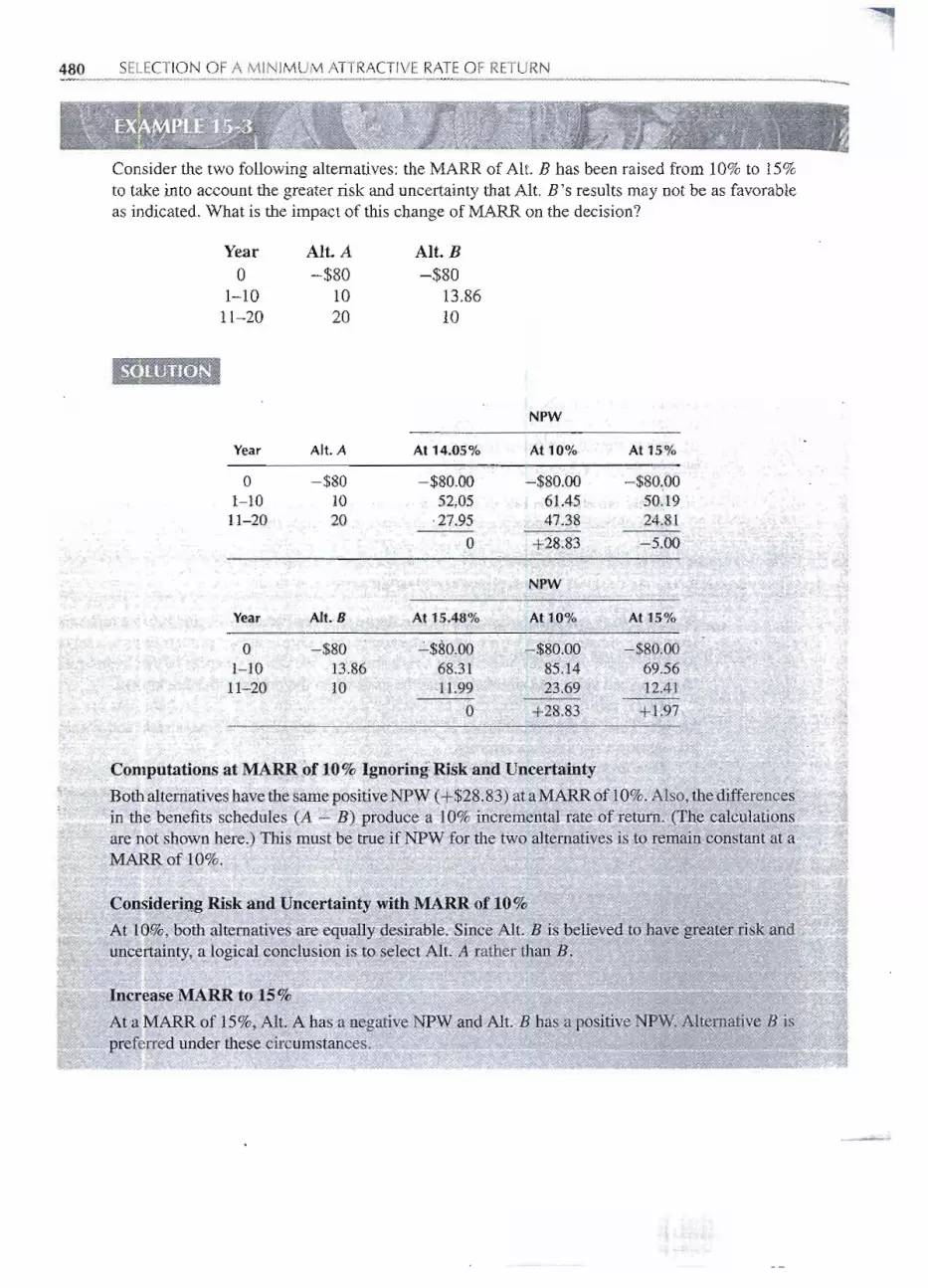
]480 SELECTIONOF A MINIMUM ATTRACTIVERATEOF RETURN -
Consider the two following alternatives:the MARR of Alt. B has been raised from 10% to 15%to take into account the greater risk and uncertainty that Alt. B's results may not be as favorableas indicated. What is the impact of this change of MARR on the decision?
Yearo
1-1011-20
Alt. A-$80
1020
Alt. B-$80
13.8610
. Computations at MARR of 10% Ignoring R.isk~d Uncertainty .
Both alternatives have the same positive NPW (+$28.83) at,a MARR o~10%. Also, the differencesin the benefits schedules (A - B) produce a...10% increrp.ental rate of.rettlrn. (The calculationsare qot shown here.) This must be tr'ueifNPW for the two alternatives is totemaJ,n constant at aMARR of 10%.
IL~I
Considering Risk.and Uncertainty with MARR of 10% I
Ai 10% ,both alternatives are equally desirable. Since Alt. B is believed to pave greater. risk arid ~ tuncertainty, a logical conclusion is to select Alt. A rather tpanB. 1
a e jt .. 'n::Cre:a~iMA.RR ta15% "'::;: =!: = "" ~ '"' ...~::: :::::: = ~~ :=-='-~ == = ...,A
.
t.a
.
:1\1
.
.
...
ARR.
of 15.
.%,A.
lt
.
..
A..
.
.
ha.
s a ne.
.
.
ga.
tiv..
e NPWand..
Alt. B..
has a.positive NPW.
.A.
71
.
tematiyeJ3is
Jp~eferred.qn<ler tl1ese..cir~mrp.stance?:: .!ii!.'! ~ ~ '" >; ~ ~::: ==='1:1=_11 oil ~ :;;:;;~ =...,
.-1000... 11\II,\:>::1 _ __ . III _ , A
-- --
NPW
Year Alt. A At 14.05% At 10% At 15%
0 -$80 -$80.00 -$80.00 -$80.001-10 10 52.05 61.45 50.1911-20 20 27.95 47.38 24.81-
0 +28.83 --5.00.
NPW
Year Alt. 8 At 15.48% At 10% At 15%
0 -$80 -$80.00 -$80.00 -$80.001-10 3.86 68.31 85.14 69.5611....20 0 11.99 23.69 12.41-
0 +28.83 +1.97

~ ~ u._ .-.
Adjusting MARR to Account for Risk and Uncertainty 481
Conclusion
Based on a business-risk MARR of 10%, the two alternativesare equivalent. Recognizing somegreater risk of failure for Alt. B makes A the preferred alternative. If the MARR is increased to15%, to add a margin of safety against risk and uncertainty, the computed decision is to selectB. Since Alt. B has been shown to be less desirable than A, the decision, based on a MARRof 15%, way be an unfortunate one. The difficulty is that the same risk adjustment (increasethe MARR by 5%) is applied to both alternatives even though they have different amountsof risk.
The conclusionto be drawn fromExample 15-3is that increasing the MARRto compensatefor risk and uncertainty is only an approximate technique and may not always achievethedesired result. Nevertheless,it is common practice in industry to adjust the MARR upwardto compensate for increased risk and uncertainty.
Inflation and the Cost of Borrowed MoneyAs inflationvaries,whatis its effecton the cost of borrowedmoney?A widelyheld viewhasbeen that interest rates on long-term borrowing, like 20-year Treasury bonds, will be about3% more than the inflationrate. For borrowers this is the real-that is, after-inflation--costof money,andfor lenders the real return on loans. If inflationrates were to increase, it wouldfollow that borrowing rates would also increase. All this suggests a rational and orderlysituation, about as we might expect.
Unfortunately, things have not worked out this way. Figure 15-3 shows that the realinterest rate has not always been about 3% and, in fact, there have been long periods
1985 1990 1995 2000Year
FIGURE 15-3 The real interest rate. The interest rate on 20-year Treasury bonds minus the inflationrate, f, as measured by changes in the Consumer Price Index.
10
8
6'-'CIJ 4'i;j
2...VJ
0£=.....-2<;JCIJ-4
-6
I I , , , I I
1975 1980

]482 SELECTIONOF A MINIMUM ATTRACTIVERATEOF RETURN -
during which the real interest rate was negative. Can this be possible? Would anyoneinvest money at an interest rate several percentage points below the inflation rate? Wellconsider this: when the U.S. inflation rate was 12%, savings banks were paying 51/2%o~regular passbook deposits. And there was a lot of money in those accounts. While theremust be a relationship between interest rates and inflation, Figure 15-3 suggests that it iscomplex.
REPRESENTATIVEVALUESOF MARR USED IN INDUSTRY
We argued that the minimum attractive rate of return should be established at the highestone of the following: cost of borrowed money, cost of capital, or the opportunity cost.
The cost of borrowed money will vary from enterprise to enterprise, with the lowest,rate being the prime interest rate. The prime rate may change several times in a year; it iswidely reported in newspapers and business publications. As we pointed out, the interestrate for firms that do not qualify for the prime interest rate may be 1/z% to several percentagepoints higher. .
The cost of capital of a firm is an elusive value. There is no widely accepted wayto compute it; we know that as a composite value for the capital structure of the finn,it conventionally is higher than the cost of borrowed money. The ,cost of capital mustconsider the market valuation of the shares (common stock, etc.) of the firm, which mayfluctuate widely,dependingon future earnings prospects of the 'firm,We cannot generalizeon representativecosts of capital.
Somewhat related to cost of capital is the computation of the return on total capital(long-term debt, capital stock, and retained earnings) actually achieved by firms.Fortunemagazine, among others, does an annual analysis of the rate of return on total capital. Theafter-tax rate of return on total capital for individual firms ranges from 0% to about 40%and averages 8%. Business Week does a periodic survey of corporate performance. Thismagazine reports an after-tax rate of return on common'stock and retaine~ earnings. Wewould expect the values to be higher than the rate of return on total capital, and this is thecase. The after-taxreturn on common stock and retained earnings ranges from 0% to about65% with an average of 14%. , .
When discussing MARR, firms can usually be divided into two general groups. First,there are firms that are struggling along with an inadequate supply of investment capital orare in an unstable situation or unstable industry. These firms cannot or do not invest money
in anything but the most critical projects with very high rates of return and a rapid returnof the capital invested. Often these firms use a payback period of one year or less, beforeincome taxes. For an investment project with a 5-year life, this correspop.ds to about a 60%after-tax rate of return. When these firms do rate of return analysis, they reduce the MARR to
possibly 25 to 30% after income taxes. There is potentially a substantial difference betweena one-year before-tax payback period and a 30% after-tax MARR, but this appare.ntly doesnot disturb firms that specify this type of dual criteria.
The second group of firms represents the bulk of all enterprises. They are in a morestable situation and take a longer-range view of capital investments. Their greater moneysupply enables them to invest in capital investment projects that firms in the first group
- ----
Representative Values of MARR Used in Industry 483
will reject. Like the first group, this group of firms also uses payback and rate of return,analysis. When small capital investments (of about $500 or less) are considered, paybackperiod is often the only analysis technique used. The criterion for accepting a proposalmay be a before-tax payback period not exceeding 1or 2 years. Larger investmentprojectsare analyzed by rate of return. Where there is a normal level of business risk, an after-taxMARR of 12 to 15% appears to be widely used. The MARR is increased when there isgreater risk involved.
In Chapter 9 we saw that payback period is not a proper methodfor the economic anal-ysis of proposals.Thus, industrial use of payback criteria is not recommended.Fortunately,the trend in industry is toward greater use of accurate methods and less use of paybackperiod.
Note that the valuesofMARR givenearlier are approximations.But the valuesquotedappear to be opportunity costs, rather than cost of borrowed money or cost of capital. Thisindicates that firms cannot or do not obtain money to fund projects whoseanticipated ratesof return are nearer to the cost of borrowed moneyor cost of capital.While one could makea case that goodprojects are needlesslybeing rejected, one reason that firmsoperate as th~ydo is that they can focus limited resources of people, management, and time on a smallernumber of good projects.
One cannot leave this section without noting that the MARR used by enterprises is somuch higher than can be obtained by individuals. (Where can you get a 30% after-tax rateof return without excessiverisk?) The reason appears to be that businesses are not obligedto compete with the thousands of individuals in any region seeking a place to invest $2000with safety,whereas the number of people who could, or would want to invest $500,000 ina business is far smaller.This diminishedcompetition,combinedwith a higher risk, appearsto explain at least some of the difference.
Spreadsheets, Cumulative Investments, and the OpportunityCost of CapitalAs shown in earlier chapters, spreadsheets make computing rates of return dramaticallyeasier. In addition, spreadsheets can be used to sort the projects by rate of return and thencalculate the cumulative first cost. This is accomplishedthrough the followingsteps. .
1. Enter or calculate each project's rate of return.2. Select the data to be sorted.Do not include headings,but do include all information
on the row that goes with each project.3. Select the SORT tool (found in the menu under DATA),identify the rate of return
column as the firstkey, and a sort order of descending.Also ensure that row sortingis selected. Sort.
4. Add a column for the cumulative first cost. This column is compared with thecapital limit to identify the opportunity cost of capital and whichprojects should befunded.
Example 15-4 illustrates these steps.
- - -
~rf:

484 SELECTIONOF A MINIMUM ATTRACTIVERATEOF RETURN1
A finn has a budget of $800,000 for projects this year.Which of the followingprojects shouldbeaccepted? What is the opportunity cost of capital?
Project First Cost Annual BenefitA $200,000 $25,000B 250,000 47,000C 150,000 17,500D 100,000 20,000E 200,000 24,000F 300,000 35,000G 100,000 18,000H 200,000 22,500I 350,000 50,000
Salvage Value$50,000
-25,00020,00015,00025,00015,000
o15,000
o
Life (years)151015102015102025
SO~UTlor,,{
The first step is to use the RATEfunction to findthe rate of return for each project. The results ofthis step are shown iI1the top portion of FigUre15-4.Next the projects are sorted in descending
Il.
fIGIJRE 15.4 Spreadshee~;.forfindingi opportunity cost of capital.'1"'"- - -
- -- --- ---
IiIJ.I1
~ i
A B C D E F G H
Annual Salvage1 Project First Cost Benefit Value Life IRR
2 A 200,000 25,000 50,000 15 10.2% = RATE(E2,C2, -B2,D2)3 B 250,000 47,000 -25,000 10 12.8%
,I
4 C 150,000,
17,000 20,000 15 8.6%5 D 100,000 20,OqO 15,000' 10 16.0%6 E 200,000 24,000 25,000 20 10.6%7 F.... 300,000 I 35,000 15,000 15 8.2% ..8 G' 100,000 18,000 I. o ", 10 12.4%9 H 200,000 22,500 15,000 20 9.6%
10 I 350,000 50,000 0 I- 25 13.7% ICumulative
11 Projects Sortedby IRR First Cost12 D 100,000 20,000 15,000 I 10 16.0% 100,00013 I 350,000 50,000 I 0 25 13.7% 450,000.I -.,...,-:-,-14 B 250,000 47,000 -2,000 10 12.8% 7oo,00615 G
,100,000 18,000 _
0 10 12.4% 800,00016 E 200,000 24,000 25,000 20 " 10.6% 1,000,00017 A 200,000 25,000 50,000 15 10.2% I 1,200,000 -18 H 200,000 22,500 15,0()() 20 9.6% 1,400,00019 ;"C 150,000 17,500 20,000 ! 15 8;6% , 155();000 ;. :i ==
20 F 300,000 35,000 I 15,000 15 I 8.2% 1,850,000
-- ~ -
Problems 485
order by thep-rates of return. Finally, the cumulativefirstcost is computed. Projects D, I, B, andG should be funded. The opportunity cost of capital is 12.4%if definedas the last project fundedand 10.6%if definedas the first project rejected.
"
SUMMARY
There are four general sources of capital available to an enterprise. The most importantone is money generated from the operation of the firm. This has two components: there isthe portion of profit that is retained in the business; in addition, a profitable firm generatesfunds equal to its depreciationcharges that are availablefor reinvestment.
The three other sources of capital are from outside the operation of the enterprise:
1. Borrowed money from banks, insurance companies, and so forth.2. Longer-termborrowingfrom a lending institution or from the public in the form of
mortgage bonds. .3. Sale of equity securities like common or preferred stock.
Retainedprofitsandcashequalto depreciationchargesaretheprimarysourcesof investmentcapital for most firms,and the only sources for many enterprises.
In selecting a value of MARR, three values are frequently considered:
1. Cost of borrowed money.2. Cost of capital. This is a composite cost of the components of the overall capital-
ization of the enterprise.3. Opportunity cost. This refers to the cost of the opportunity forgone; stated more
simply, opportunity cost is the rate of return on the best investmentproject that isrejected.
The MARR should be equal to the highest one of these three values.When there is a risk aspect to the problem (probabilities are known or reasonably
estimated), this can be handled by techniques like expected value and simulation. Wherethereis uncertainty(probabilitiesofthe variousoutcomesarenotknown),thereare analyticaltechniques, but they are less satisfactory.A method commonly used to adjust for risk anduncertaintyis to increasethe MARR.Thismethodhas the effectof distortingthe time-value-of-moneyrelationship.Theeffectis to discountlonger-termconsequencesmoreheavilythanshort-termconsequences, which mayor may not be desirable. Other possibilities might beto adjust the discounted cash flows or the lives of the alternatives. ;~
15-1 Examine the financial pages of your newspaper (orthe Wall St. Journal) and detenmne the currentinterest rate on the followingsecurities, and explainwhy the interest rates are differentfor these differentbonds.
(a) U.S. Treasury bond due in 5 years.(b) General obligation bond of a municipal district,
city, or a state due in 20 years.(c) Corporate debenture bond of a U.s. industrial
firm due in 20 years.
PROBLEMS
--- ----

--,486 SELECTION OF A MINIMUM ATTRACTIVERATEOF RETURN
Each alternative has a lO-year usefu11ife and no sal-vage value. Over what range of interest rates is C thepreferred alternative? (Answer: 4.5% < i :S 9.6%)
15-3 Frequently we read in the newspaper that one shouldlease an automobile rather than buying it. For atypical 24-month lease on a car costing $9400, themonthly lease charge is about $267. At the end of the24 months, the car is returned to the lease company(which owns the car). As an alternative, the same carcould be bought with no down payment and 24 equalmonthly payments, with interest at a 12% nominal an-nual percentage rate. At the end of 24 months the caris fully paid for. The car would then be worth abouthalf its original cost.(a) Over what range of nominal before-tax interest
rates is leasing the preferred alternative?(b) What are some of the reasons that would
make leasing more desirable than is indicatedin (a)?
15-4 Assume you have $2000 available for investment fora 5-year period. You wish to invest the money-not just spend it on fun things. There are obviouslymany alternatives available. You should be willing toassume a modest amount of risk of loss of some or
all of the money if this is necessary, but not a greatamount of risk (no investments in poker games orat horse races). How would you invest the money?What is your minimum attractive rate of return?Explain.
15-5 There are many venture capital syndicates that consistof a few (say, eight or ten) wealthy people who com-bine to make investments in small and (hopefully)growing businesses. Typically, the investors hire ayoung investment manager (often an engineer withan MBA) who seeks and analyzes investment oppor-tunities for the group. Would you estimate that theMARR sought by this group is more or less than 12%?Explain.
--
15-6 A factory has a $100,000capital budget. Determine
JJL ",:hich project(s! should be funded and the opportu_~. mty cost of capItal.
15-7 Chips USA is considering the following projects to_ improve their production process. Chips have a shortlife, so a 3-year horizon is used in evaluation. Whichprojects should be done if the budget is $70,000?What is the opportunity cost of capital?
Project12Y4567
First Cost$20,00030,00010,0005,000
25,00015,00040,000
Benefit
$11,00014,000~,0002,400
13,0007,000
21,000
15-8 National Motors's Rock Creek plant is considering_ the following projects to improve the company's pro-duction process. Which projects should be done if thebudget is $500,000? What is the opportunity cost ofcapital ?
15.2 Considerfour mutuallyexclusivealternatives:
A B C DInitial cost $0 $100 $50 $25Uniform annual 0 16.27 9.96 5.96
benefitComputedrate 0% 10% 15% 20%
of return
Annual Life SalvageProject First Cost Benefits (years) Value
A $50,000 $13,500 5 $5000B 50,000 9,000 10 0C 50,000 13,250 5 1000D 50,000 9,575 8 6000
Annual LifeProject First Cost Benefit (years)
1 $200,000 $50,000 152 300,000 70,000 103 100,000 40,000 54 50,000 12;500 105 250,000 75,000 5.6 150,000 32,000 207 400,000 125,000 5

1\
Problems 487
9 The WhatZit Company has decided to fund six of nine
I project proposals for ~e coming budget year. Deter-Iiii. mine the nextcapital budget forWhatZit.What is the
MARR?
ProjectABCDEFGHI
First Cost
$15,00020,00030,00025,00040,00050,00035,00060,00075,000
AnnualBenefits$ 4,429
6,1739,8786,261
11,93311,5506,794
12,69214,058
Life(years)
444555888
15-10 Which projects should be done if the budget is. $100,000? What is the opportunity cost of capital?8I:iiiiiiEiii
II"!
11
i-- --~--
Life Annual SalvageProject (years) First Cost Benefit Value
1 20 $20,000 $40002 20 20,000 3200 $20,0003 30 20,000 3300 10,0004 15 20,000 45005 25 20,000 4500 - 20,0006 10 20,000 58007 15 20,000 4000 10,000
.,-;:'
j

After Completing This Chapter...The student should be able to:· Distinguish the unique objective and viewpoint of public decisions.· Explain methods for determining the interest rates for evaluatingpublic projects.· Us.ethe benefit--costratio to analysis projects.· Distinguish between the conventionaland modified versions of the benefit--costratio.· Use an incrementalbenefit--costratio to evaluate a set of mutually exclusiveprojects.· Discuss the impact of financing,duration, and politics in public investment analysis.
QUESTIONS TO CONSIDER~
1. The situation described here is not unique to the Tar...,PamlicoBasin. In fact, it existsto some degree nationwide. So why has Congress"beenslow.to impose environmentalrequirements on the agricultural sector?
2. Manufacturersin the Tar-Pamlico Basin eventuallywere able to work out an agreementunder which they paid local farmers to reduce pollutant runoff. What was the highestamount they were willing to pay per kilogram of pollutants avoided? "
3. What was the lowest amount farmers were willing to accept per kilogram of pollutantto sign onto the agreement?
---

-- ---
,--~
Economic Analysis in thePublic Sector
Hogs and Heavy IndustryIndustrial facilities in North Carolina's Tar-Pamlico river basin knew they had a costlyproblem on their hands a few years ago. State environmentalofficialshad discoveredhighlevels of water pollutants flowing into a nearby estuary. Industrial plants would have tocut their pollution discharges significantly, the officials said. New regulations would beforthcoming.
There wasjust one snag in this plan: most of the pollutants weren'tcoming from industrial plants. They were coming from local farms.The Tar-Pamlico Basin's economy had a large agricultural component,including many hog and chicken farms. These farms were contributingsubstantial quantities of water pollutants in the form of runoff frommanure, fertilizer, and pesticides.
So why didn't the environmental regulators go after the farmers?Simple: They weren't coveredby the CleanWaterAct, and the factorieswere.
The region's manufacturershadbeenheavilyregulatedforyearsandhad alreadyreduced their pollutants well below required levels. Tryingto extract the last trace of pollutants from factory effluents would beextremelycostly and wouldnothavedonemuch to help the environmentin any case. When regulators ran the required cost analysis on theirproposed regulations, they found that manufacturerswould have to payas much as $500 to eliminate one kilogram of targeted pollutants.
By contrast, farmerscould cutpollutants significantly,at aboutone-tenth the cost to manufacturers, simply by instituting practices such asconstructing retention ponds, which would help keep pollutants fromrunning off their property into waterways.
- - -
-

490 ECONOMIC ANALYSISIN THE PUBLIC SECTOR
So far we haveconsideredeconomic analysis for companiesin the private sector,wherethe main objectivesare to generateprofits for growth and to reward current stockholders.Investment decisionsfor private-sectorcompaniesinvolve evaluating the costsat:J.dbene-fits associatedwith prospectiveprojectsin termsof life-cyclecashflowstreams.In earlierchapters we developed several methods for calculating measures-of-meritand making de-cisions. Public organizations, such as federal, state, and local governments, port authori-ties, school districts, and government agencies also make investment decisions. Fo! thesedecision-making bodies, economic analysis is complicated by several factors that do notaffect companies in the private sector. These factors include the overall purpose of invest-ment, project financing sources, expected project duration, effects of politics, beneficiariesof investment, and the multipurpose nature of investments. The overall mission in the publicsector is the same as that in the private sector-to make prudent investment decisions thatpromote the overall objectives of the organization.
The primary economic decision measure-of-merit used in the public sector is thebenefit-cost (B/C) ratio. This measure is calculated as a ratio of the equivalent worthof the benefits of investmentin a project to the equivalentworth of costs. If the BIC ratiois greater than 1.0, the project under evaluation is accepted; if not, it is rejected. The B/Cratio is used to evaluate both single investments and sets of mutually exclusive projects(where the incremental B/C ratio is used). The uncertainties of quantifying cash flows,long project lives, and low interest rates all tend to lessen the degree of reliability of theB/C ratio. There are two versions of the B/C ratio: conventional and modified. Both pro-vide consistent recommendations to decision makers for single investment decisions andfor decisions involving sets of mutually exclusive alternatives.Nevertheless,the BIC ratiois a widely used and accepted measure in government economic analysis and decisionmaking.
INVESTMENT OBJECTIVE
Organizationsexist to promote the overall goals of those they serve. In private-sectorcom-panies, investment decisions are based on increasing the wealth and economic stability ofthe organization.Beneficiariesof investmentsgenerally are clearly identifiedas the ownersand/or stockholders of the company.. .
In the public sector,the purpose of investmentdecisions is sometimesambiguous.Forpeople in the United States of America, the Preamble to the Constitution establishes theoverall theme or objective for why the public body exists:
We the People of the United States, in order to form a more perfect Union, establishjustice, insure domestic tranquillity, provide for the common defense, promote thegeneral welfare [italics supplied], and secure the blessings of liberty to ourselves andour posterity, do ordain and establish this Constitution for the United States of America.
The catch phrase promote the general welfare serves as a guideline for public decisionmaking. But what does this phrase mean? At best it is a general guideline, at worst it isa vague slogan that can be used to justify any action. Projects one segment of the citi-zenry deems to be useful and necessary may not be so viewedby other groups of citizens.
----

Investment Objective 491
In government economic analysis, it is not always easy to distinguish which investmentspromQtethe "general welfare" and which do not.
Consider the case of a dam construction project to provide water, electricity, floodcontrol, and recreational facilities. Such a project might seem to be advantageous for theentire population of the region. But on closer inspection, decision makers must considerthat the dam will require the loss of land upstream due to backed up water. Farmerswill lose pasture or crop land, and nature lovers will lose canyon lands. Or perhaps theland to be lost is a pivotal breeding ground for protected species, and environmentalistswill oppose the project. The project may also have a negative impact on towns, cities,and states downstream. How will it affect their water supply? Thus, a project initiallydeemed to have many benefits, on closer inspection, reveals many conflicting aspects.Such conflictingaspects are characteristicof investment and decision making in the publicsector.
Public investment decisions are more difficult than those in the private sector owingto the many people, organizations, and political units potentially affected by investments.Opposition to a proposal is more likely in public investment decisions than in those madeby private-sectorcompaniesbecause for everygroup that benefitsfrom a particular project,there is usuallyan opposinggroup.Manyconflictsin opinionarise whenthe project involvesthe use of public lands, including industrial parks, housing projects, business districts,roadways, sewageandpower facilities,and landfills.Oppositionmaybe based on the beliefthat development of any kind is bad or that the proposed developmentshould not be near"our" homes, schools, or businesses.
Consider the decision that a small town might face when considering whether to es-tablish a municipal rose garden, seemingly a beneficial public investmentwith no adverseconsequences. However, an economic analysis of the project must consider all effects ofthe project, including potential unforeseen outcomes. Where will visitors park their vehi-cles? Will increased auto travel around the park necessitate new trafficlights and signage?Will traffic and visitors to the park increase noise levels to adjacent homes? Will the gar-den's special varieties of roses create a disease hazard for local gardens? Will the gardenrequire concentrated levels of fertilizers and insecticides, and where will these substanceswind up after they have been applied? Clearly, many issues must be addressed. What ap-peared to be a simple proposal for a city rose garden, in fact, brings up many aspects to beconsidered. ..
Our simplerose garden illustrateshoweffectsonallparties involvedmustbe identified,even for projects that seem very useful. Public decision makers must reach a compromisebetween the positive effects enjoyed by some groups and the negative effects on othergroups.The overall objectiveis to makeprudent decisions thatpromote the generalwelfare,but in the public sector the decision process is not so straightforward as in the privatesector.
The Flood Act of 1936 specifiedthat waterway improvementsfor flood control couldbe made as long as "the benefits to whomsoever they accrue [italics supplied]are in excessof the estimatedcosts."Perhaps the overallgeneralobjectiveof investmentdecisionanalysisin government should be a dual one: to promote the general welfare and to ensure that thevalue to those who can potentially benefit exceeds the overall costs to those who do notbenefit.
- -
- - - - - -
i

492 ECONOMIC ANALYSIS IN THE PUBLIC SECTOR
VIEWPOINT FOR ANALYSIS
When governmentalbodiesdo economicanalysis, an importantconcern is the properview-point of the analysis. A look at industry will help to explain how the viewpoint,or perspec-tive, from which an analysis is conducted influences the final recommendation.Economicanalysis, both governmental and industrial, must be based on a viewpoint. In the case ofindustry the viewpointis obvious-a companyin theprivatesectorpays the costsandcountsits benefits.Thus, both the costs andbenefits are measuredfrom the perspectiveof the firm.
Costs and benefits that occur outside the firm are referred to as external consequences(Figure 16-1).In years past, private-sectorcompaniesgenerally ignored the externalconse-quences of their actions. Ask anyone who has lived near a cement plant, a slaughterhouse,or a steel mill about external consequences! More recently, governmenthas forced indus-try to reduce pollution and other undesirable external consequences, with the "resultthattoday many companies are evaluating the consequences of their action from a broader, orcommunity-oriented,viewpoint.
D SmokeStack
InternalConsequences
External
Consequences
FIGURE 16-1 Internal and external consequences for an industrial plant.
The council members of a small town that levies taxes can be expected to take the"viewpoint of the town" in making decisions: unless it can be shown "that the money fromtaxes can be used effectively, the town council is unlikely to spend it. But what happens when "
the money is contributed to the town by the federal government, as in "revenue sharing""or by means of some other federal grant? Often the federal government pays a share"ofproject costs varying from 10to 90%. Example 16-1illustrates the viewpointproblem thatis created.
A municipal project will cost $1 million. The federal government will pay 50% of the cost if theproject is undertaken. Although the original economic analysis showed that the PW of benefitswas $1:5 million, a subsequent detailed analysis by~the town engineer indicates a more'realisticestimate of the PW of benefits is $750,000. The town council must decide whether to proceedwith the project. What would you advise?
;--..- .. - -- ------ - --- --

~ _. .__ u _. ... . --. -. ..- ~,....-_._..-
Selecting an Interest Rate 493
From the viewpoint of the town, the project is still a good one. If the town puts up half thecost ($500,000) it will receive all the benefits ($750,000). On the other hand, from an overallviewpoint, the revised estimate of $750,000 of benefits does not justify the $1 million expenditure.This illustrates the dilemma caused by varying viewpoints. For economic efficiency, one does notwant to encourage the expenditure of money, regardless of the source, unless the benefits at leastequal the costs.
Possible viewpoints that may be taken include those of an individual, a business firm orcorporation, a town or city district, a city, a state, a nation, or a group of nations. To avoidsuboptimizing, the proper approach is to take a viewpoint at least as broad as those whopay the costs and those who receive the benefits. When the costs and benefits are totally'confined to a town, for example, the town's viewpoint seems to be an appropriate basis forthe analysis. But when the costs or the benefitsare spread beyond the proposed viewpoint,then the viewpoint should be enlarged to this broaderpopulation.
Other than investmentsin defense and social programs, most of the benefitsprovidedby government projects are realized at a regional or local level. Projects, such as damsfor electricity, flood control and recreation, and transportation facilities, such as roads,bridges, and harbors, all benefit most those in the region in which they are constructed.Even smaller-scaleprojects, such as the municipal rose garden, although funded by publicmonies at a local or state level,provide mostbenefitto those nearby.As in the caseof privatedecision making, it is important to adopt an appropriate and consistent viewpoint and todesignate all the costs and benefits that arise from the prospectiveinvestmentbased on thatperspective.To shiftperspectivewhen quantifyingcosts and benefitscould greatly skewtheresults of the analysis and subsequent decision, and thus such changes in perspective areinappropriate.
ELECTINGAN INTERESTRATE
Several factors, not present for nongovernment firms, influence the seJection of an ap-propriate interest rate for use in economic analysis.in the government sector. Recall thatfor private-sector companies the overall objective is wealth maximization. An appropri-ate interest rate for use in evaluating projects is selected consistent with this goal. Manynongovernment firms use cost of capital or opportunity cost concepts when setting an in-terest rate. The objectiveof public investment,on the other hand, involvesthe use of public .
resources to promote the general welfare and to secure the benefits of a given project towhomsoevermay accruebenefits,as long as thosebenefitsoutweighthe costs.The settingofan interest rate for use in investmentanalysis is less clear-cutin this case. Severalalternativeconcepts have been suggested for how governmentshould set this rate; these are discussednext.

-,494 ECONOMIC ANALYSIS IN THE PUBLIC SECTOR
No Time-Value-of-Money ConceptIn government, monies are obtained through taxation and spent about as quickly as theyare obtained. Often, there is little time delay between collecting money from taxpayers and
spending it. (Remember that the federal government and many states collect taxes everypaycheck in the form of withholding tax.) The collection of taxes, like their disbursement,although based on an annual budget, is actually a continuous process. Using this lineof reasoning, some would argue that there is little or no time lag between collecting andspending tax dollars. As such, they would advocate the use of a 0% interest rate for economicanalysis of public projects.
Cost of Capital ConceptAnother consideration in the determination of interest rates in public investments is thatmost levels of government(federal, state, and local) borrowmoneyfor capital expendituresin addition to collecting taxes. Where money is borrowed for a specificproject, one ~ne ofreasoning is to use an interestrate equal tothe cost of borrowedmoney.This argumentis lessvalid for state and local governmentsthan for privatefirmsbecause the federal government,through the income tax laws, subsidizes state and local bonded debt. If a state or one ofits political subdivisions (like a county, city, or special assessment district) raises moneythrough the sale of bonds, the interest paid on these bonds is exempt from federal taxes. Inthis way the federal government is subsidizing the debt, thereby encouraging investors topurchase such bonds.
These bonds, called municipal bonds, can be either general obligation or revenuebonds. Generalobligationmunicipalbonds pay interest and are retired (paid oft) throughtaxes raised by the issuing government unit. A school district may use property taxes itreceives to finance bond debt for construction of new language labs.-Revenue bonds,on the other hand, are not supported by the taxing authority of the government-unit;rather, they are supported by revenues earned by the project being funded. As an ex-ample, the city of Athens, Ohio, would use toll revenues from a new bridge over theHocking River to retire debt on revenue bonds sold for the bridge's construction. Forthose who purchase municipal bonds, the instruments' tax-free status means that the ex-pected return on this investment is somewhat less than that required of fully taXedbondinvestments (of similar risk). As a rough estimate, when fully taxed bonds yield an 8%interest rate, municipal bonds might make interest payments at a rate of 6%. The dif-ference of 2% represents the effect of the preferred treatment for federal taxation, andhence a form of hidden federal subsidy on tax-free bonds. This means that the cost ofcapital approach is sometimes skewed for debt incurred through the use of long-termbonds.
Opportunity Cost ConceptOpportunitycost, whichrelates to the interest rate on the best opportunityforgone,may taketwo forms in governmentaleconomic analysis: governmentopportunity cost and taxpayeropportunity cost. Inpublic decision making, if the interest rate is based on the opportunity
- - - - - -- -- -------
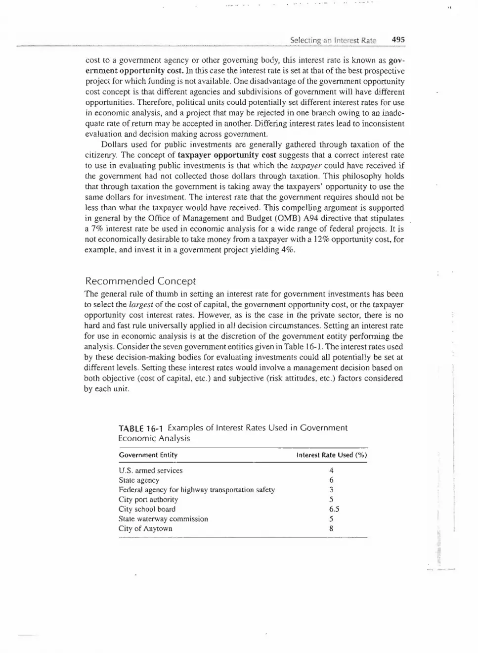
_..---- -. . -....-.1\
Selecting an Interest Rate 495
cost to a government agency or other governing body, this interest rate is known as gov-ernment opportunity cost. In this case the interest rate is set at that of the best prospectiveproject for which fundingis not available.One disadvantageof the governmentopportunitycost concept is that different agencies and subdivisionsof government will have differentopportunities. Therefore, political units could potentially set different interest rates for usein economic analysis, and a project that may be rejected in one branch owing to an inade-quate rate of return may be accepted in another.Differing interest rates lead to inconsistentevaluation and decision making across government.
Dollars used for public investments are generally gathered through taxation of thecitizenry. The concept of taxpayer opportunity cost suggests that a correct interest rateto use in evaluating public investments is that which the taxpayer could have received ifthe government had not collected those dollars through taxation. This philosophy holdsthat through taxation the government is taking awaythe taxpayers'opportunityto use thesame dollars for investment."The interest rate that the government requires should not beless than what the taxpayer would have received. This compelling argument is supportedin general by the Office of Management and Budget (OMB) A94 directive that stipulatesa 7% interest rate be used in economic analysis for a wide range of federal projects. It isnot economically desirable to take moneyfrom a taxpayerwith a 12%opportunity cost, forexample, and invest it in a governmentproject yielding 4%.
Recommended ConceptThe general rule of thumb in setting an interest rate for government investments has beento select the largestof the cost of capital, the governmentopportunitycost, or the taxpayeropportunity cost interest rates. However, as is the case in the private sector, there is nohard and fast rule universallyapplied in all decision circumstances.Setting an interest ratefor use in economic analysis is at the discretion of the government entity performing theanalysis. Consider the sevengovernmententitiesgivenin Table16-1.The interestrates usedby these decision-making bodies for evaluatinginvestments could all potentially be set atdifferent levels. Setting these interest rates would involvea management decisionbased onboth objective (cost of capital, etc.) and subjective (risk attitudes, etc.) factors consideredby each unit.
TABLE16-1 Examples of Interest Rates Used in GovernmentEconomic Analysis
Government Entity
U.S. armed services
State agencyFederal agency for highway transportation safetyCity port authorityCity school boardState waterway commissionCity of Anytown
Interest Rate Used (%)
46356.558
- - --- -- - --

496 ECONOMIC ANALYSISIN THE PUBLIC SECTOR
THE BENEFIT-COST RATIO
The benefit-cost ratio was described briefly in Chapter 9 as one of the alternative eco-nomic analysis methods for evaluating prospective projects. This method is used almostexclusively in public investment analysis, and because of the magnitude of public dOllarscommittedeach year through such analysis,the benefit-cost ratio deservesour attentionandunderstanding.
One of the primary reasons for the use of the benefit-cost ratio (B/C ratio) in publicdecision making is its simplicity.The ratio is formed by calculating the equivalentworthof the benefits accrued through investmentin a project divided by the equivalentworth ofthe costs of the project. The benefit-cost ratio can be shown as follows:
B/C. Equivalentworth of net benefitsratio =
Equivalentworth of costs
-PW benefits
PW costsFW benefits
- FW costs
AW benefits
AW costs
Notice that any of the equivalent worth methods (present, future, and annual) can be usedto calculate this ratio. Each formulation of the ratio will produce an identical result, as .
illustrated in Example 16-2.
Demonstrate that for a highway expansionproject with data given as follows,the sameBIC ratiois obtained using the present, future, and annual worth formulations.
Initial costs of expansionAnnual costs for operating/maintenanceAnnual savings and benefits to travelersScrap value after useful lifeUseful life of investmentInterest rate
$1,500,00065,000
225,000300,00030 years8%
UsingPresentWorth
PW benefits - 225,000(P IA, 8%, 30) + 300,000(P IF, 8%, 30) =$2,563,000
PW costs - 1,500,QOO+ 65,000(P IA, 8%, 30) - $2,232,000
U$in~FUtureWorth
FW benefits = 225,;00(F IA,=8%,30)+ 300,000 - $2{79'0,'Q"bd"= ;:;
FWcosts= 1,500,000(F IP, 8%,30) + 65,000(FIA, 8%,30) - $22,460,000
--
..
- - - - - ---

--- -. .----------------
The Benefit-Cost Ratio 497
Using Annu~ Worth
AW benefits = 225,000+ 300,000(AIF, 8%,30) = $227,600AW costs = 1,500,000(AI P, 8%,30) + 65,000 = $198,200
B ratio= 2,563,000 = 25,790,000 = 227,600= 1.15IC . .. ... .......
One can see that the ratio provided by each of these methods produces the sameresult: 1.15...
- -. . -~~- .~. - ;.."JI
An economic analy~is is performed to assist in the objective of making a decision.When one is using the BIC ratio, the decision rule is in two parts:
If the BIC ratio is ; 1.0,thenthe decisionshouldbe to "invest."If the BIC ratiois < 100,then the decisionshouldbe "do not invest."
Cases of a BIC ratio just equal to 1.0 are analogous to the case of a calculated n.etpresentworth of $0 or an IRR analysis that yields i = MARR%. In other words, the decisionmeasure is just at the breakeven criteria. In such cases a detailed analysis of the inputvariables and their estimates is necessary, and one should consider the merlts of otheravailableopportunities for the targeted funds. But, if the BIC ratio is greater than or lessthan 1.0, the recommendationis clear.
The B/C ratio is a numerator/denominatorrelationshipbetween the equivalentworths(EW) of benefits and costs: . .
EW of net benefits to whomsoeverthey may accrueB/C ratio =
EW of costs to the sponsors of the project
The numerator and denominator aspects of the ratio are sometimes interpreted and usedin different fashions. For instance, the conventional B/C ratio defines the numerator anddenominator as follows:
EW of net benefits
Conventional BIC ratio = EW of initial costs + EW of operating and maintenancecosts
This is the formulation of the B/C ratio used in Example 16-2.However,there is anotherversion of the ratio, called the modified BIC ratio. Using a modifiedversion, the numeratorand denominator are defined in a different manner: the annual operatingand maintenanc~costs to the users are subtracted in the numerator, whereas they are added as a cost in thedenominator.In this case the ratio becomes:
M dO
fi d B/C0 EW of net benefits - EW of operating and maintenance costs
Ole ratio =EW of initial costs

-- -- -- _.---- ----- - -- ----------------------------------------------------------------------------------------- -,498 ECONOMIC ANALYSISIN THE PUBLIC SECTOR
For decision making, the two versions of the benefit-cost ratio will produce the samerecommendation on whether to invest or not invest in the project being considered. ThenumericBIe ratiofor the twoversionswill not alwaysbe the same,but the recommendationwill be. This fact is illustrated in Example 16-3.
Consider the highway expansion project from Example 16-2. Let us use the present worthformulation of conventionaland modified versions to calculate the BIC ratio.
,\SOlUTION
Using the Conventional B / C Ratio
C . 225,000(P IA, 8%,30)+ 300,000(PI F, 8%,30) 1 5BI ratio = = .11,500,000 + 65,000(P IA, 8%,30)
Using the Modified BIC Ratio
. 225,000(P IA, 8%, 30) + 300,000(P I F, 8%,30) - 65,000(P / A, 8%, 30)B/C raho = = 1.22
1,500,000
Whether the conventionalor the modified ratio is used, the recommendation is to invest in thehighway expansion project. The ratios are not identical in magnitude (1.15 vs 1.22), but thedecision is the same.
It is important when one is using the conventional and modified BIC ratios not todirectly compare the magnitudesof the two versions. Evaluatinga project with one versionmay produce a higher ratio than i&produced with the other version, but this does not implythat the project is somehow better. .
The net benefitsto the users of governmentprojects are the differencebetween the ex-pected benefitsfrom investmentminus the expecteddisbenefits.Disbenefitsare the negativeeffectsof governmentprojects felt by some individualsor groups.For example,considertheNational Park System in the United States. Development projects by the skiing or lumberindustries might provide enormous benefits to the recreation or construction sectors whilecreating simultaneousdisbenefits for environmentalgroups. Table 16-2illustrates some ofthe primary benefitsand disbenefitsof several example public investments.
INCREMENTAL BENEFIT-COST ANALYSIS
In Chapter 9 we discussed using the incremental benefit-cost ratio in economic decisionanalysis.As is thecasewiththeinternalrate ofreturn (IRR)decisionmethod, theincrementalB/C ratio shouldbe used in comparing sets of mutually exclusivealternatives.This methodproduces a result that is consistentwith the result producedby optimizingthe present worth
---

u' . u.
Incremental Benefit-Cost Analysis 499
Public Project
TABLE 16-2 Example Benefits and Disbenefits for Public Investments
New city airport on theexterior of town
Interstate bypass aroundtown
New metro subway system
Creation of a city disposalfacility versus sendingwaste out of state
Construction of a nuclear
energy generation facility
Primary Benefits
More flights, new businesses
Quicker commute times,reduced congestion onsurface roads
Faster commute times, lesspollution
Less costly, faster and moreresponsive to customers
Cheaper energy costs, newindustry in area
Primary Disbenefits
Increased travel time to airport,more traffic on outer belt
Lost sales to businesses onsurface roads, lostagricultural lands
Lost jobs due to bus line closing,less access to service
(fewer stops)
Objectionable sight and smells,lost market value to home-
owners, lost pristine forestland
Perceived environmental risks
of the decision alternatives over their respective life cycles. As with the incremental IRRmethod, it is not proper to simplycalculate the BIC ratio for each alternativeandchoose theone with the highest value. Rather, an incrementalapproach is called for. The incrementalapproach used with the IRR method can be slightly augmentedfor use with the BIC ratio.
Elements of the Incremental Benefit-Cost Ratio Method1. Identify all relevant alternatives. Decision makers identify the set of alternatives
from which a choice is ultimatelymade.In this contextit is importantto identify all relevantand competitive alternatives. Decision rules or models can recommend a best course ofaction only from the set of identified alternatives. If a better alternative than those in theconsidered set exists, it will never be selected, and the solution will be suboptimal. Forbenefit-cost ratio problems, the "do-nothing" option is always the "base case" from whichthe incremental methodology proceeds. .
2. (Optional) Calculate the BIC ratio of each competing alternative in the set. In thisoptional step one calculates the BIC ratio of each of the competing alternativesbased onthe total cash flows for each alternative by itself. Once the individual B/C ratios havebeen calculated, the alternatives with a ratio less than 1.0 are eliminated from furtherconsideration.The alternativeswitha BIC ratio greaterthan1.0 remainin the set of feasiblealternatives. This step gets the "poor performers" out of the way before the incrementalprocedure is initiated. This step maybe omitted,however,because the incremental analysismethod will eliminate the subpar alternativesin due time.
3. Rank order the projects. The incremental IRR method is used to analyze each ofthe mutually exclusivealternativesof the set, arraying the alternativesin order of increasingfirst cost. However,when one is using the incremental B/C ratio, the alternatives must beordered according to increasing size of the denominator of the BIe ratio. (The rank orderwill be the same regardless of whether one uses the present worth, annual worth, or future
--
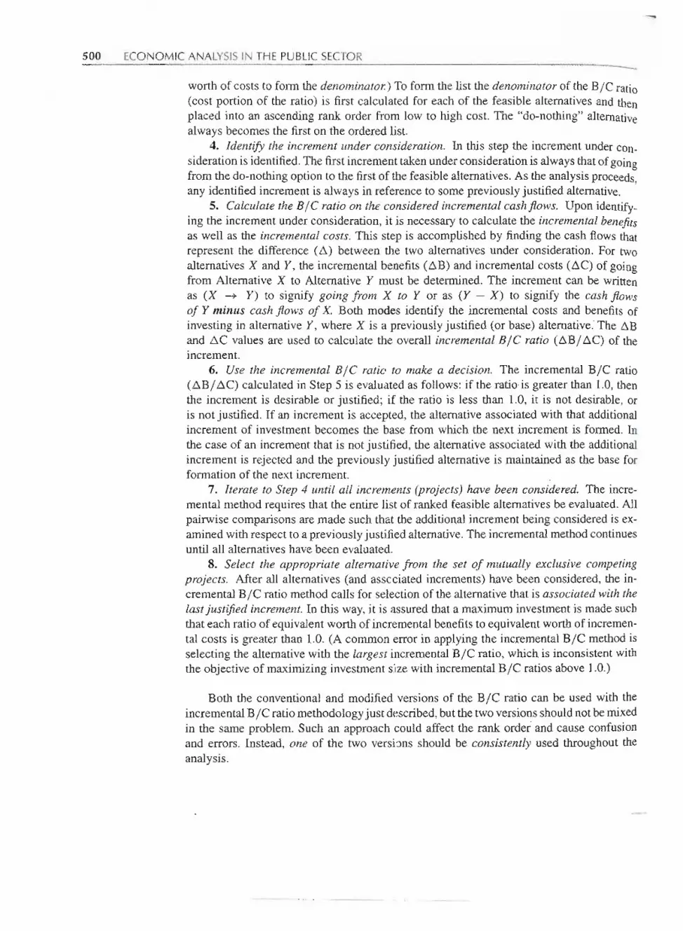
""'-
500 ECONOMIC ANALYSISIN THE PUBLIC SECTOR -worth of costs to form the denominator.) To form the list the denominator of the B IC ratio(cost portion of the ratio) is first calculated for each of the feasible alternatives and thenplaced into an ascending rank order from low to high cost. The "do-nothing" alternativealways becomes the first on the ordered list.
4. Identify the increment under consideration. In this step the increment under con-
siderationis identified.The firstincrement takenunderconsiderationis alwaysthat of goingfrom the do-nothingoption to the firstof the feasible alternatives.As the analysisproceeds,any identified increment is always in reference to some previouslyjustified alternative.
S. Calculate the B IC ratio on the considered incremental cash flows. Upon identify_ing the increment under consideration, it is necessary to calculate the incrementalbenefitsas well as the incrementalcosts.This stepis accomplishedby finding the cash flowsthatrepresent the difference (.6.) between the two alternatives under consideration. For twoalternatives X and Y, the incremental benefits (.6.B)and incremental costs (.6.C)of goingfrom Alternative X to Alternative Y must be determined. The increment can b.ewrittenas (X --+ Y) to signify going from X to Y or as (Y - X) to signify the cash flowsof Y minus cash flows of X. Both modes identify the incremental costs and benefits ofinvesting in alternative Y, where X is a previouslyjustified (or base) alternative:The .6.Band .6.Cvalues are used to calculate the overall incremental BIC ratio (.6.B/.6.C)of theincrement.
6. Use the incremental BIC ratio to make a decision. The incremental B/C ratio(.6.BI .6.C) calculated in Step 5 is evaluated as follows: if the ratio.is greater than 1.0, thenthe increment is desirable or justified; if the ratio is less than 1.0, it is not desirable, oris not justified. If an increment is accepted, the alternative associated with that additionalincrement of investment becomes the base from which the next increment is formed. Inthe case of an increment that is not justified, the alternative associated with the additionalincrement is rejected and the previously justified alternative is maintained as the base forformation of the next increment.
7. Iterate to Step 4 until all increments (projects) have been considered. The incre-mental method requires that the entire list of ranked feasible alternativesbe evaluated.Allpairwise comparisons are made such that the additional increment being consideredis ex-amined with respect to a previouslyjustified alternative.The incrementalmethodcontinuesuntil all alternativeshave been evaluated.
8. Select the appropriaie alternative from the sei of mutually exclusive competingprojects. Mter all alternatives (and associated increments) have been considered, the in-cremental BIC ratio method calls for selectionof the alternativethat is associated with thelastjustified increment. In this way, it is assured that a maximum investmentis made suchthat each ratio of equivalentworth of incrementalbenefitsto equivalentworth of incremen-tal costs is greater than 1.0. (A common error in applying the incremental B/C method isselecting the alternativewith the largest incrementalBIC ratio, which is inconsistentwiththe objective of maximizing investment size with incrementalBIC ratios above 1.0.)
Both the conventional and modified versions of the B/C ratio can be used with theincrementalBIC ratio methodologyjust described,but the two versionsshouldnot bemixedin the same problem. Such an approach could affect the rank ordei and cause confusionand errors. Instead, one of the two versions should be consistently used throughout theanalysis.
--- -- --

~-----
- ---.......
Incremental Benefit-Cost Analysis 501
Examples 16-4 and 16-5illustrate the use of the incremental B/C ratio and showhowthe conventionaland modifiedversions can be used with this procedure to evaluate sets ofmutually exclusivealternatives.
A midwesternindustrial state is consideringthe construction andoperation of facilities to provideelectricity to several state-owned properties. Electricity will be provided via two coal-burnirigpower plants and a distributionnetwork wired to the properties targeted for conversion.A groupstudying the proposal has identifiedgeneral cost and benefitcategoriesfor the project as follows.
Primary costs: Constructionof the power plantfacilities; cost of installing the power distri-bution network; life-cycle maintenance and operating costs.
Primarybenefits: Eliminationofpayments to thecurrent electricityprovider;creationofjobsfor construction, operation, andmaintenance of the facilities and distribution network;revenue from selling excess power to utility companies; increased employment at coalmines in the state.
Assume that there have been four competing designs identified for the power plants. Each designaffects costs and benefits in a unique way. Given the following data for the four mutually exclusivedesign alternatives, use the conventional BIC ratio method to recommend a course of action.
Values (x $104) for Competing Design Alternatives
II
Alternatives I through IV constitute a set of mutually exclusive choices because we will selectone and oWy one, of tp~ d~sign QpqoY§,fot;.tl:1~PoWef~g~~Qts,J)lerefore, an~incremental B IC ratio ~ j:i
: methodis usedto obtainthe solution.Letususe theincrementalmethodas describedabove:
Step 1 The alternatives are do nothin~, and designs I, II,m, and IV.- - -.-
Ill-I
4
I
;~""
~
~
.
.
..
'..
"
:'
.,.,
I
,~...
I"~f~
,
:"
"
"
,
~' ,
.::;:!,
-
II III IV
Project costs! Plant constructioncost $12,500 $11,000 $12,500 $16,800
Annual operatiIig and maintenance cost 120 480 450 145
Project benefitsAnoual savings from utility payments 580 700 950 1,3001 .mue from over;capacity 700' 550 200 250
Annual effect of jobs created 400 750 150 500
Other data
Project life, in years 45 45 45 45
Discounting rate (MARR) 8% 8% 8% 8%

- ----
]502 ECONOMIC ANALYSISIN THE PUBLIC SECTOR -
Step 2 In this optional step we calculate the conventionalB/C ratio for each alternativebasedon individual cash flows.We will use the ratio of the PW of benefitsto costs.
B/C ratio (I) = (580 + 700 + 400)(P / A, 8%,45)/[12,500 + 120(P/ A, 8%,45)] = 1.46
B/C ratio (II) = (700 + 550 + 750)(P / A, 8%,45)/[11,000 + 480(P / A, 8%, 45)] = 1.44
B/C ratio (III) = (200+ 950+ 150)(P/ A, 8%,45)/[12,500+ 325(P/ A, 8%,45)] = 0.96 .
B/C ratio (IV) = (1300 + 250 + 500)(P / A, 8%,45)/[16,800 + 145(P/ A, 8%,45)] = 1.34
Alternative I, n, and IV all have B/C ratios greater than 1.0 and thus are included inthe feasible set. Alternativeill does not meet the acceptabilitycriterion and should beeliminated from further consideration. However,to illustrate that Step 2 is optional,we will continue with.all four design alternativesin the original feasible set.
Step 3 Here we calculate the PW of costs for each alternative in the feasible set (rememberwe are keeping alternativeill along for the ride). The denominatorof the conventionalB/C r~tio includes first cost and annual O&M costs. We calculate the PW of costs foreach alternative as follows.
PW costs (I) = 12,500+ 120(P/A, 8%,45)= $13,953PW costs (II) = 11,000 + 480(P / A, 8%, 45) = $16,812
PW costs (III) = 12,500 + 325(P / A, 8%, 45) = $16,435
PW costs (IV) = 16,800 + 145(P/ A, 8%,45) = $18,556. .
The rank order from low to high value of the B/C ratio denominator is as follows: donothing, I, ill, n, IV.
Step 4 From the ranking list, the first incrementconsideredis that of going from "do nothing"to Alternative I (do nothing -+ Alternative I). The analysis proceeds from this point.
Steps 5 and 6 We proceed through the analysis, designating the incremental cash flows and calcu-lating Ll(B/C) until all feasible alternatives have b~en considered. Each additionalincrement taken under considerationmust be based on the lastjustified increment.
- - -- --------

----- .-
Incremental Benefit-Cost Analysis 503
As .anexample of these calculations, consider the third increment (I ~ II).
APlant construction cost = 11,000- 12,500= -$1500AAnnualO&Mcost =480- 120=$360PW of ACosts = -1500 + 360(P/ A, 8%,45) = $2859
or = 16,812 - 13,953 =$2859= 700 - 580 =$120= 550 -700 = -$150= 750 - 400 = $350= (120 - 150 + 350)(P / A, 8%,45)= $3875= 3875/2850 = 1.36
AAnnual utility payment savingsAAnnual overcapacityrevenuedAnnual benefits of newjobsPW of dBenefits
AB/C ratio (PW dB)/(PW dC)
Step 8 The analysis in the table proceeded as follows:do nothing to AlternativeI was justified(AB / C ratio = 1.46), Alternative I became the new base; AlternativeI to Alternativeill was not justified (AB/C ratio = -'-1.15),Alternative I remained base; AlternativeI td Alternative II was justified (dB/C ratio = 1.36), Alternative II became the base;Alternative II to Alternative IV was not justified (.AB/C ratio = 0.35), and Aiternativellbecame the recommended power plant design alternative because it is the one associatedwith the last justified increment. All alternatives in the feasible set were considered beforethe recommendation was produced. Notice that Alternative ill, even though included inthe feasible set, did not affect the recommendation and was eliminated through theincremental method. Notice also that the first increment considered (do nothing ~ I)was not selected even though it had the largest AB/C ratio (1.45). Selection is based onthe alternative associated with the last justified increment (in this case, Alt. II).
Let us reconsider Example 16-4, this time using the modified B/C ratio to analyze the set ofcr 'peting design alternatives.Again we will use the present worth method.
.SOLUTION,
Here we use the modifiedB/C ratio.
Step 1 The alternatives are still do nothing and designs I, II, ill, and IV.
Step 2 We calculate the modifiedB/C ratio using the PW of benefits and costs~
B/C ratio (I) = (580 + 700 + 400 - 120)(P/ A, 8%, 45)/(12,500) = 1.51
B/C ratio (II) = (700+ 550+ 750- 480)(P/ A, 8%,45)/(11,000) . 1.67=-: ..:;;;:r;~~=:tiC
B/C ratio (III) = (200 + 950 + 150 - 325)(P / A, 8%,45)/(12,500) = 0.95
B/C ratio (IV)= (1300+ 250+ 500- 145)(P/ A, 8%=45)/(16,&00)-).37--
-
-----
I.\)I
:z<10
ILrI
.J_;":'::

- -..
504 ECONOMIC ANALYSISIN THE PUBLIC SECTOR
, Again Alternativeill would be eliminated from further considerationbecause its B/Cratio is less than 1.0. In this case we will eliminate it from the feasible set, which nowbecomes do nothing and alternativedesigns I, II, and IV.
Step 3 The PW of costs for each alternative in the feasible set:
PW Costs (I) =$12,500
PW Costs (II) = $11,000
PW Costs (IV) = $16,800
The appropriate rank order is now do nothing, II, I, IV.Notice that the modified B/Cratio produces a rank order different from that yielded by the conventionalversion inExample 16-4.
Step 4 Thefirstincrementis now(donothing~ Alternative11).Themethodproceedsfromthis point.
Steps 5 and 6 These steps are accomplishedas follows.
As an example of the calculations in the forgoing table, consider the third increment(II ~ IV).
f
.6.Plant construction costPW of !!:.Costs
!!:.Annualutility payment savings!!:.Annualovercapacity revenue.6.Annual benefits of new jobs.6.Annual O&M disbenefitPW of !!:.Benefits
.6.B/C ratio, (PW~~B:)/(P~ ~C)
= 16,800 ~ 11,000 = $5800= $5800= 1300"7700= $600= 250- 550= -$300- 500- 750= -$250= 145- 480= -$335= (600 - 300 - 250 + 335)(P I A, 8%,45) = $4662
,y-.. .~
0;; 4fi62/5800 = 0~8~Q ~~ =~ =.. ..=
"When the modified version of the B IC ratio is used, Alt. II emerges as the recommendedpower plant design-just as it did when we used the conventional B/C ratio.
-- --
1
-
iI
IJ
J
Increment
Incremental Effects (Do Nothing -+ II) (II -+I) (II -+ IV)
Plant construction cost $11,000 $ 1500 $ 5800PW of Costs 11,000 1500 5800
Annual utility payment savings 700 -120 600
Annua1 overcapacity revenue 550 150 -300
Annua1 benefits of new jobs 750 -350 -250Annual O&M disbenefit 480 -360 -335
PW of Benefits 18,405 484 4662
B/C ratio (pW B)/(PW C) 1.67 0.32 0.80
Is increment justified? Yes No No

Other Effectsof Public Projects 505
OTHER EFFECTS OF PUBLIC PROJECTS
, Three areas remain that merit discussion in describing the differencesbetween governmentand nongovernment economic analysis: (1) financing government versus nongovernmentprojects, (2) the typical length of government versus nongovernment project lives, and(3) the general effects of politics on economic analysis.
Project FinancingGovernmentalandnongovernmentorganizationsdiffer inthe wayinvestmentsin equipment,facilities, and other projects are financed.In general, nongovernmentfirms rely on moniesfrom individual investors (through stock and bond issuance), private lenders, and retainedearningsfrom operations.These sources serveas the pool from which investmentdollarsforprojectscome. Management'sjob in the nongovernmentfirmis to matchfinancialresourceswith projects in a way that keeps the firm growing, produces an efficient and productiveenvironment,and continues to attract investorsand future lenders of capital.
On the other hand, the government sector often uses taxation and municipal bondissuance as the source of investment capital. In government, taxation and revenue fromoperations is adequate to financeonly modestprojects. However,public projects tend to belarge in scale (roadways, bridges, etc.), which means that for many public projects 100%of the investment costs must be borrowed-unlike those in the private sector. To preventexcessive public borrowing and to assure timely debt repayment, the U.S. government,through constitutionaland legislativechannels,has placed restrictionson governmentdebt.These restrictions include the following:
1. Local government bodies are limited in their borrowing to a specifiedpercentageof the assessed value of the property in their taxation district. This means thatgovernmententities in areaswithhighproperty valuescan borrowmoretotalmoniesthan those in areas where assessed values are lower.
2. For new construction,borrowedfunds attained through the saleof bonds require theapproval of local voters (sometimesby a two-thirds majority) through the electionprocess. An example might be a $2 million levy to fund a new municipaljail. If ap-provedby voters, a $2 million increasewouldraise the property taxesof landownersin the city's tax district by $2 for every $1000 of assessed property value. Theseadditional tax revenues would then be used to retire the debt on the bonds sold tofinance the cityjail project.
3. Repaymentof public debtmust be made in a preset period of timeand in accordancewith a specificplan. This is often the case with monies borrowedby issuing bonds,since bond interest payments and maturity dates are set at the time of issuance.
Limitations on the use and sources of borrowed monies make funding projects in thepublic sector much different from this process in the private sector.Private-sectorfirms areseldom able to borrow 100% of required funds for projects, as can be done in the publicsector, but at the same time, private entities do not face restrictions on debt retirement orthe uncertainty of voter approval.
I~
l
-.

.......
-,506 ECONOMIC ANALYSISIN THE PUBLIC SECTOR -
Project Duration
Another aspect distinguishing government projects from those in the private sector is thetypical duration or project life of the investment. In the private sector,projects most oftenhave a projected or intended life ranging between 5 and 15 years. On some occasionstheproject life is shorterand in others longer,but amajorityof projects fall in this interval.Com-plex advancedmanufacturingtechnologies, like computer-aidedmanufacturing or flexibleautomatedmanufacturingcells, typically haveprojects lives at the longer end of this range.In the 1980ssomecriticizedU.S.manufacturingmanagersfor short-sightedviewsof capitalinvestments in such technologies. At that time short-sightedness and lack of investmentswere blamed for the overall loss of competitivenessin such key U.S. industries as textiles,steel, electronics, automotive, and machine tools.
Government projects typically have lives in the range of 20 to 50 years (or longer).Typical projects include federal highways, city water/sewer infrastructure, county dumps,and state libraries and museums. These projects, by nature, have a longer useful life thana typical project in the private sector. There are exceptions to this rule because privatefinns invest in facilities and other long-range projects, and government entities also investin projects with shorter-term lives. But, in general, investmentduration in the governmentsector is longer than in the private sector.
Governmentprojects,because they tend tobe longrange and largescale,usuallyrequiresubstantial funding in the early stages. The highway, water/sewer,and library projectsjustmentioned could each require millions of dollars in design, surveying, and constructioncosts. Because of this requirement, it is in the best interest of decision makers who areadvocates of such projects to spread that first cost over as many years as possible to reducethe annual cost of capital recovery.This tendency to use longer project lives to downplaythe effects of a large first cost can affect the desirability of the project, as measured by theBIC ratio. Anotheraspect closely associated with managing the size of the capitalrecoverycost in a BIC ratio analysis is the interest rate used for discounting. Lower interest ratesreduce the size of the capital recoverycost by reducing the penalty of havingmoney tiedupin a project. Example 16-6 illustrates the effects that project life and interest rate can haveon the analysis and acceptability of a project.
Consider aproject that has beenapprovedby local votersto build a newjunior high school,neededbecause of increased (and projected)population growth. Informationfor the project is as follows:
IL
Building first costs (design, planning, and construction)Initial cost for roadway and parking facilitiesFirst cost to equip and furnish facility
i!I
Annual operating and maintenance costsAnnual savings from rented spaceAnnual beqefits to community
$10,000,0005,500,000
500,000350,000500,000
1,500,000- - --- --- -- - -- -- - --
--- --

'..- .... .-. -. .. .. .-
Other Effectsof Public Projects 507
With this project we examine the effect that varying project lives and interest rates have on theconventional BjC ratio. Project lives at 15,30, and 60 years and interest rates at: 3, 10, and 15%are used to calculate the ratio for the investment. The ratio for each combination of project lifeand interest rate is tabulated as follows:
Conventional Benefit-Cost Ratio for VariousCombinations of Project Lifeand Interest Rate
Interest
As an example of how the ratios are calculated, suppose that life = 30 years and interestrate = 10%.
1,500,000+ 500,000 = 1.03ConventionalBjC ratio = (10,000+ 5,500,000+ 500,000)(Aj P, 10%,30)+ 350,000
From these numbers one can see the effect of project life and interest on the analysis and rec-ommendation. At the lower interest rate, the project has BjC ratios above 1.0 in all cases ofproject,life, while at the higher rate the ratios are all less than 1.0. At an interest rate of 10% therecommendation to invest changes from no at a life of 15 years to yes at 30 and 60 years. Bymanipulating these two parameters (project life and interest rate), it is possible to reach entirelydifferent conclusions regarding the desirability of the project. The key point is that those advo-cating '~nvestment" are well advised to use lower interest rates and longer project life in theirexample calculations.
..
Project Politics .
To some degree political influences are felt in nearly every decision made in any organi-zation. Predictably, some individual or group will support its own particular interestsovercompeting views. This actuality exists in both government and nongovernmentorganiza-tions. In government the effects of politics are continuouslyfelt at a111evelsbecauseof thelarge-scale and multipurpose nature of projects and because governmentdecisionmakinginvolves the use of the citizenry's common pool of money.
To illustrate on a small scale situations faced by government, compare the decision-making process a family may face when planning an evening out. As most familiescanattest, this decision is not always easy--even when Dad is footing the bill! Imagine theincreased level of conflict that would arise if every member of the family were to con-tribute to the tab. Perhaps the choices would then be dine out, go to a ball game, have ashopping spree at the mall, loan the money to Mom, or put it into the family bank account.
This scenariocharacterizesgovernmentinvestmentdecisions-individnals andgroupswith .~-"~- - --
I
- --- -- --- - - - - -- - - -
Project Life(years) 3% 10% 15%
15 1.24 0.86 0.6930 1.79 1.03 0.7660 2.24 1.08 0.77

--.---. --. ... -. --- --- . - . - - -. - --. .-
I508 ECONOMIC ANALYSISIN THE PUBLIC SECTOR -
different values and views spending a common pool of money. As with the family decision,the parties involved often have squabbles, form alliances, and maneuver politically.
The guideline for public decision making, as set forward in the Preamble to the UnitedStates Constitution, is to promote the general welfare of citizens. However, it is impossibleto please everyone all the time. The term "general welfare" implies that the architects ofthis document understood that the political process would produce opposition, but at thesame time they empowered decision makers to act in a representative way.
As mentioned previously, government projects tend to be large in scale. Therefore,the time required to plan, design, fund, and construct such projects is usually several years.However, the political process tends to produce government leaders who support short-tenndecision making (because many government terms of office, either elected or appointed, arerelatively short). Therein lies another difference between government and nongovernmentdecision making-short-term decision making, long-term projects.
Because goveriunent decision makers are in the public eye more than those in theprivatesector,governmentaldecisionsare generallymoreaffectedby"politics."As such,thedecisions that public officialsmake may not alwaysbe the best from an overallperspective.If a particular situation exposes a public official to ridicule, he may choose an expedientaction to eliminate negative exposure (whereas a more careful analysis might have beenbetter). Or, such a decision maker may placate a small, but vocal, political group overthe interest of the majority of citizens by committing funds to a favored project (at theexpenseof otherbetterprojects).Or, a publicdecisionmakermay avoidcontroversybydeclining to make a decision on an important, but politically charged,issue (whereasitwould be in the overall interest of the citizenry if action were taken). Indeed, the role ofpolitics in governmentdecisionmaking is more complexand far ranging than in the privatesector.
Consider again Example 16-4, where we evaluated power plants designs. Remember that gov-ernmentprojects are often opposed and supported by differing groups in the populace. As such,decision makers become very aware of potential political aspects whenthey are considering suchprojects. For the electric power plant decision, several political considerations may affect anyevaluationof funding this project.
.· The governor has been a strong advocate of workers' rights and has received abundant
campaign support from organizedlabor (whichis especially important in an industrializedstate). By championing this project, the governor should be seen as pro-labor, therebybenefiting his bid for reelection, even if the project is not funded.· The regulated electric utility provideJ;s in the state are strongly against this project, claimingthat it would directly compete with rp.emand take away some of their biggestcustomers~The proviClersllave a stroT1globby and key contacts with ttie stiie'siItilities corniniSsion. Asenior state senator has already protested that this project is the first step toward "rampantsocialism in this great state."
-- --- ----- --
----------

... ou . .- ., ..----
Summary 509
· Business leaders in the municipalitieswhere the two facilitieswould be constructed are infavor of the project because it would create more jobs and increase the tax base. Theseleaders promote the project as a win-win opportunity for governmentand industry,wherethe state can benefit by reducing costs, and the electric utilities can improve their serviceby focusing more effectivelyon residential customers and their needs.· The lieutenantgovernoris promotingthisproject,proclaimingthat it is anexcellentexampleof "initiating proactive and creativesolutions to the problems that this state faces."
· Federal and state regulatory agencies are closely watching this project with respect tothe Clean Air Act. Speculation is that the state plans to use a high-sulfur grade of localcoal exclusively.Thus "stack scrubbers" would be required, or the high-sulfur coal wouldhave to be mixed with lower-sulfurcoal imported from other states to bring the overall airemissions in line with federal standards. The governor is using this opportunity to makethe point that "the people of this state don't need regulators to tell us if we can use our owncoal!"· The state's coal operators and mining unions are very much in favor of this project. Theysee the increased demands for coal and the governor's pro-laboradvocacyas very positive.They plan to lobby the legislaturestrongly in favor of the project.
· Land preservation and environmentalgroups are strongly opposing the proposed project.They have studied the potential negative impacts of this project on theland and on waterandair quality,as well as on the ecosystemand wildlife,in the areaswhere thetwo facilitieswouldbe constructed. Environmentalistshave started a public awareness campaignurgingthe governor to act as the "chief steward" of the natural beauty and resources of thestate.
Will the project be funded? We can only guess. Clearly, however, we can see the competinginfluences that can be, and often are, part of decision making in the public sector.
SUMMARY
Economic analysis and decision making in government is notably different from theseprocesses in the private sectorbecause the basic objectivesof the public and private sectorsare fundamentally different.Governmentinvestmentsin projects seek to maximize benefitsto the greatest number of citizens, while minimizing the disbenefits to citizens and coststo the government. Private firms, on the other hand, are focused primarily on maximizingstockholder wealth.
Several factors, not affecting private firms, enter into the decision-making process ingovernment. The source of capital for public projects is limited primarily to taxes andbonds. Government bonds issued for project construction are subject to legislativerestric.-tions on debt not required for private firms. Also, raising tax and bond monies involvessometimes long and politically charged processes not present in the private sector. In ad-dition, government projects tend to be larger in scale than those of competitive firms and I¥;to affect many more people and groups in the population. All these factors slow downthe process and make investmentdecision analysis more difficultfor government decision
-- -- --

510 ECONOMIC ANALYSISIN THE PUBLIC SECTOR1
makers than for those in the private sector. Another difference between the public andprivate sectors lies in how the interest rate (MARR) is set for economic studies. In theprivate sector, considerationsfor setting the rate include the cost of capital and opportunitycosts. In government, establishing the interest rate is complicatedby uncertainty in speci_fying the cost of capital and the issue of assigning opportunity costs to taxpayers or to thegovernment.
Thebenefit-costratio is widelyusedtoevaluateandjustify government-fundedprojects.This measure of merit is the ratio of the equivalentworth of benefitsto the equivalentworthof costs. This ratio can be calculated using PW, AW,or FW methods. A B/C ratio greaterthan 1.0 indicates that a project should be invested in if funding sources are available.For considering mutually exclusive alternatives, an incremental method should be used toevaluate the merits of additional cost. This method results in the recommendationof theproject with the highest investment cost that can be incrementallyjustified. Two versionsof the BIC ratio, the conventionaland modified BIC ratios, produce identical recommen-dations when single projects or sets of competing alternatives are being considered. Thedifferencebetween the two ratios is in the way that annual operatingand maintenancecostsare handled-as an added cost in the denominator in the former, or as a subtracted benefitin the numerator in the latter.
PROBLEMS
,
16-1 Economic analysis and decision making in the pub-lic sector is often called "a multi-actor or multi-stakeholder decision problem." Explain what thisphrase means. .
16-2 Compare the general underlying objective of publicdecision making versus private decision making.
16-3 In the text the authors describe a general recommen-dation regarding the scope of viewpoint that is ap-propriate in public decision making. What do theysuggest? What example is given to higWight thedilemma of viewpoint in public decision making?
16-4 In government projects, what is meant by the phrase"most of the benefits are local." What conflict does
this create for the federal government in terms of fund-ing projects from public monies.
16-5 Discuss the alternative concepts that can be employedwhen setting the discounting rate for economic anal-ysis in the public sector. What is the authors' finalrecommendation for setting this rate?
16-6 What is the essential difference between the conven-
tional and modified versions of the benefit-cost ratio?Is it possible for these two measures to provide con-flicting recommendations regarding invest/do-not-invest decisions?
16-7 List the potential costs, benefits, and disbenefits thatshould be considered when one is evaluating a nuclearpower plant construction.
16-8 Describe how a decision maker can use each of the
following to "skew" the results of a BjC ratio anal-ysis in favor of his or her own position on fundingprojects: .
(a) Conventional versus modified ratios.(b) Interest rates.(c) Project duration.(d) Benefits, costs, and disbenefits.
16-9 Think about a major government construction projectunder way in your state, city, or region. Are the de-cision makers who originally analyzed and initiatedthe project currently in office? How can politiciansuse "political posturing" with respect to governmentprojects?
16-10 Consider the following investment opportunity:
Initial costAdditional cost at end of Year 1Benefit at end of Year 1
Annual benefit per year at endof Years 2-10
$100,000150,000
o20,000
-- -- - - - - --

Problems 511
With interest at 7%, what is the benefit-cost ratio for
this project? (Ans~er: 0.51)
-11 A government agency has estimated that a flood con-trol project has costs and benefits that are parabolic,according to the equation
(Present worth of benefits)2
- 22(Present worthof cost) + 44 = 0
where both benefits and costs are stated in millions
of dollars. What is the present worth of cost for theoptimal size project?
.12 The Highridge Water District needs an additional sup-ply of water from Steep Creek. The engineer hasselected two plans for comparison:
Gravity plan: Divert water at a point 10 miles upSteep Creek and carry it through a pipeline bygravity to the district.
Pumping plan: Divert water at a point near thedistrict and pump it through 2 miles of pipelineto the district. The pumping plant can be built intwo stages, with half-capacity installed initiallyand the other half 10 years later.
Use a 4O-year analysis period and 8% interest.Salvage values can be ignored. During the first10 years, the average use of water will be less thanduring the remaining 30 years. Use the conventionalbenefit-cost ratio method to select the more econom-
ical plan.
(Answer: Pumping plan)
3 Calculate the conventional and modified benefit-cost
ratio for the investment represented by the followingdata.
Required first costsAnnual benefits to usersAnnual disbenefits to users
Annual cost to governmentProject lifeInterest rate
$1,200,000$500,000
$25,000$125,00035 years
10%
16-14 For the data given in Problem 16-13, for handlingbenefits and costs, demonstrate that the calculatedBjC ratio is the same using the each of the follow-ing methods: present worth, annual worth, and futureworth.
16-15 Big City Carl, a local politician, is advancing a projectfor the construction of a new dock and pier system atthe river to attract new commerce to the city. A com-mittee appointed by the mayor (an opponent of Carl's)has developed the following estimates for the effectsof the project.
Cost to wreck and remove currentfacilities
Material, labor, and overhead for newconstruction
Annual operating and maintenanceexpenses
Annual benefits from new commerce
Annual disbenefits to sportsmen in areaProject lifeInterest rate
$ 750,000
2,750,000
185,000
550,00035,000
20 years8%
(a) Using the conventional BjC ratio, determinewhether the project should be funded.
(b) After studying the numbers given by the com-mittee, Big City Carl argued that the project lifeshould be at least 25 years and more likely closerto 30 years. How did he arrive at this estimate,and why is he making this statement?
16-16 Two different routes, which entail driving across amountainous section, are being considered for a high-way construction project. The first route (the highroad) will require building several bridges and navi-gates around the highest mountain points, thus requir-ing more roadway. The second alternative (the lowroad) will require the construction of several tun-nels, but takes a more direct approach through themountainous area. Projected travel volume for thisnew section of road is 2500 cars per day. Given the fol-lowing data, use the modified BjC ratio to determine
--..-------.
-- - -----
1\y.
':
Gravity PumpingInitial investment $2,800,000 $1,400,000Additional investment 0 200,000
in tenth yearOperation, maintenance, 10,000 25,000
replacements, per yearAverage power cost per 0 50,000
year (first 10 years)Average power cost per 0 100,000
year (next 30 years)

512 ECONOMIC ANALYSIS IN THE PUBLIC SECTOR
I-
which alternative should be recommended. Assume
that projec~ life is 45 years and i = 6%.
16-17 The federal government proposes to construct a mul-tipurpose water project to provide water for irriga-tion and municipal use. In addition, flood control andrecreation benefits will be realized. The estimated
benefits of the project computed for 10 year periodsfor the next 50 years are given in Table P16-17. Theannual benefits may be assumed to be one-tenth ofthe decade benefits. The operation and maintenancecost of the project is estimated to be $15,000 per year.Assume a 50-year analysis period with no net projectsalvage value.(a) If an interest rate of 5% is used, and a benefit-
cost ratio of unity, what capital expenditure canbe justified to build the water project now?
(b) If the interest rate is changed to 8%, how doesthis change the justified capital expenditure?
16-18 The city engineer has prepared two plans for the con-struction and maintenance of roads in the city park.Both plans are designed to provide the anticipatedroad and road maintenance requirements for the next40 years. The minimum attractive rate of returri usedby the city is 7%.
Plan A is a three-stage development program:$300,000 is to be spent immediately, followed by$250,000 at the end of 15 years and $300,000 at the
end of 30 years. Maintenance will be $75,000 peryear for the first 15 years, $125,000 per year for thenext 15 years, and $250,000 per year for the final10 years.
Plan B is a two-stage program: $450,000 isrequired immediately (including money for specialequipment), followed by $50,000 at the end of15 years. Maintenance will be $100,000 per year forthe first 15 years and $125,000 for each of the subse-quent years. At the end of 40 years, it is believed thatthe equipment can be sold for $150,000.
(a) Use a conventional benefit-cost ratio analysis todetermine which plan should be chosen.
(b) If you favored Plan B, what value of MARR .
would you use in the computations? Explain.
16-19 The state is considering eliminating a railroad gradecrossing by building an overpass. The new Structure,together with the needed land, would cost $1.8 mil-lion. The analysis period is assumed to be 30 yearsbased on the projection that either the railroad or thehighway above it will be relocated by then. Salvagevalue of the bridge (actually, the net value of the landon either side of the railroad tracks) 30 years hence isestimated to be $100,000. A 6% interest rate is to beused.
At present, about 1000 vehicles per day are de-layed by trains at the grade crossing. Trucks repre-sent 40%, and 60% are other vehicles. Time for truckdrivers is valued at $18 per hour and for other driversat $5 per hour. Average time saving per vehicle willbe 2 minutes if the overpass is built. No time savingoccurs for the railroad.
The installation will save the railroad an annual
expehse of $48,000 now spent f-orcrossing guards.During the preceding 10-year period, the rli}.lroadhaspaid out $600,000 in settling lawsuits and awidentcases related to the grade crossing. The proposed
- - - - -- - -- - - -- -- --
The High The LowRoad Road
Averageconstructioncost $200,000 $450,000per mile
Number of miles required 35 10Annual benefitper car per $0.015 $0.045
mile
Annual O&M costs per mile $2000 $10,000
TABLE P16-17 DataDecades
Purpose First Second Third Fourth Fifth
Municipal $ 40,000 $ 50,000 $ 60,000 $ 70,000 $110,000Irrigation 350,000 370,000 370,000 360,000 350,000Flood control 150,000 150,000 150,000 150,000 150,000Recreation 60,000 70,000 80,000 80,000 90,000- -
Totals $600,000 $640,000 $660,000 $660,000 $700,000

. - ---- - .-. ..-.-
Problems 513
project will entirely eliminate both these expenses.The state estimates th~t the new overpass will save itabout $6000 per year in expenses directly due to theaccidents. The overpass, if built, will belong to thestate.
Should the overpass be built? If the overpassis built, how much should the railroad be asked tocontribute to the state as its share of the $1,800,000construction cost?
:0 An existing two-lane highway between two cities,10 miles apart, is to be converted to a four-lanedivided freeway. The average daily traffic (ADT) onthe new freeway is forecast to average 20,000 vehiclesper day over the next 20 years. Trucks represent 5% ofthe total traffic. Annual maintenance on the existirighighway is $1500 per lane-mile. The existing acci-d, + rate is 4.58 per million vehicle miles (MVM).Tlu..:e alternate plans of improvement are now underconsideration.
Plan A: Improve along the existing develop-ment by adding two lanes adjacent to the ex-isting lanes at a cost of $450,000 per mile.It is estimated that this plan will reduce autotravel time by 2 minutes and truck traveltime by 1 minute. The Plan A estimatedaccident rate is 2.50 per MVM. Annual main-tenance is estimated to be $1250 per lane-mile.
Plan B: Improve along the existing alignmentwith grade improvementsat a cost of $650,000per mile. Plan B would add two additionallanes, and it is estimated that this plan would:educe auto and truck travel time by 3 min-utes each. The accident rate on this improvedroad is estimated to be 2.40 per MVM. Annualmaintenanceis estimated to be $1000per lane-mile.
Plan C: Constructa newfreewayon newalign-ment at a cost of $800,000 per mile. It is es-timated that this plan would reduce auto traveltime by 5 minutes and truck travel time by 4minutes.Plan C is 0.3 mile longer thanA or B.The estimated accident rate for C is 2.30 perMVM. Annual maintenance is estimated to be$1000per lane-mile. Plan C includes abandon-ment of the existing highway with no salvagevalue.
IncrementaloperatingcostAutosTrucks
Time savingAutosTrucks
Averageaccidentcost
6 rt per mile
18 rt per mile
3 rt per minute
15rt per minute
$1200
If a 5% interest rate is used, which of the three pro-posed plans should be adopted? (Answer: Plan C)
16-21 The local highway department is preparing an eco-nomic analysis to see whether reconstruction of thepavement on a mountain road is justified. The numberof vehicles traveling on the road increases each year,hence the benefits to the motoring public of the pave-ment reconstruction also increase. Based on a traffic
count, the benefits are projected as follows:
Year200120022003200420052006
End-of-Year Benefit
$10,00012,00014,00016,00018,00020,000and so on, increasing$2000per year
The reconstructed pavement will cost $275,000 whenit is installed and will have a 15-year useful life. Theconstruction period is short, hence a beginning-of-year reconstruction will result in the end-of.:year ben-efits listed in the table. Assume a 6% interest rate.The reconstruction, if done at all, must be done notlater than 2006. Should it be done, and if so, in what
. year?
16-22 A section of road in the state highway system needsrepair at a cost of $150,000. At present, the volumeof traffic on the road is so low that few motoristswould benefit from the work. However, future trafficis expected to increase, with resulting increased mo-torist benefits. The repair work will produce benefitsfor 10 years after it is completed. The highway'plan-ning department is examining five mutually exclusivealternatives concerning the road repair.
Should the road be repaired and, if so, whenshould the work be done? Use a 15% MARR.
-----
- ------ --- --------
I"'!
II
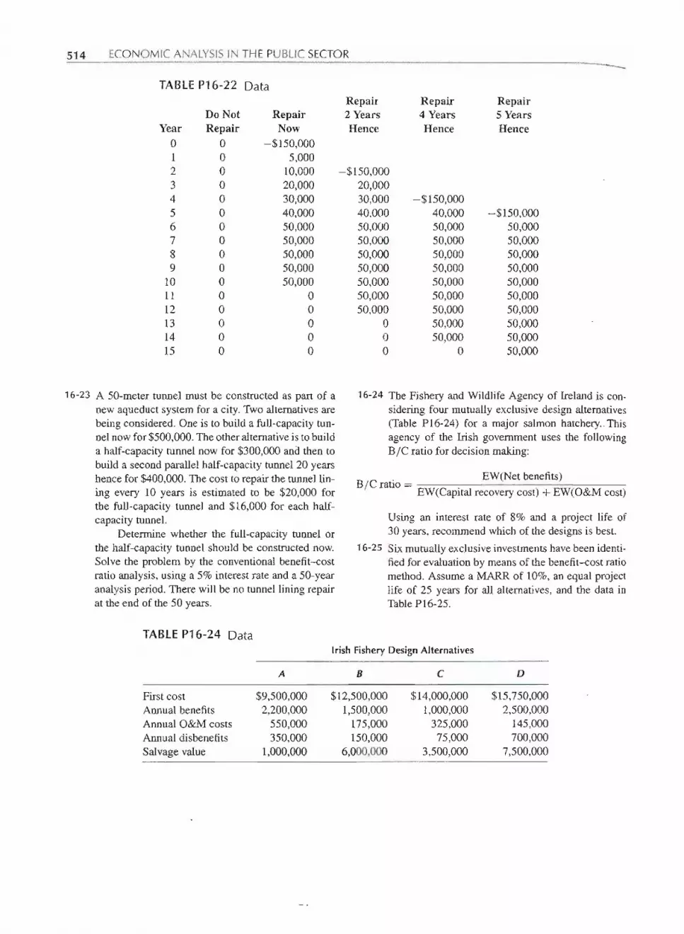
16-23 A 50-meter tunnel must be constructed as part of anew aqueduct system for a city. Two alternatives arebeing considered. One is to build a full-capacity tun-nel now for $500,000. The other alternative is to builda half-capacity tunnel now for $300,000 ana then tobuild a second parallel half-capacity tunnel 20 yearshence for $400,000. The cost to repair the tunnellin-ing every 10 years is estimated to be $20,000 forthe full-capacity tunnel and $16,000 for each half-capacity tunnel.
Determine whether the full-capacity tunnel orthe half-capacity tunnel should be constructed now.Solve the problem by the conventional benefit-costratio analysis, using a 5% interest rate and a 50-yearanalysis period. There will be no tunnel lining repairat the end of the 50 years.
16-24 The Fishery and Wildlife Agency of Ireland is con-sidering four mutually exclusive design alternatives(Table P16-24) for a major salmon hatchery.. Thisagency of the Irish government uses the followingB/C ratio for decision making:
EW(Net benefits)B IC ratio =
EW(Capital recovery cost) + EW(O&M cost)
Using an interest rate of 8% and a project life of30 years, recommend which of the designs is best.
16-25 Six mutually exclusive investments have been identi-fied for evaluation by means of the benefit-cost ratiomethod. Assume a MARR of 10%, an equal projectlife of 25 years for all alternatives, and the data inTable P16-25.
TABLEP16-24 DataIrish Fishery Design Alternatives
A B C D
First cost $9,500,000 $12,500,000 $14,000,000 $15,750,000Annual benefits 2,200,000 1,500,000 1,000,000 2,500,000Annual O&Mcosts 550,000 175,000 325,000 145,000Annual disbenefits 350,000 150,000 75,000 700,000Salvagevalue 1,000,000 6,000,000 3,500,000 7,500,000

---.-..-.-----
Problems 515
TABLEP16-25 DataMutually Exclusive Alternatives
1 2 53 4
Annualized 15.5 13.7 16.8 10.2 17.0 23.3net costs to
sponsor ($M)
Annualized 20.0 16.0 15.0 13.7 22.0 25.0net benefits to
users ($M)
(a) Use annual worth and the B/C ratio to identifythe better alternative.
(b) If this were a set of independent alternatives, howwould you conduct a comparison?
Mr. O'Gratias, a top manager in his company, hasbeen asked to consider the following mutually exclu-sive investment alternatives.
--~ -
6
Answer the following questions.
(a) Use the conventional B/C ratio to evaluate thealternatives and make a recommendation.
(b) Use the modified B/C ratio to evaluate the alter-natives and make a recommendation.
(c) Use a present worth analysis to evaluate the alter-natives and make a recommendation.
(d) Use an internal rate ofretum analysis to evaluatethe alternatives and make a recommendation.
(e) Use the simple payback period to evaluate thealternatives and make a recommendation.
r'r:~;L..~,~~~~j'.I.-''''-.
A B CInitial investment $9500 $18,500 $22,000Annualsavings 3200 5,000 9,800Annualcosts 1000 2,750 6,400Salvagevalue 6000 4,200 14,000Project life, in years 15 15 15MARR 12% 12% 12%

- ~':.-'......
After Completing This Chapter...The student should be able to:
· Identify capital expenditureproject proposals of severaltypes, including mutually.exclusive alternativesand single project proposals.· Identify and reject unattractivealternatives,and select the best alternativefrom eachproject proposal.· Use the rate of return and present worth methods to ration capital among projects.· Rank project proposals by MARR.
QUESTIONS TO CONSIDER :;.
1. Cancelling projects, particularly ones in which large investments have already beenmade, is a difficult process in any business. At the Wne that Donald Rumsfeld waspreparing to cancel the Crusader project, he would also have had to consider the caseagainst cancellation.Somepressures to keep the project would havecome, for example,from Congressionalrepresentativesfrom districts where the Crusader would be built, orwho sawmeritin the originalArmyargumentsin favorof the system,or from someArmyrepresentanves.What factors would a decision-makerlike Rumsfeldhave to consider todecide among competing interests?
2. In the past, the militaryhas generallysoughtto order largequantitiesof specificweaponsin order to keep the unit cost down. In the more uncertainmilitary future, the Pentagonmay have to order smaller quantities, but within a wider range of components, in orderto keep up with swiftly changing battlefield conditions. How could this affect defensedepartment budgeting decisions?
3. From thepoint of viewof apurchasingfirm(in thiscase, the USGovernment),you wouldneed to consideryour firm's budgets,needs, and politicalpressureswithin the firmwhenallocating capital.What other concerns do you need to allow for whenrationing capital?
4. From the point of view of an engineering firm (in this case, Crusader's manufacturer),you would need to consider the long-term prospects of your customer contracts. Howwould you prepare your firmto recover from the cancellationof an important contract?What effect would this have on your capital allocation decisions?
j
- '--'-.~- -.
- - - -- - - - - - - -- -
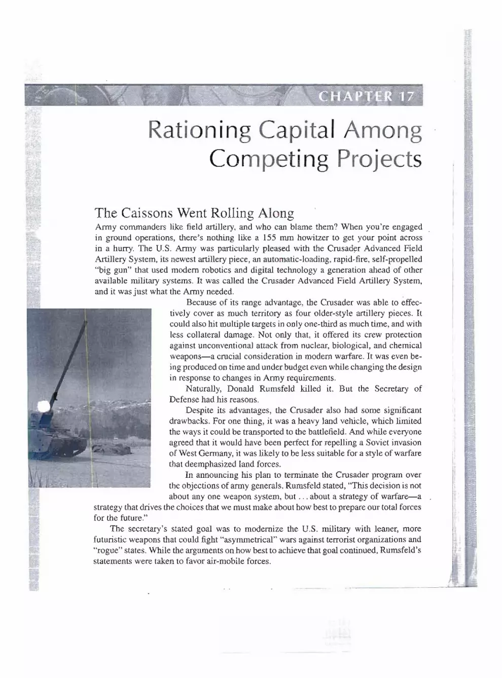
- - - -- -- - - - -- - - - -
.....
,L,"
@OO~P11~ffiW
Rationing Capital AmongCompeting Projects
The Caissons Went Rolling AlongArmy commanders like field artillery, and who can blame them? When you're engagedin ground operations, there's nothing like a 155 mm howitzer to get your point acrossin a hurry. The U.S. Army was particularly pleased with the Crusad~r Advanced FieldArtillery System, its newest artillerypiece, an automatic-loading,rapid-fire, self-propelled"big gun" that used modem robotics and digital technology a generation ahead of otheravailable military systems. It was called the Crusader Advanced Field Artillery System,andit wasjust whattheArmyneeded. . .
Because of its range advantage, the Crusader was able to effec-tively cover as much territory as four older-style artillery pieces. Itcould alsohit multiple targets in only one-third as much time, and withless collateral damage. Not only that, it offered its crew protectionagainst unconventionalattack from nuclear, biological, and chemicalweapons-a crucial consideration in modem warfare. It was evenbe-ingproducedon time andunder budgetevenwhile changingthe designin response to changes in Army requirements.
Naturally, Donald Rumsfeld killed it. But the Secretary ofDefense had his reasons.
Despite its advantages, the Crusader also had some significantdrawbacks. For one thing, it was a heavy land vehicle, which limitedthe ways it could be transported to the battlefield.And while everyoneagreed that it would have been perfect for repelling a Soviet invasionof WestGermany,it was likely to be less suitablefor a style of warfarethat deemphasized land forces.
In announcing his plan to terminate the Crusader program overthe objectionsof army generals, Rumsfeldstated, ''This decisionis notabout anyone weapon system, but ...about a strategy of warfare-a
strategy that drives the choices that we must make abouthowbest to prepare our total forcesfor the future."
The secretary's stated goal was to modernize the U.S. military with leaner, morefuturistic weapons that could fight "asymmetrical" wars against terrorist organizationsand"rogue" states. While the argumentson howbest to achievethat goalcontinued, Rumsfeld'sstatements were taken to favor air-mobile forces.
nII
-- - -, .--..-
- --- -- --

... .
-,518 RATIONING CAPITALAMONG COMPETING PROJECTS -
Sofrom this cabinetofficer'spointof view,the Crusaderhad to go. The Annyhadspent a long timejustifying the Crusaderproject to Congressunderone set of requirementsbut change in DefensePolicymeant that money needed to be freed up for differentprojects:
We have until now dealt with situations where, at some interest rate, we choose each-project's best mutuallyexclusivealternative.Thus, we were assumingthat there is an ampleamountof moneyto makealldesiredcapital investmentsin theseprojects.But the conceptofscarcity of resources is fundamentalto a free marketeconomy.It is throughthis mechanismthat more economically attractiveactivities are encouragedat the expense of less desirableactivities. For industrial firms, there are often more ways of spending money than there ismoney that is available. The result is that we must select from available alternatives themore attractiveprojects and reject-or, at least, delay-the less attractiveprojects.
This problem of rationing capital among competing projects is one part of a two-panproblem called capital budgeting. In planning its capital expenditures, an industrial firmis faced with two questions: "Where will money for capital expenditures-come from?"and, "How shall we allocate available money among the various competing projects?" InChapter 15 we discussed the sources of money for capital expenditures as one aspect indeciding on an appropriate interest rate for economic analysis calculations. Thus, the firstproblem has been treated.
Throughout this book, we have examined for any given project two or more feasi-ble alternatives. We have, therefore, sought to identify in each project the most attractivealternative. For the sake of simplicity, we have looked at these projects in an isolatedsetting-almost as if a firmhad just one project it was considering. In the business world,we know that this is rarely the case. A firmwill findthat there are a great many projects.thatare economically attractive.This situationraises two problems not previously considered:
1. Howdo yourankprojectsto showtheirorderof economicattractiveness?.
2. What do you do if there is not enough money to pay the costs of all economicallyattractiveprojects?
In this chapter we will look at the typical situationfaced by a firm:multiple attractiveprojects, with an inadequate money supply to fund them all. To do this, we review ourconcepts of capital expenditure situations and available alternatives. Then we su~arizethe various techniques that have been presented for determining whether an alternative.is economically attractive. First we screen all alternatives to find those that merit furtherconsideration. Then we will select the best alternative from each~ject, as~umingthatthere is no shortage of money.The next step will be the addition of a budget constraint.
If we findthat there is not enough money to fund the best alternativefrom each project,we will have to do what we can with the limited amount of money available. It will becomeimportant that we have a technique for accurately ranking the various competing projectsin order of economic attractiveness.All this is designed to answer the question, How shallwe allocate availablemoney among the various competingprojects-?---
CAPITAL EXPENDITURE PROJECT PROPOSALS
At the beginning of the book, we described decision making as the process of selecting thebest alternative to achieve the desired objective in a given situation or problem. By carefullydefining our objective and the model, the given situation is reduced to one of selecting thebest from the feasible alternatives. In this chapter we call the engineering decision-making
----
Capital Expenditure Project Proposals 519
The general manager of a manufacturingplant has received the followingprojectproposalsfromthe various operating departments:
1. The foundry wishes to purchase a new ladle to speed up the casting operation.2. The machine shop has asked for some new inspection equipment.3. The painting department reports that improvementsmust be made to the spray booth to
conform to new air pollution standards.4. 'Theoffice.::managerwants to buy:a larger".more modernsafe.
For each project there is a single course of actionproposed.Note that the singleprojectproposalsare also independent,for there is no interrelationshipor interdependenceamongthem.The general
~ger~.a~de.~ideJo=;allQcat~0ney;;:for.none;=some;::o~l:of the~various.'Pr{)jectproposals~-. -
process for a givensituationor problema project proposal. Associatedwithvariousprojectpropqsals are their particular availablealternatives.For a firmwithmanyprojectproposals,the following situationmay result:
Capital Expenditure Proposals
Project Alternatives
1. Acquire additional manufacturingfacility
A Lease an existing buildingB Construct a new buildingC Contract for the manufacturing to be doneoverseas
A Purchase semiautomatic machineB Purchase automatic machine
A Make the parts in the plantB Buy the parts from a subcontractor
2. Replace old grinding machine
3. Produce parts for the assembly line
Our task is to apply economic analysis techniques to this more complex problem.
Mutually Exclusive Alternatives and Single Project ProposalsUntilnowwehavedealtwithmutuallyexclusivealternatives,thatis, selectingonealternativeresults in rejecting the other alternativesbeing considered.Even in the simplestproblemsencountered, the question was one of selection between alternatives.Should, forexample,Machine A or Machine B be purchasedto perform the necessarytask?Clearly,thepurchaseof oneof the machinesmeantthatthe otheronewouldnotbepurchased.Sinceeithermachinewould perform the task, the selectionof one precludes the possibilityof selectingthe otherone as well.
Even in the case of multiple alternatives,we havebeen consideringmutuallyexclusivealternatives.A typical example was: What sizepipeline shouldbe installedto supplywaterto a remoteconstructionsite? Onlyonealternativeis tobe selected.This is differentfrom thesituation for single project proposals,where only one courseof actionis outlined.ConsiderExample 17-1.
L__ ________-
--- .J
--- ---

-'-- --- _..-----
]520 RATIONING CAPITAL AMONG COMPETING PROJECTS -
SOlUTIQN
Each of the four project proposals has a single course of action. The general manager could, forexample, buy the office manager a new safe and buy the inspection equipment for the machineshop. But he could also decide to not buy the office manager a safe or the equipment for themachine shop. There is, then, an alternativeto buying the safe for the officemanager: not to buy .
him the safe-to do nothing. Similarly,he could decide to do nothing about the request for themachine shop inspection equipment. Naturally, there are do-nothing alternativesfor each of thefour single project proposals:
IA. Purchase the foundry a new ladle.lB. Do nothing. (Do not purchase a new ladle.)2A. Obtain the inspection equipment for the machine shop.2B. Do nothing. (Do not obtain the inspection equipment.)3A. Make improvements to the spray booth in the painting department.3B. Do nothing. (Make no improvements.)4A. Buy a new safe for the officemanager.4B. Do nothing. (Let him use the old safe!)
One can adopt Alt. 1A (buy the ladle)or 1B (do not buy the ladle), but notboth. We findthat whatwe considered to be a single course of action is really a pair of mutually exclusive alternatives.Even Alt. 3 is in this category.The originallystated single proposal was:
The paintingdepartmentreports that improvementsmust be made to the spray booth toconformto newair pollutionstandards.
Since the painting department must make the improvements, is there actually another alter-native? Although at first glance we might not think so, it may be possible to change the paint,or the spray equipment, and thereby solve the air pollution problem without any improvementsto the spray booth. In this situation, there does not seem to be a practical do-nothing alternative,for failure to comply with the air pollution standards might result in large fines or even shuttingdown the plant. But if there is not a practical,do-nothing alternative,there might be a number ofdo-something-else alternatives. .
We conclude that all project proposals may be considered to have mutually exclusive alter-:natives.
Identifying and Rejecting Unattractive AlternativesIt is clear that no matter what the circumstancesmay be, we want to eliminate from furtherconsiderationanyalternativethatfailsto meettheminimumlevelof economicattractiveness,provided one of the other alternativesdoes meet the criterion. Table 17-1 summarizesfivetechniques that may be used.
At first glance it appears that many calculations are required, but this appearance ismisleading.Any of the fivetechniqueslisted in Table 17-1maybe used to determinewhetherto reject an alternative.Each will produce the same decision regarding RejectIDon't reje..o.
----

Rationing Capital by Rateof Return 521
TABLE 17-1 Criteria for Rejecting Unattractive Alternatives
For'Each Alternative Compute Reject Alternative When Do Not Reject Alternative When
Rate of return, iPresent worth, PWAnnual cost. EUACAnnual benefit, EUABBenefit-cost ratio, BjCNet present worth, NPW
i < MARRPW of benefits < PW of costsEUAC > EUAB
B/C < 1NPW < 0
i :::MARRPW of benefits :::PW of costsEUAC:::EUAB
B/C::: 1NPW :::0
TABLE17-2 Criteria for Choosing the BestAlternative from Among MutuallyExclusive Alternatives
Situations
Analysis Method
Present worth
Fixed Input
(The cost of eachalternative isthe same.)
FixedOutput
(The benefits fromeach alternativeare the same.)
Annual cash flow
Maximize presentworth of benefits
Maximize
equivalent unifonnannual benefits
Minimize presentworth of cost
Minimize
equivalent unifonnannual cost
Neither Input NorOutput Fixed
(Neither the costs nor thebenefits for the alternatives
given are the same.)
Maximize net presentworth
Maximize EAUB - EAUC
Maximize Maximize Incrementalbenefit-costbenefit-cost ratio benefit-costratio ratio analysisis required
Incrementalrate of return analysisis required
Benefit-cost ratio
Rate of return
Selecting the Best Alternative from Each Project ProposalThe task of selecting the best alternative from among two or more mutually exclusivealternatives has been a primary subject of this book. Since a project proposal is the sameform of problem, we may use anyof the severalmethodsdiscussedin Chapters5 through 9.The criteria are summarized in Table 17-2. .
TIONING CAPITAL BY RATE OF RETURN
One way of looking at the capitalrationingproblemis through the use of rate of return. Thetechnique for selecting from among independentprojects is illustrated by Example 17-2.These projects are independent, so their only interdependenceis the budget constraint onthe total accepted set of projects.
- - - -- --
1;:

522 RATIONING CAPITALAMONG COMPETING PROJECTS
1
Nine independentprojects are being considered. Figure 17-1may be prepared from the followingdata.
SOLUTION
Looking at the nine projects, we see that some are expectedto produce a larger rate of return thanothers. It is natural that if we are to select from among them, we will pick those with a higher rateof return. When the projects are arrayed by rate of return, as in Figure 17-1, the correct choice(of Projects 3, 1,4,5,6, and 2) is readily apparent.
30
f
o 50 150 250 350 450 650 700 - 1000
CumulativeCost of Projects(thousandsof dollars)
FIGURE 1.!7-'lGumulative cost of projects versus rate ofretum.,
1300
... iii' ..r __
- - - - - -
Uniform Useful Salvage ComputedCost Annual Benefit Life Value Rate of
Project (thousands) (thousands) (years) (thousands) Return1 $100 $23.85 10 $ 0 20%2 200 39.85 10 0 153 50 34.72 2 0 254 100 20.00 6 100 205 100 20.00 10 100 206 100 18.00 10 100 187 300 94.64 4 0 108 300 47.40 10 100 129 50 7.00 10 50 14
If a capital budget of $650,000 is available,which projects should be selected?
-
'-
f-3 1 4 5 6 2 9 8 7
-

Rationing Capital by Rateof Return 523
~c:::....::IV~....oII)'i;j~ Cutoff
~ Rate of'8' Return~
o CapitalBudget
CumulativeCostof Projects($)
FIGURE 17-2 Location of the cutoff rate of return.
In Example 17-2,the rate of returnwascomputedforeach project and then the projectswerearranged in order of decreasing rate of return. For a fixed amount of money in the capitalbudget, the projects are selectedby going down the list until the money is exhausted.Thuswhen we use this procedure, we cut off approvingprojects at the point where the moneyruns out. This point is called the cutoff rate of return. Figure 17-2 illustrates the generalsituation.
For any set of ranked projects and any capital budget, the rate of return at which thebudget is exhausted is the cutoff rate of return. In Figure 17-2 the cost of each individualproject is smallin comparisonto the capitalbudget.Thecumulativecost curveis a relativelysmooth curveproducinga specificcutoffrate of return.Lookingback atFigure 17-1,we seethe curve is actuallya step function. For Example 17-2,the cutoff rate of return is between14 and 15% for a capital budget of $650,000.
Significance of the Cutoff Rate of ReturnCutoff rate of return is determinedby comparisonof an established capital budget and theavailable projects. One must examine all the projects and all the money for some periodof time (like one year) to compute the cutoff rate of return. It is a computation relatingknown projects to a known money supply.For this period of time, the cutoff rate of returnis the opportunity cost (rate of return on the opportunity or project forgone) and also theminimum attractiverate of return. In other words, the minimum attractive rate of return toget a project accomplishedis the cutoff rate of return.
MARR = Cutoff rate of return =Opportunity cost
We generally use the minimum attractive rate of return to decide whether to approve anindividual project even though we do not know exactly what other projects will be proposedduring the year. In this situation, we cannot know whether the MARR is equal to the cutoff
- -- --.-- -----
pl.,.
.';'"<,WI~I
.~.
....
I..I..
I..""""
""""....
I..I..
"'i-,
""""""""11-....
-I..""""II-
-rTl

524 RATIONING CAPITALAMONG COMPETING PROJECTS
- .-- --". . -.. . -- -" . .. .
.....,
-rate of return. When the MARR is different from the cutoff rate of return, incorrect decisionsmay occur. This will be illustrated in the next section.
RATIONING CAPITAL BY PRESENT WORTH METHODS
Throughout this book we have chosen from among project alternatives to maximize netpresent worth. If we can do the same thing for a group of projects, and we do no~exceedthe availablemoney supply,then the capital budgetingproblem is solved.
But more frequently in capital budgeting problem we will be unable to accept alldesirable projects. We, therefore, have a task not previouslyencountered. We must choosethe best from the larger group of acceptableprojects.
Lorie and Savagel showedthat a proper technique is to use a multiplier,p, to decreasethe attractivenessof an alternative in proportion to its use of the scarce supply of mon~y.The revisedcriterion is
NPW - p(PW of cost) (17-1)
where p is a multiplier.If a value of p were selected (say, 0.1), then some alternatives with a positive NPW
will have a negative [NPW- p(PW of cost)]. This new criterion will reduce the numberof favorablealternativesand thereby reduce the combined cost of the projects meeting thismore severe criterion. By trial and error, the multiplier p is adjusted until the total costof the projects meeting the [NPW- p(PW of cost)] criterion equals the available moneysupply-the capital budget. .
Use the present worth method to determine which of the nine independent projects ofExample 17-2 should be included in a capital budget of $650,000. The minimum attractive rateof return has been set at 8%. .
Project123456789
Cost(thousands)
$10020050
10010010030030050
UniformAnnual Benefit
(thousands)$23.8539.8534.7220.0020.0018.0094.6447.407.00
UsefulLife
(years)101026
10104
1010
SalvageValue
Jthousands)$ 0
oo
100100100
o10050
ComputedNPW
(thous~ds)$60.0467.4011.9155.4880.5267.1.013.4664.3820.-13
1Lorie, J. and L. Savage, ''Three Problems in Rationing Capital," Journal of Business, October 1955,pp.229-239.
-------

Rationing Capital by Present Worth Methods 525
'.' .__ ,_"'_" j.c. ,_,_,.""
SQ! lJ.JjION'
Locating a value of pin [NPW- p(PW of cost)] by trial and error, we use the following table,where all amounts are in thousands of dollars.
For a value of p equal to 0.25, the best selection order is computed to be Projects 1,2,4,5,6,and 9. (Note: the smallest value for p is 0.239.)
Alternate Formation of Example 17-3
Thepreceding answer does not agree withthe solution obtained in Example 17-2.Thedifficultyisthat the interest rate used in the present worth calculationsis not equal to the computedcutoffrateof return. In Example 17-2the cutoff rate of return was between 14and 15%,say14.5%. Wewi)lrecompute the present worth solution using MARR = 14.5%, again with amounts in thousandsof dollars.
---- --
Cost
$100200
100100100
50
$650
I
,
II
\1,"':'If'I
:-;;..:'1:'~t
ComputedTrialp =0.20 Trial p = 0.25
'oject Cost NPW [NPW- p(PW of cost)) Cost [NPW - p(PW of cost)]
1 $ 100 $60.04 $40.04 $ 100 $35.042 200 67.40 27.40 200 17.403 50 11.91 1.91 50 -0.594 100 55.48 35.48 100 30.485 100 80.52 60.52 100 55.526 100 67.10 47.10 100 42.107 300 13.46 -46.54 -61.548 300 64.38 4.38 300 10.629 50 20.13 10.13 50 7.63- -
$1300 $1000
Computed NPW Cost of ProjectsProject Cost at 14.5% with Positive NPW
1 $100 $22.01 $1002 200 3.87 2003 50 6.81 504 100 21.10 1005 100 28.14 1006 100 17.91 1007 300 -27.058- 300 --,::31.69 =11I '" ::; =
9 50 -1.28-$650
--'10- _ ____ _ - -- '::!!:: = ====:;;::;= :;.n..
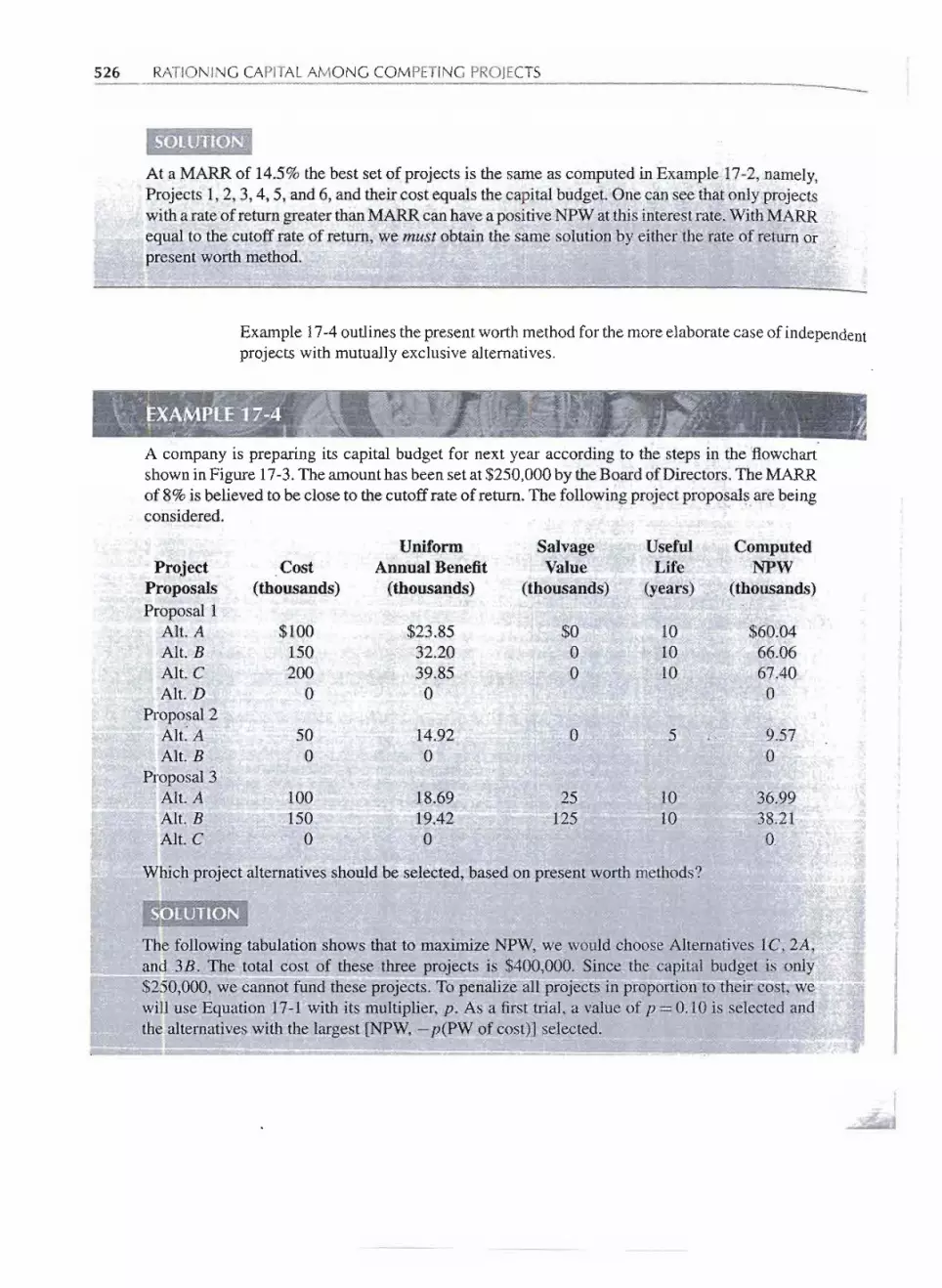
+ --..
-- .-.--
1526 RATIONING CAPITALAMONG COMPETING PROJECTS
. ,
SQ1VJ!9N
At a MARR of 14.5%the best set of projects is the same as computed in Example 17-2,namely,Projects 1,2,3,4,5, and 6, and their cost equals the capital budget.One can see that only projectswith a rate of return greater thanMARR can haveapositiveNPW at this interestrate. WithMARRequal to the cutoff rate of return, we must obtain the same solution by either the rate of return orpresent worth method.
c .,_~ ~ ~
Example 17-4outlines the presentworthmethod for the moreelaboratecase of independentprojects with mutually exclusivealternatives.
SbLUTIONI. . . ,
Tl1~following tabulation shows that to maximize NPW, we would choose Alternatives 1C, 2A,anQ.3.1I. The to.tal cost of these three projects is $400,000. Since the capital budget is only$250,000, we cannot fund ffiese projects. 1'5 pen1ilize a1fpr6jec1s 1)1propodion~tb tlfeif cost, "wewill use Equation 17-1 with its multiplier, p. As a first trial, a value of p -:..0.10 is selected andthelalternatiyes with the large~t .[NPW, - p(PW of cost)] selected.
--- ...
IIII
J
A company is preparing its capital budget for next year according to the steps in the flowchartshownin Figure 17-3.The amounthas been set at $250,000by the Boardof Directors.The MARRof 8% is believedto be close to the cutoffrate of return. The followingprojectproposals are beingconsidered.
Uniform Salvage Useful ComputedProject Cost Annual Benefit Value Life NPW
Proposals (thousands) (thousands) (thousands) (years) (thousands)Proposal1
Alt. A $100 $23.85 $0 10 $60.04Alt. B 150 32.20 0 10 66.06Alt. C 200 39.85 0 10 67.40Alt. D 0 0 0
Proposal 2Alt.'A 50 14.92 0 5 9.57Alt.B 0 0 0
Proposal 3Alt.A 100 18.69 25 10 36.99Alt. B 150 19.42 125 10 38.21Alt. C 0 0 0
Which project alternativesshould be selected, based on present worth methods?

Rationing Capital by PresentWorth Methods 527
I
ProjectProposals
Proposal I1AIBICIV Donothing
Proposal22A2B Donothing
Proposal33A3B3C Donothing
This is thedesiredset of
projects.
2
ComputeNPWfor eachalternative.
. Reject anyalternativefor which NPW
is negative.
From eachproject proposal,select alternativewith the largestpositive NPW.
For Fixed-Sum-of-MoneyConstraint
Compute Total RequiredMoney for this set of projects
Fixed sum isless thanamount
requiredfor this set ofprojects.
Select an initialvalue of p andcontinue withcalculations incolumns4 and 5.
== FIGURE,17...3Steps in computing-acapital budget =- -.. - -...-
Fixed sum isequal to orgreater thanamount
requiredfor this set ofprojects.
This is thedesired set ofprojects.
3 4
Compute foreach alternativewith positiveNPW:
NPW - p(pW of cost)
5
From each projectproposal select,alternative with thelargest positive
NPW- p(pW of cost)
Omit any projectfor which allvalues are negative.
Compute Total Required Moneyfor This Set of Projects
Fixed-Sum-of- Money Constraint
Fixed sumisless thanamountrequiredfor thisset of projects.
Increasep andrecomputecolumns4 and 5.
- --~
Fixed sum isequal toamountrequiredfor thisset of projects.
This is thedesired set ofprojects.
- - -
Fixed sum isgreater thanamountrequiredfor thisset of projects.
Decrease pand recomputecolumns4 and 5.
--~--. :!
- ------
\ \,II
,
,.
ill
:Ii~j
II!II
.L. -,~
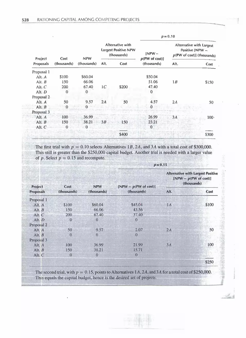
528 RATIONING CAPITALAMONG COMPETING PROJECTS
The first trial with p = 0.10 selects Alternatives 1B, 2A, and 3A with a total cost of $300,000.This still is greater than the $250,000 capital budget. Another trial is needed with alarger valueof p. Select p =0.15 and recompute.
p=O.1S'
NPW
(thousands)[NPW - p(PW of cost)]
(thousands)
Alternative with Largest Positive
[NPW- p(PW of cost»(thousands)
Alt. Cost
$60.0466.0667.40o
$45.0443.5637.40o
lA $100
9.57o
502.07o
2A
100
$250
-- - The secondtrial, witllp = 0.15,points toAlternatjveslA,2A, and3A for a totalcost Qf$250,000.-nus ~qmi1s~the"dipital"budget,:::hence'=is.the;desired'wt!()f""Prejeets~ == ~ -~ ..
~ -J!!! ~ \~ "" 4" __.,_~_ J2' _.
J
- --
p=O.10
Alternative with Alternative with LargestLargest Positive NPW Positive [NPW-
(thousands) [NPW -p(PW of cost)] (thousands)
Project Cost NPW p(PW of cost)]Proposals (thousands) (thousands) Alt. Cost (thousands) Alt. Cost-
Proposal 1Alt. A $100 $60.04 $50.04Alt. B 150 66.06 51.06 IB $150Alt.C 200 67.40 1C $200 47.40Alt. D 0 0 0
Proposal 2Alt.A 50 9.57 . 2A 50 4.57 2A 50Alt. B 0 0 0
Proposal 3Alt.A 100 36.99 26.99 3A 100.Alt.B 150 38.21 3B 150 23.21Alt.C 0 0 0-
$400 $300
Project Cost
Proposals (thousands)-Proposal 1
Alt.A $100Alt. B 150Alt. C 200Alt. D 0
Proposal2Alt. A 50Alt. B 0
Proposal3Alt. A 100Alt. B 150Alt.C 0
36.99 21.99 3A38.21 15.71
0 0: - . - :; i8i::i:::: :; :: i!!: ;:;; =iii== ;;;:.

---~--
Rationing Capital by Present Worth Methods
I.\} I
III
529
Solve Example 17-4 by the rate of return method. For project proposals with two or morealternatives, incremental rate of return analysis is required. The data from Example 17-4 andthe computed rate of return for each alternative and each increment of investment are asfollows:
The various separableincrements of investmentmay be ranked by rate of return. They areplottedin a graph of cumulativecost versus rate of return in Figure 17-4.The ranking of projectsby rateof return gives the following:
Project
lA2A3A :;;
IB in place of lAlC in place of IB3B in place of 3A
."" ~-~ ~ ~~::::iii:iii ::----------. -
Incremental Analysis
Uniform UniformAnnual Salvage Computed Annual Salvage Computed
,mbination Cost Benefit Value Rate of Cost Benefit Value Rate ofAlternatives (thousands) (thousands) (thousands) Return (thousands) (thousands) (thousands) Return
)POScu1A $100 $23.85 $ 0 20.0%B-A $ 50 $ 8.35 $ 0 10.6%B 150 32.20 0 17.0C-B 50 7.65 0 8.6C-A 100 16.00 0 9.6C 200 39.85 0 .15.0b 0 0 0 0
)posal 250 14.92 0 15.0
B 0 0 0 0
iposal 34- 100 18.69 25 15.09-A 50 0.73 100 8.3r1 150 19.42 125 12.0
0 0 0 0

-1I
530 RATIONING CAPITAL AMONG COMPETING PROJECTS
20
100 150 250 300 350CumulativeCost of InvestmentIncrements(thousandsof dollars)
FIGURE 17-4 Cumulative cost versus incremental rate of return.
o 400
For a budget of $250,000, the selected projects are lA, 2A, and 3A. Note that if a budget of$300,000 were available, IB would replace lA, making the proper set of projects IB,2A,and 3A. At a budget of $400,000, lC would replace IB; and 3B would replace 3A, makingthe selected projects lC, 2A, and 3B. These answers agree with the computations inExample 17-4.
RANKINGPROJECTPROPOSALS
Closelyrelatedto theproblemof capitalbudgetingis the matterof rankingprojectproposals.We will first examine a method of ranking by present worth methods and then show thatproject rate of return is not a suitable method of ranking projects.
Anyone whohas everbought firecrackersprobably used the practical rankingcriterionof "biggest bang for the buck" in making a selection. This same criterion-stated moreelegantly-may be used to correctly rank independentprojects.
Rank independent projects according to their value of net present worth divided by thepresent worth of cost. The appropriate interest rate is MARR (as a reasonable estimateof the cutoff rate ofreturn).
Example 17-6illustrates the method of computation.
--- -
15.0%
10.6%
8.6% 8.3%
lA 2A 3A IB - 1A lC - IB 3B - 3A
.-..15
e!....0
10
"0B='
5U

Ranking Project Proposals 531
Rank the following nine independent projects in their order of desirability, based on a 14.5%minimum attractiverate of return. (Tofacilitate matters, the necessarycomputationsare includedin the tabulation.)
SOLUTIONI
Ranked by NPw IPW of cost, the projects are listed as follows:
Project514632978
NPWIPW of Cost0.28140.22010.21100.17910.13620.0194
-0.0256-0.0902-0.1056
Rate of Return20%2020182515141012
The rate of return tabulation illustrates that it is not a satisfactoryranking criterion and wouldhave given a different ranking from the present worth criterion.
.I~
In Example 17-6, the projects are ranked according to the ratio NPWIPWof cost. In Fig-ure 17-3,the criterion used is [NPW- p(pW of cost)]. If one were to compute the value ofp at which [NPW- p(PW of cost)] = 0, we would obtain p =(NPWIPWof cost). Thusthe multiplier p is the ranking criterion at the point at which [NPW - p(PW of cost)] = 0."."
If independentprojectscan be ranked in their order of desirability,then the selectionof ::'.11,projects to be.include~in a cap.italbudget is a simple task. One may proc~eddown ~e li~t ~. ~~, I, '.
of ranked projects until the capItalbudget has been exhausted.The only difficultyWIththis i][.£-
~~
Uniform ComputedAnnual Useful Salvage Computed NPWat Computed
Cost Benefit Life Value Rate of 14.5% NPW/Cost"Oject (thousands) (thousands) (years) (thousands) Return (thousands) (thousands)1 $100 $23.85 10 $ 0 20% $22.01 0.22012 200 39.85 10 0 15 3.87 0.01943 50 34.72 2 0 25 6.81 0.13624 100 20.00 6 100 20 21.10 0.21105 100 20.00 10 100 20 28.14 0.28146 100 18.00 10 100 18 17.91 0.17917 300 94.64 4 0 10 - 27.05 -0.09028 300 47.40 10 100 12 -31.69 -0.10569 50 7.00 10 50 14 -1.28 -0.0256

_.. u _ __ .- - - --- --
532 RATIONING CAPITALAMONG COMPETING PROJECTS
scheme occurs, occasionally,when the capital budget is more than enough for n projectsbut too little for n + 1 projects. .
In Example 17-6, a capital budget of $300,000 is just right to fund the top threeprojects. But a capital budget of $550,000 is more than enough for the top five projects(sum=$450,000) but not enough for the top six projects (sum= $650,000). When wehave this lumpiness problem, it may not be possible to say with certainty that the best useof a capital budget of $550,000is to fund the top fiveprojects. There may be some otherset of projects that makesbetter use of the available $550,000.While some trial-and-errorcomputationsmay indicatethe proper set of projects, more elaboratetechniquesare neededto prove optimality.
As a practicalmatter,a capitalbudget probablyhas some flexibility.If in Example 17-6the tentativecapital budgetis $550,000, then a careful examinationof Project 2 will dictatewhether to expandthe capitalbudget to $650,000 (to be able to includeProject 2) or to dropback to $450,000 (and leaveProject 2 out of the capital budget).
SUMMARY
Prior to this chapter we had assumed that all worthwhile projects are approved and im-plemented. But industrial firms, like individuals and governments,are typically faced withmore good projects than can be funded with the money available.The task is to select thebest projects and reject, or at least delay, the rest.
Alternatives are mutually exclusive when the acceptance of one "effectivelypreventsthe adoption of the other.This could be"becausethe alternativesperform the same function(like Pump A vs Pump B) or would occupy the same physical location (like a gas stationvs a hamburger stand). If a project has a single alternativeof doing something,"weknowthere is likely to be a mutually exclusive alternative of doing nothfug-or possibly doingsomething else. A project proposal may be thought of as having two or more mutuallyexclusive alternatives.Projects are assumed in this chapter to be independent.
Capital may be rationed among competing investmentopportunitiesby either rate ofreturn or present worth methods. The results may not always be the same for these twomethods in many practical situations~ .". "
If projects are rankedby rate of return, a proper procedure is to go down the list untilthe capital budget has been exhausted. The rate of return at this point is the cutoff rate ofreturn. This procedure gives the best group of projects, but does not necessarily have themin the proper priority order.
MaximizingNPWis an appropriatepresent worthselectioncriterionwhenthe availableprojects do not exhaust the money supply. But if the amount of money required for thebest alternative from each project exceeds the availablemoney,a more severe criterion isimposed: adopt only alternativesand projects that have a positive NPW - p(PW of cost).The value of the multiplier p is chosen by trial and error until the alternativesand projectsmeeting the criterionjust equal the availablecapital budget money.
It has been shown in earlier chapters that the usual business objective is to maximizeNPW, and this is not necessarily the same as maximizing rate of return. One suitableprocedure is to use the ratio (NPW/PW of cost) to rank the projects. This present worthranking method will order the projects so that, for a limited capital budget, NPW will be
---
- -- --

Problems 533
maximized.Weknow that MARR mustbe adjustedfrom time to time to reasonablybalancethe cO,stof the projects that meet the MARR criterion and the available supply of money.This adjustment of the MARR to equal the cutoff rate of return is essential for the rate ofreturn and present worth methods to yield compatible results.
Another way of ranking is by incremental rate of return analysis. Once a ranking hasbeen made, we can go down the list and accept the projects until the moneyruns out. Thereis a theoretical difficulty if the capital budget contains more money than is required for nprojects, but not enough for one more (n + 1projects). As a practicalmatter,capital budgetsare seldom inflexible, with the result that some additional money may be allocated if the(n + l)st project looks like it should be included.
~OBLEMS
Ear 1.. of the following 10 independent projects has a10.,) ~ar life and no salvage value.
Project123456789
10
Cost(thousands)
$ 51510305
205
205
10
UniformAnnualBenefits
(thousands)$1.03
3.221.774.881.193.831.003.691.152.23
ComputedRate ofReturn
16%171210201415131918
(a) Use rate of return methods to determine which setof projects should be uQdertaken if the MARR is10%.
(b) Use rate of return methods to determine which
set of projects should,be undertaken if the capitalbudget is limited to $100,000.
(c) For a budget of $100,000, what interest rateshould be used in rationing capital by presentworth methods? (Limit your answer to a value forwhich there is a compound interest table availablein the appendix).
(d) Using the interest rate determined in part (c), rankorder the eight different investment opportunitiesby means of the present worth method.
(e) For a budget of $100,000 and the ranking in part(d), which of the investment opportunities shouldbe selected?
The projects have been proposed by the staff of theAce Card Company. The MARR of Ace has been 12%for several years.(a) If there is ample money available, what projects
should Ace approve?(b) Rank order all the acceptable projects in their
order of desirability.(c) If only $55,000 is available, which projects
should be approved?
At Miami Products, four project proposals (three withmutually exclusive alternatives) are being considered.All the alternatives have a lO-year useful life and nosalvage value.
-- -- - - -- - -
UniformAnnual Computed
Project Cost Benefits Rate ofProposal (thousands) (thousands) Return
Project 1Alt.A $25 $4.61 13%Alt. B 50 9.96 15Alt. C 10 2.39 20
Project 2Alt. A 20 4.14 16Alt. B 35 6.71 14
Project 3Alt. A 25 5.56 18Alt. B 10 2.15 17
Project 4 10 1.70 11

17-3 AI Dale is planning his Christmas shopping for sevenpeople. To quantify how much his various relativeswould enjoy receiving items from a list of prospectivegifts, AI has assigned appropriateness units (called"ohs") for each gift if given to each of the sevenpeople. A rating of 5 ohs. represents a gift that therecipient would really like. A rating of 4 ohs indi-cates the recipient would like it four-fifths as much;3 ohs, three-fifths as much, and so forth. A zero ratingindicates an inappropriate gift that cannot be given tothat person.
The objective is to select the most appropriate setof gifts for the seven people (that is, maximize totalohs) that can be obtained with the selected budget.(a) How much will it cost to buy the seven gifts the
people would like best, if there is ample moneyfor Christmas shopping?
(b) If the Christmas shopping budget is set at $112,which gifts should be purchased, and what is theirtotal appropriateness rating in ohs?
(c) If the Christmas shopping budget must be cut to$90, which gifts should be purchased, and whatis their total appropriateness rating in ohs?
(Answer: (a), $168)
The foUowing facts are to be used in solvingProblems 17-4 through 17.7 In assembling datafor the Peabody Company annual capital budget,five independent projects are being considered.Detailed examinationby the staff has resulted in theidentificationof three to six mutually exclusive do-something alternativesfor each project. In addition,
each project has a do-nothing alternative. The projectsand their alternatives are listed at the top of next page.
Each project concerns operations at Peabody'sSt. Louis brewery. The plant was leased from anotherfirm many years ago, and the lease expires 16 years.from now. For this reason, the analysis period for allprojectS is 16 years. Peabody considers 12% to be theminimum attractive rate of return.
. In solving the Peabody problems, an importantassumption concerns the situation at the end of theuseful life of an alternative when the alternative has a
useful life less than the 16-year analysis period. Tworeplacement possibilities are listed.
Assumptio.n 1: When an alternative has a usefullife less than 16 years, it will be replaced by anew alternative with the same useful life as the
original. This may need to occur more than once.The new alternative will have a 12% computedrate of return and, hence, a NPW =0 at 12%.
Assumption 2: When an alternative has a usefullife less than 16 years, it will be replaced at theend of its useful life by an identical alternative(one with the same cost, uniform annual bene-fit, useful life, and salvage value as the originalalternative).
17-4 For an unlimited supply of money, and replace-ment Assumption 1,which project alternatives shouldPeabody select? Solve the problem by present worthmethods. (Answer: Alternatives 1B, 2A, 3F, 4A,and 5A)
------
_.'_ .u _ .. ..- 1I
534 RATIONINGCAPITALAMONG COMPETINGPROJECTS -TABLE P17-3 Data
"Oh" Ratingof Gift IfGiven to Various FamilyMembers
Prospective Gift Father Mother Sister Brother Aunt Uncle Cousin-1. $20 box of candy 4 4 2 1 5 2 32. $12 box of cigars 3 0 0 1 0 1 23. $16 necktie 2 0 0 3 0 3 24. $20 shirt or blouse 5 3 4 4 4 1 45. $24 sweater 3 4 5 4 3 4 26. $30 camera 1 5 2 5 1 2 07. $ 6 calendar 0 0 1 0 1 0 18. $16 magazinesubscription 4 3 4 4 3 1 39. $18 book 3 4 2 3 4 0 3
10. $16 game 2 2 3 2 2 1 2
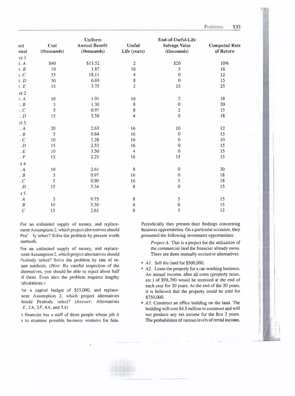
For an unlimited supply of money, and replace-mentAssumption2,whichprojectalternativesshouldPea' ly select? Solvethe problemby presentworthmethods.
For an unlimited supply of money, and replace-mentAssumption2,whichprojectalternativesshouldPeabody select? Solve the problem by rate of re-:urn methods. (Hint: By careful inspection of thel.lternatives,you should be able to reject about half)f them. Even then the problem requires lengthy;alculations.)
"or a capital budget of $55,000, and replace-nent Assumption 2, which project alternatives:hould Peabody select? (Answer: Alternatives.E, 2A, 3F, 4A, and 5A)
\. financier has a staff of three people whosejob its to examine possible business ventures for him.
Periodically they present their findings concerningbusiness opportunities. On a particular occasion, theypresented the following investment opportunities:
Project A: This is a project for the utilization ofthe commercial land the financier already owns.There are three mutually exclusive alternatives.
· Ai. Sell the land for $500,000.· A2. Lease the property for a car-washing business.An annual income, after all costs (property taxes,etc.) of $98,700 would be received at the end ofeach year for 20 years. At the end of the 20 years,it is believed that the property could be sold for$750,000.· A3. Construct an office building on the land. The
building will cost $4.5 million to construct and willnot produce any net income for the first 2 years.The probabilities of various levels of rental income,
--- --- ----- - ---
------
1\\.'''''
It. :,:
1f' '.,
"t
Problems 535
End-of-Useful-LifeUseful Salvage Value Computed Rate
Life (years) (thousands) of Return
2 $20 10%16 5 184 0 128 0 152 15 25
16 2 188 0 208 2 154 0 18
16 10 1216 0 1516 0 1016 0 154 0 15
16 15 15
8 0 2016 0 1816 5 188 0 15
8 5 154 0 158 5 12
Unifonnect Cost Annual BenefitIOSal (thousands) (thousands):ct 1t.A $40 $13.52t.B 10 1.87t.e 55 18.11t.D 30 6.69t.E 15 3.75ct 2t.A 10 1.91. B 5 1.30:.e 5 0.97:.D 15 5.58
ct 3:.A 20 2.63:.B 5 0.84.e 10 1.28.D 15 2.52.E 10 3.50.F 15 2.25
;t4.A 10 2.61.B 5 0.97.e 5 0.90.D 15 3.34
:t 5.A 5 0.75B 10 3.50e 15 2.61

I536 RATIONING CAPITALAMONG COMPETING PROJECTS
after all expenses, for the subsequent 18 years areas follows:
Annual Rental Income
$1,000,0001,100,0001,200,0001,900,000
Probability0.10.30.40.2
The property (building and land) probably can be soldfor $3 million at the end of 20 years.
Project Eo'An insurance company is seeking toborrow money for 90 days at 13 3/4%per annum,compounded continuously.
Project C: A financier owns a manufacturingcompany. The firm desires additional workingcapital to allow it to increase its inventories ofraw materials and finished products. An invest-ment of $2 million will allow the company toobtain sales that in the past the company had toforgo. The additional capital will increase com-pany profits by $500,000 a year. The financiercan recover this additional investment by order-ing the company to reduce its inventories and toreturn the $2 million. For planning purposes, as-sume the additional investment will be returned
at the end of 10 years.
Project D: The owners of Sunrise magazine areseeking a loan of $500,000 for 10 years at a 16%interest rate.
Project E: The Galveston Bank has indicated awillingness to accept a deposit of any sum ofmoney over $100,000, for any desired duration,at a 14.06% interest rate, compounded monthly.It seems likely that this interest rate will be avail-able from Galveston, or some other bank, for thenext several years.
Project F: A car rental company is seeking a loanof $2 million to expand its fleet of automobiles.The Company offers to repay the loan by paying$1 million at the end of Year 1 and $1,604,800at theendof Year2. .
· If there is $4 million available for investment now
(or $4.5 million if the Project A land is sold), whichprojects should be selected? What is the MARR inthis situation?· If there is $9 million available for investment now
(or $9.5 million if the Project A land is sold), whichprojects should be selected?
-- -- ---
17-9 The Raleigh Soap Company has been offered a 5-yearcontract to manufacture and package a leading brandof soap for Taker Bros. It is understood that the con-tract will not be extended past the 5 years becauseTaker Bros. plans to build its own plant nearby. Thecontract calls for 10,000 metric tons (one metric tonequals 1000 kg) of soap a year. Raleigh normally pro-duces 12,000 metric tons of soap a year, so productionfor the 5-year period would be increased to 22,000metric tons. Raleigh must decide what changes, ifany, to make to accommodate this increased produc-tion. Five projects are under consideration.
Project 1: Increase liquid storage capacity.Raleigh has been forced to buy caustic soda in .
tank truck quantities owing to inadequate stor-age capacity. If another liquid caustic soda tankis installed to hold 1000 cubic meters, the caus-tic soda may be purchased in railroad tank carquantities at a more favorable price. The resultwould be a saving of 0.1 cent per kilogram ofsoap. The tank, which would cost $83,400, hasno net salvage value.
Project 2: Acquire another sulfonation unit. Thepresent capacity of the plant is limited by thesulfonation unit. The additional 12,000 metrictons of soap cannot be produced without an ad-ditional sulfon~tion unit. Another unit can beinstalled for $320,000.
Project 3: Expand the packaging department.With the new contract, the packaging departmentmust either work two 8-hour shifts or have an-
other packaging line installed. If the two-shiftoperation is used, a 20% wage premium must bepaid for the second shift. This premium wouldamount to $35,000 a year. The second pack-aging line could be installed for $150,000. Itwould have a $42,000 salvage value at the endof 5 years.
Project 4: Build a new warehouse. The exist-ing warehouse will be inadequate for the greaterproduction. It is estimated that 400 square me-ters of additional warehouse is needed. A newwarehouse can be built on a lot beside the exist-
ing warehouse for $225,000, including-the land.The annual taxes, insurance, and other owner-ship costs would be $5000 a year. It is believedthe warehouse could be sold at the end of 5 yearsfor $200,000.
- - --

Project 5: Lease a warehouse. An alternativeto building an adqitional warehouse would beto lease warehouse space. A suitable warehouseone mile away could be leased for $15,000 peryear. The $15,000 includes taxes, insurance, andso forth. The annual cost of moving materials tothis more remote warehouse would be $34,000a year.
The contract offered by Taker Bros. is a favor-able one, which Raleigh Soap plans to accept. Raleighmanagement has set a 15% before-tax minimum at-tractive rate of return as the criterion for any of theprojects. Which projects should be undertaken?
Ten capital spending proposals have been made to thebudget committee as the members prepare the annualbudget for their firm. Each independent project has a5-: .life and no salvage value.
(a) sed on a MARR of 14%, which projects shouldbe approved?
(b) Rankorderall the projectsin orderof desirability.(c) If only $85,000 is available, which projects
shouldbe approved?
Problems 537
17-11 Mike Moore's microbrewery is considering produc-tion of a new ale called Mike's Honey Harvest Brew.To produce this new offering he is considering twoindependent projects. Each of these projects has twomutually exclusive alternatives and each alternativehas a useful life of 10 years and no salvage value.Mike's MARR is 8%. Information regarding theprojects and alternatives are given in the followingtable:
Project! Alternative
AnnualBenefitCost
Project 1. Purchase newfermenting tanks
Alt. A: 5000-gallon tankAlt. B: 15,000-gallon tank
Project 2. Purchase bottle fillerand capper
Alt. A: 2500-bottle/hourmachine
Alt. B: 5000-bottle/hourmachine
$ 500010,000
$11921992
15,000 3337
25,000 4425
Use incremental rate of return analysis to completethe following worksheet.
Use this information to determine:
(a) Which projects should be funded if only $15,000
is available. ~ ...~ ~(b) The cutoff rate of return if only $15,000 is
available.
(c) Which projects should be funded if $25,000 isavailable.
--
- -- - --
UniformInitial Annual ComputedCost Benefit Rate of
Project (thousands) (thousands) Return
A $10 $2.98 15%B 15 5.58 25C 5 1.53 16D 20 5.55 12E 15 4.37 14F 30 9.81 19G 25 7.81 17H 10 3.49 22I 5 1.67 20J 10 3.20 18
AnnualProj./Alt. Cost, P Benefit,A AlP, i, 10 IRRlA $ 5,000 $1192 0.2385 20%IB-IA 5,000 800 0.16012A 15,000 . 33372B-2A 10,000

..
After Completing This Chapter...The students should be able to:· Describe the links between engineering economy and accounting.· Describe the objectives of general accounting, explain what financial transactionsare,
and show how they are important.· Use a firm's balance sheet and associated financialratios to evaluate the firm's health... Use a firm's income statement and associated financial ratios to evaluate the firm's
performance.· Use traditional absorption costing to calculate product costs.· Understand the greater accuracy in product costs available with activity-basedcosting(ABC).
QUESTIONS TO CONSIDER ~
1. ABB's adoption of activity-based costing received widespread publicity and boostedthe company's reputation for innovative inanagement. How might this have affected.investors' assumptions about the company's other accounting practices?
2. Outside analystsestimated that ABB lost over $690million in 2001.Yetmany investorswere still stunned by its poor showing in late 2002. What does this say about the rela-tionship between financial accounting and investorconfidence?
3. ABB was not alone in its financial misery, of course. How did ABB's accountingproblems compare with those of well-knownAmerican companies such as Eoron andWorldCom? .,..
----

-------
Accou nting andEngineering Economy
The Two Faces of ABBIn the late 1990s,ABBLtd was flyinghigh.TheEuropean conglomeratewasan engineeringgiant with a global network of operations and forward-lookingmanagement.
Unlike many of its competitors, ABB was also committed to mod-ernizing its accounting system. ABB had previously followed the tradi-tional practice of assigning overhead costs to its divisions on a roughlyequal basis. But this practice tended to obscure the fact that some acti-vities incurred far more costs than others.
So the company spent substantialtime and resourcesswitchingoverto an activity-based costing (ABC) system, which assigns costs to theactivities that actually produce them. The results were quite positive,allowingABBto zeroin onareaswhereit couldcutcostsmosteffectively.
But in other respects, ABB's accounting practices were less thanproactive.
One of its most seriousproblems arose at CombustionEngineering,an.American subsidiarythat was exposed to numerous asbestos liabilityclaims. For years, ABB had downplayed the extent of this potentialliability, despite warnings from outside analysts. Finally, in late 2002,ABB admitted that its asbestos liability exceeded the subsidiary's totalasset value.
But there was more bad news still. The company also issued a verypoor third-quarter earnings report, after earlier assuring investors thatABB was on target to improveits earnings and decrease its debt. Whenincredulous investors asked how this could have happened, ABB man-agement blamed "poor internal reporting."
By this point, ABB's stock price had nose-dived, and credit ratingagencies viewed the company's bonds as little better than junk.
Today,ABB is struggling to survive. It has sent Combustion Engineering into bank-ruptcy in an attempt to limit asbestos claims, and has sold offother subsidiaries. It has alsoslashed thousands of jobs and embarked on a wide array of cost-cuttingprojects.
ABB now claims to have put the worst behind it. Investors must certainly be hopingthis is true.
--.----- --_.-

l540 ACCOUNTING AND ENGINEERING ECONOMY
Engineering economyfocuseson the financialaspects of projects,while accountingfocuseson the financialaspectsof firms.Thus the applicationof engineeringeconomyis mucheasierif one has some understanding of accounting principles. In fact, one important accountingtopic, depreciation, was the subject of an earlier chapter.
THE ROLE OF ACCOUNTING
Accounting data are used to value capital equipment, to decide whether to make or buy apart, to determine costs and set prices, to set indirect cost rates, and to make product mixdecisions. Accounting is used in private-sector firms and public-sector agencies, but forsimplicity this chapter uses "the firm" to designate both. Accountants track the costs ofprojects and products, which are the basis for estimating future costs and revenues.
The engineeringeconomy,accounting,andmanagerialfunctionsare interdependent..As shown in Figure' 18-1,data and communications flow between them. Whether carriedout by a single person in a small firmor by distinct divisions in a large firm,all are needed.
· Engineering economy analyzes the economic impact of design alternativ.esandprojects over their life cycles.·Accounting determinesthe dollar impact of past decisions, reports on the economicviability of a unit or firm, and evaluatespotential funding sources.·Management allocatesavailableinvestmentfunds to projects,evaluatesunit andfirmperformance,allocatesresources,andselectsanddirectspersonnel. .
I
I
FIGURE 18-1 The accounting, managerial, and engineering economy functions.
Accounting for Business TransactionsA business transaction involvestwo parties and the exchange of dollars (or the promise ofdollars) for a product or service. Each day, millions of transactions occur between firms
and their customers, suppliers, vendors, and employees. Transactions are the lifebloodof fthe business world and are most often stated in monetary terms. The accountiQ.gfunction
j
records, analyzes, and reports these exchanges.Transactions can be as simple as payment for a water bill, or as complex as the inter-
national transfer of millions of dollars of buildings, land, equipment, inventory,and othe1"
-- -- - - - 0..-_
Accountil1g . MlDagemel1t Engifi;;ringEcort6my. . .,
About past About past and future About futureAnalyzing Capital budgeting Feasibility of alternativesSummarizing Decision making Collect/analyze dataReporting Setting goals EstimateFinancial indicators Assessing impacts Evaluate projectsEconomic trends Analyzing risk Recommend
Cost acquisitions Planning Audit
Controlling Identify needsRecord keeping Trade-offslconstraints
Data and Communication Data and Communication
Budgeting Data and Communication Estimating

+ - ... -.. - .-.- . ........-.-
The Balance Sheet 541
assets. Also, with transactions, one business event may lead to another-all of which needto be.accounted for.Consider, for example,the process of selling a robot or bulldozer.Thissimple act involves several related transactions: (1) equipment released from inventory,(2) equipment shipped to the purchaser, (3) invoicing the purchaser,and finally(4) collect-ing from the purchaser.
Transactionaccountinginvolvesmore thanjustreporting: it includesfinding,synthesiz-ing, summarizing,and analyzingdata.For the engineeringeconomist,historicaldata housedin the accounting function are the foundation for estimates of future costs and revenues.
Most accounting is done in nominal or stable dollars. Higher market values and costsdue to inflationare less objectivethancost data, and with a goingconcern, accountantshavedecided that objectivity should be maintained. Similarly, most assets are valued at theiracquisition cost adjusted for depreciation and improvements. To be conservative, whenmarket value is lower than this adjusted cost, the lower value is used. This restrains theinterestsof managementin maXimizinga firm's apparentvalue. If a firmmust be liquidated,then current market value must be estimated.
The accounting function provides data for general accounting and cost accounting.This chapter's presentationbegins with the balance sheet and income statement,which arethe two key summaries of financial transactions for general accounting. This discussionincludes some of the basic financialratios used for short- and long-term evaluations.Thechapter concludes with a key topic in cost accounting-allocating indirect expenses.
::BALANCESHEET
The primary accounting statements are the balance sheet and income statement. Thebalance sheet describes the firm's financial condition at a specifictime, while the incomestatement describes the firm's performance over a period of time-usually a year.
The balance sheet lists the firm's assets, liabilities, and equityon a specifieddate. Thisis a picture of the organization's financial health or a snap shot in time. Usually, balancesheets are taken at the end of the quarter and fiscal year. The balance sheet is based on thefundamental accounting equation:
Assets = Liabilities + Equity (18-1)
Figure 18-2illustrates thebasic format of the balance sheet.Noticein thebalance sheet,as in Equation 18-1, that assets are listed on the left-hand side and liabilities and equityare on the right-hand side. The fact that the firm's resources are balanced by the sources offunds is the basis for the name of the balance sheet.
Assets
In Equation 18-1 and Figure 18-2 assets are owned by the firm and have monetary value.Liabilities are the dollar claims against the firm. Equity represents funding from the firmand its owners (the shareholders). In Equation 18-1 assets are alwaysbalanced by the sumof the liabilities and the equity.Retained earnings are set so that equity equals assets minusliabilities.
On a balance sheet, assets are listed in order of decreasing liquidity,that is, accordingto how quickly each one can be convertedto cash. Thus, current assets are listed first, and

I542 ACCOUNTING AND ENGINEERINGECONOMY
FIGURE 18-2 Sample balance sheet.
within that category in order of decreasing liquidity are listed cash, receivables,securities,and inventories.Fixed assets, or property,plant, and equipment, are used to produce anddeliver goods and/or services, and they are not intended for sale. Lastly, items su~h asprepayments and intangibles such as patents are listed. . .
The term "receivables" comes from the manner of handling billing and payment formost business sales. Rather than requesting immediate payment for every transaction bycheck or credit card, most businesses record each transaction and then once a month a billfor all transactions. The total that has been billed less payments already received is calledaccounts receivable,or receivables.
Liabilities
On the balance sheet, liabilities are divided into two major classifications-short term andlong term. The short-term or current liabilities are expenses, notes, and other payable ac-counts that are duewithinoneyear from the balancesheet date.Long-termliabilitiesincludemortgages,bonds, and loans with later due dates.For Engineered Industriesin Figure 18-2,total current and long-term liabilitiesare $2,180,000and $1,200,000,respectively.Ofteninperforming engineeringeconomic analyses, the working capital for a project must be esti-mated.The total amountof workingcapital.availablemay be calculatedusingEquation 18-2as the differencebetween current assets and current liabilities.
Workingcapital = Current assets - Current liabilities (18-2)
BalanceSheetfor EngineeredIndustries,December31, 2004 (all amountsin $1OOOs)-Assets liabilities
Cun-ent assets Cun-entliabilitiesCash 1940 Accountspayable 1150Accountsreceivable 950 Notes payable 80Securities 4100Inventories 1860 Accruedexpense
-950
(minus)Bad debt provision -80 Totalcun-entliabilities 2i8O-Total cun-ent assets 8770
Long-termliabilities 1200Fixed assets
Land 335
Plant and equipment 6500(minus)Accumulateddepr. - 2350-
Total fixedassets 4485 EquityPreferred stock 110
Other assets Commonstock 650Prepays/deferredcharges 140 Capital surplus 930Intangibles 420 Retainedearnings 8745- -
Totalother assets 560 Totalequity 10,435
Total assets 13,815 Total liabilities and equity 13,815

~ -.
The Balance Sheet 543
For Engineered Industries, there would be $4,670,000 - $2,180,000= $2,490,000available in working capital.
Equity
Equity is also called owner's equity or net worth. It includes the par value of the owners'stockholdingsand the capital surplus,which are the excessdollarsbrought in overpar valuewhen the stock was issued. Retainedearnings are dollars a firmchooses to retain rather thanpaying out as dividends to stockholders.Equity is the dollar quantity that alwaysbrings thebalance sheet, and thus the fundamentalaccounting equation, into balance. For EngineeredIndustries, total equity value is listed at $10,435,000. From Equation 18-1 and the assets,liabilities, and equity values in Figure 18-2,we can write the balance as follows:
Assets = Liabilities + Equity
Assets(current, fixed,other) = Liabilities(currentand long-term)+ Equity
(4,670,000 + 4,485,000 + 560,000) = (2,180,000 + 1,200,000) + 10,435,000
$13,815,000 = $13,815,000
An example of owner's equity is ownershipof a home. Most homes are purchased bymeans of a mortgage loan that is paid off at a certain interest rate over 15 to 30 years. Atany point in time, the difference between what is owed to the bank (the remaining balanceon the mortgage) and what the house is worth (its appraised market value) is the owner'sequity. In this case, the loan balance is the liability,and the home's value is the asset-withequity being the difference. Over time, as the house loan is paid off, the owner's equityincreases.
The balance sheet is a very useful tool that shows one view of the firm's financialcondition at a particular point in time.
Financial Ratios Derived from Balance Sheet Data
One common way to evaluate the firm's health is through ratios of quantities on the balance. sheet. Firms in a particular industry will typically have similar values, and exceptions will
often indicate firms with better or worse performance.Twocommon ratios used to analyzethe firm's current position are the current ratio and the acid-test ratio.
A firm's current ratio is the ratio of current assets to current liabilities, as in Equa-tion 18-3.
Current Ratio = Current assets/Current liabilities (18-3)
This ratio provides insight into the firm's solvency over the short term by indicating itsability to cover current liabilities. Historically, firms aim to be at or above a ratio of 2.0;however, this depends heavily on the industry as well as the individualfirm's managementpractices and philosophies. The current ratio for Engineered Industries in Figure 18-2 isabove 2 (4,670,000/2,180,000 = 2.14).
Both working capital and the current ratio indicate the firm's ability to meet currentlymaturing obligations. However, neither describes the type of assets owned. The acid-test
---

u .... ... .---
544 ACCOUNTING AND ENGINEERINGECONOMY
ratio or quick ratio becomes important when one wishes to consider the finn's ability topay debt "instantly."The acid-test ratio is computedby dividinga finn's quick assets (cash,receivables, and market securities) by total current liabilities,as in Equation 18-4.
Acid-test ratio = Quick assets/Total current liabilities (18-4)
Current inventoriesare excludedfrom quick assetsbecauseof the time requiredto sell theseinventories,collect the receivables, and subsequentlyhave the cash on hand to reduce debt.For Engineered Industries in Figure 18-2 the calculated acid-test ratio is well below thecurrent ratio [(1,940,000 + 950,000)/2,180,000 = 1.33].
Workingcapital, current ratio, and acid-test ratio allprovide an indicationof the finn'sfinancialhealth (status). A thoroughfinancialevaluationwouldconsiderall three, includingcomparisons with values from previous periods and with broad-based industry standards.
THE INCOME STATEMENT
The income statement or profit and loss statement summarizes the finn's revenues andexpensesover a month,quarter,or year.Rather than being a snapshot like the balancesheet,the income statement encompasses a period of business activity. The income statementis used to evaluate revenue and expenses that occur in the interval between consecutivebalance sheet statements. The income statement reports the finn's net income (profit)orloss by subtracting expenses from revenues. If revenues minus expenses is positive inEquation 18-5 there has been a profit, if negative a loss has occurred.
Revenues - Expenses =Net profit (Loss) (18-5)
Revenue, as in Equation 18-5, serves to increase ownershipin a finn, while expenses serveto decrease ownership.Figure 18-3 is an example income statement.
To aid in analyzing perfonnance, the income statement in Figure 18-3 separates op-erating and nonoperating activities and shows revenues and expenses for each. Operatingrevenues are made up of sales revenues(minus returns andallowances),whilenonopex:atingrevenues come from rents and interest receipts. . .
Operating expensesproduce the products and services that generate the finn's revenuestream of cash flows. Typical operating expenses include cost of goods sold, selling andpromotion costs, depreciation, general and administrativecosts, and lease payments. Costof goods sold (COGS) includes the labor, materials, and indirect costs of production.
Engineersdesignproductionsystems,and theyareinvolvedin labor loading,specifyingmaterials, and make/buy decisions. All these items affect a finn's cost of goods sold. Goodengineeringdesignfocuses notonly on technical functionalitybut alsoon cost-effectivenessas the design integrates the entire production system. Also of interest to the engin~eringeconomist is depreciation(seeChapter 11)-which is the systematic"writing off" of a cap-ital expense over a period of years. This noncash expenseis importantbecause it representsa decrease in value in the finn's capital assets.
The operating revenues and expenses are typically shown first, so that the finn's oper-ating income from its products and services can be calculated. Also shown on the income
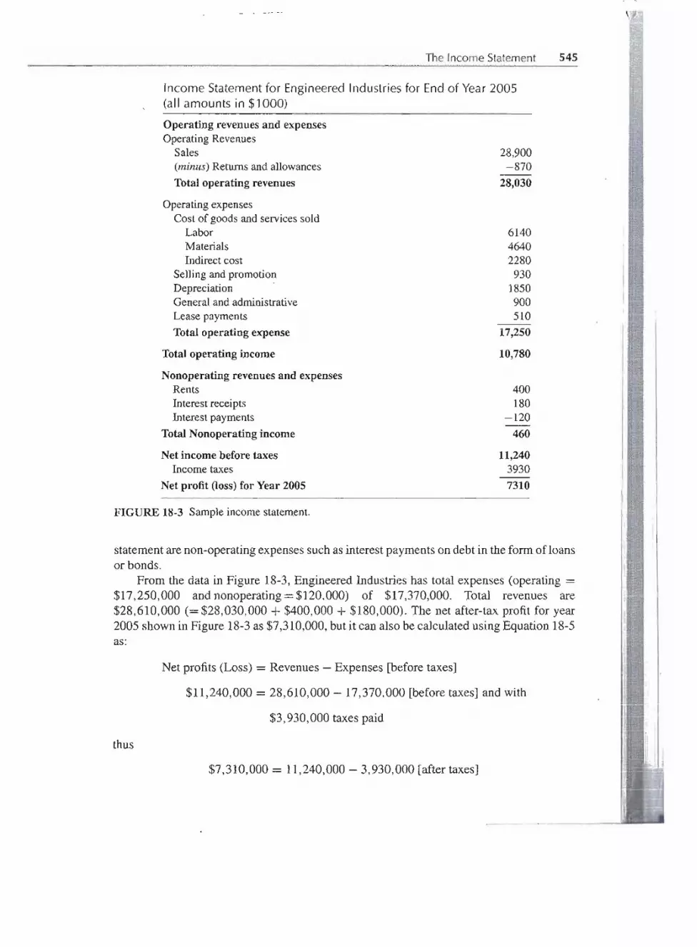
The Income Statement 545
Income Statement for Engineered Industries for End of Year 2005(all amounts in $1000)
Operating revenues and expensesOperatingRevenues
Sales(minus)Returns and allowances
Total operating revenues
OperatingexpensesCost of goods and services sold
LaborMaterialsIndirectcost
Selling and promotionDepreciation .
General and administrative
Lease payments
Total operating expense
Total operating income
Nonoperating revenues and expensesRents
Interest receiptsInterest payments
Total Nonoperating income
Net income before taxesIncome taxes
Net profit (loss) for Year 2005
28,900-870
28,030
614046402280930
1850900510
17,250
10,780
400180
-120460
11,2403930
7310
FIGURE 18-3 Sample income statement.
statement are non-operatingexpensessuch as interest payments on debt in the form of loansor bonds. . .
From the data in Figure 18-3, Engineered Industries has total expenses (operating =$17,250,000 and nonoperating= $120,000) of $17,370,000. Total revenues are$28,610,000 (= $28,030,000 + $400,000 + $180,000). The net after-tax profit for year2005 shown in Figure 18-3as $7,310,000,but it can also be calculatedusing Equation 18-5as:
Net profits (Loss) = Revenues - Expenses [before taxes]
$11,240,000 = 28,610,000 - 17,370,000 [before taxes] and with
$3,930,000taxespaid
thus
$7,310,000 = 11,240,000 - 3,930,000 [after taxes]
- - -- -
-- -- - - --- --- --

"1546 ACCOUNTING AND ENGINEERINGECONOMY
Financial Ratios Derived from Income Statement Data
Interest coverage, as given in Equation 18-6, is calculated as the ratio of total income tointerest payments-where total income is total revenuesminus all expenses except interestpayments.
Interest coverage = Total income/Interest payments (18-6)
The interest coverageratio (which for industrial firms should be at least 3.0) indicateshow much revenuemust drop to affect the firm's ability to financeits debt. With an interestcoverage ratio of 3.0, a firm's revenue would have to decrease by two-thirds (unlikely)before it became impossible to pay the interest on the debt. The larger the interest coverageratio the better.Engineered Industries in Figure 18-3 has an interest coverage ratio of
(28,610,000 - 17,250,000)/120,000 =94.7
Another importantfinancialratio based on the income statementis the net profit ratio.This ratio (Equation 18-7)equalsnet profitsdividedby net sales revenue.Net salesrevenueequals sales minus returns and allowances.
Net profit ratio = Net profit/Net sales revenue (18-7)
This ratio provides insight into the cost efficiency of operations as well as a firm'sability to convert salesinto profits. For Engineered Industries in Figure 18-3, the net profitratio is 7,310,000/28,030,000 = 0.261 = 26.1%. As with other financial measures, thenet profit ratio is best evaluated by comparisons with other time periods and industrybenchmarks.
Linking the Balance Sheet, Income Statement, and Capital TransactionsThe balance sheet and the income statement are separate, but linked documents. Under-standing how the two are linked together helps clarify each. Accounting describes theselinks as the articulation between these reports.
The balance sheet shows a firm's assets, liabilities, and equity at a particular point intime, whereas the income statement summarizes revenues and expenses over a time interval. .
These tabulationscanbe visualizedas a snapshotat the period's beginning(abalance sheet),a video summary overthe period (the income statement),and a snapshot at the period's end(anotherbalancesheet).The income statementand changesin the balancesheets summarizethe business transactionsthat have occurred during that period.
There aremany linksbetweenthese statementsand the cashflowsthatmakeupbusinesstransactions, but for engineeringeconomic analysis the followIngare the most important.
1. Overallprofitorloss (incomestatement)and the startingand endingequity (balancesheets).
2. Acquisition of capital assets.3. Depreciation of capital assets.
The overallprofit or loss during the year (shownon the income statement) is reflectedin the change in retained earnings between the balance sheets at the beginning and end of
-

- -......-...
Traditional Cost Accounting 547
the year.To findthe change in retained earnings (RE), one must also subtractany dividendsdistribp.tedto the owners and add the value of any new capital stock sold:
REbeg+ Net income/Loss + New stock - Dividends = REend
When capital equipment is purchased, the balance sheet changes,but the income state-ment does not. If cash is paid, then the cash asset account decrease equals the capitalequipment account increase-no change in total assets. If a loan is used, then the capitalequipment account increases, and so does the liability item for loans. In both cases theequity accounts and the income statement are unchanged.
The depreciation of capital equipment is shown as a line on the income statement.The depreciation for that year equals the change in accumulated depreciation between thebeginning and the end of the year-after subtraction of the accumulated depreciation forany asset that is sold or disposed of during that year.
Example 18-1 applies these relationships to with the data in Figures 18-1 and 18-2.
For simplicity,assume that Engineered Industries will not pay dividendsin 2005 and did not sellany capital equipment. It did purchase $4 million in capital equipment. What can be said aboutthe values on the balance sheet at the end of 2005, using the linkagesjust described?
SOLUTION;
First, the net profit of $7,310,000 will be added to the retained earnings from the end of 2004 tofind the new retained earnings at the end of 2005:
RE12l3112005 = $7,310,000+ $8,745,000== $16,055,000
Second, the fixed assets shown at the end of 2005 would increase from $6,500,000 toI $10,500,000. (Note: This is a major investment of the retained earnings in the finn's physicalassets.)t _
I fhird,the accumulated depreciation would increase by the $1,850,000"in depreciation shownin the 2005 income statement from the $2,350,000 shown in the 2004 balance sheet. The new
accumulated depreciation on the 2005 balance sheet would be $4,200,000. Combined with thechange in the amount of capital equipment, the new fixed asset total for 2005 would equal:
$335,000 +$10,500,000 - $4,200,000 = $6,635,000
TIONAL COST ACCOUNTING
A finn's cost-accounting system collects, analyzes, and reports operational perfonnancedata (costs, utilization rates, etc.). Cost-accountingdata are used to developproduct costs,to determine the mix of labor, materials, and other costs in a production setting, and toevaluate instances of outsourcing or subcontracting.
.-.

___A _.+__.._-.----.-
548 ACCOUNTING AND ENGINEERING ECONOMY
Direct and Indirect Costs
Costs incurred to produce a product or service are traditionally classified as either director indirect (overhead).Direct costs come from activities directly associated with the finalproduct or serviceproduced.Examplesincludematerialcostsandlaborcostsforengineeringdesign, component assembly,painting, and drilling.
Some organizational activities are difficult to link to specific projects, products, orservices. For example, the receiving and shipping areas of a manufacturingplant are"usedby all incoming materials and all outgoing products. Materials and products differ in theirweight, size, fragility,value, number of units, packaging, and so on, and the receiving andshipping costs depend on all these factors. Also, different materials arrive and differentproducts are shipped together, so these costs are intermingled and often cannot be tieddirectly to each product or material.
Othercosts, such as the organization'smanagement,sales,and administrativeexpenses, "
are difficultto link directly to individualproductsor services.Theseindirector overheadex-penses also includemachine depreciation,engineering and technical support,andcustomerwarranties.
Indirect Cost Allocation
To allocate indirect costs to different departments, products, and services, accountantsusequantitiessuchas direct-laborhours,direct-laborcosts,materialcosts,andtotaldirectcost.~
One of these is chosen to be the burden vehicle.The total of all indirect or overheadcosts isdivided by the total for the burden vehicle.For example, if direct-laborhours is the burdenvehicle, then overhead will be allocated based on overhead dollar per direct-labor hour.Then each product, project, or department will absorb (or be allocated) overhead costs,based on the number of direct-labor hours each has.
This is the basis for calling traditional costing systems absorption costing. For de-cision making, the problem is that the absorbed costs represent average, not incremental,performance.
Four common ways of allocating overhead are direct-labor hours, direct-labor cost, .
direct-materials cost, and total direct cost. The first two differ significantly only if thecost .per hour of labor differs for different products. Example 18-2 uses direct-labor anddirect-materials cost to illustrate the difference choices of burde~ vehicle.
Industrial Robots does not manufacture its own motors or computer chips. Its premium productdiffers from its standard product in having heavier-duty motors and more computer chips forgreater flexibility. "
As a result, Industrial Robots manufactures a higher fractidh 6f the standarilprotluet's v"IDlTe-itself, and it purchases a higher fraction of the premium product's value. Use the followingdatato allocate $850,000 in overhead on the basis of labor cost and materials cost.~,-- . ~ 0" . ~ .a a ~ It 15
- -i

---
Traditional Cost Accounting 549
Number of units per yearLabor cost (each)Materials cost (each)
Standard750
$400$550
SOLUTION
Premium400
$500$900
First, the labor and material costs for the standard product, the premium product, and in total arecalculated.
Number of units per yearLabor cost (each)Materials cost (each)Labor costMaterials cost
Standard750
$ 400550
300,000412,500
Premium400
$ 500900
200,000360,000
Total
$500,000772,500
Then the allocated cost per labor dollar, $1.70, is found by dividing the $850,000 in overheadby the $500,000 in total labor cost. The allocated cost per material dollar, $1.100324, is foundby dividing the $850,000 in overhead by the $772,500 in materials cost. Now, the $850,000 inallocated overhead is split between the two products using labor costs and material costs.
abor cost is the burden vehicle, then 60% of the $850,000 in overhead is allocated to thestandard product. If material cost is the burden vehicle, then 53.4% is allocated to the standardproduct. In both cases, the $850,000 has been split between the two products. Using total directcosts wouldproduce anotheroverheadallocationbetweenthese two values.However,for decisionmaking about product mix and product prices, incrementaloverhead costs must be analyzed. Allthe allocation or burden vehicles are based on an average cost of overhead per unit of burdenvehicle.
~
Problems with Traditional Cost Accounting ~!
Allocation of indirect costs can distort product costs and the decisionsbased on those costs. ii,
To be accurate, the analyst must determine which indirect or overhead expenses will be !!ii
changed because of an engineering project. In other words, what are the incremental cash 11:([' ,.J
U
" '
1I,';.f;I ;,~~:~<~;~--- ,
-- ---
Standard Premium TotalLabor cost $300,000 $200,000 $500,000
Overheadllabor 1.70 1.70Allocation by labor 510,000 340,000 850,000
Material cost 412,500 360,000 0Overhead/material 1.100324 1.100324Allocation by material 453,884 396,117 850,000

j
550 ACCOUNTINGAND ENGINEERINGECONOMY
DirectMaterial Overhead
FIGURE 18-4 Activity-based costing versus traditional overhead allocation. (Based on an exampleby Kim LaScola Needy.)
flows?For example, vacation and sick leave accrualmay be part of overhead,but will theychange if the labor content is changed? The changes in costs incurred must be estimated.Loadings, or allocations, of overheadexpenses cannot be used. .
This issue has become very importantbecause in some firms,automation has reduceddirect-labor content to less than 5% of the product's cost. Yet in some of these firms, ~ebasis for allocating overhead is still direct-labor hours or cost.
Other firmsare shiftingto activity-basedcosting (ABC),l where each activity"is linkedto specific cost drivers, and the number of dollars allocated as overhead is minimized.Figure 18-4illustratesthe differencebetweenactivity-basedcostingandtraditionaloverheadallocations.2 "
Other Problems to Watch For
Centralized accounting systems have ofteribeen accusedby project managers of being tooslowor being "untimely."Becauseengineeringeconomyis not concerned with the problemof daily project control, this is a less critical issue. However,if an organizationestablishesmultiple files and systems so that project managers (and others) have the timely data theyneed, then the level of accuracy in one or all systems may be low. As a result, analy!)tsmakingcostestimateswillhavetoconsiderotherinternaldatasources. "
There are several cases in which data on equipment or inventory values may be ques-tionable. When inventory is valued on a "last in, first out" basis, the remaining inventorymay be valued too low. Similarly,land valued at its acquisition cost is likely to be signifi-cantlyundervalued.Finally,capitalequipmentmaybe valued ateither a low or a high value,depending on allowable depreciationtechniquesand companypolicy.
1Liggett, Hampton R., Jaime Trevino, and Jerome P. Lavelle, "Activity-Based Cost ManagementSystems, in an Advanced Manufacturing Environment." In Economic and Financial Justificq.tion ofAdvanced Manufacturing Technologies, 1992, H. R. Parsaei (editor), Elsevier Science.
2Tippet, Donald D., and Peter Hoekstra, "Activity-Based Costing: a Manufacturing ManagementDecision-Making Aid," Engineering Management Journal, Vol.5, No.2, June 1993, American Societyfor Engineering Management, pp. 37-42.
- - - --

__u - ._.--. _.- --. --
Problems
\,,"f .
551
ROBLEMS
.1 Why is it important for engineers and managers tounderstand accounting principles? Name a few waysthat they can do so.
2 Explain the accounting function within a firm. Whatdoes this function do, and why is it important? Whattypes of data does it provide?
3 Develop short definitions for the following terms:balance sheet, income statement, and fundamentalaccounting equation.
4 Explain the difference between short-term and long-term liabilities.
:; List the two primary general accounting statements.What is each used for and how do they differ? Which
;ost important?
) What is the advantage of comparing financial state-ments across periods or against industry benchmarksrather than in looking at statements associated with asingle date or period?If a firm has a current ratio less than 2.0 and an
acid-test ratio less than 1.0, will the company even-tually go bankrupt and out of business? Explain youranswer.
Calculatethe equityof the GravelConstructionCom-pany if it has $1 million worth of assets? Gravelhas$127,000 in current liabilities and $210,000in long-term liabilities.
Scarmack's Paint Company has annual sales of$500,000 per year. If there is a profit of $1000 perday, 6 days per week operation, what is the total yearlyb'- .,ess expense? All calculations are on a before-taxb!1.~..s. (Answer: $188,000)
o Mama L's Baby Monitor Company has current as-sets of $5 million and current liabilities of $2 million.
Give the company's working capital and current ratio.(Answer: $3 million, 2.50)
1 Laila's Surveying Inc. had revenues of $100,000 in2004. Expenses totaled $60,000. What was her netprofit (or loss)?
~ From the following data, taken from the balance sheetof Petey's Widget Factory, determine the workingcapital, current ratio, and acid-test ratio.
CashNet accounts and notes receivableRetailers' inventories
Prepaid expensesAccounts and notes payable
(short term)Accumulated liabilities
$ 90,000175,000210,000
6,000322,000
87,000
18-13 The general ledger of the Fly-Buy-Nite (FBN)Engineering Company contained the followingaccount balances (partial listing) at the end of June,2004. Construct an income statement. What is the net
income before taxes and the net profit (or loss) aftertaxes? FBN has a tax rate of 27%.
Administrative expensesSubcontracted services
Development expensesInterest expenseSales revenue
Selling expenses
Amount
(thousands)$ 2,75018,000
900200
30,0004,500
18-14 For Gee-Whiz Devices calculate the following: work-ing capital, current ratio, and acid-test ratio.
Gee-Whiz Devices Balance Sheet Data
CashMarket securitiesNet accounts and notes receivableRetailers' inventories
Prepaid expensesAccounts and notes payable
(short term)Accumulated liabilities to date
$100,00045,000
150,000200,000
8,000315,000
90,000
(Answer: $90,000; 1.22; 0.73)
18-15 For Evergreen Environmental Engineering (EEE),determine the working capital, current ratio, and acid-test ratio. Evaluate the company's economic situationwith respect to its ability to payoff debt.

552 ACCOUNTING AND ENGINEERINGECONOMY
~
EEEBalance Sheet Data (thousands)
Cash $110,000Securities 40,000Accountsreceivable 160,000Retailers' inventories 250,000Prepaid expenses 3,000Accountspayable 351,000Accumulatedliabilities 89,000
18-16 For Magdalen Industries, compute the net income be-fore taxes and net profit (or loss). Taxes for the yearwere $1 million. Calculate the interest coverage andnet profit ratio. Is the interest coverage acceptable?Explain why or why not.
Magdalen Industries Balance SheetData (millions)
Revenues
Total operating revenue(including sales of $48 million)
Total nonoperating revenueExpenses.
Total operating expensesTotal nonoperating expenses
(interest payments)
$51
35
707
18-17 Find the net income ofThrbo Start given the followingdata.
Turbo Start Balance SheetData (thousands)
Accounts payableSelling expenseSales revenue
Owner's equityIncome taxes
Cost of goods soldAccounts receivable
$ 1,0005,000
50,0004,5002,000
30,00015,000
(Answer: $13,000,000)
18-18 Thrbo Start (Problem 18-17) has current assets total-ing $1.5 million (this includes $500,000 in current in-ventory) and current liabilities totaling $50,000. Findthe current ratio and acid-test ratio. Are the ratios at
desirable levels? Explain.
18-19 For J &W Graphics Supply, compute the current ratio.Is this a financially healthy company? Explain.
J&W Graphics Supply BalanceSheet Data (thousands)
AssetsCashInventoriesAccountsreceivableBad debt provision
LiabilitiesNotes payableAccruedexpensesAccountspayable
$1740900
2500-75
500125
1050
18-20 For Sutton Manufacturing, determine the current ratioand the acid-test ratio. Are these values acceptable?Why or why not?
Sutton Manufacturing Balance Sheet Data(thousands)
Assets LiabilitiesCurrent assets Current liabilities
Cash $870 Notes payable $500Accounts 450 Accountspayable 600
receivableInventory 1200 Accruals 200Prepaid expenses 50 Taxespayable 30
Other expenses 10 Currentportion 100long-termdebt- -
Totalcurrent assets 2670 Totalcurrent 1430liabilities
Long-termdebt 2000Officerdebt 200
Net fixed assets (subordinated) -Land 1200 Total liabilities 3630Plant and 2800
equipmentCommonstock 1670
Notes receivable 200 Capital surplus 400
Intangibles 20 Retainedearnings 1200Other assets 100 Totalnet worth 3270- -
Total assets 6900 Totalliabilities 6900and net Worth
J
.

- - ... - --- --
Problems 553
J-21 For Andrew's Electronic Instruments, calculate the
interest coverage and net profit ratio. Is Andrew'sbusinesshealthy? '
Income Statement for Andrew'sElectronics for End of Year2004(thousands)
Revenues
Operaing revenuesSales
(minus) Returns
Total operating revenuesNonoperating revenues
Interest receiptsStock revenues
Total nonoperating revenues
Total revenues, RExpensesOperating expenses
Cost of goods and services soldLaborMaterialsIndirect cost
Selling and promotionDepreciationGeneral and administrative
Lease payments
Total operating expensesNonoperating expenses
Interest paymentsTotal nonoperating expenses
Total expenses, ENet income before Taxes, R - EIncomes taXes
Net profit (Loss) for the year 2004
$395-15
380
50.25
75455
200346820301010
372
2222
394613031
22 LeGaroutte Industries makes industrial pipe manu-facturing equipment. Use direct-labor hours as theburden vehicle, and compute the total cost per unitfor eachmodelgiveninthe table.Totalmanufacturingindirect costs are $15,892,000,and there are 100,000units manufacturedper year for Model S, 50,000 forModel M, and 82,250for Model G.
Item Model S Model M Model G
Direct-materialcosts $3,800,000 $1,530,000 $2,105,000Direct-laborcosts 600,000 380,000 420,000Direct-laborhours 64,000 20,000 32,000
(Answer: $132; $93; $84)
18-23 Par Golf Equipment Company produces two types ofgolf bag: the standard and deluxe models. The totalindirect cost to be allocated to the two bags is $35,000.Determine the net revenue that Par Golf can expectfrom the sale of each bag.(a) Use direct-labor cost to allocate indirect costs.(b) Use direct-materials cost to allocate indirect
costs.
Data Item
Direct-labor costDirect-material cost
Selling priceUnits produced
Standard
$50,00035,000
601800
Deluxe
$65,00047,500
951400
18-24 RLW-II Enterprises estimated that indirect manufac-turing costs for the year would be $60 million andthat 12,000 machine-hours would be used.(a) Compute the predetermined indirect cost appli-
cation rate using machine hours as the burdenvehicle.
(b) Determine the total cost of production for a prod-uct with direct material costs of $1 million, direct-labor costs of $600,000, and 200 machine-hours.
(Answers: $5000, $2.6 million)
18-25 Categorize each of the following costs as direct orindirect. Assume that a traditional costing system isin place.
Machine run costs
Machine depreciationMaterial handling costsCost of materials
Overtime expensesMachine operator wagesUtility costsSupport (administrative)
staff salaries
Cost to market the productCost of storageInsurance costs
Cost of product sales forceEngineering drawingsMachine labor
Cost of tooling and fixtures
- - --- -
Introduction to Spreadsheets
Computerizedspreadsheetsare availablenearly everywhere,and they can be easily appliedto economic analysis. In fact, spreadsheets were originally developed to analyze financialdata, and they are often credited with initiating the explosivegrowth in demandfor desktopcomputing.
A spreadsheet is a two-dimensional table, whose cells can contain numerical val-ues, labels, or formulas. The software automatically updates the table when an entry ischanged, and there are powerfultools for copyingformulas,creatinggraphs, andformattingresults.
THE ELEMENTSOF A SPREADSHEET
A spreadsheet is a two-dimensional table that labels the columns in alphabetical order Ato Z, AA to AZ, BA to BZ, up to IV (256 columns). The rows are numbered from 1 to65,536. Thus a cell of the spreadsheet is specifiedby its column letter and row number.Forexample, A3 is the third row in column A and AA6 is the sixth row in the twenty-seventhcolumn. Each cell can contain a label, a numerical value, or a formula. .
A label is any cell where the contents should be treate~ as text. Arithmetic cannot beperformed on labels. Labels are used for variable names, row and column headings, andexplanatory notes. In Excel any cell which contains more than a simple number, such as3.14159, is treated as a label, unless it begins with an =, which is the signal for a formula.Thus 2*3 and Bl+B2 are labels. Meaningful labels can be wider than a normal column.One solution is to allowthose cells to "wrap" text, which is one of the "alignment" options.The table heading row (row 8) in Example A-I has turned this on by selecting row 8, rightclicking on the row, and selecting wrap text under the alignment tab.
A numericalvalue is any number.Acceptableformatsfor entry or display include per-centages, currency,accounting, scientific,fractions, date, and time. In addition the numberof decimal digits, the display of $ symbols, and commas for "thousands" separatorscan beadjusted. The format for cells can be changed by selecting a cell, a block of cells, a row,a column, or the entire spreadsheet. Then right click on the selected area, and a menu thatincludes "format cells" will appear. Then number formats, alignment, borders, fonts, andpatterns can be selected.
554

... - . ....
Copy Command 555
Formulasmust begin with an =, such as =3*4A2or =BI+B2. They can include manyfunptions-financial, statistical, trigonometric,etc. (and others can be definedby the user).The formulafor the "current" cell is displayedin theformulabarat the topof the spreadsheet.The value resulting from the formula is displayed in the cell in the spreadsheet.
Often the printed out spreadsheet will be part of a report or a homework assignmentand the formulas must be explained. Here is an easy way to place a copy of the formula inan adjacent or nearby cell. (1) Convert the cell with the formula to a label by inserting aspace before the = sign. (2) Copy that label to an adjacent cell by using cut and paste. Donot drag the cell to copy it, as any formula ending with a number (even an address like B4)will have the number automaticallyincremented.(3) Convertthe original formulaback intoa formula by deleting the space.
EFINING VARIABLESIN A DATA BLOCK
The cell AI, top left comer, is the HOME cell for a spreadsheet.Thus, the top left area iswhere the data block should be placed. This data block should have every variable in .thespreadsheet with an adjacent label for each. This data block supports a basic principle ofgood spreadsheet modeling, which is to use variables in your models.
The data block in Example A-I contains entered data-the loan amount (AI), thenumber of payments (A2), and the interest rate (A3), and computed data-the payment(A4). Then instead of using the loan amount of $5000 in a formula, the cell reference Alis used. Even if a value is only referenced once, it is better to include it in the data blockBy using one location to define each variable,you can change any value at one place in thespreadsheet and have the entire spreadsheetinstantly recomputed.
Even for simple homeworkproblems you should use a data block.
1. Youmay be able to use it for anotherproblem.2. Solutions to simple problems may grow into solutions for complexproblems.3. Good habits, like using data blocks, are easy t~ maintain once they are established.4. It makes the assumptions clear if you've estimated a value or for grading.
In the real world, data blocks are evenmore important.Mostproblems are solvedmorethan once, as more and more accuratevaluesare estimated.Often the spreadsheetis revisedto add other variables, time periods, locations,etc. Withoutdata blocks, it is hard to changea spreadsheet and the likelihood of missing a required change skyrockets.
If you want your formulas to be easier to read, you can name your variables. Note:In current versions of Excel, the cell's location or name is displayed at the left of theformula bar. Variablenames can be entered here. They will then automatically be appliedif cell addresses are entered by the point and click method. If cell addresses are enteredas A2, then A2 is what is displayed. To change a displayed A2, to the name of the cell(LoanAmount), the process is to click on insert, click on name, click on apply, and thenselect the names to be applied.
tPYCOMMAND
Thecopy commandandrelative/absoluteaddressingmakespreadsheetmodelseasyto build.If the range of cells to be copied contains onlylabels, numbers, andfunctions, then the copy
- -- - -

556 INTRODUCTION TO SPREADSHEETS
command is easy to use and understand. For example, the formula =EXP(1.9) would becopied unchanged to a new location. However,cell addresses are usually part of the rangebeing copied, and their absolute and relative addresses are treated differently.
An absolute address is denoted by adding $ signs before the column and/or row. .Forexamplein FigureA-la, $A$4 is the absoluteaddressfor the interestrate.Whenanabsolute address is copied, the column and/or row that is fixed is copied unchanged.Thus$A$4 is completely fixed, $A4 fixes the column, and A$4 fixes the row.One common Usefor absolute addresses is any data block entry, such as the interest rate. When entering orediting a formula,changingbetweenA4, $A$4, A$4, $A4,and A4 is most easilydone usingthe F4 key, which scrolls an address through the choices.
In contrast a relative address is best interpreted as directions from one cell to another.For example in Figure A-I a, the balance due in year t equals the balance due in year t - 1minus the principal payment in year t. Specifically for the balance due in year 1, DlOcontains =D9-ClO. From cell DlO, cell D9 is one row up and ClO is one column to theleft, so the formula is really (contents of 1 up) minus (contents of 1 to the left). When acell containing a relative address is copied to a new location, it is these directions that arecopied to determine any new relative addresses. So if cell DlO is copied to cell F14, theformula is =F13-EI4.
Thus to calculate a loan repayment schedule, as in Figure A-I, the row of formulas iscreated and then copied for the remaining years.
Table 3-1 shows four repayment schedules for a loan of $5000 to be repaid over 5 years at aninterest rate of 8%. Use a spreadsheet to calculate the amortization schedule for the constantprincipal payment option.
SOLUTION
~ ..
The first step is to enter the loan amount, number of periods, and interest rate into a data block inthe top left part of the spreadsheet. The next step is to calculate the constant principal paymentamount, which was given as $1252.28 in Table 3-1. The factor approach to findingthis value isgiven in Chapter 3 and the spreadsheet function is explained in Chapter 4;
The next step is to identify the columns for the amortizatiqu schedule. These are the year,interest owed,principal payment, and balance due. Because some of these labels arewider than anormal column, the cells are formatted so that the textwraps (rowheight increases automatically).The initial balance is shown in the year 0 row.
Next, the formulas for the first year are written, as shown m.figure A-I a. The interest owed(cellBlO) equals the interest rate ($A$4) times the balance due for year 0 (D9). The principalpayment (cell ClO) equals the annual payment ($A$6) minus the interest owed and paid (B1O).Finally, the balance due (cell DlO) equals the balance due for the previous year (D9) minus the
)?rin<:ipalpaym€?nt.(C~O):T~e re~ults are shown in Figure A-la. ... .. .
- '= Now ~ells AlO toMDlOare selecred for yefu-1. Brdra~ginglloWn d"nthe right comer'ofD10,the entire rowcan be copied for years 2 through 5. Note if cut andpaste is used,thenitis necessarytoc()I11pletethe year column separately (dragging increme,ntsthe year, b1Jtcuttinga,ndpastingdoes not). The results are shown in Figure A-Ib. .
.,
-- - --- ---
j.
- -

. . .u . ......
Copy Command 557
(a)
(b)
FIGURE A-I (a) Year 1 amortization schedule. (b) Completed amortization schedule.
This appendix has introduced the basics of spreadsheets.Chapter 2 uses spreadsheets andsimple bar charts to draw cash flow diagrams. Chapters 4-15 each have spreadsheet sec-tions. These are designed to develop spreadsheet modeling skills and to reinforce yourunderstanding of engineering economy.As current spreadsheetpackages are built aroundusing mice to click on cells and items in charts, there is usually an intuitive connectionbetween what you would like to do and how to do it. It seems the best way to learn how touse the spreadsheetpackage is to simply play around with it. In addition,as you look at themenu choices, you will find new commands that you hadn't thought of but find useful.
'~"::::
, A B C D E
1 EnteredData
2 5000 LoanAmount
3 5 Numberof Payments4 8% InterestRate5 ComputerData6 $1,252.28 LoanPayment7
Interest Principal Balance8 Year Owed Payment Due
9 0 5000.00
10 1 400.00 852.28 4147.72 =D9-ClO11 /12 $A$4*D9 =$A$6-BlO
A B C D E
Interest Principal Balance
8 Year Owed Payment Due
9 0 5000.00,
10 1 400.00 852.28 4147.72
11 2 331.82 920.46 3227.25
12 3 258.18 994.10 2233.15
13 4 178.65 1073.63 1159.52
14 5 92.76 1159.52 0.00 =Dl3-CI4,15 /16 = $A$4*D 13 =$A$6-BI4

t :1I ;,I
-----
Compound InterestTables
Values of Interest Factors When N Equals Infinity
Single Payment:(F/P, i, 00) = 00(P/F, i, 00) = 0
ArithmeticGradientSeries:(A/G, i, 00) = l/i(PIG, i, 00) = l/P
Uniform Payment Series:(A/F, i, 00) =0(A/P, i, 00) = i(F/A, i, 00) = 00(PIA, i, 00) = l/i
I


._---.._-----
jI
I
:
'.
COMPOUND INTERESTTABLES 561
0/0 Compound Interest Factors 1/20/0
Single Payment Uniform Payment Series Arithmetic Gradient
Compound Present Sinking Capital Compound Present Gradient GradientAmount Worth Fund Recovery Amount Worth Uniform PresentFactor Factor Factor Factor Factor Factor Series WorthFind F Find P Find A Find A Find F Find P Find A Find P
Given P Given F Given F Given P Given A Given A Given G Given GFIP PIF AIF AlP FIA PIA AIG PIG n
1.005 .9950 1.0000 1.0050 1.000 0.995 0 0 11.010 .9901 .4988 .5038 2.005 1.985 0.499 0.991 21.015 .9851 .3317 .3367 3.015 2.970 0.996 2.959 31.020 .9802 .2481 .2531 4.030 3.951 1.494 5.903 41.025 .9754 .1980 .2030 5.050 4.926 1.990 9.803 5
1.030 .9705 .1646 .1696 . 6.076 5.896 2.486 14.660 61.036 .9657 .1407 .1457 7.106 6.862 2.980 20.448 71.041 .9609 .1228 .1278 8.141 7.823 3.474 27.178 81.046 .9561 .1089 .1139 9.182 8.779 3.967 34.825 91.051 .9513 .0978 .1028 10.228 9.730 4.459 43.389 101.056 .9466 .0887 .0937 11.279 10.677 4.950 52.855 111.062 .9419 .0811 .0861 12.336 11.619 5.441 63.218 121.067 .9372 .0746 .0796 13.397 12.556 5.931 74.465 131.072 .9326 .0691 .0741 14.464 13.489 6.419 86.590 141.078 .9279 .0644 .0694 15.537 14.417 6.907 99.574 15
1.083 .9233 .0602 .0652 16.614 15.340 7.394 113.427 161.088 .9187 .0565 .0615 17.697 16.259 7.880 128.125 171.094 .9141 .0532 .0582 18.786 17.173 8.366 143.668 181.099 .9096 .0503 .0553 19.880 18.082 8.850 160.037 191.105 .9051 .0477 .0527 20.979 18.987 9.334 177.237 201.110 .9006 .0453 .0503 22.084 19.888 9.817 195.245 211.116 .8961 .0431 .0481 23.194 20.784 10.300 214.070 221.122 .8916 .0411 .0461 24.310 21.676 10.781 233.680 231.127 .8872 .0393 .0443 25.432 22.563 11.261 254.088 241.133 .8828 .0377 .0427 26.559 23.446 11.741 275.273 251.138 .8784 .0361 .0411 27.692 24.324 12.220 297.233 261.144 .8740 .0347 .0397 28.830 25.198 12.698 319.955 271.150 .8697 .0334 .0384 29.975 26.068 13.175 343.439 281.156 .8653 .0321 .0371 31.124 26.933 13.651 367.672 29,.161 .8610 .0310 .0360 32.280 27.794 14.127. 392.640 301.197 .8356 .0254 .0304 39.336 32.871 16.962 557.564 361.221 .8191 .0226 .0276 44.159 36.172 18.836 681.341 401.270 .7871 .0185 .0235 54.098 42.580 22.544 959.928 481.283 .7793 .0177 .0227 56.645 44.143 23.463 1035.70 501.296 .7716 .0169 .0219 59.218 45.690 24.378 . 1 113.82 521.349 .7414 .0143 .0193 69.770 51.726 28.007 1448.65 601.418 .7053 .0120 .0170 83.566 58.939 32.468 1913.65 701.432 .6983 .0116 .0166 86.409 60.340 33.351 2012.35 721.490 .6710 .0102 .0152 98.068 65.802 36.848 2424.65 801.520 .6577 .00961 .0146 104.074 68.453 38.576 2 640.67 841.567 .6383 .00883 .0138 113.311 72.331 41.145 2 976.08 901.614 .6195 .00814 .0131 122.829 76.095 43.685 3324.19 961.647 .6073 .00773 .0127 129.334 78.543 45.361 3 562.80 1001.680 .5953 .00735 .0124 135.970 80.942 47.025 3 806.29 1041.819 .5496 .00610 .0111 163.880 90.074 53.551 4 823.52 1203.310 .3021 .00216 .00716 462.041 139.581 96.113 13415.56 .2406.023 .1660 .00100 .00600 1004.5 166.792 128.324 21 403.32 360
10.957 .0913 .00050 .00550 1991.5 181.748 151.795 27 588.37 480
---

- - -
..........-
562 COMPOUND INTERESTTABLES
3/4% Compound Interest Factors 3/4%
Single Payment Uniform Payment Series Arithmetic Gradient
Compound Present Sinking Capital Compound Present Gradient GradientAmount Worth Fund Recovery Amount Worth Uniform PresentFactor Factor Factor Factor Factor Factor Series WorthFind F Find P Find A Find A Find F Find P Find A Find P
Given P Given F Given F Given P Given A Given A Given G Given Gn FIP PIF AIF AlP FIA PIA AIG PIG n
1 1.008 .9926 1.0000 1.0075 1.000 0.993 0 0 12 1.015 .9852 .4981 .5056 2.008 1.978 0.499 0.987 23 1.023 .9778 .3308 .3383 3.023 2.956 0.996 2.943 34 1.030 .9706 .2472 .2547 4.045 3.926 1.492 5.857 45 1.038 .9633 .1970 .2045 5.076 4.889 1.986 9.712 56 1.046 .9562 .1636 .1711 6.114 5.846 2.479 14.494 67 1.054 .9490 .1397 .1472 7.160 6.795 2.971 20.187 78 1.062 .9420 .1218 .1293 8.213 7.737 3.462 26.785 89 1.070 .9350 .1078 .1153 9.275 8.672 3.951 34.265 9
10 1.078 .9280 .0967 .1042 10.344 9.600 4.440 42.619 1011 1.086 .9211 .0876 .0951 11.422 10.521 4.927 51.831 1112 1.094 .9142 .0800 .0875 12.508 11.435 5.412 61.889 1213 1.102 .9074 .0735 .0810 13.602 12.342 5.897 72.779 1314 1.110 .9007 .0680 .0755 14.704 13.243 6.380 84.491 1415 1.119 .8940 .0632 .0707 15.814 14.137 6.862 97.005 1516 1.127 .8873 .0591 .0666 16.932 15.024 7.343 110.318 1617 1.135 .8807 .0554 .0629 18.059 15.905 7.822 124.410 1718 1.144 .8742 .0521 .0596 19.195 16.779 8.300 139.273 1819 1.153 .8676 .0492 .0567 20.339 17.647 8.777 154.891 1920 1.161 .8612 .0465 .0540 21.491 18.508 9.253 171.254 2021 1.170 .8548 .0441 .0516 22.653 19.363 9.727 188.352 2122 1.179 .8484 .0420 .0495 23.823 20.211 10.201 206.170 2223 1.188 .8421 .0400 .0475 25.001 21.053 10.673 224.695 2324 1.196 .8358 .0382 .0457 26.189 21.889 11.143 243.924 2425 1.205 .8296 .0365 .0440 27.385 22.719 11.613 263.834 25
26 1.214 .8234 .0350 .0425 28.591 23.542 12.081 284.421 26 =
27 1.224 .8173 .0336 .0411 29.805 24.360 12.548 305.672 2728 1.233 .8112 .0322 .0397 31.029 25.171 13.014 327.576 2829 1.242 .8052 .0310 .0385 32.261 25.976 13.479 350.122 2930 1.251 . .7992 .0298 .0373 33.503 26.775 13.942 373.302 3036 1.309 .7641 .0243 .0318 41.153 31.447 16.696 525.038 3640 1.348 .7416 .0215 .0290 46.447 34.447 18.507 37.519 4048 1.431 .6986 .0174 .0249 57.521 40.185 22.070 886.899 4850 1.453 .6882 .0166 .0241 60.395 41.567 22.949 953.911 5052 1.475 .6780 .0158 .0233 63.312 42.928 23.822 1022.64 52
60 1.566 .6387 .0133 .0208 75.425 48.174 27.268 1313.59 6070 1.687 .5927 .0109 .0184 91.621 54.305 31.465 1708.68 7072 1.713 .5839 .0105 .0180 95.008 55.477 32.289 1791.33 7280 1.818 .5500 .00917 .0167 109.074 59.995 35.540 2 132.23 8084 1.873 .5338 .00859 .0161 116.428 62.154 37.137 2 308.22 84
90 1.959 .5104 .00782 .0153 127.881 65.275 39.496 2 578.09 9096 2.049 .4881 .00715 .0147 139.858 68.259 41.812 2 854.04 96tOO 2.111 .4737 .00675 .0143 148.147 70.175 43.332 3 040.85 100t04 2.175 .4597 .00638 .0139 156.687 72.035 44.834 3229.60 104
120,c':<f.
l20 2.451 .4079 .00517 .0127 193.517 78.942 50.653 3 998.68 ...
O 6.009 .1664 .00150 .00900 667.901 111.145 85.422 9 494.26 240160 14.731 .0679 .00055 .00805 1 830.8 124.282 107.115 13 312.50 360180 36.111 .0277 .00021 .00771 4681.5 129.641 119.662 15513.16 480
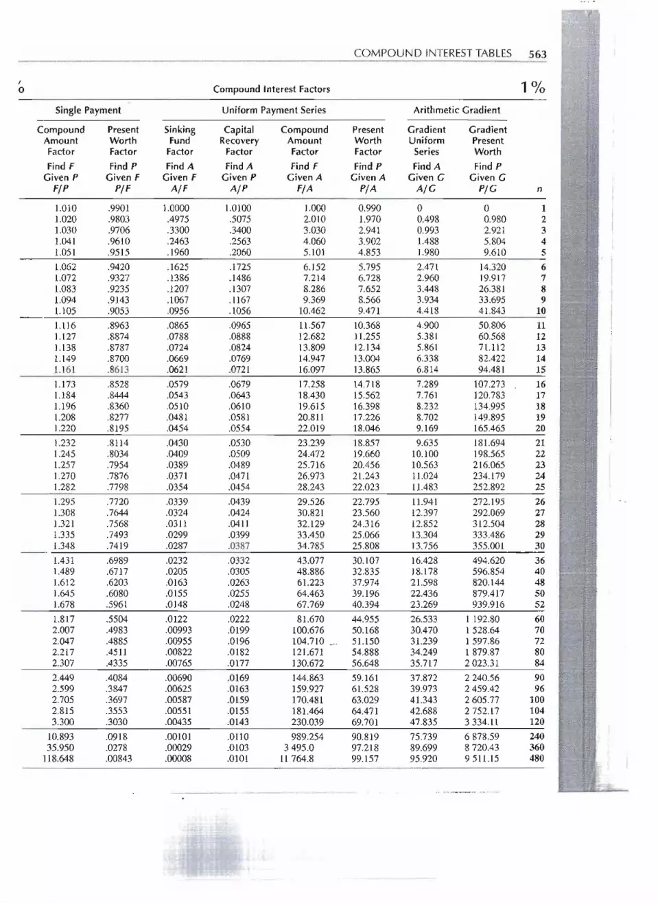
COMPOUND INTEREST TABLES 563
I 1 %0 Compound Interest Factors
Single Payment Uniform Payment Series Arithmetic Gradient-
Compound Present Sinking Capital Compound Present Gradient GradientAmount Worth Fund Recovery Amount Worth Uniform PresentFactor Factor Factor Factor Factor Factor Series WorthFind F Find P Find A Find A Find F Find P Find A Find P
Given P Given F Given F Given P Given A Given A Given G Given GFIP PIF AIF AlP FIA PIA AIG PIG n
1.010 .9901 1.0000 1.0100 1.000 0.990 0 0 11.020 .9803 .4975 .5075 2.010 1.970 0.498 0.980 21.030 .9706 .3300 .3400 3.030 2.941 0.993 2.921 31.041 .9610 .2463 .2563 4.060 3.902 1.488 5.804 41.051 .9515 .1960 .2060 5.101 4.853 1.980 9.610 51.062 .9420 .1625 .1725 6.152 5.795 2.471 14.320 61.072 .9327 .1386 .1486 7.214 6.728 2.960 19.917 71.083 .9235 .1207 .1307 8.286 7.652 3.448 26.381 81.094 .9143 .1067 .1167 9.369 8.566 3.934 33.695 91.105 .9053 .0956 .1056 10.462 9.471 4.418 41.843 101.116 .8963 .0865 .0965 11.567 10.368 4.900 50.806 111.127 .8874 .0788 .0888 12.682 11.255 5.381 60.568 121.138 .8787 .0724 .0824 13.809 12.134 5.861 71.112 131.149 .8700 .0669 .0769 14.947 13.004 6.338 82.422 141.161 .8613 .0621 .0721 16.097 13.865 6.814 94.481 151.173 .8528 .0579 .0679 17.258 14.718 7.289 107.273 161.184 .8444 .0543 .0643 18.430 15.562 7.761 120.783 171.196 .8360 .0510 .0610 19.615 16.398 8.232 134.995 181.208 .8277 .0481 .0581 20.811 17.226 8.702 149.895 191.220 .8195 .0454 .0554 22.019 18.046 9.169 165.465 201.232 .8114 .0430 .0530 23.239 18.857 9.635 181.694 211.245 .8034 .0409 .0509 24.472 19.660 10.100 198.565 221.257 .7954 .0389 .0489 25.716 20.456. 10.563 216.065 231.270 .7876 .0371 .0471 26.973 21.243 11.024 234.179 241.282 .7798 .0354 .0454 28.243 22.023 11.483 252.892 251.295 .7720 .0339 .0439 29.526 22.795 11.941 272.195 261.308 .7644 .0324 .0424 30.821 23.560 12.397 292.069 271.321 .7568 .0311 .0411 32.129 24.316 12.852 312.504 281.335 .7493 .0299 .0399 33.450 25.066 13.304 333.486 291.348 .7419 .0287 .0387 34.785 25.808 13.756 . 355.001 30
1.431 .6989 .0232 .0332 43.077 30.107 16.428 494.620 361.489 .6717 .0205 .0305 48.886 32.835 18.178 596.854 401.612 .6203 .0163 .0263 61.223 37.974 21.598 820.144 481.645 .6080 .0155 .0255 64.463 39.196 22.436 879.417 501.678 .5961 .0148 .0248 67.769 40.394 23.269 939.916 52
1.817 .5504 .0122 .0222 81.670 44.955 26.533 1 192.80 602.007 .4983 .00993 .0199 100.676 50.168 30.470 1 528.64 702.047 .4885 .00955 .0196 104.710 _ _ 51.150 31.239 1 597.86 722.217 .4511 .00822 .0182 121.671 54.888 34.249 1879.87 802.307 .4335 .00765 .0177 130.672 56.648 35.717 2023.31 84
2.449 .4084 .00690 .0169 144.863 59.161 37.872 2 240.56 902.599 .3847 .00625 .0163 159.927 61.528 39.973 2459.42 962.705 .3697 .00587 .0159 170.481 63.029 41.343 2605.77 1002.815 .3553 .00551 .0155 181.464 64.471 42.688 2752.17 1043.300 .3030 .00435 .0143 230.039 69.701 47.835 3334.11 120
10.893 .0918 .00101 .0110 989.254 90.819 75.739 6 878.59 24035.950 .0278 .00029 .0103 3495.0 97.218 89.699 8 720.43 360
118.648 .00843 .00008 .0101 11 764.8 99.157 95.920 9511.15 480
---

.
.4 COMPOUND INTERESTTABLES-
1/4% CompoundInterestFactors 11/4%
Single Payment Uniform Payment Series Arithmetic Gradient
Compound Present Sinking Capital Compound Present Gradient GradientAmount Worth Fund Recovery Amount Worth Uniform PresentFactor Factor Factor Factor Factor Factor Series WorthFind F Find P Find A Find A Find F Find P Find A Find P
Given P Given F Given F Given P Given A Given A Given G Given GFIP PIF AIF AlP FIA PIA AIG PIG n
L 1.013 .9877 1.0000 1.0125 1.000 0.988 0 0 1! 1.025 .9755 .4969 .5094 2.013 1.963 0.497 0.976 2 ,
1.038 .9634 .3292 .3417 3.038 2.927 0.992 2.904 3
I
a 1.051 .9515 .2454 .2579 4.076 3.878 1.485 5.759 41.064 .9398 .1951 .2076 5.127 4.818 1.976 9.518 5
) 1.077 .9282 .1615 .1740 6.191 5.746 2.464 14.160 67 1.091 .9167 .1376 .1501 7.268 6.663 2.951 19.660 7
1.104 .9054 .1196 .1321 8.359 7.568 3.435 25.998 8 ,) 1.118 .8942 .1057 .1182 9.463 8.462 3.918 33.152 9 i) 1.132 .8832 .0945 .1070 10.582 9.346 4.398 41.101 10
,L 1.146 .8723 .0854 .0979 11.714 10.218 4.876 49.825 11
I! 1.161 .8615 .0778 .0903 12.860 11.079 5.352 59.302 121.175 .8509 .0713 .0838 14.021 11.930 5.827 69.513 13 I
a 1.190 .8404 .0658 .0783 15.196 12.771 6.299 80.438 14
I1.205 .8300 .0610 .0735 16.386 13.601 6.769 92.058 15
) 1.220 .8197 .0568 .0693 17.591 14.420 7.237 104.355 167 1.235 .8096 .0532 .0657 18.811 15.230 7.702 117.309 17
1.251 .7996 .0499 .0624 20.046 16.030 8.166 130.903 18) 1.266 .7898 .0470 .0595 21.297 16.849 8.628 145.119 19) 1.282 .7800 .0443 .0568 22.563 17.599 9.088 159.940 20
I 1.298 .7704 .0419 .0544 23.845 18.370 9.545 175.348 211.314 .7609 .0398 .0523 25.143 19.131 10.001 191.327 221.331 .7515 .0378 .0503 26.458 19.882 10.455 207.859 231.347 .7422 .0360 .0485 27.788 20.624 10.906 224.930 241.364 .7330 .0343 .0468 29.136 21.357 11.355 242.523 25
) 1.381 .7240 .0328 .0453 30.500 22.081 11.803 260.623 267 1.399 .7150 .0314 .0439 31.881 22.796 12.248 279.215 27i 1.416 .7062 .0300 .0425 32.280 23.503 12.691 298.284 28) 1.434 .6975 .0288 .0413 34.696 24.200 13.133 317.814 29) 1.452 .6889 .0277 .0402 36.129 24.889 13.572 337.792 30
) 1.564 .6394 .0222 .0347 45.116 28.847 16.164 466.297 36) 1.644 .6084 .0194 .0319 51.490 31.327 17.852 559.247 40J 1.845 .5509 .0153 .0278 65.229 35.932 21.130 759.248 48) 1.861 .5373 .0145 .0270 68.882 37.013 21.930 811.692 50t 1.908 .5242 .0138 .0263 72.628 38.068 22.722 864.960 52
2.107 .4746 .0113 .0238 88.575 42.035 25.809 1 084.86 602.386 .4191 .00902 .0215 110.873 46.470 29.492 1 370.47 702.446 .4088 .00864 .0211 115.675 47.293 30.205 1 428.48 722.701 .3702 .00735 .---...& 136.120 50.387 32.983 1 661.89 802.839 .3522 .00680 .. .0193 147.130 51.822 34.326 1778.86 843.059 .3269 .00607 .0186 164.706 53.846 36.286 1953.85 903.296 .3034 .00545 .0179 183.643 55.725 38.180 2 127.55 96
13.463 .2887 .00507 .0176 197.074 56.901 39.406 2 242.26 1003.640 .2747 .00474 .0172 211.190 58.021 40.604 2355.90 1044.440 .2252 .00363 .0161 275.220 61.983 45.119 2 796.59 120
19.716 .0507 .00067 .0132 1497.3 75.942 67.177 5 101.55 240 --,87.543 .0114 .00014 .0126 6 923.4 79.086 75.840 5997.91 360
388.713 .00257 .00003 .0125 31017.1 79.794 78.762 6284.74 480 JJ
......

. -
COMPOUND INTERESTTABLES 565
, 0;; Compound Interest Factors 11/20/02 0
Single Payment Uniform Payment Series Arithmetic Gradient
Compound Present Sinking Capital Compound Present Gradient GradientAmount Worth Fund Recovery Amount Worth Uniform PresentFactor Factor Factor Factor Factor Factor Series Worth
Find F Find P Find A Find A Find F Find P Find A Find PGiven P Given F Given F Given P Given A Given A Given G Given G
FIP PIF AIF AlP FIA PIA AIG PIG n
1.015 .9852 1.0000 1.0150 1.000 0.985 0 0 11.030 .9707 .4963 .5113 2.015 1.956 0.496 0.970 21.046 .9563 .3284 .3434 3.045 2.912 0.990 2.883 31.061 .9422 .2444 .2594 4.091 3.854 1.481 5.709 41.077 .9283 .1941 .2091 5.152 4.783 1.970 9.422 5
1.093 .9145 .1605 .1755. 6.230 5.697 2.456 13.994 61.110 .9010 .1366 .1516 7.323 6.598 2.940 19.400 71.126 .8877 .1l86 .1336 8.433 7.486 3.422 25.614 81.143 .8746 .1046 .1l96 9.559 8.360 3.901 32.610 91.161 .8617 .0934 .1084 10.703 9.222 4.377 40.365 10
1.178 .8489 .0843 .0993 11.863 10.071 4.851 48.855 111.196 .8364 .0767 .0917 13.041 10.907 5.322 58.054 121.214 .8240 .0702 .0852 14.237 11.731 5.791 67.943 131.232 .8118 .0647 .0797 15.450 12.543 6.258 78.496 141.250 .7999 .0599 .0749 16.682 13.343 6.722 89.694 15
1.269 .7880 .0558 .0708 17.932 14.131 7.184 101.514 161.288 .7764 .0521 .0671 19.201 14.908 7.643 113.937 171.307 .7649 .0488 .0638 20.489 15.673 8.100 126.940 181.327 .7536 .0459 .0609 21.797 16.426 8.554 140.505 191.347 .7425 .0432 .0582 23.124 17.169 9.005 154.611 20
1.367 .7315 .0409 .0559 24.470 17.900 9.455 169.241 211.388 .7207 .0387 .0537 25.837 18.621 9.902 184.375 221.408 .7100 .0367 .0517 27.225 19.331 10.346 199.996 231.430 .6995 .0349 .0499 28.633 20.030 10.788 216.085 241.451 .6892 .0333 .0483 30.063 20.720 11.227 232.626 25
1.473 .6790 .0317 .0467 31.514 21.399 11.664 249.601 261.495 .6690 .0303 .0453 32.987 22.068 12.099 266.995 271.517 .6591 .0290 .0440 34.481 22.727 12.531 284.790 281.540 .6494 .0278 .0428 35.999 23.376 12.961 302.972 291.563 .6398 .0266 . .0416 37.539 24.016 13.388 321.525 30
1.709 .5851 .0212 .0362 47.276 27.661 15.901 439.823 361.814 .5513 .0184 .0334 54.268 29.916 17.528 524.349 402.043 .4894 .0144 .0294 69.565 34.042 20.666 703.537 482.105 .4750 .0136 .0286 73.682 35.000 21.428 749.955 502.169 .4611 .0128 .0278 77.925 35.929 22.179 796.868 52
2.443 .4093 .0104 .0254 96.214 39.380 25.093 988.157 602.835 .3527 .00817 .0232 122.363 43.155 28.529 1 231.15 702.921 .3423 .00781 .0228 128.076 43.845 29.189 1 279.78 723.291 .3039 .00655 .0215 152.710 46.407 31.742 1473.06 803.493 .2863 .00602 .0210 166.172 47.579 32.967 1568.50 84
3.819 .2619 .00532 .0203 187.929 49.210 34.740 1 709.53 904.176 .2395 .00472 .0197 211.719 50.702 36.438 1 847.46 964.432 .2256 .00437 .0194 228.802 51.625 37.529 1937.43 1004.704 .2126 .00405 .0190 246.932 52.494 38.589 2 025.69 1045.969 .1675 .00302 .0180 331.286 55.498 42.518 2359.69 120
35.632 .0281 .00043 .0154 2 308.8 64.796 59.737 3 870.68 240212.700 .00470 .00007 .0151 14 113.3 66.353 64.966 4310.71 360
1269.7 .00079 .00001 .0150 84 577.8 66.614 66.288 4415.74 480

- -- - - - - - - -

COMPOUND INTERESTTABLES 567
%Compound Interest Factors 2%
Single Payment Uniform Payment Series Arithmetic Gradient-
Compound Present Sinking Capital Compound Present Gradient GradientAmount Worth Fund Recovery Amount Worth Uniform PresentFactor Factor Factor Factor Factor Factor Series WorthFind F Find P Find A Find A Find F Find P Find A Find P
Given P Given F Given F Given P Given A Given A Given G Given GFIP PIF AIF AlP FIA PIA AIG PIG n
1 1.020 .9804 1.0000 1.0200 1.000 0.980 0 0 12 1.040 .9612 .4951 .5151 2.020 1.942 0.495 0.961 23 1.061 .9423 .3268 .3468 3.060 2.884 0.987 2.846 34 1.082 .9238 .2426 .2626 4.122 3.808 1.475 5.617 45 1.104 .9057 .1922 .2122 5.204 4.713 1.960 9.240 56 1.126 .8880 .1585 .1785 6.308 5.601 2.442 13.679 67 1.149 .8706 .1345 .1545 7.434 6.472 2.921 18.903 78 1.172 .8535 .1165 .1365 8.583 7.325 3.396 24.877 89 1.195 .8368 .1025 .1225 9.755 8.162 3.868 31.571 9.0 1.219 .8203 .0913 .1113 10.950 8.983 4.337 38.954 101 1.243 .8043 .0822 .1022 12.169 9.787 4.802 46.996 11.2 1.268 .7885 .0746 .0946 13.412 10.575 5.264 55.669 123 1.294 .7730 .0681 .0881 14.680 11.348 5.723 64.946 134 1.319 .7579 .0626 .0826 15.974 12.106 6.178 74.798 145 1.346 .7430 .0578 .0778 17.293 12.849 6.631 85.200 156 1.373 .7284 .0537 .0737 18.639 13.578 7.080 .96.127 167 1.400 .7142 .0500 .0700 20.012 14.292 7.526 107.553 178 1.428 .7002 .0467 .0667 21.412 14.992 7.968 119.456 189 1.457 .6864 .0438 .0638 22.840 15.678 8.407 131.812 190 1.486 .6730 .0412 .0612 24.297 16.351 8.843 144.598 201 1.516 .6598 .0388 .0588 25.783 17.011 9.276 157.793 212 1.546 .6468 .0366 .0566 27.299 17.658 9.705 171.377 223 1.577 .6342 .0347 .0547 28.845 18.292 10.132 185.328 23:I 1.608 .6217 .0329 .0529 30.422 18.914 10.555 199.628 245 1.641 .6095 .0312 .0512 32.030 19.523 10.974 214.256 25
1.673 .5976 .0297 .0497 33.671 20.121 11.391 229.196 267 1.707 .5859 .0283 .0483 35.344 20.707 11.804 244.428 27
1.741 .5744 .0270 .0470 37.051 21.281 12.214 259.936 28) 1.776 .5631 .0258 .0458 38.792 21.844 12.621 275.703 29) 1.811 .5521 . .0247 .0447 40.568 22.396 13.025 291.713 30
2.040 .4902 .0192 .0392 51.994 25.489 15.381 392.036 362.208 .4529 .0166 .0366 60.402 27.355 16.888 461.989 402.587 .3865 .0126 .0326 79.353 30.673 19.755 605.961 482.692 .3715 .0118 .0318 84.579 31.424 20.442 642.355 502.800 .3571 .0111 .0311 90.016 32.145 21.116 678.779 52
3.281 .3048 .00877 .0288 114.051 34.761 23.696 823.692 604.000 .2500 .00667 .0267 149.977 37.499 26.663 999.829 704.161 .2403 .00633 .0263 158.056 37.984 27.223 1034.050 724.875 .2051 .00516 .0252 193.771 39.744 29.357 1 166.781 805.277 .1895 .00468 .0247 213.865 40.525 30.361 1230.413 84
5.943 .1683 .00405 .0240 247.155 41.587 31.793 1 322.164 906.693 .1494 .00351 .0235 284.645 42.529 33.137 1409.291 967.245 .1380 .00320 .0232 312.230 43.098 33.986 1464.747 1007.842 .1275 .00292 .0229 342.090 43.624 34.799 1518.082 104
10.765 .0929 .00205 .0220 488.255 45.355 37.711 1710.411 120
115.887 .00863 .00017 .0202 5 744.4 49.569 47.911 2 374.878 2401247.5 .00080 .00002 .0200 62 326.8 49.960 49.711 2 483.567 360
13429.8 .00007 .0200 671 442.0 49.996 49.964 2 498.027 480
.._4'____ - - __ ____ _'_0"


Single Payment
CompoundAmountFactorFindF
Given PFIP
1.0301.0611.0931.1261.1591.1941.2301.2671.3051.3441.3841.4261.4691.5131.5581.6051.6531.7021.7541.8061.8601.9161.9742.0332.0942.1572.2212.2882.3572.427
2.5002.5752.6522.7322.8143.2623.7824.3845.0825.8926.8307.9189.179
10.64112.33614.30016.57819.219
PresentWorthFactorFindP
Given FPIF
.9709
.9426
.9151
.8885
.8626
.8375
.8131
.7894
.7664
.7441
.7224
.7014
.6810
.6611
.6419
.6232
.6050
.5874
.5703
.5537
.5375
.5219
.5067
.4919
.4776
.4637
.4502
.4371
.4243
.4120
.4000
.3883
.3770
.3660
.3554
.3066
.2644
.2281
.1968
.1697
.1464
.1263
.1089
.0940
.0811
.0699
.0603
.0520
SinkingFund
FactorFind A
Given FAIF
1.0000.4926.3235.2390.1884.1546.1305.1125.0984.0872.0781.0705.0640.0585.0538.0496.0460.0427.0398.0372
.0349
.0327
.0308
.0290
.0274
.0259
.0246
.0233
.0221
.0210
.0200
.0190
.0182
.0173
.0165
.0133
.0108
.00887
.00735
.00613
.00515
.00434
.00367
.00311
.00265
.00226
.00193
.00165
CompoundInterestFactors
UniformPaymentSeries
CapitalRecovery
FactorFindA
Given PAlP
1.0300.5226.3535.2690.2184.1846.1605.1425.1284.1172.1081.1005.0940.0885.0838.0796.0760.0727.0698.0672
.0649
.0627
.0608
.0590
.0574
.0559
.0546
.0533
.0521"';-.0510
.0500
.0490
.0482
.0473
.0465
.0433
.0408
.0389
.0373
.0361
.0351
.0343
.0337
.0331
.0326
.0323
.0319
.0316
CompoundAmountFactorFindF
Given AFIA
1.0002.0303.0914.1845.3096.4687.6628.892
10.15911.46412.80814.19215.61817.08618.59920.15721.76223.41425.11726.87028.67630.53732.45334.42636.45938.55340.71042.93145.21947.57550.00352.50355.07857.73060.46275.40192.720
112.797136.072163.053194.333
.230.594272.631
. 321.363377.857
443.349519.272607.287
- --- -
COMPOUND INTERESTTABLES 569
PresentWorthFactorFindP
Given APIA
0.9711.9132.8293.7174.5805.4176.2307.0207.7868.5309.2539.954
10.63511.29611.93812.56113.16613.75414.32414.87715.41515.93716.44416.93617.413
17.87718.32718.76419.18819.60020.00020.38920.76621.13221.487
23.11524.51925.73026.77427.67628.45329.12329.70230.20130.631
31.00231.32331.599
Arithmetic Gradient
GradientUniformSeriesFind A
Given GAIG
o0.4930.9801.4631.9412.4142.8823.3453.8034.256
4.7055.1485.5876.0216.4506.8747.2947.7088.1188.5238.9239.3199.709
10.09510.47710.85311.22611.59311.95612.31412.66813.01713.36213.70214.03715.65017.15618.55819.86021.06722.18423.21524.16325.03525.83526.56727.23527.844
GradientPresentWorthFindP
Given GPIG
o0.9432.7735.4388.889
13.07617.95523.48129.61236.30943.53351.24859.41968.01477.00086.34896.028
106.014116.279126.799137.549148.509 .159.656170.971182.433-194.026205.731217.532229.413241.361253.361265.399277.464289.544301.627
361.750420.632477.480531.741583.052631.201676.087717.698756.086791.353823.630853.074879.854
n
12345
6789
1011121314151617181920212223242526272829303132333435404550556065707580859095
100

-- --- --

- - - -
-_.._.__._--_._-
- --_.._-- - ----- - r-t:::.::::
.ICOMPOUNDINTEREST TABLES 571
I f'I .'i;
\",';"
Yo CompoundInterestFactors 4%
I
'
Single Payment Uniform Payment Series Arithmetic Gradient . (,ru::
Compound Sinking Capital Compound Gradient Gradient".51
Present Present 1jAmount Worth Fund Recovery Amount Worth Uniform Present '
Factor Factor Factor Factor Factor Factor Series Worth ;!", "
;.,ill"Find F Find P Find A Find A Find F Find P Find A Find P ;' '
Given P Given F Given F Given P Given A Given A Given G Given G ,#..:
FIP PIF AIF AlP FIA PIA AIG PIG n ' . ,I I
:}
1.040 .9615 1.0000 1.0400 1.000 0.962 0 0 1:; I I1.082 .9246 .4902 .5302 2.040 1.886 0.490 0.925 2
1.125 .8890 .3203 .3603 3.122 2.775 0.974 2.702 31.170 .8548 .2355 .2755 4.246 3.630 1.451 5.267 41.217 .8219 .1846 .2246 5.416 4.452 1.922 8.555 51.265 .7903 .1508 .1908 6.633 5.242 2.386 12.506 61.316 .7599 .1266 .1666 7.898 6.002 2.843 17.066 71.369 .7307 .1085 .1485 9.214 6.733 3.294 22.180 81.423 .7026 .0945 .1345 10.583 7.435 3.739 27.801 91.480 .6756 .0833 .1233 12.006 8.111 4.177 33.881 101.539 .6496 .0741 .1141 13.486 8.760 4.609 40.377 111.601 .6246 .0666 .1066 15.026 9.385 5.034 47.248 121.665 .6006 .0601 .1001 16.627 9.986 5.453 54.454 13
r II'"1.732 .5775 .0547 .0947 18.292 10.563 5.866 61.962 14 :..7,j1.801 .5553 .0499 .0899 20.024 11.118 6.272 69.735 15
. .
1.873 .5339 .0458 .0858 21.825 11.652 6.672 77.744 161.948 .5134 .0422 .0822 23.697 12.166 7.066 85.958 172.026 .4936 .0390 .0790 25.645 12.659 7.453 94.350 182.107 .4746 .0361 .0761 27.671 13.134 7.834 102.893 192.191 .4564 .0336 .0736 29.778 13.590 8.209 111.564 202.279 .4388 .0313 .0713 31.969 14.029 8.578 120.341 212.370 .4220 .0292 .0692 34.248 14.451 8.941 129.202 222.465 .4057 .0273 .0673 36.618 14.857 9.297 138.128 232.563 .3901 .0256 .0656 39.083 15.247 9.648 147.101 242.666 .3751 .0240 .0640 41.646 15.622 9.993 156.104 252.772 .3607 .0226 .0626 44.312 15.983 10.331 165.121 262.883 .3468 .0212 .0612 47.084 16.330 10.664 174.138 272.999 .3335 .0200 .0600 49.968 16.663 10.991 183.142 283.119 .3207 .0189 .0589 52.966 16.984 11.312 192.120 293.243 .3083 .0178 .0578 56.085 17.292 11.627 201.062 303.373 .2965 .0169 .0569 59.328 17.588 11.937 209.955 313.508 .2851 .0159 .0559 62.701 17.874 12.241 218.792 323.648 .2741 .0151 .0551 66.209 18.148 12.540 227.563 333.794 .2636 .0143 .0543 69.858 18.411 12.832 236.260 343.946 .2534 .0136 .0536 73.652 18.665 13.120 244.876 354.801 .2083 .0105 .0505 95.025 19.793 14.476 286.530 405.841 .1712 .00826 .0483 121.029 20.720 15.705 325.402 457.107 .1407 .00655 .0466 152.667 21.482 16.812 361.163 508.646 .1157 .00523 .0452 191.159 22.109 17.807 393.689 55
10.520 .0951 .00420 .0442 237.990 22.623 18.697 422.996 60
12.799 .0781 .00339 .0434 294.968 23.047 19.491 449.201 6515.572 .0642 .00275 .0427 364.290 23.395 20.196 472.479 7018.945 .0528 .00223 .0422 448.630 23.680 20.821 493.041 7523.050 .0434 .00181 .0418 551.244 23.915 21.372 511.116 8028.044 .0357 .00148 .0415 676.089 24.109 21.857 526.938 8534.119 .0293 .00121 .0412 827.981 24.267 22.283 540.737 9041.511 .0241 .00099 .0410 1012.8 24.398 22.655 552.730 9550.505 .0198 .00081 .0408 1237.6 24.505 22.980 563.125 100
- --

- - - - - -- -"- - -

--_._-_.._.._---.. -----_.- - -. -_.- -- ---
COMPOUNDINTERESTTABLES 573-
CompoundInterestFactors 5%
Single Payment Uniform Payment Series Arithmetic Gradient
Compound Present Sinking Capital Compound Present Gradient GradientAmount Worth Fund Recovery Amount Worth Uniform PresentFactor Factor Factor Factor Factor Factor Series WorthFind F Find P Find A Find A Find F Find P Find A Find P
Given P Given F Given F Given P Given A Given A Given G Given G
I IFIP PIF AIF AlP FIA PIA AIG PIG n ,
1.050 .9524 1.0000 1.0500 1.000 0.952 0 0 1 ,I!.
1.102 .9070 .4878 .5378 2.050 1.859 0.488 0.907 21.158 .8638 .3172 .3672 3.152 2.723 0.967 2.635 31.216 .8227 .2320 .2820 4.310 3.546 1.439 5.103 41.276 .7835 .1810 .2310 5.526 4.329 1.902 8.237 5
1.340 .7462 .1470 .1970 6.802 5.076 2.358 11.968 6 . Ie'"1.407 .7107 .1228 .1728 8.142 5.786 2.805 16.232 7
L lirl1.477 .6768 .1047 .1547 9.549 6.463 3.244 20.970 81.551 .6446 .0907 .1407 11.027 7.108 3.676 26.127 9
-rl'
.629 .6139 .0795 .1295 12.578 7.722 4.099 31.652 10
1.710 .5847 .0704 .1204 14.207 8.306 4.514 37.499 111.796 .5568 .0628 .1128 15.917 8.863 4.922 43.624 121.886 .5303 .0565 .1065 17.713 9.394 5.321 49.988 131.980 .5051 .0510 .1010 19.599 9.899 5.713 56.553 142.079 .4810 .0463 .0963 21.579 10.380 6.097 63.288 15
2.183 .4581 .0423 .0923 23.657 10.838 6.474 70.159 162.292 .4363 .0387 .0887 25.840 11.274 6.842 77.140 172.407 .4155 .0355 .0855 28.132 11.690 7.203 84.204 182.527 .3957 .0327 .0827 30.539 12.085 7.557 - 91.327 192.653 .3769 .0302 .0802 33.066 12.462 7.903 98.488 202.786 .3589 .0280 .0780 35.719 12.821 8.242 105.667 212.925 .3419 .0260 .0760 38.505 13.163 8.573 112.846 223.072 .3256 .0241 .0741 41.430 13.489 8.897 120.008 233.225 .3101 .0225 .0725 44.502 13.799 9.214 127.140 243.386 .2953 .0210 .0710 47.727 14.094 9.524 134.227 25
3.556 .2812 .0196 .0696 51.113 14.375 9.827 141.258 263.733 .2678 .0183 .0683 54.669 14.643 10.122 148.222 273.920 .2551 .0171 .0671 58.402 14.898 10.411 155.110 284.116 .2429 .0160 .0660 62.323 15.141 10.694 161.912 29
322 .2314 .0151 .0651 - 66.439 15.372 - 10.969 168.622 304.538 .2204 .0141 .0641 70.761 15.593 11.238 175.233 314.765 .2099 .0133 .0633 75.299 15.803 11.501 181.739 32
II: I5.003 .1999 .0125 .0625 80.063 16.003 11.757 188.135 335.253 .1904 .0118 .0618 85.067 16.193 12.006 194.416 34
;IIi:
5.516 .1813 .0111 .0611 90.320 16.374 12.250 200.580 35
1:7.040 .1420 .00828 .0583 120.799 17.159 13.377 229.545 40 r45
."'i,
8.985 .1113 .00626 .0563 159.699 17.774 14.364 255.31411.467 .0872 .00478 .0548 209.347 18.256 15.223 277.914 5014.636 .0683 .00367 .0537 272.711 18.633 15.966 297.510 55 I (I:H18.679 .0535 .00283 .0528 353.582 18.929 16.606 314.343 60 B!
23.840 .0419 .00219 .0522 456.795 19.161 17.154 328.691 6530.426 .0329 .00170 .0517 588.525 19.343 17.621 340.841 7038.832 .0258 .00132 .0513 756.649 19.485 18.018 351.072 7549.561 .0202 .00103 .0510 971.222 19.596 18.353 359.646 8063.254 .0158 .00080 .0508 1245.1 19.684 18.635 366.800 85
80.730 .0124 .00063 .0506 1594.6 19.752 18.871 372.749 90103.034 .00971 .00049 .0505 2040.7 19.806 19.069 377.677 95131.500 .00760 .00038 .0504 2610.0 19.848 19.234 381.749 100
-.------- - --- - --- -

- - -

-- .______....__n_- ..---- - -, .,'"'-'j.',;
,-,I il1
COMPOUNDINTERESTTABLES 575-
Compound Interest Factors 7%
Single Payment Uniform Payment Series Arithmetic Gradient
Compound Present Sinking Capital Compound Present Gradient GradientAmount Worth Fund Recovery Amount Worth Uniform PresentFactor Factor Factor Factor Factor Factor Series WorthFind F Find P Find A Find A Find F Find P Find A Find P
Given P Given F Given F Given P Given A Given A Given G Given GFIP PIF AIF AlP FIA PIA AIG PIG n
1.070 .9346 1.0000 1.0700 1.000 0.935 0 0 11.145 .8734 .4831 .5531 2.070 1.808 0.483 0.873 21.225 .8163 .3111 .3811 3.215 2.624 0.955 2.506 31.311 .7629 .2252 .2952 4.440 3.387 1.416 4.795 41.403 .7130 .1739 .2439 5.751 4.100 1.865 7.647 5
1.501 .6663 .1398 .2098 7.153 4.767 2.303 10.978 61.606 .6227 .1156 .1856 8.654 5.389 2.730 14.715 71.718 .5820 .0975 .1675 10.260 5.971 3.147 18.789 81.838 .5439 .0835 .1535 11.978 6.515 3.552 23.140 9
)67 .5083 .0724 .1424 13.816 7.024 3.946 27.716 102.105 .4751 .0634 .1334 15.784 7.499 4.330 32.467 112.252 .4440 .0559 .1259 17.888 7.943 4.703 37.351 122.410 .4150 .0497 .1197 20.141 8.358 5.065 42.330 132.579 .3878 .0443 .1143 22.551 8.745 5.417 47.372 142.759 .3624 .0398 .1098 25.129 9.108 5.758 52.446 152.952 .3387 .0359 .1059 27.888 9.447 6.090 57.527 163.159 .3166 .0324 .1024 30.840 9.763 6.411 62.592 173.380 .2959 .0294 .0994 33.999 10.059 6.722 67.622 183.617 .2765 .0268 .0968 37.379 10.336 7.024 72.599 193.870 .2584 .0244 .0944 40.996 10.594 7.316 77.509 204.141 .2415 .0223 .0923 44.865 10.836 7.599 82.339 214.430 .2257 .0204 .0904 49.006 11.061 7.872 87.079 224.741 .2109 .0187 .0887 53.436 11.272 8.137 91.720 235.072 .1971 .0172 .0872 58.177 11.469 8.392 96.255 245.427 .1842 .0158 .0858 63.249 11.654 8.639 100.677 255.807 .1722 .0146 .0846 68.677 11.826 8.877 104.981 266.214 .1609 .0134 .0834 74.484 11.987 9.107 109.166 276.649 .1504 .0124 .0824 80.698 12.137 9.329 113.227 287.114 .1406 .0114 .0814 87.347 12.278 9.543 117.162 29
2 .1314 .0106 .0806 . 94.461 12.409 . 9.749 120.972 308.145 .1228 .00980 .0798 102.073 12.532 9.947 124.655 318.715 .1147 .00907 .0791 110.218 12.647 10.138 128.212 329.325 .1072 .00841 .0784 118.934 12.754 10.322 131.644 339.978 .1002 .00780 .0778 128.259 12.854 10.499 134.951 34
10.677 .0937 .00723 .0772 138.237 12.948 10.669 138.135 3514.974 .0668 .00501 .0750 199.636 13.332 11.423 152.293 4021.002 .0476 .00350 .0735 285.750 13.606 12.036 163.756 4529.457 .0339 .00246 .0725 406.530 13.801 12.529 172.905 5041.315 .0242 .00174 .0717 575.930 13.940 12.921 180.124 5557.947 .0173 .00123 .0712 813.523 14.039 13.232 185.768 60
81.273 .0123 .00087 .0709 1 146.8 14.110 13.476 190.145 65113.990 .00877 .00062 .0706 1614.1 14.160 13.666 193.519 70159.877 .00625 .00044 .0704 2269.7 14.196 13.814 196.104 75224.235 .00446 .00031 .0703 3 189.1 14.222 13.927 198.075 80314.502 .00318 .00022 .0702 4478.6 14.240 14.015 199.572 85441.105 .00227 .00016 .0702 6287.2 14.253 14.081 200.704 90618.673 .00162 .00011 .0701 8 823.9 14.263 14.132 201.558 95867.720 .00115 .00008 .0701 12381.7 14.269 14.170 202.200 100 1!§!';;';i!!,.'S' I

-- - - --
---,576 COMPOUNDINTERESTTABLES -8% CompoundInterestFactors 8%
SinglePayment UniformPaymentSeries-
ArithmeticGradient-Compound Present Sinking Capital Compound Present Gradient Gradient
Amount Worth Fund Recovery Amount Worth Uniform PresentFactor Factor Factor Factor Factor Factor Series Worth
Find F Find P Find A Find A Find F Find P Find A Find PGiven P Given F Given F Given P Given A Given A Given G Given G
n FIP PIF AIF AlP FIA PIA AIG PIG n
1 1.080 .9259 1.0000 1.0800 1.000 0.926 0 0 12 1.166 .8573 .4808 .5608 2.080 1.783 0.481 0.857 23 1.260 .7938 .3080 .3880 3.246 2.577 0.949 2.445 34 1.360 .7350 .2219 .3019 4.506 3.312 1.404 4.650 45 1.469 .6806 .1705 .2505 5.867 3.993 1.846 7.372 5
6 1.587 .6302 .1363. .2163 7.336 4.623 2.276 10.523 67 1.714 .5835 .1121 .1921 8.923 5.206 2.694 14.024 78 1.851 .5403 .0940 .1740 10.637 5.747 3.099 17.806 89 1.999 .5002 .0801 .1601 12.488 6.247 3.491 21.808 9
10 2.159 .4632 .0690 .1490 14.487 6.710 3.871 25.977 . 10
11 2.332 .4289 .0601 .1401 16.645 7.139 4.240 30.266 1112 2.518 .3971 .0527 .1327 18.977 7.536 4.596 34.634 1213 2.720 .3677 .0465 .1265 21.495 7.904 4.940 39.046 1314 2.937 .3405 .0413 .1213 24.215 8.244 5.273 43.472 1415 3.172 .3152 .0368 .1168 27.152 8.559 5.594 47.886 15
16 3.426 .2919 .0330 .1130 30.324 8.851 5.905 52.264 1617 3.700 .2703 .0296 .1096 33.750 9.122 6.204 56.588 1718 3.996 .2502 .0267 .1067 37.450 9.372 6.492 60.843 18 .19 4.316 .2317 .0241 .1041 41.446 9.604 6.770 65.013 1920 4.661 .2145 .0219 .1019 45.762 9.818 7.037 69.090 20
21 5.034 .1987 .0198 .0998 50.423 10.017 7.294 73.063 2122 5.437 .1839 .0180 .0980 55.457 10.201 7.541 76.926 2223 5.871 .1703 .0164 .0964 60.893 10.371 7.779 80.673 2324 6.341 .1577 .0150 .0950 66.765. 10.529 8.007 84.300 2425 6.848 .1460 .0137 .0937 73.106 10.675 8.225 87.804 25
26 7.396 .1352 ..0125 .0925 79.954 10.810 8.435 91.184 2627 7.988 .1252 .0114 .0914 87.351 10.935 8.636 94.439 2728 8.627 .1159 .0105 .0905 95.339 11.051 8.829 97.569 2829 9.317 .1073 .00962 .0896 103.966 11.158 9.013 100.574 29
30 10.063 .0994 .00883 .0888 113.283 11.258 9.190 103.456 30
31 10.868 .0920 .00811 .0881 123.346 11.350 9.358 106.216 31
32 11.737 .0852 .00745 .0875 134.214 11.435 9.520 108.858 32
33 12.676 .0789 .00685 .0869 145.951 11.514 9.674 111.382 33
34 13.690 .0730 .00630 .0863 158.627 11.587 9.821 113.792 34
35 14.785 .0676 .00580 .0858 172.317 11.655 9.961 116.092 35
40 21.725 .0460 .00386 .0839 259.057 11.925 10.570 126.042 40
45 31.920 .0313 .00259 .0826 386.506 12.108 11.045 133.733 45
50 46.902 .0213 .00174 .0817 573.771 12.233 11.411 139.593 50
55 68.914 .0145 .00118 .0812 848.925 12.319 11.690 144.006 55
60 101.257 .00988 .00080 .0808 1253.2 12.377 11.902 147.300 60
65 148.780 .00672 .00054 .0805 1847.3 12.416 12.060 149.739 65
70 218.607 .00457 .00037 .0804 2720.1 12.443 12.178 151.533 70
75 321.205 .00311 .00025 .0802 4 002.6 12.461 12.266 152.845 75
80 471.956 .00212 .00017 .0802 5887.0 12.474 12.330 153.800 80
85 693.458 .00144 .00012 .0801 8655.7 12.482 12.377 154.492 85
90 1018.9 .00098 .00008 .0801 12724.0 12.488 12.412 154.993 90
95 1497.1 .00067 .00005 .0801 18701.6 12.492 12.437 155.352 IS
100 2 199.8 .00045 .00004 .0800 27 484.6 12.494 12.455 155.611 1"

-- - --
-_.--------- ------- r-
!j Iffi:
I
..'
COMPOUNDINTERESTTABLES 577 I
I";ir;.
I
,"I
Compound Interest Factors 9% JIC
I
) n'
Single Payment Uniform Payment Series Arithmetic GradientI
Compound Present Sinking Capital Compound Present Gradient Gradient
I
Amount Worth Fund Recovery Amount Worth Uniform PresentFactor Factor Factor Factor Factor Factor Series Worth
IFind F Find P Find A Find A Find F Find P Find A Find PGiven P Given F Given F Given P Given A Given A Given G Given G
Ii I
FIP PIF AIF AlP FIA PIA AIG PIG n
1.090 .9174 1.0000 1.0900 1.000 0.917 0 0 1 r", I:.,':/......1.188 .8417 .4785 .5685 2.090 1.759 0.478 0.842 2 -::?:?{ :ff.1.295 .7722 .3051 .3951 3.278 2.531 0.943 2.386 3
:,..;:0;-:;...-:__
1.412 .7084 .2187 .3087 4.573 3.240 1.393 4.511 41.539 .6499 .1671 .2571 5.985 3.890 1.828 7.111 5
1.677 .5963 .1329 .2229. 7.523 4.486 2.250 10.092 61.828 .5470 .1087 .1987 9.200 5.033 2.657 13.375 71.993 .5019 .0907 .1807 11.028 5.535 3.051 16.888 82.172 .4604 .0768 .1668 13.021 5.995 3.431 20.571 92.367 .4224 .0658 .1558 15.193 6.418 3.798 24.373 102.580 .3875 .0569 .1469 17.560 6.805 4.151 28.248 112.813 .3555 .0497 .1397 20.141 7.161 4.491 32.159 123.066 .3262 .0436 .1336 22.953 7.487 4.818 36.073 133.342 .2992 .0384 .1284 26.019 7.786 5.133 39.963 143.642 .2745 .0341 .1241 29.361 8.061 5.435 43.807 153.970 .2519 .0303 .1203 33.003 8.313 5.724 47.585 164.328 .2311 .0270 .1170 36.974 8.544 6.002 51.282 174.717 .2120 .0242 .1142 41.301 8.756 6.269 54.886 185.142 .1945 .0217 .1117 46.019 8.950 6.524 58.387 195.604 .1784 .0195 .1095 51.160 9.129 6.767 61.777 206.109 .1637 .0176 .1076 56.765 9.292 7.001 65.051 216.659 .1502 .0159 .1059 62.873 9.442 7.223 68.205 227.258 .1378 .0144 .1044 69.532 9.580 7.436 71.236 237.911 .1264 .0130 .1030 76.790 9.707 7.638 74.143 248.623 .1160 .0118 .1018 84.701 9.823 7.832 76.927 259.399 .1064 .0107 .1007 93.324 9.929 8.016 79.586 26
10.245 .0976 .00973 .0997 102.723 10.027 8.191 82.124 2711.167 .0895 .00885 .0989 112.968 10.116 8.357 84.542 2812.172 .0822 .00806 .0981 124.136 10.198 8.515 86.842 2913.268 .0754 .00734 .0973 136.308 10.274 8.666 g9.028 3014.462 .0691 .00669 .0967 149.575 10.343 8.808 91.102 3115.763 .0634 .00610 .0961 164.037 10.406 8.944 93.069 3217.182 .0582 .00556 .0956 179.801 10.464 9.072 94.931 3318.728 .0534 .00508 .0951 196.983 10.518 9.193 96.693 3420.414 .0490 .00464 .0946 215.711 10.567 9.308 98.359 3531.409 .0318 .00296 .0930 337.883 10.757 9.796 105.376 4048.327 .0207 .00190 .0919 525.860 10.881 10.160 110.556 4574.358 .0134 .00123 .0912 815.085 10.962 10.430 114.325 50
114.409 .00874 .00079 .0908 1260.1 11.014 10.626 117.036 55176.032 .00568 .00051 .0905 1944.8 11.048 10.768 118.968 60
270.847 .00369 .00033 .0903 2 998.3 11.070 10.870 120.334 65416.731 .00240 .00022 .0902 4619.2 11.084 10.943 121.294 70641.193 .00156 .00014 .0901 7 113.3 11.094 10.994 121.965 75986.555 .00101 .00009 .0901 10950.6 11.100 11.030 122.431 80
>III r1517.9 .00066 .00006 .0901 16854.9 11.104 11.055 122.753 85
;'..:1 ,I,2 335.5 .00043 .00004 .0900 25939.3 11.106 11.073 122.976 903 593.5 .00028 .00003 .0900 39916.8 11.108 11.085 123.129 955529.1 .00018 .00002 .0900 61422.9 11.109 11.093 123.233 100
---

-- - ------
578 COMPOUNDINTERESTTABLES-10% CompoundInterestFactors 1 0%
Single Payment Uniform Payment Series Arithmetic Gradient
Compound Present Sinking Capital Compound Present Gradient GradientAmount Worth Fund Reovery Amount Worth Uniform PresentFactor Factor Factor Factor Factor Factor Series WorthFind F Find P Find A Find A Find F Find P Find A Find P
Given P Given F Given F Given P Given A Given A Given G Given Gn FIP PIF AIF AlP FIA PIA AIG PIG n
1 1.100 .9091 1.0000 1.1000 1.000 0.909 0 0 12 1.210 .8264 .4762 .5762 2.100 1.736 0.476 0.826 23 1.331 .7513 .3021 .4021 3.310 2.487 0.937 2.329 34 1.464 .6830 .2155 .3155 4.641 3.170 1.381 4.378 45 1.611 .6209 .1638 .2638 6.105 3.791 1.810 6.8626 1.772 .5645 .1296 .2296 7.716 4.355 2.224 9.684 67 1.949 .5132 .1054 .2054 9.487 4.868 2.622 12.763 78 2.144 .4665 .0874 .1874 11.436 5.335 3.004 16.029 89 2.358 .4241 .0736 .1736 13.579 5.759 3.372 19.421 9
10 2.594 .3855 .0627 .1627 15.937 6.145 3.725 22.891 . 1011 2.853 .3505 .0540 .1540 18.531 6.495 4.064 26.396 1112 3.138 .3186 .0468 .1468 21.384 6.814 4.388 29.901 1213 3.452 .2897 .0408 .1408 24.523 7.103 4.699 33.377 1314 3.797 .2633 .0357 .1357 27.975 7.367 4.996 36.801 1415 4.177 .2394 .0315 .1315 31.772 7.606 5.279 40.152 1516 4.595 .2176 .0278 .1278 35.950 7.824 5.549 43.416 1617 5.054 .1978 .0247 .1247 40.545 8.022 5.807 46.582 1718 5.560 .1799 .0219 .1219 45.599 8.201 6.053 49.640 1819 6.116 .1635 .0195 .1195 51.159 8.365 6.286 52.583 1920 6.728 .1486 .0175 .1175 57.275 8.514 6.508 55.407 2021 7.400 .1351 .0156 .1156 64.003 8.649 6.719 58.110 2122 8.140 .1228 .0140 .1140 71.403 8.772 6.919 60.689 2223 8.954 .1117 .0126 .1126 79.543 8.883 7.108 63.146 2324 9.850 .1015 .0113 .1113 88.497 8.985 7.288 65.481 2425 10.835 .0923 .0102 .1102 98.347 9.077 7.458 67.696 2526 11.918 .0839 .00916 .1092 109.182 9.161 7.619 69.794 2627 13.110 .0763 .00826 .1083 121.100 9.237 7.770 71.777 2728 14.421 .0693 .00745 .1075 134.210 9.307 7.914 73.650 2829 15.863 .0630 .00673 .1067 148.631 9.370 8.049 75.415 2930 17.449 .0573 .00608 .1061 164.494 9.427 8.176 77.077 3031 19.194 .0521 .00550 .1055 181.944 9.479 8.296 78.640 3132 21.114 .0474 .00497 .1050 201.138 9.526 8.409 80.108 3233 23.225 .0431 .00450 .1045 222.252 9.569 8.515 81.486 3334 25.548 .0391 .00407 .1041 245.477 9.609 8.615 82.777 3435 28.102 .0356 .00369 .1037 271.025 9.644 8.709 83.987 3540 45.259 .0221 .00226 .1023 442.593 9.779 9.096 88.953 4045 72.891 .0137 .00139 .1014 718.905 9.863 9.374 92.454 4550 117.391 .00852 .00086 .1009 1 163.9 9.915 9.570 94.889 5055 189.059 .00529 .00053 .1005 1880.6 9.947 9.708 96.562 5560 304.482 .00328 .00033 .1003 3 034.8 9.967 9.802 97.701 6065 490.371 .00204 .00020 .1002 4893.7 9.980 9.867 98.471 6570 789.748 .00127 .00013 .1001 7 887.5 9.987 9.911 98.987 7075 1271.9 .00079 .00008 .1001 12709.0 9.992 9.941 99.332 7580 2 048.4 .00049 .00005 .1000 20474.0 9.995 9.961 99.561 8085 3 299.0 .00030 .00003 .1000 32979.7 9.997 9.974 99.712 8590 5313.0 .00019 .00002 .1000 53 120.3 9.998 9.983 99.812 9095 8556.7 .00012 .00001 .1000 85 556.9 9.999 9.989 99.877 95
100 13780.6 .00007 .00001 .1000 137796.3 9.999 9.993 99.920 100- I
...J

-.----.-..--...-
-),COMPOUND INTERESTTABLES
. I579
2% CompoundInterestFactors 12%
Single Payment Uniform Payment Series Arithmetic Gradient
Compound Present Sinking Capital Compound Present Gradient Gradient L
Amount Worth Fund Recovery Amount Worth Uniform PresentFactor Factor Factor Factor Factor Factor Series WorthFind F Find P Find A Find A Find F Find P Find A Find P
Given P Given F Given F Given P Given A Given A Given G Given GFIP PIF AIF AlP FIA PIA AIG PIG n
1.120 .8929 1.0000 1.1200 1.000 0.893 0 0 11.254 .7972 .4717 .5917 2.120 1.690 0.472 0.797 21.405 .7118 .2963 .4163 3.374 2.402 0.925 2.221 31.574 .6355 .2092 .3292 4.779 3.037 1.359 4.127 41.762 .5674 .1574 .2774 6.353 3.605 1.775 6.397 51.974 .5066 .1232 .2432 8.115 4.111 2.172 8.930 62.211 .4523 .0991 .2191 10.089 4.564 2.551 11.644 72.476 .4039 .0813 .2013 12.300 4.968 2.913 14.471 82.773 .3606 .0677 .1877 14.776 5.328 3.257 17.356 93.106 .3220 .0570 .1770 17.549 5.650 3.585 20.254 103.479 .2875 .0484 .1684 20.655 5.938 3.895 23.129 n3.896 .2567 .0414 .1614 24.133 6.194 4.190 25.952 124.363 .2292 .0357 .1557 28.029 6.424 4.468 28.702 134.887 .2046 .0309 .1509 32.393 6.628 4.732 31.362 145.474 .1827 .0268 .1468 37.280 6.811 4.980 33.920 156.130 .1631 .0234 .1434 42.753 6.974 5.215 36.367 166.866 .1456 .0205 .1405 48.884 7.120 5.435 38.697 177.690 .1300 .0179 .1379 55.750 7.250 5.643 40.908 188.613 .1161 .0158 .1358 63.440 7.366 5.838 42.998 199.646 .1037 .0139 .1339 72.052 7.469 6.020 44.968 20
10.804 .0926 .0122 .1322 81.699 7.562 6.191 46.819 2112.100 .0826 .0108 .1308 92.503 7.645 6.351 48.554 2213.552 .0738 .00956 .1296 104.603 7.718 6.501 50.178 2315.179 .0659 .00846 .1285 118.155 7.784 6.641 51.693 2417.000 .0588 .00750 .1275 133.334 7.843 6.771 53.105 25
19.040 .0525 .00665 .1267 150.334 7.896 6.892 54.418 2621.325 .0469 .00590 .1259 169.374 7.943 7.005 55.637 2723.884 .0419 .00524 .1252 190.699 7.984 7.110 56.767 2826.750 .0374 .00466 .1247 214.583- 8.022 7.207 57.814 2929.960 .0334 .00414 .1241 241.333 8.055 7.297 58.782 30
33.555 .0298 .00369 .1237 271.293 8.085 7.381 59.676 3137.582 .0266 .00328 .1233 304.848 8.112 . 7.459 60.501 3242.092 .0238 .00292 .1229 342.429 8.135 7.530 61.261 3347.143 .0212 .00260 .1226 384.521 8.157 7.596 61.961 3452.800 .0189 .00232 .1223 431.663 8.176 7.658 62.605 35
93.051 .0107 .00130 .1213 767.091 8.244 7.899 . 65.116 40163.988 .00610 .00074 .1207 1 358.2 8.283 8.057 66.734 45289.002 .00346 .00042 .1204 2 400.0 8.304 8.160 67.762 50509.321 .00196 .00024 .1202 4 236.0 8.317 8.225 68.408 55897.597 .00111 .00013 .1201 7471.6 8.324 8.266 68.810 60
1 581.9 .00063 .00008 .1201 13 173.9 8.328 8.292 69.058 652 787.8 .00036 .00004 .1200 23223.3 8.330 8.308 69.210 704913.1 .00020 .00002 .1200 40 933.8 8.332 8.318 69.303 758 658.5 .00012 .00001 .1200 72 145.7 8.332 8.324 69.359 80
15 259.2 .00007 .00001 .1200 127 151.7 8.333 8.328 69.393 85
26891.9 .00004 .1200 224 091.1 8.333 8.330 69.414 9047 392.8 .00002 .1200 394 931.4 8.333 8.331 69.426 9583 522.3 .00001 .1200 696010.5 8.333 8.332 69.434 100
----

- ---
580 COMPOUND INTERESTTABLES-15% CompoundInterestFactors 15%
Single Payment Uniform Payment Series Arithmetic Gradient
Compound Present Sinking Capital Compound Present Gradient GradientAmount Worth Fund Recovery Amount Worth Uniform PresentFactor Factor Factor Factor Factor Factor Series WorthFind F Find P Find A Find A Find F Find P Find A Find P
Given P Given F Given F Given P Given A Given A Given G Given Gn FIP PIF AIF AlP FIA PIA AIG PIG n
1 1.150 .8696 1.0000 1.1500 1.000 0.870 0 0 12 1.322 .7561 .4651 .6151 2.150 1.626 0.465 0.756 23 1.521 .6575 .2880 .4380 3.472 2.283 0.907 2.071 34 1.749 .5718 .2003 .3503 4.993 2.855 1.326 3.786 45 2.011 .4972 .1483 .2983 6.742 3.352 1.723 5.775 56 2.313 .4323 .1142 .2642 8.754 3.784 2.097 7.937 67 2.660 .3759 .0904 .2404 11.067 4.160 2.450 10.192 78 3.059 .3269 .0729 .2229 13.727 4.487 2.781 12.481 8
3.518 .2843 .0596 .2096 16.786 4.772 3.092 14.755 91u 4.046 .2472 .0493 .1993 20.304 5.019 3.383 16.979 . 1011 4.652 .2149 .0411 .1911 24.349 5.234 3.655 19.129 1112 5.350 .1869 .0345 .1845 29.002 5.421 3.908 21.185 1213 6.153 .1625 .0291 .1791 34.352 5.583 4.144 23.135 1314 7.076 .1413 .0247 .1747 40.505 5.724 4.362 24.972 1415 8.137 .1229 .0210 .1710 47.580 5.847 4.565 26.693 1516 9.358 .1069 .0179 .1679 55.717 5.954 4.752 28.296 1617 10.761 .0929 .0154 .1654 65.075 6.047 4.925 29.783 1718 12.375 .0808 .0132 .1632 75.836 6.128 5.084 31.156 1819 14.232 .0703 .0113 .1613 88.212 6.198 5.231 32.421 1920 16.367 .0611 .00976 .1598 102.444 6.259 5.365 33.582 2021 18.822 .0531 .00842 .1584 118.810 6.312 5.488 34.645 2122 21.645 .0462 .00727 .1573 137.632 6.359 5.601 35.615 2223 24.891 .0402 .00628 .1563 159.276 6.399 5.704 , 36.499 23.24 28.625 .0349 .00543 .1554 184.168 6.434 5.798 37.302 2425 32.919 .0304 .00470 .1547 212.793 6.464 5.883 38.031 2526 37.857 .0264 .00407 .1541 245.712 6.491 5.961 38.692 2627 43.535 .0230 .00353 .1535 283.569 6.514 6.032 39.289 2728 50.066 .0200 .00306 .1531 327.104 6.534 6.096 39.828 28
57.575 .0174 .00265 .1527 377.170 6.551 6.154 40.315 29..:JV 66.212 .0151 .00230 .1523 434.745 6.566 6.207 40.753 3031 76.144 .0131 .00200 .1520 500.957 6.579 6.254 41.147 3132 87.565 .0114 .00173 .1517 577.100 6.591 6.297 41.501 3233 100.700 .00993 .00150 .1515 664.666 6.600 6.336 41.818 3334 115.805 .00864 .00131 .1513 765.365 6.609 6.371 . 42.103 3435 133.176 .00751 .00113 .1511 881.170 6.617 6.402 42.359 3540 267.864 .00373 .00056 .1506 1779.1 6.642 6.517 43.283 4045 538.769 .00186 .00028 .1503 3585.1 6.654 6.583 43.805 4550 1083.7 .00092 .00014 .1501 7217.7 6.661 6.620 44.096 5055 2179.6 .00046 .00007 .1501 14524.1 6.664 6.641 44.256 5560 4 384.0 .00023 .00003 .1500 29 220.0 6.665 6.653 44.343 6065 8817.8 .00011 .00002 .1500 58 778.6 6.666 6.659 44.390 6570 17735.7 .00006 .00001 .1500 118231.5 6.666 6.663 44.416 7075 35 672.9 .00003 .1500 237812.5 6.666 6.665 44.429 7580 71 750.9 .00001 .1500 478 332.6 6.667 6.666 44.436 8085 144316.7 .00001 .1500 962 104.4 6.667 6.666 44.440 85

COMPOUNDINTERESTTABLES 581
8% CompoundInterestFactors 18% If :i.Ii
Single Payment Uniform Payment Series Arithmetic Gradient
I 1Compound Present Sinking Capital Compound Present Gradient Gradient ;::Amount Worth Fund Recovery Amount Worth Uniform Present .f,:
Factor Factor Factor Factor Factor Factor Series WorthFind F Find P Find A Find A Find F Find P Find A Find P 8::".
Given P Given F Given F Given P Given A Given A Given G Given GFIP PIF AIF AlP FIA PIA AIG PIG n
1.180 .8475 1.0000 1.1800 1.000 0.847 0 0 1 I Ii
1.392 .7182 .4587 .6387 2.180 1.566 0.459 0.718 2.6086 .4599 3.572 2.174 0.890
.1.643 .2799 1.935 31.939 .5158 .1917 .3717 5.215 2.690 1.295 3.483 42.288 .4371 .1398 .3198 7.154 3.127 1.673 5.231 5
L'l,. I'
2.700 .3704 .1059 .2859 9.442 3.498 2.025 7.083 6 I,
3.185 .3139 .0824 .2624 12.142 3.812 2.353 8.967 7'II3.759 .2660 .0652 .2452 15.327 4.078 2.656 10.829 '8
4.435 .2255 .0524 .2324 19.086 4.303 2.936 12.633 911111.1911 .0425 .2225 23.521 4.494 3.194 14.352 10
. "
5.2346.176 .1619 .0348 .2148 28.755 4.656 3.430 15.972 117.288 .1372 .0286 .2086 34.931 4.793 3.647 17.481 128.599 .1163 .0237 .2037 42.219 4.910 3.845 18.877 13
10.147 .0985 .0197 .1997 50.818 5.008 4.025 20.158 14 I ]11,1,
11.974 .0835 .0164 .1964 60.965 5.092 4.189 21.327 15
14.129 .0708 .0137 .1937 72.939 5.162 4.337 22.389 1616.672 .0600 .0115 .1915 87.068 5.222 4.471 23.348 1719.673 .0508 .00964 .1896 103.740 5.273 4.592 24.212 1823.214 .0431 .00810 .1881 123.413 5.316 4.700 24.988 1927.393 .0365 .00682 .1868 146.628 5.353 4.798 25.681 20
t ;Iilll32.324 .0309 .00575 .1857 174.021 5.384 4.885 26.300 2138.142 .0262 .00485 .1848 206.345 5.410 4.963 26.851 2245.008 .0222 .00409 .1841 244.487 5.432 5.033 27.339 2353.109 .0188 .00345 .1835 289.494 5.451 5.095 27.772 2462.669 .0160 .00292 .1829 342.603 5.467 5.150 28.155 25
'II73.949 .0135 .00247 .1825 405.272 5.480 5.199 28.49"'4 26 ,
87.260 .0115 .00209 .1821 479.221 5.492 5.243 28.791 27 °1'11.. ,102.966 .00971 .00177 .1818 566.480 5.502 5.281 29.054 28
. j.121.500 .00823 .00149 .1815 669.447 5.510 5.315 29.284 29 , .d!143.370 .00697 .00126 .1813 790.947 5.517 . 5.345 29.486 30
. "ii169.177 .00591 .00107 .1811 934.317 5.523 5.371 29.664 31199.629 .00501 .00091 .1809 1 103.5 5.528 5.394 29.819 32 ;:;i 'I
235.562 .00425 .00077 .1808 1303.1 L' IT 5.415 29.955 33277.963 .00360 .00065 .1806 1538.7 5.536 5.433 30.074 34327.997 .00305 .00055 .1806 1816.6 5.539 5.449 30.177 j5
750.377 .00133 .00024 .1802 4 163.2 5.548 5.502 30.527 401716.7 .00058 .00010 .1801 9 531.6 5.552 5.529 30.701 453 927.3 .00025 .00005 .1800 21813.0 5.554: 5.543 30.786 508 984.8 .00011 .00002 .1800 49910.1 5.555 5.549 30.827 55
20555.1 .00005 .00001 .1800 114 189.4 5.555 5.553 30.846 60
47025.1 .00002 .1800 261 244.7 5.555 5.554 30.856 65107581.9 .00001 .1800 597 671.7 5.556 5.555 30.860 70
".- ....

-- - -
582 COMPOUNDINTERESTTABLES
200/0 CompoundInterestFactors 200/0Single Payment Uniform Payment Series Arithmetic Gradient
Compound Present Sinking Capital Compound Present Gradient GradientAmount Worth Fund Recovery Amount Worth Uniform PresentFactor Factor Factor Factor Factor Factor Series WorthFind F Find P Find A Find A Find F Find P Find A Find P
Given P Given F Given F Given P Given A Given A Given G Given Gn FIP PIF AIF AlP FIA PIA AIG PIG n
1 1.200 .8333 1.0000 1.2000 1.000 0.833 0 0 12 1.440 .6944 .4545 .6545 2.200 1.528 0.455 0.694 23 1.728 .5787 .2747 .4747 3.640 2.106 0.879 1.852 34 2.074 .4823 .1863 .3863 5.368 2.589 1.274 3.299 45 2.488 .4019 .1344 .3344 7.442 2.991 1.641 4.906 56 2.986 .3349 .1007 .3007 9.930 3.326 1.979 6.581 67 3.583 .2791 .0774 .2774 12.916 3.605 2.290 8.255 78 4.300 .2326 .0606 .2606 16.499 3.837 2.576 9.883 89 5.160 .1938 .0481 .2481 20.799 4.031 2.836 11.434 9
10 6.192 .1615 .0385 .2385 25.959 4.192 3.074 12.887. 1011 7.430 .1346 .0311 .2311 32.150 4.327 3.289 14.233 1112 8.916 .1122 .0253 .2253 39.581 4.439 3.484 15.467 1213 10.699 .0935 .0206 .2206 48.497 4.533 3.660 16.588 1314 12.839 .0779 .0169 .2169 59.196 4.611 3.817 17.601 1415 15.407 .0649 .0139 .2139 72.035 4.675 3.959 18.509 1516 18.488 .0541 .0114 .2114 87.442 4.730 4.085 19.321 1617 22.186 .0451 .00944 .2094 105.931 4.775 4.198 20.042 1718 26.623 .0376 .00781 .2078 128.117 4.812 4.Z98 20.680 1819 31.948 .0313 .00646 .2065 154.740 4.843 4.386 21.244 1920 38.338 .0261 .00536 .2054 186.688 4.870 4.464 21.739 2021 46.005 .0217 .00444 .2044 225.026 4.891 4.533 22.174 2122 55.206 .0181 .00369 .2037 271.031 4.909 4.594 22.555 2223 66.247 .0151 .00307 .2031 326.237 4.925 4.647 22.887 2324 79.497 .0126 .00255 .2025 392.484 4.937 4.694 23.176 2425 95.396 .0105 .00212 .2021 471.981 4.948 4.735 23.428 2526 114.475 .00874 .00176 .2018 567.377 4.956 4.771 . 23.646 2627 137.371 .00728 .00147 .2015 681.853 4.964 4.802 23.835 2728 164.845 .00607 .00122 .2012 819.223 4.970 4.829 23.999 2829 197.814 .00506 .00102 .2010 984.068 4.975 4.853 24.141 2930 237.376 .00421 .00085 .2008 1 181.9 4.979. 4.873 24.263 30
31 284.852 .00351 .00070 .2007 1 419.3 4.982 4.891 24.368 3132 341.822 .00293 .00059 .2006 1 704.1 4.985 4.906 24.459 3233 410.186 .00244 .00049 .2005 2045.9 4.988 4.919 24.537 3334 492.224 .00203 .00041 .2004 2 456.1 4.990 4.931 24.604 3435 590.668 .00169 .00034 .2003 2 948.3 4.992 4.941 24.661 35
40 1 469.8 .00068 .00014 .2001 7343.9 4.997 4.973 24.847 4045 3 657.3 .00027 .00005 .2001 18281.3 4.999 4.988 24.932 4550 9 100.4 .00011 .00002 .2000 45 497.2 4.999 4.995 24.970 5055 22 644.8 .00004 .00001 .2000 113219.0 5.000 4.998 24.987 5560 56347.5 .00002 .2000 281 732.6 5.000 4.999 24.994 60

'J'.,"",',"
',f'"!."/
COMPOUND INTERESTTABLES 583 I .i:l't:
I5% Compound Interest Factors 25 %
Single Payment Uniform Payment Series Arithmetic Gradient
Compound Present Sinking Capital Compound Present Gradient GradientAmount Worth Fund Recovery Amount Worth Uniform Present
J'I
Factor Factor Factor Factor Factor Factor Series Worth
Find F Find P Find A Find A Find F Find P Find A Find P 1,1Given P Given F Given F Given P Given A Given A Given G Given G
,'.11FIP PIF AIF AlP FIA PIA AIG PIG n
1.250 .8000 1.0000 1.2500 1.000 0.800 0 0 1
Iii
1.563 .6400 .4444 .6944 2.250 1.440 0.444 0.640 21.953 .5120 .2623 .5123 3.813 1.952 0.852 1.664 3
' ,II2.441 .4096 .1734 .4234 5.766 2.362 1.225 2.893 43.052 .3277 .1218 .3718 8.207 2.689 1.563 4.204 5 I ;,
i3.815 .2621 .0888 .3388 11.259 2.951 1.868 5.514 64.768 .2097 .0663 .3163 15.073 3.161 2.142 6.773 75.960 .1678 .0504 .3004 19.842 3.329 2.387 7.947 87.451 .1342 .0388 .2888 25.802 3.463 2.605 9.021 99.313 .1074 .0301 .2801 33.253 3.571 2.797 9.987 10
11.642 .0859 .0235 .2735 42.566 3.656 2.966 10.846 1114.552 .0687 .0184 .2684 54.208 3.725 3.115 11.602 1218.190 .0550 .0145 .2645 68.760 3.780 3.244 12.262 1322.737 .0440 .0115 .2615 86.949 3.824 3.356 12.833 1428.422 .0352 .00912 .2591 109.687 3.859 3.453 13.326 15
35.527 .0281 .00724 .2572 138.109 3.887 3.537 13.748 1644.409 .0225 .00576 .2558 173.636 3.910 3.608 14.108 1755.511 .0180 .00459 .2546 218.045 3.928 3.670 14.415 1869.389 .0144 .00366 .2537 273.556 3.942 3.722 14.674 1986.736 .0115 .00292 .2529 342.945 3.954 3.767 14.893 20.
108.420 .00922 .00233 .2523 429.681 3.963 3.805 .15.078 21135.525 .00738 .00186 .2519 538.101 3.970 3.836 15.233 22169.407 .00590 .00148 .2515 673.626 3.976 3.863 15.362 23211.758 .00472 .00119 .2512 843.033 3.981 3.886 15.471 24264.698 .00378 .00095 .2509 1 054.8 3.985 3.905 15.562 25
330.872 .00302 .00076 .2508 1 319.5 3.988 3.921 15.637 26413.590 .00242 .00061 .2506 1 650.4 . 3.990 3.935 15.700 27
r
:i516.988 .00193 .00048 .2505 2 064.0 3.992 3.946 15.752 28
'Ij
646.235 .00155 .00039 .2504 2 580.9 3.994 3.955 15.796 29807.794. .00124 .00031 .2503 3 227.2 3.995 3.963 15.832 .30
r1 009.7 .00099 .00025 .2502 4035.0 3.996 3.969 15.861 31 " p I"
1262.2 .00079 .00020 .2502 5044.7 3.997 3.975 15.886 32, ., I1577.7 .00063 .00016 .2502 6 306.9 3.997 3.979 15.906 33
1 972.2 .00051 .00013 .2501 7 884.6 3.998 3.983 15.923 34 ,.',..
2 465.2 .00041 .00010 .2501 9 856.8 3.998 3.986 15.937 35
7 523.2 .00013 .00003 .2500 30088.7 3.999 3.995 15.977 4022 958.9 .00004 .00001 .2500 91 831.5 4.000 3.998 15.991 4570 064.9 .00001 .2500 280255.7 4.000 3.999 15.997 50
213 821.2 .2500 855 280.7 4.000 4.000 15.999 55Ii
" ,I I
II
).1

.'"
- --
....
584 COMPOUNDINTERESTTABLES
300/0 CompoundInterest Factors 300/0Single Payment Uniform Payment Series Arithmetic Gradient
Compound Present Sinking Capital Compound Present Gradient GradientAmount Worth Fund Recovery Amount Worth Uniform PresentFactor Factor Factor Factor Factor Factor Series WorthFind F Find P Find A Find A Find F Find P Find A Find P
Given P Given F Given F Given P Given A Given A Given G Given Gn FIP PIF AIF AlP FIA PIA AIG PIG n
1 1.300 .7692 1.0000 1.3000 1.000 0.769 0 0 12 1.690 .5917 .4348 .7348 2.300 1.361 0.435 0.592 23 2.197 .4552 .2506 .5506 3.990 1.816 0.827 1.502 34 2.856 .3501 .1616 .4616 6.187 2.166 1.178 2.552 45 3.713 .2693 .1106 .4106 9.043 2.436 1.490 3.630 56 4.827 .2072 .0784 . .3784 12.756 2.643 1.765 4.666 67 6.275 .1594 .0569 .3569 17.583 2.802 2.006 5.622 78 8.157 .1226 .0419 .3419 23.858 2.925 2.216 6.480 89 10.604 .0943 .0312 .3312 32.015 3.019 2.396 .7.234 9
10 13.786 .0725 .0235 .3235 42.619 3.092 2.551 7.887 -1011 17.922 .0558 .0177 .3177 56.405 3.147 2.683 8.445 1112 23.298 .0429 .0135 .3135 74.327 3.190 2.795 8.917 1213 30.287 .0330 .0102 .3102 97.625 3.223 2.889 9.314 1314 39.374 .0254 .00782 .3078 127.912 3.249 2.969 9.644 1415 51.186 .0195 .00598 .3060 167.286 3.268 3.034 9.917 15
16 66.542 .0150 .00458 .3046 218.472 3.283 3.089 10.143 1617 86.504 .0116 .00351 .3035 285.014 3.295 3.135 10.328 1718 112.455 .00889 .00269 .3027 371.518 3.304 3.172 10.479 1819 146.192 .00684 .00207 .3021 483.973 3.311 3.202 10.602 1920 190.049 .00526 .00159 .3016 630.165 3.316 3.228 10.702 20
21 247.064 .00405 .00122 .3012 820.214 3.320 3.248 10.783 2122 321.184 .00311 .00094 .3009 1 067.3 3.323 3.265 10.848 . 2223 417.539 .00239 .00072 .3007 1 388.5 3.325 3.278 10.901 2324 542.800 .00184 .00055 .3006 1 806.0 3.327 3.289 10.943 2425 705.640 .00142 .00043 .3004 2 348.8 3.329 3.298 10.977 25
26 917.332 .00109 .00033 .3003 3 054.4 3.330 3.305 11.005 2627 1 192.5 .00084 .00025 .3003 3 971.8 . 3.331 3.311 11.026 2728 1 550.3 .00065 .00019 .3002 5 164.3 3.331 3.315 11.044 282Y 2 015.4 .00050 .00015 .3001 6714.6 3.332 3.319 11.058 2930 2 620.0 . .00038 .00011 .3001 8 730.0 3.332 3.322 11.069 30
31 3 406.0 .00029 .00009 .300 1 11 350.0 3.332 3.324 11.078 3132 4427.8 .00023 .00007 .3001 14756.0 3.333 3.326 11.085 3233 5756.1 .00017 .00005 .3001 19 183.7 3.333 3.328 11.090 3334 7 483.0 .00013 .00004 .3000 24939.9 3.333 3.329 11.094 3435 9 727.8 .00010 .00003 .3000 32 422.8 3.333 3.330 11.098 35
40 36 118.8 .00003 .00001 .3000 120392.6 3.333 3.332 11.107 4045 134 106.5 .00001 .3000 447018.3 3.333 3.333 11.110 45

- --- -- -
- ._----------
'.
ifJ1!
I
COMPOUND INTERESTTABLES 585
5% CompoundInterestFactors 35 %-Single Payment Uniform Payment Series Arithmetic Gradient
Compound Present Sinking Capital Compound Present Gradient GradientAmount Worth Fund Recovery Amount Worth Uniform PresentFactor Factor Factor Factor Factor Factor Series WorthFind F Find P Find A Find A Find F Find P Find A Find P
Given P Given F Given F Given P Given A Given A Given G Given GFIP PIF AIF AlP FIA PIA AIG PIG n
1.350 .7407 1.0000 1.3500 1.000 0.741 0 0 11.822 .5487 .4255 .7755 2.350 1.289 0.426 0.549 22.460 .4064 .2397 .5897 4.173 1.696 0.803 1.362 33.322 .3011 .1508 .5008 6.633 1.997 1.134 2.265 44.484 .2230 .1005 .4505 9.954 2.220 1.422 3.157 5
6.053 .1652 .0693 .4193- 14.438 2.385 1.670 3.983 68.172 .1224 .0488 .3988 20.492 2.508 1.881 4.717 7
11.032 .0906 .0349 .3849 28.664 2.598 2.060 5.352 814.894 .0671 .0252 .3752 39.696 2.665 2.209 5.889 920.107 .0497 .0183 .3683 54.590 2.715 2.334 6.336 1027.144 .0368 .0134 .3634 74.697 2.752 2.436 6.705 1136.644 .0273 .00982 .3598 101.841 2.779 2.520 7.005 1249.470 .0202 .00722 .3572 138.485 2.799 2.589 7.247 1366.784 .0150 .00532 .3553 187.954 2.814 2.644 7.442 1490.158 .0111 .00393 .3539 254.739 2.825 2.689 7.597 15
121.714 .00822 .00290 .3529 344.897 2.834 2.725 7.721 16164.314 .00609 .00214 .3521 466.611 2.840 2.753 7.818 17221.824 .00451 .00158 .3516 630.925 2.844 2.776 7.895 18299.462 .00334 .00117 .3512 852.748 2.848 2.793 7.955 19404.274 .00247 .00087 .3509 1 152.2 2.850 2.808 8.002 20
545.769 .00183 .00064 .3506 1556.5 2.852 2.819 8.038 21736.789 .00136 .00048 .3505 2 102.3 2.853 2.827 8.067 22994.665 .00101 .00035 .3504 2839.0 2.854 2.834 8.089 23
1 342.8 .00074 .00026 .3503 3 833.7 2.855 2.839 8.106 24 I I>li1 812.8 .00055 .00019 .3502 5176.5 2.856 2.843 8.119 252447.2 .00041 .00014 .3501 6989.3 2.856 2.847 8.130 263 303.8 .00030 .00011 .3501 9 436.5 2.856 2.849 8.137 274460.1 .00022 .00008 .3501 12740.3 2.857 2.851 8.143 28.
021.1 .00017 .00006 .3501 17200.4 2.857 2.852 8.148 29" 128.5 .00012 .00004 .3500 23 221.6 2.857 2.853 8.152 30.
jiii'10 973.5 .00009 .00003 .3500 31 350.1 2.857 2.854 8.154 3114 814.3 .00007 .00002 .3500 42323.7 2.857 2.855 8.157 3219 999.3 .00005 .00002 .3500 57137.9 2.857 2.855 8.158 3326 999.0 .00004 .00001 .3500 77 137.2 2.857 2.856 8.159 3436448.7 .00003 .00001 .3500 104 136.3 2.857 2.856 8.160 35

- - ---
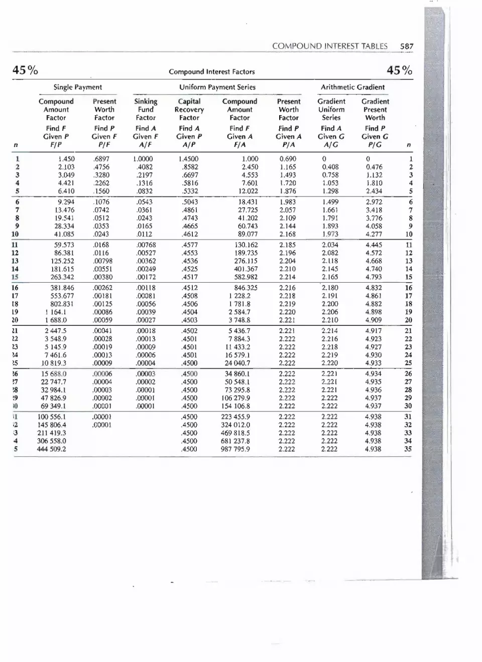
-.--- -- ----
COMPOUNDINTERESTTABLES 587
450/0 CompoundInterestFactors 450/0
SinglePayment UniformPaymentSeries ArithmeticGradient-
Compound Present Sinking Capital Compound Present Gradient GradientAmount Worth Fund Recovery Amount Worth Uniform PresentFactor Factor Factor Factor Factor Factor Series WorthFind F Find P Find A Find A Find F Find P Find A Find P
Given P Given F Given F Given P Given A Given A Given G Given Gn FIP PIF AIF AlP FIA PIA AIG PIG n
1 1.450 .6897 1.0000 1.4500 1.000 0.690 0 0 12 2.103 .4756 .4082 .8582 2.450 1.165 0.408 0.476 23 3.049 .3280 .2197 .6697 4.553 1.493 0.758 1.132 34 4.421 .2262 .1316 .5816 7.601 1.720 1.053 1.810 45 6.410 .1560 .0832 .5332 12.022 1.876 1.298 2.434 56 9.294 .1076 .0543 :5043 18.431 1.983 1.499 2.972 67 13.476 .0742 .0361 .4861 27.725 2.057 1.661 3.418 78 19.541 .0512 .0243 .4743 41.202 2.109 1.791 3.776 89 28.334 .0353 .0165 .4665 60.743 2.144 1.893 4.058 9
10 41.085 .0243 .0112 .4612 89.077 2.168 1.973 4.277 10
t1
11 59.573 .0168 .00768 .4577 130.162 2.185 2.034 4.445 1112 86.381 .0116 .00527 .4553 189.735 2.196 2.082 4.572 1213 125.252 .00798 .00362 .4536 276.115 2.204 2.118 4.668 1314 181.615 .00551 .00249 .4525 401.367 2.210 2.145 4.740 1415 263.342 .00380 .00172 .4517 582.982 2.214 2.165 4.793 . 15 ".f;'.:,
16 381.846 .00262 .00118 .4512 846.325 2.216 2.180 4.832 1617 553.677 .00181 .00081 .4508 1 28.2 2.218 2.191 4.861 1718 802.831 .00125 .00056 .4506 1781.8 2.219 2.200 4.882 1819 1164.1 .00086 .00039 .4504 2584.7 2.220 2.206 4.898 19 I ,'I
ZO 1688.0 .00059 .00027 .4503 3748.8 2.221 2.210 4.909 20U 2447.5 .00041 .00018 .4502 5 436;7 2.221 2.214 4.917
.IIII
!2 3 548.9 .00028 .00013 .4501 7 884.3 2.222 2.216 4.923i:!3 5 145.9 .00019 .00009 .4501 11433.2 2.222 2.218 4.927 I'
!4 7461.6 .00013 .00006 .4501 16579.1 2.222 2.219 4.930 2410 819.3 .00009 .00004 .4500 24040.7 2.222 2.220 4.933 25 I
6 15688.0 .00006 .00003 .4500 34 860.1 2.222 2.221 4.934 267 22747.7 .00004 .00002 .4500 50548.1 2.222 2.221 4.935 27!8 32 984.1 .00003 .00001 .4500 73 295.8 2.222 2.221 4.936 28!9 47 826.9 .00002 .00001 .45QO 106279.9 2.222 2.222 4.937 2910 69349.1 .00001 .00001 .4500 154 106.8 2.222 2.222 4.937 3011 100556.1 .00001 .4500 223 455.9 2.222 2.222 4.938 3112 145806.4 .00001 .4500 324 012.0 2.222 2.222 4.938 32i3 211 419.3 .4500 469818.5 2.222 2.222 4.938 334 306 558.0 .4500 681237.8 2.222 2.222 4.938 34.5 444 509.2 .4500 987 795.9 2.222 2.222 4.938 35
I I
, 'I' '
I;I'
"'"

- --- -
588 COMPOUND INTERESTTABLES
50% CompoundInterestFactors 50%
Single Payment Uniform Payment Series Arithmetic Gradient
Compound Present Sinking Capital Compound Present Gradient GradientAmount Worth Fund Recovery Amount Worth Uniform PresentFactor Factor Factor Factor Factor Factor Series WorthFind F Find P Find A Find A Find F Find P Find A Find P
Given P Given F Given F Given P Given A Given A Given G Given Gn FIP PIF AIF AlP FIA PIA AIG PIG n
1 1.500 .6667 1.0000 1.5000 1.000 0.667 0 0 12 2.250 .4444 .4000 .9000 2.500 1.111 0.400 0.444 23 3.375 .2963 .2105 .7105 4.750 1.407 0.737 1.037 34 5.063 .1975 .1231 .6231 8.125 1.605 1.015 1.630 45 7.594 .1317 .0758 .5758 13.188 1.737 1.242 2.156 56 11.391 .0878 .0481 .5481 20.781 1.824 1.423 2.595 67 17.086 .0585 .0311 .5311 32.172 1.883 1.565 2.947 78 25.629 .0390 .0203 .5203 49.258 1.922 1.675 3.220 8
38.443 .0260 .0134 .5134 74.887 1.948 1.760 3.428 9lu 57.665 .0173 .00882 .5088 113.330 1.965 1.824 3.584 1011 86.498 .0116 .00585 .5058 170.995 1.977 1.871 3.699 1112 129.746 .00771 .00388 .5039 257.493 1.985 1.907 3.784 1213 194.620 .00514 .00258 .5026 387.239 1.990 1.933 3.846 1314 291.929 .00343 .00172 .5017 581.859 1.993 1.952 3.890 1415 437.894 .00228 .00114 .5011 873.788 1.995 1.966 3.922 1516 656.814 .00152 .00076 .5008 1311.7 1.997 1.976 3.945 1617 985.261 .00101 .00051 .5005 1968.5 1.998 1.983 3.961 1718 1477.9 .00068 .00034 .5003 2 953.8 1.999 1.988 3.973 1819 2216.8 .00045 .00023 .5002 4431.7 1.999 1.991 3.981 1920 3 325.3 .00030 .00015 .5002 6648.5 1.999 1.994 3.987 2021 4987.9 .00020 .00010 .5001 9 973.8 2.000 1.996 3.991 2122 7481.8 .00013 .00007 .5001 14961.7 2.000 1.997 3.994 2223 11222.7 .00009 .00004 .5000 22 443.5 2.000 1.998 3.996 2324 16834.1 .00006 .00003 .5000 33 666.2 2.000 1.999 3.997 2425 25 251.2 .00004 .00002 .5000 50 500.3 2.000 1.999 3.998 25
26 . 37876.8 .00003 .00001 .5000 75751.5 2.000 1.999 3.999 2627 56815.1 .00002 .00001 .5000 113628.3 2.000 2.000 3.999 2728 85 222.7 .00001 .00001 .5000 170443.4 2.000 2.000 3.999 28
127834.0 .00001 .5000 255666.1 2.000 2.000 4.000 293u 191751.1 .00001 .5000 383500.1 2.000 2.000 4.000 .30
31 287 626.6 .5000 575251.2 2.000 2.000 4.000 3132 431439.9 .5000 862877.8 2.000 2.000 4.000 32

-- -_._-
- - -
COMPOUNDINTERESTTABLES 589
0% CompoundInterestFactors 60%-Single Payment Uniform Payment Series Arithmetic Gradient
Compound Present Sinking Capital Compound Present Gradient GradientAmount Worth Fund Recovery Amount Worth Uniform PresentFactor Factor Factor Factor Factor Factor Series WorthFind F Find P Find A Find A Find F Find P Find A Find P
Given P Given F Given F Given P Given A Given A Given G Given GFIP PIF AIF AlP FIA PIA AIG PIG n
1.600 .6250 1.0000 1.6000 1.000 0.625 0 0 12.560 .3906 .3846 .9846 2.600 1.016 0.385 0.391 24.096 .2441 .1938 .7938 5.160 1.260 0.698 0.879 36.554 .1526 .1080 .7080 9.256 1.412 0.946 1.337 4
10.486 .0954 .0633 .6633 15.810 1.508 1.140 1.718 5
16.777 .0596 .0380 .6380 26.295 1.567 1.286 2.016 626.844 .0373 .0232 .6232 43.073 1.605 1.396 2.240 "1
42.950 .0233 .0143 .6143 69.916 1.628 1.476 2.403 868.719 .0146 .00886 .6089 112.866 1.642 1.534 2.519 9
109.951 .00909 .00551 .6055 181.585 1.652 1.575 2.601 10
175.922 .00568 .00343 .6034 291.536 1.657 1.604 2.658 11281.475 .00355 .00214 .6021 467.458 1.661 1.624 2.697 12450.360 .00222 .00134 .6013 748.933 1.663 1.638 2.724 13720.576 .00139 .00083 .6008 1 199.3 1.664 1.647 2.742 14
1152.9 .00087 .00052 .6005 1919.9 1.665 1.654 2.754 151 844.7 .00054 .00033 .6003 3 072.8 1.666 1.658 2.762 162951.5 .00034 .00020 .6002 4917.5 1.666 1.661 2.767 174 722.4 .00021 .00013 .6001 7 868.9 1.666 1.663 2.771 187 555.8 .00013 .00008 .6011 12591.3 1.666 1.664 2.773 19
12089.3 .00008 .00005 .6000 20 147.1 1.667 1.665 2.775 20
19342.8 .00005 .00003 .6000 32 236.3 1.667 1.666 2.776 2130 948.5 .00003 .00002 .6000 51 579.2 1.667 1.666 2.777 2249517.6 .00002 .00001 .6000 82 527.6 1.667 1.666 2.777 2379 228.1 .00001 .00001 .6000 132045.2 1.667 1.666 2.777 24
126765.0 .00001 .6000 211 273.4 1.667 1.666 2.777 25
202 824.0 .6000 338 038.4 1.667 1.667 2.778 26324 518.4 .6000 540 862.4 1.667 1.667 2.778 27519229.5 .6000 865 380.9 1.667 1.667 2.778 28

-- ----
590 COMPOUND INTERESTTABLES
Continuous Compounding-Single Payment Factors
Compound Present Compound PresentAmount Worth Amount WorthFactor Factor Factor Factor
ern e-rn ern e-rnFind F Find P Find F Find P
Given P Given F Given P Given Frn FfP PfF rn FfP PfF
.01 1.0101 .9900 .51 1.6653 .6005
.02 1.0202 .9802 .52 1.6820 .5945
.03 1.0305 .9704 .53 1.6989 .5886
.04 1.0408 .9608 .54 1.7160 .5827
.05 1.0513 .9512 .55 1.7333 .5769
.06 1.0618 .9418 .56 1.7507 .5712
.07 1.0725 .9324 .57 1.7683 .5655
.08 1.0833 .9231. .58 1.7860 .5599
.09 1.0942 .9139 .59 1.8040 .5543
.10 1.1052 .9048 .60 1.8221 .548811 1.1163 .8958 .61 1.8404 .5434
.12 1.1275 .8869 .62 1.8589 '.5379
.13 1.1388 .8781 .63 1.8776 .5326
.14 1.1503 .8694 .64 1.8965 .5273
.15 1.1618 .8607 .65 1.9155 .5220
.16 1.1735 .8521 .66 1.9348 .5169
.17 1.1853 .8437 .67 1.9542 .5117
.18 1.1972 .8353 .68 1.9739 .5066
.19 1.2092 .8270 .69 1.9937 .5016
.20 1.2214 .8187 .70 2.0138 .4966
.21 1.2337 .8106 .71 2.0340 - .4916
.22 1.2461 .8025 .72 2.0544 .48683 1.2586 .7945 .73 2.0751 . ,4819
.24 1.2712 .7866 .74 2.0959 .4771
.25 1.2840 .7788 .75 2.1170 .4724
.26 1.2969 .7711 .76 2.1383 .4677
.27 1.3100 .7634 .77 2.1598 - .4630
.28 1.3231 .7558 .78 2.1815 .4584
.29 1.3364 .7483 .79 2.2034 .4538
.30 1.3499 .7408 .80 2.2255 .4493
.31 1.3634 .7334 .81 2.2479 .444932 1.3771 .7261 .82 2.2705 .4404.33 1.3910 .7189 .83 2.2933 .4360
1.34 1.4049 .7118 .84 2.3164 .4317"",..35 1.4191 .7047 .85 2.3396 .4274'
-,\-.36 1.4333 .6977 .86 2.3632 .4232.37 1.4477 .6907 .87 2.3869 .4190.38 1.4623 .6839 .88 2.4109 .4148.39 1.4770 .6771 .89 2.4351 .4107.40 1.4918 .6703 .90 2.4596 .4066.41 1.5068 .6637 .91 2.4843 .4025.42 1.5220 .6570 .92 2.5093 .3985.43 1.5373 .6505 .93 2.5345 .3946.44 1.5527 .6440 .94 2.5600 .3906.45 1.5683 .6376 .95 2.5857 . .3867.46 1.5841 .6313 .96 2.6117 .3829.47 1.6000 .6250 .97 2.6379 .3791.48 1.6161 .6188 .98 2.6645 .3753.49 1.6323 .6126 .99 2.6912 .3716.50 1.6487 .6065 1.00 2.7183 .3679

- - ----------------.--
AASHTO. A Manual on -User Benefit Analysis of Highway and Bus-Transit Improvements.Washington, D.C.: American Association of State Highway and Transportation Officials,1978.
American Telephone and Tele~aph Co. Engineering Eco.nomy, 3rd. McGraw-Hill, 1977.Baasel, W. D. Preliminary Chemical Engineering Plant Design, 2nd. Van Nostrand Reinhold, 1990.Benford, H. A. Naval Architect's Introduction to Engineering Economics. Ann Arbor: Dept. of Naval
Architecture and Marine Engineering Report 282,1983.Bernhard, R H. "A Comprehensive Comparison and Critique of Discounting Indices Proposed
for Capital Investment Evaluation," The Engineering Economist. Vol. 16, No.3, 1971,pp. 157-186.
Bussey, L. E., and T. G. Eschenbach. The Economic Analysis of Industrial Projects 2nd. Prentice-Hall,1992.
The Engineering Economist. A quarterly journal of the Engineering Economy Divisions of ASEE andlIE.
Eschenbach, T. G., and J. P. Lavelle. "Technical Note: MACRS Depreciation with a SpreadsheetFunction: A Teachingand Practice Note," The EngineeringEconomist. Vol.46, No.2, 2001, .
pp. 153-161.Eschenbach, T. G., and J. P. Lavelle. "How Risk and Uncertainty Are/Could/Should Be Presented in
Engineering Economy," Proceedings of the 11th Industrial Engineering Research Conference.lIE, Orlando, May 2002, CD.
Eschenbach, T. Engineering Economy: Applying Theory to Practice, 2nd. Oxford University Press,2003.
Fish, J. C. L. Engineering Economics. McGraw-Hill, 1915.Jones, B. W.lnjlation in Engineering Economic Analysis. John Wiley & Sons, 1982.Lavelle, J. P.,H. R Liggett, and H. R Parsaei, editors. Economic Evaluation of Advanced Technologies:
Techniques and Case Studies. Taylor & Francis, 2002.Liggett, H. R, J. Trevino, and J. P. Lavelle. "Activity-Based Cost Management Systems in an
Advanced Manufacturing Environment," Economic and Financial Justification of AdvancedManufacturing Technologies. H. R Parsaei, W. G. Sullivan, and T. R Hanley, editors. ElsevierScience, 1992.
Lorie, J. H., and L. J. Savage. "Three Problems in Rationing Capital," The Journal of Business. Vol.28,No.4,1955,pp.229-239.
Newnan, D. G. "Determining Rate of Return by Means of Payback Period and Useful Life," TheEngineering Economist. Vol. 15, No.1, 1969, pp. 29-39.
Peters, M. S., K. D. TlDlDlerhaus, M. Peters, and R E. West. Plant Design and Economicsfor Chemical
Engineers, 5th. McGraw-Hill, 2002.
591
'Iil!

592 REFERENCES
Perry, H. P., D. W. Green, and J. O. Maloney. Perry's Chemical Engineers' Handbook, 'Ph. McGraw-Hill, 1997.
Sundaram, M., editor. Engineering Economy Exam File. Oxford University Press, 2003.Steiner, H. M. Public and Private Investments: Socioeconomic Analysis. John Wiley & Sons, 1980.Terborgh, G. Business Investment Management. Machinery and Allied Products Institute, 1967.Tippet, D. D., and P. Hoekstra. ''Activity-Based Costing: a Manufacturing Management Decision-
Making Aid," Engineering Management Journal. Vol. 5, No.2, June 1993, American Society.for Engineering Management, pp. 3742.
Wellington, A. M. The Economic Theory of Railway Location. John Wiley & Sons, 1887.
- ----

A
Absorption costing, 548.ccounting: absorption costing, 548acid-test or quick ratio, 543~assets, 541-42balance sheet, 541~cost, 541cost of goods sold, 544current ratio, 543direct costs, 548equity, 543financial ratios from balance sheet, 543~financial ratios from income statement, 546fundamental accounting equation, 541general, 541income statement, 544-47indkect cost allocation, 548-49indirect costs, 548interest coverage, 546liabilities, 542linking balance sheet and income statement, 546-47net profit ratio, 546problems with traditional cost accounting, 549-50role of, 540-41traditional cost accounting, 547-50working capital, 542
After-tax: cash flows and spreadsheets, 385-86economic analysis, 380-83inflation, 460-62ininimum cost life problems, 427-28rate of return estimating, 385replacement analysis, 420-27
Amortization schedule, 190Analysis period: common multiple of lives, 186
for continuing requkement, 186different from lives, 151-54infinite, 154-57, 187-88lives equal, 147-51, 186
other, 188-89rate ofreturn, 219
Annual cash flow calculations, 178-82Arithmetic gradient, 98-100
present worth factor, 100uniform series factor, 100
Asset depreciation range (ADR), 347Assets, 541-42Audit results, 15Average cost, 28
B
Balance sheet, 541~links with income statement, 546-47
Benefi~costratio,490,496-98analysis, 274-80graph, 247-49, 251, 252,257, 260-61, 278,279incremental analysis, 498-504
Benefits estimating, 50Beta approximation of mean, 308Book cost, 36Book value, 341Brainstorming, 11Breakevenanalysis,285-89 . .
chart, 31-32, 285spreadsheets, 289-92
Business expenses, 374
c
Capital budgeting, 518Capital expenditures, 374Capital gains, 356-57
and losses, 384Capital rationing, 518-32
by present worth method~, 524-30
593

594 INDEX
Capital rationing-Cont.ranking project proposals, 530-32by rate of return, 521-24
Capitalized cost, 154-57Cash cost, 35Cash flow: categories, 51
computing, 62-63diagrams, 50-52, 75-76
Challenger, 400after-tax cash flows, 422future, 419-20minimum cost life, 402-4
Chance node, 316Compound interest, 65-66Compounding subperiods; 109Constant dollars, 444
versus then-current dollars, 448-50Consumer price index, 454-55-:ontinuous alternatives benefit-cost ratio graph, 279Continuous compounding, 115-21
capital recovery factor, 118compound amount factor, 117effective interest rate, 110present worth factor, 117series compound amount factor, 119series present worth factor, 119sinking fund factor, 118
Continuous uniform cash flow with continuouscompounding 120-21
Corporate income taxes: after-tax analysis, 380-83after-tax cash flows and spreadsheets, 385-86business expenses, 374capital expenditures, 374capital gains and losses, 384estimating after-tax rate of return, 385investment tax credit, 384-85rates, 377-78taxable income, 374-75
20staccounting, 547-50problems with traditional, 549-50
Cost: average, 28book,36of borrowed money, 475of capital, 475-76cash,35depletion, 360-61estimating, 38-49fixed, 28of goods sold, 544incremental, 34-35indexes, 44-45life-cycle, 36-38life-cycle committed, 37life-cycle design change, 37marginal, 28-29
nonrecurring, 34opportunity, 32-33recurring, 34sunk, 32variable, 28
Cost-push inflation, 441Cutoff rate of return, 523
D
Data block in spreadsheets, 555Decision node, 316Decision-making process, 6-15Declining balance depreciation, 346-47Defender, 400
after-tax cash flows, 422-27lowest EUAC, 411-13marginal cost data, 404-7marginal cost data not available, 415-18marginal costs are increasing, 407-13marginal costs not increasing, 41;3-15
Deflation definition, 440Demand-pull inflation, 441Depletion, 360-62, 400Depreciable life, 339Depreciated versus expensed, 339Depreciation, 546
asset disposal, 356-59basics,338-41calculation fundamentals, 341-42capital gains, 356-57declining balance, 346-47historical methods, 342-47historical methods compared with
MACRS, 355-56losses, 356-57MACRS (see MACRS)recapture, 356-57spreadsheets, 362-64straight-line, 342-44sum-of-years' -digits, 344-45unit -of-production, 359-60
Descartes' rule of signs, 231-32Deterioration due to aging, 400Direct costs, 548
. .
E
Economic criteriafixed input, 12, 146, 182
benefi~costratio,274fixed output, 12, 146, 182
benefi~costratio,274

INDEX 595
neitherinput nor output fixed, 12-13, 146, 182fixed benefit-cost ratio, 274
Economic decision trees', 316-22Economic decision-making for current costs, 15-18Effective interest rate, 109End-of-year convention, 144Engineering economic analysis: assumptions, 144-46
borrowed money viewpoint, 145choosing a method, 261-62identifying and rejecting unattractive alternatives,
520-21ignoring inflation, 448incorporating inflation, 448price indexes, 456role of, 5-6viewpoint, 145
Equity, 543Equivalence, 68-73
c:I '~nds on interest rate, 71-73Estk...dted data, 304-6
range,306-8Estimating: accuracy, 39
by analogy, 40benefits, 50cost indexes, 44-45costs, 3~9detailed, 39difficulties, 39-40learning curve, 47-49per-unit model, 41power-sizing model, 45-46rough, 38segmenting model, 43semidetailed, 38-39triangulation, 47
3xchange rates, 440-413xpected value, 3133xpl'.J'I!;edversus depreciated, 3393xtl aarket consequences, 10, 14
Financial ratios from: balance sheet, 543-44income statement, 546
Fixed cost, 28Functional notation, 74Future worth analysis, 272-73
G
Geometric gradient, 105-8Geometric series present worth factor, 108
I
~actor:arithmetic gradient presentworth, 100
arithmetic gradient uniform series, 100geometric series present worth, 108notation, 74relationships between, 97-98single payment compound amount, 74single payment present worth, 76uniform series capital recovery, 89uniform series compound amount, 87uniform series present worth, 90uniform series sinking fund, 88
Income statement, 544-47links with balance sheet, 546-47
Incremental analysis, 246-63benefi~costratio,498-504graphical, 246-52multiple alternatives, 250spreadsheets, 262-63unlimited alternatives, 258-59
Incremental cost, 34-35Incremental rate of return, 212-18, 252-58Indirect cost, 8, 548Induectcostallocation,548-49Individual income tax: capital gains and
losses, 384itemized deductions, 373personal exemption, 373rates, 375-76standard deduction, 373taxable income, 372-73
Infinite analysis period, 154-57Inflation: actual dollars, 443
after-tax calculations, 460-62cash flows at different rates, 456-58causes, 440-41composite versus commodity indexes, 453-55constant dollars versus then-current
dollars, 448-50consumer price index, 454-55cost of borrowed money, 481-82definition, 440deflation, 145-46different rates per period, 458-59engineering economic analysis ignoring, 448engineering economic analysis including, 448indexes, 450-56producer price index, 454rate, 441-42real and market interest rates, 441-42real dollars, 444spreadsheets, 462-64
r
-- --
- - - - -- ---

596 INDEX
Insurance, 320-22, 323Intangible consequ.ences, 10, 14Intangible property, 340Interest: compound, 65-66
formula notation, 73on loan, 191
Interest rate: adjusting MARR for risk, 479-81cost of capital, 475-76difficulties in solving for, 229-40effective, 109equivalence, 71-73inflation and cost of borrowed money, 481-82MARR values used in industry, 482-83nominal, 109opportunity cost government, 495opportunity cost of capital, 476-78opportunity cost taxpayer, 495plot versus PW, 209-10real and market, 441-42selecting, 474-85selecting in public sector, 493-95spreadsheets and opportunity cost of capital, 483-85simple, 64-65
Internal rate of return, 204-5modified, 238-40
Interpolation, 92, 208Investment tax credit, 384-85Itemized deductions, 373
J
Joint probabilitydistributions,311-13
L
Learning curve, 47-49Liabilities,542 .
Life-cycle cost, 36-38committed, 37design change, 37
Liquidity or speed of return versus profitability, 282, 284Lives: different from analysis period, 151-54
equal analysis period, 147-51Loan: balance due, 191-92
paying off early, 192repayment plans, 67, 69-71
Lorie and Savage, 524
M
MACRS, 347-53compared to historical methods, 355-56
------ . -.---.-..
examples, 353-54percentage derivation, 351-53percentage tables, 349-51property class, 348-50recovery period, 348-50spreadsheet using VDB, 363-64
Marginal cost, 28-29Marginal cost data defender, 404-7Market consequences, 10, 14Market interest rate, 441-42Minimum attractive rate of return: selecting, 474-85, 479
spreadsheets, 483-85Minimum cost life: after-tax, 427-28
challenger, 402-4Modified accelerated cost recovery system (see MACRS)Modified internal rate of return, 238-40Money supply, 440Most likely estimate, 306-8Multiple alternatives, 158Multiple rates of return, 231-32
how many, 234-38Multiple sign changes projects with, 232-34Mutually exclusive alternatives, 519
N
Nominal interest rate, 109Nonrecurring cost, 34
o
Obsolescence, 338, 400Opportunity cost, 32-33
of capital, 476-78, 495, 523perspective for defender's first cost, 417-18
Optimistic estimate, 306-8Outcome node, 316
p
Payback period, 280-84limitations, 282
Percentage depletion, 361-62Personal exemption, 373Personal property, 340Pessimistic estimate, 306-8Power-sizing model, 45-46Present worth: analysis with benefit-cost
graphs, 260-261techniques, 147-62
Price indexes, 450-56Probability, 308-9
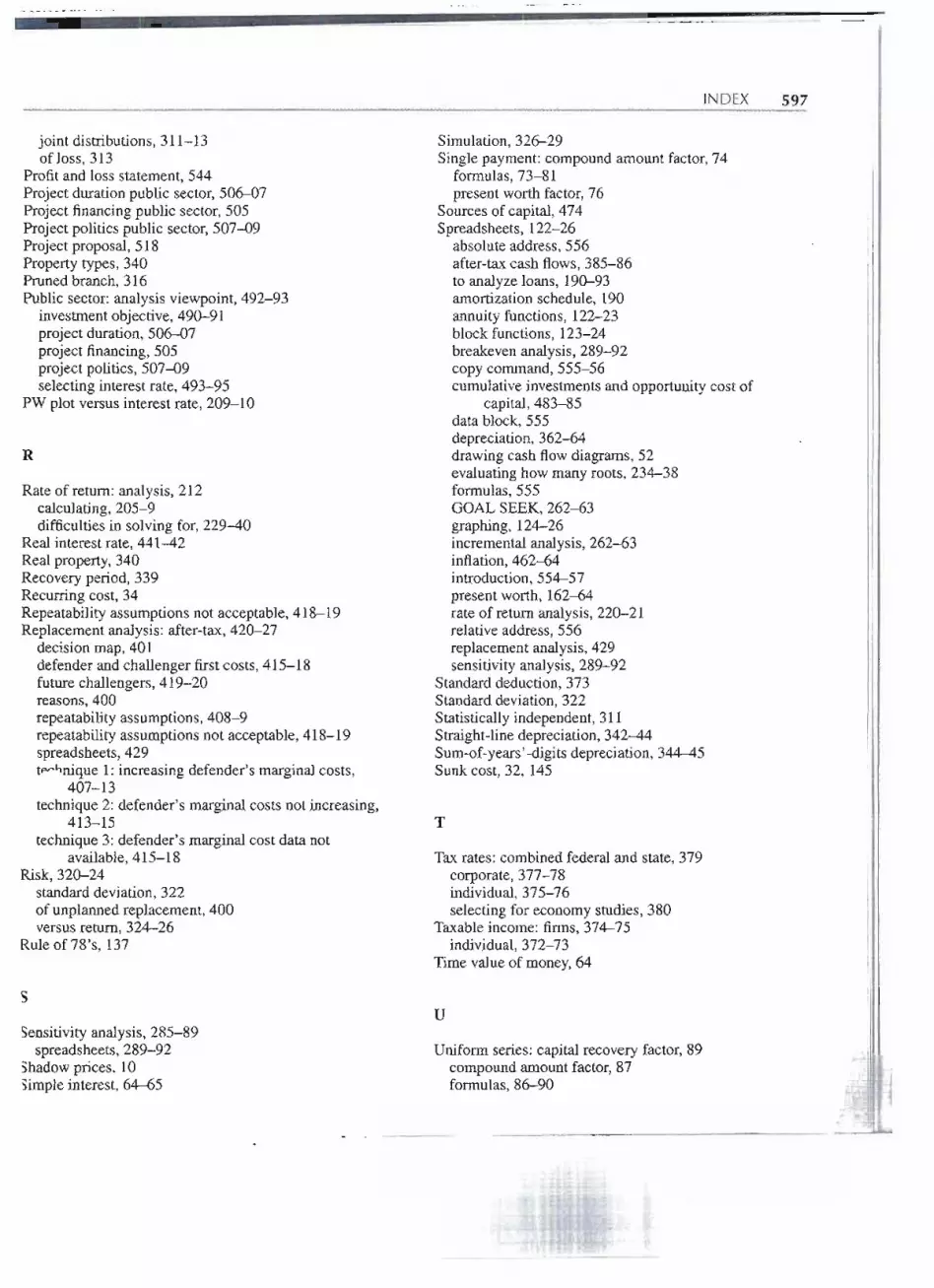
INDEX 597
joint distributions, 31.1-13ofloss, 313
Profit and loss statement, 544Project duration public sector, 506-07Project financing public sector, 505Project politics public sector, 507-09Project proposal, 518Property types, 340Pruned branch, 316Public sector: analysis viewpoint, 492-93
investment objective, 490-91project duration, 506-07project financing, 505project politics, 507-09selecting interest rate, 493-95
PW plot versus interest rate, 209-10
R
Rate of return: analysis, 212calculating, 205-9difficulties in solving for, 229-40
Real interest rate, 441-42Real property, 340Recovery period, 339Recurring cost, 34Repeatability assumptions not acceptable, 418-19Replacement analysis: after-tax, 420-27
decision map, 401defender and challenger first costs, 415-18future challengers, 419-20reasons, 400repeatability assumptions, 408-9repeatability assumptions not acceptable, 418-19spreadsheets, 429tp"J,nique 1: increasing defender's marginal costs,
407-13 .
technique 2: defender's marginal costs not increasing,413-15
technique 3: defender's marginal cost data notavailable, 415-18
Risk,320-24standard deviation, 322of unplanned replacement, 400versus return, 324-26
Rule of 78's, 137
s
Sensitivity analysis, 285-89spreadsheets, 289-92
Shadow prices, 10Simple interest, 64-65
Simulation,326-29Single payment: compound amount factor, 74
formulas, 73-81present worth factor, 76
Sources of capital, 474Spreadsheets, 122-26
absolute address, 556after-tax cash flows, 385-86to analyze loans, 190-93amortization schedule, 190annuity functions, 122-23block functions, 123-24breakeven analysis, 289-92copycommand,555-56cumulative investments and opportunity cost of
capital, 483-85data block, 555depreciation, 362-64drawing cash flow diagrams, 52evaluating how many roots, 234-38formulas, 555GOAL SEEK, 262-63graphing, 124-26incremental analysis, 262-63inflation, 462-64inkoduction, 554-57present worth, 162-64rate of return analysis, 220-21relative address, 556replacement analysis, 429sensitivity analysis, 289-92
Standard deduction, 373Standard deviation, 322Statistically independent, 311Skaight-line depreciation, 342-44Sum-of-years' -digits depreciation, 344-45Sunk cost, 32, 145
T
Tax rates: combined federal and state, 379corporate, 377-78individual, 375-76selecting for economy studies, 380
Taxable income: firms, 374-75individual,372-73
Time value of money, 64
u
Uniform series: capital recovery factor, 89compound amount factor, 87formulas, 86-90
-;
~..""r. I
:
~

l598 INDEX
Uniform series: capital recovery factor-Cont.present worth factor, 90sinking fund factor, 88
Crusader advanced field artillery system, 516-17green design, 270-71inkjet cartridges, 176-77RFID chips, 202-3Superfund, 302-3Tappan Zee Bridge, 244-45tobacco bonds, 60-61Webvan, 26-27wind turbines, 370-71World Trade Center, 2-3
v
Variable cost, 28Vignette: ABB and activity-based costing, 538-39
agricultural pollution, 488-89Anne Scheiber's bonanza, 84-85Austin Powersbaseball going broke, 336-37Boeing versus Airbus, 142-43BP and Russian oil, 472-73chip making fabrication plant, 398-99
w
Work breakdown structure, 44Working capital, 542
--

Economic Criteria
Method of Analysis
PRESENT WORTH,,--
ANNUAL CASH FLOW
FUTURE WORTH
BENEFIT-COST RATIO
RATE OF RETURN
Fixed Input Neither Input Nor Output Fixed
Maximize (PW of Benefits-PW of Costs),or Maximize Net Present Worth
Fixed Output
MaximizePW of Benefits
MinimizePW of Costs
MaximizeEquivalent
Uniform AnnualBenefits (EUAB)
Minimize
EquivalentUniform Annual
Cost (EUAC)
Maximize (EUAB-EUAC)
MaximizeFW of Benefits
Maximize (FW of Benefits-FW of Costs),or Maximize Net Future Worth
MinimizeFW of Costs
Two Alternatives: Compute the incrementalBenefit-Cost ratio (tlB / tlC) on theincrement of investment between the
alternatives. If tlB / tlC :::: 1, choose
higher-cost alternative; if not, chooselower-cost alternative.
Three or more Alternatives: Iricremental
analysis is required (see Ch. 9)..
Two Alternatives: Compute the incremental rate of return (tlROR) on the increment ofinvestment between the alternatives. If tlROR ::::minimum attractive rate of return,choose the higher-cost alternative; if not, choose lower-cost alternative.
Three or more Alternatives: Incremental analysis is required (see Ch. 8).
MaximizeBenefit-Cost
Ratio
MaximizeBenefit-Cost
Ratio
--

I ~.~. ..1 .! It.
T ow in a ninth edition, Engineering Economic Analysis offers comprehensive coverage of financial and economic deci-
~ sion making for eng~neering projects, with an emphasis on problem solving, life.:cycle costs, and the time value ofley. The spreadsheet material from the previous edition has been expanded, allowing students to create and analyze'e realistic cash-flow models. The authors' concise, accessible writing style and practical emphasis make this text idealmdergraduate engineering economy courses.
ruRESOFTHENINTHEDmON
~wpedagogical features include:Chapter-opening vignettesChapter objectivesIe new two-color interior design will improve readability, generate student interest, and facilitate comprehension of~material.
new chapter has been added: Chapter 18, Accounting and Engineering Economy.lapter 10, Probability and Uncertainty, has been completely rewritten to emphasize how to make good choices bynsidering the uncertainty that is part of every engineering economy application.Iapt- 13, Replacement Analysis, has been rewritten to clarify the comparison of existing assetswith newer alternatives.'peh..uX7A, Difficulties Solving for an Interest Rate, has been thoroughly revised to use the power of spreadsheets' tove problems..d-of-chapter problems are reorganized and updated throughout.:ompanion website is available: www.oup.com/us/engineeringeconomy.
I.
ANCED STUDENT SUPPORT
:agedwith every copy of the text:Idy Guide by Donald G. Newnan and Edward Wheeler) featuring interactive Excel@spreadsheets and tutorials
ANCEDINSTRUcroRSUPPORT
) containing exam filesby Meenakshi Sundaram, Excel@spreadsheets, and PowerPoin~ slides (ISBN 0-19-517423-2)lutions Manual (ISBN 0-19-517424-0)
ISBN 0-19-516807-0
-- - --


