Embed Size (px)
Citation preview


Oleg Okun, Giorgio Valentini, and Matteo Re (Eds.)
Ensembles in Machine Learning Applications

Studies in Computational Intelligence,Volume 373
Editor-in-Chief
Prof. Janusz Kacprzyk
Systems Research Institute
Polish Academy of Sciences
ul. Newelska 6
01-447 Warsaw
Poland
E-mail: [email protected]
Further volumes of this series can be found on our
homepage: springer.com
Vol. 352. Nik Bessis and Fatos Xhafa (Eds.)
Next Generation Data Technologies for CollectiveComputational Intelligence, 2011
ISBN 978-3-642-20343-5
Vol. 353. Igor Aizenberg
Complex-Valued Neural Networks with Multi-Valued
Neurons, 2011
ISBN 978-3-642-20352-7
Vol. 354. Ljupco Kocarev and Shiguo Lian (Eds.)
Chaos-Based Cryptography, 2011
ISBN 978-3-642-20541-5
Vol. 355.Yan Meng and Yaochu Jin (Eds.)
Bio-Inspired Self-Organizing Robotic Systems, 2011
ISBN 978-3-642-20759-4
Vol. 356. Slawomir Koziel and Xin-She Yang
(Eds.)
Computational Optimization, Methods and Algorithms, 2011
ISBN 978-3-642-20858-4
Vol. 357. Nadia Nedjah, Leandro Santos Coelho,
Viviana Cocco Mariani, and Luiza de Macedo Mourelle (Eds.)
Innovative Computing Methods and their Applications to
Engineering Problems, 2011
ISBN 978-3-642-20957-4
Vol. 358. Norbert Jankowski,Wlodzislaw Duch, and
Krzysztof Grabczewski (Eds.)
Meta-Learning in Computational Intelligence, 2011
ISBN 978-3-642-20979-6
Vol. 359. Xin-She Yang, and Slawomir Koziel (Eds.)
Computational Optimization and Applications inEngineering and Industry, 2011
ISBN 978-3-642-20985-7
Vol. 360. Mikhail Moshkov and Beata Zielosko
Combinatorial Machine Learning, 2011
ISBN 978-3-642-20994-9
Vol. 361.Vincenzo Pallotta,Alessandro Soro, and
Eloisa Vargiu (Eds.)
Advances in Distributed Agent-Based Retrieval Tools, 2011
ISBN 978-3-642-21383-0
Vol. 362. Pascal Bouvry, Horacio González-Vélez, and
Joanna Kolodziej (Eds.)
Intelligent Decision Systems in Large-Scale Distributed
Environments, 2011
ISBN 978-3-642-21270-3
Vol. 363. Kishan G. Mehrotra, Chilukuri Mohan, Jae C. Oh,
Pramod K.Varshney, and Moonis Ali (Eds.)
Developing Concepts in Applied Intelligence, 2011
ISBN 978-3-642-21331-1
Vol. 364. Roger Lee (Ed.)
Computer and Information Science, 2011
ISBN 978-3-642-21377-9
Vol. 365. Roger Lee (Ed.)
Computers, Networks, Systems, and IndustrialEngineering 2011, 2011
ISBN 978-3-642-21374-8
Vol. 366. Mario Köppen, Gerald Schaefer, and
Ajith Abraham (Eds.)
Intelligent Computational Optimization in Engineering, 2011
ISBN 978-3-642-21704-3
Vol. 367. Gabriel Luque and Enrique Alba
Parallel Genetic Algorithms, 2011
ISBN 978-3-642-22083-8
Vol. 368. Roger Lee (Ed.)
Software Engineering, Artificial Intelligence, Networking andParallel/Distributed Computing 2011, 2011
ISBN 978-3-642-22287-0
Vol. 369. Dominik Ryzko, Piotr Gawrysiak, Henryk Rybinski,
and Marzena Kryszkiewicz (Eds.)
Emerging Intelligent Technologies in Industry, 2011
ISBN 978-3-642-22731-8
Vol. 370.Alexander Mehler, Kai-Uwe Kühnberger,
Henning Lobin, Harald Lüngen,Angelika Storrer, and
Andreas Witt (Eds.)
Modeling, Learning, and Processing of Text TechnologicalData Structures, 2011
ISBN 978-3-642-22612-0
Vol. 371. Leonid Perlovsky, Ross Deming, and Roman Ilin
(Eds.)
Emotional Cognitive Neural Algorithms with EngineeringApplications, 2011
ISBN 978-3-642-22829-2
Vol. 372.Antonio E. Ruano and
Annamaria R.Varkonyi-Koczy (Eds.)
New Advances in Intelligent Signal Processing, 2011
ISBN 978-3-642-11738-1
Vol. 373. Oleg Okun, Giorgio Valentini, and Matteo Re (Eds.)
Ensembles in Machine Learning Applications, 2011
ISBN 978-3-642-22909-1

Oleg Okun, Giorgio Valentini, and Matteo Re (Eds.)
Ensembles in Machine LearningApplications
123

Editors
Dr. Oleg OkunStora Tradgardsgatan 20, lag 160121128 MalmoSwedenE-mail: [email protected]
Dr. Giorgio ValentiniUniversity of MilanDepartment of Computer ScienceVia Comelico 3920135 MilanoItalyE-mail: [email protected]://homes.dsi.unimi.it/∼valenti/
Dr. Matteo ReUniversity of MilanDepartment of Computer ScienceOffice: T303via Comelico 39/4120135 MilanoItaliaE-mail: [email protected]://homes.dsi.unimi.it/∼re/
ISBN 978-3-642-22909-1 e-ISBN 978-3-642-22910-7
DOI 10.1007/978-3-642-22910-7
Studies in Computational Intelligence ISSN 1860-949X
Library of Congress Control Number: 2011933576
c© 2011 Springer-Verlag Berlin Heidelberg
This work is subject to copyright. All rights are reserved, whether the whole or partof the material is concerned, specifically the rights of translation, reprinting, reuseof illustrations, recitation, broadcasting, reproduction on microfilm or in any otherway, and storage in data banks. Duplication of this publication or parts thereof ispermitted only under the provisions of the German Copyright Law of September 9,1965, in its current version, and permission for use must always be obtained fromSpringer. Violations are liable to prosecution under the German Copyright Law.
The use of general descriptive names, registered names, trademarks, etc. in thispublication does not imply, even in the absence of a specific statement, that suchnames are exempt from the relevant protective laws and regulations and thereforefree for general use.
Typeset & Cover Design: Scientific Publishing Services Pvt. Ltd., Chennai, India.
Printed on acid-free paper
9 8 7 6 5 4 3 2 1
springer.com

Alla piccola principessa Sara, dai bellissimi
occhi turchini
– Giorgio Valentini
To Gregory, Raisa, and Antoshka
– Oleg Okun

Preface
This book originated from the third SUEMA (Supervised and Unsupervised Ensem-
ble Methods and their Applications) workshop held in Barcelona, Spain in September
2010. It continues and follows the tradition of the previous SUEMA workshops –
small international events. These events attract researchers interested in ensemble
methods – groups of learning algorithms that solve a problem at hand by means of
combining or fusing predictions made by members of a group – and their real-world
applications. The emphasis on practical applications plays no small part in every
SUEMA workshop as we hold the opinion that no theory is vital without demon-
strating its practical value.
In 2010 we observed significant changes in both workshop audience and scope
of the accepted papers. The audience became younger and different topics, such
as Error-Correcting Output Codes and Bayesian Networks, emerged that were not
common at the previous workshops. These new trends are good signs for us as work-
shop organizers as they indicate that young researchers consider ensemble methods
as a promising R& D avenue, and the shift in scope means that SUEMA workshops
preserved the ability to timely react on changes.
This book is composed of individual chapters written by independent groups of
authors. As such, the book chapters can be read without following any pre-defined
order. However, we tried to group chapters similar in content together to facilitate
reading. The book serves to educate both a seasoned professional and a novice
in theory and practice of clustering and classifier ensembles. Many algorithms in
the book are accompanied by pseudo code intended to facilitate their adoption and
reproduction.
We wish you, our readers, fruitful reading!
Malmo, Sweden Oleg Okun
Milan, Italy Giorgio Valentini
Milan, Italy Matteo Re
May 2011

Acknowledgements
We would like to thank the ECML/PKDD’2010 organizers for the opportunity to
hold our workshop at the world-class Machine Learning and Data Mining confer-
ence in Barcelona. We would like to thank all authors for their valuable contribution
to this book as this book would clearly be impossible without your excellent work.
We also deeply appreciate the financial support of PASCAL 2 Network of Excel-
lence in organizing SUEMA’2010.
Prof. Janusz Kacprzyk and Dr. Thomas Ditzinger from Springer-Verlag deserved
our special acknowledgment for warm welcome to our book and their support and
a great deal of encouragement. Finally, we thank all other people in Springer who
participated in the publication process.

Contents
1 Facial Action Unit Recognition Using Filtered Local Binary Pattern
Features with Bootstrapped and Weighted ECOC Classifiers . . . . . . . 1
Raymond S. Smith, Terry Windeatt
1.1 Introduction . . . . . . . . . . . . . . . . . . . . . . . . . . . . . . . . . . . . . . . . . . . . . . 1
1.2 Theoretical Background . . . . . . . . . . . . . . . . . . . . . . . . . . . . . . . . . . . . 5
1.2.1 ECOC Weighted Decoding . . . . . . . . . . . . . . . . . . . . . . . . . 5
1.2.2 Platt Scaling . . . . . . . . . . . . . . . . . . . . . . . . . . . . . . . . . . . . . . 6
1.2.3 Local Binary Patterns . . . . . . . . . . . . . . . . . . . . . . . . . . . . . . 7
1.2.4 Fast Correlation-Based Filtering . . . . . . . . . . . . . . . . . . . . . 8
1.2.5 Principal Components Analysis . . . . . . . . . . . . . . . . . . . . . . 9
1.3 Algorithms . . . . . . . . . . . . . . . . . . . . . . . . . . . . . . . . . . . . . . . . . . . . . . . 10
1.4 Experimental Evaluation . . . . . . . . . . . . . . . . . . . . . . . . . . . . . . . . . . . 10
1.4.1 Classifier Accuracy . . . . . . . . . . . . . . . . . . . . . . . . . . . . . . . . 13
1.4.2 The Effect of Platt Scaling . . . . . . . . . . . . . . . . . . . . . . . . . . 14
1.4.3 A Bias/Variance Analysis . . . . . . . . . . . . . . . . . . . . . . . . . . . 15
1.5 Conclusion . . . . . . . . . . . . . . . . . . . . . . . . . . . . . . . . . . . . . . . . . . . . . . . 16
1.6 Code Listings . . . . . . . . . . . . . . . . . . . . . . . . . . . . . . . . . . . . . . . . . . . . 17
References . . . . . . . . . . . . . . . . . . . . . . . . . . . . . . . . . . . . . . . . . . . . . . . . . . . . . 19
2 On the Design of Low Redundancy Error-Correcting Output
Codes . . . . . . . . . . . . . . . . . . . . . . . . . . . . . . . . . . . . . . . . . . . . . . . . . . . . . 21
Miguel Angel Bautista, Sergio Escalera, Xavier Baro, Oriol Pujol,
Jordi Vitria, Petia Radeva
2.1 Introduction . . . . . . . . . . . . . . . . . . . . . . . . . . . . . . . . . . . . . . . . . . . . . . 21
2.2 Compact Error-Correcting Output Codes . . . . . . . . . . . . . . . . . . . . . . 23
2.2.1 Error-Correcting Output Codes . . . . . . . . . . . . . . . . . . . . . . 23
2.2.2 Compact ECOC Coding . . . . . . . . . . . . . . . . . . . . . . . . . . . . 24
2.3 Results . . . . . . . . . . . . . . . . . . . . . . . . . . . . . . . . . . . . . . . . . . . . . . . . . . 29
2.3.1 UCI Categorization . . . . . . . . . . . . . . . . . . . . . . . . . . . . . . . . 30
2.3.2 Computer Vision Applications . . . . . . . . . . . . . . . . . . . . . . . 32
XII Contents
2.4 Conclusion . . . . . . . . . . . . . . . . . . . . . . . . . . . . . . . . . . . . . . . . . . . . . . . 36
References . . . . . . . . . . . . . . . . . . . . . . . . . . . . . . . . . . . . . . . . . . . . . . . . . . . . . 37
3 Minimally-Sized Balanced Decomposition Schemes for Multi-class
Classification . . . . . . . . . . . . . . . . . . . . . . . . . . . . . . . . . . . . . . . . . . . . . . . 39
Evgueni N. Smirnov, Matthijs Moed, Georgi Nalbantov,
Ida Sprinkhuizen-Kuyper
3.1 Introduction . . . . . . . . . . . . . . . . . . . . . . . . . . . . . . . . . . . . . . . . . . . . . . 40
3.2 Classification Problem . . . . . . . . . . . . . . . . . . . . . . . . . . . . . . . . . . . . . 41
3.3 Decomposing Multi-class Classification Problems . . . . . . . . . . . . . . 41
3.3.1 Decomposition Schemes. . . . . . . . . . . . . . . . . . . . . . . . . . . . 41
3.3.2 Encoding and Decoding . . . . . . . . . . . . . . . . . . . . . . . . . . . . 44
3.4 Balanced Decomposition Schemes and Their Minimally-Sized
Variant . . . . . . . . . . . . . . . . . . . . . . . . . . . . . . . . . . . . . . . . . . . . . . . . . . 46
3.4.1 Balanced Decomposition Schemes . . . . . . . . . . . . . . . . . . . 46
3.4.2 Minimally-Sized Balanced Decomposition Schemes . . . . 47
3.4.3 Voting Using Minimally-Sized Balanced
Decomposition Schemes. . . . . . . . . . . . . . . . . . . . . . . . . . . . 49
3.5 Experiments . . . . . . . . . . . . . . . . . . . . . . . . . . . . . . . . . . . . . . . . . . . . . . 51
3.5.1 UCI Data Experiments . . . . . . . . . . . . . . . . . . . . . . . . . . . . . 51
3.5.2 Experiments on Data Sets with Large Number
of Classes . . . . . . . . . . . . . . . . . . . . . . . . . . . . . . . . . . . . . . . . 52
3.5.3 Bias-Variance Decomposition Experiments . . . . . . . . . . . . 54
3.6 Conclusion . . . . . . . . . . . . . . . . . . . . . . . . . . . . . . . . . . . . . . . . . . . . . . . 55
References . . . . . . . . . . . . . . . . . . . . . . . . . . . . . . . . . . . . . . . . . . . . . . . . . . . . . 56
4 Bias-Variance Analysis of ECOC and Bagging Using Neural Nets . . . 59
Cemre Zor, Terry Windeatt, Berrin Yanikoglu
4.1 Introduction . . . . . . . . . . . . . . . . . . . . . . . . . . . . . . . . . . . . . . . . . . . . . . 59
4.1.1 Bootstrap Aggregating (Bagging) . . . . . . . . . . . . . . . . . . . . 60
4.1.2 Error Correcting Output Coding (ECOC) . . . . . . . . . . . . . . 60
4.1.3 Bias and Variance Analysis . . . . . . . . . . . . . . . . . . . . . . . . . 62
4.2 Bias and Variance Analysis of James . . . . . . . . . . . . . . . . . . . . . . . . . 64
4.3 Experiments . . . . . . . . . . . . . . . . . . . . . . . . . . . . . . . . . . . . . . . . . . . . . . 65
4.3.1 Setup . . . . . . . . . . . . . . . . . . . . . . . . . . . . . . . . . . . . . . . . . . . . 65
4.3.2 Results . . . . . . . . . . . . . . . . . . . . . . . . . . . . . . . . . . . . . . . . . . 68
4.4 Discussion . . . . . . . . . . . . . . . . . . . . . . . . . . . . . . . . . . . . . . . . . . . . . . . 72
References . . . . . . . . . . . . . . . . . . . . . . . . . . . . . . . . . . . . . . . . . . . . . . . . . . . . . 72
5 Fast-Ensembles of Minimum Redundancy Feature Selection . . . . . . . 75
Benjamin Schowe, Katharina Morik
5.1 Introduction . . . . . . . . . . . . . . . . . . . . . . . . . . . . . . . . . . . . . . . . . . . . . . 75
5.2 Related Work . . . . . . . . . . . . . . . . . . . . . . . . . . . . . . . . . . . . . . . . . . . . . 76
5.2.1 Ensemble Methods . . . . . . . . . . . . . . . . . . . . . . . . . . . . . . . . 78
5.3 Speeding Up Ensembles . . . . . . . . . . . . . . . . . . . . . . . . . . . . . . . . . . . . 78
5.3.1 Inner Ensemble . . . . . . . . . . . . . . . . . . . . . . . . . . . . . . . . . . . 79
Contents XIII
5.3.2 Fast Ensemble . . . . . . . . . . . . . . . . . . . . . . . . . . . . . . . . . . . . 80
5.3.3 Result Combination . . . . . . . . . . . . . . . . . . . . . . . . . . . . . . . 84
5.3.4 Benefits . . . . . . . . . . . . . . . . . . . . . . . . . . . . . . . . . . . . . . . . . . 85
5.4 Evaluation . . . . . . . . . . . . . . . . . . . . . . . . . . . . . . . . . . . . . . . . . . . . . . . 85
5.4.1 Stability . . . . . . . . . . . . . . . . . . . . . . . . . . . . . . . . . . . . . . . . . 86
5.4.2 Accuracy . . . . . . . . . . . . . . . . . . . . . . . . . . . . . . . . . . . . . . . . 87
5.4.3 Runtime . . . . . . . . . . . . . . . . . . . . . . . . . . . . . . . . . . . . . . . . . 92
5.4.4 LUCAS . . . . . . . . . . . . . . . . . . . . . . . . . . . . . . . . . . . . . . . . . . 93
5.5 Conclusion . . . . . . . . . . . . . . . . . . . . . . . . . . . . . . . . . . . . . . . . . . . . . . . 94
References . . . . . . . . . . . . . . . . . . . . . . . . . . . . . . . . . . . . . . . . . . . . . . . . . . . . . 95
6 Hybrid Correlation and Causal Feature Selection for Ensemble
Classifiers . . . . . . . . . . . . . . . . . . . . . . . . . . . . . . . . . . . . . . . . . . . . . . . . . . 97
Rakkrit Duangsoithong, Terry Windeatt
6.1 Introduction . . . . . . . . . . . . . . . . . . . . . . . . . . . . . . . . . . . . . . . . . . . . . . 97
6.2 Related Research . . . . . . . . . . . . . . . . . . . . . . . . . . . . . . . . . . . . . . . . . 99
6.3 Theoretical Approach . . . . . . . . . . . . . . . . . . . . . . . . . . . . . . . . . . . . . . 100
6.3.1 Feature Selection Algorithms . . . . . . . . . . . . . . . . . . . . . . . . 100
6.3.2 Causal Discovery Algorithm . . . . . . . . . . . . . . . . . . . . . . . . 102
6.3.3 Feature Selection Analysis . . . . . . . . . . . . . . . . . . . . . . . . . . 103
6.3.4 Ensemble Classifier . . . . . . . . . . . . . . . . . . . . . . . . . . . . . . . . 106
6.3.5 Pseudo-code: Hybrid Correlation and Causal Feature
Selection for Ensemble Classifiers Algorithm . . . . . . . . . . 106
6.4 Experimental Setup . . . . . . . . . . . . . . . . . . . . . . . . . . . . . . . . . . . . . . . 108
6.4.1 Dataset . . . . . . . . . . . . . . . . . . . . . . . . . . . . . . . . . . . . . . . . . . 108
6.4.2 Evaluation . . . . . . . . . . . . . . . . . . . . . . . . . . . . . . . . . . . . . . . 109
6.5 Experimental Result . . . . . . . . . . . . . . . . . . . . . . . . . . . . . . . . . . . . . . . 110
6.6 Discussion . . . . . . . . . . . . . . . . . . . . . . . . . . . . . . . . . . . . . . . . . . . . . . . 113
6.7 Conclusion . . . . . . . . . . . . . . . . . . . . . . . . . . . . . . . . . . . . . . . . . . . . . . . 114
References . . . . . . . . . . . . . . . . . . . . . . . . . . . . . . . . . . . . . . . . . . . . . . . . . . . . . 114
7 Learning Markov Blankets for Continuous or Discrete Networks
via Feature Selection . . . . . . . . . . . . . . . . . . . . . . . . . . . . . . . . . . . . . . . . . 117
Houtao Deng, Saylisse Davila, George Runger, Eugene Tuv
7.1 Introduction . . . . . . . . . . . . . . . . . . . . . . . . . . . . . . . . . . . . . . . . . . . . . . 117
7.1.1 Learning Bayesian Networks Via Feature Selection . . . . . 118
7.2 Feature Selection Framework . . . . . . . . . . . . . . . . . . . . . . . . . . . . . . . 119
7.2.1 Feature Importance Measure . . . . . . . . . . . . . . . . . . . . . . . . 120
7.2.2 Feature Masking Measure and Its Relationship to
Markov Blanket . . . . . . . . . . . . . . . . . . . . . . . . . . . . . . . . . . . 121
7.2.3 Statistical Criteria for Identifying Relevant and
Redundant Features . . . . . . . . . . . . . . . . . . . . . . . . . . . . . . . . 124
7.2.4 Residuals for Multiple Iterations . . . . . . . . . . . . . . . . . . . . . 124
7.3 Experiments . . . . . . . . . . . . . . . . . . . . . . . . . . . . . . . . . . . . . . . . . . . . . . 125
7.3.1 Continuous Gaussian Local Structure Learning . . . . . . . . . 125
7.3.2 Continuous Non-Gaussian Local Structure Learning . . . . 127

XIV Contents
7.3.3 Discrete Local Structure Learning . . . . . . . . . . . . . . . . . . . . 128
7.4 Conclusion . . . . . . . . . . . . . . . . . . . . . . . . . . . . . . . . . . . . . . . . . . . . . . . 130
References . . . . . . . . . . . . . . . . . . . . . . . . . . . . . . . . . . . . . . . . . . . . . . . . . . . . . 130
8 Ensembles of Bayesian Network Classifiers Using Glaucoma Data
and Expertise . . . . . . . . . . . . . . . . . . . . . . . . . . . . . . . . . . . . . . . . . . . . . . . 133
Stefano Ceccon, David Garway-Heath, David Crabb, Allan Tucker
8.1 Improving Knowledge and Classification of Glaucoma . . . . . . . . . . 133
8.2 Theory and Methods . . . . . . . . . . . . . . . . . . . . . . . . . . . . . . . . . . . . . . . 134
8.2.1 Datasets . . . . . . . . . . . . . . . . . . . . . . . . . . . . . . . . . . . . . . . . . 134
8.2.2 Bayesian Networks . . . . . . . . . . . . . . . . . . . . . . . . . . . . . . . . 135
8.2.3 Combining Networks . . . . . . . . . . . . . . . . . . . . . . . . . . . . . . 140
8.3 Algorithms . . . . . . . . . . . . . . . . . . . . . . . . . . . . . . . . . . . . . . . . . . . . . . . 141
8.3.1 Learning the Structure . . . . . . . . . . . . . . . . . . . . . . . . . . . . . 141
8.3.2 Combining Two Networks . . . . . . . . . . . . . . . . . . . . . . . . . . 142
8.3.3 Optimized Combination . . . . . . . . . . . . . . . . . . . . . . . . . . . . 143
8.4 Results and Performance Evaluation . . . . . . . . . . . . . . . . . . . . . . . . . 143
8.4.1 Base Classifiers . . . . . . . . . . . . . . . . . . . . . . . . . . . . . . . . . . . 143
8.4.2 Ensembles of Classifiers . . . . . . . . . . . . . . . . . . . . . . . . . . . . 144
References . . . . . . . . . . . . . . . . . . . . . . . . . . . . . . . . . . . . . . . . . . . . . . . . . . . . . 148
9 A Novel Ensemble Technique for Protein Subcellular Location
Prediction . . . . . . . . . . . . . . . . . . . . . . . . . . . . . . . . . . . . . . . . . . . . . . . . . . 151
Alessandro Rozza, Gabriele Lombardi, Matteo Re, Elena Casiraghi,
Giorgio Valentini, Paola Campadelli
9.1 Introduction . . . . . . . . . . . . . . . . . . . . . . . . . . . . . . . . . . . . . . . . . . . . . . 151
9.2 Related Works . . . . . . . . . . . . . . . . . . . . . . . . . . . . . . . . . . . . . . . . . . . . 153
9.3 Classifiers Based on Efficient Fisher Subspace Estimation . . . . . . . 156
9.3.1 A Kernel Version of TIPCAC . . . . . . . . . . . . . . . . . . . . . . . 157
9.4 DDAG K-TIPCAC . . . . . . . . . . . . . . . . . . . . . . . . . . . . . . . . . . . . . . . . 158
9.4.1 Decision DAGs (DDAGs) . . . . . . . . . . . . . . . . . . . . . . . . . . 158
9.4.2 Decision DAG K-TIPCAC . . . . . . . . . . . . . . . . . . . . . . . . . . 158
9.5 Experimental Setting . . . . . . . . . . . . . . . . . . . . . . . . . . . . . . . . . . . . . . 159
9.5.1 Methods . . . . . . . . . . . . . . . . . . . . . . . . . . . . . . . . . . . . . . . . . 159
9.5.2 Dataset . . . . . . . . . . . . . . . . . . . . . . . . . . . . . . . . . . . . . . . . . . 160
9.5.3 Performance Evaluation . . . . . . . . . . . . . . . . . . . . . . . . . . . . 161
9.6 Results . . . . . . . . . . . . . . . . . . . . . . . . . . . . . . . . . . . . . . . . . . . . . . . . . . 161
9.6.1 DDAG K-TIPCAC Employing the Standard Multiclass
Estimation of Fs . . . . . . . . . . . . . . . . . . . . . . . . . . . . . . . . . . 163
9.6.2 DDAG K-TIPCAC without Projection on Multiclass Fs . . 164
9.7 Conclusion . . . . . . . . . . . . . . . . . . . . . . . . . . . . . . . . . . . . . . . . . . . . . . . 165
References . . . . . . . . . . . . . . . . . . . . . . . . . . . . . . . . . . . . . . . . . . . . . . . . . . . . . 166
Contents XV
10 Trading-Off Diversity and Accuracy for Optimal Ensemble Tree
Selection in Random Forests . . . . . . . . . . . . . . . . . . . . . . . . . . . . . . . . . . 169
Haytham Elghazel, Alex Aussem, Florence Perraud
10.1 Introduction . . . . . . . . . . . . . . . . . . . . . . . . . . . . . . . . . . . . . . . . . . . . . . 169
10.2 Background of Ensemble Selection . . . . . . . . . . . . . . . . . . . . . . . . . . 171
10.3 Contribution . . . . . . . . . . . . . . . . . . . . . . . . . . . . . . . . . . . . . . . . . . . . . 172
10.4 Empirical Results . . . . . . . . . . . . . . . . . . . . . . . . . . . . . . . . . . . . . . . . . 174
10.4.1 Experiments on Benchmark Data Sets . . . . . . . . . . . . . . . . 174
10.4.2 Experiments on Real Data Sets . . . . . . . . . . . . . . . . . . . . . . 175
10.5 Conclusion . . . . . . . . . . . . . . . . . . . . . . . . . . . . . . . . . . . . . . . . . . . . . . . 177
References . . . . . . . . . . . . . . . . . . . . . . . . . . . . . . . . . . . . . . . . . . . . . . . . . . . . . 178
11 Random Oracles for Regression Ensembles . . . . . . . . . . . . . . . . . . . . . . 181
Carlos Pardo, Juan J. Rodrıguez, Jose F. Dıez-Pastor,
Cesar Garcıa-Osorio
11.1 Introduction . . . . . . . . . . . . . . . . . . . . . . . . . . . . . . . . . . . . . . . . . . . . . . 181
11.2 Random Oracles . . . . . . . . . . . . . . . . . . . . . . . . . . . . . . . . . . . . . . . . . . 183
11.3 Experiments . . . . . . . . . . . . . . . . . . . . . . . . . . . . . . . . . . . . . . . . . . . . . . 183
11.4 Results . . . . . . . . . . . . . . . . . . . . . . . . . . . . . . . . . . . . . . . . . . . . . . . . . . 185
11.5 Diversity-Error Diagrams . . . . . . . . . . . . . . . . . . . . . . . . . . . . . . . . . . 191
11.6 Conclusion . . . . . . . . . . . . . . . . . . . . . . . . . . . . . . . . . . . . . . . . . . . . . . . 194
References . . . . . . . . . . . . . . . . . . . . . . . . . . . . . . . . . . . . . . . . . . . . . . . . . . . . . 198
12 Embedding Random Projections in Regularized Gradient Boosting
Machines . . . . . . . . . . . . . . . . . . . . . . . . . . . . . . . . . . . . . . . . . . . . . . . . . . 201
Pierluigi Casale, Oriol Pujol, Petia Radeva
12.1 Introduction . . . . . . . . . . . . . . . . . . . . . . . . . . . . . . . . . . . . . . . . . . . . . . 201
12.2 Related Works on RPs . . . . . . . . . . . . . . . . . . . . . . . . . . . . . . . . . . . . . 202
12.3 Methods . . . . . . . . . . . . . . . . . . . . . . . . . . . . . . . . . . . . . . . . . . . . . . . . . 203
12.3.1 Gradient Boosting Machines . . . . . . . . . . . . . . . . . . . . . . . . 203
12.3.2 Random Projections . . . . . . . . . . . . . . . . . . . . . . . . . . . . . . . 204
12.3.3 Random Projections in Boosting Machine . . . . . . . . . . . . . 205
12.4 Experiments and Results . . . . . . . . . . . . . . . . . . . . . . . . . . . . . . . . . . . 206
12.4.1 Test Patterns . . . . . . . . . . . . . . . . . . . . . . . . . . . . . . . . . . . . . . 207
12.4.2 UCI Datasets . . . . . . . . . . . . . . . . . . . . . . . . . . . . . . . . . . . . . 209
12.4.3 The Effect of Regularization in RpBoost . . . . . . . . . . . . . . 211
12.4.4 Discussion . . . . . . . . . . . . . . . . . . . . . . . . . . . . . . . . . . . . . . . 214
12.5 Conclusion . . . . . . . . . . . . . . . . . . . . . . . . . . . . . . . . . . . . . . . . . . . . . . . 215
References . . . . . . . . . . . . . . . . . . . . . . . . . . . . . . . . . . . . . . . . . . . . . . . . . . . . . 216
13 An Improved Mixture of Experts Model: Divide and Conquer
Using Random Prototypes . . . . . . . . . . . . . . . . . . . . . . . . . . . . . . . . . . . . 217
Giuliano Armano, Nima Hatami
13.1 Introduction . . . . . . . . . . . . . . . . . . . . . . . . . . . . . . . . . . . . . . . . . . . . . . 217
13.2 Standard Mixture of Experts Models . . . . . . . . . . . . . . . . . . . . . . . . . 220
13.2.1 Standard ME Model . . . . . . . . . . . . . . . . . . . . . . . . . . . . . . . 220

XVI Contents
13.2.2 Standard HME Model . . . . . . . . . . . . . . . . . . . . . . . . . . . . . . 221
13.3 Mixture of Random Prototype-Based Experts (MRPE) and
Hierarchical MRPE . . . . . . . . . . . . . . . . . . . . . . . . . . . . . . . . . . . . . . . 222
13.3.1 Mixture of Random Prototype-Based Local Experts . . . . . 222
13.3.2 Hierarchical MRPE Model . . . . . . . . . . . . . . . . . . . . . . . . . . 225
13.4 Experimental Results and Discussion . . . . . . . . . . . . . . . . . . . . . . . . . 227
13.5 Conclusion . . . . . . . . . . . . . . . . . . . . . . . . . . . . . . . . . . . . . . . . . . . . . . . 230
References . . . . . . . . . . . . . . . . . . . . . . . . . . . . . . . . . . . . . . . . . . . . . . . . . . . . . 230
14 Three Data Partitioning Strategies for Building Local Classifiers . . . . 233
Indre Zliobaite
14.1 Introduction . . . . . . . . . . . . . . . . . . . . . . . . . . . . . . . . . . . . . . . . . . . . . . 233
14.2 Three Alternatives for Building Local Classifiers . . . . . . . . . . . . . . . 234
14.2.1 Instance Based Partitioning . . . . . . . . . . . . . . . . . . . . . . . . . 235
14.2.2 Instance Based Partitioning with Label Information . . . . . 236
14.2.3 Partitioning Using One Feature . . . . . . . . . . . . . . . . . . . . . . 236
14.3 Analysis with the Modeling Dataset . . . . . . . . . . . . . . . . . . . . . . . . . . 238
14.3.1 Testing Scenario . . . . . . . . . . . . . . . . . . . . . . . . . . . . . . . . . . 239
14.3.2 Results . . . . . . . . . . . . . . . . . . . . . . . . . . . . . . . . . . . . . . . . . . 242
14.4 Experiments with Real Data . . . . . . . . . . . . . . . . . . . . . . . . . . . . . . . . 242
14.4.1 Datasets . . . . . . . . . . . . . . . . . . . . . . . . . . . . . . . . . . . . . . . . . 242
14.4.2 Implementation Details . . . . . . . . . . . . . . . . . . . . . . . . . . . . . 243
14.4.3 Experimental Goals . . . . . . . . . . . . . . . . . . . . . . . . . . . . . . . . 243
14.4.4 Results . . . . . . . . . . . . . . . . . . . . . . . . . . . . . . . . . . . . . . . . . . 244
14.5 Conclusion . . . . . . . . . . . . . . . . . . . . . . . . . . . . . . . . . . . . . . . . . . . . . . . 249
References . . . . . . . . . . . . . . . . . . . . . . . . . . . . . . . . . . . . . . . . . . . . . . . . . . . . . 250
Index . . . . . . . . . . . . . . . . . . . . . . . . . . . . . . . . . . . . . . . . . . . . . . . . . . . . . . . . . . . . . 251

List of Contributors
Giuliano Armano
DIEE- Department of Electrical and
Electronic Engineering,
University of Cagliari, Piazza d’Armi,
I-09123, Italy
E-mail: [email protected]
Alex Aussem
Universite de Lyon 1, Laboratoire GAMA,
69622 Villeurbanne, France
E-mail:
Xavier Baro
Applied Math and Analysis Department at
University of Barcelona,
Gran Via 585 08007 Barcelona, Spain
E-mail: [email protected]
Computer Vision Center, Autonomous
University of Barcelona, Spain
E-mail: [email protected]
Universitat Oberta de Catalunya,
Rambla del Poblenou 158, Barcelona, Spain
E-mail: [email protected]
Miguel Angel Bautista
Applied Math and Analysis
Department, University of Barcelona,
Gran Via 585 08007 Barcelona, Spain
E-mail:
Computer Vision Center, Autonomous
University of Barcelona, Spain
E-mail: [email protected]
Paola Campadelli
Dipartimento di Scienze dell’Informazione,
Universita degli Studi di Milano, Via
Comelico 39-41, 20135 Milano, Italy
E-mail: [email protected]
Pierluigi Casale
Computer Vision Center, Barcelona, Spain
E-mail: [email protected]
Elena Casiraghi
Dipartimento di Scienze dell’Informazione,
Universita degli Studi di Milano, Via
Comelico 39-41, 20135 Milano, Italy
E-mail: [email protected]
Stefano Ceccon
Department of Information Systems and
Computing, Brunel University, Uxbridge
UB8 3PH, London, UK
E-mail:
David Crabb
Department of Optometry and Visual
Science, City University London,
London, UK
E-mail: [email protected]

XVIII List of Contributors
Saylisse Davila
Arizona State University, Tempe, AZ
E-mail: [email protected]
Houtao Deng
Arizona State University, Tempe, AZ
E-mail: [email protected]
Jose F. Dıez-Pastor
University of Burgos, Spain
E-mail: [email protected]
Rakkrit Duangsoithong
Centre for Vision, Speech and Signal
Processing, University of Surrey,
Guildford GU2 7XH, United Kingdom
E-mail:
Haytham Elghazel
Universite de Lyon 1, Laboratoire GAMA,
69622 Villeurbanne, France
E-mail:
Sergio Escalera
Applied Math and Analysis
Department at University of Barcelona,
Gran Via 585 08007 Barcelona, Spain
E-mail: [email protected]
Computer Vision Center, Autonomous
University of Barcelona, Spain
E-mail:
Cesar Garcıa-Osorio
University of Burgos, Spain
E-mail: [email protected]
David Garway-Heath
Moorfields Eye Hospital NHS Foundation
Trust and UCL Institute of Ophthalmology,
London, UK
E-mail:
Nima Hatami
DIEE- Department of Electrical and Elec-
tronic Engineering, University of Cagliari,
Piazza d’Armi, I-09123, Italy
E-mail:
Gabriele Lombardi
Dipartimento di Scienze dell’Informazione,
Universita degli Studi di Milano, Via
Comelico 39-41, 20135 Milano, Italy
E-mail: [email protected]
Matthijs Moed
Department of Knowledge Engineering,
Maastricht University, P.O.BOX 616, 6200
MD Maastricht, The Netherlands
Katharina Morik
Technische Universitat Dortmund, Deutsch-
land
E-mail:
Georgi Nalbantov
Faculty of Health, Medicine and Life
Sciences, Maastricht University, P.O.BOX
616, 6200 MD Maastricht, The Netherlands
Carlos Pardo
University of Burgos, Spain
E-mail: [email protected]
Florence Perraud
Universite de Lyon 1, Laboratoire GAMA,
69622 Villeurbanne, France
E-mail:

List of Contributors XIX
Oriol Pujol
Applied Math and Analysis Department
at University of Barcelona, Gran Via 585
08007 Barcelona, Spain
E-mail: [email protected]
Computer Vision Center, Autonomous
University of Barcelona, Spain
E-mail: [email protected]
Petia Radeva
Applied Math and Analysis Department
at University of Barcelona, Gran Via 585
08007 Barcelona, Spain
E-mail: [email protected]
Computer Vision Center, Autonomous
University of Barcelona, Spain
E-mail: [email protected]
Matteo Re
Dipartimento di Scienze dell’Informazione,
Universita degli Studi di Milano, Via
Comelico 39-41, 20135 Milano, Italy
E-mail: [email protected]
Juan J. Rodrıguez
University of Burgos, Spain
E-mail: [email protected]
Alessandro Rozza
Dipartimento di Scienze dell’Informazione,
Universita degli Studi di Milano, Via
Comelico 39-41, 20135 Milano, Italy
E-mail: [email protected]
George Runger
Arizona State University Tempe, AZ
E-mail: [email protected]
Benjamin Schowe
Technische Universitat Dortmund, Deutsch-
land
E-mail:
Evgueni N. Smirnov
Department of Knowledge Engineering,
Maastricht University, P.O.BOX 616, 6200
MD Maastricht, The Netherlands
Raymond S. Smith
Centre for Vision, Speech and Signal
Processing, University of Surrey, Guildford,
Surrey, GU2 7XH, UK
E-mail:
Ida Sprinkhuizen-Kuyper
Radboud University Nijmegen, Donders
Institute for Brain, Cognition and Behaviour,
6525 HR Nijmegen, The Netherlands
E-mail: [email protected]
Allan Tucker
Department of Information Systems and
Computing, Brunel University, Uxbridge
UB8 3PH, London, UK
E-mail:
Eugene Tuv
Intel, Chandler, AZ
E-mail: [email protected]
Giorgio Valentini
Dipartimento di Scienze dell’Informazione,
Universita degli Studi di Milano, Via
Comelico 39-41, 20135 Milano, Italy
E-mail: [email protected]
Jordi Vitria
Applied Math and Analysis Department
at University of Barcelona, Gran Via 585
08007 Barcelona, Spain
E-mail: [email protected]
Computer Vision Center, Autonomous
University of Barcelona, Spain
E-mail: [email protected]
Terry Windeatt
Centre for Vision, Speech and Signal
Processing, University of Surrey, Guildford
GU2 7XH, United Kingdom
E-mail: [email protected]

XX List of Contributors
Berrin Yanikoglu
Sabanci University, Tuzla, Istanbul 34956,
Turkey
E-mail: [email protected]
Cemre Zor
27AB05, Centre for Vision, Speech and
Signal Processing, University of Surrey,
Guildford, Surrey, GU2 7XH, UK
E-mail: [email protected]
Indre Zliobaite
Smart Technology Research Centre,
Bournemouth University Poole House,
Talbot Campus, Fern Barrow, Poole, Dorset,
BH12 5BB, UK
Eindhoven University of Technology,
P.O. Box 513, 5600 MB Eindhoven, the
Netherlands
E-mail:
Chapter 1
Facial Action Unit Recognition UsingFiltered Local Binary Pattern Features withBootstrapped and Weighted ECOC Classifiers
Raymond S. Smith and Terry Windeatt
Abstract. Within the context face expression classification using the facial action
coding system (FACS), we address the problem of detecting facial action units
(AUs). The method adopted is to train a single Error-Correcting Output Code
(ECOC) multiclass classifier to estimate the probabilities that each one of several
commonly occurring AU groups is present in the probe image. Platt scaling is used
to calibrate the ECOC outputs to probabilities and appropriate sums of these prob-
abilities are taken to obtain a separate probability for each AU individually. Fea-
ture extraction is performed by generating a large number of local binary pattern
(LBP) features and then selecting from these using fast correlation-based filtering
(FCBF). The bias and variance properties of the classifier are measured and we show
that both these sources of error can be reduced by enhancing ECOC through the
application of bootstrapping and class-separability weighting.
1.1 Introduction
Automatic face expression recognition is an increasingly important field of study
that has applications in several areas such as human-computer interaction, human
emotion analysis, biometric authentication and fatigue detection. One approach to
Raymond S. Smith
13AB05, Centre for Vision, Speech and Signal Processing, University of Surrey,
Guildford, Surrey, GU2 7XH, UK
E-mail: [email protected]
Terry Windeatt
27AB05, Centre for Vision, Speech and Signal Processing, University of Surrey,
Guildford, Surrey, GU2 7XH, UK
E-mail: [email protected]
O. Okun et al. (Eds.): Ensembles in Machine Learning Applications, SCI 373, pp. 1–20.springerlink.com c© Springer-Verlag Berlin Heidelberg 2011
2 R.S. Smith and T. Windeatt
this problem is to attempt to distinguish between a small set of prototypical emo-
tions such as fear, happiness, surprise etc. In practice, however, such expressions
rarely occur in a pure form and human emotions are more often communicated by
changes in one or more discrete facial features. For this reason the facial action cod-
ing system (FACS) of Ekman and Friesen [8, 19] is commonly employed. In this
method, individual facial movements are characterised as one of 44 types known
as action units (AUs). Groups of AUs may then be mapped to emotions using a
standard code book. Note however that AUs are not necessarily independent as the
presence of one AU may affect the appearance of another. They may also occur
at different intensities and may occur on only one side of the face. In this chapter
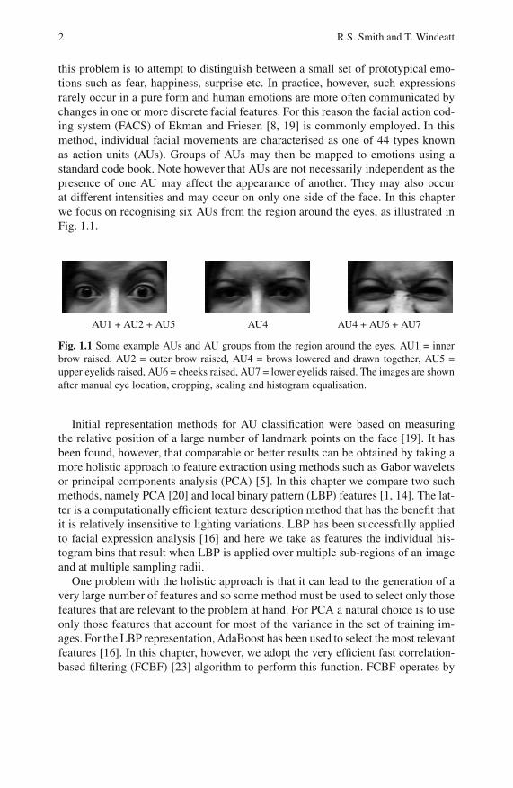
we focus on recognising six AUs from the region around the eyes, as illustrated in
Fig. 1.1.
AU1 + AU2 + AU5 AU4 AU4 + AU6 + AU7
Fig. 1.1 Some example AUs and AU groups from the region around the eyes. AU1 = inner
brow raised, AU2 = outer brow raised, AU4 = brows lowered and drawn together, AU5 =
upper eyelids raised, AU6 = cheeks raised, AU7 = lower eyelids raised. The images are shown
after manual eye location, cropping, scaling and histogram equalisation.
Initial representation methods for AU classification were based on measuring
the relative position of a large number of landmark points on the face [19]. It has
been found, however, that comparable or better results can be obtained by taking a
more holistic approach to feature extraction using methods such as Gabor wavelets
or principal components analysis (PCA) [5]. In this chapter we compare two such
methods, namely PCA [20] and local binary pattern (LBP) features [1, 14]. The lat-
ter is a computationally efficient texture description method that has the benefit that
it is relatively insensitive to lighting variations. LBP has been successfully applied
to facial expression analysis [16] and here we take as features the individual his-
togram bins that result when LBP is applied over multiple sub-regions of an image
and at multiple sampling radii.
One problem with the holistic approach is that it can lead to the generation of a
very large number of features and so some method must be used to select only those
features that are relevant to the problem at hand. For PCA a natural choice is to use
only those features that account for most of the variance in the set of training im-
ages. For the LBP representation, AdaBoost has been used to select the most relevant
features [16]. In this chapter, however, we adopt the very efficient fast correlation-
based filtering (FCBF) [23] algorithm to perform this function. FCBF operates by

1 Facial Action Unit Recognition Using ECOC 3
repeatedly choosing the feature that is most correlated with class, excluding those
features already chosen or rejected, and rejecting any features that are more cor-
related with it than with the class. As a measure of classification, the information-
theoretic concept of symmetric uncertainty is used.
To detect the presence of particular AUs in a face image, one possibility is to
train a separate dedicated classifier for each AU. Bartlett et. al. for example [2],
have obtained good results by constructing such a set of binary classifiers, where
each classifier consists of an AdaBoost ensemble based on selecting the most useful
200 Gabor filters, chosen from a large population of such features. An alternative
approach [16] is to make use of the fact that AUs tend to occur in distinct groups and
to attempt, in the first instance, to recognise the different AU groups before using
this information to infer the presence of individual AUs. This second approach is the
one adopted in this chapter; it treats the problem of AU recognition as a multiclass
problem, requiring a single classifier for its solution. This classifier generates con-
fidence scores for each of the known AU groups and these scores are then summed
in different combinations to estimate the likelihood that each of the AUs is present
in the input image.
One potential problem with this approach is that, when the number positive indi-
cators for a given AU (i.e. the number of AU groups to which it belongs) differs from
the number of negative indicators (i.e. the number of AU groups to which it does not
belong), the overall score can be unbalanced, making it difficult to make a correct
classification decision. To overcome this problem we apply Platt scaling [15] to the
total scores for each AU. This technique uses a maximum-likelihood algorithm to fit
a sigmoid calibration curve to a 2-class training set. The re-mapped value obtained
from a given input score then represents an estimate of the probability that the given
point belongs to the positive class.
The method used in this chapter to perform the initial AU group classification
step is to construct an Error-Correcting Output Code (ECOC) ensemble of Multi-
Layer Perceptron (MLP) Neural Networks. The ECOC technique [4, 10] has proved
to be a highly successful way of solving a multiclass learning problem by decompos-
ing it into a series of 2-class problems, or dichotomies, and training a separate base
classifier to solve each one. These 2-class problems are constructed by repeatedly
partitioning the set of target classes into pairs of super-classes so that, given a large
enough number of such partitions, each target class can be uniquely represented as
the intersection of the super-classes to which it belongs. The classification of a pre-
viously unseen pattern is then performed by applying each of the base classifiers so
as to make decisions about the super-class membership of the pattern. Redundancy
can be introduced into the scheme by using more than the minimum number of base
classifiers and this allows errors made by some of the classifiers to be corrected by
the ensemble as a whole.
In addition to constructing vanilla ECOC ensembles, we make use of two en-
hancements to the ECOC algorithm with the aim of improving classification per-
formance. The first of these is to promote diversity among the base classifiers by

4 R.S. Smith and T. Windeatt
training each base classifier, not on the full training set, but rather on a bootstrap
replicate of the training set [7]. These are obtained from the original training set by
repeated sampling with replacement and this results in further training sets which
contain, on average, 63% of the patterns in the original set but with some patterns
repeated to form a set of the same size. This technique has the further benefit that
the out-of-bootstrap samples can also be used for other purposes such as parameter
tuning.
The second enhancement to ECOC is to apply weighting to the decoding of base-
classifier outputs so that each base classifier is weighted differently for each target
class (i.e. AU group). For this purpose we use a method known as class-separability
weighting (CSEP) ([17] and Sect. 1.2.1) in which base classifiers are weighted ac-
cording to their ability to distinguish a given class from all other classes.
When considering the sources of error in statistical pattern classifiers it is use-
ful to group them under three headings, namely Bayes error, bias (strictly this is
measured as bias) and variance. The first of these is due to unavoidable noise but
the latter two can be reduced by careful classifier design. There is often a tradeoff
between bias and variance [9] so that a high value of one implies a low value of the
other. The concepts of bias and variance originated in regression theory and several
alternative definitions have been proposed for extending them to classification prob-
lems [11]. Here we adopt the definitions of Kohavi and Wolpert [13] to investigate
the bias/variance characteristics of our chosen algorithms. These have the advan-
tage that bias and variance are non-negative and additive. A disadvantage, however,
is that no explicit allowance is made for Bayes error and it is, in effect, rolled into
the bias term.
Previous investigation [17, 18, 21] has suggested that the combination of boot-
strapping and CSEP weighting improves ECOC accuracy and that this is achieved
through a reduction in both bias and variance error. In this chapter we apply these
techniques to the specific problem of FACS-based facial expression recognition and
show that the results depend on which method of feature extraction is applied. When
LBP features are used, in conjunction with FCBF filtering, an improvement in bias
and variance is observed; this is consistent with the results found on other datasets.
When PCA is applied, however, it appears that any reduction in variance is offset
by a corresponding increase in bias so that there is no net benefit from using these
ECOC enhancements. This leads to the conclusion that the former feature extraction
method is to be preferred to the latter for this problem.
The remainder of this chapter is structured as follows. In Sect. 1.2 we describe the
theoretical and mathematical background to the ideas described above. This is fol-
lowed in Sect. 1.3 by a more detailed exposition, in the form of pseudo-code listings,
of how the main novel algorithms presented here may be implemented (an appendix
showing executable MATLAB code for the calculation of the CSEP weights matrix
is also given in Sect. 1.6). Section 1.4 presents an experimental evaluation of these
techniques and Sect. 1.5 summarises the main conclusions to be drawn from this
work.

1 Facial Action Unit Recognition Using ECOC 5
1.2 Theoretical Background
This section describes in more detail the theoretical and mathematical principles
underlying the main techniques used in this work.
1.2.1 ECOC Weighted Decoding
The ECOC method consists of repeatedly partitioning the full set of N classes
Ω = ωi | i = 1 . . .N into L super-class pairs. The choice of partitions is repre-
sented by an N×L binary code matrix Z. The rows Zi are unique codewords that
are associated with the individual target classes ωi and the columns Z j represent
the different super-class partitions. Denoting the jth super-class pair by S j and S j,
element Zi j of the code matrix is set to 1 or 01 depending on whether class ωi has
been put into S j or its complement. A separate base classifier is trained to solve each
of these 2-class problems.
Given an input pattern vector x whose true class c(x) ∈ Ω is unknown, let the
soft output from the jth base classifier be s j (x) ∈ [0,1]. The set of outputs from
all the classifiers can be assembled into a vector s(x) = [s1(x), . . . ,sL(x)]T ∈ [0,1]L
called the output code for x. Instead of working with the soft base classifier outputs,
we may also first harden them, by rounding to 0 or 1, to obtain the binary vector
h(x) = [h1(x), . . . ,hL(x)]T ∈ 0,1L. The principle of the ECOC technique is to
obtain an estimate c(x) ∈Ω of the class label for x from a knowledge of the output
code s(x) or h(x).In its general form, a weighted decoding procedure makes use of an N×L weights
matrix W that assigns a different weight to each target class and base classifier
combination. For each class ωi we may use the L1 metric to compute a class score
Fi (x) ∈ [0,1] as follows:
Fi (x) = 1−L
∑j=1
Wij
∣∣sj (x)−Zij
∣∣ , (1.1)
where it is assumed that the rows of W are normalized so that ∑Lj=1 Wi j = 1 for i =
1 . . .N. Patterns may then be assigned to the target class c(x) = argmaxωiFi (x). If
the base classifier outputs s j (x) in Eq. 1.1 are replaced by hardened values h j (x)then this describes the weighted Hamming decoding procedure.
In the context of this chapter Ω is the set of known AU groups and we are also
interested in combining the class scores to obtain values that measure the likelihood
that AUs are present; this is done by summing the Fi (x) over all ωi that contain the
given AU and dividing by N. That is, the score Gk ∈ [0,1] for AUk is given by:
Gk (x) =1
N∑
AUk∈ωi
Fi (x) . (1.2)
1 Alternatively, the values +1 and -1 are often used.

6 R.S. Smith and T. Windeatt
The values of W may be chosen in different ways. For example, if Wi j =1L
for all i, j
then the decoding procedure of Eq. 1.1 is equivalent to the standard unweighted L1
or Hamming decoding scheme. In this chapter we make use of the CSEP measure
[17, 21] to obtain weight values that express the ability of each base classifier to
distinguish members of a given class from those of any other class.
In order to describe the class-separability weighting scheme, the concept of a
correctness function must first be introduced: given a pattern x which is known to
belong to class ωi, the correctness function for the jth base classifier takes the value
1 if the base classifier makes a correct prediction for x and 0 otherwise:
C j (x) =
1 if h j (x) = Zi j
0 if h j (x) = Zi j
. (1.3)
We also consider the complement of the correctness function C j (x) = 1−C j (x)which takes the value 1 for an incorrect prediction and 0 otherwise.
For a given class index i and base classifier index j, the class-separability weight
measures the difference between the positive and negative correlations of base clas-
sifier predictions, ignoring any base classifiers for which this difference is negative:
Wi j = max
⎧
⎪⎪⎪⎪⎪⎨
⎪⎪⎪⎪⎪⎩
0,1
Ki
⎡
⎢⎢⎢⎢⎢⎣
∑p ∈ ωi
q /∈ ωi
C j (p)C j (q)− ∑p ∈ ωi
q /∈ ωi
C j (p)C j (q)
⎤
⎥⎥⎥⎥⎥⎦
⎫
⎪⎪⎪⎪⎪⎬
⎪⎪⎪⎪⎪⎭
, (1.4)
where patterns p and q are taken from a fixed training set T and Ki is a normalization
constant that ensures that the ith row of W sums to 1.
1.2.2 Platt Scaling
It often arises in pattern recognition applications that we would like to obtain a
probability estimate for membership of a class but that the soft values output by
our chosen classification algorithm are only loosely related to probability. Here, this
applies to the scores Gk (x) obtained by applying Eq. 1.2 to detect individual AUs in
an image. Ideally, the value of the scores would be balanced, so that a value > 0.5could be taken to indicate that AUk is present. In practice, however, this is often not
the case, particularly when AUk belongs to more than or less than half the number
of AU groups.
To correct for this problem Platt scaling [15] is used to remap the training-set
output scores Gk (x) to values which satisfy this requirement. The same calibration
curve is then used to remap the test-set scores. An alternative approach would have
been to find a separate threshold for each AU but the chosen method has the added
advantage that the probability information represented by the remapped scores could
1 Facial Action Unit Recognition Using ECOC 7
be useful in some applications. Another consideration is that a wide range of thresh-
olds can be found that give low training error so some means of regularisation must
be applied in the decision process.
Platt scaling, which can be applied to any 2-class problem, is based on the regu-
larisation assumption that the the correct form of calibration curve that maps clas-
sifier scores Gk (x) to probabilities pk (x), for an input pattern x, is a sigmoid curve
described by the equation:
pk (x) =1
1 + exp(AGk (x)+ B), (1.5)
where the parameters A and B together determine the slope of the curve and its
lateral displacement. The values of A and B that best fit a given training set are
obtained using an expectation maximisation algorithm on the positive and negative
examples. A separate calibration curve is computed for each value of k.
1.2.3 Local Binary Patterns
The local binary pattern (LBP) operator [14] is a powerful 2D texture descriptor
that has the benefit of being somewhat insensitive to variations in the lighting and
orientation of an image. The method has been successfully applied to applications
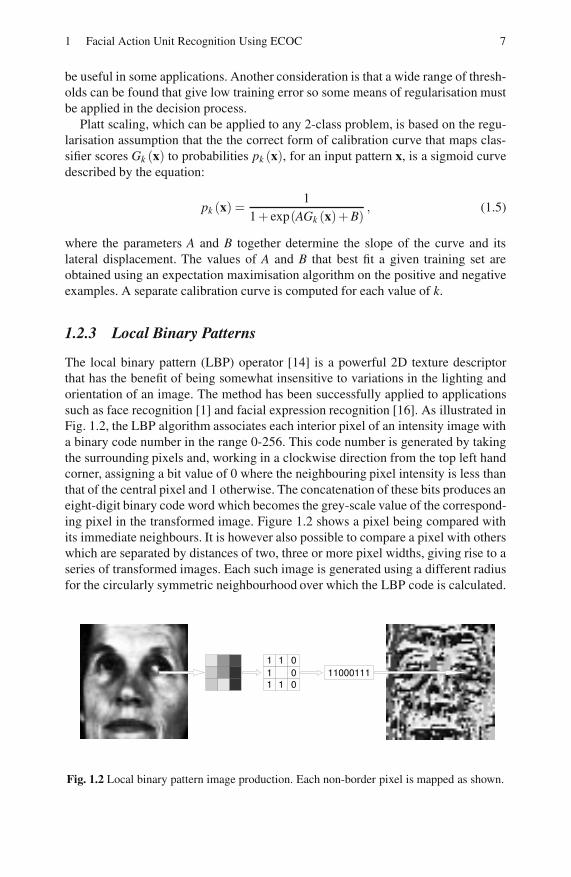
such as face recognition [1] and facial expression recognition [16]. As illustrated in
Fig. 1.2, the LBP algorithm associates each interior pixel of an intensity image with
a binary code number in the range 0-256. This code number is generated by taking
the surrounding pixels and, working in a clockwise direction from the top left hand
corner, assigning a bit value of 0 where the neighbouring pixel intensity is less than
that of the central pixel and 1 otherwise. The concatenation of these bits produces an
eight-digit binary code word which becomes the grey-scale value of the correspond-
ing pixel in the transformed image. Figure 1.2 shows a pixel being compared with
its immediate neighbours. It is however also possible to compare a pixel with others
which are separated by distances of two, three or more pixel widths, giving rise to a
series of transformed images. Each such image is generated using a different radius
for the circularly symmetric neighbourhood over which the LBP code is calculated.
Fig. 1.2 Local binary pattern image production. Each non-border pixel is mapped as shown.

8 R.S. Smith and T. Windeatt
Another possible refinement is to obtain a finer angular resolution by using more
than 8 bits in the code-word [14]. Note that the choice of the top left hand corner as
a reference point is arbitrary and that different choices would lead to different LBP
codes; valid comparisons can be made, however, provided that the same choice of
reference point is made for all pixels in all images.
It is noted in [14] that in practice the majority of LBP codes consist of a concate-
nation of at most three consecutive sub-strings of 0s and 1s; this means that when
the circular neighbourhood of the centre pixel is traversed, the result is either all 0s,
all 1s or a starting point can be found which produces a sequence of 0s followed by
a sequence of 1s. These codes are referred to as uniform patterns and, for an 8 bit
code, there are 58 possible values. Uniform patterns are most useful for texture dis-
crimination purposes as they represent local micro-features such as bright spots, flat
spots and edges; non-uniform patterns tend to be a source of noise and can therefore
usefully be mapped to the single common value 59.
In order to use LBP codes as a face expression comparison mechanism it is first
necessary to subdivide a face image into a number of sub-windows and then com-
pute the occurrence histograms of the LBP codes over these regions. These his-
tograms can be combined to generate useful features, for example by concatenating
them or by comparing corresponding histograms from two images.
1.2.4 Fast Correlation-Based Filtering
Broadly speaking, feature selection algorithms can be divided into two groups:
wrapper methods and filter methods [3]. In the wrapper approach different combi-
nations of features are considered and a classifier is trained on each combination to
determine which is the most effective. Whilst this approach undoubtedly gives good
results, the computational demands that it imposes render it impractical when a very
large number of features needs to be considered. In such cases the filter approach
may be used; this considers the merits of features in themselves without reference
to any particular classification method.
Fast correlation-based filtering (FCBF) has proved itself to be a successful feature
selection method that can handle large numbers of features in a computationally
efficient way. It works by considering the classification between each feature and
the class label and between each pair of features. As a measure of classification the
concept of symmetric uncertainty is used; for a pair random variables X and Y this
is defined as:
SU (X ,Y ) = 2
[IG(X ,Y )
H (X)+ H (Y )
]
(1.6)
where H (·) is the entropy of the random variable and IG(X ,Y )= H (X)−H (X | Y )=H (Y )−H (Y | X) is the information gain between X and Y . As its name suggests,
symmetric uncertainty is symmetric in its arguments; it takes values in the range [0,1]

1 Facial Action Unit Recognition Using ECOC 9
where 0 implies independence between the random variables and 1 implies that the
value of each variable completely predicts the value of the other. In calculating the
entropies of Eq. 1.6, any continuous features must first be discretised.
The FCBF algorithm applies heuristic principles that aim to achieve a balance
between using relevant features and avoiding redundant features. It does this by
selecting features f that satisfy the following properties:
1. SU ( f ,c) ≥ δ where c is the class label and δ is a threshold value chosen to suit
the application.
2. ∀g : SU ( f ,g) ≥ SU ( f ,c)⇒ SU ( f ,c) ≥ SU (g,c) where g is any feature other
than f .
Here, property 1 ensures that the selected features are relevant, in that they are corre-
lated with the class label to some degree, and property 2 eliminates redundant features
by discarding those that are strongly correlated with a more relevant feature.
1.2.5 Principal Components Analysis
Given a matrix of P training patterns T ∈ RP×M, where each row consists of a
rasterised image of M dimensions, the PCA algorithm [20] consists of finding the
eigenvectors (often referred to as eigenimages) of the covariance matrix of the mean-
subtracted training images and ranking them in decreasing order of eigenvalue. This
gives rise to an orthonormal basis of eigenimages where the first eigenimage gives
the direction of maximum variance or scatter within the training set and subsequent
eigenimages are associated with steadily decreasing levels of scatter. A probe image
can be represented as a linear combination of these eigenimages and, by choosing
a cut-off point beyond which the basis vectors are ignored, a reduced dimension
approximation to the probe image can be obtained.
More formally, the PCA approach is as follows. The sample covariance matrix of
T is defined as an average outer product:
S =1
P
P
∑i=1
(Ti−m)T (Ti−m) (1.7)
where Ti is the ith row of T and m is the sample mean row vector given by
m =1
P
P
∑i=1
Ti. (1.8)
Hence the first step in the PCA algorithm is to find an orthonormal projection matrix
U = [u1, . . .uM] that diagonalises S so that
SU = UΛ (1.9)

10 R.S. Smith and T. Windeatt
where Λ is a diagonal matrix of eigenvalues. The columns uq of U then constitute
a new orthonormal basis of eigenimages for the image space and we may assume,
without loss of generality, that they are ordered so that their associated eigenvalues
λq form a non-increasing sequence, that is:
q < r⇒ λq ≥ λr (1.10)
for 1≤ q,r ≤M.
An important property of this transformation is that, with respect to the basis
uq
, the coordinates of the training vectors are de-correlated. Thus each uq lies
in a direction in which the total scatter between images, as measured over the rows
of T, is statistically independent of the scatter in other orthogonal directions. By
virtue of Eq. 1.10 the scatter is maximum for u1 and decreases as the index q in-
creases. For any probe row vector x, the vector x′ = UT (x−m)T is the projection of
the mean-subtracted vector x−m into the coordinate system
uq
with the compo-
nents being arranged in decreasing order of training set scatter. An approximation
to x′ may be obtained by discarding all but the first K < M components to obtain
the row vector x′′ = [x′1, . . . ,x′K ]. The value of K is chosen such that the root mean
square pixel-by-pixel error of the approximation is below a suitable threshold value.
For face data sets it is found in practice that K can be chosen such that K ≪M and
so this procedure leads to the desired dimensionality reduction. The resulting lin-
ear subspace preserves most of the scatter of the training set and thus permits face
expression recognition to be performed within it.
1.3 Algorithms
Section 1.2 presented the theoretical background to the main techniques referred to
in this chapter. The aim of this section is to describe in more detail how the novel
algorithms used here can be implemented (for details of already established algo-
rithms such as LBP, Platt scaling and FCBF, the reader is referred to the references
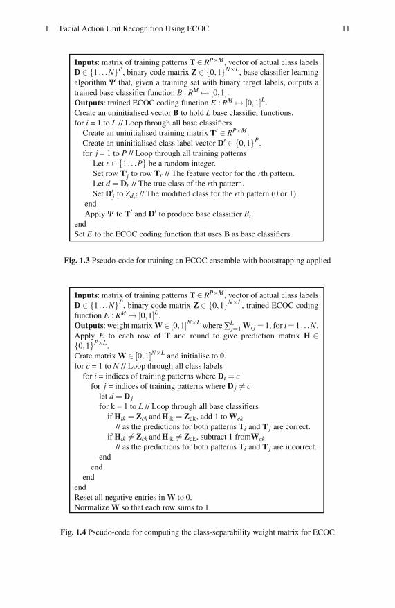
given in Sect. 1.2). To this end, Fig. 1.3 shows the pseudo-code for the application
of bootstrapping to ECOC training, Fig. 1.4 shows how the CSEP weights matrix
is calculated and Fig. 1.5 provides details on how the weights matrix is used when
ECOC is applied to the problem of calculating AU group membership scores for a
probe image.
1.4 Experimental Evaluation
In this section we present the results of performing classification experiments on
the Cohn-Kanade face expression database [12]. This dataset contains frontal video
clips of posed expression sequences from 97 university students. Each sequence
goes from neutral to target display but only the last image has available a ground
truth in the form of a manual AU coding. In carrying out these experiments we fo-
cused on detecting AUs from the the upper face region as shown in Fig. 1.1. Neutral
1 Facial Action Unit Recognition Using ECOC 11
Inputs: matrix of training patterns T ∈ RP×M, vector of actual class labels
D ∈ 1 . . .NP, binary code matrix Z ∈ 0,1N×L, base classifier learning
algorithm Ψ that, given a training set with binary target labels, outputs a
trained base classifier function B : RM → [0,1].Outputs: trained ECOC coding function E : RM → [0,1]L.
Create an uninitialised vector B to hold L base classifier functions.
for i = 1 to L // Loop through all base classifiers
Create an uninitialised training matrix T′ ∈ RP×M.
Create an uninitialised class label vector D′ ∈ 0,1P.
for j = 1 to P // Loop through all training patterns
Let r ∈ 1 . . .P be a random integer.
Set row T′j to row Tr // The feature vector for the rth pattern.
Let d = Dr // The true class of the rth pattern.
Set D′j to Zd,i // The modified class for the rth pattern (0 or 1).
end
Apply Ψ to T′ and D′ to produce base classifier Bi.
end
Set E to the ECOC coding function that uses B as base classifiers.
Fig. 1.3 Pseudo-code for training an ECOC ensemble with bootstrapping applied
Inputs: matrix of training patterns T ∈ RP×M, vector of actual class labels
D ∈ 1 . . .NP, binary code matrix Z ∈ 0,1N×L, trained ECOC coding
function E : RM → [0,1]L.
Outputs: weight matrix W∈ [0,1]N×L where ∑Lj=1 Wi j = 1, for i = 1 . . .N.
Apply E to each row of T and round to give prediction matrix H ∈0,1P×L.
Crate matrix W ∈ [0,1]N×L and initialise to 0.
for c = 1 to N // Loop through all class labels
for i = indices of training patterns where Di = c
for j = indices of training patterns where D j = c
let d = D j
for k = 1 to L // Loop through all base classifiers
if Hik = Zck and Hjk = Zdk, add 1 to Wck
// as the predictions for both patterns Ti and T j are correct.
if Hik = Zck and Hjk = Zdk, subtract 1 fromWck
// as the predictions for both patterns Ti and T j are incorrect.
end
end
end
end
Reset all negative entries in W to 0.
Normalize W so that each row sums to 1.
Fig. 1.4 Pseudo-code for computing the class-separability weight matrix for ECOC

12 R.S. Smith and T. Windeatt
Inputs: test pattern x ∈ RM , binary code matrix Z ∈ 0,1N×L, weight
matrix W ∈ [0,1]N×L where ∑Lj=1 Wi j = 1 for i = 1 . . .N, trained ECOC
coding function E : RM → [0,1]L.
Outputs: vector of class label scores F ∈ [0,1]N .
Apply E to x to produce the row vector s(x) ∈ [0,1]L of base classifier
outputs.
Create uninitialised vector F ∈ [0,1]N .
for c = 1 to N // Loop through all class labels
Set Fc = 1−abs (s(x)−Zc)WTc where abs (•) is the vector of absolute
component values.
// Set Fc to 1 - the weighted L1 distance between s(x) and row Zc
end
Fig. 1.5 Pseudo-code for weighted ECOC decoding
images were not used and AU groups with three or fewer examples were ignored. In
total this led to 456 images being available and these were distributed across the 12
classes shown in Table 1.1. Note that researchers often make different decisions in
these areas, and in some cases are not explicit about which choice has been made.
This can render it difficult to make a fair comparison with previous results. For ex-
ample some studies use only the last image in the sequence but others use the neutral
image to increase the numbers of negative examples. Furthermore, some researchers
consider only images with single AU, whilst others use combinations of AUs. We
consider the more difficult problem, in which neutral images are excluded and im-
ages contain combinations of AUs. A further issue is that some papers only report
overall error rate. This may be misleading since class distributions are unequal, and
it is possible to get an apparently low error rate by a simplistic classifier that classi-
fies all images as non-AU. For this reason we also report the area under ROC curve,
similar to [2].
Table 1.1 Classes of action unit groups used in the experiments
Class number 1 2 3 4 5 6 7 8 9 10 11 12
AUs present None 1,2 1,2,5 4 6 1,4 1,4,7 4,7 4,6,7 6,7 1 1,2,4
Number of examples 152 23 62 26 66 20 11 48 22 13 7 6
Each 640 x 480 pixel image we converted to greyscale by averaging the RGB
components and the eye centres were manually located. A rectangular window
around the eyes was obtained and then rotated and scaled to 150 x 75 pixels. His-
togram equalization was used to standardise the image intensities. LBP features
were extracted by computing a uniform (i.e. 59-bin) histogram for each sub-window
in a non-overlapping tiling of this window. This was repeated with a range of tile
sizes (from 12 x 12 to 150 x 75 pixels) and sampling radii (from 1 to 10 pixels).

1 Facial Action Unit Recognition Using ECOC 13
The histogram bins were concatenated to give 107,000 initial features; these were
then reduced to approximately 120 features by FCBF filtering. An FCBF threshold
of zero was used; this means that all features were considered initially to be rele-
vant and feature reduction was accomplished by removing redundant features, as
described in Sect. 1.2.4.
ECOC ensembles of size 200 were constructed with single hidden-layer MLP
base classifiers trained using the Levenberg-Marquardt algorithm. A range of MLP
node numbers (from 2 to 16) and training epochs (from 2 to 1024) was tried; each
such combination was repeated 10 times and the results averaged. Each run was
based on a different randomly chosen stratified training set with a 90/10 training/test
set split. The experiments were performed with and without CSEP weighting and
with and without bootstrapping. The ECOC code matrices were randomly generated
but in such a way as to have balanced numbers of 1s and 0s in each column. Another
source of random variation was the initial MLP network weights. When bootstrap-
ping was applied, each base classifier was trained on a separate bootstrap replicate
drawn from the complete training set for that run. The CSEP weight matrix was, in
all cases, computed from the full training set.
1.4.1 Classifier Accuracy
Table 1.2 shows the mean AU classification error rates and area under ROC figures
obtained using these methods (including Platt scaling); the best individual AU clas-
sification results are shown in Table 1.3. From Table 1.2 it can be seen that the LBP
feature extraction method gives greater accuracy than PCA. Furthermore, LBP is
able to benefit from the application of bootstrapping and CSEP weighting, whereas
PCA does not. The LBP method thus exhibits behaviour similar to that found on
other data sets [17], in that bootstrapping and CSEP weighting on their own each
lead to some improvement and the combination improves the results still further. By
contrast, PCA performance is not improved by either technique, whether singly or
in combination. The reasons for this anomaly, in terms of a bias/variance decompo-
sition of error, are discussed in Sect. 1.4.3.
Table 1.2 Best mean error rates and area under ROC curves for the AU recognition task
Bootstrapping CSEP Weighting Error (%) Area Under ROC
Applied Applied PCA LBP + FCBF PCA LBP + FCBF
No No 9.5 9.0 0.93 0.94
Yes No 9.8 8.8 0.93 0.94
No Yes 9.5 9.0 0.93 0.94
Yes Yes 9.6 8.5 0.93 0.95
14 R.S. Smith and T. Windeatt
Table 1.3 Best error rates and area under ROC curves for individual AU recognition. LBP
feature extraction was used, together with bootstrapping and CSEP weighting. MLPs had 16
nodes and 8 training epochs.
AU no. 1 2 4 5 6 7
Error (%) 8.9 5.4 8.7 4.8 11.2 12.3
Area under ROC 0.94 0.96 0.96 0.97 0.92 0.92
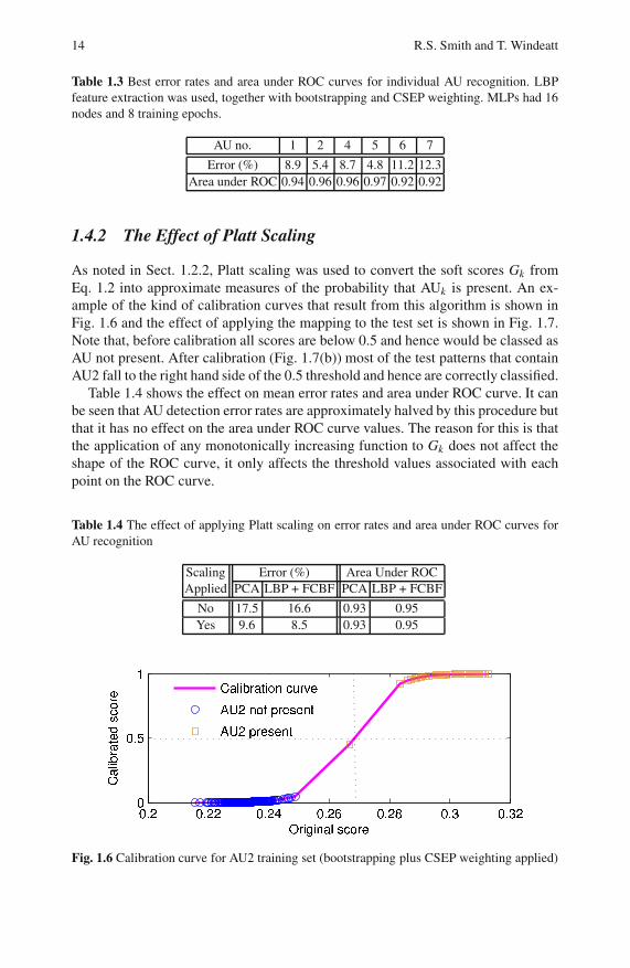
1.4.2 The Effect of Platt Scaling
As noted in Sect. 1.2.2, Platt scaling was used to convert the soft scores Gk from
Eq. 1.2 into approximate measures of the probability that AUk is present. An ex-
ample of the kind of calibration curves that result from this algorithm is shown in
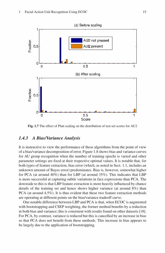
Fig. 1.6 and the effect of applying the mapping to the test set is shown in Fig. 1.7.
Note that, before calibration all scores are below 0.5 and hence would be classed as
AU not present. After calibration (Fig. 1.7(b)) most of the test patterns that contain
AU2 fall to the right hand side of the 0.5 threshold and hence are correctly classified.
Table 1.4 shows the effect on mean error rates and area under ROC curve. It can
be seen that AU detection error rates are approximately halved by this procedure but
that it has no effect on the area under ROC curve values. The reason for this is that
the application of any monotonically increasing function to Gk does not affect the
shape of the ROC curve, it only affects the threshold values associated with each
point on the ROC curve.
Table 1.4 The effect of applying Platt scaling on error rates and area under ROC curves for
AU recognition
Scaling Error (%) Area Under ROC
Applied PCA LBP + FCBF PCA LBP + FCBF
No 17.5 16.6 0.93 0.95
Yes 9.6 8.5 0.93 0.95
Fig. 1.6 Calibration curve for AU2 training set (bootstrapping plus CSEP weighting applied)
1 Facial Action Unit Recognition Using ECOC 15
Fig. 1.7 The effect of Platt scaling on the distribution of test-set scores for AU2
1.4.3 A Bias/Variance Analysis
It is instructive to view the performance of these algorithms from the point of view
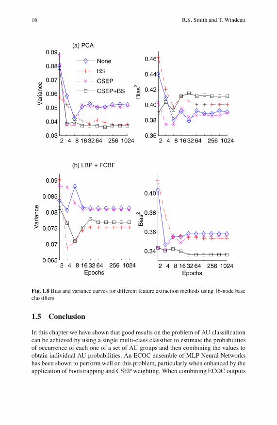
of a bias/variance decomposition of error. Figure 1.8 shows bias and variance curves
for AU group recognition when the number of training epochs is varied and other
parameter settings are fixed at their respective optimal values. It is notable that, for
both types of feature extraction, bias error (which, as noted in Sect. 1.1, includes an
unknown amount of Bayes error) predominates. Bias is, however, somewhat higher
for PCA (at around 40%) than for LBP (at around 35%). This indicates that LBP
is more successful at capturing subtle variations in face expressions than PCA. The
downside to this is that LBP feature extraction is more heavily influenced by chance
details of the training set and hence shows higher variance (at around 8%) than
PCA (at around 4.5%). It is thus evident that these two feature extraction methods
are operating at different points on the bias/variance tradeoff curve.
One notable difference between LBP and PCA is that, when ECOC is augmented
with bootstrapping and CSEP weighting, the former method benefits by a reduction
in both bias and variance; this is consistent with results found on other datasets [18].
For PCA, by contrast, variance is reduced but this is cancelled by an increase in bias
so that PCA does not benefit from these methods. This increase in bias appears to
be largely due to the application of bootstrapping.
16 R.S. Smith and T. Windeatt
2 4 8 16 32 64 256 10240.03
0.04
0.05
0.06
0.07
0.08
0.09
Va
ria
nce
(a) PCA
None
BS
CSEP
CSEP+BS
2 4 8 16 32 64 256 10240.36
0.38
0.40
0.42
0.44
0.46
Bia
s2
2 4 8 16 32 64 256 10240.065
0.07
0.075
0.08
0.085
0.09
Epochs
Va
ria
nce
(b) LBP + FCBF
2 4 8 16 32 64 256 1024
0.34
0.36
0.38
0.40
Epochs
Bia
s2
Fig. 1.8 Bias and variance curves for different feature extraction methods using 16-node base
classifiers
1.5 Conclusion
In this chapter we have shown that good results on the problem of AU classification
can be achieved by using a single multi-class classifier to estimate the probabilities
of occurrence of each one of a set of AU groups and then combining the values to
obtain individual AU probabilities. An ECOC ensemble of MLP Neural Networks
has been shown to perform well on this problem, particularly when enhanced by the
application of bootstrapping and CSEP weighting. When combining ECOC outputs

1 Facial Action Unit Recognition Using ECOC 17
it has been found necessary to apply a score-to-probability calibration technique
such as Platt scaling to avoid the bias introduced by different AU group membership
numbers.
Two methods of feature extraction have been examined, namely PCA as applied
directly to the input images, and the use of LBP to extract a wide range of texture
features followed by FCBF filtering to reduce their number. The LBP-based method
has been found to be more effective. This is particularly true when combined with
bootstrapping and CSEP weighting which lead to a reduction in both bias and vari-
ance error.
From an efficiency point of view, it is worth noting that both LBP and FCBF
(which is only required during training) are fast lightweight techniques. The use of
a single classifier, rather than one per AU, also helps to minimise the computational
overheads of AU detection.
Acknowledgements. This work was supported by EPSRC grant E061664/1. The authors
would also like to thank the providers of the PRTools [6] and Weka [22] software.
1.6 Code Listings
The following MATLAB code may be used to compute a CSEP weights matrix.
Note that this code uses some of the classes and functions from the PRTools [6]
toolkit.
function wtgMat = computeCsepMatrix(trgData,codeMatrix);
% Compute the class-separability weights matrix.% trgData = training set (a PRTools dataset)% codeMatrix = the ECOC code matrix of 1’s and 0’s% wtgMat = the returned CSEP weights matrix
[numClasses numBase] = size(codeMatrix);binData=logical(round(getdata(trgData)));% Weighting requires binarized resultspatternNlabs = getnlab(trgData);% A col vector of per pattern dense class numbersnumPatterns = length(patternNlabs);ecocErrorMatrix = xor(binData,codeMatrix(patternNlabs,:));% Populate matrix which shows where the base% classifiers went wrong wrt the ECOC targetsecocCorrectMatrix = ˜ecocErrorMatrix;% The matrix of correct decisonswtgMat = zeros(size(codeMatrix));for nlab = 1:numClasses
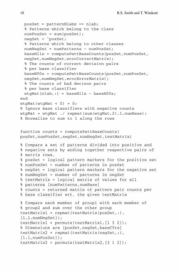
18 R.S. Smith and T. Windeatt
posSet = patternNlabs == nlab;% Patterns which belong to the classnumPosSet = sum(posSet);negSet = ˜posSet;% Patterns which belong to other classesnumNegSet = numPatterns - numPosSet;baseN11s = computePattBaseCounts(posSet,numPosSet,negSet,numNegSet,ecocCorrectMatrix);% The counts of correct decision pairs% per base classifierbaseN00s = computePattBaseCounts(posSet,numPosSet,negSet,numNegSet,ecocErrorMatrix);% The counts of bad decison pairs% per base classifierwtgMat(nlab,:) = baseN11s - baseN00s;
endwtgMat(wtgMat < 0) = 0;% Ignore base classifiers with negative countswtgMat = wtgMat ./ repmat(sum(wtgMat,2),1,numBase);% Normalise to sum to 1 along the rows
function counts = computePattBaseCounts(posSet,numPosSet,negSet,numNegSet,testMatrix)
% Compare a set of patterns divided into positive and% negative sets by anding together respective pairs of% matrix rows.% posSet = logical pattern markers for the positive set% numPosSet = number of patterns in posSet% negSet = logical pattern markers for the negative set% numNegSet = number of patterns in negSet% testMatrix = logical matrix of values for all% patterns [numPatterns,numBase]% counts = returned matrix of pattern pair counts per% base classifier wrt. the given testMatrix
% Compare each member of group1 with each member of% group2 and sum over the other grouptestMatrix1 = repmat(testMatrix(posSet,:),[1,1,numNegSet]);testMatrix1 = permute(testMatrix1,[1 3 2]);% Dimensions are [posSet,negSet,baseCfrs]testMatrix2 = repmat(testMatrix(negSet,:),[1,1,numPosSet]);testMatrix2 = permute(testMatrix2,[3 1 2]);

1 Facial Action Unit Recognition Using ECOC 19
% Dimensions are [posSet,negSet,baseCfrs]coincidenceMatrix = testMatrix1 & testMatrix2;counts = squeeze(sum(sum(coincidenceMatrix,2)))’;% Dimensions are [1,baseCfrs]
References
1. Ahonen, T., Hadid, A., Pietikainen, M.: Face description with local binary patterns:
Application to face recognition. IEEE Trans. Pattern Analysis and Machine Intell. 28,
2037–2041 (2006)
2. Bartlett, M.S., Littlewort, G., Frank, M.G., Lainscsek, C., Fasel, I.R., Movellan, J.R.:
Fully automatic facial action recognition in spontaneous behavior. In: Proc. 7th IEEE
Int. Conf. Automatic Face and Gesture Recogn., Southampton, UK, pp. 223–230. IEEE
Comp. Society, Los Alamitos (2006)
3. Das, S.: Filters, wrappers and a boosting-based hybrid for feature selection. In: Brod-
ley, C.E., Pohoreckyj Danyluk, A. (eds.) Proc. 18th Int. Conf. Machine Learning,
Williamstown, MA, pp. 74–81. Morgan Kaufmann, San Francisco (2001)
4. Dietterich, T.G., Bakiri, G.: Solving multiclass learning problems via error-correcting
output codes. J. Artif. Intell. Research 2, 263–286 (1995)
5. Donato, G., Bartlett, M.S., Hager, J.C., Ekman, P., Sejnowski, T.J.: Classifying facial
actions. IEEE Trans. Pattern Analysis and Machine Intell. 21, 974–989 (1999)
6. Duin, R.P.W., Juszczak, P., Paclik, P., Pekalska, E., de Ridder, D., Tax, D.M.J., Verzakov,
S.: PRTools 4.1, A Matlab toolbox for pattern recognition. Delft University of Technol-
ogy (2007)
7. Efron, B., Tibshirani, R.J.: An introduction to the bootstrap. Chapman & Hall/CRC
Press, Boca Raton (1993)
8. Ekman, P., Friesen, W.V.: The facial action coding system: A technique for the measure-
ment of facial movement. Consulting Psychologists Press, Palo Alto (1978)
9. Geman, S., Bienenstock, E.: Neural networks and the bias/variance dilemma. Neural
Comp. 4, 1–58 (1992)
10. James, G.: Majority vote classifiers: Theory and applications. PhD Dissertation, Stanford
University (1998)
11. James, G.: Variance and bias for general loss functions. Machine Learning 51, 115–135
(2003)
12. Kanade, T., Cohn, J.F., Tian, Y.: Comprehensive database for facial expression analysis.
In: Proc. 4th Int. Conf. Automatic Face and Gesture Recognition, Grenoble, France, pp.
46–53. IEEE Comp. Society, Los Alamitos (2000)
13. Kohavi, R., Wolpert, D.: Bias plus variance decomposition for zero-one loss functions.
In: Proc. 13th Int. Conf. on Machine Learning, Bari, Italy, pp. 275–283. Morgan Kauf-
mann, San Francisco (1996)
14. Ojala, T., Pietikainen, M., Maenpaa, T.: Multiresolution gray-scale and rotation invari-
ant texture classification with local binary patterns. IEEE Trans. Pattern Analysis and
Machine Intell. 24, 971–987 (2002)
15. Platt, J.: Probabilistic outputs for support vector machines and comparison to regularized
likelihood methods. In: Smola, A.J., Bartlett, P., Scholkopf, B., Schuurmans, D. (eds.)
Advances in Large Margin Classifiers, pp. 61–74. MIT Press, Cambridge (1999)
16. Shan, C., Gong, S., McOwan, P.W.: Facial expression recognition based on local binary
patterns: A comprehensive study. Image and Vision Comp. 27, 803–816 (2009)

20 R.S. Smith and T. Windeatt
17. Smith, R.S., Windeatt, T.: Class-separability weighting and bootstrapping in error cor-
recting output code ensembles. In: El Gayar, N., Kittler, J., Roli, F. (eds.) MCS 2010.
LNCS, vol. 5997, pp. 185–194. Springer, Heidelberg (2010)
18. Smith, R.S., Windeatt, T.: A Bias-variance analysis of bootstrapped class-separability
weighting for error-correcting output code ensembles. In: Proc. 22nd IEEE Int. Conf.
Pattern Recogn., Istanbul, Turkey, pp. 61–64. IEEE Comp. Society, Los Alamitos (2010)
19. Tian, Y.-I., Kanade, T., Cohn, J.F.: Recognizing action units for facial expression analy-
sis. IEEE Trans. Pattern Analysis and Machine Intell. 23, 97–115 (2001)
20. Turk, M., Pentland, A.: Eigenfaces for recognition. J. Cognitive Neuroscience 3, 71–86
(1991)
21. Windeatt, T., Smith, R.S., Dias, K.: Weighted decoding ECOC for facial action unit clas-
sification. In: Okun, O., Valentini, G. (eds.) Proc. 2nd Supervised and Unsupervised En-
semble Methods and their Applications, Patras, Greece, pp. 26–30 (2008)
22. Witten, I.H., Frank, E.: Data mining: Practical machine learning tools and techniques.
Morgan Kaufmann, San Francisco (2005)
23. Yu, L., Liu, H.: Feature selection for high-dimensional data: A fast correlation-based
filter solution. In: Fawcett, T., Mishra, N. (eds.) Proc. 20th Int. Conf. Machine Learning,
Washington DC, pp. 856–863. AAAI Press, Menlo Park (2003)

Chapter 2
On the Design of Low RedundancyError-Correcting Output Codes
Miguel Angel Bautista, Sergio Escalera, Xavier Baro, Oriol Pujol,
Jordi Vitria, and Petia Radeva
Abstract. The classification of large number of object categories is a challenging
trend in the Pattern Recognition field. In the literature, this is often addressed using
an ensemble of classifiers . In this scope, the Error-Correcting Output Codes frame-
work has demonstrated to be a powerful tool for combining classifiers. However,
most of the state-of-the-art ECOC approaches use a linear or exponential number of
classifiers, making the discrimination of a large number of classes unfeasible. In this
paper, we explore and propose a compact design of ECOC in terms of the number of
classifiers. Evolutionary computation is used for tuning the parameters of the clas-
sifiers and looking for the best compact ECOC code configuration. The results over
several public UCI data sets and different multi-class Computer Vision problems
show that the proposed methodology obtains comparable (even better) results than
the state-of-the-art ECOC methodologies with far less number of dichotomizers.
2.1 Introduction
Nowadays challenging applications of Pattern Recognition deal with changing en-
vironments, online adaptations, contextual information, etc. In order to deal with
Miguel Angel Bautista · Sergio Escalera · Xavier Baro · Oriol Pujol · Jordi Vitria ·Petia Radeva
Applied Math and Analysis Department at University of Barcelona, Gran Via, 585 08007
Barcelona, Spain
E-mail: [email protected],
sergio,xevi,oriol,petia,[email protected]
Computer Vision Center, Autonomous University of Barcelona, Edificio O Campus UAB,
Cerdanyola, Spain
E-mail: mbautista,sergio.escalera,xavier.baro,oriol.pujol,
petia.radeva,[email protected]
Xavier Baro
Universitat Oberta de Catalunya, Rambla del Poblenou 158, Barcelona, Spain
E-mail: [email protected]
O. Okun et al. (Eds.): Ensembles in Machine Learning Applications, SCI 373, pp. 21–38.springerlink.com c© Springer-Verlag Berlin Heidelberg 2011

22 M.A. Bautista et al.
all these problems, efficient ways for processing huge amount of data are often re-
quired. One clear example is the case of general Pattern Recognition algorithms for
classification, especially when the number of categories, namely objects, people,
brands, etc, is arbitrarily large. Usual Machine Learning strategies are effective for
dealing with small number of classes. The choices are limited when the number
of classes becomes large. In that case, the natural algorithms to consider are those
that model classes in an implicit way, such as instance based learning (i.e. nearest
neighbours). However, this choice is not necessarily the most adequate for a given
problem. Moreover, we are forgetting many algorithms of the literature such as en-
semble learning (i.e. AdaBoost [12]) or kernel based discriminant classifiers (i.e.
Support Vector Machines [20]) that have been proven to be very powerful tools.
Most of state-of-the-art multi-class architectures need to deal with the discrimi-
nation of each class either by modelling its probability density function, or by stor-
ing a classification boundary and using some kind of aggregation/selection function
to obtain a final decision. Another way to deal with this kind of problems is to
use a divide-and-conquer approach. Instead of extending a method to cope with the
multi-class case, one can divide the multi-class problem into smaller binary prob-
lems and then combine their responses using some kind of committee strategy, such
as voting. In literature, one can roughly find three main lines of research in the last
tendency: flat strategies, hierarchical classification , and Error-Correcting Output
Codes (ECOC). Flat strategies consist of using some predefined problem partition
followed by some kind of voting strategy. Good examples of this line are strategies
like one-against-all or all-pairs. Hierarchical classification relies on some similarity
metric among classes for creating a binary tree in which at each node a particular
partition of the classes is considered. Finally, ECOC encodes different partitions of
the problem in a matrix of codewords (one codeword per class) and the final deci-
sion is obtained by looking at the most similar codeword at the test step. ECOC can
be regarded as a generalization of the former strategies since it allows the inclusion
of flat strategies as well as hierarchical classifiers [22]. Moreover, the analysis of
the ECOC error evolution has demonstrated that ECOC corrects errors caused by
the bias and the variance of the learning algorithm [8]1. However, note that by con-
struction or in order to obtain the desired performance, most of the strategies need
between N and N2 classifiers, given N different classes. Although this is adequate
and acceptable when the number of classes is small, it becomes prohibitive when
the number of classes becomes large. This number of classifiers has been recently
reduced in some ECOC designs, such as the DECOC approach of [22], that requires
N− 1 classifiers. The Dense Random and Sparse Random designs [2] also reduce
this number of classifiers to 15log2(N) and 10log2(N), respectively. However this
kind of approaches design the problems without taking into account the underlying
distribution of the class characteristics.
1 The bias term describes the component of the error that results from systematic errors of
the learning algorithm. The variance term describes the component of the error that results
from random variation and noise in the training samples and random behaviour of the
learning algorithm. For more details, see [8].

2 On the Design of Low Redundancy Error-Correcting Output Codes 23
The goal of this paper is to propose and evaluate different general ways of making
the multi-class pattern recognition problem tractable when the number of categories
makes most of the models computationally unfeasible. In particular, we are inter-
ested in methods that scale sub-linearly with the number of classes, allowing their
applicability in general Pattern Recognition problems. The proposal relies on the
Error-Correcting Output Codes framework, reducing the number of binary classi-
fiers that have to be trained in the ensemble. Following the Occam razor principle,
we propose a compact ECOC design of size log2(N) in terms of the number of
classifiers. An evolutionary approximation, similar to the one proposed in [17] is
proposed for tuning the parameters of the classifiers and looking for a compact
design with high generalization capability. Moreover, this design is problem depen-
dent in the sense that the evolved ECOC fits the distribution of the object char-
acteristics. The novel compact ECOC is compared with the state-of-the-art ECOC
approaches, obtaining comparable (even better results) when classifying several ob-
ject categories in different Pattern Recognition applications with far less cost.
The paper is organized as follows: Section 2 presents the compact ECOC design.
Section 3 evaluates the novel methodology by comparing it with the state-of-the-
art approaches on public and challenging Pattern Recognition Applications. Finally,
Sect. 4 concludes the paper.
2.2 Compact Error-Correcting Output Codes
In this section, we review the ECOC framework and propose a compact ECOC
design in terms of the number of classifiers.
2.2.1 Error-Correcting Output Codes
Given a set of N classes to be learned in an ECOC framework, n different bi-
partitions (groups of classes) are formed, and n binary problems (dichotomiz-
ers) over the partitions are trained. As a result, a codeword of length n is ob-
tained for each class, where each position (bit) of the code corresponds to a re-
sponse of a given dichotomizer (coded by +1 or −1 according to their class set
membership). Arranging the codewords as rows of a matrix, we define a coding
matrix M, where M ∈ −1,+1N×n in the binary case. In Fig. 2.1 we show
an example of a binary coding matrix M. The matrix is coded using five di-
chotomizers h1, ...,h5 for a 4-class problem c1, ...,c4 of respective codewords
y1, ...,y4. The hypotheses are trained by considering the labelled training data
samples (ρ1, l(ρ1)), ...,(ρm, l(ρm)) for a set of m data samples. The white and
black regions of the coding matrix M are coded by +1 and −1, respectively. For
example, the first classifier is trained to discriminate c3 against c1, c2, and c4; the
second one classifies c2 and c3 against c1 and c4, and so on, as follows:
h1(x) =
1 if x ∈ c3−1 if x ∈ c1,c2,c4 , . . . , h5(x) =
1 if x ∈ c2,c4−1 if x ∈ c1,c3 (2.1)
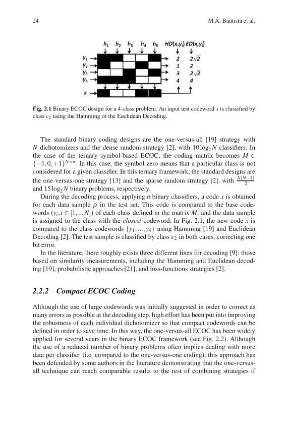
24 M.A. Bautista et al.
Fig. 2.1 Binary ECOC design for a 4-class problem. An input test codeword x is classified by
class c2 using the Hamming or the Euclidean Decoding.
The standard binary coding designs are the one-versus-all [19] strategy with
N dichotomizers and the dense random strategy [2], with 10 log2 N classifiers. In
the case of the ternary symbol-based ECOC, the coding matrix becomes M ∈−1,0,+1N×n. In this case, the symbol zero means that a particular class is not
considered for a given classifier. In this ternary framework, the standard designs are
the one-versus-one strategy [13] and the sparse random strategy [2], withN(N−1)
2and 15log2 N binary problems, respectively.
During the decoding process, applying n binary classifiers, a code x is obtained
for each data sample ρ in the test set. This code is compared to the base code-
words (yi, i ∈ [1, ..,N]) of each class defined in the matrix M, and the data sample
is assigned to the class with the closest codeword. In Fig. 2.1, the new code x is
compared to the class codewords y1, ...,y4 using Hamming [19] and Euclidean
Decoding [2]. The test sample is classified by class c2 in both cases, correcting one
bit error.
In the literature, there roughly exists three different lines for decoding [9]: those
based on similarity measurements, including the Hamming and Euclidean decod-
ing [19], probabilistic approaches [21], and loss-functions strategies [2].
2.2.2 Compact ECOC Coding
Although the use of large codewords was initially suggested in order to correct as
many errors as possible at the decoding step, high effort has been put into improving
the robustness of each individual dichotomizer so that compact codewords can be
defined in order to save time. In this way, the one-versus-all ECOC has been widely
applied for several years in the binary ECOC framework (see Fig. 2.2). Although
the use of a reduced number of binary problems often implies dealing with more
data per classifier (i.e. compared to the one-versus-one coding), this approach has
been defended by some authors in the literature demonstrating that the one-versus-
all technique can reach comparable results to the rest of combining strategies if
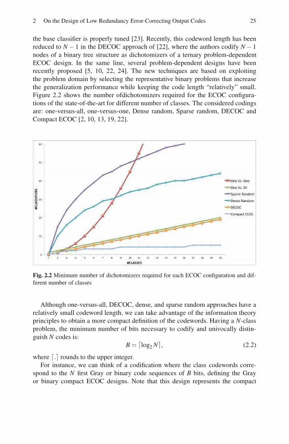
2 On the Design of Low Redundancy Error-Correcting Output Codes 25
the base classifier is properly tuned [23]. Recently, this codeword length has been
reduced to N− 1 in the DECOC approach of [22], where the authors codify N− 1
nodes of a binary tree structure as dichotomizers of a ternary problem-dependent
ECOC design. In the same line, several problem-dependent designs have been
recently proposed [5, 10, 22, 24]. The new techniques are based on exploiting
the problem domain by selecting the representative binary problems that increase
the generalization performance while keeping the code length “relatively” small.
Figure 2.2 shows the number ofdichotomizers required for the ECOC configura-
tions of the state-of-the-art for different number of classes. The considered codings
are: one-versus-all, one-versus-one, Dense random, Sparse random, DECOC and
Compact ECOC [2, 10, 13, 19, 22].
Fig. 2.2 Minimum number of dichotomizers required for each ECOC configuration and dif-
ferent number of classes
Although one-versus-all, DECOC, dense, and sparse random approaches have a
relatively small codeword length, we can take advantage of the information theory
principles to obtain a more compact definition of the codewords. Having a N-class
problem, the minimum number of bits necessary to codify and univocally distin-
guish N codes is:
B = ⌈log2 N⌉, (2.2)
where ⌈.⌉ rounds to the upper integer.
For instance, we can think of a codification where the class codewords corre-
spond to the N first Gray or binary code sequences of B bits, defining the Gray
or binary compact ECOC designs. Note that this design represents the compact
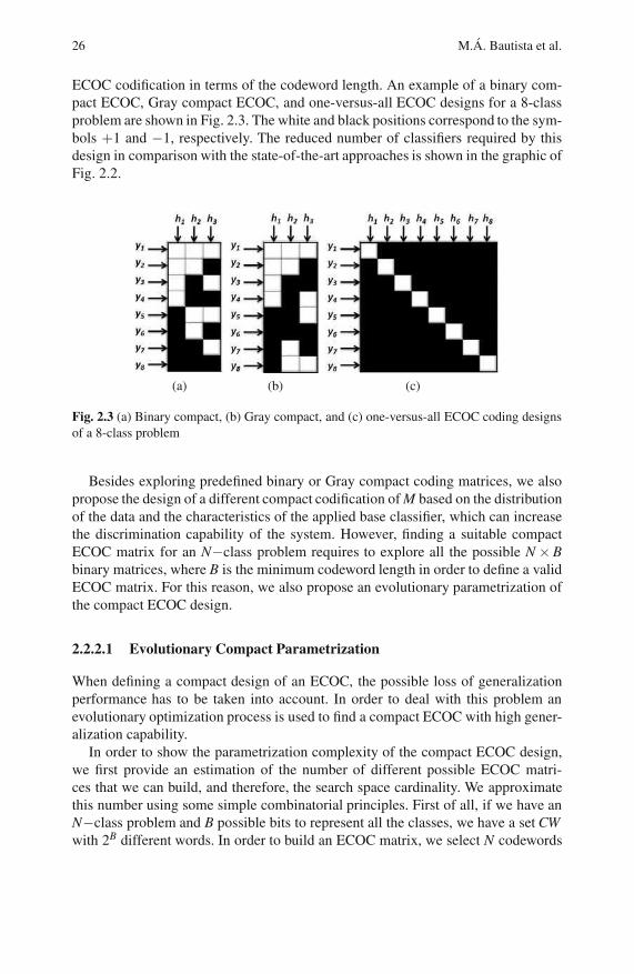
26 M.A. Bautista et al.
ECOC codification in terms of the codeword length. An example of a binary com-
pact ECOC, Gray compact ECOC, and one-versus-all ECOC designs for a 8-class
problem are shown in Fig. 2.3. The white and black positions correspond to the sym-
bols +1 and −1, respectively. The reduced number of classifiers required by this
design in comparison with the state-of-the-art approaches is shown in the graphic of
Fig. 2.2.
(a) (b) (c)
Fig. 2.3 (a) Binary compact, (b) Gray compact, and (c) one-versus-all ECOC coding designs
of a 8-class problem
Besides exploring predefined binary or Gray compact coding matrices, we also
propose the design of a different compact codification of M based on the distribution
of the data and the characteristics of the applied base classifier, which can increase
the discrimination capability of the system. However, finding a suitable compact
ECOC matrix for an N−class problem requires to explore all the possible N ×B
binary matrices, where B is the minimum codeword length in order to define a valid
ECOC matrix. For this reason, we also propose an evolutionary parametrization of
the compact ECOC design.
2.2.2.1 Evolutionary Compact Parametrization
When defining a compact design of an ECOC, the possible loss of generalization
performance has to be taken into account. In order to deal with this problem an
evolutionary optimization process is used to find a compact ECOC with high gener-
alization capability.
In order to show the parametrization complexity of the compact ECOC design,
we first provide an estimation of the number of different possible ECOC matri-
ces that we can build, and therefore, the search space cardinality. We approximate
this number using some simple combinatorial principles. First of all, if we have an
N−class problem and B possible bits to represent all the classes, we have a set CW
with 2B different words. In order to build an ECOC matrix, we select N codewords

2 On the Design of Low Redundancy Error-Correcting Output Codes 27
from CW without replacement. In combinatorics this is represented as(
2B
N
), which
means that we can construct V N2B = 2B!
(2B−N)!different ECOC matrices. Nevertheless,
in the ECOC framework, one matrix and its opposite (swapping all zeros by ones
and vice-versa) are considered as the same matrix, since both represent the same
partitions of the data. Therefore, the approximated number of possible ECOC ma-
trices with the minimum number of classifiers isV N
2B
2 = 2B!2(2B−N)!
. In addition to the
huge cardinality, it is easy to show that this space is neither continuous nor differen-
tiable, because a change in just one bit of the matrix may produce a wrong coding
design.
In this type of scenarios, evolutionary approaches are often introduced with good
results. Evolutionary algorithms are a wide family of methods that are inspired on
the Darwin’s evolution theory, and used to be formulated as optimization processes
where the solution space is neither differentiable nor well defined. In these cases,
the simulation of natural evolution process using computers results in stochastic
optimization techniques which often outperform classical methods of optimization
when applied to difficult real-world problems. Although the most used and studied
evolutionary algorithms are the Genetic Algorithms (GA), from the publication of
the Population Based Incremental Learning (PBIL) in 1995 by Baluja and Caru-
ana [4], a new family of evolutionary methods is striving to find a place in this field.
In contrast to GA, those new algorithms consider each value in the chromosome
as a random variable, and their goal is to learn a probability model to describe the
characteristics of good individuals. In the case of PBIL, if a binary chromosome is
used, a uniform distribution is learned in order to estimate the probability of each
variable to be one or zero.
In this chapter, we report experiments made with the selected evolutionary strate-
gies - i.e. GA and PBIL. Note that for both Evolutionary Strategies, the encoding
step and the adaptation function are exactly equivalent.
Problem encoding: The first step in order to use an evolutionary algorithm is to
define the problem encoding, which consists of the representation of a certain solu-
tion or point in the search space by means of a genotype or alternatively a chro-
mosome [14]. When the solutions or individuals are transformed in order to be
represented in a chromosome, the original values (the individuals) are referred as
phenotypes, and each one of the possible settings for a phenotype is the allele.
Binary encoding is the most common, mainly because the first works about GA
used this type of encoding. In binary encoding, every chromosome is a string of
bits. Although this encoding is often not natural for many problems and some-
times corrections must be performed after crossover and/or mutation, in our case,
the chromosomes represent binary ECOC matrices, and therefore, this encoding
perfectly adapts to the problem. Each ECOC is encoded as a binary chromosome
ζ =< hc11 , . . . ,hc1
B ,hc21 , . . . ,hc2
B , . . . ,hcN1 , . . . ,hcN
B >, where hc j
i ∈ 0,1 is the expected
value of the i− th classifier for the class c j, which corresponds to the i− th bit of
the class c j codeword.

28 M.A. Bautista et al.
Adaptation function: Once the encoding is defined, we need to define the adapta-
tion function, which associates to each individual its adaptation value to the envi-
ronment, and thus, their survival probability. In the case of the ECOC framework,
the adaptation value must be related to the classification error.
Given a chromosome ζ =< ζ0,ζ1, . . . ,ζL > with ζi ∈ 0,1, the first step is to re-
cover the ECOC matrix M codified in this chromosome. The elements of M allow to
create binary classification problems from the original multi-class problem, follow-
ing the partitions defined by the ECOC columns. Each binary problem is addressed
by means of a binary classifier, which is trained in order to separate both partitions
of classes. Assuming that there exists a function y = f (x) that maps each sample x
to its real label y, training a classifier consists of finding the best parameters w∗ of a
certain function y = f ′(x,w), in the manner that for any other w = w∗, f ′(x,w∗) is
a better approximation to f than f ′(x,w). Once the w∗ are estimated for each binary
problem, the adaptation value corresponds to the classification error. In order to take
into account the generalization power of the trained classifiers, the estimation of w∗
is performed over a subset of the samples, while the rest of the samples are reserved
for a validation set, and the adaptation value ξ is the classification error over that
validation subset. The adaptation value for an individual represented by a certain
chromosome ζi can be formulated as:
εi(P,Y,Mi) =∑s
j=1 δ (ρ j,Mi) = y j
s, (2.3)
where Mi is the ECOC matrix encoded in ζi, P = 〈ρ1, . . . ,ρs〉 a set of samples,
Y = 〈y1, . . . ,ys〉 the expected labels for samples in P, and δ is the function that
returns the classification label applying the decoding strategy.
Evolutionary process: Once the encoding and adaptation functions have been de-
fined, we use standard implementation for GA and PBIL, in order to evolve the
compact ECOC matrices. In the case of GA, scattered crossover operator is used,
in which we generate a random binary vector, with a binary value assigned to each
gene. The first child is created using all the genes from the first parent in those posi-
tions with a value of one, and the genes of the second parent with positions with the
value zero. The second child is created as the complementary of the first one. That
is, taking genes from second parent for values one and from first parent for values
zero. In order to introduce variations to the individuals, we use mutation operator
that adds a unit Gaussian distributed random value to the chosen gene. The new
gene value is clipped if it falls outside the user-specified lower or upper bounds for
that gene. For PBIL, the best two individuals of each population are used to update
the probability distribution. At each generation, this probability distribution is used
to sample a new population of individuals. A uniform random noise is applied to the
probability model to avoid convergence to local minima.
Finally, in both evolutionary strategies we adopt an Island Model evolution
scheme in order to exploit a more coarse grain parallel model. The main idea is to
split a population of K individuals into S sub-populations of K/S individuals. If each
sub-population is evolved independently from the others, genetic drift will tend to

2 On the Design of Low Redundancy Error-Correcting Output Codes 29
drive these populations in different directions. By introducing migration, the Island
Model is able to exploit differences in the various sub-populations (this variation in
fact represents a source of genetic diversity). Each sub-population is an island and
there is a chance movement of genetic material from one island to another.
Training the binary classifiers: In [23], Rifkin concludes that the number of clas-
sifiers in the ECOC problem can be reduced by using more accurate classifiers.
Therefore we adopt the Support Vector Machines with Gaussian Radial Basis Func-
tions kernel (SVM-RBF). Training a SVM often implies the selection of a subset of
data points (the support vectors), which are used in order to build the classification
boundaries. In the specific case of Gaussian RBF kernels, we need to optimize the
kernel parameter γ and the regularizer C, which have a close relation to the data dis-
tribution. While the support vectors selection is part of the SVM learning algorithm,
and therefore, is clearly defined, finding the best C and γ is addressed in the litera-
ture with various heuristics or brute-force approaches. The most common approach
is the use of cross-validation processes which select the best pair of parameters for
a discretization of the parameters space. Nevertheless, this can be viewed as another
optimization problem. Therefore, it can be handled using evolutionary algorithms.
For each binary problem, defined by one column of the ECOC matrix, we use Ge-
netic Algorithms in order to find good values for C and γ parameters, using the same
settings as in [17].
This coding optimization process is computationally more expensive than the
standard approaches because for every Compact coding matrix M all the dichotomiz-
ers h1 . . .hn have to be optimized. Nevertheless, large-scale multi-classification
problems, which are typically computationally unfeasible if using standard coding
designs, can be treated with this approach, since this optimization is only applied
for a reduced number of dichotomizers.
In order to save time, a historical of column codification and parameter optimiza-
tion is saved during the evolutionary parametrization process. Let k be a random it-
eration of the optimization and let M =< M1, . . . ,Mind > be the set of Compact cod-
ing matrices to be optimized. Every coding matrix will define a set of bi-partitions
BP =< bp1, . . . ,bpn > to be learned by a set of dichotomizers H =< h1, . . . ,hn >. In
fact, we can assume that a certain bi-partition bps learned by a certain dichotomizer
hs will be repeated among the coding matrices because of the nature of the evolu-
tionary optimization process.
2.3 Results
In order to present the results, first, we discuss the data, methods, and evaluation
measurements of the experiments.
• Data: The first data used for the experiments consists of twelve multi-class
data sets from the UCI Machine Learning Repository database [3]. The number of
training samples, features, and classes per data set are shown in Table 2.1. Then, we
apply the classification methodology in five challenging computer vision categoriza-
tion problems. First, we use the data of the public Labelled Faces in the Wild [15]
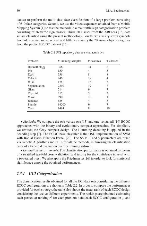
30 M.A. Bautista et al.
dataset to perform the multi-class face classification of a large problem consisting
of 610 face categories. Second, we use the video sequences obtained from a Mobile
Mapping System [1] to test the methods in a real traffic sign categorization problem
consisting of 36 traffic sign classes. Third, 20 classes from the ARFaces [18] data
set are classified using the present methodology. Fourth, we classify seven symbols
from old scanned music scores, and fifth, we classify the 70 visual object categories
from the public MPEG7 data set [25].
Table 2.1 UCI repository data sets characteristics
Problem # Training samples # Features # Classes
Dermathology 366 34 6
Iris 150 4 3
Ecoli 336 8 8
Vehicle 846 18 4
Wine 178 13 3
Segmentation 2310 19 7
Glass 214 9 7
Thyroid 215 5 3
Vowel 990 10 11
Balance 625 4 3
Shuttle 14500 9 7
Yeast 1484 8 10
• Methods: We compare the one-versus-one [13] and one-versus-all [19] ECOC
approaches with the binary and evolutionary compact approaches. For simplicity
we omitted the Gray compact design. The Hamming decoding is applied in the
decoding step [7]. The ECOC base classifier is the OSU implementation of SVM
with Radial Basis Function kernel [20]. The SVM C and γ parameters are tuned
via Genetic Algorithms and PBIL for all the methods, minimizing the classification
error of a two-fold evaluation over the training sub-set.
• Evaluation measurements: The classification performance is obtained by means
of a stratified ten-fold cross-validation, and testing for the confidence interval with
a two-tailed t-test. We also apply the Friedman test [6] in order to look for statistical
significance among the obtained performances.
2.3.1 UCI Categorization
The classification results obtained for all the UCI data sets considering the different
ECOC configurations are shown in Table 2.2. In order to compare the performances
provided for each strategy, the table also shows the mean rank of each ECOC design
considering the twelve different experiments. The rankings are obtained estimating
each particular ranking rji for each problem i and each ECOC configuration j, and

2 On the Design of Low Redundancy Error-Correcting Output Codes 31
Table 2.2 UCI classification results
Data set Binary C. ECOC Evol. C. ECOC One-vs-All ECOC One-vs-One ECOC
Perf. #C. Perf. #C. Perf. #C. Perf. #C.
Derma 96.0±2.9 3 96.3±2.1 3 95.1±3.3 6 94.7±4.3 15Iris 96.4±6.3 2 98.2±1.9 2 96.9±6.0 3 96.3±3.1 3Ecoli 80.5±10.9 3 81.4±10.8 3 79.5±12.2 8 79.2±13.8 28Vehicle 72.5±14.3 2 76.9±12.4 2 74.2±13.4 4 83.6±10.5 6Wine 95.5±4.3 2 97.2±2.3 2 95.5±4.3 3 97.2±2.4 3Segment 96.6±2.3 3 96.6±1.5 3 96.1±1.8 7 97.2±1.3 21Glass 56.7±23.5 3 50.0±29.7 3 53.85±25.8 6 60.5±26.9 15Thyroid 96.4±5.3 2 93.8±5.1 2 95.6±7.4 3 96.1±5.4 3Vowel 57.7±29.4 3 81.8±11.1 3 80.7±11.9 8 78.9±14.2 28Balance 80.9±11.2 2 87.1±9.2 2 89.9±8.4 3 92.8±6.4 3Shuttle 80.9±29.1 3 83.4±15.9 3 90.6±11.3 7 86.3±18.1 21Yeast 50.2±18.2 4 54.7±11.8 4 51.1±18.0 10 52.4±20.8 45Rank & # 2.9 2.7 2.0 2.7 2.7 5.7 2.2 15.9
computing the mean ranking R for each design as R j = 1N ∑i r
ji , where N is the total
number of data sets. We also show the mean number of classifiers (#) required for
each strategy.
In order to analyze if the difference between ranks (and hence, the methods) is
statistically significant, we apply a statistical test. In order to reject the null hypoth-
esis (which implies no significant statistical difference among measured ranks and
the mean rank), we use the Friedman test. The Friedman statistic value is computed
as follows:
X2F =
12N
k(k + 1)
[
∑j
R2j −
k(k + 1)2
4
]
. (2.4)
In our case, with k = 4 ECOC designs to compare, X2F =−4.94. Since this value
is rather conservative, Iman and Davenport proposed a corrected statistic:
FF =(N−1)X2
F
N(k−1)−X2F
. (2.5)
Applying this correction we obtain FF = −1.32. With four methods and twelve
experiments, FF is distributed according to the F distribution with 3 and 33 degrees
of freedom. The critical value of F(3,33) for 0.05 is 2.89. As the value of FF is
no higher than 2.98 we can state that there is no statistically significant difference
among the ECOC schemes. This means that all four strategies are suitable in order
to deal with multi-class categorization problems. This result is very satisfactory and
encourages the use of the compact approach since similar (or even better) results
can be obtained with far less number of classifiers. Moreover, the GA evolutionary
version of the compact design improves in the mean rank to the rest of classical
coding strategies, and in most cases outperforms the binary compact approach in
the present experiment. This result is expected since the evolutionary version looks
for a compact ECOC matrix configuration that minimizes the error over the training

32 M.A. Bautista et al.
data. In particular, the advantage of the evolutionary version over the binary one is
more significant when the number of classes increases, since more compact matrices
are available for optimization.
On the other hand, possible reasons why the evolutionary compact ECOC design
yields similar or even better performance results than the one-versus-one and one-
versus-all approaches can be fewer classifiers considered for tuning and the use of
all the classes in balanced binary problems, which can help the system to increase
generalization if a good decision boundary can be found by the classifier. Note that
the one-versus-one classifier looks for binary problems that split just two classes.
In those cases, though good and fast solutions could be found in training time, the
use of less data does not assure a high generalization capability of the individual
classifiers.
In terms of testing time, since all the trained classifiers spend the same time for
testing, classification time is proportional to the number of trained classifiers. The
mean number of dichotomizers used for each strategy is shown in the last row of Ta-
ble 2.2. Observe the great difference in terms of the number of classifiers between
the compact approaches and the classical ones. The compact approaches obtain an
average speed up improvement of 111% with respect to the one-versus-all approach
in testing time. Meanwhile in the case of the one-versus-one technique this improve-
ment is 489%.
In the next section we test if the same behaviour occurs classifying five challeng-
ing Computer Vision problems with several object categories.
2.3.2 Computer Vision Applications
In this section, we test the methodology on five challenging Computer Vision prob-
lems: faces in the wild, traffic sign, ARface, music scores, and MPEG7 categoriza-
tion data sets.
2.3.2.1 Labelled Faces in the Wild Categorization
This dataset contains 13000 faces images taken directly from the web from over
1400 people. These images are not constrained in terms of pose, light, occlusions
or any other relevant factor. For the purpose of this experiment we used a specific
subset, taking only the categories which at least have four or more examples, having
a total of 610 face categories. Finally, in order to extract relevant features from the
images, we apply an Incremental Principal Component Analysis procedure [16],
keeping 99.8% of the information. An example of face images is shown in Fig. 2.4.
The results in the first row of Table 2.3 show that the best performance is obtained
by the Evolutionary GA and PBIL compact strategies. One important observation is
that Evolutionary strategies outperform the classical one-versus-all approach, with
far less number of classifiers (10 instead of 610). Note that in this case we omitted
the one-vs-one strategy since it requires 185745 classifiers for discriminating 610
face categories.

2 On the Design of Low Redundancy Error-Correcting Output Codes 33
Fig. 2.4 Labelled Faces in the Wild dataset
Table 2.3 Computer Vision data sets classification results
Data set Binary C. ECOC GA. C. ECOC PBIL C. ECOC One-vs-All ECOC One-vs-OneECOC
Perf #C Perf #C Perf #C Perf #C Perf #C
FacesWild 26.4±2.1 10 30.7±2.3 10 30.0±2.4 10 25.0±3.1 610 - 185745Traffic 90.8±4.1 6 90.6±3.4 6 90.7±3.7 6 91.8±4.6 36 90.6±4.1 630ARFaces 76.0±7.2 5 85.8±5.2 5 84.2±5.3 5 84.0±6.3 20 96.0±2.5 190Clefs 81.2±4.2 3 81.8±9.3 3 81.7±8.2 3 80.8±11.2 7 84.2±6.8 21MPEG7 89.3±5.1 7 90.4±4.5 7 90.1±4.9 7 87.8±6.4 70 92.8±3.7 2415Rank & # 3.6 6.2 2.2 6.2 2.8 6.2 3.8 148.6 1.75 37800
2.3.2.2 Traffic Sign Categorization
For this second computer vision experiment, we use the video sequences obtained
from the Mobile Mapping System of [1] to test the ECOC methodology on a real
traffic sign categorization problem. In this system, the position and orientation of
the different traffic signs are measured with video cameras fixed on a moving ve-
hicle. The system has a stereo pair of calibrated cameras, which are synchronized
with a GPS/INS system. The result of the acquisition step is a set of stereo-pairs of
images with their position and orientation information. From this system, a set of 36
circular and triangular traffic sign classes are obtained. Some categories from this
data set are shown in Fig. 2.5. The data set contains a total of 3481 samples of size
32×32, filtered using the Weickert anisotropic filter, masked to exclude the back-
ground pixels, and equalized to prevent the effects of illumination changes. These
feature vectors are then projected into a 100 feature vector by means of PCA.
The classification results obtained when considering the different ECOC con-
figurations are shown in the second row of Table 2.3. The ECOC designs obtain
similar classification results with an accuracy of over 90%. However, note that the
compact methodologies use six times less classifiers than the one-versus-all and 105
less times classifiers than the one-versus-one approach, respectively.
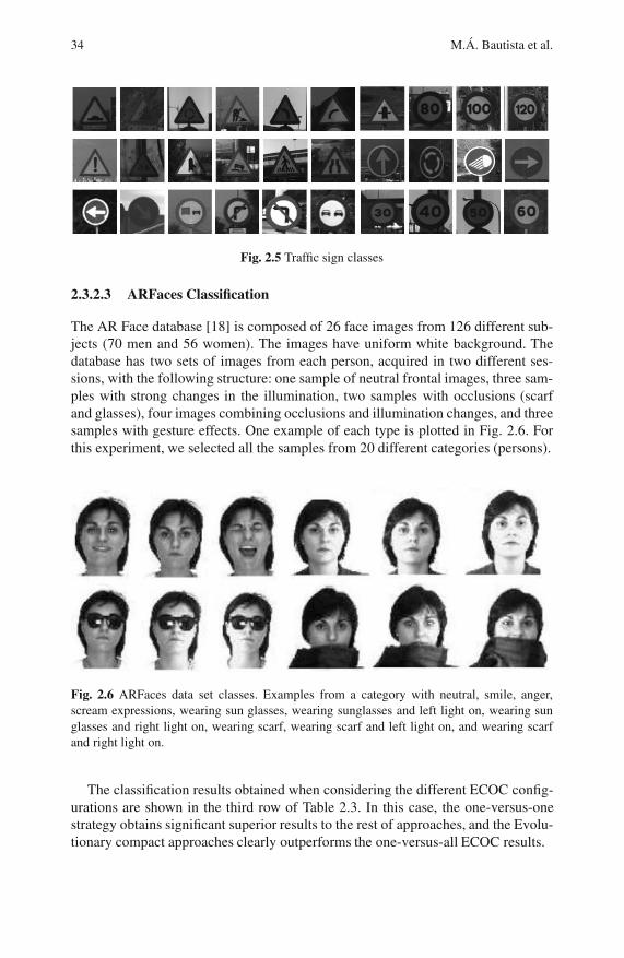
34 M.A. Bautista et al.
Fig. 2.5 Traffic sign classes
2.3.2.3 ARFaces Classification
The AR Face database [18] is composed of 26 face images from 126 different sub-
jects (70 men and 56 women). The images have uniform white background. The
database has two sets of images from each person, acquired in two different ses-
sions, with the following structure: one sample of neutral frontal images, three sam-
ples with strong changes in the illumination, two samples with occlusions (scarf
and glasses), four images combining occlusions and illumination changes, and three
samples with gesture effects. One example of each type is plotted in Fig. 2.6. For
this experiment, we selected all the samples from 20 different categories (persons).
Fig. 2.6 ARFaces data set classes. Examples from a category with neutral, smile, anger,
scream expressions, wearing sun glasses, wearing sunglasses and left light on, wearing sun
glasses and right light on, wearing scarf, wearing scarf and left light on, and wearing scarf
and right light on.
The classification results obtained when considering the different ECOC config-
urations are shown in the third row of Table 2.3. In this case, the one-versus-one
strategy obtains significant superior results to the rest of approaches, and the Evolu-
tionary compact approaches clearly outperforms the one-versus-all ECOC results.

2 On the Design of Low Redundancy Error-Correcting Output Codes 35
2.3.2.4 Clefs and Accidental Data Set Categorization
The data set of clefs and accidental is obtained from a collection of modern and
old musical scores (19th century) of the Archive of the Seminar of Barcelona. The
data set contains a total of 4098 samples among seven different types of clefs and
accidental from 24 different authors. The images have been obtained from original
image documents using a semi-supervised segmentation approach [11]. The main
difficulty of this data set is the lack 389 of a clear class separability because of the
variation of writer styles and the absence of a standard notation. A pair of segmented
samples for each of the seven classes showing the high variability of clefs and acci-
dental appearance from different authors can be observed in Fig. 2.7(a). An example
of an old musical score used to obtain the data samples is shown in Fig. 2.7(b). The
object images are described using the Blurred Shape Model descriptor (BSM).
(a) (b)
Fig. 2.7 (a) Object samples, (b) Old music score
The classification results obtained when considering the different ECOC config-
urations are shown in the fourth row of Table 2.3. In this case, the results are also
comparable for all the strategies, with accuracies upon 80%.
2.3.2.5 MPEG7 Categorization
The MPEG7 data set contains 70 classes with 20 instances per class, which rep-
resents a total of 1400 object images. All samples are described using the Blurred
Shape Model descriptor. Some categories of this data set are shown in Fig. 2.8.
The classification results obtained considering the different ECOC configurations
are shown in the fifth row of Table 2.3. These results are very satisfactory since one
can see very similar results between the evolutionaries and one-versus-one strate-
gies, taking into account that the last approach requires near 350 times the number
of classifiers required by our proposal.
Globally analyzing the results of the Computer Vision classification problems,
whose mean ranks are shown in the last row of Table 2.3, one can see that the one-
versus-one is the first choice, followed by the evolutionary proposals. The last two
positions are for the binary and one-versus-all coding designs.

36 M.A. Bautista et al.
Fig. 2.8 MPEG7 samples
In this case, applying the Friedman statistic, we obtain a value of X2F = −3.71,
and a corrected value of FF = −0.62. With five methods and five Computer Vision
experiments, FF is distributed according to the F distribution with 4 and 16 degrees
of freedom. The critical value of F(4,16) for the 0.05 significance level is 3.01.
As the value of FF is no higher than 3.01 we can state that there is no statistically
significant difference among the ECOC schemes. This means that all five strategies
are suitable in order to deal with multi-class Computer Vision problems with sev-
eral categories. This result also encourages the use of the compact approach. Note
that for example, in the Faces in the Wild experiment the compact ECOC approach
requires 10 classifiers in comparison with the 185745 classifiers required by the
one-versus-one ECOC strategy.
2.4 Conclusion
We presented a general methodology for the classification of several object cate-
gories, which only requires ⌈log2 N⌉ classifiers for a N-class problem. The method-
ology is defined in the Error-Correcting Output Codes framework, designing a com-
pact coding matrix in terms of dichotomizers which unequivocally distinguish N
codes. Moreover, in order to speed up the design of the coding matrix and the tun-
ing of the classifiers, evolutionary computation is also applied.
The results on several public UCI data sets and five multi-class Computer Vision
problems with multiple object categories show that the proposed methodology ob-
tains equivalent results than the state-of-the-art ECOC methodologies. However, it
achieves this with far less number of dichotomizers. For example, our compact ap-
proach trained 10 classifiers to split 610 face categories, meanwhile the one-versus-
all and one-versus-one approaches required 610 and 185745 classifiers, respectively.
Acknowledgements. This work has been supported by projects TIN2009-14404-C02 and
CONSOLIDER-INGENIO CSD 2007-00018.

2 On the Design of Low Redundancy Error-Correcting Output Codes 37
References
1. Alamus, R., Baron, A., Bosch, E., Casacuberta, J., Miranda, J., Pla, M., Sanchez, S.,
Serra, A., Talaya, J.: On the accuracy and performance of the GeoMobil system. In:
Proc. the 20th Congress Int. Soc. Photogrammetry and Remote Sens., Istanbul, Turkey,
pp. 262–267 (2004)
2. Allwein, E., Schapire, R., Singer, Y.: Reducing multiclass to binary: A unifying approach
for margin classifiers. J. Machine Learning Research 1, 113–141 (2002)
3. Asuncion, A., Newman, D.J.: UCI machine learning repository,
http://www.ics.uci.edu/˜mlearn/MLRepository.html4. Baluja, S., Caruana, R.: Removing the genetics from the standard genetic algorithm. In:
Prieditis, A., Russel, S. (eds.) Proc. the 12th Int. Conf. Machine Learning, Tahoe City,
CA, pp. 38–46. Morgan Kaufmann, San Francisco (1995)
5. Crammer, K., Singer, Y.: On the learnability and design of output codes for multi-class
problems. Machine Learning 47, 201–233 (2002)
6. Demsar, J.: Statistical comparisons of classifiers over multiple data sets. J. Machine
Learning Research 7, 1–30 (2006)
7. Dietterich, T., Bakiri, G.: Solving multiclass learning problems via error-correcting out-
put codes. J. Artif. Intel. Research 2, 263–286 (1995)
8. Dietterich, T., Kong, E.: Error-correcting output codes corrects bias and variance. In:
P.A., Russell, S. (eds.) Proc. 12th Int. Conf. Machine Learning, Tahoe City, CA,
pp. 313–321. Morgan Kaufmann, San Francisco (1995)
9. Escalera, S., Pujol, O., Radeva, P.: On the decoding process in ternary error-correcting
output codes. IEEE Trans. Pattern Analysis and Machine Intel. 32, 120–134 (2010)
10. Escalera, S., Pujol, O., Radeva, P.: Error-correcting output codes library. J. Machine
Learning Research 11, 661–664 (2010)
11. Fornes, A., Llados, J., Sanchez, G.: Primitive segmentation in old handwritten mu-
sic scores. In: Liu, W., Llados, J. (eds.) GREC 2005. LNCS, vol. 3926, pp. 279–290.
Springer, Heidelberg (2006)
12. Friedman, J., Hastie, T., Tibshirani, R.: Additive logistic regression: a statistical view of
boosting. The Annals of Statistics 38, 337–374 (1998)
13. Hastie, T., Tibshirani, R.: Classification by pairwise grouping. In: Jordan, M.I., Kearns,
M.J., Solla, S.A. (eds.) Advances in Neural Inf. Proc. Syst., vol. 10, pp. 507–513. MIT
Press, Cambridge (1998)
14. Holland, J.H.: Adaptation in natural and artificial systems: An introductory analysis with
applications to biology, control, and artificial intelligence. MIT Press, Cambridge (1975)
15. Huang, G.B., Ramesh, M., Berg, T., Miller, E.L.: Labeled faces in the wild: A database
for studying face recognition in unconstrained environments. Technical Report, pp. 7–49.
University of Massachusets, Amherst (2007)
16. Hwang, W., Weng, J., Zhang, Y.: Candid covariance-free incremental principal compo-
nent analysis. IEEE Trans. Pattern Analysis and Machine Intel. 25, 1034–1040 (2003)
17. Lorena, A.-C., de Carvalho, A.C.P.L.F.: Evolutionary tuning of svm parameter values in
multiclass problems. Neurocomputing 71, 3326–3334 (2008)
18. Martınez, A., Benavente, R.: The AR face database. Computer Vision Center Technical
Report 24, University of Barcelona (1998)
19. Nilsson, N.J.: Learning machines: Foundations of trainable pattern-classifying systems.
McGraw-Hill, New York (1965)
20. OSU-SVM-TOOLBOX, http://svm.sourceforge.net/21. Passerini, A., Pontil, M., Frasconi, P.: New results on error correcting output codes of
kernel machines. IEEE Trans. Neural Networks 15, 45–54 (2004)

38 M.A. Bautista et al.
22. Pujol, O., Radeva, P., Vitria, J.: Discriminant ECOC: A heuristic method for application
dependent design of error correcting output codes. IEEE Trans. Pattern Analysis and
Machine Intel. 28, 1001–1007 (2006)
23. Rifkin, R., Klautau, A.: In defense of one-vs-all classification. J. Machine Learning Re-
search 5, 101–141 (2004)
24. Utschick, W., Weichselberger, W.: Stochastic organization of output codes in multiclass
learning problems. Neural Computation 13, 1065–1102 (2004)
25. http://www.cis.temple.edu/latecki/research.html
Chapter 3
Minimally-Sized Balanced DecompositionSchemes for Multi-class Classification
Evgueni N. Smirnov, Matthijs Moed, Georgi Nalbantov,
and Ida Sprinkhuizen-Kuyper
Abstract. Error-Correcting Output Coding (ECOC) is a well-known class of de-
composition schemes for multi-class classification. It allows representing any multi-
class classification problem as a set of binary classification problems. Due to code
redundancy ECOC schemes can significantly improve generalization performance
on multi-class classification problems. However, they can face a computational-
complexity problem when the number of classes is large.
In this paper we address the computational-complexity problem of the decompo-
sition schemes. We study a particular class of minimally-sized ECOC decomposi-
tion schemes, namely the class of minimally-sized balanced decomposition schemes
(MBDSs) [14]. We show that MBDSs do not face a computational-complexity prob-
lem for large number of classes. However we also show that MBDSs cannot correct
the classification errors of the binary classifiers in MBDS ensembles. Therefore we
propose voting with MBDS ensembles (VMBDSs). We show that the generalization
performance of the VMBDSs ensembles improves with the number of MBDS clas-
sifiers. However this number can become large and thus the VMBDSs ensembles
can have a computational-complexity problem as well. Fortunately our experiments
show that VMBDSs are comparable with ECOC ensembles and can outperform
one-against-all ensembles using only a small number of MBDS ensembles.
Evgueni N. Smirnov ·Matthijs Moed
Department of Knowledge Engineering, Maastricht University, P.O. BOX 616,
6200 MD Maastricht, The Netherlands
E-mail: [email protected],
Georgi Nalbantov
Faculty of Health, Medicine and Life Sciences, Maastricht University, P.O. BOX 616,
6200 MD Maastricht, The Netherlands
E-mail: [email protected]
Ida Sprinkhuizen-Kuyper
Radboud University Nijmegen, Donders Institute for Brain, Cognition and Behaviour,
6525 HR Nijmegen, The Netherlands
E-mail: [email protected]
O. Okun et al. (Eds.): Ensembles in Machine Learning Applications, SCI 373, pp. 39–57.springerlink.com c© Springer-Verlag Berlin Heidelberg 2011
40 E.N. Smirnov et al.
3.1 Introduction
A decomposition scheme for a multi-class classification problem is a mapping from
a class set Y to a set of binary partitions of Y [4, 13]. It allows for representing the
multi-class classification problem as a set of binary classification problems. Thus,
the multi-class classification problem can be solved by a set of binary classifiers that
corresponds to the set of binary classification problems.
A decomposition scheme is applied on two stages [4, 13]: encoding and decod-
ing. During the encoding stage we first generate binary classification problems ac-
cording to the decomposition scheme and then train a binary classifier for each
problem. During the decoding stage we first apply the binary classifiers for a test
instance and then combine the class predictions of these classifiers according to the
decomposition scheme to estimate the class of that instance.
The main family of decomposition schemes is that of Error-Correcting Output
Coding (ECOC) [4]. Due to redundancy in their codes, ECOC schemes can signif-
icantly improve generalization performance on multi-class classification problems.
However this code redundancy can cause a computational-complexity problem for
ECOC schemes: the number of binary classification problems (and hence the num-
ber of classifiers to be trained) can grow exponentially with the number of classes.
Several approaches were proposed to deal with this computational-complexity prob-
lem of ECOC [1, 4, 18]. In essence these approaches try to maximize the diversity
of the binary partitions in ECOC schemes for a fixed scheme size.
In this paper we address the computational-complexity problem of ECOC sche-
mes as well. For that purpose we study ECOC decomposition schemes of minimal
size. In this respect our research differs from previous studies which so far have
only focused on ECOC schemes of a fixed size [1, 4, 18]. In the paper we show that
minimally-sized ECOC decomposition schemes can be viewed as minimally-sized
balanced decomposition schemes (MBDSs). We note that MBDSs were suggested in
[14] but was never studied in detail. This paper provides a deep analysis of MBDSs.
First, we prove that the size of MBDSs equals ⌈log2(|Y |)⌉. This property implies
that the MBDSs ensembles do not have a computational-complexity problem and
thus can be used for classification problems with a large number of classes. Second,
we quantify the space of all possible MBDSs. Third, we analyze the error-correction
properties of MBDSs. We show that: (a) the minimal Hamming distance between
MBDS class code words equals 1, and (b) the Hamming distance between MBDS
class-partition code words equals|Y |2 . Thus MBDSs cannot correct the classification
errors of the binary classifiers in MBDS ensembles.
To enforce error correction, we propose voting with MBDS ensembles, which is
denoted as VMBDSs. We show that the VMBDSs ensembles improve generaliza-
tion performance with the number of MBDS classifiers. However this number can
be large and the VMBDSs ensembles can have a computational-complexity prob-
lem. Fortunately, our experiments demonstrate that VMBDSs are comparable with
ECOC ensembles and can outperform one-against-all ensembles using a small num-
ber of MBDS ensembles.

3 Multi-class Decomposition Schemes 41
The paper is organized as follows. Section 3.2 formalizes the classification prob-
lem. Decomposing multi-class classification problems into binary classification
problems is discussed in Sect. 3.3. Section 3.4 introduces balanced decomposition
schemes, minimally-sized balanced decomposition schemes, and voting based on
these schemes. Experiments are given in Sect. 3.5. Section 3.6 concludes the paper.
3.2 Classification Problem
Let X be a non-empty instance space and Y be a class set of size K greater than 1.
A labeled instance is defined as a tuple (x,y) where x ∈ X and y ∈ Y . Training data
D is a multi-set of labeled instances. Given training data D and test instance x ∈ X ,
the classification problem CP is to find the class of the instance x.
To classify a new instance we need a classifier h : X →Y from a hypothesis space
H. To identify such a classifier in H we need to search in H. The acceptance criterion
is that the final classifier h ∈ H has to classify correctly future instances iid drawn
from the same probability distribution from which D was drawn.
When K = 2, the classification problem is said to be a binary classification prob-
lem BCP. When K > 2, the classification problem is said to be a multi-class classifi-
cation problem MCP. Many classifiers are inherently binary for various reasons [7].
However, many real-world classification problems are multi-class problems. There
are two main approaches for solving a multi-class problem using a binary classi-
fier: direct and indirect. The direct approach is to generalize the binary classifier to
a multi-class classifier (e.g., Support Vector Machines [19] and Boosting [6]). The
indirect approach is to employ decomposition schemes (e.g., ECOC [4, 13]).
3.3 Decomposing Multi-class Classification Problems
This section considers the main elements needed for decomposing a multi-class
classification problem into a set of binary problems: the decomposition scheme, the
encoding stage, and the decoding stage. More precisely, Sect. 3.3.1 formalizes the
concept of decomposition scheme and presents two of the most well-known decom-
position schemes. Section 3.3.2 provides a detailed explanation of the encoding and
decoding stages.
3.3.1 Decomposition Schemes
Consider a multi-class classification problem MCP determined on a class set Y of
size K > 2. To show how to decompose MCP into L binary classification problems
BCPl we define the notion of a binary class partition in Definition 3.1.

42 E.N. Smirnov et al.
Definition 3.1. (Binary Class Partition) Given a class set Y , the set P(Y ) is said to
be a binary class partition of Y iff P(Y ) consists of two non-empty sets Y− and Y +
such that Y−∪Y + = Y and Y−∩Y+ = /0.
Definition 3.1 allows us to introduce the notion of a decomposition scheme. A de-
composition scheme describes how to decompose a multi-class classification prob-
lem MCP into L binary classification problems BCPl , as given in Definition 3.2.
Definition 3.2. (Decomposition Scheme) Given a multi-class classification prob-
lem MCP and positive integer L, the decomposition scheme of MCP is a set SP(Y )of L binary class partitions Pl(Y ) such that for any two classes y1,y2 ∈ Y there ex-
ists a binary class partition Pm(Y ) ∈ SP(Y) so that ¬(y1,y2 ∈ Y−m )∧¬(y1,y2 ∈ Y +m )
where Y−m ,Y +m ∈ Pm(Y ).
By Definition 3.2 any decomposition scheme SP(Y ) consists of L binary class par-
titions Pl(Y ). The partitions Pl(Y ) ∈ SP(Y ) are chosen so that each class y ∈ Y can
be uniquely determined.
A natural representation for a decomposition scheme SP(Y ) is a decomposition
matrix M. The matrix M is defined as a binary matrix −1,+1K×L. Its encoding is
realized according to the following rule:
Mk,l =
−1 if class yk ∈ Y belongs to Y−l of Pl(Y );
+1 if class yk ∈ Y belongs to Y +l of Pl(Y ).
(3.1)
The rows of M form class code words wykcorresponding to the K classes in the class
set Y . The columns of M form class-partition code words wPl(Y ) corresponding to
the L binary class partitions Pl(Y ).Decomposition matrices have certain column and row properties that follow from
Definition 3.2. These properties are formulated in Corollary 3.1 and Corollary 3.2
below.
Corollary 3.1. Any two columns M∗,l and M∗,m in a matrix M of any decomposition
scheme SP(Y) are different if l = m.
Proof. By Definition 3.2 the decomposition scheme SP(Y ) is a set. This implies
that, if l = m, the columns columns M∗,l and M∗,m represent different class partitions
in SP(Y ). Thus, M∗,l and M∗,m are different.
Corollary 3.2. Any two rows Mk,∗ and Mo,∗ of a matrix M of any decomposition
scheme SP(Y) are different if k = o.
Proof. Given the decomposition scheme SP(Y ), by Definition 3.2 for any two
classes yk,yo ∈ Y there exists a binary class partition Pm(Y ) ∈ SP(Y) such that
¬(yk,yo ∈ Y−m )∧¬(yk,yo ∈ Y +m ) where Y−m ,Y +
m ∈ Pm(Y ). Thus, the rows Mk,∗ and
Mo,∗ differ at least for the position corresponding to the class partition Pm(Y ).
Any two decomposition matrices are equivalent if they represent the same decom-
position scheme SP(Y). By Theorem 3.1, given below, any two decomposition ma-
trices M and M′ are equivalent iff the columns of M′ are a permutation and/or com-
plements of the columns of M.
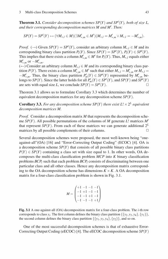
3 Multi-class Decomposition Schemes 43
Theorem 3.1. Consider decomposition schemes SP(Y ) and SP′(Y ), both of size L,
and their corresponding decomposition matrices M and M′. Then:
SP(Y) = SP′(Y )↔ (∀M∗,l ∈M)(∃M′∗,m ∈M′)(M∗,l = M′
∗,m∨M∗,l =−M′∗,m).
Proof. (→) Given SP(Y) = SP′(Y ), consider an arbitrary column M∗,l ∈M and its
corresponding binary class partition Pl(Y ). Since SP(Y ) = SP′(Y ), Pl(Y ) ∈ SP′(Y ).This implies that there exists a column M′
∗,m ∈M′ for Pl(Y ). Thus, M∗,l equals either
M′∗,m or −M′
∗,m.
(←) Consider an arbitrary column M∗,l ∈M and its corresponding binary class par-
tition P(Y ). There exists a column M′∗,m ∈M′ such that either M∗,l = M′
∗,m or M∗,l =−M′
∗,m. Thus, the binary class partition P′m(Y ) ∈ SP′(Y ) represented by M′∗,m be-
longs to SP(Y ). Since the latter holds for all P′m(Y ) ∈ SP′(Y ), and SP(Y ) and SP′(Y )are sets with equal size L, we conclude SP(Y) = SP′(Y ).
Theorem 3.1 allows us to formulate Corollary 3.3 which determines the number of
equivalent decomposition matrices for any decomposition scheme SP(Y).
Corollary 3.3. For any decomposition scheme SP(Y) there exist L!×2L equivalent
decomposition matrices M.
Proof. Consider a decomposition matrix M that represents the decomposition sche-
me SP(Y ). All possible permutations of the columns of M generate L! matrices M′
that represent SP(Y ). From each of these matrices we can generate additional 2L
matrices by all possible complements of their columns.
Several decomposition schemes were proposed, the most well-known being “one-
against-all”(OA) [16] and “Error-Correcting Output Coding” (ECOC) [4]. OA is
a decomposition scheme SP(Y ) that consists of all possible binary class partitions
P(Y ) ∈ SP(Y) containing a class set with size equal to 1. In other words, OA de-
composes the multi-class classification problem MCP into K binary classification
problems BCPl such that each problem BCPl consists of discriminating between one
particular class and all other classes. Hence any decomposition matrix correspond-
ing to the OA decomposition scheme has dimensions K×K. A OA decomposition
matrix for a four-class classification problem is shown in Fig. 3.1.
M =
⎛
⎜⎜⎝
+1 −1 −1 −1
−1 +1 −1 −1
−1 −1 +1 −1
−1 −1 −1 +1
⎞
⎟⎟⎠
Fig. 3.1 A one-against-all (OA) decomposition matrix for a four-class problem. The i-th row
corresponds to class yi. The first column defines the binary class partition y2,y3,y4,y1,the second column defines the binary class partition y1,y3,y4,y2, and so on.
One of the most successful decomposition schemes is that of exhaustive Error-
Correcting Output Coding (eECOC) [4]. The eECOC decomposition scheme SP(Y )
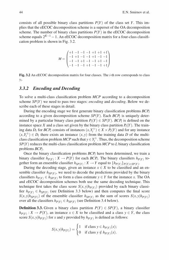
44 E.N. Smirnov et al.
consists of all possible binary class partitions P(Y ) of the class set Y . This im-
plies that the eECOC decomposition scheme is a superset of the OA decomposition
scheme. The number of binary class partitions P(Y ) in the eECOC decomposition
scheme equals 2K−1−1. An eECOC decomposition matrix for a four-class classifi-
cation problem is shown in Fig. 3.2.
M =
⎛
⎜⎜⎝
+1 −1 −1 −1 +1 +1 +1
−1 +1 −1 −1 +1 −1 −1
−1 −1 +1 −1 −1 +1 −1
−1 −1 −1 +1 −1 −1 +1
⎞
⎟⎟⎠
Fig. 3.2 An eECOC decomposition matrix for four classes. The i-th row corresponds to class
yi.
3.3.2 Encoding and Decoding
To solve a multi-class classification problem MCP according to a decomposition
scheme SP(Y ) we need to pass two stages: encoding and decoding. Below we de-
scribe each of these stages in detail.
During the encoding stage we first generate binary classification problems BCPl
according to a given decomposition scheme SP(Y). Each BCPl is uniquely deter-
mined by a particular binary class partition Pl(Y ) ∈ SP(Y ). BCPl is defined on the
instance space X and a class set given by the binary class partition Pl(Y ). The train-
ing data Dl for BCPl consists of instances (x,Y±l ) ∈ X ×Pl(Y ) and for any instance
(x,Y±l ) ∈ Dl there exists an instance (x,y) from the training data D of the multi-
class classification problem MCP such that y∈Y±l . Thus, the decomposition scheme
SP(Y ) reduces the multi-class classification problem MCP to L binary classification
problems BCPl.
Once the binary classification problems BCPl have been determined, we train a
binary classifier hP(Y) : X → P(Y ) for each BCPl . The binary classifiers hP(Y) to-
gether form an ensemble classifier hSP(Y) : X → Y equal to hP(Y)P(Y)∈SP(Y ).
During the decoding stage, given an instance x ∈ X to be classified and an en-
semble classifier hSP(Y), we need to decode the predictions provided by the binary
classifiers hP(Y) ∈ hSP(Y) to form a class estimate y ∈ Y for the instance x. The OA
and eECOC decomposition schemes both use the same decoding technique. This
technique first takes the class score S(x,y|hP(Y)) provided by each binary classi-
fier hP(Y) ∈ hSP(Y) (see Definition 3.3 below) and then computes the final score
S(x,y|hSP(Y)) of the ensemble classifier hSP(Y) as the sum of scores S(x,y|hP(Y))over all the classifiers hP(Y) ∈ hSP(Y) (see Definition 3.4 below).
Definition 3.3. Given a binary class partition P(Y ) ∈ SP(Y ), a binary classifier
hP(Y) : X → P(Y ), an instance x ∈ X to be classified and a class y ∈ Y , the class
score S(x,y|hP(Y)) for x and y provided by hP(Y) is defined as follows:
S(x,y|hP(Y)) =
1 if class y ∈ hP(Y)(x);
0 if class y /∈ hP(Y)(x).

3 Multi-class Decomposition Schemes 45
Definition 3.4. Given a decomposition scheme SP(Y), an ensemble classifier hSP(Y),
an instance x∈X to be classified and a class y∈Y , the total class score S(x,y|hSP(Y))for x and y provided by hSP(Y) is defined as follows:
S(x,y|hSP(Y)) = ∑P(Y)∈SP(Y)
S(x,y|hP(Y)). (3.2)
Traditionally, decoding is explained using decomposition matrices [4]. In this case
for any test instance x∈ X the predictions hP(Y)(x) provided by the binary classifiers
are first mapped to either the number -1 or the number +1 according to the column
of a decomposition matrix M corresponding to P(Y ). Then the resulting numbers
are combined into a class code word w according to the order of the columns in
M. This class code word w is compared against each class code word in M and the
test instance x receives as final classification the class whose code word is closest
according to the Hamming distance. As an example let us consider the eECOC
decomposition matrix shown in Fig. 3.2. Assume that the classifiers return the class
code word w = “-1 +1 -1 -1 -1 -1 -1” for a test instance x ∈ X . Then in
the matrix M from Fig. 3.2 the class code word nearest to w would be “-1 +1 -1-1 +1 -1 -1” with a Hamming distance of 1. Hence, the instance x would be
assigned the class y2.
In order to design an accurate ensemble classifier hSP(Y) a decomposition matrix
M has to satisfy two properties [17]:
• Row separation: any class code word Mk,∗ in M should be well-separated from
all other class code words Mm,∗ in terms of Hamming distance.
• Column separation: any class-partition code word M∗,l in M should be well-
separated from many other class-partition code words M∗,n and their comple-
ments −M∗,n in terms of Hamming distance.
The first property implies that the ensemble classifier hSP(Y) will be capable of cor-
recting the errors of ⌊Hmin−12 ⌋ binary classifiers hP(Y) ∈ hSP(Y) where Hmin is the
minimum Hamming distance between any pair of class code words in the decom-
position matrix M. The second property aims at minimally correlating the errors of
the binary classifiers hP(Y) ∈ hSP(Y), thus minimizing the number of the binary clas-
sifiers hP(Y) which predictions have to be corrected. Kong and Dietterich showed
experimentally in [9] that the bias and variance components of the error of the en-
semble classifier hSP(Y) are reduced by increasing the Hamming distance between all
class code words and as many as possible class-partition code words. Increasing the
Hamming distance of class code words can be achieved by introducing additional
code redundancy, i.e. by increasing the number L of columns in the decomposition
matrix M. In the extreme case of the eECOC decomposition scheme this leads to
L equal to 2K−1−1. Thus, code redundancy can cause a computational-complexity
problem for ECOC schemes: the number of binary classification problems (classi-
fiers) can grow exponentially with the number of classes. Several approaches to the

46 E.N. Smirnov et al.
computational-complexity problem of ECOC were proposed [1, 4, 18]. In essence
they try to design ECOC schemes that maximize the minimum Hamming distance
between class code words and class-partition code words for a fixed scheme size L.
3.4 Balanced Decomposition Schemes and Their
Minimally-Sized Variant
In this section we address the computational-complexity problem of ECOC schemes.
In contrast with the previous research we focus on ECOC decomposition schemes
of minimal size. We show that these schemes belong to the class of balanced de-
composition schemes. Therefore, in Subsection 3.4.1 we first introduce balanced
decomposition schemes. Then in Subsection 3.4.2 we study minimally-sized ECOC
schemes considered as minimally-sized balanced decomposition schemes. Finally
in Subsection 3.4.3 we propose voting based on minimally-sized balanced decom-
position schemes.
3.4.1 Balanced Decomposition Schemes
Balanced decomposition schemes are a subclass of decomposition schemes that are
based on balanced binary class partitions. The concept of balanced binary class
partitions is provided in Definition 3.5 given below.
Definition 3.5. (Balanced Binary Class Partitions) If the number K of classes in
a class set Y is even, then a binary class partition P(Y ) = Y−,Y + is said to be
balanced iff |Y−|= |Y+|.
The number of all balanced binary class partitions is provided in Corollary 3.4 given
below.
Corollary 3.4. The number of all balanced binary class partitions P(Y ) equalsK!
2( K2 !)2 .
Proof. The number of all balanced binary class partitions P(Y ) is 12
(KK2
)= K!
2( K2 !)2 .
Given the concept of balanced binary class partitions we define the concept of bal-
anced decomposition schemes in Definition 3.6 below.
Definition 3.6. (Balanced Decomposition Schemes) A decomposition scheme de-
noted as SP(Y) is said to be balanced iff each binary class partition P(Y ) ∈ SP(Y )is balanced.
Theorem 3.2, given below, states that the class of balanced decomposition schemes
is non-empty. More precisely we show that by using balanced binary class partitions
we can design a decomposition scheme.

3 Multi-class Decomposition Schemes 47
Theorem 3.2. There exists a set SP(Y) of balanced binary class partitions such that
SP(Y ) is a decomposition scheme.
Proof. Consider a set SP(Y) of balanced binary class partitions such that for each
two classes yi,y j ∈ Y there exists a balanced binary partition Y+,Y− ∈ SP(Y) for
which ¬(yi,y j ∈Y−)∧¬(yi,y j ∈Y +). By definition 3.2 the set SP(Y) is a decompo-
sition scheme.
Balanced decomposition schemes have an important practical property: they do not
introduce additional imbalance in the training data of the binary classifiers hP(Y)
in the ensemble classifier hSP(Y). By Definition 3.5 this is due to the fact that the
data of these classifiers are based on balanced class binary partitions P(Y ). In this
respect balanced decomposition schemes differ from other decomposition schemes
(e.g., OA, eECOC).
3.4.2 Minimally-Sized Balanced Decomposition Schemes
Minimally-sized balanced decomposition schemes (MBDSs) are balanced decom-
position schemes of minimal size. This type of decomposition schemes was sug-
gested by Mayoraz & Moreira [14] but was never studied in detail. This subsection
provides the definition of MBDSs and their properties.
Definition 3.7. (Minimally-Sized Balanced Decomposition Schemes) Given the
set SPM(Y ) of all balanced binary class partitions, a balanced decomposition scheme
SP(Y ) ⊆ SPM(Y ) is said to be minimally-sized iff there does not exist another bal-
anced decomposition scheme SP′(Y )⊆ SPM(Y ) such that |SP′(Y )|< |SP(Y )|.
Notation 1. A minimally-sized balanced decomposition scheme is denoted by
SPm(Y ).
Theorem 3.3 below determines the size of MBDSs as a function of the number K of
classes.
Theorem 3.3. A balanced decomposition scheme SP(Y) is minimally-sized iff the
size of SP(Y) equals ⌈log2(K)⌉.
Proof. (→) Consider a minimally-sized balanced decomposition scheme SP(Y ).Any decomposition matrix M of SP(Y ) represents a minimally-sized binary code
for K classes. The size of that code is ⌈log2(K)⌉.Thus, the size of SP(Y) equals
⌈log2(K)⌉.(←) Consider a balanced decomposition scheme SP(Y ) with size of ⌈log2(K)⌉. Any
decomposition matrix M of SP(Y ) represents a binary code for K classes and the size
of this code is ⌈log2(K)⌉. Thus, the code is minimally-sized. This implies that SP(Y )is minimally-sized.

48 E.N. Smirnov et al.
Corollary 3.5. Any decomposition matrix M of a minimally-sized balanced decom-
position scheme SP(Y )m forms a minimally-sized binary code for K classes.
For a multi-class classification problem we can define different minimally-sized bal-
anced decomposition schemes MBDSs. To characterize the number of all possible
MBDSs, we first determine the number of decomposition matrices of all possible
MBDSs (see Corollary 3.6) and then the number of equivalent decomposition ma-
trices for a MBDS (see Corollary 3.7). The ratio of these two numbers is the number
of all possible MBDSs stated in Theorem 3.4 below.
Corollary 3.6. If K is a power of 2, then the number of decomposition matrices of
all possible minimally-sized balanced decomposition schemes equals K!.
Proof. This follows from the fact that for K a power of 2 there are exactly K
different class code words which can be assigned to the classes in K! different
ways.
Corollary 3.7. If K is a power of 2, then there exists log2(K)!K number of equiv-
alent decomposition matrices M for any minimally-sized balanced decomposition
scheme SP(Y) .
Proof. The proof follows from Theorem 3.1.
Theorem 3.4. If K is a power of 2, then the number of all possible minimally-sized
balanced decomposition schemes SPm(Y ) equals(K−1)!log2(K)! .
Proof. By Corollary 3.6 there exist K! decomposition matrices of all possible
MBDSs. By Corollary 3.7 for any MBDS there exist log2(K)!K equivalent decom-
position matrices. Thus, the number of all possible MBDSs equals:
K!
log2(K)!K=
(K−1)!
log2(K)!.
The decoding stage for the MBDSs is realized according to Definition 3.4. In this
context we determine the (minimal) Hamming distance of class code words and
class-partition code words in decomposition matrices of MBDSs in Corollary 3.8.
Corollary 3.8. If the number K of classes is a power of 2, then for any decomposi-
tion matrix M of a minimally-sized balanced decomposition scheme SPm(Y ):
(1) the minimal Hamming distance between different rows Mk,∗ and Mo,∗ of M is
equal to 1, and
(2) the Hamming distance between any two different columns M∗,l and M∗,m of M
is equal to K2 .
Proof. By Corollary 3.5 the rows of any decomposition matrix M of a minimally-
sized balanced decomposition scheme SP(Y ) forms a minimally-sized binary code
for K classes. The properties (1) and (2) are properties of such a code.

3 Multi-class Decomposition Schemes 49
The results from Corollary 3.8 directly imply that:
• The row separation property does not hold for MBDSs. This is due to the fact
that the minimum Hamming distance between class code words in any decompo-
sition matrix corresponding to any MBDS equals one. Thus, the ensemble classi-
fiers hSP(Y) based on these decomposition schemes are not capable of correcting
errors of the binary classifiers hP(Y) ∈ hSP(Y).
• The column separation property does hold for the MBDSs. This is due to the
fact that the Hamming distance of the class-partition code words in any decom-
position matrix corresponding to any minimally-sized balanced decomposition
scheme equals K2 (the maximal possible distance). Thus, we expect that the er-
rors of the binary classifiers hP(Y) ∈ hSP(Y) are minimally correlated.
From the above we conclude that MBDSs have an error-correction problem; i.e.,
MBDSs do not have error-correction capabilities. Nevertheless, when the number of
classes is very large, MBDSs can be a viable alternative to the eECOC decomposi-
tion scheme. This is due to the fact that they do not have a computational-complexity
problem. We note that by Theorem 3.3 the number of the binary classifiers hP(Y) in
any MBDS ensemble hSP(Y) equals ⌈log2(K)⌉.
3.4.3 Voting Using Minimally-Sized Balanced Decomposition
Schemes
This subsection addresses the error-correction problem of MBDSs. To enforce error-
correction we propose to vote with ensemble classifiers hSP(Y) based on different
MBDSs. This approach is called Voting using Minimally-Sized Balanced Decom-
position Schemes (VMBDSs) and it is considered below.
Let SSP(Y) be a set of N randomly-chosen minimally-sized balanced decom-
position schemes SPm(Y ). Each minimally-sized balanced decomposition scheme
SPm(Y ) defines a classifier hSPm(Y ). The classifiers hSPm(Y ) form an ensemble classi-
fier hSSP(Y ) : X →Y equal to hSPm(Y)SPm(Y )∈SSP(Y). Decoding the predictions of the
classifiers hSPm(Y ) into the prediction of hSSP(Y ) is realized for any test instance x∈X
and class y ∈ Y by computing an integer score S(x,y|hSSP(Y)). This computation is
a two-stage process: first we take the class score S(x,y|hSPm(Y )) provided by each
classifier hSPm(Y ) (see Definition 3.4) and then compute the score S(x,y|hSSP(Y)) as
the sum of scores S(x,y|hSPm(Y )) over all the classifiers hSPm(Y ) (see Definition 3.8).
Definition 3.8. Given a set SSP(Y) of minimally-sized balanced decomposition
schemes SPm(Y ), a test instance x ∈ X , and a class y ∈ Y , the score S(x,y|hSSP(Y))for x and y provided by the ensemble classifier hSSP(Y) is defined as follows:
S(x,y|hSSP(Y)) = ∑SPm(Y )∈SSP(Y )
S(x,y|hSPm(Y)). (3.3)
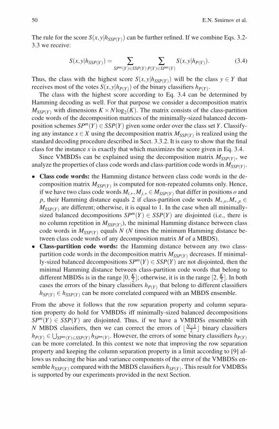
50 E.N. Smirnov et al.
The rule for the score S(x,y|hSSP(Y)) can be further refined. If we combine Eqs. 3.2-
3.3 we receive:
S(x,y|hSSP(Y)) = ∑SPm(Y )∈SSP(Y)
∑P(Y )∈SPm(Y )
S(x,y|hP(Y)). (3.4)
Thus, the class with the highest score S(x,y|hSSP(Y)) will be the class y ∈ Y that
receives most of the votes S(x,y|hP(Y)) of the binary classifiers hP(Y).
The class with the highest score according to Eq. 3.4 can be determined by
Hamming decoding as well. For that purpose we consider a decomposition matrix
MSSP(Y ) with dimensions K×N log2(K). The matrix consists of the class-partition
code words of the decomposition matrices of the minimally-sized balanced decom-
position schemes SPm(Y ) ∈ SSP(Y) given some order over the class set Y . Classify-
ing any instance x ∈ X using the decomposition matrix MSSP(Y) is realized using the
standard decoding procedure described in Sect. 3.3.2. It is easy to show that the final
class for the instance x is exactly that which maximizes the score given in Eq. 3.4.
Since VMBDSs can be explained using the decomposition matrix MSSP(Y ), we
analyze the properties of class code words and class-partition code words in MSSP(Y ).
• Class code words: the Hamming distance between class code words in the de-
composition matrix MSSP(Y ) is computed for non-repeated columns only. Hence,
if we have two class code words Mi,∗,M j,∗ ∈MSSP(Y ) that differ in positions o and
p, their Hamming distance equals 2 if class-partition code words M∗,o,M∗,p ∈MSSP(Y) are different; otherwise, it is equal to 1. In the case when all minimally-
sized balanced decompositions SPm(Y ) ∈ SSP(Y) are disjointed (i.e., there is
no column repetition in MSSP(Y)), the minimal Hamming distance between class
code words in MSSP(Y ) equals N (N times the minimum Hamming distance be-
tween class code words of any decomposition matrix M of a MBDS).
• Class-partition code words: the Hamming distance between any two class-
partition code words in the decomposition matrix MSSP(Y) decreases. If minimal-
ly-sized balanced decompositions SPm(Y ) ∈ SSP(Y) are not disjointed, then the
minimal Hamming distance between class-partition code words that belong to
different MBDSs is in the range [0, K2 ]; otherwise, it is in the range [2, K
2 ]. In both
cases the errors of the binary classifiers hP(Y) that belong to different classifiers
hSP(Y) ∈ hSSP(Y) can be more correlated compared with an MBDS ensemble.
From the above it follows that the row separation property and column separa-
tion property do hold for VMBDSs iff minimally-sized balanced decompositions
SPm(Y ) ∈ SSP(Y) are disjointed. Thus, if we have a VMBDSs ensemble with
N MBDS classifiers, then we can correct the errors of ⌊N−12 ⌋ binary classifiers
hP(Y) ∈⋃
SPm(Y )∈SSP(Y) hSPm(Y ). However, the errors of some binary classifiers hP(Y)
can be more correlated. In this context we note that improving the row separation
property and keeping the column separation property in a limit according to [9] al-
lows us reducing the bias and variance components of the error of the VMBDSs en-
semble hSSP(Y ) compared with the MBDS classifiers hSP(Y). This result for VMDBSs
is supported by our experiments provided in the next Section.
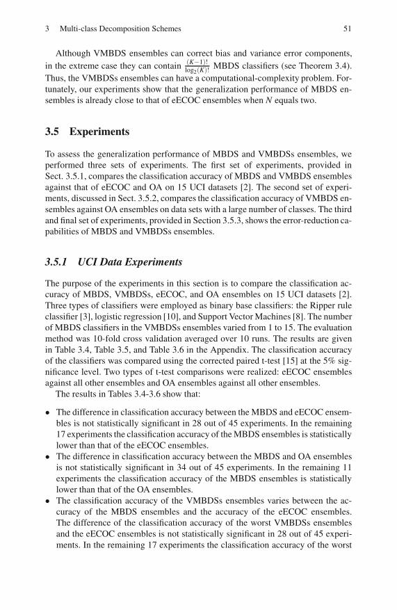
3 Multi-class Decomposition Schemes 51
Although VMBDS ensembles can correct bias and variance error components,
in the extreme case they can contain(K−1)!log2(K)!
MBDS classifiers (see Theorem 3.4).
Thus, the VMBDSs ensembles can have a computational-complexity problem. For-
tunately, our experiments show that the generalization performance of MBDS en-
sembles is already close to that of eECOC ensembles when N equals two.
3.5 Experiments
To assess the generalization performance of MBDS and VMBDSs ensembles, we
performed three sets of experiments. The first set of experiments, provided in
Sect. 3.5.1, compares the classification accuracy of MBDS and VMBDS ensembles
against that of eECOC and OA on 15 UCI datasets [2]. The second set of experi-
ments, discussed in Sect. 3.5.2, compares the classification accuracy of VMBDS en-
sembles against OA ensembles on data sets with a large number of classes. The third
and final set of experiments, provided in Section 3.5.3, shows the error-reduction ca-
pabilities of MBDS and VMBDSs ensembles.
3.5.1 UCI Data Experiments
The purpose of the experiments in this section is to compare the classification ac-
curacy of MBDS, VMBDSs, eECOC, and OA ensembles on 15 UCI datasets [2].
Three types of classifiers were employed as binary base classifiers: the Ripper rule
classifier [3], logistic regression [10], and Support Vector Machines [8]. The number
of MBDS classifiers in the VMBDSs ensembles varied from 1 to 15. The evaluation
method was 10-fold cross validation averaged over 10 runs. The results are given
in Table 3.4, Table 3.5, and Table 3.6 in the Appendix. The classification accuracy
of the classifiers was compared using the corrected paired t-test [15] at the 5% sig-
nificance level. Two types of t-test comparisons were realized: eECOC ensembles
against all other ensembles and OA ensembles against all other ensembles.
The results in Tables 3.4-3.6 show that:
• The difference in classification accuracy between the MBDS and eECOC ensem-
bles is not statistically significant in 28 out of 45 experiments. In the remaining
17 experiments the classification accuracy of the MBDS ensembles is statistically
lower than that of the eECOC ensembles.
• The difference in classification accuracy between the MBDS and OA ensembles
is not statistically significant in 34 out of 45 experiments. In the remaining 11
experiments the classification accuracy of the MBDS ensembles is statistically
lower than that of the OA ensembles.
• The classification accuracy of the VMBDSs ensembles varies between the ac-
curacy of the MBDS ensembles and the accuracy of the eECOC ensembles.
The difference of the classification accuracy of the worst VMBDSs ensembles
and the eECOC ensembles is not statistically significant in 28 out of 45 experi-
ments. In the remaining 17 experiments the classification accuracy of the worst

52 E.N. Smirnov et al.
VMBDSs ensembles is statistically lower than that of the eECOC ensembles.
The difference of the classification accuracy of the best VMBDSs ensembles and
the eECOC ensembles is not statistically significant in 44 out of 45 experiments.
In the remaining one experiment the classification accuracy of the best VMBDSs
ensembles is statistically greater than that of the eECOC ensembles.
• The difference of the classification accuracy between the worst VMBDSs ensem-
bles and the OA ensembles is not statistically significant in 34 out of 45 experi-
ments. In the remaining 11 experiments the classification accuracy of the worst
VMBDSs ensembles is statistically lower than that of the eECOC ensembles.
The difference of the classification accuracy of the best VMBDSs ensembles and
the OA ensembles is not statistically significant in 38 out of 45 experiments. In
the next 6 (1) experiments the classification accuracy of the best VMBDSs en-
sembles is statistically greater (lower) than that of the OA ensembles. In addition
we compare the VMBDSs and OA ensembles when they have an approximately
equal number of binary classifiers. In this case we compare the VMBDSs en-
sembles using two MBDS classifiers with the OA ensembles. The results are that
the difference of the classification accuracy of the VMBDSs and OA ensembles
is not statistically significant in 41 out of 45 experiments. In the next 2 (2) ex-
periments the classification accuracy of the VMBDSs ensembles is statistically
greater (lower) than that of the OA ensembles.
From the above we conclude that:
• The MBDS ensembles are the worst ensembles. The experiments confirm that
the MBDS ensembles do not have error-correction capabilities.
• The VMBDSs ensembles perform much better than MBDS ensembles. Their
classification accuracy improves with the number of the MBDS classifiers. The
results confirm that the VMBDSs ensembles do have error-correction capabili-
ties.
• The VMBDSs ensembles are comparable with the eECOC ensembles in terms of
classification accuracy if the number of MBDS ensembles is more than one. In
this case VMBDSs ensembles are more preferable, since they require a smaller
number of binary classifiers.
• The VMBDSs ensembles are comparable with the OA ensembles in terms
of classification accuracy if the number of the MBDS ensembles equals two.
VMBDSs ensembles can outperform the OA ensembles if the number of the
MBDS ensembles is greater than two.
3.5.2 Experiments on Data Sets with Large Number of Classes
The purpose of this section’s experiments is to compare the classification accuracy
of the VMBDSs and OA on three datasets with a large number of classes. The
datasets chosen are Abalone [2], Patents [12], and Faces94 [11]. Several
properties of these datasets are summarized in Table 3.1.

3 Multi-class Decomposition Schemes 53
Table 3.1 Number of instances and classes for the Abalone, Patents, and Faces94datasets
Name #instances #classes
Abalone 4177 28
Patents 2373 70
Faces94 3059 153
The eECOC ensembles were excluded from the experiments, since they require
an exponential number of binary classifiers (in our experiments at least 227− 1).
Support Vector Machines [8] were used as a base classifier. The number of MBDS
classifiers in the VMBDSs ensembles was varied from 5 - 25. The evaluation method
was 5-fold cross validation averaged over 5 runs. The results are presented in Ta-
ble 3.2. The classification accuracy of the classifiers is compared using the corrected
paired t-test [15] at the 5% significance level. The test compares the OA ensembles
against all VMBDSs ensembles.
Table 3.2 Classification Accuracy of SVM-based OA and VMBDSs ensembles on the
Abalone, Patents, and Faces94 datasets. The numbers in the VMBDSs columns in-
dicate the number of MBDS classifiers in the VMBDSs ensemble. Bold numbers indicate
statistically better results with respect to the OA ensembles.
VMBDSs
Data set OA 5 10 25
Abalone 0.023 ± 0.002 8.65 ± 5.31 13.53 ± 4.58 18.05 ± 4.29
Patents 17.23 ± 1.05 19.52 ± 1.81 21.13 ± 1.71 21.54 ± 1.30
Faces94 73.85 ± 4.29 74.98 ± 2.06 87.26 ± 1.21 93.68 ± 0.80
The experimental results from Table 3.2 show that the VMBDSs ensembles can
outperform statistically the OA ensembles on these three datasets. In this respect it
is important to know whether the VMBDSs ensembles outperform the OA ensem-
bles when both types of ensembles contain the same number of binary classifiers;
i.e., when their computational complexities are equal. We show how to organize
this experiment for the Abalone dataset. This dataset has 28 classes. Thus, the
number of binary classifiers in the OA ensemble is 28. This implies that we have to
find a configuration for the VMBDSs ensembles so that the total number of binary
classifiers is close to 28. In this context we note that the number of binary classi-
fiers in each MBDS ensemble is ⌈log2(28)⌉ = 5. Thus, in order to have close to
28 number of binary classifiers we need ⌊ 285 ⌋ = 5 MBDS classifiers. According to
Table 3.2 for this configuration the VMBDSs ensemble outperforms statistically the
OA ensemble. Analogously we can do the same computation for the Patents and
Faces94 datasets: for the Patents dataset we need 10 MBDS classifiers and for
the Faces94 dataset we need 19 MBDS classifiers in the VMBDSs ensemble. Ac-
cording to Table 3.2 for these configurations the VMBDSs ensembles outperform
statistically the OA ensemble.

54 E.N. Smirnov et al.
3.5.3 Bias-Variance Decomposition Experiments
The experiments performed in this section aim at obtaining insight into whether
eECOC and VMBDSs ensembles are able to reduce the generalization error. For
that purpose a bias-variance analysis is performed. We compare the bias, variance
and expected loss of three methods: the Ripper classifier, eECOC ensembles, and
VMBDSs ensembles. The bias-variance decomposition employed is that of Domin-
gos [5]. The binary base classifier for the ensembles is the Ripper classifier. Four
experiments are designed, each for a particular number of classes K ∈ [5,8]. For
each experiment, we use a synthetic data set generated as follows. Instances for
each class are drawn from a multivariate Gaussian distribution over three variables,
with the mean of each distribution located in a fixed octant of the three-dimensional
coordinate system such that none of the distribution means are located in the same
octant. The distributions have unit covariance. For training, 200 data sets of each
200 instances are used. For testing we use a single data set of 5000 instances [9].
The results are given in Table 3.3. They show that if the base classifier is unsta-
ble (e.g. Ripper), the bias and variance components of the error of the VMBDSs
ensembles are reduced. More precisely, the expected loss, bias, and variance of the
VMBDSs ensembles decrease with the number of MBDS classifiers. If the num-
ber of MBDS classifiers in the VMBDSs ensembles is greater than or equal to 5,
the expected loss, bias, and variance of the VMBDSs ensembles are significantly
better than those for the Ripper classifier. If the number of MBDS classifiers in the
VMBDSs ensembles is greater than or equal to 50, the expected loss, bias, and vari-
ance of the VMBDSs ensembles become close to those of the eECOC ensembles.
Table 3.3 Results for the bias-variance decomposition for data sets with 5, 6, 7 and 8 classes.
The numbers in the VMBDSs headers indicate the number of MBDS classifiers in these
ensembles.
# classes Ripper eECOC VMBDSs:1 VMBDSs:5 VMBDSs:50
5
Exp.Loss 0.28 0.20 0.33 0.24 0.21
Bias 0.02 0.02 0.11 0.04 0.02
Var. 0.23 0.14 0.24 0.17 0.15
Noise 0.06 0.06 0.06 0.06 0.06
6
Exp.Loss 0.32 0.21 0.39 0.25 0.23
Bias 0.04 0.03 0.15 0.04 0.02
Var. 0.27 0.16 0.28 0.19 0.18
Noise 0.06 0.06 0.06 0.06 0.06
7
Exp.Loss 0.36 0.21 0.41 0.26 0.22
Bias 0.05 0.03 0.15 0.06 0.04
Var. 0.32 0.16 0.31 0.19 0.17
Noise 0.05 0.05 0.05 0.05 0.05
8
Exp.Loss 0.41 0.24 0.46 0.30 0.25
Bias 0.05 0.02 0.15 0.05 0.03
Var. 0.37 0.19 0.37 0.24 0.21
Noise 0.05 0.05 0.05 0.05 0.05
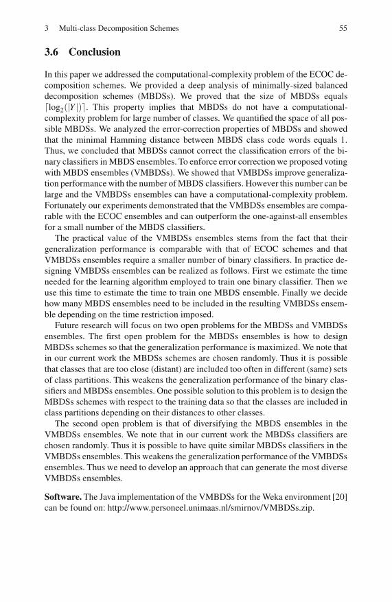
3 Multi-class Decomposition Schemes 55
3.6 Conclusion
In this paper we addressed the computational-complexity problem of the ECOC de-
composition schemes. We provided a deep analysis of minimally-sized balanced
decomposition schemes (MBDSs). We proved that the size of MBDSs equals
⌈log2(|Y |)⌉. This property implies that MBDSs do not have a computational-
complexity problem for large number of classes. We quantified the space of all pos-
sible MBDSs. We analyzed the error-correction properties of MBDSs and showed
that the minimal Hamming distance between MBDS class code words equals 1.
Thus, we concluded that MBDSs cannot correct the classification errors of the bi-
nary classifiers in MBDS ensembles. To enforce error correction we proposed voting
with MBDS ensembles (VMBDSs). We showed that VMBDSs improve generaliza-
tion performance with the number of MBDS classifiers. However this number can be
large and the VMBDSs ensembles can have a computational-complexity problem.
Fortunately our experiments demonstrated that the VMBDSs ensembles are compa-
rable with the ECOC ensembles and can outperform the one-against-all ensembles
for a small number of the MBDS classifiers.
The practical value of the VMBDSs ensembles stems from the fact that their
generalization performance is comparable with that of ECOC schemes and that
VMBDSs ensembles require a smaller number of binary classifiers. In practice de-
signing VMBDSs ensembles can be realized as follows. First we estimate the time
needed for the learning algorithm employed to train one binary classifier. Then we
use this time to estimate the time to train one MBDS ensemble. Finally we decide
how many MBDS ensembles need to be included in the resulting VMBDSs ensem-
ble depending on the time restriction imposed.
Future research will focus on two open problems for the MBDSs and VMBDSs
ensembles. The first open problem for the MBDSs ensembles is how to design
MBDSs schemes so that the generalization performance is maximized. We note that
in our current work the MBDSs schemes are chosen randomly. Thus it is possible
that classes that are too close (distant) are included too often in different (same) sets
of class partitions. This weakens the generalization performance of the binary clas-
sifiers and MBDSs ensembles. One possible solution to this problem is to design the
MBDSs schemes with respect to the training data so that the classes are included in
class partitions depending on their distances to other classes.
The second open problem is that of diversifying the MBDS ensembles in the
VMBDSs ensembles. We note that in our current work the MBDSs classifiers are
chosen randomly. Thus it is possible to have quite similar MBDSs classifiers in the
VMBDSs ensembles. This weakens the generalization performance of the VMBDSs
ensembles. Thus we need to develop an approach that can generate the most diverse
VMBDSs ensembles.
Software. The Java implementation of the VMBDSs for the Weka environment [20]
can be found on: http://www.personeel.unimaas.nl/smirnov/VMBDSs.zip.

56 E.N. Smirnov et al.
References
1. Allwein, E., Schapire, R., Singer, Y.: Reducing multiclass to binary: A unifying approach
for margin classifiers. J. Machine Learning Research 1, 113–141 (2002)
2. Asuncion, A., Newman, D.J.: UCI machine learning repository,
http://www.ics.uci.edu/˜mlearn/MLRepository.html3. Cohen, W.: Fast effective rule induction. In: Prieditis, A., Russell, R. (eds.) Proc. the
12th Int. Conf. Machine Learning, Tahoe City, CA, pp. 115–123. Morgan Kaufmann,
San Francisco (1995)
4. Dietterich, T.G., Bakiri, G.: Solving multiclass learning problems via error-correcting
output codes. J. Artif. Intell. Research 2, 263–286 (1995)
5. Domingos, P.: A unified bias-variance decomposition for zero-one and squared loss. In:
Kautz, H., Porter, B. (eds.) Proc. the 17th National Conf. Artif. Intell. and 12th Conf.
Innovative Applications Artif. Intell., pp. 564–569. AAAI Press, Menlo Park (2000)
6. Freund, Y., Schapire, R.: A decision-theoretic generalization of on-line learning and an
application to boosting. J. Comp. Syst. Sci. 55, 119–139 (1997)
7. Furnkranz, J.: Round robin classification. J. Machine Learning Research 2, 721–747
(2002)
8. Keerthi, S.S., Shevade, S.K., Bhattacharyya, C., Murthy, K.R.K.: Improvements to Platt’s
SMO algorithm for SVM classifier design. Neural Comp. 13, 637–649 (2001)
9. Kong, E.B., Dietterich, T.G.: Error-correcting output coding corrects bias and variance.
In: Prieditis, A., Russell, S.J. (eds.) Proc. the 12th Int. Conf. Machine Learning, Tahoe
City, CA, pp. 313–321. Morgan Kaufmann, San Francisco (1995)
10. le Cessie, S., van Houwelingen, J.C.: Ridge estimators in logistic regression. Applied
Statistics 41, 191–201 (1992)
11. Libor, S.: Face recognition database (2011),
http://cswww.essex.ac.uk/mv/allfaces/index.html12. Lissoni, F., Llerena, P., Sanditov, B.: Inventors small worlds: academic and CNRS re-
searchers in networks of inventors in France. In: Proc. the DIME Final Conf., Maastricht,
The Netherlands (2011)
13. Lorena, A.C., De Carvalho, A.C.P.L.F., Gama, J.M.P.: A review on the combination of
binary classifiers in multiclass problems. Artif. Intell. Rev. 30, 19–37 (2008)
14. Mayoraz, E., Moreira, M.: On the decomposition of polychotomies into dichotomies.
In: Fisher, D.H. (ed.) Proc. the 14th Int. Conf. Machine Learning, Nashville, TN, pp.
219–226. Morgan Kaufmann, San Francisco (1997)
15. Nadeau, C., Bengio, Y.: Inference for the generalization error. Machine Learning 52,
239–281 (2001)
16. Nilsson, N.: Learning machines: foundations of trainable pattern-classifying systems.
McGraw-Hill, New York (1965)
17. Peterson, W., Weldon, J.: Error-correcting codes. MIT Press, Cambridge (1972)
18. Rifkin, R., Klautau, A.: In defense of one-vs-all classification. J. Machine Learning Re-
search 5, 101–141 (2004)
19. Weston, J., Watkins, C.: Support vector machines for multi-class pattern recognition.
In: Verleysen, M. (ed.) Proc. the 7th European Symp. Artif. Neural Networks, Bruges,
Belgium, pp. 219–224 (1999)
20. Witten, I., Frank, E., Hall, M.: Data mining: Practical machine learning tools and tech-
niques. Morgan Kaufmann, San Francisco (2011)

3 Multi-class Decomposition Schemes 57
APPENDIX: Classification Accuracy of eECOC, OA, and
VMBDSs Ensembles on 15 UCI Datasets
This appendix contains the experimental results in terms of the classification accu-
racy of the eECOC, OA, and VMBDSs ensembles based on three base classifiers:
Ripper (Table 3.4), logistic regression (Table 3.5), and support vector machines (Ta-
ble 3.6). The table header numbers in the VMBDSs columns show the number of
MBDS classifiers in the VMBDSs ensembles. The numbers after the data-set names
indicate the number of classes. The lower-left (upper-left) dots show statistically
worse (better) results with respect to the OA ensembles. The lower-right (upper-
right) dots indicate statistically worse (better) results with respect to the eECOC
ensembles. The statistical test is the corrected paired t-test at the 5% significance
level.
Table 3.4 Classification accuracy of the OA, eECOC, and VMBDSs ensembles using the
Ripper classifier as a base classifier
VMBDSs
Data set OA eECOC 1 2 3 4 5 10 15
car(4) 88.5 89.5 •83.5• 87.0• 87.2• n/a n/a n/a n/a
hypothy(4) 99.2 99.3 99.1 99.1 99.2 n/a n/a n/a n/a
lymphog(4) 77.8 78.7 73.4 75.3 75.2 n/a n/a n/a n/a
molecul(4) 28.9 26.9 27.7 26.6 26.7 n/a n/a n/a n/a
clevela(5) 79.8 80.4 77.0 78.1 79.2 79.8 80.2 80.2 80.5
hungari(5) 79.8 79.9 77.9 78.6 79.2 79.7 79.8 79.8 80.2
page-bl(5) 97.0• •97.4 •96.5• 96.7• 97.0• 97.1 97.2 97.2 97.3
anneal(6) 98.7 98.5 97.9 98.1 98.2 98.4 98.3 98.4 98.5
bridge1(6) 64.0 66.8 58.4 60.0 62.2 63.4 63.3 64.1 65.0
bridge2(6) 64.1 65.6 58.0 59.2 60.3 61.7 62.3 63.3 64.6
autos(7) 71.9• •79.0 67.5• 72.6 75.0 75.8 76.3 77.1 77.4
glass(7) 67.2• •74.9 64.8• 68.5• 70.7 70.5 71.3 73.0 73.7
zoo(7) 91.5 93.1 89.0 91.0 91.5 92.4 91.9 92.7 93.0
ecoli(8) 80.7• •85.4 •76.3• 79.8• 82.8 84.1 83.7 83.7 84.1
flags(8) 58.3 62.3 51.1• 56.1 58.4 59.3 60.0 61.2 61.1

58 E.N. Smirnov et al.
Table 3.5 Classification accuracy of the OA, eECOC, and VMBDSs ensembles using logistic
regression as a base classifier
VMBDSs
Data set OA eECOC 1 2 3 4 5 10 15
car(4) 90.1 89.8 •86.2• 88.9 90.0 n/a n/a n/a n/a
hypothy(4) 95.1• •95.3 95.3 95.5 95.3 n/a n/a n/a n/a
lymphog(4) 78.4 77.7 77.4 77.9 77.4 n/a n/a n/a n/a
molecul(4) 30.0 29.5 27.9 29.1 28.5 n/a n/a n/a n/a
clevela(5) 83.7 83.7 83.7 83.7 83.7 83.7 83.7 83.7 83.7
hungari(5) 84.2 84.2 84.2 84.2 84.2 84.2 84.2 84.2 84.2
page-bl(5) 95.7• •95.3 •94.6• •94.9• •95.1 •95.2 •95.2 •95.3 •95.3
anneal(6) 99.5 99.6 99.2 99.4 99.5 99.5 99.6 99.7 99.7
bridge1(6) 59.6 63.6 46.6• 50.1• 53.6• 55.9 54.3• 57.1 58.8
bridge2(6) 55.0 57.8 46.7• 50.1• 51.4 52.5 52.3 54.6 54.0
autos(7) 66.9 71.6 •57.9• 62.5• 64.6• 66.3 66.8 68.8 69.8
glass(7) 64.3 63.9 •57.2• 59.7 60.3 60.5 60.0• 62.0 62.4
zoo(7) 89.5 91.4 82.2• 88.0 89.6 89.6 90.5 91.7 91.6
ecoli(8) 86.5 86.0 •76.9• •82.5• 85.1 86.0 85.8 85.6 85.8
flags(8) 47.1 51.3 •37.0• 42.1• 43.8• 45.8 46.6 47.9 49.0
Table 3.6 Classification accuracy of the OA, eECOC, and VMBDSs ensembles using SVM
as a base classifier
VMBDSs
Data set OA eECOC 1 2 3 4 5 10 15
car(4) 81.0• •86.0 •87.6 •87.1 •86.0 n/a n/a n/a n/a
hypothy(4) 93.3 93.3 93.3 93.4 93.3 n/a n/a n/a n/a
lymphog(4) 85.2 85.6 85.0 84.2 83.0 n/a n/a n/a n/a
molecul(4) 29.0 29.0 28.5 27.9 28.9 n/a n/a n/a n/a
clevela(5) 83.8 83.8 83.8 83.8 83.8 83.8 83.8 83.9 83.9
hungari(5) 82.7 82.7 82.7 82.7 82.7 82.7 82.7 82.7 82.7
page-bl(5) 92.0 92.0 92.1 91.9 92.1 92.2 92.3 92.4 •92.6
anneal(6) 96.6• •97.3 96.7 96.9 97.2 97.3 97.4 97.5 97.6
bridge1(6) 58.4• •65.9 61.2 61.5 62.9 63.4 64.8 •66.3 •65.4
bridge2(6) 61.5• •67.3 64.5 64.6 65.7 66.5 •67.3 66.7 66.7
autos(7) 56.0• •64.7 58.3 60.2 •62.6 •62.9 •63.4 •63.9 •64.6
glass(7) 44.4• •51.3 48.7 40.6• •50.1 •50.0 46.6 51.5 49.9
zoo(7) 93.6 94.7 94.5 94.4 95.0 95.0 95.0 94.7 94.5
ecoli(8) 68.6• •81.1 •75.4• •76.9• •77.7 •79.5 •79.8 •80.1 •80.3
flags(8) 55.1• •63.3 53.5• 56.0• 58.7 59.4 60.5 •61.3 •61.5

Chapter 4
Bias-Variance Analysis of ECOC and BaggingUsing Neural Nets
Cemre Zor, Terry Windeatt, and Berrin Yanikoglu
Abstract. One of the methods used to evaluate the performance of ensemble classi-
fiers is bias and variance analysis. In this chapter, we analyse bootstrap aggregating
(Bagging) and Error Correcting Output Coding (ECOC) ensembles using a bias-
variance framework; and make comparisons with single classifiers, while having
Neural Networks (NNs) as base classifiers. As the performance of the ensembles
depends on the individual base classifiers, it is important to understand the overall
trends when the parameters of the base classifiers – nodes and epochs for NNs –,
are changed. We show experimentally on 5 artificial and 4 UCI MLR datasets that
there are some clear trends in the analysis that should be taken into consideration
while designing NN classifier systems.
4.1 Introduction
Within Machine Learning research, many techniques have been proposed in order
to understand and analyse the success of ensemble methods over single classifiers.
One of the main approaches considers tightening the generalization error bounds
by using the margin concept [17]. Though theoretically interesting, bounds are not
usually tight enough to be used in practical design issues. Another method used to
show why ensembles work well is bias and variance analysis. In this chapter, we
try to analyse the success of bootstrap aggregating (bagging) [8] and Error Cor-
recting Output Coding (ECOC) [4] as ensemble classification techniques, by using
Neural Networks (NNs) as the base classifiers and zero-one loss as the loss func-
tion within the bias and variance framework of James [13]. As the characteristics
Cemre Zor · Terry Windeatt
Centre for Vision, Speech and Signal Processing, University of Surrey, UK, GU2 7XH
E-mail: (c.zor,t.windeatt)@surrey.ac.uk
Berrin Yanikoglu
Sabanci University, Tuzla, Istanbul, Turkey, 34956
E-mail: [email protected]
O. Okun et al. (Eds.): Ensembles in Machine Learning Applications, SCI 373, pp. 59–73.springerlink.com c© Springer-Verlag Berlin Heidelberg 2011

60 C. Zor, T. Windeatt, and B. Yanikoglu
of the ensemble depend on the specifications of the base classifiers, having a de-
tailed look at the parameters of the base classifiers within the bias-variance analysis
is of importance. Comparisons of bagging and ECOC ensembles with single classi-
fiers have been shown through various experiments by changing these parameters,
namely nodes and epochs of NN base classifiers. Similar work for bagged Support
Vector Machines (SVMs) within Domingos’ bias-variance framework [6] can be
found in [22].
4.1.1 Bootstrap Aggregating (Bagging)
Bagging [8] is a commonly used ensemble method, which suggests aggregating the
decisions of base classifiers trained on bootstrapped training sets.
Using the idea of bootstrapping, i training sets, D1,2,...,i, are formed by uniformly
sampling elements from the main training set D, with replacement. Note that on
average about 37% of each Di is replicated. By bootstrapping, a close enough ap-
proximation to random and independent data generation from a known underlying
distribution is expected to be achieved [3]. The training sets created are later used
to train the base classifiers; and classification is performed by combining their deci-
sions through majority voting.
4.1.2 Error Correcting Output Coding (ECOC)
ECOC is an ensemble technique [4], in which multiple base classifiers are created
and trained according to the information obtained from a pre-set binary code ma-
trix. The main idea behind this procedure is to solve the original multi-class problem
by combining the decision boundaries obtained from simpler two-class decompo-
sitions. The original problem is likely to be more complex compared to the sub-
problems into which it is decomposed, and therefore the aim is to come up with an
easier and/or more accurate solution using the sub-problems rather than trying to
solve it by a single complex classifier.
The base classifiers are actually two-class classifiers (dichotomizers), each of
which is trained to solve a different bi-partitioning of the original problem. The bi-
partitions are created by combining the patterns from some predetermined classes
together and relabeling them. An example bi-partitioning of an N > 2 class dataset
would be by having the patterns from the first 2 classes labeled as +1 and the last
N− 2 classes as −1. The training patterns are therefore separated into two super-
classes for each base classifier, and the information about how to create these super-
classes is obtained from the ECOC matrix.
Consider an ECOC matrix C, where a particular element Ci j is an element of the
set (+1,−1). Each Ci j indicates the desired label for class i, to be used in training
the base classifier j; and each row, called a codeword, represents the desired output
for the whole set of base classifiers for the class it indicates. Figure 4.1 shows an
ECOC matrix for a 4-class problem for illustration purposes.

4 ECOC and Bagging Using Neural Nets 61
Fig. 4.1 An example ECOC matrix for a 4-class problem. b1,. . . , 5 indicate the names of
columns to be trained by base classifiers 1,. . . , 5; and c1,. . . , 4 indicate names of rows dedi-
cated to classes 1,. . . , 4.
During testing (decoding), a given test sample is classified by computing the
similarity between the output (hard or soft decision) of each base classifier and
the codeword for each class, by using a distance metric such as the Hamming or
the Euclidean distance. The class with the minimum distance is then chosen as the
estimated class label.
As the name of the method implies, ECOC can handle incorrect base classifica-
tion results up to a certain degree. Specifically, if the minimum Hamming distance
(HD) between any pair of codewords is d, then up to ⌊(d−1)/2⌋ single bit errors
can be corrected. In order to help with the error correction in the testing stage, the
code matrix is advised to be designed to have large Hamming distances between
the codewords of different classes. Moreover, when deterministic classifiers such as
Support Vector Machines (SVMs) are used as base classifiers, the HD between a pair
of columns should also be large enough so that the outputs of the base classifiers are
uncorrelated [4] and their individual errors can be corrected by the ensemble. Many
variations of the design of the ECOC matrix, namely encoding; and the test stage,
namely decoding, have been suggested in the literature so far and are still open
problems.
While the errors made by individual dichotomizers may be corrected using the
ECOC approach, the encoding of the code matrix is also being researched in or-
der to make the method more powerful. A straightforward approach in design is to
have an exhaustive code, which includes all possible bi-partitionings of the prob-
lem. This means that for a problem consisting of n classes, an ECOC matrix of size
n× (2n−1− 1) is created1. Apart from the use of exhaustive codes which are com-
putationally expensive and do not guarantee the best performance, some commonly
used data-independent techniques such as the one-versus-all, one-versus-one, dense
random and sparse random [1] coding schemes have been suggested for the ECOC
matrix encoding. Furthermore, data dependent ECOC designs, in which training
data is used to create coding matrices meaningful within the input data domain, have
1 The number of classes is calculated as 2n−1−1 after removing the complementary and the
all-zero or all-one columns [4].
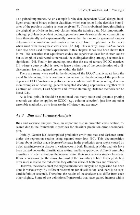
62 C. Zor, T. Windeatt, and B. Yanikoglu
also gained importance. As an example for the data dependent ECOC design, intel-
ligent creation of binary column classifiers which can better fit the decision bound-
aries of the problem training set can be given [7]. This is obtained through splitting
the original set of classes into sub-classes using the training data. Most importantly,
although problem dependent coding approaches provide successful outcomes, it has
been theoretically and experimentally proven that the randomly generated long or
deterministic equi-distant code matrices are also close to optimum performance
when used with strong base classifiers [12, 14]. This is why, long-random codes
have also been used for the experiments in this chapter. It has also been shown that
in real life scenarios that equidistant codes are superior at least for shorter codes;
but as length of code word is increased, the coding/decoding strategy becomes less
significant [24]. Finally for encoding, note that the use of ternary ECOC matrices
[1], where a zero symbol is used to leave a class out of the consideration of a di-
chotomizer, has also gained interest within the field.
There are many ways used in the decoding of the ECOC matrix apart from the
usual HD decoding. It is a common convention that the decoding of the problem-
dependent ECOC matrices is performed in accordance with their encoding. As com-
mon examples of decoding, general weighted decoding approaches, together with
Centroid of Classes, Least Squares and Inverse Hamming Distance methods can be
listed [24].
As a final point, it should be mentioned that many static and dynamic pruning
methods can also be applied to ECOC (e.g., column selection), just like any other
ensemble method, so as to increase the efficiency and accuracy.
4.1.3 Bias and Variance Analysis
Bias and variance analysis plays an important role in ensemble classification re-
search due to the framework it provides for classifier prediction error decomposi-
tion.
Initially, Geman has decomposed prediction error into bias and variance terms
under the regression setting using squared-error loss [10]. This decomposition
brings about the fact that a decrease/increase in the prediction error rate is caused by
a decrease/increase in bias, or in variance, or in both. Extensions of the analysis have
been carried out on the classification setting, and later applied on different ensemble
classifiers in order to analyse the reason behind their success over single classifiers.
It has been shown that the reason for most of the ensembles to have lower prediction
error rates is due to the reductions they offer in sense of both bias and variance.
However, the extension of the original theoretical analysis on regression has been
done in various ways by different researchers for classification; and there is no stan-
dard definition accepted. Therefore, the results of the analyses also differ from each
other slightly. Some of the definitions/frameworks that have gained interest within

4 ECOC and Bagging Using Neural Nets 63
the research field are given by Breiman [3], Kohavi and Wolpert [15], Dietterich and
Kong [16], Friedman [9], Wolpert [25], Heskes [11], Tibshirani [19], Domingos [6]
and James [13].
Although there are dissimilarities in-between the frameworks, the main intuitions
behind each are similar. Consider a training set T with patterns (xi, li), where x rep-
resents the feature vector and l the corresponding label. Given a test pattern, an op-
timal classifier model predicts a decision label by assuring the lowest expected loss
over all possible target label values. This classifier, which is actually the Bayes clas-
sifier when used with the zero-one loss function, is supposed to know and use the
underlying likelihood probability distribution for the input dataset patterns/classes.
If we call the decision of the optimal classifier as the optimal decision (OD), then
for a given test pattern (xi, li), OD = argminαEt [L(t,α)] where L denotes the loss
function used, and l the possible target label values.
The estimator, on the other hand, is actually an averaged classifier model. It pre-
dicts a decision label by assuring the lowest expected loss over all labels that are
created by classifiers trained on different training sets. The intrinsic parameters of
these classifiers are usually the same, and the only difference is the training sets that
they are trained on. In this case, instead of minimizing the loss over the target la-
bels using the known underlying probability distribution as happens in the optimal
classifier case, the minimization of the loss is carried out for the set of labels which
are created by the classifiers trained on various training sets. If the decision of the
estimator is named as the expected estimator decision (EED); then for a given test
pattern (xi, li), EED = argminαEl[L(l,α)] where L denotes the loss function used,
and l the label values obtained from the classifiers used. For regression under the
squared-error loss setting, the OD is the mean of the target labels while the EED is
the mean of the classifier decisions obtained via different training sets.
Bias can mainly be defined as the difference or the distance between OD and
EED. Therefore, it emphasizes how effectively the optimal decision can be pre-
dicted by the estimator. The type of the distance metric used depends on the loss
function of the classification. On the other hand, variance is calculated as the ex-
pected loss exposed by the classifiers, which are trained on different training sets,
while predicting OD. So, it shows how sensible the estimate is, against variations in
the training data [9].
The problem with the above mentioned definitions of bias and variance is that
most of them are given for specific loss functions such as the zero-one loss. It is
difficult to generalize them for the other loss functions; usually new definitions are
given for each new loss function. Secondly, as for the definitions which are proposed
to be applicable for all loss functions, the problem of failing to satisfy the additive
decomposition of the prediction error defined in [10] exists.
The definition of James [13] has advantages over the others as it proposes to
construct a bias and variance scheme which is generalizable to any symmetric loss
function, while assuring the additive prediction error decomposition by utilizing two
new concepts called systematic effect (SE) and variance effect (VE). These concepts
also help realizing the effects of bias and variance on the prediction error.

64 C. Zor, T. Windeatt, and B. Yanikoglu
Some characteristics of the other definitions which make James’ more preferable
are as follows:
1. Dietterich allows a negative variance and it is possible for the Bayes classifier to
have positive bias.
2. Experimentally, the trends of Breiman’s bias and variance closely follow James’
SE and VE respectively. However, for each test input pattern, Breiman separates
base classifiers into two sets, as biased and unbiased; and considers each test
pattern only to have either bias or variance accordingly.
3. Kohavi and Wolpert also assign a nonzero bias to the Bayes classifier but the
Bayes error is absorbed within the bias term. Although it helps avoid the need to
calculate the Bayes error in real datasets through making unwarranted assump-
tions, it is not preferable since the bias term becomes too high.
4. The definitions of Tibshirani, Heskes and Breiman are difficult to generalize and
extend for the loss functions other than the ones for which they were defined.
5. Friedman proposes that bias and variance do not always need to be additive.
In addition to all these differences, it should also be noted that the characteristics of
bias and variance of Domingos’ definition are actually close to James’, although the
decomposition can be considered as being multiplicative [13].
In the literature, attempts have been made to explore the bias-variance charac-
teristics of ECOC and bagging ensembles. Examples can be found in [3, 5, 13, 16,
18, 22]. In this chapter, a detailed bias-variance analysis of ECOC and bagging
ensembles using NNs as base classifiers is given while systematically changing pa-
rameters, namely nodes and epochs, based on James’ definition.
We start by taking a detailed look at the bias and variance framework of James in
the next section.
4.2 Bias and Variance Analysis of James
James [13] extends the prediction error decomposition, which is initially proposed
by Geman et al [10] for squared error under regression setting, for all symmetric loss
functions. Therefore, his definition also covers zero-one loss under classification
setting, which we use in the experiments.
In his decomposition, the terms systematic effect (SE) and variance effect (VE)
satisfy the additive decomposition for all symmetric loss functions, and for both real
valued and categorical predictors. They actually indicate the effect of bias and vari-
ance on the prediction error. For example, a negative VE would mean that variance
actually helps reduce the prediction error. On the other hand, the bias term is de-
fined to show the average distance between the response and the predictor; and the
variance term refers to the variability of the predictor. As a result, both the mean-
ings and the additive characteristics of the bias and variance concepts of the original
setup have been preserved. Following is a summary of the bias-variance derivations
of James:

4 ECOC and Bagging Using Neural Nets 65
For any symmetric loss function L, where L(a,b) = L(b,a):
EY,Y [L(Y,Y )] = EY [L(Y,SY )]+ EY [L(Y,SY )−L(Y,SY )]
+EY,Y [L(Y,Y )−L(Y,SY)]
prediction error = Var(Y )+ SE(Y ,Y )+VE(Y ,Y ) (4.1)
where L(a,b) is the loss when b is used in predicting a, Y is the response and Y
is the predictor. SY = argminµEY [L(Y,µ)] and SY = argminµEY [L(Y ,µ)]. We see
here that prediction error is composed of the variance of the response (irreducible
noise), SE and VE.
Using the same terminology, the bias and variance for the predictor are defined
as follows:
Bias(Y ) = L(SY,SY )
Var(Y ) = EY [L(Y ,SY )] (4.2)
When the specific case of classification problems with zero-one loss function is
considered, we end up with the following formulations:
L(a,b) = I(a = b), Y ε 1,2,3..N for an N class problem, PYi = PY (Y = i), PY
i =PY (Y = i), ST = argminiEY [I(Y = i)] = argmaxiP
Yi
Therefore,
Var(Y ) = PY (Y = SY ) = 1−maxiPYi
Var(Y ) = PY (Y = SY ) = 1−maxiPYi
Bias(Y ) = I(SY = SY )
VE(Y ,Y ) = P(Y = Y )−PY (Y = SY ) = PYSY−∑
i
PYi PY
i
SE(Y ,Y ) = PY (Y = SY )−PY (Y = SY ) = PYSY −PY
SY(4.3)
where I(q) is 1 if q is a true argument and 0 otherwise.
4.3 Experiments
4.3.1 Setup
In the experiments, 3 classification methods have been analysed: Single classifier,
bagging, and ECOC. In each case, 50 classifiers are created for bias-variance analy-
sis. Each of these 50 classifiers is either a single classifier, or an ensemble consisting
of 50 bagged classifiers or ECOC matrices of 50 columns. Due to the reasons ex-
plained in Sect. 4.1.2, the ECOC matrices are created by randomly assigning binary
66 C. Zor, T. Windeatt, and B. Yanikoglu
values to each matrix cell; and Hamming Distance is used as the metric in the decod-
ing stage. The optimization method used in NNs is the Levenberg-Marquart (LM)
technique; the level of training (epochs) varies between 2 and 15; and the number
of nodes between 2 and 16.
In artificial dataset experiments, training sets are created by simple random
sampling from the infinite data at hand to be used in training 50 classifiers for
bias/variance analysis. The number of training patterns per classifier is equal to 300,
and the number of test patterns is 18000. Experiments have been repeated 10 times
using different test data (also generated via simple random sampling) together with
different training data and ECOC matrices in each run, and the results are averaged.
In the two-class problem experiments, ECOC has not been used as it is a multi-class
classification technique. Applying ECOC in such cases would be nothing different
than applying bagging; effect of bootstrapping in bagging would be similar to the
effect of the random initial weights of LM in ECOC.
For the UCI datasets having separate test sets, the training sets for each of the 50
classifiers are created from the finite dataset at hand using bootstrapping. Bootstrap-
ping is expected to be a close enough approximation to random and independent
data generation from a known underlying distribution [3].The analysis has been
performed just once without repetition, as the test set is given/fixed. However, the
results of the ECOC setting are averaged over 10 iterations with different matrices.
As for the UCI datasets without separate test sets, the ssCV cross-validation
method of Webb and Conilione [23], which allows the usage of the whole dataset
both in training and test stages, has been implemented. Within a number of iter-
ations, all data is effectively used for both training and testing in each of the 50
classifiers, and the overall results for bias and variance analysis are recorded. The
procedure is not repeated as the iterations within ssCV already cover the whole
dataset. However, 10 different ECOC matrices are again used in ECOC setting, and
results are averaged. Note that in ssCV, the shortcomings of the hold-out approach
like the usage of small training and test sets, and the lack of inter-training variability
control between the successive training sets has been overcome. In our experiments,
we set the inter-training variability constant δ to 1/2.
The diagram in Fig. 4.2 visualizes the experimental setup. Experiments have been
carried out on 5 artificial and 4 UCI MLR [2] datasets; three of the artificial datasets
being created according to Breiman’s description in [3]. Detailed information about
the sets can be found in Table 4.1.
The Bayes error, namely Var(Y ) for the zero-one loss function (see Eq. 4.3), is
analytically calculated for the artificial datasets, as the underlying likelihood prob-
ability distributions are known. As for the real datasets, usually either the need
for the underlying probability distributions has been overcome by assuming zero
noise level [6], or some heuristic methods like using nearest neighbours [13] have
been proposed to estimate the underlying probability distributions and therefore the
Bayes error in the literature. The first approach has the shortcoming of a wrong es-
timate on bias. Therefore, we also use a heuristic method in our experiments to do
the estimation. Our motivation is to find the optimal classifier parameters giving the
lowest error rate possible, through cross-fold validation (CV); and then to use these
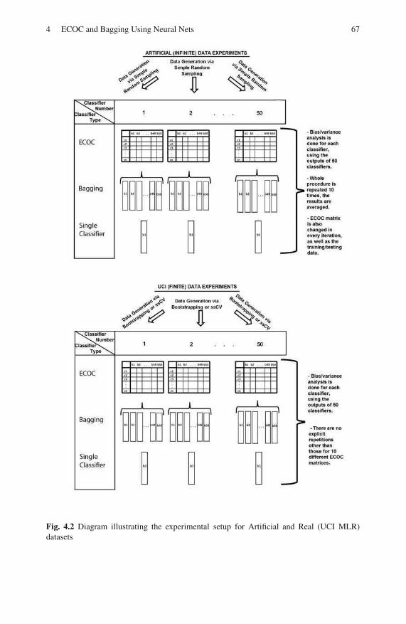
4 ECOC and Bagging Using Neural Nets 67
Fig. 4.2 Diagram illustrating the experimental setup for Artificial and Real (UCI MLR)
datasets
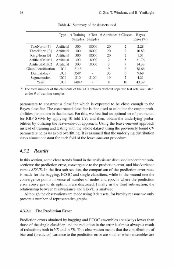
68 C. Zor, T. Windeatt, and B. Yanikoglu
Table 4.1 Summary of the datasets used
Type # Training # Test # Attributes # Classes Bayes
Samples Samples Error (%)
TwoNorm [3] Artificial 300 18000 20 2 2.28
ThreeNorm [3] Artificial 300 18000 20 2 10.83
RingNorm [3] Artificial 300 18000 20 2 1.51
ArtificialMulti1 Artificial 300 18000 2 5 21.76
ArtificialMulti2 Artificial 300 18000 3 9 14.33
Glass Identification UCI 214* - 9 6 38.66
Dermatology UCI 358* - 33 6 9.68
Segmentation UCI 210 2100 19 7 4.21
Yeast UCI 1484* - 8 10 43.39
*: The total number of the elements of the UCI datasets without separate test sets, are listed
under # of training samples.
parameters to construct a classifier which is expected to be close enough to the
Bayes classifier. The constructed classifier is then used to calculate the output prob-
abilities per pattern in the dataset. For this, we first find an optimal set of parameters
for RBF SVMs by applying 10 fold CV; and then, obtain the underlying proba-
bilities by utilizing the leave-one-out approach. Using the leave-one-out approach
instead of training and testing with the whole dataset using the previously found CV
parameters helps us avoid overfitting. It is assumed that the underlying distribution
stays almost constant for each fold of the leave-one-out procedure.
4.3.2 Results
In this section, some clear trends found in the analysis are discussed under three sub-
sections: the prediction error, convergence to the prediction error, and bias/variance
versus SE/VE. In the first sub-section, the comparison of the prediction error rates
is made for the bagging, ECOC and single classifiers, while in the second one the
convergence points in sense of number of nodes and epochs where the prediction
error converges to its optimum are discussed. Finally in the third sub-section, the
relationship between bias/variance and SE/VE is analysed.
Although the observations are made using 9 datasets, for brevity reasons we only
present a number of representative graphs.
4.3.2.1 The Prediction Error
Prediction errors obtained by bagging and ECOC ensembles are always lower than
those of the single classifier, and the reduction in the error is almost always a result
of reductions both in VE and in SE. This observation means that the contributions of
bias and (predictor) variance to the prediction error are smaller when ensembles are
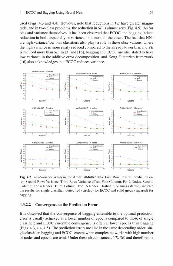
4 ECOC and Bagging Using Neural Nets 69
used (Figs. 4.3 and 4.4). However, note that reductions in VE have greater magni-
tude, and in two-class problems, the reduction in SE is almost zero (Fig. 4.5). As for
bias and variance themselves, it has been observed that ECOC and bagging induce
reduction in both, especially in variance, in almost all the cases. The fact that NNs
are high variance/low bias classifiers also plays a role in these observations, where
the high variance is more easily reduced compared to the already lower bias and VE
is reduced more than SE. In [3] and [16], bagging and ECOC are also stated to have
low variance in the additive error decomposition, and Kong-Dietterich framework
[16] also acknowledges that ECOC reduces variance.
2 3 5 7 10 15−0.1
0
0.1
0.2
0.3
0.4
0.5
0.6
0.7
0.8
0.9
Epochs
testE
rror
ArtificialMulti2 − 2 Nodes
Single Classifier
Ecoc
Bagging
2 3 5 7 10 15−0.1
0
0.1
0.2
0.3
0.4
0.5
0.6
0.7
0.8
0.9
Epochs
Test E
rror
ArtificialMulti2 − 4 nodes
Single Classifier
Ecoc
Bagging
2 3 5 7 10 15−0.1
0
0.1
0.2
0.3
0.4
0.5
0.6
0.7
0.8
0.9
Epochs
Test E
rror
ArtificialMulti2 − 16 nodes
Single Classifier
Ecoc
Bagging
2 3 5 7 10 15−0.1
0
0.1
0.2
0.3
0.4
0.5
0.6
0.7
0.8
0.9
Epochs
Variance
ArtificialMulti2 − 2 nodes
Single Classifier
Ecoc
Bagging
2 3 5 7 10 15−0.1
0
0.1
0.2
0.3
0.4
0.5
0.6
0.7
0.8
0.9
Epochs
Variance
ArtificialMulti2 − 4 nodes
Single Classifier
Ecoc
Bagging
2 3 5 7 10 15−0.1
0
0.1
0.2
0.3
0.4
0.5
0.6
0.7
0.8
0.9
Epochs
Variance
ArtificialMulti2 − 16 nodes
Single Classifier
Ecoc
Bagging
2 3 5 7 10 15−0.1
0
0.1
0.2
0.3
0.4
0.5
0.6
0.7
0.8
0.9
Epochs
Variance E
ffect
ArtificialMulti2 − 2 nodes
Single Classifier
Ecoc
Bagging
2 3 5 7 10 15−0.1
0
0.1
0.2
0.3
0.4
0.5
0.6
0.7
0.8
0.9
Epochs
Variance E
ffect
ArtificialMulti2 − 4 nodes
Single Classifier
Ecoc
Bagging
2 3 5 7 10 15−0.1
0
0.1
0.2
0.3
0.4
0.5
0.6
0.7
0.8
0.9
Epochs
Variance E
ffect
ArtificialMulti2 − 16 nodes
Single Classifier
Ecoc
Bagging
Fig. 4.3 Bias-Variance Analysis for ArtificialMulti2 data. First Row: Overall prediction er-
ror. Second Row: Variance. Third Row: Variance effect. First Column: For 2 Nodes. Second
Column: For 4 Nodes. Third Column: For 16 Nodes. Dashed blue lines (starred) indicate
the results for single classifier, dotted red (circled) for ECOC and solid green (squared) for
bagging.
4.3.2.2 Convergence to the Prediction Error
It is observed that the convergence of bagging ensemble to the optimal prediction
error is usually achieved at a lower number of epochs compared to those of single
classifier; and ECOC ensemble convergence is often at lower epochs than bagging
(Figs. 4.3, 4.4, 4.5). The prediction errors are also in the same descending order: sin-
gle classifier, bagging and ECOC; except when complex networks with high number
of nodes and epochs are used. Under these circumstances, VE, SE, and therefore the
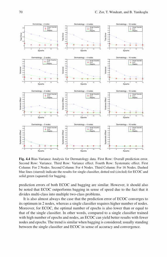
70 C. Zor, T. Windeatt, and B. Yanikoglu
2 3 5 7 10 15
0
0.2
0.4
0.6
0.8
Epochs
Test E
rror
Dermatology − 2 nodes
Single Classifier
Ecoc
Bagging
2 3 5 7 10 15−0.1
0
0.1
0.2
0.3
0.4
0.5
0.6
0.7
0.8
0.9
Epochs
Test E
rror
Dermatology − 4 nodes
Single Classifier
Ecoc
Bagging
2 3 5 7 10 15−0.1
0
0.1
0.2
0.3
0.4
0.5
0.6
0.7
0.8
0.9
Epochs
Test E
rror
Dermatology − 16 nodes
Single Classifier
Ecoc
Bagging
2 3 5 7 10 15−0.1
0
0.1
0.2
0.3
0.4
0.5
0.6
0.7
0.8
0.9
Epochs
Variance
Dermatology − 2 nodes
Single Classifier
Ecoc
Bagging
2 3 5 7 10 15−0.1
0
0.1
0.2
0.3
0.4
0.5
0.6
0.7
0.8
0.9
Epochs
Variance
Dermatology − 4 nodes
Single Classifier
Ecoc
Bagging
2 3 5 7 10 15−0.1
0
0.1
0.2
0.3
0.4
0.5
0.6
0.7
0.8
0.9
Epochs
Variance
Dermatology − 16 nodes
Single Classifier
Ecoc
Bagging
2 3 5 7 10 15−0.1
0
0.1
0.2
0.3
0.4
0.5
0.6
0.7
0.8
0.9
Epochs
Variance E
ffect
Dermatology − 2 nodes
Single Classifier
Ecoc
Bagging
2 3 5 7 10 15−0.1
0
0.1
0.2
0.3
0.4
0.5
0.6
0.7
0.8
0.9
Epochs
Variance E
ffect
Dermatology − 4 nodes
Single Classifier
Ecoc
Bagging
2 3 5 7 10 15−0.1
0
0.1
0.2
0.3
0.4
0.5
0.6
0.7
0.8
0.9
Epochs
Variance E
ffect
Dermatology − 16 nodes
Single Classifier
Ecoc
Bagging
2 3 5 7 10 15−0.1
0
0.1
0.2
0.3
0.4
0.5
0.6
0.7
0.8
0.9
Epochs
Syste
matic E
ffect
Dermatology − 2 nodes
Single Classifier
Ecoc
Bagging
2 3 5 7 10 15−0.1
0
0.1
0.2
0.3
0.4
0.5
0.6
0.7
0.8
0.9
Epochs
Syste
matic E
ffect
Dermatology − 4 nodes
Single Classifier
Ecoc
Bagging
2 3 5 7 10 15−0.1
0
0.1
0.2
0.3
0.4
0.5
0.6
0.7
0.8
0.9
Epochs
Syste
matic E
ffect
Dermatology − 16 nodes
Single Classifier
Ecoc
Bagging
Fig. 4.4 Bias-Variance Analysis for Dermatology data. First Row: Overall prediction error.
Second Row: Variance. Third Row: Variance effect. Fourth Row: Systematic effect. First
Column: For 2 Nodes. Second Column: For 4 Nodes. Third Column: For 16 Nodes. Dashed
blue lines (starred) indicate the results for single classifier, dotted red (circled) for ECOC and
solid green (squared) for bagging.
prediction errors of both ECOC and bagging are similar. However, it should also
be noted that ECOC outperforms bagging in sense of speed due to the fact that it
divides multi-class into multiple two-class problems.
It is also almost always the case that the prediction error of ECOC converges to
its optimum in 2 nodes, whereas a single classifier requires higher number of nodes.
Moreover, for ECOC, the optimal number of epochs is also lower than or equal to
that of the single classifier. In other words, compared to a single classifier trained
with high number of epochs and nodes, an ECOC can yield better results with fewer
nodes and epochs. The trend is similar when bagging is considered; usually standing
between the single classifier and ECOC in sense of accuracy and convergence.
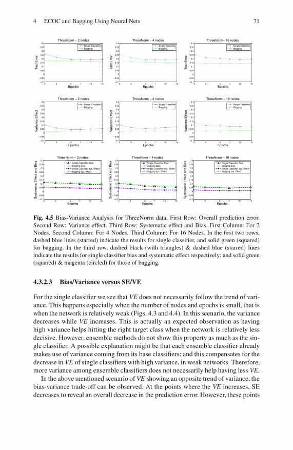
4 ECOC and Bagging Using Neural Nets 71
2 3 5 7 10 15−0.1
−0.05
0
0.05
0.1
0.15
0.2
0.25
0.3
0.35
0.4
Epochs
Test E
rror
ThreeNorm − 2 nodes
Single Classifier
Bagging
2 3 5 7 10 15−0.1
−0.05
0
0.05
0.1
0.15
0.2
0.25
0.3
0.35
0.4
Epochs
Test E
rror
ThreeNorm − 4 nodes
Single Classifier
Bagging
2 3 5 7 10 15−0.1
−0.05
0
0.05
0.1
0.15
0.2
0.25
0.3
0.35
0.4
Epochs
Test E
rror
ThreeNorm− 16 nodes
Single Classifier
Bagging
2 3 5 7 10 15−0.1
−0.05
0
0.05
0.1
0.15
0.2
0.25
0.3
0.35
0.4
Epochs
Variance E
ffect
ThreeNorm − 2 nodes
Single Classifier
Bagging
2 3 5 7 10 15−0.1
−0.05
0
0.05
0.1
0.15
0.2
0.25
0.3
0.35
0.4
Epochs
Variance E
ffect
ThreeNorm − 4 nodes
Single Classifier
Bagging
2 3 5 7 10 15−0.1
−0.05
0
0.05
0.1
0.15
0.2
0.25
0.3
0.35
0.4
Epochs
Variance E
ffect
ThreeNorm − 16 nodes
Single Classifier
Bagging
2 3 5 7 10 15−0.1
−0.05
0
0.05
0.1
0.15
0.2
0.25
0.3
0.35
0.4
Epochs
Syste
matic E
ffect and B
ias
ThreeNorm − 2 nodes
Single Classifier Bias
Bagging Bias
Single Classifier sys. Effect
Bagging sys. Effect
2 3 5 7 10 15−0.1
−0.05
0
0.05
0.1
0.15
0.2
0.25
0.3
0.35
0.4
Epochs
Syste
matic E
ffect and B
ias
ThreeNorm − 4 nodes
Single Classifier Bias
Bagging Bias
Single Classifier sys. Effect
Bagging sys. Effect
2 3 5 7 10 15−0.1
−0.05
0
0.05
0.1
0.15
0.2
0.25
0.3
0.35
0.4
Epochs
Syste
matic E
ffect and B
ias
ThreeNorm − 16 nodes
Single Classifier Bias
Bagging Bias
Single Classifier sys. Effect
Bagging sys. Effect
Fig. 4.5 Bias-Variance Analysis for ThreeNorm data. First Row: Overall prediction error.
Second Row: Variance effect. Third Row: Systematic effect and Bias. First Column: For 2
Nodes. Second Column: For 4 Nodes. Third Column: For 16 Nodes. In the first two rows,
dashed blue lines (starred) indicate the results for single classifier, and solid green (squared)
for bagging. In the third row, dashed black (with triangles) & dashed blue (starred) lines
indicate the results for single classifier bias and systematic effect respectively; and solid green
(squared) & magenta (circled) for those of bagging.
4.3.2.3 Bias/Variance versus SE/VE
For the single classifier we see that VE does not necessarily follow the trend of vari-
ance. This happens especially when the number of nodes and epochs is small, that is
when the network is relatively weak (Figs. 4.3 and 4.4). In this scenario, the variance
decreases while VE increases. This is actually an expected observation as having
high variance helps hitting the right target class when the network is relatively less
decisive. However, ensemble methods do not show this property as much as the sin-
gle classifier. A possible explanation might be that each ensemble classifier already
makes use of variance coming from its base classifiers; and this compensates for the
decrease in VE of single classifiers with high variance, in weak networks. Therefore,
more variance among ensemble classifiers does not necessarily help having less VE.
In the above mentioned scenario of VE showing an opposite trend of variance, the
bias-variance trade-off can be observed. At the points where the VE increases, SE
decreases to reveal an overall decrease in the prediction error. However, these points

72 C. Zor, T. Windeatt, and B. Yanikoglu
are not necessarily the optimal points in terms of the prediction error; the optima
are mostly where there is both VE and SE reduction (Fig. 4.4). Apart from this case,
bias and variance are mostly correlated with SE and VE respectively (Figs. 4.4 and
4.5). This is also pointed out in [13].
4.4 Discussion
By analysing bagging, ECOC and single classifiers consisting of NNs through the
bias-variance definition of James, we have found some clear trends and relation-
ships that offer hints to be used in classifier design. For multi-class classification
problems, the increase in the overall prediction performance obtained with ECOC
makes it preferable over single classifiers. The fact that it converges to the optimum
with smaller number of nodes and epochs is yet another advantage. It also outper-
forms bagging mostly, while in other cases gives similar results. As for the two-class
problems, bagging always outperforms the single classifier, and the optimum num-
ber of nodes and epochs is relatively smaller.
The increase in the performance of bagging and ECOC is a result of the decrease
in both variance effect and systematic effect, although the reductions in the magni-
tude of the variance effect are bigger. Also, when the NNs are weak, that is when
they have been trained with few nodes and epochs, we see that the trends of vari-
ance and variance effect might be in opposite directions in the single classifier case.
This implies that having high variance might help improve the classification perfor-
mance in weak networks when single classifiers are used. However, they are still
outperformed by ensembles, which have even lower variance effects.
As for further possible advantages of ensembles, the fact that they are expected to
avoid overfitting might be shown by using more powerful NNs with higher number
of nodes, or other classifiers such as SVMs that are more prone to overfitting. Future
work is also aimed at understanding and analysing the bias-variance domain within
some mathematical frameworks such as [20, 21] and using the information in the
design of ECOC matrices.
References
1. Allwein, E., Schapire, R., Singer, Y.: Reducing multiclass to binary: A unifying approach
for margin classifiers. J. Machine Learning Research 1, 113–141 (2002)
2. Asuncion, A., Newman, D.J.: UCI machine learning repository, School of Information
and Computer Science. University of California, Irvine (2007)
3. Breiman, L.: Arcing classifiers. The Annals of Stat. 26, 801–849 (1998)
4. Dietterich, T.G., Bakiri, G.: Solving multi-class learning problems via error-correcting
output codes. J. Artif. Intell. Research 2, 263–286 (1995)
5. Domingos, P.: Why does bagging work? A Bayesian account and its implications. In:
Heckerman, D., Mannila, H., Pregibon, D. (eds.) Proc. the 3rd Int. Conf. Knowledge
Discovery and Data Mining, Newport Beach, CA, pp. 155–158. AAAI Press, Menlo
Park (1997)

4 ECOC and Bagging Using Neural Nets 73
6. Domingos, P.: A unified bias-variance decomposition for zero-one and squared loss. In:
Proc. the 17th Natl. Conf. Artif. Intell., Austin, TX, pp. 564–569. MIT Press, Cambridge
(2000)
7. Escalera, S., Tax, D.M.J., Pujol, O., Radeva, P., Duin, R.P.W.: Subclass problem-
dependent design for error-correcting output codes. IEEE Trans. Pattern Analysis and
Machine Intell. 30, 1041–1054 (2008)
8. Freund, Y., Schapire, R.E.: Experiments with a new boosting algorithm. In: Saitta, L.
(ed.) Proc. the 13th Int. Conf. Machine Learning, Bari, Italy, pp. 148–156. Morgan Kauf-
mann, San Francisco (1996)
9. Friedman, J.H.: On bias, variance, 0/1 loss and the curse of dimensionality. Data Mining
and Knowledge Discovery 1, 55–77 (1997)
10. Geman, S., Bienenstock, E., Doursat, R.: Neural networks and the bias/variance
dilemma. Neural Comp. 4, 1–58 (1992)
11. Heskes, T.: Bias/variance decomposition for likelihood-based estimators. Neural
Comp. 10, 1425–1433 (1998)
12. James, G.M.: Majority vote classifiers: Theory and applications. PhD Thesis, Department
of Statistics, University of Standford (1998)
13. James, G.: Variance and bias for general loss functions. Machine Learning 51, 115–135
(2003)
14. James, G.M., Hastie, T.: The error coding method and PICT’s. Comp. and Graph. Stat. 7,
377–387 (1998)
15. Kohavi, R., Wolpert, D.H.: Bias plus variance decomposition for zero-one loss functions.
In: Saitta, L. (ed.) Proc. the 13th Int. Conf. Machine Learning, Bari, Italy, pp. 275–283.
Morgan Kaufmann, San Francisco (1996)
16. Kong, E.B., Dietterich, T.G.: Error-correcting output coding corrects bias and variance.
In: Prieditis, A., Russell, S.J. (eds.) Proc. the 12th Int. Conf. Machine Learning, Tahoe
City, CA, pp. 313–321. ACM Press, New York (1995)
17. Schapire, R.E., Freund, Y., Bartlett, P., Lee, W.S.: Boosting the margin: a new explana-
tion for the effectiveness of voting methods. The Annals of Stat. 26, 1651–1686 (1998)
18. Smith, R.S., Windeatt, T.: The bias variance trade-off in bootstrapped error correcting
output code ensembles. In: Benediktsson, J.A., Kittler, J., Roli, F. (eds.) MCS 2009.
LNCS, vol. 5519, pp. 1–10. Springer, Heidelberg (2009)
19. Tibshirani, R.: Bias, variance and prediction error for classification rules. Technical Re-
port, University of Toronto, Toronto, Canada (1996)
20. Tumer, K., Ghosh, J.: Analysis of decision boundaries in linearly combined neural clas-
sifiers. Pattern Recogn. 29, 341–348 (1996)
21. Tumer, K., Ghosh, J.: Error correlation and error reduction in ensemble classifiers. Con-
nection Science 8, 385–403 (1996)
22. Valentini, G., Dietterich, T.: Bias-variance analysis of support vector machines for
the development of SVM-based ensemble methods. J. Machine Learning Research 5,
725–775 (2004)
23. Webb, G.I., Conilione, P.: Estimating bias and variance from data. School of Comp.
Science and Software Engineering, Monash University (2005)
24. Windeatt, T., Ghaderi, R.: Coding and decoding strategies for multi-class learning prob-
lems. Inf. Fusion 4, 11–21 (2003)
25. Wolpert, D.H.: On bias plus variance. Neural Comp. 9, 1211–1244 (1996)

Chapter 5
Fast-Ensembles of Minimum RedundancyFeature Selection
Benjamin Schowe and Katharina Morik
Abstract. Finding relevant subspaces in very high-dimensional data is a challeng-
ing task not only for microarray data. The selection of features is to enhance the
classification performance, but on the other hand the feature selection must be sta-
ble, i.e., the set of features selected should not change when using different subsets
of a population. ensemble methods have succeeded in the increase of stability and
classification accuracy. However, their runtime prevents them from scaling up to
real-world applications. We propose two methods which enhance correlation-based
feature selection such that the stability of feature selection comes with little or even
no extra runtime. We show the efficiency of the algorithms analytically and empiri-
cally on a wide range of datasets.
5.1 Introduction
The growing dimensionality of recorded data, especially in bioinformatics, demands
dimension reduction methods that identify small sets of features leading to a better
learning performance. Along with the high dimensionality come small sample size
and high variance, which makes it hard to find adequate feature subsets without
being kept in local optima. The large number of features challenges the runtime of
a selection algorithm. Hence, the main quality criteria are that the algorithm is
• multivariate – It takes into account inter-feature-dependencies;
• stable – It does not vary much for unseen data of the population;
• amending learning – The learning performance is enhanced;
• fast – It scales well for very large numbers of features.
Ensemble methods increase stability and, hence, are frequently used in feature
selection. However, they usually slow down the procedure. We will present two
Benjamin Schowe · Katharina Morik
Technische Universitat Dortmund
E-mail: schowe,[email protected]
O. Okun et al. (Eds.): Ensembles in Machine Learning Applications, SCI 373, pp. 75–95.springerlink.com c© Springer-Verlag Berlin Heidelberg 2011

76 B. Schowe and K. Morik
methods which speed up ensembles in a simple and effective way. A careful eval-
uation on several real world and simulated data sets investigates the quality of our
new methods.
5.2 Related Work
Fast univariate filter approaches, like the t-test [5] or SAM-statistics [17], com-
pute a scoring function on the features, disregarding feature interplay. Wrapper
approaches [13] better solve this problem, at the cost of much longer runtime. Each
feature set evaluation demands a cross-validated training of the used learning algo-
rithm. Some learning algorithms provide the user with an implicit feature ranking
which can easily be exploited for feature selection. Such embedded approaches are
using the weight vector of a linear SVM [18] or the frequency of feature use of a
Random Forest (RF) [3]. They are aware of feature interplay and faster than wrap-
pers but biased towards the learning algorithm used.
A group of new algorithms has come up to bridge the gap between fast but uni-
variate filters on the one hand, and slow but multivariate wrappers on the other hand.
Their goal is to find a subset of features which is highly predictive with no or a min-
imum of redundant information. The correlation based feature selection (CFS) [8]
performs a sequential forward search with a correlation measure in the evaluation
step. CFS iteratively adds the feature which has the best ratio between predictive
relevance of the feature and its correlation with the already selected features. Both,
predictiveness and correlation, are measured by the entropy-based symmetrical
uncertainty
SU( fi, f j) =2IG( fi| f j)
H( fi)+ H( f j), (5.1)
where the information gain IG of feature fi w.r.t. feature f j is divided by the sum of
the entropies of fi and f j. Since CFS uses symmetrical uncertainty, it is only suitable
for discrete values.
Ding and Peng [4] reinvented CFS with the capability for handling numerical
variables calling it Minimum Redundancy Maximum Relevance FS (mRMR). For
numerical features the F-test is used. It reflects the ratio of the variance between
classes and the average variance inside theses classes. For a continuous feature X
and a nominal class variable Y with C classes, both from a data set with n examples
it is defined as
F(X ,Y ) =
(n−C)∑c
nc(Xc− X)2
(C−1)∑c(nc−1)σ2
c
(5.2)
with per-class-variance σ2c and nc the number of examples in class c ∈ 1, . . . ,C.
The redundancy of a numerical feature set is measured by the absolute value of
Pearson’s correlation coefficient

5 Fast-Ensembles of Minimum Redundancy Feature Selection 77
R(X ,Y ) =Cov(X ,Y )
√
Var(X)Var(Y )(5.3)
respectively its estimate
r(X ,Y ) =
∑i
(xi− x)(yi− y)
√
∑i
(xi− x)2 ∑i
(yi− y)2. (5.4)
It detects a linear dependency between X and Y . Another possible measure for the
dependency between two nominal variables used by mRMR [4] is the mutual infor-
mation
MI(X ,Y ) = ∑x,y
P(x,y) log2
P(x,y)
P(x)P(y), (5.5)
where x and y are the possible values of X and Y .
From now on, we will use the term correlation and the symbol Cor(·, ·) as a syn-
onym for either Pearsons’s linear correlation, Eq. (5.3), F-test, Eq. (5.2), or mutual
information, Eq. (5.5), depending on the types of variables involved, i.e. numerical
or nominal. Instead of the ratio, one can also use the difference between relevance
and redundancy [4].
The main algorithmic issue is the computation of the correlations. The set of all
features is F and the dimensionality is p = ‖F‖. In the first step, selecting the most
relevant feature takes p calculations of Cor( fi,y) with i = 1, . . . , p. The mRMR/CFS
algorithm first picks the feature which has the highest correlation with the label and
so is most relevant:
F1 = argmaxfi
(Cor( fi,y)) (5.6)
with i ∈ [1, p]. This takes p calculations of feature-label-correlation. Let Fj denote
the set of selected features in step j ∈ 1, . . . ,k of mRMR/CFS. The next steps
in mRMR/CFS are to repeatedly add the feature which has the best ratio between
relevance and redundancy to the already selected features.
Fj+1 = Fj ∪
arg maxf∈F\Fj
Cor( f ,y)1j ∑g∈Fj
Cor( f ,g)
(5.7)
This takes p− ( j−1) correlations in each step. For the whole mRMR/CFS process
of selecting k from p features
p +k−1
∑i=1
(p− i) = pk− k2− k
2(5.8)
correlations must be computed.

78 B. Schowe and K. Morik
Variants of the method like, e.g., [7] tried to improve the stability of mRMR
by introducing a weighting parameter α for the ratio of relevance and redundancy.
Tuning this parameter even increases the overall runtime. The same holds for the
approach [15], which evaluates together those pairs of features which are higher
correlated than some δ , or for Fast Correlation-based Filter (FCBF) [20], which
discards all features with relevance < δ . In any case, the measures are based on
variance and, hence, are sensitive to outliers and a high variance of the input data,
alike. This instability is not suitable, e.g., for biomedical research, where the rel-
evance of features is in the research focus. Hence, mRMR/CFS is promising but
suffering from a lack of stability.
5.2.1 Ensemble Methods
A high variance negatively effects prediction algorithms (classification & regres-
sion) as well as feature selection schemes. Ensemble methods like Bagging [2] or
Boosting [6] reduce variance. Parallel ensembles, e.g. Bagging, do so by repeating
the algorithm on different subsamples or bootstrapped samples of the input data.
This increases the stability of the set of selected features [10, 11, 16] and - in some
cases - even reduces the prediction error [19]. Saeys et al. [16] showed that (bagged)
ensembles of symmetrical uncertainty weighting, Relief, SVM-RFE or RF delivered
more stable feature selections than the non-ensembled counterparts, but did not in-
crease classification performance1. The major problem with Bagging are the e-times
repetition for ensembles of cardinality e. This increases runtime considerably [9].
5.3 Speeding Up Ensembles
We now have advantages and shortcomings of the methods which we want to
enhance, namely mRMR/CFS (being unstable) and ensemble methods (being too
slow). The basis for our algorithm is the “split-sum trick” going back to the parallel
axis theorem. The parallel axis theorem helps to compute Cor(x,y) in one pass for
any two features.
We use Pearson’s linear correlation as an example, but the other measures can
be split analogously: The parallel axis theorem allows to rewrite the variance of a
feature X
Var(X) = E((X−E(X))2) (5.9)
as
Var(X) = E(X2)− (E(X))2 (5.10)
and the covariance of two features X and Y
1 For Random Forests accuracy even decreased.

5 Fast-Ensembles of Minimum Redundancy Feature Selection 79
Cov(X ,Y ) = E((X −E(X))(Y −E(Y))) (5.11)
as
Cov(X ,Y ) = E(XY )−E(X)E(Y). (5.12)
The benefit is that the expected values of the single variables (their mean) do not
have to be estimated before computing the variance or covariance. The variance-
and covariance-terms now only contain sums of computationally independent terms.
For n examples the variance can then be estimated by
(n−1)σ2x =
n
∑i=1
(xi− x)2 =
(n
∑i=1
x2i
)
−nx2 =
(n
∑i=1
x2i
)
− 1
n
(n
∑i=1
xi
)2
.(5.13)
Applying this to Eq. (5.4) allows to compute Pearson’s linear correlation in only one
pass over the data for each feature without prior computation of the mean values of
each feature:
r(x,y) =
n
∑i=1
xiyi− 1n
(n
∑i=1
xi
n
∑i=1
yi
)
√[
n
∑i=1
x2i − 1
n
(n
∑i=1
xi
n
∑i=1
xi
)][n
∑i=1
y2i − 1
n
(n
∑i=1
yi
n
∑i=1
yi
)] (5.14)
The F-Test, Eq. (5.2), and MI, Eq. (5.5), can similarly be split into sums of in-
dependent terms. This fact is used by our Inner Ensemble method and its further
enhancement, the Fast Ensemble.
5.3.1 Inner Ensemble
correlation measures like Pearson’s linear correlation are very sensitive to outliers
[12]. This has a negative effect on the stability of the selected feature set. Our first
method, the Inner Ensemble, increases the robustness of the correlation measure
used inside the mRMR/CFS algorithm by performing a parallel ensemble of e cor-
relations for every single Cor(·, ·) computation. The correlation is calculated for e
parts on subsets of the examples, each part leaving out 1e
of the data - similar to e-
fold cross-validation. In contrast to cross-validation, the left-out fraction of the data
is not used. The average of the e correlations gives us a more robust correlation esti-
mate. Usually, for ensembles of size e, this would increase runtime of mRMR/CFS
by the factor e to (epk− (k2− k)/2) correlations to compute. Now, we use that the
Eqs. (5.2), (5.3) and (5.5) can all be split into sums of sums like
n
∑i=1
hi =m1
∑i=1
hi +m2
∑i=m1+1
hi + · · ·+n
∑i=me+1
hi =e
∑j=1
⎡
⎣
j ne
∑i=1+( j−1) n
e
hi
⎤
⎦ (5.15)
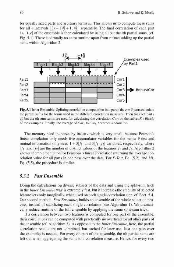
80 B. Schowe and K. Morik
for equally sized parts and arbitrary terms hi. This allows us to compute these sums
for all e intervals[( j−1) n
e+ 1, j n
e
]separately. The final correlation of each part
i ∈ [1,e] of the ensemble is then calculated by using all but the ith partial sums, (cf.
Fig. 5.1). There is virtually no extra runtime apart from e times adding up the partial
sums within Algorithm 2.
Cor1
Cor3
Cor2
Cor4
Cor5
Block1 Block3Block2 Block4 Block5
RobustCor
j en nj+1e
Part1
Part2
Part3
Part4
Part5
Examples used
by Part1
Fig. 5.1 Inner Ensemble: Splitting correlation computation into parts: the e = 5 parts calculate
the partial sums for the terms used in the different correlation measures. Then for each part i
all but the ith sum terms are used for calculating the correlation Cori on the subset X \Blocki
of the examples. Finally, the average of Cor1 to Cor5 becomes RobustCor.
The memory need increases by factor e which is very small, because Pearson’s
linear correlation only needs five accumulator variables for the sums; F-test and
mutual information only need 1 + 3| f1| and 3| f1|| f2| variables, respectively, where
| f1| and | f2| are the number of distinct values of the features f1 and f2. Algorithm 2
shows an implementation for Pearsons’s linear correlation returning the average cor-
relation value for all parts in one pass over the data. For F-Test, Eq. (5.2), and MI,
Eq. (5.5), the procedure is similar.
5.3.2 Fast Ensemble
Doing the calculations on diverse subsets of the data and using the split-sum trick
in the Inner Ensemble way is extremely fast, but it increases the stability of selected
feature sets only marginally, when used on each single correlation step, cf. Sect. 5.4.
Our second method, Fast Ensemble, builds an ensemble of the whole selection pro-
cess, instead of stabilizing each single correlation (see Algorithm 1). We dramati-
cally reduce runtime of the full ensemble by applying the same split-sum trick.
If a correlation between two features is computed for one part of the ensemble,
their correlations can be computed with practically no overhead for all other parts of
the ensemble (cf. Algorithm 3). As opposed to the Inner Ensemble, here, the partial
correlation results are not combined, but cached for later use. Just one pass over
the examples is needed: For every ith part of the ensemble, the ith partial sums are
left out when aggregating the sums to a correlation measure. Hence, for every two

5 Fast-Ensembles of Minimum Redundancy Feature Selection 81
Algorithm 1. Fast Ensemble of mRMR/CFS
1: Input: Set of all features F, desired dimension k, size of the ensemble e, labely
2: for f ∈ F do Precompute relevance of every feature3: Compute Cor( f ,y)[1..e] in parallel and store in cache4: maxrel[1,. . . , e]=−∞5: for r = 1 to e do For all parts of the ensemble test if f is most relevant6: if Cor( f ,y)[r] >maxrel[r] then7: maxrel[r] = Cor( f ,y)[r]8: Fr = f9: end if
10: end for11: end for12: for j = 2 to k do Iteratively add best feature13: best feature[1..e] = /014: best quality[1..e] = −∞15: for r = 1 to e do For all parts of the ensemble16: for f ∈ F\Fr do17: relevance = retrieve(Cor( f ,y)[r]) from cache18: redundancy = 019: for g ∈ Fr do20: redundancy += retrieve(Cor( f ,g)[r]) from cache, when unsuccessful
calculate Cor( f ,g)[1..e] and store in cache.21: end for22: if (redundancy / relevance) > best quality[r] then23: best feature[r] = f24: best quality = (redundancy / relevance)25: end if26: end for27: end for28: for r = 1 to e do For all parts of the ensemble29: Fr = Fr∪ best feature[r]30: end for31: end for32: Combine all Fr to a final F33: return F
features or a feature-class combination, only one pass over the examples is needed,
no matter in how many parts of the ensemble they appear. Where a full ensemble of
mRMR/CFS needs ep passes over the examples in order to select a first feature fi,1
for e parts of the ensemble, our method does this just once. For every further feature
fi, j in all parts of the ensemble, only those feature correlations need a pass over the
examples which were not already considered in any other part of the ensemble.
Time-complexity directly depends on the diversity of the ensemble results. If all
parts of the ensemble return the same feature set, the needed correlations have all
been computed in the first part and the runtime is the same as for a single feature
selection. If, in contrast, the resulting feature sets of the feature selections are dis-
joint, none of the feature pairs has been considered in other parts of the ensemble
and thus has not been cached. These extremes are rare.

82 B. Schowe and K. Morik
Algorithm 2. Java implementation of Inner Ensemble of Pearson’s linear correlation/** Calculates the linear Pearson’s correlation between two numerical attributes
* in one pass over the data, but with a more stable ensemble approach.
** The parameters:
* exampleset An example set - RapidMiner representation of the dataset
* x 1st nominal attribute
* y 2nd nominal attribute
* ensembleSize Size of the ensemble - number of parts
*/
double Correlation(ExampleSet exampleset, Attribute x, Attribute y, int e) double result = 0.0;double N = exampleset.size(); //Number of examples
double [] n = new double [e]; // Size of the blocksdouble [] ex = new double [e]; // Blockwise sum over all xidouble [] exx = new double [e]; // Blockwise sum over all xiˆ2double [] ey = new double [e]; // Blockwise sum over all yidouble [] eyy = new double [e]; // Blockwise sum over all yiˆ2double [] exy = new double [e]; // Blockwise sum over all yi*xi
double xi,yi;Example example;Iterator<Example> iterator = exampleset.iterator();int i=0;while (iterator.hasNext()) // Iterate over all examples once
example = iterator.next(); // Fetch next example and get values for ...xi = example.getValue(x); // attribute X and ...yi = example.getValue(y); // attribute Y.
ex[i] += xi; // Add example’s value for X and Y to the partial sumsexx[i] += xi * xi;ey[i] += yi;eyy[i] += yi * yi;exy[i] += xi * yi;n[i]++; // Increase block size counter
i++; // Increase block indexi = i % e; // To keep i in the range [0..e]. The partial sums are not build up over consecutive
// blocks, but the blocks are distributed modulo over all examples. The result is the// same and reduces the risk of ensemble parts with only one class, should the examples// be sorted.
// Now combine partial sums to partial ensemble results:
double numerator, denominator;
for (i=0; i < e; i++) // Combine the blockwise sums to the sums the each part of the ensembledouble EX=0.0, EXX=0.0, EY=0.0, EYY=0.0, EXY=0.0;for (j=0; j < e; j++)
if (j != i) // Leave out the sums of block iEX += ex[j];EXX += exx[j];EY += ey[j];EYY += eyy[j];EXY += exy[j];
numerator = EXY - (EX * EY) / (N - n[i]);
denominator = Math.sqrt((EXX - ((EX * EX) / (N - n[i]) )) *(EYY - ((EY * EY) / (N - n[i]) )) );
result += numerator / denominator; // Add partial correlation result to aggregator variable.
return result / e; // Build mor robust correlation as average of partial correlations.

5 Fast-Ensembles of Minimum Redundancy Feature Selection 83
Algorithm 3. Java implementation of Mutual Information for Fast Ensemble/** Ensemble version of mutual information.
* MI is calculate for each part of the ensemble and an array of MI values is returned.
** The parameters:
* exampleset An example set - RapidMiner representation of the dataset
* x 1st nominal attribute
* y 2nd nominal attribute
* ensembleSize Size of the ensemble - number of parts
*/
double [] MutualInformationEnsemble(ExampleSet exampleset, Attribute x, Attribute y, int ensembleSize)
double [] result = new double[ensembleSize]; // Will hold the MI-value for each ensemble part.int N = exampleset.size();if (N == 0) // Some sanity checks
return result;
if (!x.isNominal() || !y.isNominal())throw new OperatorException("Both attributes have to be nominal");
int num_x = x.getMapping().size(); // The number of distinct values/classes in Xint num_y = y.getMapping().size(); // The number of distinct values/classes in Y
double PX[] = new double[num_x]; // Occurence of each of X’s valuesdouble PY[] = new double[num_y]; // Occurence of each of Y’s valuesdouble PXY[][] = new double[num_x][num_y]; // Joint occurence of each X’s and Y’s values
double px[][] = new double[num_x][ensembleSize]; // Occurence of each of X’s values in each blockdouble py[][] = new double[num_y][ensembleSize]; // Occurence of each of Y’s values in each blockdouble pxy[][][] = new double[num_x][num_y][ensembleSize]; //Joint occ. of X’s & Y’s values in each blockdouble n[] = new double[ensembleSize]; // Size of each Block
int xi,yi;Example example;Iterator<Example> iterator = exampleset.iterator();int i=0; // Block index variable, indicating the current block
while (iterator.hasNext()) // Iterate over all examples onceexample = iterator.next(); // Fetch next example and get values for ...xi = (int)example.getValue(x); // attribute x and ...yi = (int)example.getValue(y); // attribute y.
PX[xi]++; // Increase overall occurence counter for value xiPY[yi]++; // Increase overall occurence counter for value yiPXY[xi][yi]++; // Increase overall joint occurence counter for value (xi,yi)
px[xi][i]++; // Increase occurence counter for value xi in the current blockpy[yi][i]++; // Increase occurence counter for value yi in the current blockpxy[xi][yi][i]++; // Increase joint occurence counter for (xi,yi) in the current blockn[i]++; // Increase block size counter
i++; // Increase block indexi = i % ensembleSize; // To stay in the range [0, e-1] for e blocks
double temp;for (i = 0; i < ensembleSize; i++) // Build MI value for each ensemble part by subtracting the blockwise
result[i] = 0.0; // occurences from overall occurences and inserting into MI formula.
for (int k = 0; k < num_x; k++) // Iterate over all possible values for Xfor (int j = 0; j < num_y; j++) // Iterate over all possible values for Y
temp = ((N - n[i]) * (PXY[k][j] - pxy[k][j][i])) / ((PX[k] - px[k][i]) * (PY[j] - py[j][i]));if (temp > 0 && !Double.isInfinite(temp) && !Double.isNaN(temp))
result[i] += ((PXY[k][j] - pxy[k][j][i])* Math.log(temp)) / (N - n[i]);
result[i] *= LOG2INV; //For scaling from log_e to log_2
return result;
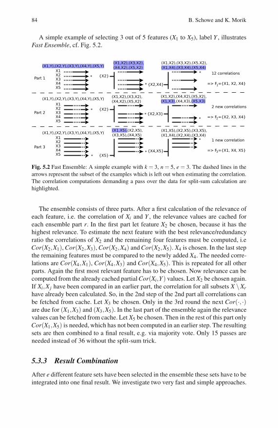
84 B. Schowe and K. Morik
A simple example of selecting 3 out of 5 features (X1 to X5), label Y , illustrates
Fast Ensemble, cf. Fig. 5.2.
(X1,X2),(X4,X2),(X5,X2),
(X1,X3),(X4,X3),(X5,X3)
(X1,X5),(X2,X5),
(X3,X5),(X4,X5)
(X1,X2),(X3,X2),(X5,X2),
(X1,X4),(X3,X4),(X5,X4)X1X2X3X4X5
=> F =X1, X2, X4
(X1,Y),(X2,Y),(X3,Y),(X4,Y),(X5,Y)(X1,X2),(X3,X2),
(X4,X2),(X5,X2)
*
*
*
X1X2X3X4X5
**
*
X1X2X3X4X5 *
*
*
12 correlations
=> F =X2, X3, X4
=> F =X1, X4, X5
2 new correlations
1 new correlation
(X1,Y),(X2,Y),(X3,Y),(X4,Y),(X5,Y)
(X1,Y),(X2,Y),(X3,Y),(X4,Y),(X5,Y)
(X1,X2),(X3,X2),
(X4,X2),(X5,X2)
(X1,X5),(X2,X5),(X3,X5),
(X1,X4),(X2,X4),(X3,X4)
X2
X2,X4
X2
X2,X3
X5
X4,X5
Part 1
Part 2
Part 3
1
2
3
Fig. 5.2 Fast Ensemble: A simple example with k = 3, n = 5, e = 3. The dashed lines in the
arrows represent the subset of the examples which is left out when estimating the correlation.
The correlation computations demanding a pass over the data for split-sum calculation are
highlighted.
The ensemble consists of three parts. After a first calculation of the relevance of
each feature, i.e. the correlation of Xi and Y , the relevance values are cached for
each ensemble part r. In the first part let feature X2 be chosen, because it has the
highest relevance. To estimate the next feature with the best relevance/redundancy
ratio the correlations of X2 and the remaining four features must be computed, i.e
Cor(X2,X1), Cor(X2,X3), Cor(X2,X4) and Cor(X2,X5). X4 is chosen. In the last step
the remaining features must be compared to the newly added X4. The needed corre-
lations are Cor(X4,X1), Cor(X4,X3) and Cor(X4,X5). This is repeated for all other
parts. Again the first most relevant feature has to be chosen. Now relevance can be
computed from the already cached partial Cor(Xi,Y ) values. Let X2 be chosen again.
If Xi,X j have been compared in an earlier part, the correlation for all subsets X \Xr
have already been calculated. So, in the 2nd step of the 2nd part all correlations can
be fetched from cache. Let X3 be chosen. Only in the 3rd round the next Cor(·, ·)are due for (X1,X3) and (X3,X5). In the last part of the ensemble again the relevance
values can be fetched from cache. Let X5 be chosen. Then in the rest of this part only
Cor(X1,X5) is needed, which has not been computed in an earlier step. The resulting
sets are then combined to a final result, e.g. via majority vote. Only 15 passes are
needed instead of 36 without the split-sum trick.
5.3.3 Result Combination
After e different feature sets have been selected in the ensemble these sets have to be
integrated into one final result. We investigate two very fast and simple approaches.

5 Fast-Ensembles of Minimum Redundancy Feature Selection 85
The first method simply counts how often a feature was selected. The k most often
selected features constitute the final set. We call this Fast Ensemble with sets.
This method does not regard the fact that features selected in later steps Fj with
j → k are more unstable and less relevant than those selected in early steps of the
mRMR/CFS algorithm. This can be overcome by a rank-combination similar to that
proposed by [16]. The mRMR/CFS algorithm implicitly provides a ranking of the
first k features (feature f is selected in iteration j⇒Rank( f )= j). For full averaging
of all ranks mRMR/CFS would have to be performed e times with k = p. This would
lead to a runtime of O(p2) and is thus only feasible for low-dimensional datasets.
One could try to average over all k existing ranks in every ensemble part and assume
a constant rank ≫ k for all p− k unranked features. This has the drawback that
features with a relatively high rank of k + ε are ignored. We instead suggest an
intermediate solution. In each part of the ensemble we calculate the ranks only for
the top 2k features. For all non-selected features assume a rank of 3k (or an arbitrary
value > 2k). Experimentation showed that this yields as good stability results as the
combination of fully ranked feature sets. We call this Fast Ensemble with ranks.
5.3.4 Benefits
Our algorithms conduct search in feature subset space like wrappers do. Yet, un-
like wrappers, the feature sets are not evaluated in long cross-validation runs but
with a fast filter approach. Unlike filters, feature interdependencies are still con-
sidered. Hence, Inner and Fast Ensemble combine the advantages of wrapper and
filter approaches. Note, that the inherent parallelism of the algorithms speeds up
computation additionally. Every correlation computation between two features is
independent of the other features. Thus, not only the parts of the ensemble can be
computed in parallel, but also all correlation computations. Only completed calcula-
tions must be reported to some central instance which conducts the search in feature
subset space.
5.4 Evaluation
We evaluated the performance of our algorithm with respect to stability, accuracy,
runtime and low-sample performance on ten publicly available datasets of a wide
range of problem settings and dimensionality (Table 5.1).
All experiments were conducted in the open-source Data Mining system Rapid-
Miner. The proposed algorithms are open-source and available as an extension2 to
RapidMiner.
2 https://sourceforge.net/projects/rm-featselext

86 B. Schowe and K. Morik
Table 5.1 Data characteristics and significance of the difference between the stabilities
achieved by Fast Ensemble and plain mRMR for 10 and 20 features. Values < 0.05 are highly
significant.
Dataset p n Classes Data k = 10 k = 20
Sonar 60 208 2 continuous 0.0085 0.0025
Ionosphere 34 351 2 continuous 0.022 0.19951
Musk 166 476 2 continuous 3.1 ·10−6 1.4 ·10−8
Lung 325 73 7 nominal 4.1 ·10−7 4.0 ·10−14
H/W Digits 64 3823 10 continuous 0.082 0.0058
Colon 2000 62 2 nominal 1.4 ·10−9 1.1 ·10−6
Lymphoma 4026 96 9 nominal 1.2 ·10−10 4.4 ·10−14
Leukemia 7070 72 2 nominal 2.6 ·10−11 1.9 ·10−15
NCI60 9712 60 9 nominal 2.4 ·10−14 0.0LUCAS 11 2000 2 nominal - -
5.4.1 Stability
We analyse how the produced feature sets differ under variation of the input data.
We compare our two methods Inner Ensemble and Fast Ensemble with set- and
rank-combination to mRMR/CFS. All ensembles consist of e = 20 parts.
The stability of a feature selection method can be measured by the similarity
of the resulting feature subset generated by a feature selection method on different
data drawn from the same basic population. Different stability indices are available
for this similarity of sets. The Jaccard index of two feature-sets as used by [16] is
defined as
SJ(Fa,Fb) =|Fa∩Fb||Fa∪Fb|
. (5.16)
A measure very similar to the Jaccard Index was proposed by [14] which we will
refer to as Kuncheva’s index SK . For two feature subsets of size k it is defined as
SK(Fa,Fb) =|Fa∩Fb| k
2
p
k− k2
p
, (5.17)
where SK(Fa,Fb)∈ [−1,1]. Its advantage over the Jaccard index is that it also regards
the size p of the whole feature set and the number k of selected features.
Similar to [16] we draw ten subsets from the example set like ten-fold cross-
validation. On each of these subsets a feature selection is computed. The overall
stability is further defined as the average of the stability indices for all combinations
of those feature selections:
S =2
l2 + l
l
∑i=1
l
∑j=i+1
S(Fi,Fj), (5.18)
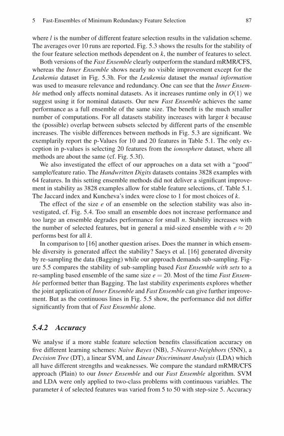
5 Fast-Ensembles of Minimum Redundancy Feature Selection 87
where l is the number of different feature selection results in the validation scheme.
The averages over 10 runs are reported. Fig. 5.3 shows the results for the stability of
the four feature selection methods dependent on k, the number of features to select.
Both versions of the Fast Ensemble clearly outperform the standard mRMR/CFS,
whereas the Inner Ensemble shows nearly no visible improvement except for the
Leukemia dataset in Fig. 5.3h. For the Leukemia dataset the mutual information
was used to measure relevance and redundancy. One can see that the Inner Ensem-
ble method only affects nominal datasets. As it increases runtime only in O(1) we
suggest using it for nominal datasets. Our new Fast Ensemble achieves the same
performance as a full ensemble of the same size. The benefit is the much smaller
number of computations. For all datasets stability increases with larger k because
the (possible) overlap between subsets selected by different parts of the ensemble
increases. The visible differences between methods in Fig. 5.3 are significant. We
exemplarily report the p-Values for 10 and 20 features in Table 5.1. The only ex-
ception in p-values is selecting 20 features from the ionosphere dataset, where all
methods are about the same (cf. Fig. 5.3f).
We also investigated the effect of our approaches on a data set with a “good”
sample/feature ratio. The Handwritten Digits datasets contains 3828 examples with
64 features. In this setting ensemble methods did not deliver a significant improve-
ment in stability as 3828 examples allow for stable feature selections, cf. Table 5.1.
The Jaccard index and Kuncheva’s index were close to 1 for most choices of k.
The effect of the size e of an ensemble on the selection stability was also in-
vestigated, cf. Fig. 5.4. Too small an ensemble does not increase performance and
too large an ensemble degrades performance for small n. Stability increases with
the number of selected features, but in general a mid-sized ensemble with e ≈ 20
performs best for all k.
In comparison to [16] another question arises. Does the manner in which ensem-
ble diversity is generated affect the stability? Saeys et al. [16] generated diversity
by re-sampling the data (Bagging) while our approach demands sub-sampling. Fig-
ure 5.5 compares the stability of sub-sampling based Fast Ensemble with sets to a
re-sampling based ensemble of the same size e = 20. Most of the time Fast Ensem-
ble performed better than Bagging. The last stability experiments explores whether
the joint application of Inner Ensemble and Fast Ensemble can give further improve-
ment. But as the continuous lines in Fig. 5.5 show, the performance did not differ
significantly from that of Fast Ensemble alone.
5.4.2 Accuracy
We analyse if a more stable feature selection benefits classification accuracy on
five different learning schemes: Naive Bayes (NB), 5-Nearest-Neighbors (5NN), a
Decision Tree (DT), a linear SVM, and Linear Discriminant Analysis (LDA) which
all have different strengths and weaknesses. We compare the standard mRMR/CFS
approach (Plain) to our Inner Ensemble and our Fast Ensemble algorithm. SVM
and LDA were only applied to two-class problems with continuous variables. The
parameter k of selected features was varied from 5 to 50 with step-size 5. Accuracy
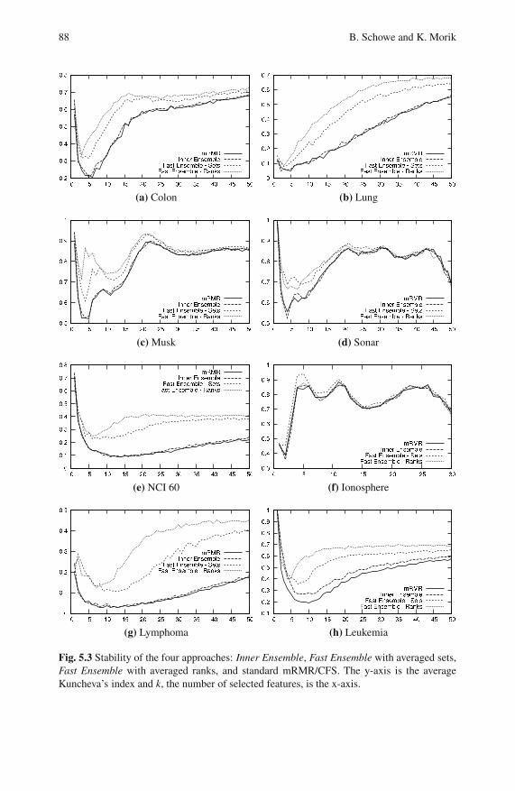
88 B. Schowe and K. Morik
(a) Colon (b) Lung
(c) Musk (d) Sonar
(e) NCI 60 (f) Ionosphere
(g) Lymphoma (h) Leukemia
Fig. 5.3 Stability of the four approaches: Inner Ensemble, Fast Ensemble with averaged sets,
Fast Ensemble with averaged ranks, and standard mRMR/CFS. The y-axis is the average
Kuncheva’s index and k, the number of selected features, is the x-axis.
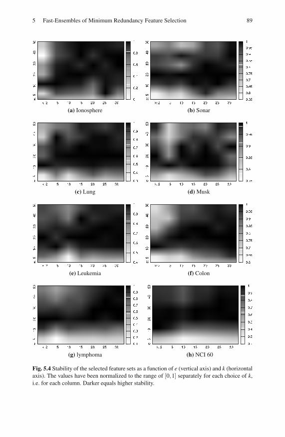
5 Fast-Ensembles of Minimum Redundancy Feature Selection 89
(a) Ionosphere (b) Sonar
(c) Lung (d) Musk
(e) Leukemia (f) Colon
(g) lymphoma (h) NCI 60
Fig. 5.4 Stability of the selected feature sets as a function of e (vertical axis) and k (horizontal
axis). The values have been normalized to the range of [0,1] separately for each choice of k,
i.e. for each column. Darker equals higher stability.
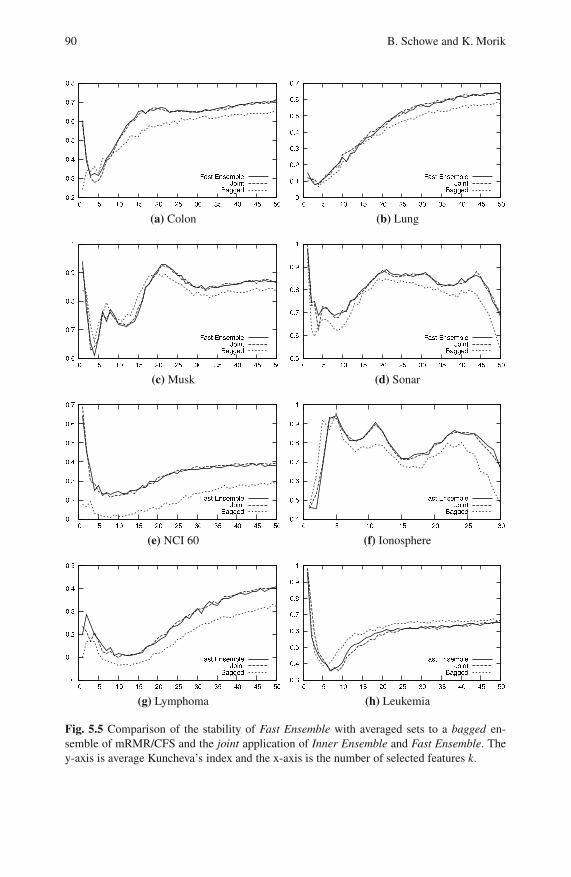
90 B. Schowe and K. Morik
(a) Colon (b) Lung
(c) Musk (d) Sonar
(e) NCI 60 (f) Ionosphere
(g) Lymphoma (h) Leukemia
Fig. 5.5 Comparison of the stability of Fast Ensemble with averaged sets to a bagged en-
semble of mRMR/CFS and the joint application of Inner Ensemble and Fast Ensemble. The
y-axis is average Kuncheva’s index and the x-axis is the number of selected features k.

5 Fast-Ensembles of Minimum Redundancy Feature Selection 91
was averaged over 10 runs of ten-fold cross-validation. Feature selection was only
performed on the training set and not on the test set, as this would lead to far too
optimistic results.
Table 5.2 shows in detail the effect of more stable feature selection on classifi-
cation accuracy for all datasets. For each choice of k, dataset and learner we com-
pared the average accuracy results for our methods to standard mRMR/CFS via an
analysis of variance (ANOVA) and counted the times that each of our methods per-
formed significantly better or worse. On the lower dimensional datasets, i.e. Sonar
and Ionosphere, the increased stability did not result in better prediction. But for the
very high-dimensional datasets a small performance increase can be detected, espe-
cially for Naive Bayes and Nearest Neighbours. In total out of the 280 experiments
our methods performed significantly
better worse
Inner Ensemble 11 6
Fast Ensemble - Sets 14 6
Fast Ensemble - Ranks 30 10
than mRMR/CFS. The Fast Ensemble with Ranks gave better results than Fast En-
semble with Sets. This might be caused by the fact that the rank combination puts
more focus on the higher ranked and thus more meaningful features. When look-
ing at the behaviour of the accuracy dependent on k it showed that Fast Ensemble
delivers better results earlier (with less features) than mRMR/CFS.
Table 5.2 Accuracy: How often was a method significantly better than/equal to/worse than
the standard mRMR/CFS algorithm
Naive Bayes Decision Tree 5NN
Dataset Inner Sets Ranks Inner Sets Ranks Inner Sets Ranks
Colon 0/10/0 1/9/0 1/9/0 2/8/0 1/9/0 0/10/0 0/10/0 0/10/0 0/10/0
Ionosphere 0/6/0 0/6/0 0/6/0 0/6/0 0/6/0 0/6/0 0/6/0 0/6/0 1/4/1
Leukemia 2/8/0 1/9/0 2/7/1 1/7/2 1/9/0 2/8/0 0/10/0 0/10/0 2/8/0
Lung 0/9/1 1/8/1 3/7/0 0/10/0 0/10/0 0/10/0 0/10/0 0/10/0 1/9/0
Lymphoma 1/9/0 4/6/0 6/4/0 1/8/1 0/10/0 0/10/0 1/9/0 0/10/0 4/6/0
Musk 0/9/1 0/9/1 0/10/0 1/9/0 1/8/1 2/8/0 0/10/0 0/8/2 0/7/3
NCI60 0/7/0 0/7/0 0/6/1 1/5/0 1/5/0 0/6/0 1/5/0 0/6/0 4/2/0
Sonar 0/10/0 1/9/0 1/9/0 0/10/0 0/10/0 1/9/0 0/10/0 0/10/0 0/9/1
Sum 3/68/2 8/63/2 13/58/2 6/63/3 4/67/1 5/67/0 2/70/0 0/70/2 12/55/5
SVM LDA
Dataset Inner Sets Ranks Inner Sets Ranks
Musk 0/9/1 0/9/1 0/9/1 0/10/0 0/10/0 0/10/0
Ionosphere 0/6/0 0/6/0 0/5/1 0/6/0 0/6/0 0/5/1
Sonar 0/10/0 0/10/0 0/10/0 0/9/1 2/8/0 0/10/0
Sum 0/25/1 0/25/1 0/24/2 0/25/1 2/24/0 0/25/1

92 B. Schowe and K. Morik
5.4.3 Runtime
Let us now compare the runtime of our new Fast Ensemble with sets to a standard
ensemble of the same size. The overlap (number of features which two sets have in
common) can be calculated based on their size k and their Jaccard index as
ol(SJ,k) = 2SJk/(SJ + 1). (5.19)
The average Jaccard index of the sets produced by the parts of the ensemble is
similar to the average Jaccard index measured for Plain mRMR/CFS for inspecting
stability.
Considering a Fast Ensemble with sets of e parts we now sum up the average
amount of correlations in the parts of the ensemble. In the first part of the ensemble,
all pk− k2−k2 correlations must be computed. In the second part, there are no cor-
relations needed for relevance estimation, and for the redundancy check, only those
k−ol(SJ,k) features, which have not been selected in the first part, must be corre-
lated with the all other features. At this point, it is unclear whether these features
are added at the end or at the beginning of the selection process, i.e., whether the
parts of the ensemble differ at the end or the beginning of the selection process. This
determines how many features it is compared to and explains the imprecision of the
estimate.
For a rough estimate assume the average probability that a feature f r in the rth
part, r ∈ 1, . . . ,e, has already been correlated to all other features in the part before
is
Pk,SJ( f r) =
r−1
∑m=1
ol(SJ,k)
k(1−Pk,SJ
( f m)) (5.20)
which reduces to
PSJ( f r) =
2SJ
SJ + 1
r−1
∑m=1
(1−PSJ( f m)) (5.21)
with PSJ( f 1) = 0. As seen from Eq. (5.8), in each step of one part, there are on aver-
age p− (k−1)/2 correlations to compute. When multiplied with the probability of
not needing to compute the correlation and adding the initial relevance computation
this gives a total average runtime of
T (p,k,e, SJ) = p +e
∑r=1
k
∑j=2
(p− j)(1−PSJ
( f rj ))
(5.22)
= p +(k−1)
(
p− k−1
2
)(
e−e
∑r=1
PSJ( f r)
)
(5.23)
under the assumption PSJ( f r
j ) = PSJ( f r), ∀ j ∈ [1,k].
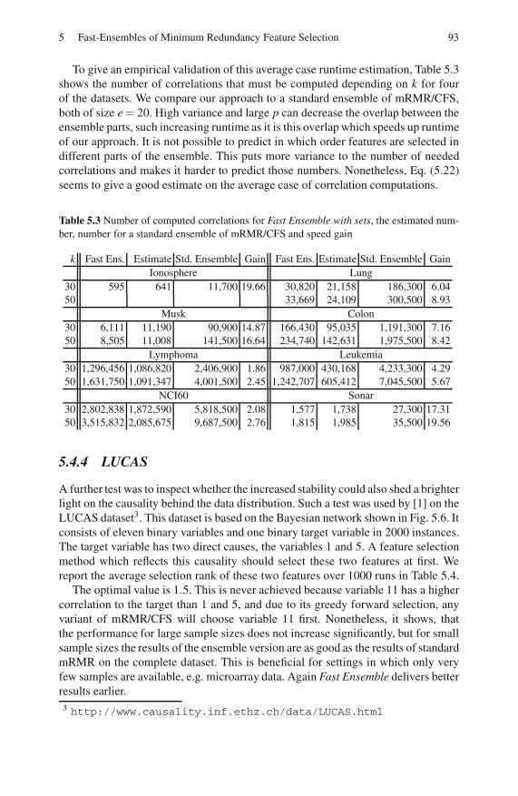
5 Fast-Ensembles of Minimum Redundancy Feature Selection 93
To give an empirical validation of this average case runtime estimation, Table 5.3
shows the number of correlations that must be computed depending on k for four
of the datasets. We compare our approach to a standard ensemble of mRMR/CFS,
both of size e = 20. High variance and large p can decrease the overlap between the
ensemble parts, such increasing runtime as it is this overlap which speeds up runtime
of our approach. It is not possible to predict in which order features are selected in
different parts of the ensemble. This puts more variance to the number of needed
correlations and makes it harder to predict those numbers. Nonetheless, Eq. (5.22)
seems to give a good estimate on the average case of correlation computations.
Table 5.3 Number of computed correlations for Fast Ensemble with sets, the estimated num-
ber, number for a standard ensemble of mRMR/CFS and speed gain
k Fast Ens. Estimate Std. Ensemble Gain Fast Ens. Estimate Std. Ensemble Gain
Ionosphere Lung
30 595 641 11,700 19.66 30,820 21,158 186,300 6.04
50 33,669 24,109 300,500 8.93
Musk Colon
30 6,111 11,190 90,900 14.87 166,430 95,035 1,191,300 7.16
50 8,505 11,008 141,500 16.64 234,740 142,631 1,975,500 8.42
Lymphoma Leukemia
30 1,296,456 1,086,820 2,406,900 1.86 987,000 430,168 4,233,300 4.29
50 1,631,750 1,091,347 4,001,500 2.45 1,242,707 605,412 7,045,500 5.67
NCI60 Sonar
30 2,802,838 1,872,590 5,818,500 2.08 1,577 1,738 27,300 17.31
50 3,515,832 2,085,675 9,687,500 2.76 1,815 1,985 35,500 19.56
5.4.4 LUCAS
A further test was to inspect whether the increased stability could also shed a brighter
light on the causality behind the data distribution. Such a test was used by [1] on the
LUCAS dataset3. This dataset is based on the Bayesian network shown in Fig. 5.6. It
consists of eleven binary variables and one binary target variable in 2000 instances.
The target variable has two direct causes, the variables 1 and 5. A feature selection
method which reflects this causality should select these two features at first. We
report the average selection rank of these two features over 1000 runs in Table 5.4.
The optimal value is 1.5. This is never achieved because variable 11 has a higher
correlation to the target than 1 and 5, and due to its greedy forward selection, any
variant of mRMR/CFS will choose variable 11 first. Nonetheless, it shows, that
the performance for large sample sizes does not increase significantly, but for small
sample sizes the results of the ensemble version are as good as the results of standard
mRMR on the complete dataset. This is beneficial for settings in which only very
few samples are available, e.g. microarray data. Again Fast Ensemble delivers better
results earlier.
3 http://www.causality.inf.ethz.ch/data/LUCAS.html
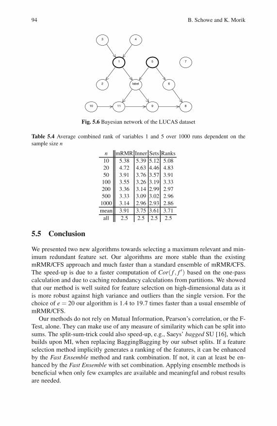
94 B. Schowe and K. Morik
label
4
1
2
3
5
6
7
8910 11
Fig. 5.6 Bayesian network of the LUCAS dataset
Table 5.4 Average combined rank of variables 1 and 5 over 1000 runs dependent on the
sample size n
n mRMR Inner Sets Ranks
10 5.38 5.39 5.12 5.08
20 4.72 4.63 4.46 4.83
50 3.91 3.76 3.57 3.91
100 3.55 3.26 3.19 3.33
200 3.36 3.14 2.99 2.97
500 3.33 3.09 3.02 2.96
1000 3.14 2.96 2.93 2.86
mean 3.91 3.75 3.61 3.71
all 2.5 2.5 2.5 2.5
5.5 Conclusion
We presented two new algorithms towards selecting a maximum relevant and min-
imum redundant feature set. Our algorithms are more stable than the existing
mRMR/CFS approach and much faster than a standard ensemble of mRMR/CFS.
The speed-up is due to a faster computation of Cor( f , f ′) based on the one-pass
calculation and due to caching redundancy calculations from partitions. We showed
that our method is well suited for feature selection on high-dimensional data as it
is more robust against high variance and outliers than the single version. For the
choice of e = 20 our algorithm is 1.4 to 19.7 times faster than a usual ensemble of
mRMR/CFS.
Our methods do not rely on Mutual Information, Pearson’s correlation, or the F-
Test, alone. They can make use of any measure of similarity which can be split into
sums. The split-sum-trick could also speed-up, e.g., Saeys’ bagged SU [16], which
builds upon MI, when replacing BaggingBagging by our subset splits. If a feature
selection method implicitly generates a ranking of the features, it can be enhanced
by the Fast Ensemble method and rank combination. If not, it can at least be en-
hanced by the Fast Ensemble with set combination. Applying ensemble methods is
beneficial when only few examples are available and meaningful and robust results
are needed.

5 Fast-Ensembles of Minimum Redundancy Feature Selection 95
References
1. Bontempi, G., Meyer, P.E.: Causal filter selection in microarray data. In: Furnkranz, J.,
Joachims, T. (eds.) Proc. the 27th Int. Conf. Machine Learning, Haifa, Israel, pp. 95–102.
Omnipress, Madison (2010)2. Breiman, L.: Bagging predictors. Machine Learning 24, 123–140 (1996)3. Breiman, L.: Random forests. Machine Learning 45, 5–32 (2001)4. Ding, C.H.Q., Peng, H.: Minimum redundancy feature selection from microarray gene
expression data. In: Proc. the 2nd IEEE Comp. Society Bioinformatics Conf., Stanford,
CA, pp. 523–529. IEEE Comp. Society, Los Alamitos (2003)5. Fox, R.J., Dimmic, M.W.: A two-sample Bayesian t-test for microarray data. BMC
Bioinformatics 7 (2006)6. Freund, Y., Schapire, R.E.: A decision-theoretic generalization of on-line learning and
an application to boosting. J. Comput. Syst. Sci. 55, 119–139 (1997)7. Gulgezen, G., Cataltepe, Z., Yu, L.: Stable and accurate feature selection. In: Buntine,
W., Grobelnik, M., Mladenic, D., Shawe-Taylor, J. (eds.) ECML PKDD 2009. LNCS,
vol. 5781, pp. 455–468. Springer, Heidelberg (2009)8. Hall, M.A.: Correlation-based feature selection for discrete and numeric class machine
learning. In: Langley, P. (ed.) Proc. the 17th Int. Conf. Machine Learning, Stanford, CA,
pp. 359–366. Morgan Kaufmann, San Francisco (2000)9. Han, Y., Yu, L.: A variance reduction framework for stable feature selection. In: Webb,
G.I., Liu, B., Zhang, C., Gunopulos, D., Wu, X. (eds.) Proc. the 10th IEEE Int. Conf.
Data Mining, Sydney, Australia, pp. 206–215. IEEE Computer Society, Los Alamitos
(2010)10. Jurman, G., Merler, S., Barla, A., Paoli, S., Galea, A., Furlanello, C.: Algebraic stability
indicators for ranked lists in molecular profiling. Bioinformatics 24, 258–264 (2008)11. Kalousis, A., Prados, J., Hilario, M.: Stability of feature selection algorithms: a study on
high-dimensional spaces. Knowledge and Inf. Syst. 12, 95–116 (2007)12. Koh, J.L.Y., Li Lee, M., Hsu, W., Lam, K.-T.: Correlation-based detection of attribute
outliers. In: Kotagiri, R., Radha Krishna, P., Mohania, M., Nantajeewarawat, E. (eds.)
DASFAA 2007. LNCS, vol. 4443, pp. 164–175. Springer, Heidelberg (2007)13. Kohavi, R., John, G.H.: Wrappers for feature subset selection. Artif. Intell. 97, 273–324
(1997)14. Kuncheva, L.I.: A stability index for feature selection. In: Devedzic, V. (ed.) IASTED
Int. Conf. Artif. Intell. and Appl., Innsbruck, Austria, pp. 421–427. ACTA Press, Calgary
(2007)15. Michalak, K., Kwasnicka, H.: Correlation-based feature selection strategy in neural
classification. In: Proc. the 6th Int. Conf. Intell. Syst. Design and Appl., Jinan, China,
pp. 741–746. IEEE Comp. Society, Los Alamitos (2006)16. Saeys, Y., Abeel, T., Van de Peer, Y.: Robust feature selection using ensemble feature
selection techniques. In: Daelemans, W., Goethals, B., Morik, K. (eds.) ECML PKDD
2008, Part II. LNCS (LNAI), vol. 5212, pp. 313–325. Springer, Heidelberg (2008)17. Tusher, V.G., Tibshirani, R., Chu, G.: Significance analysis of microarrays applied to the
ionizing radiation response. Proc. the National Academy of Sciences of the United States
of America 98, 5116–5121 (2001)18. Vapnik, V.: Statistical learning theory. Wiley, Chichester (1998)19. Xu, X., Zhang, A.: Boost feature subset selection: A new gene selection algorithm for
microarray dataset. In: Alexandrov, V.N., van Albada, G.D., Sloot, P.M.A., Dongarra, J.
(eds.) ICCS 2006. LNCS, vol. 3992, pp. 670–677. Springer, Heidelberg (2006)20. Yu, L., Liu, H.: Efficient feature selection via analysis of relevance and redundancy. J.
Machine Learning Research 5, 1205–1224 (2004)

Chapter 6
Hybrid Correlation and Causal FeatureSelection for Ensemble Classifiers
Rakkrit Duangsoithong and Terry Windeatt
Abstract. PC and TPDA algorithms are robust and well known prototype algo-
rithms, incorporating constraint-based approaches for causal discovery. However,
both algorithms cannot scale up to deal with high dimensional data, that is more
than few hundred features. This chapter presents hybrid correlation and causal fea-
ture selection for ensemble classifiers to deal with this problem. Redundant features
are removed by correlation-based feature selection and then irrelevant features are
eliminated by causal feature selection. The number of eliminated features, accuracy,
the area under the receiver operating characteristic curve (AUC) and false negative
rate (FNR) of proposed algorithms are compared with correlation-based feature se-
lection (FCBF and CFS) and causal based feature selection algorithms (PC, TPDA,
GS, IAMB).
6.1 Introduction
With rapid development of computer and information technology that can improve a
large number of applications such as web text mining, intrusion detection, biomedi-
cal informatics, gene selection in micro array data, medical data mining, and clinical
decision support systems, many information databases have been created. However,
in some applications especially in medical area, data may contain hundreds to thou-
sands of features with small sample size. A consequence of this problem is increased
complexity that leads to degradation in efficiency and accuracy by curse of dimen-
sionality and over-fitting. The resulting classifier works very well with training data
but very poorly on test data.
Rakkrit Duangsoithong · Terry Windeatt
Centre for Vision, Speech and Signal Processing, University of Surrey,
Guildford, United Kingdom GU2 7XH
E-mail: [email protected],[email protected]
O. Okun et al. (Eds.): Ensembles in Machine Learning Applications, SCI 373, pp. 97–115.springerlink.com c© Springer-Verlag Berlin Heidelberg 2011
98 R. Duangsoithong and T. Windeatt
To overcome this high dimensional feature spaces degradation problem, num-
ber of features should be reduced. Basically, there are two methods to reduce the
dimension: feature extraction and feature selection. Feature extraction transforms
or projects original features to fewer dimensions without using prior knowledge.
Nevertheless, it lacks comprehensibility and uses all original features which may
be impractical in large feature spaces. On the other hand, feature selection selects
optimal feature subsets from original features by removing irrelevant and redundant
features. It has the ability to reduce over-fitting, increase classification accuracy,
reduce complexity, speed up computation and improve comprehensibility by pre-
serving original semantic of datasets. Normally, clinicians prefer feature selection
because of its understandability and user acceptance.
Feature selection is an important pre-processing step to reduce feature dimen-
sions for classification and generally, can be divided into four categories [9, 15, 18].
Filter method is independent from learning method and uses measurement tech-
niques such as correlation and distance measurement to find a good subset from
entire set of features. Wrapper method uses pre-determined learning algorithm to
evaluate selected feature subsets that are optimum for the learning process. Hybrid
method combines advantage of both Filter and Wrapper method together. It evalu-
ates features by using an independent measure to find the best subset and then uses a
learning algorithm to find the final best subset. Finally, Embedded method interacts
with learning algorithm but it is more efficient than Wrapper method because the
filter algorithm has been built with the classifier.
As has been illustrated by Liu and Yu [15], feature selection has four basic pro-
cesses: subset generation, subset evaluation, stopping criterion and subset valida-
tion. Subset generation produces candidate subset by complete (exhaustive), se-
quential (heuristic) or random search with three directions: forward (adding feature
to selected subset that begin with empty set), backward (eliminate features from se-
lected subset that begins with full original set) and bidirectional (both adding and
removing features). After that, the candidate subset is evaluated based on criteria
such as distance, dependency and information gain and consistency measurement.
The process will stop when it reaches the stopping criterion. Finally, the selected
subset is validated with validation data.
Feature selection does not usually take causal discovery into account. However,
in some cases such as when training and testing dataset do not conform to i.i.d. as-
sumption, testing distribution is shifted from manipulation by external agent, causal
discovery can provide some benefits for feature selection under these uncertainty
conditions. Causal relationships are usually uncovered by Bayesian Networks (BNs)
which consist of a direct acyclic graph (DAG) that represents dependencies and in-
dependencies between variable and joint probability distribution among a set of vari-
ables [1]. It also can learn underlying data structure, provide better understanding
of the data generation process and better accuracy and robustness under uncertainty
[10].

6 Hybrid Correlation and Causal Feature Selection 99
An ensemble classifier or multiple classifier system (MCS) is another well-known
technique to improve system accuracy [24]. Ensembles combine multiple base clas-
sifiers to learn a target function. It has ability to increase accuracy by combining
output of multiple experts to reduce bias and variance [3], improve efficiency by de-
composing complex problem into multiple sub problems and improve reliability by
reducing uncertainty. To increase accuracy, each classifier in the ensemble should
be diverse or unique such as starting with different input, initial weight, random
features or random classes [23].
Generally, the number of features in feature selection analysis can be divided
into three categories: small scale (the number of features is less than 19), medium
scale (the number of features is between 20 and 49) and large scale (the number
of features is equal or higher than 50 features) [12, 27]. The main purpose of this
research is to find methods that can scale up to deal with hundreds or thousands of
features.
The main objective of this chapter is to find approaches that enable PC and TPDA
algorithms to deal with high dimensional data. We propose hybrid correlation and
causal feature selection for ensemble classifiers and compare number of eliminated
features, average percent accuracy, the area under the receiver operating character-
istic curve (AUC) and false negative rate (FNR).
The structure of the chapter is the following. Related research is briefly described
in Sect. 6.2. Section 6.3 explains theoretical approach of feature selection , causal
discovery and ensemble classifiers. The dataset and evaluation procedure are de-
scribed in Sect. 6.4. Experimental results are presented in Sect. 6.5 and are discussed
in Sect. 6.6. Finally, Conclusion is summarized in Sect. 6.7.
6.2 Related Research
Feature selection and ensemble classification have received attention from many re-
searchers in the areas of Statistics, Machine Learning, Neural Networks and Data
Mining for many years. Initially, most researchers focused only on removing ir-
relevant features such as ReliefF [25], FOCUS [2] and Correlation-based Feature
Selection(CFS) [8]. Recently, in Yu and Liu (2004) [26], Fast Correlation-Based
Filter (FCBF) algorithm was proposed to remove both irrelevant and redundant fea-
tures by using Symmetrical Uncertainty (SU) measurement and was successful for
reducing high dimensional features while maintaining high accuracy.
In the past few years, learning Bayesian Networks (BNs) from observation data
has received increasing attention from researchers for many applications such as
decision support system, information retrieval, natural language processing, feature
selection and gene expression data analysis [21, 22]. The category of BNs can be
divided into three approaches: Search-and-Score, Constraint-Based and Hybrid ap-
proaches [21, 22]. In Search-and-Score approach, BNs search all possible structures
to find the one that provides the maximum score. The standard Scoring functions

100 R. Duangsoithong and T. Windeatt
that normally used in BNs are Bayesian Dirichlet (BDeu), Bayesian Information
Criterion (BIC), Akaike Information Criterion (AIC), Minimum Description Length
(MDL) and K2 scoring function [21]. The second approach, Constraint-Based, uses
test of conditional dependencies and independencies from the data by estimation
using G2 statistic test or mutual information, etc. This approach defines structure and
orientation from results of the tests based on some assumptions that these tests are
accurate. Finally, Hybrid approach uses Constraint-Based approach for conditional
independence test (CI test) and then identifies the network that maximizes a scoring
function by using Search-and-Score approach [22].
Constraint-Based algorithms are computationally effective and suitable for high
dimensional feature spaces. PC algorithm [19], is a pioneer, prototype and well-
known global algorithm of Constraint-Based approach for causal discovery. Three
Phase Dependency Analysis (TPDA or PowerConstructor) [6] is another global
Constraint-Based algorithm that uses mutual information to search and test for CI
test instead of using G2 Statistics test as in PC algorithm. However, both PC and
TPDA algorithm use global search to learn from the complete network and can not
scale up to more than few hundred features (they can deal with 100 and 255 features
for PC and TPDA, respectively) [20]. Sparse Candidate algorithm (SC) [7] is one of
the prototype BNs algorithm that can deal with several hundreds of features by us-
ing local candidate set. Nevertheless, SC algorithm has some disadvantages: it may
not identify true set of parents and users have to find appropriate k parameter of SC
algorithm [21].
Recently, many Markov Blanket-based algorithms for causal discovery have been
studied extensively and they have ability to deal with high dimensional feature
spaces such as MMMB, IAMB [20] and HITON [1] algorithms. HITON is a state-
of-the-art algorithm that has ability to deal with thousands of features and can be
used as an effective feature selection method in high dimensional spaces. However,
HITON and all other MB-based algorithms may not specify features in Markov
Blanket for desired classes or target (MB(T)) when the data is not faithful [5].
6.3 Theoretical Approach
In our research, hybrid algorithm of correlation and causal feature selection is com-
pared with Fast Correlation-Based Filter (FCBF), Correlation-based Feature Se-
lection with Sequential Forward Floating Search direction (CFS+SFFS), and with
causal feature selection algorithms (PC, TPDA, GS and IAMB) using Bagging (de-
scribed in Sect. 6.3.4).
6.3.1 Feature Selection Algorithms
6.3.1.1 Fast Correlation-Based Filter (FCBF)
FCBF [26] algorithm is a correlation-based filter which has two stages: relevance
analysis and redundancy analysis.

6 Hybrid Correlation and Causal Feature Selection 101
Relevance Analysis
Normally, correlation is widely used to analyze relevance in linear system and can
be measured by linear correlation coefficient.
r =∑i(xi− xi)(yi− yi)
√
∑i(xi− xi)2√
∑i(yi− yi)2. (6.1)
However, most systems in real world applications are non-linear. Correlation in
non-linear systems can be measured by using Symmetrical Uncertainty (SU).
SU(X ,Y) = 2[ IG(X |Y )
H(X)+ H(Y)
]
, (6.2)
IG(X |Y ) = H(X)−H(X |Y) , (6.3)
H(X) =−∑i
P(xi)log2P(xi) , (6.4)
where IG(X |Y ) is the Information Gain of X after observing variable Y , H(X) and
H(Y ) are the entropy of variable X and Y , respectively, and P(xi) is the probability
of variable X .
SU is the modified version of Information Gain that has range between 0 and 1.
FCBF removes irrelevant features by ranking correlation (SU) between feature and
class. If SU between feature and class equal to 1, it means that this feature is com-
pletely related to that class. On the other hand, if SU is equal to 0, the features are
irrelevant to this class.
Redundancy analysis
Redundant features can be defined from meaning of predominant feature and ap-
proximate Markov Blanket. In Yu and Liu (2004) [26], a feature is predominant
(both relevant and non redundant feature) if it does not have any approximate
Markov Blanket in the current set.
Approximate Markov Blanket: For two relevant features Fi and Fj (i = j), Fj
forms an approximate Markov Blanket for Fi if
SU j,c ≥ SUi,c and SUi, j ≥ SUi,c , (6.5)
where SUi,c is a correlation between any feature and the class, SUi, j is a correlation
between any pair of feature Fi and Fj (i = j).
6.3.1.2 Correlation-Based Feature Selection (CFS)
CFS [8] is one of well-known techniques to rank the relevance of features by mea-
suring correlation between features and classes and between features and other
features.

102 R. Duangsoithong and T. Windeatt
Given number of features k and classes c, CFS defined relevance of features sub-
set by using Pearson’s correlation equation
Merits =krkc
√
k +(k−1)rkk
, (6.6)
where Merits is relevance of feature subset, rkc is the average linear correlation co-
efficient between these features and classes and rkk is the average linear correlation
coefficient between different features.
Normally, CFS adds (forward selection) or deletes (backward selection) one fea-
ture at a time, however, in this research, we used Sequential Forward Floating Search
(SFFS) [17] as the search direction because of its powerful search scheme which is
very fast and does not require any tuning parameters.
Sequential Forward Floating Search (SFFS). SFFS [17] is one of the classic
heuristic searching methods. It is a variation of bidirectional search and sequential
forward search (SFS) that has dominant direction on forward search. SFFS removes
features (backward elimination) after adding features (forward selection). The num-
ber of forward and backward steps is not fixed but dynamically controlled depending
on the criterion of the selected subset and therefore, no parameter setting is required.
6.3.2 Causal Discovery Algorithm
In this chapter, two standard constraint-based approaches (PC and TPDA) and two
Markov Blanket based algorithms (GS, IAMB) are used as causal feature selection
methods. In the final output of the causal graph from each algorithm, the uncon-
nected features to classes will be considered as eliminated features.
6.3.2.1 PC Algorithm
PC algorithm [10, 19] is the prototype of constraint-based algorithm. It consists of
two phases: Edge Detection and Edge Orientation.
Edge Detection: the algorithm determines directed edge by using conditionally
independent condition. The algorithm starts with:
i) Undirected edge with fully connected graph.
ii) Remove a share direct edge between A and B (A−B) iff there is a subset F of
features that can present conditional independence (A,B|F).Edge Orientation: The algorithm discovers V-Structure A−B−C in which A−C
is missing.
i) If there are direct edges between A−B and B−C but not A−C, then orient
edge A→ B←C until no more possible orientation.
ii) If there is a path A→ B−C and A−C is missing, then A→ B→C.
iii) If there is orientation A→ B→ ...→C and A−C then orient A→C.

6 Hybrid Correlation and Causal Feature Selection 103
6.3.2.2 Three Phase Dependency Analysis Algorithm (TPDA)
TPDA or PowerConstructor algorithm [6] has three phases: drafting, thickening and
thinning phases.
Drafting phase: mutual information of each pair of nodes is calculated and used
to create a graph without loop.
Thickening phase: edge will be added when that pair of nodes can not be d-
separated (node A and B are d-separated by node C iff node C blocks every path
from node A to node B [21]) The output of this phase is called an independence map
(I-map).
Thinning phase: The edge of I-map will be removed in thinning phase, if two
nodes of the edge can be d-separated and the final output is defined as a perfect
map [6].
6.3.2.3 Grow-Shrink Algorithm (GS)
GS [16] algorithm consists of two phases: forward and backward phases.
Forward phase: GS statistically ranks features by using the strength of associa-
tion with target or class (T) given empty set. After that the next ordering feature
which is not conditionally independent from class T given current Markov Blanket
(CMB) will added into CMB.
Backward phase: Identify false positive nodes and remove them from CMB. At
this stage, CMB = MB(T ). Finally, a feature X will be removed from CMB one-by-
one if that feature X is independent of class T given the remaining CMB.
6.3.2.4 Incremental Association Markov Blanket Algorithm (IAMB)
IAMB [20] is one of Markov Blanket detection algorithms using forward selec-
tion followed by removing false positive node. IAMB has two phases: forward and
backward.
Forward phase: In forward selection phase, the algorithm starts with empty set
in CMB, then adding features which maximize a heuristic function f (X ;T |CMB).A feature member in MB(T) will not return zero value of this function.
Backward phase: False positive nodes will be removed from CMB by using con-
dition independent testing of class T given the rest CMB.
6.3.3 Feature Selection Analysis
6.3.3.1 Correlation-Based Redundancy and Relevance Analysis
The concept of selecting the optimal subset from the entire set of features is pre-
sented in Fig. 6.1 [26], where I is irrelevant feature, II is weakly relevant and redun-
dant feature, III is weakly relevant but non redundant feature, IV is strongly relevant
feature. The combination of III+IV is the optimal feature subset.

104 R. Duangsoithong and T. Windeatt
Fig. 6.1 Optimal Subset
Thus, the optimal subset should include all strongly relevant features, subset of
weakly relevant features that have no redundancy and none of the irrelevant features.
In 2004, Yu and Liu [26] proposed FCBF algorithm to remove both redundant
and irrelevant features.
1) Redundancy: A feature is redundant if it has approximate Markov Blanket
(SU j,c ≥ SUi,c and SUi, j ≥ SUi,c).
2) Irrelevance: A feature is irrelevant if SU between feature and class is zero.
3) Relevance: A feature is relevant if SU between feature and class is more than
zero but less than one.
4) Strong relevance: A feature is strongly relevant if SU between feature and
class is equal to one.
6.3.3.2 Causal-Based Relevance Analysis
In Guyon [10], the notion of Markov Blanket is defined in term of Kohavi-John
feature relevance:
1) Irrelevance: A feature is irrelevant if it is disconnected from graph (condi-
tional independence).
2) Relevance: A feature is relevant if it has connected path to class (target).
3) Strong relevance: A feature is strongly relevant if it is Markov Blanket of
class.
6.3.3.3 Hybrid Correlation-Based Redundancy Causal-Based Relevance
Analysis
According to Fig. 6.1 and the above analysis, optimal subset consists of strongly
relevant features and weakly relevant features that do not contain redundant and
irrelevant features. Therefore, we propose a new analysis for Hybrid Correlation-
Based Relevance Causal-Based Redundancy Analysis as follows:
1) Redundancy: A feature is redundant if it has approximate Markov Blanket.
2) Irrelevance: A feature is irrelevant if it is disconnected from the graph (con-
ditional independence).

6 Hybrid Correlation and Causal Feature Selection 105
3) Relevance: A feature is relevant if it has connected path to the target (class).
4) Strong relevance: A feature is strongly relevant if it is Markov Blanket of the
target (class).
Table 6.1 Summary analysis of correlation, causal and proposed hybrid correlation and causal
feature selection for redundancy and relevance analysis
Relation Correlation-Based Causal-Based Hybrid algorithm
Strongly relevant SUi,c = 1 Features in Features in
Markov Blanket Markov Blanket
Weakly relevant does not has approxi-
mate
connected connected
without redundant features Markov Blanket to classes to classes
Weakly relevant has approximate connected has approximate
with redundant features Markov Blanket to classes Markov Blanket
Irrelevant SUi,c = 0 disconnected disconnected
to classes to classes
Table 6.1 shows the summary analysis of redundancy and relevancy analysis
for correlation-based [26], causal-based [10] and proposed hybrid correlation and
causal feature selection . Markov Blanket (MB(T)) of target or class (T) is the min-
imal set of conditional features that all other features are probabilistically indepen-
dent of T. It consists of the set of parents, children and spouses of T.
Figure 6.2 presents the proposed system block diagram. Redundant features are
removed by correlation-based feature selection and irrelevant features are eliminated
by causal-based feature selection . After that, selected features are passed through
ensemble classifier for training and predicting output.
Fig. 6.2 Block Diagram of proposed algorithm

106 R. Duangsoithong and T. Windeatt
6.3.4 Ensemble Classifier
Bagging [4] or Bootstrap aggregating is one of the earliest, simplest and most pop-
ular methods for ensemble based classifiers. Bagging uses Bootstrap that randomly
samples with replacement and combines with majority vote. The selected data is
divided to m bootstrap replicates and randomly sampled with replacement. Each
bootstrap replicate contains, on average, 63.2 % of the original dataset. Final out-
put will be selected from majority vote of all classifiers of each bootstrap replicate.
Bootstrap is the most well-known strategy for injecting randomness to improve gen-
eralization performance in multiple classifier systems and provides out-of-bootstrap
estimate for selecting classifier parameters [24]. Randomness is desirable since it
increases diversity among the base classifiers, which is known to be a necessary
condition for improved performance. However, there is an inevitable trade-off be-
tween accuracy and diversity known as the accuracy/diversity dilemma [24].
Nevertheless, in causal discovery, there are some disadvantages for BNs learning
using Bagging. Bootstrap method can add many extra edges in graphical model
due to more complexity especially in high dimensional features with limited dataset
[13]. Moreover, distribution from bootstrap dataset may not satisfy Markov Blanket
condition and faithfulness condition [14].
6.3.5 Pseudo-code: Hybrid Correlation and Causal Feature
Selection for Ensemble Classifiers Algorithm
Goal : To find optimal subset features for ensemble classifiers by using correlation
and causal discovery.
6.3.5.1 Eliminate Redundant Features by Using Correlation
⋄ Input: Training set (each pattern having features f1, f2, ..., fn and class C)⋄ Output: Selected features without redundant features S1• Calculate SU between features and between feature and classes, find and remove
redundant features using approximate Markov Blanket.
for i = 1 to n−1, j = i+ 1
fi = first feature, f j = next feature
calculate SUi, j, SUi,c and SU j,c
if SUi,c ≥ SU j,c and SUi, j ≥ SU j,c
then remove f j
else Append f j to output selected features list S1end for
6.3.5.2 Remove Irrelevant Features by Using Causal Discovery
⋄ Input: Selected features without redundant features. S1⋄ Output: Optimal features without redundant and irrelevant features.S2

6 Hybrid Correlation and Causal Feature Selection 107
• Find constructor and direction of graph by using causal discovery algorithm.
(PC, TPDA, GS, IAMB or other causal discovery algorithm)
• Remove irrelevant features which are disconnected from class.
- PC Algorithm
Edge Detection: using conditionally independent condition.
Starts with completely connected graph G.
i =−1
repeat
i = i+ 1
repeat
- Select and order pair of features (nodes) A,B in graph G.
- Select adjacent (neighborhood) feature F of A with size i
- if there exists a feature F that presents conditional independence
(A,B|F), delete direct edge between A and B.
until all ordered pairs of feature F have been tested.
until all adjacent features have size smaller than i.
Edge Orientation: directed edges using following rules;
• If there are direct edges between A−B and B−C but not A−C, then orient edge
A→ B←C until no more possible orientation.
• If there is a path A→ B−C and A−C is missing, then A→ B→C.
• If there is orientation A→ B→ ...→C and A−C then orient A→C.
- Three Phase Dependency Analysis Algorithm (TPDA).
Drafting phase
• calculated mutual information (MI) of each pair of features.
• create a graph without loop using MI.
Thickening phase
• add edge when that pair of nodes can not be d-separated.
• the output of this phase is called an independence map (I-map).
Thinning phase
• remove the edge of I-map, if two nodes of the edge can be d-separated.
• the final output is defined as a perfect map.
6.3.5.3 Ensemble Classifiers Using Bagging Algorithm
⋄ Input:
• Optimal features without redundant and irrelevant features S2• Number of bootstrap sample (m) (number of iterations) with 100 percentage set-
ting from original data
• Classifier or Inducer function (I)

108 R. Duangsoithong and T. Windeatt
for i = 1 to m
S′2 = bootstrap sample from S2Ci = IS′2 //(class output of each bootstrap replicate)
end for
⋄ Output:
• ensemble classifiers prediction based on majority vote (C∗(x))• y is one of the class of total Y classes
• count majority vote class from all output of bootstrap replicates
C∗(x) = argmaxy∈Y ∑i:Ci(x)=y 1
6.4 Experimental Setup
6.4.1 Dataset
The datasets used in this experiment were taken from Causality Challenge [11] and
details of each dataset are shown as follows:
LUCAS (LUng CAncer Simple set) dataset is toy data generated artificially by
causal Bayesian networks with binary features. Both this dataset and the next one
(LUCAP) are modelling a medical application for the diagnosis, prevention and
cure of lung cancer. Lucas has 11 features with binary classes and 2,000 samples.
LUCAP (LUng CAncer set with Probes) is LUCAS dataset with probes which are
generated from some functions plus some noise of subsets of the real variables. LU-
CAP has 143 features, 2,000 samples and binary classes.
REGED (REsimulationed Gene Expression Dataset) is dataset that simulated model
from real human lung cancer micro array gene expression data. The target to simu-
late this data is to find genes which could be responsible of lung cancer. It contains
500 examples with 999 features and binary classes.
CINA (Census Is Not Adult) dataset derived from Census dataset from UCI Ma-
chine learning repository. The goal of dataset is to uncover the socio-economic fac-
tors affecting high income. It has 132 features which contains 14 original features
and distracter features which are artificially generated features that are not causes of
the classes, 16,033 examples and binary classes.
SIDO (SImple Drug Operation mechanisms) has 4,932 features, 12,678 samples
and 2 classes. Sido dataset consists of molecules descriptors that have been tested
against the AIDS HIV virus and probes which artificially generated features that are
not causes of the target.

6 Hybrid Correlation and Causal Feature Selection 109
Due to large number of samples and limitation of computer memory during val-
idation in CINA and SIDO datasets, the number of samples of both dataset are
reduced to 10 percent (1,603 and 1,264 samples, respectively) from the original
dataset.
6.4.2 Evaluation
To evaluate feature selection process we use four widely used classifiers: Naive-
Bayes (NB), Multilayer Perceptron (MLP), Support Vector Machines (SVM) and
Decision Trees (DT). The parameters of each classifier were chosen as follows.
MLP has one hidden layer with 16 hidden nodes, learning rate 0.2, momentum 0.3,
500 iterations and uses backpropagation algorithm with sigmoid transfer function.
SVM uses polynomial kernel with exponent 2 and the regularization value set to
0.7. DT uses pruned C4.5 algorithm. The number of classifiers in Bagging is var-
ied from 1, 5, 10, 25 to 50 classifiers. The threshold value of FCBF algorithm in
our research is set at zero for LUCAS, REGED, CINA, SIDO and 0.14 for LUCAP
dataset, respectively.
The classifier results were validated by 10 fold cross validation with 10 repe-
titions for each experiment and evaluated by average percent of test set accuracy,
False Negative Rate (FNR) and area under the receiver operating characteristic curve
(AUC).
In two-class prediction, there are four possible results of classification as shown
in Table 6.2.
Table 6.2 Four possible outcomes from two-classes prediction
Predicted Class
Positive Negative
Actual Positive True Positive (TP) False Negative (FN)
Class Negative False Positive (FP) True Negative (TN)
Accuracy. Accuracy of classification measurement can be calculated from the ratio
between number of correct predictions (True Positive(TP) and True Negative (TN))
and total number of all possible outcomes (TP,TN,FP and FN).
Accuracy =[ TP + TN
T P+ FP+ FN + TN
]
(6.7)
The area under the receiver operating characteristic curve (AUC). AUC is a
graph of true positive against false positive. AUC has value between 0 and 1. The
AUC value of 1 represents a perfect classifier performance while AUC lower than
0.5 represents a poor prediction.

110 R. Duangsoithong and T. Windeatt
Table 6.3 Number of selected features from each algorithm
Dataset Original Correlation-Based Causal-Based Hybrid algorithm
Feature FCBF CFS PC TPDA GS IAMB H-PC H-TPDA H-GS H-IAMB
LUCAS 11 3 3 9 10 9 11 2 3 2 2
LUCAP 143 7 36 121 121 16 14 21 22 17 13
REGED 999 18 18 N/A N/A 2 2 18 N/A 2 2
CINA 132 10 15 132 N/A 4 4 5 7 10 9
SIDO 4932 23 25 N/A N/A 17 17 2 3 1 2
False Negative Rate (FNR) For medical dataset, FNR is the ratio of number of
patient with negative prediction (False Negative (FN)) and number with disease
condition (FN and TP).
FNR =[ FN
FN + TP
]
(6.8)
For causal feature selection , PC algorithm uses mutual information (MI) as sta-
tistical test with threshold 0.01 and maximum cardinality equal to 2. In TPDA al-
gorithm, mutual information was used as statistic test with threshold 0.01 and data
assumed to be monotone faithful. GS and IAMB algorithm use MI statistic test with
significance threshold 0.01 and provides output as Markov Blanket of the classes.
6.5 Experimental Result
Table 6.3 presents the number of selected features for correlation-based, causal
based feature selection and proposed hybrid algorithm. It can be seen that PC and
TPDA algorithms are impractical for high dimensional features due to their com-
plexity. However, if redundant features are removed, the number of selected features
will enable both algorithms to be practical as shown in proposed hybrid algorithm.
Nevertheless, for some datasets such as REGED, TPDA algorithm might not be
feasible because of many complex connections between nodes (features).
Figures 6.3-6.6 show the average percent accuracy, AUC and FNR of five datasets
from all four classifiers. From average accuracy in Fig. 6.3, correlation-based feature
selection (FCBF, CFS) provides the best average accuracy. Hybrid correlation and
causal feature selection has better accuracy than original causal feature selection.
Hybrid method using PC algorithm (H-PC) has slightly lower average accuracy than
correlation-based feature selection but has the ability to deal with high dimensional
features. From Fig. 6.4, PC, CFS, TPDA and FCBF algorithms provide the best and
comparable AUC. Proposed hybrid algorithm has lower AUC than both correlation
and original causal-based algorithms. In Fig. 6.5, H-PC has the lowest FNR. In all
experiments, hybrid algorithm provides lower FNR than original causal algorithm
but still higher than correlation-based algorithm.
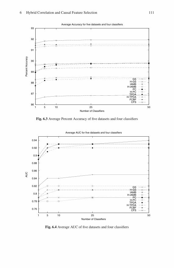
6 Hybrid Correlation and Causal Feature Selection 111
86
87
88
89
90
91
92
93
1 5 10 25 50
Perc
ent A
ccura
cy
Number of Classifiers
Average Accuracy for five datasets and four classifiers
GS H-GS IAMB
H-IAMB PC
H-PC TPDA
H-TPDA FCBF
CFS
Fig. 6.3 Average Percent Accuracy of five datasets and four classifiers
0.76
0.78
0.8
0.82
0.84
0.86
0.88
0.9
0.92
0.94
1 5 10 25 50
AU
C
Number of Classifiers
Average AUC for five datasets and four classifiers
GS H-GS IAMB
H-IAMB PC
H-PC TPDA
H-TPDA FCBF
CFS
Fig. 6.4 Average AUC of five datasets and four classifiers
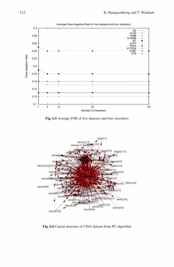
112 R. Duangsoithong and T. Windeatt
0.1
0.12
0.14
0.16
0.18
0.2
0.22
0.24
0.26
0.28
0.3
1 5 10 25 50
Fals
e N
egative R
ate
Number of Classifiers
Average False Negative Rate for five datasets and four classifiers
GS H-GS IAMB
H-IAMB PC
H-PC TPDA
H-TPDA FCBF
CFS
Fig. 6.5 Average FNR of five datasets and four classifiers
labels1
labels2 labels3
labels4
labels5
labels6
labels7
labels8
labels9
labels10
labels11
labels12
labels13
labels14
labels15
labels16
labels17
labels18
labels19
labels20
labels21
labels22labels23
labels24
labels25
labels26
labels27
labels28
labels29
labels30
labels31
labels32
labels33
labels34
labels35
labels36
labels37
labels38
labels39
labels40labels41labels42 labels43
labels44labels45
labels46
labels47
labels48
labels49
labels50
labels51labels52
labels53
labels54
labels55
labels56
labels57
labels58
labels59
labels60
labels61
labels62
labels63
labels64
labels65
labels66
labels67
labels68
labels69
labels70labels71
labels72labels73
labels74
labels75
labels76labels77
labels78
labels79
labels80
labels81
labels82
labels83
labels84
labels85
labels86
labels87
labels88
labels89
labels90
labels91
labels92
labels93 labels94
labels95
labels96
labels97
labels98
labels99
labels100
labels101
labels102
labels103
labels104
labels105
labels106
labels107labels108
labels109
labels110labels111
labels112
labels113
labels114
labels115
labels116
labels117
labels118
labels119
labels120
labels121
labels122
labels123
labels124
labels125
labels126
labels127
labels128
labels129
labels130
labels131
labels132
labels133
Fig. 6.6 Causal structure of CINA dataset from PC algorithm

6 Hybrid Correlation and Causal Feature Selection 113
labels1
labels2labels3
labels4
labels5labels6
labels7
labels8 labels9 labels10
labels11
Fig. 6.7 Causal structure of CINA dataset from Hybrid-PC algorithm (class=labels[11])
Figures 6.6-6.7 present examples of the causal structure for CINA dataset using
PC and Hybrid-PC algorithms, respectively. The high complexity of original CINA
dataset using PC algorithm can be seen in Fig. 6.6 while after removing redundant
and irrelevant features of CINA dataset using hybrid PC algorithm as shown in
Fig. 6.7, the complexity of system is decreased, easier to understand and higher
accuracy (Fig. 6.4), compared to using the original PC algorithm.
Ensemble classifiers using Bagging slightly improves accuracy and AUC for
most algorithms. Bagging also reduces FNR for CFS, PC and TPDA algorithm but
provides stable FNR for the rest. After increasing number of classifiers to 5-10, the
graphs of average accuracy, AUC and FNR all reach saturation point.
6.6 Discussion
In high dimensional features spaces, Bagging algorithm is not appropriate and im-
practical for Bayesian Networks and its complexity may overestimate extra edges
and their distribution might not satisfy Markov Blanket condition and faithfulness
condition [13, 14]. Therefore, this chapter proposed to solve this problem by reduc-
ing dimensionality before bagging while preserving efficiency and accuracy.
For small and medium number of features, a set of selected features after remov-
ing redundancy might be very small (may be only 2-3 features in some datasets and
algorithms), however, the result is still comparable to the result before removing
redundant features.
PC algorithm has tendency to select all features (all connected such as in CINA
dataset) that may be impractical due to computational expense. Therefore, removing
redundant features prior to causal discovery would benefit PC algorithm.
In some cases, such as REGED dataset as shown in Table 6.3, TPDA algorithm
can have very complex causal relations between features that might be impractical
to calculate even for medium number of features.
From the experiment results, Bagging can improve system accuracy and AUC
but cannot improve FNR.

114 R. Duangsoithong and T. Windeatt
6.7 Conclusion
In this chapter, hybrid correlation and causal feature selection for ensemble classi-
fiers is presented to deal with high dimensional features. According to the results,
the proposed hybrid algorithm provides slightly lower accuracy, AUC and higher
FNR than correlation-based. However, compared to causal-based feature selection,
the proposed hybrid algorithm has lower FNR, higher average accuracy and AUC
than original causal-based feature selection. Moreover, the proposed hybrid algo-
rithm can enable PC and TPDA algorithms to deal with high dimensional features
while maintaining high accuracy, AUC and low FNR. Also the underlying causal
structure is more understandable and has less complexity. Ensemble classifiers using
Bagging provide slightly better results than single classifier for most algorithms. Fu-
ture work will improve accuracy of search direction in structure learning for causal
feature selection algorithm.
References
1. Aliferis, C.F., Tsamardinos, I., Statnikov, A.: HITON, A novel Markov blanket algorithm
for optimal variable selection. In: Proc. American Medical Iinformation Association An-
nual Symp., Washington DC, pp. 21–25 (2003)
2. Almuallim, H., Dietterich, T.G.: Learning with many irrelevant features. In: Proc. the 9th
Natl. Conf. Artif. Intell., San Jose, CA, pp. 547–552. AAAI Press, New York (1991)
3. Bauer, E., Kohavi, R.: An empirical comparison of voting classification algorithms: bag-
ging, boosting, and variants. Machine Learning 36, 105–139 (1999)
4. Breiman, L.: Bagging predictors. Machine Learning 24, 123–140 (1996)
5. Brown, L.E., Tsamardinos, I.: Markov blanket-based variable selection. Technical Re-
port DSL TR-08-01 (2008)
6. Cheng, J., Bell, D.A., Liu, W.: Learning belief networks from data: An information the-
ory based approach. In: Golshani, F., Makki, K. (eds.) Proc. the 6th Int. Conf. Inf. and
Knowledge Management, Las Vegas, NV, pp. 325–331. ACM, New York (1997)
7. Friedman, N., Nachman, I., Peer, D.: Learning of Bayesian network structure from mas-
sive datasets: The sparse candidate algorithm. In: Laskey, K., Prade, H. (eds.) Proc. the
15th Conf. Uncertainty in Artif. Intell., Stockholm, Sweden, pp. 206–215. Morgan Kauf-
mann, San Francisco (1999)
8. Hall, M.A.: Correlation-based feature selection for discrete and numeric class machine
learning. In: Langley, P. (ed.) Proc. the 17th Int. Conf. Machine Learning, Stanford, CA,
pp. 359–366. Morgan Kaufmann, San Francisco (2000)
9. Duangsoithong, R., Windeatt, T.: Relevance and redundancy analysis for ensemble clas-
sifiers. In: Perner, P. (ed.) MLDM 2009. LNCS, vol. 5632, pp. 206–220. Springer, Hei-
delberg (2009)
10. Guyon, I., Aliferis, C., Elisseeff, A.: Causal feature selection. In: Liu, H., Motoda, H.
(eds.) Computational Methods of Feature Selection, pp. 63–86. Chapman & Hall/CRC
Press, Boca Raton (2007)
11. Guyon, I.: Causality workbench (2008),
http://www.causality.inf.ethz.ch/home.php12. Kudo, M., Sklansky, J.: Comparison of algorithms that select features for pattern classi-
fiers. Pattern Recognition 33, 25–41 (2000)

6 Hybrid Correlation and Causal Feature Selection 115
13. Liu, F., Tian, F., Zhu, Q.: Bayesian network structure ensemble learning. In: Alhajj,
R., Gao, H., Li, X., Li, J., Zaıane, O.R. (eds.) ADMA 2007. LNCS (LNAI), vol. 4632,
pp. 454–465. Springer, Heidelberg (2007)
14. Liu, F., Tian, F., Zhu, Q.: Ensembling Bayesian network structure learning on limited
data. In: Silva, M.J., Laender, A.H.F., Baeza-Yates, R.A., McGuinness, D.L., Olstad,
B., Olsen, Ø.H., Falcao, A.O. (eds.) Proc. of the 16th ACM Conf. Inf. and Knowledge
Management, Lisbon, Portugal, pp. 927–930. ACM, New York (2007)
15. Liu, H., Yu, L.: Toward integrating feature selection algorithms for classification and
clustering. IEEE Trans. Knowledge and Data Engineering 17, 491–502 (2005)
16. Margaritis, D., Thrun, S.: Bayesian network induction via local neighborhoods. In:
Solla, S.A., Leen, T.K., Muller, K.-R. (eds.) Proc. Neural Inf. Proc. Conf., Denver, CO.,
pp. 505–511. MIT Press, Cambridge (2000)
17. Pudil, P., Novovicova, J., Kittler, J.: Floating Search Methods in Feature Selection. Pat-
tern Recognition Letters 15, 1119–1125 (1994)
18. Saeys, Y., Inza, I., Larranaga, P.: A review of feature selection techniques in bioinfor-
matics. Bioinformatics 23, 2507–2517 (2007)
19. Spirtes, P., Glymour, C., Scheines, R.: Causation, prediction, and search. Springer, New
York (1993)
20. Tsamardinos, I., Aliferis, C.F., Statnikov, A.: Time and sample efficient discovery of
Markov blankets and direct causal relations. In: Getoor, L., Senator, T.E., Domingos, P.,
Faloutsos, C. (eds.) Proc. the 9th ACM SIGKDD Int. Conf. Knowledge Discovery and
Data Mining, Washington DC, pp. 673–678. ACM, New York (2003)
21. Tsamardinos, I., Brown, L.E., Aliferis, C.F.: The max-min hill-climbing Bayesian net-
work structure learning algorithm. Machine Learning 65, 31–78 (2006)
22. Wang, M., Chen, Z., Cloutier, S.: A hybrid Bayesian network learning method for con-
structing gene networks. J. Comp. Biol. and Chem. 31, 361–372 (2007)
23. Windeatt, T.: Accuracy/diversity and ensemble MLP classifier design. IEEE Trans. Neu-
ral Networks 17, 1194–1211 (2006)
24. Windeatt, T.: Ensemble MLP classifier design. In: Lakhmi, J.C., Sato-Ilic, M., Virvou,
M., Tsihrintzis, G.A., Balas, V.E., Abeynayake, C. (eds.) Computational Intelligence
Paradigms. SCI, vol. 137, pp. 133–147. Springer, Heidelberg (2008)
25. Witten, I.H., Frank, E.: Data mining: Practical machine learning tools and techniques.
Morgan Kaufmann, San Francisco (2005)
26. Yu, L., Liu, H.: Efficient feature selection via analysis of relevance and redundancy. J.
Machine Learning Research 5, 1205–1224 (2004)
27. Zhang, H., Sun, G.: Feature selection using tabu search. Pattern Recognition 35, 701–711
(2002)

Chapter 7
Learning Markov Blankets for Continuous orDiscrete Networks via Feature Selection
Houtao Deng, Saylisse Davila, George Runger, and Eugene Tuv
Abstract. Learning Markov Blankets is important for classification and regression,
causal discovery, and Bayesian network learning. We present an argument that en-
semble masking measures can provide an approximate Markov Blanket. Conse-
quently, an ensemble feature selection method can be used to learn Markov Blankets
for either discrete or continuous networks (without linear, Gaussian assumptions).
We use masking measures for redundancy and statistical inference for feature selec-
tion criteria. We compare our performance in the causal structure learning problem
to a collection of common feature selection methods. We also compare to Bayesian
local structure learning. These results can also be easily extended to other casual
structure models such as undirected graphical models.
7.1 Introduction
Structure learning in Bayesian Networks is an important step for causal inference
and Markov Blanket causal discovery algorithms can be helpful for learning the
structure of Bayesian Networks. Here we argue that ensemble masking measures
(applied in decision tree ensembles ) can provide an approximate Markov Blanket.
This result implies that an ensemble feature selection method can effectively learn
Markov Blankets for either discrete or continuous networks. Thus, Markov Blanket
learning can initialize a causal structure learning algorithm. In particular, the en-
semble methods can be used in continuous network structure learning without the
Houtao Deng · Saylisse Davila · George Runger
Arizona State University Tempe, AZ
E-mail: hdeng3,[email protected],[email protected]
Eugene Tuv
Intel, Chandler, AZ
E-mail: [email protected]
O. Okun et al. (Eds.): Ensembles in Machine Learning Applications, SCI 373, pp. 117–131.springerlink.com c© Springer-Verlag Berlin Heidelberg 2011

118 H. Deng et al.
strong linear, Gaussian assumptions. There are well-known contexts where the lin-
ear and Gaussian assumptions common in continuous Bayesian Networks (BN) do
not hold (e.g, fMRI [17]). Mixed BNs provide other examples. The sensitivity of BN
learning to linearity assumptions was described by [21]. Also, [16](LIMGAM) con-
sidered for the learning of causal structure, along with the inference in such models.
More recent work by [7] indicated the importance of relaxed assumptions.
There are few studies that applied feature selection methods to learning causal
structure in continuous networks. A linear regression model was extended by [10]
to learn structure in a Gaussian undirected graph model. [13] applied SVM-RFE
method to discover causal structure and proposed their methods for learning contin-
uous Gaussian Bayesian Networks with linear causal relations. A more related work
was by [2](C5C). C5C uses the features selected from C5.0 rules to identify Markov
Blankets of a discrete Bayesian Network. However, the C5C algorithm still needs
prior specification for the importance threshold. Furthermore, it is based on only
one decision tree and the greedy nature of a single tree could lead to local optimum.
The masking measure relationship to approximate Markov Blanket learning sug-
gests an ensemble-based feature selection method such as ACE [20] should be ef-
fective to initialize structure learning. Consequently, we compare a set of commonly
used minimum relevancy, maximum redundancy feature selection methods to learn
Markov Blankets in Bayesian Networks along with ACE. Therefore, the structure
learning problem is studied under a collection of feature selection methods. We
focus here on continuous learning experiments and illustrate performance with-
out the common strong assumptions. A discrete network example illustrates that
an ensemble-based method can also generalize to discrete networks. Finally, our
work focuses on learning causal structure in Bayesian Networks. However, it can
be easily extended to other causal graphical models such as undirected graphical
models.
In Sect. 7.2 we describe the feature selection approach and provide an argument
that a masking measure defines an approximate Markov Blanket. In Sect. 7.3 we
provide experiments for local structure learning in continuous networks for both
linear and nonlinear models and with and without Gaussian assumptions. We also
provide an example for one discrete Bayesian network to illustrate that our method
can generalize. Section 7.4 provides conclusions.
7.1.1 Learning Bayesian Networks Via Feature Selection
Let F be a full set of variables. Given a target variable Y , let MB(Y ) ⊂ F and Y /∈MB(Y ), MB(Y ) is said to be a Markov Blanket (MB) for Y if Y ⊥ (F −MB)|MB.
That is, Y is conditionally independent of other features given MB.
An MB can be considered the objective of a feature selection algorithm. How-
ever, redundant features can replace others in a feature subset. In reality, it is not so
straightforward to determine feature redundancy if a feature is partially correlated
to a set of features.

7 Learning Markov Blankets via Feature Selection 119
An MB is important for learning a Bayesian network structure because an MB is
useful for discovering the causal relationship of Y . Under certain conditions (faith-
fulness to a Bayesian network), MB(Y ) is identical to Y ’s parents, its children, and
its children’s other parents (co-parents) [18]. Therefore, Markov Blanket causal dis-
covery algorithms can be helpful for learning the structure of Bayesian networks.
By [11], MB(Y ) for all Y are identified first, and then MB(Y ) are used to construct
the Bayesian network of the domain. Algorithms (e.g., [18]) have been proposed for
identifying Markov Blankets in a Bayesian network.
MB learning is also closely related to feature selection and [9] stated that MB
is an optimal solution for a feature selection method. The MB definition is similar
to the maximal relevancy and minimal redundancy principle used in [12], and [4].
There are common characteristics between current MB learning and feature selec-
tion algorithms. For example, the feature selection methods [4, 5], select relevant
features in a forward phase and remove redundant features in a backward phase
(similar to the two phases described in a Markov Blanket learning algorithm [18]).
Therefore, those feature selection methods maximizing relevancy and minimiz-
ing redundancy could be used for learning Markov Blankets and thus for learning
causal structure in networks. [2] and [13] showed the advantages of feature selection
methods over a Bayesian network learning algorithm for learning causal structure.
Furthermore, most Bayesian network learning algorithms are designed to learn ei-
ther networks with discrete variables or networks with continuous variables under
the Gaussian-distribution, linear-relation assumptions. The ACE feature selection
method used here can deal with mixed categorical and continuous variables free of
distributions and relations [20]. Therefore, the method can be used to learn local
causal structure in both discrete and continuous Bayesian Networks without any
distribution and relation assumption.
Current feature selection approaches have been successfully used in ranking the
importance of variables [1, 14] or selecting a maximal relevancy and minimal re-
dundancy set [5, 12]. In classification and regression problems, it is well known
that selecting a combination of most important individual features can not necessar-
ily produce the best result. Therefore, a feature selection for purpose of supervised
learning should be designed to maximize relevancy and minimize redundancy.
7.2 Feature Selection Framework
The framework of our method is outlined in Algorithm 1 (shown for a regression
problem) and with notation summarized in Table 7.1. A similar algorithm applies
to classification problems. Several iterations of feature selection are considered to
include features important, but possibly weaker than a primary set. In each iteration
only the important features are used to predict the target and generate residuals (tar-
gets minus model predictions for regression). In subsequent iterations the feature
selection is applied to the residuals. However, all variables are input to the feature

120 H. Deng et al.
selection module that builds the ensembles – not only the currently important ones.
This is to recover partially masked variables that still contribute predictive power
to the model. This can occur after the effect of a masking variable is completely
removed, and the partial masking is eliminated. Based on important features, the
redundancy elimination module selects a non-redundant feature subset. Brief com-
ments for the functions SelectFeatures and RemoveRedundant are provided below
and further details were provided by [20].
Table 7.1 Notation in Algorithm 1
Algorithm 1: Ensemble-Based Feature Selection
1. Set Φ ← ; set F ←X1, . . . ,XM; set I = 0 (|I|= M)
2. Set [Φ ,∆ I] = SelectFeatures(F,Y )
3. Set Φ = RemoveRedundant(Φ )
4. If Φ is empty, then quit
5. Φ ← Φ ∪ Φ6. I(Φ) = I(Φ)+∆ I(Φ)
7. Y = Y −gY (Φ ,Y )8. Go to 2.
F set of original variables
Y target variable
M Number of variables
I cumulative variable importance vector
Φ set of important variables
∆ I current vector of variable importance scores
from an ensemble
∆ I(Φ) current variable importance scores
for the subset of variables ΦgY (F,Y) function that trains an ensemble based on variables F
and target Y , and returns a prediction of Y
7.2.1 Feature Importance Measure
Relevant feature selection is based on an ensemble of decision tees. Trees handle
mixed categorical and numerical data, capture nonlinear interactions, are simple,
fast learners. Trees also provide intrinsic feature selection scores through split val-
ues. We briefly summarize here and details were provided for the ACE feature

7 Learning Markov Blankets via Feature Selection 121
selection algorithm by [20]. For a single decision tree the measure of variable im-
portance is VI(Xi,T ) = ∑t∈T I(Xi,t) whereI(Xi,t) is the impurity decrease due
to an actual split on variable Xi at a node t of tree T . Impurity measure I(t) for
regression is defined as ∑i∈t(yi− y)2/N(t), where yi is the response of observation
i in node t, and y is the average response for all N(t) observations in node t. For
classification, I(t) equals the Gini index at node t
Gini(t) = ∑i= j
pti pt
j , (7.1)
where pti is the proportion of observations with y = i and i and j run through all
target class values. The split weight measure I(Xi,t) can be improved if out-of-
bag (OOB) samples are used. The split value for the selected variable is calculated
using the training data as usual. However, only the OOB samples are used to select
the feature as the primary splitter. The experiments show that this provides a more
accurate estimate of variable importance, and mitigates the cardinality problem of
feature selection with trees [1] (where features with greater numbers of attributes
values are scored higher by the usual metrics). Then, the importance score in a
ensemble can be obtained by averaging over the trees
E(Xi) =1
M
M
∑m=1
VI(Xi,TM) . (7.2)
Furthermore, a statistical criterion is determined through the use of artificial features
(permutations of the actual features). Variable importance scores for actual features
are compared to the distribution of scores obtained for the artificial features. Repli-
cates of the ensembles are also used so that a statistical t-test can generate a p-value
for the importance score of an actual feature. Further comments are provided below.
7.2.2 Feature Masking Measure and Its Relationship to Markov
Blanket
Next we define a feature masking measure and argue the measure can be used to
define an approximate Markov Blanket. An important issue for variable importance
in tree-based models is how to evaluate or rank variables that were masked by others
with slightly higher splitting scores, but could provide as accurate a model if used
instead. One early approach in the CART methodology used surrogate splits [1].
The predictive association of a surrogate variable X s for the best splitter X∗ at a tree
node T is defined through the probability that X s predicts the action of X∗ correctly
and this is estimated as
p(X s,X∗) = pL(X s,X∗)+ pR(X s,X∗) , (7.3)
where pL(Xs,X∗) and pR(X s,X∗) define the estimated probabilities that both X s and
X∗ send a case in T left (right).

122 H. Deng et al.
The predictive measure of association λ (X∗|X s) between X s and X∗ is defined as
[20]:
λ (X s|X∗) =min(πL,πR)− (1− p(X s,X∗))
min(πL,πR), (7.4)
where πL(πR) are the proportions of cases sent to left(right) by X∗. Here 1−p(X s,X∗) measures the error using the surrogate X s for X∗, min(πL,πR) measures
the error of the naive surrogate that assigns all cases according to max(πL,πR). If
λ (X s,X∗) < 0, then X s is disregarded as a surrogate for X∗. Sometimes a small,
nonnegative threshold is used instead of 0.
Equation 7.4 only measures the association at a node; we now extend it to define
a masking score as follows. Variable i is said to mask variable j in a tree, if there is
a split in variable i in a tree with a surrogate on variable j. We define the masking
measure for a pair of variables i, j in tree T as
Mi j(T ) = ∑t∈T,split on Xi
w(Xi,t)λ (Xi|X j) , (7.5)
where w(Xi,t) = ∆ I(Xi,t) is the decrease in impurity from the primary split on vari-
able Xi, and summation is done over the nodes where primary split was made on
variable Xi. Here we take into account both the similarity between variables Xi,X j
at the node, and the contribution of the actual split of variable Xi to the model. For
an ensemble the masking measure is simply averaged over the trees. Note that, in
general, the measure is not symmetric in the variables, e.g., Xi may mask X j, but
the reverse may not be true (one variable may mask several others, but for a single
selected masked variable the reverse may not be true).
In order to show that the masking measure corresponds to the Markov Blanket
criterion, we now proceed to show that if masking is strong, that is, if the predictive
measure of association λ approaches one, then excluding the masked variable has
no effect on the conditional distribution of the target as measured by cross-entropy.
Of course, this only determines conditional independence, which is weaker than the
Markov Blanket condition, but can well be used to define an approximate Markov
Blanket.
Now, it is intuitively sensible that masking variable Xi with globally high predic-
tive association with masked variable X j might be a good candidate for a Markov
Blanket for X j. We use expected KL-divergence δ (Xi|X j) to estimate how close Xi
is to being a Markov Blanket for X j. Consider
δ (Xi|X j) = ∑xi,x j
Pr(Xi = xi,X j = x j) ·D(Pr(C|Xi = xi,X j = x j),Pr(C|Xi = xi)) ,
(7.6)
where the KL-divergence D(p,q) between two distributions p and q is defined as
∑c∈C pc log pc
qc. In fact, it is easy to see that our masking measure between two

7 Learning Markov Blankets via Feature Selection 123
variables computed in a tree node behaves very similar to cross-entropy δ (Xi|X j)locally. Specifically λ (Xi|X j)→ 1 leads to δ (Xi|X j)→ 0.
Consider a case when node T has a stronger primary splitter Xi masking a sur-
rogate X j with a high predictive association λ (Xi|X j) ∼ 1 . Then a four-node tree
T ∗ with a split on Xi followed by splits on X j locally approximates P(C|Xi,X j) ,
and a four-node tree T s with three splits using only Xi approximates P(C|Xi). We
will show that δ (Xi|X j) ∼ 0. Because trees T ∗ and T s have a common root split, it
suffices to demonstrate δ (Xi|X j) ∼ 0 between the left (or right) two-node subtrees
of T ∗ and T s, constructed using Xi and X j splitters, correspondingly. For simplicity
we keep the same notations T ∗ and T s for the corresponding two-node subtrees, and
assume that the root nodes of both T ∗ and T s have n samples. Note that n samples
could be partitioned in four disjoint sets: n = nLL + nLR + nRL + nRR where nLL is
a number of samples sent by both Xi and X j to the left nodes of T ∗ and T s corre-
spondingly; nLR is a number of samples sent by Xi to the left node of T ∗, but sent to
the right node of T s by X j; nRL and nRR are defined in the same way. Let also n∗Lc be
a number of samples in T ∗ of class c sent to the left by Xi; quantities n∗Rc , nsRc ,ns
Lc
are defined similarly. Then
δ (Xi|X j) =C
∑c=1
(nLL
n· n∗Lc
nlog
n∗Lc
nsLc
+nRR
n· n∗Rc
nlog
n∗Rc
nsRc
+nLR
n· n∗Lc
nlog
n∗Lc
nsRc
+nRL
n· n∗Rc
nlog
n∗Rc
nsLc
) .
(7.7)
For the last two terms in Eq. (7.7) we see that
nLR
n· n∗Lc
nlog
n∗Lc
nsRc
+nRL
n· n∗Rc
nlog
n∗Rc
nsLc
≤ nLR
n· logn +
nRL
n· logn
= logn · (1− nLL + nRR
n) < log(n) · (1−λ (Xi|X j))→ 0 as λ → 1
Denote nLLc a subset of nLL samples that belongs to class c, then for the first term
in Eq. (7.7) we have nLLn· n∗Lc
nlog
n∗Lcns
Lc≤ log
n∗Lcns
Lc= log nLLc+nLRc
nLLc+nRLc, but max(nLRc,nRLc)≤
max(nLR,nRL) ≤ nLR + nRL = n−nRR−nLL → 0 as λ → 1 hence, the upper bound
for the first term log(nLLc + nLRc)/(nLLc + nRLc) → 0 as λ → 1 The same exact
argument applies for the second term in Eq. (7.7), and therefore δ (Xi|X j)→ 0 as
λ (Xi|X j)→ 1.
We have just shown that the defined masking measure indeed corresponds to KL-
divergence and thus provides an approximately optimal means to remove redundant
variables based on the Markov Blanket criterion. We next describe an efficient algo-
rithm to make use of the measure.

124 H. Deng et al.
7.2.3 Statistical Criteria for Identifying Relevant and Redundant
Features
For deleting irrelevant or redundant features, a threshold is needed. Artificial con-
trasts can be used to construct and specify the threshold in an efficient way. Let the
number of variables be M. Denote the variables set as SX = X j, j = 1,2, ...K. In
each replicate r,r = 1,2, ...R, artificial variables are generated as follows. For every
variable X j in SX , a corresponding artificial variable Zrj is generated from randomly
permutating values of X j, let SrZ = Zr
j, j = 1,2, ...K. Then the new variables set
can be denoted as SrX ,Z = SX ,Sr
Z.Consider relevant variables selection. Denote the importance score of Sr
X ,Z as
IrX ,Z = Ir
X , IrZ, where Ir
X = IrX j
, j = 1,2, ...M) and IrZ = IZr
j, j = 1,2, ...K), Ir
X j
and IZrj
are the importance scores of X j and Zrj at the rth replicate respectively.
Denote IX j= Ir
X j,r = 1,2, ...R. Then Ir
X ,Z can be obtained by using relevant fea-
ture selection methods to SrX ,Z . Denote Ir
α as the 1−α percentile value of IrZ and
Iα = Irα ,r = 1,2, ...,R. For each variable X j, a paired t-test compares IX j
to Iα . A
test that results in statistical significance, i.e., a suitably small p-value, identifies an
important variable. Therefore, an important variable here needs consistently higher
score than the artificial variables over multiple replicates.
Consider redundancy elimination. Let MrXi,X j
for j = 1,2, ...i−1, i+ 1, ...,K and
MrXi,Z j
for j = 1,2, ...,K denote the masking score of Xi over X j, and over Zrj for
replicate SrX ,Z respectively. Denote Mr
Xi,αas the 1−α percentile value of Mr
Xi,Z jand
MXi,α = MrXi,α
,r = 1,2, ...,R. A paired t-test compares between MrXi,X j
and MXi,α .
Variable X j is masked by variable Xi if the outcome is significant.
7.2.4 Residuals for Multiple Iterations
A single iteration in Algorithm 1 can select a relevant and non-redundant feature set,
but it may fail to detect some variables important but possibly weaker than a primary
set. Thus more iterations are considered here. At the end of each iteration, a subset
of features Φ can be obtained. An ensemble model gY (Φ) is built on Φ . Denote Y as
the OOB prediction of gY (Φ). Then residuals are calculated and form a new target.
For a regression problem, the new target is simply formed by: Y = Y − Y . For a
classification problem, residuals are calculated from a multi-class logistic regression
procedure. Log-odds of class probabilities for each class are predicted (typically a
gradient boosted tree [3] is used), and then pseudo-residuals are taken as residuals.
In a Bayesian network sometimes non-causal, but relevant variables, can also
contribute to the target. Though the contribution from those non-causal but rele-
vant variables could be small compared to causal related variables, ACE adds them
into the feature set. Therefore, false alarm rates might be increased. The Bonferroni
correction is a multiple-comparison correction used when several statistical tests
are performed simultaneously. The Bonferroni correction is used here to reduce the
false positive rate. For example, if the p-value of t-test in the previous sections is α ,
when there are N features, the p-value is reduced to α/N.
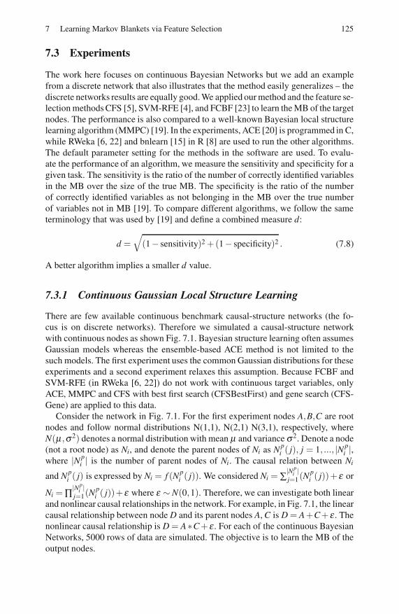
7 Learning Markov Blankets via Feature Selection 125
7.3 Experiments
The work here focuses on continuous Bayesian Networks but we add an example
from a discrete network that also illustrates that the method easily generalizes – the
discrete networks results are equally good. We applied our method and the feature se-
lection methods CFS [5], SVM-RFE [4], and FCBF [23] to learn the MB of the target
nodes. The performance is also compared to a well-known Bayesian local structure
learning algorithm (MMPC) [19]. In the experiments, ACE [20] is programmed in C,
while RWeka [6, 22] and bnlearn [15] in R [8] are used to run the other algorithms.
The default parameter setting for the methods in the software are used. To evalu-
ate the performance of an algorithm, we measure the sensitivity and specificity for a
given task. The sensitivity is the ratio of the number of correctly identified variables
in the MB over the size of the true MB. The specificity is the ratio of the number
of correctly identified variables as not belonging in the MB over the true number
of variables not in MB [19]. To compare different algorithms, we follow the same
terminology that was used by [19] and define a combined measure d:
d =√
(1− sensitivity)2 +(1− specificity)2 . (7.8)
A better algorithm implies a smaller d value.
7.3.1 Continuous Gaussian Local Structure Learning
There are few available continuous benchmark causal-structure networks (the fo-
cus is on discrete networks). Therefore we simulated a causal-structure network
with continuous nodes as shown Fig. 7.1. Bayesian structure learning often assumes
Gaussian models whereas the ensemble-based ACE method is not limited to the
such models. The first experiment uses the common Gaussian distributions for these
experiments and a second experiment relaxes this assumption. Because FCBF and
SVM-RFE (in RWeka [6, 22]) do not work with continuous target variables, only
ACE, MMPC and CFS with best first search (CFSBestFirst) and gene search (CFS-
Gene) are applied to this data.
Consider the network in Fig. 7.1. For the first experiment nodes A,B,C are root
nodes and follow normal distributions N(1,1), N(2,1) N(3,1), respectively, where
N(µ ,σ2) denotes a normal distribution with mean µ and variance σ2. Denote a node
(not a root node) as Ni, and denote the parent nodes of Ni as Npi ( j), j = 1, ..., |N p
i |,where |N p
i | is the number of parent nodes of Ni. The causal relation between Ni
and Npi ( j) is expressed by Ni = f (N p
i ( j)). We considered Ni = ∑|N p
i |j=1(N p
i ( j))+ ε or
Ni = ∏|N p
i |j=1(N p
i ( j))+ε where ε ∼N(0,1). Therefore, we can investigate both linear
and nonlinear causal relationships in the network. For example, in Fig. 7.1, the linear
causal relationship between node D and its parent nodes A, C is D = A+C+ ε . The
nonlinear causal relationship is D = A∗C+ ε . For each of the continuous Bayesian
Networks, 5000 rows of data are simulated. The objective is to learn the MB of the
output nodes.
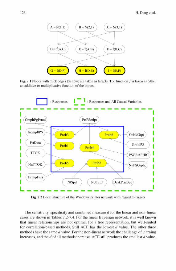
126 H. Deng et al.
A ~ N(1,1) B ~ N(2,1) C ~ N(3,1)
D = f(A,C) E = f(A,B) F = f(B,C)
G = f(D,F) H = f(D,E) I = f(E,F)
Fig. 7.1 Nodes with thick edges (yellow) are taken as targets. The function f is taken as either
an additive or multiplicative function of the inputs.
Prob1
: Responses : Responses and All Causal Variables
Prob2
PrtData
DeskPrntSpdNetPrintNtSpd
CmpltPgPrntd
Prob3IncmpltPS
PrtPScript
Prob4
PSGRAPHIC
NnPSGrphcProb5
TTOK
TrTypFnts
NnTTOK
Prob6
GrbldPS
GrbldOtpt
Fig. 7.2 Local structure of the Windows printer network with regard to targets
The sensitivity, specificity and combined measure d for the linear and non-linear
cases are shown in Tables 7.2-7.4. For the linear Bayesian network, it is well known
that linear relationships are not optimal for a tree representation, but well-suited
for correlation-based methods. Still ACE has the lowest d value. The other three
methods have the same d value. For the non-linear network the challenge of learning
increases, and the d of all methods increase. ACE still produces the smallest d value.
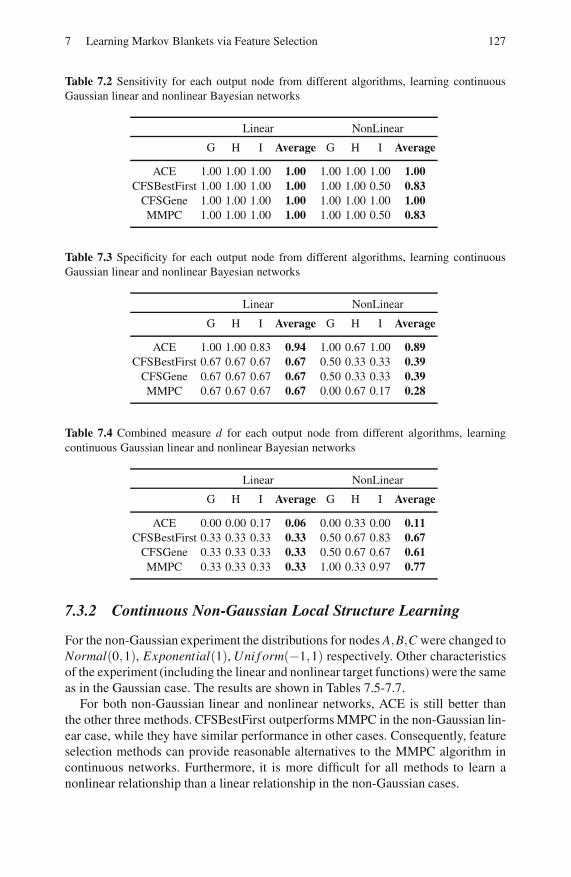
7 Learning Markov Blankets via Feature Selection 127
Table 7.2 Sensitivity for each output node from different algorithms, learning continuous
Gaussian linear and nonlinear Bayesian networks
Linear NonLinear
G H I Average G H I Average
ACE 1.00 1.00 1.00 1.00 1.00 1.00 1.00 1.00
CFSBestFirst 1.00 1.00 1.00 1.00 1.00 1.00 0.50 0.83
CFSGene 1.00 1.00 1.00 1.00 1.00 1.00 1.00 1.00
MMPC 1.00 1.00 1.00 1.00 1.00 1.00 0.50 0.83
Table 7.3 Specificity for each output node from different algorithms, learning continuous
Gaussian linear and nonlinear Bayesian networks
Linear NonLinear
G H I Average G H I Average
ACE 1.00 1.00 0.83 0.94 1.00 0.67 1.00 0.89
CFSBestFirst 0.67 0.67 0.67 0.67 0.50 0.33 0.33 0.39
CFSGene 0.67 0.67 0.67 0.67 0.50 0.33 0.33 0.39
MMPC 0.67 0.67 0.67 0.67 0.00 0.67 0.17 0.28
Table 7.4 Combined measure d for each output node from different algorithms, learning
continuous Gaussian linear and nonlinear Bayesian networks
Linear NonLinear
G H I Average G H I Average
ACE 0.00 0.00 0.17 0.06 0.00 0.33 0.00 0.11
CFSBestFirst 0.33 0.33 0.33 0.33 0.50 0.67 0.83 0.67
CFSGene 0.33 0.33 0.33 0.33 0.50 0.67 0.67 0.61
MMPC 0.33 0.33 0.33 0.33 1.00 0.33 0.97 0.77
7.3.2 Continuous Non-Gaussian Local Structure Learning
For the non-Gaussian experiment the distributions for nodes A,B,C were changed to
Normal(0,1), Exponential(1), Uni f orm(−1,1) respectively. Other characteristics
of the experiment (including the linear and nonlinear target functions) were the same
as in the Gaussian case. The results are shown in Tables 7.5-7.7.
For both non-Gaussian linear and nonlinear networks, ACE is still better than
the other three methods. CFSBestFirst outperforms MMPC in the non-Gaussian lin-
ear case, while they have similar performance in other cases. Consequently, feature
selection methods can provide reasonable alternatives to the MMPC algorithm in
continuous networks. Furthermore, it is more difficult for all methods to learn a
nonlinear relationship than a linear relationship in the non-Gaussian cases.
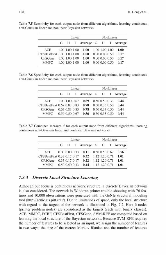
128 H. Deng et al.
Table 7.5 Sensitivity for each output node from different algorithms, learning continuous
non-Gaussian linear and nonlinear Bayesian networks
Linear NonLinear
G H I Average G H I Average
ACE 1.00 1.00 1.00 1.00 1.00 1.00 1.00 1.00
CFSBestFirst 1.00 1.00 1.00 1.00 0.00 0.00 0.50 0.17
CFSGene 1.00 1.00 1.00 1.00 0.00 0.00 0.50 0.17
MMPC 1.00 1.00 1.00 1.00 0.00 0.00 0.50 0.17
Table 7.6 Specificity for each output node from different algorithms, learning continuous
non-Gaussian linear and nonlinear Bayesian networks
Linear NonLinear
G H I Average G H I Average
ACE 1.00 1.00 0.67 0.89 0.50 0.50 0.33 0.44
CFSBestFirst 0.67 0.83 0.83 0.78 0.50 0.33 0.50 0.44
CFSGene 0.67 0.83 0.83 0.78 0.50 0.33 0.50 0.44
MMPC 0.50 0.50 0.67 0.56 0.50 0.33 0.50 0.44
Table 7.7 Combined measure d for each output node from different algorithms, learning
continuous non-Gaussian linear and nonlinear Bayesian networks
Linear NonLinear
G H I Average G H I Average
ACE 0.00 0.00 0.33 0.11 0.50 0.50 0.67 0.56
CFSBestFirst 0.33 0.17 0.17 0.22 1.12 1.20 0.71 1.01
CFSGene 0.33 0.17 0.17 0.22 1.12 1.20 0.71 1.01
MMPC 0.50 0.50 0.33 0.44 1.12 1.20 0.71 1.01
7.3.3 Discrete Local Structure Learning
Although our focus is continuous network structure, a discrete Bayesian network
is also considered. The network is Windows printer trouble shooting with 76 fea-
tures and 10,000 observations were generated with the GeNIe structural modeling
tool (http://genie.sis.pitt.edu/). Due to limitations of space, only the local structure
with regard to the targets of the network is illustrated in Fig. 7.2. Here 6 nodes
(printer problem nodes) are considered as the targets (each with binary classes).
ACE, MMPC, FCBF, CFSBestFirst, CFSGene, SVM-RFE are compared based on
learning the local structure of the Bayesian networks. Because SVM-RFE requires
the number of features to be selected as an input, we assign the number of features
in two ways: the size of the correct Markov Blanket and the number of features
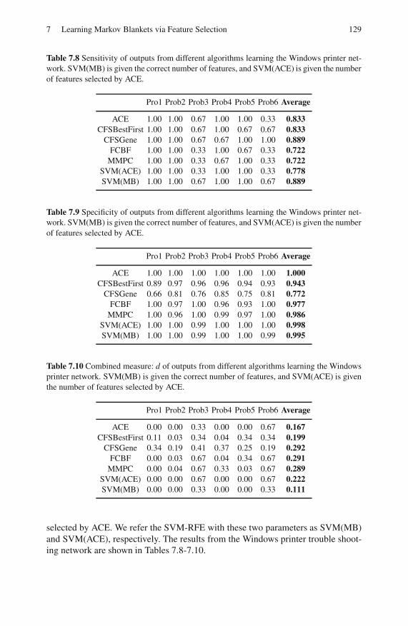
7 Learning Markov Blankets via Feature Selection 129
Table 7.8 Sensitivity of outputs from different algorithms learning the Windows printer net-
work. SVM(MB) is given the correct number of features, and SVM(ACE) is given the number
of features selected by ACE.
Pro1 Prob2 Prob3 Prob4 Prob5 Prob6 Average
ACE 1.00 1.00 0.67 1.00 1.00 0.33 0.833
CFSBestFirst 1.00 1.00 0.67 1.00 0.67 0.67 0.833
CFSGene 1.00 1.00 0.67 0.67 1.00 1.00 0.889
FCBF 1.00 1.00 0.33 1.00 0.67 0.33 0.722
MMPC 1.00 1.00 0.33 0.67 1.00 0.33 0.722
SVM(ACE) 1.00 1.00 0.33 1.00 1.00 0.33 0.778
SVM(MB) 1.00 1.00 0.67 1.00 1.00 0.67 0.889
Table 7.9 Specificity of outputs from different algorithms learning the Windows printer net-
work. SVM(MB) is given the correct number of features, and SVM(ACE) is given the number
of features selected by ACE.
Pro1 Prob2 Prob3 Prob4 Prob5 Prob6 Average
ACE 1.00 1.00 1.00 1.00 1.00 1.00 1.000
CFSBestFirst 0.89 0.97 0.96 0.96 0.94 0.93 0.943
CFSGene 0.66 0.81 0.76 0.85 0.75 0.81 0.772
FCBF 1.00 0.97 1.00 0.96 0.93 1.00 0.977
MMPC 1.00 0.96 1.00 0.99 0.97 1.00 0.986
SVM(ACE) 1.00 1.00 0.99 1.00 1.00 1.00 0.998
SVM(MB) 1.00 1.00 0.99 1.00 1.00 0.99 0.995
Table 7.10 Combined measure: d of outputs from different algorithms learning the Windows
printer network. SVM(MB) is given the correct number of features, and SVM(ACE) is given
the number of features selected by ACE.
Pro1 Prob2 Prob3 Prob4 Prob5 Prob6 Average
ACE 0.00 0.00 0.33 0.00 0.00 0.67 0.167
CFSBestFirst 0.11 0.03 0.34 0.04 0.34 0.34 0.199
CFSGene 0.34 0.19 0.41 0.37 0.25 0.19 0.292
FCBF 0.00 0.03 0.67 0.04 0.34 0.67 0.291
MMPC 0.00 0.04 0.67 0.33 0.03 0.67 0.289
SVM(ACE) 0.00 0.00 0.67 0.00 0.00 0.67 0.222
SVM(MB) 0.00 0.00 0.33 0.00 0.00 0.33 0.111
selected by ACE. We refer the SVM-RFE with these two parameters as SVM(MB)
and SVM(ACE), respectively. The results from the Windows printer trouble shoot-
ing network are shown in Tables 7.8-7.10.

130 H. Deng et al.
For the Windows printer network, ACE and SVM(MB) have the lowest d val-
ues. SVM(MB) only outperforms ACE for the target Prob6. However, SVM(MB)
is given the priori knowledge of the size of true MBs. With the number of variables
selected by ACE as input, SVM(ACE) does not perform as well as ACE. Another
feature selection method CFSBestFirst also provides better results than MMPC.
7.4 Conclusion
Structure learning is important for both discrete and continuous networks, and re-
laxed Gaussian assumptions are important for continuous networks. A relationship
between ensemble masking and Markov Blankets is argued here and exploited for
a generalized feature selection method to handle discrete and continuous cases for
local structure learning. Common feature selection methods, along with a Bayesian
structure algorithm, are compared for the structure learning problem, and exper-
iments illustrate the strength of an ensemble-based feature selection approach in
these cases.
Acknowledgements. This research was partially supported by ONR grant N00014-09-1-
0656.
References
1. Breiman, L.: Random forests. Machine Learning 45, 5–32 (2001)2. Frey, L., Fisher, D., Tsamardinos, I., Aliferis, C., Statnikov, A.: Identifying Markov blan-
kets with decision tree induction. In: Proc. the 3rd IEEE Int. Conf. Data Mining, Mel-
bourne, FL, pp. 59–66. IEEE Comp. Society, Los Alamitos (2003)3. Friedman, J., Hastie, T., Tibshirani, R.: Additive logistic regression: A statistical view of
boosting. Annals of Statistics 28, 832–844 (2000)4. Guyon, I., Weston, J., Barnhill, S., Vapnik, V.: Gene selection for cancer classification
using support vector machines. Machine Learning 46, 389–422 (2002)5. Hall, M.A.: Correlation-based feature selection for discrete and numeric class machine
learning. In: Langley, P. (ed.) Proc. the 17th Int. Conf. Machine Learning, Stanford, CA,
pp. 359–366. Morgan Kaufmann, San Francisco (2000)6. Hornik, K., Buchta, C., Zeileis, A.: Open-source machine learning: R meets Weka. Com-
putational Statistics 24, 225–232 (2009)7. Hoyer, P., Janzing, D., Mooij, J., Peters, J., Scholkopf, B.: Nonlinear causal discovery
with additive noise models. In: Koller, D., Schuurmans, D., Bengio, Y., Bottou, L. (eds.)
Advances in Neural Inf. Proc. Syst., pp. 689–696. MIT Press, Cambridge (2009)8. Ihaka, R., Gentleman, R.: A language for data analysis and graphics. J. Comp. and
Graphical Stat. 5, 299–314 (1996)9. Koller, D., Sahami, M.: Toward optimal feature selection. In: Saitta, L. (ed.) Proc. the
13th Int. Conf. Machine Learning, Bari, Italy, pp. 284–292. Morgan Kaufmann, San
Francisco (1996)10. Li, F., Yang, Y.: Use modified lasso regressions to learn large undirected graphs in a
probabilistic framework. In: Veloso, M.M., Kambhampati, S. (eds.) Proc. the 20th Natl.
Conf. Artif. Intell. and the 17th Innovative Appl. Artif. Intell. Conf., Pittsburgh, PA,
pp. 81–86. AAAI Press, MIT Press (2005)

7 Learning Markov Blankets via Feature Selection 131
11. Margaritis, D., Thrun, S.: Bayesian network induction via local neighborhoods. In: Solla,
S.A., Leen, T.K., Muller, K.-R. (eds.) Advances in Neural Inf. Proc. Syst., pp. 505–511.
MIT Press, Cambridge (2000)
12. Pudil, P., Kittler, J., Novovicova, J.: Floating search methods in feature selection. Pattern
Recognition Letters 15, 1119–1125 (1994)
13. Pellet, J.P., Elisseeff, A.: Using Markov blankets for causal structure learning. J. Machine
Learning Research 9, 1295–1342 (2008)
14. Robnik-Sikonja, M., Kononenko, I.: Theoretical and empirical analysis of relief and re-
lieff. Machine Learning 53, 23–69 (2003)
15. Scutari, M.: Learning bayesian networks with the bnlearn R package. J. Stat. Soft-
ware 35, 1–22 (2010)
16. Shimizu, S., Hoyer, P., Hyvarinen, A., Kerminen, A.: A linear non-gaussian acyclic
model for causal discovery. J. Machine Learning Research 7, 2003–2030 (2006)
17. Tillman, R., Gretton, A., Spirtes, P.: Nonlinear directed acyclic structure learning with
weakly additive noise models. In: Bengio, Y., Schuurmans, D., Lafferty, J., Williams,
C.K.I., Culotta, A. (eds.) Advances in Neural Inf. Proc. Syst., pp. 1847–1855. MIT Press,
Cambridge (2010)
18. Tsamardinos, I., Aliferis, C., Statnikov, A.: Algorithms for large scale Markov blanket
discovery. In: Russell, I., Haller, S.M. (eds.) Proc. the 16th Florida Artif. Intell. Research
Society Conference, St. Augustine, FL, pp. 376–381. AAAI Press, New York (2003)
19. Tsamardinos, I., Aliferis, C., Statnikov, A.: Time and sample efficient discovery of
Markov blankets and direct causal relations. In: Getoor, L., Senator, T.E., Domingos,
P., Faloutsos, C. (eds.) Proc. the 9th ACM SIGKDD Int. Conf. Knowledge Discovery
and Data Mining, Washington DC, pp. 673–678. ACM, New York (2003)
20. Tuv, E., Borisov, A., Runger, G., Torkkola, K.: Feature selection with ensembles,
artificial variables, and redundancy elimination. J. Machine Learning Research 10,
1341–1366 (2009)
21. Voortman, M., Druzdzel, M.: Insensitivity of constraint-based causal discovery algo-
rithms to violations of the assumption of multivariate normality. In: Wilson, D., Lane,
H.C. (eds.) Proc. the 21st Int. Florida Artif. Intell. Research Society Conf., Coconut
Grove, FL, pp. 680–695. AAAI Press, New York (2008)
22. Witten, I.H., Frank, E.: Data mining: Practical machine learning tools and techniques.
Morgan Kaufmann, San Francisco (2005)
23. Yu, L., Liu, H.: Efficient feature selection via analysis of relevance and redundancy. J.
Machine Learning Research 5, 1205–1224 (2004)

Chapter 8
Ensembles of Bayesian Network ClassifiersUsing Glaucoma Data and Expertise
Stefano Ceccon, David Garway-Heath, David Crabb, and Allan Tucker
Abstract. Bayesian Networks (BNs) are probabilistic graphical models that are pop-
ular in numerous fields. Here we propose these models to improve the classification
of glaucoma, a major cause of blindness worldwide. We use visual field and reti-
nal data to predict the early onset of glaucoma. In particular, the ability of BNs
to deal with missing data allows us to select an optimal data-driven network by
comparing supervised and semi-supervised models. An expertise-driven BN is also
built by encoding expert knowledge in terms of relations between variables. In order
to improve the overall performances for classification and to explore the relations
between glaucomatous data and expert knowledge, the expertise-driven network is
combined with the selected data-driven network using a BN-based approach. An
accuracy-weighted combination of these networks is also compared to the other
models. The best performances are obtained with the semi-supervised data-driven
network. However, combining it with the expertise-driven network improves perfor-
mance in many cases and leads to interesting insights about the datasets, networks
and metrics.
8.1 Improving Knowledge and Classification of Glaucoma
Glaucoma is the second most common cause of blindness worldwide [21], but its
underlying mechanisms are still not clear. However, early treatment has been shown
to slow the progression of the disease, thus early diagnosis is desirable [27]. To this
purpose, several medical instruments available nowadays provide a large amount
of anatomical and functional data, which can be exploited using statistical and A.I.
techniques. Our study aims to set up and combine Bayesian Network (BNs) clas-
sifiers in order to obtain more precise early diagnosis of glaucoma and to learn in-
sights from the models. BNs are models which seem to be appropriate for this issue,
Stefano Ceccon · Allan Tucker
Department of Information Systems and Computing, Brunel University,
Uxbridge UB8 3PH, London, UK
E-mail: stefano.ceccon,[email protected]@brunel.ac.uk
O. Okun et al. (Eds.): Ensembles in Machine Learning Applications, SCI 373, pp. 133–150.springerlink.com c© Springer-Verlag Berlin Heidelberg 2011

134 S. Ceccon et al.
being able to integrate different datasets and model expert knowledge in the field
[20]. Moreover, their ability in handling missing data is very useful in the context of
glaucoma, because no gold standard disease detection method is available. BNs are
white-box models, so it is possible to look at the underlying relations of the model
to improve knowledge in the field. BNs have already been successfully tested with
glaucoma data in [23].
In the first stage of this study, two different BN models are obtained using the
data (i.e. using the Advanced Glaucoma Intervention Study (AGIS) score [8] as the
class variable), and imposing an expertise-driven network based on the anatomy of
the optic nerve. The AGIS defect scoring system depends on the number and depth
of clusters of adjacent depressed test sites in the visual field (VF) test STATPAC-2
analysis. The VF test aims to measure the functional ability of an eye by expos-
ing different stimulus to different locations of the patient field and it’s a routine test
when screening for glaucoma. The anatomy-based network is obtained by modelling
the relations between sectors of the optic nerve head (ONH) and the VF sectors as
proposed by [11]. This is a widely used structure-function map which has been
proved to be correlated with previous studies. The second stage of this study aims
to combine the results of the two BN classifiers in order not only to maximize the
results, but also to learn new insights about how the two different approaches inter-
act. Two techniques are explored: a BN combiner with 3 nodes and a more classical
weighted vote technique with accuracy-based weights. A BN combiner weighted
on accuracy is also proposed. In the last part of the chapter the results of the dif-
ferent models are presented and discussed in terms of performance and qualitative
outcome to better understand glaucoma and the associated clinical metrics.
8.2 Theory and Methods
In this section we will describe the datasets available and we will present the tech-
niques used to obtain the BN models and the theory behind them. We will also
analyse how the combination of a set of base classifiers can be used to increase the
performances of the whole classification system.
8.2.1 Datasets
In this study two independent datasets were used (Table 8.1). Dataset A is a cross-
sectional dataset of 78 early glaucomatous patients and 102 healthy control subjects.
Inclusion criteria for early glaucomatous patients were Intraocular Pressure (IOP)
greater than 21 mmHg and early VF defects on at least 3 occasions. Control subjects
had IOP < 21 mmHg and known to be healthy. Dataset B is a longitudinal dataset
of 19 controls and 43 patients from Ocular Hypertensive Treatment group, who
developed glaucoma in the time span observed. Initial eligibility criteria were in
this case IOP > 21 mmHg and negative VF test, and conversion was defined as
positive AGIS score on 3 consecutive tests. Control subjects had negative VF test in
2 tests and IOP < 21 mmHg.
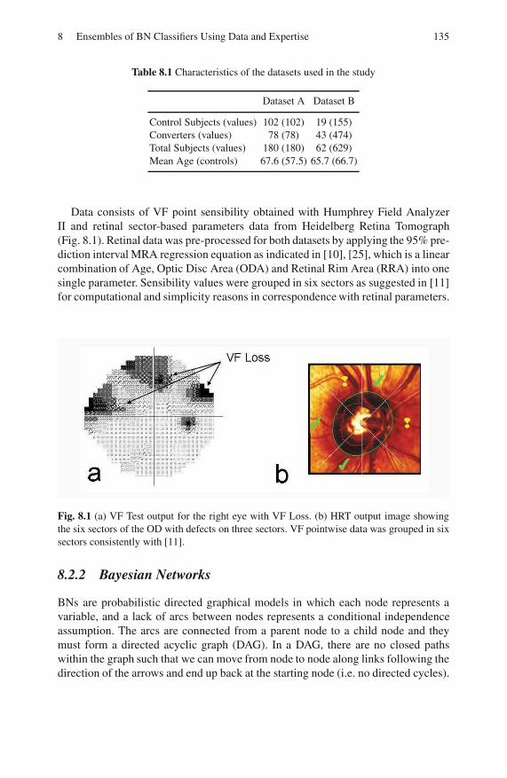
8 Ensembles of BN Classifiers Using Data and Expertise 135
Table 8.1 Characteristics of the datasets used in the study
Dataset A Dataset B
Control Subjects (values) 102 (102) 19 (155)
Converters (values) 78 (78) 43 (474)
Total Subjects (values) 180 (180) 62 (629)
Mean Age (controls) 67.6 (57.5) 65.7 (66.7)
Data consists of VF point sensibility obtained with Humphrey Field Analyzer
II and retinal sector-based parameters data from Heidelberg Retina Tomograph
(Fig. 8.1). Retinal data was pre-processed for both datasets by applying the 95% pre-
diction interval MRA regression equation as indicated in [10], [25], which is a linear
combination of Age, Optic Disc Area (ODA) and Retinal Rim Area (RRA) into one
single parameter. Sensibility values were grouped in six sectors as suggested in [11]
for computational and simplicity reasons in correspondence with retinal parameters.
Fig. 8.1 (a) VF Test output for the right eye with VF Loss. (b) HRT output image showing
the six sectors of the OD with defects on three sectors. VF pointwise data was grouped in six
sectors consistently with [11].
8.2.2 Bayesian Networks
BNs are probabilistic directed graphical models in which each node represents a
variable, and a lack of arcs between nodes represents a conditional independence
assumption. The arcs are connected from a parent node to a child node and they
must form a directed acyclic graph (DAG). In a DAG, there are no closed paths
within the graph such that we can move from node to node along links following the
direction of the arrows and end up back at the starting node (i.e. no directed cycles).

136 S. Ceccon et al.
Each variable is associated with a conditional probability distribution (CPD), so
that given the set of all CPDs in the network it is possible to infer about any value of
any node. All together, the structure provides an efficient factorization of the joint
probability
p(x) =n
∏i=1
p(xi|pai), (8.1)
where pai are the parents of the node xi (which denotes both node and variable)
[14], [23].
For classification, BNs are used by selecting the most probable value of the class
node (i.e. glaucomatous vs healthy) given the values observed for all the other
nodes. To build a BN, the CPDs of all the variables need to be estimated from
data. This is typically obtained using the Maximum Likelihood Estimation (MLE),
which involves maximizing the likelihood of the data given the parameters. In case
of missing data, however, this technique cannot be used. Therefore, the Expectation-
Maximization algorithm (EM) was used for estimating the parameters in the un-
supervised network. This technique iteratively estimates the hidden values for the
unobserved data in the first step and maximizes the estimated likelihood function at
the next step. When the algorithm converges to a local maximum, the parameters
are estimated [4]. In addition, the structure of the network (i.e. the links between
nodes) must be chosen: it can be either learned from the data or imposed using
expert knowledge. For the former case, the learning algorithm used in this study
was a Simulated Annealing (SA) technique, which is a quasi-greedy algorithm that
searches through the space of possible structures to obtain the optimal structure
[17]. The score used in the structure search is the Bayesian Information Criterion
(BIC) score, which is a metric based on the likelihood of the observed data given
the structure and the parameters, with a penalizing factor related to the number of
parameters that aims to prevent overfitting. The searching algorithm was repeated
100 times using bootstrapping on the dataset [6]. This resampling technique has
been widely used in order to reduce noise and obtain more robust results. It involves
randomly sampling a subset from the dataset (with replacement) at each iteration.
Bayesian Model Averaging was used on the learned structures in order to calculate
the posterior probability for each arc as proposed in [7], i.e. by weighting each arc f
on the network score in which it is present. Since calculation of the posterior prob-
ability on the whole set of possible structures is feasible only for tiny domains, an
approximation is made by enumerating only over the learned set of structures (i.e.
a set of optimal structures), as proposed by [19]. Thus, the formula used to estimate
the relative mass of the structures in G that contains arc f given the data D is shown
below:
P( f |D)≈ ∑G∈G P(G|D) f (G)
∑G∈G P(G|D), (8.2)
where f (G) is a binary function equal to 1 when the arc is present in the structure G,
and P(G|D) represents the posterior probability of each structure given the data D.
The latter function can be calculated as the product of the likelihood of the data and
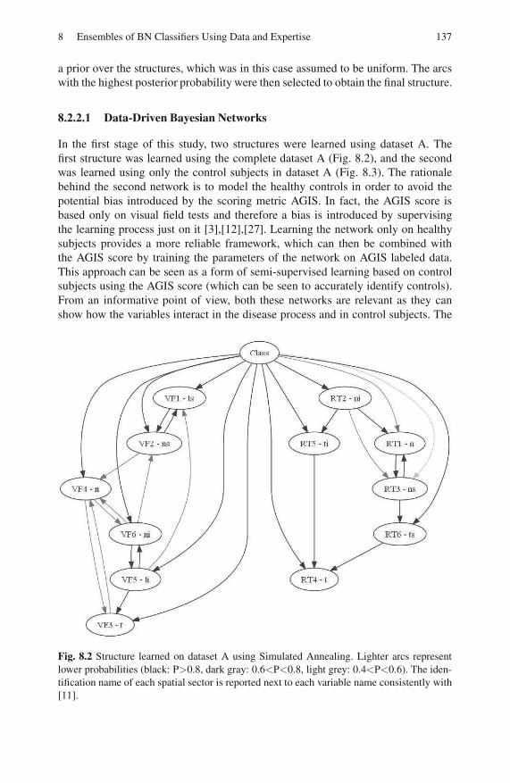
8 Ensembles of BN Classifiers Using Data and Expertise 137
a prior over the structures, which was in this case assumed to be uniform. The arcs
with the highest posterior probability were then selected to obtain the final structure.
8.2.2.1 Data-Driven Bayesian Networks
In the first stage of this study, two structures were learned using dataset A. The
first structure was learned using the complete dataset A (Fig. 8.2), and the second
was learned using only the control subjects in dataset A (Fig. 8.3). The rationale
behind the second network is to model the healthy controls in order to avoid the
potential bias introduced by the scoring metric AGIS. In fact, the AGIS score is
based only on visual field tests and therefore a bias is introduced by supervising
the learning process just on it [3],[12],[27]. Learning the network only on healthy
subjects provides a more reliable framework, which can then be combined with
the AGIS score by training the parameters of the network on AGIS labeled data.
This approach can be seen as a form of semi-supervised learning based on control
subjects using the AGIS score (which can be seen to accurately identify controls).
From an informative point of view, both these networks are relevant as they can
show how the variables interact in the disease process and in control subjects. The
Fig. 8.2 Structure learned on dataset A using Simulated Annealing. Lighter arcs represent
lower probabilities (black: P>0.8, dark gray: 0.6<P<0.8, light grey: 0.4<P<0.6). The iden-
tification name of each spatial sector is reported next to each variable name consistently with
[11].
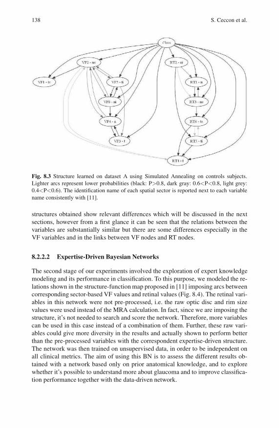
138 S. Ceccon et al.
Fig. 8.3 Structure learned on dataset A using Simulated Annealing on controls subjects.
Lighter arcs represent lower probabilities (black: P>0.8, dark gray: 0.6<P<0.8, light grey:
0.4<P<0.6). The identification name of each spatial sector is reported next to each variable
name consistently with [11].
structures obtained show relevant differences which will be discussed in the next
sections, however from a first glance it can be seen that the relations between the
variables are substantially similar but there are some differences especially in the
VF variables and in the links between VF nodes and RT nodes.
8.2.2.2 Expertise-Driven Bayesian Networks
The second stage of our experiments involved the exploration of expert knowledge
modeling and its performance in classification. To this purpose, we modeled the re-
lations shown in the structure-function map proposed in [11] imposing arcs between
corresponding sector-based VF values and retinal values (Fig. 8.4). The retinal vari-
ables in this network were not pre-processed, i.e. the raw optic disc and rim size
values were used instead of the MRA calculation. In fact, since we are imposing the
structure, it’s not needed to search and score the network. Therefore, more variables
can be used in this case instead of a combination of them. Further, these raw vari-
ables could give more diversity in the results and actually shown to perform better
than the pre-processed variables with the correspondent expertise-driven structure.
The network was then trained on unsupervised data, in order to be independent on
all clinical metrics. The aim of using this BN is to assess the different results ob-
tained with a network based only on prior anatomical knowledge, and to explore
whether it’s possible to understand more about glaucoma and to improve classifica-
tion performance together with the data-driven network.
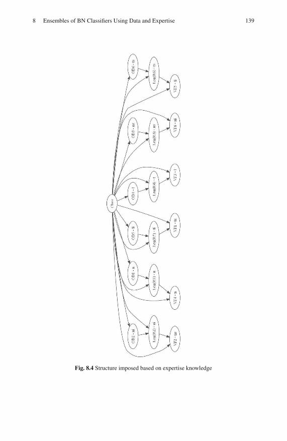
8 Ensembles of BN Classifiers Using Data and Expertise 139
Fig. 8.4 Structure imposed based on expertise knowledge
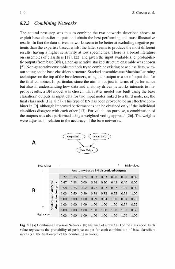
140 S. Ceccon et al.
8.2.3 Combining Networks
The natural next step was thus to combine the two networks described above, to
exploit base classifier outputs and obtain the best performing and most illustrative
results. In fact the data-driven networks seem to be better at excluding negative pa-
tients than the expertise based, whilst the latter seems to produce the most different
results, having a higher sensitivity at low specificities. There is a broad literature
on ensembles of classifiers [18], [22] and given the input available (i.e. probabilis-
tic outputs from base BNs), a non-generative stacked structure ensemble was chosen
[5]. Non-generative ensemble methods try to combine existing base classifiers, with-
out acting on the base classifiers structure. Stacked ensembles use Machine Learning
techniques on the top of the base learners, using their output as a set of input data for
the final combiner. In particular, since the aim is not just in terms of performance
but also in understanding how data and anatomy driven networks interacts to im-
prove results, a BN model was chosen. This latter model was built using the base
classifiers’ outputs as input data for two input nodes linked to a third node, i.e. the
final class node (Fig. 8.5a). This type of BN has been proved to be an effective com-
biner in [9], although improved performances can be obtained only if the individual
classifiers disagree with each other [13]. For validation purpose, a combination of
the outputs was also performed using a weighted voting approach[26]. The weights
were adjusted in relation to the accuracy of the base networks.
Fig. 8.5 (a) Combining Bayesian Network. (b) Instance of a raw CPD of the class node. Each
value represents the probability of positive output for each combination of base classifiers
inputs (i.e. the final output of the combining network).

8 Ensembles of BN Classifiers Using Data and Expertise 141
An optimized combining BN was also set up by weighting its output with the ac-
curacy of the base networks. The probabilistic outputs are in this way biased towards
the output provided by the most accurate base classifier.
8.3 Algorithms
The pseudo-code of the main algorithms used to obtain the results are here shown.
8.3.1 Learning the Structure
The SA-like learning algorithm used to obtain the data-driven base classifiers is
represented by the following pseudo-code:
input init_temp, delta_temp, iterations, data
order = random(n)Initialise structure(order)temp = init_tempresult = structure
for i=1 : iterationsscore = score(structure)new_structure = operation(structure)new_score = score(new_structure)diff_score = new_score - score
if new_score > score
if new_score > score(result)result = new_structure
end
structure = new_structure
elseif rand < exp(diff_score/temp)structure = new_structure
end
temp = temp * delta_temp
end
Here temp is the temperature factor which allows the algorithm to explore even
non-optimal links, delta temp is the “cooling” factor < 1 to decrease the temper-
ature and result is the final output structure. To explore different structures 2100

142 S. Ceccon et al.
Fig. 8.6 Operations on the structure. a to b: deleting a link, b to c: swapping two nodes, b to
a: adding a link
operations were carried by the algorithm, so that in each iteration a randomly cho-
sen link was added, removed or two nodes were swapped (Fig. 8.6): an exhaustive
search of the non-linked nodes is found and a link is implemented randomly at each
iteration, a link is deleted by choosing it randomly from the available ones and two
nodes are swapped without changing the structure of the network (i.e. the data vec-
tors pointing to the node are swapped). Notice that the two different networks were
obtained by using different portions of dataset A: in one case the full dataset and in
the other only the control subjects. For the latter, the class node pointing to all nodes
(i.e. a naive BN structure) was added only after learning.
8.3.2 Combining Two Networks
Once the networks were obtained, the combination with the data-driven and the
expertise-based classifiers was obtained by building a third BN which was then im-
posed to combine the outputs from the other two networks (Fig. 8.5a). Each output
was discretized in 8 states and then linked to a 2 states class node. As a result, an
8x8 matrix showing the interactions between the two networks was obtained by ob-
serving the CPD of the class node (Fig. 8.5b). In order to optimize the CPD, the
matrix was then smoothed using a mean-filter window of size 3. The algorithm can
be summarized as:
input Output_BN1 Output_BN2 data
discretize(Output_BN1)discretize(Output_BN2)
Initialise structureLearn_parameters(structure, data)
CPD = structure(ClassNode).CPDsmoothed_CPD = filter(CPD)new_structure(ClassNode.CPD) = smoothed_CPD

8 Ensembles of BN Classifiers Using Data and Expertise 143
Here BN1 and BN2 represent the two base classifiers’ outputs and the CPD is the
Conditional Probability Distribution of a node (Fig. 8.5b).
8.3.3 Optimized Combination
An optimized BN was also set up by weighting its output on the accuracy of the base
classifiers on the training dataset. In particular, the following algorithm was applied
to the final output of the combining BN:
input TestDataset outputoutput_BN1 output_BN2accuracy_BN1 accuracy_BN2
align(accuracy_BN1,accuracy_BN2)
Weighted_output = (output_BN1 * accuracy_BN1 +output_BN2 * accuracy_BN2) /sum(accuracy_BN1, accuracy_BN2)
Final_output = mean(output, Weighted_output)
end
Here output is the output of the raw combining BN and the suffixes BN1 and BN2
on output and accuracy represent the two base classifiers outputs and accuracies.
The align function aligns the base classifiers accuracies using the threshold values,
in order to weight each base classifiers output on the corresponding accuracy for
each threshold value on the testing dataset.
8.4 Results and Performance Evaluation
8.4.1 Base Classifiers
The base classifiers were compared using dataset A as a training set and dataset B
as a testing set. As shown in Table 8.2, the BN model built using only the control
subjects performed similarly to the model built using using all subjects. However,
at high specificity, it outperformed the others. For glaucoma, which is a relative low
frequency disease, high specificities are preferred. This reflects the higher weight
put on the False Positive (FP) rate to minimize their occurrence. Therefore, the
control-based BN was selected for combining with the expertise-driven classifier.
Another interesting result must be pointed out. Both learned structures show
some interesting features which find correspondence in literature. Typical exam-
ples are a set of links between spatially adjacent variables and links from inferior
temporal sectors (ti sector) to superior temporal sectors (ts sector) which proves the

144 S. Ceccon et al.
Table 8.2 Performances of the base classifiers trained using dataset A and tested on dataset B
AUROC Sensitivity at Sensitivity at
90% specificity 80% specificity
AGIS-supervised BN 0.85 0.68 0.82
Semi-supervised BN 0.85 0.71 0.80
hypothesis that early glaucomatous signs often occur on the arcuate sectors of the vi-
sual field and the optic nerve [2], [16]. The structure learned on the control subjects
only aims to model relations in healthy subjects, which are therefore subject to less
variability as the disease process is not present. As expected, more arcs were found
with this approach, however substantially similar to those observed on the AGIS
supervised structure. This can be explained as the presence of a class node in the
AGIS based network learning process “explains away” the relations between sec-
tors, by selecting the most informative relationships for classification as in a feature
selection process. Therefore, some links may not be interesting for discrimination
between controls and glaucomatous subjects and so they are not captured with this
approach. For classification purpose, however, the best performing network is the
controls supervised structure combined with AGIS score, which was then selected
for combination with the expertise-driven network. This points out the importance
to use a conservative approach (i.e. using the structure learned only on control sub-
jects) in the classification of glaucoma.
8.4.2 Ensembles of Classifiers
Results of the ensemble of classifiers were evaluated and compared to base classi-
fiers using 3-fold cross validation on dataset A and 6-fold cross validation on dataset
B. Different folds reflect the different sizes of the datasets. The performance of the
single and the combined networks are shown in Table 8.3 and Figs. 8.7-8.8. The
same tests were performed considering only the pre-diagnosis data subset of dataset
B, in order to take into account only patients “converting” to glaucoma. This led to
results very similar qualitatively to those in Table 8.3.
Considering the overall performances on the complete datasets A and B, the
semi-supervised data-driven BN performs better than the expertise-driven based
one and is at least comparable to the combined ones. On dataset A, however, the
performances of all the classifiers are comparable. Among the combined classifiers,
the Weighted Vote is outperformed only at high specificities, but in dataset B it’s
outperformed by both the other combined networks. The BN combined networks
perform well in both datasets, the accuracy weighted one being better on dataset
A but worse on dataset B. Their performances were the best for higher specifici-
ties. Looking at the ROC curves in a particular test on dataset B (Fig. 8.7) it can
be seen that the performances of the base semi-supervised data-driven BN are the
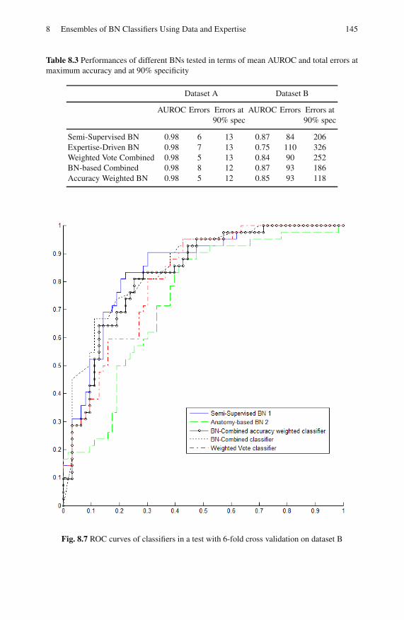
8 Ensembles of BN Classifiers Using Data and Expertise 145
Table 8.3 Performances of different BNs tested in terms of mean AUROC and total errors at
maximum accuracy and at 90% specificity
Dataset A Dataset B
AUROC Errors Errors at AUROC Errors Errors at
90% spec 90% spec
Semi-Supervised BN 0.98 6 13 0.87 84 206
Expertise-Driven BN 0.98 7 13 0.75 110 326
Weighted Vote Combined 0.98 5 13 0.84 90 252
BN-based Combined 0.98 8 12 0.87 93 186
Accuracy Weighted BN 0.98 5 12 0.85 93 118
Fig. 8.7 ROC curves of classifiers in a test with 6-fold cross validation on dataset B
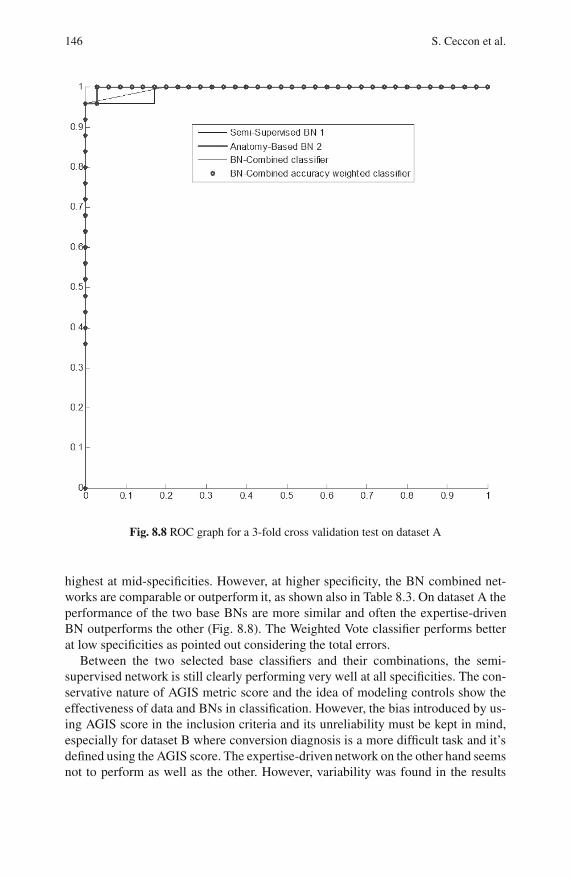
146 S. Ceccon et al.
Fig. 8.8 ROC graph for a 3-fold cross validation test on dataset A
highest at mid-specificities. However, at higher specificity, the BN combined net-
works are comparable or outperform it, as shown also in Table 8.3. On dataset A the
performance of the two base BNs are more similar and often the expertise-driven
BN outperforms the other (Fig. 8.8). The Weighted Vote classifier performs better
at low specificities as pointed out considering the total errors.
Between the two selected base classifiers and their combinations, the semi-
supervised network is still clearly performing very well at all specificities. The con-
servative nature of AGIS metric score and the idea of modeling controls show the
effectiveness of data and BNs in classification. However, the bias introduced by us-
ing AGIS score in the inclusion criteria and its unreliability must be kept in mind,
especially for dataset B where conversion diagnosis is a more difficult task and it’s
defined using the AGIS score. The expertise-driven network on the other hand seems
not to perform as well as the other. However, variability was found in the results
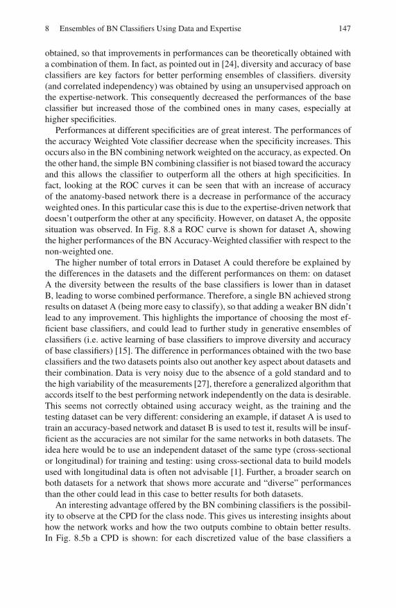
8 Ensembles of BN Classifiers Using Data and Expertise 147
obtained, so that improvements in performances can be theoretically obtained with
a combination of them. In fact, as pointed out in [24], diversity and accuracy of base
classifiers are key factors for better performing ensembles of classifiers. diversity
(and correlated independency) was obtained by using an unsupervised approach on
the expertise-network. This consequently decreased the performances of the base
classifier but increased those of the combined ones in many cases, especially at
higher specificities.
Performances at different specificities are of great interest. The performances of
the accuracy Weighted Vote classifier decrease when the specificity increases. This
occurs also in the BN combining network weighted on the accuracy, as expected. On
the other hand, the simple BN combining classifier is not biased toward the accuracy
and this allows the classifier to outperform all the others at high specificities. In
fact, looking at the ROC curves it can be seen that with an increase of accuracy
of the anatomy-based network there is a decrease in performance of the accuracy
weighted ones. In this particular case this is due to the expertise-driven network that
doesn’t outperform the other at any specificity. However, on dataset A, the opposite
situation was observed. In Fig. 8.8 a ROC curve is shown for dataset A, showing
the higher performances of the BN Accuracy-Weighted classifier with respect to the
non-weighted one.
The higher number of total errors in Dataset A could therefore be explained by
the differences in the datasets and the different performances on them: on dataset
A the diversity between the results of the base classifiers is lower than in dataset
B, leading to worse combined performance. Therefore, a single BN achieved strong
results on dataset A (being more easy to classify), so that adding a weaker BN didn’t
lead to any improvement. This highlights the importance of choosing the most ef-
ficient base classifiers, and could lead to further study in generative ensembles of
classifiers (i.e. active learning of base classifiers to improve diversity and accuracy
of base classifiers) [15]. The difference in performances obtained with the two base
classifiers and the two datasets points also out another key aspect about datasets and
their combination. Data is very noisy due to the absence of a gold standard and to
the high variability of the measurements [27], therefore a generalized algorithm that
accords itself to the best performing network independently on the data is desirable.
This seems not correctly obtained using accuracy weight, as the training and the
testing dataset can be very different: considering an example, if dataset A is used to
train an accuracy-based network and dataset B is used to test it, results will be insuf-
ficient as the accuracies are not similar for the same networks in both datasets. The
idea here would be to use an independent dataset of the same type (cross-sectional
or longitudinal) for training and testing: using cross-sectional data to build models
used with longitudinal data is often not advisable [1]. Further, a broader search on
both datasets for a network that shows more accurate and “diverse” performances
than the other could lead in this case to better results for both datasets.
An interesting advantage offered by the BN combining classifiers is the possibil-
ity to observe at the CPD for the class node. This gives us interesting insights about
how the network works and how the two outputs combine to obtain better results.
In Fig. 8.5b a CPD is shown: for each discretized value of the base classifiers a
148 S. Ceccon et al.
probability is learned from the data and can be observed. This reflects the output of
the final classifier, in particular, the probability of diagnosis of glaucoma for each
combination of inputs. Observing the CPDs obtained in an instance of a CPD in
Fig. 8.5b, it can be seen that the matrix is slightly skewed towards the bottom-left,
i.e. there are more higher probabilities in the bottom-left half than in the other. This
shows that the AGIS semi-supervised network is more reliable at high specificities.
For example, for all values of the expertise-driven network, if the data-driven net-
work’s output is low then the combined output will be low. It must also be noticed
that for lower values of the data-driven base network (e.g. value 3), the output of
the expertise-driven network increases the probability of glaucoma sensibly, adding
its knowledge to the result. Some 0 values are obtained in the corners of the matrix
due to the lack of data for these combinations of outputs: these cells are smoothed
with the mean-filter application. Several different instances of this matrix have been
found in this study, showing again variability between different datasets used. Thus,
the exploration of the CPD of the combined network confirms the higher perfor-
mances at high specificity of semi-supervised data-driven network, but also gives a
quantitative measure of the improvement that each single base classifier brings to
the final output. Further study using this approach will be carried in the future, for
example by acting on the CPDs or averaging on them, as well as using different
discretization and more complete datasets.
In conclusion, this preliminary study has shown the possibilities of using BNs
for classification and exploration of different datasets in a real problem. Data-driven
BN classifier outperformed the expertise-driven one, even if with different magni-
tude on different datasets. Combining networks have been shown to be both effec-
tive in terms of performances and illustrative. In particular, the performances of the
combined classifier seem to be better for datasets with more different results for the
base classifiers. Given the issues of the datasets, the idea of using simulated data
for future work could give a start to more deep analysis of BNs potential in model-
ing data and combining classifiers, keeping in mind the importance of an effective
choice of the base classifiers.
References
1. Artes, P.H., Chauhan, B.C.: Longitudinal changes in the visual field and optic disc in
glaucoma. Progress in Retinal and Eye Research 24, 333–354 (2005)
2. Bowd, C., Zangwill, L.M., Medeiros, F.A., Tavares, I.M., Hoffmann, E.M., Bourne, R.R.,
Sample, P.A., Weinreb, R.N.: Structure-function relationships using confocal scanning
laser ophthalmoscopy, optical coherence tomography, and scanning laser polarimetry.
Investigative Ophthalmology & Visual Science 47, 2889 (2006)
3. Chauhan, B.C., Drance, S.M., Douglas, G.R.: The use of visual field indices in detect-
ing changes in the visual field in glaucoma. Investigative Ophthalmology & Visual Sci-
ence 31, 512 (1990)

8 Ensembles of BN Classifiers Using Data and Expertise 149
4. Dempster, A.P., Laird, N.M., Rubin, D.B.: Maximum likelihood from incomplete data
via the em algorithm. J. the Royal Stat. Society. Series B (Methodological) 39, 1–38
(1977)
5. Duin, R., Tax, D.: Experiments with classifier combining rules. In: Kittler, J., Roli, F.
(eds.) MCS 2000. LNCS, vol. 1857, pp. 16–29. Springer, Heidelberg (2000)
6. Efron, B., Tibshirani, R., Tibshirani, R.J.: An introduction to the bootstrap. Chapman &
Hall/CRC Press, Boca Raton (1993)
7. Friedman, N., Koller, D.: Being Bayesian about network structure: A Bayesian approach
to structure discovery in Bayesian networks. Machine Learning 50, 95–125 (2003)
8. Gaasterland, D.E., Ederer, F., Sullivan, E.K., Caprioli, J., Cyrlin, M.N.: Advanced glau-
coma intervention study: 2. visual field test scoring and reliability. Ophthalmology 101,
1445–1455 (1994)
9. Garg, A., Pavlovic, V., Huang, T.S.: Bayesian networks as ensemble of classifiers. In:
Proc. the 16th Int. Conf. Pattern Recogn., Quebec, Canada, pp. 779–784. IEEE Comp.
Society, Los Alamitos (2002)
10. Garway-Heath, D.F.: Moorfields regression analysis. The Essential HRT Primer. Jocoto
Advertising, San Ramon (2005)
11. Garway-Heath, D.F., Poinoosawmy, D., Fitzke, F.W., Hitchings, R.A.: Mapping the
visual field to the optic disc in normal tension glaucoma eyes. Ophthalmology 107,
1809–1815 (2000)
12. Goldbaum, M.H., Sample, P.A., White, H., Colt, B., Raphaelian, P., Fechtner, R.D.,
Weinreb, R.N.: Interpretation of automated perimetry for glaucoma by neural network.
Investigative Ophthalmology & Visual Science 35, 3362 (1994)
13. Hansen, L.K., Salamon, P.: Neural network ensembles. IEEE Trans. Pattern Analysis and
Machine Intell. 12, 993–1001 (1990)
14. Heckerman, D.: A tutorial on learning with Bayesian networks. Tech. Report, Microsoft
Research (1995)
15. Jacobs, R.A., Jordan, M.I., Nowlan, S.J., Hinton, G.E.: Adaptive mixtures of local ex-
perts. Neural Comp. 3, 79–87 (1991)
16. Johnson, C.A., Sample, P.A., Zangwill, L.M., Vasil, C.G., Cioffi, G.A., Liebmann, J.R.,
Weinreb, R.N.: Structure and function evaluation (SAFE): II. Comparison of optic disk
and visual field characteristics. American J. Ophthalmology 135, 148–154 (2003)
17. Kirkpatrick, S., Gelatt, C.D., Vecchi Jr., M.P.: Optimization by simulated annealing. Sci-
ence 220, 671 (1983)
18. Kittler, J.: Combining classifiers: A theoretical framework. Pattern Analysis & Appl. 1,
18–27 (1998)
19. Madigan, D., Raftery, A.E.: Model selection and accounting for model uncertainty
in graphical models using Occam’s window. J. the American Stat. Association 89,
1535–1546 (1994)
20. Pearl, J.: Probabilistic reasoning in intelligent systems: Networks of plausible inference.
Morgan Kaufmann, San Francisco (1988)
21. Resnikoff, S., Pascolini, D., Etya’ale, D., Kocur, I., Pararajasegaram, R., Pokharel, G.P.,
Mariotti, S.P.: Global data on visual impairment in the year 2002. Bulletin of the World
Health Organization 82, 844–851 (2004)
22. Sharkey, A.J.C.: On combining artificial neural nets. Connection Science 8, 299–314
(1996)
23. Tucker, A., Vinciotti, V., Liu, X., Garway-Heath, D.: A spatio-temporal Bayesian net-
work classifier for understanding visual field deterioration. Artif. Intell. Medicine 34,
163–177 (2005)

150 S. Ceccon et al.
24. Valentini, G., Masulli, F.: Ensembles of learning machines. In: Marinaro, M., Tagliaferri,
R. (eds.) WIRN 2002. LNCS, vol. 2486, pp. 3–20. Springer, Heidelberg (2002)
25. Wollstein, G., Garway-Heath, D.F., Hitchings, R.A.: Identification of early glaucoma
cases with the scanning laser ophthalmoscope. Ophthalmology 105, 1557–1563 (1998)
26. Woods, K., Bowyer, K., Kegelmeyer Jr., W.P.: Combination of multiple classifiers using
local accuracy estimates. In: Proc. 1996 IEEE Comp. Society Conf. Comp. Vision and
Pattern Recogn., San Francisco, CA, pp. 391–396. IEEE Comp. Society, Los Alamitos
(1996)
27. Yanoff, M., Duker, J.S.: Ophthalmology. Mosby, St. Louis (2003)

Chapter 9
A Novel Ensemble Technique for ProteinSubcellular Location Prediction
Alessandro Rozza, Gabriele Lombardi, Matteo Re, Elena Casiraghi,
Giorgio Valentini, and Paola Campadelli
Abstract. In this chapter we present an ensemble classifier that performs multi-
class classification by combining several kernel classifiers through Decision Direct
Acyclic Graph (DDAG). Each base classifier, called K-TIPCAC, is mainly based
on the projection of the given points on the Fisher subspace, estimated on the
training data, by means of a novel technique. The proposed multiclass classifier
is applied to the task of protein subcellular location prediction, which is one of the
most difficult multiclass prediction problems in modern computational biology. Al-
though many methods have been proposed in the literature to solve this problem
all the existing approaches are affected by some limitations, so that the problem is
still open. Experimental results clearly indicate that the proposed technique, called
DDAG K-TIPCAC, performs equally, if not better, than state of the art ensemble
methods aimed at multi-class classification of highly unbalanced data.
Keywords: Bioinformatics, protein subcellular location prediction, Fisher sub-
space, ensemble of classifiers.
9.1 Introduction
A cell is composed by different components, such as nucleus, mitochondrion, Golgi
apparatus, endoplasmic reticulus, that correspond to different ‘subcellular loca-
tions’. The primary engines of these tasks are the protein molecules, that are com-
plex and long sequences of 20 different amino acid residues, distributed inside the
cell according to their role. Since many different protein molecules are present in
one or more subcellular locations, a better understanding of their location, distribu-
tion, and function is advisable to understand the complex biological systems that
regulate the biological life of each cell.
Alessandro Rozza · Gabriele Lombardi · Matteo Re · Elena Casiraghi · Giorgio Valentini ·Paola Campadelli
Dipartimento di Scienze dell’Informazione, Universita degli Studi di Milano,
Via Comelico 39-41, 20135 Milano, Italy
E-mail: [email protected],
http://security.dico.unimi.it/∼fox721/
O. Okun et al. (Eds.): Ensembles in Machine Learning Applications, SCI 373, pp. 151–167.springerlink.com c© Springer-Verlag Berlin Heidelberg 2011
152 A. Rozza et al.
To this aim, the first and fundamental problem to be solved is the protein sub-
cellular localization. To solve this problem, in the field of biochemical research
various biochemical experiments have been settled; although effective, these meth-
ods are both costly and time-consuming. Furthermore, thanks to the fast advances
in genomics new proteins are continuously discovered, so that the gap between the
newly found protein sequences and the knowledge about their subcellular location
increases. A solution to this bottleneck, which would allow to exploit the informa-
tion provided by the newly discovered proteins, is an efficient automatic method for
protein subcellular location prediction.
This problem can be formulated as a multi-class classification problem as fol-
lows. The training dataset, PTrain, is composed of N protein vectors, PTrain =piN
i=1, where each protein sequence can be represented as a vector p = [Rjs ], R
js be-
ing the amino acid residue whose ordered position in the sequence is s∈ 1..S (S is
the protein length, which differs in each protein), while the superscript j ∈ 1..20indicates which native amino acid is present in the sth position of the sequence.
The proteins in PTrain are classified into M subsets PTrain =⋃M
i=1 S i, where each
subset, S m (m ∈ 1..M), is composed of proteins with the same subcellular com-
ponent, and the cardinality of PTrain is |PTrain| = N = N1 + N2 + · · ·+ NM . The
classifier’s aim is to learn the information provided by PTrain to predict the subcel-
lular location of a query protein pq.
In the past decade many authors have tried to handle this problem, and several
classification methods have been proposed [12]. Nevertheless, the problem is still
open due to several difficulties that make the task of protein subcellular location
prediction quite challenging. At first, the protein data are usually codified with high
dimensional vectors, so that the employed classifiers should be designed in order
to minimize the computational complexities. Secondly, the number of subcellular
locations considered in literature is about 20, and some proteins, called multiplex
proteins, might be present in more than one cellular component, or they might move
from one location to another. Finally, the protein subcellular distribution is highly
unbalanced since some cellular components contain a significantly lower number of
protein molecules.
To achieve satisfactory results in such (multiclass, high dimensional, and highly
unbalanced) classification problem, a dataset of high cardinality is needed. Unfor-
tunately at the present, for some subcellular location, the training datasets have a
limited number of proteins, due to the following reasons: some proteins must be
discarded since they contain less than 50 amino acids, or they are annotated as
‘fragments’; to avoid homology bias proteins with ≥ 25% sequence identity to any
other in the same subcellular organelle must be eliminated; proteins belonging to
components with less than 20 proteins are generally excluded because of lacking
statistical significance; several proteins cannot be used as robust data for training
a solid predictor since they have not been experimentally annotated yet. Finally,
further deletions might be performed by some authors focusing on proteins with a
unique subcellular location, or belonging to a specific organism.
These difficulties motivate the great deal of research work that has been devoted
to the task of protein location prediction. In Sect. 9.2 we recall some state of the art

9 Ensemble Technique for Protein Subcellular Location Prediction 153
approaches that achieve promising results by coupling different protein represen-
tation methods with different learning algorithms, and eventually combine them to
create ensemble classifiers. Nevertheless, noting that all these approaches are com-
putationally expensive and they are often badly affected by unbalanced datasets with
low cardinalities, which are so common in the bioinformatics field, in this paper we
propose our efficient ensemble classifier technique.
The engine predictor at the basis of the ensemble classifier, called K-TIPCAC(see Sect. 9.3.1) is an extension of the originally proposedK-IPCAC algorithm [32],
which projects the points on the Fisher subspace estimated on the training data. The
ensemble method, described in Sect. 9.4, combines the results computed by different
K-TIPCAC predictors through a DDAG technique [31].
Experimental results and the comparison to existing techniques, reported in
Sect. 9.5 and Sect. 9.6, demonstrate both the effectiveness and the efficacy of the
proposed ensemble classifier.
9.2 Related Works
The task of protein subcellular location prediction has gained a wide interest in
the latest twenty years, and several research works have been proposed; they can
be grouped according to either the data representation method, or the employed
learning algorithm.
As explained in the previous section each protein molecule can be represented
as a vector p = [Rj1,R
j2,R
j3, · · · ,R
js ], where s ∈ 1..S is the sequence order, S is the
protein length, and j ∈ 1..20 indicates which of the 20 native amino acids is lo-
cated in the sth position. A straightforward way to represent a protein p is to employ
a vector representing its entire amino acid sequence, since this representation pro-
vides the most exhaustive description of the molecule; however, this protein coding
method has the drawback of being too long, and it has proved to be misleading when
the unknown proteins have not significant homology to the training proteins. Fur-
thermore, since each protein is composed by a different number of amino acids, the
training system should treat data vectors of different dimensionality.
A more compact representation is provided by the amino acid composition (AAC)
protein descriptor [6], which is a 20 dimensional vector p = [ f1, · · · , f20] whose el-
ements are the normalized occurrence frequencies of the 20 native amino acids.
Although the AAC has been widely used for predicting several protein attributes,
such as the structural class, it lacks the ability of representing the sequence order
effects, that affect both the secondary and the tertiary protein structures and obvi-
ously motivate the protein structure, function, and location. A protein coding model
built to capture the relations among contiguous amino acids is the pseudo-amino
acid composition (PseAAC) protein model [8]; PseAAC encodes each protein with
a (20+λ ) dimensional vector p = [p1, · · · , p20, p20+1, · · · , p20+λ ], where the first 20
elements are associated with the AAC, while the following λ components are the cor-
relations between all of the λ most contiguous residues. Some authors [22, 26, 27]
employ a similar protein representation, the k-peptide encoding vector, which is the

154 A. Rozza et al.
normalized occurrence of the k-letter pattern that appears in a window being shifted
along the sequence. Another protein representation mode, the sequential evolution
(SeqEvo) protein representation [14], exploits the PseAAC coding scheme to rep-
resent the changes in the protein sequence (that are insertions, deletions, substitu-
tions of amino acid residues) that are due to protein evolutions. More precisely, for
each native amino acid, the normalized occurrence of its changes is computed, and
the 20 dimensional vector thus obtained is then processed by utilizing the PseAACscheme to recover the sequence order information.
The preceding protein representation schemes are all strictly based on the protein
amino acid sequence. Different methods investigate the usage of physico-chemical
properties for protein representation [1], but the achieved performances are lower
than those obtained by other techniques based on protein annotations in different
databases.
Among these techniques, the two protein representation models that seem to
produce the most satisfactory results are the Functional domain (FunD) protein
model [9] and the Gene ontology (GO) protein representation [10]. According to
the content of FunD it is possible to code each protein in the form of a boolean
vector indicating the presence/absence of any of the 7785 functional protein do-
mains annotated in the database and a similar encoding scheme can be adopted by
considering the annotations stored in the Cellular Component division of the Gene
Ontology.
Although experiments reported in [14] prove that proteins defined in the FunDand GO space can be clustered in such a way that better reflects their subcellu-
lar location, both the FunD and the GO descriptors cannot encode all the proteins
since some proteins might not be annotated in these databases. Therefore, hybrid
combinations of protein representation models have been presented by researchers
in the field, so that proteins that cannot be represented by one model are repre-
sented by the others. More precisely, at the state of the art the FunD-PseAAmodel [5], the GO-FunD-PseeAA model [10], the GO-PseAA model [11], and
the GO-FunD-SeqEvomodel [14] have been employed for protein subcellular lo-
calization. All the techniques, using hybrid protein representations, choose a learn-
ing algorithm to train one predictor for each protein representation, and exclusively
combine them. More precisely, when a new protein is processed, if it can be repre-
sented with the FunD or GO representation mode the corresponding predictor takes
the decision, otherwise the other predictors are used.
To the aim of exploiting the information carried by the training set, different
classification algorithms have been proposed, which are briefly resumed below.
The covariant discriminant (CD) algorithm [7, 8] exploits a similarity function,
based on the Mahalanobis distance, to compute the distance between p and the stan-
dard (mean) vectors of each training subset, pm = 〈p ∈S m〉, where 〈·〉 is the mean
operator; p is then assigned to the subcellular location of the mean vector achieving
the maximum similarity.
Methods employing the K-nearest-neighbor(KNN) technique [16] and its modi-
fied versions have also been presented [5, 27, 35]. These methods classify a protein
p as belonging to the subcellular component containing the maximum number of the
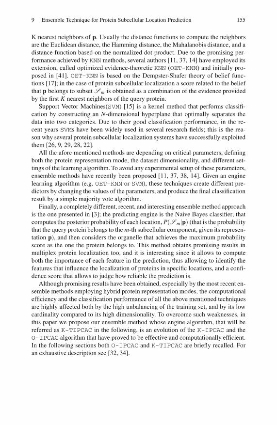
9 Ensemble Technique for Protein Subcellular Location Prediction 155
K nearest neighbors of p. Usually the distance functions to compute the neighbors
are the Euclidean distance, the Hamming distance, the Mahalanobis distance, and a
distance function based on the normalized dot product. Due to the promising per-
formance achieved by KNN methods, several authors [11, 37, 14] have employed its
extension, called optimized evidence-theoretic KNN (OET-KNN) and initially pro-
posed in [41]. OET-KNN is based on the Dempster-Shafer theory of belief func-
tions [17]; in the case of protein subcellular localization a score related to the belief
that p belongs to subset S m is obtained as a combination of the evidence provided
by the first K nearest neighbors of the query protein.
Support Vector Machines(SVM) [15] is a kernel method that performs classifi-
cation by constructing an N-dimensional hyperplane that optimally separates the
data into two categories. Due to their good classification performance, in the re-
cent years SVMs have been widely used in several research fields; this is the rea-
son why several protein subcellular localization systems have successfully exploited
them [26, 9, 29, 28, 22].
All the afore mentioned methods are depending on critical parameters, defining
both the protein representation mode, the dataset dimensionality, and different set-
tings of the learning algorithm. To avoid any experimental setup of these parameters,
ensemble methods have recently been proposed [11, 37, 38, 14]. Given an engine
learning algorithm (e.g. OET-KNN or SVM), these techniques create different pre-
dictors by changing the values of the parameters, and produce the final classification
result by a simple majority vote algorithm.
Finally, a completely different, recent, and interesting ensemble method approach
is the one presented in [3]; the predicting engine is the Naive Bayes classifier, that
computes the posterior probability of each location, P(S m|p) (that is the probability
that the query protein belongs to the m-th subcellular component, given its represen-
tation p), and then considers the organelle that achieves the maximum probability
score as the one the protein belongs to. This method obtains promising results in
multiplex protein localization too, and it is interesting since it allows to compute
both the importance of each feature in the prediction, thus allowing to identify the
features that influence the localization of proteins in specific locations, and a confi-
dence score that allows to judge how reliable the prediction is.
Although promising results have been obtained, especially by the most recent en-
semble methods employing hybrid protein representation modes, the computational
efficiency and the classification performance of all the above mentioned techniques
are highly affected both by the high unbalancing of the training set, and by its low
cardinality compared to its high dimensionality. To overcome such weaknesses, in
this paper we propose our ensemble method whose engine algorithm, that will be
referred as K-TIPCAC in the following, is an evolution of the K-IPCAC and the
O-IPCAC algorithm that have proved to be effective and computationally efficient.
In the following sections both O-IPCAC and K-TIPCAC are briefly recalled. For
an exhaustive description see [32, 34].

156 A. Rozza et al.
9.3 Classifiers Based on Efficient Fisher Subspace Estimation
The first version of our classifiers, called IPCAC, has been initially proposed in [32].
It is a binary classifier exploiting theoretical results presented in [4] to efficiently
estimate the Fisher subspace (Fs). More precisely, in [4] it is demonstrated that,
given a set of N clustered points sampled from an isotropic Mixture of Gaussians
(MoG), Fs corresponds to the span of the class means; as a consequence, when a
binary classification problem is considered, Fs is spanned by f =µµµA−µµµB||µµµA−µµµB|| , being
A/B the two classes, and µµµA/B the class means.
IPCAC exploits this result by whitening the training set PTrain, computing the
unit vector f, and then classifying a new point p by thresholding its projection on
Fs as follows:
(WTDf) ·p− γ = w ·p− γ < 0 γ =
⟨argmax γ ∈w·piScore(γ )
⟩(9.1)
where the matrix WD represents the whitening transformation estimated on the N
training points, Score(γ ) computes the number of correctly classified training points
when γ is used as threshold, and 〈·〉 represents the average operator.
Unfortunately, classifiers based on the estimation of Fs cannot work on high di-
mensional datasets for their high computational complexity. Moreover, these tech-
niques often fail when the training-set cardinality is equal or lower than the input
space dimensionality.
To address these problems, O-IPCAC (Online IPCAC) [34] improves IPCAC,
and reduces the computational complexity, by replacing the first step of data
whitening by a ‘partial whitening’ process; if the points to be classified belong
to a D dimensional space, this method whitens the data in the linear subspace
πd = Span〈v1, · · · ,vd〉, spanned by the first d ≪ D principal components, while
maintaining unaltered the information related to the orthogonal subspace (πd)⊥ =
Span〈vd+1, · · · ,vD〉.More precisely, the linear transformation WD representing the partial whiten-
ing operator is estimated as follows. The Truncated Singular Value Decomposition
(TSVD) [24] is applied to estimate the first d = min(log22N,D) principal compo-
nents, obtaining the low-rank factorization P ≃ UdQdVTd (where P is the matrix
representing the training set PTrain since it contains the training vectors). The d
largest singular values on the diagonal of Qd , and the associated left singular vec-
tors, are employed to project the points in the matrix P on the subspace H d spanned
by the columns of Ud , and to perform the whitening, as follows:
PWd= qdQ−1
d P⊥H d= qdQ−1
d UTd P = WdP
where qd is the smallest singular value of the points projected in H d . Note that, to
obtain points whose covariance matrix best resembles a multiple of the identity, we
have chosen to set the value of the d largest singular values to qd instead of 1, thus
avoiding the gap between the d-th and the (d + 1)-th singular value. The obtained
matrix Wd projects and whitens the points in the linear subspace H d ; however, di-
mensionality reduction during the whitening estimation might delete discriminative

9 Ensemble Technique for Protein Subcellular Location Prediction 157
information, decreasing the classification performance. To avoid this information
loss, we add to the partially whitened data the residuals (R) of the points in P with
respect to their projections on H d :
R = P−UdP⊥H d= P−UdUT
d P
PWD= UdPWd
+ R =(qdUdQ−1
d UTd + I−UdUT
d
)P = WDP (9.2)
where WD ∈ℜD×D represents the linear transformation that whitens the data along
the first d principal components, while keeping unaltered the information along the
remaining components.
In case of binary classification problems, once the partial whitening step has been
performed the two whitened class means, and the vector f estimating Fs in the
partially whitened space, are computed; this allows the binary predictor to compute
the class labels by employing the procedure described in [33].
The described approach increases the performance and guarantees a greater sta-
bility during the classification task. We note that O-IPCAC has been implemented
to perform both batch and online training. For convenience, in this contribution, we
refer to the batch method as TIPCAC (Truncated-whitening IPCAC).
9.3.1 A Kernel Version of TIPCAC
To relax the linear separability constraint imposed by the IPCAC algorithm, it is
possible to exploit the kernel trick as in the Kernel Principal Component Analy-
sis (KPCA, [39]), thus obtaining a Kernel Isotropic Principal Component Analysis
Classifier (KIPCAC), that has been proposed in [32].
More precisely, Rozza et al. demonstrate that a given point p can be projected on
Fs in the kernel space as follows:
pro jF(p) = Ker(p)T(
(NANB)12 AΛΛΛ
−1AT N−1
A|B
)
= Ker(p)T w
where N is the cardinality of the training set, the Kernel matrix of the training points
is Ker(p) = KerFunction(pi,p)Ni=1, ΛΛΛ are the eigenvalues obtained by the de-
composition of Ker(p), A are the associated eigenvectors, NA,NB are the cardinali-
ties of the two classes, and N−1A|B = [N−1
A · · ·︸ ︷︷ ︸
NA times
−N−1B · · ·
︸ ︷︷ ︸
NB times
]T .
In this work we extended this method by exploiting the same concept at the basis
of the TIPCAC partial whitening step. More precisely, we select the largest eigenval-
ues that represent a fixed amount of variance defined a-priori, and we set the remain-
ing part of the spectrum to 1; this process reduces the overfitting problems produced
by the smallest part of the spectrum without performing any kind of dimensionality
reduction. The advantages of employing this modified version of KIPCAC, called
K-TIPCAC, are confirmed by the performance achieved in our experimental results.

158 A. Rozza et al.
9.4 DDAG K-TIPCAC
In this section we briefly describe the DDAG technique which allows to combine
different methods to create a multiclass classifier (see Sect. 9.4.1). Secondly, we
describe how DDAG has been exploited to develop our technique, called DDAGK-TIPCAC (see Sect. 9.4.2).
9.4.1 Decision DAGs (DDAGs)
A Rooted Direct Acyclic Graph (DAG) is a graph whose edges have an orientation,
no cycles, and only one root node. A Rooted Binary DAG has nodes which have
either 0 or 2 arcs leaving them. A DDAG [31] is a method that combines the results
of one-against-one classifiers to produce a multi-class classification. To this aim,
considering a N-class problem, the DDAG is implemented using a rooted binary DAGwith K = N(N− 1)/2 internal nodes. Each node represents a classification model
trained on two of the K classes, and it produces a boolean output value (0,1).The nodes are arranged in a binary tree with the single root node at the top, two
nodes in the second layer and so on until the final layer of leaves. Considering
each classifier as a boolean function, to perform classification the DDAG proceeds
as follows: it starts at the root node and it evaluates the boolean function; the node
is then exited via the left edge, if the binary function is zero, or the right edge,
if the binary function is one; the next node binary function is then evaluated; the
membership class is the final leaf node reached through this process.
9.4.2 Decision DAG K-TIPCAC
In Sect. 9.3, an efficient binary classifier (called TIPCAC) and its kernel version
(called K-TIPCAC) are described, that are based on the projection of the data on
the one dimensional Fs estimated in a partially whitened kernel subspace.
The ensemble classifier proposed in this chapter is a C-class classifier that
projects the data on a C− 1 dimensional Fs estimated in a partially whitened sub-
space, and then applies DDAG to combine many binary K-TIPCACs to obtain the
final prediction.
More precisely, the first step of this method evaluates the Fs of the overall C
classes by generalizing the partial whitening approach recovering residuals, used by
TIPCAC; this step reduces the training time complexity.
To this aim, after the partial whitening, the whitened class means µµµcCc=1 are
computed as follows:
µµµc = WDµµµc = qdUdQ−1d UT
d µµµc + µµµc−UdUTd µµµc.
At this stage the orthonormal basis, ΠC−1, composed of C−1 vectors spanning the
Fs, is computed. More precisely, ΠC−1 is obtained by orthonormalizing the C− 1
linearly independent µµµc vectors through the Gram-Schmidt procedure. The partially

9 Ensemble Technique for Protein Subcellular Location Prediction 159
whitened training points PWDare then projected on the subspace ΠC−1, obtaining
the set of points
PΠC−1=
FsT pi|pi ∈PWD
,
where Fs is the matrix whose columns span Fs.
Exploiting the points in PΠC−1, C(C− 1)/2 K-TIPCAC binary classifiers are
trained, each discriminating two classes in a one-against-one fashion (1-vs-1), and
their results are combined by means of DDAG.
9.5 Experimental Setting
In this section we firstly remind the multi-class classification methods employed to
perform the base-line comparison (see Sect. 9.5.1); secondly, we describe in details
the employed dataset (see Sect. 9.5.2); finally, we report the performance evaluation
method (see Sect. 9.5.3).
9.5.1 Methods
Multiclass Support Vector Machine: Since SVM is a binary classifier, a problem
transformation is required before the application of this method to the considered
multiclass prediction problem. The existing approaches to cast a multi-class classi-
fication problem to a series of binary classification problems can be roughly divided
into two main classes: one-against-all and 1-vs-1. We applied the latter, and thus
we trained a committee of 231 probabilistic SVMs [30]. The probabilities produced
by each classifier were then reconciled to a multiclass prediction via pairwise cou-
pling [25] and a simple max rule over all the class probability estimates was applied
to compute a final decision.
Ensemble of Nested Dichotomies (END): Nested dichotomies [20] is a standard
statistical technique applied in polytomous classification problems where logistic
regression is applied by fitting binary logistic regression models to the internal nodes
composing a tree. In absence of domain knowledge it is difficult to decide, among
all the possible trees of nested dichotomies, the one to be adopted. A possible solu-
tion [19] is to consider all the hierarchies of nested dichotomies equally likely, and
to use an ensemble of these hierarchies for prediction. In our experiments we tuned
the END technique across nd (number of dichotomies) ∈ 5,10,20,40.
Random Forest (RF): Random Forest [2] has been applied as an effective tool for
biomolecular and bioinformatics research. This method grows many classification
trees. Instances whose class needs to be predicted are classified using the trees com-
posing the forest. Each tree computes its own prediction, and the forest employs a
plurality voting (over all the trees in the forest) to choose the final classification.
We tuned the method using a grid search over nt (number of trees of the forest)
∈ 10,20,30,40,50 and n f (number of features) ∈ 10,100.

160 A. Rozza et al.
9.5.2 Dataset
We evaluated the proposed method on a publicly available dataset1 involved in the
training of the EukP-loc method described in [13].
This dataset contains 5618 different proteins, classified into 22 eukaryotic sub-
cellular locations. Among the 5618 considered proteins, 5091 belong to one subcel-
lular location, 495 to two locations, 28 to three locations, and 4 to four locations.
None of the proteins has ≥ 25% sequence identity to any other in the same sub-
set. The collection of sequences was then evaluated to compute the Pseudo Amino
Acid compositions (PseAAC) of each protein using the PseAAC web server [36].
For each protein we produced a 495-elements vector composed by 20 numbers de-
scribing the standard amino acid composition, 400 values representing the PseAACbased on the dipeptide representation of the protein and further 75 values represent-
ing three groups of 25 PseAACs values obtained by setting the λ parameter to 25
and computing the PseAACs based on three pairs of chemico-physical properties:
Hydrophobicity-Hydrophilicity, pK1 (alpha-COOH)-pK2 (NH3) and Mass-pI.
In this preliminary investigation we focused on the location prediction of the 5091
proteins with a single experimentally annotated subcellular location. Some charac-
teristics of this dataset are depicted in Table 9.1. It is worth noting that the problem
is highly unbalanced, ranging the number of proteins associated to a subcellular
location from 13 (hydrogenosome, melanosome and synapse) to 1077 (nucleus).
Table 9.1 Protein subcellular localization prediction dataset (5091 proteins and 22 locations).
This table reports the number of annotated proteins per location; labels are mutually exclu-
sive, thus the problem is multiclass but not multilabel.
Dataset
acrosome proteins 17 cell wall proteins 47
Golgi proteins 157 spindle pole body proteins 17
hydrogenosome proteins 13 synapse proteins 13
lysosome proteins 59 vacuole proteins 91
melanosome proteins 13 centriole proteins 45
microsome proteins 23 chloroplast proteins 497
mitochondrion proteins 488 cyanelle proteins 85
nucleus proteins 1077 cytoplasm proteins 741
peroxisome proteins 92 cytoskeleton proteins 46
plasma membrane proteins 647 endoplasmic reticulum proteins 275
extracell proteins 609 endosome proteins 39
1 The protein sequences were downloaded in fasta format from the web site
http://www.csbio.sjtu.edu.cn/bioinf/euk-multi/Supp-A.pdf
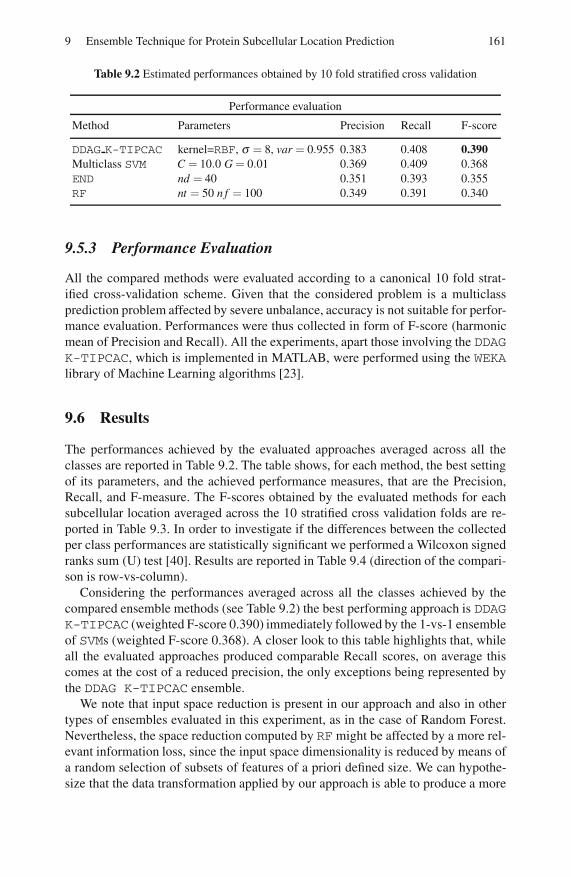
9 Ensemble Technique for Protein Subcellular Location Prediction 161
Table 9.2 Estimated performances obtained by 10 fold stratified cross validation
Performance evaluation
Method Parameters Precision Recall F-score
DDAG K-TIPCAC kernel=RBF, σ = 8, var = 0.955 0.383 0.408 0.390
Multiclass SVM C = 10.0 G = 0.01 0.369 0.409 0.368
END nd = 40 0.351 0.393 0.355
RF nt = 50 n f = 100 0.349 0.391 0.340
9.5.3 Performance Evaluation
All the compared methods were evaluated according to a canonical 10 fold strat-
ified cross-validation scheme. Given that the considered problem is a multiclass
prediction problem affected by severe unbalance, accuracy is not suitable for perfor-
mance evaluation. Performances were thus collected in form of F-score (harmonic
mean of Precision and Recall). All the experiments, apart those involving the DDAGK-TIPCAC, which is implemented in MATLAB, were performed using the WEKAlibrary of Machine Learning algorithms [23].
9.6 Results
The performances achieved by the evaluated approaches averaged across all the
classes are reported in Table 9.2. The table shows, for each method, the best setting
of its parameters, and the achieved performance measures, that are the Precision,
Recall, and F-measure. The F-scores obtained by the evaluated methods for each
subcellular location averaged across the 10 stratified cross validation folds are re-
ported in Table 9.3. In order to investigate if the differences between the collected
per class performances are statistically significant we performed a Wilcoxon signed
ranks sum (U) test [40]. Results are reported in Table 9.4 (direction of the compari-
son is row-vs-column).
Considering the performances averaged across all the classes achieved by the
compared ensemble methods (see Table 9.2) the best performing approach is DDAGK-TIPCAC (weighted F-score 0.390) immediately followed by the 1-vs-1 ensemble
of SVMs (weighted F-score 0.368). A closer look to this table highlights that, while
all the evaluated approaches produced comparable Recall scores, on average this
comes at the cost of a reduced precision, the only exceptions being represented by
the DDAG K-TIPCAC ensemble.
We note that input space reduction is present in our approach and also in other
types of ensembles evaluated in this experiment, as in the case of Random Forest.
Nevertheless, the space reduction computed by RF might be affected by a more rel-
evant information loss, since the input space dimensionality is reduced by means of
a random selection of subsets of features of a priori defined size. We can hypothe-
size that the data transformation applied by our approach is able to produce a more
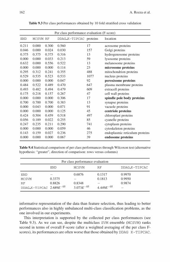
162 A. Rozza et al.
Table 9.3 Per class performances obtained by 10 fold stratified cross validation
Per class performance evaluation (F-score)
END MCSVM RF DDAG K-TIPCAC proteins location
0.211 0.000 0.300 0.560 17 acrosome proteins
0.046 0.000 0.024 0.030 157 Golgi proteins
0.375 0.375 0.375 0.316 13 hydrogenosome proteins
0.000 0.000 0.033 0.213 59 lysosome proteins
0.632 0.000 0.556 0.522 13 melanosome proteins
0.000 0.000 0.000 0.114 23 microsome proteins
0.295 0.312 0.241 0.355 488 mitochondrion proteins
0.529 0.535 0.523 0.533 1077 nucleus proteins
0.000 0.000 0.000 0.047 92 peroxisome proteins
0.484 0.522 0.489 0.470 647 plasma membrane proteins
0.493 0.482 0.494 0.479 609 extracell proteins
0.175 0.218 0.157 0.267 47 cell wall proteins
0.000 0.000 0.000 0.306 17 spindle pole body proteins
0.700 0.700 0.700 0.383 13 synapse proteins
0.000 0.043 0.000 0.071 91 vacuole proteins
0.000 0.000 0.000 0.125 45 centriole proteins
0.424 0.504 0.459 0.518 497 chloroplast proteins
0.056 0.189 0.022 0.255 85 cyanelle proteins
0.247 0.235 0.211 0.290 741 cytoplasm proteins
0.000 0.000 0.000 0.059 46 cytoskeleton proteins
0.143 0.159 0.027 0.236 275 endoplasmic reticulum proteins
0.000 0.000 0.000 0.067 39 endosome proteins
Table 9.4 Statistical comparison of per class performances through Wilcoxon test (alternative
hypothesis: “greater”, direction of comparison: rows versus columns)
Per class performance evaluation
END MCSVM RF DDAG K-TIPCAC
END − 0.6876 0.1317 0.9970
MCSVM 0.3375 − 0.1813 0.9950
RF 0.8826 0.8348 − 0.9874
DDAG K-TIPCAC 2.689E−05 3.073E−05 4.449E−05 −
informative representation of the data than feature selection, thus leading to better
performances also in highly unbalanced multi-class classification problems, as the
one involved in our experiments.
This interpretation is supported by the collected per class performances (see
Table 9.3). As we can see, despite the multiclass SVM ensemble (MCSVM) ranks
second in terms of overall F-score (after a weighted averaging of the per class F-
scores), its performances are often worse that those obtained by DDAG K-TIPCAC.
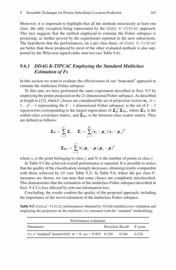
9 Ensemble Technique for Protein Subcellular Location Prediction 163
Moreover, it is important to highlight that all the methods misclassify at least one
class, the only exception being represented by the DDAG K-TIPCAC approach.
This fact suggests that the method employed to estimate the Fisher subspace is
promising, as further proved by the experiments reported in the next subsections.
The hypothesis that the performances, on a per class basis, of DDAG K-TIPCACare better than those produced by most of the other evaluated methods is also sup-
ported by the Wilcoxon signed ranks sum test (see Table 9.4).
9.6.1 DDAG K-TIPCAC Employing the Standard Multiclass
Estimation of Fs
In this section we want to evaluate the effectiveness of our “truncated” approach to
estimate the multiclass Fisher subspace.
To this aim, we have performed the same experiment described in Sect. 9.5 by
employing the points projected on the 21 dimensional Fisher subspace. As described
at length in [21], when C classes are considered the set of projection vectors wk, k =1, ..,C− 1 representing the C− 1 dimensional Fisher subspace, is the set of C− 1
eigenvectors corresponding to the largest eigenvalues of ΣΣΣ−1W ΣΣΣ Bet , where ΣΣΣW is the
within-class covariance matrix, and ΣΣΣ Bet is the between-class scatter matrix. They
are defined as follows:
ΣΣΣW =C
∑c=1
ΣΣΣ c, ΣΣΣ c =Nc
∑j=1
(x j− µµµc)(x j− µµµc)T
ΣΣΣ Bet =C
∑c=1
Nc(µµµc− µµµ)(µµµc− µµµ)T
where xi is the point belonging to class i, and Ni is the number of points in class i.
In Table 9.5 the achieved overall performance is reported. It is possible to notice
that the quality of the classification strongly decreases, obtaining results comparable
with those achieved by RF (see Table 9.2). In Table 9.6, where the per class F-
measures are shown, we can note that some classes are completely misclassified.
This demonstrates that the estimation of the multiclass Fisher subspace described in
Sect. 9.4.2 is less affected by relevant information loss.
Concluding, the results confirm the quality of the proposed approach, including
the importance of the novel estimation of the multiclass Fisher subspace.
Table 9.5 DDAG K-TIPCAC performances obtained by 10 fold stratified cross validation and
employing the projection on the multiclass Fs estimated with the “standard” methodology
Performance evaluation
Parameters Precision Recall F-score
Fs = “standard” kernel=RBF, σ = 8, var = 0.955 0.330 0.344 0.334
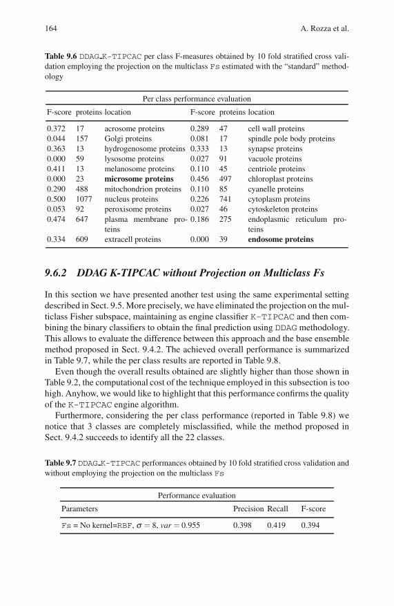
164 A. Rozza et al.
Table 9.6 DDAG K-TIPCAC per class F-measures obtained by 10 fold stratified cross vali-
dation employing the projection on the multiclass Fs estimated with the “standard” method-
ology
Per class performance evaluation
F-score proteins location F-score proteins location
0.372 17 acrosome proteins 0.289 47 cell wall proteins
0.044 157 Golgi proteins 0.081 17 spindle pole body proteins
0.363 13 hydrogenosome proteins 0.333 13 synapse proteins
0.000 59 lysosome proteins 0.027 91 vacuole proteins
0.411 13 melanosome proteins 0.110 45 centriole proteins
0.000 23 microsome proteins 0.456 497 chloroplast proteins
0.290 488 mitochondrion proteins 0.110 85 cyanelle proteins
0.500 1077 nucleus proteins 0.226 741 cytoplasm proteins
0.053 92 peroxisome proteins 0.027 46 cytoskeleton proteins
0.474 647 plasma membrane pro-
teins
0.186 275 endoplasmic reticulum pro-
teins
0.334 609 extracell proteins 0.000 39 endosome proteins
9.6.2 DDAG K-TIPCAC without Projection on Multiclass Fs
In this section we have presented another test using the same experimental setting
described in Sect. 9.5. More precisely, we have eliminated the projection on the mul-
ticlass Fisher subspace, maintaining as engine classifier K-TIPCAC and then com-
bining the binary classifiers to obtain the final prediction using DDAG methodology.
This allows to evaluate the difference between this approach and the base ensemble
method proposed in Sect. 9.4.2. The achieved overall performance is summarized
in Table 9.7, while the per class results are reported in Table 9.8.
Even though the overall results obtained are slightly higher than those shown in
Table 9.2, the computational cost of the technique employed in this subsection is too
high. Anyhow, we would like to highlight that this performance confirms the quality
of the K-TIPCAC engine algorithm.
Furthermore, considering the per class performance (reported in Table 9.8) we
notice that 3 classes are completely misclassified, while the method proposed in
Sect. 9.4.2 succeeds to identify all the 22 classes.
Table 9.7 DDAG K-TIPCAC performances obtained by 10 fold stratified cross validation and
without employing the projection on the multiclass Fs
Performance evaluation
Parameters Precision Recall F-score
Fs = No kernel=RBF, σ = 8, var = 0.955 0.398 0.419 0.394

9 Ensemble Technique for Protein Subcellular Location Prediction 165
Table 9.8 DDAG-K-TIPCAC per class F-measures obtained by 10 fold stratified cross vali-
dation without employing the projection on the multiclass Fs
Per class performance evaluation
F-score proteins location F-score proteins location
0.714 17 acrosome proteins 0.253 47 cell wall proteins
0.056 157 Golgi proteins 0.000 17 spindle pole body proteins
0.471 13 hydrogenosome proteins 0.538 13 synapse proteins
0.282 59 lysosome proteins 0.055 91 vacuole proteins
0.700 13 melanosome proteins 0.098 45 centriole proteins
0.000 23 microsome proteins 0.538 497 chloroplast proteins
0.344 488 mitochondrion proteins 0.167 85 cyanelle proteins
0.537 1077 nucleus proteins 0.290 741 cytoplasm proteins
0.019 92 peroxisome proteins 0.078 46 cytoskeleton proteins
0.489 647 plasma membrane pro-
teins
0.247 275 endoplasmic reticulum pro-
teins
0.477 609 extracell proteins 0.000 39 endosome proteins
9.7 Conclusion
In this contribution we proposed an ensemble method whose engine algorithm is
K-TIPCAC. The K-TIPCACmethod deals with the points projected on a multiclass
Fisher subspace. The final multi-class classification is performed by combining the
kernel classifiers through Direct Decision Acyclic Graph (DDAG).
This methodology was applied to one of the most difficult multiclass prediction
problems in modern computational biology: the protein subcellular location predic-
tion. The results achieved by the performed experimental tests show the effective-
ness of the K-TIPCAC algorithm and the quality of the multiclass Fisher subspace
estimation by means of the proposed approach.
It is worth noting that the ability of the proposed approach to effectively control
the precision-recall trade-off also in the prediction of small classes is of paramount
importance in real applications, when we need to reduce the costs associated with
the biological validation of new protein locations discovered through in silico
methods.
Furthermore, considering also the experiments in Sect. 9.6.1 and Sect. 9.6.2 we
can affirm that the method proposed in this chapter is an efficient and effective
technique. This is due to the fact that it outperforms state of the art ensemble meth-
ods, and it reduces the time cost employing a dimensionality reduction that is less
affected by loss of discriminative information. Moreover, only this approach guar-
antees the identification of all the classes that describe the protein localization.

166 A. Rozza et al.
References
1. Bhasin, M., Garg, A., Raghava, G.P.: PSLpred: prediction of subcellular localization of
bacterial proteins. Bioinformatics 21, 2522–2524 (2005)
2. Breiman, L.: Random Forests. Machine Learning 45, 5–32 (2001)
3. Briesemeister, S., Rahnenfuhrer, J., Kohlbacher, O.: Going from where to why - inter-
pretable prediction of protein subcellular localization. Bioinformatics 26, 1232–1238
(2010)
4. Brubaker, S.C., Vempala, S.: Isotropic PCA and affine-invariant clustering. In: Proc. the
49th Annual IEEE Symp. Foundations Comp., Philadelphia, PA, pp. 551–560 (2008)
5. Cai, Y.D., Chou, K.C.: Nearest neighbor algorithm for predicting protein subcellular
location by combining functional domain composition and pseudo-amino acid compo-
sition. Biochem. and Biophys. Research Communications 305, 407–411 (2003)
6. Chou, K.C.: A novel approach to predicting protein structural classes in a (20-1)-
D amino acid composition space. Proteins: Structure, Function, and Genetics 21,
319–344 (1995)
7. Chou, K.C., Elrod, D.W.: Protein subcellular location prediction. Protein Engineer-
ing 12, 107–118 (1999)
8. Chou, K.C.: Prediction of protein cellular attributes using pseudo amino acid composi-
tion. Proteins: Structure, Function, and Genetics 43, 246–255 (2001)
9. Chou, K.C., Cai, Y.D.: Using functional domain composition and support vector ma-
chines for prediction of protein subcellular location. J. Biol. Chem. 277, 45765–45769
(2002)
10. Chou, K.C., Cai, Y.D.: Prediction of protein subcellular locations by GO-FunD-PseAA
predictor. Biochem. and Biophys. Research Communications 320, 1236–1239 (2004)
11. Chou, K.C., Shen, H.B.: Predicting eukaryotic protein subcellular locations by fusing
optimized evidence-theoretic K-nearest neighbor classifiers. J. Proteome Research 5,
1888–1897 (2006)
12. Chou, K.C., Shen, H.B.: Recent progress in protein subcellular location prediction. An-
alytical Biochem. 370, 1–16 (2007)
13. Chou, K., Shen, H.: Cell-Ploc: a package of web servers for predicting subcellular lo-
calization of proteins in various organisms. Nature Protocol 3, 153–162 (2008)
14. Chou, K., Shen, H.: A new method for predicting the subcellular localization of eukar-
iotic proteins with both single and multiple sites: Euk-mPLoc 2.0. Plos One 5, e9931
(2010)
15. Cortes, C., Vapnik, V.: Support Vector Networks. Machine Learning 20, 273–293
(1995)
16. Cover, T.M., Hart, P.E.: Nearest neighbour pattern classification. IEEE Trans. Inf. The-
ory 13, 21–27 (1967)
17. Denoeux, T.: A K-nearest neighbor classification rule based on Dempster-Shafer theory.
IEEE Trans. System, Man, and Cybernetics 25, 804–813 (1995)
18. Duda, R.O., Hart, P.E., Stork, D.G.: Pattern Recognition, 2nd edn. Wiley- Interscience,
Hoboken (2001)
19. Frank, E., Kramer, S.: Ensembles of nested dichotomies for multi-class problems. In:
Brodley, C.E. (ed.) Proc. the 21st Int. Conf. Machine Learning, Banff, AL. ACM Press,
New York (2004)
20. Fox, J.: Applied regression analysis, linear models, and related methods. Sage, Thou-
sand Oaks (1997)
21. Fukunaga, K.: Introduction to statistical pattern recognition, 2nd edn. Academic Press,
Burlington (1990)
9 Ensemble Technique for Protein Subcellular Location Prediction 167
22. Garg, A., Bhasin, M., Raghava, G.P.: Support vector machine-based method for sub-
cellular localization of human proteins using amino acid compositions, their order, and
similarity search. J. Biol. Chem. 280, 14427–14432 (2005)23. Hall, M., Frank, E., Holmes, G., Pfahringer, B., Reutemann, P., Witten, I.H.: The
WEKA data mining software: An update. SIGKDD Explorations 11 (2009)24. Hansen, P.C.: The truncated SVD as a method for regularization. Technical Report,
Standford University, CA, USA (1986)25. Hastie, T., Tibshirani, R.: Classification by pairwise coupling. In: Jordan, M.I., Kearns,
M.J., Solla, S.A. (eds.) Proc. Neural Inf. Proc. Syst., Denver, CO, pp. 507–513. MIT
Press, Cambridge (1998)26. Hua, S., Sun, Z.: Support vector machine approach for protein subcellular localization
prediction. Bioinformatics 17, 721–728 (2001)27. Huang, Y., Li, Y.: Prediction of protein subcellular locations using fuzzy K-NN method.
Bioinformatics 20, 21–28 (2004)28. Lei, Z., Dai, Y.: An SVM-based system for predicting protein subnuclear localizations.
BMC Bioinformatics 6 (2005)29. Park, K.J., Kanehisa, M.: Prediction of protein subcellular locations by support vec-
tor machines using composition amino acid and amino acid pairs. Bioinformatics 19,
1656–1663 (2003)30. Platt, J.: Probabilistic outputs for support vector machines and comparisons to regular-
ized likelihood methods. In: Smola, A.J., Bartlett, P.L., Scholkopf, B., Schuurmans, D.
(eds.) Advances in Large Margin Classifiers, pp. 61–74. MIT Press, Cambridge (1999)31. Platt, C., Cristianini, N., Shawe-Taylor, J.: Large margin DAGs for multiclass classifi-
cation. In: Leen, T.K., Dietterich, T.G., Tresp, V. (eds.) Proc. Neural Inf. Proc. Syst.,
Denver, CO, pp. 547–553. MIT Press, Cambridge (2000)32. Rozza, A., Lombardi, G., Casiraghi, E.: Novel IPCA-based classifiers and their ap-
plication to spam filtering. In: Abraham, A., Sanchez, J.M.B., Herrera, F., Loia, V.,
Marcelloni, F., Senatore, S. (eds.) Proc. Int. Conf. Syst. Design and Appl., Pisa, Italy,
pp. 797–802. IEEE Computer Society, Washington (2009)33. Rozza, A., Lombardi, G., Casiraghi, E.: PIPCAC: A novel binary classifier assuming
mixtures of Gaussian functions. In: Proc. Artif. Intell. Appl., Innsbruck, Austria. ACTA
Press, Calgary (2010)34. Rozza, A., Lombardi, G., Rosa, M., Casiraghi, E.: O-IPCAC and its application to EEG
classification. J. Machine Learning Research 11, 4–11 (2010)35. Shen, H.B., Chou, K.C.: Virus-PLoc: A fusion classifier for predicting the subcellu-
lar localization of viral proteins within host and virus-infected cells. Biopolymers 85,
233–240 (2006)36. Shen, H., Chou, K.: PseAAC: a flexible web server for generating various kinds of
protein pseudo amino acid composition. Analytical Biochem. 373, 386–388 (2008)37. Shen, H.B., Chou, K.C.: Hum-mPLoc: an ensemble classifier for large-scale human
protein subcellular location prediction by incorporating samples with multiple sites.
Biochem. and Biophys. Research Communications 355, 1006–1011 (2007)38. Shen, H.B., Chou, K.C.: Virus-PLoc: a fusion classifier for predicting protein subcellu-
lar localization of viral proteins within host and virus-infected cells. Biopolymers 85,
233–240 (2007)39. Scholkopf, B., Smola, A., Muller, K.R.: Nonlinear component analysis as a kernel
eigenvalue problem. Neural Computing 10, 1299–1319 (1998)40. Wilcoxon, F.: Individual comparisons by ranking methods. Biometrics 1, 80–83 (1945)41. Zouhal, L.M., Denoeux, T.: An evidence theoretic K-NN rule with parameter optimiza-
tion. IEEE Trans. Syst., Man, and Cybernetics 28, 263–271 (1999)

Chapter 10
Trading-Off Diversity and Accuracy for OptimalEnsemble Tree Selection in Random Forests
Haytham Elghazel, Alex Aussem, and Florence Perraud
Abstract. We discuss an effective method for optimal ensemble tree selection in
Random Forests by trading-off diversity and accuracy of the ensemble during the
selection process. As the chances of overfitting increase dramatically with the size
of the ensemble, we wrap cross-validation around the ensemble selection to max-
imize the amount of validation data considering, in turn, each fold as a validation
fold to select the trees from. The aim is to increase performance by reducing the
variance of the tree ensemble selection process. We demonstrate the effectiveness
of our approach on several UCI and real-world data sets.
10.1 Introduction
Many advances in Machine Learning suggest using a set of individual classifiers, or
ensemble of classifiers, instead of a single predictor to address supervised classifi-
cation problems [16]. A large number of studies show that ensemble of classifiers
generally achieve better results compared to a single classifier in terms of misclas-
sification error [11, 22]. This improvement of performances relies on the concept
of diversity which states that a good classifier ensemble is an ensemble in which
the examples that are misclassified are different from one individual classifier to
another. However, the practical trade-off between diversity and accuracy of the en-
semble learning is still an open question in Machine Learning [6]. Dietterich [10]
states that “A necessary and sufficient condition for an ensemble of classifiers to be
more accurate than any of its individual members is if the classifiers are accurate
and diverse”. Many methods have been proposed to generate accurate, yet diverse,
sets of models. Bagging [4], Boosting [13], Random Forests [5] and their variants
Haytham Elghazel · Alex Aussem · Florence Perraud
Universite de Lyon, F-69000, Lyon
Universite de Lyon 1
Laboratoire GAMA, 69622 Villeurbanne, France
E-mail: [email protected]
O. Okun et al. (Eds.): Ensembles in Machine Learning Applications, SCI 373, pp. 169–179.springerlink.com c© Springer-Verlag Berlin Heidelberg 2011

170 H. Elghazel, A. Aussem, and F. Perraud
are the most popular examples of this methodology. Boosting and Random Forest
are comparable and sometimes better than state-of-the-art methods in classification
and regression [9].
Random Forests (RF) is a popular and very efficient algorithm, based on model
aggregation ideas, for both classification and regression problems [5]. The principle
of RF is to combine many binary decision trees built using several bootstrap sam-
ples coming from the learning sample and choosing randomly at each node a subset
of explanatory variables. We assume the reader already is familiar with details of
the RF procedure. RF algorithm becomes more and more popular and appears to be
computationally effective and offers good prediction performance in a lot of differ-
ent applications [12]. Breiman sketches an explanation of the good performance of
RF related to the good quality of each tree together with the small correlation (de-
noting high diversity) among the trees of the forest. However, the mechanisms that
explain this good performance of RF are not clearly elucidated from a mathematical
point of view [2]. Indeed, it appears that using random selection of variables during
the design stage of RF makes individual trees rather weak predictors and does not
always give the expected performances. In addition, Breiman observed that above
a certain number of trees, adding more trees does not allow to improve the perfor-
mance [5]. Precisely he stated that for an increasing number of trees in the forest, the
generalization error converges to a maximum. This result indicates that the number
of trees in a forest does not have to be as large as possible to produce an accurate RF.
On the other hand, pruning the irrelevant trees from huge forest is not as easy as one
may think. The tree selection process is subject to overfitting problems especially
when the number of validation samples provided is not sufficient [1, 8]. Also, we
believe there is still room for improvement.
In this work, we discuss a simple framework called Fitselect to improve RF un-
der Ensemble pruning (also called Overproduce and Choose Paradigm). The main
idea of our approach is to perform classifier selection from an initial pool of decision
trees obtained with the RF algorithm while focusing on the trade-off between accu-
racy and diversity of selected trees. The proposed method works by evaluating the
qualities of all obtained trees in terms of accuracy-diversity trade-off on a hillclimb
(validation) set, and selectively choosing part of promising trees to build the final
RF. To alleviate the overfitting problem, we wrap cross-validation around ensemble
selection to maximize the amount of validation data considering, in turn, each fold
as a validation fold. A distinct tree selection is performed in each RF model. Im-
provements are demonstrated on several classification data sets. Empirical results
show that the selected subset of trees performs similar to or better than the original
ensemble (RF).
The rest of this chapter is organized as follows. Section 10.2 reviews recent stud-
ies on ensemble pruning. Section 10.3 introduces the f itselect framework for im-
proving Random Forest. Experiments using relevant benchmarks and real data sets
are presented in Sect. 10.4. Section 10.5 concludes this chapter.

10 Optimal Ensemble Tree Selection 171
10.2 Background of Ensemble Selection
The Ensemble Selection (also called Ensemble Pruning or Overproduce and Choose
paradigm) consists in selecting the ensemble members from a set of individual clas-
sifiers that are subject to less resource consumption and response time with accuracy
that is similar to or better than that of the original ensemble. In supervised classifica-
tion, it has been known that selective classifier ensembles can always achieve better
solutions when compared with traditional ensemble methods [20, 26]. Given an en-
semble of size M, the problem of finding the sub-set of ensemble members with the
optimal generalization ability involves searching the space of 2M−1 non-empty sub
ensembles, which was proved to be an NP-complete problem [18]. Like ensemble
learning approaches, the performance gain of the ensemble pruning methods stems
from the accuracy-diversity trade-off, where choosing only the most accurate in-
dividual classifiers to form the sub ensemble is theoretically unsound [26] and a
strategy that only considers diversity for pruning does not always give the expected
performances in terms of misclassification error [20]
Many pruning algorithms exist for selecting good sub ensembles to reduce the
size of ensemble without compromising its performance. The paper [26] formulated
the ensemble selection problem as a combinatorial optimization problem to look
for a subset of classifiers that has the optimal accuracy-diversity trade-off. Their
quadratic programming method was not significantly better than other metric-based
pruning heuristics though. Most of the pruning approaches that appeared in the liter-
ature reorder the original ensemble members based on some predefined criteria and
select a subset of ensemble members from the sorted list [8, 17, 19]. A straightfor-
ward classifiers selection method is to rank the classifiers according to their individ-
ual performance on a hillclimb (validation) set and pick the best ones. The Choose
Best heuristic consists in selecting the L classifiers (among M initial classifiers)
which possess the highest individual accuracy. This heuristic does not take into ac-
count diversity. To this purpose, Margineantu and Dietterich [19] use the AdaBoost
algorithm to train an ensemble of decision trees which is pruned with different se-
lection heuristics. Of them, the Kappa Pruning heuristic aims at maximizing the
pair-wise difference between the selected ensemble members. In [17], the authors
proposed to use the clustering algorithm to prune redundant Neural Networks for
maintaining the diversity of the ensemble committee of neural networks. The major
problem with the above algorithms is that they do not consider the trade-off between
accuracy and diversity. To solve this limitation, Margineantu and Dietterich [19]
suggest pruning the initial set of M classifiers using Kappa-error convex hull crite-
ria that is a diagram-based heuristic targeting at a good accuracy-diversity trade-off
among the selected subsets. [14] proposed a genetic algorithm to study the trade-off
between accuracy and diversity for ensemble pruning. Using an iterative process,
the proposed approach evaluates an accuracy-diversity trade-off measure for differ-
ent sub ensemble solutions and the sub ensemble with the highest value is returned
by the algorithm. This approach is often subject to overfitting problems especially
when the number of validation samples provided is not sufficient. On the other hand,
Ensemble selection also employs greedy forward selection to select models to add to

172 H. Elghazel, A. Aussem, and F. Perraud
the ensemble [8]. Compared to previous works, ensemble selection uses many more
classifiers, allows optimizing to arbitrary performance metrics, and includes refine-
ments to prevent overfitting to the ensembles hillclimb data. Ensemble selection of
classifiers from a large and diverse library of base classifiers have been shown to be
most competitive learning principles in a recent world-wide KDD’09 Cup Orange
Challenge [21].
Most of the methods proposed in the literature are based on a single parameter
to select the ensemble members. Selection-based methods in [14, 19] consider both
diversity and accuracy to train the ensemble but we currently lack effective pruning
principles to consider the individual accuracy-diversity trade-off “contribution” that
each ensemble member can bring to the ensemble. So it seems that there are still
many unanswered questions: (1) What is a good balance between accuracy and di-
versity for each individual classifier in the ensemble? (2) Should different data sets
have different control parameters? and (3) which refinements could be included to
prevent overfitting ? We address some of these above concerns in the next section.
10.3 Contribution
In this section, we describe our algorithm, called Fitselect, to select the classifier
ensemble under the Overproduce and Choose paradigm. We restrict our approach
to the RF but it is straightforward to generalize the method to any library of general
classifiers. Fitselect belongs to the pruning approaches that reorder the original en-
semble members based on some predefined criteria and select a subset of ensemble
members from the sorted list. The training data set is subdivided into “training” and
“validation” subsets. The training subset serves to construct the RF and the valida-
tion set is used for ensemble selection. Fitselect works by evaluating the accuracy
and diversity of the decision trees in the RF and selecting the promising trees. The
final solution is achieved by combining all the selected trees from the original forest.
To study the trade-off between accuracy and diversity, we use the fitness function
employed in [14, 22] to evaluate each decision tree hi. Given a RF H with M deci-
sion trees h1,h2, . . . ,hM, the fitness function of each decision tree hi is given by:
f itness(hi) = α× a(hi)
ma
+(1−α)× d(hi)
md
(10.1)
where a(hi) and d(hi) stands respectively for the accuracy and the diversity of the
tree hi computed on the validation data set; ma and md denotes respectively the
maximal accuracy and diversity overall trees in the forest H ; 0≤ α ≤ 1 is a control
parameter that balances the accuracy and the diversity. The accuracy a(hi) is defined
as the average correct predictions of hi on the validation set.
Two classifiers Ci and C j are said diverse if they assign different class labels to
the same examples. Various measures have been proposed to quantify the diversity
between two classifiers from their respective outputs [14, 16, 19, 23, 24]. In this
study, we define the diversity d(hi) to be the average Hamming distance, computed
on the validation set, between the prediction of hi and the other trees in the forest.

10 Optimal Ensemble Tree Selection 173
Accuracy and diversity values are normalized separately (using respectively the ma
and md factors) so that the values range from 0 to 1. Normalizing both terms allows
α to have the same meaning across multiple domains. Once the fitness scores have
been calculated for a given α , we rank all the trees according to their fitness values
and we select the first L < M trees that maximize the accuracy only of the ensemble
on the validation set. In other terms, there is no L′ = L such that the L′ first trees
are more accurate than the L first trees in the ordered list. The search is in O(M).The selected trees form the new forest. To summarize, the fitness is used for ranking
only, and accuracy is used for selecting. Note that any arbitrary performance metric
could be used instead of accuracy, like the area under the ROC curve [21].
As there are a large number of trees to select from, the chances of overfitting
increase dramatically [7, 8]. In addition, ensemble selection is still prone to overfit-
ting when the validation set is small. We therefore propose to wrap cross-validation
around ensemble selection to maximize the amount of validation data considering,
in turn, each fold as a validation fold. This has a Bagging like effect that combats
overfitting. A cross-validated RF is created by training a tree in each fold. If there
are K folds, there will be K individual RF models (each trained on a fraction of
K− 1/K training points). These RF differ due to their different training samples.
Tree ensemble selection is performed in each RF model. The aim is to increase
performance by reducing the variance of the forward stepwise selection process.
While adding cross-validation to ensemble selection is computationally expensive,
the ensemble selection method is far simpler than the sequential forward selection
(SFS) and sequential backward selection (SBS) discussed in [1], as well as the more
complex genetic algorithm proposed in [14], since the ranking is performed once in
O(M log(M)). The methods is, of course, sub-optimal, however, it is very fast and
simple. The final tree ensemble is obtained through combining all the selected trees
obtained over the different K cross-validation steps. As the combined selected trees
are obtained from K different training and model selection process, the chances of
finding combinations of trees that overfit the validation sets are minimized.
The balance between diversity and accuracy is a controversial issue, so it is un-
clear what value α should take. We believe it should be adjusted to the data set
at hand. Therefore, we perform multiple runs with increasing values of α (10%
increase at each step) as done in [22]. The value of α which produces the high-
est average overall accuracy on the K different sub ensembles of selected trees
S(α ,1), . . . ,S(α ,K) is used to rank and select the trees. Note that simple majority
voting is used to combine the predictions of the ensembles. The average overall ac-
curacy Accα over the K cross-validation steps S(α ,1), . . . ,S(α ,K) for a given value
α is measured as:
Accα =1
K
K
∑j=1
Acc(α , j) (10.2)
where Acc(α , j) corresponds to the ensemble’s accuracy of tree sub ensemble S(α , j)
selected for the cross-validation step j. Algorithm below summarizes the overall
approach.

174 H. Elghazel, A. Aussem, and F. Perraud
Algorithm 4. Pseudo code for FitSelect
1: for each cross-validation step j ∈ [1,K] do
2: H j : Construct a RF with M decision trees h1, j,h2, j, . . . ,hM, j on the training set.
3:
a(h1, j), ...,a(hM, j)
: Calculate (on the validation set) the tree accuracies in H j .
4:
d(h1, j), ...,d(hM, j)
: Calculate (on the validation set) the tree diversity values using
the average Hamming distance between prediction of each tree and all the other trees
in H j
5: end for
6: for each value of α ∈ [0,1]; α = α +0,1 do
7: for each cross-validation step j ∈ [1,K] do
8:
f itnessα(h1, j), . . . , f itnessα(hM, j)
: Calculate the tree fitness values as
f itnessα (hi, j) = α× a(hi)ma
+(1−α)× d(hi)md
9: Sort the trees
h1, j, . . . ,hM, j
in decreasing order of the fitness
10: Select the (L < M) first trees S(α , j) =
h1, j, . . . ,hL, j
that maximize, A(α , j), the
ensemble’s accuracy (using majority voting) of the selected trees in S(α , j) on the
validation set
11: end for
12: Calculate the average overall accuracy Accα = 1K
K
∑j=1
Acc(α , j) of the K selected sub
ensembles S(α ,1), . . . ,S(α ,K)13: end for
14: αopt = argmaxα∈[0,1](Accα)
15: RF( f inal) = Combine S(αopt ,1), . . . ,S(αopt ,K)
10.4 Empirical Results
10.4.1 Experiments on Benchmark Data Sets
The Fitselect RF selection algorithm was tested on 11 binary classification prob-
lems: Clean, Haberman, Madelon, Pima, Spamb, Transfusion, Wdbc from the UCI
repository [3], Engytime [25] and Leukemia [15]. The characteristics of data sets
are reported in Table 10.1. For each problem we split the data set into a training
and testing sets of equal sizes. In order to guarantee the original class distribution
within training and testing sets, a proportionate stratified sampling was applied. The
training set was split using a 3-fold cross-validation: 3 RF models with 500 decision
trees were trained on a fraction of 2/3 training points. Selection was performed on
the 1/3 withheld data points using Fitselect. The testing set was used to evaluate
the performance of the final tree ensemble returned by Fitselect. Four performance
metrics were used. Three threshold metrics: accuracy (Acc), recall (Rec), F-Score
(F) and one ordering/rank metric: the area under the ROC curve (AUC).
For each dataset, the performance of the classifier ensemble obtained with
Fitselect was compared to (1) the unpruned tree ensemble obtained from learning
the RF algorithm on the whole training set and (2) the forward ensemble selection
method (which we will refer to as Forward) [8] used by the winner of the recently
KDD Cup Orange Challenge (2009). To test the statistical relevancy of the results,

10 Optimal Ensemble Tree Selection 175
Table 10.1 Data sets used in the experiments
Data sets # instance # features
Clean 476 166
Engytime 4096 2
Haberman 306 3
Leukemia 72 7129
Madelon 2600 500
Pima 768 8
Spamb 4601 57
Transfusion 748 4
Wdbc 569 30
we used Wilcoxon signed-rank test, a non-parametric equivalent of paired t-test.
Table 10.2 shows that Fitselect outperformed both RF and the ensemble selection
algorithm proposed in [8] for the majority of the data sets (except for the recall met-
ric for Madelon and the AUC value for Transfusion). The difference in accuracy,
over all data sets, between Fitselect and the Forward selection algorithm is signifi-
cant at 0.01 level using the Wilcoxon signed-rank test, at 0.04 for Recall, at 0.01 for
F-Score and at 0.02 for AUC. The difference in accuracy, over all data sets, between
Fitselect and the RF is significant at 0.01 for accuracy, at 0.04 for Recall, at 0.01
for F-Score and at 0.02 for AUC. In all cases, the test statistics were less than the
critical value for a two-tailed p-value of 0.05 so the differences in performance be-
tween Fitselect and both RF and Forward approaches were significant at this level.
In a way of conclusion, we suggest that adaptively trading off diversity and accuracy
during the tree selection on cross-validated data sets is adequate for improving RF
predictions. It seems however difficult to extract any general conclusion about the
best trade-off between accuracy and diversity. The value of αopt varied significantly
from on data set to another, from 0.3 up to 1 (for Leukemia and Transfusion), in-
dicating that accuracy tends to be favored more than diversity during the ensemble
pruning. Although its effectiveness is confirmed for a library of heterogeneous mod-
els, our experiments suggest that the ensemble selection method proposed in [8] is
not effective in the RF framework.
10.4.2 Experiments on Real Data Sets
In this section, we report very briefly on some investigations with Fitselect on real-
world data to illustrate the usefulness of the method in a real breast cancer (BC)
epidemiological study conducted by Dr. Corbex at the World Health Organization
located in Cairo. The overall purpose of the study was to investigate if the psycho-
logical, economic, or socio/cultural profile of women in Egypt can be predictive of
the delays between: 1) the first symptoms and the first visit to a doctor, and 2) the
first visit to a doctor and the effective diagnosis. The first delay is mainly women
dependent, while the second is mainly dependent on the health system. These de-
lay values were binned into two bins according to the epidemiologist: “short delay”
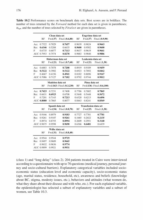
176 H. Elghazel, A. Aussem, and F. Perraud
Table 10.2 Performance scores on benchmark data sets. Best scores are in boldface. The
number of trees returned by the Forward method for each data set is given in parentheses;
αopt and the number of trees selected by Fitselect are given in parentheses.
Clean data set Engytime data set
RF Fwd(37) Fitsel.(0.6,80) RF Fwd(37) Fitsel.(0.9,90)
Acc 0.7322 0.7029 0.7657 0.9639 0.9624 0.9663
Rec 0.6346 0.5288 0.6635 0.9600 0.9502 0.9600
F 0.6735 0.6077 0.7113 0.9637 0.9619 0.9661
AUC 0.7953 0.7574 0.8278 0.9883 0.9840 0.9886
Haberman data set Leukemia data set
RF Fwd(21) Fitsel.(0.7,60) RF Fwd(21) Fitsel.(1,30)
Acc 0.6883 0.7078 0.7208 0.8919 0.9189 0.9459
Rec 0.5122 0.3902 0.5122 0.6923 0.7692 0.8462
F 0.4667 0.4156 0.4941 0.8182 0.8696 0.9167
AUC 0.7086 0.7127 0.7182 0.9792 0.9744 0.9812
Madelon data set Pima data set
RF Fwd(163) Fitsel.(0.3,230) RF Fwd(136) Fitsel.(0.6,100)
Acc 0.7423 0.7231 0.7408 0.7786 0.7682 0.7865
Rec 0.6631 0.6923 0.6708 0.5448 0.5448 0.5672
F 0.7201 0.7143 0.7213 0.6320 0.6213 0.6496
AUC 0.8080 0.7865 0.8077 0.8463 0.8241 0.8569
Spamb data set Transfusion data set
RF Fwd(54) Fitsel.(0.8,70) RF Fwd(25) Fitsel.(1,30)
Acc 0.9166 0.8979 0.9183 0.7727 0.7701 0.7781
Rec 0.9261 0.9107 0.9261 0.1685 0.2022 0.2135
F 0.8974 0.8755 0.8994 0.2609 0.2951 0.3140
AUC 0.9675 0.9598 0.9690 0.6366 0.6481 0.6439
Wdbc data set
RF Fwd(31) Fitsel.(0.8,40)
Acc 0.9544 0.9544 0.9719
Rec 0.9497 0.9609 0.9665
F 0.9632 0.9636 0.9774
AUC 0.9899 0.9921 0.9931
(class 1) and “long delay” (class 2). 204 patients treated in Cairo were interviewed
according to a questionnaire with up to 70 questions (medical journey, personal jour-
ney and socio-cultural barriers). Explanatory categorical variables included socio-
economic status (education level and economic capacity), socio-economic status
(age, marital status, residence, household, etc), awareness and beliefs (knowledge
about BC, stigma, modesty issues, etc.), behaviors and attitudes (what women do,
what they share about their disease and with who, etc.). For each explained variable,
the epidemiologist has selected a subset of explanatory variables and a subset of
women, see Table 10.3.
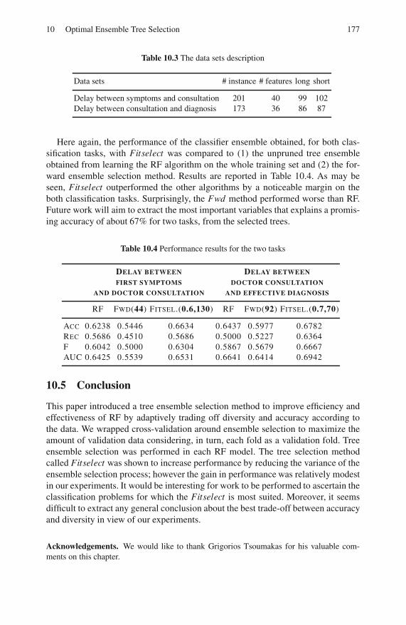
10 Optimal Ensemble Tree Selection 177
Table 10.3 The data sets description
Data sets # instance # features long short
Delay between symptoms and consultation 201 40 99 102
Delay between consultation and diagnosis 173 36 86 87
Here again, the performance of the classifier ensemble obtained, for both clas-
sification tasks, with Fitselect was compared to (1) the unpruned tree ensemble
obtained from learning the RF algorithm on the whole training set and (2) the for-
ward ensemble selection method. Results are reported in Table 10.4. As may be
seen, Fitselect outperformed the other algorithms by a noticeable margin on the
both classification tasks. Surprisingly, the Fwd method performed worse than RF.
Future work will aim to extract the most important variables that explains a promis-
ing accuracy of about 67% for two tasks, from the selected trees.
Table 10.4 Performance results for the two tasks
DELAY BETWEEN DELAY BETWEEN
FIRST SYMPTOMS DOCTOR CONSULTATION
AND DOCTOR CONSULTATION AND EFFECTIVE DIAGNOSIS
RF FWD(44) FITSEL.(0.6,130) RF FWD(92) FITSEL.(0.7,70)
ACC 0.6238 0.5446 0.6634 0.6437 0.5977 0.6782
REC 0.5686 0.4510 0.5686 0.5000 0.5227 0.6364
F 0.6042 0.5000 0.6304 0.5867 0.5679 0.6667
AUC 0.6425 0.5539 0.6531 0.6641 0.6414 0.6942
10.5 Conclusion
This paper introduced a tree ensemble selection method to improve efficiency and
effectiveness of RF by adaptively trading off diversity and accuracy according to
the data. We wrapped cross-validation around ensemble selection to maximize the
amount of validation data considering, in turn, each fold as a validation fold. Tree
ensemble selection was performed in each RF model. The tree selection method
called Fitselect was shown to increase performance by reducing the variance of the
ensemble selection process; however the gain in performance was relatively modest
in our experiments. It would be interesting for work to be performed to ascertain the
classification problems for which the Fitselect is most suited. Moreover, it seems
difficult to extract any general conclusion about the best trade-off between accuracy
and diversity in view of our experiments.
Acknowledgements. We would like to thank Grigorios Tsoumakas for his valuable com-
ments on this chapter.

178 H. Elghazel, A. Aussem, and F. Perraud
References
1. Bernard, S., Heutte, L., Adam, S.: On the selection of decision trees in random forests.
In: Proc. 2009 Int. Joint Conf. Neural Networks, Atlanta, GA, pp. 302–307. IEEE Comp.
Press, Los Alamitos (2009)
2. Biau, G., Devroye, L., Lugosi, G.: Consistency of random forests and other averaging
classifiers. J. Machine Learning Research 9, 2039–2057 (2008)
3. Blake, C.L., Merz, C.J.: UCI repository of machine learning databases. University of
California, Dept. of Information and Computer Sciences, Irvine (1998)
4. Breiman, L.: Bagging predictors. Machine Learning 26, 123–140 (1996)
5. Breiman, L.: Random forests. Machine Learning 45, 5–32 (2001)
6. Brown, G., Kuncheva, L.I.: “Good” and “bad” diversity in majority vote ensembles.
In: El Gayar, N., Kittler, J., Roli, F. (eds.) MCS 2010. LNCS, vol. 5997, pp. 124–133.
Springer, Heidelberg (2010)
7. Caruana, R., Munson, A., Niculescu-Mizil, A.: Getting the most out of ensemble selec-
tion. In: Proc. the 6th Int. Conf. Data Mining, Hong Kong, China, pp. 828–833. IEEE
Comp. Society, Los Alamitos (2006)
8. Caruana, R., Niculescu-Mizil, A., Crew, G., Ksikes, A.: Ensemble selection from li-
braries of models. In: Brodley, C. (ed.) Proc. the 21st Int. Conf. Machine Learning, Banff,
AB. ACM Press, New York (2004)
9. Caruana, R., Niculescu-Mizil, A.: An empirical comparison of supervised learning algo-
rithms. In: Cohen, W.W., Moore, A. (eds.) Proc. the 23rd Int. Conf. Machine Learning,
Pittsburgh, PA, pp. 161–168. ACM Press, New York (2006)
10. Dietterich, T.G.: Ensemble methods in machine learning. In: Kittler, J., Roli, F. (eds.)
MCS 2000. LNCS, vol. 1857, pp. 1–15. Springer, Heidelberg (2000)
11. Dietterich, T.G.: An experimental comparison of three methods for constructing en-
sembles of decision trees: bagging, boosting and randomization. Machine Learning 40,
139–157 (2000)
12. Dıaz-Uriarte, R., Alvarez de Andres, S.: Gene selection and classification of microarray
data using random forest. BMC Bioinformatics 7 (2006)
13. Freund, Y., Shapire, R.E.: Experiments with a new boosting algorithm. In: Saitta, L.
(ed.) 1996 Proc. the 13th Int. Conf. Machine Learning, Bari, Italy, pp. 148–156. Morgan
Kaufmann, San Francisco (1996)
14. Gacquer, D., Delcroix, V., Delmotte, F., Piechowiak, S.: On the effectiveness of diversity
when training multiple classifier systems. In: Sossai, C., Chemello, G. (eds.) ECSQARU
2009. LNCS, vol. 5590, pp. 493–504. Springer, Heidelberg (2009)
15. Golub, T.R., Slonim, D.K., Tamayo, P., Huard, C., Gaasenbeek, M., Mesirov, J.P., Coller,
H., Loh, M.L., Downing, J.R., Caligiuri, M.A., Bloomfield, C.D., Lander, E.S.: Molec-
ular classification of cancer: Class discovery and class prediction by gene expression
monitoring. Science 286, 531–537 (1999)
16. Kuncheva, L.I.: Combining pattern classifiers: Methods and algorithms. Wiley Inter-
science, Hoboken (2004)
17. Li, G., Yang, J., Kong, A.S., Chen, N.: Clustering algorithm based selective ensemble. J.
Fudan University 43, 689–695 (2004)
18. Lu, Z., Wu, X., Bongard, J.: Ensemble pruning via individual contribution ordering. In:
Rao, B., Krishnapuram, B., Tomkins, A., Yang, Q. (eds.) Proc. the 16th ACM SIGKDD
Conf. Knowledge Discovery and Data Mining, Washington, DC, pp. 871–880. ACM
Press, New York (2010)

10 Optimal Ensemble Tree Selection 179
19. Margineantu, D.D., Dietterich, T.G.: Pruning adaptive boosting. In: Fisher, D.H. (ed.)
Proc. the 14th Int. Conf. Machine Learning, Nashville, TN, pp. 211–218. Morgan Kauf-
mann, San Francisco (1997)
20. Martınez-Munoz, G., Hernandez-Lobato, D., Suarez, A.: An analysis of ensemble prun-
ing techniques based on ordered aggregation. IEEE Trans. Pattern Analysis and Machine
Intell. 31, 245–259 (2009)
21. Niculescu-Mizil, A., Perlich, C., Swirszcz, G., Sindhwani, V., Liu, Y., Melville, P., Wang,
D., Xiao, J., Hu, J., Singh, M., Shang, W.X., Zhu, W.F.: Winning the KDD Cup Orange
Challenge with ensemble selection. J. Machine Learning Research 7, 23–34 (2009)
22. Opitz, D., Maclin, R.: Popular ensemble methods: An empirical study. J. Artif. Intell.
Research 11, 169–198 (1999)
23. Partalas, I., Tsoumakas, G., Vlahavas, I.P.: An ensemble uncertainty aware measure for
directed hill climbing ensemble pruning. Machine Learning 81, 257–282 (2010)
24. Tsoumakas, G., Partalas, I., Vlahavas, I.P.: An ensemble pruning primer. In: Okun, O.,
Valentini, G. (eds.) Applications of Supervised and Unsupervised Ensemble Methods.
SCI, vol. 245, pp. 1–13. Springer, Heidelberg (2009)
25. Ultsch, A.: Fundamental clustering problems suite (2005)
26. Zhang, Y., Burer, S., Street, W.N.: Ensemble pruning via semi-definite programming. J.
Machine Learning Research 7, 1315–1338 (2006)

Chapter 11
Random Oracles for Regression Ensembles⋆
Carlos Pardo, Juan J. Rodrıguez, Jose F. Dıez-Pastor, and Cesar Garcıa-Osorio
Abstract. This paper considers the use of Random Oracles in Ensembles for re-
gression tasks. A Random Oracle model (Kuncheva and Rodrıguez, 2007) consists
of a pair of models and a fixed randomly created “oracle” (in the case of the Linear
Random Oracle, it is a hyperplane that divides the dataset in two during training and,
once the ensemble is trained, decides which model to use). They can be used as the
base model for any ensemble method. Previously, they have been used for classifi-
cation. Here, the use of Random Oracles for regression is studied using 61 datasets,
Regression Trees as base models and several ensemble methods: Bagging , Random
Subspaces, AdaBoost.R2 and Iterated Bagging. For all the considered methods and
variants, ensembles with Random Oracles are better than the corresponding version
without the Oracles.
11.1 Introduction
Ensembles [12] are combinations of base models (also referred as ensemble mem-
bers). In many situations, an ensemble gives better results than any of its members.
Although they have been studied mainly for classification, there are also ensemble
methods for regression.
The models to be combined have to be different, otherwise the ensemble is un-
necessary. One way to have different models is to construct them with different
methods. Nevertheless, there are ensemble methods that combine models obtained
from the same method, but change the dataset in some way.
In Bagging [1], each base member is trained with a sample of the training data.
Normally, the size of the sample is the same as the size of the original training data,
Carlos Pardo · Juan J. Rodrıguez · Jose F. Dıez-Pastor · Cesar Garcıa-Osorio
University of Burgos
E-mail: cpardo,jjrodriguez,jfdiez,[email protected]
⋆ This work was supported by the Project TIN2008-03151 of the Spanish Ministry of
Education and Science.
O. Okun et al. (Eds.): Ensembles in Machine Learning Applications, SCI 373, pp. 181–199.springerlink.com c© Springer-Verlag Berlin Heidelberg 2011

182 C. Pardo et al.
but the sample is with replacement. Hence, some training examples will appear sev-
eral times in the sample, while others will not appear. The prediction of the ensemble
is the average of the predictions of its members.
In Random Subspaces [10], each member is trained with all the training exam-
ples, but with a subset of the attributes. The dimension of the subspaces is a pa-
rameter of the method. The prediction of the ensemble is also the average of the
predictions.
Bagging and Random Subspaces can be used for classification and regression.
AdaBoost [7] initially was a method for classification, but there are some variants
for regression, such as AdaBoost.R2 [5]. In these methods, each training example
has a weight. Initially, all the examples have the same weight. The construction of
the ensemble members must take into account the weights of the examples. After
an ensemble member is constructed, the weights of the examples are adjusted. The
idea is to give more weight to the examples with greater errors in the previous iter-
ations. Hence, in the construction of the next member, these examples will be more
important. The ensemble members also have weights, they depend on their error. In
AdaBoost.R2, the predicted value of the ensemble is a weighted median. In [20],
this method was the one with the best results among several ensemble methods for
regression.
Iterated Bagging [2] is a method for regression based on Bagging . It combines
several Bagging ensembles. The first Bagging ensemble is constructed as usual.
Based on the predictions of the previous Bagging ensemble, the values of the pre-
dicted variable are altered. The next Bagging ensemble is trained with these altered
values. These values are the residuals: the difference between the real and the pre-
dicted values. Nevertheless, these predictions are not obtained using all the members
in the Bagging ensemble. The error of the predictions for a training example would
be too optimistic, since the majority of the ensemble methods have been trained
with that example. These predictions are obtained using the out-of-bag estimation:
the prediction for an example is obtained using only those ensemble members that
were not trained with that example. The prediction of an Iterated Bagging ensemble
is the sum of the predictions of its Bagging ensembles. In [17], Iterated Bagging is
compared to other methods giving the best results.
Random Oracles [13] are mini-ensembles formed by two models, they can be
used as base models for other ensemble methods. The objective of using Random
Oracles is to have more diversity among the base models that form an ensemble.
This additional diversity can improve the accuracy of the ensembles.
The rest of this chapter is organised as follows. Next section explains Random
Oracles. Section 11.3 describes the experimental setting. The results are presented
and discussed in Sect. 11.4. In Sect. 11.5, diversity-error diagrams are used to ana-
lyze the behaviour of the base models. Finally, Sect. 11.6 presents some concluding
remarks. Appendix includes the source code.

11 Random Oracles for Regression Ensembles 183
11.2 Random Oracles
A Random Oracle model [13] is a mini-ensemble formed by a pair of models and
a Random Oracle that chooses between them. It can be thought of as a random
discriminant function which splits the data into two subsets with no regard of any
class labels or cluster structure. Also, a Random Oracle can be used as the base
model of any ensemble method. Given a base method, the training of a Random
Oracle model consists of:
• Select randomly the Random Oracle.
• Split the training data in two subsets using the Random Oracle.
• For each subset of the training data, build a model. The Random Oracle model is
formed by the pair of models and the oracle itself.
The prediction of a test instance is done in the following way:
• Use the Random Oracle to select one of the two models.
• Return the prediction given by the selected model.
If the computational complexity of the oracle is low, both in training and predic-
tion, the computational complexity of a Random Oracle model is very similar to the
complexity of the base method. In the prediction phase, only one of the two models
is used. In the training phase, two models are built. Nevertheless, they are trained
with a disjoint partition of the training examples and the training time of any method
depends, at least linearly, on the number of training examples.
Different types of Oracles can be considered. In this work, the Linear Random
Oracle is used. This oracle divides the space into two subspaces using a hyperplane.
To build the oracle, two different training objects are selected at random, each re-
maining training object is assigned to the subspace of the selected training object
for which is closer1.
Algorithms 5 and 6 show the pseudo-code for the training and prediction phases
of the method.
In this work, the distances are calculated according to the Euclidean distance,
numerical attributes are scaled within [0,1], for nominal attributes we consider that
the distance is 0 or 1 depending if the two valued are different or equal.
11.3 Experiments
The experiments were conducted using 5× 2 fold cross validation [4]. The per-
formance of the different methods over different datasets was measured using root
mean squared error (RMSE). The base models were Regression Trees. They were
used pruned P or unpruned U. The method used for pruning was Reduced Error
Pruning (REP) [6]. Ensemble size was 100.
1 Note that a generalization of this would be to select more than two training objects, then
the remaining training objects would be assigned to the Voronoi region defined by the
closest selected training object.

184 C. Pardo et al.
Algorithm 5. Pseudo-code of the Random Oracle method: training phase
Input: Training dataset D; base learning method L
Output: Random Oracle Model RO
RO.instance[1]← x | (x,y) is a random instance from DRO.instance[2]← x | (x,y) is a random instance from DD1 ← /0 // The training dataset for the 1st sub-model
D2 ← /0 // The training dataset for the 2nd sub-model
Foreach instance(x,y) ∈D do
If distance(RO.instance[1],x) < distance(RO.instance[2],x) then
D1 ← D1∪ (x,y) // Add the instance to the 1st subset
else
D2 ← D2∪ (x,y) //Add the instance to the 2nd subset
end
end
RO.model[1]← L(D1) // Train the 1st sub-model
RO.model[2]← L(D2) // Train the 2nd sub-model
Algorithm 6. Pseudo-code of the Random Oracle method: prediction phase
Input: Trained Random Oracle RO; instance x
Output: Predicted value
If distance(RO.instance[1],x) < distance(RO.instance[2],x) then
return RO.model[1].predict(x) // Predict with the 1st sub-model
else
return RO.model[2].predict(x) // Predict with the 2nd sub-model
end
Several ensemble methods were considered:
• Randomization. When the base method has a random element, different models
can be obtained from the same training data. Randomization is an ensemble of
such randomizable models in which the prediction is the average of the predic-
tions of its members. In the case of regression trees, when pruning is used, the
training data is partitioned randomly: one subset for building the tree and another
for pruning. For unpruned trees, there is no random element.
• Bagging [1].
• Random Subspaces [10]. For the dimension of the subspaces, two values were
considered: 50% and 75% of the number of attributes.
• AdaBoost.R2 [5]. This method can be used with different loss functions. Three
are proposed in [5] and used in this work: linear, square and exponential. The
suffixes “-Li”, “-Sq” and “-Ex” are used to denote the used function. Moreover,
methods based on AdaBoost can be used in two ways [8]. In the reweighting
version, the base model is trained with all the training data, it must take into
account the weights distribution. In the resampling version, the base model is
trained with a sample from the training data. This sample is constructed taken
into account the weights. These versions are denoted with “-W” and “-S”.
• Iterated Bagging [2]. Two configurations were considered 10× 10 (Bagging is
iterated 10 times, the ensemble size of each Bagging is 10) and 5×20 (Bagging

11 Random Oracles for Regression Ensembles 185
is iterated 5 times, the ensemble size of each Bagging is 20). In both cases, the
maximum ensemble size is 100.
For all the configurations of these methods, two versions were considered: com-
bined or not combined with Random Oracles.
Moreover, other methods were included in the study, as a baseline for the com-
parisons:
• A single Regression Tree, with and without pruning.
• Linear regression. Two versions were considered: using all the features and using
only the selected features with the method described in [18].
• Nearest neighbors. There are two versions, in the first one the number of neigh-
bors is 1. In the other, the number of neighbors is selected using “leave one out”.
Weka [9] was used for the experiments. It includes the base method (Regression
Tree), Bagging and Random Subspaces. The rest of the methods (i.e., Iterated Bag-
ging and AdaBoost.R2), were implemented using this library.
Table 11.1 shows the characteristics of the 61 datasets considered, of which 30
have been collected by Luis Torgo2. All of them are available in the format used by
Weka3.
11.4 Results
In order to compare all the configurations considered, average ranks [3] are used.
For each dataset, the methods are sorted according to their performance. The best
method has rank 1, the second rank 2 and so on. If there are ties, these methods have
the same rank, the average value. For each method, its average rank is calculated as
the average value over all the considered datasets. According to [3], “average ranks
by themselves provide a fair comparison of the algorithms”.
Table 11.2 shows the methods sorted according to their average ranks. The pre-
fix “∗−” denotes methods that use Random Oracles. The 12 top positions are for
methods that use Random Oracles.
For a method that uses Random Oracles, the benefit is defined as the difference
between the average ranks of the corresponding method without Random Oracles
and the method with Random Oracles. In Table 11.2, all the benefits are positive.
When comparing two methods, the number of datasets where one method has
better, equal, or worse results than the other is calculated. According to [3], using
a sign test, one method is significantly better than other, with a confidence level of
0.05, if the number of wins plus half the ties is at least N/2+1.96√
N/2 (for N = 61
datasets, this number is 39). Table 11.2 shows, in the columns denoted as W/T/L,
the paired comparisons of methods with Random Oracles and the corresponding
methods without Random Oracles. The symbol “•” denotes significant differences.
The number of wins, ties and losses and the average ranks are calculated using
a direct comparison of the results for the different methods: less, equal or greater.
2 http://www.liaad.up.pt/∼ltorgo/Regression/DataSets.html3 http://www.cs.waikato.ac.nz/ml/weka/index datasets.html

186 C. Pardo et al.
Table 11.1 Datasets used in the experiments
Dataset Examples Numeric Nominal
2d-planes 40768 10 0
abalone 4177 7 1
ailerons 13750 40 0
auto93 93 16 6
auto-horse 205 17 8
auto-mpg 398 4 3
auto-price 159 15 0
bank-32nh 8192 32 0
bank-8FM 8192 8 0
baskball 96 4 0
bodyfat 252 14 0
bolts 40 7 0
breast-tumor 286 1 8
cal-housing 20640 8 0
cholesterol 303 6 7
cleveland 303 6 7
cloud 108 4 2
cpu-act 8192 21 0
cpu 209 6 1
cpu-small 8192 12 0
delta-ailerons 7129 5 0
delta-elevators 9517 6 0
detroit 13 13 0
diabetes-numeric 43 2 0
echo-months 130 6 3
elevators 16599 18 0
elusage 55 1 1
fishcatch 158 5 2
friedman 40768 10 0
fruitfly 125 2 2
gascons 27 4 0
Dataset Examples Numeric Nominal
house-16H 22784 16 0
house-8L 22784 8 0
housing 506 12 1
hungarian 294 6 7
kin8nm 8192 8 0
longley 16 6 0
lowbwt 189 2 7
machine-cpu 209 6 0
mbagrade 61 1 1
meta 528 19 2
mv 40768 7 3
pbc 418 10 8
pharynx 195 1 10
pole 15000 48 0
pollution 60 15 0
puma32H 8192 32 0
puma8NH 8192 8 0
pw-linear 200 10 0
pyrimidines 74 27 0
quake 2178 3 0
schlvote 38 4 1
sensory 576 0 11
servo 167 0 4
sleep 62 7 0
stock 950 9 0
strike 625 5 1
triazines 186 60 0
veteran 137 3 4
vineyard 52 3 0
wisconsin 194 32 0
Nevertheless, they do not take into account the size of the differences. For this pur-
pose, we use the quantitative scoring [16, 20]. Given the results for two methods i
and j in one dataset, this score is defined as
Si, j =RMSE j−RMSEi
max(RMSEi,RMSE j)
where RMSEi is the root mean squared error of method i. Unless both methods have
zero error, this measure will be between −1 and 1, although it is usually expressed
as a percentage. The sign indicates which method is better.
Figure 11.1 shows these scores (as percentages) for the considered methods,
comparing the versions with and without Random Oracles. The score is calculated
for each dataset and the datasets are sorted according to its score. The number
of values above and below zero corresponds to the number of wins and losses in
Table 11.2.
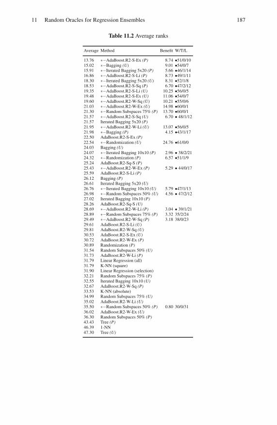
11 Random Oracles for Regression Ensembles 187
Table 11.2 Average ranks
Average Method Benefit W/T/L
13.76 ∗−AdaBoost.R2-S-Ex (P) 8.74 •51/0/1015.02 ∗−Bagging (U) 9.01 •54/0/715.91 ∗−Iterated Bagging 5x20 (P) 5.66 •46/1/1416.86 ∗−AdaBoost.R2-S-Li (P) 8.73 •49/1/1118.30 ∗−Iterated Bagging 5x20 (U) 8.31 •52/1/818.53 ∗−AdaBoost.R2-S-Sq (P) 6.70 •47/2/1219.35 ∗−AdaBoost.R2-S-Li (U) 10.25 •56/0/519.48 ∗−AdaBoost.R2-S-Ex (U) 11.06 •54/0/719.60 ∗−AdaBoost.R2-W-Sq (U) 10.21 •55/0/621.03 ∗−AdaBoost.R2-W-Ex (U) 14.98 •60/0/121.30 ∗−Random Subspaces 75% (P) 13.70 •60/0/121.57 ∗−AdaBoost.R2-S-Sq (U) 6.70 • 48/1/1221.57 Iterated Bagging 5x20 (P)
21.95 ∗−AdaBoost.R2-W-Li (U) 13.07 •56/0/521.98 ∗−Bagging (P) 4.15 •43/1/1722.50 AdaBoost.R2-S-Ex (P)
22.54 ∗−Randomization (U) 24.76 •61/0/024.03 Bagging (U)
24.07 ∗−Iterated Bagging 10x10 (P) 2.96 • 38/2/2124.32 ∗−Randomization (P) 6.57 •51/1/925.24 AdaBoost.R2-Sq-S (P)
25.43 ∗−AdaBoost.R2-W-Ex (P) 5.29 • 44/0/1725.59 AdaBoost.R2-S-Li (P)
26.12 Bagging (P)
26.61 Iterated Bagging 5x20 (U)
26.76 ∗−Iterated Bagging 10x10 (U) 5.79 •47/1/1326.98 ∗−Random Subspaces 50% (U) 4.56 • 47/2/1227.02 Iterated Bagging 10x10 (P)
28.26 AdaBoost.R2-Sq-S (U)
28.69 ∗−AdaBoost.R2-W-Li (P) 3.04 • 39/1/2128.89 ∗−Random Subspaces 75% (P) 3.32 35/2/2429.49 ∗−AdaBoost.R2-W-Sq (P) 3.18 38/0/2329.61 AdaBoost.R2-S-Li (U)
29.81 AdaBoost.R2-W-Sq (U)
30.53 AdaBoost.R2-S-Ex (U)
30.72 AdaBoost.R2-W-Ex (P)
30.89 Randomization (P)
31.54 Random Subspaces 50% (U)
31.73 AdaBoost.R2-W-Li (P)
31.79 Linear Regression (all)31.79 K-NN (square)31.90 Linear Regression (selection)32.21 Random Subspaces 75% (P)
32.55 Iterated Bagging 10x10 (U)
32.67 AdaBoost.R2-W-Sq (P)
33.53 K-NN (absolute)34.99 Random Subspaces 75% (U)
35.02 AdaBoost.R2-W-Li (U)
35.50 ∗−Random Subspaces 50% (P) 0.80 30/0/3136.02 AdaBoost.R2-W-Ex (U)
36.30 Random Subspaces 50% (P)
43.43 Tree (P)
46.39 1-NN47.30 Tree (U)
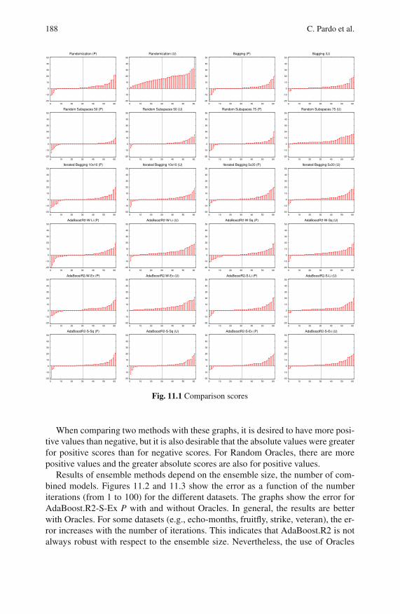
188 C. Pardo et al.
-20
-10
0
10
20
30
40
50
0 10 20 30 40 50 60
Randomization (P)
-20
-10
0
10
20
30
40
50
0 10 20 30 40 50 60
Randomization (U)
-20
-10
0
10
20
30
40
50
0 10 20 30 40 50 60
Bagging (P)
-20
-10
0
10
20
30
40
50
0 10 20 30 40 50 60
Bagging (U)
-20
-10
0
10
20
30
40
50
0 10 20 30 40 50 60
Random Subspaces 50 (P)
-20
-10
0
10
20
30
40
50
0 10 20 30 40 50 60
Random Subspaces 50 (U)
-20
-10
0
10
20
30
40
50
0 10 20 30 40 50 60
Random Subspaces 75 (P)
-20
-10
0
10
20
30
40
50
0 10 20 30 40 50 60
Random Subspaces 75 (U)
-20
-10
0
10
20
30
40
50
0 10 20 30 40 50 60
Iterated Bagging 10x10 (P)
-20
-10
0
10
20
30
40
50
0 10 20 30 40 50 60
Iterated Bagging 10x10 (U)
-20
-10
0
10
20
30
40
50
0 10 20 30 40 50 60
Iterated Bagging 5x20 (P)
-20
-10
0
10
20
30
40
50
0 10 20 30 40 50 60
Iterated Bagging 5x20 (U)
-20
-10
0
10
20
30
40
50
0 10 20 30 40 50 60
AdaBoostR2-W-Li (P)
-20
-10
0
10
20
30
40
50
0 10 20 30 40 50 60
AdaBoostR2-W-Li (U)
-20
-10
0
10
20
30
40
50
0 10 20 30 40 50 60
AdaBoostR2-W-Sq (P)
-20
-10
0
10
20
30
40
50
0 10 20 30 40 50 60
AdaBoostR2-W-Sq (U)
-20
-10
0
10
20
30
40
50
0 10 20 30 40 50 60
AdaBoostR2-W-Ex (P)
-20
-10
0
10
20
30
40
50
0 10 20 30 40 50 60
AdaBoostR2-W-Ex (U)
-20
-10
0
10
20
30
40
50
0 10 20 30 40 50 60
AdaBoostR2-S-Li (P)
-20
-10
0
10
20
30
40
50
0 10 20 30 40 50 60
AdaBoostR2-S-Li (U)
-20
-10
0
10
20
30
40
50
0 10 20 30 40 50 60
AdaBoostR2-S-Sq (P)
-20
-10
0
10
20
30
40
50
0 10 20 30 40 50 60
AdaBoostR2-S-Sq (U)
-20
-10
0
10
20
30
40
50
0 10 20 30 40 50 60
AdaBoostR2-S-Ex (P)
-20
-10
0
10
20
30
40
50
0 10 20 30 40 50 60
AdaBoostR2-S-Ex (U)
Fig. 11.1 Comparison scores
When comparing two methods with these graphs, it is desired to have more posi-
tive values than negative, but it is also desirable that the absolute values were greater
for positive scores than for negative scores. For Random Oracles, there are more
positive values and the greater absolute scores are also for positive values.
Results of ensemble methods depend on the ensemble size, the number of com-
bined models. Figures 11.2 and 11.3 show the error as a function of the number
iterations (from 1 to 100) for the different datasets. The graphs show the error for
AdaBoost.R2-S-Ex P with and without Oracles. In general, the results are better
with Oracles. For some datasets (e.g., echo-months, fruitfly, strike, veteran), the er-
ror increases with the number of iterations. This indicates that AdaBoost.R2 is not
always robust with respect to the ensemble size. Nevertheless, the use of Oracles
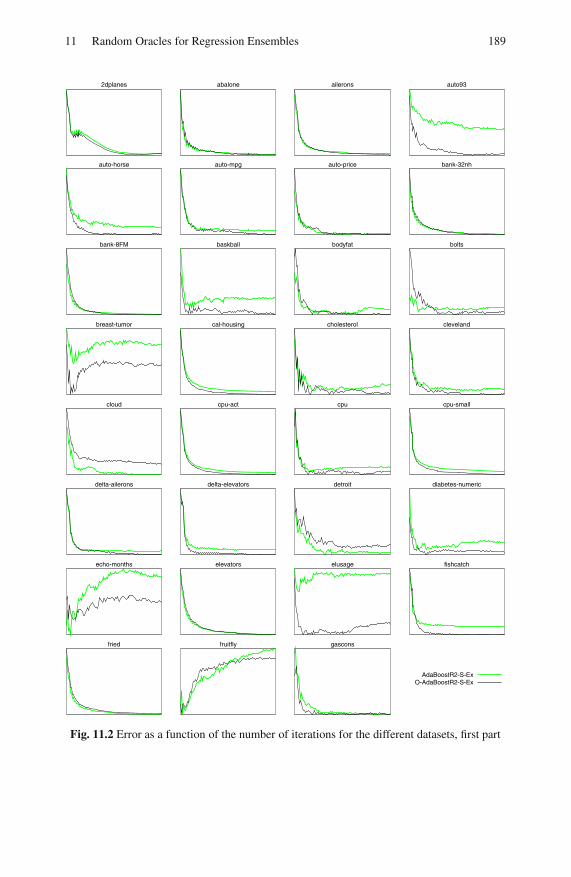
11 Random Oracles for Regression Ensembles 189
2dplanes abalone ailerons auto93
auto-horse auto-mpg auto-price bank-32nh
bank-8FM baskball bodyfat bolts
breast-tumor cal-housing cholesterol cleveland
cloud cpu-act cpu cpu-small
delta-ailerons delta-elevators detroit diabetes-numeric
echo-months elevators elusage fishcatch
fried fruitfly gascons
AdaBoostR2-S-ExO-AdaBoostR2-S-Ex
Fig. 11.2 Error as a function of the number of iterations for the different datasets, first part
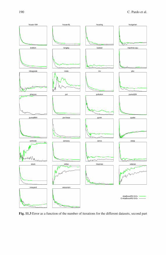
190 C. Pardo et al.
house-16H house-8L housing hungarian
kin8nm longley lowbwt machine-cpu
mbagrade meta mv pbc
pharynx pol pollution puma32H
puma8NH pw-linear pyrim quake
schlvote sensory servo sleep
stock strike triazines veteran
vineyard wisconsin
AdaBoostR2-S-ExO-AdaBoostR2-S-Ex
Fig. 11.3 Error as a function of the number of iterations for the different datasets, second part
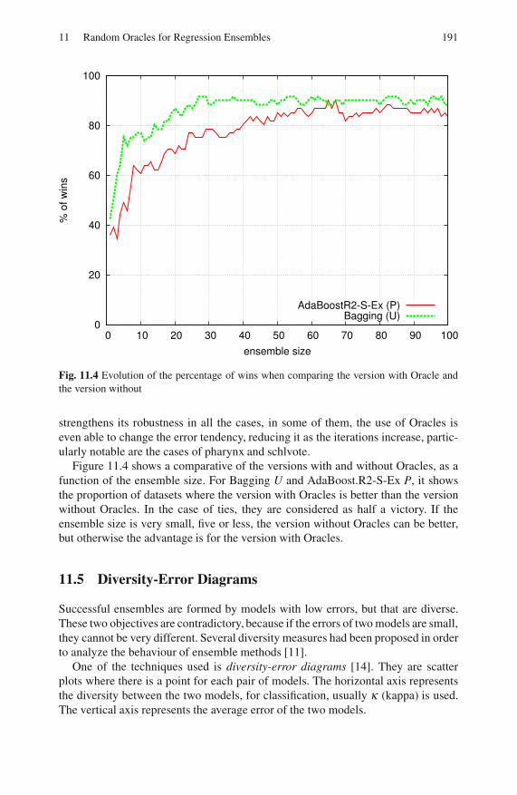
11 Random Oracles for Regression Ensembles 191
0
20
40
60
80
100
0 10 20 30 40 50 60 70 80 90 100
% o
f w
ins
ensemble size
AdaBoostR2-S-Ex (P)Bagging (U)
Fig. 11.4 Evolution of the percentage of wins when comparing the version with Oracle and
the version without
strengthens its robustness in all the cases, in some of them, the use of Oracles is
even able to change the error tendency, reducing it as the iterations increase, partic-
ularly notable are the cases of pharynx and schlvote.
Figure 11.4 shows a comparative of the versions with and without Oracles, as a
function of the ensemble size. For Bagging U and AdaBoost.R2-S-Ex P, it shows
the proportion of datasets where the version with Oracles is better than the version
without Oracles. In the case of ties, they are considered as half a victory. If the
ensemble size is very small, five or less, the version without Oracles can be better,
but otherwise the advantage is for the version with Oracles.
11.5 Diversity-Error Diagrams
Successful ensembles are formed by models with low errors, but that are diverse.
These two objectives are contradictory, because if the errors of two models are small,
they cannot be very different. Several diversity measures had been proposed in order
to analyze the behaviour of ensemble methods [11].
One of the techniques used is diversity-error diagrams [14]. They are scatter
plots where there is a point for each pair of models. The horizontal axis represents
the diversity between the two models, for classification, usually κ (kappa) is used.
The vertical axis represents the average error of the two models.
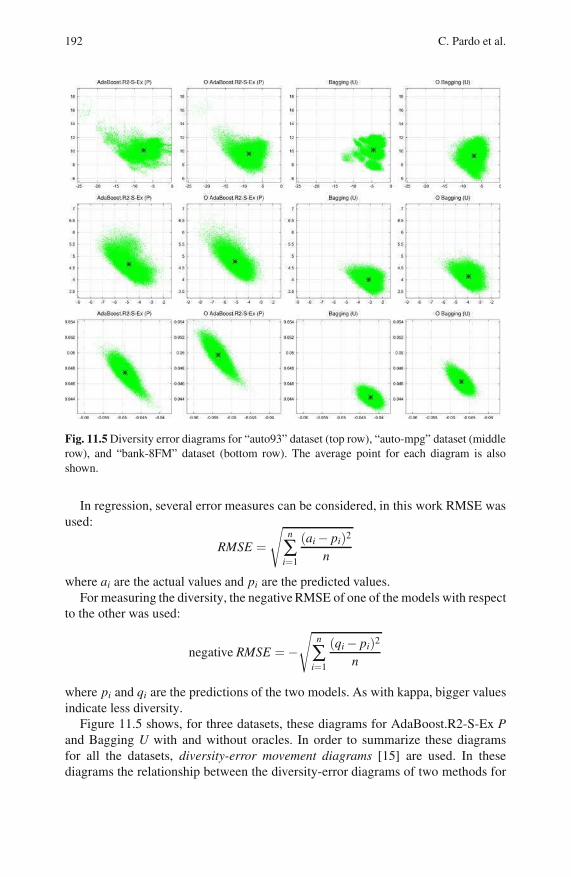
192 C. Pardo et al.
Fig. 11.5 Diversity error diagrams for “auto93” dataset (top row), “auto-mpg” dataset (middle
row), and “bank-8FM” dataset (bottom row). The average point for each diagram is also
shown.
In regression, several error measures can be considered, in this work RMSE was
used:
RMSE =
√n
∑i=1
(ai− pi)2
n
where ai are the actual values and pi are the predicted values.
For measuring the diversity, the negative RMSE of one of the models with respect
to the other was used:
negative RMSE =−√
n
∑i=1
(qi− pi)2
n
where pi and qi are the predictions of the two models. As with kappa, bigger values
indicate less diversity.
Figure 11.5 shows, for three datasets, these diagrams for AdaBoost.R2-S-Ex P
and Bagging U with and without oracles. In order to summarize these diagrams
for all the datasets, diversity-error movement diagrams [15] are used. In these
diagrams the relationship between the diversity-error diagrams of two methods for
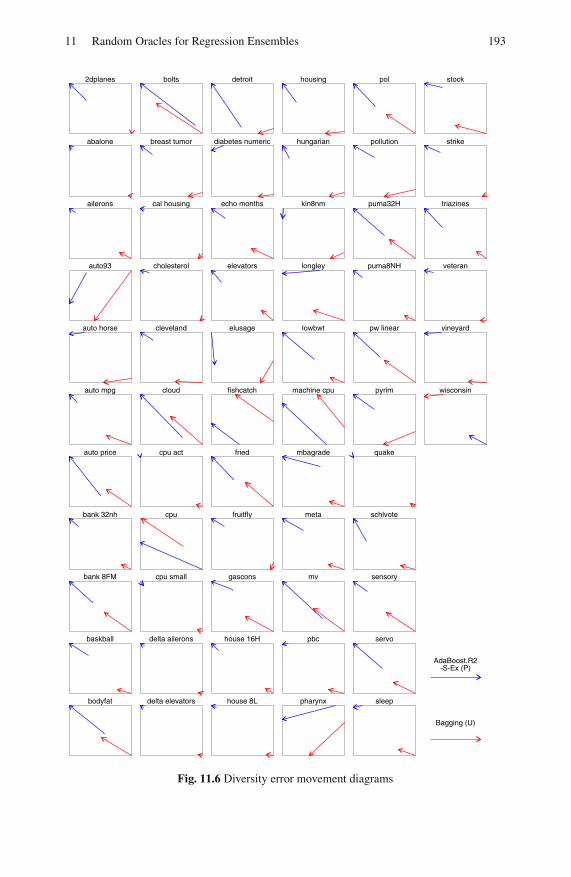
11 Random Oracles for Regression Ensembles 193
2dplanes
abalone
ailerons
auto93
auto horse
auto mpg
auto price
bank 32nh
bank 8FM
baskball
bodyfat
bolts
breast tumor
cal housing
cholesterol
cleveland
cloud
cpu act
cpu
cpu small
delta ailerons
delta elevators
detroit
diabetes numeric
echo months
elevators
elusage
fishcatch
fried
fruitfly
gascons
house 16H
house 8L
housing
hungarian
kin8nm
longley
lowbwt
machine cpu
mbagrade
meta
mv
pbc
pharynx
pol
pollution
puma32H
puma8NH
pw linear
pyrim
quake
schlvote
sensory
servo
sleep
stock
strike
triazines
veteran
vineyard
wisconsin
AdaBoost.R2-S-Ex (P)
Bagging (U)
Fig. 11.6 Diversity error movement diagrams

194 C. Pardo et al.
the same dataset is represented using an arrow, the extremes of the arrow are the
average points from the diversity-error diagrams. Figure 11.6 shows these diagrams
for all the considered datasets. The origins of the arrows are for the methods without
Random Oracles, while the heads are for the methods with Random Oracles. The
majority of the arrows go to the left, this indicates that the base classifiers are more
diverse when using Random Oracles. In general, the arrows go up, this means that
the base classifiers have more error when using Random Oracles. The price for the
increased diversity is the increased error, but in this case it is worth, because the
error of the ensembles are generally smaller when using Random Oracles.
11.6 Conclusion
The performance of Random Oracles for regression ensembles have been studied,
using 61 datasets and regression trees as base models. They have been combined
with Bagging, Random Subspaces, AdaBoost.R2 and Iterated Bagging. For all the
configurations considered using Random Oracles gives better results. The robust-
ness of the method, as shown for AdaBoost, can be greatly increased by using Or-
acles as base models. The cause for these improvements is probably the increased
diversity of the base models, as shown by the diversity-error diagrams.
Acknowledgements. We wish to thank the developers of Weka. We also express our grati-
tude to the donors of the different datasets.
Appendix: Source Code
This appendix includes the source code of the method. It is for Weka [9], version
3.7.2. The license is the GNU General Public License, version 2 or any later version.
package weka.classifiers.meta;
import java.util.Random;
import weka.classifiers.AbstractClassifier;import weka.classifiers.Classifier;import weka.classifiers.RandomizableSingleClassifierEnhancer;import weka.core.DistanceFunction;import weka.core.EuclideanDistance;import weka.core.Instance;import weka.core.Instances;import weka.core.Randomizable;import weka.core.WeightedInstancesHandler;
/** Random Linear Oracle. Can do classification and
* regression depending on the base learner.
*/

11 Random Oracles for Regression Ensembles 195
public class LinearOracleextends RandomizableSingleClassifierEnhancerimplements WeightedInstancesHandler
/** For serialization */static final long serialVersionUID = -9217393623430792225L;
/** The number of sub-models */protected int m_NumSubModels = 2;
/** The sub-models */protected Classifier [] m_SubModels = null;
/** The distance function */protected DistanceFunction m_Distance = null;
/** The selected instances */private Instances m_Selected;
/*** Returns the corresponding region for a given instance
** @param inst the instance
* @return the region
* @throws Exception if there are not training instances
*/int region( Instance inst ) throws Exception
if ( m_Selected.numInstances( ) == 0 ) throw new Exception( "No training instances!" );
double minDistance = m_Distance.distance( inst,m_Selected.instance( 0 ) );
int region = 0;for ( int i = 1; i < m_NumSubModels; i++ )
Instance trainInstance = m_Selected.instance( i );double distance = m_Distance.distance( inst,
trainInstance );if ( distance < minDistance ) minDistance = distance;region = i;
return region;
/*** Calculates the class membership probabilities for the
* given test instance.
*

196 C. Pardo et al.
* @param instance the instance to be classified
* @return predicted class probability distribution
* @throws Exception if distribution can’t be computed
* successfully
*/public double [] distributionForInstance( Instance
instance )throws Exception
int r = region( instance );if ( m_SubModels[ r ] == null )
// There is not a submodel for that region, a not// null submodel is selectedfor ( r = 0; r < m_SubModels.length; r++ ) if ( m_SubModels[ r ] != null )
break;
return m_SubModels[ r ].distributionForInstance(instance );
/*** Random Linear Oracle method.
** @param data the training data to be used for generating
* the Random Linear Oracle model.
* @throws Exception if the classifier could not be built
* successfully
*/public void buildClassifier( Instances data )
throws Exception
// Initializationsm_Distance = new EuclideanDistance( data );Random random = data.getRandomNumberGenerator(
getSeed( ) );
// Random selection of the instancesm_Selected = new Instances( data, m_NumSubModels );int n = data.numInstances( );int previous = -1;for ( int i = 0; i < m_NumSubModels; i++ )
int selected = random.nextInt( n );if ( previous == selected ) // If the selected value if the same as for the// previous iteration, we take the next one.// This guarantees at least two different instances.

11 Random Oracles for Regression Ensembles 197
selected++;if ( selected >= n )
selected = 0;m_Selected.add( data.instance( selected ) );previous = selected;
// Initialize the data subsetsInstances [] subDataset = new Instances[ m_NumSubModels ];for ( int i = 0; i < m_NumSubModels; i++ )
subDataset[ i ] = new Instances( data, 0 );
// Split the instances in the subsetsfor ( int i = 0; i < data.numInstances( ); i++ )
Instance inst = data.instance( i );subDataset[ region( inst ) ].add( inst );
// Build the sub-modelsm_SubModels = AbstractClassifier.makeCopies( m_Classifier,
m_NumSubModels );boolean isRandomizable = m_Classifier instanceof
Randomizable;for ( int i = 0; i < m_NumSubModels; i++ )
if ( subDataset[i].numInstances() == 0 ) // If there are not instances, there is not a modelm_SubModels[ i ] = null;
else subDataset[ i ].randomize( random );if ( isRandomizable )
( ( Randomizable )m_SubModels[ i ] ).setSeed(random.nextInt() );
try
m_SubModels[ i ].buildClassifier( subDataset[ i ] ); catch( Exception e )
// If the classifier has not ben built, there is// not a sub-modelm_SubModels[ i ] = null;
/*** Returns description of the Random Oracle model.

198 C. Pardo et al.
** @return description of the Random Oracle as a string
*/public String toString( )
if ( m_SubModels == null )return "No model built yet!";
String s = m_Classifier.toString( );for ( int i = 0; i < m_SubModels.length; i++ )
s += "\n\nSubModel " + ( i + 1 ) + ":\n"+ m_SubModels[ i ];
return s;
/*** Main method for testing this class.
** @param argv the options
*/public static void main( String [ ] argv )throws Exception
runClassifier( new LinearOracle( ), argv );
References
1. Breiman, L.: Bagging predictors. Machine Learning 24, 123–140 (1996)
2. Breiman, L.: Using iterated bagging to Debias regressions. Machine Learning 45,
261–277 (2001)
3. Demsar, J.: Statistical comparisons of classifiers over multiple data sets. J. Machine
Learning Research 7, 1–30 (2006)
4. Dietterich, T.G.: Approximate statistical test for comparing supervised classification
learning algorithms. Neural Comp. 10, 1895–1923 (1998)
5. Drucker, H.: Improving regressors using boosting techniques. In: Fisher, D.H. (ed.) Proc.
the 14th Int. Conf. Machine Learning, Nashville, TN, pp. 107–115. Morgan Kaufmann,
San Francisco (1997)
6. Elomaa, T., Kaariainen, M.: An analysis of reduced error pruning. J. Artif. Intell. Re-
search 15, 163–187 (2001)
7. Freund, Y., Schapire, R.E.: Experiments with a new boosting algorithm. In: Saitta, L.
(ed.) Proc. the 13th Int. Conf. Machine Learning, Bari, Italy, pp. 148–156. Morgan Kauf-
mann, San Francisco (1996)
8. Freund, Y., Schapire, R.E.: A decision-theoretic generalization of on-line learning and
an application to boosting. J. Comp. and Syst. Sciences 55, 119–139 (1997)
9. Hall, M., Frank, E., Holmes, G., Pfahringer, B., Reutemann, P., Witten, I.H.: The WEKA
data mining software: An update. SIGKDD Explorations 11, 10–18 (2009)
10. Ho, T.K.: The random subspace method for constructing decision forests. IEEE Trans.
Pattern Analysis and Machine Intell. 20, 832–844 (1998)

11 Random Oracles for Regression Ensembles 199
11. Kuncheva, L.I., Whitaker, C.J.: Measures of diversity in classifier ensembles. Machine
Learning 51, 181–207 (2003)
12. Kuncheva, L.I.: Combining pattern classifiers: Methods and algorithms. John Wiley &
Sons, Hoboken (2004)
13. Kuncheva, L.I., Rodrıguez, J.J.: Classifier ensembles with a random linear oracle. IEEE
Trans. Knowledge and Data Engineering 19, 500–508 (2007)
14. Margineantu, D.D., Dietterich, T.G.: Pruning adaptive boosting. In: Fisher, D.H. (ed.)
Proc. 14th Int. Conf. Machine Learning, Nashville, TN, pp. 211–218. Morgan Kauf-
mann, San Francisco (1997)
15. Rodrıguez, J.J., Garcıa-Osorio, C., Maudes, J.: Forests of nested dichotomies. Pattern
Recognition Letters 31, 125–132 (2010)
16. Shrestha, D.L., Solomatine, D.P.: Experiments with AdaBoost.RT: An improved boost-
ing scheme for regression. Neural Comp. 18, 1678–1710 (2006)
17. Suen, Y., Melville, P., Mooney, R.: Combining bias and variance reduction techniques
for regression trees. In: Gama, J., Camacho, R., Brazdil, P.B., Jorge, A.M., Torgo, L.
(eds.) ECML 2005. LNCS (LNAI), vol. 3720, pp. 741–749. Springer, Heidelberg (2005)
18. Wang, Y., Witten, I.H.: Induction of model trees for predicting continuous classes. In: van
Someren, M., Widmer, G. (eds.) ECML 1997. LNCS, vol. 1224, pp. 128–137. Springer,
Heidelberg (1997)
19. Witten, I.H., Frank, E.: Data mining: Practical machine learning tools and techniques.
Morgan Kaufmann, San Francisco (2005)
20. Zhang, C., Zhang, J., Wang, G.: An empirical study of using Rotation Forest to improve
regressors. Applied Mathematics and Comp. 195, 618–629 (2008)

Chapter 12
Embedding Random Projections in RegularizedGradient Boosting Machines
Pierluigi Casale, Oriol Pujol, and Petia Radeva
Abstract. Random Projections are a suitable technique for dimensionality reduc-
tion in Machine Learning. In this work, we propose a novel Boosting technique
that is based on embedding Random Projections in a regularized gradient boosting
ensemble. Random Projections are studied from different points of view: pure Ran-
dom Projections, normalized and uniform binary. Furthermore, we study the effect
to keep or change the dimensionality of the data space. Experimental results per-
formed on synthetic and UCI datasets show that Boosting methods with embedded
random data projections are competitive to AdaBoost and Regularized Boosting.
12.1 Introduction
Random Projections (RPs) have been widely employed as dimensionality reduction
technique. RPs are based on the idea that high dimensional data can be projected
into a lower dimensional space without significantly losing the structure of the data.
RPs can also be viewed as a tool for generating diversity in the creation of an en-
semble of classifiers. The underlying idea is the same used in various new ensemble
methods such as Rotation Forest [11] or Rotboost [13]. Using RPs, the different em-
beddings of the original feature space provide multiple view of the original features
space. This kind of diversity can be generated while projecting data into subspaces,
the space having the dimensionality of the original feature space or even spaces of
higher dimensionality than the original one. Here, different Random Projections are
studied and applied in the construction of a Boosting ensemble.
Pierluigi Casale
Computer Vision Center, Barcelona, Spain
E-mail: [email protected]
Oriol Pujol · Petia Radeva
Dept. of Applied Mathematics and Analysis, University of Barcelona, Barcelona, Spain
Computer Vision Center, Barcelona, Spain
E-mail: oriol,[email protected]
O. Okun et al. (Eds.): Ensembles in Machine Learning Applications, SCI 373, pp. 201–216.springerlink.com c© Springer-Verlag Berlin Heidelberg 2011

202 P. Casale, O. Pujol, and P. Radeva
From the point of view of incremental optimization, AdaBoost can be viewed
as an additive model fitting procedure that approximates the optimization of an ex-
ponential loss function. Changing the exponential loss function with a least square
loss function yields to a new model of Boosting, known as LsBoost [7]. Gradient
Boosting Machines (GBMs) generalize this idea for any arbitrary loss function. In
this study, RPs have been integrated into the LsBoost algorithm. The stepwise ap-
proximation is obtained by projecting data onto random spaces at each step of the
optimization process and searching for the classifier that best fits the data in the
new space. Nevertheless, fitting the data too closely yields to poor results. Reg-
ularization methods attempt to prevent the over-fitting by constraining the fitting
procedure. For that reason, a study on the effect of the L2 penalization term has also
been conducted.
The approach has been evaluated on synthetic and real problems datasets. The
new method has been compared with AdaBoost and LsBoost. Results show that the
new method is competitive with respect to AdaBoost and LsBoost and, for some
specific problems, using RPs significantly improves the classification accuracy. Ad-
ditionally, results show that the use of the L2 regularization parameter is specially
justified as a way to avoid overfitting and model noise ensuring smoothness in the
solutions.
This chapter is organized as follows. In the next section, previous works about
RPs in the Machine Learning are briefly reported. In Sect. 12.3, GBMs and RPs
are formally introduced and the proposed method for embedding RPs into GMBs
is described. In Sect. 12.4, results are reported and finally, in Sect. 12.5, we give
conclusions.
12.2 Related Works on RPs
Arriaga and Vempala [1] propose an algorithmic theory of learning based on RPs
and robust concepts. They show how RPs are a suitable procedure for reducing di-
mensionality while preserving the structure of the problem. In their work, they pro-
posed a very simple learning algorithm based on RPs mainly consisting in two steps:
randomly projecting the data into a random subspace and running the algorithm in
that space, taking advantage of working with a lower dimensionality. Blum [2] re-
ports this basic algorithm showing how, if a learning problem is separable with a
large margin, the problem still remains separable in a reduced random space. More-
over, even picking a random separator on data projected down to a line, provides
a reasonable change to get a weak hypothesis as well. Dasgupta [3] used RPs with
Gaussian mixture models for classification of both synthetic and real data. In his
work, data are projected into a randomly chosen d-dimensional subspace and the
learning algorithm works in this new smaller space, achieving highly accurate clas-
sification results. In the context of supervised learning, Fradkin and Madigan [5]
compare the performances of C4.5, Nearest Neighbours and SVM, using both PCA
and RPs as dimensionality reduction technique. The results of their experiments are
always favorable to PCA. More recently, Rahimi and Recht [10] use also Random

12 Embedding Random Projections 203
Projections for building a weighted sum of linear separators. In their work, authors
show that using Random Projections is equivalent to use the kernel trick. At the
same time, Random Projections provide a faster decaying of the testing error rate
with respect to the standard AdaBoost.
12.3 Methods
In this section, the formulation of both GBMs and RPs is presented. Starting from
LsBoost algorithm, a particular definition of GBMs, a new method for embedding
RPs into the GBMs is described. The method is a slight modification of the original
LsBoost algorithm. In the modified version, training data are projected onto random
spaces where the best classifier fitting the data is found.
12.3.1 Gradient Boosting Machines
In regression and classification problems, given a set of training sample yi,xiN1 , we
look for a function F∗(x) that maps x to y such that, over the joint distribution of all
(y,x)-values, the expected value of some specified loss function Ψ (y,F(x)) is min-
imized. Usually, the function F(x) is member of parameterized class of functions
F(x;P) :
F(x;P) =M
∑m=0
βmh(x;am) , (12.1)
where P = βm,am M0 is a set of parameters. Nevertheless, we can consider F(x)
evaluated at each point x to be a parameter and minimize:
Φ(F(x)) = Ey[Ψ (y,F(x)|x)], (12.2)
at each individual x, directly with respect to F(x). The solution is of the type:
F∗(x) =M
∑m=0
fm(x) , (12.3)
where f0(x) is an initial guess, and fmM1 are incremental functions, known as
“steps” or “boosts”. Using steepest-descent, we get :
fm(x) =−ρmgm(x) , (12.4)
where, assuming that differentiation and integration can be interchanged,
gm(x) = Ey
[∂Ψ (y,F(x))
∂F(x)|x]
F(x)=Fm−1(x)
(12.5)

204 P. Casale, O. Pujol, and P. Radeva
and
Fm−1(x) =m−1
∑i=0
fi(x). (12.6)
When the joint distribution of (y,x) is represented by a finite data sample, Ey[·|x]cannot be evaluated accurately at each xi and, if we could perform parameter opti-
mization, the solution is difficult to obtain. In this case, given the current approxi-
mation Fm−1(x) at the m-th iteration, the function βmh(x;a) is the best greedy step
towards the minimizing solution F∗(x), under the constraint that the step direction
h(x,am) be a member of the parameterized class of functions h(x,a). One possibility
is to choose the member of the parameterized class h(x;a) that is most parallel in the
N-dimensional data space with the unconstrained negative gradient −gm(xi)N1 . In
this case, it is possible to use h(x,am) instead of the unconstrained negative gradient
−gm(x). Weights ρm are given by the following line search:
ρm = argminρ
N
∑i=1
Ψ(yi,Fm−1(xi)+ ρh(xi;am)) (12.7)
and the approximation updated in the following way:
Fm(x) = Fm−1(x)+ ρmh(x;am). (12.8)
When y ∈ −1,1 and the loss function Ψ(y,F) depends on y and F only through
their product Ψ(y,F) = Ψ (yF), the algorithm reduces to Boosting. If the loss func-
tion is Ψ (y,F) = (y−F)2
2 , gradient boosting produces the stagewise approach of it-
eratively fitting the current residuals. The algorithm, shown in Table 12.1, is called
LsBoost.
Table 12.1 LsBoost Algorithm
1. F0(x) = argminρ ∑Ni=1Ψ(yi,ρ)
2. For m = 1 to M or meanwhile error > ε do:
3. ymi = yi−Fm−1, i = 1,N
4. (ρm,am) = argmina,ρ ∑Ni=1[y
mi −ρh(xi;a)]2
5. Fm(x) = Fm−1(x)+ρmh(xi;am)6. End
12.3.2 Random Projections
RPs are techniques that allow to reduce the dimensionality of a problem while still
retaining a significant degree of the structure of the data. The Johnson-Lindenstrauss
Lemma [8] states that, given m points in ℜn, it is possible to project these points into
a d-dimensional subspace, with d = O( 1γ2 log(m)). In this space, relative distances
and angles between all pairs of points are approximately preserved up to 1± γ , with
high probability.

12 Embedding Random Projections 205
Formally, given 0 < γ < 1, a set X of m points in ℜN , and a number n > n0 =O( 1
γ2 log(m)), there is a Lipschitz function f : ℜN →ℜn such that
(1− γ)‖u− v‖2≤ ‖ f (u)− f (v)‖2 ≤ (1 + γ)‖u− v‖2. (12.9)
If m data points in a feature space are considered row-vectors of length N, the
projection can be performed by multiplying all the m points by a randomly generated
N×n matrix. The random matrix should be one of the following types:
• P with columns to be d pure random orthonormal vectors;
• U−1,1 with each entry to be 1 or −1 drawn independently at random;
• N0,1 with each entry drawn independently from a standard Normal Distribution
N(0,1).
While using these types of projections ensures that relative distances and angles are
approximately preserved, there is no guarantee that using other types of matrices
could preserve the structure of the data. Though data might be projected down to
much lower dimensions or into the same space [2], projecting data onto spaces of
higher dimension does not rely on any theoretical results. Here, the possibility to
project data in a superspace is also taken into account.
12.3.3 Random Projections in Boosting Machine
The original algorithm of LsBoost has been slightly modified to be adapted to RPs.
In the line 4 of the algorithm in Table 12.1, it is possible first searching analyti-
cally for the optimal set of weighting values for each candidate classifier and select
the classifier that best approximates the negative gradient with the corresponding
precomputed weight [9]. It is possible to find the optimal weighting value for each
candidate classifier h(x;a) by:
∂ [(ym−ρTa h(x;a))T (ym−ρT
a h(x;a))]
∂ρa
= 0 (12.10)
solved by
ymTh(x;a) = ρT
a h(x;a)T h(x;a) = ρTa N. (12.11)
where, since h(x;a) ∈ +1,−1, the dot product h(x;a)T h(x;a) is just the num-
ber of training examples and the regularization parameter might simply be added.
Therefore, the optimal set of weights is given by Eq.(12.12)
ρm =ymA
N + λ, (12.12)
where ym denotes the vector of residuals at step m, A is the matrix of training ex-
amples, N is the number of training examples and λ represents the L2 penalization

206 P. Casale, O. Pujol, and P. Radeva
term. For λ = 0, regularization is not taken into account. Once the optimal set of val-
ues is found, a simple selection of the classifier that best approximates the negative
gradient can be performed. The described procedure can be performed on training
data projected onto random spaces.
Therefore, RpBoost is defined as Regularized Gradient Boosting where before
considering the data by the weak classifiers, they are projected by a transformation
represented by a specific RPs technique. Table 12.2 defines the RpBoost algorithm.
In addition, the following is defined :
Definition 12.1. Rpboost.sub as RpBoost working of data projected into a random
subspace;
Definition 12.2. Rpboost.same as RpBoost working of data projected into a random
space of the same dimension than the original feature space;
Definition 12.3. Rpboost.super as RpBoost working of data projected into a random
superspace.
Table 12.2 RpBoost Algorithm
Select the type of projection in P,N0,1,U−1,1Set the dimension of the random space
Set the random matrix Rp
1. F0(x) = argminρ ∑Ni=1Ψ(yi,ρ)
2. For m = 1 to M do:
3. ymi = yi−Fm−1, i = 1,N
4. Set a new Rp
5. Ar = ARp
6. ρm = ymAr
N+λ7. am = argmina ∑N
i=1[ymi −ρmh(xi;a)]2
8. Fm(x) = Fm−1(x)+ρmh(xi;am)9. End
12.4 Experiments and Results
In order to test the performance of RpBoost, several tests on synthetic and real prob-
lems have been performed. RpBoost is compared with AdaBoost and LsBoost. In
this setting, decision stumps are used as weak classifiers. The maximum dimension
of the ensemble has been set to 500 classifiers. In order to have a straightforward
comparison, in all the experiments, the dimension of the subspace and of the su-
perspace have been set equal to the half and the double of the dimension of the
feature space, respectively RPs are performed using a matrix M ∈ P,U−1,1,N0,1.Finally, results related to the effect of regularization in the creation of the ensemble
are shown in the last section.
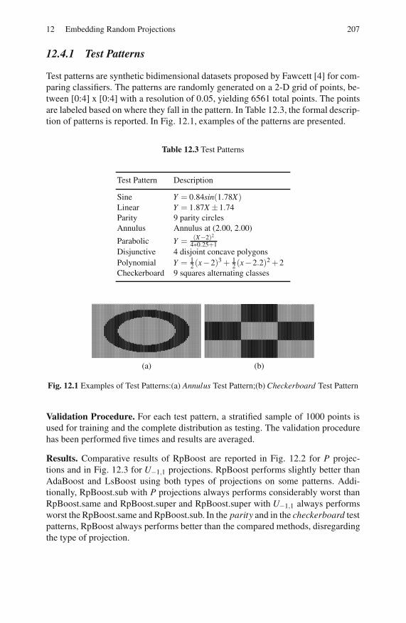
12 Embedding Random Projections 207
12.4.1 Test Patterns
Test patterns are synthetic bidimensional datasets proposed by Fawcett [4] for com-
paring classifiers. The patterns are randomly generated on a 2-D grid of points, be-
tween [0:4] x [0:4] with a resolution of 0.05, yielding 6561 total points. The points
are labeled based on where they fall in the pattern. In Table 12.3, the formal descrip-
tion of patterns is reported. In Fig. 12.1, examples of the patterns are presented.
Table 12.3 Test Patterns
Test Pattern Description
Sine Y = 0.84sin(1.78X)Linear Y = 1.87X ±1.74
Parity 9 parity circles
Annulus Annulus at (2.00, 2.00)
Parabolic Y = (X−2)2
4∗0.25+1Disjunctive 4 disjoint concave polygons
Polynomial Y = 12 (x−2)3 + 1
2 (x−2.2)2 +2
Checkerboard 9 squares alternating classes
(a) (b)
Fig. 12.1 Examples of Test Patterns:(a) Annulus Test Pattern;(b) Checkerboard Test Pattern
Validation Procedure. For each test pattern, a stratified sample of 1000 points is
used for training and the complete distribution as testing. The validation procedure
has been performed five times and results are averaged.
Results. Comparative results of RpBoost are reported in Fig. 12.2 for P projec-
tions and in Fig. 12.3 for U−1,1 projections. RpBoost performs slightly better than
AdaBoost and LsBoost using both types of projections on some patterns. Addi-
tionally, RpBoost.sub with P projections always performs considerably worst than
RpBoost.same and RpBoost.super and RpBoost.super with U−1,1 always performs
worst the RpBoost.same and RpBoost.sub. In the parity and in the checkerboard test
patterns, RpBoost always performs better than the compared methods, disregarding
the type of projection.
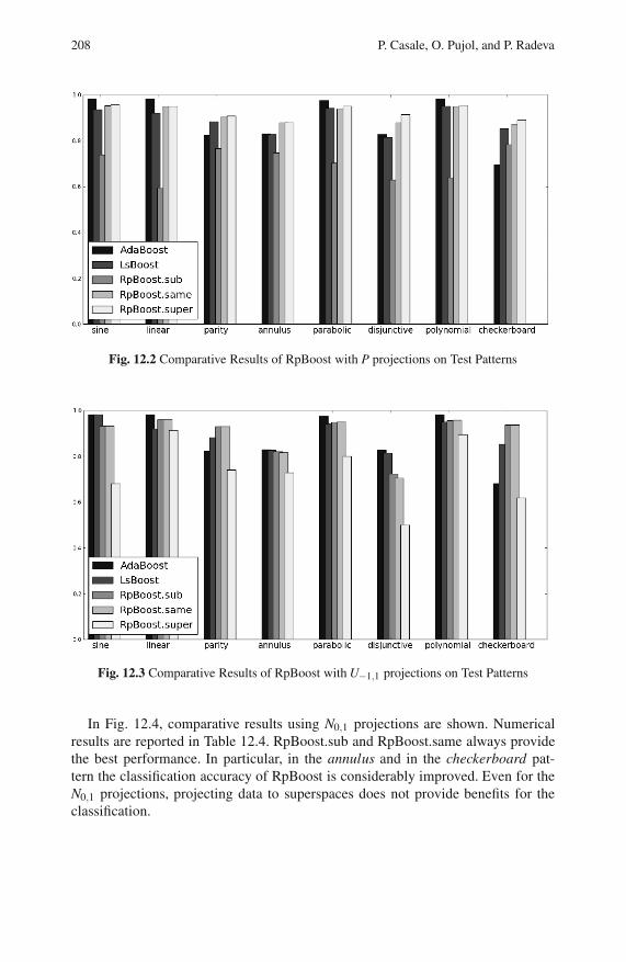
208 P. Casale, O. Pujol, and P. Radeva
Fig. 12.2 Comparative Results of RpBoost with P projections on Test Patterns
Fig. 12.3 Comparative Results of RpBoost with U−1,1 projections on Test Patterns
In Fig. 12.4, comparative results using N0,1 projections are shown. Numerical
results are reported in Table 12.4. RpBoost.sub and RpBoost.same always provide
the best performance. In particular, in the annulus and in the checkerboard pat-
tern the classification accuracy of RpBoost is considerably improved. Even for the
N0,1 projections, projecting data to superspaces does not provide benefits for the
classification.
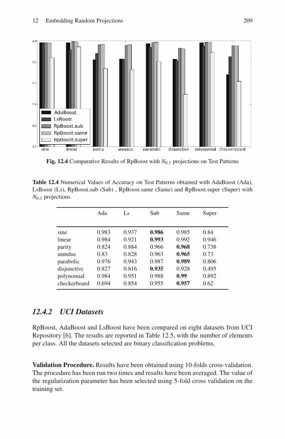
12 Embedding Random Projections 209
Fig. 12.4 Comparative Results of RpBoost with N0,1 projections on Test Patterns
Table 12.4 Numerical Values of Accuracy on Test Patterns obtained with AdaBoost (Ada),
LsBoost (Ls), RpBoost.sub (Sub) , RpBoost.same (Same) and RpBoost.super (Super) with
N0,1 projections
Ada Ls Sub Same Super
sine 0.983 0.937 0.986 0.985 0.84
linear 0.984 0.921 0.993 0.992 0.946
parity 0.824 0.884 0.966 0.968 0.738
annulus 0.83 0.828 0.963 0.965 0.73
parabolic 0.976 0.943 0.987 0.989 0.806
disjunctive 0.827 0.816 0.935 0.928 0.495
polynomial 0.984 0.951 0.988 0.99 0.892
checkerboard 0.694 0.854 0.955 0.957 0.62
12.4.2 UCI Datasets
RpBoost, AdaBoost and LsBoost have been compared on eight datasets from UCI
Repository [6]. The results are reported in Table 12.5, with the number of elements
per class. All the datasets selected are binary classification problems.
Validation Procedure. Results have been obtained using 10-folds cross-validation.
The procedure has been run two times and results have been averaged. The value of
the regularization parameter has been selected using 5-fold cross validation on the
training set.
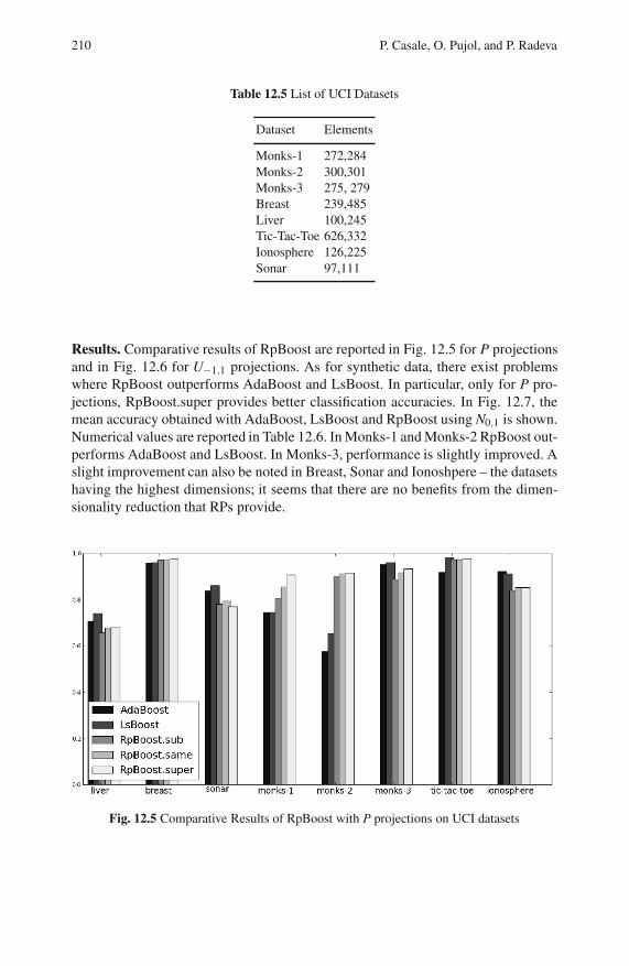
210 P. Casale, O. Pujol, and P. Radeva
Table 12.5 List of UCI Datasets
Dataset Elements
Monks-1 272,284
Monks-2 300,301
Monks-3 275, 279
Breast 239,485
Liver 100,245
Tic-Tac-Toe 626,332
Ionosphere 126,225
Sonar 97,111
Results. Comparative results of RpBoost are reported in Fig. 12.5 for P projections
and in Fig. 12.6 for U−1,1 projections. As for synthetic data, there exist problems
where RpBoost outperforms AdaBoost and LsBoost. In particular, only for P pro-
jections, RpBoost.super provides better classification accuracies. In Fig. 12.7, the
mean accuracy obtained with AdaBoost, LsBoost and RpBoost using N0,1 is shown.
Numerical values are reported in Table 12.6. In Monks-1 and Monks-2 RpBoost out-
performs AdaBoost and LsBoost. In Monks-3, performance is slightly improved. A
slight improvement can also be noted in Breast, Sonar and Ionoshpere – the datasets
having the highest dimensions; it seems that there are no benefits from the dimen-
sionality reduction that RPs provide.
Fig. 12.5 Comparative Results of RpBoost with P projections on UCI datasets
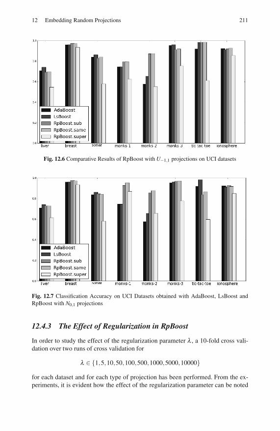
12 Embedding Random Projections 211
Fig. 12.6 Comparative Results of RpBoost with U−1,1 projections on UCI datasets
Fig. 12.7 Classification Accuracy on UCI Datasets obtained with AdaBoost, LsBoost and
RpBoost with N0,1 projections
12.4.3 The Effect of Regularization in RpBoost
In order to study the effect of the regularization parameter λ , a 10-fold cross vali-
dation over two runs of cross validation for
λ ∈ 1,5,10,50,100,500,1000,5000,10000
for each dataset and for each type of projection has been performed. From the ex-
periments, it is evident how the effect of the regularization parameter can be noted
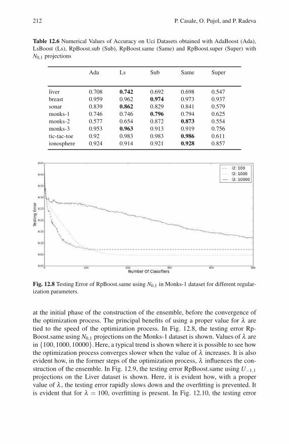
212 P. Casale, O. Pujol, and P. Radeva
Table 12.6 Numerical Values of Accuracy on Uci Datasets obtained with AdaBoost (Ada),
LsBoost (Ls), RpBoost.sub (Sub), RpBoost.same (Same) and RpBoost.super (Super) with
N0,1 projections
Ada Ls Sub Same Super
liver 0.708 0.742 0.692 0.698 0.547
breast 0.959 0.962 0.974 0.973 0.937
sonar 0.839 0.862 0.829 0.841 0.579
monks-1 0.746 0.746 0.796 0.794 0.625
monks-2 0.577 0.654 0.872 0.873 0.554
monks-3 0.953 0.963 0.913 0.919 0.756
tic-tac-toe 0.92 0.983 0.983 0.986 0.611
ionosphere 0.924 0.914 0.921 0.928 0.857
Fig. 12.8 Testing Error of RpBoost.same using N0,1 in Monks-1 dataset for different regular-
ization parameters.
at the initial phase of the construction of the ensemble, before the convergence of
the optimization process. The principal benefits of using a proper value for λ are
tied to the speed of the optimization process. In Fig. 12.8, the testing error Rp-
Boost.same using N0,1 projections on the Monks-1 dataset is shown. Values of λ are
in 100,1000,10000. Here, a typical trend is shown where it is possible to see how
the optimization process converges slower when the value of λ increases. It is also
evident how, in the former steps of the optimization process, λ influences the con-
struction of the ensemble. In Fig. 12.9, the testing error RpBoost.same using U−1,1
projections on the Liver dataset is shown. Here, it is evident how, with a proper
value of λ , the testing error rapidly slows down and the overfitting is prevented. It
is evident that for λ = 100, overfitting is present. In Fig. 12.10, the testing error
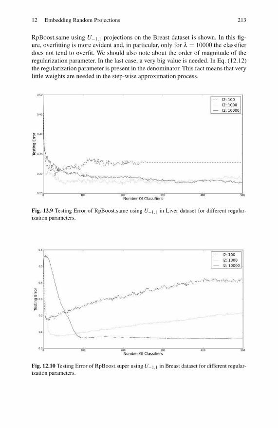
12 Embedding Random Projections 213
RpBoost.same using U−1,1 projections on the Breast dataset is shown. In this fig-
ure, overfitting is more evident and, in particular, only for λ = 10000 the classifier
does not tend to overfit. We should also note about the order of magnitude of the
regularization parameter. In the last case, a very big value is needed. In Eq. (12.12)
the regularization parameter is present in the denominator. This fact means that very
little weights are needed in the step-wise approximation process.
Fig. 12.9 Testing Error of RpBoost.same using U−1,1 in Liver dataset for different regular-
ization parameters.
Fig. 12.10 Testing Error of RpBoost.super using U−1,1 in Breast dataset for different regular-
ization parameters.
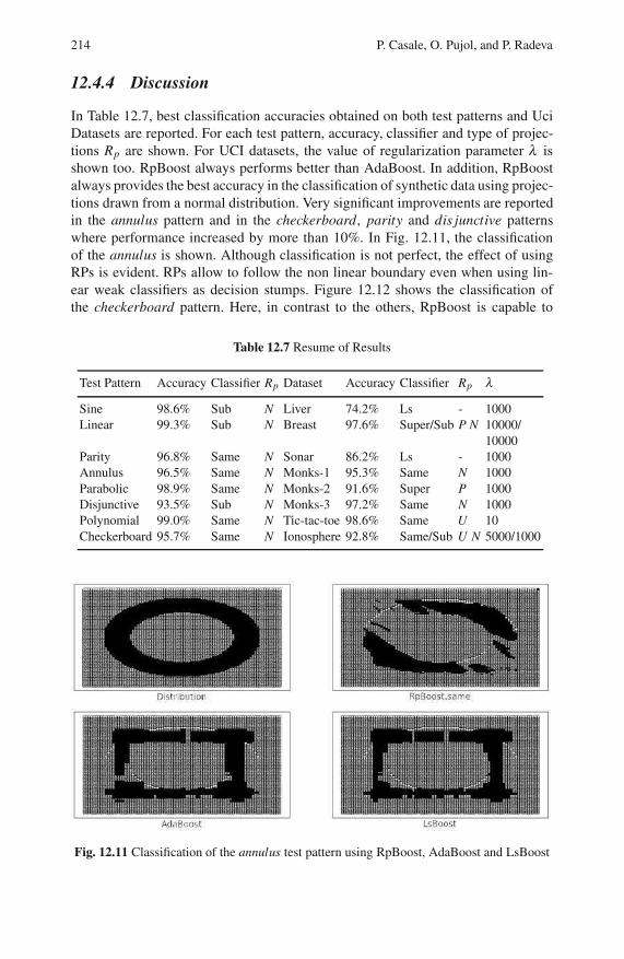
214 P. Casale, O. Pujol, and P. Radeva
12.4.4 Discussion
In Table 12.7, best classification accuracies obtained on both test patterns and Uci
Datasets are reported. For each test pattern, accuracy, classifier and type of projec-
tions Rp are shown. For UCI datasets, the value of regularization parameter λ is
shown too. RpBoost always performs better than AdaBoost. In addition, RpBoost
always provides the best accuracy in the classification of synthetic data using projec-
tions drawn from a normal distribution. Very significant improvements are reported
in the annulus pattern and in the checkerboard, parity and dis junctive patterns
where performance increased by more than 10%. In Fig. 12.11, the classification
of the annulus is shown. Although classification is not perfect, the effect of using
RPs is evident. RPs allow to follow the non linear boundary even when using lin-
ear weak classifiers as decision stumps. Figure 12.12 shows the classification of
the checkerboard pattern. Here, in contrast to the others, RpBoost is capable to
Table 12.7 Resume of Results
Test Pattern Accuracy Classifier Rp Dataset Accuracy Classifier Rp λ
Sine 98.6% Sub N Liver 74.2% Ls - 1000
Linear 99.3% Sub N Breast 97.6% Super/Sub P N 10000/
10000
Parity 96.8% Same N Sonar 86.2% Ls - 1000
Annulus 96.5% Same N Monks-1 95.3% Same N 1000
Parabolic 98.9% Same N Monks-2 91.6% Super P 1000
Disjunctive 93.5% Sub N Monks-3 97.2% Same N 1000
Polynomial 99.0% Same N Tic-tac-toe 98.6% Same U 10
Checkerboard 95.7% Same N Ionosphere 92.8% Same/Sub U N 5000/1000
Fig. 12.11 Classification of the annulus test pattern using RpBoost, AdaBoost and LsBoost
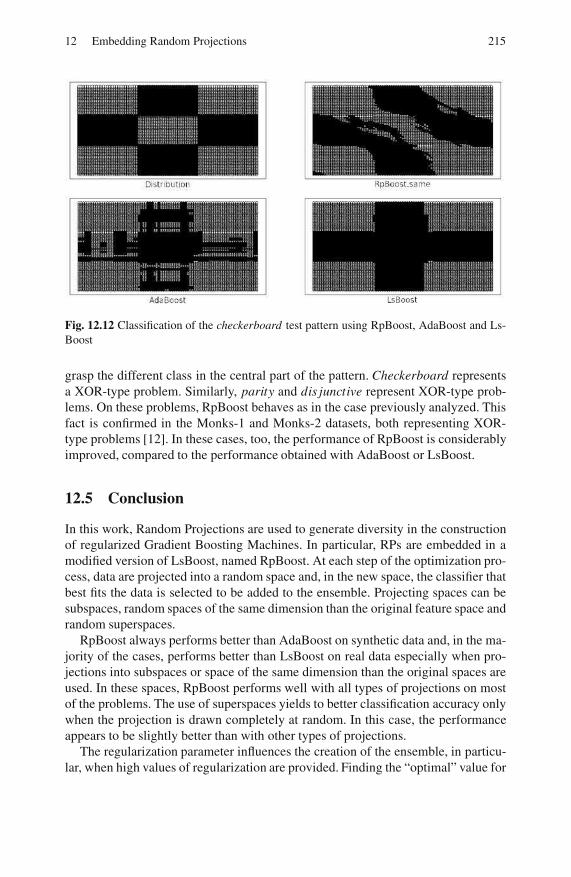
12 Embedding Random Projections 215
Fig. 12.12 Classification of the checkerboard test pattern using RpBoost, AdaBoost and Ls-
Boost
grasp the different class in the central part of the pattern. Checkerboard represents
a XOR-type problem. Similarly, parity and dis junctive represent XOR-type prob-
lems. On these problems, RpBoost behaves as in the case previously analyzed. This
fact is confirmed in the Monks-1 and Monks-2 datasets, both representing XOR-
type problems [12]. In these cases, too, the performance of RpBoost is considerably
improved, compared to the performance obtained with AdaBoost or LsBoost.
12.5 Conclusion
In this work, Random Projections are used to generate diversity in the construction
of regularized Gradient Boosting Machines. In particular, RPs are embedded in a
modified version of LsBoost, named RpBoost. At each step of the optimization pro-
cess, data are projected into a random space and, in the new space, the classifier that
best fits the data is selected to be added to the ensemble. Projecting spaces can be
subspaces, random spaces of the same dimension than the original feature space and
random superspaces.
RpBoost always performs better than AdaBoost on synthetic data and, in the ma-
jority of the cases, performs better than LsBoost on real data especially when pro-
jections into subspaces or space of the same dimension than the original spaces are
used. In these spaces, RpBoost performs well with all types of projections on most
of the problems. The use of superspaces yields to better classification accuracy only
when the projection is drawn completely at random. In this case, the performance
appears to be slightly better than with other types of projections.
The regularization parameter influences the creation of the ensemble, in particu-
lar, when high values of regularization are provided. Finding the “optimal” value for

216 P. Casale, O. Pujol, and P. Radeva
the regularization parameter is crucial especially when there exists a trend to over-
fitting. Obviously, in the cases where overfitting is present, using a small number of
classifiers in the ensemble would have to provide better classification accuracy.
Finally, results clearly show that RpBoost is a promising technique and encour-
ages future research with studies on real-world problems.
Acknowledgements. This work is partially supported by a research grant from projects
TIN2009-14404-C02, La Marato de TV3 082131 and CONSOLIDER (CSD2007-00018).
References
1. Arriaga, R.I., Vempala, S.: An algorithmic theory of learning: Robust concepts and ran-
dom projection. Machine Learning 63, 161–182 (2006)
2. Blum, A.: Random projection, margins, kernels, and feature-selection. In: Saunders, C.,
Grobelnik, M., Gunn, S., Shawe-Taylor, J. (eds.) SLSFS 2005. LNCS, vol. 3940, pp.
52–68. Springer, Heidelberg (2006)
3. Dasgupta, S.: Experiments with random projection. In: Proc. the 16th Conf. Uncertainty
in Artif. Intell., Stanford, CA, pp. 143–151. Morgan Kaufmann, San Francisco (2000)
4. Fawcett, T.: Comparing patterns classifiers,
http://home.comcast.net/ tom.fawcett/public html/ML--gallery/pages/index.html
5. Fradkin, D., Madigan, D.: Experiments with random projections for machine learning.
In: Proc. the 9th ACM SIGKDD Int. Conf. Knowledge Discovery and Data Mining,
Washington, DC, pp. 517–522. ACM Press, New York (2003)
6. Frank, A., Asuncion, A.: UCI machine learning repository. University of California,
School of Information and Computer Sciences, Irvine (2010)
7. Friedman, J.H.: Greedy function approximation: A gradient boosting machine. Annals
of Stat. 29, 1189–1232 (2000)
8. Johnson, W.B., Lindenstrauss, J.: Extensions of Lipschitz maps into a Hilbert space.
Contemporary Mathematics 26, 189–206 (1984)
9. Pujol, O.: Boosted geometry-based ensembles. In: El Gayar, N., Kittler, J., Roli, F. (eds.)
MCS 2010. LNCS, vol. 5997, pp. 195–204. Springer, Heidelberg (2010)
10. Rahimi, A., Recht, B.: Weighted sums of random kitchen sinks: Replacing minimization
with randomization in learning. In: Advances in Neural Inf. Proc. Syst., vol. 21, pp.
1313–1320. MIT Press, Cambridge (2008)
11. Rodriguez, J.J., Kuncheva, L.I., Alonso, C.J.: Rotation Forest: A new classifier ensemble
method. IEEE Trans. Pattern Analysis and Machine Intell. 28, 1619–1630 (2006)
12. Thrun, S., Bala, J., Bloedorn, E., Bratko, I., Cestnik, B., Cheng, J., De Jong, K., Dze-
roski, S., Hamann, R., Kaufman, K., Keller, S., Kononenko, I., Kreuziger, J., Michal-
ski, R.S., Mitchell, T., Pachowicz, P., Roger, B., Vafaie, H., Van de Velde, W., Wenzel,
W., Wnek, J., Zhang, J.: The MONK’s problems: A performance comparison of differ-
ent learning algorithms. Technical Report CMU-CS-91-197, Carnegie Mellon University
(1991)
13. Zhang, C.-X., Zhang, J.-S.: RotBoost: A technique for combining Rotation Forest and
AdaBoost. Pattern Recogn. Letters 29, 1524–1536 (2008)

Chapter 13
An Improved Mixture of Experts Model:Divide and Conquer Using Random Prototypes
Giuliano Armano and Nima Hatami
Abstract. The Mixture of Experts (ME) is one of the most popular ensemble meth-
ods used in Pattern Recognition and Machine Learning. This algorithm stochas-
tically partitions the input space of a problem into a number of subspaces, experts
becoming specialized on each subspace. To manage this process, the ME uses an ex-
pert called gating network, which is trained together with the other experts. In this
chapter, we propose a modified version of the ME algorithm which first partitions
the original problem into centralized regions and then uses a simple distance-based
gating function to specialize the expert networks. Each expert contributes to classify
an input sample according to the distance between the input and a prototype embed-
ded by the expert. The Hierarchical Mixture of Experts (HME) is a tree-structured
architecture which can be considered a natural extension of the ME model. The
training and testing strategies of the standard HME model are also modified, based
on the same insight applied to standard ME. In both cases, the proposed approach
does not require to train the gating networks, as they are implemented with sim-
ple distance-based rules. In so doing the overall time required for training a modi-
fied ME/HME system is considerably lower. Moreover, centralizing input subspaces
and adopting a random strategy for selecting prototypes permits to increase at the
same time individual accuracy and diversity of ME/HME modules, which in turn
increases the accuracy of the overall ensemble. Experimental results on a binary toy
problem and on selected datasets from the UCI machine learning repository show
the robustness of the proposed methods compared to the standard ME/HME models.
13.1 Introduction
Most real-world pattern recognition problems are too complicated for a single clas-
sifier to solve. Divide-and-conquer has proved to be efficient in many of these
Giuliano Armano · Nima Hatami
DIEE- Department of Electrical and Electronic Engineering, University of Cagliari,
Piazza d’Armi, I-09123, Italy
E-mail: armano,[email protected]
O. Okun et al. (Eds.): Ensembles in Machine Learning Applications, SCI 373, pp. 217–231.springerlink.com c© Springer-Verlag Berlin Heidelberg 2011

218 G. Armano and N. Hatami
complex situations, using a combination of classifiers which have complementary
properties. The issues are (i) how to divide the problem into simpler subproblems,
(ii) how to assign base classifiers to solve these subproblems, and (iii) how to obtain
the final decision using their outputs.
In some cases the problem can be decomposed manually. However, in most real-
world problems, we either know too little about the problem, or it is difficult to
achieve a clear understanding of how to manually decompose it into subproblems.
Thus, a method for automatically decomposing a complex problem into a set of
overlapping or disjoint subproblems is desirable, assigning one or more classifiers
(experts hereinafter) to each subproblem.
Jacobs et al. [5, 6] have proposed an ensemble method based on the divide-and-
conquer principle called Mixture of Experts (ME), in which a set of networks re-
ferred to as expert networks is trained together with a gate network. This tight cou-
pling mechanism (i) encourages diversity among experts by automatically localizing
them in different regions of the input space and (ii) achieves good dynamic combi-
nation weights of the ensemble members by concurrently training the gate together
with the experts. The Hierarchical Mixture of Experts (HME) [7] is a well-known
tree-structured architecture, which can be thought of as a natural extension of the
Mixture of Experts (ME) model. The expert networks form the leaves of the tree,
whereas gating networks are located at the branch-points. Tasks are approached
using a “recursive” divide-and-conquer strategy: complex tasks are decomposed
into subtasks which in turn are themselves decomposed into sub-subtasks. Like
many known classical artificial neural network ensemble methods, diversity in the
standard HME is promoted by randomly initializing their weight parameters. This
choice drives experts to start learning their task from different points in the search
space, with the goal of getting them specialized on different subspaces.
Since Jacobs’ proposal in 1991, the ME model has been widely investigated.
Many of the earlier works on the ME and HME models use preprocessing to parti-
tion or transform the input space into simpler and more separable spaces. An expert
is then specialized on each subspace without altering the learning rules established
by the standard ME model. As a consequence, the major effort in earlier works has
been spent in the task of increasing the individual accuracy of experts, so to facil-
itate their task on the corresponding areas of expertise. Waterhouse and Cook [11]
and Avnimelech and Intrator [2] proposed to combine ME with the Boosting al-
gorithm. Since Boosting encourages classifiers to become experts on patterns that
previous experts disagree on, it can be successfully used to split the data set into
regions for the experts in the ME model, thus ensuring their localization and diver-
sity. Tang et al. [9] tried to explicitly “localize” experts by applying a cluster-based
preprocessing step, aimed at partitioning their input space. In particular, they used
self-organizing maps (SOM) to partition the input space according to the underlying
probability distribution of the data. As a result, better generalization ability together
with more stability in parameter setting is achieved. Nevertheless, as they argue at
the end of the paper, the proposed method has been designed for (and validated on)
only binary and low dimensional problems. Wan and Bone [10] used a mixture of
radial basis function networks to partition the input space into statistically correlated

13 An Improved Mixture of Experts Model 219
regions and learn the local covariance model of the data in each region. Ebrahim-
pour et al. [3] proposed a view-independent face recognition system using ME by
manual decomposition of the face view space into specific angles (views), an expert
being specialized on each view. Nevertheless, the proposed method is only efficient
in 2D face recognition and, as argued by the authors, extending this approach to
other classification problems and applications could be challenging and not always
possible.
It is worth pointing out that, in the original formulation of the ME model, param-
eters are determined by maximum likelihood, which is prone to severe overfitting,
including singularities in the likelihood function. This can be particularly problem-
atic in a complex model such as the HME, due to the relatively large number of
parameters involved in defining the distributions for experts and gating networks.
Indeed, there are many singularities in the likelihood function which arise when-
ever one of the mixture components “collapses” onto a single data point. In any
case, simultaneously training gating networks and experts in an HME architecture
(with the goal of obtaining sufficiently accurate classifiers with relatively optimum
parameters) continues to pose a research challenge.
Recently, Armano and Hatami have proposed a classifier selection method to be
used in selection-fusion strategies [1]. The method called Random Prototype-based
Oracle, RPO, splits the input domain based on some prototypes selected randomly
from training data and then builds a classifier on each subset. These classifiers are
used in combination with an oracle that knows the area of expertise of each classi-
fier, thus generating a mini-ensemble. Thanks to the random nature of this splitting
procedure, mini-ensembles created on a specific problem differ from one run to
another. Each mini-ensemble can be used as base classifier in any ensemble strat-
egy to improve its accuracy without increasing the computational cost required for
training.
Inspired by the above mentioned idea, we decided to assign a random prototype
to each expert in the ME model. In this modified ME model, called “Mixture of
Random Prototype-based Experts” , the input space is partitioned according to the
nearest distance from randomly-chosen prototypes. This facilitates the adoption of
a weighting policy based on distances in both training and testing. In other words,
instead of a complex gating network which requires a training process to adjust its
weight parameters, the proposed gating function manages both training and testing
using a distance-based measure.
Subsequently, we extended the idea above by embedding a set of random proto-
types into each module of the HME model. Instead of specializing each expert on a
stochastic and nested area in the feature space, ME experts focus on the centralized
subspace defined by their corresponding prototypes. This allows to simplify the gat-
ing networks with simple distance-based measures, thus simplifying the structure
of the modified HME model. Moreover, while increasing the individual accuracy
of the ME modules used in the first layer of an HME architecture, their diversity is
also expected to increase due to the random selection of prototypes (which makes
the prototypes of a module different from those used by the others). Finally, the time
required to train the proposed HME architecture dramatically decreases due to the

220 G. Armano and N. Hatami
large saving in the training time of each ME module. Experimental results confirm
the above mentioned claims.
The rest of the chapter is organized as follows. In Sect. 13.2, we briefly recall
the standard ME model and its hierarchical counterpart. Section 13.3 first presents
random prototype-based splitting, then introduces the proposed mixture of random
prototype-based experts, and finally extends it to the hierarchical setting. Experi-
mental results are reported and discussed in Sect. 13.4. Section 13.5 concludes the
chapter and briefly outlines future research directions.
13.2 Standard Mixture of Experts Models
13.2.1 Standard ME Model
The adaptive mixture of local experts [5, 6] is a learning procedure which achieves
improved generalization performance by assigning different subtasks to different
experts. Its basic idea consists of concurrently training several experts and a gating
network. The gating function assigns a “probability” to each expert based on the
current input. In the training phase, this value denotes the probability for a pattern
to appear in the training set of an expert. In the test step, it defines the relative
contribution of each expert to the ensemble. The training step attempts to achieve
two goals: (i) for a given expert, find the optimal gating function; (ii) for a given
gating function (network), train each expert to achieve maximal performance on the
distribution assigned to it by the gating function. Accordingly, the accuracy of an
ME classifier is affected by the performance of both expert networks and gating
network. Resulting misclassifications in this model derive from two sources: (a)
the gating network is unable to correctly estimate the probability for a given input
sample and (b) local experts do not learn their subtask perfectly. Let us consider the
network shown in Fig. 13.1, which represents an ME model with N = 3 experts. The
ith expert produces its output oi(x) as a generalized linear function of the input x:
oi(Wi,x) = f (Wix), (13.1)
where Wi is the weight matrix of the ith expert and f (.) is a predefined continuous
nonlinearity. The gating network is also a generalized linear function, and its ith
output, gi(Vi,x), is the multinomial logit or softmax function of the gating network’s
output, ogi.
gi(Vi,x) =exp(ogi
)
∑Nj=1 ogi
i = 1, ...,N, (13.2)
where Vi is the weight vector of the gating network. Hence, the overall output of the
ME architecture, o(x), is
o(x) = ∑i
gi(Vi,x)oi(Wi,x). (13.3)

13 An Improved Mixture of Experts Model 221
Two training procedures are suggested in the literature [5, 7] for finding opti-
mal weight parameters Wi and Vi. The first is the standard error back-propagation
algorithm with gradient descent, whereas the second is based on the Expectation-
Maximization (EM) method.
Fig. 13.1 Block diagram representing the Mixture of Experts (ME) model. The generic model
shown here has three experts (N=3) and the gating network as a mediator for managing the
process.
13.2.2 Standard HME Model
The HME architecture (Fig. 13.2) is a tree in which the gating networks lie at the
nonterminal nodes and the expert networks lie at the leaves of the tree. Hence, it
can be considered an ensemble of ME modules (as shown by dashed boxes). The
task of each expert is to approximate a function over a region of the input space.
Given a sample, the task of the gating network is to assign the weights to each
expert. Figure 13.2 illustrates a mixture of four experts. In accordance with the
typical terminology used for describing HME architectures: x is the input vector,
oi j(x) is the output (expected value) of the ijth expert, gi(x) is the output of the
top gating network, denoting the prior probability for the pattern to be generated
by the left or right branch of the root, and g j|i(x) is the output of the ith bottom
gating network, denoting the prior probability that the pattern is generated by the
i jth expert. In addition, t is the target (desired output) and Pi j(t|x) is the probability
associated with the ijth expert.
Assuming that experts are mutually exclusive, the overall probability, P(t|x) and
the expected value at the network output, o(x), are given by:
P(t|x) = ∑i
gi(x)∑j
g j|i(x)Pi j(t|x), (13.4)
o(x) = ∑i
gi(x)∑j
g j|i(x)oi j(x). (13.5)

222 G. Armano and N. Hatami
Fig. 13.2 Block diagram representing a two-layer HME. The generic model shown here has
four experts (two ME modules, each embedding two experts) and three gating networks which
act as mediators.
Note that the notations defined for the two-level depth tree shown in Fig. 13.2 can
be easily extended to larger HME networks with a binary tree architecture.
Two training procedures are suggested in the literature [3, 9, 10] for finding opti-
mal weight parameters of the HME architecture. The first is the standard error back-
propagation algorithm with gradient descent and the second procedure is based on
the Expectation-Maximization (EM) method.
13.3 Mixture of Random Prototype-Based Experts (MRPE)
and Hierarchical MRPE
13.3.1 Mixture of Random Prototype-Based Local Experts
In this section, we illustrate the proposed mixture of random prototype-based ex-
perts with more detail. The key underlying idea is to randomly partition the input
space of the problem into subspaces and then specialize each expert on each sub-
space by means of “soft” competitive learning. First of all, the input space is parti-
tioned according to some prototypes randomly chosen from the training set, so that
the input samples are weighted during the training and testing phases based on their
distances from the selected prototypes. The main advantage of this method is that,
instead of a complex gating network which must be trained concurrently with other
experts, the generated gating function has no parameters (weights) to adjust – as

13 An Improved Mixture of Experts Model 223
it simply enforces a distance-based weighting policy. This modification improves
three important aspects of the standard ME model. First, it reduces the training
time by decreasing the number of parameters to be estimated. Secondly, as simple
distance measures used by the gating function are more robust with respect to errors
in determining the area of expertise of an expert, errors in the proposed ME model
are mainly limited to the error made by the expert networks, thus improving the
overall accuracy of the classifier. Lastly, the region of expertise for each expert in
the standard ME model is nested, which makes the problem difficult to learn. In the
proposed method, each expert’s area of expertise is more centralized, which makes
the subproblem easier to learn. The latter property also makes the rules embedded
by an expert easy to analyze, which is vital in some applications that need to make
explicit the information about the area of expertise of each expert.
For the sake of simplicity and ease of comprehension, we describe this approach
for the synthetic two-class problem shown in Fig. 13.3a. We used two different
partitioning methods, i.e. disjoint and overlapping, shown in Figs. 13.3b and 13.3c
respectively. In case of disjoint partitioning, we first measure the distance between
each training sample and the prototypes, and then assign a fixed value, η j , to the hi
of the expert proportional to these distances. hi is an estimate of the “a posteriori”
probability for the ith expert to generate the desired output o and used as the coef-
ficient of the learning rate for updating the weight parameters of the expert (static
strategy). This implies that the weight update on the expert network whose proto-
type is nearest to the current input sample will be stronger than those performed on
the others (the closer the expert, the stronger the update is). Similarly, in the testing
phase, the expert whose prototype is nearest to the input sample will contribute to a
greater extent to the final output.
Unlike disjoint partitioning, where the learning rate coefficients are fixed for each
partition and change sharply from one to another, in the overlapping method they
change smoothly, proportional to the distances (dynamic strategy). Similarly, the
amount of di for the ith expert depends on how close the prototype is to the current
input sample x. In other words, for disjoint learning, the amount of expertise and
contribution of experts is fixed for each partition, whereas, for overlapping learning,
their expertise smoothly vary with the distance di from the prototypes embedded in
the experts. It is worth pointing out that the proposed method is general enough to
be applied for building ME classifiers using both standard error back-propagation
and EM learning rules. Algorithm 7 reports the procedure to be used for training
and testing a mixture of random prototype-based experts, using both disjoint and
overlapping partitioning rules for any chosen learning method.
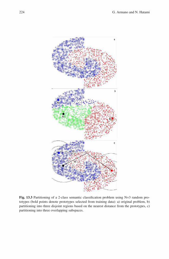
224 G. Armano and N. Hatami
Fig. 13.3 Partitioning of a 2-class semantic classification problem using N=3 random pro-
totypes (bold points denote prototypes selected from training data): a) original problem, b)
partitioning into three disjoint regions based on the nearest distance from the prototypes, c)
partitioning into three overlapping subspaces.

13 An Improved Mixture of Experts Model 225
Algorithm 7. Mixture of Random Prototype-based Experts
PARAMETERS:
• strategy = static,dynamic• N number of experts in an ME classifier
• E = η j ∈ (0,1) | j = 1..N such that: ηk ≤ ηk+1;k = 1..N−1 and |E|= ∑ j η j = 1
WITH:
• Ψ = εi | i = 1..N set of experts
• P = pi ∈ LS | i = 1..N set of randomly chosen prototypes, each assigned to an expert
• LS/TS = Learning/Training Set
TRAINING:
For x ∈ LS Do:
• D(x) = di(x) | i = 1..N where
di(x) = ‖x− pi‖• H(x) = hi(x) | i = 1..N where
hi(x) represents the expected capability of εi to deal with the given input x
[strategy = static] : hi(x) = ηr , r = Rank(εi,D(x))∗
[strategy = dynamic] : hi(x) = 1− di
‖D(x)‖ , ‖D(x)‖= ∑ j d j(x)
• update each expert εi (i = 1..N) according to the standard learning rule for ME
TESTING:
Given an x ∈ TS Do:
• D(x) = di(x) | i = 1..N• G(x) = gi(x) | i = 1..N where
[strategy = static] : gi(x) = ηr , r = Rank(εi,D(x))∗
[strategy = dynamic] : gi(x) = 1− di
‖D(x)‖ , ‖D(x)‖= ∑ j d j(x)
• calculate the overall output:
o j(x) = ∑Ni gi(x) ·o(x,Wi)
• select the class label ck such that
k = argmax j (o j(x))
* r = Rank(εi,D(x)) returns the rank of expert εi (i.e. a number in [1,N]) according to the
distance D(x) evaluated on the input x (the lower the distance, the highest the ranking).
13.3.2 Hierarchical MRPE Model
This section presents the proposed hierarchical mixture of random prototype-based
experts (HMRPE) with more detail. The key underlying idea is to randomly parti-
tion the input space of the problem into subspaces and then pushing each expert to
specialize on its subspace by means of “soft” competitive learning.
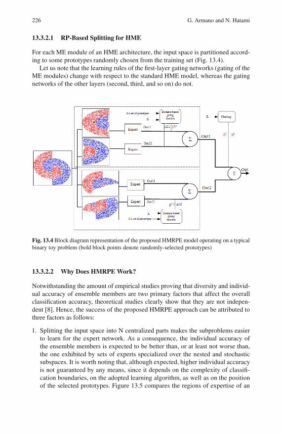
226 G. Armano and N. Hatami
13.3.2.1 RP-Based Splitting for HME
For each ME module of an HME architecture, the input space is partitioned accord-
ing to some prototypes randomly chosen from the training set (Fig. 13.4).
Let us note that the learning rules of the first-layer gating networks (gating of the
ME modules) change with respect to the standard HME model, whereas the gating
networks of the other layers (second, third, and so on) do not.
Fig. 13.4 Block diagram representation of the proposed HMRPE model operating on a typical
binary toy problem (bold block points denote randomly-selected prototypes)
13.3.2.2 Why Does HMRPE Work?
Notwithstanding the amount of empirical studies proving that diversity and individ-
ual accuracy of ensemble members are two primary factors that affect the overall
classification accuracy, theoretical studies clearly show that they are not indepen-
dent [8]. Hence, the success of the proposed HMRPE approach can be attributed to
three factors as follows:
1. Splitting the input space into N centralized parts makes the subproblems easier
to learn for the expert network. As a consequence, the individual accuracy of
the ensemble members is expected to be better than, or at least not worse than,
the one exhibited by sets of experts specialized over the nested and stochastic
subspaces. It is worth noting that, although expected, higher individual accuracy
is not guaranteed by any means, since it depends on the complexity of classifi-
cation boundaries, on the adopted learning algorithm, as well as on the position
of the selected prototypes. Figure 13.5 compares the regions of expertise of an

13 An Improved Mixture of Experts Model 227
ME module, embedded in both the standard HME and the HMRPE models, on
a four-class toy problem. The figure (first row, first column) shows the original
problem, and the next three figures report the nested areas of expertise for the
three experts in the standard ME module. The figure (third row, first column)
shows how the problem is partitioned using three random prototypes, and the
next three figures highlight the centralized areas of expertise of three experts in
the proposed HMRPE module.
2. Since each ME module embedded in the HMRPE architecture has its own set of
prototypes (which are different from those embedded by the other ME modules),
experts are specialized on very different data subsets, thus enforcing diversity.
3. The accuracy of an HME classifier is affected by the performance of both experts
and gating networks. Accordingly, resulting misclassifications in this model de-
rive from two sources: (a) the gating networks are unable to correctly estimate
the probability for a given input sample and (b) local experts do not learn their
subtask perfectly. Since simple distance rules used by the gating function are
more robust with respect to errors in determining the area of expertise of an ex-
pert, errors in the proposed HMRPE model are mainly limited to the error made
by the expert networks, thus improving the overall accuracy of the classifier.
13.4 Experimental Results and Discussion
Some UCI machine learning data sets [12] have been used to check the validity of
the proposed method. These data sets include real-world and synthetic problems,
with variable characteristics. Table 13.1 shows the selected datasets.
Table 13.1 The main characteristics of the selected UCI datasets
Problem # Train # Test # Attributes # Classes
Glass 214 - 9 7
Iris 150 - 4 3
Letter 20000 - 16 26
Pendigits 7494 3498 16 10
Satimage 4435 2000 36 6
Segment 210 2100 19 7
Vowel 990 - 11 11
Yeast 1484 - 8 10
For the datasets with no train/test partitioning, the classification performance as-
sessed by the 10-fold cross-validation provides realistic generalization accuracy for
unseen data. To build the standard HME and the proposed HMRPE models, we
used a Multi-Layer Perceptron (MLP) architecture with one hidden layer, trained
with the back-propagation learning rule [4]. To determine the best value for the N
partitions, which is equal to the number of experts, we varied it from 2 to 10 for each
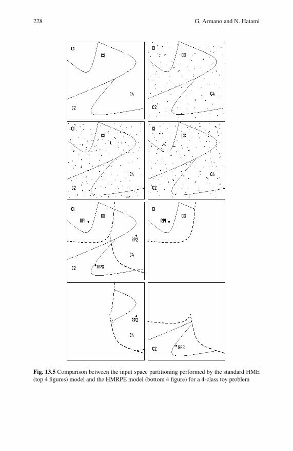
228 G. Armano and N. Hatami
Fig. 13.5 Comparison between the input space partitioning performed by the standard HME
(top 4 figures) model and the HMRPE model (bottom 4 figure) for a 4-class toy problem
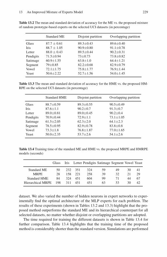
13 An Improved Mixture of Experts Model 229
Table 13.2 The mean and standard deviation of accuracy for the ME vs. the proposed mixture
of random prototype-based experts on the selected UCI datasets (in percentage)
Standard ME Disjoint partition Overlapping partition
Glass 87.7 ± 0.61 89.3±0.43 89.6±0.40
Iris 88.7 ± 1.05 90.9±0.80 91.1±0.78
Letter 88.0 ± 0.43 89.5±0.44 90.2±0.31
Pendigits 71.5±0.94 73±0.73 73.8±0.82
Satimage 60.9±1.55 63.8±1.0 64.4±1.21
Segment 79±0.85 82.2±0.68 82.9±0.79
Vowel 72.1±1.75 75.8±1.77 76.9±1.44
Yeast 50.6±2.22 52.7±1.56 54.0±1.45
Table 13.3 The mean and standard deviation of accuracy for the HME vs. the proposed HM-
RPE on the selected UCI datasets (in percentage)
Standard HME Disjoint partition Overlapping partition
Glass 88.7±0.59 89.3±0.55 90.5±0.49
Iris 87.6±1.1 90.2±0.7 91.3±0.7
Letter 89.0±0.81 89.0±0.45 90.2±0.4
Pendigits 70.9±0.44 72.9±1.1 73.1±1.05
Satimage 61.5±2.05 62.3±2.0 64.1±2.3
Segment 78.5±0.95 82.9±0.78 83.8±0.8
Vowel 73.3±1.8 76.8±1.87 77.0±1.65
Yeast 50.0±2.35 53.7±2.6 54.1±2.6
Table 13.4 Training time of the standard ME and HME vs. the proposed MRPE and HMRPE
models (seconds)
Glass Iris Letter Pendigits Satimage Segment Vowel Yeast
Standard ME 50 232 351 324 59 49 30 41
MRPE 28 158 221 258 39 32 21 29
Standard HME 84 324 451 604 99 71 44 67
Hierarchical MRPE 198 311 451 451 63 53 30 42
dataset. We also varied the number of hidden neurons in expert networks to exper-
imentally find the optimal architecture of the MLP experts for each problem. The
results of these experiments (shown in Tables 13.2 and 13.3) highlight that the pro-
posed method outperforms the standard ME and its hierarchical counterpart for all
selected datasets, no matter whether disjoint or overlapping partitions are adopted.
The time required for training the different datasets is shown in Table 13.4 for
further comparison. Table 13.4 highlights that the training time of the proposed
method is considerably shorter than the standard version. Simulations are performed
230 G. Armano and N. Hatami
using an Intel CPU with 2.83GHz and 4GB RAM memory. Note that the results
presented here which compare standard HME and the proposed method, use the
same parameters and architecture.
13.5 Conclusion
In this chapter, a modified version of the popular ME algorithm has been presented.
Unlike the standard ME, which specializes expert networks on nested and stochastic
regions of the input space, the proposed method partitions the sample space into
subspaces based on similarities with randomly-selected prototypes. This strategy
enables to define a simple rule for the gating network for both training and testing. As
shown by experimental results, despite its simplicity, the proposed method improves
the accuracy of the both standard ME and HME models while reducing the training
time.
Future work will be focused on defining a light procedure for automatically de-
termining the number of experts for a given problem, without resorting to com-
plex preprocessing and time consuming methods. Adapting this method to simple
distance-based classifiers (instead of artificial neural networks) is another interesting
future research direction, concerned with reducing the training time of the overall
network while maintaining high accuracy.We are also experimenting with heuristics able to help in the process of partition-
ing the input space (instead of using random prototypes).
References
1. Armano, G., Hatami, N.: Random prototype-based oracle for selection-fusion ensembles.
In: Proc. the 20th Int. Conf. Patt. Recogn., Istanbul, Turkey, pp. 77–80. IEEE Comp.
Society, Los Alamitos (2010)
2. Avnimelech, R., Intrator, N.: Boosted mixture of experts: An ensemble learning scheme.
Neural Comp. 11, 483–497 (1999)
3. Ebrahimpour, R., Kabir, E., Yousefi, M.R.: Teacher-directed learning in view-
independent face recognition with mixture of experts using overlapping eigenspaces.
Comp. Vision and Image Understanding 111, 195–206 (2008)
4. Haykin, S.: Neural networks: A comprehensive foundation. Prentice Hall, Upper Saddle
River (1999)
5. Jacobs, R., Jordan, M.I., Barto, A.: Task decomposition through competition in a modular
connectionist architecture: The what and where vision tasks. Technical Report 90-44,
Univ. Massachusetts, Amherst (1991)
6. Jacobs, R., Jordan, M.I., Nowlan, S., Hinton, G.: Adaptive mixtures of local experts.
Neural Comp. 87, 79–87 (1991)
7. Jordan, M.I., Jacobs, R.A.: Hierarchical mixtures of experts and the EM algorithm. Neu-
ral Comp. 6, 181–214 (1994)
8. Kuncheva, L.I.: Combining pattern classifiers: Methods and algorithms. John Wiley &
Sons, Hoboken (2004)

13 An Improved Mixture of Experts Model 231
9. Tang, B., Heywood, M., Shepherd, M.: Input partitioning to mixture of experts. In: Proc.
the 2002 Int. Joint Conf. Neural Networks, Honolulu, HI, pp. 227–232. IEEE Comp.
Society, Los Alamitos (2002)
10. Wan, E., Bone, D.: Interpolating earth-science data using RBF networks and mixtures
of experts. In: Mozer, M., Jordan, M.I., Petsche, T. (eds.) Advances in Neural Inf. Proc.
Syst., vol. 9, pp. 988–994. MIT Press, Cambridge (1997)
11. Waterhouse, S., Cook, G.: Ensemble methods for phoneme classification. In: Mozer, M.,
Jordan, M.I., Petsche, T. (eds.) Advances in Neural Inf. Proc. Syst., vol. 9, pp. 800–806.
MIT Press, Cambridge (1997)
12. UCI Repository of Machine Learning Databases, Dept. of Inf. and Comp. Sci., Univ. of
California, Irvine, http://archive.ics.uci.edu/ml/

Chapter 14
Three Data Partitioning Strategiesfor Building Local Classifiers
Indre Zliobaite
Abstract. Divide-and-conquer approach has been recognized in multiple classifier
systems aiming to utilize local expertise of individual classifiers. In this study we
experimentally investigate three strategies for building local classifiers that are based
on different routines of sampling data for training. The first two strategies are based
on clustering the training data and building an individual classifier for each cluster
or a combination. The third strategy divides the training set based on a selected
feature and trains a separate classifier for each subset. Experiments are carried out
on simulated and real datasets. We report improvement in the final classification
accuracy as a result of combining the three strategies.
14.1 Introduction
Divide-and-conquer approach has been recognized in multiple classifier systems.
The idea is to build and maintain individual classifiers with local specialization [3,
6, 7, 9, 11]. As an illustration, consider the task of evaluating scientific research
proposals for funding. Given a research proposal in accordion music we would like
to assign it to an expert in music rather than biology.
There are two main design issues when constructing such systems of local clas-
sifiers. The first is how to partition the data to form the clusters of local expertise. In
the research funding example, the tracks for submissions may be defined in differ-
ent ways: based on the area (biology, music, literature, physics), theoretical versus
Indre Zliobaite
Smart Technology Research Centre, Bournemouth University
Poole House, Talbot Campus, Fern Barrow, Poole, Dorset, BH12 5BB, UK
Eindhoven University of Technology, P.O. Box 513, 5600 MB Eindhoven, the Netherlands
E-mail: [email protected]
O. Okun et al. (Eds.): Ensembles in Machine Learning Applications, SCI 373, pp. 233–250.springerlink.com c© Springer-Verlag Berlin Heidelberg 2011

234 I. Zliobaite
industrial projects, based on the size of a requested budget or combination of all cri-
teria. In multiple classifier systems, this corresponds to different ways to train local
experts to ensure local specialization.
The second design issue is how to assign the incoming data to one or several
available experts for a decision making. In the research proposal example, suppose
that there is no annotation, only the proposal text itself is available. A secretary
reads through the incoming proposals and determines to which track to assign it.
In multiple classifier systems, this corresponds to associating an incoming instance
with a particular cluster of expertise.
A popular design of such locally specialized systems is to cluster the training
data and train a separate classifier on each cluster. In such systems the incoming
instance is directed to one of the classifiers for decision making based on its cluster
membership (e.g. [3, 7, 11, 12]). Depending on the data, this approach may lead
to high class imbalance within clusters and raise challenges for training individual
classifiers. We introduce one modification and one alternative partitioning strategy
to overcome this problem.
We experimentally analyze the three strategies for data partitioning to build local
classifiers. The effects to the final classification accuracy are demonstrated using a
synthetic dataset and six real datasets. We experimentally show under what circum-
stances these strategies are beneficial. We report improvement in final classification
accuracy as a result of combining the three strategies.
The paper is organized as follows. In Sect. 14.2 we present three alternatives for
training local classifiers. In Sect. 14.3 we illustrate the alternatives by analyzing a
synthetic dataset. In Sect. 14.4 we present and analyze experimental results using
six real datasets. Section 14.5 concludes the study.
14.2 Three Alternatives for Building Local Classifiers
Multiple classifier systems with local expertise can be designed in two different
ways. The first way is to train local classifiers on random subsets of data and then
control the diversity by fusion rules (e.g. Bagging [1], see also a review [2]). The
second way is to partition the data in a directed manner to form clusters of similar
data (e.g. using clustering as in [3, 7, 11]). In such a case an individual classifier (a
local expert) is trained on each cluster; we call this approach a directed diversity.
Our study concerns the second type of approaches. Intuitively, expert based deci-
sion making is meaningful if we can train competent experts. We investigate strate-
gies how to build competent local experts in classification. More specifically, we
look how to divide the input space into regions of competence, so that each region
represents a local classification problem.
Regions of competence can be defined using all or selected features of the in-
put data, and the label information. We study three alternatives for partitioning the
training data, based on: all features without label information, all features with label
information and one selected feature.

14 Building Local Classifiers 235
14.2.1 Instance Based Partitioning
A straightforward way to form local experts is to cluster the input data [3, 7, 11].
In such a case no label information is used for partitioning the data. Let X be the
input data. The instance space is partitioned into k regions by applying a selected
clustering algorithm on X. Let R1,R2, . . . ,Rk be the sets of indices of the instances,
belonging to one of k regions. An ensemble of classifiers L = L1,L2, . . . ,Lk is con-
structed using each subset for training one classifier: Li : y = fRi(X). Note that for
partitioning the unlabeled data is used, while for training local classifiers the class
labels are needed. We refer to this partitioning strategy as CLU.
Two design decision needs to be made for CLU. First, the number of clusters k
needs to be fixed as close as possible to the nature of the data. Second, a clustering
algorithm with a distance metric needs to be chosen. Recall the research proposal
example. Suppose we have a pile of historical not annotated documents, but we
know (domain knowledge) that the proposals came from three departments: biol-
ogy, physics and music. Thus, we can choose to partition the documents into k = 3
clusters. If we do not have the background knowledge, we need to guess k.
After we decided how to train local classifiers, we need to decide in what way
to assign the incoming instances to those classifiers. Typically in CLU they are
assigned to the classifier, ‘in charge’ for the closest cluster center. The same distance
metric as in the original clustering needs to be used.
In the proposal example the ultimate task is to classify the new incoming docu-
ment to ‘accept’ or ‘reject’ class. Given a new document we do not know its label,
but we can extract the content features the same way we did for the historical data.
Based on these features we can assign the document to one of the existing clus-
ters. Based on the cluster assignment we ask the local expert to decide ‘accept’ or
‘reject’. The procedure for CLU is summarized in Fig. 14.1.
CLUSTERING (CLU)
input: training dataset X with labels y; number of partitions k.
output: trained multiple classifier system L .
1. Cluster the input data (R1,R2, . . . ,Rk) = clust(X,k),where clust(.,k) is any distance based clustering algorithm,
Ri is a set of indices, assigned to cluster i.
2. For each cluster i = 1 . . .k
train a local expert Li : y = fRi(X),
where fRiis a classifier trained on Ri instances.
3. Form an ensemble L = L1,L2, . . . ,Lk,
where an unseen instance X ′ is assigned to the classifier
Li: i = argmini=1...k dist (X ′,center(Ri)) .
Fig. 14.1 Clustering strategy (CLU) to form local classifiers

236 I. Zliobaite
14.2.2 Instance Based Partitioning with Label Information
The problem with clustering approach to build local classifiers is that it may produce
clusters with high class imbalance. This happens as clusters may capture some of
the actual class membership (‘accept’ or ‘reject’) information. This distorts prior
distributions of the classes, for instance, we may get many ‘accepts’ in one cluster,
while many ‘rejects’ in the other. Training an accurate classifier on such distorted
subsets may be challenging.
We propose an alternative to overcome capturing class discriminative informa-
tion. The idea is to cluster the classes separately and then use all possible combina-
tions selecting one cluster from each class. Let X (1),X (2), . . . ,X (c) be the partition-
ing of historical data based on the class membership, where c is the number of the
classes. First we cluster each X ( j) to obtain k j subsets R( j)1 ,R
( j)2 , . . . ,R
( j)k j
. Then we
build a multiple classifier system, consisting of k1×k2× . . .×kc classifiers: Li1i2...ic :
y = fR
(1)i1∪...∪R
(c)ic
(X). One classifier is trained on a combination of c subsets of the
training data, where each class is represented by one subset. Such an approach al-
lows to handle the problem of class imbalance within one cluster. As the data is par-
titioned within each class separately, class discriminatory information does not af-
fect the partitioning. Note, that the subsets R(1)1 ,R
(1)2 , . . . ,R
(1)k1
, . . . ,R(c)1 ,R
(c)2 , . . . ,R
(c)kc
do not intersect, and together form an input data X . We refer to this strategy as CL2.
We assign a new incoming instance for a decision making based on the proximity
to the cluster centers, in a similar way to CLU. However in CL2 an instance is
assigned to c nearest clusters (one from each class), since we do not know the true
class membership.
CL2 approach requires the number of clusters k1,k2, . . . ,kc to be given as
parameters.
For the intuition behind the approach recall the proposal example. We know the
labels of the historical documents, i.e. which of them were ‘accepted’, which were
‘rejected’. The ‘rejected’ proposals in biology may happen to be similar in content to
the ‘accepted’ proposals in physics. Thus we are interested to learn the peculiarities
to distinguish between the two. We first cluster all the ‘accepted’ documents. Then
we cluster all the ‘rejected’ documents independently. Then build a local classifier
using the two closest clusters as a training set. We illustrate CL2 in Fig. 14.2 and
summarize the procedure in Fig. 14.3.
14.2.3 Partitioning Using One Feature
The result of data partitioning using clustering may differ depending on which clus-
tering algorithm and distance measure are used. We propose an alternative way to
form local experts, which is expected to be more robust. We propose to select a fea-
ture and slice the data based on that feature. We will call the selected feature the
slicing feature
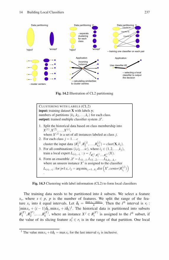
14 Building Local Classifiers 237
Fig. 14.2 Illustration of CL2 partitioning
CLUSTERING WITH LABELS (CL2)
input: training dataset X with labels y;
numbers of partitions (k1,k2, . . . ,kc) for each class.
output: trained multiple classifier system L .
1. Split the historical data based on class membership into
X (1),X (2), . . . ,X (c),
where X ( j) is a set of all instances labeled as class j.
2. For each class j = 1 . . .c
cluster the input data (R( j)1 ,R
( j)2 , . . . ,R
( j)k j
) = clust(X,k j).
3. For all combinations (i1i2 . . . ic), where i j ∈ (1,2, . . . ,k j),train a local expert Li1i2 ...ic : y = f
R(c)1 ,R
(c)2 ,...,R
(c)kc
(X).
4. Form an ensemble L = L11...1,L11...2, . . . ,Lk1k2...kc,
where an unseen instance X ′ is assigned to the classifier
Li1i2...ic : for j=1:c, i j = argmini j=1...k jdist(
X ′,center(R( j)i j
))
.
Fig. 14.3 Clustering with label information (CL2) to form local classifiers
The training data needs to be partitioned into k subsets. We select a feature
xs, where s ∈ p, p is the number of features. We split the range of the fea-
ture xs into k equal intervals. Let δk = maxxs−minxsk
. Then the ith interval is ri :
[minxs + (i− 1)δk,minxs + iδk)1. The historical data is partitioned into subsets
R(F)1 ,R
(F)2 , . . . ,R
(F)k , where an instance X j ∈ R
(F)i is assigned to the ith subset, if
the value of its slicing feature xjs ∈ ri is in the range of that partition. One local
1 The value minxs +kδk = maxxs for the last interval rk is inclusive.

238 I. Zliobaite
classifier is trained on each subset. An incoming instance will be assigned to a clas-
sifier based on the value of its feature xs the same way. We call this approach FEA.
In the research proposal example there may be experts that are good in evaluat-
ing short and concise proposals and another experts that are good in long detailed
proposals. Suppose we have a feature in the feature space that records the number
of words in the document. The partitions may be formed conditioning on that fea-
ture, e.g. if the number of words is less than 2000 then assign it to the first cluster,
otherwise to the second cluster.
There are two parameters to be specified for FEA: k and xi. A simple way is to
select xi using domain expertise or visual inspection of the data. We will elaborate
more on selecting the slicing feature in Sect. 14.4.4.4.
The procedure for FEA is summarized in Fig. 14.4.
ONE FEATURE BASED PARTITIONING (FEA)
input: training dataset X with labels y;
number of partitions k; slicing feature xs.
output: trained multiple classifier system L .
1. For i = 1 . . .k, calculate slicing intervals:
ri : [minxs +(i−1)δk,minxs + iδk),where δk = maxxs−minxs
k.
2. Partition the input data into R(F)1 ,R
(F)2 , . . . ,R
(F)k
,
where X j ∈ R(F)i if x
js ∈ ri.
3. For i = 1 . . .k each partition
train a local expert Li : y = fR
(F)i
(X),
where fR
(F)i
is a classifier trained on R(F)i instances.
4. Form an ensemble L = L1,L2, . . . ,Lk,
where an unseen instance X ′ is assigned to classifier Li if
x′ js ∈ ri.
Fig. 14.4 Slicing based on one feature (FEA) to form local classifiers
14.3 Analysis with the Modeling Dataset
For exploring CLU, CL2 and FEA partitioning strategies we construct a modeling
dataset. We generate dataset in 2D, where four cluster centers are fixed at (0,0),(4.5,3), (1,3), (3,0.1). We label two centers as ‘class 1’ and the other two as ‘class
2’. We generate 5000 normally distributed instances for each center. The data is
illustrated in Fig. 14.5. As it is seen from the plot, the data is linearly inseparable. We
will demonstrate how a multiple classifier system, consisting of locally specialized
linear classifiers classifies this data.

14 Building Local Classifiers 239
−4 −2 0 2 4 6 8−4
−2
0
2
4
6
8
Fig. 14.5 Modeling dataset, green and red colors represent two classes
14.3.1 Testing Scenario
We generate an independent testing set using the same distribution as for training.
We generate a testing set of 20000 instances in total.
14.3.1.1 Performance Metrics
We compare testing errors of the alternative strategies that indicate their general-
ization performance. We use the mean absolute error measure. A standard error
is calculated assuming Binomial distribution over testing errors SE =
√E×(1−E)
N,
where E is the observed error and N is the testing sample size.
14.3.1.2 Alternative Strategies
We experimentally compare the performance of CLU, CL2 and FEA. Figure 14.6
gives an example of the partitions by the three strategies on the modeling data. ’×’
indicates an instance under consideration. We plot the areas of local expertise around
this instance (a) for CLU, in (b) for CL2 and in (c) for FEA.
In addition to the three discussed strategies, we experiment the strategy that aver-
ages the outputs of the three. We will refer to it as MMM. Let YCLU , YCL2 and YFEA
be the labels output by the three respective strategies. Then YMMM = YCLU+YCL2+YFEA3 .
The intuition is to combine the diverse views on the same instance obtained by the
respective strategies.
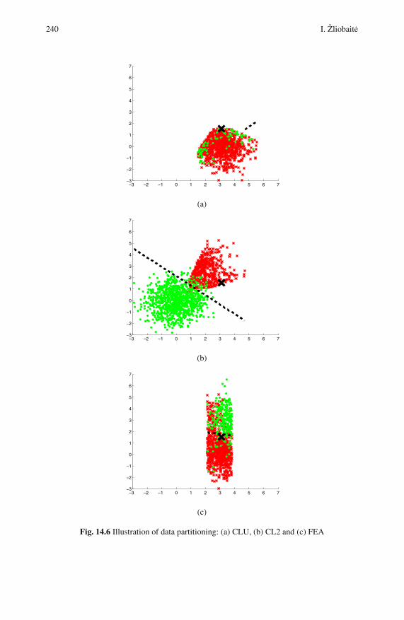
240 I. Zliobaite
−3 −2 −1 0 1 2 3 4 5 6 7−3
−2
−1
0
1
2
3
4
5
6
7
(a)
−3 −2 −1 0 1 2 3 4 5 6 7−3
−2
−1
0
1
2
3
4
5
6
7
(b)
−3 −2 −1 0 1 2 3 4 5 6 7−3
−2
−1
0
1
2
3
4
5
6
7
(c)
Fig. 14.6 Illustration of data partitioning: (a) CLU, (b) CL2 and (c) FEA

14 Building Local Classifiers 241
This strategy can be viewed as an ensemble of ensembles, where classifier se-
lection is used in the first level and then classifier fusion is applied on top of that.
This combination is similar to the random oracle [10]. The principal difference is
that random oracle uses the same partitioning strategy for all mini-ensembles. In
this experimental study we investigate the performance of alternative partitioning
strategies rather than ensemble building strategies, thus we do not include oracles in
our experiments.
In addition, we include two benchmark strategies in our experiments. With the
first strategy we test the benefits of specialization. Here the instances to train local
classifiers are assigned at random instead of employing a directed procedure. In this
case the classifiers are expected to have no specialization, since it will be trained on
a random subset of the historical data. We refer to this strategy as RSS.
The second benchmark strategy does not do any partitioning of the data. It trains
a single classifier on all the available historical data. We call it ALL. Comparing
to this strategy allows us to investigate the effects of reduced training sample size
towards the prediction accuracy.
Finally, we include a baseline strategy, which assigns all the labels according to
the highest prior probability. We refer to it as NAY.
14.3.1.3 Number of Clusters
In the modeling dataset four clusters can be identified visually. We investigate the
strategies of building local classifiers under two scenarios: A) the number of sub-
classes fits correctly (in our modeling dataset k = 4) and B) the number of classes
is incorrect (we use k = 9). That means for CLU, FEA and RSS we test k = 4 and
k = 9 respectively. For CL2 we test k1 = k2 = 2 and k1 = k2 = 3. The latter case
leads to k = 3×3 = 9 local experts for CL2.
14.3.1.4 Base Classifier
We choose logistic regression as the base classifier. The motivation for this choice
is twofold. First, the weights can be interpreted as the importance score of each
feature. Thus it is popular in application tasks, such as credit scoring. Second, it is a
parametric classifier, thus rearranging the training subsets changes the local expert
rules significantly.
We already mentioned that partitioning strategies are likely to distort prior prob-
abilities of the classes within each subset as compared to the whole set of historical
data. Logistic regression uses prior information in training, thus a correction for
priors is required. We use a prior correction for rare events [8]. The regression co-
efficients are statistically consistent estimates, while the correction for an intercept
is as follows: β0 = β0− log[(
1−ττ
)(π
1−π
)], where β0 is an intercept estimated from
the training sample, τ is the population prior for the ‘class 1’ and π is the sample
prior for the ‘class 1’.
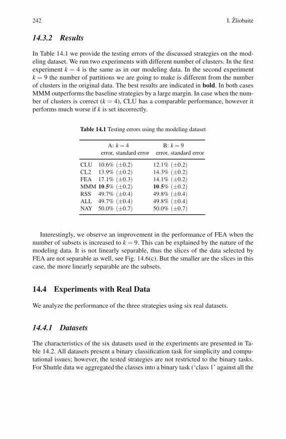
242 I. Zliobaite
14.3.2 Results
In Table 14.1 we provide the testing errors of the discussed strategies on the mod-
eling dataset. We run two experiments with different number of clusters. In the first
experiment k = 4 is the same as in our modeling data. In the second experiment
k = 9 the number of partitions we are going to make is different from the number
of clusters in the original data. The best results are indicated in bold. In both cases
MMM outperforms the baseline strategies by a large margin. In case when the num-
ber of clusters is correct (k = 4), CLU has a comparable performance, however it
performs much worse if k is set incorrectly.
Table 14.1 Testing errors using the modeling dataset
A: k = 4 B: k = 9
error, standard error error, standard error
CLU 10.6% (±0.2) 12.1% (±0.2)CL2 13.9% (±0.2) 14.3% (±0.2)FEA 17.1% (±0.3) 14.1% (±0.2)MMM 10.5% (±0.2) 10.5% (±0.2)RSS 49.7% (±0.4) 49.8% (±0.4)ALL 49.7% (±0.4) 49.8% (±0.4)NAY 50.0% (±0.7) 50.0% (±0.7)
Interestingly, we observe an improvement in the performance of FEA when the
number of subsets is increased to k = 9. This can be explained by the nature of the
modeling data. It is not linearly separable, thus the slices of the data selected by
FEA are not separable as well, see Fig. 14.6(c). But the smaller are the slices in this
case, the more linearly separable are the subsets.
14.4 Experiments with Real Data
We analyze the performance of the three strategies using six real datasets.
14.4.1 Datasets
The characteristics of the six datasets used in the experiments are presented in Ta-
ble 14.2. All datasets present a binary classification task for simplicity and compu-
tational issues; however, the tested strategies are not restricted to the binary tasks.
For Shuttle data we aggregated the classes into a binary task (‘class 1’ against all the

14 Building Local Classifiers 243
others). In Marketing data we transformed the categorical features to numerical by
expanding the feature space. We constructed Chess dataset2 using the statistics from
Chess.com, the task is to predict the outcome of a game given the players and game
setup characteristics. Elec2 dataset is known to be non-stationary. In these settings
non-stationarity is expected to be handled directly by local learners.
Table 14.2 Real datasets used in the experimental evaluation
size dimensionality class balance source
cred 1000 23 70%−30% (German credit) [13]
shut 43500 9 22%−78% (Shuttle) [13]
spam 4601 57 39%−61% (Spam) [5]
marc 8993 48 47%−53% (Marketing) [5]
elec 44235 7 43%−57% (Elec2) [4]
chess 503 8 39%−61% author collection
14.4.2 Implementation Details
Testing sets were formed using the holdout testing procedure. Each dataset was split
into two equal parts at random, one was used for training, the other for testing.
The parameters and experimental choices were fixed as follows, unless reported
otherwise. The number of partitions was fixed to k = 4 in all partitioning strategies
(CLU, CL2, FEA, RSS). We chose to use simple and intuitive k-means clustering
algorithm.
For FEA we chose the slicing feature to be the first feature in a row having 4 or
more distinct values. The selected feature may be different across the datasets, but
the procedure for choosing it is the same for all.
14.4.3 Experimental Goals
The goal of these experiments is to compare the classification accuracies when
using the three partitioning strategies (CLU, CL2, FEA) and a combination of
those (MMM) and analyze the underlying properties of the data leading to these
accuracies.
We aim to be able to assign the credits for a better accuracy. Thus, two bench-
marks (ALL, RSS) and a baseline (NAY) are included for control reasons. We look
at the following guidelines for control:
• We expect the partitioning strategies (CLU, CL2, FEA) to do better than no par-
titioning (ALL) in order for partitioning to make sense.
2 The dataset is available at
http://sites.google.com/site/zliobaite/resources-1
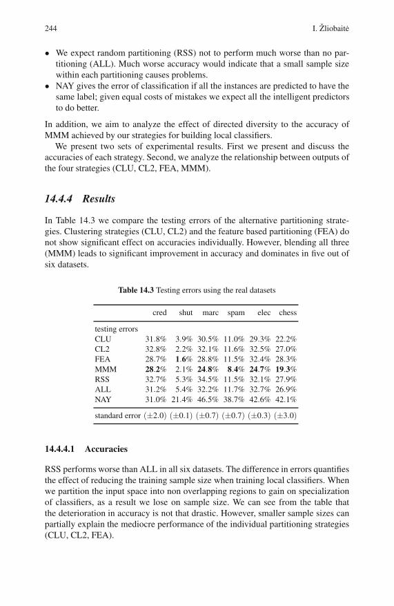
244 I. Zliobaite
• We expect random partitioning (RSS) not to perform much worse than no par-
titioning (ALL). Much worse accuracy would indicate that a small sample size
within each partitioning causes problems.
• NAY gives the error of classification if all the instances are predicted to have the
same label; given equal costs of mistakes we expect all the intelligent predictors
to do better.
In addition, we aim to analyze the effect of directed diversity to the accuracy of
MMM achieved by our strategies for building local classifiers.
We present two sets of experimental results. First we present and discuss the
accuracies of each strategy. Second, we analyze the relationship between outputs of
the four strategies (CLU, CL2, FEA, MMM).
14.4.4 Results
In Table 14.3 we compare the testing errors of the alternative partitioning strate-
gies. Clustering strategies (CLU, CL2) and the feature based partitioning (FEA) do
not show significant effect on accuracies individually. However, blending all three
(MMM) leads to significant improvement in accuracy and dominates in five out of
six datasets.
Table 14.3 Testing errors using the real datasets
cred shut marc spam elec chess
testing errors
CLU 31.8% 3.9% 30.5% 11.0% 29.3% 22.2%
CL2 32.8% 2.2% 32.1% 11.6% 32.5% 27.0%
FEA 28.7% 1.6% 28.8% 11.5% 32.4% 28.3%
MMM 28.2% 2.1% 24.8% 8.4% 24.7% 19.3%
RSS 32.7% 5.3% 34.5% 11.5% 32.1% 27.9%
ALL 31.2% 5.4% 32.2% 11.7% 32.7% 26.9%
NAY 31.0% 21.4% 46.5% 38.7% 42.6% 42.1%
standard error (±2.0) (±0.1) (±0.7) (±0.7) (±0.3) (±3.0)
14.4.4.1 Accuracies
RSS performs worse than ALL in all six datasets. The difference in errors quantifies
the effect of reducing the training sample size when training local classifiers. When
we partition the input space into non overlapping regions to gain on specialization
of classifiers, as a result we lose on sample size. We can see from the table that
the deterioration in accuracy is not that drastic. However, smaller sample sizes can
partially explain the mediocre performance of the individual partitioning strategies
(CLU, CL2, FEA).
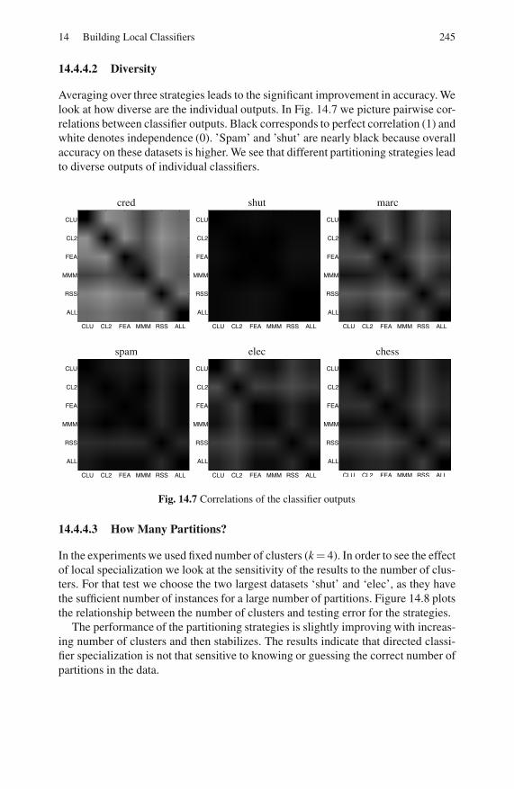
14 Building Local Classifiers 245
14.4.4.2 Diversity
Averaging over three strategies leads to the significant improvement in accuracy. We
look at how diverse are the individual outputs. In Fig. 14.7 we picture pairwise cor-
relations between classifier outputs. Black corresponds to perfect correlation (1) and
white denotes independence (0). ’Spam’ and ’shut’ are nearly black because overall
accuracy on these datasets is higher. We see that different partitioning strategies lead
to diverse outputs of individual classifiers.
cred shut marc
CLU CL2 FEA MMM RSS ALL
CLU
CL2
FEA
MMM
RSS
ALL
CLU CL2 FEA MMM RSS ALL
CLU
CL2
FEA
MMM
RSS
ALL
CLU CL2 FEA MMM RSS ALL
CLU
CL2
FEA
MMM
RSS
ALL
spam elec chess
CLU CL2 FEA MMM RSS ALL
CLU
CL2
FEA
MMM
RSS
ALL
CLU CL2 FEA MMM RSS ALL
CLU
CL2
FEA
MMM
RSS
ALL
CLU CL2 FEA MMM RSS ALL
CLU
CL2
FEA
MMM
RSS
ALL
Fig. 14.7 Correlations of the classifier outputs
14.4.4.3 How Many Partitions?
In the experiments we used fixed number of clusters (k = 4). In order to see the effect
of local specialization we look at the sensitivity of the results to the number of clus-
ters. For that test we choose the two largest datasets ‘shut’ and ‘elec’, as they have
the sufficient number of instances for a large number of partitions. Figure 14.8 plots
the relationship between the number of clusters and testing error for the strategies.
The performance of the partitioning strategies is slightly improving with increas-
ing number of clusters and then stabilizes. The results indicate that directed classi-
fier specialization is not that sensitive to knowing or guessing the correct number of
partitions in the data.
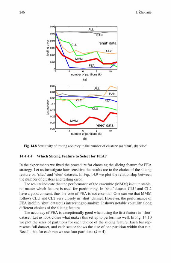
246 I. Zliobaite
2 4 6 8 100
0.01
0.02
0.03
0.04
0.05
0.06
number of partitions (k)
testing e
rror
’shut’ data
CL2
CLU
MMM
FEA
RAN
ALL
(a)
2 4 6 8 100.22
0.24
0.26
0.28
0.3
0.32
0.34
0.36
number of partitions (k)
testing e
rror
’elec’ data
MMM
CL2
CLU
FEA
RAN
ALL
(b)
Fig. 14.8 Sensitivity of testing accuracy to the number of clusters: (a) ‘shut’, (b) ‘elec’
14.4.4.4 Which Slicing Feature to Select for FEA?
In the experiments we fixed the procedure for choosing the slicing feature for FEA
strategy. Let us investigate how sensitive the results are to the choice of the slicing
feature on ‘shut’ and ‘elec’ datasets. In Fig. 14.9 we plot the relationship between
the number of clusters and testing error.
The results indicate that the performance of the ensemble (MMM) is quite stable,
no matter which feature is used for partitioning. In ‘shut’ dataset CLU and CL2
have a good consent, thus the vote of FEA is not essential. One can see that MMM
follows CLU and CL2 very closely in ‘shut’ dataset. However, the performance of
FEA itself in ‘shut’ dataset is interesting to analyze. It shows notable volatility along
different choices of the slicing feature.
The accuracy of FEA is exceptionally good when using the first feature in ‘shut’
dataset. Let us look closer what makes this set up to perform so well. In Fig. 14.10
we plot the sizes of partitions for each choice of the slicing feature. Each bar rep-
resents full dataset, and each sector shows the size of one partition within that run.
Recall, that for each run we use four partitions (k = 4).
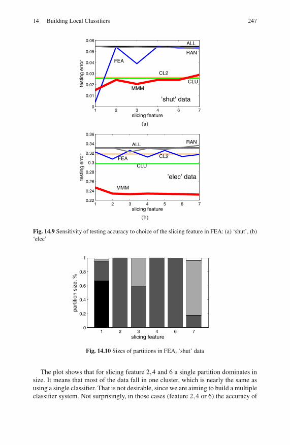
14 Building Local Classifiers 247
1 2 3 4 6 70
0.01
0.02
0.03
0.04
0.05
0.06
slicing feature
testing e
rror
’shut’ data
MMM
CLU
CL2
FEA
ALL
RAN
(a)
1 2 3 4 5 6 70.22
0.24
0.26
0.28
0.3
0.32
0.34
0.36
slicing feature
testing e
rror
’elec’ data
MMM
RANALL
FEA CL2
CLU
(b)
Fig. 14.9 Sensitivity of testing accuracy to choice of the slicing feature in FEA: (a) ‘shut’, (b)
‘elec’
1 2 3 4 6 70
0.2
0.4
0.6
0.8
1
slicing feature
pa
rtitio
n s
ize
, %
Fig. 14.10 Sizes of partitions in FEA, ‘shut’ data
The plot shows that for slicing feature 2,4 and 6 a single partition dominates in
size. It means that most of the data fall in one cluster, which is nearly the same as
using a single classifier. That is not desirable, since we are aiming to build a multiple
classifier system. Not surprisingly, in those cases (feature 2,4 or 6) the accuracy of
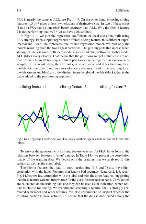
248 I. Zliobaite
FEA is nearly the same as ALL, see Fig. 14.9. On the other hand, choosing slicing
features 1,3 or 7 gives at least two clusters of distinctive size. In two of these cases
(1 and 3) FEA stand alone gives better accuracy than ALL. Why the slicing feature
7 is not performing that well? Let us have a closer look.
In Fig. 14.11 we plot the regression coefficients of local classifiers built using
FEA strategy. Each subplot represents different slicing feature, thus different exper-
imental run. Each line represents one trained regression model. We plot only the
models resulting from the two largest partitions. The plot suggests that in case when
slicing feature 7 is used, both local models (green and blue) follow the global model
ALL (black) very closely. That means that the partitions we get in that case are not
that different from all training set. Such partitions can be regarded as random sub-
samples of the whole data, thus do not give much value added for building local
models. On the other hand, in cases of slicing features 1 and 3 the resulting local
models (green and blue) are quite distinct from the global models (black), that is the
value added to the partitioning approach.
slicing feature 1 slicing feature 3 slicing feature 7
Fig. 14.11 Regression coefficients of FEA local classifiers (green and blue) and ALL classifier
(black)
To answer the question, which slicing feature to select for FEA, let us look at the
relations between features in ‘shut’ dataset. In Table 14.4 we present the correlation
matrix of the training data. We depict only the features that we analyzed in this
section as well as the class label.
The slicing features that lead to good partitioning (1,3 and 7) also have high
correlation with the label. Features that lead to bad accuracy (features 2,4,6, recall
Fig. 14.9) show low correlation with the label and with the other features, suggesting
that these features are not informative for the classification task at hand. Correlations
are calculated on the training data and they can be used as an indication, which fea-
ture to choose for slicing. We recommend selecting a feature, that is strongly cor-
related with label and other features. We also recommend to inspect whether the
resulting partitions have volume, i.e. ensure that the data is distributed among the

14 Building Local Classifiers 249
Table 14.4 Correlation matrix of ‘shut’ training data (high correlations in bold)
feature 1 2 3 4 6 7 label
1 - 0.06 0.26 -0.01 0 -0.75 -0.66
2 0.06 - -0.01 -0 -0 -0.06 0
3 0.26 -0.01 - 0.02 -0 0.43 -0.13
4 -0.01 -0 0.02 - 0 0.03 0
6 0 -0 -0 0 - -0.01 0.01
7 -0.75 -0.06 0.43 0.03 -0.01 - 0.54
label -0.66 0.00 -0.13 0.00 0.01 0.54 -
clusters. Finally, we recommend to inspect the resulting local classifiers, to ensure
that they represent different data distributions. This can be done by inspecting the
parameters of the trained models, or by monitoring the diversity of the classifier
outputs.
14.5 Conclusion
We experimentally investigated three approaches of building local classifiers. Each
partitioning strategy individually often does not give significant improvement in
accuracy as compared to a single classifier. However, blending the three strategies
demonstrates significant improvement in accuracy as compared to the baseline and
benchmarks.
This approach can be viewed as a two level ensemble. The first level uses deter-
ministic classifier selection from a pool of local classifiers. The second level aver-
ages over individual classifiers selected from different partitions of the input space.
We identify several properties of the partitions that lead to improvement in over-
all accuracy as compared to a single classifier. We recommend partitioning using a
feature that is strongly correlated with the labels and other features. We also recom-
mend to inspect whether the resulting partitions have sufficient data volume as well
as to monitor that the resulting local classifiers output diverse predictions.
A natural and interesting extension of this study would be to look at partitioning
strategies, not limited to distance in space as clustering. One relevant direction for
further research is developing meta features to describe subsets of instances and use
them for nominating the classifiers (experts) that make the final decision.
Acknowledgements. The research leading to these results has received funding from the
European Commission within the Marie Curie Industry and Academia Partnerships and Path-
ways (IAPP) programme under grant agreement no. 251617. The author thanks Dr. Tomas
Krilavicius for feedback on the experimental setting.

250 I. Zliobaite
References
1. Breiman, L.: Bagging predictors. Machine Learning 24(1996), 123–140 (1996)
2. Brown, G., Wyatt, J., Harris, R., Yao, X.: Diversity creation methods: a survey and cate-
gorization. Inf. Fusion 6, 5–20 (2005)
3. Frosyniotis, D., Stafylopatis, A., Likas, A.: A divide-and-conquer method for multi-net
classifiers. Pattern Analysis and Appl. 6, 32–40 (2003)
4. Harries, M.: Splice-2 comparative evaluation: Electricity pricing. Technical Report
UNSW-CSE -TR-9905, Artif. Intell. Group, School of Computer Science and Engineer-
ing, The University of New South Wales, Sidney (1999)
5. Hastie, T., Tibshirani, R., Friedman, J.: The elements of statistical learning: data mining,
inference and prediction. Springer, Heidelberg (2005)
6. Jacobs, R., Jordan, M., Nowlan, S., Hinton, G.: Adaptive mixtures of local experts. Neu-
ral Computation 3, 79–87 (1991)
7. Katakis, I., Tsoumakas, G., Vlahavas, I.: Tracking recurring contexts using ensemble
classifiers: an application to email filtering. Knowledge and Inf. Syst. 22, 371–391 (2009)
8. King, G., Zeng, L.: Logistic regression in rare events data. Political Analysis 9(2001),
137–163 (2001)
9. Kuncheva, L.: Clustering-and-selection model for classifier combination. In: Proc. the
4th Int. Conf. Knowledge-Based Intell. Eng. Syst. and Allied Technologies, Brighton,
UK, pp. 185–188 (2000)
10. Kuncheva, L.I., Rodriguez, J.J.: Classifier ensembles with a random linear oracle. IEEE
Trans. Knowledge and Data Eng. 19, 500–508 (2007)
11. Lim, M., Sohn, S.: Cluster-based dynamic scoring model. Expert Systems with Appl. 32,
427–431 (2007)
12. Liu, R., Yuan, B.: Multiple classifiers combination by clustering and selection. Inf. Fu-
sion 2, 163–168 (2001)
13. Newman, D.J., Asuncion, A.: UCI machine learning repository,
http://archive.ics.uci.edu/ml/
Index
accuracy-diversity trade-off 170–172
AdaBoost 2, 3, 22, 171, 181, 182, 184,
185, 188, 191, 192, 194, 201–203,
206, 207, 209, 210, 214, 215
Bagging 59, 60, 64–66, 68–70, 72, 78,
87, 94, 100, 106, 109, 113, 114, 169,
173, 181, 182, 184, 185, 191, 192,
194, 234
balanced decomposition schemes 41, 46,
47
Bayesian Networks 93, 98, 99, 108, 113,
117–119, 124–126, 128, 133
bias 1, 4, 15, 17, 22, 45, 50, 51, 54, 59,
62–66, 68, 69, 72, 99, 137, 146
bias-variance trade-off 15, 71
Boosting 41, 78, 169, 170, 201, 202, 204,
218
bootstrap 4, 13, 59, 106, 170
class-separability classifier weighting 4
classification 1–4, 6, 8, 10, 13, 16, 21,
22, 28–30, 32–36, 41–45, 51–53, 55,
59–65, 72, 78, 87, 91, 98, 99, 109,
117, 119, 121, 124, 133, 134, 136,
138, 144, 146, 148, 152, 154–159,
163, 169–171, 174, 177, 181, 182,
191, 202, 203, 208–210, 214–216,
219, 224, 226, 227, 233, 234,
242–244, 248
Cohn-Kanade face expression database
10
correlation 76–80, 84, 85, 92–94, 101,
102, 106, 110, 170, 245, 248
correlation-based feature selection 75,
76, 97, 99–101, 105, 110
decomposition schemes 39–49
directed diversity 234, 244
diversity 3, 40, 81, 87, 106, 138, 147,
169–175, 177, 182, 191, 192, 194,
201, 215, 217–219, 226, 227, 234, 249
diversity-error diagrams 182, 191, 192,
194
ensemble 3, 16, 21–23, 44, 45, 47, 49, 50,
59–62, 65, 69, 71, 75, 77–81, 83–85,
87, 89–95, 97, 99, 105, 106, 113,
114, 117, 120–122, 124, 130, 140,
144, 151, 153, 155, 158, 159, 161,
162, 164, 165, 169, 171–174, 177,
181–185, 188, 191, 201, 206, 212,
215–221, 226, 235, 241, 246, 249
ensemble selection 169–175, 177
Error-Correcting Output Codes 1, 3,
21–23, 36
Error-Correcting Output Coding 39, 40,
43, 51, 54, 59
Evolutionary Computation 21, 36
expert knowledge 133, 134, 136, 138
facial action coding system 1, 2
facial action units 1, 2
facial expression recognition 1, 4, 7
fast correlation-based filtering 1, 2, 8, 99,
100
252 Index
feature selection 8, 75, 76, 78, 81, 86,
87, 91, 93, 94, 98–100, 102, 105, 109,
110, 114, 117–121, 124, 125, 127,
130, 144, 162
Fisher subspace 156, 164
gating network 217, 219–222, 227, 230
glaucoma 133, 134, 138, 143, 144, 148
Grow-Shrink algorithm 103
Hierarchical Mixture of Experts 217, 218
Incremental Association Markov Blanket
algorithm 103
IPCAC, 156
Iterated Bagging 181, 182, 184, 185, 194
K-nearest-neighbor 154
Kernel Isotropic Principal Component
Analysis Classifier 157
Linear Random Oracle 181, 183
local binary pattern 1, 2, 7
local classifiers 233–236, 241, 244, 248,
249
local experts 234–236, 241
LsBoost 202–207, 209, 210, 215
Machine Learning 22, 59, 99, 140, 161,
169, 201, 202, 217
Markov Blanket 100–106, 110, 113,
117–119, 121–123, 128
microarray data 75, 93
minimally-sized balanced decomposition
schemes 39, 40, 47
Mixture of Experts 217, 218
Mixture of Random Prototype-Based
Experts 219, 222
model averaging 136
multi-class classification 39–44, 48, 66,
72, 151, 152, 158, 159, 162, 165
Multi-Layer Perceptron 3, 227
Naive Bayes 87, 91, 155
Neural Networks 3, 16, 59, 99, 171
one-against-all decomposition schemes
39, 40, 43, 53, 55
out-of-bag estimation 182
partial whitening 156
PC algorithm 102
Platt scaling 1, 3, 7, 10, 13, 14, 17
Principal Component Analysis 2, 32, 157
protein subcellular localization 152
quantitative scoring 186
Random Forest 76, 159, 161, 170
Random Oracle 181–183
Random Projections 201, 203, 215
regions of competence 234
regression 4, 51, 57, 62–64, 117–119, 121,
124, 135, 159, 170, 181, 182, 185,
192, 194, 241, 248
Regression Tree 185
Regularized Gradient Boosting 206
ROC curve 12, 14, 147, 173, 174
Rooted Direct Acyclic Graph (DAG) 158
RpBoost 206–210, 214–216
semi-supervised models 133
Sequential Forward Floating Search 100,
102
simulated annealing 136, 141
slicing feature 236–238, 243, 246–248
stacked ensembles 140
supervised models 133
Support Vector Machines 22, 29, 41, 51,
53, 60, 61, 109, 155
Three phase dependency analysis algorithm
103
Truncated Singular Value Decomposition
156
variance 1, 2, 4, 15, 17, 22, 45, 50, 51,
54, 59, 62–66, 69, 72, 75, 76, 78, 93,
94, 99, 157, 169, 173, 177
voting 22, 39–41, 46, 49, 55, 159, 173
weighted vote 134, 144, 146, 147
Weka 17, 55, 161, 185, 194


