Embed Size (px)
Citation preview
Appl Intell (2011) 34: 347–359DOI 10.1007/s10489-011-0283-2
O R I G I NA L PA P E R
Random projections for linear SVM ensembles
Jesús Maudes · Juan J. Rodríguez ·César García-Osorio · Carlos Pardo
Published online: 30 March 2011© Springer Science+Business Media, LLC 2011
Abstract This paper presents an experimental study usingdifferent projection strategies and techniques to improvethe performance of Support Vector Machine (SVM) en-sembles. The study has been made over 62 UCI datasetsusing Principal Component Analysis (PCA) and threetypes of Random Projections (RP), taking into accountthe size of the projected space and using linear SVMsas base classifiers. Random Projections are also combinedwith the sparse matrix strategy used by Rotation Forests,which is a method based in projections too. Experimentsshow that for SVMs ensembles (i) sparse matrix strategyleads to the best results, (ii) results improve when pro-jected space dimension is bigger than the original one,and (iii) Random Projections also contribute to the re-sults enhancement when used instead of PCA. Finally,random projected SVMs are tested as base classifiers ofsome state of the art ensembles, improving their perfor-mance.
Keywords Ensembles · Random projections · Rotationforests · Diversity · Kappa-error relative movementdiagrams · SVMs
J. Maudes (�) · J.J. Rodríguez · C. García-Osorio · C. PardoUniversity of Burgos, Escuela Politécnica Superior C/Fco.,Vitoria s/n, 09006, Spaine-mail: [email protected]
J.J. Rodrígueze-mail: [email protected]
C. García-Osorioe-mail: [email protected]
C. Pardoe-mail: [email protected]
1 Introduction
Projections techniques are broadly used to reduce input di-mensionality in classification problems [2, 20]. Projectionmethods are designed to preserve in someway data origi-nal structure in the projected space, so projected data can beused to speed up classifiers training and sometimes help toavoid noise and over-fitting [2]. PCA is probably the mostpopular projection method. It is used to reduce data dimen-sionality capturing a percentage of the variance in the origi-nal data. A drawback of PCA is its computational complex-ity. Random Projections (RP) [1, 9] have a lower computa-tional cost. Some RPs can maintain pairwise distances in theprojected space within an arbitrary small factor.
RPs have been used to build classifiers. In [20] RPsare used to build ensembles of Nearest Neighbors, and [5]shows a variant of KD-trees that uses RPs. Both approachesreduce input space dimensionality.
SVMs [21] are very stable classifiers. Small changes inthe training dataset does not make very different SVMs.Therefore, it is difficult to get an ensemble of SVMs that per-form better than a single SVM using state of the art ensem-ble methods. One question to answer in this paper is if therandomness inherent to RPs can be considered as a sourceof diversity that aims at getting accurate SVM ensembles.So, we are not interested in using projection for reducinginput dimensionality, but to increase SVM ensembles per-formance.
Rotation Forests [19] is an ensemble method for decisiontrees. It uses PCA to project different groups of attributes ineach base classifier. In [16] it is shown that PCA is betterthan RP for such ensemble method of decision trees. How-ever, the essential ingredient of Rotation Forests is to projectusing those groups of attributes, which also makes base clas-sifiers in the ensemble to be trained differently each other.
348 J. Maudes et al.
That difference in the training process does not produce verydiverse base classifiers, but it seems to keep their individ-ual accuracy. In [16] diversity is analyzed for RPs with andwithout splitting into groups of attributes. Projecting with-out splitting the input space turn into more diverse classifiersbut are also less accurate. Hence, the additional diversity ob-tained through the “full” random projection is not useful forthe ensemble. That work was made for decision trees whichare very sensitive to small changes. In our work we also testthe effect of splitting projections, but using SVM as baseclassifiers this time.
The rest of the paper is organized as follows: RandomProjections considered in this work are described in Sect. 2.A brief introduction to the Random Forests method is pro-vided at Sect. 3. An experimental study is presented inSect. 4. In Sect. 5, SVMs trained with RPs are tested as baseclassifiers within state of the art ensembles. Analysis of di-versity is in Sect. 6. Finally, conclusions are summarized inSect. 7.
2 Random projections
Data projections are made using a transformation matrixDo × Dp , where Do is the dimension of the original datasetspace, and Dp is the dimension of the projected space. Whenan instance x is projected, the vector containing its valuesis multiplied by this matrix obtaining a new vector (i.e., xprojection). Usually, projections are used to reduce datasetdimensionality (i.e., Do > Dp) with the aim of noise reduc-tion or to speed up computation. In most projection methodsthe resulting transformation matrix can not take a Dp valuebigger than Do (e.g., PCA) . However, for RPs it is possibleto get a projected space which is bigger than the original,because in RPs the matrix entries are simply random num-bers. These RPs that make dimensionality grows has alsobeen tested in this work. Three types of RPs have been used:
1. Each entry in transformation matrix comes from aGaussian distribution (mean 0 and standard deviation 1).This RP is denoted as Gaussian in this work.
2. The entries values are√
3×x, where x is a random num-ber taking the following values: −1 with probability 1/6,0 with probability 2/3 and +1 with probability 1/6. ThisRP is denoted as Sparse in this work.
3. The entries are −1 with probability 1/2 and +1 withprobability 1/2. This RP is denoted as Binary in thiswork.
The two latter are described in [1]. They are basedon Johnson and Lindenstrauss theorem [14]. This theoremstates that given ε > 0, an integer n and k a positive inte-ger such that k ≥ k0 = O(ε−2 log(n)). For every set P of
n points in Rd there exists f : R
d → Rk such that for all
u,v ∈ P
(1 − ε)‖u − v‖2 ≤ ∥∥f (u) − f (v)
∥∥2 ≤ (1 + ε)‖u − v‖2 (1)
Hence, these two methods aim at preserving pairwiseeuclidean distances in the projected space. They are fast tocompute as well.
It is expected that Sparse projection can contribute to di-versity because of the amount of zeros. The zeros would re-ject some original dimensions in the computation of some ofthe new dimensions. There are successful ensemble methodsthat also train their base classifiers by excluding some exist-ing features. In the Random Subspaces method [13], eachbase classifier only takes into account a subset of the at-tributes from the original space. The size of this subset ofattributes is specified as a percentage.
3 Rotation forest method
Rotation Forest [16, 19] is a novel ensemble method. Maybebecause of its youngness, it is not as popular as other ensem-ble approaches, but its performance has been proved, gettingremarkable results. This section is intended to explain thisnew method briefly.
Rotation Forest base classifiers are decision trees. Eachbase classifier is trained on a rotated dataset. For transform-ing the dataset, the attributes are randomly split in groups. Ineach group, a random non empty subset of the classes is se-lected, and the examples of the classes that are not in the sub-set are removed. From the remaining examples, a sample istaken that is used to calculate PCA. All the components fromall the groups are the features of the transformed dataset.All the examples in the original training data are used forconstructing the base classifier, the selection of classes andexamples are only used to calculate the PCA projection ma-trices (one per group), but then all the data is transformedaccording with these matrices.
The base classifier receives all the information availablein the dataset, because all the examples and all the compo-nents obtained from PCA are used.
Rotation Forest pseudo-code is showed at Algorithm 1.
4 Experiments
Experimental validation has been made using WEKA [12]for the ensembles and projections. In order to limit theanalysis scope to a manageable number of combinations, thelinear kernel was the only kernel considered for SVMs in theexperiment. LIBLINEAR [8] was used because it provides afast linear kernel SVM implementation. Default parameterswere used in all methods where not indicated.
Random projections for linear SVM ensembles 349
Algorithm 1: Pseudocode of the Rotation Forestmethod.
Input: Training set S = (x1, y1), . . . , (xn, yn); baselearning algorithm L; number of iterations t ;group size g.
Output: Classifier ensemble C∗m ← {dimensionality of xi}1
k ← m/g� // the number of groups2
for i ← 1 to t do3
Split the feature set F into k disjoint groups of size4
m: Fi,j (for j = 1 . . . k), such as F = ⋃kj=1 Fi,j
// a group could have repeated featuresforeach Fi,j do5
Si,j ← {S in subspace Fi,j }.6
Select a proper subset of the classes in S,7
remove from Si,j all the examples from theclasses in the subset.Remove from Si,j a random subset of the8
examples.Obtain projection Pi,j using Si,j .9
end10
Pi ← ⋃kj=1 Pi,j // combine the projections of each11
groupCi ← L(Pi(S)) // train the base classifier in the12
projected space
end13
C∗ ← ⋃ti=1 Ci // the ensemble is the union of the base14
classifiers
62 datasets from UCI repository [10] used in the exper-iments are shown in Table 1. Nominal attributes are com-puted using Nominal to Binary transformation in all meth-ods. This approach translates each nominal value into n bi-nary features, where n is the number of possible values thatthe nominal feature can take. So, each nominal value be-comes into n values all equal to 0 but the value of the binaryfeature representing such nominal value, which is set to 1.
Random Projections were used in the following ensem-bles:
1. An ensemble of SVMs trained with projected data. Threesizes of projected space dimension have been tested (i.e.,75%, 100%, and 125% of attributes). The ensemble com-putes its prediction probabilities as the straight averageof the probabilities predicted by its members. These con-figurations are denoted as RP-Ensemble n%, where n isthe percentage indicating the dimension of the projectedspace. Hence 125% configuration makes input dimen-sionality grow.
2. A Rotation Forests [19] variant that replaces PCA pro-jection by RPs and the Decision Trees by SVMs. Rota-
Table 1 Datasets used in the experiments. #N: Numeric features, #D:Discrete features, #I: Inputs, #E: Examples, #C: Classes
Dataset #N #D #I #E #C
abalone 7 1 10 4177 28anneal 6 32 90 898 6audiology 0 69 93 226 24autos 15 10 71 205 6balance-scale 4 0 4 625 3breast-w 9 0 9 699 2breast-y 0 9 48 286 2bupa 6 0 6 345 2car 0 6 21 1728 4credit-a 6 9 43 690 2credit-g 7 13 61 1000 2crx 6 9 42 690 2dna 0 180 180 3186 3ecoli 7 0 7 336 8glass 9 0 9 214 6heart-c 6 7 22 303 2heart-h 6 7 22 294 2heart-s 5 8 25 123 2heart-statlog 13 0 13 270 2heart-v 5 8 25 200 2hepatitis 6 13 19 155 2horse-colic 7 15 60 368 2hypo 7 18 25 3163 2ionosphere 34 0 34 351 2iris 4 0 4 150 3krk 6 0 6 28056 18kr-vs-kp 0 36 40 3196 2labor 8 8 26 57 2led-24 0 24 24 5000 10letter 16 0 16 20000 26lrd 93 0 93 531 10lymphography 3 15 38 148 4mushroom 0 22 121 8124 2nursery 0 8 26 12960 5optdigits 64 0 64 5620 10page 10 0 10 5473 5pendigits 16 0 16 10992 10phoneme 5 0 5 5404 2pima 8 0 8 768 2primary 0 17 23 339 22promoters 0 57 228 106 2ringnorm 20 0 20 300 2sat 36 0 36 6435 6segment 19 0 19 2310 7shuttle 9 0 9 58000 7sick 7 22 33 3772 2sonar 60 0 60 208 2soybean 0 35 84 683 19soybean-small 0 35 84 47 4splice 0 60 287 3190 3threenorm 20 0 20 300 2tic-tac-toe 0 9 27 958 2twonorm 20 0 20 300 2vehicle 18 0 18 846 4vote1 0 15 45 435 2voting 0 16 16 435 2vowel-context 10 2 26 990 11vowel-nocontext 10 0 10 990 11waveform 40 0 40 5000 3yeast 8 0 8 1484 10zip 256 0 256 9298 10zoo 1 15 16 101 7
350 J. Maudes et al.
tion Forests divide input space into different partitionsfor each base classifier. In this experiment the size of allpartitions has been set to 5.1
For each partition an RP is computed. The sizes ofthe projections tested has been set again to 75%, 100%and 125% of the 5 attributes. Once more, we want to testprojections that augment the original problem dimension.These configurations has been denoted as Rot-RP n%,where n is the percentage indicating the dimension of theprojected partitions. For Rot-RP all nominal attributeshave been previously converted into binary to increasethe number or partitions. Column #I in Table 1 shows theresulting dimensionality after such conversion.
These 6 configurations have been tested using the 3random projections described in previous section (i.e.,Gaussian, Sparse, and Binary, denoted as G, S and B re-spectively), resulting into 18 RP based ensembles.
These RP based ensembles have been tested against thebase method on its own, (i.e., LIBLINEAR SVM) and thefollowing state of art ensemble methods:
– Bagging [3] of SVM.– Boosting of SVM. AdaBoost [11] and MultiBoost [22]
versions were considered. Resampling version of bothmethods was used (i.e., training instances for each baseclassifier are obtained as a sample of the original data ac-cording to its weights distribution). The number of sub-committees in MultiBoost was set to 10.
– Random Subspaces [13] using 50% and 75% of originalfeatures (each nominal feature is considered as one fea-ture).
– Rotation Forests [19] replacing Decision Trees by SVM.Two configurations was tested changing the parameterthat controls the proportion of variance retained by PCAprojection, which was set to 75% and 100%. These con-figurations are denoted as Rot-PCA in tables. In order tocompare Rotation PCAs to Rotation-RPs the size of at-tribute partitions was also set to 5, and nominal to binaryconversion is applied beforehand as well.
All ensemble configurations in the experiment use 50base SVM classifiers. The results were obtained using 5 × 2stratified cross validations [7].
Table 2 shows all the methods ordered by their aver-age ranks [6], “average ranks by themselves provide a faircomparison of the algorithms”. Average ranks are com-puted sorting all the methods by their accuracy for eachdataset. Then the average position of each method throughall datasets is assigned as the average rank for that method.
1If dataset dimension is less than 5, Rotation Forests implementationresamples from the existing attributes until such number is reached,according to comment on line 4 of Algorithm 1. This strategy givesrandomly more weight to some attributes, leading usually to differenttraining datasets for each base classifier.
Table 2 Average rank of the considered methods. Avg Rank col-umn represents the average position taken by the method through alldatasets. The methods are ordered by this column. Pos points themethod position according such order
Pos Method Avg Rank
1 Rot RP 125% B 9.21
2 Rot RP 100% G 9.23
3 Rot RP 125% S 9.52
4 Rot RP 125% G 9.85
5 Rot RP 100% S 10.47
6 Rot RP 100% B 10.88
7 Rot PCA 100% 10.93
8 Bagging 11.28
10.5 RP Ensemble 125% S 12.34
10.5 SVM 12.34
11 RS 75% 12.47
12 MultiBoost 12.79
13 RP Ensemble 100% S 13.28
14 RP Ensemble 125% G 13.73
15 Rot RP 75% G 14.69
16 Rot RP 75% B 14.98
17 Rot PCA 75% 15.01
18 RP Ensemble 100% G 15.10
19 RP Ensemble 125% B 15.19
20 AdaBoost 15.69
21 Rot RP 75% S 16.02
22 RP Ensemble 75% S 16.14
23 RP Ensemble 100% B 16.31
24 RS 50 16.90
25 RP Ensemble 75% G 17.64
26 RP Ensemble 75% B 19.01
The six best ranked methods in the table are Rot-RPs con-figurations followed by Rot-PCA 100% and Bagging. More-over, Binary and Sparse configurations projecting 125% ofattributes from these six configurations get better resultsthan projecting 100%.
For each method using projections, its 75% configura-tion is always the worst. Therefore, dimensionality reduc-tion leads to poor results, and it is better to keep or increaseoriginal dimensionality.
When a given random projection technique (i.e., Binary,Sparse or Gaussian) is taken, the RP-Ensemble configura-tions for that technique in the ranking are also ordered de-scending by the percentage of projected attributes. So itseems that increasing the number of random projected fea-tures leads to a performance enhancement.
However, such a rule is not true for Rot-RP methods (e.g.,125% configuration is not the best for Gaussian Rot-RP).
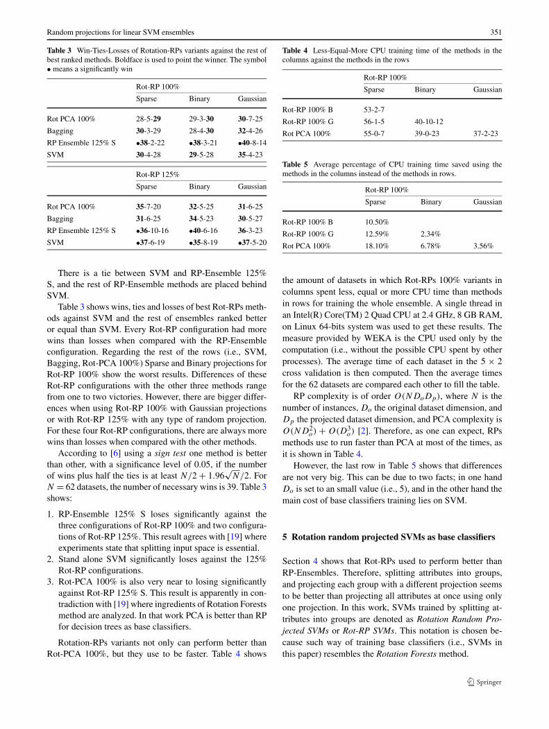
Random projections for linear SVM ensembles 351
Table 3 Win-Ties-Losses of Rotation-RPs variants against the rest ofbest ranked methods. Boldface is used to point the winner. The symbol• means a significantly win
Rot-RP 100%
Sparse Binary Gaussian
Rot PCA 100% 28-5-29 29-3-30 30-7-25
Bagging 30-3-29 28-4-30 32-4-26
RP Ensemble 125% S •38-2-22 •38-3-21 •40-8-14
SVM 30-4-28 29-5-28 35-4-23
Rot-RP 125%
Sparse Binary Gaussian
Rot PCA 100% 35-7-20 32-5-25 31-6-25
Bagging 31-6-25 34-5-23 30-5-27
RP Ensemble 125% S •36-10-16 •40-6-16 36-3-23
SVM •37-6-19 •35-8-19 •37-5-20
There is a tie between SVM and RP-Ensemble 125%S, and the rest of RP-Ensemble methods are placed behindSVM.
Table 3 shows wins, ties and losses of best Rot-RPs meth-ods against SVM and the rest of ensembles ranked betteror equal than SVM. Every Rot-RP configuration had morewins than losses when compared with the RP-Ensembleconfiguration. Regarding the rest of the rows (i.e., SVM,Bagging, Rot-PCA 100%) Sparse and Binary projections forRot-RP 100% show the worst results. Differences of theseRot-RP configurations with the other three methods rangefrom one to two victories. However, there are bigger differ-ences when using Rot-RP 100% with Gaussian projectionsor with Rot-RP 125% with any type of random projection.For these four Rot-RP configurations, there are always morewins than losses when compared with the other methods.
According to [6] using a sign test one method is betterthan other, with a significance level of 0.05, if the numberof wins plus half the ties is at least N/2 + 1.96
√N/2. For
N = 62 datasets, the number of necessary wins is 39. Table 3shows:
1. RP-Ensemble 125% S loses significantly against thethree configurations of Rot-RP 100% and two configura-tions of Rot-RP 125%. This result agrees with [19] whereexperiments state that splitting input space is essential.
2. Stand alone SVM significantly loses against the 125%Rot-RP configurations.
3. Rot-PCA 100% is also very near to losing significantlyagainst Rot-RP 125% S. This result is apparently in con-tradiction with [19] where ingredients of Rotation Forestsmethod are analyzed. In that work PCA is better than RPfor decision trees as base classifiers.
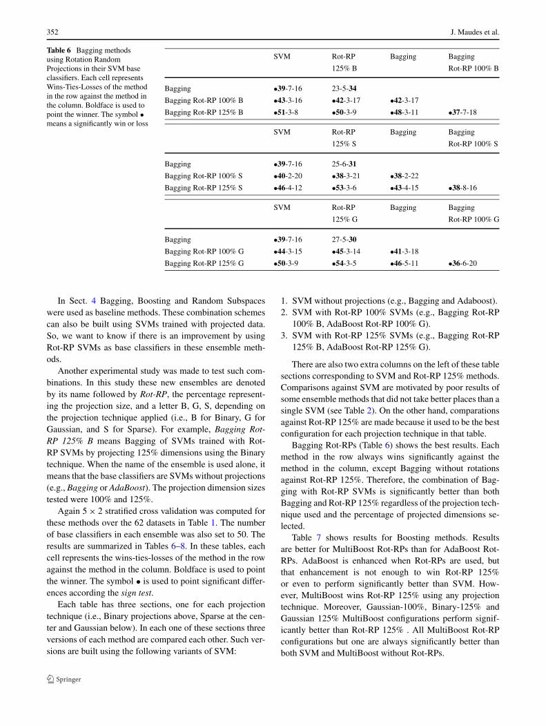
Rotation-RPs variants not only can perform better thanRot-PCA 100%, but they use to be faster. Table 4 shows
Table 4 Less-Equal-More CPU training time of the methods in thecolumns against the methods in the rows
Rot-RP 100%
Sparse Binary Gaussian
Rot-RP 100% B 53-2-7
Rot-RP 100% G 56-1-5 40-10-12
Rot PCA 100% 55-0-7 39-0-23 37-2-23
Table 5 Average percentage of CPU training time saved using themethods in the columns instead of the methods in rows.
Rot-RP 100%
Sparse Binary Gaussian
Rot-RP 100% B 10.50%
Rot-RP 100% G 12.59% 2.34%
Rot PCA 100% 18.10% 6.78% 3.56%
the amount of datasets in which Rot-RPs 100% variants incolumns spent less, equal or more CPU time than methodsin rows for training the whole ensemble. A single thread inan Intel(R) Core(TM) 2 Quad CPU at 2.4 GHz, 8 GB RAM,on Linux 64-bits system was used to get these results. Themeasure provided by WEKA is the CPU used only by thecomputation (i.e., without the possible CPU spent by otherprocesses). The average time of each dataset in the 5 × 2cross validation is then computed. Then the average timesfor the 62 datasets are compared each other to fill the table.
RP complexity is of order O(NDoDp), where N is thenumber of instances, Do the original dataset dimension, andDp the projected dataset dimension, and PCA complexity isO(ND2
o) + O(D3o) [2]. Therefore, as one can expect, RPs
methods use to run faster than PCA at most of the times, asit is shown in Table 4.
However, the last row in Table 5 shows that differencesare not very big. This can be due to two facts; in one handDo is set to an small value (i.e., 5), and in the other hand themain cost of base classifiers training lies on SVM.
5 Rotation random projected SVMs as base classifiers
Section 4 shows that Rot-RPs used to perform better thanRP-Ensembles. Therefore, splitting attributes into groups,and projecting each group with a different projection seemsto be better than projecting all attributes at once using onlyone projection. In this work, SVMs trained by splitting at-tributes into groups are denoted as Rotation Random Pro-jected SVMs or Rot-RP SVMs. This notation is chosen be-cause such way of training base classifiers (i.e., SVMs inthis paper) resembles the Rotation Forests method.
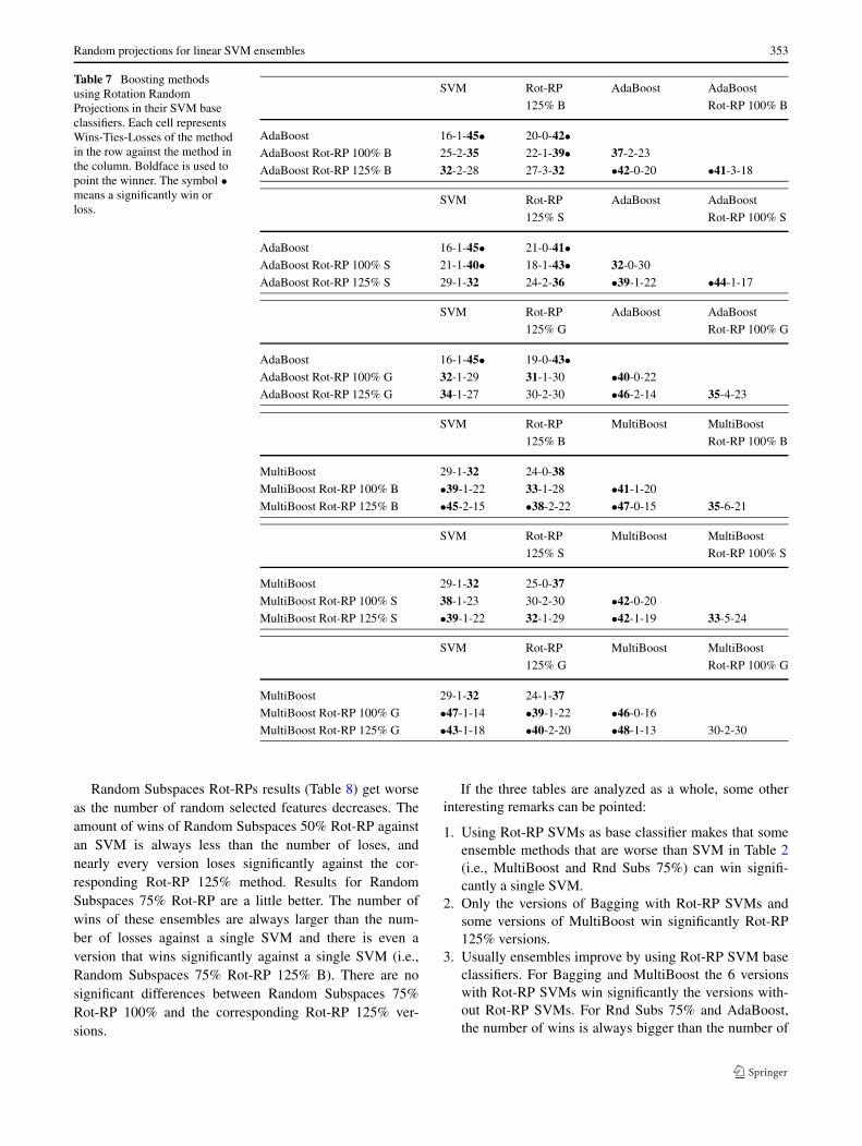
352 J. Maudes et al.
Table 6 Bagging methodsusing Rotation RandomProjections in their SVM baseclassifiers. Each cell representsWins-Ties-Losses of the methodin the row against the method inthe column. Boldface is used topoint the winner. The symbol •means a significantly win or loss
SVM Rot-RP Bagging Bagging
125% B Rot-RP 100% B
Bagging •39-7-16 23-5-34
Bagging Rot-RP 100% B •43-3-16 •42-3-17 •42-3-17
Bagging Rot-RP 125% B •51-3-8 •50-3-9 •48-3-11 •37-7-18
SVM Rot-RP Bagging Bagging
125% S Rot-RP 100% S
Bagging •39-7-16 25-6-31
Bagging Rot-RP 100% S •40-2-20 •38-3-21 •38-2-22
Bagging Rot-RP 125% S •46-4-12 •53-3-6 •43-4-15 •38-8-16
SVM Rot-RP Bagging Bagging
125% G Rot-RP 100% G
Bagging •39-7-16 27-5-30
Bagging Rot-RP 100% G •44-3-15 •45-3-14 •41-3-18
Bagging Rot-RP 125% G •50-3-9 •54-3-5 •46-5-11 •36-6-20
In Sect. 4 Bagging, Boosting and Random Subspaceswere used as baseline methods. These combination schemescan also be built using SVMs trained with projected data.So, we want to know if there is an improvement by usingRot-RP SVMs as base classifiers in these ensemble meth-ods.
Another experimental study was made to test such com-binations. In this study these new ensembles are denotedby its name followed by Rot-RP, the percentage represent-ing the projection size, and a letter B, G, S, depending onthe projection technique applied (i.e., B for Binary, G forGaussian, and S for Sparse). For example, Bagging Rot-RP 125% B means Bagging of SVMs trained with Rot-RP SVMs by projecting 125% dimensions using the Binarytechnique. When the name of the ensemble is used alone, itmeans that the base classifiers are SVMs without projections(e.g., Bagging or AdaBoost). The projection dimension sizestested were 100% and 125%.
Again 5 × 2 stratified cross validation was computed forthese methods over the 62 datasets in Table 1. The numberof base classifiers in each ensemble was also set to 50. Theresults are summarized in Tables 6–8. In these tables, eachcell represents the wins-ties-losses of the method in the rowagainst the method in the column. Boldface is used to pointthe winner. The symbol • is used to point significant differ-ences according the sign test.
Each table has three sections, one for each projectiontechnique (i.e., Binary projections above, Sparse at the cen-ter and Gaussian below). In each one of these sections threeversions of each method are compared each other. Such ver-sions are built using the following variants of SVM:
1. SVM without projections (e.g., Bagging and Adaboost).2. SVM with Rot-RP 100% SVMs (e.g., Bagging Rot-RP
100% B, AdaBoost Rot-RP 100% G).3. SVM with Rot-RP 125% SVMs (e.g., Bagging Rot-RP
125% B, AdaBoost Rot-RP 125% G).
There are also two extra columns on the left of these tablesections corresponding to SVM and Rot-RP 125% methods.Comparisons against SVM are motivated by poor results ofsome ensemble methods that did not take better places than asingle SVM (see Table 2). On the other hand, comparationsagainst Rot-RP 125% are made because it used to be the bestconfiguration for each projection technique in that table.
Bagging Rot-RPs (Table 6) shows the best results. Eachmethod in the row always wins significantly against themethod in the column, except Bagging without rotationsagainst Rot-RP 125%. Therefore, the combination of Bag-ging with Rot-RP SVMs is significantly better than bothBagging and Rot-RP 125% regardless of the projection tech-nique used and the percentage of projected dimensions se-lected.
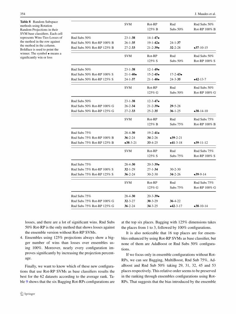
Table 7 shows results for Boosting methods. Resultsare better for MultiBoost Rot-RPs than for AdaBoost Rot-RPs. AdaBoost is enhanced when Rot-RPs are used, butthat enhancement is not enough to win Rot-RP 125%or even to perform significantly better than SVM. How-ever, MultiBoost wins Rot-RP 125% using any projectiontechnique. Moreover, Gaussian-100%, Binary-125% andGaussian 125% MultiBoost configurations perform signif-icantly better than Rot-RP 125% . All MultiBoost Rot-RPconfigurations but one are always significantly better thanboth SVM and MultiBoost without Rot-RPs.
Random projections for linear SVM ensembles 353
Table 7 Boosting methodsusing Rotation RandomProjections in their SVM baseclassifiers. Each cell representsWins-Ties-Losses of the methodin the row against the method inthe column. Boldface is used topoint the winner. The symbol •means a significantly win orloss.
SVM Rot-RP AdaBoost AdaBoost
125% B Rot-RP 100% B
AdaBoost 16-1-45• 20-0-42•AdaBoost Rot-RP 100% B 25-2-35 22-1-39• 37-2-23
AdaBoost Rot-RP 125% B 32-2-28 27-3-32 •42-0-20 •41-3-18
SVM Rot-RP AdaBoost AdaBoost
125% S Rot-RP 100% S
AdaBoost 16-1-45• 21-0-41•AdaBoost Rot-RP 100% S 21-1-40• 18-1-43• 32-0-30
AdaBoost Rot-RP 125% S 29-1-32 24-2-36 •39-1-22 •44-1-17
SVM Rot-RP AdaBoost AdaBoost
125% G Rot-RP 100% G
AdaBoost 16-1-45• 19-0-43•AdaBoost Rot-RP 100% G 32-1-29 31-1-30 •40-0-22
AdaBoost Rot-RP 125% G 34-1-27 30-2-30 •46-2-14 35-4-23
SVM Rot-RP MultiBoost MultiBoost
125% B Rot-RP 100% B
MultiBoost 29-1-32 24-0-38MultiBoost Rot-RP 100% B •39-1-22 33-1-28 •41-1-20
MultiBoost Rot-RP 125% B •45-2-15 •38-2-22 •47-0-15 35-6-21
SVM Rot-RP MultiBoost MultiBoost
125% S Rot-RP 100% S
MultiBoost 29-1-32 25-0-37MultiBoost Rot-RP 100% S 38-1-23 30-2-30 •42-0-20
MultiBoost Rot-RP 125% S •39-1-22 32-1-29 •42-1-19 33-5-24
SVM Rot-RP MultiBoost MultiBoost
125% G Rot-RP 100% G
MultiBoost 29-1-32 24-1-37MultiBoost Rot-RP 100% G •47-1-14 •39-1-22 •46-0-16
MultiBoost Rot-RP 125% G •43-1-18 •40-2-20 •48-1-13 30-2-30
Random Subspaces Rot-RPs results (Table 8) get worseas the number of random selected features decreases. Theamount of wins of Random Subspaces 50% Rot-RP againstan SVM is always less than the number of loses, andnearly every version loses significantly against the cor-responding Rot-RP 125% method. Results for RandomSubspaces 75% Rot-RP are a little better. The number ofwins of these ensembles are always larger than the num-ber of losses against a single SVM and there is even aversion that wins significantly against a single SVM (i.e.,Random Subspaces 75% Rot-RP 125% B). There are nosignificant differences between Random Subspaces 75%Rot-RP 100% and the corresponding Rot-RP 125% ver-sions.
If the three tables are analyzed as a whole, some otherinteresting remarks can be pointed:
1. Using Rot-RP SVMs as base classifier makes that someensemble methods that are worse than SVM in Table 2(i.e., MultiBoost and Rnd Subs 75%) can win signifi-cantly a single SVM.
2. Only the versions of Bagging with Rot-RP SVMs andsome versions of MultiBoost win significantly Rot-RP125% versions.
3. Usually ensembles improve by using Rot-RP SVM baseclassifiers. For Bagging and MultiBoost the 6 versionswith Rot-RP SVMs win significantly the versions with-out Rot-RP SVMs. For Rnd Subs 75% and AdaBoost,the number of wins is always bigger than the number of
354 J. Maudes et al.
Table 8 Random Subspacemethods using RotationRandom Projections in theirSVM base classifiers. Each cellrepresents Wins-Ties-Losses ofthe method in the row againstthe method in the column.Boldface is used to point thewinner. The symbol • means asignificantly win or loss
SVM Rot-RP Rnd Rnd Subs 50%
125% B Subs 50% Rot-RP 100% B
Rnd Subs 50% 23-1-38 14-1-47•Rnd Subs 50% Rot-RP 100% B 26-1-35 19-1-42• 24-1-37
Rnd Subs 50% Rot-RP 125% B 27-2-33 21-2-39• 32-2-28 •37-10-15
SVM Rot-RP Rnd Rnd Subs 50%
125% S Subs 50% Rot-RP 100% S
Rnd Subs 50% 23-1-38 12-1-49•Rnd Subs 50% Rot-RP 100% S 21-1-40• 15-2-45• 17-2-43•Rnd Subs 50% Rot-RP 125% S 24-1-37 21-1-40• 24-3-35 •42-13-7
SVM Rot-RP Rnd Rnd Subs 50%
125% G Subs 50% Rot-RP 100% G
Rnd Subs 50% 23-1-38 12-3-47•Rnd Subs 50% Rot-RP 100% G 26-2-34 21-2-39• 29-5-28
Rnd Subs 50% Rot-RP 125% G 27-2-33 25-2-35 36-1-25 •38-14-10
SVM Rot-RP Rnd Rnd Subs 75%
125% B Subs 75% Rot-RP 100% B
Rnd Subs 75% 28-4-30 19-2-41•Rnd Subs 75% Rot-RP 100% B 36-2-24 34-2-26 •39-2-21
Rnd Subs 75% Rot-RP 125% B •38-3-21 33-4-25 •41-3-18 •39-11-12
SVM Rot-RP Rnd Rnd Subs 75%
125% S Subs 75% Rot-RP 100% S
Rnd Subs 75% 28-4-30 20-3-39•Rnd Subs 75% Rot-RP 100% S 32-1-29 27-1-34 30-2-30
Rnd Subs 75% Rot-RP 125% S 36-2-24 30-2-30 34-2-26 •39-9-14
SVM Rot-RP Rnd Rnd Subs 75%
125% G Subs 75% Rot-RP 100% G
Rnd Subs 75% 28-4-30 20-3-39•Rnd Subs 75% Rot-RP 100% G 32-3-27 30-3-29 36-4-22
Rnd Subs 75% Rot-RP 125% G 36-2-24 34-3-25 •42-3-17 •38-10-14
losses, and there are a lot of significant wins. Rnd Subs50% Rot-RP is the only method that shows losses againstthe ensemble version without Rot-RP SVMs.
4. Ensembles using 125% projections always show a big-ger number of wins than losses over ensembles us-ing 100%. Moreover, nearly every configuration im-proves significantly by increasing the projection percent-age.
Finally, we want to know which of these new configura-tions that use Rot-RP SVMs as base classifiers results thebest for the 62 datasets according to the average rank. Ta-ble 9 shows that the six Bagging Rot-RPs configurations are
at the top six places. Bagging with 125% dimensions takesthe places from 1 to 3, followed by 100% configurations.
It is also noticeable that 16 top places are for ensem-bles enhanced by using Rot-RP SVMs as base classifier, butnone of them are AdaBoost or Rnd Subs 50% configura-tions.
If we focus only in ensemble configurations without Rot-RPs, we can see Bagging, MultiBoost, Rnd Sub 75%, Ad-aBoost and Rnd Sub 50% taking 29, 31, 32, 45 and 53places respectively. This relative order seems to be preservedin the ranking through ensembles configurations using Rot-RPs. That suggests that the bias introduced by the ensemble
Random projections for linear SVM ensembles 355
Table 9 Average rank through the 62 datasets adding the ensemblesthat uses Rot-RP SVMs
Pos Method Avg Rank
1 Bagging Rot-RP 125% B 13.902 Bagging Rot-RP 125% G 14.133 Bagging Rot-RP 125% S 14.854 Bagging Rot-RP 100% G 16.445 Bagging Rot-RP 100% B 16.486 Bagging Rot-RP 100% S 18.637 MultiBoost Rot-RP 125% G 19.118 MultiBoost Rot-RP 125% B 19.399 MultiBoost Rot-RP 100% G 19.60
10 Rnd Sub 75% Rot-RP 125% G 20.1911 Rnd Sub 75% Rot-RP 125% B 20.7112 Rnd Sub 75% Rot-RP 125% S 22.7913 MultiBoost Rot-RP 100% B 23.0414 Rnd Sub 75% Rot-RP 100% B 23.5915 MultiBoost Rot-RP 125% S 23.8016 Rnd Sub 75% Rot-RP 100% G 24.1317 Rot-RP 100% G 24.9618 Rot-RP 125% B 25.0919 Rot-RP 125% S 25.3320 MultiBoost Rot-RP 100% S 25.4121 Rot-RP 125% G 25.9422 AdaBoost Rot-RP 125% G 26.5423 Rnd Sub 75% Rot-RP 100% S 26.9624 Rot-RP 100% S 27.0225 Rot-PCA 100% 27.3126 AdaBoost Rot-RP 125% B 27.4227 Rot-RP 100% B 27.4728 AdaBoost Rot-RP 100% G 28.2129 Bagging 28.2830 SVM 29.9631 MultiBoost 30.4232 Rnd Sub 75% 30.5333 RP-Ensemble 125% S 30.6034 AdaBoost Rot-RP 125% S 31.4035 Rnd Sub 50% Rot-RP 125% G 32.4836 AdaBoost Rot-RP 100% B 32.6237 RP-Ensemble 100% S 32.6838 RP-Ensemble 125% G 33.0739 Rot-RP 75% G 33.7340 Rnd Sub 50% Rot-RP 125% B 33.7641 Rot-PCA 75% 34.0342 Rot-RP 75% B 34.3543 RP-Ensemble 125% B 35.1344 RP-Ensemble 100% G 35.2745 AdaBoost 35.4446 Rnd Sub 50% Rot-RP 100% G 35.6847 Rot-RP 75% S 35.8548 AdaBoost Rot-RP 100% S 36.0249 Rnd Sub 50% Rot-RP 125% S 36.2250 Rnd Sub 50% Rot-RP 100% B 36.3051 RP-Ensemble 100% B 36.8152 RP-Ensemble 75% S 37.4053 Rnd Sub 50% 38.1954 RP-Ensemble 75% G 39.3955 Rnd Sub 50% Rot-RP 100% S 40.8156 RP-Ensemble 75% B 41.15
method is stronger than the effect of using Rot-RPs in baseclassifiers.
6 Kappa-error analysis
Base classifiers make errors sometimes. If some base clas-sifiers in an ensemble make a wrong prediction and thereare some others that make a correct one, these latter clas-sifiers can compensate the formers. So ensembles successrequires both accuracy and diversity from its base members.There are a few measures of diversity [15]. In this paper, κ
statistic is used, because it is the typical statistical measureused in diversity visualization techniques, (e.g., κ-error dia-grams [17]).
κ statistic is presented in [4], and it can be used to mea-sure how diverse two base classifiers are. Given a datasetcontaining L classes, a contingency matrix C of L × L di-mension is computed, such each Ci,j represents the numberof instances from the dataset that are predicted as class i in-stances by the first base classifier, and as class j instances bythe second one. Therefore, the matrix diagonal cells counthow many times both classifiers agree. The probability ofboth classifiers predicting for an instance the i class canbe computed as Ci,i/n, where n is the number of instancesthe dataset contains. So, the probability that both classifiersagree is the sum of all these probabilities:
�1 =∑L
i=1 Ci,i
n(2)
Therefore, �1 (i.e., the probability that both classifiersagree) is on its own a measure on classifier predictions’ sim-ilarity. However, if the dataset is biased toward a dominantclass, both classifiers would be prone to predict such class,making that �1 takes big values whatever both classifiers be.That is why introducing a correction is needed to avoid theeffect of predicting a class by chance by the base classifiers.
The probability that a base classifier predicts class i bychance, can be computed as
∑Lj=1
Ci,j
nfor the first base clas-
sifier, and as∑L
j=1Cj,i
nfor the second one. So, the probabil-
ity of both classifiers agreeing by predicting the same classby chance is computed as �2 by (3).
�2 =L
∑
i=1
(L
∑
j=1
Ci,j
n×
L∑
j=1
Cj,i
n
)
(3)
Once �1 and �2 are computed, κ can be calculated as:
κ = �1 − �2
1 − �2(4)
κ values range from −1 to +1. If both base classifiersalways agree, the only non-zero values in C are in its diago-nal, so �1 = 1 and κ reaches its maximum (i.e., κ = 1). As
356 J. Maudes et al.
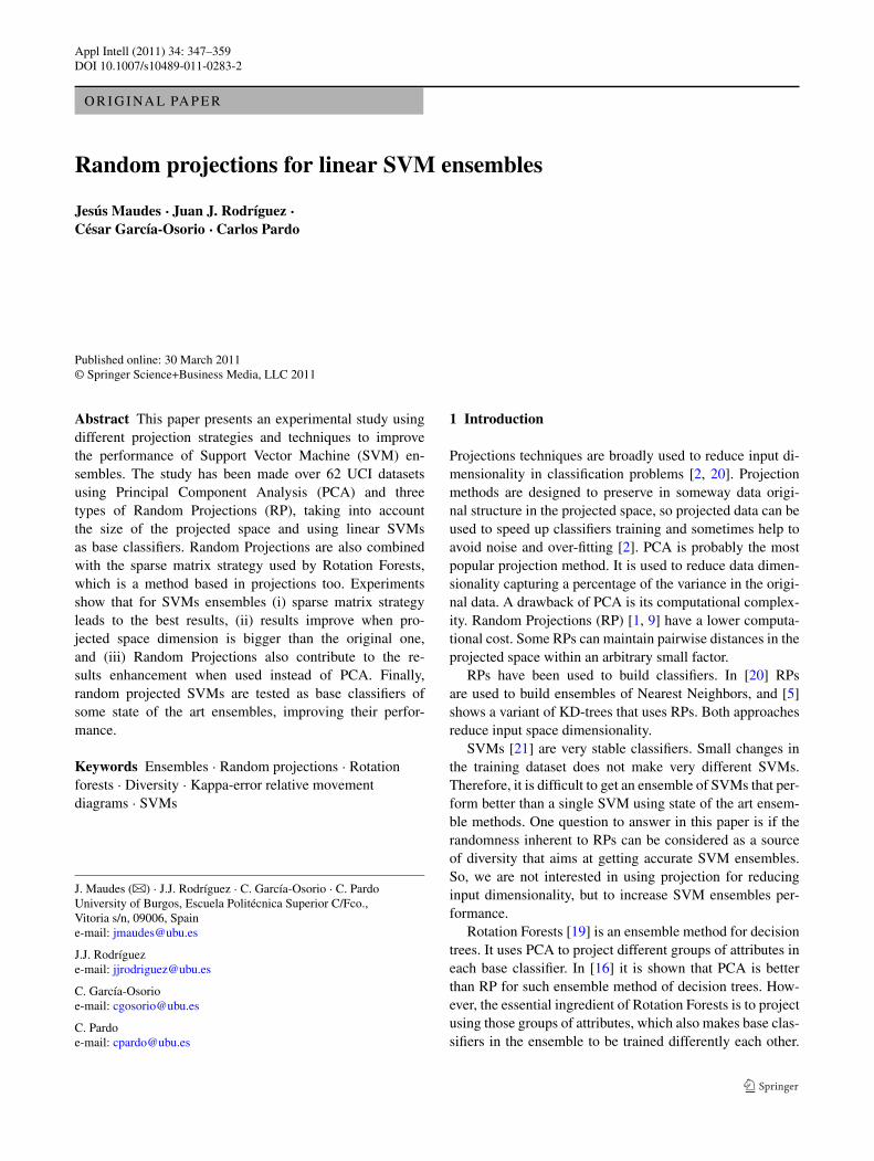
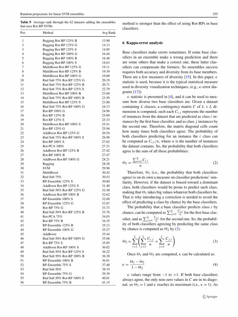
Fig. 1 κ-error diagram for dna dataset showing clouds for two ensem-ble methods. Points in Bagging cloud are located toward the right partof the diagram, so this ensemble is less diverse than Bagging Rot-RP125% B, which points lay toward the left part of the diagram. The lat-ter method increases its diversity as expense of decreasing its accuracy(i.e., Bagging Rot-RP 125% B cloud is below Bagging cloud)
base classifiers predict differently from each other, valueson C diagonal get smaller, whereas values out of the diago-nal get bigger. That makes �1 decrease until �1 = �2 (i.e.,κ = 0). That means that the probability of agreement (i.e.,�1) is equal to the probability of agreement by chance (i.e.,�2). However, if disagreements are higher than for randomoutputs, the difference �1 − �2 takes negative values. Suchκ negative values are not usual, because all base classifiersin an ensemble are based on the same dataset, so they areprone to agree in their predictions.
κ-error diagrams [17] are used to show how accurateand diverse base classifiers of an ensemble are for a givendataset. In these diagrams, a cloud is plotted. Each point ofthe cloud represents a pair of base classifiers. The coordi-nate x of a point is a measure of diversity between thesebase classifiers measured by κ , and the y coordinate is theaverage error from both classifiers. The average error rangesfrom 0 to 1.
Therefore, a cloud of points at bottom left corner meansthat base classifiers of an ensemble are accurate and diverse.Figure 1 shows kappa-error diagram for dna dataset and twovariants of Bagging. In this dataset Bagging without RPsseems to have less diverse but more accurate classifiers thanBagging Rot-RP 125% B.
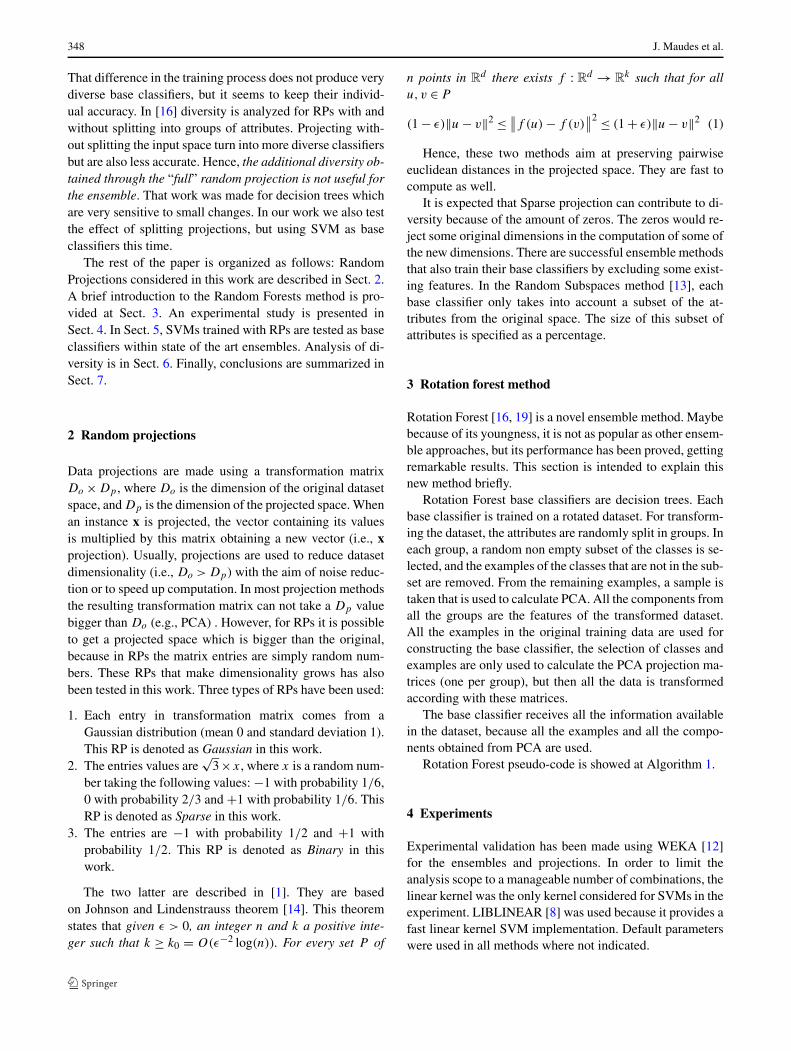
Each κ-error diagram can only contain a few clouds. Usu-ally two clouds are plotted in each diagram representing thebehavior of two ensembles for an only dataset. To showthe behavior of 62 datasets κ-error relative movement di-agrams [18] are more suitable. Figures 2 and 3 show thesediagrams for our experiment. In these diagrams each arrowrepresents a dataset. Each diagram compares overall accu-racy and diversity between two ensembles.
Computation of κ-error relative movement diagrams ismade as follows:
1. For each dataset and ensemble in the study, centers ofclouds from kappa error diagrams are computed. For di-agrams in this work, clouds come from computing 5 × 2cross validation.
2. An arrow is drawn for each dataset connecting the centersof each pair of ensembles to compare.
3. Finally, all arrows are taken to the origin of coordinates.
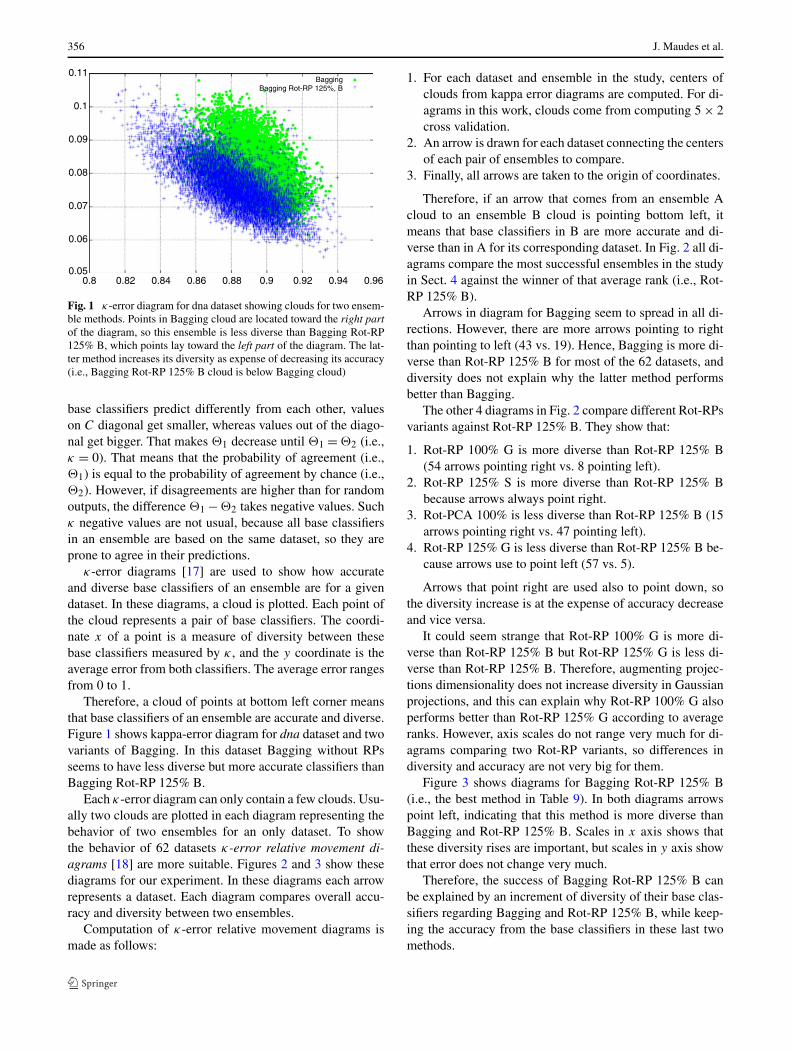
Therefore, if an arrow that comes from an ensemble Acloud to an ensemble B cloud is pointing bottom left, itmeans that base classifiers in B are more accurate and di-verse than in A for its corresponding dataset. In Fig. 2 all di-agrams compare the most successful ensembles in the studyin Sect. 4 against the winner of that average rank (i.e., Rot-RP 125% B).
Arrows in diagram for Bagging seem to spread in all di-rections. However, there are more arrows pointing to rightthan pointing to left (43 vs. 19). Hence, Bagging is more di-verse than Rot-RP 125% B for most of the 62 datasets, anddiversity does not explain why the latter method performsbetter than Bagging.
The other 4 diagrams in Fig. 2 compare different Rot-RPsvariants against Rot-RP 125% B. They show that:
1. Rot-RP 100% G is more diverse than Rot-RP 125% B(54 arrows pointing right vs. 8 pointing left).
2. Rot-RP 125% S is more diverse than Rot-RP 125% Bbecause arrows always point right.
3. Rot-PCA 100% is less diverse than Rot-RP 125% B (15arrows pointing right vs. 47 pointing left).
4. Rot-RP 125% G is less diverse than Rot-RP 125% B be-cause arrows use to point left (57 vs. 5).
Arrows that point right are used also to point down, sothe diversity increase is at the expense of accuracy decreaseand vice versa.
It could seem strange that Rot-RP 100% G is more di-verse than Rot-RP 125% B but Rot-RP 125% G is less di-verse than Rot-RP 125% B. Therefore, augmenting projec-tions dimensionality does not increase diversity in Gaussianprojections, and this can explain why Rot-RP 100% G alsoperforms better than Rot-RP 125% G according to averageranks. However, axis scales do not range very much for di-agrams comparing two Rot-RP variants, so differences indiversity and accuracy are not very big for them.
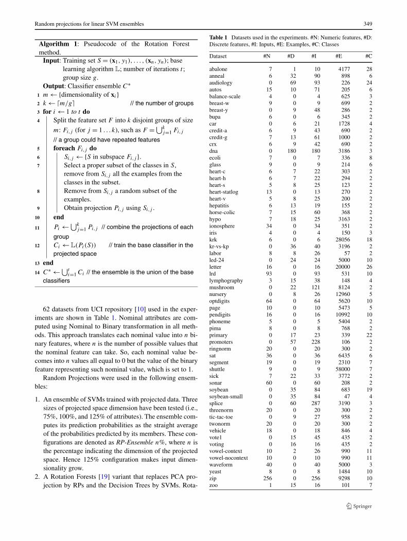
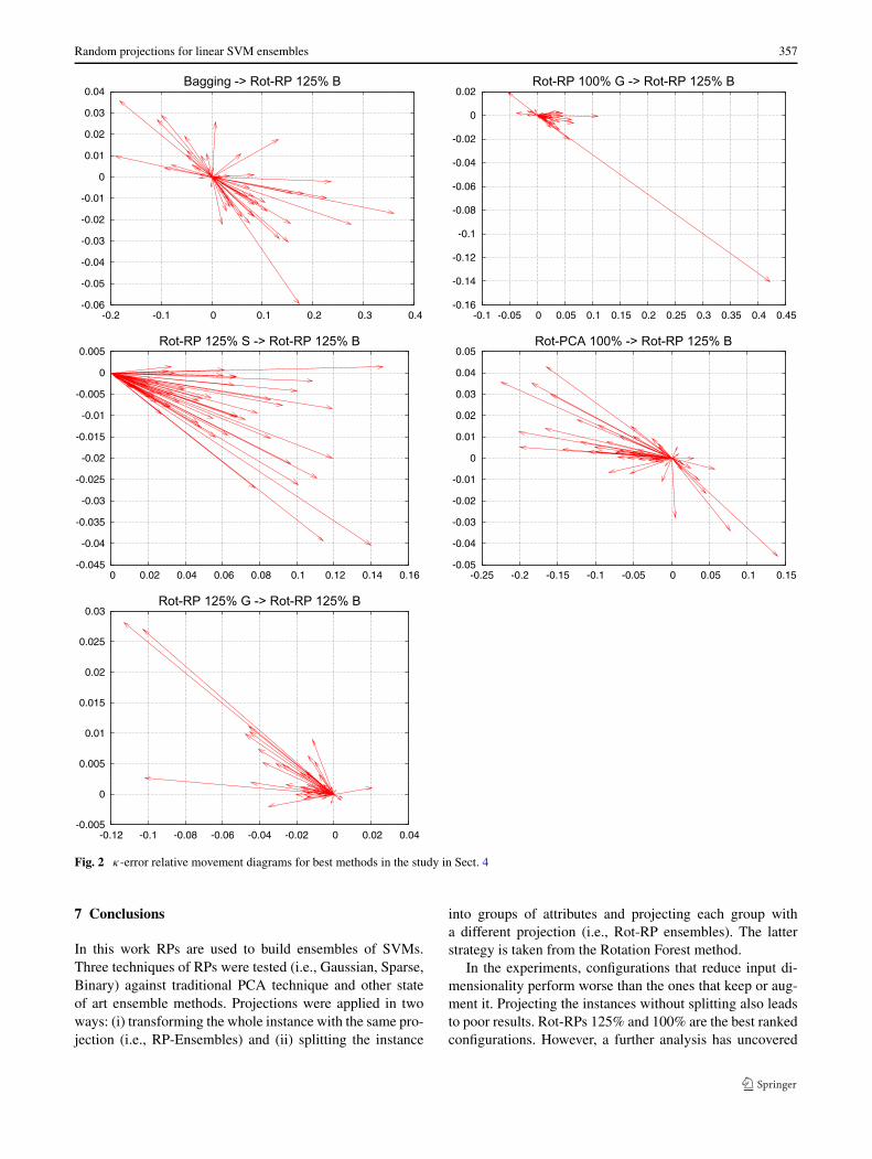
Figure 3 shows diagrams for Bagging Rot-RP 125% B(i.e., the best method in Table 9). In both diagrams arrowspoint left, indicating that this method is more diverse thanBagging and Rot-RP 125% B. Scales in x axis shows thatthese diversity rises are important, but scales in y axis showthat error does not change very much.
Therefore, the success of Bagging Rot-RP 125% B canbe explained by an increment of diversity of their base clas-sifiers regarding Bagging and Rot-RP 125% B, while keep-ing the accuracy from the base classifiers in these last twomethods.
Random projections for linear SVM ensembles 357
Fig. 2 κ-error relative movement diagrams for best methods in the study in Sect. 4
7 Conclusions
In this work RPs are used to build ensembles of SVMs.Three techniques of RPs were tested (i.e., Gaussian, Sparse,Binary) against traditional PCA technique and other stateof art ensemble methods. Projections were applied in twoways: (i) transforming the whole instance with the same pro-jection (i.e., RP-Ensembles) and (ii) splitting the instance
into groups of attributes and projecting each group witha different projection (i.e., Rot-RP ensembles). The latterstrategy is taken from the Rotation Forest method.
In the experiments, configurations that reduce input di-mensionality perform worse than the ones that keep or aug-ment it. Projecting the instances without splitting also leadsto poor results. Rot-RPs 125% and 100% are the best rankedconfigurations. However, a further analysis has uncovered
358 J. Maudes et al.
Fig. 3 κ-error relative movement diagrams for Bagging using Rot-RP SVMs as base classifiers
that 125% configurations seem to perform slightly betterthan 100% configurations.
Rot-RP SVMs (i.e., SVMs trained projecting data likeRot-RP ensembles do) can also be used as base classifier inthe state of art ensemble methods. Experiments show thatthere is a generalized improvement in SVM ensemble meth-ods when Rot-RP SVMs are applied. Moreover, some en-semble methods that do not win to Rot-RP ensembles, canwin against them significantly by using Rot-RP SVMs intheir base classifiers. Ensembles using Rot-RP SVMs pro-jecting 125% dimensions use to perform better than ensem-bles projecting 100%. Bagging with Rot-RP SVMs are thebest tested configurations.
κ-error relative movement diagrams do not show thatRot-RP ensembles are more diverse than Bagging, but theyseem more diverse than Rot-PCA. A not very large varia-tion of diversity has been noted between Rot-RP ensemblesusing the three different random projection techniques.
Bigger diversity increments can be shown in κ-errorrelative movement diagrams involving Bagging Rot-RP125% B. These diagrams show that Bagging Rot-RP is morediverse than both Bagging and Rot-RP 125% B without los-ing much accuracy. That diversity increment can be behindthe success of combining Bagging resampling with randomprojections.
Acknowledgements This work was supported by the ProjectTIN2008-03151 of the Spanish Ministry of Education and Science.
We wish to thank the developers of WEKA and LIBLINEAR. Wealso express our gratitude to the donors of the different datasets and themaintainers of the UCI Repository.
References
1. Achlioptas D (2003) Database-friendly random projections:Johnson-Lindenstrauss with binary coins. J Comput Syst Sci66(4):671–687
2. Bingham E, Mannila H (2001) Random projection in dimension-ality reduction: applications to image and text data. In: KnowledgeDiscovery and Data Mining. ACM, New York, pp 245–250
3. Breiman L (1996) Bagging predictors. Mach Learn 24(2):123–140
4. Cohen J (1960) A coefficient of agreement for nominal scales.Educ Psychol Meas 20(1):37–46
5. Dasgupta S, Freund Y (2008) Random projection trees and lowdimensional manifolds. In: STOC ’08: proceedings of the 40th an-nual ACM symposium on theory of computing. ACM, New York,pp 537–546
6. Demšar J (2006) Statistical comparisons of classifiers over multi-ple data sets. J Mach Learn Res 7:1–30
7. Dietterich TG (1998) Approximate statistical test for compar-ing supervised classification learning algorithms. Neural Comput10(7):1895–1923
8. Fan RE, Chang KW, Hsieh CJ, Wang XR, Lin CJ (2008) Liblinear:a library for large linear classification. J Mach Learn Res 9:1871–1874
9. Fradkin D, Madigan D (2003) Experiments with random projec-tions for machine learning. In: KDD ’03: proceedings of the ninthACM SIGKDD international conference on knowledge discoveryand data mining. ACM, New York, pp 517–522
10. Frank A, Asuncion A (2010) UCI machine learning repository.URL http://archive.ics.uci.edu/ml
11. Freund Y, Schapire RE (1997) A decision-theoretic generalizationof on-line learning and an application to boosting. J Comput SystSci 55(1):119–139
12. Hall M, Frank E, Holmes G, Pfahringer B, Reutemann P, WittenIH (2009) The weka data mining software: an update. SIGKDDExplor 11(1):10–18
13. Ho TK (1998) The random subspace method for constructing deci-sion forests. IEEE Trans Pattern Anal Mach Intell 20(8):832–844
14. Johnson W, Lindenstrauss J (1984) Extensions of Lipschitz mapsinto a Hilbert space. In: Conference in modern analysis and proba-bility (1982, Yale University). Contemporary mathematics, vol 26.AMS, New York, pp 189–206
15. Kuncheva LI (2004) Combining pattern classifiers: methods andalgorithms. Wiley-Interscience, New York
16. Kuncheva LI, Rodríguez JJ (2007) An experimental study on rota-tion forest ensembles. In: 7th international workshop on multipleclassifier systems, MCS 2007. LNCS, vol 4472. Springer, Berlin,pp 459–468
17. Margineantu DD, Dietterich TG (1997) Pruning adaptive boost-ing. In: Proc. 14th international conference on machine learning.Morgan Kaufmann, San Mateo, pp 211–218
Random projections for linear SVM ensembles 359
18. Maudes J, Rodríguez JJ, García-Osorio C (2009) Disturbingneighbors diversity for decision forests. In: Okun O, ValentiniG (eds) Applications of supervised and unsupervised ensemblemethods. Studies in computational intelligence, vol 245. Springer,Berlin, pp 113–133
19. Rodríguez JJ, Kuncheva LI, Alonso CJ (2006) Rotation forest: Anew classifier ensemble method. IEEE Trans Pattern Anal MachIntell 28(10):1619–1630
20. Schclar A, Rokach L (2009) Random projection ensemble classi-fiers. In: Enterprise information systems 11th international confer-ence proceedings. Lecture notes in business information process-ing, pp 309–316
21. Vapnik VN (1999) The nature of statistical learning theory. Infor-mation science and statistics. Springer, Berlin
22. GI Webb (2000) Multiboosting: a technique for combining boost-ing and wagging. Mach Learn 40(2)
Jesús Maudes is an Associate Pro-fessor at the Department of CivilEngineering in the University ofBurgos, Spain. His teaching is main-ly on Database Management Sys-tems. He received his B.S., M.S.in Computer Science both fromthe University of Valladolid, Spain,in 1989 and 1991 respectively. Heworked for the industry from 1991to 1995 and in the University ofBurgos since 1992. He received in2010 his Ph.D. degree in ComputerScience from the University of Bur-gos. His research is focused on en-semble classifiers.
Juan J. Rodríguez received theB.S., M.S., and Ph.D. degrees incomputer science from the Univer-sity of Valladolid, Spain, in 1992,1994, and 2004, respectively. Heworked with the Department ofComputer Science, University ofValladolid from 1995 to 2000. Cur-rently he is working with the De-partment of Civil Engineering, Uni-versity of Burgos, Spain, where heis a Profesor Titular de Universi-dad (Associate Professor). He hasreceived Mobility grants for visitingthe University of Stockholm (1999,
2000) and Bangor University (2005, 2007, 2009). His main researchinterest is data mining, specially ensemble methods.
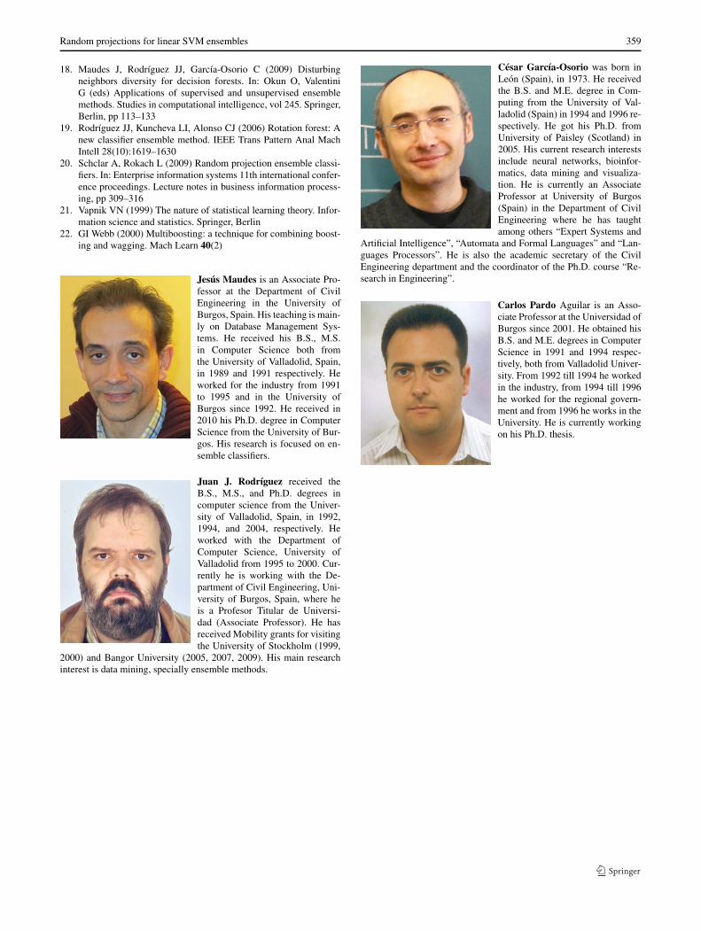
César García-Osorio was born inLeón (Spain), in 1973. He receivedthe B.S. and M.E. degree in Com-puting from the University of Val-ladolid (Spain) in 1994 and 1996 re-spectively. He got his Ph.D. fromUniversity of Paisley (Scotland) in2005. His current research interestsinclude neural networks, bioinfor-matics, data mining and visualiza-tion. He is currently an AssociateProfessor at University of Burgos(Spain) in the Department of CivilEngineering where he has taughtamong others “Expert Systems and
Artificial Intelligence”, “Automata and Formal Languages” and “Lan-guages Processors”. He is also the academic secretary of the CivilEngineering department and the coordinator of the Ph.D. course “Re-search in Engineering”.
Carlos Pardo Aguilar is an Asso-ciate Professor at the Universidad ofBurgos since 2001. He obtained hisB.S. and M.E. degrees in ComputerScience in 1991 and 1994 respec-tively, both from Valladolid Univer-sity. From 1992 till 1994 he workedin the industry, from 1994 till 1996he worked for the regional govern-ment and from 1996 he works in theUniversity. He is currently workingon his Ph.D. thesis.


