Embed Size (px)
Citation preview

HAL Id: tel-02012964https://tel.archives-ouvertes.fr/tel-02012964v2
Submitted on 24 Jun 2019
HAL is a multi-disciplinary open accessarchive for the deposit and dissemination of sci-entific research documents, whether they are pub-lished or not. The documents may come fromteaching and research institutions in France orabroad, or from public or private research centers.
L’archive ouverte pluridisciplinaire HAL, estdestinée au dépôt et à la diffusion de documentsscientifiques de niveau recherche, publiés ou non,émanant des établissements d’enseignement et derecherche français ou étrangers, des laboratoirespublics ou privés.
Preparation of large cold atomic ensembles andapplications in efficient light-matter interfacing
Pierre Vernaz-Gris
To cite this version:Pierre Vernaz-Gris. Preparation of large cold atomic ensembles and applications in efficient light-matter interfacing. Quantum Physics [quant-ph]. Sorbonne Université; Australian national university,2018. English. NNT : 2018SORUS060. tel-02012964v2

THÈSE DE DOCTORATDE L’UNIVERSITÉ PIERRE ET MARIE CURIE
Spécialité : Physique
École doctorale : « Physique en Île-de-France »
réalisée
au Laboratoire Kastler Brosselet à l’Australian National University
présentée par
Pierre VERNAZ-GRIS
pour obtenir le grade de :
DOCTEUR DE L’UNIVERSITÉ PIERRE ET MARIE CURIE
Sujet de la thèse :
Preparation of large cold atomic ensembles and applicationsin efficient light-matter interfacing


Contents
1 Description of light-matter interaction in quantum memories 51.1 Quantum fundamentals . . . . . . . . . . . . . . . . . . . . . . . . . . . 5
1.1.1 Superposition . . . . . . . . . . . . . . . . . . . . . . . . . . . . . 51.1.2 Entanglement . . . . . . . . . . . . . . . . . . . . . . . . . . . . . 71.1.3 Quantum information . . . . . . . . . . . . . . . . . . . . . . . . 81.1.4 Properties of light and matter . . . . . . . . . . . . . . . . . . . . 9
Light, from intense beams down to single photons . . . . . . . . 9The Playground: Atoms . . . . . . . . . . . . . . . . . . . . . . . 10Engineering the light-matter interaction . . . . . . . . . . . . . . 10
1.2 Light-matter interfacing formalism . . . . . . . . . . . . . . . . . . . . . 111.2.1 Classical matter and light . . . . . . . . . . . . . . . . . . . . . . 11
Polarisability . . . . . . . . . . . . . . . . . . . . . . . . . . . . . 11Light propagation . . . . . . . . . . . . . . . . . . . . . . . . . . 12Optical depth . . . . . . . . . . . . . . . . . . . . . . . . . . . . . 12
1.2.2 Description of quantum atom-light systems . . . . . . . . . . . . 14Single atom . . . . . . . . . . . . . . . . . . . . . . . . . . . . . . 14Atomic ensembles . . . . . . . . . . . . . . . . . . . . . . . . . . 16
1.2.3 Optical Bloch equations . . . . . . . . . . . . . . . . . . . . . . . 171.3 Quantum information networks and applications . . . . . . . . . . . . . 18
1.3.1 Implementations of quantum information . . . . . . . . . . . . . 19Quantum communication . . . . . . . . . . . . . . . . . . . . . . 19Information processing . . . . . . . . . . . . . . . . . . . . . . . . 19Quantum cryptography . . . . . . . . . . . . . . . . . . . . . . . 20
1.3.2 Realisation of quantum network elements with light and atoms . 20Encoding of information in photonic and atomic qubits . . . . . 20Quantum state generation . . . . . . . . . . . . . . . . . . . . . . 21
1.3.3 Quantum memories . . . . . . . . . . . . . . . . . . . . . . . . . 21Historical introduction . . . . . . . . . . . . . . . . . . . . . . . . 21Figures of merit . . . . . . . . . . . . . . . . . . . . . . . . . . . 21More than just memories . . . . . . . . . . . . . . . . . . . . . . 26
1.4 Review of optical quantum memory schemes . . . . . . . . . . . . . . . . 261.4.1 Pre-programmed delay . . . . . . . . . . . . . . . . . . . . . . . . 26
Fibre loop . . . . . . . . . . . . . . . . . . . . . . . . . . . . . . . 26Atomic Frequency Comb . . . . . . . . . . . . . . . . . . . . . . . 27
1.4.2 Dynamic Electromagnetically-Induced Transparency . . . . . . . 271.4.3 Raman Memory . . . . . . . . . . . . . . . . . . . . . . . . . . . 281.4.4 On-demand photon-echo techniques . . . . . . . . . . . . . . . . 30
Controlled-Reversed Inhomogeneous Broadening . . . . . . . . . 30Revival of silenced echo . . . . . . . . . . . . . . . . . . . . . . . 30
iii
iv Contents
Gradient Echo Memory . . . . . . . . . . . . . . . . . . . . . . . 301.4.5 Heralded preparation . . . . . . . . . . . . . . . . . . . . . . . . . 32
The DLCZ protocol . . . . . . . . . . . . . . . . . . . . . . . . . 321.4.6 Performance comparison . . . . . . . . . . . . . . . . . . . . . . . 33
2 Key elements for the preparation of large atomic ensembles 352.1 Considerations for atomic ensemble preparation . . . . . . . . . . . . . . 352.2 Warm atomic ensembles . . . . . . . . . . . . . . . . . . . . . . . . . . . 36
2.2.1 Doppler shift . . . . . . . . . . . . . . . . . . . . . . . . . . . . . 362.2.2 Sources of decoherence . . . . . . . . . . . . . . . . . . . . . . . . 37
2.3 Large cold atomic ensembles . . . . . . . . . . . . . . . . . . . . . . . . . 382.3.1 Atom cooling and trapping . . . . . . . . . . . . . . . . . . . . . 38
Optical cooling . . . . . . . . . . . . . . . . . . . . . . . . . . . . 38Zeeman trapping . . . . . . . . . . . . . . . . . . . . . . . . . . . 41Two-dimensional MOT geometry . . . . . . . . . . . . . . . . . . 42Dynamical compression . . . . . . . . . . . . . . . . . . . . . . . 42
2.3.2 Temperature reduction . . . . . . . . . . . . . . . . . . . . . . . . 43Polarisation-Gradient Cooling . . . . . . . . . . . . . . . . . . . . 43Dark spontaneous-force optical trap . . . . . . . . . . . . . . . . 43
2.3.3 Typical experimental setup . . . . . . . . . . . . . . . . . . . . . 43Vacuum . . . . . . . . . . . . . . . . . . . . . . . . . . . . . . . . 44Dispensers . . . . . . . . . . . . . . . . . . . . . . . . . . . . . . . 44Magnetic trapping . . . . . . . . . . . . . . . . . . . . . . . . . . 44Sources of light for optical trapping . . . . . . . . . . . . . . . . 45
2.3.4 Preparation sequences . . . . . . . . . . . . . . . . . . . . . . . . 45LKB . . . . . . . . . . . . . . . . . . . . . . . . . . . . . . . . . . 45ANU . . . . . . . . . . . . . . . . . . . . . . . . . . . . . . . . . . 46
2.3.5 Atomic ensemble characterisation . . . . . . . . . . . . . . . . . . 47Measurement of optical depth . . . . . . . . . . . . . . . . . . . . 47Magnetic cancellation . . . . . . . . . . . . . . . . . . . . . . . . 51Temperature measurement . . . . . . . . . . . . . . . . . . . . . 54
2.4 Machine-learning optimisation . . . . . . . . . . . . . . . . . . . . . . . . 562.4.1 Teaching the machine-learner . . . . . . . . . . . . . . . . . . . . 562.4.2 Machine-learned compression-and-cooling sequence . . . . . . . . 572.4.3 Comparison of preparation sequences . . . . . . . . . . . . . . . . 592.4.4 Going beyond the optimisation of OD . . . . . . . . . . . . . . . 59
3 Efficient qubit storage based on electromagnetically-induced transparency 613.1 Background . . . . . . . . . . . . . . . . . . . . . . . . . . . . . . . . . . 613.2 Formalism with three-level atoms . . . . . . . . . . . . . . . . . . . . . . 62
3.2.1 Coherent Population Trapping . . . . . . . . . . . . . . . . . . . 623.2.2 The Electromagnetically-Induced Transparency phenomenon . . 623.2.3 Dynamic control over slow light . . . . . . . . . . . . . . . . . . . 65
Group velocity . . . . . . . . . . . . . . . . . . . . . . . . . . . . 65Adiabatic transfer to a halted pulse . . . . . . . . . . . . . . . . 66

Contents v
3.2.4 Residual absorption . . . . . . . . . . . . . . . . . . . . . . . . . 67Control intensity . . . . . . . . . . . . . . . . . . . . . . . . . . . 67Absorption from Zeeman sub-levels . . . . . . . . . . . . . . . . . 67
3.2.5 Additional excited levels . . . . . . . . . . . . . . . . . . . . . . . 69Theoretical model for all excited levels . . . . . . . . . . . . . . . 69Results . . . . . . . . . . . . . . . . . . . . . . . . . . . . . . . . 71
3.3 Multiplexed polarisation qubit storage . . . . . . . . . . . . . . . . . . . 753.3.1 Polarisation encoding: preparation, manipulation and detection . 753.3.2 Storage of orthogonal polarisations . . . . . . . . . . . . . . . . . 753.3.3 Atom preparation for dual-rail storage . . . . . . . . . . . . . . . 753.3.4 Transparency measurement . . . . . . . . . . . . . . . . . . . . . 783.3.5 Memory efficiency . . . . . . . . . . . . . . . . . . . . . . . . . . 79
3.4 Qubit storage and retrieval . . . . . . . . . . . . . . . . . . . . . . . . . 823.4.1 Quantum state tomography . . . . . . . . . . . . . . . . . . . . . 823.4.2 Quantum storage benchmarking . . . . . . . . . . . . . . . . . . 823.4.3 Storage time . . . . . . . . . . . . . . . . . . . . . . . . . . . . . 833.4.4 Discussion . . . . . . . . . . . . . . . . . . . . . . . . . . . . . . . 86
3.5 Future of the experiment . . . . . . . . . . . . . . . . . . . . . . . . . . . 86
4 High-performance backward-recall Raman memory 894.1 Theoretical basis for a Raman memory . . . . . . . . . . . . . . . . . . . 89
4.1.1 From scattering to a memory scheme . . . . . . . . . . . . . . . . 894.1.2 Optimal shaping . . . . . . . . . . . . . . . . . . . . . . . . . . . 93
Degrees of excitation of light and spin wave . . . . . . . . . . . . 93Singular Value Decomposition . . . . . . . . . . . . . . . . . . . . 94Numerical model . . . . . . . . . . . . . . . . . . . . . . . . . . . 96Finding the optimum . . . . . . . . . . . . . . . . . . . . . . . . 96Optimisation results . . . . . . . . . . . . . . . . . . . . . . . . . 98
4.1.3 Backward and forward retrieval configurations . . . . . . . . . . 984.2 Experimental Raman memory . . . . . . . . . . . . . . . . . . . . . . . . 99
4.2.1 Experimental setup . . . . . . . . . . . . . . . . . . . . . . . . . . 99Atomic ensemble preparation . . . . . . . . . . . . . . . . . . . . 99Signal and control beams . . . . . . . . . . . . . . . . . . . . . . 100
4.2.2 High-efficiency memory . . . . . . . . . . . . . . . . . . . . . . . 1044.2.3 Memory lifetime . . . . . . . . . . . . . . . . . . . . . . . . . . . 1044.2.4 Delay-bandwidth product . . . . . . . . . . . . . . . . . . . . . . 1044.2.5 Dynamically-reprogrammable beam-splitting . . . . . . . . . . . 106
4.3 Discussion of the results . . . . . . . . . . . . . . . . . . . . . . . . . . . 1084.3.1 Backward-retrieval geometry . . . . . . . . . . . . . . . . . . . . 1084.3.2 Outlook for this Raman memory realisation . . . . . . . . . . . . 108
5 Spin-wave interference for stationary light and memory enhancement 1115.1 Stationary light history and formalism . . . . . . . . . . . . . . . . . . . 111
5.1.1 Electromagnetically-Induced-Transparency Stationary Light . . . 1125.1.2 One-colour Raman stationary light . . . . . . . . . . . . . . . . . 1135.1.3 Two-colour Raman stationary light . . . . . . . . . . . . . . . . . 115

vi Contents
5.2 Early experimental stationary light investigations . . . . . . . . . . . . . 1165.3 Self-stabilising stationary light in a cold atomic ensemble . . . . . . . . 117
5.3.1 Atom-light configuration . . . . . . . . . . . . . . . . . . . . . . . 1195.3.2 Self-stabilisation dynamics . . . . . . . . . . . . . . . . . . . . . . 119
Theoretical description of the stabilisation process . . . . . . . . 119Evolution of spin-wave pairs with a relative phase . . . . . . . . 120
5.3.3 Experimental spin-wave imaging . . . . . . . . . . . . . . . . . . 120Imaging setup . . . . . . . . . . . . . . . . . . . . . . . . . . . . . 122Agreement between measurements and simulations . . . . . . . . 122
5.4 Time-Reversed And Coherently-Enhanced memory . . . . . . . . . . . . 1255.4.1 Single-mode memory without a cavity . . . . . . . . . . . . . . . 1255.4.2 Phase matching and interference . . . . . . . . . . . . . . . . . . 1265.4.3 Efficiency scaling with optical depth . . . . . . . . . . . . . . . . 1275.4.4 Experimental realisation . . . . . . . . . . . . . . . . . . . . . . . 128
Interference between counter-propagating signals . . . . . . . . . 128Performance as a memory scheme . . . . . . . . . . . . . . . . . 130
5.4.5 Outlook . . . . . . . . . . . . . . . . . . . . . . . . . . . . . . . . 1305.5 Future investigation of stationary light . . . . . . . . . . . . . . . . . . . 132

Introduction
Light-matter interaction leads to an extremely broad range of applications, rangingfrom the preparation of large atomic ensembles to the realisation of quantum memoriesand the generation of single photons. The PhD work presented here was undertaken asa cotutelle between the Laboratoire Kastler Brossel (LKB) and the Australian NationalUniversity (ANU).The LKB has a long history with light-matter interaction, stemming from the very
founding of the laboratory under the name “Laboratoire de Spectroscopie hertzienne del’ENS” (ENS laboratory of hertzian spectroscopy) in 1951, and actually a few yearsbefore that with the works of Jean Brossel and Alfred Kastler on the phenomenonof double – optical and magnetic – resonance. Optical pumping is often said to havebeen invented by these two founding fathers of LKB, as early as 1950, and is nowa preeminent technique in any atomic experiment, either in solids, warm and coldvapours. I joined there the Quantum Networks team led by Julien Laurat, aiming atthe development of quantum network resources.The interaction of light and atoms is just as central to the Centre for Quantum
Computation and Communication Technology (CQC2T), which explains the manycollaborations between the Parisian laboratory and this centre of excellence of theAustralian Research Council. In particular, at its node at the ANU, the Photonicsgroup led by Ping Koy Lam, focuses on the realisations of quantum memories, with BenBuchler at the helm of those, and continuous-variable quantum information protocols.Holding the optical memory efficiency record since 2011 with the gradient echo memory,the memory scheme developed in the group and implemented in various forms andplatforms, the group has a renowned expertise which complements perfectly the one atLKB.When I started my PhD, the experiments in Paris and in Canberra has both gone
through a very fruitful phase performing well-known protocols and it was time toexplore their capabilities from there. One of the challenges at LKB was to improve theperformance of the Duan-Lukin-Cirac-Zoller scheme that had been implemented overthe work of previous PhD students. We hoped increasing the optical depth of the atomicensemble with a 2D geometry would suffice, but instead the geometry first enabledus to perform the storage of polarisation qubits based on electromagnetically-induced-transparency, which benefited greatly from this improvement on optical depth. At ANU,our aim was to come up with new protocols to investigate. Stationary light had beenpreviously considered as a candidate and so fellow students and I became the pioneersof its study at ANU. We not only characterised its evolution and self-stabilisation in acold atomic ensemble, we also extend the scope of its applications with a novel memoryscheme inspired from its properties of symmetry.
The philosophy with which this thesis has been written is to share my insight on thepreparation of large atomic ensembles and the experiments which use this platform for
1

2 Contents
efficient atom-light interfacing. I have become acquainted with both topics during myPhD and I present them in this thesis with a focus on all the aspects relevant to anexperimental quantum optician.
Thesis layout This dissertation is organised in the following chapters:
1. I start by presenting classical and quantum interaction of light with matter, andits numerous applications, and I expose the mathematical formalism which I willuse throughout this thesis. Among the applications, I focus on quantum memoryschemes and I review in detail their performance achieved so far.
2. Secondly, I present the role of large atomic ensembles in experimental realisationsand the state of the art of their production. I describe in detail the warm atomicvapour and the two cold-atom apparatuses that I have been using during thecourse of my PhD.
3. Among quantum memory schemes, the one based on electromagnetically-inducedtransparency is arguably the most popular and is central to the experiment atLKB which I have led. I present this phenomenon, followed by the theory ofadditional excited levels we have developed and the experiment of the storage ofa qubit in spatially-multiplexed configuration.
4. A second experimental highlight of my PhD, this time at ANU, was the realisationof a Raman memory, where the signal and control pair are brought off resonancefrom the excited state transition. The uniqueness of our configuration was to recallthe stored light in the backward direction, which is known to be fundamentallypreferable and yet is rarely performed.
5. Stationary light, although it is generated in similar setups, differs from the“stopped”-light experiments presented in the two previous chapters. The lastchapter is devoted to its theoretical description and the series of experimentsinvolving this other form of light, followed by a new memory protocol, conceptuallyclose to stationary light.
Publications The work presented in this thesis has led to the following articles, whichhave been published or are pending publication by peer-review journals:
[1] J. L. Everett, P. Vernaz-Gris, A. D. Tranter, K. V. Paul, A. C. Leung, G. T.Campbell, P. K. Lam, and B. C. Buchler. Time-Reversed and Coherently EnhancedMemory: A single mode quantum atom-optic memory in free space. In preparation.
[2] P. Vernaz-Gris, A. D. Tranter, J. L. Everett, A. C. Leung, K. V. Paul, G. T.Campbell, P. K. Lam, and B. C. Buchler. High-Performance Raman Memorywith Spatio-Temporal Reversal. In preparation.
[3] J. L. Everett, G. T. Campbell, Y.-W. Cho, P. Vernaz-Gris, D. Higginbottom,O. Pinel, N. P. Robins, P. K. Lam, and B. C. Buchler. Dynamical observationsof self-stabilizing stationary light. Nature Physics, 13, 68–73 (January 2016).doi:10.1038/nphys3901.

Contents 3
[4] P. Vernaz-Gris, K. Huang, M. Cao, A. S. Sheremet, and J. Laurat. Highly-Efficient Quantum Memory for Polarization Qubits in a Spatially-MultiplexedCold Atomic Ensemble. ArXiv e-prints, 1707.09372 (July 2017). Accepted inNature Communications.


Chapter 1
Description of light-matter interaction in quantummemories
To cover the broad topic of light-matter interaction, I first describe some fundamentalquantum properties relevant to this whole study.
1.1 Quantum fundamentalsIt is not an understatement to state the twentieth century has experienced a quantum
revolution, with the emergence of the theory describing quantum phenomena in itsearly years. A handful of new concepts were developed, like probability amplitudes,superposition, entanglement, decoherence, to cite only a few. Stemming from theseprinciples applied to the radiation of light, the invention of the laser in 1960 broughtabout what we can call a new experimental and even industrial era.I briefly introduce here some main concepts of quantum physics.
1.1.1 SuperpositionLet us consider a classical object which can be in a number of possible states, noted
state 1, state 2, etc. We can affect a number i = 1, 2, . . . to each state and we additionallyassume that the physical processes are completely deterministic, i.e. a given operationon state i always gives the same result. If the exact state of the object is unknown butwe can attribute a probability pi to the state i, we say the object is a statistical mixtureof the states i. A measurement made on the statistical mixture has a probability pi toyield the result of the same measurement made on state i. The particle has to be inone of its possible states, so the probabilities pi verify
∑i pi = 1.
A coherent superposition of states i with amplitudes √pi corresponds to the statewhich can be written in Dirac notation:
|ψ〉 = √p1 |1〉+√p2 |2〉+ . . .
A measurement made on state |ψ〉 also has a probability |〈i|ψ〉|2 = pi to give the resultas if made on state |i〉, but a coherent superposition is quite different from a statisticalmixture, as we will see now. Indeed, let us consider a which-path experiment: a particleis sent through a plate pierced with two slits or pin-holes, and then detected on a screen.If the particle goes along one of the two paths, without any observer knowing, quantumphysics state that it is in a coherent superposition of state 1, which corresponds to the
5

6 Description of light-matter interaction in quantum memories
Figure 1.1: Representation of the state |ψ〉 = cos(θ/2) |+1/2〉+ sin(θ/2) exp(iϕ) |−1/2〉on the Bloch sphere. The latitude θ defines the projection of state |ψ〉 onthe zenith direction, which gives the probability to measure the state instate |+1/2〉 or |−1/2〉. The longitude ϕ defines the phase between thetwo components, which only plays a role for example when interfering withanother state. Pure states belong to the surface of the sphere, statisticalmixtures are inside it.
first path, and state 2, the second path. If the two paths are subsequently recombined,it can lead to quantum interference. If somehow the path taken by the particle is knownby some other observer, but we do not have access to this information, the interferenceis blurred and what we observe simply corresponds to a statistical mixture of states 1and 2. The superposition state conveys the idea that the particle has simultaneouslytaken both paths, an especially bewildering quantum peculiarity.In addition to the absolute value of the coefficient for state |i〉, which corresponds
to the square root of the probability to detect the object in this state, each coefficientalso has a phase ϕi, which manifests only in interference effects. As an example, let usconsider the spin of a particle. Simply put, the spin is a unit vector in three dimensionsbut a measurement along a given axis of a spin can only take discrete – quantised –values which are equally spaced and by definition separated by integer values. A spin ½is the spin of smallest non-zero value, whose measurements can take two values: +1/2and −1/2. A spin ½ can therefore a priori be considered in a superposed state |ψ〉defined as:
|ψ〉 = α
∣∣∣∣+12
⟩+ β
∣∣∣∣−12
⟩.
with α and β two complex numbers which verify |α|2 + |β|2 = 1. This relation isreminiscent of the cartesian equation of a circle of a radius 1, x2 + y2 = 1, which isalso a trigonometric circle if we define cos2(θ/2) = |α|2 and sin2(θ/2) = |β|2. We notice,however, that the single variable θ cannot fully describe the two complex numbers αand β on its own, and indeed no information on their phase is included. If we considerα to be real and positive (which is equivalent to aligning the x-axis onto its value, oralso equivalent to choosing the argument origin at α), we can define a phase ϕ so that:

1.1 Quantum fundamentals 7
α = cos(θ
2
)β = sin
(θ
2
)eiϕ.
We now have a bijection between (α, β) and (θ, ϕ) and because θ ∈ [0, π] and ϕ ∈ [0, 2π],we can place any state |ψ〉 on a unit-radius sphere, called the Bloch sphere, picturedin figure 1.1. The north and south poles of this sphere correspond to state |+1/2〉and |−1/2〉, respectively, and any point elsewhere on the sphere corresponds to a state|ψ〉 fully characterised by θ its latitude and ϕ its longitude. Statistical mixtures arerepresented inside the sphere.
1.1.2 EntanglementThe second property is arguably the most compelling of quantum systems: entangle-
ment. In a Hilbert space H which is a tensorial product of subspaces A and B, eachwith a corresponding Hilbert space HA and HB, i.e. H = HA⊗HB, a quantum state issaid to be entangled if it cannot be written in the separable form of a tensor productof states |ψ〉A ⊗ |φ〉B, with states |ψ〉 and |φ〉 lying in subspaces A and B, respectively,denoted by the indices. Not being separable means that measurements on one stateaffect the outcome of the measurements on the other one, in whatever arrangement ofthe measurement in space-time, seemingly in violation of the principle of local realistcausality when it would require supraluminal signalling to be explained.It remains an open question, given the density matrix of any multipartite state,
to determine whether the state is entangled. In a given system, it is possible tobuild an entanglement witness, which is an observable which only exhibits values in aspecific range for (some) entangled states. To quote a famous example, the Clauser-Horne-Shimony-Holt (CHSH) inequality constrains the correlation of the measurementsoutcomes on two particles A and B [Clauser1969]. The measurement on A (B) can takethe value a or a′ (b or b′), and we note E(a, b) the expectation value of the event whena and b are coincidentally measured. We can define the operator S:
S = E(a, b)− E(a, b′) + E(a′, b) + E(a′, b′).
The CHSH inequality states that local realism implies |S| ≤ 2, whereas a class ofentangled states of A and B verifies 2 < S ≤ 2
√2 . The quantity S is therefore an
entanglement witness for the system of particles A and B: if it takes any value greaterthan 2, it implies the system state is necessarily entangled. However, there are usuallymany entangled states which are not witnessed as being so by this observable. Ingeneral, entanglement witnesses give a sufficient yet not necessary condition for beingentangled.The Peres-Horodecki criterion [Horodecki1996, Peres1996], which is based on the
partial transposition of density matrices, is one of the rare entanglement conditionswhich are necessary and sufficient. This only occurs in systems of dimension 2 × 2and 2× 3, i.e. a system of two qubits or one qubit and one qutrit, terms which will beintroduced just next, in 1.1.3.
8 Description of light-matter interaction in quantum memories
bit Q0 1
bit P 0 0 11 1 0
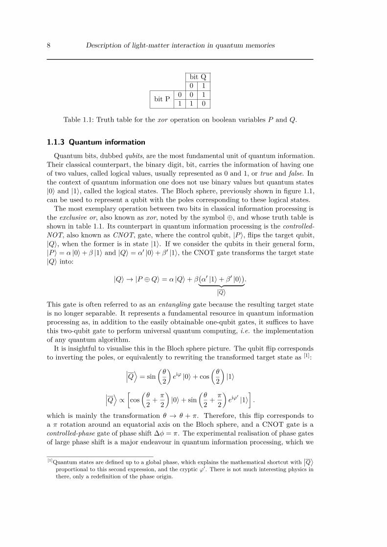
Table 1.1: Truth table for the xor operation on boolean variables P and Q.
1.1.3 Quantum informationQuantum bits, dubbed qubits, are the most fundamental unit of quantum information.
Their classical counterpart, the binary digit, bit, carries the information of having oneof two values, called logical values, usually represented as 0 and 1, or true and false. Inthe context of quantum information one does not use binary values but quantum states|0〉 and |1〉, called the logical states. The Bloch sphere, previously shown in figure 1.1,can be used to represent a qubit with the poles corresponding to these logical states.
The most exemplary operation between two bits in classical information processing isthe exclusive or, also known as xor, noted by the symbol ⊕, and whose truth table isshown in table 1.1. Its counterpart in quantum information processing is the controlled-NOT, also known as CNOT, gate, where the control qubit, |P 〉, flips the target qubit,|Q〉, when the former is in state |1〉. If we consider the qubits in their general form,|P 〉 = α |0〉+ β |1〉 and |Q〉 = α′ |0〉+ β′ |1〉, the CNOT gate transforms the target state|Q〉 into:
|Q〉 → |P ⊕Q〉 = α |Q〉+ β(α′ |1〉+ β′ |0〉
)︸ ︷︷ ︸|Q〉
.
This gate is often referred to as an entangling gate because the resulting target stateis no longer separable. It represents a fundamental resource in quantum informationprocessing as, in addition to the easily obtainable one-qubit gates, it suffices to havethis two-qubit gate to perform universal quantum computing, i.e. the implementationof any quantum algorithm.
It is insightful to visualise this in the Bloch sphere picture. The qubit flip correspondsto inverting the poles, or equivalently to rewriting the transformed target state as [1]:∣∣∣Q⟩ = sin
(θ
2
)eiϕ |0〉+ cos
(θ
2
)|1〉
∣∣∣Q⟩ ∝ [cos(θ
2 + π
2
)|0〉+ sin
(θ
2 + π
2
)eiϕ′ |1〉
].
which is mainly the transformation θ → θ + π. Therefore, this flip corresponds toa π rotation around an equatorial axis on the Bloch sphere, and a CNOT gate is acontrolled-phase gate of phase shift ∆φ = π. The experimental realisation of phase gatesof large phase shift is a major endeavour in quantum information processing, which we
[1]Quantum states are defined up to a global phase, which explains the mathematical shortcut with∣∣Q⟩
proportional to this second expression, and the cryptic ϕ′. There is not much interesting physics inthere, only a redefinition of the phase origin.

1.1 Quantum fundamentals 9
a) b)
Figure 1.2: a) Representation of the controlled-NOT gate with qubits |P 〉 and |Q〉 ina quantum circuit. b) Representation of
∣∣∣Q⟩, the qubit flipped by a NOToperation, on the Bloch sphere.
will review in 1.3.1.The concept of units of information can be extended to states with three logical
values, named qutrits, and even generalised to d-dimensional units as qudits. Quantuminformation can also take the form of continuous variables, a subject I won’t detailhere. I instead refer the curious reader to the review [Braunstein2005]. Whichever formquantum information is taking, its efficient transmission between different parties andhow it can be stored and processed are core topics, reviewed in 1.3.1.
1.1.4 Properties of light and matterHaving formalised these few concepts, we can now move to the main frame of this
thesis, the physics governing light-matter interaction.Using radiation, especially light, to probe the properties of matter, is a technique
known as spectroscopy, which has been an abundant source of knowledge on thematerial world around us. A whole field of spectroscopy in the microwave and mid- andfar-infrared frequency ranges is dedicated to the study of vibrational and rotationalstates of molecules, degrees of freedom that atoms do not possess. Spectroscopy forcrystals additionally involves x-rays, and, for nuclei, gamma rays, and other types ofspectroscopy use particles or acoustic waves: they are completely different realms tothe one covered here, which involve the interaction of light with atoms on transitions atvisible, near-infrared or near-ultraviolet frequencies.
Light, from intense beams down to single photons
Light is an electromagnetic field which can be described by the Maxwell equations.These equations describe the evolution of the electric and magnetic fields in the presenceor absence of charges and currents, in particular those of an atomic medium: thepropagation of light is derived from the Maxwell equations, as well as the polarisationof a collection of dipoles in the presence of light. The formalism of these phenomena isdescribed in 1.2.

10 Description of light-matter interaction in quantum memories
The most easily available form of light is laser light, typically used at intensity levelsin the range 10 µW cm−2 – 100 mW cm−2, with a transverse diameter between 10 µmand a few centimetres. This light is well described in terms of coherent light. This isusually the case for light used as a classical control parameter changing the propertiesof the system, as will be described in the following chapters.
At very low intensities, the quantised nature of light favours its description in termsof photons, the quantum of the electromagnetic field. For experimental quantum optics,the previous semi-classical approach holds in most cases, even when “weak” probes andsignals are used, as those are weak enough not to saturate the atoms but are usuallymade out of 103 − 106 photons, numbers much greater than a few units. The quantumpicture is required when specifically single-photon-level light, or actual single or fewphotons, are used. In this thesis, this is especially looked into in section 3.3 whichdescribes the storage of an optical qubit encoded in light at the single-photon level.Photons are ideal candidates as carriers of quantum information, as they are ele-
mentary quantum objects, intrinsically possess many modes to encode this information[Heshami2016] and can be quickly distributed in a quantum information network.Photon-photon interaction in vacuum is however intrinsically low [Roy2017]. As aresult, in order to perform anything else than sending light from one place to another,it calls for the addition of a second ingredient to mediate the interaction: atoms.
The Playground: Atoms
Whereas two photons cannot directly interact between themselves, they can both becoupled to an atomic medium which effectively mediates this interaction. Moreover,in contrast to photons which usually propagate at the speed of light, atoms representstationary quantum resources.
Atoms as single quantum objects can now be obtained. Single ions and neutral atomscan be trapped and individually addressed by light. Artificial atoms such as quantumdots can be integrated in nanophotonics circuits. However, strong coupling betweenlight and single ions or atoms is experimentally challenging, with avenues consisting ofplacing them at the focus of high-aperture optics, or in structured arrays.
Another widespread solution to compensate the weak coupling with individual atomsconsists in preparing large atomic ensembles to enhance this coupling. This preparationcan be made in warm vapours or laser-cooled ensembles, two methods which areextensively described in chapter 2. With an ensemble which can potentially coupleefficiently to light, the interaction still needs to be engineered to provide the form ofinteraction of interest.
Engineering the light-matter interaction
The most natural non-engineered interaction with an atomic ensemble is the absorptionof light around a set of optical frequencies, which forms the basis of the spectroscopyintroduced earlier.When we look into more detail, the atoms can either coherently or incoherently
absorb this light, resulting in two very different regimes. In the first case, the absorbedlight is reversibly mapped to a collective atomic excitation – the system keeps someinformation on the impinging light –whereas in the second one all information is lost.

1.2 Light-matter interfacing formalism 11
This coherent mapping has been studied extensively in the last decades, in particularfor the conversion of “flying” photonic qubits to “stationary” atomic qubits, which isthe essential operation of optical quantum memories reviewed in 1.4.
Slow light is another scheme of light manipulation enabled by atoms, one of the firstcollective effects to be engineered for applications in quantum information processing.More recently, the stationary light effect has enabled “formally-zero” group velocitiesand also keeping all light under its photonic form. This new regime of light-matterinteraction is compelling by itself and also promises great enhancement for a range ofapplications.Before going into more details of the mechanism of the interaction between atoms
and light, I will now present the range of applications in quantum information enabledby this interaction.
1.2 Light-matter interfacing formalismI describe in this section the formalism used to describe the atomic and photonic
states, and especially their interplay through the interaction processes that will be usedthroughout this thesis.
1.2.1 Classical matter and lightLet us start with the “semi-classical” behaviour of light and atoms.
Polarisability
A basic model for the atom is a single electron bound to the nucleus by a harmonicforce, with ω0 the atomic resonance frequency, and a damping of coefficient γ. Theresponse of the electron to an external electric field ~E = ~E0 exp (−iωt) is given by theequation:
d2~r
dt2+ γ
d~r
dt+ ω2
0~r = −e~E0m
exp (−iωt) ,
with m the mass of the electron, of charge qe = −e. The steady state solution to thisequation is the dipole ~d(t) = −e~r0 exp(−iωt) where:
~d0 = −e~r0 = ε0αc ~E0
with ε0 the electric permittivity of vacuum, and αc the classical polarisability given by:
αc(ω) = e2
mε0
1ω2
0 − ω2 − iγω .
The motion of the electron is accompanied by its dipole radiation. The average radiatedpower diffused by the atom is given by the Larmor formula:
P = ε012πc3 |αc|
2ω4∥∥∥ ~E0
∥∥∥2,

12 Description of light-matter interaction in quantum memories
with c the speed of light in vacuum. For a plane wave, the incident power per unitsurface is Ppw = ε0c
∥∥∥ ~E0∥∥∥2/2, hence a diffusion cross section:
σc(ω) = PPpw
= 8π3 r2
e
ω4
(ω20 − ω2)2 + γ2ω2 . (1.1)
Close to resonance, this cross section becomes:
σc(ω ≈ ω0) = 8π3 r2
e
ω20
4(ω0 − ω)2 + γ2 ,
which is proportional to a Lorentzian of width γ, the damping coefficient of the motionof the electron.
Light propagation
The propagation of an electric field at frequency ω verifies:
∆ ~E + ω2
c2 εr ~E = ~0,
with εr the relative permittivity also known as the dielectric constant. The mediumrefraction index n verifies n2 = εr. To identify the dispersion and attenuation of theelectric field, the real and imaginary parts of the index, hence of the polarisability αc,need to be made explicit. The imaginary part of the classical polarisability, whichdescribes the attenuation, hence its absorption by the medium, is given by:
Im [αc(ω)] = e2
mω0
γω
(ω20 − ω2)2 + γ2ω2 . (1.2)
Optical depth
The most universal figure of merit for atomic ensembles is their optical depth (OD),which measures the coupling of light with the atoms on its path through the ensemble.
We commonly refer to the attenuation of resonant light through a medium from anintensity I0 to an intensity I to be caused by the OD of the medium, noted d, whichequals − ln (I/I0). OD can be defined in terms of an effective cross-section σ:
d = σ
AN,
where N is the total number of atoms and A the cross-section between the light andthe atomic medium it is going through. The cross-sections are proportional to λ2
0,with λ0 = 2πc/ω0 the wavelength associated with the resonance frequency, as seen inequation 1.1. The adjective “effective” now hides the atom-light coupling. We knowthis coupling to depend on the dipole strength at a given frequency for the consideredatoms. The expression of the OD for light resonant with an excited level of linewidth Γis derived in [Gorshkov2007b] as:
d = 4g2NL
Γc , (1.3)

1.2 Light-matter interfacing formalism 13
Transmission
0
0.2
0.4
0.6
0.8
0.1
0.3
0.5
0.7
0.9
a)
b)
Figure 1.3: a) Incident light of intensity I0 and detuning δ from resonance with anexcited state is attenuated down to intensity I(δ) after crossing an atomiccloud of optical density d. On resonance (δ = 0), the light is attenuateddown to I0 exp(−d). b) Transmission profile I(δ)/I0 in function of thedetuning δ. Γ corresponds to the linewidth of the excited state.
with g the coupling of the light field to one atom, and L the length of the sample.Our definition of OD is that the intensity of resonant light is attenuated by a factor
exp(−d)[2].The absorption from the atoms can be obtained from the polarisability expressed in
equation 1.2: it has the shape of a Lorentzian, which means that light detuned by afrequency difference δ = ω − ω0 from the excited state is attenuated down to:
I(δ) = I0 exp[− d
1 + 4(δ/Γ)2
].
This equivalently gives, knowing the attenuation of light detuned by δ from resonance,the OD:
d =[1 + 4
(δ
Γ
)2]ln(I0I
).
[2]An amplitude attenuation of exp(−d), which means an intensity attenuation of exp(−2d), is sometimesfound in the literature.

14 Description of light-matter interaction in quantum memories
1.2.2 Description of quantum atom-light systemsTo go into more details than the absorption in terms of a heuristic OD introduced
previously, a quantum description of the atoms is now required.
Single atom
The simplest system is made of only one atom, which is additionally assumed to haveonly a few levels.
Two-level atom Let us consider the simplest case of a two-level atom. The two levelsare taken non-degenerate i.e. have different energies. The lowest-energy state is byconvention called the ground state, and very often noted |g〉, and the higher-energyone is called the excited state, |e〉. Their energy difference in the context of atom-lightcoupling is best expressed as ~ωeg, which is the energy of a photon at frequency ωeg.Before going into the details of how such a photon can change the quantum state of theatom, we can define a raising operator that transfer the atom from state |g〉 to state |e〉:
σ+ = |e〉 〈g| .
And conversely, a lowering operator:
σ− = |g〉 〈e| .
The Pauli matrices span the Bloch sphere, which was introduced in figure 1.1, withpoles |g〉 and |e〉. They make explicit the correspondence between any unitary vectoron the sphere and the projection of this vector. These operators can be expressed inthe basis of Pauli matrices, which are expressed in the |g〉 , |e〉 basis as:
σx =(
0 11 0
)
σy =(
0 −ii 0
)
σz =(
1 00 −1
)In terms of the Pauli matrices, the raising and lowering operators correspond to:
σ+ = σx + iσy2 =
(0 10 0
)
σ− = σx − iσy2 =
(0 01 0
)Taking as a reference of zero energy the mid-point between the ground and excitedlevels, the energy of the atom is given by an operator proportional to σz:
~ωeg2 σz = ~ωeg
2 (|e〉 〈e| − |g〉 〈g|) ,

1.2 Light-matter interfacing formalism 15
hence an atomic Hamiltonian:
H0 = ~ωeg2 σz.
The interaction of the atomic dipole with an external electric field leads to the raisingto the excited state or lowering to its ground state. For an external electric field ~E =~E0 cos(ωt+ ϕ), it is found that the Hamiltonian describing the atom-light interactionin the dipole approximation reads:
Hint = −~µ. ~E0 cos(ωt+ ϕ)σx = −~Ω cos(ωt+ ϕ)σx.
with ~µ the dipole moment of the atom. Ω = ~µ · ~E0/~ is called the Rabi frequencyassociated with the electric field ~E0 and it is very common to directly bypass the wholeelectric field description to keep only the Rabi frequency of the field, which, we will see,is fundamental in the context of atom-light coupling.In the interaction representation, the full Hamiltonian is:
H = ~2 (ωeg − ω) σz −
~2Ω
(ei(ωt+ϕ) + e−i(ωt+ϕ)
) (eiωtσ+ + e−iωtσ−
).
where we can define the detuning ∆ = ωeg − ω.The rotating wave approximation consists in neglecting the terms varying at frequen-
cies ±2ω and keeping only the constant terms:
H = ~2∆σz −
~2Ω
(σ+e
−iϕ + σ−eiϕ)
= ~2Ω′σ~n.
with σ~n the spin operator in the direction ~n:
~n = −Ω cosϕ~ex − Ω sinϕ~ey + ∆~ezΩ′ .
In the interaction picture, the evolution on the Bloch sphere of the state of the atomcoupled to light is the rotation around the ~n-axis at angular frequency Ω′:
Ω′ =√
Ω2 + ∆2 .
Three-level atom Without losing generality, I am choosing to describe Λ-type atomicstructures as this is the configuration chosen in most realisations of EIT, including ours,and all the experiments described in this thesis. [3] This configuration is also sometimesreferred to as the Raman configuration, as it allows Raman scattering processes, whichI describe in chapter 4.The interaction Hamiltonian of an atom with a Λ-shaped structure, with ground
state |g〉, excited state |e〉, and a second ground state, also called metastable state |s〉,shown in figure 1.4, has the general form:[3]Ladder (Ξ) and “vee” (V) are the two other possible structures with three atomic levels.

16 Description of light-matter interaction in quantum memories
Figure 1.4: Λ-type three level atom. A light field of Rabi frequency Ωeg (Ωes) andfrequency ωeg(ωes) couples to the |g〉 (|s〉)→ |e〉 transition.
Hint = −~2(Ωege
−iωegt |e〉 〈g|+ Ωese−iωest |e〉 〈s|
)+ h.c.
where Ωji is the Rabi frequency of the field addressing the |i〉 → |j〉 transition. Wecall light which addresses the |g〉 → |e〉 transition probe light, and |g〉 → |s〉 controllight, denoted with indices p and c, respectively.
Atomic ensembles
In the case of N identical atoms, the interaction Hamiltonian is:
Hint = −~2(g√N Ee−iωpt |e〉 〈g|+ Ωce
−iωct |e〉 〈s|)
+ h.c.
As large atomic ensemble are considered, the continuous limit approximation canreasonably be made: the atomic quantities are a function of a continuous positionvariable, in lieu of discrete atoms, each at a given location (or each with an individualposition wave function).
Spin wave The Raman scattering with the emission of an anti-Stokes photon, definedin chapter 4, leaves the atomic ensemble with a collective excitation: one of all theatoms from the ensemble has been transferred to state |s〉. This is reminiscent, in acollection of spins[4], of the superposition of all the possible states where one given spinis raised (or lowered): this state is called a spin wave. This collective state, where thetotal spin of the system has been increased, is an eigenstate of the system. In our case,the state resulting from anti-Stokes Raman scattering is also commonly referred to as aspin wave in the literature, a name I also adopt in the following.The spin wave can be seen as a Dicke state of the form:
|ψ〉 = 1√N
N∑j=1
eiϕj |g〉1 . . . |s〉j . . . |g〉N ,
[4]For example, a ferromagnet.
1.2 Light-matter interfacing formalism 17
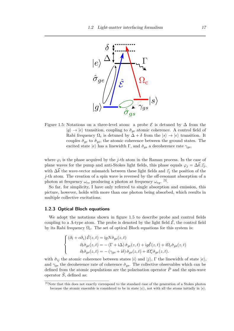
Figure 1.5: Notations on a three-level atom: a probe E is detuned by ∆ from the|g〉 → |e〉 transition, coupling to σge atomic coherence. A control field ofRabi frequency Ωc is detuned by ∆ + δ from the |s〉 → |e〉 transition. Itcouples σge to σgs, the atomic coherence between the ground states. Theexcited state |e〉 has a linewidth Γ, and σgs a decoherence rate γgs.
where ϕi is the phase acquired by the j-th atom in the Raman process. In the case ofplane waves for the pump and anti-Stokes light fields, this phase equals ϕj = ∆~k.~zj ,with ∆~k the wave-vector mismatch between these light fields and ~zj the position of thej-th atom. The creation of a spin wave is reversed by the off-resonant absorption of aphoton at frequency ωes producing a photon at frequency ωeg. [5].So far, for simplicity, I have only referred to single absorption and emission, this
picture, however, holds with more than one photon being absorbed, which results inmultiple collective excitations.
1.2.3 Optical Bloch equationsWe adopt the notations shown in figure 1.5 to describe probe and control fields
coupling to a Λ-type atom. The probe is denoted by the light field E , the control fieldby its Rabi frequency Ωc. The set of optical Bloch equations for this system is:
(∂t + c∂z) E(z, t) = igNσge(z, t)∂tσge(z, t) = − (Γ + i∆) σge(z, t) + igE(z, t) + iΩcσgs(z, t)∂tσgs(z, t) = − (γgs + iδ) σgs(z, t) + iΩ∗c σge(z, t).
with σij the atomic coherence between states |i〉 and |j〉, Γ the linewidth of state |e〉,and γgs the decoherence rate of coherence σgs. The collective observables which can bedefined from the atomic populations are the polarisation operator P and the spin-waveoperator S, defined as:[5]Note that this does not exactly correspond to the standard case of the generation of a Stokes photon
because the atomic ensemble is considered to be in state |ψ〉, not with all the atoms initially in |s〉.

18 Description of light-matter interaction in quantum memories
P (z, t) =√N σge(z, t)
S(z, t) =√N σgs(z, t).
Using these notations, we obtain the following set of canonical Maxwell-Bloch equations:(∂t + c∂z) E = ig
√N P
∂tP = −(Γ + i∆)P + ig√N E + iΩcS
∂tS = − (γgs + iδ) S + iΩ∗cP .(1.4)
In these equations, we can identify the coupling factor in terms of the OD: d = g2N . Anapproximation which is almost always true in the realisations described in this thesis isthat the excited state population remains small, and does not vary significantly, whichgives ∂tP = 0 and:
P = i√d ΓE + iΩcS
Γ + i∆ .
In this approximation, the remaining Maxwell-Bloch equations simplify to:(∂t + c∂z) E = i
(d
Γ∆E +√d
Ωc
∆S
)∂tS = −
(γ′ + iδ′
)S + i
√d
ΓΩ∗c∆E .
(1.5)
with the effective one-photon detuning δ′ – which includes the Stark shift fromthe control Rabi frequency – and effective spin-wave decay rate γ′gs and complexdetuning ∆:
δ′ = δ − |Ωc|2∆Γ2 + ∆2
γ′gs = γgs + Γ |Ωc|2
Γ2 + ∆2
∆ = ∆2 + Γ2
∆ + iΓ .
These equations are sufficient to describe most of the dynamics of the optical memoriesinvestigated in this thesis when the three-level approximation stands. This is not thecase of the EIT-based qubit storage described in chapter 3, where additional excitedstates on the D2 line have a significant effect. Chapters 4 and 5 only require the additionof the role of forward and backward signal-and-control pairs.
1.3 Quantum information networks and applicationsThe development of a global quantum network, dubbed the quantum internet, is
an exciting prospect of the development of quantum information science [Kimble2008].

1.3 Quantum information networks and applications 19
This research endeavour has seen numerous achievements in the last three decades,which I describe now.
1.3.1 Implementations of quantum informationThe quantum properties of light and matter as carriers of information grant them
a number of properties which are at the core of their applications in the context ofquantum information, which are presented in this section.
Quantum communication
Quantum networks require the transmission of quantum information over thousandsof kilometres to reach the global scale. Similarly, in classical communication becauseof the losses on transmission over optical fibres, the channel features repeaters thatre-amplify the signal. A quantum version of these repeaters, however, is not trivialto build: precisely the quantum nature of the transmitted information prevents signalamplification or “measure-and-prepare” scheme. In a measurement, the quantum stateis projected onto the measurement basis, and all its information is not recovered,making those solutions unsuitable. Fundamentally, any of these schemes cannot beacceptable as it otherwise would violate the “no-cloning” theorem stating that it isfundamentally forbidden by quantum mechanics to deterministically create copies ofan unknown quantum state. Quantum repeaters based on entanglement swapping ofmemory-synchronised photon pairs allow scalable quantum information transmissionat long range [Briegel1998]. The architecture involving quantum repeaters enables theerror probability to scale only polynomially instead of exponentially with the distance,along with logarithmic scaling for the number of particles whose control is required.As a fibre would experience at best attenuation of the order of 15 dB over a
distance of 100 km, a recently demonstrated alternative is the space-borne quan-tum communication scheme that was first envisioned in [Aspelmeyer2003]. A seriesof landmark articles showed the feasibility of free-space quantum key distribution[Hughes2002, Kurtsiefer2002], distribution of entangled photons pairs over kilometredistances [Peng2005] and quantum teleportation schemes [Aspelmeyer2003, Yin2012].Quantum key distribution with low-orbiting (∼ 100 km) satellites has recently beendemonstrated [Yin2017].
Information processing
Transferring quantum information from one location to another is one of the majoraspects studied in the literature, the other aspects concern the processing of thisinformation.The solving of linear systems of equations is an example of a general computation
problem. It can be performed with quantum resources [Harrow2009], and even specifi-cally with only photons and linear optics, a technique known as linear optical quantumcomputation (LOQC) [Knill2001]. Although this computational system would showa quantum advantage, a computer like the classical version we are familiar with iseasily re-programmable: a promising alternative to LOQC which would be adaptableinvolves the generation of cluster states, where a large collection of qubits are intricately

20 Description of light-matter interaction in quantum memories
entangled and the performed computation is chosen by classical measurements andoperations on nodes of this cluster state [Walther2005].
Quantum cryptography
The “no-cloning” theorem mentioned above and the perturbation of a quantum stateby its measurement are actually aspects of quantum information which can be exploitednot as a limitation but as a feature. Indeed, the perturbation of a quantum state meansthat two parties can communicate on a quantum information channel and realise ifan eavesdropper is listening to the channel. Moreover, they are guaranteed that theinformation they exchange is secure, as it is impossible to duplicate it [Gisin2002].
These ideas can also be used to produce unforgeable quantum money, an idea datingto the premises of quantum cryptography [Wiesner1983, Bennett1983]. This topic hasbeen increasingly popular in the last years, arguably due to the emergence of crypto-currencies like Bitcoin or Ethereum, the former unexpectedly skyrocketing to valuesabove 16k$US at the close of 2017, starting from below a thousand early that year.
1.3.2 Realisation of quantum network elements with light and atomsLight and atoms are central to the implementations of quantum information protocols,
both as carriers of this information and as sources of quantum states through theirinteraction.
Encoding of information in photonic and atomic qubits
Photonic qubits are central to quantum networks as they can easily be distributedbetween distant nodes, a reason for which they are often dubbed flying qubits, in contrastwith qubits defined on atoms, ions, superconducting circuits, etc. which are usuallystationary, although they can in some cases be moved around over small distancesby optical tweezers, for example in proposals of scalable quantum computers withthe transport of ions qubits [Cirac2000, Kielpinski2002]. They both have their ownadvantage, flying qubits connecting different nodes, exchanging information, whilestationary qubits in each node are addressable and can be coupled to other qubits, inorder to process that information.
Just like in classical information, where the logical values 0 and 1 correspond to twodifferent values of voltage in a circuit, or the presence or absence of light through anoptical fibre, the quantum logical states |0〉 and |1〉 are two states of a given mode inthe considered system. In our case, with light and atoms, many options are available,which we can group into two main categories, corresponding to either internal statesor external degrees of freedom. The external degrees of freedom can be the locationwithin the system or the path taken by the carrier of information. A popular encodingis the time-binning: the time at which the carrier can trigger a detector is dividedinto bins, two or many more, which each corresponds to a mode to encode information.Alternatively, among internal states, qubits can be defined on the polarisation, frequency,phase, value of the orbital-angular-momentum, etc.[6].[6]The number of excitations can also define the logical state, with however the limitation that if there
are losses anywhere in the network operation, the fidelity of the qubit quickly degrades.

1.3 Quantum information networks and applications 21
Quantum state generation
The interaction between light and matter can be used to generate the non-classicalstates required in quantum information protocols. In 2001, a major practical imple-mentation was proposed for the generation of single photons [Duan2001], defining theso-called Duan-Lukin-Cirac-Zoller (DLCZ) protocol. The process relies on the prepara-tion of an on-demand single photon from the heralded writing of a collective atomicexcitation.Its principle consists in preparing a spin wave from a spontaneous Raman process,
the non-classical resource of this protocol emerges from the single-photon photodetectorused to herald the success of loading the atomic ensemble. Once the atomic ensembleis loaded with a single excitation, a classical read pulse deterministically triggers theemission of a single photon in a well-determined mode.The DLCZ protocol was first realised a few years after its proposal [Kuzmich2003],
then the heralded photon was isolated [Chou2004] and stored in a remote quantummemory [Chaneliere2005]. The protocol was made more elaborate with frequencyconversion of the photon to telecommunication wavelengths [Radnaev2010]. A recentdemonstration involved, after conversion to telecom wavelength, the transmission in afibre and storage in a solid-state memory, therefore performing a full transfer betweentwo heterogeneous nodes of an elementary quantum network [Maring2017].
In a broader context, the brightness of single-photon sources can greatly benefit fromquantum memories to synchronise the probabilistic generation of single photons, aswell as making the sources deterministic [Nunn2013]. These quantum memories aredescribed in the following.
1.3.3 Quantum memoriesIn the description of the above quantum network elements, a recurrent theme has been
the storage, synchronisation and conversion of quantum information. Essentially, quan-tum memories do not only perform the storage of quantum information but more broadlythe transfer to and from the different forms of this information [Matsukevich2004]. Inthis section, I describe optical quantum memories and their characterisation in themost general case. The different memory schemes and their specificity are extensivelyreviewed in the following section 1.4.
Historical introduction
The last decade has seen the experimental realisation of the envisioned optical memoryschemes proposed in the early 2000’s, such as dynamically-controlled electromagnetically-induced transparency applied to light storage [Fleischhauer2000], and controlled-reversibleinhomogeneous broadening (CRIB) proposed the following year in [Moiseev2001].Since then, quantum memories are and remain one of the most sought-after appli-cations of the interaction of light and matter, with a handful of dedicated reviews[Bussieres2013, Heshami2016, Ma2017].

22 Description of light-matter interaction in quantum memories
Figures of merit
With many different memory platforms and schemes, the comparison between experi-mental realisations relies on a set of universal figures of merit, listed in table 1.2 anddescribed in the following.
Figure of merit Definition Comments and thresholdsEfficiency η η = Eout/Ein No-cloning requires >50%Fidelity F F (ρin) = Tr
(√ρin ρout
√ρin)
Classical limit: 2/3Memory lifetime TS Time at which η(t = TS) = η0/2 Delay-bandwidth productBandwidth ∆ω Frequencies at which η > η0/2 T∆ω
Multimode capacity Nb of simultaneously stored modes > 2 for qubit storage
Table 1.2: The table lists the most commonly-cited figures of merit for quantum memo-ries. The second column gives the usual definition of these figures of merit.The third column indicates the usual thresholds to compare to. Eout andρout (Ein and ρin) are the energy and density matrix the output (input) ofthe memory, η0 represents the efficiency at immediate retrieval and at thecentre frequency.
Efficiency (storage, retrieval) The operation of a quantum memory proceeds in twosteps: the storage of information within it, and the subsequent retrieval from it. Eachstep is performed with some efficiency, limited by the imperfect nature of the transfer,by the loss of energy to other channels than the one used for retrieval, etc. The universaldefinition of the memory efficiency is the ratio between the output and input energies,Eout and Ein:
η = EoutEin
.
Sometimes, especially when the stored quantum state is prepared in situ instead ofbeing externally produced and transferred in the memory, the memory efficiency isbroken down in storage and retrieval efficiencies, ηs and ηr, obviously with η = ηsηr.This distinction between the two steps is especially meaningful when we distinguishbetween schemes with forward and backward retrieval, a priori with the same dynamicsof storage. Contrasting these schemes for a Raman memory is the purpose of section4.1.3.
The storage-and-retrieval efficiency of quantum memories is a stringent parameter fortheir envisioned applications [Bussieres2013, Heshami2016], especially for the scalabilityof optical quantum networks [Sangouard2011]. A main threshold for memory efficienciesis 50%: above, more information is retrieved than lost after being stored in the memory.It is necessary to perform above this limit to be in the no-cloning regime. Indeed, ifmore information is lost to the environment than retrieved, it is possible that the stateread-out from the memory is a copy of the input state, which is itself kept somewhereelse. We can never prevent this scenario if the efficiency is below 50%. On the otherhand, performing above this limit enables error correction on qubit losses in linearoptics quantum computation [Varnava2006] and unconditional security in quantum

1.3 Quantum information networks and applications 23
communication protocols [Grosshans2001].To reach high efficiencies, optical quantum memories require a strong coupling
between photons and atoms [Gorshkov2007]. Two main approaches are consideredto enhance this coupling: placing individual quantum systems in high finesse cavi-ties [Specht2011], or mapping the photonic states onto collective atomic excitations[Duan2001, Fleischhauer2000]. In both case, the main limitation to the efficiency ofmemories is ultimately the available OD of the system [Gorshkov2007a, Gorshkov2007b].The increase of OD in atomic ensembles is the main topic of chapter 2.
Fidelity The involved fidelity is implied as being between the output and input quantumstates handled by the memory. If we can define a density matrix for each of these states,ρout and ρin respectively, then the fidelity is defined as the following trace:
F (ρin) = Tr (√ρin ρout√ρin ) .
The memory fidelity is defined as the lowest fidelity over the set of possible inputs ρin.The fidelity lies in the [0, 1] interval, reaching 1 when ρout = ρin. In the case of pure
states |ψ〉 and |ϕ〉, the fidelity is given by the square of their overlap |〈ψ|ϕ〉|2.An important bound here complements the no-cloning limit introduced for the
efficiency. The bound known as the classical limit is the maximum fidelity achievableby a classical memory. It is shown that for a state with N photons, this bound is equalto (N + 1)/(N + 2) [Massar1995]. In particular, for single photons, this equals 2/3, i.e.approximately 68%.
In the case of qubits, on average, a random output has a 20% overlap with the input.The performance should be considered with this lower bound in mind, rather than zero.
Memory lifetime The typical memory time is defined as the storage duration at whichhalf[7] of the information initially stored remains. This duration has to be compared tothe relevant time scales of the system. For example, in a two-level structure where theexcited state has a bandwidth of the order of the megahertz, the typical decay timeis at the microsecond scale, which means that memory times appreciable at a humanscale, of the order of the second or the minute, represent quite a challenge, howevertackled in [Dudin2013, Heinze2013].
Bandwidth Bandwidth is the converse aspect of storage duration. Many endeavoursaim at providing a quantum memory with the largest achievable bandwidth, as it notonly enables a full storage of the fast-varying features in the temporal profile of thesignal, but also the simultaneous storage of several signals defined in different frequencybands or a train of pulses, for example. For a memory relying on the absorption ofsignal light, one could think this figure is limited by the width of the atomic absorptionlines, which is of the order of a few MHz for the excited state of the alkali D lines. Onthe other hand, single photons generated by spontaneous down-conversion typicallyhave natural bandwidths of a few nanometres, which can be reduced by the use ofcavities. Many memory schemes do circumvent this limitation and obtain increased
[7]Decay times can be defined at 1/e, or 1/e2.

24 Description of light-matter interaction in quantum memories
memory bandwidths by a clever use of broadening. These schemes are detailed in thefollowing review in section 1.4.
Delay-bandwidth product A figure of merit unifying the two previous ones is thedelay-bandwidth product, the product of the typical delay enabled by the memoryand its bandwidth, i.e. the ratio of memory lifetime and the pulse duration. Thedelay-bandwidth product indicates how many pulses would fit in the typical decay timeof the memory efficiency. It is a useful metric to compare memories operating at verydifferent time scales.
Multimode capacity Some memories are able to simultaneously store more than onemode supporting information, in which case they are said to be multimode. The multi-mode capacity denotes the number of modes stored simultaneously and independently.It is required that simultaneous storage is completely independent i.e. that each memorymode can be written and read-out independently and without alteration of any storedmode from another stored one. A large bandwidth can be divided up in order to storemultiple signals in the frequency domain; multimode storage can rely on other degreesof freedom, reviewed in the upcoming section 1.4.For example, for qubits, a suitable quantum memory needs to be able to uniformly
store the two modes on which the qubit is encoded. This ability to store multiplemodes requires multiplexing, which can either be either temporal [Nunn2008], spatial[Higginbottom2012, Nicolas2014, Zhou2015] or spectral [Sinclair2014, Higginbottom2015].
Extended figures of merit A few additional figures of merit are sometimes quoted inthe literature, which I am listing here, although the memories I have worked on duringmy thesis perform quite poorly on these.
Operating wavelength suitability Atomic quantum memories can only store signalsat a set of wavelengths corresponding to atomic transitions and those are not necessarilycompatible with other elements of a prospective quantum network. In particular, opticalfibres have been optimised to transmit the light at telecommunication wavelength bands,defined in the range 1260 nm − 1675 nm. Rare-earth ion doped solids (REIDS) havebeen put forward for their compatibility at those wavelength. In contrast, the D spectrallines of the commonly-used alkali species are in the visible and near-infrared range.However frequency conversion of the light stored in alkali ensembles is an availablesolution to integrate this category of memories in a future global quantum network.
Implementation practicality A typical cold atom vacuum system is human-sizedand would not be easily duplicated. For this reason, a push is made to reduce the sizeof the memories, as well as simplifying the alignments, required optical powers, etc.in order to be able to easily scale up and multiply the number of memories within anetwork.
Another concern linked to the scaling of quantum technologies is the integrability ofall the devices. An ideal quantum device will not be a patchwork of juxtaposed deviceswith many losses on the interconnections, but rather a single platform integrating all

1.3 Quantum information networks and applications 25
the functional elements. Considering the progress of the silicon industry to that regard,quantum devices which can directly be integrated on a silicon wafer are actively soughtafter.
Difference between optical and quantum memories Before going into the details ofthe quantum memory platforms, we should define the vocabulary which is used in theliterature. A major distinction to be made here is the difference between quantummemories and memories which are only said to be optical for example. The adjectivequantum does imply non-classical properties which need to be demonstrated: the storageof laser light mediated by the quantum states of a collection of atoms is not sufficientto prove the quantum character of the memory. Conversely, “true” quantum resourcessuch as single photons or entanglement are not needed to demonstrate it, an oftenmisconceived aspect.
The relevant figure of merit is the fidelity of the memory which was previously defined.The quantum performance of these memories can be demonstrated by achieving a fidelityoutperforming the best performance attainable by a classical device [Hammerer2010],which was defined as the classical limit. In the case of qubits, i.e. one quantum ofinformation, the classical limit equals 2/3, like for a single photon.
Checking that property does not necessarily involve storing actual single photons orentanglement but can instead be done using weak coherent light, in particular at thesingle-photon level [Riedmatten2008, Hedges2010]. One could naively think that thecoherent state |α = 1〉 is weak enough and a good approximation of the single photon.In fact, such a coherent state is defined as:
|α = 1〉 =∑n
1√n!|n〉 = e−1/2
(|0〉+ |1〉+ 1√
2|2〉+ 1√
6|3〉+ . . .
)The overlap of |α = 1〉 with a single photon is 〈1|α = 1〉 = 1/
√e , which means
the probability of measuring exactly one photon from a coherent state with α = 1 is|〈1|α = 1〉|2 = 1/e ≈ 37%. It is also just as likely to obtain a vacuum state in this case.More importantly, though, the two-photon component is rather large (|〈2|α = 1〉|2 =1/(2e) ≈ 18%). This component and those of even more photons contaminate thequantum state, which has a direct effect on using coherent states with values of α around1 when trying to benchmark the quantum operation of a memory. The one-photonto two-photon component ratio is
√2 /α, therefore a solution to decrease the relative
contribution from two and more photons is to choose a lower value for α. This choiceis at the expense of an even larger vacuum component, however. For example, withα = 0.1, the coherent is made up of roughly 90% vacuum, 9% single photon and lessthan 0.5% two photons and more. The consequence is that the success rate of thepreparation of one photon is low, but this is not necessarily an issue, for example ifthe interaction of the single photon with the memory can be heralded. Using weakcoherent states is nonetheless rather common as they are a widely-available resource,and low values of α can be obtained simply by attenuating the intensity of a laser on abeam-splitter or with neutral densities.The terms “classical” or “optical” memory can state explicitly that the quantum
nature of the memory has not been demonstrated. For example when the information

26 Description of light-matter interaction in quantum memories
is redundant in the stored signal, one could rely on a “measure-and-prepare” strategy –a classical solution – to outperform the performance of the memory, storing informationfor a arbitrarily long duration as this would simply be determined by the time at whicha copy of the measured signal is prepared. On another hand, as for most memoryschemes, there has already been demonstrations in the quantum regime which provethe process is indeed quantum, it is usually more convenient to operate well above thesingle-photon level, which explains why many realisations operate in this regime.
More than just memories
As interaction platforms between light and matter, optical quantum memories findapplications even beyond the general quantum state transfer [Bussieres2013]. Indeed,they can encode non-linear operations between qubits “within” the memory, duringtheir storage or by altering the retrieval stage. For example, a configurable LOQCnetwork can be built only relying on quantum memories [Campbell2014].
Among non-linear operations between qubits, cross-phase modulation (XPM) is oneof the applications we have had in mind since the beginning of our investigationsof stationary light, as it essentially is a controlled-phase gate, which would lead tothe realisation of a controlled-NOT gate for universal quantum computation. Indeed,the topic has attracted a lot of attention in the past decade, with counter-arguments[Gea-Banacloche2010] formulated against a proposed scheme based on EIT-based “giantKerr effect” to provide XPM [Schmidt1996]. Indeed, as is explained in chapter 3, it canbe interpreted that the increase of the interaction time with a decrease in group velocityis accompanied by a shift of the polariton coefficients to a large atomic component anda low photonic one. As a result, it cannot lead to enhanced non-linear interaction suchas XPM. Stationary light, on the other hand, can precisely decrease the group velocitywhile keeping the signal in its light field mode. The nature and generation of stationarylight is the topic of chapter 5.
1.4 Review of optical quantum memory schemesAs I intend in this section to provide an overall vision of the vast field of quantum
memories, let us classify them in a few categories, choose common notations and focuson their similarities and differences.While all quantum memories are handling similar inputs of a quantum nature (be
it single photon, squeezed light, entanglement, etc.), a central aspect to each quan-tum memory which differentiates the different schemes is the way there are classicallycontrolled. Two main approaches are chosen here, as pointed out in the review paper[Ma2017]: memories that are optically-controlled and those based on engineered ab-sorption. In the first category, classical auxiliary fields are used to control the memoryoperation, for example to dynamically change the susceptibility of the atomic mediumto store and retrieve light. In the second, the absorption spectrum of the atoms isinitially prepared thereby storing light for a pre-programmed duration.

1.4 Review of optical quantum memory schemes 27
1.4.1 Pre-programmed delayA pre-programmed memory does not require any intervention when an incident signal
arrives, its properties have been prepared to perform light storage for a given duration.
Fibre loop
Sending light through a fibre is a basic way of delaying it, which does present manydrawbacks: first of all, although the loss of light in optical fibres is minimised attelecommunication wavelengths around 1550 nm, light propagates in a physical materialand bounces off the core-cladding interface, leading to inevitable losses. The state ofthe art of fibres have losses of 0.15 dB km−1, which is equivalent to 0.03 dB µs−1. Thisconstitutes nonetheless a benchmark for quantum memories: can they outperform themost straightforward solution of delaying the light in a fibre loop? High efficiency andlong storage time need to be simultaneously obtained in order to outperform a fibre.For example, the 50% efficiency limit, above which operation in the no-cloning regimeis possible, corresponds to a propagation in a fibre for 100 µs. So far only the ANUexperiment reported in [Cho2016] performed in this region.
Atomic Frequency Comb
The Atomic Frequency Comb (AFC) scheme relies on the preparation of a collectionof atoms starting with a large inhomogeneously-broadened absorption profile which isthen shaped as a periodic comb with optical pumping techniques. The atoms start inground state |g〉, have an excited level |e〉 and can be shelved to a long-lived auxiliarystate |aux〉 which is decoupled from all the optical transitions of interest. Only theatoms j which have a frequency detuning which is a multiple integer of ∆ are kept instate |g〉: δj = mj∆, mj ∈ Z. The others atoms are transferred to |aux〉. This resultsin an absorption spectrum for the atomic ensemble which is a series of absorption at aregular interval ∆. After an AFC medium absorbs a photon, the atoms quickly dephase,but they all rephase at a pre-programmed time 2π/∆, which leads to a coherent photonecho.If we can approximate each absorption peak to be a narrow Gaussian of full-width
half maximum γ, the memory has a finesse F = ∆/γ and an effective OD close tod/F , with a memory efficiency crucially depending on the latter. The memory requirestherefore a compromise between finesse and memory efficiency.This scheme was proposed in [Afzelius2009] and subsequently demonstrated the
following year in [Afzelius2010]. It has since established itself as a remarkable memoryon many figures of merit, especially bandwidth [Saglamyurek2011, Vivoli2013] andmultimode capacity [Gundogan2013, Jobez2016]. An AFC memory in an impedance-matched cavity has been used to demonstrate an efficiency of 56% [Afzelius2010a].AFC can also be extended to an on-demand memory with delay by involving
a metastable state, forming a Λ configuration, the so-called Λ-AFC configuration[Jobez2014].

28 Description of light-matter interaction in quantum memories
a)
b)
c)
d)
e)
Figure 1.6: Principle of dynamic EIT a) A signal (blue) is sent to an atomic ensemble(green) in which a transparency window is opened by a control field (red).b) The signal experiences a slowdown effect as it enters the atomic ensemble.c) When the whole signal pulse fits inside the atomic ensemble, turning offthe control field causes the signal to be converted to stopped light (lightgreen). d) Turning the control field back on restores the propagation of thesignal. e) As the signal exits the atomic ensemble, it recovers its originalshape.
1.4.2 Dynamic Electromagnetically-Induced TransparencyElectromagnetically-induced transparency (EIT) is accompanied by a decrease of the
group velocity, which enables the dynamic control of the propagation of the light. Theslowdown can be controlled by the intensity of a auxiliary control field, and the lightcan even be brought to a halt by decreasing this control to zero.
EIT originates from coherent population trapping (CPT) which manifested througha decrease in the fluorescence of sodium atoms in a vapour cell, in the seminal paper[Alzetta1976]. The name of the phenomenon conveys the idea that the evolution ofatoms starting from any state eventually brings them to a so-called dark state, fromwhich they are decoupled to the rest of the system and therefore remain trapped there.The application of CPT is mainly the preparation of atomic states for clocks [Scully1992],magnetometry [Vanier2005] and laser cooling [Aspect1988]. It is not directly applicableas a input-output quantum memory for light in our case, but it has been used to storetransmon qubits [Koch2007] into a nitrogen vacancy spin ensemble [Kubo2011]. CPTalso allows the preparation of single nuclear spins at room temperature, with possibleinformation storage applications [Jamonneau2016].The EIT phenomenon itself, where atoms are made transparent to light they
would normally be opaque to, was first observed in 1991 [Boller1991] before be-ing formally described in the context of dark-state polaritons and applied to lightstorage [Fleischhauer2000, Fleischhauer2002]. The first demonstrated EIT memorywas performed in [Andre2005]. Of particular interest for us, in comparison with

1.4 Review of optical quantum memory schemes 29
our qubit storage experiment reported in chapter 3, is the storage of polarisationqubits. It has been performed with vacuum-stimulated Raman adiabatic passagein trapped single atoms [Specht2011, Kalb2015], atomic frequency combs in rare-earth doped solids [Clausen2011, Zhou2012, Gundogan2012, Clausen2012, Jin2015,Laplane2015], as well as EIT in warm [Cho2010, Kupchak2015] and cold atomic en-sembles [Matsukevich2006, Choi2008, Lettner2011, Zhang2011, Xu2013]. Some quan-tum memories have also simultaneously stored multiple photonic degrees of freedom[Tiranov2015, Parigi2015, Zhang2016].
1.4.3 Raman Memory
input recall
b)a)
Figure 1.7: Raman memory with backward retrieval. a) A signal E+ traverses anelongated atomic cloud where a two-photon resonant control beam Ω+converts it to a collective atomic excitation. b) A backward-propagatingcontrol beam Ω− subsequently retrieves the signal in the backward direction,as E−.
Simply put, Raman memory is the far-detuned variant of EIT. There are, however,some significant differences between the two schemes. A Raman memory relies on theabsorption of signal light and its conversion to a spin-wave coherence, mediated by thecontrol field. It is not a slowdown effect like EIT. Both memory scheme nonethelessshare the aspect that when the control field is turned off, the signal becomes entirelyatomic, it corresponds to stopped light.Figure 1.7 shows the configuration for a Raman memory with backward retrieval,
accordingly to the experiment reported in chapter 4. Although the backward config-uration exhibits a mirror symmetry that enhances retrieval, it is not usually chosenin realisations of Raman memories, even the most performing to date [Reim2010,Reim2011, Reim2012, Michelberger2015, Saunders2016]. A few experiments do em-ploy elements of a backward geometry in Raman systems to immediate advantages[Chen2013a]. Beyond the replacement of the control beam at the retrieval stage by itsmirror image, configurations with the simultaneous application of a pair of counter-propagating control beams has led to the recent development of stationary light, which

30 Description of light-matter interaction in quantum memories
brings a range of novel effects [Moiseev2006, Nikoghosyan2009, Wu2010, Iakoupov2016,Blatt2016, Iakoupov2016a, Everett2017].Symmetry can be introduced between the storage and read-out processes with an
angle between the control with the signal, which cancels the longitudinal componentspin wave k-vector. Moreover, the read-out can be made conveniently collinear with thesignal axis in the configuration where the long-lived storage state lies below energeticallyand the control angle compensates the wave vector mismatch from this energy difference[Surmacz2008].As pointed out in [Gorshkov2007a], the condition of large detuning in the case of
large atomic ensembles is ∆ dΓ and not the usual condition ∆ Γ which is valid fora single atom. Our configuration at ANU uses a detuning which is only around 200 MHz,which under this condition would not exactly be referred to as Raman memory. Thecondition is however perfectly verified in the realisation of the group of Ian Walmsleyin Oxford, where detunings — as well as bandwidths — of the order of the gigahertz[Nunn2007, Michelberger2015], or even terahertz [Bustard2013] are used.
1.4.4 On-demand photon-echo techniquesAnother type of quantum memories rely on photon echoes, which correspond to the
time reversal of the absorption of light: it usually corresponds to the reversal of thebroadening of the medium [Tittel2010]. The first photon-echo memories originate froma proposal in 2001 [Moiseev2001] to use counter-propagating pulses to generate photonechoes with high efficiency in spite of the inhomogeneous Doppler broadening presentin an atomic gas. The technique was extended to solids in [Moiseev2003] and very soonafter led to the controlled-reversed inhomogeneous broadening protocol.
Controlled-Reversed Inhomogeneous Broadening
Controlled-Reversed Inhomogeneous Broadening (CRIB) is experimentally very closeto the photon-echo concept described above but it really was in 2005 with [Nilsson2005]where controllable external fields are used to create this inhomogeneous broadening,which can therefore be reversed, that the name was given to the technique as a whole andadopted in the first subsequent realisations, for example [Alexander2006, Hetet2008].CRIB is still a popular scheme in rare-earth-doped solids [Chaneliere2015] and hasalso led to the emergence of other memory protocols based on photon echo: revival ofsilenced echo and gradient echo memory.
Revival of silenced echo
Revival of silenced echo (ROSE) is a two-pulse photon echo which circumvents thenoise arising from the population inversion in standard CRIB protocol. This techniquewas developed at the Laboratoire Aimé Cotton [Damon2011] and it subsequentlydemonstrated a 42% retrieval efficiency, at telecom wavelength [Dajczgewand2014].

1.4 Review of optical quantum memory schemes 31
z
Figure 1.8: Principle of the gradient echo memory. Top: a signal E is coupled to a spinwave S by the control field of Rabi frequency Ω. The atomic medium isinhomogeneously broadened by a longitudinal frequency gradient in the zdirection +η0 is applied on the atomic transitions. Each frequency compo-nent of the signal is stored at the location in the cloud which correspondsto the two-photon resonance with the control field. Bottom: The gradientis reversed to −η0. At the time symmetric from the storage time relative tothe gradient reversal time, the frequency components of the signal — storedin spin waves along the z axis — all simultaneously rephase, producing aphoton echo.
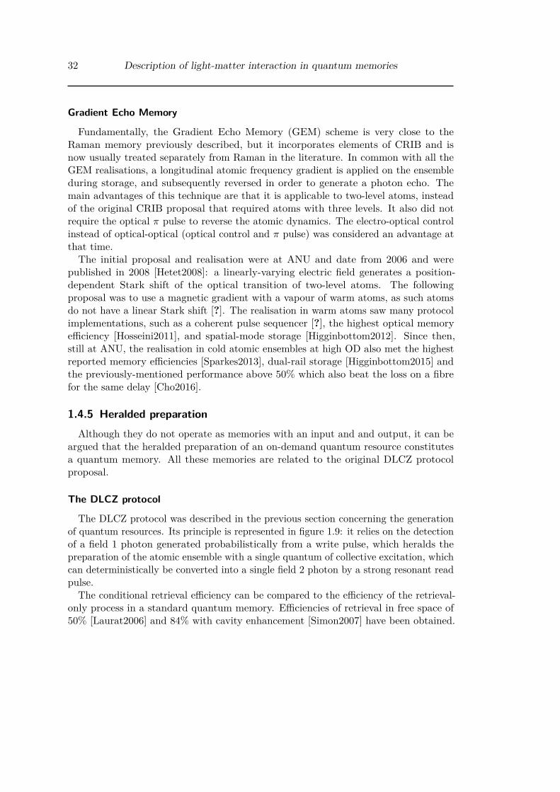
32 Description of light-matter interaction in quantum memories
Gradient Echo Memory
Fundamentally, the Gradient Echo Memory (GEM) scheme is very close to theRaman memory previously described, but it incorporates elements of CRIB and isnow usually treated separately from Raman in the literature. In common with all theGEM realisations, a longitudinal atomic frequency gradient is applied on the ensembleduring storage, and subsequently reversed in order to generate a photon echo. Themain advantages of this technique are that it is applicable to two-level atoms, insteadof the original CRIB proposal that required atoms with three levels. It also did notrequire the optical π pulse to reverse the atomic dynamics. The electro-optical controlinstead of optical-optical (optical control and π pulse) was considered an advantage atthat time.The initial proposal and realisation were at ANU and date from 2006 and were
published in 2008 [Hetet2008]: a linearly-varying electric field generates a position-dependent Stark shift of the optical transition of two-level atoms. The followingproposal was to use a magnetic gradient with a vapour of warm atoms, as such atomsdo not have a linear Stark shift [?]. The realisation in warm atoms saw many protocolimplementations, such as a coherent pulse sequencer [?], the highest optical memoryefficiency [Hosseini2011], and spatial-mode storage [Higginbottom2012]. Since then,still at ANU, the realisation in cold atomic ensembles at high OD also met the highestreported memory efficiencies [Sparkes2013], dual-rail storage [Higginbottom2015] andthe previously-mentioned performance above 50% which also beat the loss on a fibrefor the same delay [Cho2016].
1.4.5 Heralded preparationAlthough they do not operate as memories with an input and and output, it can be
argued that the heralded preparation of an on-demand quantum resource constitutesa quantum memory. All these memories are related to the original DLCZ protocolproposal.
The DLCZ protocol
The DLCZ protocol was described in the previous section concerning the generationof quantum resources. Its principle is represented in figure 1.9: it relies on the detectionof a field 1 photon generated probabilistically from a write pulse, which heralds thepreparation of the atomic ensemble with a single quantum of collective excitation, whichcan deterministically be converted into a single field 2 photon by a strong resonant readpulse.
The conditional retrieval efficiency can be compared to the efficiency of the retrieval-only process in a standard quantum memory. Efficiencies of retrieval in free space of50% [Laurat2006] and 84% with cavity enhancement [Simon2007] have been obtained.

1.4 Review of optical quantum memory schemes 33
write
read
field2 field1field2
field1 readwrite
a) b)
Figure 1.9: Principle of the DLCZ protocol. a) A write pulse, detuned from the excitedstate probabilistically generates a single photon in mode field 1, whosedetection heralds a single collective excitation in |s〉. Subsequently applyinga strong resonant read pulse deterministically produces a single photonin field 2. b) The geometry of the write and read beams to generatecounter-propagating field 1 and field 2.
1.4.6 Performance comparisonThe highest reported performance of optical memories was recently compiled in
[Ma2017]. Table 1.3 lists the relevant figures of merit for our discussion of quantummemories. Note that each figure of merit is independent of the others for the sameplatform, i.e. high efficiency and high bandwidth can be listed for a memory scheme,this does not necessarily mean that both have or can be obtained simultaneously.
Memory scheme Efficiency η Storage time TS ∆ωmax Multimode capacityEIT 78% 1 s 100 MHz Low
Raman 30%† 1.5 µs 1 THz LowCRIB/GEM 80% 0.2 ms 1 GHz Moderate
AFC 56% 5 µs 1 GHz HighRaman-GEM 87% 1 ms 1 GHz Moderate
Λ-AFC 12% 1 ms 1 GHz High
Table 1.3: Record reported memory performance. ∆ωmax stands for maximum memorybandwidth. References to the articles reporting the figures for efficiency andstorage time are given in table 1.4.
The references are listed in table 1.4.[8]
Looking at this collection of results indicates that different strategies, platforms andspecific memory schemes give heterogeneous performance on the different figures ofmerit. In the context of the work presented in this thesis, we notice in particular howthe record efficiency for Raman memories seems comparatively low to either EIT orRaman-GEM, although one could think realisation with high memory efficiency ineither of these schemes should also perform well with a Raman memory. This, however,can be contrasted with the high bandwidth obtained in the reported Raman memories,
[8]†Our result of backward-retrieval Raman memory presented in chapter 4, which is pending peerreview, would set the record efficiency of Raman memories up to 68%.

34 Description of light-matter interaction in quantum memories
Category Memory scheme Efficiency η Storage time TS
Optically-controlled EIT [Chen2013] [Heinze2013](on-demand) Raman [Reim2011] [England2012]
Engineered absorption CRIB/GEM [Sparkes2013] [Sparkes2013](pre-programmed) AFC [Sabooni2013a] [Maring2014]
Hybrid Raman-GEM [Hosseini2011] [Cho2016](on-demand with delay) Λ-AFC [Jobez2014] [Jobez2015]
Table 1.4: References to the values of memory efficiency and storage time shown intable 1.3.
which could hint that the groups working on those have mainly focused on this figureof merit instead of the storage-and-retrieval efficiency. A second point is the multimodecapacity of EIT which is stated as low, and although there were some challengingaspects of performing qubit, i.e. two-mode, storage at LKB, our prospects for the futureof the experiment may question a supposedly-low multimode capacity of EIT-basedmemories.
Chapter Conclusion
In this introductory chapter:
• The context of atom-light interaction has been introduced, especially itsapplications in quantum information encoding, transfer and processing.
• A formalism for light-matter interaction in large atomic ensembles has beenpresented, including a general set of optical Bloch equations for Λ-type atoms,which are referred to throughout this thesis.
• The state of the art of photonic implementations was presented, especiallyoptical quantum memories schemes whose performance were reviewed, inorder to appreciate the results presented in this thesis.

Chapter 2
Key elements for the preparation of large atomicensembles
The central piece to all the experiments reported in this thesis is a large atomicensemble. They all relied on the preliminary preparation of a collection of atoms, eithervia the heating-up of a vapour cell or cycles of trapping, cooling and release of anatomic cloud in vacuum. As the techniques for this preparation evolved over the years,the ensembles got denser and their atomic coherence longer-lived. My arrival at LKBcoincided with the cold atomic ensemble running into the limitation of its moderateOD and ongoing efforts aiming at improving this number. On the other hand, newhighs in OD were being obtained at ANU with the help of the neighbouring atom-lasergroup led by Nick Robins. There was a significant overlap between the challenges inboth institutions and some expertise which could be shared both ways. Contrastingthe realisations, through my personal experience with them, has let me see the broaderpicture as well as the perks of each atom preparation.This chapter is a review of the modern techniques used for warm and cold atom
preparation that I have become familiar with during my PhD. Hopefully this list providesall the useful guidelines for the preparation of large atomic ensembles and highlightsthe relevant aspects for the protocols I describe in the following chapters.
2.1 Considerations for atomic ensemble preparationOur objective is to prepare a large ensemble of atoms, which we typically address with
an optical signal to be stored. There are a handful of avenues to this end, among whichtwo I have been acquainted with and I am describing here: warm atomic vapours, morebriefly, and, in more detail, cold atomic clouds prepared by magneto-optical trapping.Alternative preparations include crystals with atom-like impurities, such as ions dopantsor vacancies like nitrogen in diamond, to cite only a few of the other platforms.
One of the attributes required of this ensemble preparation is that it should be wellcontrolled, repeatable and stable, so that it does not change significantly between itscharacterisation and its use as a platform for quantum protocols. This is usually easilyobtained with magnetically-shielded warm vapours, which simply need to be heatedup at a constant rate, and which stabilise within tens of minutes. This is not so muchthe case with laser-cooled ensembles which are exposed to variations of the ambientmagnetic field – from electronics anywhere in the vicinity being turned on or off, or ascrewdriver forgotten close to magnetic coils – variations in power or polarisation of the
35

36 Key elements for the preparation of large atomic ensembles
cooling laser, or variations of the frequency of any laser used to prepare the ensemble,caused by a change in the ambient temperature, by mechanical vibrations or by thedrop of an electro-optical lock. These environmental issues aside, and provided a fewdaily realignements, both methods ideally yield a ensemble in a deterministic fashion.
The preparation of cold atomic ensembles was initiated by previous group membersin the recent years, in both labs, and many details can be found in their PhD theses[Sparkes2013PhD, Veissier2013PhD, Giner2013PhD, Nicolas2014PhD].
2.2 Warm atomic ensemblesWarm atomic ensembles are relatively easy and cheap to obtain, especially when we
compare them to cold atoms in vacuum which require an apparatus of many elements,vacuum chamber parts, pumps, laser light dedicated to the preparation, etc. I describethem in the next section. Instead for warm atoms, it is sufficient to buy a vapour cell,i.e. a glass cell containing the atoms, usually in a solidified form on the walls at roomtemperature. Obtaining an appreciable vapour only requires to heat it up above thistemperature, usually with a resistance wire coiled around the windows and the cold pointwhere the vapour condenses when cooling down. In our case, rubidium has a meltingpoint of 39°C and caesium 28.5°C, with a vapour pressure of 10−6 Torr− 10−7 Torr at25°C. In practice, at ANU, the temperature reached for the cell in which the quantumprotocols are performed is of the order of 60°C and the ones used for filtering is closerto 120°C to obtain very high densities at the expense of more atomic collisions, whichis acceptable as light just goes through those cells. The ambient magnetic field can becancelled by using shielding, for example with mu-metal. A photo of the main vapourcell for the GEM experiments at ANU, along with a filter cell, is shown in figure 2.1.
The main drawback of warm vapours is obviously their temperature. The atoms havea root mean squared velocity of a few hundreds of metres per second, which leads todetrimental effects on different aspects relevant to the prospective quantum applications.
2.2.1 Doppler shiftThe distribution of velocities in a warm atomic vapour at temperature T is well
described by a Boltzmann distribution. The probability p(v) to find an atom withvelocity v on along an axis is given by:
p(v) = 1√2π
(m
kBT
)3/2exp
(− mv2
2kBT
).
With this distribution, the root mean squared velocity is vrms =√
3kBT/m , which,for rubidium, equals 320 m s−1 at 80°C. The first consequence of this atomic motion isfrequency shifts due to the Doppler effect. Light at frequency ω0 and wave-vector ~k0 isseen by an atom moving at velocity ~v is shifted to:
ω(~v) = ω0 − ~k0 · ~v.
For the D1 line transitions at λ0 = 795 nm, this corresponds to a typical frequency shift∆D = 2πvrms/λ0 = 2π×400 MHz, which is a significant shift, relatively to the linewidth

2.2 Warm atomic ensembles 37
Figure 2.1: A rubidium-87 vapour cell inside a mu-metal shielding can be seen in thecentre. On the left, inside a mu-metal cylinder of smaller diameter, arubidium-85 filter cell is held by teflon caps on each end. In front, the cablesof the gradient coils and heating wires.
of the excited level around 5 MHz. The main issue is that the Doppler shift is notuniform, the width of the atomic velocity distribution translates into an inhomogeneousbroadening of the atomic transitions, of the order of ∆D.For two-photon processes, with co-propagating light fields of wave vectors ~k1 and
~k2, the effect partially cancels out as both light fields experience the same Dopplershift. There is a residual shift δ12 when the frequency of the light fields does not match,as the wave vectors also do not; the residual shift is equal to δ12 = (~k1 − ~k2) · ~v. Forexample, for a Raman process between the hyperfine states of alkali species, whichdiffer in energy by the splitting ∆ωhf ∼ GHz, we have δ12 = 2πvrms∆ωhf/c ∼ 10 kHz.Introducing a small angle β 1 between the wave vectors accounts for a quickly
increasing shift: δ′12(β) ≈ k1vrms (1− cosβ) = k1vrmsβ2/2 +O
(β4). For an angle of 1°,
that is already a shift of the order of the megahertz. Of course the worst case scenariocorresponds to counter-propagating light fields, which are shifted in opposite directionsby the atoms in a given velocity class.
2.2.2 Sources of decoherenceWe see here that the Doppler effect does not make the frequency shifts that dramatic
when the wave vectors are strictly co-propagating. The other type of limitation due tothe temperature of the atoms is their decoherence.As we have seen in 1.3, the aim of many quantum protocols relies on the atomic
coherence created in an ensemble. In a warm vapour, however, the atoms diffuse andcollide inelastically with each other, which leads to decoherence. The diffusion effects inmemory experiments are reviewed in [Chrapkiewicz2014], and collisional decoherence in[Horsley2013]. Both these effects can be mitigated by using buffer gases, which consistsin adding an inert gas in the cell, usually at pressures of the order ∼ 1 Torr− 10 Torr[Arimondo1996a]. In the presence of this buffer gas, the atoms of interest are morelikely to elastically collide with them than with each other inelastically. These collisionseffectively reduce both the diffusion and collision decoherence rates. The drawback

38 Key elements for the preparation of large atomic ensembles
comes from collisional broadening, resulting from the additional decay channel for theexcited state of the atoms. The kinetic collision rate with the buffer gas is given by[Erhard2001]:
Rk = p
kBTσkvrms,
with p the pressure of the buffer gas and σk the kinetic cross section for the consideredmix of gases.
The atoms not only collide with other gases in the cell, but also with the walls of thecell itself. A now widespread solution to prevent these collisions to be inelastic is to coatthe inside walls of the cell with an anti-relaxation coating, which makes the wall collisionspreserve the atomic spin state. This technique using paraffin has been known for sometime [Bouchiat1966] and has specifically been used since the first few memory experi-ments in warm vapour in Polzik’s group [Julsgaard2001, Schori2002, Julsgaard2004], orat LKB during the PhD of Jean Cviklinski [Cviklinski2008PhD]. Alternatively to paraf-fin, coatings can be made of alkanes, alkenes and other hydrocarbons [Balabas2013]. Inspite of these limitations, atomic memories at room temperature were recently reportedwith a storage time as long as 150 ms [Katz2017].
2.3 Large cold atomic ensemblesAtomic ensembles can be prepared at temperatures in the nanokelvin-microkelvin
range from laser cooling of a low-pressure background vapour in vacuum. This preventsmany decoherence processes due to atomic motion or collisions, between atoms orbetween atoms and their environment. A standard magneto-optical trap (MOT),however, only reaches ODs of a few tens or hundreds, which is below the thousandseasily attainable in warm vapours [Hosseini2012]. Nonetheless there are techniques toprepare atomic ensembles reaching such high ODs, an achievement which was only metrecently [Sparkes2013, Hsiao2014]. This section first reminds the important aspects ofa MOT, in order to introduce the more advanced methods to reach large cold atomicensembles with ODs in the same range as the warm vapours.
2.3.1 Atom cooling and trappingA MOT relies on a velocity- and position-dependent atom-light interaction, which
enables the cooling and trapping of an atomic ensemble. The principle behind theoptical and magnetic components of a MOT are reminded here.
Optical cooling
In a usual MOT, six beams – three pairs of counter-propagating beams – are usedto cool down the atoms. They are usually referred as trapping or cooling beams. Theprinciple of this cooling, and what makes it velocity dependent is the following.
Radiation pressure When an atom is promoted to the excited state |e〉 by the absorp-tion of a photon of momentum ~~k, this momentum is fully transferred to the atom.

2.3 Large cold atomic ensembles 39
0.4
0.6
1
0.8
-4 -2 2 400
0.2
Figure 2.2: Dependence of the radiation pressure pressure force with the laser detuning,δ. The force is scaled to the maximum one, which is obtained with I Isand at resonance. The detuning is given in units of Γ, the excited statelinewidth. The radiation pressure is given for I/Is ratios equal to 0.1 (blue),1 (yellow), 10 (green) and 100 (red).
When the atom decays back to the ground state, it also emits a photon of momentum~~k, although this emission is isotropic and therefore does not contribute to a net force.Overall, a single absorption-reemission sequence results in a radiation pressure forcefrom the net momentum exchange ∆~p = ~~k.The rate of decay for an atom in the excited state is equal to the excited state
linewidth Γ, the rate at which these absorptions occur is simply Γ multiplied by theaverage population of the excited state. In the presence of a laser light which couplesthe ground and excited states, we found this population to be:
σee = 12
s
1 + s,
with s the saturation parameter, which is given on resonance as s = I/Is, with I theintensity of the laser and Is the saturation intensity characteristic of the atoms andtypically of the order of a few mW cm−2. The average radiation pressure force thereforeis:
~Frp = Γ2
s
1 + s~~k.
Doppler cooling The radiation pressure force depends on the detuning of the coolinglight, which is itself affected by the Doppler effect. Red-detuned light can actually beresonantly absorbed by an atom moving towards it. To explain this quantitatively, letus have a look at the saturation parameter with the detuning taking into account theDoppler shift:
s(~v) = Ω2/2δ(~v)2 + Γ2/4 = I
Is
11 + 4δ(~v)2/Γ2 ,

40 Key elements for the preparation of large atomic ensembles
with δ(~v) = ω − ω0︸ ︷︷ ︸δ0
− ~k · ~v.
The radiation pressure force as a function of the detuning δ is represented in figure 2.2for different I/Is ratios.δ0 is the detuning for the class of atoms whose velocity is orthogonal to the cooling
light wave vector. The saturation parameter for those can be noted s0. Hence avelocity-dependent radiation pressure force:
~Frp(~v) = Γ2 ~~k
Ω2/2Ω2/2 + Γ2/4 + (δ0 − ~k · ~v)2
.
For small enough velocities, i.e.∣∣∣2δ0~k.~v
∣∣∣ Ω2/2 + Γ2/4 + δ20, this expression can be
linearised as:
~Frp(~v) = Γ2 ~~k
Ω2/2Ω2/2 + Γ2/4 + δ2
0
(1 + 2δ0
Ω2/2 + Γ2/4 + δ20~k · ~v
)+O
(~k · ~v2
). (2.1)
In practice, the condition comes down to∣∣∣~k · ~v∣∣∣ Γ/2.
For simplicity, I now assume that both the velocity and the cooling light are onthe z-axis, i.e. ~v = v~ez and ~k = k~ez, with ~ez the unit vector in the +z direction.For red-detuned cooling light, δ0 < 0, the velocity dependent term radiation pressureforce is of the form ~F = −αv~ez, which is a friction force. The force is maximal when|δ0|ΓΩ2/
(Ω2/2 + Γ2/4 + δ2
0)2 is. This factor is actually:
2δ0Γδ2
0 + Γ2/4 ×s0
(1 + s0)2 ,
which is found to be maximal with:
δ0 = −Γ2 and s0 = 1.
The force in this case equals:
~Frp(v) = ~Frp(~v = ~0)− ~k2
4 v~ez +O(k2v2
).
The force can be interpreted in terms of the recoil energy from one cooling photon,~2k2/2m. At low saturation values s0 1, the radiation pressure force is:
~Frp(v) = ~Frp(~v = ~0)− α
2 v~ez +O(v2),
with the friction coefficient:
α = 2s0~k2 |δ|Γδ2 + Γ2/4 . (2.2)
The stochastic scattering of cooling photons causes the atoms to diffuse. Their spread

2.3 Large cold atomic ensembles 41
∆z is given by:
∆z2 = 2Dt,
with the diffusion coefficient D = Γ/k2 for δ0 = −Γ/2. D is of the order of 1 mm2 s−1,to be compared to the typical cross-section of the cooling beams, a few centimetres. Ina MOT, such cooling beams cross from all six directions of space, reducing the overallkinetic energy of atoms close to the crossing point.
With real atoms, however, there are always other states to which the atoms can decayfrom the excited state. In particular, alkali species have two hyperfine ground states,separated by much more than the linewidth of a typical cooling beam, hence only theatoms in one of these states are effectively trapped and cooled down. Atoms whichdecay to the other state are not addressed by the cooling beam, and if their temperatureis still high, they escape from the trapping volume. In order to restore these atoms to atrapped state, repump beams are used, usually resonant to the transition between theother ground states and the excited level.
Zeeman trapping
Starting from a low background pressure, however, there are few atoms in the captureregion of the cooling beams, which demands the addition of a position-dependent forceto prepare dense clouds, which is what the second half of magneto-optical trappingprovides, through its magnetic component.For a linear magnetic gradient along the z-axis, ~B = bz~ez, the magnetic sub-levels|F,mF 〉 are shifted by the energy [SteckCesium]:
E|F,mF 〉(z) = ~ω|F,mF 〉(z) = µBgFmF bz,
with µB the Bohr magneton and gF the Landé factor in state F . The detuning δ0 inthe radiation pressure force 2.1 is replaced by the mF -dependent detuning:
δmF (z) = δ0 −µBgFmF b
~z.
The idea of magneto-optical trapping is to use this detuning for a position and state-dependent radiation pressure force. To this end, circularly-polarised cooling light isused, with a σ±-polarised beam along the ±z-direction. This cooling light exerts aforce:
~F±rp,mF(~v = ~0, z) = ±Γ
2 ~~k
Ω2/2Ω2/2 + Γ2/4 + (δ0 ∓ µBgFmF bz/~)2 .
In the simplest case of a unique ground state |g〉 = |F = 0,mF = 0〉 and a |F = 1〉 excitedstate, the atomic level structure is made of three Zeeman sub-levels mF ∈ −1, 0,+1.σ±-polarised light only addresses the |g〉 → |F = 1,mF = ±1〉 transition.
The same derivation as the velocity-dependent force gives a position-dependent force:
~F (z) = −κz~ez with κ = µBgF b
~kα, (2.3)
42 Key elements for the preparation of large atomic ensembles
with α defined in equation 2.2.This expression stands near the centre z < zc = ~Γ/(µBgF b), which defines a capture
range of the order of zc. With the typical numbers of a rubidium MOT, we havezc ∼ cm, which is the desired order of magnitude to trap atoms within cooling beamsof few-inch diameter. In practice, the magnetic gradient in three directions is providedby a set of quadrupole coils, with the direction of the axis of the coils experiencingtwice the magnetic gradient in order to satisfy div ~B = 0. This detail, however, doesnot change the principle of Zeeman trapping in three dimensions.
Two-dimensional MOT geometry
An elongated ensemble geometry consists in shaping the atomic cloud along theoptical axis, which enables a much larger proportion of the atoms to be addressed by thesignal. This idea was demonstrated in [Lin2008a] and now a widespread configuration.This geometry is obtained by giving the atoms a position-dependent recoil only in
two directions, and leaving them free to expand in the third one, giving it the nameof 2D-MOT. In practice, a pair of coils on the third direction, usually called cap coils,implements a small gradient (about 10 times smaller than the axial one) in order tokeep the atoms in the overlapping region of the trapping beams.
This configuration easily enables ODs above 100. To refer to my own experience,the LKBMOT typically yielded OD around 50 in the conventional 3D-confinementgeometry. When we changed its configuration to a 2D-MOT one, along withtwo-inch trapping beams but comparable optical trapping power, with no otherchanges to the loading scheme, ODs up to 150 were obtained. This corresponds toa three-fold improvement, comparable with the increase reported in the original2D-MOT proposal.
Dynamical compression
A technique used to further increase the OD, at least transiently, is to radiallycompress the atomic cloud by increasing the magnetic gradient at the end of the loadingsequence, possibly accompanied by a further detuning of the optical trapping beams[Petrich1994]. From equation 2.3, we notice that both result in a stronger radiationpressure force towards the centre of the MOT, effectively compressing the atomic cloud.The larger magnetic gradient or detuning is the decrease in capture efficiency fromthe low-pressure atomic background, which explains why the compression is madedynamically at the end of the preparation sequence, after first loading the MOT.

2.3 Large cold atomic ensembles 43
The usual techniques to load a 2D-MOT are confronted to another limit on theOD, at best up to 300 at ANU, for example. The use of a dynamical compressionphase at the end of the loading typically yields a 50% increase of the OD.However this process where atoms are being pushed to the centre of the MOT canintuitively be associated to an increase in the overall temperature. The effect ismitigated or maybe even cancelled by simultaneously performing a temperaturereduction sequence, such as polarisation-gradient cooling, introduced in thefollowing section.
2.3.2 Temperature reductionThe temperature of the atoms captured in the MOT is another crucial parameter
to reduce. The performance of warm vapours is limited by the atomic motion attemperatures close to the room one. While MOTs provide atomic ensembles with atemperature orders of magnitude below this, the residual motion of the atoms has adetrimental effect, for example on their ability to store information [Tikhonov2015].
Polarisation-Gradient Cooling
Also known as Sysiphus cooling, polarisation-gradient cooling (PGC) is a technique todecrease the temperature of the atomic cloud obtained initially. Indeed the cooling beamintensity and frequency profiles are first optimised to collect as many atoms as possiblein the centre of the MOT. The second step consists in decreasing the heating ratefrom the intense cooling beams by gradually increasing their detuning from resonance.With a decrease in the pumping rate to the other ground state, the repump intensitycan concurrently be decreased without losing atoms to states not addressed by theMOT. This also contributes to decreasing the unnecessary atom-light interaction forthe atoms accumulated in the MOT. In practice, for rubidium and caesium, that givestemperatures of the order of 10 µK− 100 µK.
Dark spontaneous-force optical trap
Temporal dark spontaneous optical trapping (dark SPOT) is similar to the PGCsequence described previously. Another implementation is the spatial dark SPOT, witha region within the atomic cloud where the cooling or repump beams are masked. Whenentering this region, the atoms are not addressed by light anymore, and the higher theirtemperature is, the faster the rate at which they exit it. This effectively selects atomsat lower temperatures in this dark region.
2.3.3 Typical experimental setupNow that all the relevant concepts have been introduced, I present the components
of a typical experimental setup and the values of the different parameters involved.

44 Key elements for the preparation of large atomic ensembles
Vacuum
The aim of atom cooling and trapping is to replace ensembles in warm vapourcell, where their collisions – with the walls or other atoms – fundamentally limit theircoherence time to ∼ 10 µs−100 µs [Horsley2013]. To prevent such collisions with a warmbackground, the preparation of cold atoms is performed in vacuum, at residual ambientpressures of the order of 10−10 Torr. For the detail procedure to reach this pressure level,I refer the reader to the previous theses at LKB [Giner2013PhD, Gouraud2016PhD].
Dispensers
The atoms used to form the MOT are provided by dispensers, also known as getters[1].Their principle relies on the heating up of a alkali-metal wire to dispense a vapour of agiven element in a vacuum background.
Dispensers from SAES (SAES CS/N F/3.9/12F T 10) are used at LKB. They contain5 mg of caesium and should last 6 months each, if used on average 10h per day. Inpractice during the course of my PhD, we have switched dispensers twice in 4 years.At ANU, where the experiment uses rubidium, we are also using dispensers, from
Alfavakuo, formerly known as Alvatec, with similar specifications. Rubidium having twostable isotopes, the dispensers provide a mixture of these, with their natural abundance.However as their atomic transitions differ, only one isotope is captured in the MOT,the other one only contributing to background pressure.
Magnetic trapping
A typical magneto-optical trap uses a 10-G/cm magnetic gradient over 10 cm, mostcommonly achieved with a pair of coils in an anti-Helmholtz configuration, in two or allthree directions of space, whether it is a 2D or 3D MOT. The anti-Helmholtz configura-tion ensures the cancellation of the magnetic field in the centre and a uniform gradientover the overlap region of the cooling beams, with minimal next-order contribution offthe anti-symmetry axis.
Wire radius The radius of the coil wire limits the maximum current they can sustainwith no other heat dissipation than standard air flow, possibly helped by placingradiators on the coils thermally-conductive structure. Although some realisationsinvolve the use of water cooling, a standard MOT setup usually simply relies on usingwires with a large-enough radius to decrease their resistance. The compromise is madeon the volume taken by a coils with the tens if not hundreds of turns required to achievethe desired gradient. Secondarily, a thicker wire is less pliable, which makes the windingmore challenging: often the practicality of tightly winding the coil calls for using thethinnest wire capable of supporting the required current. In practice, typical wires havea 1 mm− 2 mm radius.
[1]The term getter usually refers to the use of the component to react and condense, i.e. “get”, residualgas inside a sealed vacuum system.

2.3 Large cold atomic ensembles 45
Current source The typical current used during a MOT loading sequence rangesbetween 5 A−10 A, with coils which have a resistance of a 1 Ω−10 Ω. The simplest wayto provide this current is with a power supply, of about 1 kW and capable of deliveringthe relatively high current. A commercial solution adopted on both experiments Iworked on is the Delta Elektronika SM 52-30. Usually such a source cannot sink thecurrent injected in the high inductance circuit. This task needs to rely on anothercomponent, which can in this case be a solid-state relay like the Power-IO HDD-1V50.The original setup at ANU consisted of having the relay in series with the coils, andrelying on its internal resistance when switched off to dissipate the current, effectivelygiving a 1 ms current decay time, on the same order as the decay of the eddy currentsinduced in nearby conductors by the varying magnetic field. The relays, especiallynewer units, can wear off quickly with this operation, however, as it does not correspondto their intended use. Shorter decay times and a more sustainable solution would be touse a capacitor and resistor in parallel to the coils, in order to form a critically dampedRLC circuit when switching off the relay. This solution is currently being investigated.
Previously at LKB, a current source was developed by our electronic engineers Jean-Pierre Okpisz and Brigitte Delamour to commute the coils to a discharge circuit whenwe want the magnetic gradient turned off. The discharge circuit was made of a few1 mF capacitors capable of withstanding the potential difference and speeding up thedecrease of the current by effectively applying an opposite voltage to the loading one,yielding decay times around 50 µs− 100 µs.
Sources of light for optical trapping
A general rule with optical trapping is that the more available power, the better.Indeed it is always desirable to increase the trapping detuning to reduce the scatteringon the atoms, and this can be done without compromising on the number of capturedatoms by increasing the intensity of the trapping beams.
A typical experiment uses trapping beams with total power around 100 mW−500 mW,and diameters of one or two inches. Laser diode light amplified by a tapered amplifiertypically provides around 1 W of continuous light power. Frequency control and gatingwith AOMs and coupling in single-mode fibres reduces this figure to the required powerrange. This light is then divided in several beams to provide the six-directional opticaltrapping. A widespread method to roughly divide by two the amount of power needed isto retro reflect each of three beams. This however limits the flexibility of independentlyfine tuning the power in each direction, and the retro-reflected beams always experiencesome losses due to the optics reflecting them.
2.3.4 Preparation sequencesI describe here the typical atom preparation sequences used in both experiments, at
LKB and ANU.
LKB
The atomic transitions involved in the elongated MOT for caesium-133 atoms at LKBare shown in figure 2.3. The preparation features dynamic compression, a polarisation-

46 Key elements for the preparation of large atomic ensembles
gradient-cooling phase and depumping to the lower ground state F = 3, as shown inthe preparation sequence presented in figure 2.4.
trappingrepump depump
Figure 2.3: The atomic level scheme for the MOT preparation at LKB. During loading,the three retro-reflected two-inch cooling beams have a total power around300 mW and the repump beams have 10 mW. At the end of the preparationsequence, the atoms are “depumped” to the lower ground state, in |g〉 =∣∣∣6S1/2, F = 3
⟩, in a superposition of all the Zeeman sub-levels. This is
performed by a depump beam resonant with the |s〉 →∣∣∣6P3/2, F
′ = 4⟩
transition, accompanied by a the trapping beams relatively close to resonanceand the repump off. The repetition rate of the complete sequence is 16 Hz.
The two-dimensional magneto-optical trapping consists of a set of rectangular coils forradial confinement, completed by a pair of cap coils to generate a shallow gradient alongthe optical axis. Three retro-reflected two-inch cooling beams have a total power around300 mW, corresponding to a density of 17 mW cm−2, and the repump beams 10 mW,which corresponds to 0.5 mW cm−2. At the end of the preparation sequence, the atomsare “depumped” to the lower ground state, in |g〉 =
∣∣∣6S1/2, F = 3⟩, in a superposition
of all the Zeeman sub-levels. This is performed by a depump beam resonant with the|s〉 →
∣∣∣6P3/2, F′ = 4
⟩transition, with an intensity around 0.1 mW cm−2, accompanied
by the trapping beams relatively close to resonance and the repump off.The ambient magnetic field is compensated by a set of three orthogonal coils and
measured by the Raman spectroscopy technique presented in section 2.3.5. The com-pensation is performed down to 20 mG, corresponding to an inhomogeneous broadeningbecause of the equally-populated Zeeman sub-levels around 50 kHz. It is equivalent toa 8 mG cm−1 gradient over the 2.5-cm length of the atomic cloud.
ANU
The atomic transitions involved in the elongated MOT for rubidium-87 atoms atANU are shown in figure 2.5. The preparation features dynamic compression, a cooling

2.3 Large cold atomic ensembles 47
26 G/cm6.5 G/cm
-17 MHz
0.5 mW/cm²
17 mW/cm²
Transversemagnetic field
Repump
Experiment(2 ms)
Preparation(2 ms)
Compression(8 ms)
Loading(37.5 ms)
Cooling beams
time
-107 MHz
Depump
0 mW/cm²
0 mW/cm²
0.1 mW/cm²
Figure 2.4: The typical atomic ensemble preparation sequence at LKB. An elongatedensemble of caesium atoms is prepared by loading a two-dimensional magnetooptical trap with a magnetic gradient of 6.5 G cm−1.
phase and optical pumping to the edge Zeeman sub-level, as shown in the preparationsequence presented in figure 2.6.The two-dimensional magneto-optical trapping consists of a set of rectangular coils
for radial confinement, completed by a pair of coils for longitudinal capping, and threeretro-reflected two-inch-diameter cooling beams that intersect at the zero-magnetic-field location. The cooling beams have a total power around 400 mW, which corre-sponds to a intensity ∼20 mW cm−2 . During loading, repump has a total power ofand 40 mW, which provide two-inch-diameter beams of intensity 2 mW cm−2 on the∣∣∣5S1/2, F = 1
⟩→∣∣∣5P3/2, F
′ = 2⟩transition combined with the cooling beams. Follows
a 20-ms sequence where the atomic ensemble is radially compressed and further cooleddown by a “temporal” dark spontaneous-force optical trapping technique. Last, auniform bias magnetic field of 0.5 G is applied along the optical axis direction tolift the degeneracy between the Zeeman sub-levels and the atoms are transferred tothe |g〉 =
∣∣∣5S1/2, F = 2,mF = +2⟩state by employing a ∼0.7 mW cm−2 σ+-polarised
optical pumping beam resonant with the |g〉 →∣∣∣5P3/2, F
′ = 2⟩transition. The Earth
magnetic field is cancelled by a set of three orthogonal 1-meter-diameter coils.
2.3.5 Atomic ensemble characterisationNow that preparation sequences for cold atomic ensembles have been presented, this
section describes the tools to characterise the ensemble which is obtained, in particularits OD.
Measurement of optical depth
The OD being the limiting factor for the efficiency of the light-matter interfacing, itis crucial to be able to measure it in our atomic ensemble. There are several methods

48 Key elements for the preparation of large atomic ensembles
trapping
repumpopticalpumping
Figure 2.5: The atomic level scheme for the MOT preparation at ANU. During loading,the three retro-reflected two-inch cooling beams have a total power around400 mW and 40 mW for repump light. At the end of the preparation sequence,the atoms are optically-pumped to the edge Zeeman state by a σ+-polarisedbeam, at the same frequency as the cooling beams. The optical pumping isaccompanied by a resonant repump to leave the atoms in the ground state|g〉 =
∣∣∣5S1/2, F = 2,mF = +2⟩.
28 G/cm6 G/cm
-24 MHz
2 mW/cm²
20 mW/cm²
Optical pumping 0.1 mW/cm²
-68 MHz
Transversemagnetic field
Repump
Available for experiments(2 ms)
Preparation(1 ms)
Compression(20 ms)
Loading(400 ms)
Cooling beams
0 MHz-9 MHz -32 MHz
time
Figure 2.6: The typical atomic ensemble preparation sequence at ANU. The sequence isdivided in a MOT loading phase, a compression and a final preparation phase.The magnetic gradient, intensity and detuning profile is as represented here.The repetition rate is around 2 Hz The atoms are optically-pumped to theedge Zeeman state by a σ+-polarised beam, sent along a resonant repumpto leave the atoms in the ground state |g〉 =
∣∣∣5S1/2, F = 2,mF = +2⟩.

2.3 Large cold atomic ensembles 49
Detuning (MHz)0-20 20-30 -10 10 30
Tra
nsm
ission
0
0.2
0.4
0.6
0.8
0.1
0.3
0.5
0.7
0.9
Figure 2.7: Typical transmission profile for a moderate OD around 20. The frequency ofthe probe is varied on an AOM and the transmission at each frequency (red)is measured by a sensitive photodiode. The best fit to the experimentaltransmission profile provides an estimate of the OD.
to this end, depending on the precision needed and the available probe frequencies.
Off-resonance absorption In order to measure the OD, the simplest method wouldbe to send a resonant probe beam and measure the transmitted intensity. However, thiswould only work at very low ODs as the transmission on resonance goes as exp(−d).The second simplest technique is to detune the probe from resonance by δ and determinethe on-resonance OD with the formula:
d =[1 + 4
(δ
Γ
)2]ln(I0I
), (2.4)
with I0 the incident intensity, and I the transmitted one. In practice, because thisconsists in extrapolating the OD from a single measurement, it is rather imprecise,yielding ODs that typically vary by 10% from run to run.
A more elaborate measurement requires a probe beam whose frequency can be variedaround the resonance frequency with the transition of interest, and consists in sending itthrough the atoms and to a high-sensitivity photo-detector. The measured transmissioncan be fitted with the model of equation 2.4 and a value of the OD be determined.Figure 2.7 shows a typical experimental absorption profile and its fit. Signal-to-noiseratio is enhanced with polarisation and spatial filtering by coupling the probe beam toan optical fibre. This allows the operation at low intensity levels, which ensure the probelight does not saturate the atoms. However, because the near-resonant probe beam isnot only attenuated by the atomic transition but also deflected with the "atomic lensingeffect" occurring in the spatially inhomogeneous atomic cloud, we collect the probe

50 Key elements for the preparation of large atomic ensembles
Detuning (MHz)
0-20 20-30 -10 10 30
0
0.2
0.4
0.1
0.3
0.5
0-20 20-30 -10 10 30
0
0.2
0.4
0.1
0.3
0.5
0
0.2
0.4
0.1
0.3
0
0.2
0.4
0.6
0.1
0.3
0.5
Tra
nsm
ission
No currentOD 96
Current 1.3 AOD 106
Current 5.0 AOD 128
Current 8.8 AOD 60
Figure 2.8: Transmission profiles for increasing current in the cap coils of the MOT.The OD of best fit is indicated as an inset of each plot. The top-left plotcorresponds to no current through the coils. Increasing it slightly (top-right)provides some MOT Zeeman trapping along the optical axis, but increasingit further shortens the atomic ensemble, and in the limit of a longitudinalgradient of the same order of magnitude than the axial one, correspondsto a 3D-MOT configuration, of lower OD. The optimal current is found tocorrespond to an intermediate current of 5.0 A, realising an OD of 128, a30% increase on the initial OD without cap coils.
using a large-core multi-mode fibre. We scan the frequency of the probe beam aroundresonance using a acousto-optical modulator (AOM) in double-pass configuration. Thetransmission at each frequency is measured by alternating sequences with the atomiccloud fully loaded and without atoms to update the intensity of the incident beamwhich can fluctuate over time.
The application of this method is illustrated in figure 2.8. It corresponds to a seriesof OD measurements which were performed on the LKB experiment with differentvalues of the current through gradient cap coils along the axis of the 2D-MOT. Thesemeasurements were taken in order to determine the optimal gradient in this directionto increase the density of the MOT in the interaction volume, without decreasing thisvolume by reducing the length of the atomic cloud with a too steep gradient.

2.3 Large cold atomic ensembles 51
Raman line In the far off-resonance Raman configuration, a single probe does notexperience any significant absorption. A control field is required to observe the so-calledRaman lines, sharp absorption peaks where the frequency difference between the probeand control matches the hyperfine splitting with an atomic level. The addition of thecontrol field comes with another parameter: its intensity. Measuring the OD of theensemble adds the complexity of also calibrating this intensity.In order to perform this calibration as well as determining the OD, the Zeeman
sub-levels are split by a bias field, typically of 0.5 G − 1 G, and the optical pumpingand polarisation of the probe and control are chosen so that they can address morethan one Raman transition. The frequency of the probe pulse is swept over a couple ofmegahertz, which covers the splitting of the Zeeman sub-levels at this value of the biasfield. A control beam at fixed frequency is sent simultaneously, with its intensity, andthereby its Rabi frequency, being varied across acquisitions. This results in absorptionlines corresponding to the different Zeeman sub-levels, as shown in figure 2.9. The depthof each absorption peak depends on the OD, the Rabi frequency of the control, as wellas the Clebsch–Gordan coefficient corresponding to this transition. Additionally, therelative Stark frequency shift of each line depends on the square of the Rabi frequency.This method enables an independent calibration of the OD and of the Rabi frequencyfor each control field intensity, as performed on the presented set of experimental Ramanlines.
Magnetic cancellation
Unlike warm atoms which could be shielded from any environmental magnetic field,cold atoms not only require a lot of optical access which prevents a shielding in alldirections, their preparation with a MOT actually involves magnetic gradients to trapthem. Even if these gradients are turned off, eddy currents are generated in surroundingelectrical conductors and the magnetic field at the location of the atomic ensemblechanges and is rarely truly zero. Compensation coils aim at minimising this magneticfield by creating an opposite field in a volume around the atoms to cancel the totalmagnetic field there.
An atom-light interaction which is sensitive to the inhomogeneous magnetic broaden-ing of the atoms, such as a Raman two-photon process, or electromagnetically-inducedtransparency, can be used to evaluate the residual magnetic field. Another methodis to perform the Raman spectroscopy of the atoms [Ringot2001]. The principle isillustrated in figure 2.10, in the case of caesium atoms initially prepared in state|g〉 =
∣∣∣6S1/2, F = 4⟩. The residual magnetic field defines a quantisation axis, along
which its amplitude is Bz. This causes a lift in the degeneracy of the energy of theZeeman sub-levels. A microwave pulse of frequency νMF is sent by an antenna placedclose the atoms. Its frequency is sweeped around the hyperfine splitting of the groundstates. When this frequency corresponds to the energy difference with Zeeman sub-levelof state |s〉 with ∆mF ∈ −1, 0,+1, the pulse populates this sub-level. Ideally in thecase of a pulse of area π, all the population in the sub-level of |g〉 is transferred to |s〉.Subsequently, a probe beam Ep is sent through the atoms to measure the population in|s〉. The probe needs to have a large enough spectrum — which usually implies it isshort — to address the whole |s〉-state manifold to an excited state only coupled to |s〉
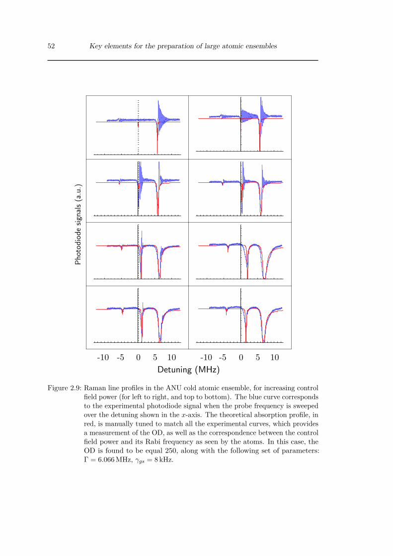
52 Key elements for the preparation of large atomic ensembles
Pho
todi
ode
sign
als
(a.u
.)
-10 0 10-5 5 -10 0 10-5 5Detuning (MHz)
Figure 2.9: Raman line profiles in the ANU cold atomic ensemble, for increasing controlfield power (for left to right, and top to bottom). The blue curve correspondsto the experimental photodiode signal when the probe frequency is sweepedover the detuning shown in the x-axis. The theoretical absorption profile, inred, is manually tuned to match all the experimental curves, which providesa measurement of the OD, as well as the correspondence between the controlfield power and its Rabi frequency as seen by the atoms. In this case, theOD is found to be equal 250, along with the following set of parameters:Γ = 6.066 MHz, γgs = 8 kHz.

2.3 Large cold atomic ensembles 53
-0.25 -0.20 -0.15 -0.10 -0.05 0.150 0.05 0.10 0.250.20
1.2
1.0
0.8
0.6
0.4
0.2
Opt
ical
dep
th
a)
b)
Figure 2.10: a) Raman spectroscopy scheme for caesium atoms initially prepared in|g〉 =
∣∣∣6S1/2, F = 4⟩, in the presence of a magnetic field Bz. The energy
difference between adjacent Zeeman sub-levels is µBgFBz. The frequencyof a microwave π-pulse, ωMF, is sweeped around the hyperfine splittingof the ground states, ωhf. When this frequency corresponds to the energydifference with Zeeman sub-level of state |s〉 with ∆mF ∈ −1, 0,+1,the π-pulse populates this sub-level. A short probe beam Ep addresses atransition to the state |F ′ = 2〉 on the D2 line. b) The optical depth onthe |s〉 → |F ′ = 2〉 transition is measured by monitoring the transmissionof the probe right after the application of the microwave pulse, and aftera repump phase to restore the atoms the ground state |g〉. The profileof the optical depth shows frequency peaks which correspond to Zeemansub-levels of different mF . The range over which these peaks are observedindicates the residual magnetic field seen by the atoms.

54 Key elements for the preparation of large atomic ensembles
and uncoupled to |g〉, for example the state |F ′ = 2〉 on the D2 line of caesium. Afterthe probe interrogation of the atoms, a reference level is obtained by repumping theatoms to |g〉 and sending the probe again. The OD on the |s〉 → |F ′ = 2〉 transition ismeasured by the absorption during the interrogation, relative to this reference level.The profile of the OD shows frequency peaks which correspond to Zeeman sub-levelswith different mF . The range over which these peaks are observed indicates the residualmagnetic field seen by the atoms. Moreover, the initial population distribution in thedifferent mF sub-levels can be inferred from the relative heights of the absorption peaks.For example, an atomic ensemble integrally pumped to the edge state mF = +4 willdisplay only one absorption peak, corresponding to the |g,mF = +4〉 → |s,mF = +3〉transition. If pumped to the magnetically-insensitive state mF = 0, the spectroscopygraph displays absorption peaks corresponding to the transition to the Zeeman sub-levels mF = −1 and mF = −1, with no peak in the centre as the mF = 0→ mF = 0transition is forbidden.
Using this spectroscopic method to evaluate the residual magnetic field at LKB,we can then adjust the magnetic compensation to reduce this residual field. Inpractice, we can then achieve cancellation of the magnetic field down to a fewtens of milligauss, which corresponds to a broadening in the 10-kHz range.
Temperature measurement
Temperature is usually thought of as a macroscopic quantity that is not necessarilyrelevant for cold atomic ensembles. Thermal velocity is probably the concept that bestcaptures their non-zero temperature.
Doppler broadening The direct effect of temperature is to broaden the absorptionlines via the Doppler effect. We could argue that temperature can be measured this way.There are, however, many sources of broadening and it is only when we can distinguishthe thermal contribution from magnetic and collision broadening, or ignore the latter,that this technique gives access to the temperature.
Time-of-flight technique When free from any external force, an atomic cloud willfall due to gravity and the distribution of the velocity within it becomes apparent overtime. The spatial extent of an atomic cloud having fallen over a given height can belinked to their initial temperature distribution, governed by Boltzmann statistics.
Dropping the atomic cloud and imaging them after a given time is referred to as thetime-of-flight technique. Sample images are shown in figure 2.11. Because the velocitiesin the atomic cloud are initially distributed according to a Boltzmann statistic, thewidth r of the atomic cloud after a time t is given by:
r2(t) = r20 + kBT
mt2
where the temperature of the atoms T appears explicitly.However, it is not obvious how to measure the width of the atomic cloud from the
images taken, if the imaging system is not perfectly known, which may depend on the

2.3 Large cold atomic ensembles 55
Figure 2.11: Time-of-flight measurement: the atomic cloud is imaged at different timeintervals after its release from the magneto-optical trap. The position andspatial extent of the atoms is obtained by shining an imaging beam coveringthe whole cloud and monitoring its absorption on a CCD. The verticalposition of the centre of mass of the ensemble follows the accelerating down-fall due to gravity. The expansion of the cloud transverse size indicates theinitial velocity distribution, which gives access to the cloud temperature.This series of images are taken 2, 19 and 33 ms after releasing the cloud ofcaesium 133 atoms. The expansion of the cloud is found to correspond toa temperature around 20 µK.
exact focal length of a zoom lens, for example. However, the release of the atoms fromthe MOT also coincidentally causes its free fall, as it is subjected to gravity. Whilethis means even atoms at extremely low temperatures would eventually escape theinteraction area, it provides us with a easily-accessible calibration of the imaging system:the position of the centre of mass of the atoms is known to fall with gravity beingthe only force acting on it, therefore following the equation z = z0 − gt2/2, when theinitial vertical velocity distribution can be assumed to be symmetric. This enables usto calibrate the pixel scale in the imaging plane, and subsequently to determine thecloud temperature, as shown in figure 2.12.
0 5 10 15 20 25 30 35 40 45time [ms]
400
450
500
550
600
650
700
750
cente
r [p
ixels
]
pixel calibration: 33.6 um/pixel
0 5 10 15 20 25 30 35 40 45time [ms]
800
1000
1200
1400
1600
1800
2000
2200
half w
idth
(um
)
temperature calculation: 20.4 uK
Figure 2.12: a) Position of the atomic centre of mass with time of flight. Knowing themass of the atoms, a free-fall model gives access to the pixel scale for theimaging system. b) The width of the atomic cloud with the time of flightindicates the cloud temperature from a Boltzmann statistics.

56 Key elements for the preparation of large atomic ensembles
2.4 Machine-learning optimisationWe have mentioned the relevant parameters for MOT compression and PGC, and the
LKB preparation sequence shows a ramp profile for the parameters during these phases.Ramp profiles are commonly used in experiments because they are the simplest profilethat “makes sense”. A closer look to the ANU preparation sequence shows a raggedprofile. This results from a current approach using a machine-learning algorithm, amethod that has already proved to be successful is the optimisation of these phases.The idea is that the atomic ensemble preparation can be optimised using an online
machine-learning optimisation process to reach higher OD and lower temperatures.In order to set up this process, the OD is probed close to resonance in order to givethe machine-learning algorithm a cost function to work with. The algorithm is givencontrol over a set of parameters and it is first trained by letting it try values for theseparameters over their whole range, and measure the cost function for each set of values.A second step after this training, when the algorithm has conceived a model for thesemeasurements, is to let it explore the region where it predicts a minimum of the costfunction associated with a maximum of OD, according to this model. After someexploration, the algorithm is looped back to training itself to refine its model, then comeback with a better prediction, and so on, until hopefully it converges to a minimum ofthe cost function.A similar method has been used to optimise the evaporation cooling of a Bose-
Einstein condensate [Wigley2016], but also dynamical decoupling [Mavadia2017] andthe feedback control of a qubit [August2017].
2.4.1 Teaching the machine-learnerThe machine-learning optimisation algorithm is first trained to infer a statistical
model over a multidimensional parameter set. A probe pulse close to resonance on the|g〉 → |e〉 transition is sent through the atoms and its absorption, which is linked to theOD, is monitored. The photodiode signal is used as feedback for the algorithm, whichtranslates it into a cost function and actively minimises that cost in the machine-learningprocess.Our first implementation used a Gaussian process to infer the statistical model,
available at [Hush2016]. With the available computing power, the learner was limitedto about 20 parameters, and at that limit it actually spent more time computing themodel than learning from probing the experiment. It was however sufficient to performoptimisation over fewer parameters, and the preparation sequence presented in 2.6 wasoptimised by a Gaussian process.
Nonetheless, we quickly moved to another process to infer the model: artificial neuralnetworks. The structure of a neural network, presented in figure 2.13, consists of aseries of layers of neurons, the first one being a set of inputs, and the last one theoutput. Neurons are linked with different weights and have an activation function,typically a logistic function. A large range of functions can already be approximatedwith a handful of layers of a few neurons each. With the same computing power, thealgorithm could sustain the 63 independent parameters we used, corresponds to 21time-bin values on three different quantities: the magnetic gradient from the trapping
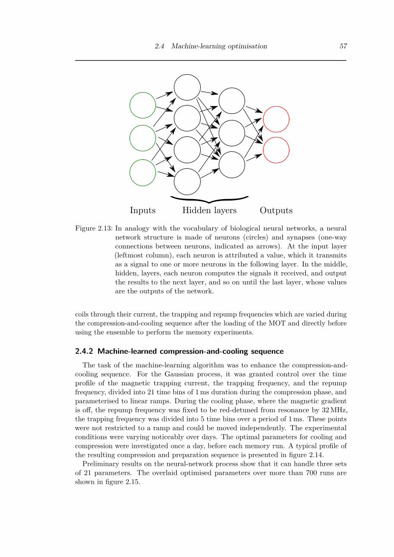
2.4 Machine-learning optimisation 57
Inputs OutputsHidden layers
Figure 2.13: In analogy with the vocabulary of biological neural networks, a neuralnetwork structure is made of neurons (circles) and synapses (one-wayconnections between neurons, indicated as arrows). At the input layer(leftmost column), each neuron is attributed a value, which it transmitsas a signal to one or more neurons in the following layer. In the middle,hidden, layers, each neuron computes the signals it received, and outputthe results to the next layer, and so on until the last layer, whose valuesare the outputs of the network.
coils through their current, the trapping and repump frequencies which are varied duringthe compression-and-cooling sequence after the loading of the MOT and directly beforeusing the ensemble to perform the memory experiments.
2.4.2 Machine-learned compression-and-cooling sequenceThe task of the machine-learning algorithm was to enhance the compression-and-
cooling sequence. For the Gaussian process, it was granted control over the timeprofile of the magnetic trapping current, the trapping frequency, and the repumpfrequency, divided into 21 time bins of 1 ms duration during the compression phase, andparameterised to linear ramps. During the cooling phase, where the magnetic gradientis off, the repump frequency was fixed to be red-detuned from resonance by 32 MHz,the trapping frequency was divided into 5 time bins over a period of 1 ms. These pointswere not restricted to a ramp and could be moved independently. The experimentalconditions were varying noticeably over days. The optimal parameters for cooling andcompression were investigated once a day, before each memory run. A typical profile ofthe resulting compression and preparation sequence is presented in figure 2.14.
Preliminary results on the neural-network process show that it can handle three setsof 21 parameters. The overlaid optimised parameters over more than 700 runs areshown in figure 2.15.

58 Key elements for the preparation of large atomic ensembles
0 20Relative Duration (ms)
-68
-24
Det
unin
g (M
Hz)
-32
-9
Compression
0 1
PGC
Trapping
Repum
pM
agnetic Field
0
33Cur
rent
(A
)
Figure 2.14: The compression and polarisation-gradient cooling sequences are dividedinto 20 and 5 time bins, respectively, and are passed onto a machine-learning algorithm with a model inferred by a Gaussian process. Thisalgorithm determines the optimal values of repump and cooling beamfrequencies, and current through the transverse coils for magnetic trapping.A typical optimised set of parameters is presented here.
Figure 2.15: Overlaid best parameters for 703 sequences optimised by machine-learning.The darker a parameter region is, the more sequences had values of thisparameter optimised in this range. Therefore the darkest line correspondsto a optimal run across all sequences, associated with a global minimum ofthe cost function.

2.4 Machine-learning optimisation 59
Cooling No coolingCompression 730 430
No compression 250 270
Table 2.1: Comparison between the optimal OD obtained by the machine-learning algo-rithm depending whether the algorithm was given control of the parametersto perform compression and cooling of the atomic ensemble. The lower valuewhen the algorithm was allowed to perform cooling than when it was not isan artifact that could be due to the uncertainty of the OD measurement.
The solution provided by the neural net yielded an OD of 970±20, to be comparedto the best “human-optimised” solution with an OD equal to 540± 10, an almosttwo-fold increase in OD which is promising for the use of a neural network toassist with the optimisation of the preparation of the atomic ensemble on a dailybasis.
2.4.3 Comparison of preparation sequencesAnother application of the machine-learning optimisation is to investigate the impor-
tance of different parameters during the preparation of the atomic ensemble. It shouldbe possible to extract this information from the inferred model of algorithm, and it ishinted on figure 2.15 where for some parameters at given time bins, such as the lastones of the trapping, most of the possible values at a given time bin have been exploreda similar number of times.A second approach which was undertaken is to restrict the parameters that the
algorithm has access to and see how good is the optimal OD it yields after optimisationon this subset. We performed this by preventing or letting the algorithm performcompression and/or cooling. When the algorithm was not allowed to perform thosepreparation sequences, it was nonetheless given one parameter: it could choose aconstant value for the duration of the sub-sequence, similarly to how a human usuallyoptimises a MOT preparation. Results of a one-off trial are presented in table 2.1.
2.4.4 Going beyond the optimisation of ODThe machine-learning algorithm optimises a cost function and there is of course no
reason that OD should be the only figure of merit the algorithm optimises. Actually, aneasy extension is to optimise OD after a given duration during which the atoms releasedfrom the MOT diffuse: the lower the temperature of the atomic cloud, the sloweris its diffusion. In that case, both the OD and the temperature are simultaneouslyoptimised. Our next step, however, is to directly optimise another figure of merit:memory efficiency and its decay. Until now, the setup to measure the cost function hassimply been the transmission of a probe close to resonance, which had to be minimised.Optimising a memory performance directly implies performing the full memory scheme,and providing an adequate cost function to the algorithm. It should especially beremembered that such unsupervised machine-learning algorithm have a tendency to
60 Key elements for the preparation of large atomic ensembles
“cheat” in the following sense. Let us assume that we ask the algorithm to optimisestorage-and-retrieval in an atomic ensemble, with a cost function corresponding to lightreceived on a photodiode in a given time window. If it is given control over auxiliarylaser beams, it won’t sound unreasonable to the algorithm to try blasting these lasersin every direction: if somehow, by saturation of filtering optics, diffraction or reflectionfrom odd places, light can reach the detector when the read-out from the memory isexpected, it can accept it as a solution. Definitely, careful planning will have to beconsidered before extending the parameter range of the machine-learning algorithm formore complex optimisation goals.
Chapter Conclusion
In this chapter:
• We have characterised the experimental methods to prepare large ensemblesof cold atoms and fully characterise them, in particular their optical depth(OD), which is a crucial figure of merit in the applications presented in thefollowing of this thesis.
• The state-of-the-art preparation techniques and typical sequences were pre-sented here, along with the OD they achieve on a reproducible basis.
• As much as possible, the OD improvement of individual preparation tech-niques were given, such as the use of a 2D-MOT, the compression and thepolarisation-gradient-cooling sequences.
• An extensive toolbox for the optimisation of the OD with any relevantparameter of the MOT was introduced with our first trials with a machine-learning algorithm. This algorithm can also be used to characterise the roleof different elements of the preparation sequence.

Chapter 3
Efficient qubit storage based onelectromagnetically-induced transparency
The storage-and-retrieval efficiency of quantum memories is a stringent parameter fortheir envisioned applications. Boosting this key figure of merit has been a long-standingeffort for a large community, using different physical platforms and a variety of protocols.While efficient storage of light pulses has been obtained, the storage of optical qubits isstill limited to an efficiency below 30% whatever the platform or the qubit encoding.This is attributed to the very challenging features of the storage of the two modesthat define the qubit, which requires some form of multiplexing. The limitation of thememory efficiency constitutes a current hurdle for further tests of quantum networkfunctionalities or synchronized photonic circuits.
In the work realised in this thesis and presented in this chapter, we more than doublethis key figure of merit. More importantly, our device enabled us to perform an opticalqubit mapping for the first time in the no-cloning regime without post-selection, witha storage-and-recall efficiency at 68%. Relative to previous works, this advance hasbeen possible by combining a high-OD medium — whose preparation was the topic ofthe previous chapter —, an efficient spatial multiplexing, and a low-noise operation.The research article reporting this work has been accepted in Nature Communications[Vernaz-Gris2017].
3.1 BackgroundThe memory we have demonstrated relies on EIT. Since the building of a magneto-
optical trap at LKB during the course of Sidney Burks and Lambert Giner’s thesis[Burks2010PhD, Giner2013PhD], EIT has been at the core of the research done there.The first published work was the study of the transition between the Autler-Townessplitting and EIT models [Giner2013], which was followed by memory experiments:storage and retrieval of light with conservation of its orbital angular momentum (OAM)[Veissier2013] and subsequently a memory for OAM qubits [Nicolas2014], as well as amemory for rotationally-invariant vector beams at the single-photon level [Parigi2015].During my thesis, with the substantial increase in OD, we could perform the quantumstorage of polarisation-encoded qubits, for the first time with large efficiency. AtANU, EIT has also been a benchmark for the highest OD obtained in our cold atomicensembles at that time, especially for investigating four-wave mixing effects [Geng2014].
61
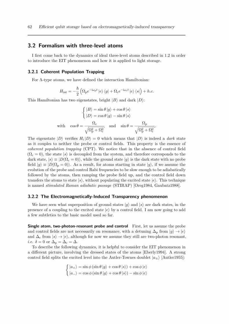
62 Efficient qubit storage based on electromagnetically-induced transparency
3.2 Formalism with three-level atomsI first come back to the dynamics of ideal three-level atoms described in 1.2 in order
to introduce the EIT phenomenon and how it is applied to light storage.
3.2.1 Coherent Population TrappingFor Λ-type atoms, we have defined the interaction Hamiltonian:
Hint = −~2(Ωpe
−iωpt |e〉 〈g|+ Ωce−iωct |e〉 〈s|
)+ h.c.
This Hamiltonian has two eigenstates, bright |B〉 and dark |D〉:|B〉 = sin θ |g〉+ cos θ |s〉|D〉 = cos θ |g〉 − sin θ |s〉
with cos θ = Ωc√Ω2
p + Ω2c
and sin θ = Ωp√Ω2
p + Ω2c.
The eigenstate |D〉 verifies Hi |D〉 = 0 which means that |D〉 is indeed a dark stateas it couples to neither the probe or control fields. This property is the essence ofcoherent population trapping (CPT). We notice that in the absence of control field(Ωc = 0), the state |s〉 is decoupled from the system, and therefore corresponds to thedark state, |s〉 ≡ |D(Ωc = 0)〉, while the ground state |g〉 is the dark state with no probefield |g〉 ≡ |D(Ωp = 0)〉. As a result, for atoms starting in state |g〉, if we assume theevolution of the probe and control Rabi frequencies to be slow enough to be adiabaticallyfollowed by the atoms, then ramping the probe field up, and the control field downtransfers the atoms to state |s〉, without populating the excited state |e〉. This techniqueis named stimulated Raman adiabatic passage (STIRAP) [Oreg1984, Gaubatz1988].
3.2.2 The Electromagnetically-Induced Transparency phenomenonWe have seen what superposition of ground states |g〉 and |s〉 are dark states, in the
presence of a coupling to the excited state |e〉 by a control field. I am now going to adda few subtleties to the basic model used so far.
Single atom, two-photon-resonant probe and control First, let us assume the probeand control fields are not necessarily on resonance, with a detuning ∆p from |g〉 → |e〉and ∆c from |s〉 → |e〉, although for now we assume they still are two-photon resonant,i.e. δ = 0 or ∆p = ∆c = ∆.
To describe the following dynamics, it is helpful to consider the EIT phenomenon ina different picture, involving the dressed states of the atoms [Eberly1994]. A strongcontrol field splits the excited level into the Autler-Townes doublet |a±〉 [Autler1955]:
|a+〉 = sinφ (sin θ |g〉+ cos θ |s〉) + cosφ |e〉|a−〉 = cosφ (sin θ |g〉+ cos θ |s〉)− sinφ |e〉

3.2 Formalism with three-level atoms 63
Figure 3.1: Equivalent configurations assuming a weak probe Ωp Ωc. (Left) three-level atom with transition |s〉 → |e〉 addressed by a control field of Rabifrequency Ωc. (Right) Autler-Townes doublet |a±〉 of energies shifted by~ω± from the bare excited state.
with tan 2φ =√
Ω2p + Ω2
c /∆. We recognise here the bright eigenstate |B〉 = sin θ |g〉+
cos θ |s〉. These states are separated from |e〉 by energy ~ω± = ~/2(∆±
√∆2 + Ω2
p + Ω2c
),
as shown in figure 3.1 [Fleischhauer2005]. In the approximation of a weak probe(Ωp Ωc), the dark state |D〉 is |g〉 and the bright one |B〉 is |s〉, as previously noted.Indeed we have cos θ → 1 and sin θ → 0. Additionally, on resonance (∆ = 0), φapproaches π/4, hence the Autler-Townes doublet states become:
|a+〉 = |s〉+ |e〉√2
|a−〉 = |s〉 − |e〉√2
These two states are orthogonal, and their energies are equidistant to the excited level:~ω± = ±~Ωc/2. Their contributions to the linear susceptibility destructively interfereand the medium is made transparent, which is the EIT effect.
Dependence on the frequency of the probe and control Moreover, this transparencydepends on the relative frequency of the probe and control, which we now introduce asbeing non-zero. Let us assume the probe is detuned by δ relative to the control, i.e.∆p = ∆c + δ. Up to the pre-factor notably including the OD, the susceptibility is foundto be proportional to:
χ(δ) ∝ δ + iγgsδ2 − Ω2
c/4− Γγgs/2 + iδ(Γ/2 + γgs). (3.1)
This is represented in figure 3.2, with different values of the Rabi frequency. The valueused for Γ is the reference value for the D2 line of caesium 133 [SteckCesium] andγgs is typical of the LKB experiment as 10−3Γ. Depending whether Ωc is larger thanthe factor Γ/2 + γgs, the poles of the susceptibility are real or imaginary. In the caseΩc < Γ/2 + γgs, the absorption profile is a Lorentzian of width close to Γ with a narrow

64 Efficient qubit storage based on electromagnetically-induced transparency
-0.2
0
-0.3
-0.1
-20 0 20-10 10-0.2
0
0.2
-0.1
0.1
-20 0 20-10 10-20 0 20-10 10
Detuning (MHz)
Figure 3.2: Electromagnetically-induced transparency as a function of the probe detun-ing from two-photon resonance with the control. The top row represents theimaginary part of the medium susceptibility, the bottom row its real part.Each column corresponds to different value of the control Rabi frequency.In all graphs, Γ corresponds to the reference value for the D2 line of caesium133, 5.2 MHz, the ground state decoherence rate γgs verifies γgs/Γ = 10−3.The imaginary part displays a transparency window within the absorptionprofile in the first two columns, which is wider and comes closer to zeroabsorption for a larger control Rabi frequency. In the rightmost colmun,the susceptibility is better described as two Lorentzians of similar widthson each side of the two-photon resonance. The real part displays a sharpervariation for lower control Rabi frequencies, denoting a stronger decrease ofa stored pulse group velocity.
transparency window centred around the two-photon resonance. If Ωc > Γ/2 + γgs, theabsorption profile is best approximated with two Lorentzians of similar widths on eachside of the two-photon resonance. The transition between these two behaviours hasbeen studied experimentally in the group at LKB [Giner2013].
Collection of atoms Now, let us consider a homogeneous collection of N identicalatoms forming a uniform ensemble, with the same energy levels and other characteristics.For brevity, the collective state of atom 1 in state |ϕ1〉, atom 2 in state |ϕ2〉, and so on,is noted |ϕ1 . . . ϕi . . . ϕN 〉. With all atoms initially prepared in state |g〉, the only statescoupled by the interaction Hamiltonian are under the form [Fleischhauer2002]:

3.2 Formalism with three-level atoms 65
|g〉 = |g1 . . . gN 〉
|s〉 = 1√N
N∑j=1|g1 . . . sj . . . gN 〉
|ss〉 = 1√2N(N − 1)
N∑i 6=j=1
|g1 . . . si . . . sj . . . gN 〉
. . .
We define the tensor product of the atoms and light field |ϕ〉 ⊗ |n〉 – shortened to|ϕ, n〉 – with ϕ ∈ g, s, gg, . . . and |n〉 the Fock state with n photons in the probelight field. The collective dark state, |D〉, along with a single photon in the probe is:
|D, 1〉 = cos θ |g, 1〉 − sin θ |s, 0〉 ,
with cos θ = g√N√
g2N + Ω2c
and sin θ = g√N√
g2N + Ω2c.
The case of probes with more than one photon but much fewer photons than the numberof atoms are governed by similar dynamics to the single-photon case. In practice, weensure this is always the case by choosing probes of low-enough intensities.
3.2.3 Dynamic control over slow lightIn the context of optical memory schemes, the light field previously used to probe
the atoms can now be seen as a signal to store and retrieve. This time-varying signal,as will be explained, experiences a slowdown effect within the narrow transparencywindow of the atoms, and can even be brought to a halt by dynamically controlling thecontrol field.
Group velocity
The real and imaginary parts of the susceptibility are linked by the Kramers-Kronigrelations[1]. These relations mean that a narrow transparency window is associatedby a fast variation of the dispersion index, which in turn leads to a decrease of thegroup velocity of a probe pulse around the resonant frequency: this is the slow lightphenomenon associated with EIT.
To quantitatively describe slow light, we need to introduce a time dimension, whichhas been absent from our equations so far. The Maxwell-Bloch equations 1.4 for a one-and two-photon resonant probe and control are:
(∂t + c∂z) E(z, t) = ig√N P (z, t)
∂tP (z, t) = −ΓP (z, t) + ig√N E(z, t) + iΩcS(z, t)
∂tS(z, t) = iΩ∗cP (z, t)(3.2)
[1]For a complex function χ(ω) = χr(ω) + iχi(ω), with χr and χi real functions, then χr(ω) =(1/π)P
∫∞−∞ dω′ χi(ω′)/(ω′ − ω). P denotes Cauchy principal value.

66 Efficient qubit storage based on electromagnetically-induced transparency
Performing a Fourier transform on these equations yields the linear susceptibility forthe weak probe component at frequency ω, detuned from resonance by δ[2]:
χ(δ) = −dΓ2
δ + iγgsδ2 − Ω2
c/4− Γγgs/2 + iδ(Γ/2 + γgs).
The effective optical index of the medium is given by n = 1 + Re [χ]. The groupvelocity of the probe is by definition vg = ∂ω/∂k, which can also be obtained from thesusceptibility. Evaluated around resonance[3], the group velocity equals:
vg = 2Ω2cL
Γd .
This expression encompasses all the relevant factors for slow light:• A large control Rabi frequency enables transparency but also increases the group
velocity, which indicates it is preferable to keep it below a certain threshold.This threshold corresponds to a sufficient diminution of the group velocity sothat the whole pulse fits inside the atomic medium. On the other hand, so thatits spectrum is contained in a narrow transparency window, the probe shouldpreferably be long, which makes it harder to fit inside the length of the atoms.
• The independent parameter here is the OD: it enhances every aspect of the storageof light with EIT by making the coupling with the atoms stronger and reducingthe group velocity. This stresses on the importance of achieving large OD in thepreparation of the atomic ensemble. However, as will be explained next, eitherfundamental or experimental limitations usually lead to residual absorption, whichimposes a compromise on the optimal OD.
Adiabatic transfer to a halted pulse
A decrease of the control Rabi frequency down to zero while the signal is containedwithin the atoms closes down the transparency window. This causes the group velocityto also decrease to zero: the signal is stopped. To describe this mechanism, the polaritonpicture introduced in [Fleischhauer2002] is probably the most insightful. The dark statepolariton is defined as:
Ψ(z, t) = cos θ(t)E(z, t)− sin θ(t)√N σ12(z, t),
with cos θ(t) = g√N√
g2N + Ω2c(t)
and sin θ(t) = g√N√
g2N + Ω2c(t)
.
which are now explicitly time-dependent. In the approximation of slow-varying envelopefor the control field, the time evolution of the dark state polariton is given by:[2]The susceptibility χ(ω) is defined by the expression of the probe light field exiting the ensembleE(L, ω) = exp i (1 + χ(ω)) kLE(0, ω).
[3]This expression is valid only for a control field resonant with the |s〉 → |e〉 transition. Otherwise, fora one-photon detuning of the control ∆, we need to add −i∆Γ/2−∆δ to the denominator of χ(δ),with our notations [Anisimov2008].

3.2 Formalism with three-level atoms 67
(∂t + c cos2 θ(t)∂z
)Ψ(z, t) = 0.
This indicates that the polariton propagates at a velocity c cos2 θ(t) through the medium,which can be controlled with the mixing angle θ(t) via the control field intensity. Adecrease of the control field down to zero brings the polariton to become fully atomic(Ψ(z, t) → −
√N σ12(z, t)); the light is stopped. Furthermore, in the assumption that
the ground state decoherence is negligible, the polariton does not decay.Subsequently, increasing the coupling field intensity back to its previous value results
in the conversion of the polariton back to a superposition of slow-propagating lightand atomic coherence. This light exits the atomic medium as an optical pulse in thesame mode as the input one. That recall is obtained on-demand thanks to the classicalcontrol over the coupling intensity.
3.2.4 Residual absorptionIn more practical terms, performing EIT in a real, non-ideal system does not exactly
follow the behaviour I have described until now. The transparency of the atomic mediumis usually imperfect. I now list the factors which can result in residual absorption andwhat is performed experimentally to find the set of optimal parameters.
Control intensity
The intensity of the control beam not only determines the width of the transparencywindow, it also defines how much transparency is obtained with a finite ground-statedecoherence. The transparency window should be wide enough for the spectral widthof the signal while providing enough slowdown so that the pulse fits in a medium offinite length. These two effects are seen in figure 3.2: a large control intensity increasesthe amount of transparency and the width of the window while it reduces the sharpnessof the optical index variation and reduces the slowdown effect.
A non-ideal configuration results in incoherent absorption of the frequency componentsof the signal outside a window which is too narrow, and leakage of parts of the pulsewhen the slowdown is not sufficient. Additionally, a strong control field intensity causesinhomogeneous power broadening, which in turn increases incoherent absorption andtherefore should be avoided. The compromise which needs to be made on controlintensity is always favoured by large ODs as it increases the group velocity reductionand does not affect the transparency window in ideal three-level atoms.
Absorption from Zeeman sub-levels
In a system with more levels than in the ideal three-level case considered so far, thesignal can simultaneously address several transitions. Taking into account the Zeemanstructure of the atoms, even in the degenerate case, the absorption on some transitionsmay not be made transparent by EIT when there is no ground state the control canaddress. The different configurations with caesium atoms, of hyperfine ground states|F = 3〉 and |F = 4〉, are illustrated with circular polarisations in figure 3.3.

68 Efficient qubit storage based on electromagnetically-induced transparency
a) b)
c)
Figure 3.3: Different atomic level configurations for EIT on the caesium D1 or D2lines. Probe and control have circular polarisations. The probe transition isrepresented in blue, the control in red. a) The probe and control field havethe same circular polarisation. There are Zeeman sub-levels in |s〉 to form anEIT system with all sub-levels in |g〉: perfect transparency is theoreticallyachievable. b) Probe and control of opposite circular polarisation form EITsystems with ground states of |∆mF | = 2: there is absorption from theatoms populating the edge Zeeman sub-level, mF = +3 in the examplerepresented here. c) Starting with the atoms in the ground state of higherenergy (|g〉 = |F = 4〉) results in residual absorption from one edge of theZeeman states, here mF = −4. Note also that atoms in state mF = +4 donot contribute to any absorption, which effectively decreases the OD of theensemble.

3.2 Formalism with three-level atoms 69
With atoms whose Zeeman sub-levels are equally populated, a higher OD meansmore residual absorption from the uncoupled transitions. This can be prevented usingan adequate optical pumping removing the sub-levels involved in these transitions.In a configuration where the uncoupled transitions cannot be fully suppressed, ODis a parameter which has to be mitigated, unlike for the previous source of residualabsorption.
3.2.5 Additional excited levelsIn real atoms, there are also other excited states at different transition frequencies
and they can generate incoherent absorption which cannot be prevented with any choiceof polarisation or ground state. Similarly to the absorption from some Zeeman sub-levels, large ODs give a prominence to this detrimental effect. At the ODs required fornear-unity storage efficiencies, our investigation showed that incoherent absorption fromadditional excited states was significant. We have developed the formalism presented inthe following to quantify this absorption in the qubit storage experiment we performed,in particular because it determines the maximum achievable storage efficiency. Thestudy of EIT in more complex atomic structures than three levels had been the subjectof previous theoretical work in our group at LKB [Mishina2011, Sheremet2010], butthis new model is the fullest to date and provides good agreement with the experimentaldata presented later in 3.3.
Theoretical model for all excited levels
We have developed a model to take into account all the excited levels in the interactionHamiltonian. I describe this model specifically in the case of the D2 line of caesiumatoms initially prepared in
∣∣∣6S1/2, F = 3⟩, but it can easily be adapted to other alkali
species by changing the value of the total atomic angular momentum F and of thedetunings involved.
Atomic level structure We suppose the atoms initially occupy all the Zeeman sub-levels |gm〉 defined as |6S1/2, F = 3,mF = m〉. The excited levels that a σ+-polarisedprobe can address on the D2 line are the
∣∣eF ′,n⟩ =∣∣∣6P3/2, F
′ ∈ 2, 3, 4 ,mF ′ = n = m+ 1⟩
states. On this line, the excited levels are relatively close to each other — ∆ω(F ′, F ′ +1) ∼ 100 MHz — compared to the D1 line — ∆ω(F ′ = 3, F ′ = 4) ∼ 1 GHz — with thelatter also advantageously having only two excited levels [SteckCesium]. The D2-lineconfiguration is shown in figure 3.4.The ensemble is addressed by a probe at frequency ωp. We can define a detuning
from the probe to each Zeeman sub-level n of each excited level,∣∣eF ′,n⟩: ∆p(F ′, n) =
ωp−[Ee(F ′, n = m+ 1)− Eg(m)]. Similarly, the control field at frequency ωc is detunedby ∆c(F ′, n) = ωc − [Ee(F ′, n = m+ 1)− Es(m)]. Additionally, in the presence of amagnetic field B(z) at position z, the degeneracy of the Zeeman sub-levels is lifted andthe detunings are shifted by:

70 Efficient qubit storage based on electromagnetically-induced transparency
Figure 3.4: Full atomic level structure for EIT on the D2 line of caesium. The probe Eand control Ωc are detuned by ∆p and ∆c from the |F ′ = 4〉 excited state.Moreover, a residual magnetic field along the quantisation axis, Bz, splitsthe Zeeman sub-levels by mFµBgFBz.
δ(p)m (z) = µBB(z)
~mgg − (m+ 1)ge,F ′
δ(c)m (z) = µBB(z)
~mgs − (m+ 1)ge,F ′
with gg,gs and ge,F ′ the hyperfine Landé factors of |g〉,|s〉 and |eF ′〉, respectively.
Optical Bloch equations There is a dipole transition associated to all possible excitedlevels from |g〉 and |s〉, which all contribute to the dynamics. The dipole interactionHamiltonian is written as:
Vp = −3∑
m=−3
∑F ′∈2,3,4
deg,F ′,m∣∣eF ′,m+1
⟩〈gm|E(+)
p + h.c.
Vc = −3∑
m=−3
∑F ′∈3,4,5
des,F ′,m∣∣eF ′,m+1
⟩〈sm|E(+)
c + h.c.
with deg,F ′,m the dipole moment⟨eF ′,m+1
∣∣ d |gm〉, and similarly for des,F ′,m.With this more complex dipole interaction, we obtain a set of optical Bloch equa-
tions for the optical coherences between |gm〉, |sm〉 and∣∣eF ′,m+1
⟩. The slow-varying
amplitude of the optical coherence between |gm〉 and∣∣eF ′,m+1
⟩is noted σeg,F ′,m(t, z) =
ρeg,F ′,m(t, z) exp(−iωpt) and verifies the equation:

3.2 Formalism with three-level atoms 71
dσeg,F ′,mdt = i
(∆p + δ(p)
m (z)− ωee,F ′,m+1(z) + iΓ2
)σeg,F ′,m(t, z)
+ i
Ω(p)eg,F ′,m
2 ρgg,m +Ω(c)es,F ′,m
2 σsg,m(t, z)
, (3.3)
where ~ωee,F ′,m+1(z) is the energy difference between the hyperfine level∣∣eF ′,m+1
⟩and
∣∣eF ′=4,m+1⟩at position z, and Ω(p)
eg,F ′,m (Ω(c)es,F ′,m) the Rabi frequency of the probe
(control) for the dipole transition between |gm〉 (|sm〉) and∣∣eF ′,m+1
⟩.
Likewise, the slow-varying amplitude of the optical coherence between |gm〉 and |sm〉is given by:
dσsg,mdt = i
[(∆p + δ(p)
m (z))−(∆c + δ(c)
m (z))
+ iγgs]σsg,m(t, z)
+ i∑
F ′∈3,4,5
Ω(c)se,F ′,m
2 σeg,F ′,m(t, z). (3.4)
Equations 3.3 and 3.4 are solved by taking the Fourier transform of the atomic coherences,σij,F ′,m(ω, z) =
∫∞−∞ dt σij,F ′,m(t, z) exp(iωt). From the solutions, we can define the
linear response of the atomic system to a weak probe field, which can then be describedby the susceptibility χ (ω, z,∆p,∆c) with contributions from all atomic states of theD2 line:
χ (ω, z,∆p,∆c) = −3∑
m=−3
∑F ′∈2,3,4
n0(z)deg,F ′,mσeg,F ′,m(ω, z),
with n0(z) the atomic density at position z.
Results
Effective Stark shift and ground state decoherence The coupling to the excitedstates F ′ = 3 and F ′ = 5 give rise to an additional Stark shift and increase the groundstate decoherence rate relatively to a Λ-type three-level system. The effective probedetuning including this Stark shift and the effective decoherence rate can be written as:
∆(eff)p = ∆p +
3∑m=−3
∑F ′∈3,5
∣∣∣Ω(c)es,F ′,m
∣∣∣2/4ωee,F ′,m+1
γ(eff)gs = γgs +
3∑m=−3
∑F ′∈3,5
∣∣∣Ω(c)es,F ′,m
∣∣∣2/4ωee,F ′,m+1
Γ2
Importantly, these additional terms depend on the power of the control. Recentlythese contributions were also described in [Hsiao2016] for N -type four-level configuration

72 Efficient qubit storage based on electromagnetically-induced transparency
Figure 3.5: Theoretical transmission spectra with increasing OD and constant controlpower. The simulation parameters are: hyperfine ground state decoherenceγgs = 10−3Γ, residual magnetic field modelled as a gradient b0 = 8 mG cm−1
over a cloud length L = 2.5 cm, control power P = 1 mW.
in the context of optical memories with atoms optically-pumped to one Zeeman sub-level.In contrast, the present model includes not only the several excited levels but also allthe Zeeman sub-levels.
Propagation losses through the medium The propagation of the signal through themedium can be modelled by a macroscopic Maxwell equation for the light field ofamplitude ε: [1
c
∂
∂t+ ∂
∂z
]ε(z, t) = 2πiω
c
∫ t
−∞dt′ χ
(z, t, t′
)ε(z, t′).
The light field from the memory medium, written as εout(t) = ε(z = L, t), is given by:
εout(L, t) =∫ ∞−∞
dω2π e
−iωtεin(0, ω) exp[−2πiω
c
∫ L
0dz χ (ω, z,∆p,∆c)
],
where εin(ω) = ε(z = 0, ω) is the component at frequency ω of the input probe pulseand L the length of the atomic cloud.The transmission spectrum of the atomic ensemble is obtained from the imaginary
part of the susceptibility:
T (ω) = exp[−4πω
cIm[∫ L
0dz χ (ω, z,∆p,∆c)
]].

3.2 Formalism with three-level atoms 73
This EIT transmission spectrum is shown in figure 3.5 for increasing ODs, showing adecrease of the maximal transmission with OD as well as the frequency shift on wherethis maximum occurs.The overall loss during the propagation is obtained by integrating over all the
frequency components of the input and output pulses or, equivalently, over all times.The upper bound for the storage-and-recall efficiency of the EIT memory is therebygiven by the transmission :
ηmax =∫∞−∞ dt |εout(t)|2∫∞−∞ dt |εin(t)|2
. (3.5)
Pulse storage and recall The value given by equation 3.5 only sets a maximum storage-and-recall efficiency of the EIT memory due to the absorption during the necessarypropagation through the length of the cloud, whatever the dynamics of the storage andrecall. In practice, the achieved efficiency may be lower due to leakage of the inputpulse and decoherence during storage.
The signal pulse is given a Gaussian profile of full-width half-maximum (FWHM) τ ,centred around t = 0:
εin(t) = ε0 exp(−2 ln 2 t
2
τ2
).
The control is assumed to be turned off at a time Tc. The leakage is discarded byconsidering the output pulse only after Tc. The atomic density n0(z) is assumed tobe a Gaussian distribution of the form n0(z) = n0 exp
(−4z2/L2). The optical depth
is defined as d0 = n0Lλ2/(2π)2. At each OD, the control power is chosen so that the
pulse experiences a delay Td = 2τ . The stopped pulse is then stored over 4τ .Figure 3.6 illustrates the effect of the additional excited states on the maximum
memory efficiency in two configurations. In the first one, the atoms populate all theZeeman sub-levels, in the second, they are regrouped in a single sub-level, correspondingfor example to the case when the atomic ensemble is optically pumped to this sub-level.The hyperfine ground state decoherence is taken to be γgs = 10−3Γ, the residual magneticfield is modelled as a gradient b0 = 8 mG cm−1 over a cloud length of L = 2.5 cm. TheFWHM of the input pulse, τ , is taken to be 0.5 µs, for which the storage time, 4τ , is2 µs.

74 Efficient qubit storage based on electromagnetically-induced transparency
0 200 400 600 800 1000Optical depth
0.0
0.2
0.4
0.6
0.8
Mem
ory
eff
icie
ncy
single Zeeman level
all Zeeman levels
Figure 3.6: Numerical simulation of the maximum achievable storage-and-recall effi-ciency with EIT on the D2 line of caesium versus optical depth when theexcited states |eF ′〉 =
∣∣∣63/2, F′ ∈ 2, 3, 4
⟩are considered. The blue line cor-
responds to the case where all the ground state Zeeman sub-levels are equallypopulated, the red line when only Zeeman sub-level
∣∣∣6S1/2, F = 3,mF = 3⟩
is populated. The simulation parameters are: hyperfine ground state de-coherence γgs = 10−3Γ, residual magnetic field modelled as a gradientb0 = 8 mG cm−1 over a cloud length L = 2.5 cm, signal pulse is a Gaussianof FWHM τ = 0.5 µs and storage time is 2 µs.
The storage process has an efficiency close to unity for moderately-large OD(> 50), which corresponds to a negligible leakage but at low OD, the signalpulse cannot be entirely contained in the atomic medium and a significant partof the pulse leaks from the medium. The effective ground state decoherenceincreases with the control field Rabi frequency. This decoherence becomes moresignificant in the region of large ODs due to the large control power needed. Thisdependency leads to a reduction of the EIT transparency and, as a result, of thememory efficiency. In our configuration, without optical pumping, the efficiencyis expected to be limited to about 70%. With all the atoms in a single Zeemansub-level, the maximum achievable memory efficiency increases by about 10%,and the maximum is obtained at a slightly lower OD.
3.3 Multiplexed polarisation qubit storageNow that an extended formalism has been presented to fully describe EIT storage
on the D2 line at large ODs, the experiment central to this chapter can be introduced.The atomic ensemble is prepared for multiplexed storage, using a dual-rail geometry.In the logic of the experiments in the group, this extension was somehow a natural step

3.3 Multiplexed polarisation qubit storage 75
Figure 3.7: A polarisation qubit is encoded via a quarter- (QWP) and a half-wave plate(HWP) and converted into a dual-rail qubit with a beam-displacer (BD).The orthogonally-polarised beams, separated by 4 mm, are then mappedinto an elongated ensemble of laser-cooled caesium atoms prepared in a2D magneto-optical trap in a glass chamber. The spatial multiplexing isrealised by focusing the two parallel paths into the 2.5-cm-long ensemblewith a small crossing angle of 0.5° in order to preserve a large OD for eachmode, an essential but challenging feature. A large OD of 300 is obtained.A single control beam propagates with an angle of 1° relative to the signalmodes in the plane of symmetry.
after having greatly enhanced the OD with the elongated-MOT geometry, using themethods described in the previous chapter. We wanted to prove in this new setup thatwe had not lost the spatial multimode capacity we used for the storage of OAM-encodedqubits [Nicolas2014]. It was now time to prove this improved platform could surpassthe previous realisations and this experiment was the perfect benchmark for that.
3.3.1 Polarisation encoding: preparation, manipulation and detectionIn our implementation, depicted in figure 3.7, we have chosen to encode the qubits
on polarisation. The preparation of different qubit states only requires a well-definedpolarisation for the input, easily obtained with polarisation optics, namely retardationwave plates in our case. Simply the rotation of these optics gives us access to thewhole parameter space to prepare input qubits for storage. This resource requirementis much less stringent than the previous experiment we performed in the group withthe preparation and analysis of OAM-encoded qubits, which required Spatial LightModulation (SLM) and holographic plates, respectively.

76 Efficient qubit storage based on electromagnetically-induced transparency
3.3.2 Storage of orthogonal polarisationsPolarisation qubits require the storage of two orthogonal polarisations on which the
quantum information is written. Our configuration with all the ground-state Zeeman sub-levels initially populated, however, prevents us from simply extending the basic storageprotocol for light we studied previously in this chapter to the storage of polarisationqubits. Instead, we choose to convert the orthogonal polarisation components of thequbit into two spatially-separated beams which can be stored in the atomic ensemble.This ends up using not a multimode capacity in the polarisation modes of light, butrather different spatial modes.In the context of spatially-multiplexed optical memories, the signal is usually in a
single spatial mode and its multimode character is in another degree of freedom. Thesignal components are divided into several rails, the details of the division dependingon the scheme, and all the rails can be stored in different locations of the memory.Upon their retrieval, the rails are recombined into a common spatial mode, restoringthe initial signal.
3.3.3 Atom preparation for dual-rail storageWe use the MOT loading sequence described in 2.3.4, which produces an atomic
cloud of cold caesium atoms prepared in state |g〉 =∣∣∣6S1/2, F = 3
⟩. We do not perform
Zeeman optical pumping, and actually do not properly define a quantisation axis, whicha fortiori leaves the atoms in an equal superposition of all Zeeman sub-levels. We haveseen that this atomic level configuration with circularly-polarised signal and controlallows unity-transparency EIT, with the only residual absorption being accountable tothe additional excited levels on the D2 line.The increase in OD comes at the expense of spatial multimode capacity as the
atomic cloud is elongated along a direction and radially compressed, resulting in asmaller transverse size. Spatial multiplexing can only be performed in atomic ensembleswhose transverse size is kept sufficient to support spatially-separated modes. The newgeometry and the MOT compression had greatly reduced the transverse size of theatom cloud and preliminary tests showed that the signal beam was not overlapping thewhole ensemble, so it was unlikely that a second signal beam could be added in thesystem and “fit” equally well in the cloud.
Dual-rail storage can be performed in different fashions in an atomic ensemble. Hereare the possibilities we have considered, shown in figure 3.8:
• Parallel rails: The first one consists of two parallel signal beams with a separationlarger than their transverse size over the cloud depth. With a 1/e2-waist of 250 µm,a separation of at least a few waists was required. In the end, the compromiseto be made on the MOT compression was too detrimental to the OD and thissolution was abandoned.
• Rails separated and crossing in the middle of the atomic ensemble. This is anacceptable solution because the EIT process would not induce cross-talk betweenthe stored polaritons generated from signals crossing at an angle, which was madeto be 1°. The control beam could make the same angle with both signal paths

3.3 Multiplexed polarisation qubit storage 77
a)
b)
Figure 3.8: Diagrams for two different rail configurations envisioned for the spatially-multiplexed EIT storage. a) The two rails are parallel, with a separationlarger than their transverse size over the cloud depth. b) The two rails arecrossing in the middle of the cloud. Their angular separation ensures thatthey do not contaminate each other.
by making a vertical angle with the plane where the signals belong. This is thesolution that was eventually adopted.
Moreover, in this second configuration, the alignment was considered in two variants,shown in figure 3.9:
• The two rails can be independently aligned with a set of beam-splitters andmirrors. This configuration was expected to allow an optimisation of the overlapof each rail with the atomic ensemble, resulting in larger ODs. Its main limitation,however, was the interferometric stability of two very differentiated optical paths.
• The crossing angle between two parallel rails is introduced by a lens placed atits focal distance from the centre of the atomic cloud. The angle is determinedby the initial beam separation and the focal length, both fixed by the chosenoptics, which therefore limits its versatility. On the other hand, this configurationprovides interferometric stability of the two rails, which was crucial to provideuniform storage of both rails.
In the chosen configuration of figure 3.9(b), the separation of the orthogonal polarisa-tion components of light into two parallel beams can be obtained by polarisation-selectivebeam-displacing optics, a calcite displacer in our case (Thorlabs BD40). The sufficientseparation between the two rails, 4 mm, allows us to control the polarisation of one railonly, with a wave plate, so that the signal going through the atomic ensemble effectivelyhas the same polarisation on both rails, and therefore can be addressed by the samecontrol beam. The signal on the rail whose polarisation was changed is restored to itsoriginal one by a second wave plate. The geometry involving only one pair of waveplates on one rail and no other optics makes it a passively-stabilised interferometer.
3.3.4 Transparency measurementThe control beam is chosen with a 2-mm waist, so it can overlap with both rails
which intersect at the centre of the MOT. The control is making a small angle of 1°,

78 Efficient qubit storage based on electromagnetically-induced transparency
a)
b)
Figure 3.9: Configurations for crossing rails: a) The two rails are independently alignedwith a set of adjustable beam-splitters and mirrors. This configurationis expected to be more flexible: the angle can be easily tuned and theoverlap of each rail with the atomic ensemble can be maximised, resultingin larger ODs. b) The two rails correspond to the two parallel outputports of a beam-displacer, which are then focused at the middle of theatomic ensemble by a lens. This configuration advantageously providesinterferometric stability of the two rails. In both configurations, half-waveplates (in green) are placed on a single rail to have both incoming beamswith the same polarisation. Additionally, quarter-wave plates (in yellow)make the beams circularly-polarised.
vertically from the plane of the signals. The transparency of the atomic ensemble oneach rail was measured for different ODs, with the results presented in figure 3.10. Theexperimental data is shown against the theoretical model from the previous section,with independently-measured parameters. In particular, we remind that the hyperfineground state decoherence is taken as γgs = 10−3Γ, corresponding to a residual magneticfield independently measured by Raman spectroscopy and modelled as a gradientb0 = 8 mG cm−1 over a cloud length L = 2.5 cm. The control power was measured asP = 1 mW and kept constant across the measurements.
Higher OD enable narrower transparency windows at moderate control field intensities— which prevents inhomogeneous broadening — and the reduction of the group velocity,enabling the storage of long pulses. The decrease in transparency which is observed atlarger ODs, in spite of the increase the coupling efficiency with the ensemble, confirmsthe prediction made in our theoretical model. Precisely in the case of non-negligibleincoherent scattering from the other excited states, we want to limit the interactionstrength to those, which can only be achieved by a compromise on the OD. Weeventually found that relatively high ODs around 200 correspond to the optimum forthe performance of the EIT memory protocol explained in the following.
3.3.5 Memory efficiencyHaving prepared a large-OD ensemble, we now turn to the memory protocol. EIT
enables the conversion of a signal photon into a long-lived collective excitation bydynamically changing the power of an auxiliary control field. The laser source for the

3.3 Multiplexed polarisation qubit storage 79
0.0
0.5
1.0
OD = 40
0.0
0.5
1.0Tra
nsm
issi
on
OD = 140
-40 -20 0 20 40Detuning (MHz)
0.0
0.5
1.0
OD = 330
Figure 3.10: Transmission spectra with increasing OD. The experimental data (red) isshown against the theoretical model including additional excited states(blue). The model parameters are taken as: hyperfine ground state de-coherence γgs = 10−3Γ, residual magnetic field modelled as a gradientb0 = 8 mG cm−1 over a cloud length L = 2.5 cm, control power P = 1 mW.
control is an external-cavity diode (Toptica Photonics, DL Pro) which provides the10-mW repump and is also used for the signal. The signal and control beams are tightlyphase locked at the caesium hyperfine splitting frequency (Vescent Photonics, D2-135).Special care is taken with alignment of the light polarisation, as only a slightly-wrongmatching of the polarisation would lead to a significant absorption of the signal in ahigh-OD medium like the one prepared here.To ensure negligible leakage during the storage process, the power of the control
beam is chosen to provide a slow-light delay equal to twice the signal pulse durationof 1 µs when the control is continuously on. Figure 3.11 gives a single-photon levelmeasurement of the slowed pulse and an example of a dynamic memory operation witha few microseconds of storage. Before detection, the signal passes through a home-made atomic filter and a commercial lens-based cavity for spectral filtering (QuantaserFPE001A), with an overall rejection of 70 dB for the control field.

80 Efficient qubit storage based on electromagnetically-induced transparency
0
0.2
0.4
0.6
0.8
1.0
0 1 2 3 4 5 6Time (µs)
Cou
nts
(a.u
.)referenceslow light
memory
control
Figure 3.11: Histogram of the photodetection counts. The blue-filled region gives thereference pulse without atoms while the green and red regions correspondto the slow and the stored-and-retrieved pulses, respectively. The blackdashed line indicates the control intensity for the storage experiment. Thememory efficiency reaches (69 ± 1)%.
Thanks to the range of ODs achievable in this atomic ensemble, we couldinvestigate the scaling behaviour of the storage-and-retrieval efficiency with OD,to compare with the model shown in figure 3.6. Figure 3.12 shows the efficiencyas a function of the OD, which is varied by adjusting the power of the trappingbeams during loading. At each value, the time delay is maintained constantand equal to twice the signal duration by adapting the intensity of the controlbeam. As can be seen, the memory efficiency saturates at an OD of around 200before decreasing. The maximal efficiency achieved here reaches (69± 1) %. Thisrepresents a record on the caesium D2 line and, more importantly, the highestachievable value in this configuration. We also obtain strong agreement betweenthe measurements from the experiment and the model where all the Zeemansub-levels are equally populated. The model also confirms that the intrinsicground state decoherence γgs = (1.0± 0.5)× 10−3Γ estimated in our experimentis not the limiting factor for the memory performance.

3.3 Multiplexed polarisation qubit storage 81
Figure 3.12: Storage-and-retrieval efficiency as a function of the OD. Red dots corre-spond to the experimental measurements of the memory efficiency, witherror bars from the uncertainty on the determination of OD and the sta-tistical uncertainty on photon counts across acquisitions. The theoreticallines correspond to the two limiting cases with a single Zeeman sub-level(in red) and all Zeeman sub-levels (in blue), respectively. For each case, thesolid lines correspond to an intrinsic ground state decoherence estimatedto γgs = 10−3Γ while the dashed lines correspond to the limiting case withγgs = 0.

82 Efficient qubit storage based on electromagnetically-induced transparency
3.4 Qubit storage and retrievalWe now proceed to the qubit storage in this dual-rail setting. At the memory output,
the two paths are recombined into a single spatial mode with a second beam displacer.The position of the second lens is optimised to obtain a visibility over 99% betweenthese two paths, which is a critical step to achieve high fidelity. The two displacersform a passively-stable Mach-Zehnder interferometer, where the relative phase is set tozero by adjusting the tilt of the second beam displacer. The recombined state shouldbe as faithful as possible to the prepared one, which is evaluated quantitatively by thefidelity of the memory process.
3.4.1 Quantum state tomographyThe retrieved states are then characterised by usual quantum state tomography.
Figure 3.13 gives the reconstructed density matrices in the H,V logical basis. Fromthe measured matrices, one can estimate the conditional fidelity of the output stateswith the initially-encoded state. The values for the complete set of inputs are listedin table 3.1. The average fidelity is (97.7± 0.8)% and raises up to (97.7± 0.8)% aftercorrection for background noise that mainly comes from residual control leakage anddetector dark counts.
The fidelity corrected for background noise amounts on average to (99.5± 0.5) %. Inthe absence of an input signal, the background floor corresponds to 5.10−4 events perdetection window. The storage-and-retrieval efficiencies for each prepared state are alsogiven in the table, with an average efficiency that reaches (68.5± 2)%. The performanceof the memory is uniform over these six canonical states, within two percent of efficiency.
Figure 3.14 presents the achieved fidelities as a function of the mean photon numberper pulse n.
3.4.2 Quantum storage benchmarkingIn order to conclude about the quantum performance of the storage, we need to
compare our fidelity with the maximum achievable using a classical memory device,based for instance on the so-called measure-and-prepare strategy. It can be shown thatthe classical benchmark is given by a fidelity equal to (N + 1)/(N + 2) for a state
0.5
1
0H
V HV
0.5
1
0H
V HV
0.5
1
0H
V HV
Figure 3.13: Reconstructed density matrices in the H,V basis from preparing, storingand retrieving input states |H〉, |D〉 and |R〉, after a 1.2-µs storage time.The height of the bar represents the absolute value while the colour denotesthe phase. No background has been subtracted.

3.4 Qubit storage and retrieval 83
Input state Fidelity F (%) Efficiency η (%)|H〉 98.7± 0.1 68.9± 1.5|V 〉 98.5± 0.1 69.7± 2.6|D〉 97.5± 0.1 68.1± 2.3|A〉 96.8± 0.1 67.5± 2.8|R〉 97.3± 0.1 68.8± 1.3|L〉 97.2± 0.1 67.4± 1.2
Average 97.7± 0.8 68± 2
Table 3.1: Conditional fidelity and memory efficiency for the three standard polarisationbases, and their average. The error bars for the fidelity are estimated bytaking into account the statistical uncertainty of photon counts. The errorfor the efficiency is obtained from multiple measurements. The mean numberof photons per input pulse is n = 0.5, storage time is τs = 1.2 µs.
containing N photons [Massar1995], which is equal to 2/3 for the particular case of asingle photon. In the limit N 1, the fidelity becomes close to unity: the quantumcharacter of the memory cannot be demonstrated with such bright states.
Polarisation qubits are implemented with weak coherent states with a mean photonnumber per pulse n = 0.5 and subsequently stored into the memory. In this case, using co-herent states, the bound has to be modified to take into account the Poissonian statisticsof the signal and the finite memory efficiency, as done in [Specht2011, Gundogan2012].
The coherent mapping of arbitrary polarisation states of light into and out ofthe memory was performed with fidelities of 97 ± 1%, well above the classicalbenchmark, which unambiguously indicates that the optical memory is operatingin the quantum regime. Moreover, this quantum feature is still verified whenstoring coherent light with an average photon number as low as 0.02, below whichthe control leakage and detector dark counts become predominant.
3.4.3 Storage timeTo evaluate the decay time of the memory, we measure the probability to measure
the retrieved light after a variable storage time. Figure 3.15 shows the decay of thememory efficiency, as measured experimentally. The efficiency is corrected for the lossesfrom the atoms to the APD, and the efficiency of the detector. Moreover, we comparethese measurements to the following model, with three decoherence mechanisms whichcan be evaluated independently:
• First, the atomic motion related to the finite temperature results is a possibleloss of the atoms from the interaction area. With a temperature estimated at20 µK by time-of-flight measurement and a 250-µm signal beam diameter, thecorresponding transit time is evaluated to τ1 = 7 ms. This is not a limiting factorin our experiment.

84 Efficient qubit storage based on electromagnetically-induced transparency
Mean photon number
Fid
elity
1.0
0.9
0.8
0.7
0.6
0.5
0.40.01 0.1 1 10 100
Figure 3.14: Storage and retrieval beyond classical benchmark. The fidelity is given asa function of the mean photon number per pulse n, for a 1-µs storage time.No background correction has been applied. The blue solid line indicatesthe classical limit for the finite storage-and-retrieval efficiency and takesinto account the Poissonian statistics of the weak coherent states. Theerror bars are smaller than the data points and are given by the standarddeviations of fidelities for the set of stored states.
• The two other decoherence contributions come from dephasing of the collectiveexcitation. The first source of possible dephasing is the so-called motional dephas-ing due to the strong angular dependence of EIT. In the experiment, we usedindeed an off-axis configuration and the control and signal beams are overlappedwith an angle θ = 1°. The resulting lifetime is then given by:
τ2 = λ
2π sin θ
√m
kBT.
In our case, this expression leads to a decay time τ2 = 220 µs.
• The second dephasing process is caused by residual magnetic fields which resultin an atom-dependent Larmor precession. The magnetic field is compensatedvia three pairs of coils and the inhomogeneous broadening in the ground state istherefore limited to around 50 kHz, as measured via microwave spectroscopy. Byassuming a gradient of magnetic field equal to b0 = 8 mG cm−1 over a cloud lengthL = 2.5 cm and a quadratic atomic distribution, the expected time constant isτ3 = 15 µs. This dephasing is the main decoherence source in our experiment.
The model is represented with an independently-measured OD equal to 200 and a50-kHz inhomogeneous broadening. The shaded area corresponds to an uncertainty onthe residual magnetic field of ±1 mG cm−1.
Figure 3.16 shows the decay of the fidelity with storage time, and the fidelity bench-mark, which increases because the memory efficiency decreases with storage time. Thequantum nature of the memory is maintained for a storage time of more than 20 µs.

3.4 Qubit storage and retrieval 85
0 5 10 15 20 25 30Storage time (µs)
0.0
0.1
0.2
0.3
0.4
0.5
0.6
0.7
Eff
icie
ncy
model
data
Figure 3.15: Retrieval efficiency as a function of the storage time. The blue points givethe experimental measurements and the red solid line corresponds to ourmodel including additional excited levels. with a measured OD equal to 200and a 50-kHz inhomogeneous broadening. The shaded area corresponds toan uncertainty on the residual magnetic field equal to ±1 mG cm−1.
Storage time (µs)0 5 10 15 20
Fid
elity
1.0
0.9
0.8
0.7
0.6
0.5
0.425
Figure 3.16: Fidelity as a function of the storage time, for a mean photon numbern = 0.5. No background correction has been applied. The blue solid lineindicates the classical limit for the finite storage-and-retrieval efficiencyand takes into account the Poissonian statistics of the weak coherent states.The error bars are smaller than the data points and are given by thestandard deviations of fidelities for the set of stored states.

86 Efficient qubit storage based on electromagnetically-induced transparency
3.4.4 DiscussionThis value is the highest efficiency reported so far for a reversible memory that
demonstrates the quantum storage of photonic qubits. Moreover, we have shown that,because of the multiple level structure of the caesium D2 line, the achieved efficiency isclose to the highest one which can be obtained in this configuration. Direct extension ofour setup to the D1 line where excited levels are much more separated should enable usto reach an efficiency above 90% [Hsiao2016], although this has yet to be demonstratedin the quantum regime.
In our realisation, the pulse duration of the qubits has been chosen around 400 ns toobtain the highest efficiency after one pulse-width delay. It corresponds to a memorybandwidth of a few MHz, as expected from EIT storage. Single-photon sources withsub-MHz bandwidths have been demonstrated [Du2008, Fekete2013, Rambach2016]and can be adapted to our reported quantum memory.
3.5 Future of the experimentThe most immediate improvement foreseen for the experiment is the use of D1-line
transitions for the memory scheme, with the incoherent absorption on the D2 lineidentified as the main limitation in the performed experiment. New diode lasers arebeing bought as I write these lines and EIT without this limitation will soon be studied.The realisation of qubit storage follows a series of multimode experiments with the
free-space setup, and this one explores once again the spatial multimode capacityof the ensemble. Bases of orthogonal polarisation states, however, are limited tospanning only two modes. Laguerre-Gauss (LG) modes, which carry orbital-angularmomentum (OAM), which were previously investigated in the group, or alternativelylinear-polarisation (LP) modes, do not suffer from this limitation. Low-loss phaseplates for the generation of LG modes were manufactured on the ultra precision lathe(Nanotech 250UPL) at ANU during the course of my thesis. Following this course, thenext planned experiment is to demonstrate the storage in a basis of more than tenmodes.Concurrently to the progress of the free-space experiment, our neighbours working
on nanofibre-guided light are greatly improving the achievable OD, which should soonenable efficient EIT storage as well.

3.5 Future of the experiment 87
Chapter Conclusion
We have introduced the cornerstone effect of electromagnetically-induced trans-parency, which is the basis for our realisation of a dual-rail memory for polarisationqubits that gathers the following achievements:
• The memory possesses the highest reported storage-and-retrieval efficiencyfor a qubit memory, close to 70%, along with near-unity fidelity for thepreparation and memory processes, above 99% conditionally.
• This result is enabled by the high-efficiency storage on two optical pathsthrough the same elongated cold caesium ensemble, yielding the ability tostore two modes that encode a polarisation qubit without compromising onefficiency.
• A quantitative theoretical model was developed to represent realistic atomiclevel configurations with additional excited levels which become relevantat the high ODs obtained in current cold atomic ensembles. Maximumefficiency for the EIT scheme on the D2 line is achieved for an optimal valueof OD. This was verified experimentally, and sets our result within the bestefficiencies achievable on this line.
• The model also predicts it is possible to perform better on the D2 line withthe preparation of the atoms in a single Zeeman sub-level, although theenhancement would only be of about 10%.
• Operation on the D1 line would not suffer from such a stringent limitation,due to the interaction with off-resonant excited levels, and would allowstorage efficiencies above 90%.


Chapter 4
High-performance backward-recall Raman memory
The Gradient Echo Memory (GEM) variant of a off-resonant Raman memory hasexperienced many improvements in its realisations in the group at the AustralianNational University over the last decade. After originating there with the first experi-ments in rare-earth solids [Alexander2006, Hedges2010] and a warm vapour of rubidiumatoms [Hetet2008, Hetet2008a, Hosseini2011], it was later implemented in a cold atomicensemble breaking records of ODs [Sparkes2010, Sparkes2013, Higginbottom2015]. Myvery first research experience at the ANU during my master’s in 2012 was towards theend of the first era, when the prospect of moving to cold atoms was the best promise toextend the memory performance – especially its lifetime – to a new high. During mysecond visit, then starting as a PhD student, the original warm vapour experiment wasan available platform for new ideas and experiments that Jesse Everett and I were infull charge of. It was at this time that we first investigated stationary light, in numericalsimulations and experimental trials in the warm vapour, which I discuss in the nextchapter. It was finally during the last years of my PhD that I got to work on thecold-atom setup, although we had moved on from GEM to focus on stationary lightrealisations.In this chapter, I report on a high-performance optical Raman memory which uses
backward retrieval. We achieved a recall efficiency of 65± 6% and a delay-bandwidthproduct of 160. It is the first reported Raman memory with an efficiency above 50%,which is an important criterion for unconditional security in quantum communicationprotocols.This work has led to an article in preparation.
4.1 Theoretical basis for a Raman memoryIn order to apprehend the Raman memory experiment, in particular the backward-
retrieval configuration we investigated, I begin this chapter with an extension on thefew theoretical aspects relevant to the experiment.
4.1.1 From scattering to a memory schemeLight scattering is a prominent effect of atomic physics, described in section 1.2. It
can indeed be applied to quantum memories if we consider this process as a reversiblequantum-state transfer from light to the atoms: all the information from impinging light
89

90 High-performance backward-recall Raman memory
is converted via inelastic scattering into information encoded in the atomic state, andvice versa. Raman scattering is the exemplary form of inelastic scattering with photonsof low energy compared to the ionisation energy[1]. Let us give a quick reminder on theRaman scattering process and then look into the details of how it can be applied to amemory scheme.
Reminder on Raman scattering In a Λ configuration, a light field at frequency ωcan lead to the emission of an anti-Stokes photon at frequency ω′ which matchesthe energy difference between states |g〉 and |s〉, and which transfers one atom tostate |s〉, as shown on figure 4.1[2]. The process involves a virtual level of energy~ (ω3 + ∆) = ~ (ω1 + ω) = ~ (ω2 + ω′), where ∆ is the frequency difference between theexcited state |e〉 and this virtual level.
Figure 4.1: The absorption of a pump photon ω and emission of an anti-Stokes photonat frequency ω′. This operation transfers one atom from state |g〉 to |s〉.
The emission of a photon at frequency ω′ can be strongly enhanced with stimulatedemission: applying a strong driving field at this frequency results in stimulated Ramanscattering.
Another form of scattering is coherent anti-Stokes Raman scattering (CARS), whichcorresponds to the simultaneous generation of a Stokes and anti-Stokes photons fromtwo pump photons. As it involves four electromagnetic waves, the process is oftendubbed four-wave mixing (FWM)[3].
Spin wave The Raman scattering with the emission of an anti-Stokes photon leavesthe atomic ensemble with a collective excitation: one of all the atoms from the ensemblehas been transferred to state |s〉.
[1]Photons with energies much larger than the ionisation energy lead to Compton scattering.[2]In the case of state |g〉 lying energetically below |s〉, it is a less-energetic Stokes photon that is emitted,
verifying ~ω′ = ~ω −∆E12.[3]The acronym for the process is sometimes written as 4WM

4.1 Theoretical basis for a Raman memory 91
Figure 4.2: The signal E detuned by ∆ from the |g〉 → |e〉 transition is mapped to thespin-wave S between |g〉 and |s〉 by the two-photon resonant control Ω.
Raman memory scheme In the context of optical quantum memories, it is customaryto define the light field to be stored as the signal and the auxiliary field stimulating thescattering as a control or coupling beam. The Raman memory scheme in Λ-type atomsconsists of the absorption and subsequent retrieval of a signal detuned by ∆ from thetransition between ground state |g〉 and excited state |e〉, stored in a spin wave betweenstates |g〉 and |s〉 (see figure 4.2).
Although the applicable theory of stimulated Raman scattering has been known formuch longer [Raymer1985, Raymer1981], and similar equations were laid out during thefirst demonstration of a quantum memory [Kozhekin2000], I use as a reference the 2007article series by Alexey Gorshkov, which is the most comprehensive in the analytical treat-ment of Λ-type atomic ensembles [Gorshkov2007a, Gorshkov2007b, Gorshkov2007c].The thorough description of this type of system is aimed at the storage of light, whichis especially relevant to our approach.
As a reminder of chapter 1.2, Λ-type three-level atoms are governed by the followingset of Maxwell-Bloch equations:
(1c∂t + ∂z
)E = i
√d
Ω(t)∆ S(z, t)
∂tS = i√d ΓΩ(t)
∆ E(z, t).(4.1)
Efficient retrieval Upon retrieval, the choice can be made to retrieve the signal inthe backward direction and indeed time-reversal of the absorption process in thememory medium implies re-emission in this direction [Moiseev2011]. To this end,the mirror image of the control beam needs to be applied. This backward-retrieval

92 High-performance backward-recall Raman memory
b)a)
Figure 4.3: Symmetric configuration for backward-retrieval Raman memories: a) Thespin-wave is orthogonal to the signal axis, as the angle θ between the signaland control matches their energy mismatch. The spin-wave displays ak-vector mismatch ∆k. b) The spin-wave is not orthogonal to the signalaxis. Consequently, the retrieved signal is not collinear with the input.Notice that the k-vector mismatch ∆k′ is smaller than ∆k in the previousconfiguration.
configuration enables fundamentally-higher conversion efficiencies to and from anymemory based on three-level atoms than in the forward direction [Gorshkov2007b,Nunn2007, LeGouet2009], an argument I will now explain.First, a necessary extension to the theoretical model is the introduction of the
backward versions of the signal and control, noted with a minus subscript, and forclarity a plus subscript is added to the forward-propagating quantities. The propagationin the backward direction modifies the set of equations as follows:
(1c∂t + ∂z
)E+ = +i
√d
Ω+∆−
S(1c∂t − ∂z
)E− = −i
√d
Ω−∆+
S
∂tS = i√d Γ
(Ω+∆+E+ + Ω−
∆−E−).
(4.2)
The z and t dependence have been dropped for clarity. Note the minus sign of the left-hand side of the second equation, describing the propagation in the −z direction. Mostnotably, the spin-wave, which can now be converted into either forward or backwardlight through the controls Ω+ and Ω−, is governed by the third equation.
As we want to perform backward retrieval, special care has to be taken of the phasematching of the storage-and-retrieval process, as previously shown in [Surmacz2008].Choosing the storage state energetically below the initial state, enables the configurationdepicted in figure 4.3(a), with an angle θ between each signal-and-control pair, in whichthe spin wave is orthogonal to the signal axis, which conveniently makes the input signaland its read-out collinear. Figure 4.3(b) shows an alternative symmetric configurationwhere the signal and control make an angle θ′ < θ instead, which makes the effectivek-vector mismatch smaller. Only the control beams, not the signals, can be madecollinear if the storage state lies energetically above the initial state.

4.1 Theoretical basis for a Raman memory 93
Moreover, as pointed out in [Moiseev2011], the time-reversal of the storage processrequires the detuning of the control beam to be inverted for read-out, i.e. ∆+ = −∆−.As will be explained in the description of the experiment, with available light resonanton |s〉 → |e〉 transition, the forward and backward control can have opposite detuningby respectively picking the positive and negative orders of the AOM on each beampath.
4.1.2 Optimal shapingWith the main elements of a Raman memory having been introduced, we can further
study the question of the retrieval direction. More specifically, we will see in the light ofthe optimal shaping (of the signal to be stored, or equivalently the spin wave which issubsequently recalled) and what considerations are raised by the configuration involvingforward or backward retrieval.The spatial and temporal profile of light emitted from an atomic ensemble has very
specific properties which carry information of the ensemble. Conversely, signal lightwith various spatio-temporal shapes will couple differently to the atomic ensemble, andsome will more efficiently map to collective excitations. The study of optimal shapingaims at determining the light field profiles which couple the most efficiently, and thecorresponding spin wave shapes [Nunn2007]. The idea of an optimal conversion processwas first introduced in [Vidal1999] in the context of quantum communication with twoparties optimising the local transformations they can perform on a shared entangled stateto obtain another entangled state with the highest probability. In another context, thismethod has also been applied for example in synchronously-pumped optical parametricoscillator for cluster state generation [Manukhova2017].
Degrees of excitation of light and spin wave
Let us first describe formally the relevant efficiencies which correspond to the quantitiesthe shaping process should optimise.
Considering a time-varying input field Ein(t), it comprises a number of photons givenby:
Nin =∫ ∞−∞
dt⟨E†in(t)Ein(t)
⟩.
If the quantum properties of the signal are not relevant for the storage efficiency, wecan consider the number of photons simply as the integrated squared norm of the fieldamplitude:
Nin =∫ ∞−∞
dt|Ein(t)|2.
In the case where no extra excitation can be produced by the process, the number ofexcitations in the spin wave NS (in the atomic ensemble which ranges from 0 to L onthe z-axis) and photons in the retrieved field Nr are the respective results of the storageand retrieval processes. These numbers are defined as:
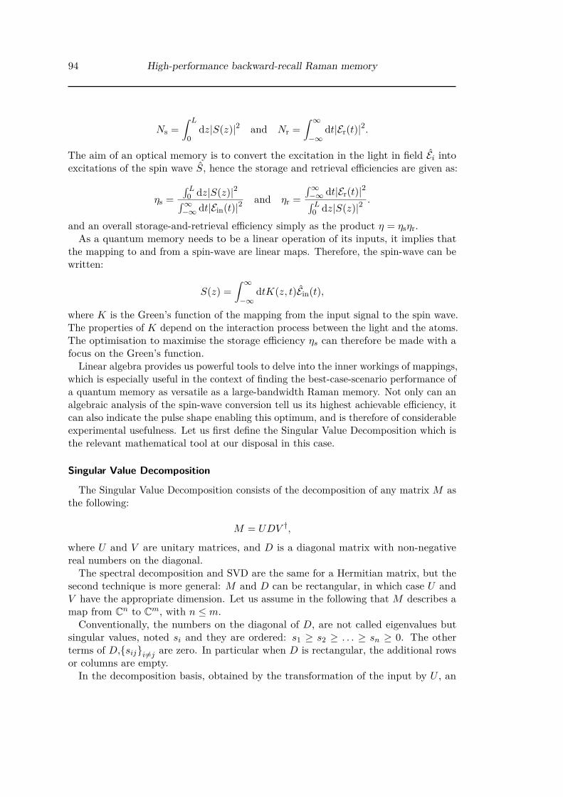
94 High-performance backward-recall Raman memory
Ns =∫ L
0dz|S(z)|2 and Nr =
∫ ∞−∞
dt|Er(t)|2.
The aim of an optical memory is to convert the excitation in the light in field Ei intoexcitations of the spin wave S, hence the storage and retrieval efficiencies are given as:
ηs =∫ L
0 dz|S(z)|2∫∞−∞ dt|Ein(t)|2
and ηr =∫∞−∞ dt|Er(t)|2∫ L0 dz|S(z)|2
.
and an overall storage-and-retrieval efficiency simply as the product η = ηsηr.As a quantum memory needs to be a linear operation of its inputs, it implies that
the mapping to and from a spin-wave are linear maps. Therefore, the spin-wave can bewritten:
S(z) =∫ ∞−∞
dtK(z, t)Ein(t),
where K is the Green’s function of the mapping from the input signal to the spin wave.The properties of K depend on the interaction process between the light and the atoms.The optimisation to maximise the storage efficiency ηs can therefore be made with afocus on the Green’s function.
Linear algebra provides us powerful tools to delve into the inner workings of mappings,which is especially useful in the context of finding the best-case-scenario performance ofa quantum memory as versatile as a large-bandwidth Raman memory. Not only can analgebraic analysis of the spin-wave conversion tell us its highest achievable efficiency, itcan also indicate the pulse shape enabling this optimum, and is therefore of considerableexperimental usefulness. Let us first define the Singular Value Decomposition which isthe relevant mathematical tool at our disposal in this case.
Singular Value Decomposition
The Singular Value Decomposition consists of the decomposition of any matrix M asthe following:
M = UDV †,
where U and V are unitary matrices, and D is a diagonal matrix with non-negativereal numbers on the diagonal.The spectral decomposition and SVD are the same for a Hermitian matrix, but the
second technique is more general: M and D can be rectangular, in which case U andV have the appropriate dimension. Let us assume in the following that M describes amap from Cn to Cm, with n ≤ m.Conventionally, the numbers on the diagonal of D, are not called eigenvalues but
singular values, noted si and they are ordered: s1 ≥ s2 ≥ . . . ≥ sn ≥ 0. The otherterms of D,siji 6=j are zero. In particular when D is rectangular, the additional rowsor columns are empty.In the decomposition basis, obtained by the transformation of the input by U , an

4.1 Theoretical basis for a Raman memory 95
x
y
x
y
Figure 4.4: Singular Value Decomposition: a matrix M addressing the vector ~a to ~b canbe visualised in 2D as a rotation V † onto the x-axis, followed by a rescalingD and a rotation U onto the axis of vector ~b. The SVD theorem states thatthese two rotations and the rescaling can be found for any linear mappingdescribed by M , in any dimension.
input vector ~a can be decomposed as
~a =
a1a2...an
It follows that when the matrixM is applied to a unitary vector ~a
(‖~a‖ = ∑n
i=1 |ai|2 = 1
),
then the norm of ~b = M~a verifies:
∥∥∥~b∥∥∥2=
m∑i=1|bi|2 =
n∑i=1
s2i |ai|
2.
Because s1 is the largest singular value, we have:
∥∥∥~b∥∥∥2≤ |s1|2
n∑i=1|ai|2
≤ |s1|2.
Therefore, characterising the largest singular value s1 indicates the maximum efficiencyachievable by the mapping M , which corresponds to the storage and/or retrievalprocess[4].SVD is performed on matrices, i.e. in finite dimension, whereas the usual equations
involved in the description of Raman memories are continuous. We need to discretisethe temporal and spatial domains of the signal pulse shape and spin wave, respectively,to generate a matrix that can be decomposed using this method. A fine enough grid
[4]The interested reader can refer to [Wasilewski2006] for a detailed theoretical analysis of SVD appliedto Raman storage.

96 High-performance backward-recall Raman memory
correctly describes the behaviour of the system, which is usually verified numericallywhere some convergence of the optimum with the grid size is observed. The Green’sfunction K that we previously described is what we decompose according to the SVD.Note that the Schmidt decomposition many physicists are familiar with is a special
type of SVD.
Numerical model
Starting from the Maxwell-Bloch equations introduced in 1.2, we can move to theco-moving frame, defining a local time t′ = t − z/c, and introduce dimensionlessparameters:
• We change the spatial variable z to the dimensionless z =∫ z
0 dz′n(z′)/N . In
the case of a uniform linear density, we have n(z) = N/L, which is equivalentto z = z/L. The latter form shows more explicitly that the interaction lengthcorresponds to z between 0 and 1.
• We define the dimensionless time t = γt′, which reduces all the quantities expressedin terms of frequency: γS = γS/Γ, ∆ = ∆/Γ, Ω = Ω/Γ.
Following these notations, the Maxwell-Bloch equations are reduced to:∂zE = ig
√d P
∂tP = −i(1 + i∆)P + i√d E + iΩS
∂tS = −γSS + iΩ∗P .The above assumptions on the system simplifies the general Maxwell-Bloch equationsin order to obtain a computionally-tractable numerical model or a solvable eigenvalueequation.
Finding the optimum
Largest singular value The optimal solution consists of choosing an input Ain(t) asthe right singular function φ1(t) associated with the largest singular value of K, λ1. Inthe case of a Raman memory with detuning ∆, excited state width Γ and control Rabifrequency Ω(t), we can define the integrated Rabi frequency:
ω(t) =∫ t
−∞dt′∣∣Ω(t′)
∣∣2 ,and W = ω(∞) =
∫ ∞−∞
dt′∣∣Ω(t′)
∣∣2 ,and the coupling parameter C:
C =√dΓW|Γ + i∆| .
The right singular function φ1 is defined as [Surmacz2008]:
φ1(t) = exp[iω(t)∆/ |Γ + i∆|2
]Ω(t)Φ1
[C
(1− ω(t)
W
)], (4.3)

4.1 Theoretical basis for a Raman memory 97
Am
plitu
de (
a.u.
)
Time (a.u.)
Figure 4.5: The optimal control shape (in red) for forward-retrieval of a given Gaussian-shaped signal (blue). The simulation parameters are d = 100, ∆ = 20,∆τs ≈ 0.42Γ−1. The largest singular value is found to be 35% and thecontrol 1/e2-width ≈ 0.97Γ−1.
where Φ1 is the right singular function associated with the largest singular value of thekernel K, which is equivalent to K, previously defined, up to a unitary transform:
K(y, y′) =∫ C
0dx k(y, x)k(x, y),
with k(x, y) = e− sin(β)(x/R+Ry)J0(2eiβ√xy
),
with R =√W/(dΓ) and β = π/2−arg (Γ + i∆) = Γ/∆+O
[(Γ/∆)3
]for large detuning
∆ Γ.K and k are defined on [0, C]2. We can sample these intervals in order to find
numerically the singular values associated with K. We take N + 1 samples of [0, C],valued yjj∈0..N = C.j/N)j∈0..N and define the matrix K from elements Kij =K(yi, yj). There are powerful tools to numerically perform the SVD of matrix K, forexample in Mathematica. They provide in particular the largest singular value λ1 thatwe can link to the optimal storage-and-retrieval efficiency, as well as the right singularfunction Φ1 to which it is associated. Equation 4.3 finally provides the optimal signalpulse shape φ1.
Numerical iterations To converge to the optimal spin wave shape, we can rely on thefact that the read-out process will favour the shape associated with the largest singularvalue associated with the mapping between the spin wave and the output field, i.e. thehighest retrieval efficiency.
The optimal spin wave shape is the eigenvector associated with the largest eigenvalueof the problem [Gorshkov2007b]:
ηrS(z) =∫ L
0dz′kr(z, z′)S(z′),
where kr(z, z′) is the kernel associated to the retrieval process, obtained from the

98 High-performance backward-recall Raman memory
experimental parameters.By renormalising the spin-wave obtained by computing the right-hand side of this
equation with a test spin-wave S1(z), we obtain a spin-wave S2(z), etc. Performingthis protocol many times converges to the optimal spin wave Sd enabling maximumretrieval efficiency. The index d denotes that this optimal spin wave shape dependsonly on the OD.This is especially heuristic when comparing the forward and backward retrieval
schemes of a Raman memory, which possess different pairs of kernel functions forstorage and retrieval.
Optimisation results
The analyses were made both in the case of a known control field profile (which canrepresent, for example, the constraint of limited control power) [Nunn2007] and withknown signal fields, what would be the optimal control shape and power [Gorshkov2007],enabling optimisation in both situations. A variant of this optimisation with gradientascent is described in [Gorshkov2008].The experiment in [Novikova2007] performs the optimisation steps of storage in
an EIT memory with an arbitrary control field profile. Starting with a test signalGaussian profile, the procedure successfully minimises the leakage at the write-in stageand maximises the retrieved pulse area, matching the theoretical prediction with thenumerical optimisation previously described.
Now that we have seen how to access optimal signal and spin wave shapes dependingon the memory dynamics, in the next section, we focus on the role of the retrievaldirection which drastically affects the optimal shape, as well as the phase-matchingconditions.
4.1.3 Backward and forward retrieval configurationsIt was studied in detail in [Gorshkov2007b] how large OD is always beneficial to reach
higher conversion efficiency. It was also found that, even at large ODs, the asymptoticscaling of storage and retrieval efficiencies, as well as the optimal spin wave shape,greatly differ whether the forward or backward signal retrieval is performed, as shownin figure 4.6. Indeed, the spin wave optimised for backward retrieval is linear, whichoptimises both the storage with a signal from one direction and its recall in the oppositedirection, whereas the optimal spin wave for forward retrieval compromises betweenthe two processes. This is in contrast with the idea that one can get away with carefulshaping and strong coupling provided they have a large enough OD.Moreover, the optimal mode shapes can also be associated with very strong control
powers in forward retrieval, which is non-ideal for inhomogeneous broadening and noiseconsiderations [Nunn2007], and are also arguably less convenient and possibly harderto generate as they are spatially more complex than in the backward retrieval case.Phase matching is known to determine the direction of the reemitted signal [Braje2004]and has also been shown to impose, more specifically for the applications of quantummemories, a limitation on the achievable forward-retrieval efficiency [Surmacz2008].
Another aspect is that in the case of non-degenerate ground and storage states, whichis the usual case when two hyperfine states are used as the long-lived ground states,

4.2 Experimental Raman memory 99
Figure 4.6: Optimal spin wave shapes S(z) for forward retrieval (blue) and backwardretrieval (orange) computed from [Gorshkov2007b], for Λ-type atoms withdegenerate ground states, in the limit of infinite optical depth. z is adimensionless distance through the atomic medium and the signal is assumedto be stored from propagating to the positive z. The spin wave optimisedfor backward retrieval corresponds to linearly absorbed light during storagefrom left to right, which becomes a linearly amplified from right to left. Onthe other hand, the spin wave optimised for forward retrieval is a parabolawhich is a compromise between a spin wave optimised for storage (whichis the backward-optimised shape) and the one for forward retrieval (thesymmetric of that shape).
the backward-retrieval Raman memory scheme suffers from imperfect phase-matching,arising from the differentiated propagation inside the medium [Nunn2007].With these considerations and, to our knowledge so far, the absence of reported
experiments demonstrating a Raman memory with backward-retrieval, we decided toconduct one in the cold atom experiment at ANU.
4.2 Experimental Raman memoryNow that we have seen the relevant theoretical background behind Raman memories,
and understood the advantages of a backward-retrieval scheme, I will introduce theexperiment performed at ANU of a versatile backward-Raman memory.
4.2.1 Experimental setupAtomic ensemble preparation
An elongated cloud of rubidium 87 atoms is prepared using the 2D-Magneto-OpticalTrap configuration described in 2.3.4. The atomic level scheme is shown in figure 4.7.The initial state in which we pump the atoms is |g〉 =
∣∣∣5S1/2, F = 2,mF = +2⟩. This
is conveniently the Zeeman edge state of the F = 2 hyperfine ground state, enablingnear-perfect optical pumping with a σ+-polarised beam. The optical pumping beam isproduced by the same diode laser as the optical trapping and has the same frequency. It
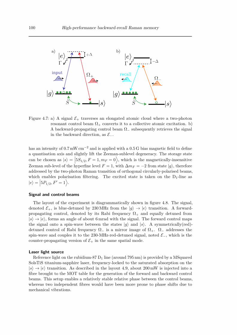
100 High-performance backward-recall Raman memory
input recall
b)a)
Figure 4.7: a) A signal E+ traverses an elongated atomic cloud where a two-photonresonant control beam Ω+ converts it to a collective atomic excitation. b)A backward-propagating control beam Ω− subsequently retrieves the signalin the backward direction, as E−.
has an intensity of 0.7 mW cm−2 and is applied with a 0.5 G bias magnetic field to definea quantisation axis and slightly lift the Zeeman-sublevel degeneracy. The storage statecan be chosen as |s〉 =
∣∣∣5S1/2, F = 1,mF = 0⟩, which is the magnetically-insensitive
Zeeman sub-level of the hyperfine level F = 1, with ∆mF = −2 from state |g〉, thereforeaddressed by the two-photon Raman transition of orthogonal circularly-polarised beams,which enables polarisation filtering. The excited state is taken on the D1-line as|e〉 =
∣∣∣5P1/2, F′ = 1
⟩.
Signal and control beams
The layout of the experiment is diagrammatically shown in figure 4.8. The signal,denoted E+, is blue-detuned by 230 MHz from the |g〉 → |e〉 transition. A forward-propagating control, denoted by its Rabi frequency Ω+ and equally detuned from|s〉 → |e〉, forms an angle of about 6 mrad with the signal. The forward control mapsthe signal onto a spin-wave between the states |g〉 and |s〉. A symmetrically(red)-detuned control of Rabi frequency Ω− is a mirror image of Ω+. Ω− addresses thespin-wave and couples it to the 230-MHz-red-detuned signal, noted E−, which is thecounter-propagating version of E+ in the same spatial mode.
Laser light sourceReference light on the rubidium-87 D1 line (around 795 nm) is provided by a MSquared
SolsTiS titanium-sapphire laser, frequency-locked to the saturated absorption on the|s〉 → |e〉 transition. As described in the layout 4.9, about 200 mW is injected into afibre brought to the MOT table for the generation of the forward and backward controlbeams. This setup enables a relatively stable relative phase between the control beams,whereas two independent fibres would have been more prone to phase shifts due tomechanical vibrations.

4.2 Experimental Raman memory 101
a) b)
Figure 4.8: Configuration of the signal and control beams: a) The forward-propagatingsignal E+ and forward control beam Ω+ form an angle of 6 mrad. As a result,the spin-wave wave vector is orthogonal to the signal axis. b) The backwardcontrol Ω− and retrieved signal E− are mirror images of Ω+ and E+, whichensures a symmetry between the storage and retrieval processes. Detectorsare placed after beam-splitters in the forward and backward directions fromthe atoms to monitor a E+ signal without the atoms, leakage and retrievalin any direction.
PumpTi:Sapph EOM
Signals~ 1 mW
Controls~ 200 mW
To SaturatedAbsorption
Figure 4.9: D1-light layout: The titanium-sapphire laser is frequency-locked on a satu-rated absorption channel (not depicted), and divided into control and signalchannels. The signal channel goes through a fibre-EOM and the +6.8 GHzside-band is separated from the carrier on a ring cavity.

102 High-performance backward-recall Raman memory
Backward Control
Forward Control
Figure 4.10: Forward and backward control beam powers are distributed on two channelsand independently controlled. AOMs provide spectro-temporal shapingof the control pulses. Opposite diffraction orders are chosen and ensuresymmetrical detuning relative to excited level |e〉.
Light resonant with the |g〉 → |e〉 transition for signals is obtained from filteringout the +6.8 GHz side-band of an EOM-phase-modulated beam on a ring cavity withfinesse F = 100. We are limited in producing signal light by the power the fibre-EOMcan handle, which on the order of a couple of milliwatts. AOMs are used to shapethe forward and backward signal beams, which are fibre-coupled and injected in theexperiment on the two ends of the MOT table. For this experiment, the signal sent forstorage was chosen as a coherent beam with a mean photon number |α|2 ∼ 106.
Forward and backward pairs The configuration depicted in figure 4.10 shows howoptical power was divided between the two beams, and individually controlled. Thisprovided around 100 mW of total available control power. A similar configuration isadopted to generate forward and backward signals, which was central to the TRACEscheme developed in section 5.4 but also significantly helped the alignment procedureof the Raman memory, as we will see.
Choice of the one-photon detuning The detuning of the signal and control beamsto state |e〉 was initially chosen to be 160 MHz, upon availability of AOMs with a centrefrequency at 80 MHz[5], but it was found that, for example, at a typical OD of 500,incoherent absorption accounts for more than 11%. This absorption is experimentallyverified by comparing the forward detector signal without control, with and withoutatoms. As memory efficiencies around 70% were eventually achieved, this absorptionnot contributing to the memory process was an unfortunate limitation. The AOMswere swapped to a model with a higher centre frequency and the detuning was increasedto 230 MHz, the highest frequency at which our arbitrary waveform generator couldsample sine-modulated Gaussian pulses for the signal and control AOMs. At 230 MHzand the same OD, incoherent absorption is predicted to be reduced to less than 6%.The only trade-off was the control beam intensity which needed to be increased to keepthe same Raman coupling, which scales as Ω/∆. This would have been an impediment
[5]enabling detunings equal to twice this frequency in the double-pass configuration.

4.2 Experimental Raman memory 103
for operation at the single-photon level, as our filtering capability is limited. However,it was not a drawback considering the available control power and the storage of brightpulses.
Pulse shaping and filtering A Gaussian-shaped signal pulse with a full width athalf-maximum (FWHM) of 2 µs is coherently mapped onto the atomic ensemble andsubsequently recalled in the backward direction with a pair of forward and backwardGaussian-shaped control pulses. The width, delay and intensity of the co-propagatingcontrol pulse for storage is optimised to minimise the leakage of signal light through theatoms. The retrieval control pulse, counter-propagating, is given the same shape as theoptimal storage pulse, which is found numerically and experimentally to be a Gaussianpulse with a FWHM around 3 µs. The intensity of the backward control is optimisedon the amount of retrieved signal. Polarisation filtering is achieved on a Glan-Taylorprism, with an isolation of 30 dB and spatial filtering on a 150-µm pin-hole in the focalpoint of telescope formed by two 150-mm lenses give a 90% transmission of the signaland 15 dB of additional isolation from the control. Moreover, after crossing the atomicensemble, each of the control beams is sent to a photodiode and their residual leakageonto the signal detectors is subtracted.
Optical depth and Rabi frequency calibration We need to find the relation betweenthe optical power measured on each control beam path and the Rabi frequency involvedin the Raman memory dynamics. This correspondence is obtained from the frequencyscanning of the Raman lines. Optical pumping to mF = +2 is skipped in the atomicpreparation sequence, enabling the Raman line absorption from an additional mF state,namely
∣∣∣5S1/2, F = 2,mF = +1⟩, addressed to
∣∣∣5S1/2, F = 1,mF = −1⟩. A probe pulse,
whose frequency is swept during the 400 µs of its duration, is sent simultaneouslywith a control beam at fixed frequency. The intensity of the control, and therebyits Rabi frequency, is varied across acquisitions. This results in absorption lines onthe mF = +2,+1 states with a depth relative to the Rabi frequency of the control.Additionally, the relative Stark frequency shift of each line depends on the square ofthe Rabi frequency, which enables an independent calibration of the OD, on one hand,and the Rabi frequency as experienced by the atoms in |g〉 as a function of the controlbeam power, on the other hand.
Alignement procedure An avalanche photodiode (Thorlabs APD120A) is placedafter the atomic ensembles to calibrate the energy of the input signal and the portionthat leaks through. A portion of the signal is injected into a single-mode fibre and thecoupling efficiency is optimised to match the spatial mode of the fibre to the one ofthe signal. A reference beam is subsequently sent through this fibre in the backwarddirection. The path to the backward detector is aligned onto this reference beamand a collection lens ensures a wide enough detection plateau. Losses through allthe optics from the atomic ensemble to forward and backward detectors are carefullycharacterised in order to calibrate the quantum efficiencies of the detectors. The losseson the forward and bacwkard channels are estimated to (50± 10) % and the ratioforward/backward of the overall detection efficiencies is found to be 1.2± 0.1. Measured

104 High-performance backward-recall Raman memory
photodiode signals are scaled accordingly. I believe the difficulty of calibrating thepair of forward and backward detectors which come after different optical paths fromthe atomic ensemble is definitely a reason why the backward-recall scheme is not verypopular in the implementations of Raman memories.
4.2.2 High-efficiency memoryThe memory efficiency is defined as the ratio between the integration of the retrieved
signal on the backward detector and the signal without atoms on the forward detector,corrected for the detection losses and sensitivities.
The highest recorded memory efficiency after a storage time of one pulse widthis found to be (65 ± 6)%. The large uncertainty is owed to the imperfectionsof measuring the optical losses on the two different detection paths. Thisfigure more than doubles the previous recorded efficiency of 30% for an opticalRaman memory and also outperforms the maximum achievable efficiency of54% with Controlled-Reversed Inhomogeneous Broadening with forward retrieval[Sangouard2007, Longdell2008].Contrary to previous Raman memory experiments operating at very large detun-ing with ultra-short pulses performed in Walmsley’s group in Oxford, the signalcan be incoherently absorbed by the excited level, which fundamentally limitsthe memory efficiency.
4.2.3 Memory lifetimeThe storage duration is determined by the delay of the read-out control beam,
which can be controlled at will. The memory efficiency is measured after differentstorage duration, shown in figure 4.11. The memory efficiency over time is fitted as theproduct of exponential and Gaussian decay functions, found to have the characteristictimes τexp = 190 µs and τgaussian = 120 µs, respectively linked to the magnetic biasinginhomogeneities and the motional dephasing of the atoms. An alternative analysisis based on the model described in [Jenkins2012], which yields a dephasing timeτD = 110 µs and a transit time τT = 170 µs. These analyses suggest that the thermalmotion of the atoms is the limiting factor to the memory lifetime.
4.2.4 Delay-bandwidth productWe have employed the same protocol for the storage of shorter pulses, demonstrating
large delay-bandwidth products with little compromise on the efficiency. To maintain acomparable efficiency, the control beams intensity had to be increased for shorter signalpulse widths and the memory was eventually limited by the available laser power, aswell as the optical depth of the ensemble.

4.2 Experimental Raman memory 105
20 40 60 80 100 120 140
0.1
0.2
0.3
0.4
0.5
0.6
0.7Effi
cien
cy
Storage time (µs)
Figure 4.11: Decay of the memory efficiency with storage time. The error bars corre-spond to the standard deviation. The efficiency is fitted to a decoherencemodel, with dephasing and transit times τD = 110 µs and τT = 170 µs. Thestorage-and-retrieval efficiency at the origin is η0 = (69± 6)%.
0 0.5 1.0 1.5Pho
todi
ode
inte
nsity
(a.
u.)
Time (µs)
÷3Reference
Recall t1
Recall t2
22%
40%
41.0 41.5 42.02.0
Figure 4.12: Efficient memory for a a 360-ns 1/e2-width signal (in red, scaled down).Recalls at times t1 = 1.5 µs and t2 = 41 µs (blue) are shown with theirstorage-and-retrieval efficiency. The decay of the memory efficiency corre-sponds to a delay-bandwidth product of 160.

106 High-performance backward-recall Raman memory
The highest delay-bandwidth product of 160 was obtained with a signal of 360-ns1/e2-width, for which the measured characteristic decay time was τ = 60 µs.A storage efficiency after one pulse-width was limited to 40%, as the memoryprocess was much less efficient with such a short pulse, with the amount ofavailable OD and control power.
Figure 4.12 shows the reference experimental photodiode signal for the pulse to bestored in the memory, and the signals for recalls at times t1 = 1.5 µs and t2 = 41 µs.
For comparison, delay-bandwidth products of the order of 104 have been demonstratedin cold atomic ensembles [Bao2012] although from the creation of a spin-wave with awrite pulse, not the storage of an input signal, and [Dudin2013] where the memory decaytime has been extended on the minute scale, but the storage efficiency is limited around14%. The drawbacks in these two realisations set the context for our simultaneousrealisation of a modest delay-bandwidth product also at a relatively high efficiency.
4.2.5 Dynamically-reprogrammable beam-splittingThe memory can be used as dynamically-reprogrammable array of beam splitters,
an application first demonstrated in Raman memories in [Reim2012] and depicted infigure 4.13. This operation finds many uses in the context of quantum informationprocessing. For example, a weak control beam has a low probability of reading-outthe memory, however the beam-splitter operation can be repeated many times untilone output photon is detected: this leads to the photon subtraction of the stored statewhich is available for efficient recall at a subsequent time with now a strong controlbeam.This scheme has been shown to enable a doubly-exponential enhancement on the
scaling of continuous-variable entanglement distillation [Datta2012]. This beam-splittingoperation enables interference between the memory read-out and another input sentsimultaneously [Campbell2012]. This is of course reminiscent of a cavity where “fresh”light is sent after a integer number of round-trips inside the cavity: this is the effectthat has been investigated in [Pinel2015]. This study of polariton interference has ledto the development of the TRACE memory, described in section 5.4.

4.2 Experimental Raman memory 107
11%
35%65%
b)
Leakage
Wrong mode
89%
Recalls
time
Input
a)
44% 26% 14% 8.6%11%
Input
timeLeakage Recalls
LightSpin-wave
Phot
odio
de s
igna
l (a.
u.)
Figure 4.13: a) Schematic of an beam-splitter array equivalent to the Raman memoryread with a series of weak control pulses. The percentages represent thelosses and conversion efficiencies at different stages. First a fraction ofthe input light leaks from the atomic ensemble and is not addressed toa collective atomic excitation. Second, some of the absorbed light is notmode-matched to be efficiently recalled. It is estimated at roughly 35% inthis short-pulse configuration. Then, at the given control beam intensity,each retrieval pulse extracts only about 60± 4% of the stored spin wave,the remainder is left for a subsequent retrieval step. The memory decaybetween retrievals is ignored at this time scale. b) Experimental photodiodesignal for the subsequently-retrieved pulses and correspond beam-splitterarray with the fractions of the total signal intensity.
108 High-performance backward-recall Raman memory
4.3 Discussion of the results4.3.1 Backward-retrieval geometry
Phase-matching between the spin-wave and the optical fields is known to determine thedirection of the retrieved signal [Braje2004] and has also been shown to impose a limit onthe achievable efficiency of memories in forward- and backward-retrieval configurations[Surmacz2008]. The memory efficiency benefits from the backward-retrieval geometryof our realisation, as it more than doubles the record storage-and-recall efficiency for aRaman memory [Reim2011].
Few experiments employ elements of a symmetrical geometry in Raman systems,although this symmetry is found to enhance the conversion of light to spin-waves.To our knowledge, however, our realisation is the first Raman memory withbackward retrieval. This demonstration has enabled the experimental verificationof the predicted contrast with its forward-retrieval variant and the improvementon the memory performance in a backward-retrieval geometry.
4.3.2 Outlook for this Raman memory realisationWe can argue that with Gaussian pulses only and the limited amount of control
power we have (≈ 100 mW with a waist of 250 µm), there could be other limitations tothe maximum achievable efficiency, not taking into account the decrease in efficiencydue to incoherent absorption. We are aware that this procedure generated unavoidablenoise on our detectors, which prevents us from demonstrating the quantum operation ofour system. The improvement of the filtering stages could enable the operation at thesingle-photon level, or with heralded single photons generated from the spontaneousdown-conversion source developed at the University of Queensland, developed by MarkusRambach and Till Weinhold, reported in [Rambach2016] and brought to the ANU toexperiment with the storage of single photons.The memory lifetime is limited by atomic motion, which has been predicted as a
main limitation on backward-retrieval Raman experiments, blurring the spin wave[Tikhonov2015, Surmacz2008]. Further optimisation of the cooling sequence with themachine-learning algorithm is expected to decrease the temperature of the atoms. Inparallel, the redesign of the biasing coils should enhance the uniformity of the magneticfield environment. I have additionally designed voltage-controlled current sources whichenable the dynamical control over the current for the cancellation of the ambientmagnetic field when no bias is applied. These extra steps are expected to decreasethe temperature of the atoms to a few tens of µK and removing limitations caused byan imperfect magnetic environment, which should consequently extend the memorylifetime by an order of magnitude.

4.3 Discussion of the results 109
Chapter Conclusion
This chapter has been focused on the off-resonant Raman memory:
• We have explored — theoretically and experimentally — retrieval from aRaman memory in the forward and backward directions.
• Our realisation of a Raman memory was the first reported one with backwardretrieval. This retrieval direction, symmetrical to the storage, is known toimprove its efficiency.
• Our memory implementation showed a storage-and-retrieval efficiency of65± 5%, setting it as the first Raman memory with an efficiency above theno-cloning limit of 50%.
• We also employed the memory with shorter pulses of 360-ns-width anddemonstrated a delay-bandwidth product of 160.
• With weak recall control pulses, we used the memory as a dynamically-reprogrammable array of beam-splitters.


Chapter 5
Spin-wave interference for stationary light and memoryenhancement
The memory schemes that were discussed until now store signal light in a stoppedform: it is converted into collective atomic excitations, it does not subsist as lightper se. An alternative form of light is stationary light (SL), which is light with avanishing group velocity. SL has been proposed in the early 2000’s, followed by a fewnumerical simulations and only a handful of experimental realisations. We had in mindto investigate it at ANU, after the realisation of the spin wave resonator [Pinel2015]with which it shares a few concepts which are detailed in this chapter. In early 2015after exchanging with Darrick Chang, visiting at LKB, we also started collaboratingwith Anders Sørensen on the theoretical study of SL. Their approach is documented inIvan Iakoupov’s PhD thesis [Iakoupov2016PhD].
A landmark achievement during this PhD was the study of the dynamics leading tothe generation of SL. This work led to the publication in Nature Physics [Everett2017].Following this first study, we then implemented the TRACE memory, a novel memoryscheme closely-related to SL, as well as the backward-retrieval Raman memory of theprevious chapter. An article is in preparation to cover the theoretical aspects of theTRACE memory and its experimental proof-of-concept [Everett2017a].
5.1 Stationary light history and formalismThe approach to SL has evolved a great deal since it was first conceived. It was first
mentioned in [Andre2002], in the context of EIT with the addition of a standing wave,creating a “photonic band gap” in which light propagation is forbidden. Light withinthis band gap would be made stationary, and unlike traditional EIT, with non-vanishingphotonic component.
Early proposals justified the phenomenon as Bragg reflections off periodically spacedabsorption peaks, a representation that was later proved not to be correct. The studyin [Bajcsy2003] displayed a misleading schematic illustration of the spatial variationof the signal absorption throughout the atomic ensemble, and [Andre2005] stated “thesignal light cannot propagate in the medium due to Bragg reflections off the sharpabsorption peaks, resulting in vanishing group velocity of the signal pulse”.
The key to understanding more accurately SL dynamics stemmed from [Moiseev2006]which extended SL to a Raman system. Moreover it introduces a two-colour variant, i.e.forward and backward signal-control pairs have different one-photon detuning to the
111

112 Spin-wave interference for stationary light and memory enhancement
Figure 5.1: |g〉, |s〉 and |e〉 form a three-level EIT system, with signal E+ and control ofRabi frequency Ωc. The standing wave of Rabi frequency Ωs, off-resonantfrom state |d〉, induces a spatially-modulated refraction index, which gener-ates Bragg scattering into the backward signal E−.
excited state. In this picture, SL was relying on multi-wave mixing. The description ofSL with Bragg gratings was explicitly challenged in [Lin2009], titled “Stationary LightPulses in Cold Atomic Media and without Bragg Gratings”. Indeed in this realisation,although it is based on EIT, the forward and backward controls open transparencywindows on two different, non-degenerate excited states, and therefore do not establisha standing wave. The formalism was refined in [Wu2010, Wu2010a] with the inclusionof the interaction between counter-propagating signal and control, which can be two-photon resonant when the Doppler frequency shift is minimal, for example in coldatomic media.The description of the generation of SL was specifically addressed in [Zhang2012a,
Zhang2013].
5.1.1 Electromagnetically-Induced-Transparency Stationary LightThe first SL scheme involves EIT in a Λ configuration, with an additional standing
wave between state |s〉 and an additional state noted |d〉, as shown in figure 5.1.The establishment of a dark-state polariton is governed by the dynamics presented
in chapter 3. The mixing angle of the polariton is noted θ(τ), it verifies tan θ(τ) =g√N /Ωc(τ).If initially only the forward polariton is populated, the addition of the standing wave
couples the forward and backward propagating polaritons, leading to the equations[Andre2002]:

5.1 Stationary light history and formalism 113
Ψ+(k, τ) =
[cos (ζτ)− ikc
ζsin (ζτ)
]Ψ+(k, 0)
Ψ−(k, τ) = iχζ
sin (ζτ) Ψ+(k, 0)
with Ωs the Rabi frequency of the standing wave light field, χ = ∆s(τ) tan2 θ(τ) =(g2N/∆
)Ω2
c/Ω2s and ζ =
√(kc)2 + χ2 .
Owing to the opposite and equal propagation of the forward and backward polaritons,light remains trapped within the atomic ensemble, with a non-vanishing photonic com-ponent, proportional to the non-zero Ωc Rabi frequency. There remains electromagneticenergy in the ensemble, which is stationary. This contrasts with a stopped light scheme,where the control field is turned off and the photonic component of the polaritondisappears.
The experiment was conducted in [Bajcsy2003] and a central element which inspiredour implementation was the side-imaging of the fluorescence of the atoms, which enablesthe visualisation of the polariton when SL is generated.
5.1.2 One-colour Raman stationary lightThe simplest Raman configuration is the one-colour configuration represented in
figure 5.2. All the light fields, signals and controls, in both forward and backwarddirections, address the same virtual state, detuned by ∆ from the excited one:
∂tρ21 = −γρ21(z, t) + iΩ∗(z, t)ρ31(z, t)∂tρ31 = −(Γ− i∆)ρ31(z, t) + iΩ(z, t)ρ21(z, t) + igNE(z, t)
The signal E is made of its forward component, E+, and backward component, E−:
E(z, t) = E+(z, t) exp(+ikz) + E−(z, t) exp(−ikz).
The controls are represented by their Rabi frequency Ω±:
Ω(z, t) = Ω+(t) exp(+ikz) + Ω−(t) exp(−ikz).
In this configuration, a priori all the coherences can couple with each other. To makethis explicit, the spin coherence and optical coherence can be decomposed as [Wu2010a]:
ρ21(z, t) =∞∑
n=−∞ρ
(2n)21 (z, t) exp (+2nikz)
ρ31(z, t) =∞∑
n=−∞ρ
(2n+1)31 (z, t) exp (+(2n+ 1)ikz)
Usually, only the quantities with the superscripts (0), (+1) and (−1) are considered,and the higher-order terms are ignored. Including these higher-order terms yields:
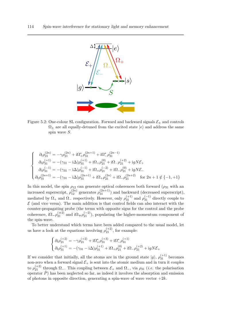
114 Spin-wave interference for stationary light and memory enhancement
Figure 5.2: One-colour SL configuration. Forward and backward signals E± and controlsΩ± are all equally-detuned from the excited state |e〉 and address the samespin wave S.
∂tρ(2n)21 = −γρ(2n)
21 + iΩ∗+ρ(2n+1)31 + iΩ∗−ρ
(2n−1)31
∂tρ(+1)31 = −(γ31 − i∆)ρ(+1)
31 + iΩ+ρ(0)21 + iΩ−ρ(+2)
21 + igNE+
∂tρ(−1)31 = −(γ31 − i∆)ρ(−1)
31 + iΩ+ρ(−2)21 + iΩ−ρ(0)
21 + igNE−∂tρ
(2n+1)31 = −(γ31 − i∆)ρ(2n+1)
31 + iΩ+ρ(2n)21 + iΩ−ρ(2n+2)
21 for 2n+ 1 /∈ −1,+1
In this model, the spin ρ12 can generate optical coherences both forward (ρ31 with anincreased superscript, ρ(2n)
12 generates ρ(2n+1)31 ) and backward (decreased superscript),
mediated by Ω+ and Ω− respectively. However, only ρ(+1)31 and ρ(−1)
31 directly couple toE (and vice versa). The main addition is that control fields can also interact with thecounter-propagating probe (the terms with opposite signs for the control and the probecoherence, iΩ−ρ
(+2)21 and iΩ+ρ
(−2)21 ), populating the higher-momentum component of
the spin-wave.To better understand which terms have been added compared to the usual model, let
us have a look at the equations involving ρ(+2)21 , for example: ∂tρ
(+2)21 = −γρ(+2)
21 + iΩ∗+ρ(+3)31 + iΩ∗−ρ
(+1)31
∂tρ(+1)31 = −(γ31 − i∆)ρ(+1)
31 + iΩ+ρ(0)21 + iΩ−ρ(+2)
21 + igNE+
If we consider that initially, all the atoms are in the ground state |g〉, ρ(+1)31 becomes
non-zero when a forward signal E+ is sent into the atomic medium and in turn it couplesto ρ(+2)
21 through Ω−. This coupling between E+ and Ω−, via ρ31 (i.e. the polarisationoperator P ) has been neglected so far, as indeed it involves the absorption and emissionof photons in opposite direction, generating a spin-wave of wave vector +2k.
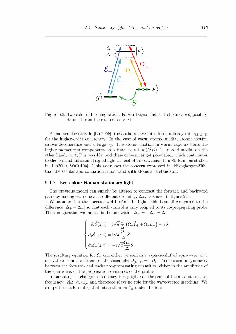
5.1 Stationary light history and formalism 115
Figure 5.3: Two-colour SL configuration. Forward signal and control pairs are oppositely-detuned from the excited state |e〉.
Phenomenologically in [Lin2009], the authors have introduced a decay rate γ2 ≥ γ1for the higher-order coherences. In the case of warm atomic media, atomic motioncauses decoherence and a large γ2. The atomic motion in warm vapours blurs thehigher-momentum components on a time-scale t ≈
(k2
cD)−1. In cold media, on the
other hand, γ2 Γ is possible, and these coherences get populated, which contributesto the loss and diffusion of signal light instead of its conversion to a SL form, as studiedin [Lin2009, Wu2010a]. This addresses the concern expressed in [Nikoghosyan2009]that the secular approximation is not valid with atoms at a standstill.
5.1.3 Two-colour Raman stationary lightThe previous model can simply be altered to contrast the forward and backward
pairs by having each one at a different detuning, ∆±, as shown in figure 5.3.We assume that the spectral width of all the light fields is small compared to the
difference |∆+ −∆−| so that each control is only coupled to its co-propagating probe.The configuration we impose is the one with +∆+ = −∆− = ∆:
∂tS(z, t) = i√d
Γ∆(Ω+E+ + Ω−E−
)− γS
∂zE+(z, t) = i√d
Ω+∆ S
∂zE−(z, t) = −i√d
Ω−∆ S
The resulting equation for E− can either be seen as a π-phase-shifted spin-wave, or aderivative from the far end of the ensemble: ∂(L−z) = −∂z. This ensures a symmetrybetween the forward- and backward-propagating quantities, either in the amplitude ofthe spin-wave, or the propagation dynamics of the probes.
In our case, the change in frequency is negligible on the scale of the absolute opticalfrequency: 2|∆| ωij , and therefore plays no role for the wave-vector matching. Wecan perform a formal spatial integration on E± under the form:

116 Spin-wave interference for stationary light and memory enhancement
E±(z)− E±(z0) = ±i√d
Ω±∆
∫ z
z0dz′ S(z′, t).
For each light field, it is more natural to integrate with the origin at the correspondingentrance into the atomic cloud, which is z0 = 0 for E+, and z0 = L for E−. In thecase Ω+ = Ω− = Ω and a negligible spin-wave decay rate γ ≈ 0, the spin-wave evolvesaccording to the simplifying equation:
∂tS(z, t) = −dΓΩ2
∆2
(∫ z
0dz′ S(z′, t)−
∫ z
Ldz′ S(z′, t)
)= −dΓΩ2
∆2
∫ L
0dz′ S(z′, t).
The right-hand side does not depend upon z anymore, which conveys a uniform decayof the spin-wave at a constant rate, proportional to its integral over the atomic domain[0, L],
∫ L0 dz′ S(z′, t). It ensues that a spin-wave integrating to zero does not decay,
neither does the light field: this is stationary light.
5.2 Early experimental stationary light investigationsWith the Gradient Echo Memory moved to the neighbouring cold atomic ensemble,
its warm vapour implementation was decommissioned and I had an available platformto experiment with SL. Our knowledge of the technique as the time was limited to theliterature I have mentioned in the previous section: there had been no trials in thegroup before.
My initial trial was to introduce a backward control to retrieve the E− signal. Thatbackward control would match the existing (forward) one and would go through theatomic cell from its far end. This configuration required beam-splitters before and afterthe cell, to send in the backward control and to extract the backward signal, as shownin figure 5.4.
The measurement of forward signal required isolating the signal and filtering out theco-propagating control, which was performed by two types of filtering: polarisationfiltering of about 20 dB on a polarising beam-splitter, and frequency filtering on a 20-cmlong rubidium-85 cell providing about 100 dB of isolation. Moreover, the heterodynedetection provided additional mode filtering. The same detection setup was copied forthe backward signal, with a rubidium-85 filter cell and heterodyne detection. Howeverunlike the forward detection arm, this backward one did not have a readily availableprobe to align it to, and the backward control could not easily be fine tuned: thebackward recall was not expected to produce a signal brighter than the control lightbackground.The alignment procedure I developed was to separate an additional, backward-
propagating beam, made to overlap with the probe as far as possible. This referencebeam, or backward probe, shown in figure 5.4, was bright enough to place the filtercell and the optics of the heterodyne detection, and align the local oscillator of the

5.3 Self-stabilising stationary light in a cold atomic ensemble 117
Parallel
4 4
GEM cell
filter cell
Forward Control
Backward Control
Probe & SignalTo backward
detectionTo forward detection
Reference
orthogonalLinear
circular
Figure 5.4: Experimental layout for trial investigation of SL in the warm vapour ofrubidium-87 atoms usually used for GEM protocols. Rubidium-85 filter cellsare placed on forward and backward detection arms. A reference beam isseparated from the forward probe and signal and made to overlap with thisbeam in the backward direction, in order to align the backward detectionarm. Forward and backward control beams are combined with the signal onbeam-splitters.
latter. From there, after coarsely aligning it to be counter-propagating with its forwardcounterpart, tweaking the backward control alignment yielded a noticeable signal on theheterodyne, which was our backward recall and could be optimised with the parametersof the backward control.Our first investigations showed that we could observe a distribution of signal light
between forward and backward, depending on the ratio of the controls. It was howeverhard to make it quantitative. A more fundamental problem was to answer the question:“How do we prove that we have stationary light?”. Indeed, we would need to show thatno light is escaping from the atoms, and yet argue that this light is not lost. No opticalaccess was possible from the side, because of the magnetic shielding, and demonstratinginteraction between SL and probe light seemed like a too-long leap forward.
In parallel, more study of the available bibliography on SL showed that forward andbackward signal-control pairs oppositely-detuned from the excited level was preferableas it ensures a temporal symmetry between the processes involving the spatially-symmetric pairs of signal and control. The issue was that the filtering with rubidium-85was only possible for a few values of detuning that made the control frequency fallin the absorption of that isotope, there was not a solution to filter out the secondcontrol, symmetrically-detuned. Spatial filtering was limited because no angle could beintroduced with warm atoms.
5.3 Self-stabilising stationary light in a cold atomic ensembleWith the numerous limitations in the warm atomic system, we decided to develop SL
experiments in the cold atomic ensemble. The first achievement came from the study

118 Spin-wave interference for stationary light and memory enhancement
of the self-stabilisation dynamics of an atomic spin wave to a solution that supports SL.I detail here the model for these dynamics and their experimental verification whichhas led to a publication in Nature Physics [Everett2017].
5.3.1 Atom-light configurationAn elongated cloud of rubidium-87 atoms is prepared by the sequence described
in 2.3.4. The atoms are optically-pumped to the mF = +1 Zeeman sub-level. Weakcounter-propagating probe fields (E±) are each addressed to the same spin wave by aRaman process with mirror-imaged control fields (Ω±), and the light escaping from theatoms is acquired on a forward and backward detectors. The experimental layout isshown in figure 5.5 and the wave-vector geometry in its inset. The bright control fieldsdrive the spin wave in the atoms through a coherent scattering process. The forwardand backward probe-control pairs have opposite detunings, which corresponds to atwo-colour SL configuration.
5.3.2 Self-stabilisation dynamicsWe first describe theoretically how an initial spin wave encoded in the atoms evolves
to a spatial distribution which is stable and accompanied by SL.
Theoretical description of the stabilisation process
After adiabatically eliminating the excited state by assuming the one-photon detuningto be much larger than the excited-state linewidth ∆ Γ, we obtain the followingMaxwell–Bloch equations governing the system:
∂tS(z, t) = i√d
Γ∆(Ω+E+(z, t) + Ω−E−(z, t)
)∂zE±(z, t) = ±i
√d
Ω±∆ S(z, t)
(5.1)
A formal integration of the E± equations over space yields:
∂tS(t) = −dΓ |Ω|2
∆2
[∫ z
0dz′ S(z′, t)−
∫ z
LS(z′, t)
]= −dΓ |Ω|
2
∆2
∫ L
0dz′ S(z′, t).
The right-hand side is proportional to the integral of the spin wave over the length ofthe ensemble, which means that the time derivative of S(z) is equal at all points inthe ensemble. Consequently, the integrated spin-wave amplitude will evolve at the ratedΓ|Ω|2/∆2 towards a state where the average of S(z) over the ensemble is zero.In the case where the spin wave is uniform, it will decay to zero. It evolves to a
non-zero spin wave if it possesses an initial spatial structure. Moreover, when the spatialintegral of S(z) is zero, in this formalism, the amplitudes of the probe fields drop to zerooutside the ensemble. This means that the counter-propagating probe fields within the

5.3 Self-stabilising stationary light in a cold atomic ensemble 119
PBS
D1
D2
QWPLens
CCD
GEM coils
Imaging beamProbe
θ θ
Figure 5.5: The experimental schematic for the SL pulse generation in an ensemble ofcold 87Rb atoms. The spinwave is created by storing a probe pulse via thegradient echo memory technique with forward control field. The magneticfield gradient over the ensemble is controlled by a set of coils (GEM coils).A backward control field couples to a backward probe, counter-propagatingwith its forward counterpart. Forward and backward probe and controlbeams are denoted by their wave vector ~k±(p,c). An imaging beam resonantwith |s〉 →
∣∣∣52P3/2(F ′ = 2)⟩) is used for the absorption imaging of the
spinwave. Detector D1 measures the backwards probe field; D2 measuresthe forward probe field; QWP is a quarter-wave plate and PBS is a polarizingbeamsplitter. Inset: The angles between the forward (backward) probe fieldand the forward (backward) control field are set to be θ ≈ 6 mrad, wherethe phase matching condition ~k+
p −~k+c = ~k−p −~k−c = ~ks is satisfied. Here, ~ks
denotes the spin-wave wave vector. Please note that the convention for probeand control colour fields slightly differs in this figure from [Everett2017].

120 Spin-wave interference for stationary light and memory enhancement
ensemble have equal magnitude but opposite phase, which corresponds to a destructiveinterference which manifests as a suppression of the emission of probe light outside ofthe ensemble.These dynamics can also be translated in terms of bright and dark eigenstates, Ψb
and Ψd: Ψb = Ω+E+(z, t) + Ω−E−(z, t)√
|Ω+|2 + |Ω−|2
Ψd = Ω−E+(z, t)− Ω+E−(z, t)√|Ω+|2 + |Ω−|2
Equation 5.1 becomes:∂tS(z, t) = i
√d
Γ∆
√|Ω+|2 + |Ω−|2 Ψb
∂zE±(z, t) = ±i√d
Ω±∆ S(z, t).
It show that the spin-wave decay is driven by the bright state only, which in turnsleads to the emission of light out of the system. On the other hand, the dark stateis decoupled from the evolution of the spin wave. It is not however decoupled fromthe atom-light interaction, as it gives rises to the counter-propagating probe fieldswith equal magnitude and opposite phase within the ensemble. This corresponds tostationary light which is stable and remains in the atomic medium.
Evolution of spin-wave pairs with a relative phase
To represent the dynamics of the stabilisation of SL, we consider two initial spin-waveconfigurations that both consist of equal amplitude Gaussian excitations at each endof the atomic ensemble, which differ by a relative phase ϕ. The first configurationcorresponds to excitations at each end with an opposite phase (ϕ = π), the secondone to excitations in phase (ϕ = 0). With equal Rabi frequency of both controls, thespin-wave with opposite-phase excitations is a dark state. Figure 5.8 shows the spatialdistribution of the spin-wave and probe light amplitude in the memory, initially andafter at time 5T with T the duration of the probe light used to write each of theGaussian spin-wave excitations that compose the initial states. Sub-figures 5.8(a,b)illustrates that this solution is stationary and that no probe light can escape the atoms.With spin waves of equal phase, the system evolves as illustrated in figure 5.8(c,d).The initial unstable spin wave self-stabilises to a dark state where there is no furthercoherent emission of probe light. The initial spin wave can be interpreted as a sum of abright state and a dark state. The former decays, resulting in the emission of light outthe ensemble, while the latter remains stable.
5.3.3 Experimental spin-wave imagingTo verify the SL dynamics derived theoretically, we implement a protocol with
the writing of two spin-waves with relative phase in an elongated atomic ensemble

5.3 Self-stabilising stationary light in a cold atomic ensemble 121
a)
b) d)
c)
0 0Figure 5.6: Evolution of spatially-structured spin waves along the ensemble of length
L. The total initial spin wave is made of two spin waves, each written by aprobe light Gaussian spin-wave of duration T . The spin waves have a relativephase ϕ. a) The two spin waves have an opposite phase (ϕ = π). Forwardand backward controls drive the coupling of the spin waves to forward andbackward probes E+and E−, which cancel out outside the atomic ensembleand cycle between the two spin waves. b) After a coupling duration of 5T ,the overall spin wave has not evolved, it corresponds to a dark eigenstateof the system. c) The spin wave are in phase (ϕ = 0), they couple toprobe emission out of the ensemble. d) After at duration 5T , the spin wavehas significantly decreased and stabilised to a spatial distribution where itintegrates to zero over the ensemble.
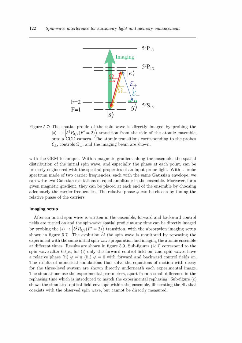
122 Spin-wave interference for stationary light and memory enhancement
Imaging
Figure 5.7: The spatial profile of the spin wave is directly imaged by probing the|s〉 →
∣∣∣52P3/2(F ′ = 2)⟩transition from the side of the atomic ensemble,
onto a CCD camera. The atomic transitions corresponding to the probesE±, controls Ω±, and the imaging beam are shown.
with the GEM technique. With a magnetic gradient along the ensemble, the spatialdistribution of the initial spin wave, and especially the phase at each point, can beprecisely engineered with the spectral properties of an input probe light. With a probespectrum made of two carrier frequencies, each with the same Gaussian envelope, wecan write two Gaussian excitations of equal amplitude in the ensemble. Moreover, for agiven magnetic gradient, they can be placed at each end of the ensemble by choosingadequately the carrier frequencies. The relative phase ϕ can be chosen by tuning therelative phase of the carriers.
Imaging setup
After an initial spin wave is written in the ensemble, forward and backward controlfields are turned on and the spin-wave spatial profile at any time can be directly imagedby probing the |s〉 →
∣∣∣52P3/2(F ′ = 2)⟩transition, with the absorption imaging setup
shown in figure 5.7. The evolution of the spin wave is monitored by repeating theexperiment with the same initial spin-wave preparation and imaging the atomic ensembleat different times. Results are shown in figure 5.9. Sub-figures (i-iii) correspond to thespin wave after 60 µs, for (i) only the forward control field on, and spin waves havea relative phase (ii) ϕ = π (iii) ϕ = 0 with forward and backward control fields on.The results of numerical simulations that solve the equations of motion with decayfor the three-level system are shown directly underneath each experimental image.The simulations use the experimental parameters, apart from a small difference in therephasing time which is introduced to match the experimental rephasing. Sub-figure (c)shows the simulated optical field envelope within the ensemble, illustrating the SL thatcoexists with the observed spin wave, but cannot be directly measured.

5.3 Self-stabilising stationary light in a cold atomic ensemble 123
a)
b)
c)
d)
Figure 5.8: CCD images for a 4-µs imaging pulse during a 300-µs exposition time, corre-sponding to the duration of the whole SL experiment. Each measurement isconstructed from ten images that are averaged to reduce shot-to-shot noiseof the CCD camera. a) Single raw image capture showing a shadow wherea spin wave has been written to the atoms. Averaged image over the tenacquisitions, hinting more precisely where spin-wave intensity
∣∣∣S∣∣∣2 — andtherefore absorption — is significant: b) after the optical pulse is initiallyencoded in the atoms, and after it has evolved into a steady state for spinwaves c) with opposite phase, d) with the same phase.
Agreement between measurements and simulations
The relative phase of the spin waves cannot be measured directly, which preventsus from checking the two configurations effectively correspond to spin waves in phaseand in phase opposition. Nonetheless, the two cases correspond to very different spin-wave dynamics. Therefore, the measured spin-wave evolution can be compared to thetheoretical prediction of it.
This comparison shows that our experimental data show excellent agreementwith the behaviour predicted by the simulations. The middle column of figure 5.9shows results and simulations for a stationary spin wave, where the integratedamplitude of the initial spin wave is zero. In this case, as expected, we observe noevolution of the shape of the spin wave, similarly to the theoretical result shownin figure 5.6. When the counter-propagating control fields are turned on at 60 µs,there is only a gradual evolution due to decay. The right-hand column where theinitial spin wave is not stable shows a rapid evolution to a stationary spin wave,marked by a horizontal discontinuity in the plot, in both the experimental dataand simulated results.
Once the spin wave has reached a steady state in terms of shape, it continues to decayat a rate given by the control field scattering. The spin-wave decay rate is measured as(10± 1) kHz in the experiment, which roughly agrees with the value 12 kHz used in thesimulations.

124 Spin-wave interference for stationary light and memory enhancement
Timing
0 40 80 120Time
a)
b)
c)
Figure 5.9: a) Timing of the gradient η and control fields Ω± for the stabilisation ofstationary light. b) Top row shows the experimentally measured evolutionof the spinwave. Middle row shows simulations of the spinwave. Bottom rowcompares experiment (green) and simulation (black line) over the z directionat time 70 µs. In the results of the left column, only the forward control fieldis on after 60 µs. The other columns have forward and backward controlfields on, as shown in the timing of sub-figure (a). The two spin waves havea relative phase of ϕ = π in the middle column, and ϕ = π in right column.c) Simulations of the probe field intensities for the situations correspondingto the columns of sub-figure (b). Top row shows the magnitude of theforward probe. Bottom row shows cross-sections at 70 µs with both forward(blue) and backward (yellow) probe field components.

5.4 Time-Reversed And Coherently-Enhanced memory 125
5.4 Time-Reversed And Coherently-Enhanced memoryStationary light has been observed by altering optical memory schemes but it does not
a priori constitute a memory itself. In the previous sections, however, we have seen whatspin-wave profiles give rise to SL. The spatial anti-symmetry of the spin-wave eigenmoderesulting in SL suggests some symmetry would be beneficial for a memory scheme relyingon the conversion of light into collective atomic excitations. Moreover, from generalconsiderations on Λ-type atoms, it is known that spatial and temporal symmetriesfavour the efficient interfacing between atoms and light [Gorshkov2007b]. On anotherhand, the interference between polaritons recalled from storage and to be stored hadalready been investigated in the group [Campbell2012, Pinel2015]. The synthesis ofthese two aspects is made with the new scheme we have developed: Time-Reversed andCoherently-Enhanced (TRACE) memory. The symmetries with counter-propagatingsignals sent simultaneously as well their recall corresponding to their temporal reversalcorrespond to the time-reversed in the name, while coherently-enhanced refers to theconstructive interference of the two signals.
The theory for this scheme was initiated by Jesse Everett, who also coined its name.Upon my return to ANU in 2016, I pushed for its experimental trial, which led to thefirst observation of the interference in February 2017. From there, we tamed this newmemory scheme, figuring out how to align the many different beams involved and theirprecise frequency.
5.4.1 Single-mode memory without a cavityWhereas a multimode memory stores distinguishing information about the different
modes in some internal degree-of-freedom of its medium (location within the memory,polarisation or frequency mode), there is little variation in the distribution of the storedinformation in a single-mode memory. Placing a cavity around an absorbing medium is awidespread technique to create a single-mode optical memory. This configuration enablesthe signal to traverse the memory many times, which leads to a uniform interactionalong the memory medium. The stored information, in that case, is contained in thephase and magnitude of the uniform atomic excitation.The spatially-distributed reflection of light in an atomic medium can create useful
optical interactions, with applications in quantum information processing. The origin ofthe spatially-distributed reflection can be a Bragg grating effect due to spatially-orderedatoms, or, in a disordered medium, a reflection process with imposed phase-matching.We use this second process to implement a single-mode optical memory, specificallywith four-wave mixing between two counter-propagating signals mapped to the samespin-wave mode by a control field.

126 Spin-wave interference for stationary light and memory enhancement
5.4.2 Phase matching and interferenceThe configuration for TRACE is closely related to the one for SL, with two counter-
propagating signals, each coupled to the atoms by a control beam making an angleso that both pairs address the same spin-wave. The difference in this case is thesimultaneous injection of both signals. The pulse shape for optimal storage is the risingexponential profile, shown in the figure inset.Taking the dimensionless spatial variable ζ = z/L, the coupling of both signals to
the same spin wave is described by the following equations:∂tS(ζ, t) = i
√d ΓΩ∗c
∆(E+(ζ, t) + E−(ζ, t)
)∂ζ E±(ζ, t) = ±i
√d
Ωc
∆ S(ζ, t)
A formal integration of the E± equations over space yields:
∂tS(t) = −dΓ |Ωc|2
∆2
∫ 1
0dζ ′ S(ζ ′, t) + i
√d ΓΩ∗c
∆(E+(ζ = 0, t) + E−(ζ = 1, t)
)(5.2)
As explicitly denoted in the left-hand side of the equation, the time evolution of thespin wave is independent of the position within the memory, only the overall spin waveis involved in the spin-wave dynamics. With no input field and a constant control field,an exponential decay of the spin wave occurs simultaneously with signal fields exitingboth sides of the memory.
When input signals sent from both sides are chosen symmetric and equal to Ein(t) wehave at each exit the same output Eout(t):
Ein(t) = E+(ζ = 0, t) = E−(ζ = 1, t)Eout(t) = E+(ζ = 1, t) = E−(ζ = 0, t)
In particular when E+(ζ = 0, t) + E−(ζ = 1, t) = 2Ein(t) corresponds to the value whichcompensates the first term of equation 5.2, a condition expressed as:
Ein(t) = −12i√d Γ |Ωc(t)|2
∆2
∫ 1
0dζ ′ S(ζ ′, t),
then it cancels the re-emission of light at each exit, Eout(t) = 0.To ensure the result Eout(t) = 0 during storage, the time evolution of the input fields
must match the evolution of the time-varying term |Ωc(t)|2∫ 1
0 dζ ′ S(ζ ′, t). In particular,for a constant control field Rabi frequency during storage, the condition is verified withan exponentially-rising pulse with the profile of the form:
Ein(t) ∝ exp[dΓ(Ω/∆)2t
].
When the whole signal is absorbed, turning the control fields off prevents re-emission.Turning the controls back on at a later time leads to the retrieval of the time-reversedcounter-propagating signals, providing a single-mode optical memory.

5.4 Time-Reversed And Coherently-Enhanced memory 127
5.4.3 Efficiency scaling with optical depthAn approach to determine the limit on the memory efficiency is given in [Gorshkov2007].
In this model, the limit comes from the decay of the excited state coherence, P . Wedefine forward and backward excited state coherence, P+ and P−, associated with eachprobe field. Assuming full absorption of the input probe pair, the equations governingthe atomic system are:
E+(ζ = 1, t) = i√d P+
E−(ζ = 0, t) = i√d P−
∂tP+ = −[Γ(1 + dζ) + i∆]P+ + iΩS∂tP− = −[Γ(1 + d(1− ζ) + i∆]P− + iΩS∂tS = iΩ∗(P+ + P−)
From these equations, we can for the time derivative of the quantity∣∣∣S∣∣∣2 +
∣∣∣P+∣∣∣2 +
∣∣∣P−∣∣∣2,which corresponds to the total energy transferred to the atoms. This gives:
∂t
(∣∣∣S∣∣∣2 +∣∣∣P+
∣∣∣2 +∣∣∣P−∣∣∣2) = −2Γ
(∣∣∣P+∣∣∣2 +
∣∣∣P−∣∣∣2)+ 2dΓ(ζ∣∣∣P+
∣∣∣2 + (1− ζ)∣∣∣P−∣∣∣2)
In the adiabatic limit, P+ = P− and the integration over time of the output light fieldEout(t) = E+(ζ = 0, t) = E−(ζ = 1, t) gives:∫ ∞
0dt′∣∣∣Eout
∣∣∣2 = − d
d+ 2
[∣∣∣S(t)∣∣∣2 +
∣∣∣P+(t)∣∣∣2 +
∣∣∣P−(t)∣∣∣2]t→∞
t=0
which corresponds to a maximum storage-and-retrieval efficiency equal to d2/(d+ 2)2.Asymptotically, this yields an efficiency scaling as 1 − 4/d, for d 1. Our schemetherefore has a favourable dependence on OD compared to other typical free-spacememories, for which ideal storage followed by retrieval goes as 1−5.8/d [Gorshkov2007b].The term coherently enhanced refers to the ability to distribute the spin-wave throughoutthe memory, making the most efficient use of the available OD, as well as enhancing theabsorption through the constructive interference of the forward and backward processes.In comparison, the efficiency of the ideal storage followed by retrieval is 1 − 1/C
in a cavity-enhanced memory with cooperativity C. Cooperativity is proportional tothe OD, with C = 2dc/(Lκ), where L is the cavity length and κ is the transmissionof the cavity output-coupler. The lower efficiency obtainable in our scheme is due tothe extra control field and associated decay. However, cavity single-mode memoriesrequire back-action on the atomic ensemble from light building up in the cavity to beprevented. This imposes that the decay rate out of the cavity is significantly faster thanthe memory decay rate, which is a limitation the bandwidth of such memories. On theother hand, in the TRACE memory scheme, although it acts as a single-mode memorylike a cavity-enhanced memory, there is no such back-action as light that reaches theend of the ensemble never returns to the ensemble.
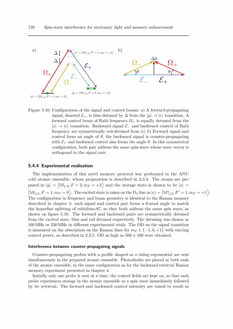
128 Spin-wave interference for stationary light and memory enhancement
a) b)
Figure 5.10: Configuration of the signal and control beams: a) A forward-propagatingsignal, denoted E+, is blue-detuned by ∆ from the |g〉 → |e〉 transition. Aforward control beam of Rabi frequency Ω+ is equally detuned from the|s〉 → |e〉 transition. Backward signal E− and backward control of Rabifrequency are symmetrically red-detuned from |e〉 b) Forward signal andcontrol form an angle of θ, the backward signal is counter-propagatingwith E+ and backward control also forms the angle θ. In this symmetricalconfiguration, both pair address the same spin-wave whose wave vector isorthogonal to the signal axis.
5.4.4 Experimental realisationThe implementation of this novel memory protocol was performed in the ANU
cold atomic ensemble, whose preparation is described in 2.3.4. The atoms are pre-pared in |g〉 =
∣∣∣5S1/2, F = 2,mF = +2⟩and the storage state is chosen to be |s〉 =∣∣∣5S1/2, F = 1,mF = 0
⟩. The excited state is taken on the D1-line as |e〉 =
∣∣∣5P1/2, F′ = 1,mF = +1
⟩.
The configuration in frequency and beam geometry is identical to the Raman memorydescribed in chapter 4: each signal and control pair forms a 6 mrad angle to matchthe hyperfine splitting of rubidium-87, so they both address the same spin wave, asshown on figure 5.10. The forward and backward pairs are symmetrically detunedfrom the excited state, blue and red detuned respectively. The detuning was chosen as160 MHz or 230 MHz in different experimental trials. The OD on the signal transitionis measured on the absorption on the Raman lines for mF ∈ −1, 0,+1 with varyingcontrol power, as described in 2.3.5. OD as high as 500± 100 were obtained.
Interference between counter-propagating signals
Counter-propagating probes with a profile shaped as a rising exponential are sentsimultaneously in the prepared atomic ensemble. Photodiodes are placed at both endsof the atomic ensemble, in the same configuration as for the backward-retrieval Ramanmemory experiment presented in chapter 4.
Initially only one probe is sent at a time, the control fields are kept on, so that eachprobe experiences storage in the atomic ensemble as a spin wave immediately followedby its retrieval. The forward and backward control intensity are tuned to result in

5.4 Time-Reversed And Coherently-Enhanced memory 129
0 5 10 15 200
5
10
15
20
25
30
Time (μs)
Inte
nsity
(arb
)Backward Detector
0 5 10 15 200
10
20
30
40
50
Time (μs)
Inte
nsity
(arb
)
Forward Detector
Figure 5.11: Photodiode signals on forward and backward detectors during the realisa-tion of the TRACE protocol. A rising-exponential-shaped probe is sentfrom both sides of the cold atomic ensemble. Depending on the relativephase of the counter-propagating probes, the absorption process of eachone interfere either constructively (in blue) or destructively (orange). Herethe forward and backward control beams are sent continuously and theprobes are immediately retrieved, with their time-reversed profile. Thereference probes without atoms is shown for reference (green).
the distribution of each probe pulse in four equal parts: leakage to the detector in thesame direction, reflection to the detector in the opposite direction and retrieval in bothdirections.
Both probes are sent simultaneously and their relative phase becomes random fromrun to run from the interferometric instability between their different paths. Figure5.11 shows the forward and backward photodiode signals for the cases of minimum andmaximum absorption on the probe pair.The relative phase between control-probe pairs is almost completely random after
each loading phase, of the order of a second. However, it varies only by a small amountover each memory sequence, which lasts about 400 µs. Therefore a series of 17 pairs ofprobe pulses are sent within the same sequence, with constant control field intensity,in order to investigate the phase dependence of the observed interference. The phaseof each successive E+ pulse is incremented by 0.3π while in a second experiment, thephase is not incremented. The spin waves produced by each counter-propagating pairinterfere. Constructive interference results in an enhanced mapping to the spin wavewhile destructive interference corresponds to a dark state which inhibits the absorption.A complete interference fringe is obtained when a total of 2π is incremented to the phaseover the length of the train of pulses. The results are shown in figure 5.12. Interferenceis also visible when the frequency of the control fields are detuned from the two-photonresonance.

130 Spin-wave interference for stationary light and memory enhancement
Visibilities were calculated by comparing the most constructive and destructiveinterference into the spin wave relative to the total optical power of the inputpulses. Visibilities of 70% are achieved which testifies to the spatio-temporalmatching of the forward and backward pairs. The production of temporalinterference fringes indicates that deterministic storage could be achieved bymeasuring the relative phase of input probes and adjusting a control field phaseor a path length accordingly.
Performance as a memory scheme
The interference fringe shows that some pulses are efficiently stored while othersdestructively interfere into the ensemble. By monitoring the leakage from the atomicensemble as the phase shifts between and within experimental runs we could heraldthe efficient writing of constructively-interfering spin waves and recall them on-demand.We have measured the amount of probe light retrieved from the stored spin waves andcharacterised this heralded probabilistic optical memory and compared it to gradientecho and Raman memory schemes using the same preparation of the atomic ensemble.
At large ODs around 500, we could not conclude favourably on the relativeperformance of the TRACE memory scheme compared to GEM or Ramanmemory: the schemes performed equivalently in the 50 − 65% storage-and-retrieval efficiency range. With an OD decreased to a few tens, TRACE performedcomparatively better in the only experimental attempt of performing the threememory schemes at high and low OD within a few hours. However, we cannotassert that the GEM and Raman parameters and alignment were optimisedto reach the highest efficiency. In particular, the configuration with an anglebetween the probe and control does not minimise the spin-wave wave vector andis therefore sub-optimal for these memory schemes.
The decay of the TRACE memory with storage time was investigated by varying theduration for which both controls are kept off after absorption of the probe pulses. Figure5.13 shows the dependence of the retrieval efficiency against storage time, which isfitted to exponential decay of characteristic time (130± 10) µs, which corresponds to atemperature (270± 40) µK, compatible with an independent time-of-flight temperaturemeasurement.
5.4.5 OutlookWe have demonstrated a new type of optical memory based on a distributed reflection
within an atomic ensemble. We have shown how the memory has improved efficiencyexpected of a single-mode memory, while still being accessible to free-space atom-lightinteraction techniques. The cost of this improvement is the division of the signal in twohalves, the addition of a second, backward, control and the relative phase control of allfour beams.

5.4 Time-Reversed And Coherently-Enhanced memory 131
a)
b)
c)
Pulse phase (rad)
0
Pul
se a
rea
(a.u
.)
0
200
400
600
800
1000
Relative phase offset (rad)
Tra
nsm
ission
and
retr
ieva
l effi
cien
cy
0
0.2
0.4
0.6
0.8
Pho
todi
ode
sign
al (
a.u.
)
0 100 200 300
Figure 5.12: a) A series of 17 pairs of probe pulses are sent within the same sequence,with constant control field intensity. Here, the phase of each successive E+pulse is incremented by 0.3π. The spin waves produced by each counter-propagating pair interfere constructively or destructively, which enhancesor inhibits the absorption, respectively. The retrieval which immediatelyfollows is similarly enhanced or inhibited. b) The area of the pulse beingtransmitted and reflected during the sending of the probe (blue dots),or retrieved in the following time window (red dots), are represented foreach phase increment. Solid lines correspond to sinusoidal fit functions. c)A complete interference fringe compiled over all acquisitions to find therelative phase offset, as well as the visibility of the interference.

132 Spin-wave interference for stationary light and memory enhancement
Figure 5.13: Decay of the memory efficiency with storage time. The decay time is fittedto a gaussian decay of characteristic time (130± 10) µs.
The TRACE memory scheme can be linked up with SL and specifically the applicationproposal to generate cross-phase modulation between a target state, stored in the middleof an atomic ensemble, and a signal state producing stationary light [Everett2017]. Theideal signal state can be efficiently generated using the TRACE protocol, while leavingthe memory accessible for storing the target state at the centre and in the same modeas the signal state.
5.5 Future investigation of stationary lightThe two experiments reported in this chapter demonstrate our increasing understand-
ing of Raman SL systems, whose dynamics was confused with diffraction off Bragggratings in the earlier investigations from the community. Harnessing this form oflight promises applications in non-linear photon-photon interaction between storedsignals which keep a non-vanishing optical component, in contrast with stopped-lightexperiments. Our future endeavour are aimed at this direction, with the experimentalrealisation of cross-phase modulation between a single photon and coherent light, oreven between two single photons. Our single photons would either be provided by aSPDC source built in Andrew White’s group and brought to the ANU [Rambach2016],or generated by four-wave mixing in a second cold atomic ensemble for which a MOT isbeing built.

5.5 Future investigation of stationary light 133
Chapter Conclusion
In this chapter, I have reported on two experiments based on stationary light:
• The first one provided a model for the dynamics of self-stabilisation ofstationary light. Several spin-wave spatial distributions were prepared inan atomic ensemble and their evolution was monitored by imaging the spinwaves at different times. The model and the measured spin wave structureover time showed excellent agreement. This work enabled the observation ofstationary light although this light was not directly observable as it does notescape the atomic ensemble.
• The TRACE memory scheme was proposed and demonstrated. This schemerelies on the interference between the writing process of counter-propagatingsignals to the same spin wave. This new form of a free-space memory showsa single-mode character, which benefits from a better scaling of the efficiencywith OD than regular free-space memories. It also enables the efficientgeneration of the ideal target state to perform cross-phase-modulation witha stationary-light signal.


Conclusion
The work of this PhD has been focused on the preparation of large atomic ensemblesand the enhancement of their interfacing with light. The increase of the optical depthin these ensembles is the universally-known method of accessing the efficient mappingof light to and from collective excitations in atomic ensembles. The implementation ofstate-of-the-art cold-atom preparation methods both at ANU and LKB has led to asteady increase of this figure of merit over the last years. This has enabled the high-performance memory-scheme implementations described in this thesis. In particularthis PhD work has seen the breaking of the no-cloning limit for EIT-based qubit storage,more than doubling the previous figure for any qubit storage, along with a memoryfidelity close to unity. A second highlight was the advantageous use of backward retrievalin a Raman memory, which contributed to beating the efficiency record for Ramanoptical memories. These experimental achievements were nonetheless accompaniedby significant theoretical progress on understanding these platforms, especially athigh optical depths, with the development of a model describing the contributions ofadditional excited levels in EIT storage, a model which showed a strong agreement withthe experimental data, which could be taken over a large range of optical depths thanksto the efficient preparation method. In Raman configurations, it was the symmetries inthe geometry and detunings to the excited level that were central to the study of theself-stabilisation of stationary light in a gradient echo memory and the time-reversed andcoherently-enhanced memory scheme envisioned and its concept proved experimentallyin the course of this PhD.
The developments described in this thesis offer many options for future investigations.The generation of single photons with the DLCZ protocol is still a source of struggle,but now that the atomic ensemble has overcome the optical-depth limitation it wasrunning into as a standard 3D-MOT, there should be a sufficiently-strong atom-lightcoupling to enable the efficient heralding efficiency of the single-photon while keepinga high non-classical character. Machine-learning applied to the optimisation of anatom-light experiment has been a increasingly-exciting aspect of this PhD over the lastmonths, and a significant help generating and maintaining a high-performance atomicensemble, with an automatic execution of the parameters tweaks to go from high tovery high optical depths, which can otherwise be quite a burden on a daily basis in thelab. However, machine-learning is giving promises to provide much more than a fewtime-saving adjustments: the solutions it has found to optimise compression-and-coolingsequences, for example, demonstrate that it can find unexpected optimal sequences,which would probably be impossible for a human to converge to. In a not-so-distantfuture, the application of the machine-learning algorithm to directly optimise a memory,and from there any atom-light interaction protocol, is definitely a fascinating prospect,which is likely to revolutionise our approach to quantum-information implementationsin atomic ensembles.
135


Bibliography
[Afzelius2010a] Mikael Afzelius & Christoph Simon. Impedance-matchedcavity quantum memory. Physical Review A, 82(2):022310,2010. doi:10.1103/physreva.82.022310. 27
[Afzelius2009] Mikael Afzelius, Christoph Simon, Hugues De Riedmatten &Nicolas Gisin. Multimode quantum memory based on atomicfrequency combs. Physical Review A, 79(5):052329, 2009.doi:10.1103/physreva.79.052329. 27
[Afzelius2010] Mikael Afzelius, Imam Usmani, Atia Amari, Björn Lauritzen,Andreas Walther, Christoph Simon, Nicolas Sangouard, JiříMinář, Hugues De Riedmatten, Nicolas Gisin et al. Demon-stration of atomic frequency comb memory for light with spin-wave storage. Physical Review Letters, 104(4):040503, 2010.doi:10.1103/physrevlett.104.040503. 27
[Alexander2006] A. L. Alexander, J. J. Longdell, M. J. Sellars & N. B.Manson. Photon Echoes Produced by Switching ElectricFields. Physical Review Letters, 96(4):043602, February 2006.doi:10.1103/PhysRevLett.96.043602. 30, 89
[Alzetta1976] G. Alzetta, A. Gozzini, L. Moi & G. Orriols. An experimentalmethod for the observation of r.f. transitions and laser beatresonances in oriented Na vapour. Il Nuovo Cimento B (1971-1996), 36(1):5–20, November 1976. doi:10.1007/BF02749417.27
[Andre2005] A André, M D Eisaman, R L Walsworth, A S Zibrov &M D Lukin. Quantum control of light using electromagnet-ically induced transparency. Journal of Physics B: Atomic,Molecular and Optical Physics, 38(9):S589–S604, April 2005.doi:10.1088/0953-4075/38/9/010. 28, 111
[Andre2002] A. André & M. D. Lukin. Manipulating Light Pulsesvia Dynamically Controlled Photonic Band gap. Phys-ical Review Letters, 89(14):143602, September 2002.doi:10.1103/PhysRevLett.89.143602. 111, 112
[Anisimov2008] Petr Anisimov & Olga Kocharovskaya. Decaying-dressed-state analysis of a coherently driven three-level Λ system.Journal of Modern Optics, 55(19-20):3159–3171, November2008. doi:10.1080/09500340802302378. 66
137

138 Spin-wave interference for stationary light and memory enhancement
[Arimondo1996a] Ennio Arimondo. Relaxation processes in coherent-populationtrapping. Physical Review A, 54(3):2216–2223, September1996. doi:10.1103/PhysRevA.54.2216. 37
[Aspect1988] A. Aspect, E. Arimondo, R. Kaiser, N. Vansteenkiste &C. Cohen-Tannoudji. Laser Cooling below the One-PhotonRecoil Energy by Velocity-Selective Coherent Population Trap-ping. Physical Review Letters, 61(7):826–829, August 1988.doi:10.1103/PhysRevLett.61.826. 28
[Aspelmeyer2003] M. Aspelmeyer, T. Jennewein, M. Pfennigbauer, W. R. Leeb& A. Zeilinger. Long-distance quantum communication withentangled photons using satellites. IEEE Journal of Se-lected Topics in Quantum Electronics, 9(6):1541–1551, 2003.doi:10.1109/JSTQE.2003.820918. 19
[August2017] Moritz August & Xiaotong Ni. Using recurrent neu-ral networks to optimize dynamical decoupling for quan-tum memory. Physical Review A, 95(1):012335, 2017.doi:10.1103/PhysRevA.95.012335. 56
[Autler1955] S. H. Autler & C. H. Townes. Stark Effect in Rapidly Vary-ing Fields. Physical Review, 100(2):703–722, October 1955.doi:10.1103/PhysRev.100.703. 62
[Bajcsy2003] M. Bajcsy, A. S. Zibrov & M. D. Lukin. Stationary pulsesof light in an atomic medium. Nature, 426(6967):638–641,December 2003. doi:10.1038/nature02176. 111, 113
[Balabas2013] M. V. Balabas & O. Yu Tretiak. Comparative study of alkali-vapour cells with alkane-, alkeneand 1-nonadecylbenzene-based antirelaxation wall coatings. Quantum Electronics,43(12):1175, 2013. doi:10.1070/QE2013v043n12ABEH015196.38
[Bao2012] Xiao-Hui Bao, Andreas Reingruber, Peter Dietrich, Jun Rui,Alexander Duck, Thorsten Strassel, Li Li, Nai-Le Liu, Bo Zhao& Jian-Wei Pan. Efficient and long-lived quantum memorywith cold atoms inside a ring cavity. Nature Physics, 8(7):517–521, July 2012. doi:10.1038/nphys2324. 106
[Bennett1983] Charles H. Bennett, Gilles Brassard, Seth Breidbart &Stephen Wiesner. Quantum Cryptography, or UnforgeableSubway Tokens. In Advances in Cryptology, pages 267–275.Springer, Boston, MA, 1983. ISBN 978-1-4757-0604-8 978-1-4757-0602-4. 20
[Blatt2016] Frank Blatt, Lachezar S. Simeonov, Thomas Halfmann &Thorsten Peters. Stationary light pulses and narrowband

5.5 Future investigation of stationary light 139
light storage in a laser-cooled ensemble loaded into a hollow-core fiber. Physical Review A, 94(4):043833, October 2016.doi:10.1103/PhysRevA.94.043833. 29
[Boller1991] K.-J. Boller, A. Imamoglu & S. E. Harris. Obser-vation of electromagnetically induced transparency.Physical Review Letters, 66(20):2593–2596, 1991.doi:10.1103/PhysRevLett.66.2593. 28
[Bouchiat1966] M. A. Bouchiat & J. Brossel. Relaxation of OpticallyPumped Rb Atoms on Paraffin-Coated Walls. Physical Review,147(1):41–54, July 1966. doi:10.1103/PhysRev.147.41. 38
[Braje2004] Danielle A. Braje, Vlatko Balić, Sunil Goda, G. Y.Yin & S. E. Harris. Frequency mixing using elec-tromagnetically induced transparency in cold atoms.Physical Review Letters, 93:183601, October 2004.doi:10.1103/PhysRevLett.93.183601. 98, 108
[Braunstein2005] Samuel L. Braunstein & Peter van Loock. Quantum informa-tion with continuous variables. Reviews of Modern Physics,77(2):513–577, June 2005. doi:10.1103/RevModPhys.77.513.9
[Briegel1998] H.-J. Briegel, W. Dür, J. I. Cirac & P. Zoller. Quantumrepeaters: The role of imperfect local operations in quantumcommunication. Physical Review Letters, 81(26):5932–5935,1998. doi:10.1103/PhysRevLett.81.5932. 19
[Burks2010PhD] Sidney Burks. Towards A Quantum Memory For Non-Classical Light With Cold Atomic Ensembles. phdthesis, Uni-versité Pierre et Marie Curie - Paris VI, October 2010. 61
[Bussieres2013] Félix Bussières, Nicolas Sangouard, Mikael Afzelius,Hugues de Riedmatten, Christoph Simon & Wolfgang Tit-tel. Prospective applications of optical quantum memories.Journal of Modern Optics, 60(18):1519–1537, October 2013.doi:10.1080/09500340.2013.856482. 21, 22, 26
[Bustard2013] Philip J. Bustard, Rune Lausten, Duncan G. England& Benjamin J. Sussman. Toward quantum process-ing in molecules: A THz-bandwidth coherent memoryfor light. Physical Review Letters, 111(8):083901, 2013.doi:10.1103/PhysRevLett.111.083901. 29
[Campbell2012] G. Campbell, M. Hosseini, B. M. Sparkes, P. K. Lam & B. C.Buchler. Time- and frequency-domain polariton interference.New Journal of Physics, 14(3):033022, 2012. doi:10.1088/1367-2630/14/3/033022. 106, 125

140 Spin-wave interference for stationary light and memory enhancement
[Campbell2014] GT Campbell, Olivier Pinel, Mahdi Hosseini, Timo-thy Cameron Ralph, BC Buchler & Ping Koy Lam. Config-urable Unitary Transformations and Linear Logic Gates UsingQuantum Memories. Physical Review Letters, 113(6):063601,August 2014. doi:10.1103/PhysRevLett.113.063601. 26
[Chaneliere2005] T. Chanelière, D. N. Matsukevich, S. D. Jenkins, S.-Y.Lan, T. A. B. Kennedy & A. Kuzmich. Storage and re-trieval of single photons transmitted between remote quan-tum memories. Nature, 438(7069):833–836, December 2005.doi:10.1038/nature04315. 21
[Chaneliere2015] Thierry Chanelière & Gabriel Hétet. Light-shift-modulatedphoton-echo. Optics Letters, 40(7):1294–1297, April 2015.doi:10.1364/OL.40.001294. 30
[Chen2013a] Bing Chen, Kai Zhang, Chengling Bian, Cheng Qiu, Chun-Hua Yuan, L. Q. Chen, Z. Y. Ou & Weiping Zhang. Efficientraman frequency conversion by coherent feedback at low lightintensity. Optics Express, 21(9):10490–10495, May 2013.doi:10.1364/OE.21.010490. 29
[Chen2013] Yi-Hsin Chen, Meng-Jung Lee, I-Chung Wang, ShengwangDu, Yong-Fan Chen, Ying-Cheng Chen & Ite A. Yu. Co-herent optical memory with high storage efficiency and largefractional delay. Physical Review Letters, 110(8), February2013. doi:10.1103/physrevlett.110.083601. 33
[Cho2016] Y.-W. Cho, G. T. Campbell, J. L. Everett, J. Bernu, D. B.Higginbottom, M. T. Cao, J. Geng, N. P. Robins, P. K. Lam& B. C. Buchler. Highly efficient optical quantum memorywith long coherence time in cold atoms. Optica, 3(1):100–107,January 2016. doi:10.1364/OPTICA.3.000100. 27, 32, 33
[Cho2010] Young-Wook Cho & Yoon-Ho Kim. Atomic va-por quantum memory for a photonic polarization qubit.Optics Express, 18(25):25786–25793, December 2010.doi:10.1364/OE.18.025786. 28
[Choi2008] K. S. Choi, H. Deng, J. Laurat & H. J. Kimble. Mappingphotonic entanglement into and out of a quantum memory. Na-ture, 452(7183):67–71, March 2008. doi:10.1038/nature06670.28
[Chou2004] C. W. Chou, S. V. Polyakov, A. Kuzmich & H. J. Kim-ble. Single-photon generation from stored excitation in anatomic ensemble. Physical Review Letters, 92(21):213601,2004. doi:10.1103/PhysRevLett.92.213601. 21

5.5 Future investigation of stationary light 141
[Chrapkiewicz2014] Radosław Chrapkiewicz, Wojciech Wasilewski & CzesławRadzewicz. How to measure diffusional decoherence in mul-timode rubidium vapor memories? Optics Communications,317:1–6, 2014. doi:10.1016/j.optcom.2013.12.020. 37
[Cirac2000] J. I. Cirac & P. Zoller. A scalable quantum computer withions in an array of microtraps. Nature, 404(6778):579–581,April 2000. doi:10.1038/35007021. 20
[Clausen2012] Christoph Clausen, Félix Bussières, Mikael Afzelius &Nicolas Gisin. Quantum storage of heralded polarizationqubits in birefringent and anisotropically absorbing mate-rials. Physical Review Letters, 108:190503, May 2012.doi:10.1103/PhysRevLett.108.190503. 28
[Clausen2011] Christoph Clausen, Imam Usmani, Felix Bussieres, Nico-las Sangouard, Mikael Afzelius, Hugues de Riedmatten &Nicolas Gisin. Quantum storage of photonic entanglementin a crystal. Nature, 469(7331):508–511, January 2011.doi:10.1038/nature09662. 28
[Clauser1969] John F. Clauser, Michael A. Horne, Abner Shimony &Richard A. Holt. Proposed Experiment to Test Local Hidden-Variable Theories. Physical Review Letters, 23(15):880–884,October 1969. doi:10.1103/PhysRevLett.23.880. 7
[Cviklinski2008PhD] Jean Cviklinski. Interface quantique atomes-champ en régimede variables continues. Ph.D. thesis, Université Pierre etMarie Curie - Paris VI, 2008. 38
[Dajczgewand2014] Julián Dajczgewand, Jean-Louis Le Gouët, Anne Louchet-Chauvet & Thierry Chanelière. Large efficiency at tele-com wavelength for optical quantum memories. Opt. Lett.,39(9):2711–2714, May 2014. doi:10.1364/OL.39.002711. 30
[Damon2011] V. Damon, M. Bonarota, A. Louchet-Chauvet, T. Chanelière& J.-L. Le Gouët. Revival of silenced echo and quantummemory for light. New Journal of Physics, 13(9):093031, 2011.doi:10.1088/1367-2630/13/9/093031. 30
[Datta2012] Animesh Datta, Lijian Zhang, Joshua Nunn, Nathan K.Langford, Alvaro Feito, Martin B. Plenio & Ian A. Walm-sley. Compact Continuous-Variable Entanglement Distilla-tion. Physical Review Letters, 108(6):060502, February 2012.doi:10.1103/PhysRevLett.108.060502. 106
[Riedmatten2008] Hugues de Riedmatten, Mikael Afzelius, Matthias U. Staudt,Christoph Simon & Nicolas Gisin. A solid-state light-matterinterface at the single-photon level. Nature, 456(7223):773–777, December 2008. 25

142 Spin-wave interference for stationary light and memory enhancement
[Du2008] Shengwang Du, Pavel Kolchin, Chinmay Belthangady,G. Y. Yin & S. E. Harris. Subnatural linewidthbiphotons with controllable temporal length. Phys-ical Review Letters, 100(18):183603, May 2008.doi:10.1103/PhysRevLett.100.183603. 86
[Duan2001] L.-M. Duan, M. D. Lukin, J. I. Cirac & P. Zoller. Long-distance quantum communication with atomic ensembles andlinear optics. Nature, 414(6862):413–418, November 2001.doi:10.1038/35106500. 21, 22
[Dudin2013] Y. O. Dudin, L. Li & A. Kuzmich. Light storage on the timescale of a minute. Physical Review A, 87(3):031801, 2013.doi:10.1103/PhysRevA.87.031801. 23, 106
[Eberly1994] J. H. Eberly, M. L. Pons & H. R. Haq. Dressed-field pulses inan absorbing medium. Physical Review Letters, 72(1):56–59,January 1994. doi:10.1103/PhysRevLett.72.56. 62
[England2012] D. G. England, P. S. Michelberger, T. F. M. Champion,K. F. Reim, K. C. Lee, M. R. Sprague, X.-M. Jin, N. K.Langford, W. S. Kolthammer, J. Nunn & I. A. Walmsley.High-fidelity polarization storage in a gigahertz bandwidthquantum memory. Journal of Physics B: Atomic, Molecularand Optical Physics, 45(12):124008, 2012. doi:10.1088/0953-4075/45/12/124008. 33
[Erhard2001] Michael Erhard & Hanspeter Helm. Buffer-gas effects ondark resonances: Theory and experiment. Physical Review A,63(4):043813, March 2001. doi:10.1103/PhysRevA.63.043813.38
[Everett2017] J. L. Everett, G. T. Campbell, Y.-W. Cho, P. Vernaz-Gris,D.B. Higginbottom, O. Pinel, N. P. Robins, P. K. Lam &B. C. Buchler. Dynamical observations of self-stabilizingstationary light. Nature Physics, 13(1):68–73, January 2017.doi:10.1038/nphys3901. 29, 111, 117, 118, 132
[Everett2017a] J. L. Everett, P. Vernaz-Gris, A. D. Tranter, K. V. Paul, A. C.Leung, G. T. Campbell, P. K. Lam & B. C. Buchler. Time-Reversed and Coherently Enhanced Memory: a single modequantum atom-optic memory in free space. In preparation.111
[Fekete2013] Julia Fekete, Daniel Rieländer, Matteo Cristiani & Huguesde Riedmatten. Ultranarrow-Band Photon-Pair Source Com-patible with Solid State Quantum Memories and Telecommu-nication Networks. Physical Review Letters, 110(22):220502,May 2013. doi:10.1103/PhysRevLett.110.220502. 86

5.5 Future investigation of stationary light 143
[Fleischhauer2002] M. Fleischhauer & M. D. Lukin. Quantum memory for pho-tons: Dark-state polaritons. Physical Review A, 65(2):022314,January 2002. doi:10.1103/PhysRevA.65.022314. 28, 64, 66
[Fleischhauer2000] M. Fleischhauer, S.F. Yelin & M.D. Lukin. How to trapphotons ? storing single-photon quantum states in collectiveatomic excitations. Optics Communications, 179(1-6):395–410,2000. doi:10.1016/s0030-4018(99)00679-3. 21, 22, 28
[Fleischhauer2005] Michael Fleischhauer, Atac Imamoglu & Jonathan P. Maran-gos. Electromagnetically induced transparency: Optics incoherent media. Reviews of Modern Physics, 77(2):633–673,July 2005. doi:10.1103/RevModPhys.77.633. 63
[Gaubatz1988] U. Gaubatz, P. Rudecki, M. Becker, S. Schiemann, M. Külz &K. Bergmann. Population switching between vibrational levelsin molecular beams. Chemical Physics Letters, 149(5):463–468,September 1988. doi:10.1016/0009-2614(88)80364-6. 62
[Gea-Banacloche2010] Julio Gea-Banacloche. Impossibility of large phase shiftsvia the giant Kerr effect with single-photon wave pack-ets. Physical Review A, 81(4):043823, April 2010.doi:10.1103/PhysRevA.81.043823. 26
[Geng2014] J. Geng, G. T. Campbell, J. Bernu, D. B. Higginbottom, B. M.Sparkes, S. M. Assad, W. P. Zhang, N. P. Robins, P. K. Lam& B. C. Buchler. Electromagnetically induced transparencyand four-wave mixing in a cold atomic ensemble with largeoptical depth. New Journal of Physics, 16(11):113053, 2014.doi:10.1088/1367-2630/16/11/113053. 61
[Giner2013] L. Giner, L. Veissier, B. Sparkes, A. S. Sheremet, A. Nico-las, O. S. Mishina, M. Scherman, S. Burks, I. Shomroni,D. V. Kupriyanov, P. K. Lam, E. Giacobino & J. Laurat.Experimental investigation of the transition between Autler-Townes splitting and electromagnetically-induced-transparencymodels. Physical Review A, 87(1):013823, January 2013.doi:10.1103/PhysRevA.87.013823. 61, 64
[Giner2013PhD] Lambert Giner. Etude de la transparence électromagnétique-ment induite dans un ensemble d’atomes froids et applicationaux mémoires quantiques. Ph.D. thesis, Université Pierre etMarie Curie - Paris VI, 2013. 36, 44, 61
[Gisin2002] Nicolas Gisin, Grégoire Ribordy, Wolfgang Tittel & HugoZbinden. Quantum cryptography. Reviews of Modern Physics,74(1):145–195, March 2002. doi:10.1103/RevModPhys.74.145.20

144 Spin-wave interference for stationary light and memory enhancement
[Gorshkov2007] Alexey V. Gorshkov, Axel André, Michael Fleischhauer,Anders S. Sørensen & Mikhail D. Lukin. Univer-sal approach to optimal photon storage in atomic me-dia. Physical Review Letters, 98:123601, March 2007.doi:10.1103/PhysRevLett.98.123601. 22, 98, 127
[Gorshkov2007a] Alexey V. Gorshkov, Axel André, Mikhail D. Lukin & An-ders S. Sørensen. Photon storage in Λ-type optically denseatomic media. i. cavity model. Physical Review A, 76:033804,September 2007. doi:10.1103/PhysRevA.76.033804. 23, 29,91
[Gorshkov2007b] Alexey V. Gorshkov, Axel André, Mikhail D. Lukin & An-ders S. Sørensen. Photon storage in Λ-type optically denseatomic media. ii. free-space model. Physical Review A,76:033805, September 2007. doi:10.1103/PhysRevA.76.033805.12, 23, 91, 92, 97, 98, 99, 125, 127
[Gorshkov2007c] Alexey V. Gorshkov, Axel André, Mikhail D. Lukin &Anders S. Sørensen. Photon storage in Λ-type opticallydense atomic media. iii. effects of inhomogeneous broad-ening. Physical Review A, 76:033806, September 2007.doi:10.1103/PhysRevA.76.033806. 91
[Gorshkov2008] Alexey V. Gorshkov, Tommaso Calarco, Mikhail D. Lukin& Anders S. Sørensen. Photon storage in Λ-type opti-cally dense atomic media. IV. Optimal control using gra-dient ascent. Physical Review A, 77(4):043806, April 2008.doi:10.1103/PhysRevA.77.043806. 98
[Gouraud2016PhD] Baptiste Gouraud. Optical nanofibers interfacing cold toms.A tool for quantum optics. phdthesis, Université Pierre etMarie Curie - Paris VI, 2016. 44
[Grosshans2001] Frédéric Grosshans & Philippe Grangier. Quantumcloning and teleportation criteria for continuous quan-tum variables. Physical Review A, 64(1):010301, 2001.doi:10.1103/PhysRevA.64.010301. 22
[Gundogan2013] M Gündoğan, M Mazzera, P M Ledingham, M Cristiani &H de Riedmatten. Coherent storage of temporally multimodelight using a spin-wave atomic frequency comb memory. NewJournal of Physics, 15(4):045012, 2013. doi:10.1088/1367-2630/15/4/045012. 27
[Gundogan2012] Mustafa Gündoğan, Patrick M. Ledingham, AttaallahAlmasi, Matteo Cristiani & Hugues de Riedmatten.Quantum storage of a photonic polarization qubit in a

5.5 Future investigation of stationary light 145
solid. Physical Review Letters, 108:190504, May 2012.doi:10.1103/PhysRevLett.108.190504. 28, 83
[Hammerer2010] Klemens Hammerer, Anders S. Sørensen & Eugene S.Polzik. Quantum interface between light and atomic ensem-bles. Reviews of Modern Physics, 82:1041–1093, April 2010.doi:10.1103/RevModPhys.82.1041. 25
[Harrow2009] Aram W. Harrow, Avinatan Hassidim & Seth Lloyd.Quantum Algorithm for Linear Systems of Equations.Physical Review Letters, 103(15):150502, October 2009.doi:10.1103/PhysRevLett.103.150502. 19
[Hedges2010] Morgan P. Hedges, Jevon J. Longdell, Yongmin Li& Matthew J. Sellars. Efficient quantum memoryfor light. Nature, 465(7301):1052–1056, June 2010.doi:10.1038/nature09081. 25, 89
[Heinze2013] Georg Heinze, Christian Hubrich & Thomas Halfmann.Stopped Light and Image Storage by Electromagneti-cally Induced Transparency up to the Regime of OneMinute. Physical Review Letters, 111(3):033601, July 2013.doi:10.1103/PhysRevLett.111.033601. 23, 33
[Heshami2016] Khabat Heshami, Duncan G. England, Peter C. Humphreys,Philip J. Bustard, Victor M. Acosta, Joshua Nunn & Ben-jamin J. Sussman. Quantum memories: emerging applicationsand recent advances. Journal of Modern Optics, 63(20):2005–2028, 2016. doi:10.1080/09500340.2016.1148212. http://dx.doi.org/10.1080/09500340.2016.1148212. 10, 21, 22
[Higginbottom2015] D. B. Higginbottom, J. Geng, G. T. Campbell, M. Hosseini,M. T. Cao, B. M. Sparkes, J. Bernu, N. P. Robins, P. K.Lam & B. C. Buchler. Dual-rail optical gradient echo mem-ory. Optics Express, 23(19):24937–24944, September 2015.doi:10.1364/OE.23.024937. 24, 32, 89
[Higginbottom2012] D. B. Higginbottom, B. M. Sparkes, M. Rancic, O. Pinel,M. Hosseini, P. K. Lam & B. C. Buchler. Spatial-mode storagein a gradient-echo memory. Physical Review A, 86:023801,August 2012. doi:10.1103/PhysRevA.86.023801. 24, 30
[Horodecki1996] Michał Horodecki, Paweł Horodecki & Ryszard Horodecki.Separability of mixed states: necessary and sufficient con-ditions. Physics Letters A, 223(1):1–8, November 1996.doi:10.1016/S0375-9601(96)00706-2. 7
[Horsley2013] Andrew Horsley, Guan-Xiang Du, Matthieu Pellaton,Christoph Affolderbach, Gaetano Mileti & Philipp Treutlein.

146 Spin-wave interference for stationary light and memory enhancement
Imaging of relaxation times and microwave field strength in amicrofabricated vapor cell. Physical Review A, 88(6):063407,December 2013. doi:10.1103/PhysRevA.88.063407. 37, 44
[Hosseini2012] M. Hosseini, B. M. Sparkes, G. T. Campbell, P. K. Lam& B. C. Buchler. Storage and manipulation of light us-ing a Raman gradient-echo process. Journal of Physics B:Atomic, Molecular and Optical Physics, 45(12):124004, 2012.doi:10.1088/0953-4075/45/12/124004. 38
[Hosseini2011] M. Hosseini, B.M. Sparkes, G. Campbell, P.K. Lam & B.C.Buchler. High efficiency coherent optical memory with warmrubidium vapour. Nature Communications, 2:174, February2011. doi:10.1038/ncomms1175. 30, 33, 89
[Hosseini2009] Mahdi Hosseini, Ben M. Sparkes, Gabriel Hétet, Jevon J.Longdell, Ping Koy Lam & Ben C. Buchler. Coherentoptical pulse sequencer for quantum applications. Nature,461(7261):241–245, September 2009. doi:10.1038/nature08325.30
[Hsiao2016] Y.-F. Hsiao, P.-J. Tsai, H.-S. Chen, S.-X. Lin, C.-C. Hung,C.-H. Lee, Y.-H. Chen, Y.-F. Chen, I. A. Yu & Y.-C. Chen.Eit-based photonic memory with near-unity storage efficiency.ArXiv e-prints, 2016. 1605.08519. 71, 86
[Hsiao2014] Ya-Fen Hsiao, Hung-Shiue Chen, Pin-Ju Tsai & Ying-Cheng Chen. Cold atomic media with ultrahigh opticaldepths. Physical Review A, 90:055401, November 2014.doi:10.1103/PhysRevA.90.055401. 38
[Hughes2002] Richard J. Hughes, Jane E. Nordholt, Derek Derkacs &Charles G. Peterson. Practical free-space quantum key distri-bution over 10 km in daylight and at night. New Journal ofPhysics, 4(1):43, 2002. doi:10.1088/1367-2630/4/1/343. 19
[Hush2016] Michael Hush. M-loop: Machine-learning online optimizationpackage, 2016. 56
[Hetet2008b] G. Hétet, M. Hosseini, B. M. Sparkes, D. Oblak, P. K. Lam& B. C. Buchler. Photon echoes generated by reversing mag-netic field gradients in a rubidium vapor. Optics Letters,33(20):2323–2325, October 2008. doi:10.1364/OL.33.002323.30
[Hetet2008] G. Hétet, J. J. Longdell, A. L. Alexander, P. K. Lam & M. J.Sellars. Electro-Optic Quantum Memory for Light Using Two-Level Atoms. Physical Review Letters, 100(2):023601, January2008. doi:10.1103/PhysRevLett.100.023601. 30, 89

5.5 Future investigation of stationary light 147
[Hetet2008a] G. Hétet, J. J. Longdell, M. J. Sellars, P. K. Lam & B. C. Buch-ler. Multimodal Properties and Dynamics of Gradient EchoQuantum Memory. Physical Review Letters, 101(20):203601,November 2008. doi:10.1103/PhysRevLett.101.203601. 89
[Iakoupov2016PhD] Ivan Iakoupov. Enhancement of optical nonlinearities withstationary light. Ph.D. thesis, University of Copenhagen, 2016.111
[Iakoupov2016] Ivan Iakoupov, Johannes Borregaard & Anders S. Sørensen.Controlled-phase gate for photons based on stationary light.ArXiv e-prints, pages 1610.09206 [quant–ph], October 2016.ArXiv: 1610.09206. 29
[Iakoupov2016a] Ivan Iakoupov, Johan R. Ott, Darrick E. Chang & An-ders S. Sørensen. Dispersion relations for stationary lightin one-dimensional atomic ensembles. Physical Review A,94(5):053824, 2016. doi:10.1103/PhysRevA.94.053824. 29
[Jamonneau2016] P. Jamonneau, G. Hétet, A. Dréau, J.-F. Roch & V. Jacques.Coherent Population Trapping of a Single Nuclear Spin UnderAmbient Conditions. Physical Review Letters, 116(4):043603,January 2016. doi:10.1103/PhysRevLett.116.043603. 28
[Jenkins2012] S. D. Jenkins, T. Zhang & T. A. B. Kennedy. Motionaldephasing of atomic clock spin waves in an optical lattice.Journal of Physics B: Atomic, Molecular and Optical Physics,45(12):124005, 2012. doi:10.1088/0953-4075/45/12/124005.104
[Jin2015] Jeongwan Jin, Erhan Saglamyurek, Marcel. lí Grimau Pui-gibert, Varun Verma, Francesco Marsili, Sae Woo Nam,Daniel Oblak & Wolfgang Tittel. Telecom-wavelength atomicquantum memory in optical fiber for heralded polarizationqubits. Physical Review Letters, 115:140501, September 2015.doi:10.1103/PhysRevLett.115.140501. 28
[Jobez2014] P. Jobez, I. Usmani, N. Timoney, C. Laplane, N. Gisin &M. Afzelius. Cavity-enhanced storage in an optical spin-wave memory. New Journal of Physics, 16(8):083005, 2014.doi:10.1088/1367-2630/16/8/083005. 27, 33
[Jobez2015] Pierre Jobez, Cyril Laplane, Nuala Timoney, Nicolas Gisin,Alban Ferrier, Philippe Goldner & Mikael Afzelius. CoherentSpin Control at the Quantum Level in an Ensemble-BasedOptical Memory. Physical Review Letters, 114(23):230502,June 2015. doi:10.1103/PhysRevLett.114.230502. 33

148 Spin-wave interference for stationary light and memory enhancement
[Jobez2016] Pierre Jobez, Nuala Timoney, Cyril Laplane, Jean Etesse,Alban Ferrier, Philippe Goldner, Nicolas Gisin & MikaelAfzelius. Towards highly multimode optical quantum memoryfor quantum repeaters. Physical Review A, 93(3):032327,March 2016. doi:10.1103/PhysRevA.93.032327. 27
[Julsgaard2001] Brian Julsgaard, Alexander Kozhekin & Eugene S. Polzik.Experimental long-lived entanglement of two macroscopicobjects. Nature, 413(6854):400–403, September 2001.doi:10.1038/35096524. 38
[Julsgaard2004] Brian Julsgaard, Jacob Sherson, J. Ignacio Cirac, JaromírFiurášek & Eugene S. Polzik. Experimental demonstrationof quantum memory for light. Nature, 432(7016):482–486,November 2004. doi:10.1038/nature03064. 38
[Kalb2015] Norbert Kalb, Andreas Reiserer, Stephan Ritter & GerhardRempe. Heralded storage of a photonic quantum bit in asingle atom. Physical Review Letters, 114:220501, June 2015.doi:10.1103/PhysRevLett.114.220501. 28
[Katz2017] Or Katz & Ofer Firstenberg. Light storage for 150 millisecondsat room temperature. arXiv:1710.06844 [quant-ph], October2017. ArXiv: 1710.06844. 38
[Kielpinski2002] D. Kielpinski, C. Monroe & D. J. Wineland. Architecture for alarge-scale ion-trap quantum computer. Nature, 417(6890):709–711, June 2002. doi:10.1038/nature00784. 20
[Kimble2008] H. J. Kimble. The quantum internet. Nature, 453(7198):1023–1030, June 2008. doi:10.1038/nature07127. 18
[Knill2001] E. Knill, R. Laflamme & G. J. Milburn. A scheme for efficientquantum computation with linear optics. Nature, 409(6816):46–52, January 2001. doi:10.1038/35051009. 19
[Koch2007] Jens Koch, Terri M. Yu, Jay Gambetta, A. A. Houck,D. I. Schuster, J. Majer, Alexandre Blais, M. H. De-voret, S. M. Girvin & R. J. Schoelkopf. Charge-insensitive qubit design derived from the Cooper pairbox. Physical Review A, 76(4):042319, October 2007.doi:10.1103/PhysRevA.76.042319. 28
[Kozhekin2000] A. E. Kozhekin, K. Mølmer & E. Polzik. Quantum memoryfor light. Physical Review A, 62(3):033809, August 2000.doi:10.1103/PhysRevA.62.033809. 91
[Kubo2011] Y. Kubo, C. Grezes, A. Dewes, T. Umeda, J. Isoya,H. Sumiya, N. Morishita, H. Abe, S. Onoda, T. Ohshima,

5.5 Future investigation of stationary light 149
V. Jacques, A. Dréau, J.-F. Roch, I. Diniz, A. Auffeves,D. Vion, D. Esteve & P. Bertet. Hybrid Quantum Circuitwith a Superconducting Qubit Coupled to a Spin Ensemble.Physical Review Letters, 107(22):220501, November 2011.doi:10.1103/PhysRevLett.107.220501. 28
[Kupchak2015] Connor Kupchak, Thomas Mittiga, Bertus Jordaan,Mehdi Namazi, Christian Nölleke & Eden Figueroa.Room-temperature single-photon level memory for polar-ization states. Scientific Reports, 5:7658, January 2015.doi:10.1038/srep07658. 28
[Kurtsiefer2002] C. Kurtsiefer, P. Zarda, M. Halder, H. Weinfurter, P. M.Gorman, P. R. Tapster & J. G. Rarity. Quantum cryptography:A step towards global key distribution. Nature, 419(6906):450–450, 2002. doi:10.1038/419450a. 19
[Kuzmich2003] A. Kuzmich, W. P. Bowen, A. D. Boozer, A. Boca, C. W.Chou, L.-M. Duan & H. J. Kimble. Generation of nonclas-sical photon pairs for scalable quantum communication withatomic ensembles. Nature, 423(6941):731–734, June 2003.doi:10.1038/nature01714. 21
[Laplane2015] Cyril Laplane, Pierre Jobez, Jean Etesse, Nuala Timoney,Nicolas Gisin & Mikael Afzelius. Multiplexed on-demandstorage of polarization qubits in a crystal. New Journal ofPhysics, 18(1):013006, December 2015. doi:10.1088/1367-2630/18/1/013006. 28
[Laurat2006] Julien Laurat, Hugues de Riedmatten, Daniel Felinto,Chin-Wen Chou, Erik W. Schomburg & H. Jeff Kim-ble. Efficient retrieval of a single excitation stored in anatomic ensemble. Opt. Express, 14(15):6912–6918, Jul 2006.doi:10.1364/OE.14.006912. 32
[LeGouet2009] J.-L. Le Gouët & P. R. Berman. Raman scheme for adjustable-bandwidth quantum memory. Physical Review A, 80(1):012320,2009. doi:10.1103/PhysRevA.80.012320. 92
[Lettner2011] M. Lettner, M. Mücke, S. Riedl, C. Vo, C. Hahn, S. Baur,J. Bochmann, S. Ritter, S. Dürr & G. Rempe. Remote en-tanglement between a single atom and a bose-einstein con-densate. Physical Review Letters, 106:210503, May 2011.doi:10.1103/PhysRevLett.106.210503. 28
[Lin2008a] Yen-Wei Lin, Hung-Chih Chou, Prashant P. Dwivedi, Ying-Cheng Chen & Ite A. Yu. Using a pair of rectangular coilsin the MOT for the production of cold atom clouds with large

150 Spin-wave interference for stationary light and memory enhancement
optical density. Optics Express, 16(6):3753–3761, March 2008.doi:10.1364/OE.16.003753. 42
[Lin2009] Yen-Wei Lin, Wen-Te Liao, Thorsten Peters, Hung-Chih Chou, Jian-Siung Wang, Hung-Wen Cho, Pei-Chen Kuan & Ite A. Yu. Stationary Light Pulsesin Cold Atomic Media and without Bragg Gratings.Physical Review Letters, 102(21):213601, May 2009.doi:10.1103/PhysRevLett.102.213601. 112, 114
[Longdell2008] J. J. Longdell, G. Hétet, P. K. Lam & M. J. Sellars.Analytic treatment of controlled reversible inhomogeneousbroadening quantum memories for light using two-levelatoms. Physical Review A, 78(3):032337, September 2008.doi:10.1103/PhysRevA.78.032337. 104
[Ma2017] Lijun Ma, Oliver Slattery & Xiao Tang. Optical quantummemory based on electromagnetically induced transparency.Journal of Optics, 19(4):043001, 2017. doi:10.1088/2040-8986/19/4/043001. 21, 26, 33
[Manukhova2017] A. D. Manukhova, K. S. Tikhonov, T. Yu. Golubeva & Yu. M.Golubev. Noiseless signal shaping and cluster-state generationwith a quantum memory cell. Physical Review A, 96(2):023851,2017. doi:10.1103/PhysRevA.96.023851. 93
[Maring2017] Nicolas Maring, Pau Farrera, Kutlu Kutluer, MargheritaMazzera, Georg Heinze & Hugues de Riedmatten. Pho-tonic quantum state transfer between a cold atomic gasand a crystal. Nature, 551(7681):485–488, November 2017.doi:10.1038/nature24468. 21
[Maring2014] Nicolas Maring, Kutlu Kutluer, Joachim Cohen, MatteoCristiani, Margherita Mazzera, Patrick M. Ledingham &Hugues de Riedmatten. Storage of up-converted telecom pho-tons in a doped crystal. New Journal of Physics, 16(11):113021,2014. doi:10.1088/1367-2630/16/11/113021. 33
[Massar1995] S. Massar & S. Popescu. Optimal extraction of in-formation from finite quantum ensembles. Physi-cal Review Letters, 74:1259–1263, February 1995.doi:10.1103/PhysRevLett.74.1259. 23, 83
[Matsukevich2006] D. N. Matsukevich, T. Chanelière, S. D. Jenkins, S.-Y. Lan,T. A. B. Kennedy & A. Kuzmich. Entanglement of remoteatomic qubits. Physical Review Letters, 96:030405, January2006. doi:10.1103/PhysRevLett.96.030405. 28

5.5 Future investigation of stationary light 151
[Matsukevich2004] D. N. Matsukevich & A. Kuzmich. Quantum State Trans-fer Between Matter and Light. Science, 306(5696):663–666,October 2004. doi:10.1126/science.1103346. 21
[Mavadia2017] Sandeep Mavadia, Virginia Frey, Jarrah Sastrawan, StephenDona & Michael J. Biercuk. Prediction and real-timecompensation of qubit decoherence via machine learn-ing. Nature Communications, 8:ncomms14106, 2017.doi:10.1038/ncomms14106. 56
[Michelberger2015] P. S. Michelberger, T. F. M. Champion, M. R. Sprague, K. T.Kaczmarek, M. Barbieri, X. M. Jin, D. G. England, W. S.Kolthammer, D. J. Saunders, J. Nunn & I. A. Walmsley. In-terfacing GHz-bandwidth heralded single photons with a warmvapour Raman memory. New Journal of Physics, 17(4):043006,April 2015. doi:10.1088/1367-2630/17/4/043006. 29
[Mishina2011] O. S. Mishina, M. Scherman, P. Lombardi, J. Ortalo, D. Fe-linto, A. S. Sheremet, A. Bramati, D. V. Kupriyanov, J. Lau-rat & E. Giacobino. Electromagnetically induced transparencyin an inhomogeneously broadened Λ transition with multi-ple excited levels. Physical Review A, 83:053809, May 2011.doi:10.1103/PhysRevA.83.053809. 69
[Moiseev2006] S. A. Moiseev & B. S. Ham. Quantum manipulationof two-color stationary light: Quantum wavelength con-version. Physical Review A, 73(3):033812, March 2006.doi:10.1103/PhysRevA.73.033812. 29, 111
[Moiseev2001] S. A. Moiseev & S. Kröll. Complete Reconstruc-tion of the Quantum State of a Single-Photon WavePacket Absorbed by a Doppler-Broadened Transition.Physical Review Letters, 87(17):173601, October 2001.doi:10.1103/PhysRevLett.87.173601. 21, 30
[Moiseev2003] S. A. Moiseev, V. F. Tarasov & B. S. Ham. Quantum mem-ory photon echo-like techniques in solids. Journal of Op-tics B: Quantum and Semiclassical Optics, 5(4):S497, 2003.doi:10.1088/1464-4266/5/4/356. 30
[Moiseev2011] S A Moiseev & W Tittel. Optical quantum memorywith generalized time-reversible atom-light interaction. NewJournal of Physics, 13(6):063035, 2011. doi:10.1088/1367-2630/13/6/063035. 91, 92
[Nicolas2014] A. Nicolas, L. Veissier, L. Giner, E. Giacobino, D. Maxein &J. Laurat. A quantum memory for orbital angular momentumphotonic qubits. Nature Photonics, 8(3):234–238, March 2014.doi:10.1038/nphoton.2013.355. 24, 61, 75

152 Spin-wave interference for stationary light and memory enhancement
[Nicolas2014PhD] Adrien Nicolas. Optical quantum memories with cold atomicensembles : a free space implementation for multimode stor-age, or a nanofiber-based one for high collection efficiency.phdthesis, Université Pierre et Marie Curie - Paris VI, 2014.36
[Nikoghosyan2009] Gor Nikoghosyan & Michael Fleischhauer. Stationary lightin cold-atomic gases. Physical Review A, 80(1):013818, July2009. doi:10.1103/PhysRevA.80.013818. 29, 114
[Nilsson2005] Mattias Nilsson & Stefan Kröll. Solid state quantum mem-ory using complete absorption and re-emission of photons bytailored and externally controlled inhomogeneous absorptionprofiles. Optics Communications, 247(4):393–403, March 2005.doi:10.1016/j.optcom.2004.11.077. 30
[Novikova2007] Irina Novikova, Alexey V. Gorshkov, David F. Phillips,Anders S. Sørensen, Mikhail D. Lukin & Ronald L.Walsworth. Optimal control of light pulse storage andretrieval. Physical Review Letters, 98(24), June 2007.doi:10.1103/physrevlett.98.243602. 98
[Nunn2013] J. Nunn, N. K. Langford, W. S. Kolthammer, T. F. M. Cham-pion, M. R. Sprague, P. S. Michelberger, X.-M. Jin, D. G.England & I. A. Walmsley. Enhancing multiphoton rates withquantum memories. Physical Review Letters, 110(13):133601,2013. doi:10.1103/PhysRevLett.110.133601. 21
[Nunn2008] J. Nunn, K. Reim, K. C. Lee, V. O. Lorenz, B. J. Sussman,I. A. Walmsley & D. Jaksch. Multimode memories in atomicensembles. Physical Review Letters, 101(26), December 2008.doi:10.1103/physrevlett.101.260502. 24
[Nunn2007] J. Nunn, I. A. Walmsley, M. G. Raymer, K. Surmacz,F. C. Waldermann, Z. Wang & D. Jaksch. Map-ping broadband single-photon wave packets into an atomicmemory. Physical Review A, 75:011401, January 2007.doi:10.1103/PhysRevA.75.011401. 29, 92, 93, 98, 99
[Oreg1984] J. Oreg, F. T. Hioe & J. H. Eberly. Adiabatic followingin multilevel systems. Physical Review A, 29(2):690–697,February 1984. doi:10.1103/PhysRevA.29.690. 62
[Parigi2015] Valentina Parigi, Vincenzo D’Ambrosio, Christophe Arnold,Lorenzo Marrucci, Fabio Sciarrino & Julien Laurat. Storageand retrieval of vector beams of light in a multiple-degree-of-freedom quantum memory. Nature Communications, 6:7706,July 2015. doi:10.1038/ncomms8706. 28, 61

5.5 Future investigation of stationary light 153
[Peng2005] Cheng-Zhi Peng, Tao Yang, Xiao-Hui Bao, Jun Zhang, Xian-Min Jin, Fa-Yong Feng, Bin Yang, Jian Yang, Juan Yin,Qiang Zhang, Nan Li, Bao-Li Tian & Jian-Wei Pan. Ex-perimental free-space distribution of entangled photon pairsover 13 km: Towards satellite-based global quantum com-munication. Physical Review Letters, 94(15):150501, 2005.doi:10.1103/PhysRevLett.94.150501. 19
[Peres1996] Asher Peres. Separability Criterion for Density Matrices.Physical Review Letters, 77(8):1413–1415, August 1996.doi:10.1103/PhysRevLett.77.1413. 7
[Petrich1994] Wolfgang Petrich, Michael H. Anderson, Jason R. Ensher& Eric A. Cornell. Behavior of atoms in a compressedmagneto-optical trap. JOSA B, 11(8):1332–1335, 1994.doi:10.1364/JOSAB.11.001332. 42
[Pinel2015] Olivier Pinel, Jesse L. Everett, Mahdi Hosseini, Geoff T.Campbell, Ben C. Buchler & Ping Koy Lam. A mirrorlessspinwave resonator. Scientific Reports, 5:srep17633, December2015. doi:10.1038/srep17633. 106, 111, 125
[Radnaev2010] A. G. Radnaev, Y. O. Dudin, R. Zhao, H. H. Jen, S. D. Jenk-ins, A. Kuzmich & T. a. B. Kennedy. A quantum memory withtelecom-wavelength conversion. Nature Physics, 6(11):894–899,November 2010. doi:10.1038/nphys1773. 21
[Rambach2016] Markus Rambach, Aleksandrina Nikolova, Till J. Weinhold& Andrew G. White. Sub-megahertz linewidth single pho-ton source. APL Photonics, 1(9):096101, November 2016.doi:10.1063/1.4966915. 86, 108, 132
[Raymer1981] M. G. Raymer & J. Mostowski. Stimulated raman scatter-ing: Unified treatment of spontaneous initiation and spa-tial propagation. Physical Review A, 24(4):1980–1993, 1981.doi:10.1103/PhysRevA.24.1980. 91
[Raymer1985] M. G. Raymer, I. A. Walmsley, J. Mostowski & B. Sobolewska.Quantum theory of spatial and temporal coherence propertiesof stimulated raman scattering. Physical Review A, 32(1):332–344, 1985. doi:10.1103/PhysRevA.32.332. 91
[Reim2011] K. F. Reim, P. Michelberger, K. C. Lee, J. Nunn, N. K. Lang-ford & I. A. Walmsley. Single-Photon-Level Quantum Memoryat Room Temperature. Physical Review Letters, 107(5):053603,July 2011. doi:10.1103/PhysRevLett.107.053603. 29, 33, 108
[Reim2012] K. F. Reim, J. Nunn, X.-M. Jin, P. S. Michelberger, T. F. M.Champion, D. G. England, K. C. Lee, W. S. Kolthammer,

154 Spin-wave interference for stationary light and memory enhancement
N. K. Langford & I. A. Walmsley. Multipulse Addressing of aRaman Quantum Memory: Configurable Beam Splitting andEfficient Readout. Physical Review Letters, 108(26):263602,June 2012. doi:10.1103/PhysRevLett.108.263602. 29, 106
[Reim2010] K. F. Reim, J. Nunn, V. O. Lorenz, B. J. Sussman, K. C. Lee,N. K. Langford, D. Jaksch & I. A. Walmsley. Towards high-speed optical quantum memories. Nature Photonics, 4(4):218–221, April 2010. doi:10.1038/nphoton.2010.30. 29
[Ringot2001] J. Ringot, P. Szriftgiser & J. C. Garreau. Sub-recoil Raman spectroscopy of cold cesium atoms.Physical Review A, 65(1):013403, December 2001.doi:10.1103/PhysRevA.65.013403. 51
[Roy2017] Dibyendu Roy, C.M. Wilson & Ofer Firstenberg. Collo-quium: Strongly interacting photons in one-dimensional con-tinuum. Reviews of Modern Physics, 89(2):021001, May 2017.doi:10.1103/RevModPhys.89.021001. 10
[Sabooni2013a] Mahmood Sabooni, Qian Li, Stefan Kröll & Lars Rippe.Efficient Quantum Memory Using a Weakly Absorbing Sam-ple. Physical Review Letters, 110(13):133604, March 2013.doi:10.1103/PhysRevLett.110.133604. 33
[Saglamyurek2011] Erhan Saglamyurek, Neil Sinclair, Jeongwan Jin, Joshua A.Slater, Daniel Oblak, Felix Bussieres, Mathew George,Raimund Ricken, Wolfgang Sohler & Wolfgang Tittel. Broad-band waveguide quantum memory for entangled photons. Na-ture, 469(7331):512–515, January 2011. 27
[Sangouard2007] Nicolas Sangouard, Christoph Simon, Mikael Afzelius &Nicolas Gisin. Analysis of a quantum memory for pho-tons based on controlled reversible inhomogeneous broad-ening. Physical Review A, 75(3):032327, March 2007.doi:10.1103/PhysRevA.75.032327. 104
[Sangouard2011] Nicolas Sangouard, Christoph Simon, Hugues de Riedmatten& Nicolas Gisin. Quantum repeaters based on atomic ensem-bles and linear optics. Reviews of Modern Physics, 83:33–80,March 2011. doi:10.1103/RevModPhys.83.33. 22
[Saunders2016] D. J. Saunders, J. H. D. Munns, T. F. M. Champion, C. Qiu,K. T. Kaczmarek, E. Poem, P. M. Ledingham, I. A. Walmsley& J. Nunn. Cavity-enhanced room-temperature broadbandraman memory. Physical Review Letters, 116(9):090501,March 2016. doi:10.1103/PhysRevLett.116.090501. 29

5.5 Future investigation of stationary light 155
[Schmidt1996] H. Schmidt & A. Imamoglu. Giant Kerr nonlin-earities obtained by electromagnetically induced trans-parency. Optics Letters, 21(23):1936–1938, December 1996.doi:10.1364/OL.21.001936. 26
[Schori2002] C. Schori, B. Julsgaard, J. L. Sørensen & E. S. Polzik. Record-ing Quantum Properties of Light in a Long-Lived Atomic SpinState: TowardsQuantum Memory. Physical Review Letters,89(5):057903, July 2002. doi:10.1103/PhysRevLett.89.057903.38
[Scully1992] Marlan O. Scully & Michael Fleischhauer. High-sensitivity magnetometer based on index-enhanced media.Physical Review Letters, 69(9):1360–1363, August 1992.doi:10.1103/PhysRevLett.69.1360. 27
[Sheremet2010] A. S. Sheremet, L. V. Gerasimov, I. M. Sokolov, D. V.Kupriyanov, O. S. Mishina, E. Giacobino & J. Laurat.Quantum memory for light via a stimulated off-resonantraman process: Beyond the three-level Λ-scheme approxi-mation. Physical Review A, 82:033838, September 2010.doi:10.1103/PhysRevA.82.033838. 69
[Simon2007] Jonathan Simon, Haruka Tanji, James K. Thompson &Vladan Vuletić. Interfacing collective atomic excitations andsingle photons. Physical Review Letters, 98(18):183601, 2007.doi:10.1103/PhysRevLett.98.183601. 32
[Sinclair2014] Neil Sinclair, Erhan Saglamyurek, Hassan Mallahzadeh,Joshua A. Slater, Mathew George, Raimund Ricken, Mor-gan P. Hedges, Daniel Oblak, Christoph Simon, WolfgangSohler & Wolfgang Tittel. Spectral multiplexing for scalablequantum photonics using an atomic frequency comb quantummemory and feed-forward control. Physical Review Letters,113:053603, July 2014. doi:10.1103/PhysRevLett.113.053603.24
[Sparkes2013] B M Sparkes, J Bernu, M Hosseini, J Geng, Q Glorieux, P AAltin, P K Lam, N P Robins & B C Buchler. Gradient echomemory in an ultra-high optical depth cold atomic ensemble.New Journal of Physics, 15(8):085027, 2013. doi:10.1088/1367-2630/15/8/085027. 30, 33, 38, 89
[Sparkes2010] B. M. Sparkes, M. Hosseini, G. Hétet, P. K. Lam &B. C. Buchler. ac stark gradient echo memory in coldatoms. Physical Review A, 82(4):043847, October 2010.doi:10.1103/PhysRevA.82.043847. 89

156 Spin-wave interference for stationary light and memory enhancement
[Sparkes2013PhD] Benjamin M. Sparkes. Storage and Manipulation of OpticalInformation Using Gradient Echo Memory in Warm Vapoursand Cold Ensembles. phdthesis, The Australian NationalUniversity, 2013. 36
[Specht2011] Holger P. Specht, Christian Nolleke, Andreas Reiserer, ManuelUphoff, Eden Figueroa, Stephan Ritter & Gerhard Rempe.A single-atom quantum memory. Nature, 473(7346):190–193,May 2011. doi:10.1364/icqi.2011.qtug3. 22, 28, 83
[SteckCesium] Daniel A Steck. Cesium D Line Data. Available online athttp://steck.us/alkalidata (revision 2.1.4, 23 December2010). 41, 63, 69
[Surmacz2008] K. Surmacz, J. Nunn, K. Reim, K. C. Lee, V. O. Lorenz,B. Sussman, I. A. Walmsley & D. Jaksch. Efficient spatiallyresolved multimode quantum memory. Physical Review A,78:033806, September 2008. doi:10.1103/PhysRevA.78.033806.29, 92, 96, 98, 108
[Tikhonov2015] Kirill Tikhonov, Tania Golubeva & Yuri Golubev. Atomicthermal motion effect on efficiency of a high-speed quantummemory. The European Physical Journal D, 69(11):252, 2015.doi:10.1140/epjd/e2015-60370-6. 43, 108
[Tiranov2015] Alexey Tiranov, Jonathan Lavoie, Alban Ferrier, PhilippeGoldner, Varun B. Verma, Sae Woo Nam, Richard P.Mirin, Adriana E. Lita, Francesco Marsili, Harald Her-rmann, Christine Silberhorn, Nicolas Gisin, Mikael Afzelius& Félix Bussières. Storage of hyperentanglement in a solid-state quantum memory. Optica, 2(4):279–287, April 2015.doi:10.1364/OPTICA.2.000279. 28
[Tittel2010] W. Tittel, M. Afzelius, T. Chaneliére, R.l. Cone, S. Kröll,S.a. Moiseev & M. Sellars. Photon-echo quantum memory insolid state systems. Laser & Photonics Reviews, 4(2):244–267,February 2010. doi:10.1002/lpor.200810056. 30
[Vanier2005] J. Vanier. Atomic clocks based on coherent population trapping:a review. Applied Physics B, 81(4):421–442, August 2005.doi:10.1007/s00340-005-1905-3. 27
[Varnava2006] Michael Varnava, Daniel E. Browne & Terry Rudolph. LossTolerance in One-Way Quantum Computation via Counterfac-tual Error Correction. Physical Review Letters, 97(12):120501,September 2006. doi:10.1103/PhysRevLett.97.120501. 22
[Veissier2013] L. Veissier, A. Nicolas, L. Giner, D. Maxein, A. S. Sheremet,E. Giacobino & J. Laurat. Reversible optical memory for

5.5 Future investigation of stationary light 157
twisted photons. Optics Letters, 38(5):712–714, March 2013.doi:10.1364/OL.38.000712. 61
[Veissier2013PhD] Lucile Veissier. Quantum memory protocols in large coldatomic ensembles. phdthesis, Université Pierre et Marie Curie- Paris VI, 2013. 36
[Vernaz-Gris2017] P. Vernaz-Gris, K. Huang, M. Cao, A. S. Sheremet &J. Laurat. Highly-efficient quantum memory for polariza-tion qubits in a spatially-multiplexed cold atomic ensemble.ArXiv e-prints, 2017. Accepted in Nature Communications.,1707.09372. 61
[Vidal1999] Guifré Vidal. Entanglement of pure states for a singlecopy. Physical Review Letters, 83(5):1046–1049, 1999.doi:10.1103/PhysRevLett.83.1046. 93
[Vivoli2013] Valentina Caprara Vivoli, Nicolas Sangouard, Mikael Afzelius& Nicolas Gisin. High-bandwidth quantum memory pro-tocol for storing single photons in rare-earth doped crys-tals. New Journal of Physics, 15(9):095012, September 2013.doi:10.1088/1367-2630/15/9/095012. 27
[Walther2005] P. Walther, K. J. Resch, T. Rudolph, E. Schenck, H. Wein-furter, V. Vedral, M. Aspelmeyer & A. Zeilinger. Experimentalone-way quantum computing. Nature, 434(7030):169, March2005. doi:10.1038/nature03347. 19
[Wasilewski2006] Wojciech Wasilewski & M. G. Raymer. Pairwise entanglementand readout of atomic-ensemble and optical wave-packet modesin traveling-wave Raman interactions. Physical Review A,73(6):063816, June 2006. doi:10.1103/PhysRevA.73.063816.95
[Wiesner1983] StephenWiesner. Conjugate Coding. SIGACT News, 15(1):78–88, January 1983. doi:10.1145/1008908.1008920. 20
[Wigley2016] P. B. Wigley, P. J. Everitt, A. van den Hengel, J. W. Bastian,M. A. Sooriyabandara, G. D. McDonald, K. S. Hardman, C. D.Quinlivan, P. Manju, C. C. N. Kuhn, I. R. Petersen, A. N.Luiten, J. J. Hope, N. P. Robins & M. R. Hush. Fast machine-learning online optimization of ultra-cold-atom experiments.Scientific Reports, 6:srep25890, 2016. doi:10.1038/srep25890.56
[Wu2010a] Jin-Hui Wu, M. Artoni & G. C. La Rocca. Decay of sta-tionary light pulses in ultracold atoms. Physical Review A,81(3):033822, March 2010. doi:10.1103/PhysRevA.81.033822.112, 114

158 Spin-wave interference for stationary light and memory enhancement
[Wu2010] Jin-Hui Wu, M. Artoni & G. C. La Rocca. Stationary lightpulses in cold thermal atomic clouds. Physical Review A,82(1):013807, July 2010. doi:10.1103/PhysRevA.82.013807.29, 112
[Xu2013] Zhongxiao Xu, Yuelong Wu, Long Tian, Lirong Chen, Zhiy-ing Zhang, Zhihui Yan, Shujing Li, Hai Wang, Changde Xie& Kunchi Peng. Long lifetime and high-fidelity quantummemory of photonic polarization qubit by lifting zeeman de-generacy. Physical Review Letters, 111:240503, December2013. doi:10.1103/PhysRevLett.111.240503. 28
[Yin2017] Juan Yin, Yuan Cao, Yu-Huai Li, Sheng-Kai Liao, LiangZhang, Ji-Gang Ren, Wen-Qi Cai, Wei-Yue Liu, Bo Li, HuiDai, Guang-Bing Li, Qi-Ming Lu, Yun-Hong Gong, Yu Xu,Shuang-Lin Li, Feng-Zhi Li, Ya-Yun Yin, Zi-Qing Jiang, MingLi, Jian-Jun Jia, Ge Ren, Dong He, Yi-Lin Zhou, Xiao-XiangZhang, Na Wang, Xiang Chang, Zhen-Cai Zhu, Nai-Le Liu,Yu-Ao Chen, Chao-Yang Lu, Rong Shu, Cheng-Zhi Peng,Jian-Yu Wang & Jian-Wei Pan. Satellite-based entanglementdistribution over 1200 kilometers. Science, 356(6343):1140–1144, 2017. doi:10.1126/science.aan3211. 19
[Yin2012] Juan Yin, Ji-Gang Ren, He Lu, Yuan Cao, Hai-Lin Yong, Yu-Ping Wu, Chang Liu, Sheng-Kai Liao, Fei Zhou, Yan Jiang,Xin-Dong Cai, Ping Xu, Ge-Sheng Pan, Jian-Jun Jia, Yong-Mei Huang, Hao Yin, Jian-Yu Wang, Yu-Ao Chen, Cheng-ZhiPeng & Jian-Wei Pan. Quantum teleportation and entan-glement distribution over 100-kilometre free-space channels.Nature, 488(7410):185–188, 2012. doi:10.1038/nature11332.19
[Zhang2011] Han Zhang, Xian-Min Jin, Jian Yang, Han-Ning Dai, Sheng-Jun Yang, Tian-Ming Zhao, Jun Rui, Yu He, Xiao Jiang, FanYang, Ge-Sheng Pan, Zhen-Sheng Yuan, Youjin Deng, Zeng-Bing Chen, Xiao-Hui Bao, Shuai Chen, Bo Zhao & Jian-WeiPan. Preparation and storage of frequency-uncorrelated en-tangled photons from cavity-enhanced spontaneous parametricdownconversion. Nature Photonics, 5(10):628–632, October2011. doi:10.1038/nphoton.2011.213. 28
[Zhang2016] Wei Zhang, Dong-Sheng Ding, Ming-Xin Dong, Shuai Shi,Kai Wang, Shi-Long Liu, Yan Li, Zhi-Yuan Zhou, Bao-SenShi & Guang-Can Guo. Experimental realization of entan-glement in multiple degrees of freedom between two quantummemories. Nature Communications, 7:13514, November 2016.doi:10.1038/ncomms13514. 28

5.5 Future investigation of stationary light 159
[Zhang2012a] Xiao-Jun Zhang, Hai-Hua Wang, Cheng-Zhi Liu, Xing-Wei Han, Cun-Bo Fan, Jin-Hui Wu & Jin-Yue Gao.Direct conversion of slow light into a stationary lightpulse. Physical Review A, 86(2):023821, August 2012.doi:10.1103/PhysRevA.86.023821. 112
[Zhang2013] Xiao-Jun Zhang, Hai-Hua Wang, Zeng-Bin Wang, Xue Dong,Lei Wang, Li-Li Han, Yan Xu, Cheng-Zhi Liu, Cun-Bo Fan &Jin-Yue Gao. Tunable reflection based on electromagneticallyinduced transparency. JOSA B, 30(7):1905–1910, July 2013.doi:10.1364/JOSAB.30.001905. 112
[Zhou2015] Zong-Quan Zhou, Yi-Lin Hua, Xiao Liu, Geng Chen,Jin-Shi Xu, Yong-Jian Han, Chuan-Feng Li & Guang-Can Guo. Quantum storage of three-dimensionalorbital-angular-momentum entanglement in a crystal.Physical Review Letters, 115:070502, August 2015.doi:10.1103/PhysRevLett.115.070502. 24
[Zhou2012] Zong-Quan Zhou, Wei-Bin Lin, Ming Yang, Chuan-Feng Li & Guang-Can Guo. Realization of reliablesolid-state quantum memory for photonic polarizationqubit. Physical Review Letters, 108:190505, May 2012.doi:10.1103/PhysRevLett.108.190505. 28

Pierre VERNAZ-GRIS
Sujet : Préparation de grands ensembles atomiques et applicationsen interface lumière-matière efficace
Résumé : Cette thèse de doctorat en cotutelle a été centrée sur des expériences d’optique quan-tique faisant intervenir de grands ensembles atomiques. L’étude de l’interaction entre la lumièreet la matière et l’augmentation de leur couplage dans ces systèmes sont des étapes fondamentalespour le développement et l’amélioration de protocoles de génération, de stockage et de manipu-lation d’information quantique. Le travail de thèse exposé ici traite en particulier de l’évolutiondes techniques de préparation d’ensembles atomiques denses, des protocoles de lumière arrêtée etde lumière stationnaire développés et étudiés expérimentalement. Les ensembles d’atomes froidspréparés par refroidissement laser dans les deux réalisations expérimentales ont été portés jusqu’àdes épaisseurs optiques de plusieurs centaines, à des températures d’une dizaine de microkelvin.De plus, l’adressage de ces ensembles dans des configurations symétriques ont permis l’étude deprotocoles basés sur le renversement temporel de la conversion de lumière en excitations ato-miques collectives. Ces améliorations ont mené au stockage de bits quantiques par transparenceinduite électromagnétiquement, et de lumière cohérente par symétrie temporelle dans une mé-moire Raman, tous deux à des record d’efficacité, à de plus de 50%. Ce travail a également conduità l’étude expérimentale de la lumière stationnaire et de nouveaux protocoles en découlant.
Cette thèse est rédigée en anglais.
Mots clés : Atomes froids, optique quantique, mémoire quantique, communication quantique,transparence induite électromagnétiquement, mémoire Raman
Subject : Preparation of large cold atomic ensembles andapplications in efficient light-matter interfacing
Abstract: This cotutelle PhD thesis revolves around quantum optics experiments which involvelarge atomic ensembles. The study of light-matter interaction and its enhancement are crucialsteps in the development and progress of quantum information generation, storage and processingprotocols. The work presented here focuses on the evolution of large atomic ensemble preparationtechniques, on the development and experimental investigation of stopped and stationary lightprotocols. Laser-cooled atomic ensembles in both experimental realisations have been brought tooptical depths of a few hundreds, at temperatures of tens of microkelvin. Moreover, addressingthese ensembles in symmetric configurations has enabled the study of protocols based on thetemporal reversal of the mapping of light to collective atomic excitations. These enhancementshave led to the storage of qubits based on electromagnetically-induced transparency, and theoptical storage in a backward-retrieval Raman scheme, both demonstrating efficiency records,above 50%. This work has also led to the experimental investigation of stationary light and newprotocols based on it.
Keywords : Cold atoms, quantum optics, quantum memory, quantum communication,electromagnetically-induced transparency, Raman memory


