Embed Size (px)
Citation preview
EnvironmentalAssessmentof theAlaskanContinental Shelf
Final Reports of Principal Investigators
Volume 22 February 1984
U.S. DEPARTMENT OF COMMERCENational Oceanic and Atmospheric AdministrationNational Ocean ServiceOffice of Oceanography and Marine ServicesOcean Assessments Division
Outer Continental Shelf Environmental Assessment Program
ENVIRONMENTAL ASSESSMENT
OF THE
ALASKAN CONTINENTAL SHELF
FINAL REPORTS OF PRINCIPAL INVESTIGATORS
VOLUME 22
FEBRUARY 1984
U.S. DEPARTMENT OF COMMERCENATIONAL OCEANIC AND ATMOSPHERIC ADMINISTRATION
NATIONAL OCEAN SERVICE
OFFICE OF OCEANOGRAPHY AND MARINE SERVICES
OCEAN ASSESSMENTS DIVISION
JUNEAU, ALASKA
The facts, conclusions, and issues appearing in this report arebased on results of an Alaskan environmental studies programmanaged by the Outer Continental Shelf Environmental AssessmentProgram (OCSEAP) of the National Oceanic and AtmosphericAdministration, U.S. Department of Commerce, and primarilyfunded by the Minerals Management Service, U.S. Department ofthe Interior, through interagency agreement.
Mention of a commercial company or product does not constituteendorsement by the National Oceanic and Atmospheric Administra-tion. Use for publicity or advertising purposes of informationfrom this publication concerning proprietary products or thetests of such products is not authorized.
Environmental Assessment of the Alaskan Continental Shelf
Final Reports of Principal Investigators
VOLUME 22 FEBRUARY 1984
CONTENTS
J. R. PAYNE, B. E. KIRSTEIN, G. D. MCNABB, JR., J. L. LAMBACH,R. REDDING, R. E. JORDAN, W. HOM, C. DE OLIVEIRA, G. S. SMITH,D. M. BAXTER, AND R. GAEGEL (RU 597): Multivariate Analysisof Petroleum Weathering in the Marine Environment - Sub Arctic.Volume II - Appendices.
["Multivariate Analysis of Petroleum Weathering in the Marine Environ-ment - Sub Arctic. Volume I - Technical Results," is contained inVolume 21 of OCSEAP Final Reports.]
Contract No. NA80RAC00018Research Unit No. 597
Final Report
Multivariate Analysis of PetroleumWeathering in the Marine Environment -
Sub Arctic
Volume II - Appendices
Submitted by:
James R. Payne, Bruce E. Kirstein, G. Daniel McNabb, Jr.,James L. Lambach, Robert Redding, Randolph E. Jordan,
Wilson Hom, Celso de Oliveira, Gary S. Smith, Daniel M. Baxter,and Russel Gaegel (NOAA Kasitsna Bay laboratory manager)
James R. Payne, Principal InvestigatorDivision of Environmental Chemistry and Geochemistry
Science Applications, Inc.La Jolla, CA 92038
January 18, 1984

___1____~I~ UI__ · _ _ _ _ CCIIIU _ _CI· · III
VOLUME II
TABLE OF CONTENTS
Section Page
APPENDIX A CODE LISTING FOR OPEN-OCEAN OIL-WEATHERINGCALCULATIONS ................ Al - A28
APPENDIX B OIL-WEATHERING COMPUTER PROGRAM USER'SMANUAL ................ . . . . B1 - B60
APPENDIX C CODE DESCRIPTION FOR COMPONENT-SPECIFICDISSOLUTION . . . ............... Cl - C13
APPENDIX D CODE LISTING FOR DISPERSED-OIL CONCENTRATIONPROFILES WITH A TIME VARYING FLUX . . . . . . U1 - D12
APPENDIX E CODE LISTING FOR DISPERSED-OIL CONCENTRATIONPROFILES WITH A CONSTANT FLUX . . .... . . . . El - E7
APPENDIX F METHODS FOR MICROBIAL DEGRADATION STUDIES . . . . Fl - F9
APPENDIX G THE X-RAY DIFFRACTION ANALYSIS OF NINESEDIMENT SAMPLES ................ G1 - G16
APPENDIX H CHEMICAL WEATHERING OF PETROLEUM HYDROCARBONSIN SUB-ARCTIC SEDIMENTS: RESULTS OF CHEMICALANALYSES OF NATURALLY WEATHERED SEDIMENT PLOTSSPIKED WITH FRESH AND ARTIFICIALLY WEATHEREDCOOK INLET CRUDE OILS . . . . . . . . . . . . . . H - H56
iii

BACKGROUND
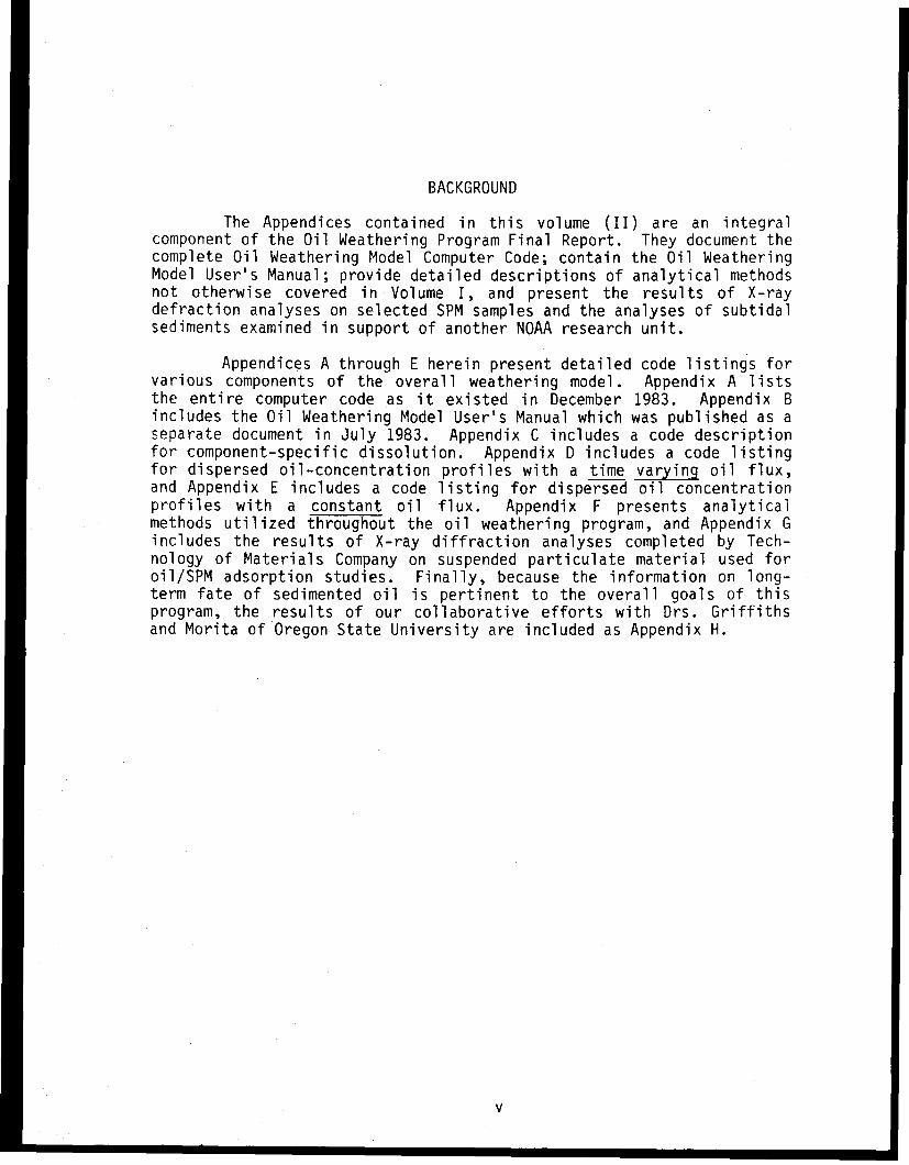
The Appendices contained in this volume (II) are an integralcomponent of the Oil Weathering Program Final Report. They document thecomplete Oil Weathering Model Computer Code; contain the Oil WeatheringModel User's Manual; provide detailed descriptions of analytical methodsnot otherwise covered in Volume I, and present the results of X-raydefraction analyses on selected SPM samples and the analyses of subtidalsediments examined in support of another NOAA research unit.
Appendices A through E herein present detailed code listings forvarious components of the overall weathering model. Appendix A liststhe entire computer code as it existed in December 1983. Appendix Bincludes the Oil Weathering Model User's Manual which was published as aseparate document in July 1983. Appendix C includes a code descriptionfor component-specific dissolution. Appendix D includes a code listingfor dispersed oil-concentration profiles with a time varying oil flux,and Appendix E includes a code listing for dispersed oil concentrationprofiles with a constant oil flux. Appendix F presents analyticalmethods utilized throughout the oil weathering program, and Appendix Gincludes the results of X-ray diffraction analyses completed by Tech-nology of Materials Company on suspended particulate material used foroil/SPM adsorption studies. Finally, because the information on long-term fate of sedimented oil is pertinent to the overall goals of thisprogram, the results of our collaborative efforts with Drs. Griffithsand Morita of Oregon State University are included as Appendix H.
v

I
APPENDIX A
CODE LISTING FOR OPEN-OCEAN
OIL-WEATHERING CALCULATIONS
A-1
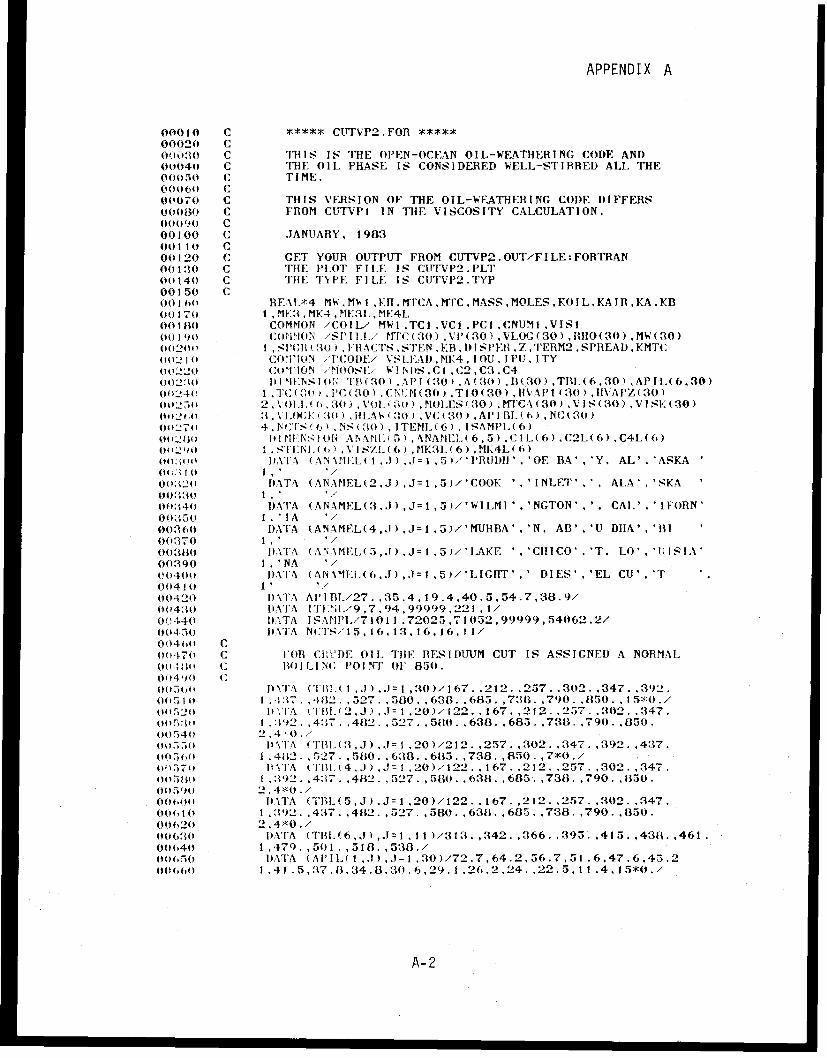
APPENDIX A
00010 C **** CUTVP2.FOR ****00020 C*00030 C THIS IS THE OPEN-OCFAN OIL-WEATHERING CODE AND00040 C THE OIL PHASE IS CONSIDERED WELL-STIRRED ALL. THE00050 C TIME.00(06( C00070 C THIS VERSION OF THE OIL-WEATHERING CODE DIFFERS00080 C FROM CUTVP1 IN TIE VISCOSITY CALCULATION.*0009( C00100 C JANUARY, 198300110 C00120 C GET YOUR OUTPUT FROM CUTVP2.OUT/FILE:FORTRAN00130 C THE PLOT FILE IS CUTVP'2.PLT00140 C 'THE TYPE FILE IS CUTVP2.TYP00150 C00O160 REAL,*4 M', .MM1 ,iKH.MTCATCC MASS,MOLES, OIL, KAIRKAKB00170 1, MK;3,t M, M II3L, ME-4L00180 COMMON /COIL/ MW1,TC1,VC1.PCI,CNUMI,VISI( 001 9 C()OHON /SPILL/ MTC(30) ,Vl(30) ,VI.OC(30) ,1110(30) ,MW(30)00204? 1 ,S1'(C r30) ,lIACTS .STEN, KB. DI SPF.Il Z,TERM2, SPREAD,KMTC(1)2 1 )o CONiON .I'CODE/ VSLEA1) ,Ml4, IOU, I PU, 1TYo(02-20 CON('ION /PlOOSE/ I NS , C1 . C2, C3 . C400230 I1I N'.NSI()N '1B(30 .AI'I (30 .. A(30) B(30) ,TL.(6,30) .APIL(6,30)( 0240 1 ,TC(: (30 .1'C(301 ,CM;IMH30) ,T10(30) .VAI'P (30) ,II\AI'Z(30)00254> 2.',01,1.( ,..30) ,VOL '3o),MOLES(30) , MTCA ( 30) VIS(30) ,VISK(30)(012tf, 3. \.LOKC 30 ) ,il.A (30) ,VC(30) ,APIBI.(6) ,NC(30)0o27 1 4,51"IS (t01 .NS(30) , ITEML(6) . ISAMPL(6)00(280l) IlNINS(IONi ANArPI(l5) , NAHII1I.(6,5) ,C1l(6),C2L(6) C4L(6)(00290 1 .STI:NI.(4,) .VISZL(6) ,MK3IL(6) ,MK4L(6)
01l14) DIATA (ANAMEL( I , J) , J= , 5 )/ 'PRUDIH ', 'OE BA' , 'Y. AL' , 'ASKA04t'1( i II ' /0'1:-)2( DAITA (ANAMEL(2,J) .J= ,5)/'COOK ','INLET'.', ALA' ,'SKA
I00880 I . ' /00340 DATA (ANAMEL(3,J),J=1,5)/'WIL.MI' ',NGTON' ', CAL', 'IFORN'(00o50 1 .I A '/00360 DATA (ANAMEL(4,J),J=1,5)/'MURBA','N, AB','U DIIA','BI00370 1 ' ' /00(380 IATA (ANAMEL(5,J) J= ,5)/'LAKE ', 'CHICO' . 'T. LO', 'I1SIA'00)390 . 'NA '/((040()0 DATA (ANAMI1EL(6.J),J=1 ,5)/'LIGHT' ' DIES', 'EL CU', 'T00410 1' ' /00420 DATA AI'IBL/27. .35.4,19.4,40.5,54.7,38.9/0(430 I AlTA IT:LiL/9 ,7.94,99999,221, 1/00(440 1DTA ISANI'L/71011.72025, 71052,99999,54062,2/00(45 0 I)iAA NCTS/15,16,13,16,16, 1/004(0l C0( 470 C FOR CliUDE OIL TIIE RESIDUUM CUT IS ASSIGNED A NORMAL0( '484; C BOILING POINT 01f 850.0041)4 C0(>05T I),TA (IlI.( 1 , J) .J = ,30)/167..212. .257. ,302..347. .392.0051() 1.:47. 4382. ,527. ,580. ,631. .685. ,73 .790. .850 ., 15*:0./0052o DVI'A (I'!.(2,J) ,J=1 ,20)/122. .167. 212. ,257. ,302. .347.0<5>:1, 1 .;9(2 . ,41;7.,482 . ,527. ,580. . 638., 685 .,738.,.790.. 850.00540) 2.4 './o5,iSo 1I I'A (ITHL.(3,J) ,J= ,20)/212. ,257.,302..347. ,392. ,437.
(00>560 I .48t2. ,527. 580. ,6'8..685..738.,850., 70./0'57(70 D1 I'A (t' 1. 4.J) ,J=1 .20)/122..167. .212. .257. ,302. ,347.(0(1581 1.:(92. ,4317. ,482. .527. ,580. .638. ,685. ,738. ,790. .850.
(00590 2,4*-0./o00(,00 11TA (TL(5,J) ,J=1 ,20)/122., 167. .212. .257. .302. 347.
00( 10 1 ,,92.,4317.,482., 527.,580.,638.,685. 738.,790..850.00(620 2,4*0./00630 I)ATA (TBL(6,J), J=1 ,11)/313.,342.,366. ,395. ,415.,438. 461.00640 1,479.,501.,518.,53'8./00(6.50 DATA (Al'IL.(1 ,,1) ,J=1 ,30)/72.7,64.2,56.7,51.6,47.6,45.200 60 1 ,41 .5,'37. 1,34.8,'30.6,29.1 ,26.2.24.,22.5,11 .4, 15*0./
A-2
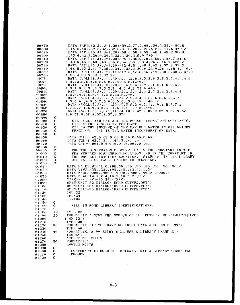
00670 DATA (APIL(2,J).J=1,20)/89.2,77.2.65.. 595.55.4,50.800600 1.46.5,43..39.6.37.,32.8,.31.3,28.7.26.6.25...1.6.4*0./00690 DATA (APIL(3,J).J=1,20)/68.6,58.7.53..48.1,43.2.38.800700 1 35.4,32.3.26.8,24.5,22.3.20.3,8.9,7*0./0(0710 DATA (APIL(4,.J),J=1,20)/,96;.7,86.2,70.6.62.3,55.7.51.600720 1,48.5,45.6.43.,40.,35.8.34..30..28.4,26.6.16.7,4*0./00730 DATA (APIL(5,J),J=1,20)/92.4,81..68.9,62.1.57.2.52.500740 1.48.8.45.2.41.7,38.2.34.4,33.2.30.6,28.9.26.1.18.1.4*0./00750 DATA (APIL(6,J),J=1.11)/49.6,47.3.46.,44. ,38.6.38.81,37.200760 1,35.4,33.9.33.1.32.2/00770 DATA (VOLL( ,J).J=I ,30).2.1.2.6.3.5.3.6.3.7.3.5.4.3.4.800780 1.5. ,2.8,6.5,6.8,6.0,7.4.;36.3,15*0./00790 DATA (VOLL(2,J),J=1,20)/2.4.2.5.5.9.6.1.5.1.5.2,4.900800 1.5.1.5.2.5. ,3.3.5.2,7..4.2.4.2.25.6.4*0./00810 DATA (VOLI.(3,J),J=1,20)/2.3,2.4,2.4,2..52.8.3.6,4.400820 1,5.3,4.7,6.3,4.1,5.5,53.3,7*0./008130 DATA (VOLL(4,J),J=I ,20)/1 .7,2.9.4.9.6. .6.8,6.5.5.700840 1,5.6.6.,4.9.5.7,5.6,6.5.6..5.6.19.3'.4, 0./00850 D.TFA (VO[.L(5,J),J=1 20)/7.5,8.2.9.7.11 .9.1.8..3.7.200860 1,7.2.7.4,6.9,3.5,3.,1.6,1.4.1.9.2. .4*0./00870 DATA (VOLL.(6.J),J= I.11)/4.78.9.57.9.09.9.57.9.57.9.57008()0 1.9.57.9.57,9.57,9.57,9.57/00890 C00900 C CIL. C2L. ANI C4L ARE THE MOUSSE FORMATION CONSTANTS.00910 C C1L IS TIE VISCOSITY CONSTANT.00920 C C21, IS TIlE INVERSE OF TIlE MAXIMUlM WATER IN OIL WEIGHTI00930 C FRACTION. C4L IS TIlE WATER INCOIPOIRATION RATE.00940 C00950 DATA CI(/0.62.62 ,0.62, 0.63 64,0.65,0.65/00960 DATA C21./1 .42,3.33 1.43.5..-1 . -1 . /00970 DATA- 1 C41./0..001 , 0. 0 01 .00.001,0 0. ,0./00980 C00990 C FOR TIIE DISPERSION PROCESS. IA IS TIIE CONSTANT IN THE01000 C SEA SlUtFACE DISPENSI10 E(QUATION, KEl IS TilE CONSTXNT IN01010 C THIE DIIOI'LET FRACTION EOUATION. STENL<6) IF 'TI: I.IBRAIRY01020 C OIL-WATER SURFACE TENSION IN DYNES/CM.01030 C01040 DATA EA.,KB.STENL/O.108.50. .30..30..30 . ,30.,30..30./01050 DATA VI SZL,/35. 35. .195. .15. 13.5. 11 .5/01060 DATA MK31./9000. 9000..9000.,9000. 9.000 . .3000./01070 DATA M141./10.5.7.4,15.3.10.5,2. ,2.01080 YI(X)=((1.-X)**0.38)/(X*X)01090 OP'EN(UN1T=32,DIALOG= 'DSED; CUTVP2. OJUT' )01100 OPEN(UNIT=34,DIALOG='DSfKD:CUTVP2.PLT')
1110 OI'EN(UNIT=35.DIALOG= 'I)SED:CUTVP2.TYP' )01 120 1 0U=3201130 IPU=3401140 ITY=35( 1150 C011(0( C FILL IN SOME LIBRARY IDENTIFICATIONS.01170 C01180 10 TYPE 2001190 20 FORIIAT(IX, 'ENTER THE NUMBER OF TBP CUTS TO BE CHAR\CTEFRI .ED01200 1 ON 12')01210 . TYPE 3001220 30 FORHIAT(IX. 'IF YOU HAVE NO INPUT DATA JUST ENTER 99')01230 TYPE' 4001240 40 FOlRMAT( IX. 'A 99 ENTRY WILL USE A 1.IBRARY EXAMPE')(01250 1 COD)E 101260 ACCEPT 50. NCUTS01270 50 FOIIMAT(12)01280 LSWTCIINCUTS01290 C013O00 C LSWTCII=99 IS USED TO INDICATE THAT A LIBRARY CRIJDE WAS01310 C CHOSEN.01320 C
A-3
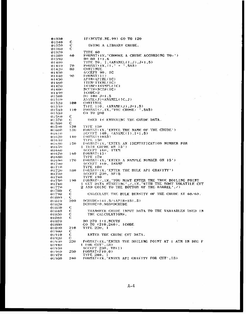
01,30 IF(NCUTS.NE.99) GO TO 12001340 C01350 C USING A LIBRARY CRUDE.
t03,60 C01370 TYPE 60013801 60 FOIRMAT(IX, CHOOSE A CRUDE ACCORDING TO:')0139(0 1)0 80 1=1,601400 TYPE 70, I,(ANAMEL(I,J),J=1,5)01410 70 FORllAT(IIXI I.' = ',5A5)
01420 80 CONTINUE0 1430 ACCEPT 90, IC01440 90 FORMAT( I 11)01450 APIB=AIPIBI.(IC)01460 ITEM= ITEML(IC)01470 ISAMP= ISAMPI(1C)01480 NCUTS=S NCTS ( I C01490 1 CODE=201500 I)D 100 ,1=l,501510 AhA\ME(J)=ANAMEL(IC,J)01520 10 CONT I NUE01530 T'PEI 110, (ANAME(J ) ,J=1 .5)01540 110 FORMAT(/, IX, 'YOU CHOSE: ',5A5)01550 GO TO 20001560 C01570 C USER IS ENTERING THE CRUDE DATA.0 15i80 C01590 120 TYPE 13001600 130 F(lR-I-\T( IX, 'ENTER THE NAME OF THE CRUDE')(161( fA (CCIP'T 140, (ANAME( ), I = ,5)0 1 620 140 1'4IHNAT( I OlA)01 :0 TY'E 1 50
0 1, 1 150 FlWINAT* ( IX. 'ENTER AN IDENTIFICATION NUMBER FOR01 50 1 TIII S CRUIDE ON 15 '01 660 ACCEPT 160, ITEM01670 1 60 FOlRMAT ( 5)01 1(,1( TYPE 17001,90 170 1 FoIRAT( IX. 'ENTER A SAMPLE NUMBER ON 15')01700 ACCEPT 60, ISAMP01710 TYPE 18001720 180 FOIlIAT( IX, 'ENTER THE BULK API GRAVITY')01730 ACCEP'T 230, APIB01740 TYPE 1 9001750 190 FOHMAT(/,1X,'YOU MUST ENTER THE TRUE BOILING POINT0 1760 1 CUT DATA STARTING' ,/ IX,' WITH THE MOST VOLATILE CUT01770 2 AND GOING TO TIIE BOTTOM OF THE BARREL' /)01780 C01790 C CALCULATE THE BULK DENSITY OF THE CRUDE AT 60/60.l01t80( C01110( 200 DCBUDE=141.5/(APIB+131.5)01 820 DCIUDE=O. 983*DCRUDE01 :80 C01840 C TRANSFER CRUDE INPUT DATA TO TIlE VARIABLES USED IN0 1850 C TlHE CALCULAT IONS.01860 C01870 DO 270 1=1.NCUTS01880 GO TO (210,260), ICODE01890 210 TYPE 220, I0I 1900 C01910 C ENTER THE CRUDE CUT DATA.01 920 C01980 220 FORMPAT(IX,'ENTER TIE BOILING POINT AT I ATM IN DEG F01940 1 FOR CUT' .13)(01 95 ACCEPT 230, TB(I)01960 230 FORMAT(F10.0)01970 TYPE 240, I01980 240 FORMAT(IX,-ENTER API GRAVITY FOR CUT',13)
A-4
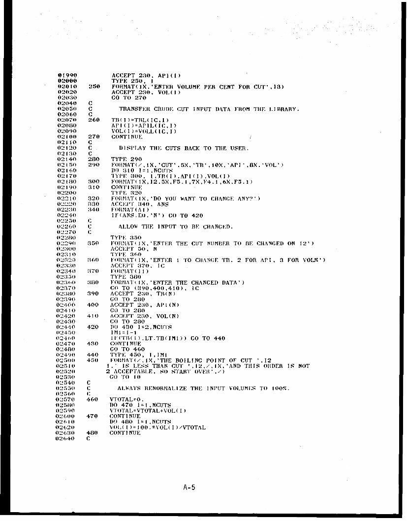
01990 ACCEPT 230. API(I)02000 TYPE 250, I02010 250 FORMAT(IX,'ENTER VOLUME PER CENT FOR CUT',13)02020 ACCEPT 230, VOL(I)02030 CO TO 27002040 C02050 C TRANSFER CRUDE CUT INPUT DATA FROM THE LIBRARY.02060 C02070 260 TB(I)=TBL(IC,I)02080 API(I)=APIL(IC,I)02090 VOL(I)=VOLL(IC,I)02100 270 CONTINUE02110 C02120 C DISPLAY THE CUTS BACK TO THE USER.021 30 C02140 280 TYPE 29002150 290 FOIlHAT(/,IX,'CUT',5X,'TB' ,10X 'API ',8X,'VOL')02160 D10 310 I=1. NCUTS02170 TYPE 300, I,TB(I).API(1I).VOL(1)02180 0 300 FOHRAT( X,12,5X,F5.1,7X.F4.1,6X.F5.1)042190 310 CONTINUE02200 TYPE 32002210 320 FOIIlAT(IX,'DO YOU WANT TO CHANCE ANY?')02220 330 3 ACCEPT 340. ANS02230 340 FOIlHAT(AI)02240 IF(ANS.EO.'N') GO TO 4200225 0 C02260 C ALLOW TIlE INPUT TO BE CHANGED.02270 C02280 TYPE 35002290 350 FO(RAT(IX.'ENTER THE CUT NUMBER TO BE CHANGED ON 12')02300 ACCEPT 50, N02310 TYIE 36002,320 360 FO1AlIAT(IX,'ENTER 1 TO CHANGE TB. 2 FOR API. 3 FOR VOL%')02'330 ACCEPT 370, IC02340 370 FOIIAT( I )02350 TYPE 380023,60 380 FOIMAT( IX.'ENTER THE CHANGED DATA')02370 GO TO (390.400,410), 1C02380 390 ACCEPT 230. TB(N))02390 GO TO 280
02400 400 ACCEPT 230. API(N)02410 GO TO 28002420 410 ACCEPT 230, VOL(N)02430 GO TO 28002440 420 11O 430 1=2,NCUTS02450 IM1=I-102460 IF(TB(I).LT.TB(IMI)) GO TO 44002470 430 CONTINUE02480 GO TO 46002490 440 TYPE 450, I,IMI02500 450 FORNAT(/.IX,'TIIE BOILING POINT OF CUT '.12(02510 1.' IS LESS THAN CUT '.12,/.1X.'AND THIS ORDER IS NOT02520 2 ACCEPTABLE, SO START OVER',/)02530 GO TO 1002540 C02550 C ALWAYS RENORPIALIZE THE INPUT VOLUMES TO 100%.02560 C02570 460 VTOTAL=0.02580 DO 470 I=1,NCUTS02590 VTOTAL=VTOTAL+VOL(I)02600 470 CONTI NIE02610 DO 480 I=1,NCUTS02620 VOl.(I)=100.*VOI(I)/VTOTAL02630 480 CONTI NUE02640 C
A-5
02650 C NOW CHARACTERIZE ALL THE CUTS. IF THE LAST CUT IS02660 C RESIDUUM DO NOT CIARACTERIZE IT BUT USE A VAPOR02( 70 C PRESSURE OF 0. AND A MOLECULAR WEIGHT OF 600.02680 C02690 MW (NCUTS)=600.02700 VP (NCUTS) =0.027 10 C02720 C NV=I MEANS NO RESIDUUM CUT PRESENT.02730 C NV=2 MEANS A RESIDUUM IS PRESENT.02740 C0275( NV=102760 N(1 =NCUTS02770 DO 550 1= I,NCUTS02t78 APIN=API (I)02790 SI'Gl( I ) 141 .5/(API (I)+131.5)02800 SPGR ( I ) =0. 983*Sl'GR ( I )02810 TBN=TB( I )02820 C02830( C TIlE RESIDUUM CUT IS IDENTIFIED BY A NORMAL BOILING02840 C 1'OINT 01 850. LOOP AROUND THE NV=2 SWITCH IF A02850 C ILESIIDUiU IS PRESENT. NCI IS THE NUMBEI OF PSEUDO COMPONENTS028t0 C WITH FINITE VAPOR PRESSURES.02870 C02880 IF(TBN.LT.850.) GO TO 49002890 NV=202900 NC 1 =NCUTS-102910 490 CALIl CIIAR(APIN,TBN,AN. BN, NSN,NV)02920 C029,(0 C THE CHARACTERIZATION SUBROUTINE RETURNS THE LOGIO OF THE0294( C KINEMATIC VISCOSITY (CENTISTOKES) AT 122 DEG F.02950 C02960 VISK((I)=10.**VISI02970 VLOGK(I)=ALOGCV1ISK (I))02980 CO TO (500,550), NV02990 C03000 C STORE TIE CUT INFORMATION FOR A NON-RESIDUUM CUT.0(0 1 0 C0302)0 500 NS(I)=NSN03030 A(I)=AN08O040 B(I )=BN0',050 M( ) =MWl03060 TC (I) =TC I03070 TC (I) =TC ( +459.0:080 VC(I) =VC103090 PC(I)=PCI0 100 CNUM(I)=CNUM103 1 0 C0:120 C FIND TIlE TEMPERATURE AT WHICH THE VAPOR PRESSURE IS 10 MMHG03'130 C BY USING NEWTON-RAPHSON WITH TB AS TIE FIRST GUESS.0(:1140 C03150 NC( I )=00:160 YTEN=AL.OG0(0.01315/PC(I))03170 X=(TB( 1 )+459.)/TC(I)0(180 510 fX=EX'(-20.*(X-B(1))**2)03190 Y=-A(I)*(I.-X)/X-EX08200 YOBJ=Y-YTEN03210 t'( I )=PC( I )*10.**Y08220 TI:ST=ABS (VP( I )-O. 01315)08230 1F(TEST.LT.0.0.01315) GO TO 54003240 NC(I)=NC(I)+I0:250 IF(NC(I).GT.20) CO TO 52003260 DY=A(I)/(X*X)+40.*(X-B(1))*EX03270 B I= YOBIL-DIY*X032480 X =-Bl/DY)03290 GO TO 5100;3(00 C
A-6
03310 C UNSUCCESSFUL EXIT FROM NEWTON-RAPHSON03320 C03330 520 TYPE 530, I,X,Y033'40 530 FORMAT(IX.'TIO FAILURE FOR'.14,' AT T = '.IPEIO.3,' WHERE03350 1 LOGIO(P) = ',1PE10.3)03360 GO TO 213003370 C03380 C SUCCESSFUL EXIT FROM NEWTON-RAPHSON03390 C03400 540 T10(I)=X*TC(I)031410 C03420 C CALCULATE TIIE HEAT OF VAPOR IZ.ATION AT 10 MMHG WITH THE03430 C CLAPEYRON EQUATION AND USE WATSONS METIOD FOR THE031440 C VAPOI; PrIESSURE BELOW 10 NMII(;. SEIE GA1MSi N AND WATSON.08450 C 1944, NATIONAL PETROLEUM NlES. H-258 TO H-264.03460 C03470 TR2=TO( I )/TC( I)03480 EX=92.12:1: (T'I2-B( I) )*EXP(-20.* (TR2-B( I )):2)03490 IiVAP=1 .987*TlO( I )TI0(I ):!: (2. 303-sA( )/(TII2-TIR2)+EX) /TC( I )0;;500 11V\1'1 (I )=IIVAP/MW( I )03510 IIVAPZ( I )=IIVAP/( I . -TR2)**0 .38031520 550 CONTINUE03530 C03540 C END OF TRUE-BOILING-POINT CUTS CIIARACTEIlZAT I ON03'550 C0:1560 WRITE (IOU,560) (ANAME(I).I=1.5)03570 560 FOIMAT 11III, 'SUMMARY OF TBP CUTS ClARACTER'H IZAT ION FOR:038580 1,5A5)03:590 WHITE (IOI 01 570)(03600 570 FOlllMAT(/,IX,'CODE VERSION IS CUTVP2 OF FEBRUARY 83')031610 WIITE (IO. 580) ITEM,I SAMI'03o20 510 FORMAT( IX.'ITEM ' ,15.', S\lMPLE ',15)0(630 HI1ITEI (IOU.590)0:1640 590 FORMIIAT(/,8X, 'TI' ,7X, 'API ' ,6X, 'SPG' .7X, 'VOL' . X, ' MW' , 8X03650 1,'TC' ,BX,'PC',8X, 'VC' ,X, 'A' ,9X,'B' ,8X, 'IO' ,7X.' IS'03660 2.4X,'NC NS')03670 DO 610 I=1.NCUTS(0'680 WHI'ITE (IOU,600) I,TB(I).API(I) .SPCR(I).VOI. (I).MW(I),TC(I)03690 1 .PC( I) ,VC(I ) ,A( I) ,B( I) ,TIO(I ) ,VIS( 1 ) ,NC I ) ,NS( I )03700 600 FOIIrAT( IX,12,12(IX .1PE9.2),2(1X,12))03710 610 CONTIINUE031720 W1:ITE (IOU.620) APIB0730 620 FOIIPI!ATt//.IX,'BULK API GRAVITY = ',F5.1)031740 WR ITE (1011,630)0'3750 630 FORHIATr(//,IX,'TB = NORMAL BOILING TEMPERATURE. DEC F')03760 WRITE ( IOU,640)03770 640 FORrMAT(IX 'API = API GRAVITY')0:7800 WI ITE (1OU,650)0 3790 650 FORMAT ( IX. 'VOL = VOLUME PER CENT OF TOTAL CRUDE')03100 W I1'ITE ( IOU.660)0381(10 660 FORMAT(IX 'MW = MOLECULAR WEIGHT')03820 WH I TE (IOU,670)O03,;30 670 FORMAT(IX, 'TC = CRITICAL TEMPERATURE. DEC RANEINE')03840 WRITE (IOU,680)03'850 680 FORHIAT(IX 'PC = CRITICAL PRESSURE. ATMOSI'HERES')03860 WHII TE (IOU,690)038170 690 FOHMAT(IX,'VC = CRITICAL VOLUME, CC/MOLE')03188(0 WRITE (IOU,700)030190 700 FORMAT(IX.'A AND B ARE PARAMETERS IN THll VAPOR PRESSURE03900 1 EQUATION')03910 WRITE (IOU,710)03920 710 FORMPAT( IX,'TI0 IS THE TEMPERATURE 1N DEC R WHERE TIHE VAPOR03930 1 PRESSURE IS 10 MM HG')039410 WRITE (10U,720)039,50 720 FORMAT(IX.'VIS IS TIE KINEMATIC VISCOSITY IN CENTISTOKES03960 1 AT 122 DEC F')
A-7
03970 WRITE (IOU.730)03980 730 FORMAT(IX,'NC = ERROR CODE, SHOULD BE LESS THAN 20')03990 WHITE (IOU,740)04000 740 FORMAT(IX.'NS = ERROR CODE, SHOULD BE EQUAL TO 1')04010 WRITE (IOU,750) NCUTS04020 750 FORMAT(IX.'IGNORE THE ERROR CODES FOR COMPONENT NUMBER ',1204030 1,' IF IT IS A RESIDUUM')040404 760 WHRITE (IPU,770) ITEM,ISAMP04050) 770 FORMAT(215)04000 WRITE (IPU,780) (ANAME(I),I=1 ,5)04070 780 FOI1MAT' 5A5)04080 C04090 C TIHE CUTVP2.PLT PLOT FILE IS WRITTEN AS:04100 C 1. ITEM AND SAMPLE NUMBER ON 21504110 C 2. THE CRUIE NAME ON 5A5014120 C 3. NCUTS ON 1504130 C 4. BOILING POINT IN DEC F OF EACH CUT ON04140 C 1OfIX.IPE10.3).0415»1 C 5. TEMI'EIIVTURE IN DEC F OF EVAPORATION, XPRINT04160 C WIND SI'EED IN KNOTS, WINDSo4170 C KA AND KB IN THE DISPERSION EQUATION,04180 C SURFACE TENSION IN DYNES/CM. STEN0 41I90 C VOlllUE OF TIHE SPILL IN BARRELS. BBL04200 C Cl. C2, AND C4 IN THE MOUSSE EQUATION,04210 C KMTC, MASS TRANSFER COEFFICIENT CODE (FLOATED).04220 C ALI. ON 10(1X,1PEIO.3).04230 C 6. NUlBERl OF CUTS+I ON 1504240 C 7. TIME. M\SS OF CUTS, AREA ON 10(1X.IPE10.3)04250 C 8. TOTAL MASS FRACTION REMAINING IN THE O11.04260 C SLICE 1FOR EACH TIME STEP PRINTED ON04270 C 10(1X,1PE10.3)04280 C04290 C ITEMS 6 AND 7 ABOVE ARE WRITTEN FOR EACH TIME STEP04300 C WITHl THE FIRST TIME STEP BEING ZERO. WIEN THE04t310 C V:ERY LAST TIME STEP IS WRITTEN TIIEN ITEM 8 IS WRITTEN.04.320 C04330 C TIlE NUMBER OF LINES WRITTEN ON THE CUTVI'2.PLT PLOT FILE0)4340 C liEFERS TO Till: NUIMBER OF 'TIMES' WRI'TTEN TIIIOIGIH04350 C ITEMS 6 AND 7 ABOVE.043160 C04370 WRITE (IPU,790) NCUTS04380 790 FORNAT(15)04390 WlITE (IPU,800) (TB(I),I=1,NCUTS)04400 800 80 FOiHAT(I0(IX, IPEI0.3))04410 TYPE 81004- 420 810 FOBrIAT( IX, 'ENTEB TIIE TEMPERATURE IN DEG F FOR04430 1 TIlE VAPOR PRESSUHE CALCULATION')04440 ACCEPIT 230, XSAVE04450 C04400 C TK IS TIHE ABSOLUTE TEMPERATURE IN DEG K.0447( C04480 TK=(XSAVE-32.)/1.8+273.04490 XI'RINT=XSAVE04500 C04510 C CALCULATE AN ABSOLUTE TEMPERATURE IN DEC RANKINE.04520 C045341 XSAVE=XSAVE+459.04540 C045'50 C CALCULATE THE VAPOR PRESSURE AT THE INPUT TEMPERATURE.04560 C04570 C AT THIS POINT IF THE INPUT TEMPERATURE IS LESS THAN THE04580 C 10-MMII TEMI'ERA'TURE USE TIE WATSON-CLAPEYRON EQUATION.04590 C04600 C THE WATSON-CLAPEYRON EQUATION IS:04610 C04620 C LN(P2/PI) = (HVAPZ/(R*TC))*INTEGRAL
A-8
04630 C04640 C WHERE P1 = PRESSURE AT TRI, P2 = PRFSSURE AT TR2. HVAPZ IS04650 C TIIE HEAT OF VAPORIZATION AT ABSOLUTE ZERO,04660 C R = 1.987 BTU/(LBMOLE, DEG R),04670 C TC = CRITICAL TEMPERATURE AND INTEGRAL = VAPORIZATION04680 C INTEGRAL BETWEEN TRI AND TR2.04690 C04700 WRITE (IOU.820)04710 820 FORMAT(111, 'CRUDE OIL CHARACTERIZATION AND PSEUDOCOMPONENT04720 1 EVAPORATION MODEL')04730 WRITE (IOU,830) (ANAME(I).I=1.5)04740 830 FORMAT(IX. 'IDENTIFICATION: ',5A5,/)04750 WRITE (IOU,580) ITEM.ISAMI'04760 WHITE (1011,840) XPRINT04770 840 FORMAT( IX, 'VAPOR PRESSURE IN ATMOSPHERES AT '.IP.1O.3.' DEC F')04780 WRITE ( I O1 850)04790 850 FORIIAT(/,12X, 'VP' /)04800 DO 900 1=1 ,NC104810 X=XSAVE04820 IF(X.LT.T0I(I)) GO TO 860(04830 X=X/TC(I)04840 EN=EXP(-20.*(X-B( I) )**2)04850 Y=-A(I ):( .- X)/X-EX04-160 VP( I ) = I'C( I )*10.**Y04870 GO TO 88004880 860 TR 1 =X/TC ( I)04890 C*04900 C DO INTEGRAL BY SIMPSONS RULE WITH 21 POINTS04910 C04920 TR2=TO( I)/TC(I)04930 Di = (TRI2-TR 1)/20.04940 RE:SULT=YI (TR1)04950 TR=TR104960 DO 870 K=1,1004970 TR=TR+DII04980 RESULT= IESULT+4.*YI (TR)04990 TII=TR+DII05000 RF.SULT=RESULT+2.*YI (TR)05010 870 CONT I NI Et05020 TII=TR+DH05030 RESULT=RESULT+4.*YI(TR)05040 TH=TR+DH05050 RESULT=DII* (RESILT+YI (TR) )/3.05060 P =-4.33-IVAPZ(I)*RESULT/(1.987*TC(I))05070 VP(I)=EXP(P1)05080 880 WRITE (1IU.890) I.VP(I)05090 890 FOIlMAT( IX,12,5X,1PE10.3)05100 900 CONT INIUE05110 TYPE 91005120 910 FORMAT(IX,'THE TBP CUTS HAVE BEEN CHARACTERIZED')05130 TYPE 92005140 920 FOIIMAT(IX,'DO YOU WANT TO WEATHER THIS CRUDE?')05150 MWSCTII= 105160 ACCEPT 340, ANS05170 IF(ANS.EQ.'Y') GO TO 93005180 CO05190 C GO CALCULATE TIIE MEAN MOLECULAR WEIGHT OF THE CRUDE05200 C BEFOIRE EXITING, MWSCTH IS TIE ROUTIN, SW'ITCII TO05210 C WEATHER THE CRUDE OR STOP.05220 C05230 MWSCTH=205240 BBL=1000.05250 GO TO 121005260 C05270 C THIS ENDS THE CRUDE CHARACTERIZATION. BEGIN THE 01L-05280 C WEATHERING INPUT.
A-9
05290 C05.300 930 TYPE 94005310 940 FOHAAT(IX,'ENTER THE SPILL SIZE IN BARRELS')05320 ACCEPT 230, BBL05334) TYPE 95005340 950 FORMATIIX.'ENTER NUMBER OF HOURS FOR OIL WEATHERING TO OCCUR')05'50 ACCEPT 230, X2053',O 11-'(LSWTCII.EQ.99) GO TO 980(05:170 TYPE 96005'80O 960 IFUHOIAT(1X,'SINCE YOU DID NOT USE A LIBRARY CRUDE,')05390 TYPE 9700540o 970 FORMAT( IX,'YOU MUST ENTER THE FOLLOWING THREE MOUSSE05410 1 FOIRMAT ION CONSTANTS')05420 CO TO 1000054:3 980 TYPE 99005440 990 FORliHAT IX, 'DO YOU WANT TO ENTER MOUSSE FORMATION CONS05450 ITANTS?' )054.,0 ACCEIPT 340. ANS05470 I'F(ANS.EO.'N') GO TO 1060054V0 C05490 C TO SPECIFY NO MOUSSE, ENTER C2 = 005500( C05510 1000 TYPE 10100552i 1010 FOHIlAT(IX, '1. ENTER THE MAXIMUM WEIGHT FRACTION WATER05530 1 IN OIL')05540 ACCEPT 230, C205550 IF (C2.GIT.O.) GO TO 1030055,60 C05570 C SET C2=-1. IF A MOUSSE CANNOT BE FORMED AND LOOP OUT.055,80 C055,90 C2=-105(.00 'TYPE 102005(, 10 1020 FOIrlAT(/.IX, 'SINCE A 0. WATER CONTENT WAS SPECIFIED05f,20 1, 'Ill: HE MAININ(; TWO MOUSSE',/,1X, 'CONSTANTS ARE NOT05'30 2 NEEDElD')05040 GO TO 107005.)510 1030 (C2=1./C2o056,o TYPE 104005«.70 1040 FOIIHlAT(IX.'2. ENTER TIE MOUSSE-VISCOSITY CONSTANT*050;10 1 . TIHY 0.65')05,'90 ACCEPT 230. Cl05700 TYPE 105005710 1050 FOIlIAT( IX.'3. ENTER THE WATER INCORPORATION RATE CONSTANT*05720 1, TiHY 0.001')0;5730 ACCEPT 230, C405740 GO TO 107005750 1060 CI=CIL(IC)(05700 C2=C2L( 1 (C)05770 C-1 C41L(IC)01571t 1070 II(I.-SW'iTCII.EQ.99) GO TO 110005790 TYPE' 101005800 1080 F(oI1.A-T(., IX.'YOU MUST ALSO ENTER AN OIL-WATER SURFACE05810 1 TENSION tDYNES/CM')05i20o TYPE 10900581'0 1090 FO(MAT( 1X, 'FOR DISPERSION, TRY 30.')0584-0 CO TTO113005850 1100 TYPE 111005.8(0 1110 FlIIrAT( IX. 'DO YOU WANT TO ENTER AN OIL-WATER SURFACE05870 I TENSION (DYNES/CM)?')
i05(;i80 ACCEIT 340, ANS05 8')0 11'(ANS.EOQ.'N') GO TO 114005)900 TYIE 11200 5'110 1120 FlFOHAT( IX, 'TRY 30.')05920 1130 ACCEPT 230. STEN059(0 GO TO 115005940 1140 STEN=STENI,(IC)
A-10
05950 C05960 C START THE MASS-TRANSFER COEFFICIENT SPECIFICATION.05970 C05980 1150 TYPE 116005990 1160 FORMAT(IX,'ENTER THE MASS-TRANSFER COEFFICIENT CODE: 106000 1, 2, OR 3 WHERE:')06010 TYPE 117006020 1170 FORMAT(1X,'1=USER SPECIFIED OVER-AL. MASS-TRANSFEIl COEF06030 IFICIENT')06040 TYPE 118006050 1180 FORMAT(IX. '2=CORRELATION MASS-TRANSFER COEFFICIENT BY06060 1 MACKAY I MATSUGU')06070 TYPE 11900(.080 1190 FORHAT( IX.'3=INDIVIDUAL-PIIASE MASS-TRANSFER COEFFICIENTS')06090 ACCEPT' 370. KMTC06100 C06110 C NOW ENTER TIlE WIND SPEED IN KNOTS AND CONVEIIT TO METER/SEC06120 C AND METER/HOUR.06130 C06 140 TYPE 120006150 1200 FORIIAT'IX.'ENTER THE WIND SPEED IN KNOTS')06160 ACCEPT 230, WINDS06170 C06180 C NEVER IET TIIE WIND SPEED DROI BF.LOW 2 KNOTS. A ZERO WIND06 190 C SPEED I)ESTROYS THE IMAS'-TIIANSFEB CALCULATION AND WILL06200 C YIELD A ZERO MASS-TRAIqSFEIR COEFFICIENT.06210 C06220 IF(WINDS.LT.2.) WINDS=2.06230 WINDMS=0 .514*W NDS06240 W I NDNII= 1 53. *W I NDS06250 C0260NOW C N (ALCULATEI TIE INITIAL CRAM MOLES FOIl EACH COMPONENT TO06270 C GET THlE INTEGRATION STA-ITED.06280 C06290 1210 BM-O.159*BBL06(300 TMOIES=O.063I10 DO 1220 I=1,NCUTS(06320 AI\ SS=1582.*SPGRI( I )*BBL*VOL( I)
06C330 M OIES (I) =AMASS/MW (I)063(40 T'rOLES=TMOLES+MOLES( I )Oh350 C06f360 C RHIO IS THE DENSITY IN GM MOLES/CUBIC METER.06370 C06380 R1) O( I) =100.*MOLES(I)/( BM*VOL(I))O06390 1220 CONTINUE06400 C06410 C CALCULATE THE MEAN MOLECULAR WEIGHT OF THE CRUDE06420 C06430 WTMOLE=0.06440 DO 1230 I=1,NCUTS06450 W'TMOLE=WT'OLE+MW(I )*MOLES(I)/TMOLES06460 1230 CONTINUE06470 WHITE (IOU,1240) WTMOLE06,4610 1240 FORMAT(/,1X,'MEAN MOLECULAR WEIGIT OF THE CRUDE '. PE10.3)06490 C06500 C IF MWSCTII=1, WEATHER THE OIL.06510 C IF MWS(TH=2, EXIT.06520 C0( 6530 GO TO (1250,2110) MWSCTII06540 C06550 C SPECIFY SLICK SPREADING.06560 C06(570 1250 SPRFAD=0.06,58Po TYPE 126006590 1260 FORMAT (IX. 'DO YOU WANT THE SLICE TO SPREAD?')06600 ACCEPT 340, ANS
A-11
06610 IF(ANS.EQ.'N') GO TO 127006620 SPREAD= .06630 GO TO 12900t0640 C06650 C CALCUIATE AN AREA IN SAME WAY IT WILL BE CALCULATED06660 C AS THE SLICK WEATHERS. Z=THICKNESS IN METERS.t0670 C06680 1270 TYPE 1280066'0 1280 FORMAT(IX, 'SINCE THE SLICK DOES NOT SPREAD, ENTER067o00 1 A STARTING THICKNESS IN CM')06710 ACCEPT 230, Z0(,720 Z= /100.06(,30 CiO TO 130006740 C0f,754» C TIIE SLICK ALWAYS STARTS AT 2-CM THICKNESS.(,7(,0 C0(,770 1290 7=0.020,7il()0 100 ()( .lJUM=O0.0,7<9( DO[ 1310 I=1,NCUTS0.ll",04 VIl.JM=VOOLUM+MOL.ES (I )/RHO(I)Ol>;lo 1310 CONTI NI E0(i-820 C0(,8:r( C CALCULATE TIIE INITIAL AREA AND DIAMETER.0(,840 C0(,it50 Arf:A=VOIUM/Z0o11(60 1A I A SQIIT (AH EA/0 .785 )0(,(870 C068,H( ; C THE M\SS-TIANSFER COEFFICIENT CAN BE CALCULATED ACCORDING TO:
t(,9o0m C I. A USER-SPECIFIED OVER-ALL MASS-TRANSFER COEFFICIENT.0(91(0 C(t0920 C 2. THE MASS-TRANSFIER COEFFICIENT CORRELATION ACCORTDING0 ,930 C TO M\CKIAY AND ATSUGU , 1973, CAN. J. CRE, V51.f,0694o C P434-439.0t,')50 C069641 C 3. INDIVIDUAL OIL- AND AIR-PIIASE MASS-TRANSFER COEFFI-0<970 C CIENTS BASED ON SOME REAL ENVIBONMENTAL DATA SUCH06980 C AS TIHAT OF LISS AND SLATER. SCALE TH:E AI -I'PIIASE0(990 C VALUE WITHl RESPECT TO WIND SIPEED ACCORDING TO07000 C GARBATT', 1977. MONTHLY WEATHER REVIEW, VI05,(17010 C P915-920.07)020 C(07030 C TEMP IS R*T AND USED TO CHANGE THE UNITS ON THE MASS-07040 C TIIANSFER COEFIFICIENT.0750() C070(,0 1320 T:MP= (8. 2E-05 ) *TKo077o (;1 TO0 ( 1330,1370,1450). KMTC(170180 C]0704(1 C UJSER SPIECIFIEl'I OVER-ALL MASS-TRANSFER COEFFICIENT.07 10( C(10711 130 l TYPE 1 4007120 134" F-(,I'nT( IX,. 'ENTER THE OVER-ALL MASS-TRANSFER COEFFICIENT0.71 3: 1 , CM/,Htl, TRY 10')07 1 40 ACCEI'T 230, UMTCI'('071 50 WI, I F (IOU . 13501 UMTC07 1,0 1350 FIllMATtlll , 'OVl:-ALL MASS-TRANSFER COEFFICIENT WAS USER07170 1 -SPEC IFIIED AT ',I PE1.3, ' CM/HR BY INPUT CODE 1')t7 1(80 C07190 C CONVEIT CM/HR TO GM-MOLES/(HR)(ATM)(M**2) SINCE VAPOR07200 C PRESSURI IS TIlE DRIIVINC FORCE FOR MASS TRANSFER.07210 C07220 UnTC= UHTC/TEMP/100.0723(1 DI) 1360 I=1,NCI07240 MTC( I )=UNTC07250 1360 CONTINUE07260 GO TO 1530
A-12
07270 C07280 C USE THE MACKAY AND MATSUGU MASS-TRANSFER COEFFICIENT.07290 C07300 1370 TERM1=0.015*WINDMH**0.7807310 IF(SPREAD.EQ.0.) GO TO 138007320 TERM2=DIA**(-0.11)07330 GO TO 139007340 C07350 C IF THE SLICK DOES NOT SPREAD BASE THE DIAMETER DEPENDENCE07360 C ON 1000 METERS AND DIVIDE THE RESULT BY 0.707370 C07380 1380 TERM2=0.6507390 C07400 C KH INCLUDES THE SCHMIDT NUMBER FOR CUMENE.07410 C07420 1390 KH=TERM1*TERM207430 WRITE (IOU. 1400) KMTC07440 1400 FOIIMAT(IHI.'OVER-ALL MASS-TRANSFER COEFFICIENTS BY INPUT07450 1 CODE',12)07460 WRITE (10U.1410) KH07470 1410 FORMAT(/,IX, 'OVER-ALL MASS-TRANSFER COEFFICIENT FOR CUMENE =07480 1. IPE10.3,' M/l/HH',/)(07490 WHITE (10U.1420)07500 1420 FOIIMAT(3':, 'CUT' , 12X. M'/IIII .7X, 'GM-MOLES/(HIR)(ATM) (M**2) ')07510 DO 1440 I=I,NCI07520 C07530 C THE MASS-TRANSFER COEFFICIENT IS CORRECTED FOR TllJE07540 C DIFFUSIVITY OF COMPONENT I IN AIR. TIlE SORT IS IJSED07550 C (I.E. L1SS AND SLATFI/I). BUT TIlE 1/3 'POEl:R COULD) A\,SO07560 C BE USED (I.E. THE SCHI ID)T NUMBER).07570 C07580 MTCA(I)=EKH0.93*SQRT((MW(I)+29.)/MW(I))07590 C07600 C MTC(I) IS TIlE OVER-ALL MASS-TRANSFER COEFFICIENT DIVIDED07610 C BY RtT. R=82.06E-O6 (ATrI) (M:*3 :)/(G-MOII:) (DEC K)07620 C07630 MTC( I )=MTCA( I)/TEMP07640 WRITE (IOU.1430) I,MTCA(I),MTC(I)07650 1430 FOlilIAT(2X, 13,2( 1X. 1PEIO.3 )07(60 1440 CONTINUE07670 GO TO 153007680 C07690 C USER SPECIFIED INDIVIDUAL-PHASE MASS-TRANSFER07700 C COEFFICIENTS.07710 C07720 1450 TYPE 146007730 1460 FORMAT(IX,'ENTER THE OIL-PHASE MASS-TRANSFER COEFFICIENT07740 1 IN CM/1I1, TRY 10')07750 ACCEPT 230, KOIL07760 TYPE 147007770 1470 FORIMAT(IX, 'ENTER TIIE AIR-PHASE MASS-TRANSFER COEFFICIENT07780 1 IN CM/IHR. TRY 1000')07790 ACCEPT 230, KAIR07800 TYPE 148007810 1480 FOIRPAT(IX,'ENTER THE MOLECULAR WEIGHT OF THE COMPOUND07820 1 FOR K-AIR ABOVE, TRY 200')07830 ACCEPT 230, DATAMW07840 C07850 C SCALE K-AIR ACCORDING TO WIND SPEED (GARRATT. 1977),07860 C SO THAT AS THE WIND SPEED GOES UP THE MASS TRANSFER07170 C GOES UP, I.E., TIlE CONDUCTANCE INCREASE;S.07880 C07890 KAIR=KAIR*( .+0.089*WINDMS)07900 RKAIR= ./KAIR07910 C07920 C CALCULATE R*T IN ATM*CM**3/GM-MOLE
A-13
07930 C07940 RT=82.06*TK07950 HTERM=WTMOLE/(DCRUDE*RT)07960 WRITE (IOU,1400) KMTC07970 C07980 C WRITE THE USERS INPUT, WIND SPEED, AND HENRYS LAW07990 C TERM TO TIlE OUTPUT.
f08000 C*080 1, WRITE (IOU,1490) KAIR.KOIL.DATAMW0 (;0211 1490 FORIAT(/, IX, 'K-AIR = ' IPE1.3, ', AND K-OIL = ' ,1PE10.30803( 1,' CM/II1. BASEI) ON A MOLECULAR WEIGIIT OF ',IPE10.3)081040 WIIITE (10U,1500) WINDMS08050 1500 FORMAT(IX, 'WIND SPEED = ',IPE10.3,' M/S')*080<60 WRITE tIOU.1510) I'TERM0(»70 ( 1510 FORMAT(IX, 'TIHE IHENRYS LAW CONVERSION TERM FOR OIL =08080 1,IPEI1O .3 ' I/ATM' )08109o W I TE (101, 1420)(8 Of (10 C08110 C' CLACUILATE TIIE OVER-ALL MASS-TRANSFER COEFFICIENT BASED0l; 120 C ON GAS-I'HASE CONCENTRATIONS FOR EACH CUT.08 1 '8l( (C011140 DO 1520 I I ,NC(081 50 Hli. A I )=I1TEIIM*VP( I )08;1 (0 MTCA (I )= =I;A IR+IILAW( I )/KOIL01 O1 70 C08181( C NOW TAKE THE INVERSE TO OBTAIN CM/HR AND THEN MULTIPLY( 01 9 C BY 0.01 TO GET M/HR.08200) (C0821 MTCA( I )=0.0 1/MTCA(I)08220 C08230 C C(ORRECT FOR MOLECULAR WEIGHT ACCORDING TO LISS f SLATFR,081240 C 1974, NATURE, V247, P181-184.0811250 C0812,0 MTCA( I )=MTCA( I )*SORT(DATAMW/MW( I) )01270 MIC ( I )MTCA ( I ) /TEFIP(H82i() C08290 C AND WRITE THE OVER-ALL MASS-TRANSFER COEFFICIENT0t081i( C IN M/IIR AND MOLE/IIR*ATM*M*M.08131 0 C0l1320 WRITE (IOU,1430) I,MTCA(I),MTC(I)08I331 1520 CONTI NUE08340 1530 Si'GRB= 141 .5/(AI'IB+131.5)08:50 PIASS=O. I 582*BBIl.SPGRB083600 WIl TE (10U.1540) BBL,MASSQ08;370 1540 FOIMlAT(/,IX, 'FOR THIS SPILL OF ',1PE10.3.' BARRELS, THE(08131( 1 r SS IS '.1Pl1 0.3 ' METRIC TONNES')08390 VOI.UMIIl=\:OLUM/0. 159081 00 IIT'E (101,.1550) VOLUM,VOLUMB081410 1550 FOIMAT(/. IX, 'VOLUJIE FRON SUMMING THE CUTS = ',IPE8. , ' M**3081420 1, 011 ' I'El10.3. ' BARRELS')0 181 0 CO TO (1 580, 1 560 , 1580 ), KMTC081440 1560 lTE'I' (10 1OU,15701 WIND)S,WINDMH08450 1570 FoIlIAT(/,IX,'WIND SPEED = ',IPEIO.3,' KNOTS, on '.IPE10.3011460 1 , M/HR' )011470 1580f WHI'TE (IOU,1590) DIA,ARIEA084110 1590 FORIMAT'(/,IX,'INITIAL SI.ICK DIAMETER = ',1PE10.3,' M, OR AREA0814'40 1 = ', IPE10.3,' M:*2')
)085001 I '( SPR'IEAD .GT.O.. GO TO 1610085 10 WIITE (IOU,1600)08520 1600 I'ORMAT(/,IX,'THIIS SLICK DOES NOT SPREAD FOR THIS CALCULATION')08530 C081540 C CALCULATE TIE KINEMATIC VISCOSITY OF THE CRUDE AT 12208550 C DEC F AND TlHE ENTERED ENVIRONMENTAL TEMPERATURE.081560 C USE THE VISCOSITY MIXING RULE OF (MOLE RACTION)*(LOG),
l08570 C SEE PACE 460 OF REI), PRAUSNITZ 8 SHERWOOD IN081580 C THE BOOK 'THE PROPERTIES OF GASES AND LIQUIDS'
A-14
08590 C08600 1610 VISMIX=O.08610 DO 1620 I=I,NCUTS08620 VISMIX=VISMIX+MOLES( I )*VLOGK( I )/TOLES08630 1620 CONTI NUE01640 VISMIX=EXP(VISMIX)08650 WRITE (10U,1630) VISMIX08660 1630 FORMAT(/.IX,'KINEMATIC VISCOSITY OF THE BULK CRUDE FROM08670 1 TIlE CUTS = ',IPE8.I,' CENT'ISTOKES AT 122 DEC F')08680 VISMIX=0.08690 C08700 C SCALE THE VISCOSITY WITH TEMPERATURE ACCORDING TO08710 C ANDRADE.08720 C08730 EXPT=EXP(1923.*(1./XSAVE-0.001721))08740 DO 1640 I=1,NCUTS08750 VIS(I)=VISK(1)*EXPTl08760 VLOG( I )=ALOG(VIS(I))
08770 VISMIX=VISMIX+MOLES(I )*VLOG( I )/TMOLES011780 1640 CONTINUE08790 VIStIIX=EXP(VISMIX)08800 WRITE (IOU.1650) VISMIX.XPRINT.EXPT0(8810 1650 FORMAT(/,IX, 'KINEMATIC VISCOSITY OF THE BULK CRUDE FROM THE08820 1 CUTS = , IPE8.I, ' AT T = ',OPF5. I ' DEC F, SCAILE08830 2 FACTOR = ',IPE8.1)08840 C08850 C IMPORTANT NOTE: THE VISCOSITY PREDICTION OF THE WHOLE0886,0 C CRtUDE' I'ROM CUr INFORMATION IS NOT GOOD AT ALL. SO THEI08870 C VISCOSITY INFOMATION CALCULATED ABOVE IS NOT USED IN088801 C TIllIS VEIlSION OF THlE COI'E, BUT IT COULID) E IF A GOODo08890 C MIXING RULE IS EVER DETEIIMINED.08900 C THIEREFORE, FOR THE TIME BEING. TIIE VISCOSITY OF TIHE WHOLE081910 C 1EATIHEtEI D CRUDE IS CAICULATED ACCORDING TO MACKAY.08920 C089310 C NOW LOAD THE VISCOSITY INFORMATION IN TIIE FORM08940 C OF TlHREE CONSTANTS:08950 C 1. THE VISCOSITY IN CP AT 25 DEC C08960 C 2. TIIE ANDRADE-VISCOSITY-SCALING CONSTANT08197( C WITH RESPECT TO TEMPEFRATURE SEE GOID ,D08980 C OGLE, 1969. CHEM. EN(;G.. JULY 14. P121-12308990 C 3. THE VISCOSITY AS AN EXPONENTIAL FUNCTION OF09000 C TIlE FRACTION OF OIL WEATHERED09010 C09020 IF(LSWTCII.EO.99) GO TO 167009030 TYPE 166009040 1660 FORMAT(IX,'SINCE A LIBRARY CRUDE WAS NOT USED09050 1.',/,IX. 'ENTER THE FOLLOWING TIIRlEE VISCOSITY CONSTANTS')09060 CO TO 169009070 1670 TYPE 168009080 1680 FORAT( IX, 'DO YOU WANT TO ENTER VISCOSITY CONSTANTS?')09090 ACCEPT 340, ANS09100 IF(ANS.EO. 'N') CO TO 173009110 1690 TYPE 170009120 1700 FORHPAT(IX,'1. ENTER TIE BUIK CRUDE VISCOSITY09130 1 AT 25 DEG C, CENTIPOISE. TRY 35.')09140 ACCEPT 230, VISZ09150 TYPE 171009160 1710 FORMATIX, '2. ENTER THE VISCOSITY TEMPERATURE SCALING09170 1 CONSTANT (ANDRADE), TRY 9000.')09180 ACCEPT 230. MK309190 TYPE 172009200 1720 FORIMAT( IX,'3. ENTER THE VISCOSITY-FRACTION-OIL09210 1-WI'EATHERIED CONSTANT, TRY 10.5')09220 ACCEPT 230. MK409230 GO TO 174009240 C
A-15
09250 C USE THE LIBRARY VISCOSITY DATA092o00 C09270 1730 VISZ=VISZL(IC)092810 MK3=MK3L(IC)09290 MIK4=MK4Lt IC)09300 Co09310 C INSERT VISCOSITY CALCULATION ACCORDING TO MASS09q32o C FRACTION EVAPORATED. THIS IS THE VISCOSITY09330 C MODIFICATION RELATIVE TO CUTVPI09340 C09,ii 50 1740 VSI.EAD-V I S.*EXP (MK3* ( 1./TK-0.003357))093(0 WHITE (10U.1750) VISZ,MK3,MK4.VSLEAD09370 1750 FOtRIAT(/.1X, 'VISCOSITY ACCORDING TO MASS EVAPORATED:094380 1 VIS25C =' 1PE9.2 ', ANDRADE =' ,1PE9.2'09390 2. ' FRACT WEATHERED =',IPE9.2', VSLEAD =',IPE9.2*09400 3, ' C"' )09410 C2P=1 ./C209420 WHIITE ( 10U.1960) C1,C2P,C40 94 30 N:( = hNCUTS09440 C(09450 C SET UP T1E DISPERSION PROCESS CONSTANTS.09460 C CALCULATE TIlE FRACTION OF TIIE SEA SURFACE SUBJECT TO09470 C 1)1 S'ENS I ONS/IIOUR.0948it< C09490 TYI'E 1760(09'50 1760 FON'AT(IX. 'DO YOU WANT THE WEATHERING TO OCCUR WITI09510 1 DISPEIRS ION?' )0'.520 ACCEPT 340, ANS09(530 F. ' ACTS=0.09540 IIF(ANS.EO. 'N') GO TO 181009550 TYI'E 177009560 1770 FIORM.T( I X, 'DO YOU WANT TO ENTER THE DISPERSION09570 1 CONSTANTS?')0'9580 ACCEI'T 340, ANS09590 IF(ANS.E. 'N') GO TO 180009600, TYPE 178009610 1780 FO IRMAT'(IX, 'ENTERI THE WIND SPEED CONSTANT, TRY 0.1')09620 ACCEPT 230, KA(09(630 TYPE 179009(.40 1790 FOIlllAT(1X, 'ENTER THE CRITICAL DROPLET SIZE CONSTANT019650 1 . TI Y 50')09660 ACCEPT 230, KB09 70 1800 F'llCTS=:A~: (1 .+WINDMS)**2096180 1810 li ITrE f IOU. 1820) FRACTS0()96'i0 1820 FliiMAT /,. IX, 'TIIL FRACTIONAL SLICK AREA SUBJECT TO09700 1 1.iISEII ON IS ' , IPE8. I ' PER HOUR')(09710 Ih (ANS.'QO. 'N') CO TO 184009720 WMH I TE (101U.18'30) VA ,KB.STEN0973O 0 1830 FI.'IIrAT(IX, 'TILE DISPERSION PARAMETERS USED: KA = '09740 1,1P'E9.2. ' KB = ', 1'E9.2,', SURFACE TENSION = ',1PE9.209750 2,' DYNES/CM')09760 C0l'977o C IRINT EVERY XP TIME INCREMENT (HOURS).0 .780 C Xl IS THIll STARTING TIME = 0.0979 C X2 IS TiHE NUMIBE1 OF HOURS FOR WEATHERING TO OCCUR.098t00 C09( 10 1840 XP=I.*09820 X =0.(09830. MOLES( NCUTS+ 1) =AREA09(840 C093850 C PRINT AN OUTPUT FILE FOR 80 COLUMN OUTPUT, THIS IS09860 C THE CUTVP2.TYP FILE.091170 C*09(t)0 WRITE (ITY.1850) (ANAME(J),J=1,5)091890 1850 FORIMAT(/,IX, 'OI . WEATHEIRING FOR ',5A5)09900 WRITE (ITY,570)
A-16
09910 WRITE (ITY,1860) XPRINT,WINDS09920 1860 FORMAT(IX, 'TEMPFJRATURE= '.F5.1,' DFC F, WIND SPEED=09930 1,F5.1,' KNOTS')09940 WRITE (ITY,1870) BBL09950 1870 FORMAT(IX.'SPILL SIZE= '.IPE10.3,' BARRELS')099,0 WRITE (ITY,1880) KMTC09970 1880 FORMAT(IX, 'MASS-TRANSFER COEFFICIENT CODE='.13)09980 WRITE (ITY,1890)09990 1890 FOilMAT(/,IX,'FOR THE OUTPUT THAT FOLLOWS, MOLES10000 =GRAM MOLES')1(0010 WhlITE ( ITY, 1900)10020 1900 FOIRMAT(IX,'GMS=GRAMS, VP=VAPOR PRESSURE IN ATMOSPHERES')10030 WRITE (ITY.1910)10040 1910 FOIRIAT(IX,'BP=BOILING POINT IN DE( F, API =GRIAV'IY'10050 WRITE ( ITY. 1920)100(,0 1920 FORMAT(IX,'MW=MOLECULAR WEIGIT')10070 WRITE (IITY1930)100l(8 1930 FO1RMAT(/,2X,'CIrT' ,3X,'MOILES',6X.'GMS' ,8X, 'VP',8X,'BP'10090 1,7X.'API',5X,'MW')1(100 DO 1950 I=1,NCUTS10110 GMS=MOLES(I)*MW(I)10120 1MW=MW(1)10130 WI'ITE (ITY,1940) I MOLES( I) GMS,VP(I).TB(I) ,API ( ) I MW10140 1940 FORMAXT(3X, 12,5(IX, IPE9.2).IX,13)10150 1950 CONTI NUE10160 WRITE (ITY,1960) C1,C2P,C410170 1960 FORMAT(/.IX, 'MOUSSE CONSTANTS: MOONEY='.IPE9.2I01 0 1,', MAX 1120='.,01F5.2.' WIND**2:'.1PE9.2)10190 WRITE (ITY,1970) KAKB.STEN10200 1970 FORMAT (IX,'DI SPERSI ON CONSTANTS: KA = . PE9.210210 1,', KB=',IPE9.2,'. S-TI:NSION= '.lPE9.2)1022(0 WRITE (ITY,1980) VISZ.M l3. MK410230 1980 FORMAT(IX.'VIS CONSTANTS: VIS25C=',IPE9.210240 1,', ANDRADE =',1PE9.2,'. FRACT ='.IPE9.2)10250 WIITE (ITY,1990)10260 1990 FOIIMAT(/,IX,'FOR TIlE OUTI'UT THAT FOLLOWS. TIME=HOURS')10270 WRITE (ITY,2000)101280 2000 FOIIRAT( IX, 'BL=BARRELS, SPGR=SPECIFIC GRAVITY, AREA=M*M')101290 WHITE (ITY.2010)10300 2010 FOIMAT(IX. 'THICKNESS=CM. W=PERCE.NT WATER IN OIL (10310 IMOUSSE )10320 WRITE (ITY,2020)10330 2020 FORMAT(IX,'DISP=DISPERSION RATE IN GMS/M*M/HR')10340 Wl'ITE (ITY,2030)10350 2030 FOIMAT(1X,'ERATE=EVAPORTION RATE IN GMS/M*M/HR')
(10360 WRITE (ITY,2040)10370 2040 IOIRMAT(1X, 'M/A=MASS PER M-iM OF OIL IN TIIE SLICK')10,180 WiITE (ITY,2050)10390 2050 FORMAT(IX,'I=FIRST CUT WITH GREATER THAN 1% (MASS)10400 I REMAINING')10410 WRITE (ITY,2060)10420 2060 FORlMAT(IX, 'J=FIRST CUT WITH GREATER THAN 50%. (MASS)10430 1 REMAINING')10440 IF(FRACTS.NE.O.) GO TO 208010450 WRITE (ITY,2070)10460 2070 FORMAT(IX, 'DISPERSION WAS TURNED OFF')10470 2080 IF(SPREAD.NE.0.) GO TO 2100104110 WRITE (ITY,2090)10490 2090 FORMAT(/,IX,'SP'READING WAS TURNED OFF')10500 C10510 C WRITE SOME INFORMATION TO THE PLOT FILE.10520 C10530 2100 TCODE=KMTC10540 C10550 C XPRINT IS THE ENVIRONMENTAL TEMPERATURE. DEG F.105<,0 C
A-17
10570 WRITE (IPU,800) XPRINT,WINDS,KAKB,STEN,BBL,C1,C2,C410580 1 ,TCODE10590 C10600 C TO TIlIS POINT IT WAS JUST GETTING READY, NOW10610 C INTEGRATE IT.10620 C10630 CALL BRKG4(MOLES,XI,X2,XP,NEQ)16640 2110 TYPE 212010t50 2120 FORMAT(IX,'DO IT AGAIN?')10660 ACCEPT 340, ANS10670 IF(ANS.EQ.'Y') CO TO 76010680 2130 CONTINUE106,90 END10700 SUBROUTINE CIIAR(API,TD,A,B,NS,NV)10710 REAL*4 MW110720 COMMON /COIL/ MWI .TCI ,VC1 ,PC ,CNUM1 ,VIS10730 D I MLENSION C(2,6).T(2,6) P(4).V(2,6)10740 1AI'A (C(I,J).J=1 ,6), 1 =.2)/6.241E+01,-4.595E-02,-2.836E-0110750 1, 3 .256l-03 ,4.578E-04,5.279E-0410760 24 .2618E+02,-1 .007, -7.449, 1 . 38E1-02,1 .047E-03.2.621 E-02/10770 D\T\ ( T(I ,J),J=1.6),1=1 ,2)/4.055E+02,1 .337,-2.662,-2.169E-0310780 I. -4.94:31-04 I . 454E-0210790 2.412.2, .276, -2. 83-5, -2. 888E-03, -3 .707E-04.2 .888E-02/I100 IDAT A P/I .237E-02 .0.2516.4.039E-02,-4.0241E:-02/lOt'10\ DATA ((V( I .J) .J=1.6), 1=1 2)/ -0.4488,-9.344E-04,,0.015831 t112 1 . -5.219E-05,5.268E-06 . . 536E-041 :0 2. -0.601 9t I .7931E-03 -3. 1 59E-03,-5. 1E-06.9.067E-07,3. 522E-05/10840 C10850 C TIIIS SU1BROUTINE CHARACTERIZES A CUT OF CRUDE OIL WITH RESPECT10(860 C TO VAPOII PRESSURE. TIHE INPUT REQUIREI IS API G1RA ITY AND THEIt08- C BOI1INC POINT AT I ATOSPHIERE. THE OUTPUT IS A SWITCII NS10 t;t0" C WIIEll NS= I MElANS THE VAPOR PRESSURE :EQlUATION CAN BE USED DOWN TO1(;890 C 10MMI HG AND NS=2 MEANS TIlE CLAPEYRION EOUATION SHIOULD BE USED).10900 C10910 C TIIE VAPOR PRESSURE EQUATION IS:10920 C10930 C LOGIO(PR) = -A*(1.-TR)/TR - EXP(-20*(TR-B)**2)10940 C10950 C WIIERE Pl1 = REDUCED PRESSURE, TR = REDUCED TEMPERATURE AND10960 C A ANI B ARE RIETURNED BY THIS SUBROUTINE.10970 C10980 C API = GRAVITY, TB = BOILING POINT AT I ATMOSPHERE IN DEC F.10990 C CALCULATE CRITICAL TEMPEIRATURE AND MOLECULAR WEIGHT.tI 100 C11010 API2=API*API11020 }TB2 =TB-TB
110 30 C(:OSS=API*TB1(040 1=1
11050 IF(API.CT.35.) 1=21100 ISI=V(1 , 1 )+V( 1,2)*TB+V(I,3)*API+V(I,4)*CROSS+V(1 ,5)*TB211070 1+V( 1,6)*AP21108( G( TO (10.30). NV11(90 10 1=1
100 I F (TB.GT.500.) 1=2I 10t M\ I=C( 1,1)+C(I ,2):TB+C(I,3)*API+C(I,4)I*COSS+( I ,5)*TB21120 +C( I ,6)*AP1211130 TC1=T(I.1)+T(I,2)*TB+T(1,3)*API+T(I,4)*CROSS+T(I,5)*TB211140 +T( ,6)*AI11211150 TCK=(TCI+459.)/1.811160 C11170 C CALCULATE THE VISCOSITY OF THE CUT.11180 C11190 1=111200 IF(API.GT.35.) 1=211210 VISI=V(1.1)+V(I,2)*TB+V(I,3)*API+V(I,4)*CROSS+V(I.5)*TB211220 l+V(I ,6)*API2
A-18
11230 C11240 C CALCULATE THE CARBON NUMBER11250 C11260 CNUMI=(MW1-2.)/14.11270 X=ALOG,0(CNUMI)11280 C11290 C CALCULATE B FOR THE VAPOR PRESSURE EQUATION1 130( C11310 BPRIME=P(1)+X*(P(2)+X*(P(3)+X*P(4)))
1320 B=BPBlI E-0.0211330 C11340 C CALCULATE THE CRITICAL VOLUME, CC/GMOLE11 350 C113 60 VW=1 .803+2.44*CNUMI11370 VCI =VW/0.044
11380 C11390 C CALCULATE TIlE CRITICAL PRESSURE IN ATMOSPHERES1140 ' C11410 PCP=20.8*TCK/(VC1-8.)11420 IPC1=PCP+10.11430( Tll=(TB+459.)/(TCI+459.)11440 PIll = ./P'C111450 NS=111460 IF(TR.LE.B) GO TO 2011470 A=(AL.OG I 0 ('R)+EXP(-20 .*(TR-B)**2))*TR/((TR- .)114i1 GO TO 3011490 20 NS=21 5(4) 30 IIBETI)RN11510 END1152 SU11BROUTINE BRKG4(YXI1.X2.XP.NFQ)11530 5 11: \AL*4 K .K2.K3,K4, MTC.M lM. MWI .U,1. ME4I 540 COlMMON /SI I LL/ MTC (30) 1' ( 30) , VLO (30) , lO () .0(30) MW (30)11550 1 , S'C (30), FRACTS,S 'EN .}K. l 1SPiER, Z , TERM2 .SI'READl, IMTC
1 ,50 COrrlrON /PCODE/ VSI.IAD, ME4, 0U. I 'lP , ITY11570 CO'IION /TAI.K/ MWU(30 ) N.1 NEO 1, NE02 . NE0311510 D IINSION Y(30 ),YAIGC(3K30)1 (30) .K2(30) .l13(30) ,K4(30 )159( 1 ,GONE(200).YSAVE(30) .YFO'30),YMSAVE(O3) .YM 30) .YMI (310)I 11600 CIbl t1 C RUNGA\-EIFTTA 4-TII ORDER NUMERICAL INTEGIIATION FOR SIMULTANEOUS1620 C DIFFERENTIAL EQUATIONS, SEE C.H. WYLIE. PAGES 108-117 OR
11630 C D. GREENSPAN, PAGES 113-115.11640 C11650 C THIS SUBROUTINE DOES THE PRINTING, THE INITIAL AND FINAL VALUES11660 C ARE ALW.AYS PRINTED. PRINT TIIE RESULTS EVERY XP INCREMENT11670 C IN X.11680 C169( C TliE USER MUST WRITE SUBROUTINE FXY7. WI!CHI CALCULATES TIIF
11700 C K , E2. K3. AND K4 VECTORS AS A FUNCTION OF N AND TIllE11710 C CiURRENT Y VECTOR. I NTFICIATI ON FOLLOW'S TH' RIEFIKIINt:IS AND11720 C WAS TESTED ON PROBLEM 5. PAGE 116 IN WYI.IE.1173(0 C11740 C TIIE FIRST NCUTS POSITIONS IN THE Y VECTOR ARE Till: MOI.ES11750 C OF TIIE COMPONENTS. POSITION NCUTS+1 IS TlE AIIEA OF T111:11760 C SLICK. POSITION NCUTS-'2 IS Till: MASS LOST FROM TII: SLICE11770 C BY DISPERSION ALONE. POSITION NCUTS+' IS rill. MASS LOST117%10 C FROM TIIE SLICK BY EVAPORATION ALONE.11790 C
I 1t(0 C LINE KEEPS TRACK OF H1OW MANY LI.NES AHi. W ITT'EN To Tl TEI 1 1 C PLOT FILE. NE I IS THIE NUMBER OF CO'l'ON;iNTS+ 1 . NS IS
11 20 C A ROUTING SWITCH TO CHINGE TIlE PRINT INTERVAL. IN IS1 1830 C AN INIUT ROUTIN(; SWITCI TO DELETE RAPIDl.Y CIIANGINC11840 C COMPONENTS. GONE(LINE) IS T1E MASS FRIACTION REM%\NING11 850 C AT TIME STEP LINE. INT IS A SWIITCH TO INDICATE WHEN THE11 860 C INTEGR(ATION HAS STARTE): INT1=, NOT STARTED): I1NT'=2,11870 C STARTEI). ITYP IS A IEAIER PRINT SITCHII FOR THE
I 1 80% C 80-COLUMN FILE.
A-19
1890 C11900 INT= 11910 ITYPI=1
11920 LINE=0I 1930 NEQI =NEQ+I11940 NEQ2=NEQ+2
11950 NE03=NEQ+311960 NS=11197(1 IN:=11980 IKEEP=11 1990 GONE( 1) =.12000 DISPER=O.1201(1 C12>020 C TOTAL IS THE INITIAL NUMBER OF MOLES.120(30 C TSAVE IS TIlE INITIAL MASS.120404 C12050 TOTAL=0.1 20(0 'S VE\\E=0.12-'074 11DI 10 1=1 .NEQ1 2It'8 (C1240, C CAI.CULATE AND SAVE THE INITIAL CONDITIONS.121 1 C121104 YS'\;Ef I )Y( I)I 1212'0 5 S \ E I S Y( )*MW( I )121 ;t NV Ih ( I ) =MW ( I )12140 'TS \VE:TSA\I:+YMSAVE( I )121 54 T4lTAI =TOTI'A.L+Y ( I )I :21 (, 10 C((NTI' NlUE1 217.- C121841 C SAVE TIHE INITIAL AREA.121I0 t( C1 22(' YMSA'VE(NEO )= Y(NEO 1)122 10 C12220 C INITIAI.IZE THIE MASS LOST BY DISPERSION ALONE AND
22:30 C EVAI'OIIATTION ALONE.1 2240 C12250 Y(NEO2) =.122(4o YtNE03=:0.12270 C12284' C NDEL IS THE NUMBER OF COMPONENTS DELETED BECAUSE THEY1 2290 C E\Al'1Oi tTE TOO FAST. NFAST IS THE CIIRIIENT ARIIAY LOCATION12300' C OF THE FASTEST MOVING COMPONENT.1231 } C1232(1 NDE. =O12330 NI'AST=012:3444 X=XI123'5.4 C123to C INITIALIZE THE PRINT SWITCH TO FORCE A PRINT AND12.7i C SUBSEI:QUENT CAL.CULATION.S TIIE FIRST TIME ''THROIJGH.12384' C12q9} XW'=- 1 .12400 1W11'TE ( IOU.20)12410 20 FI:O'AT(/,IX,'COUNT THE CUTS IN THE FOLLOWING OUTPUT FROM LEFT1 2424 1 '1it RI H ', / )1 24:30 WRITE (1011.30)1244( 30 I')1Hi'\T(IX,'T1iHE INITIAL GRAM MOLES IN THE SLICK ARE:')12450 Ii ITL (1OU,40) (Y(I),I=1,NEQ)12460 40 FOINAT I I (IX 1PE10.3))12470 lWHITE (10(1,50)12480 50 FORMAT(/,IX,'TIIE INITIAL MASSES (GRAMS) IN THE SLICK ARE12490 1: ' )12500 W1ITE (IOU,40) (YMSAVE(I),I=1,NEQ)12510 WHITE (10U160) TSAVE12520 60 FOIIMAT( IX, 'THE TOTAL MASS FROM THESE CUTS IS '1253: 1I.1PE10.3,' GRAMS')12540 WIIITE (IOU,70)
A-20
12550 70 FORMAT(/)12560 C12570 C CALCULATE DY/DX AND SET THE STEP SIZE TO APPROXIMATE125110 C A 5% CIANGE IN THE MOST RAPIDLY CIIAN(;IIi: Y. WHEN rTHIs12590 C Y DECREASES BY A FACTOR OF 20, RESET TIll STEP SIZE12600 C ACCORDING TO THE NEXT Y.12610 C SOME Y'S WILL CHANGE SO FAST THAT THEY WILL BE GONE12620 C IN A FEW MINUTES. TIIESE ARE DELETED IEIFOIE INTE;GRATION12630 C STARTS AND NOTED ON THE PRINTED RESULTS.12640 C12650 C INITIALIZE OR INCREMENT NFAST.12660 C12670 80 NFAST=NFAST+112680 90 CALL, FXYZ(X, YKI NEQ)12690 C12700 C TIlE TIME UNIT IS HOUR.12710 C SET TIlE STEP SIZE TO II=0.05*Y/(DIY/DX).12720 C12730 H=0.05:Y(NFAST)/KI (NFAST)12740 YOLD=Y(NI'AST)12750 lH=ABS(II)12760 112=11/2.12770 GO TO (100.170). IN12780 C12790 C IF TIERE IS A RAPIDLY MOVINC COMPONENT AT THE BEl.INNINC2800 C ITS STEIP SIZE WILL BE VERY SMALL,. DO NOT LET TIll
1 2810 C STEP SIZE BE LESS TIIAN 0.05 HOU' .128(20 C128,30 100 IF(.CGT.0.05) GO TO 13012840 C12850 C Y(NFAST) CIANGES TOO FAST TO CALCULATE. DELETE IT AND MOVE128160 C EVEHIYIOJDY ONE SPACE TO TIIE LEFT.12870 C1 2t80 C WIIEN YOU MOVE 'THE AREA BE SURE TO SUIBT'IICT 1THE CONTRIBUT ION1 2890 C OF TIlE CUT ,JUST DELE ED.1 2900 C12910 ISTART=112920 NFAST=112930 NI)EL= NDE,+ 112940 C12950 C DECREASE THE NUMBER OF COMPONENTS BY 112960 C12970 NEQ=NEQ-112910 NE1I=NEQ+112990 NE02=NEO+2I t000 N E0(3=N:EO+,1010 NI:Q4=NEQ+413020 AI)=Y( I )/RIIO( I )/Z13030 DO 110 1 = NEQ1:8040 C1 3050 C SHIFT TIE ARRAYS.13(060 C
:1070 11=I+113080 Y( I)=Y(I1)1 3090 VP(I)=VP( I1)13100 MTC(I)=MTC(I1)13110 YSAVE I )=YSAVE(I)13120 VLOG ( I )=VLOG I I)13130 RHIO( I )=R1HI( I )13140 MWU( I )=MMWU( I )13150 YPISAVE( I )=YMSAVE( II )13160 110 CONTINUE13170 C13180 C BE SURE AND DO THE LAST THREE POSITIONS WHEN SHIFTING13190 C13200 Y ( NEQ1 )=Y(NF2 ) -AD
A-21
13210 Y(NEQ2)=Y(NEQ3)13220 Y(NEQ3)=Y(NE04)I 32f0 l I '1E (IOIU,120) NDEL1 3240 120 FiilHlAT(IX.'CUT ',12.' GOES AWAY IN MINUTES, THEREFORE IT WAS1 3250 1 DELETEI) AND TIE CUTS RENUMBERED'./)13260 hINITE (ITY.120) NDEL1 3270 GO TO 901 3210 130 IN=21 :290 GO TO (140,160) ITYP1;3010 140 ITYP=2133l10 WHIITE (ITY,150)1332o 150 FOIIrIAT(//.IX, 'TIME'.2X.'BBL',3X,'SPGR'.2X. 'AREA'2Xl:10:o 1, 'TI1 CKNESS W',2X, 'DISP' .4X, 'ERATE' ,4X, M/A I J')18340 C138(5 C TIlE COMI'ONENTS TIAT MOVE TOO FAST TO CONSIDER (AT TIME13360 C ZERO) II~VE BEEN DELETED AND THE ARILAYS SHIFTED.1 8870 C1 338( 160 NEQ =NEO +11 38'1 N1EQ2=NEQ+213400 NLOQ3= NEQ+313410 C13420 C NEVEII LET TIE STEP SIZE BE GREATER THAN 0.5'14'30 C13440 170 IF(II.GT.0.5) H=0.51,45>o WHIITE 1011. 18o) H. NFAST1';4(4, 100 I'O01WIXTi. ,.2X, 'STLP SIZE OF ',IPE10.3.' IS BASED ON CUT ',1./)18470 CI1 48't C CIIl:CEK TIlE PI'iNT SWITCH.
1:t5t(4 190 IF(X.LT.XW) CO TO 3801 8'5 1 0 C1:;520 C INCIILIMINT TllE I'nRINT SWITCH AND CALCULATE INTERMEDIATE1:35:0 C 1RESU1.TS NOT (CAiHIEI) WITH THE INTEGRATION.I:.540 C
;550 X =X+Xl'I 8 5 60 YTOT=O .I 3570 TlNSS=o.I 't531 Ht1 20(1 1=1, NE13590 YF( I ) =Y( I )/YSAVE(I)I 3(00 '1'(T= YTOT+Y ( 1 )18610 VY( I )=)Y(I )*MWU(I)1 3620 Yll ( I )=Yl( I )1 363( T`Pl/SS=THASS+YM(I)1 3640 Yt I )=YM I )/YMSAVE( )13650 200 CONTINUE1,360 YI (NEQI)=Y(NEQ1)I 86770 C13(610 C CALCULATE THE MEAN MOLECULAR WEIGHT OF THE SLICK.I 3(690( (1 3700( WNEANS=0.183710 DO 210 1=1 .NEQ1 ;720 VW'E\NS = WEANS+MWU( I )Y( I )/YTOTl 37I3 210 CONTI NUE187 io LINE=LI.NE+I1375 ) WHBITE (IOU.220) X,LINE13760 220 FOIIllAT(2X. 'TIME = 'IPE8.1.' HOURS, MASS FRACTION OF EACH13770 1 CUT REIAlNINING:',65X. 13)1:8780 Wi I'ITE (101U.230) (YM( I ), =1,NEQ)1 3790 230 FOIHl AT( 14( I X, IPEl. ) )11 3I(i04 CI(:I.i'(:I=T'II.\SS+Y ( NEU2 ) +Y ( NEQ3 )1 /3; I 0 lhl 1 TE (I il .240 ) 'ITASS . Y ( NEo2 ) , Y ( NEQ3 ) , CECK1 3820 240 FOI1IMAT(2X. 'MASS 11IE NINNG = ',IPE10.3,'. MASS DISPF.RSED38301 = ' , IPEIO.3, M\SS EVAPORATED = ',PE10.3,
13840 2, SUM = ', IPE1.3)13115(0 WH ITE (1IPU.250) NEQ113;860 250 FOHMAT( 15)
A-22
13870 FWITE (IPU.260) X.(YM1(I).I1=INFQI)13880 260 F01 MPAT(10 I X IX, 1PEI0.3))133890 C139)00 C WHEN THE FRACTION REMAINING OF COMPONENT I GETS LOW,13910 C SET ITS VAPOR PRESSURE AND MOLES EQUAL TO ZERO.1I,92t C13930 DO 270 I=ISTARTNEQ13940 IF(YF(I).GT.1.OE-08) GO TO 27013 i950 IKEEP=I+113960 VP'(I)=0.13970 Y(I)=0.13980 270 CONTI NIlE13990 ISTAR1= I KEEP140)00 NFAST= I KEEP14010 GONE(LIN E)=TMASS/TSAVE1402( ZI'=Z 100.14030 iWITE (IOU,280) GONE(LIINE).Y(NEQ1).ZP .WMF.MNS14040 280 FORMAT(2X.'FRACTION (BASED ON MASS) REMAIINING IN TIHE SLICK14050 1 = ' ,1 PEO. 1. ', AREA= ' , 1PIP. . 1 ,' M**2. THl I CYN .SS= '140(0( 2.1PE8.1.' CM, MOLE WT='.O'F5.1)14070 C140180 C WIO IS THE MOUSSE CALCULATION.140'9' C14100 CALL WIO(X.W,V TERM)14110 C14120 C VISCP1 IS THE VISCOSITY OF TIIE PARENT (011, WITH NO W'ATER141 30 C INCOIIPO1ATED.14140 C VISCI'I IS IN CENTIPOISE. FEVAI' IS TiE: FRACTION (01 011,14150 C EVAI'OIIATED. NOTE THAT FEVAP IS NOT141( 0 C I - 'FRAC'TION RElMAINIING) BlCAIUSE DISI'F.ISION IOSSIES1417 , C WOULD BI`i INCLIDEI)1. TIIE FRACTION EVAlPOliTED MUlST14 110 C COI('.ElCT FORl ThE' LOSS DUE TO DISl'ERSION.14190 C14200 FEVAP=1 .O-GONE(LINE)14210 i FEV A '='IEVA P/YM ( NEQ )14220 V I SCl' I =VSI.EALD-EXP (MK4,FEVAP )142t0 C14240 C VTERN IS THE VISCOSITY MULTIPLIER FROM TIlE MOUSSE142-0 C CAl CULATION.1420() C142-70 V I SCP=V SCP *VTERM14211'0 C14290 C CALCULATE TIIE BULK SPGR.14300 C14310 B I'GR=O.14320 DO 290 1=ISTARTNEQ14330( BSI'(:R = BSPGR+SPGR( I) *Y( I )/YTOT141340 290 CONTI NUE14350 \ ISQT=SORT(VISCP/10.)I 460 C14370 C CALCULATE TIE DISPERSION FACTOR.14310 C14390 FB=1 ./( I. +KB*VISOT*Z*STEN/0.024)14400 DI SPEI=FRACTS*FB14410 WRITE (IOU.300) W,VISCP,DISPER14420 300 FORMAT(2X,'WEIGHT FRACTION WATER IN OIL = ' .PE8. I'. VIS1443(0 1COSITY = '.IPE8.1,' CENTISTOFES, DISPERSION TERM14440 2.1PE8.1, WEIGHT FRACTION/IIR' )14450 CVOLUM=Y(NEQ1)*Z14460 TBBI11 =CVOLUM/0. 15914470 CVOIUM=(I.OE+06)*CVOLUM144(0 CS 'G R =TMSS/CVOIUM14490 WAREAA= . OE+06)*Z*CSPGR14500 D 1ISP=W'ARF.A*D1SPER14510 IF(INT.EOQ.) ERATE=0.14520 EIRATE= ERATE/Y (EQ1)
A-23
14530 WRITE (IOU.310) WAnEA.CSPGR,TBBL.WDISP,ERATE14540 310 FORMAT(2'X, *'IASS/AIi:=' , IPE8. 1, * GNS/M*M SIPGR='14550 1, IPE8.I, ', TOTAL \OLUE= ', IPE8. 1,' BBL, I)ISPERSION='145,-60 2, IPE8. 1,' GMS/M::M.'IIR, EVAP RATE = ' , IPE8. I, GMS/M*M/HR' )14570 C145i80 C PRINT AN OUTPUT FILE FOR 80 COLUMN OUTPUT.i 4590 C14600 DO 320 J=I,NEQ14610 JCUT=J14,620 IF(YM(J).GT.0.5) GO TO 33014»30 320 CONTINUE14(440 330 DO( 340 1=1 , NEQ1 41(50 1 CUT= I14160 IF(YM(I).CT.O.OI) GO TO 350146(70 340 CONTI NUEI 4-,1 ;O 3;50 IX=X14i690 1I=lk*100.14970,0 BWI''r (ITY.360) IX,TBBL,CSPGR,Y(NEQI ),ZP, IW,WDISP14710 1. :IJITE, I, AIEA , I CUTJCUT14720 ;30 t"FOItTI' IN. 13, 3 lI.1. 1 ,IOPF5.2,2( 1PEB. I), IX. 13147,t0 1 .: I PEt. I ) , 12. 3)14740 1' 11R ' t IU. .70)147,5, C1 470, C INCR:ASI: XP TO 10 IOURS AFTER 50 HOURS OF WEATIHEIING.1477. C1470t CGO TO (370,380), NS147,1 370 II (X.LT.50.) CO TO 3801480o NS=21-481 1) XP= I 0.1482" C1483:l0 C TA:E A STEP IN TIME1411484) C1 4850 380 XAHI(;=X
4111-0 Do 390 I = I .NEO3
14f117( Y lfif;( I )=Y( )1 4111i 390 CONTI NUE1 4890 C14914o1 C INT IS A SWITCH TO INDICATE THAT THE INTEGRATION WAS14910 C INITIATED.14920 C149'30 INT=214'4(0 C IAL FXYZ(XARG.YARG, K ,NEQ)14950 X \HG=X+11214900 DI1 400 I I, NEQ31497o YvRC;( I l=Y( I )+HI*KI (I )/2.149UO1 400 CONTINUE141990 (C1,>00( C SAVE TIIE EVAPORATION RATE FROM THE FIRST TIMEI 0 1 0 C TIlL DIEi I VATI V S ARE CALCULATED.1350211 C
530 F. ETIATE:=K1 (NEQ3)1 ,540 CAI.L FXYZ(XARC,YARC,K2,NEQ)15050 IDO 410 1=1, NEO3
31(60t Y\IIC( ( I = ( I )+Il-K2( I )/2.I 5-70 410 CONTI NUEI 54()80 C(I.. FXYZ(XARG;,YAIG,.K3.NEQ)I 5,oo X\AIi=(X+Hl15100 DO 420 1=1,NEQ315110 YARC((I)=Y(I)+I1*K3(I)15120 420 CONTINUE15130 CALL FXYZ(XARC.YARG,K4,NEO)15140 DO 430 I=1,NEQ315150 Y(I)=Y(I)+II*IKI(I)+2.,(K2(I)+K3(I))+K4(1))/6.15160 430 CONTINUE15170 C15180 C IF 10 PER CENT BY MOLES OR LESS OF THE SLICK IS LEFT, STOP
A-24
15190 C TIIE CALCULATION BECAUSE STRANGE THINGS HAPPEN CLOSE TO15200 C ZERO OIL.15210 C15220 REMAIN=O.15230 DO 440 I=I,NEQ15240 REMAlN=REMAIN+Y(I)15250 440 CONTI NUE15260 TEST= REMA I N/TOTAL15270 IF(TEST.GT.0.1) GO TO 47015280 WRITE (IOU,450)15290 450 FORMAT(/,1X,'THE SLICK (MOLES) HAS DECREASED TO 10%153'00 1 OR LESS. THEREFORE THE CALCULATION WAS STOPPED.')15310 WRHITE (ITY,460)15320( 460 FORNMAT(/.IX,'SLICK DECREASED TO 10% MASS **STIOP**')155330 GO TO 510153'40 C1 5350 C RECALCULATE TIE OVER-ALI. MASS-TRANSFER COIFFl C I ENTS OUTSIDE15t60 C THIE I)ERIVATIE SIBROUTI l.E. THE DIAMEITEII DEII'i'.NII'NCE IS ' IY15370 C SLOW. TER'1M2 IS TIHE OLD DII A-:* (-0 . 1) . SO DIVIDE TIE OLD1 5380 C COEIFFICIENT BY TERII2 AND UI.TIPLY IN TlHE NIEW ONE.153'90 C1540t C WHEN YOU CHANGE THE WIND SPEED WITII IESPECT TO TIME.15410 C CHIANC( E TII: ASS-TRANS'EIt COEF.I C I ENT II t1111. DI V I D15420 C 011O TlE OLD WIND TEII AND IML ITI I'l.Y IN TIlE Nl' ON:.I 5430 C ALSO, IF Til' T 'EIIA'PEATU1 CII\NGLES. EA(:AI.:CUtJ.A'IE Till15440 C %A'PO1l PlIESSUI)E HERIE. THIS APPLIES ONLY TO MACFAY15450 C AND MATSUIJGU.1546(0 C15470 470 CO TO (500.480.500), KMTC15480 480 DIA=SQIIT(Y(NE1I )/0.785)15490 TN EW= I A:, s(-0. I )15500 AD.IlS'I''EW/TERl215510 DO 490 1 =.,NEO15520 'TC (I1 )=M TC (I) -ADJUST15530 490 CONTI NUE15540 T'E12 = TNEW15554) C15560 C ClhECK TO SEE IF THE INTEGRATION IS COMPLETED.15570 C15580 500 IF(X.GE.X2) GO TO 51015590 X=XARG15600 C15610 C CIECK TO SEE IS THE FIRST NON-ZERO MOLES IIAS FALLEN TO15620 C 0.01 OF' ITS STARTING VALUE. IF IT HAS. RECAICULATE TIIE151'30 C STEP SIZE ON TIIE NEXT NON-ZERO COMPONENTI. NOTE IIIAT15640 C A COMPONENT IS NOT ZEROED UNTIL ITS MOl.E NUMBER IIHAS15650 C FALLEN TO LESS TIIAN I.OE-08.15660 C1 5670 TEST=AnS(Y(NFAST)/YOLD)15680 IF(TEST.LT.O0.01) GO TO 801569(0 CO TO 1901 5700 510 NDI:EL: N)DEL+ 115710 WRITE (IOU.520) NDEL15720 520 FOIIAT(/, IX, 'TIE CIT NUMBERING BEGINS WIT',I 3' , ' BASED ON15730 1 TIIE ORIGINAL CUT NUMBERS',/)15740 LINE=L.INE+115750 WRITE (IOU.530) XLINE15760 530 FORMIAT IX,. 'TIlE FINAL MASS FRACTIONS FOI TIIE SI.ICK AT'15770 1, I I1PE8. I1 ' HOURS ARE: ' 65X. I13)15780 'TYPE 540. LI NE15790 540 FORMAT(IX, 'NUMBER OF LINES WIIITTEN TO CUTVP2. 11.1P ' ,14)1 5800 TMASS=0.15810 1)0 550 I=1,NEQ15820 YM(I)=Y(I)*MWU(I)1511 30 TMASS=TMASS+YM( I )15840 YM (I )=YM(I)
A-25
15850 YM(I)=YM(I)/YMSAVE(I)15860 550 CONTINUE15870 YN1(NEQI)=Y(NEQI)15880O GONE( LINE)=TMXSS/TSAVE1 58i90 WITE (1011,40) (YM(I),I=1,NEQ)15900 WIIITE (IPU,250) NEQI15910 'W'I'TE (IPU.260) X,(YMI(I),I=I,NEQI)15920 WIIITE (IPU.260) (GONE(I),I=,1LINE)1 5930 Zt'=Z* 1 0.1594(0 WITE (1011,280) CONE(LINE).Y(NEQI).ZP.WMEANS1595, (C111:C:T -\SS+Y NEQ2 ) +Y(NEQ3)159(o0 li I TE ( 111 ,240) TMASS,Y(NEQ2),Y(NEQ3),CHECKI 5970 hII TE (10 .560)1 59(0) 560 Flil1.\,T( / 1 X, '**************************************I 5990 :I /)i:, :; ;X:.i**X.************** ',/)
1 <0(010 HETUIINI 6,o( i ENDI f,024 SI:tO()UTINE FXYZ(XARG,MOLES,K.NEQ)I fi'i8 1f.\1A.4 M' LES.K.NTC.NW.NWU.KBI 64(14 C0N"1N0' /SPIILL/ MTC(30) ,VP(30),VLOC(30) .RHO(30) ,MW(,30)I f,6(05 1 , SlI'Gl ( 30) IRACTS STEN .KB . DISPE , Z, TERM2. SPREAD, KMTCI 60f0, (C. 'Nl IN i'T\I.K/ Nl ( 30 ) . NEOI , N EE2,NI0Q3
(,(070 Ii III sO MO)LES(30) ,K(30) .TMPVIP(30),TMPDS(30)I t,10,t C
(,o090 C TlHE VECTOR BEINC INTEGRATED RESIDES IN MOLES(I).(, 100 C PO'SITIONS 1=1 THRlOUGH(; I=NEQ ARE THE PSEUDO COMI'ONENTS,
1611 t C P'OSITI0!; N1I(I=NEQ+1 IS THE AREA.I 6l24 C I'O(tl'll1 NL)2=NEQ+2 IS TIIE MASS LOST BY DISPERSION ALONE.I f,3 (C IOSITI'I (N NE;(;i=N1:O+3 IS THE MASS LOST BY EVAPORATION ALONE.1,i140 C161, 50 C
(1, 0 SUM=0.16170 I}O 10 1 1 .NEQ
(, 180 SlUIM=SUPl+MOF.ES(I )161 90 10 CO(NTINUE162010 1l( 20 1 =1 . NEQI f210 C(220 C CAILCULI.ATE TIIE MOLE DERIVATIVES.
I 62:1( C1 6240 TMPVP( I )rTC ( I ) *IOLES (NEQI)*VP( I )MOLES( I)/SUM1 6250 TrlI'S ] )= 1)I SPl'EIi:MOLt.ES ( I )1 626,0 K I ) TPI'VI'( I )+'TrPIS( I )I 6270 .F I )=-E( )1 62(t0 20 CONTINUE1 (290 V 41-=10.
6(,:800 DO 1 =1 .NFEQ, 6; I t0 \(OL=VOI+PIOLES( I)/RIO( I)
I 63204 :0 C(ONTI NUEI 6,88(1 (:1 6340 C CAI.CULATE THE AREA DERIVATIVE.1 6f50 C1636(, Z=VOI./MOI.ES(NE1 )16370 E V NEQI ) = ( 5.4E+05)* (Z**1.33)*MOLES(NEQI)**0.33I 6310 : N EQ ) = S'REAI)*K ( NEQ )I 6')0 CI 6400 C CALCULATE TIIE MASS LOST FROM THE SLICK DUE TO1( 4140 C EVAPOIIATION ALOliE AND THEN DISPERSION AI.ONE.1642( C1,4 3( K Y(NE02)=0.1,44(0 L'( NQ3)=0.I 645,0 DO 40 I=1, NE6460 FI( NEQ3)=K(NEQ3)+TMPVP(I)*MWU(I)(6470 K NI:02 ) = (NEO2)+TMPDS( I )*MWU( I)
1 ,404 40 CONT'I NUE0 6490 IET'URN
16500 IN 1)
A-26
I (¢510 S1ilr0ITI'l N'. WI('T1M I,W, VT'''IM)1(,520 COMtWrI1oN .'MOOSEI/ Iq DS ,C1 ,C2, C3 ,C416530 WFIJNC(W)= (1 .O-C2-:W )*EXPI(-2. 5*W/( 1.O-CI*W))16540 VIS (W) =EXP(2.5*W-/( .0-CI*W))1 ,550 DATA WSAVE.C4SAVE/- . ,-i ../1656( C16570 C THIS IS THE WATER-IN-OIL (MOUSSE) ROUTINE.16580 C W IS THE FRACTIONAL WATER CONTENT IN Till: OIL.16590 C WINDS IS THE WIND SPEED IN KNOTS.16(;00 C TIME IS IN HOIURS.16610 C Cl IS A VISCOSITY CONSTANT = 0.6516620 C C2 IS AN OIL-COALESCING CONSTANT AND IS OIL166310 C DEPENDENT, AND IS THE INVERSE 01' TIHEI MAX'IM1M WEIGHT16640 C FRACTION WATER IN O11..16630 C C3 IS A WATERl INCOIIIPOIA TION RATE (1./1111 . USUALI Y 0.01*U*UI (660 C16670 C TIE PIREDICTION EQUATION FOR W IS IMPI'ICIT AND IS1, 6680 C SOLVE[) BY TRIAL AND E.RlBOl.16690( C1,767o0 C RIFERENCE: CHAPTER 4 BY MACKAY IN 011. SPILl. PRECiS'F.SES16,710 C AND MODEI(IS.I o,720 C16730 C IDECEBERII. 198116740 C16750 C IREBI IS THE ERROR CODE.16760 C IEB-:=1- IS A NOBlAL EXIT. IERI1=2 IS A 'IRO131LEM IN TIlE16770 C TlllAl.-AND-ERlhOR BOUTINE. IEIR=3 IS A STI-ADY-SST/ATE.:1,06781 C MOUSSIE EXIT.1I,790 C1((800 C IF TIIE OIL DOES NOT FORM MOIISSE. C2 WAS SET TO -1.1(810( CH16120) IF(C2.GT.O.) GO 'TO 101, 83:10 C16(840 C NO MOUSSE FOR THIS OIL, SET TERMS AND RIETURN.1 .(6850 CI 6860 W=O.1670 VTERM= I .16880 GO TO 901689(0 10 I E111: I1 690( C16910 C CHECK TO SEE IF TIIE WIND OR INCORPORATION RATE CONSTANT16920 C CIIANGED.169'30 C16940 IF(WINDS.EQ:.WSAVE.AND.C4.EQ.C4SAVE) GO TO 20
)16950 WSAVE=WINDS1 6960 C4SAVE=C416970 J2=WlINDS*WINDSI 4930 C3=C4IU20990 20 EX=C3'*T1IME
17000 IF(EX.GT.20.) GO TO 801 70 1 TEST: EXP (-EX)17020 C17030 C BRACKET THIE TIME WITH TWO VALU.ES OF W.17040 C17050 W=O.7060 WMA'X= I ./C2
17070 WST'I'EP:=WMlhX/10.17080 30 W=W+WS'TE:'17090 TIY=WFIJNC (W)17100 IF(ThY.LT.TEST) GO TO 4017110 IF(W.LT.WMAX) GO TO 3017120 IERR:=217130 GO TO 9017140 C17150 C NOW DO INTERVAL HALVING TO FIND W.17160 C
A-27
17170 40 NTRY=O17180 W = W17190 WL=W-WSTEP17200 50 W=(WR+WL)/2.17210 THY=WFUNC(W)17220 IFtTRY.LT.TEST) GO TO 6017230 WI=W17240 GO TO 7017250 60 WR=W17260 70 NTRY=NTRY+117270 IF(NTRY.LT.10) GO TO 5017280 VTERM=V 1S(W)17290 GO TO 9017;00 80 I ER =1317q310 90 CONTI NUE17,i20 I 'ITURN17330 END
APPENDIX B
B-1
APPENDIX B
Contract No. NA8ORACOOO18Research Unit No. 597
OIL-WEATHERING COMPUTER PROGRAMUSER'S MANUAL
for
MULTIVARIATE ANALYSIS OF PETROLEUMWEATHERING IN THE MARINE ENVIRONMENT -
SUB ARCTIC
Submitted to:
Outer Continental Shelf Environmental Assessment ProgramNational Oceanic and Atmospheric Administration
Submitted by:
Bruce E. Kirstein, James R. Payne,Robert T. Redding
James R. Payne, Principal InvestigatorDivision of Environmental Chemistry and Geochemistry
Science Applications, Inc.La Jolla, California 92038
July 26, 1983
SCIENCE APPLICATIONS, LA JOLLA, CALIFORNIAALBUQUERQUE * ANN ARBOR * ARLINGTON * ATLANTA * BOSTON * CHICAGO * HUNTSVILLELOS ANGELES * McLEAN * PALO ALTO * SANTA BARBARA. SUNNYVALE * TUCSON
P.O. Box 2351. 1200 Prospect Street. La Jolla, California 92037
B-2
TABLE OF CONTENTS
Section Page
Model Overview .............................................. B-7
Model Description ........................... ............. B-8
User Input Description ............................................. B-10
Output Description ......... ....................................... B-32
Accessing the Computer ............................................ B-33
References ..................... ......... . .... B-47
Attachment 1: Telenet Information B-49
B-3
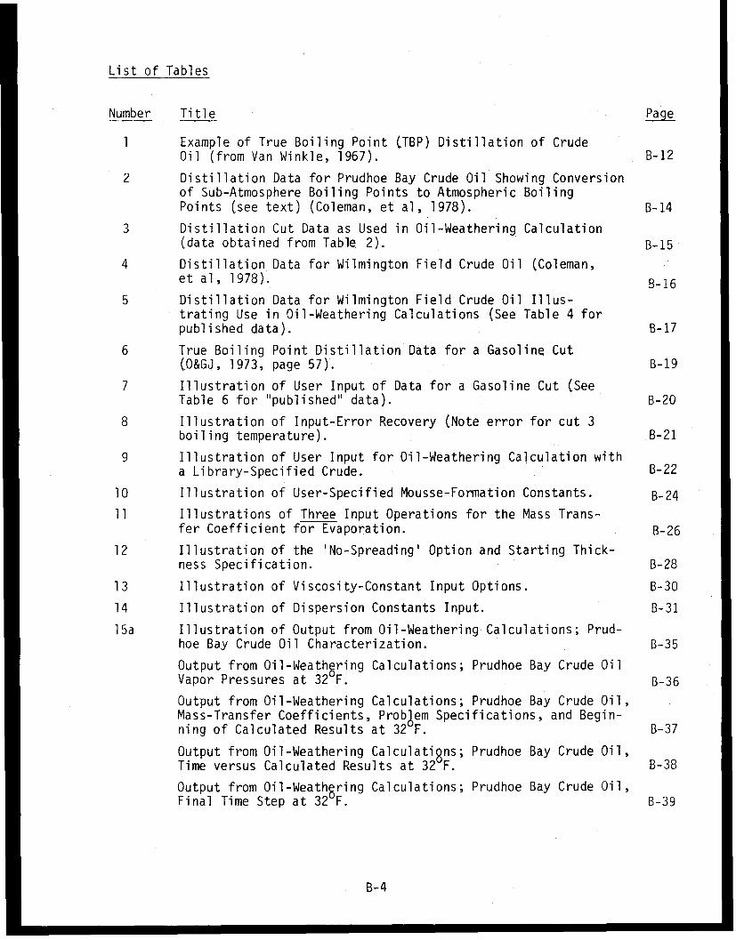
List of Tables
Number Title Page
1 Example of True Boiling Point (TBP) Distillation of CrudeOil (from Van Winkle, 1967). B-12
2 Distillation Data for Prudhoe Bay Crude Oil Showing Conversionof Sub-Atmosphere Boiling Points to Atmospheric BoilingPoints (see text) (Coleman, et al, 1978). B-14
3 Distillation Cut Data as Used in Oil-Weathering Calculation(data obtained from Table 2). B-15
4 Distillation Data for Wilmington Field Crude Oil (Coleman,et al, 1978). B-16
5 Distillation Data for Wilmington Field Crude Oil Illus-trating Use in Oil-Weathering Calculations (See Table 4 forpublished data). B-17
6 True Boiling Point Distillation Data for a Gasoline Cut(O&GJ, 1973, page 57). B-19
7 Illustration of User Input of Data for a Gasoline Cut (SeeTable 6 for "published" data). B-20
8 Illustration of Input-Error Recovery (Note error for cut 3boiling temperature). B-21
9 Illustration of User Input for Oil-Weathering Calculation witha Library-Specified Crude. B-22
10 Illustration of User-Specified Mousse-Formation Constants. B-24
11 Illustrations of Three Input Operations for the Mass Trans-fer Coefficient for Evaporation. B-26
12 Illustration of the 'No-Spreading' Option and Starting Thick-ness Specification. B-28
13 Illustration of Viscosity-Constant Input Options. B-30
14 Illustration of Dispersion Constants Input. B-31
15a Illustration of Output from Oil-Weathering Calculations; Prud-hoe Bay Crude Oil Characterization. B-35
Output from Oil-Weathering Calculations; Prudhoe Bay Crude OilVapor Pressures at 32 F. B-36
Output from Oil-Weathering Calculations; Prudhoe Bay Crude Oil,Mass-Transfer Coefficients, Problem Specifications, and Begin-ning of Calculated Results at 32 F. B-37
Output from Oil-Weathering Calculatigns; Prudhoe Bay Crude Oil,Time versus Calculated Results at 32 F. B-38
Output from Oil-Weathering Calculations; Prudhoe Bay Crude Oil,Final Time Step at 32 F. B-39
B-4
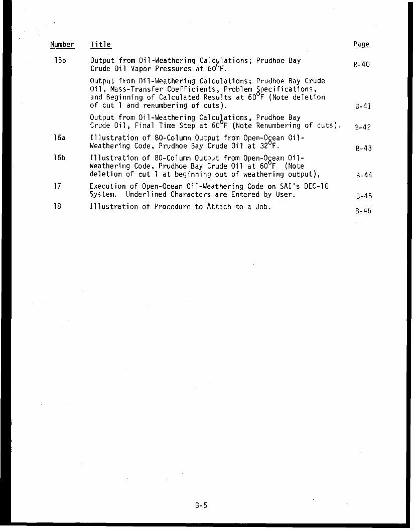
Number Title Page
15b Output from Oil-Weathering Calculations; Prudhoe Bay B-40Crude Oil Vapor Pressures at 60°F.
Output from Oil-Weathering Calculations; Prudhoe Bay CrudeOil, Mass-Transfer Coefficients, Problem Specifications,and Beginning of Calculated Results at 60 F (Note deletionof cut 1 and renumbering of cuts). B-41
Output from Oil-Weathering Calculations, Prudhoe BayCrude Oil, Final Time Step at 60 F (Note Renumbering of cuts). B-42
16a Illustration of 80-Column Output from Open-Ogean Oil-Weathering Code, Prudhoe Bay Crude Oil at 32 F. B-43
16b Illustration of 80-Column Output from Open-Ocean Oil-Weathering Code, Prudhoe Bay Crude Oil at 60 F (Notedeletion of cut 1 at beginning out of weathering output), B-44
17 Execution of Open-Ocean Oil-Weathering Code on SAI's DEC-10System. Underlined Characters are Entered by User. B-45
18 Illustration of Procedure to Attach to a Job. B-46
B-5
ABSTRACT
The Open-Ocean Oil-Weathering User's Manual is written to provide
specific instructions on the use the computer code CUTVP2.FOR.
This code calculates crude oil properties and the weathering of
oil for a set of environmental parameters. The use of the code
requires knowledge about the physical properties of crude oil and
the weathering of oil. In order to aid the user, the code has
been written to ask the user for specific input and provide
examples of input. The best way to learn to use the code is to
access the computer and work through some of the examples
presented in this manual.
B-6
OIL-WEATHERING COMPUTER PROGRAM
USER'S MANUAL
Model Overview
The open-ocean oil-weathering code is written in FORTRAN as a stand-
alone code that can be easily installed on any machine. All the trial-and-
error routines, integration routines, and other special routines are written
in the code so that nothing more than the normal system functions such as EXP
are required. The code is user-interactive and requests input by prompting
questions with suggested input. Therefore, the user can actually learn about
the nature of crude oil and its weathering by using this code.
The open-ocean oil-weathering model considers the following weather-
ing processes:
o evaporation
o dispersion (oil into water)
o mousse (water into oil)
o spreading
These processes are used to predict the mass balance and composition
of oil remaining in the slick as a function of time and environmental para-
meters. Dissolution of oil into the water column is not considered because
this weathering process is not significant with respect to the over-all
material balance of the oil slick.
An important assumption required in order to write material balance
equations for evaporation is the state of mixedness of the oil in the slick.
The open-ocean oil-weathering model is based on the assumption that the oil is
well mixed. This might not always be true but data have been taken and inter-
preted as if the oil is well mixed. Thus, experimental results based on this
B-7
assumption must be used in the same way mathematically. There is growing
thought based on physical observations (not compositional) that the oil is not
always well mixed. As the oil weathers its viscosity increases (measured and
known to be true) resulting in a slab-like oil phase. Clearly, the mass trans-
fer within the oil will change drastically in going from a well-mixed to a
slab-like phase.
The other three processes noted above are not explicitly component
specific as is evaporation. However, the dispersion process is a function of
the oil viscosity; oil viscosity is a function of composition. Thus the dis-
persion process does depend on the evaporation process. Mousse formation also
alters the oil viscosity but the present knowledge of this process does not
point to any quantifiable compositional dependence. The spreading of the
slick results in an ever-increasing area for mass transfer.
The composition of the oil is described in terms of pseudocomponents
that are obtained by fractionating the oil in a true-boiling-point distilla-
tion column. This procedure yields cuts of the oil which are characterized by
boiling point and density. This information is then used to calculate many
more parameters about the cut. The most important calculated parameters
pertain to vapor pressure and molecular weight. The evaporation process is
driven by vapor pressures, and system partial pressures are calculated
assuming Raoult's law.
Model Description
The pseudocomponents characterization of crude oil for the open-ocean
oil-weathering model is described in detail (Payne, Kirstein, et al., 1983).
The specific detail presented in the oil characterization can vary depending
upon exactly which literature references are used. Those references used to
write the current open-ocean oil-weathering model are all essentially
contained in a standard text (Hougen, Watson and Ragatz, 1965).
B-8
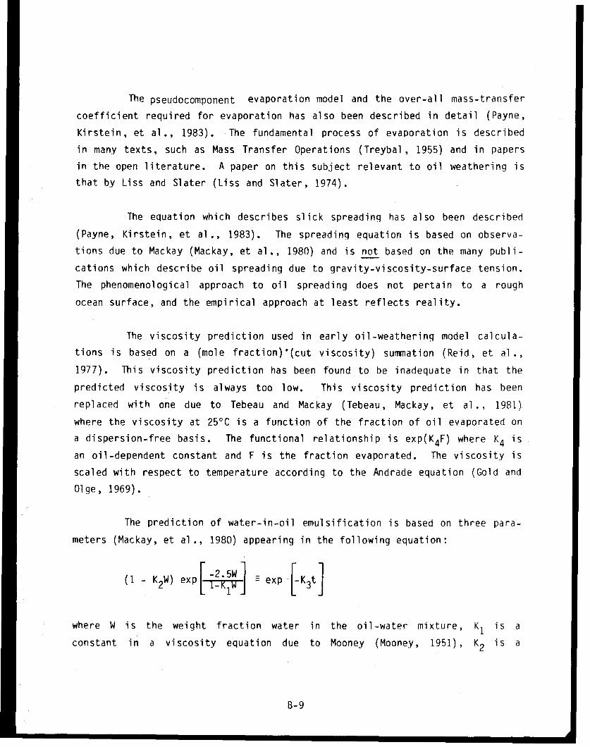
The pseudocomponent evaporation model and the over-all mass-transfer
coefficient required for evaporation has also been described in detail (Payne,
Kirstein, et al., 1983). The fundamental process of evaporation is described
in many texts, such as Mass Transfer Operations (Treybal, 1955) and in papers
in the open literature. A paper on this subject relevant to oil weathering is
that by Liss and Slater (Liss and Slater, 1974).
The equation which describes slick spreading has also been described
(Payne, Kirstein, et al., 1983). The spreading equation is based on observa-
tions due to Mackay (Mackay, et al., 1980) and is not based on the many publi-
cations which describe oil spreading due to gravity-viscosity-surface tension.
The phenomenological approach to oil spreading does not pertain to a rough
ocean surface, and the empirical approach at least reflects reality.
The viscosity prediction used in early oil-weathering model calcula-
tions is based on a (mole fraction)'(cut viscosity) summation (Reid, et al.,
1977). This viscosity prediction has been found to be inadequate in that the
predicted viscosity is always too low. This viscosity prediction has been
replaced with one due to Tebeau and Mackay (Tebeau, Mackay, et al., 1981)
where the viscosity at 25°C is a function of the fraction of oil evaporated on
a dispersion-free basis. The functional relationship is exp(K4 F) where K4 is
an oil-dependent constant and F is the fraction evaporated. The viscosity is
scaled with respect to temperature according to the Andrade equation (Gold and
Olge, 1969).
The prediction of water-in-oil emulsification is based on three para-
meters (Mackay, et al., 1980) appearing in the following equation:
(1 - K2W) exp K1 ] - exp K3t
where W is the weight fraction water in the oil-water mixture, K1 is a
constant in a viscosity equation due to Mooney (Mooney, 1951), K2 is a
B-9
coalescing-tendency constant, and K3 is a lumped water incorporation rate
constant. The viscosity equation due to Mooney is
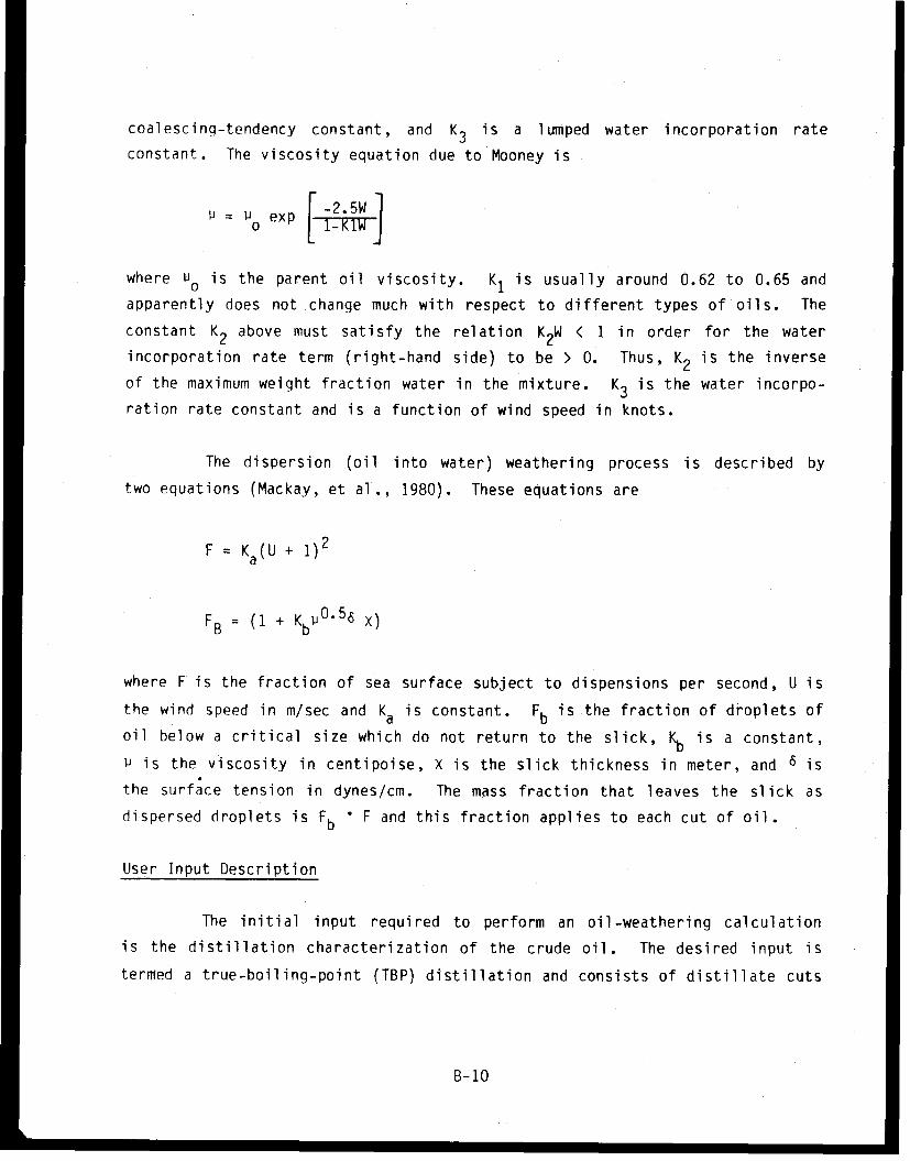
0 1-KIW: = O exp [-25W]
where uo is the parent oil viscosity. K1 is usually around 0.62 to 0.65 and
apparently does not change much with respect to different types of oils. The
constant K2 above must satisfy the relation K2W < 1 in order for the water
incorporation rate term (right-hand side) to be > 0. Thus, K2 is the inverse
of the maximum weight fraction water in the mixture. K3 is the water incorpo-
ration rate constant and is a function of wind speed in knots.
The dispersion (oil into water) weathering process is described by
two equations (Mackay, et al., 1980). These equations are
F = Ka(U + 1)2
FB = (1 + KbVO-56 x)
where F is the fraction of sea surface subject to dispensions per second, U is
the wind speed in m/sec and Ka is constant. Fb is the fraction of droplets of
oil below a critical size which do not return to the slick, Kb is a constant,
* is the viscosity in centipoise, x is the slick thickness in meter, and 6 is
the surface tension in dynes/cm. The mass fraction that leaves the slick as
dispersed droplets is Fb F and this fraction applies to each cut of oil.
User Input Description
The initial input required to perform an oil-weathering calculation
is the distillation characterization of the crude oil. The desired input is
termed a true-boiling-point (TBP) distillation and consists of distillate cuts
B-10
of the oil with each cut characterized by its average boiling point and API
gravity. For a description of the TBP distillation see Van Winkle (Van
Winkle, 1967). An example of a TBP distillation is shown in Table 1 for a
typical crude oil.
TBP distillations of crude oils are not always readily available.
The more common inspection on crude oil is termed an ASTM (D-86) distillation.
The ASTM distillation (Perry, R. H., and C. H. Chilton, 1973) differs in that
the ASTM distillation is essentially a flask distillation and thus has no more
than a few theoretical plates. The TBP distillation (ASTM D-2982, 1977) is
performed in a column with greater than 15 theoretical plates and at high
reflux ratios. The high degree of fractionation in this distillation yields
an accurate component distribution for the crude oil (mixture). Another type
of crude oil inspection available is the equilibrium flash vaporation (EFV)
which differs from both the ASTM and TBP distillation in that the vapor is
allowed to equilibrate with the liquid, and the quantity vaporized reported.
In the distillations vapor is continuously removed from the still pot.
Both the ASTM distillation and EFV can be converted to a TBP distilla-
tion (API, 1964). However, at the present the ASTM D-86 distillation results
can be used directly in the oil-weathering calculations because it is a reason-
able approximation to the TBP-distillation result at the light end of the
barrel. The differences between the two distillations at the heavy end of the
barrel are noticeable but since the heavy ends of the barrel do not evaporate
in oil weathering, this difference is of little consequence.
Currently the best sources of distillation data are "Evaluation of
World's Important Crudes" (O&GJ, 1973) where a tremendous number of distilla-
tions and other characterizations are reported. The distillations reported
are a mix of ASTMs and TBPs. Another excellent source of distillation data is
"Analyses of 800 Crude Oils from United States Oilfields" (Coleman, et al.,
1978). The distillations reported by Coleman are not TBP distillations but
are essentially ASTM distillations and can be used in the oil-weathering
B-11
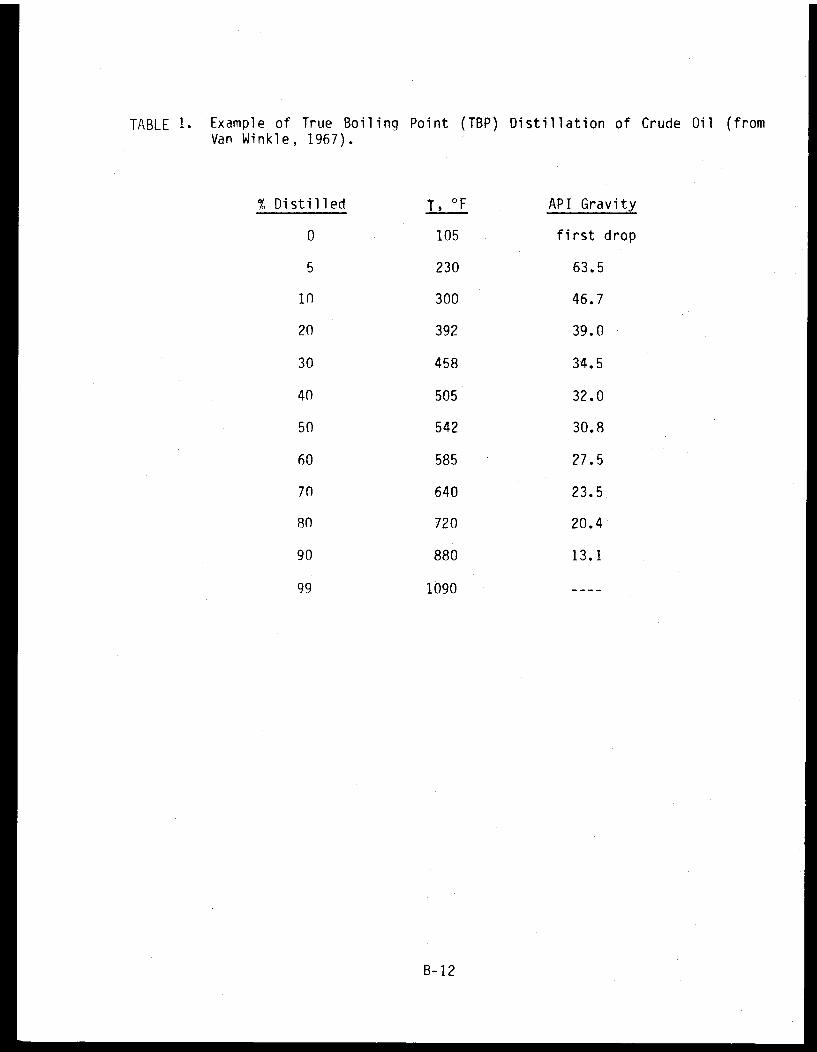
TABLE 1. Example of True Boiling Point (TBP) Distillation of Crude Oil (fromVan Winkle, 1967).
% Distilled T, OF API Gravity
0 105 first drop
5 230 63.5
10 300 46.7
20 392 39.0
30 458 34.5
40 505 32.0
50 542 30.8
60 585 27.5
70 640 23.5
80 720 20.4
90 880 13.1
99 1090 -
B-12
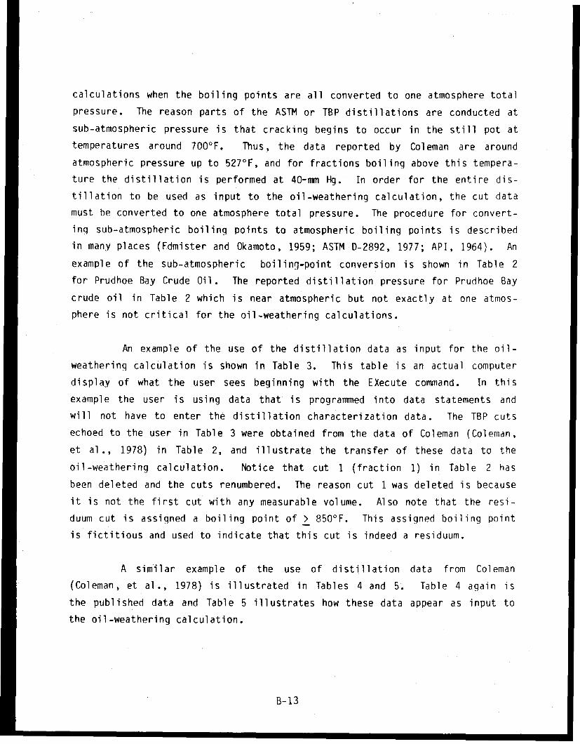
calculations when the boiling points are all converted to one atmosphere total
pressure. The reason parts of the ASTM or TBP distillations are conducted at
sub-atmospheric pressure is that cracking begins to occur in the still pot at
temperatures around 700°F. Thus, the data reported by Coleman are around
atmospheric pressure up to 527°F, and for fractions boiling above this tempera-
ture the distillation is performed at 40-mm Hg. In order for the entire dis-
tillation to be used as input to the oil-weathering calculation, the cut data
must be converted to one atmosphere total pressure. The procedure for convert-
ing sub-atmospheric boiling points to atmospheric boiling points is described
in many places (Fdmister and Okamoto, 1959; ASTM D-2892, 1977; API, 1964). An
example of the sub-atmospheric boiling-point conversion is shown in Table 2
for Prudhoe Bay Crude Oil. The reported distillation pressure for Prudhoe Bay
crude oil in Table 2 which is near atmospheric but not exactly at one atmos-
phere is not critical for the oil-weathering calculations.
An example of the use of the distillation data as input for the oil-
weathering calculation is shown in Table 3. This table is an actual computer
display of what the user sees beginning with the EXecute command. In this
example the user is using data that is programmed into data statements and
will not have to enter the distillation characterization data. The TBP cuts
echoed to the user in Table 3 were obtained from the data of Coleman (Coleman,
et al., 1978) in Table 2, and illustrate the transfer of these data to the
oil-weathering calculation. Notice that cut 1 (fraction 1) in Table 2 has
been deleted and the cuts renumbered. The reason cut 1 was deleted is because
it is not the first cut with any measurable volume. Also note that the resi-
duum cut is assigned a boiling point of > 850°F. This assigned boiling point
is fictitious and used to indicate that this cut is indeed a residuum.
A similar example of the use of distillation data from Coleman
(Coleman, et al., 1978) is illustrated in Tables 4 and 5. Table 4 again is
the published data and Table 5 illustrates how these data appear as input to
the oil-weathering calculation.
B-13
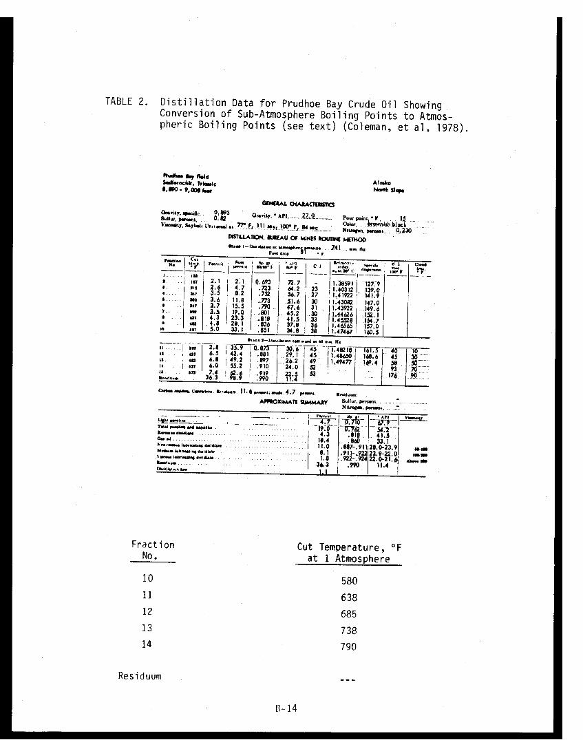
TABLE 2. Distillation Data for Prudhoe Bay Crude Oil ShowingConversion of Sub-Atmosphere Boiling Points to Atmos-pheric Boiling Points (see text) (Coleman, et al, 1978).
Fraction Cut Temperature, °FNo. at 1 Atmosphere
10 58011 63812 68513 73814 790
Residuum ---
B-14
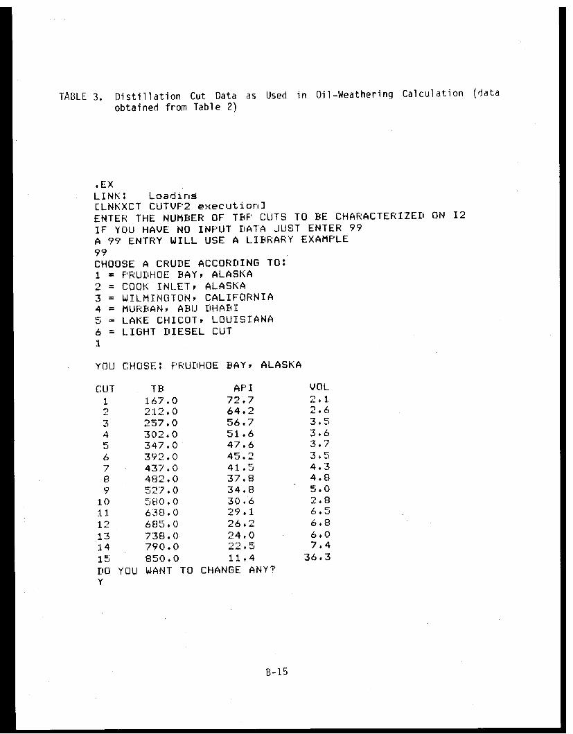
TABLE 3. Distillation Cut Data as Used in Oil-Weathering Calculation (data
obtained from Table 2)
.EXLINK: LoadiNGCLNKXCT CUTVF'2 executioinENTER THE NUMBER OF TBP CUTS TO BE CHARACTERIZED ON I2
IF YOU HAVE NO INFUT DATA JUST ENTER 99A 99 ENTRY WILL USE A LIBRARY EXAMPLE99CHOOSE A CRUDE ACCORDING TO:1 PRUDHOE BAY, ALASKA2 = COOK INLET, ALASKA3 = WILMINGTON, CALIFORNIA4 = MURBAN, ABU DHABI5 = LAKE CHICOT, LOUISIANA6 = LIGHT DIESEL CUT1
YOU CHOSE: PRUDHOE BAY, ALASKA
CUT TB API VOL
1 167.0 72.7 2.12 212.0 64.2 2.63 257.0 56,7 3.54 302.0 51.6 3.65 347.0 47.6 3.76 392.0 45.2 3.57 437.0 41.5 4.38 482.0 37.8 4.89 527.0 34.8 5.0
10 580.0 30.6 2.811 638.0 29.1 6.5
12 685,0 26.2 6.813 738.0 24.0 6.014 790,0 22.5 7.415 850.0 11.4 36.3DO YOU WANT TO CHANGE ANY?Y
B-15
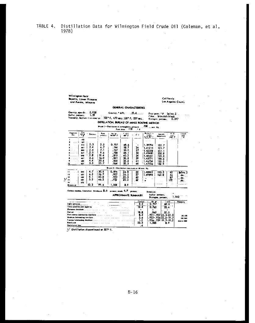
TABLE 4. Distillation Data for Wilmington Field Crude Oil (Coleman, et al,1978)
B-16
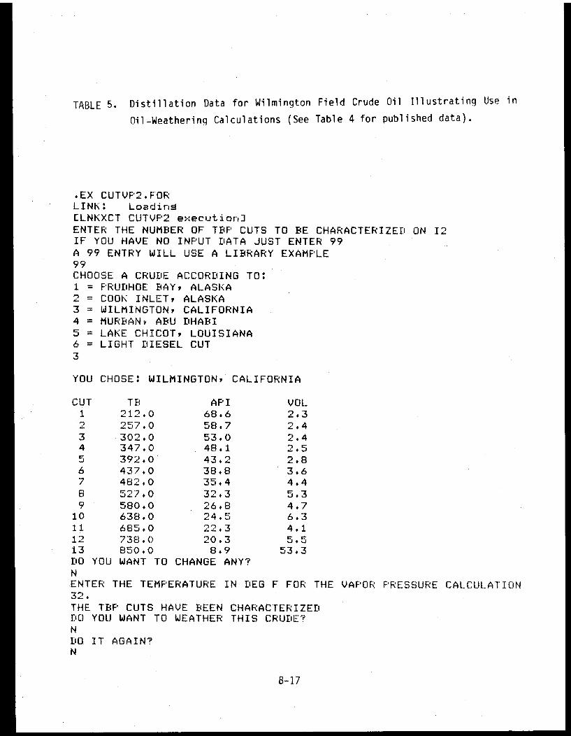
TABLE 5. Distillation Data for Wilmington Field Crude Oil Illustrating Use in
Oil-Weathering Calculations (See Table 4 for published data).
B-17
The distillation cut data can be entered by the user. An example of
this entering procedure is illustrated using the TBP data for a gasoline cut
(O&GJ, 1973, page 57) which is presented in Table 6. The user's entries to
the oil-weathering calculation is shown in Table 7. Each time an input is
required the user is prompted with an appropriate question. Since it is impos-
sible to enter many numbers into the oil-weathering calculation without an
error, the distillation cut data are always echoed to the user for review. In
the event an input error is discovered or it is desired to change an entry,
the user's response to DO YOU WANT TO CHANGE ANY? is yes. The error recovery
is illustrated in Table 8 where the gasoline-cut data from Table 6 is entered.
Note the input error for TB (boiling temperature) for cut 3 where 22.8 was
entered instead of 228. The user is prompted for the error-recovery
information and the final data is echoed to the user. In the event another
error is to be corrected, a "YES" would be entered in response to the very
last question in Table 8.
After entering the distillation-cut data, the user is asked for a
temperature in degrees Fahrenheit. This temperature is used to calculate the
vapor pressure of each cut as previously described (J. R. Payne, B. E.
Kirstein, et al., 1983). At this point the calculation can be stopped and the
crude oil characterization is all that will have been calculated. However, in
order to "weather the crude", the user types "YES" in response to DO YOU WANT
TO WEATHFR THIS CRUDE?
The user input required for an oil-weathering calculation begins with
a YES in response to the question DO YOU WANT TO WEATHER THIS CRUDE? The user
is then prompted for the spill size in barrels and the number of hours for oil
weathering to occur. The input responses presented in Table 9 follow the
specification of a library crude (i.e., programmed into the code) such as
those illustrated in Tables 3 or 5.
After specifying the spill size and number of hours for weathering to
occur, and a library crude has been specified, the user is prompted for
mousse-formation constants and an oil-water surface tension. By responding NO
B-18
TABLE 6. True Boiling Point Distillation Data for a Gasoline Cut (O&GJ, 1973,page 57).
Cut Cut temp, °F Vol % API Gravity
1 137 1.5 71.6
2 196 2.1 59.7
3 228 2.0 55.0
4 256 2.0 53.8
5 283 2.0 49.6
B-19
TABLE 7. Illustration of User Input of Data for a Gasoline Cut (See Table 6for "published" data).
B-20
TABLE 8. Illustration of Input-Error Recovery (Note error for cut 3 boilingtemperature).
B-21
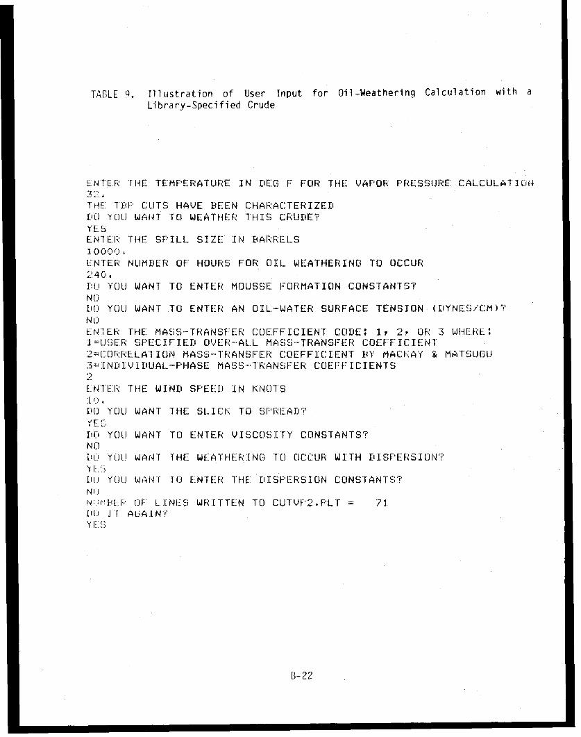
TABLE 9. Illustration of User Input for Oil-Weathering Calculation with aLibrary-Specified Crude
ENTER THE TE:MF:E:RATURE IN DEG F FCOR THE VAPOR F:fRESSURE CALCULATION32?ITIHE1 T'BP CUTS HAVE DEEN CHARACTERIZEDl DO YOU WANT TO WEATHER THIS CRUDE?
YE. SENIER:I THIE SPILL SIZE IN DARRELS1 000':)I.ENTER NUMBER OF' HOURS F'OR OIL WEATHERING TO OCCUR
'I: ( YOU WANT TO ENTER MOUSSE FORMATION CONSTANTS?NOD IL YOU WANT TO ENTER AN OIL-WATER SURFACE TENSION (DYNES/CM)'?'NoEt'TER 'THE MASS-TRANSf:ER CO)EF'FICIENT CODE: 1, 2, OR 3 WIER:F.1 -USl:ER SPE:'I-CIFIED OVER-AL.L MASS-TRANSFER COEFF IC I ENT2 COR FREL..ATI ION MASS-'TRANSFER COEFFIC I ENT BY MACKAY & MATSU.U:=.[ INDIVI DUAL-PHASE MASS TRAN SFER COEFI::'ICIENTS
ENTER:l: THE WIND SPEEI: IN KNOTS
:DO) YOU WANT 'THE SL.ICK TO SPFIREAD'?Y E,DO:: YOU WANT TO ENTER VISCOSITY CONSTANTS?N O111 YOU WANT THE W::ATHER ING TO OCCUR WITH R IS :'PERSION'?1::.'l i: YOJ WANT 'TO EN'TER THE DISPERSION CONSTANTS'
ir.lBP OF1: LINES. WRITTEN TO CUTVP2.PLT - 71L. I. T A i AiN'
Y -::
B-22
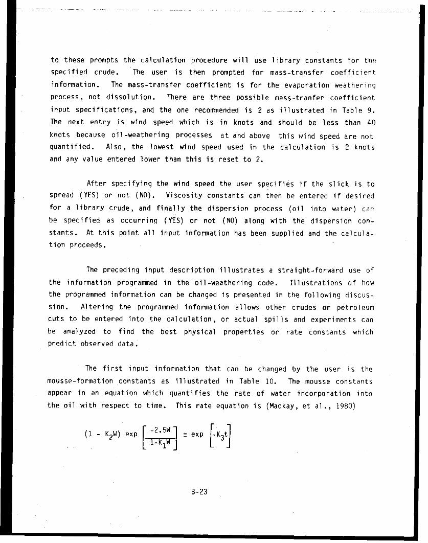
to these prompts the calculation procedure will use library constants for the
specified crude. The user is then prompted for mass-transfer coefficient
information. The mass-transfer coefficient is for the evaporation weathering
process, not dissolution. There are three possible mass-tranfer coefficient
input specifications, and the one recommended is 2 as illustrated in Table 9.
The next entry is wind speed which is in knots and should be less than 40
knots because oil-weathering processes at and above this wind speed are not
quantified. Also, the lowest wind speed used in the calculation is 2 knots
and any value entered lower than this is reset to 2.
After specifying the wind speed the user specifies if the slick is to
spread (YES) or not (NO). Viscosity constants can then be entered if desired
for a library crude, and finally the dispersion process (oil into water) can
be specified as occurring (YES) or not (NO) along with the dispersion con-
stants. At this point all input information has been supplied and the calcula-
tion proceeds.
The preceding input description illustrates a straight-forward use of
the information programmed in the oil-weathering code. Illustrations of how
the programmed information can be changed is presented in the following discus-
sion. Altering the programmed information allows other crudes or petroleum
cuts to be entered into the calculation, or actual spills and experiments can
be analyzed to find the best physical properties or rate constants which
predict observed data.
The first input information that can be changed by the user is the
mousse-formation constants as illustrated in Table 10. The mousse constants
appear in an equation which quantifies the rate of water incorporation into
the oil with respect to time. This rate equation is (Mackay, et al., 1980)
(1 - K2W) exp F exp -K3t1-B-23
B-23
TABLE 10. Illustration of User-Specified Mousse-Formation Constants
:DO YOU WANT TO ENTER MOUSSE FORMATION CONSTANTS?YES'1. ENTER THE MAXIMUM WEIGHT FRACTION WATER IN OIL.602. ENTER THE MOUSSE-VISCOSITY CONSTANT, TRY 0.65.65
3. ENTER THE WATER XNCORPORATION RATE CONSTANT, TRY 0.001.001I:)0 YOU WANT TO ENTER AN OIL-WATER SURFACE TENSION (DYNES/CM)?YES.00130.
B-24
where W is the weight fraction water in mousse. K[subscript]1 is a constant in the
viscosity equation, K[subscript]2 is a coalescing-tendency constant and K[subscript]3 is a lumped
water incorporation rate constant. K[subscript]1 appears in a stand-alone equation for
the apparent viscosity of the emulsion as (Mooney, 1951)
where µ[subscript]0 is the parent oil viscosity. K[subscript]1 is usually around 0.62 to 0.65 and
apparently does not change much with respect to different types of oils.
The constant K[subscript]2 must satisfy the relation K[subscript]2W < 1 in order for the
water incorporation rate to be > 0. Thus, K[subscript]2 is the inverse of the maximum
weight fraction water in mousse. K[subscript]3 is the water incorporation rate constant
and is a function of wind speed in knots. Currently the oil-weathering code
calculates K[subscript]3 from
and the constant actually entered by the user is the 0.001 constant above.
Thus, referring to Table 10, the first mousse formation constant
entered is the maximum weight fraction water in the mousse. The reciprocal of
this number is used for K[subscript]1. The second constant entered is the viscosity
constant in Mooney's equation and this number should be 0.62 to 0.65 unless
experimental evidence suggests otherwise. The third constant entered is the
multiplier of the (wind speed)² which then yields K[subscript]3. This number is around
0.001 as indicated. Note that the prompting for input also prints suggested
values for each constant.
The next input parameter that the user can change is the mass-
transfer coefficient for evaporation. The input illustration in Table 9 uses
the correlation mass transfer coefficient as developed by Mackay and Matsugu
(Mackay and Matsugu, 1973). Table 11 illustrates the three possible input
B-25
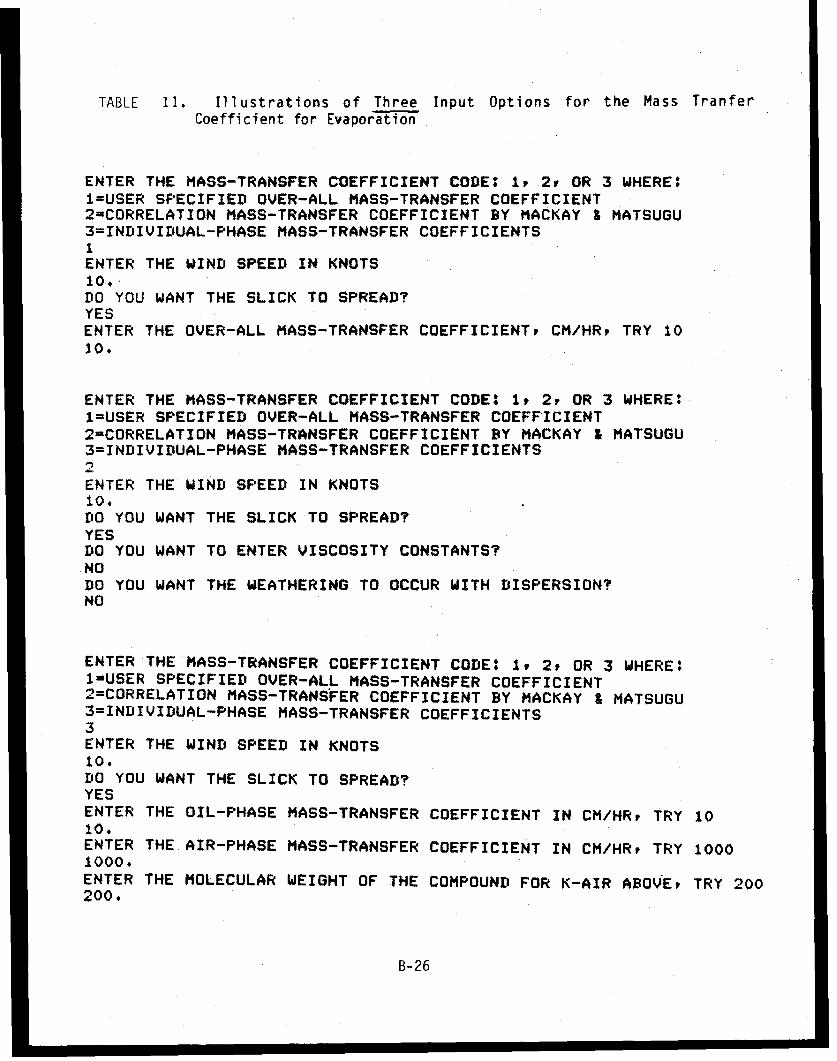
TABLE 11. Illustrations of Three Input Options for the Mass TranferCoefficient for Evaporation
ENTER THE MASS-TRANSFER COEFFICIENT CODE: 1l 2, OR 3 WHERE:1=USER SPECIFIED OVER-ALL MASS-TRANSFER COEFFICIENT2=CORRELATION MASS-TRANSFER COEFFICIENT BY MACKAY i MATSUGU3=INDIVIDUAL-PHASE MASS-TRANSFER COEFFICIENTS1ENTER THE WIND SPEED IN KNOTS10,DO YOU WANT THE SLICK TO SPREAD?YESENTER THE OVER-ALL MASS-TRANSFER COEFFICIENT, CM/HR, TRY 1010.
ENTER THE MASS-TRANSFER COEFFICIENT CODE: 1 2r OR 3 WHERE:1=USER SPECIFIED OVER-ALL MASS-TRANSFER COEFFICIENT2-CORRELATION MASS-TRANSFER COEFFICIENT BY MACKAY i MATSUGU3=INDIVIDUAL-PHASE MASS-TRANSFER COEFFICIENTS
ENTER THE WIND SPEED IN KNOTS10.DO YOU WANT THE SLICK TO SPREAD?YESDO YOU WANT TO ENTER VISCOSITY CONSTANTS?NODO YOU WANT THE WEATHERING TO OCCUR WITH DISPERSION?NO
ENTER THE MASS-TRANSFER COEFFICIENT CODE: 1, 2, OR 3 WHERE:1=USER SPECIFIED OVER-ALL MASS-TRANSFER COEFFICIENT2=CORRELATION MASS-TRANSFER COEFFICIENT BY MACKAY & MATSUGU3=INDIVIDUAL-PHASE MASS-TRANSFER COEFFICIENTS3ENTER THE WIND SPEED IN KNOTS10.DO YOU WANT THE SLICK TO SPREAD?YESENTER THE OIL-PHASE MASS-TRANSFER COEFFICIENT IN CM/HR, TRY 1010.ENTER THE AIR-PHASE MASS-TRANSFER COEFFICIENT IN CM/HR, TRY 10001000.ENTER THE MOLECULAR WEIGHT OF THE COMPOUND FOR K-AIR ABOVE, TRY 200200.
B-26
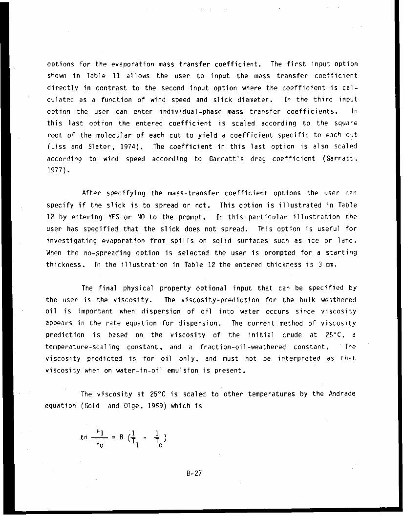
options for the evaporation mass transfer coefficient. The first input option
shown in Table 11 allows the user to input the mass transfer coefficient
directly in contrast to the second input option where the coefficient is cal-
culated as a function of wind speed and slick diameter. In the third input
option the user can enter individual-phase mass transfer coefficients. In
this last option the entered coefficient is scaled according to the square
root of the molecular of each cut to yield a coefficient specific to each cut
(Liss and Slater, 1974). The coefficient in this last option is also scaled
according to wind speed according to Garratt's drag coefficient (Garratt,
1977).
After specifying the mass-transfer coefficient options the user can
specify if the slick is to spread or not. This option is illustrated in Table
12 by entering YES or NO to the prompt. In this particular illustration the
user has specified that the slick does not spread. This option is useful for
investigating evaporation from spills on solid surfaces such as ice or land.
When the no-spreading option is selected the user is prompted for a starting
thickness. In the illustration in Table 12 the entered thickness is 3 cm.
The final physical property optional input that can be specified by
the user is the viscosity. The viscosity-prediction for the bulk weathered
oil is important when dispersion of oil into water occurs since viscosity
appears in the rate equation for dispersion. The current method of viscosity
prediction is based on the viscosity of the initial crude at 25°C, a
temperature-scaling constant, and a fraction-oil-weathered constant. The
viscosity predicted is for oil only, and must not be interpreted as that
viscosity when on water-in-oil emulsion is present.
The viscosity at 25°C is scaled to other temperatures by the Andrade
equation (Gold and Olge, 1969) which is
l B1 1n B (T1 - )
B-27
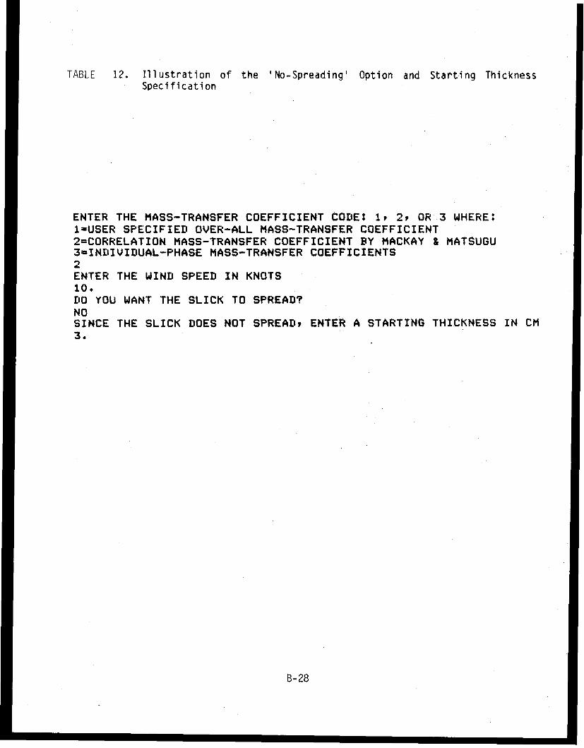
TABLE 12. Illustration of the 'No-Spreading' Option and Starting ThicknessSpecification
ENTER THE MASS-TRANSFER COEFFICIENT CODE: 1, 2, OR 3 WHERE:1=USER SPECIFIED OVER-ALL MASS-TRANSFER COEFFICIENT2=CORRELATION MASS-TRANSFER COEFFICIENT BY MACKAY & MATSUGU3=INDIVIDUAL-PHASE MASS-TRANSFER COEFFICIENTS2ENTER THE WIND SPEED IN KNOTS10.DO YOU WANT THE SLICK TO SPREAD?NOSINCE THE SLICK DOES NOT SPREADY ENTER A STARTING THICKNESS IN CM3.
B-28
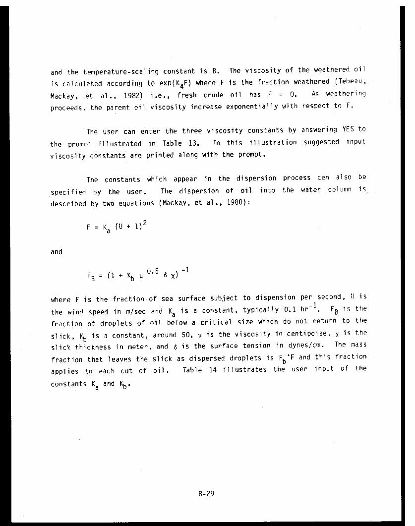
and the temperature-scaling constant is B. The viscosity of the weathered oil
is calculated according to exp(K[subscript]4 F) where F is the fraction weathered (Tebeau,
Mackay, et al., 1982) i.e., fresh crude oil has F = 0. As weathering
proceeds, the parent oil viscosity increase exponentially with respect to F.
The user can enter the three viscosity constants by answering YES to
the prompt illustrated in Table 13. In this illustration suggested input
viscosity constants are printed along with the prompt.
The constants which appear in the dispersion process can also be
specified by the user. The dispersion of oil into the water column is
described by two equations (Mackay, et al., 1980):
where F is the fraction of sea surface subject to dispension per second, U is
the wind speed in m/sec and K[subscript]a is a constant, typically 0.1 hr-¹. F[subscript]B is the
fraction of droplets of oil below a critical size which do not return to the
slick, K[subscript]b is a constant, around 50, µ is the viscosity in centipoise, [chi] is the
slick thickness in meter, and [delta] is the surface tension in dynes/cm. The mass
fraction that leaves the slick as dispersed droplets is F[subscript]b·F and this fraction
applies to each cut of oil. Table 14 illustrates the user input of the
constants K[subscript]a and K[subscript]b.
B-29
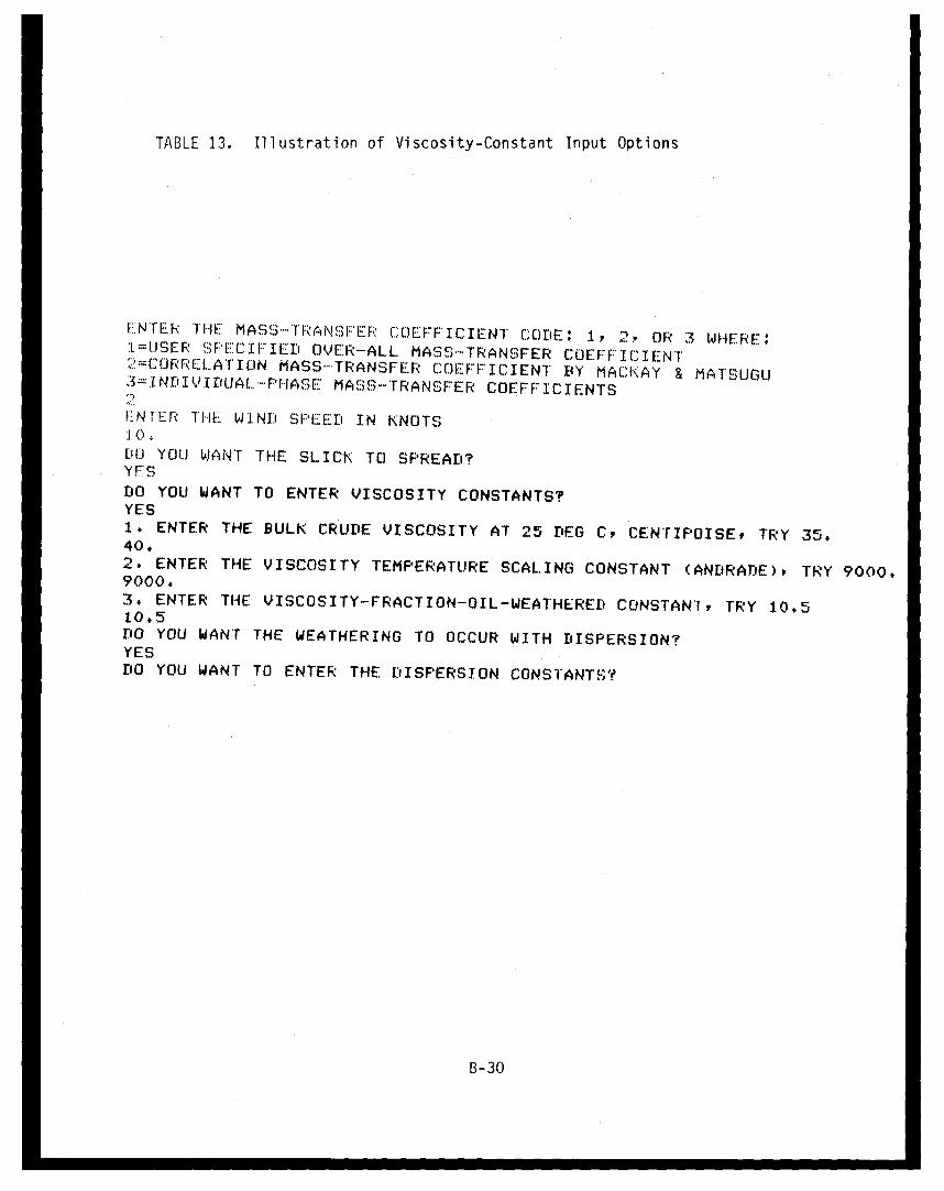
TABLE 13. Illustration of Viscosity-Constant Input Options
ENTER ITHE MASS 'FTR'ANSF:'ER COEFF:'ICI.ENT CODEE: 1, 2, OR 3 WHERE::L =SER SPF:CI I:IED OVE:R-ALL MASS-TRANSFER COEliFF:F'IIE N NT1':.C1:RRL...ATICN MASS- TRANSFE:R CC)EFFICIENT BY MACKAY & MATSUJGl.3=INDIVIDUIAL-F -LPHASE MASS-TRANSFER COEFFICIENTS
IN'TER THE WIND SI'liEDl IN KNOTSJ. 0)DLl YOU WANT THE SLICK TO SPREAD?YE:SDO YOU WANT TO ENTER VISCOSITY CONSTANTS?YES1. ENTER THE BULK CRUDE VISCOSITY AT 25 DEG C, CENrTIFOISE, TRY 35.40.2. ENTER THE VISCOSITY TEMPERATURE SCALING CONSTANT (ANDRAT.iE), TRY 9000.9000.3. ENTER THE VISCOSITY-FRACTION-OIL-WEATHERED CONSTANT, TRY 10.510.5DO YOU WANT THE WEATHERING TO OCCUR WITH DISPERSION?YESDO YOU WANT TO ENTER THE DISPERSION CONSTANTXS
B-30
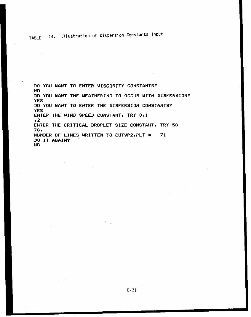
TABLE 14. Illustration of Dispersion Constants Input
DO YOU WANT TO ENTER VISCOSITY CONSTANTS?NODO YOU WANT THE WEATHERING TO OCCUR WITH DISPERSION?YESDO YOU WANT TO ENTER THE DISPERSION CONSTANTS?YESENTER THE WIND SPEED CONSTANT, TRY 0.1.2ENTER THE CRITICAL DROPLET SIZE CONSTANT, TRY 5070.NUMBER OF LINES WRITTEN TO CUTVP2.PLT = 71DO IT AGAIN?NO
B-31
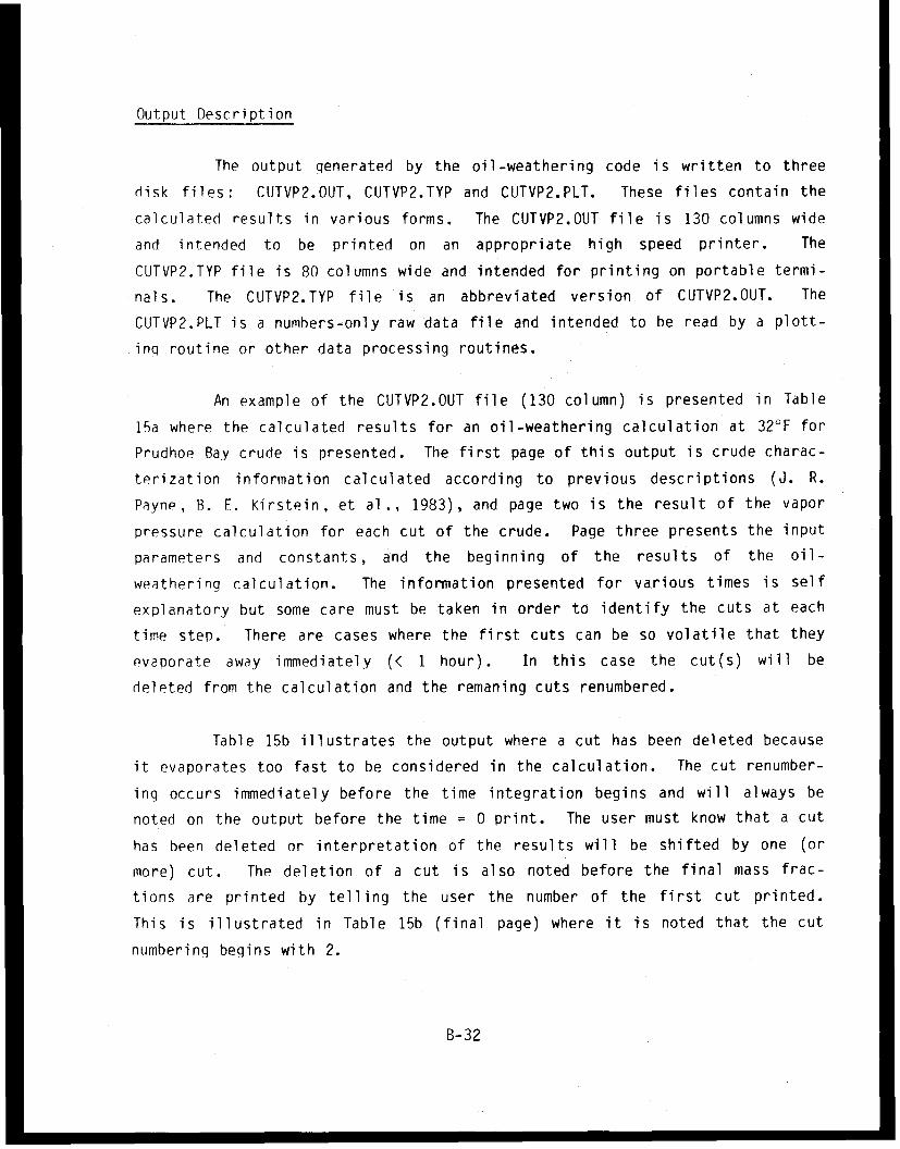
Output Description
The output qenerated by the oil-weathering code is written to three
disk files: CUTVP2.0UT, CUTVP2.TYP and CUTVP2.PLT. These files contain the
calculated results in various forms. The CUTVP2.0UT file is 130 columns wide
and intended to be printed on an appropriate high speed printer. The
CUTVP2.TYP file is 80 columns wide and intended for printing on portable termi-
nals. The CUTVP2.TYP file is an abbreviated version of CUTVP2.0UT. The
CUTVP2.PLT is a numbers-only raw data file and intended to be read by a plott-
inq routine or other data processing routines.
An example of the CUTVP2.0UT file (130 column) is presented in Table
15a where the calculated results for an oil-weathering calculation at 32°F for
Prudhoe Bay crude is presented. The first page of this output is crude charac-
terization information calculated according to previous descriptions (J. R.
Payne, B. F. Kirstein, et al., 1983), and page two is the result of the vapor
pressure calculation for each cut of the crude. Page three presents the input
parameters and constants, and the beginning of the results of the oil-
weathering calculation. The information presented for various times is self
explanatory but some care must be taken in order to identify the cuts at each
time step. There are cases where the first cuts can be so volatile that they
evaporate away immediately (< 1 hour). In this case the cut(s) will be
deleted from the calculation and the remaning cuts renumbered.
Table 15b illustrates the output where a cut has been deleted because
it evaporates too fast to be considered in the calculation. The cut renumber-
ing occurs immediately before the time integration begins and will always be
noted on the output before the time = 0 print. The user must know that a cut
has been deleted or interpretation of the results will be shifted by one (or
more) cut. The deletion of a cut is also noted before the final mass frac-
tions are printed by telling the user the number of the first cut printed.
This is illustrated in Table 15b (final page) where it is noted that the cut
numbering begins with 2.
B-32
Examples of the 80-column output is presented in Tables 16d and 16b
for weathering Prudhoe Bay crude oil at 32 and 60°F. The output in Tables 16a
and 16b was generated at the same time as the output in Tables 15a and 15b.
Note that the output in Tables 16a and 16b is essentially a condensed, self-
contained, version of the calculated results.
Most of the output information is self explanatory as illustrated in
Tables 15a and 15b. These two tables are examples of calculated results at
two different temperatures for Prudhoe Bay crude oil. Currently some of the
information printed is not used. Refer to Table 15a (page 3) which begins at
the top of the page with: OVER-ALL MASS-TRANSFER COEFFICIENTS BY INPUT CODE
2. On this page of the output the two lines beginning with KINEMATIC
VISCOSITY present information that is not used. This viscosity information
was used early in program development and found not to be applicable for
predicting the viscosity of weathered crude. The viscosity of weathered crude
is now calculated according to the fraction weathered, as previously described
in the input description and noted here by the parameters printed immediately
below the kinematic viscosity information.
Accessing the Computer
Currently the oil-weathering code resides on a DEC System-10Y at
Science Applications, Inc. in La Jolla, California. Table 17 presents a des-
cription of the commands to execute the code that pertain to this specific
installation. Accessing the DEC-10 from anywhere in the United States can be
accomplished through TELENET. The TELENET access procedure is described in
Appendix A. Once access to DEC-10 has been obtained the system will then ask
for a project-programmer number (PPN) which in the example in Table 17 is
4601,4601. The password must then be typed in. The typed password will not
show up at the terminal. The current password must be obtained by calling
SAI. Once logged in the code can be executed by typing EX CUTVP2.FOR. The
code will then execute and the user will be prompted for input. After an
oil-weathering calculation is finished the FORTRAN code will ask the user: DO
B-33
IT AGAIN? By replying NO a normal exit and file closing will be accomplished.The system will then print CPU time and elapsed time. In order to obtain the
calculated results the user must instruct the system to print or type the
results from the appropriate disk files. To obtain 130-column detailed outputthe user types PRINT CUTVP2.0UT. The output will be printed at SAI's La Jolla
facility and it must then be picked up by the user. By typing TYPE CUTVP2.TYP
the user will obtain the 80-column abbreviated output file at his terminal.
To log off the computer type BYE.
There will be times when the connection to the DEC-10 will be lost
during execution or while the user is doing something else. When this happens
the job becomes detached but can be picked up again by the user. When com-
puter access is obtained the user must login using the same PPN and PASSWORD.
The system will then type to the user the detached job number, program name,
and status. The user will then be asked if he wants to attach. The attach
procedure is illustrated in Table 18.
A listing of the open-ocean oil-weathering code is presented in
Appendix B.
B-34
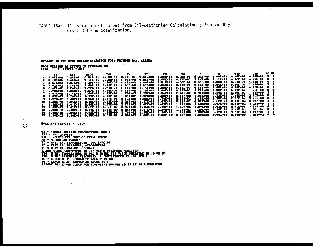
TABLE 15a: Illustration of Output from Oil-Weathering Calculations; Prudhoe Bay
Crude Oil Characterization.
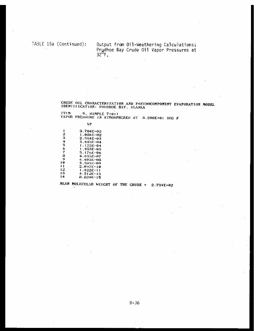
TABLE 15a (Continued): Output from Oil-Weathering Calculations;Prudhoe Bay Crude Oil Vapor Pressures at32°F.
B-36
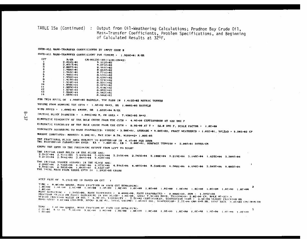
TABLE 15a (Continued) : Output from Oil-Weathering Calculations; Prudhoe Bay Crude Oil,Mass-Transfer Coefficients, Problem Specifications, and Beginningof Calculated Results at 32°F.
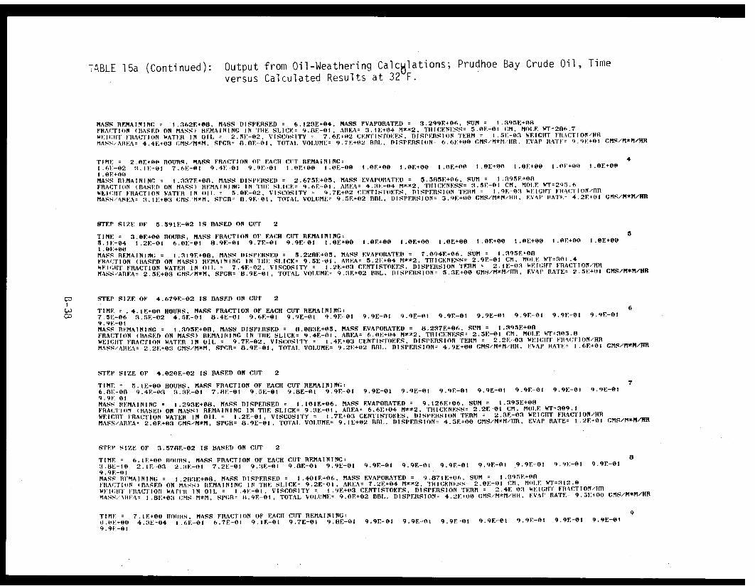
TABLE 15a (Continued): Output from Oil-Weathering Calculations; Prudhoe Bay Crude Oil, Time
versus Calculated Results at 32°F.
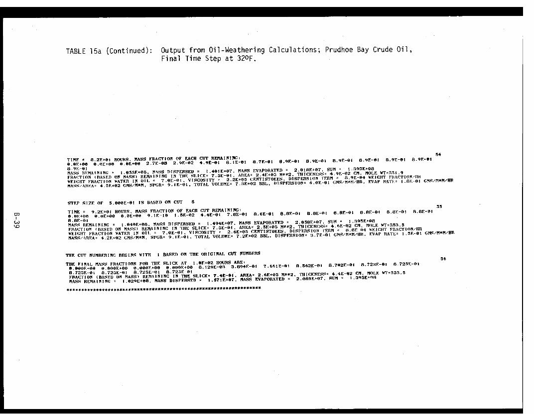
TABLE 15a (Continued): Output from Oil-Weathering Calculations; Prudhoe Bay Crude Oil,Final Time Step at 32°F.
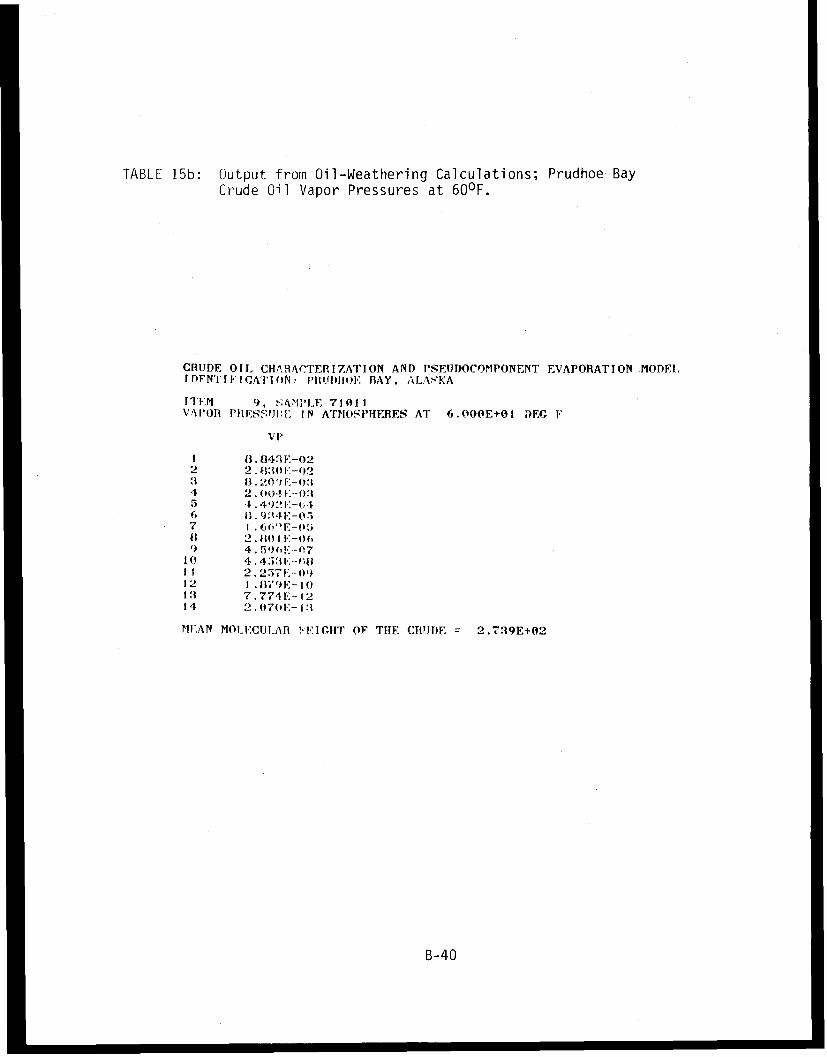
TABLE 15b: Output from Oil-Weathering Calculations; Prudhoe BayCrude Oil Vapor Pressures at 60°F.
CRUDE OIL CHARACTERIZATION AND PSEUDOCOMPONENT EVAPORATION MODELI FNT I FICATI ON: PlUIDIIOE BAY, ALASKA
ITEM 9, :;AMI'IF. 71011VAI'Pon PIIESpSJI:E 1N ATMOSPHIERES AT 6.000E+01 DEG F
VI'
HI 1. 843F.-022 2.83 f 0 -023 84.20'9I;:-074 2. ( 0 t4:--03;5 4.492* :-t.46 8. 9q4E-057 I . 66"E-05I1 2. 80 I E-o69 4. 59 1,!.--}7
10 4.4:;'WE--;I 2.2571:--0912 1 .871gE-IO1I1 7.774E1-1214 2.07(1I- 1:1
ME AN MOLECUI.An ,'EIGIT OF THE CRUDE = 2.739E+02
B-40
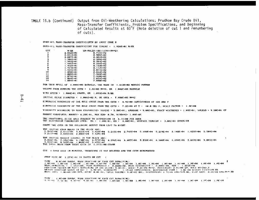
TABLE 15.b (Continued) Output from Oil-Weathering Calculations; Prudhoe Bay Crude Oil,Mass-Transfer Coefficients, Problem Specifications, and Beginningof Calculated Results at 60°F (Note deletion of cut 1 and renumberingof cuts).
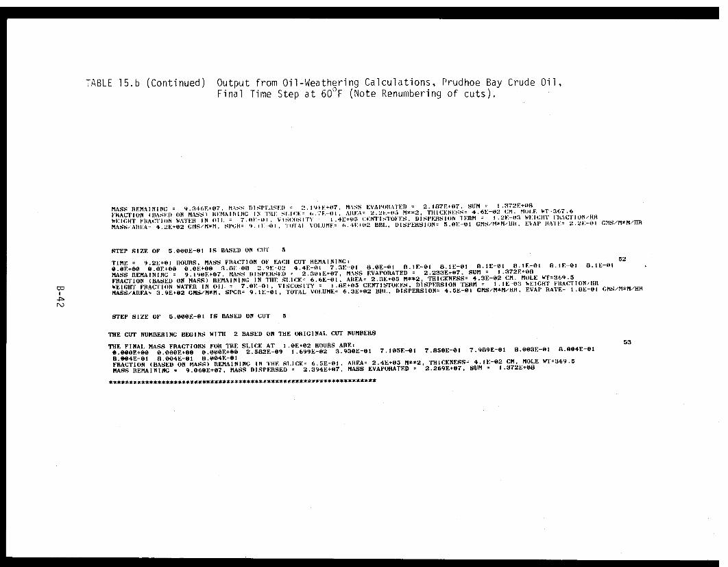
TABLE 15.b (Continued) Output from Oil-Weathering Calculations, Prudhoe Bay Crude Oil,Final Time Step at 60°F (Note Renumbering of cuts).
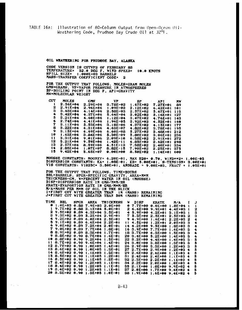
TABLE 16a: Illustration of 80-Column Output from Open-Ocean Oil-Weathering Code, Prudhoe Bay Crude Oil at 32°F.
B-43
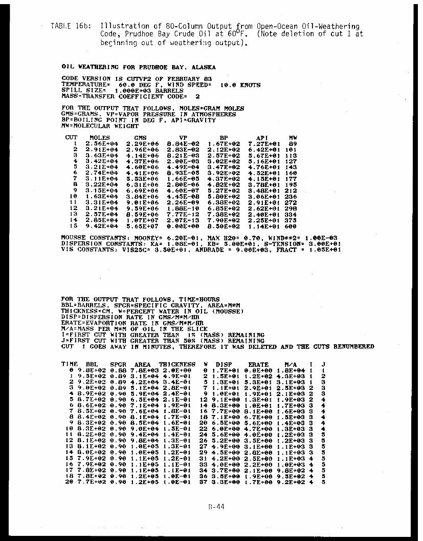
TABLE 16b: Illustration of 80-Column Output from Open-Ocean Oil-WeatheringCode, Prudhoe Bay Crude Oil at 60°F. (Note deletion of cut 1 atbeginning out of weathering output).
B-44
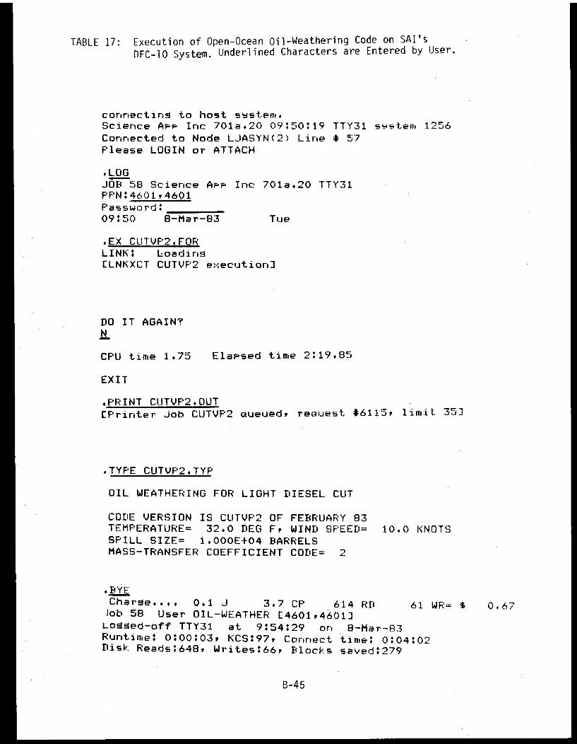
TABLE 17: Execution of Open-Ocean Oil-Weathering Code on SAI's
DFC-10 System. Underlined Characters are Entered by User.
B-45
TABLE 18. Illustration of Procedure to Attach to a Job
.log 1234,1234JOB 29 Science App Inc 701.17e TTY25Password: cr>
Other jobs detached with same PPN:Job 73 <program name> running
Do you want to ATTACH to this job? [YJ<cr>ATTACH 7Sf12S14,234[LGNATJ Attaching to job 73 running <program name> in user mode]< cr>
B-46
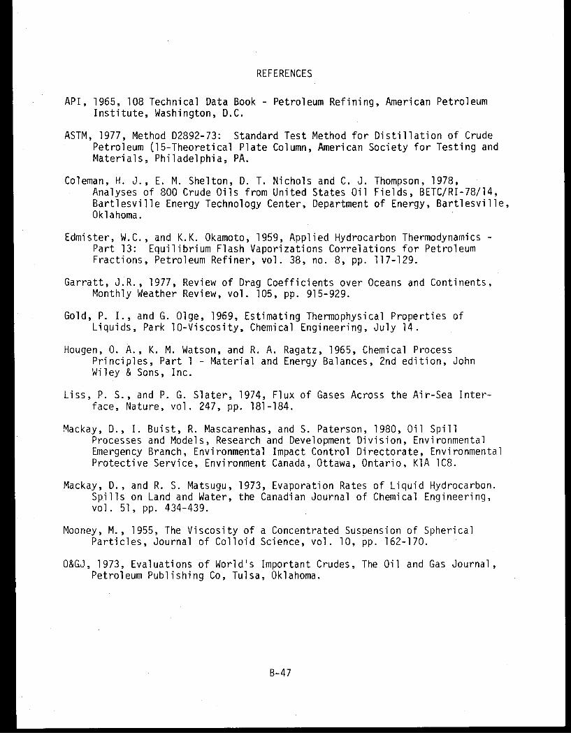
REFERENCES
API, 1965, 108 Technical Data Book - Petroleum Refining, American PetroleumInstitute, Washington, D.C.
ASTM, 1977, Method D2892-73: Standard Test Method for Distillation of CrudePetroleum C15-Theoretical Plate Column, American Society for Testing andMaterials, Philadelphia, PA.
Coleman, H. J., E. M. Shelton, D. T. Nichols and C. J. Thompson, 1978,Analyses of 800 Crude Oils from United States Oil Fields, BETC/RI-78/14,Bartlesville Energy Technology Center, Department of Energy, Bartlesville,Oklahoma.
Edmister, W.C., and K.K. Okamoto, 1959, Applied Hydrocarbon Thermodynamics -Part 13: Equilibrium Flash Vaporizations Correlations for PetroleumFractions, Petroleum Refiner, vol. 38, no. 8, pp. 117-129.
Garratt, J.R., 1977, Review of Drag Coefficients over Oceans and Continents,Monthly Weather Review, vol. 105, pp. 915-929.
Gold, P. I., and G. Olge, 1969, Estimating Thermophysical Properties ofLiquids, Park 10-Viscosity, Chemical Engineering, July 14.
Hougen, O. A., K. M. Watson, and R. A. Ragatz, 1965, Chemical ProcessPrinciples, Part 1 - Material and Energy Balances, 2nd edition, JohnWiley & Sons, Inc.
Liss, P. S., and P. G. Slater, 1974, Flux of Gases Across the Air-Sea Inter-face, Nature, vol. 247, pp. 181-184.
Mackay, D., I. Buist, R. Mascarenhas, and S. Paterson, 1980, Oil SpillProcesses and Models, Research and Development Division, EnvironmentalEmergency Branch, Environmental Impact Control Directorate, EnvironmentalProtective Service, Environment Canada, Ottawa, Ontario, K1A 1C8.
Mackay, D., and R. S. Matsugu, 1973, Evaporation Rates of Liquid Hydrocarbon.Spills on Land and Water, the Canadian Journal of Chemical Engineering,vol. 51, pp. 434-439.
Mooney, M., 1955, The Viscosity of a Concentrated Suspension of SphericalParticles, Journal of Colloid Science, vol. 10, pp. 162-170.
O&GJ, 1973, Evaluations of World's Important Crudes, The Oil and Gas Journal,Petroleum Publishing Co, Tulsa, Oklahoma.
B-47
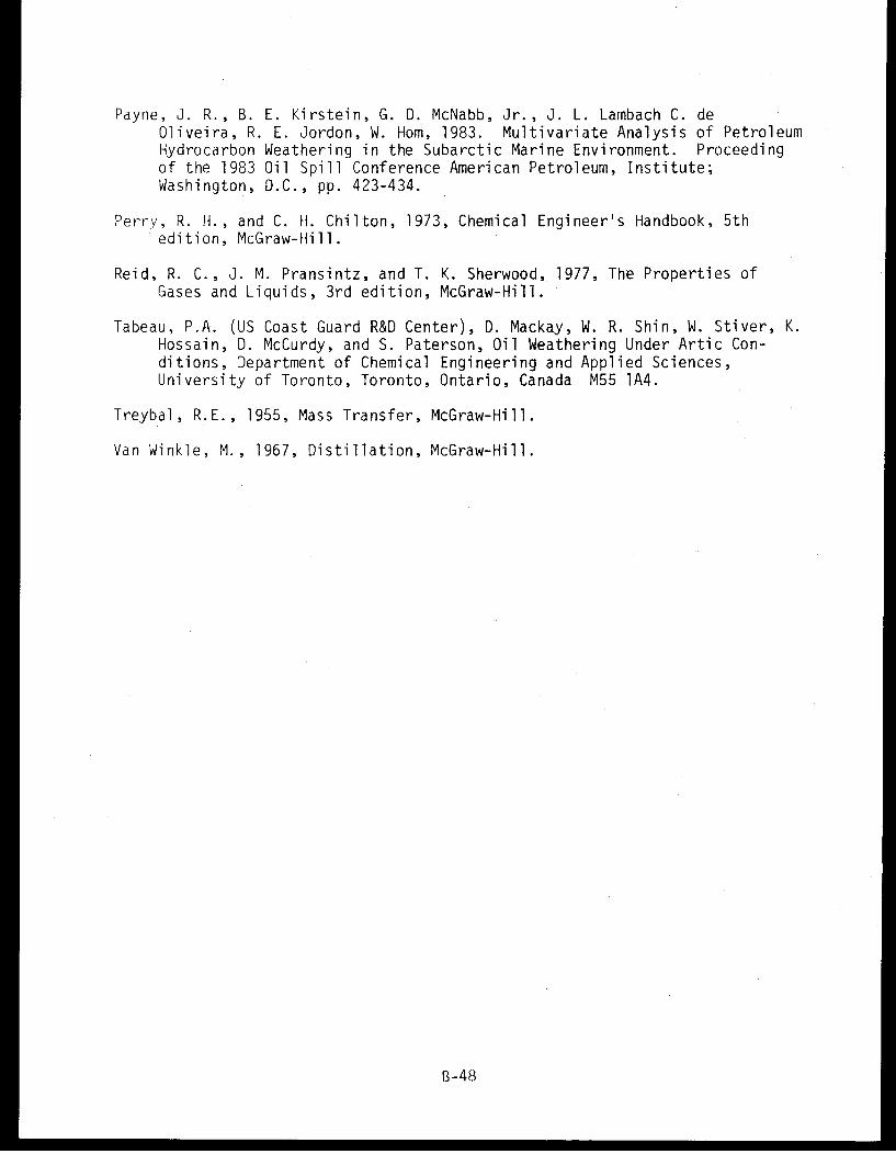
Payne, J. R., B. E. Kirstein, G. D. McNabb, Jr., J. L. Lambach C. deOliveira, R. E. Jordon, W. Horn, 1983. Multivariate Analysis of PetroleumHydrocarbon Weathering in the Subarctic Marine Environment. Proceedingof the 1983 Oil Spill Conference American Petroleum, Institute;Washington, D.C., pp. 423-434.
Perry, R. H., and C. H. Chilton, 1973, Chemical Engineer's Handbook, 5thedition, McGraw-Hill.
Reid, R. C., J. M. Pransintz, and T. K. Sherwood, 1977, The Properties ofGases and Liquids, 3rd edition, McGraw-Hill.
Tabeau, P.A. (US Coast Guard R&D Center), D. Mackay, W. R. Shin, W. Stiver, K.Hossain, D. McCurdy, and S. Paterson, Oil Weathering Under Artic Con-ditions, Department of Chemical Engineering and Applied Sciences,University of Toronto, Toronto, Ontario, Canada M55 1A4.
Treybal, R.E., 1955, Mass Transfer, McGraw-Hill.
Van Winkle, M., 1967, Distillation, McGraw-Hill.
B-48
Attachment 1
HOW TO USE TELENET
B-49
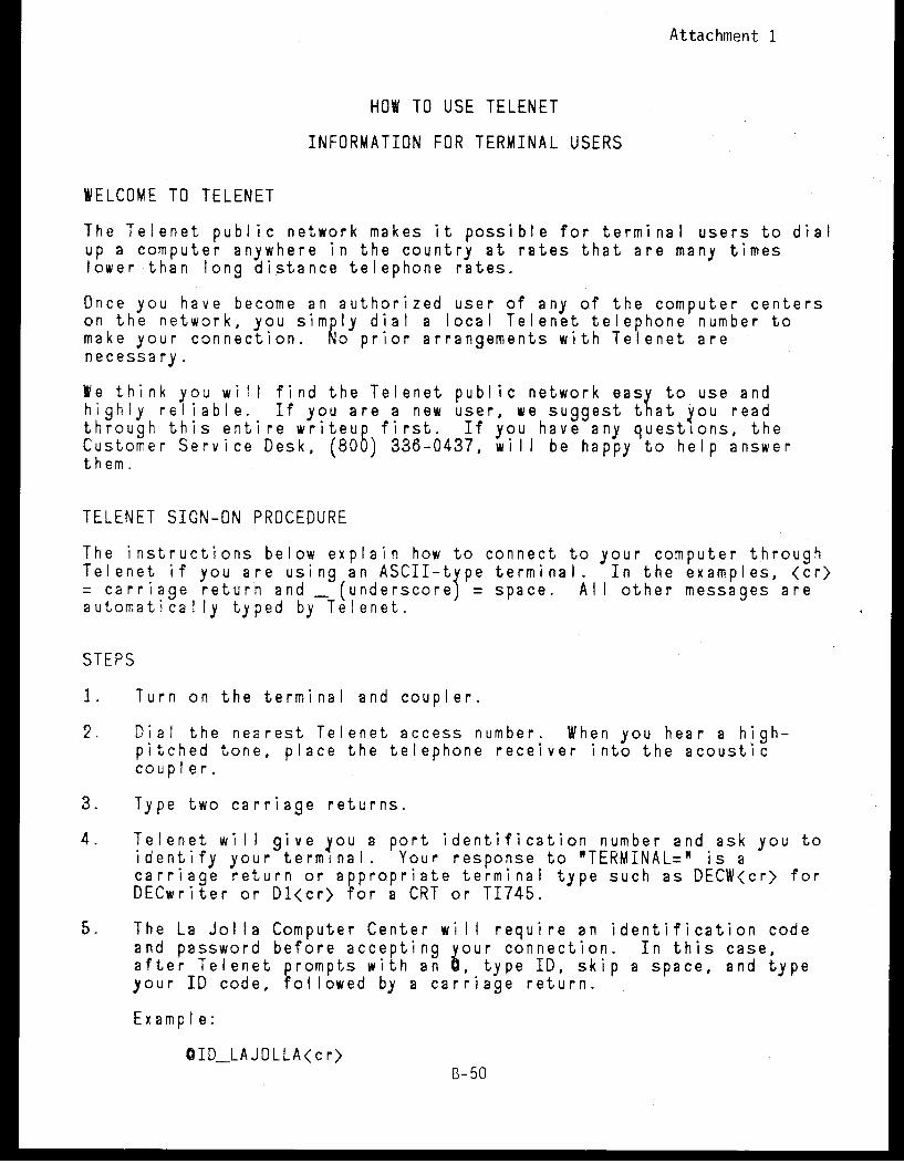
Attachment 1
HOW TO USE TELENET
INFORMATION FOR TERMINAL USERS
WELCOME TO TELENET
The Telenet public network makes it possible for terminal users to dialup a computer anywhere in the country at rates that are many timeslower than long distance telephone rates.
Once you have become an authorized user of any of the computer centerson the network, you simply dial a local Telenet telephone number tomake your connection. o prior arrangements with Telenet arenecessary.
We think you will find the Telenet public network easy to use andhighly reliable. If you are a new user, we suggest that you readthrough this entire writeup first. If you have any questions, theCustomer Service Desk, (800) 336-0437, will be happy to help answerthem.
TELENET SIGN-ON PROCEDURE
The instructions below explain how to connect to your computer throughTelenet if you are using an ASCII-type terminal. In the examples, <cr>= carriage return and (underscore) = space. All other messages areautomatically typed by Telenet.
STEPS
1. Turn on the terminal and coupler.
2. Dial the nearest Telenet access number. When you hear a high-pitched tone, place the telephone receiver into the acousticcoup ler.
3. Type two carriage returns.
4. Telenet will give you a port identification number and ask you toidentify your terminal. Your response to "TERMINAL=" is acarriage return or appropriate terminal type such as DECW<cr> forDECwriter or Dl<cr> for a CRT or TI745.
5. The La Jolla Computer Center will require an identification codeand password before accepting your connection. In this case,after Telenet prompts with an a, type ID, skip a space, and typeyour ID code, followed by a carriage return.
Example:
OID_LAJOLLA<cr>B-50
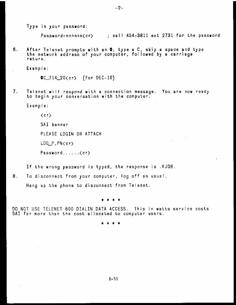
B-51
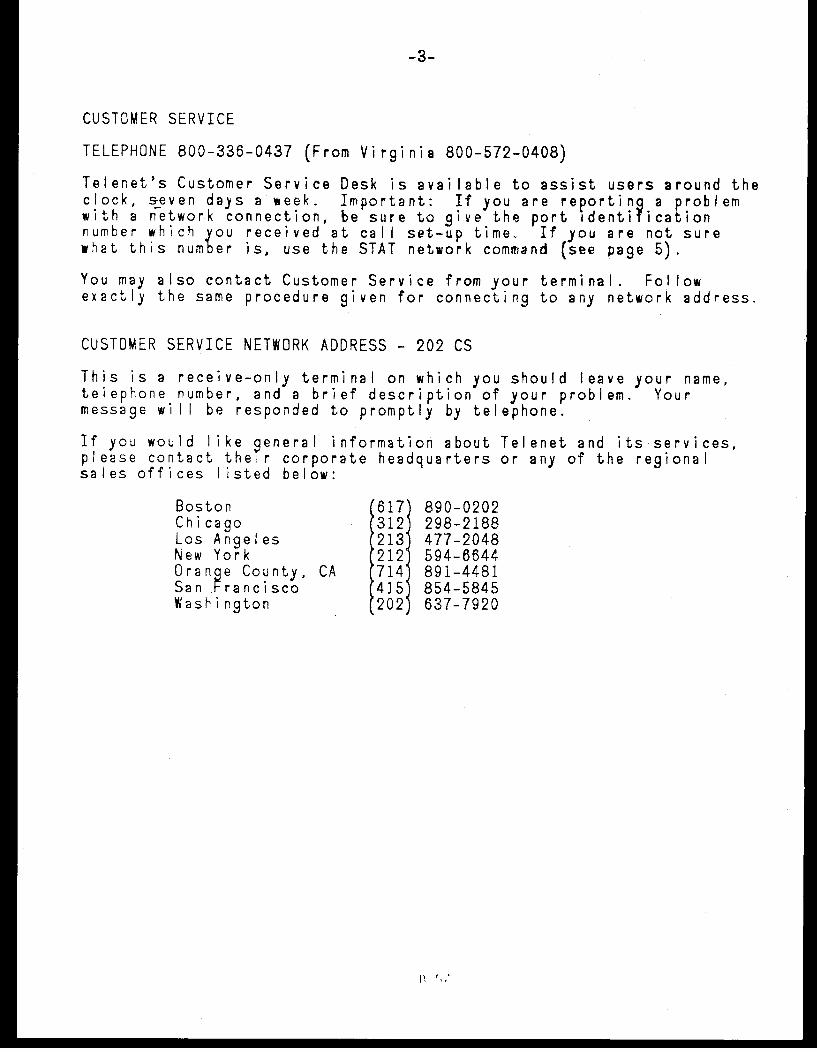
-3-
CUSTOMER SERVICE
TELEPHONE 800-336-0437 (From Virginia 800-572-0408)
Telenet's Customer Service Desk is available to assist users around theclock, seven days a week. Important: If you are reporting a problemwith a network connection, be sure to give the port identificationnumber which you received at call set-up time. If you are not surewhat this number is, use the STAT network command (see page 5).
You may also contact Customer Service from your terminal. Followexactly the same procedure given for connecting to any network address.
CUSTOMER SERVICE NETWORK ADDRESS - 202 CS
This is a receive-only terminal on which you should leave your name,telephone number, and a brief description of your problem. Yourmessage will be responded to promptly by telephone.
If you would like general information about Telenet and its services,please contact their corporate headquarters or any of the regionalsales offices listed below:
Boston 617 890-0202Chicago 312 298-2188Los Angeles 213 477-2048New York 212 594-6644Orange County, CA 714 891-4481San Francisco 415 854-5845Washington 202 637-7920
|' !,'
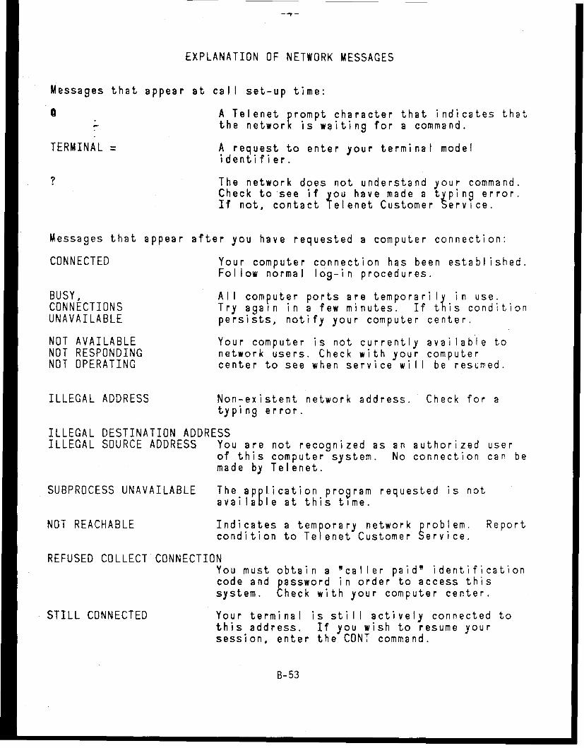
EXPLANATION OF NETWORK MESSAGES
Messages that appear at call set-up time:
0 A Telenet prompt character that indicates that- the network is waiting for a command.
TERMINAL = A request to enter your terminal modelidentifier.
? The network does not understand your command.Check to see if you have made a typing error.If not, contact elenet Customer Service.
Messages that appear after you have requested a computer connection:
CONNECTED Your computer connection has been established.Follow normal log-in procedures.
BUSY, All computer ports are temporarily in use.CONNECTIONS Try again in a few minutes. If this conditionUNAVAILABLE persists, notify your computer center.
NOT AVAILABLE Your computer is not currently available toNOT RESPONDING network users. Check with your computerNOT OPERATING center to see when service will be resumed.
ILLEGAL ADDRESS Non-existent network address. Check for atyping error.
ILLEGAL DESTINATION ADDRESSILLEGAL SOURCE ADDRESS You are not recognized as an authorized user
of this computer system. No connection can bemade by Telenet.
SUBPROCESS UNAVAILABLE The application program requested is notavailable at this time.
NOT REACHABLE Indicates a temporary network problem. Reportcondition to Telenet Customer Service.
REFUSED COLLECT CONNECTIONYou must obtain a "caller paid" identificationcode and password in order to access thissystem. Check with your computer center.
STILL CONNECTED Your terminal is still actively connected tothis address. If you wish to resume yoursession, enter the CONT command.
B-53
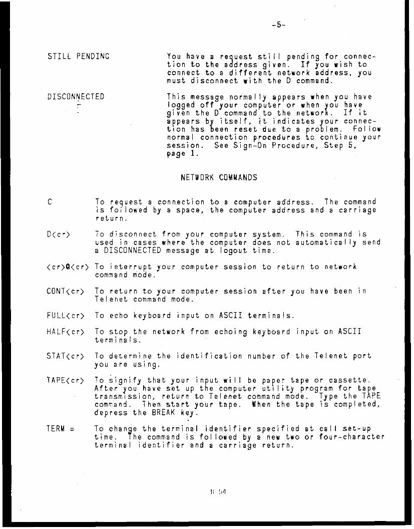
-5-
STILL PENDING You have a request still pending for connec-tion to the address given. If you wish toconnect to a different network address, youmust disconnect with the D command.
DISCONNECTED This message normally appears when you have- logged off your computer or when you have
given the D command to the networ. If itappears by itself, it indicates your connec-tion has een reset due to a problem. Follownormal connection procedures to continue yoursession. See Sign-On Procedure, Step 5,page 1.
NETWORK COMMANDS
C To request a connection to a computer address. The commandis followed by a space, the computer address and a carriagereturn.
D<cr> To disconnect from your computer system. This command isused in cases where the computer does not automatically senda DISCONNECTED message at logout time.
<cr>O<cr> To interrupt your computer session to return to networkcommand mode.
CONT<cr> To return to your computer session after you have been inTelenet command mode.
FULL<cr> To echo keyboard input on ASCII terminals.
HALF<cr> To stop the network from echoing keyboard input on ASCIIterminals.
STAT<cr> To determine the identification number of the Telenet portyou are using.
TAPE<cr> To signify that your input will be paper tape or cassette.After you have set up the computer utility program for tapetransmission, return to Telenet command mode. Type the TAPEcommand. Then start your tape. When the tape is completed,depress the BREAK key.
TERM = To change the terminal identifier specified at call set-uptime. The command is followed by a new two or four-characterterminal identifier and a carriage return.
wi ,4
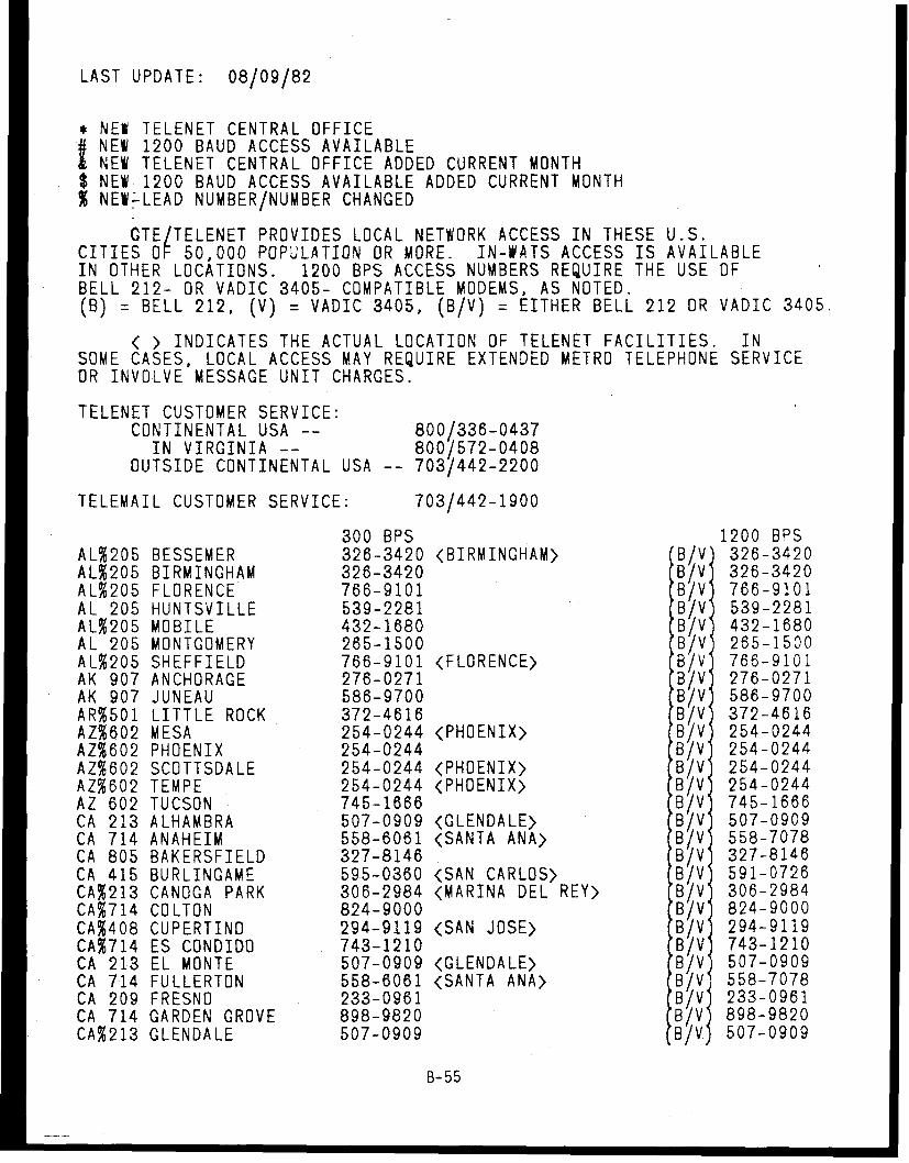
LAST UPDATE: 08/09/82
* NEW TELENET CENTRAL OFFICENEW 1200 BAUD ACCESS AVAILABLENEW TELENET CENTRAL OFFICE ADDED CURRENT MONTH
$ NEW 1200 BAUD ACCESS AVAILABLE ADDED CURRENT MONTH% NEW-LEAD NUMBER/NUMBER CHANGED
GTE/TELENET PROVIDES LOCAL NETWORK ACCESS IN THESE U.S.CITIES OF 50,000 POPULATION OR MORE. IN-WATS ACCESS IS AVAILABLEIN OTHER LOCATIONS. 1200 BPS ACCESS NUMBERS REQUIRE THE USE OFBELL 212- OR VADIC 3405- COMPATIBLE MODEMS, AS NOTED.(B) = BELL 212, (V) = VADIC 3405, (B/V) = EITHER BELL 212 OR VADIC 3405.
< > INDICATES THE ACTUAL LOCATION OF TELENET FACILITIES. INSOME CASES, LOCAL ACCESS MAY REQUIRE EXTENDED METRO TELEPHONE SERVICEOR INVOLVE MESSAGE UNIT CHARGES.
TELENET CUSTOMER SERVICE:CONTINENTAL USA -- 800/336-0437
IN VIRGINIA -- 800/572-0408OUTSIDE CONTINENTAL USA -- 703/442-2200
TELEMAIL CUSTOMER SERVICE: 703/442-1900
300 BPS 1200 BPSAL%205 BESSEMER 326-3420 <BIRMINGHAM> B/V 326-3420AL%205 BIRMINGHAM 326-3420 B/V 326-3420AL%205 FLORENCE 766-9101 B/V 766-9101AL 205 HUNTSVILLE 539-2281 B/V 539-2281AL%205 MOBILE 432-1680 B/V 432-1680AL 205 MONTGOMERY 265-1500 B/V 265-1500AL%205 SHEFFIELD 766-9101 <FLORENCE> B/V 766-9101AK 907 ANCHORAGE 276-0271 B/V 276-0271AK 907 JUNEAU 586-9700 B/V 586-9700AR%501 LITTLE ROCK 372-4616 B/V 372-4616AZ%602 MESA 254-0244 <PHOENIX> B/V 254-0244AZ%602 PHOENIX 254-0244 B/V 254-0244AZ%602 SCOTTSDALE 254-0244 <PHOENIX> B/V 254-0244AZ%602 TEMPE 254-0244 <PHOENIX> B/V 254-0244AZ 602 TUCSON 745-1666 B/V 745-1666CA 213 ALHAMBRA 507-0909 <GLENDALE> B/V 507-0909CA 714 ANAHEIM 558-6061 <SANTA ANA> B/V 558-7078CA 805 BAKERSFIELD 327-8146 B/V 327-8146CA 415 BURLINGAME 595-0360 <SAN CARLOS> B/V 591-0726CA%213 CANOGA PARK 306-2984 <MARINA DEL REY> B/V 306-2984CA%714 COLTON 824-9000 B/V 824-9000CA%408 CUPERTINO 294-9119 <SAN JOSE> B/V 294-9119CA%714 ES CONDIDO 743-1210 B/V 743-1210CA 213 EL MONTE 507-0909 <GLENDALE> B/V 507-0909CA 714 FULLERTON 558-6061 <SANTA ANA> B/V 558-7078CA 209 FRESNO 233-0961 B/V 233-0961CA 714 GARDEN GROVE 898-9820 B/V 898-9820CA%213 GLENDALE 507-0909 B/V 507-0909
B-55
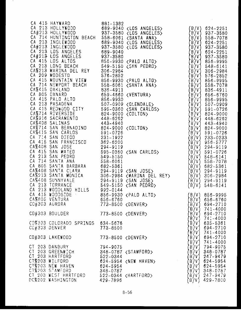
CA 415 HAYWARD 881-1382CA 213 HOLLYWOOD 689-9040 <LOS ANGELES> B/V 624-2251CA#213 HOLLYWOOD 937-3580 (LOS ANGELES> B/V 937-3580CA 714 HUNTINGTON BEACH 558-6061 (SANTA ANA> B/V 558-7078CA 213 INGLEWOOD 689-9040 <LOS ANGELES) B/V 624-2251CA#213 INGLEWOOD 937-3580 (LOS ANGELES> B/V 937-3580CA 213 LOS ANGELES 689-9040 B/V 624-2251CA#219 LOS ANGELES 937-3580 B/V 937-3580CA 415 LOS ALTOS 856-9930 (PALO ALTO> B/V 856-9995CA 213 LONG BEACH 549-5150 <SAN PEDRD> B/V 548-6141CA%213 MARINA DEL REY 306-2984 B/V 306-2984CA 209 MODESTO 576-2852 B/V 576-2852CA 415 MOUNTAIN VIEW 856-9930 <PALO ALTO> B/V 856-9995CA 714 NEWPORT BEACH 558-6061 (SANTA ANA> B/V 558-7078CA%415 OAKLAND 836-4911 B/V 836-4911CA 805 OXNARD 659-4660 <VENTURA> B/V 656-6760CA 415 PALO ALTO 856-9930 B/V 856-9995CA 213 PASADENA 507-0909 (GLENDALE> B/V 507-0909CA 415 REDWOOD CITY 595-0360 <SAN CARLOS> B/V 591-0726CA%714 RIVERSIDE 824-9000 <COLTON> B/V 824-9000CA%916 SACRAMENTO 448-6262 B/V 448-6262CA%408 SALINAS 443-4940 B/V 443-4940CA%714 SAN BERNADINO 824-9000 <COLTON> B/V 824-9000CA%415 SAN CARLOS 591-0726 B/V 591-0726CA 7i4 SAN DIEGO 231-1922 B/V 233-0233CA 415 SAN FRANCISCO 362-6200 B/V 956-5777CA%408 SAN JOSE 294-9119 B/V 294-9119CA 415 SAN MATEO 595-0360 <SAN CARLOS> B/V 591-0726CA 213 SAN PEDRO 549-5150 B/V 548-6141CA 714 SANTA ANA 558-6061 B/V 558-7078CA 805 SANTA BARBARA 682-5361 B/V 682-5361CA%408 SANTA CLARA 294-9119 <SAN JOSE> B/V 294-9119CA%213 SANTA MONICA 306-2984 <MARINA DEL REY> B/V 306-2984CA%408 SUNNYVALE 294-9119 <SAN JOSE> B/V 294-9119CA 213 TORRANCE 549-5150 <SAN PEDRO> B/V 548-6141CA 213 WOODLAND HILLS 992-0144CA 415 WOODSIDE 856-9930 <PALO ALTO> B/V 856-9995CA%805 VENTURA 656-6760 B/V 656-6760CO#303 AURORA 773-8500 <DENVER> B/V 694-2710
B/V 741-4000C0#303 BOULDER 773-8500 (DENVER> B/V 694-2710
B/V 741-4000C0O303 COLORADO SPRINGS 634-5676 B/V 635-5361CO#303 DENVER 773-8500 B/V 694-2710
*B/V 741-4000CO#303 LAKEWOOD 773-8500 (DENVER> B/V 694-2710
B/V 741-4000CT 203 DANBURY 794-9075 B/V 794-9075CT 203 GREENWICH 348-0787 <STAMFORD> B/V 348-0787CT 203 HARTFORD 522-0344 B/V 247-9479CT%203 MILFORD 624-5954 <NEW HAVEN) B/V 624-5954CT%203 NEW HAVEN 624-5954 B/V 624-5954CT%203 STAMFORD 348-0787 B/V 348-0787CT 203 WEST HARTFORD 522-0344 <HARTFORD> B/V 247-9479DC%202 WASHINGTON 429-7896 B/V 429-7800
B-56
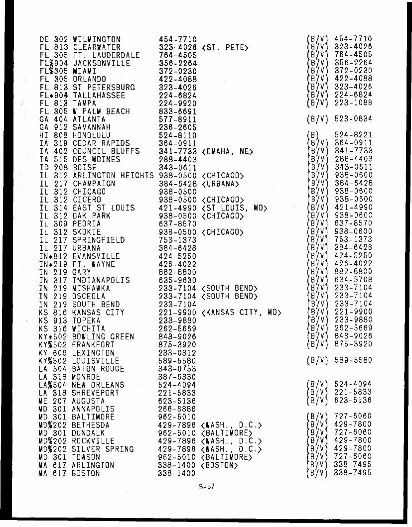
DE 302 WILMINGTON 454-7710 B/V) 454-7710FL 813 CLEARWATER 323-4026 <ST. PETE> B/V 323-4026FL 305 FT. LAUDERDALE 764-4505 B/V 764-4505PL%904 JACKSONVILLE 356-2264 B/V) 356-2264FL%305 MIAMI 372-0230 B/V) 372-0230FL 305 ORLANDO 422-4088 B/V) 422-4088FL 813 ST PETERSBURG 323-4026 B/V 323-4026FL*904 TALLAHASSEE 224-6824 B/V 224-6824FL 813 TAMPA 224-9920 B/V 223-1088FL 305 W PALM BEACH 833-6691GA 404 ATLANTA 577-8911 (B/V) 523-0834GA 912 SAVANNAH 236-2605HI 808 HONOLULU 524-8110 IB) 524-8221IA 319 CEDAR RAPIDS 364-0911 B/V 364-0911IA 402 COUNCIL BLUFFS 341-7733 <OMAHA, NE> B/V 341-7733IA 515 DES MOINES 288-4403 B/V 288-4403ID 208 BOISE 343-0611 B/V 343-0611IL 312 ARLINGTON HEIGHTS 938-0500 <CHICAGO> B/V 938-0600IL 217 CHAMPAIGN 384-6428 <URBANA> B/V 384-6428IL 312 CHICAGO 938-0500 B/V 938-0600IL 312 CICERO 938-0500 <CHICAGO> B/V 938-0600IL 314 EAST ST LOUIS 421-4990 <ST LOUIS, MO> B/V 421-4990IL 312 OAK PARK 938-0500 <CHICAGO> B/V 938-0600IL 309 PEORIA 637-8570 B/V 637-8570IL 312 SKOKIE 938-0500 <CHICAGO> B/V 938-0600IL 217 SPRINGFIELD 753-1373 B/V 753-1373IL 217 URBANA 384-6428 B/V 384-6428IN*812 EVANSVILLE 424-5250 B/V 424-5250IN*219 FT. WAYNE 426-4022 B/V 426-4022IN 219 GARY 882-8800 B/V 882-8800IN 317 INDIANAPOLIS 635-9630 B/V 634-5708IN 219 MISHAWKA 233-7104 <SOUTH BEND> B/V 233-7104IN 219 OSCEOLA 233-7104 <SOUTH BEND> B/V 233-7104IN 219 SOUTH BEND 233-7104 B/V 233-7104KS 816 KANSAS CITY 221-9900 <KANSAS CITY, MO> B/V 221-9900KS 913 TOPEKA 233-9880 B/V 233-9880KS 316 WICHITA 262-5669 B/V 262-5669KY*502 BOWLING GREEN 843-9026 B/V 843-9026KY%502 FRANKFORT 875-3920 B/V 875-3920KY 606 LEXINGTON 233-0312KY%502 LOUISVILLE 589-5580 (B/V) 589-5580LA 504 BATON ROUGE 343-0753LA 318 MONROE 387-6330LA%504 NEW ORLEANS 524-4094 B/V 524-4094LA 318 SHREVEPORT 221-5833 2B/V 221-5833ME 207 AUGUSTA 623-5136 B/V 623-5136MD 301 ANNAPOLIS 266-6886MD 301 BALTIMORE 962-5010 B/V 727-6060MD%202 BETHESDA 429-7896 <WASH., D.C.> B/V 429-7800MD 301 DUNDALK 962-5010 <BALTIMORE> B/V 727-6060MD%202 ROCKVILLE 429-7896 <WASH., D.C.> B/V 429-7800MD%202 SILVER SPRING 429-7896 <WASH., D.C.> B/V 429-7800MD 301 TOWSON 962-5010 <BALTIMORE> B/V 727-6060MA 617 ARLINGTON 338-1400 <BOSTON> B/V 338-7495MA 617 BOSTON 338-1400 B/V 338-7495
B-57
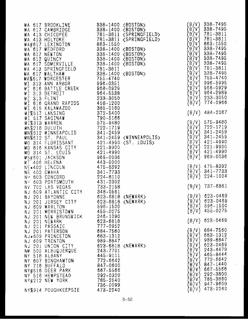
MA 617 BROOKLINE 338-1400 (BOSTON> B/V 338-7495MA 617 CAMBRIDGE 338-1400 <BOSTON> B/V 338-7495MA 413 CHICOPEE 781-3811 <SPRINGFIELD> B/V 781-3811MA 413 HOLYOKE 781-3811 <SPRINGFIELD> B/V 781-3811MA#617 LEXINGTON 863-1550 B/V 863-1550MA 617 MEDFORD 338-1400 <BOSTON> B/V 338-7495MA 617 NEWTON 338-1400 <BOSTON> B/V 338-7495MA 61Z QUINCY 338-1400 <BOSTON> B/V 338-7495MA 617 SOMERVILLE 338-1400 <BOSTON> B/V 338-7495MA 413 SPRINGFIELD 781-3811 B/V 781-3811MA 617 WALTHAM 338-1400 <BOSTON> B/V 338-7495MA%617 WORCESTER 755-4740 B/V 755-4740MI 313 ANN ARBOR 996-0351 B/V 996-5995MI 616 BATTLE CREEK 968-0929 B/V 968-0929MI 313 DETROIT 964-5538 B/V 964-2989MI 313 FLINT 233-3050 B/V 233-3050MI 616 GRAND RAPIDS 458-1200 B/V 774-0966MI 616 KALAMAZOO 385-0160MI%517 LANSING 372-5400 (B/V) 484-2067MI 517 SAGINAW 790-5166MI%313 WARREN 575-9480 B/V 575-9480MN%218 DULUTH 722-1719 B/V 722-1719MN%612 MINNEAPOLIS 341-2459 B/V 341-2459MN%612 ST. PAUL 341-2459 <MINNEAPOLIS> B/V 341-2459MO 314 FLORISSANT 421-4990 <ST. LOUIS> B/V 421-4990MO 816 KANSAS CITY 221-9900 B/V 221-9900MO 314 ST. LOUIS 421-4990 B/V 421-4990MS#601 JACKSON 969-0036 B/V 969-0036MT 406 HELENA 443-0000NE*402 LINCOLN 475-8392 (B/V 475-8392NE 402 OMAHA 341-7733 B/V 341-7733NH 603 CONCORD 224-8110 B/V 224-1024NH 603 PORTSMOUTH 431-2302NV 702 LAS VEGAS 733-2158 (B/V) 737-6861NJ 609 ATLANTIC CITY 348-0561NJ 201 BAYONNE 623-6818 <NEWARK> B/V) 623-0469NJ 201 JERSEY CITY 623-6818 <NEWARK> B/V 623-0469NJ 609 MARLTON 596-1500 /V 596-1500NJ 201 MORRISTOWN 455-0275 B/V 455-0275NJ 201 NEW BRUNSWICK 246-1090NJ 201 NEWARK 623-6818 (B/V) 623-0469NJ 201 PASSAIC 777-0952NJ 201 PATERSON 684-7560 B/V 684-7560NJ*609 PRINCETON 683-1312 B/V 683-1312NJ 609 TRENTON 989-8847 B/V 989-8847NJ 201 UNION CITY 623-6818 <NEWARK> B/V 623-0469NM 505 ALBUQUERQUE 243-7701 B/V 243-4479NY 518 ALBANY 445-9111 B/V 465-8444NY 607 BINGHAMTON 772-6642 B/V 772-6642NY 716 BUFFALO 847-0600 B/V 847-1440NY#516 DEER PARK 667-5566 B/V 667-5566NY 516 HEMPSTEAD 292-0320 B/V 292-3800NY#212 NEW YORK 785-2540 B/V 785-3860
736-0099 B/V 947-9600NY%914 POUGHKEEPSIE 473-2240 B/V 473-2240
B-58
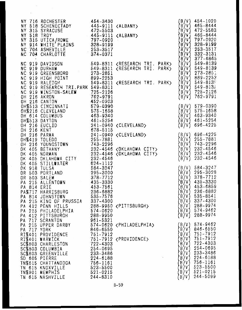
NY 716 ROCHESTER 454-3430 B/V 454-1020NY 518 SCHENECTADY 445-9111 <ALBANY> B/V 465-8444NY 315 SYRACUSE 472-5503 B/V 472-5583NY 518 TROY 445-9111 <ALBANY> B/V 465-8444NY 315 UTICA/ROME 797-0920 B/V 797-0920NY 914 WHITE PLAINS 328-9199 B/V 328-9199NC 704 ASHEVILLE 253-3517 B/V 253-3517NC 704 CHARLOTTE 374-0371 B/V 332-3131
B/V 377-6865NC 919 DAVIDSON 549-8311 <RESEARCH TRI. PARK> B/V 549-8139NC 919 DURHAM 549-8311 <RESEARCH TRI. PARK> B/V 549-8139NC 919 GREENSBORO 273-2851 B/V 273-285iNC 919 HIGH POINT 899-2253 B/V 889-2253NC 919 RALEIGH 549-8311 <RESEARCH TRI. PARK> B/V 549-813'NC 919 RESEARCH TRI.PARK 549-8311 B/V 549-813.-NC 919 WINSTON-SALEM 725-2126 B/V 725-2126OH 216 AKRON 762-9791 B/V 762-9791OH 216 CANTON 452-0903OH%513 CINCINNATI 579-0390 B/V 579-0390OH%216 CLEVELAND 575-1658 B/V 575-1658OH 614 COLUMBUS 463-9340 B/V 463-9340OH%513 DAYTON 461-5254 B/V 461-5254OH 216 EUCLID 241-0940 (CLEVELAND> B/V 696-4225OH 216 KENT 678-5115OH 216 PARMA 241-0940 <CLEVELAND> B/V 696-4225OH%419 TOLEDO 255-7881 B/V 255-7881OH 216 YOUNGSTOWN 743-2296 B/V 743-2296OK 405 BETHANY 232-4546 <OKLAHOMA CITY> B/V 232-4546OK 405 NORMAN 232-4546 <OKLAHOMA CITY> B/V 232-4546OK 405 OKLAHOMA CITY 232-4546 B/V 232-4546OK 405 STILLWATER 624-1112OK 918 TULSA 584-3247 B/V 584-3247OR 503 PORTLAND 295-3000 B/V 295-3028OR 503 SALEM 378-7712 B/V 378-7712PA 215 ALLENTOWN 435-3330 B/V 435-3330PA 814 ERIE 453-7561 B/V 453-6859PA%717 HARRISBURG 236-6882 B/V 236-6882PA 814 JOHNSTOWN 535-7576 B/V 535-8541PA 215 KING OF PRUSSIA 337-4300 B/V 337-4300PA 412 PENN HILLS 288-9950 <PITTSBURGH> B/V 288-9974PA 215 PHILADELPHIA 574-0620 B/V 574-9462PA 412 PITTSBURGH 288-9950 B/V 288-9974PA 717 SCRANTON 961-5321PA 215 UPPER DARBY 574-0620 <PHILADELPHIA> B/V 574-9462PA 717 YORK 846-6550 B/V 846-6550RI%401 PROVIDENCE 751-7912 B/V 751-7912RI%401 WARWICK 751-7912 <PROVIDENCE> B/V 751-7912SC%803 CHARLESTON 722-4303 B/V 722-4303SC%803 COLUMBIA 254-0695 B/V 254-0695SC%803 GREENVILLE 233-3486 B/V 233-3486SD 605 PIERRE 224-6188 B/V 224-6188TN%615 CHATTANOOGA 756-1161 B/V 756-1161TN 615 KNOXVILLE 523-5500 B/V 523-5500TN%901 MEMPHIS 521-0215 B/V 521-0215TN 615 NASHVILLE 244-8310 B/V 244-5099
B-59
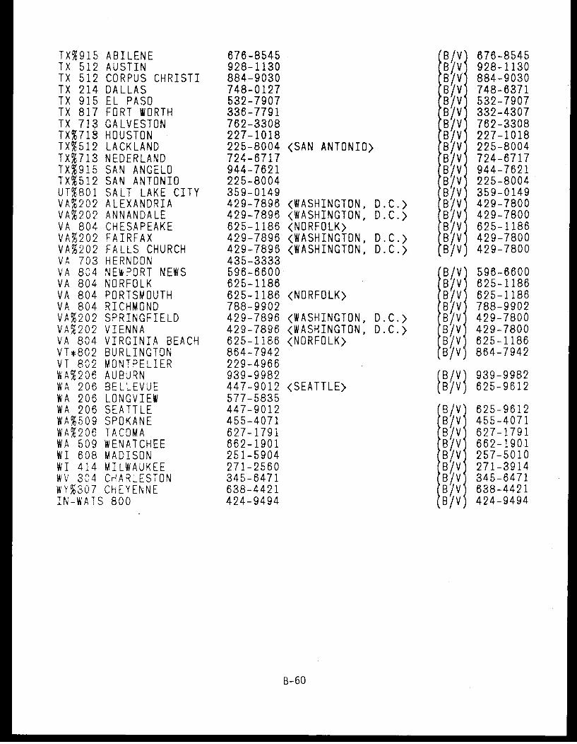
TX%915 ABILENE 676-8545 B/V 676-8545TX 512 AUSTIN 928-1130 B/V 928-1130TX 512 CORPUS CHRISTI 884-9030 B/V 884-9030TX 214 DALLAS 748-0127 B/V 748-6371TX 915 EL PASO 532-7907 B/V 532-7907TX 817 FORT WORTH 336-7791 B/V 332-4307TX 713 GALVESTON 762-3308 B/V 762-3308TX%718 HOUSTON 227-1018 B/V 227-1018TX%512 LACKLAND 225-8004 (SAN ANTONIO> B/V 225-8004TX%713 NEDERLAND 724-6717 B/V 724-6717TX%915 SAN ANGELO 944-7621 B/V 944-7621TX%512 SAN ANTONIO 225-8004 B/V 225-8004UT%801 SALT LAKE CITY 359-0149 B/V 359-0149VA%202 ALEXANDRIA 429-7896 <WASHINGTON, D.C.> B/V 429-7800VA%202 ANNANDALE 429-7896 <WASHINGTON, D.C.> B/V 429-7800VA 804 CHESAPEAKE 625-1186 <NORFOLK> B/V 625-1186VA%202 FAIRFAX 429-7896 <WASHINGTON, D.C.> B/V 429-7800VA%202 FALLS CHURCH 429-7896 <WASHINGTON, D.C.> B/V 429-7800VA 703 HERNDON 435-3333VA 804 NEWPORT NEWS 596-6600 B/V 596-6600VA 804 NORFOLK 625-1186 B/V 625-1186VA 804 PORTSMOUTH 625-1186 <NORFOLK> B/V 625-1186VA 804 RICHMOND 788-9902 B/V 788-9902VA%202 SPRINGFIELD 429-7896 <WASHINGTON, D.C.> B/V 429-7800VA%202 VIENNA 429-7896 <WASHINGTON, D.C.> B/V 429-7800VA 804 VIRGINIA BEACH 625-1186 <NORFOLK> B/V 625-1186VT*802 BURLINGTON 864-7942 B/V 864-7942VT 802 MONTPELIER 229-4966WA%206 AUBURN 939-9982 (B/V) 939-9982WA 206 BELLEVUE 447-9012 <SEATTLE> B/V) 625-9612WA 206 LONGVIEW 577-5835WA 206 SEATTLE 447-9012 B/V 625-9612WA%509 SPOKANE 455-4071 B /V 455-4071WA%206 TACOMA 627-1791. B/V' 627-1791WA 509 WENATCHEE 662-1901 B/V 662-1901WI 608 MADISON 251-5904 B/V 257-5010WI 414 MILWAUKEE 271-2560 B/V 271-3914WV 304 CHARLESTON 345-6471 B/V 345-6471WY%307 CHEYENNE 638-4421 B/V 638-4421IN-WATS 800 424-9494 B/V 424-9494
B-60
APPENDIX C
CODE DESCRIPTION FOR COMPONENT-SPECIFIC DISSOLUTION
C-1
APPENDIX C. COMPONENT-SPECIFIC DISSOLUTION:
COMPUTER CODE DESCRIPTION
In order to make the analytical solutions (as described in Section
4.5) for the component-specific dissolution usable they have been programmed
in FORTRAN to allow easy investigation of the results. This appendix presents
the details of input-output information, examples of code usage, and a code
listing.
Tables 1 through 3 present details on how the code is used. Table 1
is an illustration of the input procedure. All the required input is prompted
from the keyboard and echoed back to the user. An input error can be correct-
ed by answering yes to the question following the echo.
The output presented in Table 2 is the result of the input in Table
1. Reasonable estimates of the input parameters are used in this example from
which an important conclusion can be drawn. The important parameters are the
(vertical) eddy diffusivity = 185 cm2/sec (Pelto, 1982), the over-all mass-
transfer coefficient = 1 cm/hr (Cohen, Mackay and Shin, 1980), and the ocean
depth = 5 meters. The calculated concentration profiles are always quite flat
from top to bottom while the average water column concentration increases by a
factor of 5 from the first hour to the fifth. This indicates that the over-
all mass transfer coefficient is controlling the rate at which the entire
water column is gaining mass of the transferring species. Increasing the
over-all mass-transfer from 1 cm/hr to 10 cm/hr and keeping all other param-
eters the same results in approximately 10 times more mass in the water column
over the same time frame as illustrated by the results in Table 3. As a re-
sult of this example it is evident that the over-all mass-transfer coefficient
is important and appears to be controlling the rate at which mass enters the
water column.
C-2
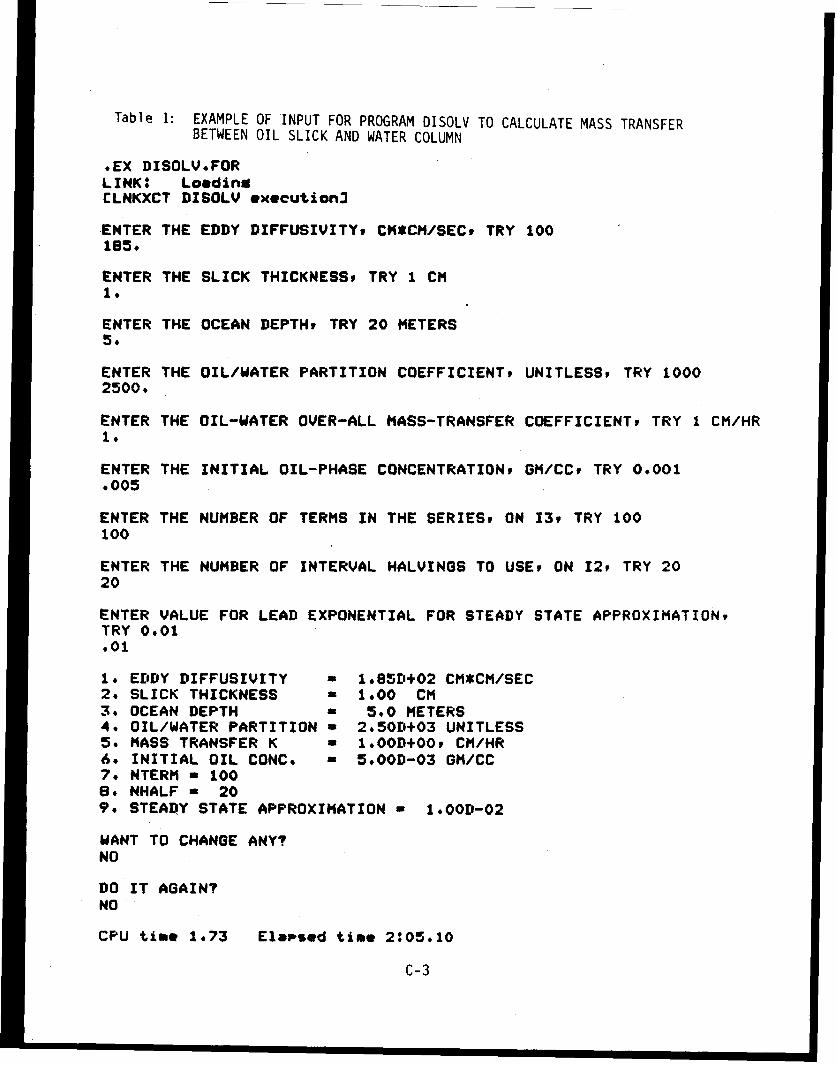
Table 1: EXAMPLE OF INPUT FOR PROGRAM DISOLV TO CALCULATE MASS TRANSFERBETWEEN OIL SLICK AND WATER COLUMN
.EX DISOLV.FORLINK: LoadingCLNKXCT DISOLV execution3
ENTER THE EDDY DIFFUSIVITY, CKtCM/SEC, TRY 100185.
ENTER THE SLICK THICKNESSP TRY 1 CM1.
ENTER THE OCEAN DEPTH, TRY 20 METERS5.
ENTER THE OIL/WATER PARTITION COEFFICIENT, UNITLESS, TRY 10002500.
ENTER THE OIL-WATER OVER-ALL MASS-TRANSFER COEFFICIENT, TRY 1 CM/HR1.
ENTER THE INITIAL OIL-PHASE CONCENTRATIONS GM/CC, TRY 0.001.005
ENTER THE NUMBER OF TERMS IN THE SERIES, ON I3, TRY 100100
ENTER THE NUMBER OF INTERVAL HALVINGS TO USE, ON I2, TRY 2020
ENTER VALUE FOR LEAD EXPONENTIAL FOR STEADY STATE APPROXIMATION,TRY 0.01.01
1. EDDY DIFFUSIVITY -1.85D+02 CM*CM/SEC2, SLICK THICKNESS - 1.00 CM3. OCEAN DEPTH " 5.0 METERS4. OIL/WATER PARTITION ' 2.50D+03 UNITLESS5. MASS TRANSFER K a 1.00D+00, CM/HR6o INITIAL OIL CONCo - 5.00D-03 GM/CC7. NTERM a 1008o NHALF - 209. STEADY STATE APPROXIMATION - 1.OOD-02
WANT TO CHANGE ANY?NO
DO IT AGAIN?NO
CPU time 1.73 Elawsed time 2:05.10
C-3
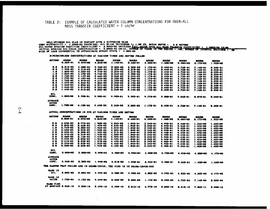
TABLE 2: EXAMPLE OF CALCULATED WATER COLUMN CONCENTRATIONS FOR OVER-ALLMASS TRANSFER COEFFICIENT = 1 cm/hr
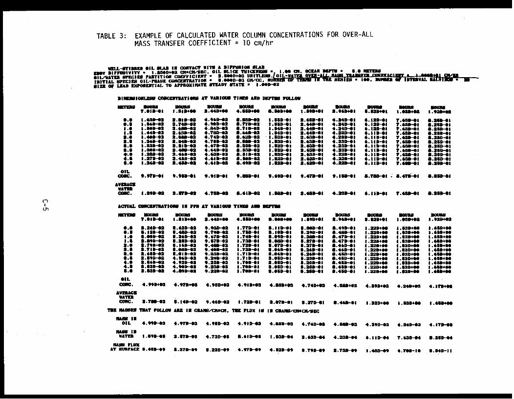
TABLE 3: EXAMPLE OF CALCULATED WATER COLUMN CONCENTRATIONS FOR OVER-ALLMASS TRANSFER COEFFICIENT = 10 cm/hr
Mass transfer within the 5-meter water column is quite fast as
indicated by the relatively flat concentration profiles.
The over-all mass-transfer coefficient appears to control the rate at
which dissolved mass enters the water column. The over-all mass-transfer for
this problem is based on water-phase concentrations since water-phase
concentrations are of interest. This coefficient is based on the individual
phase coefficients and a thermodynamic equilibrium expression relating the
concentrations in each phase. This thermodynamic equilibrium expression is
typically called a Henry's Law coefficient or partition coefficient (Leo, et
al , 1971). The general relationships for the quantities of interest in the
oil/water system are (Treybal, 1955):
where K stands for the over-all mass-transfer coefficient based on the phase
identified in the subscript and k stands for the individual-phase coefficient.
For the oil/water system transferring molecular species will have m
on the order of >1000 (unitless) which implies that the substance is quite
soluble in oil and sparingly soluble in water. Since the over-all
mass-transfer coefficient of interest is K[subscript]water, this yields
C-6
Based on published work kwater is somewhat less than koil but for
sparingly soluble substances, such as naphthalene, the above expression becomes:
1 1
Kwater kwater
since the reciprocal of mkoil is quite small. Typical values for Kwater range
from 1 to 10 cm/hr (Cohen, et al , 1980). In general, since the transferring
substances of interest are quite soluble in oil relative to water, the water
phase resistance usually is the controlling resistance to mass transfer.
Thus, the mass transfer coefficient in the water phase (under the oil slick)
is the area of interest in improving prediction capabilities and understanding.
C-7
REFERENCES
Jaeger, J. C., 1945, Conduction of Heat in a Slab in Contact with aWell-Stirred Fluid, Cambridge Philosophical Society, Proceedings, Vol.41, pp. 43-49.
Pelto, M., 1982, Personnel Communication regarding vertical eddy diffusivitiesin the ocean.
Cohen, Y., D. Mackay, and W. Y. Shin, 1980, Mass Transfer Rates Between OilSlicks and Water, the Canadian Journal of Chemical Engineering, Vol. 58,pp. 569-575.
Leo, A. C. Hanseh, and D. Elkins, 1971, Partition Coefficients and TheirUses, Chemical Reviews, Vol. 71, pp. 525-616.
Treybal, R. E., 1955, Mass Transfer Operations, McGraw-Hill, pp. 79-89.
C-8
APPENDIX - CODE TO CALCULATE WATER COLUMN CONCENTRATIONSOF DISSOLVE OIL SPECIES
C-9
C-10
C-ll
C-12
C-13

APPENDIX D
CODE LISTING FOR DISPERSED-OIL CONCENTRATIONPROFILES WITH A TIME VARYING FLUX
D-1
The computer code listing and user's instructions in this Appendix are for the
calculation of dispersed-oil concentrations in the water column for a time-
varying flux (Section 4.9). The user's instructions presented in the
following example prompt the user for specific input and provides sample input.
D-2
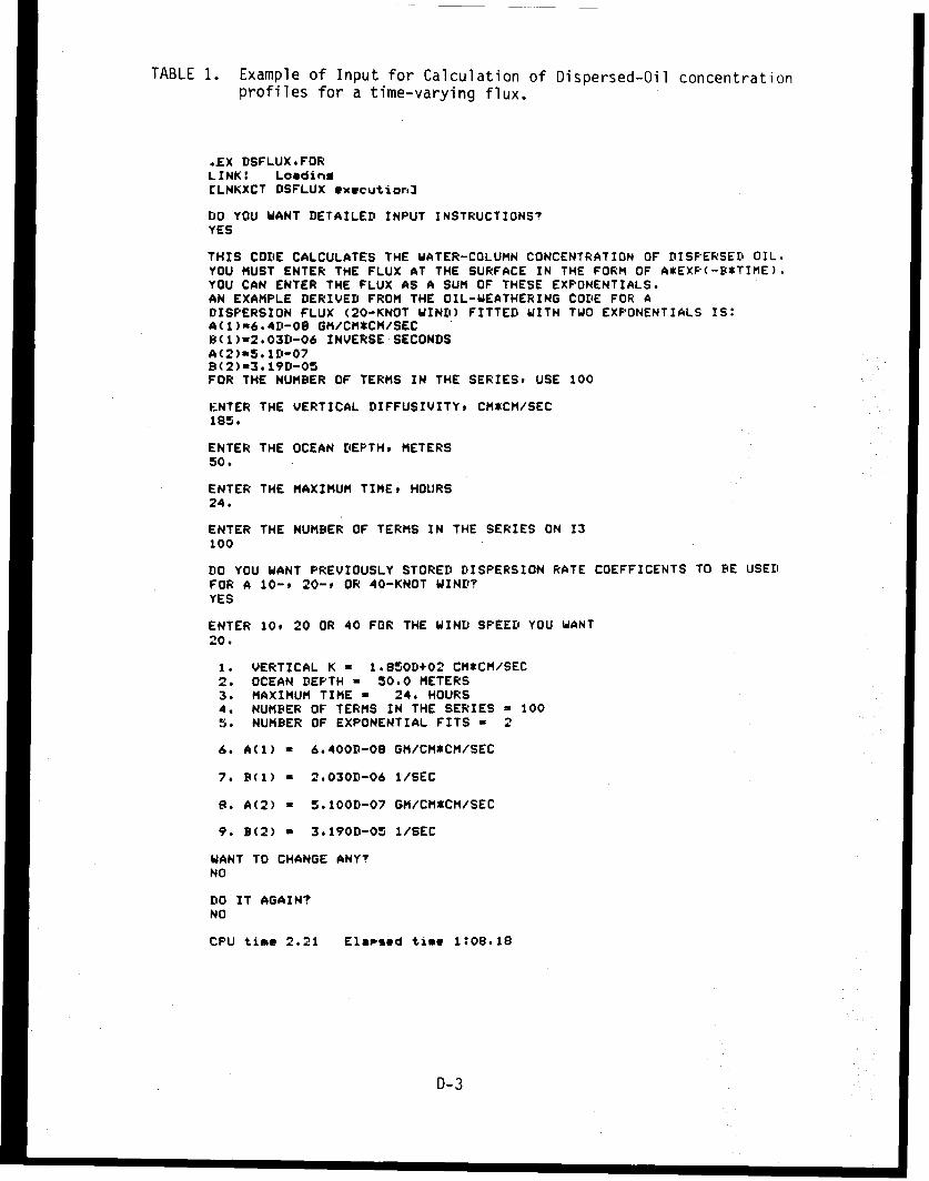
TABLE 1. Example of Input for Calculation of Dispersed-Oil concentrationprofiles for a time-varying flux.
.EX DSFLUX.FORLINK: LoadingCLNKXCT DSFLUX *xecution3
DO YOU WANT DETAILED INPUT INSTRUCTIONS?YES
THIS CODE CALCULATES THE WATER-COLUMN CONCENTRATION OF DISPERSED OIL.YOU MUST ENTER THE FLUX AT THE SURFACE IN THE FORM OF A*EXP(-B*TIME).YOU CAN ENTER THE FLUX AS A SUM OF THESE EXPONENTIALS.AN EXAMPLE DERIVED FROM THE OIL-WEATHERING CODE FOR ADISPERSION FLUX (20-KNOT WIND) FITTED WITH TWO EXPONENTIALS IS:A(1)a6.4D-08 GM/CM*CM/SECB(1)-2.03D-06 INVERSE SECONDSA(2)"S.ID-07B(2)n3.19D-05FOR THE NUMBER OF TERMS IN THE SERIES. USE 100
ENTER THE VERTICAL DIFFUSIVITY. CM*CM/SEC185.
ENTER THE OCEAN DEPTH, METERS50.
ENTER THE MAXIMUM TIME, HOURS24.
ENTER THE NUMBER OF TERMS IN THE SERIES ON 13100
DO YOU WANT PREVIOUSLY STORED DISPERSION RATE COEFFICENTS TO BE USEDFOR A 10-» 20-, OR 40-KNOT WIND?YES
ENTER 10, 20 OR 40 FOR THE WIND SPEED YOU WANT20.
1. VERTICAL K - 1.850D+02 CM*CM/SEC2. OCEAN DEPTH - 50.0 METERS3. MAXIMUM TIME - 24. HOURS4. NUMBER OF TERMS IN THE SERIES = 1005. NUMBER OF EXPONENTIAL FITS - 2
6. A(1) * 6.400D-08 GM/CM*CM/SEC
7. B(1) - 2.030D-06 1/SEC
8. A(2) - 5.100D-07 GM/CM*CM/SEC
9. B(2) 3 3.190D-05 1/SEC
WANT TO CHANGE ANY?NO
DO IT AGAIN?NO
CPU time 2.21 Elapsed time 1:08.18
D-3
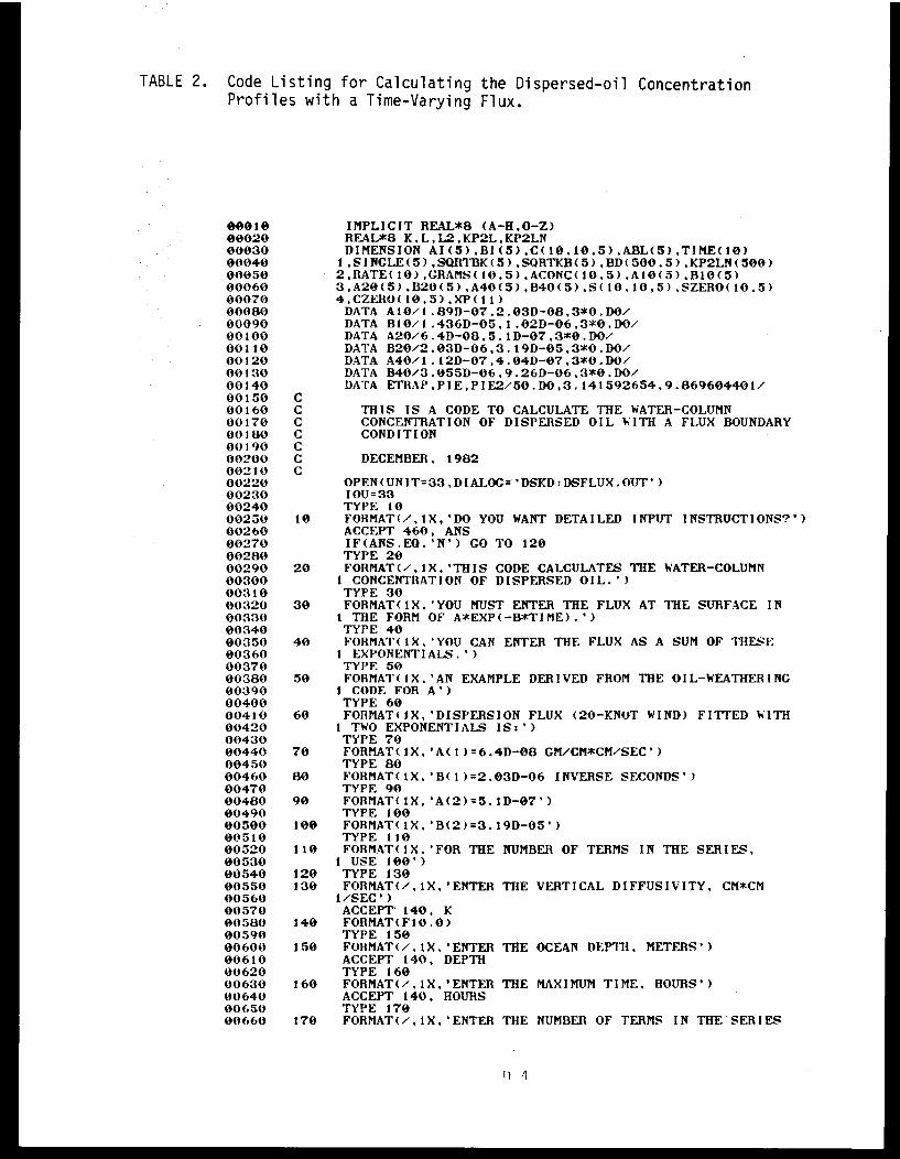
TABLE 2. Code Listing for Calculating the Dispersed-oil ConcentrationProfiles with a Time-Varying Flux.
D1

TABLE 2. (Continued)
D-5
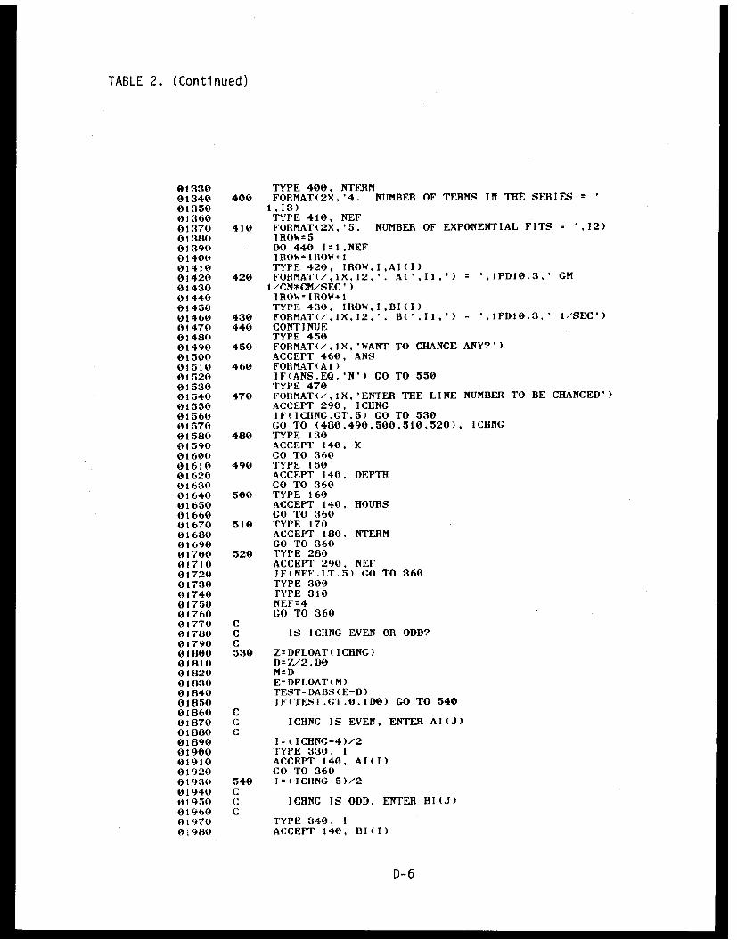
TABLE 2. (Continued)
D-6
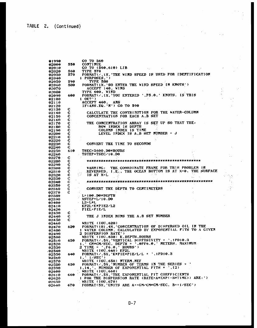
TABLE 2. (Continued)
D-7
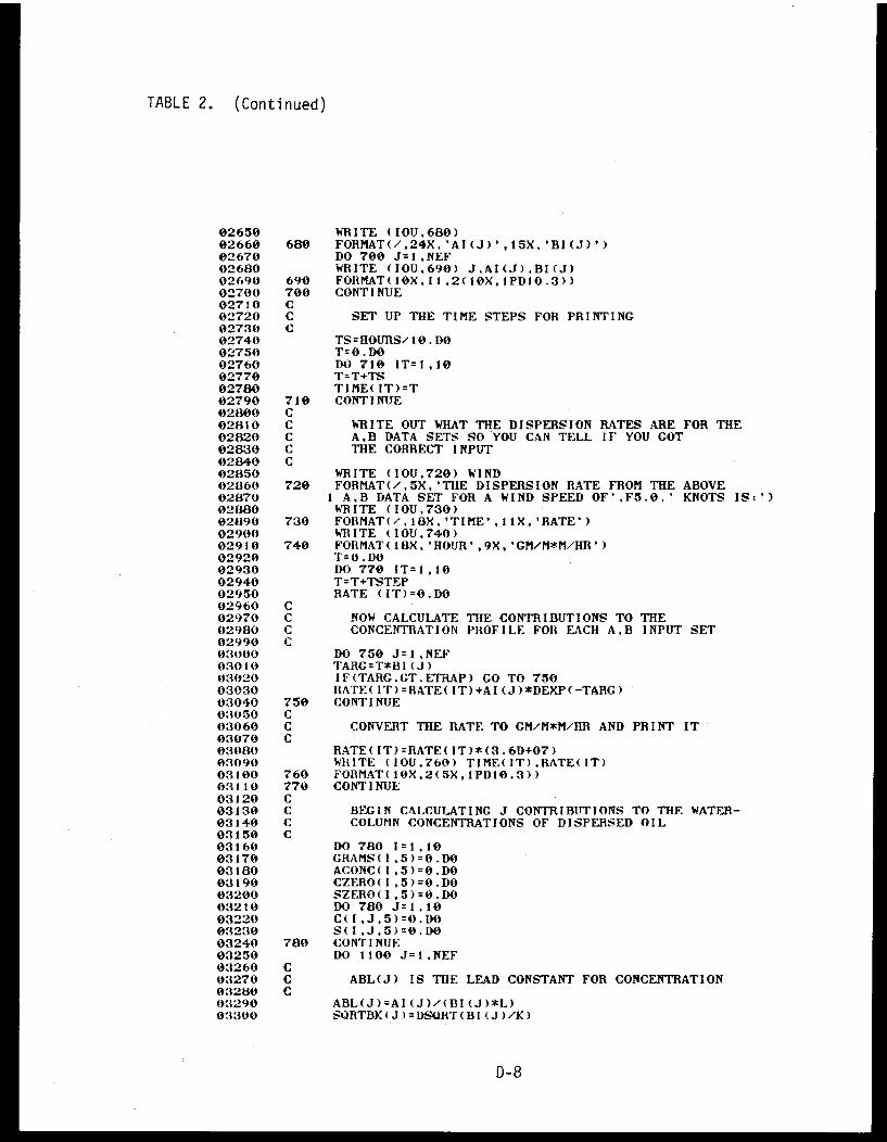
TABLE 2. (Continued)
D-8
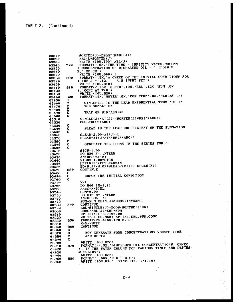
TABLE 2. (Continued)
D-9
TABLE 2. (Continued)
D-10
TABLE 2 . (Continued)
D-11
TABLE 2. (Continued)
D-12
APPENDIX E
CODE LISTING FOR DISPERSED-OIL CONCENTRATIONPROFILES WITH A CONSTANT FLUX
E-1
The computer code listing and user's instructions in this Appendix
are for the calculation of dispersed-oil concentrations in the water column
for a constant flux (Section 4.9). The user's instructions presented in the
following example prompt the user for specific input.
E-2
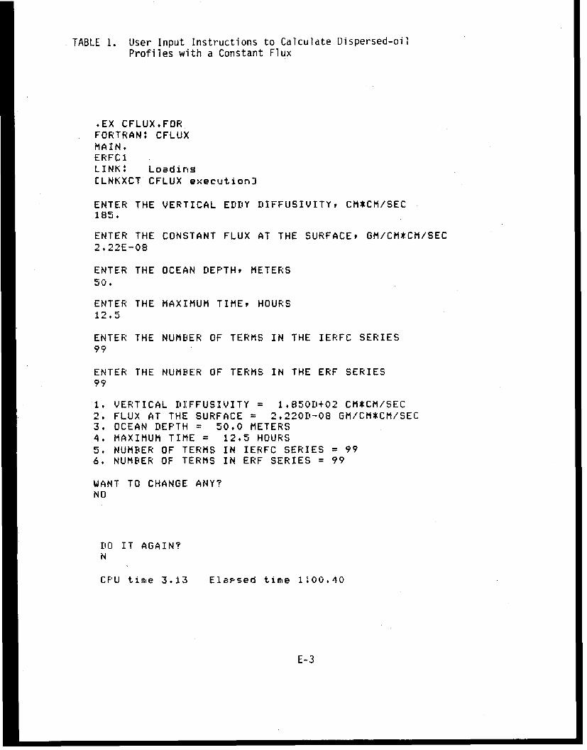
TABLE 1. User Input Instructions to Calculate Dispersed-oilProfiles with a Constant Flux
.EX CFLUX.FORFORTRAN: CFLUXMAIN,ERFC1LINK: Loadins[LNKXCT CFLUX execution]
ENTER THE VERTICAL EDDY DIFFUSIVITY, CM*CM/SEC185,
ENTER THE CONSTANT FLUX AT THE SURFACE, GM/CM*CM/SEC2.22E-08
ENTER THE OCEAN DEPTH, METERS50.
ENTER THE MAXIMUM TIME, HOURS12.5
ENTER THE NUMBER OF TERMS IN THE IERFC SERIES99
ENTER THE NUMBER OF TERMS IN THE ERF SERIES99
1. VERTICAL DIFFUSIVITY = 1.850D+02 CM*CM/SEC2. FLUX AT THE SURFACE = 2.220D-08 GM/CM*CM/SEC3. OCEAN DEPTH = 50.0 METERS4. MAXIMUM TIME = 12.5 HOURS5. NUMBER OF TERMS IN IERFC SERIES = 996. NUMBER OF TERMS IN ERF SERIES = 99
WANT TO CHANGE ANY?NO
DO IT AGAIN?N
CPU time 3.13 ElaPsed time 1 00.40
E-3
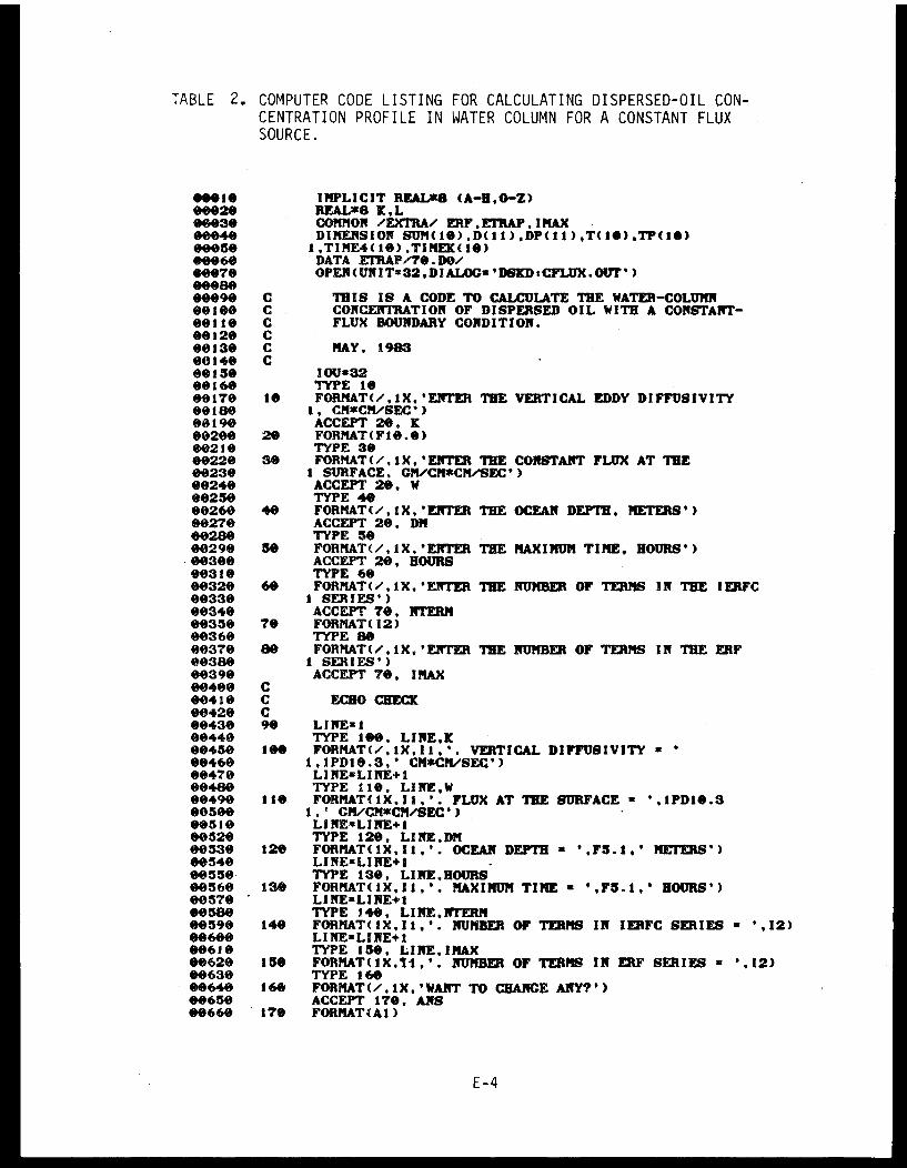
TABLE 2. COMPUTER CODE LISTING FOR CALCULATING DISPERSED-OIL CON-CENTRATION PROFILE IN WATER COLUMN FOR A CONSTANT FLUXSOURCE.
E-4
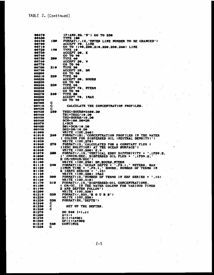
TABLE 2. (Continued)
E-5
TABLE 2. (Continued)
E-6
TABLE 2. (Continued)
E-7

I
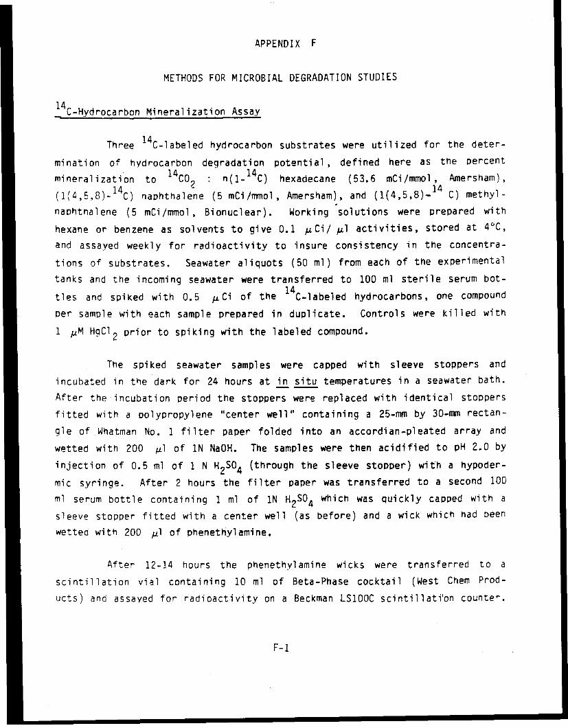
APPENDIX F
METHODS FOR MICROBIAL DEGRADATION STUDIES
14C-Hydrocarbon Mineralization Assay
Three 14C-labeled hydrocarbon substrates were utilized for the deter-
mination of hydrocarbon degradation potential, defined here as the percent
14 14mineralization to 14CO : n(l- 4C) hexadecane (53.6 mCi/mmol, Amersham),(1(4,5,8)-14C) naphthalene (5 mCi/mmol, Amersham), and (1(4,5,8)- 14 C) methyl-
naphthalene (5 mCi/mmol, Bionuclear). Working solutions were prepared with
hexane or benzene as solvents to give 0.1 /Ci/ A1 activities, stored at 4°C,
and assayed weekly for radioactivity to insure consistency in the concentra-
tions of substrates. Seawater aliquots (50 ml) from each of the experimental
tanks and the incoming seawater were transferred to 100 ml sterile serum bot-
tles and spiked with 0.5 L Ci of the 1C-labeled hydrocarbons, one compound
per sample with each sample prepared in duplicate. Controls were killed with
1 MM HgC1 2 prior to spiking with the labeled compound.
The spiked seawater samples were capped with sleeve stoppers and
incubated in the dark for 24 hours at in situ temperatures in a seawater bath.
After the incubation period the stoppers were replaced with identical stoppers
fitted with a polypropylene "center well" containing a 25-mm by 30-mm rectan-
gle of Whatman No. 1 filter paper folded into an accordian-pleated array and
wetted with 200 il of 1N NaOH. The samples were then acidified to pH 2.0 by
injection of 0.5 ml of 1 N H2S04 (through the sleeve stopper) with a hypoder-
mic syringe. After 2 hours the filter paper was transferred to a second 100
ml serum bottle containing 1 ml of IN H2S04 which was quickly capped with a
sleeve stopper fitted with a center well (as before) and a wick which had been
wetted with 200 ul of phenethylamine.
After 12-14 hours the phenethylamine wicks were transferred to a
scintillation vial containing 10 ml of Beta-Phase cocktail (West Chem Prod-
ucts) and assayed for radioactivity on a Beckman LS100C scintillation counter.
F-1
The resulting counts for duplicates were averaged and corrected for the con-
trol counts prior to further data treatment. The data (in counts per minute)
were converted to uq/liter.day by the following equation.
I )( 1 _ VS A 3-w)(10 00 ml( 1 )(-)
* ^(0.9 CMcpI2.22 x 10 dpm day)
where a counting efficiency of 90% was utilized, SA is the specific activity
in uCi,/ mole, and M.W. is the molecular weight of the particular labeled sub-
strate.
References: WATSON et al. (1971); CAPARELLO and LA ROCK (1975); WALKER and
COLWELL (1976); HODSON et al. (1977).
H-Thymidine Incorporation
Thymidine (methyl-3H) solutions were stored as supplied (20 Ci/mmol,
New England Nuclear) in 70% aqueous ethanol for maximum stability. Working
solutions were prepared by evaporating to dryness the appropriate volume under
a stream of dry filtered air and reconstituting with distilled water. These
solutions were stored at 4°C and checked weekly for radioactivity.
Duplicate seawater aliquots (10 ml) from each experimental aquarium
and the incoming seawater were spiked with 5nM of labeled thymidine and incu-
bated in the dark at in situ temperatures for 1 hour. Incubation uptake was
terminated by filtration through a 25-mm dia. type HA membrane (0.45 lzm nomi-
nal pore size, Millipore Corp.). After filtration the vacuum was stopped and
10 ml of ice-cold (< 5°C) filtered (sterile) seawater was added to cool the
filter. This was filtered through and the vacuum was stopped prior to addi-
tion of 15 ml ice-cold (< 5°C) 5% trichloroacetic acid (TCA) to extract the
soluble thymidine pools from the cells. Temperature control is critical dur-
inq the extraction as a temperature rise above 10°C for TCA will hydrolyse DNA
and allow incorporated label to solubilize and pass through the filter. After
F-2
3 min. the vacuum was started and the filter was rinsed twice with -5 ml ice-
cold 5%, TCA, and then placed in a scintillation vial. Ethyl acetate (1 ml)
was added to dissolve the filter; 10 ml of Beta-Phase cocktail was added andthe radioactivity was assayed by liquid scintillation spectrometry.
The resulting counts for duplicates were averaged and corrected for
poisoned controls (1 ALM HgC1 2) and a counting efficiency of 35%. The data
were converted to nmoles/liter day of incorporation by the formula:
,».a , ( / 1 dpm I C_1 n1 M mo1\/10 6 n mio1\/24 hr\I1
n moles/C-day = cpm ( I)(- X )(-1 --- )(- )(-)( 1 )( h)0.35 cpm /\2.22 x 1012 dpm/\ 20 Ci m mol day o.015t hr
References: FUHRMAN and AZAM (1980); FUHRMAN et al. (1980); FUHRMAN and AZAM
(in Dress, 1981)
3 3H-Leucine and H-Glucose Uptake
The procedure for both substrates was identical except for the amino
acid leucine, in that a larger sample was prepared such that an aliquot could
be saved and preserved for the autoradiography procedure (details in thissection).
Working solutions of 3H-Leucine (60 Ci/mmol, New England Nuclear)
were prepared by diluting an aliquot of the stock solution into distilledwater. The 3H-Glucose solutions (30 Ci/mmol, New England Nuclear) were pre-
pared by evaporating an aliquot under a stream of dry, filtered air followed
by reconstitution in distilled water. All solutions were stored at 4°C and
assayed weekly for radioactivity to check stability.
F-3
Each experimental aquarium and the incoming seawater was sampled in
duplicate and controls were k lled with 1 M HgCl2 prior to addition of radio-
labeled substrate. To each sample (10 ml for 3H-Glucose; 15 ml for 3H-
Leucine) 50 l1 (1.5 ACi) of rad/iolabeled compound was added, followed by
incubation for 2 hr. in the dark at in situ temperature.
The incubation was terminated by sample filtration through a HA mem-
brane (0.45 um nominal pore size, Millipore Corp.), followed by several
washes with filter-sterilized seawater to remove any nonincorporated label.
After filtration, each filter was placed in a scintillation vial, and 1 ml
Ethyl acetate added to dissolve the membrane. After approximately 10 min., 10
ml of Beta-Phase cocktail was added and the sample assayed for radioactivity
by liquid scintillation spectrometry. Duplicates were averaged and corrected
for control blanks, and the resulting counts were converted to uptake in
nmoles/liter day with the formula:
n / day = (cp) ()(106n mo1 (24 hr\( 1 ) ( 1 Imole=/ day \) 0.35 cpm 2.22 x 10¹² x dpm m Aol day 12 hr.
where a counting efficiency of 35% was utilized and S.A. is the specific activ-
ity (in Ci/mmol) for the labeled substrate.
References: AZAM and HOLM-HANSEN (1973); FUHRMAN et al. (1980).
Epifluorescence Enumeration
Seawater samples (10-15 ml) from each experimental aquarium and the
incoming seawater were immediately preserved with 4% filter-sterilized forma-
lin (buffered with Na2B407), and the cellular DNA was stained to fluoresce
with Acridine orange (0.01%, 2 min.) prior to filtration. The Nucleopore
polycarbonate filters were stained prior to use with Irgalan black (to
eliminate autofluorescence) and a type AA (0.8 /Am, Millipore) membrane was
F-4
used as a back filter to distribute the vacuum evenly. After filtration, the
filter was mounted on a microscope slide with a cover slip affixed with paraf-
fin oil. Blanks were preoared in a similar fashion except that filter-
sterilized seawater (GS, 0.2 um, Millipore Corp.) was preserved and stained.
The slides were examined by epifluorescence microscopy and counted in
a random fashion by grids. All counts for each grid were averaged (10 grids
per slide) for duplicate slides and the data converted to cells x 10 /ml sea-water.
References: HOBBIE et al. (1977); FUHRMAN and AZAM (1980).
Autoradioqraohy Assay
The micro-autoradioqraphic technique provides for simultaneous examin-
ation by phase contrast microscopy of bacterial cells stained with acridineorange and labeled with developed silver grains. The method of preparation
provides for orientation of bacteria between the photographic emulsion and themicroscope objective to prevent visual Interference by the silver grains.
The 5 ml aliquots from the 3H-leucine uptake assays (preserved with
4% formalin) were stained with sterile-filtered 0.01% acridine orange for 1
min., followed by filtration through a 0.2 Am pore size nucleospore membrane
(25 mm dia.). A type AA filter (0.8 gm, Millipore) was used as a back filter
for even vacuum distribution. The filter was rinsed with sterile, filtered,
distilled water, and kept damp for subsequent transfer of cells onto the sur-
face of a mounted gelatin-coated coverslip. (Details of the gelatin-coated
coverslip preparation are presented elsewhere - see References below).
Resulting autoradiograms were prepared in total darkness with KodakNTB2 Nuclear track emulsion coating, dried, and exposed at 4°C. After the
appropriate exposure time, the autoradiograms were developed, fixed and fur-ther prepared as detailed elsewhere (see References below). Bacteria were
F-5
counted by epifluorescence microscopy and silver gain clusters were counted by
transmitted phase con rast microscopy.
References: MEYER-REIL (1978); FUHRMAN and AZAM (in press, 1981).
F-6
METHODS FOR HYDROCARBON ANALYSES AND PHOTOCHEMICAL/MICROBIAL
OXIDATION PRODUCT CHARACTERIZATION
Volatile Hydrocarbon Analyses
Volatile hydrocarbons are sampled from the air above the slick in the
evaooration/dissolution chamber (or the flow-through outdoor tanks in Alaska)
by vacuum-pumping measured volumes of air through 1/8 in. ID x 12 in. long
stainless tubes packed with Tenax® GC polymer. For each sample, two tubes are
connected in series with Swagelok fittings, and prior to and immediately after
sampling, all tubes are sealed with Swagelok endcaps and plugs. Sampling is
achieved by use of a Gast Mfg. Corp. vacuum pump attached to the Tenax® traps
via flow regulators and flexible Teflon tubing. Air velocities above the
slick in the evaporation/dissolution chamber are measured with a Kurz air
velocity meter 4m above the oil/seawater interface.
Before each sample is obtained, the Tenax® trap's flow velocity is
checked with a bubble flow meter. ' Approximately 60 second samples are
generally obtained at flow rates ranging from 20 to 30 ml/min; thus, sample
volumes ranged from 20-30 ml.
Water samples for analysis of dissolved lower-molecular-weight
aliphatic and aromatic hydrocarbons are taken in Pierce septum-capped vials
for subsequent purge and trap analysis by GC/MS techniques similar to those
developed by Bellar and Lichtenberg (1974) and others.
Following collection, the water samples are refrigerated (no preserva-
tives are added), and they are maintained at 3°C until analysis. Capped
stainless-steel Tenax® traps are stored at ambient temperature until analysis.
The Tenax® air samples are analyzed by heat desorption followed by
Flame Ionization Detector (FID) qas chromatography on a Hewlett Packard 57330A
F-7
instrument or gas chromatography/mass spectrometry (GC/MS) using a Finnigan
4021 quadrupo'e instrument. The heat desorption is accomplished by installing
the Tenaxa traps in a Tekmar liquid sample concentrator (LSC-2) interfaced to
the injection port system of either the FID GC or GC/MS (PAYNE et al., 1980b).
At the time of desorption (5 min. at 180°C at 20 ml/min He flow) the
gas chromatographic column (packed 6 ft. x 22 mm I.D. SP-1000) and oven are
cryogenically cooled to 30°C. Following desorption, the oven is programmed
rapidly (30°C/min) to 100°C and then from 100°C to 200°C at 10°C/min. The
final temperature of 200°C is held for the duration of the chromatographic
run. A GC column flow rate of 20 ml/min He is also used and the injector
temperature is held at 200°C.
The effluent from the gas chromatograph is then analyzed by FID on
the HP-GC or it is passed through a glass jet separator for enrichment and
then directly into the ion source of the GC/MS (operated in the electron
impact-mode at 300°C). Spectra are acquired by operating the ion source at
70eV from 35 to 300 amu in 1.95 sec. A hold time of 0.05 sec is used to allow
the electronics to stabilize before the next scan. The ion source is tuned
for maximum sensitivity with perfluorotributylamine and the ion fragments at
m/e 69- and m/e 219 are calibrated to give a 2.5:1 ratio; the electron multi-
plier is ooerated at 1600V with the preamplifier gain at 10 amps/volt.
GC/MS data acquisition is initiated at the moment of desorption. Typically,
900-1000 scans are acquired for each data file.
The water samples stored in Pierce vials are allowed to come to room
temperature and 5-mi aliquots are withdrawn and injected into the purge device
of the LSC-2. Before purging in mass spectrometry operations, 100 ng each ofthree internal standards, dichiorobutane (m/e 55), bromochloromethane (m/e
130), and bromochloropropane (m/e 77) are added. This allows correction ofrecovered values for matrix effects and corrects for differences in ionization
Dotential, lens voltage, etc., among runs. Instrumental conditions are
identical to those described for Tenax® column analysis.
F-8
Before analyses with either instrument, response factors are deter-mined for 0-12 target aliphatic and aromatic compounds of interest by spikingSeveral known mixed standards into salt water blanks which are then analyzedas samples (PAYNE et al., 1980b).
Higher Molecular Weight Petroleum Hydrocarbon Analyses
Water sediment and oil/mousse samples are analyzed by procedureswhich basically involve: 1) extraction, 2) fractionation into aliphatic,
aromatic and polar constituents by liquid/solid (Si0 2) column chromatographyand analysis by FID capillary gas chromatrography and capillary gas
chromatography/mass spectrometry. Specific details with regard to theseanalytical procedures (including instrument calibrations, sensitivity, datareduction, etc.) are presented in Appendix H to this report (Methods Section,Page 4 of "Chemical Weathering of Petroleum Hydrocarbons in Sub-Artic Sedi-
ments: Results of Chemical Analyses of Naturally Weathered Sediment PlotsSpiked with Fresh and Artificially Weathered Cook Inlet Crude Oil").
Water samples from the flow-thtrough seawater systems are collected in20-liter carboys and pH was adjusted to 2.0. Three hundred-fifty ml of meth-ylene chloride is then added to each carboy (approximately 200 ml of methylenechloride goes into solution on the first addition).and the mixture is stirredvigorously for 3 minutes. The methylene chloride is removed by pressurizingthe carboys with N2 and forcing the methylene chloride through a stainless
steel syphon tube into a separatory funnel. This procedure is repeated twomore times. The methylene chloride extract is concentrated to 100 ml in K-Dconcentrators and then passed through sodium sulfate to remove the residualwater. The anhydrous methylene chloride extract is then concentrated to 2 ml
and solvent-exchanged to hexane. The concentrate is then fractionated onsilica gel using the three fraction schemes described in Appendix H, page 4 of"Chemical Weathering of Petroleum Hydrocarbons in Sub-Artic Sediments: Re-sults of Chemical Analyses of Naturally Weathered Sediment Parts Spiked withFresh and Artificially Weathered Cook Inlet Crude Oil".
F-9

I
APPENDIX G
THE X-RAY DIFFRACTION ANALYSIS OF NINE SEDIMENT SAMPLES
Report Submitted to:
James R. PayneScience Applications, Inc.
La Jolla, CA 92037
March 15, 1983
by:
Technology of Materials
Santa Barbara, CA 93103
G-1
INTRODUCTION
Nine sediment samples were received in the laboratory for X-ray
diffraction analysis. Of particular interest was the characterization
of possible clay types and other mineral identification. The following
report represents the results of the studies and is submitted
respectfully.
SAMPLES
Samples were received with the following identifications:
BULK SAMPLES:
K-Bay Site #1 OW-1 ( b(&r¢ ,ik 6lJ* SpJ)
K-Bay Site #2 OW-2 ( Ck"J Po ' Bg)
K-Bay Site #3 OW-3 ( 4i';Jt By)
K-Bay Site #4 OW-4 (l ' EAR
K-Bay Site #5 OW-5 ( Ack Lh BP^/)
Glacial Till OW-7 ( J
FILTER SAMPLES:
1M ( iKA,4' JA SP PA
2M ( .ldou, 8- Y ' )
6M ( Gl A' ̂ ,' .S/: )
SAMPLE PREPARATION AND STUDY METHODS
Aliquotes of each sample were first very lightly ground to break up
agglomerates. Care was taken to not break down the larger particals.
G-2
By using a combination of washing, seiving and centritugation, the
fraction faalling below 50 microns was separated for the studies.
After drying, the powders were packed into standard sample holders and
run in a Philips Electronics X-ray diffractometer equipped with a
crystal monochrometer. The operating conditions are marked on the
enclosed X-ray diffraction charts. The filter samples were studied
without further treatment by placing the filters across the openings
of a sample holder.
In order to further identify the clay fractions, several other
techniques were utilized on the bulk specimens where there was a
sufficient quantity of fine material. Using gravometric separation of
a clay suspension in water, the heavy fraction was allowed to settle
out and the light suspension was then decanted and concentrated by
centrifugation. This light fraction was reslurried and allowed to
settle on a microscope slide, forming an oriented mount with the clay
platelets tending to lie flat causing a stronger diffraction of the
clay (001) reflections. This mount was also run in the
diffractometer.
A portion of this fine (less than 3 micron) fraction was also studied
using long exposure Debye-Scherrer powder camera methods. Specific
tests for montmorillonite were also performed on a portion of the clay
which was heat treated to 350 degrees C to remove the absorbed water.
Portions of this heat treated clay were then subjected to ethylene
G-3
Page 3
glycol treatment. A separate portion was modified by strontium ion
exchange using strontium chloride. Both of these methods sharpen the
(001) diffraction peaks and shift them to a different d-spacing value
by interlayer expansion.
All three samples were found to contain measurable amounts of
carbonate minerals. The samples were therefore refined by leaching
out these carbonates using dilute hydrochloric acid. These treated
samples were neutralized, dried,and reweighed, then rerun in the X-ray
diffractometer.
DISCUSSION
The x-ray diffraction charts enclosed are marked with the interplanar
spacing measurements (d-spacings) in angstrom units and with the
corresponding Miller Index (hkl) of the crystallographic planes
causing each reflection. Phase identification was made by comparison
with standard data in the JCPDS/ASTM diffraction files.
All of the samples show quartz and feldspar to be the major
constituents, however some differences were encountered. Although
spectrochemical data was not obtained for the feldspar mineral, the
X-ray pattern is quite similar to that of Laboradorite, which is an
anorthite-albite rich feldspar mineral.
G-4
Page 4
Sample OW-2B shows a high calcite concentration (probably in the range
of 30-40 percent), while the other samples have little or none.
Traces of mica are found in many of the samples and a possible trace
of gypsum (calcium sulfate dihydrate) may be in OW-3. Certainity
cannot be placed on the identification of these trace phaces due to
lack of confirming reflections.
A summary of the diffraction data is presented in chart form on a
separate page. Rough quantitative approximations have been given as
follows:
Major........... over 50%
Intermediate +.......40-50%
Intermediate........20-40%
Intermediate -....... 10-20%..
Minor +...............5-10%
Minor................2-5%
Trace .............. less than 2%
The tests for expanding clays were negative. Sensitivity for this
clay type is variable depending upon the degree of crystallinity.
However it can be said to be present to less than 10%.
G-5
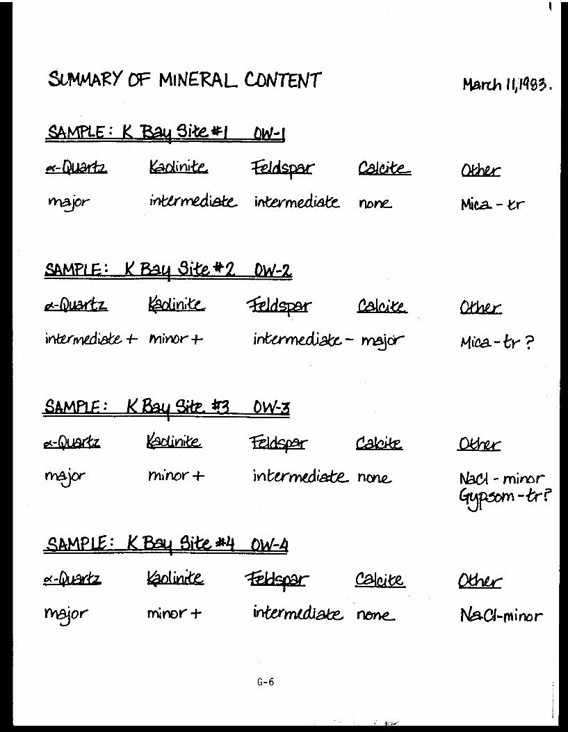
SUMMARY OF MINERAL CONTENT March 11,1983.
G-6
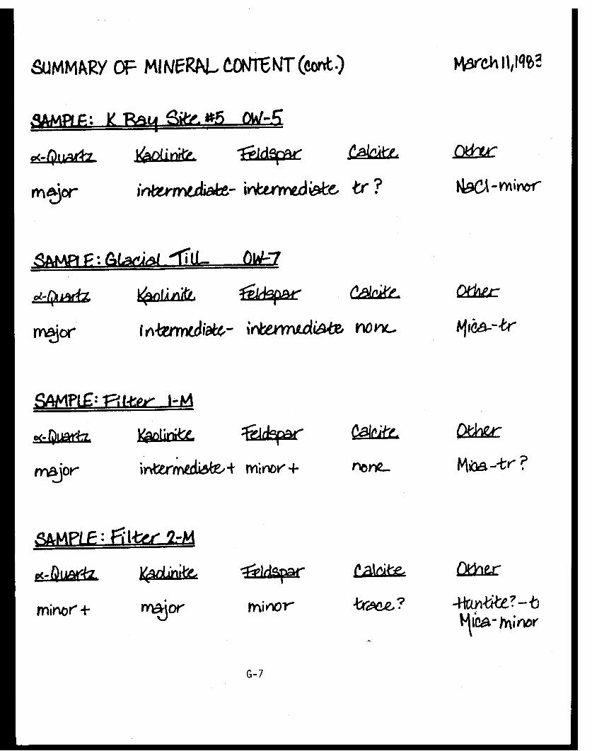
SUMMARY OF MINERAL CONTENT (cont.) March 11,1983
G-7
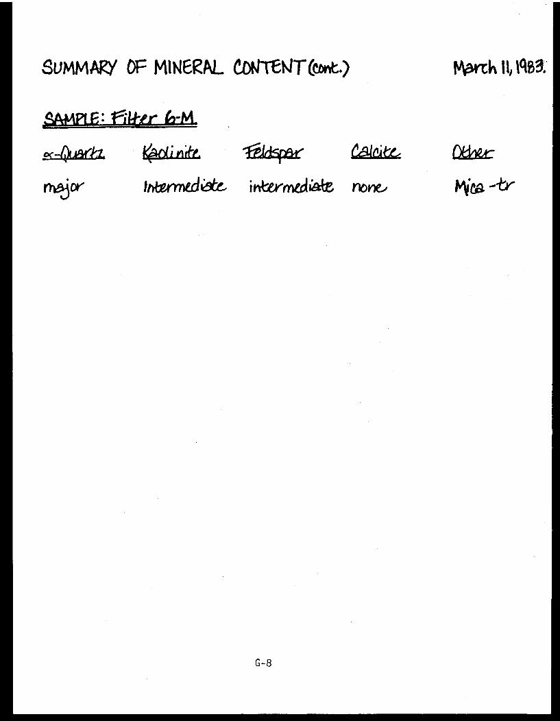
SUMMARY OF MINERAL CONTENT (cont.) March 11,1983.
G-8
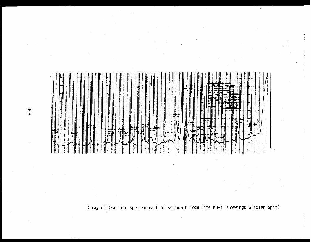
X-ray diffraction spectrograph of sediment from Site KB-1 (Grewingk Glacier Spit).
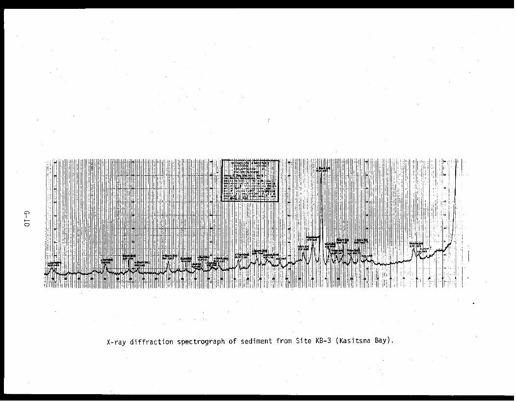
X-ray diffraction spectrograph of sediment from Site KB-3 (Kasitsna Bay).
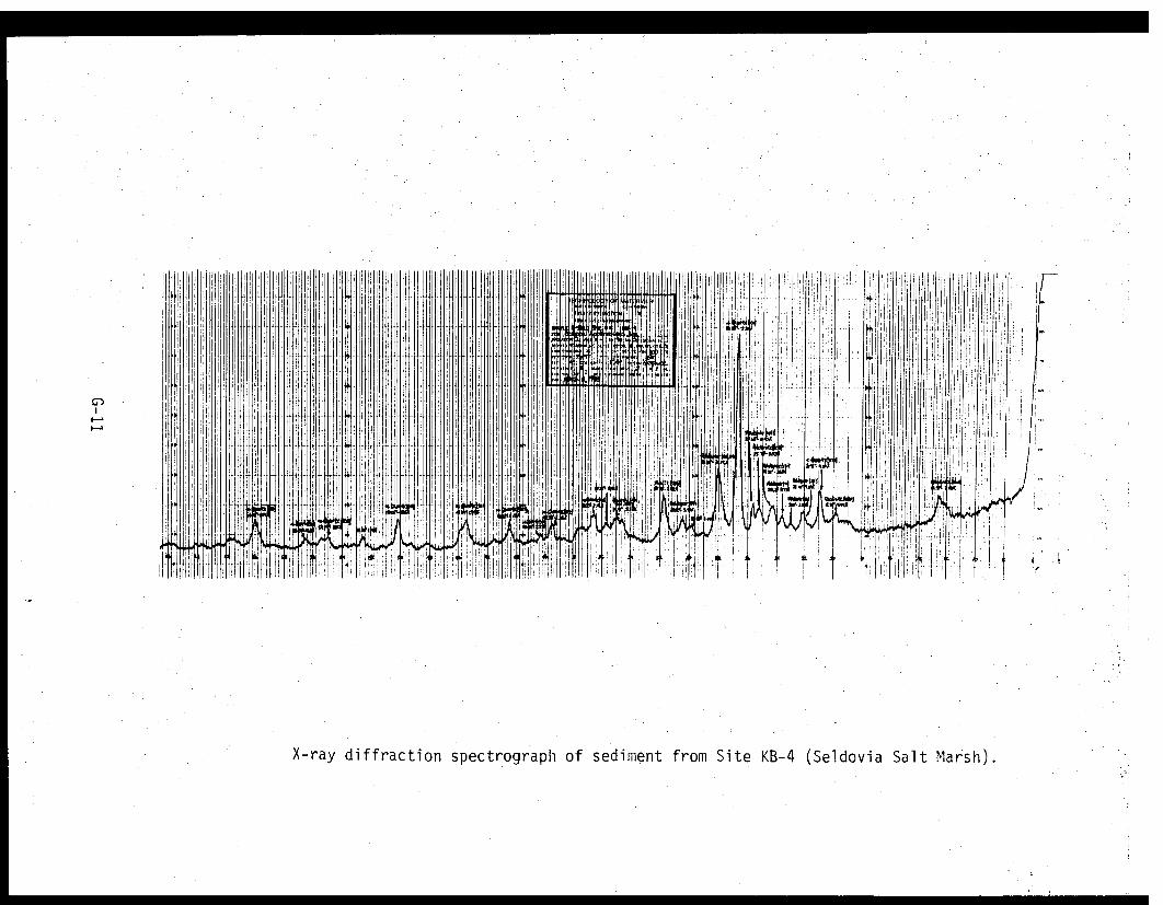
X-ray diffraction spectrograph of sediment from Site KB-4 (Seldovia Salt Marsh).
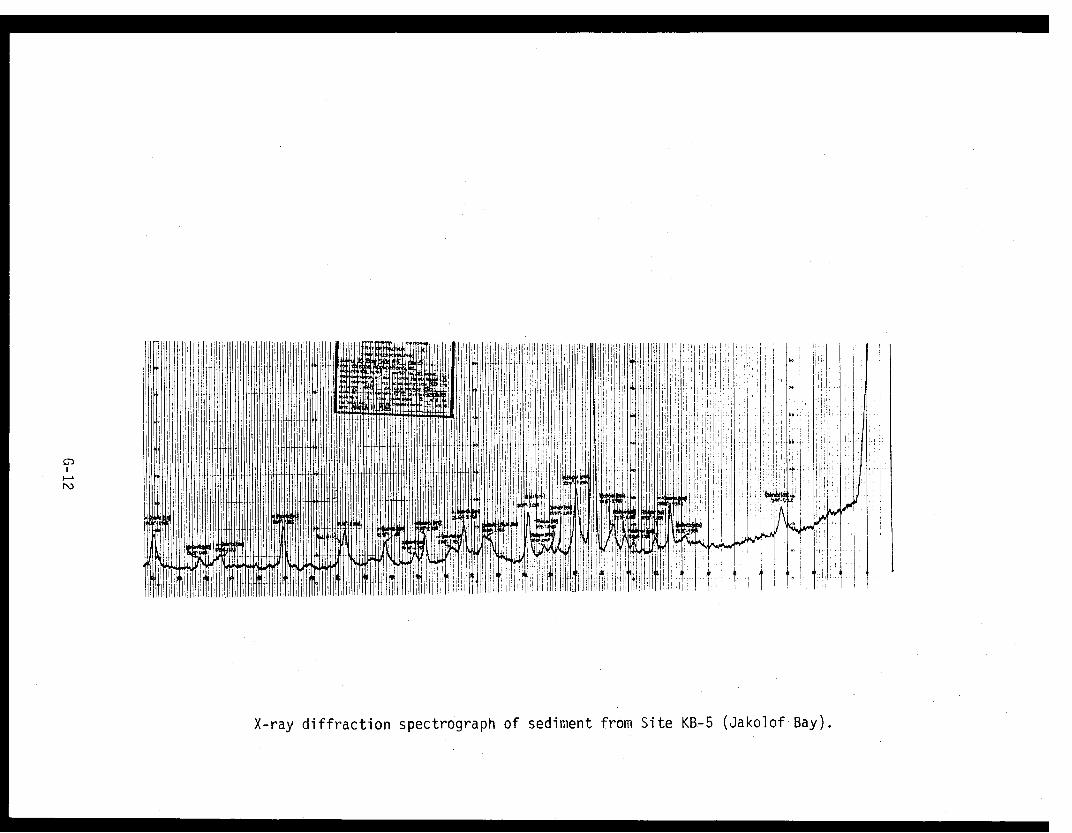
X-ray diffraction spectrograph of sediment from Site KB-5 (Jakolof Bay).
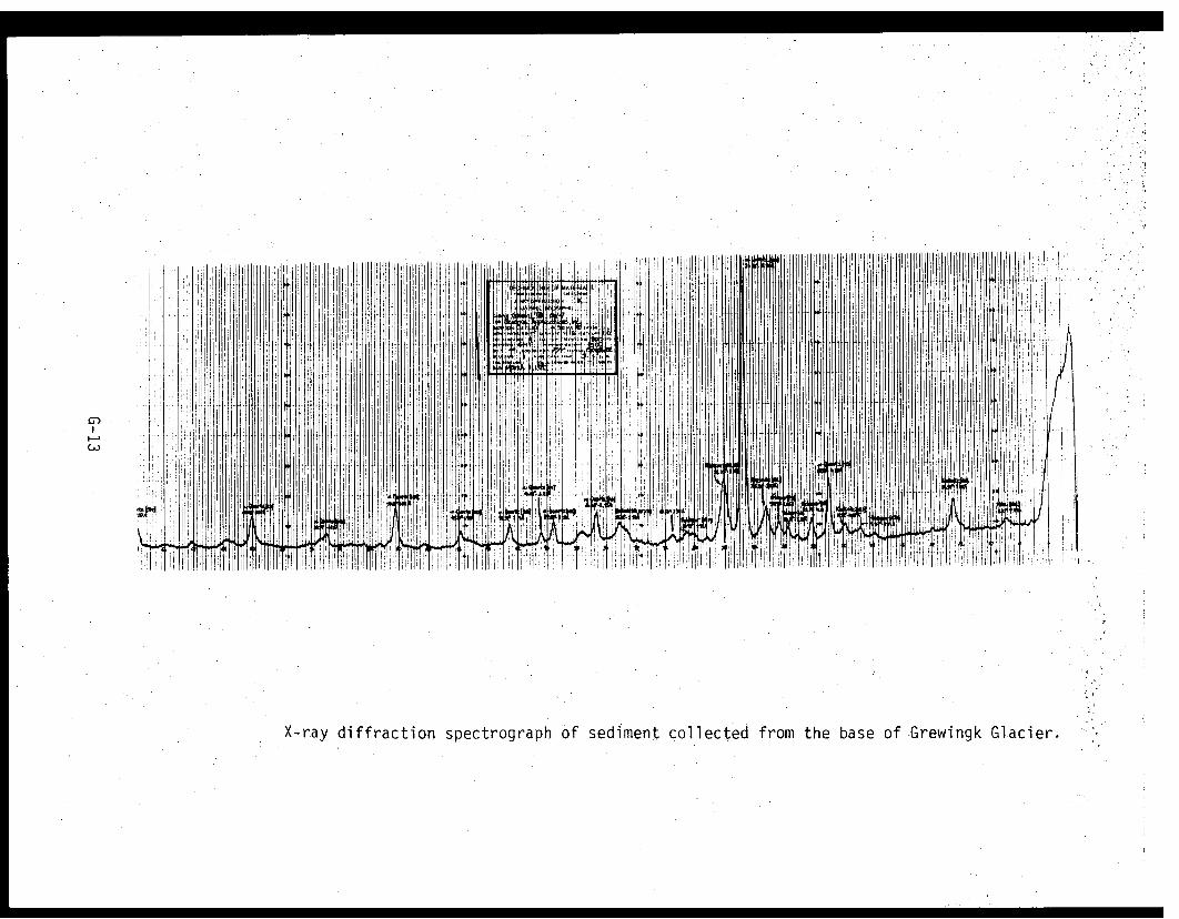
X-ray diffraction spectrograph of sediment collected from the base of Grewingk Glacier.
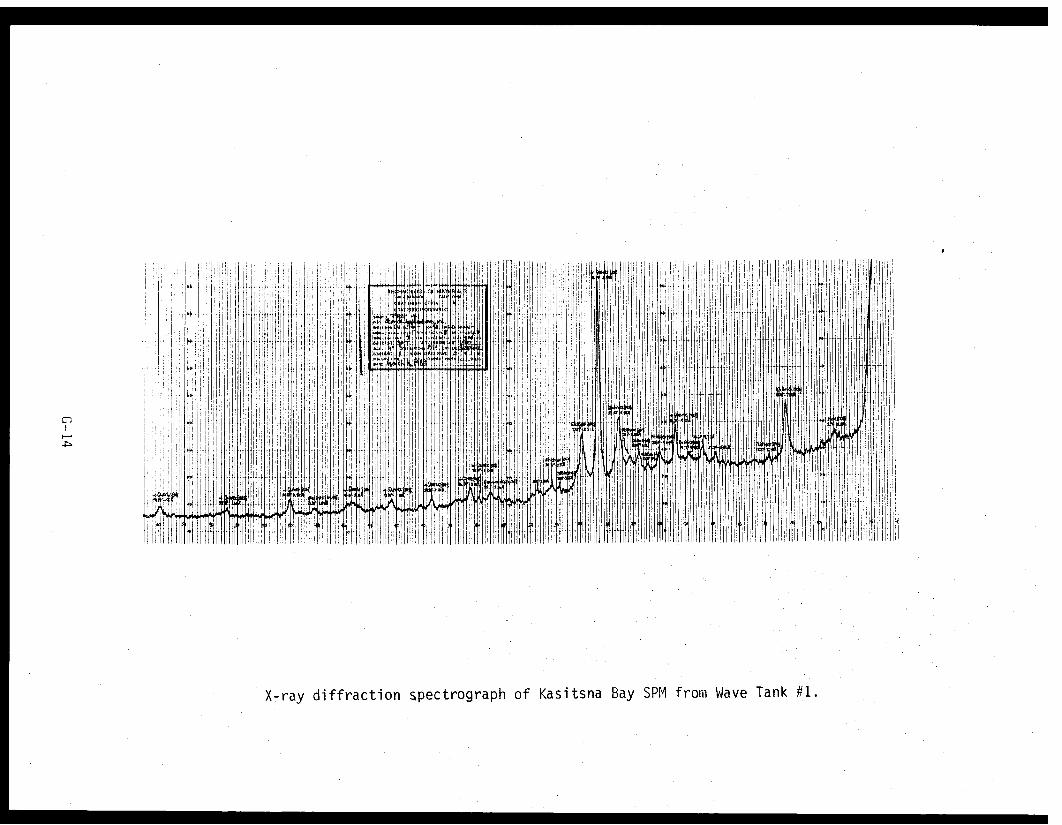
X-ray diffraction spectrograph of Kasitsna Bay SPM from Wave Tank #1.
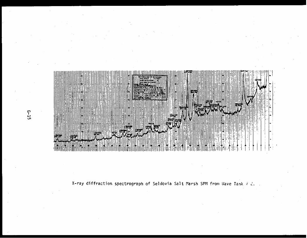
X-ray diffraction spectrograph of Seldovia Salt Marsh SPM from Wave Tank # 2.
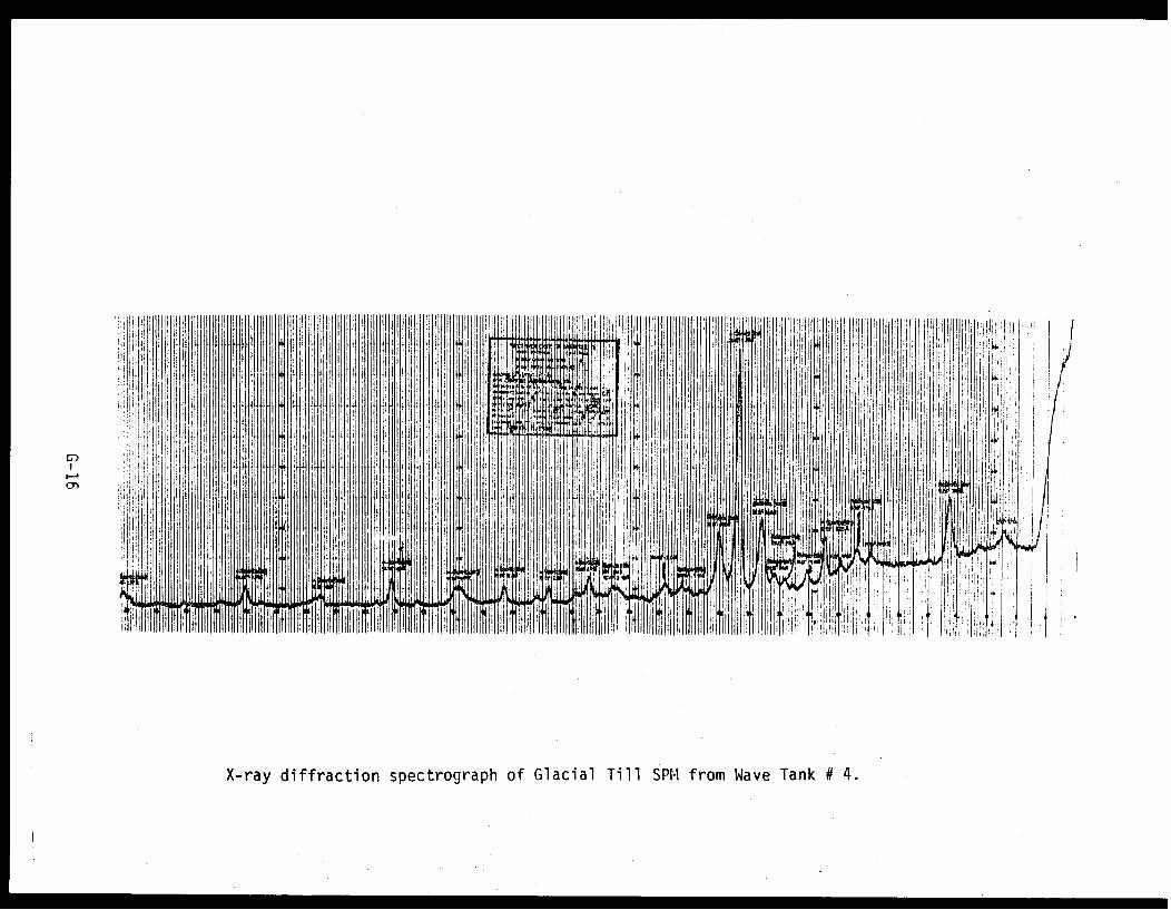
X-ray diffraction spectrograph of Glacial Till SPM from Wave Tank # 4.
APPENDIX H
CHEMICAL WEATHERING OF PETROLEUM HYDROCARBONS
IN SUB-ARCTIC SEDIMENTS: RESULTS OF CHEMICAL
ANALYSES OF NATURALLY WEATHERED SEDIMENT PLOTS
SPIKED WITH FRESH AND ARTIFICALLY WEATHERED
COOK INLET CRUDE OILS
H-1
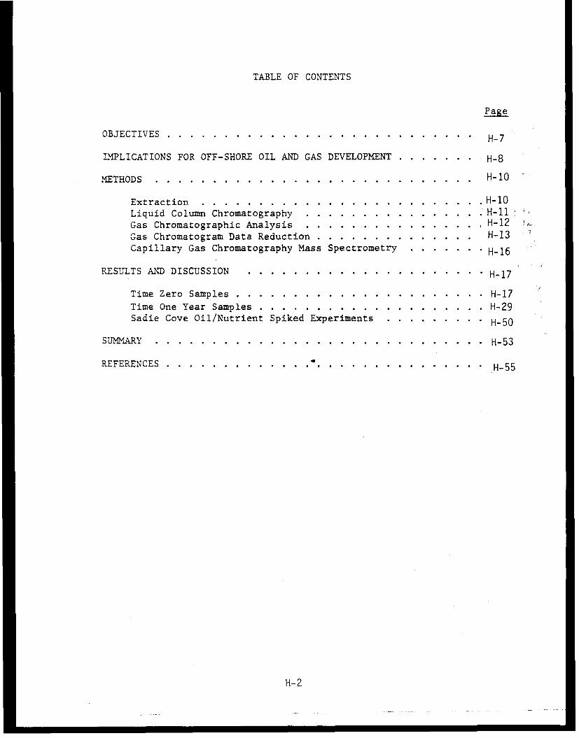
TABLE OF CONTENTS
Page
OBJECTIVES . . . . . . . . . . . . . . . . . . . . . . . . . .H-7
IMPLICATIONS FOR OFF-SHORE OIL AND GAS DEVELOPMENT . . . . . . . H-8
METHODS . . . . . . . . . . . . . . . . . . . . . . . . ......... H-10
Extraction .................. ..... ...H-10
Liquid Column Chromatography . . . . . . . . . . . . . . . ; H-llGas Chromatographic Analysis . . . . . . . . . . . . . . .. H-12Gas Chromatogram Data Reduction . . . . . . . . . . . ... . H-13Capillary Gas Chromatography Mass Spectrometry ....... H 16
RESULTS AND DISCUSSION ....................... H-17
Time Zero Samples ...................... H-17
Time One Year Samples . . . . . . . . . . . . . . . ... ... . H-29Sadie Cove Oil/Nutrient Spiked Experiments . . . . . . . .. .H-50
SUMMARY . .... . . . . . . . . . . ..... . ........ . . . . H-53
REFERENCES . . . . ......... .. . . . . . . . . . . . H-55
H-2
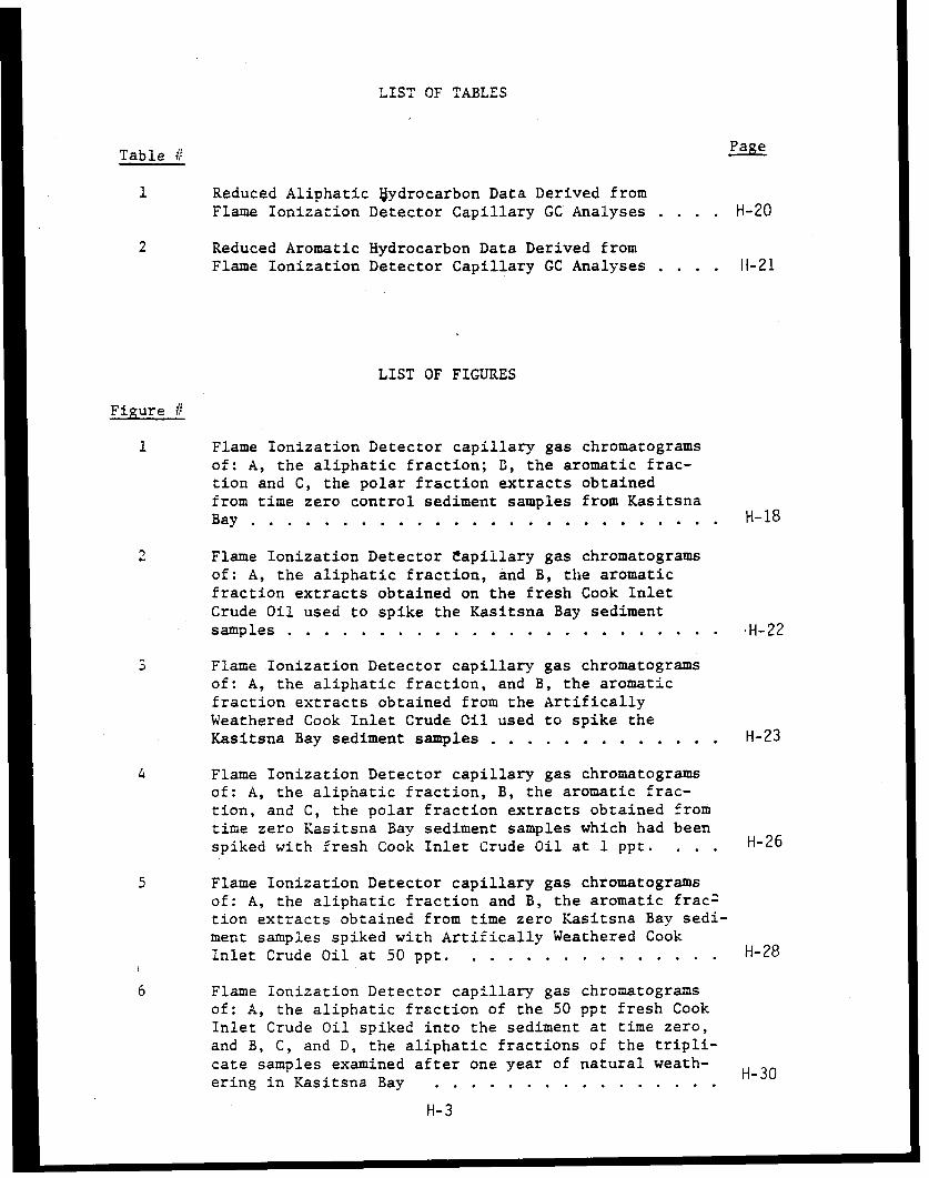
LIST OF TABLES
Table Pge
1 Reduced Aliphatic hydrocarbon Data Derived fromFlame Ionization Detector Capillary GC Analyses . . . . H-20
2 Reduced Aromatic Hydrocarbon Data Derived fromFlame Ionization Detector Capillary GC Analyses . . . 11-21
LIST OF FIGURES
Figure #
1 Flame Ionization Detector capillary gas chromatogramsof: A, the aliphatic fraction; B, the aromatic frac-tion and C, the polar fraction extracts obtainedfrom time zero control sediment samples from KasitsnaBay . .................. ....... H-18
2 Flame Ionization Detector Capillary gas chromatogramsof: A, the aliphatic fraction, and B, the aromaticfraction extracts obtained on the fresh Cook InletCrude Oil used to spike the Kasitsna Bay sedimentsamples . . . . . . . . . . . . . . . . ... .. .... . .H-22
S Flame Ionization Detector capillary gas chromatogramsof: A, the aliphatic fraction, and B, the aromaticfraction extracts obtained from the ArtificallyWeathered Cook Inlet Crude Oil used to spike theKasitsna Bay sediment samples . . . . . . . . . . ... . H-23
4 Flame Ionization Detector capillary gas chromatogramsof: A, the aliphatic fraction, B, the aromatic frac-tion, and C, the polar fraction extracts obtained fromtime zero Kasitsna Bay sediment samples which had beenspiked with fresh Cook Inlet Crude Oil at 1 ppt. .H-26
5 Flame Ionization Detector capillary gas chromatogramsof: A, the aliphatic fraction and B, the aromatic frac=tion extracts obtained from time zero Kasitsna Bay sedi-ment samples spiked with Artifically Weathered CookInlet Crude Oil at 50 ppt . . . . . . . . . . . . . . H-28
6 Flame Ionization Detector capillary gas chromatogramsof: A, the aliphatic fraction of the 50 ppt fresh CookInlet Crude Oil spiked into the sediment at time zero,and B, C, and D, the aliphatic fractions of the tripli-cate samples examined after one year of natural weath- H30ering in Kasitsna Bay ........
H-3
LIST OF FIGURES (CONTINUED)
Figure # Page
7 Concentration abundance of the n-alkanes in a sedi-ment sample spiked with 50 parts per thousand freshcrude illustrating the time zero sample and sampleafter one year of weathering. . . . . . . . . . . . . 31
8 Flame Ionization Detector gas chromatograms of: A,the aromatic fraction df the 50 ppt fresh Cook InletCrude Oil spiked into the sediment at time zero andB, C, and D, the aromatic fractions of the triplicatesamples examined after one year of natural weatheringin Kasitsna Bay . . . . . . . . . . . . . . . . . . . H-33
9 Concentration abundance of selected aromatic hydro-carbons from a 50 parts per thousand spike of freshcrude (Top) showing the time zero sample and sampleafter one year of weathering, and bottom, a 50 pptspike of artifically weathered crude at time zero andafter one year of weathering . . . . . . . . . .... H-34
10 Flame Ionization Detector gas chromatograms of: A,the aliphatic fraction and B, the aromatic fraction ex-tracts obtained from 1 ppt fresh Cook Inlet Crude Oilspiked sediments after one year of weathering inKasitsna Bay ...... . . . . . . . . . . . . . . . H-37
11 Concentration abundance of the n-alkanes for a sedi-ment oil spike of 1.0 part per thousand fresh crudeillustrating the time zero sample and sample afterone year of weathering. . . . . . . . . . . . . . . . H-38
12 Concentration abundance of selected aromatic hydro-carbons from a 1.0 part per thousand spike of freshcrude (Top) showing the time zero sample and sampleafter one year of weathering. Bottom shows a 1.0 pptspike of artifically weathered crude for the timezero sample and sample after one year of weathering
13 Flame Ionization Detector gas chromatograms of ex-tracts of the aromatic fractions obtained from: A,the sediment spiked with 1 ppt fresh crude oil at timezero; B, the 1 ppt fresh crude sample after one yearof natural weathering in Kasitsna Bay and C, the 1ppt sediment sample spiked with artifically weatheredcrude oil after one year of additional weathering inKasitsna Bay . . . . . . . . . . . . . . . . . . . . .
H-4
LIST OF . JURES (CONTINUED)
Figure # Page
14 Flame Ionization Detector capillary gas chromatogramsof A, the aliphatic fraction of the sediment spikedwith 0.1 ppt Fresh Crude Oil at time zero and B, thealiphatic fraction, C, the aromatic fraction, and D,the polar fraction extracts obtained on the 0.1 pptFresh Crude Oil spiked sample after one year of NaturalWeathering in Kasitsna Bay. . . . . . . . . . . . . .
15 Flame Ionization Detector capillary gas chromatogramsof: A, the aliphatic fraction and B, the Aromatic frac-tion extracts obtained from the time one year KasitsnaBay sample spiked with Artifically Weathered Cook InletCrude Oil at 50 ppt .. . . . . . . . . . . . . . . . . H-46
16 Concentration abundance of the n-alkanes for a sedimentoil spike of 50 parts per thousand artifically weatheredcrude illistrating the time zero sample and sample afterone year of weathering. . ................. H-47
17 Concentration abundance of the n-alkanes for a sedimentoil spike of 1.0 parts per thousand artifically weatheredcrude illustrating the time zero sample and sample afterone year of weathering. . ................. H-49
18 Flame Ionization Detector capillary gas chromatograms ofaliphatic fraction extracts obtained on: A, 50 pptfresh Oil plus starch, B, 50 ppt fresh Oil alone, and C,50 ppt fresh Oil plus Chitin after one year of naturalweathering in the sediments of Sadie Cove. . . . . . . H-51
19 Flame Ionization Detector capillary gas chromatogramsof aromatic fraction extracts obtained on: A, 50 pptfresh Oil plus starch, B, 50 ppt Oil alone, and C, 50 pptfresh Oil plus Chitin after one year of natural weather-ing in the sediments of Sadie Cove . . . . . . . . . . H-52
H-5
APPENDIX H
CHEMICAL WEATHERING OF PETROLEUM HYDROCARBONS
IN SUB-ARCTIC SEDIMENTS: RESULTS OF CHEMICAL
ANALYSES OF NATURALLY WEATHERED SEDIMENT PLOTS
SPIKED WITH FRESH AND ARTIFICALLY WEATHERED
COOK INLET CRUDE OILS
Report Submitted to:
Dr. Robert GriffithDepartment of MicrobiologyOregon State UniversityCorvallis, Oregon
by:
James R. Payne, Gary S. Smith, James L. Lambachand Paul J. Mankiewicz
Division of EnvironmentalChemistry and GeochemistryScience Applications, Inc.476 Prospect StreetLa Jolla, California 92038
December, 1980
H-6
OBJECTIVES
The primary goal of this program was to examine the biological
and chemical impact of fresh and weathered crude oil after its incor-
poration into sub-arctic sedimentary regimes. The experiments that were
used in this program were designed by Dr. Robert Griffith and his col-
leagues at Oregon State University to study one-year time series changes
in biological productivity, recruitment and recolonization as a function
of the chemical composition of the oil within the sedimentary study
plots.
In an effort to assist Dr. Griffith in this program, the Envi-
ronmental Chemistry and Geochemistry Division of Science Applications,
Inc. (SAI) undertook detailed chemical analyses of the sediment samples
used in these experiments. Specifically, hydrocarbon profiles (con-
centrations) were determined in control and experimental sedimentary plots
which had been spiked with three different levels of fresh and artificially
weathered Cook Inlet Crude Oil. These sediments were examined: first, after
the initial spiking, and second, after one year of natural weathering in the
sedimentary regime at Kasitsna Bay, Alaska. Additional studies were also
undertaken in Sadie Cove, Alaska, where oiled sediments were spiked with
Chiton and starch before deployment into the field, to determine if biotic
weathering processes were controlled by limited nutrient concentrations.
Results of the hydrocarbon analyses from these experiments are
presented in this section.
H-7

IMPLICATIONS FOR OFF-SHORE OIL AND GAS DEVELOPMENT
Many investigators have long suspected that spilled oil on the
water surface or in the water column does not constitute as great an
environmental threat as oil which has been incorporated into sedimentary
regimes. Ironically, in the case of most major oil spills and labora-
tory studies, the sediments have been found to be the ultimate reposi-
tory or sink for the bulk of the higher molecular weight components in
the released oil (Jordan and Payne, 1980, D'Oxouville et al., 1979;
Meyers, 1978; Mayo et al., 1978; Gearing et al., 1979; Winters 1978;
Meyers and Quinn 1973; Zurcher and Thuer 1978; Bassin and Ichiye 1977).
Once incorporated into the sediments, many of the unweathered toxic
components of oil are retained unaltered for extended periods (Teal et
al., 1978; Mayo et al., 1978) causing a variety of long term pertibations
to plants, organisms and the physical (areobic vs. an aerobic) nature of the
sediment itself. If contaminant concentrations reach high enough levels,
the biological productivity of an entire area may be completely destroyed
immediately after the spill impact, and residual toxic levels may prevent
recolonization of native species for a number of years (American Institute
of Biological Sciences, 1978). This is a significant problem in areas of
high productivity or in sedimentary regimes critical to the survival of
juvenile species. Alternately, competing species with different degrees
of tolerance to oil could opportunistically recolonize an area, thus fur-
ther altering the biological balance at the spill site for years.
H-8
In these experiments, we attempted to determine the levels or
concentrations of oil in sub-Arctic sediments that could cause limited
recovery or long term damage to an area. We also sought to determine
concentrations and conditions under which specific compounds in the
complex hydrocarbon mixture are selectively removed due to biotic and
abiotic processes after incorporation of oil into the sediments. The
results of these studies indicate that spiked levels of oil approaching
50 parts per thousand (ppt) (total oil wt/wt) cause extensive and sig-
nificant long term damage to sub-Arctic sediments, and that little or no
significant additional weathering (removal of toxic components) occurs
at least up to one year following initial exposure. This was observed
when both fresh and artificially weathered crude oils were spiked into
the sedimentary matrix at the 50'ppt level. Similar trends were ob-
served at the 1 ppt level, but some evidence of selective lower molecu-
lar weight hydrocarbon degradation after one year was found. The
experimental results also suggest that at levels of oil approaching 50
ppt, the biotic utilization of specific hydrocarbon components is not
inhibited by limited nutrient levels but rather by the toxicity of the
oil itself.
A recommendation which can be drawn from these results is that
in oil spill prevention, mitigation, and clean-up efforts, every attempt
should be made to prevent oil from reaching sub-Arctic sediments par-
ticularly in low energy nearshore subtidal regimes where high biological
productivity is observed.
H-9
METHODS
Techniques for artificially weathering Cook Inlet Crude Oil and
subsequent spiking, homogenization, and deployment of sediment into the
experimental trays for in situ weathering are described elsewhere.
Subsamples of the spiked and control sediments from the experimental
trays were frozen at the initiation of the experiment and again after
one year in the field. All frozen sediment samples were shipped on ice
to SAI's Trace Environmental Chemistry Laboratory in one lot on 17
October 1980, where they were subsequently stored at -4°C until analyses
were begun.
Extraction
Each sediment sample was extracted using a shaker-table pro-
cedure which is similar to that described by Payne et al. (1978) and
Brown et al. (1980) and which has been shown to yield comparable results
to Soxhlet extraction (MacLeod and Fischer, 1980; and Payne et al.,
1979). Briefly, the thawed sediment was placed in tared 500 ml Teflon
jars and a wet weight was determined. Approximately 50 ml of methanol
was added to the sediment for water removal, and the jars were sealed
and agitated on a shaker table for 15 minutes. The jars were then
centrifuged at 3000 rpm for 20 minutes at room temperature and the
supernatant was decanted off and saved, and the drying procedure was
repeated. After the second drying step, 150 ml of methylene chloride
(CH^Cl2 ) and methanol (65:35 v/v) were added to the jars and agitation
H-10
was continued for 12 hours. The samples were centrifuged, the super-
natant saved, and the procedure was repeated with the agitation oc-
curring for a period of 6 hours. The methanol-water washes and the
methanol-methylene chloride extracts were combined in a separatory
funnel and back extracted with 400-500 ml of saturated sodium chloride
in distilled water which had been previously extracted with hexane. The
lower layer (CH2C12) was removed and the water phase was back extracted
with three additional 100 ml aliquots of CH2C12. The combined CH2C1 2
extracts were concentrated to approximately 100 ml using a Kuderna-
Danish (K-D) apparatus, and dried by passage through a column of sodium
sulfate followed by additional elution with CH2C12. The dried extract
was concentrated to about 10 ml using a K-D apparatus and solvent ex-
changed (3x) into hexane, followed by solvent reduction to 1-2 ml in
preparation for column chromatography.
Liquid Column Chromatography
To fractionate the sediment extracts, a three-part fractiona-
tion scheme was employed to separate the aliphatic, aromatic, and polar
compounds (Payne, et al., 1980). A 10 mm I.D. x 23 cm long column with
a 16 ml pore volume was packed with 1.5 cm of activated copper at the
base of the column (to remove elemental sulfur), followed by a hexane
slurry of 60/200-mesh silica gel that had been cleaned with CH2C12 and
activated at 210°C for 24 hours. The elution scheme was as follows:
H-ll
Fraction/Solvent Amount Compound Class
1. Hexane 30 ml Aliphatic hydrocarbons
2. Hexane:Benzene 50:50 45 ml Aromatic hydrocarbons
3. 50% CH30H in CH2C12 60 ml Polar compounds
Gas Chromatographic Analysis
All gas chrmatographic results were obtained on a Hewlett-
Packard 5840A gas chromatograph equipped with an 18835A glass capillary
inlet system and flame ionization detector. The microprocessor-based
instrument was interfaced to a Texas Instruments Silent 700 ASR data
terminal equipped with casette tape drive, allowing permanent storage of
calibration data, retention times, and peak areas required for the data
reduction system.
A 30-meter J&W Scientific Co. SE-54 wall-coated open tubular
fused silica capillary column was utilized for the desired chromatog-
raphic separations. Temperature programming used with this column
included:
Initial Temperature 50°C for 5 minutes
Program Rate 3.5°C/min
Final Temperature 275° for 60 minutes
The injection port and detector were maintained at 280° and
350°C, respectively. All injections were made in the splitless mode of
operation with an injection port backflush 1 minute into the run.
H-12
Constant injection volumes of 1.0 pl were analyzed automat-
ically using a Hewlett-Packard model 7671A Automatic Liquid Sampler,
increasing precision substantially relative to manual injection.
Gas Chromatogram Data Reduction
Hydrocarbon concentrations for individual resolved peaks in
each gas chromatogram were calculated on a DEC-10 System Computer using
the formula given in equation 1. This particular example is of the
program used for seawater analysis. Operator-controlled modification of
the DEC-10 program allows similar data reduction on sediments, tissues,
or individual oil (mousse) samples.
ug compound X/L seawater - (Ax ) x (R.F.) x
P.I.V. + 2 Pre-C.S. Vol. 100 100 1Inj.S.Vol. Post-C.S.Vol. %NSL on LC x DF x liters
where:
A - the area of peak X as integrated by the gas chromat-ograph (in arbitrary GC area units)
R.F. - the response factor (in units of pg/GC area unit)
P.I.V. + 1 - the post-injection volume (in ul) from which a 1-u1aliquot had been removed for analysis by GC (meas-ured by syringe immediately following sampleinjection)
Inj.S.Vol. = the volume of sample injected into the GC (always1.0 1l as measured by an HP Automatic LiquidSampler)
H-13
Pre-C.S.Vol. & - the total solvent volumes before and after anPost-C.S. Vol. aliquot is removed for gravimetric analysis on a
Cahn electrobalance
%NSL on LC - the percent of sample non-saponifiable lipid usedfor SiO 2 column chromatography
%DW/FW - the percent dry weight of wet weight in the sedimenttissue, or oil sample being analyzed
liters - liters of seawater initially extracted (or grams wetweight of oil or sediment).
During analysis of the extracts, the 5840A gas chromatograph
was recalibrated after every 8 to 10 injections, and individual response
factors were calculated for all detected even and odd n-alkanes between
nC8 and nC32. Concentrations of other components (e.g., branched and
cyclic) that eluted between the major n-alkanes were calculated by
linear interpolation of the adjacent n-alkane response factors and the
unknown compound peak's KOVAT index. By incorporating the post-
injection volume (PIV) into the calculation, the amount of hydrocarbons
measured in the injected sample were converted to the total hydrocarbon
concentration in the sample.
Unresolved complex mixtures (UCM's) were measured in triplicate
by planimetry; the planimeter area was converted to the gas chromato-
graph's standard area units at a given attenuation and then quantitated
using the average response factors of all the n-alkanes occurring within
the range of the UCM, as shown in equation 2.
wg UCM S. Att. - -liter Area x (Conf. F) x Ref Att x (R.F.ab) x [..]liter p Ref. Att. a-b
where:
Area - UCM area in arbitrary planimeter units,
Conv. F. - a factor for converting arbitrary planimeter unitsto GC area units at a specific GC attentuation,
S. Att. and - the GC attenuation at which the sample chromatogramRef. Att. was run and the reference attenuation to determine
the conversion factor (Conv. F.), respectively,
R.F. ab - the mean response factor for all sequentialn-alkanes (with carbon numbers a to b) whose reten-tion times fall within the retention time window of
the UCM, and
[..1] - the same parameters enclosed in brackets in equation1. *6
Confirmation of KOVAT index assignment to n-alkanes was done by
computer correlation with n-alkane standard retention times and direct
data-reduction-operator input.
Assignment of a KOVAT index to each branched or cyclic compound
eluting between the n-alkanes was done by interpolation using the
unknown compound and adjacent n-alkane retention times. Assignment of
KOVAT indices to peaks in the aromatic fraction was made by direct
correlation of unknown peaks with retention times from the n-alkane and
aromatic standard runs completed prior to sample injection (Payne, et
al., 1978b).
H-15
Capillary Gas Chromatography Mass Spectrometry
Selected extractable organic compounds previously analyzed by
fused silica capillary column-FID GC were also subjected to fused silica
capillary gas chromatography/mass spectrometry (GC/MS). A 30-meter J&W
Scientific Co. SE-54 capillary column (0.25-mm I.D. with a film thick-
ness of 25 um was used to achieve chromatographic separation in a
Finnigan 4021 quadrupole mass spectrometer. The capillary system was
operated in the splitless (Grob-type) mode. The static time upon injec-
tion was 0.8 min, after which time the injection port was backflushed
with the split and septum sweep flows at a combined rate of 35 ml/min.
Linear velocity was set at 35 cm/sec, which gave a flow rate of 1.18
ml/min. The GC was programmed to remain isothermal at 300C for 1.5 min
following injection, elevated at 4°C/min from 30 to 160°, and 8°C/min
from 160-275°, after which the oven was held isothermally at 275°C for
approximately 20 minutes.
The flexible fused silica column was routed directly into
the ion source of the mass spectrometer, which was operated in the
electron impact mode at 70eV with the lens potentials optimized for
maximum ion transmission. The quadrupole offset and offset programs
were adjusted to yield a fragmentation ratio for perfluorotributylamine
m/e 69-to-219 of 4:1. This tuning yields quadrupole electron impact
spectra that are comparable to magnetic sector electron impact spectra,
thereby allowing optimal matches in the computer search routines used in
the INCOS data system that scans the quadrupole rods from 35-475 amu in
H-16
0.95 sec. A hold time of 0.05 sec between scans allows the elect.ronlics
to stabilize prior to the next scan. The mass spectrometer was tuned at
the beginning of each day using perfluorotributylamine. A calibration
was accomplished with a routine diagostic fit of 2% mass accuracy.
Prior to analysis of samples, standard mixtures of n-alkanes, pristane,
phytane, and mixed aromatic hydrocarbons were injected.
RESULTS AND DISCUSSION
Time Zero Samples
Figure 1 presents the FID capillary gas chromatograms obtained
on the control sediment samples taken from Kasitsna Bay at the beginning
of the spiked sediment experiments. The most characteristic feature in
the aliphatic fraction chromatogram, A, is the predominance of odd
numbered n-alkanes in the molecular weight range of nC2 1 to nC29, (RT
56.53; 62.12; 67.03; 71.93; 78.77) reflecting biogenic input. The
sample also contains very low levels of nC17 and pristane (RT 44.55;
44.75) and nC1 8 and phytane (RT 47.40; 47.83). The three major com-
ponents at retention times 31.21, 35.77 and 43.08 are internal spikes
and a GC recovery standard (triisopropylbenzene, 31.21; n-decylcyclo-
hexane, 43.08; and hexamethylbenzene, 35.77, respectively). There is no
apparent evidence of any petroleum contamination and there appears to be
a small cluster of branched and unsaturated biogenic hydrocarbons be-
tween nC20 and nC2 1. The aromatic fraction chromatogram, B, from this
H-17
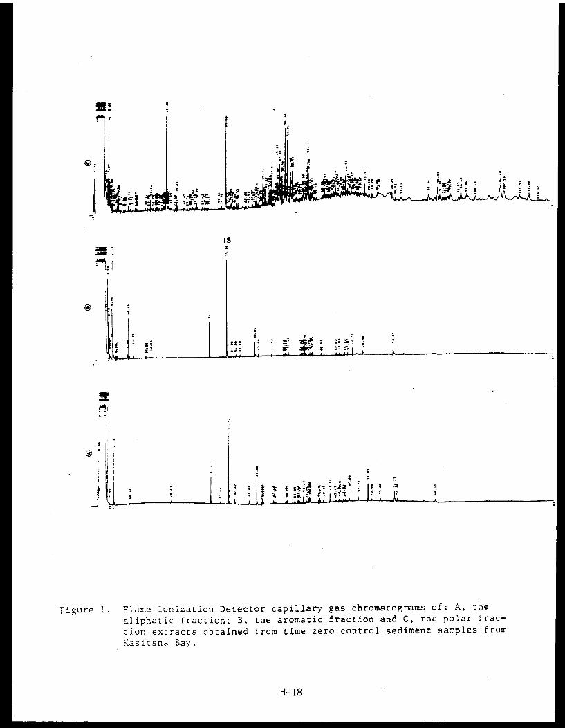
Figure 1. Flame Ionization Detector capillary gas chromatograms of: A, the
aliphatic fraction; B, the aromatic fraction and C, the polar frac-
tion extracts obtained from time zero control sediment samples from
Kasitsna Bay.
H-18
sample shows very little contamination of any kind, with only sub-
nanogram per gram-dry-weight components present. The polar fraction
chromatogram, C, does show evidence of several polar materials which are
currently underoing analysis by GC/MS. From GC/MS analyses of similar
sediment samples, the identities of these peaks are suspected to be long
chain fatty acid esters of biogenic origin.
Tables 1 and 2 present the reduced quantitative data obtained
from the capillary FID gas chromatographic runs of these and all the
other sediment samples analyzed as part of this program. The data in
Tables 1 and 2 illustrate several interesting quantitative aspects which
should be considered when interpreting the results. First, the back-
ground levels of hydrocarbons in the control samples from Kasitsna Bay
at times zero and one year were both extremely low. In neither case was
an Unresolved Complex Mixture (UCM) present, and the highest hydrocarbon
concentration in these two samples was only six micrograms per gram dry
weight. The odd to even n-alkane ratios for these samples (1 and 625)
were high, ranging from 5.2 to 7.9, reflecting predominance of the odd
n-alkanes of biogenic origin.
Figures 2 and 3 present gas chromatograms of the hexane and
benzene fractions from the fresh Cook Inlet crude oil and the artifi-
cially weathered Cook Inlet crude oil used to spike the sediment
samples, respectively. Figure 2A clearly shows a high degree of com-
plexity in the lower molecular weight range from nC8 through nC 12,
H-19
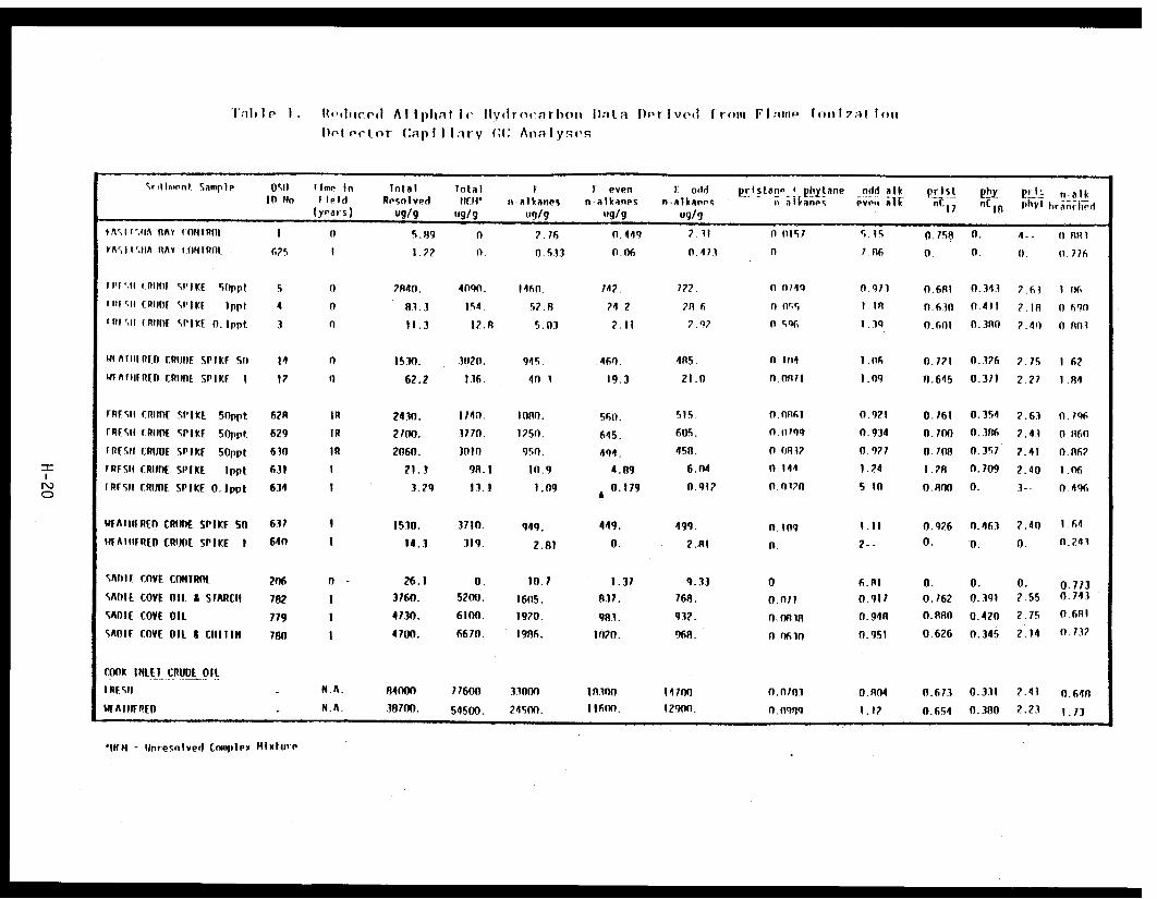
Table 1. Reduced Aliphatic Hydrocarbon Data Derived from Flame IonizationDetector Capillary GC Analyses
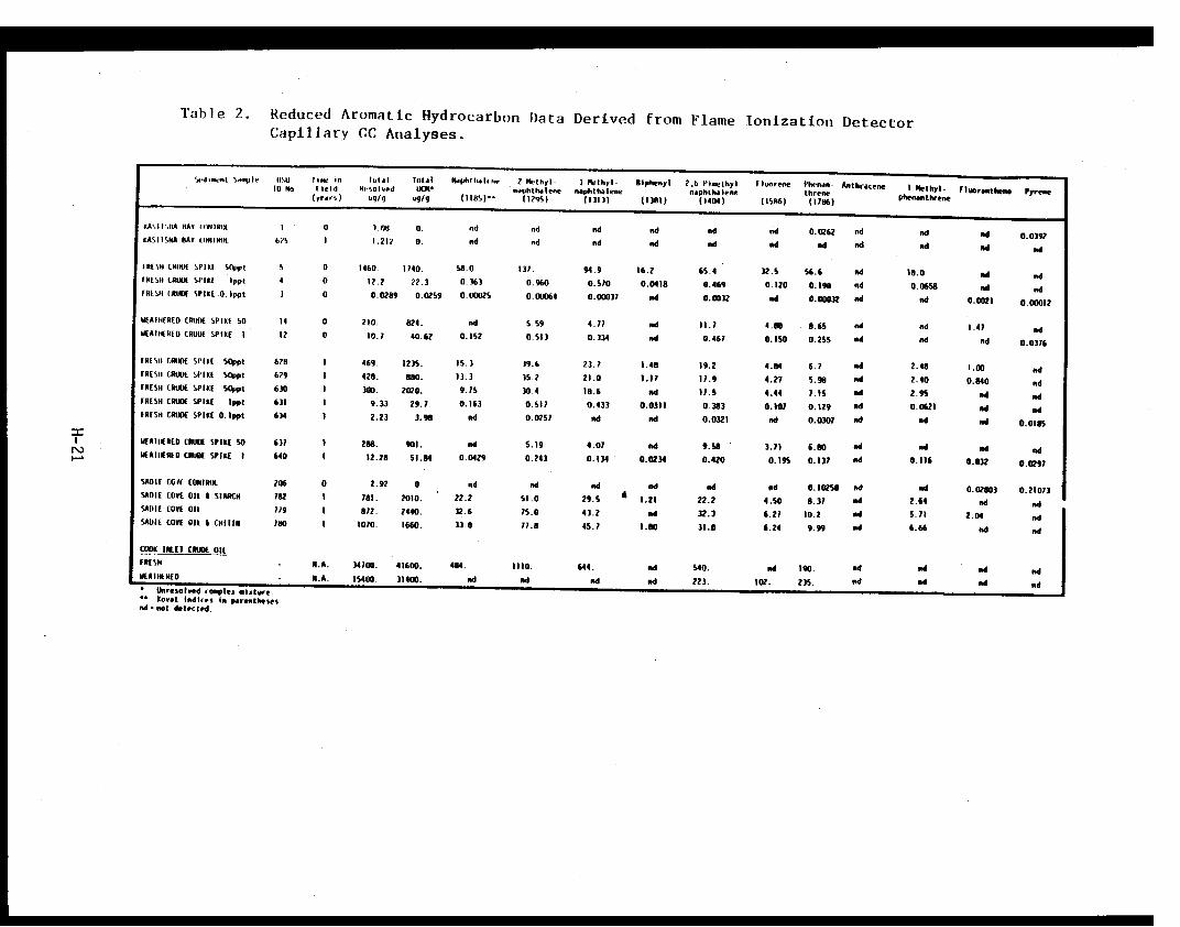
Table 2. Reduced Aromatic Hydrocarbon Data Derived from Flame Ionization DetectorCapillary GC Analyses.
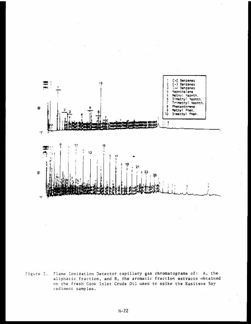
Figure 2. Flame Ionization Detector capillary gas chromatograms of: A, thealiphatic fraction, and B, the aromatic fraction extracts obtainedon the fresh Cook Inlet Crude Oil used to spike the Kasitsna Baysediment samples.
H-22
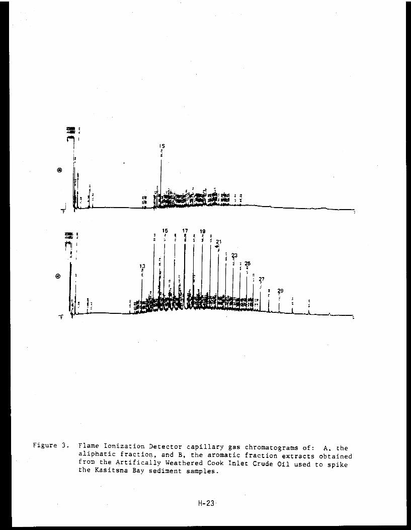
Figure 3. Flame Ionization Detector capillary gas chromatograms of: A, thealiphatic fraction, and B, the aromatic fraction extracts obtainedfrom the Artifically Weathered Cook Inlet Crude Oil used to spikethe Kasitsna Bay sediment samples.
H-23
although the aliphatic fraction is characterized in general, by n-
alkanes from nC8 through nC32. The aromatic fraction shows a number of
lower molecular weight aromatic compounds in the range of KOVAT index
800 to KOVAT index 1500 (RT 10.09 to 35.79). These compounds were
identified by GC/MS as alkyl substituted benzenes such as xylenes,
ethylbenzene, trimethylbenzene and propylbenzenes. The large peak at RT
35.79 is the GC internal standard hexamethylbenzene. Also in this
sample are peaks identified as napthalene (RT 24.64), 2-methylnapthalene
(RT 29.38), 1-methylnapthalene (RT 30.11), 2,6-dimethylnapthalene (RT
33.87), and several low level alkyl substituted phenanthrenes, as shown
by the data in Table 2.
Figure 3 shows the gas chromatograms of artificially weathered
crude oil used to spike the sediment samples. Clearly the aliphatic
fraction, Figure 3A, shows loss of the lower molecular weight n-alkanes
below nC1 3 ; however, the higher molecular weight materials are present
at approximately the same ratios as in the starting crude oil. This is
illustrated by the consistency in the pristane/phytane, pristane/nC 1 7,
and phytane/nC18 ratios for the fresh and weathered crude oils, as shown
by the data in Table 1. The aromatic fraction of the artificially
weathered crude shows nearly complete dimunition of the lower molecular
weight hydrocarbons below dimethylnapthalene; however, there still are
several higher molecular weight polynuclears present. These are
primarily phenanthrene at RT 47.34 (KOVAT 1790), 1-methylphenanthrene at
RT 51.97 (KOVAT 1933), and fluorantheneat RT 55.45 (KOVAT 2070). Higher
H-24
molecular weight compounds such as benz(a)anthracene, benzo(e)pyrene,
benzo(a)pyrene and perylene are not apparently present in either the
starting or weathered Cook Inlet crude oil to an appreciable degree.
Figure 4 shows the gas chromatograms of the aliphatic, aromatic
and polar fractions obtained on the Kasitsna Bay time zero sample spiked
with fresh crude oil at 1.0 ppt. The chromatograms obtained on the
sediments spiked at 50 ppt were essentially identical in appearance to
those in Figure 4, and thus the heavier spiked sample's chromatograms
are not shown here. Further, the concentrations of crude oil in the 50
ppt samples were at such a high level that only approximately 2% of the
extractable materials could be effectively applied to the liquid
chromatography columns for separation into aliphatic, aromatic and polar
fractions. This allowed accurate quantitation of the materials but did
not figuratively show the presence of the lower molecular weight com-
pounds to the same degree as the lower level spiked samples where the
entire sample could be fractionated and analyzed without prior dilution.
With regard to the chromatograms in Figure 4, the aliphatic
fraction, A, is nearly identical to the aliphatic fraction of the start-
ing fresh Cook Inlet Crude oil shown in Figure 2. This is reflected
qualitatively in the chromatograms presented in the figures and also
quantitatively by the pristane/phytane, pristane/nC17 and phytane/nC18
ratio data presented in Table 1. The suite of nC2 0-nC2 1 branched/unsat-
urated compounds in the background control sample are completely masked
in the spiked sediment samples. The aromatic fractions of the spiked
H-25
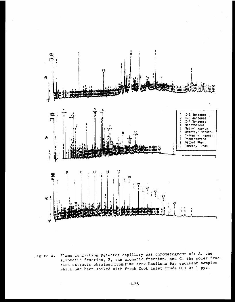
Figure 4. Flame Ionization Detector capillary gas chromatograms of: A, the
aliphatic fraction, B, the aromatic fraction, and C, the polar frac-
tion extracts obtained from time zero Kasitsna Bay sediment samples
which had been spiked with fresh Cook Inlet Crude Oil at 1 ppt.
H-26
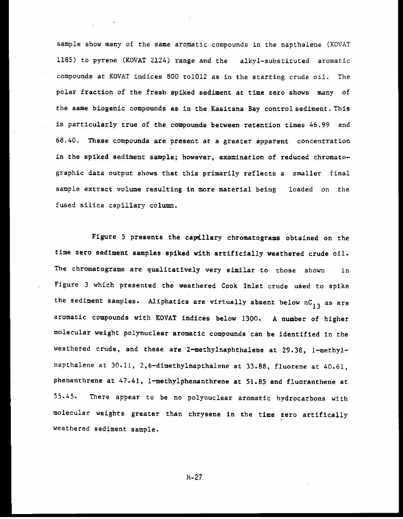
sample show many of the same aromatic compounds in the napthalene (KOVAT
1185) to pyrene (KOVAT 2124) range and the alkyl-substituted aromatic
compounds at KOVAT indices 800 tol012 as in the starting crude oil. The
polar fraction of the fresh spiked sediment at time zero shows many of
the same biogenic compounds as in the Kasitsna Bay control sediment. This
is particularly true of the compounds between retention times 46.99 and
68.40. These compounds are present at a greater apparent concentration
in the spiked sediment sample; however, examination of reduced chromato-
graphic data output shows that this primarily reflects a smaller final
sample extract volume resulting in more material being loaded on the
fused silica capillary column.
Figure 5 presents the capillary chromatograms obtained on the
time zero sediment samples spiked with artificially weathered crude oil.
The chromatograms are qualitatively very similar to those shown in
Figure 3 which presented the weathered Cook Inlet crude used to spike
the sediment samples. Aliphatics are virtually absent below nC13 as are
aromatic compounds with KOVAT indices below 1300. A number of higher
molecular weight polynuclear aromatic compounds can be identified in the
weathered crude, and these are 2-methylnaphthalene at 29.38, 1-methyl-
napthalene at 30.11, 2,6-dimethylnapthalene at 33.88, fluorene at 40.61,
phenanthrene at 47.41, 1-methylphenanthrene at 51.85 and fluoranthene at
55.45. There appear to be no polynuclear aromatic hydrocarbons with
molecular weights greater than chrysene in the time zero artifically
weathered sediment sample.
H-27
Figure 5. Flame Ionization Detector capillary gas chromatograms of: A, thealiphatic fraction and B, the aromatic fraction extracts obtainedfrom time zero Kasitsna Bay sediment samples spiked with ArtificallyWeathered Cook Inlet Crude Oil at 50 ppt.
H-28
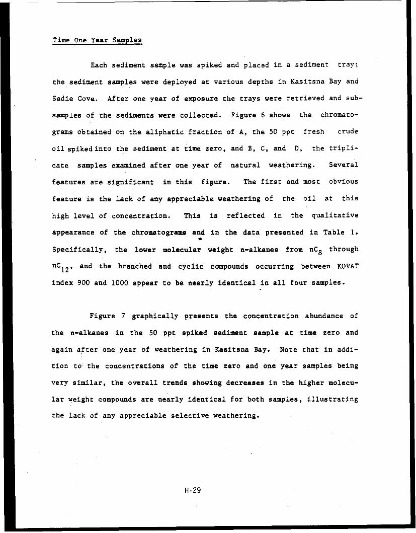
Time One Year Samples
Each sediment sample was spiked and placed in a sediment tray;
the sediment samples were deployed at various depths in Kasitsna Bay and
Sadie Cove. After one year of exposure the trays were retrieved and sub-
samples of the sediments were collected. Figure 6 shows the chromato-
grams obtained on the aliphatic fraction of A, the 50 ppt fresh crude
oil spiked into the sediment at time zero, and B, C, and D, the tripli-
cate samples examined after one year of natural weathering. Several
features are significant in this figure. The first and most obvious
feature is the lack of any appreciable weathering of the oil at this
high level of concentration. This is reflected in the qualitative
appearance of the chromatograms and in the data presented in Table 1.
Specifically, the lower molecular weight n-alkanes from nC8 through
nC12, and the branched and cyclic compounds occurring between KOVAT
index 900 and 1000 appear to be nearly identical in all four samples.
Figure 7 graphically presents the concentration abundance of
the n-alkanes in the 50 ppt spiked sediment sample at time zero and
again after one year of weathering in Kasitsna Bay. Note that in addi-
tion to the concentrations of the time zero and one year samples being
very similar, the overall trends showing decreases in the higher molecu-
lar weight compounds are nearly identical for both samples, illustrating
the lack of any appreciable selective weathering.
H-29
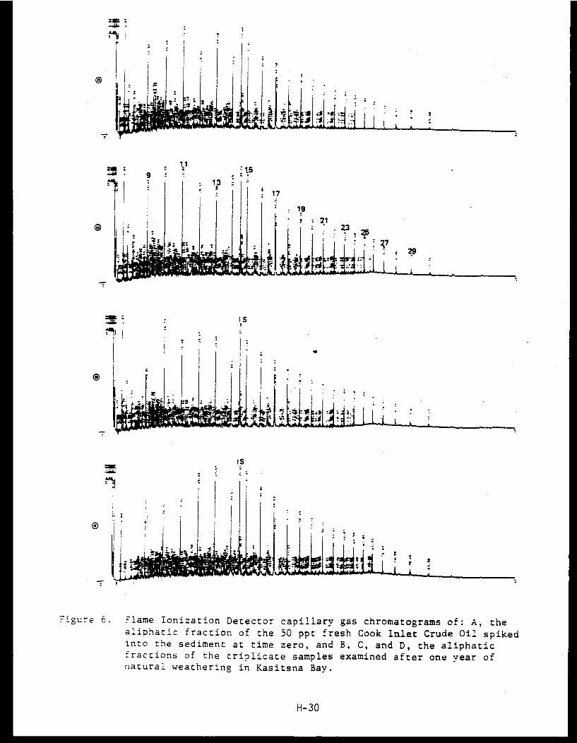
Figure 6. Flame Ionization Detector capillary gas chromatograms of: A, thealiphatic fraction of the 50 ppt fresh Cook Inlet Crude Oil spikedinto the sediment at time zero, and B, C, and D, the aliphaticfractions of the triplicate samples examined after one year ofnatural weathering in Kasitsna Bay.
H-30
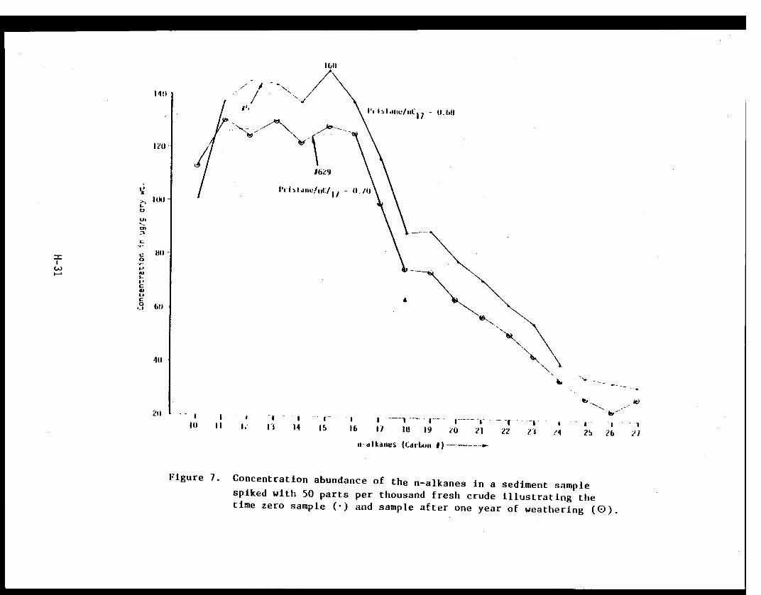
Figure 7. Concentration abundance of the n-alkanes in a sediment samplespiked with 50 parts per thousand fresh crude illustrating thetime zero sample (·) and sample after one year of weathering (0)
The similarity of the pristane/nC17 and phytane/nC 18 ratios, as
observed qualitatively in Figure 6 and Table 1, also illustrates the
lack of any appreciable biotic or abiotic weathering in these samples.
The chromatographic profiles are essentially superimposable, reflecting
the homogeniety of the initial spiked sediment, the replicability of the
weathering process in the field and the precision of the analytical meth-
od. Individual values for these three fractions are presented in Table
1, and the agreement of such features as the total n-alkanes, sum of the
odd n-alkanes, even n-alkanes, pristane/phytane ratios, etc., is worthy
of consideration.
Figure 8 presents the gas chromatograms of the aromatic frac-
tions obtained on the 50 ppt frewh Cook Inlet-spiked sediment at time
zero (A) and the replicate fractions (B, C and D) obtained from analyses
of the triplicate sediment samples after one year of natural weathering.
As in Figure 6, there does not appear to be any selective weathering of
the individual components present; however, examination of the reduced
data in Table 2 and Figure 9 shows that some, decreases in aromatic
hydrocarbon concentrations did occur after 1 year. The apparent lower
levels of material in chromatogram A (Figure 8) only reflect a larger
final sample extract volume from which an aliquot was removed for
analysis by GC. Figure 9A presents a graphical representation of the
concentrations of eight selected aromatic compounds in the fresh 50 ppt
H-32
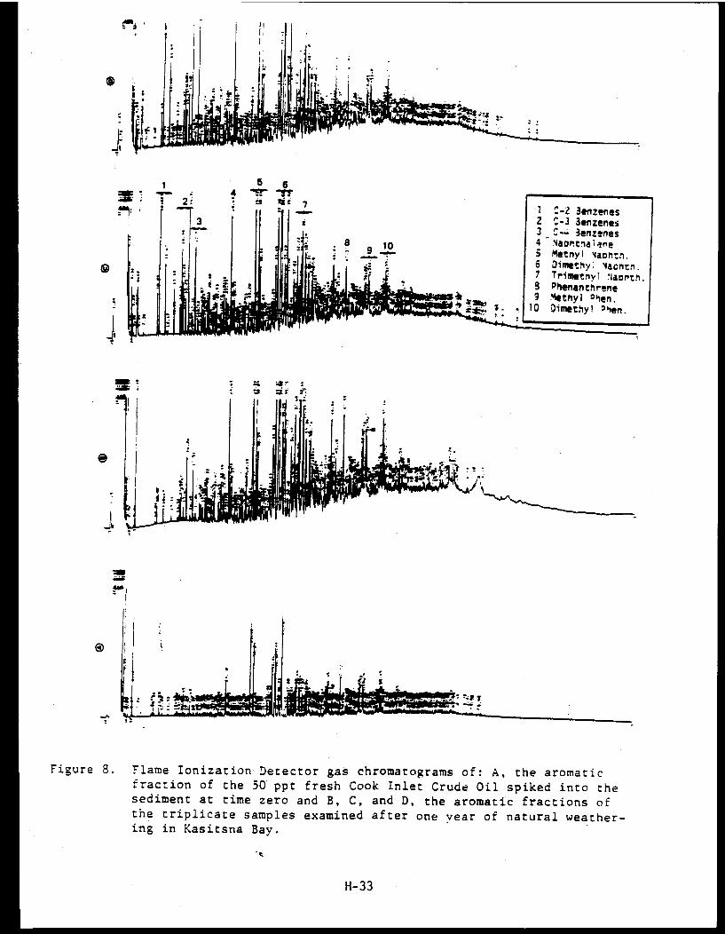
Figure 8. Flame Ionization Detector gas chromatograms of: A, the aromaticfraction of the 50 ppt fresh Cook Inlet Crude Oil spiked into thesediment at time zero and B, C, and D, the aromatic fractions ofthe triplicate samples examined after one year of natural weather-ing in Kasitsna Bay.
H-33

Figure 9. Concentration abundance of selected aromatic hydro-carbons from a 50 parts per thousand spike of freshcrude (Top) showing the time zero sample (·) andsample after one year of weathering (®),and bottom,a 50 ppt spike of artifically weathered crude attime zero (·) and after one year of weathering (0).
H-34
spiked sediments at time zero and time one year. While time zero levels
of individual aromatic compounds ranged from 50 to 137 micrograms per
gram dry weight (for napthalene through 2,6-dimethylnapthalene), after one
year these compounds were present at concentrations ranging from 15 to
40 micrograms per gram dry weight. The decreases in aromatic compounds
from Kovat indices 1100 to 1500 were greater than the decreases in aroma-
tics with Kovat indices ranging from 1500 to 2000. This presumably re-
flects two things: 1) the greater volatility and water solubility of the
lower molecular weight aromatic compounds, and 2) the lower relative a-
bundance of the higher molecular weight aromatics in the crude oil to be-
gin with.
Figure 9B shows the relative losses of aromatic hydrocarbons in
the artifically weathered crude oil spiked into the Kasitsna Bay sedi-
ments at time zero and time one year. This figure illustrates that much
smaller relative changes occurred over the one year period after the oil
was spiked into the sediment. That is, the starting concentrations of
aromatic compounds such as 2-methylnaphthalene through phenanthrene rang-
ed between only 6 and 12 micrograms per gram dry weight of sediment when
artifically weathered crude was used to spike the sample at time zero.
These levels were not significantly reduced after one year of weather-
ing in the sediments of Kasitsna Bay: the most significant weathering
occurred while the oil was "artifically weathered" on the surface of a
H-35
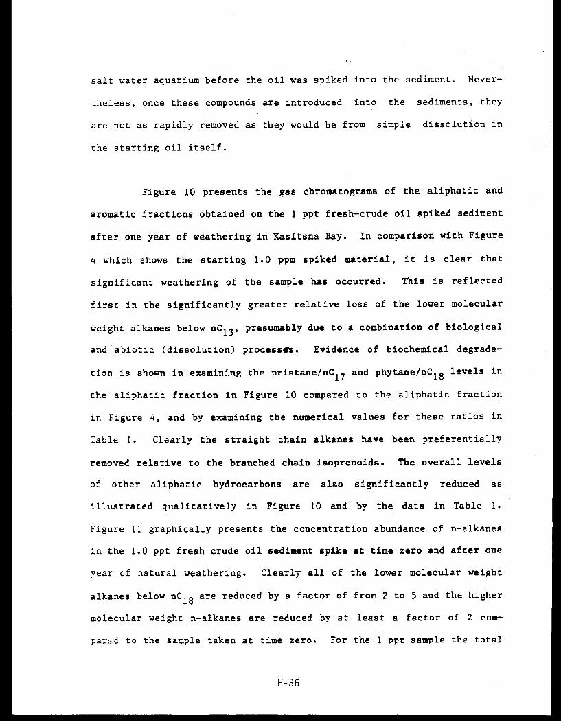
salt water aquarium before the oil was spiked into the sediment. Never-
theless, once these compounds are introduced into the sediments, they
are not as rapidly removed as they would be from simple dissolution in
the starting oil itself.
Figure 10 presents the gas chromatograms of the aliphatic and
aromatic fractions obtained on the 1 ppt fresh-crude oil spiked sediment
after one year of weathering in Kasitsna Bay. In comparison with Figure
4 which shows the starting 1.0 ppm spiked material, it is clear that
significant weathering of the sample has occurred. This is reflected
first in the significantly greater relative loss of the lower molecular
weight alkanes below nC13, presumably due to a combination of biological
and abiotic (dissolution) processes. Evidence of biochemical degrada-
tion is shown in examining the pristane/nC 1 7 and phytane/nC18 levels in
the aliphatic fraction in Figure 10 compared to the aliphatic fraction
in Figure 4, and by examining the numerical values for these ratios in
Table 1. Clearly the straight chain alkanes have been preferentially
removed relative to the branched chain isoprenoids. The overall levels
of other aliphatic hydrocarbons are also significantly reduced as
illustrated qualitatively in Figure 10 and by the data in Table 1.
Figure 11 graphically presents the concentration abundance of n-alkanes
in the 1.0 ppt fresh crude oil sediment spike at time zero and after one
year of natural weathering. Clearly all of the lower molecular weight
alkanes below nC 18 are reduced by a factor of from 2 to 5 and the higher
molecular weight n-alkanes are reduced by at least a factor of 2 com-
pared to the sample taken at time zero. For the 1 ppt sample the total
H-36
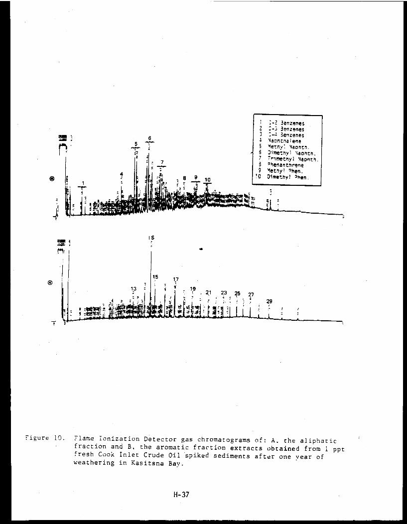
Figure 10. Flame Ionization Detector gas chromatograms of: A, the aliphaticfraction and B, the aromatic fraction extracts obtained from 1 pptfresh Cook Inlet Crude Oil spiked sediments after one year ofweathering in Kasitsna Bay.
H-37
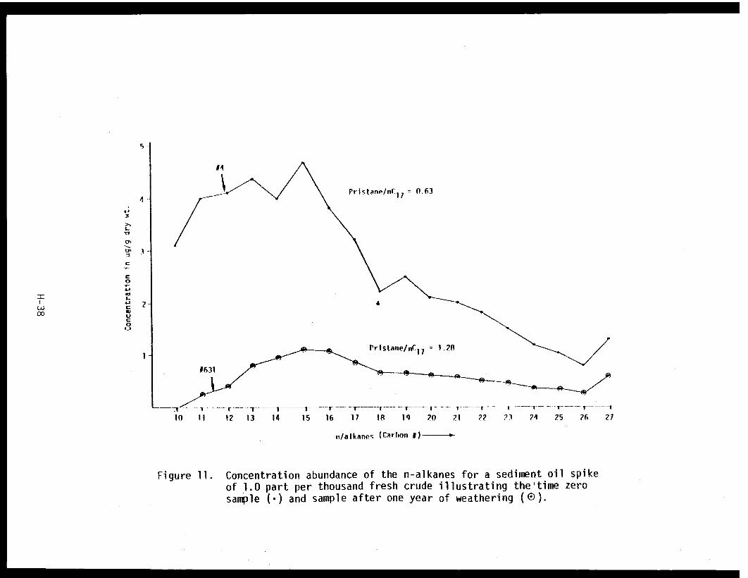
Figure 11. Concentration abundance of the n-alkanes for a sediment oil spikeof 1.0 part per thousand fresh crude illustrating the time zerosample (·) and sample after one year of weathering (®).
resolved hydrocarbons decreased from 83 to 21 ug/g dry weight during the
year of exposure and the unresolved complex mixture decreased from 154
to 98 pg/g dry weight.
The aromatic fraction data in Figure 10B show somewhat less
degradation compared to the aliphatic fraction. Compounds with
molecular weights less than naphthalene (KOVAT < 1185) are obviously
removed due to a combination of biological and abiotic factors (dis-
solution and evaporation); however, compounds with molecular weights
greater than 1-methylnapthalene (KOVAT > 1315) appear to be present in
relatively identical concentrations compared to the starting materials.
That is, while overall levels are slightly reduced as illustrated by the
data in Table 2, the relative concentrations of the individual poly-
nuclear aromatics are very similar in the time zero and time one year
samples. This is also reflected quite obviously by the qualitative
appearance of the aromatic fractions shown in Figures 4B and 10B,
respectively, and by the data presented in Figure 12A. Figure 12A
graphically presents the relative concentration abundance of selected
aromatic hydrocarbons from the 1 ppt spike of fresh crude oil at time
zero and after one year. Clearly while the relative range of concentra-
tions of all of the compounds in the time zero and one year samples are
lower compared to the 50 ppt sample shown in Figure 9A, the overall con-
centrations of the time zero and naturally weathered 1 ppt samples are
still relatively similar. This is particularly true of the higher
molecular weight compounds, bi-phenyl, fluorene, phenanthrene and
H-39
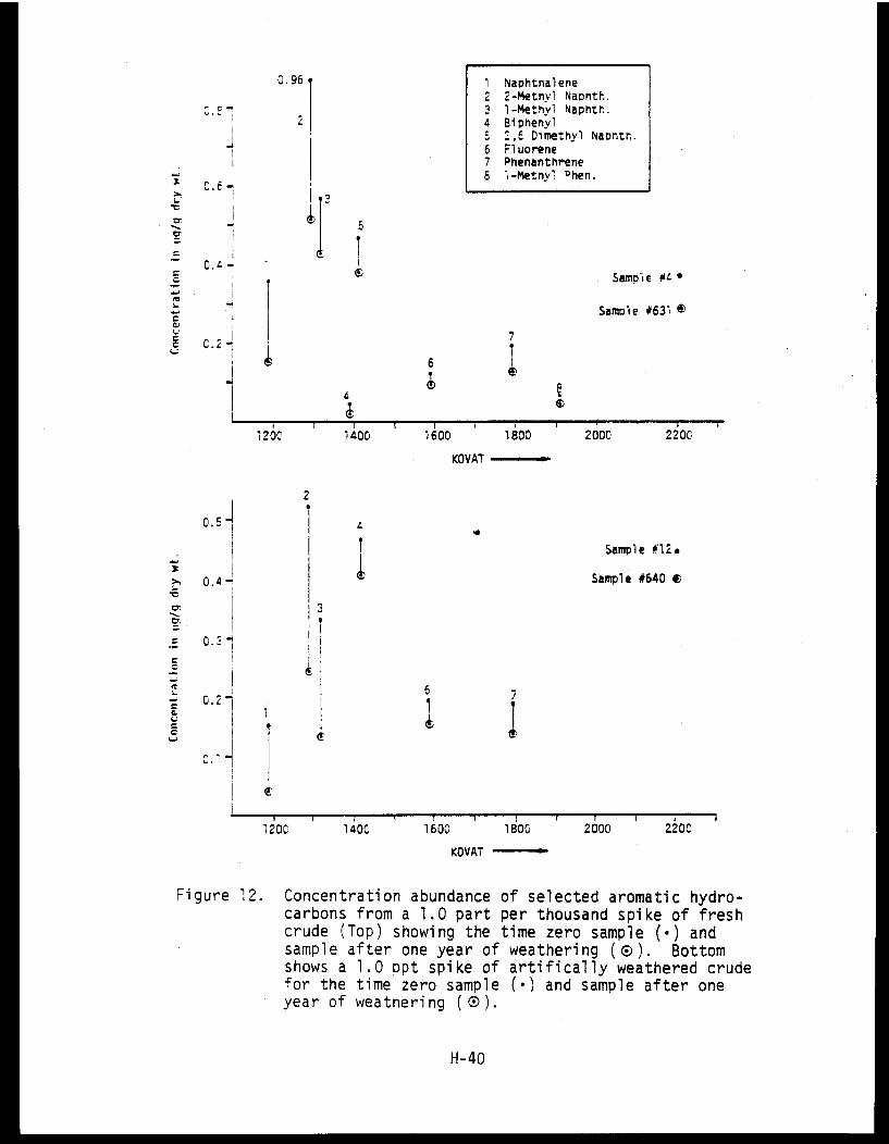
Figure 12. Concentration abundance of selected aromatic hydro-carbons from a 1.0 part per thousand spike of freshcrude (Top) showing the time zero sample (·) andsample after one year of weathering (®). Bottomshows a 1.0 ppt spike of artifically weathered crudefor the time zero sample (·) and sample after oneyear of weathering (®).
H-40
1-methylphenanthrene. As in Figure 9A and B, the relative concencra-
tions of artifically weathered aromatic compounds from the 1.0 ppt
sample shown in 12B show that concentrations are in the same range in
the artifically weathered sample as in the fresh sample after it had
been weathered for a full year.
Clearly, while biological degradation of the aliphatic hydro-
carbons (primarily n-alkane) occurred at the 1 ppt level, concommitant
degradation of the higher molecular weight polynuclear aromatics com-
pounds with molecular weights above that of methylnapthalene did not
occur at a significant level.
This lack of degradation-of higher molecular weight PNA's at
the 1.0 ppt level is also illustrated in Figure 13, which presents the
aromatic fraction chromatograms of: A) the 1 part per thousand fresh
crude spiked into the sediment at time zero; B) the aromatic fraction
obtained from the 1 ppt sediment after one year of in situ weathering in
Kasitsna Bay; and C) the aromatic fraction of the 1 ppt sediment spiked
with artificially weathered crude oil after one year of additional
weathering in Kasitsna Bay. Clearly, examination of chromatograms 13A
and B shows that some loss of the lower molecular weight alkyl substi-
tuted benzenes at retention times 10.45, 11.68, 15.15, 15.90, 16.49 and
17.71 has occurred due to either evaporation or dissolution. Compounds
with molecular weights greater than that of 1-methylnapthalene at reten-
tion time 29.41 (B) are present in nearly identical relative concentra-
tions. The chromatogram in 13C shows that the same compounds were also
H-41
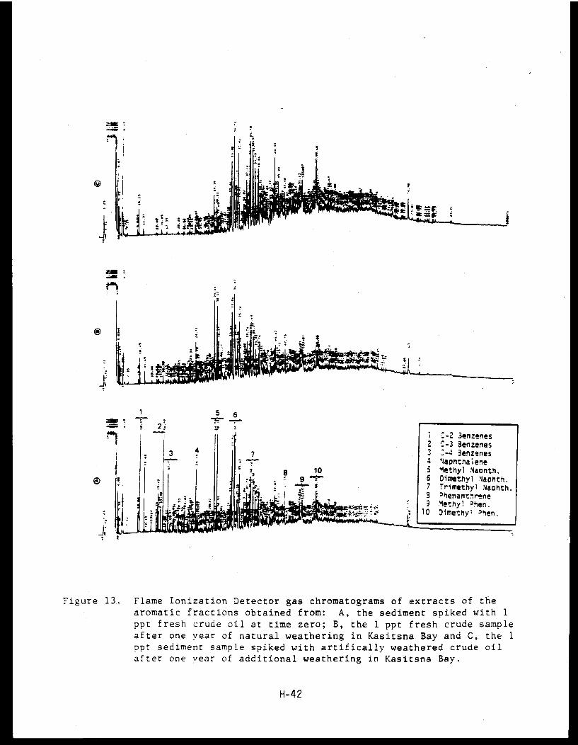
Figure 13. Flame Ionization Detector gas chromatograms of extracts of thearomatic fractions obtained from: A, the sediment spiked with 1ppt fresh crude oil at time zero; B, the 1 ppt fresh crude sampleafter one year of natural weathering in Kasitsna Bay and C, the 1ppt sediment sample spiked with artifically weathered crude oilafter one year of additional weathering in Kasitsna Bay.
H-42
present in the "artificially weathered" oil which was spiked into the
sediment after an additional year of natural weathering. This suggests
that although many lower molecular weight aromatic compounds are removed
from natural weathering of spilled oil while the oil is still at the
surface,once the less water soluble and volatile higher molecular weight
PNA's are incorporated into the sediment, additional degradative pro-
cesses are extremely slow. Thus, while the relatively non-toxic alipha-
tic hydrocarbons are significantly degraded by biological processes in
the sediments at 1 ppt, the more toxic aromatic compounds appear to be
longer lived when introduced to the sediment from either fresh or
weathered crude oil at similar levels.
Figure 14 presents the aiiphatic, aromatic and polar fraction
chromatograms obtained on the 0.1 ppt fresh crude oil spiked into the
sediment at time zero (a) and after one year of weathering in the sedi-
ments of Kasitsna Bay (b, aliphatic fraction; c, aromatic fraction; d,
polar fraction). Clearly, almost all of the n-alkanes in the starting
oil are no longer present in the sediment after one year of weathering.
In fact, the only compounds of any significance in the aliphatic frac-
tion of the fully weathered sediment are higher molecular weight odd
n-alkanes, nC23 , nC25, nC2 7, and nC29. These same compounds are also
predominant in the fresh crude sample shown in Figure 14A. That is,
instead of seeing a regular decrease in higher molecular weight
n-alkanes from nC2 2 through nC32, the odd carbons at 23, 25 and 27 from
biogenic input are clearly present. These are the only compounds which
H-43
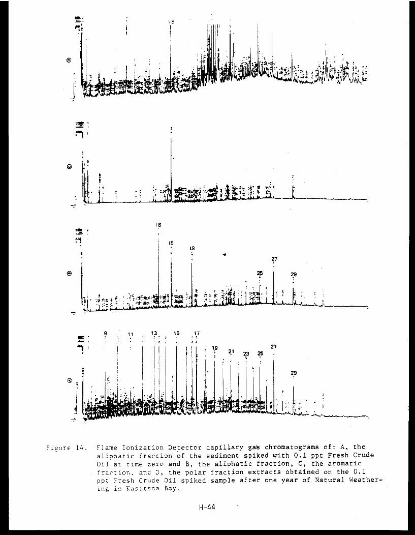
Figure 14. Flame Ionization Detector capillary gas chromatograms of: A, the
aliphatic fraction of the sediment spiked with 0.1 ppt Fresh CrudeOil at time zero and B, the aliphatic fraction, C, the aromatic
fraction, and D, the polar fraction extracts obtained on the 0.1ppt Fresh Crude Oil spiked sample after one year of Natural Weather-ing in Kasitsna Bay.
H-44
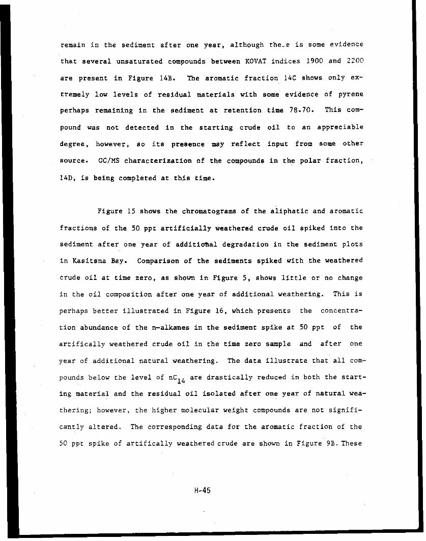
remain in the sediment after one year, although the-e is some evidence
that several unsaturated compounds between KOVAT indices 1900 and 2200
are present in Figure 14B. The aromatic fraction 14C shows only ex-
tremely low levels of residual materials with some evidence of pyrene
perhaps remaining in the sediment at retention time 78.70. This com-
pound was not detected in the starting crude oil to an appreciable
degree, however, so its presence may reflect input from some other
source. GC/MS characterization of the compounds in the polar fraction,
14D, is being completed at this time.
Figure 15 shows the chromatograms of the aliphatic and aromatic
fractions of the 50 ppt artificially weathered crude oil spiked into the
sediment after one year of additional degradation in the sediment plots
in Kasitsna Bay. Comparison of the sediments spiked with the weathered
crude oil at time zero, as shown in Figure 5, shows little or no change
in the oil composition after one year of additional weathering. This is
perhaps better illustrated in Figure 16, which presents the concentra-
tion abundance of the n-alkanes in the sediment spike at 50 ppt of the
artifically weathered crude oil in the time zero sample and after one
year of additional natural weathering. The data illustrate that all com-
pounds below the level of nC14 are drastically reduced in both the start-
ing material and the residual oil isolated after one year of natural wea-
thering; however, the higher molecular weight compounds are not signifi-
cantly altered. The corresponding data for the aromatic fraction of the
50 ppt spike of artifically weathered crude are shown in Figure 9B. These
H-45
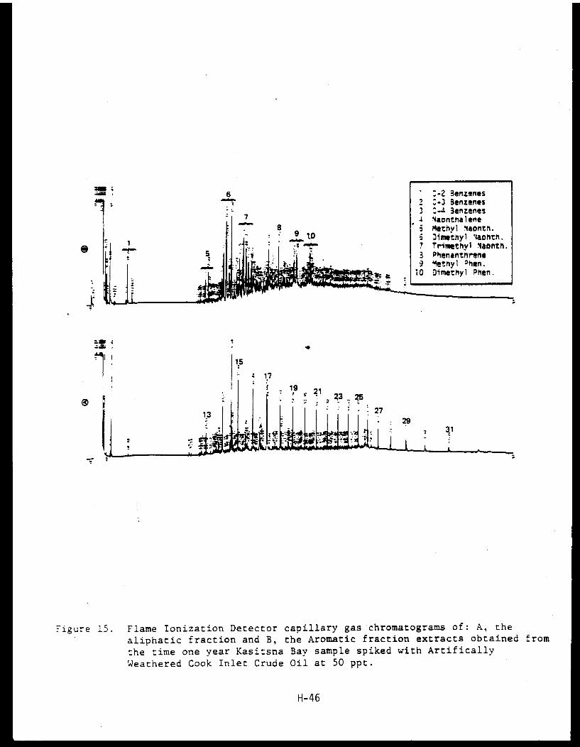
Figure 15. Flame Ionization Detector capillary gas chromatograms of: A, the
aliphatic fraction and B, the Aromatic fraction extracts obtained from
the time one year Kasitsna Bay sample spiked with Artifically
Weathered Cook Inlet Crude Oil at 50 ppt.
H-46
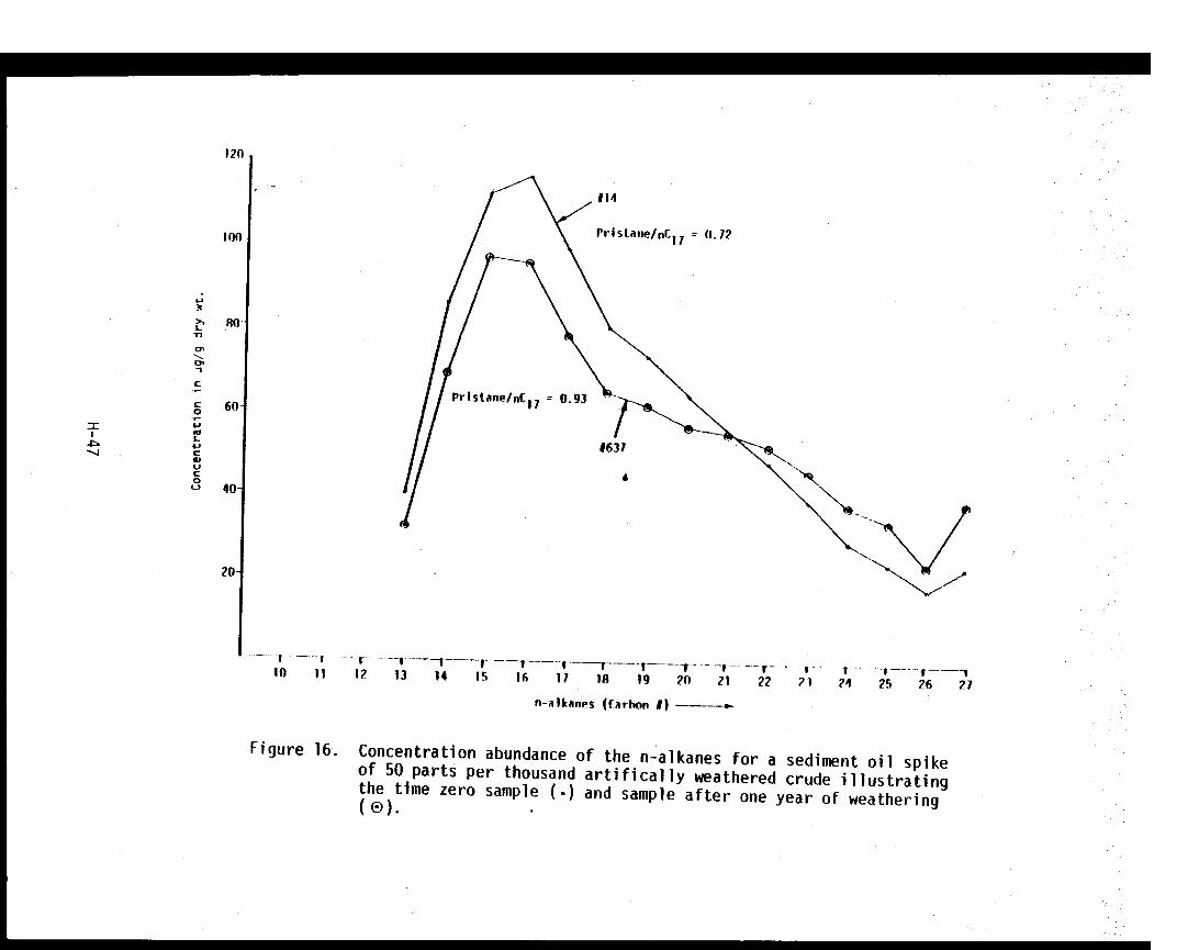
Figure 16. Concentration abundance of the n-alkanes for a sediment oil spikeof 50 parts per thousand artifically weathered crude illustratingthe time zero sample (·) and sample after one year of weathering(e).
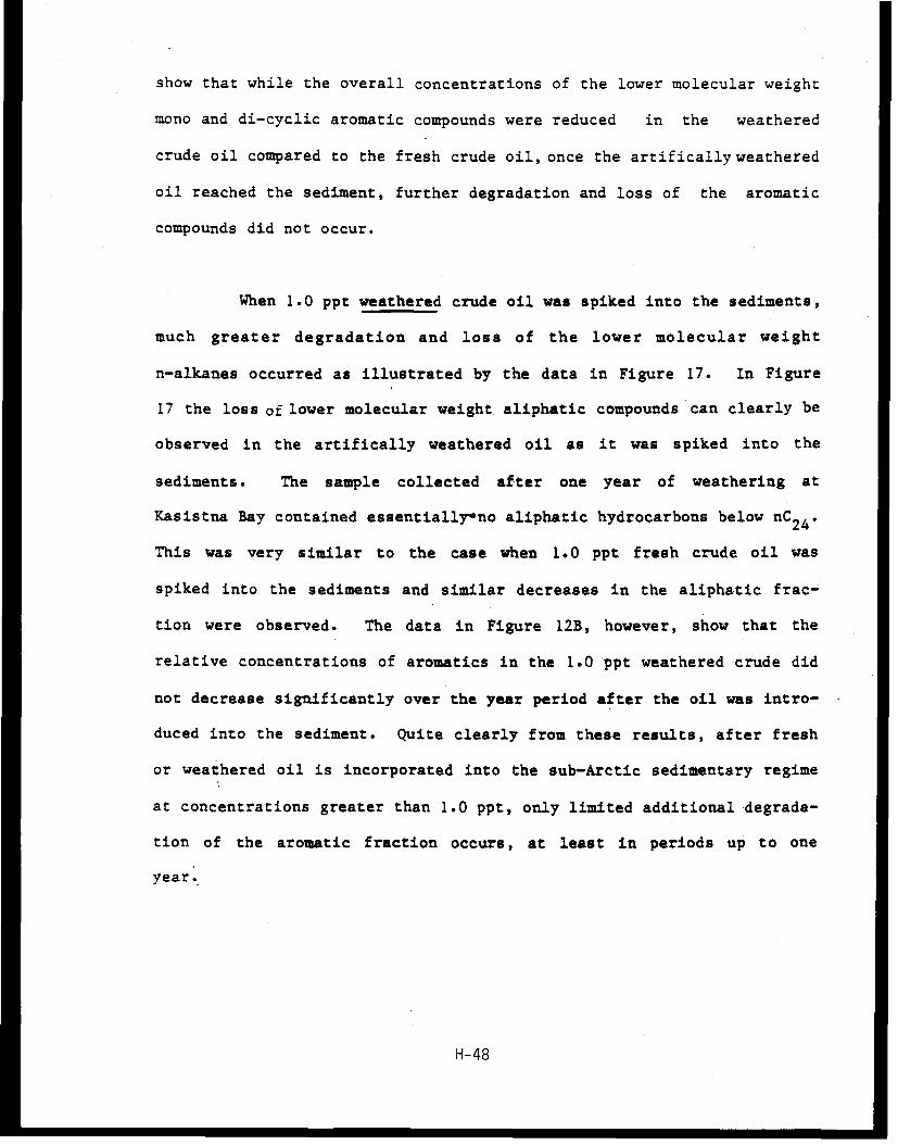
show that while the overall concentrations of the lower molecular weight
mono and di-cyclic aromatic compounds were reduced in the weathered
crude oil compared to the fresh crude oil, once the artifically weathered
oil reached the sediment, further degradation and loss of the aromatic
compounds did not occur.
When 1.0 ppt weathered crude oil was spiked into the sediments,
much greater degradation and loss of the lower molecular weight
n-alkanes occurred as illustrated by the data in Figure 17. In Figure
17 the loss of lower molecular weight aliphatic compounds can clearly be
observed in the artifically weathered oil as it was spiked into the
sediments. The sample collected after one year of weathering at
Kasistna Bay contained essentially-no aliphatic hydrocarbons below nC2 4.
This was very similar to the case when 1.0 ppt fresh crude oil was
spiked into the sediments and similar decreases in the aliphatic frac-
tion were observed. The data in Figure 12B, however, show that the
relative concentrations of aromatics in the 1.0 ppt weathered crude did
not decrease significantly over the year period after the oil was intro-
duced into the sediment. Quite clearly from these results, after fresh
or weathered oil is incorporated into the sub-Arctic sedimentary regime
at concentrations greater than 1.0 ppt, only limited additional degrada-
tion of the aromatic fraction occurs, at least in periods up to one
year.
H-48
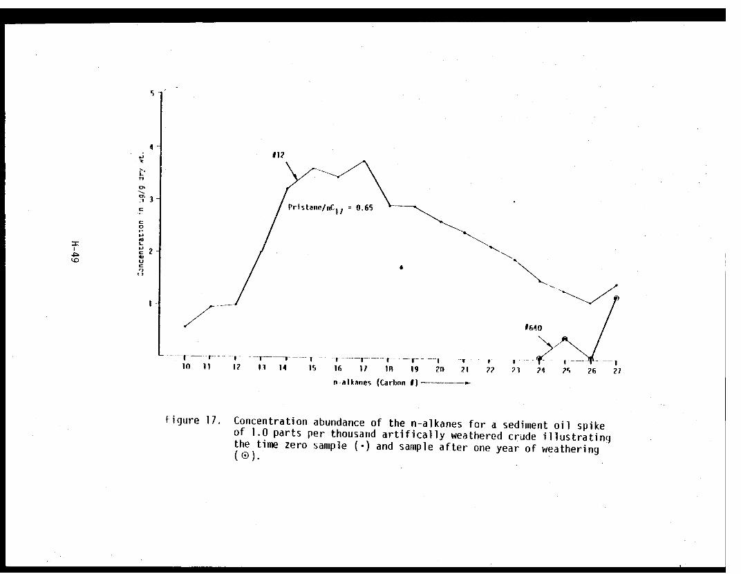
Figure 17. Concentration abundance of the n-alkanes for a sediment oil spikeof 1.0 parts per thousand artifically weathered crude illustratingthe time zero sample (·) and sample after one year of weathering(0).
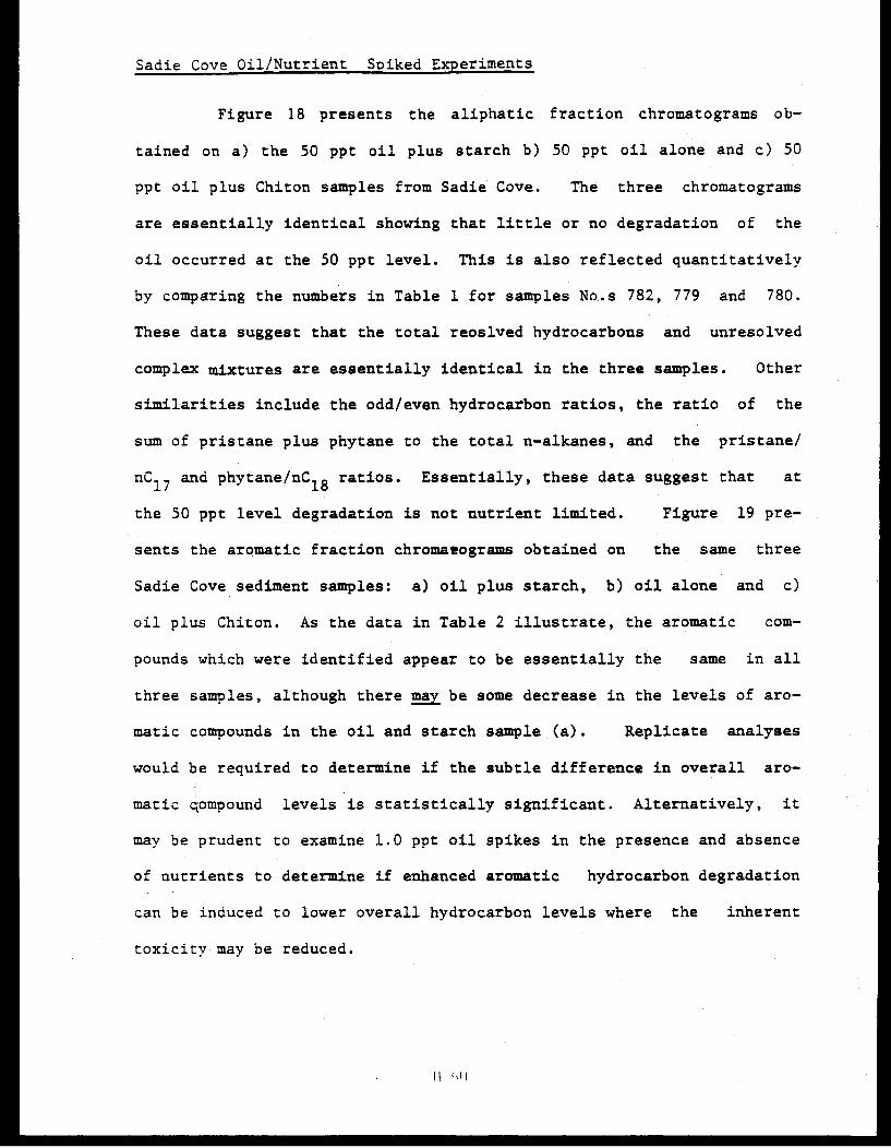
Sadie Cove Oil/Nutrient Spiked Experiments
Figure 18 presents the aliphatic fraction chromatograms ob-
tained on a) the 50 ppt oil plus starch b) 50 ppt oil alone and c) 50
ppt oil plus Chiton samples from Sadie Cove. The three chromatograms
are essentially identical showing that little or no degradation of the
oil occurred at the 50 ppt level. This is also reflected quantitatively
by comparing the numbers in Table 1 for samples No.s 782, 779 and 780.
These data suggest that the total reoslved hydrocarbons and unresolved
complex mixtures are essentially identical in the three samples. Other
similarities include the odd/even hydrocarbon ratios, the ratio of the
sum of pristane plus phytane to the total n-alkanes, and the pristane/
nC17 and phytane/nC1 8 ratios. Essentially, these data suggest that at
the 50 ppt level degradation is not nutrient limited. Figure 19 pre-
sents the aromatic fraction chromatograms obtained on the same three
Sadie Cove sediment samples: a) oil plus starch, b) oil alone and c)
oil plus Chiton. As the data in Table 2 illustrate, the aromatic com-
pounds which were identified appear to be essentially the same in all
three samples, although there may be some decrease in the levels of aro-
matic compounds in the oil and starch sample (a). Replicate analyses
would be required to determine if the subtle difference in overall aro-
matic compound levels is statistically significant. Alternatively, it
may be prudent to examine 1.0 ppt oil spikes in the presence and absence
of nutrients to determine if enhanced aromatic hydrocarbon degradation
can be induced to lower overall hydrocarbon levels where the inherent
toxicity may be reduced.
I( I , )
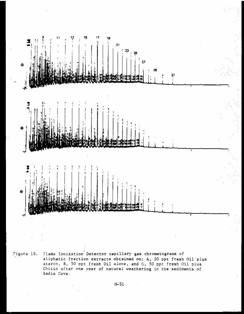
Figure 18. Flame Ionization Detector capillary gas chromatograms ofaliphatic fraction extracts obtained on: A, 50 ppt fresh Oil plusstarch, B, 50 ppt fresh Oil alone, and C, 50 ppt fresh Oil plusChitin after one year of natural weathering in the sediments ofSadie Cove.
H-51
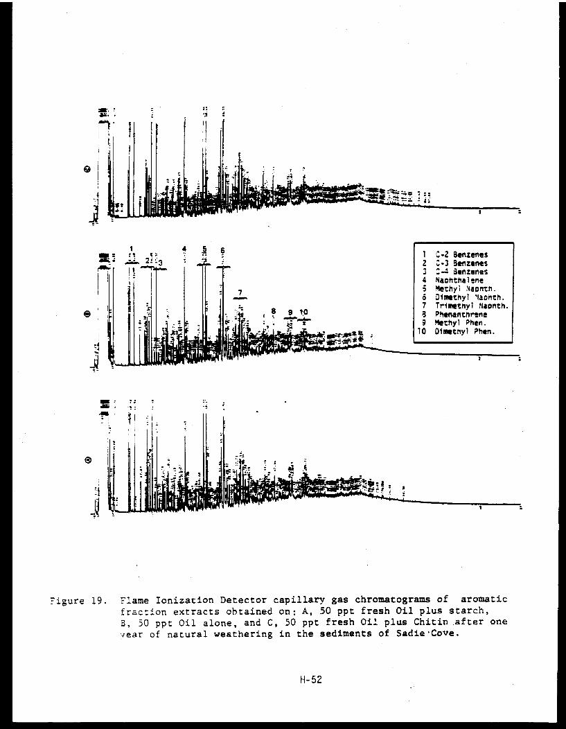
Figure 19. Flame Ionization Detector capillary gas chromatograms of aromatic
fraction extracts obtained on: A, 50 ppt fresh Oil plus starch,
B, 50 ppt Oil alone, and C, 50 ppt fresh Oil plus Chitin.after one
year of natural weathering in the sediments of Sadie Cove.
H-52
SUMMARY
The results presented here support the conclusion that in a
major oil spill event in the sub-Arctic marine environment, the most sig-
nificant weathering of the oil will occur at the air/sea interface or in
the water column before the oil is incorporated into the sedimentary re-
gime. This is particularly true in fine-grain sediment matrices in low-
energy environments. Once levels of fresh and weathered Cook Inlet Crude
oil reached concentrations in excess of 1 ppt in the sediment plots ex-
amined in the study, very little additional weathering or loss of higher
molecular weight aromatic hydrocarbons occurred. At spiked levels of 50
ppt with both fresh and weathered crude oil, nearly complete inhibition
of microbiological utilization or selective removal of aliphatic hydro-
carbons was also observed, especially for those sediments spiked with
fresh crude. Recovery of biological activity and selective utilization
of aliphatic hydrocarbons did occur in the samples spiked with fresh and
weathered crude at 1 ppt, and in the 0.1 ppt spiked samples, there was
little or no evidence of either aliphatic or aromatic petroleum hydro-
carbon contamination after one year. At that time, the 0.1 ppt spiked
samples appeared to contain only the same biogenic hydrocarbons observed
in the non-spiked control sediment samples from Kasitsna Bay.
In the study plots which were spiked with 50 ppt oil plus added
nutrients (starch and Chitin), there was no evidence of any enhanced bio-
tic recovery or selective hydrocarbon utilization with either fresh or
weathered crude oil. This suggests inhibition of biological processes
H-53
from the high levels of toxic aromatic compounds in the oil itself rather
than inhibition from limited nutrient concentrations. To more accurately
address the role of added nutrients in oil degradation, detailed analyses
should be completed on lower spiked oil concentrations in the presence
and absence of nutrients. Also, experiments to assess the role of dis-
solved oxygen, grain-size, the energy (tidal and wave) input to the sed-
imentary environment, total organic carbon content and other factors such
as total bio-mass, could be considered in future studies.
From the results obtained on the fresh and weathered crude oils
and the sediment samples examined in this program, it appears that the
maximum amount of weathering and removal (dissolution and evaporation)
of toxic components can be achieved if spill clean up and treatment ef-
forts are designed to prolong the time that the oil remains on the water
surface or suspended in the water column. This may suggest limited use
of dispersants or detergents in certain spill situations, particularly
if damage to coastal zones is not imminent. Containment and recovery
of the residual higher molecular weight materials should take precedence
over other strategies such as chemical dispersal which may result in high-
er sub-tidal sediment loadings.
H-54
REFERENCES
American Institute of Biological Sciences, 1978. The Proceedings of theConference on Assessment of Ecological Impacts of Oil Spills, Keystone,Colorado, 14-17 June 1980, 936 pgs.
Bassin, J.J., T. Ichiye. 1977. Flocculation behavior of suspended sedi-ments and oil emulsions. Journal of Sedimentary Petrology 47(2): 671-677.
Brown, D.W., L.S. Ramos, M.Y. Uyeda, A.J. Friedman, and W.D. MacLeod, Jr.(1980): Ambient-temperature extraction of hydrocarbons from marine sedi-ments-comparison with boiling-solvent extractions. In: Petroleum inthe Marine Environment, L. Petrakis and F.T. Weiss (Eds.), Advances inChemistry Series 185, American Chemical Society, Washington, DC, pp.313-326.
D'Oxouville, L., M.O. Hayes, E.R. Gundlach, W.J. Sexton, and J. Michel.1979. Occurrence of oil in offshore bottom sediments at the AMOCOCADIZ oil spill site, In: Proceedings of the 1979 Oil Spill Conference,March 19-22, Los Angeles, CA, p. 187-192.
Gearing, J.N., P.J. Gearing, T. Wade, J.G. Quinn, H. B. McCarty, J. Far-rington and R.F. Lee. 1979. The rates of transport and fates ofpetroleum hydrocarbons in a controlled marine ecosystem and a note onanalytical variability, p. 555-564. In: Proceedings of the 1979 OilSpill Conference (Prevention, Behavior, Control, Cleanup) 19-22 March1979, Los Angeles, Calif.
Jordon, R.E. and J.R. Payne, Fate and Weathering of Petroleum Spills inthe Marine Environment: A Literature Review and Synopsis. Ann ArborScience Publishers Inc., Ann Arbor, Michigan. 1980. 175 pp.
MacLeod, W.D., Jr. and J.R. Fisher, 1980. Intercalibration of AnalyticalLaboratories. Manuscript presented at the Researcher/Pierce IXTOC-ISymposium, Miami, Florida, 9-11 June, 1980. 7 pp.
Mayo, D.W., D.S. Page, J. Cooley, E. Sorenson, F. Bradley, E.S. Gilfillan,F.A. Hanson. 1978. Weathering characteristics of petroleum hydrocar-bons deposited in fine clay marine sediments, Searsport, Maine, Journalof Fisheries Research Board of Canada, 35(5):552-565.
Meyers, P.A. 1976. Sediments--sources of sinks for petroleum hydrocarbons?In: Sources, Effects and Sinks of Hydrocarbons in the Aquatic Environ-ment; Proceedings of the Symposium, American University, Washington,D.C., 9-11 August, 1976 (American Institute of Biological Sciences 1977).
Meyers-, P.A. and J.G. Quinn. 1973. Association of hydrocarbons and mineralparticles in saline solutions. Nature 244:23-4.
National Academy of Sciences. 1975. Petroleum in the marine environment,Washington, D.C., 107 pp.
Parker, P.L. and S. Macko. 1978. An intensive study of the heavy hydro-carbons in the suspended particulate matter of seawater, ch. 11 of SouthTexas Outer-Continental Shelf BLM Study.
H-55
Payne, J.R., P.J. Mankiewicz, J.R. Nemmers, R.E. Jordan, I.R. Kaplan,M.I. Venkatesan, S. Brenner, J. Bonilla, D. Meredith, B. Meyers, B.Haddad, A.L. Burlingame, A. Ensminger, G. Gould, and M.L. Moberg.1978 a. High molecular weight petroleum hydrocarbon analytical pro-cedures. Southern California Baseline Study, Benthic Year II. VolumeIII, Report 5.0. Final report submitted to the Bureau of Land Manage-ment, Department of Interior, Washington, D.C. by Science Applications,Inc.
Payne, J.R., J.R. Clayton, Jr., B.W. de Lappe, P.L. Millikin, J.S. Parkin,R.K. Okazaki, E.F. Letterman, and R.W. Risebrough. Hydrocarbons in theWater Column. Southern California Baseline Study, Vol. III, Report3.2.3., p. 1-207. 1978 b. Final Report, submitted to the Bureau of LandManagement, Washington D.C. by the University of California BodegaMarine Laboratory, Bodega Bay, California, and Science Applications,Inc., La Jolla, California.
Payne, J.R., J.E. Nemmers, R.E. Jordan, P.J. Mankiewicz, A.D. Oesterle,S. Laughon, and G. Smith. Measurement of petroleum hydrocarbon burdensin marine sediments by three commonly accepted procedures: results of aNOAA inter-laboratory calibration exercise, Fall, 1978. Submitted toDr. John A. Calder, Staff Chemist, OCSEAP, U.S. Department of Commerce,National Oceanic and Atmospheric Administration, Environmental ResearchLaboratory, Boulder, CO, January 1979. pp. 1-34, plus appendix.
Payne, J.R., G.S. Smith, P.J. Mankiewicz, R.F. Shokes, N.W. Flynn, W.Moreno and J. Altamirano. Horizontal and Vertical Transport of Dissolvedand Particulate-Bound Higher Molecular Weight Hydrocarbons from theIXTOC-1 Blowout. Manuscript presented at the RESEARCHER/PIERCE IXTOC-ISymposium, Miami, Florida, June 9-11, 1980. 47 pp.
Teal, J.M., C. Burns, and J. Farrington. 1978. Analysis of aromatic hydro-carbons in intertidal sediments, resulting in two spills of Number 2Fuel Oil in Buzzard's Bay, Massachusetts. Journal of Fisheries ResearchBoard of Canada 35(5):510-520.
Winters, J.K. 1978. Fate of petroleum derived aromatic compounds in sea-water held in outdoor tanks and South Texas Outer-continental ShelfStudy-BLM, ch. 12. Draft final report.
Zurcher, F. and M. Thuer. 1978. Rapid weathering processes of fuel oilin natural waters. Analysis and interpretations. Environmental Scienceand Tech. 12(7):838-843.
H-56
U.S. DEPARTMENT OF COMMERCENATIONAL OCEANIC AND ATMOSPHERIC ADMINISTRATION
N/OMS33x3 POSTAGE AND FEES PAIDN/OMS33x3 (OCSEAP) U.S. DEPARTMENT OF COMMERCE
P.O. Box 1808 COM-210
Juneau, Alaska 99802 PRINTED MATTERCLASS OF POSTAL SERVICE
OFFICIAL BUSINESSPENALTY FOR PRIVATE USE, $300
: . .
NOAA FORM 61-32A (11-77)See NDM 61-50 for Class of Postal Service


