eScholarship provides open access, scholarly publishingservices to the University of California and delivers a dynamicresearch platform to scholars worldwide.

Berkeley Program in Law and EconomicsUC Berkeley

Title:Environmental Remedies: An Incomplete Information Aggregation Game

Author:Rausser, Gordon C., University of California at BerkeleySimon, Leo K., University of California BerkeleyZhao, Jinhua, Iowa State University

Publication Date:05-11-2000

Series:Berkeley Program in Law and Economics, Working Paper Series

Permalink:http://escholarship.org/uc/item/9z00731z

Abstract:The burden of resolving an environmental problem is typically shared among several responsibleparties. To clarify the nature and extent of the problem, these parties must provide informationto the regulator. Based on this information, the regulator will instigate an investigation of theproblem, to determine an appropriate remedy. This paper investigates the incentives facingagents to promote excessive investigation and postpone remediation. Our incomplete informationgame-theoretic model may be of general interest to game theorists: we apply a new theoremguaranteeing pure-strategy equilibria and introduce a class of games called " aggregation games"which have interesting properties and are widely applicable.

Copyright Information:All rights reserved unless otherwise indicated. Contact the author or original publisher for anynecessary permissions. eScholarship is not the copyright owner for deposited works. Learn moreat http://www.escholarship.org/help_copyright.html#reuse

ENVIRONMENTAL REMEDIES:

AN INCOMPLETE INFORMATION AGGREGATION GAME

GORDON C. RAUSSER, LEO K. SIMON, AND JINHUA ZHAO

May 11, 2000

Abstract. The burden of resolving an environmental problem is typically shared among severalresponsible parties. To clarify the nature and extent of the problem, these parties must provideinformation to the regulator. Based on this information, the regulator will instigate an investigationof the problem, to determine an appropriate remedy. This paper investigates the incentives facingagents to promote excessive investigation and postpone remediation. Our incomplete informationgame-theoretic model may be of general interest to game theorists: we apply a new theorem guar-anteeing pure-strategy equilbria and introduce a class of games called \aggregation games" whichhave interesting properties and are widely applicable.

JEL classi�cation: D82, Q28

Keywords: Environmental economics; environmental remediation; Superfund; hazardous wastecleanups; incomplete information games; pure-strategy equilibria; aggregation games; strategic in-formation transmission; strategic delay.

Corresponding author: Leo Simon, Department of Agricultural Economics, 207 Giannini Hall, University of California atBerkeley, Berkeley, CA 94709-3301. Email: simon@are.berkeley.edu. Phone: 510 642 8230.Rausser: Dean and Robert Gordon Sproul Distinguished Professor, College of Natural Resources, University of California,Berkeley, CA 94720 and member, Giannini Foundation of Agricultural Economics; Simon: Adjunct Professor, Departmentof Agricultural Economics, University of California, Berkeley, CA 94720 and member, Giannini Foundation of AgriculturalEconomics; Zhao: Assistant Professor, Department of Economics, Iowa State University, Ames, IA 50011. The authors aregrateful to seminar participants at the University of Washington, at the Economic Theory Seminar Series at Iowa StateUniversity, and at the Graduate Seminar, Department of Agricultural and Resource Economics, University of California atBerkeley. Susan Athey and Chris Shannon provided very helpful advice relating to the application of Athey's methodologyto our problem. Larry Karp provided useful comments on an earlier draft.

We consider a class of problems in which several agents contribute to the creation of an environmen-

tal problem and are required to share the �nancial burden of remediation. In many instances, there

is a natural information asymmetry between these Responsible Parties (RP's) and the regulatory

authority responsible for implementing a remediation strategy. The asymmetry arises when RP's

have private information regarding their individual contributions to the problem. For example, if

the problem is a toxic contamination site, only the RP's themselves will have detailed information

about the nature, volume and spatial/intertemporal distribution of the substances they have con-

tributed. Alternatively, if the problem involves overuse of a common property resource, only the

users themselves will be able to provide detailed information about their individual use-patterns.

Typically, even individuals' own private information will be imperfect, because, for example, his-

torical records may be incomplete and not readily accessible. However, RPs' private information

about their own contribution will generally be more precise than the information that is directly

available to any regulatory authority.

For this class of problems, a tradeo� arises between time and information. On one hand, it is

obviously preferable that environmental problems be remediated sooner rather than later, espe-

cially when contamination is spreading and the public is exposed to health hazards. On the other

hand, because, typically, the nature and magnitude of any given environmental problem is highly

uncertain, it will generally be suboptimal to proceed rapidly to the implementation phase of the

remediation process. Rather, time is needed to conduct �eld investigations that will provide more

precise information about the characteristics and extent of the remediation task. If the investiga-

tion period is too short, the severity of the problem may be over- or underestimated: in the �rst

instance, excessive resources will be allocated to mitigation; in the second, the remediation plan

may be inadequate, resulting in costly revisions to the original remediation schedule and possibly

exacerbated health risks.

2

The optimal length of the investigation period depends on the regulator's initial information: the

greater the uncertainty, the longer is the optimal period, and hence the longer is the optimal delay

before the problem is resolved. The issue of strategic information revelation naturally arises because

the authority has to rely on the RPs for its initial information about the contamination. In order to

determine an appropriate investigation program, the regulator must make an preliminary estimate

of the uncertainty associated with the site. Since this estimate will be based on RP reports, RPs

can, by strategically misreporting their private information, manipulate the regulator's decision

and either hasten or delay the proceedings.

Even when the social costs of the environmental problem are fully internalized by the RP's as a

group, individual RP's views about the optimal timing of remediation will typically di�er from

each other as well as from those of the regulator. One reason, of course, is that individual �rms'

intertemporal discount rates are higher than the social rate. For this reason alone, an RP has an

incentive to manipulate the information transmission process, and thereby delay the remediation

process without incurring legal sanctions. The Superfund program provides a dramatic illustration

of delayed implementation. While for this program there are other factors leading to delay,1 it has

been observed that RPs bene�t considerably from delayed implementation because it reduces their

discounted cleanup costs (see, for example, Dixon (1994)). Cost savings due to discounting may be

signi�cant: as reported by Birdsall and Salah (1993), prejudgment interest is typically the single

largest cost item at a Superfund site and accounts for nearly one-third of the total costs.2

Apart from di�erences between their respective rates of discount, there are other factors that lead

RPs to prefer remediation schedules that di�er from the socially optimal one. In particular, they

have di�erent degrees of risk aversion and face liabilities that di�er in both their nature and extent.

1 Primarily the enormously contentious issue of how to apportion burden shares among RP's.2 Prejudgment interest is accumulated when the government or an RP sues other RPs for past cleanup costs.

3

Typically, the regulator will be less risk averse than the RPs, because the former can pool risks

across the many sites that it oversees. Moreover, even when they are in principle liable for all

costs that are incurred as a result of delayed remediation, in practice RP's typically bear only a

fraction of the incremental costs resulting from delay.3 For most RP's, there is also the issue of

insurance indemni�cation and the reluctance of insurance carriers to admit liability. For all these

reasons, RPs are likely to overvalue the bene�ts of uncertainty reduction and to undervalue the

costs of extending the investigation period beyond its socially optimal length. On the other hand,

each individual RP is responsible for only a fraction of total remediation costs, and for this reason

will underweight the bene�ts of uncertainty reduction. The net e�ect of these di�erences is thus

indeterminate.

In a previous paper (Rausser, Simon and Zhao (1998), henceforth RSZ), we examined the strate-

gic interaction between RPs and the regulator in the speci�c context of Superfund cleanup. In

that paper RP's strategically report the quality of their information. It identi�es incentives for

misreporting of accuracy levels and suggests several Bayesian mechanisms which would enable the

regulator to extract the truth from the RPs. In the present paper, we investigate the abstract

problem of delayed implementation, and formalize the interaction among the RPs as an incomplete

information game, given the regulator's policy. To sharpen the analysis, we make three simplifying

assumptions. First, we assume that while the magnitude of the environmental problem is a random

variable, the mean of the distribution governing this variable is commonly known. Second, we

assume that RPs' burden shares are predetermined. Third, we do not impose as an equilibrium

condition that the regulator's decision rule elicits truthful behavior from the RP's. These simpli�-

cations allow us to single out other factors which a�ect PRPs' incentives to delay, to focus upon the

3 For example, while health damage increases with exposure time, a�ected individuals and communities can obtain compen-sation for this damage only through a private cost recovery action. Such actions tend to be very costly to initiate andmay not be successful. Accordingly the e�ect of delay on the extent of health damages is in practice unlikely to be fullyinternalized by RP's.

4

strategies the PRPs can pursue, and to identify the implications of some widespread government

practices.

The second of these assumptions is problematic in some contexts|for example, as we have observed,

burden shares are an enormously contentious issue in the context of environmental remediation|

but perfectly reasonable in others|for example, in many instances, remediation activities are

funded by special-purpose taxes levied on the basis of observable criteria.4 The third assumption

sets this paper apart from the vast agency-theoretic literature which focuses on the design of

mechanisms that eÆciently induce agents to truthfully reveal their private information. On the

other hand, our approach is more consistent with actual regulator behavior. In most instances

governmental bureaucrats typically accept reports from agents under their jurisdiction at face

value, rather than attempting to reverse engineer \the truth" from these reports, based on what

they know about the agents' motivations.

The paper is organized as follows. In Section 1, we formulate the incomplete information aggre-

gation game among the RPs. Each RP in our game has information about the precision of its

own records relating to the site. We identify this information with the agent's type and assume

that types are nonatomically distributed. A strategy for an RP is a function mapping its type

into announced levels of precision. Once types have been realized, the regulator aggregates RP's

announcements and imposes the investigation schedule that is optimal relative to this aggregated

announcement. Applying Athey's methodology, we establish the existence of a pure strategy Nash

equilibrium in which each RP's report is monotone in its type. In section 2 we study the class of

\linear-quadratic" aggregation games and preview our subsequent results in this special context.

Section 3 examines the role of burden shares. We demonstrate that RPs with higher burden shares

on average report a higher level of uncertainty than those with lower shares. In Section 4, we show

4 One recent example is the famous \penny-per-pound" tax on sugar production, proposed (although not ultimately adopted)as a way of �nancing the $700 million cost of restoring the Florida Everglades.

5

(for the case of two RPs) that under certain conditions, when their burden shares become more

heterogeneous, the RPs' expected aggregate report increases. Section 5 extends this result to the

case of multiple RPs, but imposes signi�cant restrictions on functional forms. In Section 6 we apply

our theory to the topic of Superfund cleanups, and study the implications of two widespread policy

options: de minimis RP buyouts and the formation of RP steering committees. We discuss and

conclude the paper in Section 7. Proofs are presented in the appendix.

1. The Model

We assume that there are n RPs, indexed by i = 1; : : : ; n, who have contributed to an environ-

mental problem which must now be remediated. Parties' contributions are additive, i.e., the total

magnitude of the problem is the sum of individual contributions. Prior to any evaluation of the

problem, each RP has private information about its contribution level. This information is as-

sumed to be imperfect, because, for example, historical records may be incomplete and not readily

accessible. More precisely, we assume that i's contribution mi is a random variable with mean �mi

and variance �i. We assume that the �mi's are commonly known, while �i is known only by agent

i. We assume that the mi's are independent of each other, so that no RP can infer from its own

uncertainty anything about the degree of uncertainty about other RPs' contributions. The total

magnitude of the problem is denoted by �m.5 Thus, �m is a random variable with commonly

known mean � �m. Each RP has partial information about the variance of �m, denoted by ��; that

is, it knows the variance of its own contribution only. The regulator has no independent information

at all about ��.

Each RP is required to make a report to the regulator about �i. Based on the aggregate of RPs'

reports, the regulator determines a �eld investigation schedule that will generate further information

5 Throughout this paper, we will use the following notational convention: given a vector x = (x1; :::; xn) or function f(x) =(f1(x1); :::; f1(xn)) we denote the sum of the elements of x (resp:f(x)) by �x (resp. �f(x) or �f) and the sum of all butthe i'th element by �x�i (resp. �f�i).

6

about the magnitude of the problem, i.e., will reduce the variance of its estimate of �m. Since it is

common knowledge that the regulator's decision is a function of reported variances, each RP can,

by strategically misreporting its uncertainty, manipulate this decision. Intuitively, if RP i prefers

to delay the start of remediation beyond the socially optimal date, it will report a value of �i that

exceeds its true value and thus prolong the investigation period.

Both the investigation and the remediation processes will be �nanced entirely by the RPs as a group.

We assume that there is a predetermined vector of burden shares, or burden pro�le, k = (k1; :::; kn),

with ki � 0 andPn

i=1 ki = 1: agent i is held responsible for the share ki of total costs, whatever

these costs turn out to be. (In some cases|e.g., Superfund cleanups,|the ki's re ect individual

agents' relative expected or estimated contributions to the toal problem. In others|e.g., when

costs are �nanced by output taxation|burden shares re ect other considerations, such as market

share.)

We formalize the interaction among the RPs as an incomplete information, simultaneous-move

game. The i'th RP's type is identi�ed with the variance, �i, of its contribution, which is known

only by RP i. We assume that the �i's are identically and independently distributed on the interval

[�l; �u], where �l � 0. Let g(�) denote the density of agents' types. We assume that g(�) is nonatomic

on [�l; �u]. Let� = [�l; �u]nwith generic element �. Similarly, let��i = [�l; �u]

n�1. For ��i 2��i,

let g�i(��i) =Qj 6=i g(�j).

A pure strategy for the i'th RP is a function si : [�l; �u] ! H = [�

�; ��] � R+ where H is the set

of admissible variance announcements: si(�i) is the level of individual uncertainty declared by the

i'th RP when its actual level of uncertainty is �i. The strategy vector s = (s1; :::; sn) is called

a pure strategy pro�le. Thus a strategy pro�le is a mapping from � to H = Hn. The scalar

si(�i) represents i's declared (as opposed to its actual) type. Of course, the notion that an RP

7

would declare a number representing the variance of its contribution is no more than a convenient

abstraction. In reality, an RP might report an upper and lower bound to its contributions. In this

case, a high (resp. low) value of si would be interpreted as a wide (resp. negligible) gap between

the two reported bounds.

Strategy pro�les are mapped into outcomes. An outcome is a scalar, t, representing the length of

the investigation period selected by the regulator. An important restriction on the outcome func-

tion, t : H ! R+ , is that this mapping depends only on the sum of agents' announcements. We

shall refer to games that satisfy this restriction as aggregation games. Formally, the restriction is

that ifPn

i=1 si(�i) =Pn

i=1 si(�0i) then t

�s1(�1); :::; sn(�n)

�= t�s1(�

01); :::; sn(�

0n)�. This restriction

formalizes the idea that the regulator aggregates individual RPs' declarations before choosing an

investigation schedule. To streamline notation, we will henceforth write t as a mapping from R

to R, with argument �s. We assume that t(�s) is thrice continuously di�erentiable and nonde-

creasing with �s. We assume also that t0(�) is nonnegative and nondecreasing. Note that while the

aggregation assumption is very natural in our context, the class of aggregation games is very spe-

cial. In Cournot games, for example, payo�s depend both on the sum of agents' actions|because

this sum determines prices|and on agent's individual actions|because these determine quantities.

In a Bertrand, or auction game, on the other hand, what matters is the whole pro�le of agents'

individual actions; the sum of agents' actions is immaterial.

As will soon become apparent, the bounds �l and �u on agents' strategies play a very important

role in any aggregation game. A natural value for the lower bound, ��, on variance announcements

would be zero, but for generality, we assume that ��is nonnegative. On the other hand, we will

choose �� to exceed the optimal report for an RP whose type is �u and whose burden share is one,

assuming that all other RPs report ��with probability one. Now RPs' strategies are bounded below

by ��� 0. Moreover it can be shown that their strategies both increase in their burden share and

8

decrease in other agents' strategies. It follows that regardless of its type or burden-share, if an RP

responds optimally to other agents' strategies, then this response must lie strictly below ��. Thus,

while ��will often constrain agents' behavior, �� will never do so. This asymmetry will turn out to

have important consequences for our model, and will drive our comparative statics results.

Before specifying the payo� function, F , for the game, we de�ne a preliminary function, C, which

represents the RPs' anticipated �nancial exposure. The only distinction between C and F is that

the former depends on the outcome of the game (i.e., the length of the investigation period) while

the latter depends on agents' strategies. Speci�cally, C(t;��; k) : R+ �R+ � [0; 1]! R+ represents

the anticipated �nancial exposure of an RP when the length of the investigation period is t, the

variance of the contamination is �� and the RP is responsible for a fraction k of total costs.6 C is

assumed to be thrice continuously di�erentiable in each of its arguments.

Obviously, C must increase with k, the RP's share of anticipated costs. We also assume that C

increases with ��. This re ects RP risk aversion|intuitively, for risk-averse agents, anticipated

costs will increase with uncertainty.7 Even if RP's were risk neutral, however, anticipated costs

would, typically, still increase with ��. To see this, consider the following, simple example: suppose,

for example, that the regulator's decision rule is is to impose a remediation plan that \will be

adequate 90% of the time." As uncertainty over the magnitude of the underlying problem increases,

so also will the range of problems that lies within this percentile range, and, in turn, so also will

the minimal remediation plan that will be satisfactory for all these possibilities8

The relationship between C and the length of the investigation period, t, is less straightfoward.

A longer investigation period reduces the level of uncertainty and delays the commencement of

6 We use the term anticipated exposure to distinguish C from the expected exposure function, which would depend on therandom variable �m rather than the (unobserved) statistic ��.

7 In RSZ, we provide an explicit functional form for anticipated costs.8 This point is developed in more detail in Zimmerman (1988), in the context of Superfund cleanups.

9

remediation activities, thus reducing the present value of remediation costs. Both these e�ects

tend to reduce C. On the other hand, more lengthy investigations are more costly. Moreover, they

delay the remediation process, and thus increase the period during which society is exposed to the

original environmental problem. Re ecting these considerations, we assume that C is convex in t

and that for any values of �� and k, an optimal investigation time (that minimizes C) exists.

We assume that Ct�� < 0, i.e., that the greater is uncertainty, the greater is the marginal bene�t

from extending the investigation period. This condition would be satis�ed, for example, if investi-

gation reduced uncertainty proportionally. It has the natural implication that given the types and

strategies of other RPs, an RP's optimal investigation period increases with its uncertainty about

the degree of contamination.

We also assume that Ctk < 0, so that �C satis�es Milgrom and Shannon (1994)'s \single crossing

property (SCP) in (t; k)," i.e., for all t, if Ct(t; kL) < 0 and kL < kH , then Ct(t; kH) < 0. The SCP

is a necessary and suÆcient condition for the conclusion that an RP's optimal investigation length

increases in its burden share, provided that that other agents' strategies are monotone increasing

in their types. RPs with larger burden shares prefer longer investigation periods because they

assign more weight to uncertainty reduction. As Zimmerman (1988) point out, larger RPs weight

uncertainty reduction more heavily because they will be held responsible for a larger share of the

remediation. To illustrate with a simple example, suppose that RP i's anticipated exposure is

jointly linear in the mean and the variance of (ki�m), that is, i's burden-share times the magnitude

of the environmental problem. The mean of (ki� �m) increases linearly with �m, but the variance

increases quadratically. Hence as ki increases, the importance of the second moment relative to

the �rst increases also. While this mean-variance example is illuminating, our model is much more

general. For the comparative statics results we present below, all we need is that Ctk < 0. The

mean-variance framework implies this condition but is not implied by it.

10

The payo� function for the game can now be written as a simple transformation of C. For � 2 H,

let F ((�; s�i); (�i;��i); ki) � C(t(�+�s�i(��i)); (�i;��i); ki) be the anticipated cost to RP i when

its burden share is ki, when the realized type-pro�le is (�i;��i), when i announces � and other

RP's are playing s�i(�). HenceR��i

�F ((�; s�i); (�i;#�i); ki)g�i(#�i)d#�i is i's expected payo�

function in the game between RP's.

De�ne the function f : R3 ! R by f(� + �s�i(��i);��; ki) = dF ((�;s�i);(�i;��i);ki)d� . f is the

marginal cost to i of increasing his announcement, given the realized types of all other RP's.

If s is a pure-strategy equilibrium pro�le, then for each i and each �i, si(�i) must minimize

E��iF ((�; s�i); (�i;#�i); ki) on [��; ��]. Since by construction, the upper bound �� is never binding, a

necessary condition for s to be an equilibrium pro�le is that:

for all i and all �i ; 0 �

Z��i

f (si(�i) + �s�i(#�i); � +�#�i; ki) g�i(#�i)d#�i (1)

with equality holding whenever si(�i) > ��.

To conclude this section, we establish that our incomplete information game has a pure strategy

Nash equilibrium (PSNE). Theorem 3.1 in Athey (1997) states that if payo�s are continuous and

satisfy a natural integrability condition, if type distributions are nonatomic and if player i's expected

payo� satis�es SCP in (�i; �i) provided that all other players' strategies are nondecreasing in their

types (cf. the de�nition of SCP in (t; k) on p 9), then a pure-strategy Nash equilibrium exists

in which each player's strategy is nondecreasing in its type. In our case, Athey's quali�ed SCP

condition is trivially satis�ed: regardless of the strategies chosen by other players, RP i's expected

payo� function �R��i

F ((�; s�i); (�i;��i); ki)g�i(��i)d��i satis�es:

d2(�E��iF )

d�d�i= �E��i

d2C

d�dt

dt

d�s> 0 (2)

11

since dtd�s > 0 and Ct�� < 0. Thus �E��i

F satis�es SCP in (�; �i), implying that a PSNE exists.

Proposition 1 (Existence of a monotone PSNE). Every game has a pure-strategy Nash equi-

librium. Moreover, for any pure strategy pro�le s and any i, there exists ~�i � �l such that si equals��

on [�l; ~�i), and strictly exceeds ��

on (~�i; �u].9 Moreover, si is increasing and continuously di�er-

entiable on (~�i; �u].

2. Aggregation Games: the linear-quadratic case

In this section, we abstract from the speci�c details of the model developed above and consider

a particularly tractable subclass of aggregation games. We will say that an aggregation game is

linear-quadratic if its outcome function is aÆne in the sum of agents' actions and if agents' payo�s

are quadratic in the outcome of the game. Preserving where possible the notation in section 1, we

assume that the i'th agent's pure strategies map �i to Hi = [��i; ��i] and that the outcome function

t is an aÆne, increasing function from H =Qni=1Hi to R such that for any two pro�les � and

�0 such that �� = ��0, we have t(�) = t(�0). We assume further that the payo� function for

the �'th type of the i'th agent, Fi(�; �) = F (�; �; ki) is quadratic in t, with F 00i < 0. Finally, we

assume that payo�s satisfy Athey's quali�ed SCP condition (see page 10), so that the existence of

a pure-strategy equilibrium is guaranteed. Note that this class of games is more general in some

respects, but less general in others, than the class of games de�ned in section 1.

We impose one additional assumption, which corresponds to the condition on page 7 relating to

the upper bound, ��, on actions: we assume that for each i and �, there exists ~�i 2 Hi such that

Fi(�; �) is globally maximized at t�~�i+

Pj 6=i �

�j

�. This last assumption implies that the upper bound

on i's set of admissible actions will never be a binding constraint on i's behavior: even if for all

j 6= i, the j's agent selects its lowest possible action with probability one, i can, by selecting ~�i,

9 Note that if si(�) > ��on � then the interval [�l; ~�i) will be empty.

12

singlehandedly induce i's most preferred outcome; since the outcome function is monotone, i will

thus never wish to select an action that exceeds ~�i.

Linear-quadratic aggregation games exhibit a very striking property. Assume that in a pure-strategy

equilibrium, the action taken by type � of player i exceeds the lower bound on i's action space. Then

the expected outcome of the game coincides with the outcome that globally maximizes i's payo�

function. Accordingly, with the exception of player-types who bid their lower bounds, every player

of every type achieves, in expectation, the very best outcome he can possibly achieve! Formally:

Proposition 2 (Linear-quadratic aggregation games). Suppose that s is a pure-strategy e-quilibrium for a linear quadratic aggregation game and that for some i and � 2 �i, si(�) > �

�i.

Then E��t��s(�)

�j�i = �

�= argmax Fi(�; �).

We include the proof in the text since it is both simple and instructive. Note in particular the

critical role of the linear-quadratic speci�cation: it allows us to pass the expectation operator

through two sets of parentheses.

Proof of Proposition 2: As argued above, the upper bound on i's strategy space is never

binding. Hence a necessary condition for si(�) > ��i to be optimal is that

E��i

hF 0i

�t�si(�) + �s�i(�)

�; ��i

= 0. By assumption t(�) is aÆne in �s. Moreover, since F

is quadratic, F 0 is aÆne also. Hence F 0i

�t�si(�) +E��i

��s�i(�)

��; ��

= 0. Since F 00 < 0, there is

a unique ~t such that F 0i (~t; �) = 0. Hence E�

�t��s(�)

�j�i = �

�= t

�si(�) +E��i

[�s�i(�)]�= ~t. �

This result is puzzling at �rst sight. If the optimal outcome for i is strictly greater when i's type

is �0 than when it is �, how can the realized outcome be optimal for both types? In the same vein,

if the optimal outcome for type �i of agent i di�ers from that for type �j of player j, how can the

outcome when both types are realized be optimal for both players simultaneously? In particular, if

13

j's preferred outcome is lower than i's, why is there not an in�nite tug-of-war, in which each agent

tries to counteract the other's e�ect on the aggregate action?

These puzzles are, of course, only arti�cial. The answer to the second puzzle is that the proposition

refers to conditional outcomes, and each type of i and j are conditioning on di�erent events.

To illustrate, suppose that both types are uniformly distributed on the unit interval and that

the set of admissible actions is [0; 2]. Suppose furthermore that argmax Fi(�; �) = � + 1=4, while

argmax Fj(�; �) = �. Now consider a game with outcome function t = �s. In this case, the following

pair is (the unique) pure-strategy equilibrium: si(�) = �, while sj = 0, if � < 1=2, and � � 1=2,

otherwise. To see that these strategies are optimal, observe that the expected outcome conditional

on �i = � is � + 1=4, while the expected outcome conditional on �j = � is 1=2, if � < 1=2, and

� otherwise. Hence for each type of player i and each type � of player j, � � 1=2, the expected

outcome conditional on each type being realized is globally optimal. For future reference, note that

the (unconditional) expected outcome of the game is 3=4.

The preceding example also demonstrates why an in�nite tug-of-war between i and j does not

arise. In general j cannot tug hard enough against i, because j's action space is bounded below by

��j . Because we chose ��i suÆciently high (relative, of course, to �

�j) i is not similarly constrained.

In our example, types of player j below 1/2 would prefer to select negative actions to o�set i's

expected action, but negative actions are infeasible. Thus the asymmetry between the upper and

lower bounds on agents' action spaces ensures that i will always win the tug-of-war. Note that this

asymmetry is not simply a game-theoretic contrivance. In many applications, the natural action

space is the set of nonnegative numbers: that is, agents can reasonably select arbitrarily large

positive actions, while negative actions have no natural interpretation.

14

As a preview to the heterogeneity results in sections 4 and 5 below, consider the following \mean-

preserving spread" of the payo�s in our original example: argmax Fi(�; �) = � + 1=2, while

argmax Fj(�; �) = ��1=4. That is, all types of player i want more of t than originally, while all types

of player j want less. The pure-strategy equilibrium for the perturbed game is: si(�) = � + 1=3,

while sj = 0, if � < 2=3, and � � 2=3, otherwise. The (unconditional) expected outcome of this

game is unity. That is, a mean preserving spread in preferences increases the expected outcome

of the game. Note that all types of i continue to get exactly what they want, while more types of

player j are thwarted, and thwarted to a greater extent. This asymmetry arises, of course, because

of the asymmetry in the bounds on agents' action spaces.

3. Burden shares and preferences over investigation lengths

Proposition 1 established the existence of an equilibrium in which players' announcements are

monotone with respect to their types. We now establish that in any such equilibrium, players'

strategies will be monotone with respect to their burden shares. That is, players who bear more

responsibility for the remediation will select larger actions than players of the same type with

smaller shares. While the proof of this result is quite technical, the basic idea is straightforward.

Loosely, RP's with higher burden shares are more sensitive to changes in the level of uncertainty

than those with smaller shares (see Lemma 2.1 below). Hence those with higher shares will prefer

longer investigation periods, and will, therefore, choose larger values of � in order to induce the

regulator to select a higher level of t. Our task in this section is to formalize this intuition. We �rst

identify certain properties of the function f measuring the marginal bene�t of an announcement

for a given RP, when the types and strategies of other RPs are given.

Lemma 2.1. (a) For each i, s and each �, f(� + �s�i(��i);��; ki) decreases w.r.t. ki. (b) Thereexists � > 0 such that if either jCtj < � or jt00(�)j < �, then f(� + �s�i(��i);��; ki) increases in �.

15

Part (a) simply says that an increase in an agent's burden share raises the marginal bene�t of

over-reporting when an RP knows the types of all other RPs. That is, higher burden shares lead

to higher reports if ��i is known. Part (b) provides a suÆcient condition for a result that we need,

namely, that F is convex in �. The condition is that either the regulator's response function is

suÆciently close to linear in the RPs' aggregate report, or that the the distribution of types is

suÆciently concentrated (that is, for each j 6= i, the variance of gj must be suÆciently small).10

The conditions in (b) are quite restrictive; they are, however, only suÆcient, not necessary, for the

convexity of F . We will henceforth simply assume (Assumption 1 below) that F is convex in �. This

assumption ensures that if an RP knew for certain the types of all other RP's, the Kuhn-Tucker

conditions in (1) would be both necessary and suÆcient for cost minimization.

Assumption 1. For each i, dFd� increases with �.

Now consider a given monotone PSNE strategy pro�le. Lemma 2.1 implies the following result

relating the strategies of any two RPs i and j, with ki > kj : sj(�) = ��at any point � at which the

di�erence between si(�) and sj(�) is minimized.

Lemma 2.2. Assume that ki > kj. Let �ij = f� 2 [�l; �u] :�si(�)� sj(�)

�= min#2[�l;�u]

�si(#)�

sj(#)�g. (Since si and sj are continuous [Proposition 1], the set �ij is closed.) For all � 2 �ij,

there exists a neighborhood U of � such that sj(�) = ��

on U .

This Lemma has three immediate implications: (a) for any � such that si(�) > ��, si(�) > sj(�); (b)

there exists an interval on which si(�) > ��but sj(�) = �

�and (c) if all types of a given agent select

actions greater than ��, then that agent's burden share must weakly exceed all other RPs' shares.

10 To see this, observe that if the variances of the gj 's were zero, then in any pure-strategy equilibrium Ct would be zero withprobability one. By continuity, for any positive � there must exist Æ > 0 such that if the variance of gj is less than Æ, then

the absolute value of Ct will be less than � with probability 1� �.

16

Proposition 3 follows almost immediately from Lemma 2.2. It states that in a PSNE, RPs with

larger burden shares have a greater tendency to over-report their uncertainty than smaller RPs.

Proposition 3 (Monotonicity w.r.t. burden shares). Let s be a PSNE strategy pro�le. If

ki > kj and if ~�i < �u, then (a) ~�i < ~�j and (b) si(�) > sj(�) on (~�i; �u],

4. Comparative Statics analysis: two RP's

In section 3 we compared the strategies of di�erent RPs within a given game. In this section, we

compare two-player games with di�erent burden pro�les. We begin by showing (Prop 4) that a

transfer of burden from one RP to another results in an increase in the latter's strategy and a

reduction in the former's. We are, of course, ultimately more interested the net e�ect of these

changes on the expected length of the investigation period. While we cannot make any general

statements about this, we can (Prop 5) identify conditions under which a transfer of burden from

the smaller RP to larger one will result in an increase in the expected investigation time.

Consider two burden pro�les (k1; k2) and (k01; k02), with k

01 > k1 and k

02 < k2. We will show that in

the latter pro�le, 1's announcement will be higher, and 2's will be lower, than in the former one,

except when either is equal to ��. This result holds regardless of relative sizes of k1 and k2.

Proposition 4 (Heterogeneity: two RPs). Consider two burden pro�les

(k1; k2) and (k01; k02) such that k01 > k1 and k02 < k2. Then ~�01 <

~�1 and s01(�) > s1(�) for all

� > ~�01. Similarly, ~�02 >~�2 and s02(�) < s1(�) for all � > ~�2.

This result is quite intuitive. As an RP's burden share increases, its preferred investigation length

increases also, so that holding 2's strategy constant, an increase in k1 will result in an increase in 1's

announcement. Similarly, holding 1's strategy constant, a decrease in k2 must result in a decrease

in 2's announcement. Thus if s01(�) � s1(�) for some � � ~�1, then there must be some type of

2 whose announcement has increased. Indeed, the largest decrement in 1's announcement (which

17

depends on 1's type) must be more than o�set by the largest increment in 2's announcement. On

the other hand, if s02(�) > s2(�) the largest increment in 2's announcement must be more than

o�set by the largest decrement in 1's announcement. But these two requirements are mutually

contradictory and the proposition now follows.

We now consider the net e�ect on investigation length of increasing the degree of hetorogeneity

between RP's. In general, this issue cannot be resolved without an extensive speci�cation of the

third order derivatives of the RPs' payo� functions. We can, however, obtain a determinate result

for games that are \nearly" linear-quadratic (cf. section 2), provided that one additional condition

is satis�ed. Speci�cally, suppose that: (a) the third order derivatives of agents' payo�s are relatively

insigni�cant; (b) the regulator's response function is suÆciently close to linear; (c) for most types

of the larger RP, the lower bound ��is not binding. In this case, an increase in heterogeneity

will increase the expected length of investigation (cf. the example on page 14). The basic idea

is extremely simple: as the larger RP's share increases, it prefers longer investigations; under (c),

most of the time, it gets more-or-less what it wants (cf. Proposition 2). Under conditions (a) and

(b), we can \almost" pass the expectation operator through the two integral signs, as we did in the

proof of Prop 2.

To fully understand this result, the \tug-of-war" discussion on page 13 is critical. The smaller RP's

strategic options are signi�cantly limited by the lower bound on the action space, while the larger

RP is not comparably constrained. To see this, observe once again that as an RP's burden share

increases (decreases), its preferred investigation length increases (decreases) also. Any decrease in

the smaller RP's announcement can be more than counterbalanced by the larger RP, who can simply

increase its own announcement. The reverse is not true: the smaller RP cannot counterbalance the

larger's increased announcement, because the smallest possible announcement it can make is ��.11

18

To make the above ideas precise, we need some preliminary constructions. Fix two burden pro�les

k and k0, with k01 > k1 > k2 > k02. De�ne the function � : [0; 1] ! R2 by, for � 2 [0; 1],

�(�) = �k0+(1��)k. For each �, let s(�;�) be a PSNE corresponding to the burden pro�le �(�).

For each r 2 f1; 2g and � 2 [0; 1], de�ne ~�r(�) as follows (cf. the de�nition of ~� in Proposition 1):

if there exists �0r 2 � satisfying12

0 =

Z�

"Ct

�t���+ s:r(#:r;�)

�; (�0r; #:r); �r(�)

�d �t���+ s:r(#:r;�)

��dsr

#g(#:r)d#:r (3)

then set ~�r(�) equal to �0r; otherwise set

~�r(�) equal to �u. We will assume that for � 2 (0; 1) and

each � except ~�r(�), sr(�;�) is di�erentiable w.r.t. �. >From Prop 4, we know that ~�1(�) decreases,

while ~�2(�) increases with �. To implement condition (c) above, we choose k0 so that ~�1(�) > �l,

for all � < 1, but ~�1(1) = �l. That is, as � approaches one, the lower bound on actions binds

for fewer and fewer types of RP 1. Next, let Et(�) =R�2 t(�s(#;�))g(#)d# denote the expected

length of the investigation period associated with the PSNE s(�;�). Finally, given any continuous

function f mapping a compact set to R++ , we will say that f is �- at if for some positive scalar f ,

f(�) 2 [f; (1 + �)f ]. We can now state the above result formally:

Proposition 5 (Heterogeneity and delay: two RPs ). There exists �C > 0 and �t > 0 such

that if (a) Ctt is �C- at13and (b) maxft00(�s):sr2Hg

minft0(�s):sr2Hg< �t then for some �� < 1, dEt(�)

d� is positive on

[��; 1].

Because the proof of Proposition 5 is long and complex, we provide an outline in the text. The

conclusion of the proposition can be rewritten as:

0 <

Z �u

�l

�Z�t0(s1(#1; �) + s2(#2; �))

�d [s1(#1; �)]

d�+

d [s2(#2; �)]

d�

�g(#2)d#2

�g(#1)d#1: (4)

11 More concretely, there is no natural upper bound to the level of uncertainty one can declare. One cannot, however, assertthat the level of uncertainty is negative!

12 :r = 2, if r = 1, and 1 if r = 2.13 Recall from page 9 that C is assumed to be convex.

19

E�

h t0(�s(�;�))P d[si(�;�)]

d�

j�1=�

i

��l �u~�1(�)

Figure 1. Total shaded area must be positive

Graphically, this inequality amounts to the requirement that the shaded area below the axis in

�gure 1 is dominated by the shaded area above it. To prove (4), we establish two properties of

the graph: (i) to the right of ~�1(�), it is positive; and (ii) to the left of this point, it is bounded

below. The inequality follows from these properties, provided that ~�1(�) is suÆciently close to �l.

Conditions (a) and (b) above are used to prove (i); (c) corresponds to the proviso. By far the

hardest task is to prove (ii): informally, we need to rule out the possibility of a tug-of-war between

1 and 2 in derivative space; in this case we cannot invoke a natural lower bound analogous to ��.14

Returning to the details, note from (1) and (3) that for each � and �1 > ~�r(�),

0 =

Z�

(Ct

�t�s1(�1; �) + s2(#2; �)

�; (�1; #2); �1(�)

�d �t�s1(�1; �) + s2(#2; �)��

d�s

)g(#2)d#2:

14 We were unable to generalize step (ii) to the n-person case. Had we been able to do so, the remainder of the proof wouldhave generalized quite straightfowardly.

20

Hence for each �1 > ~�1(�):

0 =d

d�

"Z�

(Ct

�t�s1(�1; �) + s2(#2; �)

�; (�1; #2); �1(�)

�d �t�s1(�1; �) + s2(#2; �)��

d�s

)g(#2)d#2

#

Now �1(�) increases with � and Ct decreases with �. It follows that for each �1 > ~�1(�), there

exists Æ1(�1; �) > 0 such that:

Æ1(�1; �) = �

Z�

(@

@k

"Ct

�t�s1(�1; �) + s2(#2; �)

�; (�1; #2); �1(�)

�d �t�s1(�1; �) + s2(#2; �)��

d�s

#�

d�1(�)

d�

�g(#2)d#2

=

Z�

(@

@t

"Ct

�t�s1(�1; �) + s2(#2; �)

�; (�1; #2); �1(�)

�d �t�s1(�1; �) + s2(#2; �)��

d�s

#�

�d [s1(�1; �)]

d�+

d [s2(#2; �)]

d�

��g(#2)d#2 (5)

Moreover continuity and compactness ensure that Æ1(�; �) is both bounded away from zero and

bounded above onn(�; �) : � 2 [~�1(�); �

u]o. If @

@t [Ct(�; �; �)t0(�)] = (Cttt

0 + Ctt00) were constant (and

positive), then certainlyR�

�d [s1(�;�)]

d� + d [s2(#2;�)]d�

�g(#2)d#2 would be bounded away from zero on

the interval [~�1(�); �u]. Our assumptions|i.e., Ctt is suÆciently at and t00 is suÆciently small

relative to t0|together with continuity ensure that this integral is positive on the required interval.

It follows that if t0(�) is suÆciently at, then on the same interval:

0 <

Z�t0(s1(�; �) + s2(#2; �))

�d [s1(�; �)]

d�+

d [s2(#2; �)]

d�

�g(#2)d#2; (6)

as depicted in �gure 1. Now since s1(�; �) � ��on [�l; ~�1),

d [s1(�;�)]d� is identically zero on [�l; ~�1(�)).

Moreover, ~�1(�) & �l as � % 1. Hence (4) will follow from (6), for � suÆciently close to 1,

provided that d [s2(�;�)]d� is bounded below by a number that is independent of �. To establish this

fact, however, requires a considerable amount of work.

21

~�2(�)~�2(�)

~�1(�)~�1(�)

Figure 2. Intuition for Lemma 5.2.

The formal argument that d [s2(�;�)]d� is bounded requires two steps (see lemma 5.2). First, in a \pre-

liminary step", we show that for r = 1; 2, if d [sr(�;�)]d� is not bounded above (resp. not bounded below)

independently of �, then for any given �, d [sr(�;�)]d� is a nonnegative (resp. nonpositive), function of

#r. Boundedness then follows from the following argument. Assume that for some sequence f�mg,

supd [s1(�;�m)]d� increases without bound. Since Æ1(�; �) in (5) is bounded above, this assumption im-

plies that d [s2(�;�m)]d� must decrease without bound on some open subset of �. Since @

@t [Ct(�; �; �)t0(�)]

is nearly constant, it follows from the preliminary step and the boundedness of Æ1(�; �) in (5) that

as m!1, the ratio of���E hd [s2(�;�m)]

d� j�1 > ~�1(�m)i��� to ���E hd [s1(�;�m)]

d� j�1 > ~�1(�m)i��� must converge

to a number close to unity.

At this point, consider the left panel of �gure 2. The square represents [�l; �u]2. It is important

to note (see Proposition 4) that since ~�1(�) & �l as � % 1, ~�2(�) must be bounded away from �l,

as depicted in the �gure. Now, we established above that the integrals of d [s1(�;�m)]d� and d [s2(�;�m)]

d�

on the shaded region to the right of ~�1(�) must roughly o�set each other. But d [s2(�;�m)]d� is zero on

the region below ~�2(�). Hence��� d [s2(�;�m)]

d�

��� must be signi�cantly larger on average than���d [s1(�;�m)]

d�

���on the cross-hatched region above ~�2(�) and to the right of ~�1(�). However, by an exactly parallel

argument, which starts by reversing 1's and 2's in expression (5), the integrals of d [s1(�;�m)]d� and

d [s2(�;�m)]d� must also roughly o�set each other on the shaded region above ~�2(�) (see the right panel

22

of �gure 2). Since d [s1(�;�m)]d� is zero to the left of ~�1(�), this requirement implies that

���d [s2(�;�m)]d�

��� isnot, on average, signi�cantly larger than

���d [s1(�;�m)]d�

��� on the region above ~�2(�) and to the right of

~�1(�). But now we have reached a contradiction, which completes the proof.

5. Comparative Statics analysis: multiple RP's

Matters are more complex when there are multiple RP's. Accordingly, we will analyze the special

case in which (a) the social and private anticipated �nancial exposure functions are quadratic in

investigation time and the sum of agents' private uncertainty parameters, and (b) the regulator's

response function would minimize society's expected �nancial exposure, if RPs were to truthfully

revealed their types. Under these restrictions, the regulator's response function will be linear in

agents' actions. Consequently, the induced incomplete information game will belong to the class of

linear-quadratic aggregation games, de�ned in section 2.

The linear-quadratic speci�cation clearly oversimpli�es the nature of our time-information tradeo�.

Its o�setting bene�t is that the comparative statics result we obtain is quite transparent, providing

useful insights into the structure of our model. Moreover, as will be clear from the structure of

its proof, the conclusion of Proposition 6 below will hold more generally, provided that third-order

e�ects are suÆciently small relative to lower-order e�ects.

Let Cs denote society's anticipated �nancial exposure when the length of the investigation period

is t and the vector of RP types is � = (�1; :::; �n), with �i 2 � = [�l; �u]:

Cs(t;�) = 0:5�11t2 � �12t�� + �22 (��)

2 ; where �11; �12; �22 > 0:

Note that Cstt > 0 while Cst�� < 0. Thus, Cs satis�es all of the conditions we imposed on the

RPs' anticipated exposure function C (see page 8), except that, of course, burden shares are not

23

involved, and Cs�� is not globally positive. In a moment, we will identify a restriction which will

ensure that Cs�� is positive on the relevant range of the function.

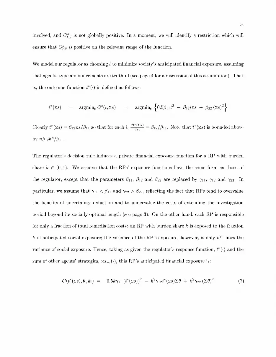
We model our regulator as choosing t to minimize society's anticipated �nancial exposure, assuming

that agents' type announcements are truthful (see page 4 for a discussion of this assumption). That

is, the outcome function t�(�) is de�ned as follows:

t�(�s) = argmint Cs(t;�s) = argmint

n0:5�11t

2 � �12t�s + �22 (�s)2o

Clearly t�(�s) = �12�s=�11 so that for each i,dt�(�s)

dsi= �12=�11. Note that t

�(�s) is bounded above

by n�12�u=�11.

The regulator's decision rule induces a private �nancial exposure function for a RP with burden

share k 2 (0; 1). We assume that the RPs' exposure functions have the same form as those of

the regulator, except that the parameters �11, �12 and �22 are replaced by 11, 12 and 22. In

particular, we assume that 11 < �11 and 22 > �22, re ecting the fact that RPs tend to overvalue

the bene�ts of uncertainty reduction and to undervalue the costs of extending the investigation

period beyond its socially optimal length (see page 3). On the other hand, each RP is responsible

for only a fraction of total remediation costs: an RP with burden share k is exposed to the fraction

k of anticipated social exposure; the variance of the RP's exposure, however, is only k2 times the

variance of social exposure. Hence, taking as given the regulator's response function, t�(�) and the

sum of other agents' strategies, �s�i(�), this RP's anticipated �nancial exposure is:

C(t�(�s);�; ki) = 0:5k 11 (t�(�s))2 � k2 12t

�(�s)�� + k2 22 (��)2 (7)

24

We will assume that even if all burden shares are equal (i.e., when ki = 1=n, for all i), the

expected investigation period that results when �rms act strategically exceeds the socially optimal

investigation period.

RP i's strategy is a map si : � ! [��; ��]. We assume that �

�= 0. Given the mapping �s�i(�) from

�n�1 to the sum of other agents strategies, si(�) must satisfy the �rst order condition:

0 �

Z�n�1

��ki 11t

� (si(�i) + �s�i(��i)) � k2i 12(�i +���i)� dt�(�s)

dsi

�g�i(��i)d��i

with equality holding whenever si(�i) > ��.

Dividing through by ki, the constantdt�(�)dsi

= �12=�11 and the constant 12= 11, and substituting

for t�(�), we obtain

0 =

Z�n�1

�si(�i) + �s�i(��i) � ki

12�11 11�12

(�i +���i)

�g�i(��i)d��i; for all �i � ~�i (8)

so that, de�ning ~�i implicitly by ki 12�11 11�12

(~�i +E�n�1���i) = ��+ E�n�1�s�i(��i), i's strategy can

be written as:

si(�i) =

8>>>><>>>>:��

if �i � ~�i

ki 12�11 11�12

(�i +E�n�1���i) � E�n�1�s�i(��i) if �i > ~�i

The following proposition establishes that under the linear-quadratic speci�cation, any shift in

burden from smaller RPs to larger ones results in an increase in the expected investigation period.

More precisely, arrange RP's by burden share in decreasing order, so that RP's with larger burdens

have smaller indices. Now partition the set f1; :::; ng into two subsets, i.e., larger RP's are to the left

and smaller are to the right. Now consider a new burden pro�le in which shares for RP's in the left

25

subset are no smaller, while shares for those in the right subset are no larger, than originally. Then

in the new equilibrium, the expected value of the outcome function increases. Since by assumption,

the investigation period is too long even when �rms' burden shares are equal, the burden shift

further exacerbates the delay.

Proposition 6 (Heterogeneity and delay: multiple RPs). Consider a burden pro�le, k, suchthat not all burden shares are equal. Arrange RPs so that i < j implies ki � kj. Now considera shift in burden shares to k0 6= k. Assume that for some j 2 f1; :::; n � 1g, k0i � ki, for al-l i � j and k0i � ki otherwise. Let s and s0 be PSNE's corresponding to these pro�les. ThenE�n t(�s0(�)) > E�n t(�s(�)).

6. A policy application: Superfund cleanups

In this section we apply our theoretical framework to evaluate two practices that are widespread in

the management of Superfund cleanups. In particular, we consider the e�ect on cleanup delay of de

minimis RP buyouts and the formation of steering committees by RP's. Each of these practices has

been widely advocated as an e�ective way to reduce litigation and transaction costs, and thereby

expedite the cleanup process. Our model suggests that each may have side-e�ects that have been

hitherto ignored. It must be emphasized that the formal results we obtain in this section are

valid only under the linear-quadratic speci�cation in section 5. As we noted above, however, the

key comparative statics result we obtain in that section, Proposition 6, will hold more generally,

provided that third-order e�ects do not dominate lower-order e�ects.

6.1. de minimis RP buyouts. A RP is classi�ed as de minimis if its burden share falls below

some (small) critical fraction. In a de minimis RP buyout, small RPs pay the regulator a �xed

amount in exchange for relief from all future liabilities. Typically the buyout price that a given

RP will pay will more than cover its expected burden, because the RP will be willing to pay a risk

premium to avoid the uncertainty arising from continued liability. From a policy standpoint, a de

26

minimis buyout serves several useful purposes. In particular, it is a source of immediate liquidity

to fund short-term expenses. Moreover, by reducing the number of RPs involved in the negotiation

process, it may lower transactions costs and thus expedite the cleanup process.

After a buyout, on the other hand, all of the costs of uncertainty that the small RPs originally

had to bear will be transferred to the larger RPs that remain. Thus although the expected burden

borne by each remaining RP will remain the same, or will actually decline if the de minimis parties

pay a risk premium, the variance of this burden will increase, because each remaining party is

now responsible for a larger share of total cleanup costs. In the context of our model, this shift

will increase the marginal bene�t to an individual RP of further investigation and thus exacerbate

its incentive to induce delay. A striking fact is that this negative consequence of buyouts cannot

be mitigated by increasing the risk premiums extracted from the de minimis parties. From the

perspective of a remaining RP, buyout revenue is a lump-sum transfer; it reduces the RP's exposure

by an amount that is independent of the variable (private uncertainty level) over which the RP has

discretion. The following proposition summarizes this discussion.

Proposition 7 (de minimis buyouts and delay). Consider a burden pro�le, k, and �x k > 0such that for some j, kj � k. For the model speci�ed in section 5, a de minimis buyout of all RPswhose burden shares do not exceed k will increase the expected investigation length. Moreover, thisincrease will be invariant with respect to the magnitude of the buyout premiums.

6.2. RP steering committees. Just as regulators have encouraged small RPs to settle early via

de minimis buyouts, they have also encouraged large RPs to form steering committees that will

negotiate with the regulators on behalf of their members. Such committees are socially useful to the

extent that they encourage cooperative behavior between RP's, and reduce contentious litigation

over burden shares. Once again, however, our model highlights an attribute of steering committees

that could have potentially major negative social consequences.

27

As we have seen, the extent of cleanup delay is determined by balancing the marginal expected cost

of increasing the investigation period against the marginal bene�t of the reduction in uncertainty

resulting from a more thorough investigation. As noted above, an individual RP's share of total

expected cost increases in proportion to its burden share, while the uncertainty associated with

its liability exposure increases with the square of its burden share. Thus, larger RPs assign a

greater relative importance to uncertainty than smaller ones. Consequently cleanup sites with

many small RPs are likely to be less subject to delay than ones with a few large RPs. When a

steering committee is formed, the interests of several RP's are coalesced: e�ectively, several smaller

RP's are replaced by a single large one. From the RPs' perspective, the formation of a steering

committee thus internalizes an important externality. From a social perspective, however, this

externality is a positive one, since it reduces delay. When a steering committee is formed, this

externality is mitigated and social welfare is reduced.15

The formation of a steering committee can be represented as a change in burden pro�le. Consider a

burden pro�le k, ordered as usual so that i < j implies ki � kj . Suppose that a subset J � f1; :::; ng

of RPs, #J � 2, form a committee, and let j = minfj 2 Jg be the RP in J whose liability share

is the largest. After the steering committee is formed, there is, e�ectively, a new liability pro�le in

which j's share is now equal to the sum of the shares of all RP's in J , and the shares of all RP's

in J except j's are reduced to zero. Formally, de�ne the pro�le k0 6= k as follows: k0i =P

j2J kj ,

if i = j; k0i = ki, if i 2= J ; and k0i = 0 otherwise. Observe that k0 satis�es the condition of

Proposition 6, since k0 6= k, k0i � ki for i � j, and k0i � ki otherwise. Consequently, the following

result is an immediate corollary of Proposition 6.

Proposition 8 (Steering Committees and delay). For the model speci�ed in section 5, if atleast two RP's form a steering committee, then the expected investigation length will increase.

15 Of course, the social bene�ts of reduced litigation may o�set this loss, but in this paper, these bene�ts are unmodeled.

28

7. Conclusion

In this paper, we study an incomplete information game among parties who have contributed to the

creation of an environmental problem and are now responsible for its remediation. A key assumption

is that these RPs are better informed about their individual contributions to the problem than the

regulator. Provided that the distributions of RPs' types are nonatomic, there exists a pure-strategy

Nash equilibrium in which each RP's report about its level of uncertainty is positively related to its

true level. Moreover, larger RP's are more likely to over-report than smaller RP's. Under certain

conditions, aggregate over-reporting increases with the degree to which RPs' burden shares are

heterogeneous.

While this paper focuses primarily on environmental policy and regulation, the model we present

may be of general interest to game-theorists. Our model applies a very powerful theorem by

Athey (1997), which to our knowledge has not yet been applied to the theory of regulation. The

theorem guarantees existence of pure strategy equilibria for incomplete information games satisfying

a condition that is very natural in many applications. We can thus bene�t for the well known and

very considerable advantages that pure strategies have over mixed strategies. In addition, the

game we model belongs to a class of games called aggregation games, which are applicable in a

wide variety of economic and political contexts. This class has the property that each agent's

payo� depends only on the sum of all agents' actions. Under certain conditions, games of this kind

exhibit a property that is both very striking and facilitates comparative static analysis.

Modi�ed versions of the game presented in this paper can be applied to a wide range of regulatory

problems. In particular, our model may be applicable whenever there is incomplete information and

an aggregation �lter is applied to individual actions. One class of problems arise in competition

or antitrust regulation of collusion. Here each �rm has private information and �rms' pro�ts

29

depend on the sum of all �rms' pricing and output decisions (Athey, Bagwell and Sanchiroico,

1998). In the implementation of collusive pricing, the vector of market shares is the publicly known

parameter, playing the role that the ki's play in our model. Strategic behavior in the presence of

an aggregation �lter also arises in the context of group decision-making, when individual group

members have incentives to manipulate the information transmission process. For example, in a

model of committee voting behavior, the parameter ki might represent the i'th committee member's

publicly known indvidual stake in the issue at hand.

Finally, our results have important policy implications. Current regulatory policy does not include

guidelines for strategically extracting accurate information from RPs. Furthermore, some wide-

spread practices in the management of environmental remediation, such as the formation of RP

steering committees and de minimis RP buyouts, may exacerbate strategic behavior. This paper

demonstrates that the issue of strategic information transmission may be signi�cant.

References

Athey, S. (1997). Single crossing properties and the existence of pure strategy equilibria in games of incomplete

information, Technical report, MIT.

Athey, S., Bagwell, K. and Sanchiroico, C. (1998). Collusion and price rigidity, Working paper, MIT Department of

Economics.

Birdsall, T. H. and Salah, D. (1993). Prejudgment interest on superfund costs: Cercla's running meter, Environmental

Law Reporter 23: 10424+.

Dixon, L. S. (1994). Fixing superfund: The e�ects of the proposed superfund reform act of 1994 on transaction costs,

Technical Report RAND/MR-455-ICJ, RAND.

Milgrom, P. and Shannon, C. (1994). Monotone comparative statics, Econometrica 62(1): 1089{1122.

Rausser, G. C., Simon, L. K. and Zhao, J. (1998). Information asymmetries, uncertainties, and cleanup delays at

Superfund sites, Journal of Environmental Economics and Management 35(1): 48{68.

30

Zimmerman, R. (1988). Federal-state hazardous waste management policy implementation in the context of risk un-

certainties, in C. E. Davis and J. P. Lester (eds), Dimensions of Hazardous Waste Politics and Policy, Greenwood

Press, chapter 11, pp. 177{201.

31

Appendix: Proofs

Proof of Proposition 1: Existence and the fact that si is ��on an interval (which may be

null) and then increasing, follows immediately from Athey's theorem. �

Proof of Lemma 2.1: Part (a) follows from the fact that f = dFd� = dC

dt t0 and t0 > 0 while

Ct� < 0. To prove (b), observe that d2Fdsi

2 = Cttt0 + Ctt

00 with Ctt > 0 and t0 > 0. The sign of

f�s = d2Fdsi

2 will be determined by the �rst of these terms, provided that either jCtj or jd2td�s2

j is

suÆciently small. This proves part (b) of the Lemma. �

Proof of Lemma 2.2: Pick ��i 2 �ij and let ̂ = si(�

�i)� sj(�

�i). We have

0 �dE��i

F ((si(��i); s�i); (�

�i;��i); ki)

d�

=

Z[�l;�u]

E��ij[f(si(�

�i) + sj(#) + �s�ij ; �

�i + #+���ij; ki)] g(#)d#

=

Z[�l;�u]

E��ij[f(sj(�

�i) + ̂ + sj(#) + �s�ij; �

�i + #+���ij; ki)] g(#)d#

<

Z[�l;�u]

E��ij[f(sj(�

�i) + ( ̂ + sj(#)) + �s�ij; �

�i + #+���ij; kj)] g(#)d#

�

Z[�l;�u]

E��ij[f(sj(�

�i) + si(#) + �s�ij ; �

�i + #+���ij; kj)] g(#)d#

=dE��j

F ((sj(��i); s�j); (�

�i;��j); kj)

d�

The strict inequality follows from Lemma 2.1(a), i.e., f decreases w.r.t. ki; the weak inequalityholds because for all #, si(#) � sj(#) + ̂ and, by Lemma 2.1(b), f increases w.r.t. t, which inturn increases w.r.t. �s. Since f is continuous, there exists a neighborhood U of �

�i such that for

all � 2 U , 0 <dE�

�jF ((sj(�);s�j);(�;��j);kj)

d� and hence, from (1), sj(�) = ��. �

Proof of Proposition 3: To prove part (a), suppose ~�i � ~�j. If min#2[�l;�u](si(#)�sj(#)) = 0,

then since sj(~�j) = si(~�j) = ��, ~�j 2 argmin#2[�l;�u](si(#)� sj(#)). If min#2[�l;�u](si(#)� sj(#)) < 0,

then since sj(�) = si(�) = ��on [�l; ~�j ], argmin#2[�l;�u](si(#) � sj(#)) � (~�j; �

u]. In either case,

argmin#2[�l;�u](si(#)� sj(#))\ [~�j; �u] 6= ;. But for all � > ~�j, sj(�) > �

�, contradicting Lemma 2.2.

To prove part (b), assume that for some ��i 2 (~�i; �

u], si(��i) � sj(�

�i). >From part (a), ~�j > ~�i. Since

si(�) > sj(�) on (~�i; ~�j ], it follows that ��i 2 (~�j ; �

u]. Assume w.l.o.g. that ��i 2 argmin#2(~�j ;�u](si(#)�

sj(#)). Since si(�) � ��= sj(�) on [�l; ~�j ], �

�i 2 argmin#2(�l;�u](si(#) � sj(#)). But by de�nition of

~�j, sj(��i) > �

�, contradicting Lemma 2.2. �

32

Proof of Proposition 4: We �rst consider RP i and argue that

~�0i <~�i and s0i(�) > si(�) for � � ~�i: (9)

An exactly analogous argument establishes the corresponding properties for RP j. Let �1 = min#2[~�i;�u]

�s0i(#) � si(#)

�and � 2 = max#2[�l;�u]

�s0j(#) � sj(#)

�. Suppose that

�1 � 0 and

pick ��1 2 [~�i; �

u] such that s0i(��1)� si(�

�1) =

�1. We �rst establish that � 2+

�1 must be positive. If

not then,

0 �

Z[�l;�u]

�f(s0i(��

1) + s0j(�j); ��1 + �j ; k

0i)�g(�j)d�j

<

Z[�l;�u]

�f(s0i(��

1) + s0j(�j); ��1 + �j ; ki)

�g(�j)d�j

�

Z[�l;�u]

�f(si(�

�1) +

�1 + s2(�j) + � 2; �

�1 + �j; ki)

�g(�j)d�j

�

Z[�l;�u]

[f(si(��1) + s2(�j); �

�1 + �j; ki)] g(�j)d�j (10)

The strict inequality follows from Lemma 2.1(a), i.e., f decreases w.r.t. ki. The �rst weak inequalityholds because s0i(��

1) = si(��1) +

�1, s

0j(�) � sj(�) + � 2 and, by Lemma 2.1(b), f increases w.r.t. �s.

The second weak inequality holds because by assumption, � 2 + �1 � 0 and f increases w.r.t. �s.

But inequality (10) is impossible since ��1 � ~�i implies

0 =

Z[�l;�u]

[f(si(��1) + s2(�j); �

�1 + �j; ki)] g(�j)d�j (11)

This establishes that �1 � 0 implies � 2+

�1 > 0. Now pick ��2 such that s0j(

��2)� sj(��2) = � 2. Since

� 2 > � �1 � 0, it follows that ��2 > ~�0j. Hence

0 =

Z[�l;�u]

�f(s0j(

��2) + s0i(�i);��2 + �i; k

0j)�g(�i)d�i

�

Z[�l;�u]

�f(s0j(

��2) + s0i(�i);��2 + �i; kj)

�g(�i)d�i

�

Z[�l;�u]

�f(sj(��2) + � 2 + si(�i) +

�1; ��2 + �i; kj)

�g(�i)d�i

>

Z[�l;�u]

�f(sj(��2) + si(�i); ��2 + �i; kj)

�g(�i)d�i (12)

33

Once again, the �rst weak inequality hold because f(�) decreases with k and k0j � kj . The second

weak inequality holds because s0j(��2) = sj(��2) + � 2, s

0i(�) � si(�) +

�1 and f increases w.r.t. �s.

The strict inequality holds because � 2+ �1 > 0 and, once again, because f increases w.r.t. �s. But

inequality (12) is impossible because

0 �

Z[�l;�u]

�f(sj(��2) + si(�i); ��2 + �i; kj)

�g(�i)d�i

Thus we know �1 > 0, or s0i(�) > si(�) for � � ~�i, and from continuity of s(�), ~�0i <

~�i. �

Proof of Proposition 5: The proof relies on two Lemmas. The �rst gathers together severalresults about �- atness.

Lemma 5.1. (a): If X � R and for all x; x0 2 X,��� f 0(x)f(x0)

��� < �max(x2X)�min(x2X) , then f is �- at.

Now �x an integer n, scalars �; 2 R+ , and an integrable function y : X ! R such that jy(�)j < .

(b): If f is �- at for � < �Æ and

RX f(x)y(x)g(x)dx � �nÆf , then

RX y(x)g(x)dx � �(n� 1)Æ

(c): If f is �- at for � < �Æf and

RX y(x)g(x)dx �

�nÆf , then

RX f(x)y(x)g(x)dx � �(n� 1)Æ.

The second lemma establishes a uniform boundedness property on a family of functions, parama-terized by � 2 [0; 1]. Let � = [�l; �u] and let � = �2. For each �, let f(�; �) be a continuousfunction mapping � to R2++ and let x(�; �) = (x1(�; �); x2(�; �)) be an integrable function mapping

� to R2 .

Lemma 5.2. Assume that there exists ! 2 R+ and �� 2 � with ��2 > �l such that for all �,the following conditions are satis�ed: (a) for each r = 1; 2, xr(�; �) depends only on �r; (b) there

exists ~�(�) 2 �, ~�(�) � ��, such that xr(�; �) = 0 on [�l; ~�r(�)); and (c) for each �r 2 [~�r(�); �u],

E[fr(#; �)P2

2=1 x2(#; �)j#r = �r] 2 (�!; !). For any � > 0 satisfyingR �l~�2g(#)d# < 1=(1 + �)2,

there exists 2 R such that if f is �- at, then for r = 1; 2, sup (jxr(�; �)j) < , for all � 2 [0; 1].

We can now proceed with the proof of Proposition 5. We need to prove that for � suÆciently closeto unity,

0 �

Z�

dt(#; �)

d�g(#)d# =

Z�

�t0��s(#; �)

�� 2Xr=1

d [sr(#r; �)]

d�g(#)d# (13)

We will proceed as follows.

1. For �xed �, partition� into�(�) =n# 2 � : # < ~�1(�)

oand�(�) =

n# 2 � : # � ~�1(�)

o.

In expression (17) below, we de�ne a function 1t : � � [0; 1] ! R+ below and prove thatthere exists Æ > 0 such thatZ

�(�) 1t(#; �)

2Xr=1

d [sr(#r; �)]

d�

!g(#)d# >

3Æ 1t

t0(2��)

(14)

34

where 1t= min f 1t(#; �) : # 2 �g.

2. Invoke Lemma 5.2 to establish that there exists 2 R+ such that for all � 2 � and all

� 2 [0; 1], sup���d [sr(�;�)]d�

��� < .

3. If 1t(�; �) is - at, for <Æ

1tt0 it follows from Step 1 and Part (b) of Lemma 5.1 that

Z�(�)

2Xr=1

d [sr(#r; �)]

d�

!g(#)d# >

2Æ

t0:

4. If Ctt is �C1- at, for �C1 < (1+ )1=3�1 and t00(2��)t0(2�

�) < �t, for �t < min

n(1+ )min(Ct)

max(Ct); (1+ )

1=3�12(����

�)

o,

then 1t(�; �) is - at.5. If t0 is �C2- at, for �C2 <

Æt0(2�

�) it follows from Step 3 and Part (c) of Lemma 5.1 that

Z�(�)

�t0��s(#; �)

�� 2Xr=1

d [sr(#r; �)]

d�g(#)d# > Æ:

6. Since ~�1(�) & �l as � ! 1, and since t0(�) is increasing in �s, we can pick �� < 1 suÆcientlylarge that

R�(�)(�) g(#)d# < Æ

t0(2��) . thus ensuring that for � > ��,R�(�)

�t0��s(#; �)

��P2r=1

d [sr(#r;�)]d� g(#)d# > �Æ. This, together with step 5, will complete

the proof.

Of these steps, 3, 5 and 6 require no further work.

Step 1: Fix � 2 [0; 1], r 2 f1; 2g and �0r 2 (~�r(�); �u]. It follows from Proposition 1 and (1) that

0 =

Z�

"Ct

�t�sr(�

0r; �) + s:r(#:r; �)

�; (�0r; #:r); �r(�)

�d �t�sr(�0r; �) + s:r(#:r; �)��

dsr

#g(#:r)d#:r

=

Z� r((�

0r; #:r); �)g(#:r)d#:r (15)

where

r((�0r; #:r); �) = Ct

�t��s((�0r; #:r); �)

�; (�0r; #:r); �r(�)

�t0��s((�0r; #:r); �)

�d�s((�0r; #:r); �)dsr

= Ct

�t��s((�0r; #:r); �)

�; (�0r; #:r); �r(�)

�t0��s((�0r; #:r); �)

�

Since (15) holds for all �, the total derivative w.r.t. � of the right hand side of (15) must beidentically zero. To expand this derivative, we must �rst compute the total derivative of r((�

0r; �); �)

with respect to �. For each #:r, we have:

d

d�

� r((�

0r; #:r); �)

�= rt((�

0r; #:r); �)

2X2=1

d [s2((�0r; #:r); �)]

d�+ rk((�

0r; #:r); �)

d�r(�)

d�(16)

35

where

rt((�0r; #:r); �) =

Ctt

�t��s((�0r; #:r); �)

�; (�0r; #:r); �r(�)

� �t0��s((�0r; #:r); �)

��2

+ Ct

�t��s((�0r; #:r); �)

�; (�0r; #:r); �r(�)

�t00��s((�0r; #:r); �)

�!(17)

and

rk((�0r; #:r); �) = Ctk

�t��s((�0r; #:r); �)

�; (�0r; #:r); �r(�)

�d �t��s((�0r; #:r); �)��dsr

Our assumptions on C and t (Ct; Ctt; t0; t00 > 0, Ctk < 0) guarantee that rt(�) > 0 and rk(�) < 0.

Now, taking the total derivative of (15) w.r.t. � we obtain:

0 =d

d�

�Z� r((�

0r; #:r); �)g(#:r)d#:r

�

=

Z� rt((�

0r; #:r); �)

2X2=1

�d [s2((�

0r; #:r)�)]

d�

�g(#:r)d#:r

+d�r(�)

d�

Z� rk((�

0r; #:r); �)g(#:r)d#:r (18)

For future reference, note that for all r, � and �0r 2 (~�r(�); �u],

Z� rt((�

0r; #:r); �)

2X2=1

�d [s2((�

0r; #:r)�)]

d�

�g(#:r)d#:r 2 �

�k0r � kr

� rk

� [� rk; rk] (19)

where rk = max f rk(#; �) : # 2 �; � 2 [0; 1]g. Now set r = 1 and integrate (18) over the interval

(~�r(�); �u] on which this equality holds to obtain:

Z�(�)

1t(#; �)

2Xr=1

d [sr(#r; �)]

d�

!g(#)d# =

d�1(�)

d�

Z�(�)

rk(#; �)g(#)d#

� ��k01 � k1

� 1k

> 0

where 1k

= min f 1k(#; �) : # 2 �; � 2 [0; 1]g. Hence Æ > 0 can be chosen suÆciently small to

ensure that inequality (14) is satis�ed. This completes the proof of Step 1.

Step 2: Consider the family of functions x(�; �), where xr(�; �) = d [sr(�;�)]d� , and f(�; �) where

fr(�; �) = rt(�; �). Let ! = rk and �� = (�l; ~�2(0)). Note that for each �, (~�1(�); ~�2(�)) �(�l; ~�2(0)) = ��. Observe that (a) for each r, xr(�; �) depends only on �r; for ~�(�) = (~�1(�); ~�2(�))~�(�) � �� and the following conditions are satis�ed for each r, (b) (cf. Proposition 1 and (1))

xr(�; �) = 0 on [�l; ~�r(�)); (c) (cf. (19)). for each �r 2 [~�r(�); �u], E[fr(#)

P22=1 x2(#; �)j#r = �r] 2

(�!; !). Hence the conclusion of Lemma 5.2 applies.

36

Step 4: >From (17)

1t(�; �) = Ctt(�; �; �)(t0(�))2 + Ct(�; �; �)t

00(�)

>From Part (a) of Lemma 5.1, t00 is ((1 + )1=3 � 1)- at. By assumption, Ctt is also. Hencemax[Ctt(�;�;�)(t0(�))2]min[Ctt(�;�;�)(t0(�))2]

� (1 + ). Moreover, since t00(�) < (1 + )min(Ct)max(Ct)

, max[Ct(�;�;�)t00(�)]min[Ct(�;�;�)t00(�)]

� (1 + ) also.

Hence max[ 1t(�;�)]min[ 1t(�;�)]

� (1 + ). �

We now prove the two lemmas.

Proof of Lemma 5.1:

(a): Let f = min(f(x) : x 2 X) and f = max(f(x) : x 2 X). Note that jf 0(x)j <�f

max(x2X)�min(x2X) . Pick x and x in X such that f(x) = f and f(x) = f . Assume (w.l.o.g.)

that x > x.

f � f =

Z x

xf 0(x)dx � sup(f 0)

Z x

xdx � sup(f 0)

Z max(x2X)

min(x2X)dx

��f

[max(x 2 X)�min(x 2 X)][max(x 2 X)�min(x 2 X)] = �f

(b):

�nÆf �

ZXf(x)y(x)g(x)dx

� f

ZX(y(x))�g(x)dx + f

�1 +

�Æ

�ZX(y(x))+g(x)dx

= f

�ZXy(x)g(x)dx +

�Æ

�

Hence

�(n� 1)Æ �

ZXy(x)g(x)dx

(c): ZXf(x)y(x)g(x)dx � f

�ZX(y(x))+g(x)dx +

�1 +

�Æ

f

�ZX(y(x))�g(x)dx

�

� f

��nÆ

f�

�Æ

f

�= �(n� 1)Æ

�

37

Proof of Lemma 5.2:Preliminary Step: If � < 1, there exists such that for all � 2 [0; 1] and r = f1; 2g, if jxr(�)j >

for some � 2 [~�r(�); �u], then xr(�); xr(�

0) > 0. for all �0 2 [~�r(�); �u].

Proof of the Preliminary Step: Suppose that the preliminary step is false, i.e., that there exist-

s a sequence f�mg 2 [0; 1] and two sequences f�m1 g and f�m1 g such that xm1 (�

m1 ) ! 1 while

for all m, xm1 (�m1 ) � 0, where xm1 (�) = x1(�; �

m). It follows that �xm1 ! 1, where �xm1 =

supnxm1 (#) : # 2 [~�1(�); �

u)o� inf

nxm1 (#) : # 2 [~�1(�); �

u]o. Letting fm1 = f1(�; �

m), we have16

! � xm1 (�m1 )

Z�fm1 (�

m1 ; #2)g2(#2)d#2 +

Z�fm1 (�

m1 ; #2)x

m2 (#2)g2(#2)d#2

� f1xm1 (�

m1 ) + f

1Eh�xm2

�+i+ f1E

h�xm2

��i

� f1

�xm1 (�

m1 ) + E

hxm2

i+ �E

h�xm2

��i�(20)

Similarly,

�! � xm1 (�m1 )

Z�fm1 (�m1 ; #2)g2(#2)d#2 +

Z�fm1 (�m1 ; #2)x

m2 (#2)g2(#2)d#2

� f1xm1 (�

m1 ) + f1E

h�xm2

�+i+ f

1Eh�xm2

��i

� f1

�xm1 (�

m1 ) + E

hxm2

i+ �E

h�xm2

�+i�(21)

Let �xm =P2

r=1�xmr . Since �x

m1 ! 1 and for all m, �xm � �xm1 , it follows that �x

m ! 1.Dividing both sides of (20) and (21) by f

1�xm we obtain:

xm1 (�m1 )

�xm+

Ehxm2

i�xm

+�Eh�xm2

��i�xm

! 0 (22)

xm1 (�m1 )

�xm+

Ehxm2

i�xm

+�Eh�xm2

�+i�xm

! 0 (23)

Note that (22), (23) and the fact that limm!1 xm1 (�m1 ) � 0 together imply that

infnxm2 (#) : # 2 [~�m2 ; �

u]o

� Eh�xm2

��i! �1 while

supnxm2 (#) : # 2 [~�m2 ; �

u]o

� Eh�xm2

�+i! 1 (24)

16 For any variable or function x taking values in R, let x+ = max(x; 0) and x� = min(x; 0).

38

Subtracting (23) from (22), we obtain

�xm1 � �

�Eh�xm2

�+i�E

h�xm2

��i��xm

! 0 (25)

Hence from (24)

limm!1

�xm1 � ��xm2�xm

� 0 (26)

It follows that �xm2 ! 1. Repeating the argument that gave rise to (25) for 1, we obtain (27)below:

�xm2 � �

�Eh�xm1

�+i�E

h�xm1

��i��xm

! 0 (27)

Hence, reasoning as above:

limm!1

�xm2 � ��xm1�xm

� 0 (28)

But if � < 1, (26) and (28) cannot hold simultaneously, proving that the Preliminary Step is true.

Now suppose (w.l.o.g.) that the conclusion of the lemma is false for 1,, i.e., that there exists asequence f�mg 2 [0; 1] and a sequence f�m1 g such that for all m, jxm1 (�

m1 )j > m, where xm1 (�) =

x1(�; �m). Assume w.l.o.g. that xm1 (�

m1 ) is positive for all m. Moreover, we can clearly choose �m1

so that for each m, xm1 (�m1 ) � E[xm2 (#1)j#1 �

~�m1 ], where~�m1 = ~�1(�

m). >From the preliminary

step, it follows that if m is suÆciently large, xm1 (�) is positive on [~�m1 ; �u]. >From condition (c) in

the statement of the Lemma,

!

xm1 (�m1 )E(f

m1 (�m1 ; #2))

� 1 +E[fm1 (#)xm2 (#)j#1 = �m1 ]

xm1 (�m1 )E(f

m1 (�m1 ; #2))

��!

xm1 (�m1 )E(f

m1 (�m1 ; #2))

Since xm2 (�) depends only on #2 and is identically zero on [�l; ~�m2 ), the above expression can berewritten as

!

xm1 (�m1 )E(f

m1 (�m1 ; #2))

� 1 +p2(~�

m)E[fm1 (#)xm2 (#)j#1 �

~�m2 ]

xm1 (�m1 )E(f

m1 (�m1 ; #2))

��!

xm1 (�m1 )E(f

m1 (�m1 ; #2))

Clearly both of the outer bounds converge to zero. Hence

limm!1

E[fm1 (#)xm2 (#)j#1 �~�m2 ]

xm1 (�m1 )E(f

m1 (�m1 ; #2))

= �1

p2(~�m)

(29)

39

Necessarily, there exists a sequence f�m2 g in [~�m2 ; �u], such that xm2 (�

m2 )! �1. >From the prelim-

inary step, it follows if m is suÆciently large, xm2 (�) is negative on [~�m2 ; �u]. Hence, since xm1 (�

m1 ) �

E[xm2 (#1)j#1 �~�m1 ]:

limm!1

E[fm1 (#)xm2 (#)j#1 �~�m2 ]

xm1 (�m1 )E(f

m1 (�m1 ; #2))

� limm!1

f1E[xm2 (#)j#1 �

~�m2 ]

xm1 (�m1 )E(f

m1 (�m1 ; #2))

� limm!1

f1E[xm2 (#)j#1 �

~�m2 ]

f1E[xm1 (#)j#1 �

~�m1 ](30)

Since f1 = (1 + �)f1, (29) and (30) imply that

limm!1

E[xm2 (#2)j#2 �~�m2 ]

E[xm1 (#1)j#1 �~�m1 ]

��1

p2(~�m)(1 + �)

(31)

Note, however, that the chain of reasoning we have just applied leads to the following, exactcounterpart of (31):

limm!1

E[xm1 (#2)j#1 �~�m1 ]

E[xm2 (#1)j#2 �~�m2 ]

��1

p1(~�m)(1 + �)

(32)

Since p1(~�m) � 1, it follows that limm!1

E[xm2 (#2)j#1�~�m1 ]

E[xm1(#1)j#2�~�m

2]� �(1+�). But since p2(~�

m) � p(��) <

1=(1 + �)2, this inequality and (31) cannot hold simultaneously. �

Proof of Proposition 6: De�ne the function � : [0; 1] ! Rn by, for � 2 [0; 1], �(�) =

�k0 + (1 � �)k. Observe that for all i � j and all � 2 [0; 1], d�i(�)d� � 0, while d�i(�)

d� � 0 oth-erwise. For each � 2 [0; 1], let s(�;�) be the PSNE corresponding to �. We will prove thatdd� [E�n (t(�s(�; �)))] > 0. Integrating this derivative w.r.t. � from zero to one, it will then followE�n t(�s0(�)) > E�n t(�s(�)).

For each i de�ne ~�i(�) implicitly by the equation �i(�) 12�11 11�12

(~�i(�)+E�n�1���i) = ��+E�n�1�s�i(��i; �).

Observe from (8) that for i and �i > ~�i(�),

0 =

Z�n�1

�si(�i; �) + �s�i(��i; �) � �i(�)

12�11 11�12

(�i +���i)

�g�i(��i)d��i

It follows that for all i and all �:

dsi(�i; �)

d�=

(0 if �i < ~�i(�) 12�11 11�12

(�i +E�n�1���i)d�i(�)d� � E�n�1

d�s�i(��i;�)d� if �i > ~�i(�)

(33)

Applying Leibniz's rule to (33) and noting that si(~�i) = ��= 0, we obtain

d

d�[E�si(�; �)] = � si(~�i; �)

d ~�i(�)

d�+

Z �u

~�i(�)

dsi(�i; �)

d�g(�i)d�i =

Z �u

~�i(�)

dsi(�i; �)

d�g(�i)d�i:

(34)

40

For # 2 �, let (#) = 12�11 11�12

R �u# (#+E�n�1���i) g(#)d#. Also let pi(�) =

R �u~�i(�)

g(�i)d�i denote

the probability that si(�; �) > ��. Substituting (33) into (34), we obtain

d

d�[E�si(�i; �)] = (~�i(�))

d�i(�)

d�� pi(�)

d

d�[E�n�s(�; �)] + pi(�)

d

d�[E�si(�i; �)]

=(~�i(�))

1� pi(�)

d�i(�)

d��

pi(�)

1� pi(�)

d

d�[E�n�s(�; �)] : (35)

Now by assumption, there exists j 2 f1; :::; n � 1g such that d�i(�)d� � 0 i� i � j and d�i(�)

d� � 0

otherwise. Moreover, since i � j implies ki(�) � kj(�), it follows from Proposition 3 that ~�i(�) �~�j(�) and pi(�) � pj(�) if i � j, while ~�i(�) � ~�j(�) and pi(�) � pj(�) otherwise, with equality

holding only if �i(�) = �j(�). It follows that(~�i(�))1�pi(�)

�(~�j(�))

1�pj(�)if i � j, while (~�i(�))

1�pi(�)�

(~�j(�))

1�pj(�),

otherwise. Moreover, by assumption not all of the ki's are equal, so that for at least one i, one ofthe above inequalities holds strictly. These relationships imply that for all i,

d

d�[E�si(�i; �)] �

(~�j(�))

1� pj(�)

d�i(�)

d��

pi(�)

1� pi(�)

d

d�[E�n�s(�; �)] :

with strictly inequality holding for at least one i. Summing over all i, we obtain:

d

d�[E�n�s(�; �)] >

(~�j(�))

1� pj(�)

nXi=1

d�i(�)

d��

nXi=1

pi(�)

1� pi(�)

d

d�[E�n�s(�; �)]

=

1 +

nXi=1

pi(�)

1� pi(�)

!�1(~�j(�))

1� pj(�)

nXi=1

d�i(�)

d�(36)

SincePn

i=1d�i(�)d� = 0, it follows that d

d� [E�n�s(�; �)] is positive. �

Proof of Proposition 7: Let k0 denote the burden pro�le after the buyout. That is,

k0i = ki

�Pfi:ki>kg

ki

��1if ki > k and 0 otherwise. Clearly, the conditions of Proposition 6

are satis�ed, except for the fact that each remaining RP's objective function (see expression (7))is decremented by a constant number (the sum of de minimis RPs' buyout payments). Specif-ically, assume that burden shares are ordered as usual so that i < j implies ki � kj . Letj = minfj 2 f1; :::; ng : kj > kg and observe that k0i > ki if i � j while k0i = 0 otherwise. Thusfor each i the �rst order condition (8) remains valid and is independent of buyout payments. Theconclusion of the proposition now follows immediately from Proposition 6. �