Embed Size (px)
Citation preview
ESSAYS ON ECONOMETRIC MODELING OF
SUBJECTIVE PERCEPTIONS OF
RISKS IN ENVIRONMENT AND HUMAN HEALTH
A Dissertation
by
TO NGOC NGUYEN
Submitted to the Office of Graduate Studies of Texas A&M University
in partial fulfillment of the requirements for the degree of
DOCTOR OF PHILOSOPHY
May 2008
Major Subject: Agricultural Economics
ESSAYS ON ECONOMETRIC MODELING OF
SUBJECTIVE PERCEPTIONS OF
RISKS IN ENVIRONMENT AND HUMAN HEALTH
A Dissertation
by
TO NGOC NGUYEN
Submitted to the Office of Graduate Studies of Texas A&M University
in partial fulfillment of the requirements for the degree of
DOCTOR OF PHILOSOPHY
Approved by:
Co-Chairs of Committee, Richard T. Woodward W. Douglass Shaw Committee Members, David A. Bessler Steven L. Puller Head of Department, John P. Nichols
May 2008
Major Subject: Agricultural Economics
iii
ABSTRACT
Essays on Econometric Modeling of Subjective Perceptions of Risks
in Environment and Human Health. (May 2008)
To Ngoc Nguyen, B.S., Vietnam National Institute of Technology;
M.B.A., Illinois Institute of Technology;
M.S., National University of Singapore
Co-Chairs of Advisory Committee: Dr. Richard T. Woodward Dr. W. Douglass Shaw
A large body of literature studies the issues of the option price and other ex-ante
welfare measures under the microeconomic theory to valuate reductions of risks inherent
in environment and human health. However, it does not offer a careful discussion of how
to estimate risk reduction values using data, especially the modeling and estimating
individual perceptions of risks present in the econometric models. The central theme of
my dissertation is the approaches taken for the empirical estimation of probabilistic risks
under alternative assumptions about individual perceptions of risk involved: the
objective probability, the Savage subjective probability, and the subjective distributions
of probability. Each of these three types of risk specifications is covered in one of the
three essays.
The first essay addresses the problem of empirical estimation of individual
willingness to pay for recreation access to public land under uncertainty. In this essay I
developed an econometric model and applied it to the case of lottery-rationed hunting
permits. The empirical result finds that the model correctly predicts the responses of
84% of the respondents in the Maine moose hunting survey.
The second essay addresses the estimation of a logit model for individual binary
choices that involve heterogeneity in subjective probabilities. For this problem, I
introduce the use of the hierarchical Bayes to estimate, among others, the parameters of
distribution of subjective probabilities. The Monte Carlo study finds the estimator
asymptotically unbiased and efficient.
iv
The third essay addresses the problem of modeling perceived mortality risks
from arsenic concentrations in drinking water. I estimated a formal model that allows for
ambiguity about risk. The empirical findings revealed that perceived risk was positively
associated with exposure levels and also related individuating factors, in particular
smoking habits and one’s current health status. Further evidence was found that the
variance of the perceived risk distribution is non-zero.
In all, the three essays contribute methodological approaches and provide
empirical examples for developing empirical models and estimating value of risk
reductions in environment and human health, given the assumption about the
individual’s perceptions of risk, and accordingly, the reasonable specifications of risks
involved in the models.

v
ACKNOWLEDGEMENTS
I would like to thank my committee co-chairs, Dr. Shaw and Dr. Woodward, and
my committee members, Dr. Bessler and Dr. Puller, for their guidance and support
throughout the course of this research. I would like to thank Dr. Klaus Moeltner at the
University of Nevada, Reno for his valuable comments for my dissertation.
Thanks also go to Dr. Leatham and the department faculty for making my time at
Texas A&M University a great experience. I appreciate Ms. Vicki Heard for all of her
generous help for my study.
I would also like to thank Aaron and Hwa who were working with me in team
meetings during years and gave me useful comments.
I give special thanks to my wife for her patience and love. Finally, my
dissertation is dedicated to my parents and my teachers who built the foundations for my
primary education and made possible my further education.
vi
TABLE OF CONTENTS
Page
ABSTRACT.............................................................................................................. iii
ACKNOWLEDGEMENTS ...................................................................................... v
TABLE OF CONTENTS.......................................................................................... vi
LIST OF FIGURES................................................................................................... viii
LIST OF TABLES .................................................................................................... ix
CHAPTER
I INTRODUCTION: RISK AND VALUATION .................................. 1
II AN EMPIRICAL MODEL OF OPTION PRICE WITH
OBJECTIVE PROBABILITIES .......................................................... 3
Introduction .................................................................................... 3 Literature Review........................................................................... 4 The Empirical Model for OP.......................................................... 9 Maine Moose Hunting and the Survey........................................... 12 Data and Model Estimation............................................................ 14 Individual EOPs and Discussion .................................................... 18 Concluding Remarks ...................................................................... 20
III A HIERARCHICAL BAYES (HB) MODEL OF
SUBJECTIVE PROBABILITIES........................................................ 22
Introduction and Literature Review ............................................... 22 The Hierarchical Bayes Model....................................................... 24 An Example Using the Pseudo Data .............................................. 30 Further Research Topics................................................................. 39 Concluding Remarks ...................................................................... 41
IV AN ECONOMETRIC MODEL OF SUBJECTIVE
DISTRIBUTIONS OF MORTALITY RISKS..................................... 43
Introduction .................................................................................... 43 Background and Brief Literature Review ...................................... 44 The Survey and Sample Statistics .................................................. 48 Modeling the Perceived Risks........................................................ 58 Estimation Results and Discussion ................................................ 61 Further Research Topic .................................................................. 66 Concluding Remarks ...................................................................... 66

vii
CHAPTER Page
V SUMMARY AND CONCLUSION..................................................... 68
REFERENCES.......................................................................................................... 69
APPENDIX A ........................................................................................................... 74
VITA ......................................................................................................................... 76
viii
LIST OF FIGURES
FIGURE Page
2.1 Histogram for Expected Option Price ........................................................ 19 3.1 Structure of the Hierarchical Model for the Lottery Choice Model........... 27 4.1 The Risk Ladder Used in the Arsenic Survey ............................................ 52 4.2 Distribution of Risk Responses .................................................................. 54
ix
LIST OF TABLES
TABLE Page
2.1 A Profile of the Resident Respondents ...................................................... 14 2.2 Summary Statistics of Data ........................................................................ 15 2.3 Bids and Percentages of YES..................................................................... 16 2.4 Model Estimation Results .......................................................................... 17 2.5 Expected Option Price (EOP) over the Sample ......................................... 18 2.6 Actual and Predicted Responses ................................................................ 20 3.1 True Values vs. Priors of the Parameters ................................................... 31 3.2 The Proposed Distributions and the Probabilities of Acceptance .............. 35 3.3 Summary Statistics of Posterior Means for α, β, and m ............................ 38 3.4 Summary Statistics of Posterior Standard Deviations for α, β, and m....... 39 4.1 Profile of Arsenic Concentration in the Locations..................................... 49 4.2 Response Rates........................................................................................... 50 4.3 Risk Responses........................................................................................... 53 4.4 Basic Statistics of Key Variables ............................................................... 57 4.5 ML Estimation of Median and Variance Factors ....................................... 64 4.6 Summary Statistics of Estimated Risk Perceptions.................................... 64 4.7 Estimation of Model without Variance Factors (Z) ................................... 66
1
CHAPTER I
INTRODUCTION: RISK AND VALUATION
In the area of nonmarket valuation under uncertainty, the option price has been
argued in (Graham, 1981) to be the most typically appropriate measure of ex-ante
welfare effect of a change in risk involved in an event such as environmental quality or
human health. However there are few empirical applications of the option price in the
literature of environmental and health economics (Shaw, Riddel, and Jakus, 2005). As
recognized in Smith (1992), a problem in an empirical study of the option price is the
specification of probabilistic risk present in the econometric models. This problem
continues to be a concern in the non-market valuation literature, for instance the research
studies relating to lottery-rationed recreational activities such as hunting and fishing
(Boxall, 1995; Akabua et al, 1999; Scrogin and Berrens, 2003).
Conventional approaches to the specification of probability include use of an
objective probability or the scientific experts’ estimates and elicited subjective
probability. However, the objective probability approach is not always appropriate when
individuals’ perceptions of probabilistic risks are shown to be distinct from the objective
probability or the experts’ technical estimates (Slovic, 1987). If these are important, they
must be elicited from subjects. But, in using these elicited probabilities, the approach
might be problematic because of the risk communication issues. In contrast to those two
approaches, the use of risk perceptions modeled and estimated from survey data has
been recently suggested (Boxall, 1995; Riddel, 2007).
My dissertation focuses on approaches for empirical estimation of probabilistic
risks under alternative assumptions about individual perceptions of risk involved. The
cases that provide data typically involve individual discrete choices under risks inherent
in environment and/or human health. I present my dissertation in the form of three
essays, each of which is based on a specific assumption about individual perceptions of This dissertation follows the style of the American Journal of Agricultural Economics.
2
risks. The first essay, presented in the next chapter, follows the objective probability
approach and develops an econometric model for estimating a theoretically-based option
price from dichotomous response data. The model is applied to the case of Maine moose
hunting permit to estimate the ex-ante benefit of a guarantee for participation in hunting.
In this case the individual perceptions of the nonparticipation risk are assumed to be
homogenous and aligned to the probability explicitly informed to them.
The second essay introduces the use of the hierarchical Bayes approach to model
subjective probabilities inherent in a typical setting of individual choices under risk. An
application using pseudo-data is presented to show the working of this approach in
recovering predetermined parameters that generate the data. The first two essays are
within the framework of the expected utility theory and without individual ambiguity
about risks.
The third essay presents an empirical model of ambiguity about risk, a concept
that is experimentally studied by Ellsberg (1961). In this essay I develop an econometric
model for estimating individual subjective distributions of health risks using data from a
survey involving arsenic contamination conducted in 2006 and 2007 (Shaw et al., 2006).
In that survey, a risk ladder was used to communicate risk with the individuals and elicit
the perceptions of risks associated with arsenic concentration in their drinking water.
The model for perceived risks developed in this essay is based on an augmented probit
function introduced by Lillard and Willis (2001).
Altogether, my dissertation is expected to make contributions in terms of
methodology and empirical studies to the literature of nonmarket valuation of reductions
of risks in environment and human health. The special focus is on modeling risk and
uncertainty.
3
CHAPTER II
AN EMPIRICAL MODEL OF OPTION PRICE
WITH OBJECTIVE PROBABILITIES
Introduction
In this chapter I develop an empirical model within the expected utility
framework to value a change in risks using discrete choice data. I also present an
application of this model to the case of Maine moose hunting to estimate the benefit of
eliminating the risk of not being drawn in an annual hunting lottery. The lottery scheme
is one that randomly allocates hunting permits when supply is scarce relative to demand.
In a hunting survey in 1992 that provides the data1, hunters were asked whether or not
they would be willing to pay a certain amount to guarantee themselves a hunting permit
in the next year. If they chose not to pay any sum of money for this program, they could
still participate in the annual lottery for the hunting permit with the usual number of
granted permits.
This chapter provides estimates of the option price (OP) for Maine moose
hunting permits using referendum price data from survey. The OP is Graham’s (1981)
measure of ex ante welfare based on the expected utility framework. The estimated OP
indicates the individual's valuation of the program that effectively increases the
probability of obtaining a permit to a value of one. The measurement of recreation
values can be critical for the economically efficient management of hunting activities,
especially when federal funding for wildlife management has diminished while at the
same time many states face an expansion of urban residential areas and other human
activities. The study of hunters’ behaviors under the risks involved with permit lotteries
1 I thank Mr. Robert Paterson at Industrial Economics and Dr. Kevin Boyle at Virginia Tech for providing the data.
4
produces additional useful inputs for the management over the standard valuation
models that assume there is no such risk.
As clarified later in this chapter, the specification of risk in this model follows
the objective probability approach based on the assumption that the individuals’
perceptions of risk are homogenous and aligned to the objective probability. In the case
study of Main moose hunting option price, this assumption is reasonable since the risk of
not being drawn in the lottery is a simple probability concept and especially this
probability was clearly put in the survey question.
The organization of the remainder of this chapter is as follows. Next section
provides a brief review of the literature on valuing hunting permits and on valuing
environmental changes that involve uncertainty with the focus on the relevant
econometric estimation methods. The following section constructs the theoretical and
econometric models of the OP for the Maine moose hunting permit. Then one section
summarizes the survey and questionnaires followed by the report and discussion of
estimation results. The final section is devoted for concluding this chapter and transiting
to more advanced topics of risks in the next two chapters.
Literature Review
In this section, I briefly review the travel cost method (TCM) literature on the
valuation of hunting permits under a lottery-rationed system. Next, I discuss the
referendum contingent valuation method and the generic model for estimating OP.
Lottery-Rationed Hunting Valuation with TCM
Within the non-market valuation literature, the estimation of the value of hunting
and other recreational activities under a lottery-rationed system has been studied using
various approaches. In such studies the hunting value is different than the usual values
for resources or recreational activities because the supply of permits is constrained
through a lottery. Loomis (1982), Boxall (1995) and Scrogin, Berrens, and Bohara
(2000) propose variants on the travel cost framework to model the demand at aggregate
5
or individual level. As an alternative to the standard travel cost method, a hedonic
regression model is presented in Buschena, Anderson, and Leonard (2001) for obtaining
the marginal value of a hunting permit.
Traditionally, the estimation of expected Marshallian consumer surplus for a
hunting activity follows the standard travel cost method (TCM). The TCM utilizes the
total number of trips actually taken as the dependent variable, with no risk or uncertainty
prevalent in the model. It is implicitly assumed that the individual hunter knows
everything with certainty, including how many trips he or she will take, environmental
and stock conditions at the hunting areas, etc. However, this certainty approach is
inappropriate in the context of a lottery-based hunting system because the lottery
introduces an element of risk in participating in the activity. For example, Loomis (1982)
showed that the standard TCM would result in biased estimation when a lottery system
for hunting permits pertains, and suggested a modified version of the TCM that specifies
per capita hunting permit applications in zones of origin as the dependent variable. This
modified model follows the zonal TCM structure, which refers to the use of zonal level
of data as against individual level. Scrogin, Berrens, and Bohara (2000) also essentially
apply a zonal TCM, in which total zonal hunting permit applications for each site were
treated as counts within a count-data model. They use their data to estimate expected
consumer surplus associated with lottery-rationed hunting permits.
As an alternative to the zonal structure, Boxall (1995) presented the discrete
choice TCM using data on individual choices of alternative lottery-rationed hunts for
estimation of compensating surplus for a permit and for changes in site attributes. At the
individual level, applications for hunting permits at specific hunting sites (destinations)
were appropriately modeled as a discrete choice among a limited set of sites. Boxall’s
model estimation follows the multinomial logit approach. Further, in realizing the effect
of uncertainty in getting a permit, Boxall’s model specified permit applicants’ site
choices based on their expected utilities. In addition, hunters were assumed
homogeneous in their perception about the chance of being drawn. The chances were
based on the probabilities of obtaining permits in the previous year.
6
More recently Scrogin and Berrens (2003) investigated a discrete choice model
estimated in two stages. In the first stage of their model, individual expected access
probabilities were estimated for the alternative lotteries by modeling the observed binary
outcomes of being drawn or not drawn. Explanatory variables for the model of expected
access probabilities include the probability of being drawn in the previous season and
participant characteristics. In the second stage, the lottery choice model was developed
by following the multinomial logit framework, conditioned on the first stage estimates of
the access probabilities.
With the prevalence of using individual level of data, the discrete choice travel
cost models seem to have emerged as the preferred approach to derive the value of
lottery-rationed hunting and other similar recreational activities. However, as recognized
in Boxall (1995), Scrogin and Berrens (2003), and Akabua et al. (1999) the key and
challenging task in the analysis of these models is the specification of the hunters’
individual perceived probability. This problem continues to be a concern in the
literature.
In the next section I briefly review the option price concept and discuss the
referendum-style contingent valuation method (CVM) to set the stage for the
econometric model for option prices.
Option Price and Referendum Contingent Valuation Method
Option Price
The OP instead of other measures of ex ante welfare, such as the option value or
expected surplus, has been shown to be the appropriate measure for valuing
environmental changes under conditions involving risk (Graham, 1981). To clarify the
meaning of the OP, first consider the example of a public project or policy that will
improve on the quality (or level) of environmental service. Assume the quality of
environmental service (X) takes a value of X0 or X1 contingent on state of nature ω (e.g.:
weather), either good (ω=1) or bad (ω=0) respectively. The benefit of the project is
generated from increasing the quality from X1 to X1’ in the good state of nature and from
7
X0 to X0’ in the bad state. In case X0’ = X1 and X1’ = X1 the project has the effect just as
eliminating the risk of bad weather.
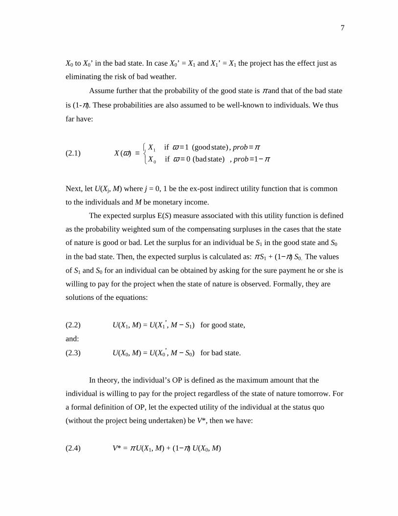
Assume further that the probability of the good state is π and that of the bad state
is (1-π). These probabilities are also assumed to be well-known to individuals. We thus
far have:
(2.1) 1
0
if 1 (goodstate) ,( )
if 0 (badstate) , 1
X probX
X prob
ω πω
ω π= =
= = = −
Next, let U(Xj, M) where j = 0, 1 be the ex-post indirect utility function that is common
to the individuals and M be monetary income.
The expected surplus E(S) measure associated with this utility function is defined
as the probability weighted sum of the compensating surpluses in the cases that the state
of nature is good or bad. Let the surplus for an individual be S1 in the good state and S0
in the bad state. Then, the expected surplus is calculated as: π S1 + (1−π) S0. The values
of S1 and S0 for an individual can be obtained by asking for the sure payment he or she is
willing to pay for the project when the state of nature is observed. Formally, they are
solutions of the equations:
(2.2) U(X1, M) = U(X1’, M − S1) for good state,
and:
(2.3) U(X0, M) = U(X0’, M − S0) for bad state.
In theory, the individual’s OP is defined as the maximum amount that the
individual is willing to pay for the project regardless of the state of nature tomorrow. For
a formal definition of OP, let the expected utility of the individual at the status quo
(without the project being undertaken) be V*, then we have:
(2.4) V* = π U(X1, M) + (1−π) U(X0, M)
8
For an individual who is assumed to be expected-utility maximizing, the amount
of payment is chosen such that his or her new expected utility is not less than in the
status quo. The values of OP as defined will solve the equation:
(2.5) π U(X1’, M − OP) + (1−π) U(X0
’, M − OP) = V*
where V* is defined in (2.4).
If the OP is obtained via a survey question, the question must make it clear to the
individual that the state of nature that will hold cannot be determined, and that the
individual must pay his or her OP prior to, and in whatever the state of nature will occur.
In general, the values of E(S) and OP are different. For a more detailed discussion about
OP and expected surplus, see Graham (1981), Smith (1992), and Cameron (1997).
The Discrete-Choice Contingent Valuation Method
In order to empirically estimate OP as well as in other CVM practices, the use of
referendum-style CVM has become very popular. In a typical referendum CVM
application to hunting (no lottery involved), respondents might be asked if they are
willing to pay to secure an improvement in the species population. Strictly speaking, a
referendum format means that individuals are told that there will be a vote, and that the
program will not be undertaken unless the majority (or some decision rule) votes for the
referendum to support the program. However, the discrete choice style of asking the
question (i.e. would you pay $X or not?) is often referred to as the referendum-style
CVM even when there is no test of the vote.
Any errors or randomness in the conventional discrete choice or referendum
CVM model (one without risk or uncertainty) are assumed to be attributable to the
investigator’s failure to observe all the dimensions of the problem. These errors are
typically introduced in a fashion that leads to estimation using the logit or probit models
9
of discrete choice. Such errors are the conventional “investigator’s” error and they are
not synonymous with the randomness introduced as part of a known risk.
Hanemann (1984) introduced the use of the referendum or discrete choice CVM
and the random utility model (RUM) approach to build logit model for estimation of the
Hicksian compensating and equivalent surplus for a hunting permit. Recently, Cameron
(2005) used a modified version of the referendum CVM approach, allowing for risk
ambiguity to estimate individual OP’s for global climate change mitigation programs.
The Empirical Model for OP
The objective of this section is to develop a specific econometric model for the
OP and derive the equation that allows the calculation of the OP for increasing the
probability of obtaining a hunting permit to a value of one, i.e. a guarantee for permit.
This elimination of risk inherent in the lottery is what is presented to hunters in the
survey questionnaire.
Again, let M be income and the states be specified with the j index (j = 1 if
awarded a permit, and j = 0 if not awarded a permit). Suppose that the individual derives
his or her utility from income and other non-income activities such as hunting and that
the individual utility function is linear in the logarithm of income (Hanemann, 1984):
(2.6) U(j, M) = αj + β log(M)
where β denotes marginal utility of a one-percent increase in income M; α1 is all non-
income utility including the utility obtained from hunting and α0 is all non-income utility
without hunting taking place. Non-income utility differs whether one hunts or not
because of the value of this constant term. The difference (α1−α0) reflects the utility
purely derived from hunting, should be positive. Note that the functional form in (2.6)
allows for income effects, as the marginal utility of income is not assumed to be
constant.
10
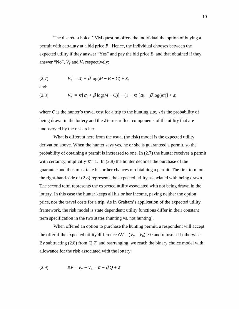
The discrete-choice CVM question offers the individual the option of buying a
permit with certainty at a bid price B. Hence, the individual chooses between the
expected utility if they answer “Yes” and pay the bid price B, and that obtained if they
answer “No”, Vy and Vn respectively:
(2.7) Vy = α1 + β log(M − B − C) + εy
and:
(2.8) Vn = π [α1 + β log(M − C)] + (1 − π) [α0 + β log(M)] + εn
where C is the hunter’s travel cost for a trip to the hunting site, π is the probability of
being drawn in the lottery and the ε terms reflect components of the utility that are
unobserved by the researcher.
What is different here from the usual (no risk) model is the expected utility
derivation above. When the hunter says yes, he or she is guaranteed a permit, so the
probability of obtaining a permit is increased to one. In (2.7) the hunter receives a permit
with certainty; implicitly π = 1. In (2.8) the hunter declines the purchase of the
guarantee and thus must take his or her chances of obtaining a permit. The first term on
the right-hand-side of (2.8) represents the expected utility associated with being drawn.
The second term represents the expected utility associated with not being drawn in the
lottery. In this case the hunter keeps all his or her income, paying neither the option
price, nor the travel costs for a trip. As in Graham’s application of the expected utility
framework, the risk model is state dependent: utility functions differ in their constant
term specification in the two states (hunting vs. not hunting).
When offered an option to purchase the hunting permit, a respondent will accept
the offer if the expected utility difference ∆V = (Vy – Vn) > 0 and refuse it if otherwise.
By subtracting (2.8) from (2.7) and rearranging, we reach the binary choice model with
allowance for the risk associated with the lottery:
(2.9) ∆V = Vy − Vn = α − β Q + ε
11
where: ε = (εy − εn) ,
α = (α1 − α0) (1 − π) ,
and: Q = [π log(M − C) + (1 − π) log(M) ] − log(M − B − C) .
The term Q is the expected reduction in the logarithm of net income associated
with buying the offer instead of participating in the lottery. In other words, Q measures,
in logarithm term, the expected increase in expenditure for hunting by buying the offer.
In the sample under study travel costs are relatively small to incomes so that Q can be
approximated as Q ≈ log(M) − log(M − B − C). On the benefit side, the constant term α
in (2.9) reflects the gain in expected hunting utility if buying the offer. On the cost side,
the product term β∗Q reflects the loss in expected utility caused by the bid price and the
destination travel cost if buying the offer.
Assuming ε follows a logistic distribution, we can estimate the parameters α and
β in (2.9) by using a logit model with the observed Yes / No responses to the option
offer being the dependent variable. Given the estimated values of α and β, the individual
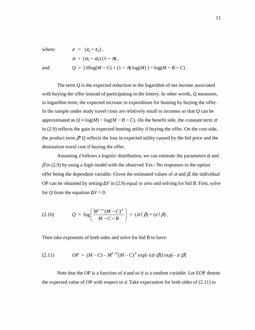
OP can be obtained by setting ∆V in (2.9) equal to zero and solving for bid B. First, solve
for Q from the equation ∆V = 0:
(2.10) Q = log1 ( )M M C
M C B
π π− − − −
= (α / β) + (ε / β) .
Then take exponents of both sides and solve for bid B to have:
(2.11) OP = (M – C) – M1−π (M – C)π exp[–(α /β)] exp[– ε /β]
Note that the OP is a function of ε and so it is a random variable. Let EOP denote
the expected value of OP with respect to ε. Take expectation for both sides of (2.11) to
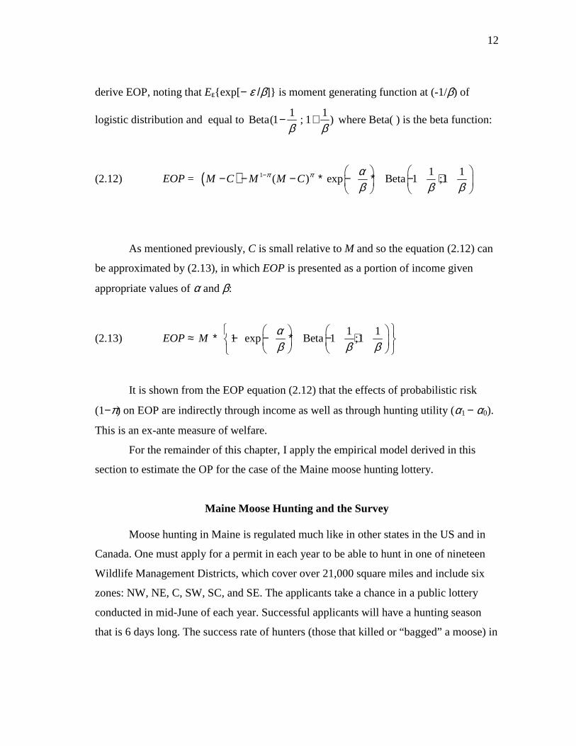
12
derive EOP, noting that Eεexp[− ε /β] is moment generating function at (-1/β) of
logistic distribution and equal to 1 1
Beta(1 ; 1 )β β
− + where Beta( ) is the beta function:
(2.12) EOP = ( ) 1 1 1( ) exp Beta 1 ;1M C M M Cπ π α
β β β− − − − ∗ − ∗ − +
As mentioned previously, C is small relative to M and so the equation (2.12) can
be approximated by (2.13), in which EOP is presented as a portion of income given
appropriate values of α and β:
(2.13) EOP ≈ 1 1
1 exp Beta 1 ;1Mαβ β β
∗ − − ∗ − +
It is shown from the EOP equation (2.12) that the effects of probabilistic risk
(1−π) on EOP are indirectly through income as well as through hunting utility (α1 − α0).
This is an ex-ante measure of welfare.
For the remainder of this chapter, I apply the empirical model derived in this
section to estimate the OP for the case of the Maine moose hunting lottery.
Maine Moose Hunting and the Survey
Moose hunting in Maine is regulated much like in other states in the US and in
Canada. One must apply for a permit in each year to be able to hunt in one of nineteen
Wildlife Management Districts, which cover over 21,000 square miles and include six
zones: NW, NE, C, SW, SC, and SE. The applicants take a chance in a public lottery
conducted in mid-June of each year. Successful applicants will have a hunting season
that is 6 days long. The success rate of hunters (those that killed or “bagged” a moose) in
13
1992 was 91%. For virtually all moose hunters then, winning the lottery leads to a high
chance of bagging a moose.
In 1992 the 900 permits were to be awarded to hunt moose and as a result 69,237
individuals applied to participate in the permit lottery. Thus, the probability of being
selected in the lottery (π) was 1.3 percent. This probability is similar to that of
preceding years. In that year a random sample of 900 residents who applied for but did
not receive a permit were sent a survey asking about a proposal to allow a small group of
hunters the right to buy a permit with certainty outside of the lottery.2 This sample of
individuals was drawn using the same procedures as was used to allocate the 900
hunting permits and the response rate for this survey was 78 percent.
Two main sections in this survey were of my interest. First, there were a number
of questions regarding the travel costs the hunter may incur, such as travel distance and
time as well. Second, there was an OP question. The respondent was informed that the
probability of winning the lottery in the previous year was 1.3%. They were also
informed that the Maine Legislature had increased the number of moose hunting permits
issued to Maine residents from 900 to 1000. The extra 100 permits were to be sold to
resident hunters under the program to cover the current costs of managing Maine’s
moose herd. Then he or she was offered an amount to guarantee a permit in the
following year. They were asked to response “yes” or “no” to purchase this guarantee. If
they did not want to buy the guarantee, they could still participate in the annual lottery.
The last section of the survey elicits the socio-economic characteristics (age,
gender, education, and income) of the individual. Income is categorized into 16 interval
ranges and the respondents’ income varies from less than $5,000 to more than $100,000.
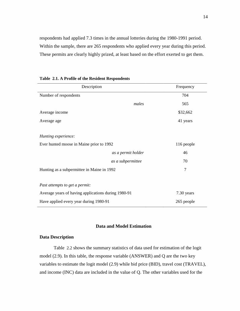
Shown in table 2.1 is a profile for the resident respondents. The data shows that there is
only a small portion of respondents, 46 out of the 704 respondents, who have ever
hunted in Maine as a permit holder, and 70 other people hunted as a subpermittee, a
guest of the permittee without a right to an additional moose. The data also shows that
respondents have expended a great deal of effort to obtain a permit. On average, 2 The 900 residents who received a permit were also sent a survey. These responses are not relevant to this study about option price.
14
respondents had applied 7.3 times in the annual lotteries during the 1980-1991 period.
Within the sample, there are 265 respondents who applied every year during this period.
These permits are clearly highly prized, at least based on the effort exerted to get them.
Table 2.1. A Profile of the Resident Respondents
Description Frequency
Number of respondents 704
males 565
Average income $32,662
Average age 41 years
Hunting experience:
Ever hunted moose in Maine prior to 1992 116 people
as a permit holder 46
as a subpermittee 70
Hunting as a subpermittee in Maine in 1992 7
Past attempts to get a permit:
Average years of having applications during 1980-91 7.30 years
Have applied every year during 1980-91 265 people
Data and Model Estimation
Data Description
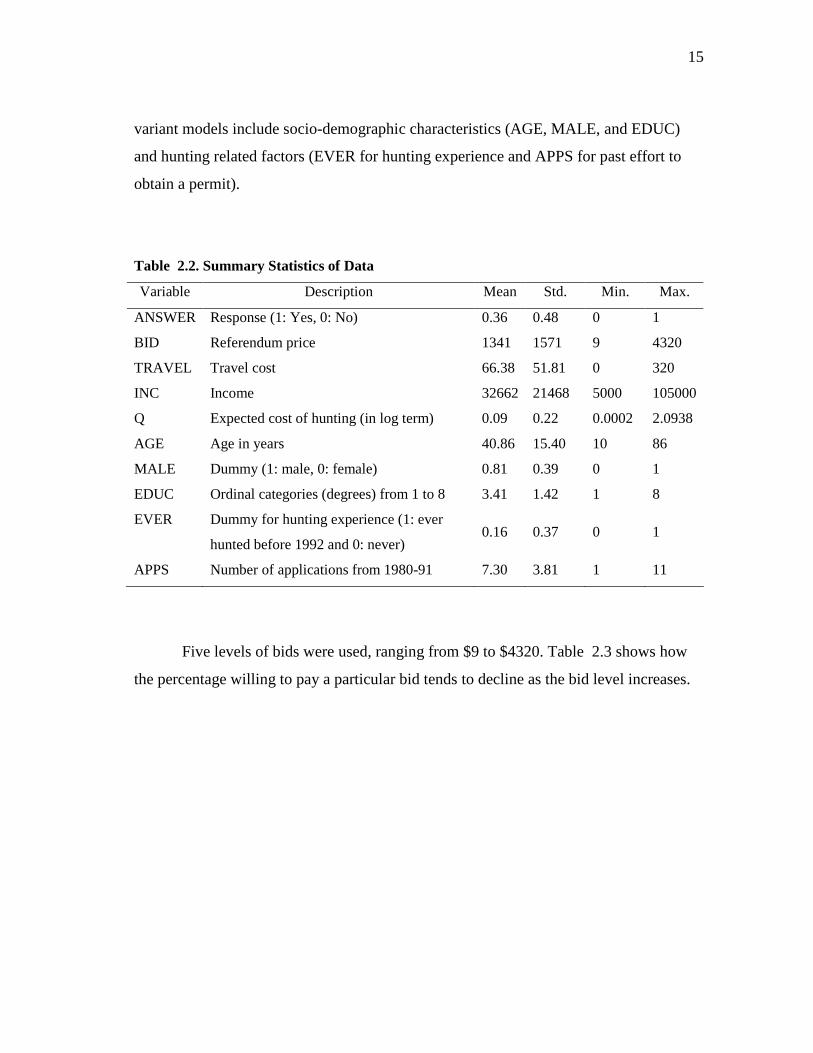
Table 2.2 shows the summary statistics of data used for estimation of the logit
model (2.9). In this table, the response variable (ANSWER) and Q are the two key
variables to estimate the logit model (2.9) while bid price (BID), travel cost (TRAVEL),
and income (INC) data are included in the value of Q. The other variables used for the
15
variant models include socio-demographic characteristics (AGE, MALE, and EDUC)
and hunting related factors (EVER for hunting experience and APPS for past effort to
obtain a permit).
Table 2.2. Summary Statistics of Data
Variable Description Mean Std. Min. Max.
ANSWER Response (1: Yes, 0: No) 0.36 0.48 0 1
BID Referendum price 1341 1571 9 4320
TRAVEL Travel cost 66.38 51.81 0 320
INC Income 32662 21468 5000 105000
Q Expected cost of hunting (in log term) 0.09 0.22 0.0002 2.0938
AGE Age in years 40.86 15.40 10 86
MALE Dummy (1: male, 0: female) 0.81 0.39 0 1
EDUC Ordinal categories (degrees) from 1 to 8 3.41 1.42 1 8
EVER Dummy for hunting experience (1: ever
hunted before 1992 and 0: never) 0.16 0.37 0 1
APPS Number of applications from 1980-91 7.30 3.81 1 11
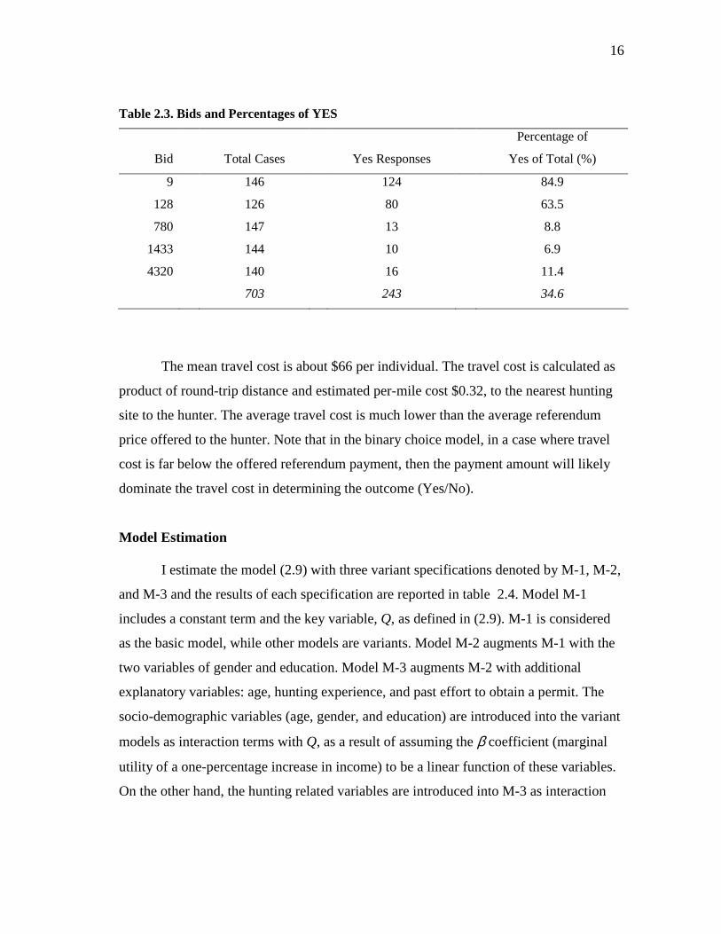
Five levels of bids were used, ranging from $9 to $4320. Table 2.3 shows how
the percentage willing to pay a particular bid tends to decline as the bid level increases.
16
Table 2.3. Bids and Percentages of YES
Bid
Total Cases
Yes Responses
Percentage of
Yes of Total (%)
9 146 124 84.9
128 126 80 63.5
780 147 13 8.8
1433 144 10 6.9
4320 140 16 11.4
703 243 34.6
The mean travel cost is about $66 per individual. The travel cost is calculated as
product of round-trip distance and estimated per-mile cost $0.32, to the nearest hunting
site to the hunter. The average travel cost is much lower than the average referendum
price offered to the hunter. Note that in the binary choice model, in a case where travel
cost is far below the offered referendum payment, then the payment amount will likely
dominate the travel cost in determining the outcome (Yes/No).
Model Estimation
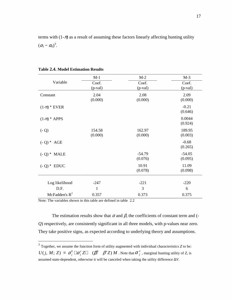
I estimate the model (2.9) with three variant specifications denoted by M-1, M-2,
and M-3 and the results of each specification are reported in table 2.4. Model M-1
includes a constant term and the key variable, Q, as defined in (2.9). M-1 is considered
as the basic model, while other models are variants. Model M-2 augments M-1 with the
two variables of gender and education. Model M-3 augments M-2 with additional
explanatory variables: age, hunting experience, and past effort to obtain a permit. The
socio-demographic variables (age, gender, and education) are introduced into the variant
models as interaction terms with Q, as a result of assuming the β coefficient (marginal
utility of a one-percentage increase in income) to be a linear function of these variables.
On the other hand, the hunting related variables are introduced into M-3 as interaction
17
terms with (1-π) as a result of assuming these factors linearly affecting hunting utility
(α1 − α0)3.
Table 2.4. Model Estimation Results
M-1 M-2 M-3 Variable Coef.
(p-val)
Coef. (p-val)
Coef. (p-val)
Constant 2.04 (0.000)
2.08
(0.000)
2.09 (0.000)
(1-π) ∗ EVER -0.21
(0.646)
(1-π) ∗ APPS 0.0044 (0.924)
(- Q) 154.58 (0.000)
162.97 (0.000)
189.95 (0.003)
(- Q) ∗ AGE -0.68
(0.265)
(- Q) ∗ MALE -54.79 (0.076)
-54.05 (0.095)
(- Q) ∗ EDUC 10.91
(0.078)
11.09 (0.098)
Log likelihood -247 -221 -220
D.F. 1 3 6
McFadden's R2 0.357 0.373 0.375 Note: The variables shown in this table are defined in table 2.2
The estimation results show that α and β, the coefficients of constant term and (-
Q) respectively, are consistently significant in all three models, with p-values near zero.
They take positive signs, as expected according to underlying theory and assumptions.
3 Together, we assume the function form of utility augmented with individual characteristics Z to be:
0 0( , ; ) ( ) z zj jU j M Z Z Z Mα α β β= + + + . Note that
zjα , marginal hunting utility of Z, is
assumed state-dependent, otherwise it will be canceled when taking the utility difference ∆V.
18
Gender and education interacted with Q, are significant at the 10% level. The negative
sign on the interaction term with gender predicts that there is a greater chance for a male
respondent to accept the offer than a female, assuming the same values for other
characteristics. Higher education is expected to have negative effect on the chance to
accept the offer for the permit guarantee. Age, hunting experience, and past effort for a
permit are statistically insignificant, as shown in M-3.
Further, the likelihood ratio (LR) test statistic for M-3 and M-2 is computed to be
1.572 and we fail to reject the null hypothesis that all three additional variables in M-3
are zero simultaneously. The LR-stat for M-2 and M-1 is 51.479 leading to rejecting the
null. In terms of goodness of fit to data, the R-square of M-2 is a bit better than that of
M-1, but the R-square of M-3 is not improved considerably, as compared to M-2. In
addition, the log-likelihood of M-3 is not much different from that of M-2. In all, I prefer
to use the model M-2 for estimating OP in the next section.
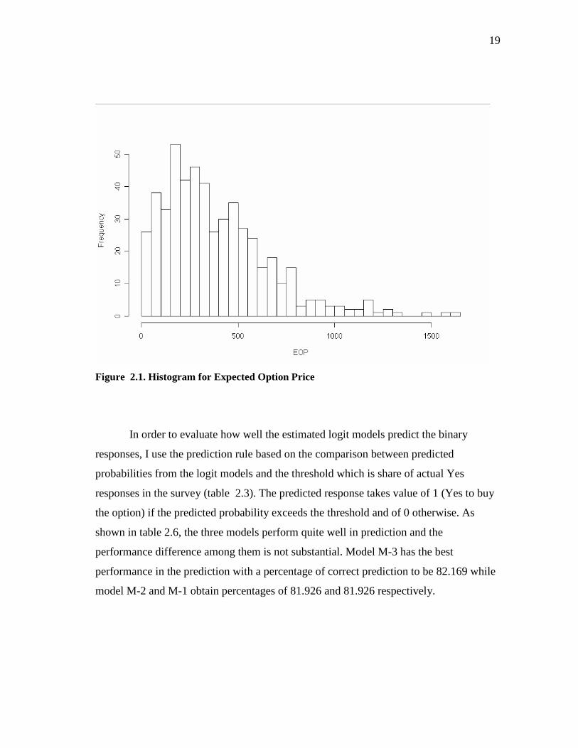
Individual EOPs and Discussion
The individual expected Option Prices (EOP) over the sample are computed by
substituting the estimated coefficients of the model M-2 into the EOP equation (2.12).
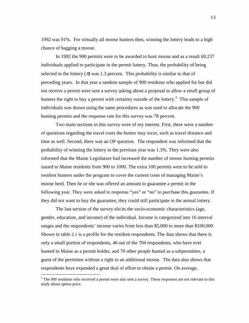
The summary statistics of EOP is reported in table 2.5 and the histogram in figure 2.1.4
We find the average EOPs over the sample is $384.65. This approach finds that more
than 80% of respondents have an implied EOP greater than $77 and less than $740.
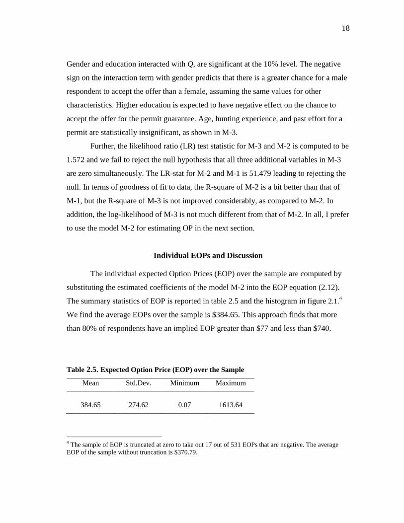
Table 2.5. Expected Option Price (EOP) over the Sample
4 The sample of EOP is truncated at zero to take out 17 out of 531 EOPs that are negative. The average EOP of the sample without truncation is $370.79.
Mean Std.Dev. Minimum Maximum
384.65 274.62 0.07 1613.64
19
Figure 2.1. Histogram for Expected Option Price
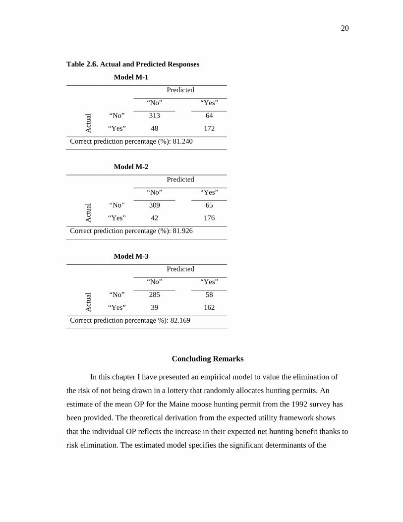
In order to evaluate how well the estimated logit models predict the binary
responses, I use the prediction rule based on the comparison between predicted
probabilities from the logit models and the threshold which is share of actual Yes
responses in the survey (table 2.3). The predicted response takes value of 1 (Yes to buy
the option) if the predicted probability exceeds the threshold and of 0 otherwise. As
shown in table 2.6, the three models perform quite well in prediction and the
performance difference among them is not substantial. Model M-3 has the best
performance in the prediction with a percentage of correct prediction to be 82.169 while
model M-2 and M-1 obtain percentages of 81.926 and 81.926 respectively.
20
Table 2.6. Actual and Predicted Responses
Model M-1
Predicted
“No” “Yes”
“No” 313 64
Act
ual
“Yes” 48 172
Correct prediction percentage (%): 81.240
Model M-2
Predicted
“No” “Yes”
“No” 309 65
Act
ual
“Yes” 42 176
Correct prediction percentage (%): 81.926
Model M-3
Predicted
“No” “Yes”
“No” 285 58
Act
ual
“Yes” 39 162
Correct prediction percentage %): 82.169
Concluding Remarks
In this chapter I have presented an empirical model to value the elimination of
the risk of not being drawn in a lottery that randomly allocates hunting permits. An
estimate of the mean OP for the Maine moose hunting permit from the 1992 survey has
been provided. The theoretical derivation from the expected utility framework shows
that the individual OP reflects the increase in their expected net hunting benefit thanks to
risk elimination. The estimated model specifies the significant determinants of the
21
hunters’ responses, including the informed probability of being successful in the annual
lottery, referendum price and travel cost. The model correctly predicts the responses of
84% of the respondents in the Maine moose hunting survey.
In the case under study, the risk facing the individuals is a simple probability
concept and especially it is clearly informed to the respondents. So in this situation it is
likely quite reasonable to use the objective probability approach. However, the
homogeneity assumed for the hunter’s risk perceptions here seems not often to be the
case. Slovic (1987) found that the individual conceptualization of risk is much richer
than that of the expert and their perception of risk tend to be heterogeneous across
individuals. In the next two chapters I present the modeling approaches addressing this
issue, which is at the core of empirical researches in the area of valuation under
uncertainty.
22
CHAPTER III
A HIERARCHICAL BAYES (HB) MODEL OF
SUBJECTIVE PROBABILITIES
Introduction and Literature Review
The Subjective Probability (SP) Theory
In the von Neumann-Morgenstern theory, probabilities are assumed to be
objective and typically considered being inherent in nature. However, the SP idea
pioneered by Ramsey (1926) and De Finetti (1974) argued that by observing the bets
people make on a horse race, one can presume that these reflect their personal beliefs on
the outcome of the horse race. Thus, subjective probabilities, which are defined as
personal beliefs in risks, can be inferred from observation of people's choices. The SP
idea was axiomatized and developed into a full theory, the SP theory, by Leonard J.
Savage in his Foundations of Statistics (1954). The SP theory assures that well-defined
probabilistic beliefs are revealed by choice behavior.
In order to make the SP idea clear, consider an illustrative example adapted from
Schmeidler (1989, p. 574). Supposes a bettor draws a ball from an urn that contains balls
of either red or black color and the ratio between these two types is not known to him or
her. Denote by R and B the event of drawing a red ball and a back ball respectively. Now
consider a bet that offers $100 if R happens and $0 if otherwise. According to the SP
theory, if the bettor is indifferent between betting on R for $100 and betting on another
risky event with an (objective) probability of 3/7 for $100 then the subjective probability
of the event R is equal to its risk equivalent, i.e. prob(R) = 3/7.
23
Empirical Estimation of SP
The empirical estimation of SP has been a concern in the literature of decision
making and nonmarket valuation under risks. For example, Boxall (1995) suggests using
estimates of hunters’ perception of their chance from permit lotteries instead of using
objective probabilities in modeling hunters’ choice of participation in the lotteries as I
have in the earlier chapter. This suggestion is in line with findings in Slovic (1987) that
the individual conceptualization of risk is much richer than that of the expert and that
perception of risk tends to be heterogeneous across individuals. In other words, there is
no reason to expect that one individual’s perception of risks is the same as someone
else’s.
Viscusi and Evans (1998) estimate individual’s perceptions of risks associated
with household chemical products by using survey data on how much the individual is
willing to pay for the safer product. The estimation is based on the concept of
prospective reference theory (Viscusi, 1989), which asserts that risk belief is in effect a
weighted average between an individual’s prior probability and some objective
information about the risks given to the individual, which follows from a Bayesian
learning framework.
In empirical research on lottery-rationed access to public resource and welfare,
Scrogin and Berrens (2003) also use the logit/probit probabilities to be proxies of the
individuals’ perception of their chance in the current lottery. The logit/probit models
take observed outcomes of being drawn or not being drawn in the lottery as the
dependent variable. While seeking proxies for subjective perceptions, this approach in
fact obtains ‘objective’ measure of expected chance of being drawn in the lotteries since
the outcomes of being drawn or not drawn in a lottery are independently distributed from
people’s estimates of that chance.
Shaw, Walker, and Benson (2005) also use predicted probabilities from a logit
model of observed choices or decisions to treat arsenic contaminated water, which act as
indicators of the households’ assessment of the risks of drinking the water. The
assumption made in their approach is that there is a positive relationship between the
24
predicted probability of treatment and individual assessment of arsenic risk from
drinking water. This approach was initially taken in a similar study (but on toxic
contamination of fish) by Jakus and Shaw (2003).
As distinct from the approaches presented above, this chapter explores for the
first time the application of the hierarchical Bayes (HB) approach to model and estimate
subjective probabilities using discrete choice data. While the HB approach can apply to
various choice settings to estimate subjective probabilities, this chapter uses binary
valuation responses (yes/no to an offer relating to buying a lottery) to illustrate the
procedure of the HB modeling method. The basic framework of the expected utility
model (EUM) is assumed throughout this chapter, as opposed to any alternatives to the
EUM5.
The remainder of this chapter consists of two major parts. The first part describes
a typical binary decision setting involving risk and sets up the HB model. The second
part shows an example using simulated data for the estimation of the HB model. The
final section provides the conclusions and introduces to the subjective risks with
ambiguity, the topic of next chapter.
The Hierarchical Bayes Model
Background on the HB Approach
Applications of the HB approach have become widespread in many areas such as
biostatistics and marketing (Rossi, et al. 2005). In his book about discrete choice
methods with simulation, Train (2002) devotes one chapter to the practice of the HB
approach, applied specifically to mixed logit models. However, most typical applications
of the HB approach assume linear forms in parameters, deterministic and random, even
5 Many studies have shown that people behave in ways that systematically violate the expected utility maximization (see Starmer (2000) for an overview). Among evidences the two most well-known are Allais (1953) and Ellsberg (1961) paradoxes. The former leads to violating the independence axiom while the latter refutes the neutrality of uncertainty about subjective probability. As a result, theorists devise non-expected utility models that relax some assumptions underlying the expected utility framework. Among the most popular are the rank-dependent models such as Quiggin (1981) and Schmeidler (1989). The issue of uncertainty about probability is the topic to be explored in next chapter.
25
though in theory the approach can be applied to nonlinear models. As is made clear
below, the special position of probabilities in relation with other parameters in a decision
model makes the model under study here nonlinear.
The Binary Choice Setting and Probability Model
Consider a sample of N individuals who are offered the opportunity to buy a
lottery ticket at a price of B. If an individual is drawn in the lottery s/he will have access
to a service of which the benefit, denoted by α, is unknown to the researcher. For an
example, the benefit obtained by winning the lottery is the utility from hunting as in the
case of moose hunting permit explored in the previous chapter.
Following Hanemann (1984) the ex-post indirect utility of an individual i is
supposedly derived from the unknown benefit α and the money income, denoted by M,
that is:
(3.1) U(j, Mi) = αj + β ∗ Mi ,
where j ∈ 1, 0 represents the 2 states of being drawn or not being drawn in the lottery.
Let πi represent the individual i’s subjective probability for his or her chance of being
drawn in the lottery. The expected utilities associated with buying (accepting the offer)
and not buying (declining the offer) a lottery ticket are determined respectively as:
(3.2) Viy = πi * U(1, Mi – Bi – Ci) + (1 – πi) * U(0, Mi – Bi) + εiy ,
and:
(3.3) Vin = U(0, Mi) + εin ,
where the error terms above reflect the unobserved components of utility, M and B
represents gross income and bid price respectively, and C represents total costs
associated with consumption of the service, e.g. travel costs. Subtracting Vn from Vy
26
yields the increment in the individual expected utility when choosing to buy the
prospect:
(3.4) ∆Vi = Vyi – Vni = πi *α – β * (Bi + πi * Ci) + εi ,
where εi = εyi – εni and α = α1 – α0.
The individuals are assumed to be maximizing subjective expected utility (SEU),
so they will accept the offer if ∆Vi is positive and decline the offer otherwise. Assume ε
follows a standard logistic distribution. The probability that an individual i accepts the
offer can be derived directly from (3.4) as:
(3.5) ϕ i = Prob(Yi = 1) = Prob(∆Vi > 0) = Ω[πi *α – β * (Bi + πi * Ci)] ,
where Yi ∈ 1 (yes), 0 (no) defines for the response for individual i, and Ω represents
the cdf of the standard logistic distribution. It is clear that the probability model in (3.5)
represents a logit model that involves risks, because of the presence of the probability
term, πi.
Now the question of concern is how to estimate α and β in (3.5) and the
distribution of πi over the sample given a dataset of individual characteristics, Bi, Ci, and
observed responses Yi. There are two approaches for the estimation of (3.5): the
maximum simulated likelihood (MSL) and the HB approach. However, as shown in
Train (2002), the HB approach has theoretical advantages from both a classical and
Bayesian perspective and it works faster computationally. Further, while maximum
likelihood estimation is susceptible to a flat or nearly flat likelihood function, often due
to an insufficient number of observations, the Bayesian approach can still work in this
case (Rossi, 2005, page 19). This research chooses the HB for the analysis and in the
next section I will build the model based on this approach.
To begin, it is necessary to have a distribution functional form assumed for the
subjective probabilities πi for the logit model (3.5) to be estimable. At this point, I
27
denote by P(πi| m) the generic distribution of πi characterized by vector of parameters m
and I defer specifying any form for the distribution of πi until the next section. Using this
assumption, the probability model (3.5) possesses a hierarchical structure of parameters
in which the first level of parameters includes πi, α, and β and the second level includes
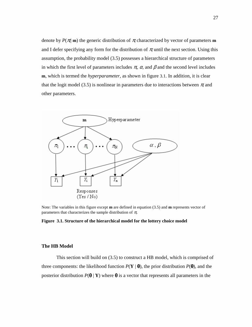
m, which is termed the hyperparameter, as shown in figure 3.1. In addition, it is clear
that the logit model (3.5) is nonlinear in parameters due to interactions between πi and
other parameters.
Note: The variables in this figure except m are defined in equation (3.5) and m represents vector of parameters that characterizes the sample distribution of πi.
Figure 3.1. Structure of the hierarchical model for the lottery choice model
The HB Model
This section will build on (3.5) to construct a HB model, which is comprised of
three components: the likelihood function P(Y | θθθθ), the prior distribution P(θθθθ), and the
posterior distribution P(θθθθ | Y) where θθθθ is a vector that represents all parameters in the
28
model as specified below. Especially, the prior distribution is structured with first- and
second-level priors corresponding to the levels of parameters (Gelman et al., 2004).
For convenience in notation, define vectors:
Y = (Y1, …, Yn) ,
ππππ = (π1, …, πN) ,
and: θθθθ = (ππππ, α, β, m) ,
where θθθθ is vector of all parameters in (3.5).
Likelihood Function: P(Y | θθθθ)
In order to derive the likelihood function from (3.5), suppose the individual i’s
response Yi follows a Bernoulli distribution with parameter ϕ i determined in (3.5). Then
the choice probability of the individual i conditional on (πi, α, β) will be:
(3.6) P(Yi | πi , α, β) = ϕ i Yi ∗ (1− ϕ i)
(1−Yi) .
Assuming choices by the individuals are made independently, multiplication of
(3.6) over i yields the likelihood function of observed responses:
(H-1) P(Y | ππππ,α, β, m) = P(Y | ππππ, α, β) = 1
n
i=∏ P(Yi | πi, α, β ) ,
where the first equality holds because the data distribution, P(Y | ππππ,α, β, m), depends
only on (ππππ,α, β) while the hyperparameter m affects Y through ππππ.
29
Prior: P(θθθθ)
In specifying a joint prior distribution for θθθθ, first assume independence between
the risk-related parameters (ππππ, m) and the other parameters, (α, β). Further assume that α
and β are independently distributed and that perceptions of the probability are
independent across all of the individuals. Together these assumptions imply:
(H-2) P(ππππ, α, β, m) = P(ππππ, m) ∗ P(α, β)
= P(ππππ | m) ∗ P(m) ∗ P(α) ∗ P(β)
= 1
n
i=∏ P(πi | m) ∗ P(m) ∗ P(α) ∗ P(β)
where the first-level priors include P(α), P(β), and P(πi | m) and the second-level is
P(m).
Posterior: P(θθθθ | Y)
Following Bayes’ rule, we obtain the un-normalized joint posterior distribution
of all parameters by multiplying the likelihood (H-1) by the prior (H-2):
(H-3) P(θθθθ | Y) ∝ 1
n
i=∏ P(Yi | πi, α, β) ∗ P(πi | m) ∗ P(α) ∗ P(β) ∗ P(m)
In theory, samples for each of the parameters can be drawn if the specific forms
of all functions P(.) in the posterior (H-3) are defined. Since the posterior distribution
shown in (H-3) is not a standard distribution, the sampling requires using the Monte
Carlo Markov Chain (MCMC) algorithms. The rest of this chapter presents a numerical
example using pseudo-data to illustrate the computational algorithm and to evaluate on
the performance of the application of HB framework to recover the parameters in (H-3).
30
An Example Using the Pseudo Data
This section presents a numerical example of the HB approach discussed above
using pseudo data. The process includes generating a number of datasets for the model in
(3.5) and then implementing the sampling algorithm described below to simulate the
posterior distributions of the parameters. The sample sizes are chosen to be increasing to
verify the approaching of the posterior distributions around the population parameters,
i.e. these distributions will have variances smaller and means closer to true values of the
parameters when the sample larger. Details of the process are described in the three main
steps below.
Step 1: Generating the pseudo-data:
• Assume values for the population parameters (α, β, m);
• Generateεi, πi, Bi and Ci (details given below);
• Derive choices Yi using the binary choice rule in (3.4).
Step 2: Using the sampling algorithm described in the previous section and the
data generated in Step 1 to simulate the posterior distribution, mean and
variance, for each of the parameters (α, β, m).
Step 3: Evaluating how well posterior samples of the parameters approach the
true parameters.
The results from implementing these three steps are presented next.
The Pseudo Data
The parameters α and β are in this example presumed to be 1 and 0.001
respectively. Since α represents the unobserved utility derived from a good or service
and β is the marginal utility of money, it implies a monetary benefit of $1,000. The data
for εi is drawn from standard logistic distribution, as presumed in the formulation of the
model 3.4. For the case of πi it is assumed following a standard triangular distribution,
31
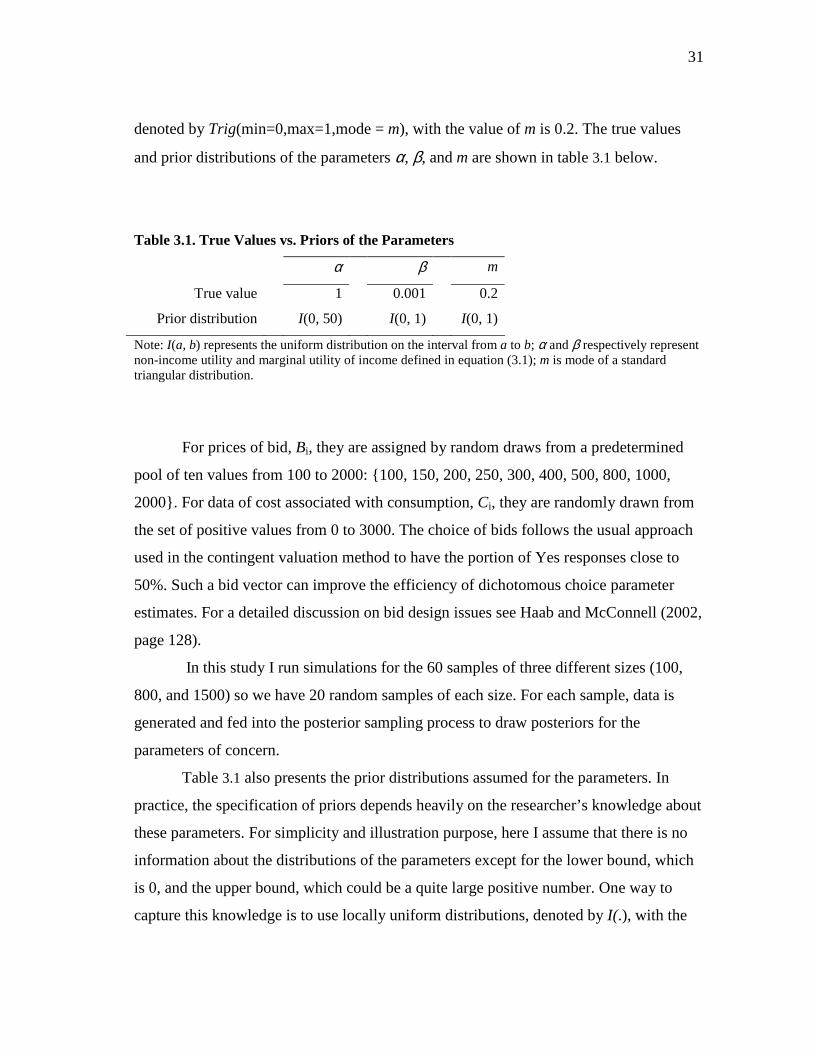
denoted by Trig(min=0,max=1,mode = m), with the value of m is 0.2. The true values
and prior distributions of the parameters α, β, and m are shown in table 3.1 below.
Table 3.1. True Values vs. Priors of the Parameters
α β m
True value 1 0.001 0.2
Prior distribution I(0, 50) I(0, 1) I(0, 1)
Note: I(a, b) represents the uniform distribution on the interval from a to b; α and β respectively represent non-income utility and marginal utility of income defined in equation (3.1); m is mode of a standard triangular distribution.
For prices of bid, Bi, they are assigned by random draws from a predetermined
pool of ten values from 100 to 2000: 100, 150, 200, 250, 300, 400, 500, 800, 1000,
2000. For data of cost associated with consumption, Ci, they are randomly drawn from
the set of positive values from 0 to 3000. The choice of bids follows the usual approach
used in the contingent valuation method to have the portion of Yes responses close to
50%. Such a bid vector can improve the efficiency of dichotomous choice parameter
estimates. For a detailed discussion on bid design issues see Haab and McConnell (2002,
page 128).
In this study I run simulations for the 60 samples of three different sizes (100,
800, and 1500) so we have 20 random samples of each size. For each sample, data is
generated and fed into the posterior sampling process to draw posteriors for the
parameters of concern.
Table 3.1 also presents the prior distributions assumed for the parameters. In
practice, the specification of priors depends heavily on the researcher’s knowledge about
these parameters. For simplicity and illustration purpose, here I assume that there is no
information about the distributions of the parameters except for the lower bound, which
is 0, and the upper bound, which could be a quite large positive number. One way to
capture this knowledge is to use locally uniform distributions, denoted by I(.), with the
32
support bounded on a certain range of non-negative values. In this particular example,
prior distribution for α is assumed to be I(0, 50), a uniform distribution over the range of
(0, 50), while true value of α is 1. For β the prior is I(0, 1) while its true value is 0.001.
For m the prior is I(0, 1) and its true value is 0.2. The priors chosen for the parameters
are quite far from their true values so that it is easy to observe the approaching of
posterior distributions of the parameters towards the true values when samples getting
larger sizes.
Computation: The Gibbs Sampling Algorithm
In order for the computation to proceed, we need to assign distribution functional
forms for the priors present in (H-3). Above I have assumed functional forms for the
prior distribution. We still need a functional form for the prior distribution of πi over
individuals in the sample, P(πi | m).
For a distribution to be eligible for being prior distribution of πi , that distribution
needs to be one with the support bounded between 0 and 1. Examples of adequate
representation of the population of probabilistic risks include beta, triangular, truncated
normal, and locally uniform distributions. In practice, a true distribution of πi might be
known to the researcher or not known. It is ideal for the researcher to know and hence
use the true distribution of πi over the sample. Otherwise, she needs to make an
assumption about the distribution. Since beta distribution is very flexible in capturing
variability over a fixed range, it is potentially a good candidate for the assumption about
unknown distribution of πi. However, the beta distribution is complicated
mathematically (Covello and Merkhofer, 1993, p. 61). For the reason of ease in
computation and isolation of other sources of error or bias from the estimator itself, I
assume the prior distribution of πi to be the standard triangular distribution, Trig(.| m)
where m represents for the mode of this distribution.
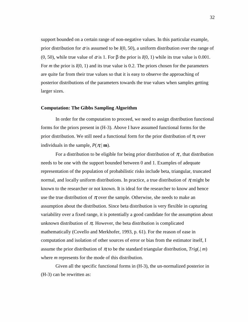
Given all the specific functional forms in (H-3), the un-normalized posterior in
(H-3) can be rewritten as:
33
(H-4) P(θθθθ | Y) ∝ 1
n
i=∏ [P(Yi | πi, α, β) * Trig(πi | m)] * I(α) * I(β) * I(m) ,
where P(Yi | πi, α, β) is determined by (3.6) and (3.5).
In order to draw from (H-4) the samples for each of the parameters, we need to
implement the Monte Carlo Markov Chain (MCMC) algorithms. Most applications of
MCMC have used the Gibbs sampler (Gilks, 1996). This is especially true for HB
models. The Gibbs sampler is to generate an instance from the distribution of each
random variable in turn, conditional on the current values of the other variables (see for
details Gelfand and Smith, 1990). So the Gibbs algorithm requires knowing all full
conditional posteriors, i.e. the distribution of one parameter given all other quantities in
the model. It is ideal if all conditional posteriors are standard, so that drawing from the
conditionals becomes straightforward. Otherwise another MCMC algorithm should be
used to draw from those conditional posteriors.
For the case under study, the nonlinearity in the model makes all conditional
posteriors non-standard distribution, as shown below, hence combining Gibbs sampler
with another MCMC algorithm is chosen for computation. The rest of this section is
dedicated for the implementation of this algorithm, including deriving all full conditional
posteriors from (H-4) and describing specific steps of the sampling procedure.
Full Conditional Posteriors
Given the joint posterior distribution in (H-4), the full conditional posteriors for
each of the parameters (πi,α, β, m) are obtained below, from (G-1) to (G-4). Note that all
of these conditionals are non-standard distributions and this makes the sampling
procedure complicated, as discussed next.
(G-1) P(πi | α, β, m, Yi) ∝ P(Yi | πi, α, β) * Trig(πi | m) , ∀i = 1,…, N
34
(G-2) P(α | ππππ, β, m, Y) ∝ 1
n
i=∏ [P(Yi | πi, α, β)] * I(α) ,
(G-3) P(β | ππππ, α, m, Y) ∝ 1
n
i=∏ [P(Yi | πi, α, β)] * I(β) ,
(G-4) P(m| ππππ, α, β, Y) ∝ 1
n
i=∏ [Trig(πi | m)] * I(m) .
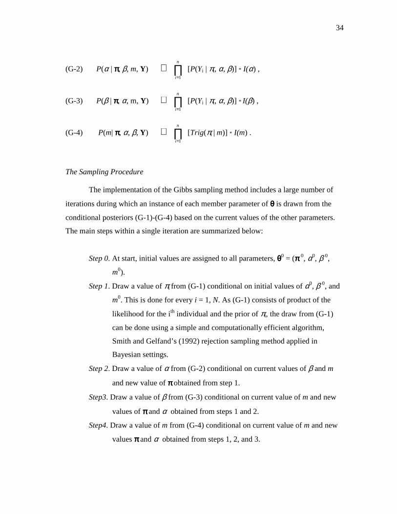
The Sampling Procedure
The implementation of the Gibbs sampling method includes a large number of
iterations during which an instance of each member parameter of θθθθ is drawn from the
conditional posteriors (G-1)-(G-4) based on the current values of the other parameters.
The main steps within a single iteration are summarized below:
Step 0. At start, initial values are assigned to all parameters, θθθθ0 = (ππππ 0, α0, β 0,
m0).
Step 1. Draw a value of πi from (G-1) conditional on initial values of α0, β 0, and
m0. This is done for every i = 1, N. As (G-1) consists of product of the
likelihood for the ith individual and the prior of πi, the draw from (G-1)
can be done using a simple and computationally efficient algorithm,
Smith and Gelfand’s (1992) rejection sampling method applied in
Bayesian settings.
Step 2. Draw a value of α from (G-2) conditional on current values of β and m
and new value of ππππ obtained from step 1.
Step3. Draw a value of β from (G-3) conditional on current value of m and new
values of ππππ and α obtained from steps 1 and 2.
Step4. Draw a value of m from (G-4) conditional on current value of m and new
values ππππ and α obtained from steps 1, 2, and 3.
35
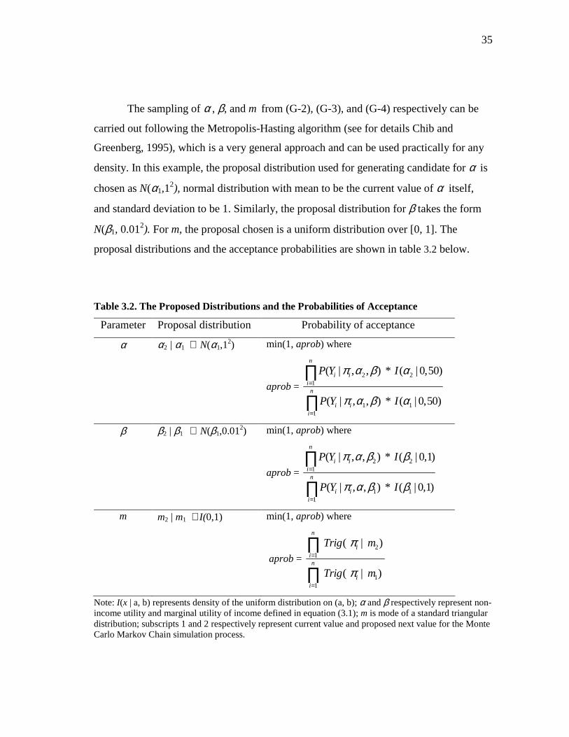
The sampling of α , β, and m from (G-2), (G-3), and (G-4) respectively can be
carried out following the Metropolis-Hasting algorithm (see for details Chib and
Greenberg, 1995), which is a very general approach and can be used practically for any
density. In this example, the proposal distribution used for generating candidate for α is
chosen as N(α1,12), normal distribution with mean to be the current value of α itself,
and standard deviation to be 1. Similarly, the proposal distribution for β takes the form
N(β1, 0.012). For m, the proposal chosen is a uniform distribution over [0, 1]. The
proposal distributions and the acceptance probabilities are shown in table 3.2 below.
Table 3.2. The Proposed Distributions and the Probabilities of Acceptance
Parameter Proposal distribution Probability of acceptance
α α2 | α1 ∼ N(α1,12) min(1, aprob) where
aprob = 2 2
1
1 11
( | , , ) * ( | 0,50)
( | , , ) * ( | 0,50)
n
i iin
i ii
P Y I
P Y I
π α β α
π α β α
=
=
∏
∏
β β2 | β1 ∼ N(β1,0.012) min(1, aprob) where
aprob = 2 2
1
1 11
( | , , ) * ( | 0,1)
( | , , ) * ( | 0,1)
n
i iin
i ii
P Y I
P Y I
π α β β
π α β β
=
=
∏
∏
m m2 | m1 ∼ I(0,1) min(1, aprob) where
aprob = 2
1
11
( | )
( | )
n
iin
ii
Trig m
Trig m
π
π
=
=
∏
∏
Note: I(x | a, b) represents density of the uniform distribution on (a, b); α and β respectively represent non-income utility and marginal utility of income defined in equation (3.1); m is mode of a standard triangular distribution; subscripts 1 and 2 respectively represent current value and proposed next value for the Monte Carlo Markov Chain simulation process.
36
Simulation Results and Analysis
As discussed in the previous section, the simulation process includes drawing
samples of α, β, and m from their joint posterior distribution (H-4) so that their posterior
distributions can be obtained. The simulation results for 60 datasets of three sizes (100,
800, and 1500) are reported in two tables in Appendix A. Table A-1 presented in
Appendix A shows means and the Table A-2 shows standard deviations of the posterior
distributions of the parameters α, β, and m.
Each row in those two tables corresponds to an instance of the computational
process discussed above, i.e. drawing random samples of size N (=100, 800, 1500),
inputting these data into the MCMC simulation to get posterior distributions of the
parameters, and finally, calculating means and standard deviations of these posterior
distributions. It is clear that means and standard deviations obtained from such a process
have a degree of randomness. So we should not evaluate an estimator, in terms of
unbiasedness and efficiency, based on just one instance of the process. Take an example,
for the experiment corresponding to line “Sample 10”, the posterior mean of α estimated
for N = 100 (=0.986) is closer to the true α than the estimate for N = 1500 (=1.448). This
result seems to contradict the common-sense notion that a larger sample should provide
better estimate. However, as seen in Table A-1, on average an estimate with N=1500
leads to a prediction closer to the true value and the standard deviation of these estimates
decreases as N increase. The evaluation of the hierarchical Bayesian estimator used in
this study will be made under this perspective as follows.
Summary statistics for sampling distribution of the posterior mean and standard
deviation are shown in table 3.3 and table 3.4. In Bayesian statistics, the posterior
estimate is an information weighted compromise between prior and data estimates. In the
numerical example presented in this section, the prior belief is presumed to be quite far
from the true parameters and it is expected from the HB procedure that the posterior
means approach the true parameter values. The result presented in table 3.3 shows the
actual working of the HB across three different sample sizes. In the analysis below, I
37
first compare the posteriors derived from datasets of the smallest size (100) with the
prior and then evaluate the converging to the true parameters as sample size grows.
For the 20 samples of N = 100, the average posterior mean for α is 2.145, much
closer to its true value (= 1) rather than the prior mean for α (= 25). Similarly for β, the
average posterior mean is about 1.344*10−3 while the actual value is 1*10−3 and the prior
mean is 5*10−3. So the estimator improves substantially the posterior belief on the true
parameters of α and β even with small samples. However, the result for m is not as good
as for α or β. The posterior mean for m is 0.378 a value close to the middle between its
true value (= 0.2) and the prior mean (= 0.5).
It is shown from table 3.3 that the HB procedure provides an estimator that is less
biased and more efficient as the sample size grows. For example, at small size of N =
100 the average posterior mean of α is 2.145 and while it’s true value is 1. However, it
can be observed that the sampling distribution of posterior mean converges in
probability to the true parameters when the datasets get larger, i.e. average values of the
posterior means gets closer to the true values and their variances gets smaller.
Consider the posterior means of α across three sizes of sample. Its average
posterior mean is 2.145 for N = 100, reduced to 1.058 for N = 800 and again reduced to
1.051 for N = 1500. So there’s tending to the true value of α, which is 1. In terms of
variance, the standard deviations are 1.251, 0.421, and 0.290 respectively. The similar
pattern also occurs with the posterior means of β and the hyperparameter m. For β, its
average posterior means change from 1.344 to 1.007 and to 0.998 respectively in
increasing sample sizes. These values approaches the true value (= 1) at smaller standard
deviations of 0.421, 0.177, and 0.100 respectively. For the hyperparameter m, the
converging to its true value occurs at a slower rate compared to α and β. With N = 800,
the mean error for α estimate is 0.058 (= 5.8% of the true value) and the mean error for
β estimate is 1.007*10−3 (= 0.7%) respectively, while the mean error for m estimate is
0.022 (= 11%) even with greater sample size of N = 1500.
In this particular example, since the prior is biased from the true parameters
while the data is generated from the true parameters, the bias in posterior estimates is
38
associated with the prior, not because of the estimator. When sample size grows the
estimator is able to get rid of this type of bias. These results allow us to believe that the
HB procedure is capable of recovering the true parameters given sufficient data.
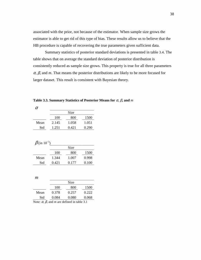
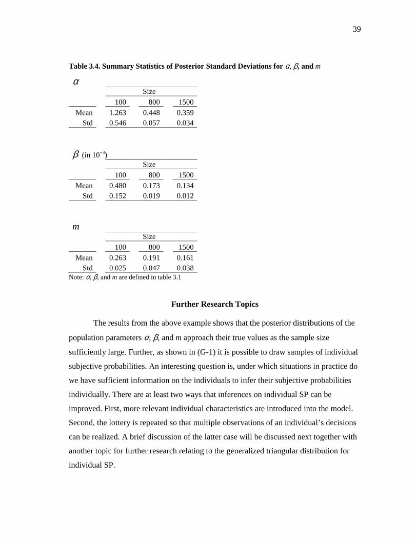
Summary statistics of posterior standard deviations is presented in table 3.4. The
table shows that on average the standard deviation of posterior distribution is
consistently reduced as sample size grows. This property is true for all three parameters
α, β, and m. That means the posterior distributions are likely to be more focused for
larger dataset. This result is consistent with Bayesian theory.
Table 3.3. Summary Statistics of Posterior Means for α, β, and m
α Size
100 800 1500
Mean 2.145 1.058 1.051 Std 1.251 0.421 0.290
β (in 10−3) Size
100 800 1500
Mean 1.344 1.007 0.998 Std 0.421 0.177 0.100
m Size
100 800 1500
Mean 0.378 0.257 0.222 Std 0.084 0.080 0.068
Note: α, β, and m are defined in table 3.1
39
Table 3.4. Summary Statistics of Posterior Standard Deviations for α, β, and m
α Size
100 800 1500
Mean 1.263 0.448 0.359 Std 0.546 0.057 0.034
β (in 10−3) Size
100 800 1500
Mean 0.480 0.173 0.134 Std 0.152 0.019 0.012
m Size
100 800 1500
Mean 0.263 0.191 0.161 Std 0.025 0.047 0.038
Note: α, β, and m are defined in table 3.1
Further Research Topics
The results from the above example shows that the posterior distributions of the
population parameters α, β, and m approach their true values as the sample size
sufficiently large. Further, as shown in (G-1) it is possible to draw samples of individual
subjective probabilities. An interesting question is, under which situations in practice do
we have sufficient information on the individuals to infer their subjective probabilities
individually. There are at least two ways that inferences on individual SP can be
improved. First, more relevant individual characteristics are introduced into the model.
Second, the lottery is repeated so that multiple observations of an individual’s decisions
can be realized. A brief discussion of the latter case will be discussed next together with
another topic for further research relating to the generalized triangular distribution for
individual SP.
40
HB with Panel Data
Consider a model with multiple individuals’ responses to different levels of bid.
Let t subscript denote the index of bid and t = 1, T. In fact, T is not necessarily the same
for all individuals but for convenience subscript i is suppressed in T. For an example, the
double-bounded bid approach used in contingent valuation (Hanemann, Loomis, and
Kanninen, 1991) will give the individual two levels of bid to get her two responses to the
offer. Another case that multiple responses/choices can be observed is the repetition of
lotteries over periods. In those cases, the probability of observed responses will be a
joint probability over a series of t choices:
(3.7) P(Yi1,…, YiT| πi , α, β) = 1
T
t=∏ ϕi
Yit ∗ (1 − ϕi)(1−Yit)
It is the same procedure as in this chapter to construct the HB model for the
multiple participation setting. With more observations on revelation of individual SP, πi,
through (3.7), the likelihood will be sharper and thereby the inference on πi will be
closer to the true values.
General Triangular Distribution
In the example presented in the second part of this chapter, the standard triangle
distribution with lower-bound and upper bound are fixed at 0 and 1 respectively is used
as the actual distribution and the prior distribution of SPs over the sample. As discussed
above it is usual that the researcher may not know the actual distribution of SPs, and
hence beta distribution, a very flexible distribution, is more appealing to be the prior
rather than the standard triangle distribution. Another adequate distribution is the general
triangle distribution of which the parameters include min, max, and mode. While less
complicated mathematically compared to beta distribution, the general triangular
41
distribution can be used as a proxy for the beta distribution except when the latter takes
irregular shapes Johnson (1997).
The use of general triangular distribution in this framework requires an
adaptation from the algorithm used in the example by adding two more population
parameters, min and max of the triangular distribution, into the full conditional
distributions shown in (G-1, G-4). Further the algorithm for computing (min, max, mode)
of the triangular can developed from the version for the standard triangular by
transforming the density of the latter distribution (Johnson, 1997).
Concluding Remarks
In this chapter, I have shown an application of the HB approach to model
subjective probabilities in a typical discrete choice setting under uncertainty. The model
found is a HB nonlinear logit model with individual SP treated as individual-level
parameters. I have also applied the MH within Gibbs algorithm to simulate the posteriors
for the sixty different datasets generated from assumed distributions. It is found that
given a sufficiently large sample size of data the HB framework can perform well in
recovering parameters of the distribution of SPs over the sample. However, if dataset is
generated from a one-shot lottery such as in the Maine moose survey presented in the
previous chapter then it is less likely that we can estimate individual SPs precisely. In
such a case we can only simulate sample values such as mean for option price rather
than individual option prices.
As for the specification of individual risk perceptions in the model, the subjective
probabilities are heterogeneous among the individuals. But the individuals are still
assumed certain about the probabilistic risk, i.e. no ambiguity about risk. However, in
several cases people might be uncertain about the risk they face such as the case of
mortality risk. In fact, many researchers have noted discrepancies between the
assessments of risk based on statistical information, by so-called experts, and the
subjective risks of the public, who may or may not be informed. When there are
substantial differences, an individual’s behavior is better explained by his subjective

42
risks than by objective risks, but a problem arises when subjective risks are imprecise or
individuals are in fact ambiguous about the risks. This is exacerbated when experts do
not know risks, leaving all decision makers facing uncertainty.
In the next chapter I develop and estimate a formal model of perceived risk
distributions that allows for such risk ambiguity. The data used for estimation was
collected from a survey given to a sample of people living in areas with potential health
risk problems from drinking water contaminated with naturally occurring arsenic.
43
CHAPTER IV
AN ECONOMETRIC MODEL OF
SUBJECTIVE DISTRIBUTIONS OF MORTALITY RISKS
Introduction
The purpose of this chapter is to model and estimate subjective or perceived risks
that individuals have for mortality related to consuming drinking water with high arsenic
concentrations. Arsenic has been demonstrated to increase the usual average risks of
dying from lung and bladder cancers that exists for the U.S. population, and can cause
other health problems in both adults and children. However, the causal relationships are
imprecise. The model developed here allows for individuals to be uncertain or
ambiguous about these risks.
The data used in the modeling below are obtained from a survey in a study on
arsenic contamination in selected regions in the United States (see Shaw, et al. 2006 for
a complete description). As will be enumerated below, respondents answer questions
posed in an information brochure during a follow-up telephone call that allows
interaction between the trained interviewer and the respondent. Each information
brochure mailed to households in the survey contained a risk ladder, a common means of
visually conveying and communicating risks to subjects in surveys and experiments. The
survey questionnaire format allowed the respondents to mark either a distinct, single
rung on the risk ladder, or a range of risks on the ladder if they chose to do so.
Methodologically, the perceived distribution of risk is modeled as a probit
function of the sum of two terms representing factors of median and variance of the
distribution. This basic modeling approach was first developed by Lillard and Willis
(2001), and is applied by Hill, Perry and Willis (2005), and extended and applied by
Riddel (2007). Such a modeling approach allows estimating the factors that influence the
median and variance of the subject’s perceived arsenic risk distribution.
44
The organization of the remainder of this chapter is as follows. The next section
briefly reviews some relevant literature to provide background on the topic of risk
ambiguity. The following section summaries the arsenic survey questionnaire and
describes the approach taken to obtain or elicit perceived risks from the respondents.
Then I develop an empirical model for stated or indicated risks based on an assumption
about the individuals’ behaviors in marking on the risk ladder. Finally, the estimation
result using the arsenic survey data is reported and discussed.
The research in this chapter makes two contributions to the literature. First, it
provides an empirical study in the area of environmental economics that may guide
arsenic risk reduction policy and programs in the United States. This is one of the first
studies that focus on U.S. arsenic exposure from a socio-economic point of view.
Second, it provides another, though yet still rare, empirical application of new
approaches in modeling health risks that allow for, and include ambiguity from survey
responses.
Background and Brief Literature Review
Arsenic and Health Risk
Arsenic, a semi-metal and an element in the periodic table, has long been known
to be an acute toxin. It has been shown that consumption of water contaminated with
arsenic at high levels may cause skin damage or problems with circulatory systems, and
may increase the risk of getting lung or bladder cancer. Since January 2006 the new EPA
regulatory standard for arsenic in public water systems has been reduced to 10 parts-per-
billion (ppb) from 50 ppb. This new regulation was promulgated to provide more
protection for about 13 million Americans in areas with naturally occurring arsenic in
their water supplies (USEPA, 2006). Sources of arsenic contamination in drinking water
are from natural deposits in the earth or from agricultural and industrial practices.
Ground water sources tend to be contaminated with arsenic at higher levels as compared
to surface water sources such as lakes and rivers.

45
Even though scientists generally agree that human exposure to arsenic can cause
health effects, the exact dose-mortality relationship between arsenic levels and health
risks is still controversial. The estimated increases in the health risks that accompany a
level of 50 ppb vary (Shaw et al., 2006). The dose-response relationship is especially
uncertain at low levels, below 10 ppb, so some scientists still believe the newly
mandated 10 ppb threshold is not low enough to ensure safety. However, the 1999 report
to the United States Environmental Protection Agency (USEPA) by the National
Research Council (NRC) showed that evidence of risk at lower dose is very weak.
Burnett and Hahn (2001) raised concerns about the data and the methodology employed
by the USEPA to estimate the risks of low-level exposure. They also cast doubt on
inferences from animal and epidemiological studies, and the way that the USEPA
quantified low-dose risks from arsenic. In addition, they believe that the dose-response
relationship from arsenic should be a nonlinear relationship and that the actual risk from
low levels of arsenic concentration is much less than the results from EPA’s linear dose-
response model.
The complex dose-response relationship is also due to many other issues and
factors such as various consumption and exposure thresholds, confounding influences,
and the latency period. Some biologists and toxicologists insist that there is a threshold
below which arsenic concentration causes no effects. However, this conclusion was
drawn from experiments on animals, and extrapolation to humans is questioned by a
growing number of arsenic researchers (Wilson, 2001). In addition, there are many
confounding factors affecting exposure and mortality rates of arsenic concentration.
Smoking is an example of a strong confounding factor. The NRC indicates smoking as a
factor that may substantially increase the risks associated with arsenic exposures. The
effects of smoking on mortality risks from arsenic exposure need more research before
having an exact estimate, but indications are a doubling of the risks for a smoker.
Finally, the mapping from arsenic exposure to health risks is made even more
problematic by the latency issue because there’s no agreement in the estimates of the
46
length of the latency period in contracting the cancers; an additional question relates to
the length of the period to recovery when arsenic exposure ceases.
The controversy that exists among experts related to quantifying the dose -
response relationship between arsenic levels and health risks no doubt contributes to the
public’s confusion about the risks of arsenic. A standard procedure in finding the
public’s sense of the risk is to inform them using the best available data and information.
Thus, it is easy to see that in the case of arsenic this information might well contribute
to, rather than reduce, confusion about the risks. This is clearly a case where people hold
ambiguous and heterogeneous perceptions of risks, and this ambiguity is a compelling
reason that any economic modeling related to arsenic risks must address this type of
complexity, the perceived risks.
Ambiguity and Heterogeneity
The psychologist Paul Slovic (1987) found that the individual conceptualization
of risk is much richer than that of the expert and their perception of risk tend to be
heterogeneous across individuals. Slovic’s work, as well as that done by other
psychologists and risk scholars, has demonstrated why we need to look at perceived
risks in stead of objective probabilities, especially if we wish to predict behavior in the
face of risks. However, perceived risks are often fraught with ambiguity, making the
risk, at one extreme, tantamount to total uncertainty. As in the case of arsenic where
people’s perceptions of risks are influenced by conflicting expert estimations, there is
more likely to be ambiguity.
The notion of ambiguity was defined by the psychologist Daniel Ellsberg (1961)
as the “quality depending on the amount, type, reliability, and ‘unanimity’ of
information.” More generally, Frisch and Baron (1988) define ambiguity as uncertainty
about a probability, created by missing information that is relevant and could be known.
Ellsberg (1961) was one of the first we know of to address such ambiguity, and the
concept has been extended and analyzed both theoretically (e.g. Segal 1987), and in
several laboratory experiments in economics and psychology. There are several possible

47
psychological reasons for why people are ambiguous about some types of risks (e.g.
Heath and Tversky, 1991 and Fox and Tversky, 1995). Most work in economics on
ambiguity, and on risks in general, has focused on financial risks, but while mortality
risks relate to many decisions people make, they have been studied much less.
Mortality risks might be calculated for average people in certain populations,
from certain diseases, but these vary greatly by age. For example, the Center for Disease
Control regularly updates age-specific estimates of mortality risk, for several diseases,
providing one source of estimates that are supposedly “objective” measures of mortality
risk. However, people asked to determine their own probability of dying from a
particular cause, and at a particular point in their life, may face difficulty in doing so
because of emotions involved in the task, or due to a lack of information at their
disposal. There is good reason to think that ambiguity may be prevalent in subjective
estimates of death or survival risks for any number of causes.
Recently Cameron (2005), and Riddel and Shaw (2006) introduce ambiguity
about environmental and mortality risks in somewhat rare empirical models that do not
rely on laboratory experiments; each of these relies on survey data, although Cameron’s
(2005) data is for classroom students. In each of these studies the introduction of an
ambiguity term into an empirical model is somewhat ad hoc, at least from a theoretical
point of view. From a statistical point of view, the models are sensible in that each relies
on introduction of non-linear terms for probability, a break from the standard linear-in-
probabilities expected utility model (EUM).
Somewhat more formally, Lillard and Willis (2001), hereafter L&W, introduce
the probit function approach to model the relationship between the information that a
respondent has about the probability of a given outcome and the shape of the density
function of her probabilistic beliefs. This approach is then used in combination with the
modal responses hypothesis to explain a link between an individual’s degree of
uncertainty and her propensity to give responses as focal point answers at zero, one-half,
or one and as exact answers. The basic idea is that high degree of uncertainty results in
clusters or “heaps” of responses around certain probabilities. This may indicate that
48
people have an easier time understanding certain values for risks, thus clinging to these
in their subjective estimates. The modal response hypothesis is tested empirically using
data from a large set of subjective probability questions from the Health and Retirement
Survey (HRS). Hill, Perry and Willis (2005), HPW hereafter, extend the L&W’s work
and develop an econometric model to estimate the determinants of individual-level
uncertainty about personal longevity, and they also use HRS data. Riddel (2007) applies
parts of HPW in her test of various specifications for subjective risk distributions, using
a different data set on perceived mortality risks from nuclear waste storage and
transportation.
Next, because the development of our risk model is tied to data from the arsenic
survey, I discuss the sample and survey data used for my analysis. While the survey
sample is small, an advantage of it over larger survey samples such as the HRS, is that
the subjects are informed about risks using risk communication devices. Another
advantage is that while the HRS forces an individual to make a point estimate about
survival risks, the survey used here does not.
The Survey and Sample Statistics
The sample consists of households living in five communities exposed to arsenic
levels in excess of the new EPA standard of 10 ppb. Table 4.1 provides information on
the sources of drinking water and arsenic exposure, including the mean and range of
contamination where appropriate, for the five communities. The public water supply
systems of Albuquerque, Fernley and Oklahoma City were not in compliance with
federal standard for arsenic. The Outagamie County/Appleton Wisconsin region was
selected for the study because of the high arsenic levels in privately owned wells.
Private drinking water wells are not regulated under the Safe Drinking Water Act, so any
knowledge that well owners have about their well quality is obtained on their own or in
conjunction with a state or local health agency.
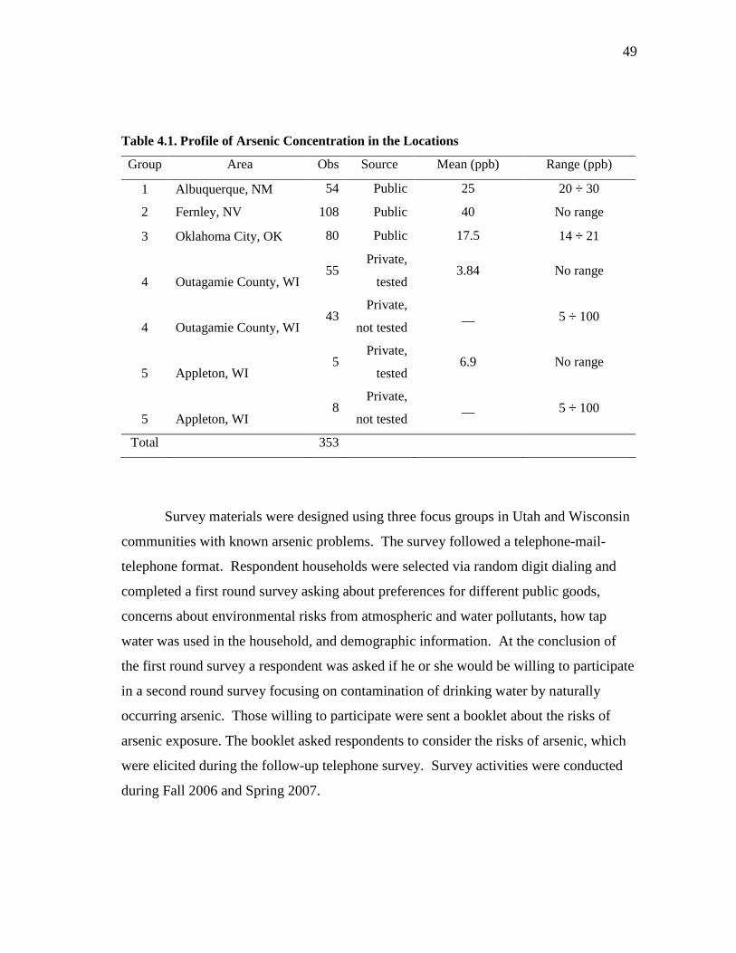
49
Table 4.1. Profile of Arsenic Concentration in the Locations
Group Area Obs Source Mean (ppb) Range (ppb)
1 Albuquerque, NM 54 Public 25 20 ÷ 30
2 Fernley, NV 108 Public 40 No range
3 Oklahoma City, OK 80 Public 17.5 14 ÷ 21
4 Outagamie County, WI 55
Private,
tested 3.84 No range
4 Outagamie County, WI 43
Private,
not tested __ 5 ÷ 100
5 Appleton, WI 5
Private,
tested 6.9 No range
5 Appleton, WI 8
Private,
not tested __ 5 ÷ 100
Total 353
Survey materials were designed using three focus groups in Utah and Wisconsin
communities with known arsenic problems. The survey followed a telephone-mail-
telephone format. Respondent households were selected via random digit dialing and
completed a first round survey asking about preferences for different public goods,
concerns about environmental risks from atmospheric and water pollutants, how tap
water was used in the household, and demographic information. At the conclusion of
the first round survey a respondent was asked if he or she would be willing to participate
in a second round survey focusing on contamination of drinking water by naturally
occurring arsenic. Those willing to participate were sent a booklet about the risks of
arsenic exposure. The booklet asked respondents to consider the risks of arsenic, which
were elicited during the follow-up telephone survey. Survey activities were conducted
during Fall 2006 and Spring 2007.
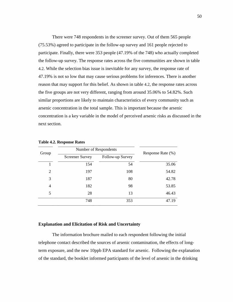
50
There were 748 respondents in the screener survey. Out of them 565 people
(75.53%) agreed to participate in the follow-up survey and 161 people rejected to
participate. Finally, there were 353 people (47.19% of the 748) who actually completed
the follow-up survey. The response rates across the five communities are shown in table
4.2. While the selection bias issue is inevitable for any survey, the response rate of
47.19% is not so low that may cause serious problems for inferences. There is another
reason that may support for this belief. As shown in table 4.2, the response rates across
the five groups are not very different, ranging from around 35.06% to 54.82%. Such
similar proportions are likely to maintain characteristics of every community such as
arsenic concentration in the total sample. This is important because the arsenic
concentration is a key variable in the model of perceived arsenic risks as discussed in the
next section.
Table 4.2. Response Rates
Number of Respondents Group
Screener Survey Follow-up Survey Response Rate (%)
1 154 54 35.06
2 197 108 54.82
3 187 80 42.78
4 182 98 53.85
5 28 13 46.43
748 353 47.19
Explanation and Elicitation of Risk and Uncertainty
The information brochure mailed to each respondent following the initial
telephone contact described the sources of arsenic contamination, the effects of long-
term exposure, and the new 10ppb EPA standard for arsenic. Following the explanation
of the standard, the booklet informed participants of the level of arsenic in the drinking
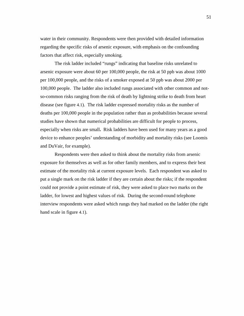
51
water in their community. Respondents were then provided with detailed information
regarding the specific risks of arsenic exposure, with emphasis on the confounding
factors that affect risk, especially smoking.
The risk ladder included “rungs” indicating that baseline risks unrelated to
arsenic exposure were about 60 per 100,000 people, the risk at 50 ppb was about 1000
per 100,000 people, and the risks of a smoker exposed at 50 ppb was about 2000 per
100,000 people. The ladder also included rungs associated with other common and not-
so-common risks ranging from the risk of death by lightning strike to death from heart
disease (see figure 4.1). The risk ladder expressed mortality risks as the number of
deaths per 100,000 people in the population rather than as probabilities because several
studies have shown that numerical probabilities are difficult for people to process,
especially when risks are small. Risk ladders have been used for many years as a good
device to enhance peoples’ understanding of morbidity and mortality risks (see Loomis
and DuVair, for example).
Respondents were then asked to think about the mortality risks from arsenic
exposure for themselves as well as for other family members, and to express their best
estimate of the mortality risk at current exposure levels. Each respondent was asked to
put a single mark on the risk ladder if they are certain about the risks; if the respondent
could not provide a point estimate of risk, they were asked to place two marks on the
ladder, for lowest and highest values of risk. During the second-round telephone
interview respondents were asked which rungs they had marked on the ladder (the right
hand scale in figure 4.1).
52
Figure 4.1. The risk ladder used in the arsenic survey
(Risk of deaths per 100,000 over 20 years)
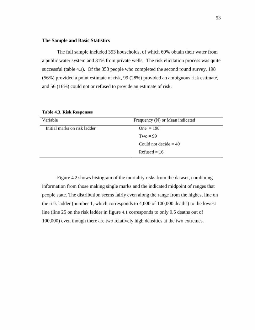
53
The Sample and Basic Statistics
The full sample included 353 households, of which 69% obtain their water from
a public water system and 31% from private wells. The risk elicitation process was quite
successful (table 4.3). Of the 353 people who completed the second round survey, 198
(56%) provided a point estimate of risk, 99 (28%) provided an ambiguous risk estimate,
and 56 (16%) could not or refused to provide an estimate of risk.
Table 4.3. Risk Responses
Variable Frequency (N) or Mean indicated
Initial marks on risk ladder
One = 198
Two = 99
Could not decide = 40
Refused = 16
Figure 4.2 shows histogram of the mortality risks from the dataset, combining
information from those making single marks and the indicated midpoint of ranges that
people state. The distribution seems fairly even along the range from the highest line on
the risk ladder (number 1, which corresponds to 4,000 of 100,000 deaths) to the lowest
line (line 25 on the risk ladder in figure 4.1 corresponds to only 0.5 deaths out of
100,000) even though there are two relatively high densities at the two extremes.
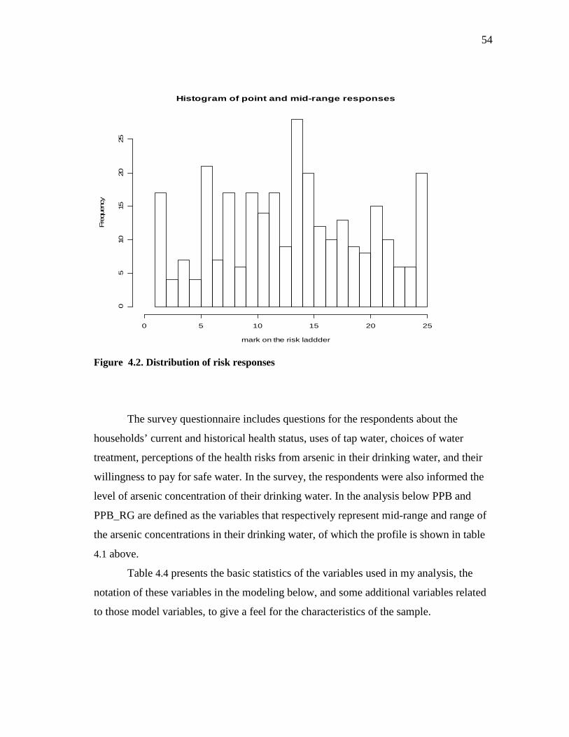
54
Histogram of point and mid-range responses
mark on the risk laddder
Fre
quen
cy
0 5 10 15 20 25
05
1015
2025
Figure 4.2. Distribution of risk responses
The survey questionnaire includes questions for the respondents about the
households’ current and historical health status, uses of tap water, choices of water
treatment, perceptions of the health risks from arsenic in their drinking water, and their
willingness to pay for safe water. In the survey, the respondents were also informed the
level of arsenic concentration of their drinking water. In the analysis below PPB and
PPB_RG are defined as the variables that respectively represent mid-range and range of
the arsenic concentrations in their drinking water, of which the profile is shown in table
4.1 above.
Table 4.4 presents the basic statistics of the variables used in my analysis, the
notation of these variables in the modeling below, and some additional variables related
to those model variables, to give a feel for the characteristics of the sample.

55
The average age of the sample is around 51 years (ranging from 20 to 93 years):
the survey protocol does not allow for respondents under the age of 18, as is often the
case in such survey efforts. Education was thought to possibly influence risk responses,
though the direction of influence is an empirical issue. While cognitive ability may
increase with education and lead to a better understanding of information about risks,
awareness of the complicated nature of the risk issues may also increase ambiguity.
Education is categorized into 7 levels, from no high school as lowest educational level,
to the highest, an advanced degree. The majority of the sample have an education from
at least high school to an advanced degree with quite even distribution across those
levels. There are only 26 people without a high school degree.
A person’s health status may also influence his or her perceived risks. Again, the
direction of influence is not obvious: people in poor health may feel that they have little
additional mortality risk from any event or exposure, but people in good health may
believe they can fight off or avoid extreme consequences of exposure. The respondents
are asked to rate their own health status in one of the 5 levels from excellent (coded 1) to
poor condition (coded 5). Most of the sample, 322 out of 353 people, rate their health
good, very good, or excellent.
Most in the sample have some type of health insurance. Only 14 people in the
sample do not have any type of health insurance. Health insurance purchases may reflect
the individual’s perceptions of many types of risk. Health insurance might be purchased
because of the financial means to obtain health care, but some types of coverage also
may reflect preferences for taking risks. That is, a risk-taker might choose to purchase no
health insurance, while a person with extreme concerns about the possibility of
contracting diseases may purchase a large amount of coverage. For a more detailed
discussion about alternative reasons to why people buy health insurance see Nyman
(2002).
Though relevant to individual perception of risks, the health insurance purchase
will not be included as an independent variable in the model because of two reasons.
First, health insurance is likely to be an effect from individual’s perception of arsenic
56
risk rather than a causal factor. That is, the higher risk perceived may cause higher
probability that the individual to purchase health insurance, rather than the inverse. Since
the model aims to explain the effects of the causal factors, the inclusion of this variable
is not appropriate. Second, there are only 14 respondents out of 353 who did not have
health insurance. So, it is not likely that there’s sufficient variation in this variable to see
its effect if any on the perceived risks.
When the respondents receive the information brochure in the mail, they are
shown that smoking has an effect on increasing the mortality risks associated with
arsenic in drinking water. Therefore smoking is expected to have a significant effect on
people’s thoughts about their own and others’ mortality risks. In the empirical analysis, I
use two dummy variables relevant to the smoking habit. One dummy variable takes a
value of 1 if the individual has ever smoked in their life and is equal to 0 otherwise. The
other dummy variable takes a value equal to 1 if the respondent has smoked in past but
has now stopped, and equals 0 if they have smoked and still do at the time the survey
questionnaire is administered to them. In the sample, there are many past smokers: 161
people of our 353 in the sample have smoked in the past. Among these past smokers,
116 people said they had stopped smoking and 45 people were still smoking.
Some occupations have been shown to increase mortality risks from arsenic
exposure because the individual is simultaneously exposed to substances that may
enhance lung and bladder cancer risks. The survey thus also asks the respondents if they
have worked in the jobs that may increase basic lung and bladder cancer risks, such as
manufacturing paint, manufacturing textiles, leather, or rubber products, beautician or
hairstylist, packaging dues or other chemicals, printing, and aluminum worker. As
shown in table 4.4 there are 93 respondents who have worked, or still work in those
occupations. They are again told in the information brochure about the possibility that
working in these types of jobs may increase risks.

57
Table 4.4. Basic Statistics of Key Variables
Variable Notation Frequency
Gender
Age
Education
Occupation
Self-rating health status
Have private or public insurance?
Homeowner (=1 if yes, 0 = No)
Have smoked in the past?
If smoked are you smoking now?
Is all water you drink from the tap?
Do you use a treatment device?
MALE
AGE
EDU
OCC
HEALTH
SMOEVER
SMOQUIT
TREAT
Male = 200, female = 153
Mean = 51 (of 350 reporting)
No high school = 15
Some high school = 11
High school degree = 85
Some college = 66
2-year college = 61
4-year college = 65
Advanced degree = 49
Risky jobs = 92 , None = 261
Excellent = 97
Very good = 130
Good = 95
Fair = 27
Poor = 4
Yes = 336, No = 14
1 = 320, 0 = 21 (12 missing)
Yes = 161, No = 192
Yes = 45, No = 116
Yes = 231, No = 122
Yes = 182, No = 171
Note: Total responses may not equal 353 because of item non-response or skipped questions.
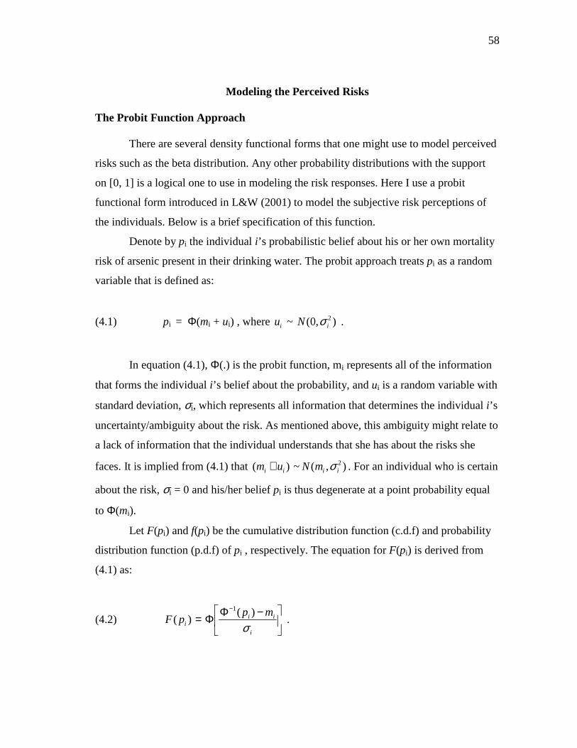
58
Modeling the Perceived Risks
The Probit Function Approach
There are several density functional forms that one might use to model perceived
risks such as the beta distribution. Any other probability distributions with the support
on [0, 1] is a logical one to use in modeling the risk responses. Here I use a probit
functional form introduced in L&W (2001) to model the subjective risk perceptions of
the individuals. Below is a brief specification of this function.
Denote by pi the individual i’s probabilistic belief about his or her own mortality
risk of arsenic present in their drinking water. The probit approach treats pi as a random
variable that is defined as:
(4.1) pi = Φ(mi + ui) , where 2~ (0, )i iu N σ .
In equation (4.1), Φ(.) is the probit function, mi represents all of the information
that forms the individual i’s belief about the probability, and ui is a random variable with
standard deviation, σi, which represents all information that determines the individual i’s
uncertainty/ambiguity about the risk. As mentioned above, this ambiguity might relate to
a lack of information that the individual understands that she has about the risks she
faces. It is implied from (4.1) that 2( ) ~ ( , )i i i im u N m σ+ . For an individual who is certain
about the risk, σi = 0 and his/her belief pi is thus degenerate at a point probability equal
to Φ(mi).
Let F(pi) and f(pi) be the cumulative distribution function (c.d.f) and probability
distribution function (p.d.f) of pi , respectively. The equation for F(pi) is derived from
(4.1) as:
(4.2)
−ΦΦ=−
i
iii
mppF
σ)(
)(1
.
59
Taking the derivative of the right-hand-side (hereafter RHS) of (4.2) yields the
equation for the p.d.f., or f(pi). It can be verified from (4.2) that Φ(mi) is the median of
f(pi). For convenience in notation, the subscript i will be suppressed in all that follows
below.
Assumptions Regarding the Subjective Risk Responses
In order to formulate a likelihood function for the stated risk responses on the
risk ladder, we need an assumption about the relationship between an individual’s
responses to the survey questions that elicit individual beliefs about the arsenic risks and
the functional form of their subjective beliefs, f(p). For the arsenic risks under this study,
I assume that a probability range response [p1, p2] reflects the individual’s belief that
probability mass of f(p) outside this range approaches zero. This assumption is quite
intuitive. It says that the range a respondent selected reflects a perceived distribution of
risk that has the most heavy mass within that range. Further, I treat a probability point
response as a special case of range response in that the range is bounded by the two
midpoints from the rung chosen and the two rungs next to it. Hereafter, we refer to this
assumption as the probability mass assumption.
Likelihood Function
The information contained in the two factors m and σ must be parameterized to
derive an estimable model. To do so, let:
(4.3) m = X α ,
and:
(4.4) lnσ = Z β ,
where X and Z are two sets of variables that influences people’s subjective thoughts
about median and variance of risk respectively, where X and Z need not, but may have
60
some identical elements; α and β reflect weights that the individual put on factors present
in the equations. Note that the form in (4.4) as a semi-log ensures that σ will be positive.
Substituting (4.3) and (4.4) into equation (4.2) yields the distribution of the risk
belief in terms of causal factors for which we have data:
(4.5)
−ΦΦ=−
)exp(
)()()(
1
βα
Z
XppF
The likelihood of range p ∈ [p1, p2] is specified as:
(4.6) prob(p1 ≤ p ≤ p2) = F(p2) – F(p1)
The likelihood of point p = po can be calculated as a special case of (4.6) where
two ladder rungs are degenerate at half way from the marked rung of the ladder and the
two next closest rungs. Let pou denote the mid-range from po to the risk at the next upper
rung and pou denote the mid-range from po to the risk at the next lower rung on the risk
ladder. The likelihood of point p = po can be written as:
(4.7) prob( p = po) = F(pou) – F(pol)
For consistence in treating data between point and range responses, a two-mark
response [p1, p2] in equation (4.6) is treated in computation as range [p2u, p1l].
Multiplication of (4.6) or (4.7) over the appropriate respondents, i.e. those who provide a
point estimate versus a range estimate, yields the likelihood function for the entire
sample under this first assumption. Maximizing this function will yield the maximum
likelihood (ML) estimates of α and β. Note that the objective function to be maximized
is a function of the parameters conditional on data. So, the procedure to compute
standard errors and p-values is similar to the one for a normal likelihood function.
61
Estimation Results and Discussion
Table 4.5 reports the parameter estimates for the probit function, the standard
errors, p-values, and significant levels of α and β from the estimation using the arsenic
risk data. The coefficients of the median-shifting variables such as the arsenic parts per
billion concentrations (PPB) represent the marginal effect of these variables on the Z-
score, i.e. the inverse probit function Φ-1 of the median of perceived distribution of
arsenic risks, f(pi), as mentioned above.
The choice of variables in the model is based on the expectation and intuition of
relevance of these variables to location or variance of individual perceived risks. It is
informed to the respondents that levels of arsenic concentration and smoking behaviors
will critically affect mortality risks facing them. So the variables related to these factors
are included in the model. In addition, since health status and health related factors such
as risky occupation are likely to affect any health risks they are also included in the
model. For the factors of variance, it is quite intuitive that range of arsenic concentration
will have a positive impact on diffusion of perceived risks. Education, as discussed in
above section, is factor of cognitive ability and it is expected to reduce uncertainty
inherent in individual perceptions.
Among the variables that are expected to be relevant to the location of the
median of the subjective distribution of arsenic risk, PPB, which represents the mean of
arsenic concentrations in parts per billion, and the two variables related to smoking
habit, SMOEVER (ever smoking) and SMOQUIT (quit smoking) are found to be of
highly significant: the p-values of PPB, SMOEVER, and SMOQUIT are 0.0002, 0.0088,
and 0.0026 respectively. The influence of the concentration is consistent with our
expectation and intuition that people live in the region with the higher levels of arsenic
in their drinking water tend to have higher perceived risks from arsenic. The positive
coefficient of SMOEVER shows that a respondent who has smoked at some point in
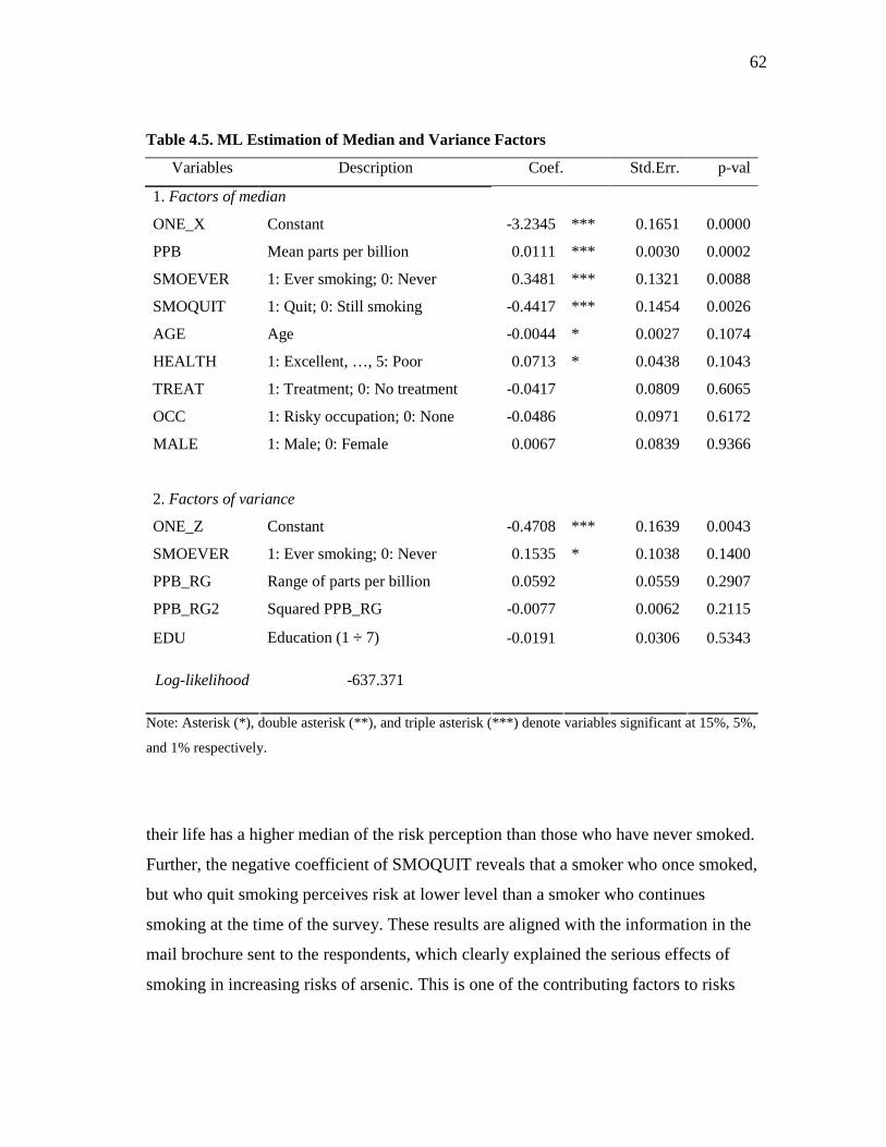
62
Table 4.5. ML Estimation of Median and Variance Factors
Variables Description Coef. Std.Err. p-val
1. Factors of median
ONE_X Constant -3.2345 *** 0.1651 0.0000
PPB Mean parts per billion 0.0111 *** 0.0030 0.0002
SMOEVER 1: Ever smoking; 0: Never 0.3481 *** 0.1321 0.0088
SMOQUIT 1: Quit; 0: Still smoking -0.4417 *** 0.1454 0.0026
AGE Age -0.0044 * 0.0027 0.1074
HEALTH 1: Excellent, …, 5: Poor 0.0713 * 0.0438 0.1043
TREAT 1: Treatment; 0: No treatment -0.0417 0.0809 0.6065
OCC 1: Risky occupation; 0: None -0.0486 0.0971 0.6172
MALE 1: Male; 0: Female 0.0067 0.0839 0.9366
2. Factors of variance
ONE_Z Constant -0.4708 *** 0.1639 0.0043
SMOEVER 1: Ever smoking; 0: Never 0.1535 * 0.1038 0.1400
PPB_RG Range of parts per billion 0.0592 0.0559 0.2907
PPB_RG2 Squared PPB_RG -0.0077 0.0062 0.2115
EDU Education (1 ÷ 7) -0.0191 0.0306 0.5343
Log-likelihood -637.371
Note: Asterisk (*), double asterisk (**), and triple asterisk (***) denote variables significant at 15%, 5%,
and 1% respectively.
their life has a higher median of the risk perception than those who have never smoked.
Further, the negative coefficient of SMOQUIT reveals that a smoker who once smoked,
but who quit smoking perceives risk at lower level than a smoker who continues
smoking at the time of the survey. These results are aligned with the information in the
mail brochure sent to the respondents, which clearly explained the serious effects of
smoking in increasing risks of arsenic. This is one of the contributing factors to risks
63
about which the scientists who study arsenic are most certain. Evidently, most in the
sample processed this information appropriately.
In addition to the above influences on the median, HEALTH is also a factor that
is significant at the 0.10 level. The positive sign of HEALTH coefficient shows that a
person in a poorer health condition perceives higher risk than those who are in better
health status. This evidence seems to be reasonable, and my interpretation of this is that
a person with poor health is more likely to think that a poor health state increases risks of
mortality, probably because of the perception that the person is more vulnerable to any
health risks than a healthy person is.
The variable AGE is also found to be statistically significant at the 0.10 level.
The negative sign of AGE shows that an older person tends to perceive less risk from
arsenic than a younger person. This is likely to be relevant to the latency period for the
arsenic-induced cancers: an older person might think that time left to live is relatively
short compared to the latency period of 10 or 20 years.
The remaining median shifting variables are statistically insignificant. The p-
value of the gender variable is around 0.93 and so there’s no significant difference
between male and female in their perceived levels of risk from arsenic concentration.
Those who treated their drinking water (TREAT = 1) perceive lower risks than those
who do not treat (TREAT = 0) but the difference is not statistically significant. In
addition, the risky occupations tend not to impact on the individual’s perceptions of
risks.
Among the factors potentially affecting the distribution variance (σ2), the
smoking is the most significant factor, as compared to education and range of arsenic
contamination. The signs of PPB_RG and PPB_RG2, positive and negative respectively,
provide evidence that the individual with drinking water with a wider range of PPB is
more likely to perceive a mortality risk distribution that is more diffuse, and that this
effect is decreasing in the level of PPB. In addition, individuals who have sometime
smoked are more uncertain, i.e. perceiving a more diffuse distribution of risk, while
education tends to reduce the people’s uncertainty about their risk facing them. The
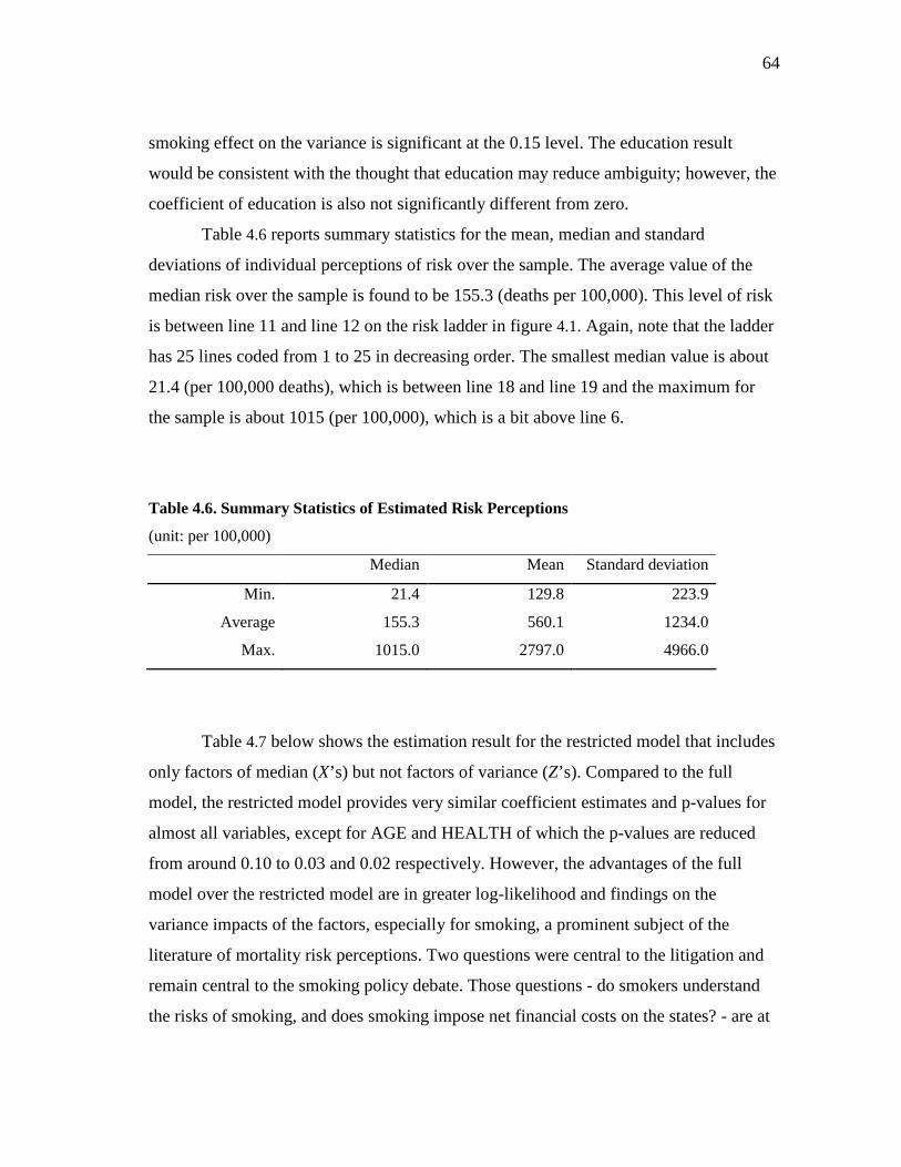
64
smoking effect on the variance is significant at the 0.15 level. The education result
would be consistent with the thought that education may reduce ambiguity; however, the
coefficient of education is also not significantly different from zero.
Table 4.6 reports summary statistics for the mean, median and standard
deviations of individual perceptions of risk over the sample. The average value of the
median risk over the sample is found to be 155.3 (deaths per 100,000). This level of risk
is between line 11 and line 12 on the risk ladder in figure 4.1. Again, note that the ladder
has 25 lines coded from 1 to 25 in decreasing order. The smallest median value is about
21.4 (per 100,000 deaths), which is between line 18 and line 19 and the maximum for
the sample is about 1015 (per 100,000), which is a bit above line 6.
Table 4.6. Summary Statistics of Estimated Risk Perceptions
(unit: per 100,000)
Median Mean Standard deviation
Min. 21.4 129.8 223.9
Average 155.3 560.1 1234.0
Max. 1015.0 2797.0 4966.0
Table 4.7 below shows the estimation result for the restricted model that includes
only factors of median (X’s) but not factors of variance (Z’s). Compared to the full
model, the restricted model provides very similar coefficient estimates and p-values for
almost all variables, except for AGE and HEALTH of which the p-values are reduced
from around 0.10 to 0.03 and 0.02 respectively. However, the advantages of the full
model over the restricted model are in greater log-likelihood and findings on the
variance impacts of the factors, especially for smoking, a prominent subject of the
literature of mortality risk perceptions. Two questions were central to the litigation and
remain central to the smoking policy debate. Those questions - do smokers understand
the risks of smoking, and does smoking impose net financial costs on the states? - are at
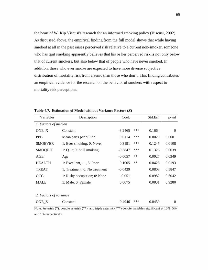
65
the heart of W. Kip Viscusi's research for an informed smoking policy (Viscusi, 2002).
As discussed above, the empirical finding from the full model shows that while having
smoked at all in the past raises perceived risk relative to a current non-smoker, someone
who has quit smoking apparently believes that his or her perceived risk is not only below
that of current smokers, but also below that of people who have never smoked. In
addition, those who ever smoke are expected to have more diverse subjective
distribution of mortality risk from arsenic than those who don’t. This finding contributes
an empirical evidence for the research on the behavior of smokers with respect to
mortality risk perceptions.
Table 4.7. Estimation of Model without Variance Factors (Z)
Variables Description Coef. Std.Err. p-val
1. Factors of median
ONE_X Constant -3.2465 *** 0.1664 0
PPB Mean parts per billion 0.0114 *** 0.0029 0.0001
SMOEVER 1: Ever smoking; 0: Never 0.3191 *** 0.1245 0.0108
SMOQUIT 1: Quit; 0: Still smoking -0.3847 *** 0.1326 0.0039
AGE Age -0.0057 ** 0.0027 0.0349
HEALTH 1: Excellent, …, 5: Poor 0.1005 ** 0.0428 0.0193
TREAT 1: Treatment; 0: No treatment -0.0439 0.0803 0.5847
OCC 1: Risky occupation; 0: None -0.051 0.0982 0.6042
MALE 1: Male; 0: Female 0.0075 0.0831 0.9280
2. Factors of variance
ONE_Z Constant -0.4946 *** 0.0459 0
Note: Asterisk (*), double asterisk (**), and triple asterisk (***) denote variables significant at 15%, 5%,
and 1% respectively.
66
Further Research Topic
In this chapter I have used the probability mass assumption consistent with the
fact that a range marked on the risk ladder by our subjects implies the mass of the latent
subjective distribution is heavily concentrated on that range. Alternatively, the modal
response hypothesis in L&W (2001) assumes that the respondents report the most likely
value of p, i.e. the mode of f(p). This implies that for the individual who chose a point
response at p, the mode of f(p) is assumed to be p. In their original framework, the
survey used by L&W (2001) asked respondent to choose a number between 0 and 100 to
represent their probabilistic beliefs. Note that there’s no elicitation of uncertainty in their
survey. In contrast, the arsenic survey uses the risk ladder and allows single or double
marks that the respondent makes on this ladder. So it is natural to extend the modal
response hypothesis to cover probability range response [p1, p2] in that it reflects the
individual’s belief that the mode of f(p) lies within this range.
Compared to the probability mass assumption, the modal response hypothesis
does not restrict the probability mass outside the range selected to be small. The latter
assumption just suggests that the most likely (mode) value of the mortality rate will be
within the stated range for the individual, while the chance for values outside that range
might be considerable. It is also worth nothing that these two assumptions are not
exclusive each other.
Concluding Remarks
Many, if not all environmental stressors on human health involve some
uncertainty, or unknown risks. Most analysis of the effect of stressors on health either
ignore risk and uncertainty altogether, or assume that risks are known. Few such studies
use the individual’s perceived mortality or health risks from a stressor. In this chapter I
have presented an approach that uses the probit function to model individual’s perceived
distribution of mortality risks from arsenic in drinking water. Factors that influence the
median and variance of the perceived risk distribution are included as arguments of the
probit function. Further, the parametric estimation model here has been derived from the
67
assumption relating to the markings on a risk ladder that people make, and the
corresponding probability mass distribution.
This modeling approach is applied to the case of the arsenic survey to estimate
perceptions of the respondents about risks associated with arsenic in their drinking
water, and ambiguity or uncertainty about these risks is allowed in the approach. The
findings show that the level of arsenic concentrations that households face, which is
measured in parts per billions, and the respondents’ smoking habits are of the strongest
influences that affect the medians of the individuals’ perceived distributions of risks.
Health status and age are also significant factors influencing the median. I also explore
influences on the variance of the perceived risk distribution, finding that again, the range
of arsenic concentration is found having a positive and significant relationship with the
variance. This variance represents an individual’s ambiguity about mortality risk faced
by the household.
68
CHAPTER V
SUMMARY AND CONCLUSION
In the three essays of my dissertation, I have presented the modeling approaches
for empirical estimation of probabilistic risks, which is critical to valuation of risky
goods such as risks inherent in environment and human health. The first essay briefly
reviews the option price concept as a measure of ex-ante benefit and develops an
empirical model to estimate option price from individual discrete choice data. The first
essay also provides a case study in which I use an empirical measure of the option price
to estimate the ex-ante benefit of a guarantee of participation for a Maine moose hunter.
In this essay, I assume the hunters were homogeneous in their thought about the chance
they had to face in the annual lottery allocating the hunting permits. This chance was
presented to them as the actual statistical odds of winning the lottery.
In the second essay, I relax the homogeneity assumption and consider the
individuals’ heterogeneity in their thoughts about the probabilistic risk inherent in a
risky event such as lottery. However no ambiguity about risks is assumed in this essay,
as well as in the first one.
The third essay introduces ambiguity for the risks, a characteristic usually
observed in individual perceptions of mortality risks. The modified probit approach has
been shown capable in estimating factors of median and variance of subjective
distributions of risks using the individuals’ markings on risk ladder.
All three of the essays are set in the general area of nonmarket valuation under
uncertainty with particular focus on econometric modeling of individual perceptions of
risks in environmental quality and human health. They contribute empirical examples
and methodological approaches to developing estimation models given the assumption
about the individual’s perceptions of risk, and accordingly, the reasonable specifications
of risks involved in the models.
69
REFERENCES
Allais, P.M. 1953. “Le Comportement de l'Homme Rationnel devant le Risque: Critique
des Postulats et Axiomes de l'Ecole Americaine.” Econometrica 21(4):503-546.
Akabua, K.M., W. L. Adamowicz, W.E. Phillips, and P. Trelawny. 1999. “Implications
of Realization Uncertainty on Random Utility Models: The Case of Lottery-
Rationed Hunting.” Canadian Journal of Agricultural Economics 47(2):165-179.
Boxall, P.C. 1995. “The Economic Value of Lottery-Rationed Recreational Hunting.”
Canadian Journal of Agricultural Economics 43(1):119-131.
Burnett, J.K., and R.W. Hahn. 2001. “A Costly Benefit.” Regulation 24(3):44-49.
Buschena D.E., T.L. Anderson, and J.L. Leonard. 2001. “Valuing Non-Marketed Goods:
The Case of Elk Permit Lotteries.” Journal of Environmental Economics and
Management 41:33-43.
Camerer, C., and M. Weber. 1992. “Recent Developments in Modeling Preferences:
Uncertainty and Ambiguity.” Journal of Risk and Uncertainty 5:325-370.
Cameron, T.A. 2005. “Individual Option Prices for Climate Change Mitigation.” Journal
of Public Economics 89(2-3):283-301.
Cameron, T.A., and J. Englin. 1997. “Welfare Effects of Changes in Environmental
Quality under Individual Uncertainty about Use.” RAND Journal of Economics
28:S45-S70.
Chib S., and E. Greenberg. 1995. “Understanding the Metropolis-Hastings Algorithm.”
The American Statistician 49(4):327-335.
De Finetti, B. 1974. Theory of Probability: A Critical Introductory Treatment. Vols 1
and 2. New York: Wiley.
Debora, F., and J. Baron. 1988. “Ambiguity and Rationality.” Journal of Behavioral
Decision Making 1:149-157.
Ellsberg, D. 1961. “Risk, Ambiguity, and the Savage Axioms.” Quarterly Journal of
Economics 75:643-669.
Fox, C.R., and A. Tversky. 1995. “Ambiguity Aversion and Comparative Ignorance.”
70
Quarterly Journal of Economics 110:585-603.
Gelfand, A.E., and A.F.M. Smith. 1990. “Sampling-Based Approaches to Calculating
Marginal Densities.” Journal of American Statistics Association 85:398-409.
Gelman, A., J.B Carlin, H.S. Stern, and D.B. Rubin. 2004. “Hierarchical Models.” In
Bayesian Data Analysis (2nd ed.), Chapter 5. Boca Raton, FL: Chapman &
Hall/CRC.
Gilks, W.R., S. Richardson, and D.J. Spiegelhalter (Eds.). 1996. Markov Chain Monte
Carlo in Practice. Boca Raton, FL: Chapman & Hall/CRC.
Graham, D.A. 1981. “Cost-Benefit Analysis under Uncertainty.” American Economic
Review 71(4):715-725.
Haab, T.C., and K.E. McConnell. 2002. Valuing Environmental and Natural Resources.
Northampton, MA: Edward Elgar.
Hanemann, W.M. 1984. “Welfare Evaluations in Contingent Valuation Experiments
with Discrete Responses.” American Journal of Agricultural Economics 66:332-
341.
Hanemann, M., J. Loomis, and B. Kanninen. 1991. “Statistical Efficiency of Double-
Bounded Dichotomous Choice Contingent.” American Journal of Agricultural
Economics 73(4):1255-1263.
Heath, C., and A. Tversky. 1991. “Preferences and Belief: Ambiguity and Competence
in Choice under Uncertainty.” Journal of Risk and Uncertainty 4:5-28.
Heckman, J.J., and R.J. Willis. 1977. “A Beta-Logistic Model for the Analysis of
Sequential Labor Force Participation by Married Woman.” Journal of Political
Economy 85(1):27-58.
Hill, D., M. Perry, and R.J. Willis. 2005. “Estimating Knightian Uncertainty from
Survival Probability Questions on the HRS.” Manuscript, University of
Michigan, Ann Arbor.
Jakus P.M., and W.D. Shaw. 2003. “Perceived Hazard and Product Choice: An
Application to Recreational Site Choice.” Journal of Risk and Uncertainty 26
(1):77-92.
71
Johnson, D. 1997. “The Triangular Distribution as a Proxy for the Beta Distribution in
Risk Analysis.” Journal of the Royal Statistical Society - Series D - The
Statistician 46(3):387-398.
Lillard, L.A., and R.J. Willis. 2001. “Cognition and Wealth: The Importance of
Probabilistic Thinking.” Michigan Retirement Research Center Working Paper
UM00-04, University of Michigan, Ann Arbor.
Loomis, J. 1982. “Use of Travel Cost Models for Evaluating Lottery Rationed
Recreation: Application to Big Game Hunting.” Journal of Leisure Research 1
(2):117-124.
Loomis, J.B., and P.H. duVair. 1993. “Evaluating the Effect of Alternative Risk
Communication Devices on Willingness to Pay: Results from a Dichotomous
Choice Contingent Valuation Experiment.” Land Economics 69(3):287-298.
Nyman, J.A. 2002. The Theory of Demand for Health Insurance. Stanford, CA: Stanford
University Press.
Ramsey, F.P. 1926. “Truth and Probability.” In F.P. Ramsey, 1931, The Foundations of
Mathematics and other Logical Essays, Ch. VII, pp.156-198, R.B. Braithwaite
(Ed.), New York: Harcourt.
Riddel, M. 2007. “Risk Perception, Ambiguity, and Nuclear-Waste Transport.” Revised
manuscript, Dept. of Economics, University of Nevada, Las Vegas.
Riddel, M., and W.D. Shaw. 2006. “A Theoretically-Consistent Empirical Model of
Non-Expected Utility: An Application to Nuclear-Waste Transport.” Journal of
Risk and Uncertainty 32(2):131-150.
Rossi, P.E., G.M. Allenby, and McCulloch. 2005. Bayesian Statistics and Marketing.
Hoboken, NJ: Wiley.
Savage, L.J. 1954. The Foundations of Statistics. New York: J. Wiley.
Schmeidler, D. 1989. “Subjective Probability and Expected Utility without Additivity.”
Econometrica 57(3):571-587.
Scrogin, D., and Berrens R.P. 2003. “Rationed Access and Welfare: The Case of Public
Resource Lotteries.” Land Economics 79(2):137-148.
72
Scrogin, D., R.P. Berrens, and A. Bohara. 2000. “Policy Changes and the Demand for
Lottery-Rationed Hunting Privileges.” Journal of Agricultural and Resource
Economics 25(2):501-519.
Segal, U. 1987. “The Ellsberg Paradox and Risk Aversion: An Anticipated Utility
Approach.” International Economics Review 28:175-202.
Shaw, W.D., P. Jakus, M. Riddel, M. Walker, and P. Jindapon. 2006. “Incorporating
Perceived Mortality Risks from Arsenic into Models of Drinking Water Behavior
and Valuation of Arsenic Risk Reductions: Preliminary Results.” Presented at the
U.S. EPA Workshop on Mortality Risks, April 10-12, 2006.
Shaw, W.D., M. Riddel, and P.M. Jakus. 2005. “Valuing Environmental Changes in the
Presence of Risk: An Update and Discussion of Some Empirical Issues.” In H.
Folmer and T. Tietenberg (Eds.), The International Yearbook of Environmental
and Resource Economics: A Survey of Current Issues, Chapter 7. Northampton,
MA: Edward Elgar Press.
Shaw, W.D., M. Walker, and M. Benson. 2005. “Treating and Drinking Well Water in
the Presence of Health Risks from Arsenic Contamination: Results from a U.S.
Hot Spot.” Risk Analysis 25 (6):1531-1543.
Slovic P. 1987. “Perceptions of Risk.” Science 236 (17):280-285.
Smith A.F.M., and A.E. Gelfand. 1992. “Bayesian Statistics without Tears: A Sampling-
Resampling Perspective.” The American Statistician 46 (2):84-88.
Smith, V.K. 1992. “Environmental Risk Perception and Valuation: Conventional Versus
Prospective Reference Theory.” In Bromley, D.W. and Segerson, K. (Eds), The
Social Response to Environmental Risk, pp. 23-56. Boston: Kluwer.
Starmer, C. 2000. “Developments in Non-Expected Utility Theory: The Hunt for a
Descriptive Theory of Choice under Risk.” Journal of Economic Literature
28:332-382.
Train, K.E. 2002. Discrete Choice Methods with Simulations. Cambridge, UK:
Cambridge University Press.
U.S. Environmental Protection Agency. 2006. “Arsenic in Drinking Water.” Retrieved
73
Sep 01, 2007, from http://www.epa.gov/safewater/arsenic/
Viscusi, W.K. 2002. Smoke-Filled Rooms: A Postmortem on the Tobacco Deal.
Chicago: University Of Chicago Press.
Viscusi, W.K. 1989. “Prospective References Theory: Toward an Explanation of the
Paradoxes.” Journal of Risk and Uncertainty 2:235-264.
Viscusi, W.K., and W.N. Evans. 1998. “Estimation of Revealed Probabilities and Utility
Functions for Product Safety Decisions.” The Review of Economics and Statistics
80(1):28-33.
Wilson, R. 2001. “Underestimating Arsenic’ Risk.” Regulation 24(3):50-53.
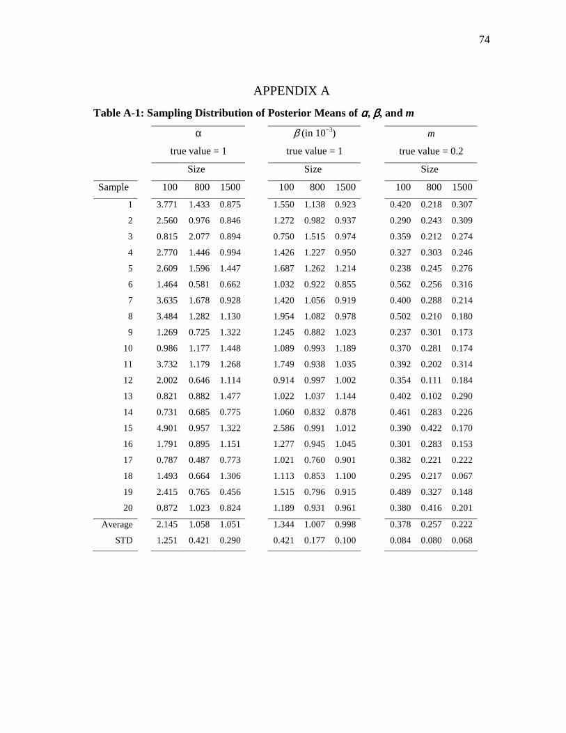
74
APPENDIX A
Table A-1: Sampling Distribution of Posterior Means of αααα, ββββ, and m
α
true value = 1
β (in 10−3)
true value = 1
m
true value = 0.2
Size Size Size
Sample 100 800 1500 100 800 1500 100 800 1500
1 3.771 1.433 0.875 1.550 1.138 0.923 0.420 0.218 0.307
2 2.560 0.976 0.846 1.272 0.982 0.937 0.290 0.243 0.309
3 0.815 2.077 0.894 0.750 1.515 0.974 0.359 0.212 0.274
4 2.770 1.446 0.994 1.426 1.227 0.950 0.327 0.303 0.246
5 2.609 1.596 1.447 1.687 1.262 1.214 0.238 0.245 0.276
6 1.464 0.581 0.662 1.032 0.922 0.855 0.562 0.256 0.316
7 3.635 1.678 0.928 1.420 1.056 0.919 0.400 0.288 0.214
8 3.484 1.282 1.130 1.954 1.082 0.978 0.502 0.210 0.180
9 1.269 0.725 1.322 1.245 0.882 1.023 0.237 0.301 0.173
10 0.986 1.177 1.448 1.089 0.993 1.189 0.370 0.281 0.174
11 3.732 1.179 1.268 1.749 0.938 1.035 0.392 0.202 0.314
12 2.002 0.646 1.114 0.914 0.997 1.002 0.354 0.111 0.184
13 0.821 0.882 1.477 1.022 1.037 1.144 0.402 0.102 0.290
14 0.731 0.685 0.775 1.060 0.832 0.878 0.461 0.283 0.226
15 4.901 0.957 1.322 2.586 0.991 1.012 0.390 0.422 0.170
16 1.791 0.895 1.151 1.277 0.945 1.045 0.301 0.283 0.153
17 0.787 0.487 0.773 1.021 0.760 0.901 0.382 0.221 0.222
18 1.493 0.664 1.306 1.113 0.853 1.100 0.295 0.217 0.067
19 2.415 0.765 0.456 1.515 0.796 0.915 0.489 0.327 0.148
20 0.872 1.023 0.824 1.189 0.931 0.961 0.380 0.416 0.201
Average 2.145 1.058 1.051 1.344 1.007 0.998 0.378 0.257 0.222
STD 1.251 0.421 0.290 0.421 0.177 0.100 0.084 0.080 0.068
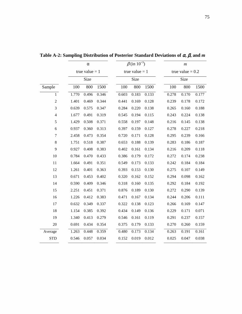
75
Table A-2: Sampling Distribution of Posterior Standard Deviations of αααα, ββββ, and m
α
true value = 1
β (in 10−3)
true value = 1
m
true value = 0.2
Size Size Size
Sample 100 800 1500 100 800 1500 100 800 1500
1 1.770 0.496 0.346 0.603 0.183 0.133 0.278 0.170 0.177
2 1.401 0.469 0.344 0.441 0.169 0.128 0.239 0.178 0.172
3 0.639 0.575 0.347 0.284 0.220 0.138 0.265 0.160 0.188
4 1.677 0.491 0.319 0.545 0.194 0.115 0.243 0.224 0.138
5 1.429 0.508 0.371 0.558 0.197 0.148 0.216 0.145 0.138
6 0.937 0.360 0.313 0.397 0.159 0.127 0.278 0.227 0.218
7 2.458 0.473 0.354 0.720 0.171 0.128 0.295 0.239 0.166
8 1.751 0.518 0.387 0.653 0.188 0.139 0.283 0.186 0.187
9 0.927 0.408 0.383 0.402 0.161 0.134 0.216 0.209 0.118
10 0.784 0.470 0.433 0.386 0.179 0.172 0.272 0.174 0.238
11 1.664 0.491 0.351 0.549 0.173 0.133 0.242 0.184 0.184
12 1.261 0.401 0.363 0.393 0.153 0.130 0.275 0.107 0.149
13 0.671 0.453 0.402 0.320 0.162 0.152 0.294 0.098 0.162
14 0.590 0.409 0.346 0.318 0.160 0.135 0.292 0.184 0.192
15 2.251 0.451 0.371 0.876 0.189 0.130 0.272 0.290 0.139
16 1.226 0.412 0.383 0.471 0.167 0.134 0.244 0.206 0.111
17 0.632 0.349 0.337 0.322 0.138 0.123 0.266 0.169 0.147
18 1.154 0.385 0.392 0.434 0.149 0.136 0.229 0.171 0.071
19 1.340 0.413 0.279 0.546 0.161 0.119 0.291 0.237 0.157
20 0.691 0.434 0.354 0.375 0.179 0.133 0.270 0.260 0.159
Average 1.263 0.448 0.359 0.480 0.173 0.134 0.263 0.191 0.161
STD 0.546 0.057 0.034 0.152 0.019 0.012 0.025 0.047 0.038
76
VITA
Name: To Ngoc Nguyen
Address: Department of Agricultural Economics 2124 TAMU College Station, TX 77843-2124 Email Address: [email protected] Education: B.S., Systems Control, Vietnam National Institute of Technology, 1985 M.B.A., Operations and Technology Management, Illinois Institute of Technology, 2000 M.S., Economics, National University of Singapore, 2002


