Embed Size (px)
Citation preview
ECONOMETRIC MODELING AND FORECASTING
IN FINANCIAL MARKETS
By Daniel Borup
A PhD thesis submitted to
School of Business and Social Sciences, Aarhus University,
in partial fulfilment of the requirements of
the PhD degree in
Economics and Business Economics
June 2019
CREATESCenter for Research in Econometric Analysis of Time Series

This version: October 9, 2019 © Daniel Borup

PREFACE
This dissertation represents a tangible outcome of my graduate studies at the Depart-
ment of Economics and Business Economics at Aarhus University and was written
during the period from September 2015 through June 2019. I am grateful to the De-
partment of Economics and Business Economics and the Center for Research in
Econometric Analysis of Time Series (CREATES) for providing an outstanding re-
search environment and generous financial support for participation in conferences
and courses.
Special thanks go first and foremost to my main thesis advisor Bent Jesper Christensen
for his valuable guidance, help with funding applications, and continued readiness to
discuss academic problems, no matter the timing. Another special thanks to my thesis
co-advisor Yunus Emre Ergemen. Your encouragement and constructive attitude
has made my graduate studies both enjoyable and productive. I have always found
both your doors open and for that I am thankful. The first chapter in this dissertation
illustrates the outcome of our joint effort. It has been a joy to work with both of you. It
is my hope that we can continue our collaborations in the years to come. Likewise, I
would like to thank Solveig Nygaard Sørensen for being the glue that keeps everything
together and always being available for help.
In the fall of 2017, I had the great pleasure of visiting Francis X. Diebold at the Depart-
ment of Economics, University of Pennsylvania, USA. I am thankful to University of
Pennsylvania for the hospitality, to Frank for inviting me to present at their seminar
series, attend dinners, and stimulating discussions about forecast evaluation, and
to Janne Lehto, my office mate, for excellent company. I would also like to express
my gratitude to Danmark-Amerika Fondet, Augustinus Fonden, Oticon Fonden and
Knud Højgaards Fond for the travel funds they granted me.
I appreciate the abundance of great colleagues at the Department of Economics
and Business Economics and CREATES. I am grateful to all of them for creating an
outstanding academic and social environment. To all the people at (what used to
be) the CREATES corridor, thank you for a multitude of coffee breaks. I especially
want to thank Jorge W. Hansen and Martin Thyrsgaard, with whom I shared office
i

ii
for the majority of my graduate studies, for their company, insightful discussions,
and endless conversations on important aspects of life such as Formula 1, football
and LATEX. Jorge, I sincerely hope we will continue our bi-annual Formula 1 trips
perpetually. People who also deserve a special thanks are my fellow PhD students and
friends at Aarhus University; Benjamin, Nicolaj, Christian, Thomas, Jonas, Mikkel,
Kristoffer, Simon, and Niels for many interesting conversations, social activities, and
so much more. I also want to extend a special thanks to Johan S. Jakobsen, my co-
author and close friend. It is a privilege to be able to include our joint work as part of
this dissertation. I hope the future will bring additional scientific contributions and
plenty of hiking, hunting, and fishing trips.
Finally and most importantly, I am thankful to my parents, Dan and Lone, for their pa-
tience and never-ending support, and to my brother, Kenneth, for the many inspiring
discussions on statistical matters. An especially heartfelt thank you is reserved for my
girlfriend Cecilie. I have no words to adequately describe your never-ending encour-
agement and love. Thank you for everything. Lastly, a thank you to our son, Lauge,
who has made the last endeavours of my graduate studies the most memorable of all.
Daniel Borup
Aarhus, June 2019

UPDATED PREFACE
The pre-defence meeting was held on September 11, 2019, in Aarhus. I am grateful
to the members of the assessment committee consisting of Peter Reinhard Hansen
(University of North Carolina, Chapel Hill), Joakim Westerlund (Lund University
and Deakin University), and Stig Vinther Møller (Aarhus University) for their careful
reading of the dissertation and their many insightful comments and suggestions.
Some of the suggestions have been incorporated into the present version of the
dissertation while others remain for future research.
Daniel Borup
Aarhus, October 2019
iii

CONTENTS
Summary vii
Danish summary xi
1 Assessing predictive accuracy in panel data models with long-range de-pendence 11.1 Introduction . . . . . . . . . . . . . . . . . . . . . . . . . . . . . . . . . 2
1.2 Model framework . . . . . . . . . . . . . . . . . . . . . . . . . . . . . . 4
1.3 Forecasting . . . . . . . . . . . . . . . . . . . . . . . . . . . . . . . . . . 10
1.4 Monte Carlo study . . . . . . . . . . . . . . . . . . . . . . . . . . . . . . 20
1.5 Predictive relation between stock market volatility and economic
policy uncertainty . . . . . . . . . . . . . . . . . . . . . . . . . . . . . . 21
1.6 Concluding remarks . . . . . . . . . . . . . . . . . . . . . . . . . . . . . 24
1.7 References . . . . . . . . . . . . . . . . . . . . . . . . . . . . . . . . . . 25
Appendix . . . . . . . . . . . . . . . . . . . . . . . . . . . . . . . . . . . . . . 29
2 Capturing volatility persistence: a dynamically complete realized EGARCH-MIDAS model 512.1 Introduction . . . . . . . . . . . . . . . . . . . . . . . . . . . . . . . . . 52
2.2 Persistence in a multiplicative realized EGARCH . . . . . . . . . . . . 55
2.3 Estimation . . . . . . . . . . . . . . . . . . . . . . . . . . . . . . . . . . 60
2.4 Empirical results . . . . . . . . . . . . . . . . . . . . . . . . . . . . . . . 61
2.5 Concluding remarks . . . . . . . . . . . . . . . . . . . . . . . . . . . . . 72
2.6 References . . . . . . . . . . . . . . . . . . . . . . . . . . . . . . . . . . 74
Appendix . . . . . . . . . . . . . . . . . . . . . . . . . . . . . . . . . . . . . . 79
3 Asset pricing model uncertainty 1153.1 Introduction . . . . . . . . . . . . . . . . . . . . . . . . . . . . . . . . . 116
3.2 Methodology . . . . . . . . . . . . . . . . . . . . . . . . . . . . . . . . . 122
3.3 The long-horizon effect of dividend initiations and resumptions . . 130
3.4 Application to characteristics-sorted portfolios . . . . . . . . . . . . . 142
3.5 Concluding remarks . . . . . . . . . . . . . . . . . . . . . . . . . . . . . 143
3.6 References . . . . . . . . . . . . . . . . . . . . . . . . . . . . . . . . . . 145
Appendix . . . . . . . . . . . . . . . . . . . . . . . . . . . . . . . . . . . . . . 152
v

SUMMARY
This dissertation is composed of three self-contained chapters on the econometric
modeling and forecasting in financial markets. The object of interest in all chapters
is the conditional expectation of asset returns or their volatility, whether for use in
forecasting or asset pricing tests, of interest to academics as well as practitioners.
The first chapter considers forecasting and predictive accuracy in a general panel
data model that jointly allows for various typical features observed in financial data.
The application is to realized stock market volatility in a multi-country analysis,
using a textual measure of economic policy uncertainty as predictor. The second
chapter considers a particular type of data feature of the conditional volatility process,
long-range dependence, and proposes an extension of the popular realized GARCH
framework to empirically capture this. The final chapter addresses model uncertainty
and time-varying parameters when estimating the conditional expectation of asset
returns and proposes a novel econometric framework suitable for event study and
asset pricing tests.
Chapter 1, Assessing predictive accuracy in panel data models with long-range de-
pendence (joint with Bent Jesper Christensen and Yunus Emre Ergemen), examines
forecasting and predictive accuracy in a general panel data model. As many macroe-
conomic and financial variables are presented in the form of panels, such as inter-
national panels of asset return volatility or cross-country panels of inflation rates,
it should be natural to treat data as a panel rather than separate time series. We
consider a predictive setting motivated from the data-generating process of Ergemen
(2019), which allows for individual and interactive fixed effects that control for cross-
sectional dependence, endogenous predictors, and both short-range and long-range
dependence, often faced in empirical studies, see e.g. Gil-Alaña and Robinson (1997)
and Andersen, Bollerslev, Diebold, and Labys (2003). The paper then discusses fore-
casting in this setting and proposes tests of the null hypothesis that model-based
forecasts are uninformative. Motivated from the analysis in Breitung and Knüppel
(2018), we consider a Diebold-Mariano style test based on comparison of the model-
based forecast and a nested no-predictability benchmark, an encompassing style
test of the same null, and a test of pooled uninformativeness in the entire panel.
A simulation study shows that the encompassing style test is reasonably sized in
vii
viii SUMMARY
finite samples, whereas the Diebold-Mariano style test is oversized. Both tests have
non-trivial local power. We apply our new methodology to analyze the relation be-
tween a textual measure of economic policy uncertainty (EPU) (Baker, Bloom, and
Davis, 2016) and stock market realized volatility (RV) in a multi-country analysis.
While our analysis is supportive of a contemporaneous relation between EPU and RV,
uninformativeness of EPU for RV is not rejected. Weak predictive power of EPU for
RV can, nevertheless, be ascribed to a common (global) factor structure in the panel.
Chapter 2, Capturing volatility persistence: a dynamically complete realized EGARCH-
MIDAS model (joint with Johan Stax Jakobsen),1 introduces extensions of the Realized
Exponential GARCH model (REGARCH) (Hansen, Huang, and Shek, 2012; Hansen
and Huang, 2016) that capture the evident high persistence typically observed in
measures of financial market volatility. The R(E)GARCH models facilitate exploitation
of granular information in high-frequency data by including realized measures, which
constitute a much stronger signal of latent volatility than squared returns (Andersen
et al., 2003). Despite their empirical success, these models do not adequately capture
the dependence structure in volatility (both latent and realized) without proliferation
in parameters incurred by using the classical ARMA structures embedded in the
model. This dependence structure is typically characterized by a positive and slowly
decaying autocorrelation function or a persistence parameter close to unity, known as
the "integrated GARCH effect". Our extensions decompose conditional variance into
a short-term and a long-term component via a multiplicative specification motivated
from the popular GARCH-MIDAS model of Engle, Ghysels, and Sohn (2013). The long-
term component utilizes mixed-data sampling or a heterogeneous autoregressive
structure to capture the persistence of volatility, avoiding parameter proliferation.
The proposed models are dynamically complete, facilitating multi-period forecasting.
We conduct a thorough empirical investigation with an exchange traded fund that
tracks the S&P500 Index and 20 individual stocks which shows that our models better
capture the dependency structure of volatility, relative to the original REGARCH
and natural competitors that allow for shifts in unconditional variance and includes
fractional integration explicitly. This leads to substantial improvements in empirical
in-sample fit and predictive ability at both short and long horizons. A volatility-timing
trading strategy also shows that capturing this volatility persistence yields substantial
utility gains for a mean-variance investor at longer investment horizons.
Chapter 3, Asset pricing model uncertainty,2 considers a new event study methodol-
ogy. The purpose of an event study is to isolate the incremental impact of an event on
asset price performance relative to established determinants of performance (Kothari
and Warner, 2006). Two most crucial problems with inference are, however, reliance
on a single, possibly misspecified model of asset pricing, the bad-model problem of
1Published in Quantitative Finance 19 (2019), 1839-1855.2Published in Journal of Empirical Finance 54 (2019), 166-189.

ix
Fama (1998), and the imposition of constant coefficients (Fama and French, 1997;
Boehme and Sorescu, 2002; Armstrong, Banerjee, and Corona, 2013). This paper
provides a unified calendar-time portfolio methodology for assessing whether re-
turns following an event are abnormal which efficiently handles asset pricing model
uncertainty and allows for time-varying alpha and factor exposures. This is achieved
by specifying a Bayesian framework that assumes a dynamic linear model for the
return-generating process and, given a candidate set of asset pricing factors, permits
the computation of conditional model and factor posterior probabilities. As such, the
approach disciplines researchers’ use of asset pricing factors and assigns a probability
measure to the appropriateness of (dynamically) selecting a single model that best
approximates the true factor structure or whether model averaging across an asset
pricing universe is desired. The methodology is applied to the long-horizon effect
of dividend initiations and resumptions in the 1980 to 2015 period. Resulting post-
announcement conditional abnormal returns are generally significant, statistically
and economically, which contrasts recent evidence, and exhibits a break in mean
from positive until the mid-1990s and negative onwards. We also document substan-
tial time-variation in the dimensionality and composition of the factor structure in
expected returns, which goes beyond what captured by conditional versions of the
CAPM and Fama-French specifications. This also generalizes to a large panel of 202
characteristics-sorted portfolios.
x SUMMARY
References
Andersen, T. G., Bollerslev, T., Diebold, F. X., Labys, P., 2003. Modeling and forecasting
realized volatility. Econometrica 71 (2), 579–625.
Armstrong, C. S., Banerjee, S., Corona, C., 2013. Factor-loading uncertainty and
expected returns. The Review of Financial Studies 26 (1), 158–207.
Baker, S. R., Bloom, N., Davis, S. J., 2016. Measuring economic policy uncertainty. The
Quarterly Journal of Economics 131 (4), 1593–1636.
Boehme, R. D., Sorescu, S. M., 2002. The long-run performance following dividend
initiations and resumptions: Underreaction or product of chance? The Journal of
Finance 57 (2), 871–900.
Breitung, J., Knüppel, M., 2018. How far can we forecast? Statistical tests of the predic-
tive content. Deutsche Bundesbank working paper.
Engle, R. F., Ghysels, E., Sohn, B., 2013. Stock market volatility and macroeconomic
fundamentals. The Review of Economics and Statistics 95 (3), 776–797.
Ergemen, Y. E., 2019. System estimation of panel data models under long-range
dependence. Journal of Business and Economics Statistics 37 (1), 13–26.
Fama, E. F., 1998. Market efficiency, long-term returns, and behavioral finance. Journal
of Financial Economics 49, 283–306.
Fama, E. F., French, K. R., 1997. Industry costs of equity. Journal of Financial Eco-
nomics 43 (2), 153–193.
Gil-Alaña, L., Robinson, P., 1997. Testing of unit root and other nonstationary hy-
potheses in macroeconomic time series. Journal of Econometrics 80(2), 241–268.
Hansen, P. R., Huang, Z., 2016. Exponential GARCH modeling with realized measures
of volatility. Journal of Business and Economic Statistics 34 (2), 269–287.
Hansen, P. R., Huang, Z., Shek, H. H., 2012. Realized GARCH: a joint model for return
and realized mesures of volatility. Journal of Applied Econometrics 27, 877–906.
Kothari, S. P., Warner, J. B., 2006. Econometrics of event studies. In: Eckbo, B. E. (Ed.),
Handbook of corporate finance: Empirical coporate finance. Vol. A. Elsevier/North-
Holland, Ch. 1.
DANISH SUMMARY
Denne afhandling består af tre uafhængige kapitler omhandlende økonometrisk
modellering og forudsigelse i de finansielle markeder. Alle tre kapitler interesserer
sig for den betingede forventning af aktivers afkast eller deres volatilitet, hvad enten
til brug i forudsigelse eller aktivprisfastsættelsestests, hvilket er interessant fra både
et akademisk og praktisk synspunkt. Det første kapitel omhandler forudsigelse og
prædiktiv præcision i en generel paneldatamodel, der simultant tillader for adskil-
lige typiske egenskaber observeret i finansielt data. Kapitlets metoder er anvendt
til forudsigelsen af aktiemarkeders afkastsvolatilitet i en tværnational analyse, hvor
forudsigelsesvariablen er et tekstbaseret mål for økonomisk-politisk usikkerhed. Det
andet kapitel omhandler én bestemt egenskab, langsigtet afhængighed, af den betin-
gede variansproces, og foreslår en udvidelse af den populære Realized GARCH-model
til empirisk at matche denne. Det sidste kapitel adresserer modelusikkerhed og tidsva-
rierende parametre i estimationen af den betingede forventning af aktivafkast og
foreslår et nyt teoretisk setup anvendeligt til eventstudier og tests i forbindelse med
aktivprisfastsættelse.
Kapitel 1, Assessing predictive accuracy in panel data models with long-range de-
pendence (fælles med Bent Jesper Christensen and Yunus Emre Ergemen), betragter
forudsigelighed med en generel paneldatamodel. Da mange makroøkonomiske og fi-
nansielle variable er struktureret som et panel, eksempelvist internationale paneler af
afkastsvolatilitet eller tværnationale paneler af inflationsrater, bør det være naturligt
at håndtere data som et panel og ikke som separate tidsrækker. Vi betragter et setup
motiveret af den datagenererende proces foreslået af Ergemen (2019), som tillader for
individuelle og interaktive fixed effects, der kontrollerer for tværsnitsafhængighed,
endogene forudsigelsesvariable samt både kortsigtet og langsigtet afhængighed. Alle
er egenskaber, der typisk findes i empiriske studier, se eksempelvist Gil-Alaña og
Robinson (1997) og Andersen et al. (2003). Vi diskuterer forudsigelse i dette setup og
foreslår test af nulhypotesen om modelbaserede forudsigelser ikke er informative.
Vi betragter en Diebold-Mariano-type af test, motiveret af analysen i Breitung og
Knüppel (2018), baseret på en sammenligning af den modelbaserede forudsigelse
og et indeholdt benchmark, der ingen forudsigelighed besidder. Vi betragter også
en encompassing-type af test af den samme nulhypotese foruden en test af samlet
xi

xii DANISH SUMMARY
forudsigelighed i hele panelet. Et simulationsstudium viser, at encompassing-typen
har tilfredsstillende egenskaber under nulhypotesen, mens Diebold-Mariano-typen
forkaster for ofte. Begge test har ikke-triviel lokal styrke. Vi anvender vores nye meto-
dologi til at analysere relationen mellem et tekstbaseret mål for økonomisk-politisk
usikkerhed (EPU) (Baker et al., 2016) og fremtidigt realiseret aktiemarkedsvolatilitet
(RV) i en tværnational analyse. Vi finder generelt evidens for en kontemporær relation
mellem EPU og RV, men kan ikke forkaste at de modelbaserede forudsigelser ved
hjælp af EPU for RV ikke er informative. Svag forudsigelighed af RV vha. EPU kan dog
identificeres i en fælles (global) faktorstruktur på tværs af landene.
Kapitel 2, Capturing volatility persistence: a dynamically complete realized EGARCH-
MIDAS model (fælles med Johan Stax Jakobsen),1 introducerer udvidelser af Realized
EGARCH-modellen (REGARCH) (Hansen et al., 2012; Hansen og Huang, 2016), som
modellerer den evidente høje afhængighed typisk observeret i mål for volatilitet i de
finansielle markeder. R(E)GARCH-modellerne tillader for brugen af granulær infor-
mation i højfrekvent data ved at inkludere såkaldte realiserede mål, der udgør et langt
stærkere signal for latent volatilitet i forhold til kvadrerede afkast (Andersen et al.,
2003). På trods af modellernes empiriske success, er de ikke i stand til tilstrækkeligt
at matche afhængighedsstrukturen i volatilitet (både latent og realiseret) uden en
større forøgelse af antallet af parametre. Denne afhængighedsstruktur er typisk karak-
teriseret ved en positiv og langsomt aftagende autokorrelationsfunktion (langsigtet
afhængighed) eller en persistensparameter tæt på én, også kendt som "integrated
GARCH-effekten". Vores udvidelser dekomponerer den betingede variansproces i
en kortsigtet og langsigtet komponent via en multiplikativ specicifikation, der er
motiveret fra den populære GARCH-MIDAS-model af Engle et al. (2013). Den langsig-
tede komponent udnytter data på forskellig frekvens eller en heterogen autoregressiv
struktur, hvilket undgår den store forøgelse af parametre krævet af den klassiske AR-
MA struktur indeholdt i REGARCH. De foreslåede modeller er dynamiske komplette,
hvilket muliggør forudsigelse flere perioder frem i tiden. En grundig empirisk analyse,
der anvender data på en børshandlet indeksfond, som følger S&P500-indekstet, og
20 individuelle aktier, finder, at vores nye modeller bedre er i stand til at matche
afhængighedsstrukturen af volatilitet relativt til den originale REGARCH og oplagte
konkurrenter, som tillader for skift i den ubetingede varians og inkluderer fraktionel
integration eksplicit. Dette medfører betydelige forbedringer i empirisk fit og forudsi-
gelsesevne på både korte og lange horisonter. En volatilitets-timinig handelsstrategi
viser desuden, at evnen til at matche afhængighedsstrukturen leder til betydelige
forbedringer i nytte for en mean-variance-investor på længere investeringshorisonter.
Kapitel 3, Asset pricing model uncertainty,2 betragter en ny eventstudiemetodolo-
gi. Formålet med et eventstudium er at isolere den inkrementelle inflydelse af et
1Publiceret i Quantitative Finance 19 (2019), 1839-1855.2Publiceret i Journal of Empirical Finance 54 (2019), 166-189.

xiii
event på et aktivs prisudvikling relativt til etablerede determinanter af prisudvik-
lingen (Kothari og Warner, 2006). To af de mest kritiske problemer med inferens
er dog tilliden til en enkelt, potentielt misspecificeret aktivprisfaststættelsesmodel,
også kendt som bad-model-problemet (Fama, 1998), samt pålæggelsen af konstante
koefficienter (Fama og French, 1997; Boehme og Sorescu, 2002; Armstrong et al.,
2013). Dette kapitel fremsætter en forenet calendar-time-portfolio-metodologi til
at bestemme, hvorvidt afkast som følge af et event er overnormale, som håndterer
usikkerhed om aktivprisfastsættelsesmodellen på en efficient måde samt tillader
for tidsvarierende alpha og faktoreksponering. Dette er opnået ved at formulere et
Bayesiansk setup, der antager en dynamisk lineær model for den afkastgenererende
process og, givet et sæt af potentielle aktivprisfastsættelsesfaktorer, beregner betinge-
de posterior-sandsynligheder for modeller og faktorer. Metoden disciplinerer, som
resultat, forskeres brug af aktivprisfastsættelsesfaktorer og tildeler et sandsynligheds-
mål til hensigtsmæssigheden ved at (dynamisk) udvælge en enkelt model, der bedst
approksimerer den sande faktorstruktur, eller hvorvidt et vægtet gennemsnit over
alle modellerne i aktivprisfastsættelsesuniverset er fordelagtig. Vi anvender meto-
den på den langsigtede effekt af udbytteigangsættelser og -genoptagelser i perioden
1980-2015. De resulterende betingede overnormale afkast som følge af annoncerin-
gen er generelt signifikante både statistisk og økonomisk, hvilket står i kontrast til
nyere evidens fra litteraturen. Samtidigt udviser de et brud i middelværdi fra po-
sitiv indtil midten af 1990’erne til negativ efterfølgende. We finder også betydelig
tidsvariation i dimensionen og sammensætningen af faktorstrukturen i de forventede
afkast, hvilket overgår hvad betingede versioner af CAPM og Fama-French specifi-
kationer kan matche. Disse resultater generaliserer desuden til et stort panel af 202
karakteristikasorterede porteføljer.
xiv DANISH SUMMARY
Litteratur
Andersen, T. G., Bollerslev, T., Diebold, F. X., Labys, P., 2003. Modeling and forecasting
realized volatility. Econometrica 71 (2), 579–625.
Armstrong, C. S., Banerjee, S., Corona, C., 2013. Factor-loading uncertainty and
expected returns. The Review of Financial Studies 26 (1), 158–207.
Baker, S. R., Bloom, N., Davis, S. J., 2016. Measuring economic policy uncertainty. The
Quarterly Journal of Economics 131 (4), 1593–1636.
Boehme, R. D., Sorescu, S. M., 2002. The long-run performance following dividend
initiations and resumptions: Underreaction or product of chance? The Journal of
Finance 57 (2), 871–900.
Breitung, J., Knüppel, M., 2018. How far can we forecast? Statistical tests of the predi-
ctive content. Deutsche Bundesbank working paper.
Engle, R. F., Ghysels, E., Sohn, B., 2013. Stock market volatility and macroeconomic
fundamentals. The Review of Economics and Statistics 95 (3), 776–797.
Ergemen, Y. E., 2019. System estimation of panel data models under long-range
dependence. Journal of Business and Economics Statistics 37 (1), 13–26.
Fama, E., French, K. R., 1997. Industry cost of equity. Journal of Financial Economics
43 (2), 153–193.
Fama, E. F., 1998. Market efficiency, long-term returns, and behavioral finance. Journal
of Financial Economics 49, 283–306.
Gil-Alaña, L., Robinson, P., 1997. Testing of unit root and other nonstationary hypot-
heses in macroeconomic time series. Journal of Econometrics 80(2), 241–268.
Hansen, P. R., Huang, Z., 2016. Exponential GARCH modeling with realized measures
of volatility. Journal of Business and Economic Statistics 34 (2), 269–287.
Hansen, P. R., Huang, Z., Shek, H. H., 2012. Realized GARCH: a joint model for return
and realized mesures of volatility. Journal of Applied Econometrics 27, 877–906.
Kothari, S. P., Warner, J. B., 2006. Econometrics of event studies. In: Eckbo, B. E. (Ed.),
Handbook of corporate finance: Empirical coporate finance. Vol. A. Elsevier/North-
Holland, Ch. 1.
C H A P T E R 1ASSESSING PREDICTIVE ACCURACY IN PANEL
DATA MODELS WITH LONG-RANGE DEPENDENCE
Daniel BorupAarhus University and CREATES
Bent Jesper ChristensenAarhus University, CREATES, and Dale T. Mortensen Center
Yunus Emre ErgemenAarhus University and CREATES
Abstract
This paper proposes tests of the null hypothesis that model-based forecasts are unin-
formative in panels, allowing for individual and interactive fixed effects that control
for cross-sectional dependence, endogenous predictors, and both short-range and
long-range dependence. We consider a Diebold-Mariano style test based on com-
parison of the model-based forecast and a nested no-predictability benchmark, an
encompassing style test of the same null, and a test of pooled uninformativeness in
the entire panel. A simulation study shows that the encompassing style test is rea-
sonably sized in finite samples, whereas the Diebold-Mariano style test is oversized.
Both tests have non-trivial local power. The methods are applied to the predictive
relation between economic policy uncertainty and future stock market volatility in a
multi-country analysis.
1
2
CHAPTER 1. ASSESSING PREDICTIVE ACCURACY IN PANEL DATA MODELS WITH LONG-RANGE
DEPENDENCE
1.1 Introduction
Bollerslev, Osterrieder, Sizova, and Tauchen (2013) Andersen et al. (2003) Ergemen,
Haldrup, and Rodríguez-Caballero (2016) Kruse, Leschinski, and Will (2018) Deo,
Hurvich, and Lu (2006) Bos, Franses, and Ooms (2002) (Westerlund, Karabiyik, and
Narayan, 2016) Pesaran, Schuermann, and Smith (2009) Chudik, Grossman, and
Pesaran (2016) Liu, Patton, and Sheppard (2015) (Baker et al., 2016) Pesaran, Pick, and
Timmermann (2011) Bialkowski, Gottschalk, and Wisniewski (2008) Rapach, Strauss,
and Zhou (2013) Gonçalves, McCracken, and Perron (2017) Engel, Mark, and West
(2008) Busch, Christensen, and Nielsen (2011)
Many macroeconomic and financial variables are presented in the form of panels,
describing dynamic characteristics of the individual units such as countries or assets.
Examples include cross-country panels of GDP and inflation, international panels of
stock returns or their volatility, and intraday electricity prices, see, e.g., Ergemen et al.
(2016). In the interest of forecasting such variables, it should be natural to treat data
as a panel rather than separate time series. Relative to a pure time series approach, a
panel approach has the potential to yield efficiency gains and improved forecasts by
accounting for the interaction between cross-sectional units, see, e.g., Canova and
Ciccarelli (2004), Groen (2005), and Baltagi (2013).
Many macroeconomic and financial time series have been shown to exhibit possibly
fractional long-range dependence, see, e.g., Gil-Alaña and Robinson (1997) and An-
dersen et al. (2003). Model-based forecasting accounting for such features has been
considered, e.g., by Christensen and Nielsen (2005), Corsi (2009), Busch et al. (2011),
and Bollerslev et al. (2013). As argued by, among others, Robinson and Velasco (2015),
Ergemen and Velasco (2017), and Ergemen (2019), panel data models should also
account for these features, both in order to obtain valid inference, see Kruse et al.
(2018), and for possibly more accurate forecasts, see, e.g., Bos et al. (2002), Bhardwaj
and Swanson (2006), Deo et al. (2006), and Chiriac and Voev (2011).
In this paper, we study out-of-sample predictive accuracy in a general fractionally
integrated panel data model and develop formal tests of (un)informativeness of the
model-based forecasts. We consider a predictive setting motivated from the data-
generating process proposed by Ergemen (2019), which allows for individual and
interactive fixed effects, endogenous predictors, and both short-range and long-range
dependence. The model nests stationary I (0) and nonstationary I (1) panel data mod-
els and features a multifactor structure that accounts for cross-sectional dependence
in data. It allows for potentially different integration orders of factor components
and the possibility of cointegrating relations, which may improve forecasting via
an error-correction mechanism, see, e.g., Engel et al. (2008) for an application to
exchange rate modelling in a panel context. Our approach allows for heterogeneity in
both slope parameters and persistence characteristics, providing flexibility and wider
applicability than a model restricting all panel units to share common dynamics. The
model also nests popular forecasting frameworks, such as panel vector-autoregressive
systems (Westerlund et al., 2016), predictive regressions (Welch and Goyal, 2008), and
autoregressive forecasting (Stock and Watson, 1999), possibly with the addition of
exogenous or endogenous predictors (Clark and McCracken, 2006).
The estimation approach is based on proxying the multifactor structure by a cross-
sectional averaging procedure, following Ergemen and Velasco (2017) and Ergemen
(2019). Our main interest is then in testing the null hypothesis of uninformative-
1.1. INTRODUCTION 3
ness, at a given forecast horizon, of forecasts obtained from the general model, after
removing the multifactor structure. First, for each unit in the panel, we develop a
Diebold and Mariano (1995) style test statistic comparing the loss associated with the
model-based forecasts relative to that from a no-predictability benchmark, i.e., the
unconditional mean. We estimate the unconditional mean on the evaluation sample,
thus also facilitating an evaluation of the informativeness of externally obtained
forecasts, such as those from surveys or market-implied values. Next, we develop an
encompassing version of our predictability test, which is as easy to implement as the
Diebold-Mariano style test. Finally, it may also be of interest to evaluate predictive
accuracy for the entire panel. To this end, we propose pooled versions of our test
statistics, in a spirit similar to Pesaran (2007).
We contribute to the literature on forecast evaluation in several ways. Primarily, we
provide the first tests of predictive accuracy in a panel with long-range dependence.
This extends the results in Kruse et al. (2018) by treating a panel, rather than working
with individual time series. Moreover, our approach considers the underlying process
of the forecasts, rather than being silent about the origin of these. This distinction
is important, since it allows us to compare model-based forecasts with the nested
unconditional mean. Accordingly, the resulting Diebold-Mariano (DM) style statistic
has a non-standard, half-normal distribution under the null hypothesis similarly to
the univariate, short-range dependent setting in Breitung og Knüppel (2018). The
encompassing test on the other hand possesses a standard normal distribution.
Our framework extends Hjalmarson (2010), Westerlund and Narayan (2015a,b), and
Westerlund et al. (2016) who present in-sample analyses of predictive regressions
in short-range dependent panel settings which may allow for either endogenous
predictors or factor structure, but not both simultaneously. These studies focus on
stock return predictability, whereas our framework would be relevant for the analysis
of general panels involving other variables such as stock return volatility or aggregate
macroeconomic variables, because it features out-of-sample analysis, long-range de-
pendence, and the co-existence of endogenous predictors and a factor structure. The
in-sample test in Westerlund et al. (2016) does not require predictors to be stationary,
however errors are required to be I (0), as opposed to our case. Moreover, to the best
of our knowledge, there are only a few papers examining out-of-sample forecast
evaluation within the typical short-range dependent panel literature. Pesaran et al.
(2009) and Chudik et al. (2016) propose pooled DM tests, possibly accounting for
cross-sectional dependence, whereas Liu et al. (2015) employ a panel-wide Giaco-
mini and White (2006) conditional test of predictive ability. Recently, Timmermann
and Zhu (2019) provide appealing and elaborate tests for equal predictive accuracy
in a panel setting, covering both tests of average predictability and predictability
conditional on the realization of common factors of foreast loss differentials. They
do, however, work with forecast series directly, similarly to Kruse et al. (2018), being
generally silent about the underlying forecasting model and data-generating process.

4
CHAPTER 1. ASSESSING PREDICTIVE ACCURACY IN PANEL DATA MODELS WITH LONG-RANGE
DEPENDENCE
They do not treat long-range dependence either.
We explore the finite-sample properties of our testing procedures by means of Monte
Carlo experiments. The encompassing test is reasonably sized, whereas the DM style
test suffers from oversizing, paralleling the findings in Breitung og Knüppel (2018),
and the pooled test is quite conservative. Both tests have non-trivial power against
local departures from the null. In an empirical application, we apply our methodology
to estimate the relationship between a newspaper-based index of economic policy
uncertainty (Baker et al., 2016) and stock market volatility in 14 countries, obtain
forecasts, and evaluate the predictive accuracy of the economic policy index for future
stock market volatility.
The rest of the paper is laid out as follows. Section 1.2 presents the model frame-
work and the conditions imposed to study it based on Ergemen (2019). Section 1.3
introduces the forecast setting based on the model framework and discusses the null
hypothesis of interest. It also provides the main results for DM and encompassing
style tests and related panel-wide generalization. Section 1.4 examines the finite-
sample properties of the proposed tests based on Monte Carlo experiments and
Section 1.5 presents the empirical application. Section 2.5 concludes.
Throughout the paper, “(n,T ) j ” and “(n,T,m) j ” denote the joint asymptotics in
which the sample is growing in multiple dimensions, with n the cross-section dimen-
sion, T the length of the in-sample and m the out-of-sample window, “⇒” denotes
weak convergence, “p−→” convergence in probability, “
d−→” convergence in distribution,
and ‖A‖ = (trace(A A′))1/2 for a matrix A. All proofs are collected in the Appendix.
1.2 Model framework
We describe the model framework and estimation procedure of Ergemen (2019) as
the basis for our forecasting discussions in the next sections. This is done to motivate
the mechanics of the system and explain the associated estimation procedures before
formulating the forecasting model under consideration.
The starting point of this approach is a triangular array describing a long-range
dependent panel data model of the observed series (yi t , xi t ) given by
yi t =αi +β′i 0xi t +λ′
i ft +∆−di 0t ε1i t ,
xi t =µi +γ′i ft +∆−ϑi 0t ε2i t ,
(1.1)
where, for i = 1, . . . ,n and t = 1, . . . ,T, the scalar yi t and the k-vector of covariates xi t
are observable, αi and µi are unobserved individual fixed effects, ft is the q-vector
of unobserved common factors whose j -th component is fractionally integrated of
order δ j (so we write f j t ∼ I (δ j )), j = 1, . . . , q, and the q-vector λi and the q×k matrix
1.2. MODEL FRAMEWORK 5
γi contain the corresponding unobserved factor loadings indicating how much each
cross-section unit is impacted by ft . Both k and q are fixed throughout. The factor
structure in xi t allows for endogeneity among yi t and xi t and captures their joint
exposure to, e.g., global economic shocks, see for instance Hjalmarson (2010). In
(1.1), with prime denoting transposition, εi t = (ε1i t ,ε′2i t )′ is a covariance stationary
process, allowing for Cov[ε1i t ,ε2i t
] 6= 0, with short-range vector-autoregressive (VAR)
dynamics described by
B(L;θi )εi t ≡Ik+1 −
p∑j=1
B j (θi )L j
εi t = vi t , (1.2)
where L is the lag operator, θi the short-range dependence parameters, Ik+1 the
(k +1)× (k +1) identity matrix, B j are (k +1)× (k +1) upper-triangular matrices, and
vi t is a (k +1)×1 sequence that is identically and independently distributed across i
and t with zero mean and variance-covariance matrixΩi > 0. Throughout the paper,
the operator ∆−dt applied to a vector or scalar εi t is defined by
∆−dt εi t =∆−dεi t1(t > 0) =
t−1∑j=0
π j (−d)εi t− j , π j (−d) = Γ( j +d)
Γ( j +1)Γ(d),
where 1(·) is the indicator function and Γ(·) the gamma function, such that Γ(d) =∞for d = 0,−1,−2, . . . , and Γ(0)/Γ(0) = 1.
For the analysis of the system in (1.1), Ergemen (2019) considers di 0 ∈Di = [d i ,d i ]
and ϑi 0 ∈Vi = [ϑi ,ϑi ]k with d i ,ϑi > 0, implying that the observable series are frac-
tionally integrated. In particular, yi t ∼ I (maxϑi 0,di 0,δmax ) and xi t ∼ I (maxϑi 0,δmax )
where δmax = max j δ j . Further, setting
ϑmax = maxiϑi 0 and dmax = max
idi 0
and letting d∗ denote a prewhitening parameter chosen by the econometrician, the
following conditions are imposed on (1.1).
Assumption A (Long-range dependence and common-factor structure). Persis-
tence and cross-section dependence are introduced according to the following:
1. The fractional integration parameters, with true values ϑi 0 6= di 0, satisfy di 0 ∈Di =[d i ,d i ] ⊂ (0,3/2), ϑi 0 ∈Vi = [ϑi ,ϑi ]k ⊂ (0,3/2)k , ϑmax −ϑi < 1/2, ϑmax −d i < 1/2,
δmax−ϑi < 1/2,δmax−d i < 1/2, dmax−d i < 1/2, and d∗ > maxϑmax ,dmax ,δmax −1/4.
2. For j = 1, . . . , q, the j -th component of the common factor vector satisfies f j t =α fj +
∆−δ jt z f
j t , δ j ≥ 0, for δmax < 3/2, where the vector z ft containing the I (0) series z f
j t
satisfies z ft =Ψ f (L)ε f
t , with Ψ f (s) = ∑∞l=0Ψ
fl sl ,
∑∞l=0 l‖Ψ f
l ‖ <∞, det(Ψ f (s)
)6= 0
for |s| ≤ 1, and ε ft ∼ i i d(0,Σ f ), Σ f > 0,E‖ε f
t ‖4 <∞.
6
CHAPTER 1. ASSESSING PREDICTIVE ACCURACY IN PANEL DATA MODELS WITH LONG-RANGE
DEPENDENCE
3. ft and εi t are independent, and independent of the factor loadings λi and γi , for
all i and t .
4. The factor loadings λi and γi are independent across i , and r ank(Cn) = q ≤ k +1
for all n, where the (k+1)×q matrix Cn containing cross-sectionally averaged factor
loadings is defined as
Cn =(β′
0γ′n +λ′
n
γ′n
),
with γn = n−1 ∑ni=1γi , λn = n−1 ∑n
i=1λi , and β′0γ
′n = n−1 ∑n
i=1β′i 0γ
′i .
Assumption A.1 imposes restrictions on the range of memory orders allowed, moti-
vated by the use of first differences (to remove fixed effects) in the methodology. The
requirement on the lower bounds of the sets Di and Vi is necessary to ensure that
the initial-condition terms, arising due to the use of truncated filters and uniformly
of size Op (T −d i ) and Op (T −ϑi ), vanish asymptotically. The conditions that restrict
the distance between the parameter values allowed and the lower bounds of the sets
are necessary to control for the unobserved individual fixed effects, see Robinson
and Velasco (2015), and cross-section dependence, see Ergemen and Velasco (2017),
as well as to ensure that the projection approximations adopted below work well with
the original integration orders of the series, see Ergemen (2019) for rigorous details.
The projection method based on the cross-section averages of the d∗-differenced
observables is guaranteed to work under Assumption A.1 since the projection errors
vanish asymptotically with the prescribed choice of d∗. For most applications, first
differences, d∗ = 1, would suffice, anticipating ϑi 0,δmax ,di 0 < 5/4.
Assumption A.2 allows for a fractionally integrated common factor vector that may
also exhibit short-memory dynamics, where the I (0) innovations of ft are not collinear
and each common factor can have different memory, unlike the homogeneity restric-
tion imposed by Ergemen and Velasco (2017). The upper bound condition on the
maximal factor memory is not restrictive and is motivated by working with d∗ ≥ 1.
The non-zero mean possibility in common factors, i.e., when α fj 6= 0, allows for a drift.
Assumption A.3 is standard in the factor model literature and has been used, e.g.,
by Pesaran (2006) and Bai (2009). When λi 6= 0 and γi 6= 0, further endogeneity is
induced by the common factors, in addition to that stemming from Cov[ε1i t ,ε2i t
] 6= 0
in (1.1).
Assumption A.4 states that sufficiently many covariates whose sample averages
can span the factor space are required. When the system in (1.1) is written for
zi t = (yi t , x ′i t )′, the matrix Cn basically contains the cross-sectionally averaged factor
loadings. The full rank condition on Cn ensures the identification of q factors with
1.2. MODEL FRAMEWORK 7
k+1 cross-section averages of observables. This condition is also imposed by Pesaran
(2006) in establishing the asymptotics of heterogeneous slope parameters.
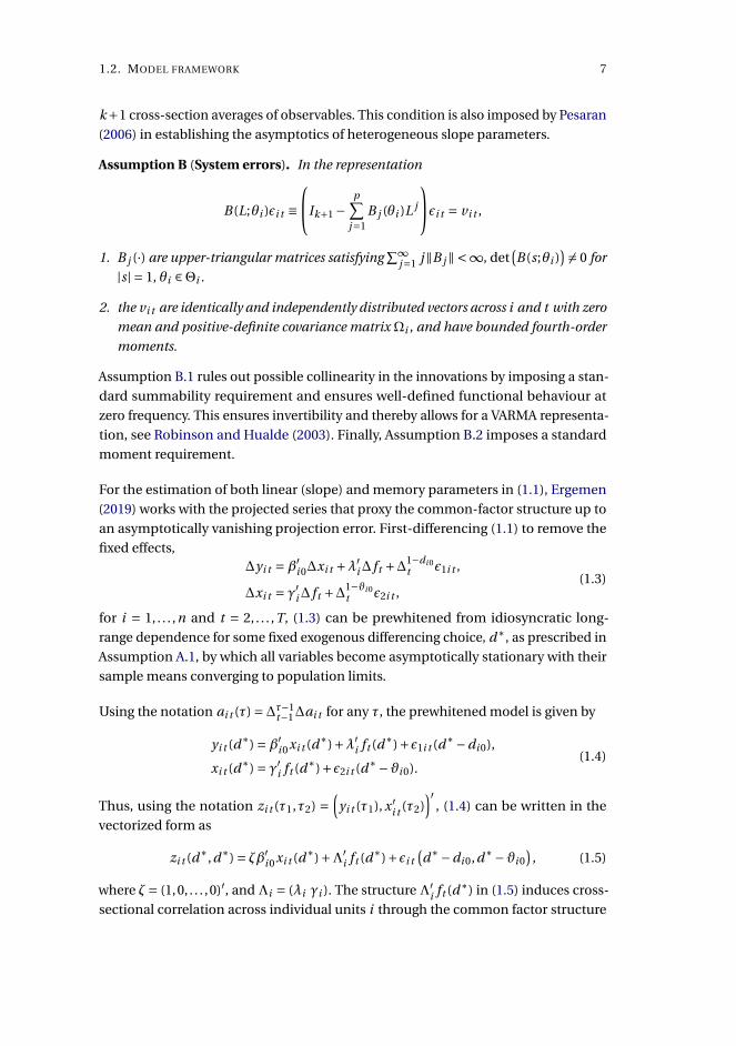
Assumption B (System errors). In the representation
B(L;θi )εi t ≡Ik+1 −
p∑j=1
B j (θi )L j
εi t = vi t ,
1. B j (·) are upper-triangular matrices satisfying∑∞
j=1 j‖B j ‖ <∞, det(B(s;θi )
) 6= 0 for|s| = 1, θi ∈Θi .
2. the vi t are identically and independently distributed vectors across i and t with zero
mean and positive-definite covariance matrixΩi , and have bounded fourth-order
moments.
Assumption B.1 rules out possible collinearity in the innovations by imposing a stan-
dard summability requirement and ensures well-defined functional behaviour at
zero frequency. This ensures invertibility and thereby allows for a VARMA representa-
tion, see Robinson and Hualde (2003). Finally, Assumption B.2 imposes a standard
moment requirement.
For the estimation of both linear (slope) and memory parameters in (1.1), Ergemen
(2019) works with the projected series that proxy the common-factor structure up to
an asymptotically vanishing projection error. First-differencing (1.1) to remove the
fixed effects,∆yi t =β′
i 0∆xi t +λ′i∆ ft +∆1−di 0
t ε1i t ,
∆xi t = γ′i∆ ft +∆1−ϑi 0t ε2i t ,
(1.3)
for i = 1, . . . ,n and t = 2, . . . ,T, (1.3) can be prewhitened from idiosyncratic long-
range dependence for some fixed exogenous differencing choice, d∗, as prescribed in
Assumption A.1, by which all variables become asymptotically stationary with their
sample means converging to population limits.
Using the notation ai t (τ) =∆τ−1t−1∆ai t for any τ, the prewhitened model is given by
yi t (d∗) =β′i 0xi t (d∗)+λ′
i ft (d∗)+ε1i t (d∗−di 0),
xi t (d∗) = γ′i ft (d∗)+ε2i t (d∗−ϑi 0).(1.4)
Thus, using the notation zi t (τ1,τ2) =(
yi t (τ1), x ′i t (τ2)
)′, (1.4) can be written in the
vectorized form as
zi t (d∗,d∗) = ζβ′i 0xi t (d∗)+Λ′
i ft (d∗)+εi t(d∗−di 0,d∗−ϑi 0
), (1.5)
where ζ= (1,0, . . . ,0)′, andΛi = (λi γi ). The structureΛ′i ft (d∗) in (1.5) induces cross-
sectional correlation across individual units i through the common factor structure
8
CHAPTER 1. ASSESSING PREDICTIVE ACCURACY IN PANEL DATA MODELS WITH LONG-RANGE
DEPENDENCE
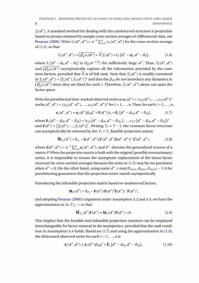
ft (d∗). A standard method for dealing with this unobserved structure is projection
based on proxies obtained by sample cross-section averages of (differenced) data, see
Pesaran (2006). Write z t (d∗,d∗) = n−1 ∑ni=1 zi t (d∗,d∗) for the cross-section average
of (1.5), so that
z t (d∗,d∗) = ζβ′0xt (d∗)+Λ′ ft (d∗)+εt
(d∗−d0,d∗−ϑ0
), (1.6)
where εt(d∗−d0,d∗−ϑ0
)is Op (n−1/2) for sufficiently large d∗. Thus, z t (d∗,d∗)
and ζβ′0xt (d∗) asymptotically capture all the information provided by the com-
mon factors, provided that Λ is of full rank. Note that x t (d∗) is readily contained
in z t (d∗,d∗) = (y t (d∗), x t (d∗)′)′ and that the βi 0 do not introduce any dynamics in
ζβ′0xt (d∗) since they are fixed for each i . Therefore, z t (d∗,d∗) alone can span the
factor space.
Write the prewhitened time-stacked observed series as xi (d∗) = (xi 2(d∗), . . . , xi T (d∗))′
and zi (d∗,d∗) = (zi 2(d∗,d∗), . . . , zi T (d∗,d∗))′ for i = 1, . . . ,n. Then, for each i = 1, . . . ,n,
zi (d∗,d∗) = xi (d∗)βi 0ζ′+F(d∗)Λi +Ei
(d∗−di 0,d∗−ϑi 0
), (1.7)
where Ei(d∗−di 0,d∗−ϑi 0
)= (εi 2(d∗−di 0,d∗−ϑi 0,
), . . . ,εi T
(d∗−di 0,d∗−ϑi 0
))′
and F(d∗) = (f2(d∗), . . . , fT (d∗)
)′ . Writing T1 = T −1, the common factor structure
can asymptotically be removed by the T1 ×T1 feasible projection matrix
MT1 (d∗) = IT1 −z(d∗,d∗)(z′(d∗,d∗)z(d∗,d∗))−z′(d∗,d∗), (1.8)
where z(d∗,d∗) = n−1 ∑ni=1 zi (d∗,d∗), and P− denotes the generalized inverse of a
matrix P. When the projection matrix is built with the original (possibly nonstationary)
series, it is impossible to ensure the asymptotic replacement of the latent factor
structure by cross-section averages because the noise in (1.5) may be too persistent
when d∗ = 0. On the other hand, using some d∗ > maxϑmax ,dmax ,δmax −1/4 for
prewhitening guarantees that the projection errors vanish asymptotically.
Introducing the infeasible projection matrix based on unobserved factors,
MF (d∗) = IT1 −F(d∗)(F(d∗)′F(d∗))−F(d∗)′,
and adopting Pesaran (2006)’s argument under Assumption A.2 and A.4, we have the
approximation as (n,T ) j →∞ that
MT1 (d∗)F(d∗) ≈ MF (d∗)F(d∗) = 0. (1.9)
This implies that the feasible and infeasible projection matrices can be employed
interchangeably for factor removal in the asymptotics, provided that the rank condi-
tion in Assumption A.4 holds. Based on (1.7) and using the approximation in (1.9),
the defactored observed series for each i = 1, . . . ,n is
zi (d∗,d∗) ≈ xi (d∗)βi 0ζ′+ Ei
(d∗−di 0,d∗−ϑi 0
), (1.10)
1.2. MODEL FRAMEWORK 9
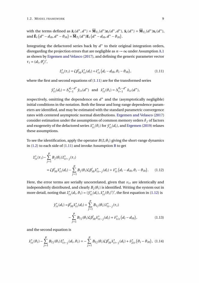
with the terms defined as zi (d∗,d∗) = MT1 (d∗)zi (d∗,d∗), xi (d∗) = MT1 (d∗)xi (d∗),
and Ei(d∗−di 0,d∗−ϑi 0
)= MT1 (d∗)Ei(d∗−di 0,d∗−ϑi 0
).
Integrating the defactored series back by d∗ to their original integration orders,
disregarding the projection errors that are negligible as n →∞ under Assumption A.1
as shown by Ergemen and Velasco (2017), and defining the generic parameter vector
τi = (di ,ϑ′i )′,
z∗i t (τi ) = ζβ′
i 0x∗i t (di )+ ε∗i t
(di −di 0,ϑi −ϑi 0
), (1.11)
where the first and second equations of (1.11) are for the transformed series
y∗i t (di ) =∆di−d∗
t−1 yi t (d∗) and x∗i t (ϑi ) =∆ϑi−d∗
t−1 xi t (d∗),
respectively, omitting the dependence on d∗ and the (asymptotically negligible)
initial conditions in the notation. Both the linear and long-range dependence param-
eters are identified, and may be estimated with the standard parametric convergence
rates with centered asymptotic normal distributions. Ergemen and Velasco (2017)
consider estimation under the assumptions of common memory orders δ j of factors
and exogeneity of the defactored series x∗i t (ϑi ) for y∗
i t (di ), and Ergemen (2019) relaxes
these assumptions.
To see the identification, apply the operator B(L;θi ) giving the short-range dynamics
in (1.2) to each side of (1.11) and invoke Assumption B to get
z∗i t (τi )−
p∑j=1
B j (θi )z∗i t− j (τi )
= ζβ′i 0x∗
i t (di )−p∑
j=1B j (θi )ζβ′
i 0x∗i t− j (di )+ v∗
i t
(di −di 0,ϑi −ϑi 0
). (1.12)
Here, the error terms are serially uncorrelated, given that vi t are identically and
independently distributed, and clearly B j (θi ) is identified. Writing the system out in
more detail, noting that z∗i t (di ,ϑi ) = (y∗
i t (di ), x∗i t (ϑi )′)′, the first equation in (1.12) is
y∗i t (di ) =β′
i 0x∗i t (di )+
p∑j=1
B1 j (θi )z∗i t− j (τi )
−p∑
j=1B1 j (θi )ζβ′
i 0x∗i t− j (di )+ v∗
1i t
(di −di 0
), (1.13)
and the second equation is
x∗i t (ϑi )−
p∑j=1
B2 j (θi )z∗i t− j (di ,ϑi ) =−
p∑j=1
B2 j (θi )ζβ′i 0x∗
i t− j (di )+ v∗2i t
(ϑi −ϑi 0
), (1.14)
10
CHAPTER 1. ASSESSING PREDICTIVE ACCURACY IN PANEL DATA MODELS WITH LONG-RANGE
DEPENDENCE
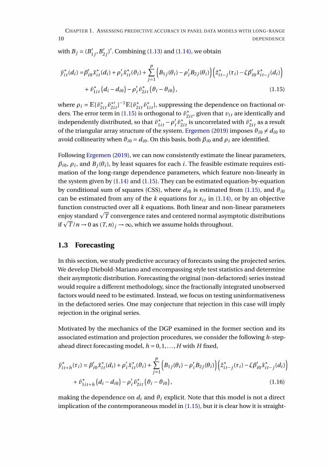
with B j = (B ′1 j ,B ′
2 j )′. Combining (1.13) and (1.14), we obtain
y∗i t (di ) =β′
i 0x∗i t (di )+ρ′
i x∗i t (ϑi )+
p∑j=1
(B1 j (θi )−ρ′
i B2 j (θi ))(
z∗i t− j (τi )−ζβ′
i 0x∗i t− j (di )
)+ v∗
1i t
(di −di 0
)−ρ′i v∗
2i t
(ϑi −ϑi 0
), (1.15)
where ρi =E[v∗2i t v∗′
2i t ]−1E[v∗2i t v∗
1i t ], suppressing the dependence on fractional or-
ders. The error term in (1.15) is orthogonal to v∗2i t , given that vi t are identically and
independently distributed, so that v∗1i t −ρ′
i v∗2i t is uncorrelated with v∗
2i t as a result
of the triangular array structure of the system. Ergemen (2019) imposes ϑi 0 6= di 0 to
avoid collinearity when ϑi 0 = di 0. On this basis, both βi 0 and ρi are identified.
Following Ergemen (2019), we can now consistently estimate the linear parameters,
βi 0, ρi , and B j (θi ), by least squares for each i . The feasible estimate requires esti-
mation of the long-range dependence parameters, which feature non-linearly in
the system given by (1.14) and (1.15). They can be estimated equation-by-equation
by conditional sum of squares (CSS), where di 0 is estimated from (1.15), and ϑi 0
can be estimated from any of the k equations for xi t in (1.14), or by an objective
function constructed over all k equations. Both linear and non-linear parameters
enjoy standardp
T convergence rates and centered normal asymptotic distributions
ifp
T /n → 0 as (T,n) j →∞, which we assume holds throughout.
1.3 Forecasting
In this section, we study predictive accuracy of forecasts using the projected series.
We develop Diebold-Mariano and encompassing style test statistics and determine
their asymptotic distribution. Forecasting the original (non-defactored) series instead
would require a different methodology, since the fractionally integrated unobserved
factors would need to be estimated. Instead, we focus on testing uninformativeness
in the defactored series. One may conjecture that rejection in this case will imply
rejection in the original series.
Motivated by the mechanics of the DGP examined in the former section and its
associated estimation and projection procedures, we consider the following h-step-
ahead direct forecasting model, h = 0,1, . . . , H with H fixed,
y∗i t+h(τi ) =β′
i 0x∗i t (di )+ρ′
i x∗i t (ϑi )+
p∑j=1
(B1 j (θi )−ρ′
i B2 j (θi ))(
z∗i t− j (τi )−ζβ′
i 0x∗i t− j (di )
)+ v∗
1i t+h
(di −di 0
)−ρ′i v∗
2i t
(ϑi −ϑi 0
), (1.16)
making the dependence on di and ϑi explicit. Note that this model is not a direct
implication of the contemporaneous model in (1.15), but it is clear how it is straight-
1.3. FORECASTING 11
forwardly motivated from it simply by leading the forecast objective h periods. Con-
ditional on information through time t , we can write down the forecasting equation
as
y∗i t+h|t (τi ) =β′
i 0x∗i t (di )+ρ′
i x∗i t (ϑi )
+p∑
j=1
(B1 j (θi )−ρ′
i B2 j (θi ))(
z∗i t− j (τi )−ζβ′
i 0x∗i t− j (di )
). (1.17)
Thus, forecasts are derived from a heterogeneous predictive model, facilitating unit-
specific inferences on predictive accuracy, while still treating each unit as part of a
panel.
It is important to understand the generality of this model, which nests several models
employed in the literature, while still accounting for long-range and cross-sectional
dependence. If B j (θi ) = 0 and ρi = 0, for all i , we recover the well-known predictive
regression for each i , with coefficients βi 0. This is especially popular in the financial
literature on stock return and volatility prediction, typically relating aggregate finan-
cial ratios or macroeconomic conditions to future stock returns and their volatility. In
the pure time series setting, Welch and Goyal (2008) is a classical example of an exam-
ination of the in- and out-of-sample predictive performance of stock characteristics,
interest-rate related and macroeconomic indicators for future stock market returns,
whereas Hjalmarson (2010) and Westerlund and Narayan (2015a,b) employ panel
predictive regressions. If the zero condition on ρi is relaxed, the framework allows for
endogenous predictors, even after accounting for cross-sectional dependence, which
is a common issue in finance (Stambaugh, 1999). If, instead, βi 0 = ρi = B2 j (θi ) = 0
for all i , we obtain a short-range dependent autoregressive model in yi t+h with coef-
ficients B1 j (θi ), as often used in macroeconomic settings, for instance for inflation
forecasting (Stock and Watson, 1999). Again, once the zero conditions on βi 0 or ρi
are relaxed, other exogenous or endogenous predictors are accommodated, as, e.g.,
in Phillips curve forecasting models, with xi t a measure of economic activity, such
as the output gap or unemployment rate. Clark and McCracken (2006) explore each
of these in a univariate, short-range dependent setting. The predictor may enter
with additional lags in (1.17) by allowing non-zero B2 j (θi ). Once k ≥ 1, we have an
upper-triangular panel VAR system, which is typical in forecasting settings where yi t
can depend on lagged values of itself and the predictors, whereas each component in
xi t depends only its own past values, see, e.g., Westerlund et al. (2016).
For an evaluation sample (out-of-sample) that includes m observations, indexed by
t = 1, . . . ,m, we estimate, cf. Section 1.2, model parameters using the recursive scheme
similarly to Breitung og Knüppel (2018). This fixes the starting point of the estimation
sample (in-sample) window at t = −T + 1 and increases its endpoint recursively
with t . In a classical predictive regression framework, Hansen and Timmermann
(2015) show an appealing result that the comparison of mean squared forecast errors
12
CHAPTER 1. ASSESSING PREDICTIVE ACCURACY IN PANEL DATA MODELS WITH LONG-RANGE
DEPENDENCE
is asymptotically equivalent to conventional Wald statistics. Yet, standard out-of-
sample test remain of interest when one is, as we are in the present context, interested
in whether a given forecast is superior to another. Given the parameter estimates at
time t , we then form the h-step forecasts from the forecasting equation in (1.17).
The theoretical forecast error is
ei t+h|t (τi ) := y∗i t+h(τi )− y∗
i t+h|t (τi )
= v∗1i t+h
(di −di 0
)−ρ′i v∗
2i t
(ϑi −ϑi 0
). (1.18)
Since under Assumption A.1 the difference between the maximum integration or-
ders and the lower bounds of allowed set values is less than 1/2, the forecast error
ei t+h|t (τi ) is stationary and exhibits long memory whenever di 6= di 0 or ϑi 6= ϑi 0,
which must be accounted for when conducting inference on predictive accuracy.
We are interested in testing the null hypothesis that the forecast function y∗i t+h|t (τi )
is uninformative for y∗i t+h(τi ) for fixed i ,
H0 :E[
e2i t+h|t (τi )
]≥E
[(y∗
i t+h(τi )− y∗i t (τi )
)2]
, (1.19)
where y∗i t (τi ) is the expectation of y∗
i t (τi ) for fixed i . In order to gain more insight on
the forecast error, we can decompose the mean squared error (MSE) as
E[
e2i t+h|t (τi )
]=E
[(y∗
i t+h(τi )− y∗i t (τi )
)2]
−2E
[(y∗
i t+h(τi )− y∗i t (τi )
)(y∗
i t+h|t (τi )− y∗i t (τi )
)]+E
[(y∗
i t+h|t (τi )− y∗i t (τi )
)2]
. (1.20)
Clearly,E
[(y∗
i t+h(τi )− y∗i t (τi )
)(y∗
i t+h|t (τi )− y∗i t (τi )
)]= 0 is a sufficient condition for
the forecast to be uninformative, asE
[(y∗
i t+h|t (τi )− y∗i t (τi )
)2]≥ 0. Furthermore, for a
rational forecast satisfyingE[
ei t+h|t (τi )y∗i t+h|t (τi )
]= 0 and since under Assumption
B.2E[ei ,t+h|t (τi )] = 0, we have that
E
[(y∗
i t+h(τi )− y∗i t (τi )
)(y∗
i t+h|t (τi )− y∗i t (τi )
)]=E
[(ei t+h|t (τi )+ y∗
i t+h|t (τi )− y∗i t (τi )
)(y∗
i t+h|t (τi )− y∗i t (τi )
)]=E
[(y∗
i t+h|t (τi )− y∗i t (τi )
)2]
. (1.21)
1.3. FORECASTING 13
Therefore, by combining (1.20) and (1.21), any rational forecast with positive variance
is informative and the null hypothesis (1.19) is then equivalent to
Cov[
y∗i t+h(τi ), y∗
i t+h|t (τi )]= 0,
which will be utilized further below in constructing an alternative to a Diebold-
Mariano style test statistic.
Furthermore, an iterative scheme can be used if, instead of (1.16), we write
y∗i t+h(τi ) =β′
i 0x∗i t+h(di )+ρ′
i x∗i t+h(ϑi )
+p∑
j=1
(B1 j (θi )−ρ′
i B2 j (θi ))(
z∗i t+h− j (τi )−ζβ′
i 0x∗i t+h− j (di )
)+ v∗
1i t+h
(di −di 0
)−ρ′i v∗
2i t+h
(ϑi −ϑi 0
), (1.22)
in which both the dependent variable and regressors need to be forecast. This error-
correction representation of the system may form the basis of iterative forecasts,
including in the case of possible fractional cointegration among the original series
yi t and xi t , in which case the cointegration can potentially be used to improve fore-
casting performance. In general, the h-step-ahead iterative forecast error exhibits an
M A(h−1) structure in the usual way, in addition to stationary long-range dependence
as discussed for (1.18). For the iterative forecasting scheme, a vector autoregressive
moving average (VARMA) specification or seemingly unrelated regression estimation
(SURE) can be used, as in Pesaran et al. (2011). However, VARMA models are not
commonly used in practice and can have stability and convergence problems in the
face of large-dimensional data.
1.3.1 Panel Diebold-Mariano test
In order to construct the test statistic, we concentrate on the direct forecasting scheme
and give the details accordingly. This is due to the fact that for iterative forecasting,
the same asymptotic arguments follow under Assumption B by taking further into
account the resulting M A forecast errors, and the main ideas are better motivated
under the direct scheme whose treatment avoids further notational complexity.
We use y∗i h(τi ) = m−1 ∑m+h
t=h+1 y∗i t (τi ) as a consistent estimator forE
[y∗
i t (τi )]
, focusing
on information in the evaluation sample. Denote
ui t+h(τi ) = y∗i t+h(τi )− y∗
i h(τi ). (1.23)
Then, to be able to work with the forecasting functions y∗i t+h|t (τi ) and ˆy∗
i t+h|t (τi ), τi
being the estimate of τi = (di ,ϑ′i )′, we adapt conditions used by Breitung og Knüppel
(2018) to our panel setting in the following.
14
CHAPTER 1. ASSESSING PREDICTIVE ACCURACY IN PANEL DATA MODELS WITH LONG-RANGE
DEPENDENCE
Assumption C (Forecasting functions).
1. Under the null hypothesis in (1.19), ui t+h(τi ) is independent of the estimation error;
E[ui t+h |τi s −τi
]= 0 for all i and s = t , t −1, . . . .
2. The parameter vector τi is consistently estimated and the convergence rates satisfy
τi 0 −τi =Op (T −1/2) and τi t − τi 0 =Op (p
t/T ), t = 1, . . . ,m.
Assumption C.1 states that the time series is not predictable given the information
set at time t which includes the estimation error τi t −τi and is implied by (1.19). The
conditions in Assumption C.2 set the usual convergence rate in the in-sample period
and limit the variation in the recursive estimation, respectively. The first condition in
Assumption C.2 is shown to be satisfied using conditional-sum-of-squares estimation
for memory parameters under Assumptions A and B by Ergemen (2019).
Note also that we can only observe the actual forecast error,
ei t+h|t (τi ) := ˆy∗i t+h(τi )− ˆy∗
i t+h|t (τi )
= ˆv∗1i t+h
(di −di 0
)− ρ′
iˆv∗
2i t
(ϑi −ϑi 0
). (1.24)
Define the loss differential for fixed i as
ϕhi t = e2
i t+h|t (τi )− u2i t+h(τi )
and let ω2ϕ denote the consistent long-run variance estimator with long-memory/anti-
persistence correction (MAC) due to Robinson (2005) applied to ϕhi t . Then we can
construct a Diebold-Mariano type test as
DMi h = m1/2−κi1
ωϕm
m∑t=1
ϕhi t (1.25)
for i = 1, . . . ,n, where κi is a consistent estimator of the integration order of the
squared loss differential ϕhi t , which may be determined cf. Propositions 2-4 of Kruse
et al. (2018). Here, it is important to note that under Assumptions A and B, Ergemen
(2019) establishes thep
T -consistency of both individual memory estimates, di and
ϑi , so that κi also enjoys thep
T -consistency under any scenario prescribed in Propo-
sitions 2-4 of Kruse et al. (2018).1 This means that for all i , the (logT )(κi −κi ) = op (1)
condition as imposed by Robinson (2005) and Abadir, Distaso, and Giraitis (2009) for
consistent estimation of ω2ϕ is naturally satisfied. In practice, it can be much simpler
to estimate κi by resorting to CSS or semi-parametric, e.g., local Whittle, methods.
It should be noted that it is also possible to consider a modified version of (1.19) for
comparing the model forecast to an external forecast if we write
H †0 :E
[e2
i t+h|t (τi )]≥E
[ξ2
i t+h|t]
, (1.26)
1The scenarios depends on biasedness of forecasts and the presence of (common) long memoryamong forecasting losses, among other things.
1.3. FORECASTING 15
where ξ2i t+h|t corresponds to the squared forecast error resulting from an external
forecast, e.g., a survey, for cross-section unit i . The methodologies described here
can be adapted to test (1.26), noting that the memory of the loss differential, κi ,
needs to be estimated in this case. It cannot be deduced based on the model memory
parameter estimates, since the memory transmission rules listed in Kruse et al. (2018)
are no longer guaranteed to apply.
To study the asymptotic behavior of the test statistic, we further impose the following
rate conditions.
Assumption D (Rate conditions for DM type test). As (n,T,m) j →∞,
m1/2−κi n−1 +m1/2−κi n−1/2T −1/2 +m3/2−3κi T −1/2 → 0
and κi ∈ (−1/2,1/2) for all i .
The requirement on the relative asymptotic size of the number of forecasts and the
number of cross-section units, m1/2−κi n−1 +m1/2−κi n−1/2T −1/2 → 0, is to control
for the projection error, see Appendix A.3. The condition m3/2−3κi T −1/2 → 0 ensures
that the first-order approximations of conditional forecasts depending on estimated
parameters around the true parameters work well, imposing that there is enough
information gathered in the estimation period so that forecasts can be evaluated
in the following m periods. The condition on κi is imposed in order to include the
case where the predictive accuracy comparison is made to an external forecast, i.e.,
when testing (1.26) (it is automatically satisfied when testing the null in (1.19)). This
condition also enables the estimation of the long-run variance of the loss differential
using readily available techniques such as local Whittle methods, see Robinson (2005)
and Abadir et al. (2009).
The following result establishes the asymptotic distribution of the test statistic in
(1.25).
Theorem 1. Under Assumptions A-D and H0 in (1.19), as (n,T,m) j →∞,
DMi h ⇒∣∣wi
∣∣2
,
for fixed i , where wi is a standard normally distributed random variable.
This result states that for each cross-section unit i , the Diebold-Mariano type (hence-
forth DM) test statistic converges weakly to a random variable that has an asymptotic
half-normal distribution with unit variance under the null hypothesis in (1.19). By
corollary, 2DMi hd−→ |N (0,1)|. It is important to note here that the null hypothesis is
rejected for smaller values of the test statistic, as dictated by the null hypothesis. Bre-
itung og Knüppel (2018) obtain the same limiting result, but under a setup in which
16
CHAPTER 1. ASSESSING PREDICTIVE ACCURACY IN PANEL DATA MODELS WITH LONG-RANGE
DEPENDENCE
the series and thus the forecasts are I (0) time series, imposing only that m/T → 0
as both m and T diverge, in contrast to our Assumption D. Therefore, showing the
result in Theorem 1 is quite different under our setup, particularly because of the
estimation of the long-run variance, due to the allowance for long memory as well as
the proxying for the common-factor structure in the panel.
The DM type test statistic in (1.25) can be adopted for use under (1.26), yielding the
same asymptotic properties, if we replace ϕhi t by ϕh†
i t defined as
ϕh†i t = e2
i t+h|t (τi )− ξ2i t+h|t ,
where ξ2i t+h|t is the (actual) observed squared forecast error from the external forecast,
and ω2ϕ by ω2
ϕ†, obtained by applying the MAC estimator to ϕh†i t .
1.3.2 Panel encompassing test
The DM type and related test statistics considered so far encounter size problems
in small samples due to the null in (1.19) being rejected for small values of the test
statistic, see also Breitung og Knüppel (2018) and our simulation results in Section
1.4. Furthermore, the rate condition m3/2−3κi T −1/2 → 0 in Assumption D can be too
stringent, particularly when κi ∈ (−1/2,0). To offer a remedy, we reformulate the null
hypothesis as
H ′0 :E
[(y∗
i t+h(τi )− y∗i h(τi )
)(y∗
i t+h|t (τi )− y∗i h(τi )
)]= 0, (1.27)
which, for a rational forecast satisfying E[
y∗i t+h(τi )− y∗
i t+h|t (τi )∣∣y∗
i t+h|t (τi )]= 0, is
equivalent to (1.19). The null hypothesis is rejected when there is positive correlation
between y∗i t+h(τi ) and y∗
i t+h|t (τi ). To motivate this further, writing
m∑t=1
ϕhi t =
m∑t=1
[y∗
i t+h(τi )− y∗i h(τi )− (y∗
i t+h|t (τi )− y∗i h(τi ))
]2 −(
y∗i t+h(τi )− y∗
i h(τi ))2
=m∑
t=1
(y∗
i t+h|t (τi )− y∗i h(τi )
)2 −2m∑
t=1
[(y∗
i t+h(τi )− y∗i h(τi ))(y∗
i t+h|t (τi )− y∗i h(τi )
]shows the link to the DM type test statistic. The covariance between y∗
i t+h(τi ) and
y∗i t+h|t (τi ) plays the key role in terms of deciding the power of the test, since the first
term is non-negative.
Our approach may be considered as a one-sided Mincer-Zarnowitz regression,
y∗i t+h(τi ) =φi 0,h +φi 1,h y∗
i t+h|t (τi )+ei t+h ,
in which we test φi 1,h = 0 versus φi 1,h > 0 for fixed i and unrestricted φi 0,h . In the
literature, the errors from similar regressions are typically mean zero I (0) processes,
1.3. FORECASTING 17
and this is asymptotically so for ei t+h in our setup, given the consistency of τi . We
consider the null as one of uninformativeness of the forecast, whereas Mincer and
Zarnowitz (1969) focused on the joint null of informativeness and unbiasedness,
φi 1,h = 1 and φi 0,h = 0. Our test can also be seen as a forecast encompassing test by
writing
y∗i t+h(τi ) =ψi h y∗
i t+h|t (τi )+ (1−ψi h)y∗i h(τi )+ei t+h
y∗i t+h(τi )− y∗
i h(τi ) =ψi h(y∗i t+h|t (τi )− y∗
i h(τi ))+ei t+h ,
since testing for φi 1,h = 0 is the same as testing for ψi h = 0. Further, in analogy with
Breitung og Knüppel (2018), our DM type statistics can be interpreted as likelihood
ratio tests of the uninformativeness null in the Mincer-Zarnowitz or encompassing
regressions, against the joint informativeness and unbiasedness alternative.
We focus here on the encompassing type test statistic given by
%i h = m1/2−υi1
ωΞm
m∑t=1Ξh
i t , (1.28)
essentially an LM type statistic, where
Ξhi t = ( ˆy∗
i t+h(τi )− ˆy∗i h(τi ))( ˆy∗
i t+h|t (τi )− ˆy∗i h(τi )),
υi is a consistent memory estimate of Ξhi t satisfying (logT )(υi −υi ) = op (1), and ω2
Ξ is
the MAC-robust long-run variance estimator of Robinson (2005) applied to Ξhi t . We
impose the following condition to study the asymptotic behavior of the test statistic
in (1.28).
Assumption E (Rate conditions for encompassing type test). As (n,T,m) j →∞,
m1/2−υi n−1 +m1/2−υi n−1/2T −1/2 +mT −1 → 0,
and υi ∈ (−1/2,1/2) for all i .
The first two terms ensure that the projection errors in the panel setting do not have
any asymptotic contribution, see Appendix A.3. The third condition, m/T → 0, is
standard and is also imposed by Breitung og Knüppel (2018). It simply states that
the out-of-sample length must be smaller than the in-sample length so that there is
enough information at hand for prediction.
The next result establishes the asymptotic behavior of the encompassing type test.
Theorem 2. Under Assumptions A-C and E and H ′0 in (1.27), as (n,T,m) j →∞,
%i hd−→ N (0,1),
for fixed i .
18
CHAPTER 1. ASSESSING PREDICTIVE ACCURACY IN PANEL DATA MODELS WITH LONG-RANGE
DEPENDENCE
The null in (1.27) is rejected when %i h is large compared to the critical value from the
standard normal distribution.
Given our panel setup, it is interesting in addition to analyze the cross-sectional
average of the test statistic in (1.28). Noting that, as n →∞, the projection errors, of
size Op (n−1+(nT )−1/2), become op (1), making the cross-section units asymptotically
independent of each other under Assumption B.2. Thus, the individual %i h test
statistics are asymptotically approximately independent for large n. Thus, we can
simply consider the test statistic
%h := n−1/2n∑
i=1%i h , (1.29)
based on the first result in Theorem 2, in a similar spirit to the aggregation behind the
CIPS test statistic proposed by Pesaran (2007). We present the asymptotic behavior of
%h in the next result.
Theorem 3. Under the conditions of Theorem 2,
%hd−→ N (0,1).
Theorem 3 shows that the cross-sectionally averaged test statistic is asymptotically
distributed as standard normal, under the conditions of Theorem 2. Note that al-
though %h uses equal weighting, it is also possible to allow for different weights for
cross-section units, as in Chudik et al. (2016), and the asymptotic normality result
in Theorem 3 still holds under suitable conditions imposed on the weights, see, e.g.,
Pesaran (2006), although in this case the asymptotic mean and variance are charac-
terized based on those weights. It would be also possible to consider the combination
of p-values of the individual encompassing test statistics. For example, the inverse
chi-squared test statistics defined by
P (n,T ) =−2n∑
i=1ln(pi T ),
where pi T , the p-value corresponding to cross-section unit i , see also Pesaran (2007),
can be used when n is large.
1.3.3 Local power analysis
In order to study the local power properties of the encompassing type test, we work
with a restricted version of (1.16) in which ρi = 0 and B j (θi ) = 0, for all i , so that we
end up with a predictive regression setup taking h = 1,
y∗i t+1(τi ) =β′
i 0x∗i t (di )+ v∗
1i t+1
(di −di 0
). (1.30)
1.3. FORECASTING 19
Our choice in (1.30) is motivated by a desire to contrast our setup to the popular
predictive regression setup in the literature, and we present Monte Carlo results and
an empirical application to this case in the following sections.
Under Assumptions A.1 and B.2, and the asymptotic independence of v∗1i t+1
(di −di 0
)and x∗
i t (di ), x∗i t−1(di ), . . ., as T →∞, we have that
E
[(y∗
i t+1(τi )− y∗i 1(τi )
)2]=σ2
v1+β2
i 0σ2x .
So, ifβi 0 6= 0, the forecast is informative, and DM i 1 and %i 1 are Op (m1/2). Accordingly,
both the encompassing type tests are consistent against fixed alternatives βi 0 6= 0.
We consider local alternatives of the form βi 0 = ci /p
m, for all i , extending the case
in Breitung og Knüppel (2018) to the panel setup with factor projection and long-
range dependence. It is also possible to consider deviations in short/long-range
dependence, as well as contemporaneous correlation parameters, but we focus on
the simplest case to show our test have nontrivial local power.
In relation to the aggregate test statistic in (1.29), we note that it is possible to allow
for ci = 0 for some non-negligible, but non-dominating, fraction of the cross-section
units, as in Su and Chen (2013), under further regularity conditions, but this is beyond
the scope of the current paper.
The next result establishes the local asymptotic behavior of the encompassing type
test statistic.
Theorem 4. Under the conditions of Theorem 2, imposing mT −1/2+di 0−dmi n → 0, with
dmi n = mini di , and βi 0 = ci /p
m in (1.30), as (n,T,m) j →∞,
%i 1d−→ si g n(ci )w1i +ηi (1.31)
for fixed i where η2i = c2
i σ2x /σ2
v1is the signal-to-noise ratio and w1i is a standard
normally distributed random variable.
This result states that the encompassing type test statistic has non-trivial power
against local alternatives. The rate condition is the one imposed in Theorem 4 of Bre-
itung og Knüppel (2018) adjusted to uniformly handle long memory under the alter-
native model considered in (1.30) since it carries along the error term v∗1i t+1
(di −di 0
).
Figure 1 depicts the resulting power curve for ci ≥ 0 for a 5% significance level. As
expected, the encompassing type test becomes more powerful when the signal-to-
noise ratio grows large. Note also that the power curve is symmetric in c since the
asymptotic distribution in (1.31) is unchanged by replacing w1 with −w1.
20
CHAPTER 1. ASSESSING PREDICTIVE ACCURACY IN PANEL DATA MODELS WITH LONG-RANGE
DEPENDENCE
1.4 Monte Carlo study
In this section, we carry out a Monte Carlo experiment to study the finite-sample
properties of our proposed tests. The simulation experiment builds upon the setup
considered by Ergemen (2019). We simulate scalar yi t and xi t and draw the idiosyn-
cratic vector (ε1i t ,ε2i t )′ as standard normal with covariance matrix
Ω=(
a11 a12
a21 a22
),
with signal-to-noise ratio s = a22/a11 and correlation ρ = a12/(a11a22)1/2. Without
loss of generality, we set a11 = 1 and introduce short-memory dynamics via B1(θi ) =diagθ1i ,θ2i . We generate a serially correlated common factor via ft = 1/2 ft−1 +∆−δ
t z ft based on iid innovations z f
t drawn as standard normal and then fractionally
integrated to the order δ. The individual fixed effects are left unspecified since they
are removed via first differencing2 and projections are based on the first-differenced
data. We then obtain yt+1 from the general DGP
yi t+1 =αi +βi 0xi t +λi ft+1 +∆−di 0t+1 ε1i t+1,
xi t =µi +γi ft +∆−ϑi 0t ε2i t .
(1.32)
Under the null, yi t+1 is obtained by setting βi 0 = 0, θ1 = θ2 = 0, and ρ = 0 for all i ,
whereas forecasts are based on the predictive model including xi t as a predictor. This
model is estimated recursively, using information known through t , and forecasts
are made in a direct manner according to (1.17). We employ an alternative that only
fixes θ1 = θ2 = 0 and ρ = 0. The memory orders κi and υi of the loss series ϕhi t and
Ξhi t are estimated on the evaluation sample with the CSS parametric estimator from
Ergemen and Velasco (2017). We consider two choices of bandwidth length, bmqc,in the MAC estimator, setting q = 3/5 and q = 4/5, where the latter corresponds to
the MSE optimal boundary (Abadir et al., 2009). We focus on different in-sample and
out-of-sample sizes, T , and m, and consider di 0 = 0.4,1 and ϑi 0 = 0.4,0.7,1. For this
study, we fix s = 1 and d∗ = 1. Simulations are carried out via 20,000 replications.
In terms of size, Table 1 reports results for the DM style test from Theorem 1, 2DMi h ,
with n = 20 and various combinations of the length of the in-sample and out-of-
sample windows. The DM style test suffer from considerable oversizing. This is not
entirely surprising, since the critical values of the half-normal is very close to zero,
leaving a considerable amount of probability mass in the vicinity of the critical values.
That is, small asymptotically negligible terms may have a large impact on the size
of the test. It is, however, clear that without in-sample estimation and projection
errors, as indicated by the “T =∞”, finite sample properties of the test is much closer
2In practice, we set fixed effects equal to zero for simulating yi t , but stress that it has no influence dueto the first differencing.
1.5. PREDICTIVE RELATION BETWEEN STOCK MARKET VOLATILITY AND ECONOMIC POLICY
UNCERTAINTY 21
to its asymptotic properties. These results are also consistent with the findings in
Breitung og Knüppel (2018). On the contrary, from Table 2, the size properties of
the encompassing style test from Theorem 2, which rejects for large, positive values
in the standard normal distribution, are much more reasonable, though somewhat
conservative. The choice of bandwidth in the MAC estimator has little impact on the
size properties of the Diebold-Mariano style test, whereas the encompassing style
test provides the best results when q = 3/5.
To examine the power properties of the tests, we consider a local departure from the
null via βi 0 = ci /p
m, motivated by the analysis of the local alternative in Theorem 4.
For ease of exposition, we analyse the case in which the tests depart from the null
for all i with ci = 2 and ci = 5, corresponding to βi 0 = 0.2 and βi 0 = 0.5, respectively,
for m = 100. The second of the two values of βi 0 is similar to that in Breitung og
Knüppel (2018). Table 3 shows that when the departure from the null is proportional
to ci = 2, the power of the Diebold-Mariano style test is reasonably high, while
the power of the encompassing style test (cf. Table 4) is moderate at the 5% and
10% significance levels and quite low otherwise. Increasing the length of the in-
sample and out-of-sample window generally improves power. Also, q = 3/5 provides
the best results. When ci = 5 (Tables 5-6), the power of both Diebold-Mariano and
encompassing style tests is generally high. According to the local power analysis in
Theorem 4, the encompassing style test have local asymptotic power equal to 63.0%
for ci = 2 and 99.9% for ci = 5 and the given parameter values. These theoretical
predictions correspond well to the experimental findings reported in Table 6. Finally,
Table 7 reports size and power properties for the pooled test statistic in (1.29). Its size
properties are quite conservative, but the local power is high for both choices of ci .
1.5 Predictive relation between stock market volatility andeconomic policy uncertainty
The relation between stock market return volatility and political uncertainty has
gained considerable interest in the literature. Recent structural models of Pástor and
Veronesi (2012, 2013) (PV) show that increasing uncertainty about economic policy
makes stocks more volatile. The main reason is that as uncertainty about government
policy actions increases, stock markets become unsettled in view of the uncertain
prospects of the economy. Such political uncertainty may be triggered by, among
other things, elections (see, e.g., Bialkowski et al. (2008)) or economic crises (see,
e.g., Schwert (1989) and Bittlingmayer (1998)). It may arguably be prominent not
only in the USA, but also in Europe and the developing countries. In this empiri-
cal application we apply our methodology to the predictive relation between stock
market volatility and economic policy uncertainty (EPU) in a multi-country panel
analysis, treating the former as the forecast objective and the latter as the predictor.
22
CHAPTER 1. ASSESSING PREDICTIVE ACCURACY IN PANEL DATA MODELS WITH LONG-RANGE
DEPENDENCE
We use the Baker et al. (2016) EPU indices for 14 countries, quantifying newspaper
coverage of policy-related economic uncertainty in a given month. We compute the
realized volatility (RV) from daily returns on each stock market index within the
month, obtained from Global Financial Data and Yahoo! Finance (see, e.g., Chernov
(2007), Rapach et al. (2013), and Luo and Qi (2017) for use of similar data sources).
The data set spans the time period 2001-2017, totalling 204 time series observations.
We find that both RV and EPU exhibit cross-sectional variation in volatility charac-
teristics, which we take into account by standardizing within country so that valid
comparisons can be made on the estimates. Figure 2 depicts RV and EPU. Both series
show spikes in accordance with the global financial crisis. The EPU of the UK rose
sharply in 2016 at the time of the Brexit referendum and has remained elevated since
then. Table 8 reports the full-sample integration order of RV and EPU for each coun-
try. Both RV and EPU are found to exhibit long-range dependence with integration
orders in the neighborhood of 0.5. The estimates are strongly significant and exhibit
cross-sectional variation, thus calling for the methods outlined in this paper.
Following PV, we specify a linear relation between RV and EPU, including a first-order
short-range dependent component of RV,
RVi t =αi +βi EPUi t +θi RVi t−1 +λ′i ft +∆−di
t ε1i t ,
EPUi t =µi +γ′i ft +∆−ϑit ε2i t .
(1.33)
In the analysis, we allow for an unobserved common factor structure that on average
captures other relevant indicators for the study. This allowance can be considered
a more flexible way of modelling the relation between RV and EPU, appropriately
controlling for relevant factors, as opposed to adding separate observable series. We
also allow the innovations of RV and EPU to carry correlation after accounting for this
common factor structure. For example, Bittlingmayer (1998) notes that the highly
volatile stock markets of the 1930s in the USA may very well have reflected a non-
negligible probability that the USA would “go socialist”, whereas a critic would argue
that the highly volatile markets were driven mainly by the business cycle, eventually
causing uncertainty about government (in)actions as response (Schwert, 1989).
With these specifications, we estimate (1.33) to get the results collected in Table 9 for
a contemporaneous analysis. For comparison with PV, we also report estimates of the
coefficient on EPU from a short-range regression of RV on EPU and its own lag. The
structural model of PV suggests that the contemporaneous relation should be positive.
The results indicate a positive relation for most countries, which is significant at
conventional levels for Australia, Canada, Greece, Ireland, Japan, and Mexico. Across
the entire panel, the average (mean-group) estimate is 0.025 with a (one-sided) p-
value of 0.086. Interestingly, the relation is insignificant for the USA, which contrasts
with the findings in PV of a strongly significant relation (also confirmed in our data set
when applying their procedure, cf. Table 9). Our results differ in this regard because
1.5. PREDICTIVE RELATION BETWEEN STOCK MARKET VOLATILITY AND ECONOMIC POLICY
UNCERTAINTY 23
we account for the evident long-range dependent features in the data to obtain
consistent slope estimates, and control for possible endogeneity of EPU with respect
to RV, as well as for other relevant (global) factors.
Given the presence of this contemporaneous relation, which is the only one studied
in PV, it is natural to ask whether it also translates into a predictive relation with rele-
vance for, e.g., risk management, asset allocation, and policy-making. For instance,
market unsettlement driven by current political uncertainty may likely persist for
several periods. Specifically, we ask whether EPU is informative about future RV. To
examine this, we construct direct forecasts with a recursive (expanding) estimation
scheme based on (1.17) and the same specification as above. We set the initial in-
sample window to the 2001-2007 pre-crisis period, and for h = 1,2,3,6,9,12 construct
the first forecast for month h of 2008. This splits data roughly equally, matching the
parameter choices in the simulation study in Section 1.4. Based on the findings in the
simulation study, we use the encompassing type %i h statistic from (1.28) with MAC
bandwidth bm3/5c for inference on uninformativeness of EPU for future RV. Table 10
reports the results. We find that the contemporaneous relation documented above
generally does not translate into an out-of-sample predictive relation. On the basis
of our proposed inferential framework, uninformativeness of EPU for future RV is
only rejected at conventional levels for the UK (h = 1), Greece (h = 3), Spain (h = 6),
Mexico (h = 6), and Australia (h = 12). Moreover, the pooled statistic %h does not
reject uninformativeness across the entire panel for any of the forecast horizons.
Assuming that no factor structure is present, Panel B of the table, there is some
evidence of informativeness of EPU for future RV in the case of Canada, Spain, Greece,
Japan, and Mexico at various forecast horizons. Indeed, the pooled statistic rejects
uninformativeness at the 10% level for one-quarter and one-year ahead forecast
horizons. This suggests that some (weak) informativeness of EPU for future RV is
contained in the common (international) component, leaving, however, the domestic
predictive relation mostly non-existent when accounted for (Panel A). We also ran the
procedure including the global crisis period in the initial in-sample window such that
the first forecast is constructed for month h of 2010. Conclusions were qualitatively
unaltered.
In summary, our panel-wide treatment of the relation between stock market volatility
and economic policy uncertainty generally supports the logic from PV of a contempo-
raneous relation between economic political uncertainty and stock market volatility.
However, after a proper account of common factors (obtained from the panel struc-
ture of the data) as well as the presence of long-range dependence, the relation in
the USA is insignificant, in contrast to the finding obtained using the short-range
dependence, univariate procedure in PV. Moreover, using the encompassing style
test of the present paper, we find only weak evidence of informativeness in economic
24
CHAPTER 1. ASSESSING PREDICTIVE ACCURACY IN PANEL DATA MODELS WITH LONG-RANGE
DEPENDENCE
policy uncertainty for future stock market volatility, and it is mainly contained in the
common factor structure. These results demonstrate the importance of long-range
dependence treatments in practice and underpin the value of panel data modelling.
1.6 Concluding remarks
This paper develops a forecast evaluation framework for testing the null hypothesis
that model-based forecasts at a given horizon are uninformative in panels under po-
tential long-range dependence. We consider a predictive setting motivated from the
fractionally integrated panel data system of Ergemen (2019) with individual stochas-
tic components, cross-section dependence, and endogenous predictors. In this setup,
a Diebold-Mariano style test statistic has a half-normal asymptotic distribution, but
suffers from oversizing in finite samples. For an equivalent null hypothesis, an alter-
native test derived from the encompassing principle is reasonably sized. Both tests
have non-trivial power for local departures from the null. We also provide natural gen-
eralizations for evaluating pooled uninformativeness of the model-based forecasts in
the entire panel.
An interesting direction for future research is the estimation of the fractionally in-
tegrated latent factor structure. Estimates of the factors may be used in a plug-in
scheme to exploit the potential predictive content in the factors themselves, see, e.g.,
Gonçalves et al. (2017). Asymptotic results for such factor estimates are, however, yet
to be developed. Moreover, although our model framework allows for heterogene-
ity in parameters, it is not necessarily given that this results in superior forecasting
performance relative to a homogeneous specification, see, e.g., Baltagi (2013). A thor-
ough analysis of the relative merits of the two specifications is left for future research.
Finally, it is also common in macroeconomics to employ a univariate autoregressive
model as benchmark in forecasting exercises, see, e.g., Stock and Watson (2003), and
our framework can be extended to this case, too.
Acknowledgements
We are grateful to Carlos Vladimir Rodriguez Caballero, Federico Carlini, Bo Honoré,
Morten Ørregaard Nielsen, Carlos Velasco, and participants at the Long Memory
Conference (2018) at Aalborg University, the IXt Workshop in Time Series Economet-
rics (2019) at University of Zaragoza and the joint Econometrics-Finance seminar
(2018) at the Center for Research in Econometric Analysis of Time Series (CREATES)
at Aarhus University for useful comments, and to CREATES (DNRF78), the Dale T.
Mortensen Center, Aarhus University, and the Danish Social Science Research Council
for research support.

1.7. REFERENCES 25
1.7 References
Abadir, K. M., Distaso, W., Giraitis, L., 2009. Two estimators of the long-run variance:
beyond short memory. Journal of Econometrics 150(1), 56–70.
Andersen, T. G., Bollerslev, T., Diebold, F. X., Labys, P., 2003. Modeling and forecasting
realized volatility. Econometrica 71 (2), 579–625.
Bai, J., 2009. Panel data models with interactive fixed effects. Econometrica 77(4),
1229–1279.
Baker, S. R., Bloom, N., Davis, S. J., 2016. Measuring economic policy uncertainty. The
Quarterly Journal of Economics 131 (4), 1593–1636.
Baltagi, B. H., 2013. Panel data forecasting. In: Elliott, G., Timmermann, A. (Eds.),
Handbook of economic forecasting, 1st Edition. Vol. 2B. North Holland, 995–1024.
Bhardwaj, G., Swanson, N. R., 2006. An empirical investigation of the usefulness of
arfima models for predicting macroeconomic and financial time series. Journal of
Econometrics 131, 539–578.
Bialkowski, J., Gottschalk, K., Wisniewski, T. P., 2008. Stock market volatility around
national elections. Journal of Banking and Finance 32 (9), 1941–1953.
Bittlingmayer, G., 1998. Output, stock volatility, and political uncertainty in a natural
experiment: Germany 1880-1940. The Journal of Finance 53 (6), 2243–2257.
Bollerslev, T., Osterrieder, D., Sizova, N., Tauchen, G., 2013. Risk and return: long-
run relationships, fractional cointegration, and return predictability. Journal of
Financial Economics 108(2), 409–424.
Bos, C. S., Franses, P. H., Ooms, M., 2002. Inflation, forecast intervals and long memory
regression models. International Journal of Forecasting 18, 243–264.
Busch, T., Christensen, B. J., Nielsen, M. Ø., 2011. The role of implied volatility in
forecasting future realized volatility and jumps in foreign exchange, stock, and
bond markets. Journal of Econometrics 160, 48–57.
Canova, F., Ciccarelli, M., 2004. Forecasting and turning point predictions in a
bayesian panel var model. Journal of Econometrics 120 (2), 327–359.
Chernov, M., 2007. On the role of risk premia in volatility forecasting. Journal of
Business and Economic Statistics 25 (4), 411–426.
Chiriac, R., Voev, V., 2011. Modelling and forecasting multivariate realized volatility.
Journal of Applied Econometrics 26, 922–947.

26
CHAPTER 1. ASSESSING PREDICTIVE ACCURACY IN PANEL DATA MODELS WITH LONG-RANGE
DEPENDENCE
Christensen, B. J., Nielsen, M. Ø., 2005. Asymptotic normality of narrow-band least
squares in the stationary fractional cointegration model and volatility forecasting.
Journal of Econometrics 133, 343–371.
Chudik, A., Grossman, V., Pesaran, M. H., 2016. A multi-country approach to forecast-
ing output growth using PMIs. Journal of Econometrics 192, 349–365.
Clark, T. E., McCracken, M. W., 2006. The predictive content of the output gap for in-
flation: resolving in-sample and out-of-sample evidence. Journal of Money, Credit
and Banking (5), 1127–1148.
Corsi, F., 2009. A simple approximate long-memory model of realized volatility. Jour-
nal of Financial Econometrics 7, 174–196.
Deo, R., Hurvich, C., Lu, Y., 2006. Forecasting realized volatility using a long-memory
stochastic volatility model: estimation, prediction and seasonal adjustment. Jour-
nal of Econometrics 131 (1-2), 29–58.
Diebold, F. X., Mariano, R. S., 1995. Comparing predictive accuracy. Journal of Busi-
ness Economics and Statistics 13 (3), 253–263.
Engel, C., Mark, N. C., West, K. D., 2008. Exchange rate models are not as bad as
you think. NBER Macroeconomics Annual 2007 22, 381–441, National Bureau of
Economic Research.
Ergemen, Y., Haldrup, N., Rodríguez-Caballero, C., 2016. Common long-range depen-
dence in a panel of hourly nord pool electricity prices and loads. Energy Economics
60, 79–96.
Ergemen, Y. E., 2019. System estimation of panel data models under long-range
dependence. Journal of Business and Economics Statistics 37 (1), 13–26.
Ergemen, Y. E., Velasco, C., 2017. Estimation of fractionally integrated panels with
fixed effects and cross-section dependence. Journal of Econometrics (196), 248–
258.
Giacomini, R., White, H., 2006. Tests of conditional predictive ability. Econometrica
74 (6), 1545–1578.
Gil-Alaña, L., Robinson, P., 1997. Testing of unit root and other nonstationary hy-
potheses in macroeconomic time series. Journal of Econometrics 80(2), 241–268.
Gonçalves, S., McCracken, M. W., Perron, B., 2017. Tests of equal accuracy for nested
models with estimated factors. Journal of Econometrics 198 (2), 231–252.
Groen, J. J. J., 2005. Exchange rate predictability and monetary fundamentals in a
small multi-country panel. Journal of Money, Credit and Banking 37 (3), 495–516.
1.7. REFERENCES 27
Hansen, P. R., Timmermann, A., 2015. Equivalence between out-of-sample forecast
comparisons and Wald statistics. Econometrica 83 (6), 2485–2505.
Hjalmarson, E., 2010. Predicting global stock returns. Journal of Financial and Quan-
titative Analysis 45 (1), 49–80.
Kruse, R., Leschinski, C., Will, M., 2018. Comparing predictive accuracy under long
memory, with an application to volatility forecasting. Journal of Financial Econo-
metrics, 1–49.
Liu, L. Y., Patton, A. J., Sheppard, K., 2015. Does anything beat 5-minute RV? A com-
parison of realized measures across multiple asset classes. Journal of Econometrics
187, 293–311.
Luo, X., Qi, X., 2017. The dynamic correlations between the G7 economies and china:
Evidence from both realized and implied volatilities. Journal of Futures Markets
37 (10), 989–1002.
Mincer, J. A., Zarnowitz, V., 1969. The evalution of economic forecasts. NBER, Ch. 1,
1–46.
Pástor, L., Veronesi, P., 2012. Uncertainty about government policy and stock prices.
The Journal of Finance 67 (4), 1219–1264.
Pástor, L., Veronesi, P., 2013. Political uncertainty and risk premia. Journal of Financial
Economics 110 (3), 520–545.
Pesaran, H., 2006. Estimation and inference in large heterogeneous panels with a
multifactor error structure. Econometrica 74(4), 967–1012.
Pesaran, H., 2007. A simple panel unit root test in the presence of cross-section
dependence. Journal of Applied Econometrics 22(2), 265–312.
Pesaran, M. H., Pick, A., Timmermann, A., 2011. Variable selection, estimation and
inference for multi-period forecasting problems. Journal of Econometrics 164(1),
173–187.
Pesaran, M. H., Schuermann, T., Smith, L. V., 2009. Forecasting economic and financial
variables with global vars. International Journal of Forecasting 25, 642–675.
Rapach, D. E., Strauss, J. K., Zhou, G., 2013. International stock return predictability:
What is the role of the United States? The Journal of Finance 68 (4), 1633–1662.
Robinson, P. M., 2005. Robust covariance matrix estimation : ‘HAC’ estimates with
long memory/antipersistence correction. Econometric Theory 21(1), 171–180.
Robinson, P. M., Hualde, J., 2003. Cointegration in fractional systems with unknown
integration orders. Econometrica 71(6), 1727–1766.
28
CHAPTER 1. ASSESSING PREDICTIVE ACCURACY IN PANEL DATA MODELS WITH LONG-RANGE
DEPENDENCE
Robinson, P. M., Velasco, C., 2015. Efficient estimation of fractionally integrated panel
data models with fixed effects. Journal of Econometrics 185, 435–452.
Schwert, G. W., 1989. Business cycles, financial crisis, and stock volatility. Carnegie-
Rochester Conference Series on Public Policy 31, 83–125, National Bureau of Eco-
nomic Research.
Stambaugh, R. F., 1999. Predictive regressions. Journal of Financial Economics 54,
375–421.
Stock, J. H., Watson, M. W., 1999. Forecasting inflation. Journal of Monetary Eco-
nomics 44, 293–335.
Stock, J. H., Watson, M. W., 2003. Forecasting output and inflation: the role of asset
prices. Journal of Economic Literature 41 (3), 788–829.
Su, l., Chen, Q., 2013. Testing homogeneity in panel data models with interactive fixed
effects. Econometric Theory 29, 1079–1135.
Timmermann, A., Zhu, Y., 2019. Comparing forecasting performance with panel data,
Working paper.
Welch, I., Goyal, A., 2008. A comprehensive look at the empirical performance of
equity premium prediction. The Review of Financial Studies 21, 1455–1508.
Westerlund, J., Karabiyik, H., Narayan, P., 2016. Testing for predictability in panels
with general predictors. Journal of Applied Econometrics 32 (3), 554–574.
Westerlund, J., Narayan, P., 2015a. A random coefficient approach to the predictability
of stock returns in panels. Journal of Financial Econometrics 13 (3), 605–664.
Westerlund, J., Narayan, P., 2015b. Testing for predictability in conditionally het-
eroskedastic stock returns. Journal of Financial Econometrics 13 (2), 342–375.
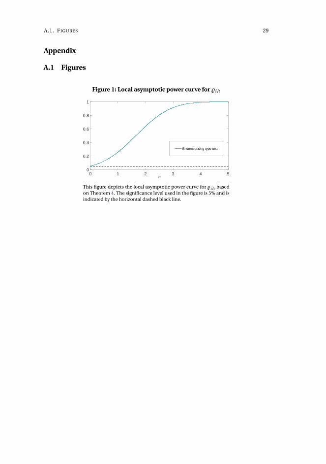
A.1. FIGURES 29
Appendix
A.1 Figures
Figure 1: Local asymptotic power curve for %i h
0 1 2 3 4 50
0.2
0.4
0.6
0.8
1
Encompassing type test
This figure depicts the local asymptotic power curve for %i h basedon Theorem 4. The significance level used in the figure is 5% and isindicated by the horizontal dashed black line.
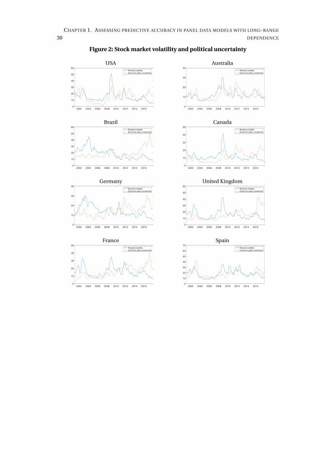
30
CHAPTER 1. ASSESSING PREDICTIVE ACCURACY IN PANEL DATA MODELS WITH LONG-RANGE
DEPENDENCE
Figure 2: Stock market volatility and political uncertainty
USA
2002 2004 2006 2008 2010 2012 2014 20160
10
20
30
40
50
60Realized volatility
Economic policy uncertainty
Australia
2002 2004 2006 2008 2010 2012 2014 20160
10
20
30
40Realized volatility
Economic policy uncertainty
Brazil
2002 2004 2006 2008 2010 2012 2014 20160
10
20
30
40
50
60Realized volatility
Economic policy uncertainty
Canada
2002 2004 2006 2008 2010 2012 2014 20160
10
20
30
40
50Realized volatility
Economic policy uncertainty
Germany
2002 2004 2006 2008 2010 2012 2014 20160
10
20
30
40Realized volatility
Economic policy uncertainty
United Kingdom
2002 2004 2006 2008 2010 2012 2014 20160
10
20
30
40
50
60Realized volatility
Economic policy uncertainty
France
2002 2004 2006 2008 2010 2012 2014 20160
10
20
30
40
50Realized volatility
Economic policy uncertainty
Spain
2002 2004 2006 2008 2010 2012 2014 20160
10
20
30
40
50
60
70Realized volatility
Economic policy uncertainty
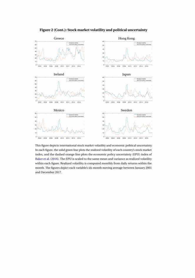
Figure 2 (Cont.): Stock market volatility and political uncertainty
Greece
2002 2004 2006 2008 2010 2012 2014 20160
10
20
30
40
50
60
70Realized volatility
Economic policy uncertainty
Hong Kong
2002 2004 2006 2008 2010 2012 2014 20160
10
20
30
40
50
60Realized volatility
Economic policy uncertainty
Ireland
2002 2004 2006 2008 2010 2012 2014 20160
10
20
30
40
50
60
70Realized volatility
Economic policy uncertainty
Japan
2002 2004 2006 2008 2010 2012 2014 20160
10
20
30
40
50
60Realized volatility
Economic policy uncertainty
Mexico
2002 2004 2006 2008 2010 2012 2014 20160
10
20
30
40
50
60Realized volatility
Economic policy uncertainty
Sweden
2002 2004 2006 2008 2010 2012 2014 20160
10
20
30
40
50
60Realized volatility
Economic policy uncertainty
This figure depicts international stock market volatility and economic political uncertainty.
In each figure, the solid green line plots the realized volatility of each country’s stock market
index, and the dashed orange line plots the economic policy uncertainty (EPU) index of
Baker et al. (2016). The EPU is scaled to the same mean and variance as realized volatility
within each figure. Realized volatility is computed monthly from daily returns within the
month. The figures depict each variable’s six-month moving average between January 2001
and December 2017.
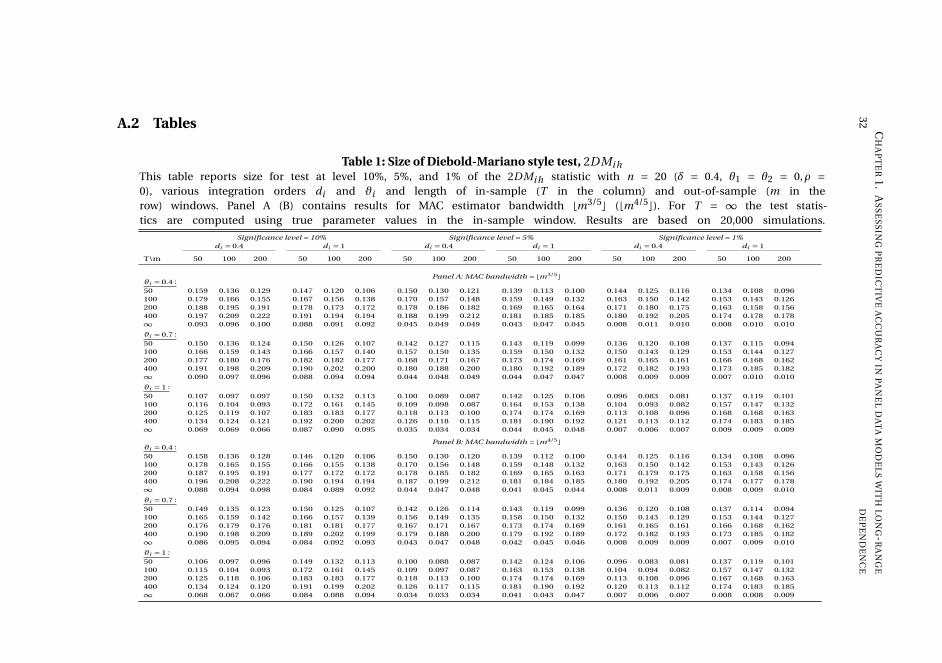
32
CH
AP
TE
R1
.A
SS
ES
SIN
GP
RE
DIC
TIV
EA
CC
UR
AC
YIN
PA
NE
LD
AT
AM
OD
EL
SW
ITH
LO
NG
-RA
NG
E
DE
PE
ND
EN
CE
A.2 Tables
Table 1: Size of Diebold-Mariano style test, 2DMi hThis table reports size for test at level 10%, 5%, and 1% of the 2DMi h statistic with n = 20 (δ = 0.4, θ1 = θ2 = 0,ρ =0), various integration orders di and ϑi and length of in-sample (T in the column) and out-of-sample (m in therow) windows. Panel A (B) contains results for MAC estimator bandwidth bm3/5c (bm4/5c). For T = ∞ the test statis-tics are computed using true parameter values in the in-sample window. Results are based on 20,000 simulations.
Significance level = 10% Significance level = 5% Significance level = 1%di = 0.4 di = 1 di = 0.4 di = 1 di = 0.4 di = 1
T\m 50 100 200 50 100 200 50 100 200 50 100 200 50 100 200 50 100 200
Panel A: MAC bandwidth = bm3/5cϑi = 0.4 :50 0.159 0.136 0.129 0.147 0.120 0.106 0.150 0.130 0.121 0.139 0.113 0.100 0.144 0.125 0.116 0.134 0.108 0.096100 0.179 0.166 0.155 0.167 0.156 0.138 0.170 0.157 0.148 0.159 0.149 0.132 0.163 0.150 0.142 0.153 0.143 0.126200 0.188 0.195 0.191 0.178 0.173 0.172 0.178 0.186 0.182 0.169 0.165 0.164 0.171 0.180 0.175 0.163 0.158 0.156400 0.197 0.209 0.222 0.191 0.194 0.194 0.188 0.199 0.212 0.181 0.185 0.185 0.180 0.192 0.205 0.174 0.178 0.178∞ 0.093 0.096 0.100 0.088 0.091 0.092 0.045 0.049 0.049 0.043 0.047 0.045 0.008 0.011 0.010 0.008 0.010 0.010
ϑi = 0.7 :50 0.150 0.136 0.124 0.150 0.126 0.107 0.142 0.127 0.115 0.143 0.119 0.099 0.136 0.120 0.108 0.137 0.115 0.094100 0.166 0.159 0.143 0.166 0.157 0.140 0.157 0.150 0.135 0.159 0.150 0.132 0.150 0.143 0.129 0.153 0.144 0.127200 0.177 0.180 0.176 0.182 0.182 0.177 0.168 0.171 0.167 0.173 0.174 0.169 0.161 0.165 0.161 0.166 0.168 0.162400 0.191 0.198 0.209 0.190 0.202 0.200 0.180 0.188 0.200 0.180 0.192 0.189 0.172 0.182 0.193 0.173 0.185 0.182∞ 0.090 0.097 0.096 0.088 0.094 0.094 0.044 0.048 0.049 0.044 0.047 0.047 0.008 0.009 0.009 0.007 0.010 0.010
ϑi = 1 :50 0.107 0.097 0.097 0.150 0.132 0.113 0.100 0.089 0.087 0.142 0.125 0.106 0.096 0.083 0.081 0.137 0.119 0.101100 0.116 0.104 0.093 0.172 0.161 0.145 0.109 0.098 0.087 0.164 0.153 0.138 0.104 0.093 0.082 0.157 0.147 0.132200 0.125 0.119 0.107 0.183 0.183 0.177 0.118 0.113 0.100 0.174 0.174 0.169 0.113 0.108 0.096 0.168 0.168 0.163400 0.134 0.124 0.121 0.192 0.200 0.202 0.126 0.118 0.115 0.181 0.190 0.192 0.121 0.113 0.112 0.174 0.183 0.185∞ 0.069 0.069 0.066 0.087 0.090 0.095 0.035 0.034 0.034 0.044 0.045 0.048 0.007 0.006 0.007 0.009 0.009 0.009
Panel B: MAC bandwidth = bm4/5cϑi = 0.4 :50 0.158 0.136 0.128 0.146 0.120 0.106 0.150 0.130 0.120 0.139 0.112 0.100 0.144 0.125 0.116 0.134 0.108 0.096100 0.178 0.165 0.155 0.166 0.155 0.138 0.170 0.156 0.148 0.159 0.148 0.132 0.163 0.150 0.142 0.153 0.143 0.126200 0.187 0.195 0.191 0.177 0.172 0.172 0.178 0.185 0.182 0.169 0.165 0.163 0.171 0.179 0.175 0.163 0.158 0.156400 0.196 0.208 0.222 0.190 0.194 0.194 0.187 0.199 0.212 0.181 0.184 0.185 0.180 0.192 0.205 0.174 0.177 0.178∞ 0.088 0.094 0.098 0.084 0.089 0.092 0.044 0.047 0.048 0.041 0.045 0.044 0.008 0.011 0.009 0.008 0.009 0.010
ϑi = 0.7 :50 0.149 0.135 0.123 0.150 0.125 0.107 0.142 0.126 0.114 0.143 0.119 0.099 0.136 0.120 0.108 0.137 0.114 0.094100 0.165 0.159 0.142 0.166 0.157 0.139 0.156 0.149 0.135 0.158 0.150 0.132 0.150 0.143 0.129 0.153 0.144 0.127200 0.176 0.179 0.176 0.181 0.181 0.177 0.167 0.171 0.167 0.173 0.174 0.169 0.161 0.165 0.161 0.166 0.168 0.162400 0.190 0.198 0.209 0.189 0.202 0.199 0.179 0.188 0.200 0.179 0.192 0.189 0.172 0.182 0.193 0.173 0.185 0.182∞ 0.086 0.095 0.094 0.084 0.092 0.093 0.043 0.047 0.048 0.042 0.045 0.046 0.008 0.009 0.009 0.007 0.009 0.010
ϑi = 1 :50 0.106 0.097 0.096 0.149 0.132 0.113 0.100 0.088 0.087 0.142 0.124 0.106 0.096 0.083 0.081 0.137 0.119 0.101100 0.115 0.104 0.093 0.172 0.161 0.145 0.109 0.097 0.087 0.163 0.153 0.138 0.104 0.094 0.082 0.157 0.147 0.132200 0.125 0.118 0.106 0.183 0.183 0.177 0.118 0.113 0.100 0.174 0.174 0.169 0.113 0.108 0.096 0.167 0.168 0.163400 0.134 0.124 0.120 0.191 0.199 0.202 0.126 0.117 0.115 0.181 0.190 0.192 0.120 0.113 0.112 0.174 0.183 0.185∞ 0.068 0.067 0.066 0.084 0.088 0.094 0.034 0.033 0.034 0.041 0.043 0.047 0.007 0.006 0.007 0.008 0.008 0.009
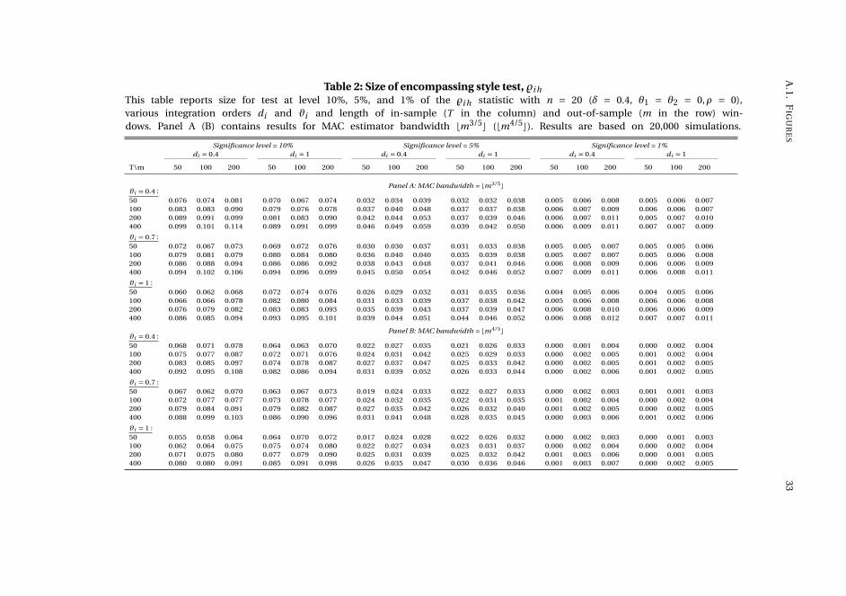
A.1
.F
IGU
RE
S33
Table 2: Size of encompassing style test, %i hThis table reports size for test at level 10%, 5%, and 1% of the %i h statistic with n = 20 (δ = 0.4, θ1 = θ2 = 0,ρ = 0),various integration orders di and ϑi and length of in-sample (T in the column) and out-of-sample (m in the row) win-dows. Panel A (B) contains results for MAC estimator bandwidth bm3/5c (bm4/5c). Results are based on 20,000 simulations.
Significance level = 10% Significance level = 5% Significance level = 1%di = 0.4 di = 1 di = 0.4 di = 1 di = 0.4 di = 1
T\m 50 100 200 50 100 200 50 100 200 50 100 200 50 100 200 50 100 200
Panel A: MAC bandwidth = bm3/5cϑi = 0.4 :50 0.076 0.074 0.081 0.070 0.067 0.074 0.032 0.034 0.039 0.032 0.032 0.038 0.005 0.006 0.008 0.005 0.006 0.007100 0.083 0.083 0.090 0.079 0.076 0.078 0.037 0.040 0.048 0.037 0.037 0.038 0.006 0.007 0.009 0.006 0.006 0.007200 0.089 0.091 0.099 0.081 0.083 0.090 0.042 0.044 0.053 0.037 0.039 0.046 0.006 0.007 0.011 0.005 0.007 0.010400 0.099 0.101 0.114 0.089 0.091 0.099 0.046 0.049 0.059 0.039 0.042 0.050 0.006 0.009 0.011 0.007 0.007 0.009
ϑi = 0.7 :50 0.072 0.067 0.073 0.069 0.072 0.076 0.030 0.030 0.037 0.031 0.033 0.038 0.005 0.005 0.007 0.005 0.005 0.006100 0.079 0.081 0.079 0.080 0.084 0.080 0.036 0.040 0.040 0.035 0.039 0.038 0.005 0.007 0.007 0.005 0.006 0.008200 0.086 0.088 0.094 0.086 0.086 0.092 0.038 0.043 0.048 0.037 0.041 0.046 0.006 0.008 0.009 0.006 0.006 0.009400 0.094 0.102 0.106 0.094 0.096 0.099 0.045 0.050 0.054 0.042 0.046 0.052 0.007 0.009 0.011 0.006 0.008 0.011
ϑi = 1 :50 0.060 0.062 0.068 0.072 0.074 0.076 0.026 0.029 0.032 0.031 0.035 0.036 0.004 0.005 0.006 0.004 0.005 0.006100 0.066 0.066 0.078 0.082 0.080 0.084 0.031 0.033 0.039 0.037 0.038 0.042 0.005 0.006 0.008 0.006 0.006 0.008200 0.076 0.079 0.082 0.083 0.083 0.093 0.035 0.039 0.043 0.037 0.039 0.047 0.006 0.008 0.010 0.006 0.006 0.009400 0.086 0.085 0.094 0.093 0.095 0.101 0.039 0.044 0.051 0.044 0.046 0.052 0.006 0.008 0.012 0.007 0.007 0.011
Panel B: MAC bandwidth = bm4/5cϑi = 0.4 :50 0.068 0.071 0.078 0.064 0.063 0.070 0.022 0.027 0.035 0.021 0.026 0.033 0.000 0.001 0.004 0.000 0.002 0.004100 0.075 0.077 0.087 0.072 0.071 0.076 0.024 0.031 0.042 0.025 0.029 0.033 0.000 0.002 0.005 0.001 0.002 0.004200 0.083 0.085 0.097 0.074 0.078 0.087 0.027 0.037 0.047 0.025 0.033 0.042 0.000 0.002 0.005 0.001 0.002 0.005400 0.092 0.095 0.108 0.082 0.086 0.094 0.031 0.039 0.052 0.026 0.033 0.044 0.000 0.002 0.006 0.001 0.002 0.005
ϑi = 0.7 :50 0.067 0.062 0.070 0.063 0.067 0.073 0.019 0.024 0.033 0.022 0.027 0.033 0.000 0.002 0.003 0.001 0.001 0.003100 0.072 0.077 0.077 0.073 0.078 0.077 0.024 0.032 0.035 0.022 0.031 0.035 0.001 0.002 0.004 0.000 0.002 0.004200 0.079 0.084 0.091 0.079 0.082 0.087 0.027 0.035 0.042 0.026 0.032 0.040 0.001 0.002 0.005 0.000 0.002 0.005400 0.088 0.099 0.103 0.086 0.090 0.096 0.031 0.041 0.048 0.028 0.035 0.045 0.000 0.003 0.006 0.001 0.002 0.006
ϑi = 1 :50 0.055 0.058 0.064 0.064 0.070 0.072 0.017 0.024 0.028 0.022 0.026 0.032 0.000 0.002 0.003 0.000 0.001 0.003100 0.062 0.064 0.075 0.075 0.074 0.080 0.022 0.027 0.034 0.023 0.031 0.037 0.000 0.002 0.004 0.000 0.002 0.004200 0.071 0.075 0.080 0.077 0.079 0.090 0.025 0.031 0.039 0.025 0.032 0.042 0.001 0.003 0.006 0.000 0.001 0.005400 0.080 0.080 0.091 0.085 0.091 0.098 0.026 0.035 0.047 0.030 0.036 0.046 0.001 0.003 0.007 0.000 0.002 0.005
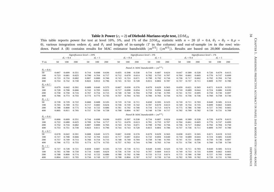
34
CH
AP
TE
R1
.A
SS
ES
SIN
GP
RE
DIC
TIV
EA
CC
UR
AC
YIN
PA
NE
LD
AT
AM
OD
EL
SW
ITH
LO
NG
-RA
NG
E
DE
PE
ND
EN
CE
Table 3: Power (ci = 2) of Diebold-Mariano style test, 2DMi hThis table reports power for test at level 10%, 5%, and 1% of the 2DMi h statistic with n = 20 (δ = 0.4, θ1 = θ2 = 0,ρ =0), various integration orders di and ϑi and length of in-sample (T in the column) and out-of-sample (m in the row) win-dows. Panel A (B) contains results for MAC estimator bandwidth bm3/5c (bm4/5c). Results are based on 20,000 simulations.
Significance level = 10% Significance level = 5% Significance level = 1%di = 0.4 di = 1 di = 0.4 di = 1 di = 0.4 di = 1
T\m 50 100 200 50 100 200 50 100 200 50 100 200 50 100 200 50 100 200
Panel A: MAC bandwidth = bm3/5cϑi = 0.4 :50 0.667 0.609 0.551 0.744 0.698 0.636 0.655 0.598 0.538 0.734 0.687 0.624 0.647 0.589 0.528 0.726 0.679 0.615100 0.723 0.681 0.625 0.790 0.764 0.717 0.712 0.670 0.614 0.782 0.755 0.707 0.704 0.661 0.605 0.776 0.747 0.699200 0.753 0.734 0.682 0.807 0.800 0.766 0.743 0.724 0.671 0.798 0.792 0.756 0.736 0.717 0.662 0.792 0.784 0.750400 0.754 0.752 0.730 0.822 0.812 0.796 0.745 0.743 0.720 0.815 0.804 0.787 0.737 0.737 0.711 0.809 0.797 0.780
ϑi = 0.7 :50 0.679 0.642 0.591 0.689 0.640 0.575 0.667 0.630 0.576 0.679 0.629 0.563 0.659 0.621 0.565 0.671 0.619 0.553100 0.728 0.708 0.666 0.743 0.705 0.651 0.717 0.698 0.654 0.733 0.694 0.640 0.710 0.689 0.644 0.724 0.686 0.630200 0.758 0.750 0.716 0.767 0.754 0.715 0.748 0.740 0.704 0.758 0.746 0.705 0.741 0.731 0.695 0.750 0.736 0.697400 0.766 0.773 0.755 0.775 0.775 0.755 0.757 0.764 0.745 0.766 0.765 0.744 0.751 0.756 0.736 0.760 0.758 0.736
ϑi = 1 :50 0.728 0.729 0.722 0.660 0.608 0.535 0.719 0.718 0.711 0.650 0.595 0.523 0.710 0.711 0.703 0.640 0.585 0.514100 0.765 0.769 0.751 0.717 0.682 0.624 0.756 0.759 0.742 0.707 0.670 0.613 0.749 0.754 0.735 0.699 0.662 0.603200 0.788 0.800 0.775 0.743 0.722 0.686 0.781 0.792 0.766 0.734 0.713 0.674 0.775 0.786 0.760 0.727 0.705 0.665400 0.805 0.811 0.795 0.757 0.750 0.728 0.798 0.804 0.787 0.748 0.739 0.717 0.792 0.799 0.782 0.739 0.731 0.709
Panel B: MAC bandwidth = bm4/5cϑi = 0.4 :50 0.666 0.609 0.551 0.744 0.698 0.636 0.655 0.597 0.538 0.734 0.687 0.624 0.646 0.589 0.528 0.726 0.679 0.615100 0.722 0.680 0.625 0.789 0.764 0.717 0.711 0.670 0.613 0.781 0.755 0.707 0.704 0.661 0.605 0.776 0.747 0.699200 0.752 0.734 0.682 0.807 0.800 0.765 0.743 0.724 0.671 0.798 0.792 0.756 0.736 0.717 0.662 0.792 0.784 0.750400 0.753 0.751 0.730 0.823 0.811 0.796 0.744 0.743 0.720 0.815 0.804 0.786 0.737 0.736 0.711 0.809 0.797 0.780
ϑi = 0.7 :50 0.678 0.642 0.591 0.688 0.640 0.575 0.667 0.630 0.576 0.679 0.629 0.563 0.658 0.621 0.565 0.671 0.619 0.553100 0.727 0.708 0.666 0.742 0.704 0.651 0.717 0.697 0.654 0.732 0.694 0.640 0.710 0.689 0.644 0.724 0.685 0.630200 0.757 0.749 0.715 0.766 0.754 0.715 0.748 0.740 0.704 0.758 0.746 0.705 0.741 0.731 0.695 0.750 0.736 0.697400 0.766 0.772 0.755 0.774 0.774 0.755 0.757 0.763 0.744 0.766 0.765 0.744 0.751 0.756 0.736 0.760 0.758 0.736
ϑi = 1 :50 0.727 0.728 0.721 0.659 0.607 0.535 0.719 0.718 0.711 0.649 0.595 0.523 0.710 0.711 0.703 0.640 0.585 0.514100 0.765 0.768 0.750 0.716 0.681 0.624 0.756 0.759 0.742 0.707 0.669 0.613 0.749 0.753 0.735 0.699 0.662 0.603200 0.788 0.800 0.774 0.742 0.722 0.686 0.780 0.792 0.766 0.733 0.713 0.674 0.775 0.786 0.760 0.727 0.705 0.665400 0.804 0.811 0.795 0.756 0.749 0.727 0.798 0.804 0.787 0.747 0.739 0.716 0.792 0.799 0.782 0.739 0.731 0.709
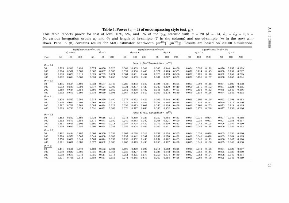
A.1
.F
IGU
RE
S35
Table 4: Power (ci = 2) of encompassing style test, %i hThis table reports power for test at level 10%, 5%, and 1% of the %i h statistic with n = 20 (δ = 0.4, θ1 = θ2 = 0,ρ =0), various integration orders di and ϑi and length of in-sample (T in the column) and out-of-sample (m in the row) win-dows. Panel A (B) contains results for MAC estimator bandwidth bm3/5c (bm4/5c). Results are based on 20,000 simulations.
Significance level = 10% Significance level = 5% Significance level = 1%di = 0.4 di = 1 di = 0.4 di = 1 di = 0.4 di = 1
T\m 50 100 200 50 100 200 50 100 200 50 100 200 50 100 200 50 100 200
Panel A: MAC bandwidth = bm3/5cϑi = 0.4 :50 0.515 0.518 0.499 0.575 0.636 0.626 0.302 0.339 0.349 0.348 0.444 0.466 0.064 0.093 0.119 0.076 0.137 0.183100 0.564 0.587 0.565 0.607 0.687 0.688 0.337 0.396 0.408 0.371 0.485 0.523 0.070 0.114 0.145 0.080 0.151 0.207200 0.593 0.628 0.611 0.625 0.709 0.724 0.361 0.431 0.457 0.378 0.499 0.556 0.072 0.125 0.170 0.082 0.157 0.225400 0.592 0.654 0.660 0.630 0.713 0.756 0.360 0.459 0.494 0.381 0.507 0.589 0.076 0.136 0.187 0.080 0.158 0.244
ϑi = 0.7 :50 0.495 0.514 0.498 0.538 0.567 0.549 0.288 0.333 0.342 0.324 0.381 0.395 0.063 0.093 0.118 0.064 0.107 0.138100 0.553 0.593 0.594 0.577 0.624 0.609 0.331 0.397 0.428 0.349 0.430 0.449 0.068 0.115 0.152 0.071 0.124 0.165200 0.588 0.644 0.651 0.595 0.659 0.660 0.352 0.438 0.482 0.358 0.461 0.493 0.073 0.131 0.182 0.075 0.140 0.186400 0.602 0.675 0.690 0.610 0.680 0.693 0.367 0.470 0.519 0.365 0.478 0.530 0.079 0.139 0.196 0.074 0.145 0.203
ϑi = 1 :50 0.478 0.537 0.586 0.515 0.520 0.490 0.277 0.352 0.423 0.302 0.344 0.343 0.061 0.106 0.160 0.062 0.094 0.113100 0.550 0.645 0.709 0.563 0.594 0.571 0.329 0.443 0.532 0.334 0.404 0.414 0.075 0.136 0.217 0.069 0.113 0.146200 0.597 0.701 0.783 0.585 0.624 0.622 0.358 0.493 0.609 0.356 0.428 0.458 0.080 0.163 0.255 0.073 0.124 0.165400 0.609 0.730 0.824 0.591 0.651 0.663 0.376 0.517 0.653 0.356 0.452 0.496 0.088 0.170 0.290 0.077 0.133 0.186
Panel B: MAC bandwidth = bm4/5cϑi = 0.4 :50 0.482 0.502 0.489 0.538 0.616 0.616 0.214 0.289 0.325 0.250 0.384 0.433 0.004 0.030 0.074 0.007 0.049 0.118100 0.532 0.570 0.558 0.571 0.671 0.680 0.240 0.343 0.380 0.264 0.421 0.490 0.005 0.039 0.091 0.007 0.053 0.137200 0.561 0.611 0.606 0.591 0.693 0.714 0.257 0.375 0.430 0.272 0.436 0.522 0.005 0.042 0.105 0.006 0.057 0.150400 0.559 0.643 0.656 0.590 0.694 0.748 0.259 0.404 0.466 0.267 0.441 0.559 0.005 0.048 0.119 0.006 0.057 0.162
ϑi = 0.7 :50 0.462 0.494 0.487 0.506 0.550 0.538 0.207 0.288 0.318 0.231 0.324 0.365 0.004 0.031 0.070 0.005 0.036 0.086100 0.524 0.578 0.585 0.544 0.608 0.602 0.237 0.342 0.397 0.247 0.370 0.422 0.006 0.040 0.098 0.005 0.044 0.105200 0.558 0.628 0.644 0.565 0.644 0.652 0.252 0.382 0.453 0.254 0.402 0.463 0.006 0.046 0.119 0.006 0.047 0.120400 0.571 0.661 0.680 0.577 0.662 0.686 0.265 0.413 0.490 0.258 0.417 0.498 0.005 0.049 0.126 0.005 0.049 0.130
ϑi = 1 :50 0.441 0.511 0.573 0.480 0.502 0.481 0.190 0.300 0.390 0.214 0.292 0.315 0.006 0.041 0.106 0.004 0.029 0.067100 0.510 0.622 0.696 0.531 0.578 0.563 0.232 0.377 0.494 0.238 0.348 0.386 0.007 0.052 0.145 0.005 0.037 0.089200 0.558 0.676 0.772 0.556 0.611 0.613 0.251 0.425 0.575 0.256 0.374 0.430 0.007 0.064 0.174 0.006 0.040 0.104400 0.571 0.708 0.814 0.559 0.637 0.655 0.271 0.445 0.618 0.260 0.394 0.466 0.008 0.068 0.199 0.005 0.046 0.119
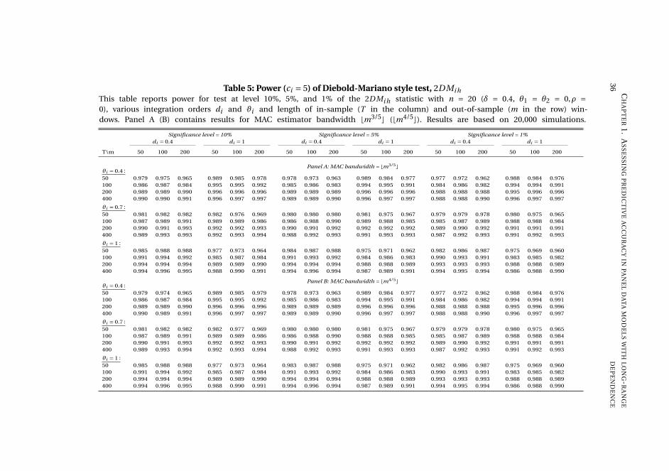
36
CH
AP
TE
R1
.A
SS
ES
SIN
GP
RE
DIC
TIV
EA
CC
UR
AC
YIN
PA
NE
LD
AT
AM
OD
EL
SW
ITH
LO
NG
-RA
NG
E
DE
PE
ND
EN
CE
Table 5: Power (ci = 5) of Diebold-Mariano style test, 2DMi hThis table reports power for test at level 10%, 5%, and 1% of the 2DMi h statistic with n = 20 (δ = 0.4, θ1 = θ2 = 0,ρ =0), various integration orders di and ϑi and length of in-sample (T in the column) and out-of-sample (m in the row) win-dows. Panel A (B) contains results for MAC estimator bandwidth bm3/5c (bm4/5c). Results are based on 20,000 simulations.
Significance level = 10% Significance level = 5% Significance level = 1%di = 0.4 di = 1 di = 0.4 di = 1 di = 0.4 di = 1
T\m 50 100 200 50 100 200 50 100 200 50 100 200 50 100 200 50 100 200
Panel A: MAC bandwidth = bm3/5cϑi = 0.4 :50 0.979 0.975 0.965 0.989 0.985 0.978 0.978 0.973 0.963 0.989 0.984 0.977 0.977 0.972 0.962 0.988 0.984 0.976100 0.986 0.987 0.984 0.995 0.995 0.992 0.985 0.986 0.983 0.994 0.995 0.991 0.984 0.986 0.982 0.994 0.994 0.991200 0.989 0.989 0.990 0.996 0.996 0.996 0.989 0.989 0.989 0.996 0.996 0.996 0.988 0.988 0.988 0.995 0.996 0.996400 0.990 0.990 0.991 0.996 0.997 0.997 0.989 0.989 0.990 0.996 0.997 0.997 0.988 0.988 0.990 0.996 0.997 0.997
ϑi = 0.7 :50 0.981 0.982 0.982 0.982 0.976 0.969 0.980 0.980 0.980 0.981 0.975 0.967 0.979 0.979 0.978 0.980 0.975 0.965100 0.987 0.989 0.991 0.989 0.989 0.986 0.986 0.988 0.990 0.989 0.988 0.985 0.985 0.987 0.989 0.988 0.988 0.984200 0.990 0.991 0.993 0.992 0.992 0.993 0.990 0.991 0.992 0.992 0.992 0.992 0.989 0.990 0.992 0.991 0.991 0.991400 0.989 0.993 0.993 0.992 0.993 0.994 0.988 0.992 0.993 0.991 0.993 0.993 0.987 0.992 0.993 0.991 0.992 0.993
ϑi = 1 :50 0.985 0.988 0.988 0.977 0.973 0.964 0.984 0.987 0.988 0.975 0.971 0.962 0.982 0.986 0.987 0.975 0.969 0.960100 0.991 0.994 0.992 0.985 0.987 0.984 0.991 0.993 0.992 0.984 0.986 0.983 0.990 0.993 0.991 0.983 0.985 0.982200 0.994 0.994 0.994 0.989 0.989 0.990 0.994 0.994 0.994 0.988 0.988 0.989 0.993 0.993 0.993 0.988 0.988 0.989400 0.994 0.996 0.995 0.988 0.990 0.991 0.994 0.996 0.994 0.987 0.989 0.991 0.994 0.995 0.994 0.986 0.988 0.990
Panel B: MAC bandwidth = bm4/5cϑi = 0.4 :50 0.979 0.974 0.965 0.989 0.985 0.979 0.978 0.973 0.963 0.989 0.984 0.977 0.977 0.972 0.962 0.988 0.984 0.976100 0.986 0.987 0.984 0.995 0.995 0.992 0.985 0.986 0.983 0.994 0.995 0.991 0.984 0.986 0.982 0.994 0.994 0.991200 0.989 0.989 0.990 0.996 0.996 0.996 0.989 0.989 0.989 0.996 0.996 0.996 0.988 0.988 0.988 0.995 0.996 0.996400 0.990 0.989 0.991 0.996 0.997 0.997 0.989 0.989 0.990 0.996 0.997 0.997 0.988 0.988 0.990 0.996 0.997 0.997
ϑi = 0.7 :50 0.981 0.982 0.982 0.982 0.977 0.969 0.980 0.980 0.980 0.981 0.975 0.967 0.979 0.979 0.978 0.980 0.975 0.965100 0.987 0.989 0.991 0.989 0.989 0.986 0.986 0.988 0.990 0.988 0.988 0.985 0.985 0.987 0.989 0.988 0.988 0.984200 0.990 0.991 0.993 0.992 0.992 0.993 0.990 0.991 0.992 0.992 0.992 0.992 0.989 0.990 0.992 0.991 0.991 0.991400 0.989 0.993 0.994 0.992 0.993 0.994 0.988 0.992 0.993 0.991 0.993 0.993 0.987 0.992 0.993 0.991 0.992 0.993
ϑi = 1 :50 0.985 0.988 0.988 0.977 0.973 0.964 0.983 0.987 0.988 0.975 0.971 0.962 0.982 0.986 0.987 0.975 0.969 0.960100 0.991 0.994 0.992 0.985 0.987 0.984 0.991 0.993 0.992 0.984 0.986 0.983 0.990 0.993 0.991 0.983 0.985 0.982200 0.994 0.994 0.994 0.989 0.989 0.990 0.994 0.994 0.994 0.988 0.988 0.989 0.993 0.993 0.993 0.988 0.988 0.989400 0.994 0.996 0.995 0.988 0.990 0.991 0.994 0.996 0.994 0.987 0.989 0.991 0.994 0.995 0.994 0.986 0.988 0.990
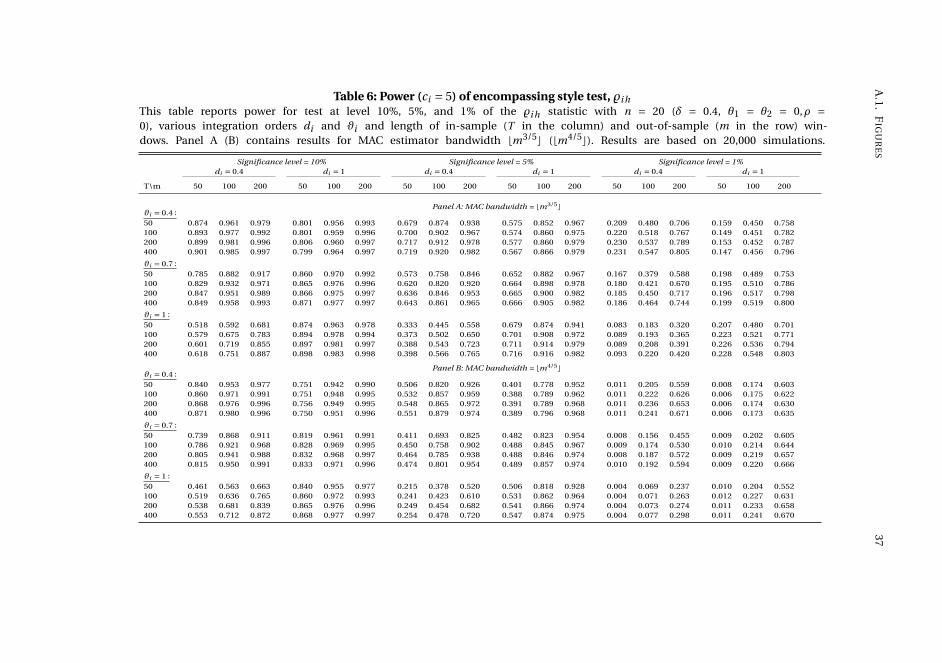
A.1
.F
IGU
RE
S37
Table 6: Power (ci = 5) of encompassing style test, %i hThis table reports power for test at level 10%, 5%, and 1% of the %i h statistic with n = 20 (δ = 0.4, θ1 = θ2 = 0,ρ =0), various integration orders di and ϑi and length of in-sample (T in the column) and out-of-sample (m in the row) win-dows. Panel A (B) contains results for MAC estimator bandwidth bm3/5c (bm4/5c). Results are based on 20,000 simulations.
Significance level = 10% Significance level = 5% Significance level = 1%di = 0.4 di = 1 di = 0.4 di = 1 di = 0.4 di = 1
T\m 50 100 200 50 100 200 50 100 200 50 100 200 50 100 200 50 100 200
Panel A: MAC bandwidth = bm3/5cϑi = 0.4 :50 0.874 0.961 0.979 0.801 0.956 0.993 0.679 0.874 0.938 0.575 0.852 0.967 0.209 0.480 0.706 0.159 0.450 0.758100 0.893 0.977 0.992 0.801 0.959 0.996 0.700 0.902 0.967 0.574 0.860 0.975 0.220 0.518 0.767 0.149 0.451 0.782200 0.899 0.981 0.996 0.806 0.960 0.997 0.717 0.912 0.978 0.577 0.860 0.979 0.230 0.537 0.789 0.153 0.452 0.787400 0.901 0.985 0.997 0.799 0.964 0.997 0.719 0.920 0.982 0.567 0.866 0.979 0.231 0.547 0.805 0.147 0.456 0.796
ϑi = 0.7 :50 0.785 0.882 0.917 0.860 0.970 0.992 0.573 0.758 0.846 0.652 0.882 0.967 0.167 0.379 0.588 0.198 0.489 0.753100 0.829 0.932 0.971 0.865 0.976 0.996 0.620 0.820 0.920 0.664 0.898 0.978 0.180 0.421 0.670 0.195 0.510 0.786200 0.847 0.951 0.989 0.866 0.975 0.997 0.636 0.846 0.953 0.665 0.900 0.982 0.185 0.450 0.717 0.196 0.517 0.798400 0.849 0.958 0.993 0.871 0.977 0.997 0.643 0.861 0.965 0.666 0.905 0.982 0.186 0.464 0.744 0.199 0.519 0.800
ϑi = 1 :50 0.518 0.592 0.681 0.874 0.963 0.978 0.333 0.445 0.558 0.679 0.874 0.941 0.083 0.183 0.320 0.207 0.480 0.701100 0.579 0.675 0.783 0.894 0.978 0.994 0.373 0.502 0.650 0.701 0.908 0.972 0.089 0.193 0.365 0.223 0.521 0.771200 0.601 0.719 0.855 0.897 0.981 0.997 0.388 0.543 0.723 0.711 0.914 0.979 0.089 0.208 0.391 0.226 0.536 0.794400 0.618 0.751 0.887 0.898 0.983 0.998 0.398 0.566 0.765 0.716 0.916 0.982 0.093 0.220 0.420 0.228 0.548 0.803
Panel B: MAC bandwidth = bm4/5cϑi = 0.4 :50 0.840 0.953 0.977 0.751 0.942 0.990 0.506 0.820 0.926 0.401 0.778 0.952 0.011 0.205 0.559 0.008 0.174 0.603100 0.860 0.971 0.991 0.751 0.948 0.995 0.532 0.857 0.959 0.388 0.789 0.962 0.011 0.222 0.626 0.006 0.175 0.622200 0.868 0.976 0.996 0.756 0.949 0.995 0.548 0.865 0.972 0.391 0.789 0.968 0.011 0.236 0.653 0.006 0.174 0.630400 0.871 0.980 0.996 0.750 0.951 0.996 0.551 0.879 0.974 0.389 0.796 0.968 0.011 0.241 0.671 0.006 0.173 0.635
ϑi = 0.7 :50 0.739 0.868 0.911 0.819 0.961 0.991 0.411 0.693 0.825 0.482 0.823 0.954 0.008 0.156 0.455 0.009 0.202 0.605100 0.786 0.921 0.968 0.828 0.969 0.995 0.450 0.758 0.902 0.488 0.845 0.967 0.009 0.174 0.530 0.010 0.214 0.644200 0.805 0.941 0.988 0.832 0.968 0.997 0.464 0.785 0.938 0.488 0.846 0.974 0.008 0.187 0.572 0.009 0.219 0.657400 0.815 0.950 0.991 0.833 0.971 0.996 0.474 0.801 0.954 0.489 0.857 0.974 0.010 0.192 0.594 0.009 0.220 0.666
ϑi = 1 :50 0.461 0.563 0.663 0.840 0.955 0.977 0.215 0.378 0.520 0.506 0.818 0.928 0.004 0.069 0.237 0.010 0.204 0.552100 0.519 0.636 0.765 0.860 0.972 0.993 0.241 0.423 0.610 0.531 0.862 0.964 0.004 0.071 0.263 0.012 0.227 0.631200 0.538 0.681 0.839 0.865 0.976 0.996 0.249 0.454 0.682 0.541 0.866 0.974 0.004 0.073 0.274 0.011 0.233 0.658400 0.553 0.712 0.872 0.868 0.977 0.997 0.254 0.478 0.720 0.547 0.874 0.975 0.004 0.077 0.298 0.011 0.241 0.670
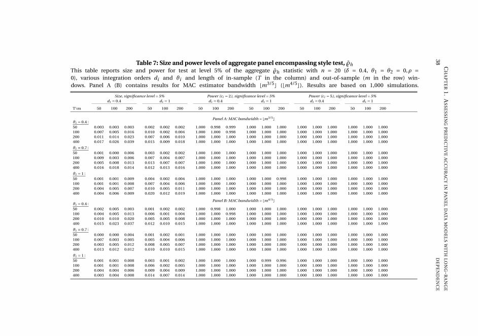
38
CH
AP
TE
R1
.A
SS
ES
SIN
GP
RE
DIC
TIV
EA
CC
UR
AC
YIN
PA
NE
LD
AT
AM
OD
EL
SW
ITH
LO
NG
-RA
NG
E
DE
PE
ND
EN
CE
Table 7: Size and power levels of aggregate panel encompassing style test, %hThis table reports size and power for test at level 5% of the aggregate %h statistic with n = 20 (δ = 0.4, θ1 = θ2 = 0,ρ =0), various integration orders di and ϑi and length of in-sample (T in the column) and out-of-sample (m in the row) win-dows. Panel A (B) contains results for MAC estimator bandwidth bm3/5c (bm4/5c). Results are based on 1,000 simulations.
Size, significance level = 5% Power (ci = 2), significance level = 5% Power (ci = 5), significance level = 5%di = 0.4 di = 1 di = 0.4 di = 1 di = 0.4 di = 1
T\m 50 100 200 50 100 200 50 100 200 50 100 200 50 100 200 50 100 200
Panel A: MAC bandwidth = bm3/5cϑi = 0.4 :50 0.003 0.003 0.003 0.002 0.002 0.002 1.000 0.998 0.999 1.000 1.000 1.000 1.000 1.000 1.000 1.000 1.000 1.000100 0.007 0.005 0.016 0.010 0.002 0.004 1.000 1.000 0.998 1.000 1.000 1.000 1.000 1.000 1.000 1.000 1.000 1.000200 0.011 0.014 0.023 0.007 0.006 0.010 1.000 1.000 1.000 1.000 1.000 1.000 1.000 1.000 1.000 1.000 1.000 1.000400 0.017 0.026 0.039 0.015 0.009 0.018 1.000 1.000 1.000 1.000 1.000 1.000 1.000 1.000 1.000 1.000 1.000 1.000
ϑi = 0.7 :50 0.001 0.000 0.006 0.003 0.002 0.002 1.000 1.000 1.000 1.000 1.000 1.000 1.000 1.000 1.000 1.000 1.000 1.000100 0.009 0.003 0.006 0.007 0.004 0.007 1.000 1.000 1.000 1.000 1.000 1.000 1.000 1.000 1.000 1.000 1.000 1.000200 0.005 0.008 0.013 0.013 0.007 0.007 1.000 1.000 1.000 1.000 1.000 1.000 1.000 1.000 1.000 1.000 1.000 1.000400 0.016 0.018 0.014 0.012 0.013 0.016 1.000 1.000 1.000 1.000 1.000 1.000 1.000 1.000 1.000 1.000 1.000 1.000
ϑi = 1 :50 0.001 0.001 0.009 0.004 0.002 0.004 1.000 1.000 1.000 1.000 1.000 0.998 1.000 1.000 1.000 1.000 1.000 1.000100 0.001 0.001 0.008 0.007 0.004 0.006 1.000 1.000 1.000 1.000 1.000 1.000 1.000 1.000 1.000 1.000 1.000 1.000200 0.004 0.005 0.007 0.010 0.005 0.011 1.000 1.000 1.000 1.000 1.000 1.000 1.000 1.000 1.000 1.000 1.000 1.000400 0.004 0.006 0.009 0.020 0.012 0.019 1.000 1.000 1.000 1.000 1.000 1.000 1.000 1.000 1.000 1.000 1.000 1.000
Panel B: MAC bandwidth = bm4/5cϑi = 0.4 :50 0.002 0.005 0.003 0.001 0.002 0.002 1.000 0.998 1.000 1.000 1.000 1.000 1.000 1.000 1.000 1.000 1.000 1.000100 0.004 0.005 0.013 0.006 0.001 0.004 1.000 1.000 0.998 1.000 1.000 1.000 1.000 1.000 1.000 1.000 1.000 1.000200 0.010 0.010 0.020 0.005 0.005 0.008 1.000 1.000 1.000 1.000 1.000 1.000 1.000 1.000 1.000 1.000 1.000 1.000400 0.015 0.023 0.037 0.012 0.010 0.015 1.000 1.000 1.000 1.000 1.000 1.000 1.000 1.000 1.000 1.000 1.000 1.000
ϑi = 0.7 :50 0.000 0.000 0.004 0.001 0.002 0.001 1.000 1.000 1.000 1.000 1.000 1.000 1.000 1.000 1.000 1.000 1.000 1.000100 0.007 0.003 0.005 0.005 0.004 0.006 1.000 1.000 1.000 1.000 1.000 1.000 1.000 1.000 1.000 1.000 1.000 1.000200 0.003 0.005 0.012 0.008 0.005 0.007 1.000 1.000 1.000 1.000 1.000 1.000 1.000 1.000 1.000 1.000 1.000 1.000400 0.013 0.012 0.012 0.010 0.010 0.015 1.000 1.000 1.000 1.000 1.000 1.000 1.000 1.000 1.000 1.000 1.000 1.000
ϑi = 1 :50 0.001 0.001 0.008 0.003 0.001 0.002 1.000 1.000 1.000 1.000 0.999 0.996 1.000 1.000 1.000 1.000 1.000 1.000100 0.001 0.001 0.008 0.006 0.002 0.005 1.000 1.000 1.000 1.000 1.000 1.000 1.000 1.000 1.000 1.000 1.000 1.000200 0.004 0.004 0.006 0.009 0.004 0.009 1.000 1.000 1.000 1.000 1.000 1.000 1.000 1.000 1.000 1.000 1.000 1.000400 0.003 0.004 0.008 0.014 0.007 0.014 1.000 1.000 1.000 1.000 1.000 1.000 1.000 1.000 1.000 1.000 1.000 1.000
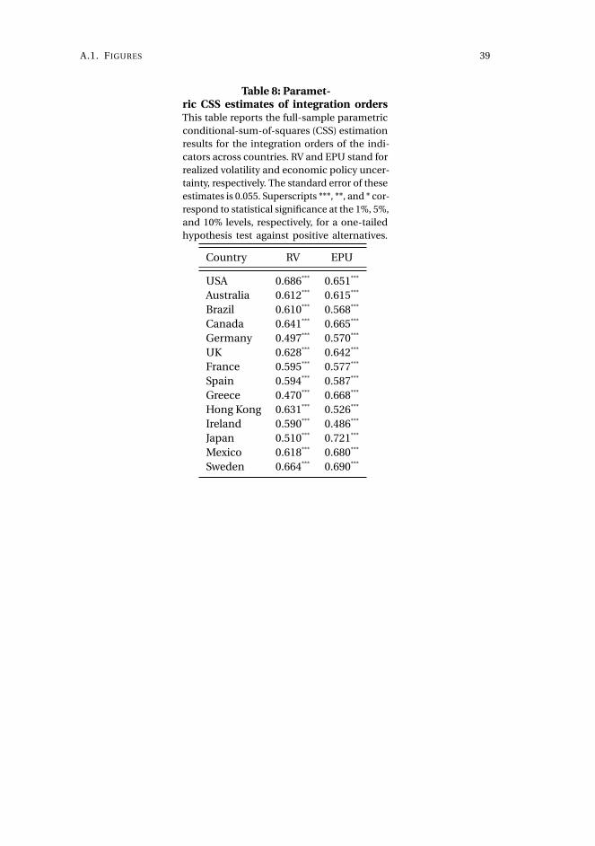
A.1. FIGURES 39
Table 8: Paramet-ric CSS estimates of integration ordersThis table reports the full-sample parametricconditional-sum-of-squares (CSS) estimationresults for the integration orders of the indi-cators across countries. RV and EPU stand forrealized volatility and economic policy uncer-tainty, respectively. The standard error of theseestimates is 0.055. Superscripts ***, **, and * cor-respond to statistical significance at the 1%, 5%,and 10% levels, respectively, for a one-tailedhypothesis test against positive alternatives.
Country RV EPU
USA 0.686*** 0.651***
Australia 0.612*** 0.615***
Brazil 0.610*** 0.568***
Canada 0.641*** 0.665***
Germany 0.497*** 0.570***
UK 0.628*** 0.642***
France 0.595*** 0.577***
Spain 0.594*** 0.587***
Greece 0.470*** 0.668***
Hong Kong 0.631*** 0.526***
Ireland 0.590*** 0.486***
Japan 0.510*** 0.721***
Mexico 0.618*** 0.680***
Sweden 0.664*** 0.690***
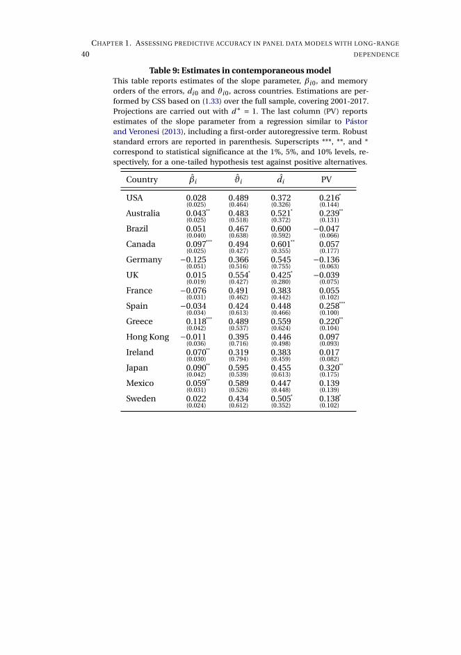
40
CHAPTER 1. ASSESSING PREDICTIVE ACCURACY IN PANEL DATA MODELS WITH LONG-RANGE
DEPENDENCE
Table 9: Estimates in contemporaneous modelThis table reports estimates of the slope parameter, βi 0, and memoryorders of the errors, di 0 and ϑi 0, across countries. Estimations are per-formed by CSS based on (1.33) over the full sample, covering 2001-2017.Projections are carried out with d∗ = 1. The last column (PV) reportsestimates of the slope parameter from a regression similar to Pástorand Veronesi (2013), including a first-order autoregressive term. Robuststandard errors are reported in parenthesis. Superscripts ***, **, and *correspond to statistical significance at the 1%, 5%, and 10% levels, re-spectively, for a one-tailed hypothesis test against positive alternatives.
Country βi ϑi di PV
USA 0.028(0.025)
0.489(0.464)
0.372(0.326)
0.216(0.144)
*
Australia 0.043(0.025)
** 0.483(0.518)
0.521(0.372)
* 0.239(0.131)
**
Brazil 0.051(0.040)
0.467(0.638)
0.600(0.592)
−0.047(0.066)
Canada 0.097(0.025)
*** 0.494(0.427)
0.601(0.355)
** 0.057(0.177)
Germany −0.125(0.051)
0.366(0.516)
0.545(0.755)
−0.136(0.063)
UK 0.015(0.019)
0.554(0.427)
* 0.425(0.280)
* −0.039(0.075)
France −0.076(0.031)
0.491(0.462)
0.383(0.442)
0.055(0.102)
Spain −0.034(0.034)
0.424(0.613)
0.448(0.466)
0.258(0.100)
***
Greece 0.118(0.042)
*** 0.489(0.537)
0.559(0.624)
0.220(0.104)
**
Hong Kong −0.011(0.036)
0.395(0.716)
0.446(0.498)
0.097(0.093)
Ireland 0.070(0.030)
** 0.319(0.794)
0.383(0.459)
0.017(0.082)
Japan 0.090(0.042)
** 0.595(0.539)
0.455(0.613)
0.320(0.175)
**
Mexico 0.059(0.031)
** 0.589(0.526)
0.447(0.448)
0.139(0.139)
Sweden 0.022(0.024)
0.434(0.612)
0.505(0.352)
* 0.138(0.102)
*
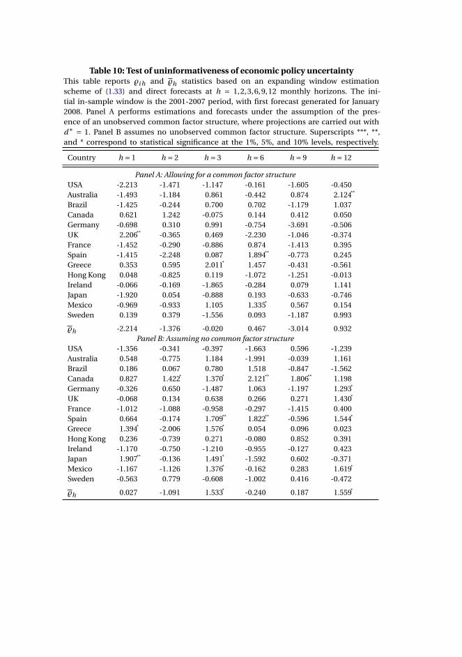
Table 10: Test of uninformativeness of economic policy uncertaintyThis table reports %i h and %h statistics based on an expanding window estimationscheme of (1.33) and direct forecasts at h = 1,2,3,6,9,12 monthly horizons. The ini-tial in-sample window is the 2001-2007 period, with first forecast generated for January2008. Panel A performs estimations and forecasts under the assumption of the pres-ence of an unobserved common factor structure, where projections are carried out withd∗ = 1. Panel B assumes no unobserved common factor structure. Superscripts ***, **,and * correspond to statistical significance at the 1%, 5%, and 10% levels, respectively.
Country h = 1 h = 2 h = 3 h = 6 h = 9 h = 12
Panel A: Allowing for a common factor structureUSA -2.213 -1.471 -1.147 -0.161 -1.605 -0.450Australia -1.493 -1.184 0.861 -0.442 0.874 2.124**
Brazil -1.425 -0.244 0.700 0.702 -1.179 1.037Canada 0.621 1.242 -0.075 0.144 0.412 0.050Germany -0.698 0.310 0.991 -0.754 -3.691 -0.506UK 2.206** -0.365 0.469 -2.230 -1.046 -0.374France -1.452 -0.290 -0.886 0.874 -1.413 0.395Spain -1.415 -2.248 0.087 1.894** -0.773 0.245Greece 0.353 0.595 2.011* 1.457 -0.431 -0.561Hong Kong 0.048 -0.825 0.119 -1.072 -1.251 -0.013Ireland -0.066 -0.169 -1.865 -0.284 0.079 1.141Japan -1.920 0.054 -0.888 0.193 -0.633 -0.746Mexico -0.969 -0.933 1.105 1.335* 0.567 0.154Sweden 0.139 0.379 -1.556 0.093 -1.187 0.993
%h -2.214 -1.376 -0.020 0.467 -3.014 0.932Panel B: Assuming no common factor structure
USA -1.356 -0.341 -0.397 -1.663 0.596 -1.239Australia 0.548 -0.775 1.184 -1.991 -0.039 1.161Brazil 0.186 0.067 0.780 1.518 -0.847 -1.562Canada 0.827 1.422* 1.370* 2.121** 1.806** 1.198Germany -0.326 0.650 -1.487 1.063 -1.197 1.293*
UK -0.068 0.134 0.638 0.266 0.271 1.430*
France -1.012 -1.088 -0.958 -0.297 -1.415 0.400Spain 0.664 -0.174 1.709** 1.822** -0.596 1.544*
Greece 1.394* -2.006 1.576* 0.054 0.096 0.023Hong Kong 0.236 -0.739 0.271 -0.080 0.852 0.391Ireland -1.170 -0.750 -1.210 -0.955 -0.127 0.423Japan 1.907** -0.136 1.491* -1.592 0.602 -0.371Mexico -1.167 -1.126 1.376* -0.162 0.283 1.619*
Sweden -0.563 0.779 -0.608 -1.002 0.416 -0.472
%h 0.027 -1.091 1.533* -0.240 0.187 1.559*

42
CHAPTER 1. ASSESSING PREDICTIVE ACCURACY IN PANEL DATA MODELS WITH LONG-RANGE
DEPENDENCE
A.3 Proofs
We here prove the theoretical results presented in the main text, along with an auxil-
iary lemma.
Proof of Theorem 1. Given the parameter consistency arguments derived in Ergemen
(2019), ϕhi t is a consistent estimator for ϕh
i t . First, it can be easily verified that
V ar
(1
m
m∑t=1
ϕhi t
)∝O(1+m2κi−1),
see, e.g., the proofs of Theorems 1 and 2 of Ergemen and Velasco (2017) for a similar
treatment, so
V ar
(1
mκi−1/2
1
m
m∑t=1
ϕhi t
)∝O(1).
Under Assumptions A-B, Ergemen (2019) establishes that the projected series incurs
a projection error of size Op (n−1 + (nT )−1/2). Given that the test statistic is based on
the projected series and has a m1/2−κi convergence rate, we need to account for the
projection error that becomes of size
Op
(m1/2−κi n−1 +m1/2−κi n−1/2T −1/2
)= op (1)
if m1/2−κi n−1 +m1/2−κi n−1/2T −1/2 → 0 as (m,n,T ) j →∞.
Next, we analyze the asymptotic behavior of the test statistic under the null in (1.19).
Define Di t+h(τi ) = ∂y∗i t+h|t (τi )/∂τi , extending the parameter vector τi to include all
model parameters for ease of exposition, and assuming that Assumption C applies to
this new vector. Applying the Mean Value Theorem,
y∗i t+h|t (τi t ) = y∗
i t+h|t (τi )+Di t+h(τi t )(τi t −τi )
for some τi t ≤ τi t ≤ τi , so, for fixed i ,
ϕhi t =
[ui t+h(τi )+Di t+h(τi t )(τi t −τi )
]2 − (ui t+h(τi )−ui h(τi ))2
= (ui t+h(τi ))2 − (ui t+h(τi )−ui h(τi ))2
+2ui t+h(τi )Di t+h(τi t )(τi t −τi )+Di t+h(τi t )2(τi t −τi )2
= ui h(τi )(2ui t+h(τi )−ui h(τi ))
+2ui t+h(τi )Di t+h(τi t )(τi t −τi )+Di t+h(τi t )2(τi t −τi )2 (A.1)
where ui h(τi ) = m−1 ∑m+ht=h+1 ui t (τi ) and
τi t −τi = (τi t − τi 0)+ (τi 0 −τi ) =Op (T −1/2)
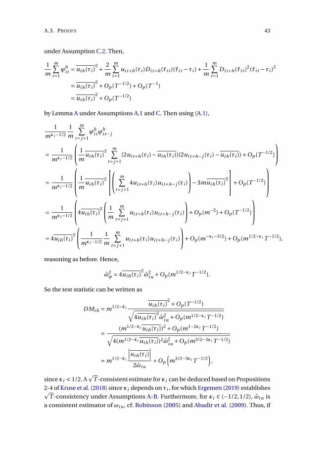
A.3. PROOFS 43
under Assumption C.2. Then,
1
m
m∑t=1
ϕhi t = ui h(τi )
2 + 2
m
m∑t=1
ui t+h(τi )Di t+h(τi t )(τi t −τi )+ 1
m
m∑t=1
Di t+h(τi t )2(τi t −τi )2
= ui h(τi )2 +Op (T −1/2)+Op (T −1)
= ui h(τi )2 +Op (T −1/2)
by Lemma A under Assumptions A.1 and C. Then using (A.1),
1
mκi−1/2
1
m
m∑t= j+1
ϕhi tϕ
hi t− j
= 1
mκi−1/2
1
mui h(τi )
2 m∑t= j+1
(2ui t+h(τi )−ui h(τi ))(2ui t+h− j (τi )−ui h(τi ))+Op (T −1/2)
= 1
mκi−1/2
1
mui h(τi )
2
m∑
t= j+14ui t+h(τi )ui t+h− j (τi )
−3mui h(τi )2
+Op (T −1/2)
= 1
mκi−1/2
4ui h(τi )2
1
m
m∑t= j+1
ui t+h(τi )ui t+h− j (τi )
+Op (m−2)+Op (T −1/2)
= 4ui h(τi )
2
1
mκi−1/2
1
m
m∑t= j+1
ui t+h(τi )ui t+h− j (τi )
+Op (m−κi−3/2)+Op (m1/2−κi T −1/2),
reasoning as before. Hence,
ω2ϕ = 4ui h(τi )
2ω2
i u +Op (m1/2−κi T −1/2).
So the test statistic can be written as
DMi h = m1/2−κiui h(τi )
2 +Op (T −1/2)√4ui h(τi )
2ω2
i u +Op (m1/2−κi T −1/2)
= (m1/2−κi ui h(τi ))2 +Op (m1−2κi T −1/2)√4(m1/2−κi ui h(τi ))2ω2
i u +Op (m3/2−3κi T −1/2)
= m1/2−κi
∣∣∣ui h(τi )∣∣∣
2ωi u+Op
(m3/2−3κi T −1/2
),
sinceκi < 1/2. Ap
T -consistent estimate forκi can be deduced based on Propositions
2-4 of Kruse et al. (2018) since κi depends on τi , for which Ergemen (2019) establishespT -consistency under Assumptions A-B. Furthermore, for κi ∈ (−1/2,1/2), ωi u is
a consistent estimator of ωi u , cf. Robinson (2005) and Abadir et al. (2009). Thus, if
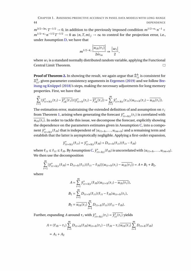
44
CHAPTER 1. ASSESSING PREDICTIVE ACCURACY IN PANEL DATA MODELS WITH LONG-RANGE
DEPENDENCE
m3/2−3κi T −1/2 → 0, in addition to the previously imposed condition m1/2−κi n−1 +m1/2−κi n−1/2T −1/2 → 0 as (n,T,m) j → ∞ to control for the projection error, i.e.,
under Assumption D, we have that
m1/2−κi
∣∣∣ui h(τi )∣∣∣
2ωi u⇒
∣∣wi∣∣
2,
where wi is a standard normally distributed random variable, applying the Functional
Central Limit Theorem.
Proof of Theorem 2. In showing the result, we again argue that Ξhi t is consistent for
Ξhi t , given parameter consistency arguments in Ergemen (2019) and we follow Bre-
itung og Knüppel (2018)’s steps, making the necessary adjustments for long memory
properties. First, we have that
m∑t=1
(y∗i t+h|t (τi )− y∗
i h(τi ))(y∗i t+h(τi )− y∗
i h(τi )) =m∑
t=1y∗
i t+h|t (τi t )(ui t+h(τi )−ui h(τi )).
The estimation error, maintaining the extended definition of and assumption on τi
from Theorem 1, arising when generating the forecast y∗i t+h|t (τi ) is correlated with
ui h(τi ). In order to tackle this issue, we decompose the forecast, explicitly showing
the dependence on the parameters estimates given in Assumption C, into a compo-
nent y∗i t+h|t (τi 0) that is independent of ui 1+h , . . . ,ui m+h and a remaining term and
establish that the latter is asymptotically negligible. Applying a first-order expansion,
y∗i t+h|t (τi t ) = y∗
i t+h|t (τi 0)+Di t+h(τi t )(τi t − τi 0)
where τi t ≤ τi t ≤ τi 0. By Assumption C, y∗i t+h|t (τi 0) is uncorrelated with ui 1+h , . . . ,ui m+h.
We then use the decomposition
m∑t=1
[y∗i t+h|t (τi 0)+Di t+h(τi t )(τi t − τi 0)](ui t+h(τi )−ui h(τi )) = A+B1 +B2,
where
A =m∑
t=1y∗
i t+h|t (τi 0)(ui t+h(τi )−ui h(τi )),
B1 =m∑
t=1Di t+h(τi t )(τi t − τi 0)ui t+h(τi ),
B2 = ui h(τi )m∑
t=1Di t+h(τi t )(τi t − τi 0).
Further, expanding A around τi with y∗i t+h|t (τi ) = y∗
i t (τi ) yields
A = (τi 0 −τi )m∑
t=1Di t+h(τi 0)ui t+h(τi )− (τi 0 −τi )ui h(τi )
m∑t=1
Di t+h(τi 0)
= A1 + A2

A.3. PROOFS 45
with τi 0 ≤ τi 0 ≤ τi . Since τi 0 and Di t+h(τi 0) are uncorrelated with ui t+h(τi ), we have
that A1 =Op (T −1/2)Op (m1/2) and A2 =Op (T −1/2)Op (mυi−1/2)Op (m) by Assumption
C.2, using arguments as in the proof of Lemma A and reasoning as in the proof
of Theorem 1. Thus, A =Op (T −1/2mυi+1/2). Under the null in (1.27), (τi t − τi 0) and
Di t+h(τi t ) are uncorrelated with ui t+h(τi ). Then, by Assumptions C.2 and using
similar arguments as in the proof of Lemma A, it follows that
m∑t=1
(τi t − τi 0)2Di t+h(τi t )2ui t+h(τi )2 =Op
(m2υi+2
T 2
).
Thus, B1 =Op (mυi+1T −1). Since by Assumptions C.2 and Lemma A,
m∑t=1
(τi t − τi 0)Di t+h(τi t ) =Op
(m3/2
T
),
B2 =Op (mυi−1/2)Op (m3/2T −1) =Op (mυi+1T −1). Therefore, we have
A+B1 +B2 =Op (mυi+1/2T −1/2 +mυi+1T −1),
and, thus,
T 1/2m−1/2−υi (A+B1 +B2) =Op (1)+Op (m1/2T −1/2),
where the Op (1) term leading to the asymptotic normal distribution is
T 1/2m−1/2−υi A =p
T (τi 0 −τi )m1/2−υi1
m
m∑t=1
Di t+h(τi 0)(ui t+h(τi )−ui h(τi )
). (A.2)
Next, we analyze
m∑t=1
(y∗i t+h|t (τi )− y∗
i h(τi ))2(y∗i t+h(τi )− y∗
i h(τi ))2
=m∑
t=1(y∗
i t+h|t (τi t )− y∗i h(τi ))2(ui t+h(τi )−ui h(τi ))2.
Using the mean value expansions above,
y∗i t+h|t (τi )− y∗
i h(τi ) = Di t+h(τi 0)(τi 0 −τi )+ Ψi t+h(τi t , τi 0),
where
Di t+h(τi s ) = Di t+h(τi s )−m−1m∑
t=1Di t+h(τi s ),
Ψi t+h(τi t , τi 0) = Di t+h(τi t )(τi t − τi 0)−m−1m∑
t=1Di t+h(τi t )(τi t − τi 0),

46
CHAPTER 1. ASSESSING PREDICTIVE ACCURACY IN PANEL DATA MODELS WITH LONG-RANGE
DEPENDENCE
for s = 0,1, . . . . We can then write
m∑t=1
(y∗i t+h|t (τi )− y∗
i h(τi ))2(y∗i t+h(τi )− y∗
i h(τi ))2 =C0 +C1 +C2,
where
C0 = (τi 0 −τi )2m∑
t=1Di t+h(τi 0)2(ui t+h(τi )−ui h(τi ))2,
C1 =m∑
t=1Ψi t+h(τi t , τi 0)2(ui t+h(τi )−ui h(τi ))2,
C2 = 2(τi 0 −τi )m∑
t=1Di t+h(τi 0)Ψi t+h(τi t , τi 0)(ui t+h(τi )−ui h(τi ))2.
Proceeding as before, the leading term
C0 =Op (T −1m2υi+1),
whereas
C1 =Op (T −2m2υi+2),
C2 =Op (T −3/2m2υi+5/2),
by Assumption C and since m−1 ∑mt=1 ui t+h(τi ) =Op (mυi−1/2). Thus,
T m−1−2υi (C0 +C1 +C2)
= T (τi 0 −τi )2m1−2υi1
m2
m∑t=1
Di t+h(τi 0)2(ui t+h(τi )−ui h(τi ))2 +Op (m3/2T −3/2).
(A.3)
Further, as in the proof of Theorem 1, we note again that we work with the projected
series. Given the convergence rate, we require that m1/2−υi (n−1 + (nT )−1/2) → 0 as
(n,T,m) j → ∞. Then, from (A.2) and (A.3), if additionally m/T → 0, i.e., invoking
Assumption E, and applying the FCLT, we establish that
m1/2−υi1
ωΞm
m∑t=1Ξh
i td−→ N (0,1)
since consistency of υi can be shown, reasoning as for κi in the proof of Theorem
1.
Proof of Theorem 3. Due to asymptotic approximate independence of the individual
%i h test statistics for large n, see Appendix 1 in Ergemen (2019), the result in the
Theorem follows from a standard CLT.

A.3. PROOFS 47
Proof of Theorem 4. We again motivate the cases based on the true parameters, given
the parameter consistency arguments discussed earlier. Under the local alternative
in (1.30) where the only deviation in parameters is in βi 0,
y∗i t+1(τi )− y∗
i 1(τi ) = v∗1i t+1
(di −di 0
)− v∗1i t+1
(di −di 0
)+ (ci /p
m)(x∗i t (di )− x∗
i t (di )).
Reasoning as in the proof of Theorem 1 and further noting that the error term is now
v∗1i t+1
(di −di 0
)as T →∞, we have under Assumption A.1 and B.2 that by a standard
CLT,
m1/2−maxdi−ϑi 0,di−di 0 1
σv1σx m
m∑t=1
(x∗i t (di )− x∗
i t (di ))v∗1i t+1
(di −di 0
) d−→ w1i
for fixed i , where w1i is a standard normally distributed random variable.
Next, since σ2v1
= m−1 ∑mt=1(v∗
1i t+1
(di −di 0
)− v∗1i t+1
(di −di 0
)+ (ci /p
m)x∗i t (di ))2 =
σ2v1+Op (m−1/2+maxdi−ϑi 0,di−di 0) and using
y∗i t+1|t (τi ) = cip
mx∗
i t (di )+Op (T −1/2+di 0−dmi n )
under Assumption A.1, we have as mT −1/2+di 0−dmi n → 0,
m∑t=1Ξ1
i t =m∑
t=1
[v∗
1i t+1
(di −di 0
)− v∗1i t+1
(di −di 0
)+ (ci /p
m)(x∗i t (di )− x∗
i t (di ))]
y∗i t+1|t (τi )
d−→ ciσv1σx wi 1 + c2i σ
2x .
Furthermore, since mT −1/2+di 0−dmi n → 0,,
mω2Ξ =
m∑t=1
(Ξ1i t )2 = ci
m
m∑t=1
(v∗1i t+1
(di −di 0
)− v∗1i t+1
(di −di 0
))2(x∗
i t (di )− x∗i t (di ))2 +op (1)
p−→ c2i σ
2v1σ2
x .
Thus,
%i 1d−→ si g n(ci )wi 1 +
∣∣ci∣∣ σx
σv1
.
Lemma A. Under Assumption A.1,
supi
∣∣∣ 1
m
m∑t=1
ui t+h(τi )Di t+h(τi t )∣∣∣=Op (1),
supi
∣∣∣ 1
m
m∑t=1
Di t+h(τi t )2∣∣∣=Op (1).

48
CHAPTER 1. ASSESSING PREDICTIVE ACCURACY IN PANEL DATA MODELS WITH LONG-RANGE
DEPENDENCE
Proof of Lemma A. Let dmi n and ϑmi n denote mini di and mini ϑi , respectively. We
first observe that
x∗i t (di ) =∆di−ϑi 0
t v2i t =t−1∑j=0
π j (di −ϑi 0)v2i t− j ,
x∗i t (ϑi ) =∆ϑi−ϑi 0
t v2i t =t−1∑j=0
π j (ϑi −ϑi 0)v2i t− j .
We then analyze the dominating terms in 1m
∑mt=1 ui t+h(τi )Di t+h(τi t ), since the re-
maining terms are bounded above by the Cauchy-Schwarz inequality. The first term,
supi
∣∣∣ 1
m
m∑t=1
x∗i t (di ) ˙x∗
i t (di )∣∣∣= sup
i
∣∣∣ 1
m
m∑t=1
t−1∑j=0
π j (di −ϑi 0)π j (di −ϑi 0)∣∣∣
=Op (1+m2(ϑmax−dmi n )−1 logm)
=Op (1)
under Assumption A.1. Similarly,
supi
∣∣∣ 1
m
m∑t=1
x∗i t (ϑi ) ˙x∗
i t (ϑi )∣∣∣= sup
i
∣∣∣ 1
m
m∑t=1
t−1∑j=0
π j (ϑi −ϑi 0)π j (ϑi −ϑi 0)∣∣∣
=Op (1+m2(ϑmax−ϑmi n )−1 logm)
=Op (1).
The third term,
supi
∣∣∣ 1
m
m∑t=1
˙x∗i t (di )
(v∗
1i t+h
(di −di 0
)−ρ′i v∗
2i t
(ϑi −ϑi 0
))∣∣∣= sup
i
∣∣∣ 1
m
m∑t=1
t−1∑j=0
π j (di −ϑi 0)(π j (di −di 0)+π j (ϑi −ϑi 0)
)∣∣∣=Op (1+mϑmax+dmax−2dmi n−1 logm +m2ϑmax−dmi n−ϑmi n−1 logm)
=Op (1)
by Assumption A.1 and following similar reasoning as above. The fourth term,
supi
∣∣∣ 1
m
m∑t=1
˙x∗i t (ϑi )
(v∗
1i t+h
(di −di 0
)−ρ′i v∗
2i t
(ϑi −ϑi 0
))∣∣∣=Op (1+mϑmax+dmax−dmi n−ϑmi n−1 logm +m2(ϑmax−ϑmi n )−1 logm)
=Op (1).

A.3. PROOFS 49
To analyze the expression 1m
∑mt=1 Di t+h(τi t )2, we again study only the dominating
terms. The first term
supi
∣∣∣ 1
m
m∑t=1
˙x∗i t (di )2
∣∣∣= supi
∣∣∣ 1
m
m∑t=1
t−1∑j=0
π2j (di −ϑi 0)
∣∣∣=Op (1+m2(ϑmax−dmi n )−1 log2 m)
=Op (1)
under Assumption A.1. Similarly, the second term
supi
∣∣∣ 1
m
m∑t=1
˙x∗i t (ϑi )2
∣∣∣=Op (1+m2(ϑmax−ϑmi n )−1 log2 m)
=Op (1).
Finally, the third term
supi
∣∣∣ 1
m
m∑t=1
˙x∗i t (di ) ˙x∗
i t (ϑi )∣∣∣=Op (1+mϑmax+dmax−ϑmi n−dmi n−1 log2 m)
=Op (1).
All remaining terms are of smaller asymptotic size, and thus the results in the lemma
follow.

C H A P T E R 2CAPTURING VOLATILITY PERSISTENCE:
A DYNAMICALLY COMPLETE REALIZED
EGARCH-MIDAS MODEL
PUBLISHED IN QUANTITATIVE FINANCE 19 (2019), 1839-1855
Daniel BorupAarhus University and CREATES
Johan Stax JakobsenCopenhagen Business School and CREATES
Abstract
We introduce extensions of the Realized Exponential GARCH model (REGARCH)
that capture the evident high persistence typically observed in measures of financial
market volatility in a tractable fashion. The extensions decompose conditional vari-
ance into a short-term and a long-term component. The latter utilizes mixed-data
sampling or a heterogeneous autoregressive structure, avoiding parameter prolifer-
ation otherwise incurred by using the classical ARMA structures embedded in the
REGARCH. The proposed models are dynamically complete, facilitating multi-period
forecasting. A thorough empirical investigation with an exchange traded fund that
tracks the S&P500 Index and 20 individual stocks shows that our models better cap-
ture the dependency structure of volatility. This leads to substantial improvements
in empirical fit and predictive ability at both short and long horizons relative to the
51
52
CHAPTER 2. CAPTURING VOLATILITY PERSISTENCE: A DYNAMICALLY COMPLETE REALIZED
EGARCH-MIDAS MODEL
original REGARCH. A volatility-timing trading strategy shows that capturing volatility
persistence yields substantial utility gains for a mean-variance investor at longer
investment horizons.
2.1 Introduction
The Realized GARCH model (RGARCH) and Realized Exponential GARCH model
(REGARCH) (Hansen et al., 2012; Hansen and Huang, 2016) provide an advantageous
structure for the joint modeling of stock returns and realized measures of their volatil-
ity. The models facilitate exploitation of granular information in high-frequency data
by including realized measures, which constitute a much stronger signal of latent
volatility than squared returns (Andersen, Bollerslev, Diebold, and Labys, 2001; An-
dersen et al., 2003). Despite the empirical success of the R(E)GARCH models, these
models do not adequately capture the dependence structure in volatility (both la-
tent and realized) without proliferation in parameters. This dependence structure is
typically characterized by a positive and slowly decaying autocorrelation function
(long-range dependence) or a persistence parameter close to unity, known as the
"integrated GARCH effect". Indeed, Hansen and Huang (2016) point out that the
REGARCH does a good job at modeling returns, but falls short in describing the
dynamic properties of the realized measure.
In this paper, we introduce parsimonious extensions of the REGARCH to capture
this evident high persistence by means of a multiplicative decomposition of the
conditional variance into a short-term and long-term component. The multiplica-
tive decomposition was popularized by Feng (2004), Engle and Rangel (2008), and
Engle et al. (2013)), among others. This structure is particularly useful since it en-
ables explicit modeling of a "baseline volatility", whose level arguably shifts over
time, and is the basis around which short-term movements occur. This structure is
appealing since it is intuitive and facilitates parsimonious specifications of a slow-
moving component in volatility. Moreover, it allows for great flexibility as opposed
to formal long-memory models employing, e.g., fractional integration. Whether the
high persistence arises due to structural breaks, fractional integration or another
source (see e.g. Lamoureux and Lastrapes (1990), Diebold and Inoue (2001), Hille-
brand (2005), McCloskey and Perron (2013), and Varneskov and Perron (2017)) our
proposed models are able to reproduce the high persistence of volatility observed in
stock return data and alleviate the integrated GARCH effect. This plays an important
role in stationarity of the short-term component and existence of the unconditional
variance, but also provides a means to obtain improved multi-step forecasts by re-
ducing the long-lasting impact of the short-term component and its innovations via
faster convergence to the time-varying baseline volatility.
When specifying our models, we retain the dynamics of the short-term component

2.1. INTRODUCTION 53
like those from a first-order REGARCH, but model the long-term component either
via mixed-data sampling (MIDAS) or a heterogeneous autoregressive (HAR) structure.
Motivated by Engle et al. (2013), the former specifies the slow-moving component
as a weighted average of weekly or monthly aggregates of the realized measure with
the backward-looking window and weights estimated from the data. The latter is
motivated by the simple, yet empirically successful HAR model of Corsi (2009), which
approximates the dependencies in volatility by a simple additive cascade structure of
a daily, weekly and monthly component of realized measures. Both our extensions
introduce only two or three additional parameters, hence avoid parameter prolifer-
ation otherwise incurred by means of the classical ARMA structures embedded in
the original REGARCH. Moreover, they remain dynamically complete. That is, the
models fully characterize the dynamic properties of all variables included in the
model. This property is especially relevant for forecasting purposes, since it allows for
multi-period forecasting. This contrasts GARCH-X models, which only provide fore-
casts one period into the future, and related extensions including macroeconomic
factors who rely on assumptions about the included variables’ exogenous dynamics.
We apply our REGARCH-MIDAS and REGARCH-HAR to the exchange traded index
fund SPY which tracks the S&P500 Index and 20 individual stocks and compare
their performances to a quadratic REGARCH-Spline and a fractionally integrated
REGARCH, the FloEGARCH (Vander Elst, 2015). We find that both our proposed
models better capture the autocorrelation structure of latent and realized volatility
relative to the original REGARCH, which is only able to capture the dependency
over the very short term. This leads to substantial improvements in empirical fit
(log-likelihood and information criteria) and predictive ability, particularly beyond
shorter horizons, when benchmarked to the original REGARCH. We document, ad-
ditionally, that the backward-looking horizon of the HAR specification is too short
to sufficiently capture autocorrelation beyond approximately one month. While the
REGARCH-Spline comes short relative to our proposals (with four-five extra param-
eters), the FloEGARCH performs well. It does, however, not perform better than
our best-performing REGARCH-MIDAS specifications in-sample and lack predictive
accuracy in the short-term. This leaves the REGARCH-MIDAS as a very attractive
model for capturing volatility persistence in the REGARCH framework and improving
forecasting performance at both short and long horizons. To assess the economic
value of the improvements in predictive accuracy, we examine a volatility-timing
strategy that uses each model’s forecast as input to constructing optimal portfolio
weights. A risk-averse investor with mean-variance preferences who allocates funds
into one risky asset and one risk-free asset would be willing to pay on average about
15 basis points per year, and for certain stocks as much as 40 basis points, to achieve
the level of utility that is obtained by our REGARCH-MIDAS compared to the original
REGARCH.

54
CHAPTER 2. CAPTURING VOLATILITY PERSISTENCE: A DYNAMICALLY COMPLETE REALIZED
EGARCH-MIDAS MODEL
The remainder of the paper is laid out as follows. Section 2.2 introduces our ex-
tensions to the original REGARCH; the REGARCH-MIDAS and the REGARCH-HAR.
Section 2.3 outlines the associated estimation procedure. Section 2.4 summarizes our
data set, examines the empirical fit and predictive ability of our proposed models,
and introduces a procedure for generating multi-period forecasts. Section 2.5 con-
cludes. Further empirical results and additional technical details are collected in the
Supplementary Appendix available online. Programs for estimating our proposed
models are available from the authors upon request.
2.1.1 Related literature
Our work builds on several strands of the literature on volatility modeling. We now
briefly describe the primary strands most closely related to the present paper and pro-
vide a few examplary contributions in each. The outset is the R(E)GARCH framework,
but other models have been proposed to utilize information from realized measures.
Notable innovations include the GARCH-X model (Engle, 2002), the multiplicative
error model (Engle and Gallo, 2006), and the HEAVY model (Shephard and Shep-
pard, 2010). Within the class of GARCH models without realized measures, several
contributions have been made to capture the evident volatility persistence. A few
notable references include the Integrated GARCH (Engle and Bollerselv, 1986), the
Fractionally Integrated (E)GARCH (Baillie, Bollerslev, and Mikkelsen, 1996; Bollerslev
and Mikkelsen, 1996), FIAPARCH (Tse, 1998), regime-switching GARCH (Diebold
and Inoue, 2001), HYGARCH (Davidson, 2004), the Spline-GARCH (Engle and Rangel,
2008), and the time-varying component GJR-GARCH (Amado and Teräsvirta, 2013). In
the class of R(E)GARCH models, Vander Elst (2015) proposes a fractionally integrated
REGARCH, whereas Huang, Liu, and Wang (2016) suggest adding weekly and monthly
averages of a realized measure in the GARCH equation of the RGARCH.
Another strand of literature utilizes the idea of decomposing volatility, which origi-
nates from Engle and Lee (1999). This has primarily been used to empirically support
countercyclicality in stock market volatility (see e.g. Engle et al. (2013) and Dominicy
and Vander Elst (2015)). Inspired by the findings of Mikosch and Starica (2004) which
show that long-range dependence and the integrated GARCH effect may be explained
by level shifts in the unconditional variance, Amado and Teräsvirta (2013) propose a
multiplicative component version of the GJR-GARCH model for capturing volatility
persistence. The MIDAS concept originally introduced in a regression framework
(Ghysels, Santa-Clara, and Valkanov, 2004, 2005; Ghysels, Sinko, and Valkanov, 2007)
has recently been successfully incorporated into the GARCH framework with the
GARCH-MIDAS proposal of Engle et al. (2013). Conrad and Kleen (2018) indeed show
formally that the autocorrelation function of squared returns is better captured by a
multiplicative GARCH specification rather than its nested GARCH(1,1) model, arising
from the persistence in the long-term component. Our innovation relative to this
2.2. PERSISTENCE IN A MULTIPLICATIVE REALIZED EGARCH 55
literature is to introduce the multiplicative component modeling of conditional vari-
ance into the popular R(E)GARCH framework in order to capture the evident volatility
persistence.
2.2 Persistence in a multiplicative realized EGARCH
Let rt denote a time series of returns, xt a time series of realized measures,1 and
Ft a filtration so that rt , xt is adapted to Ft . We define the conditional mean
by µt =E[rt |Ft−1] and the conditional variance by σ2t = Var[rt |Ft−1]. Our aim is to
allow for more flexible dependence structures in the state-of-the-art specification of
conditional variance provided by the REGARCH of Hansen and Huang (2016). To that
end, we define
rt =µt +σt zt ,
where zt is an i.i.d. innovation process with zero mean and unit variance, and
assume that the conditional variance can be multiplicatively decomposed into two
components as
σ2t = ht g t . (2.1)
We refer to ht as the short-term component, supposed to capture day-to-day (high-
frequency) fluctuations in the conditional variance. On the contrary, g t is supposed to
capture secular (low-frequency) movements in the conditional variance, henceforth
referred to as the long-term component or baseline volatility. With the multiplicative
decomposition in (2.1), we extend a daily REGARCH(1,1) to
rt =µt +σt zt , (2.2)
loght =β loght−1 +τ(zt−1)+αut−1, (2.3)
log xt = ξ+φ logσ2t +δ(zt )+ut , (2.4)
log g t =ω+ f (xt−2, xt−3, . . . ;η), (2.5)
where f (·;η) is a Ft−1-measurable function, which can be linear or non-linear. The
equations are labeled as the "return equation", the "GARCH equation", the "mea-
surement equation", and the "long-term equation", respectively. For identification
purposes, we have omitted an intercept in (2.3). Note that the specification of the
GARCH and measurement equations is a generalization of the logarithmic RGARCH
1For the remainder of this paper, we assume for clarity of exposition that xt is one-dimensional,containing a single (potentially robust) realized measure consistently estimating integrated variance suchas the realized variance or the realized kernel (Barndorff-Nielsen, Hansen, Lunde, and Shephard, 2008).This assumption is without loss of generality in the sense that additional realized measures (and theirassociated measurement equations) can be added, such as daily range or the realized quarticity (Bollerslev,Patton, and Quaedvlieg, 2016), rendering xt a vector.
56
CHAPTER 2. CAPTURING VOLATILITY PERSISTENCE: A DYNAMICALLY COMPLETE REALIZED
EGARCH-MIDAS MODEL
in Hansen et al. (2012).2 Our model framework applies, as a result, also to the nested
RGARCH framework. Hansen and Huang (2016) document, moreover, considerable
empirical superiority of REGARCH over RGARCH.
We facilitate level shifts in the baseline volatility via the function f (·;η), which takes
as input past values of the realized measure. We make the dependence on η explicit
in the function f (·;η), and prefer that it is low-dimensional. If f (·;η) is constant,
we obtain the REGARCH as a special case. If f (·;η) is time-varying and persistent,
past information may assist in capturing the dependency structure of conditional
variance better. We propose in the following sections two ways to parsimoniously
formulate f (·;η) using non-overlapping weekly and monthly averages of the realized
measure to be consistent with the idea of a slow-moving, low-frequency component.3
We model low-frequency movements in conditional variance using (aggregates of)
past information of the realized measure rather than tying it to macroeconomic
state variables as in Engle et al. (2013) and Dominicy and Vander Elst (2015). This
procedure renders the model in (2.2)-(2.5) complete with dynamic specifications of
all variables included in the model. Consequently, multi-period forecasting can be
conducted on the basis of the jointly estimated empirical dynamics. This contrasts
specifications using exogenous information (from e.g. macroeconomic variables)
that typically rely on additional assumptions on the dynamics of the exogenous
variables (e.g. random walks (Dominicy and Vander Elst, 2015)), outside-generated
forecasts (usually from a standard autoregressive specification) of the exogenous
variables in the model (Conrad and Loch, 2015) or the assumption that the long-
term component is constant for the forecasting horizon (Engle et al., 2013).4 We do,
however, emphasize that our proposed model accommodates well the inclusion of
exogenous information such as (possibly low-frequency) macroeconomic variables if
deemed appropriate.
2Without multiplicative decomposition, the logarithmic RGARCH takes the form
loght =β loght−1 +αxt−1,
log xt = ξ+φ loght +δ(zt )+ut ,
such that by substitution we obtain
loght = ω+ β loght−1 +αδ(zt−1)+αut−1,
where ω=αξ and β=β+αφ. It is clear that the logarithmic RGARCH is nested in the REGARCH if the twoleverage functions are proportional, τ(zt−1) =αδ(zt−1), and that the coefficient on ut−1 determines therelative magnitude.
3The idea is to separate the effects of the realized measure into two, such that the day-to-day effects is(mainly) contained in the short-term component ht via ut−1 and the long-term component captures theinformation contained in the realized measure further back in time. Excluding information in the realizedmeasure on day t −1 from the function f (·;η) is consistent with the rolling-window formulations withrealized variance in the GARCH-MIDAS framework of Engle et al. (2013).
4As suggested by a referee, a thorough comparison of the forecasting performance resulting fromdynamically complete and incomplete specifications would be interesting for future research.
2.2. PERSISTENCE IN A MULTIPLICATIVE REALIZED EGARCH 57
Given the high persistence of the conditional variance (documented in the empirical
section below), simply including additional lags in the ARMA structure embedded
in the original REGARCH is not a viable solution, keeping parameter proliferation
in mind (cf. Section 2.4). Instead, we utilize the multiplicative component structure
which is both intuitively appealing and maintain parsimony. Whether high persis-
tence of the conditional variance process arises due to structural breaks, fractional
integration or any other source, the long-term component, if modeled accurately,
facilitates high persistence in the REGARCH framework. That is, we do not explicitly
take a stance on the reason for the presence of high persistence. Our models may be
seen as a flexible alternative to a formal long-memory model (see e.g. Bollerslev and
Mikkelsen (1996) and Vander Elst (2015)). This is motivated by Mikosch and Starica
(2004), who show that the high persistence can be explained by level shifts in the un-
conditional variance (see also Diebold (1986) and Lamoureux and Lastrapes (1990)).
On this basis, Amado and Teräsvirta (2013) propose a multiplicative decomposition
of the GJR-GARCH model, where the "baseline volatility" changes deterministically
according to the passage of time. We may, therefore, capture high persistence via the
structure proposed above, when the long-term component in (2.5) is specified as
a slow-moving baseline volatility around which stationary short-term fluctuations
occur via the standard GARCH equation. Naturally, this interpretation (and the exis-
tence of the unconditional variance) depends on whether |β| < 1 holds in practice,
which may be questionable on the basis of former evidence for the original REGARCH
(confirmed in Section 2.4). However, this integrated GARCH effect is alleviated in our
proposed models, where (estimated) β is notably below unity.
The leverage functions, τ(·) and δ(·), facilitate modeling of the dependence between
return innovations and volatility innovations known to be empirically important
(see e.g. Christensen, Nielsen, and Zhu (2010)). If the leverage functions are left out,
the residuals zt and ut will be correlated and thereby at odds with the underlying
assumptions (Hansen et al., 2012; Hansen and Huang, 2016). We adopt the quadratic
form of the leverage functions based on the second-order Hermite polynomial,
τ(z) = τ1z +τ2(z2 −1),
δ(z) = δ1z +δ2(z2 −1).
The leverage functions have a flexible form and implyE[τ(z)
]=E[δ(z)
]= 0 when
E [z] = 0 and Var[z] = 1. Thus, if |β| < 1, our identification restriction implies that
E[loght
]= 0 such thatE[
logσ2t
]=E[
log g t].5 In the (Quasi-)Maximum Likelihood
analysis below, we employ a Gaussian specification like Hansen and Huang (2016)
with zt ∼ N (0,1) and ut ∼ N (0,σ2u), and zt ,ut mutually and serially independent. We
check the validity of this approach via a parametric bootstrap in Section 2.3.
5The GARCH equation implies that loght = β j loght− j +∑ j−1
i=0 βi [τ(zt−1−i )+αut−1−i
]such that
loght has a stationary representation if |β| < 1.
58
CHAPTER 2. CAPTURING VOLATILITY PERSISTENCE: A DYNAMICALLY COMPLETE REALIZED
EGARCH-MIDAS MODEL
The return and GARCH equations are canonical in the GARCH literature. In the return
equation, the conditional mean, µt , may be modeled in various ways including a
GARCH-in-Mean specification or simply as a constant.6 Following the latter approach,
we estimate the constant µt = µ. In our multiplicative specification, the GARCH
equation drives the dynamics of the high-frequency part of latent volatility. The
dynamics are specified as a slightly modified version of the EGARCH model of Nelson
(1991) (different leverage function) with the addition of the term αut−1 that relates
the latent volatility with the innovation to the realized measure. Hence, α represents
how informative the realized measure is about future volatility. The persistence
parameter β can be interpreted as the AR-coefficient in an AR(1) model for loght
with innovations τ(zt−1)+αut−1.
The measurement equation is the true innovation in the R(E)GARCH, which makes
the model dynamically complete. The equation links the ex-post realized measure
with the ex-ante conditional variance. Discrepancies between the two measures
are expected, since the conditional variance (and returns) refers to a close-to-close
market interval, whereas the realized measure is computed from a shorter, open-to-
close market interval. Hence, the realized measure is expected to be smaller than
the conditional variance on average. Additionally, the realized measure may be an
imperfect measure of volatility. Therefore, the equation includes both a proportional,
ξ, and an exponential, φ, correction parameter. The innovation term, ut , can be seen
as the true difference between ex-ante and ex-post volatility.
2.2.1 The realized EGARCH-MIDAS model
Inspired by the GARCH-MIDAS model of Engle et al. (2013), we consider the following
MIDAS specification of the long-term component
log g t =ω+λK∑
k=1Γk
(γ)
y (N )t−1,k , (2.6)
where Γk(γ)
is a non-negative weighting function parametrized by the vector γwhich
satisfies the restriction∑K
k=1Γk(γ)= 1, and y (N )
t ,k = 1N
∑Ni=1 log xt−N (k−1)−i is an N -day
average of the logarithm of the realized measure. Hence, the value of N determines
the frequency of the data feeding into the low-frequency component. We consider in
the following N = 5,22, corresponding to weekly and monthly averages.
By estimating γ, for a given weighting function and K , the term∑K
k=1Γk(γ)
yt−1,k acts
as a filter, which extracts the empirically relevant information from past values of
6The mean is typically modeled as a constant since stock market returns generally are found to beclose to serially uncorrelated, see, e.g., Ding, Granger, and Engle (1993). Sometimes the assumption ofzero mean, µ= 0, is imposed for simplicity and may in fact generate better out-of-sample performance(Hansen and Huang, 2016). However, in option-pricing applications a GARCH-in-Mean specification isusually employed, see, e.g., Huang, Wang, and Hansen (2017).
2.2. PERSISTENCE IN A MULTIPLICATIVE REALIZED EGARCH 59
the realized measure with assigned importance given by λ. That is, the lag selection
process is allowed to be data driven. In practice, we need to choose a value for K and
a weighting scheme. Conventional weighting schemes are based on the exponential,
exponential Almon lag, or the beta-weight specification. A detailed discussion can
be found in Ghysels et al. (2007), who study the choice of weighting function in the
context of MIDAS regression models. We employ in the following the two-parameter
beta-weight specification defined by
Γk(γ1,γ2
)= (k/K
)γ1−1 (1−k/K
)γ2−1∑Kj=1
(j /K
)γ1−1 (1− j /K
)γ2−1 (2.7)
due to its flexible form. We restrict γ2 > 1, which ensures a monotonically decreasing
weighting scheme when γ1 = 1. We examine a single-parameter case in which we
impose γ1 = 1 (see Engle et al. (2013) and Asgharian, Christiansen, and Hou (2016)
for a similar restriction) and a case where γ1 is a free parameter. More rich structures
for the weighting scheme can obviously be considered by introducing additional
parameters, but we will not explore that route, since one important aim of the MIDAS
models is parsimony. As long as the weighting function is reasonably flexible, the
choice of lag length of the MIDAS component, K , is of limited importance if chosen
reasonably large. The reason is that the estimated γ assigns the relevant weights
to each lag simultaneously while estimating the entire model. Should one want to
determine an ‘optimal’ K , we simply suggest to estimate the model for a range of
values of K and choose that for which higher values lead to no sizeable gain in the
maximized log-likelihood value.
2.2.2 The realized EGARCH-HAR model
Inspired by Corsi (2009), we suggest the following HAR specification of the long-term
component
log g t =ω+γ11
5
5∑i=1
log xt−i−1 +γ21
22
22∑i=i
log xt−i−1. (2.8)
The argument for this particular lag structure is motivated by the heterogeneous mar-
ket hypothesis (Müller et al., 1993), which suggests accounting for the heterogeneity
in information arrival due to e.g. different trading frequencies of financial market
participants. See Corsi (2009) for a more detailed discussion. This particular choice
of lag structure including the lagged weekly and monthly average of the logarithm
of the realized measure is intuitive and has been empirically successful, but is not
data driven as opposed to the MIDAS lag structure. The lag structure can be seen as a
special case of the step-function MIDAS specification in Forsberg and Ghysels (2007),
which was, indeed, inspired by an unpublished version of Corsi (2009).
60
CHAPTER 2. CAPTURING VOLATILITY PERSISTENCE: A DYNAMICALLY COMPLETE REALIZED
EGARCH-MIDAS MODEL
2.3 Estimation
We estimate the models using (Quasi-)Maximum Likelihood (QML) consistent with
the procedures in Hansen et al. (2012) and Hansen and Huang (2016). The log-
likelihood function can be factorized as
L(r, x;θ) =T∑
t=1`t (rt , xt ;θ) =
T∑t=1
[`t (rt ;θ)+`t (xt |rt ;θ)], (2.9)
where θ = (µ,β,τ1,τ2,α,ξ,φ,δ1,δ2,ω,η,σ2u)′ is the vector of parameters in (2.2)-(2.5),
and `t (rt ;θ) is the partial log-likelihood, measuring the goodness of fit of the return
distribution. Given the distributional assumptions, zt ∼ N (0,1) and ut ∼ N (0,σ2u),
and zt ,ut mutually and serially independent, we have
`t (rt ;θ) =−1
2
[log2π+ logσ2
t + z2t
], (2.10)
`t (xt |rt ;θ) =−1
2
[log2π+ logσ2
u + u2t
σ2u
], (2.11)
where zt = zt (θ) = (rt −µ)/σt . We initialize the conditional variance process to be
equal to its unconditional mean, i.e. logh0 = 0. Alternatively, one can treat logh0 as an
unknown parameter and estimate it as in Hansen and Huang (2016), who show that
the initial value is asymptotically negligible. To initialize the long-term component,
log g t , at the beginning of the sample, we simply set past values of log xt equal to
log x1 for the length of the backward-looking horizon in the MIDAS filter. This is
done to avoid giving our proposed models an unfair advantage by utilizing more
data than the benchmark REGARCH. To avoid inferior local optima in the numerical
optimization, we perturb starting values and re-estimate the parameters for each
perturbation.
2.3.1 Asymptotic properties
We document an MDS property of the score vector in Proposition 1 in the Supple-
mentary Appendix. This is similar to the original REGARCH, leading Hansen and
Huang (2016) to conjecture that the limiting distribution of the estimators is normal.
We follow the same route and leave the development of the asymptotic theory for
estimators of the REGARCH-MIDAS and REGARCH-HAR for future research. Hence,
we conjecture that
pT (θ−θ)
d−→ N (0,T H−1SH−1), (2.12)
where S is the limit of the outer-product of the scores and H is the negative limit of
the Hessian matrix for the log-likelihood function. In practice, we rely on estimates
of these two components in the sandwich formula for computing robust standard
2.4. EMPIRICAL RESULTS 61
errors of the coefficients. The estimate θ is obtained via QML.7 To check the validity
of this approach, we employ a parametric bootstrapping technique (Paparoditis and
Politis, 2009) in the Supplementary Appendix and find that the in-sample distribution
of estimated parameters for both the REGARCH, REGARCH-MIDAS and REGRACH-
HAR is generally in agreement with a normal distribution. We also compared the
bootstrapped standard errors with the robust QML standard errors computed from
the sandwich-formula in (2.12). The standard errors were also quite similar, which in
summary does not contradict the assertion that the QML approach and associated
inferences are valid.
2.4 Empirical results
In this section, we examine the empirical fit as well as the forecasting performance of
the REGARCH-MIDAS and REGARCH-HAR, including an outline of the forecasting
procedures involved with the proposed models. We mainly comment on the weekly
REGARCH-MIDAS, since the empirical results are qualitatively similar for the monthly
version.
2.4.1 Data
The full sample data set consists of daily close-to-close returns and the daily realized
kernels (RK) of the SPY exchange-traded fund that tracks the S&P500 Index and 20
individual stocks for the 2002/01-2013/12 period. In the computation of the realized
kernel, we use tick-by-tick data, restrict attention to the official trading hours 9:30:00
and 16:00:00 New York time, and employ the Parzen kernel as in Barndorff-Nielsen,
Hansen, Lunde, and Shephard (2011). See also Barndorff-Nielsen et al. (2008) and
Barndorff-Nielsen, Hansen, Lunde, and Shephard (2009) for additional details. For
each stock, we remove short trading days where trading occurred in a span of less
than 20,000 seconds (compared to typically 23,400 for a full trading day). We also
remove data on February 27, 2007, which contains an extreme outlier associated
with a computer glitch on the New York Exchange that day. This leaves a sample
size for each stock of about 3,000 observations. Figure 1 depicts the evolution of
returns, squared returns, realized kernel and the autocorrelation function (ACF) of
the logarithm of the realized kernel for SPY.8
We estimate the fractional integration parameter d in the logarithm of the realized
kernel with the two-step exact local Whittle estimator of Shimotsu (2010). Over the full
7Han and Kristensen (2014) and Han (2015) conclude that inference for the QML estimator is quiterobust to the level of persistence in covariates included in GARCH-X models, irrespective of them beingstationary or not. Moreover, Francq and Thieu (2018) develop asymptotic theory for a wide class ofasymmetric GARCH models with exogenous covariates, but not for EGARCH nor log-GARCH specifications.
8We include in the Supplementary Appendix a table with summary statistics of the daily returns andthe logarithm of daily realized kernels for all 20 individual stocks.
62
CHAPTER 2. CAPTURING VOLATILITY PERSISTENCE: A DYNAMICALLY COMPLETE REALIZED
EGARCH-MIDAS MODEL
sample all series satisfy 0.5 < d < 1, suggesting that volatility is highly persistent.9 This
finding is supported by the slowly decaying ACF of the logarithm of the realized kernel
for SPY. Moreover, we reject (Dickey-Fuller) unit root tests across all assets considered
using both regular least-squares and instrumented persistence parameters, following
the procedures in Hansen and Lunde (2014). See Supplementary Appendix for further
details. Collectively, these findings motivate a modeling framework that is capable
of capturing a high degree of persistence. Given the requirement that |β| < 1, this
also motivates a framework that pulls β away from unity. This is where the proposed
REGARCH-MIDAS and REGARCH-HAR prove useful.
2.4.2 In-sample results
In this section, we examine the empirical fit of the proposed REGARCH-HAR and
REGARCH-MIDAS using the full sample of observations for SPY and the 20 individual
stocks. We start out by presenting some appropriate benchmarks.
2.4.2.1 Benchmark models
For comparative purposes, we estimate (using QML) two direct antecedents of
the REGARCH-MIDAS and REGARCH-HAR proposed in this paper. The first is a
REGARCH-Spline (REGARCH-S), with the only difference stemming from the spec-
ification of the long-term component. That is, we consider the quadratic spline
formulation
log g t =ω+ c0t
T+
K∑k=1
ck
(max
t
T− tk−1
T,0
)2
,
where t0 = 0, t1, t2, . . . , tK = T denotes a partition of the time horizon T in K + 1
equidistant intervals. Consequently, the smooth fluctuations in the long-term com-
ponent arises from the (deterministic) passage of time instead of (stochastic) move-
ments in the realized kernel as prescribed by the REGARCH-HAR and REGARCH-
MIDAS.10 The formulation of the long-term component originates from Engle and
Rangel (2008) and is also examined in Engle et al. (2013), to which we refer for further
details. The number of knots, K , is selected using the BIC information criterion.11
The second benchmark is the fractionally integrated REGARCH (FloEGRACH) of Van-
der Elst (2015), which incorporates fractional integration in the GARCH equation of
the REGARCH in a similar vein to the development of the FI(E)GARCH model of Baillie
9We estimated the parameters with m = bT q c for q =∈ 0.50,0.55, . . . ,0.80, leading to no alterations ofthe conclusions obtained for q = 0.65. See also Wenger, Leschinski, and Sibbertsen (2017) for a compre-hensive empirical study on long memory in volatility and the choice of estimator of d .
10When the long-term component is specified as a deterministic component it follows that E[logσ2t ] =
log gt .11In a similar spirit to the choice of K for the REGARCH-MIDAS, we apply the number of knots
determined in the estimation on SPY uniformly in all subsequent analyses.
2.4. EMPIRICAL RESULTS 63
et al. (1996) and Bollerslev and Mikkelsen (1996). The model, thus, explicitly incor-
porates long-memory via fractionally integrated polynomials in the ARMA structure
defined via the parameter d . In contrast to our proposals and the REGARCH-S, the
FloEGARCH does not incorporate a multiplicative component structure. Following
Vander Elst (2015), we implement a FloEGARCH(1,d ,1),
rt =µ+σt zt ,
logσ2t =ω+ (1−β)L−1(1−L)−d (
τ(zt−1)+αut−1)
,
log xt = ξ+φ logσ2t +δ(zt )+ut ,
where (1−L)d is the fractional differencing operator. The infinite polynomial can be
written as
(1−β)L−1(1−L)−d =∞∑
n=0
(n∑
m=0βmψ−d ,n−m
)Ln ,
where ψ−d ,k =ψ−d ,k−1k−1+d
k and ψ−d ,0 = 1. In the implementation, we truncate the
infinite sum at 1,000, similarly to Bollerslev and Mikkelsen (1996) and Vander Elst
(2015), and initialize the process similarly to Vander Elst (2015). For completeness,
we also estimate a multiplicative component version of the EGARCH(1,1) model in
Nelson (1991).
2.4.2.2 Results for the S&P500 Index
In Table 1, we report estimated parameters, their standard errors, and the associated
maximized log-likelihood values for the models under consideration.12
We derive a number of notable findings. First, the multiplicative component struc-
tures lead to substantial increases in the maximized log-likelihood value relative
to the original REGARCH. It is worth noting that the null hypothesis of no MIDAS
component, λ= 0 such that f (·;η) = 0, renders γ1 and γ2 unidentified nuisance pa-
rameters. Hence, assessing the statistical significance of the differences in maximized
log-likelihood values via a standard LR test and a limiting χ2 distribution is infeasible.
Instead, we construct a bootstrapped LR test (BLR), where the null is the REGARCH
and the alternative is one of our proposed extensions. Specifically, we simulate 999
series using estimates for the null model (REGARCH) and compute the LR statistic
for each simulated series. To avoid problems with local maxima in the estimation (of
especially the alternative model) under the null hypothesis, we consider a wide grid
of starting values by perturbation. Given this perturbation, numerical optimization is
12Given the importance of choosing the value of K , the maximum lag length of the MIDAS filter, largeenough, we let data decide. A detailed analysis in the Supplementary Appendix shows that K = 12 andK = 52 are suitable choices for the monthly and weekly filters, respectively. We apply these uniformly in allsubsequent analyses, including the individual stock results.
64
CHAPTER 2. CAPTURING VOLATILITY PERSISTENCE: A DYNAMICALLY COMPLETE REALIZED
EGARCH-MIDAS MODEL
stable. Despite that the critical values of the bootstrap distributions are noticeably
greater than those from a regular chi-square distribution with two-three degrees
of freedom, we strongly reject the null of the REGARCH versus all versions of the
REGARCH-MIDAS with a p-value of less than 1%. The log-likelihood improvements
obtained from the REGARCH-HAR and our benchmark models are statistically signif-
icant at a 1% level as well.
We also nuance our interpretation of the log-likelihood gains by information crite-
ria. The substantial increases in log-likelihood value by only a small increase in the
number of parameters in the REGARCH-MIDAS and REGARCH-HAR lead to system-
atic improvements in information criteria. Despite the noticeably greater number
of parameters in the REGARCH-S, the increase in the log-likelihood value is only
comparable to that of the REGARCH-HAR, leading to a modest improvement in the
AIC, only a slight improvement in the BIC, and even a worsening of the HQIC. The
FloEGARCH comes closest to the REGARCH-MIDAS specifications, but is still short
about seven log-likelihood points. Since it only introduces one additional parameter,
the information criteria remain comparable to those of the REGARCH-MIDAS.13
We have also considered higher-order versions of the original REGARCH(p,q), with
p, q ∈ 1, . . . ,5. The best fitting version, the REGARCH(5,5), provides a likelihood
gain close to, but still less than the REGARCH-MIDAS models. This gain is, however,
obtained with the inclusion of additional eight parameters, causing the information
criteria to deteriorate.14
Secondly, we find that the single-parameter REGARCH-MIDAS performs similarly
to the two-parameter version. Additionally, for the same number of parameters, the
single-parameter REGARCH-MIDAS provides a considerable 16-point log-likelihood
gain relative to the REGARCH-HAR. This suggests that the HAR formulation is too
short-sighted to fully capture the conditional variance dynamics (despite providing
a substantial gain relative to the original REGARCH) by using only the most recent
month’s realized kernels. The differences of the lag functions, as depicted in Figure 2,
corroborate this point, by attaching a positive weight on observations further than
a month in the past. The cascade structure as evidenced in Corsi (2009) and Huang
et al. (2016) of the HAR formulation is clear from the figure as well, leading to the
conclusion that it constitutes a rather successful, yet suboptimal, approximation of
the beta-lag function used in the MIDAS formulation.
13It is also noteworthy that the FloEGARCH attaches a positive weight to information four years in thepast (1,000 daily lags), whereas the REGARCH-MIDAS only carries information from at most the last year.This suggests that the outperformance of the REGARCH-MIDAS relative to the FloEGARCH is somewhatconservative.
14It also stands out from Table 1 that the improvements in maximized value from all models underconsideration arise from a better modeling of the realized measure and not returns, which comes asno surprise given the motivation behind their development and that the original REGARCH is already avery successful model in fitting returns while lacking adequate modelling of the realized measure, as putforward in Hansen and Huang (2016).
2.4. EMPIRICAL RESULTS 65
In Figure 3, we depict the fitted conditional variance along with the long-term compo-
nents of each multiplicative component model under consideration. The long-term
component of the REGARCH-MIDAS models appear smooth and do, indeed, resem-
ble a time-varying baseline volatility. The long-term component in the REGARCH-
HAR is less smooth in contrast to that from the REGARCH-S, which is excessively
smooth. To elaborate on the pertinence of the long-term component within each
model, we compute the variance ratio given by
VR = Var[log g t ]
Var[loght g t ]= Var[log g t ]
Var[logσ2t ]
, (2.13)
which reveals how much of the variation in a model’s fitted conditional variance
can be attributed to the long-term component. Note that it is not a goodness-of-fit
measure. Rather, it measures how much variation a given model finds it optimal
to assign to the long-term component. The last row in Table 1 suggests that the
long-term component’s contribution is important with more than two-thirds of the
variation for the REGARCH-HAR and REGARCH-MIDAS - noticeably larger than that
for the REGARCH-S. Moreover, the monthly aggregation scheme for the realized
kernel leads to a smoother slow-moving component and, by implication, a smaller
VR ratio.
In terms of parameter estimates and associated standard errors, the values are very
similar across the various REGARCH extensions for most of the intersection of pa-
rameters. The leverage effect appears to be supported in all model formulations,
and estimated values of φ are less than unity with relatively small standard errors,
consistent with the realized measure being computed from open-to-close data and
conditional variance referring to the close-to-close period. Moreover, the estimated λ
is close to 0.9 and precisely estimated, suggesting that past information in the realized
kernels are highly informative on conditional variance. The fractional integration pa-
rameter, d , is estimated to 0.65 in the FloEGARCH, confirming the high persistence in
the conditional variance process also suggested by the summary statistics presented
above. Note also that the parameters of the beta-weight function are imprecisely
estimated when the restriction γ1 = 1 is not imposed. The reason is that two almost
identical weight structures may be obtained for two (possibly very) different combi-
nations of γ1 and γ2, leaving the pair imprecisely estimated and hints at a potential
identification issue.15 This indeed motivates the restricted, single-parameter version
also considered in this paper. Importantly, the estimated values of β are considerably
smaller in our proposed models relative to the original REGARCH. A similar, but less
pronounced result, is obtained for the REGARCH-S. This reduction in estimated β
plays an important role in satisfying the condition that |β| < 1 and alleviating the
integrated GARCH effect. This occurs intuitively since we enable a flexible level of
15For example, the weighting schemes are similar if (γ1,γ2) is set to either (−0.5,2), (0,7.5), or (0.5,12).
66
CHAPTER 2. CAPTURING VOLATILITY PERSISTENCE: A DYNAMICALLY COMPLETE REALIZED
EGARCH-MIDAS MODEL
the baseline volatility which the short-term component fluctuates around. Lastly, the
measurement equations in the REGARCH-MIDAS and REGARCH-HAR have smaller
estimated residual variances, σ2u , than the original REGARCH. This may indicate that
the new models also provide a better empirical fit of the realized measure via the
multiplicative component specifications proposed here.
Those conclusions for the SPY are echoed in our analysis of individual stocks, reported
in the Supplementary Appendix. In summary, the REGARCH-MIDAS is the preferred
model for all but two stocks when assessed by the likelihood gain. It also stands out
that the weekly REGARCH-MIDAS consistently outperforms the REGARCH-HAR.
This is generally the case for the monthly REGARCH-MIDAS as well, albeit with a
few exceptions. These exceptions may relate to its crude aggregation scheme, which
sacrifices too much fit of the autocorrelation structure in the short term for a better
fit in the long-term compared to the relatively short-sighted formulation in the
REGARCH-HAR. Moreover, the estimated β is substantially smaller than unity across
all stocks for the REGARCH-MIDAS and REGARCH-HAR models as opposed to the
original REGARCH.
2.4.2.3 Autocorrelation function of conditional variance
In this section, we consider the implications of the REGARCH-HAR and REGARCH-
MIDAS on the ACF of the conditional variance and the realized kernel relative to
the original formulation in REGARCH. We depict in Figure 4 the simulated and
sample ACF of the logarithm of the conditional variance, logσ2t , for the REGARCH,
REGARCH(5,5), REGARCH-HAR, single-parameter and two-parameter REGARCH-
MIDAS, and FloEGARCH on SPY. The simulated ACF is obtained using the estimated
parameters in Table 1 with a sample size of 3,750 (approximately 15 years), 10,000
Monte Carlo replications and the Gaussian specification of the error terms as in
Hansen and Huang (2016). The sample ACF is based on the fitted conditional vari-
ance.
In general and for a given model, the closer the simulated and sample ACF are to
each other, the larger is the degree of internal consistency between theoretical and
actual model predictions of the dependency structure in conditional variance. This
is especially relevant for economic applications of the models. For instance, in risk-
management (e.g. Value-at-Risk) or option valuation, the researcher may rely on
simulations from a given model to produce trajectories of conditional variances, see,
e.g., Engle (2004). If the internal consistency is low, the autocorrelation property of the
simulated variance processes is far from what the model tries to capture in data. We
note that the original REGARCH is only able to capture the autocorrelation structure
over the very short term. Moreover, the REGARCH(5,5) does not substantially improve
upon the REGARCH. The simulated ACF of the REGARCH-HAR is closer to the sample
2.4. EMPIRICAL RESULTS 67
ACF, but starts diverging at about lag 30. Only the REGARCH-MIDAS models and the
FloEGARCH are capable of capturing the pattern of the autocorrelation structure
over a long horizon. The monthly REGARCH-MIDAS, however, trades off some fit in
the short term for improved accuracy in the long term by using a cruder aggregation
scheme of the realized measure. Overall, this suggests that the multiplicative com-
ponent structure used in the REGARCH-HAR and REGARCH-MIDAS constitutes a
very appealing and parsimonious way of capturing high persistence in the REGARCH
framework.16
2.4.3 Forecasting with the REGARCH-MIDAS and REGARCH-HAR
Denote by k, k ≥ 1, the forecast horizon measured in days. Our aim is to forecast
the conditional variance k days into the future. To that end, we note that for k = 1
one-step ahead forecasting can be easily achieved directly via the GARCH equation
in (2.3). For multi-period forecasting (k > 1), we note that recursive substitution of
the GARCH equation implies
loght+k =βk loght +k∑
j=1β j−1
(τ(zt+k− j )+αut+k− j
),
such that
logσ2t+k = loght+k g t+k =βk loght +
k∑j=1
β j−1(τ(zt+k− j )+αut+k− j
)+ log g t+k .
Multi-period forecasts of logσ2t+k may then be obtained via
logσ2t+k|t ≡ E[logσ2
t+k |Ft ] =βk loght +βk−1 (τ(zt )+αut
)+ log g t+k|t .
Consequently, the contribution of the short-term component to the forecast is easily
computed with known quantities at time t , namely ht ,ut , zt . To obtain g t+k|t , we
generate recursively, using estimated parameters, the future path of the realized
measure using the measurement equation in (2.4) and 10,000 simulations that re-
samples from the empirical distributions of zt and ut . It is worth noting that for
multi-step forecast horizons a lower magnitude of β causes the forecast to converge
more rapidly towards the baseline volatility, determined by (the forecast of) the long-
term component. Because this baseline volatility is allowed to be time-varying, a
lower magnitude of β is preferable since it generates more flexibility and reduces the
long-lasting impact on the forecast from the most recent ht and its innovation. By
implication, the ability to generate reasonable forecasts of the long-term component
is valuable, which strongly motivates the dynamic completeness of the models.17
16We also compared the simulated and sample ACFs of the logarithm of the realized kernel for eachmodel to provide an insight into whether the models are able to capture the autocorrelation structureof the market realized variance. The conclusions are, expectedly, similar to the one in Figure 4, and areprovided in the Supplementary Appendix.
17We found, indeed, that setting gt+k|t = gt leads to notably inferior forecasting performance relativeto the case that exploits the estimated dynamics of the realized kernel.
68
CHAPTER 2. CAPTURING VOLATILITY PERSISTENCE: A DYNAMICALLY COMPLETE REALIZED
EGARCH-MIDAS MODEL
Jensen’s inequality stipulates that expE[logσ2t+k |Ft ] 6= E[explogσ2
t+k |Ft ] such that
we need to consider the distributional aspects of logσ2t+k|t to obtain an unbiased
forecast of σ2t+k|t . As a solution, we utilize a simulation procedure with empirical dis-
tributions of zt and ut . Using M simulations and re-sampling the estimated residuals,
the resulting forecast of the conditional variance given by
σ2t+k|t =
1
M
M∑m=1
explogσ2t+k|t ,m
is unbiased. In the implementation, we estimate model parameters on a rolling
basis with 10 years of data (2,500 observations) and leave the remaining (about 500)
observations for (pseudo) out-of-sample evaluation. The empirical distribution of
zt and ut is similarly obtained using the same historical window of observations.
Forecasting with the REGARCH follows directly from the above with log g t+k|t =ω.
2.4.3.1 Forecast evaluation
Given the latent nature of the conditional variance, we require a proxy, σ2t , of σ2
t for
forecast evaluation. To that end, we employ the adjusted realized kernel similarly to,
e.g., Fleming, Kirkby, and Ostdiek (2001, 2003), Martens (2002), Koopman, Jungbacker,
and Hol (2005), Bandi and Russell (2006) and Huang et al. (2016) given by σ2t = κRKt ,
where κ=∑Tt=1 r 2
t /∑T
t=1 RKt . The adjustment is needed since the realized measure is
a measure of open-to-close variance, whereas the forecast generated by the REGARCH
framework measures close-to-close variance. We compute κ on the basis of the out-
of-sample period.18 A second implication of using the realized kernel as proxy is that
we implicitly restrict ourselves to the choice of robust loss functions (Hansen and
Lunde, 2006; Patton, 2011) when quantifying the forecast precisions in order to obtain
consistent ranking of forecasts. Let Li ,t+k (σ2t+k ,σ2
t+k|t ) denote the loss function for
the i ’th k-step ahead forecast. Two such robust functions are the Squared Prediction
Error (SPE) and Quasi-Likelihood (QLIKE) loss function given as
L(SPE)i ,t+k (σ2
t+k ,σ2t+k|t ) = (σ2
t+k −σ2t+k|t )2, (2.14)
L(QLIKE)i ,t+k (σ2
t+k ,σ2t+k|t ) = σ2
t+k
σ2t+k|t
− log
σ2t+k
σ2t+k|t
−1. (2.15)
In both cases, a value of zero is obtained for a perfect forecast. The SPE (QLIKE) loss
function penalizes forecast error symmetrically (asymmetrically), and the QLIKE
often gives rise to more power in statistical forecast evaluation procedures, espe-
cially when comparing losses across different regimes (see e.g. Borup and Thyrs-
gaard (2017)). Given the objective of evaluating whether the REGARCH-MIDAS and
18As pointed out by a referee, an alternative approach would be to add squared overnight returns tothe realized kernel. We find that the conclusions are unaltered.

2.4. EMPIRICAL RESULTS 69
REGARCH-HAR provide an improvement in forecasts relative to the REGARCH, we
implement a Diebold-Mariano test (Diebold and Mariano, 1995) computed using
Newey and West (1987) standard errors with a Bartlett kernel and data-dependent
bandwidth based on an AR(1) approximation (Andrews, 1991).19 We perform the test
against the alternative that the i ’th forecast losses are smaller than the ones arising
from the original REGARCH and evaluate the test statistic in the standard normal
distribution. Moreover, we conduct a Model Confidence Set (MCS) procedure to
identify the best-performing set of models. See the explanation associated with Table
2 and Hansen, Lunde, and Nason (2011) for additional details.
2.4.3.2 Forecasting results
Figure 5 depicts Theil’s U statistic in terms of the ratio of forecast losses on the
SPY arising from forecasts generated by the original REGARCH to those from the
REGARCH-HAR and the weekly REGARCH-MIDAS (single-parameter) on horizons
k = 1, . . . ,22. It depicts their associated statistical significance, too. Quantitatively and
qualitatively similar results for the remaining MIDAS specifications are left out, but
are available upon request.
The figure convincingly concludes that both the REGARCH-HAR and REGARCH-
MIDAS improve upon the forecasting performance of the original REGARCH for all
forecast horizons. These improvements tend to grow as the forecast horizon increases
from a few percentages to roughly 30-40% depending on the loss function. This
indicates the usefulness of modeling a slow-moving component, particularly for
forecasting beyond short horizons. In general, the improvements are statistically
significant for all horizons, except for the shorter horizons in the REGARCH-MIDAS
case.20 Identical conclusions hold for our 20 individual stocks, which are reported
in the Supplementary Appendix. Having established the improvement upon the
original REGARCH, we turn to a complete comparison of all our proposed models, the
REGARCH-S and the FloEGARCH. Table 2 reports the percentage of stocks (including
SPY) for which a given model is included in the MCS at an α= 10% significance level.
The inclusion frequency of our proposed REGARCH-MIDAS models are high and
indicate superiority over all competing models in both the short-term and beyond.
19We acknowledge that the Diebold-Mariano test is technically not appropriate for comparing forecastsof nested models since the limiting distribution is non-standard under the null hypothesis (see e.g. Clarkand McCracken (2001) and Clark and West (2007)). The adjusted mean squared errors of Clark andWest (2007) or the bootstrapping procedure of Clark and McCracken (2015) are appropriate alterationsto standard inferences. However, since we estimate our models on a rolling basis with a finite, fixedwindow size, the asymptotic framework of Giacomini and White (2006) provides a rigorous justification forproceeding with the Diebold-Mariano test statistic evaluated in a standard normal distribution. See alsoDiebold (2015) for a discussion.
20We have also examined the models’ predictive ability of cumulative forecasts for a 5,10, and 22horizon. Consistent with the findings for the point forecasts, both the REGARCH-HAR and REGARCH-MIDAS provide substantial and statistically significant improvements relative to the original REGARCH.

70
CHAPTER 2. CAPTURING VOLATILITY PERSISTENCE: A DYNAMICALLY COMPLETE REALIZED
EGARCH-MIDAS MODEL
Interestingly, the cruder, monthly aggregation scheme dominates for longer horizons,
whereas the finer, weekly scheme is preferred for short horizons. The REGARCH-S
shows moderate improvement over the original REGARCH, but is less frequently in-
cluded in the MCS compared to our proposed REGARCH-MIDAS and REGARCH-HAR.
The FloEGARCH performs relatively bad for horizons 2,3,4 and 5, but is increasingly
included in the MCS as the forecast horizon increases, reaching similar performance
as the REGARCH-MIDAS models at monthly predictions. These findings indicate the
usefulness of the flexibility obtained via the multiplicative component structure as
opposed to, e.g., incorporating fractional integration as in the FloEGARCH.
2.4.3.3 Economic value of volatility timing
To assess the economic value of the improvements in predictive accuracy, we examine
a volatility-timing strategy that uses each model’s forecast as input to constructing
optimal portfolio weights. We consider a risk-averse investor with mean-variance
preferences who allocates funds into one risky asset and one risk-free asset. The
investor uses conditional mean-variance analysis to make allocation decisions each
day with an investment horizon of k days into the future. For risk-aversion parameter
A, this determines the weights on the risky asset between at time t by
wi ,t+k|t =µi ,t+k|t − r f
t+k
Aσ2i ,t+k|t
,
where µi ,t+k|t and σ2i ,t+k|t denote the cumulative forecasts of the stock return and
variance, respectively, obtained from the i ’th model, and r ft+k the risk-free rate. The
realized portfolio return is then
r pi ,t+k = r f
t+k +wi ,t+k|t (rt+k − r ft+k ).
To evaluate the incremental impact of the variance forecast, we assume the investor
treats future returns as unpredictable and use a rolling mean over the same in-sample
window used for generating the variance forecasts. This is consistent with approaches
in, e.g., Fleming et al. (2001, 2003) and Bandi and Russell (2006). We proxy the daily
risk-free rate by the T-Bill return which, over the number of trading days within the
month, compounds to the one month T-Bill rate obtained from Kenneth French’s
data library. For k = 1,5,10,22 investment horizons and P = 521−k out-of-sample
forecasts, the investor’s realized average utility is
U(r p
i ,t+k
)= 1
P
P∑t=1
r pi ,t+k −
A
2
(r p
i ,t+k −1
P
P∑t=1
r pi ,t+k
)2 .
To quantify the economic benefit relative to a benchmark model indexed by "0", here
the original REGARCH, we use the performance fee metric put forward by Fleming
2.4. EMPIRICAL RESULTS 71
et al. (2001, 2003). Denoted by Φ, the performance fee measures the amount (in
basis points) the investor would be willing to pay to switch from the benchmark
strategy to the competing strategy. In our context it, thus, captures the value of the
forecasts from each of our considered models relative to those from the REGARCH
seen from the perspective of an investor. The performance fee is the solution to
U(r p
i ,t+k −Φ)= U
(r p
0,t+k
)such that
Φ= U(r p
i ,t+k
)−U
(r p
0,t+k
)(2.16)
in the case of mean-variance preferences.21 Figure 6 depicts the performance fee on
SPY for two conventional levels of the risk-aversion parameter, A = 2,10, and our set
of models under consideration.
At short investment horizons, there is an economically small, yet positive gain from
applying our models. The gain is monotonically increasing in the investment horizon,
and at monthly horizons the gain is substantial for both risk-aversion levels. This is
consistent with the intuitive finding above that capturing volatility persistence leads
to substantial improvements in predictive accuracy at especially longer horizons.
The REGARCH-HAR is the worst performing model, whereas the REGARCH-MIDAS
fares comparably to the FloEGARCH. Interestingly, even though the REGARCH-S was
strongly outperformed in the statistical forecast evaluation, it is the best-performing
model in terms of economic value. We evaluate the statistical significance of the
performance fees via a one-sided Diebold-Mariano type statistic and Newey and
West (1987) standard errors as in 2.4.3.1, see Engle and Colacito (2006) and Bandi,
Russell, and Zhu (2008) for a similar approach. The p-values associated with the null
hypothesis Φ = 0 against the alternative Φ > 0 indicate rejections at k = 22 for all
models and both risk-aversion values, applying conventional significance levels of
the test. The economic gain is statistically insignificant at shorter investment hori-
zons, except for the REGARCH-S case, which remains significant at k = 10 at both
risk-aversion values. These findings confirm the link between statistical and eco-
nomic evaluation in that improved predicative accuracy leads to improved portfolio
performance. This link is, however, not monotonic. In the Supplementary Appendix,
we report the distribution of performance fees across all our individual stocks. Con-
clusions are identical to those from SPY, except that the REGARCH-S is no longer
21Another frequently used measure to assess portfolio performance is the Sharpe ratio. However, thismeasure can easily be manipulated (Goetzmann, Ingersoll, Spiegel, and Welch, 2007). As such we alsocompute the manipulation-proof performance measure of Goetzmann et al. (2007) relative to the originalREGARCH defined as
Θ= 1
1− A
log
1
P
P∑t=1
rpi ,t+k
1+ rft+k
1−A
− log
1
P
P∑t=1
rp0,t+k
1+ rft+k
1−A
.
We find that the conclusions are identical.

72
CHAPTER 2. CAPTURING VOLATILITY PERSISTENCE: A DYNAMICALLY COMPLETE REALIZED
EGARCH-MIDAS MODEL
uniformly the best-performing model on average. Moreover, the cross-sectional vari-
ation of performance fees is notably smaller for the REGARCH-MIDAS compared to
both REGARCH-S and FloEGARCH with a similar average, showing indications of an
appealing overall economic gain across all stocks. For certain stocks and high risk-
aversion value, the performance fee can be as high as 70 basis points for REGARCH-S,
60 for FloEGARCH and 40 for REGARCH-MIDAS.
2.5 Concluding remarks
We introduce two extensions of the otherwise successful REGARCH model to capture
the evident high persistence observed in stock return volatility series. Both exten-
sions exploit a multiplicative decomposition of the conditional variance process
into a short-term and a long-term component. The latter is modeled either using
mixed-data sampling or a heterogeneous autoregressive structure, giving rise to the
REGARCH-MIDAS and REGARCH-HAR, respectively. Both models lead to substantial
in-sample improvements of the REGARCH with the REGARCH-MIDAS dominating
the REGARCH-HAR. Evidently, the backward-looking horizon of the HAR specifica-
tion is too short to adequately capture the autocorrelation structure of volatility for
horizons longer than a month.
Our suggested models are dynamically complete, facilitating multi-period forecasting.
Coupled with a lower estimated β and time-varying baseline volatility, we show
in a forecasting exercise that the REGARCH-MIDAS and REGARCH-HAR lead to
significant improvements in predictive ability of the REGARCH at both short and
long horizons. A volatility-timing trading strategy shows that capturing volatility
persistence yields substantial utility gains for a mean-variance investor at longer
investment horizons.
Our proposed models enable an easy inclusion of additional realized measures,
macroeconomic variables or event-related dummies (e.g. from policy announce-
ments). Some additional questions remain for future research. On the empirical side,
applications to other asset classes exhibiting high persistence such as commodities,22
bonds or exchange rates, or the use of our proposed models in estimating the (term
structure of) variance risk premia, or investigating the risk-return relationship via
the return equation (see e.g. Christensen et al. (2010)) are of potential interest. On
the theoretical side, development of a misspecification test for comparison of our
models with the nested REGARCH and asymptotic properties of the QML estimator
would prove very useful.
22See e.g. Lunde and Olesen (2013) for an application of the REGARCH to commodities.

2.5. CONCLUDING REMARKS 73
Acknowledgements
We thank Jim Gatheral (the Editor), two anonymous referees, Timo Teräsvirta, As-
ger Lunde, Peter Reinhard Hansen, Bent Jesper Christensen, Esther Ruiz Ortega,
Charlotte Christiansen, Bezirgen Veliyev, Onno Kleen, Jorge Wolfgang Hansen and
participants at research seminars at Aarhus University (2017) and the Frontiers of
Factor Investing Conference (2018) at the Centre for Financial Econometrics, Asset
Markets and Macroeconomic Policy, Lancaster University Management School, for
useful comments and suggestions. We also thank Asger Lunde for providing cleaned
high-frequency tick data. The authors acknowledge support from CREATES - Center
for Research in Econometric Analysis of Time Series (DNRF78), funded by the Dan-
ish National Research Foundation. Some of this research was carried out while D.
Borup was visiting the Department of Economics, University of Pennsylvania, and the
generosity and hospitality of the department is gratefully acknowledged. An earlier
version of this paper was circulated under the title "Long-range dependence in the
Realized (Exponential) GARCH framework".
74
CHAPTER 2. CAPTURING VOLATILITY PERSISTENCE: A DYNAMICALLY COMPLETE REALIZED
EGARCH-MIDAS MODEL
2.6 References
Amado, C., Teräsvirta, T., 2013. Modelling volatility by variance decomposition. Jour-
nal of Econometrics 175, 142–153.
Andersen, T. G., Bollerslev, T., Diebold, F. X., Labys, P., 2001. The distribution of realized
exchange rate volatility. Journal of the American Statistical Association 96 (453),
42–55.
Andersen, T. G., Bollerslev, T., Diebold, F. X., Labys, P., 2003. Modeling and forecasting
realized volatility. Econometrica 71 (2), 579–625.
Andrews, D. W. K., 1991. Heteroskedasticity and autocorrelation consistent covariance
matrix estimation. Econometrica 59 (3), 817–858.
Asgharian, H., Christiansen, C., Hou, A. J., 2016. Macro-finance determinants of the
long-run stock-bond correlation: The dcc-midas specification. Journal of Financial
Econometrics 14 (3), 617.
Baillie, R. T., Bollerslev, T., Mikkelsen, H. O., 1996. Fractionally integrated generalized
autoregressive conditional heteroskedasticity. Journal of Econometrics 74 (1), 3–30.
Bandi, F. M., Russell, J. F., 2006. Separating microstructure noise from volatility. Journal
of Financial Economics 79 (3), 655–692.
Bandi, F. M., Russell, J. F., Zhu, Y., 2008. Using high-frequency data in dynamic portfo-
lio choice. Econometric Reviews 27 (1-3), 163–198.
Barndorff-Nielsen, O. E., Hansen, P. R., Lunde, A., Shephard, N., 2008. Designing
realized kernels to measure the ex post variation of equity prices in the presence of
noise. Econometrica 76 (6), 1481–1536.
Barndorff-Nielsen, O. E., Hansen, P. R., Lunde, A., Shephard, N., 2009. Realised kernels
in practice: trades and quotes. Econometrics Journal 12 (3), 1–32.
Barndorff-Nielsen, O. E., Hansen, P. R., Lunde, A., Shephard, N., 2011. Multivariate
realised kernels: Consistent positive semi-definite estimators of the covariation of
equity prices with noise and non-synchronous trading. Journal of Econometrics
162 (2), 149–169.
Bollerslev, T., Mikkelsen, H. O., 1996. Modeling and pricing long memory in stock
market volatility. Journal of Econometrics 73 (1), 542–547.
Bollerslev, T., Patton, A. J., Quaedvlieg, R., 2016. Exploiting the errors: A simple ap-
proach for improved volatility forecasting. Journal of Econometrics 192 (1), 1–18.
Borup, D., Thyrsgaard, M., 2017. Statistical tests for equal predictive ability across
multiple forecasting methods, cREATES Research Paper.
2.6. REFERENCES 75
Christensen, B. J., Nielsen, M. O., Zhu, J., 2010. Long memory in stock market volatility
and the volatility-in-mean effect: The fiegarch-m model. Journal of Empirical
Finance 17, 460–470.
Clark, T. E., McCracken, M., 2001. Tests of equal forecast accuracy and encompassing
for nested models. Journal of Econometrics 105 (1), 85–110.
Clark, T. E., McCracken, M., 2015. Nested forecast model comparisons: a new ap-
proach to testing equal accuracy. Journal of Econometrics 186, 160–177.
Clark, T. E., West, K. D., 2007. Approximately normal tests for equal predictive accuracy
in nested models. Journal of Econometrics 138 (1), 291–311.
Conrad, C., Kleen, O., 2018. Two are better than one: volatility forecasting using
multiplicative component garch models, working paper.
Conrad, C., Loch, K., 2015. Anticipating long-term stock market volatility. Journal of
Applied Econometrics 30, 1090–1114.
Corsi, F., 2009. A simple approximate long-memory model of realised volatility. Jour-
nal of Financial Econometrics 7 (2), 174–196.
Davidson, J., 2004. Moment and memory properties of linear conditional het-
eroscedasticity models, and a new model. Journal of Business and Economic
Statistics 22 (1), 16–29.
Diebold, F. X., 1986. Modeling the persistence of conditional variance: A comment.
Econometric Reviews 5 (1), 51–56.
Diebold, F. X., 2015. Comparing predictive accuracy, twenty years later: A personal
perspective on the use and abuse of the diebold-mariano tests. Journal of Business
and Economic Statistics 33 (1), 1–9.
Diebold, F. X., Inoue, A., 2001. Long memory and regime switching. Journal of Econo-
metrics 105, 131–159.
Diebold, F. X., Mariano, R. S., 1995. Comparing predictive accuracy. Journal of Busi-
ness and Economic Statistics 13 (3), 253–263.
Ding, Z., Granger, C. W., Engle, R. F., 1993. A long memory property of stock market
returns and a new model. Journal of Empirical Finance 1 (1), 83 – 106.
Dominicy, Y., Vander Elst, H., 2015. Macro-driven var forecasts: From very high to
very low-frequency data, working paper.
Engle, R., 2002. New frontiers for ARCH models. Journal of Applied Econometrics 17,
425–446.
76
CHAPTER 2. CAPTURING VOLATILITY PERSISTENCE: A DYNAMICALLY COMPLETE REALIZED
EGARCH-MIDAS MODEL
Engle, R., 2004. Risk and volatility: Econometric models and financial practice. The
American Economic Review 94 (3), 405–420.
Engle, R., Bollerselv, T., 1986. Modeling the persistence in conditional variances.
Econometric Reviews 5 (1), 1–50.
Engle, R., Colacito, R., 2006. Testing and valuing dynamic correlations for asset alloca-
tion. Journal of Business Economics and Statistics 24 (2), 238–253.
Engle, R. F., Gallo, G. M., 2006. A multiple indicators model for volatility using intra-
daily data. Journal of Econometrics 131, 3–27.
Engle, R. F., Ghysels, E., Sohn, B., 2013. Stock market volatility and macroeconomic
fundamentals. The Review of Economics and Statistics 95 (3), 776–797.
Engle, R. F., Lee, G., 1999. A long-run and short-run component model of stock
return volatility. In R. F. Engle and H. White (eds.), Cointegration, Causality, and
Forecasting: A Festschrift in Honour of Clive WJ Granger, 475–497.
Engle, R. F., Rangel, J. G., 2008. The spline-garch model for low-frequency volatility
and its global macroeconomic causes. The Review of Financial Studies 21 (3),
1187–1222.
Feng, Y., 2004. Simultaneously modeling conditional heteroskedasticity and scale
change. Econometric Theory 20 (3), 563–596.
Fleming, J., Kirkby, C., Ostdiek, B., 2001. The economic value of volatility timing. The
Journal of Finance 56 (1), 329–352.
Fleming, J., Kirkby, C., Ostdiek, B., 2003. The economic value of volatility timing using
realized volatility. Journal of Financial Economics 67 (3), 473–509.
Forsberg, L., Ghysels, E., 2007. Why do absolute returns predict volatility so well?
Journal of Financial Econometrics 5 (1), 31.
Francq, C., Thieu, L. Q., 2018. Qml inference for volatility models with covariates.
Econometric Theory Forthcoming, 1–36.
Fuller, W. A., 1996. Introduction to statistical time series, 2nd Edition. Wiley.
Ghysels, E., Santa-Clara, P., Valkanov, R., 2004. The midas touch: mixed data sampling
regression models, working paper.
Ghysels, E., Santa-Clara, P., Valkanov, R., 2005. There is a risk-return trade-off after all.
Journal of Financial Economics 76 (3), 509 – 548.
Ghysels, E., Sinko, A., Valkanov, R., 2007. Midas regressions: further results and new
directions. Econometric Reviews 26 (1), 53–90.
2.6. REFERENCES 77
Giacomini, R., White, H., 2006. Tests of conditional predictive ability. Econometrica
74 (6), 1545–1578.
Goetzmann, W., Ingersoll, J., Spiegel, M., Welch, I., 2007. Portfolio performance manip-
ulation and manipulation-proof performance measures. The Review of Financial
Studies 20 (5), 1503–1546.
Han, H., 2015. Asymptotic properties of garch-x processes. Journal of Financial Econo-
metrics 13 (1), 188–221.
Han, H., Kristensen, D., 2014. Asymptotic theory for the qmle in garch-x models
with stationary and nonstationary covariates. Journal of Business and Economic
Statistics 32, 416–429.
Hansen, P. R., Huang, Z., 2016. Exponential GARCH modeling with realized measures
of volatility. Journal of Business and Economic Statistics 34 (2), 269–287.
Hansen, P. R., Huang, Z., Shek, H. H., 2012. Realized GARCH: a joint model for return
and realized mesures of volatility. Journal of Applied Econometrics 27, 877–906.
Hansen, P. R., Lunde, A., 2006. Consistent ranking of volatility models. Journal of
Econometrics 131 (1-2), 97–121.
Hansen, P. R., Lunde, A., 2014. Estimating the persistence and the autocorrelation
function of a time series that is measured with error. Econometric Theory 30, 60–93.
Hansen, P. R., Lunde, A., Nason, J. M., 2011. The model confidence set. Econometrica
79 (2), 453–497.
Hillebrand, E., 2005. Neglecting parameter changes in garch models. Journal of Econo-
metrics 129, 121 – 138.
Huang, Z., Liu, H., Wang, T., 2016. Modeling long memory volatility using realized
measures of volatility: a realized har garch model. Economic Modelling 52, 812–821.
Huang, Z., Wang, T., Hansen, P. R., 2017. Option pricing with the realized garch model:
an analytical approximation approach. Journal of Futures Markets 37 (4), 328–358.
Kim, T.-H., White, H., 2004. On more robust estimation of skewness and kurtosis.
Finance Research Letters 1, 56–73.
Koopman, S. J., Jungbacker, B., Hol, E., 2005. Forecasting daily variability of the s&p100
stock index using historical, realised and implied volatility measurements. Journal
of Empirical Finance 12 (3), 445–475.
Lamoureux, C. G., Lastrapes, W. D., 1990. Persistence in variance, structural change,
and the GARCH model. Journal of Business and Economic Statistics 8, 225–234.

78
CHAPTER 2. CAPTURING VOLATILITY PERSISTENCE: A DYNAMICALLY COMPLETE REALIZED
EGARCH-MIDAS MODEL
Lunde, A., Olesen, K. V., 2013. Modeling and forecasting the distribution of energy
forward returns, cREATES Research Paper, 2013-19.
Martens, M., 2002. Measuring and forecasting s&p500 index-futures volatility using
high-frequency data. Jornal of Futures Markets 22 (6), 497–518.
McCloskey, A., Perron, P., 2013. Memory parameter estimation in the presence of level
shifts and deterministic trends. Econometric Theory 29 (6), 1196–1237.
Mikosch, T., Starica, C., 2004. Nonstationarities in financial time series, the long-range
dependence, and igarch effects. The Review of Economics and Statistics 86 (1),
378–390.
Müller, U. A., et al., 1993. Fractals and intrinsic time - a challenge to econometricians.
In: 39th International AEA Conference on Real Time Econometrics, 14-15 October
1993, Luxembourg.
Nelson, D. B., 1991. Conditional heteroskedasticity in asset returns: A new approach.
Econometrica 59 (2), 347–370.
Newey, W. K., West, K. D., 1987. A simple, positive semi-definite, heteroskedasticity
and autocorrelation consistent covariance marix. Econometrica 55 (3), 703–708.
Paparoditis, E., Politis, D. N., 2009. Resampling and subsampling for financial time
series. In "Handbook of financial time series", Springer, 983–999.
Patton, A. J., 2011. Volatility forecast comparison using imperfect volatility proxies.
Journal of Econometrics 160 (1), 246–256.
Shephard, N., Sheppard, K., 2010. Realising the future: forecasting with high-
frequency-based volatility (HEAVY) models. Journal of Applied Econometrics 25,
197–231.
Shimotsu, K., 2010. Exact local whittle estimation of fractional integration with un-
known mean and time trend. Econometric Theory 26 (2), 501–540.
Tse, Y., 1998. The conditional heteroskedasticity of the yen-dollar exchange rate.
Journal of Applied Econometrics 13 (1), 49–55.
Vander Elst, H., 2015. Flogarch: Realizing long memory and asymmetries in returns
volatility, working paper.
Varneskov, R., Perron, P., 2017. Combining long memory and level shifts in modeling
and forecasting the volatility of asset returns. Quantitative Finance, 1–23.
Wenger, K., Leschinski, C., Sibbertsen, P., 2017. Long memory of volatility, working
paper.
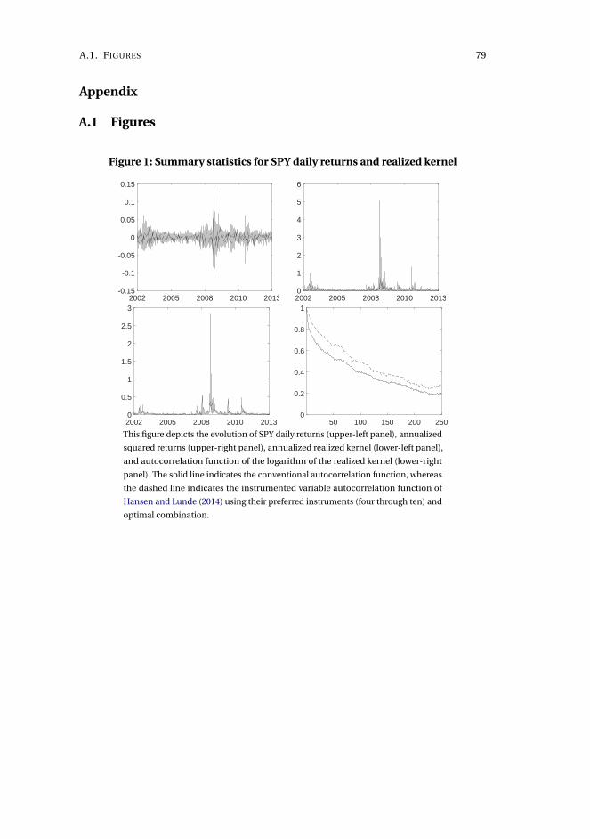
A.1. FIGURES 79
Appendix
A.1 Figures
Figure 1: Summary statistics for SPY daily returns and realized kernel
2002 2005 2008 2010 2013-0.15
-0.1
-0.05
0
0.05
0.1
0.15
2002 2005 2008 2010 20130
1
2
3
4
5
6
2002 2005 2008 2010 20130
0.5
1
1.5
2
2.5
3
50 100 150 200 2500
0.2
0.4
0.6
0.8
1
This figure depicts the evolution of SPY daily returns (upper-left panel), annualized
squared returns (upper-right panel), annualized realized kernel (lower-left panel),
and autocorrelation function of the logarithm of the realized kernel (lower-right
panel). The solid line indicates the conventional autocorrelation function, whereas
the dashed line indicates the instrumented variable autocorrelation function of
Hansen and Lunde (2014) using their preferred instruments (four through ten) and
optimal combination.
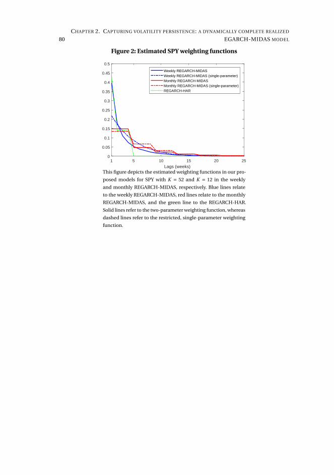
80
CHAPTER 2. CAPTURING VOLATILITY PERSISTENCE: A DYNAMICALLY COMPLETE REALIZED
EGARCH-MIDAS MODEL
Figure 2: Estimated SPY weighting functions
1 5 10 15 20 25
Lags (weeks)
0
0.05
0.1
0.15
0.2
0.25
0.3
0.35
0.4
0.45
0.5
Weekly REGARCH-MIDASWeekly REGARCH-MIDAS (single-parameter)Monthly REGARCH-MIDASMonthly REGARCH-MIDAS (single-parameter)REGARCH-HAR
This figure depicts the estimated weighting functions in our pro-
posed models for SPY with K = 52 and K = 12 in the weekly
and monthly REGARCH-MIDAS, respectively. Blue lines relate
to the weekly REGARCH-MIDAS, red lines relate to the monthly
REGARCH-MIDAS, and the green line to the REGARCH-HAR.
Solid lines refer to the two-parameter weighting function, whereas
dashed lines refer to the restricted, single-parameter weighting
function.
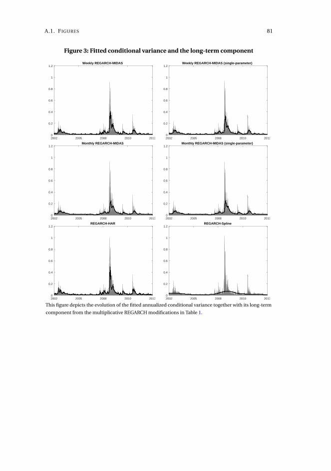
A.1. FIGURES 81
Figure 3: Fitted conditional variance and the long-term component
2002 2005 2008 2010 20130
0.2
0.4
0.6
0.8
1
1.2Weekly REGARCH-MIDAS
2002 2005 2008 2010 20130
0.2
0.4
0.6
0.8
1
1.2Weekly REGARCH-MIDAS (single-parameter)
2002 2005 2008 2010 20130
0.2
0.4
0.6
0.8
1
1.2Monthly REGARCH-MIDAS
2002 2005 2008 2010 20130
0.2
0.4
0.6
0.8
1
1.2Monthly REGARCH-MIDAS (single-parameter)
2002 2005 2008 2010 20130
0.2
0.4
0.6
0.8
1
1.2REGARCH-HAR
2002 2005 2008 2010 20130
0.2
0.4
0.6
0.8
1
1.2REGARCH-Spline
This figure depicts the evolution of the fitted annualized conditional variance together with its long-term
component from the multiplicative REGARCH modifications in Table 1.
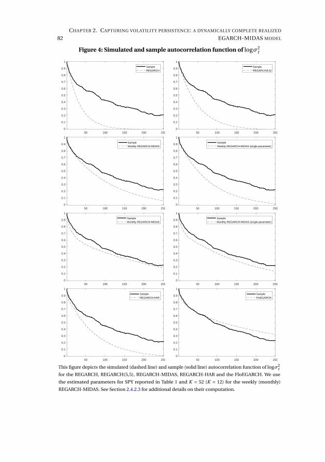
82
CHAPTER 2. CAPTURING VOLATILITY PERSISTENCE: A DYNAMICALLY COMPLETE REALIZED
EGARCH-MIDAS MODEL
Figure 4: Simulated and sample autocorrelation function of logσ2t
50 100 150 200 2500
0.1
0.2
0.3
0.4
0.5
0.6
0.7
0.8
0.9
1
SampleREGARCH
50 100 150 200 2500
0.1
0.2
0.3
0.4
0.5
0.6
0.7
0.8
0.9
1
SampleREGARCH(5,5)
50 100 150 200 2500
0.1
0.2
0.3
0.4
0.5
0.6
0.7
0.8
0.9
1
SampleWeekly REGARCH-MIDAS
50 100 150 200 2500
0.1
0.2
0.3
0.4
0.5
0.6
0.7
0.8
0.9
1
SampleWeekly REGARCH-MIDAS (single-parameter)
50 100 150 200 2500
0.1
0.2
0.3
0.4
0.5
0.6
0.7
0.8
0.9
1
SampleMonthly REGARCH-MIDAS
50 100 150 200 2500
0.1
0.2
0.3
0.4
0.5
0.6
0.7
0.8
0.9
1
SampleMonthly REGARCH-MIDAS (single-parameter)
50 100 150 200 2500
0.1
0.2
0.3
0.4
0.5
0.6
0.7
0.8
0.9
1
SampleREGARCH-HAR
50 100 150 200 2500
0.1
0.2
0.3
0.4
0.5
0.6
0.7
0.8
0.9
1
SampleFloEGARCH
This figure depicts the simulated (dashed line) and sample (solid line) autocorrelation function of logσ2t
for the REGARCH, REGARCH(5,5), REGARCH-MIDAS, REGARCH-HAR and the FloEGARCH. We use
the estimated parameters for SPY reported in Table 1 and K = 52 (K = 12) for the weekly (monthly)
REGARCH-MIDAS. See Section 2.4.2.3 for additional details on their computation.
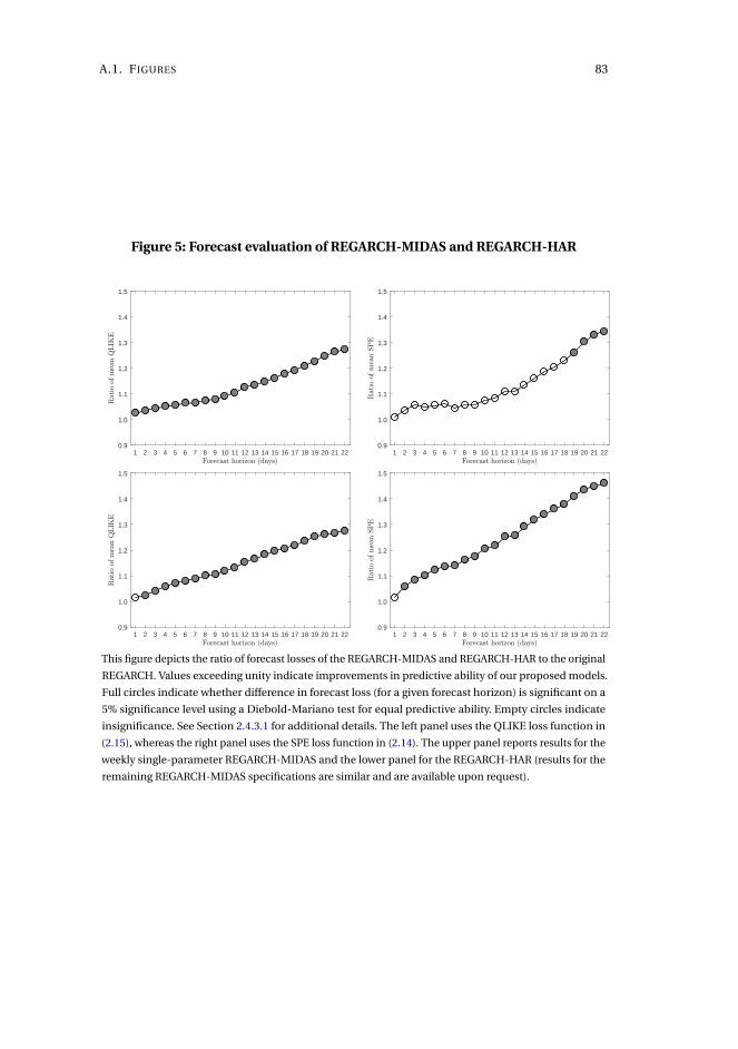
A.1. FIGURES 83
Figure 5: Forecast evaluation of REGARCH-MIDAS and REGARCH-HAR
1 2 3 4 5 6 7 8 9 10 11 12 13 14 15 16 17 18 19 20 21 220.9
1.0
1.1
1.2
1.3
1.4
1.5
1 2 3 4 5 6 7 8 9 10 11 12 13 14 15 16 17 18 19 20 21 220.9
1.0
1.1
1.2
1.3
1.4
1.5
1 2 3 4 5 6 7 8 9 10 11 12 13 14 15 16 17 18 19 20 21 220.9
1.0
1.1
1.2
1.3
1.4
1.5
1 2 3 4 5 6 7 8 9 10 11 12 13 14 15 16 17 18 19 20 21 220.9
1.0
1.1
1.2
1.3
1.4
1.5
This figure depicts the ratio of forecast losses of the REGARCH-MIDAS and REGARCH-HAR to the original
REGARCH. Values exceeding unity indicate improvements in predictive ability of our proposed models.
Full circles indicate whether difference in forecast loss (for a given forecast horizon) is significant on a
5% significance level using a Diebold-Mariano test for equal predictive ability. Empty circles indicate
insignificance. See Section 2.4.3.1 for additional details. The left panel uses the QLIKE loss function in
(2.15), whereas the right panel uses the SPE loss function in (2.14). The upper panel reports results for the
weekly single-parameter REGARCH-MIDAS and the lower panel for the REGARCH-HAR (results for the
remaining REGARCH-MIDAS specifications are similar and are available upon request).
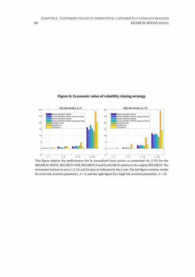
84
CHAPTER 2. CAPTURING VOLATILITY PERSISTENCE: A DYNAMICALLY COMPLETE REALIZED
EGARCH-MIDAS MODEL
Figure 6: Economic value of volatility-timing strategy
Low risk aversion: A = 3
k = 1 k = 5 k = 10 k = 22-5
0
5
10
15
20
25
30
Weekly REGARCH-MIDAS
Weekly REGARCH-MIDAS (single-parameter)
Monthly REGARCH-MIDAS
Monthly REGARCH-MIDAS (single-parameter)
REGARCH-HAR
REGARCH-S
FloEGARCH
High risk aversion: A = 10
k = 1 k = 5 k = 10 k = 22-5
0
5
10
15
20
25
30
Weekly REGARCH-MIDAS
Weekly REGARCH-MIDAS (single-parameter)
Monthly REGARCH-MIDAS
Monthly REGARCH-MIDAS (single-parameter)
REGARCH-HAR
REGARCH-S
FloEGARCH
This figure depicts the performance fee in annualized basis points as computed via (2.16) for the
REGARCH-MIDAS, REGARCH-HAR, REGARCH-S and FLoEGARCH relative to the original REGARCH. The
investment horizon is set to 1,5,10, and 22 days as indicated by the x-axis. The left figure contains results
for a low risk-aversion parameter, A = 3, and the right figure for a high risk-aversion parameter, A = 10.
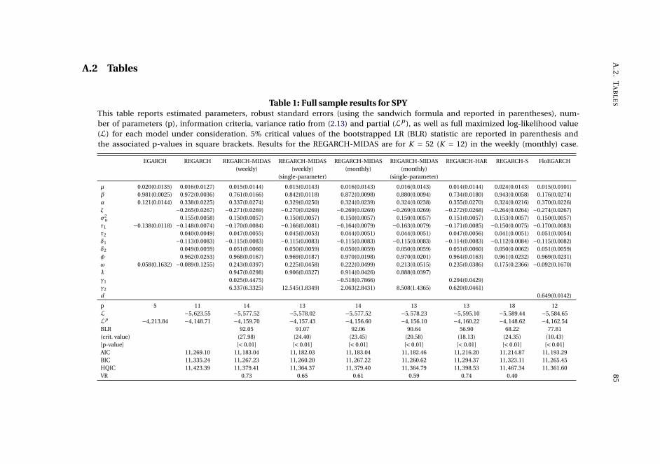
A.2
.T
AB
LE
S85
A.2 Tables
Table 1: Full sample results for SPYThis table reports estimated parameters, robust standard errors (using the sandwich formula and reported in parentheses), num-ber of parameters (p), information criteria, variance ratio from (2.13) and partial (Lp ), as well as full maximized log-likelihood value(L) for each model under consideration. 5% critical values of the bootstrapped LR (BLR) statistic are reported in parenthesis andthe associated p-values in square brackets. Results for the REGARCH-MIDAS are for K = 52 (K = 12) in the weekly (monthly) case.
EGARCH REGARCH REGARCH-MIDAS REGARCH-MIDAS REGARCH-MIDAS REGARCH-MIDAS REGARCH-HAR REGARCH-S FloEGARCH(weekly) (weekly) (monthly) (monthly)
(single-parameter) (single-parameter)
µ 0.020(0.0135) 0.016(0.0127) 0.015(0.0144) 0.015(0.0143) 0.016(0.0143) 0.016(0.0143) 0.014(0.0144) 0.024(0.0143) 0.015(0.0101)β 0.981(0.0025) 0.972(0.0036) 0.761(0.0166) 0.842(0.0118) 0.872(0.0098) 0.880(0.0094) 0.734(0.0180) 0.943(0.0058) 0.176(0.0274)α 0.121(0.0144) 0.338(0.0225) 0.337(0.0274) 0.329(0.0250) 0.324(0.0239) 0.324(0.0238) 0.355(0.0270) 0.324(0.0216) 0.370(0.0226)ξ −0.265(0.0267) −0.271(0.0269) −0.270(0.0269) −0.269(0.0269) −0.269(0.0269) −0.272(0.0268) −0.264(0.0264) −0.274(0.0267)σ2
u 0.155(0.0058) 0.150(0.0057) 0.150(0.0057) 0.150(0.0057) 0.150(0.0057) 0.151(0.0057) 0.153(0.0057) 0.150(0.0057)τ1 −0.138(0.0118) −0.148(0.0074) −0.170(0.0084) −0.166(0.0081) −0.164(0.0079) −0.163(0.0079) −0.171(0.0085) −0.150(0.0075) −0.170(0.0083)τ2 0.040(0.0049) 0.047(0.0055) 0.045(0.0053) 0.044(0.0051) 0.044(0.0051) 0.047(0.0056) 0.041(0.0051) 0.051(0.0054)δ1 −0.113(0.0083) −0.115(0.0083) −0.115(0.0083) −0.115(0.0083) −0.115(0.0083) −0.114(0.0083) −0.112(0.0084) −0.115(0.0082)δ2 0.049(0.0059) 0.051(0.0060) 0.050(0.0059) 0.050(0.0059) 0.050(0.0059) 0.051(0.0060) 0.050(0.0062) 0.051(0.0059)φ 0.962(0.0253) 0.968(0.0167) 0.969(0.0187) 0.970(0.0198) 0.970(0.0201) 0.964(0.0163) 0.961(0.0232) 0.969(0.0231)ω 0.058(0.1632) −0.089(0.1255) 0.243(0.0397) 0.225(0.0458) 0.222(0.0499) 0.213(0.0515) 0.235(0.0386) 0.175(0.2366) −0.092(0.1670)λ 0.947(0.0298) 0.906(0.0327) 0.914(0.0426) 0.888(0.0397)γ1 0.025(0.4475) −0.518(0.7866) 0.294(0.0429)γ2 6.337(6.3325) 12.545(1.8349) 2.063(2.8431) 8.508(1.4365) 0.620(0.0461)d 0.649(0.0142)
p 5 11 14 13 14 13 13 18 12L −5,623.55 −5,577.52 −5,578.02 −5,577.52 −5,578.23 −5,595.10 −5,589.44 −5,584.65Lp −4,213.84 −4,148.71 −4,159.70 −4,157.43 −4,156.60 −4,156.10 −4,160.22 −4,148.62 −4,162.54BLR 92.05 91.07 92.06 90.64 56.90 68.22 77.81(crit. value) (27.98) (24.40) (23.45) (20.58) (18.13) (24.35) (10.43)[p-value] [< 0.01] [< 0.01] [< 0.01] [< 0.01] [< 0.01] [< 0.01] [< 0.01]AIC 11,269.10 11,183.04 11,182.03 11,183.04 11,182.46 11,216.20 11,214.87 11,193.29BIC 11,335.24 11,267.23 11,260.20 11,267.22 11,260.62 11,294.37 11,323.11 11,265.45HQIC 11,423.39 11,379.41 11,364.37 11,379.40 11,364.79 11,398.53 11,467.34 11,361.60VR 0.73 0.65 0.61 0.59 0.74 0.40
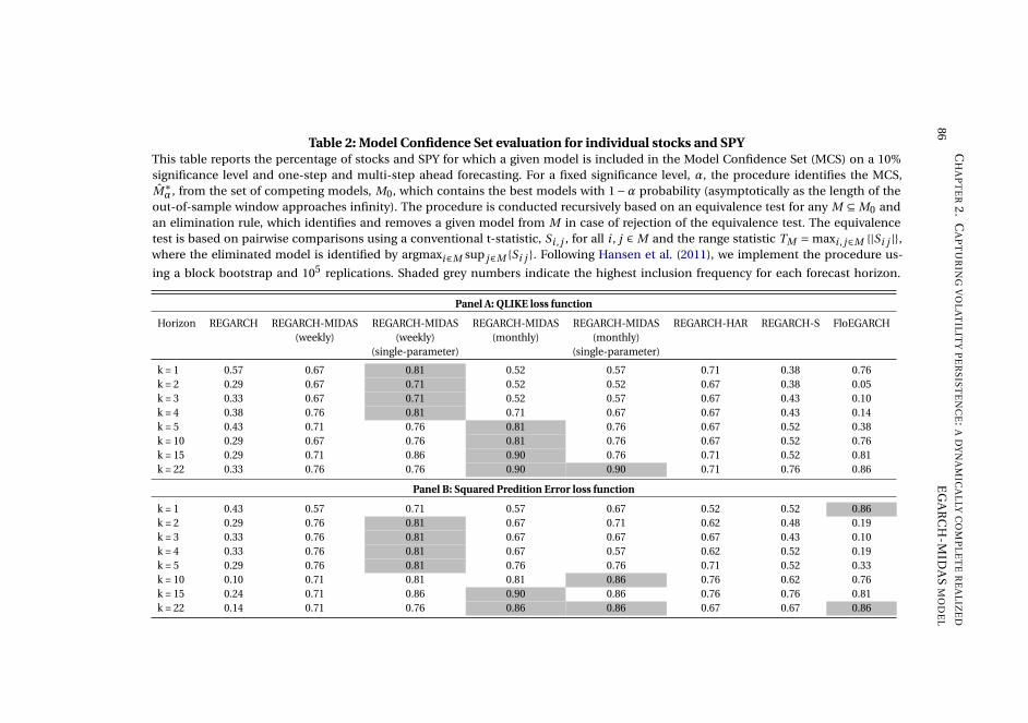
86
CH
AP
TE
R2
.C
AP
TU
RIN
GV
OL
AT
ILIT
YP
ER
SIS
TE
NC
E:A
DY
NA
MIC
AL
LYC
OM
PL
ET
ER
EA
LIZ
ED
EG
AR
CH
-MID
AS
MO
DE
L
Table 2: Model Confidence Set evaluation for individual stocks and SPYThis table reports the percentage of stocks and SPY for which a given model is included in the Model Confidence Set (MCS) on a 10%significance level and one-step and multi-step ahead forecasting. For a fixed significance level, α, the procedure identifies the MCS,M∗α, from the set of competing models, M0, which contains the best models with 1−α probability (asymptotically as the length of the
out-of-sample window approaches infinity). The procedure is conducted recursively based on an equivalence test for any M ⊆ M0 andan elimination rule, which identifies and removes a given model from M in case of rejection of the equivalence test. The equivalencetest is based on pairwise comparisons using a conventional t-statistic, Si , j , for all i , j ∈ M and the range statistic TM = maxi , j∈M |Si j |,where the eliminated model is identified by argmaxi∈M sup j∈M Si j . Following Hansen et al. (2011), we implement the procedure us-
ing a block bootstrap and 105 replications. Shaded grey numbers indicate the highest inclusion frequency for each forecast horizon.
Panel A: QLIKE loss function
Horizon REGARCH REGARCH-MIDAS REGARCH-MIDAS REGARCH-MIDAS REGARCH-MIDAS REGARCH-HAR REGARCH-S FloEGARCH(weekly) (weekly) (monthly) (monthly)
(single-parameter) (single-parameter)
k = 1 0.57 0.67 0.81 0.52 0.57 0.71 0.38 0.76k = 2 0.29 0.67 0.71 0.52 0.52 0.67 0.38 0.05k = 3 0.33 0.67 0.71 0.52 0.57 0.67 0.43 0.10k = 4 0.38 0.76 0.81 0.71 0.67 0.67 0.43 0.14k = 5 0.43 0.71 0.76 0.81 0.76 0.67 0.52 0.38k = 10 0.29 0.67 0.76 0.81 0.76 0.67 0.52 0.76k = 15 0.29 0.71 0.86 0.90 0.76 0.71 0.52 0.81k = 22 0.33 0.76 0.76 0.90 0.90 0.71 0.76 0.86
Panel B: Squared Predition Error loss function
k = 1 0.43 0.57 0.71 0.57 0.67 0.52 0.52 0.86k = 2 0.29 0.76 0.81 0.67 0.71 0.62 0.48 0.19k = 3 0.33 0.76 0.81 0.67 0.67 0.67 0.43 0.10k = 4 0.33 0.76 0.81 0.67 0.57 0.62 0.52 0.19k = 5 0.29 0.76 0.81 0.76 0.76 0.71 0.52 0.33k = 10 0.10 0.71 0.81 0.81 0.86 0.76 0.62 0.76k = 15 0.24 0.71 0.86 0.90 0.86 0.76 0.76 0.81k = 22 0.14 0.71 0.76 0.86 0.86 0.67 0.67 0.86

A.3. SUPPLEMENTARY APPENDIX 87
A.3 Supplementary Appendix
Abstract
This Supplementary Appendix provides results, in this order, on the score func-
tion of the log-likelihood functions associated with the REGARCH-MIDAS and
REGARCH-HAR, the choice of the lag length of the MIDAS filter for the use in our
empirical analysis, the autocorrelation function of the realized kernel of the mod-
els under consideration as well as summary statistics and in- and out-of-sample
results for our sample of 20 individual stocks.
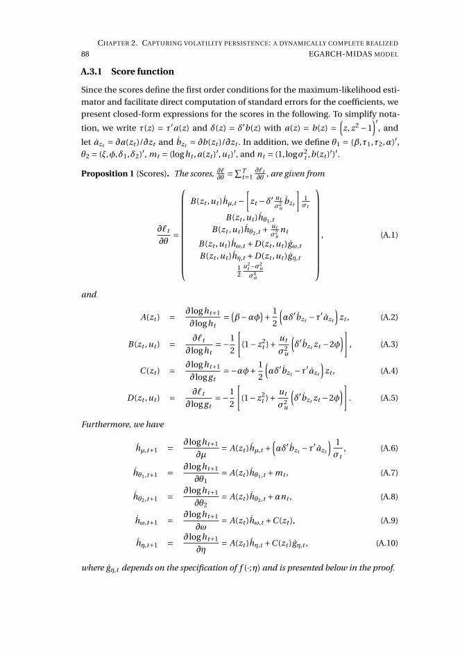
88
CHAPTER 2. CAPTURING VOLATILITY PERSISTENCE: A DYNAMICALLY COMPLETE REALIZED
EGARCH-MIDAS MODEL
A.3.1 Score function
Since the scores define the first order conditions for the maximum-likelihood esti-
mator and facilitate direct computation of standard errors for the coefficients, we
present closed-form expressions for the scores in the following. To simplify nota-
tion, we write τ(z) = τ′a(z) and δ(z) = δ′b(z) with a(z) = b(z) =(z, z2 −1
)′, and
let azt = ∂a(zt )/∂zt and bzt = ∂b(zt )/∂zt . In addition, we define θ1 = (β,τ1,τ2,α)′,θ2 = (ξ,φ,δ1,δ2)′, mt = (loght , a(zt )′,ut )′, and nt = (1, logσ2
t ,b(zt )′)′.
Proposition 1 (Scores). The scores, ∂`∂θ =∑Tt=1
∂`t∂θ , are given from
∂`t
∂θ=
B(zt ,ut )hµ,t −[
zt −δ′ ut
σ2u
bzt
]1σt
B(zt ,ut )hθ1,t
B(zt ,ut )hθ2,t + ut
σ2u
nt
B(zt ,ut )hω,t +D(zt ,ut )gω,t
B(zt ,ut )hη,t +D(zt ,ut )gη,t
12
u2t −σ2
u
σ4u
, (A.1)
and
A(zt ) = ∂ loght+1
∂ loght= (
β−αφ)+ 1
2
(αδ′bzt −τ′azt
)zt , (A.2)
B(zt ,ut ) = ∂`t
∂ loght=−1
2
[(1− z2
t )+ ut
σ2u
(δ′bzt zt −2φ
)], (A.3)
C (zt ) = ∂ loght+1
∂ log g t=−αφ+ 1
2
(αδ′bzt −τ′azt
)zt , (A.4)
D(zt ,ut ) = ∂`t
∂ log g t=−1
2
[(1− z2
t )+ ut
σ2u
(δ′bzt zt −2φ
)]. (A.5)
Furthermore, we have
hµ,t+1 = ∂ loght+1
∂µ= A(zt )hµ,t +
(αδ′bzt −τ′azt
) 1
σt, (A.6)
hθ1,t+1 = ∂ loght+1
∂θ1= A(zt )hθ1,t +mt , (A.7)
hθ2,t+1 = ∂ loght+1
∂θ2= A(zt )hθ2,t +αnt , (A.8)
hω,t+1 = ∂ loght+1
∂ω= A(zt )hω,t +C (zt ), (A.9)
hη,t+1 = ∂ loght+1
∂η= A(zt )hη,t +C (zt )gη,t , (A.10)
where gη,t depends on the specification of f (·;η) and is presented below in the proof.
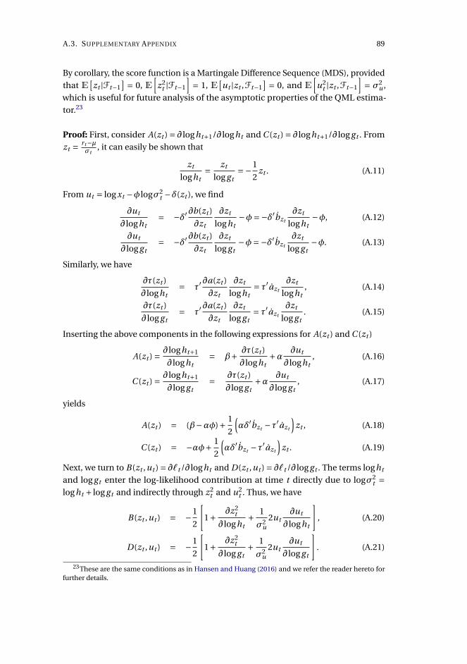
A.3. SUPPLEMENTARY APPENDIX 89
By corollary, the score function is a Martingale Difference Sequence (MDS), provided
that E[zt |Ft−1
] = 0, E[
z2t |Ft−1
]= 1, E
[ut |zt ,Ft−1
] = 0, and E[
u2t |zt ,Ft−1
]= σ2
u ,
which is useful for future analysis of the asymptotic properties of the QML estima-
tor.23
Proof: First, consider A(zt ) = ∂ loght+1/∂ loght and C (zt ) = ∂ loght+1/∂ log g t . From
zt = rt−µσt
, it can easily be shown that
zt
loght= zt
log g t=−1
2zt . (A.11)
From ut = log xt −φ logσ2t −δ(zt ), we find
∂ut
∂ loght= −δ′ ∂b(zt )
∂zt
∂zt
loght−φ=−δ′bzt
∂zt
loght−φ, (A.12)
∂ut
∂ log g t= −δ′ ∂b(zt )
∂zt
∂zt
log g t−φ=−δ′bzt
∂zt
log g t−φ. (A.13)
Similarly, we have
∂τ(zt )
∂ loght= τ′
∂a(zt )
∂zt
∂zt
loght= τ′azt
∂zt
loght, (A.14)
∂τ(zt )
∂ log g t= τ′
∂a(zt )
∂zt
∂zt
log g t= τ′azt
∂zt
log g t. (A.15)
Inserting the above components in the following expressions for A(zt ) and C (zt )
A(zt ) = ∂ loght+1
∂ loght= β+ ∂τ(zt )
∂ loght+α ∂ut
∂ loght, (A.16)
C (zt ) = ∂ loght+1
∂ log g t= ∂τ(zt )
∂ log g t+α ∂ut
∂ log g t, (A.17)
yields
A(zt ) = (β−αφ)+ 1
2
(αδ′bzt −τ′azt
)zt , (A.18)
C (zt ) = −αφ+ 1
2
(αδ′bzt −τ′azt
)zt . (A.19)
Next, we turn to B(zt ,ut ) = ∂`t /∂ loght and D(zt ,ut ) = ∂`t /∂ log g t . The terms loght
and log g t enter the log-likelihood contribution at time t directly due to logσ2t =
loght + log g t and indirectly through z2t and u2
t . Thus, we have
B(zt ,ut ) = −1
2
[1+ ∂z2
t
∂ loght+ 1
σ2u
2ut∂ut
∂ loght
], (A.20)
D(zt ,ut ) = −1
2
[1+ ∂z2
t
∂ log g t+ 1
σ2u
2ut∂ut
∂ log g t
]. (A.21)
23These are the same conditions as in Hansen and Huang (2016) and we refer the reader hereto forfurther details.
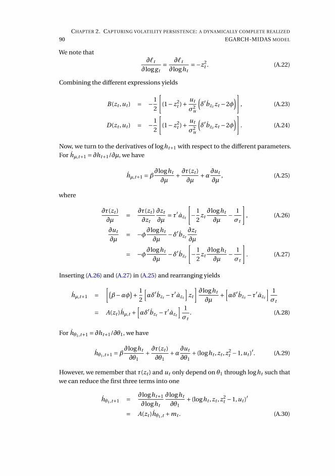
90
CHAPTER 2. CAPTURING VOLATILITY PERSISTENCE: A DYNAMICALLY COMPLETE REALIZED
EGARCH-MIDAS MODEL
We note that∂`t
∂ log g t= ∂`t
∂ loght=−z2
t . (A.22)
Combining the different expressions yields
B(zt ,ut ) = −1
2
[(1− z2
t )+ ut
σ2u
(δ′bzt zt −2φ
)], (A.23)
D(zt ,ut ) = −1
2
[(1− z2
t )+ ut
σ2u
(δ′bzt zt −2φ
)]. (A.24)
Now, we turn to the derivatives of loght+1 with respect to the different parameters.
For hµ,t+1 = ∂ht+1/∂µ, we have
hµ,t+1 =β∂ loght
∂µ+ ∂τ(zt )
∂µ+α∂ut
∂µ, (A.25)
where
∂τ(zt )
∂µ= ∂τ(zt )
∂zt
∂zt
∂µ= τ′azt
[−1
2zt∂ loght
∂µ− 1
σt
], (A.26)
∂ut
∂µ= −φ∂ loght
∂µ−δ′bzt
∂zt
∂µ
= −φ∂ loght
∂µ−δ′bzt
[−1
2zt∂ loght
∂µ− 1
σt
]. (A.27)
Inserting (A.26) and (A.27) in (A.25) and rearranging yields
hµ,t+1 =[(β−αφ)+ 1
2
[αδ′bzt −τ′azt
]zt
]∂ loght
∂µ+
[αδ′bzt −τ′azt
] 1
σt
= A(zt )hµ,t +[αδ′bzt −τ′azt
] 1
σt. (A.28)
For hθ1,t+1 = ∂ht+1/∂θ1, we have
hθ1,t+1 =β∂ loght
∂θ1+ ∂τ(zt )
∂θ1+α∂ut
∂θ1+ (loght , zt , z2
t −1,ut )′. (A.29)
However, we remember that τ(zt ) and ut only depend on θ1 through loght such that
we can reduce the first three terms into one
hθ1,t+1 = ∂ loght+1
∂ loght
∂ loght
∂θ1+ (loght , zt , z2
t −1,ut )′
= A(zt )hθ1,t +mt . (A.30)

A.3. SUPPLEMENTARY APPENDIX 91
For hθ2,t+1 = ∂ht+1/∂θ2, hω,t+1 = ∂ht+1/∂ω and hη,t+1 = ∂ht+1/∂η, we obtain
hθ2,t+1 = ∂ loght+1
∂ loght
∂ loght
∂θ2+α(1, logσ2
t , zt , z2t −1)′
= A(zt )hθ2,t +nt , (A.31)
hω,t+1 = ∂ loght+1
∂ loght
∂ loght
∂ω+ ∂ loght+1
∂ log g t
∂ log g t
∂ω
= A(zt )hω,t +C (zt ), (A.32)
hη,t+1 = ∂ loght+1
∂ loght
∂ loght
∂η+ ∂ loght+1
∂ log g t
∂ log g t
∂η
= A(zt )hη,t +C (zt )gη,t , (A.33)
respectively. Finally, we turn to the scores. The parameter µ enters the log-likelihood
contribution at time t through loght , zt , and u2t such that
∂`t
∂µ= −1
2hµ,t −
z2t
∂µ− 1
2
1
σ2u
∂u2t
∂µ
= ∂`t
∂ loght
∂ loght
∂µ−
[zt −δ′ ut
σ2u
bzt
]1
σt
= B(zt ,ut )hµ,t −[
zt −δ′ ut
σ2u
bzt
]1
σt. (A.34)
Since θ1 only enters the log-likelihood contribution at time t indirectly through loght ,
an application of the chain-rule yields
∂`t
∂θ1= B(zt ,ut )hθ1,t . (A.35)
The parameter vector θ2 also enters through u2t ,
∂`t
∂θ2= B(zt ,ut )hθ2,t +
ut
σ2u
nt . (A.36)
The parameters ω and η enter through loght and log g t ,
∂`t
∂ω= B(zt ,ut )hω,t +D(zt ,ut )gω,t ,
∂`t
∂η= B(zt ,ut )hη,t +D(zt ,ut )gη,t . (A.37)
The parameter σ2u only enters directly in the log-likelihood contribution such that
∂`t
∂σ2u
= 1
2
u2t −σ2
u
σ2u
. (A.38)
Stacking the above scores,
∂`t
∂θ=
(∂`t
∂µ,∂`t
∂θ′1,∂`t
∂θ′2,∂`t
∂ω,∂`t
∂η′,∂`t
∂σ2u
)′, (A.39)
yields the result in Proposition 1.
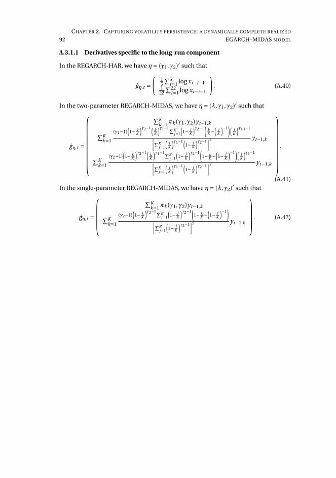
92
CHAPTER 2. CAPTURING VOLATILITY PERSISTENCE: A DYNAMICALLY COMPLETE REALIZED
EGARCH-MIDAS MODEL
A.3.1.1 Derivatives specific to the long-run component
In the REGARCH-HAR, we have η= (γ1,γ2)′ such that
gη,t =(
15
∑5i=1 log xt−i−1
122
∑22i=1 log xt−i−1
). (A.40)
In the two-parameter REGARCH-MIDAS, we have η= (λ,γ1,γ2)′ such that
gη,t =
∑Kk=1πk (γ1,γ2)yt−1,k∑K
k=1
(γ1−1)(1− k
K
)γ2−1(kK
)γ1−1 ∑Kj=1
(1− j
K
)γ2−1(
kK −
(j
K
)−1)(
jK
)γ1,i −1
[∑Kj=1
(j
K
)γ1−1(1− j
K
)γ2−1]2 yt−1,k
∑Kk=1
(γ2−1)(1− k
K
)γ2−1(kK
)γ1−1 ∑Kj=1
(1− j
K
)γ2−1(1− k
K −(1− j
K
)−1)(
jK
)γ1−1
[∑Kj=1
(j
K
)γ1−1(1− j
K
)γ2−1]2 yt−1,k
.
(A.41)
In the single-parameter REGARCH-MIDAS, we have η= (λ,γ2)′ such that
gη,t =
∑K
k=1πk (γ1,γ2)yt−1,k∑Kk=1
(γ2−1)(1− k
K
)γ2−1 ∑Kj=1
(1− j
K
)γ2−1(1− k
K −(1− j
K
)−1)
[∑Kj=1
(1− j
K
)γ2−1]2 yt−1,k
. (A.42)

A.3. SUPPLEMENTARY APPENDIX 93
A.3.2 Checking validity of the asymptotic distribution of the estimators
To check the validity of the assumed asymptotic distribution of the estimators, we
employ a parametric bootstrapping technique (Paparoditis and Politis, 2009). We use
999 replications, a sample size of 2,500 observations (approximately 10 years, similar
to the size of the rolling in-sample window used in the forecasting exercise below),
and re-sampled residuals from the empirical distribution to bootstrap observations.
Figure 7 depicts the empirical standardized distribution of a subset of the estimated
parameters.
It stands out that the in-sample distribution of the estimated parameters for both the
REGARCH, REGARCH-MIDAS and REGRACH-HAR is generally in agreement with a
standard normal distribution. We also compared the bootstrapped standard errors
with the robust QML standard errors computed from the sandwich-formula, which
are reported in the empirical section below. The standard errors were quite similar,
which in conjunction with Figure 7 does not contradict the assertion that the QML
approach and associated inferences are valid. We do, however, note that the QML
standard errors are slightly smaller on average relative to the bootstrapped standard
errors, causing us to be careful in not putting too much weight on the role of standard
errors in the interpretation of the results in the paper.
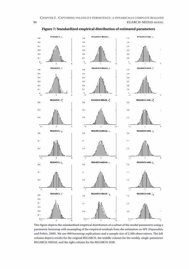
94
CHAPTER 2. CAPTURING VOLATILITY PERSISTENCE: A DYNAMICALLY COMPLETE REALIZED
EGARCH-MIDAS MODEL
Figure 7: Standardized empirical distribution of estimated parameters
This figure depicts the standardized empirical distribution of a subset of the model parameters using a
parametric bootstrap with resampling of the empirical residuals from the estimation on SPY (Paparoditis
and Politis, 2009). We use 999 bootstrap replications and a sample size of 2,500 observations. The left
column depicts results for the original REGARCH, the middle column for the weekly, single-parameter
REGARCH-MIDAS, and the right column for the REGARCH-HAR.

A.3. SUPPLEMENTARY APPENDIX 95
A.3.3 Fractional integration parameter d and unit root tests
We estimate the fractional integrated parameter d in the logarithm of the realized
kernel with the two-step exact local Whittle estimator of Shimotsu (2010). Over the
full sample all series have d > 0.5, suggesting that volatility is highly persistent.24
This finding is supported by the slowly decaying ACF of the logarithm of the realized
kernel for SPY. Since the conventional ACF may be biased for the unobserved ACF
of the logarithm conditional variance due to the presence of measurement errors,25
we also compute the instrumented ACF proposed by Hansen and Lunde (2014). We
use the authors’ preferred specification with multiple instruments (four through
ten) and optimal combination. The instrumented ACF show a similar pattern as
the conventional ACF, but points toward an even higher degree of persistence. We
also conducted a (Dickey-Fuller) unit root test across all assets considered using the
instrumented persistence parameter (cf. Table 3).
The (biased) conventional least square estimates point to moderate persistence and
strong rejection of a unit root. The persistence parameter is, as expected, notably
higher when using the instrumented variables estimator of Hansen and Lunde (2014),
however the null hypothesis of a unit root remains rejected for all assets. Collectively,
these findings motivate a modeling framework that is capable of capturing a high
degree of persistence. Given the requirement that |β| < 1, this also motivates a frame-
work that pulls β away from unity. This is where the proposed REGARCH-MIDAS and
REGARCH-HAR prove useful.
24We estimated the parameters with m = bT q c for q =∈ 0.50,0.55, . . . ,0.80, leading to no alterations ofthe conclusions obtained for q = 0.65. See also Wenger et al. (2017) for a comprehensive empirical studyon long memory in volatility and the choice of estimator of d .
25The element of microstructure noise is, arguably, low, given the construction of the realized kernel,however sampling error may still be present, causing the differences in the conventional and instrumentedACF.
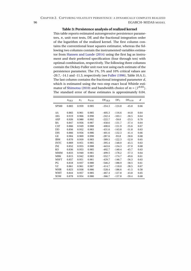
96
CHAPTER 2. CAPTURING VOLATILITY PERSISTENCE: A DYNAMICALLY COMPLETE REALIZED
EGARCH-MIDAS MODEL
Table 3: Persistence analysis of realized kernelThis table reports estimated autoregressive persistence parame-ters, π, unit root tests, DF, and the fractional integration orderof the logarithm of the realized kernel. The first column con-tains the conventional least squares estimator, whereas the fol-lowing two columns contain the instrumented variables estima-tor from Hansen and Lunde (2014) using the first lag as instru-ment and their preferred specification (four through ten) withoptimal combination, respectively. The following three columnscontain the Dickey-Fuller unit root test using each estimate of thepersistence parameter. The 1%, 5% and 10% critical values are-20.7, -14.1 and -11.3, respectively (see Fuller (1996), Table 10.A.1).The last column contains the fractional integrated parameter d ,which is estimated using the two-step exact local Whittle esti-mator of Shimotsu (2010) and bandwidth choice of m = bT 0.65c.The standard error of these estimates is approximately 0.04.
πOLS π1 π4:10 DFOLS DF1 DF4:10 d
SP500 0.883 0.959 0.985 -354.3 -124.8 -45.8 0.66
AA 0.865 0.961 0.985 -405.3 -116.6 -44.8 0.64AIG 0.919 0.966 0.990 -242.4 -103.1 -30.5 0.64AXP 0.926 0.980 0.992 -222.7 -59.0 -23.5 0.70BA 0.847 0.956 0.987 -458.6 -131.7 -37.4 0.64CAT 0.866 0.949 0.988 -400.6 -151.9 -35.6 0.67DD 0.856 0.952 0.983 -431.6 -143.8 -51.8 0.63DIS 0.866 0.956 0.986 -401.6 -132.3 -41.4 0.66GE 0.904 0.969 0.990 -287.6 -93.8 -30.6 0.68IBM 0.870 0.959 0.983 -389.5 -122.3 -52.0 0.65INTC 0.869 0.951 0.985 -395.4 -148.0 -45.5 0.63JNJ 0.852 0.955 0.988 -443.6 -134.3 -37.0 0.68KO 0.836 0.953 0.985 -492.7 -140.4 -45.7 0.63MMM 0.833 0.940 0.981 -499.5 -178.2 -57.3 0.64MRK 0.815 0.942 0.983 -552.7 -174.7 -49.6 0.61MSFT 0.857 0.951 0.981 -429.7 -146.7 -56.3 0.63PG 0.818 0.937 0.980 -546.2 -188.9 -58.5 0.61VZ 0.861 0.961 0.987 -414.7 -118.0 -38.5 0.67WHR 0.823 0.938 0.986 -528.4 -186.6 -41.5 0.58WMT 0.844 0.957 0.985 -467.4 -127.8 -43.8 0.65XOM 0.878 0.954 0.980 -366.7 -137.8 -59.4 0.68
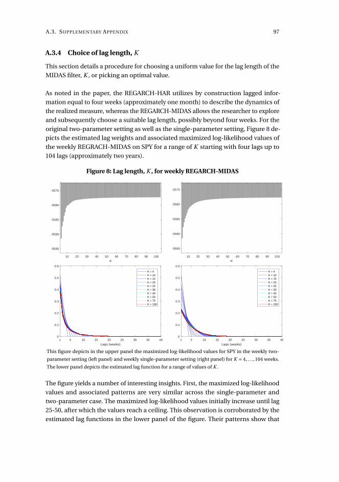
A.3. SUPPLEMENTARY APPENDIX 97
A.3.4 Choice of lag length, K
This section details a procedure for choosing a uniform value for the lag length of the
MIDAS filter, K , or picking an optimal value.
As noted in the paper, the REGARCH-HAR utilizes by construction lagged infor-
mation equal to four weeks (approximately one month) to describe the dynamics of
the realized measure, whereas the REGARCH-MIDAS allows the researcher to explore
and subsequently choose a suitable lag length, possibly beyond four weeks. For the
original two-parameter setting as well as the single-parameter setting, Figure 8 de-
picts the estimated lag weights and associated maximized log-likelihood values of
the weekly REGRACH-MIDAS on SPY for a range of K starting with four lags up to
104 lags (approximately two years).
Figure 8: Lag length, K , for weekly REGARCH-MIDAS
10 20 30 40 50 60 70 80 90 100
K
-5595
-5590
-5585
-5580
-5575
10 20 30 40 50 60 70 80 90 100
K
-5595
-5590
-5585
-5580
-5575
1 5 10 15 20 25 30 35 40
Lags (weeks)
0
0.1
0.2
0.3
0.4
0.5
0.6
K = 4K = 10K = 15K = 20K = 25K = 30K = 40K = 50K = 75K = 100
1 5 10 15 20 25 30 35 40
Lags (weeks)
0
0.1
0.2
0.3
0.4
0.5
0.6
K = 4K = 10K = 15K = 20K = 25K = 30K = 40K = 50K = 75K = 100
This figure depicts in the upper panel the maximized log-likelihood values for SPY in the weekly two-
parameter setting (left panel) and weekly single-parameter setting (right panel) for K = 4, . . . ,104 weeks.
The lower panel depicts the estimated lag function for a range of values of K .
The figure yields a number of interesting insights. First, the maximized log-likelihood
values and associated patterns are very similar across the single-parameter and
two-parameter case. The maximized log-likelihood values initially increase until lag
25-50, after which the values reach a ceiling. This observation is corroborated by the
estimated lag functions in the lower panel of the figure. Their patterns show that
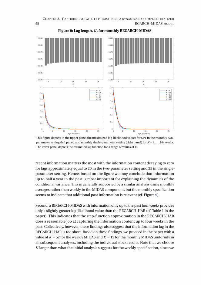
98
CHAPTER 2. CAPTURING VOLATILITY PERSISTENCE: A DYNAMICALLY COMPLETE REALIZED
EGARCH-MIDAS MODEL
Figure 9: Lag length, K , for monthly REGARCH-MIDAS
5 10 15 20 25
K
-5590
-5585
-5580
-5575
-5570
-5565
-5560
5 10 15 20 25
K
-5590
-5585
-5580
-5575
-5570
-5565
-5560
1 5 10 15 20 25
Lags (months)
0
0.1
0.2
0.3
0.4
0.5
0.6
0.7
K = 5K = 10K = 15K = 20K = 25
1 5 10 15 20 25
Lags (months)
0
0.1
0.2
0.3
0.4
0.5
0.6
K = 5K = 10K = 15K = 20K = 25
This figure depicts in the upper panel the maximized log-likelihood values for SPY in the monthly two-
parameter setting (left panel) and monthly single-parameter setting (right panel) for K = 4, . . . ,104 weeks.
The lower panel depicts the estimated lag function for a range of values of K .
recent information matters the most with the information content decaying to zero
for lags approximately equal to 20 in the two-parameter setting and 25 in the single-
parameter setting. Hence, based on the figure we may conclude that information
up to half a year in the past is most important for explaining the dynamics of the
conditional variance. This is generally supported by a similar analysis using monthly
averages rather than weekly in the MIDAS component, but the monthly specification
seems to indicate that additional past information is relevant (cf. Figure 9).
Second, a REGARCH-MIDAS with information only up to the past four weeks provides
only a slightly greater log-likelihood value than the REGARCH-HAR (cf. Table 1 in the
paper). This indicates that the step-function approximation in the REGARCH-HAR
does a reasonable job at capturing the information content up to four weeks in the
past. Collectively, however, these findings also suggest that the information lag in the
REGARCH-HAR is too short. Based on these findings, we proceed in the paper with a
value of K = 52 for the weekly MIDAS and K = 12 for the monthly MIDAS uniformly in
all subsequent analyses, including the individual stock results. Note that we choose
K larger than what the initial analysis suggests for the weekly specification, since we
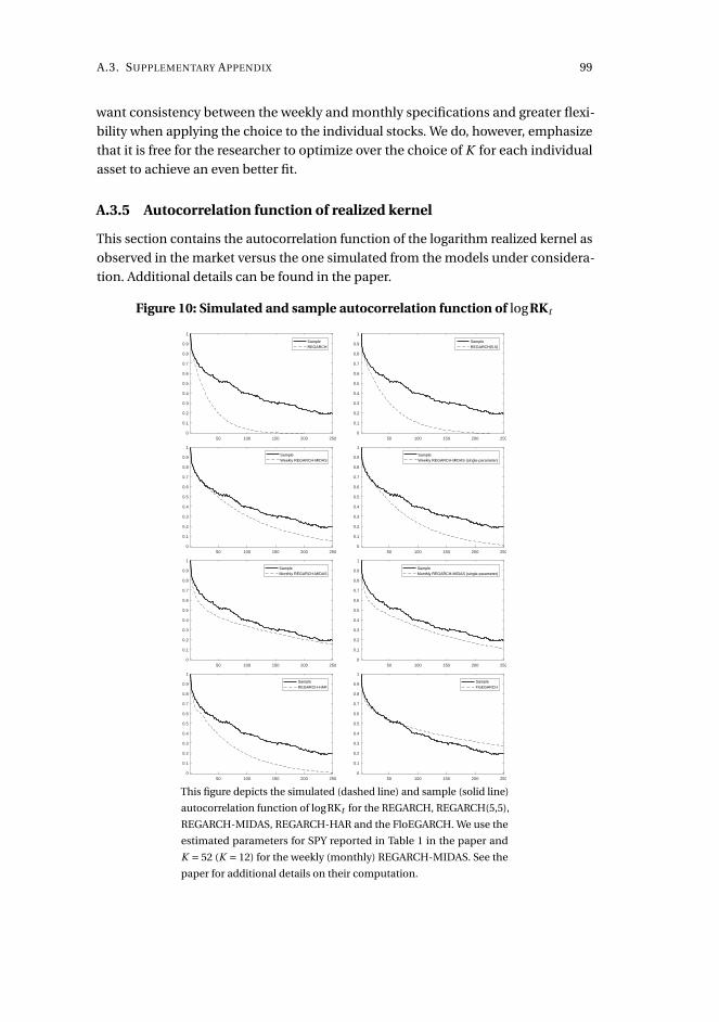
A.3. SUPPLEMENTARY APPENDIX 99
want consistency between the weekly and monthly specifications and greater flexi-
bility when applying the choice to the individual stocks. We do, however, emphasize
that it is free for the researcher to optimize over the choice of K for each individual
asset to achieve an even better fit.
A.3.5 Autocorrelation function of realized kernel
This section contains the autocorrelation function of the logarithm realized kernel as
observed in the market versus the one simulated from the models under considera-
tion. Additional details can be found in the paper.
Figure 10: Simulated and sample autocorrelation function of logRKt
50 100 150 200 2500
0.1
0.2
0.3
0.4
0.5
0.6
0.7
0.8
0.9
1
SampleREGARCH
50 100 150 200 2500
0.1
0.2
0.3
0.4
0.5
0.6
0.7
0.8
0.9
1
SampleREGARCH(5,5)
50 100 150 200 2500
0.1
0.2
0.3
0.4
0.5
0.6
0.7
0.8
0.9
1
SampleWeekly REGARCH-MIDAS
50 100 150 200 2500
0.1
0.2
0.3
0.4
0.5
0.6
0.7
0.8
0.9
1
SampleWeekly REGARCH-MIDAS (single-parameter)
50 100 150 200 2500
0.1
0.2
0.3
0.4
0.5
0.6
0.7
0.8
0.9
1
SampleMonthly REGARCH-MIDAS
50 100 150 200 2500
0.1
0.2
0.3
0.4
0.5
0.6
0.7
0.8
0.9
1
SampleMonthly REGARCH-MIDAS (single-parameter)
50 100 150 200 2500
0.1
0.2
0.3
0.4
0.5
0.6
0.7
0.8
0.9
1
SampleREGARCH-HAR
50 100 150 200 2500
0.1
0.2
0.3
0.4
0.5
0.6
0.7
0.8
0.9
1
SampleFloEGARCH
This figure depicts the simulated (dashed line) and sample (solid line)
autocorrelation function of logRKt for the REGARCH, REGARCH(5,5),
REGARCH-MIDAS, REGARCH-HAR and the FloEGARCH. We use the
estimated parameters for SPY reported in Table 1 in the paper and
K = 52 (K = 12) for the weekly (monthly) REGARCH-MIDAS. See the
paper for additional details on their computation.

100
CHAPTER 2. CAPTURING VOLATILITY PERSISTENCE: A DYNAMICALLY COMPLETE REALIZED
EGARCH-MIDAS MODEL
A.3.6 Empirical results for individual stocks
This section presents in-sample and out-of-sample results for our parallel analysis
on 20 individual stocks as referred to in the paper. Additional details are provided in
the table text.
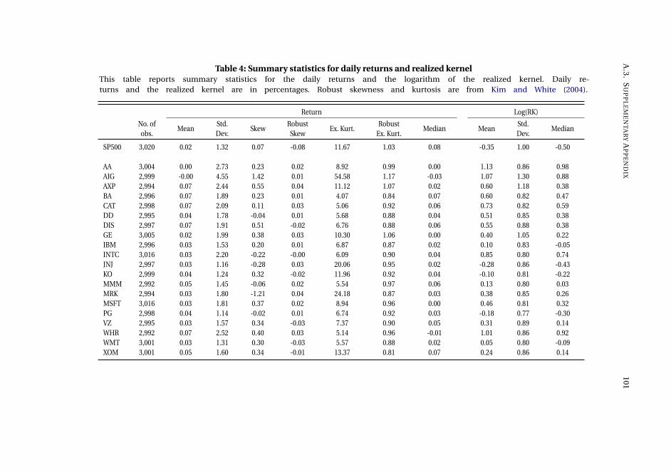
A.3
.S
UP
PL
EM
EN
TA
RY
AP
PE
ND
IX101
Table 4: Summary statistics for daily returns and realized kernelThis table reports summary statistics for the daily returns and the logarithm of the realized kernel. Daily re-turns and the realized kernel are in percentages. Robust skewness and kurtosis are from Kim and White (2004).
Return Log(RK)
No. ofobs.
MeanStd.Dev.
SkewRobustSkew
Ex. Kurt.Robust
Ex. Kurt.Median Mean
Std.Dev.
Median
SP500 3,020 0.02 1.32 0.07 -0.08 11.67 1.03 0.08 -0.35 1.00 -0.50
AA 3,004 0.00 2.73 0.23 0.02 8.92 0.99 0.00 1.13 0.86 0.98AIG 2,999 -0.00 4.55 1.42 0.01 54.58 1.17 -0.03 1.07 1.30 0.88AXP 2,994 0.07 2.44 0.55 0.04 11.12 1.07 0.02 0.60 1.18 0.38BA 2,996 0.07 1.89 0.23 0.01 4.07 0.84 0.07 0.60 0.82 0.47CAT 2,998 0.07 2.09 0.11 0.03 5.06 0.92 0.06 0.73 0.82 0.59DD 2,995 0.04 1.78 -0.04 0.01 5.68 0.88 0.04 0.51 0.85 0.38DIS 2,997 0.07 1.91 0.51 -0.02 6.76 0.88 0.06 0.55 0.88 0.38GE 3,005 0.02 1.99 0.38 0.03 10.30 1.06 0.00 0.40 1.05 0.22IBM 2,996 0.03 1.53 0.20 0.01 6.87 0.87 0.02 0.10 0.83 -0.05INTC 3,016 0.03 2.20 -0.22 -0.00 6.09 0.90 0.04 0.85 0.80 0.74JNJ 2,997 0.03 1.16 -0.28 0.03 20.06 0.95 0.02 -0.28 0.86 -0.43KO 2,999 0.04 1.24 0.32 -0.02 11.96 0.92 0.04 -0.10 0.81 -0.22MMM 2,992 0.05 1.45 -0.06 0.02 5.54 0.97 0.06 0.13 0.80 0.03MRK 2,994 0.03 1.80 -1.21 0.04 24.18 0.87 0.03 0.38 0.85 0.26MSFT 3,016 0.03 1.81 0.37 0.02 8.94 0.96 0.00 0.46 0.81 0.32PG 2,998 0.04 1.14 -0.02 0.01 6.74 0.92 0.03 -0.18 0.77 -0.30VZ 2,995 0.03 1.57 0.34 -0.03 7.37 0.90 0.05 0.31 0.89 0.14WHR 2,992 0.07 2.52 0.40 0.03 5.14 0.96 -0.01 1.01 0.86 0.92WMT 3,001 0.03 1.31 0.30 -0.03 5.57 0.88 0.02 0.05 0.80 -0.09XOM 3,001 0.05 1.60 0.34 -0.01 13.37 0.81 0.07 0.24 0.86 0.14
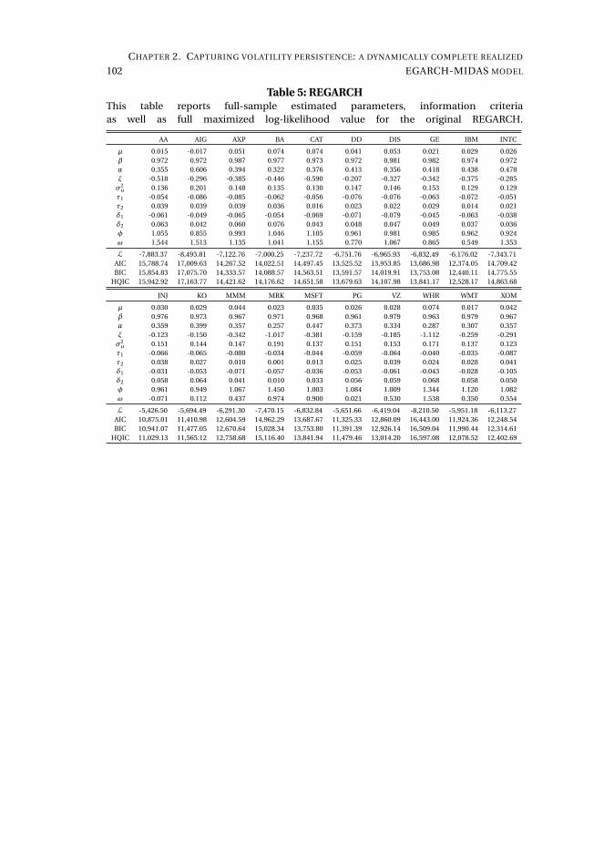
102
CHAPTER 2. CAPTURING VOLATILITY PERSISTENCE: A DYNAMICALLY COMPLETE REALIZED
EGARCH-MIDAS MODEL
Table 5: REGARCHThis table reports full-sample estimated parameters, information criteriaas well as full maximized log-likelihood value for the original REGARCH.
AA AIG AXP BA CAT DD DIS GE IBM INTC
µ 0.015 -0.017 0.051 0.074 0.074 0.041 0.053 0.021 0.029 0.026β 0.972 0.972 0.987 0.977 0.973 0.972 0.981 0.982 0.974 0.972α 0.355 0.606 0.394 0.322 0.376 0.413 0.356 0.418 0.438 0.478ξ -0.518 -0.296 -0.385 -0.446 -0.590 -0.207 -0.327 -0.342 -0.375 -0.285σ2
u 0.136 0.201 0.148 0.135 0.130 0.147 0.146 0.153 0.129 0.129τ1 -0.054 -0.086 -0.085 -0.062 -0.056 -0.076 -0.076 -0.063 -0.072 -0.051τ2 0.039 0.039 0.039 0.036 0.016 0.023 0.022 0.029 0.014 0.021δ1 -0.061 -0.049 -0.065 -0.054 -0.069 -0.071 -0.079 -0.045 -0.063 -0.038δ2 0.063 0.042 0.060 0.076 0.043 0.048 0.047 0.049 0.037 0.036φ 1.055 0.855 0.993 1.046 1.105 0.961 0.981 0.985 0.962 0.924ω 1.544 1.513 1.135 1.041 1.155 0.770 1.067 0.865 0.549 1.353
L -7,883.37 -8,493.81 -7,122.76 -7,000.25 -7,237.72 -6,751.76 -6,965.93 -6,832.49 -6,176.02 -7,343.71AIC 15,788.74 17,009.63 14,267.52 14,022.51 14,497.45 13,525.52 13,953.85 13,686.98 12,374.05 14,709.42BIC 15,854.83 17,075.70 14,333.57 14,088.57 14,563.51 13,591.57 14,019.91 13,753.08 12,440.11 14,775.55
HQIC 15,942.92 17,163.77 14,421.62 14,176.62 14,651.58 13,679.63 14,107.98 13,841.17 12,528.17 14,863.68
JNJ KO MMM MRK MSFT PG VZ WHR WMT XOM
µ 0.030 0.029 0.044 0.023 0.035 0.026 0.028 0.074 0.017 0.042β 0.976 0.973 0.967 0.971 0.968 0.961 0.979 0.963 0.979 0.967α 0.359 0.399 0.357 0.257 0.447 0.373 0.334 0.287 0.307 0.357ξ -0.123 -0.150 -0.342 -1.017 -0.381 -0.159 -0.185 -1.112 -0.259 -0.291σ2
u 0.151 0.144 0.147 0.191 0.137 0.151 0.153 0.171 0.137 0.123τ1 -0.066 -0.065 -0.080 -0.034 -0.044 -0.059 -0.064 -0.040 -0.035 -0.087τ2 0.038 0.027 0.010 0.001 0.013 0.025 0.039 0.024 0.028 0.041δ1 -0.031 -0.053 -0.071 -0.057 -0.036 -0.053 -0.061 -0.043 -0.028 -0.105δ2 0.058 0.064 0.041 0.010 0.033 0.056 0.059 0.068 0.058 0.050φ 0.961 0.949 1.067 1.450 1.003 1.084 1.009 1.344 1.120 1.082ω -0.071 0.112 0.437 0.974 0.900 0.021 0.530 1.538 0.350 0.554
L -5,426.50 -5,694.49 -6,291.30 -7,470.15 -6,832.84 -5,651.66 -6,419.04 -8,210.50 -5,951.18 -6,113.27AIC 10,875.01 11,410.98 12,604.59 14,962.29 13,687.67 11,325.33 12,860.09 16,443.00 11,924.36 12,248.54BIC 10,941.07 11,477.05 12,670.64 15,028.34 13,753.80 11,391.39 12,926.14 16,509.04 11,990.44 12,314.61
HQIC 11,029.13 11,565.12 12,758.68 15,116.40 13,841.94 11,479.46 13,014.20 16,597.08 12,078.52 12,402.69
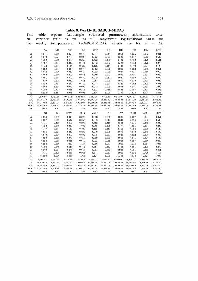
A.3. SUPPLEMENTARY APPENDIX 103
Table 6: Weekly REGARCH-MIDASThis table reports full-sample estimated parameters, information crite-ria, variance ratio as well as full maximized log-likelihood value forthe weekly two-parameter REGARCH-MIDAS. Results are for K = 52.
AA AIG AXP BA CAT DD DIS GE IBM INTC
µ 0.011 -0.016 0.056 0.078 0.071 0.044 0.063 0.025 0.033 0.031β 0.649 0.577 0.710 0.606 0.553 0.623 0.520 0.817 0.612 0.602α 0.392 0.589 0.410 0.360 0.432 0.455 0.429 0.452 0.479 0.531ξ -0.487 -0.291 -0.392 -0.441 -0.572 -0.202 -0.322 -0.333 -0.378 -0.276σ2
u 0.133 0.191 0.144 0.132 0.126 0.144 0.142 0.149 0.127 0.125τ1 -0.062 -0.094 -0.096 -0.076 -0.062 -0.090 -0.089 -0.068 -0.086 -0.061τ2 0.044 0.050 0.048 0.047 0.022 0.025 0.029 0.035 0.015 0.018δ1 -0.063 -0.048 -0.065 -0.054 -0.069 -0.071 -0.080 -0.046 -0.064 -0.040δ2 0.061 0.047 0.059 0.075 0.042 0.047 0.045 0.050 0.037 0.032φ 1.039 0.872 0.999 1.044 1.093 0.959 0.976 0.978 0.963 0.920ω 0.538 0.361 0.402 0.448 0.547 0.224 0.340 0.362 0.392 0.331λ 0.900 1.117 0.973 0.908 0.873 0.999 0.993 0.945 0.981 1.038γ1 -0.156 -0.577 -0.041 -0.214 -0.822 -0.758 -0.866 2.003 -0.971 -0.296γ2 6.538 1.481 6.938 6.994 2.134 1.000 1.130 27.928 1.004 4.883
L -7,836.88 -8,367.58 -7,081.18 -6,956.80 -7,187.14 -6,716.86 -6,912.97 -6,791.63 -6,144.97 -7,280.34AIC 15,701.75 16,763.15 14,190.36 13,941.60 14,402.28 13,461.72 13,853.93 13,611.26 12,317.94 14,588.67BIC 15,785.86 16,847.24 14,274.42 14,025.67 14,486.36 13,545.79 13,938.01 13,695.38 12,402.01 14,672.84
HQIC 15,897.98 16,959.33 14,386.49 14,137.75 14,598.44 13,657.86 14,050.09 13,807.49 12,514.09 14,785.01VR 0.82 0.87 0.89 0.85 0.85 0.82 0.89 0.80 0.83 0.84
JNJ KO MMM MRK MSFT PG VZ WHR WMT XOM
µ 0.034 0.032 0.045 0.025 0.038 0.028 0.031 0.067 0.021 0.051β 0.627 0.562 0.587 0.552 0.613 0.547 0.649 0.554 0.536 0.598α 0.411 0.453 0.415 0.297 0.492 0.416 0.384 0.315 0.342 0.382ξ -0.128 -0.149 -0.340 -1.002 -0.365 -0.158 -0.177 -1.055 -0.254 -0.288σ2
u 0.147 0.141 0.143 0.188 0.133 0.147 0.150 0.164 0.133 0.120τ1 -0.076 -0.071 -0.086 -0.039 -0.048 -0.068 -0.071 -0.048 -0.045 -0.102τ2 0.049 0.036 0.018 0.002 0.015 0.031 0.048 0.032 0.036 0.046δ1 -0.029 -0.053 -0.070 -0.057 -0.038 -0.053 -0.060 -0.045 -0.027 -0.105δ2 0.058 0.065 0.041 0.010 0.033 0.055 0.058 0.067 0.056 0.049φ 0.958 0.936 1.060 1.437 0.986 1.071 1.000 1.315 1.117 1.084ω 0.103 0.149 0.324 0.712 0.391 0.132 0.192 0.861 0.225 0.279λ 0.949 1.017 0.873 0.647 0.951 0.863 0.938 0.701 0.855 0.851γ1 1.471 -0.875 -0.638 -0.563 -0.477 -0.957 0.001 -0.034 -0.776 -1.116γ2 48.950 1.000 3.334 4.365 3.124 1.000 11.393 7.918 2.321 1.000
L -5,395.67 -5,652.84 -6,256.25 -7,438.83 -6,785.22 -5,604.99 -6,390.01 -8,138.73 -5,910.60 -6,069.31AIC 10,819.34 11,333.68 12,540.50 14,905.66 13,598.45 11,237.98 12,808.02 16,305.46 11,849.19 12,166.62BIC 10,903.42 11,417.77 12,624.56 14,989.73 13,682.61 11,322.06 12,892.09 16,389.52 11,933.29 12,250.72
HQIC 11,015.50 11,529.86 12,736.61 15,101.79 13,794.78 11,434.14 13,004.16 16,501.58 12,045.39 12,362.82VR 0.83 0.84 0.80 0.83 0.82 0.80 0.84 0.81 0.87 0.80
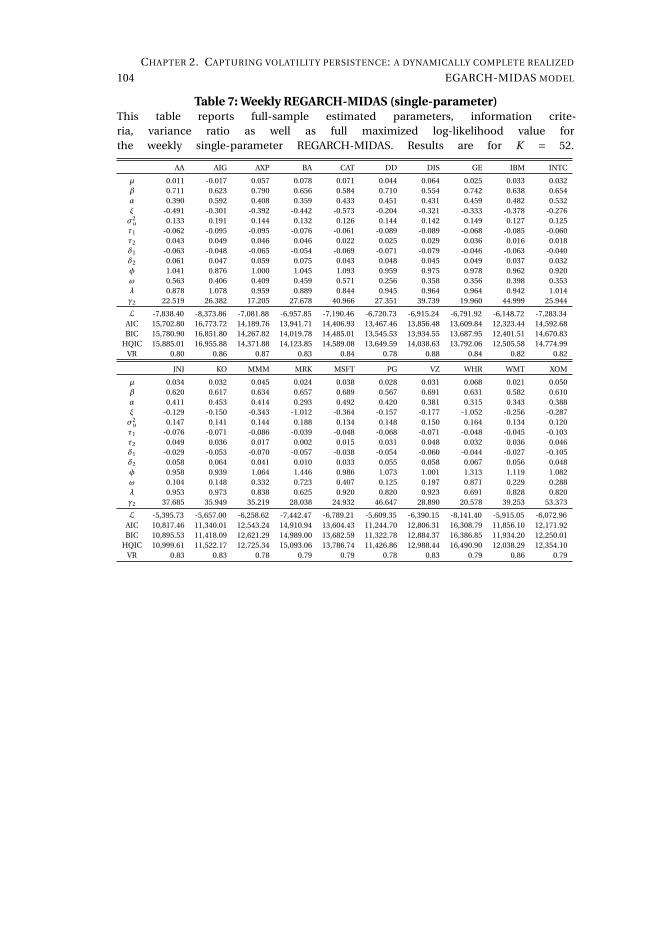
104
CHAPTER 2. CAPTURING VOLATILITY PERSISTENCE: A DYNAMICALLY COMPLETE REALIZED
EGARCH-MIDAS MODEL
Table 7: Weekly REGARCH-MIDAS (single-parameter)This table reports full-sample estimated parameters, information crite-ria, variance ratio as well as full maximized log-likelihood value forthe weekly single-parameter REGARCH-MIDAS. Results are for K = 52.
AA AIG AXP BA CAT DD DIS GE IBM INTC
µ 0.011 -0.017 0.057 0.078 0.071 0.044 0.064 0.025 0.033 0.032β 0.711 0.623 0.790 0.656 0.584 0.710 0.554 0.742 0.638 0.654α 0.390 0.592 0.408 0.359 0.433 0.451 0.431 0.459 0.482 0.532ξ -0.491 -0.301 -0.392 -0.442 -0.573 -0.204 -0.321 -0.333 -0.378 -0.276σ2
u 0.133 0.191 0.144 0.132 0.126 0.144 0.142 0.149 0.127 0.125τ1 -0.062 -0.095 -0.095 -0.076 -0.061 -0.089 -0.089 -0.068 -0.085 -0.060τ2 0.043 0.049 0.046 0.046 0.022 0.025 0.029 0.036 0.016 0.018δ1 -0.063 -0.048 -0.065 -0.054 -0.069 -0.071 -0.079 -0.046 -0.063 -0.040δ2 0.061 0.047 0.059 0.075 0.043 0.048 0.045 0.049 0.037 0.032φ 1.041 0.876 1.000 1.045 1.093 0.959 0.975 0.978 0.962 0.920ω 0.563 0.406 0.409 0.459 0.571 0.256 0.358 0.356 0.398 0.353λ 0.878 1.078 0.959 0.889 0.844 0.945 0.964 0.964 0.942 1.014γ2 22.519 26.382 17.205 27.678 40.966 27.351 39.739 19.960 44.999 25.944
L -7,838.40 -8,373.86 -7,081.88 -6,957.85 -7,190.46 -6,720.73 -6,915.24 -6,791.92 -6,148.72 -7,283.34AIC 15,702.80 16,773.72 14,189.76 13,941.71 14,406.93 13,467.46 13,856.48 13,609.84 12,323.44 14,592.68BIC 15,780.90 16,851.80 14,267.82 14,019.78 14,485.01 13,545.53 13,934.55 13,687.95 12,401.51 14,670.83
HQIC 15,885.01 16,955.88 14,371.88 14,123.85 14,589.08 13,649.59 14,038.63 13,792.06 12,505.58 14,774.99VR 0.80 0.86 0.87 0.83 0.84 0.78 0.88 0.84 0.82 0.82
JNJ KO MMM MRK MSFT PG VZ WHR WMT XOM
µ 0.034 0.032 0.045 0.024 0.038 0.028 0.031 0.068 0.021 0.050β 0.620 0.617 0.634 0.657 0.689 0.567 0.691 0.631 0.582 0.610α 0.411 0.453 0.414 0.293 0.492 0.420 0.381 0.315 0.343 0.388ξ -0.129 -0.150 -0.343 -1.012 -0.364 -0.157 -0.177 -1.052 -0.256 -0.287σ2
u 0.147 0.141 0.144 0.188 0.134 0.148 0.150 0.164 0.134 0.120τ1 -0.076 -0.071 -0.086 -0.039 -0.048 -0.068 -0.071 -0.048 -0.045 -0.103τ2 0.049 0.036 0.017 0.002 0.015 0.031 0.048 0.032 0.036 0.046δ1 -0.029 -0.053 -0.070 -0.057 -0.038 -0.054 -0.060 -0.044 -0.027 -0.105δ2 0.058 0.064 0.041 0.010 0.033 0.055 0.058 0.067 0.056 0.048φ 0.958 0.939 1.064 1.446 0.986 1.073 1.001 1.313 1.119 1.082ω 0.104 0.148 0.332 0.723 0.407 0.125 0.197 0.871 0.229 0.288λ 0.953 0.973 0.838 0.625 0.920 0.820 0.923 0.691 0.828 0.820γ2 37.685 35.949 35.219 28.038 24.932 46.647 28.890 20.578 39.253 53.373
L -5,395.73 -5,657.00 -6,258.62 -7,442.47 -6,789.21 -5,609.35 -6,390.15 -8,141.40 -5,915.05 -6,072.96AIC 10,817.46 11,340.01 12,543.24 14,910.94 13,604.43 11,244.70 12,806.31 16,308.79 11,856.10 12,171.92BIC 10,895.53 11,418.09 12,621.29 14,989.00 13,682.59 11,322.78 12,884.37 16,386.85 11,934.20 12,250.01
HQIC 10,999.61 11,522.17 12,725.34 15,093.06 13,786.74 11,426.86 12,988.44 16,490.90 12,038.29 12,354.10VR 0.83 0.83 0.78 0.79 0.79 0.78 0.83 0.79 0.86 0.79
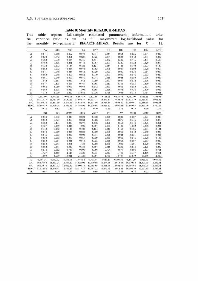
A.3. SUPPLEMENTARY APPENDIX 105
Table 8: Monthly REGARCH-MIDASThis table reports full-sample estimated parameters, information crite-ria, variance ratio as well as full maximized log-likelihood value forthe monthly two-parameter REGARCH-MIDAS. Results are for K = 12.
AA AIG AXP BA CAT DD DIS GE IBM INTC
µ 0.011 -0.018 0.057 0.078 0.071 0.044 0.064 0.025 0.034 0.032β 0.820 0.742 0.861 0.837 0.825 0.864 0.832 0.843 0.891 0.812α 0.383 0.590 0.404 0.345 0.414 0.432 0.390 0.445 0.451 0.515ξ -0.492 -0.306 -0.391 -0.441 -0.567 -0.201 -0.335 -0.333 -0.379 -0.276σ2
u 0.133 0.193 0.144 0.132 0.127 0.144 0.143 0.149 0.127 0.126τ1 -0.062 -0.092 -0.094 -0.073 -0.063 -0.086 -0.087 -0.069 -0.078 -0.060τ2 0.041 0.048 0.044 0.042 0.020 0.023 0.026 0.034 0.014 0.018δ1 -0.063 -0.048 -0.065 -0.054 -0.070 -0.071 -0.080 -0.046 -0.063 -0.040δ2 0.061 0.049 0.059 0.075 0.044 0.048 0.044 0.050 0.036 0.033φ 1.042 0.881 0.999 1.044 1.089 0.957 0.987 0.978 0.966 0.920ω 0.577 0.405 0.404 0.467 0.565 0.241 0.361 0.355 0.390 0.349λ 0.864 1.080 0.959 0.869 0.842 0.951 0.951 0.952 0.897 1.009γ1 -0.583 -1.605 0.025 1.398 -0.865 -0.266 -0.878 0.424 0.800 1.028γ2 4.112 1.000 5.262 13.651 3.036 2.728 1.933 8.113 6.714 9.921
L -7,842.06 -8,377.55 -7,081.13 -6,963.39 -7,202.89 -6,721.18 -6,928.36 -6,792.40 -6,153.55 -7,292.92AIC 15,712.13 16,783.10 14,190.26 13,954.77 14,433.77 13,470.37 13,884.72 13,612.79 12,335.11 14,613.85BIC 15,796.24 16,867.19 14,274.33 14,038.85 14,517.86 13,554.44 13,968.80 13,696.91 12,419.18 14,698.01
HQIC 15,908.35 16,979.28 14,386.39 14,150.92 14,629.94 13,666.51 14,080.88 13,809.03 12,531.26 14,810.18VR 0.72 0.82 0.83 0.73 0.70 0.65 0.76 0.78 0.60 0.74
JNJ KO MMM MRK MSFT PG VZ WHR WMT XOM
µ 0.034 0.032 0.045 0.024 0.038 0.028 0.031 0.067 0.021 0.049β 0.850 0.827 0.863 0.864 0.826 0.831 0.875 0.745 0.852 0.873α 0.388 0.434 0.380 0.277 0.476 0.400 0.359 0.314 0.325 0.361ξ -0.127 -0.149 -0.344 -1.006 -0.367 -0.159 -0.180 -1.032 -0.256 -0.294σ2
u 0.148 0.142 0.144 0.188 0.134 0.149 0.151 0.165 0.134 0.121τ1 -0.074 -0.069 -0.084 -0.038 -0.050 -0.065 -0.069 -0.048 -0.040 -0.095τ2 0.045 0.033 0.013 0.001 0.014 0.028 0.044 0.031 0.032 0.044δ1 -0.030 -0.053 -0.070 -0.057 -0.039 -0.053 -0.060 -0.045 -0.028 -0.105δ2 0.058 0.064 0.041 0.010 0.033 0.056 0.058 0.067 0.057 0.049φ 0.958 0.941 1.071 1.439 0.988 1.080 1.005 1.301 1.120 1.089ω 0.082 0.141 0.330 0.730 0.407 0.118 0.205 0.874 0.225 0.297λ 0.914 0.962 0.783 0.595 0.906 0.794 0.877 0.686 0.807 0.761γ1 -1.427 -1.388 2.524 3.325 0.013 -0.931 1.769 3.777 1.456 -0.651γ2 1.000 1.000 18.021 21.725 5.094 1.783 13.707 33.579 13.546 2.319
L -5,404.34 -5,662.62 -6,265.13 -7,446.52 -6,791.44 -5,623.29 -6,395.34 -8,141.29 -5,921.83 -6,087.31AIC 10,836.68 11,353.24 12,558.27 14,921.04 13,610.88 11,274.58 12,818.68 16,310.58 11,871.65 12,202.61BIC 10,920.76 11,437.32 12,642.32 15,005.10 13,695.05 11,358.66 12,902.75 16,394.64 11,955.75 12,286.71
HQIC 11,032.84 11,549.41 12,754.38 15,117.17 13,807.22 11,470.75 13,014.82 16,506.70 12,067.85 12,398.81VR 0.67 0.70 0.58 0.63 0.69 0.59 0.68 0.74 0.72 0.54
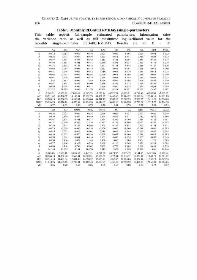
106
CHAPTER 2. CAPTURING VOLATILITY PERSISTENCE: A DYNAMICALLY COMPLETE REALIZED
EGARCH-MIDAS MODEL
Table 9: Monthly REGARCH-MIDAS (single-parameter)This table reports full-sample estimated parameters, information crite-ria, variance ratio as well as full maximized log-likelihood value for themonthly single-parameter REGARCH-MIDAS. Results are for K = 12.
AA AIG AXP BA CAT DD DIS GE IBM INTC
µ 0.012 -0.017 0.057 0.078 0.071 0.045 0.065 0.025 0.034 0.032β 0.824 0.737 0.865 0.836 0.831 0.871 0.841 0.845 0.893 0.812α 0.383 0.591 0.404 0.345 0.413 0.431 0.387 0.445 0.450 0.515ξ -0.492 -0.311 -0.391 -0.441 -0.568 -0.201 -0.337 -0.333 -0.378 -0.276σ2
u 0.134 0.192 0.144 0.132 0.127 0.144 0.143 0.149 0.127 0.126τ1 -0.062 -0.093 -0.094 -0.073 -0.063 -0.085 -0.087 -0.069 -0.078 -0.060τ2 0.041 0.048 0.044 0.042 0.019 0.023 0.026 0.034 0.014 0.018δ1 -0.063 -0.047 -0.065 -0.054 -0.070 -0.071 -0.080 -0.046 -0.063 -0.040δ2 0.061 0.048 0.059 0.075 0.044 0.048 0.044 0.050 0.036 0.033φ 1.042 0.883 0.999 1.045 1.090 0.957 0.988 0.978 0.966 0.920ω 0.587 0.431 0.406 0.466 0.576 0.252 0.373 0.356 0.390 0.349λ 0.855 1.054 0.955 0.871 0.828 0.930 0.933 0.950 0.894 1.009γ2 12.772 21.575 9.843 11.378 13.169 8.224 10.921 11.252 7.447 9.787
L -7,842.51 -8,381.29 -7,081.41 -6,963.39 -7,203.34 -6,721.53 -6,929.11 -6,792.42 -6,153.56 -7,292.92AIC 15,711.02 16,788.57 14,188.81 13,952.79 14,432.67 13,469.06 13,884.22 13,610.84 12,333.13 14,611.85BIC 15,789.13 16,866.65 14,266.87 14,030.86 14,510.75 13,547.13 13,962.29 13,688.95 12,411.20 14,690.00
HQIC 15,893.23 16,970.74 14,370.94 14,134.93 14,614.83 13,651.19 14,066.36 13,793.06 12,515.27 14,794.16VR 0.72 0.82 0.83 0.73 0.70 0.64 0.76 0.78 0.59 0.74
JNJ KO MMM MRK MSFT PG VZ WHR WMT XOM
µ 0.034 0.033 0.045 0.024 0.038 0.028 0.031 0.067 0.021 0.049β 0.856 0.829 0.856 0.849 0.834 0.837 0.871 0.742 0.850 0.880α 0.387 0.434 0.381 0.277 0.474 0.399 0.360 0.314 0.326 0.361ξ -0.127 -0.149 -0.345 -1.016 -0.367 -0.159 -0.180 -1.037 -0.256 -0.293σ2
u 0.148 0.142 0.144 0.188 0.134 0.149 0.151 0.165 0.134 0.121τ1 -0.073 -0.069 -0.085 -0.038 -0.050 -0.065 -0.069 -0.048 -0.041 -0.095τ2 0.045 0.033 0.013 0.001 0.014 0.028 0.044 0.030 0.032 0.044δ1 -0.030 -0.052 -0.070 -0.058 -0.039 -0.053 -0.060 -0.044 -0.028 -0.105δ2 0.058 0.064 0.041 0.010 0.033 0.056 0.058 0.067 0.057 0.049φ 0.958 0.940 1.072 1.448 0.988 1.080 1.005 1.304 1.120 1.089ω 0.077 0.140 0.329 0.728 0.409 0.116 0.203 0.874 0.224 0.304λ 0.889 0.938 0.792 0.602 0.901 0.772 0.883 0.686 0.809 0.739γ2 14.140 14.689 10.161 10.076 9.315 11.923 9.798 15.579 11.051 10.146
L -5,405.05 -5,663.48 -6,265.40 -7,447.15 -6,791.78 -5,623.97 -6,395.39 -8,141.55 -5,921.85 -6,087.94AIC 10,836.10 11,352.96 12,556.81 14,920.31 13,609.55 11,273.94 12,816.77 16,309.10 11,869.70 12,201.87BIC 10,914.18 11,431.04 12,634.86 14,998.37 13,687.71 11,352.02 12,894.84 16,387.16 11,947.79 12,279.96
HQIC 11,018.25 11,535.13 12,738.91 15,102.43 13,791.87 11,456.10 12,998.90 16,491.21 12,051.89 12,384.05VR 0.65 0.70 0.59 0.65 0.69 0.58 0.68 0.74 0.72 0.52
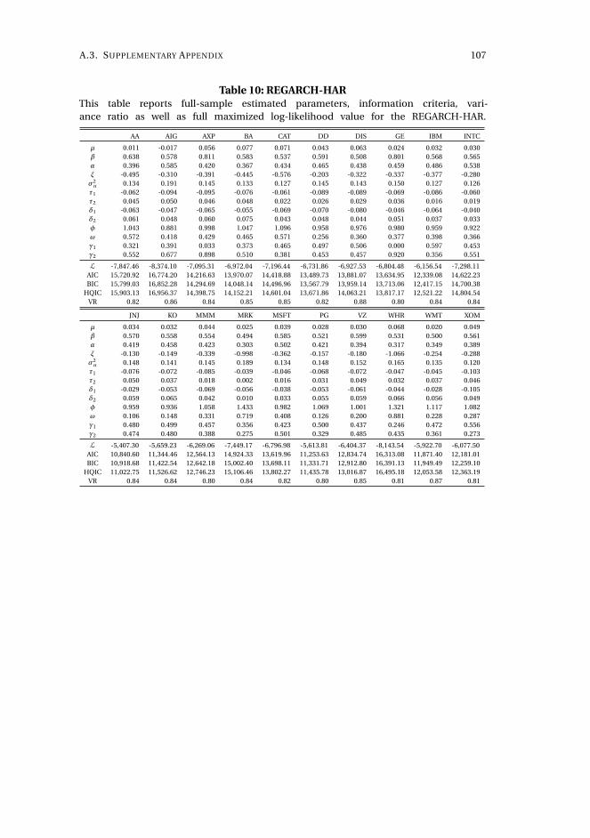
A.3. SUPPLEMENTARY APPENDIX 107
Table 10: REGARCH-HARThis table reports full-sample estimated parameters, information criteria, vari-ance ratio as well as full maximized log-likelihood value for the REGARCH-HAR.
AA AIG AXP BA CAT DD DIS GE IBM INTC
µ 0.011 -0.017 0.056 0.077 0.071 0.043 0.063 0.024 0.032 0.030β 0.638 0.578 0.811 0.583 0.537 0.591 0.508 0.801 0.568 0.565α 0.396 0.585 0.420 0.367 0.434 0.465 0.438 0.459 0.486 0.538ξ -0.495 -0.310 -0.391 -0.445 -0.576 -0.203 -0.322 -0.337 -0.377 -0.280σ2
u 0.134 0.191 0.145 0.133 0.127 0.145 0.143 0.150 0.127 0.126τ1 -0.062 -0.094 -0.095 -0.076 -0.061 -0.089 -0.089 -0.069 -0.086 -0.060τ2 0.045 0.050 0.046 0.048 0.022 0.026 0.029 0.036 0.016 0.019δ1 -0.063 -0.047 -0.065 -0.055 -0.069 -0.070 -0.080 -0.046 -0.064 -0.040δ2 0.061 0.048 0.060 0.075 0.043 0.048 0.044 0.051 0.037 0.033φ 1.043 0.881 0.998 1.047 1.096 0.958 0.976 0.980 0.959 0.922ω 0.572 0.418 0.429 0.465 0.571 0.256 0.360 0.377 0.398 0.366γ1 0.321 0.391 0.033 0.373 0.465 0.497 0.506 0.000 0.597 0.453γ2 0.552 0.677 0.898 0.510 0.381 0.453 0.457 0.920 0.356 0.551
L -7,847.46 -8,374.10 -7,095.31 -6,972.04 -7,196.44 -6,731.86 -6,927.53 -6,804.48 -6,156.54 -7,298.11AIC 15,720.92 16,774.20 14,216.63 13,970.07 14,418.88 13,489.73 13,881.07 13,634.95 12,339.08 14,622.23BIC 15,799.03 16,852.28 14,294.69 14,048.14 14,496.96 13,567.79 13,959.14 13,713.06 12,417.15 14,700.38
HQIC 15,903.13 16,956.37 14,398.75 14,152.21 14,601.04 13,671.86 14,063.21 13,817.17 12,521.22 14,804.54VR 0.82 0.86 0.84 0.85 0.85 0.82 0.88 0.80 0.84 0.84
JNJ KO MMM MRK MSFT PG VZ WHR WMT XOM
µ 0.034 0.032 0.044 0.025 0.039 0.028 0.030 0.068 0.020 0.049β 0.570 0.558 0.554 0.494 0.585 0.521 0.599 0.531 0.500 0.561α 0.419 0.458 0.423 0.303 0.502 0.421 0.394 0.317 0.349 0.389ξ -0.130 -0.149 -0.339 -0.998 -0.362 -0.157 -0.180 -1.066 -0.254 -0.288σ2
u 0.148 0.141 0.145 0.189 0.134 0.148 0.152 0.165 0.135 0.120τ1 -0.076 -0.072 -0.085 -0.039 -0.046 -0.068 -0.072 -0.047 -0.045 -0.103τ2 0.050 0.037 0.018 0.002 0.016 0.031 0.049 0.032 0.037 0.046δ1 -0.029 -0.053 -0.069 -0.056 -0.038 -0.053 -0.061 -0.044 -0.028 -0.105δ2 0.059 0.065 0.042 0.010 0.033 0.055 0.059 0.066 0.056 0.049φ 0.959 0.936 1.058 1.433 0.982 1.069 1.001 1.321 1.117 1.082ω 0.106 0.148 0.331 0.719 0.408 0.126 0.200 0.881 0.228 0.287γ1 0.480 0.499 0.457 0.356 0.423 0.500 0.437 0.246 0.472 0.556γ2 0.474 0.480 0.388 0.275 0.501 0.329 0.485 0.435 0.361 0.273
L -5,407.30 -5,659.23 -6,269.06 -7,449.17 -6,796.98 -5,613.81 -6,404.37 -8,143.54 -5,922.70 -6,077.50AIC 10,840.60 11,344.46 12,564.13 14,924.33 13,619.96 11,253.63 12,834.74 16,313.08 11,871.40 12,181.01BIC 10,918.68 11,422.54 12,642.18 15,002.40 13,698.11 11,331.71 12,912.80 16,391.13 11,949.49 12,259.10
HQIC 11,022.75 11,526.62 12,746.23 15,106.46 13,802.27 11,435.78 13,016.87 16,495.18 12,053.58 12,363.19VR 0.84 0.84 0.80 0.84 0.82 0.80 0.85 0.81 0.87 0.81
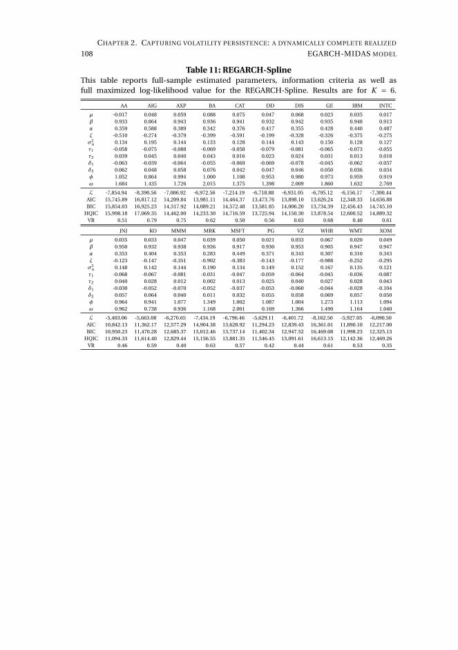
108
CHAPTER 2. CAPTURING VOLATILITY PERSISTENCE: A DYNAMICALLY COMPLETE REALIZED
EGARCH-MIDAS MODEL
Table 11: REGARCH-SplineThis table reports full-sample estimated parameters, information criteria as well asfull maximized log-likelihood value for the REGARCH-Spline. Results are for K = 6.
AA AIG AXP BA CAT DD DIS GE IBM INTC
µ -0.017 0.048 0.059 0.088 0.075 0.047 0.068 0.023 0.035 0.017β 0.933 0.864 0.943 0.936 0.941 0.932 0.942 0.935 0.948 0.913α 0.359 0.588 0.389 0.342 0.376 0.417 0.355 0.428 0.440 0.487ξ -0.510 -0.274 -0.379 -0.399 -0.591 -0.199 -0.328 -0.326 -0.375 -0.275σ2
u 0.134 0.195 0.144 0.133 0.128 0.144 0.143 0.150 0.128 0.127τ1 -0.058 -0.075 -0.088 -0.069 -0.058 -0.079 -0.081 -0.065 -0.073 -0.055τ2 0.039 0.045 0.040 0.043 0.016 0.023 0.024 0.031 0.013 0.018δ1 -0.063 -0.039 -0.064 -0.055 -0.069 -0.069 -0.078 -0.045 -0.062 -0.037δ2 0.062 0.048 0.058 0.076 0.042 0.047 0.046 0.050 0.036 0.034φ 1.052 0.864 0.994 1.000 1.108 0.953 0.980 0.973 0.959 0.919ω 1.684 1.435 1.726 2.015 1.375 1.398 2.009 1.860 1.632 2.769
L -7,854.94 -8,390.56 -7,086.92 -6,972.56 -7,214.19 -6,718.88 -6,931.05 -6,795.12 -6,156.17 -7,300.44AIC 15,745.89 16,817.12 14,209.84 13,981.11 14,464.37 13,473.76 13,898.10 13,626.24 12,348.33 14,636.88BIC 15,854.03 16,925.23 14,317.92 14,089.21 14,572.48 13,581.85 14,006.20 13,734.39 12,456.43 14,745.10
HQIC 15,998.18 17,069.35 14,462.00 14,233.30 14,716.59 13,725.94 14,150.30 13,878.54 12,600.52 14,889.32VR 0.51 0.79 0.75 0.62 0.50 0.56 0.63 0.68 0.40 0.61
JNJ KO MMM MRK MSFT PG VZ WHR WMT XOM
µ 0.035 0.033 0.047 0.039 0.050 0.021 0.033 0.067 0.020 0.049β 0.950 0.932 0.938 0.926 0.917 0.930 0.953 0.905 0.947 0.947α 0.353 0.404 0.353 0.283 0.449 0.371 0.343 0.307 0.310 0.343ξ -0.123 -0.147 -0.351 -0.902 -0.383 -0.143 -0.177 -0.988 -0.252 -0.295σ2
u 0.148 0.142 0.144 0.190 0.134 0.149 0.152 0.167 0.135 0.121τ1 -0.068 -0.067 -0.081 -0.031 -0.047 -0.059 -0.064 -0.045 -0.036 -0.087τ2 0.040 0.028 0.012 0.002 0.013 0.025 0.040 0.027 0.028 0.043δ1 -0.030 -0.052 -0.070 -0.052 -0.037 -0.053 -0.060 -0.044 -0.028 -0.104δ2 0.057 0.064 0.040 0.011 0.032 0.055 0.058 0.069 0.057 0.050φ 0.964 0.941 1.077 1.349 1.002 1.087 1.004 1.273 1.113 1.094ω 0.962 0.738 0.936 1.168 2.001 0.169 1.366 1.490 1.164 1.040
L -5,403.06 -5,663.08 -6,270.65 -7,434.19 -6,796.46 -5,629.11 -6,401.72 -8,162.50 -5,927.05 -6,090.50AIC 10,842.13 11,362.17 12,577.29 14,904.38 13,628.92 11,294.23 12,839.43 16,361.01 11,890.10 12,217.00BIC 10,950.23 11,470.28 12,685.37 15,012.46 13,737.14 11,402.34 12,947.52 16,469.08 11,998.23 12,325.13
HQIC 11,094.33 11,614.40 12,829.44 15,156.55 13,881.35 11,546.45 13,091.61 16,613.15 12,142.36 12,469.26VR 0.46 0.59 0.40 0.63 0.57 0.42 0.44 0.61 0.53 0.35
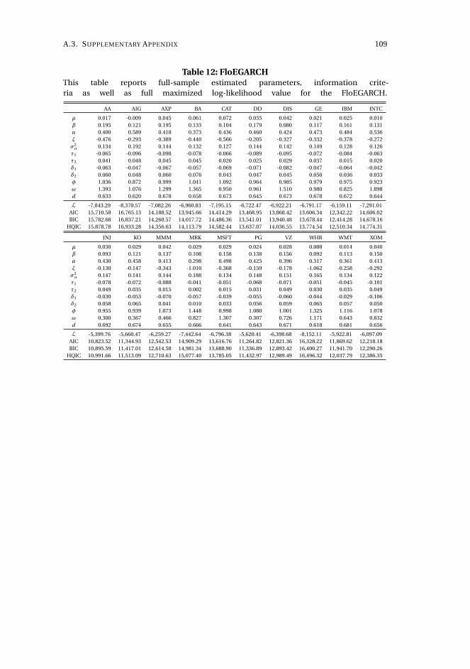
A.3. SUPPLEMENTARY APPENDIX 109
Table 12: FloEGARCHThis table reports full-sample estimated parameters, information crite-ria as well as full maximized log-likelihood value for the FloEGARCH.
AA AIG AXP BA CAT DD DIS GE IBM INTC
µ 0.017 -0.009 0.045 0.061 0.072 0.035 0.042 0.021 0.025 0.010β 0.195 0.121 0.195 0.133 0.104 0.179 0.080 0.117 0.161 0.131α 0.400 0.589 0.418 0.373 0.436 0.460 0.424 0.473 0.484 0.536ξ -0.476 -0.293 -0.389 -0.440 -0.566 -0.205 -0.327 -0.332 -0.378 -0.272σ2
u 0.134 0.192 0.144 0.132 0.127 0.144 0.142 0.149 0.128 0.126τ1 -0.065 -0.096 -0.098 -0.078 -0.066 -0.089 -0.095 -0.072 -0.084 -0.063τ2 0.041 0.048 0.045 0.045 0.020 0.025 0.029 0.037 0.015 0.020δ1 -0.063 -0.047 -0.067 -0.057 -0.069 -0.071 -0.082 -0.047 -0.064 -0.042δ2 0.060 0.048 0.060 0.076 0.043 0.047 0.045 0.050 0.036 0.033φ 1.036 0.872 0.999 1.041 1.092 0.964 0.985 0.979 0.975 0.923ω 1.393 1.076 1.299 1.365 0.950 0.961 1.510 0.980 0.825 1.898d 0.633 0.620 0.678 0.658 0.673 0.645 0.673 0.678 0.672 0.644
L -7,843.29 -8,370.57 -7,082.26 -6,960.83 -7,195.15 -6,722.47 -6,922.21 -6,791.17 -6,159.11 -7,291.01AIC 15,710.58 16,765.13 14,188.52 13,945.66 14,414.29 13,468.95 13,868.42 13,606.34 12,342.22 14,606.02BIC 15,782.68 16,837.21 14,260.57 14,017.72 14,486.36 13,541.01 13,940.48 13,678.44 12,414.28 14,678.16
HQIC 15,878.78 16,933.28 14,356.63 14,113.79 14,582.44 13,637.07 14,036.55 13,774.54 12,510.34 14,774.31
JNJ KO MMM MRK MSFT PG VZ WHR WMT XOM
µ 0.030 0.029 0.042 0.029 0.029 0.024 0.028 0.088 0.014 0.040β 0.093 0.121 0.137 0.108 0.158 0.138 0.156 0.092 0.113 0.150α 0.430 0.458 0.413 0.298 0.498 0.425 0.396 0.317 0.361 0.413ξ -0.130 -0.147 -0.343 -1.010 -0.368 -0.159 -0.178 -1.062 -0.258 -0.292σ2
u 0.147 0.141 0.144 0.188 0.134 0.148 0.151 0.165 0.134 0.122τ1 -0.078 -0.072 -0.088 -0.041 -0.051 -0.068 -0.071 -0.051 -0.045 -0.101τ2 0.049 0.035 0.015 0.002 0.015 0.031 0.049 0.030 0.035 0.049δ1 -0.030 -0.053 -0.070 -0.057 -0.039 -0.055 -0.060 -0.044 -0.029 -0.106δ2 0.058 0.065 0.041 0.010 0.033 0.056 0.059 0.065 0.057 0.050φ 0.955 0.939 1.073 1.448 0.998 1.080 1.001 1.325 1.116 1.078ω 0.300 0.367 0.466 0.827 1.307 0.307 0.726 1.171 0.643 0.832d 0.692 0.674 0.655 0.666 0.641 0.643 0.671 0.618 0.681 0.656
L -5,399.76 -5,660.47 -6,259.27 -7,442.64 -6,796.38 -5,620.41 -6,398.68 -8,152.11 -5,922.81 -6,097.09AIC 10,823.52 11,344.93 12,542.53 14,909.29 13,616.76 11,264.82 12,821.36 16,328.22 11,869.62 12,218.18BIC 10,895.59 11,417.01 12,614.58 14,981.34 13,688.90 11,336.89 12,893.42 16,400.27 11,941.70 12,290.26
HQIC 10,991.66 11,513.09 12,710.63 15,077.40 13,785.05 11,432.97 12,989.49 16,496.32 12,037.79 12,386.35
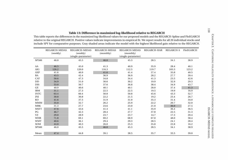
110
CH
AP
TE
R2
.C
AP
TU
RIN
GV
OL
AT
ILIT
YP
ER
SIS
TE
NC
E:A
DY
NA
MIC
AL
LYC
OM
PL
ET
ER
EA
LIZ
ED
EG
AR
CH
-MID
AS
MO
DE
L
Table 13: Difference in maximized log-likelihood relative to REGARCHThis table reports the differences in the maximized log-likelihood values for our proposed models and the REGARCH-Spline and FloEGARCHrelative to the original REGARCH. Positive values indicate improvements in empirical fit. We report results for all 20 individual stocks andinclude SPY for comparative purposes. Gray shaded areas indicate the model with the highest likelihood gain relative to the REGARCH.
REGARCH-MIDAS REGARCH-MIDAS REGARCH-MIDAS REGARCH-MIDAS REGARCH-HAR REGARCH-S FloEGARCH(weekly) (weekly) (monthly) (monthly)
(single-parameter) (single-parameter)
SP500 46.0 45.5 46.0 45.3 28.5 34.1 38.9
AA 46.5 45.0 41.3 40.9 35.9 28.4 40.1AIG 126.2 120.0 116.3 112.5 119.7 103.3 123.2AXP 41.6 40.9 41.6 41.4 27.4 35.8 40.5BA 43.5 42.4 36.9 36.9 28.2 27.7 39.4CAT 50.6 47.3 34.8 34.4 41.3 23.5 42.6DD 34.9 31.0 30.6 30.2 19.9 32.9 29.3DIS 53.0 50.7 37.6 36.8 38.4 34.9 43.7GE 40.9 40.6 40.1 40.1 28.0 37.4 41.3IBM 31.1 27.3 22.5 22.5 19.5 19.9 16.9INTC 63.4 60.4 50.8 50.8 45.6 43.3 52.7JNJ 30.8 30.8 22.2 21.5 19.2 23.4 26.7KO 41.6 37.5 31.9 31.0 35.3 31.4 34.0MMM 35.0 32.7 26.2 25.9 22.2 20.7 32.0MRK 31.3 27.7 23.6 23.0 21.0 36.0 27.5MSFT 47.6 43.6 41.4 41.1 35.9 36.4 36.5PG 46.7 42.3 28.4 27.7 37.8 22.5 31.3VZ 29.0 28.9 23.7 23.7 14.7 17.3 20.4WHR 71.8 69.1 69.2 68.9 67.0 48.0 58.4WMT 40.6 36.1 29.4 29.3 28.5 24.1 28.4XOM 44.0 40.3 26.0 25.3 35.8 22.8 16.2SP500 46.0 45.5 46.0 45.3 28.5 34.1 38.9
Mean 47.4 44.8 39.1 38.5 35.7 33.5 39.0
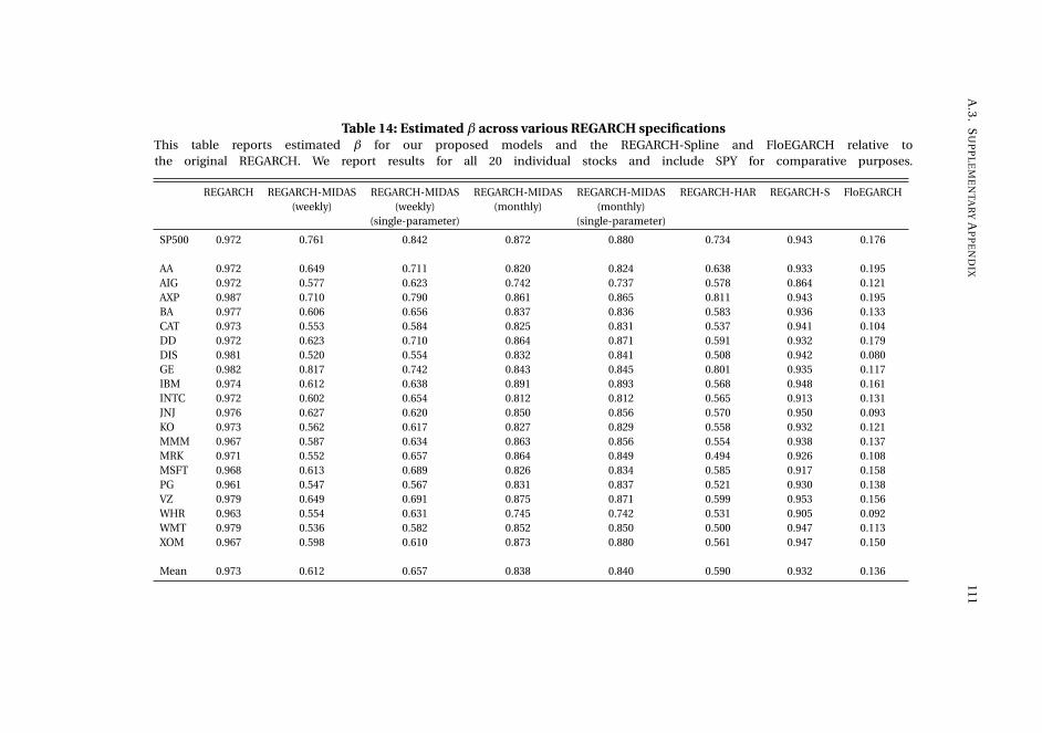
A.3
.S
UP
PL
EM
EN
TA
RY
AP
PE
ND
IX111
Table 14: Estimated β across various REGARCH specificationsThis table reports estimated β for our proposed models and the REGARCH-Spline and FloEGARCH relative tothe original REGARCH. We report results for all 20 individual stocks and include SPY for comparative purposes.
REGARCH REGARCH-MIDAS REGARCH-MIDAS REGARCH-MIDAS REGARCH-MIDAS REGARCH-HAR REGARCH-S FloEGARCH(weekly) (weekly) (monthly) (monthly)
(single-parameter) (single-parameter)
SP500 0.972 0.761 0.842 0.872 0.880 0.734 0.943 0.176
AA 0.972 0.649 0.711 0.820 0.824 0.638 0.933 0.195AIG 0.972 0.577 0.623 0.742 0.737 0.578 0.864 0.121AXP 0.987 0.710 0.790 0.861 0.865 0.811 0.943 0.195BA 0.977 0.606 0.656 0.837 0.836 0.583 0.936 0.133CAT 0.973 0.553 0.584 0.825 0.831 0.537 0.941 0.104DD 0.972 0.623 0.710 0.864 0.871 0.591 0.932 0.179DIS 0.981 0.520 0.554 0.832 0.841 0.508 0.942 0.080GE 0.982 0.817 0.742 0.843 0.845 0.801 0.935 0.117IBM 0.974 0.612 0.638 0.891 0.893 0.568 0.948 0.161INTC 0.972 0.602 0.654 0.812 0.812 0.565 0.913 0.131JNJ 0.976 0.627 0.620 0.850 0.856 0.570 0.950 0.093KO 0.973 0.562 0.617 0.827 0.829 0.558 0.932 0.121MMM 0.967 0.587 0.634 0.863 0.856 0.554 0.938 0.137MRK 0.971 0.552 0.657 0.864 0.849 0.494 0.926 0.108MSFT 0.968 0.613 0.689 0.826 0.834 0.585 0.917 0.158PG 0.961 0.547 0.567 0.831 0.837 0.521 0.930 0.138VZ 0.979 0.649 0.691 0.875 0.871 0.599 0.953 0.156WHR 0.963 0.554 0.631 0.745 0.742 0.531 0.905 0.092WMT 0.979 0.536 0.582 0.852 0.850 0.500 0.947 0.113XOM 0.967 0.598 0.610 0.873 0.880 0.561 0.947 0.150
Mean 0.973 0.612 0.657 0.838 0.840 0.590 0.932 0.136
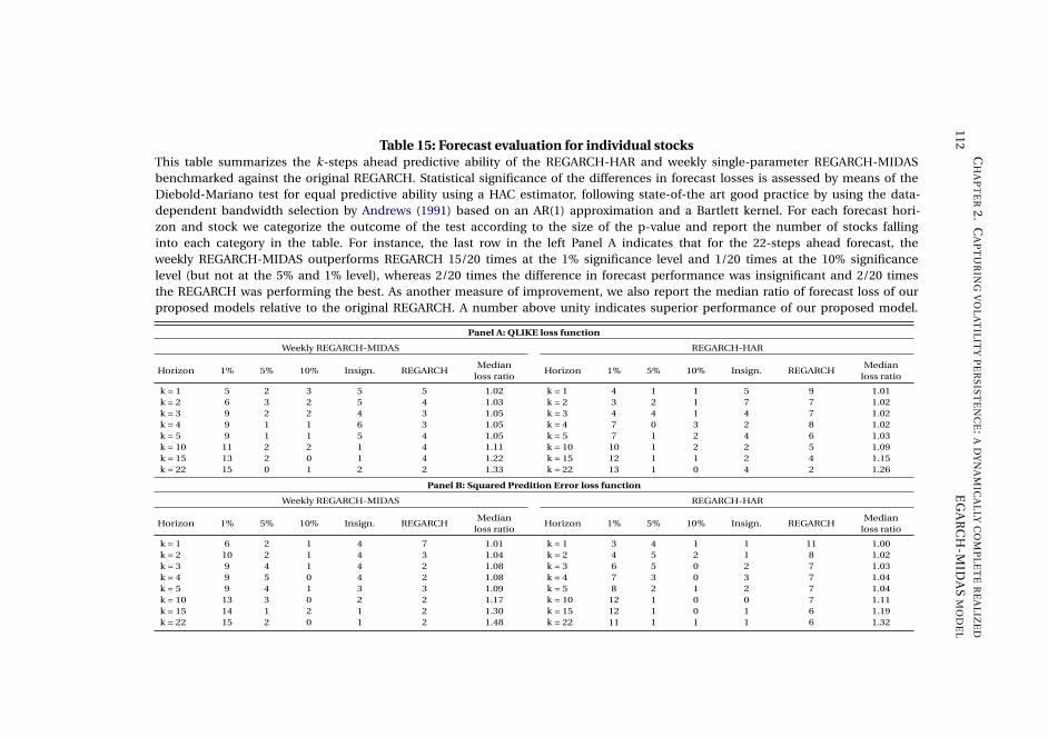
112
CH
AP
TE
R2
.C
AP
TU
RIN
GV
OL
AT
ILIT
YP
ER
SIS
TE
NC
E:A
DY
NA
MIC
AL
LYC
OM
PL
ET
ER
EA
LIZ
ED
EG
AR
CH
-MID
AS
MO
DE
L
Table 15: Forecast evaluation for individual stocksThis table summarizes the k-steps ahead predictive ability of the REGARCH-HAR and weekly single-parameter REGARCH-MIDASbenchmarked against the original REGARCH. Statistical significance of the differences in forecast losses is assessed by means of theDiebold-Mariano test for equal predictive ability using a HAC estimator, following state-of-the art good practice by using the data-dependent bandwidth selection by Andrews (1991) based on an AR(1) approximation and a Bartlett kernel. For each forecast hori-zon and stock we categorize the outcome of the test according to the size of the p-value and report the number of stocks fallinginto each category in the table. For instance, the last row in the left Panel A indicates that for the 22-steps ahead forecast, theweekly REGARCH-MIDAS outperforms REGARCH 15/20 times at the 1% significance level and 1/20 times at the 10% significancelevel (but not at the 5% and 1% level), whereas 2/20 times the difference in forecast performance was insignificant and 2/20 timesthe REGARCH was performing the best. As another measure of improvement, we also report the median ratio of forecast loss of ourproposed models relative to the original REGARCH. A number above unity indicates superior performance of our proposed model.
Panel A: QLIKE loss function
Weekly REGARCH-MIDAS REGARCH-HAR
Horizon 1% 5% 10% Insign. REGARCHMedian
loss ratioHorizon 1% 5% 10% Insign. REGARCH
Medianloss ratio
k = 1 5 2 3 5 5 1.02 k = 1 4 1 1 5 9 1.01k = 2 6 3 2 5 4 1.03 k = 2 3 2 1 7 7 1.02k = 3 9 2 2 4 3 1.05 k = 3 4 4 1 4 7 1.02k = 4 9 1 1 6 3 1.05 k = 4 7 0 3 2 8 1.02k = 5 9 1 1 5 4 1.05 k = 5 7 1 2 4 6 1.03k = 10 11 2 2 1 4 1.11 k = 10 10 1 2 2 5 1.09k = 15 13 2 0 1 4 1.22 k = 15 12 1 1 2 4 1.15k = 22 15 0 1 2 2 1.33 k = 22 13 1 0 4 2 1.26
Panel B: Squared Predition Error loss function
Weekly REGARCH-MIDAS REGARCH-HAR
Horizon 1% 5% 10% Insign. REGARCHMedian
loss ratioHorizon 1% 5% 10% Insign. REGARCH
Medianloss ratio
k = 1 6 2 1 4 7 1.01 k = 1 3 4 1 1 11 1.00k = 2 10 2 1 4 3 1.04 k = 2 4 5 2 1 8 1.02k = 3 9 4 1 4 2 1.08 k = 3 6 5 0 2 7 1.03k = 4 9 5 0 4 2 1.08 k = 4 7 3 0 3 7 1.04k = 5 9 4 1 3 3 1.09 k = 5 8 2 1 2 7 1.04k = 10 13 3 0 2 2 1.17 k = 10 12 1 0 0 7 1.11k = 15 14 1 2 1 2 1.30 k = 15 12 1 0 1 6 1.19k = 22 15 2 0 1 2 1.48 k = 22 11 1 1 1 6 1.32
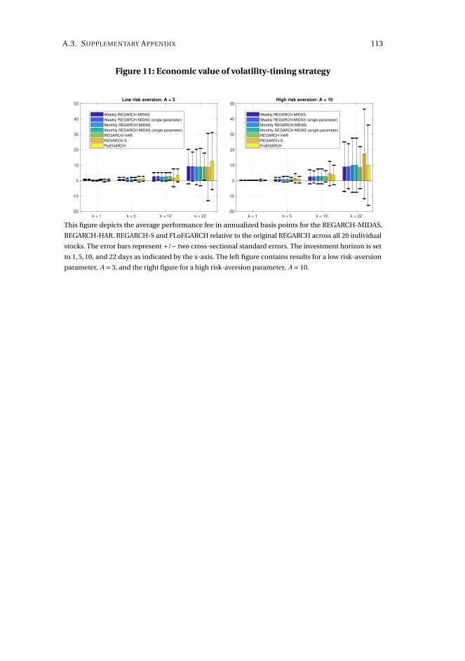
A.3. SUPPLEMENTARY APPENDIX 113
Figure 11: Economic value of volatility-timing strategy
Low risk aversion: A = 3
k = 1 k = 5 k = 10 k = 22-20
-10
0
10
20
30
40
50
Weekly REGARCH-MIDAS
Weekly REGARCH-MIDAS (single-parameter)
Monthly REGARCH-MIDAS
Monthly REGARCH-MIDAS (single-parameter)
REGARCH-HAR
REGARCH-S
FloEGARCH
High risk aversion: A = 10
k = 1 k = 5 k = 10 k = 22-20
-10
0
10
20
30
40
50
Weekly REGARCH-MIDAS
Weekly REGARCH-MIDAS (single-parameter)
Monthly REGARCH-MIDAS
Monthly REGARCH-MIDAS (single-parameter)
REGARCH-HAR
REGARCH-S
FloEGARCH
This figure depicts the average performance fee in annualized basis points for the REGARCH-MIDAS,
REGARCH-HAR, REGARCH-S and FLoEGARCH relative to the original REGARCH across all 20 individual
stocks. The error bars represent +/− two cross-sectional standard errors. The investment horizon is set
to 1,5,10, and 22 days as indicated by the x-axis. The left figure contains results for a low risk-aversion
parameter, A = 3, and the right figure for a high risk-aversion parameter, A = 10.


C H A P T E R 3ASSET PRICING MODEL UNCERTAINTY
PUBLISHED IN JOURNAL OF EMPIRICAL FINANCE 54 (2019), 166-189
Daniel BorupAarhus University and CREATES
Abstract
This paper provides a unified calendar-time portfolio methodology for assessing
whether returns following an event are abnormal which efficiently handles asset pric-
ing model uncertainty and allows for time-varying alpha and factor exposures. The
approach disciplines researchers’ use of asset pricing factors and assigns a probability
measure to the appropriateness of (dynamically) selecting a single model that best
approximates the true factor structure or whether model averaging across an asset
pricing universe is desired. It is applied to the long-horizon effect of dividend initi-
ations and resumptions in the 1980 to 2015 period. Resulting post-announcement
conditional abnormal returns are generally significant, statistically and economically,
which contrasts recent evidence, and exhibits a break in mean from positive until
the mid-1990s and negative onwards. We document substantial time-variation in the
dimensionality and composition of the factor structure in expected returns, which
goes beyond what captured by conditional versions of the CAPM and Fama-French
specifications. This also generalizes to a large panel of 202 characteristics-sorted
portfolios.
115

116 CHAPTER 3. ASSET PRICING MODEL UNCERTAINTY
3.1 Introduction
The purpose of an event study is to isolate the incremental impact of an event on
price performance relative to established determinants of performance (Kothari and
Warner, 2006). In long-horizon event studies on abnormal stock returns, a widely
applied methodology is the calendar-time portfolio (CTP) approach. The method
constructs at each time point, t , an event portfolio of the firms which have experi-
enced the event in question within a fixed horizon prior to time t . Inference on the
event effect is then based on a Jensen’s alpha procedure (Jensen, 1967; Jaffe, 1974;
Mandelker, 1974) which amounts to evaluating the intercept in a time series CAPM
or Fama-French regression, possibly including a momentum factor (Carhart, 1997).
Two most crucial problems with inference are, however, reliance on a single, possi-
bly misspecified model of asset pricing and the imposition of constant coefficients
(“alpha" and “betas"). First, the true asset pricing model is unknown, and perfect
factor selection rarely happens in practice. In other words, model uncertainty is
predominant. Moreover, investors may be concerned about different types of risk
conditional on, e.g., the economic environment, such that the composition of the
factor structure in returns is time-varying (Fama, 1998; Lyon, Barber, and Tsai, 1999;
Johannes, Korteweg, and Polson, 2014). Secondly, due to changes over time in the
composition of the event portfolio or shifts in the surrounding economic environ-
ment, factor exposures are most likely time-varying (Fama and French, 1997; Boehme
and Sorescu, 2002; Armstrong et al., 2013).
In this paper we introduce a unified framework which allows for time-varying al-
pha and betas as well as efficiently and dynamically handles asset pricing model
uncertainty. We specify a dynamic linear model (West and Harrison, 1997) for the
return-generating process where coefficients are defined as an endogenous latent
process such that their values are inferred from returns directly. This avoids the un-
derconditioning bias typically faced in conditional asset pricing models where the
researcher is required to instrument coefficients by certain observables that are sup-
posed to proxy investors’ information set (Cochrane, 2005; Lewellen and Nagel, 2006).
The degree of time-variation in coefficients can either be fixed by the researcher
or inferred simultaneously by data. Our framework also nests the specification of
constant regression coefficients allowing for both conditional and unconditional
analysis of the pricing of excess returns.
To handle asset pricing model uncertainty and explicitly address the “bad-model
problem" of Fama (1998), we define an asset pricing universe of factor models as
spanned by (linear combinations of) K candidate factors derived from the asset
pricing literature. This universe nests conventional models typically employed in
the literature, e.g. CAPM or the three-factor Fama-French model, and evaluates the

3.1. INTRODUCTION 117
pricing performance of each factor both individually and in conjunction with others.
Accordingly, Fletcher (2018) empirically finds that better performing pricing models
can be constructed from new combinations of the set of factors included in a set
of conventional global asset pricing models, see also Bryzgalova (2016), Fama and
French (2018), and Asness, Frazzini, Israel, Moskowitz, and Pedersen (2018). Some
factors may not be uniformly strong for pricing purposes at all times when assessed in
this asset pricing universe, but it is crucial for obtaining valid inference on abnormal
returns that relevant factors for pricing excess returns and reducing an omitted
variable bias are accounted for in the asset pricing model. If these factors are ignored,
and they are correlated with the included factors, it may lead to incorrect inference
and even sign of the abnormality in a given return pattern.
In response, we specify a dynamic Bayesian framework on the basis of Dangl and
Halling (2012) and Raftery, Kárný, and Ettler (2010) which infers from data (at each
point in time) the support for a given factor and factor model. In the interest of
efficiency and parsimony, those factors should be included only to the degree they
matter. Most financial literature focuses, however, on two polar viewpoints. Based on
empirical tests they tend to either reject an asset pricing model and discard it or vice
versa. Acknowledging as Fama (1998) that such models are inevitably simplifications
of reality while at the same time recognizing that complete confidence in a single
asset pricing model may be rather extreme, even if data rejects a model, one ought
to still account for the information in the model or factors to some degree (see also
Pástor (2000), Pástor and Stambaugh (2000), and Avramov (2004)). In our framework,
this degree is measured by posterior model probabilities which capture the time-t
support for a factor or model. Hence, to efficiently utilize the entire asset pricing
universe, we can base our model choice on the time series of those posterior model
probabilities which allow for either dynamic selection of the “most correct" model
or averaging over all model combinations. Employing posterior model probabilities
as weights in model averaging, which penalize overspecified models with needlessly
many factors through Occam’s razor effect, the procedure allows for an efficient way
of accommodating the ’multidimensional challenge’ of expected returns (Cochrane,
2011) for the use in event studies or asset pricing in general.
Our framework assesses pricing models simultaneously and, as a result, it is less prone
to pre-testing or repeated analyses for several model specifications.1 In essence, our
1Repeated analyses is a common choice of methodology in event studies when the authors are uncer-tain about model specification. Gregory (1997) and Boehme and Sorescu (2002), for example, implicitlyrecognize the presence of model uncertainty in long-horizon event studies by implementing severaldifferent model specifications and report the results arising from all the different specifications. However,while such a procedure highlights differences between methods, it also leaves inferences incompleteunless all models lead to the same conclusion. That is, it is not given how one should distinguish among orsynthesize the conclusions derived from different model specifications. We suggest a disciplined solution,providing a single measure of abnormality.
118 CHAPTER 3. ASSET PRICING MODEL UNCERTAINTY
proposal is a more disciplined approach to asset pricing that avoids data-snooping,
relative to the conventional practice of selecting some arbitrary factors for inclusion
in the benchmark model, which leaves researchers much more freedom (Fama and
French, 2018). Rather, the researcher needs to specify a broad asset pricing universe,
from which our framework delivers pricing, robust to model misspecification. Our
ultimate goal is, hence, not to come up with the true asset pricing model. Instead,
we acknowledge the fact that we do not know the true asset pricing model but are
able to identify its closest approximation as a function of a potentially large set of
candidate asset pricing factors whose elements we do not know when to (potentially)
apply. However, if the researcher has strong prior knowledge or desire about the
inclusion of certain factors, it can easily be accommodated by fixing the particular
factors’ inclusion probability to unity at all time periods beforehand. If the researcher
wants a test of abnormality against, say, the CAPM, robust to model misspecification
and omitted variable bias, one fixes the inclusion of the market risk premium and
treats the remainder of the asset pricing universe of risk/mispricing factors as control
whose relevance is determined and corrected for by our proposed framework. Besides
its econometric benefits, our framework gives rise to interesting insights into the
main drivers of the anomaly return pattern under investigation.
Recent contributions to the literature on event study methodology have primarily
focused on the characteristics-based matching framework, see, e.g., Bessembinder
and Zhang (2013) and Bessembinder, Cooper, and Zhang (2018), who substantially
refine those methods. However, according to Kozak, Nagel, and Santosh (2018b) no
good characteristics-sparse pricing model exists for the cross-section of expected
stock returns, limiting the applicability of procedures that require ex-ante choos-
ing a somewhat low-dimensional characteristic-based model. As argued above, our
proposal adds a required level of sophistication to the Jensen’s alpha/calendar-time
portfolio framework, improving its usefulness. By doing so, our method is applicable
to all long-horizon event studies and (un)conditional asset pricing in general which
we discuss further below. As noted by Kothari and Warner (2006), Bessembinder and
Zhang (2013) and Bessembinder et al. (2018) it is valuable to continue to refine both
methods and assess the consistency of results across methods, because neither the
characteristics-based matching method nor the calendar-time portfolio method to
event studies are perfect. We, therefore, apply the technique to the widely discussed
hypothesis of long-horizon overperformance following dividend initiations and re-
sumptions, which continues to draw attention in the literature (Hameed and Xie,
2018), and illustrate the type of economic insights our framework gives rise to. Conse-
quently, we take a conditional view and examine the “chance proposal" of Boehme
and Sorescu (2002) who attribute a significant event effect to pure chance (choice of
sample period).
Applying our unified framework, we find a significant one-, three- and five-year
3.1. INTRODUCTION 119
conditional abnormal return in the 1980 to 2015 period for an equally-weighted
portfolio. The abnormality of the one-year value-weighted event portfolio is confined
to sub-periods whereas the evidence is significant over the full sample for the three-
and five-year horizons. Our conditional view reveals a clear regime shift in mid-1990s,
switching from weakly positive to negative abnormal returns, interestingly matching
with increases in the relative importance of share repurchases as an alternative
payout policy. It appears, thus, as if investors have changed their idea about dividends
from being positive to negative signals, possibly realizing that managers’ decision of
dividend initiations is not necessarily a sign of good future performance, and that it
might even be decoupled from firm fundamentals (Chetty and Saez, 2005). Seen over
the full sample, event effects for both portfolio weighting schemes are mostly negative.
This contrasts the general conclusion in recent literature (see, e.g., Bessembinder and
Zhang (2013), Chen, Chou, and Lee (2014), and Bessembinder et al. (2018)) that event
effects are largely positive, yet insignificant. Interestingly, our unified framework and
conventional models disagree notably from late-1990s and onwards and sometimes
by more than 1% in the conditional monthly alpha. Their abnormal returns are even
negatively correlated showing opposite signs and movements in periods related to
economic crises. In conjunction with substantial improvements in empirical fit of our
CTP-DMA methodology, this indicates that conclusions from conventional models
may be biased due to model misspecification.
Moreover, the 1980-2015 period is associated with increasing dimensionality of ex-
pected returns, from about six-seven factors in the 1980-1990s to about eight-nine
most recently. Underlying these numbers is a strong time-variation in the pertinence
of specific factors. For instance, the event portfolio returns contain a large compensa-
tion for macroeconomic risk in crisis periods. This is consistent with recent findings
in Boons (2016), who finds that macroeconomic risks are significant in excess of mar-
ket risk and conventional Fama-French factors. Interestingly, even in the best case
scenario where the (time-varying) “most correct" asset pricing model (in the sense of
the highest posterior model probability) is known and available to the researcher in
each period, one still puts faith in models that are at best 97% likely not the true ones.
This underscores the appropriate use of the entire asset pricing universe via Bayesian
model averaging and the inappropriateness of rejecting information contained in
parts of the asset pricing universe which cannot be captured by a dynamic selection
of a single, best model. To assess these implications in a general asset pricing context,
we also apply our methodology to a large panel of 202 characteristics-sorted portfo-
lios in the spirit of Giglio and Xiu (2018). We confirm the superior performance of our
DMA procedure relative to DMS and conventional models. We also find supporting
evidence for the fact that asset pricing models should contain quite a large number
of factors (about eight on average), with time-variation in the pertinence of factors,
as well as notable time-variation in their associated abnormal returns.
120 CHAPTER 3. ASSET PRICING MODEL UNCERTAINTY
The remainder of the paper is laid out as follows. The following section positions our
proposal in the most recent and related general asset pricing literature. Section 3.2
introduces the setting of the CTP long-horizon event study and presents our unified
framework. We also show how to conduct inference on both alpha and asset pricing
factors and models. Section 3.3 presents the event study application to dividend
initiations and resumptions and Section 3.4 conducts the application to the large
panel of characteristics-sorted portfolios. Section 3.5 concludes.
3.1.1 Relation to general asset pricing literature
Treating model uncertainty and time variability of coefficients jointly in a unified
framework, which nests several proposals introduced separately in the literature, also
contributes to the very large and active research field on equity asset pricing. Instead
of attempting a thorough review, we briefly relate our paper to some of the most
recent contributions in the general asset pricing literature most closely related to our
analysis.
A recent literature has focused on pitfalls in estimating and interpreting conventional
factor models and that inference should be robust to model misspecification (Kan
and Zhang (1999a,b), Shanken and Zhou (2007), Kan and Robotti (2008), Kan, Robotti,
and Shanken (2013), Gospodinov, Kan, and Robotti (2013), Burnside (2016), Bryz-
galova (2016), and Gospodinov, Kan, and Robotti (2017)). Existing literature considers
mostly inference on pseudo-true coefficients under the presence of model misspec-
ification. On the contrary, Feng, Giglio, and Xiu (2017) make inference on original
coefficients by correcting for the model misspecification bias via a two-stage Lasso
procedure that selects relevant asset pricing factors for excess returns and reducing
an omitted variable bias. Our Bayesian alternative achieves similar ideas, but with
a different objective. Their interest is in cross-sectional inference on the risk price
of a new candidate factor. Our interest is in time series pricing and, primarily, an
associated alpha. Moreover, we explicitly model time-varying coefficients. Despite
the fundamental differences, our general logic is similar in that we acknowledge the
presence of model uncertainty and that perfect model selection may be implausible
requiring the researcher to specify a broad asset pricing universe from which we can
get a reliable approximation of the true model.
Kelly, Pruitt, and Su (2019) propose an intriguing Instrumented PCA (IPCA) approach.
They treat factors as latent and instrument alpha and betas with firm character-
istics. The factors are estimated with PCA as those components that line up with
characteristics-driven exposures. If they do not exist, the characteristics-driven alpha
will dominate. Our methodology differs from theirs in several ways. First, we retain in-
terpretability of the driving risk/mispricing patterns of the excess return to be priced.
We allow the researcher to determine the pertinence of a factor or factor model at
3.1. INTRODUCTION 121
a given point in time. This is relevant because a researcher evaluating a candidate
anomalous return pattern would be interested in assessing not only its alpha, but
also whether it reflects compensated risk and/or resembles an already documented
anomaly. Such interpretability is generally lost in factors derived statistically (from,
e.g., PCA). Secondly, the implementation of the IPCA requires the researcher to take
a stance of investors’ information set by specifying the instruments of the coeffi-
cients which drives the time variability. As pointed out in Cochrane (2005), investors’
information is inherently unobserved for the econometrician, making conditional
asset pricing models impossible to test. Indeed, Halling, Ibert, and Lenz (2018) find
that betas are largely described by a yet unknown component. To avoid this issue,
it is preferable to infer coefficients directly from information in returns themselves.
Lewellen and Nagel (2006) develop an early contribution that acknowledges this
point. They propose to estimate conditional CAPM betas from daily or weekly data
within a month or quarter. The method by Lewellen and Nagel (2006) applies, how-
ever, only in the case where daily (or weekly) data is available on factors which may
be restrictive given that many factors are constructed on the basis of low-frequent
macroeconomic or accounting data. There is, too, no need for instrumenting betas
(or alpha) in our framework. Thirdly, with no risk or mispricing interpretation of the
identified IPCA factors, the interpretation of their IPCA betas is also reduced in that it
is not clear which type of return premium they represent exposure to.
Barillas and Shanken (2018) propose a Bayesian framework for unconditional as-
set pricing. Like us, they also examine an asset pricing universe spanned by linear
combinations of a set of candidate factors and allow for simultaneous comparison
between all of the implied factor models on the basis of posterior model probabili-
ties. We differ methodologically in that we, in addition to model uncertainty, jointly
treat time-variation in alpha and betas, allowing for (but not requiring) conditional
asset pricing. Moreover, they focus on Bayesian model selection for absolute asset
pricing. Our framework allows the researcher to determine the appropriateness of
selecting a single model or the need for Bayesian model averaging which utilizes
relevant information in the remaining asset pricing universe. Consistent with an
unconditional focus, model selection is conducted ex-post at the end of the sample
in Barillas and Shanken (2018). We, in addition, show how to dynamically assess
factor models, consistent with conditional asset pricing that maps directly to the
decision-making of investors who conduct asset allocation based on conditional
expectations. Lastly, as the authors also point out themselves, their set of candidate
asset pricing factors are somewhat limited. In fact, their preferred model exploits
the maximum amount of factors possible suggesting that additional factors may be
relevant. We find an average model size of seven-eight factors, derived from a greater
asset pricing universe spanned by additional factors, which exceeds that of Barillas
and Shanken (2018)’s six factors.
122 CHAPTER 3. ASSET PRICING MODEL UNCERTAINTY
3.2 Methodology
We are in essence concerned about the average long-horizon abnormal return across
N event firms after the occurrence of an event. According to the CTP procedure, we
construct in each time period (months) a portfolio of firms that have experienced
the event within h periods prior to the given month t . In monthly long-horizon
event studies, one usually fixes h as either 12,36, or 60, representing a one-, three-,
and five-year event horizon, respectively. The monthly event portfolio return, Rp,t ,
is computed as the equally-weighted average of the event firms’ monthly returns
or as the value-weighted average return to better replicate investors’ total wealth
effects from holding the portfolio. Denote by R f ,t the risk-free rate and define Rep,t =
Rp,t −R f ,t , the portfolio excess return. The conventional CTP approach then dictates
the relation
Rep,t =α+X tβ+εt , (3.1)
where X (of appropriate dimension) usually contains the market risk premium and
the Fama-French factors (Fama and French, 1993), possibly along with the momen-
tum factor of Carhart (1997), and εt constitutes an error term. Under the assumption
that the factor model used in (3.1) is the true asset pricing model describing expected
excess returns, the intercept, α, measures the average abnormal return to the event
portfolio following the event. That is, it measures the average impact of the event.
Under the null hypothesis of no event effects, the intercept should be zero. Numer-
ous studies employ this method, for instance Boehme and Sorescu (2002), Moeller,
Schlingemann, and Stulz (2004), and Bessembinder and Zhang (2013).
3.2.1 Calendar-time portfolio returns, time-varying coefficients, and
model uncertainty
In this section, we present a CTP framework which jointly allows for time-varying
coefficients and a large number of candidate asset pricing factors in a parsimonious
manner. Specifically, the framework utilizes the concept of dynamic model averaging
(DMA) (see, e.g., Raftery et al. (2010)) and builds upon the work of Dangl and Halling
(2012).
Let the filtration Ft be the σ-field which represents the time-t conditioning informa-
tion set which, in line with the CTP methodology, contains asset pricing factors and
past returns. In general, it holds that
Rep,t = E[Re
p,t |Ft ]+εt , (3.2)
where E[Rep,t |Ft ] is the conditional expectation of the event portfolio excess return,
henceforth referred to as the normal return of the event portfolio, and εt is an error
term. The overarching model in (3.2) is the starting point for our analysis. The purpose
3.2. METHODOLOGY 123
of the event study is then to isolate the incremental impact of the event on stock
returns in excess of this normal return. Given the existence of the risk-free rate, we
model the normal excess portfolio return as a linear factor pricing model which is
rooted in conventional asset pricing theory (Cochrane, 2005). Suppose the factor
model contains at most K ≥ 1 pricing factors which the researcher deem potentially
relevant for measuring normal returns. Like other asset pricing analyses, we require
those factors to be traded portfolio excess returns and, consequently, in case of
non-traded factors (e.g., real consumption growth), we construct relevant factor
mimicking portfolios. The theoretical foundation of such procedure is documented
in Breeden (1979) and Huberman, Kandel, and Stambaugh (1987), and the asset
pricing model is without an intercept term. Thus, by adding an intercept term to the
relation in (3.2), we introduce a measure of an abnormal return following a given
event. The framework we propose below is Bayesian in nature. As such, it represents
a setting where investors recursively learn about both alpha, factor exposures and
the relevance of asset pricing factors, gradually incorporating their beliefs to form
the conditional expected returns in (3.2).
The return-generating process is specified as a dynamic linear model (DLM)2 (West
and Harrison, 1997)
Rep,t = X tθt +εt , εt ∼N (0, Ht ), (3.3)
θt = θt−1 +ηt , ηt ∼N (0,Qt ), (3.4)
where X t is a (1×K +1) vector of factors (including a constant) and θt = (αt ,βt )′ is
a (K +1×1) vector of coefficients (alpha and betas). A few remarks are worthwhile
here. First, coefficients are specified as an endogenous latent process where time
variability is allowed for by letting them follow a random walk. This tends to be su-
perior in empirical applications (Dangl and Halling, 2012). Essentially, changes in
alpha and betas are unpredictable, consistent with the suggestion in Boehme and
Sorescu (2002).3 Moreover, the case of constant regression coefficients is nested in
(3.4) if Qt is equal to zero for all t . This coefficient specification avoids the need of
instrumentation. This is suitable because the investors’ information set is latent to the
econometrician, making any instrumentation only an approximation of the true time
2Other studies apply a related DLM specification when examining the relationship between returnsand pricing factors. An incomplete list includes Conrad and Kaul (1988), Lamoureux and Zhou (1996), Angand Piazzesi (2003), Brandt and Kang (2004), Pástor and Stambaugh (2009), Rytchkov (2010), and Johanneset al. (2014).
3From an econometric point of view, the assumption of random walk coefficients may theoreticallyallow coefficients to drift arbitrarily high or low causing returns to be non-stationary. However, as pointedout by Dangl and Halling (2012), data at monthly frequency or higher tend to provide a remedy to theconcerns of non-stationarity since the high frequency of observations drives dynamics of estimatedcoefficients rather than an increase in variance coming from the random walk assumption. Moreover, weshow below how to model the time-variation of coefficients in a data-driven manner which avoids anyunreasonable behavior. Evidently, in the empirical section all estimated coefficients behave “reasonably".
124 CHAPTER 3. ASSET PRICING MODEL UNCERTAINTY
variability in coefficients. Indeed, Halling et al. (2018) document that factor exposures
are dominated by a yet unkown, time-invariant component not captured by known
firm characteristics nor their industry relation. Secondly, the stochastic dynamics
for the variation in coefficients in the style of (3.4) utilize information efficiently by
keeping track of information in the past and weighting most recent exogenous shocks
higher. It can be shown that the weights assigned to past information contained in re-
turns decay exponentially with the decay being a function of the signal-to-noise ratio
in returns (Bianchi, 2018). Hence, we differ from the proposal in Lewellen and Nagel
(2006) who use only contemporaneous, higher-frequent information to infer betas.
This also contrasts, for instance, a rolling least squares approach which assumes
coefficients are constant in each estimation and weighted equally, as implemented
in Bessembinder et al. (2018).4 In the context of an event study, this is especially
relevant because the characteristics of the event portfolio may change substantially
due to the rolling nature of creating cohorts of event firms. This requires the factor
exposures to be responsive and, importantly, to weight recent information highest
since a firm usually enters the portfolio only once and for a limited, fairly short period
of time (depending on the event horizon). Changing economic environments, such
as periods of increasing market stress, may also require factor exposures to be flexible.
We document the relevance of both instances in the empirical section below. Lastly, in
many long-horizon studies, the event follows a period of unusual firm performance
such that the event itself may impose gradual changes in firm characteristics follow-
ing the event (Bessembinder and Zhang, 2013; Hameed and Xie, 2018), causing factor
exposures to change as also empirically documented in Boehme and Sorescu (2002).
Via (3.4), we obtain a time series of Jensen’s alpha, measuring the event impact at
each time t . We show in Section 3.2.2 formal Bayesian inference in this setting which
enables an examination of abnormal returns over time in line with the proposal of
Fama (1998): “one way to test whether [an] anomaly is real or the sample-specific result
of chance is to examine a different sample period". Notably, this also reduces reliance
on ad hoc subperiod investigations otherwise resorted to in the literature.
The DLM is itself restricted to implementing the same set of factors for all time
periods. That is, it is unable to directly capture model uncertainty. For this matter,
we consider a set of candidate DLMs. We define each model by the inclusion and
exclusion of a factor from the set of K candidate factors. We, thus, consider an asset
pricing universe of 2K candidate models for each time period, such that denoting a
particular model and quantities associated with it by k = 1,2, . . .2K the set of models
4In fact, a recursive least squares approach can be obtained as a nested case of this specification,see Branch and Evans (2006), but this do not efficienctly utilize information due to the assumption ofconstancy in the recursive window, nor is it sufficiently responsive to new information (Li and Yang, 2011).
3.2. METHODOLOGY 125
are
Rep,t = X (k)
t θ(k)t +ε(k)
t , ε(k)t ∼N (0, H (k)
t ), (3.5)
θ(k)t = θ(k)
t−1 +η(k)t , η(k)
t ∼N (0,Q(k)t ). (3.6)
Since this setup would be computationally infeasible and result in imprecise inference
unless K is small, Raftery et al. (2010) construct an accurate approximation that
enables estimation via a single run of a Kalman filter for each model in each time
period. That is, there is no need for a Markov Chain Monte Carlo (MCMC) algorithm.5
The approximation involves two forgetting parameters, δ and λ, both in the interval
(0,1]. Here, δ is related to the (uncertainty in) estimation of the factor loadings in
(3.5)-(3.6) while λ is related to the model probability component in same expression.
That is, δ controls coefficient time variation whereas λ controls model uncertainty.
The Kalman filter prediction of the factor exposures and their covariance matrix are
given by
θ(k)t |t−1 = θ(k)
t−1|t−1 (3.7)
Σ(k)t |t−1 =
1
δΣ(k)
t−1|t−1, (3.8)
where (3.8) implies that the state error covariance matrix reduces to Q(k)t = (δ−1 −
1)Σ(k)t−1|t−1. Hence, if δ= 1, the system variance Q(k)
t is zero, and the factor exposures
are constants. The lower the value of δ, the larger the system variance, and, thus,
the greater flexibility in the time variation of betas. The implication is that we may
conduct both conditional (δ< 1) and unconditional analyses (δ= 1).
The estimation is completed with the updating equations given by
θ(k)t |t = θ(k)
t |t−1 +Σ(k)t |t−1X (k)′
t
(H (k)
t +X (k)t Σ(k)
t |t−1X (k)′t
)−1 (Re
p,t −X (k)t θ(k)
t−1
), (3.9)
Σ(k)t |t =Σ(k)
t |t−1 −Σ(k)t |t−1X (k)′
t
(H (k)
t +X (k)t Σ(k)
t |t−1X (k)′t
)−1X (k)
t Σ(k)t |t−1. (3.10)
In periods with high stock market stress, factor exposures of firms could be expected
to change more frequently with the converse being expected in periods with low
market volatility. Dangl and Halling (2012) provide a very elegant solution by asso-
ciating a grid of δs with each factor model specification. We can then obtain a time
series of estimates of time variability in coefficients by performing Bayesian model
averaging (BMA) over this grid at each time point. Consequently, let δ j ∈ δ1, . . . ,δd
denote a certain choice of time variation of the betas, and let Mk denote a certain
5If the model space gets too big for computational feasibility, one can resort to a slightly augmentedprocedure as suggested by Onorante and Raftery (2016) and Risse and Ohl (2017). They propose a dynamicOccam’s window (Madigan and Raftery, 1994) which dynamically eliminates most of the low posteriorprobability models determined by some lower threshold level set by the researcher while still being able toresurrect them if needed.
126 CHAPTER 3. ASSET PRICING MODEL UNCERTAINTY
choice (model) of the K candidate factors. The total (i.e., choice of both model and δ)
posterior model probability is given by
p(Mk ,δ j |Ft ) = p(Mk |δ j ,Ft )p(δ j |Ft ), (3.11)
the Kalman filter model prediction equations are given by
p(Mk |δ j ,Ft−1) = p(Mk |δ j ,Ft−1)λ∑2K
l=1 p(Ml |δ j ,Ft−1)λ, (3.12)
p(δ j |Ft−1) = p(δ j |Ft−1)λ∑dl=1 p(δl |Ft−1)λ
, (3.13)
and the associated updating equations are
p(Mk |δ j ,Ft ) =p(Mk |δ j ,Ft−1)p(Re
p,t |Mk ,δ j ,Ft−1)∑2K
l=1 p(Ml |δ j ,Ft−1)p(Rep,t |Ml ,δ j ,Ft−1)
, (3.14)
p(δ j |Ft ) =p(δ j |Ft−1)p(Re
p,t |δ j ,Ft−1)∑dl=1 p(δl |Ft−1)p(Re
p,t |δl ,Ft−1). (3.15)
In the particular case of λ = δt = 1 for all t , the procedure reduces to a constant
coefficient BMA procedure.
In terms of modeling H (k)t , we follow the suggestions of, among others, Raftery et al.
(2010), Dangl and Halling (2012), and Byrne, Korobilis, and Ribeiro (2018) and assume
that H (k)t = H (k) for all t . Conveniently, if the prior on H (k) is inverse gamma, and
if the prior on θ(k) is normal, integrating the conditional density of excess portfolio
returns over the range of θ(k) and H (k) leads to a closed-form solution of the marginal
likelihood, given as the density of a t-distribution. This also enable fast recursive
computations. Alternatively, a time-varying error variance can be allowed.
The setup in (3.7)-(3.15) constitutes the Kalman filter procedure for estimation where
the recursions are initiated with a prior on the model probabilities, p(Mk ,δ j |F0), and
on the coefficients for all models. In the implementation of the procedure, we use a
burn-in period in order to train the model and hyperparameters as in Avramov and
Chao (2006). We discuss this further in Section 3.3.3.
3.2.2 Bayesian inference
When conducting the event study, we are interested in the value of alpha above
all to determine the sign and size of a potential event-induced abnormal return.
Additionally, we may be interested in examining betas to assess the exposure to return-
generating factors. In order to obtain these, it is useful to examine the implications of
the posterior model probabilities obtained via (3.14) and (3.15) first.
3.2. METHODOLOGY 127
3.2.2.1 Model and factor posterior probabilities
The metric
p(Mk |Ft ) =d∑
j=1p(Mk |δ j ,Ft )p(δ j |Ft ) (3.16)
measures the posterior model probability of model k after integrating out the effect ofδ j . It measures the relative support of a particular model, e.g., the three-factor modelof Fama and French (1993), relative to the remainder of the asset pricing universe. Inthe spirit of Barillas and Shanken (2018), this is a simultaneous model-comparisonframework that analyzes models jointly as opposed to classical pairwise test oftenseen in the literature (Vuong, 1989). This information is useful for several purposes.First, it informs about whether there exists a single best model that receives themajority of the support. In this case, inference on the event effect and the identifi-cation of main return drivers could be reasonably based on the outcome from themodel with highest posterior model probability at each point in time. It should benoted that the composition of this model need not be the same over time, given thedynamic feature of our framework, which is documented in the empirical sectionbelow. We refer to this procedure as dynamic model selection (DMS). If the relativestrength of the single-best model is weak, much relevant information is left in theremainder of the asset pricing universe.6 It is crucial to account for this informationin the interest of obtaining valid inference which is robust to model misspecificationand omitted variable bias. Inference should be based on a weighted average over allthe models in the asset pricing universe where the weights are determined by the(trajectory of) posterior model probabilities. We refer to this procedure as dynamicmodel averaging.7 In the empirical section below, the strongest model recieves atmost 3.5% weight across the full sample, suggesting a need for DMA. This goes wellwith points made in Fama (1998):
“[p.291] The problem is that all models for expected returns are incom-plete descriptions of the systematic patterns in average returns duringany sample period. [p.285] All models show problems describing averagereturns. The bad-model problem is ubiquitous, but it is more serious inlong-term returns."
At first hand, these procedures may hint at potential issues with overfitting and
lack of efficiency, and, therefore, a method that may favor the null hypothesis in the
asset pricing study. However, we put forward two arguments that contradict this. First,
6Note that DMS effectively treats the posterior model probability for the selected model as equalto unity, making an oracle-like assumption that there exists only one relevant and identifiable assetpricing model for each t in the asset pricing universe specified by the researcher, ignoring potential modeluncertainty within each t .
7Note that in principle we could minimize the omitted variable bias by including all variables at once ina kitchen-zink manner. However, with a large set of candidate factors and limited post-event observations,this is no viable solution due to less powerful inference. Importantly, a kitchen-zink procedure imposes a100% inclusion probability for all factors at all points, which is unnecessary given our empirical findingsbelow and distorts inference on alpha and eliminates information content in the time-varying inclusionprobabilities inferred from data.
128 CHAPTER 3. ASSET PRICING MODEL UNCERTAINTY
it is important to note that for an equal prior on each model, the posterior model
probabilities are largely determined by the likelihood function. Since they integrate
over the entire parameter space, parsimonious models are preferred over complex
models that include needlessly many factors, effectively employing Occam’s razor
effect. That is, the likelihood will be highest for parsimonious models that use only the
parts of the asset pricing universe required to provide a satisfactory fit of the excess
returns. Since we define the asset pricing universe by all linear combinations of the K
factors, many of the models considered are parsimonious allowing the procedure to
favor those if deemed relevant by data. Secondly, only if certain factors are relevant
for excess returns and for reducing an omitted variable bias, will they be assigned a
non-zero weight. If a factor is highly correlated with another factor, and they share a
signal for excess returns, our procedure will, by construction, share the total posterior
probability assigned to the common signal betweeen those two factors. That is, both
factors get assigned a non-zero weight but in a fair proportion compared to the
remainder of the asset pricing universe. Generally, these weights are rarely unity at
all times, nor are they constant. Hence, as opposed to techniques that apply hard
thresholding in that a factor is either included or not at all times, e.g., in Feng et al.
(2017), we address the trade-off in efficiency by using only the information in factors
when data tells us it matters to do so and in a manner that weigths its relevance. This
is a means to efficiently handle the multidimensional challenge in Cochrane (2011).
Denote by γ(k)t , j the size (number of factors included) of the k’th model with degree
of coefficient uncertainty δ j at time t . Then we define the time-t expected (average)
model size as
γt =d∑
j=1
2K∑k=1
γ(k)t , j p(Mk |δ j ,Ft )
p(δ j |Ft ). (3.17)
The average model size is an interesting output informing about the dimensionality
of expected excess returns over time. It may also function as an informal sanity check
of the specification of the asset pricing universe. If it takes a value close to the total
number of candidate factors, it may indicate that the chosen asset pricing universe is
underspecified and potentially cause of an unintentional omitted variable bias.
We may also be interested in inference on single factors and their relevance in the
asset pricing universe. To that end, the l ’th factor inclusion probability, ζl , may be
determined as
ζl =2K∑
k=11k⊂l p(Mk |Ft ) (3.18)
with “k ⊂ l " indicating that the k’th model includes the l ’th candidate factor. The tra-
jectory of inclusion probabilities informs about the main drivers of excess returns over
3.2. METHODOLOGY 129
time. It allows us to examine whether the candidate anomaly return pattern under
investigation resembles already documented anomaly patterns (such as momentum),
or whether it is driven by risk compensation (coming from, e.g., real consumption
growth). Depending on the specification of the asset pricing universe, this gives rise
to valuable information about the components of expected excess returns.
3.2.2.2 Abnormal returns and factor exposures
To obtain estimates of the event effect (alpha) and the factor exposures (betas), model
averaging dictates for t = 1, . . . ,T recursive identification as
αt =d∑
j=1
2K∑k=1
α(k)t |t , j p(Mk |δ j ,Ft )
p(δ j |Ft ), (3.19)
βt =d∑
j=1
2K∑k=1
β(k)t |t , j p(Mk |δ j ,Ft )
p(δ j |Ft ), (3.20)
performing model averaging over both the uncertainty surrounding choice of pricing
factors and degree of time variation in coefficients.8 Formal inference on the event
effect at a given point in time dictates the null hypothesis H0 : αt = 0 against the
alternative hypothesis H1 : αt 6= 0 for some fixed t . Hypothesis testing can be con-
ducted on the basis of standard Bayes factors comparing a restricted model with
zero intercept at time t to a model with unrestricted intercept at the same point
in time without requiring this restriction to be imposed at any other time. Thus, a
testing methodology, which determines the time-t probability that the intercept is
zero, given the information set available up to that point in time, is based on the
recursive Bayes factor
BFt =p(Re
p,1, . . . ,Rep,t |Ft , H0)
p(Rep,1, . . . ,Re
p,t |Ft , H1), (3.21)
such that, (see, e.g., Robert (2007) and Bianchi (2018))
p(H0|Ft ) =(
1+ p(H1|F0)
p(H0|F0)
1
BFt
)−1
, (3.22)
given that the prior structure is common for the null and alternative model. With
equal prior over the null and alternative hypothesis, p(H0|F0) = p(H1|F0), the poste-
rior probability of the null hypothesis p(H0|Ft ) is obtained as BFt /(1+BFt ).9 This
8The posterior distribution of coefficients admits a multivariate t-distribution, Tnt (θt |t ,Σt |t ), wherent = nt−1 +1 is the degrees of freedom. Inference on coefficients is, thus, more robust to extreme realiza-tions of exogenous shocks due to fatter tails compared to a normal distribution in the beginning of thesample when less information is available.
9BFt may be conveniently computed using the Savage-Dickey density ratio and the fact that the priorstructure is common for the the null and alternative model. The ratio requires only computation underthe alternative model, see, e.g., Bianchi (2018), and benefits from a closed-form expression of the marginallikelihood.
130 CHAPTER 3. ASSET PRICING MODEL UNCERTAINTY
probability can broadly be interpreted as a frequentist p-value of the null hypothesis,
but it differs fundamentally since it automatically includes Occam’s razor effect in
that models with needlessly many factors that do not deliver improved pricing ability
are penalized. The value BFT provides the means of inference over the full sample
capturing the cumulative evidence against or in favour of the null hypothesis over all
time periods.
3.3 The long-horizon effect of dividend initiations andresumptions
We now apply the unified CTP framework to the lively debated post-event stock
performance following dividend initiations and resumptions. In a seminal article,
Michaely, Thaler, and Womack (1995) find a significant positive abnormal return
of 24.8% for three years following dividend initiations in the period of 1964-1988
applying the characteristics-based matching (BHAR)10 method using as benchmark
the return on an equally-weighted market index. Boehme and Sorescu (2002) find
supporting evidence when applying the BHAR method using dimensional matching
on size and book-to-market ratios to construct benchmark returns. They document,
in contrast, a disappearing abnormal return when applying the conventional CTP ap-
proach leading to the argument that the abnormal performance is attributed to pure
chance (choice of sample period). A recent study by Chen et al. (2014) supports the
“chance proposal" while controlling for the possibility of a negative bias arising from
the presence of initial public offerings (IPOs) in the event sample. As a response to
improving additional statistical rigour in event study methodologies, Bessembinder
and Zhang (2013) propose a modified union of the BHAR and CTP approach and
find that it leads to positive, yet insignificant abnormal returns following dividend
initiations. Kolari, Pynnonen, and Tuncez (2018) methodologically criticize Bessem-
binder and Zhang (2013) and find contrasting evidence in terms of positive and
statistically significant long-horizon effects (see Bessembinder and Zhang (2017) for
a response) confirming that long-run price effects are sensitive to choice of method-
ology. Bessembinder et al. (2018) document supporting evidence for the insignificant
results in Bessembinder and Zhang (2013) in a novel characteristics-based matching
event methodology. This overall ambiguity in findings motivates an application of
our method proposed above to the long-horizon performance following dividend
initiations and resumptions.
10The buy-and-hold abnormal return for the i ’th firm with an event horizon of T months is defined asthe difference between the buy-and-hold realized return on the i ’th firm and the buy-and-hold return of abenchmark firm or portfolio supposed to capture the expected return over the event horizon. The eventeffect is then measured as the sample average of all event firms’ buy-and-hold abnormal returns.
3.3. THE LONG-HORIZON EFFECT OF DIVIDEND INITIATIONS AND RESUMPTIONS 131
3.3.1 Events sample
We obtain the events sample following the lines of Michaely et al. (1995), Boehme and
Sorescu (2002), and Bessembinder and Zhang (2013). For the 1980 to 2010 time period,
we identify dividend initiations as the first cash dividend in the lifetime of a firm from
the Center of Research in Security Prices (CRSP) database. We stop the events sample
at year 2010 in order to ensure that all post-event windows may be up to five-years
length. In addition, we identify dividend resumptions as the first cash dividend paid
by a firm subsequent to a dividend omission with a hiatus of at least five years. We
require that the firms have been listed in CRSP for a minimum of two years and have
not experienced an IPO in two years before the dividend announcement, following
Kale, Kini, and Payne (2012). The firms must be U.S. based, traded on the NYSE,
Nasdaq, or AMEX exchanges, and be a common stock (share code 10 and 11). Lastly,
the cash dividends must have a monthly, quarterly, semi-annual, or annual frequency.
We also include the ones with an unspecified payment frequency since most of these
have a quarterly payment frequency. In total, we identify 1016 event firms composed
of 934 dividend initiations and 82 dividend resumptions. The distribution of events
over the sample period is depicted in Figure 1.
We note that the yearly frequency of events decreases from mid-1990s to 2002, consis-
tent with the disappearing dividend phenomenon (Fama and French, 2001), before
surging in 2003-2005 which aligns well with the introduction of the Jobs and Growth
Tax Relief Reconciliation Act of 2003. This act effectively reduced the tax rate on
corporate dividends to 15%. It also aligns well with the timing of a correction to
the SEC Rule 10b-18. The rule was released in 1982 to clarify circumstances under
which corporations could make share repurchases without being subject to dividend
taxation, causing firms to adjust their payout policies, which caused changes to the
informational content in dividend payments (Boudoukh, Michaely, Richardson, and
Roberts, 2007). The rule was then altered in 2003 by requiring firms to disclose more
detailed information about certain types of share repurchases. Chetty and Saez (2005)
find that the increase in dividend initiations in this period is solely due to the tax
cut and are not confounded by other factors that might have influenced the payout
decision, including a “relabelling" of share repurchases as dividends after the reform
and firm fundamentals.
3.3.2 Set of candidate asset (mis)pricing factors
Navigating in the zoo of asset pricing factors (Cochrane, 2011) is not a trivial task.
Indeed, Harvey, Liu, and Zhu (2016) identify as much as 316 factors published in
leading journals and supposed to explain the cross-section of average returns. For
many of those factors it is not clear whether they are driven by risk or common sources
of mispricing as they are mostly observationally equivalent and both can belong in
132 CHAPTER 3. ASSET PRICING MODEL UNCERTAINTY
the pricing model, as discussed in Kozak, Nagel, and Santosh (2018a). Behavioral
ideas (e.g., liquidity demands, distorted beliefs, etc.) result in mispricing only if they
represent factor risk because otherwise they would not exist due to arbitrageurs
exploiting them. Fortunately, this complication is not fatal in event studies. The
purpose of an event study, no matter the method, is to isolate the incremental impact,
relative to the controls, of an event on price performance. As also pointed out in
Kothari and Warner (2006) and Loughran and Ritter (2000), it is a relevant empirical
question to ask whether a potential anomaly pattern is distinct from other anomaly
patterns already established. Since the price performance associated with size, book-
to-market, and other characteristics is applicable to all stocks, not just the sample of
event firms, the performance following the event itself must be different from those
to be considered anomalous. From a methodological point of view, an event study
methodology should, therefore, control for the relevant return patterns common to
all stocks, regardless of a risk or mispricing interpretation.
Similarly in spirit to Giglio and Xiu (2018), we construct on this basis a set of candi-
date asset pricing factors combining macroeconomic, non-equity, and equity related
factors which represent both common sources of mispricing or sources generally
accepted to be true risk. Specifically, we include the well-known real consumption
growth factor (CONS) (Breeden, 1979) from the consumption-based asset pricing
framework. Secondly, we include macroeconomic and non-equity factors proposed
primarily in the seminal article by Chen, Roll, and Ross (1986), namely industrial pro-
duction growth (IND), unanticipated inflation, (INF), term spread (TMS), default risk
premium (DFR), and default yield spread (DFY). Thirdly, we add equity-related fac-
tors, specifically, the prominent factors of the Fama-French five-factor model (Fama
and French, 1993, 2015); market risk premium (MKT), small-minus-big (SMB), high-
minus-low (HML), robust-minus-weak (RMW), and conservative-minus-aggressive
(CMA). Additionally, we add momentum11 (MOM), betting-against-beta12 (BAB),
illiquidity13 (ILLIQ), and quality-minus-junk14 (QMJ). Hence, the set of candidate
factors includes the commonly used three factors of Fama and French (1993) and the
momentum factor of Carhart (1997), thus facilitating comparison with other studies
implementing conventional CTP models.
This amounts to a total of 15 different candidate pricing factors somewhat overlap-
ping and extending the set in Harvey and Liu (2018) and Barillas and Shanken (2018),
comprising a model space of 2K = 32,768 potential models each associated with d
degrees of time variation in coefficients. For all factors, we obtain a time series of
monthly observations for the 1980 to 2015 period. The non-traded factors, INF, IND,
11See Carhart (1997).12See Frazzini and Pedersen (2014).13See Pástor and Stambaugh (2003).14See Asness, Frazzini, and Pedersen (2019).

3.3. THE LONG-HORIZON EFFECT OF DIVIDEND INITIATIONS AND RESUMPTIONS 133
and CONS, are transformed to traded factors using mimicking portfolios following
the procedures in Jagannathan and Wang (2007) and Malloy, Moskowitz, and Vissing-
Jørgensen (2009). We obtain a monthly time series of per capita real consumption
growth using the National Income and Product Accounts (NIPA) tables from 1959 to
2015.15 Data on the monthly production growth series and inflation is obtained from
the Federal Reserve Bank of St. Louis database. We construct unanticipated inflation
similarly to Chen et al. (1986) and Liu and Zhang (2008). Subsequently, we regress
(including an intercept and macroeconomic controls, see Eckbo, Masulis, and Norli
(2000)) real consumption growth, industrial production growth, and unanticipated in-
flation on the excess returns of 30 industry portfolios obtained from Kenneth French’s
data library, which provides the mimicking portfolio weights (in a least square sense).
Consequently, the mimicking factor portfolio returns are these normalized weights
multiplied by the excess returns of the benchmark portfolios. Data on TMS, DFR,
and DFY is obtained from an updated Welch and Goyal (2008) data set. Data on the
remaining (traded) factors is obtained from the respective authors’ websites. For
elaboration on the factor constructions, we refer the reader to the specific references.
Summary statistics on the final candidate asset pricing factors are reported in Table
1.
3.3.3 Robustness of parameter and prior choices
In order to implement the procedure outlined in Section 3.2, we need to elicit priors
for the models, coefficients, and error variance along with a choice of range and gran-
ularity of the grid of δ. For the latter, we choose δ ∈ 0.97,0.98,0.99 in the conditional
analysis such that d = 3. We evaluated the results with a choice of granularity of d = 7,
but results do not change notably. We use a non-informative model prior where all
model combinations and degrees of time variation in the coefficients are equally
likely, p(Mk |F0) = 1/2K and p(δ j |F0) = 1/d such that p(Mk ,δ j |F0) = 1/(d2K ) for all
k and j consistent with Dangl and Halling (2012). Moreover, we use a proper prior
on the coefficients following the suggestions in Barillas and Shanken (2018) with
θ(k)0, j = N (0, g Ink ) for all k and j where nk ∈ 1,2, . . . ,K is the number of included vari-
ables in the k’th model. We use a burn-in training sample of three-years’ observations
to train g which is common in Bayesian asset pricing analyses (see, e.g., Avramov
and Chao (2006)).16 In this way, we put very little subjective information into the
start of the procedure and initiate it under the null hypothesis of zero alpha. The
prior on H (k) is inverse-gamma for all k similar to Dangl and Halling (2012). We also
15NIPA Table 2.8.5 provides the nominal personal consumption on non-durables and services. NIPATable 2.8.4 provides the price deflators and NIPA Table 2.6 provides population size.
16Our choice of grid for values of g is chosen to ensure a priori plausible deviations of alpha from zero.This is to avoid concerns of Bartlett’s paradox where posterior model probabilities favor a restricted, nullmodel despite substantial alpha deviations from zero due to them being even further from the valuesenvisioned under the unrestricted, alternative model. Empirically, we also found that very large values forg perform worse based on a comparison of marginal likelihoods.

134 CHAPTER 3. ASSET PRICING MODEL UNCERTAINTY
implemented an uninformative natural conjugate g-prior specification of the Zellner
(1986) type with g = T as Nonejad (2017) and Byrne et al. (2018), and we found that
the main conclusions are largely robust but somewhat affected primarily in the first
part of the sample and mainly for factor exposures. We attribute this to the prior
for the coefficient covariance matrix which is given by the g -scaled OLS estimate of
the variance in coefficients over the entire sample. With only a limited length of the
event portfolio return series, this g -prior seems to dominate too much initially before
the Bayesian procedure is able to pick up empirical patterns in data. Finally, we set
λ= 0.98 which is consistent with a case where model change is allowed, but not in a
too rapid manner. The conclusions, though, do not materially change for λ= 0.95
and λ= 0.99.
3.3.4 Empirical results
For comparative purposes, we report in addition to the results from our unified
framework also results applying conditional versions of conventional CTP models:
1. CTP-DMA: Calendar-time portfolio approach utilizing dynamic model averag-
ing and all candidate factors.
2. CTP-DMS: Calendar-time portfolio approach utilizing dynamic model selec-
tion and all candidate factors.
3. CTP-CAPM: Conditional CAPM with the MKT factor.
4. CTP-FF3: Conditional three-factor Fama-French model with the MKT, SMB,
and HML factors.
5. CTP-FF4: Conditional four-factor Fama-French-Carhart model with the MKT,
SMB, HML, and MOM factors.
6. CTP-FF5: Conditional five-factor Fama-French model with the MKT, SMB,
HML, RMW, and CMA factors.
In our analysis below, we fix the inclusion probability of the MKT to unity for all
periods.17 This is consistent with Barillas and Shanken (2018) and is motivated by
its unique role in portfolio analysis and equilibrium pricing of assets (Sharpe (1964),
Lintner (1965), Mossin (1966), Merton (1973)).18 It also facilitates straight comparison
of the CTP-DMA and CTP-DMS procedures to the CTP-CAPM, in that they differ
precisely in the use of controls.
17This reduces the model space to 2K−1 = 16,384 combinations for each d .18We also completed the application without this requirement, and results are almost quantitatively
identical due to MKT being chosen with probability one in close to all periods by DMA/DMS procedures.
3.3. THE LONG-HORIZON EFFECT OF DIVIDEND INITIATIONS AND RESUMPTIONS 135
We report results for both equally- and value-weighted portfolios (EW and VW, respec-
tively) where the monthly value-weights are constructed from prior month’s market
capitalization obtained from the CRSP/Compustat merged database. The weights are
rebalanced every month to reflect the changing composition of the portfolio. Con-
sidering both types of portfolios is relevant for economic as well as methodological
reasons. First, value-weighting better reflects investors’ wealth effects from holding
the portfolio. Secondly, event studies and general asset pricing studies tend to find
different results, depending on the choice of portfolio (Boehme and Sorescu, 2002;
Plyakha, Uppal, and Vilkov, 2016). Fama (1998) and Fama and French (2015) posits,
indeed, that value-weighting mitigates problems with model misspecification, since
it assigns a higher (lower) weight to larger (smaller) firms for which the problem
is likely to be less (more) severe. Given our focus on model specification, it is thus
interesting to examine the impact of model misspecification on the results from both
EW and VW portfolios.
To examine the relative evidence for each model specification, Table 2 reports the
empirical fit of the CTP-DMA relative to CTP-DMS and conventional models as
measured by logarithmic Bayes factors. An advantage of using Bayes factors, as
noted above, is their penalization of highly parametrized models that do not deliver
improved empirical fit. In all but four cases, the evidence in favour of the CTP-DMA
relative to all other models is either strong or very strong, in the wording of Kass
and Raftery (1995).19 By corollary, the CTP-DMA provides a much more accurate
characterization of the factor structure in the event portfolio returns.
3.3.4.1 Empirical abnormal returns
Table 3 provides results on average conditional abnormal returns, inference, and av-
erage model sizes for one-, three-, and five-year post-event horizons for the dividend
initiation and resumption event sample over the period of 1983-2015.20
For the EW portfolios, the conditional versions of the conventional models (CTP-
19According to the rule-of-thumb interpretation rules of Kass and Raftery (1995), values below 1 arenot worth more than a bare mention, values between 1-3 are positive in favour of the CTP-DMA, valuesbetween 3-5 are strongly in favour of the CTP-DMA, and values greater than 5 are very strongly in favour ofthe CTP-DMA.
20We have run standard unconditional FF3 and FF4 CTP regressions as in Bessembinder and Zhang(2013) and confirmed their findings of small, insignificant average abnormal returns on EW portfolios.The results were similar for the VW portfolios. We have also run WLS regressions with the square root ofnumber of firms contained in each month as weights. Such a procedure may be appropriate if the studyconcerns selective management events (such as dividend initiations, initial public offerings, or mergersand acquisitions) where the selection is partly driven by industry- and economy-wide conditions or stockmisvaluations, because the events may be bunched in calendar time. The resulting abnormal return wouldthen possibly be concentrated in certain periods. In the present paper, year 2003 and 2004 (cf. Figure 1)contain more events relative to remaining months. The WLS procedure should reveal any bunching effects,but the results were remarkably similar to the OLS results, providing no consistent support for bunchingeffects.
136 CHAPTER 3. ASSET PRICING MODEL UNCERTAINTY
CAPM, CTP-FF3, CTP-FF4, and CTP-FF5) show significant abnormal returns over the
full sample, which are positive on average and economically large, across all horizons.
The event effect is, though, decreasing as the horizon increases. These findings are
consistent with Boehme and Sorescu (2002). The conditional alphas from the CTP-
DMS, which dynamically selects the most correct model in each time period based
on the posterior model probabilities, and CTP-DMA, which averages over the alphas
across all factor models based on their relative posterior model probabilities, are
generally much smaller. They disappear on average at five year horizons for both CTP-
DMS and CTP-DMA and at three year horizons for CTP-DMA only. This disappearance
is, however, a consequence of a major intertemporal difference in abnormal returns
which can be seen from Figure 2 that depicts alpha with a three-year event horizon
for CTP-DMA and conventional models.
Interestingly, the upper figure shows that abnormal returns are positive and stable
from 1983 to 1988, zero and stable from 1989 to 1992, after which they are generally
negative and less stable. At most time points, the event effect is non-zero, but the
positive effects in the first part of the sample cancel out on average the negative effects
in remainder of the sample.21 On the basis of this analysis, it appears as if investors
have changed their idea about dividend signalling from being positive to negative. It
goes well in hand with the idea that the information content in dividend payments
is changing over time, as documented in Goyal and Welch (2003) and Boudoukh
et al. (2007). One explanation might be that investors have realized that managers’
decision of dividend initiations is not necessarily a sign of good future performance
(it might, indeed, be the opposite, as profitability tends to decrease in the years
subsequent to the announcement (Grullon, Michaely, and Swaminathan, 2002)),
and that it might even be decoupled from firm fundamentals. This is supported by
Chetty and Saez (2005) who documents that the dividend initiation decision in the
2003-2004 period was solely driven by above-mentioned tax reform on dividend
income and amplified by self-interest of managers. Additionally, they posit that
shareholders’ awareness of severe accounting fraud in the 2001-2003 period might
also have pressured management to pay out dividends.
Another explanation may arise from the increasing importance of share repurchases.
Interestingly, the timing of the shift of sign in the abnormal return aligns perfectly
with the empirical findings in Farre-Mensa, Michaely, and Schmalz (2014) which show
that the preferred payout policy shifted from being dividends before the mid-1990s
to being share repurchases after the mid-1990s and until today.22 Share repurchases
21In an earlier version of this paper, we conducted a (frequentist) test of change in the mean alphabased on a wild bootstrap procedure. The test rejected for all portfolios and event horizons, estimating thebreak for the equal-weighted three-year event horizon at 1994:3 with a positive (negative) mean in the first(second) part of the sample.
22There seem to be no complete agreement why firms did not prefer share repurchases before themid-1990s. One argument is that corporations were simply wrong (Grinblatt and Titman, 1998) and spent
3.3. THE LONG-HORIZON EFFECT OF DIVIDEND INITIATIONS AND RESUMPTIONS 137
are now considered by executives the most efficient way of paying out money to
investors, partly due to a preferable taxation scheme for investors relative to divi-
dends and partly because of its flexibility (Brav, Graham, Harvey, and Michaely, 2005).
Moreover, investors are aware of the possibility for firms to pay out using share re-
purhcases as an alternative to dividends (Grullon et al., 2002). Brav et al. (2005) find,
additionally, that 80% of surveyed executives make repurchase decisions after all their
other investment plans are determined. Only a third of the executives responded that
they make dividend decisions after investment plans are determined. The difference
is statistically significant. This indicates that executives might pay out using share
repurchases when they consider their own firm the most profitable investment avail-
able, whereas dividend payouts may occur before pursuing all profitable investment
opportunities. In light of these payout policy characteristics, our findings indicates
that when dividend payments were firms’ preferred payout policy, investors’ perceive
dividend initiations as a positive signal. However, when firms and investors realize
the appealing features of share repurchases relative to dividend payments, from the
1990s and onwards, they perceive dividend imitations as a negative signal. This can
occur, since investors evaluate the choice of dividend initiations relative to the, possi-
bly preferred, choice of share repurchases, and hence decrease their valuation of the
firm, see also Hartzmark and Solomon (2019). No matter the explanation, it is clear
that in order to extract this change in investor perception or information content,
it is a necessity to allow for a time-varying alpha that quickly learns, in real-time,
changes to the economic environment jointly with time-varying factor exposures
and relevance which we facilitate in CTP-DMA and CTP-DMS.
The lower part of the figure reveals stark contrasts between the CTP-DMA abnormal
returns and those obtained from conventional models pointing towards a severe
issue of omitted variable bias, especially in the second part of the sample. From
late-1990s and onwards, the trajectory of alpha is oftentimes negatively correlated
between CTP-DMA alpha and all conventional models. At times, the difference is well
above 1%. For instance, in the wake of the 2001 NBER recession conventional models
pointed to a positive event effect, whereas CTP-DMA suggests a considerable negative
effect. In the most recent recession, conventional models’ abnormal return decreased
substantially to negative terrain, whereas CTP-DMA’s abnormal return increased
from negative terrain to zero. The implication is that the significance of the different
models’ abnormal returns is derived from largely different reasons. Conventional
methods generally deem dividend initiations to be a positive event at most times,
but the effect might have been negative during the most recent recession. On the
contrary, CTP-DMA assesses the event effect to being positive only in the 1980s
from which on the effect is generally negative. Overall, it stands out that choosing
considerable time in learning that paying out cash through repurchases would not result in IRS taxingrepurchases at the ordinary income tax rate (like dividends). Another is that there were too high a risk forviolating antimanipulative provisions of the Securities Exchange Act of 1934 (Grullon et al., 2002).
138 CHAPTER 3. ASSET PRICING MODEL UNCERTAINTY
among conventional models as the CAPM, FF3, FF4, or FF5 has little influence on the
conclusions and measurement of event effects. However, all those models appear to
be facing a severe omitted variable bias, causing misleading conclusions.23
For the VW portfolio, all methods tend to agree on the sign of the average effect
but not the magnitude nor significance.24 For a one-year horizon, the conditional
event effect is significant for conventional models, but its average is economically
insignificant. This contrasts the findings for CTP-DMA, which shows an economically
significant negative event effect, but seen over the full sample it is insignificant. It is
important to note that this does not imply that it is insignificant at all times. Figure 3
shows the cumulative evidence for no event effect based on (3.21) and (3.22). During
the late-1990s and up to the beginning of 2001 NBER recession, abnormal returns
appeared significant by becoming significantly neagative. Figure 4 depicts the CTP-
DMA abnormal return for the VW portfolio and a three-year event horizon as well
as the abnormal returns obtained from conventional models. The conclusions are
analogue to those of the EW portfolio in that abnormal returns from conventional
models are very different from (and generally negatively correlated with) CTP-DMA
abnormal returns since mid-1990s.
Collectively, these findings strongly support the conditional nature of our analysis
with a time varying alpha in (3.5) and, importantly, underscore the relevance of asset
pricing model uncertainty for measuring abnormal returns. The discrepancy between
CTP-DMA and CTP-DMS is less pronounced, but the difference in average conditional
alpha remains noteworthy, nonetheless. This may arise from lack of empirical support
in a single model, even the best one. We analyze the factor composition of the CTP-
DMS and CTP-DMA approach below, examining what causes these differences across
models.
3.3.4.2 Empirical asset pricing model uncertainty
To get an overview of the relevance of each factor in our asset pricing universe, Table
4 reports average inclusion probabilities, ζl , l = 1, . . . ,K , from (3.18), of the candidate
factors across the sample period.
For the EW portfolio, SMB is close to globally relevant in that, whenever applicable, it
is included in almost all models at all times. This contrasts the case of the VW portfolio
23Relatedly, Bessembinder and Zhang (2013) documents that firm characteristics like idiosyncraticvolatility, illiquidity, momentum and capital investment differ between event firms and firms matched onsize and the book-to-market ratio, and that these differences vary over the event window. Our findings areconsistent with Bessembinder and Zhang (2013) in that there are other variables determining expectedreturns to event firms than size and the book-to-market ratio, driving a wedge between conventionalmodels and our proposals.
24That average event effects disappear in conventional models when applying a VW portfolio asopposed to an EW portfolio is also found in Boehme and Sorescu (2002).

3.3. THE LONG-HORIZON EFFECT OF DIVIDEND INITIATIONS AND RESUMPTIONS 139
which reduces the SMB inclusion probability substantially. This seems natural given
the construction of the portfolios. Across the macro space, real consumption growth
seems to be the most relevant factor, especially at longer event horizons. Industrial
production growth achieves, on the contrary, relatively little importance on average.
There is some support for the conventional Fama-French models and the MOM in
that they have a relatively high inclusion probability, mostly for the EW portfolio.
These are, however, far from unity and are attached with a noticeable standard
deviation, indicating they do not matter at all times, which is otherwise imposed by
conventional models. Generally, most factors’ inclusion probability is non-negligible,
indicating most factors are relevant at some point in time. Hence, fixing the inclusion
probability to unity of any factor is unnecessary to conduct proper control. Moreover,
including only the conventional factors leaves out much relevant information in the
remainder of the asset pricing universe.
To examine the time variability in the importance of each factor further and its role
in the difference across models’ abnormal returns, we depict in Figure 5 the time
series of each factor’s inclusion probability. We focus in the remaining of the analysis
mainly on the three-year event horizon to ease exposition. Conclusions are similar
for the one-year and five-year horizons. The inclusion probabilities generally show
noticeable moves during NBER recessions. For instance, MOM, BAB, INF, and CONS
spike in the two most recent recessions for the EW portfolio. It is clear from this
figure in conjunction with Figure 2 and 4 that we can associate their patterns to the
disagreement between CTP-DMA and conventional models’ abnormal returns. It is
important, however, to note that the non-zero, yet non-unity inclusion probability
of most factors plays a role in proper and efficient control, driving a further wedge
between conventional models and CTP-DMA.
To understand the difference between CTP-DMA and CTP-DMS better, we plot in
Figure 6 the size of the single-best model at each time and in Figure 7 its composition
of factors at each time point, which is to be compared with the average model size of
the model averaging procedure in Figure 8 and the time series of inclusion probabili-
ties. We derive a number of interesting findings. First, the size of the DMS model is
time-varying and fluctuates between four and nine factors (three and eleven) with an
average of about seven (five) for the EW (VW) portfolio. The average model size using
the entire asset pricing universe is generally increasing over time, from seven (six)
to nine (seven), yet with noticeable time-variation, for the EW (VW) portfolio. This
well exceeds that achievable from conventional models which includes at most five
factors (and does so at all times). It, thus, appears increasingly relevant to allow for a
broader set of factors to handle the dimensionality of expected returns.
Secondly, the composition of the best model varies over time, but the inclusion of
certain factors are somewhat persistent. Except from ILLIQ and DFR all factors appear
140 CHAPTER 3. ASSET PRICING MODEL UNCERTAINTY
at some point in the best model for the EW portfolio whereas the VW portfolio requires
use of all factors. Indeed, many of the variables not included in the conventional
models are included in the best model. Moreover, HML, RMW, CMA, and MOM are
not included at all times, pointing towards the difference between CTP-DMS and
conventional models’ abnormal returns. Additionally, none of the factors excluded
from the DMS have zero inclusion probability on average. At times, their values are
above 40% (cf. Figure 5), exceeding that of, among others, HML, MOM, and QMJ.
Hence, treating them as globally irrelevant as in the CTP-DMS may be at risk of
causing an omitted variable bias at those times, indicating why abnormal returns
differ between CTP-DMS from CTP-DMA.
Thirdly, the size of the CTP-DMS is somewhat comparable to the average size of
CTP-DMA though on average one (two) factor(s) smaller for the EW (VW) portfolio,
cf. Table 3. Importantly, however, CTP-DMA exploits information from the entire
universe, weighting their relevance. CTP-DMS effectively puts all faith in the selected
model at time t . The appropriateness of this can be inferred from the relative support
for the best model at each time point as depicted (after integrating out the effect of
δ j ) in Figure 9. The relative support for even the best model is low. It is higher than
the equal share of 100/2K = 0.003% but still receives, at best, only a relative support of
just above 3.5%. This means that there is substantial cumulative relevant information
in the remainder of the asset pricing universe besides that in the single best model.
That is, if one were to use the most correct model from the model space in each
period, one would put faith in models that are at best 96.5% not the correct ones. For
comparison, Figure 10 depicts the posterior model probability for each conventional
model and the EW and VW portfolios. The relative support for conventional models
is generally higher than the equal share except for the conditional CAPM and an
EW portfolio. Taking into account their low-dimensional specification, they actually
perform relatively well in the asset pricing universe. However, the confidence in
either model is never above 0.01% and, as seen above, they all suffer from an omitted
variable bias. Even though CTP-DMS uses the entire asset pricing universe better
than those conventional models, it does so in a manner which is still at odds with the
data. Rather, CTP-DMA utilizes information across the entire asset pricing universe
in an efficient manner according to data to derive an accurate measure of abnormal
returns.
It is relevant to compare these findings to Barillas and Shanken (2018). The average
model size obtained by CTP-DMA is about seven-eight factors which compares to
six in their preferred model. It should, however, be noted that their model is derived
from an asset pricing universe that allows for at most six factors leaving it unclear
whether other factors (such as those considered in this application) are also relevant.
Moreover their preferred model effectively attaches a 100% inclusion probability to
all included factors at all times. Our results show that no single factor, not even from
3.3. THE LONG-HORIZON EFFECT OF DIVIDEND INITIATIONS AND RESUMPTIONS 141
the conventional Fama-French set, is globally relevant at all times (at least on this
sample). At the same time, the evidence for all factors is such that the dimensional-
ity of returns can be comprised into seven-eight factors from a set of 15 while still
controlling for an omitted variable bias. This is interesting because this number ex-
ceeds what is sometimes found in statistical approaches, subsuming returns into 2-4
standard principal components (see, e.g., Kelly et al. (2019)). It goes, however, well in
hand with the findings in Kozak et al. (2018b) that a few characteristic-based factors
are insufficient to capture returns unless they are translated into orthogonal principal
components. The reason is that most observed and traded factors are correlated as
opposed to principal components, requiring the econometric technique to address
a potential omitted variable bias. Our procedure indeed subsumes a large number
of factors into a lower dimensional representation, and does so efficiently, whilst
maintaining interpretability of the factors, which is otherwise lost by representing
them as principal components as in Kozak et al. (2018b). It should also be noted that
even though both Barillas and Shanken (2018) and our framework obtain posterior
model probabilities, the use of those are very different. Consistent with an uncondi-
tional view, they select their preferred model at the end of the sample. We specify a
conditional framework at the outset, enabling utilization of information contained at
each time point recursively either via selection or averaging.
3.3.4.3 Empirical factor exposures
Figures 11 and 12 depict the estimated factor exposures using equation (3.20) for an
EW and VW portfolio, respectively. We readily observe that all factor exposures show
some time varying behavior. For instance, the exposure to MKT (“market beta") fluc-
tuates around a mean of approximately 0.8 (1.0) for the EW (VW) portfolio. The factor
exposures often show a noticeably move in periods with market stress accompanied
by an increase in magnitude consistent with increasing risks during market stress.
This is especially true for the exposure towards macroeconomic-based factors, MOM
and BAB.
Figure 13 depicts the posterior-probability weighted average of δt . It is apparent that
coefficients vary differently over time, with estimated δt fluctuating around a mean of
approximately 0.98. Especially periods surrounding crises show notable moves where
periods leading up to crises seem to be facing an increasing coefficient variation,
which is then resolved gradually in the later parts of the crisis. Moreover, periods
with large changes in the portfolio composition show notable moves which seems
natural since the characteristics of the portfolio may change notably according to the
inclusion and exclusion of different event firms. Interestingly, this may indicate that
the firms entering the event portfolio possess quite different characteristics and factor
exposures relative to those experiencing the event prior to this period, supporting the
idea of a different signal in dividend initiations during the second part of our sample.
142 CHAPTER 3. ASSET PRICING MODEL UNCERTAINTY
3.4 Application to characteristics-sorted portfolios
The analysis above has, at least, two important implications in a general asset pricing
context. First, asset pricing models should contain quite a large number of factors
(about 6-8) on average and exhibit substantial time-variation in the pertinence of
various factors. Secondly, abnormal returns are strongly time-varying with DMA
alphas sometimes negatively correlated with those from conventional models. To
investigate whether these findings are general in a broader asset pricing context, we
also apply our methodology to a large set of characteristics-sorted portfolios similarly
in spirit to Giglio and Xiu (2018). We examine 202 portfolios over the 1980-2015 period
comprised by 17 industry portfolios, 25 portfolios sorted by size and book-to-market
ratio, 25 portfolios sorted by operating profitability and investment, 25 portfolios
sorted by size and variance, 25 portfolios sorted by size and momentum, 35 portfolios
sorted by size and net issuance, 25 portfolios sorted by size and accruals, and 25
portfolios sorted by size and stock market beta.25 This set of portfolios captures a vast
cross-section of anomalies and exposures to various factors. As such, this application
also serves as benchmark for the interpretation on the dividend initiation event effects
documented above. Portfolio returns are obtained from Kenneth French’s library, and
we employ identical model specifications as in the event study application. Since
conclusions are similar for equal- and value-weighted portfolios, we comment only
on the latter.
Table 5 summarizes the improvement of the DMA methodology relative to the DMS
and conventional models as measured by logarithmic Bayes factors. The evidence
in favour of the DMA relative to the DMS and conventional models are very strong
on average, in the wording of Kass and Raftery (1995). In only a few cases some
of the conventional models are preferred which is due to their smaller number of
parameters relative to empirical fit, the Occam’s razor effect. This never happens
for the conditional CAPM, 2/202 times for the conditional FF3, 3/202 times for the
conditional FF4, and 4/202 times for the conditional FF5. The DMS is preferred over
DMA only once. The improvements obtained from the event study above are generally
in line with the average improvements obtained on this large cross-section of assets.
Tables 6-7 report summary statistics on, among other things, the number of factors
and factor inclusion probabilities. On this basis, we may conclude that the results
from the event study application carry over to the broad cross-section of stock returns
in that the average model size is quite high (eight factors) with an average standard
deviation of about one factor, showing some time-variation. This goes well in line with
the findings in Feng et al. (2017) and Kozak et al. (2018b) that just a few characteristics-
based factors, like in the FF3, cannot adequately capture variation in expected returns.
Interestingly, we also note that there is generally little support for the dynamic, single
25Details on the portfolio constructions can be found on on Kenneth French’s website.
3.5. CONCLUDING REMARKS 143
model that best approximates the true factor structure. It receives an average of about
1% posterior model probability, yet at times reaches almost 100%. This best model is
just above two factors smaller than DMA on average, however with a larger degree of
time-variation. Lastly, we find strong evidence for inclusion of the size factor, SMB,
relative to most of the other candidate factors. This goes well in line with the findings
in Asness et al. (2018) of resurrecting the size effect, when controlling for the quality
effect of the firms, achieved here by the allowed inclusion of the QMJ factor.
Table 8 reports a summary of the conditional abnormal returns and Table 9 reports
their average correlation matrix across the various methods. According to this applica-
tion, returns on the large panel of portfolios are generally considered less anomalous
by our DMA methodology, relative to the benchmark methods typically considered
in the literature. The time-variation of alphas is substantial across all methods, yet
larger in magnitude for our DMA comparing to the various Fama-French models, but
similar to the CAPM. The alphas generally share a positive, yet semi-weak correlation.
For comparison, the correlation between DMA and the FF3 abnormal returns in the
dividend initiation application is in the range of 50-70%, but with notable negative
correlation at times of market turmoil.
3.5 Concluding remarks
When evaluating the long-horizon impact of an event on firms’ performance, the
validity of the conclusions depends crucially on accurate measurement of the normal
return the event firms are expected to earn in the wake of the event. Using inaccurate
measures may lead to wrong conclusions. We argue that such accurate measures
must take into account potential misspecification of the asset pricing model while
simultaneously allowing for shifting factor exposures over calendar-time. In response,
we introduce a unified calendar-time portfolio framework which efficiently handles
asset pricing model uncertainty and allows for time-varying alpha and factor expo-
sures. The approach disciplines researchers’ use of asset pricing factors and assigns a
probability measure to the appropriateness of (dynamically) selecting a single model
that best approximates the true return factor structure or whether averaging across
an asset pricing universe is desired.
We apply the proposed procedure to the widely debated hypothesis of long-horizon
event effects following dividend initiations and resumptions in the 1980 to 2015
period. Our findings point to large economical and statistical differences in the results
based on our unified framework and conventional models such as the conditional
CAPM and versions of the Fama-French models. Choosing among conventional
models has little influence on the conclusions and measurement of event effects, but
they appear to be facing a severe omitted variable bias. Our finding of a generally
negative event effect contrasts general conclusions in recent literature that event

144 CHAPTER 3. ASSET PRICING MODEL UNCERTAINTY
effects are largely positive, yet insignificant. An interesting route for further research is
to test the robustness of existing findings on the long-horizon effect from other event
studies such as equity offerings or mergers and acquisitions. Moreover, our findings
from the large cross-section of portfolio returns suggest notable time-variation in the
dimensionality and composition of the factor structure in expected returns. Capturing
this in structural asset pricing models is interesting future research.
Acknowledgements
I thank Rossen Valkanov (the Editor), an anonymous referee, Bent Jesper Christensen,
Martin Thyrsgaard, Erik Christian Montes Schütte, and participants at research semi-
nars at Aarhus University for useful comments and suggestions, and to the Center for
Research in Econometric Analysis of Time Series (CREATES, funded by the Danish
National Research Foundation, DNRF78) for research support. Some of this research
was carried out while I was visiting the Department of Economics, University of
Pennsylvania, and the generosity and hospitality of the department is gratefully
acknowledged.

3.6. REFERENCES 145
3.6 References
Ang, A., Piazzesi, M., 2003. A no-arbitrage vector autoregression of term structure dy-
namics with macroeconomic and latent variables. Journal of Monetary Economics
50, 745–787.
Armstrong, C. S., Banerjee, S., Corona, C., 2013. Factor-loading uncertainty and
expected returns. The Review of Financial Studies 26 (1), 158–207.
Asness, C., Frazzini, A., Israel, R., Moskowitz, T. J., Pedersen, L. H., 2018. Size matters,
if you control your junk. Journal of Financial Economics 129, 479–509.
Asness, C. S., Frazzini, A., Pedersen, L. H., 2019. Quality minus junk. Review of Ac-
counting Studies 24 (1), 34–112.
Avramov, D., 2004. Stock return predictability and asset pricing models. The Review
of Financial Studies 17 (3), 699–738.
Avramov, D., Chao, J. C., 2006. An exact Bayes test of asset pricing models with appli-
cation to international markets. The Journal of Business 79 (1), 293–324.
Barillas, S., Shanken, J., 2018. Comparing asset pricing models. The Journal of Finance
73 (2), 715–754.
Bessembinder, H., Cooper, M. J., Zhang, F., 2018. Characteristic-based benchmark
returns and corporate events. The Review of Financial Studies Forthcoming.
Bessembinder, H., Zhang, F., 2013. Firm characteristics and long-run stock returns
after corporate events. Journal of Financial Economics 109, 83–102.
Bessembinder, H., Zhang, F., 2017. Long run stock returns after corporate events
revisited, working paper.
Bianchi, D., 2018. A dynamic test of conditional asset pricing models, working paper.
Boehme, R. D., Sorescu, S. M., 2002. The long-run performance following dividend
initiations and resumptions: Underreaction or product of chance? The Journal of
Finance 57 (2), 871–900.
Boons, M., 2016. State variables, macroeconomic activity, and the cross-section of
individual stocks. Journal of Financial Economics 119, 489–511.
Boudoukh, J., Michaely, R., Richardson, M., Roberts, M. R., 2007. On the importance
of measuring payout yield: implications for empirical asset pricing. The Journal of
Finance 62 (2), 877–915.
Branch, W. A., Evans, G. W., 2006. A simple recursive forecasting model. Economics
Letters 91, 158–166.
146 CHAPTER 3. ASSET PRICING MODEL UNCERTAINTY
Brandt, M. W., Kang, Q., 2004. On the relationship between the conditional mean and
volatility of stock returns: A latent VAR approach. Journal of Financial Economics
72, 217–257.
Brav, A., Graham, J. R., Harvey, C. R., Michaely, R., 2005. Payout policy in the 21st
century. Journal of Financial Economics 77 (3), 483–527.
Breeden, D. T., 1979. An intertemporal asset pricing model with stochastic consump-
tion and investment opportunities. Journal of Financial Economics 7, 265–296.
Bryzgalova, S., 2016. Spurious factors in linear asset pricing models, working paper.
Burnside, C., 2016. Identification and inference in linear stochastic discount factor
models with excess returns. Journal of Financial Econometrics 14 (2), 295–330.
Byrne, J. P., Korobilis, D., Ribeiro, P. J., 2018. On the sources of uncertainty in exchange
rate predictability. International Economic Review 59 (1), 329–357.
Carhart, M. M., 1997. On persistence in mutual fund performance. The Journal of
Finance 52 (1), 57–82.
Chen, N.-F., Roll, R., Ross, S. A., 1986. Economic forces and the stock market. The
Journal of Business 59 (3), 383–403.
Chen, S.-S., Chou, R. K., Lee, Y.-C., 2014. The long-term performance following div-
idend initiations and resumptions revisited. Journal of Economics and Finance
38 (38), 643–657.
Chetty, R., Saez, E., 2005. Dividend taxes and corporate behaviour: evidence from the
2003 dividend tax cut. The Quarterly Journal of Economics 120, 791–833.
Cochrane, J. H., 2005. Asset pricing (revised edition). Princeton University Press.
Cochrane, J. H., 2011. Presidential adress: discount rates. The Journal of Finance
66 (4), 1047–1108.
Conrad, J., Kaul, G., 1988. Time-variation in expected returns. The Journal of Business
61 (4), 409–425.
Dangl, T., Halling, M., 2012. Predictive regressions with time-varying coefficients.
Journal of Financial Economics 106, 157–181.
Eckbo, B. E., Masulis, R. W., Norli, Ø., 2000. Seasoned public offerings: resolution of
the ’new issues puzzle’. Journal of Financial Economics 56, 251–291.
Fama, E. F., 1998. Market efficiency, long-term returns, and behavioral finance. Journal
of Financial Economics 49, 283–306.

3.6. REFERENCES 147
Fama, E. F., French, K. R., 1993. Common risk factors in the returns on stocks and
bonds. Journal of Financial Economics 33 (1), 3–56.
Fama, E. F., French, K. R., 1997. Industry costs of equity. Journal of Financial Eco-
nomics 43 (2), 153–193.
Fama, E. F., French, K. R., 2001. Disappearing dividends: changing firm characteristics
or lower propensity to pay? Journal of Financial Economics 60, 3–43.
Fama, E. F., French, K. R., 2015. A five-factor asset pricing model. Journal of Financial
Economics 116 (1), 1–22.
Fama, E. F., French, K. R., 2018. Choosing factors. Journal of Financial Economics 128,
234–252.
Farre-Mensa, J., Michaely, R., Schmalz, M., 2014. Payout policy. Annual Review of
Financial Economics 6, 75–134.
Feng, G., Giglio, S., Xiu, D., 2017. Taming the factor zoo, working paper.
Fletcher, J., 2018. Bayesian tests of global factor models. Journal of Empirical Finance
48, 279–289.
Frazzini, A., Pedersen, L. H., 2014. Betting against beta. Journal of Financial Eco-
nomics 111 (1), 1–25.
Giglio, S., Xiu, D., 2018. Asset pricing with omitted factors, working paper.
Gospodinov, N., Kan, R., Robotti, C., 2013. Chi-squared tests for evaluation and
comparison of asset pricing models. Journal of Econometrics 173 (1), 108–125.
Gospodinov, N., Kan, R., Robotti, C., 2017. Spurious inference in reduced-rank asset-
pricing models. Econometrica 85 (5), 1613–1628.
Goyal, A., Welch, I., 2003. Predicting the equity premium with dividend ratios. Man-
agement Science 49 (5), 636–654.
Gregory, A., 1997. An examination of the long run performance of UK acquiring firms.
Journal of Business Finance and Accounting 24 (7), 971–1002.
Grinblatt, M., Titman, S., 1998. Financial markets and corporate strategy. Ir-
win/McGraw Hill.
Grullon, G., Michaely, R., Swaminathan, B., 2002. Are dividend changes a sign of firm
maturity. The Journal of Business 75 (3), 387–424.
Halling, M., Ibert, M., Lenz, M., 2018. Firm fundamentals and realized factor betas,
working paper.
148 CHAPTER 3. ASSET PRICING MODEL UNCERTAINTY
Hameed, A., Xie, J., 2018. Preference for dividends and return comovement. Journal
of Financial Economics, Forthcoming.
Hartzmark, S. M., Solomon, D. H., 2019. The dividend disconnect. The Journal of
Finance, 1–47.
Harvey, C. R., Liu, Y., 2018. Lucky factors, working paper.
Harvey, C. R., Liu, Y., Zhu, H., 2016. ... and the cross-section of expected returns. The
Review of Financial Studies 1 (29), 5–68.
Huberman, G., Kandel, S., Stambaugh, R. F., 1987. Mimicking portfolios and exact
arbitrage pricing. The Journal of Finance 42 (1), 1–9.
Jaffe, J. F., 1974. Special information and insider trading. The Journal of Business
47 (3), 410–428.
Jagannathan, R., Wang, Y., 2007. Lazy investors, discretionary consumption and the
cross-section of stock returns. The Journal of Finance 62 (4), 1623–1661.
Jensen, M. C., 1967. The performance of mutual fund in the period 1945-1964. The
Journal of Finance 23 (2), 389–416.
Johannes, M., Korteweg, A., Polson, N., 2014. Sequential learning, predictability and
optimal portfolio returns. The Journal of Finance 69 (2), 611–643.
Kale, J. R., Kini, O., Payne, J. D., 2012. The dividend initiation decision of newly
public firms: Some evidence on signaling with dividends. Journal of Financial and
Quantitative Analysis 47 (2), 365–396.
Kan, R., Robotti, C., 2008. Specification tests of asset pricing models using excess
returns. Journal of Empirical Finance 15 (5), 816–838.
Kan, R., Robotti, C., Shanken, J., 2013. Pricing-model performance and the two-pass
cross-sectional regression methodology. The Journal of Finance 68 (6), 2617–2649.
Kan, R., Zhang, C., 1999a. GMM tests of stochastic discount factor models with useless
factors. Journal of Financial Economics 54, 103–127.
Kan, R., Zhang, C., 1999b. Two-pass tests of asset pricing models with useless factors.
The Journal of Finance 54 (1), 203–235.
Kass, R. E., Raftery, A. E., 1995. Bayes factors. Journal of the American Statistical
Association 90 (430), 773–795.
Kelly, B. T., Pruitt, S., Su, Y., 2019. Characteristics are covariances: A unified model of
risk and return. Journal of Financial Economics, 1–24.
3.6. REFERENCES 149
Kolari, J. W., Pynnonen, S., Tuncez, A. M., 2018. On long-run stock returns after
corporate events. Critical Finance Review 7.
Kothari, S. P., Warner, J. B., 2006. Econometrics of event studies. In: Eckbo, B. E. (Ed.),
Handbook of corporate finance: Empirical coporate finance. Vol. A. Elsevier/North-
Holland, Ch. 1.
Kozak, S., Nagel, S., Santosh, S., 2018a. Interpreting factor models. The Journal of
Finance 73 (3), 1183–1223.
Kozak, S., Nagel, S., Santosh, S., 2018b. Shrinking the cross section, working paper.
Lamoureux, C. G., Zhou, G., 1996. Temporary components of stock returns: What do
the data tell us? The Review of Financial Studies 9 (4), 1033–1059.
Lewellen, J., Nagel, S., 2006. The conditional CAPM does not explain asset-pricing
anomalies. Journal of Financial Economics 82 (2), 289–314.
Li, Y., Yang, L., 2011. Testing conditional factor models: a nonparametric approach.
Journal of Empirical Finance 18 (5), 972–992.
Lintner, J., 1965. The valuation of risk assets and the selection of risky investments
in stock portfolios and capital budgets. Review of Economics and Statistics 47 (1),
13–37.
Liu, L. X., Zhang, L., 2008. Momentum profits, factor pricing, and macroeconomic
risk. The Review of Financial Studies 21 (6), 2417–244.
Loughran, T., Ritter, J. R., 2000. Uniformly least powerful tests of the market efficiency.
The Journal of Finance 55, 361–389.
Lyon, J. D., Barber, B. M., Tsai, C.-L., 1999. Improved methods for tests of long-run
abnormal stock returns. The Journal of Finance 54 (1), 165–201.
Madigan, D., Raftery, A. E., 1994. Model selection and accounting for model uncer-
tainty in graphical models using Occam’s window. Journal of American Statistical
Association 89, 1535–1546.
Malloy, C. J., Moskowitz, T. J., Vissing-Jørgensen, A., 2009. Long-run stockholder
consumption risk and asset returns. The Journal of Finance 64 (6), 2427–2479.
Mandelker, G., 1974. Risk and return: the case of merging firms. Journal of Financial
Economics 1 (4), 303–335.
Merton, R. C., 1973. An intertemporal capital asset pricing model. Econometrica 41,
867–887.
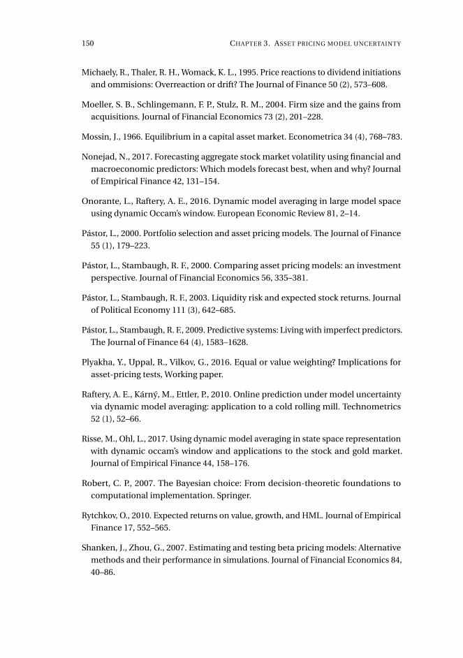
150 CHAPTER 3. ASSET PRICING MODEL UNCERTAINTY
Michaely, R., Thaler, R. H., Womack, K. L., 1995. Price reactions to dividend initiations
and ommisions: Overreaction or drift? The Journal of Finance 50 (2), 573–608.
Moeller, S. B., Schlingemann, F. P., Stulz, R. M., 2004. Firm size and the gains from
acquisitions. Journal of Financial Economics 73 (2), 201–228.
Mossin, J., 1966. Equilibrium in a capital asset market. Econometrica 34 (4), 768–783.
Nonejad, N., 2017. Forecasting aggregate stock market volatility using financial and
macroeconomic predictors: Which models forecast best, when and why? Journal
of Empirical Finance 42, 131–154.
Onorante, L., Raftery, A. E., 2016. Dynamic model averaging in large model space
using dynamic Occam’s window. European Economic Review 81, 2–14.
Pástor, L., 2000. Portfolio selection and asset pricing models. The Journal of Finance
55 (1), 179–223.
Pástor, L., Stambaugh, R. F., 2000. Comparing asset pricing models: an investment
perspective. Journal of Financial Economics 56, 335–381.
Pástor, L., Stambaugh, R. F., 2003. Liquidity risk and expected stock returns. Journal
of Political Economy 111 (3), 642–685.
Pástor, L., Stambaugh, R. F., 2009. Predictive systems: Living with imperfect predictors.
The Journal of Finance 64 (4), 1583–1628.
Plyakha, Y., Uppal, R., Vilkov, G., 2016. Equal or value weighting? Implications for
asset-pricing tests, Working paper.
Raftery, A. E., Kárný, M., Ettler, P., 2010. Online prediction under model uncertainty
via dynamic model averaging: application to a cold rolling mill. Technometrics
52 (1), 52–66.
Risse, M., Ohl, L., 2017. Using dynamic model averaging in state space representation
with dynamic occam’s window and applications to the stock and gold market.
Journal of Empirical Finance 44, 158–176.
Robert, C. P., 2007. The Bayesian choice: From decision-theoretic foundations to
computational implementation. Springer.
Rytchkov, O., 2010. Expected returns on value, growth, and HML. Journal of Empirical
Finance 17, 552–565.
Shanken, J., Zhou, G., 2007. Estimating and testing beta pricing models: Alternative
methods and their performance in simulations. Journal of Financial Economics 84,
40–86.

3.6. REFERENCES 151
Sharpe, W. F., 1964. Capital asset prices: A theory of market equilibrium under condi-
tions of risk. The Journal of Finance 19 (3), 425–442.
Vuong, Q. H., 1989. Likelihood ratio tests for model selection and non-nested hy-
potheses. Econometrica 57 (2), 307–333.
Welch, I., Goyal, A., 2008. A comprehensive look at the empirical performance of
equity premium prediction. Review of Financial Studies 21 (4), 1455–1508.
West, M., Harrison, J., 1997. Bayesian forecasting and dynamic models. Springer.
Zellner, A., 1986. On assessing prior distributioms and Bayesian regression analysis
with g-prior distributions. In Bayesian Inference and Decision Techniques: Essays
in Honour of Bruno de Finetti.
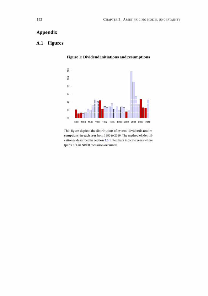
152 CHAPTER 3. ASSET PRICING MODEL UNCERTAINTY
Appendix
A.1 Figures
Figure 1: Dividend initiations and resumptions
1980 1983 1986 1989 1992 1995 1998 2001 2004 2007 2010
020
40
60
80
100
120
This figure depicts the distribution of events (dividends and re-
sumptions) in each year from 1980 to 2010. The method of identifi-
cation is described in Section 3.3.1. Red bars indicate years where
(parts of) an NBER recession occurred.
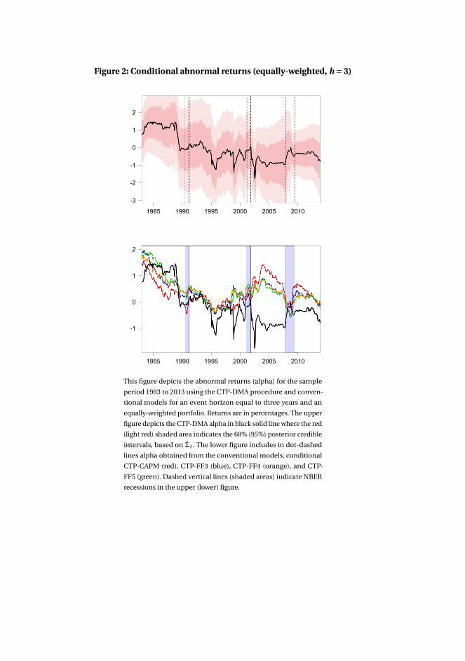
Figure 2: Conditional abnormal returns (equally-weighted, h = 3)
1985 1990 1995 2000 2005 2010
-3
-2
-1
0
1
2
1985 1990 1995 2000 2005 2010
-1
0
1
2
This figure depicts the abnormal returns (alpha) for the sample
period 1983 to 2013 using the CTP-DMA procedure and conven-
tional models for an event horizon equal to three years and an
equally-weighted portfolio. Returns are in percentages. The upper
figure depicts the CTP-DMA alpha in black solid line where the red
(light red) shaded area indicates the 68% (95%) posterior credible
intervals, based on Σt . The lower figure includes in dot-dashed
lines alpha obtained from the conventional models; conditional
CTP-CAPM (red), CTP-FF3 (blue), CTP-FF4 (orange), and CTP-
FF5 (green). Dashed vertical lines (shaded areas) indicate NBER
recessions in the upper (lower) figure.
Figure 3: Conditional abnormal returns (value-weighted, h = 1)
1985 1990 1995 2000 2005 2010
-4
-2
0
2
1985 1990 1995 2000 2005 2010
0.0
0.1
0.2
0.3
0.4
0.5
This figure depicts the abnormal returns (alpha) for the sample
period 1983 to 2011 using the CTP-DMA procedure for an event
horizon equal to one year and a value-weighted portfolio. Returns
are in percentages. The upper figure depicts the CTP-DMA alpha
in black solid line where the red (light red) shaded area indicates
the 68% (95%) posterior credible intervals, based on Σt . The lower
figure depicts the probability of the null hypothesis of zero al-
pha using (3.21) and (3.22). Dashed vertical lines (shaded areas)
indicate NBER recessions in the upper (lower) figure.
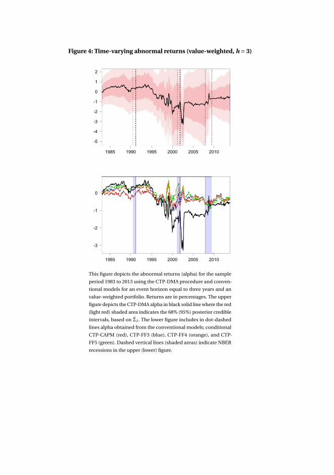
Figure 4: Time-varying abnormal returns (value-weighted, h = 3)
1985 1990 1995 2000 2005 2010
-5
-4
-3
-2
-1
0
1
2
1985 1990 1995 2000 2005 2010
-3
-2
-1
0
This figure depicts the abnormal returns (alpha) for the sample
period 1983 to 2013 using the CTP-DMA procedure and conven-
tional models for an event horizon equal to three years and an
value-weighted portfolio. Returns are in percentages. The upper
figure depicts the CTP-DMA alpha in black solid line where the red
(light red) shaded area indicates the 68% (95%) posterior credible
intervals, based on Σt . The lower figure includes in dot-dashed
lines alpha obtained from the conventional models; conditional
CTP-CAPM (red), CTP-FF3 (blue), CTP-FF4 (orange), and CTP-
FF5 (green). Dashed vertical lines (shaded areas) indicate NBER
recessions in the upper (lower) figure.
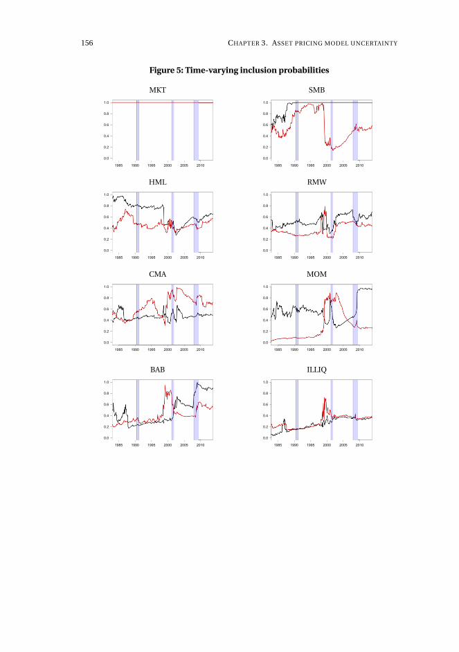
156 CHAPTER 3. ASSET PRICING MODEL UNCERTAINTY
Figure 5: Time-varying inclusion probabilities
MKT
1985 1990 1995 2000 2005 2010
0.0
0.2
0.4
0.6
0.8
1.0
SMB
1985 1990 1995 2000 2005 2010
0.0
0.2
0.4
0.6
0.8
1.0
HML
1985 1990 1995 2000 2005 2010
0.0
0.2
0.4
0.6
0.8
1.0
RMW
1985 1990 1995 2000 2005 2010
0.0
0.2
0.4
0.6
0.8
1.0
CMA
1985 1990 1995 2000 2005 2010
0.0
0.2
0.4
0.6
0.8
1.0
MOM
1985 1990 1995 2000 2005 2010
0.0
0.2
0.4
0.6
0.8
1.0
BAB
1985 1990 1995 2000 2005 2010
0.0
0.2
0.4
0.6
0.8
1.0
ILLIQ
1985 1990 1995 2000 2005 2010
0.0
0.2
0.4
0.6
0.8
1.0
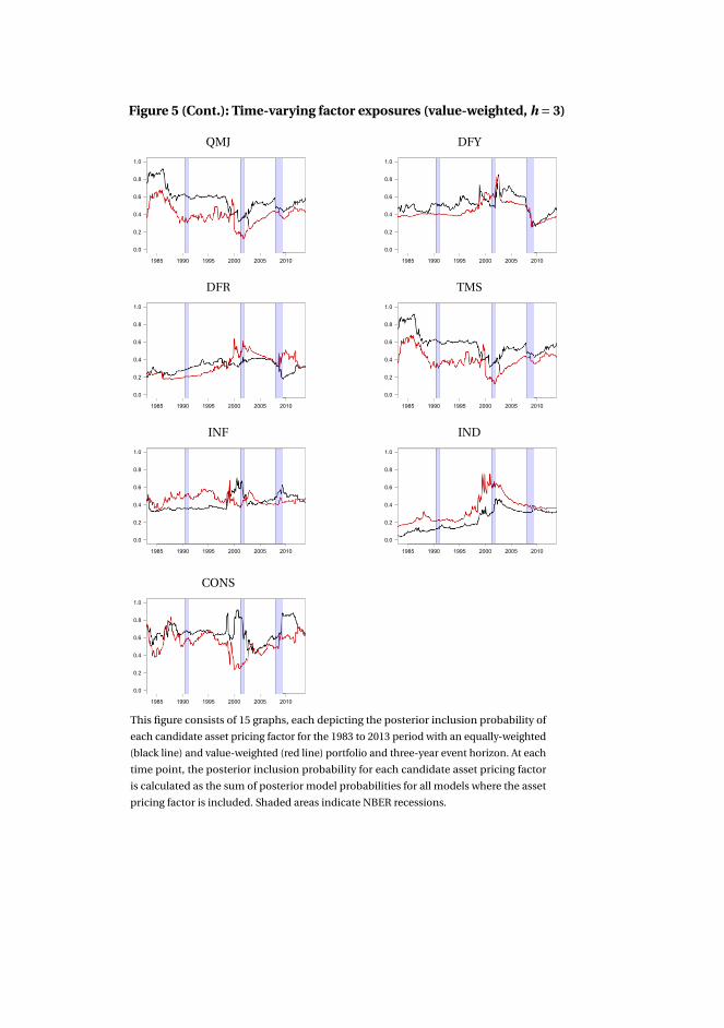
Figure 5 (Cont.): Time-varying factor exposures (value-weighted, h = 3)
QMJ
1985 1990 1995 2000 2005 2010
0.0
0.2
0.4
0.6
0.8
1.0
DFY
1985 1990 1995 2000 2005 2010
0.0
0.2
0.4
0.6
0.8
1.0
DFR
1985 1990 1995 2000 2005 2010
0.0
0.2
0.4
0.6
0.8
1.0
TMS
1985 1990 1995 2000 2005 2010
0.0
0.2
0.4
0.6
0.8
1.0
INF
1985 1990 1995 2000 2005 2010
0.0
0.2
0.4
0.6
0.8
1.0
IND
1985 1990 1995 2000 2005 2010
0.0
0.2
0.4
0.6
0.8
1.0
CONS
1985 1990 1995 2000 2005 2010
0.0
0.2
0.4
0.6
0.8
1.0
This figure consists of 15 graphs, each depicting the posterior inclusion probability of
each candidate asset pricing factor for the 1983 to 2013 period with an equally-weighted
(black line) and value-weighted (red line) portfolio and three-year event horizon. At each
time point, the posterior inclusion probability for each candidate asset pricing factor
is calculated as the sum of posterior model probabilities for all models where the asset
pricing factor is included. Shaded areas indicate NBER recessions.
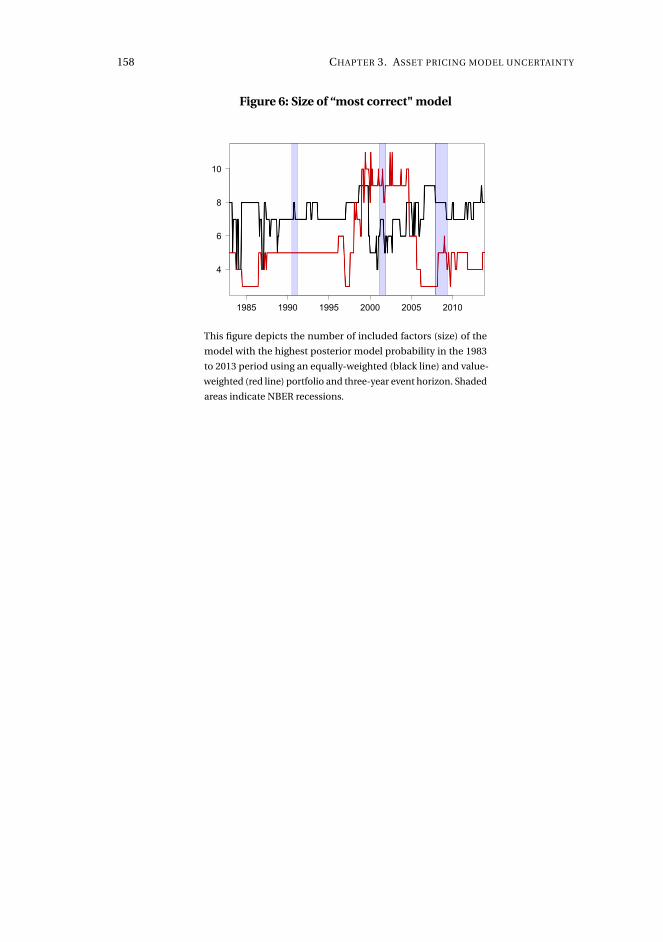
158 CHAPTER 3. ASSET PRICING MODEL UNCERTAINTY
Figure 6: Size of “most correct" model
1985 1990 1995 2000 2005 2010
4
6
8
10
This figure depicts the number of included factors (size) of the
model with the highest posterior model probability in the 1983
to 2013 period using an equally-weighted (black line) and value-
weighted (red line) portfolio and three-year event horizon. Shaded
areas indicate NBER recessions.
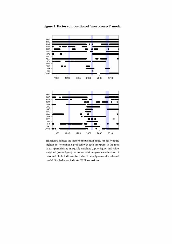
Figure 7: Factor composition of “most correct" model
1985 1990 1995 2000 2005 2010
CONS
IND
INF
TMS
DFR
DFY
QMJ
ILLIQ
BAB
MOM
CMA
RMW
HML
SMB
MKT
1985 1990 1995 2000 2005 2010
CONS
IND
INF
TMS
DFR
DFY
QMJ
ILLIQ
BAB
MOM
CMA
RMW
HML
SMB
MKT
This figure depicts the factor composition of the model with the
highest posterior model probability at each time point in the 1983
to 2013 period using an equally-weighted (upper figure) and value-
weighted (lower figure) portfolio and three-year event horizon. A
coloured circle indicates inclusion in the dynamically selected
model. Shaded areas indicate NBER recessions.
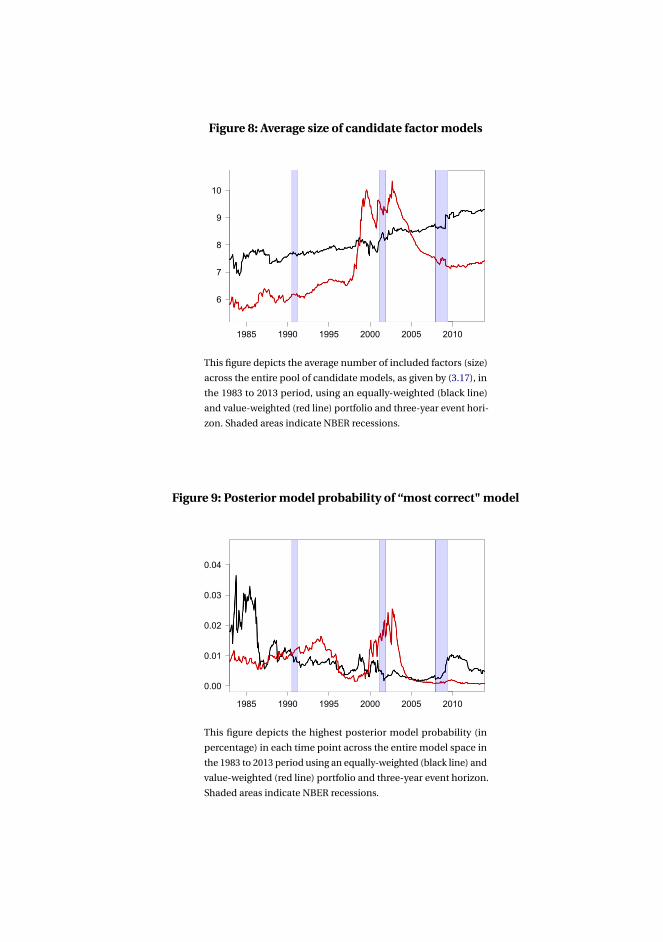
Figure 8: Average size of candidate factor models
1985 1990 1995 2000 2005 2010
6
7
8
9
10
This figure depicts the average number of included factors (size)
across the entire pool of candidate models, as given by (3.17), in
the 1983 to 2013 period, using an equally-weighted (black line)
and value-weighted (red line) portfolio and three-year event hori-
zon. Shaded areas indicate NBER recessions.
Figure 9: Posterior model probability of “most correct" model
1985 1990 1995 2000 2005 2010
0.00
0.01
0.02
0.03
0.04
This figure depicts the highest posterior model probability (in
percentage) in each time point across the entire model space in
the 1983 to 2013 period using an equally-weighted (black line) and
value-weighted (red line) portfolio and three-year event horizon.
Shaded areas indicate NBER recessions.
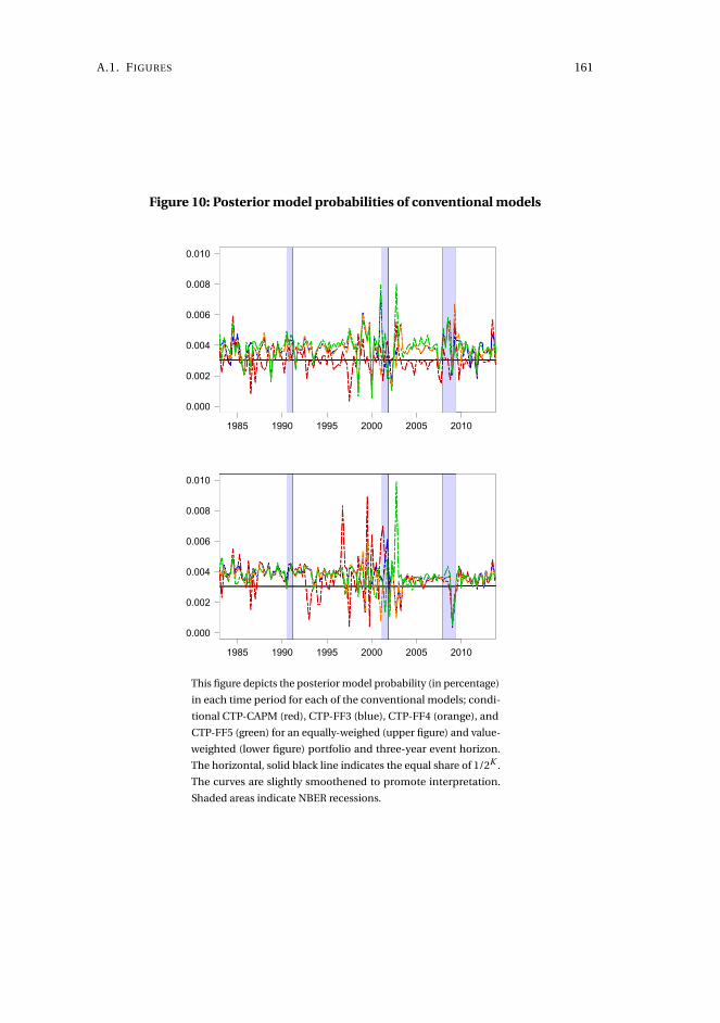
A.1. FIGURES 161
Figure 10: Posterior model probabilities of conventional models
1985 1990 1995 2000 2005 2010
0.000
0.002
0.004
0.006
0.008
0.010
1985 1990 1995 2000 2005 2010
0.000
0.002
0.004
0.006
0.008
0.010
This figure depicts the posterior model probability (in percentage)
in each time period for each of the conventional models; condi-
tional CTP-CAPM (red), CTP-FF3 (blue), CTP-FF4 (orange), and
CTP-FF5 (green) for an equally-weighed (upper figure) and value-
weighted (lower figure) portfolio and three-year event horizon.
The horizontal, solid black line indicates the equal share of 1/2K .
The curves are slightly smoothened to promote interpretation.
Shaded areas indicate NBER recessions.
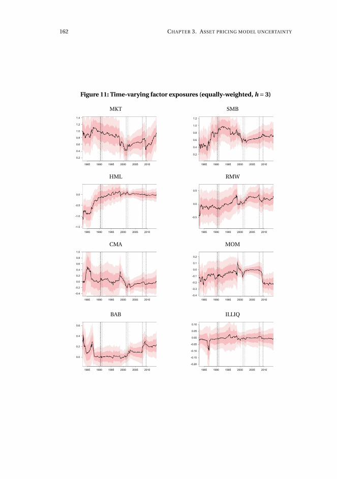
162 CHAPTER 3. ASSET PRICING MODEL UNCERTAINTY
Figure 11: Time-varying factor exposures (equally-weighted, h = 3)
MKT
1985 1990 1995 2000 2005 2010
0.2
0.4
0.6
0.8
1.0
1.2
1.4
SMB
1985 1990 1995 2000 2005 2010
0.2
0.4
0.6
0.8
1.0
1.2
HML
1985 1990 1995 2000 2005 2010
-1.5
-1.0
-0.5
0.0
RMW
1985 1990 1995 2000 2005 2010
-0.5
0.0
0.5
CMA
1985 1990 1995 2000 2005 2010
-0.4
-0.2
0.0
0.2
0.4
0.6
0.8
1.0
MOM
1985 1990 1995 2000 2005 2010
-0.4
-0.3
-0.2
-0.1
0.0
0.1
0.2
BAB
1985 1990 1995 2000 2005 2010
0.0
0.2
0.4
0.6
ILLIQ
1985 1990 1995 2000 2005 2010
-0.20
-0.15
-0.10
-0.05
0.00
0.05
0.10
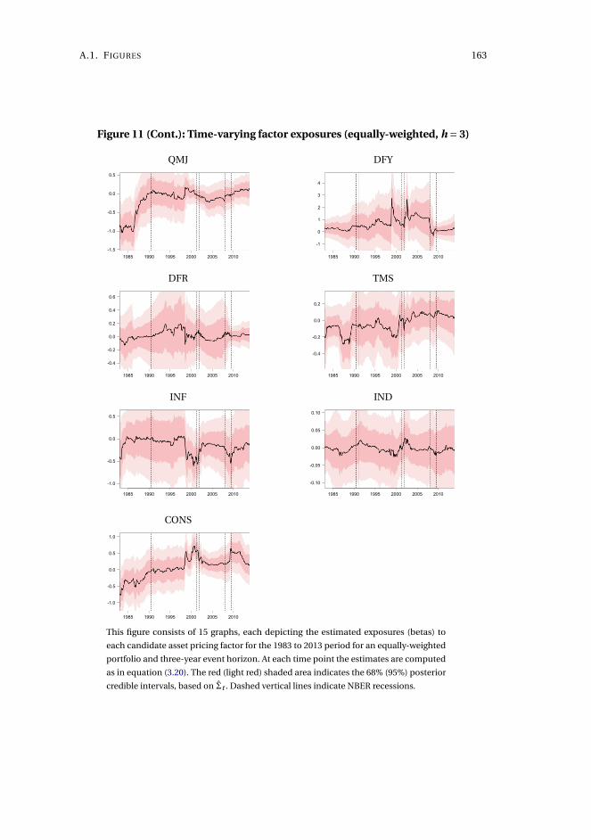
A.1. FIGURES 163
Figure 11 (Cont.): Time-varying factor exposures (equally-weighted, h = 3)
QMJ
1985 1990 1995 2000 2005 2010
-1.5
-1.0
-0.5
0.0
0.5
DFY
1985 1990 1995 2000 2005 2010
-1
0
1
2
3
4
DFR
1985 1990 1995 2000 2005 2010
-0.4
-0.2
0.0
0.2
0.4
0.6
TMS
1985 1990 1995 2000 2005 2010
-0.4
-0.2
0.0
0.2
INF
1985 1990 1995 2000 2005 2010
-1.0
-0.5
0.0
0.5
IND
1985 1990 1995 2000 2005 2010
-0.10
-0.05
0.00
0.05
0.10
CONS
1985 1990 1995 2000 2005 2010
-1.0
-0.5
0.0
0.5
1.0
This figure consists of 15 graphs, each depicting the estimated exposures (betas) to
each candidate asset pricing factor for the 1983 to 2013 period for an equally-weighted
portfolio and three-year event horizon. At each time point the estimates are computed
as in equation (3.20). The red (light red) shaded area indicates the 68% (95%) posterior
credible intervals, based on Σt . Dashed vertical lines indicate NBER recessions.
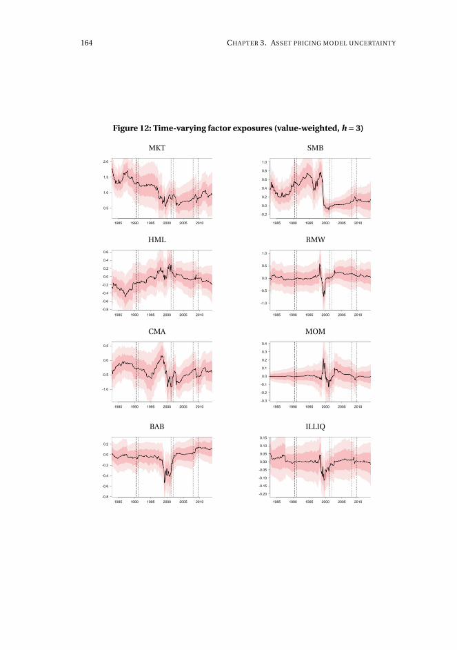
164 CHAPTER 3. ASSET PRICING MODEL UNCERTAINTY
Figure 12: Time-varying factor exposures (value-weighted, h = 3)
MKT
1985 1990 1995 2000 2005 2010
0.5
1.0
1.5
2.0
SMB
1985 1990 1995 2000 2005 2010
-0.2
0.0
0.2
0.4
0.6
0.8
1.0
HML
1985 1990 1995 2000 2005 2010
-0.8
-0.6
-0.4
-0.2
0.0
0.2
0.4
0.6
RMW
1985 1990 1995 2000 2005 2010
-1.0
-0.5
0.0
0.5
1.0
CMA
1985 1990 1995 2000 2005 2010
-1.0
-0.5
0.0
0.5
MOM
1985 1990 1995 2000 2005 2010
-0.3
-0.2
-0.1
0.0
0.1
0.2
0.3
0.4
BAB
1985 1990 1995 2000 2005 2010
-0.8
-0.6
-0.4
-0.2
0.0
0.2
ILLIQ
1985 1990 1995 2000 2005 2010
-0.20
-0.15
-0.10
-0.05
0.00
0.05
0.10
0.15
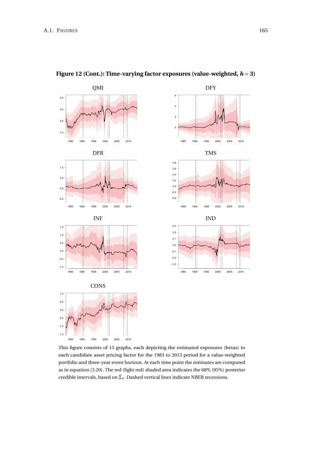
A.1. FIGURES 165
Figure 12 (Cont.): Time-varying factor exposures (value-weighted, h = 3)
QMJ
1985 1990 1995 2000 2005 2010
-1.0
-0.5
0.0
0.5
DFY
1985 1990 1995 2000 2005 2010
0
2
4
6
DFR
1985 1990 1995 2000 2005 2010
-0.5
0.0
0.5
1.0
TMS
1985 1990 1995 2000 2005 2010
-0.4
-0.2
0.0
0.2
0.4
0.6
0.8
INF
1985 1990 1995 2000 2005 2010
-1.0
-0.5
0.0
0.5
1.0
1.5
IND
1985 1990 1995 2000 2005 2010
-0.3
-0.2
-0.1
0.0
0.1
0.2
0.3
CONS
1985 1990 1995 2000 2005 2010
-1.5
-1.0
-0.5
0.0
0.5
1.0
This figure consists of 15 graphs, each depicting the estimated exposures (betas) to
each candidate asset pricing factor for the 1983 to 2013 period for a value-weighted
portfolio and three-year event horizon. At each time point the estimates are computed
as in equation (3.20). The red (light red) shaded area indicates the 68% (95%) posterior
credible intervals, based on Σt . Dashed vertical lines indicate NBER recessions.
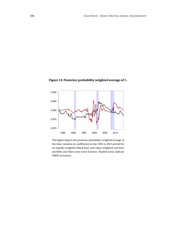
166 CHAPTER 3. ASSET PRICING MODEL UNCERTAINTY
Figure 13: Posterior-probability weighted average of δt
1985 1990 1995 2000 2005 2010
0.970
0.975
0.980
0.985
0.990
This figure depicts the posterior-probability weighted average of
the time variation in coefficients in the 1983 to 2013 period for
an equally-weighted (black line) and value-weighted (red line)
portfolio and three-year event horizon. Shaded areas indicate
NBER recessions.
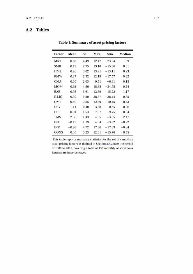
A.2. TABLES 167
A.2 Tables
Table 1: Summary of asset pricing factors
Factor Mean Sd. Max. Min. Median
MKT 0.62 4.49 12.47 −23.24 1.09
SMB 0.12 2.95 19.18 −15.36 0.01
HML 0.26 3.02 13.91 −13.11 0.23
RMW 0.37 2.32 12.19 −17.57 0.32
CMA 0.30 2.03 9.51 −6.81 0.15
MOM 0.62 4.56 18.38 −34.58 0.74
BAB 0.95 3.61 12.89 −15.22 1.17
ILLIQ 0.30 5.80 28.67 −38.44 0.85
QMJ 0.49 2.55 12.89 −10.45 0.43
DFY 1.11 0.48 3.38 0.55 0.96
DFR −0.01 1.53 7.37 −9.75 0.04
TMS 2.30 1.43 4.55 −3.65 2.47
INF −0.19 1.19 4.04 −3.92 −0.22
IND −0.98 4.72 17.66 −17.89 −0.84
CONS 0.40 3.23 12.81 −15.76 0.45
This table reports summary statistics for the set of candidate
asset pricing factors as defined in Section 3.3.2 over the period
of 1980 to 2015, covering a total of 432 monthly observations.
Returns are in percentages.
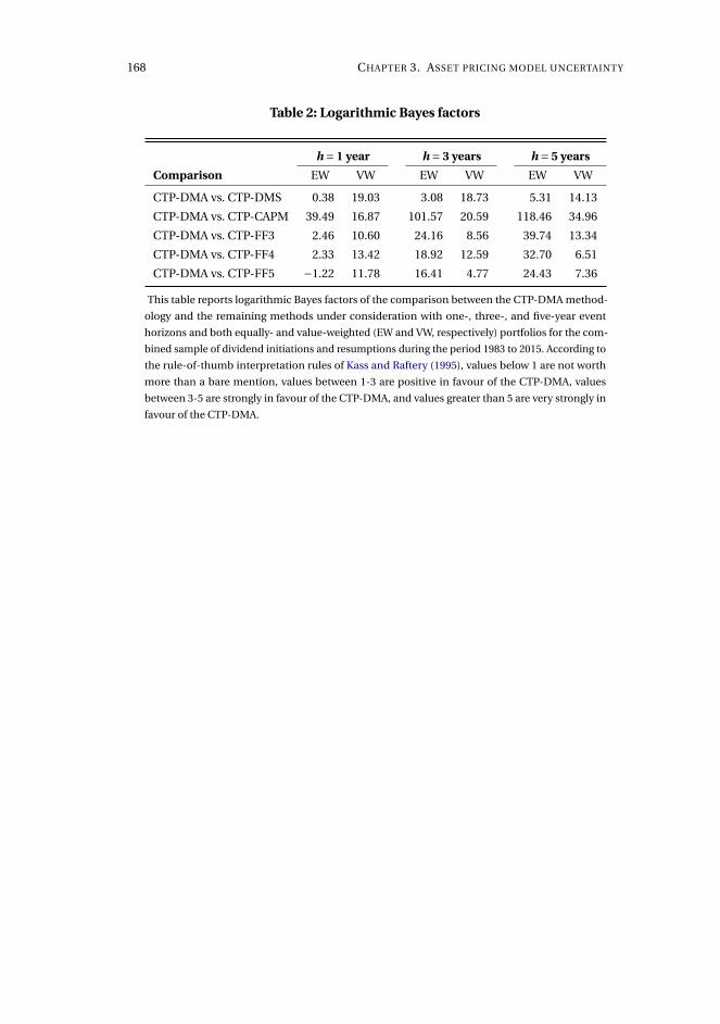
168 CHAPTER 3. ASSET PRICING MODEL UNCERTAINTY
Table 2: Logarithmic Bayes factors
h = 1 year h = 3 years h = 5 years
Comparison EW VW EW VW EW VW
CTP-DMA vs. CTP-DMS 0.38 19.03 3.08 18.73 5.31 14.13
CTP-DMA vs. CTP-CAPM 39.49 16.87 101.57 20.59 118.46 34.96
CTP-DMA vs. CTP-FF3 2.46 10.60 24.16 8.56 39.74 13.34
CTP-DMA vs. CTP-FF4 2.33 13.42 18.92 12.59 32.70 6.51
CTP-DMA vs. CTP-FF5 −1.22 11.78 16.41 4.77 24.43 7.36
This table reports logarithmic Bayes factors of the comparison between the CTP-DMA method-
ology and the remaining methods under consideration with one-, three-, and five-year event
horizons and both equally- and value-weighted (EW and VW, respectively) portfolios for the com-
bined sample of dividend initiations and resumptions during the period 1983 to 2015. According to
the rule-of-thumb interpretation rules of Kass and Raftery (1995), values below 1 are not worth
more than a bare mention, values between 1-3 are positive in favour of the CTP-DMA, values
between 3-5 are strongly in favour of the CTP-DMA, and values greater than 5 are very strongly in
favour of the CTP-DMA.
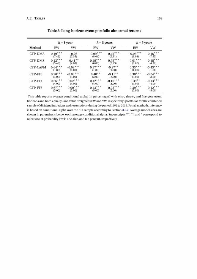
A.2. TABLES 169
Table 3: Long-horizon event portfolio abnormal returns
h = 1 year h = 3 years h = 5 years
Method EW VW EW VW EW VW
CTP-DMA 0.19∗∗∗(7.42)
-0.26(7.35)
-0.09∗∗∗(8.04)
-0.45∗∗∗(6.91)
-0.06∗∗∗(8.04)
-0.16∗∗∗(7.55)
CTP-DMS 0.12∗∗∗(5.49)
-0.41∗∗(4.03)
0.29∗∗∗(6.89)
-0.55∗∗∗(5.23)
0.01∗∗∗(6.82)
-0.18∗∗∗(4.31)
CTP-CAPM 0.64∗∗∗(1.00)
-0.08∗∗∗(1.00)
0.37∗∗∗(1.00)
-0.27∗∗(1.00)
0.33∗∗∗(1.00)
-0.43∗∗∗(1.00)
CTP-FF3 0.70∗∗∗(3.00)
-0.00∗∗∗(3.00)
0.40∗∗(3.00)
-0.11∗∗(3.00)
0.38∗∗∗(3.00)
-0.24∗∗∗(3.00)
CTP-FF4 0.66∗∗∗(4.00)
0.02∗∗∗(4.00)
0.42∗∗∗(4.00)
-0.10∗∗∗(4.00)
0.39∗∗(4.00)
-0.13∗∗∗(4.00)
CTP-FF5 0.67∗∗∗(5.00)
0.00∗∗∗(5.00)
0.43∗∗∗(5.00)
-0.03∗∗∗(5.00)
0.39∗∗∗(5.00)
-0.12∗∗∗(5.00)
This table reports average conditional alpha (in percentages) with one-, three-, and five-year event
horizons and both equally- and value-weighted (EW and VW, respectively) portfolios for the combined
sample of dividend initiations and resumptions during the period 1983 to 2015. For all methods, inference
is based on conditional alpha over the full sample according to Section 3.2.2. Average model sizes are
shown in parenthesis below each average conditional alpha. Superscripts ***, **, and * correspond to
rejections at probability levels one, five, and ten percent, respectively.
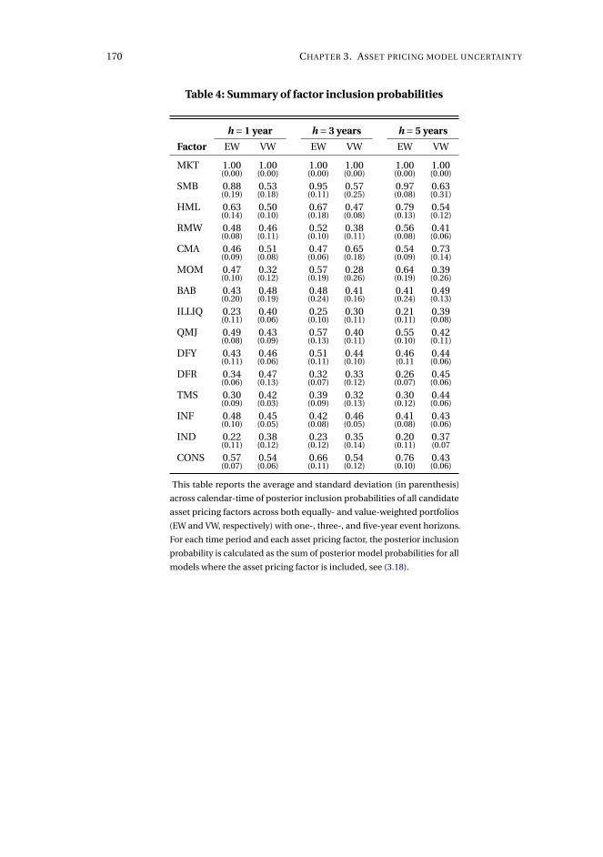
170 CHAPTER 3. ASSET PRICING MODEL UNCERTAINTY
Table 4: Summary of factor inclusion probabilities
h = 1 year h = 3 years h = 5 years
Factor EW VW EW VW EW VW
MKT 1.00(0.00)
1.00(0.00)
1.00(0.00)
1.00(0.00)
1.00(0.00)
1.00(0.00)
SMB 0.88(0.19)
0.53(0.18)
0.95(0.11)
0.57(0.25)
0.97(0.08)
0.63(0.31)
HML 0.63(0.14)
0.50(0.10)
0.67(0.18)
0.47(0.08)
0.79(0.13)
0.54(0.12)
RMW 0.48(0.08)
0.46(0.11)
0.52(0.10)
0.38(0.11)
0.56(0.08)
0.41(0.06)
CMA 0.46(0.09)
0.51(0.08)
0.47(0.06)
0.65(0.18)
0.54(0.09)
0.73(0.14)
MOM 0.47(0.10)
0.32(0.12)
0.57(0.19)
0.28(0.26)
0.64(0.19)
0.39(0.26)
BAB 0.43(0.20)
0.48(0.19)
0.48(0.24)
0.41(0.16)
0.41(0.24)
0.49(0.13)
ILLIQ 0.23(0.11)
0.40(0.06)
0.25(0.10)
0.30(0.11)
0.21(0.11)
0.39(0.08)
QMJ 0.49(0.08)
0.43(0.09)
0.57(0.13)
0.40(0.11)
0.55(0.10)
0.42(0.11)
DFY 0.43(0.11)
0.46(0.06)
0.51(0.11)
0.44(0.10)
0.46(0.11
0.44(0.06)
DFR 0.34(0.06)
0.47(0.13)
0.32(0.07)
0.33(0.12)
0.26(0.07)
0.45(0.06)
TMS 0.30(0.09)
0.42(0.03)
0.39(0.09)
0.32(0.13)
0.30(0.12)
0.44(0.06)
INF 0.48(0.10)
0.45(0.05)
0.42(0.08)
0.46(0.05)
0.41(0.08)
0.43(0.06)
IND 0.22(0.11)
0.38(0.12)
0.23(0.12)
0.35(0.14)
0.20(0.11)
0.37(0.07
CONS 0.57(0.07)
0.54(0.06)
0.66(0.11)
0.54(0.12)
0.76(0.10)
0.43(0.06)
This table reports the average and standard deviation (in parenthesis)
across calendar-time of posterior inclusion probabilities of all candidate
asset pricing factors across both equally- and value-weighted portfolios
(EW and VW, respectively) with one-, three-, and five-year event horizons.
For each time period and each asset pricing factor, the posterior inclusion
probability is calculated as the sum of posterior model probabilities for all
models where the asset pricing factor is included, see (3.18).
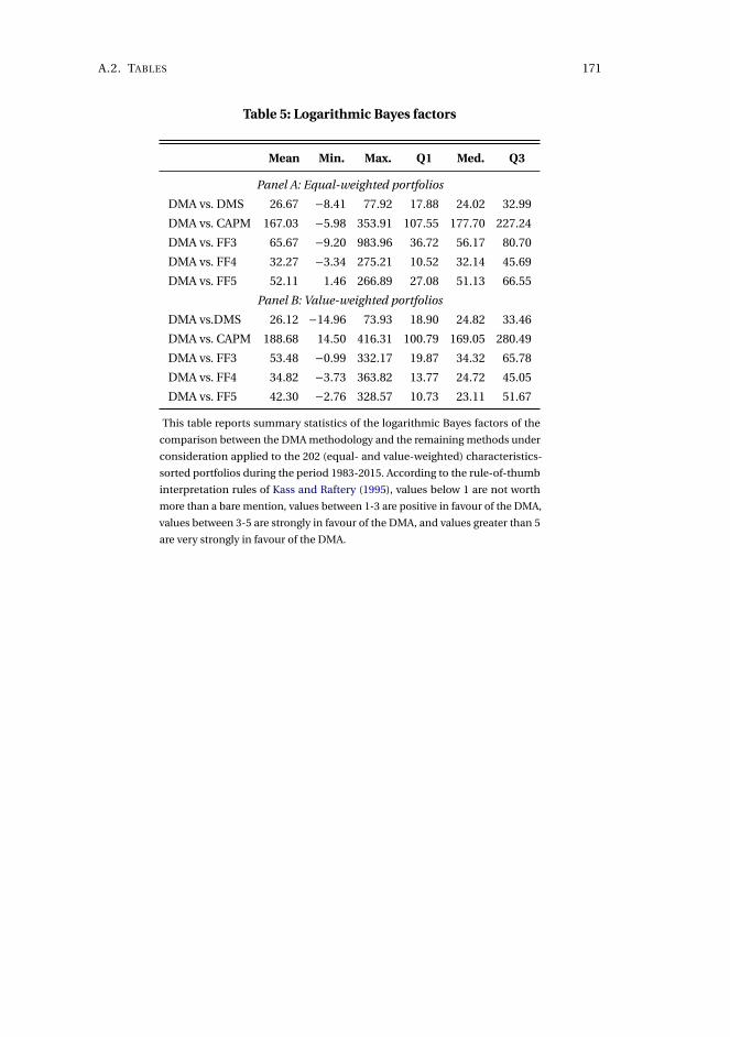
A.2. TABLES 171
Table 5: Logarithmic Bayes factors
Mean Min. Max. Q1 Med. Q3
Panel A: Equal-weighted portfolios
DMA vs. DMS 26.67 −8.41 77.92 17.88 24.02 32.99
DMA vs. CAPM 167.03 −5.98 353.91 107.55 177.70 227.24
DMA vs. FF3 65.67 −9.20 983.96 36.72 56.17 80.70
DMA vs. FF4 32.27 −3.34 275.21 10.52 32.14 45.69
DMA vs. FF5 52.11 1.46 266.89 27.08 51.13 66.55
Panel B: Value-weighted portfolios
DMA vs.DMS 26.12 −14.96 73.93 18.90 24.82 33.46
DMA vs. CAPM 188.68 14.50 416.31 100.79 169.05 280.49
DMA vs. FF3 53.48 −0.99 332.17 19.87 34.32 65.78
DMA vs. FF4 34.82 −3.73 363.82 13.77 24.72 45.05
DMA vs. FF5 42.30 −2.76 328.57 10.73 23.11 51.67
This table reports summary statistics of the logarithmic Bayes factors of the
comparison between the DMA methodology and the remaining methods under
consideration applied to the 202 (equal- and value-weighted) characteristics-
sorted portfolios during the period 1983-2015. According to the rule-of-thumb
interpretation rules of Kass and Raftery (1995), values below 1 are not worth
more than a bare mention, values between 1-3 are positive in favour of the DMA,
values between 3-5 are strongly in favour of the DMA, and values greater than 5
are very strongly in favour of the DMA.
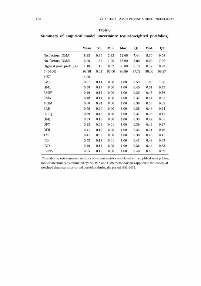
172 CHAPTER 3. ASSET PRICING MODEL UNCERTAINTY
Table 6:
Summary of empirical model uncertainty (equal-weighted portfolios)
Mean Sd. Min. Max. Q1 Med. Q3
No. factors (DMA) 8.23 0.90 2.32 12.06 7.44 8.30 9.08
No. factors (DMS) 6.00 1.69 1.00 13.00 5.00 6.00 7.00
Highest post. prob. (%) 1.18 1.15 0.02 98.88 0.19 0.37 0.73
δt (·100) 97.98 0.34 97.00 98.89 97.72 98.06 98.27
MKT 1.00 - - - - - -
SMB 0.81 0.11 0.00 1.00 0.59 1.00 1.00
HML 0.58 0.17 0.00 1.00 0.40 0.51 0.79
RMW 0.49 0.14 0.00 1.00 0.39 0.45 0.56
CMA 0.48 0.14 0.00 1.00 0.37 0.44 0.55
MOM 0.60 0.24 0.00 1.00 0.38 0.55 0.89
BAB 0.55 0.20 0.00 1.00 0.38 0.49 0.74
ILLIQ 0.39 0.12 0.00 1.00 0.31 0.38 0.45
QMJ 0.53 0.15 0.00 1.00 0.39 0.47 0.65
DFY 0.43 0.08 0.01 1.00 0.39 0.43 0.47
DFR 0.41 0.10 0.00 1.00 0.34 0.41 0.46
TMS 0.41 0.08 0.00 1.00 0.36 0.40 0.45
INF 0.53 0.13 0.01 1.00 0.41 0.48 0.63
IND 0.46 0.14 0.00 1.00 0.36 0.44 0.53
CONS 0.55 0.15 0.00 1.00 0.40 0.48 0.69
This table reports summary statistics of various metrics associated with empirical asset pricing
model uncertainty as estimated by the DMA and DMS methodologies applied to the 202 equal-
weighted characteristics-sorted portfolios during the period 1983-2015.
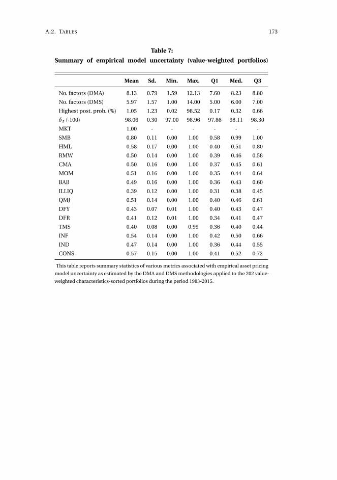
A.2. TABLES 173
Table 7:
Summary of empirical model uncertainty (value-weighted portfolios)
Mean Sd. Min. Max. Q1 Med. Q3
No. factors (DMA) 8.13 0.79 1.59 12.13 7.60 8.23 8.80
No. factors (DMS) 5.97 1.57 1.00 14.00 5.00 6.00 7.00
Highest post. prob. (%) 1.05 1.23 0.02 98.52 0.17 0.32 0.66
δt (·100) 98.06 0.30 97.00 98.96 97.86 98.11 98.30
MKT 1.00 - - - - - -
SMB 0.80 0.11 0.00 1.00 0.58 0.99 1.00
HML 0.58 0.17 0.00 1.00 0.40 0.51 0.80
RMW 0.50 0.14 0.00 1.00 0.39 0.46 0.58
CMA 0.50 0.16 0.00 1.00 0.37 0.45 0.61
MOM 0.51 0.16 0.00 1.00 0.35 0.44 0.64
BAB 0.49 0.16 0.00 1.00 0.36 0.43 0.60
ILLIQ 0.39 0.12 0.00 1.00 0.31 0.38 0.45
QMJ 0.51 0.14 0.00 1.00 0.40 0.46 0.61
DFY 0.43 0.07 0.01 1.00 0.40 0.43 0.47
DFR 0.41 0.12 0.01 1.00 0.34 0.41 0.47
TMS 0.40 0.08 0.00 0.99 0.36 0.40 0.44
INF 0.54 0.14 0.00 1.00 0.42 0.50 0.66
IND 0.47 0.14 0.00 1.00 0.36 0.44 0.55
CONS 0.57 0.15 0.00 1.00 0.41 0.52 0.72
This table reports summary statistics of various metrics associated with empirical asset pricing
model uncertainty as estimated by the DMA and DMS methodologies applied to the 202 value-
weighted characteristics-sorted portfolios during the period 1983-2015.
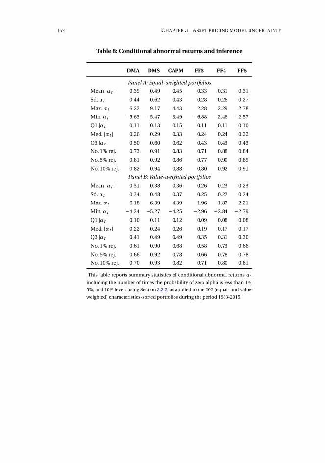
174 CHAPTER 3. ASSET PRICING MODEL UNCERTAINTY
Table 8: Conditional abnormal returns and inference
DMA DMS CAPM FF3 FF4 FF5
Panel A: Equal-weighted portfolios
Mean |αt | 0.39 0.49 0.45 0.33 0.31 0.31
Sd. αt 0.44 0.62 0.43 0.28 0.26 0.27
Max. αt 6.22 9.17 4.43 2.28 2.29 2.78
Min. αt −5.63 −5.47 −3.49 −6.88 −2.46 −2.57
Q1 |αt | 0.11 0.13 0.15 0.11 0.11 0.10
Med. |αt | 0.26 0.29 0.33 0.24 0.24 0.22
Q3 |αt | 0.50 0.60 0.62 0.43 0.43 0.43
No. 1% rej. 0.73 0.91 0.83 0.71 0.88 0.84
No. 5% rej. 0.81 0.92 0.86 0.77 0.90 0.89
No. 10% rej. 0.82 0.94 0.88 0.80 0.92 0.91
Panel B: Value-weighted portfolios
Mean |αt | 0.31 0.38 0.36 0.26 0.23 0.23
Sd. αt 0.34 0.48 0.37 0.25 0.22 0.24
Max. αt 6.18 6.39 4.39 1.96 1.87 2.21
Min. αt −4.24 −5.27 −4.25 −2.96 −2.84 −2.79
Q1 |αt | 0.10 0.11 0.12 0.09 0.08 0.08
Med. |αt | 0.22 0.24 0.26 0.19 0.17 0.17
Q3 |αt | 0.41 0.49 0.49 0.35 0.31 0.30
No. 1% rej. 0.61 0.90 0.68 0.58 0.73 0.66
No. 5% rej. 0.66 0.92 0.78 0.66 0.78 0.78
No. 10% rej. 0.70 0.93 0.82 0.71 0.80 0.81
This table reports summary statistics of conditional abnormal returns αt ,
including the number of times the probability of zero alpha is less than 1%,
5%, and 10% levels using Section 3.2.2, as applied to the 202 (equal- and value-
weighted) characteristics-sorted portfolios during the period 1983-2015.
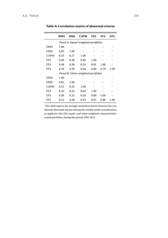
A.2. TABLES 175
Table 9: Correlation matrix of abnormal returns
DMA DMS CAPM FF3 FF4 FF5
Panel A: Equal-weighted portfolios
DMA 1.00 - - - - -
DMS 0.82 1.00 - - - -
CAPM 0.35 0.27 1.00 - - -
FF3 0.40 0.30 0.66 1.00 - -
FF4 0.48 0.38 0.54 0.81 1.00 -
FF5 0.49 0.39 0.50 0.80 0.78 1.00
Panel B: Value-weighted portfolios
DMA 1.00 - - - - -
DMS 0.81 1.00 - - - -
CAPM 0.31 0.23 1.00 - - -
FF3 0.45 0.32 0.64 1.00 - -
FF4 0.46 0.33 0.54 0.89 1.00 -
FF5 0.52 0.38 0.45 0.81 0.80 1.00
This table reports the average correlation matrix between the con-
ditional abnormal returns among the models under consideration,
as applied to the 202 (equal- and value-weighted) characteristics-
sorted portfolios during the period 1983-2015.


![Developments in theory and empirical applications of endogenous governmental behavior [Econometric forecasting modes for agricultural systems]](https://img.pdfslide.net/doc/110x75/63555e89f4b7d3d11c0c9c41/developments-in-theory-and-empirical-applications-of-endogenous-governmental-behavior-1700897455.jpg)


