Econometric Modelling

Econometrics II: Econometric Modelling

Jurgen Meinecke

Research School of Economics, Australian National University

19 October, 2018

Logistics for week 12

We will return assignment 2 in your last tutorial

You can keep your assignment and take it with you

However, if you want to qualify for a remark you need to:

I raise and explain any concerns regarding the marking with

your tutor as soon as possible during the week 12 tutorial

I hand your assignment back to your tutor by the end of the

week 12 tutorial

Once you leave the tutorial room with your assignment, you

cannot as for a remark

Other logistics

Tutorial participation:

I will post marks on Wattle by end of week 12

I you can contest your participation mark until 2 November

(by sending me an e-mail), no remarks thereafter

Exam consults:

I will be announced in last lecture

Next Week’s Lecture

Will wrap up panel data estimation in first hour

We can use second our to answer any questions you may have

Please send me any comments, suggestions and/or questions

for next week

Roadmap

Introduction

Panel Data Estimation

Panel Data: What and Why

Example: Traffic Deaths and Alcohol Taxes

Panel Data with Two Time Periods

Individual Fixed Effects

Time Fixed Effects

Individual and Time Fixed Effects

A panel dataset contains observations on multiple entities

(individuals, states, companies . . . ), where each entity is

observed at two or more points in time

Examples:

I Data on 500 Australian schools in 2010 and again in 2011,

for a total of 1,000 observations

I Data on 50 U.S. states, each observed in 5 consecutive

years, for a total of 250 observations

I Data on 10,000 Australians, annually, starting in 2001

(this is the famous HILDA data set)

So far we have always dealt with cross-sectional data

(ignoring our time-series adeventure in EMET2007)

Cross-sectional data have one dimension:

the unit/entity/individual i

In contrast, panel data have two dimensions:

I cross sectional: the unit/entity/individual i

I time t

Panel data notation therefore is a bit more complicated

We need a double subscript for each variable

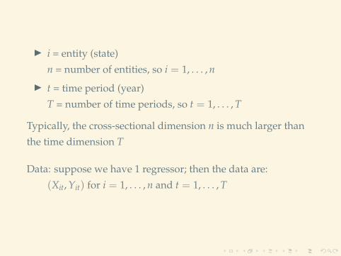
I i = entity (state)

n = number of entities, so i = 1, . . . , n

I t = time period (year)

T = number of time periods, so t = 1, . . . , T

Typically, the cross-sectional dimension n is much larger than

the time dimension T

Data: suppose we have 1 regressor; then the data are:

(Xit, Yit) for i = 1, . . . , n and t = 1, . . . , T

Notation gets even more cumbersome when we allow for kregressors

(X1it, X2it, . . . , Xkit, Yit) for i = 1, . . . , n and t = 1, . . . , T

Some jargon

I Another term for panel data is longitudinal data

I balanced panel: no missing observations, that is, all

variables are observed for all entities (states) and all time

periods (years)

Why are panel data useful?

Panel data help overcome problems that stem from variables

that

I vary across entities i but are constant over time t

I would cause ovb if they were unobserved

Key advantage of panel data:

If an omitted variable does not change over time, then any changes inY over time cannot be caused by that omitted variable

Roadmap

Introduction






Time Fixed Effects


I Cross-sectional unit: U.S. states

(48 U.S. states, so n = # of entities = 48)

I Time dimension: 1982 to 1988

(7 years, so T = # of time periods = 7)

I Balanced panel, so total # observations = 7× 48 = 336

Variables:

I traffic fatality rate

(# traffic deaths in that state in that year,

per 10,000 state residents)

I tax on a case of beer

I other: legal driving age, drunk driving laws, etc.

Just looking at 1982 data:

Paradox: higher alcohol taxes, more traffic deaths?

Why might there be more traffic deaths in states that have

higher alcohol taxes?

Other factors that determine traffic fatality rate:

I density of cars on the road

I “culture” around drinking and driving

If these are omitted, may lead to ovb

Example #1: traffic density

I High traffic density means more traffic deaths

I (Western) states with lower traffic density have lower

alcohol taxes

This would lead to ovb b/c

I high taxes positively correlated with high traffic density

I high traffic density positively correlated with high fatality

I ergo: high taxes positively correlated with high fatality

=⇒ spurious causation

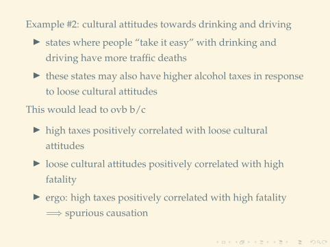
Example #2: cultural attitudes towards drinking and driving

I states where people “take it easy” with drinking and

driving have more traffic deaths

I these states may also have higher alcohol taxes in response

to loose cultural attitudes

This would lead to ovb b/c

I high taxes positively correlated with loose cultural

attitudes

I loose cultural attitudes positively correlated with high

fatality

I ergo: high taxes positively correlated with high fatality

=⇒ spurious causation

These are two hypothetical examples of how traffic fatalities

could be spuriously correlated with high alcohol taxes

Let’s suppose we are not able to control for traffic density and

cultural attitudes

Then we may erroneously conclude that high alcohol taxes

increase traffic fatalities

But these two examples (traffic density and cultural attitudes)

are perfect cases for how panel data can overcome this ovb

problem

Both traffic density and cultural attitudes can be thought of as

being constant over time within a given entity i (here the states)

Roadmap

Introduction






Time Fixed Effects


To get things started, suppose we only observe two time

periods: 1982 and 1988

Now, consider the panel data model,

FatalityRateit = β0 + β1BeerTaxit + β2Zi + uit,

where Zi is a factor that does not change over time (density),

at least during the years on which we have data

I Suppose Zi is not observed, so its omission could result in

omitted variable bias

I The effect of Zi can be eliminated using T = 2 years

The key idea:

Any change in the fatality rate from 1982 to 1988 cannot be causedby Zi, because Zi (by assumption) does not change between 1982 and1988The math: consider fatality rates in 1988 and 1982:

FatalityRatei1988 = β0 + β1BeerTaxi1988 + β2Zi + ui1988

FatalityRatei1982 = β0 + β1BeerTaxi1982 + β2Zi + ui1982

Subtracting 1988− 1982 (that is, calculating the change),

eliminates the effect of Zi . . .

FatalityRatei1988 − FatalityRatei1982 =

β1(BeerTaxi1988 − BeerTaxi1982) + (ui1988 − ui1982)

FatalityRatei1988 − FatalityRatei1982 =

β1(BeerTaxi1988 − BeerTaxi1982) + (ui1988 − ui1982)

We just subtracted out the effect of Zi

While Zi affects the fatality rates in both years, it does not affect

the difference in the fatality rates between the two years

The new error term, (ui1988 − ui1982), is uncorrelated with either

BeerTaxi1988 or BeerTaxi1982

This “difference” equation can be estimated by OLS, even

though Zi isn’t observed

This differences regression doesn’t have an intercept - it was

eliminated by the subtraction step

Only 1982 data:

FatalityRate = 2.01(0.15)

+ 0.15(0.13)

BeerTax (n = 48)

Only 1988 data:

FatalityRate = 1.86(0.11)

+ 0.44(0.13)

BeerTax (n = 48)

1982 and 1988 data combined:

FR1988 − FR1982 = −0.072(0.065)

− 1.04(0.36)

(BeerTax1988 − BeerTax1982)

Using the difference specification, we actually do find a negativeeffect of the beer tax on traffic fatalities (as we would expect)

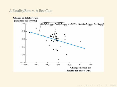
∆ FatalityRate v. ∆ BeerTax:

Brief summary so far:

I panel data let us remove the influence of certain

unobserved variables

I any unobserved variable that does not vary over time but

would affect the outcome can be taken care of

I the nice thing:

we do not need to observe that variable at all

I we only need to exploit the time structure in a clever way

and the influence of the unobserved variable disappears

I here, we only had to study the simple difference in the

outcome variable between two years

Roadmap

Introduction






Time Fixed Effects


What if you have more than 2 time periods (T > 2)?

Yit = β0 + β1Xit + β2Zi + uit

We can rewrite this in two useful ways:

I “n− 1 binary regressor” regression model

I “fixed effects” regression model

We first rewrite this in “fixed effects” form

For the sake of illustration, suppose we have n = 3 states:

California, Texas, and Massachusetts

Yit = β0 + β1Xit + β2Zi + uit

Population regression for California (that is, i = CA):

YCA,t = β0 + β1XCA,t + β2ZCA + uCA,t

= (β0 + β2ZCA) + β1XCA,t + uCA,t

or:

YCA,t = αCA + β1XCA,t + uCA,t

I αCA = β0 + β2ZCA doesn’t change over time

I αCA is the intercept for CA, and β1 is the slope

I The intercept is unique to CA, but the slope is the same in

all the states: parallel lines

For Texas:

YTX,t = β0 + β1XTX,t + β2ZTX + uTX,t

= (β0 + β2ZTX) + β1XTX,t + uTX,t

= αTX + β1XTX,t + uTX,t

and similarly for Massachusetts

Collecting the lines for all three states:

YCA,t = αCA + β1XCA,t + uCA,t

YTX,t = αTX + β1XTX,t + uTX,t

YMA,t = αMA + β1XMA,t + uMA,t

More compactly

Yi,t = αi + β1Xi,t + ui,t, where i = CA, TX, MA

The equation

Yit = αi + β1Xit + uit

is called the fixed effects regression model

The terms αi are the state fixed effects

All states share the same slope coefficient β1

But each state has its own individual intercept term αi

(the fixed effect)

The regression lines for each state in a picture

The shifts in the intercept can be represented using binary

regressors. . .

The fixed effects regression model is one of two possible

representations

Alternatively, can rewrite model as binary regressor model

Going back to the example of three states CA, TX and MA, the

fixed effects model was

Yit = αi + β1Xit + uit, where i = CA, TX, MA

It should be obvious that this can be written equivalently as

Yit = β0 + γCACAi + γTXTXi + β1Xit + uit

I CAi = 1 if state is CA, = 0 otherwise

I TXi = 1 if state is TX, = 0 otherwise

Instead of having state fixed effects αi you include a dummy

variable for each state

Summary: Two equivalent ways to write the fixed effects model

1. “Fixed effects” model

Yit = β0 + β1Xit + αi + uit

2. “n-1 binary regressor” model

Yit = β0 + β1Xit + γ2D2i + . . . + γnDni + uit

where

D2i =

1, if i = 2 (state 2)

0, otherwise

and similary for the other dummies

Two equivalent estimation methods

1. “n-1 binary regressors” OLS regression

2. “Entity-demeaned” OLS regression

These methods produce identical estimates of the regression

coefficients, and identical standard errors

Method 2 is preferred because method 1 can be

computationally demanding (think of n as a large number)

“n-1 binary regressors” OLS regression

Yit = β0 + β1Xit + γ2D2i + . . . + γnDni + uit

I First create the binary variables D2i, . . . , Dni

I Then simply estimate by OLS

I Inference (hypothesis tests, confidence intervals) is as

usual (using heteroskedasticity-robust standard errors)

I This is impractical when n is very large

(for example if n = 1000 workers)

“Entity-demeaned” OLS regression

Entity demeaning is based on the fixed effects regression model

Yit = β1Xit + αi + uit

Now define entity means:

Yi :=1T

T

∑t=1

Yit Xi :=1T

T

∑t=1

Xit

ui :=1T

T

∑t=1

uit αi :=1T

T

∑t=1

αi = αi

These are the averages of each variable over time

Only for αi: the time average coincides with the variable itself

(b/c it is constant over time)

Now define “demeaned” variables:

Yit := Yit − Yi Xit := Xit − Xi

uit := uit − ui αi := αi − αi = 0

These are the deviations (each year) from the time average

Only for αi: this collapses to zero

(b/c it is constant over time)

Demeaning the entire fixed effects regression model

Yit = β1Xit + αi + uit

−(

Yi = β1Xi + αi + ui

)= Yit = β1Xit + αi + uit

= β1Xit + uit

We have just “demeaned” the whole model

As a result, the fixed effect term αi dropped out

This was the reason for “demeaning” in the first place

“Demeaning” is an easy data transformation that gets rid of the

fixed effect (similar to first differencing in the case of T = 2)

Recall that when T = 2 we simply “first differenced” the data

The reason was that any changes in Yit over time can only be

due to changes in Xit (because the only other regressor, αi, is

fixed over time)

Now, allowing T > 2 we “demean” the data

The reasoning is slightly more complicated but actually quite

similar:

Any deviations of Yit from its time average Yi can only be due

to deviations of Xit from its time average Xi (because the only

other regressor, αi, is fixed over time and does not have any

deviations from its time average)

Our regression model reduces to

Yit = β1Xit + uit

Practical steps:

I First construct the entity-demeaned variables Yit and Xit

I Then simply regress Yit on Xit; this is straightforward OLS

estimation

This is like the “changes” approach, but instead Yit is deviated

from the state average instead of Yi1

This can be done in a single command in STATA

First let STATA know you are working with panel data by

defining the entity variable (state) and time variable (year):

xtset state year

panel variable: state (strongly balanced)

time variable: year, 1982 to 1988

delta: 1 unit

xtreg vfrall beertax, fe vce(cluster state)

Fixed-effects (within) regression Number of obs = 336

Group variable: state Number of groups = 48

R-sq: within = 0.0407 Obs per group: min = 7

between = 0.1101 avg = 7.0

overall = 0.0934 max = 7

F(1,47) = 5.05

corr(u_i, Xb) = -0.6885 Prob > F = 0.0294

(Std. Err. adjusted for 48 clusters in state)

------------------------------------------------------------------------------

| Robust

vfrall | Coef. Std. Err. t P>|t| [95% Conf. Interval]

-------------+----------------------------------------------------------------

beertax | -.6558736 .2918556 -2.25 0.029 -1.243011 -.0687358

_cons | 2.377075 .1497966 15.87 0.000 2.075723 2.678427

------------------------------------------------------------------------------

The panel data command xtreg with the option fe performs

fixed effects regression

The fe option means use fixed effects regression

(Stata permits other options, but we won’t discuss these)

This is equivalent to the entity demeaning described a few

slides earlier

The reported intercept is arbitrary, and the estimated

individual effects are not reported in the default output

The vce(cluster state) option tells STATA to use clustered

standard errors

When you use the vce option, you do not need to “robustify” to

heteroskedasticity (it’s already being taken care of)

Stata’s xtreg commands saves you a lot of work

I it creates the time averages Yi and Xi

I it creates the deviations of each variable from its time

average, that is, Yit and Xit

I it runs the OLS regression of Yit on Xit

I it computes the correct standard errors

Why can’t you use first differencing when T > 2?

Actually, you can

But the asymptotic properties of the estimator are not as good

as the one that’s based on “demeaning”

This is not at all an obvious thing but requires some nasty math

to show

Bottom line: the entity demeaned estimator is more efficient

than the first difference estimator

Roadmap

Introduction






Time Fixed Effects


An omitted variable might vary over time but not across states:

I Safer cars (air bags, etc.); changes in national laws

I These produce intercepts that change over time

I Let St denote the combined effect of variables which

changes over time but not states (“safer cars”)

I The resulting population regression model is:

Yit = β0 + β1Xit + β2Zi + β3St + uit

I Let’s tentatively assume that β2 = 0

(for sake of illustration)

This model can be recast as having an intercept that varies from

one year to the next:

Yi,1982 = β0 + β1Xi,1982 + β3S1982 + ui,1982

= (β0 + β3S1982) + β1Xi,1982 + ui,1982

= λ1982 + β1Xi,1982 + ui,1982

where λ1982 = β0 + β3S1982

Similarly,

Yi,1983 = λ1983 + β1Xi,1983 + ui,1983

where λ1983 = β0 + β3S1983

Two formulations of regression with time fixed effects

1. “Fixed effects” form

Yit = λt + β1Xit + uit

2. “T-1 binary regressor” form

Yit = β0 + β1Xit + γ2B2t + . . . + γTBTt + uit

where

B2t =

1, if t = 2 (year 2)

0, otherwise

and similar for other years

Two ways of estimating this

1. “Year-demeaned” OLS regressionI Deviate Yit, Xit from year (not state) averagesI Estimate by OLS using “year-demeaned” data

2. “T-1 binary regressor” OLS regression

Yit = β0 + β1Xit + γ2B2t + . . . + γTBTt + uit

I Create binary variables B2, . . . , BTI B2 = 1 if t = year #2, = 0 otherwiseI Regress Y on X, B2,. . . ,BT using OLS

Both methods result in exactly the same estimates

Because in panel data applications T is usually small, the

second method is preferred here

Roadmap

Introduction






Time Fixed Effects


What if you have both entity and time fixed effects?

Yit = β1Xit + αi + λt + uit

I When T = 2, computing the first difference and including

an intercept is equivalent to (gives exactly the same

regression as) including entity and time fixed effectsI When T > 2, there are various equivalent ways to

incorporate both entity and time fixed effects:I entity demeaning & T - 1 time indicators

(preferable and done in the following STATA example)I time demeaning & n - 1 entity indicatorsI T - 1 time indicators & n - 1 entity indicatorsI entity & time demeaning

gen y83=(year==1983) First generate all the time binary variables

gen y84=(year==1984)





xtreg vfrall beertax y83-y88, fe vce(cluster state)

Fixed-effects (within) regression Number of obs = 336

Group variable: state Number of groups = 48

R-sq: within = 0.0803 Obs per group: min = 7

between = 0.1101 avg = 7.0

overall = 0.0876 max = 7

corr(u_i, Xb) = -0.6781 Prob > F = 0.0009

(Std. Err. adjusted for 48 clusters in state)

------------------------------------------------------------------------------

| Robust

vfrall | Coef. Std. Err. t P>|t| [95% Conf. Interval]

-------------+----------------------------------------------------------------

beertax | -.6399799 .3570783 -1.79 0.080 -1.358329 .0783691

y83 | -.0799029 .0350861 -2.28 0.027 -.1504869 -.0093188

y84 | -.0724206 .0438809 -1.65 0.106 -.1606975 .0158564

y85 | -.1239763 .0460559 -2.69 0.010 -.2166288 -.0313238

y86 | -.0378645 .0570604 -0.66 0.510 -.1526552 .0769262

y87 | -.0509021 .0636084 -0.80 0.428 -.1788656 .0770615

y88 | -.0518038 .0644023 -0.80 0.425 -.1813645 .0777568

_cons | 2.42847 .2016885 12.04 0.000 2.022725 2.834215

-------------+----------------------------------------------------------------

Are the time effects jointly statistically significant?

test y83-y88

( 1) y83 = 0

( 2) y84 = 0

( 3) y85 = 0

( 4) y86 = 0

( 5) y87 = 0

( 6) y88 = 0

F( 6, 47) = 4.22

Prob > F = 0.0018

Yes

Practical guidelines for estimating panel data models

1. If you have individual fixed effects only

You should use Stata’s xtreg command

I adding option fe (for fixed effect estimation)I adding option vce(cluster state) (for correct standard errors)

(note: depending on your application, the cross-sectionalvariable “state” may have a different name)

2. If you have both individual and time fixed effects

You should use Stata’s xtreg command

I adding dummy variables for T− 1 yearsI adding option fe (for fixed effect estimation)I adding option vce(cluster state) (for correct standard errors)

(note: depending on your application, the cross-sectionalvariable “state” may have a different name)

But remember:

Before you use xtreg you need to tell Stata that your data set is a

panel data set by typing xtset state year

3. If you have time fixed effects only

You should use Stata’s regress command

I adding option vce(cluster state) (for correct standard errors)(note: depending on your application, the cross-sectionalvariable “state” may have a different name)

Documents

Econometric Modelling