1 - NASA Technical Memorandum 100521

ESTIMATING THE DISTRIBUTION OF FAULT LATENCY IN A DIGITAL PROCESSOR

(HASA-TPI-lOO521) ESTJdATXIG THE D I S T R I B U T I O N OF FAULT LATENCY IN A D I G I T A L

PBUCESSOR [HASA) 22 p CSCL 098

N88-14666

Uncla s 63/62 0114262

Erik L. Ellis and Ricky W. Butler

NOVEMBER 1987

In this paper a new technique is presented for estimating fault latency in a digital processor. occurrence of a fault until the generation of an error. the error generation until the fault is detected will be referred to as error latency. Unfortunately, the time of error generation is not directly observable. merefore, traditionally the sum of fault-latency and error latency has been measured [HccOUgh, 1981, HccOUgh 19831. have presented a method of measuring fault latency in memory (Chillarege and Iyer, 19861. Since this method relies on periodic memory dumping to observe the approximate time of error generation, the method does not apply to other sections of a digital processor. of measuring the fault-latency of injected faults in a physical processor [Shin, 19861. This paper improves Shin's methodology by providing a more powerful statistical method to analyze the results of experimentation.

lies latent in a processor, the fault cannot be detected, and, therefore, it cannot be removed. the greater the probability that a fault will arrive in a second processor, and, at some later time, both faults will produce errors simultaneously. These errors could defeat the voter and the system would fail. reasons, some reliability analysis tools require estimates of certain characteristics of fault latency [Geist, 1983; Bavuso 19851. Second, if error propagation times in separate channels are not independent, long latency times can be particularly disastrous. manifestations can be significantly larger than in the independent case. An

effective method for measuring fault latency is clearly a prerequisite to investigations into the nature of error correlations.

In Shin's study, an indirect method of measuring the fault latency distribution was described. authors - the technique could yield an empirical distribution with decreasing intervals. independently of each other.

decreasing estimate of the distribution function and confidence bounds for points on the distribution function.

Fault latency is defined as the time interval from the The time interval from

Chillarege and Iyer

Recently Shin has presented a general method

Fault latency is important for several reasons. First, as long as a fault

In a fault-tolerant system the longer a fault lies latent,

For these

The likelihood of simultaneous error

One drawback to this technique was noted by the

This occurs because the points on the distribution are estimated

In this paper statistical methods are presented which provide a non-

The details of the experimental process

are described along with the results of an experiment which was perfomd on the SIFT computer system.

Since fault latency in a digital processor is not deterministic, it is necessary to model it with a random variable L,. directly measurable, a histogram of fault latency times could be constructed from which characteristics of the distribution function could be inferred. Unfortunately, this cannot be done. by Shin [Shin, 19861.

If the latency time were

Therefore, an indirect method was proposed

Let F(t) represent the distribution function of fault latency:

Next, consider the injection of a fault of duration ti.l generation is the end point of the fault latency period (see fig. 1).

The moment of error

I +.---- injection duration, ti ------+I

I +.---e- fault latency ---- + I +----- error latency ----+I fault

occurs error

generated error

detected

Figure 1. - Fault Latencyfirror Latency Periods

1 I t i s n e c e s s a r y t o a r t i f i c i a l l y i n t r o d u c e f a u l t s i n t o t h e d i g i t a l p r o c e s s o r f o r t w o r e a s o n s : ( 1 ) n a t u r a l f a u l t s o c c u r t o o i n f r e q u e n t l y t o o b t a i n s t a t i s t i c a l l y s i g n i f i c a n t q u a n t i t i e s o f d a t a . ( 2 1 t h e t i m e o f o c c u r r e n c e of a n a t u r a l f a u l t i s n o t n e a s u r a b l s .

2

E;,) = "An error is generated during a fault injection of duration ti"

EAi ) = "An error is detected durinwafter an injection of duration ti"

Since the muanent of error generation can only occur in the presence of a fault, the event EAi is equivalent to the event "L, ti . " Under the assumption that all errors generated are eventually detected, the event EAi) is equivalent to the event EAi) . Let J, be an indicator variable for the event E A i ) . Then

Therefore, the random variable Ji has a Bernoulli distribution with parameter F(t, )

The method for estimating F(t) at t = ti: i = 1, ... r is a five step process :

(1) sample fault injection locations proportional to location failure rates

To characterize the average behavior of fault latency in a processor, data These is gathered from faults injected at various locations in the processor.

locations are chosen proportional to their failure rates. there are M possible injection locations in the processor with known failure rates zi,.. .,zn then location j is sampled with probability z j / ( q 2,).

In other words, if

(2) inject ni faults of duration ti at each of the sampled locations: i = l,...r

After each injection, record whether an error is detected or not. Since the analysis method presented in this paper does not take censoring into account, it is assumed that the error detection mechanism is perfect. In other

3

words, a fault is injected and a period of time C elapses. At the end of that elapsed period if no errors have been detected it is assumed that the fault injection has produced no errors and will produce no errors in the future (i.e., L, = O D ) . The choice of an appropriate C may be restricted by sane maximum 'waiting time' allowed by the experimental system. If not, C may be chosen to be some value suitably greater than any error detection times observed in previous fault injection experiments.

(3) let Di = "the number of injections in which the event EAi' occurred": i = l,...r

(4) let P(t,) = Di/ni: i - l,...r Since J, has the Bernoulli distribution with parameter F(ti) and the

The maximum likelihood estimate (MLE) and uniform minimum Bernoulli trials are independent, Di is binomially distributed with parameters F ( t , ) and ni . variance unbiased estimate (UMVUE) of F(t, ) is P(t, ) = Di/ni fact, the Shin estimate of F(t,).

by definition, is non-decreasing, the Shin estimates may not be. is possible to observe:

F(ti ) is, in

The problem with the Shin estimate is that while the distribution function, That is, it

P(t,) > P(tj), for sane i,j: lSi<j<r

Therefore a fifth step is proposed.

( 5 )

Isotonic regression enables one to take into account the monotonic property of the distribution in the data analysis. regression is the maximum likelihood estimate and the least-squares estimate of the sequence F(tl, ..., F(tr) over the domain of non-decreasing sequences [Barlow, et. al., 19721. always non-decreasing. must be non-decreasing, the use of isotonic regression is justified.

It has been shown that isotonic

Consequently, the isotonic regression estimate is Since, theoretically, the fault latency distribution

The method presented here to compute the isotonic regression is based on

4

the "greatest convex minorant" graphical interpretation given in [Barlaw, et. a1.,1972].

(a) G, - Ci P(tj)nj: (b) W, - Ci nj: (d) S i , j = (Gj-Gi)/(Wj-Wi):

(e) q = min{S,,,+, ,... ,Si,,}: (f) m(i) = max{j: S i , j - 4): (9) Then F'(t,) = h c 0 , :

i - 1, ... ,r i - l,...,r

(c) G, - wo = 0 i - 0 ,... ,r-1 and j - i+l, ... ,r

i = 0 ,... ,r-1 i = O,...,r-l

i - 1, ..., m(0) and F*(ti) - h ( m ( o ) ) : and F'(ti) - q, , ( , , , (n(0) ) ) : i - m(m(O))+l, ...,m(m(m(O))) and so on until F' (t, ) is computed.

i * m(O)+l,...,m(m(O))

The resulting sequence, F'(t,), ... ,F'(t, 1, is the isotonic regression of P( t, ) , . . . ,P( t, ) with weights n, , . . . ,n, .

While very little has been published on the subject of computing confidence intervals under order restrictions, a technique was developed recently by David A. Schoenfeld to compute isotonic confidence bounds for a sequence of normal ordered means (Schoenfeld, 1986). To compute a 1-a confidence interval, the isotonic confidence bounds method will be employed to find the upper 1-a/2 isotonic confidence bound and then the lower 1 - 4 isotonic confidence bound.

The upper isotonic confidence bounds, mi , for F(ti ) is computed by testing The basic idea is to let FUi be the upper bound of the appropriate hypothesis.

the acceptance region of this test using the likelihood ratio test statistic. The likelihood ratio test statistic is a function of the MLE. In the isotonic confidence bounds method, however, isotonic regression estimates (which are MLE's over the domain of non-decreasing sequences) are used instead. manner, the non-decreasing property of the distribution is taken into account. The method itself may be described in five steps.

In this

(1) compute the estimate P(t, ) = Di/ni for i = 1, ..., r

5

(2) perform a variance stabilizing transformation on the Shin estimates

~ssume P( tl ) , . . . , P( t, ) are statistically independent. Let

Yi = ~rcsin{[P(t,))1/~}, i - 1, ..., r Then y1, ..., yr are independent and, if ni is reasonably large, Yi is approximately normally distributed with unknown mean ui and known variance (4x1, )-I : bounds for %,. ..,u,. above are $: x ui: i = l,...,r.

i - 1,. . ., r. The problem now is to find upper isotonic confidence Therefore the appropriate hypothesis tests mentioned

(3) compute critical value ci: i = 1,. ..,r

The critical values of the tests are the solutions, cl,...,cr, to the equations

4 = C;;i+l g(j,r-i+1)[l-xj(ci)], i - l,...,r (7 )

where g(p,q) is the probability that the isotonic regression estimates of q normally distributed random variables with man zero and variance nil: i = 1, ...,q, will have C distinct negative values. This g function is easily approximated by a Monte Carlo simulation. function of the Chi-squared distribution with j degrees of freedom.

X, is the cuwulative distribution

(4) compute v i , the upper isotonic confidence bound for ui: i - 1, ... ,r The vi *s are the solutions to the equations

T i ( v i ) = ci, i = 1, ..., r Where Ti ( x ) is defined as

w and u; , . . . ,u: are the isotonic regression estimates of Yl , . . . ,Y, ; U, , . . . ,ui-l are the isotonic regression estimates of Yl,...,Yi-l; CA denotes sunmation

6

over the set ( j: (j:

u: 5 u; < x); and C, denotes summation over the set j < i, u: 5 U, < x).

(5) perform the inverse variance stabilizing transformation on, vi , the isotonic confidence bound for ui: i = l , . . . , r

The upper bounds, ml ,.. . ,Fur , are colaplted by performing the inverse of the variance stabilizing transformation perfond earlier.

The 1 - 4 2 lower bounds, FL,, ..., FL,, are computed by inverting the order of the ni's and inverting the order and sign of the Y i * s , and then solving for the upper 1 - 4 bounds as above. That is

Then perform steps 3 and 4 above to obtain v{,...,v):. ul , . . . ,u; into lower isotonic confidence bounds on F( t, 1,. . . ,F( t, ) , the sign and order must also be restored. Therefore

To transform the

The pairs (FLi,FUi) define a 1-a isotonic confidence interval for the

Since the FLits and mi's are random variables, it is only approximately distribution value F(ti).

true that

Pr{FLi I F(ti ) mi) = 1-a, i = l , . . . , r ( 1 4 )

It is not necessarily true, however, that

The probability of this event is normally somewhat less than 1-a.

7

Software Implemented Fault Tolerance (SIFT) is an experimental fault tolerant computer system developed for NASA Langley Research Center as a testbed for fault tolerant systems research. [Goldberg, et. al., 1984) The system consists of up to six BDX 930 processors. The processors crmnnmicate via a fully-connected comoaunications network. The processors are frame- synchronized by the interactive-convergence clock synchronization algorithm. The system obtains fault-tolerance through the use of task replication and exact-match voting of the outputs of identical tasks. according to a static schedule table which is performed cyclically. dispatched in response to clock interrupts. illustrates this process:

The tasks are scheduled Tasks are

The following time-graph

1 vote I task execution l- clock clock

interrupt interrupt

Since the results of identical tasks are voted in an exact-match manner all propagated errors are eventually detected. bound on the error latency. detectable. fault latency depends critically upon the existence of such a voting technique which can detect 100% of all propagated errors.

detection on the non-injected processors. This time was obtained on each processor from a global clock with millisecond resolution. detection is accomplished by voting, error detection is possible only in subframes where voting occurs. A board is attached to an extender board, and the fault injector clip is physically connected to the chip which is to be faulted.

There is, however, no guaranteed Also, while the faults are latent, they are not

The experimental approach discussed in this paper for measuring

The SIFT operating system was instrumented to obtain the time of each error

Since error

A fault may or may not generate errors which are detectable by the operating system's voters. Figure 2 illustrates the the effect of an injected fault:

8

. ... > t

t t t t t t t t t t S e1 e2 e3 e4 es e6 ... en C

where s - time fault injection initiated e,- the time of detection of the ith error r - time operating system reconfigures (if reconfiguration occurs) C - censoring point (i.e. point where experimental observation is

(1 $ i $ n)

terminated)

Figure 2. - Effect of an injected fault

The methodology for estimating the distribution of fault latency does not require the error detections times. not an error is detected.

The only information needed is whether or

It is impractical to perform fault injections at every pin in a processor. Thus, the fault injection locations were chosen randanly weighted according to the chip failure rates and a small set of fault durations (to be injected at every randdy-selected pin) were predetermined. determined using HIL-SlD-217D. proportional to the rate of chip failure. where injections (eg., power supply pins, ground pins) could not be performed and were removed from the sanrple. The remaining 19 locations constituted the sample of fault injection locations. These locations are enmerated in table 1.

The chip failure rates were The injection locations (25) were sampled

There were six locations in SIFT

9

Board

W W CPU cpu CPU MPMl MPMl MPMl M P M l MPM2 MPM2 MPM2 MpM2 MPM2 MPM2 MPM2 MpM2 MPM2 BR

- Chip Number

AM29ol.A AM29olA AM29ol.A 54S151 548288 MK4114.3 MK4114.3 MK4114.3 54LS04 MK4114.3 MK4114.3 MK4114.3 MK4114.3 ~~4114.3 MK4114.3 MK4114.3 MK4114.3 54LS04 54LS244

U38 u35 U29 u4 U70 U21 u12 u45 us9 u21 Ull U17 U41 U52 u37 u35 U28 us3 U81

Pin

21 26 21 2 13 11 12 14 12 16 15 4 8 6 6 12 5 1 11

-

.

Table 1 - Fault Injection Locations

The set of fault durations were not chosen to be equally far apart (i.e. equal successive differences). several orders of magnitude longer for some pins than for others. A spacing appropriate for one pin location in the processor would not be appropriate for another. linearly from 0 to 64 seconds. durations, a preliminary data analysis revealed that more detail in the shape of the distribution was required for same intervals on the abscissa. Therefore, additional ti's were chosen between the previously chosen ti's. full list of injection durations are listed in Table 2.

This is impractical since the fault latency is

Ten injection durations (i.e., ti: i - 1, ..., r) were chosen log- After injecting at each location for these

The

0.001 0.002 0.003 0.005 0.008 0.010 0.017 0.024 0.032 0.054 0.077 0.100 0.208 0.316 0.554 0.772 1.000 2.081 3.162 5.442 7.721 10.00 20.81 31.62 100.000 316.220 1000.000

Table 2. - Fault Injection Durations ( m s )

Five stuck at logical one and five stuck at logical zero faults were performed at each pin location of table 1 for each of the fault durations listed in table 2. A total of 4860 faults were injected - 180 injections for each ti.

10

The isotonic regression estimate of the fault latency distribution function and the 95% isotonic confidence bounds are given in table 3 and plotted in figure 3.

ti 95% Confidence Bounds

0.001 0.002 0.003 0.005 0.008 0.010 0.017 0.024 0.032 0.054 0.077 0.100 0.208 0.316 0.554 0.772 1.000 2.081 3.162 5.442 7.721 10.000 20.811 31.622 100.000 316.220 1000.000

0.11842 0.11842 0.13684 0.20000 0.20526 0.22632 0.31053 0.36316 0.36316 0.47018 0.47018 0.47018 0.51316 0.51316 0.68421 0.68421 0.71579 0.83947 0.83947 0.91053 0.91842 0.91842 0.95789 0.95789 0.95789 0.95789 0.96316

( 0.07852, ( 0.08439, (0.09508, (0.13474, ( 0.15403, ( 0.17031, (0.22813, ( 0.29000, (0.29999, (0.38328, ( 0.40919, ( 0.41407, ( 0.44473, ( 0.44844, ( 0.59829, ( 0.61667, (0.64233, ( 0.77870, ( 0.78407, (0.84390, (0.87462, (0.88048, (0.90874, ( 0.92703, (0.93254, ( 0.93469, ( 0.93873,

0.16571 ) 0.17784 ) 0.21414 ) 0.25968) 0.27763 ) 0.31761 ) 0.39647 ) 0.43395) 0.44945) 0.52753) 0.53437 ) 0.54466) 0.58318 ) 0.59074 ) 0.74396 ) 0.75433 ) 0.79893 ) 0.88693 ) 0.89009 ) 0.94347 ) 0.95088 ) 0.95665 ) 0.97336 ) 0.97471 ) 0.97540 ) 0.97766 ) 0.98522 )

Table 3. - Isotonic regression of fault latency

11

I '

Figure 3. - Isotonic regression of fault latency

.

12

Figure 4 shows the Shin estimate of the distribution and the standard binanial model confidence bounds.

.

Figure 4. - Shin estimate and binomial confidence bounds

An additional analysis was p e r f o d to determine whether fault latency is different in different areas of the processor. injection locations were in the memory of the processor, 5 in the CPU and 1 in the broadcast register. An isotonic regression analysis was performed on each of these three areas separately. The results are shown in figure 5.

In the sample, 13 of the

13

.

Figure 5. - Fault latency in CPU, memory, and broadcast register

It can be seen that that the average fault latency is greater in memory than Also, the variance of fault latency is greater on the CPU in this processor.

in memory than in the CHI.

in the broadcast register, the man and variance of fault latency can not be characterized with appreciable confidence.

Since only 10 injections were performed for each ti

14

It is useful in some instances to represent the distribution of fault latency in a parametric form. If P(t;p) - is the distribution function for the parametric distribution of interest, where - p is the vector of parameters, then P(t;r,) is said to be the %est fit' if - p = ko minimizes the expression

where F'(tl), ..., F*(tr) are the isotonic regression estimates. simplex algorithm was used to minimize (16) for the two parameter distributions (i.e., Normal, Gama, and Weibull) [Press, 19861.

%e downhill

The data from table 3 was cornpared to the following parametric forms:

The parameters of the best fit for four parametric distributions are given in table 4. The distribution function, the value of (16) at - p o , the go, and the mean and variance of P(*;r,) are also reported. From this table, it is clear that the Weibull distribution provides the best fit of the four forms considered.

Distribution Squared Error Loss - NO mean variance - - Exponential 0.7788 X, = 4.60 0.217 0.0472

Normal

Weibull

0.2836 po = 0.374 0.374 0.444 d = 0.444

0.0489 X, = 0.170 1.32 7.76 a, = 0.224

0.0296 e, = 1.30 2.95 183 a, = 0.325

Table 4. - Results of distribution fitting ( m s )

15

The exponential distribution provided the worst fit. that in a reliability analysis which includes fault latency, a pure Markov model should not be used. distribution should be investigated with the more general semi-Markov model.

This strongly suggests

The effect of the non-exponential shape of the

.

In this paper an indirect statistical method is presented for estimating the distribution of fault latency in a digital processor. upon the availability of a fault-injector where the duration of an injected fault can be controlled. mechanism that is usually available in a fault-tolerant systems. An experiment was conducted on the SIFT computer system to illustrate the feasibility of the method. locations in the processor. Four distributions were fit to the data. Of the four distributions analyzed, the Weibull distribution was found to give the best fit and the exponential distribution the worst. Finally, a method was presented to calculate confidence bounds for the estimated distribution.

The method depends

The method also requires a 100% error detection

The fault latency was found to vary significantly over different

16

A P P m I X A

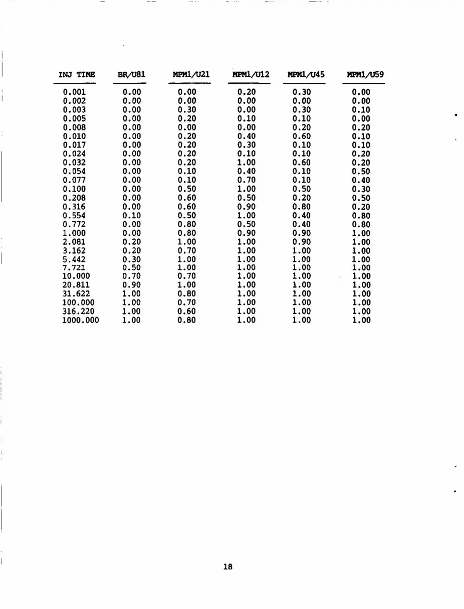
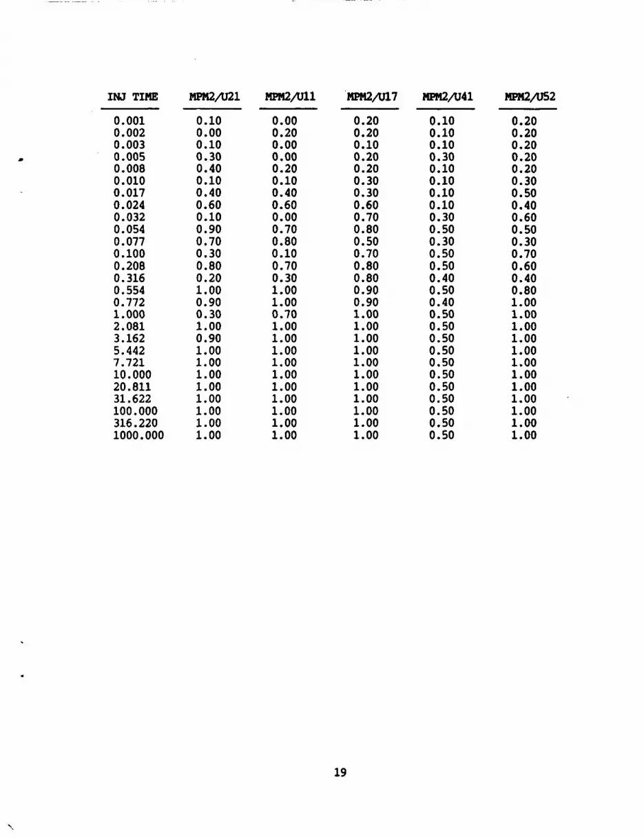
In this section the raw data from the fault-injection experiment is given.

For example The first column contains the fault injection durations. contain the results of the injections at a particular location. the second column contains the fraction of detections (Di/ni) for the CPU chip ~ 3 8 . The specific pin injected on the chip can be found by examining table 1. mere were 10 injections performed for each injection-duration for each pin (i.e. ni = 10 for all i).

The other columns

INJ TIME CPU/u38 m / u 3 5 cpu/u29 CPU/u04

0.001 0.002 0.003 0.005 0.008 0.010 0.017 0.024 0.032 0.054 0.077 0.100 0.208 0.316 0.554 0.772 1.000 2.081 3.162 5.442 7.721 10.000 20.811 31.622 100.000 316.220 1000.000

0.00 0.10 0.00 0.10 0.00 0.10 0.10 0.00 0.10 0.00 0.10 0.10 0.20 0.20 0.50 0.40 0.50 0.90 0.80 1.00 1.00 1.00 1.00 1.00 1.00 1.00 1.00

0.00 0.10 0.30 0.30 0.10 0.20 0.20 0.50 0.30 0.40 0.60 0.40 0.50 0.90 0.70 0.70 1.00 1.00 1.00 1.00 1.00 1.00 1.00 1.00 1.00 1.00 1.00

0.00 0.00 0.00 0.00 0.00 0.00 0.00 0.20 0.10 0.00 0.20 0.00 0.40 0.30 0.30 0.40 0.50 0.60 0.40 1.00 1.00 1.00 1.00 1.00 1.00 1.00 1.00

0.10 0.00 0.00 0.00 0.10 0.10 0.00 0.20 0.10 0.10 0.10 0.00 0.00 0.00 0.10 0.20 0.00 0.40 0.10 0.50 0.60 0.40 0.90 1.00 1.00 1.00 1.00

0.40 0.20 0.70 0.20 0.40 0.60 0.70 0.60 0.60 0.70 0.60 0.80 0.60 0.60 0.90 0.70 1.00 0.90 1.00 1.00 1.00 1.00 1.00 1.00 1.00 1.00 1.00

17

I INJ TIME

0.001 0.002 0.003 0.005 0.008 0.010 0.017 0.024 0.032 0.054 0.077 0.100 0.208 0.316 0.554 0.772 1.000 2.081 3.162 5.442 7.721 10.000 20.811 31.622 100.000 316.220 1000.000

m / u 2 1 m / u 5 9

0.00 0.00 0.00 0.00 0.00 0.00 0.00 0.00 0.00 0.00 0.00 0.00 0.00 0.00 0.10 0.00 0.00 0.20 0.20 0.30 0.50 0.70 0.90 1.00 1.00 1.00 1.00

0.00 0.00 0.30 0.20 0.00 0.20 0.20 0.20 0.20 0.10 0.10 0.50 0.60 0.60 0.50 0.80 0.80 1.00 0.70 1.00 1.00 0.70 1.00 0.80 0.70 0.60 0.80

0.20 0.00 0.00 0.10 0.00 0.40 0.30 0.10 1.00 0.40 0.70 1.00 0.50 0.90 1.00 0.50 0.90 1.00 1.00 1.00 1.00 1.00 1.00 1.00 1.00 1.00 1.00

0.30 0.00 0.30 0.10 0.20 0.60 0.10 0.10 0.60 0.10 0.10 0.50 0.20 0.80 0.40 0.40 0.90 0.90 1.00 1.00 1.00 1.00 1.00 1.00 1.00 1.00 1.00

0.00 0.00 0.10 0.00 0.20 0.10 0.10 0.20 0.20 0.50 0.40 0.30 0.50 0.20 0.80 0.80 1.00 1.00 1.00 1.00 1.00 1.00 1.00 1.00 1.00 1.00 1.00

18

INJ TINE “ 2 / U 4 1 HPM2fl52

0.001 0.002 0.003 0.005 0.008 0.010 0.017 0.024 0.032 0.054 0.077 0.100 0.208 0.316 0.554 0.772 1.000 2.081 3.162 5.442 7.721 10.000 20.811 31.622 100.000 316.220 1000.000

0.10 0.00 0.10 0.30 0.40 0.10 0.40 0.60 0.10 0.90 0.70 0.30 0.80 0.20 1.00 0.90 0.30 1.00 0.90 1.00 1.00 1.00 1.00 1.00 1.00 1.00 1.00

0.00 0.20 0.00 0.00 0.20 0.10 0.40 0.60 0.00 0.70 0.80 0.10 0.10 0.30 1.00 1.00 0.70 1.00 1.00 1.00 1.00 1.00 1.00 1.00 1.00 1.00 1.00

0.20 0.20 0.10 0.20 0.20 0.30 0.30 0.60 0.70 0.80 0.50 0.70 0.80 0.80 0.90 0.90 1.00 1.00 1.00 1.00 1.00 1.00 1.00 1.00 1.00 1.00 1.00

0.10 0.10 0.10 0.30 0.10 0.10 0.10 0.10 0.30 0.50 0.30 0.50 0.50 0.40 0.50 0.40 0.50 0.50 0.50 0.50 0.50 0.50 0.50 0.50 0.50 0.50 0.50

0.20 0.20 0.20 0.20 0.20 0.30 0.50 0.40 0.60 0.50 0.30 0.70 0.60 0.40 0.80 1.00 1.00 1.00 1.00 1.00 1.00 1.00 1.00 1.00 1.00 1.00 1.00

‘.

19

INJ TIME mpm2/v37 MPM2/2135 “2/2153c

0.001 0.002 0.003 0.005 0.008 0.010 0.017 0.024 0.032 0.054 0.077 0.100 0.208 0.316 0.554 0.772 1.000 2.081 3.162 5.442 7.721 10.000 20.811 31.622 100.000 316.220 1000.000

0.10 0.10 0.00 0.20 0.30 0.10 0.50 0.40 0.00 0.90 0.80 0.60 0.80 0.30 1.00 0.90 0.80 1.00 1.00 1.00 1.00 1.00 0.90 1.00 1.00 1.00 1.00

0.50 0.40 0.20 0.90 0.60 0.80 0.80 0.90 1.00 0.90 1.00 1.00 1.00 1.00 1.00 0.90 1.00 1.00 1.00 1.00 1.00 1.00 1.00 1.00 1.00 1.00 1.00

0.00 0.30 0.00 0.60 0.50 0.00 0.80 0.90 0.30 0.90 0.90 0.30 1.00 0.40 0.80 1.00 0.70 1.00 0.90 1.00 1.00 1.00 1.00 1.00 1.00 1.00 1.00

0.10 0.30 0.20 0.10 0.40 0.20 0.40 0.60 0.40 0.70 0.90 0.80 0.60 0.90 0.90 0.90 1.00 1.00 1.00 1.00 1 .oo 1.00 1.00 1.00 1.00 1.00 1.00

20

- 1. J. G. McGough and F. L. Swern; Measurement of Fault Latency in a Digital

Avionic Mini Processor, NASA Contractor Report 3462, Oct. 1981.

c 2. J. G. McGough and F. L. Swern; Measurement of Fault Latency in a Digital

Avionic Mini Processor, NASA Contractor Report 3651, Jan. 1983.

3. R. Chillarege and R. K. Iyer; Fault Latency in the Memory - AN

Experimental Study on VAX 11/780, Proceedings of the 16th ~ ~ u a l International Symposium on Fault-Tolerant Computing, pp. 258-263, 1986.

4. K.G. Shin and Y. H. Lee; Measurement and Application of Fault Latency, IEEE Transactions on Computers, Vol. C-35, No. 4, pp. 370-375, April 1986.

5. Geist, Robert M; and Trivedi, Kishor S.: Ultrahigh Reliability Prediction in Fault-Tolerant Computer Systems. IEEE Trans. Complt., C-32, no. 12, Dee. 1983, pp. 1118-1127.

6. Bavuso, S. J.; and Petersen, P. L.: CARE I11 Model Overview and User's Guide (First Revision). NASA TM-86404, 1985.

7. R.E. Barlow, D.J. Bartholomew, J.M. Bremner, and H.D. Brunk: Statistical Inference -- under Order Restrictions, John Wiley & Sons, New York, 1972.

8. Schoenfeld, David A.: Confidence Bounds for Normal mans under Order

Restrictions, With Application to Dose-Response Curves, Toxicology Experiments, and Low-Dose Extrapolation, Journal of the American Statistical Association, Vol. 81, No. 393, pp. 186-195, March 1986.

.

9. Goldberg, Jack; Kautz, William H.; Melliar-Smith, P. Michael; Green, Milton W.; Levitt, Karl N.; Schwartz, Richard L.; and Weinstock, Charles B.: (SIFT) Computer. NASA CR-172146, 1984.

Development and Analysis of the Software Implemented Fault Tolerance

10. Press, Flannery, et. al.: Numerical Recipes, Cambridge University Press, Cambridge, England, 1986, pp. 289-293, 739-740.

21

Report Documentation Page 1. Report No.

NASA TM-100521

2. Government Acxessbn No.

7. Authods)

E r i k L. E l l i s and Ricky W. B u t l e r

Unc lass i f ied Unc lass i f ied

9. Performing Organization Name and Address

22 A02

NASA Langley Research Center Hampton, VA 23665-5225

12. Sponsoring Awncy Name and Address

Nat ional Aeronautics and Space Admin is t ra t ion Washington, DC 20546-0001

3. Recipient's Catalog No.

5. Report Date

November 1987 6. Performing Organization Code

8. Performing Organization Report No.

10. work unit No.

505-66-21 -01 11. Contract or Grant No.

13. Type of Report and Period Covered

Technical Memorandum 14. Sponsoring Agency Code

~~

5. Supplementary Notes

16. Abstract

This paper presents a s t a t i s t i c a l approach t o measuring f a u l t la tency

i n a d i q i t a l processor. The method r e l i e s on the use o f phys ica l f a u l t

i n j e c t i o n where the du ra t i on of the f a u l t i n j e c t i o n can be con t ro l l ed . Although

a s p e c i f i c f a u l t ' s la tency pe r iod i s never d i r e c t l y measured, the method

i n d i r e c t l y determines the d i s t r i b u t i o n o f f a u l t la tency.

7. Key Words (Suggested by Author(r1) I 18. Distribution Statement

Fau 1 t 1 a tency , r e 1 i abi 1 i ty , f a u l t tolerance, computer systems Unc lass i f i ed - Un l im i ted

Subject Category 62 I

9. Security Classif. (of ths report) 120. Security classif. (of ths page) 121. No. of pages 122. Price

NASA FORM 1626 OCT 86