Embed Size (px)
Citation preview
�����������������
Citation: Zeng, Q.; Xie, T.; Zhu, S.;
Fan, M.; Chen, L.; Tian, Y. Estimating
the Near-Ground PM2.5 Concentration
over China Based on the CapsNet
Model during 2018–2020. Remote Sens.
2022, 14, 623. https://doi.org/
10.3390/rs14030623
Academic Editor: Carmine Serio
Received: 17 December 2021
Accepted: 24 January 2022
Published: 27 January 2022
Publisher’s Note: MDPI stays neutral
with regard to jurisdictional claims in
published maps and institutional affil-
iations.
Copyright: © 2022 by the authors.
Licensee MDPI, Basel, Switzerland.
This article is an open access article
distributed under the terms and
conditions of the Creative Commons
Attribution (CC BY) license (https://
creativecommons.org/licenses/by/
4.0/).
remote sensing
Article
Estimating the Near-Ground PM2.5 Concentration over ChinaBased on the CapsNet Model during 2018–2020Qiaolin Zeng 1,2, Tianshou Xie 1, Songyan Zhu 3,*, Meng Fan 4, Liangfu Chen 4 and Yu Tian 1
1 The College of Computer Science and Technology, Chongqing University of Posts and Telecommunications,Chongqing 400065, China; [email protected] (Q.Z.); [email protected] (T.X.);[email protected] (Y.T.)
2 The Chongqing Institute of Meteorological Sciences, Chongqing 401147, China3 The Department of Geography, University of Exeter, Rennes Drive, Exeter EX4 4RJ, UK4 The Aerospace Information Research Institute, Chinese Academy of Sciences, Beijing 100094, China;
[email protected] (M.F.); [email protected] (L.C.)* Correspondence: [email protected]
Abstract: Fine particulate matter (PM2.5) threatens human health and the natural environment. Esti-mating the near-ground PM2.5 concentrations accurately is of great significance in air quality research.Statistical and deep-learning models are widely used for estimating PM2.5 concentration based onremotely sensed aerosol optical depth (AOD) products. Deep-learning models can effectively expressthe nonlinear relationship between AOD, parameters, and PM2.5. This study proposed a capsulenetwork model (CapsNet) to address the spatial differences in PM2.5 concentration distribution byintroducing a capsule structure and dynamic routing algorithm for the first time, which integratesAOD, surface PM2.5 measurements, and auxiliary variables (e.g., normalized difference vegetationindex (NDVI) and meteorological parameters). Moreover, we examined the longitude and latitudeof pixels as input parameters to reflect spatial location information, and the results showed that theintroduction of longitude (LON) and latitude (LAT) parameters improved the model fitting accuracy.The coefficient of determination (R2) increased by 0.05± 0.01, and the root mean square error (RMSE),mean relative error (MRE), and mean absolute error (MAE) decreased by 3.30 ± 1.0 µg/m3, 8 ± 3%,and 1.40 ± 0.2 µg/m3, respectively. To verify the accuracy of our proposed CapsNet, the deep neuralnetwork (DNN) model was executed. The results indicated that the R2 values of the validation datasetusing CapsNet improved by 4 ± 2%, and RMSE, MRE, and MAE decreased by 1.50 ± 0.4 µg/m3,~5%, and 0.60 ± 0.2 µg/m3, respectively. Finally, the effects of seasons and spatial region on thefitting accuracy were examined separately from 2018 to 2020. With respect to seasons, the modelperformed more robustly in the cold season. In terms of spatial region, the R2 values exceeded 0.9in the central-eastern region, while the accuracy was lower in the western and coastal regions. Thisstudy proposed the CapsNet model to estimate PM2.5 concentrations for the first time and achievedgood accuracy, which could be used for the estimation of other air contaminants.
Keywords: aerosol optical depth; PM2.5 concentration; dynamic routing algorithm; CapsNet; DNN
1. Introduction
Fine particulate matter (PM2.5) is defined as particulate matter with an aerodynamicdiameter less than or equal to 2.5 µm, and it is a main pollutant causing hazy weather.Numerous studies in relation to environmental epidemiology have shown that fine par-ticulate matter has a variety of negative effects on human health (e.g., causing respiratoryand cardiovascular diseases) [1,2]. To monitor and evaluate air quality, the China NationalEnvironmental Monitoring Centre has established ground-based stations since 2013 to mea-sure PM2.5 concentrations in real time at an hourly scale. Despite some PM2.5 concentrationreductions measured, the PM2.5 concentration is still very worrying, especially in somemetropolitan regions in winter [3]. The number of ground-based stations is still limited,
Remote Sens. 2022, 14, 623. https://doi.org/10.3390/rs14030623 https://www.mdpi.com/journal/remotesensing
Remote Sens. 2022, 14, 623 2 of 19
and existing sites are distributed unevenly, which causes issues called “blind monitoringzones” [4]. Providing large-scale and frequent (near-daily) images, satellite remote sensingis gaining popularity to compensate for the deficiency of ground-based stations in quanti-fying PM2.5 distribution and temporal variations [5–7]. For example, Terra (Aqua)/MODIS(Moderate Resolution Imaging Spectroradiometer) [8–12], Terra/MISR (Multiangle ImagingSpectroRadiometer) [13–15], the Visible Infrared Imaging Radiometer Suite (VIIRS) [16,17],Himawiri-8/AHI (Advanced Himawari Imagers) [18], and FY-4/AGRI (Multichannel ScanImagery Radiometer) [19] are common satellite sensors that measure the aerosol opticaldepth (AOD) to estimate PM2.5 concentrations.
PM2.5 estimation approaches were developed from early simple scaling relation-ships [20] and atmospheric model simulations [21] to complex physical models [11,22]and statistical models [23–25]. For example, Liu et al. established a regression model ofAOD-PM2.5 by combining AOD and assimilation data, obtaining an R2 value of 0.43 inthe eastern United States [26]. Wang et al. realized the estimation of surface PM2.5 atdifferent regional scales by utilizing MODIS AOD, lidar, and atmospheric model data [22].Although the estimation accuracy has greatly increased, simple scaling relationships stillcannot represent the nonlinear interactions between particulate matter, satellite detectiondata, and environmental parameters. The satellite retrieval AOD represents the integralof extinction coefficient from top to bottom of the atmosphere, while PM2.5 is the concen-tration of near-ground particulate matter. Therefore, the correlation between AOD andPM2.5 is strongly affected by external factors in terms of physical mechanisms, such asthe difference in extinction due to the hygroscopic growth characteristics of particulatematter, the vertical profile distribution of aerosol, and the particle size causing differentscattering and extinction. To express the physical mechanism of AOD-PM2.5, some physicalmechanism models have been proposed. Koelemeijer et al. used the boundary layer heightand humidity to perform vertical and hygroscopic corrections, and the results showedthat the correlation coefficients between AOD and PM2.5 were improved [27]. Chu et al.obtained the aerosol extinction profile from 2006 to 2009 to described the vertical distribu-tion of aerosols, and haze layer height (HLH) was discussed for use for the near-groundextinction [28]. Compared with the single-factor estimation of PM2.5, the estimation errorwas reduced by 2.9 µg/m3. Lin et al. introduced the fine particle ratio, mass extinctionefficiency, and hygroscopic growth factor to the hygroscopic correction process based on anobservation-based semi-physical model [29]. Zhang et al. obtained the fine mode fraction(FMF) from MODIS and other data to propose a physical mechanism [11]. However, thephysical model cannot fully express the relationship between parameters in a formula.With the development of machine-learning, some methods (e.g., random forests (RF) [4],deep neural networks (DNN) [30], and residual network models (RNM) [31]) are usuallyused to estimate PM2.5 and to improve estimation accuracy by establishing the associa-tion between AOD and PM2.5 via apparent reflectance inversion to directly establish therelationship between apparent reflectance, observed parameters, and PM2.5 [32]. Overall,the PM2.5 estimation of different machine-learning models has been proposed to addressthe nonlinearity of the AOD-PM2.5 relationship, and these models have obtained greataccuracy. Spatial variability exists in the AOD-PM2.5 relationship, and models that canaddress both the nonlinearity and spatial variability are still continuously pursued in theremote sensing estimation of surface PM2.5.
In the field of image classification, graph convolutional networks (GCNs) [33], multi-modal deep learning (MDL) [34], and capsule network model (CapsNet) [35] have beensuccessfully applied in irregular data representation and analysis, which can solve thedifficulties in positional relation recognition and spatial reasoning more efficiently. Theseapproaches have been widely used in imagery classification in recent years [36], but havenever been applied for atmospheric research. This study addresses spatial variability bydeveloping a CapsNet model that can reflect more accurate location information comparedwith RF and DNN widely used in PM2.5 estimation. Longitude and latitude information ofthe stations was used as input factors, by combining multiple-source satellite products (e.g.,
Remote Sens. 2022, 14, 623 3 of 19
aerosol and vegetation) and ground-based PM2.5 measurements and day of year (DOY) toestimate surface PM2.5. This model was tested by utilizing a case study in China over threeyears (from 2018 to 2020), and daily estimates of surface PM2.5 were effectively generatedfrom satellite observations. The main contributions of this letter are listed as follows:
(1) We proposed a CapsNet model that introduced the capsule structure and dynamicrouting algorithm to estimate daily PM2.5 concentrations over China. The longitude(LON) and latitude (LAT) of pixels were used as input parameters to verify whether itis helpful to improve the accuracy of the model. The coefficient of determination (R2),root mean square error (RMSE), mean relative error (MRE), and mean absolute error(MAE) are used as the evaluation metrics.
(2) To evaluate the CapsNet proposed by us effectively, the DNN model was executed,and the LON and LAT were also included in the DNN model. We discussed theaccuracy of CaspNet and DNN in both the cold season and warm season, and theresults indicate that CaspNet performs better. Therefore, we used CaspNet to estimatedaily PM2.5 concentrations and analyzed the characteristics of PM2.5 concentrationvariations.
(3) We examined the different advanced capsule layers in CaspNet, which influence theaccuracy of PM2.5 estimation. Multiple capsules and a single weight are better whenconsidering the accuracy and operating efficiency. Moreover, we verified the accuracyof the CaspNet model in different regions.
The flowchart of CapsNet modeling for remote sensing estimation of PM2.5 concen-tration is shown in Figure 1 in this study. First, we downloaded ground-measured PM2.5,satellite data, and meteorological data. All data were preprocessed to obtain a spatialtempo-rally dataset, and we handed some missing data. Subsequently, the parameters of the inputmodel are discussed, and the CapsNet model could be trained. Finally, evaluation metricswere used to verify the accuracy of PM2.5 estimation, and then daily PM2.5 concentrationswere obtained. The rest of this paper is structured as follows: Section 2 mainly introducesthe CapsNet model; the data used in this study and preprocessing are presented in Section 3;the experimental results are analyzed in Section 4; Section 5 discusses the advantage anddisadvantage of this model; and the final section briefly concludes our work.
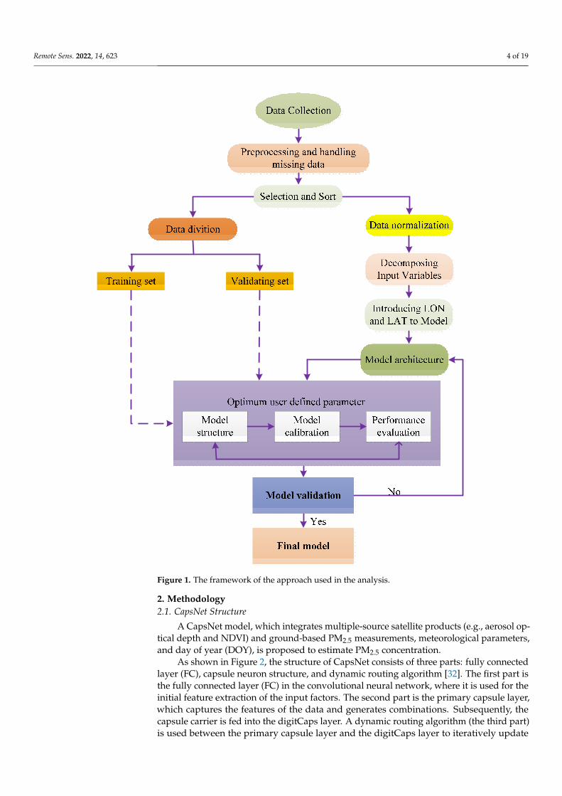
Remote Sens. 2022, 14, 623 4 of 19Remote Sens. 2022, 13, x FOR PEER REVIEW 4 of 19
Figure 1. The framework of the approach used in the analysis.
2. Methodology 2.1. CapsNet Structure
A CapsNet model, which integrates multiple-source satellite products (e.g., aerosol optical depth and NDVI) and ground-based PM2.5 measurements, meteorological pa-rameters, and day of year (DOY), is proposed to estimate PM2.5 concentration.
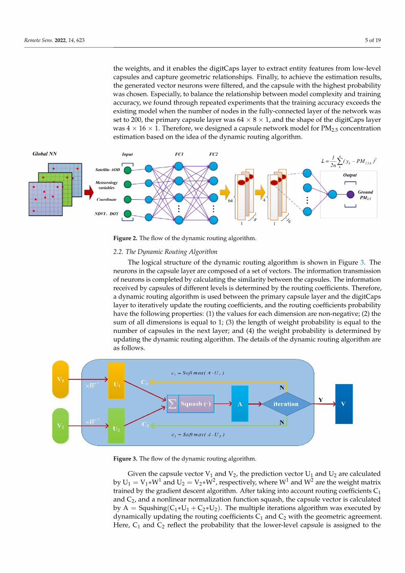
As shown in Figure 2, the structure of CapsNet consists of three parts: fully con-nected layer (FC), capsule neuron structure, and dynamic routing algorithm [32]. The first part is the fully connected layer (FC) in the convolutional neural network, where it is used for the initial feature extraction of the input factors. The second part is the prima-ry capsule layer, which captures the features of the data and generates combinations. Subsequently, the capsule carrier is fed into the digitCaps layer. A dynamic routing al-gorithm (the third part) is used between the primary capsule layer and the digitCaps
Figure 1. The framework of the approach used in the analysis.
2. Methodology2.1. CapsNet Structure
A CapsNet model, which integrates multiple-source satellite products (e.g., aerosol op-tical depth and NDVI) and ground-based PM2.5 measurements, meteorological parameters,and day of year (DOY), is proposed to estimate PM2.5 concentration.
As shown in Figure 2, the structure of CapsNet consists of three parts: fully connectedlayer (FC), capsule neuron structure, and dynamic routing algorithm [32]. The first part isthe fully connected layer (FC) in the convolutional neural network, where it is used for theinitial feature extraction of the input factors. The second part is the primary capsule layer,which captures the features of the data and generates combinations. Subsequently, thecapsule carrier is fed into the digitCaps layer. A dynamic routing algorithm (the third part)is used between the primary capsule layer and the digitCaps layer to iteratively update
Remote Sens. 2022, 14, 623 5 of 19
the weights, and it enables the digitCaps layer to extract entity features from low-levelcapsules and capture geometric relationships. Finally, to achieve the estimation results,the generated vector neurons were filtered, and the capsule with the highest probabilitywas chosen. Especially, to balance the relationship between model complexity and trainingaccuracy, we found through repeated experiments that the training accuracy exceeds theexisting model when the number of nodes in the fully-connected layer of the network wasset to 200, the primary capsule layer was 64 × 8 × 1, and the shape of the digitCaps layerwas 4 × 16 × 1. Therefore, we designed a capsule network model for PM2.5 concentrationestimation based on the idea of the dynamic routing algorithm.
Remote Sens. 2022, 13, x FOR PEER REVIEW 5 of 19
layer to iteratively update the weights, and it enables the digitCaps layer to extract enti-ty features from low-level capsules and capture geometric relationships. Finally, to achieve the estimation results, the generated vector neurons were filtered, and the cap-sule with the highest probability was chosen. Especially, to balance the relationship be-tween model complexity and training accuracy, we found through repeated experiments that the training accuracy exceeds the existing model when the number of nodes in the fully-connected layer of the network was set to 200, the primary capsule layer was 64 × 8 × 1, and the shape of the digitCaps layer was 4 × 16 × 1. Therefore, we designed a capsule network model for PM2.5 concentration estimation based on the idea of the dynamic routing algorithm.
Figure 2. The flow of the dynamic routing algorithm.
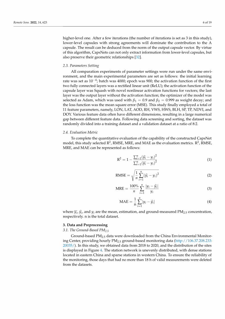
2.2. The Dynamic Routing Algorithm The logical structure of the dynamic routing algorithm is shown in Figure 3. The
neurons in the capsule layer are composed of a set of vectors. The information transmis-sion of neurons is completed by calculating the similarity between the capsules. The in-formation received by capsules of different levels is determined by the routing coeffi-cients. Therefore, a dynamic routing algorithm is used between the primary capsule lay-er and the digitCaps layer to iteratively update the routing coefficients, and the routing coefficients probability have the following properties: (1) the values for each dimension are non-negative; (2) the sum of all dimensions is equal to 1; (3) the length of weight probability is equal to the number of capsules in the next layer; and (4) the weight prob-ability is determined by updating the dynamic routing algorithm. The details of the dy-namic routing algorithm are as follows.
Given the capsule vector V and V , the prediction vector U and U are calculated by U = V ∗ W and U = V ∗ W , respectively, where W and W are the weight matrix trained by the gradient descent algorithm. After taking into account routing coefficients C and C , and a nonlinear normalization function squash, the capsule vector is calculat-ed by A = Squshing(C ∗ U + C ∗ U ). The multiple iterations algorithm was executed by dynamically updating the routing coefficients C and C with the geometric agree-ment. Here, C and C reflect the probability that the lower-level capsule is assigned to the higher-level one. After a few iterations (the number of iterations is set as 3 in this study), lower-level capsules with strong agreements will dominate the contribution to the A capsule. The result can be deduced from the norm of the output capsule vector. By virtue of this algorithm, CapsNets can not only extract information from lower-level capsules, but also preserve their geometric relationships [32].
Figure 2. The flow of the dynamic routing algorithm.
2.2. The Dynamic Routing Algorithm
The logical structure of the dynamic routing algorithm is shown in Figure 3. Theneurons in the capsule layer are composed of a set of vectors. The information transmissionof neurons is completed by calculating the similarity between the capsules. The informationreceived by capsules of different levels is determined by the routing coefficients. Therefore,a dynamic routing algorithm is used between the primary capsule layer and the digitCapslayer to iteratively update the routing coefficients, and the routing coefficients probabilityhave the following properties: (1) the values for each dimension are non-negative; (2) thesum of all dimensions is equal to 1; (3) the length of weight probability is equal to thenumber of capsules in the next layer; and (4) the weight probability is determined byupdating the dynamic routing algorithm. The details of the dynamic routing algorithm areas follows.
Remote Sens. 2022, 13, x FOR PEER REVIEW 6 of 19
Figure 3. The flow of the dynamic routing algorithm.
2.3. Parameters Setting All comparation experiments of parameter settings were run under the same envi-
ronment, and the main experimental parameters are set as follows: the initial learning rate was set as 10−4; batch was 4000; epoch was 900; the activation function of the first two fully connected layers was a rectified linear unit (ReLU); the activation function of the capsule layer was Squash with novel nonlinear activation functions for vectors; the last layer was the output layer without the activation function; the optimizer of the model was selected as Adam, which was used with 𝛽 = 0.9 and 𝛽 = 0.999 as weight decay; and the loss function was the mean square error (MSE). This study finally em-ployed a total of 11 feature parameters, namely, LON, LAT, AOD, RH, VWS, HWS, BLH, SP, TP, NDVI, and DOY. Various feature data often have different dimensions, re-sulting in a large numerical gap between different feature data. Following data screen-ing and sorting, the dataset was randomly divided into a training dataset and a valida-tion dataset at a ratio of 8:2.
2.4. Evaluation Metric To complete the quantitative evaluation of the capability of the constructed Cap-
sNet model, this study selected R2, RMSE, MRE, and MAE as the evaluation metrics. R2, RMSE, MRE, and MAE can be represented as follows: R = 1 − ∑ (y − y )∑ (y − y ) (1)
RMSE = 1n (y − y ) (2)
MRE = 100%n |y − y |y (3)
MAE = 1n |y − y | (4)
where 𝑦 , 𝑦 , and 𝑦 are the mean, estimation, and ground-measured PM2.5 concentration, respectively. n is the total dataset.
3. Data and Preprocessing 3.1. The Ground-Based PM2.5
Ground-based PM2.5 data were downloaded from the China Environmental Moni-toring Center, providing hourly PM2.5 ground-based monitoring data (http://106.37.208.233:20035/). In this study, we obtained data from 2018 to 2020, and the distribution of the sites is displayed in Figure 4. The station network is unevenly distrib-
Figure 3. The flow of the dynamic routing algorithm.
Given the capsule vector V1 and V2, the prediction vector U1 and U2 are calculatedby U1 = V1∗W1 and U2 = V2∗W2, respectively, where W1 and W2 are the weight matrixtrained by the gradient descent algorithm. After taking into account routing coefficients C1and C2, and a nonlinear normalization function squash, the capsule vector is calculatedby A = Squshing(C1∗U1 + C2∗U2). The multiple iterations algorithm was executed bydynamically updating the routing coefficients C1 and C2 with the geometric agreement.Here, C1 and C2 reflect the probability that the lower-level capsule is assigned to the
Remote Sens. 2022, 14, 623 6 of 19
higher-level one. After a few iterations (the number of iterations is set as 3 in this study),lower-level capsules with strong agreements will dominate the contribution to the Acapsule. The result can be deduced from the norm of the output capsule vector. By virtueof this algorithm, CapsNets can not only extract information from lower-level capsules, butalso preserve their geometric relationships [32].
2.3. Parameters Setting
All comparation experiments of parameter settings were run under the same envi-ronment, and the main experimental parameters are set as follows: the initial learningrate was set as 10−4; batch was 4000; epoch was 900; the activation function of the firsttwo fully connected layers was a rectified linear unit (ReLU); the activation function of thecapsule layer was Squash with novel nonlinear activation functions for vectors; the lastlayer was the output layer without the activation function; the optimizer of the model wasselected as Adam, which was used with β1 = 0.9 and β2 = 0.999 as weight decay; andthe loss function was the mean square error (MSE). This study finally employed a total of11 feature parameters, namely, LON, LAT, AOD, RH, VWS, HWS, BLH, SP, TP, NDVI, andDOY. Various feature data often have different dimensions, resulting in a large numericalgap between different feature data. Following data screening and sorting, the dataset wasrandomly divided into a training dataset and a validation dataset at a ratio of 8:2.
2.4. Evaluation Metric
To complete the quantitative evaluation of the capability of the constructed CapsNetmodel, this study selected R2, RMSE, MRE, and MAE as the evaluation metrics. R2, RMSE,MRE, and MAE can be represented as follows:
R2 = 1− ∑ni=1(yi − yi)
2
∑ni=1(yi − yi)
2 (1)
RMSE =
√1n
n
∑i=1
(yi − yi)2 (2)
MRE =100%
n
n
∑i=1
|yi − yi|yi
(3)
MAE =1n
n
∑i=1|yi − yi| (4)
where yi, yi, and yi are the mean, estimation, and ground-measured PM2.5 concentration,respectively. n is the total dataset.
3. Data and Preprocessing3.1. The Ground-Based PM2.5
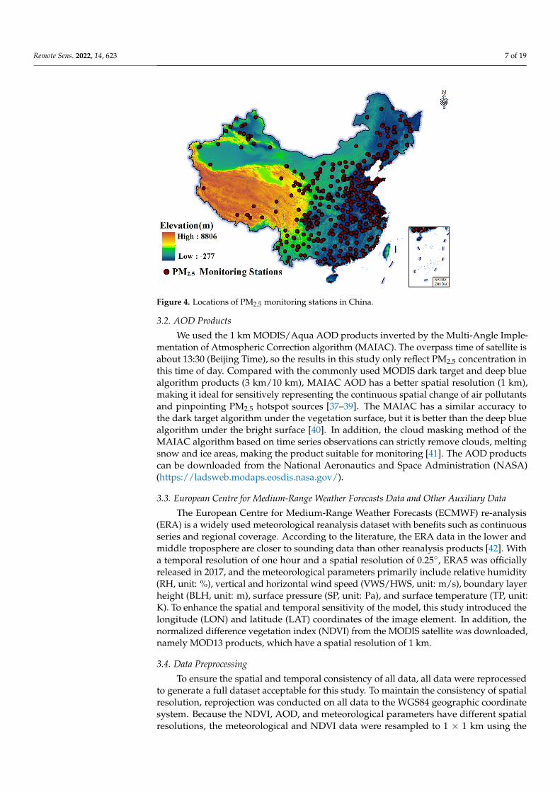
Ground-based PM2.5 data were downloaded from the China Environmental Monitor-ing Center, providing hourly PM2.5 ground-based monitoring data (http://106.37.208.233:20035/). In this study, we obtained data from 2018 to 2020, and the distribution of the sitesis displayed in Figure 4. The station network is unevenly distributed, with dense stationslocated in eastern China and sparse stations in western China. To ensure the reliability ofthe monitoring, those days that had no more than 18 h of valid measurements were deletedfrom the datasets.
Remote Sens. 2022, 14, 623 7 of 19
Remote Sens. 2022, 13, x FOR PEER REVIEW 7 of 19
uted, with dense stations located in eastern China and sparse stations in western China. To ensure the reliability of the monitoring, those days that had no more than 18 h of val-id measurements were deleted from the datasets.
Figure 4. Locations of PM2.5 monitoring stations in China.
3.2. AOD Products We used the 1 km MODIS/Aqua AOD products inverted by the Multi-Angle Im-
plementation of Atmospheric Correction algorithm (MAIAC). The overpass time of sat-ellite is about 13:30 (Beijing Time), so the results in this study only reflect PM2.5 concen-tration in this time of day. Compared with the commonly used MODIS dark target and deep blue algorithm products (3 km/10 km), MAIAC AOD has a better spatial resolution (1 km), making it ideal for sensitively representing the continuous spatial change of air pollutants and pinpointing PM2.5 hotspot sources [37–39]. The MAIAC has a similar ac-curacy to the dark target algorithm under the vegetation surface, but it is better than the deep blue algorithm under the bright surface [40]. In addition, the cloud masking meth-od of the MAIAC algorithm based on time series observations can strictly remove clouds, melting snow and ice areas, making the product suitable for monitoring [41]. The AOD products can be downloaded from the National Aeronautics and Space Admin-istration (NASA) (https://ladsweb.modaps.eosdis.nasa.gov/).
3.3. European Centre for Medium-Range Weather Forecasts Data and Other Auxiliary Data The European Centre for Medium-Range Weather Forecasts (ECMWF) re-analysis
(ERA) is a widely used meteorological reanalysis dataset with benefits such as continu-ous series and regional coverage. According to the literature, the ERA data in the lower and middle troposphere are closer to sounding data than other reanalysis products [42]. With a temporal resolution of one hour and a spatial resolution of 0.25°, ERA5 was offi-cially released in 2017, and the meteorological parameters primarily include relative humidity (RH, unit: %), vertical and horizontal wind speed (VWS/HWS, unit: m/s), boundary layer height (BLH, unit: m), surface pressure (SP, unit: Pa), and surface tem-perature (TP, unit: K). To enhance the spatial and temporal sensitivity of the model, this study introduced the longitude (LON) and latitude (LAT) coordinates of the image ele-ment. In addition, the normalized difference vegetation index (NDVI) from the MODIS satellite was downloaded, namely MOD13 products, which have a spatial resolution of 1 km.
Figure 4. Locations of PM2.5 monitoring stations in China.
3.2. AOD Products
We used the 1 km MODIS/Aqua AOD products inverted by the Multi-Angle Imple-mentation of Atmospheric Correction algorithm (MAIAC). The overpass time of satellite isabout 13:30 (Beijing Time), so the results in this study only reflect PM2.5 concentration inthis time of day. Compared with the commonly used MODIS dark target and deep bluealgorithm products (3 km/10 km), MAIAC AOD has a better spatial resolution (1 km),making it ideal for sensitively representing the continuous spatial change of air pollutantsand pinpointing PM2.5 hotspot sources [37–39]. The MAIAC has a similar accuracy tothe dark target algorithm under the vegetation surface, but it is better than the deep bluealgorithm under the bright surface [40]. In addition, the cloud masking method of theMAIAC algorithm based on time series observations can strictly remove clouds, meltingsnow and ice areas, making the product suitable for monitoring [41]. The AOD productscan be downloaded from the National Aeronautics and Space Administration (NASA)(https://ladsweb.modaps.eosdis.nasa.gov/).
3.3. European Centre for Medium-Range Weather Forecasts Data and Other Auxiliary Data
The European Centre for Medium-Range Weather Forecasts (ECMWF) re-analysis(ERA) is a widely used meteorological reanalysis dataset with benefits such as continuousseries and regional coverage. According to the literature, the ERA data in the lower andmiddle troposphere are closer to sounding data than other reanalysis products [42]. Witha temporal resolution of one hour and a spatial resolution of 0.25◦, ERA5 was officiallyreleased in 2017, and the meteorological parameters primarily include relative humidity(RH, unit: %), vertical and horizontal wind speed (VWS/HWS, unit: m/s), boundary layerheight (BLH, unit: m), surface pressure (SP, unit: Pa), and surface temperature (TP, unit:K). To enhance the spatial and temporal sensitivity of the model, this study introduced thelongitude (LON) and latitude (LAT) coordinates of the image element. In addition, thenormalized difference vegetation index (NDVI) from the MODIS satellite was downloaded,namely MOD13 products, which have a spatial resolution of 1 km.
3.4. Data Preprocessing
To ensure the spatial and temporal consistency of all data, all data were reprocessedto generate a full dataset acceptable for this study. To maintain the consistency of spatialresolution, reprojection was conducted on all data to the WGS84 geographic coordinatesystem. Because the NDVI, AOD, and meteorological parameters have different spatialresolutions, the meteorological and NDVI data were resampled to 1 × 1 km using the
Remote Sens. 2022, 14, 623 8 of 19
bilinear interpolation method. The corresponding pixel values (satellite and meteorologicaldata) were extracted with the longitude and latitude information of PM2.5 monitoringstations to produce the corresponding records. To be as consistent in temporal as possible,the average PM2.5 concentration of ground-based monitoring was determined half anhour before and after the satellite pass time to maintain the consistency between ground-based and satellite observations, because the scanning time of Aqua/AOD data wasapproximately 13:30 daily.
4. Experiment Analysis4.1. Experimental Results4.1.1. Normalization Methods
In the process of model training, a large number of dimensional values greatly weakenthe role of small dimensional values in the model, preventing the model from being correctlytrained to obtain accurate fitting relationships. To eliminate the effects of dimensionaldifferences, all data need to be normalized. The results of different normalization methodscan ultimately affect the results of the model. In the mainstream normalization methods,we separately discussed the minimum–maximum method and standard score (Z-Score)method, and the methods can be expressed as follows:
minimum−maximum : I =I − Imin
Imax − Imin(5)
Z− Score : I =I − Imean
Istd(6)
where I is the feature data and Imin, Imax, Imean, and Istd denote the minimum, maximum,mean value, and standard deviation in the feature data, respectively.
The above two methods were used to conduct normalization experiments on the samedataset, and we calculated normalization rules on the data of the training set and appliedthem to the validation set for experiments. The experimental results are shown in Table 1.According to the results of the normalization methods, R2, RMSE, MRE, and MAE are0.81, 12.75 µg/m3, 41%, and 7.93 µg/m3, respectively, in validation datasets by the Z-score,which is beyond that of the minimum–maximum method; therefore, the next experimentaldatasets were normalized by the Z-Score.
Table 1. Experimental results of two normalization methods.
Methods Dataset R2 RMSE MRE MAE
minimum–maximumTrain 0.89 9.84 30% 6.06
Validation 0.79 13.30 40% 8.06
Z-scoreTrain 0.96 6.39 18% 3.23
Validation 0.81 12.75 41% 7.93
4.1.2. Parameter Validation
Other research has examined meteorological parameters, NDVI, and DOY as inputparameters impacting PM2.5 [30], while we mainly focused on the effect of LON and LATinformation on the accuracy of model fitting. Table 2 shows the effect of including LONand LAT information factors in the training data on the simulation outcomes. The trainingand validation results of the CapsNet model for 2018, 2019, and 2020 data showed R2
value increasing by 0.05, 0.05, and 0.04; RMSE decreasing by 3.30 µg/m3, 2.43 µg/m3, and1.33 µg/m3; MRE decreasing by 10%; and MAE decreasing by 1.35 µg/m3, 1.37 µg/m3,and 1.57 µg/m3. Therefore, the introduction of LON and LAT pixel information as inputparameters in this study performed better on both training and validation datasets. Thedensity scatter plots of the fitting results are shown in Figure 5. There were differences inmodel accuracy from 2018 to 2020. The majority of the data are concentrated around the
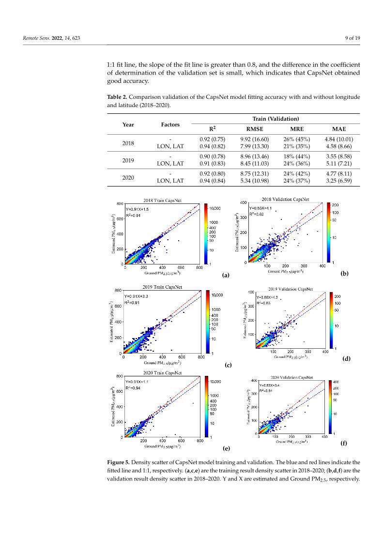
Remote Sens. 2022, 14, 623 9 of 19
1:1 fit line, the slope of the fit line is greater than 0.8, and the difference in the coefficientof determination of the validation set is small, which indicates that CapsNet obtainedgood accuracy.
Table 2. Comparison validation of the CapsNet model fitting accuracy with and without longitudeand latitude (2018–2020).
Year FactorsTrain (Validation)
R2 RMSE MRE MAE
2018- 0.92 (0.75) 9.92 (16.60) 26% (45%) 4.84 (10.01)
LON, LAT 0.94 (0.82) 7.99 (13.30) 21% (35%) 4.58 (8.66)
2019- 0.90 (0.78) 8.96 (13.46) 18% (44%) 3.55 (8.58)
LON, LAT 0.91 (0.83) 8.45 (11.03) 24% (36%) 5.11 (7.21)
2020- 0.92 (0.80) 8.75 (12.31) 24% (42%) 4.77 (8.11)
LON, LAT 0.94 (0.84) 5.34 (10.98) 24% (37%) 3.25 (6.59)
Remote Sens. 2022, 13, x FOR PEER REVIEW 9 of 19
value increasing by 0.05, 0.05, and 0.04; RMSE decreasing by 3.30 μg/m3, 2.43 μg/m3, and 1.33 μg/m3; MRE decreasing by 10%; and MAE decreasing by 1.35 μg/m3, 1.37 μg/m3, and 1.57 μg/m3. Therefore, the introduction of LON and LAT pixel information as input parameters in this study performed better on both training and validation datasets. The density scatter plots of the fitting results are shown in Figure 5. There were differences in model accuracy from 2018 to 2020. The majority of the data are concentrated around the 1:1 fit line, the slope of the fit line is greater than 0.8, and the difference in the coeffi-cient of determination of the validation set is small, which indicates that CapsNet ob-tained good accuracy.
Table 2. Comparison validation of the CapsNet model fitting accuracy with and without longitude and latitude (2018–2020).
Year Factors Train (Validation)
R2 RMSE MRE MAE
2018 - 0.92(0.75) 9.92(16.60) 26% (45%) 4.84(10.01) LON, LAT 0.94(0.82) 7.99(13.30) 21% (35%) 4.58(8.66)
2019 - 0.90(0.78) 8.96(13.46) 18% (44%) 3.55(8.58) LON, LAT 0.91(0.83) 8.45(11.03) 24% (36%) 5.11(7.21)
2020 - 0.92(0.80) 8.75(12.31) 24% (42%) 4.77(8.11) LON, LAT 0.94(0.84) 5.34(10.98) 24% (37%) 3.25(6.59)
(a) (b)
(c) (d)
(e) (f)
Figure 5. Density scatter of CapsNet model training and validation. The blue and red lines indicate thefitted line and 1:1, respectively. (a,c,e) are the training result density scatter in 2018–2020; (b,d,f) are thevalidation result density scatter in 2018–2020. Y and X are estimated and Ground PM2.5, respectively.
Remote Sens. 2022, 14, 623 10 of 19
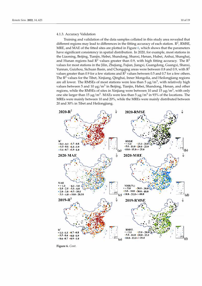
4.1.3. Accuracy Validation
Training and validation of the data samples collated in this study area revealed thatdifferent regions may lead to differences in the fitting accuracy of each station. R2, RMSE,MRE, and MAE of the fitted sites are plotted in Figure 6, which shows that the parametershave significant consistency in spatial distribution. In 2020, for example, most stations inthe Liaoning, Beijing, Tianjin, Hebei, Shandong, Shanxi, Henan, Hubei, Anhui, Shanghai,and Hunan regions had R2 values greater than 0.9, with high fitting accuracy. The R2
values for most stations in the Jilin, Zhejiang, Fujian, Jiangxi, Guangdong, Guangxi, Shanxi,Yunnan, Guizhou, Sichuan Basin, and Chongqing areas were between 0.8 and 0.9, with R2
values greater than 0.9 for a few stations and R2 values between 0.5 and 0.7 for a few others.The R2 values for the Tibet, Xinjiang, Qinghai, Inner Mongolia, and Heilongjiang regionsare all lower. The RMSEs of most stations were less than 5 µg/m3, with relatively highvalues between 5 and 10 µg/m3 in Beijing, Tianjin, Hebei, Shandong, Henan, and otherregions, while the RMSEs of sites in Xinjiang were between 10 and 15 µg/m3, with onlyone site larger than 15 µg/m3. MAEs were less than 5 µg/m3 in 93% of the locations. TheMREs were mainly between 10 and 20%, while the MREs were mainly distributed between20 and 30% in Tibet and Heilongjiang.
Remote Sens. 2022, 13, x FOR PEER REVIEW 10 of 19
Figure 5. Density scatter of CapsNet model training and validation. The blue and red lines indi-cate the fitted line and 1:1, respectively. (a), (c), and (e) are the training result density scatter in 2018-2020; (b), (d), and (f) are the validation result density scatter in 2018-2020. Y and X are esti-mated and Ground PM2.5, respectively.
4.1.3. Accuracy Validation Training and validation of the data samples collated in this study area revealed that
different regions may lead to differences in the fitting accuracy of each station. R2, RMSE, MRE, and MAE of the fitted sites are plotted in Figure 6, which shows that the parameters have significant consistency in spatial distribution. In 2020, for example, most stations in the Liaoning, Beijing, Tianjin, Hebei, Shandong, Shanxi, Henan, Hubei, Anhui, Shanghai, and Hunan regions had R2 values greater than 0.9, with high fitting accuracy. The R2 values for most stations in the Jilin, Zhejiang, Fujian, Jiangxi, Guang-dong, Guangxi, Shanxi, Yunnan, Guizhou, Sichuan Basin, and Chongqing areas were be-tween 0.8 and 0.9, with R2 values greater than 0.9 for a few stations and R2 values be-tween 0.5 and 0.7 for a few others. The R2 values for the Tibet, Xinjiang, Qinghai, Inner Mongolia, and Heilongjiang regions are all lower. The RMSEs of most stations were less than 5 μg/m3, with relatively high values between 5 and 10 μg/m3 in Beijing, Tianjin, He-bei, Shandong, Henan, and other regions, while the RMSEs of sites in Xinjiang were be-tween 10 and 15 μg/m3, with only one site larger than 15 μg/m3. MAEs were less than 5 μg/m3 in 93% of the locations. The MREs were mainly between 10 and 20%, while the MREs were mainly distributed between 20 and 30% in Tibet and Heilongjiang.
(a) (b)
(c) (d)
(e) (f)
Figure 6. Cont.
Remote Sens. 2022, 14, 623 11 of 19Remote Sens. 2022, 13, x FOR PEER REVIEW 11 of 19
(g) (h)
(i) (j)
(k) (l)
Figure 6. Spatial distribution of R2, root means square error (RMSE), mean relative error (MRE), and mean absolute error (MRE). (a)-(d), (e)-(h), and (i)-(l) represent in 2020, 2019, and 2018. There are 1475, 1478, and 1489 sites.
4.2. Model Comparison We used the DNN model to estimate the PM2.5 concentration to compare the ability
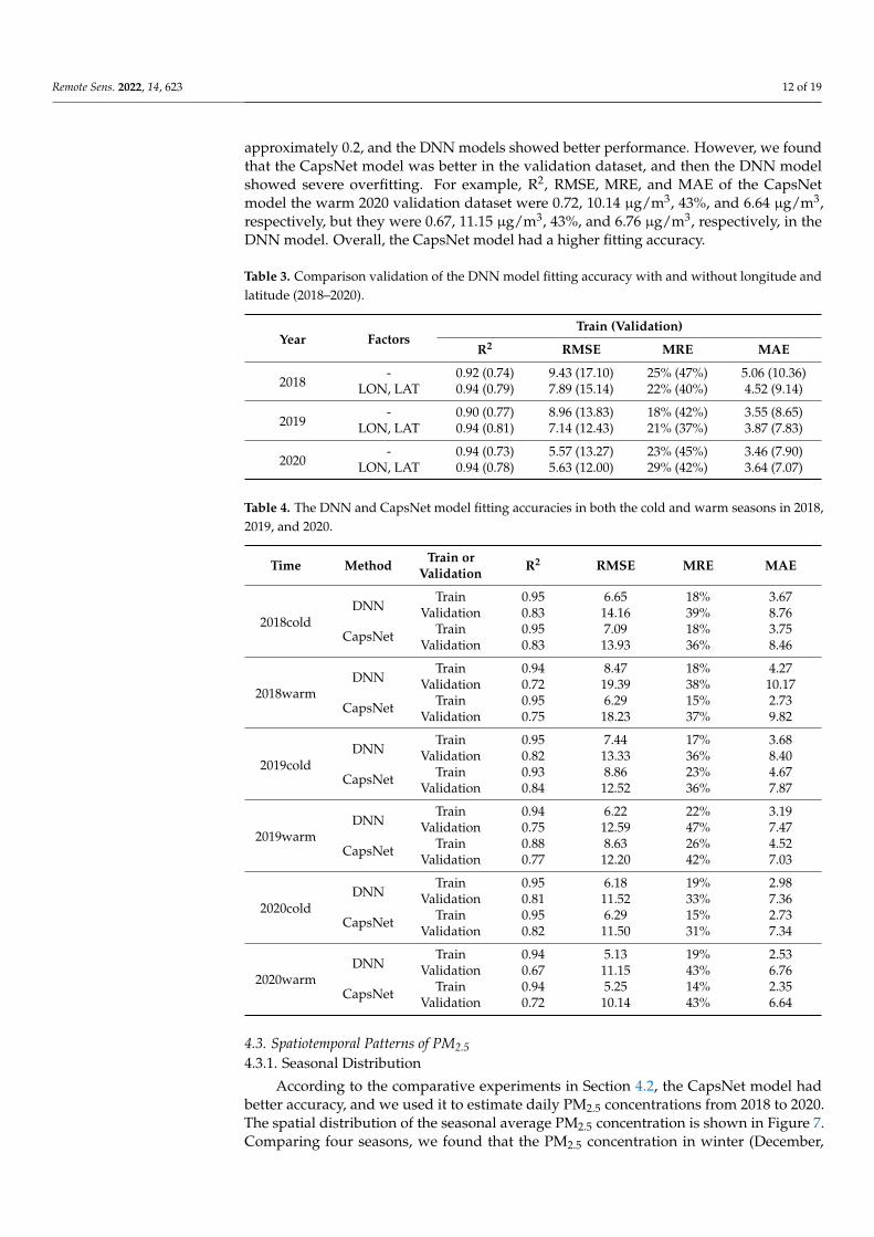
of the CapsNet model. We selected four hidden layers with the structure of 300-300-10-20; please refer to the study by Sun [16] for other detailed parameters. The same dataset as the CapsNet model was used for DNN. Table 3 shows the results of building the DNN model using the same dataset to assess the ability of the CapsNet model. The re-sults of using LON and LAT as input parameters in the DNN model were more accu-rate, especially in the validation dataset, similar to the findings of the CapsNet model. When comparing the DNN and CapsNet models, we found that the R2 values improved by 3%, 2%, and 6% from 2018 to 2020, respectively, when using the CapsNet model. The RMSEs decreased by 1.84, 1.40, and 1.02 μg/m3, respectively, in different years. The MREs and MAEs showed some reduction.
Table 3. Comparison validation of the DNN model fitting accuracy with and without longitude and latitude (2018–2020).
Year Factors Train (Validation)
R2 RMSE MRE MAE
2018 - 0.92(0.74) 9.43(17.10) 25% (47%) 5.06(10.36)
LON, LAT 0.94(0.79) 7.89(15.14) 22% (40%) 4.52(9.14)
Figure 6. Spatial distribution of R2, root means square error (RMSE), mean relative error (MRE), andmean absolute error (MRE). (a–d), (e–h), and (i–l) represent in 2020, 2019, and 2018. There are 1475,1478, and 1489 sites.
4.2. Model Comparison
We used the DNN model to estimate the PM2.5 concentration to compare the ability ofthe CapsNet model. We selected four hidden layers with the structure of 300-300-10-20;please refer to the study by Sun [16] for other detailed parameters. The same dataset asthe CapsNet model was used for DNN. Table 3 shows the results of building the DNNmodel using the same dataset to assess the ability of the CapsNet model. The results ofusing LON and LAT as input parameters in the DNN model were more accurate, especiallyin the validation dataset, similar to the findings of the CapsNet model. When comparingthe DNN and CapsNet models, we found that the R2 values improved by 3%, 2%, and 6%from 2018 to 2020, respectively, when using the CapsNet model. The RMSEs decreased by1.84, 1.40, and 1.02 µg/m3, respectively, in different years. The MREs and MAEs showedsome reduction.
To assess the fitting capacity of the two models in terms of seasons, the data weredivided into the cold season (January, February, and September–December) and warmseason (March–August), as shown in Table 4. Both the CapsNet and DNN models exhibitedhigher accuracy in the cold season than in the warm season, and the R2 values were0.83 ± 0.02 and 0.74 ± 0.03 in the validation dataset, respectively. The RMSEs, MAEs,and MREs also had large differences. When comparing the CapsNet and DNN modelson the training dataset in the cold and warm seasons, the difference in R2 values was
Remote Sens. 2022, 14, 623 12 of 19
approximately 0.2, and the DNN models showed better performance. However, we foundthat the CapsNet model was better in the validation dataset, and then the DNN modelshowed severe overfitting. For example, R2, RMSE, MRE, and MAE of the CapsNetmodel the warm 2020 validation dataset were 0.72, 10.14 µg/m3, 43%, and 6.64 µg/m3,respectively, but they were 0.67, 11.15 µg/m3, 43%, and 6.76 µg/m3, respectively, in theDNN model. Overall, the CapsNet model had a higher fitting accuracy.
Table 3. Comparison validation of the DNN model fitting accuracy with and without longitude andlatitude (2018–2020).
Year FactorsTrain (Validation)
R2 RMSE MRE MAE
2018- 0.92 (0.74) 9.43 (17.10) 25% (47%) 5.06 (10.36)
LON, LAT 0.94 (0.79) 7.89 (15.14) 22% (40%) 4.52 (9.14)
2019- 0.90 (0.77) 8.96 (13.83) 18% (42%) 3.55 (8.65)
LON, LAT 0.94 (0.81) 7.14 (12.43) 21% (37%) 3.87 (7.83)
2020- 0.94 (0.73) 5.57 (13.27) 23% (45%) 3.46 (7.90)
LON, LAT 0.94 (0.78) 5.63 (12.00) 29% (42%) 3.64 (7.07)
Table 4. The DNN and CapsNet model fitting accuracies in both the cold and warm seasons in 2018,2019, and 2020.
Time Method Train orValidation R2 RMSE MRE MAE
2018coldDNN
Train 0.95 6.65 18% 3.67Validation 0.83 14.16 39% 8.76
CapsNet Train 0.95 7.09 18% 3.75Validation 0.83 13.93 36% 8.46
2018warmDNN
Train 0.94 8.47 18% 4.27Validation 0.72 19.39 38% 10.17
CapsNet Train 0.95 6.29 15% 2.73Validation 0.75 18.23 37% 9.82
2019coldDNN
Train 0.95 7.44 17% 3.68Validation 0.82 13.33 36% 8.40
CapsNet Train 0.93 8.86 23% 4.67Validation 0.84 12.52 36% 7.87
2019warmDNN
Train 0.94 6.22 22% 3.19Validation 0.75 12.59 47% 7.47
CapsNet Train 0.88 8.63 26% 4.52Validation 0.77 12.20 42% 7.03
2020coldDNN
Train 0.95 6.18 19% 2.98Validation 0.81 11.52 33% 7.36
CapsNet Train 0.95 6.29 15% 2.73Validation 0.82 11.50 31% 7.34
2020warmDNN
Train 0.94 5.13 19% 2.53Validation 0.67 11.15 43% 6.76
CapsNet Train 0.94 5.25 14% 2.35Validation 0.72 10.14 43% 6.64
4.3. Spatiotemporal Patterns of PM2.54.3.1. Seasonal Distribution
According to the comparative experiments in Section 4.2, the CapsNet model hadbetter accuracy, and we used it to estimate daily PM2.5 concentrations from 2018 to 2020.The spatial distribution of the seasonal average PM2.5 concentration is shown in Figure 7.Comparing four seasons, we found that the PM2.5 concentration in winter (December,
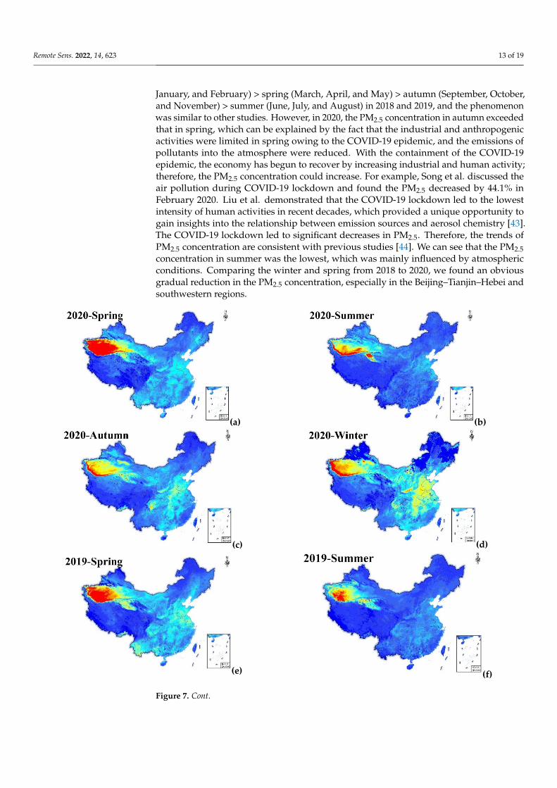
Remote Sens. 2022, 14, 623 13 of 19
January, and February) > spring (March, April, and May) > autumn (September, October,and November) > summer (June, July, and August) in 2018 and 2019, and the phenomenonwas similar to other studies. However, in 2020, the PM2.5 concentration in autumn exceededthat in spring, which can be explained by the fact that the industrial and anthropogenicactivities were limited in spring owing to the COVID-19 epidemic, and the emissions ofpollutants into the atmosphere were reduced. With the containment of the COVID-19epidemic, the economy has begun to recover by increasing industrial and human activity;therefore, the PM2.5 concentration could increase. For example, Song et al. discussed theair pollution during COVID-19 lockdown and found the PM2.5 decreased by 44.1% inFebruary 2020. Liu et al. demonstrated that the COVID-19 lockdown led to the lowestintensity of human activities in recent decades, which provided a unique opportunity togain insights into the relationship between emission sources and aerosol chemistry [43].The COVID-19 lockdown led to significant decreases in PM2.5. Therefore, the trends ofPM2.5 concentration are consistent with previous studies [44]. We can see that the PM2.5concentration in summer was the lowest, which was mainly influenced by atmosphericconditions. Comparing the winter and spring from 2018 to 2020, we found an obviousgradual reduction in the PM2.5 concentration, especially in the Beijing–Tianjin–Hebei andsouthwestern regions.
Remote Sens. 2022, 13, x FOR PEER REVIEW 13 of 19
According to the comparative experiments in Section 4.2, the CapsNet model had better accuracy, and we used it to estimate daily PM2.5 concentrations from 2018 to 2020. The spatial distribution of the seasonal average PM2.5 concentration is shown in Figure 7. Comparing four seasons, we found that the PM2.5 concentration in winter (December, January, and February) > spring (March, April, and May) > autumn (September, October, and November) > summer (June, July, and August) in 2018 and 2019, and the phenome-non was similar to other studies. However, in 2020, the PM2.5 concentration in autumn exceeded that in spring, which can be explained by the fact that the industrial and an-thropogenic activities were limited in spring owing to the COVID-19 epidemic, and the emissions of pollutants into the atmosphere were reduced. With the containment of the COVID-19 epidemic, the economy has begun to recover by increasing industrial and human activity; therefore, the PM2.5 concentration could increase. For example, Song et al. discussed the air pollution during COVID-19 lockdown and found the PM2.5 de-creased by 44.1% in February 2020. Liu et al. demonstrated that the COVID-19 lockdown led to the lowest intensity of human activities in recent decades, which provided a unique opportunity to gain insights into the relationship between emission sources and aerosol chemistry [43]. The COVID-19 lockdown led to significant decreases in PM2.5. Therefore, the trends of PM2.5 concentration are consistent with previous studies [44]. We can see that the PM2.5 concentration in summer was the lowest, which was mainly influ-enced by atmospheric conditions. Comparing the winter and spring from 2018 to 2020, we found an obvious gradual reduction in the PM2.5 concentration, especially in the Bei-jing–Tianjin–Hebei and southwestern regions.
(a) (b)
(c) (d)
(e) (f)
Figure 7. Cont.
Remote Sens. 2022, 14, 623 14 of 19Remote Sens. 2022, 13, x FOR PEER REVIEW 14 of 19
(g) (h)
(i) (j)
(k) (l)
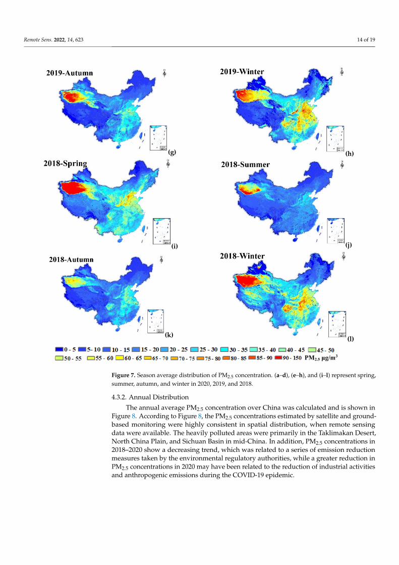
Figure 7. Season average distribution of PM2.5 concentration. (a)-(d), (e)-(h), and (i)-(l) represent spring, summer, autumn, and winter in 2020, 2019, and 2018.
4.3.2. Annual Distribution The annual average PM2.5 concentration over China was calculated and is shown in
Figure 8. According to Figure 8, the PM2.5 concentrations estimated by satellite and ground-based monitoring were highly consistent in spatial distribution, when remote sensing data were available. The heavily polluted areas were primarily in the Taklimakan Desert, North China Plain, and Sichuan Basin in mid-China. In addition, PM2.5 concentrations in 2018–2020 show a decreasing trend, which was related to a series of emission reduction measures taken by the environmental regulatory authorities, while a greater reduction in PM2.5 concentrations in 2020 may have been related to the reduction of industrial activities and anthropogenic emissions during the COVID-19 ep-idemic.
Figure 7. Season average distribution of PM2.5 concentration. (a–d), (e–h), and (i–l) represent spring,summer, autumn, and winter in 2020, 2019, and 2018.
4.3.2. Annual Distribution
The annual average PM2.5 concentration over China was calculated and is shown inFigure 8. According to Figure 8, the PM2.5 concentrations estimated by satellite and ground-based monitoring were highly consistent in spatial distribution, when remote sensingdata were available. The heavily polluted areas were primarily in the Taklimakan Desert,North China Plain, and Sichuan Basin in mid-China. In addition, PM2.5 concentrations in2018–2020 show a decreasing trend, which was related to a series of emission reductionmeasures taken by the environmental regulatory authorities, while a greater reduction inPM2.5 concentrations in 2020 may have been related to the reduction of industrial activitiesand anthropogenic emissions during the COVID-19 epidemic.
Remote Sens. 2022, 14, 623 15 of 19Remote Sens. 2022, 13, x FOR PEER REVIEW 15 of 19
(a) (b)
(c) (d)
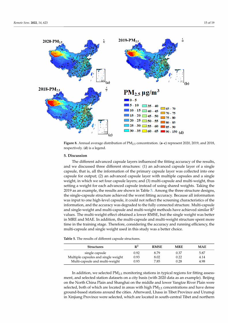
Figure 8. Annual average distribution of PM2.5 concentration. (a), (b), and (c) represent 2020, 2019, and 2018, respectively. (d) is a legend.
5. Discussion The different advanced capsule layers influenced the fitting accuracy of the results,
and we discussed three different structures: (1) an advanced capsule layer of a single capsule, that is, all the information of the primary capsule layer was collected into one capsule for output; (2) an advanced capsule layer with multiple capsules and a single weight, in which we set four capsule layers; and (3) multi-capsule and multi-weight, thus setting a weight for each advanced capsule instead of using shared weights. Taking the 2019 as an example, the results are shown in Table 5. Among the three structure de-signs, the single-capsule structure achieved the worst fitting accuracy. Because all in-formation was input to one high-level capsule, it could not reflect the screening charac-teristics of the information, and the accuracy was degraded to the fully connected struc-ture. Multi-capsule and single-weight and multi-capsule and multi-weight methods have achieved similar R2 values. The multi-weight effect obtained a lower RMSE, but the single weight was better in MRE and MAE. In addition, the multi-capsule and multi-weight structure spent more time in the training stage. Therefore, considering the accu-racy and running efficiency, the multi-capsule and single weight used in this study was a better choice.
Table 5. The results of different capsule structures.
Structures R2 RMSE MRE MAE single capsule 0.92 8.79 0.37 5.87
Multiple capsules and single weight 0.93 8.02 0.22 4.14 Multi-capsule and multi-weight 0.93 7.85 0.28 4.98
In addition, we selected PM2.5 monitoring stations in typical regions for fitting as-sessment, and selected station datasets on a city basis (with 2020 data as an example). Beijing on the North China Plain and Shanghai on the middle and lower Yangtze River Plain were selected, both of which are located in areas with high PM2.5 concentrations and have dense ground-based stations around the cities. Afterward, Lhasa in Tibet Prov-ince and Urumqi in Xinjiang Province were selected, which are located in south-central
Figure 8. Annual average distribution of PM2.5 concentration. (a–c) represent 2020, 2019, and 2018,respectively. (d) is a legend.
5. Discussion
The different advanced capsule layers influenced the fitting accuracy of the results,and we discussed three different structures: (1) an advanced capsule layer of a singlecapsule, that is, all the information of the primary capsule layer was collected into onecapsule for output; (2) an advanced capsule layer with multiple capsules and a singleweight, in which we set four capsule layers; and (3) multi-capsule and multi-weight, thussetting a weight for each advanced capsule instead of using shared weights. Taking the2019 as an example, the results are shown in Table 5. Among the three structure designs,the single-capsule structure achieved the worst fitting accuracy. Because all informationwas input to one high-level capsule, it could not reflect the screening characteristics of theinformation, and the accuracy was degraded to the fully connected structure. Multi-capsuleand single-weight and multi-capsule and multi-weight methods have achieved similar R2
values. The multi-weight effect obtained a lower RMSE, but the single weight was betterin MRE and MAE. In addition, the multi-capsule and multi-weight structure spent moretime in the training stage. Therefore, considering the accuracy and running efficiency, themulti-capsule and single weight used in this study was a better choice.
Table 5. The results of different capsule structures.
Structures R2 RMSE MRE MAE
single capsule 0.92 8.79 0.37 5.87Multiple capsules and single weight 0.93 8.02 0.22 4.14
Multi-capsule and multi-weight 0.93 7.85 0.28 4.98
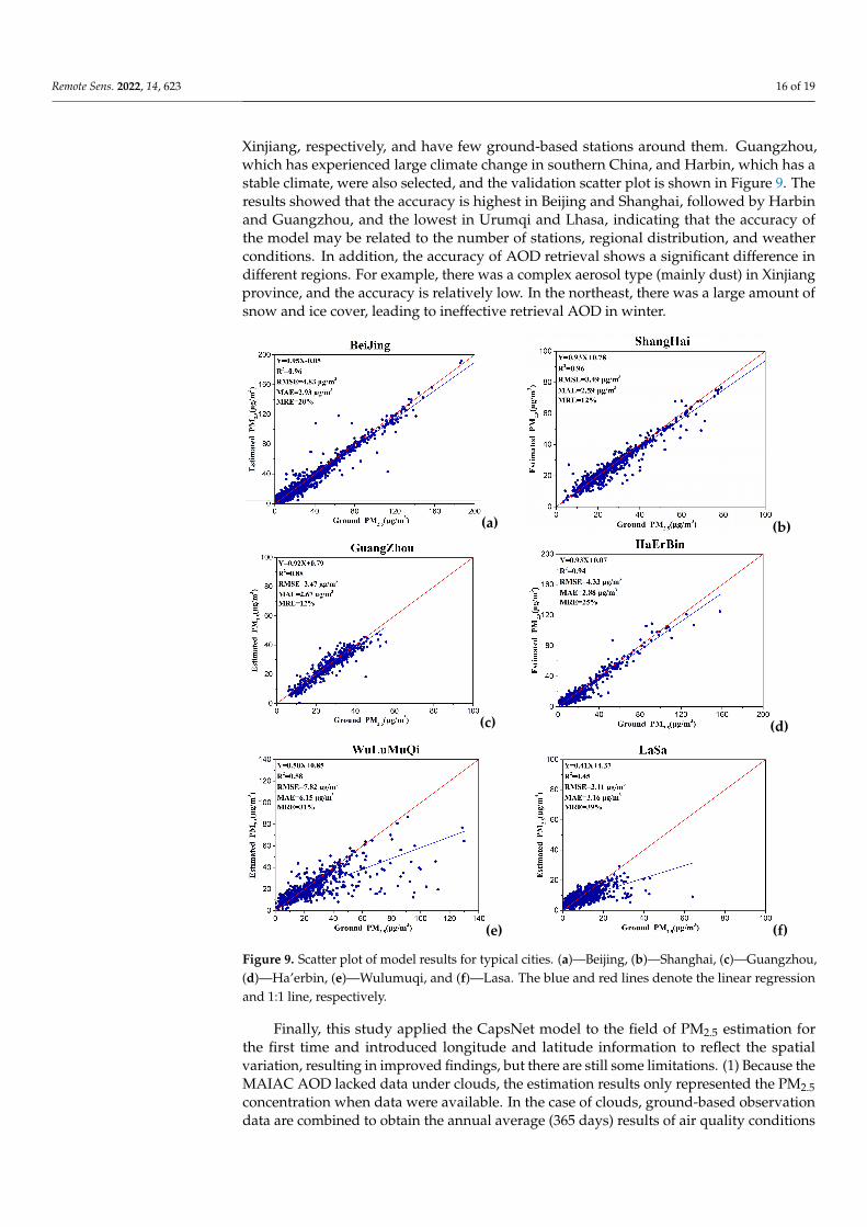
In addition, we selected PM2.5 monitoring stations in typical regions for fitting assess-ment, and selected station datasets on a city basis (with 2020 data as an example). Beijingon the North China Plain and Shanghai on the middle and lower Yangtze River Plain wereselected, both of which are located in areas with high PM2.5 concentrations and have denseground-based stations around the cities. Afterward, Lhasa in Tibet Province and Urumqiin Xinjiang Province were selected, which are located in south-central Tibet and northern
Remote Sens. 2022, 14, 623 16 of 19
Xinjiang, respectively, and have few ground-based stations around them. Guangzhou,which has experienced large climate change in southern China, and Harbin, which has astable climate, were also selected, and the validation scatter plot is shown in Figure 9. Theresults showed that the accuracy is highest in Beijing and Shanghai, followed by Harbinand Guangzhou, and the lowest in Urumqi and Lhasa, indicating that the accuracy ofthe model may be related to the number of stations, regional distribution, and weatherconditions. In addition, the accuracy of AOD retrieval shows a significant difference indifferent regions. For example, there was a complex aerosol type (mainly dust) in Xinjiangprovince, and the accuracy is relatively low. In the northeast, there was a large amount ofsnow and ice cover, leading to ineffective retrieval AOD in winter.
Remote Sens. 2022, 13, x FOR PEER REVIEW 16 of 19
Tibet and northern Xinjiang, respectively, and have few ground-based stations around them. Guangzhou, which has experienced large climate change in southern China, and Harbin, which has a stable climate, were also selected, and the validation scatter plot is shown in Figure 9. The results showed that the accuracy is highest in Beijing and Shang-hai, followed by Harbin and Guangzhou, and the lowest in Urumqi and Lhasa, indicat-ing that the accuracy of the model may be related to the number of stations, regional dis-tribution, and weather conditions. In addition, the accuracy of AOD retrieval shows a significant difference in different regions. For example, there was a complex aerosol type (mainly dust) in Xinjiang province, and the accuracy is relatively low. In the northeast, there was a large amount of snow and ice cover, leading to ineffective retrieval AOD in winter.
Finally, this study applied the CapsNet model to the field of PM2.5 estimation for the first time and introduced longitude and latitude information to reflect the spatial varia-tion, resulting in improved findings, but there are still some limitations. (1) Because the MAIAC AOD lacked data under clouds, the estimation results only represented the PM2.5 concentration when data were available. In the case of clouds, ground-based ob-servation data are combined to obtain the annual average (365 days) results of air quality conditions under clouds. (2) According to the Table 3, the accuracy of the CapsNet mod-el was different in 2018, 2019, and 2020, which may be affected by dataset quality. Be-sides, there were significant differences between the seasons according to the results of the models constructed in Table 4, and the specific influencing factors need to be inves-tigated further. (3) This study mainly considered the feasibility of the CapsNet model for estimating PM2.5 concentrations, and only obtained meteorological parameters and the NDVI to construct the model for comparison with the DNN. More factors affecting PM2.5 generation can be considered in future work.
(a) (b)
(c) (d)
Remote Sens. 2022, 13, x FOR PEER REVIEW 17 of 19
(e) (f)
Figure 9. Scatter plot of model results for typical cities. (a) -Beijing, (b) -Shanghai, (c) -Guangzhou, -Ha’erbin, (e) -Wulumuqi, and (f) -Lasa. The blue and red lines denote the linear regression and 1:1 line, respectively.
6. Conclusions In this study, we proposed a CapsNet model to estimate the daily PM2.5 concentra-
tions at a national scale from 2018 to 2020. The CapsNet model was applied to atmos-pheric research for the first time. First, we discussed whether introducing longitude and latitude information as input factors could improve the accuracy of both the CapsNet and DNN models. Compared with the DNN models with the same input parameters, the CapsNet model developed by us achieved the better validation performance. Next, we separately built CapsNet and DNN in the cold and warm seasons. The results indi-cated that the cold season had better fitting accuracy. The PM2.5 seasonal and annual dis-tributions were shown in 2018–2020, which presented that the PM2.5 concentration de-creased. We found that the PM2.5 concentration in autumn was beyond that in spring of 2020, which could have mainly been influenced by the COVID-19 epidemic. In addition, we found that there were some regional disparities in model accuracy, and the overall accuracy is higher. Not only can the CapsNet model suggested in this work be used to predict PM2.5 concentrations, but it can also be used to estimate other atmospheric com-ponents.
Author Contributions: Q.Z. proposed the method, collected data, and wrote this paper; T.X. trans-lated the manuscript; and S.Z., M.F., and L.C. revised the manuscript. Y.T. constructed the model and analyzed data. All authors have read and agreed to the published version of the manuscript.
Funding: This research was funded by the National Natural Science Foundation of China under Grant 41830109, the National Natural Science Foundation of China under Grant 42001315, the Na-tional Key Research and Development Program of China under Grant 2018YFC0214003, and Chongqing Meteorological Department Business Technology Project under Grant YWJSGG-202107.
Institutional Review Board Statement: Not applicable.
Informed Consent Statement: Not applicable.
Data Availability Statement: The datasets presented in this study can be found here: https://ladsweb.modaps.eosdis.nasa.gov/; http://www.ecmwf.int/; http://106.37.208.233:20035/.
Acknowledgments: All authors would sincerely thank the reviewers and editors for their benefi-cial, careful, and detailed comments and suggestions for improving the paper
Conflicts of Interest: The authors declare no conflict of interest.
References 1. Crouse, D.L.; Peters, P.A.; Donkelaar, A.V.; Goldberg, M.S.; Villeneuve, P.J.; Brion, O.; Khan, S.; Atari, D.O.; Jerrett, M.; Pope,
C.A.; et al. Risk of Nonaccidental and Cardiovascular Mortality in Relation to Long-term Exposure to Low Concentrations of Fine Particulate Matter: A Canadian National-Level Cohort Study. Environ. Health Perspect. 2012, 120, 708–714.
Figure 9. Scatter plot of model results for typical cities. (a)—Beijing, (b)—Shanghai, (c)—Guangzhou,(d)—Ha’erbin, (e)—Wulumuqi, and (f)—Lasa. The blue and red lines denote the linear regressionand 1:1 line, respectively.
Finally, this study applied the CapsNet model to the field of PM2.5 estimation forthe first time and introduced longitude and latitude information to reflect the spatialvariation, resulting in improved findings, but there are still some limitations. (1) Because theMAIAC AOD lacked data under clouds, the estimation results only represented the PM2.5concentration when data were available. In the case of clouds, ground-based observationdata are combined to obtain the annual average (365 days) results of air quality conditions
Remote Sens. 2022, 14, 623 17 of 19
under clouds. (2) According to the Table 3, the accuracy of the CapsNet model wasdifferent in 2018, 2019, and 2020, which may be affected by dataset quality. Besides, therewere significant differences between the seasons according to the results of the modelsconstructed in Table 4, and the specific influencing factors need to be investigated further.(3) This study mainly considered the feasibility of the CapsNet model for estimating PM2.5concentrations, and only obtained meteorological parameters and the NDVI to constructthe model for comparison with the DNN. More factors affecting PM2.5 generation can beconsidered in future work.
6. Conclusions
In this study, we proposed a CapsNet model to estimate the daily PM2.5 concentrationsat a national scale from 2018 to 2020. The CapsNet model was applied to atmosphericresearch for the first time. First, we discussed whether introducing longitude and latitudeinformation as input factors could improve the accuracy of both the CapsNet and DNNmodels. Compared with the DNN models with the same input parameters, the CapsNetmodel developed by us achieved the better validation performance. Next, we separatelybuilt CapsNet and DNN in the cold and warm seasons. The results indicated that the coldseason had better fitting accuracy. The PM2.5 seasonal and annual distributions were shownin 2018–2020, which presented that the PM2.5 concentration decreased. We found that thePM2.5 concentration in autumn was beyond that in spring of 2020, which could have mainlybeen influenced by the COVID-19 epidemic. In addition, we found that there were someregional disparities in model accuracy, and the overall accuracy is higher. Not only can theCapsNet model suggested in this work be used to predict PM2.5 concentrations, but it canalso be used to estimate other atmospheric components.
Author Contributions: Q.Z. proposed the method, collected data, and wrote this paper; T.X. trans-lated the manuscript; and S.Z., M.F. and L.C. revised the manuscript. Y.T. constructed the model andanalyzed data. All authors have read and agreed to the published version of the manuscript.
Funding: This research was funded by the National Natural Science Foundation of China under Grant41830109, the National Natural Science Foundation of China under Grant 42001315, the NationalKey Research and Development Program of China under Grant 2018YFC0214003, and ChongqingMeteorological Department Business Technology Project under Grant YWJSGG-202107.
Institutional Review Board Statement: Not applicable.
Informed Consent Statement: Not applicable.
Data Availability Statement: The datasets presented in this study can be found here: https://ladsweb.modaps.eosdis.nasa.gov/; http://www.ecmwf.int/; http://106.37.208.233:20035/.
Acknowledgments: All authors would sincerely thank the reviewers and editors for their beneficial,careful, and detailed comments and suggestions for improving the paper.
Conflicts of Interest: The authors declare no conflict of interest.
References1. Crouse, D.L.; Peters, P.A.; Donkelaar, A.V.; Goldberg, M.S.; Villeneuve, P.J.; Brion, O.; Khan, S.; Atari, D.O.; Jerrett, M.; Pope, C.A.;
et al. Risk of Nonaccidental and Cardiovascular Mortality in Relation to Long-term Exposure to Low Concentrations of FineParticulate Matter: A Canadian National-Level Cohort Study. Environ. Health Perspect. 2012, 120, 708–714. [CrossRef] [PubMed]
2. Chen, J.P.; Yin, J.H.; Zang, L.; Zhao, M.D. Stacking machine learning model for estimating hourly PM2.5 in China based onHimawari 8 aerosol optical depth data. Sci. Total Environ. 2019, 697, 134021. [CrossRef]
3. Wei, J.; Huang, W.; Li, Z.P.; Xue, Y.P.; Peng, Y.R.; Sun, L.; Cribb, M. Estimating 1-km-resolution PM2.5 concentrations across Chinausing the space-time random forest approach. Remote Sens. Environ. 2019, 231, 111221. [CrossRef]
4. Guo, B.; Zhang, D.M.; Pei, L.; Su, Y.; Wang, X.X.; Bian, Y.; Zhang, D.H.; Yao, W.Q.; Zhou, Z.X.; Guo, L.Y. Estimating PM2.5concentrations via random forest method using satellite, auxiliary, and ground-level station dataset at multiple temporal scalesacross China in 2017. Sci. Total Environ. 2021, 778, 146228. [CrossRef] [PubMed]
5. Liang, X.Y.; Zhang, S.J.; Wu, X.; Guo, X.; Han, L.; Liu, H.; Wu, Y.; Hao, J.M. Air quality and health impacts from using ethanolblended gasoline fuels in China. Atoms. Environ. 2020, 228, 117396. [CrossRef]
Remote Sens. 2022, 14, 623 18 of 19
6. Zhang, T.H.; Zhu, Z.M.; Gong, W.; Zhu, Z.R.; Sun, K.; Wang, L.C.; Huang, L.C.; Mao, X.F.; Shen, H.F.; Li, Z.W.; et al. Estimation ofultrahigh resolution PM2.5 concentrations in urban areas using 160m Gaofen-1 AOD retrievals. Remote Sens. Environ. 2018, 216,91–104. [CrossRef]
7. Hutchison, K.D.; Smith, S.; Faruqui, S.J. Correlating MODIS aerosol optical thickness data with ground-based PM2.5 observationsacross Texas for use in a real-time air quality prediction system. Atoms. Environ. 2005, 39, 7190–7203. [CrossRef]
8. Yao, F.; Si, M.; Li, W.; Wu, J. A multidimensional comparison between MODIS and VIIRS AOD in estimating ground-level PM2.5concentrations over a heavily polluted region in China. Sci. Total Environ. 2018, 618, 819–828. [CrossRef]
9. Sreekanth, V.; Mahesh, B.; Niranjan, K. Satellite Remote Sensing of Fine Particulate air pollutants over Indian Mega Cities. Adv.Space Res. 2017, 60, 2268–2276. [CrossRef]
10. Ma, Z.; Hu, X.; Sayer, A.M.; Levy, R.; Zhang, Q.; Xue, Y.; Tong, S.; Bi, J.; Huang, L.; Liu, Y. Satellite-Based Spatiotemporal Trends inPM2.5 Concentrations: China, 2004–2013. Environ. Health Perspect. 2016, 124, 184–192. [CrossRef]
11. Zhang, Y.; Li, Z. Remote sensing of atmospheric fine particulate matter (PM2.5) mass concentration near the ground from satelliteobservation. Remote Sens. Environ. 2015, 160, 252–262. [CrossRef]
12. Lee, H.J.; Liu, Y.; Coull, B.A.; Schwartz, J.; Koutrakis, P. A novel calibration approach of MODIS AOD data to predict PM2.5concentrations. Atmos. Chem. Phys. 2011, 11, 9769–9795. [CrossRef]
13. You, W.; Zang, Z.; Pan, X.; Zhang, L.; Chen, D. Estimating PM2.5 in Xi’an, China using aerosol optical depth: A comparisonbetween the MODIS and MISR retrieval models. Sci. Total Environ. 2015, 505, 1156–1165. [CrossRef] [PubMed]
14. Liu, Y.; Franklin, M.; Kahn, R.; Koutrakis, P. Using aerosol optical thickness to predict ground-level PM2.5 concentrations in the St.Louis area: A comparison between MISR and MODIS. Remote Sens. Environ. 2007, 107, 33–44. [CrossRef]
15. Liu, Y.; Paciorek, C.J.; Koutrakis, P. Estimating regional spatial and temporal variability of PM2.5 concentrations using satellitedata, meteorology, and land use information. Environ. Health Perspect. 2009, 117, 886. [CrossRef]
16. Zhang, X.; Hu, H. Improving Satellite-Driven PM2.5 Models with VIIRS Nighttime Light Data in the Beijing–Tianjin–HebeiRegion, China. Remote Sens. 2017, 9, 908. [CrossRef]
17. Wang, J.; Aegerter, C.; Xu, X.; Szykman, J.J. Potential application of VIIRS Day/Night Band for monitoring nighttime surfacePM2.5 air quality from space. Atmos. Environ. 2016, 124, 55–63. [CrossRef]
18. Wang, W.; Mao, F.; Du, L.; Pan, Z.; Gong, W.; Fang, S. Deriving Hourly PM2.5 Concentrations from Himawari-8 AODs overBeijing–Tianjin–Hebei in China. Remote Sens. 2017, 9, 858. [CrossRef]
19. Mao, F.Y.; Hong, J.; Min, Q.L.; Gong, W.; Zang, L.; Yin, J.H. Estimation hourly full-coverage PM2.5 over China base on TOAreflectance data from the Fengyun-4A satellite. Environ. Pollut. 2021, 270, 116119. [CrossRef]
20. Liu, Y.; Park, R.J.; Jacob, D.J.; Qinbin Li, Q.B.; Vasu Kilaru, K.; Sarnat, J. Mapping annual mean ground-level PM2.5 concentrationsusing Multiangle Imaging Spectroradiometer aerosol optical thickness over the contiguous United States. J. Geophys. Res. Atmos.2004, 109, D22206.
21. Donkelaar, A.V.; Martin, R.V.; Park, R.J. Estimating ground-level PM2.5 using aerosol optical depth determined from satelliteremote sensing. J. Geophys. Res. Atmos. 2006, 111, 5049–5066.
22. Wang, Z.F.; Chen, L.F.; Tao, J.H.; Zhang, Y.; Su, L. Satellite-based estimation of regional particulate matter (PM) in Beijing usingvertical-and-RH correcting method. Remote Sens. Environ. 2010, 114, 50–63. [CrossRef]
23. Guo, J.P.; Zhang, X.Y.; Che, H.Z.; Gong, S.L.; An, X.Q.; Cao, C.X.; Guang, J.; Zhang, H.; Wang, Y.Q.; Zhang, X.C.; et al. Correlationbetween concentrations and aerosol optical depth in eastern China. Atmos. Environ. 2009, 43, 5876–5886. [CrossRef]
24. Hu, X.; Waller, L.A.; Al-Hamdan, M.Z.; Crosson, W.L.; Estesjr, M.G.; Estes, S.M.; Quattrochi, D.A.; Sarnat, J.A.; Liu, Y. Estimatingground-level PM2.5 concentrations in the southeastern U.S. using geographically weighted regression. Environ. Res. 2013, 121,1–10. [CrossRef] [PubMed]
25. Guo, Y.X.; Tang, Q.H.; Gong, D.Y.; Zhang, Z.Y. Estimating ground-level PM2.5 concentrations in Beijing using a satellite-basedgeographically and temporally weighted regression model. Remote Sens. Environ. 2017, 198, 140–149. [CrossRef]
26. Liu, Y.; Sarnat, J.A.; Kilaru, V.; Jacob, D.J.; Koutrakis, P. Estimating ground-level PM2.5 in the eastern United States using satelliteremote sensing. Environ. Sci. Technol. 2005, 39, 3269. [CrossRef] [PubMed]
27. Koelemeijer, R.; Homan, C.D.; Matthijsen, J. Comparison of spatial and temporal variations of aerosol optical thickness andparticulate matter over Europe. Atoms. Environ. 2006, 40, 5304–5315. [CrossRef]
28. Chu, D.A.; Tsai, T.C.; Chen, J.P.; Cheng, S.C.; Jeng, Y.J.; Chiang, W.L.; Lin, N.H. Interpreting aerosol lidar profiles to better estimatesurface PM2.5 for columnar AOD measurements. Atoms. Environ. 2013, 79, 172–187. [CrossRef]
29. Lin, C.Q.; Li, Y.; Yuan, Z.B.; Lau, A.K.H.; Li, C.C.; Fung, J.C.H. Using satellite remote sensing data to estimate the high-resolutiondistribution of ground-level PM2.5. Remote Sens. Environ. 2015, 156, 117–128. [CrossRef]
30. Sun, Y.B.; Zeng, Q.L.; Geng, B.; Lin, X.W.; Sude, B.; Chenl, L.F. Deep learning architecture for estimating hourly ground-levelPM2.5 using satellite remote sensing. IEEE Geosci. Remote Sens. Lett. 2019, 16, 1343–1347. [CrossRef]
31. Li, L.F.; Franklin, M.; Girguis, M.; Lurmann, F.; Wu, J.; Pavlovic, N.; Breton, C.; Gilliland, F.; Habre, R. Spatiotemporal Imputationof MAIAC AOD Using Deep Learning with Downscaling. Remote Sens. Environ. 2020, 237, 111584. [CrossRef] [PubMed]
32. Shen, H.F.; Li, T.W.; Yuan, Q.Q.; Zhang, L.P. Estimating Regional Ground-Level PM2.5 Directly from Satellite Top-Of-AtmosphereReflectance Using Deep Belief Networks. J. Geophys. Res. Atmos. 2018, 123, 13875–13886. [CrossRef]
33. Hong, D.F.; Gao, L.R.; Yao, J.; Zhang, B.; Plaza, A.; Chanussot, J. Graph Convolutional Networks for Hyperspectral ImageClassification. IEEE Trans. Geosci. Remote Sens. 2021, 59, 5966–5978. [CrossRef]
Remote Sens. 2022, 14, 623 19 of 19
34. Hong, D.F.; Gao, L.R.; Yokoya, N.; Yao, J.; Chanussot, J.; Du, Q.; Zhang, B. More Diverse Means Better: Multimodal Deep LearningMeeets Remote-Sensing Imagery Classificaion. IEEE Trans. Geosci. Remote Sens. 2021, 59, 4340–4354. [CrossRef]
35. Sabour., S.; Frosst, N.; Hinton, G. Dynamic routing between capsules. In Proceedings of the Neural Information ProcessingSystems (NIPS Proceeding), Long Beach, CA, USA, 4–9 December 2017; pp. 3856–3866.
36. Afshar, P.; Mohammadi, A.; Plataniotis, K.N. Brain tumor type classification via capsule networks. In Proceedings of the 25thIEEE International Conference on Image Processing, Athens, Greece, 7–10 October 2018; pp. 3129–3133.
37. Levy, R.C.; Mattoo, S.; Munchak, L.A.; Remer, L.A.; Sayer, A.M.; Patadia, F.; Hsu, N.C. The Collection 6 MODIS aerosol productsover land and ocean. Atmos. Meas. Tech. 2013, 6, 2989–3034. [CrossRef]
38. Xie, Y.Y.; Wang, Y.X.; Zhang, K.; Dong, W.H.; Lv, B.; Bai, Y.Q. Daily estimation of ground-level PM2.5 concentrations over Beijingusing 3 km resolution MODIS AOD. Environ. Sci. Technol. 2015, 49, 12280–12288. [CrossRef] [PubMed]
39. Liu, N.; Zou, B.; Feng, H.H.; Wang, W.; Tang, Y.Q.; Liang, Y. Evaluation and comparison of multiangle implementation of theatmospheric correction algorithm, Dark Target, and Deep Blue aerosol products over China. Atmos. Chem. Phys. 2019, 19,8243–8268. [CrossRef]
40. Lyapustin, A.; Wang, Y.; Laszlo, I.; Kahn, R.; Korkin, S.; Remer, L.; Levy, R.; Reid, J.S. Multiangle implementation of atmosphericcorrection (MAIAC): 2. Aerosol algorithm. J. Geophys. Res. Atmos. 2011, 116, 1–15. [CrossRef]
41. Tao, M.H.; Wang, J.; Li, R.; Wang, L.L.; Wang, L.C.; Wang, Z.F.; Tao, J.H.; Chen, H.Z.; Chen, L.F. Performance of MODIShigh-resolution MAIAC aerosol algorithm in China: Characterization and limitation. Atmos. Environ. 2019, 213, 159–169.[CrossRef]
42. Zhi, X.; Xu, H.M. Comparative analysis of free atmospheric temperature between three reanalysis datasets and radiosonde datasetin China: Annual mean characteristic. Trans. Atmos. Sci. 2013, 36, 77–87.
43. Song, Z.G.; Bai, Y.; Wang, D.F.; Li, T.; He, X.Q. Satellite Retrieval of Air Pollution Changes in Central and Eastern China duringCOVID-19 Lockdown Based on a Machine Learning Model. Remote Sens. 2021, 13, 2525. [CrossRef]
44. Liu, L.; Zhang, J.; Du, R.G.; Teng, X.M.; Hu, R.; Yuan, Q.; Tang, S.S.; Ren, C.H.; Huang, X.; Xu, L.; et al. Chemistry of atmosphericfine particles during the COVID-19 pandemic in a megacity of Eastern China. Geophys. Res. Lett. 2021, 48, 2020GL091611.[CrossRef] [PubMed]


