Evolutionary time–frequency distributions usingBayesian regularised neural network model

I. Shafi, J. Ahmad, S.I. Shah and F.M. Kashif

Abstract: Time–frequency distributions (TFDs) that are highly concentrated in the time–frequencyplane are computed using a Bayesian regularised neural network model. The degree of regularisationis automatically controlled in the Bayesian inference framework and produces networks with bettergeneralised performance and lower susceptibility to over-fitting. Spectrograms and Wigner trans-forms of various known signals form the training set. Simulation results show that regularisation,with input training under Mackay’s evidence framework, produces results that are highlyconcentrated along the instantaneous frequencies of the individual components present in the testTFDs. Various parameters are compared to establish the effectiveness of the approach.

1 Introduction

Time-varying spectral representations have been provenuseful in a wide variety of applications. There are manyapproaches to time–frequency spectral analysis [1–6].Time–frequency distributions (TFDs) are two-dimensionalfunctions that indicate the time-varying frequency contentof one-dimensional signals. The instantaneous frequency(IF) describes the changing spectral structure of a time-varying signal. Energy concentration along the IF is desir-able in TFDs to correctly interpret the fundamental natureof signals under analysis in time–frequency coordinates.Two of the popular tools used for the study of the changingspectral content of signals are the spectrogram and WignerVille distribution (WVD) [1]. Both the spectrogram and theWVD belong to the general class of bilinear distributions(BDs).

It has been shown that the BDs including the spectrogramresult in a blurred version of the true TFD [1, 7].Spectrograms suffer from the windowing effect resulting ina tradeoff between the time and frequency resolutions. ATFD with reduced blurring effect may be obtained bycombining spectrograms or computing spectrogram with anadaptive window; however in either case, blurring is notfully removed [1]. The WVD is qualitatively different fromthe spectrogram. It produces ideal concentration along theIF for a linear frequency modulated signal but for multi-component signals it results in cross terms [1]. Moreover ifthe signal’s frequency has nonlinear variations then WVDdoes not produce the ideal concentration along the IF.

Several methods have been proposed to computede-blurred TFDs [2, 3, 7–14]. Gabor representationbased on a non-rectangular tiling of the time–frequency

# The Institution of Engineering and Technology 2007

doi:10.1049/iet-spr:20060311

Paper first received 4th October 2006 and in revised form 22nd February 2007

I. Shafi is with the Center for Advanced Studies in Engineering (C@SE), 19-Ataturk Avenue, G-5/1, Islambad, Pakistan

J. Ahmad and S.I. Shah are with Iqra University, Islamabad Campus, Sector H-9, Islamabad, Pakistan

F.M. Kashif is with the Laboratory for Electromagnetic and Electronic Systems(LEES), Massachusetts Institute of Technology, Cambridge MA 02139, USA

E-mail: imran.shafi@gmail.com

IET Signal Process., 2007, 1, (2), pp. 97–106

plane has been used to improve the time and frequency res-olutions of evolutionary spectra [2]. Another methodmakes use of adaptation by estimating the IF of thesignal components present in the signal from an initialevolutionary spectrum by using masks along the differentcomponents present in the signal [3]. In [8], the authorsproposed the use of informative estimation to computeTFDs by the method of minimum cross entropy thatsatisfies the marginals [1]. However the result greatlydepends on the initial estimate used. An interestingapproach has been to use image processing techniques toestimate the IF that include a piece-wise linear approxi-mation of the IF using Hough transform (used in imageprocessing to infer the presence of lines or curves in animage) and the evolutionary spectrum [9]. The efficiencyand practicality of this approach lie in localised proces-sing, linearisation of the IF estimate, recursive correc-tion and minimum problems because of cross terms inthe TFDs or in the matching of parametric models.Barbarossa in [10] proposed the combination of WVDand Hough transform for detection and parameter esti-mation of chirp signals to a problem of detection of linesin an image, which is the WVD of the signal under analy-sis. This method provides a bridge between signal andimage processing techniques, has been found asymptoti-cally efficient, and offers a good rejection capability ofthe cross terms, but has an increased computational com-plexity. Another development in this area has been tofilter out different portions of the signal using a time-varying filter, compute the TFD of the individual com-ponents and then combine these individual TFDs toobtain the combined TFD of the signal [14]. However,this requires the knowledge of the components present inthe signal. In yet another appproach, the aim is to designthe TFD along the IFs of the individual componentspresent in the signal using the pseudo-quantum signalrepresentation [13]. However, this also requires someprior knowledge of the components present in the signal.In all the approaches, the main aim has been to obtain aTFD, Q(n, v), that is free of undesired cross componentsand highly concentrated along the IFs of the individualcomponents present in the signal.

The approach used takes advantage of the artificial neuralnetwork (ANN) learning capabilities to estimate de-blurred

97

TFDs of different signals. We consider the removal of dis-tortions in the TFDs as a case of image de-blurring. This isparticularly suited for learning [15] by ANNs because offollowing reasons [16]:

(i) There is little information available on the source ofblurring.(ii) Usually blurring is the result of combination of events,which makes it too complex to be mathematicallydescribed.(iii) Sufficient data are available and it is conceivable thatdata capture the fundamental principle at work.

The method fundamentally involves training a set of suit-ably chosen ANN with spectrograms of known signals asthe input, and processed WVD as the target. Judiciouslyselected signals having time-varying frequency componentsare employed for the training purposes and the trained ANNmodel then provides the de-blurred TFDs from spectro-grams of unknown signals. The objectives of this work are:

(i) To explore the effectiveness of the Bayesian regularisedneural network model (BRNNM) for the application.(ii) To compute informative and de-blurred TFDs of signalswhose frequency components vary with time withoutassuming any prior knowledge about the componentspresent in the signal.

2 Proposed model

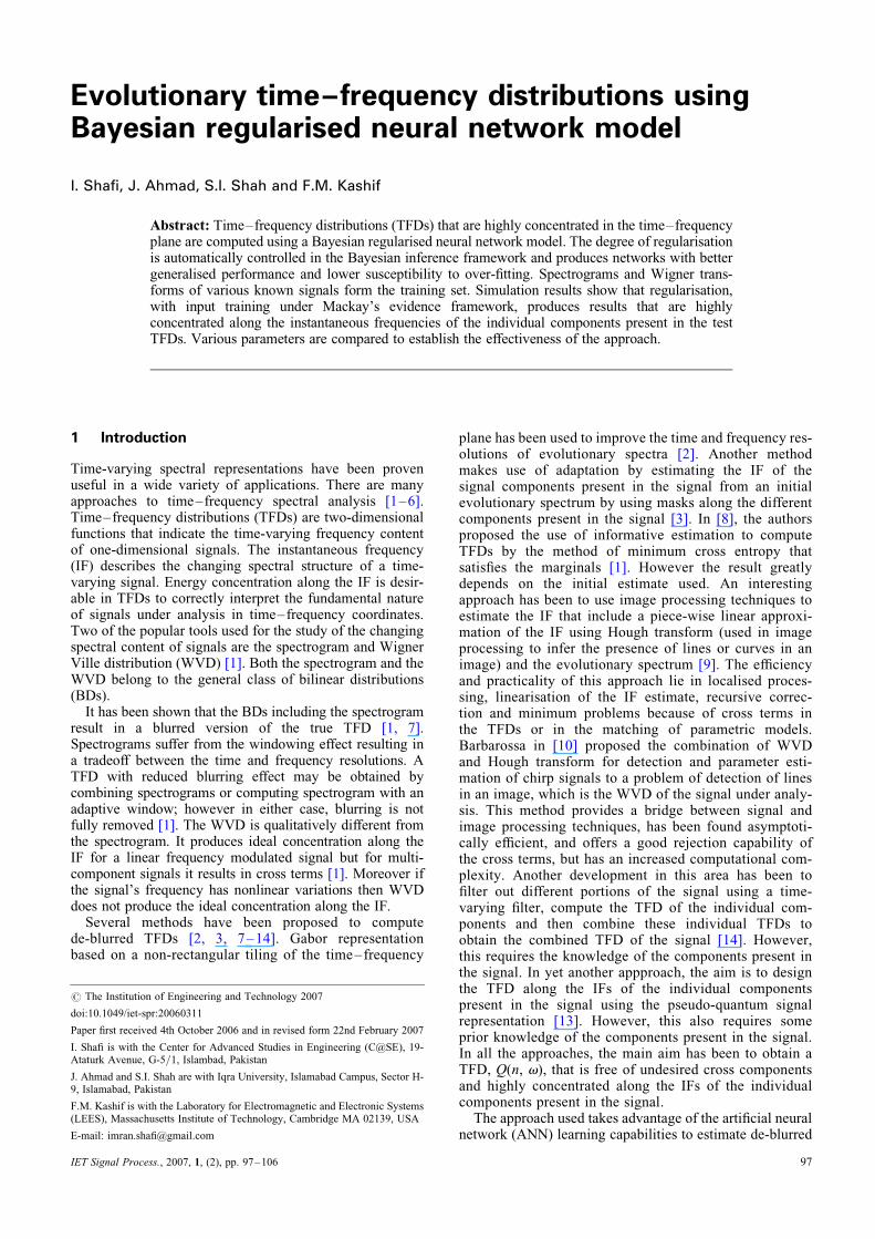
Fig. 1 is the block form representation of the proposedmethod. The proposed method consists of three majormodules: (i) pre-processing of training data, (ii) processingthrough the BRNNM, and (iii) post-processing of outputdata. These major modules are further elaborated inFigs. 2–4. They are discussed in the following subsections.

2.1 Pre-processing of training data

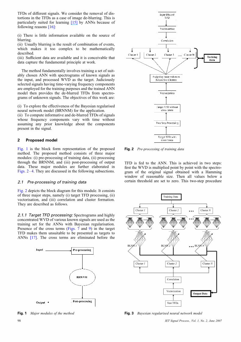
Fig. 2 depicts the block diagram for this module. It consistsof three major steps, namely (i) target TFD processing, (ii)vectorisation, and (iii) correlation and cluster formation.They are described as follows.

2.1.1 Target TFD processing: Spectrograms and highlyconcentrated WVD of various known signals are used as thetraining set for the ANNs with Bayesian regularisation.Presence of the cross terms (Figs. 7 and 9) in the targetTFD makes them unsuitable to be presented as targets toANNs [17]. The cross terms are eliminated before the

Fig. 1 Major modules of the method

98

TFD is fed to the ANN. This is achieved in two steps:first the WVD is multiplied point by point with the spectro-gram of the original signal obtained with a Hammingwindow of reasonable size. Then all values below acertain threshold are set to zero. This two-step procedure

Fig. 2 Pre-processing of training data

Fig. 3 Bayesian regularised neural network model

IET Signal Process., Vol. 1, No. 2, June 2007

is termed as pre-processing of the target data. The resultanttarget TFDs are depicted in Figs. 8 and 10 for the two train-ing signals.

2.1.2 Vectorisation: The input and target TFDs are thenconverted to vectors of a particular length. This procedureis repeated for both the inputs presented in Figs. 5 and 6and the target TFDs depicted in Figs. 8 and 10. Inputvectors of specified length from the input TFD and themean values of vectors of the same length from the corre-sponding region of the concentrated target TFD are accumu-lated in different vector spaces to be used in the subsequenttraining phase.

2.1.3 Correlation and cluster formation: Vectors ofthe input TFD are clustered according to certain underlying

Fig. 4 Post-processing of the output data

Fig. 5 Input spectrogram of parallel chirps used for training ofBRNNM

IET Signal Process., Vol. 1, No. 2, June 2007

features. The objective is to divide the input vector spaceinto number of sub-spaces described by directional unitvectors (vn). In our case, vn are intuitively three directionalvectors, used to characterise three types of edges (ascend-ing, descending, triangular) in the TFD image. We consideredges because they are important characteristics and blur-ring mostly causes loss of edge information [7]. Thechoice of number and directions of vectors remains depen-dent and is dictated by the problem at hand.

Each vector is correlated with all types of directionalvectors by taking their inner product. Respectively, avector is declared of a particular type with which it givesthe maximum value of inner product. The process of corre-lation divides the input space into various clusters. The aimof clustering is to detect the underlying structure in data, notonly for classification and pattern recognition, but also formodel reduction and optimisation. Clustering is importantbecause of the following reasons.

(i) It is believed that different parts of the cerebral cortexare designated to perform different tasks [15]. The natureof the task imposes certain structure on the region. Thus,there is a structure-function correspondence in the brain.Furthermore, it has been theorised that different regions

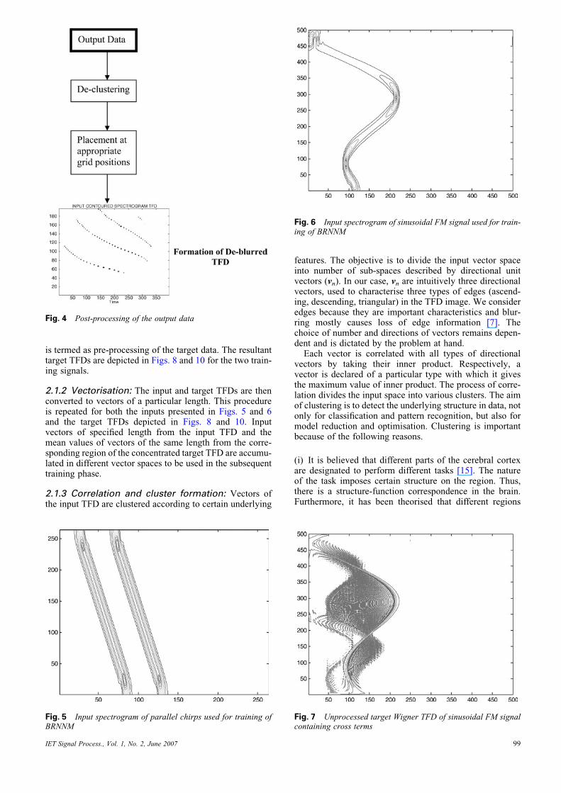
Fig. 6 Input spectrogram of sinusoidal FM signal used for train-ing of BRNNM

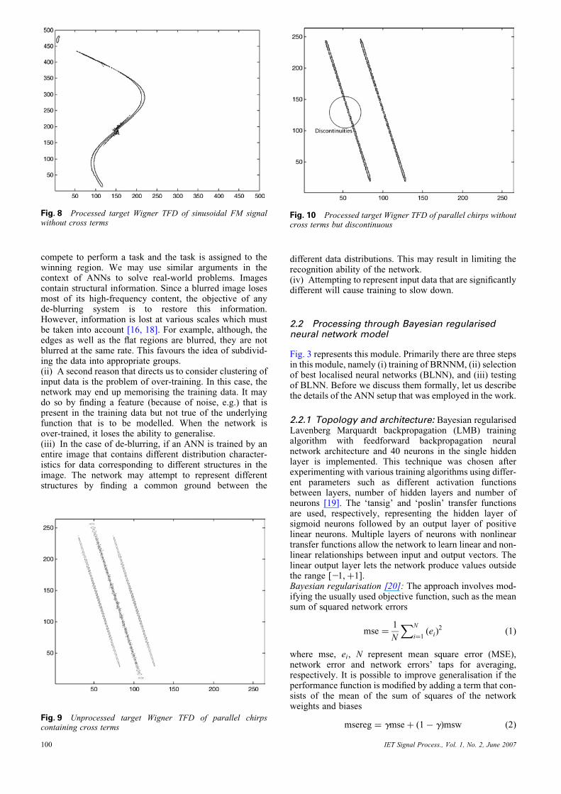
Fig. 7 Unprocessed target Wigner TFD of sinusoidal FM signalcontaining cross terms

99

compete to perform a task and the task is assigned to thewinning region. We may use similar arguments in thecontext of ANNs to solve real-world problems. Imagescontain structural information. Since a blurred image losesmost of its high-frequency content, the objective of anyde-blurring system is to restore this information.However, information is lost at various scales which mustbe taken into account [16, 18]. For example, although, theedges as well as the flat regions are blurred, they are notblurred at the same rate. This favours the idea of subdivid-ing the data into appropriate groups.(ii) A second reason that directs us to consider clustering ofinput data is the problem of over-training. In this case, thenetwork may end up memorising the training data. It maydo so by finding a feature (because of noise, e.g.) that ispresent in the training data but not true of the underlyingfunction that is to be modelled. When the network isover-trained, it loses the ability to generalise.(iii) In the case of de-blurring, if an ANN is trained by anentire image that contains different distribution character-istics for data corresponding to different structures in theimage. The network may attempt to represent differentstructures by finding a common ground between the

Fig. 9 Unprocessed target Wigner TFD of parallel chirpscontaining cross terms

Fig. 8 Processed target Wigner TFD of sinusoidal FM signalwithout cross terms

100

different data distributions. This may result in limiting therecognition ability of the network.(iv) Attempting to represent input data that are significantlydifferent will cause training to slow down.

2.2 Processing through Bayesian regularisedneural network model

Fig. 3 represents this module. Primarily there are three stepsin this module, namely (i) training of BRNNM, (ii) selectionof best localised neural networks (BLNN), and (iii) testingof BLNN. Before we discuss them formally, let us describethe details of the ANN setup that was employed in the work.

2.2.1 Topology and architecture: Bayesian regularisedLavenberg Marquardt backpropagation (LMB) trainingalgorithm with feedforward backpropagation neuralnetwork architecture and 40 neurons in the single hiddenlayer is implemented. This technique was chosen afterexperimenting with various training algorithms using differ-ent parameters such as different activation functionsbetween layers, number of hidden layers and number ofneurons [19]. The ‘tansig’ and ‘poslin’ transfer functionsare used, respectively, representing the hidden layer ofsigmoid neurons followed by an output layer of positivelinear neurons. Multiple layers of neurons with nonlineartransfer functions allow the network to learn linear and non-linear relationships between input and output vectors. Thelinear output layer lets the network produce values outsidethe range [21, þ1].Bayesian regularisation [20]: The approach involves mod-ifying the usually used objective function, such as the meansum of squared network errors

mse ¼1

N

XN

i¼1(ei)

2 (1)

where mse, ei, N represent mean square error (MSE),network error and network errors’ taps for averaging,respectively. It is possible to improve generalisation if theperformance function is modified by adding a term that con-sists of the mean of the sum of squares of the networkweights and biases

msereg ¼ gmse þ (1 � g)msw (2)

Fig. 10 Processed target Wigner TFD of parallel chirps withoutcross terms but discontinuous

IET Signal Process., Vol. 1, No. 2, June 2007

where g, msereg, msw are the performance ratio, perform-ance function and mean of the sum of squares of networkweights and biases, respectively. msw is mathematicallydescribed as

msw ¼1

n

Xn

j¼1w

2j (3)

Using this performance function causes the network to havesmaller weights and biases, and this force the networkresponse to be smoother and less likely to over-fit.Moreover, it is desirable to determine the optimal regularis-ation parameters in an automated fashion. One approach tothis process is the Bayesian framework of David Mackay[20]. In this framework, the weights and biases of thenetwork are assumed to be random variables with specifieddistributions. The regularisation parameters are related tothe unknown variances associated with these distributions.Statistical techniques can then be used to estimate theseparameters.Learning by LMB training algorithm [15, 21]: The LMBalgorithm is a variation of Newton’s method [15] that wasdesigned for minimising functions that are sums ofsquares of other nonlinear functions. This is very wellsuited to ANN training where the performance index isthe mean squared error. Newton’s method approximates tothe Gauss–Newton method and after a number ofsubstitutions transforms to the LMB algorithm

xkþ1 ¼ xk � [=T(xk)=(xk)mkI]�1=

T(xk)n(xk) (4)

where x, =(x), v, I and mk are learning vectors, Jacobianmatrix, nonlinear functions, identity matrix and step size,respectively. This algorithm has the very useful featurethat as mk is increased it approaches the steepest descentalgorithm with small learning rate

xkþ1 ’ xk �1

mk

=T(xk)n(xk)

¼ xk �1

2mkrF(x), for large mk (5)

whereas as mk is decreased to zero the algorithm becomesGauss–Newton. Here we assume that F(x) is a sum ofsquares function

F(x) ¼ yT(x)y(x) (6)

The algorithm begins with mk set to some small value(e.g. mk ¼ 0.01). If a step does not yield a smaller valuefor F(x), then the step is repeated with mk multiplied bysome factor h . 1 (e.g. h ¼ 10). Eventually F(x) shoulddecrease, since we would be taking a small step in the direc-tion of steepest descent. If a step does reduce a smaller valuefor F(x), then is divided by h for the next step, so that thealgorithm will approach Gauss–Newton, which shouldprovide faster convergence. The algorithm provides a nicecompromise between the speed of Newton’s method andthe guaranteed convergence of steepest descent.

Now we shall describe the steps involved in secondmodule.

2.2.2 Description of the module: As described earlierin the text, the three primary steps obvious from Fig. 3are (i) training of BRNNM, (ii) selection of BLNN and(iii) testing through BLNN. The details are as follows.Training of BRNNM: We train multiple ANNs for eachgroup of vectors in a cluster. For each cluster from the pre-vious module, three networks are trained by LMB training

IET Signal Process., Vol. 1, No. 2, June 2007

algorithm incorporating the Bayesian regularisation. Usingmultiple networks is found to be advantageous becausethe weights are initialised to random values and when thenetwork begins to over-fit the data, the error in the vali-dation set typically begins to rise. If this happens for a speci-fied number of iterations, the training is stopped, and theweights and biases at the minimum of the validation errorare obtained.Selection of BLNN. By keeping track of the network error orperformance, accessible via the training record, the bestnetwork is selected for each cluster. The training record isa defined structure in which the training algorithm savesthe performance of the training-set, test-set, validation-set,the epoch number and the learning rate. The trainingrecord makes it possible to plot the performance graphduring the training as well as to obtain the best networksbased on the network performance on the validation-set.In this way, we obtain the BLNN that includes the special-ised networks for each type of vector with better generalis-ation abilities. This also eliminates forcing one network tolearn input patterns that are distant from each other [9].Testing through BLNN: Test TFDs are also subjected tovectorisation. Vectors are correlated with the same direc-tional vectors, resulting in various clusters. Various typesof vectors thus obtained from test TFDs are fed to BLNN.

2.3 Post-processing of the output data

This module is illustrated in Fig. 4. In the first module, wedivided a complex computational task into a set of lesscomplex tasks. These less complex tasks were handled inmodule two. The solutions of these are combined at thisstage to produce the solution to the original problem.Various types of vectors obtained from test TFDs accordingto the above-mentioned procedure are fed to the BLNN andthe resultant vectors are subjected to post-processing whichincludes de-clustering and constituting resultant TFD fromthe output vectors, by placing them at appropriate gridpositions.

3 Training and test set of signals for BRNNM

3.1 Training set

To train the BRNNM, the spectrograms of following twosignals are used as input to the BRNNM.

3.1.1 Sinusoidal frequency modulated (FM)signals: The first training signal is a sinusoidal frequencymodulated (FM) signal. It is given by

x(n) ¼ e jp 12�v nð Þnð Þ (7)

where v(n) ¼ 0.1sin(2pn/N ), N is the number of samplepoints. The spectrogram of this signal is depicted inFig. 6. The respective target TFD, obtained throughWVD, is depicted in Fig. 8.

3.1.2 Parallel chirps signal: The second signal is onewith two parallel chirps given by

Y (n) ¼ x1(n) þ x2(n) (8)

where

x1ðnÞ ¼ ejv1ðnÞn with v1ðnÞ ¼ pn=4N

101

and

x2ðnÞ ¼ e jv2 ðnÞn with v2 nð Þ ¼

p

3þ

pn

4N

where N represents the total number of points in the signal.The spectrogram of this signal is depicted in Fig. 5. Therespective target TFD, obtained through WVD, is depictedin Fig. 10.

3.2 Examples taken as test set

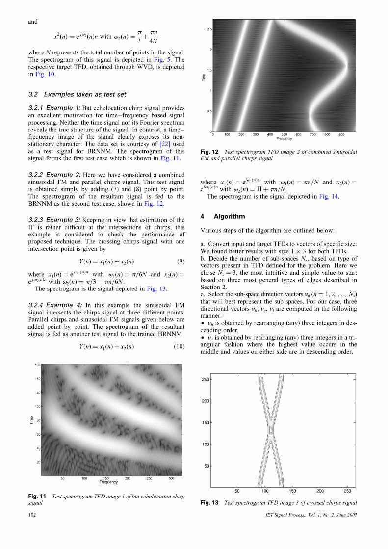
3.2.1 Example 1: Bat echolocation chirp signal providesan excellent motivation for time–frequency based signalprocessing. Neither the time signal nor its Fourier spectrumreveals the true structure of the signal. In contrast, a time–frequency image of the signal clearly exposes its non-stationary character. The data set is courtesy of [22] usedas a test signal for BRNNM. The spectrogram of thissignal forms the first test case which is shown in Fig. 11.

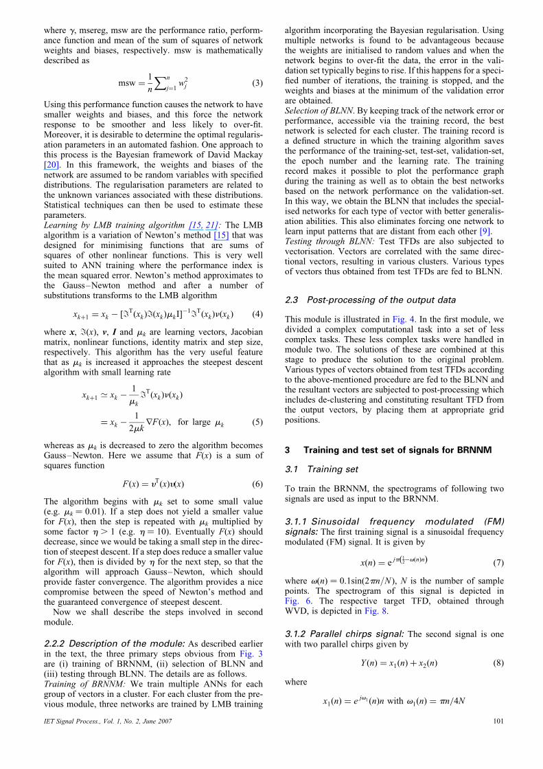
3.2.2 Example 2: Here we have considered a combinedsinusoidal FM and parallel chirps signal. This test signalis obtained simply by adding (7) and (8) point by point.The spectrogram of the resultant signal is fed to theBRNNM as the second test case, shown in Fig. 12.

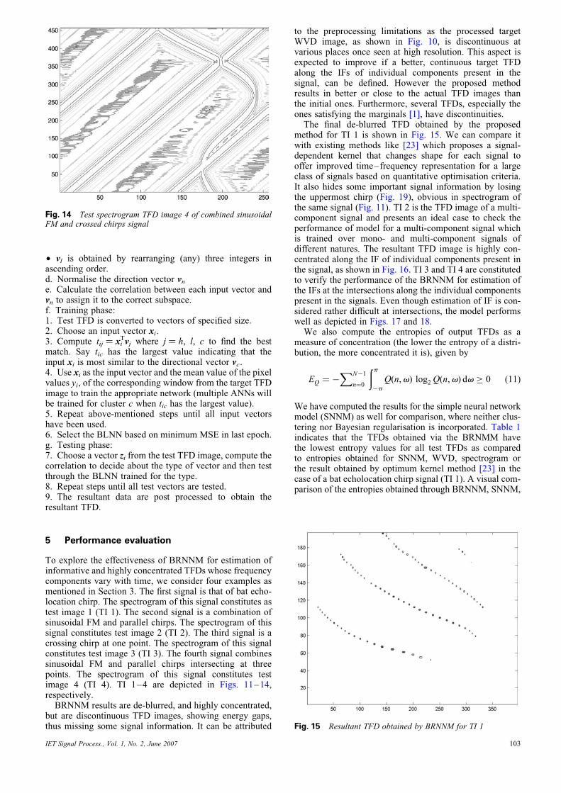
3.2.3 Example 3: Keeping in view that estimation of theIF is rather difficult at the intersections of chirps, thisexample is considered to check the performance ofproposed technique. The crossing chirps signal with oneintersection point is given by

Y (n) ¼ x1(n) þ x2(n) (9)

where x1(n) ¼ e jv1(n)n with v1(n) ¼ p/6N and x2(n) ¼e jv2(n)n with v2(n) ¼ p=3 � pn=6N .

The spectrogram is the signal depicted in Fig. 13.

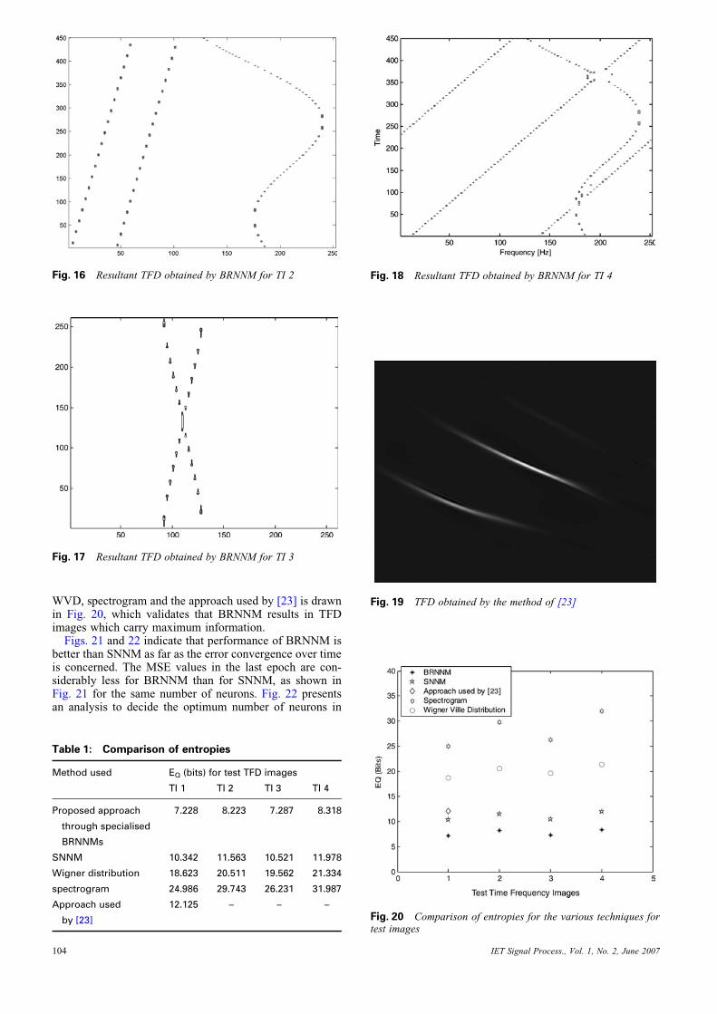
3.2.4 Example 4: In this example the sinusoidal FMsignal intersects the chirps signal at three different points.Parallel chirps and sinusoidal FM signals given below areadded point by point. The spectrogram of the resultantsignal is fed as another test signal to the trained BRNNM

Y (n) ¼ x1(n) þ x2(n) (10)

Fig. 11 Test spectrogram TFD image 1 of bat echolocation chirpsignal

102

where x1(n) ¼ ejv1(n)n with v1(n) ¼ pn/N and x2(n) ¼ejv2(n)n with v2(n) ¼ Pþ pn=N .

The spectrogram is the signal depicted in Fig. 14.

4 Algorithm

Various steps of the algorithm are outlined below:

a. Convert input and target TFDs to vectors of specific size.We found better results with size 1 � 3 for both TFDs.b. Decide the number of sub-spaces Ns, based on type ofvectors present in TFD defined for the problem. Here wechose Ns ¼ 3, the most intuitive and simple value to startbased on three most general types of edges described inSection 2.c. Select the sub-space direction vectors vn (n ¼ 1, 2, . . . ,Ns)that will best represent the sub-spaces. For our case, threedirectional vectors vh, vc, vl are computed in the followingmanner:† vh is obtained by rearranging (any) three integers in des-cending order.† vc is obtained by rearranging (any) three integers in a tri-angular fashion where the highest value occurs in themiddle and values on either side are in descending order.

Fig. 12 Test spectrogram TFD image 2 of combined sinusoidalFM and parallel chirps signal

Fig. 13 Test spectrogram TFD image 3 of crossed chirps signal

IET Signal Process., Vol. 1, No. 2, June 2007

† vl is obtained by rearranging (any) three integers inascending order.d. Normalise the direction vector vne. Calculate the correlation between each input vector andvn to assign it to the correct subspace.f. Training phase:1. Test TFD is converted to vectors of specified size.2. Choose an input vector xi.3. Compute tij ¼ xi

Tvj where j ¼ h, l, c to find the bestmatch. Say tic has the largest value indicating that theinput xi is most similar to the directional vector vc.4. Use xi as the input vector and the mean value of the pixelvalues yi, of the corresponding window from the target TFDimage to train the appropriate network (multiple ANNs willbe trained for cluster c when tic has the largest value).5. Repeat above-mentioned steps until all input vectorshave been used.6. Select the BLNN based on minimum MSE in last epoch.g. Testing phase:7. Choose a vector zi from the test TFD image, compute thecorrelation to decide about the type of vector and then testthrough the BLNN trained for the type.8. Repeat steps until all test vectors are tested.9. The resultant data are post processed to obtain theresultant TFD.

5 Performance evaluation

To explore the effectiveness of BRNNM for estimation ofinformative and highly concentrated TFDs whose frequencycomponents vary with time, we consider four examples asmentioned in Section 3. The first signal is that of bat echo-location chirp. The spectrogram of this signal constitutes astest image 1 (TI 1). The second signal is a combination ofsinusoidal FM and parallel chirps. The spectrogram of thissignal constitutes test image 2 (TI 2). The third signal is acrossing chirp at one point. The spectrogram of this signalconstitutes test image 3 (TI 3). The fourth signal combinessinusoidal FM and parallel chirps intersecting at threepoints. The spectrogram of this signal constitutes testimage 4 (TI 4). TI 1–4 are depicted in Figs. 11–14,respectively.

BRNNM results are de-blurred, and highly concentrated,but are discontinuous TFD images, showing energy gaps,thus missing some signal information. It can be attributed

Fig. 14 Test spectrogram TFD image 4 of combined sinusoidalFM and crossed chirps signal

IET Signal Process., Vol. 1, No. 2, June 2007

to the preprocessing limitations as the processed targetWVD image, as shown in Fig. 10, is discontinuous atvarious places once seen at high resolution. This aspect isexpected to improve if a better, continuous target TFDalong the IFs of individual components present in thesignal, can be defined. However the proposed methodresults in better or close to the actual TFD images thanthe initial ones. Furthermore, several TFDs, especially theones satisfying the marginals [1], have discontinuities.

The final de-blurred TFD obtained by the proposedmethod for TI 1 is shown in Fig. 15. We can compare itwith existing methods like [23] which proposes a signal-dependent kernel that changes shape for each signal tooffer improved time–frequency representation for a largeclass of signals based on quantitative optimisation criteria.It also hides some important signal information by losingthe uppermost chirp (Fig. 19), obvious in spectrogram ofthe same signal (Fig. 11). TI 2 is the TFD image of a multi-component signal and presents an ideal case to check theperformance of model for a multi-component signal whichis trained over mono- and multi-component signals ofdifferent natures. The resultant TFD image is highly con-centrated along the IF of individual components present inthe signal, as shown in Fig. 16. TI 3 and TI 4 are constitutedto verify the performance of the BRNNM for estimation ofthe IFs at the intersections along the individual componentspresent in the signals. Even though estimation of IF is con-sidered rather difficult at intersections, the model performswell as depicted in Figs. 17 and 18.

We also compute the entropies of output TFDs as ameasure of concentration (the lower the entropy of a distri-bution, the more concentrated it is), given by

EQ ¼ �XN�1

n¼0

ðp�p

Q(n,v) log2 Q(n,v) dv � 0 (11)

We have computed the results for the simple neural networkmodel (SNNM) as well for comparison, where neither clus-tering nor Bayesian regularisation is incorporated. Table 1indicates that the TFDs obtained via the BRNMM havethe lowest entropy values for all test TFDs as comparedto entropies obtained for SNNM, WVD, spectrogram orthe result obtained by optimum kernel method [23] in thecase of a bat echolocation chirp signal (TI 1). A visual com-parison of the entropies obtained through BRNNM, SNNM,

Fig. 15 Resultant TFD obtained by BRNNM for TI 1

103

WVD, spectrogram and the approach used by [23] is drawnin Fig. 20, which validates that BRNNM results in TFDimages which carry maximum information.

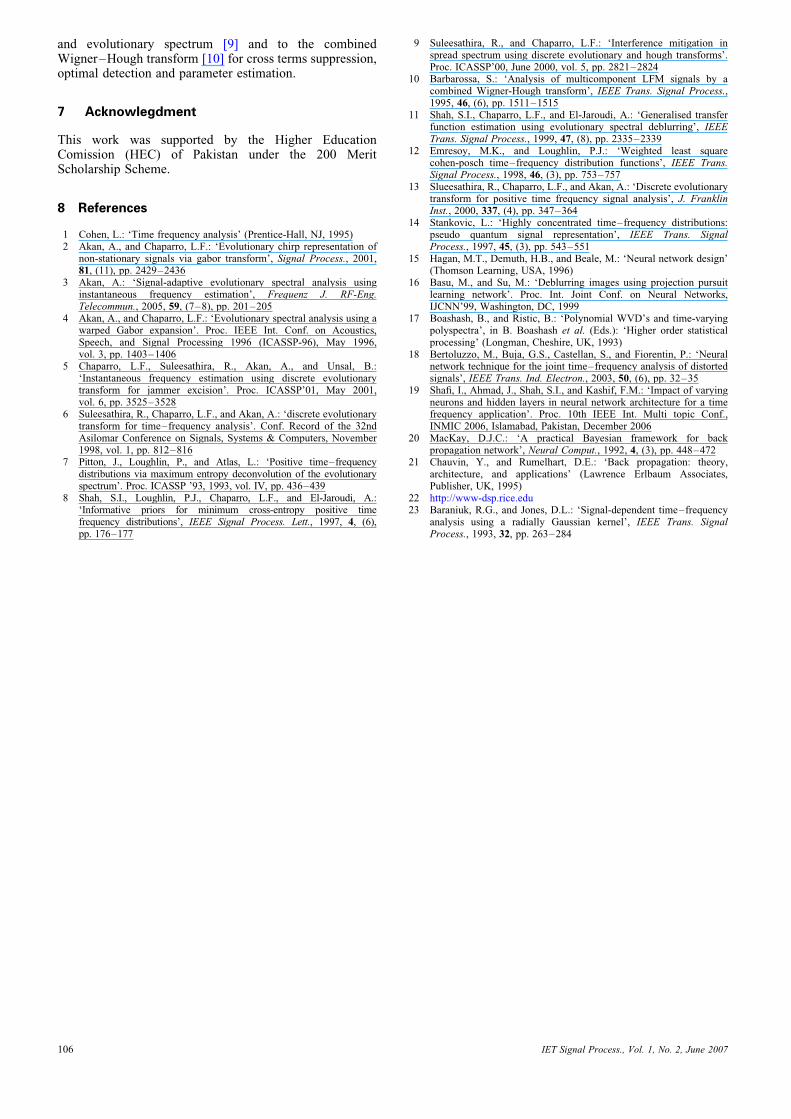
Figs. 21 and 22 indicate that performance of BRNNM isbetter than SNNM as far as the error convergence over timeis concerned. The MSE values in the last epoch are con-siderably less for BRNNM than for SNNM, as shown inFig. 21 for the same number of neurons. Fig. 22 presentsan analysis to decide the optimum number of neurons in

Fig. 16 Resultant TFD obtained by BRNNM for TI 2

Fig. 17 Resultant TFD obtained by BRNNM for TI 3

Table 1: Comparison of entropies

Method used EQ (bits) for test TFD images

TI 1 TI 2 TI 3 TI 4

Proposed approach

through specialised

BRNNMs

7.228 8.223 7.287 8.318

SNNM 10.342 11.563 10.521 11.978

Wigner distribution 18.623 20.511 19.562 21.334

spectrogram 24.986 29.743 26.231 31.987

Approach used

by [23]

12.125 – – –

104

Fig. 18 Resultant TFD obtained by BRNNM for TI 4

Fig. 19 TFD obtained by the method of [23]

Fig. 20 Comparison of entropies for the various techniques fortest images

IET Signal Process., Vol. 1, No. 2, June 2007

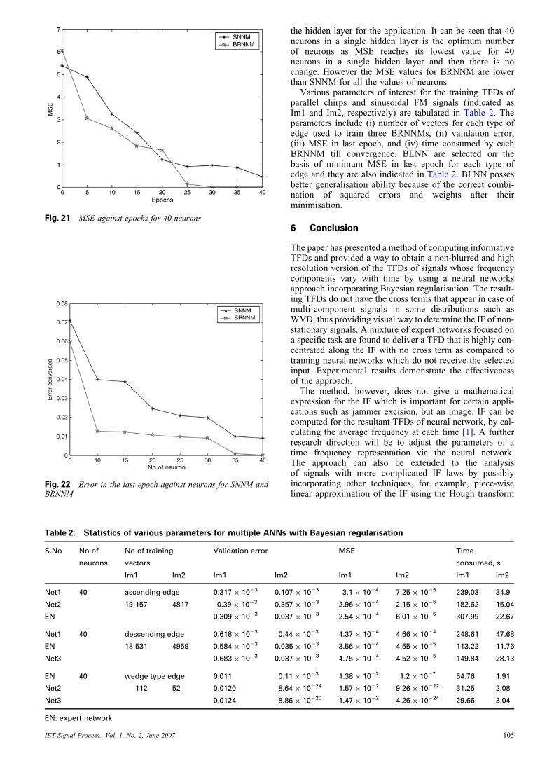
Fig. 22 Error in the last epoch against neurons for SNNM andBRNNM

Fig. 21 MSE against epochs for 40 neurons

IET Signal Process., Vol. 1, No. 2, June 2007

the hidden layer for the application. It can be seen that 40neurons in a single hidden layer is the optimum numberof neurons as MSE reaches its lowest value for 40neurons in a single hidden layer and then there is nochange. However the MSE values for BRNNM are lowerthan SNNM for all the values of neurons.

Various parameters of interest for the training TFDs ofparallel chirps and sinusoidal FM signals (indicated asIm1 and Im2, respectively) are tabulated in Table 2. Theparameters include (i) number of vectors for each type ofedge used to train three BRNNMs, (ii) validation error,(iii) MSE in last epoch, and (iv) time consumed by eachBRNNM till convergence. BLNN are selected on thebasis of minimum MSE in last epoch for each type ofedge and they are also indicated in Table 2. BLNN possesbetter generalisation ability because of the correct combi-nation of squared errors and weights after theirminimisation.

6 Conclusion

The paper has presented a method of computing informativeTFDs and provided a way to obtain a non-blurred and highresolution version of the TFDs of signals whose frequencycomponents vary with time by using a neural networksapproach incorporating Bayesian regularisation. The result-ing TFDs do not have the cross terms that appear in case ofmulti-component signals in some distributions such asWVD, thus providing visual way to determine the IF of non-stationary signals. A mixture of expert networks focused ona specific task are found to deliver a TFD that is highly con-centrated along the IF with no cross term as compared totraining neural networks which do not receive the selectedinput. Experimental results demonstrate the effectivenessof the approach.

The method, however, does not give a mathematicalexpression for the IF which is important for certain appli-cations such as jammer excision, but an image. IF can becomputed for the resultant TFDs of neural network, by cal-culating the average frequency at each time [1]. A furtherresearch direction will be to adjust the parameters of atime–frequency representation via the neural network.The approach can also be extended to the analysisof signals with more complicated IF laws by possiblyincorporating other techniques, for example, piece-wiselinear approximation of the IF using the Hough transform

Table 2: Statistics of various parameters for multiple ANNs with Bayesian regularisation

S.No No of

neurons

No of training

vectors

Validation error MSE Time

consumed, s

Im1 Im2 Im1 Im2 Im1 Im2 Im1 Im2

Net1 40 ascending edge 0.317 � 1023 0.107 � 1023 3.1 � 1024 7.25 � 1025 239.03 34.9

Net2 19 157 4817 0.39 � 1023 0.357 � 1023 2.96 � 1024 2.15 � 1025 182.62 15.04

EN 0.309 � 1023 0.037 � 1023 2.54 � 1024 6.01 � 1025 307.99 22.67

Net1 40 descending edge 0.618 � 1023 0.44 � 1023 4.37 � 1024 4.66 � 1024 248.61 47.68

EN 18 531 4959 0.584 � 1023 0.035 � 1023 3.56 � 1024 4.55 � 1025 113.22 11.76

Net3 0.683 � 1023 0.037 � 1023 4.75 � 1024 4.52 � 1025 149.84 28.13

EN 40 wedge type edge 0.011 0.11 � 1023 1.38 � 1022 1.2 � 1027 54.76 1.91

Net2 112 52 0.0120 8.64 � 10224 1.57 � 1022 9.26 � 10222 31.25 2.08

Net3 0.0124 8.86 � 10220 1.47 � 1022 4.26 � 10224 29.66 3.04

EN: expert network

105

and evolutionary spectrum [9] and to the combinedWigner–Hough transform [10] for cross terms suppression,optimal detection and parameter estimation.

7 Acknowlegdment

This work was supported by the Higher EducationComission (HEC) of Pakistan under the 200 MeritScholarship Scheme.

8 References

1 Cohen, L.: ‘Time frequency analysis’ (Prentice-Hall, NJ, 1995)2 Akan, A., and Chaparro, L.F.: ‘Evolutionary chirp representation of

non-stationary signals via gabor transform’, Signal Process., 2001,81, (11), pp. 2429–2436

3 Akan, A.: ‘Signal-adaptive evolutionary spectral analysis usinginstantaneous frequency estimation’, Frequenz J. RF-Eng.Telecommun., 2005, 59, (7–8), pp. 201–205

4 Akan, A., and Chaparro, L.F.: ‘Evolutionary spectral analysis using awarped Gabor expansion’. Proc. IEEE Int. Conf. on Acoustics,Speech, and Signal Processing 1996 (ICASSP-96), May 1996,vol. 3, pp. 1403–1406

5 Chaparro, L.F., Suleesathira, R., Akan, A., and Unsal, B.:‘Instantaneous frequency estimation using discrete evolutionarytransform for jammer excision’. Proc. ICASSP’01, May 2001,vol. 6, pp. 3525–3528

6 Suleesathira, R., Chaparro, L.F., and Akan, A.: ‘discrete evolutionarytransform for time–frequency analysis’. Conf. Record of the 32ndAsilomar Conference on Signals, Systems & Computers, November1998, vol. 1, pp. 812–816

7 Pitton, J., Loughlin, P., and Atlas, L.: ‘Positive time–frequencydistributions via maximum entropy deconvolution of the evolutionaryspectrum’. Proc. ICASSP ’93, 1993, vol. IV, pp. 436–439

8 Shah, S.I., Loughlin, P.J., Chaparro, L.F., and El-Jaroudi, A.:‘Informative priors for minimum cross-entropy positive timefrequency distributions’, IEEE Signal Process. Lett., 1997, 4, (6),pp. 176–177

106

9 Suleesathira, R., and Chaparro, L.F.: ‘Interference mitigation inspread spectrum using discrete evolutionary and hough transforms’.Proc. ICASSP’00, June 2000, vol. 5, pp. 2821–2824

10 Barbarossa, S.: ‘Analysis of multicomponent LFM signals by acombined Wigner-Hough transform’, IEEE Trans. Signal Process.,1995, 46, (6), pp. 1511–1515

11 Shah, S.I., Chaparro, L.F., and El-Jaroudi, A.: ‘Generalised transferfunction estimation using evolutionary spectral deblurring’, IEEETrans. Signal Process., 1999, 47, (8), pp. 2335–2339

12 Emresoy, M.K., and Loughlin, P.J.: ‘Weighted least squarecohen-posch time–frequency distribution functions’, IEEE Trans.Signal Process., 1998, 46, (3), pp. 753–757

13 Slueesathira, R., Chaparro, L.F., and Akan, A.: ‘Discrete evolutionarytransform for positive time frequency signal analysis’, J. FranklinInst., 2000, 337, (4), pp. 347–364

14 Stankovic, L.: ‘Highly concentrated time–frequency distributions:pseudo quantum signal representation’, IEEE Trans. SignalProcess., 1997, 45, (3), pp. 543–551

15 Hagan, M.T., Demuth, H.B., and Beale, M.: ‘Neural network design’(Thomson Learning, USA, 1996)

16 Basu, M., and Su, M.: ‘Deblurring images using projection pursuitlearning network’. Proc. Int. Joint Conf. on Neural Networks,IJCNN’99, Washington, DC, 1999

17 Boashash, B., and Ristic, B.: ‘Polynomial WVD’s and time-varyingpolyspectra’, in B. Boashash et al. (Eds.): ‘Higher order statisticalprocessing’ (Longman, Cheshire, UK, 1993)

18 Bertoluzzo, M., Buja, G.S., Castellan, S., and Fiorentin, P.: ‘Neuralnetwork technique for the joint time–frequency analysis of distortedsignals’, IEEE Trans. Ind. Electron., 2003, 50, (6), pp. 32–35

19 Shafi, I., Ahmad, J., Shah, S.I., and Kashif, F.M.: ‘Impact of varyingneurons and hidden layers in neural network architecture for a timefrequency application’. Proc. 10th IEEE Int. Multi topic Conf.,INMIC 2006, Islamabad, Pakistan, December 2006

20 MacKay, D.J.C.: ‘A practical Bayesian framework for backpropagation network’, Neural Comput., 1992, 4, (3), pp. 448–472

21 Chauvin, Y., and Rumelhart, D.E.: ‘Back propagation: theory,architecture, and applications’ (Lawrence Erlbaum Associates,Publisher, UK, 1995)

22 http://www-dsp.rice.edu23 Baraniuk, R.G., and Jones, D.L.: ‘Signal-dependent time–frequency

analysis using a radially Gaussian kernel’, IEEE Trans. SignalProcess., 1993, 32, pp. 263–284

IET Signal Process., Vol. 1, No. 2, June 2007