arX

iv:c

ond-

mat

/021

2519

v2 [

cond

-mat

.sta

t-m

ech]

13

Apr

200

4

Exact scaling functions for one-dimensional

stationary KPZ growth

Michael Prahofer and Herbert Spohn,Zentrum Mathematik and Physik Department, TU Munchen,

D-80290 Munchen, Germany

emails: praehofer@ma.tum.de, spohn@ma.tum.de

With deep appreciation dedicated to Giovanni Jona-Lasinio at

the occasion of his 70th birthday.

Abstract

We determine the stationary two-point correlation function of the one-dimensional KPZ equation through the scaling limit of a solvable micro-scopic model, the polynuclear growth model. The equivalence to a di-rected polymer problem with specific boundary conditions allows one toexpress the corresponding scaling function in terms of the solution to aRiemann-Hilbert problem related to the Painleve II equation. We solvethese equations numerically with very high precision and compare our, upto numerical rounding exact, result with the prediction of Colaiori andMoore [1] obtained from the mode coupling approximation.

1 Introduction

In their well-known work [2] Kardar, Parisi, and Zhang argue that surface growththrough random ballistic deposition can be modeled by a stochastic continuumequation, which in the case of a one-dimensional substrate reads

∂th = 12λ(∂xh)2 + ν∂2

xh + η. (1.1)

Here h(x, t) is the height at time t at location x relative to a suitable referenceline. η(x, t) is space-time white noise of strength D, 〈η(x, t)η(x′, t′)〉 = Dδ(x −x′)δ(t − t′), and models the randomness in deposition. ν∂2

xh is a not furtherdetailed smoothening mechanism. The important insight of [2] is to observe thatthe growth velocity is nonlinear, in general, and is relevant for the large scaleproperties of the solution to (1.1). To simplify, the growth velocity is expandedin the slope. The first two terms can be absorbed through a suitable choice

1

of coordinate frame. The quadratic nonlinearity in (1.1) is relevant and higherorders can be ignored, unless λ = 0.

The one-dimensional KPZ equation (1.1) is regarded as exactly solved inthe usual terminology. In fact, what can be obtained is the dynamic scalingexponent z = 3/2 [3, 2, 4]. No other universal quantity has been computedexactly so far. In our contribution we will improve the situation and explainhow to extract the scaling function for the stationary two-point function. A fewother universal quantities can be computed as well. But they have been discussedalready elsewhere [5, 6, 7].

In [4] a mode-coupling equation for the two-point function is written down,in essence following the scheme from critical dynamics and kinetic theory. Atthe time only z = 3/2 and a few qualitative properties could be extracted fromthe mode-coupling equation. In [8] this equation is solved numerically. Suchcomputations are repeated in [1] with greatly improved precision and using amore convenient set of coordinates. Thus for the 1D KPZ equation we are inthe unique position of an exact solution and an accurate numerical solution tothe mode-coupling equation with no adjustable parameters. As will be explainedbelow, given the uncontrolled approximation, mode-coupling does surprisinglywell.

To attack (1.1) directly does not seem to be feasible, a situation which israther similar to the one for two-dimensional models in equilibrium statisticalmechanics. For example, the Ginzburg-Landau φ4-theory is given through the(formal) functional measure

Z−1∏

x∈R2

dφ(x) exp[−

∫d2x

((∇φ)2 + gφ2 + φ4

)](1.2)

for the scalar field φ. (1.2) is not the proper starting point for computing theexact two-point scaling function at the critical coupling gc. Rather one discretizesthrough the lattice Z2 and replaces the φ-field by Ising spins ±1. Then, followinge.g. [9], the scaling function at and close to criticality can be obtained. Byuniversality this scaling function is the one of (1.2). (While certainly true, toestablish universality is difficult and carried out in a few cases only [10].) Inthe same spirit we replace (1.1) by a discrete model, where the most convenientchoice seems to be the polynuclear growth (PNG) model.

Before explaining the PNG model let us review the standard scaling the-ory for (1.1). If the initial conditions h(x, 0) of the KPZ equation are dis-tributed according to two-sided Brownian motion, then formally the distributionof h(x, t)−h(0, t) is again two-sided Brownian motion. Therefore it is natural todefine the stationary time correlation

C(x, t) =⟨(

h(x, t) − h(0, 0) − t〈∂th〉)2⟩

, (1.3)

where from the height difference the average displacement is subtracted. By

2

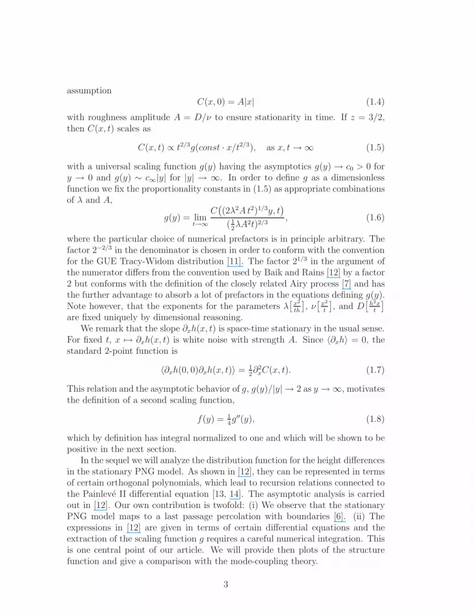
assumptionC(x, 0) = A|x| (1.4)

with roughness amplitude A = D/ν to ensure stationarity in time. If z = 3/2,then C(x, t) scales as

C(x, t) ∝ t2/3g(const · x/t2/3), as x, t → ∞ (1.5)

with a universal scaling function g(y) having the asymptotics g(y) → c0 > 0 fory → 0 and g(y) ∼ c∞|y| for |y| → ∞. In order to define g as a dimensionlessfunction we fix the proportionality constants in (1.5) as appropriate combinationsof λ and A,

g(y) = limt→∞

C((2λ2A t2)1/3y, t

)

(12λA2t)2/3

, (1.6)

where the particular choice of numerical prefactors is in principle arbitrary. Thefactor 2−2/3 in the denominator is chosen in order to conform with the conventionfor the GUE Tracy-Widom distribution [11]. The factor 21/3 in the argument ofthe numerator differs from the convention used by Baik and Rains [12] by a factor2 but conforms with the definition of the closely related Airy process [7] and hasthe further advantage to absorb a lot of prefactors in the equations defining g(y).Note however, that the exponents for the parameters λ

[x2

th

], ν

[x2

t

], and D

[h2xt

]

are fixed uniquely by dimensional reasoning.We remark that the slope ∂xh(x, t) is space-time stationary in the usual sense.

For fixed t, x 7→ ∂xh(x, t) is white noise with strength A. Since 〈∂xh〉 = 0, thestandard 2-point function is

〈∂xh(0, 0)∂xh(x, t)〉 = 12∂2

xC(x, t). (1.7)

This relation and the asymptotic behavior of g, g(y)/|y| → 2 as y → ∞, motivatesthe definition of a second scaling function,

f(y) = 14g′′(y), (1.8)

which by definition has integral normalized to one and which will be shown to bepositive in the next section.

In the sequel we will analyze the distribution function for the height differencesin the stationary PNG model. As shown in [12], they can be represented in termsof certain orthogonal polynomials, which lead to recursion relations connected tothe Painleve II differential equation [13, 14]. The asymptotic analysis is carriedout in [12]. Our own contribution is twofold: (i) We observe that the stationaryPNG model maps to a last passage percolation with boundaries [6]. (ii) Theexpressions in [12] are given in terms of certain differential equations and theextraction of the scaling function g requires a careful numerical integration. Thisis one central point of our article. We will provide then plots of the structurefunction and give a comparison with the mode-coupling theory.

3

2 The polynuclear growth model

The polynuclear growth (PNG) model is a model for layer-by-layer growth throughdeposition from the ambient atmosphere. The surface is parameterized by a timedependent integer-valued height function h(x, t), t ∈ R, above a one-dimensionalsubstrate, x ∈ R. Thus the height function consists of terraces bordered by stepsof unit height. The up-steps move to the left and the down-steps to the rightwith speed 1. Steps disappear upon collision. In addition to this deterministicdynamical rule new islands of unit height are nucleated randomly with space-timedensity 2 on top of already existing terraces. The corresponding stochastic pro-cess h(x, t) is well defined even in infinite volume (cf. [15] for the closely relatedHammersley particle process).

Of interest to us here is the stationary growth process, which means that theslope ∂xh(x, t) = ρ(x, t) is stationary in space-time. One can think of ρ(x, t) asthe density of a particle/antiparticle process. The particles are located at theup-steps and thus move with velocity −1, the antiparticles are located at thedown-steps and move with velocity 1. Upon collision particle/antiparticle pairsannihilate. In addition, with space-time density 2, a particle/antiparticle pair iscreated with the particle moving to the left, the antiparticle to the right. To makeρ stationary, one prescribes at t = 0 up-steps Poisson distributed with density ρ+

and down-steps independently Poisson distributed with intensity ρ− such that

ρ+ρ− = 1. (2.1)

This measure for steps is stationary under the PNG dynamics. The mean slopeis given by

u = ρ+ − ρ− = 〈∂xh(x, t)〉, (2.2)

which is the only remaining free parameter. For fixed t, x 7→ h(x, t)− h(0, t) is a(two-sided) random walk with rate ρ± for a jump from n to n± 1. It has averageu and variance ρ+ + ρ−, which implies for the roughness amplitude

A(u) =√

4 + u2. (2.3)

For the growth velocity one obtains

v(u) = 〈∂th〉 = ρ+ + ρ− =√

4 + u2. (2.4)

Given ρ(x, t) the height h(x, t) is determined only up to a constant which wefix as h(0, 0) = 0. To emphasize that only height differences count, h(0, 0) issometimes kept in the formulas.

The stationary process with slope u transforms to the stationary process withslope 0 through the Lorentz transformation

x′ = (1 − c2)−1/2(x − ct), t′ = (1 − c2)−1/2(t − cx), (2.5)

4

with the speed of “light” equal to 1 and the velocity parameter c = −u/√

4 + u2.Thus it suffices to restrict ourselves to u = 0 which we do from now on. Inparticular ρ+ = 1 = ρ−. 〈 · 〉 and E refer to the stationary density field at slopeu = 0.

The central objects are the height-height correlation

C(x, t) = 〈(h(x, t) − h(0, 0) − 2t)2〉 (2.6)

and the closely related two-point function for the density,

S(x, t) = 〈ρ(x, t)ρ(0, 0)〉. (2.7)

They are related as

12∂2

xC(x, t) = 12∂2

xE

((h(x, t) − h(0, 0) − 2t

)2)

= ∂xE

(ρ(x, t)

(h(x, t) − h(0, 0) − 2t

))

= ∂xE

(ρ(0, t)

(h(0, t) − h(−x, 0) − 2t

))

= E(ρ(0, t)ρ(−x, 0)

)

= S(x, t). (2.8)

The height correlation is convex, equivalently

S(x, t) ≥ 0. (2.9)

To prove this property we show that the structure function S(x, t) can be regardedas the transition probability for a second class particle starting at the origin.Its initial velocity is ±1 with probability 1

2, as for the “first-class” up/down-

steps. In contrast to an ordinary step the second class particle is never destroyedupon colliding with another step. Rather it eats up the step encountered and,by reversing its own direction of motion, continues along the trajectory of theabsorbed step, cf. Figure 1. Let ρ(x, t) be a given realization of the PNG process.The second class particle is added as

ρ(σ)(x, 0) = ρ(x, 0) + σδ(x), σ = ±1. (2.10)

ρ(σ)(x, 0) evolves to ρ(σ)(x, t) with nucleation events identical to the one for ρ(x, t).By construction, if Xt denotes the position of the second class particle at time t,

ρ(σ)(x, t) − ρ(x, t) = σδ(x − Xt). (2.11)

Noting that by the Poisson property ρ(σ)(x, 0) is given by ρ(x, 0) conditioned onthe presence of either an up-step (σ = +1) or down-step (σ = −1) at the origin,

5

Figure 1: The trajectory of a second-class particle.

we obtain

0 ≤ pt(x) =1

2

∑

σ=±1

E

(σ(ρ(σ)(x, t) − ρ(x, t)

))=

1

2

∑

σ=±1

E(σρ(σ)(x, t)

)

= limδց0

1

2

∑

σ=±1

σE

(ρ(x, t)

∣∣∣∫ δ

−δ

ρ(y, 0) dy = σ)

= limδց0

1

2

∑

σ,σ′=±1

σσ′P{ ∫ δ

−δρ(x + y, t) dy = σ′,

∫ δ

−δρ(y, 0) dy = σ

}

2 δ P{ ∫ δ

−δρ(y, 0) dy = σ

}

= 12E(ρ(x, t)ρ(0, 0)

)= 1

2S(x, t). (2.12)

For arbitrary slope u the normalization of S(x, t) would be given by v(u) =√4 + u2 and the mean of pt(x) evolves along the characteristics of the macroscopic

evolution equation ∂tu = −∂xv(u). Thus

∫S(x, t)dx =

√4 + u2, and

∫xS(x, t)dx = −t u. (2.13)

3 The distribution functions for the height dif-

ferences

For the PNG model the distribution function for the height difference h(x, t) −h(0, 0) satisfies certain recursion relations, which are the tool for analyzing the

6

scaling limit when t → ∞ and x = y t2/3 with y = O(1). The second momentsyield C(x, t) and therefore by (2.8) also S(x, t).

Since the nucleation events are Poisson, h(x, t)− h(0, 0) depends only on theevents in the backward light cone {(x′, t′) ∈ R2, 0 ≤ t′ ≤ t, |x − x′| ≤ t − t′}and the initial conditions at t = 0. Along the line {x′ = t′} the down-steps arePoisson distributed with line density

√2 and correspondingly for the up-steps

along the line {x′ = −t′}. This property can be deduced from the uniqueness ofthe stationary state at given slope and the Lorentz invariance (2.5) in the limitc → ±1. Thus h(x, t) − h(0, 0) is determined by the nucleation events in therectangle Rx,t = {(x′, t′) ∈ R2, |x′| ≤ |t′|, |x − x′| ≤ t − t′} together with thesaid boundary conditions. h(x, t) − h(0, 0) can be reexpressed as a directed lastpassage percolation according to the following rules: Inside Rx,t there are Poissonpoints with density 2. Along the two lower edges of Rx,t there are independentlyPoisson points with line density

√2. A directed passage from (0, 0) to (x, t)

is given through a directed path (polymer). It is a piecewise linear path in theplane, starts at (0, 0) and ends at (x, t), alters its direction only at Poisson points,and is time-like in the sense that for any two points (x′, t′), (x′′, t′′) on the pathone has |x′ − x′′| ≤ |t′ − t′′|. Note that, once the directed path leaves one of thelower edges to move into the bulk, it can never return. By definition the lengthof a directed path equals the number of Poisson points traversed. With theseconventions

h(x, t) − h(0, 0) = maximal length of a directed path from (0, 0) to (x, t).(3.14)

We remark that in general there are several maximizing paths, their numberpresumably growing exponentially with t.

Under the Lorentz transformation (2.5) the distribution for the height differ-ences (3.14) does not change. Therefore, we might as well transform R(x,t) to a

square. By an additional overall scaling by√

2 one arrives at a v × v square, v =√t2 − x2, with bulk density 1 and the line densities α− = α =

√(t − x)(t + x)

for the lower left, resp. α+ = 1/α for the lower right edge. In this way we haverecovered precisely the setting in [12, 13] with t replaced by v. Baik and Rainsderive an explicit expression for the height distribution in terms of Toeplitz deter-minants, which can be further simplified by means of corresponding orthogonalpolynomials.

Let us state the result for the distribution function of h(x, t) − h(0, 0),

Fx,t(n) = P{h(x, t) − h(0, 0) ≤ n}= Gn(α)F (n) − Gn−1(α)F (n − 1). (3.15)

For fixed v the functions g and F are given in terms of the monic polynomialsπn(z) = zn + O(zn−1), which are pairwise orthogonal on the unit circle |z| = 1with respect to the weight ev(z+z−1). Their norm Nn is given by

〈πn, πm〉 = δn,mNn (3.16)

7

with 〈p, q〉 =∮

p(z)q(z−1)ev(z+z−1)(2πiz)−1dz. One has

F (n) = e−v2

n−1∏

k=0

Nk, (3.17)

where F (n) itself is the distribution function of the maximal length of a directedpath in the case α+ = 0 = α−. Thus limn→∞ F (n) = 1 and

Gn(α) = e−v(α+α−1)Nn

n∑

k=0

N−1k πk(−α)πk(−α−1)

= e−v(α+α−1)((1 − n)πn(−α)πn(−α−1)

−απ′n(−α)πn(−α−1) − α−1πn(−α)π′

n(−α−1)). (3.18)

Defining the dual polynomials π∗n(z) = znπn(z−1), the second equality in (3.18)

is an easy consequence of the Christoffel-Darboux formula [16],

Nn

n−1∑

k=0

πk(a)πk(b)

Nk=

π∗n(a)π∗

n(b) − πn(a)πn(b)

1 − ab, (3.19)

valid for a, b ∈ C, ab 6= 1 and extended by l’Hospital’s rule to ab = 1, and thetrivial relation

π∗n(z)z−1π∗

n′(z−1) + z π′

n(z)πn(z−1)=n πn(z)πn(z−1) = n π∗n(z)π∗

n(z−1). (3.20)

Taking only the leading order of a in (3.19) one obtains the well-known rela-tions

πn+1(z) = z πn(z) + pn+1π∗n(z),

π∗n+1(z) = z pn+1πn(z) + π∗

n(z), (3.21)

Nn+1 = Nn

(1 − p2

n+1

)

which are closed given pn = πn(0) for n ≥ 0. For the particular weight functionev(z+z−1) one can derive a nonlinear recursion relation for the pn’s,

pn = −v

n(pn+1 + pn−1)(1 − p2

n), (3.22)

with initial values p0 = 1, p1 = − I1(2v)I0(2v)

. Ik(2v) = (2π)−1∫ 2π

0eikθe2v cos θdθ is the

modified Bessel function of order k and thus N0 = I0(2v). Eq. (3.22) is thediscrete Painleve II equation. It has been derived in the context of orthogonal

8

polynomials for the first time in [14], and later on more or less independently in[17, 18, 13, 19]. The differential equations for πn, π∗

n,

πn′(z) = (n/z + v/z2 − pn+1pnv/z)πn(z) + (pn+1v/z − pnv/z2)π∗

n(z)

π∗n′(z) = (−pn+1v/z + pnv)πn(z) + (−v + pn+1pnv/z)π∗

n(z), (3.23)

can be shown to hold by a tedious but straightforward induction, using (3.21) and(3.22). They are implicitly derived in [13], from which we learned their actualform. In [20] an integral expression is obtained for the derivative of orthogo-nal polynomials on the circle with respect to (up to some technical conditions)an arbitrary weight function. Specializing to the weight ev(z+z−1) results in adifferential-difference equation equivalent to (3.23).

Of course, the mean of the probability distribution Fx,t(n) − Fx,t(n − 1) is 2tand its variance, the correlation function (2.6), is given by

C(x, t) =∑

n≥0

(2(n − 2t) − 1

)Fx,t(n). (3.24)

Thus to establish (1.5), one has to understand the scaling properties of the dis-tribution function Fx,t(n). Let us introduce the new variables s, y defined by

n = 2v + v1/3s, (3.25)

x = v2/3y, (3.26)

where v =√

t2 − x2 is regarded as fixed when varying n and x. In [12] thedifferent scaling variable w = 1

2y is used, which leads to a string of factors of 2,

avoided by our convention. Setting

Rn = −(−1)npn, (3.27)

we rewrite (3.22) as

Rn+1 − 2Rn + Rn−1 =(n

v− 2)Rn + 2R3

n

1 − R2n

. (3.28)

Under the scaling (3.26), Rn = v−1/3u(v−1/3(n − 2v)

)+ O(v−1), it becomes the

Painleve II equationu′′(s) = 2u(s)3 + s u(s), (3.29)

in the limit v → ∞. The starting value R0 = −1 is consistent with the leftasymptotics of u(s) only if

u(s) ∼ −√

−s/2 as s → −∞, (3.30)

which singles out the Hastings-McLeod solution to (3.29) [21]. This particularsolution will be denoted by u(s) and we conclude that

u(s) = limv→∞

v1/3R[2v+v1/3s], (3.31)

9

provided the limit exists (A complete proof is the main content of [22]). u(s) < 0and u has the right asymptotics

u(s) ∼ −Ai(s) as s → ∞. (3.32)

At this point we can derive the scaling limit for F (n). It is the GUE Tracy-Widomdistribution function [11]

FGUE(s) = e−V (s), V (s) = −∫ ∞

s

v(x)dx, v(s) =(u(s)2 + s

)u(s)2 − u′(s)2,

(3.33)which appears already as the limiting height distribution for nonstationary curvedselfsimilar growth [23]. Since v′(s) = u(s)2, one has v1/3 log N[2v+v1/3s] → v(s) and

F ([2v + v1/3s]) → FGUE(s) as v → ∞.Next we turn to the scaling limit for the orthogonal polynomials. For it to be

nontrivial we set

Pn(α) = e−vαπ∗n(−α),

Qn(α) = −e−vα(−1)nπn(−α). (3.34)

(3.26) implies α = 1 − v−1/3y + O(v−2/3). Setting n as in (3.25), we claim that

a(s, y) = limv→∞

Pn(α), b(s, y) = limv→∞

Qn(α). (3.35)

If so, the limit functions a, b satisfy the differential equations

∂sa = u b,

∂sb = u a − y b, (3.36)

as a consequence of (3.21), and

∂ya = u2a − (u′ + y u)b,

∂yb = (u′ − y u)a + (y2 − s − u2)b, (3.37)

as a consequence of (3.23). From (3.21) one immediately obtains π∗n(−1) =

(−1)nπn(−1) =∏n

k=1(1 − Rk). One has the limit∏∞

k=1(1 − Rk) = ev since

e−v2+vN0

∏nk=1 Nk(1 − Rk)

−1 has an interpretation as a probability distributionfunction [24]. Therefore the initial conditions to (3.37) are

a(s, 0) = −b(s, 0) = e−U(s), U(s) = −∫ ∞

s

u(x)dx. (3.38)

The scaling limit of Gn(α) as defined in Eq. (3.18) is the function

G(s, y) =

∫ s

−∞

a(s′, y)a(s′,−y)ds′

= a(s,−y)∂ya(s, y) − b(s,−y)∂yb(s, y), (3.39)

10

where the second equality can be verified by differentiation with respect to s andusing the identity

a(s, y) = −b(s,−y)e1

3y3−sy, (3.40)

itself being a direct consequence of (3.37) and (3.38). Putting these pieces to-gether we obtain as scaling limit for the distribution functions Fx,t(n),

Fy(s) =d

ds

(G(s + y2, y)FGUE(s + y2)

). (3.41)

The shift in (3.41) by y2 comes from the fact that Fy(s) is evaluated for constantt = v + 1

2v1/3y + O(v−1/3).

In conclusion we arrive at the scaling function g(y) as defined in the Intro-duction. From (1.6), with λ = 1

2and A = 2 for the PNG model, and (3.24) we

obtain

g(y) =

∫s2dFy(s). (3.42)

As already mentioned, except for (3.23), all our relations are derived in [12,13], and the existence of limits is proven with Riemann-Hilbert techniques. Forcompleteness let us collect some more properties of a shown in [12]:

a(s, y) → 1, as s → +∞,

a(s, y) → 0, as s → −∞,

a((2y)1/2x + y2, y

)→ 1, as y → +∞,

a((−2y)1/2x + y2, y

)→ 1

(2π)1/2

∫ x

−∞

e−1

2ξ2

dξ, as y → −∞. (3.43)

Therefore Fy(s) is asymptotically Gaussian and we recover g(y) ≃ 2|y| for largey.

4 Numerical determination of the scaling func-

tion

The key object in determining the scaling functions g(y), f(y) is the Hastings-McLeod solution [21] to Painleve II, u(s), which is the unique solution to

u′′ = 2u3 + su (4.1)

with asymptotic boundary conditions (3.30) and (3.32). Tracy and Widom[11, 25] integrate (4.1) numerically with conventional differential equation solversusing the known asymptotics at s = ±∞. The precision achieved with thistechnique does not suffice for our purposes, since we need u(s) as starting values(3.38) for the differential equations (3.37). We develop here a different method to

11

obtain u(s), in principle with arbitrary precision. Next the functions a(s, y) andb(s, y) have to be determined, which directly leads to values for the distributionfunctions Fy(s). They have to be further integrated with respect to s in orderto obtain their variance, which is the desired scaling function g(y). The Taylorexpansion method to be explained intrinsically produces not only function valuesat a point but also higher derivatives. Therefore we obtain f(y) not by numer-ically differentiating g(y) but rather by direct calculation via the knowledge of∂2

yFy(s).In a first step, to obtain reliable approximations to the Hastings-McLeod so-

lution, we need to guess its initial data at some finite s0 by using asymptoticexpansions around ±∞. Any initial data u(s0) = u0, u′(s0) = u1 give rise to amaximal solution, u(s) of (4.1), which admits analytic continuation to a mero-morphic function on C. The only essential singularity for Painleve II solutions liesat ∞. If u(s) is close to u(s) we can estimate the difference ∆(s) = u(s)−u(s) bylinearizing (4.1) around u(s). One obtains that ∆(s)/∆(0) is of order exp(D(s))if (∆(s), ∆′(s)) is in the unstable subspace and of order exp(−D(s)) for the sta-ble subspace, where D(s) ≈ −1

3(−2s)3/2 for s ≪ 0 and ≈ 2

3s3/2 for s ≫ 0. Note

that on the exponential scale we are looking at, derivation with respect to sleaves invariant the order. Therefore the exponential orders of ∆(s) and ∆′(s)are the same. Since generically initial values at s0 have a component in bothsubspaces one obtains that ∆(s)/∆(s0) is of order exp(|D(s) − D(s0)|) in therange of validity of the linear approximation, |∆(s)| ≪ |u(s)|.

It turns out that the left asymptotic expansion in (−s)−1/2, optimally trun-cated at large negative s0, gives rise to initial values with ∆(s0) only of orderexp(−1

3(−2s0)

3/2). Thus control of the approximation always breaks down nears = 0. Approximations of the right asymptotics on the other hand allow a, inprinciple, arbitrary precision on any given finite interval.

For s → ∞ the deviations of u(s) from the Airy function can be expanded inan alternating asymptotic power series with exponentially small prefactor,

uright,n(s) = −Ai(s) − e−2s3/2

32π3/2s7/4

n∑

k=0

(−1)kak

(23s3/2)k

. (4.2)

The coefficients are a0 = 1, a1 = 2324

, a2 = 14931152

, . . . , and can be obtained via therecursion relation

an = Ai(3)n + 34n an−1 − 1

8(n − 1

6)(n − 5

6)an−2 for n ≥ 0 (4.3)

with initial conditions a−1 = a−2 = 0.

Ai(3)n =∑

0≤k≤l≤n

Ain−lAil−kAik. (4.4)

are the coefficients in the asymptotic expansion of Ai(x)3 and

Ain =(6n − 1)(6n − 5)

72nAin−1, Ai0 = 1 (4.5)

12

are the coefficients of the asymptotic expansion of the Airy function itself [26],

Ai(s) ∼ e−2

3s3/2

2√

πs1/4

∑

n≥0

(−1)n

(23s3/2)n

Ain. (4.6)

Empirically we observe that for s0 ≫ 0 the optimal truncation in (4.2) is

n ≈ 43s3/20 leading to an exponentially improved (relative) precision

∣∣∣∣uright,n(s0) − u(s0)

u(s0)

∣∣∣∣ ≈ exp(−83s3/20 ). (4.7)

The linear perturbation argument for u(s) with initial values u(s0) = uright,n(s0),

u′(s0) = u′right,n(s0), n = [4

3s3/20 ], is now valid for a slightly smaller interval than

[−2s0, 33/2s0]. For example, by choosing the interval [−21/3s0, s0] and gluing u(s)

at the boundaries smoothly to the optimally truncated asymptotic expansions,the maximal relative error of u(s) with respect to the Hastings-McLeod solution

is of order e−4/3s3/2

0 . For our purpose it turns out that we do not need valueswith s < −20. On the other hand, to access large values of y in (3.41), becauseof the shift in (3.41), we need u(s) for large s with high precision. uright,n(s)is numerically costly to evaluate for large s, so we finally choose s0 = 100 andintegrate in the interval [−20, 200]. This requires a maximal working precision of1500 digits and, given the integration of (4.1) is precise enough, u(s) and u(s)coincide in the first 1000 digits for s ∈ [−20, 115] and still up to 50 digits ats = 200, where u(s) ≈ 10−820. In the sequel we drop the distinction between u(s)and its numerical approximation. The arithmetic computing is done partiallywith Mathematica r© and for the computationally intensive tasks with the C++-based multiprecision package MPFUN++ [28].

To solve initial value problems for ordinary differential equations highly so-phisticated iteration schemes are available, like Runge-Kutta, Adams-Bashfordand multi-step methods. For arbitrary high (but fixed) precision results, all thesemethods become ineffective, since the step size is a decreasing function of the re-quired precision goal for the solution and tends to become ineffectively small. Theonly remaining choice is to Taylor expand the solution at a given point. The stepsize is limited by the radius of convergence only and the precision is controlledby the error made in truncating the Taylor series at some order [27].

u(s) is expanded at s0 as

u(s) =∑

n≥0

un(s − s0)n. (4.8)

For the Painleve II equation the expansion coefficients un at s0 are determinedby u0 = u(s0), u1 = u′(s0) and

un+2 =2u

(3)n + s0 un + un−1

(n + 2)(n + 1), (4.9)

13

where u(k)n =

∑nj=0 un−ju

(k−1)j are the expansion coefficients of u(s)k at s0, u

(1)n =

un. We include the factorial into the expansion coefficients instead of taking thebare Taylor coefficients, in order to reduce the workload from multiplications bybinomials when multiplying two expansions numerically.

Numerically we find that the Hastings-McLeod solution does not have anypole in a strip |Im(s)| < 2.9. To have a safety margin we choose a step size onefor the extrapolation of the expansion (4.8).

We take the starting values u(s0), u′(s0) from (4.2) at s0 = 100. The coeffi-cients of the functions U(s), V (s), see (3.33) and (3.38), when expanded arounds0, as in (4.8), are given by

Un+1 =un

n + 1, Vn+2 =

u(2)n

(n + 2)(n + 1), n ≥ 0, (4.10)

and V1 = u40−u2

1+s0u20, leaving unspecified the yet unknown integration constants

U0 = U(s0) and V0 = V (s0). The higher expansion coefficients of u, u′, U ,and V are independent of the values for U0 and V0 and are calculated with therecursion relations (4.9) and (4.10). The values of u, u′, U , and V at s = s0 ± 1are extrapolated, the expansion coefficients at s0 ± 1 iterated. Then values arecalculated at s = s0 ± 2 by extrapolation, and so on. A posteriori we assign toU(s0) and V (s0) values, such that U(200) = 0 = V (200). The numerical errorsfrom iterating (4.9) and from truncating (4.8) can be neglected compared to theuncertainty originating from the initial conditions. At the end of this first stepwe have at our disposal the expansion coefficients for u, u′, U, V at the integersin the interval [−20, 200]. For the convenience of the interested reader let us juststate the values at s = 0 up to 50 digits,

u(0) = -0.367061551548078427747792113175610961512192053613139,

u′(0) = 0.295372105447550054557007047310237988227233798735629,

U(0) = 0.336960697930551393597884426960964843885993886628226,

V (0) = 0.0311059853063123536659591008775670005642241689547838,

which might be used as starting values for a quick conventional integration ofPainleve II to reproduce parts of our results with much less effort but also lessprecision. Tables can be found at [29].

The next step is to determine a(s, y), b(s, y) at s0 ∈ {−20, . . . , 200} in theinterval y ∈ [−9, 9] employing (3.37) and (3.38). Setting

a(s, y) =∑

m,n≥0

am,n(s − s0)m(y − y0)

n,

b(s, y) =∑

m,n≥0

bm,n(s − s0)m(y − y0)

n, (4.11)

14

(3.37) becomes a recursion relation for the expansion coefficients,

am,n+1 =1

n + 1

m∑

k=0

(u

(2)k am−k,n − (k + 1)uk+1bm−k,n − ukbm−k,n−1

),

bm,n+1 =1

n + 1

(bm,n−2 − bm−1,n

+m∑

k=0

(− u

(2)k bm−k,n + (k + 1)uk+1am−k,n − ukam−k,n−1

)),

(4.12)

n ≥ 0, allowing one to determine a0,n, b0,n, n ≥ 0 upon the knowledge of a0,0,b0,0. We integrate along ±y with an extrapolation step size of 1

8. From (3.36) one

obtains the recursions

am+1,n =1

m + 1

m∑

k=0

ukbm−k,n

bm+1,n =1

m + 1

(− bm,n−1 +

m∑

k=0

ukam−k,n

). (4.13)

The expansion coefficients Gm,n of G(s, y) at (s0, y0), are determined from (3.39)as

Gm,n = (n + 1)(a−

m,nam,n+1 − b−m,nbm,n+1

)(4.14)

where a−m,n, b−m,n are the corresponding expansion coefficients of a and b at

(s0,−y0).To finally determine g(y) and its derivatives we write

g(n)(y0) =dn

dyn0

∑

s0∈Z

∫ s0+1

s0

(s − y20)

2 d2

ds2

(G(s, y0)FGUE(s)

)ds

=∑

s0∈Z

n!∑

m≥1

cm,n. (4.15)

cm,n are the expansion coefficients of (s, y) 7→∫ s

s0

(r − y2)2 d2

dr2

(G(r, y)FGUE(r)

)dr

at (s0, y0),

cm,n = (m − 2)(GF )m−1,n − 2m(GF )m,n−2 + m(m+1)m−1

(GF )m+1,n−4. (4.16)

Here

(GF )m,n =m∑

k=0

FkGm−k,n (4.17)

are the expansion coefficients of G(s, y)FGUE(s) and Fn = −∑nk=1

knVkFn−k are

the expansion coefficients of FGUE. Numerically the sum over s0 in (4.15) is

15

truncated to values inside [−15, 200], since outside contributions turn out to benegligible at the chosen precision goal. After accomplishing this program we keepvalues for g(y) at y ∈ 1

128Z∩[−9, 9] and for g(n)(y), n = 0, . . . , 4, at y ∈ 1

8Z∩[−9, 9]

with an accuracy of about 100 digits (a table in ASCII format is available onlineat [29]). For interpolating these values we used the Interpolation-function ofthe Mathematica r© package yielding best results due to the high precision datawith an interpolation order of 57.

5 Discussion of the scaling function

There have been numerous attempts to approximately determine g(·) [4, 30, 31,8, 32]. For historical reasons a different scaling function, F (·), is analyzed in someof these works. The relation to our scaling function g(·) is

F (ξ) = (ξ/2)2/3 g((2ξ2)−1/3

), resp. g(y) = 2y F

(1/(21/2y3/2)

). (5.18)

Note that by (1.6) the large y behavior of g is fixed by definition as g(y) ∼2|y|. The special value g(0) = 1.1503944782594709729961 is the Baik-Rainsconstant [12, 6]. In the literature the universal amplitude ratio RG = 2−2/3g(0) =0.7247031092 and the universal coupling constant g∗ = g(0)−3/2 = 0.810456700have been investigated. Approximate values have been determined by meansof Monte-Carlo simulations for the single step model [31], numerically withina mode-coupling approximation [30, 8, 1], and even experimentally for slowlycombusting paper [33] yielding estimates for g(0) within reasonable ranges aroundthe (numerically) exact value indicated.

In Figure 2 the scaling function f(y) = 14g′′(y) is shown as determined by the

multiprecision expansion method explained in the previous section. We estimateits large y asymptotics as

log f(y) ≈ −c|y|3 + o(|y|) for y → ∞. (5.19)

The cubic behavior is very robust and numerical fits yield about 2.996–2.998 quiteindependently of the assumed nature of the finite size corrections. The prefactorc = 0.295(5) has a relatively high uncertainty because of the unknown subleadingcorrections. Even though unaccessible in nature we estimate the error term, asindicated in (5.19), to be sublinear or even only logarithmic from the numericaldata. Possibly, the exact asymptotic behavior could be extracted from a refinedasymptotic analysis of the Riemann-Hilbert problem.

Colaiori and Moore [1, 34] tackled the same scaling function by completelydifferent means. Starting from the continuum version of the KPZ equation theynumerically solved the corresponding mode-coupling equation [4, 8], which con-tains an uncontrolled approximation, since diagrams which would renormalize thethree-point vertex coupling are neglected. Nevertheless a qualitative comparison

16

1e-100

1e-90

1e-80

1e-70

1e-60

1e-50

1e-40

1e-30

1e-20

1e-10

1

0 1 2 3 4 5 6 7 8 9

y

f(y)

exp(-0.295y3)

Figure 2: The scaling function f(y) versus y in a semilogarithmic plot. The dottedline exp(−0.295|y|3) is drawn as a guide to the eye for the large y asymptotics off .

of their result with the exact scaling function f(y) shows reasonable similarity,cf. Figure 3. Both functions are normalized to integral 1 by definition. The modecoupling solution oscillates around 0 for |y| > 3, whereas f(y) > 0 for the exactsolution. We do not know whether this is a numerical artifact or an inherent prop-erty of the mode-coupling equation. On the other hand, the second moments arereasonably close together, 0.510523 for f(y), and 0.4638 for the mode-couplingapproximation. So is the value of the Baik-Rains constant g(0) = 2

∫|y|f(y)dy

for which mode-coupling predicts the value 1.1137.From the solution to the mode-coupling equations one does not directly obtain

f(y), but rather its Fourier transform. The function G(τ) from [1] is definedthrough

G(k3/2/27/2) = f(k) = 2

∫ ∞

0

cos(ky)f(y)dy. (5.20)

Moore and Colaiori predict a stretched exponential decay of G(τ) as∝ exp(−c|τ |2/3)[34] and numerically find a superimposed oscillatory behavior on the scale |τ |2/3

[1]. In Figure 4 f(k) is plotted as obtained by a numerical Fourier transform off(y). Indeed it exhibits an oscillatory behavior as can be seen in Figure 5 where

the modulus of f(k) is shown on a semilogarithmic scale. The dotted line in theplot is the modulus of the function

10.9k−9/4 sin(12k3/2 − 1.937)e−

1

2k3/2

, (5.21)

shifted by a factor of 1000 for visibility, which fits f(k) very well in phase andamplitude for k ' 15. This behavior is not in accordance with the results of

17

0

0.1

0.2

0.3

0.4

0.5

0.6

-2 -1 0 1 2

y

f(y)

mode-coupling

Figure 3: The exact scaling function f(y) compared to the mode coupling resultof Colaiori and Moore [1](dotted line). Both functions are even.

Colaiori and Moore, since the oscillations and the exponential decay of G(τ) forthe exact solution are apparently on the scale τ and not τ 2/3.

Note that f(k) is the scaling function for the intermediate structure function

S(k, t) =

∫dxeikxS(x, t) ≃ 2f(t2/3k). (5.22)

By Fourier transforming with respect to t we determine the dynamical structurefunction,

S(k, ω) =

∫dx dtei(kx+ωt)S(x, t) ≃ 2k−3/2

◦

f (ω/k3/2), (5.23)

where

◦

f (τ) =

∫ds eiτsf(s2/3) = 2

∫ ∞

0

dy τ−1L′(y/τ 2/3)f(y) (5.24)

and L has the convenient representation

L(κ) = 2 · 32/3Ai(−3−4/3κ2) sin(2κ3/27). (5.25)

The correlation function (2.6) in Fourier space is given by

C(k, ω) = 2k−2S(k, ω) ∼ CKPZ(k, ω)def= 4k−7/2

◦

f (ω/k3/2), (5.26)

describing the asymptotic behavior at k, ω = 0. Note that C(k, ω) > 0 by defi-nition, since 〈hk,ωhk′,ω′〉 = δk,−k′δω,−ω′C(k, ω) for (k, ω) 6= (0, 0). The anomalous

18

0

0.2

0.4

0.6

0.8

1

0 1 2 3 4 5 6

k

^f (k)

-0.001

0

0.001

0.002

0.003

0.004

4 5 6 7 8

k

Figure 4: The Fourier transform f(k) of the scaling function f(y).

scaling behavior in real space is reflected by the exponents for the divergence ofCKPZ(k, ω) at k = ω = 0. In the linear case, the Edwards-Wilkinson equationλ = 0 in (1.1), one easily obtains

CEW(k, ω) =D

ω2 + ν2k4. (5.27)

A 3d-plot of CKPZ(k, ω) is shown in Figure 6. Its striking features are the smoothbehavior away from k, ω = 0, especially on the lines where k = 0 and ω = 0 andthe two symmetric maxima of k 7→ CKPZ(k, ω) for constant ω. Our numericaldata yield for the singular behavior at k = 0, ω = 0,

CKPZ(k, ω) = ω−7/3(2.10565(1) + 0.85(1) k2w−4/3 + O(k4ω−8/3)

),

= k−7/2(19.4443(1)− 52.5281(1) ω2k−3 + O(ω4k−6)

). (5.28)

6 Conclusions and Outlook

For systems close to equilibrium many properties valid in generality rely on de-tailed balance, amongst them in particular the link between correlation and re-sponse functions. The KPZ equation does not satisfy detailed balance, since thegrowth is directed. However, it has been speculated that in 1 + 1 dimensions de-tailed balance is recovered in the scaling regime. With our exact scaling functionat hand, such a claim can be tested.

Detailed balance implies that the eigenvalues of the generator in the mas-ter equation lie on the negative real axis. Thus autocorrelations in the form〈X(t)X(0)〉 can be written as the Laplace transform of a positive measure. The

19

1e-40

1e-35

1e-30

1e-25

1e-20

1e-15

1e-10

1e-05

1

5 10 15 20 25 30

k

|f(k)|

Figure 5: The modulus of f(k) on a semilogarithmic scale. The dotted line is aheuristic fit, shifted by a factor 1000 for visibility.

structure function S(k, t) at fixed k is such an autocorrelation. Using the scalingform (5.22) detailed balance would imply

S(k, t) =

∫ 0

−∞

ν(|k|−3/2dλ

)eλ|t| (6.1)

with ν(dλ) ≥ 0. In particular S(k, t) ≥ 0. From (5.21) we know that S(k, t)oscillates around zero. Definitely, at |k| ≈ 5 there is a negative dip, cf. Fig. 4.Thus (6.1) cannot be correct.

The Bethe ansatz [35, 36] indicates that, for large system size, the density ofstates is concentrated on an arc touching 0. If so, the integration in (6.1) wouldhave to be replaced by a corresponding line integral. It is not clear to us how toextract from the numerical knowledge of S(k, t) such a representation.

Our main result is the exact scaling function f , see Figure 3, for the two-pointfunction of the stationary KPZ equation in 1 + 1 dimensions. “Exact” must bequalified in two respects. Firstly f is given indirectly through the solution ofcertain differential equations, which can be solved numerically only with con-siderable effort. The errors are well controlled, however. Secondly, we rely onuniversality, in the sense that the scaling function is derived for the PNG model,which is one rather particular model within the KPZ universality class. Of course,it would be most welcome to establish the scaling limit also for other models inthis class.

The KPZ equation (1.1) is a two-dimensional field theory and, in spirit, be-longs to the same family as two-dimensional models of equilibrium statisticalmechanics, one-dimensional quantum spin chains, and other (1 + 1)-dimensional

20

-4

-2

0

2

4

k

-4

-2

0

2

4

w

0

1

2

3

4

-4

-2

0

2k

Figure 6: The correlation function CKPZ(k, ω) in Fourier space.

quantum field theories at zero temperature. While in the latter cases, thereare a number of models for which the two-point function can be computed, inthe dynamical context such solutions are scarce. In addition, the KPZ equationdoes not satisfy the condition of detailed balance. Such nonreversible models areknown to be difficult and we believe that the PNG model is the first one in thelist of exact solutions, disregarding noninteracting field theories.

For the nonstationary KPZ equation with a macroscopic profile of nonzerocurvature the analogue of F0 is the Tracy-Widom distribution function. In thatcase the full statistics of x 7→ h(x, t) for large but fixed t is available [7]. It isconceivable that an extension of the techniques used there also admits a moredetailed study of, say, the joint distribution of h(x, t) − h(0, 0), h(x′, t)− h(0, 0).On the other hand the joint distribution of h(0, t)−h(0, 0), h(0, t′)−h(0, 0) doesnot seem to be accessible. In the representation through the directed polymersit means that space-like points, even several of them, can be handled, whereastime-like points remain a challenge.

Acknowledgments. We greatly enjoyed the collaboration with Jinho Baik atthe early stage of this project and are most grateful for his important input.We also thank Mike Moore for providing us with the numerical solution of themode-coupling equation.

21

References

[1] F. Colaiori and M. A. Moore. Numerical solution of the mode-couplingequations for the Kardar-Parisi-Zhang equation in one dimension. Phys.Rev. E, 65:017105, 2002.

[2] M. Kardar, G. Parisi, and Y. Z. Zhang. Dynamic scaling of growing inter-faces. Phys. Rev. Lett., 56:889–892, 1986.

[3] D. Forster, D. R. Nelson, and M. J. Stephen. Large-distance and long-timeproperties of a randomly stirred fluid. Phys. Rev. A, 16:732–749, 1977.

[4] H. van Beijeren, R. Kutner, and H. Spohn. Excess noise for driven diffusivesystems. Phys. Rev. Lett., 54(18):2026–2029, 1985.

[5] M. Prahofer and H. Spohn. Current fluctuations for the totally asymmetricsimple exclusion process. In Sidoravicius V., editor, In and out of equilibrium,volume 51 of Progress in Probability, pages 185–204. Birkhauser Boston,2002.

[6] M. Prahofer and H. Spohn. Universal distributions for growth processes inone dimension and random matrices. Phys. Rev. Lett., 84(21):4882–4885,2000.

[7] M. Prahofer and H. Spohn. Scale invariance of the PNG droplet and theAiry process. J. Stat. Phys., 108(5–6):1071–1106, 2002.

[8] E. Frey, U. C. Tauber, and T. Hwa. Mode-coupling and renormalizationgroup results for the noisy Burgers equation. Phys. Rev. E, 53(5):4424–4438,1996.

[9] T. T. Wu, B. M. McCoy, C.A. Tracy, and E. Barouch. The spin-spin corre-lation function of the 2-dimensional Ising model: exact results in the scalingregion. Phys. Rev. B, 13:316–374, 1976.

[10] T. Spencer. A mathematical approach to universality in two dimensions.Physica A, 279(1-4):250–259, 2000.

[11] C. A. Tracy and H. Widom. Level spacing distribution and the Airy kernel.Commun. Math. Phys., 159:151–174, 1994.

[12] J. Baik and E. M. Rains. Limiting distributions for a polynuclear growthmodel with external sources. J. Stat. Phys., 100(3-4):523–541, 2000.

[13] J. Baik. Riemann–Hilbert problems for last passage percolation.math.PR/0107079, 2001.

22

[14] V. Periwal and D. Shevitz. Unitary-matrix models as exactly solvable stringtheories. Phys. Rev. Lett., 64(12):1326–1329, 1990.

[15] T. Seppalainen. A microscopic model for the Burgers equation and longestincreasing subsequences. Electronic J. Prob., 1(5):1–51, 1996.

[16] G. Szego. Orthogonal Polynomials. American Mathematical Society Provi-dence, Rhode Island, 1967.

[17] M. Hisakado. Unitary matrix models and Painleve III. Mod. Phys. Letts A,11:3001–3010, 1996.

[18] C. A. Tracy and H. Widom. Random unitary matrices, permutations andPainleve. Commun. Math. Phys., 207(3):665–685, 1999.

[19] A. Borodin. Discrete gap probabilities and discrete Painleve equations. math-ph/0111008, 2001.

[20] M. E. H. Ismail and N. S. Witte.. Discriminants and functional equationsfor polynomials orthogonal on the unit circle. J. Approx. Th., 110:200–228,2001.

[21] S. P. Hastings and J. B. McLeod. A boundary value problem associatedwith the second Painleve transcendent and the Korteweg-deVries equation.Arch. Rat. Mech. Anal., 73:31–51, 1980.

[22] J. Baik, P. Deift, and K. Johansson. On the distribution of the length ofthe longest increasing subsequence of random permutations. J. Amer. Math.Soc., 12:1119, 1999.

[23] M. Prahofer and H. Spohn. Statistical self-similarity of one-dimensionalgrowth processes. Physica A, 279(1-4):342–352, 2000.

[24] J. Baik and E. M. Rains. Algebraic aspects of increasing subsequences. DukeMath. J., 109(1):1–65, 2001.

[25] C. A. Tracy and H. Widom. private communication. 1999.

[26] M. Abramowitz and I. A. Stegun, editors. Pocketbook of Mathematical Func-tions. Verlag Harri Deutsch, Thun - Frankfurt am Main, 1984.

[27] D. Barton, I. M. Willers, and R. V. M. Zahar. Taylor series methods forordinary differential equations – An evaluation. In John Rice, editor, Math-ematical Software, pages 369–390. Academic Press, New York, 1971.

[28] S. Chatterjee. MPFUN++, a C++-based multiprecision system.http://www.cs.unc.edu/Research/HARPOON/mpfun++/, 2000.

23

[29] M. Prahofer and H. Spohn. The scaling function g(y).http://www-m5.ma.tum.de/KPZ/, 2002.

[30] T. Hwa and E. Frey. Exact scaling function of interface growth dynamics.Phys. Rev. A, 44:R7873–R7876, 1991.

[31] L.-H. Tang. Steady–state scaling function of the (1+1)–dimensional single–step model. J. Stat. Phys., 67:819–826, 1992.

[32] H. C. Fogedby. Scaling function for the noisy Burgers equation in the solitonapproximation. Europhys. Lett., 56(4):492–498, 2001.

[33] M. Myllys, J. Maunuksela, M. Alava, J. Merikoski, and J. Timonen. Kineticroughening in slow combustion of paper. Phys. Rev. E, 64(036101):1–12,2001.

[34] F. Colaiori and M. A. Moore. Stretched exponential relaxation in themode-coupling theory for the Kardar-Parisi-Zhang equation. Phys. Rev. E,63:057103, 2001.

[35] L.-H. Gwa and H. Spohn. Six-vertex model, roughened surfaces, and anasymmetric spin Hamiltonian. Phys. Rev. Lett, 68:725–728, 1992.

[36] L.-H. Gwa and H. Spohn. Bethe solution for the dynamical-scaling exponentof the noisy Burgers equation. Phys. Rev. A, 46:844–854, 1992.

24